
Formal Specification of the x87 Floating-Point Instruction Set
135
Diploma Thesis Formal Specification of the x87 Floating-Point Instruction Set Christoph Baumann [email protected] Saarbr¨ ucken, 13. Februar 2008 Supervisor: Prof. Dr. Wolfgang J. Paul Advisor: M. Sc. Ulan Degenbaev Reviewers: Prof. Dr. Wolfgang J. Paul Prof. Dr. Michael Backes
-
Upload
dinhnguyet -
Category
Documents
-
view
224 -
download
0
Transcript of Formal Specification of the x87 Floating-Point Instruction Set
Diploma Thesis
Formal Specification of the
x87 Floating-Point Instruction Set
Christoph Baumann
Saarbrucken, 13. Februar 2008
Supervisor: Prof. Dr. Wolfgang J. Paul
Advisor: M. Sc. Ulan Degenbaev
Reviewers: Prof. Dr. Wolfgang J. Paul
Prof. Dr. Michael Backes

ii

Ich versichere hiermit an Eides Statt, dass ich die von mir eingereichte Diplomarbeit selbstandigverfasst und ausschließlich die angegebenen Quellen und Hilfsmittel verwendet habe. Ich habe dieseArbeit keinem anderen Prufungsamt vorgelegt.
Saarbrucken, den 13. Februar 2008
iii

iv

“Cypl�t po oseni sqita�t.”(Russian proverb)
Acknowledgments
I want to express my gratitude to Prof. Dr. Wolfgang J. Paul for his helpful assistance during myresearch. Also throughout my studies i constantly benefited from his expertise as the knowledgeand experience i gained from his lectures enabled me to write this thesis in the first place.Moreover his collaborative work with Silvia M. Muller on the formalization of floating-pointarithmetics was an important basis for this document.
Furthermore I am thankful to Ulan Degenbaev for his considerable contributions to this thesis. Ialways appreciated his valuable suggestions and corrections during my work and it was a pleasureworking together with him.
Last but not least i would like to thank my family and friends for their love and support in thepast months and years.
v

vi
Contents
1 Introduction 1
1.1 Goals . . . . . . . . . . . . . . . . . . . . . . . . . . . . . . . . . . . . . . . . . . . . 1
1.2 Related Work . . . . . . . . . . . . . . . . . . . . . . . . . . . . . . . . . . . . . . . . 2
1.3 Scope of this Document . . . . . . . . . . . . . . . . . . . . . . . . . . . . . . . . . . 2
1.4 Model Overview . . . . . . . . . . . . . . . . . . . . . . . . . . . . . . . . . . . . . . 3
1.5 Outline . . . . . . . . . . . . . . . . . . . . . . . . . . . . . . . . . . . . . . . . . . . 5
2 Notation 7
2.1 Types and Domains . . . . . . . . . . . . . . . . . . . . . . . . . . . . . . . . . . . . 7
2.1.1 Basic Domains . . . . . . . . . . . . . . . . . . . . . . . . . . . . . . . . . . . 7
2.1.2 Tuples and Records . . . . . . . . . . . . . . . . . . . . . . . . . . . . . . . . 8
2.1.3 Data Types . . . . . . . . . . . . . . . . . . . . . . . . . . . . . . . . . . . . . 9
2.1.4 Functions . . . . . . . . . . . . . . . . . . . . . . . . . . . . . . . . . . . . . . 9
2.2 Source Code . . . . . . . . . . . . . . . . . . . . . . . . . . . . . . . . . . . . . . . . . 10
2.3 Number Representations . . . . . . . . . . . . . . . . . . . . . . . . . . . . . . . . . . 12
2.3.1 Bit Strings . . . . . . . . . . . . . . . . . . . . . . . . . . . . . . . . . . . . . 12
2.3.2 Binary Numbers . . . . . . . . . . . . . . . . . . . . . . . . . . . . . . . . . . 14
2.3.3 Binary Fractions . . . . . . . . . . . . . . . . . . . . . . . . . . . . . . . . . . 14
2.3.4 Two’s Complement Numbers . . . . . . . . . . . . . . . . . . . . . . . . . . . 15
2.3.5 Hexadecimal Numbers . . . . . . . . . . . . . . . . . . . . . . . . . . . . . . . 16
2.4 Abbreviations . . . . . . . . . . . . . . . . . . . . . . . . . . . . . . . . . . . . . . . . 16
2.5 Conventions . . . . . . . . . . . . . . . . . . . . . . . . . . . . . . . . . . . . . . . . . 17
vii
2.5.1 Empty and Undefined Results . . . . . . . . . . . . . . . . . . . . . . . . . . . 17
2.5.2 Quotations . . . . . . . . . . . . . . . . . . . . . . . . . . . . . . . . . . . . . 17
2.5.3 Signed Zero . . . . . . . . . . . . . . . . . . . . . . . . . . . . . . . . . . . . . 18
3 Interface 19
3.1 x87 Model Extensions . . . . . . . . . . . . . . . . . . . . . . . . . . . . . . . . . . . 19
3.2 Decoding x87 Instructions and Operands . . . . . . . . . . . . . . . . . . . . . . . . . 21
3.3 Executing x87 Instructions . . . . . . . . . . . . . . . . . . . . . . . . . . . . . . . . 22
3.4 XMM state Save and Restore . . . . . . . . . . . . . . . . . . . . . . . . . . . . . . . 24
3.5 Handling Exceptions . . . . . . . . . . . . . . . . . . . . . . . . . . . . . . . . . . . . 25
4 Configuration 27
4.1 x87 Stack Registers . . . . . . . . . . . . . . . . . . . . . . . . . . . . . . . . . . . . . 28
4.2 x87 Tag Word . . . . . . . . . . . . . . . . . . . . . . . . . . . . . . . . . . . . . . . . 29
4.3 x87 Status Word . . . . . . . . . . . . . . . . . . . . . . . . . . . . . . . . . . . . . . 29
4.4 x87 Control Word . . . . . . . . . . . . . . . . . . . . . . . . . . . . . . . . . . . . . 30
4.5 x87 Instruction Information . . . . . . . . . . . . . . . . . . . . . . . . . . . . . . . . 32
4.5.1 Instruction components . . . . . . . . . . . . . . . . . . . . . . . . . . . . . . 32
4.5.2 Image Formats . . . . . . . . . . . . . . . . . . . . . . . . . . . . . . . . . . . 33
4.5.3 Flags and Data . . . . . . . . . . . . . . . . . . . . . . . . . . . . . . . . . . . 34
4.5.4 Memory Pointers . . . . . . . . . . . . . . . . . . . . . . . . . . . . . . . . . . 34
4.6 Initial Values . . . . . . . . . . . . . . . . . . . . . . . . . . . . . . . . . . . . . . . . 35
5 Numbers 37
5.1 x87 Floating-Point Data Representations . . . . . . . . . . . . . . . . . . . . . . . . . 37
5.2 Factorings and Rounding . . . . . . . . . . . . . . . . . . . . . . . . . . . . . . . . . 42
5.3 Converting Factorings and Bit Strings . . . . . . . . . . . . . . . . . . . . . . . . . . 44
5.4 Binary-Coded Decimal Numbers . . . . . . . . . . . . . . . . . . . . . . . . . . . . . 46
5.5 x87 Exceptions . . . . . . . . . . . . . . . . . . . . . . . . . . . . . . . . . . . . . . . 46
6 Operations 49
viii
6.1 x87 Instruction Groups . . . . . . . . . . . . . . . . . . . . . . . . . . . . . . . . . . . 49
6.1.1 Grouping by Functions . . . . . . . . . . . . . . . . . . . . . . . . . . . . . . . 50
6.1.2 Grouping by Operand and Result Scheme . . . . . . . . . . . . . . . . . . . . 53
6.1.3 Operand and Result Predicates . . . . . . . . . . . . . . . . . . . . . . . . . . 54
6.1.4 Sources and Destinations . . . . . . . . . . . . . . . . . . . . . . . . . . . . . 55
6.1.5 Grouping by Stack Manipulation Behaviour . . . . . . . . . . . . . . . . . . . 58
6.2 x87 Format Converting Functions . . . . . . . . . . . . . . . . . . . . . . . . . . . . . 58
6.2.1 Converting Precision . . . . . . . . . . . . . . . . . . . . . . . . . . . . . . . . 59
6.2.2 Converting to Binary Integer Format . . . . . . . . . . . . . . . . . . . . . . . 59
6.2.3 Converting to BCD Format . . . . . . . . . . . . . . . . . . . . . . . . . . . . 60
6.2.4 Maximal an Minimal Values . . . . . . . . . . . . . . . . . . . . . . . . . . . . 60
6.3 x87 Mathematical Functions . . . . . . . . . . . . . . . . . . . . . . . . . . . . . . . . 61
6.3.1 Addition . . . . . . . . . . . . . . . . . . . . . . . . . . . . . . . . . . . . . . . 63
6.3.2 Substraction . . . . . . . . . . . . . . . . . . . . . . . . . . . . . . . . . . . . 64
6.3.3 Multiplication . . . . . . . . . . . . . . . . . . . . . . . . . . . . . . . . . . . . 64
6.3.4 Division . . . . . . . . . . . . . . . . . . . . . . . . . . . . . . . . . . . . . . . 65
6.3.5 Rounding . . . . . . . . . . . . . . . . . . . . . . . . . . . . . . . . . . . . . . 65
6.3.6 Extracting Significand and Exponent . . . . . . . . . . . . . . . . . . . . . . . 65
6.3.7 Partial Remainder . . . . . . . . . . . . . . . . . . . . . . . . . . . . . . . . . 66
6.3.8 Square Root . . . . . . . . . . . . . . . . . . . . . . . . . . . . . . . . . . . . 67
6.3.9 Sine and Cosine . . . . . . . . . . . . . . . . . . . . . . . . . . . . . . . . . . 67
6.3.10 Tangent and Arc Tangent . . . . . . . . . . . . . . . . . . . . . . . . . . . . . 68
6.3.11 Exponentiation . . . . . . . . . . . . . . . . . . . . . . . . . . . . . . . . . . . 69
6.3.12 Logarithm . . . . . . . . . . . . . . . . . . . . . . . . . . . . . . . . . . . . . . 69
6.4 x87 Comparison Functions . . . . . . . . . . . . . . . . . . . . . . . . . . . . . . . . . 70
7 Execution 73
7.1 x87 Pre-Computation Exception Checks . . . . . . . . . . . . . . . . . . . . . . . . . 73
7.1.1 Detecting Pre-Computation Exceptions . . . . . . . . . . . . . . . . . . . . . 74
ix
7.1.2 Transition Function . . . . . . . . . . . . . . . . . . . . . . . . . . . . . . . . 76
7.2 x87 Result Computation and Storage . . . . . . . . . . . . . . . . . . . . . . . . . . . 77
7.2.1 Transition Function . . . . . . . . . . . . . . . . . . . . . . . . . . . . . . . . 78
7.2.2 Stack Operations . . . . . . . . . . . . . . . . . . . . . . . . . . . . . . . . . . 78
Pushing Values to the Stack . . . . . . . . . . . . . . . . . . . . . . . . . . . . 78
Saving Values in the Stack . . . . . . . . . . . . . . . . . . . . . . . . . . . . 79
7.2.3 Computing the Result . . . . . . . . . . . . . . . . . . . . . . . . . . . . . . . 80
Calculation Results . . . . . . . . . . . . . . . . . . . . . . . . . . . . . . . . . 81
Sign Operation Results . . . . . . . . . . . . . . . . . . . . . . . . . . . . . . 82
Comparison Results . . . . . . . . . . . . . . . . . . . . . . . . . . . . . . . . 82
Constant Results . . . . . . . . . . . . . . . . . . . . . . . . . . . . . . . . . . 83
Conversion Results . . . . . . . . . . . . . . . . . . . . . . . . . . . . . . . . . 83
Load Results . . . . . . . . . . . . . . . . . . . . . . . . . . . . . . . . . . . . 83
Control Results . . . . . . . . . . . . . . . . . . . . . . . . . . . . . . . . . . . 84
Special Results . . . . . . . . . . . . . . . . . . . . . . . . . . . . . . . . . . . 86
7.2.4 Comparison, Stack Management and Control Instructions . . . . . . . . . . . 87
Image Components . . . . . . . . . . . . . . . . . . . . . . . . . . . . . . . . . 88
Effects on the Configuration . . . . . . . . . . . . . . . . . . . . . . . . . . . . 89
7.3 x87 Post-Computation Exceptions Checks . . . . . . . . . . . . . . . . . . . . . . . . 92
7.3.1 Detecting Post-Computation Exceptions . . . . . . . . . . . . . . . . . . . . . 92
7.3.2 Impact on the FPU Environment . . . . . . . . . . . . . . . . . . . . . . . . . 92
7.3.3 Adjusting the Result . . . . . . . . . . . . . . . . . . . . . . . . . . . . . . . . 94
7.3.4 Transition Function . . . . . . . . . . . . . . . . . . . . . . . . . . . . . . . . 95
7.4 Returning the x87 Result . . . . . . . . . . . . . . . . . . . . . . . . . . . . . . . . . 95
7.4.1 Storing a Result to Memory . . . . . . . . . . . . . . . . . . . . . . . . . . . . 95
7.4.2 Popping the Stack . . . . . . . . . . . . . . . . . . . . . . . . . . . . . . . . . 96
7.4.3 Transition Function . . . . . . . . . . . . . . . . . . . . . . . . . . . . . . . . 96
8 Conclusion 99
x

A Opcode Table 101
B Instruction Predicates 105
C FPU Image Formats 109
D Next State FPU Configuration 113
xi

xii
List of Figures
1.1 old CPU Model vs. new CPU Model . . . . . . . . . . . . . . . . . . . . . . . . . . . 4
3.1 New CPU model with FPU . . . . . . . . . . . . . . . . . . . . . . . . . . . . . . . . 20
4.1 FPU configuration components . . . . . . . . . . . . . . . . . . . . . . . . . . . . . . 28
4.2 x87 Physical and Stack Registers . . . . . . . . . . . . . . . . . . . . . . . . . . . . . 28
5.1 The floating-point formats of the FPU . . . . . . . . . . . . . . . . . . . . . . . . . . 38
5.2 Transferring real numbers into floating-point representation . . . . . . . . . . . . . . 45
5.3 Structure of 80-bit BCD numbers . . . . . . . . . . . . . . . . . . . . . . . . . . . . . 46
6.1 Structured x87 instruction set . . . . . . . . . . . . . . . . . . . . . . . . . . . . . . . 52
7.1 Effect of a push operation on the x87 stack . . . . . . . . . . . . . . . . . . . . . . . 79
7.2 Effect of a pop operation on the x87 stack . . . . . . . . . . . . . . . . . . . . . . . . 96
C.1 x87 Environment image format for 32-bit protected mode . . . . . . . . . . . . . . . 109
C.2 x87 Environment image format for 32-bit real/virtual mode . . . . . . . . . . . . . . 109
C.3 x87 Environment image format for 16-bit protected mode . . . . . . . . . . . . . . . 110
C.4 x87 Environment image format for 16-bit real/virtual mode . . . . . . . . . . . . . . 110
C.5 XMM/x87/Media image format for non-64-bit mode . . . . . . . . . . . . . . . . . . 111
C.6 XMM/x87/Media image format for 64-bit mode . . . . . . . . . . . . . . . . . . . . . 112
xiii

xiv
Chapter 1
Introduction
In this thesis we will define the semantics of x87 floating-point instructions. These instructionsare part of the Intel IA32 and AMD64 Instruction Set Architectures for modern processors. Theyimplement floating-point functionalities in hardware, benefitting numeric and multimedia-relatedcalculations that make extensive use of floating-point arithmetics. Floating-point numbers representreal numbers with a limited precision and enable more complex calculations than plain integers. Wewill describe how the particular instructions are executed within the framework of an IA32/AMD64-compliant processor. For that purpose we will produce a formal model of the Floating-Point Unit(FPU) and specify the effects of x87 instructions on its various components. A CPU model wasalready established by Ulan Degenbaev for general purpose instructions (cf. [Deg07]) and we willextend it to support the x87 instruction subset.
The formalization of the complete x86-64 ISA is part of the VerisoftXT project, which aims amongother things at verifying a modern hypervisor. A hypervisor is a system software that runs severaloperating systems in parallel as so-called guest partitions. For each guest an entire CPU withsystem and user mode is simulated. To prove the correctness of a hypervisor a formal model ofthat CPU is needed and the x87 part of it is contributed by this thesis.
1.1 Goals
Our main goal in this document is to translate the informal specification of the instruction setinto a formal model that is complete and well-defined. It shall comprise the behaviour of allx87 instructions in an efficient and coherent way. A major difficulty will be the sheer abundanceand depth in form and content of the x87 instruction subset. This set of instructions sums up avast diversity of different functions and routines. Furthermore for many operations several variantinstructions exist and for every instruction a multitude of special and exceptional cases must bedistinguished. In addition we will have to deal with different number formats and precisions,rounding modes, image formats etc. This confusingly high level of details will possibly result ina quite complex model of the FPU. Nevertheless it is our objective to create a model that is asabstract and generalized as possible but still incorporates all the special cases and details of the
1
specification. In the end the reader shall be able to effortlessly comprehend the impact of floating-point instructions on the CPU.
1.2 Related Work
Of course this thesis relies on the specification of the x87 instruction set. It is taken from the“Intel 64 and IA-32 Architectures Software Developer’s Manual”[IA07] and the “AMD64 Archi-tecture Programmer’s Manual”[AMD07]. In total about 400 pages from these specifications arecompressed in this document. Furthermore this thesis is based on the general purpose instructionCPU model created by Ulan Degenbaev in his Master thesis “Formal Specification of Parts of thex86-64 Instruction Set Architecture”[Deg07]. Although we give an introduction to his model lateron we expect the reader to be familiar with his work as we use and extend some of his definitionsto build our model. Floating-point numbers are defined in the IEEE 754 Standard for BinaryFloating-Point Arithmetic [IE85]. To formalize these numbers we revert to the book “ComputerArchitecture, Complexity and Correctness”[MP00] written by Silvia M. Muller and Wolfgang J.Paul. There we find a complete formalization of the IEEE 754 standard and useful definitions todefine rounding and format conversion. However we will have to customize them to fit into ourmodel. Also at other subjects we are influenced by Prof. Wolfgang J. Paul’s books and lectures.
Besides the formalization of the IEEE floating-point standard in [MP00] there have been manyprojects about specification and verification of IEEE 754 compliant hardware components. How-ever to our knowledge up to now there have been no attempts to specify the semantics of the entirex87 instruction set for a modern processor. Thus we literally have to start from scratch for ourmodel.
1.3 Scope of this Document
As stated before this document deals with the x87 floating-point instruction subset. A table of allx87 instructions apart from FWAIT , FXSAV E and FXRSTOR can be found in Appendix B.All in all we consider 83 distinct instructions.1 To state the effects of these instructions we presenta formal model for the FPU. It is embedded into the CPU model of Ulan Degebaev described inthe next section. Therefore we have to develop an interface between both models. Moreover theinstructions FXSAV E and FXRSTOR access components of the XMM instruction environment.Although this environment is not formally defined yet, we have to specify the semantics of the twoinstructions mentioned above. To this end we will have to presume a reasonable definition of therespective XMM components. Apart from these subjects the remaining parts of the CPU are notdiscussed in this thesis. We particularly consider the following issues to be beyond the scope ofthis document.
• instruction fetch of x87 instructions (part of [Deg07])
1Note that there may be aliases for some x87 instructions. For instance WAIT is an alias for FWAIT andFSAV E is a compiler macro for FWAIT followed by FNSAV E. There are aliases like this for every x87 controlinstruction beginning with FN .
2
• loading x87 memory operands from memory (part of [Deg07])
• storing x87 results to memory (part of [Deg07])
• 128-bit/XMM and 64-bit/MMX media instructions besides FXSAV E and FXRSTOR (notdefined yet)
• FERR# and IGNNE# signals for handling x87 exceptions by external logic (external pro-cessor signals not defined yet)
• handling of non-floating-point exceptions raised by x87 instructions outside of the FPU (notdefined yet)
The last point is very important. In this thesis we assume that exceptions occurring for x87instructions after the FPU has finished computation, do not cause a repetition of the instructionexecution as the FPU is not able to reverse an instruction execution on its own. The CPU modelhas to provide means to restore the old FPU configuration in case of exceptions causing a repeatedinstruction execution.
Having stated what is not part of this thesis we also want to list the capabilities of our model. Itincludes the following features.
• x87 instruction and operand decoding
• an interface between FPU and CPU model ensuring full compatibility to [Deg07]
• execution of the XMM-related FXSAV E and FXRSTOR instructions
• formalization of the FPU components
• a complete formalism for the x87 floating-point and integer number formats
• a general definition of all mathematical operations defined in the x87 instruction set
• calculation, conversion and storage of x87 instruction results
• execution of x87 stack management and control instructions
• detection and treatment of x87 exceptions
• overview of the FPU next state configuration
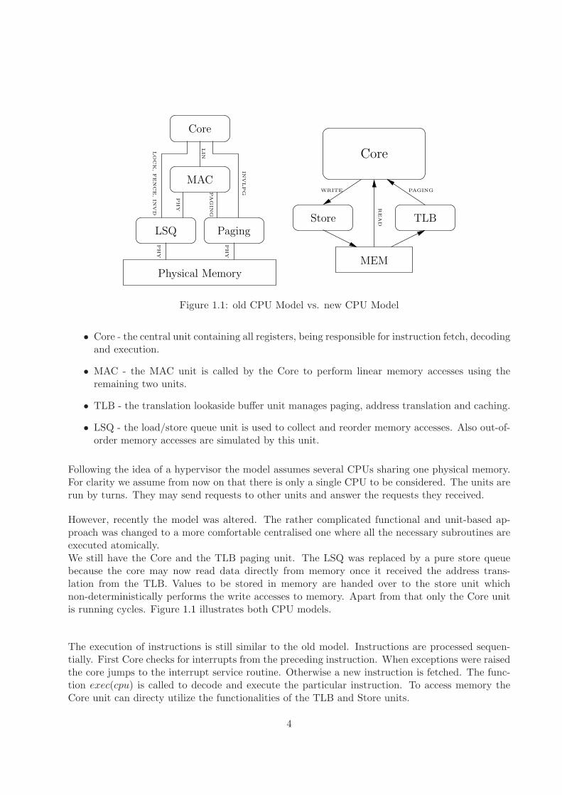
1.4 Model Overview
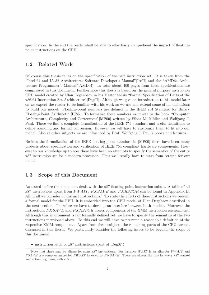
In his Master’s Thesis [Deg07] Ulan Degenbaev established a model for general purpose and systeminstructions. This model is based on several concurrently running units which communicate witheach other using requests. A CPU contains the following units in this model.
3
LO
CK
,FEN
CE,IN
VD
Core
MAC
Physical Memory
LSQ Paging
INV
LPG
PH
Y
PH
Y
LIN
PH
Y
PA
GIN
G
MEM
REA
D
WRITE PAGING
Core
Store TLB
Figure 1.1: old CPU Model vs. new CPU Model
• Core - the central unit containing all registers, being responsible for instruction fetch, decodingand execution.
• MAC - the MAC unit is called by the Core to perform linear memory accesses using theremaining two units.
• TLB - the translation lookaside buffer unit manages paging, address translation and caching.
• LSQ - the load/store queue unit is used to collect and reorder memory accesses. Also out-of-order memory accesses are simulated by this unit.
Following the idea of a hypervisor the model assumes several CPUs sharing one physical memory.For clarity we assume from now on that there is only a single CPU to be considered. The units arerun by turns. They may send requests to other units and answer the requests they received.
However, recently the model was altered. The rather complicated functional and unit-based ap-proach was changed to a more comfortable centralised one where all the necessary subroutines areexecuted atomically.We still have the Core and the TLB paging unit. The LSQ was replaced by a pure store queuebecause the core may now read data directly from memory once it received the address trans-lation from the TLB. Values to be stored in memory are handed over to the store unit whichnon-deterministically performs the write accesses to memory. Apart from that only the Core unitis running cycles. Figure 1.1 illustrates both CPU models.
The execution of instructions is still similar to the old model. Instructions are processed sequen-tially. First Core checks for interrupts from the preceding instruction. When exceptions were raisedthe core jumps to the interrupt service routine. Otherwise a new instruction is fetched. The func-tion exec(cpu) is called to decode and execute the particular instruction. To access memory theCore unit can directy utilize the functionalities of the TLB and Store units.
4
Within this framework the FPU environment is a component of the Core unit. We will extend theexec(cpu) function by a case for x87 instructions and define an interface function execFPU(cpu)that connects both models with each other and computes the next FPU state.
1.5 Outline
We choose a deductive, top-down approach to define the semantics of floating-point instructions.
Chapter 2 introduces the basic Notation used in this document. We will define the main typesand sets of numbers that represent the domains for the components and functions we will use tomodel the floating-point unit. As we also use source code to establish the interface between CPUand FPU, we will explain the correspoding functional language in the subsequent section. Becausenumber formats play a central role in this thesis, we will also introduce the fundamental numberrepresentations in this chapter. In the end we establish several abbreviations and conventions.
Chapter 3 starts the definition of our FPU model. We extend the given CPU framework with thefloating-point unit and develop the Interface between both models. We will also manipulate therespective functions from [Deg07] to enable decoding of x87 instructions. Finally the exception sig-naling as well as the implementation of XMM state saving and restoring are parts of this chapter.
Chapter 4 defines the Configuration of the floating-point unit comprising all of its components.This configuration describes the current state of the x87 environment. The main goal of this thesiswill be to define the next state configuration f ′ resulting from executing an x87 instruction on anarbitrary configuration f . To this end we provide functionality to comfortably access or manipulatethe FPU components and current instruction information.
Chapter 5 introduces a formalism for Floating-Point Numbers. Many definitions are therefor takenfrom [MP00], however we must modify the respective functions to fit our needs. In this chapter wewill also discuss the issues of rounding and conversion between real numbers and floating-point bitstrings. Additionally we introduce BCD numbers and x87 exceptions.
Chapter 6 deals with the various Operations implemented by the x87 instruction set. In thefirst part we structurize this instruction set by dividing the instructions into different functionalgroups, establishing predicates for certain instruction types and investigating on several instructioncharacteristics that are appropriate for distinguishing instruction variants. In these sections we alsoprovide definitions for the x87 instruction operands. The second part of this chapter concerns thesemantics of the various operations. We define the exact results for conversions, calculations andcomparisons in a generalized way.
Chapter 7 eventually implements the FPU state transition function σfpu which simulates the Ex-ecution of x87 instructions. We divide this simulation into four steps, namely the detection ofpre-computation exceptions, the computation of the result followed by the post-computation ex-ception detection and finally the returning of the result back to the CPU. By the end of this chapterour FPU model will be complete.
We conclude in chapter 8.
5

6
Chapter 2
Notation
In this chapter we will cover notation issues and establish necessary conventions for the followingthesis.
2.1 Types and Domains
In order to give the syntax and semantics of functions we need to formally define the types anddomains of arguments and results.
2.1.1 Basic Domains
The basic domains contain boolean, natural and integer numbers.
B = {0, 1}N = {0, 1, 2, 3, . . .}Z = {. . . ,−2,−1, 0, 1, 2, . . .}
Observe that 0 and 1 occur in all three sets. One can determine the original set of these numbersfrom the context of their occurrences. In addition to the domains above the set of real numbers R
may be referenced by functions we define. For some more comfort we denote certain subsets of thenatural numbers by the following shorthand notations.
N+ = N \ {0}Nn = {0, 1, 2, . . . , n − 1}
N+ denotes the strictly positive natural numbers, while Nn ⊂ N comprises the the first n ∈ N+
natural numbers. For the well-known boolean operations we use the following notation.
• ∧ - logical AND
• ∨ - logical OR
7
• ⊕ - exclusive OR
The negation of a boolean variables x is given by x. Accordingly ⊼ represents the boolean NANDoperation. In addition we make use of the following mathematical operations on real and integernumbers x, y.
• x + y - Addition
• x − y - Subtraction
• x · y - Subtraction
• x/y - Division
• x mod y - modulo computation (only for integers)
• xy - Exponentiation
• logx y - Logarithm
• √x - Square Root
• sin x, cos x - Sine and Cosine
• tan x, arctanx - Tangent and Arc Tangent
• sgn(x) - Signum (returns the sign of a number)
• |x| - Absolute value
These operations are defined as known from mathematics, however we will state the results forspecial arguments when necessary.
2.1.2 Tuples and Records
In this document we produce a model for the floating-point unit of an IA-32 compliant processor.Similar to the main part of the processor formalization written by Ulan Degenbaev our model shallbe translated to a programming language later on. That is why we would like to base our functionson data types rather than on mathematical domains. Therefore we introduce tuples and records aswell as data type definitions in the following.
Tuples and records are our main means to define the type of our model components and functions.An n-tuple with n ∈ N+ consists of n variables x1, . . . , xn while xi has type Ti. Then the tuple isrepresented as (x1, x2, . . . , xn) with type T1 × T2 × . . . × Tn. For our type declarations we use asimplified notation for type tuples.
(x1, x2, . . . , xn) ∈ (T1, T2, . . . , Tn)
8
In addition we want to comprise all our model components in a data structure. To this end weadopt records. These are data types similar to tuples with the difference that here the componentsof the record have names. A record type T with is obtained through the following type definition.
T = {x1 : T1, x2 : T2, . . . , xn : Tn}
Here xi is the identifier of the i-th record component with type Ti. A component xi of record rmay be accessed via:
r.xi
Note that a record may contain further complex data types.
2.1.3 Data Types
Accessorily to the basic types we may want to construct auxiliary data types. The basic types serveas the atomic elements for type construction. We may define a new type T from available types Ti
by
T = T1 | T2 | · · · | Ti | · · · | Tn .
The “|”works as a type union operator here. Apart from this mere joining of basic types we mayuse type constructor functions that take an arbitrary number of type arguments to define morecomplex types. A type T resulting from a type construction is indentified by the name of theconstructor function and the argument types.
T = CONSTR T1 | T2 | · · · | Ti | · · · | Tn
An instance of this type with arguments xi is then represented by CONSTR x1, . . . , xn. Wemostly use type joining and constructor functions without arguments to define enumeration types.Additionally we may extend a type T with the empty value ǫ via T|ǫ. For more information aboutǫ see subsection 2.5.1.
2.1.4 Functions
To define the semantics of the x87 instruction subset mathematically, we have to use functions ofcourse. A function maps arguments of one type S to a result of type T in a well-defined manner.However functions may be interpreted as types, too. Therefore the type of function f is given by
f : S → T ,
while the body of the function is represented in the usual way for an s ∈ S.
f(s) = expr
Here expr is a logical or arithmetic expression defining the result of f . Only arguments containedin s may be used to determine the result. However sometimes we may omit common arguments in
9
the notation and reference them implicitly for the sake of simplicity. From a programmer’s pointof view this may be interpreted as dependencies on the values of global variables. Nevertheless wewill always make remarks, when dealing with implicite arguments.
Observe that we keep using the “∈”operator for stating type affiliation. Only for record and functiondeclarations the “:”is used.
2.2 Source Code
In [Deg07] a functional programming language is used to define the general purpose CPU model.In this thesis we want to restrict ourselves to mathematical definitions as far as possible, howeverat least concerning the interface between CPU and FPU we will not be able to avoid providingsource code in the aforementioned language. A description of its syntax and semantics can be foundin [Deg07], sections 2.5 and 4.4.5. Nevertheless we want to give a short introduction on severalspecialities of the language. As a functional language, all procedures are defined like mathematicalfunctions. At first a type declaration is given. It is followed by the body definition for the respectivefunction. The body consists mainly of ordinary expressions, case destinctions and let statements.
• Ordinary expressions are valid terms of type T for a function f : S → T .
• A simple case distinction is the if-then-else expression.
1 if cond then expr1
2 else expr2
Here cond is a logical expression of type B. The expression is interpreted in the well-knownway. For cond = 1 it results in expr1, else expr2 is returned. if-then-else expressions may benested.
1 if cond1 then expr1
2 else
3 if cond2 then expr2
4 else
5 if cond3 then expr3
6 else
7
...
8 if condn then exprn
9 else exprn+1
This may be written in a simplified way.
1 |> cond1 → expr1
2 |> cond2 → expr2
3 |> cond3 → expr3
4
...
5 |> condn → exprn
6 |> otherwise → exprn+1
10
• Another case distinction is the case expression for distinguishing different values of an ex-pression x.
1 case x of
2 x1 →expr1
3 x2 →expr2
4
...
5 xn →exprn
6 default → exprn+1
This is just the same as:
1 |> x = x1 → expr1
2 |> x = x2 → expr2
3 |> x = x3 → expr3
4
...
5 |> x = xn → exprn
6 |> otherwise → exprn+1
• The let expression is used to define temporary variables and abbreviations that can be usedin the expression following the in keyword.
1 let x1 =a2 x2 =b
3
...
4 xn =abc in
5 expr1
All appearances of xi in expr1 are replaced by the assigned values according to the let state-ment. Note that pattern matching may be used to define the abbreviation.
In addition to these expressions the syntax is extended by a special type extension and a let?statement. In the old model the execution was interupted whenever an exception occurred or arequest was raised in the course of the next state computation. In these cases the Core componenthad to be returned to the CPU updating only the respective exception or request components. Tothis end the source code would have been spoiled with a lot of if-then-else case distinctions of theform:
1 A: Core → Core
2 A (c) =3 let c’ = B(c) in
4 |> c’.req 6= ǫ → c’
5 |> c’.excp 6= ǫ → c’
6 |> otherwise → // do some computation with c ’
In this example B : Core → Core returns a modified version of the core and we have to checkwhether exceptions or requests occurred. To find a shorter notation for this Ulan Degenbaev defineda special type ?T for any given typ T as follows.
?T = NORMAL T |PASS Core
11
Thus a value of ?T could either be NORMAL t or PASS c with t ∈ T and c ∈ Core. So now everyfunction of type X → T that might have to pass the core at some point may be defined as X →?Tto catch these exceptional cases. Then the example from above may be written as:
1 A: Core → ?Core
2 A (c) =3 let r = B(c) in
4 case r of
5 PASS c’ → PASS c’
6 NORMAL c’ → // do some computation with c ’
This combination of let and case may be abbreviated by the following let? statement.
1 A: Core → ?Core
2 A (c) =3 let? c’ = B(c) in
4 // do some computation with c ’
Accordingly
1 let? y = f(x) in
2 // do some computation with y
stands for
1 let r = f(x) in
2 case r of
3 PASS c → PASS c
4 NORMAL y → // do some computation with y
Please refer to [Deg07] for more explanations and examples on this subject. Also note that inthe new model the whole Cpu type is passed to all functions so that all memory accesses can beexecuted atomically. This means for our document that type ?T has a new definition.
?T = NORMAL T |PASS Cpu
2.3 Number Representations
This section deals with basic represenations of integer numbers and binary fractions. Additionalformats for floating-point numbers and binary coded decimal numbers will be discussed in chapter5.
2.3.1 Bit Strings
In the processor all data is saved in bit format. Therefore also all numbers are stored as strings ofbits. Before examining the different representations we want to investigate bit strings first.
12
Fixed length bit strings of length n may be modelled as boolean n-tuples.
B × B × · · · × B︸ ︷︷ ︸
n times
= Bn
Sometimes functions will result in bit strings of different lengths. For instance the binary represen-tation of an FPU operation’s result varies in its size with respect to the format of the particularresult. Instead of defining bit string type unions for all the special cases, we denote the type forvariable-length bit strings by B∗. This is a common notation from set theory which might beinterpreted as
B∗ ⊆∞⋃
n=1Bn
Now let x ∈ Bm and y ∈ Bn be bit strings. We want to introduce methods to access and manipulatethem.
• x[i] is the i-th element of the string for some i ∈ Nm. We use Little Endian notation, i.e. thebits are arranged from left to right in descending order and the leftmost bit contains x[m−1].As an abbreviation xi = x[i] can be used.
• x ◦ y is the concatenation of two bit strings. With i ∈ Nn+m the following statement holdsfor the concatenated string.
(x ◦ y)[i] =
{
x[i − n] n ≤ i < n + m
y[i] else
That means y is appended to the rightmost bit of x. Apparently x can be represented asx[m − 1] ◦ x[m − 2] ◦ · · · ◦ x[1] ◦ x[0]. For constructing bit strings from boolean constants weallow leaving out the concatenation symbols for clarity. For example 1 ◦ 0 ◦ 13 ◦ 03 can bewritten as 101303.
• xk concatenates k ∈ N copies of x yielding a new string with type Bm·k.
xk = x ◦ x ◦ · · · ◦ x︸ ︷︷ ︸
k times
When a string is copied using zero or a negative value for k, it is omitted and replaced withan empty string respectively.
• x[j : i] represents the substring x[j] ◦ x[j − 1] ◦ · · · ◦ x[i + 1] ◦ x[i] for some i, j ∈ N and0 ≤ i ≤ j < m. Depending on the context substring selections with i > j may be omitted orthey may produce a substring with reversed bit order. x[j : i] with j = i naturally returnsx[i].
These definitions allow us to comfortably handle bit strings.
13
2.3.2 Binary Numbers
Bit strings may be interpreted in several ways to determine the number they represent. Themost common format is that of unsigned binary numbers. The value 〈x〉 of a number’s binaryrepresentation x ∈ Bn can be obtained by applying the following definition from [MP00].
〈x[n − 1 : 0]〉 =n−1∑
i=0xi · 2i
This just complies with the well-known concept of binary numbers. An n-bit binary number canencode values from range {0, . . . , 2n − 1}.
To return the binary representation of length n for a given natural number a we introduce theconversion function binn.
binn : {0, . . . , 2n − 1} → Bn
binn(a) = x[n − 1 : 0] ⇔ 〈x〉 = a
Sometimes we need to increase the length of a bit string without changing the value of the numberit represents. This is called zero-extension. Basically it is just appending zeroes in front of the bitstring. For a bit string x ∈ Bm the zero-extended bit string with length n is denoted by zxtn(x) aslong as n ≥ m holds.
zxtn : Bm → Bn
zxtn(x) = 0m−n ◦ x[m − 1 : 0]
One can easily prove that 〈zxtn(x)〉 = 〈x〉. At last we want to care about addition and substractionof binary numbers. We would like to comfortably obtain the bit strings representing the result ofthe addition or substraction of two integers in binary format. Therefore we establish the modulo-n-bit binary addition and substraction +n and −n. They implement the following characteristicsfor some binary numbers a, b, c ∈ Bn.
a[n − 1 : 0] +n b[n − 1 : 0] = c[n − 1 : 0] ⇔ 〈a〉 + 〈b〉 = 〈c〉 mod 2n
a[n − 1 : 0] −n b[n − 1 : 0] = c[n − 1 : 0] ⇔ 〈a〉 − 〈b〉 = 〈c〉 mod 2n
Observe that overflowing or negative results will be wrapped around to a representable number dueto the modulo computation. One can show that calculating modulo 2n with binary numbers canbe emulated by computing the exact result with a higher number of bits an then truncating theupmost bits to receive a bit string of length n.
2.3.3 Binary Fractions
Besides binary integers we will be confronted with binary fractions. Luckily they follow the samerules as decimal fractions and have a limited precision, so we can simply handle them as binarynatural numbers that are scaled by some power of two with a negative exponent. From [MP00] welearn that a binary fraction consists of two bit strings a ∈ Bn and b ∈ Bp seperated by a point, so
a[n − 1 : 0].b[1 : p]
14
represents the corresponding binary fraction. Note that the fractional part b is kept in reversedbit order. This reflects the magnitude of the negative exponent the respective bits are scaled with.According to [MP00] the value of a binary fraction a.b can be obtained by the following formula.
〈a[n − 1 : 0].b[1 : p]〉 =n−1∑
i=0ai · 2i +
p∑
j=1bj · 2−j
Observe that the fraction’s value can be split into the sum 〈a.b〉 = 〈a〉+〈b〉 ·2−p which uses only thecommon definition of the binary representation for natural numbers. Similarly for some x ∈ [0, 1)with the property ⌊x · 2p⌋ = x · 2p the binary fractional representation 0.b with b ∈ Bp can bedetermined via
b[1 : p] = binp(x · 2p).
It can be proven that 〈0.b〉 = x holds.
2.3.4 Two’s Complement Numbers
Up to now we only considered positive numbers. The common format for negative integers is thetwo’s complement representation. [MP00] gives the definition of a bit vector a[n − 1 : 0]’s two’scomplement value.
[a] = −an−1 · 2n−1 + 〈a[n − 2 : 0]〉
Thus the range of representable numbers is defined as
[a] ∈ {−2n−1, . . . , 2n−1 − 1}
For an integer x from this range we can produce the n-bit two’s complement bit string via twocn(x).
twocn : {−2n−1, . . . 2n−1 − 1} → Bn
twocn(x) = a[n − 1 : 0] ⇔ [a] = x
An important observation is that the upmost bit an−1 of the two’s complement number determinesthe sign of its value. That’s why this bit is also called sign bit. Comparable with the zero-extensionfor binary numbers, two’s complement numbers can be enlarged while conserving their values viasign-extension. The sign-extended n-bit version of a ∈ Bm is given by sxtn(a) for n ≥ m.
sxtn : Bm → Bn
sxtn(a) = (an−1)m−n ◦ a[m − 1 : 0]
Sign-extension assures that [sxtn(a)] = [a] holds true.
At first sight two’s complement numbers might appear to be a somewhat unintuitive approach toimplement integers. However their structure bears some great benefits compared to other solutions,as for instance the equation [a] = 〈a〉 mod 2n holds for any bit string a ∈ Bn. See [MP00] for moreinformation on this number format.
15
2.3.5 Hexadecimal Numbers
Besides binary format we also use hexadecimal numbers in this document. They are mainly usedto state opcodes or bit masks because one hexadecimal digit is able to encode four bits. Thuslonger bit strings become more clear and memorable when given in hex format. We denote the setof hexadecimal digits by Q.
Q = {0,1,2,3,4,5,6,7,8,9,A,B,C,D,E,F}
Then any bit string x ∈ B4n can be encoded by a hexadecimal number h ∈ Qn. The value of a hexnumber h can be easily computed as follows.
〈h[n − 1 : 0]〉 =n−1∑
i=0〈hi〉 · 16i
Here the digits 0,. . .,F are evaluated by the overloaded 〈·〉-brackets as the natural numbers from 0to 15. Though, we are rather interested in the corresponding bit vector than in the actual value ofa hexadecimal number. Hence we establish the “0x”prefix for these numbers. For h ∈ Qn it yieldsthe bit vector x ∈ B4n such that
0xh = x〈h[n − 1 : 0]〉 = 〈x[4n − 1 : 0]〉
holds. This way we are able to comfortably include hex-codes in our formulae.
2.4 Abbreviations
Throughout this document we utilize several abbreviatory notations to promote clarity and avoidtedious repetitions of similar definitions. For instance when defining various functions with thesame type scheme and related names, we allow to abbreviate the several similar declarations by asingle one containing a placeholder x that can be replaced by the appropriate letters to form thedeclaration for a particular function.
Another measure of combining definitions are the ± and ∓ signs. They are used to distinguishthe two cases of positive and negative arguments - or addition and substraction respectively - in asingle definition. An expression expr(±,∓) containing the ± and ∓ signs stands for two definitionswhere the respective signs are symbolically replaced by + or − according to the following rules.
expr(±,∓) ≡ expr(+,−) ∧ expr(−, +)
For example the equations sin(32π) = −1 and sin(−3
2π) = 1 maybe combined to the statement
sin(±32π) = ∓1
We can extract the two equations back from this by applying the rule from above. ± and ∓ arereplaced by + and − for the first equation and vice versa for the second one.
Another abbreviatory notation can be found in table B.1 of Appendix B. There we list the sets of
16
opcodes in hexadecimal format which belong to a certain instruction. Many of these opcodes aresucceeding each other, that means they only differ in the last hexadecimal digits. For clarity andto reduce the size of the definitions we allow to define hexadecimal ranges in the following way. Leti, j ∈ Qm be some hex digit strings with 〈j〉 > 〈i〉 and h ∈ Qn a hexadecimal number with n ≥ m,then h[n − 1 : m][i : j] denotes the following range of hex numbers.
h[n − 1 : m][i : j] = h[n − 1 : m] ◦ i, h[n − 1 : m] ◦ i + 1, . . . , h[n − 1 : m] ◦ j
For example the opcodes for the instruction FXCH, namely 0xD9C8, 0xD9C9, 0xD9CA, . . .,0xD9CF may be comprised by the hex-code range 0xD9C[8:F]. Note that we overload the selectionbrackets here with contrary semantics. However as we use the range abbreviation brackets only forconstants and the substring selection brackets only for variables there is no conflict between bothnotations.
2.5 Conventions
There are some general subjects left we want to discuss.
2.5.1 Empty and Undefined Results
The x87 part of the IA-32 specification as well as the whole instruction set itself comprises amultitude of different functionalities. For each instruction we have to consider various specialcases. In addition we want to keep our functions as general and comprehensive as possible. Thishowever will make it hard for us to give reasonable results for these functions considering all possibleFPU configurations. That is why we introduce the empty result ǫ which is returned in all the caseswhere a well-defined result is neither available nor required from a certain function. It just assuresthat we have exhaustive case destinctions and definitions. In addition the functions of our modelmay accept empty arguments when necessary, that means they are also defined for the cases thattheir inputs may become ǫ.
On the contrary the Intel IA-32 and AMD64 Architecture specifications often leave particular issuesundefined. Whenever this is the case the components under consideration will be updated withthe value “undefined”. Note that ǫ will never be assigned to an FPU component. It is in a waythe “undefined”value of our internal model. We apply this distinction to point out where thespecification itself is unclear on certain subjects. Moreover an undefined bit is represented by an“X”.
2.5.2 Quotations
This document is based on the general purpose CPU model in [Deg07]. Therefore we will at leastfor the interface need to recall definitions and functions from Ulan Degenbaev’s thesis. Additionallythe IEEE floating-point number format was already formalized in [MP00]. Thus we will also citedefinitions from this book. Whenever we refer to ideas and formulae from external sources we will
17
state their origin in brackets close to the quoted material. For the interface we will have to quoteand extend sourcecode from [Deg07]. All cited lines will be held in a grey shade to mark whichportions of code were added by us and which were taken from that thesis. We also may leave outcertain parts of definitions and code listings by “. . .”when they are irrelevant for our model.
2.5.3 Signed Zero
A famous speciality of floating-point numbers is that they have two representations for zero, namelypositive and negative zero. Reading this one will surely wonder about the purpose of signed zeroes.One main reason is the rounding of very small numbers. When a floating-point number is roundedto zero one may determine whether the exact result was a positive or negative number from thesign of zero. Also when finite values are divided by infinities the sign of the resulting zero reflectsthe signs of the operands. Of course in mathematics zero has no explicit sign, however in thisdocument we assume that +0 and −0 may be distinguished not only for floating-point but also forreal and integer numbers. Still these representations have the same value and are considered equalby comparisons. We want to set up conventions to handle this ambiguous subject.
Within this model the sign of zero is stated explicitely for all definitions. Whenever a variablex’s value shall be just zero regardless of the sign, we apply an absolute value notation. Thus thefollowing expressions may be found.
x = +0 x = −0 |x| = 0 |x| 6= 0
In the third case the value of the variable may either be +0 or −0, its sign is undefined. Whennecessary we interpret these zeroes as positive by default. In the fourth case x contains neithersigned nor unsigned zeroes at all. We never use the ± symbol to state that a zero’s sign is undefined.
For the various mathematical operations we will identify special cases and state the results forcomputations involving signed zeroes. As mentioned before the x87 comparison instructions ignorethe sign of zero. On the contrary the sign of zeroes is always taken into account when convertingnumbers to IEEE floating-point or BCD format. For these formats the sign may be stored explicitelyin a sign bit, so we must not omit it in the course of our result computation.
18
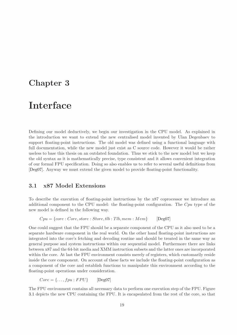
Chapter 3
Interface
Defining our model deductively, we begin our investigation in the CPU model. As explained inthe introduction we want to extend the new centralised model invented by Ulan Degenbaev tosupport floating-point instructions. The old model was defined using a functional language withfull documentation, while the new model just exist as C source code. However it would be ratheruseless to base this thesis on an outdated foundation. Thus we stick to the new model but we keepthe old syntax as it is mathematically precise, type consistent and it allows convenient integrationof our formal FPU specification. Doing so also enables us to refer to several useful definitions from[Deg07]. Anyway we must extend the given model to provide floating-point functionality.
3.1 x87 Model Extensions
To describe the execution of floating-point instructions by the x87 coprocessor we introduce anadditional component to the CPU model: the floating-point configuration. The Cpu type of thenew model is defined in the following way.
Cpu = {core : Core, store : Store, tlb : T lb, mem : Mem} [Deg07]
One could suggest that the FPU should be a separate component of the CPU as it also used to be aseparate hardware component in the real world. On the other hand floating-point instructions areintegrated into the core’s fetching and decoding routine and should be treated in the same way asgeneral purpose and system instructions within our sequential model. Furthermore there are linksbetween x87 and the 64-bit media and XMM instruction subsets and the latter ones are incorporatedwithin the core. At last the FPU environment consists merely of registers, which customarily resideinside the core component. On account of these facts we include the floating-point configuration asa component of the core and establish functions to manipulate this environment according to thefloating-point operations under consideration.
Core = {. . . , fpu : FPU} [Deg07]
The FPU environment contains all necessary data to perform one execution step of the FPU. Figure3.1 depicts the new CPU containing the FPU. It is encapsulated from the rest of the core, so that
19
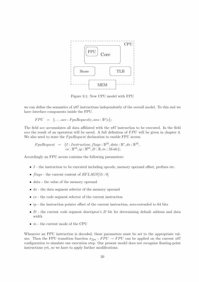
Store TLB
MEM
FPU
CPU
Core
Figure 3.1: New CPU model with FPU
we can define the semantics of x87 instructions independently of the overall model. To this end wehave interface components inside the FPU.
FPU = {. . . , acc : FpuRequest|ǫ, ans : B∗|ǫ};
The field acc accumulates all data affiliated with the x87 instruction to be executed. In the fieldans the result of an operation will be saved. A full definition of FPU will be given in chapter 4.We also need to state the FpuRequest declaration to enable FPU access.
FpuRequest = {I : Instruction, flags : B16, data : B∗, ds : B16,cs : B16, ip : B64, D : B, m : Mode};
Accordingly an FPU access contains the following parameters:
• I - the instruction to be executed including opcode, memory operand offset, prefixes etc.
• flags - the current content of RFLAGS[15 : 0]
• data - the value of the memory operand
• ds - the data segment selector of the memory operand
• cs - the code segment selector of the current instruction
• ip - the instruction pointer offset of the current instruction, zero-extended to 64 bits
• D - the current code segment descriptor’s D bit for determining default address and datawidth
• m - the current mode of the CPU
Whenever an FPU instruction is decoded, these parameters must be set to the appropriate val-ues. Then the FPU transition function σfpu : FPU → FPU can be applied on the current x87configuration to simulate one execution step. Our present model does not recognize floating-pointinstructions yet, so we have to apply further modifications.
20
3.2 Decoding x87 Instructions and Operands
Before the FPU can be called, the core must be able to recognize x87 instructions. It also needsto know whether there are memory operands to be fetched. Therefore we modify definitions fromthe ”Instruction Fetch and Decode” chapter in [Deg07] to suit floating-point instructions. First ofall we introduce two new operand types FPM and FPS for x87 operands.
optype : (B24, B8|ǫ, B, {1, 2, 3}) → {. . . , FPM, FPS} [Deg07]optype(opc, modrm, is64mode, index) = . . .
As in [Deg07] we will compute the operand type using a table given in Appendix A. All x87 relatedinstruction are listed there as an extension to the opcode tables in [Deg07]. Note that all floating-point operations except one1 have either operand types FPM or FPS. Their default operand sizeis 80 bit. However there are memory operands with deviating sizes that were not considered yet.Thus we extend opsize as well.
opsize : (B24, B8|ǫ, {1, 2, 3}, {16, 32, 64}) → {. . . , 112, 224, 752, 864, 4096} [Deg07]opsize(opc, modrm, is64mode, index, dataw) = . . .
The operand bitsize can be determined from the opcode table by checking the subscripts of theoperand type alias. There are x87 state-saving instructions that allow to save the entire floating-point environment to memory and to restore the state based on this data later on. The contiguousbit string containing the information for the FPU components is called image. The image size isvariable and dependent on the current data width. We denote three different image categories bythe aliases iS (small image - 14/28 byte), iM (medium image - 94/108 byte) and iL (large image- 512 byte). They stand for the following bit sizes.
iS =
{
112 : dataw = 16
224 : else
iM =
{
752 : dataw = 16
864 : else
iL = 4096
To learn more about images and state saving/restoring please confer to sections 3.4, 7.2.3 andAppendix C. It is worth mentioning that x87 operand size ranges from 16 to 4096 bit.All x87 instructions need a ModR/M-byte, hence the needModRM predicate is updated.
needModRM : B24 → B [Deg07]needModRM(opc) = opc2(opc) 6= ǫ ∨ ∃i ∈ {1, 2, 3} : (optype(opc, i) ∈ {. . . , FPM, FPS})
The function opdecode : (Core, {1, 2, 3}) → (Operand, B) from [Deg07] relates operand type andthe actual operand description. Floating-Point operands may be x87 registers, or data residing inmemory. As the core shall not access FPU registers directly we only need to assign meaningfuldecodings to the memory operands. On account of this we add FPM (Floating-Point Mem-ory) and FPS (Floating-Point Stack) operand types to opdecode. Note that Instructions I withI.modrm.mod = 11 can not reference memory operands.
1Solely an obsolete version of FNSTSW allows to store the x87 status word to the AX register.
21
1 opdecode : (Core, {1, 2, 3}) → (Operand, B)
2 opdecode (c, i) =3 let size’ = opsize(c.I.opc, c.I.modrm, x64mode(c), i, dataw(c)) in
4 case optype(c.I.opc, c.I.modrm, i) of
5 A → (MEM {sreg=opseg(c), addr=c.I.imm, size=size’}, 1)
6 . . .7 Y → (MEM {sreg=ES, addr=c.R[DI], size=size’}, 1)
8 FPM ∧ c.I.modrm.mod = 11 → (ǫ, 1)
9 FPM ∧ c.I.modrm.mod 6= 11 → (MEM {sreg=opseg(c), addr=opaddr(c), size=size’}, 1)
10 FPS → (ǫ, 1)
11 SS → (REG {type=SEG, reg=0◦SS, size= 16}, 1)
12 . . .13 ǫ →(ǫ, 1)
Finally in the fetch phase the instruction field’s operand components are filled with the respectivecontents gained from decoding. Also the opcode fields are updated with the appropriate data.Therefore we henceforth are able to recognize x87 instructions by examining the opcode. Thenecessary predicates are defined in section 6 and table B.1 in Appendix B. As we included floating-point operations into the regular operand decoding scheme, floating-point memory operands can befetched and updated without extra effort using the readOp and writeOp functions from [Deg07].All functionality to fetch and decode x87 instructions and operands and to write back result tomemory resides in the core unit hence the FPU unit is only required for the actual floating-pointcalculations.
3.3 Executing x87 Instructions
As described above, the core must deliver all required data to the FPU environment wheneveran x87 instruction is decoded. The FPU operation may involve a memory operand, which canbe loaded utilising the readOp function. After decoding an x87 instruction the suitable functionexecFPU : Cpu →?Cpu is called for the execution. Recognizing x87 instructions by the opcode iseasy using table A.1 or the predicates defined in chapter 6. These predicates identify the currentx87 instruction. They are written in capital letters and are named after the mnemonic of thecorresponding operation. Now we want to give the definition for the function execFPU thatrepresents the interface between CPU and FPU environment. For information on the syntax seesection 2.2 in the notations chapter.
1 execFPU : Cpu → ?Cpu
2 execFPU(cpu) =3 let c = cpu.core in
4 let MP = c.CR(0)[1] in // ’monitor coprocessor ’ control b i t5 let EM = c.CR(0)[2] in // ’ emulate coprocessor ’ control b i t6 let TS = c.CR(0)[3] in // ’ task switched ’ control b i t7 let mf = es(cpu.fpu) in
8 |> (EM=1∧WAIT(c.I))∨(TS=1∧(WAIT(c.I)∨(WAIT(c.I)∧MP=1))) →9 PASS cpu{core = core{excp = eNM}}
10 |> (mf=1 ∧ nonctrl(instr)) →PASS cpu{core =core{excp =eMF}}11 |> WAIT(c.I) →if mf=1 then PASS cpu{core =core{excp =eMF}}12 else NORMAL cpu
22
13 |> otherwise →14 let? (cpu1,op) = if xread(c.I) then readOp(cpu, c.I.op1)
15 else NORMAL (cpu, 0) in
16 let? (cpu2,op1) = if FXRSTOR(c.I) then xmmrstor(cpu1,op)
17 else NORMAL (cpu1, op) in
18 let c1 = cpu2.core in
19 let fpu1 = reqFPU(c1,op1) in
20 let fpu2 = σfpu(fpu1) in
21 let res = fpu2.ans in
22 let (c2,res1) = if FXSAV E(c.I) then xmmsave(c1,res) else (c1,res) in
23 let cpu3 = cpu2{core = c2{fpu = fpu2}} in
24 |> xupdm(c.I) →writeOp(cpu3, c.I.op1, res1)
25 |> xupdf(c.I) →NORMAL cpu3{core =core{RFLAGS =RFLAGS[63:16] ◦ res1}}
26 |> otherwise → NORMAL cpu3
At first we have to catch some exceptions affiliated with the EM (emulate coprocessor), TS (taskswitched) and MP (monitor coprocessor) bits in the CR0 control register.FPU requests can not always be served because there may be pending floating-point exceptionsfrom the last non-control x87 instruction executed. Therefore the CPU must check for exceptionsbefore the execution of another non-control x87 instruction. To this end we test for unmasked x87exceptions. es : FPU → B is used to determine the FPU exception status. nonctrl : Instruction →B is a predicate which identifies non-control x87 instructions by examining the two x87-opcodebytes. The exact defintions of these functions can be found in sections 4.4 and 6.1.1 respectively.Furthermore WAIT : Instruction → B identifies a WAIT instruction, which forces the processorto check for pending floating-point exceptions and to handle them.Then - when necessary - the above function loads a memory operand for the FPU operation. Fromthe last section we can deduce that field op1 of Instruction is either a memory operand MEM x orǫ for x87 instructions. The predicate xread states whether a memory operand must be read. It isdefined in section 6.1.2. Predicates FXSAV E/FXRSTOR being defined in section 6.1.1 identifyspecial cases which are discussed in the next subsection.To prepare the FPU access, reqFpu is called. This function determines the required parametersof the request and sets them accordingly in the field acc. Memory operands are saved in the datacomponent. A copy of the lower 16 bits of the RFLAGS register is stored as well as the x87exception pointers (data and instruction addresses), D bit and the current mode of the CPU. Nowthe state transition function σfpu can be applied on the floating-point unit. Its complete semanticsis defined in section 7. The operation’s result is then contained in the FPU configuration’s fieldans.The predicates xupdf, xupdm : Instruction → B signal whether an x87 instruction updates theRFLAGS register or a memory operand respectively. Those predicates’ exact definitions can befound in section 6.1.2.Accordingly the memory or the flags are updated when required.
1 reqFPU : (Cpu, B∗) → FPU
2 reqFPU (cpu, op) =3 let c = cpu.core in
4 let (ddesc, dex, dsel) = if (c.I.op1 6= ǫ) then segment(cpu, c.I.op1.sreg)
5 else (ǫ, ǫ, ǫ) in
6 let (idesc, iex, isel) = segment(cpu, CS) in
7 let ioff = zeroext64(c.oldRIP[ipw(c)-1:0]) in
23
8 let d = idesc.D in
9 let M = mode(c) in
10 let f = c.RFLAGS[15:0] in
11 let fpuacc = FPU {I=c.I, flags=f, data=op, ds=dsel, cs=isel, ip=ioff, D=d, m=M} in
12 fpu{acc = fpuacc}
Here segment : (Cpu, B3) → (B128, B8, B16) returns the segment descriptor, the affiliated exceptionand the segment selector for a certain segment register. ipw(c) stands for the instruction pointeraddress width as defined in [Deg07].
3.4 XMM state Save and Restore
For FXSAVE and FXRSTOR instructions we must consider not only x87 components, but alsothe XMM state. The respective instructions save or restore this information together with theFPU state to or from memory using a joined image format. However inside the FPU we cannot access the XMM components, thus in execFPU the data transmitted to or received fromthe FPU must be further manipulated. At a save of the configuration we must merge the XMMdata with the FPU data to build the final image. When the whole floating-point and mediastate shall be restored we have to strip the respective XMM data from the image first, updatethe corresponding XMM components and transmit the remaining floating-point state to the FPU.These image manipulations are executed using xmmsave : (Core,B1280) → (Core,B4096) andxmmrstor : (Cpu, B4096) →?(Cpu, B1280). Being called from execFPU these functions extractFPU information from or add non-FPU information to the memory images and also carry out theXMM part of the instruction execution. For clarity, illustrations of the XMM image formats aregiven in Appendix C.
1 xmmrstor : (Cpu, B4096) → ?(Cpu, B1280)
2 xmmrstor(cpu,image) =3 let c = cpu.core in
4 let fpuim = image[1279:0] in
5 let mask = if (mxcsr mask(c) =0x00000000) then 0x0000FBFF else mxcsr mask(c) in
6 |> c.CR(4)[9] = 0 → NORMAL (cpu,fpuim)
7 |> (mask∧image[223:192] 6= image[223:192]) →PASS cpu{core =c{excp =eGP}}
8 |> otherwise →9 let c1 = c{MXCSR = image[223:192]} in
10 let c2 = |> c.EFER[14]=1 ∧ cpl(c)=0 ∧ x64mode(c)→ c1
11 |> x64mode(c) →12 c1{XMM = XMM[ ∀i ∈ N8 : i →image[128·(i + 1)+1279:128·i+1280] ]}
13 |> otherwise →14 c1{XMM = XMM[ ∀i ∈ N16 : i →image[128·(i + 1)+1279:128·i+1280] ]} in
15 NORMAL (cpu{core = c2},fpuim)
Here it is assumed, that XMM : N16 → B128 and MXCSR ∈ B32 represent the 16 XMM registersand the XMM control/status register of the core. The FPU relevant information is contained in thelower 160 bytes of the image. CR(4)[9] contains the OSFXSR bit which toggles the saving/restoringof the XMM registers. We must consider some special characteristics of the MXCSR register.Several bits in this register are reserved and may only be written with zeroes. These zero bits
24
signal that the associated features are not available. To gain information, which bits are reserved,software may examine the field MXCSR MASK in the FXSAVE memory image at bytes 28-31.We assume function mxcsr mask : Core → B32 to compute this mask bit field on the basis of thecurrent configuration and machine-specific information. When there is an attempt to write onesto reserved bits in the MXCSR, a General Protection exception must be raised. To this end thecurrent MXCSR MASK is compared with the new data for the MXCSR. Furthermore the XMMrestoration depends on bit 14 of the EFER register (FFXSR bit) and on the current mode. TheFFXSR bit enables fast save and restore of the XMM state as it omits restoring the XMM registerswhen FXRSTOR is executed in 64-bit mode with privilege level 0. Note that regardless of FFXSRbit only in 64-bit mode all 16 XMM registers can be restored. According to the same rules theFXSAVE image is built using the x87 environment image received from the FPU.
1 xmmsave : (Core, B1280) → (Core, B4096)
2 xmmsave(c,image) =3 let img = image[1279:256]◦mxcsr mask(c) ◦ c.MXCSR◦image[191:0] in
4 |> c.CR(4)[9]=0 → (c, 02816◦image)5 |> c.EFER[14]=1 ∧ cpl(c)=0 ∧ x64mode(c) →(c, 02816◦img)6 |> x64mode(c) →(c, 01792◦c.XMM(7)◦c.XMM(6)◦ . . . ◦c.XMM(1)◦c.XMM(0)◦img)7 |> otherwise → (c, 0768◦c.XMM(15)◦c.XMM(14)◦ . . . ◦c.XMM(1)◦c.XMM(0)◦img)
Note that for FXSAV E and FXRSTOR the x87 part is located in the image’s lower 160 bytes or1280 bits respectively. Now the interface of the Floating-Point Unit is complete. We have obtaineda framework to decode floating-point instructions and generate the corresponding x87 requests.The next chapters describe how these requests are processed by the FPU in order to return a resultto the core.
3.5 Handling Exceptions
As one can already see above, exception handling is somewhat special for x87 instructions. Thefloating-point exceptions are not reported to the CPU immediately after their occurrence. Insteadthey are not detected by the processor before executing the next WAIT or non-control floating-point instruction. That means that control instructions may manipulate the FPU configuration inthe meantime before the exception is recognized. We implemented this behaviour in the beginningof the execFPU function. Besides the numerical eMF exceptions FPU instructions may cause thefollowing general purpose exceptions.
• eDB - Debug
• eBP - Breakpoint
• eUD - Invalid-Opcode
• eNM - Device-Not-Available
• eDF - Double-Fault
• eSS - Stack
25
• eGP - General-Protection
• ePF - Page-Fault
• eAC - Alignment-Check
• eMC - Machine-Check
The origins of these exceptions lie outside of the FPU. They mostly occur when accessing memoryto read operands or write results or due to improper use of the instructions. The checking andhandling of them is already given in [Deg07]. However we have to consider a speciality for floating-point instructions.
Whenever an exception causing a repetition of the respective x87 instruction occurs after the FPUfinished computation and returned the result to the CPU, the old FPU configuration has to berestored before the instruction’s execution can be repeated. Everything else would result in acorrupted FPU state and a likely erroneous result. Therefore arrangements to save and restore thefloating-point unit component have to be incorporated in the core’s exception handling routines.
26
Chapter 4
Configuration
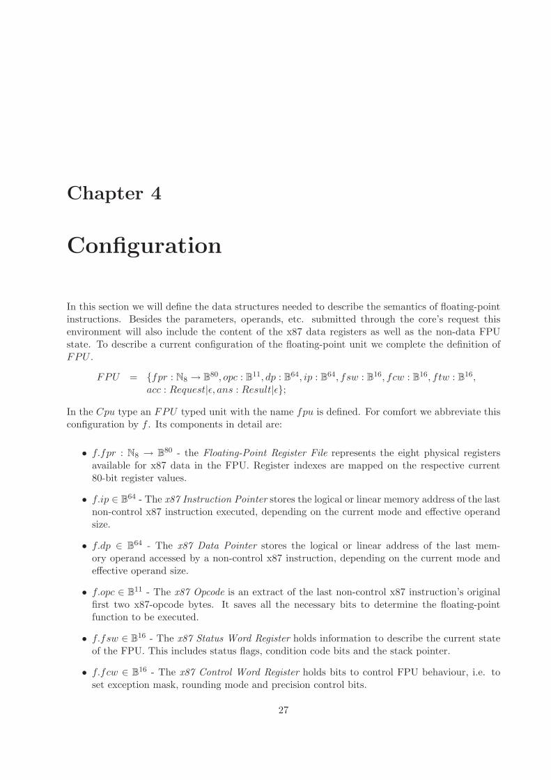
In this section we will define the data structures needed to describe the semantics of floating-pointinstructions. Besides the parameters, operands, etc. submitted through the core’s request thisenvironment will also include the content of the x87 data registers as well as the non-data FPUstate. To describe a current configuration of the floating-point unit we complete the definition ofFPU .
FPU = {fpr : N8 → B80, opc : B11, dp : B64, ip : B64, fsw : B16, fcw : B16, ftw : B16,acc : Request|ǫ, ans : Result|ǫ};
In the Cpu type an FPU typed unit with the name fpu is defined. For comfort we abbreviate thisconfiguration by f . Its components in detail are:
• f.fpr : N8 → B80 - the Floating-Point Register File represents the eight physical registersavailable for x87 data in the FPU. Register indexes are mapped on the respective current80-bit register values.
• f.ip ∈ B64 - The x87 Instruction Pointer stores the logical or linear memory address of the lastnon-control x87 instruction executed, depending on the current mode and effective operandsize.
• f.dp ∈ B64 - The x87 Data Pointer stores the logical or linear address of the last mem-ory operand accessed by a non-control x87 instruction, depending on the current mode andeffective operand size.
• f.opc ∈ B11 - The x87 Opcode is an extract of the last non-control x87 instruction’s originalfirst two x87-opcode bytes. It saves all the necessary bits to determine the floating-pointfunction to be executed.
• f.fsw ∈ B16 - The x87 Status Word Register holds information to describe the current stateof the FPU. This includes status flags, condition code bits and the stack pointer.
• f.fcw ∈ B16 - The x87 Control Word Register holds bits to control FPU behaviour, i.e. toset exception mask, rounding mode and precision control bits.
27
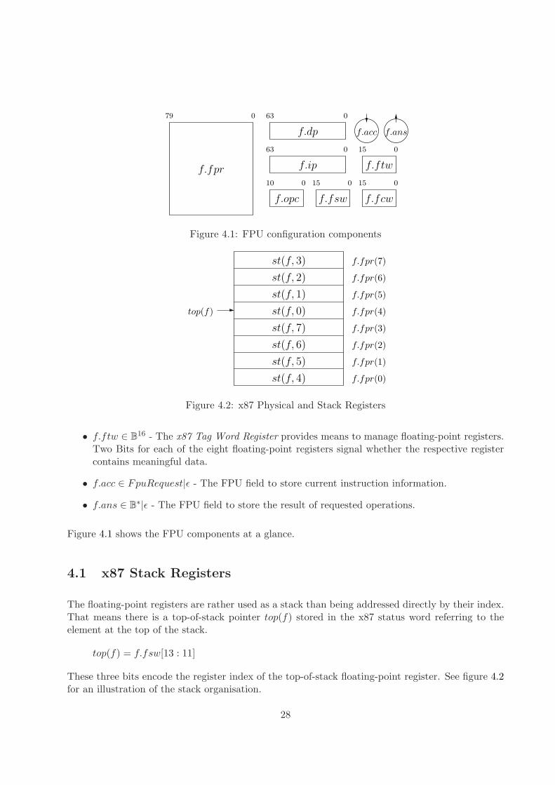
f.ftwf.fpr
79 0 0
0
63
63
f.dp
f.ip
f.opc
010
0
015
15
15 0
f.fsw f.fcw
f.acc f.ans
Figure 4.1: FPU configuration components
st(f, 4)
f.fpr(7)
f.fpr(6)
f.fpr(5)
f.fpr(4)
f.fpr(3)
f.fpr(2)
f.fpr(1)
f.fpr(0)
st(f, 0)top(f)
st(f, 1)
st(f, 2)
st(f, 3)
st(f, 7)
st(f, 6)
st(f, 5)
Figure 4.2: x87 Physical and Stack Registers
• f.ftw ∈ B16 - The x87 Tag Word Register provides means to manage floating-point registers.Two Bits for each of the eight floating-point registers signal whether the respective registercontains meaningful data.
• f.acc ∈ FpuRequest|ǫ - The FPU field to store current instruction information.
• f.ans ∈ B∗|ǫ - The FPU field to store the result of requested operations.
Figure 4.1 shows the FPU components at a glance.
4.1 x87 Stack Registers
The floating-point registers are rather used as a stack than being addressed directly by their index.That means there is a top-of-stack pointer top(f) stored in the x87 status word referring to theelement at the top of the stack.
top(f) = f.fsw[13 : 11]
These three bits encode the register index of the top-of-stack floating-point register. See figure 4.2for an illustration of the stack organisation.
28
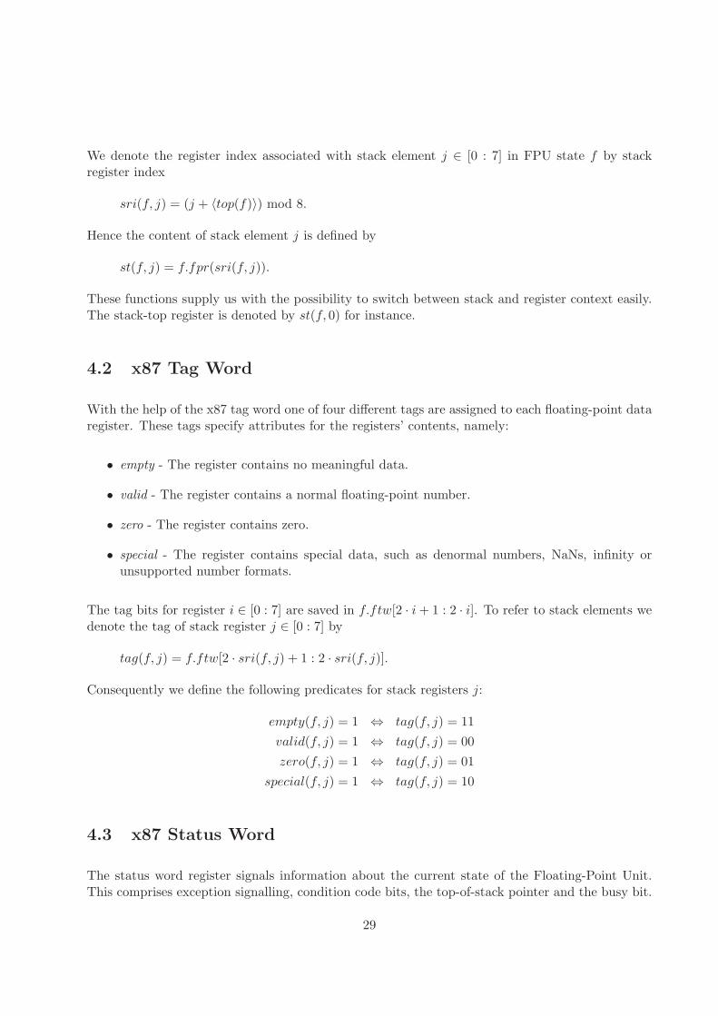
We denote the register index associated with stack element j ∈ [0 : 7] in FPU state f by stackregister index
sri(f, j) = (j + 〈top(f)〉) mod 8.
Hence the content of stack element j is defined by
st(f, j) = f.fpr(sri(f, j)).
These functions supply us with the possibility to switch between stack and register context easily.The stack-top register is denoted by st(f, 0) for instance.
4.2 x87 Tag Word
With the help of the x87 tag word one of four different tags are assigned to each floating-point dataregister. These tags specify attributes for the registers’ contents, namely:
• empty - The register contains no meaningful data.
• valid - The register contains a normal floating-point number.
• zero - The register contains zero.
• special - The register contains special data, such as denormal numbers, NaNs, infinity orunsupported number formats.
The tag bits for register i ∈ [0 : 7] are saved in f.ftw[2 · i + 1 : 2 · i]. To refer to stack elements wedenote the tag of stack register j ∈ [0 : 7] by
tag(f, j) = f.ftw[2 · sri(f, j) + 1 : 2 · sri(f, j)].
Consequently we define the following predicates for stack registers j:
empty(f, j) = 1 ⇔ tag(f, j) = 11
valid(f, j) = 1 ⇔ tag(f, j) = 00
zero(f, j) = 1 ⇔ tag(f, j) = 01
special(f, j) = 1 ⇔ tag(f, j) = 10
4.3 x87 Status Word
The status word register signals information about the current state of the Floating-Point Unit.This comprises exception signalling, condition code bits, the top-of-stack pointer and the busy bit.
29
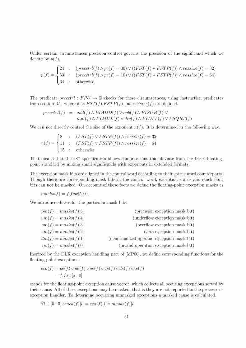
rc(f) Rounding Mode pc(f) Precision Mode00 Round to nearest 00 Single precision01 Round down 01 undefined
10 Round up 10 Double precision11 Round toward zero 11 Double-extended precision
Table 4.1: Rounding and Precision Modes
We define aliases for the particular status word bits as given below.
busy(f) = f.fsw[15] (busy bit)
cc(f)[3 : 0] = f.fsw[14] ◦ f.fsw[10 : 8] (condition code)
top(f) = f.fsw[13 : 11] (top-of-stack pointer)
es(f) = f.fsw[7] (exception status)
sf(f) = f.fsw[6] (stack fault)
pe(f) = f.fsw[5] (precision exception)
ue(f) = f.fsw[4] (underflow exception)
oe(f) = f.fsw[3] (overflow exception)
ze(f) = f.fsw[2] (zero exception)
de(f) = f.fsw[1] (denormalized operand exception)
ie(f) = f.fsw[0] (invalid operation exception)
4.4 x87 Control Word
The control word register is used to customize floating-point operations to certain extents. Softwarecan influence rounding modes and precision settings for the calculations as well as mask occuringfloating exceptions. There are four different rounding and three precision modes as defined in table4.1 using the following functions.
rc(f) = f.fcw[11 : 10] (rounding control)
pc(f) = f.fcw[9 : 8] (precision control)
Rounding control enables the user to choose the way floating-point numbers are rounded by theFPU. For some instructions the actual rounding mode is fixed, so the rounding control has no effect.We denote the current rounding mode by rm(f) : FPU → B2.
rm(f) =
00 : FPREM1(f)
11 : FISTTP (f) ∨ FPREM(f)
rc(f) : otherwise
FISTTP (f), FPREM(f) and FPREM1(f) are instruction predicates. They are defined in chap-ter 6 and identify the instructions corresponding to their names.
30
Under certain circumstances precision control governs the precision of the significand which wedenote by p(f).
p(f) =
24 : (precctrl(f) ∧ pc(f) = 00) ∨ ((FST (f) ∨ FSTP (f)) ∧ ressize(f) = 32)
53 : (precctrl(f) ∧ pc(f) = 10) ∨ ((FST (f) ∨ FSTP (f)) ∧ ressize(f) = 64)
64 : otherwise
The predicate precctrl : FPU → B checks for these circumstances, using instruction predicatesfrom section 6.1, where also FST (f),FSTP (f) and ressize(f) are defined.
precctrl(f) = add(f) ∧ FIADD(f) ∨ sub(f) ∧ FISUB(f) ∨mul(f) ∧ FIMUL(f) ∨ div(f) ∧ FIDIV (f) ∨ FSQRT (f)
We can not directly control the size of the exponent n(f). It is determined in the following way.
n(f) =
8 : (FST (f) ∨ FSTP (f)) ∧ ressize(f) = 32
11 : (FST (f) ∨ FSTP (f)) ∧ ressize(f) = 64
15 : otherwise
That means that the x87 specification allows computations that deviate from the IEEE floating-point standard by mixing small significands with exponents in extended formats.
The exception mask bits are aligned in the control word according to their status word counterparts.Though there are corresponding mask bits in the control word, exception status and stack faultbits can not be masked. On account of these facts we define the floating-point exception masks as
masks(f) = f.fcw[5 : 0].
We introduce aliases for the particular mask bits.
pm(f) = masks(f)[5] (precision exception mask bit)
um(f) = masks(f)[4] (underflow exception mask bit)
om(f) = masks(f)[3] (overflow exception mask bit)
zm(f) = masks(f)[2] (zero exception mask bit)
dm(f) = masks(f)[1] (denormalized operand exception mask bit)
im(f) = masks(f)[0] (invalid operation exception mask bit)
Inspired by the DLX exception handling part of [MP00], we define corresponding functions for thefloating-point exceptions.
eca(f) = pe(f) ◦ ue(f) ◦ oe(f) ◦ ze(f) ◦ de(f) ◦ ie(f)
= f.fsw[5 : 0]
stands for the floating-point exception cause vector, which collects all occuring exceptions sorted bytheir cause. All of these exceptions may be masked, that is they are not reported to the processor’sexception handler. To determine occurring unmasked exceptions a masked cause is calculated.
∀i ∈ [0 : 5] : mca(f)[i] = eca(f)[i] ∧ masks(f)[i]
31
An x87 stack fault is signalled together with an invalid operation exception. It can not be maskeddirectly, however no stack fault is reported to the core when im(f) = 1. The exception status bitindicates for a given FPU state f that the last non-control x87 instruction caused an unmaskedexception. This is specified by the following statement:
es(f) ≡5∨
i=0
mca(f)[i]
In addition we denote the case that only exceptions occurred whose mask bits were active by themasked exception predicate.
mexcp : FPU → B
mexcp(f) = es(f) ∧ (∨5
i=0 eca(f)[i] = 1)
When there are only masked exceptions, that means that there are active exception flags butes(f) = 0, the FPU returns a default result for the given situation.The busy bit of the FPU is obsolete and serves only backward compatibility purposes for old 8087coprocessors. It holds that
busy(f) ≡ es(f).
Note that all exception flags and the stack fault flag are sticky bits. That means they will keepthere values until they are altered by software.
4.5 x87 Instruction Information
Besides the x87 environment the FPU configuration also contains the fields acc and ans. Thelatter one is only used to store the answer to the core’s request. In the FpuRequest-type acc fieldwe find all the information for the current instruction. To access them easily we define shorthandfunctions in the following. Note that all these functions exist provided that
f.acc 6= ǫ
holds as a precondition.
4.5.1 Instruction components
The instruction that caused a floating-point unit request is included in the respective data. Iincloses information about the operation to be executed, its operands and activated prefixes. Wedenote the current instruction of the FPU by
I : FPU → InstructionI(f) = f.acc.I
For the sake of comfort we also define an alias for the current opcode which is included in I(f).
opc : FPU → B16
opc(f) = I(f).opc[7 : 0] ◦ I(f).modrm
32
The original x87-opcode is composed of the instruction’s first opcode byte and the modr/m byte.As opc[15 : 8] ∈ {0xD8, . . . , 0xDF} and thus opc(f)[15 : 11] = 11011 for all FPU related instructionsexcept FWAIT and FXSAVE/FXRSTOR, only opc(f)[10 : 0] needs to be saved in f.opc in case ofnon-control floating-point instructions.Instructions’ corresponding operand data and address widths depend on the current mode and thedefault widths of the current code segment. They may be modified by prefixes as well. Addressand effective operand sizes must be considered at several points in the FPU. That’s why we definethe following predicates with type FPU → B. They imply that a certain prefix was set for theactive instruction.
RexW (f) =
{
I(f).rex[3] : I(f).rex 6= ǫ
0 : otherwise(REX.W prefix)
66h(f) = (0x66 ∈ I(f).legacy) (0x66 prefix)67h(f) = (0x67 ∈ I(f).legacy) (0x67 prefix)
REX.W and 0x66 prefixes exclusively affect the choice of image formats when saving or restoringx87 environment. A 0x67 prefix solely impacts on x87 instructions which are accessing memoryoperands. See the following subsections for details. The FpuRequest type also contains the D-bitof the instructions code segment descriptor, which toggles the default address and data width.
D : FPU → B
D(f) = f.acc.D
The current mode of the CPU is denoted by m(f).
m : FPU → Modem(f) = f.acc.m
4.5.2 Image Formats
Several x87 instructions may save the floating-point environment to memory or restore it fromthere. To this end memory image formats are used. Their structure depends on the currentmode m : Mode, default bitwidth bit D as well as on REX.W and 0x66 prefixes. By FXSAVE/FXRSTOR not only x87 environment but also the 64-bit MMX and 128-bit XMM instructionenvironment states are saved or restored alternatively. For this purpose two formats may be chosenvia REX.W prefix. For FLDENV, FNSTENV, FNSAVE, and FRSTOR four different formats areavailable in each case. The structure of these formats is depicted in Appendix B. We determinewhich format shall be used by the following predicates with type FPU → B, referring to the currentmode and effective operand size.
prot32(f) = x16 mode(m(f)) ∧ ((D(f) ⊕ 66h(f)) ∨ RexW (f))
prot16(f) = x16 mode(m(f)) ∧ ((D(f) ⊕ 66h(f)) ∨ RexW (f))real32(f) = x16 mode(m(f)) ∧ 66h(f)
real16(f) = x16 mode(m(f)) ∧ 66h(f)
The mnemonics prot and real stand for Protected/Compatibility Mode and Real/Virtual-8086Mode. The functions for determining mode are defined in [Deg07]. Figures of the correspondingformats may be found in Appendix C.
33
4.5.3 Flags and Data
In the field acc also the components flags and data are included. flags : B16 holds the lower 16bits of the core’s RFLAGS register. From this word only three bits are relevant to the FPU.
xf : FPU → B
zf(f) = f.acc.flags[6] (zero flag)pf(f) = f.acc.flags[2] (parity flag)cf(f) = f.acc.flags[0] (carry flag)
To conveniently alter these bits we define the following function, which returns the field f.acc.flagswith changed values for zero, parity and carry flag.
chflg : (FPU, B, B, B) → B16
chflg(f, z, p, c) = f.acc.flags[15 : 7] ◦ z ◦ f.acc.flags[5 : 3] ◦ (change flags)p ◦ f.acc.flags[2 : 1] ◦ c
If an instruction references a memory operand, its content will be transmitted using the field dataof the FpuRequest type.
mop : FPU → B∗
mop = f.acc.data (memory operand)
When there is no memory operand data contains 0.
4.5.4 Memory Pointers
An FPU request must also contain the memory addresses of the instruction and of a potentialx87 data memory operand, because this information is saved in the x87 environment for exceptionhandling purposes. To this end the FpuRequest type comprises field ds for storing the data segmentselector, field cs for storing the code segment selector and ip for storing the current instruction’sinstruction pointer. The offset for the memory operand’s data pointer does not need to be saved inan extra field as it is already contained in field I(f).op1. For I(f).op1 6= ǫ we compose instructionand data pointer in the subsequent way.
xp : FPU → (B16, B64)dp(f) = (dp.s, dp.o)
= (f.acc.ds, I(f).op1.addr) (data pointer)ip(f) = (ip.s, ip.o)
= (f.acc.cs, f.acc.ip) (instruction pointer)
Selectors and offsets of the pointers can be accessed via components xp(f).s and xp(f).o respectively.Depending on current mode m, D-bit and 0x67 prefix we can adjust the data and instructionpointers to the right format which is applied to save them in the corresponding x87 environment
34
registers f.dp and f.ip.
adjustdp : FPU → B64
adjustdp(f) =
dp(f).o : x64 mode(m(f))
zeroext64(dp(f).s ◦ dp(f).o[31 : 0]) : x32 mode(m(f))
∧(D(f) ⊕ 67h(f))
zeroext64(dp(f).s ◦ dp(f).o[15 : 0]) : x32 mode(m(f))
∧(D(f) ⊕ 67h(f))
zeroext64(dp(f).s ◦ 04 +32 dp(f).o[31 : 0]) : x16 mode(m(f))
∧67h(f)
zeroext64(dp(f).s ◦ 04 +20 dp(f).o[15 : 0]) : x16 mode(m(f))
∧67h(f)
In 64-bit Mode the 64 offset bits are saved and the data segment selector is omitted. In Protectedand Compatibility Mode the concatenation of 16-bit selector and 16 or 32-bit offset are saved. Inreal mode the 20 or 32-bit linear address is saved. In all modes however only pointers pertainingto non-control x87 instructions are stored in f.dp. We adjust the instruction pointer in a similarway.
adjustip : FPU → B64
adjustip(f) =
ip(f).o : x64 mode(m(f))
zeroext64(ip(f).s ◦ ip(f).o[31 : 0]) : x32 mode(m(f)) ∧ D(f)
zeroext64(ip(f).s ◦ ip(f).o[15 : 0]) : x32 mode(m(f)) ∧ D(f)
zeroext64(ip(f).s ◦ 04 +20 ip(f).o[16 : 0]) : x16 mode(m(f))
Since the instruction pointer width can not depend on prefixes, only mode and default addresswidth influence the instruction pointer format. As above just non-control x87 instructions causethe FPU to update f.ip with a new instruction pointer.
4.6 Initial Values
To complete the configuration definition we will state the initial values of the FPU componentsafter reset. We denote this first configuration by f0. For the several components we have:
∀i ∈ N8 :f0.fpr(i) = undefinedf0.opc = 011
f0.dp = 064
f0.ip = 064
f0.fsw = 016
f0.fcw = 0x0300f0.ftw = 116
f0.acc = ǫf0.ans = ǫ
35

That means, that rounding control is set to nearest even mode, precision control to double-extendedprecision mode and all stack registers are tagged as empty. Note also that after reset all floating-point exceptions are unmasked.
36
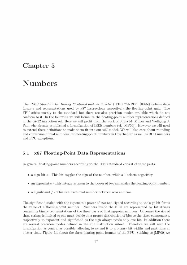
Chapter 5
Numbers
The IEEE Standard for Binary Floating-Point Arithmetic (IEEE 754-1985, [IE85]) defines dataformats and representations used by x87 instructions respectively the floating-point unit. TheFPU sticks mostly to the standard but there are also precision modes available which do notconform to it. In the following we will formalize the floating-point number representations definedin the IA-32 intruction set. Here we will profit from the work of Silvia M. Muller and Wolfgang J.Paul who already established a formalization of IEEE numbers (cf. [MP00]). However we will needto extend these definitions to make them fit into our x87 model. We will also care about roundingand conversion of real numbers into floating-point numbers in this chapter as well as BCD numbersand FPU exceptions.
5.1 x87 Floating-Point Data Representations
In general floating-point numbers according to the IEEE standard consist of three parts:
• a sign-bit s - This bit toggles the sign of the number, while a 1 selects negativity.
• an exponent e - This integer is taken to the power of two and scales the floating-point number.
• a significand f - This is a fractional number between zero and two.
The significand scaled with the exponent’s power of two and signed according to the sign bit formsthe value of a floating-point number. Numbers inside the FPU are represented by bit stringscontaining binary representations of the three parts of floating-point numbers. Of course the size ofthese strings is limited so one must decide on a proper distribution of bits to the three components,respectively to exponent and significand as the sign always needs only one bit. In addition thereare several precision modes defined in the x87 instruction subset. Therefore we will keep theformalization as general as possible, allowing to extend it to arbitrary bit widths and partitions ata later time. Figure 5.1 shows the three floating-point formats of the FPU. Sticking to [MP00] we
37
22
78 63
51
0
79
06362
3130
0
s
s
s
e
e
e
double-extended precision (80 bits)
double precision (64 bits)
single precision (32 bits)
f
f ′
f ′
Figure 5.1: The floating-point formats of the FPU
call the size of the exponent n and the size of the significand p.1 Additionally we denote the totalbit width of a floating-point number by m.
m =
{
80 : (n, p) = (15, 64)
n + p : otherwise
Obviously the double-extended precision with 15-bit exponent and 64-bit significand plays an extrarole compared to all other precision modes. This has to do with the way significands are normallystored in IEEE 754 number bit strings. For a p-bit significand only p′ bits are saved.
p′ =
{
64 : (n, p) = (15, 64)
p − 1 : otherwise
That is for most bit patterns one significand bit is not saved. We call this the hidden bit h : Bm → B
for a floating-point representation bit string x ∈ Bm. Strangely this hidden bit is explicit for the80-bit double-extended format. For all other formats it is defined by the exponent. We can easilygive shorthand functions for exponent and sign of x.
s : Bm → B
s(x[m − 1 : 0]) = x[m − 1]e : Bm → Bn
e(x[m − 1 : 0]) = x[m − 2 : p′]
Then the hidden bit is defined as:
h(x[m − 1 : 0]) =
x[63] : (n, p) = (15, 64)
1 : (n, p) 6= (15, 64) ∧ e(x) 6= 0n
0 : otherwise
Now let f ′(x) be the significand bits saved explicitely in the binary floating-point number repre-sentation x
f ′ : Bm → Bp′
f ′(x[m − 1 : 0]) = x[p′ − 1 : 0]
1Note that for the x87 model many definitions depend on the particular values of n or p. However for the sake ofsimplicity and because mostly double-extended precision is used, we want to keep the dependance on these parametersimplicit as long as it is obvious which precision values should be used. We will make the dependance explicit anddeclare n and p as arguments to the respective function only when results depend on the n(f) or p(f) settings.
38
Then the hidden bit is the most significand bit of the significand f(x) which is composed in thefollowing way.
f : Bm → Bp
f(x[m − 1 : 0]) = h(x) ◦ f ′(x)[p − 2 : 0]
Apart from floating-point numbers also special values can be encoded with x87 numbers. Theseare:
• positive and negative infinity
• Not-a-Number symbolic values (NaNs)
To be able to handle infinities we explicitely extend the real numbers by the infinity symbol.
R∞ = R ∪ {+∞,−∞}
Calculations with these numbers are done in the intuitive way known from mathematics. One couldreplace the ∞ symbols with variables tending to infinity and then obtain the result by computingthe limit of the term under consideration. Nevertheless some of these limits are undefined. Hencewe will be confronted with exceptional situations and special cases later on.
Not-a-Number symbolic values are introduced to handle these and other exceptions because underseveral cases it is necessary to return a result although the actual operation generates an undefinedresult respectively an error. Programmers can embed an error code in the Not-a-Number value.This is useful for identifying the type of error that occurred. There are also predefined indefinitevalue NaNs for every data format. Furthermore two types of NaNs exist:
• Signaling NaNs (SNaN) - These cause an x87 exception when they are used as floating-pointoperands.
• Quiet NaNs (QNaN) - These do not cause an x87 exception when they are used as floating-point operands. Floating-point operations involving QNaNs generate another QNaN as theresult.2
To represent NaNs we define the NaN data type that comprises all SNaN and QNaN values for asignificand precision p.
NaN = QNaN Bp−1 | SNaN Bp−1
The p − 1-bit binary value accompanying the NaN contains the sign bit followed by the p − 2-biterror code belonging to the NaN.
Now we would like to define the value of a binary floating-point representation x ∈ Bm. For thispurpose we first have to evaluate the values of exponent and significand. While the significand is inplain binary fractional format exhibiting one integer bit, the exponent is stored in a special biased
2Also operations with SNaNs generate further NaNs when the FPU invalid operation exception is masked.
39
integer format. This number representation allows to indroduce negative number while avoidingtwo’s complement numbers. The value of an exponent e is then given by [[ e ]]bias.
[[ ]]bias : Bn → Z
Note that this representation is defined only for exponents e[n− 1 : 0] /∈ {0n, 1n}. Then the biasedvalue is computed by substracting the bias 2n−1 − 1 from the binary value of the bit string.
[[ e[n − 1 : 0] ]]bias = 〈e[n − 1 : 0]〉 − (2n−1 − 1)
As e[n − 1 : 0] /∈ {0n, 1n} the minimal and maximal values for the exponent are:
emin = −2n−1 + 2emax = 2n−1 − 1
Thusly we can now define the value [[ x ]] of x87 floating-point representations x. We want to givethe definition for both the complete bit-string as well as the decomposed version.
[[ ]] : {B, Bn, Bp} → R∞|NaN[[ ]] : Bm → R∞|NaN
Upgrading the definition from [MP00] we yield the floating-point value for sign s ∈ B, biasedexponent e ∈ Bn and significand f ∈ Bp in the following way
[[ s, e, f ]] =
(−1)s · 2[[ e ]]bias · 〈f [p − 1].f [p − 2 : 0]〉 : e /∈ {0n, 1n}
(−1)s · 2emin · 〈f [p − 1].f [p − 2 : 0]〉 : e = 0n
(−1)s · ∞ : e = 1n ∧ f [p − 2 : 0] = 0p−1
QNaN s ◦ f [p − 3 : 0] : e = 1n ∧ f [p − 2 : 0] 6= 0p−1∧f [p − 2] = 1
SNaN s ◦ f [p − 3 : 0] : e = 1n ∧ f [p − 2 : 0] 6= 0p−1∧f [p − 2] = 0
Note that this definition does not check for e = 1n ⇒ f [p − 1] = 1. Thus also triples in anunsupported format are assigned to their pseudo-values.3 For contiguous bit strings x ∈ Bm wesimply set
[[ x[m − 1 : 0] ]] = [[ s(x), e(x), f(x) ]].
The first row of the case distinction above stands for the standard case of normal numbers. Theseare floating-point numbers with e /∈ {0n, 1n} and the hidden integer bit being 1. That means thesignificand is always in the range of [1, 2) for normal numbers.4 In contradiction there are denormalnumbers to represent tiny values. For denormal numbers the exponent is minimal due to e = 0n
3We do not include cases which cause undefined results for unsupported formats as they only occur for the double-extended precision with (n, p) = (15, 64). Furthermore we would not like to depend the general definition of thefloating-point value on the support preferences of the FPU. Instead we care about unsupported formats later by aseperate predicate.
4Actually according to the definition the value may also be in range [0, 1) for (n, p) = (15, 64) when f [p − 1] = 0,but these so-called unnormal numbers are not supported by the floating-point unit.
40
and the hidden integer bit is 0.5 This allows a range of [0, 1) for the significand and thus adds anarea of very small numbers to the set of representable values. We detect denormal numbers withthe following predicate.
dnrml : Bm|ǫ → B
dnrml(x[m − 1 : 0]) = 1 ⇔ e(x) = 0n ∧ f ′(x) 6= 0p′
Note that this definition excludes zero from being denormal. Furthermore dnrml(ǫ) = 0 holds.Another special case of the floating point value definition is infinity. The predicate infty(x) holdstrue for all bit strings that represent floating-point infinity. For ǫ it is false.
infty : Bm|ǫ → B
infty(x[m − 1 : 0]) = 1 ⇔ e(x) = 1n ∧ f(x)[p − 1 : 0] = 10p−1
The last exceptional case for floating-point values are NaNs. A bit string contains a quiet NaNwhen the exponent is all ones and the hidden integer bit is 1 as well as the most significant bit ofthe significand’s fractional part.
QNaN : Bm → B
QNaN(x) = 1 ⇔ e(x) = 1n ∧ f(x)[p − 1 : p − 2] = 11
SNaNs have the same structure like QNaNs besides that the significand bit following the hiddenbit is 0. Also the representation of infinity is not an SNaN.
SNaN : Bm → B
SNaN(x) = 1 ⇔ e(x) = 1n ∧ f(x)[p − 1 : p − 2] = 10 ∧ f(x) 6= 10p−1
Finally a bit string encodes a NaN if it contains either a QNaN or an SNaN.
NaN : Bm → B
NaN(x) = 1 ⇔ QNaN(x) ∨ SNaN(x)⇔ e(x) = 1n ∧ h(x) = 1 ∧ f(x) 6= 10p−1
A special case of QNaNs are the predefined x87 indefinite values. They are generated as resultswhen invalid operation exceptions are masked. The indefinite values for each floating-point, integerand BCD format are listed below.
indeffp32 = 110 ◦ 022 indefint16 = 1 ◦ 015 indefbcd = 118 ◦ 062
indeffp64 = 113 ◦ 051 indefint32 = 1 ◦ 031
indeffp80 = 118 ◦ 062 indefint64 = 1 ◦ 063
At last we have a look at unsupported encodings. These may only occur in the double-extendedprecision mode as here the hidden bit is not implicit anymore. That is why its value can be zerowhen it originally was supposed to be one and vice versa. This leads to unsupported floating-point encodings such as pseudo-NaNs, pseudo-infinities and unnormal numbers. We identify theseencodings via the unsup predicate.
unsup : B80|ǫ → B
unsup(x[79 : 0]) = 1 ⇔ e(x) 6= 015 ∧ x[63] = 0
Now that we learned about floating-point representation the next section is about how to transferreal numbers and infinitely precise results into our discrete number model.
5Actually because of the “unhidden” hidden bit for extended-double precision the integer bit of the significandmay also be 1. Such numbers are called pseudo-denormal numbers. They are accepted as operands by the FPU butnever generated as a result.
41
5.2 Factorings and Rounding
Naturally we can only represent a subset of the real numbers with floating-point bit strings. Thisfollows from finite precision on the one hand and a limited exponent on the other hand. Thereforewe must provide means to round real numbers to a representable floating-point number. Luckilymost of the necessary definitions can already be found in chapter 7 of [MP00]. All we have to dois adapting these definitions to our x87 model and the various precision modes.
First of all let us investigate the set of representable numbers. In [MP00] this was introduced asR so we stick to the notation. We extend it with the infinite values. Not-a-Number values are notnumbers so they are omitted here.
R∞ = R∪ {+∞,−∞} [MP00]( R ∪ {+∞,−∞}
With the definition of floating-point representation one can easily state the contents of this set forsome bit size and partition values m and (n, p) as defined in the preceding section.
R∞ = {[[ s, e, f ]] | s = s(x), e = e(x), f = f(x), x ∈ Bm ∧ NaN(x) ∧ unsup(x)}
Now we search for a way to assign infinitely precise numbers to representable ones. This reductionof precision is commonly known as rounding. Rounding of floating-point numbers is fully definedin [MP00] so we can rely on the several rounding functions from there.
rne,u,d,z : R → R∞ [MP00]
The different rounding modes are defined as follows for x ∈ R.
ru(x) = min{y ∈ R∞ | x ≤ y} (rounding up)
rd(x) = max{y ∈ R∞ | x ≥ y} (rounding down) [MP00]
rz(x) =
{
rd(x) : x ≥ 0
ru(x) : x < 0(rounding towards zero)
The definition of rounding to nearest even mode is not as trivial as those above. A real numberis rounded to the nearest representable one and when there are two candidates, that means whenthe number is lying exactly between two representable numbers the even one of both is chosen.[MP00] defines X∗
max = 2emax · (2−2−p) as the smallest number which would be rounded to 2emax+1
according to these rules, given that 2emax+1 would be representable at all. Then we can definerne(x) as follows.
rne(x) =
ru(x) : −X∗max < x < X∗
max ∧ |x − ru(x)| < |x − rd(x)|rd(x) : −X∗
max < x < X∗max ∧ |x − ru(x)| > |x − rd(x)|
z :−X∗
max < x < X∗max ∧ |x − ru(x)| = |x − rd(x)| ∧
∃z ∈ R, q ∈ Z : z = 2q · 2−(p−1) ∧ z ∈ {ru(x), rd(x)}∞ : X∗
max ≤ x
−∞ : x ≤ −X∗max
42
In the FPU concurring rounding modes and precisions may be selected. Nevertheless perpetuallyneeding to choose the right rounding function and setting the precision parameters to their respec-tive values might get tedious. Thus we introduce a master rounding function r which takes all thenecessary information as arguments and selects the right rounding function automatically.
r : (R∞, B2, N+, N+) → R∞
r(x, y, u, v) =
rne(x) : y = 00
rd(x) : y = 01
ru(x) : y = 10
rz(x) : y = 11
(n := u, p := v)
The various inputs are:
• x ∈ R - the number to be rounded
• y ∈ B2 - the rounding control bits
• u, v ∈ N+ - the exponent size and precision controlling parameters.
Observe that all rounding functions implicitly are functions of (n, p). Setting these parameters to(u, v) therefore changes the results of the rounding functions accordingly. For further comfort wedefine shorthand rounding functions which allow control of the precision while the exponent size isfixed to 15. This reflects the fact that for some FPU operations the destination precision can beselected while the exponent size is fixed. For y ∈ N+ we have:
ryne(x) ≡ r(x, 00, 15, y)
ryd(x) ≡ r(x, 01, 15, y)
ryu(x) ≡ r(x, 10, 15, y)
ryz (x) ≡ r(x, 11, 15, y)
In addition we supply a function rf (x) which rounds x according to the settings of the current x87configuration f .
rf (x) ≡ r(x, rm(f), n(f), p(f))
So we have the machinery now to round real numbers to representable ones with respect to acertain precision and rounding control. Anyway these numbers are still real and not in floating-point representation. To this end - as an intermediate step between real numbers and floating-pointrepresentation - Silvia M. Muller and Wolfgang J. Paul established factorings in [MP00]. Theseare triples of numbers that imitate the floating-point number structure. However only the sign isin bit format while exponent and significand are unbounded and infinitly precise integers or realnumbers respectively. We comprise all possible factorings in the set F.
F : (B, Z ∪ {∞}, [0, 2))
Similar to earlier definitions we included infinity for the exponent here as well. The value of afactoring (s, e, f) is yielded from [[ s, e, f ]].
[[ ]] : F → R∞
[[ s, e, f ]] = (−1)s · 2e · f
43
Note that we overload the [[ ]]-brackets for the floating-point representation and thus mix notationof factorings and bit strings value. However as one can determine the type of the arguments from thecontext this is more comfortable than establishing several different notations for related subjects.Now in [MP00] we can find the function η which yields an IEEE-normal factoring with a boundedexponent for a given real number x ∈ R∞.
η : R∞ → F [MP00]
IEEE-normality means that for all x ∈ R∞, a certain exponent size n with the correspondingminimal exponent emin and η(x) = (s, e, f) holds:
e ≥ emin ∧ f ∈ [0, 1) ⇒ e = emin ∧ e > emin ⇒ f ∈ [1, 2) ∧ [[ s, e, f ]] = x
There are special factorings for zero and infinity. Note that η considers the sign of zero.
η((−1)s · 0) = (s, emin, 0)η((−1)s · ∞) = (s,∞, 0)
When we yield the IEEE-normal factoring of a representable number it is only another small stepto gain the floating-point representation bit string.
5.3 Converting Factorings and Bit Strings
In the last step of transferring real numbers into IEEE 754 representation we need to build thefloating-point bit string from a given IEEE-normal factoring of the rounded number under consid-eration. We call this packing the factoring into a bit string.
pack : (F, (N+, N+)) → B∗
pack : (F, {32, 64, 80}) → B∗
Once again we have to consider various precision modes. We will thus define the packing func-tion for general bit partitions (n, p) but we will also define a shorthand version for the commonprecision modes of the FPU. We assume that our input factoring (s, e, f) is an IEEE-normalfactoring regarding (n, p) and that it is representable. That implies [[ s, e, f ]] ∈ R∞ and thusemin ≤ e ≤ emax ∨ e ∈ {+∞,−∞}. Furthermore ⌊f · 2p−1⌋ = f · 2p−1 holds. Then the packingfunction has the succeeding definition.
pack((s, e, f), (n, p)) =
s ◦ 1n ◦ 1063 : (n, p) = (15, 64) ∧ e = ∞s ◦ bin15(e + 214 − 1) ◦ bin1(⌊f⌋) ◦ bin63((f − ⌊f⌋) · 2p−1) : (n, p) = (15, 64) ∧ e 6= ∞s ◦ binn(e + 2n−1 − 1) ◦ binp−1((f − 1) · 2p−1) : (n, p) 6= (15, 64) ∧ e /∈ {∞, emin}s ◦ 0n ◦ binp−1(f) : (n, p) 6= (15, 64) ∧ e = emin
s ◦ 1n ◦ 0p−1 : (n, p) 6= (15, 64) ∧ e = ∞
We must take the special cases of infinity into account. For the double-extended precision modewe have to explicitely save the integer significand bit. The exponents are converted back to biased
44
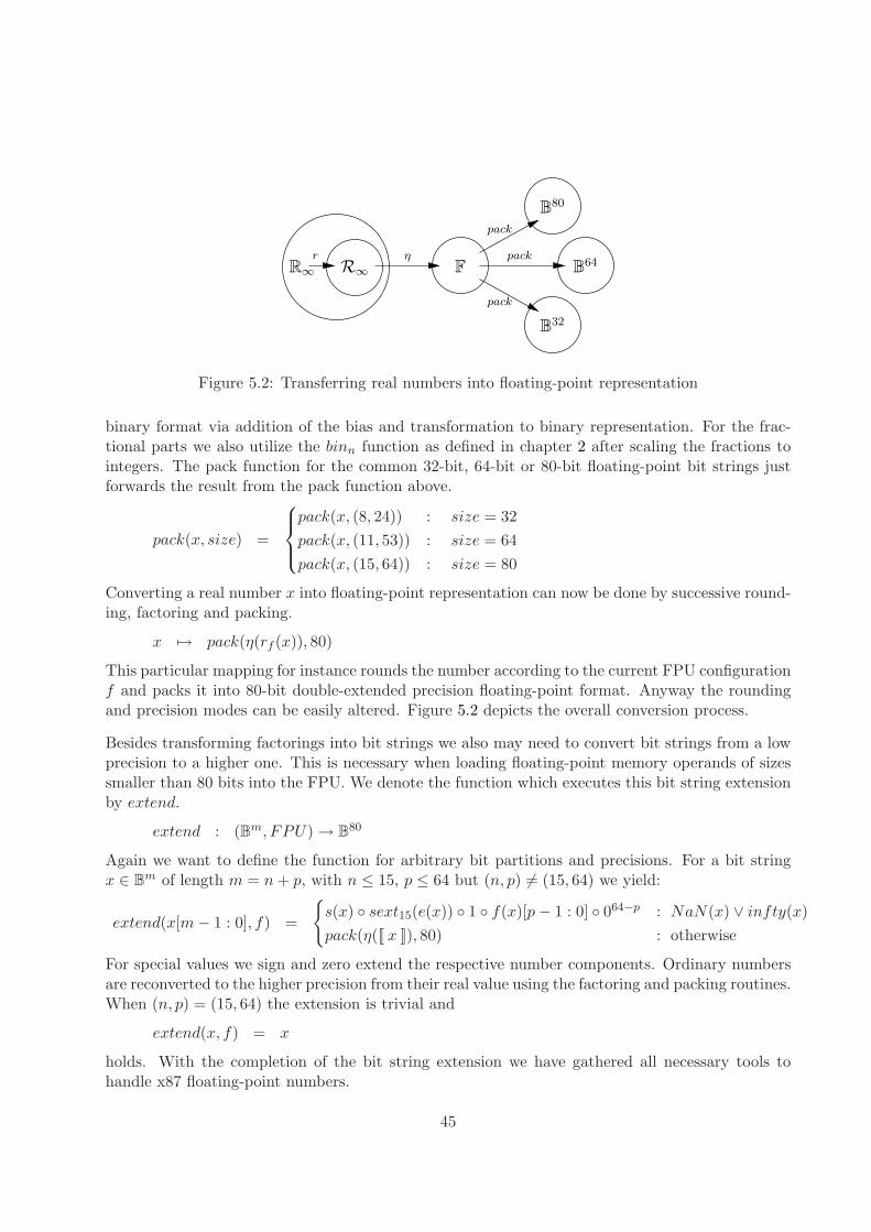
R∞
B80
B64
B32
R∞
r η
pack
pack
pack
F
Figure 5.2: Transferring real numbers into floating-point representation
binary format via addition of the bias and transformation to binary representation. For the frac-tional parts we also utilize the binn function as defined in chapter 2 after scaling the fractions tointegers. The pack function for the common 32-bit, 64-bit or 80-bit floating-point bit strings justforwards the result from the pack function above.
pack(x, size) =
pack(x, (8, 24)) : size = 32
pack(x, (11, 53)) : size = 64
pack(x, (15, 64)) : size = 80
Converting a real number x into floating-point representation can now be done by successive round-ing, factoring and packing.
x 7→ pack(η(rf (x)), 80)
This particular mapping for instance rounds the number according to the current FPU configurationf and packs it into 80-bit double-extended precision floating-point format. Anyway the roundingand precision modes can be easily altered. Figure 5.2 depicts the overall conversion process.
Besides transforming factorings into bit strings we also may need to convert bit strings from a lowprecision to a higher one. This is necessary when loading floating-point memory operands of sizessmaller than 80 bits into the FPU. We denote the function which executes this bit string extensionby extend.
extend : (Bm, FPU) → B80
Again we want to define the function for arbitrary bit partitions and precisions. For a bit stringx ∈ Bm of length m = n + p, with n ≤ 15, p ≤ 64 but (n, p) 6= (15, 64) we yield:
extend(x[m − 1 : 0], f) =
{
s(x) ◦ sext15(e(x)) ◦ 1 ◦ f(x)[p − 1 : 0] ◦ 064−p : NaN(x) ∨ infty(x)
pack(η([[ x ]]), 80) : otherwise
For special values we sign and zero extend the respective number components. Ordinary numbersare reconverted to the higher precision from their real value using the factoring and packing routines.When (n, p) = (15, 64) the extension is trivial and
extend(x, f) = x
holds. With the completion of the bit string extension we have gathered all necessary tools tohandle x87 floating-point numbers.
45
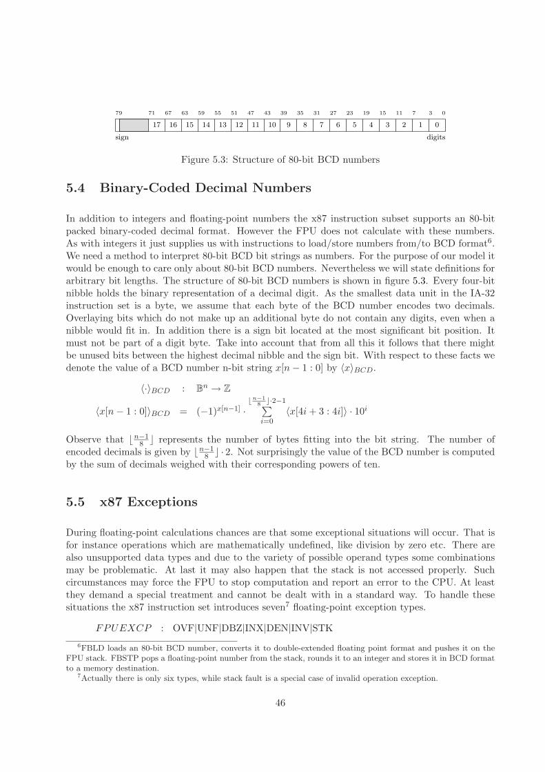
67
17
sign
16 15 14 13 12 11 10 9 8 7 6 5 4 3 2 1 0
digits
79 71 0371115192327313539434751555963
Figure 5.3: Structure of 80-bit BCD numbers
5.4 Binary-Coded Decimal Numbers
In addition to integers and floating-point numbers the x87 instruction subset supports an 80-bitpacked binary-coded decimal format. However the FPU does not calculate with these numbers.As with integers it just supplies us with instructions to load/store numbers from/to BCD format6.We need a method to interpret 80-bit BCD bit strings as numbers. For the purpose of our model itwould be enough to care only about 80-bit BCD numbers. Nevertheless we will state definitions forarbitrary bit lengths. The structure of 80-bit BCD numbers is shown in figure 5.3. Every four-bitnibble holds the binary representation of a decimal digit. As the smallest data unit in the IA-32instruction set is a byte, we assume that each byte of the BCD number encodes two decimals.Overlaying bits which do not make up an additional byte do not contain any digits, even when anibble would fit in. In addition there is a sign bit located at the most significant bit position. Itmust not be part of a digit byte. Take into account that from all this it follows that there mightbe unused bits between the highest decimal nibble and the sign bit. With respect to these facts wedenote the value of a BCD number n-bit string x[n − 1 : 0] by 〈x〉BCD.
〈·〉BCD : Bn → Z
〈x[n − 1 : 0]〉BCD = (−1)x[n−1] ·⌊n−1
8⌋·2−1
∑
i=0〈x[4i + 3 : 4i]〉 · 10i
Observe that ⌊n−18 ⌋ represents the number of bytes fitting into the bit string. The number of
encoded decimals is given by ⌊n−18 ⌋ · 2. Not surprisingly the value of the BCD number is computed
by the sum of decimals weighed with their corresponding powers of ten.
5.5 x87 Exceptions
During floating-point calculations chances are that some exceptional situations will occur. That isfor instance operations which are mathematically undefined, like division by zero etc. There arealso unsupported data types and due to the variety of possible operand types some combinationsmay be problematic. At last it may also happen that the stack is not accessed properly. Suchcircumstances may force the FPU to stop computation and report an error to the CPU. At leastthey demand a special treatment and cannot be dealt with in a standard way. To handle thesesituations the x87 instruction set introduces seven7 floating-point exception types.
FPUEXCP : OVF|UNF|DBZ|INX|DEN|INV|STK
6FBLD loads an 80-bit BCD number, converts it to double-extended floating point format and pushes it on theFPU stack. FBSTP pops a floating-point number from the stack, rounds it to an integer and stores it in BCD formatto a memory destination.
7Actually there is only six types, while stack fault is a special case of invalid operation exception.
46
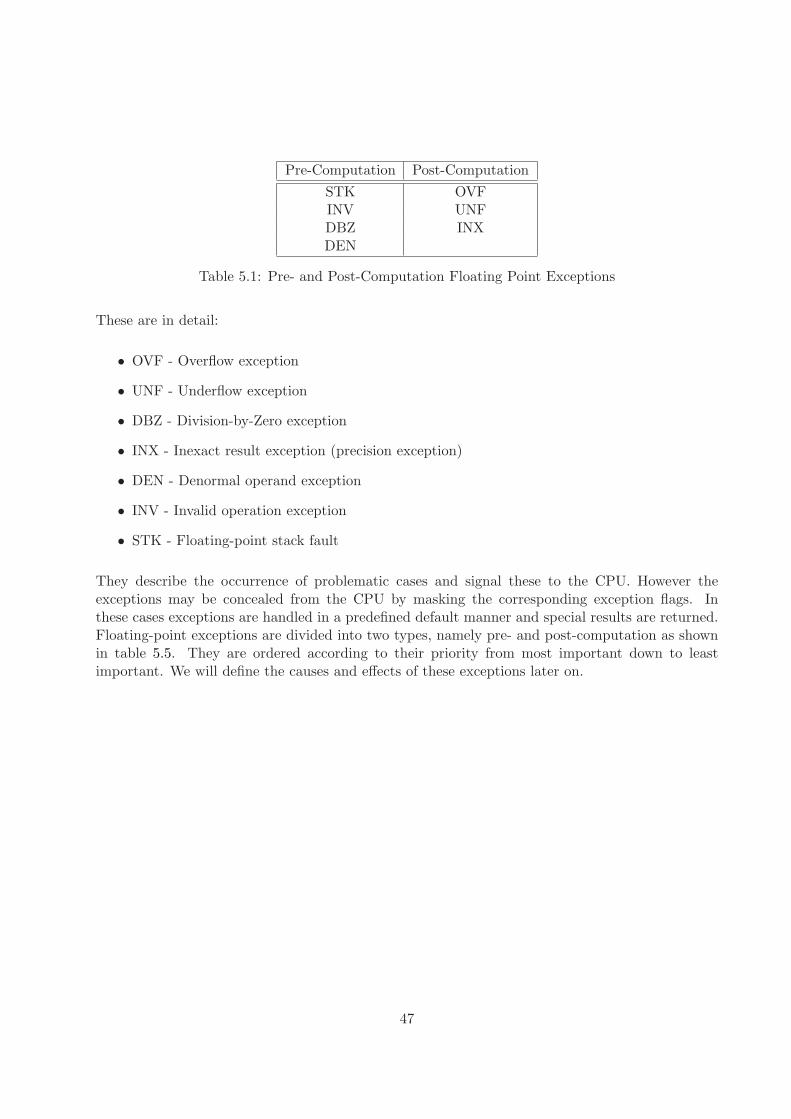
Pre-Computation Post-Computation
STK OVFINV UNFDBZ INXDEN
Table 5.1: Pre- and Post-Computation Floating Point Exceptions
These are in detail:
• OVF - Overflow exception
• UNF - Underflow exception
• DBZ - Division-by-Zero exception
• INX - Inexact result exception (precision exception)
• DEN - Denormal operand exception
• INV - Invalid operation exception
• STK - Floating-point stack fault
They describe the occurrence of problematic cases and signal these to the CPU. However theexceptions may be concealed from the CPU by masking the corresponding exception flags. Inthese cases exceptions are handled in a predefined default manner and special results are returned.Floating-point exceptions are divided into two types, namely pre- and post-computation as shownin table 5.5. They are ordered according to their priority from most important down to leastimportant. We will define the causes and effects of these exceptions later on.
47

48
Chapter 6
Operations
At this point we have all the information available to proceed to the execution routine to computethe result for an FPU instruction. What we have not discussed yet, is the computation of the resultitself. We need to investigate the instruction set as well as the mathematical aspects of floating-point operations. Also operation-specific floating-point exceptions are taken into consideration.
6.1 x87 Instruction Groups
There are more than 80 floating point instructions which compute many different kinds of functions- mathematical and non-mathematical ones. However it would be inexpedient to make case distinc-tions with 80 cases. Thus we need to further examine the instruction set and divide instructionsinto functional groups. There are also variant instructions of the same function which differ instack manipulation and operand scheme. We will define predicates which allow us to distinguishbetween instructions and between several instruction groups.
In general we determine the type of an FPU operation by analysing the corresponding opcode.We define predicates to report the group membership of an instruction. The predicates will belabelled with a certain mnemonic associated with the respective instruction. For more conveniencewe overload these mnemonic(X)-predicates to be applied within several contexts and to severalarguments X.
mnemonic : Instruction → B
mnemonic : FPU → B
mnemonic : B16 → B
mnemonic : B11 → B
If not defined otherwise these are always computed on the following way.
mnemonic(I) = mnemonic(I.opc[7 : 0] ◦ I.modrm)mnemonic(f) = mnemonic(opc(f))mnemonic(opc[15 : 0]) = (opc[15 : 11] = 11011) ∧ mnemonic(opc[10 : 0])
49
Following this scheme mostly just the predicate mnemonic(opc[10 : 0]) for 11-bit opcode fields mustbe defined individually. E.g. the predicates for the FNOP instruction are defined according to therules given above by exchanging mnemonic with FNOP .
FNOP (I) = FNOP (I.opc[7 : 0] ◦ I.modrm)FNOP (f) = FNOP (opc(f))FNOP (opc[15 : 0]) = (opc[15 : 11] = 11011) ∧ FNOP (opc[10 : 0])
All mnemonic(opc[10 : 0]) instruction predicates are defined in Appendix B. From now on by Iwe denote Instruction-type arguments and f represents an FPU configuration. opc[. . .] stands foran opcode string of either 16 or 11-bit length. A single opc shall be interpreted as an 11-bit x87opcode string.
6.1.1 Grouping by Functions
We can classify x87 instructions into nine general groups. Predicate x87(X) signals that the in-struction or opcode under consideration belongs to the x87 instruction subset. Here we have toadopt individual definitions to incorporate the special cases of FXSAVE/FXRSTOR and WAITinstructions which deviate from the standard x87 opcode format.
x87(I) =
x87(I.opc[7 : 0] ◦ I.modrm) : I.opc[23 : 3] = 01611011
1 : I.opc[15 : 0] = 0x0FAE
∧〈I.modrm[5 : 3]〉 ∈ {0, 1}∨I.opc[15 : 0] = 0x009B
0 : otherwise
x87(f) =
x87(opc(f)[7 : 0] ◦ I(f).modrm) : opc(f)[23 : 3] = 01611011
1 : opc(f)[15 : 0] = 0x0FAE
∧〈I(f).modrm[5 : 3]〉 ∈ {0, 1}∨opc(f)[15 : 0] = 0x009B
0 : otherwise
x87(opc[15 : 0]) = (opc[15 : 11] = 11011) ∧ x87(opc[10 : 0])
x87(opc[10 : 0]) = data(opc) ∨ arith(opc) ∨ sign(opc) ∨ const(opc) ∨ cmp(opc)∨trans(opc) ∨ stack(opc) ∨ fnop(opc) ∨ ctrl(opc)
Accordingly we need to define the predicates for the nine function classes.
• data(X) - Data Transfer
• arith(X) - Arithmetic Operations
• sign(X) - Sign Changing Operations
• const(X) - Load Constants
50
• cmp(X) - Compare and Test
• trans(X) - Transcendental Functions
• stack(X) - Stack Management
• fnop(X) - No Operation
• ctrl(X) - Control Operations
Many of these groups even consist of function subclasses. Those subclasses comprise instructionpredicates at last. See table B.1 for their exact definitions. Note that one instruction may bereferred to by more than one opcode. The different opcode variants are discussed later in thissection. For FXSAVE and FXRSTOR which are not pure x87 instructions we define the followingpredicates for an instruction I.
FXSAV E(I) = 1 ⇔ (I.opc[15 : 0] = 0x0FAE) ∧ 〈I.modrm[5 : 3]〉 = 0FXRSTOR(I) = 1 ⇔ (I.opc[15 : 0] = 0x0FAE) ∧ 〈I.modrm[5 : 3]〉 = 1
The IA32 instruction set also specifies waiting control instructions FINIT , FCLEX, FSTCW ,FSTSW , FSTENV and FSAV E. These Fx mnemonics do not refer to self-contained instructions.They are rather compiler macros which are translated to a pair of instructions. The first one isan FWAIT/WAIT to handle any pending x87 exceptions. It is followed by the counterpart FNxnon-waiting control instruction. We detect a wait instruction by using the following predicate.
WAIT (I) = (I.opc[24 : 16] = 0x9B)
Now we can define the function classes as shown in figure 6.1. We begin with data(X).
data(opc) = load(opc) ∨ store(opc) ∨ FCMOV (opc) ∨ FXCH(opc) ∨ FXTRACT (opc)load(opc) = FLD(opc) ∨ FILD(opc) ∨ FBLD(opc)store(opc) = FST (opc) ∨ FSTP (opc) ∨ FBSTP (opc)∨
FIST (opc) ∨ FISTP (opc) ∨ FISTTP (opc)
Arithmetic Operations are divided into several subclasses.
arith(opc) = add(opc) ∨ sub(opc) ∨ mul(opc) ∨ div(opc)∨prem(opc) ∨ FRNDINT (opc) ∨ FSQRT (opc)
add(opc) = FADD(opc) ∨ FADDP (opc) ∨ FIADD(opc)sub(opc) = FSUB(opc) ∨ FSUBP (opc) ∨ FISUB(opc)∨
FSUBR(opc) ∨ FSUBPR(opc) ∨ FISUBR(opc)mul(opc) = FMUL(opc) ∨ FMULP (opc) ∨ FIMUL(opc)div(opc) = FDIV (opc) ∨ FDIV P (opc) ∨ FIDIV (opc)∨
FDIV R(opc) ∨ FDIV PR(opc) ∨ FIDIV R(opc)prem(opc) = FPREM(opc) ∨ FPREM1(opc)
Sign Changing Operations manipulate the sign bit of floating-point numbers.
sign(opc) = FABS(opc) ∨ FCHS(opc)
51
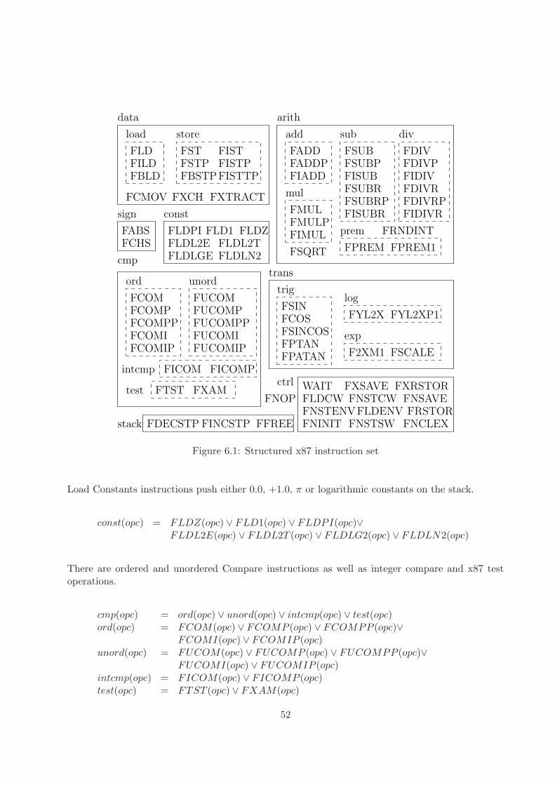
FYL2XP1
FLDCWFNSTENVFNINIT
FXRSTORFXSAVE
FNSTSW FNCLEX
FNSTCWFLDENV FRSTOR
FNSAVE
FLD
load
FST FIST
store
data
FADD
add
FSUB
sub div
arith
FILDFBLD
FCMOV FXCH FXTRACT
FSTPFBSTPFISTTP
FISTP
FCHSFABS
sign
FLD1 FLDZFLDL2EFLDLGE
const
FLDPIFLDL2TFLDLN2
FIADDFADDP
FISUBR
FSUBR
FSUBPFISUB
FSUBRP
FPREM FPREM1
prem
mul
FMULFMULPFIMUL
FIDIVRFDIVRPFDIVRFIDIV
FDIVFDIVP
FSQRT
FRNDINT
cmp
ord
FCOM
unord
FUCOMFCOMPFCOMPP
FCOMIPFCOMI FUCOMI
FUCOMPFUCOMPP
FUCOMIP
FICOM FICOMP
FTST FXAMtest
intcmp
stack FDECSTP FINCSTP FFREE
ctrl
FNOP
trans
trig
FSINFCOSFSINCOSFPTANFPATAN
log
exp
F2XM1 FSCALE
FYL2X
WAIT
Figure 6.1: Structured x87 instruction set
Load Constants instructions push either 0.0, +1.0, π or logarithmic constants on the stack.
const(opc) = FLDZ(opc) ∨ FLD1(opc) ∨ FLDPI(opc)∨FLDL2E(opc) ∨ FLDL2T (opc) ∨ FLDLG2(opc) ∨ FLDLN2(opc)
There are ordered and unordered Compare instructions as well as integer compare and x87 testoperations.
cmp(opc) = ord(opc) ∨ unord(opc) ∨ intcmp(opc) ∨ test(opc)ord(opc) = FCOM(opc) ∨ FCOMP (opc) ∨ FCOMPP (opc)∨
FCOMI(opc) ∨ FCOMIP (opc)unord(opc) = FUCOM(opc) ∨ FUCOMP (opc) ∨ FUCOMPP (opc)∨
FUCOMI(opc) ∨ FUCOMIP (opc)intcmp(opc) = FICOM(opc) ∨ FICOMP (opc)test(opc) = FTST (opc) ∨ FXAM(opc)
52
Transcendental functions are either trigonometric, logarithmic or exponential.
trans(opc) = trig(opc) ∨ log(opc) ∨ exp(opc)trig(opc) = FSIN(opc) ∨ FCOS(opc) ∨ FSINCOS(opc)∨
FPTAN(opc) ∨ FPATAN(opc)log(opc) = FY L2X(opc) ∨ FY L2XP1(opc)exp(opc) = F2XM1(opc) ∨ FSCALE(opc)
Only three instructions may directly influence the stack management.
stack(opc) = FDECSTP (opc) ∨ FINCSTP (opc) ∨ FFREE(opc)
At last we set fnop(opc) = FNOP (opc) and define the control instruction class.
ctrl(I) = WAIT (I) ∨ FXSAV E(I) ∨ FXRSTOR(I) ∨ ctrl(I.opc[7 : 0] ◦ I.modrm)ctrl(f) = FXSAV E(I(f)) ∨ FXRSTOR(I(f)) ∨ ctrl(opc(f)[7 : 0] ◦ I(f).modrm)ctrl(opc[15 : 0]) = (opc[15 : 11] = 11011) ∧ ctrl(opc[10 : 0])ctrl(opc[10 : 0]) = FLDENV (opc) ∨ FNSTENV (opc) ∨ FNINIT (opc)∨
FNSTSW (opc) ∨ FNCLEX(opc) ∨ FNSTCW (opc)∨FLDCW (opc) ∨ FNSAV E(opc) ∨ FRSTOR(opc)
Finally we can give the definition for non-control instructions. The corresponding predicate isneeded for the interface when reporting unmasked floating-point exceptions to the CPU.
nonctrl(I) = ctrl(I)
Furthermore we consider all instructions which calculate floating-point type results with the calcpredicate.
calc(opc) = arith(opc) ∨ trans(opc) ∨ FXTRACT (opc)
6.1.2 Grouping by Operand and Result Scheme
Now we are able to distinguish between all kinds of FPU instructions. However even a singleinstruction may have different variants concerning number and type of source and destinationoperands. We want to shed light on this circumstance below. Source operands are argument inputsto the various x87 instructions. Mostly they are floating-point or integer numbers, but there mayalso be image inputs. They may reside in memory or in some x87 stack register. Floating-pointinstructions can have one, two or no operands. The following schemes can be distinguished for theseveral instructions.
• One operand is always st(f, 0) and the other one is either empty, 0.0 or st(f, 1).
• One operand is chosen from the stack and the other one is either empty or st(f, 0).
• One operand is read from memory. The other operand may be empty or st(f, 0).
• The instruction does not need any source operands.
53
Concerning results we can distinguish four cases.
• A result from a calculation, sign changing, constant or data transfer operation is saved at orpushed to the x87 stack.
• A result from a data transfer or control operation is stored in memory.
• The instruction does not produce any result data. Components of the FPU environment maybe updated.
• The RFLAGS bits are updated after certain comparison instructions.
Observe that one instruction can have zero, one or two results. However only instructions withone result may save it to a memory destination. Note also that especially the result schemes arepartly linked to the different stack manipulation schemes. We will focus on these matters in thenext subsection.
6.1.3 Operand and Result Predicates
For now we care merely about where source operands come from, their number and size as well aswhere the results are stored in the end. Therefore we begin with defining three general predicateson the basis of the opcode table in Appendix A.
xread(opc) = 1 ⇔ x87(I) ∧ (r?(opc[15 : 8], opc[7 : 0]) = 1)xread(I) = xread(I.opc ◦ I.modrm)xupdf(opc) = 1 ⇔ x87(I) ∧ (uf?(opc[15 : 8], opc[7 : 0]) = 1)xupdf(I) = xupdf(I.opc ◦ I.modrm)xupdm(opc) = 1 ⇔ x87(I) ∧ (um?(opc[15 : 8], opc[7 : 0]) = 1)xupdm(I) = xupdm(I.opc ◦ I.modrm)
xread identifies functions which read an operand from memory. These are already marked witha 1 in the r? column of the opcode table. Accordingly xupdf recognizes intructions that updatethe RFLAGS register and xupdm perceives instructions storing a result to memory1. The x87results can have various sizes. We denote the size of the result of the current instruction regardingconfiguration f by ressize(f).
ressize : FPU → {16, 32, 64, 80, 112, 224, 752, 864, 4096}
ressize(f) =
{
opsize(I(f).opc, I(f).modrm, x64 mode(m(f)), 1, 32) : xupdm(I(f))
80 : otherwise
Once again the opcode table is utilized for the definition. We can also refer to it to determine thenumber of operands pertaining to a specific instruction. However this definition is partly inexact asthe table mixes source and destination operands. That is why instructions without source operands
1This also incorporates the case when FNSTSW stores the x87 status word to the AX register. Although AX
is not a part of memory we can embed this special case here, because the writeOp function in the interface can beused for all kinds of non-FPU destination operands.
54
may be assigned to the one-operand group. Nevertheless in all cases of instructions featuring sourceoperands, we can trust in nops(f).
nops : B16 → N3
nops(opc[15 : 0]) =
2 : op1(opc[15 : 8], opc[7 : 0]) 6= ǫ ∧ op2(opc[15 : 8], opc[7 : 0]) 6= ǫ
1 : op1(opc[15 : 8], opc[7 : 0]) 6= ǫ ∧ op2(opc[15 : 8], opc[7 : 0]) = ǫ
0 : otherwise
In addition we want to cover the case of instructions having two floating-point results.
2results : FPU → B
2results(f) = FXTRACT (f) ∨ FPTAN(f) ∨ FSINCOS(f)
Furthermore we define predicates signalling when images have to be loaded or saved.
imgsave(f) = FNSTENV (f) ∨ FNSAV E(f) ∨ FXSAV E(f)imgload(f) = FLDENV (f) ∨ FRSTOR(f)
Actually also for FXRSTOR an image must be restored but this instruction differs in many detailsfrom the imgload functions, so we exclude it from this predicate to the benefit of a more convenientnotation later on.
6.1.4 Sources and Destinations
In this subsection we accomplish some essential definitions, namely those of the two floating-point operands and the target stack register indices of instructions as well. We begin with theoperands, where we focus on operands containing numbers. That means we exclude images ascontrol instruction operands for the sake of simplification. Image saving and restoring will behandled later.
op1 : FPU → B80|ǫop2 : FPU → B80|ǫ
All numbers are translated into double-extended precision floating-point numbers for usage in theFPU. Thus it is convenient to have not only a reference to the source operand but also already theformat conversion included into the operand functions.
op1(f) =
pack(η(rf ([mop(f)])), 80) : intop1(f)
extend(mop(f), f) : fpmop1(f)
pack(η(rf (〈mop(f)〉BCD)), 80) : FBLD(f)
st(f, 〈opc(f)[2 : 0]〉) : srop1(f)
ǫ : ctrl(f) ∨ fnop(f) ∨ stack(f)
st(f, 0) : otherwise
In case of certain integer loading arithmetic instructions and FILD the first operand is the memoryinteger operand’s value rounded and transformed into a floating-point number.
intop1(f) = FISUBR(f) ∨ FIDIV R(f) ∨ FILD(f)
55
When a floating-point number is loaded from memory as the first operand it may have to beextended to a higher precision.
fpmop1(f) = xread(I(f)) ∧ (FSUBR(f) ∨ FDIV R(f) ∨ FLD(f))
For FBLD the memory operand in BCD representation is translated into IEEE 754 format. Thereare also instructions which allow the programmer to choose the source x87 stack register for thefirst operand by the last three bits of the x87 opcode.
srop1(f) = xread(I(f)) ∧ (opc(f)[15 : 8] = 0xD8 ∧ (FSUBR(f) ∨ FDIV R(f)) ∨ FLD(f))∨FSUBP (f) ∨ FDIV P (f)
However mostly the stack-top register contains the first operand. For control, NOP and stackmanipulation instructions no floating-point operands are needed. Concerning the second floating-point operand we distinguish seven cases.
op2(f) =
pack(η(rf ([mop(f)])), 80) : intop2(f)
extend(mop(f), f) : fpmop2(f)
st(f, 〈opc(f)[2 : 0]〉) : srop2(f)
st(f, 1) : st1op2(f)
st(f, 0) : st0op2(f)
080 : FTST (f)
ǫ : otherwise
Certain instructions demand an integer memory operand as second operand. They are identifiedby intop2(f) predicate.
intop2(f) = FISUB(f) ∨ FIDIV (f) ∨ FIADD(f) ∨ FIMUL(f) ∨ intcmp(f)
Also floating-point numbers in memory may represent the second operand. Using the extendfunction they are brought into the right precision format.
fpmop2(f) = xread(I(f)) ∧ (FCOM(f) ∨ FCOMP (f) ∨ FADD(f)∨FSUB(f) ∨ FMUL(f) ∨ FDIV (f))
Some variants of the arithmetic operations allow to choose the second operand from the x87 registerstack via the last three x87 opcode bits. Predicate srop2(f) specifies which opcodes cause thisbehaviour.
srop2(f) = xread(I(f)) ∧ (opc(f)[15 : 8] = 0xD8∧(FADD(f) ∨ FSUB(f) ∨ FMUL(f) ∨ FDIV (f))
∨(cmp(f) ∧ pop2(f)) ∨ (opc(f)[15 : 8] = 0xDC∧(FADD(f) ∨ FSUBR(f) ∨ FMUL(f) ∨ FDIV R(f))))∨FADDP (f) ∨ FSUBRP (f) ∨ FMULP (f) ∨ FDIV RP (f)
Further on there are sets of instructions which always use st(f, 0) or st(f, 1) as the second operand.We introduce st0op2 and st1op2 to detect them.
st0op2(f) = FSUBP (f) ∨ FISUBR(f) ∨ FDIV P (f) ∨ FIDIV R(f)∨((opc(f)[15 : 8] = 0xD8 ∨ xread(I(f))) ∧ (FSUBR(f) ∨ FDIV R(f)))
∨(opc(f)[15 : 8] = 0xDC ∧ xread(I(f)) ∧ (FSUB(f) ∨ FDIV (f)))st1op2(f) = FY L2X(f) ∨ FY L2XP1(f) ∨ FPATAN(f) ∨ FSCALE(f)
∨FUCOMPP (f) ∨ FCOMPP (f) ∨ prem(f)
56
At last FTST compares a number with 0.0. All other instructions do not possess a second operand.
Now we want to investigate the destination operands. That is the target components which areupdated with the respective result of an x87 instruction. Considering the aforementioned resultschemes, x87 stack registers are the only destinations which reside inside the FPU. The othersare either the RFLAGS register bits or a memory destination. We already established means todistinguish between the instructions which update memory operands or flags by the predicatesxupdf(I(f)) and xupdm(I(f)). They are defined implicitly based on a table search. With our newknowledge we can replace them by explicitly defined predicates xupdf(f) and xupdm(f).
xupdf : FPU → B
xupdf(f) = FCOMI(f) ∨ FCOMIP (f) ∨ FUCOMI(f) ∨ FUCOMIP (f)xupdm : FPU → B
xupdm(f) = store(f) ∨ imgsave(f) ∨ FNSTCW (f) ∨ FNSTSW (f)
Now we want to determine which stack elements are affected by a floating-point operation. There-fore we define the targets of the current configuration’s instruction trgt(f).
trgt : FPU → (N8|ǫ, N8|ǫ)trgt(f) = (trgt1(f), trgt2(f))
Obviously these targets may be empty, when an instruction does not save or push a value to thestack. The targets define the stack element indices which identify the registers the results shall bestored to. We begin with the target for the first result.
trgt1(f) =
ǫ : push?(f) ∧ save?(f)
7 : push?(f) ∧ save?(f)
1 : FPATAN(f) ∨ FY L2X(f) ∨ FY L2XP1(f)
〈opc(f)[2 : 0]〉 : opc(f)[15 : 8] = 0xDC ∧ xread(I(f)) ∧ arith(f)
∨arith(f) ∧ pop?(f)
∨xread(I(f)) ∧ (FST (f) ∨ FSTP (f))
0 : otherwise
In most cases this is the stack-top register. For a separate push we aim at the stack register abovethe stack-top, which is stack register 7 following the modulo-8 computation. Several instructionsmay also choose the target via opcode bits or they always store the result to stack element 1.A second target only exists when there is a push and a save or for the FXCH instruction.
trgt2(f) =
7 : push?(f) ∧ save?(f)
〈opc(f)[2 : 0]〉 : FXCH(f)
ǫ : otherwise
At a push and a save the second result is pushed to stack register 7. FXCH allows to choosethe target using the last three x87 opcode bits. Note that the predicates push?(f), save?(f) andpop?(f) are defined in the following subsection.
57
6.1.5 Grouping by Stack Manipulation Behaviour
Besides the function that instructions implement, the type and number of operands they utilize orwhere they store their results, we can also group instructions regarding the way they manipulatethe floating-point register stack. Instructions may save data to the stack, that is they just overwritethe content of an existing stack element with a new value without changing the stack structure. Inaddition data may be pushed on top of the stack. This implies updating the top-of-stack pointeras a side effect. After saving the results instructions have also the possibility to pop the stack-topelement off the stack. Thereby the stack-top pointer will be adjusted and the respective registerwill be tagged empty. Some instructions even pop two elements off the stack at once. Furtherinformation about the execution of these stack operations can be found in sections 7.2.2 and 7.4.2.
Most x87 instructions including all arithmetic and sign changing operations save a value to thestack. we can identify these instructions by the save? : FPU → B predicate.
save?(f) = sign(f) ∨ calc(f) ∨ ((FST (f) ∨ FSTP (f)) ∧ xupdm(f))
All load and constant instructions as well as arithmetic instructions which produce two results maypush results onto the x87 stack. In case they are the current instructions of an FPU configurationf the push? : FPU → B predicate becomes true.
push?(f) = load(f) ∨ const(f) ∨ 2results(f)
A variety of instructions may pop the FPU stack. The predicate pop? : FPU → B comprises alloperations which pop one element off the stack.
pop?(f) = FSTP (f) ∨ FISTP (f) ∨ FISTTP (f) ∨ FBSTP (f) ∨ FCOMP (f) ∨FCOMIP (f) ∨ FUCOMP (f) ∨ FUCOMIP (f) ∨ FICOMP (f) ∨ FADDP (f) ∨FMULP (f) ∨ FSUBP (f) ∨ FSUBRP (f) ∨ FDIV P ∨ FDIV RP (f) ∨FPATAN(f) ∨ FY L2X(f) ∨ FY L2XP1(f)
There are only two instructions which pop the stack twice. They are detected by pop2? : FPU → B.
pop2?(f) = FCOMPP (f) ∨ FUCOMPP (f)
6.2 x87 Format Converting Functions
After having structurized the instruction set we want to have a look at actual computation issues.Computation is done on double-extended precision floating-point numbers and inside the FPUonly this kind of numbers is stored. However there are certain instructions such as FST, FIST,FBSTP etc., which may convert floating-point data to different number formats or precisions.Some instructions also need to round floating-point numbers to integers, thus before dealing withthe mathematical functions of the FPU we have to establish means to convert numbers to differentformats.
58
6.2.1 Converting Precision
Some variants of FSTP and all FST instructions store floating-point data to 32- or 64-bit memorydestinations. For this purpose their formats must be converted to single or double precision. Tothis end we define a precision conversion function prc which returns the first operand converted tothe suitable precision in case the predicate cvtprc(f) holds.
cvtprc : FPU → B
cvtprc(f) = FST (f) ∨ FSTP (f)
prc : (B80, B2, {32, 64, 80}) → B∗
prc(x, rm, size) =
pack(η(r([[ x ]], rm, 8, 24)), 32) : size = 32 ∧ NaN(x)
x[79 : 71] ◦ 1 ◦ x[62 : 41] : size = 32 ∧ NaN(x)
pack(η(r([[ x ]], rm, 11, 53)), 64) : size = 64 ∧ NaN(x)
x[79 : 68] ◦ 1 ◦ x[62 : 12] : size = 64 ∧ NaN(x)
x : otherwise
The particular numbers are rounded according to the current rounding mode. In case a number’smagnitude exceeds the limits of representable numbers it is rounded to infinity or the biggestrepresentable number respectively.
6.2.2 Converting to Binary Integer Format
For integer storing instructions FIST, FISTP and FISTTP but also several other operations wemust be able to convert floating-point numbers to integers. The Predicate cvtint(f) signals whethera number shall be stored in integer format.
cvtint : FPU → B
cvtint(f) = FIST (f) ∨ FISTP (f) ∨ FISTTP (f)
This conversion of a floating-point number naturally forces us to apply rounding. The same round-ing modes as for floating-point rounding are available, however we can not utilize our floating-pointrounding functions in this case. For rounding x to the nearest even integer, we introduce thefunction rne(x).
rne : R → Z
rne(x) =
{
sgn(x) · |⌈x⌉| : ⌈x⌉ − x < 0.5 ∨ ⌈x⌉ − x = 0.5 ∧ ∃n ∈ Z : ⌈x⌉ = 2 · nsgn(x) · |⌊x⌋| : otherwise
Then depending on a given rounding mode rm the rounded integer number regarding a real numberx is denoted by rndint(x, rm).
rndint : (R, B2) → Z
rndint(x, rm) =
rne(x) : rm = 00 (round to nearest even)
sgn(x) · |⌊x⌋| : rm = 01 (round down)
sgn(x) · |⌈x⌉| : rm = 10 (round up)
sgn(x) · ⌊|x|⌋ : rm = 11 (round to zero)
59
We do not need to care about infinities as these result in invalid operation exceptions for thefunctions under consideration. The factor sgn(x) ensures that the number’s sign is kept, when thenumber is rounded to zero. Thus from the sign of zero one can determine from which direction thenumber was rounded to zero. Keep in mind that we keep the sign of zero explicit also for integers.
6.2.3 Converting to BCD Format
We already introduced the BCD number format and postulated a method to compute the value ofa number’s binary-coded decimal representation in section 5.4. For the FBSTP instruction we alsomust be able to convert an integer a to BCD format. Therefore we define the following conversionfunction with n ∈ N, n > 8 and ⌊n−1
8 ⌋ · 2 > log10 a.
bcdn : Z → Bn
bcdn(a) = x[n − 1 : 0], with 〈x〉BCD = a
So we implicitly defined the BCD representation of an integer. We can implement this functionrecursively as follows.
bcdn(a) =
{
1 ◦ 0n−1−⌊n−18
⌋·8 ◦ bcd′(|a|, ⌊n−18 ⌋ · 2 − 1) : a ≤ −0
0 ◦ 0n−1−⌊n−18
⌋·8 ◦ bcd′(|a|, ⌊n−18 ⌋ · 2 − 1) : else
At first the sign bit must be set. Waste bits between sign and the first digit nibble are cleared tozero. Then the actual digits are computed from the number’s absolute value.
bcd′ : (N, N) → B∗
bcd′(a, n) =
{
bin4(a mod 10) : n = 0
bcd′(⌊a/10⌋, n − 1) ◦ bin4(a mod 10) : else
One can prove that 〈bcdn(a)〉BCD = a holds for this implementation.
6.2.4 Maximal an Minimal Values
The configuration-specific maximal and mininal values Xmax(f) and Xmin(f) are defined in thefollowing way for the different formats.
Xmax(f) =
263 − 1 : cvtint(f) ∧ ressize(f) = 64
231 − 1 : cvtint(f) ∧ ressize(f) = 32
215 − 1 : cvtint(f) ∧ ressize(f) = 16
1018 − 1 : FBSTP (f)
2emax · (2 − 2−(p(f)−1)) : otherwise
Xmin(f) =
−263 : cvtint(f) ∧ ressize(f) = 64
−231 : cvtint(f) ∧ ressize(f) = 32
−215 : cvtint(f) ∧ ressize(f) = 16
−(1018 − 1) : FBSTP (f)
2emin · 2−(p(f)−1) : otherwise
60
Note that emax and emin are also depending on the current configuration via n(f). In additionthese values represent the maximal positive or minimal negative numbers for integer data types,while they stand for the maximal or minimal non-zero absolute values for floating-point numbers.
6.3 x87 Mathematical Functions
Now we will focus on the mathematical functions behind the different instructions. We want toabstract this from the FPU and the several x87 intructions as far as possible. Thus we define a setof FPU functions by declaring the FPUF type as follows.
FPUF : ADD|SUB|MUL|DIV|PREM|SQRT|RND|XTRACT|SIN|COS|SINCOS|TAN|ATAN|2XM1|SCALE|YL2X|YL2XP1
All these functions can be computed by the FPU and we later on want to state for each of themseperately how the result is calculated and which exceptions may occur. The particular functioncorresponding to the current floating-point configuration is denoted by fpuf(opc[15 : 0]) or fpuf(f)respectively.
fpuf : B16 → FPUF |ǫfpuf : FPU → FPUF |ǫ
fpuf(opc[15 : 0]) =
ADD : add(opc) COS : FCOS(opc)SUB : sub(opc) SINCOS : FSINCOS(opc)MUL : mul(opc) TAN : FPTAN(opc)DIV : div(opc) ATAN : FPATAN(opc)PREM : prem(opc) 2XM1 : F2XM1(opc)SQRT : FSQRT (opc) SCALE : FSCALE(opc)RND : FRNDINT (opc) YL2X : FY L2X(opc)XTRACT : FXTRACT (opc) YL2XP1 : FY L2XP1(opc)SIN : FSIN(opc) ǫ : otherwise
fpuf(f) = fpuf(opc(f))
In addition it is important to know how many operands a function needs to operate correctly.We already introduced a nops(opc) function to determine the number of operands for particularinstructions. Using fpuf function we can easily specify the number of operands associated withparticular mathematical functions.
nops : FPUF |ǫ → N3
nops(fn) =
2 : ∃x ∈ B16 : fpuf(x) = fn ∧ nops(x) = 2
1 : ∃x ∈ B16 : fpuf(x) = fn ∧ nops(x) = 1
0 : otherwise
Thus we do not have to consider opcodes any longer. Our abstract computation model becomesindependent of the actual instruction set opcode specification. Now we can define the precise resultof a calculating floating-point operation. In the style of the ALU result aluop of the DLX in [MP00]we denote this by fpuop.
fpuop : (FPUF, B80|ǫ, B80|ǫ, B2) → (R∞|NaN |ǫ, R∞|NaN |ǫ)
61
Note that this function is only dependent of the specific function to be computed, two operandsand a rounding mode indicator. Under certain circumstances it will return an empty result.
fpuop(fn, op1, op2, rm) = (ǫ, ǫ) ⇔ fn = ǫ ∨ (op1 = ǫ ∧ nops(fn) 6= 0 ∨ op2 = ǫ ∧ nops(fn) = 2)
Furthermore we are confronted with NaN operands, which produce NaN results. The followingequations show how the NaNs are converted. Note that SNaNs in contrary to QNaNs cause invalidoperation exceptions for mathematical operations and the results stated below are only valid whenINV exceptions are masked. We also need to care about those functions producing two results, thatis fn2 ∈ {SINCOS, TAN, XTRACT}. With fn /∈ {SINCOS, ATAN, XTRACT}, qnanx ∈ B80, x ∈B63, [[ qnanx ]] = QNaN x and [[ op1 ]], [[ op2 ]] /∈ NaN we get:
fpuop(fn, qnanx, op2, rm) = (QNaN x, ǫ)fpuop(fn, op1, qnanx, rm) = (QNaN x, ǫ)
fpuop(fn2, qnanx, op2, rm) =
{
(QNaN x, 1) : fn2 = TAN
(QNaN x,QNaN x) : otherwise
Now for snanx ∈ B80, [[ snanx ]] = SNaN x, SNaN(op1) and SNaN(op2) we have:
fpuop(fn, snanx, op2, rm) = (QNaN x, ǫ)fpuop(fn, op1, snanx, rm) = (QNaN x, ǫ)
fpuop(fn2, snanx, op2, rm) =
{
(QNaN x, 1) : fn2 = TAN
(QNaN x,QNaN x) : otherwise
At last we have a look at the combination of two equal NaN operands. Let qnanx′, snanx′ ∈B80,x′ ∈ B63, [[ qnanx′ ]] = QNaN x′ and [[ snanx′ ]] = SNaN x′, then:
fpuop(fn, qnanx, qnanx′, rm) =
(QNaN x, ǫ) : 〈x[62 : 0]〉 > 〈x′[62 : 0]〉(QNaN x′, ǫ) : 〈x[62 : 0]〉 < 〈x′[62 : 0]〉(QNaN x, ǫ) : x = x′
undefined : otherwise
fpuop(fn, snanx, snanx′, rm) =
(SNaN x, ǫ) : 〈x[62 : 0]〉 > 〈x′[62 : 0]〉(SNaN x′, ǫ) : 〈x[62 : 0]〉 < 〈x′[62 : 0]〉(SNaN x, ǫ) : x = x′
undefined : otherwise
We do not have to consider fn2 here because all x87 instructions which generate two resultsreference only one operand. The undefined cases identify the situations that both NaNs exhibit thesame error codes but have different signs.In the following subsections we will give the exact definition of fpuop by a case split on FPUF .That means for each function fpuop will be defined separately. Accordingly we set up the detectionof pre-computation exceptions and the definition of the respective masked exception results. Herewe will focus on function specific exceptions which are mostly invalid operation exceptions, butalso division-by-zero ones. The function prechk checks for pre-computation exceptions based onthe respective function and operands.
prechk : (FPUF, B80|ǫ, B80|ǫ) → FPUEXCP ∗
62
It returns a set of floating-point exceptions which were provoked by the given operands for theparticular floating-point function. We will complete its definition step by step for each functiontype. For an empty function type we define:
prechk(ǫ, op1, op2) = ∅
In addition we must state the masked exception result, that is the result of a computation returnedin case of a masked pre-computation exception.
mexcpres : (FPUF, FPUEXCP |ǫ, B80|ǫ, B80|ǫ) → (B80|ǫ, B80|ǫ)mexcpres(fn, excp, op1, op2) = (ǫ, ǫ) ⇔ fn = ǫ ∨ excp = ǫ ∨ op1 = ǫ ∨ (op2 = ǫ ∧ nops(fn) = 2)
Once again we will specify these results individually for each function type.
From the IA-32 specification we learn that
∀fn ∈ FPUF : ∀f ∈ FPU :mexcpres(fn, DEN, op1(f), op2(f)) = pack(η(rf (fpuop(fn, op1(f), op2(f), rm(f)))), 80)
holds. I.e. in case of denormal operands, the default result for masked exceptions is the ordinaryfpuop result rounded and converted to double-extended floating-point format just like no exceptionoccurred at all.
6.3.1 Addition
Not surprisingly the FPU is able to add two floating-point numbers. The result is the sum ofthe operands’ values. In case of an invalid exception the 80-bit floating-point indefinite value isreturned as a default response.
fpuop(ADD, op1, op2, rm) =
(+0, ǫ) : s(op1) 6= s(op2) ∧ |[[ op1 ]] + [[ op2 ]]| = 0 ∧ rm 6= 01
(−0, ǫ) : s(op1) 6= s(op2) ∧ |[[ op1 ]] + [[ op2 ]]| = 0 ∧ rm = 01
([[ op1 ]] + [[ op2 ]], ǫ) : otherwise
mexcpres(ADD, INV, op1, op2) = (indeffp80, ǫ)
An INV exception is caused when one operand exhibits an unsupported data format or when theoperands are infinities with opposing signs.
INV ∈ prechk(ADD, op1, op2) ⇔ unsup(op1) ∨ unsup(op2) ∨ SNaN(op1) ∨ SNaN(op2)∨(infty(op1) ∧ infty(op2) ∧ (s(op1) 6= s(op2)))
Addition of infinities is exact, as long as the signs are equal. For these cases and for addition ofequally signed zeroes we have:
±∞ + ±∞ = ±∞ ±0 + ±0 = ±0∀x ∈ R : ±∞ + x = ±∞ x + ±∞ = ±∞
63
6.3.2 Substraction
The FPU is also capable of substracting two floating-point numbers. The result is the difference ofthe operands’ values, while the first operand serves as minuend and the second one as subtrahend.In case of an invalid exception the 80-bit floating-point indefinite value is returned as a defaultresponse.
fpuop(SUB, op1, op2, rm) =
(+0, ǫ) : s(op1) = s(op2) ∧ |[[ op1 ]] − [[ op2 ]]| = 0 ∧ rm 6= 01
(−0, ǫ) : s(op1) = s(op2) ∧ |[[ op1 ]] − [[ op2 ]]| = 0 ∧ rm = 01
([[ op1 ]] − [[ op2 ]], ǫ) : otherwise
mexcpres(SUB, INV, op1, op2) = (indeffp80, ǫ)
An INV exception is caused when one operand exhibits an unsupported data format or when theoperands are infinities with identical signs.
INV ∈ prechk(SUB, op1, op2) ⇔ unsup(op1) ∨ unsup(op2) ∨ SNaN(op1) ∨ SNaN(op2)∨(infty(op1) ∧ infty(op2) ∧ (s(op1) = s(op2)))
Subtraction of infinities is exact, as long as the signs are opposites. For these cases and for sub-straction of oppositely signed zeroes we have:
±∞−∓∞ = ±∞ ±0 −∓0 = ±0∀x ∈ R : ±∞− x = ±∞ x −±∞ = ∓∞
6.3.3 Multiplication
The floating-point unit provides multiplication of two floating-point numbers. The result is theproduct of the operands’ values. In case of an invalid exception the 80-bit floating-point indefinitevalue is returned as a default response.
fpuop(MUL, op1, op2, rm) = ([[ op1 ]] · [[ op2 ]], ǫ)mexcpres(MUL, INV, op1, op2) = (indeffp80, ǫ)
An INV exception is caused when one operand exhibits an unsupported data format or when theoperands are infinity and zero
INV ∈ prechk(MUL, op1, op2) ⇔ unsup(op1) ∨ unsup(op2) ∨ SNaN(op1) ∨ SNaN(op2)∨infty(op1) ∧ (|[[ op2 ]]| = 0) ∨ infty(op2) ∧ (|[[ op1 ]]| = 0)
Multiplication of infinities is always exact when there is no factor of zero:
±∞ · ±∞ = +∞ ±∞ · ∓∞ = −∞∀x ∈ R : |x| 6= 0 ⇒ ∀x ∈ R : |x| 6= ∞ ⇒
±∞ · |x| = ±∞ ±0 · |x| = ±0±∞ · −|x| = ∓∞ ±0 · −|x| = ∓0|x| · ±∞ = ±∞ |x| · ±0 = ±0
−|x| · ±∞ = ∓∞ −|x| · ±0 = ∓0
64
6.3.4 Division
Also division of two floating-point numbers is available in the FPU. The result is the quotient of theoperands’ values, while the first operand serves as dividend and the second one as divisor. In caseof an invalid exception the 80-bit floating-point indefinite value is returned as a default response.
fpuop(DIV, op1, op2, rm) = ([[ op1 ]]/[[ op2 ]], ǫ)mexcpres(DIV, INV, op1, op2) = (indeffp80, ǫ)mexcpres(DIV, DBZ, op1, op2) = ((s(op1) ⊕ s(op2)) ◦ 115 ◦ 1063, ǫ)
For a divide-by-zero exception, infinity is returned with a sign corresponding to the operands’ signbits. An INV exception is caused when one operand exhibits an unsupported data format or whenthe operands are both infinities or zeroes.
INV ∈ prechk(DIV, op1, op2) ⇔ unsup(op1) ∨ unsup(op2) ∨ SNaN(op1) ∨ SNaN(op2)∨infty(op1) ∧ infty(op2) ∨ (|[[ op1 ]]| = 0 ∧ |[[ op2 ]]| = 0)
DBZ ∈ prechk(DIV, op1, op2) ⇔ |[[ op2 ]]| = 0
A DBZ exception occurs when the divisor is zero. Division of infinities is exact as long as not bothoperands are infinity:
∀x ∈ R : |x| 6= ∞ ⇒ ±∞/|x| = ±∞±∞/ − |x| = ∓∞|x|/ ±∞ = ±0
−|x|/ ±∞ = ∓0
6.3.5 Rounding
Apart from the inevitable rounding of exact results the FPU offers the possibility to explicitelyround a floating-point number to an integer. However the result is stored in floating-point format.In case of an invalid exception the 80-bit floating-point indefinite values are returned as a defaultresponse.
fpuop(RND, op1, op2, rm) =
{
([[ op1 ]], ǫ) : infty(op1)
(rndint([[ op1 ]], rm), ǫ) : mathrmotherwise
mexcpres(RND, INV, op1, op2) = (indeffp80, ǫ)
Infinities can not be rounded to an integer. An INV exception is caused when one operand exhibitsan unsupported data format.
INV ∈ prechk(RND, op1, op2) ⇔ unsup(op1) ∨ SNaN(op1)
6.3.6 Extracting Significand and Exponent
In some application it may be useful to split a floating point number into two parts, namelyits exponend and signed significand. The FPU’s FXTRACT instruction supplies us with this
65
functionality. In case of an invalid exception the 80-bit floating-point indefinite value is returnedas a default response.
fpuop(XTRACT, op1, op2, rm) = (⌊log2|[[ op1 ]]|⌋, [[ op1 ]]/2⌊log2|[[ op1 ]]|⌋)mexcpres(XTRACT, INV, op1, op2) = (indeffp80, indeffp80)mexcpres(XTRACT, DBZ, op1, op2) = (op1, 1 ◦ 115 ◦ 1063)
For a divide-by-zero exception, zero and negative infinity are returned. An INV exception is causedwhen one operand exhibits an unsupported data format. A DBZ exception occurs, when the sourceoperand is zero.
INV ∈ prechk(XTRACT, op1, op2) ⇔ unsup(op1) ∨ SNaN(op1)DBZ ∈ prechk(XTRACT, op1, op2) ⇔ |[[ op1 ]]| = 0
6.3.7 Partial Remainder
The FPU offers the possibility to calculate the partial remainder of a division of two floating-point numbers. In fact there are even two instructions2 computing the partial remainder, buttheir algorithms only differ in the rounding modes they use. In case of an invalid exception the80-bit floating-point indefinite value is returned as a default response. Let ediff = 〈e(op1)〉bias −〈e(op2)〉bias and N = 32 + (ediff mod 32), then the result is computed as follows.
fpuop(PREM, op1, op2, rm) =
(±0, ǫ) : [[ op1 ]] = ±0([[ op1 ]], ǫ) : ediff < 0 ∨ infty(op2)
([[ op1 ]] − ([[ op2 ]] · rndint([[ op1 ]][[ op2 ]]
, rm)), ǫ) : ediff < 64
([[ op1 ]] − ([[ op2 ]] · rndint([[ op1 ]]/2ediff−N
[[ op2 ]], 11) · 2ediff−N ), ǫ) : otherwise
mexcpres(PREM, INV, op1, op2) = (indeffp80, ǫ)mexcpres(PREM, DBZ, op1, op2) = ([[ op1 ]], ǫ)
In the third case the exponent difference of the two operands is larger than the number of fractionaldigits. Thus the quotient may have too many digits to be represented exactly. Then a computationaccording to the second case would not guarantee that the resulting remainder is smaller than thedivisor. We want to exemplify the method of the operation for integers x and y. Analysing theformula of the third case the exponent difference between x and y · 2ediff−N is then limited to therange {32, . . . , 63}. Thus an exact partial remainder
x − ⌊ x2ediff−Ny
⌋ · 2ediff−Ny = x mod 2ediff−Ny
can be computed. This partial remainder can be further processed to the actual remainder bysuccessive application of the PREM instructions. Because of ⌊ x
2ediff−Ny⌋ · 2ediff−N ∈ Z we can
follow that (⌊ x2ediff−Ny
⌋ · 2ediff−Ny) mod y = 0 and thus:
(x − ⌊ x2ediff−Ny
⌋ · 2ediff−Ny) mod y = ((x mod y) − (⌊ x2ediff−Ny
⌋ · 2ediff−Ny mod y)) mod y
= ((x mod y) − 0) mod y= x mod y
2FPREM and FPREM1, while the latter one computes the partial remainder according to IEEE 754 standard.
66
In a similar way3 the exact remainder of[[ op1 ]][[ op2 ]]
is contained in the partial remainder.
Moreover an invalid operation exception is generated when one of the operands is in an unsupportedformat, the dividend is infinity or both operands are zero.
INV ∈ prechk(PREM, op1, op2) ⇔ unsup(op1) ∨ unsup(op2) ∨ SNaN(op1) ∨ SNaN(op2)∨infty(op1) ∨ (|[[ op1 ]]| = 0 ∧ |[[ op2 ]]| = 0)
DBZ ∈ prechk(PREM, op1, op2) ⇔ infty(op1) ∧ (|[[ op1 ]]| 6= 0) ∧ (|[[ op2 ]]| = 0)
When only the divisor is zero it depends on the instruction if an INV or DBZ exception is caused.FPREM1 provokes a divide-by-zero exception in this case, while FPREM considers it as an invalidoperation4
6.3.8 Square Root
For many applications it is necessary to compute the square root of floating-point numbers. Hencethe FPU provides a hardware implementation of this function. In case of an invalid exceptionthe 80-bit floating-point indefinite value is returned as a default response. Otherwise the result iscomputed as follows.
fpuop(SQRT, op1, op2, rm) = (√
[[ op1 ]], ǫ)mexcpres(SQRT, INV, op1, op2) = (indeffp80, ǫ)
An invalid operation exception occurs for non-zero negative numbers.
INV ∈ prechk(SQRT, op1, op2) ⇔ unsup(op1) ∨ ([[ op1 ]] < −0) ∨ SNaN(op1)
For positive infinity√∞ = ∞ holds and for signed zeroes we have
√±0 = ±0.
6.3.9 Sine and Cosine
Also trigonometric functions are supported by the x87 instruction subset. At first we have a lookat sine and cosine. There are three FPU functions which return either sine, cosine or both sineand cosine of a floating-point number5. Only when the source operand is in the range [−263, 263] acomputation is performed. In case of an invalid exception the 80-bit floating-point indefinite valueis returned as a default response. For fn ∈ {SIN, COS, SINCOS} we have:
fpuop(fn, op1, op2, rm) =
(sin [[ op1 ]], ǫ) : fn = SIN ∧ −263 ≤ [[ op1 ]] ≤ 263
(cos [[ op1 ]], ǫ) : fn = COS ∧ −263 ≤ [[ op1 ]] ≤ 263
(sin [[ op1 ]], cos [[ op1 ]]) : fn = SINCOS ∧ −263 ≤ [[ op1 ]] ≤ 263
(undefined, ǫ) : otherwise
3We can conclude from integers on floating-point numbers because they have only a finite precision and can bescaled to integers. In a way floating-point numbers can be seen as rational numbers with a maximal denominator of2p.
4The Intel IA-32 Instruction Set Reference is unclear on this subject, thus we rely on the AMD64 ArchitectureProgrammer’s Manual.
5FSIN, FCOS and FSINCOS
67
mexcpres(SIN, INV, op1, op2) = (indeffp80, ǫ)mexcpres(COS, INV, op1, op2) = (indeffp80, ǫ)mexcpres(SINCOS, INV, op1, op2) = (indeffp80, ǫ)
An INV exception is triggered by infinities being held in the source operand.Let fn ∈ {SIN, COS, SINCOS}, then:
INV ∈ prechk(fn, op1, op2) ⇔ unsup(op1) ∨ infty(op1) ∨ SNaN(op1)
Observe the following definitions for signed zeroes.
sin±0 = ±0 cos±0 = 1
6.3.10 Tangent and Arc Tangent
Additionally the FPU facilitates calculation of tangent as well as arc tangent of floating-pointnumbers. For the tangent the computation is executed only when the operand lies in the range[−263, 263] . Furthermore 1.0 is pushed on the stack.6
fpuop(TAN, op1, op2, rm) =
(±0, 1) : [[ op1 ]] = ±0
(tan [[ op1 ]], 1) : −263 ≤ [[ op1 ]] ≤ 263
(undefined, 1) : otherwise
fpuop(ATAN, op1, op2, rm) =
(arctan([[ op2 ]][[ op1 ]]
), ǫ) : [[ op1 ]] > 0 ∧ |[[ op2 ]]| 6= 0
(arctan([[ op2 ]][[ op1 ]]
) + π, ǫ) : [[ op1 ]] < 0 ∧ [[ op2 ]] > 0
(arctan([[ op2 ]][[ op1 ]]
) − π, ǫ) : [[ op1 ]] < 0 ∧ [[ op2 ]] < 0
(π2 , ǫ) : |[[ op1 ]]| = 0 ∧ [[ op2 ]] > 0
(−π2 , ǫ) : |[[ op1 ]]| = 0 ∧ [[ op2 ]] < 0
(±π, ǫ) : [[ op1 ]] ≤ −0 ∧ [[ op2 ]] = ±0
(±0, ǫ) : [[ op1 ]] ≥ +0 ∧ [[ op2 ]] = ±0
mexcpres(TAN, INV, op1, op2) = (indeffp80, ǫ)mexcpres(ATAN, INV, op1, op2) = (indeffp80, ǫ)
For invalid operation exceptions the floating-point indefinite value is returned as default. Besidesoperands in unsupported formats only infinities can cause an INV exception for FPTAN instruction.
INV ∈ prechk(TAN, op1, op2) ⇔ unsup(op1) ∨ infty(op1) ∨ SNaN(op1)INV ∈ prechk(ATAN, op1, op2) ⇔ unsup(op1) ∨ SNaN(op1)
The ATAN operation’s result is well-defined for all possible arguments as the polar coordinatesystem angle of a point with ordinate [[ op2 ]] and abscissa [[ op1 ]]. The following equations showthe behaviour of arctan for special operands.
arctan(±∞−∞) = ∓π
4 arctan(±∞+∞) = ±π
4
∀x ∈ R : arctan(−∞±|x|) = ∓π
2 ∀x ∈ R : arctan( +∞±|x|) = ±π
2
∀x ∈ R : arctan(±|x|−∞ ) = ∓0 ∀x ∈ R : arctan(±|x|
+∞ ) = ±0
6This is done to ensure comfortable reversibility of the FPTAN instruction by the FPATAN instruction.arctan( tan x
1.0) = x
68
These special results shall be inserted for the arctan terms in the above definitions.
6.3.11 Exponentiation
There are two exponential functions available in the FPU. The first 2XM1 one directly exponentiates2 with the value of the first operand and then substracts 1. Only for operands in the range [−1.0, 1.0]the computation is executed7. This is a restriction from the specification. The second functionSCALE, scales the first operand with the power of two, gained from the truncated integer value ofthe second operand.
fpuop(2XM1, op1, op2, rm) =
{
(2[[ op1 ]] − 1, ǫ) : −1 ≤ [[ op1 ]] ≤ 1
(undefined, ǫ) : otherwise
fpuop(SCALE, op1, op2, rm) =
(QNaN 1 ◦ 062, ǫ) : (|[[ op1 ]]|, [[ op2 ]]) ∈{(0, +∞), (∞,−∞)}
([[ op1 ]] · 2rndint([[ op2 ]],11), ǫ) : otherwise
mexcpres(2XM1, INV, op1, op2) = (indeffp80, ǫ)mexcpres(SCALE, INV, op1, op2) = (indeffp80, ǫ)
In case of invalid operation exceptions the floating-point indefinite value is returned. This exceptionoccurs only because of unsupported operand data formats for these functions.
INV ∈ prechk(2XM1, op1, op2) ⇔ unsup(op1) ∨ SNaN(op1)INV ∈ prechk(SCALE, op1, op2) ⇔ unsup(op1) ∨ SNaN(op1)
However there is a speciality about the FSCALE instruction, as it is the only one which createsa NaN result, without causing an exception and without any operands containing a NaN. Thishappens for the cases that |[[ op1 ]]| = 0 ∧ [[ op2 ]] = +∞ or |[[ op1 ]]| = ∞∧ [[ op2 ]] = −∞, due to thefact that the product of zero and infinity is undefined.
6.3.12 Logarithm
As a counterpart to exponentiation the FPU is also able to compute the dual logarithm of floating-point numbers. There are two functions available to this end, YL2X and YL2XP1. For YL2X thefirst operand must be greater than zero, while YL2XP1 demands the first operand to be in range
7When the operand is outside the range, the result is undefined.
69
[√
12 − 1,
√2 − 1].8 Then the results are computed as follows.
fpuop(YL2X, op1, op2, rm) =
{
((−1)s(op2) · ∞, ǫ) : |[[ op1 ]]| = 0 ∧ infty(op2)
([[ op2 ]] · log2 [[ op1 ]], ǫ) : otherwise
fpuop(YL2XP1, op1, op2, rm) =
(±0, ǫ) : [[ op1 ]] = ±0 ∧ [[ op2 ]] ≥ +0
(∓0, ǫ) : [[ op1 ]] = ±0 ∧ [[ op2 ]] ≤ −0
([[ op2 ]] · log2([[ op1 ]] + 1), ǫ) :√
12 − 1 ≤ [[ op1 ]] ≤
√2 − 1
undefined : otherwise
mexcpres(YL2X, INV, op1, op2) = (indeffp80, ǫ)
mexcpres(YL2X, DBZ, op1, op2) = (s(op2) ◦ 115 ◦ 1063, ǫ)mexcpres(YL2XP1, INV, op1, op2) = (indeffp80, ǫ)
In case of invalid operation exceptions the floating-point integer value is returned. For a divide-by-zero exception during computation of YL2X infinity is returned with a sign in opposition to theone of the second operand. In the following cases exceptions are triggered.
INV ∈ prechk(YL2X, op1, op2) ⇔ unsup(op1) ∨ SNaN(op1) ∨ [[ op1 ]] < 0∨([[ op1 ]] = 1 ∧ infty(op2))∨(|[[ op1 ]]| ∈ {0,∞} ∧ |[[ op2 ]]| = 0)
DBZ ∈ prechk(YL2X, op1, op2) ⇔ |[[ op1 ]]| = 0 ∧ |[[ op2 ]]| /∈ {0,∞}INV ∈ prechk(YL2XP1, op1, op2) ⇔ unsup(op1) ∨ SNaN(op1) ∨ (|[[ op1 ]]| = 0 ∧ infty(op2))
For YL2X there are a lot of exceptional situations. The logarithm of negative numbers is undefinedand thus interpreted as an invalid operation. For the first operand being zero the logaritm tends tonegative infinity and a DBZ exception is raised as long as the other operand is a finite and non-zeronumber. Whenever zero is multiplied with infinity an INV exception is provoked.
6.4 x87 Comparison Functions
Now that we finished the mathematical floating-point functions only comparison functions are leftto be defined. Comparisons in the floating-point unit are related to the values of the RFLAGS orx87 condition code zero, carry and parity bits. These flags can be altered using cmp(f)-instructionsaccording to the comparison of two floating-point numbers. Conditional moves may rely on theseresults as they reference the respective RFLAGS bits. At first we introduce the various conditionsthat may be checked for by conditional move instructions. The condition type is denoted by COND.
COND : B|BE|E|NB|NBE|NE|NU|U
These comparison result types stand for:
8Here the Intel IA-32 Instruction Set Reference and AMD64 Architecture Programmer’s Manual contradict them-
selves. For Intel IA-32 processors the upper interval boundary is already at 1−
√12
while for AMD64 processors the
given range is valid.
70
• B - Below
• BE - Below or Equal
• E - Equal
• NB - Not Below
• NBE - Neither Below nor Equal
• NE - Not Equal
• NU - Not Unordered
• U - Unordered
They are associated with a conditional move in case of FCMOV (f) = 1 using the followingfunction.
cond : FPU → COND
cond(f) =
B : FCMOV (f) ∧ opc(f)[7 : 0] = 0xDA ∧ 〈I(f).modrm[5 : 3]〉 = 0
BE : FCMOV (f) ∧ opc(f)[7 : 0] = 0xDA ∧ 〈I(f).modrm[5 : 3]〉 = 2
E : FCMOV (f) ∧ opc(f)[7 : 0] = 0xDA ∧ 〈I(f).modrm[5 : 3]〉 = 1
NB : FCMOV (f) ∧ opc(f)[7 : 0] = 0xDB ∧ 〈I(f).modrm[5 : 3]〉 = 4
NBE : FCMOV (f) ∧ opc(f)[7 : 0] = 0xDB ∧ 〈I(f).modrm[5 : 3]〉 = 6
NE : FCMOV (f) ∧ opc(f)[7 : 0] = 0xDB ∧ 〈I(f).modrm[5 : 3]〉 = 5
U : FCMOV (f) ∧ opc(f)[7 : 0] = 0xDA ∧ 〈I(f).modrm[5 : 3]〉 = 3
NU : FCMOV (f) ∧ opc(f)[7 : 0] = 0xDB ∧ 〈I(f).modrm[5 : 3]〉 = 7
To compute the values of the zero, carry and parity flags in the condition code and RFLAGS bitswe define three compxf(x, y)-functions. They determine for two floating-point operands whetherthe particular flag is set to one or cleared to zero.
compzf : (B80, B80) → B
compcf : (B80, B80) → B
comppf : (B80, B80) → B
The zero flag is set to one for equal operands or an unordered exception.
compzf(x, y) = 1 ⇔ ([[ x ]] = [[ y ]]) ∨ NaN(x) ∨ NaN(y) ∨ unsup(x) ∨ unsup(y) = 1
The carry flag is set to one when the first operand is less than the second one or there is anunordered exception.
compcf(x, y) = 1 ⇔ ([[ x ]] < [[ y ]]) ∨ NaN(x) ∨ NaN(y) ∨ unsup(x) ∨ unsup(y) = 1
Keep in mind that equality and less relations ignore the sign of zero.The parity flag is only set to one for unordered exceptions.
comppf(x, y) = 1 ⇔ NaN(x) ∨ NaN(y) ∨ unsup(x) ∨ unsup(y) = 1
71
For a given FPU Configuration we yield the flag values from the following functions. Note thatx stands for z, c and p here. The three functions are defined under the condition that cmp(f) ∧FXAM(f) = 1 holds.
compxf : FPU → B
compxf(f) = compxf(op1(f), op2(f))
No more functions are necessary to handle floating-point comparisons.
There are also no floating-point operations left to take care of. Remaining functionalities suchas stack manipulation or control instructions will be handled in the next chapter along with thecomplete x87 execution routine and the rounding and packing of results.
72
Chapter 7
Execution
Finally we have collected all the important ingredients necessary to build our transition functionσfpu : FPU → FPU on the set of floating-point configurations. For relevant cases we decomposethis function into four subfunctions which are applied on the FPU configuration sequentially. Thisallows us to describe the floating-point execution routine in a structural and orderly way.
σfpu(fpu) =
{
σstorefpu (σpostchk
fpu (σexecfpu (σprechk
fpu (fpu)))) : fpu.acc 6= ǫ
fpu : otherwise
The various functions serve the following purposes.
• σprechkfpu : FPU → FPU - Checking for pre-computation exceptions and setting the x87
exception pointers and flags.
• σexecfpu : FPU → FPU - Computing the instruction’s result and storing it on the stack when
required.
• σpostchkfpu : FPU → FPU - Checking for post-computation exceptions, setting the correspond-
ing flags and adjusting the computed result when required.
• σstorefpu : FPU → FPU - Returning the instruction’s result and popping the stack when
required.
In the following sections we will define each function separately, taking care of all different functionclasses and variants. After finishing these tasks our model to describe the effect of x87 instructionswill be complete.
7.1 x87 Pre-Computation Exception Checks
The first transition subfunction serves solely pre-computation exception related purposes. On theone hand it detects these exception and sets the corresponding flags on the other hand it saves the
73
floating-point exception pointers, that is information for the exception handler to recover from anexception. We already introduced x87 exceptions and investigated the possible pre-computationexceptions for mathematical floating-point instructions. Now we want to complete the overall pic-ture by defining all possible circumstances under which the particular exceptions occur. Afterwardswe will state the effect of transistion function σprechk
fpu (f).
7.1.1 Detecting Pre-Computation Exceptions
The detection of pre-computation exceptions is quite complex, as there is a huge amount of specialcases for each floating-point instruction which will result in an exception. We already covered alot of these with the prechk : (FPUF, B80|ǫ, B80|ǫ) → FPUEXCP ∗ function, yet there are stillsome instructions left which deserve our attention. Thus we introduce the following function whichsubsumes all possible pre-computation exceptions in a set of floating-point exceptions.
prechk : FPU → FPUEXCP ∗
The prechk(f) function comprises all x87 pre-computation exceptions which may occur for afloating-point operation. As there may occure multiple exceptions for one instruction it resultsin a set of FPU exceptions. The prechk-function for calculating instructions was defined accord-ingly. Before we examine the particular exceptions we define the following predicates covering NaNoperands.
NaNs : FPU → B
NaNs(f) = 1 ⇔ (NaN(op1(f)) ∨ NaN(op2(f))) = 1SNaNs : FPU → B
SNaNs(f) = 1 ⇔ (SNaN(op1(f)) ∨ SNaN(op2(f))) = 1QNaNs : FPU → B
QNaNs(f) = 1 ⇔ (QNaN(op1(f)) ∨ QNaN(op2(f))) = 1
Now we will define the conditions for every kind of pre-computation exception. We begin withstack faults as they are the most important exceptions. Stack faults may occur for stack overflowsor underflows.
STK ∈ prechk(f) ⇔ stkovf(f) ∨ stkunf(f)
These predicates are defined as follows.
stkovf : FPU → B
stkovf(f) = push?(f) ∧ save?(f) ∧ empty(f, trgt1(f))∨push?(f) ∧ save?(f) ∧ empty(f, trgt2(f))
stkunf : FPU → B
stkunf(f) = (srop1(f) ∨ srop2(f)) ∧ empty(f, 〈opc(f)[2 : 0]〉)∨(xread(f) ∧ op1(f) 6= ǫ ∧ srop1(f) ∨ st0op2(f)) ∧ empty(f, 0)∨st1op2(f) ∧ empty(f, 1)
That means a stack overflow occurs when a value is pushed to a non-empty register location. Astack underflow on the contrary is caused by referencing an empty FPU register. Observe that the
74
term xread(f) ∧ op1(f) 6= ǫ ∧ srop1(f) identifies the situation that the first operand is located inthe stack-top register.We continue with invalid operation exceptions which may be raised in various situations. For thesake of clarity we define a predicate for each individual situation. The most common case is thata mathematical operation is invalid.
INV calc(f) = calc(f) ∧ INV ∈ prechk(fpuf(f), op1(f), op2(f))
We already covered these cases with the prechk function. Furthermore a divide-by-zero exceptionfor the FPREM instruction results in an invalid operation exception.
INV prem(f) = FPREM(f) ∧ (DBZ ∈ prechk(fpuf(f), op1(f), op2(f)))
When floating-point numbers shall be rounded to integers and stored to memory their magnitudemay not exceed the limits of the destination format. Otherwise an INV exception is raised. Thishappens also if one or both operands are infinity, NaNs or in an unsupported format. In the lattertwo cases the precision converting floating-point store instructions produce the invalid operationexception, too.
INV cvt(f) = (FBSTP (f) ∨ cvtint(f)) ∧ (NaNs(f) ∨ infty(op1(f)) ∨ unsup(op1(f))∨rndint([[ op1(f) ]]) > Xmax(f) ∨ rndint([[ op1(f) ]]) < Xmin(f))∨cvtprc(f) ∧ (SNaN(op1(f)) ∨ unsup(op1(f)))
Also comparison instructions cause invalid operations for NaNs or unsupported operands, dependingon the kind of comparisons. Unordered compare instructions ignore whether the operands areQNaNs.
INV cmp(f) = (ord(f) ∨ FTST (f) ∨ intcmp(f)) ∧ NaNs(f) ∨ unord(f) ∧ SNaNs(f)∨cmp(f) ∧ (unsup(op1(f)) ∨ unsup(op2(f)))
Finally we can state the conditions for an INV exception.
INV ∈ prechk(f) ⇔ INV calc(f) ∨ INV prem(f) ∨ INV cvt(f) ∨ INV cmp(f) = 1
Besides we have also divide-by-zero exceptions. These occur only for mathematical operations.
DBZ ∈ prechk(f) ⇔ calc(f) ∧ FPREM(f) ∧ (DBZ ∈ prechk(fpuf(f), op1(f), op2(f)))
Again we have to consider that a DBZ exception while executing FPREM is signalled as an invalidoperation. The least significant pre-computation exception is the denormalized operation exception.It is called if a computation or comparison involves a denormal operand. For FXAM no DENexception is generated because it examines the content of a register for all types of numbers.
DEN ∈ prechk(f) ⇔ (calc(f) ∨ cmp(f) ∧ FXAM(f))∧(dnrml(op1(f)) ∨ dnrml(op2(f)))
Thusly we accomplished the detection of pre-computation exceptions in a quite intuitive manner.In the following we care about the according changes in the FPU configuration.
75
7.1.2 Transition Function
The σprechkfpu (f) transition subfunction results in a new FPU configuration f ′.
σprechkfpu (f) = f ′
This configuration shall embody the changes due to the detected pre-computation exception. It alsocontains the x87 exception pointers for non-control x87 instructions. Accordingly the componentsof f ′ are defined as follows.
sf(f ′) =
{
1 : STK ∈ prechk(f)
sf(f) : otherwise
ie(f ′) =
{
1 : STK ∈ prechk(f) ∨ INV ∈ prechk(f)
ie(f) : otherwise
ze(f ′) =
{
1 : DBZ ∈ prechk(f)
ze(f) : otherwise
de(f ′) =
{
1 : DEN ∈ prechk(f)
ie(f) : otherwise
Because the exception flags are not cleared automatically, masked exception flags are accumulatedduring consecutive x87 calculations. The exception status flag and busy bit are set according totheir definitions.
es(f ′) ≡ ∨5i=0 mca(f ′)[i]
busy(f ′) ≡ es(f ′)
Only for non-control instructions the x87 exception information is saved.
f ′.dp =
{
adjustdp(f) : nonctrl(I(f))
f.dp : otherwise
f ′.ip =
{
adjustip(f) : nonctrl(I(f))
f.ip : otherwise
f ′.opc =
{
opc(f)[10 : 0] : nonctrl(I(f))
f.opc : otherwise
76
The precomputation exception check phase may also affect condition code bits 1 and 2.
cc(f ′)[1] =
0 : sign(f) ∨ FDECSTP (f) ∨ FINCSTP (f) ∨ FXCH(f)∨FUCOMI(f) ∨ FUCOMIP (f)∨(STK ∈ prechk(f) ∧ stkunf(f))∨(STK /∈ prechk(f) ∧ (load(f) ∨ const(f)))
1 : (STK ∈ prechk(f) ∧ stkovf(f))
cc(f)[1] : otherwise
cc(f ′)[2] =
0 : (FSIN(f) ∨ FCOS(f) ∨ FSINCOS(f) ∨ FPTAN(f))∧[[ op1(f) ]] ∈ [−263, 263]
1 : (FSIN(f) ∨ FCOS(f) ∨ FSINCOS(f) ∨ FPTAN(f))∧[[ op1(f) ]] /∈ [−263, 263] ∧ NaN(op1(f))
cc(f)[2] : otherwise
The first condition code bit signals in case of a stack fault whether a stack underflow or overflowoccurred. For some instructions it is always zero in case no stack fault was raised. The second codebit is set to one in case an argument was out of range for the trigonometric functions. All othercomponents remain unchanged by σprechk
fpu (f).
∀comp ∈ f ′ :comp ∈ {fsw[14 : 11], fsw[8], fsw[5 : 3], fpr, fcw, ftw, acc, ans} ⇒ f ′.comp = f.comp
This completes the definition of the first transition subfunction.
7.2 x87 Result Computation and Storage
The second transition subfunction σexecfpu (f) computes the result of an instruction and saves it to the
floating-point register stack when necessary. This happens only when no unmasked pre-computationexceptions occurred. As the execution stage is based on the result of the σprechk
fpu (f) function, thesechecks were already performed and we can use their results. To comfortably determine the activepre-computation exception with top priority we define the following function.
prexcp : FPU → FPUEXCP |ǫ
prexcp(f) =
STK : ie(f) ∧ sf(f)
INV : ie(f) ∧ sf(f)
DBZ : ze(f) ∧ ie(f)
DEN : de(f) ∧ ze(f) ∨ ie(f)
ǫ : otherwise
For the case of masked exceptions σexecfpu (f) incorporates the necessary default routines and results.
77
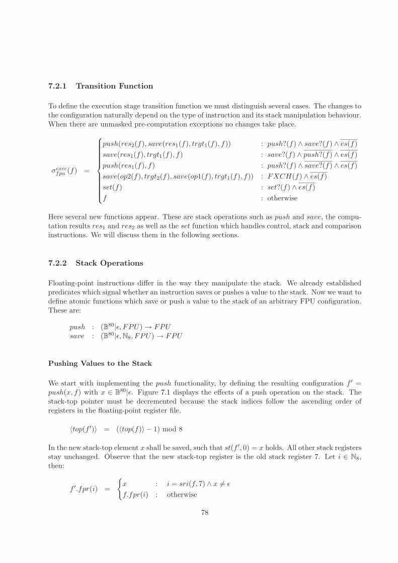
7.2.1 Transition Function
To define the execution stage transition function we must distinguish several cases. The changes tothe configuration naturally depend on the type of instruction and its stack manipulation behaviour.When there are unmasked pre-computation exceptions no changes take place.
σexecfpu (f) =
push(res2(f), save(res1(f), trgt1(f), f)) : push?(f) ∧ save?(f) ∧ es(f)
save(res1(f), trgt1(f), f) : save?(f) ∧ push?(f) ∧ es(f)
push(res1(f), f) : push?(f) ∧ save?(f) ∧ es(f)
save(op2(f), trgt2(f), save(op1(f), trgt1(f), f)) : FXCH(f) ∧ es(f)
set(f) : set?(f) ∧ es(f)
f : otherwise
Here several new functions appear. These are stack operations such as push and save, the compu-tation results res1 and res2 as well as the set function which handles control, stack and comparisoninstructions. We will discuss them in the following sections.
7.2.2 Stack Operations
Floating-point instructions differ in the way they manipulate the stack. We already establishedpredicates which signal whether an instruction saves or pushes a value to the stack. Now we want todefine atomic functions which save or push a value to the stack of an arbitrary FPU configuration.These are:
push : (B80|ǫ, FPU) → FPUsave : (B80|ǫ, N8, FPU) → FPU
Pushing Values to the Stack
We start with implementing the push functionality, by defining the resulting configuration f ′ =push(x, f) with x ∈ B80|ǫ. Figure 7.1 displays the effects of a push operation on the stack. Thestack-top pointer must be decremented because the stack indices follow the ascending order ofregisters in the floating-point register file.
〈top(f ′)〉 = (〈top(f)〉 − 1) mod 8
In the new stack-top element x shall be saved, such that st(f ′, 0) = x holds. All other stack registersstay unchanged. Observe that the new stack-top register is the old stack register 7. Let i ∈ N8,then:
f ′.fpr(i) =
{
x : i = sri(f, 7) ∧ x 6= ǫ
f.fpr(i) : otherwise
78
st(f ′, 5)
st(f, 0)top(f)
st(f, 1)
st(f, 2)
st(f, 3)
st(f, 7)
st(f, 6)
st(f, 5)
st(f, 4)
st(f, 0)
st(f, 1)
st(f, 2)
st(f, 3)
st(f, 6)
st(f, 5)
st(f, 4)
xtop(f ′)
push(x, f)
st(f ′, 1)
st(f ′, 2)
st(f ′, 3)
st(f ′, 4)
st(f ′, 0)
st(f ′, 7)
st(f ′, 6)
Figure 7.1: Effect of a push operation on the x87 stack
At last we examine x and set the tag bits accordingly.
f ′.ftw[2 · sri(f, 7) + 1 : 2 · sri(f, 7)] =
11 : x = ǫ
01 : |[[ x ]]| = 0
10 : NaN(x) ∨ unsup(x) ∨ dnrml(x) ∨ infty(x)
00 : otherwise
The remaining components are kept unaltered.
f ′.opc = f.opcf ′.dp = f.dp f ′.fsw[15 : 14] = f.fsw[15 : 14]f ′.ip = f.ip f ′.fsw[10 : 0] = f.fsw[10 : 0]f ′.fcw = f.fcw f ′.ftw[15 : 2 · sri(f, 7) + 2] = f.ftw[15 : 2 · sri(f, 7) + 2]f ′.acc = f.acc f ′.ftw[2 · sri(f, 7) − 1 : 0] = f.ftw[2 · sri(f, 7) − 1 : 0]f ′.ans = f.ans
Saving Values in the Stack
Saving a value in a stack register is even more simple. Once again we have f ′ = save(x, i, f) withx ∈ B80|ǫ and i, j ∈ N8. As the stack-top pointer is not changed all we have to do is updating theregister and its tag bits.
f ′.fpr(j) =
{
x : j = i ∧ x 6= ǫ
f.fpr(j) : otherwise
f ′.ftw[2i + 1 : 2i] =
11 : x = ǫ
01 : |[[ x ]]| = 0
10 : NaN(x) ∨ unsup(x) ∨ dnrml(x) ∨ infty(x)
00 : otherwise
79
Accordingly the other components do not change.
f ′.opc = f.opc f ′.fsw = f.fsw f ′.fcw = f.fcwf ′.dp = f.dp f ′.acc = f.acc f ′.ftw[15 : 2i + 2] = f.ftw[15 : 2i + 2]f ′.ip = f.ip f ′.ans = f.ans f ′.ftw[2i − 1 : 0] = f.ftw[2i − 1 : 0]
Apart from these stack operations instructions may also pop the stack. This is handled in section7.4.2.
7.2.3 Computing the Result
The main task of the execution phase is to deliver the result of a floating-point instruction. Notevery operation produces such a result bit string, on the other hand some instructions even returntwo results. We denote these results by res1(f) and res2(f) respectively.
res : FPU → (B∗|ǫ, B∗|ǫ)res(f) = (res1(f), res2(f))
The pair of results res(f) is a non-trivial definition as it compiles a multitude of instruction classesand types. We distinguish eight different result types.
• Calculation result - a result obtained from a floating-point calculation
• Sign operation result - a result obtained from manipulating the sign of a floating-point number
• Comparison result - the resulting EFLAGS register content corresponding to a floating-pointcomparison
• Constant result - a floating-point number from a fixed set of predefined constants which is tobe pushed on the stack
• Conversion result - a floating-point number converted to a different number format or precisionwhich shall be stored to memory
• Load result - a floating-point number which is loaded from memory or is involved in a condi-tional move operation
• Control result - a bitstring which contains parts or even a whole image of the floating-pointenvironment
• Special result - a default result generated by a masked pre-computation exception
80
Correspondingly we define result subfunctions for each type. For res(f) we apply the followingcase distinction
res(f) =
calcres(f) : calc(f) ∧ spec(f)
(signres(f), ǫ) : sign(f) ∧ spec(f)
(cmpres(f), ǫ) : intcmp(f) ∧ spec(f)
(constres(f), ǫ) : const(f) ∧ spec(f)
(cvtres(f), ǫ) : store(f) ∧ spec(f)
(loadres(f), ǫ) : (load(f) ∨ FCMOV (f)) ∧ spec(f)
(ctrlres(f), ǫ) : ctrl(f) ∧ spec(f)
specres(f) : spec(f)
(ǫ, ǫ) : otherwise
Special results can occur for every result type, thus we need a predicate spec(f) to distinguishwhether the result must be computed in the ordinary way or whether the special result is returnedinstead.
spec(f) = (mexcp(f) ∧ prexcp(f) 6= DEN)
In the following each result function is discussed separately.
Calculation Results
At first we care about the main purpose of the FPU: floating-point calculations. Luckily wealready defined the semantics of the several floating-point operations. All we have left to do, isintegrating this general description into our model. The calculation result consists of one or twodouble-extended precision floating-point number bit strings.
calcres : FPU → (B80, B80|ǫ)
However we base these numbers on the infinitely precise results pres1(f) and pres2(f). They canbe obtained using the fpuop function for the current FPU function and operands.
pres : FPU → (R∞|NaN |ǫ, R∞|NaN |ǫ)pres(f) = (pres1(f), pres2(f))
=
{
fpuop(fpuf(f), op1(f), op2(f), rm(f)) : calc(f)
[[ op1(f) ]] : store(f)
This precise result is also relevant for detecting post-computation exceptions like INX. Exceptiondetection for format conversion operations benefits from this definition, too.Naturally hardware can not store infinitely precise numbers, therefore the result must be roundedand transformed into a double-extended floating-point number bit string. To this end we define
81
the following function.
packres : (FPU, R∞|NaN |ǫ) → B80|ǫ
packres(f, pres) =
x[62] ◦ 115 ◦ 11 ◦ x[61 : 0] : ∃x ∈ B63 : pres = QNaN x
x[62] ◦ 115 ◦ 10 ◦ x[61 : 0] : ∃x ∈ B63 : pres = SNaN x
ǫ : pres = ǫ
pack(η(rf (pres)), 80) : otherwise
It regards NaNs and uses the pack function from 5.3. Observe that although all numbers are packedinto an 80-bit string, results can be rounded using smaller precisions via the rf function1. Finallywe can state the definition of the calculation result for calc(f) = 1.
calcres(f) = (packres(f, pres1(f)), packres(f, pres2(f)))
Sign Operation Results
The effect of sign operations is trivial. Depending on the instruction the sign of a floating-pointregister content is either switched or cleared to zero. For sign(f) = 1 we have:
signres : FPU → B80
signres(f) =
{
0 ◦ op1(f)[78 : 0] : FABS(f)
s(op1(f)) ◦ op1(f)[78 : 0] : FCHS(f)
Comparison Results
In most cases floating-point comparisons do not produce a result in the sense of a bit string thatought to be saved to some register oder memory destination. However there are four x87 instruc-tions2 which update the the lower 16-bit part of the RFLAGS register with the resulting flags of afloating-point comparison. With the flag computation functions and chflg the resulting bit stringfor cmp(f) = 1 is easily defined.
cmpres : FPU → B16
cmpres(f) = chflg(f, compzf(f), comppf(f), compcf(f))
1This means on the other hand that we always use 15 bits to represent the exponent of a floating-point number.Thus the results of x87 operations may deviate from implementations that stick to the IEEE standard more strictly.
2FCOMI, FCOMIP, FUCOMI and FUCOMIP
82
Constant Results
The FPU offers seven different constants which can be pushed on the stack. For const(f) = 1 thechosen constant is denoted by constant(f).
constant(f) =
0.0 : FLDZ(f)
1.0 : FLD1(f)
π : FLDPI(f)
log2 10 : FLDL2T (f)
log2 e : FLDL2E(f)
log10 2 : FLDLG2(f)
ln 2 : FLDLN2(f)
This value is rounded and packed to 80-bit double-extended format.
constres : FPU → B80
constres(f) = pack(η(rf (constant(f))), 80)
Conversion Results
Inside the FPU all computations are done in double-extended floating-point format. Neverthelessthere are store instructions to export numbers to deviating precisions and formats. We alreadyintroduced this fact along with the corresponding conversion functions. Thus the conversion resultis a simple application of these utilities.
cvtres : FPU → B∗
cvtres(f) =
twocressize(f)(rndint([[ op1(f) ]], rm(f))) : cvtint(f)
bcd80(rndint([[ op1(f) ]], rm(f))) : FBSTP (f)
prc(op1(f), rm(f), ressize(f)) : cvtprc(f)
op1(f) : otherwise
Note that for BCD and integer conversion the floating-point numbers are first rounded to integersand then transformed into the right representation.
Load Results
As stated before, load results comprise the results from load instructions and conditional moves.For loads actually the result is nothing but the first operand containing the converted memoryoperand. In the latter case a value is only moved, if a certain condition holds. We denote thiscondition by cmove(f).
cmove : FPU → B
83
Using this predicate the conditional move may be emulated by switching the actual source withthe destination content. This assures that the destination’s value is not altered in case of a missedcondition.
loadres : FPU → B∗
loadres(f) =
{
st(f, trgt1(f)) : FCMOV (f) ∧ cmove(f)
op1(f) : otherwise
Now we have to define cmove(f). The condition is determined with regard to the current conditionalmove instruction and the values of zero, carry and parity flags in the RFLAGS register. ForFCMOV (f) we yield:
cmove(f) =
cf(f) : cond(f) = B
cf(f) ∨ zf(f) : cond(f) = BE
zf(f) : cond(f) = E
cf(f) : cond(f) = NB
cf(f) ∨ zf(f) : cond(f) = BE
zf(f) : cond(f) = E
pf(f) : cond(f) = U
pf(f) : cond(f) = NU
The respective flags may have been set by preceding FCOMI, FCOMIP or FUCOMI as well asFUCOMIP instructions.
Control Results
Several control instructions may save FPU configuration data to memory to enable restoring theFPU state at a later time. Thus control results are FPU components or image bit strings of differentlength.
ctrlres : FPU → B∗|ǫ
There are three different image types:
• x87 Environment - contains only the floating-point environment registers but not the contentof the FPU stack
• x87/MMX State - a complete image of the x87 environment and data register contents - Asthe FPU registers are shared by x87 and MMX media instructions this image also saves theMMX state.
• XMM/x87/Media state - contains the complete XMM and x87/MMX state
84
For imgsave(f) = 1 the image to be saved is denoted by image(f). Its definition reflects the imagetype seperation above.
image : FPU → B∗
image(f) =
x87env(f) : FNSTENV (f)
x87img(f) : FNSAV E(f)
xmmimg(f) : FXSAV E(f)
The figures in Appendix C visualize the various image formats. In the following we will describemathematically how these images are composed. It is coherent that their structure depends on thecurrent mode and data width of the CPU. We begin with defining the complete 94/108-byte x87configuration image.
x87img : FPU → B∗
x87img(f) =
st(f, 7) ◦ · · · ◦ st(f, 0) ◦ 016 ◦ f.dp[47 : 0] ◦ 05 ◦ f.opc : prot32(f)
◦f.ip[47 : 0] ◦ 016 ◦ f.ftw ◦ 016 ◦ f.fsw ◦ 016 ◦ f.fcw
st(f, 7) ◦ · · · ◦ st(f, 0) ◦ 04 ◦ f.dp[31 : 16] ◦ 028 : real32(f)
◦f.dp[15 : 0] ◦ 04 ◦ f.ip[31 : 16] ◦ 0 ◦ f.opc ◦ 016
◦f.ftw ◦ 016 ◦ f.fsw ◦ 016 ◦ f.fcw
st(f, 7) ◦ · · · ◦ st(f, 0) ◦ f.dp[31 : 0] ◦ f.ip[31 : 0] : prot16(f)
◦f.ftw ◦ f.fsw ◦ f.fcw
st(f, 7) ◦ · · · ◦ st(f, 0) ◦ f.dp[19 : 16] ◦ 012 ◦ f.dp[15 : 0] : real16(f)
◦f.ip[19 : 16] ◦ 0 ◦ f.opc ◦ f.ftw ◦ f.fsw ◦ f.fcw
It contains the eight FPU stack registers followed by the exception pointers and the x87 status,control and tag word. Depending on the mode varying portions of the data and instruction pointerfields are saved in the image. This affects also the order and position of the other components.The 14/28-byte x87 environment is then a part of the complete image.
x87env : FPU → B∗
x87env(f) =
{
x87img(f)[223 : 0] : prot32(f) ∨ real32(f)
x87img(f)[111 : 0] : otherwise
The XMM/x87/Media state image is the biggest one. It spans 512 bytes, while most of the spaceis needed for the 16 128-bit XMM register contents. This XMM information is not available to theFPU, thus only the x87 part of the image is returned to the CPU, while there are routines in theinterface which insert the missing data and compile the full image. These routines are defined insection 3.4.
xmmimg : FPU → B1280
xmmimg(f) =
zeroext128(st(f, 7)) ◦ · · · ◦ zeroext128(st(f, 0)) ◦ 064 : es(f) = 1
◦f.dp ◦ f.ip ◦ 05 ◦ f.opc ◦ 016 ◦ ftw8(f) ◦ f.fsw ◦ f.fcw
zeroext128(st(f, 7)) ◦ · · · ◦ zeroext128(st(f, 0)) ◦ 0192 : otherwise
◦05 ◦ f.opc ◦ 016 ◦ ftw8(f) ◦ f.fsw ◦ f.fcw
85
As a speciality FXSAV E only stores the FPU exception data and instruction pointers when anunmasked exception is pending. Also it only saves eight bits for the x87 tag word. These eight bitsjust signal whether the corresponding stack registers are full or empty. They are computed in thefollowing way.
ftw8 : FPU → B16
ftw8(f) = (f.ftw[15] ⊼ f.ftw[14]) ◦ (f.ftw[13] ⊼ f.ftw[12]) ◦ (f.ftw[11] ⊼ f.ftw[10])◦(f.ftw[9] ⊼ f.ftw[8]) ◦ (f.ftw[7] ⊼ f.ftw[6]) ◦ (f.ftw[5] ⊼ f.ftw[4])◦(f.ftw[3] ⊼ f.ftw[2]) ◦ (f.ftw[1] ⊼ f.ftw[0])◦
Thus a 1 signals an empty register while a 0 signals some valid data in the corresponding stackregister.
At last we incorporate the images into our control result function. Besides images also the x87status and control word may be stored to memory.
ctrlres(f) =
image(f) : imgsave(f)
fsw(f) : FNSTSW (f)
fcw(f) : FNSTCW (f)
ǫ : otherwise
Special Results
Finally only the special results are left. They play an exceptional role among the different resulttypes as they embody not really another self-contained type of results. Instead they represent thedefault results for all instruction and result types in the event of masked exceptions.
specres : FPU → (B∗|ǫ, B∗|ǫ)
In section 6.3 we did define the masked exception results by the mexcpres function for mathematicaloperations. However exceptions may occur for all kind of instructions so we must investigate further.The most common default response to masked exceptions - especially masked INV exceptions - areindefinite values. We define the cases in which indefinite values are returned - apart from the casesof mathematical functions - with the following predicate.
indefinite : FPU → B
indefinite(f) = 1 ⇔ ((prexcp(f) = STK) ∨ ((prexcp(f) = INV ∨ QNaNs(f))∧(FIST (f) ∨ FISTP (f) ∨ FISTTP (f) ∨ FBSTP (f)))∨(prexcp(f) = INV ∧ unsup(op1(f)) ∧ (FST (f) ∨ FSTP (f)))) = 1
In these cases one of the seven predefined indefinite values is stored as a result. Which one of themis chosen depends on the instruction and the destination size. We denote the indefinite result by
86
indefres(f).
indefres : FPU → B∗
indefres(f) =
indefbcd : FBSTP (f)
indefint16 : cvtint(f) ∧ ressize(f) = 16
indefint32 : cvtint(f) ∧ ressize(f) = 32
indefint64 : cvtint(f) ∧ ressize(f) = 64
indeffp32 : cvtprc(f) ∧ ressize(f) = 32
indeffp64 : cvtprc(f) ∧ ressize(f) = 64
indeffp80 : otherwise
Furthermore there may be NaN results as a default response to masked invalid operation exceptions.Most of the cases are already covered by fpuop, nevertheless there is another case for precisionconverting functions that deserves some attention. When a NaN operand shall be stored to somememory destination it may be necessary to convert the NaN to a lower precision format. To this endthe floating-point precision conversion function can be used. Note that SNaNs are not convertedto QNaNs in this case.Another exception which requires special treatment is when unordered operands are used in acomparison and the RFLAGS register shall be updated. The corresponding circumstances aredetected by the predicate unordexcp(f).
unordexcp : FPU → B
unordexcp(f) = 1 ⇔ (indefinite(f)∧(SNaNs(f) ∧ (FUCOMI(f) ∨ FUCOMIP (f))∨NaNs(f) ∧ (FCOMI(f) ∨ FCOMIP (f)))) = 1
In these cases the respective RFLAGS bits must be set to unordered state.Considering all these facts we define the special result function.
specres(f) =
(indefres(f), ǫ) : indefinite(f)
(prc(op1(f), rm(f), ressize(f)), ǫ) : indefinite(f) ∧ prexcp(f) = INV∧(FST (f) ∨ FSTP (f)) ∧ NaN(op1(f))
(chflg(f, 1, 1, 1), ǫ) : unordexcp(f)
calcres(f) : calc(f) ∧ prexcp(f) = INV ∧ SNaNs(f)
mexcpres(fpuf(f), prexcp(f), op1(f), op2(f)) : otherwise
This completes our general result definition as well.
7.2.4 Comparison, Stack Management and Control Instructions
Apart from the instructions which deliver a direct result there are also instructions which affect thex87 environment. These are floating-point comparisons, stack and control instructions. To graspthese effects we define another transition subfunction called set(f).
set : FPU → FPU
87
It manages all the changes applied to the FPU components due to the aforementioned instructiontypes. Anyway this function results in a new configuration f ′ = set(f) and in the following we willdefine the new values of the particular components according to the several instructions we haveto consider. Before we can define these components we should have a look at image operands asthese contain the new values for our components in case of restore instructions.
Image Components
As with image saving functions also at FPU restoration we are confronted with the multitudeof image formats and instructions. Therefore we define functions that deliver the desired FPUcomponent from whatever image format in case of image restoration instructions imgload(f) ∨FXRSTOR(f). Confer Appendix C for illustrations of the various image formats.
imgfsw(f) =
{
mop(f)[47 : 32] : imgload(f) ∧ (prot32(f) ∨ real32(f))
mop(f)[31 : 16] : imgload(f) ∧ (prot16(f) ∨ real16(f)) ∨ FXRSTOR(f)
imgfcw(f) = mop(f)[15 : 0]
imgftw(f) =
mop(f)[79 : 64] : imgload(f) ∧ (prot32(f) ∨ real32(f))
mop(f)[47 : 32] : imgload(f) ∧ (prot16(f) ∨ real16(f))
mop(f)[39 : 32] : FXRSTOR(f)
The functions for control, status and tag word are quite comprehensible. For the x87 tag word atFXRSTOR only eight bits are saved. That is why imgftw has type FPU → B∗ they have to beextended to the two bit tags later. Moreover the images contain the x87 excepion pointers.
imgdp(f) =
016 ◦ mop(f)[207 : 160] : imgload(f) ∧ prot32(f)
032 ◦ mop(f)[219 : 204] ◦ mop(f)[175 : 160] : imgload(f) ∧ real32(f)
032 ◦ mop(f)[111 : 80] : imgload(f) ∧ prot16(f)
044 ◦ mop(f)[111 : 108] ◦ mop(f)[95 : 80] : imgload(f) ∧ real32(f)
mop(f)[191 : 128] : FXRSTOR(f)
imgip(f) =
016 ◦ mop(f)[143 : 96] : imgload(f) ∧ prot32(f)
032 ◦ mop(f)[155 : 140] ◦ mop(f)[111 : 96] : imgload(f) ∧ real32(f)
032 ◦ mop(f)[79 : 48] : imgload(f) ∧ prot16(f)
044 ◦ mop(f)[79 : 76] ◦ mop(f)[63 : 48] : imgload(f) ∧ real32(f)
mop(f)[127 : 64] : FXRSTOR(f)
imgopc(f) =
mop(f)[154 : 144] : imgload(f) ∧ prot32(f)
mop(f)[138 : 128] : imgload(f) ∧ real32(f)
undefined : imgload(f) ∧ prot16(f)
mop(f)[74 : 64] : imgload(f) ∧ real32(f)
mop(f)[58 : 48] : FXRSTOR(f)
Note that the last non-control instruction opcode is not contained in the x87 image for 16-bitprotected mode.
88
The last image component relevant for the FPU is the stack register contents. They are not includedin the x87 environment. Thus imgstk : FPU → B640 is only defined for FRSTOR or FXRSTORinstruction.
imgstk(f) =
mop(f)[863 : 224] : FRSTOR(f) ∧ (prot32(f) ∨ real32(f))
mop(f)[767 : 128] : FRSTOR(f) ∧ (prot16(f) ∨ real16(f))
xmmimgstk(f) : FXRSTOR(f)
xmmimgstk(f) = mop(f)[1231 : 1152] ◦ mop(f)[1103 : 1024] ◦ mop(f)[975 : 896]◦mop(f)[847 : 768] ◦ mop(f)[719 : 640] ◦ mop(f)[591 : 512]◦mop(f)[463 : 384] ◦ mop(f)[335 : 256]
Effects on the Configuration
Now we have all the ingredients to define the configuration which results from set(f). We startwith the stack registers. They are only affected by state restoring instructions.
∀j ∈ N8 :
f ′.fpr(sri(f, j)) =
{
imgstk(f)[80 · j + 79 : 80 · j] : FRSTOR(f) ∨ FXRSTOR(f)
f.fpr(sri(f, j)) : otherwise
Also the x87 exception pointers an opcode fields are changed during execution phase by instructionsthat load the FPU environment from memory. In addition they are also cleared to zero in case ofinstructions that reinitialize the FPU configuration. For FXRSTOR instructions these componentsare only restored when there are pending unmasked exceptions with respect to the restored statusword content.
f ′.dp =
imgdp(f) : imgload(f) ∨ (FXRSTOR(f) ∧ imgfsw(f)[7])
064 : FNINIT (f) ∨ FNSAV E(f)
f.dp : otherwise
f ′.ip =
imgip(f) : imgload(f) ∨ (FXRSTOR(f) ∧ imgfsw(f)[7])
064 : FNINIT (f) ∨ FNSAV E(f)
f.ip : otherwise
f ′.opc =
imgopc(f) : imgload(f) ∨ (FXRSTOR(f) ∧ imgfsw(f)[7])
011 : FNINIT (f) ∨ FNSAV E(f)
f.opc : otherwise
Keep in mind that the x87 exception information is regurlarly updated in the pre-computationphase. Thus the values for the current instruction do not appear in this case distinction.The x87 tag word may be updated by state restoring, initializing and FFREE instructions. In thefirst case for FXRSTOR the 2-bit tags must be restored from the image 1-bit tags3 examining the
3In the XMM/x87/media images only a eight-bit version of the tag word is saved, where for each register a 0 marksempty registers and a 1 marks registers that are occupied by a value. That is why we must examine the particularregister contents to determine the corresponding 2-bit tag. For state restoring instructions other than FXRSTOR
we can immediately copy the tag values from the image.
89
contents of the stack register fields in the image. Therefore we define the new tag word contentseparately for each register. In the case of initialization all tags are marked empty. In the caseof FFREE only one register is tagged empty. Let j ∈ N8 be a floating-point register index andi = ((j − 〈imgfsw(f)[13 : 11]〉) mod 8) be the corresponding stack element index, then:
f ′.ftw[2j + 1 : 2j] =
imgftw(f)[2j + 1 : 2j] : imgload(f)
11 : FNINIT (f) ∨ FNSAV E(f)∨FXRSTOR(f) ∧ imgftw(f)[j]∨FFREE(f) ∧ j = 〈opc(f)[2 : 0]〉
01 : FXRSTOR(f) ∧ imgftw(f)[j]∧|[[ imgstk(f)[80i + 79 : 80i] ]]| = 0
10 : FXRSTOR(f) ∧ imgftw(f)[j]∧(NaN(imgstk(f)[80i + 79 : 80i])∨unsup(imgstk(f)[80i + 79 : 80i])∨dnrml(imgstk(f)[80i + 79 : 80i])∨infty(imgstk(f)[80i + 79 : 80i]))
f.ftw : imgload(f) ∧ FXRSTOR(f)∧FNSAV E(f) ∧ FNINIT (f)
00 : otherwise
The else case represents the situation that the respective stack register contains a normal non-zerofloating-point number and FXRSTOR is executed.Next we define the changes to the x87 control word evoked during the execution phase of the FPUstate transition. It is affected by image loading or initializing operations as well as the FLDCWand the FNSTENV instructions.
f ′.fcw =
imgfcw(f) : imgload(f) ∨ FXRSTOR(f)
mop(f) : FLDCW (f)
0x037F : FNINIT (f) ∨ FNSAV E(f)
f.fcw[15 : 7] ◦ 17 : FNSTENV (f)
f.fcw : otherwise
At initialization all exceptions are masked, precision control is set to double-extended precision androunding mode to nearest-even rounding. FNSTENV set all exception mask bits to one as well4.At last only the x87 status word is left to be considered.
f ′.fsw =
imgfsw(f) : imgload(f) ∨ FXRSTOR(f)
016 : FNINIT (f) ∨ FNSAV E(f)
0 ◦ X ◦ top(f) ◦ XXX ◦ 08 : FNCLEX(f)
f.fsw[15]◦cmpcc(f)[3]◦stktop(f)◦cmpcc(f)[2 : 0] ◦ f.fsw[7 : 0]
: otherwise
4This is useful for implementing floating-point exception handlers as this instruction saves the FPU environmentto the memory for further examination and at the same time masks all further x87 exceptions which may interruptthe exception handling routine.
90
In the event of an FNCLEX instruction the exception flags are cleared to zero. The stack-toppointer stays unchanged while the condition code bits are undefined. Furthermore besides controloperations, comparison and stack management instructions can affect the condition code bits orthe stack-top pointer. We introduce these effects by cmpcc(f) and stktop(f).
stktop : FPU → B3
stktop(f) =
top(f) −3 001 : FDECSTP (f)
top(f) +3 001 : FINCSTP (f)
top(f) : otherwise
The stack management functions solely increment or decrement the stack-top pointer. For the newcondition code bits we must distinguish between comparison instructions that affect cc(f) and theFXAM instruction.
cmpcc : FPU → B4
cmpcc(f) =
compzf(f) ◦ comppf(f) ◦0 ◦ compcf(f)
: cmp(f) ∧ FXAM(f) ∧ xupdf(I(f)) ∧ stkunf(f)
1101 : cmp(f) ∧ FXAM(f) ∧ xupdf(I(f)) ∧ stkunf(f)
xam(op1(f), f) : FXAM(f)
cc(f) : otherwise
Either the condition code bits are associated with their corresponding flag values or they containa special code for the type of the first operand according to the definition of xam(x, f). Thisrepresents the type of a 80-bit floating-point number x and is defined as follows below. In case ofa masked stack underflow the unordered condition code 1101 is returned by cmpcc(f).
xam : (B80, FPU) → B4
xam(x, f) =
00 ◦ s(x) ◦ 0 : unsup(x) ∧ empty(f, 0)
00 ◦ s(x) ◦ 1 : NaN(x) ∧ empty(f, 0)
01 ◦ s(x) ◦ 1 : infty(x) ∧ empty(f, 0)
10 ◦ s(x) ◦ 0 : |[[ x ]]| = 0 ∧ empty(f, 0)
11 ◦ s(x) ◦ 0 : dnrml(x) ∧ empty(f, 0)
10 ◦ s(x) ◦ 1 : empty(f, 0)
01 ◦ s(x) ◦ 0 : otherwise
This function completes the semantics of control, stack management and comparison instructions.The sign of the value in the stack-top register is assigned to condition code bit cc(f ′)[1]. In the elsecase the stack-top register is not empty and it contains a non-zero normal floating-point number.
Finally we finished the core piece of the FPU. In the execution phase the results and main effects ofall instructions are computed and adopted. The following phases consider the consequences theseresults imply. There may be additional changes due to exceptions and other side effects to careabout.
91
7.3 x87 Post-Computation Exceptions Checks
Apart from pre-computation exceptions there may also be exceptions based on the rounded resultof the computation. These are called post-computation exceptions, as they may only be discoveredafter the computation routine. We already introduced the function σpostchk
fpu (f) : FPU → FPUwhich shall serve to check for and apply all the effects of post-computation exceptions to the post-computation FPU configuration. Before we give the exact definition of this function we must supplymeans to detect these exceptions.
7.3.1 Detecting Post-Computation Exceptions
Basically there are three types of post-computation exceptions:
• OVF - computation caused an overflow exception
• UNF - computation caused an underflow exception
• INX - computation caused a precision exception (inexact result)
As there cannot occur an overflow and an underflow simultaneously, only two post-computationexceptions may be caused by a single instruction at a time. Also only calculating and certainprecision converting store instructions may produce such exceptions. Thus we choose a more simpleand straight forward approach than for the more complex pre-computation exceptions. We justdefine the following three predicates to determine whether a computation caused the correspondingexception. Note that these definitions are only valid for the case that (calc(f) ∨ store(f)) = 1 andprexcp(f) ∈ {ǫ, DEN}∧es(f), that means that there must have occurred no exceptions but maskeddenormalized operand exceptions. In any other case there is no definite result that could result ina post-computation exception.
ovf(f) = 1 ⇔ (|pres1(f)| 6= ∞) ∧ (|[[ res1(f) ]]| > Xmax(f)) ∧ (cvtint(f) ∨ FBSTP (f))
unf(f) = 1 ⇔ dnrml(res1(f) ∧ (cvtint(f) ∨ FBSTP (f)))∨dnrml(res2(f)) ∧ FSINCOS(f)
inx(f) = 1 ⇔ ([[ res1(f) ]] 6= pres1(f)) ∨ FSINCOS(f) ∧ ([[ res2(f) ]] 6= pres2(f))
Instruction FSINCOS demands a special case treatment as it is the only instruction that producestwo floating-point results which might be underflowing or inexact. Note that it is not consideredas an underflow when a very tiny exact result is rounded to zero. This just results in an INXexception.
7.3.2 Impact on the FPU Environment
Similar to pre-computation exceptions also post-computation exceptions affect the floating-pointunit environment. To cover these changes we define the function postxcp(f), which returns thealtered FPU configuration.
postxcp : FPU → FPUpostxcp(f) = f ′
92
We describe the altered configuration f ′ separately for each component. At first we have a look atthe post-computation exception flags for overflow, underflow and precision exceptions. Once againwe only consider cases where (calc(f) ∨ store(f)) = 1 and prexcp(f) ∈ {ǫ, DEN} ∧ es(f) holds.
oe(f ′) =
{
1 : ovf(f)
oe(f) : otherwise
ue(f ′) =
{
1 : unf(f) ∧ (inx(f) ∧ um(f) ∨ um(f))
ue(f) : otherwise
pe(f ′) =
{
1 : inx(f) ∧ (xupdm(f) ∧ (ovf(f) ∧ om(f) ∨ unf(f) ∧ um(f)))
pe(f) : otherwise
Observe also here how masked exception flags are accumulated by assigning the old flag values.The underflow flag is only set when the underflow exception is unmasked or when the result is alsoinexact. Precision exceptions are only raised when they were not provoked by instructions thatgenerated unmasked overflows or underflow and update memory.The condition code bits in the status word are affected by post-computation exceptions as well.Whenever a result is inexact cc(f ′)[1] will contain information, whether the result was roundedupwards or downwards. For this purpose we define a helper function which compares rounded andexact results x and y respectively.
roundup? : (R∞, R∞) → B
roundup?(x, y) =
{
1 : |x| > |y|0 : otherwise
Note that this definition does not comply with the round up mode we already introduced. Instead ofchecking whether a number was rounded towards positive infinity, the function tests if the roundingincreased the number’s magnitude.Besides rounding we may also need to consider the three least significant bits of the quotientq : FPU → B3 and exponent difference Diff : FPU → Z for partial remainder instructions.
q(f) = bin3(|rndint([[ op1(f) ]][[ op2(f) ]]
, rm(f))| mod 8)
Diff(f) = 〈e(op1(f))〉bias − 〈e(op2(f))〉bias
Now the new value of the condition code flag after applying postxcp(f) will be:
cc(f ′)[1] =
roundup?([[ res1(f) ]], pres1(f)) : inx(f) ∧ ovf(f) ∧ unf(f)∧(calc(f) ∧ prem(f) ∨ store(f))
roundup?([[ adjres1(f) ]], [[ res1(f) ]]) : xupdm(f) ∧ prem(f)∧(ovf(f) ∧ om(f) ∨ unf(f) ∧ um(f))
cc(f)[1] : inx(f) ∧ ovf(f) ∧ unf(f)∧(FST (f) ∨ FSTP (f))
q(f)[0] : prem(f) ∧ (0 ≤ Diff(f) < 64)
0 : otherwise
93
The function adjres1(f) returns an adjusted result for masked overflow or underflow exceptions.This is called exponent wrapping and will be defined in the next subsection. The other conditioncode bits are only affected by partial remainder instructions during post-computation exceptioncheck phase.
cc(f ′)[0] =
q(f)[2] : prem(f) ∧ (0 ≤ Diff(f) < 64)
0 : prem(f) ∧ (Diff(f) < 0 ∨ Diff(f) ≥ 64)
cc(f)[0] : otherwise
cc(f ′)[2] =
0 : prem(f) ∧ (Diff(f) < 64)
1 : prem(f) ∧ (Diff(f) ≥ 64)
cc(f)[2] : otherwise
cc(f ′)[3] =
q(f)[1] : prem(f) ∧ (0 ≤ Diff(f) < 64)
0 : prem(f) ∧ (Diff(f) < 0 ∨ Diff(f) ≥ 64)
cc(f)[3] : otherwise
For partial remainder instructions the condition code bits contain the last three bits of the quotientq(f) in a quite confusing order. The quotient bits q(f)[2], q(f)[1] and q(f)[0] are assigned to thecondition code bits cc(f)[0], cc(f)[3] and cc(f)[1].Due to the its definition in section 4.4, es(f ′) = 1 an busy(f ′) = 1 holds in case of unmaskedpost-computation exceptions. All remaining configuration components are kept unmodified bypostxcp(f).
f ′.fpr = f.fpr f ′.opc = f.opc f ′.fsw[13 : 11] = f.fsw[13 : 11]f ′.dp = f.dp f ′.fcw = f.fcw f ′.fsw[6] = f.fsw[6]f ′.ip = f.ip f ′.ftw = f.ftw f ′.fsw[2 : 0] = f.fsw[2 : 0]f ′.acc = f.acc f ′.ans = f.ans
7.3.3 Adjusting the Result
As stated above, there may be cases where the rounded result of a computation is exchanged withan adjusted one. For unmasked overflows or underflows upon instructions which do not affectmemory, the result is divided by or multiplied with a certain constant, thus yielding a new resultwhich is inside the range of normal representable numbers. Basically this multiplication/divisionis only an addition to/substraction from the exponent, i.e. the significant is kept unchanged andthe exception handler later on can restore the original value of the result by reversing the constantmultiplication/division. The new exponent is called wrapped exponent (cf. [MP00]). We establish
94
the adjusted results by the following functions.
adjres1(f) =
pack(η(rf (pres1(f)/224576)), 80) : ovf(f) ∧ om(f) ∧ xupdm(f)
pack(η(rf (pres1(f) · 224576)), 80) : unf(f) ∧ um(f) ∧ xupdm(f)
res1(f) : otherwise
adjres2(f) =
pack(η(rf (pres2(f)/224576)), 80) : ovf(f) ∧ om(f) ∧ 2results(f)
pack(η(rf (pres2(f) · 224576)), 80) : unf(f) ∧ um(f) ∧ 2results(f)
res2(f) : otherwise
To save the adjusted result we also need to define an adjusted target, because pushes to the stackmay have antiquated the old target index.
adjtgt(f) =
{
(trgt1(f) + 1) mod 8 : push?(f)
trgt1(f) : otherwise
7.3.4 Transition Function
At last we produce the definition of the post-computation exception checking transition function.We utilise our atomic stack functions to this end.
σpostchkfpu (f) =
save(adjres1(f), adjtgt(f), postxcp(f))︸ ︷︷ ︸
f ′:
(calc(f) ∨ store(f))∧(prexcp(f) ∈ {ǫ, DEN}) ∧FSINCOS(f) ∧ es(f)
save(adjres2(f), 0, f ′) :(prexcp(f) ∈ {ǫ, DEN}) ∧FSINCOS(f) ∧ es(f)
f : otherwise
Again we have to consider the special case that FSINCOS could produce two underflowing results.Note that an adjusted result is only saved for unmasked overflows or underflows at mathematicalinstructions which store their results to a register destination. In the absence of post-computationexceptions or if there were pre-computation exceptions other than a masked DEN, no changes tothe configuration are evoked by σpostchk
fpu (f).
7.4 Returning the x87 Result
Finally the computation of results is done and all checks for exceptions are complete. Now we mustreturn the result to the CPU in case the instruction’s destination is a memory operand. At lastthe floating-point stack is popped when necessary.
7.4.1 Storing a Result to Memory
Due to the interface between CPU and FPU which we already established, writing back a resultto memory is easy. All we have to do is to update the field ans of the floating-point configuration
95
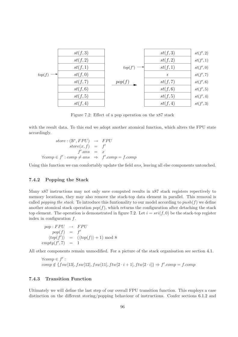
st(f ′, 5)
st(f, 0)top(f)
st(f, 1)
st(f, 2)
st(f, 3)
st(f, 7)
st(f, 6)
st(f, 5)
st(f, 4)
st(f, 1)
st(f, 2)
st(f, 3)
st(f, 6)
st(f, 5)
st(f, 4)
top(f ′)
pop(f) st(f, 7)
ǫ
st(f ′, 1)
st(f ′, 2)
st(f ′, 0)
st(f ′, 7)
st(f ′, 6)
st(f ′, 4)
st(f ′, 3)
Figure 7.2: Effect of a pop operation on the x87 stack
with the result data. To this end we adopt another atomical function, which alters the FPU stateaccordingly.
store : (B∗, FPU) → FPUstore(x, f) = f ′
f ′.ans = x∀comp ∈ f ′ : comp 6= ans ⇒ f ′.comp = f.comp
Using this function we can comfortably update the field ans, leaving all else components untouched.
7.4.2 Popping the Stack
Many x87 instructions may not only save computed results in x87 stack registers repectively tomemory locations, they may also remove the stack-top data element in parallel. This removal iscalled popping the stack. To introduce this funtionality to our model according to push(f) we defineanother atomical stack operation pop(f), which returns the configuration after detaching the stacktop element. The operation is demonstrated in figure 7.2. Let i = sri(f, 0) be the stack-top registerindex in configuration f .
pop : FPU → FPUpop(f) = f ′
〈top(f ′)〉 = (〈top(f)〉 + 1) mod 8empty(f ′, 7) = 1
All other components remain unmodified. For a picture of the stack organisation see section 4.1.
∀comp ∈ f ′ :comp /∈ {fsw[13], fsw[12], fsw[11], ftw[2 · i + 1], ftw[2 · i]} ⇒ f ′.comp = f.comp
7.4.3 Transition Function
Ultimately we will define the last step of our overall FPU transition function. This employs a casedistinction on the different storing/popping behaviour of instructions. Confer sections 6.1.2 and
96
6.1.5 to identify the corresponding instructions.
σstorefpu (f) =
store(res1(f), f) : xupdm(f) ∧ pop?(f) ∧ es(f)
pop(store(res1(f), f)) : xupdm(f) ∧ pop?(f) ∧ es(f)
pop(f) : xupdm(f) ∧ pop(f) ∧ es(f)
pop(pop(f)) : pop2?(f) ∧ es(f)
f : otherwise
If a floating-point instruction does neither returns its result to memory nor pops the stack, nochanges are applied to the configuration.
At last we completed the definition of the FPU state transfer function. Based on the floating-point interface it describes the effects of the multitude of x87 instructions on the FPU in a formalmathematical way. In the interface execFPU function the resulting FPU configuration is savedas the new value of the fpu component. This next state FPU configuration is wrapped up inAppendix D.As we already explained in section 3.5, any further exception after this point5 lies outside thescope of the FPU. However in case of a repetition of the instruction under consideration the oldfloating-point configuration must be restored.
5for instance a page fault while storing the result to memory
97

98
Chapter 8
Conclusion
In the preceding chapters we established a formal model of the x86-64 Floating-Point Unit. Start-ing from a given general purpose CPU model, we constructed an interface and a floating-pointenvironment, encapsulating the execution of x87 instructions from the rest of the processor. Thuswe were able to describe the semantics of floating-point instructions in a precise and self-containedmanner. In doing so we benefited from the formalization of floating-point arithmetics in [MP00].Nevertheless we had to extend these definitions to meet the complexity of the x87 instruction set.By generalizing the FPU operations and subdividing the execution process into four consecutivephases we were finally able to define the resulting floating-point configuration in a structured, step-by-step way.
However the presented model is quite sophisticated and it is rather complicated to extract thenext state of the FPU after executing an x87 instruction. Hence we wrapped up the next stateconfiguration based on our model, specifying the available cases for every component of the FPU.This summary can be found in Appendix D. It tops off this thesis and allows a clear view on thevariety of functionalities and features incorporated in our model.
In the future this thesis will contribute to the completion of the x86-64 CPU model and thus to theverification of a modern hypervisor as aspired by the Verisoft XT project. We will try to furthersimplify the model and check its correctness via automated tools. In addition parts of our thesismay be reused for defining the semantics of XMM and MMX multimedia instructions. Eventually aformal model of the x87 instruction subset may also complement and to a certain extent substitutethe existing architecture manuals regarding floating-point instructions.
99

100
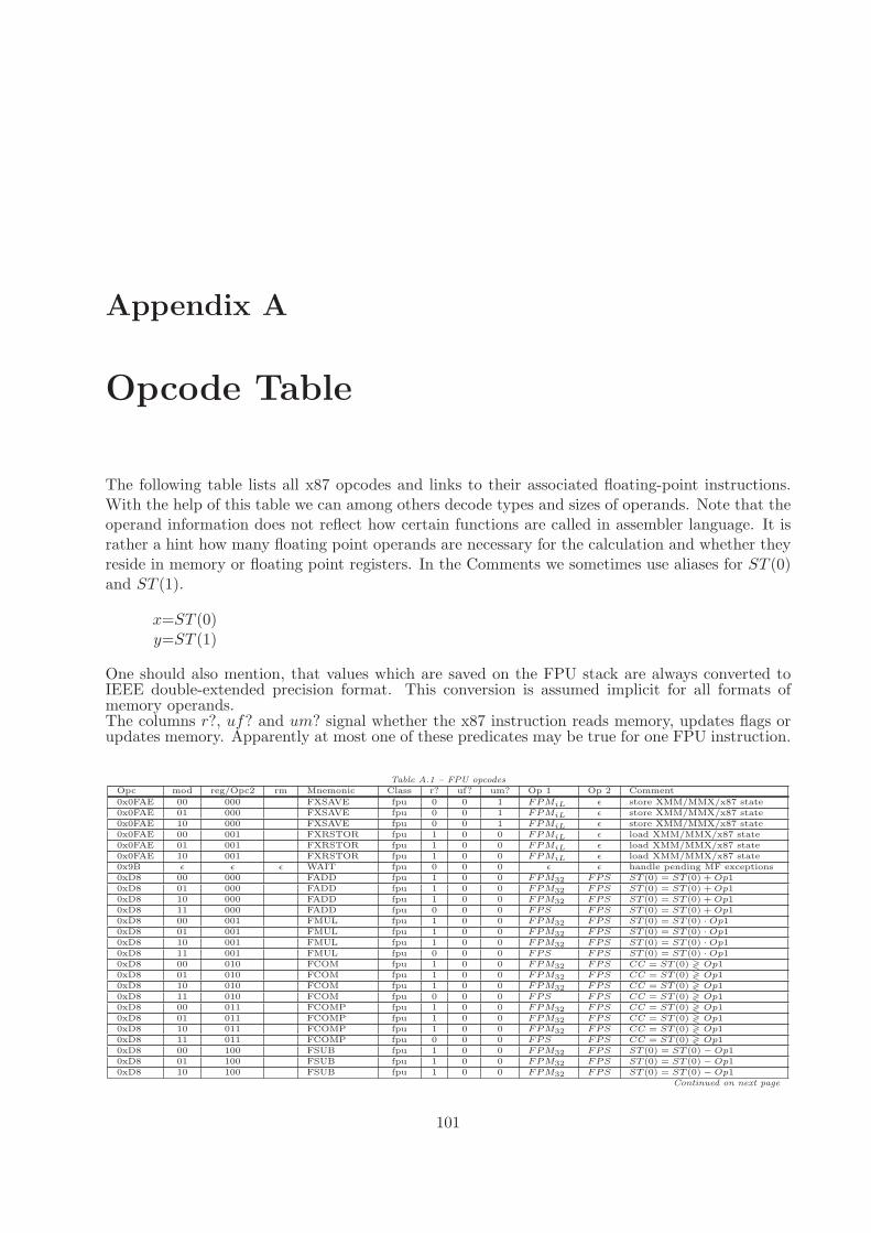
Appendix A
Opcode Table
The following table lists all x87 opcodes and links to their associated floating-point instructions.With the help of this table we can among others decode types and sizes of operands. Note that theoperand information does not reflect how certain functions are called in assembler language. It israther a hint how many floating point operands are necessary for the calculation and whether theyreside in memory or floating point registers. In the Comments we sometimes use aliases for ST (0)and ST (1).
x=ST (0)y=ST (1)
One should also mention, that values which are saved on the FPU stack are always converted toIEEE double-extended precision format. This conversion is assumed implicit for all formats ofmemory operands.The columns r?, uf? and um? signal whether the x87 instruction reads memory, updates flags orupdates memory. Apparently at most one of these predicates may be true for one FPU instruction.
Table A.1 – FPU opcodes
Opc mod reg/Opc2 rm Mnemonic Class r? uf? um? Op 1 Op 2 Comment
0x0FAE 00 000 FXSAVE fpu 0 0 1 FPMiL ǫ store XMM/MMX/x87 state0x0FAE 01 000 FXSAVE fpu 0 0 1 FPMiL ǫ store XMM/MMX/x87 state0x0FAE 10 000 FXSAVE fpu 0 0 1 FPMiL ǫ store XMM/MMX/x87 state0x0FAE 00 001 FXRSTOR fpu 1 0 0 FPMiL ǫ load XMM/MMX/x87 state0x0FAE 01 001 FXRSTOR fpu 1 0 0 FPMiL ǫ load XMM/MMX/x87 state0x0FAE 10 001 FXRSTOR fpu 1 0 0 FPMiL ǫ load XMM/MMX/x87 state0x9B ǫ ǫ ǫ WAIT fpu 0 0 0 ǫ ǫ handle pending MF exceptions0xD8 00 000 FADD fpu 1 0 0 FPM32 FPS ST (0) = ST (0) + Op10xD8 01 000 FADD fpu 1 0 0 FPM32 FPS ST (0) = ST (0) + Op10xD8 10 000 FADD fpu 1 0 0 FPM32 FPS ST (0) = ST (0) + Op10xD8 11 000 FADD fpu 0 0 0 FPS FPS ST (0) = ST (0) + Op10xD8 00 001 FMUL fpu 1 0 0 FPM32 FPS ST (0) = ST (0) · Op10xD8 01 001 FMUL fpu 1 0 0 FPM32 FPS ST (0) = ST (0) · Op10xD8 10 001 FMUL fpu 1 0 0 FPM32 FPS ST (0) = ST (0) · Op10xD8 11 001 FMUL fpu 0 0 0 FPS FPS ST (0) = ST (0) · Op10xD8 00 010 FCOM fpu 1 0 0 FPM32 FPS CC = ST (0) ≷ Op10xD8 01 010 FCOM fpu 1 0 0 FPM32 FPS CC = ST (0) ≷ Op10xD8 10 010 FCOM fpu 1 0 0 FPM32 FPS CC = ST (0) ≷ Op10xD8 11 010 FCOM fpu 0 0 0 FPS FPS CC = ST (0) ≷ Op10xD8 00 011 FCOMP fpu 1 0 0 FPM32 FPS CC = ST (0) ≷ Op10xD8 01 011 FCOMP fpu 1 0 0 FPM32 FPS CC = ST (0) ≷ Op10xD8 10 011 FCOMP fpu 1 0 0 FPM32 FPS CC = ST (0) ≷ Op10xD8 11 011 FCOMP fpu 0 0 0 FPS FPS CC = ST (0) ≷ Op10xD8 00 100 FSUB fpu 1 0 0 FPM32 FPS ST (0) = ST (0) − Op10xD8 01 100 FSUB fpu 1 0 0 FPM32 FPS ST (0) = ST (0) − Op10xD8 10 100 FSUB fpu 1 0 0 FPM32 FPS ST (0) = ST (0) − Op1
Continued on next page
101

Table A.1 – FPU opcodes, continued from previous page
Opc mod reg/Opc2 rm Mnemonic Class r? uf? um? Op 1 Op 2 Comment
0xD8 11 100 FSUB fpu 0 0 0 FPS FPS ST (0) = ST (0) − Op10xD8 00 101 FSUBR fpu 1 0 0 FPM32 FPS ST (0) = Op1 − ST (0)0xD8 01 101 FSUBR fpu 1 0 0 FPM32 FPS ST (0) = Op1 − ST (0)0xD8 10 101 FSUBR fpu 1 0 0 FPM32 FPS ST (0) = Op1 − ST (0)0xD8 11 101 FSUBR fpu 0 0 0 FPS FPS ST (0) = Op1 − ST (0)0xD8 00 110 FDIV fpu 1 0 0 FPM32 FPS ST (0) = ST (0)/Op10xD8 01 110 FDIV fpu 1 0 0 FPM32 FPS ST (0) = ST (0)/Op10xD8 10 110 FDIV fpu 1 0 0 FPM32 FPS ST (0) = ST (0)/Op10xD8 11 110 FDIV fpu 0 0 0 FPS FPS ST (0) = ST (0)/Op10xD8 00 111 FDIVR fpu 1 0 0 FPM32 FPS ST (0) = Op1/ST (0)0xD8 01 111 FDIVR fpu 1 0 0 FPM32 FPS ST (0) = Op1/ST (0)0xD8 10 111 FDIVR fpu 1 0 0 FPM32 FPS ST (0) = Op1/ST (0)0xD8 11 111 FDIVR fpu 0 0 0 FPS FPS ST (0) = Op1/ST (0)0xD9 00 000 FLD fpu 1 0 0 FPM32 ǫ push(Op1)0xD9 01 000 FLD fpu 1 0 0 FPM32 ǫ push(Op1)0xD9 10 000 FLD fpu 1 0 0 FPM32 ǫ push(Op1)0xD9 11 000 FLD fpu 0 0 0 FPS ǫ push(Op1)0xD9 11 001 FXCH fpu 0 0 0 FPS FPS ST (0) = Op1, Op1 = ST (0)0xD9 00 010 FST fpu 0 0 1 FPM32 ǫ Op1 = ST (0)0xD9 01 010 FST fpu 0 0 1 FPM32 ǫ Op1 = ST (0)0xD9 10 010 FST fpu 0 0 1 FPM32 ǫ Op1 = ST (0)0xD9 11 010 000 FNOP fpu 0 0 0 ǫ ǫ no operation0xD9 00 011 FSTP fpu 0 0 1 FPM32 ǫ Op1 = ST (0), pop0xD9 01 011 FSTP fpu 0 0 1 FPM32 ǫ Op1 = ST (0), pop0xD9 10 011 FSTP fpu 0 0 1 FPM32 ǫ Op1 = ST (0), pop0xD9 00 100 FLDENV fpu 1 0 0 FPMiS ǫ load x87 environment0xD9 01 100 FLDENV fpu 1 0 0 FPMiS ǫ load x87 environment0xD9 10 100 FLDENV fpu 1 0 0 FPMiS ǫ load x87 environment0xD9 11 100 000 FCHS fpu 0 0 0 FPS ǫ ST (0) = −ST (0)0xD9 11 100 001 FABS fpu 0 0 0 FPS ǫ ST (0) = |ST (0)|0xD9 11 100 100 FTST fpu 0 0 0 FPS ǫ CC = ST (0) ≷ 0.00xD9 11 100 101 FXAM fpu 0 0 0 FPS ǫ CC = type of ST (0)0xD9 00 101 FLDCW fpu 1 0 0 FPM16 ǫ FCW = Op10xD9 01 101 FLDCW fpu 1 0 0 FPM16 ǫ FCW = Op10xD9 10 101 FLDCW fpu 1 0 0 FPM16 ǫ FCW = Op10xD9 11 101 000 FLD1 fpu 0 0 0 ǫ ǫ push(+1.0)0xD9 11 101 001 FLDL2T fpu 0 0 0 ǫ ǫ push(log2 10)0xD9 11 101 010 FLDL2E fpu 0 0 0 ǫ ǫ push(log2 e)0xD9 11 101 011 FLDPI fpu 0 0 0 ǫ ǫ push(π)0xD9 11 101 100 FLDLG2 fpu 0 0 0 ǫ ǫ push(log10 2)0xD9 11 101 101 FLDLN2 fpu 0 0 0 ǫ ǫ push(ln 2)0xD9 11 101 110 FLDZ fpu 0 0 0 ǫ ǫ push(0.0)0xD9 00 110 FNSTENV fpu 0 0 1 FPMiS ǫ store x87 environment0xD9 01 110 FNSTENV fpu 0 0 1 FPMiS ǫ store x87 environment0xD9 10 110 FNSTENV fpu 0 0 1 FPMiS ǫ store x87 environment
0xD9 11 110 000 F2XM1 fpu 0 0 0 FPS ǫ ST (0) = 2ST (0) − 10xD9 11 110 001 FY2LX fpu 0 0 0 FPS FPS y = y · log2 x, pop0xD9 11 110 010 FPTAN fpu 0 0 0 FPS ǫ x = tan(x), push(1.0)0xD9 11 110 011 FPATAN fpu 0 0 0 FPS FPS y = arctan(y/x), pop0xD9 11 110 100 FXTRACT fpu 0 0 0 FPS ǫ x = ⌊log2|x|⌋, push( x
2⌊log2|x|⌋)
0xD9 11 110 101 FPREM1 fpu 0 0 0 FPS FPS x = x − rne(x/y) · y0xD9 11 110 110 FDECSTP fpu 0 0 0 ǫ ǫ top = top + 10xD9 11 110 111 FINCSTP fpu 0 0 0 ǫ ǫ top = top − 10xD9 00 111 FNSTCW fpu 0 0 1 FPM16 ǫ Op1 = FCW0xD9 01 111 FNSTCW fpu 0 0 1 FPM16 ǫ Op1 = FCW0xD9 10 111 FNSTCW fpu 0 0 1 FPM16 ǫ Op1 = FCW0xD9 11 111 000 FPREM fpu 0 0 0 FPS FPS x = x − trunc(x/y) · y0xD9 11 111 001 FY2LXP1 fpu 0 0 0 FPS FPS y = y · log2(x + 1), pop
0xD9 11 111 010 FSQRT fpu 0 0 0 FPS ǫ ST (0) =√
ST (0)0xD9 11 111 011 FSINCOS fpu 0 0 0 FPS ǫ x = sin x, push(cos x)0xD9 11 111 100 FRNDINT fpu 0 0 0 FPS ǫ ST (0) = int(ST (0))
0xD9 11 111 101 FSCALE fpu 0 0 0 FPS FPS ST (0) = ST (0) · 2int(ST (1))
0xD9 11 111 110 FSIN fpu 0 0 0 FPS ǫ ST (0) = sin ST (0)0xD9 11 111 111 FCOS fpu 0 0 0 FPS ǫ ST (0) = cos ST (0)0xDA 00 000 FIADD fpu 1 0 0 FPM32 FPS ST (0) = ST (0) + Op10xDA 01 000 FIADD fpu 1 0 0 FPM32 FPS ST (0) = ST (0) + Op10xDA 10 000 FIADD fpu 1 0 0 FPM32 FPS ST (0) = ST (0) + Op10xDA 11 000 FCMOVB fpu 0 0 0 FPS FPS < ⇒ ST (0) = Op10xDA 00 001 FIMUL fpu 1 0 0 FPM32 FPS ST (0) = ST (0) · Op10xDA 01 001 FIMUL fpu 1 0 0 FPM32 FPS ST (0) = ST (0) · Op10xDA 10 001 FIMUL fpu 1 0 0 FPM32 FPS ST (0) = ST (0) · Op10xDA 11 001 FCMOVE fpu 0 0 0 FPS FPS = ⇒ ST (0) = Op10xDA 00 010 FICOM fpu 1 0 0 FPM32 FPS CC = ST (0) ≷ Op10xDA 01 010 FICOM fpu 1 0 0 FPM32 FPS CC = ST (0) ≷ Op10xDA 10 010 FICOM fpu 1 0 0 FPM32 FPS CC = ST (0) ≷ Op10xDA 11 010 FCMOVBE fpu 0 0 0 FPS FPS ≤ ⇒ ST (0) = Op10xDA 00 011 FICOMP fpu 1 0 0 FPM32 FPS CC = ST (0) ≷ Op1, pop0xDA 01 011 FICOMP fpu 1 0 0 FPM32 FPS CC = ST (0) ≷ Op1, pop0xDA 10 011 FICOMP fpu 1 0 0 FPM32 FPS CC = ST (0) ≷ Op1, pop0xDA 11 100 FCMOVU fpu 0 0 0 FPS FPS Unordered ⇒ ST (0) = Op1
Continued on next page
102

Table A.1 – FPU opcodes, continued from previous page
Opc mod reg/Opc2 rm Mnemonic Class r? uf? um? Op 1 Op 2 Comment
0xDA 00 100 FISUB fpu 1 0 0 FPM32 FPS ST (0) = ST (0) − Op10xDA 01 100 FISUB fpu 1 0 0 FPM32 FPS ST (0) = ST (0) − Op10xDA 10 100 FISUB fpu 1 0 0 FPM32 FPS ST (0) = ST (0) − Op10xDA 00 101 FISUBR fpu 1 0 0 FPM32 FPS ST (0) = Op1 − ST (0)0xDA 01 101 FISUBR fpu 1 0 0 FPM32 FPS ST (0) = Op1 − ST (0)0xDA 10 101 FISUBR fpu 1 0 0 FPM32 FPS ST (0) = Op1 − ST (0)0xDA 11 101 001 FUCOMPP fpu 0 0 0 FPS FPS CC = ST (0) ≷ ST (1), pop, pop0xDA 00 110 FIDIV fpu 1 0 0 FPM32 FPS ST (0) = ST (0)/Op10xDA 01 110 FIDIV fpu 1 0 0 FPM32 FPS ST (0) = ST (0)/Op10xDA 10 110 FIDIV fpu 1 0 0 FPM32 FPS ST (0) = ST (0)/Op10xDA 00 111 FIDIVR fpu 1 0 0 FPM32 FPS ST (0) = Op1/ST (0)0xDA 01 111 FIDIVR fpu 1 0 0 FPM32 FPS ST (0) = Op1/ST (0)0xDA 10 111 FIDIVR fpu 1 0 0 FPM32 FPS ST (0) = Op1/ST (0)0xDB 00 000 FILD fpu 1 0 0 FPM32 ǫ push(Op1)0xDB 01 000 FILD fpu 1 0 0 FPM32 ǫ push(Op1)0xDB 10 000 FILD fpu 1 0 0 FPM32 ǫ push(Op1)0xDB 11 000 FCMOVNB fpu 0 0 0 FPS FPS ≮ ⇒ ST (0) = Op10xDB 00 001 FISTTP fpu 0 0 1 FPM32 ǫ Op1 = trunc(ST (0)), pop0xDB 01 001 FISTTP fpu 0 0 1 FPM32 ǫ Op1 = trunc(ST (0)), pop0xDB 10 001 FISTTP fpu 0 0 1 FPM32 ǫ Op1 = trunc(ST (0)), pop0xDB 11 001 FCMOVNE fpu 0 0 0 FPS FPS 6= ⇒ ST (0) = Op10xDB 00 010 FIST fpu 0 0 1 FPM32 ǫ Op1 = int(ST (0))0xDB 01 010 FIST fpu 0 0 1 FPM32 ǫ Op1 = int(ST (0))0xDB 10 010 FIST fpu 0 0 1 FPM32 ǫ Op1 = int(ST (0))
0xDB 11 010 FCMOVNBE fpu 0 0 0 FPS FPS � ⇒ ST (0) = Op1
0xDB 00 011 FISTP fpu 0 0 1 FPM32 ǫ Op1 = int(ST (0)), pop0xDB 01 011 FISTP fpu 0 0 1 FPM32 ǫ Op1 = int(ST (0)), pop0xDB 10 011 FISTP fpu 0 0 1 FPM32 ǫ Op1 = int(ST (0)), pop0xDB 11 011 FCMOVNU fpu 0 0 0 FPS FPS ¬Unordered ⇒ ST (0) = Op10xDB 11 100 010 FNCLEX fpu 0 0 0 ǫ ǫ clear FSW exception bits0xDB 11 100 011 FNINIT fpu 0 0 0 ǫ ǫ initialize FPU0xDB 00 101 FLD fpu 1 0 0 FPM80 ǫ push(Op1)0xDB 01 101 FLD fpu 1 0 0 FPM80 ǫ push(Op1)0xDB 10 101 FLD fpu 1 0 0 FPM80 ǫ push(Op1)0xDB 11 101 FUCOMI fpu 0 1 0 FPS FPS rFlags = ST (0) ≷ Op10xDB 11 110 FCOMI fpu 0 1 0 FPS FPS rFlags = ST (0) ≷ Op10xDB 00 111 FSTP fpu 0 0 1 FPM80 ǫ Op1 = ST (0), pop0xDB 01 111 FSTP fpu 0 0 1 FPM80 ǫ Op1 = ST (0), pop0xDB 10 111 FSTP fpu 0 0 1 FPM80 ǫ Op1 = ST (0), pop0xDC 00 000 FADD fpu 1 0 0 FPM64 FPS ST (0) = ST (0) + Op10xDC 01 000 FADD fpu 1 0 0 FPM64 FPS ST (0) = ST (0) + Op10xDC 10 000 FADD fpu 1 0 0 FPM64 FPS ST (0) = ST (0) + Op10xDC 11 000 FADD fpu 0 0 0 FPS FPS Op1 = ST (0) + Op10xDC 00 001 FMUL fpu 1 0 0 FPM64 FPS ST (0) = ST (0) · Op10xDC 01 001 FMUL fpu 1 0 0 FPM64 FPS ST (0) = ST (0) · Op10xDC 10 001 FMUL fpu 1 0 0 FPM64 FPS ST (0) = ST (0) · Op10xDC 11 001 FMUL fpu 0 0 0 FPS FPS Op1 = ST (0) · Op10xDC 00 010 FCOM fpu 1 0 0 FPM64 FPS CC = ST (0) ≷ Op10xDC 01 010 FCOM fpu 1 0 0 FPM64 FPS CC = ST (0) ≷ Op10xDC 10 010 FCOM fpu 1 0 0 FPM64 FPS CC = ST (0) ≷ Op10xDC 00 011 FCOMP fpu 1 0 0 FPM64 FPS CC = ST (0) ≷ Op1, pop0xDC 01 011 FCOMP fpu 1 0 0 FPM64 FPS CC = ST (0) ≷ Op1, pop0xDC 10 011 FCOMP fpu 1 0 0 FPM64 FPS CC = ST (0) ≷ Op1, pop0xDC 00 100 FSUB fpu 1 0 0 FPM64 FPS ST (0) = ST (0) − Op10xDC 01 100 FSUB fpu 1 0 0 FPM64 FPS ST (0) = ST (0) − Op10xDC 10 100 FSUB fpu 1 0 0 FPM64 FPS ST (0) = ST (0) − Op10xDC 11 100 FSUBR fpu 0 0 0 FPS FPS Op1 = ST (0) − Op10xDC 00 101 FSUBR fpu 1 0 0 FPM64 FPS ST (0) = Op1 − ST (0)0xDC 01 101 FSUBR fpu 1 0 0 FPM64 FPS ST (0) = Op1 − ST (0)0xDC 10 101 FSUBR fpu 1 0 0 FPM64 FPS ST (0) = Op1 − ST (0)0xDC 11 101 FSUB fpu 0 0 0 FPS FPS Op1 = Op1 − ST (0)0xDC 00 110 FDIV fpu 1 0 0 FPM64 FPS ST (0) = ST (0)/Op10xDC 01 110 FDIV fpu 1 0 0 FPM64 FPS ST (0) = ST (0)/Op10xDC 10 110 FDIV fpu 1 0 0 FPM64 FPS ST (0) = ST (0)/Op10xDC 11 110 FDIVR fpu 0 0 0 FPS FPS Op1 = ST (0)/Op10xDC 00 111 FDIVR fpu 1 0 0 FPM64 FPS ST (0) = Op1/ST (0)0xDC 01 111 FDIVR fpu 1 0 0 FPM64 FPS ST (0) = Op1/ST (0)0xDC 10 111 FDIVR fpu 1 0 0 FPM64 FPS ST (0) = Op1/ST (0)0xDC 11 111 FDIV fpu 0 0 0 FPS FPS Op1 = Op1/ST (0)0xDD 00 000 FLD fpu 1 0 0 FPM64 ǫ push(Op1)0xDD 01 000 FLD fpu 1 0 0 FPM64 ǫ push(Op1)0xDD 10 000 FLD fpu 1 0 0 FPM64 ǫ push(Op1)0xDD 11 000 FFREE fpu 0 0 0 ǫ ǫ set FP register tag to empty0xDD 00 001 FISTTP fpu 0 0 1 FPM64 ǫ Op1 = trunc(ST (0)), pop0xDD 01 001 FISTTP fpu 0 0 1 FPM64 ǫ Op1 = trunc(ST (0)), pop0xDD 10 001 FISTTP fpu 0 0 1 FPM64 ǫ Op1 = trunc(ST (0)), pop0xDD 00 010 FST fpu 0 0 1 FPM64 ǫ Op1 = ST (0)0xDD 01 010 FST fpu 0 0 1 FPM64 ǫ Op1 = ST (0)0xDD 10 010 FST fpu 0 0 1 FPM64 ǫ Op1 = ST (0)0xDD 11 010 FST fpu 0 0 0 FPS ǫ Op1 = ST (0)0xDD 00 011 FSTP fpu 0 0 1 FPM64 ǫ Op1 = ST (0), pop
Continued on next page
103

Table A.1 – FPU opcodes, continued from previous page
Opc mod reg/Opc2 rm Mnemonic Class r? uf? um? Op 1 Op 2 Comment
0xDD 01 011 FSTP fpu 0 0 1 FPM64 ǫ Op1 = ST (0), pop0xDD 10 011 FSTP fpu 0 0 1 FPM64 ǫ Op1 = ST (0), pop0xDD 11 011 FSTP fpu 0 0 0 FPS ǫ Op1 = ST (0), pop0xDD 00 100 FRSTOR fpu 1 0 0 FPMiM ǫ load x87/MMX state0xDD 01 100 FRSTOR fpu 1 0 0 FPMiM ǫ load x87/MMX state0xDD 10 100 FRSTOR fpu 1 0 0 FPMiM ǫ load x87/MMX state0xDD 11 100 FUCOM fpu 0 0 0 FPS FPS CC = ST (0) ≷ Op10xDD 11 101 FUCOMP fpu 0 0 0 FPS FPS CC = ST (0) ≷ Op1, pop0xDD 00 110 FNSAVE fpu 0 0 1 FPMiM ǫ store x87/MMX state0xDD 01 110 FNSAVE fpu 0 0 1 FPMiM ǫ store x87/MMX state0xDD 10 110 FNSAVE fpu 0 0 1 FPMiM ǫ store x87/MMX state0xDD 00 111 FNSTSW fpu 0 0 1 FPM16 ǫ Op1 = FSW0xDD 01 111 FNSTSW fpu 0 0 1 FPM16 ǫ Op1 = FSW0xDD 10 111 FNSTSW fpu 0 0 1 FPM16 ǫ Op1 = FSW0xDE 00 000 FIADD fpu 1 0 0 FPM16 FPS ST (0) = ST (0) + Op10xDE 01 000 FIADD fpu 1 0 0 FPM16 FPS ST (0) = ST (0) + Op10xDE 10 000 FIADD fpu 1 0 0 FPM16 FPS ST (0) = ST (0) + Op10xDE 11 000 FADDP fpu 0 0 0 FPS FPS Op1 = ST (0) + Op1, pop0xDE 00 001 FIMUL fpu 1 0 0 FPM16 FPS ST (0) = ST (0) · Op10xDE 01 001 FIMUL fpu 1 0 0 FPM16 FPS ST (0) = ST (0) · Op10xDE 10 001 FIMUL fpu 1 0 0 FPM16 FPS ST (0) = ST (0) · Op10xDE 11 001 FMULP fpu 0 0 0 FPS FPS Op1 = ST (0) · Op10xDE 00 010 FICOM fpu 1 0 0 FPM16 FPS CC = ST (0) ≷ Op10xDE 01 010 FICOM fpu 1 0 0 FPM16 FPS CC = ST (0) ≷ Op10xDE 10 010 FICOM fpu 1 0 0 FPM16 FPS CC = ST (0) ≷ Op10xDE 00 011 FICOMP fpu 1 0 0 FPM16 FPS CC = ST (0) ≷ Op1, pop0xDE 01 011 FICOMP fpu 1 0 0 FPM16 FPS CC = ST (0) ≷ Op1.pop0xDE 10 011 FICOMP fpu 1 0 0 FPM16 FPS CC = ST (0) ≷ Op1, pop0xDE 11 011 FCOMPP fpu 1 0 0 FPS FPS CC = ST (0) ≷ ST (1), pop, pop0xDE 00 100 FISUB fpu 1 0 0 FPM16 FPS ST (0) = ST (0) − Op10xDE 01 100 FISUB fpu 1 0 0 FPM16 FPS ST (0) = ST (0) − Op10xDE 10 100 FISUB fpu 1 0 0 FPM16 FPS ST (0) = ST (0) − Op10xDE 11 100 FSUBRP fpu 0 0 0 FPS FPS Op1 = ST (0) − Op1, pop0xDE 00 101 FISUBR fpu 1 0 0 FPM16 FPS ST (0) = Op1 − ST (0)0xDE 01 101 FISUBR fpu 1 0 0 FPM16 FPS ST (0) = Op1 − ST (0)0xDE 10 101 FISUBR fpu 1 0 0 FPM16 FPS ST (0) = Op1 − ST (0)0xDE 11 101 FSUBP fpu 0 0 0 FPS FPS Op1 = Op1 − ST (0), pop0xDE 00 110 FIDIV fpu 1 0 0 FPM16 FPS ST (0) = ST (0)/Op10xDE 01 110 FIDIV fpu 1 0 0 FPM16 FPS ST (0) = ST (0)/Op10xDE 10 110 FIDIV fpu 1 0 0 FPM16 FPS ST (0) = ST (0)/Op10xDE 11 110 FDIVRP fpu 0 0 0 FPS FPS Op1 = ST (0)/Op1, pop0xDE 00 111 FIDIVR fpu 1 0 0 FPM16 FPS ST (0) = Op1/ST (0)0xDE 01 111 FIDIVR fpu 1 0 0 FPM16 FPS ST (0) = Op1/ST (0)0xDE 10 111 FIDIVR fpu 1 0 0 FPM16 FPS ST (0) = Op1/ST (0)0xDE 11 111 FDIVP fpu 0 0 0 FPS FPS Op1 = Op1/ST (0), pop0xDF 00 000 FILD fpu 1 0 0 FPM16 ǫ push(Op1)0xDF 01 000 FILD fpu 1 0 0 FPM16 ǫ push(Op1)0xDF 10 000 FILD fpu 1 0 0 FPM16 ǫ push(Op1)0xDF 00 001 FISTTP fpu 0 0 1 FPM16 ǫ Op1 = trunc(ST (0)), pop0xDF 01 001 FISTTP fpu 0 0 1 FPM16 ǫ Op1 = trunc(ST (0)), pop0xDF 10 001 FISTTP fpu 0 0 1 FPM16 ǫ Op1 = trunc(ST (0)), pop0xDF 00 010 FIST fpu 0 0 1 FPM16 ǫ Op1 = int(ST (0))0xDF 01 010 FIST fpu 0 0 1 FPM16 ǫ Op1 = int(ST (0))0xDF 10 010 FIST fpu 0 0 1 FPM16 ǫ Op1 = int(ST (0))0xDF 00 011 FISTP fpu 0 0 1 FPM16 ǫ Op1 = int(ST (0)), pop0xDF 01 011 FISTP fpu 0 0 1 FPM16 ǫ Op1 = int(ST (0)), pop0xDF 10 011 FISTP fpu 0 0 1 FPM16 ǫ Op1 = int(ST (0)), pop0xDF 00 100 FBLD fpu 1 0 0 FPM16 ǫ push(Op1)0xDF 01 100 FBLD fpu 1 0 0 FPM16 ǫ push(Op1)0xDF 10 100 FBLD fpu 1 0 0 FPM16 ǫ push(Op1)0xDF 11 100 000 FNSTSW fpu 0 0 1 AX16 ǫ Op1 = FSW0xDF 00 101 FILD fpu 1 0 0 FPM64 ǫ push(Op1)0xDF 01 101 FILD fpu 1 0 0 FPM64 ǫ push(Op1)0xDF 10 101 FILD fpu 1 0 0 FPM64 ǫ push(Op1)0xDF 11 101 FUCOMIP fpu 0 1 0 FPS FPS rFlags = ST (0) ≷ Op1, pop0xDF 00 110 FBSTP fpu 0 0 1 FPM80 ǫ Op1 = bcd(ST (0), pop0xDF 01 110 FBSTP fpu 0 0 1 FPM80 ǫ Op1 = bcd(ST (0), pop0xDF 10 110 FBSTP fpu 0 0 1 FPM80 ǫ Op1 = bcd(ST (0), pop0xDF 11 110 FCOMIP fpu 0 1 0 FPS FPS rFlags = ST (0) ≷ Op1, pop0xDF 00 111 FISTP fpu 0 0 1 FPM64 ǫ Op1 = int(ST (0)), pop0xDF 01 111 FISTP fpu 0 0 1 FPM64 ǫ Op1 = int(ST (0)), pop0xDF 10 111 FISTP fpu 0 0 1 FPM64 ǫ Op1 = int(ST (0)), pop
104
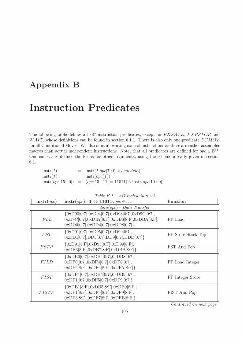
Appendix B
Instruction Predicates
The following table defines all x87 instruction predicates, except for FXSAV E, FXRSTOR andWAIT , whose definitions can be found in section 6.1.1. There is also only one predicate FCMOVfor all Conditional Moves. We also omit all waiting control instructions as these are rather assemblermacros than actual independent instructions. Note, that all predicates are defined for opc ∈ B11.One can easily deduce the forms for other arguments, using the scheme already given in section6.1.
instr(I) = instr(I.opc[7 : 0] ◦ I.modrm)instr(f) = instr(opc(f))instr(opc[15 : 0]) = (opc[15 : 11] = 11011) ∧ instr(opc[10 : 0])
Table B.1 – x87 instruction set
instr(opc) instr(opc)=1 ⇔ 11011◦opc ∈ . . . function
data(opc) - Data Transfer
FLD{0xD90[0:7],0xD94[0:7],0xD98[0:7],0xD9C[0:7],0xD9C[0:7],0xDB2[8:F],0xDB6[8:F],0xDBA[8:F],0xDD0[0:7],0xDD4[0:7],0xDD8[0:7]}
FP Load
FST{0xD91[0:7],0xD95[0:7],0xD99[0:7],0xDD1[0:7],DD5[0:7],DD9[0:7],DDD[0:7]} FP Store Stack Top
FSTP{0xD91[8:F],0xD95[8:F],0xD99[8:F],0xDB3[8:F],0xDB7[8:F],0xDBB[8:F]} FST And Pop
FILD{0xDB0[0:7],0xDB4[0:7],0xDB8[0:7],0xDF0[0:7],0xDF4[0:7],0xDF8[0:7],0xDF2[8:F],0xDF6[8:F],0xDFA[8:F]}
FP Load Integer
FIST{0xDB1[0:7],0xDB5[0:7],0xDB9[0:7],0xDF1[0:7],0xDF5[0:7],0xDF9[0:7]} FP Integer Store
FISTP{0xDB1[8:F],0xDB5[8:F],0xDB9[8:F],0xDF1[8:F],0xDF5[8:F],0xDF9[8:F],0xDF3[8:F],0xDF7[8:F],0xDFB[8:F]}
FIST And Pop
Continued on next page
105
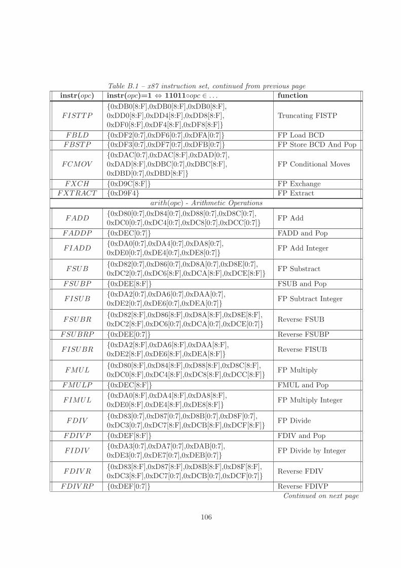
Table B.1 – x87 instruction set, continued from previous page
instr(opc) instr(opc)=1 ⇔ 11011◦opc ∈ . . . function
FISTTP{0xDB0[8:F],0xDB0[8:F],0xDB0[8:F],0xDD0[8:F],0xDD4[8:F],0xDD8[8:F],0xDF0[8:F],0xDF4[8:F],0xDF8[8:F]}
Truncating FISTP
FBLD {0xDF2[0:7],0xDF6[0:7],0xDFA[0:7]} FP Load BCD
FBSTP {0xDF3[0:7],0xDF7[0:7],0xDFB[0:7]} FP Store BCD And Pop
FCMOV{0xDAC[0:7],0xDAC[8:F],0xDAD[0:7],0xDAD[8:F],0xDBC[0:7],0xDBC[8:F],0xDBD[0:7],0xDBD[8:F]}
FP Conditional Moves
FXCH {0xD9C[8:F]} FP Exchange
FXTRACT {0xD9F4} FP Extract
arith(opc) - Arithmetic Operations
FADD{0xD80[0:7],0xD84[0:7],0xD88[0:7],0xD8C[0:7],0xDC0[0:7],0xDC4[0:7],0xDC8[0:7],0xDCC[0:7]} FP Add
FADDP {0xDEC[0:7]} FADD and Pop
FIADD{0xDA0[0:7],0xDA4[0:7],0xDA8[0:7],0xDE0[0:7],0xDE4[0:7],0xDE8[0:7]} FP Add Integer
FSUB{0xD82[0:7],0xD86[0:7],0xD8A[0:7],0xD8E[0:7],0xDC2[0:7],0xDC6[8:F],0xDCA[8:F],0xDCE[8:F]} FP Substract
FSUBP {0xDEE[8:F]} FSUB and Pop
FISUB{0xDA2[0:7],0xDA6[0:7],0xDAA[0:7],0xDE2[0:7],0xDE6[0:7],0xDEA[0:7]} FP Subtract Integer
FSUBR{0xD82[8:F],0xD86[8:F],0xD8A[8:F],0xD8E[8:F],0xDC2[8:F],0xDC6[0:7],0xDCA[0:7],0xDCE[0:7]} Reverse FSUB
FSUBRP {0xDEE[0:7]} Reverse FSUBP
FISUBR{0xDA2[8:F],0xDA6[8:F],0xDAA[8:F],0xDE2[8:F],0xDE6[8:F],0xDEA[8:F]} Reverse FISUB
FMUL{0xD80[8:F],0xD84[8:F],0xD88[8:F],0xD8C[8:F],0xDC0[8:F],0xDC4[8:F],0xDC8[8:F],0xDCC[8:F]} FP Multiply
FMULP {0xDEC[8:F]} FMUL and Pop
FIMUL{0xDA0[8:F],0xDA4[8:F],0xDA8[8:F],0xDE0[8:F],0xDE4[8:F],0xDE8[8:F]} FP Multiply Integer
FDIV{0xD83[0:7],0xD87[0:7],0xD8B[0:7],0xD8F[0:7],0xDC3[0:7],0xDC7[8:F],0xDCB[8:F],0xDCF[8:F]} FP Divide
FDIV P {0xDEF[8:F]} FDIV and Pop
FIDIV{0xDA3[0:7],0xDA7[0:7],0xDAB[0:7],0xDE3[0:7],0xDE7[0:7],0xDEB[0:7]} FP Divide by Integer
FDIV R{0xD83[8:F],0xD87[8:F],0xD8B[8:F],0xD8F[8:F],0xDC3[8:F],0xDC7[0:7],0xDCB[0:7],0xDCF[0:7]} Reverse FDIV
FDIV RP {0xDEF[0:7]} Reverse FDIVP
Continued on next page
106
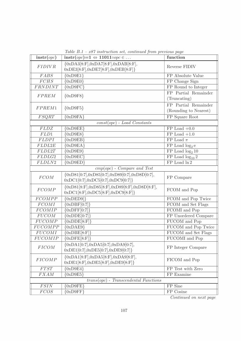
Table B.1 – x87 instruction set, continued from previous page
instr(opc) instr(opc)=1 ⇔ 11011◦opc ∈ . . . function
FIDIV R{0xDA3[8:F],0xDA7[8:F],0xDAB[8:F],0xDE3[8:F],0xDE7[8:F],0xDEB[8:F]} Reverse FIDIV
FABS {0xD9E1} FP Absolute Value
FCHS {0xD9E0} FP Change Sign
FRNDINT {0xD9FC} FP Round to Integer
FPREM {0xD9F8} FP Partial Remainder(Truncating)
FPREM1 {0xD9F5} FP Partial Remainder(Rounding to Nearest)
FSQRT {0xD9FA} FP Square Root
const(opc) - Load Constants
FLDZ {0xD9EE} FP Load +0.0
FLD1 {0xD9E8} FP Load +1.0
FLDPI {0xD9EB} FP Load π
FLDL2E {0xD9EA} FP Load log2 e
FLDL2T {0xD9E9} FP Load log2 10
FLDLG2 {0xD9EC} FP Load log10 2
FLDLN2 {0xD9ED} FP Load ln 2
cmp(opc) - Compare and Test
FCOM{0xD81[0:7],0xD85[0:7],0xD89[0:7],0xD8D[0:7],0xDC1[0:7],0xDC5[0:7],0xDC9[0:7]} FP Compare
FCOMP{0xD81[8:F],0xD85[8:F],0xD89[8:F],0xD8D[8:F],0xDC1[8:F],0xDC5[8:F],0xDC9[8:F]} FCOM and Pop
FCOMPP {0xDED9]} FCOM and Pop Twice
FCOMI {0xDBF[0:7]} FCOM and Set Flags
FCOMIP {0xDFF[0:7]} FCOMI and Pop
FUCOM {0xDDE[0:7]} FP Unordered Compare
FUCOMP {0xDDE[8:F]} FUCOM and Pop
FUCOMPP {0xDAE9} FUCOM and Pop Twice
FUCOMI {0xDBE[8:F]} FUCOM and Set Flags
FUCOMIP {0xDFE[8:F]} FUCOMI and Pop
FICOM{0xDA1[0:7],0xDA5[0:7],0xDA9[0:7],0xDE1[0:7],0xDE5[0:7],0xDE9[0:7]} FP Integer Compare
FICOMP{0xDA1[8:F],0xDA5[8:F],0xDA9[8:F],0xDE1[8:F],0xDE5[8:F],0xDE9[8:F]} FICOM and Pop
FTST {0xD9E4} FP Test with Zero
FXAM {0xD9E5} FP Examine
trans(opc) - Transcendental Functions
FSIN {0xD9FE} FP Sine
FCOS {0xD9FF} FP Cosine
Continued on next page
107
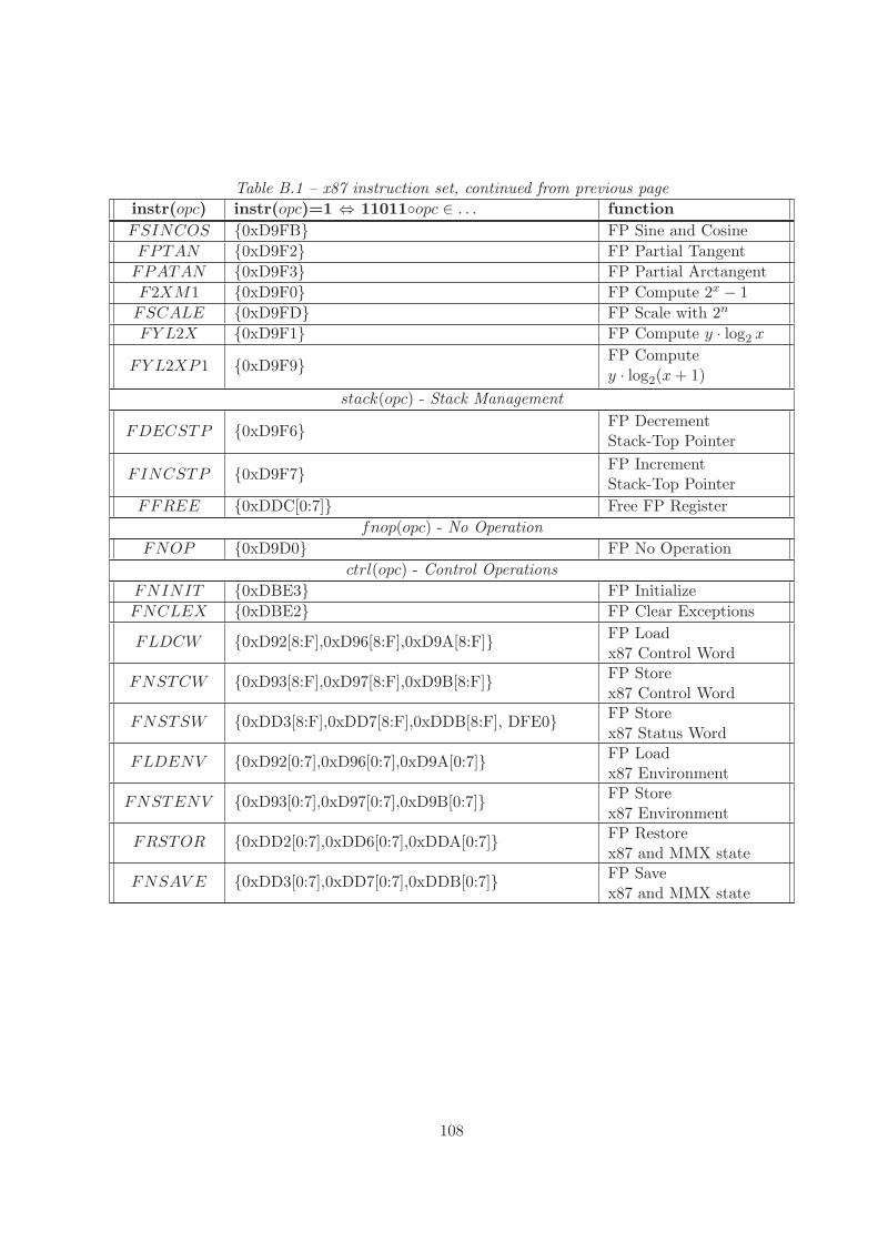
Table B.1 – x87 instruction set, continued from previous page
instr(opc) instr(opc)=1 ⇔ 11011◦opc ∈ . . . function
FSINCOS {0xD9FB} FP Sine and Cosine
FPTAN {0xD9F2} FP Partial Tangent
FPATAN {0xD9F3} FP Partial Arctangent
F2XM1 {0xD9F0} FP Compute 2x − 1
FSCALE {0xD9FD} FP Scale with 2n
FY L2X {0xD9F1} FP Compute y · log2 x
FY L2XP1 {0xD9F9} FP Computey · log2(x + 1)
stack(opc) - Stack Management
FDECSTP {0xD9F6} FP DecrementStack-Top Pointer
FINCSTP {0xD9F7} FP IncrementStack-Top Pointer
FFREE {0xDDC[0:7]} Free FP Register
fnop(opc) - No Operation
FNOP {0xD9D0} FP No Operation
ctrl(opc) - Control Operations
FNINIT {0xDBE3} FP Initialize
FNCLEX {0xDBE2} FP Clear Exceptions
FLDCW {0xD92[8:F],0xD96[8:F],0xD9A[8:F]} FP Loadx87 Control Word
FNSTCW {0xD93[8:F],0xD97[8:F],0xD9B[8:F]} FP Storex87 Control Word
FNSTSW {0xDD3[8:F],0xDD7[8:F],0xDDB[8:F], DFE0} FP Storex87 Status Word
FLDENV {0xD92[0:7],0xD96[0:7],0xD9A[0:7]} FP Loadx87 Environment
FNSTENV {0xD93[0:7],0xD97[0:7],0xD9B[0:7]} FP Storex87 Environment
FRSTOR {0xDD2[0:7],0xDD6[0:7],0xDDA[0:7]} FP Restorex87 and MMX state
FNSAV E {0xDD3[0:7],0xDD7[0:7],0xDDB[0:7]} FP Savex87 and MMX state
108
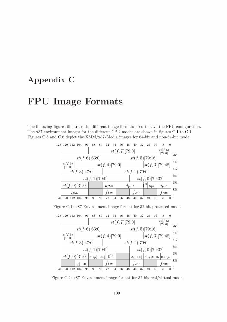
Appendix C
FPU Image Formats
The following figures illustrate the different image formats used to save the FPU configuration.The x87 environment images for the different CPU modes are shown in figures C.1 to C.4.Figures C.5 and C.6 depict the XMM/x87/Media images for 64-bit and non-64-bit mode.
st(f, 7)[79:0]
081624324048566472112 96 8088104120
128 081624324048566472112 96 8088104120
0
128
256
384
512
640
768
fcwfswftwip.o
ip.sopc05dp.odp.s
st(f, 5)
st(f, 6)
st(f, 0)[31:0]
st(f, 0)[79:32]st(f, 1)[79:0]
st(f, 3)[47:0] st(f, 2)[79:0]
st(f, 3)[79:48]st(f, 4)[79:0][15:0]
[79:0]
st(f, 5)[79:16]st(f, 6)[63:0]
128
Figure C.1: x87 Environment image format for 32-bit protected mode
ip[15:0]
081624324048566472112 96 8088104120
128 081624324048566472112 96 8088104120
0
128
256
384
512
640
768
fcwfswftw
st(f, 5)
st(f, 6)
st(f, 0)[31:0]
st(f, 0)[79:32]st(f, 1)[79:0]
st(f, 3)[47:0] st(f, 2)[79:0]
st(f, 3)[79:48]st(f, 4)[79:0][15:0]
[79:0]
st(f, 5)[79:16]st(f, 6)[63:0]
st(f, 7)[79:0]
0 ◦ opc0404 012dp[31:16] dp[15:0] ip[31:16]
128
Figure C.2: x87 Environment image format for 32-bit real/virtual mode
109
dp.s081624324048566472112 96 8088104120
128 081624324048566472112 96 8088104120
0
128
256
384
512
640
768
fcwst(f, 0)[15:0]
st(f, 0)[79:16]
st(f, 1)
st(f, 1)[63:0][79:64]
st(f, 2)[79:0]st(f, 3)[31:0]
st(f, 3)[79:32]st(f, 4)[79:0]
st(f, 5)[79:48]st(f, 6)[47:0]
st(f, 6)[79:48]st(f, 7)[79:0]
fswftwip.oip.sdp.o128
Figure C.3: x87 Environment image format for 16-bit protected mode
dp
081624324048566472112 96 8088104120
128 081624324048566472112 96 8088104120
0
128
256
384
512
640
768
fcwst(f, 0)[15:0]
st(f, 0)[79:16]
st(f, 1)
st(f, 1)[63:0][79:64]
st(f, 2)[79:0]st(f, 3)[31:0]
st(f, 3)[79:32]st(f, 4)[79:0]
st(f, 6)[47:0]
st(f, 6)[79:48]st(f, 7)[79:0]
fswftw0 ◦ opcipdp[15:0] ip[15:0]012
st(f, 5)[79:0]
128
Figure C.4: x87 Environment image format for 16-bit real/virtual mode
110
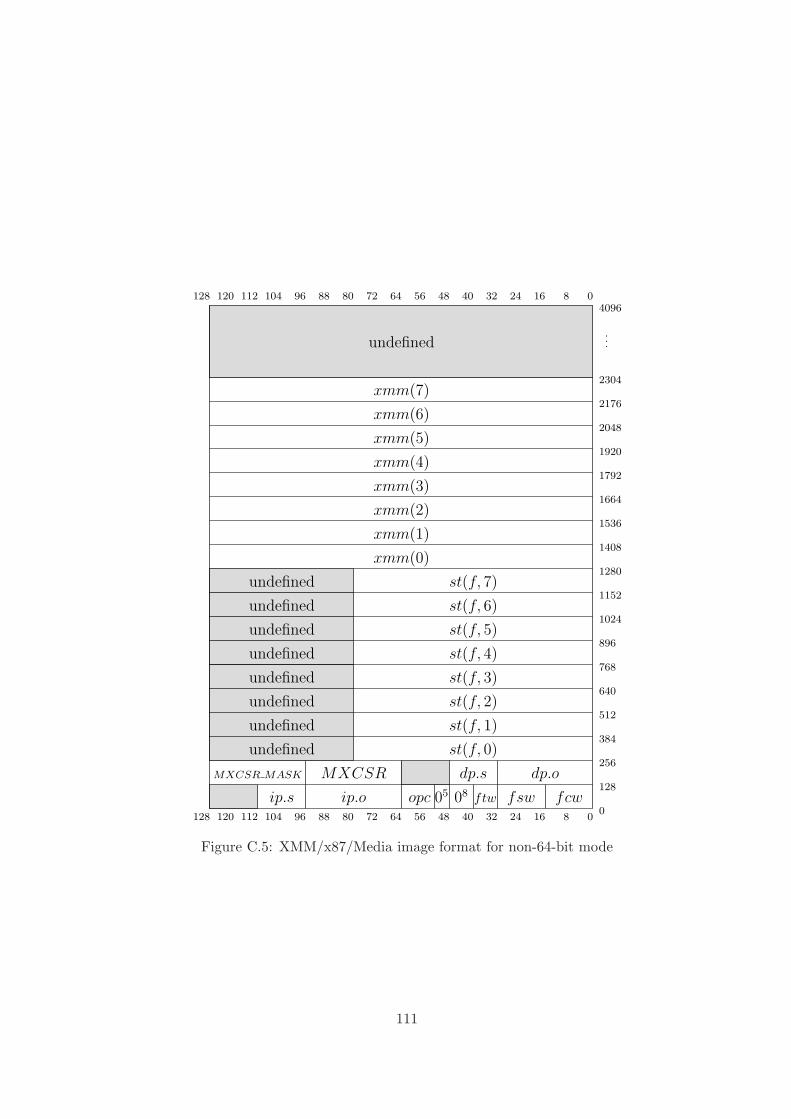
.
.
.
128 081624324048566472112 96 8088104120
128 081624324048566472112 96 8088104120
0
128
256
384
512
640
768
896
1024
1152
1280
1408
1536
1664
1792
1920
2048
2176
2304
xmm(0)
xmm(7)
xmm(6)
xmm(5)
xmm(4)
xmm(3)
xmm(2)
xmm(1)
st(f, 7)
st(f, 6)
st(f, 5)
st(f, 4)
st(f, 3)
st(f, 2)
st(f, 1)
fcwfsw0805
MXCSRMXCSR MASK
opc ftw
st(f, 0)
undefined
undefined
undefined
undefined
undefined
undefined
undefined
undefined
undefined
4096
ip.oip.s
dp.odp.s
Figure C.5: XMM/x87/Media image format for non-64-bit mode
111
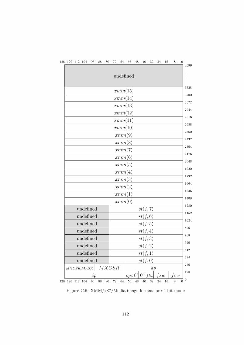
undefined
128 081624324048566472112 96 8088104120
128 081624324048566472112 96 80881041200
128
256
384
512
640
768
896
1024
1152
1280
1408
1536
1664
1792
1920
2048
2176
2304
2432
2560
2688
2816
2944
3072
3200
3328
4096
.
.
.
xmm(0)
xmm(15)
xmm(14)
xmm(13)
xmm(12)
xmm(11)
xmm(10)
xmm(9)
xmm(8)
xmm(7)
xmm(6)
xmm(5)
xmm(4)
xmm(3)
xmm(2)
xmm(1)
st(f, 7)
st(f, 6)
st(f, 5)
st(f, 4)
st(f, 3)
st(f, 2)
st(f, 1)
fcwfsw0805ip
dpMXCSRMXCSR MASK
opc ftw
st(f, 0)
undefined
undefined
undefined
undefined
undefined
undefined
undefined
undefined
Figure C.6: XMM/x87/Media image format for 64-bit mode
112
Appendix D
Next State FPU Configuration
In the following we will summarise the components of the next state FPU configuration f ′ resultingfrom applying the FPU transition function to some floating-point configuration f .
f ′ = σfpu(f)
To this end we will use functions from this document. We will try to refer to the original config-uration f as far as possible, nevertheless we will have to make cases distinctions on the exceptionstatus. This forces us to rely on the resulting FPU configurations of the pre- or post-computationexception checking phase.
fpre = σprechkfpu (f) fpost = σpostchk
fpu (σexecfpu (fpre))
We do not need to consider any other transition subfunctions. Additionally we want to state theinitial configuration f0 again.
∀i ∈ N8 :f0.fpr(i) = undefinedf0.opc = 011
f0.dp = 064
f0.ip = 064
f0.fsw = 016
f0.fcw = 0x0300f0.ftw = 116
f0.acc = ǫf0.ans = ǫ
Now we want to list the contents for the several components of f ′. We begin with the fields accand ans, which are trivially defined.
f ′.acc = f ′acc
f ′.ans =
{
res1(fpre) : xupdm(f) ∧ es(fpost)
f.ans : otherwise
113
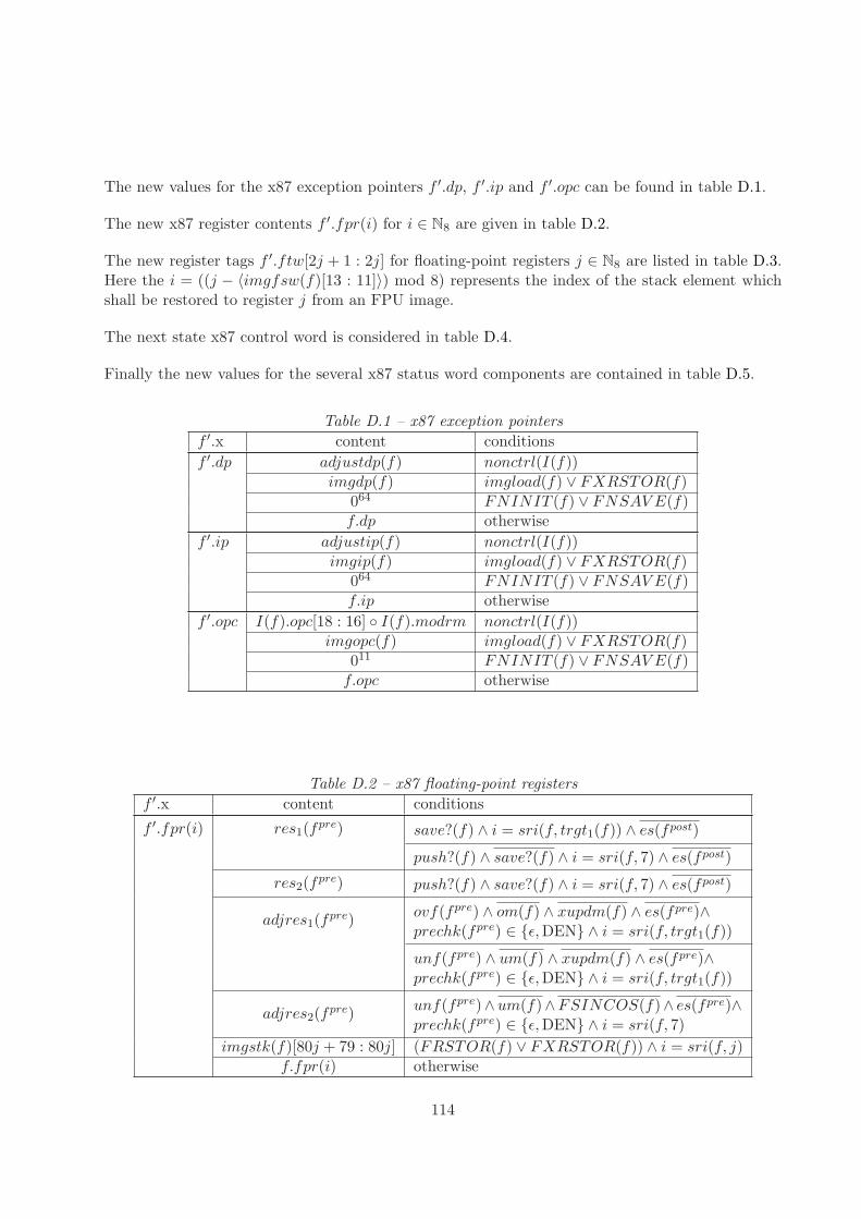
The new values for the x87 exception pointers f ′.dp, f ′.ip and f ′.opc can be found in table D.1.
The new x87 register contents f ′.fpr(i) for i ∈ N8 are given in table D.2.
The new register tags f ′.ftw[2j + 1 : 2j] for floating-point registers j ∈ N8 are listed in table D.3.Here the i = ((j − 〈imgfsw(f)[13 : 11]〉) mod 8) represents the index of the stack element whichshall be restored to register j from an FPU image.
The next state x87 control word is considered in table D.4.
Finally the new values for the several x87 status word components are contained in table D.5.
Table D.1 – x87 exception pointers
f ′.x content conditions
f ′.dp adjustdp(f) nonctrl(I(f))imgdp(f) imgload(f) ∨ FXRSTOR(f)
064 FNINIT (f) ∨ FNSAV E(f)f.dp otherwise
f ′.ip adjustip(f) nonctrl(I(f))imgip(f) imgload(f) ∨ FXRSTOR(f)
064 FNINIT (f) ∨ FNSAV E(f)f.ip otherwise
f ′.opc I(f).opc[18 : 16] ◦ I(f).modrm nonctrl(I(f))imgopc(f) imgload(f) ∨ FXRSTOR(f)
011 FNINIT (f) ∨ FNSAV E(f)f.opc otherwise
Table D.2 – x87 floating-point registers
f ′.x content conditions
f ′.fpr(i) res1(fpre) save?(f) ∧ i = sri(f, trgt1(f)) ∧ es(fpost)
push?(f) ∧ save?(f) ∧ i = sri(f, 7) ∧ es(fpost)
res2(fpre) push?(f) ∧ save?(f) ∧ i = sri(f, 7) ∧ es(fpost)
adjres1(fpre)
ovf(fpre) ∧ om(f) ∧ xupdm(f) ∧ es(fpre)∧prechk(fpre) ∈ {ǫ, DEN} ∧ i = sri(f, trgt1(f))
unf(fpre) ∧ um(f) ∧ xupdm(f) ∧ es(fpre)∧prechk(fpre) ∈ {ǫ, DEN} ∧ i = sri(f, trgt1(f))
adjres2(fpre)
unf(fpre)∧um(f)∧FSINCOS(f)∧ es(fpre)∧prechk(fpre) ∈ {ǫ, DEN} ∧ i = sri(f, 7)
imgstk(f)[80j + 79 : 80j] (FRSTOR(f) ∨ FXRSTOR(f)) ∧ i = sri(f, j)f.fpr(i) otherwise
114
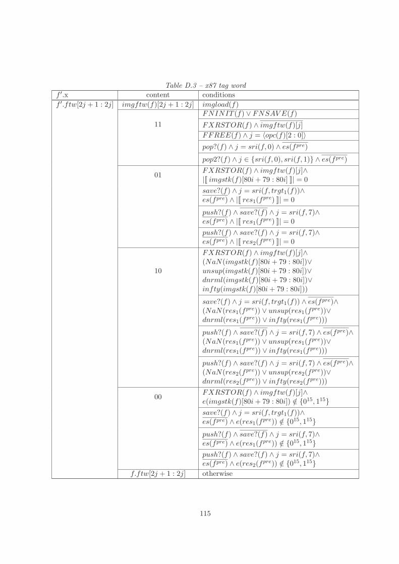
Table D.3 – x87 tag word
f ′.x content conditions
f ′.ftw[2j + 1 : 2j] imgftw(f)[2j + 1 : 2j] imgload(f)FNINIT (f) ∨ FNSAV E(f)
11 FXRSTOR(f) ∧ imgftw(f)[j]
FFREE(f) ∧ j = 〈opc(f)[2 : 0]〉pop?(f) ∧ j = sri(f, 0) ∧ es(fpre)
pop2?(f) ∧ j ∈ {sri(f, 0), sri(f, 1)} ∧ es(fpre)
01FXRSTOR(f) ∧ imgftw(f)[j]∧|[[ imgstk(f)[80i + 79 : 80i] ]]| = 0
save?(f) ∧ j = sri(f, trgt1(f))∧es(fpre) ∧ |[[ res1(f
pre) ]]| = 0
push?(f) ∧ save?(f) ∧ j = sri(f, 7)∧es(fpre) ∧ |[[ res1(f
pre) ]]| = 0
push?(f) ∧ save?(f) ∧ j = sri(f, 7)∧es(fpre) ∧ |[[ res2(f
pre) ]]| = 0
10
FXRSTOR(f) ∧ imgftw(f)[j]∧(NaN(imgstk(f)[80i + 79 : 80i])∨unsup(imgstk(f)[80i + 79 : 80i])∨dnrml(imgstk(f)[80i + 79 : 80i])∨infty(imgstk(f)[80i + 79 : 80i]))
save?(f) ∧ j = sri(f, trgt1(f)) ∧ es(fpre)∧(NaN(res1(f
pre)) ∨ unsup(res1(fpre))∨
dnrml(res1(fpre)) ∨ infty(res1(f
pre)))
push?(f) ∧ save?(f) ∧ j = sri(f, 7) ∧ es(fpre)∧(NaN(res1(f
pre)) ∨ unsup(res1(fpre))∨
dnrml(res1(fpre)) ∨ infty(res1(f
pre)))
push?(f) ∧ save?(f) ∧ j = sri(f, 7) ∧ es(fpre)∧(NaN(res2(f
pre)) ∨ unsup(res2(fpre))∨
dnrml(res2(fpre)) ∨ infty(res2(f
pre)))
00FXRSTOR(f) ∧ imgftw(f)[j]∧e(imgstk(f)[80i + 79 : 80i]) /∈ {015, 115}save?(f) ∧ j = sri(f, trgt1(f))∧es(fpre) ∧ e(res1(f
pre)) /∈ {015, 115}push?(f) ∧ save?(f) ∧ j = sri(f, 7)∧es(fpre) ∧ e(res1(f
pre)) /∈ {015, 115}push?(f) ∧ save?(f) ∧ j = sri(f, 7)∧es(fpre) ∧ e(res2(f
pre)) /∈ {015, 115}f.ftw[2j + 1 : 2j] otherwise
115
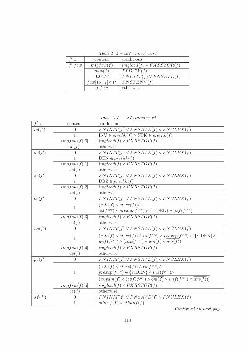
Table D.4 – x87 control word
f ′.x content conditions
f ′.fcw imgfcw(f) imgload(f) ∨ FXRSTOR(f)mop(f) FLDCW (f)0x037F FNINIT (f) ∨ FNSAV E(f)
fcw[15 : 7] ◦ 17 FNSTENV (f)f.fcw otherwise
Table D.5 – x87 status word
f ′.x content conditions
ie(f ′) 0 FNINIT (f) ∨ FNSAV E(f) ∨ FNCLEX(f)1 INV ∈ prechk(f) ∨ STK ∈ prechk(f)
imgfsw(f)[0] imgload(f) ∨ FXRSTOR(f)ie(f) otherwise
de(f ′) 0 FNINIT (f) ∨ FNSAV E(f) ∨ FNCLEX(f)1 DEN ∈ prechk(f)
imgfsw(f)[1] imgload(f) ∨ FXRSTOR(f)de(f) otherwise
ze(f ′) 0 FNINIT (f) ∨ FNSAV E(f) ∨ FNCLEX(f)1 DBZ ∈ prechk(f)
imgfsw(f)[2] imgload(f) ∨ FXRSTOR(f)ze(f) otherwise
oe(f ′) 0 FNINIT (f) ∨ FNSAV E(f) ∨ FNCLEX(f)
1(calc(f) ∨ store(f))∧es(fpre) ∧ prexcp(fpre) ∈ {ǫ, DEN} ∧ ovf(fpre)
imgfsw(f)[3] imgload(f) ∨ FXRSTOR(f)oe(f) otherwise
ue(f ′) 0 FNINIT (f) ∨ FNSAV E(f) ∨ FNCLEX(f)
1(calc(f) ∨ store(f)) ∧ es(fpre) ∧ prexcp(fpre) ∈ {ǫ, DEN}∧unf(fpre) ∧ (inx(fpre) ∧ um(f) ∨ um(f))
imgfsw(f)[4] imgload(f) ∨ FXRSTOR(f)ue(f) otherwise
pe(f ′) 0 FNINIT (f) ∨ FNSAV E(f) ∨ FNCLEX(f)
1
(calc(f) ∨ store(f)) ∧ es(fpre)∧prexcp(fpre) ∈ {ǫ, DEN} ∧ inx(fpre)∧(xupdm(f) ∧ (ovf(fpre) ∧ om(f) ∨ unf(fpre) ∧ um(f)))
imgfsw(f)[5] imgload(f) ∨ FXRSTOR(f)pe(f) otherwise
sf(f ′) 0 FNINIT (f) ∨ FNSAV E(f) ∨ FNCLEX(f)1 stkovf(f) ∨ stkunf(f)
Continued on next page
116
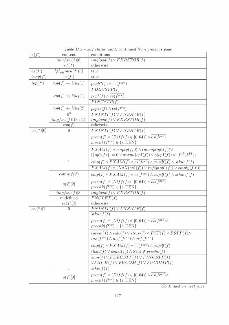
Table D.5 – x87 status word, continued from previous page
x(f ′) content conditions
imgfsw(f)[6] imgload(f) ∨ FXRSTOR(f)sf(f) otherwise
es(f ′)∨5
i=0 mca(f ′)[i] true
busy(f ′) es(f ′) true
top(f ′) top(f) −3 bin3(1) push?(f) ∧ es(fpre)
FDECSTP (f)
top(f) +3 bin3(1) pop?(f) ∧ es(fpre)
FINCSTP (f)
top(f) +3 bin3(2) pop2?(f) ∧ es(fpre)
03 FNINIT (f) ∨ FNSAV E(f)imgfsw(f)[13 : 11] imgload(f) ∨ FXRSTOR(f)
top(f) otherwise
cc(f ′)[0] 0 FNINIT (f) ∨ FNSAV E(f)
prem(f) ∧ (Diff(f) /∈ [0, 64)) ∧ es(fpre)prechk(fpre) ∈ {ǫ, DEN}FXAM(f) ∧ empty(f, 0) ∧ (unsup(op1(f))∨|[[ op1(f) ]]| = 0 ∨ dnrml(op1(f)) ∨ e(op1(f)) /∈ {015, 115})
1 cmp(f) ∧ FXAM(f) ∧ es(fpre) ∧ xupdf(f) ∧ stkunf(f)
FXAM(f) ∧ (NaN(op1(f)) ∨ infty(op1(f)) ∨ empty(f, 0))
compcf(f) cmp(f) ∧ FXAM(f) ∧ es(fpre) ∧ xupdf(f) ∧ stkunf(f)
q(f)[2]prem(f) ∧ (Diff(f) ∈ [0, 64)) ∧ es(fpre)prechk(fpre) ∈ {ǫ, DEN}
imgfsw(f)[8] imgload(f) ∨ FXRSTOR(f)undefined FNCLEX(f)cc(f)[0] otherwise
cc(f ′)[1] 0 FNINIT (f) ∨ FNSAV E(f)stkunf(f)
prem(f) ∧ (Diff(f) /∈ [0, 64)) ∧ es(fpre)∧prechk(fpre) ∈ {ǫ, DEN}(prem(f) ∧ calc(f) ∨ store(f) ∧ FST (f) ∨ FSTP (f)∧inx(fpre) ∧ unf(fpre) ∧ ovf(fpre)
cmp(f) ∧ FXAM(f) ∧ es(fpre) ∧ xupdf(f)
(load(f) ∨ const(f)) ∧ STK /∈ prechk(f)
sign(f) ∨ FDECSTP (f) ∨ FINCSTP (f)∨FXCH(f) ∨ FUCOM(f) ∨ FUCOMP (f)
1 stkovf(f)
q(f)[0]prem(f) ∧ (Diff(f) ∈ [0, 64)) ∧ es(fpre)∧prechk(fpre) ∈ {ǫ, DEN}
Continued on next page
117
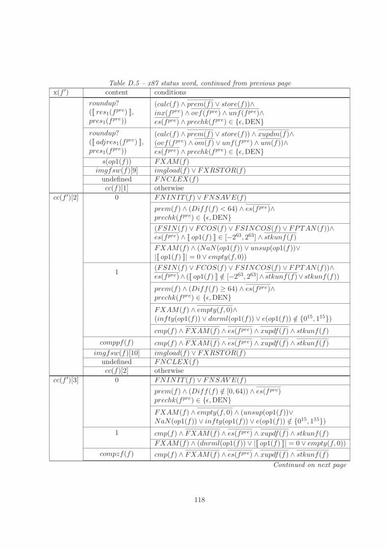
Table D.5 – x87 status word, continued from previous page
x(f ′) content conditions
roundup?([[ res1(f
pre) ]],pres1(f
pre))
(calc(f) ∧ prem(f) ∨ store(f))∧inx(fpre) ∧ ovf(fpre) ∧ unf(fpre)∧es(fpre) ∧ prechk(fpre) ∈ {ǫ, DEN}
roundup?([[ adjres1(f
pre) ]],pres1(f
pre))
(calc(f) ∧ prem(f) ∨ store(f)) ∧ xupdm(f)∧(ovf(fpre) ∧ om(f) ∨ unf(fpre) ∧ um(f))∧es(fpre) ∧ prechk(fpre) ∈ {ǫ, DEN}
s(op1(f)) FXAM(f)imgfsw(f)[9] imgload(f) ∨ FXRSTOR(f)
undefined FNCLEX(f)cc(f)[1] otherwise
cc(f ′)[2] 0 FNINIT (f) ∨ FNSAV E(f)
prem(f) ∧ (Diff(f) < 64) ∧ es(fpre)∧prechk(fpre) ∈ {ǫ, DEN}(FSIN(f) ∨ FCOS(f) ∨ FSINCOS(f) ∨ FPTAN(f))∧es(fpre) ∧ [[ op1(f) ]] ∈ [−263, 263] ∧ stkunf(f)
FXAM(f) ∧ (NaN(op1(f)) ∨ unsup(op1(f))∨|[[ op1(f) ]]| = 0 ∨ empty(f, 0))
1(FSIN(f) ∨ FCOS(f) ∨ FSINCOS(f) ∨ FPTAN(f))∧es(fpre)∧ ([[ op1(f) ]] /∈ [−263, 263]∧ stkunf(f)∨ stkunf(f))
prem(f) ∧ (Diff(f) ≥ 64) ∧ es(fpre)∧prechk(fpre) ∈ {ǫ, DEN}FXAM(f) ∧ empty(f, 0)∧(infty(op1(f)) ∨ dnrml(op1(f)) ∨ e(op1(f)) /∈ {015, 115})cmp(f) ∧ FXAM(f) ∧ es(fpre) ∧ xupdf(f) ∧ stkunf(f)
comppf(f) cmp(f) ∧ FXAM(f) ∧ es(fpre) ∧ xupdf(f) ∧ stkunf(f)
imgfsw(f)[10] imgload(f) ∨ FXRSTOR(f)undefined FNCLEX(f)cc(f)[2] otherwise
cc(f ′)[3] 0 FNINIT (f) ∨ FNSAV E(f)
prem(f) ∧ (Diff(f) /∈ [0, 64)) ∧ es(fpre)prechk(fpre) ∈ {ǫ, DEN}FXAM(f) ∧ empty(f, 0) ∧ (unsup(op1(f))∨NaN(op1(f)) ∨ infty(op1(f)) ∨ e(op1(f)) /∈ {015, 115})
1 cmp(f) ∧ FXAM(f) ∧ es(fpre) ∧ xupdf(f) ∧ stkunf(f)
FXAM(f) ∧ (dnrml(op1(f)) ∨ |[[ op1(f) ]]| = 0 ∨ empty(f, 0))
compzf(f) cmp(f) ∧ FXAM(f) ∧ es(fpre) ∧ xupdf(f) ∧ stkunf(f)
Continued on next page
118

Table D.5 – x87 status word, continued from previous page
x(f ′) content conditions
q(f)[1]prem(f) ∧ (Diff(f) ∈ [0, 64)) ∧ es(fpre)prechk(fpre) ∈ {ǫ, DEN}
imgfsw(f)[14] imgload(f) ∨ FXRSTOR(f)undefined FNCLEX(f)cc(f)[3] otherwise
119

120

Bibliography
[AMD07] AMD64 Architecture Programmer’s Manual, September 2007.
[Deg07] Ulan Degenbaev. Formal specification of parts of the x86-64 instruction set architecture.Master’s thesis, Saarland University, 2007.
[IA07] Intel 64 and IA-32 Architectures Software Developer’s Manual, November 2007.
[IE85] IEEE standard for binary floating-point arithmetic, August 1985.
[MP00] S.M. Muller and W.J. Paul. Computer Architecture, Complexity and Correctness.Springer Verlag, 2000.
121