Formale Systeme II: Theorie - Formal VerificationFormale Systeme II: Theorie SS 2018 Prof. Dr....
125
Formale Systeme II: Theorie SS 2018 Prof. Dr. Bernhard Beckert · Dr. Mattias Ulbrich Slides by courtesy of Andr´ e Platzer, CMU KIT – Die Forschungsuniversit¨ at in der Helmholtz-Gemeinschaft www.kit.edu
Transcript of Formale Systeme II: Theorie - Formal VerificationFormale Systeme II: Theorie SS 2018 Prof. Dr....
Formale Systeme II: Theorie
SS 2018
Prof. Dr. Bernhard Beckert · Dr. Mattias UlbrichSlides by courtesy of Andre Platzer, CMU
KIT – Die Forschungsuniversitat in der Helmholtz-Gemeinschaft www.kit.edu
Roadmap
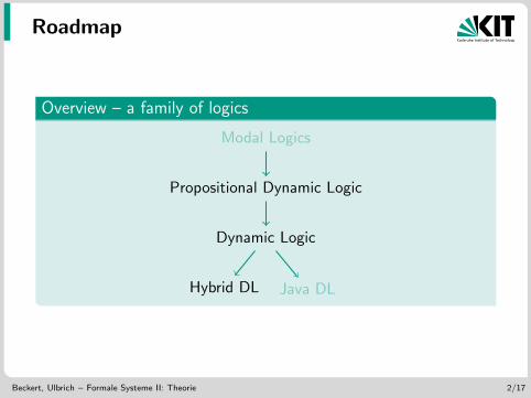
Overview – a family of logics
Modal Logics
Propositional Dynamic Logic
Dynamic Logic
Hybrid DL Java DL
Beckert, Ulbrich – Formale Systeme II: Theorie 2/17
Roadmap
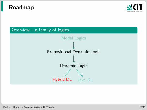
Overview – a family of logics
Modal Logics
Propositional Dynamic Logic
Dynamic Logic
Hybrid DL Java DL
Beckert, Ulbrich – Formale Systeme II: Theorie 2/17
Goals
differential equations
hybrid automata
hybrid dynamic logic
differential invariants
Beckert, Ulbrich – Formale Systeme II: Theorie 3/17
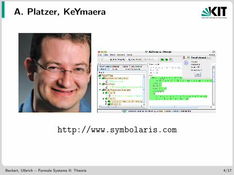
A. Platzer, KeYmaera
http://www.symbolaris.com
Beckert, Ulbrich – Formale Systeme II: Theorie 4/17
15-424/15-624: Foundations of Cyber-Physical Systems01: Overview
Andre Platzer
Carnegie Mellon University, Pittsburgh, PA
http://symbolaris.com/course/fcps16.html
http://www.cs.cmu.edu/~aplatzer/course/fcps16.html
0.20.4
0.60.8
1.00.1
0.2
0.3
0.4
0.5
Andre Platzer (CMU) FCPS/01: Overview FCPS 1 / 29
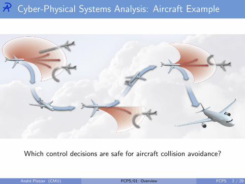
Cyber-Physical Systems Analysis: Aircraft Example
Which control decisions are safe for aircraft collision avoidance?
Andre Platzer (CMU) FCPS/01: Overview FCPS 2 / 29
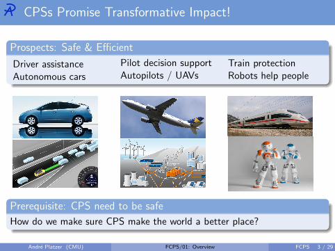
CPSs Promise Transformative Impact!
Prospects: Safe & Efficient
Driver assistanceAutonomous cars
Pilot decision supportAutopilots / UAVs
Train protectionRobots help people
Prerequisite: CPS need to be safe
How do we make sure CPS make the world a better place?
Andre Platzer (CMU) FCPS/01: Overview FCPS 3 / 29
Can you trust a computer to control physics?
Rationale1 Safety guarantees require analytic foundations.
2 Foundations revolutionized digital computer science & our society.
3 Need even stronger foundations when software reaches out into ourphysical world.
How can we provide people with cyber-physical systems they can bet theirlives on? — Jeannette Wing
Cyber-physical Systems
CPS combine cyber capabilities with physical capabilities to solve problemsthat neither part could solve alone.
Andre Platzer (CMU) FCPS/01: Overview FCPS 4 / 29
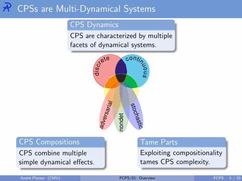
CPSs are Multi-Dynamical Systems
dis
cre
te contin
uo
us
no
nd
et
sto
chastic
advers
arial
CPS Dynamics
CPS are characterized by multiplefacets of dynamical systems.
CPS Compositions
CPS combine multiplesimple dynamical effects.
Tame Parts
Exploiting compositionalitytames CPS complexity.
Andre Platzer (CMU) FCPS/01: Overview FCPS 5 / 29
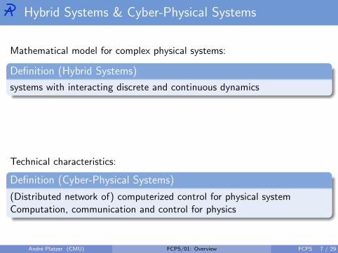
Hybrid Systems & Cyber-Physical Systems
Mathematical model for complex physical systems:
Definition (Hybrid Systems)
systems with interacting discrete and continuous dynamics
Technical characteristics:
Definition (Cyber-Physical Systems)
(Distributed network of) computerized control for physical systemComputation, communication and control for physics
Andre Platzer (CMU) FCPS/01: Overview FCPS 7 / 29
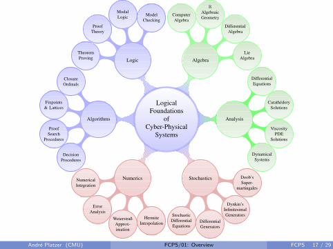
LogicalFoundations
ofCyber-Physical
Systems
Logic
TheoremProving
ProofTheory
ModalLogic Model
Checking
Algebra
ComputerAlgebra
RAlgebraicGeometry
DifferentialAlgebra
LieAlgebra
Analysis
DifferentialEquations
CarathedorySolutions
ViscosityPDE
Solutions
DynamicalSystems
Stochastics Doob’sSuper-
martingales
Dynkin’sInfinitesimalGenerators
DifferentialGenerators
StochasticDifferentialEquations
Numerics
HermiteInterpolation
WeierstraßApprox-imation
ErrorAnalysis
NumericalIntegration
Algorithms
DecisionProcedures
ProofSearch
Procedures
Fixpoints& Lattices
ClosureOrdinals
Andre Platzer (CMU) FCPS/01: Overview FCPS 17 / 29
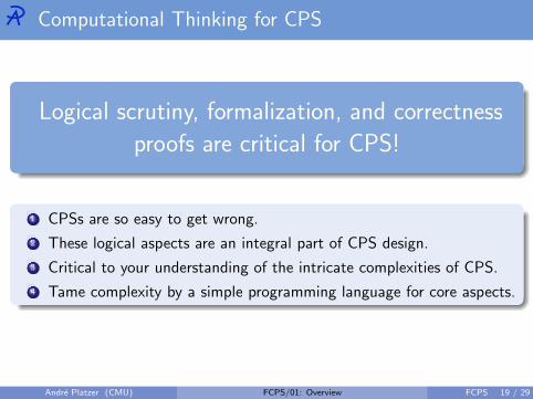
Computational Thinking for CPS
Logical scrutiny, formalization, and correctness
proofs are critical for CPS!
1 CPSs are so easy to get wrong.
2 These logical aspects are an integral part of CPS design.
3 Critical to your understanding of the intricate complexities of CPS.
4 Tame complexity by a simple programming language for core aspects.
Andre Platzer (CMU) FCPS/01: Overview FCPS 19 / 29
Lecture Notes and Book
Andre Platzer.Foundations of Cyber-Physical Systems.Lecture notes.Computer Science DepartmentCarnegie Mellon University.http://symbolaris.com/course/
fcps16-schedule.html
Andre Platzer.Logical Analysis of Hybrid Systems.Springer, 426p., 2010.DOI 10.1007/978-3-642-14509-4http://symbolaris.com/lahs/
CMU library e-book
Andre Platzer (CMU) FCPS/01: Overview FCPS 25 / 29
02: Differential Equations & Domains15-424: Foundations of Cyber-Physical Systems
Andre Platzer
Computer Science DepartmentCarnegie Mellon University, Pittsburgh, PA
0.20.4
0.60.8
1.00.1
0.2
0.3
0.4
0.5
Andre Platzer (CMU) FCPS / 02: Differential Equations & Domains 1 / 12
Outline
1 Introduction
2 Differential Equations
3 Examples of Differential Equations
4 Domains of Differential Equations
Andre Platzer (CMU) FCPS / 02: Differential Equations & Domains 2 / 12
Outline
1 Introduction
2 Differential Equations
3 Examples of Differential Equations
4 Domains of Differential Equations
Andre Platzer (CMU) FCPS / 02: Differential Equations & Domains 2 / 12
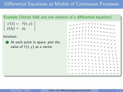
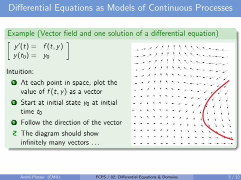
Differential Equations as Models of Continuous Processes
Example (Vector field and one solution of a differential equation)[
y ′(t) = f (t, y)y(t0) = y0
]
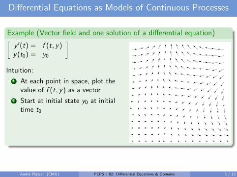
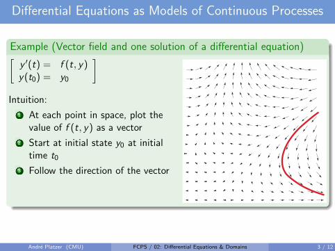
Intuition:
1 At each point in space, plot thevalue of f (t, y) as a vector
2 Start at initial state y0 at initialtime t0
3 Follow the direction of the vector
The diagram should showinfinitely many vectors . . .
Your car’s ODE x ′ = v , v ′ = a Well it’s a wee bit more complicated
Andre Platzer (CMU) FCPS / 02: Differential Equations & Domains 3 / 12
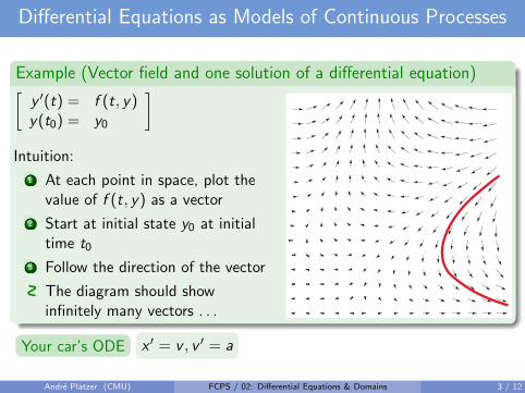
Differential Equations as Models of Continuous Processes
Example (Vector field and one solution of a differential equation)[
y ′(t) = f (t, y)y(t0) = y0
]
Intuition:
1 At each point in space, plot thevalue of f (t, y) as a vector
2 Start at initial state y0 at initialtime t0
3 Follow the direction of the vector
The diagram should showinfinitely many vectors . . .
Your car’s ODE x ′ = v , v ′ = a Well it’s a wee bit more complicated
Andre Platzer (CMU) FCPS / 02: Differential Equations & Domains 3 / 12
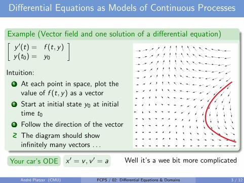
Differential Equations as Models of Continuous Processes
Example (Vector field and one solution of a differential equation)[
y ′(t) = f (t, y)y(t0) = y0
]
Intuition:
1 At each point in space, plot thevalue of f (t, y) as a vector
2 Start at initial state y0 at initialtime t0
3 Follow the direction of the vector
The diagram should showinfinitely many vectors . . .
Your car’s ODE x ′ = v , v ′ = a Well it’s a wee bit more complicated
Andre Platzer (CMU) FCPS / 02: Differential Equations & Domains 3 / 12
Differential Equations as Models of Continuous Processes
Example (Vector field and one solution of a differential equation)[
y ′(t) = f (t, y)y(t0) = y0
]
Intuition:
1 At each point in space, plot thevalue of f (t, y) as a vector
2 Start at initial state y0 at initialtime t0
3 Follow the direction of the vector
The diagram should showinfinitely many vectors . . .
Your car’s ODE x ′ = v , v ′ = a
Well it’s a wee bit more complicated
Andre Platzer (CMU) FCPS / 02: Differential Equations & Domains 3 / 12
Differential Equations as Models of Continuous Processes
Example (Vector field and one solution of a differential equation)[
y ′(t) = f (t, y)y(t0) = y0
]
Intuition:
1 At each point in space, plot thevalue of f (t, y) as a vector
2 Start at initial state y0 at initialtime t0
3 Follow the direction of the vector
The diagram should showinfinitely many vectors . . .
Your car’s ODE x ′ = v , v ′ = a Well it’s a wee bit more complicated
Andre Platzer (CMU) FCPS / 02: Differential Equations & Domains 3 / 12
Outline
1 Introduction
2 Differential Equations
3 Examples of Differential Equations
4 Domains of Differential Equations
Andre Platzer (CMU) FCPS / 02: Differential Equations & Domains 4 / 12
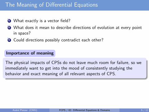
The Meaning of Differential Equations
1 What exactly is a vector field?
2 What does it mean to describe directions of evolution at every pointin space?
3 Could directions possibly contradict each other?
Importance of meaning
The physical impacts of CPSs do not leave much room for failure, so weimmediately want to get into the mood of consistently studying thebehavior and exact meaning of all relevant aspects of CPS.
Andre Platzer (CMU) FCPS / 02: Differential Equations & Domains 5 / 12
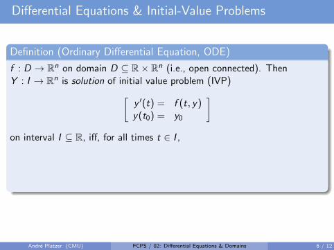
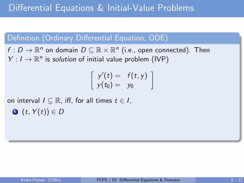
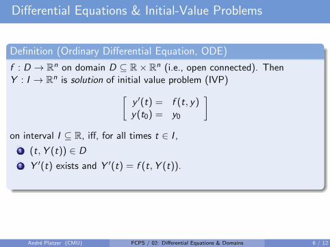
Differential Equations & Initial-Value Problems
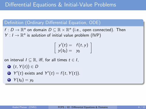
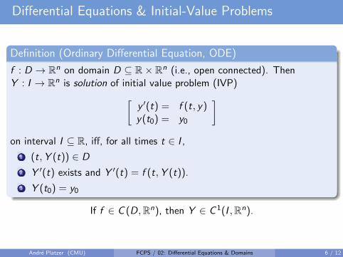
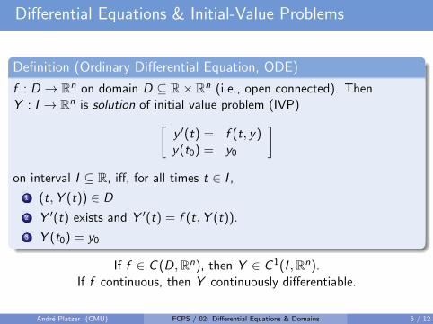
Definition (Ordinary Differential Equation, ODE)
f : D → Rn on domain D ⊆ R× Rn (i.e., open connected). ThenY : I → Rn is solution of initial value problem (IVP)
[y ′(t) = f (t, y)y(t0) = y0
]
on interval I ⊆ R, iff, for all times t ∈ I ,
1 (t,Y (t)) ∈ D
2 Y ′(t) exists and Y ′(t) = f (t,Y (t)).
3 Y (t0) = y0
If f ∈ C (D,Rn), then Y ∈ C 1(I ,Rn).If f continuous, then Y continuously differentiable.
Andre Platzer (CMU) FCPS / 02: Differential Equations & Domains 6 / 12
Differential Equations & Initial-Value Problems
Definition (Ordinary Differential Equation, ODE)
f : D → Rn on domain D ⊆ R× Rn (i.e., open connected). ThenY : I → Rn is solution of initial value problem (IVP)
[y ′(t) = f (t, y)y(t0) = y0
]
on interval I ⊆ R, iff, for all times t ∈ I ,
1 (t,Y (t)) ∈ D
2 Y ′(t) exists and Y ′(t) = f (t,Y (t)).
3 Y (t0) = y0
If f ∈ C (D,Rn), then Y ∈ C 1(I ,Rn).
If f continuous, then Y continuously differentiable.
Andre Platzer (CMU) FCPS / 02: Differential Equations & Domains 6 / 12
Differential Equations & Initial-Value Problems
Definition (Ordinary Differential Equation, ODE)
f : D → Rn on domain D ⊆ R× Rn (i.e., open connected). ThenY : I → Rn is solution of initial value problem (IVP)
[y ′(t) = f (t, y)y(t0) = y0
]
on interval I ⊆ R, iff, for all times t ∈ I ,
1 (t,Y (t)) ∈ D
2 Y ′(t) exists and Y ′(t) = f (t,Y (t)).
3 Y (t0) = y0
If f ∈ C (D,Rn), then Y ∈ C 1(I ,Rn).If f continuous, then Y continuously differentiable.
Andre Platzer (CMU) FCPS / 02: Differential Equations & Domains 6 / 12
Outline
1 Introduction
2 Differential Equations
3 Examples of Differential Equations
4 Domains of Differential Equations
Andre Platzer (CMU) FCPS / 02: Differential Equations & Domains 6 / 12
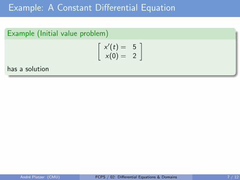
Example: A Constant Differential Equation
Example (Initial value problem)[x ′(t) = 5x(0) = 2
]
has a solution
x(t) = 5t + 2
Check by inserting solution into ODE+IVP.[
(x(t))′ = (5t + 2)′ = 5x(0) = 5 · 0 + 2 = 2
]
Andre Platzer (CMU) FCPS / 02: Differential Equations & Domains 7 / 12
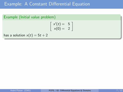
Example: A Constant Differential Equation
Example (Initial value problem)[x ′(t) = 5x(0) = 2
]
has a solution x(t) = 5t + 2
Check by inserting solution into ODE+IVP.[
(x(t))′ = (5t + 2)′ = 5x(0) = 5 · 0 + 2 = 2
]
Andre Platzer (CMU) FCPS / 02: Differential Equations & Domains 7 / 12
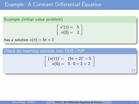
Example: A Constant Differential Equation
Example (Initial value problem)[x ′(t) = 5x(0) = 2
]
has a solution x(t) = 5t + 2
Check by inserting solution into ODE+IVP.[
(x(t))′ = (5t + 2)′ = 5x(0) = 5 · 0 + 2 = 2
]
Andre Platzer (CMU) FCPS / 02: Differential Equations & Domains 7 / 12
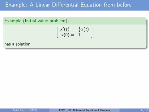
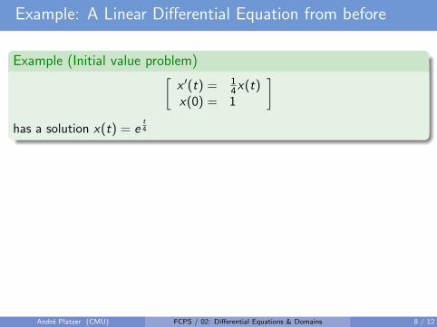
Example: A Linear Differential Equation from before
Example (Initial value problem)[x ′(t) = 1
4x(t)x(0) = 1
]
has a solution
x(t) = et4
Check by inserting solution into ODE+IVP.[
(x(t))′ = (et4 )′ = e
t4 ( t
4 )′ = et4
14 = 1
4x(t)
x(0) = e04 = 1
]
Andre Platzer (CMU) FCPS / 02: Differential Equations & Domains 8 / 12
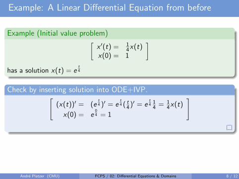
Example: A Linear Differential Equation from before
Example (Initial value problem)[x ′(t) = 1
4x(t)x(0) = 1
]
has a solution x(t) = et4
Check by inserting solution into ODE+IVP.[
(x(t))′ = (et4 )′ = e
t4 ( t
4 )′ = et4
14 = 1
4x(t)
x(0) = e04 = 1
]
Andre Platzer (CMU) FCPS / 02: Differential Equations & Domains 8 / 12
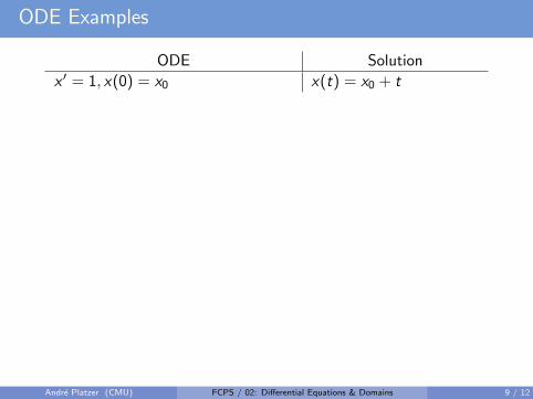
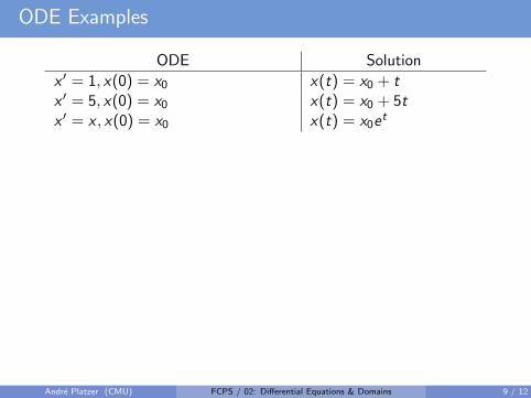
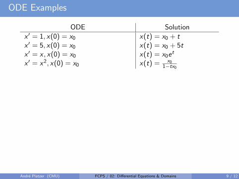
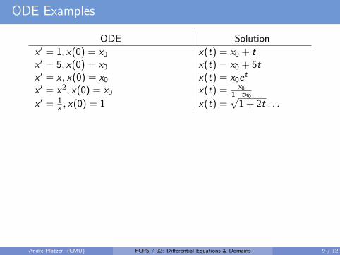
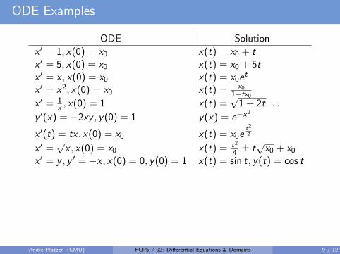
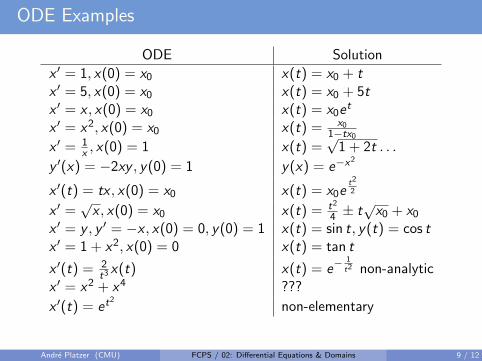
ODE Examples
Solutions more complicated than ODE
ODE Solution
x ′ = 1, x(0) = x0 x(t) = x0 + t
x ′ = 5, x(0) = x0 x(t) = x0 + 5tx ′ = x , x(0) = x0 x(t) = x0e
t
x ′ = x2, x(0) = x0 x(t) = x01−tx0
x ′ = 1x , x(0) = 1 x(t) =
√1 + 2t . . .
y ′(x) = −2xy , y(0) = 1 y(x) = e−x2
x ′(t) = tx , x(0) = x0 x(t) = x0et2
2
x ′ =√x , x(0) = x0 x(t) = t2
4 ± t√x0 + x0
x ′ = y , y ′ = −x , x(0) = 0, y(0) = 1 x(t) = sin t, y(t) = cos tx ′ = 1 + x2, x(0) = 0 x(t) = tan t
x ′(t) = 2t3 x(t) x(t) = e−
1t2 non-analytic
x ′ = x2 + x4 ???
x ′(t) = et2
non-elementary
Andre Platzer (CMU) FCPS / 02: Differential Equations & Domains 9 / 12
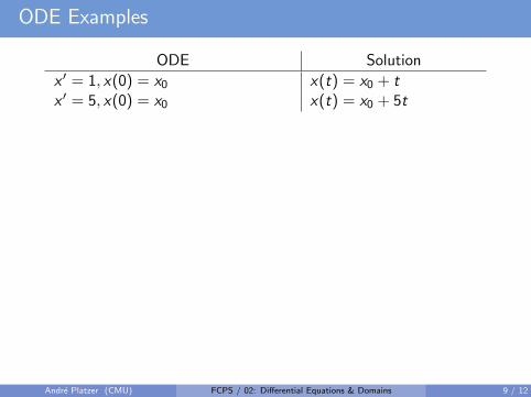
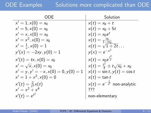
ODE Examples
Solutions more complicated than ODE
ODE Solution
x ′ = 1, x(0) = x0 x(t) = x0 + tx ′ = 5, x(0) = x0 x(t) = x0 + 5t
x ′ = x , x(0) = x0 x(t) = x0et
x ′ = x2, x(0) = x0 x(t) = x01−tx0
x ′ = 1x , x(0) = 1 x(t) =
√1 + 2t . . .
y ′(x) = −2xy , y(0) = 1 y(x) = e−x2
x ′(t) = tx , x(0) = x0 x(t) = x0et2
2
x ′ =√x , x(0) = x0 x(t) = t2
4 ± t√x0 + x0
x ′ = y , y ′ = −x , x(0) = 0, y(0) = 1 x(t) = sin t, y(t) = cos tx ′ = 1 + x2, x(0) = 0 x(t) = tan t
x ′(t) = 2t3 x(t) x(t) = e−
1t2 non-analytic
x ′ = x2 + x4 ???
x ′(t) = et2
non-elementary
Andre Platzer (CMU) FCPS / 02: Differential Equations & Domains 9 / 12
ODE Examples
Solutions more complicated than ODE
ODE Solution
x ′ = 1, x(0) = x0 x(t) = x0 + tx ′ = 5, x(0) = x0 x(t) = x0 + 5tx ′ = x , x(0) = x0 x(t) = x0e
t
x ′ = x2, x(0) = x0 x(t) = x01−tx0
x ′ = 1x , x(0) = 1 x(t) =
√1 + 2t . . .
y ′(x) = −2xy , y(0) = 1 y(x) = e−x2
x ′(t) = tx , x(0) = x0 x(t) = x0et2
2
x ′ =√x , x(0) = x0 x(t) = t2
4 ± t√x0 + x0
x ′ = y , y ′ = −x , x(0) = 0, y(0) = 1 x(t) = sin t, y(t) = cos tx ′ = 1 + x2, x(0) = 0 x(t) = tan t
x ′(t) = 2t3 x(t) x(t) = e−
1t2 non-analytic
x ′ = x2 + x4 ???
x ′(t) = et2
non-elementary
Andre Platzer (CMU) FCPS / 02: Differential Equations & Domains 9 / 12
ODE Examples
Solutions more complicated than ODE
ODE Solution
x ′ = 1, x(0) = x0 x(t) = x0 + tx ′ = 5, x(0) = x0 x(t) = x0 + 5tx ′ = x , x(0) = x0 x(t) = x0e
t
x ′ = x2, x(0) = x0 x(t) = x01−tx0
x ′ = 1x , x(0) = 1 x(t) =
√1 + 2t . . .
y ′(x) = −2xy , y(0) = 1 y(x) = e−x2
x ′(t) = tx , x(0) = x0 x(t) = x0et2
2
x ′ =√x , x(0) = x0 x(t) = t2
4 ± t√x0 + x0
x ′ = y , y ′ = −x , x(0) = 0, y(0) = 1 x(t) = sin t, y(t) = cos t
x ′ = 1 + x2, x(0) = 0 x(t) = tan t
x ′(t) = 2t3 x(t) x(t) = e−
1t2 non-analytic
x ′ = x2 + x4 ???
x ′(t) = et2
non-elementary
Andre Platzer (CMU) FCPS / 02: Differential Equations & Domains 9 / 12
ODE Examples
Solutions more complicated than ODE
ODE Solution
x ′ = 1, x(0) = x0 x(t) = x0 + tx ′ = 5, x(0) = x0 x(t) = x0 + 5tx ′ = x , x(0) = x0 x(t) = x0e
t
x ′ = x2, x(0) = x0 x(t) = x01−tx0
x ′ = 1x , x(0) = 1 x(t) =
√1 + 2t . . .
y ′(x) = −2xy , y(0) = 1 y(x) = e−x2
x ′(t) = tx , x(0) = x0 x(t) = x0et2
2
x ′ =√x , x(0) = x0 x(t) = t2
4 ± t√x0 + x0
x ′ = y , y ′ = −x , x(0) = 0, y(0) = 1 x(t) = sin t, y(t) = cos tx ′ = 1 + x2, x(0) = 0 x(t) = tan t
x ′(t) = 2t3 x(t) x(t) = e−
1t2 non-analytic
x ′ = x2 + x4 ???
x ′(t) = et2
non-elementary
Andre Platzer (CMU) FCPS / 02: Differential Equations & Domains 9 / 12
ODE Examples Solutions more complicated than ODE
ODE Solution
x ′ = 1, x(0) = x0 x(t) = x0 + tx ′ = 5, x(0) = x0 x(t) = x0 + 5tx ′ = x , x(0) = x0 x(t) = x0e
t
x ′ = x2, x(0) = x0 x(t) = x01−tx0
x ′ = 1x , x(0) = 1 x(t) =
√1 + 2t . . .
y ′(x) = −2xy , y(0) = 1 y(x) = e−x2
x ′(t) = tx , x(0) = x0 x(t) = x0et2
2
x ′ =√x , x(0) = x0 x(t) = t2
4 ± t√x0 + x0
x ′ = y , y ′ = −x , x(0) = 0, y(0) = 1 x(t) = sin t, y(t) = cos tx ′ = 1 + x2, x(0) = 0 x(t) = tan t
x ′(t) = 2t3 x(t) x(t) = e−
1t2 non-analytic
x ′ = x2 + x4 ???
x ′(t) = et2
non-elementary
Andre Platzer (CMU) FCPS / 02: Differential Equations & Domains 9 / 12
Takeaway Message
Descriptive power of differential equations
1 Solutions of differential equations can be much more involved thanthe differential equations themselves.
2 Representational and descriptive power of differential equations!
3 Simple differential equations can describe quite complicated physicalprocesses.
4 Local description as the direction into which the system evolves.
Andre Platzer (CMU) FCPS / 02: Differential Equations & Domains 10 / 12
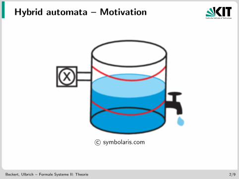
Hybrid automata – Motivation
c© symbolaris.com
Beckert, Ulbrich – Formale Systeme II: Theorie 2/9
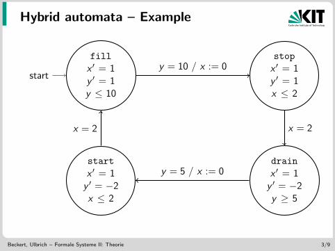
Hybrid automata – Example
fill
x ′ = 1y ′ = 1y ≤ 10
start
stop
x ′ = 1y ′ = 1x ≤ 2
drain
x ′ = 1y ′ = −2y ≥ 5
start
x ′ = 1y ′ = −2x ≤ 2
y = 10 / x := 0
x = 2
y = 5 / x := 0
x = 2
Beckert, Ulbrich – Formale Systeme II: Theorie 3/9
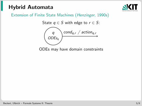
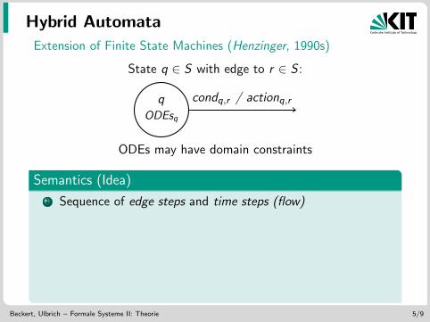
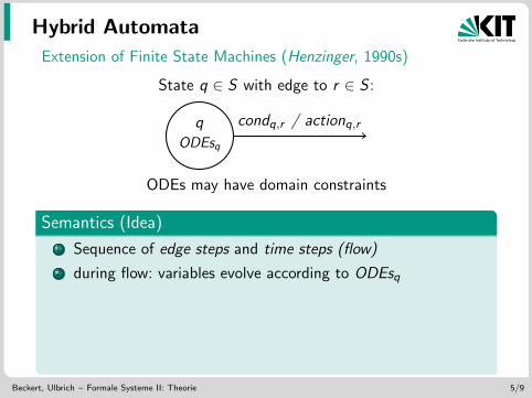
Hybrid Automata
Extension of Finite State Machines (Henzinger, 1990s)
State q ∈ S with edge to r ∈ S :
qODEsq
condq,r / actionq,r
ODEs may have domain constraints
Semantics (Idea)
1 Sequence of edge steps and time steps (flow)
2 during flow: variables evolve according to ODEsq3 discrete state changes at ti from qi to qi+1:
condqi must hold, actionqi ,qi+1 is performed
4 edge: condition condq,r satisfied, actionq,r performeddiscretely, new state is r
Beckert, Ulbrich – Formale Systeme II: Theorie 5/9
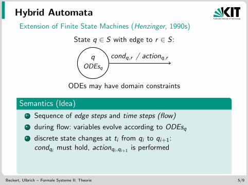
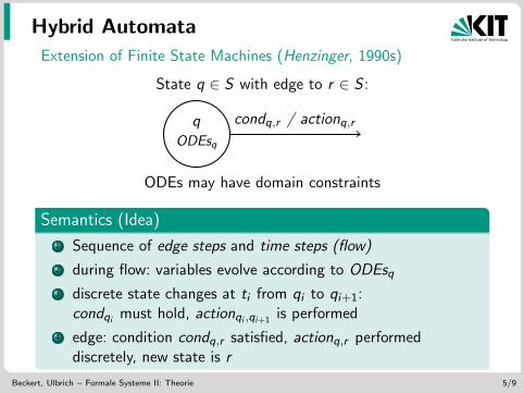
Hybrid Automata
Extension of Finite State Machines (Henzinger, 1990s)
State q ∈ S with edge to r ∈ S :
qODEsq
condq,r / actionq,r
ODEs may have domain constraints
Semantics (Idea)
1 Sequence of edge steps and time steps (flow)
2 during flow: variables evolve according to ODEsq
3 discrete state changes at ti from qi to qi+1:condqi must hold, actionqi ,qi+1 is performed
4 edge: condition condq,r satisfied, actionq,r performeddiscretely, new state is r
Beckert, Ulbrich – Formale Systeme II: Theorie 5/9
Hybrid Automata
Extension of Finite State Machines (Henzinger, 1990s)
State q ∈ S with edge to r ∈ S :
qODEsq
condq,r / actionq,r
ODEs may have domain constraints
Semantics (Idea)
1 Sequence of edge steps and time steps (flow)
2 during flow: variables evolve according to ODEsq3 discrete state changes at ti from qi to qi+1:
condqi must hold, actionqi ,qi+1 is performed
4 edge: condition condq,r satisfied, actionq,r performeddiscretely, new state is r
Beckert, Ulbrich – Formale Systeme II: Theorie 5/9
Hybrid Automata
Extension of Finite State Machines (Henzinger, 1990s)
State q ∈ S with edge to r ∈ S :
qODEsq
condq,r / actionq,r
ODEs may have domain constraints
Semantics (Idea)
1 Sequence of edge steps and time steps (flow)
2 during flow: variables evolve according to ODEsq3 discrete state changes at ti from qi to qi+1:
condqi must hold, actionqi ,qi+1 is performed
4 edge: condition condq,r satisfied, actionq,r performeddiscretely, new state is r
Beckert, Ulbrich – Formale Systeme II: Theorie 5/9
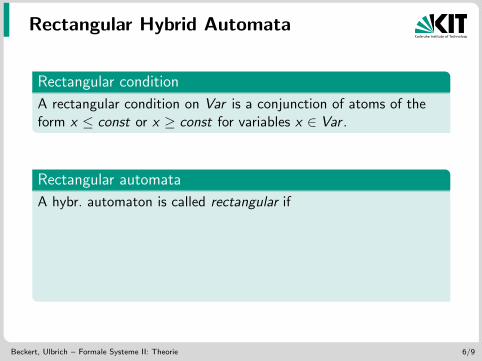
Rectangular Hybrid Automata
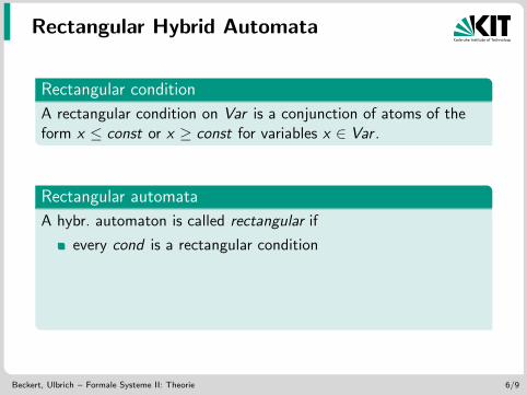
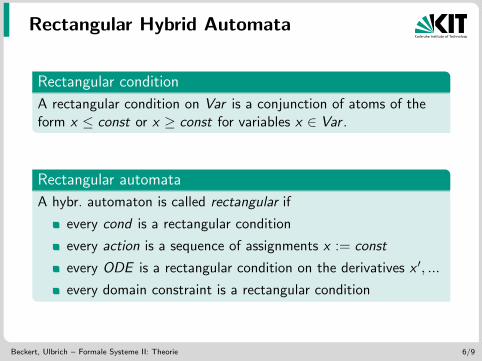
Rectangular condition
A rectangular condition on Var is a conjunction of atoms of theform x ≤ const or x ≥ const for variables x ∈ Var .
Rectangular automata
A hybr. automaton is called rectangular if
every cond is a rectangular condition
every action is a sequence of assignments x := const
every ODE is a rectangular condition on the derivatives x ′, ...
every domain constraint is a rectangular condition
Beckert, Ulbrich – Formale Systeme II: Theorie 6/9
Rectangular Hybrid Automata
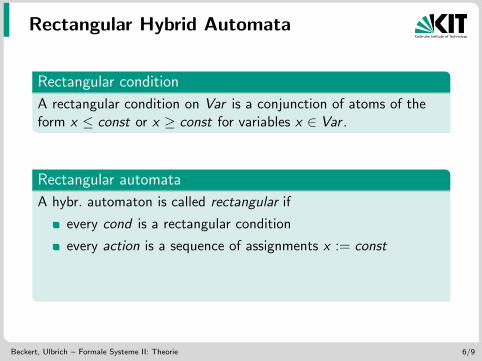
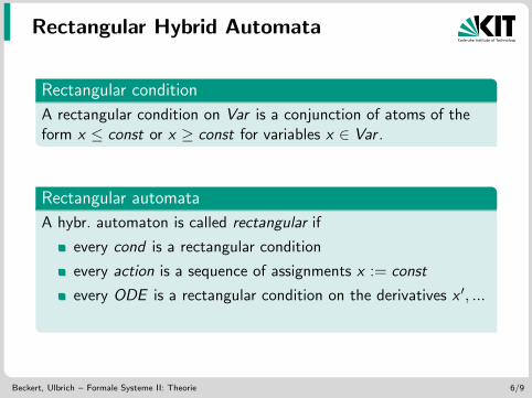
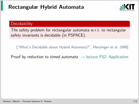
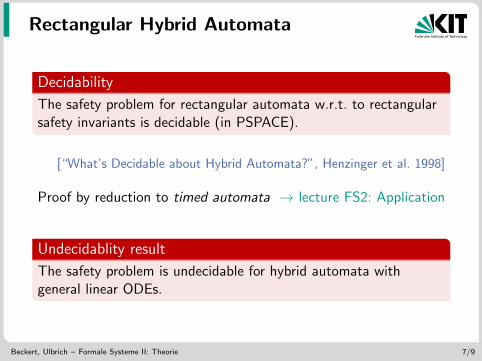
Decidability
The safety problem for rectangular automata w.r.t. to rectangularsafety invariants is decidable (in PSPACE).
[“What’s Decidable about Hybrid Automata?”, Henzinger et al. 1998]
Proof by reduction to timed automata → lecture FS2: Application
Undecidablity result
The safety problem is undecidable for hybrid automata withgeneral linear ODEs.
Beckert, Ulbrich – Formale Systeme II: Theorie 7/9
Rectangular Hybrid Automata
Decidability
The safety problem for rectangular automata w.r.t. to rectangularsafety invariants is decidable (in PSPACE).
[“What’s Decidable about Hybrid Automata?”, Henzinger et al. 1998]
Proof by reduction to timed automata → lecture FS2: Application
Undecidablity result
The safety problem is undecidable for hybrid automata withgeneral linear ODEs.
Beckert, Ulbrich – Formale Systeme II: Theorie 7/9
Differential Dynamic Logic
Beckert, Ulbrich – Formale Systeme II: Theorie 16/17
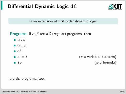
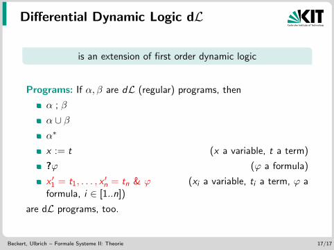
Differential Dynamic Logic dL
is an extension of first order dynamic logic
Programs: If α, β are dL (regular) programs, then
α ; β
α ∪ βα∗
x := t (x a variable, t a term)
?ϕ (ϕ a formula)
x ′1 = t1, . . . , x′n = tn & ϕ (xi a variable, ti a term, ϕ a
formula, i ∈ [1..n])
are dL programs, too.
Beckert, Ulbrich – Formale Systeme II: Theorie 17/17
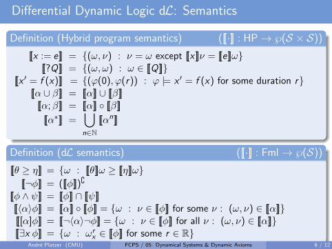
Differential Dynamic Logic dL: Semantics
Definition (Hybrid program semantics) ([[·]] : HP→ ℘(S × S))
[[x := e]] = {(ω, ν) : ν = ω except [[x ]]ν = [[e]]ω}[[?Q]] = {(ω, ω) : ω ∈ [[Q]]}
[[x ′ = f (x)]] = {(ϕ(0), ϕ(r)) : ϕ |= x ′ = f (x) for some duration r}[[α ∪ β]] = [[α]] ∪ [[β]]
[[α;β]] = [[α]] ◦ [[β]]
[[α∗]] =⋃
n∈N[[αn]]
Definition (dL semantics) ([[·]] : Fml→ ℘(S))
[[θ ≥ η]] = {ω : [[θ]]ω ≥ [[η]]ω}[[¬φ]] = ([[φ]]){
[[φ ∧ ψ]] = [[φ]] ∩ [[ψ]][[〈α〉φ]] = [[α]] ◦ [[φ]] = {ω : ν ∈ [[φ]] for some ν : (ω, ν) ∈ [[α]]}[[[α]φ]] = [[¬〈α〉¬φ]] = {ω : ν ∈ [[φ]] for all ν : (ω, ν) ∈ [[α]]}[[∃x φ]] = {ω : ωr
x ∈ [[φ]] for some r ∈ R}Andre Platzer (CMU) FCPS / 05: Dynamical Systems & Dynamic Axioms 6 / 12
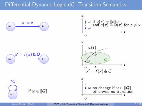
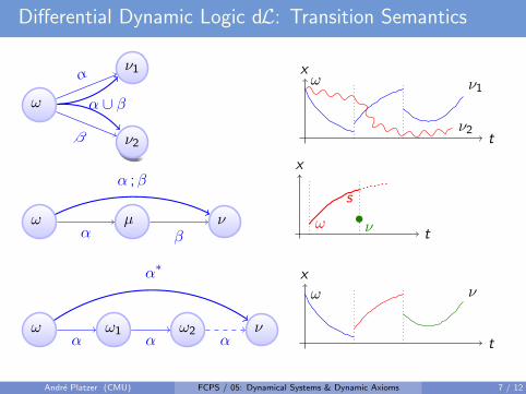
Differential Dynamic Logic dL: Transition Semantics
ω νx := e
t
x
0
ω
ν if ν(x) = [[e]]ωand ν(z) = ω(z) for z 6= x
ω νx ′ = f (x) &Q
t
x
Qν
ω
ϕ(t)
0 rx ′ = f (x) &Q
ω
?Q
if ω ∈ [[Q]]t
x
0
ω no change if ω ∈ [[Q]]otherwise no transition
Andre Platzer (CMU) FCPS / 05: Dynamical Systems & Dynamic Axioms 7 / 12
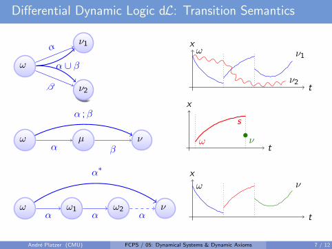
Differential Dynamic Logic dL: Transition Semantics
ω
ν1
ν2
α
β
α ∪ β
t
xω ν1
ν2
ω µ ν
α ;β
α β t
x
s
ω ν
ω ω1 ω2 ν
α∗
α α α
α β α β α β
t
xω ν
Andre Platzer (CMU) FCPS / 05: Dynamical Systems & Dynamic Axioms 7 / 12
Differential Dynamic Logic dL: Transition Semantics
ω
ν1
ν2
α
β
α ∪ β
t
xω ν1
ν2
ω µ ν
α ;β
α β t
x
s
ω ν
ω ω1 ω2 ν
α∗
α α α
α β α β α β
t
xω ν
Andre Platzer (CMU) FCPS / 05: Dynamical Systems & Dynamic Axioms 7 / 12
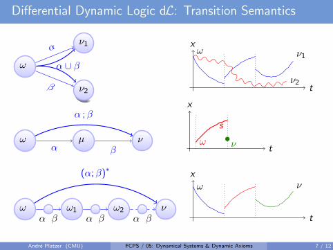
Differential Dynamic Logic dL: Transition Semantics
ω
ν1
ν2
α
β
α ∪ β
t
xω ν1
ν2
ω µ ν
α ;β
α β t
x
s
ω ν
ω ω1 ω2 ν
(α;β)∗
α β α β α β t
xω ν
Andre Platzer (CMU) FCPS / 05: Dynamical Systems & Dynamic Axioms 7 / 12
04: Safety & Contracts15-424: Foundations of Cyber-Physical Systems
Andre Platzer
Computer Science DepartmentCarnegie Mellon University, Pittsburgh, PA
0.20.4
0.60.8
1.00.1
0.2
0.3
0.4
0.5
Andre Platzer (CMU) FCPS / 04: Safety & Contracts 1 / 7
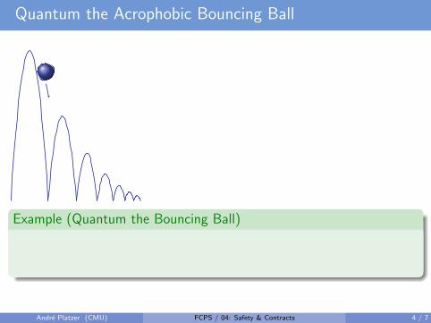
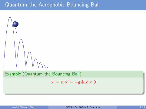
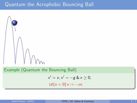
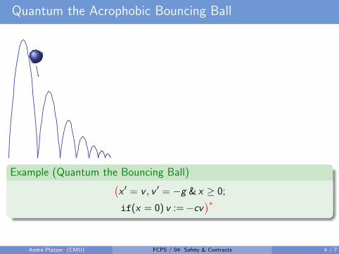
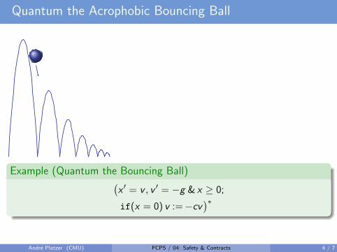
Quantum the Acrophobic Bouncing Ball
Example (Quantum the Bouncing Ball)
(x ′ = v , v ′ = −g & x ≥ 0;
if(x = 0) v :=−cv)∗
Andre Platzer (CMU) FCPS / 04: Safety & Contracts 4 / 7
Quantum the Acrophobic Bouncing Ball
Example (Quantum the Bouncing Ball)
(
x ′ = v , v ′ = −g & x ≥ 0
;
if(x = 0) v :=−cv)∗
Andre Platzer (CMU) FCPS / 04: Safety & Contracts 4 / 7
Quantum the Acrophobic Bouncing Ball
Example (Quantum the Bouncing Ball)
(
x ′ = v , v ′ = −g & x ≥ 0;
if(x = 0) v :=−cv
)∗
Andre Platzer (CMU) FCPS / 04: Safety & Contracts 4 / 7
Quantum the Acrophobic Bouncing Ball
Example (Quantum the Bouncing Ball)(x ′ = v , v ′ = −g & x ≥ 0;
if(x = 0) v :=−cv)∗
Andre Platzer (CMU) FCPS / 04: Safety & Contracts 4 / 7
Quantum the Acrophobic Bouncing Ball
Example (Quantum the Bouncing Ball)(x ′ = v , v ′ = −g & x ≥ 0;
if(x = 0) v :=−cv)∗
Andre Platzer (CMU) FCPS / 04: Safety & Contracts 4 / 7
Conjecture: Quantum the Acrophobic Bouncing Ball
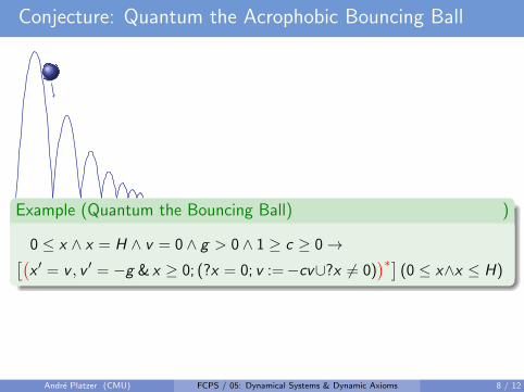
Example (Quantum the Bouncing Ball) )
0 ≤ x ∧ x = H ∧ v = 0 ∧ g > 0 ∧ 1 ≥ c ≥ 0→[(x ′ = v , v ′ = −g & x ≥ 0; (?x = 0; v :=−cv∪?x 6= 0)
)∗](0 ≤ x∧x ≤ H)
Removing the repetition grotesquely changes the behavior to a single hop
Andre Platzer (CMU) FCPS / 05: Dynamical Systems & Dynamic Axioms 8 / 12
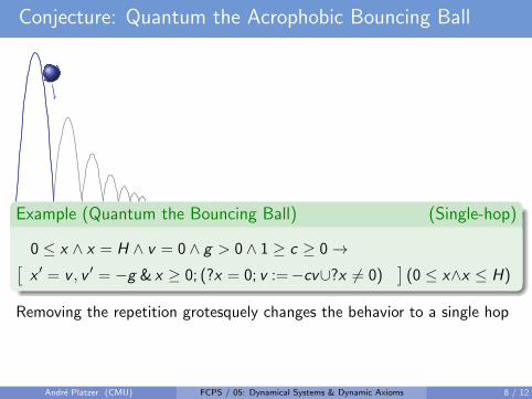
Conjecture: Quantum the Acrophobic Bouncing Ball
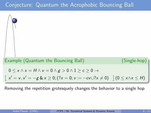
Example (Quantum the Bouncing Ball) (Single-hop)
0 ≤ x ∧ x = H ∧ v = 0 ∧ g > 0 ∧ 1 ≥ c ≥ 0→[
(
x ′ = v , v ′ = −g & x ≥ 0; (?x = 0; v :=−cv∪?x 6= 0)
)∗
](0 ≤ x∧x ≤ H)
Removing the repetition grotesquely changes the behavior to a single hop
Andre Platzer (CMU) FCPS / 05: Dynamical Systems & Dynamic Axioms 8 / 12

Conjecture: Quantum the Acrophobic Bouncing Ball
Example (Quantum the Bouncing Ball) (Single-hop)
0 ≤ x ∧ x = H ∧ v = 0 ∧ g > 0 ∧ 1 ≥ c ≥ 0→[
(
x ′ = v , v ′ = −g & x ≥ 0; (?x = 0; v :=−cv∪?x 6= 0)
)∗
](0 ≤ x∧x ≤ H)
Removing the repetition grotesquely changes the behavior to a single hop
Andre Platzer (CMU) FCPS / 05: Dynamical Systems & Dynamic Axioms 8 / 12
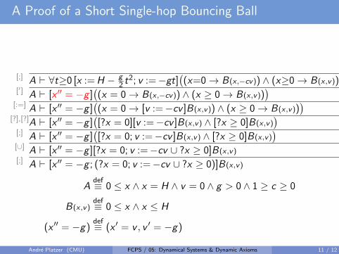
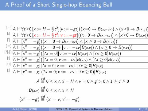
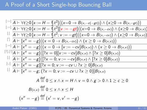
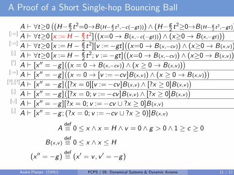
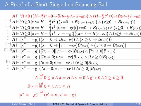
A Proof of a Short Single-hop Bouncing Ball
A ` ∀t≥0((H−g
2 t2=0→B(H− g
2t2,−c(−gt))) ∧ (H−g
2 t2≥0→B(H− g
2t2,−gt))
)
[:=] A ` ∀t≥0 [x := H − g2 t
2]((x=0→ B(x ,−c(−gt))) ∧ (x≥0→ B(x ,−gt))
)
[:=] A ` ∀t≥0 [x := H − g2 t
2][v :=−gt]((x=0→ B(x ,−cv)) ∧ (x≥0→ B(x ,v))
)
[;] A ` ∀t≥0 [x := H − g2 t
2; v :=−gt]((x=0→ B(x ,−cv)) ∧ (x≥0→ B(x ,v))
)
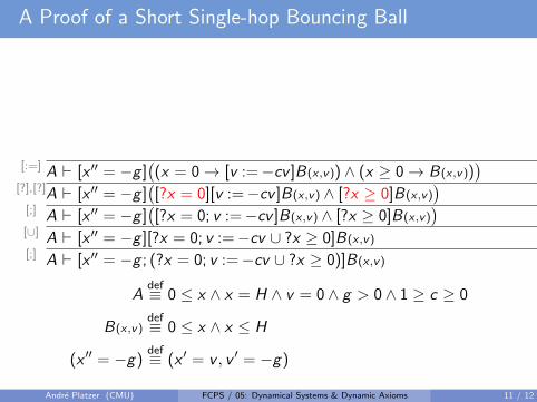
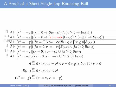
[′] A ` [x ′′ = −g ]((x = 0→ B(x ,−cv)) ∧ (x ≥ 0→ B(x ,v))
)
[:=] A ` [x ′′ = −g ]((x = 0→ [v :=−cv ]B(x ,v)) ∧ (x ≥ 0→ B(x ,v))
)
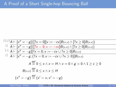
[?],[?]A ` [x ′′ = −g ]([?x = 0][v :=−cv ]B(x ,v) ∧ [?x ≥ 0]B(x ,v)
)
[;] A ` [x ′′ = −g ]([?x = 0; v :=−cv ]B(x ,v) ∧ [?x ≥ 0]B(x ,v)
)
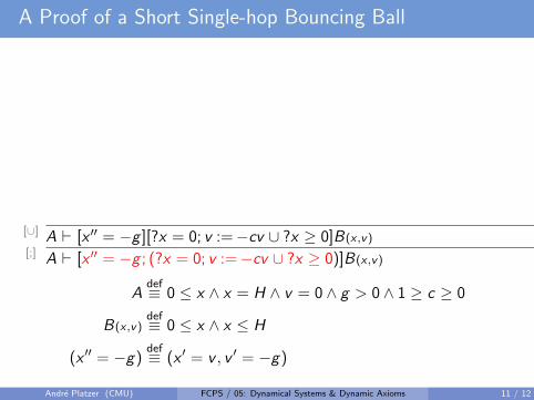
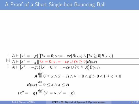
[∪] A ` [x ′′ = −g ][?x = 0; v :=−cv ∪ ?x ≥ 0]B(x ,v)
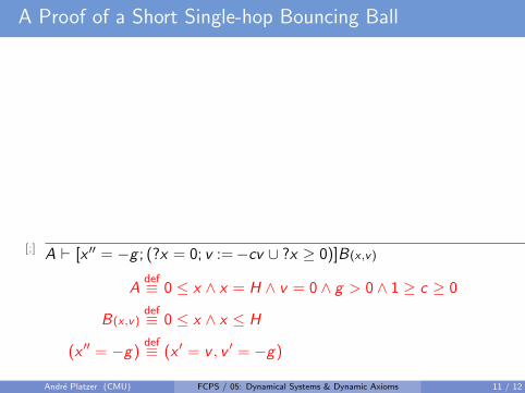
[;] A ` [x ′′ = −g ; (?x = 0; v :=−cv ∪ ?x ≥ 0)]B(x ,v)
Adef≡ 0 ≤ x ∧ x = H ∧ v = 0 ∧ g > 0 ∧ 1 ≥ c ≥ 0
B(x ,v)def≡ 0 ≤ x ∧ x ≤ H
(x ′′ = −g)def≡ (x ′ = v , v ′ = −g)
Andre Platzer (CMU) FCPS / 05: Dynamical Systems & Dynamic Axioms 11 / 12
A Proof of a Short Single-hop Bouncing Ball
A ` ∀t≥0((H−g
2 t2=0→B(H− g
2t2,−c(−gt))) ∧ (H−g
2 t2≥0→B(H− g
2t2,−gt))
)
[:=] A ` ∀t≥0 [x := H − g2 t
2]((x=0→ B(x ,−c(−gt))) ∧ (x≥0→ B(x ,−gt))
)
[:=] A ` ∀t≥0 [x := H − g2 t
2][v :=−gt]((x=0→ B(x ,−cv)) ∧ (x≥0→ B(x ,v))
)
[;] A ` ∀t≥0 [x := H − g2 t
2; v :=−gt]((x=0→ B(x ,−cv)) ∧ (x≥0→ B(x ,v))
)
[′] A ` [x ′′ = −g ]((x = 0→ B(x ,−cv)) ∧ (x ≥ 0→ B(x ,v))
)
[:=] A ` [x ′′ = −g ]((x = 0→ [v :=−cv ]B(x ,v)) ∧ (x ≥ 0→ B(x ,v))
)
[?],[?]A ` [x ′′ = −g ]([?x = 0][v :=−cv ]B(x ,v) ∧ [?x ≥ 0]B(x ,v)
)
[;] A ` [x ′′ = −g ]([?x = 0; v :=−cv ]B(x ,v) ∧ [?x ≥ 0]B(x ,v)
)
[∪] A ` [x ′′ = −g ][?x = 0; v :=−cv ∪ ?x ≥ 0]B(x ,v)[;] A ` [x ′′ = −g ; (?x = 0; v :=−cv ∪ ?x ≥ 0)]B(x ,v)
Adef≡ 0 ≤ x ∧ x = H ∧ v = 0 ∧ g > 0 ∧ 1 ≥ c ≥ 0
B(x ,v)def≡ 0 ≤ x ∧ x ≤ H
(x ′′ = −g)def≡ (x ′ = v , v ′ = −g)
Andre Platzer (CMU) FCPS / 05: Dynamical Systems & Dynamic Axioms 11 / 12
A Proof of a Short Single-hop Bouncing Ball
A ` ∀t≥0((H−g
2 t2=0→B(H− g
2t2,−c(−gt))) ∧ (H−g
2 t2≥0→B(H− g
2t2,−gt))
)
[:=] A ` ∀t≥0 [x := H − g2 t
2]((x=0→ B(x ,−c(−gt))) ∧ (x≥0→ B(x ,−gt))
)
[:=] A ` ∀t≥0 [x := H − g2 t
2][v :=−gt]((x=0→ B(x ,−cv)) ∧ (x≥0→ B(x ,v))
)
[;] A ` ∀t≥0 [x := H − g2 t
2; v :=−gt]((x=0→ B(x ,−cv)) ∧ (x≥0→ B(x ,v))
)
[′] A ` [x ′′ = −g ]((x = 0→ B(x ,−cv)) ∧ (x ≥ 0→ B(x ,v))
)
[:=] A ` [x ′′ = −g ]((x = 0→ [v :=−cv ]B(x ,v)) ∧ (x ≥ 0→ B(x ,v))
)
[?],[?]A ` [x ′′ = −g ]([?x = 0][v :=−cv ]B(x ,v) ∧ [?x ≥ 0]B(x ,v)
)
[;] A ` [x ′′ = −g ]([?x = 0; v :=−cv ]B(x ,v) ∧ [?x ≥ 0]B(x ,v)
)[∪] A ` [x ′′ = −g ][?x = 0; v :=−cv ∪ ?x ≥ 0]B(x ,v)[;] A ` [x ′′ = −g ; (?x = 0; v :=−cv ∪ ?x ≥ 0)]B(x ,v)
Adef≡ 0 ≤ x ∧ x = H ∧ v = 0 ∧ g > 0 ∧ 1 ≥ c ≥ 0
B(x ,v)def≡ 0 ≤ x ∧ x ≤ H
(x ′′ = −g)def≡ (x ′ = v , v ′ = −g)
Andre Platzer (CMU) FCPS / 05: Dynamical Systems & Dynamic Axioms 11 / 12
A Proof of a Short Single-hop Bouncing Ball
A ` ∀t≥0((H−g
2 t2=0→B(H− g
2t2,−c(−gt))) ∧ (H−g
2 t2≥0→B(H− g
2t2,−gt))
)
[:=] A ` ∀t≥0 [x := H − g2 t
2]((x=0→ B(x ,−c(−gt))) ∧ (x≥0→ B(x ,−gt))
)
[:=] A ` ∀t≥0 [x := H − g2 t
2][v :=−gt]((x=0→ B(x ,−cv)) ∧ (x≥0→ B(x ,v))
)
[;] A ` ∀t≥0 [x := H − g2 t
2; v :=−gt]((x=0→ B(x ,−cv)) ∧ (x≥0→ B(x ,v))
)
[′] A ` [x ′′ = −g ]((x = 0→ B(x ,−cv)) ∧ (x ≥ 0→ B(x ,v))
)
[:=] A ` [x ′′ = −g ]((x = 0→ [v :=−cv ]B(x ,v)) ∧ (x ≥ 0→ B(x ,v))
)
[?],[?]A ` [x ′′ = −g ]([?x = 0][v :=−cv ]B(x ,v) ∧ [?x ≥ 0]B(x ,v)
)[;] A ` [x ′′ = −g ]
([?x = 0; v :=−cv ]B(x ,v) ∧ [?x ≥ 0]B(x ,v)
)[∪] A ` [x ′′ = −g ][?x = 0; v :=−cv ∪ ?x ≥ 0]B(x ,v)[;] A ` [x ′′ = −g ; (?x = 0; v :=−cv ∪ ?x ≥ 0)]B(x ,v)
Adef≡ 0 ≤ x ∧ x = H ∧ v = 0 ∧ g > 0 ∧ 1 ≥ c ≥ 0
B(x ,v)def≡ 0 ≤ x ∧ x ≤ H
(x ′′ = −g)def≡ (x ′ = v , v ′ = −g)
Andre Platzer (CMU) FCPS / 05: Dynamical Systems & Dynamic Axioms 11 / 12
A Proof of a Short Single-hop Bouncing Ball
A ` ∀t≥0((H−g
2 t2=0→B(H− g
2t2,−c(−gt))) ∧ (H−g
2 t2≥0→B(H− g
2t2,−gt))
)
[:=] A ` ∀t≥0 [x := H − g2 t
2]((x=0→ B(x ,−c(−gt))) ∧ (x≥0→ B(x ,−gt))
)
[:=] A ` ∀t≥0 [x := H − g2 t
2][v :=−gt]((x=0→ B(x ,−cv)) ∧ (x≥0→ B(x ,v))
)
[;] A ` ∀t≥0 [x := H − g2 t
2; v :=−gt]((x=0→ B(x ,−cv)) ∧ (x≥0→ B(x ,v))
)
[′] A ` [x ′′ = −g ]((x = 0→ B(x ,−cv)) ∧ (x ≥ 0→ B(x ,v))
)
[:=] A ` [x ′′ = −g ]((x = 0→ [v :=−cv ]B(x ,v)) ∧ (x ≥ 0→ B(x ,v))
)[?],[?]A ` [x ′′ = −g ]
([?x = 0][v :=−cv ]B(x ,v) ∧ [?x ≥ 0]B(x ,v)
)[;] A ` [x ′′ = −g ]
([?x = 0; v :=−cv ]B(x ,v) ∧ [?x ≥ 0]B(x ,v)
)[∪] A ` [x ′′ = −g ][?x = 0; v :=−cv ∪ ?x ≥ 0]B(x ,v)[;] A ` [x ′′ = −g ; (?x = 0; v :=−cv ∪ ?x ≥ 0)]B(x ,v)
Adef≡ 0 ≤ x ∧ x = H ∧ v = 0 ∧ g > 0 ∧ 1 ≥ c ≥ 0
B(x ,v)def≡ 0 ≤ x ∧ x ≤ H
(x ′′ = −g)def≡ (x ′ = v , v ′ = −g)
Andre Platzer (CMU) FCPS / 05: Dynamical Systems & Dynamic Axioms 11 / 12
A Proof of a Short Single-hop Bouncing Ball
A ` ∀t≥0((H−g
2 t2=0→B(H− g
2t2,−c(−gt))) ∧ (H−g
2 t2≥0→B(H− g
2t2,−gt))
)
[:=] A ` ∀t≥0 [x := H − g2 t
2]((x=0→ B(x ,−c(−gt))) ∧ (x≥0→ B(x ,−gt))
)
[:=] A ` ∀t≥0 [x := H − g2 t
2][v :=−gt]((x=0→ B(x ,−cv)) ∧ (x≥0→ B(x ,v))
)
[;] A ` ∀t≥0 [x := H − g2 t
2; v :=−gt]((x=0→ B(x ,−cv)) ∧ (x≥0→ B(x ,v))
)
[′] A ` [x ′′ = −g ]((x = 0→ B(x ,−cv)) ∧ (x ≥ 0→ B(x ,v))
)[:=] A ` [x ′′ = −g ]
((x = 0→ [v :=−cv ]B(x ,v)) ∧ (x ≥ 0→ B(x ,v))
)[?],[?]A ` [x ′′ = −g ]
([?x = 0][v :=−cv ]B(x ,v) ∧ [?x ≥ 0]B(x ,v)
)[;] A ` [x ′′ = −g ]
([?x = 0; v :=−cv ]B(x ,v) ∧ [?x ≥ 0]B(x ,v)
)[∪] A ` [x ′′ = −g ][?x = 0; v :=−cv ∪ ?x ≥ 0]B(x ,v)[;] A ` [x ′′ = −g ; (?x = 0; v :=−cv ∪ ?x ≥ 0)]B(x ,v)
Adef≡ 0 ≤ x ∧ x = H ∧ v = 0 ∧ g > 0 ∧ 1 ≥ c ≥ 0
B(x ,v)def≡ 0 ≤ x ∧ x ≤ H
(x ′′ = −g)def≡ (x ′ = v , v ′ = −g)
Andre Platzer (CMU) FCPS / 05: Dynamical Systems & Dynamic Axioms 11 / 12
A Proof of a Short Single-hop Bouncing Ball
A ` ∀t≥0((H−g
2 t2=0→B(H− g
2t2,−c(−gt))) ∧ (H−g
2 t2≥0→B(H− g
2t2,−gt))
)
[:=] A ` ∀t≥0 [x := H − g2 t
2]((x=0→ B(x ,−c(−gt))) ∧ (x≥0→ B(x ,−gt))
)
[:=] A ` ∀t≥0 [x := H − g2 t
2][v :=−gt]((x=0→ B(x ,−cv)) ∧ (x≥0→ B(x ,v))
)
[;] A ` ∀t≥0 [x := H − g2 t
2; v :=−gt]((x=0→ B(x ,−cv)) ∧ (x≥0→ B(x ,v))
)[′] A ` [x ′′ = −g ]
((x = 0→ B(x ,−cv)) ∧ (x ≥ 0→ B(x ,v))
)[:=] A ` [x ′′ = −g ]
((x = 0→ [v :=−cv ]B(x ,v)) ∧ (x ≥ 0→ B(x ,v))
)[?],[?]A ` [x ′′ = −g ]
([?x = 0][v :=−cv ]B(x ,v) ∧ [?x ≥ 0]B(x ,v)
)[;] A ` [x ′′ = −g ]
([?x = 0; v :=−cv ]B(x ,v) ∧ [?x ≥ 0]B(x ,v)
)[∪] A ` [x ′′ = −g ][?x = 0; v :=−cv ∪ ?x ≥ 0]B(x ,v)[;] A ` [x ′′ = −g ; (?x = 0; v :=−cv ∪ ?x ≥ 0)]B(x ,v)
Adef≡ 0 ≤ x ∧ x = H ∧ v = 0 ∧ g > 0 ∧ 1 ≥ c ≥ 0
B(x ,v)def≡ 0 ≤ x ∧ x ≤ H
(x ′′ = −g)def≡ (x ′ = v , v ′ = −g)
Andre Platzer (CMU) FCPS / 05: Dynamical Systems & Dynamic Axioms 11 / 12
A Proof of a Short Single-hop Bouncing Ball
A ` ∀t≥0((H−g
2 t2=0→B(H− g
2t2,−c(−gt))) ∧ (H−g
2 t2≥0→B(H− g
2t2,−gt))
)
[:=] A ` ∀t≥0 [x := H − g2 t
2]((x=0→ B(x ,−c(−gt))) ∧ (x≥0→ B(x ,−gt))
)
[:=] A ` ∀t≥0 [x := H − g2 t
2][v :=−gt]((x=0→ B(x ,−cv)) ∧ (x≥0→ B(x ,v))
)[;] A ` ∀t≥0 [x := H − g
2 t2; v :=−gt]
((x=0→ B(x ,−cv)) ∧ (x≥0→ B(x ,v))
)[′] A ` [x ′′ = −g ]
((x = 0→ B(x ,−cv)) ∧ (x ≥ 0→ B(x ,v))
)[:=] A ` [x ′′ = −g ]
((x = 0→ [v :=−cv ]B(x ,v)) ∧ (x ≥ 0→ B(x ,v))
)[?],[?]A ` [x ′′ = −g ]
([?x = 0][v :=−cv ]B(x ,v) ∧ [?x ≥ 0]B(x ,v)
)[;] A ` [x ′′ = −g ]
([?x = 0; v :=−cv ]B(x ,v) ∧ [?x ≥ 0]B(x ,v)
)[∪] A ` [x ′′ = −g ][?x = 0; v :=−cv ∪ ?x ≥ 0]B(x ,v)[;] A ` [x ′′ = −g ; (?x = 0; v :=−cv ∪ ?x ≥ 0)]B(x ,v)
Adef≡ 0 ≤ x ∧ x = H ∧ v = 0 ∧ g > 0 ∧ 1 ≥ c ≥ 0
B(x ,v)def≡ 0 ≤ x ∧ x ≤ H
(x ′′ = −g)def≡ (x ′ = v , v ′ = −g)
Andre Platzer (CMU) FCPS / 05: Dynamical Systems & Dynamic Axioms 11 / 12
A Proof of a Short Single-hop Bouncing Ball
A ` ∀t≥0((H−g
2 t2=0→B(H− g
2t2,−c(−gt))) ∧ (H−g
2 t2≥0→B(H− g
2t2,−gt))
)
[:=] A ` ∀t≥0 [x := H − g2 t
2]((x=0→ B(x ,−c(−gt))) ∧ (x≥0→ B(x ,−gt))
)[:=] A ` ∀t≥0 [x := H − g
2 t2][v :=−gt]
((x=0→ B(x ,−cv)) ∧ (x≥0→ B(x ,v))
)[;] A ` ∀t≥0 [x := H − g
2 t2; v :=−gt]
((x=0→ B(x ,−cv)) ∧ (x≥0→ B(x ,v))
)[′] A ` [x ′′ = −g ]
((x = 0→ B(x ,−cv)) ∧ (x ≥ 0→ B(x ,v))
)[:=] A ` [x ′′ = −g ]
((x = 0→ [v :=−cv ]B(x ,v)) ∧ (x ≥ 0→ B(x ,v))
)[?],[?]A ` [x ′′ = −g ]
([?x = 0][v :=−cv ]B(x ,v) ∧ [?x ≥ 0]B(x ,v)
)[;] A ` [x ′′ = −g ]
([?x = 0; v :=−cv ]B(x ,v) ∧ [?x ≥ 0]B(x ,v)
)[∪] A ` [x ′′ = −g ][?x = 0; v :=−cv ∪ ?x ≥ 0]B(x ,v)[;] A ` [x ′′ = −g ; (?x = 0; v :=−cv ∪ ?x ≥ 0)]B(x ,v)
Adef≡ 0 ≤ x ∧ x = H ∧ v = 0 ∧ g > 0 ∧ 1 ≥ c ≥ 0
B(x ,v)def≡ 0 ≤ x ∧ x ≤ H
(x ′′ = −g)def≡ (x ′ = v , v ′ = −g)
Andre Platzer (CMU) FCPS / 05: Dynamical Systems & Dynamic Axioms 11 / 12
A Proof of a Short Single-hop Bouncing Ball
A ` ∀t≥0((H−g
2 t2=0→B(H− g
2t2,−c(−gt))) ∧ (H−g
2 t2≥0→B(H− g
2t2,−gt))
)[:=] A ` ∀t≥0 [x := H − g
2 t2]((x=0→ B(x ,−c(−gt))) ∧ (x≥0→ B(x ,−gt))
)[:=] A ` ∀t≥0 [x := H − g
2 t2][v :=−gt]
((x=0→ B(x ,−cv)) ∧ (x≥0→ B(x ,v))
)[;] A ` ∀t≥0 [x := H − g
2 t2; v :=−gt]
((x=0→ B(x ,−cv)) ∧ (x≥0→ B(x ,v))
)[′] A ` [x ′′ = −g ]
((x = 0→ B(x ,−cv)) ∧ (x ≥ 0→ B(x ,v))
)[:=] A ` [x ′′ = −g ]
((x = 0→ [v :=−cv ]B(x ,v)) ∧ (x ≥ 0→ B(x ,v))
)[?],[?]A ` [x ′′ = −g ]
([?x = 0][v :=−cv ]B(x ,v) ∧ [?x ≥ 0]B(x ,v)
)[;] A ` [x ′′ = −g ]
([?x = 0; v :=−cv ]B(x ,v) ∧ [?x ≥ 0]B(x ,v)
)[∪] A ` [x ′′ = −g ][?x = 0; v :=−cv ∪ ?x ≥ 0]B(x ,v)[;] A ` [x ′′ = −g ; (?x = 0; v :=−cv ∪ ?x ≥ 0)]B(x ,v)
Adef≡ 0 ≤ x ∧ x = H ∧ v = 0 ∧ g > 0 ∧ 1 ≥ c ≥ 0
B(x ,v)def≡ 0 ≤ x ∧ x ≤ H
(x ′′ = −g)def≡ (x ′ = v , v ′ = −g)
Andre Platzer (CMU) FCPS / 05: Dynamical Systems & Dynamic Axioms 11 / 12
A Proof of a Short Single-hop Bouncing Ball
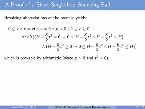
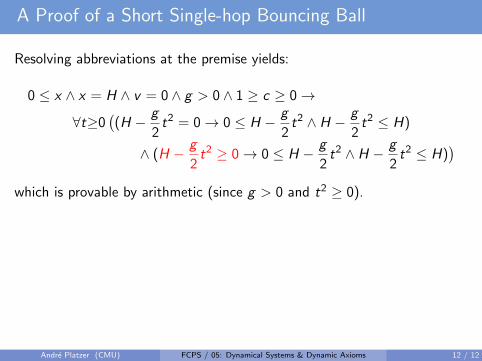
Resolving abbreviations at the premise yields:
0 ≤ x ∧ x = H ∧ v = 0 ∧ g > 0 ∧ 1 ≥ c ≥ 0→∀t≥0
((H − g
2t2 = 0→ 0 ≤ H − g
2t2 ∧ H − g
2t2 ≤ H)
∧ (H − g
2t2 ≥ 0→ 0 ≤ H − g
2t2 ∧ H − g
2t2 ≤ H)
)
which is provable by arithmetic (since g > 0 and t2 ≥ 0).
Exciting!
We have just formally verified our very first CPS!
Okay, alright, it was a grotesquely simplified single-hop bouncing ball.But the axioms of our proof technique were completely general and notspecific to bouncing balls, so they should carry us forward to true CPS.
Andre Platzer (CMU) FCPS / 05: Dynamical Systems & Dynamic Axioms 12 / 12
A Proof of a Short Single-hop Bouncing Ball
Resolving abbreviations at the premise yields:
0 ≤ x ∧ x = H ∧ v = 0 ∧ g > 0 ∧ 1 ≥ c ≥ 0→∀t≥0
((H − g
2t2 = 0→ 0 ≤ H − g
2t2 ∧ H − g
2t2 ≤ H)
∧ (H − g
2t2 ≥ 0→ 0 ≤ H − g
2t2 ∧ H − g
2t2 ≤ H)
)
which is provable by arithmetic (since g > 0 and t2 ≥ 0).
Exciting!
We have just formally verified our very first CPS!
Okay, alright, it was a grotesquely simplified single-hop bouncing ball.But the axioms of our proof technique were completely general and notspecific to bouncing balls, so they should carry us forward to true CPS.
Andre Platzer (CMU) FCPS / 05: Dynamical Systems & Dynamic Axioms 12 / 12
Conjecture: Quantum the Acrophobic Bouncing Ball
Example (Quantum the Bouncing Ball) (Single-hop)
0 ≤ x ∧ x = H ∧ v = 0 ∧ g > 0 ∧ 1 ≥ c ≥ 0→[
(
x ′ = v , v ′ = −g & x ≥ 0; (?x = 0; v :=−cv∪?x 6= 0)
)∗
](0 ≤ x∧x ≤ H)
Removing the repetition grotesquely changes the behavior to a single hop
Andre Platzer (CMU) FCPS / 05: Dynamical Systems & Dynamic Axioms 8 / 12
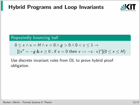
Hybrid Programs and Loop Invariants
Repeatedly bouncing ball
0 ≤ x ∧ x = H ∧ v = 0 ∧ g > 0 ∧ 0 < c ≤ 1→[(x ′′ = −g & x ≥ 0 ; if x = 0 then v := −c · v)∗](0 ≤ x ≤ H)
Use discrete invariant rules from DL to prove hybrid proofobligation.
Beckert, Ulbrich – Formale Systeme II: Theorie 12/17
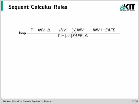
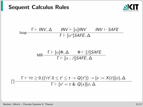
Sequent Calculus Rules
loopΓ ` INV ,∆ INV ` [α]INV INV ` SAFE
Γ ` [α∗]SAFE ,∆
MRΓ ` [α]Φ,∆ Φ ` [β]SAFE
Γ ` [α ; β]SAFE ,∆
[’]Γ ` ∀t ≥ 0.([x := X (t)]φ),∆
Γ ` [x ′ = t & Q(x)]φ,∆
Beckert, Ulbrich – Formale Systeme II: Theorie 13/17
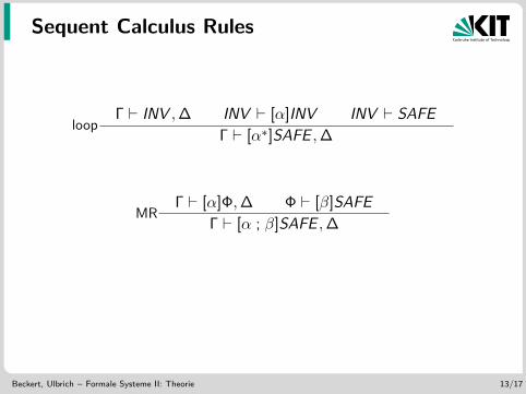
Sequent Calculus Rules
loopΓ ` INV ,∆ INV ` [α]INV INV ` SAFE
Γ ` [α∗]SAFE ,∆
MRΓ ` [α]Φ,∆ Φ ` [β]SAFE
Γ ` [α ; β]SAFE ,∆
[’]Γ ` ∀t ≥ 0.([x := X (t)]φ),∆
Γ ` [x ′ = t & Q(x)]φ,∆
Beckert, Ulbrich – Formale Systeme II: Theorie 13/17
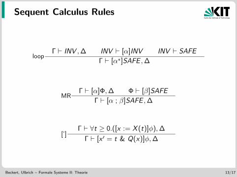
Sequent Calculus Rules
loopΓ ` INV ,∆ INV ` [α]INV INV ` SAFE
Γ ` [α∗]SAFE ,∆
MRΓ ` [α]Φ,∆ Φ ` [β]SAFE
Γ ` [α ; β]SAFE ,∆
[’]Γ ` ∀t ≥ 0.([x := X (t)]φ),∆
Γ ` [x ′ = t & Q(x)]φ,∆
Beckert, Ulbrich – Formale Systeme II: Theorie 13/17
Sequent Calculus Rules
loopΓ ` INV ,∆ INV ` [α]INV INV ` SAFE
Γ ` [α∗]SAFE ,∆
MRΓ ` [α]Φ,∆ Φ ` [β]SAFE
Γ ` [α ; β]SAFE ,∆
[’]Γ ` ∀t ≥ 0.((∀t ′.0 ≤ t ′ ≤ t → Q(t ′))→ [x := X (t)]φ),∆
Γ ` [x ′ = t & Q(x)]φ,∆
Beckert, Ulbrich – Formale Systeme II: Theorie 13/17
10: Differential Equations & Differential Invariants15-424: Foundations of Cyber-Physical Systems
Andre Platzer
Computer Science DepartmentCarnegie Mellon University, Pittsburgh, PA
0.20.4
0.60.8
1.00.1
0.2
0.3
0.4
0.5
Andre Platzer (CMU) FCPS / 10: Differential Equations & Differential Invariants 1 / 24
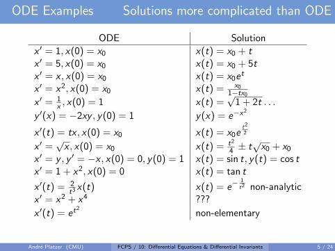
ODE Examples Solutions more complicated than ODE
ODE Solution
x ′ = 1, x(0) = x0 x(t) = x0 + tx ′ = 5, x(0) = x0 x(t) = x0 + 5tx ′ = x , x(0) = x0 x(t) = x0e
t
x ′ = x2, x(0) = x0 x(t) = x01−tx0
x ′ = 1x , x(0) = 1 x(t) =
√1 + 2t . . .
y ′(x) = −2xy , y(0) = 1 y(x) = e−x2
x ′(t) = tx , x(0) = x0 x(t) = x0et2
2
x ′ =√x , x(0) = x0 x(t) = t2
4 ± t√x0 + x0
x ′ = y , y ′ = −x , x(0) = 0, y(0) = 1 x(t) = sin t, y(t) = cos tx ′ = 1 + x2, x(0) = 0 x(t) = tan t
x ′(t) = 2t3 x(t) x(t) = e−
1t2 non-analytic
x ′ = x2 + x4 ???
x ′(t) = et2
non-elementary
Andre Platzer (CMU) FCPS / 10: Differential Equations & Differential Invariants 5 / 24
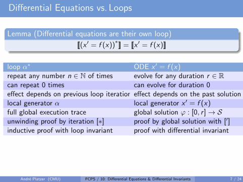
Differential Equations vs. Loops
Lemma (Differential equations are their own loop)
[[(x ′ = f (x))∗]] = [[x ′ = f (x)]]
loop α∗ ODE x ′ = f (x)repeat any number n ∈ N of times evolve for any duration r ∈ Rcan repeat 0 times can evolve for duration 0effect depends on previous loop iteration effect depends on the past solutionlocal generator α local generator x ′ = f (x)full global execution trace global solution ϕ : [0, r ]→ Sunwinding proof by iteration [∗] proof by global solution with [′]inductive proof with loop invariant proof with differential invariant
Andre Platzer (CMU) FCPS / 10: Differential Equations & Differential Invariants 7 / 24
Intuition for Differential Invariants
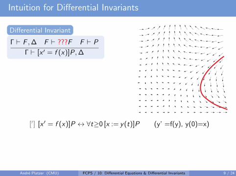
Differential Invariant
Γ ` F ,∆ F ` ???F F ` P
Γ ` [x ′ = f (x)]P,∆
Want: F remains true inthe direction of the dynamics
¬ ¬FF F
[′] [x ′ = f (x)]P ↔ ∀t≥0 [x := y(t)]P (y’ =f(y), y(0)=x)
Don’t need to know where exactly the system evolves to. Just that itremains somewhere in F .Show: only evolves into directions in which formula F stays true.
Andre Platzer (CMU) FCPS / 10: Differential Equations & Differential Invariants 9 / 24
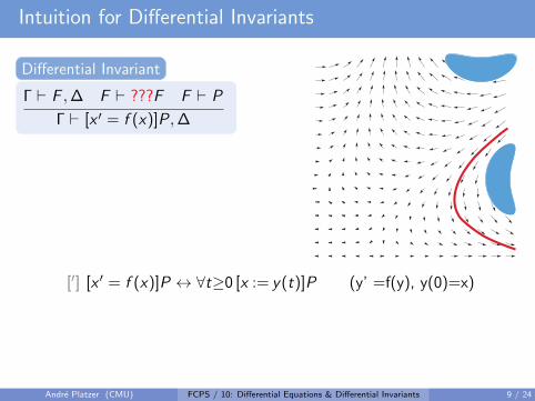
Intuition for Differential Invariants
Differential Invariant
Γ ` F ,∆ F ` ???F F ` P
Γ ` [x ′ = f (x)]P,∆
Want: F remains true inthe direction of the dynamics
¬ ¬FF F
[′] [x ′ = f (x)]P ↔ ∀t≥0 [x := y(t)]P (y’ =f(y), y(0)=x)
Don’t need to know where exactly the system evolves to. Just that itremains somewhere in F .Show: only evolves into directions in which formula F stays true.
Andre Platzer (CMU) FCPS / 10: Differential Equations & Differential Invariants 9 / 24
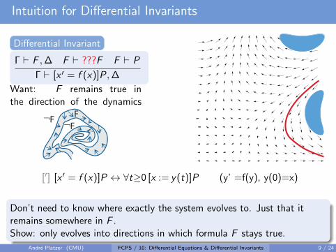
Intuition for Differential Invariants
Differential Invariant
Γ ` F ,∆ F ` ???F F ` P
Γ ` [x ′ = f (x)]P,∆
Want: F remains true inthe direction of the dynamics
¬ ¬FF F
[′] [x ′ = f (x)]P ↔ ∀t≥0 [x := y(t)]P (y’ =f(y), y(0)=x)
Don’t need to know where exactly the system evolves to. Just that itremains somewhere in F .Show: only evolves into directions in which formula F stays true.
Andre Platzer (CMU) FCPS / 10: Differential Equations & Differential Invariants 9 / 24
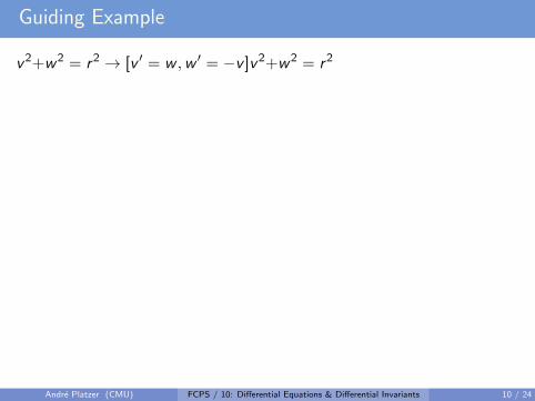
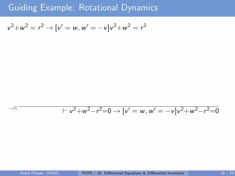
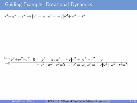
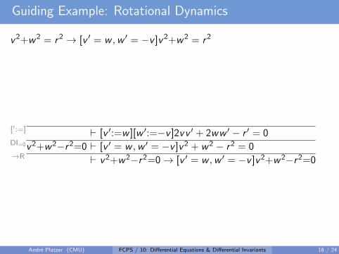
Guiding Example
: Rotational Dynamics
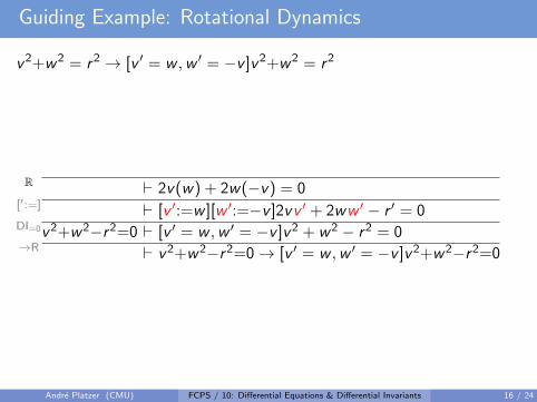
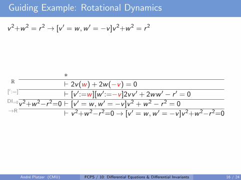
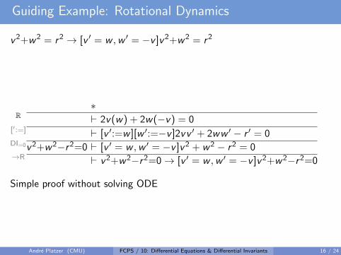
v2+w2 = r2 → [v ′ = w ,w ′ = −v ]v2+w2 = r2
∗
R ` 2v(w) + 2w(−v) = 0
[′:=] ` [v ′:=w ][w ′:=−v ]2vv ′ + 2ww ′ − r ′ = 0
DI=0v2+w2−r2=0 ` [v ′ = w ,w ′ = −v ]v2 + w2 − r2 = 0
→R ` v2+w2−r2=0→ [v ′ = w ,w ′ = −v ]v2+w2−r2=0
Simple proof without solving ODE
Andre Platzer (CMU) FCPS / 10: Differential Equations & Differential Invariants 10 / 24

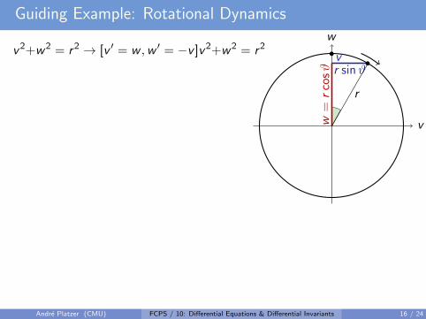
Guiding Example: Rotational Dynamics
v2+w2 = r2 → [v ′ = w ,w ′ = −v ]v2+w2 = r2
v
w
w=
rco
sϑ
vr sinϑ
r
∗
R ` 2v(w) + 2w(−v) = 0
[′:=] ` [v ′:=w ][w ′:=−v ]2vv ′ + 2ww ′ − r ′ = 0
DI=0v2+w2−r2=0 ` [v ′ = w ,w ′ = −v ]v2 + w2 − r2 = 0
→R ` v2+w2−r2=0→ [v ′ = w ,w ′ = −v ]v2+w2−r2=0
Simple proof without solving ODE
Andre Platzer (CMU) FCPS / 10: Differential Equations & Differential Invariants 10 / 24

Guiding Example: Rotational Dynamics
v2+w2 = r2 → [v ′ = w ,w ′ = −v ]v2+w2 = r2
∗
R ` 2v(w) + 2w(−v) = 0
[′:=] ` [v ′:=w ][w ′:=−v ]2vv ′ + 2ww ′ − r ′ = 0
DI=0v2+w2−r2=0 ` [v ′ = w ,w ′ = −v ]v2 + w2 − r2 = 0
→R ` v2+w2−r2=0→ [v ′ = w ,w ′ = −v ]v2+w2−r2=0
Simple proof without solving ODE
Andre Platzer (CMU) FCPS / 10: Differential Equations & Differential Invariants 10 / 24
Derivatives for a Change
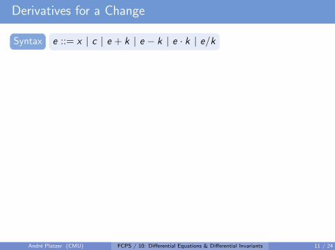
Syntax e ::= x | c | e + k | e − k | e · k | e/k
Derivatives
(e + k)′ = (e)′ + (k)′
(e − k)′ = (e)′ − (k)′
(e · k)′ = (e)′ · k + e · (k)′
(e/k)′ =((e)′ · k − e · (k)′
)/k2
same singularities
(c())′ = 0 for constants/numbers c()
. . . What do these primes mean? . . .
Andre Platzer (CMU) FCPS / 10: Differential Equations & Differential Invariants 11 / 24

Derivatives for a Change
Syntax e ::= x | c | e + k | e − k | e · k | e/k
Derivatives
(e + k)′ = (e)′ + (k)′
(e − k)′ = (e)′ − (k)′
(e · k)′ = (e)′ · k + e · (k)′
(e/k)′ =((e)′ · k − e · (k)′
)/k2
same singularities
(c())′ = 0 for constants/numbers c()
. . . What do these primes mean? . . .
Andre Platzer (CMU) FCPS / 10: Differential Equations & Differential Invariants 11 / 24
Augmented states
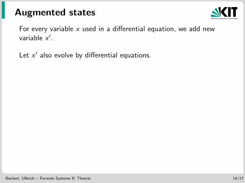
For every variable x used in a differential equation, we add newvariable x ′.
Let x ′ also evolve by differential equations.
Semantics of diff. eq.
(s1, s2) ∈ ρ(x ′ = e & Q)⇐⇒
ex. t > 0 and X : [0, t]→ R with
1 X (0) = s1(x)
2 X ′(u) = vals[x 7→X (u)](e) for all 0 ≤ u ≤ t
3 X (t) = s2(x)
4 s1[x 7→ X (u)] |= Q for all 0 ≤ u ≤ t
5 s1(y) = s2(y) for all other variables y .
Beckert, Ulbrich – Formale Systeme II: Theorie 14/17
Augmented states
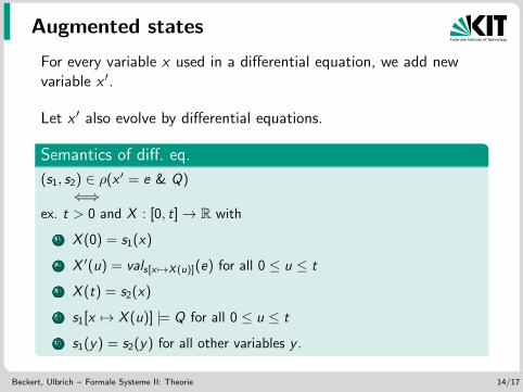
For every variable x used in a differential equation, we add newvariable x ′.
Let x ′ also evolve by differential equations.
Semantics of diff. eq.
(s1, s2) ∈ ρ(x ′ = e & Q)⇐⇒
ex. t > 0 and X : [0, t]→ R with
1 X (0) = s1(x)
2 X ′(u) = vals[x 7→X (u)](e) for all 0 ≤ u ≤ t
3 X (t) = s2(x)
4 s1[x 7→ X (u)] |= Q for all 0 ≤ u ≤ t
5 s1(y) = s2(y) for all other variables y .
Beckert, Ulbrich – Formale Systeme II: Theorie 14/17
Augmented states
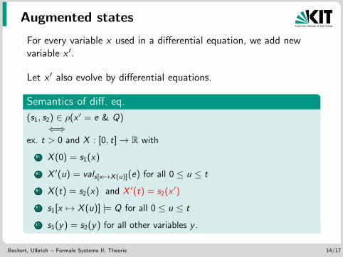
For every variable x used in a differential equation, we add newvariable x ′.
Let x ′ also evolve by differential equations.
Semantics of diff. eq.
(s1, s2) ∈ ρ(x ′ = e & Q)⇐⇒
ex. t > 0 and X : [0, t]→ R with
1 X (0) = s1(x)
2 X ′(u) = vals[x 7→X (u)](e) for all 0 ≤ u ≤ t
3 X (t) = s2(x) and X ′(t) = s2(x ′)
4 s1[x 7→ X (u)] |= Q for all 0 ≤ u ≤ t
5 s1(y) = s2(y) for all other variables y .
Beckert, Ulbrich – Formale Systeme II: Theorie 14/17
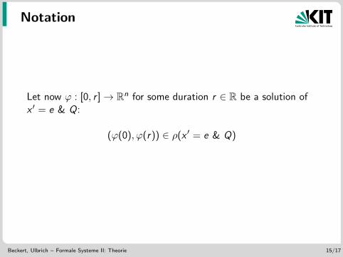
Notation
Let now ϕ : [0, r ]→ Rn for some duration r ∈ R be a solution ofx ′ = e & Q:
(ϕ(0), ϕ(r)) ∈ ρ(x ′ = e & Q)
Beckert, Ulbrich – Formale Systeme II: Theorie 15/17
Derivatives for a Change
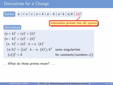
Syntax e ::= x | c | e + k | e − k | e · k | e/k | (e)′
Derivatives
(e + k)′ = (e)′ + (k)′
(e − k)′ = (e)′ − (k)′
(e · k)′ = (e)′ · k + e · (k)′
(e/k)′ =((e)′ · k − e · (k)′
)/k2 same singularities
(c())′ = 0 for constants/numbers c()
. . . What do these primes mean? . . .
internalize primes into dL syntax
Andre Platzer (CMU) FCPS / 10: Differential Equations & Differential Invariants 11 / 24
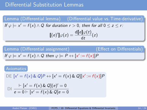
Differential Substitution Lemmas
Lemma (Differential lemma) (Differential value vs. Time-derivative)
If ϕ |= x ′ = f (x) ∧ Q for duration r > 0, then for all 0 ≤ z ≤ r :
[[(e)′]]ϕ(z) =d[[e]]ϕ(t)
dt(z)
Lemma (Differential assignment) (Effect on Differentials)
If ϕ |= x ′ = f (x) ∧ Q then ϕ |= P ↔ [x ′ := f (x)]P
Axiomatics
DE [x ′ = f (x) &Q]P ↔ [x ′ = f (x) &Q][x ′ := f (x)]P
DI` [x ′ = f (x) &Q](e)′ = 0
e = 0 ` [x ′ = f (x) &Q]e = 0
Andre Platzer (CMU) FCPS / 10: Differential Equations & Differential Invariants 14 / 24
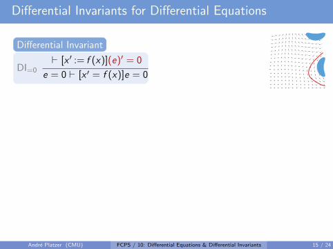
Differential Invariants for Differential Equations
Differential Invariant
DI=0` [x ′ := f (x)](e)′ = 0
e = 0 ` [x ′ = f (x)]e = 0
DI` [x ′ = f (x)](e)′ = 0
e = 0 ` [x ′ = f (x)]e = 0DE [x ′ = f (x)]P ↔ [x ′ = f (x)][x ′ := f (x)]P
DI=0 is a derived rule:
` [x ′ := f (x)](e)′ = 0
G ` [x ′ = f (x)][x ′ := f (x)](e)′ = 0
DE ` [x ′ = f (x)](e)′ = 0
DIe = 0 ` [x ′ = f (x)]e = 0
GP
[α]P
Andre Platzer (CMU) FCPS / 10: Differential Equations & Differential Invariants 15 / 24
Guiding Example: Rotational Dynamics
v2+w2 = r2 → [v ′ = w ,w ′ = −v ]v2+w2 = r2
v
w
w=
rco
sϑ
vr sinϑ
r
∗
R ` 2v(w) + 2w(−v) = 0
[′:=] ` [v ′:=w ][w ′:=−v ]2vv ′ + 2ww ′ − r ′ = 0
DI=0v2+w2−r2=0 ` [v ′ = w ,w ′ = −v ]v2 + w2 − r2 = 0
→R ` v2+w2−r2=0→ [v ′ = w ,w ′ = −v ]v2+w2−r2=0
Simple proof without solving ODE
Andre Platzer (CMU) FCPS / 10: Differential Equations & Differential Invariants 16 / 24
Guiding Example: Rotational Dynamics
v2+w2 = r2 → [v ′ = w ,w ′ = −v ]v2+w2 = r2
∗
R ` 2v(w) + 2w(−v) = 0
[′:=] ` [v ′:=w ][w ′:=−v ]2vv ′ + 2ww ′ − r ′ = 0
DI=0v2+w2−r2=0 ` [v ′ = w ,w ′ = −v ]v2 + w2 − r2 = 0→R ` v2+w2−r2=0→ [v ′ = w ,w ′ = −v ]v2+w2−r2=0
Simple proof without solving ODE
Andre Platzer (CMU) FCPS / 10: Differential Equations & Differential Invariants 16 / 24
Guiding Example: Rotational Dynamics
v2+w2 = r2 → [v ′ = w ,w ′ = −v ]v2+w2 = r2
∗
R ` 2v(w) + 2w(−v) = 0
[′:=] ` [v ′:=w ][w ′:=−v ]2vv ′ + 2ww ′ − r ′ = 0DI=0v2+w2−r2=0 ` [v ′ = w ,w ′ = −v ]v2 + w2 − r2 = 0→R ` v2+w2−r2=0→ [v ′ = w ,w ′ = −v ]v2+w2−r2=0
Simple proof without solving ODE
Andre Platzer (CMU) FCPS / 10: Differential Equations & Differential Invariants 16 / 24
Guiding Example: Rotational Dynamics
v2+w2 = r2 → [v ′ = w ,w ′ = −v ]v2+w2 = r2
∗
R ` 2v(w) + 2w(−v) = 0[′:=] ` [v ′:=w ][w ′:=−v ]2vv ′ + 2ww ′ − r ′ = 0DI=0v2+w2−r2=0 ` [v ′ = w ,w ′ = −v ]v2 + w2 − r2 = 0→R ` v2+w2−r2=0→ [v ′ = w ,w ′ = −v ]v2+w2−r2=0
Simple proof without solving ODE
Andre Platzer (CMU) FCPS / 10: Differential Equations & Differential Invariants 16 / 24
Guiding Example: Rotational Dynamics
v2+w2 = r2 → [v ′ = w ,w ′ = −v ]v2+w2 = r2
∗R ` 2v(w) + 2w(−v) = 0
[′:=] ` [v ′:=w ][w ′:=−v ]2vv ′ + 2ww ′ − r ′ = 0DI=0v2+w2−r2=0 ` [v ′ = w ,w ′ = −v ]v2 + w2 − r2 = 0→R ` v2+w2−r2=0→ [v ′ = w ,w ′ = −v ]v2+w2−r2=0
Simple proof without solving ODE
Andre Platzer (CMU) FCPS / 10: Differential Equations & Differential Invariants 16 / 24
Guiding Example: Rotational Dynamics
v2+w2 = r2 → [v ′ = w ,w ′ = −v ]v2+w2 = r2
∗R ` 2v(w) + 2w(−v) = 0
[′:=] ` [v ′:=w ][w ′:=−v ]2vv ′ + 2ww ′ − r ′ = 0DI=0v2+w2−r2=0 ` [v ′ = w ,w ′ = −v ]v2 + w2 − r2 = 0→R ` v2+w2−r2=0→ [v ′ = w ,w ′ = −v ]v2+w2−r2=0
Simple proof without solving ODE
Andre Platzer (CMU) FCPS / 10: Differential Equations & Differential Invariants 16 / 24
Strengthening Induction Hypotheses
Stronger Induction Hypotheses
1 As usual in math and in proofs with loops:
2 Inductive proofs may need stronger induction hypotheses to succeed.
3 Differentially inductive proofs may need a stronger differentialinductive structure to succeed.
4 Even if {(x , y) ∈ R2 : x2 + y2 = 0} = {{(x , y) ∈ R2 : x4 + y4 = 0}have the same solutions, they have different differential structure.
Andre Platzer (CMU) FCPS / 10: Differential Equations & Differential Invariants 20 / 24