From Constructive Mathematics to Computable Analysis …streicher/THESES/lietz.pdf · From...
97
From Constructive Mathematics to Computable Analysis via the Realizability Interpretation Vom Fachbereich Mathematik der Technischen Universit¨ at Darmstadt zur Erlangung des akademischen Grades eines Doktors der Naturwissenschaften (Dr. rer. nat.) genehmigte Dissertation von Dipl.-Math. Peter Lietz aus Mainz Referent: Prof. Dr. Thomas Streicher Korreferent: Dr. Alex Simpson Tag der Einreichung: 22. Januar 2004 Tag der m¨ undlichen Pr¨ ufung: 11. Februar 2004 Darmstadt 2004 D17
-
Upload
duongkhanh -
Category
Documents
-
view
218 -
download
2
Transcript of From Constructive Mathematics to Computable Analysis …streicher/THESES/lietz.pdf · From...
From Constructive Mathematicsto Computable Analysis
via the Realizability Interpretation
Vom Fachbereich Mathematik
der Technischen Universitat Darmstadt
zur Erlangung des akademischen Grades eines
Doktors der Naturwissenschaften (Dr. rer. nat.)
genehmigte
Dissertation
von
Dipl.-Math. Peter Lietz
aus Mainz
Referent: Prof. Dr. Thomas StreicherKorreferent: Dr. Alex SimpsonTag der Einreichung: 22. Januar 2004Tag der mundlichen Prufung: 11. Februar 2004
Darmstadt 2004D17


Hiermit versichere ich, dass ich diese Dissertation selbstandig verfasst und nur dieangegebenen Hilfsmittel verwendet habe.
Peter Lietz
Abstract
Constructive mathematics is mathematics without the use of the principle of theexcluded middle. There exists a wide array of models of constructive logic. Oneparticular interpretation of constructive mathematics is the realizability interpreta-tion. It is utilized as a metamathematical tool in order to derive admissible rules ofdeduction for systems of constructive logic or to demonstrate the equiconsistency ofextensions of constructive logic. In this thesis, we employ various realizability mod-els in order to logically separate several statements about continuity in constructivemathematics.
A trademark of some constructive formalisms is predicativity. Predicative logicdoes not allow the definition of a set by quantifying over a collection of sets that theset to be defined is a member of. Starting from realizability models over a typedversion of partial combinatory algebras we are able to show that the ensuing modelsprovide the features necessary in order to interpret impredicative logics and typetheories if and only if the underlying typed partial combinatory algebra is equivalentto an untyped pca.
It is an ongoing theme in this thesis to switch between the worlds of classicaland constructive mathematics and to try and use constructive logic as a method inorder to obtain results of interest also for the classically minded mathematician. Aclassical mathematician can see the value of a solution algorithm as opposed to anabstract proof of the existence of a solution, but he or she would not insist on aconstructive correctness proof for that algorithm. We introduce a class of formulaewhich is supposed to capture this pragmatic point of view. The class is defined insuch a way that existence statements have a strong status, yet the correctness ofan operation need only be proved classically. Moreover, this theory contains onlyclassically true formulae. We pose the axiomatization of this class of formulae as anopen problem and provide partial results.
Like ordinary recursion theory, computable analysis is a branch of classical math-ematics. It applies the concept of computability to entities of analysis by equippingthem with a generalization of Godelizations called representations. Representationscan be organized into a realizability category with rich logical properties. In thisway, natural representations of spaces can be found by categorically interpreting thedescription of the underlying set of a space. Computability and non-computabilityresults can be and are shown on an abstract, logical level.
Finally, we turn to another application of realizability models, the field of strongnormalization proofs for type theoretic frameworks. We will argue why we thinkthat the modified realizability topos is not suited for this purpose and propose analternative.
Zusammenfassung
Konstruktive Mathematik ist Mathematik ohne die Verwendung des Prinzips ter-tium non datur. Es gibt eine Vielzahl unterschiedlicher Modelle fur die konstruk-tive Logik. Eine bestimmte Interpretation der konstruktiven Mathematik ist dieRealisierbarkeits-Interpretation. Sie findet Anwendung als ein metamathematischesWerkzeug welches es gestattet, zulassige Regeln oder Aquikonsistenzaussagen fur lo-gische Kalkule nachzuweisen. In dieser Dissertation verwenden wir die Realisierbar-keits-Interpretation zum Zwecke der Separierung verschiedener Aussagen uber Stetig-keit im Rahmen der konstruktiven Mathematik.
Eine Eigenart einiger konstruktiver Formalismen ist die Pradikativitat. PradikativeLogik verbietet die Definition einer Menge durch Quantifikation uber eine Familie vonMengen, welche die zu definierende Menge enthalt. Ausgehend von Realisierbarkeits-Modellen uber einer getypten Version partieller kombinatorischer Algebren zeigenwir, dass die zugehorigen Modelle die notigen Eigenschaften zur Interpretation im-pradikativer Logik und Typ Theorie genau dann besitzen, wenn die zugrundeliegendepartielle kombinatorische Algebra aquivalent ist zu einer ungetypten pca.
Der Wechsel zwischen den Welten der konstruktiven und der klassischen Mathe-matik und der Versuch, die konstruktive Logik als eine Methode zu benutzen, umResultate zu erzielen, welche von Interesse fur klassische Mathematiker sind, ist einwiederkehrendes Thema dieser Dissertation. Ein klassischer Mathematiker erkenntsehr Wohl den Wert eines Losungsalgorithmus im Vergleich zu einem bloßen Beweisder Existenz einer Losung, aber er wird gewohnlich nicht darauf bestehen, dass derKorrektheitsbeweis fur den Algorithmus konstruktiv ist. Wir fuhren eine Klasse vonFormeln ein, welche diesen pragmatischen Blickwinkel erfassen soll. Die Klasse istderart definiert, dass Existenzaussagen einen starken Status haben, Korrektheitsbe-weise fur Operationen jedoch nur klassisch gefuhrt werden brauchen. Die besagteKlasse von Formeln enthalt nur klassisch wahre Formeln. Wir stellen die Axioma-tisierung dieser Klasse als ein Problem und bieten Teilergebnisse.
Wie die Rekursionstheorie, so ist auch die berechenbare Analysis ein Zweig der klas-sischen Mathematik. Die berechenbare Analysis wendet das Konzept der Berechen-barkeit an auf Großen der Analysis, indem sie sie mit einer Verallgemeinerung vonGodelisierungen, genannt Darstellungen, ausstattet. Darstellungen konnen in einerRealisierbarkeits-Kategorie mit reichhaltigen logischen Eigenschaften zusammenge-fasst werden. Auf diesem Wege konnen naturliche Darstellungen von Raumen gefun-den werden, indem man die Beschreibung der unterliegenden Menge der Raume kat-egoriell interpretiert. Berechenbarkeits- und Nicht-Berechenbarkeitsresultate konnenso auf einer abstrakten, logischen Ebene hergeleitet werden.
Zuletzt wenden wir uns einer weiteren Anwedung der Realisierbarkeitsmodelle zu,namlich dem Gebiet der starken Normalisierungbeweise fur typtheoretische Kalkule.Wir legen dar warum wir denken, dass der modified realizability topos nicht dasgeeignete Modell fur diesen Zweck ist und schlagen eine Alternative vor.
Acknowledgements
I would like to gratefully acknowledge the many fruitful discussions that have con-tributed to this thesis. I am greatly indebted to: Andrej Bauer, Lars Birkedal, VascoBrattka, Martın Escardo, Helge Glockner, Karl Heinrich Hofmann, Martin Hofmann,Shin-ya Katsumata, Klaus Keimel, John Longley, Matias Menni, Jaap van Oosten,Matthias Schroder, Klaus Weihrauch, Alex Simpson, Eike Ritter, Peter Schuster,Helmut Schwichtenberg, Dana Scott and Bas Spitters.
In particular, I would like to thank Andrej Bauer, whose two visits to Darmstadthave meant times of great motivation and good progress. The regular correspon-dence with Andrej Bauer, John Longley, Jaap van Oosten, Matthias Schroder, AlexSimpson and Bas Spitters has always been very stimulating and valuable to me andis much appreciated.
I would like to express my gratitude for invitations to present my work at the IT-University of København, the FernUniversitat Hagen, and the Ludwig MaximiliansUniversitat in Munchen.
I have profited from having been allowed to participate in the “Postgraduate Coursein the Theory of Computation” of the “Laboratory for Foundations of ComputerScience” at the University of Edinburgh.
I would like to thank my officemates in Edinburgh and Darmstadt and my fellowmembers of the research unit “Logik und mathematische Grundlagen der Informatik”at the Technische Universitat Darmstadt.
Finally and foremost, I would like to thank my supervisor Thomas Streicher for thegreat many things I have learnt from him and for his enduring support and patience.
I gratefully acknowledge receipt of the Promotionsstipendium nach dem hessischenGesetz zur Forderung von Nachwuchswissenschaftlern (PhD–grant according to theHessian Law for the furtherance of young scientists) during the time from July 1998to September 2000.
This document was typeset with LATEX2ε using the KOMA–Script documentclassscrbook, Kristoffer Rose’s XY–pic package, Paul Taylor’s prooftree package and theAMS-packages.
7

8

Contents
Introduction 11
1 Constructive Mathematics 131.1 General philosophy of constructivism . . . . . . . . . . . . . . . . . . 131.2 Branches of constructivism . . . . . . . . . . . . . . . . . . . . . . . . 14
1.2.1 Bishop’s constructive mathematics . . . . . . . . . . . . . . . 141.2.2 Brouwer’s intuitionism . . . . . . . . . . . . . . . . . . . . . . 181.2.3 Markov’s constructive recursive mathematics . . . . . . . . . . 21
1.3 Formalized constructive logic . . . . . . . . . . . . . . . . . . . . . . . 221.3.1 Constructive many-sorted predicate logic with equality . . . . 221.3.2 Heyting arithmetic . . . . . . . . . . . . . . . . . . . . . . . . 251.3.3 Elementary analysis . . . . . . . . . . . . . . . . . . . . . . . 261.3.4 Heyting arithmetic with higher types . . . . . . . . . . . . . . 261.3.5 Higher order arithmetic . . . . . . . . . . . . . . . . . . . . . 28
1.4 Constructive Principles . . . . . . . . . . . . . . . . . . . . . . . . . . 281.4.1 Definitions . . . . . . . . . . . . . . . . . . . . . . . . . . . . . 291.4.2 Status with respect to classcial mathematics . . . . . . . . . . 331.4.3 Consequences of constructive principles in analysis . . . . . . 331.4.4 Inconsistencies between constructive principles . . . . . . . . . 37
1.5 Categorical Logic . . . . . . . . . . . . . . . . . . . . . . . . . . . . . 37
2 Realizability Interpretations 392.1 Formalized realizability interpretation . . . . . . . . . . . . . . . . . . 39
2.1.1 Numerical realizability . . . . . . . . . . . . . . . . . . . . . . 392.1.2 Function realizability . . . . . . . . . . . . . . . . . . . . . . . 432.1.3 Classically provably realizable formulas . . . . . . . . . . . . . 46
2.2 Categorical Realizability Semantics . . . . . . . . . . . . . . . . . . . 512.2.1 Typed Partial Combinatory Algebras . . . . . . . . . . . . . . 512.2.2 Universal Types . . . . . . . . . . . . . . . . . . . . . . . . . . 542.2.3 Realizability Models . . . . . . . . . . . . . . . . . . . . . . . 572.2.4 Impredicativity entails Untypedness . . . . . . . . . . . . . . . 592.2.5 Discussion of related work . . . . . . . . . . . . . . . . . . . . 62
2.3 Separating models for continuity axioms . . . . . . . . . . . . . . . . 63
9

3 Computable Analysis 693.1 Introduction . . . . . . . . . . . . . . . . . . . . . . . . . . . . . . . . 69
3.1.1 Numberings . . . . . . . . . . . . . . . . . . . . . . . . . . . . 693.1.2 Representations . . . . . . . . . . . . . . . . . . . . . . . . . . 703.1.3 Admissibility . . . . . . . . . . . . . . . . . . . . . . . . . . . 71
3.2 Category theoretic approach to representations . . . . . . . . . . . . . 733.2.1 The category of representations . . . . . . . . . . . . . . . . . 733.2.2 Logical aspects of admissibility . . . . . . . . . . . . . . . . . 75
3.3 Categorical approach to computable analysis . . . . . . . . . . . . . . 813.3.1 Motivation . . . . . . . . . . . . . . . . . . . . . . . . . . . . . 813.3.2 Models . . . . . . . . . . . . . . . . . . . . . . . . . . . . . . . 823.3.3 Examples of inductive limits of csm’s . . . . . . . . . . . . . . 843.3.4 From constructive mathematics to computable analysis . . . . 86
4 (Appendix) Semantic Strong Normalization 89
Bibliography 91
10

Introduction
Constructive mathematics is mathematics without the use of the principle of the ex-cluded middle or, equivalently, without the proof principle of reductio ad absurdum.While it is often harder and sometimes impossible to prove a classical theorem con-structively, a constructive proof, once obtained, is much more informative. From aconstructive existence proof, for instance, one can extract a witness for the existencestatement, which is in general impossible for a classical proof. One might say that inconstructive logic, the status of existence statements is much stronger than in clas-sical logic. Moreover, there exists a wide array of models of constructive logic. Oneparticular interpretation of constructive mathematics (actually, a theme with manyvariations) is the realizability interpretation. The realizability interpretation can beseen as a concrete incarnation of the Brouwer Heyting Kolmogorof interpretation ofthe logical connectives. It is utilized as a metamathematical tool in order to deriveadmissible rules of deduction for systems of constructive logic or to demonstrate theequiconsistency of extensions of constructive logic. It is an ongoing theme in thisthesis to switch between the worlds of classical and constructive mathematics andto try and use constructive logic as a method in order to obtain results of interestalso for the classically minded mathematician. A classical mathematician can seethe value of a solution algorithm as opposed to an abstract proof of the existenceof a solution, but he or she would not insist on a constructive correctness proof forthat algorithm. In section 2.1.3 we introduce a class of formulae which is supposedto capture this pragmatic point of view. The class is defined in such a way that exis-tence statements have a strong status, yet the correctness of an operation need onlybe proved classically. Moreover, this theory contains only classically true formulae.We pose the axiomatization of this class of formulae as an open problem and providepartial results.
A trademark of some constructive formalisms is predicativity. Predicativism meansthat, for any set, the collection of subsets of that set is not an entity in its own rightbut each subset has to be defined by refering only to previously defined subsets. Thisin particular prevents the definition of a set by quantifying over a collection of setsthat the set to be defined is a member of. This is perceived by predicavists as a viciouscircle. Starting from realizability models over a typed version of partial combinatoryalgebras we are able to show that the ensuing models provide the features necessary inorder to interpret impredicative logics and type theories if and only if the underlying
11
Introduction
typed partial combinatory algebra is equivalent to an untyped pca.One aspect of constructive mathematics as opposed to classical mathematics is that
it can be extended in various ways incompatible with classical reasoning. A continuityprinciple is an axiom which states that every function defined on a metric spacepertaining to some specified class of spaces to another metric space is continuous.This is generally incompatible with classical logic, but perfectly (equi-)consistentwith constructive logic. As possible classes we can for example choose the class ofcomplete separable metric spaces or the class of complete totally bounded spaces. Weexhibit realizability models that satisfy the weaker and fail to satisfy the strongerprinciple, thereby demonstrating that the implication between these principles isstrict. Moreover we give an easy model validating the statement “all functions fromR to R are sequentially continuous” and falsifying the statement “all functions fromR to R are continuous”.
Like ordinary recursion theory, computable analysis is a branch of classical math-ematics. It applies the concept of computability to entities of analysis. In additionto whether or not there exists a solution to a mathematical problem, in computablemathematics one is interested in the question whether, given that the input datais computable, there is a computable solution. Furthermore one asks whether onecan uniformly compute a solution from the input data. In order to give mean-ing to sentences such as “the real number x is computable” or “some function fis computable” one has to introduce some computability structure. Amongst theseveral, non-equivalent approaches, we shall concentrate on the approach taken byWeihrauch and Kreitz. It utilizes a generalization of the notion of Godel numberings,called representations. Representations can be organized into a category with richlogical properties, which is essentially a realizability category. In this way, naturalrepresentations of spaces can be found by categorically interpreting the descriptionof the underlying set of a space. Computability and non-computability results canbe shown on an abstract, logical level.
Finally, we turn to another application of realizability models, the field of strongnormalization proofs for type theoretic frameworks. We will argue why we thinkthat the modified realizability topos is not suited for this purpose and propose analternative.
12

1 Constructive Mathematics
This chapter attempts to give a brief overview over several schools of constructivemathematics. The most important branches of constructivism for the purposes ofthis thesis are E. Bishop’s constructivism and L.E.J. Brouwer’s intuitionism.
The introduction to the underlying philosophy of constructivist schools is followedby a section on formalized mathematics and an analysis of the principles employedby the various schools.
In the last section of this chapter we give a short introduction to categorical se-mantics of constructive logic.
1.1 General philosophy of constructivism
Constructive Mathematics is mathematics without the law of the excluded middleor, equivalently, without the rule of reductio ad absurdum. That is, in order toprove an existence statement ∃x.A in constructive mathematics, it is not sufficientto demonstrate that the non-existence ∀x.¬A is absurd. Likewise, in order to provea disjunction A ∨ B it is not sufficient to show that ¬A ∧ ¬B is absurd. This selfimposed restriction results in a finer distinction of concepts that would be equivalentunder the reign of classical logic.
Another aspect of constructivism, often, but not necessarily, combined with con-structive logic is predicativism. In predicative logic it is not admissible to, in order toconstruct one set, quantify over a collection of sets of which the set in statu nascendiis a member of. If one does not adopt the philosophy that sets are entities that havean ideal existence, then such a construction of a set would constitute a vicious circle.
Both restrictions of ordinary mathematics, while being not far from each otherin spirit, can be and are applied independently and in each of the possible combi-nations. While it is more difficult (and sometimes impossible) to prove a theoremconstructively, the existence of a constructive proof has stronger implications thanthat of a classical proof.
Consistency or enhanced safety from contradiction, by the way, is not amongst thereasons to drop the law of the excluded middle. Due to the negative translation ofGodel and Gentzen, it is just as hard to prove 0 = 1 in Heyting arithmetic as it is inPeano arithmetic.
13

1 Constructive Mathematics
1.2 Branches of constructivism
We shall, in the following three sections, give a very brief account of the main branchesof constructive mathematics. A more extensive comparative overview can be foundin [BR87] or, amongst many other things, in [TvD88a, TvD88b] or [Bee85]. Thefollowing sections touch on each of the constructive schools from the point of view ofthis thesis, they do not serve as a real introduction. Also they lack all due historicalinformation.
1.2.1 Bishop’s constructive mathematics
The definitive introductory presentation of the ideas of Bishop’s mathematics is theconstructivist manifesto, the first chapter of the seminal book “Foundations of con-structive analysis” [Bis67]. Although not formalized, it is rather clear in practicewhat are the valid constructions and derivations in Bishop’s mathematics (BISH forshort).
Bishop style mathematics is based on constructive logic. As Bishop puts it: “whena man proves a positive integer to exist, he should show how to find it”. This rulesout the unrestricted use of indirect proofs.
Bishop’s mathematics is also predicative. As he writes: “A set is not an entitywhich has an ideal existence: a set exists only when it has been defined. To define aset we prescribe, at least implicitly, what we (the constructing intelligence) must doin order to construct an element of the set, and what we must do in order to showthat two elements are equal.” [Bis67, p.2]. This implies that, in defining a set, onemust not quantify over some collection of ideal sets, but may only refer to previouslydefined sets. Bishop refers to sets and existence as used in classical mathematicsas ideal sets and ideal existence as opposed to constructive sets and constructiveexistence. Sets may have a hypothetical status in order to allow a proof generic forall possible sets, but quantification over all sets or even only all subsets of a givenset in order to define a new set is not allowed.
The set that Bishop’s mathematics starts out with is the set of natural numbers.Given two sets, it is permissible to construct the set of ordered pairs of elementsof these, or the set of functions between these. Furthermore, given a set, one canform the subset of all elements satisfying some given property. Quotient sets are notpart of Bishop’s mathematics, instead, every set is equipped with a defined notionof equality. Equality is in most cases derived from a notion of apartness. This istypical for constructive mathematics: in order to be able to prove some result, thehypotheses have to be expressed in a positive way. The property that two elements of,say, a metric space are apart is stronger constructively than the property of merelybeing not equal. Instead, equality can be defined as non-apartness. If equalityon some set is defined as the negation of apartness, which is frequently the case,the apartness relation is called tight. Indeed, apartness is the key notion in the
14

1.2 Branches of constructivism
constructive redevelopment of topology (see [BSV02]). Classical topology is notapplicable, here, as the dualism between open and closed sets is intrinsically basedon non-constructive reasoning.
It is to be emphasized that constructive mathematics is not about imposing re-strictions and hindering mathematical development but about maintaining a higherstandard for valid proofs. If theorems fail to be provable constructively, they do sofor a good reason.
Equally important, one should keep in mind that Bishop style mathematics is nota logical discipline, but a flavor of ordinary mathematics in its own right. Therefore,the main activity in the field consists in proving theorems rather then demonstrat-ing the unprovability of theorems or making other metamathematical observations.Nevertheless, it is essential to have some clear indicators of when some theorem Ais unprovable, constructively. In classical mathematics, in this situation one usuallytries, and often succeeds, to prove ¬A. This method will, however, succeed less oftenin constructive mathematics. The reason is that in contrast to classical mathemat-ics, in constructive mathematics a lot more statements, even mathematically naturalones, are undecided by the theory.
Omniscience principles
The principle of the excluded middle is undecided in Bishop style mathematics. It isneither adopted, as in classical mathematics, nor does Bishop’s mathematics containany principle that refutes instances of the principle of the excluded middle, as does,for instance, Bouwer’s intuitionism. However, as intuitionism is an equiconsistentextension of Bishop style mathematics, instances of the principle of the excludedmiddle that are refuted by intuitionism cannot be proved in Bishop’s mathematics.
One such instance has been taunted by Bishop the principle of omniscience:
PO For a set A either all elements of A have the property P or there is an elementof A with the property not P .
A particular choice of a set A and a property P , for which this principle is not partof constructive mathematics, is the so called limited principle of omniscience:
LPO Let (an) be a binary sequence. Then either there is a k such that ak = 1 orak = 0 for all k.
A number of theorems of classical mathematics are intrinsically non-constructive,which can be demonstrated by deriving LPO from them. Another principle, weakerthan LPO but yet non-constructive and often used for the refutation of theorems, isthe lesser limited principle of omniscience:
LLPO Let (an) be a binary sequence with at most one 1. Then either a2k = 0 for allk or a2k+1 = 0 for all k.
15
1 Constructive Mathematics
Constructive versions of classical theorems
There is quite a number of classical theorems that are provable constructively. Amongstthese are for instance the fundamental theorem of algebra or the Picard-Lindeloftheorem. Other classical theorems are non-constructive, but are provable subject tomodifications. The law of trichotomy for the reals
∀r ∈ R. r < 0 ∨ r = 0 ∨ r > 0
is equivalent to LPO relative to BISH and therefore non-constructive. Another exam-ple of a classical theorem that entails LPO is the bounded completeness of the reals,i.e. the statement that every inhabited subset of the reals that is bounded above hasa supremum. In the other direction, LPO itself proves that every sequence of realsthat is bounded above has a supremum.
As to the first example, the theorem
∀x, y ∈ R. x < y → ∀r ∈ R. r < y ∨ x < r
serves as a constructive substitute for trichotomy. As to the second example, everyinhabited subset P ⊆ R that is bounded above and has the additional propertythat for all y, z ∈ R such that y < z either P < z or there is an x ∈ P withy < x does have a supremum, constructively. Such a form of constructive theorem iscalled an equal conclusion substitute, as only the hypothesis of the theorem is altered.The additional assumption is void from a classical point of view but essential for aconstructive proof. It can be shown that the image of a uniformly continuous functiondefined on a totally bounded metric space meets the additional requirement. Thisfact is important for the constructive definition of Banach spaces like C[0, 1]. On theother hand, the operator norm of the dual of a Banach space can not be defined,constructively, unless the original space is finite dimensional.
The failure of bounded completeness of the reals is also the culprit for the fact thatthe distance of some inhabited subset of a metric space to a point is not guaranteedto exist. Subsets, whose distances to any point exist are called located. Locatednessis quite a central notion in constructive mathmatics and often has to be required asan extra assumption for a theorem to work, see for instance [Spi02]. These kinds ofsubtleties are levelled off by the use of classical logic.
The principles
∀r ∈ R. r ≤ 0 ∨ r ≥ 0 and ∀x, y ∈ R. xy = 0→ (x = 0 ∨ y = 0)
are each equivalent to LLPO relative to BISH We shall see that the former principleis a consequence of the intermediate value theorem. Define
fr : [0, 1] //R fr(x) =
−1 + 3(1 + r)x for x < 1
3
r for 13≤ x < 2
3
−2 + 3r + 3(1− r)x for 23≤ x
16

1.2 Branches of constructivism
In the light of the constructive failure of x < a ∨ x ≥ a one would of course have toargue why the piecewise definition of fr is admissible. A constructive argument isthat given functions
f : R≤a//R and g : R≥a
//R such that f(a) = g(a)
we can constructively define a pasted function h as
h : R //R x 7→ f(min(x, a)) + g(max(x, a))− f(a)
A more general justification for the pasting of continuous functions can also begiven but does involve the constructive Tietze extension theorem (see [BB85, Theo-rem (6.6)]).
Now regarding the intermediate value theorem, a given zero z of the functionfr would allow us, using the constructive substitute for the law of trichotomy, todecide whether z < 2
3or 1
3< z and hence to decide whether r ≥ 0 or r ≤ 0. This
demonstrates the non-constructivity of the intermediate value theorem.There are two constructive substitutes for the intermediate value theorem, one with
equal hypothesis and one with equal conclusion, The latter has the extra assumptionthat the function f is locally non-zero, i.e. between any two numbers in the domainof definition, there is an argument for which the function yields a result apart fromzero. This hypothesis is met e.g. by non-constant polynomials. The equal hypothesissubstitute has the weaker conclusion that, for every ε > 0, there is an x ∈ [0, 1] suchthat |f(x)| < ε.
Given two real numbers a, b, their maximum and their minimum exist. However, itis not possible to pick a maximal number amongst a and b, as this again would allowus to decide whether a−b ≤ 0 or a−b ≥ 0. As a consequence, a uniformly continuousfunction on a closed interval, albeit having a supremum (i.e., a least upper bound),need not have a maximum (i.e., need not attain a maximal value).
A subset P of some set X is called decidable if ∀x ∈ X. x ∈ P ∨¬x ∈ P . The onlysubsets of R that can be proven to be decidable are ∅ and R. On the other hand, theequality relation and the relations ≤ and < are decidable subsets of both N×N andQ×Q. As the principle of the excluded middle is not at our disposition, this has tobe proven by natural induction.
Continuity
Several classically equivalent notions of continuity fall apart in Bishop style mathe-matics. Let f : R −→ R be a function. If f is uniformly continuous on every compactinterval, then f is continuous (i.e. ε-δ-continuous) in every point. If f is continuousthen it is sequentially continuous (i.e. the image of a convergent sequence is conver-gent). Unfortunately, neither of these implications can be reversed (see [Ish92] for adetailed analysis of continuity in BISH).
17
1 Constructive Mathematics
When classically equivalent notions diversify under a constructive examination, itis crucial to choose the most meaningful amongst them. It cannot be shown con-structively that every continuous function defined on a compact interval is uniformlycontinuous. Also, it turns out that continuity alone is too weak a property in thepurely constructive setting: One cannot show that a continuous function defined ona compact interval is Riemann-integrable or even just bounded. Therefore, the moremeaningful notion of continuity for functions defined on subsets of Euclidean spaceis that of locally uniform continuity, and hence we define C(Rn) to be the set of allreal-valued functions on Rn that are uniformly continuous on every bounded subset.
Choice
The use of choice principles in Bishop style mathematics goes as far as including theaxiom of dependent choice and the axiom of unique choice. Although Bishop writesthat “a choice function exists because a choice function is implied by the very meaningof existence”[BB85, A Constructivist Manifesto], it still has to be verified that thechoice function respects the defined equality relation. This reveals an intensionalview that Bishop has on mathematics (see also Bridges comment at the end of loc.cit.).
1.2.2 Brouwer’s intuitionism
Like Bishop’s constructivism, Brouwer’s intuitionism (INT) is not a formalized theory,in its original conception it is not even based on mathematical logic. This, however,did not prevent Brouwer’s disciple Heyting from giving a formalized account of in-tuitionistic logic [Hey30]. A lively introduction to intuitionism is [Hey56], anotherextensive treatment is [Dum77].
Brouwer’s intuitionism is an extension of Bishop’s constructivism, that is, everyargument valid in BISH is also valid in INT. Brouwer takes a more fundamentalstance than Bishop in that he breaks with classical mathematics. Unlike Bishopstyle mathematics, Brouwer’s intuitionism is not a subset of classical mathematics.It contains axioms that negate instances of the principle of the excluded middle andis hence incompatible with classical mathematics.
Infinitely prodeeding sequences
A fundamental notion in Intuitionism is the notion of an infinitely prodeeding sequenceof natural numbers. Such a sequence may, but need not, be determined by a law.In order to talk about sequences, both finite and infinite ones, we have got to fixsome notation. We choose to use the symbols introduced in [TvD88a, p.186]. Finitesequences are denoted as 〈a1, a2, . . . an〉, in particular the empty sequence is denotedas 〈〉. The concatenation of the sequences a and x is denoted by a ∗ x, where a
18

1.2 Branches of constructivism
is a finite sequence and x is either finite or infinite. The initial segment of lengthn of the sequence α is denoted by αn. We write a ≺ a′ if a is a prefix of a′. Ifa ≺ a′, we say that a is an ascendent of a′ and a′ is a descendent of a. The prefixof length lth(a) − 1 of a is called the immediate ascendent of a, a sequence that ais the immediate ascendent of is called an immediate descendent of a. If the finitesequence a is an element of some set S of finite sequences then any descendent of athat is a member of S is called an S-descendent.
Definition 1.2.1. A decidable set of finite sequences that contains the empty se-quence and that with any sequence contains all its prefixes is called a tree. A spreadis a tree such that every finite sequence in S has an immediate S-descendent. Thatis, a tree S is a spread if ∀a ∈ S∃n ∈ N. a ∗ 〈n〉 ∈ S. Finally, a fan is a finitelybranching spread, i.e. a spread in which each node has a finite number of immediatedescendents.
Every spread determines a set of infinite sequences. We say that the infinitesequence α belongs to the spread S if all initial segments of α are elements of S.By abuse of language we call the thus defined set of sequences S as well. The senseof the statement x ∈ S, depends on whether x is a finite or an infinite sequence. Weusually denote finite sequences by small roman and infinite sequences by small greekletters.
Example 1.2.2. Let (rn)n∈N be some standard bijective enumeration of the setQ. We define the spread S as the set of all finite sequences 〈a1, . . . an〉 such that|rα(k)−rα(k+1)| ≤ 2−(n+1) for all 1 ≤ k < n. Then for each α ∈ S the rational sequence(qα(n))n∈N is a Cauchy sequence. The condition of α, α′ ∈ S representing the samereal number does as well depend on the initial segments, alone: The sequences α andα′ represent the same real number if and only if |rα(n) − rα′(n)| ≤ 2−n for all n ∈ N.
Example 1.2.3. Let F be the set of −1, 0, 1-valued finite sequences. Obviously,F is defined by a a fan. With each infinite sequence α ∈ F we associate the realnumber
∑∞k=0 αk2
−αk−1. The set of real numbers that is represented by a sequencein F is exactly the closed interval [−1, 1]. Two sequences α, α′ represent the samenumber if and only if |
∑nk=0 αk2
−αk−1 −∑n
k=0 α′k2−αk−1| ≤ 2−n for all n ∈ N, that
is, two sequences represent the same number if and only if all their pairs of initialsegments satisfy some decidable property.
The continuity principle
Two principles govern the nature of infinitely proceeding sequences in intuitionism,the continuity principle and the principle of bar induction. The continuity principleas taken from [Hey56] (with a slight modification) reads as follows.
19
1 Constructive Mathematics
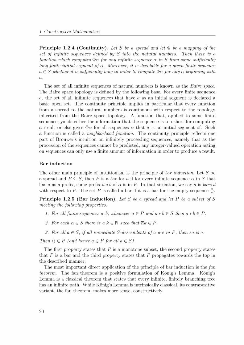
Principle 1.2.4 (Continuity). Let S be a spread and let Φ be a mapping of theset of infinite sequences defined by S into the natural numbers. Then there is afunction which computes Φα for any infinite sequence α in S from some sufficientlylong finite initial segment of α. Moreover, it is decidable for a given finite sequencea ∈ S whether it is sufficiently long in order to compute Φα for any α beginning witha.
The set of all infinite sequences of natural numbers is known as the Baire space.The Baire space topology is defined by the following base. For every finite sequencea, the set of all inifinite sequences that have a as an initial segment is declared abasic open set. The continuity principle implies in particular that every functionfrom a spread to the natural numbers is continuous with respect to the topologyinherited from the Baire space topology. A function that, applied to some finitesequence, yields either the information that the sequence is too short for computinga result or else gives Φα for all sequences α that a is an initial segment of. Sucha function is called a neighborhood function. The continuity principle reflects onepart of Brouwer’s intuition on infinitely proceeding sequences, namely that as theprocession of the sequences cannot be predicted, any integer-valued operation actingon sequences can only use a finite amount of information in order to produce a result.
Bar induction
The other main principle of intuitionism is the principle of bar induction. Let S bea spread and P ⊆ S, then P is a bar for a if for every infinite sequence α in S thathas a as a prefix, some prefix a ∗ b of α is in P . In that situation, we say a is barredwith respect to P . The set P is called a bar if it is a bar for the empty sequence 〈〉.
Principle 1.2.5 (Bar Induction). Let S be a spread and let P be a subset of Smeeting the following properties.
1. For all finite sequences a, b, whenever a ∈ P and a ∗ b ∈ S then a ∗ b ∈ P .
2. For each α ∈ S there is a k ∈ N such that αk ∈ P .
3. For all a ∈ S, if all immediate S-descendents of a are in P , then so is a.
Then 〈〉 ∈ P (and hence a ∈ P for all a ∈ S).
The first property states that P is a monotone subset, the second property statesthat P is a bar and the third property states that P propagates towards the top inthe described manner.
The most important direct application of the principle of bar induction is the fantheorem. The fan theorem is a positive formulation of Konig’s Lemma. Konig’sLemma is a classical theorem that states that every infinite, finitely branching treehas an infinite path. While Konig’s Lemma is intrinsically classical, its contrapositivevariant, the fan theorem, makes more sense, constructively.
20

1.2 Branches of constructivism
Theorem 1.2.6 (Fan). Let S be a fan and let P be a subset of S. If P is a bar,then there is a natural number n such that for every infinite sequence in S, an inititalsegment with length less than n can be found that is an element of P .
The continuity principle and the fan theorem can be used to show that all real-valued functions on the reals are continuous and all real-valued functions defined on aclosed interval are uniformly continuous. Hence, in contrast to Bishop’s mathematics,in intuitionism one does not have to distinguish between various forms of continuitybut in fact all functions on the reals (or any complete separable metric space for thatmatter) are continuous in the strongest possible sense.
It is to be noted that the bar theorem is classically provable. The continuityprinciple, on the other hand, is expressedly inconsistent with classical logic in thatit refutes instances of LPO and even LLPO.
Another consequence of the fan theorem is that every continuous, real-valued func-tion defined on the unit interval that has only positive values, has a positive infimum.Bishop’s mathematics alone is too weak to prove this, in fact, the existence of a uni-formly continuous positive-valued function that has infimum zero is undecided inBishop’s mathematics.
This is an appetizer rather than a complete introduction to Intuitionism. Creativesubject arguments for instance, will be completely neglected in this thesis. For ourpurposes we will unduly simplify matters and identify Intuitionism with Bishop’smathematics augmented with the continuity principle and the principle of bar induc-tion.
1.2.3 Markov’s constructive recursive mathematics
The third major school of constructivism is Markov’s constructive recursive mathe-matics (CRM). We shall touch upon CRM only very briefly for the sake of complete-ness, as it is of less importance for the purposes of this thesis.
For e, n ∈ N, we denote by e.n the result of applying the eth partial recursivefunction (with respect to some fixed admissible numbering) to the argument n. Theformula e.n↓ expresses that the eth partial recursive function terminates when appliedto n.
The two main principles governing CRM are Church’s Thesis and Markov’s Prin-ciple.
Principle 1.2.7 (Church’s Thesis). Assume ∀x ∈ N∃y ∈ N. A(x, y). Then thereexists some e ∈ N such that ∀x ∈ N. e.x↓ ∧A(x, e.x).
Principle 1.2.8 (Markov’s Principle). Assume ∀x ∈ N. A(x) ∨ ¬A(x) and¬¬∃x ∈ N. A(x). Then ∃x ∈ N. A(x).
21
1 Constructive Mathematics
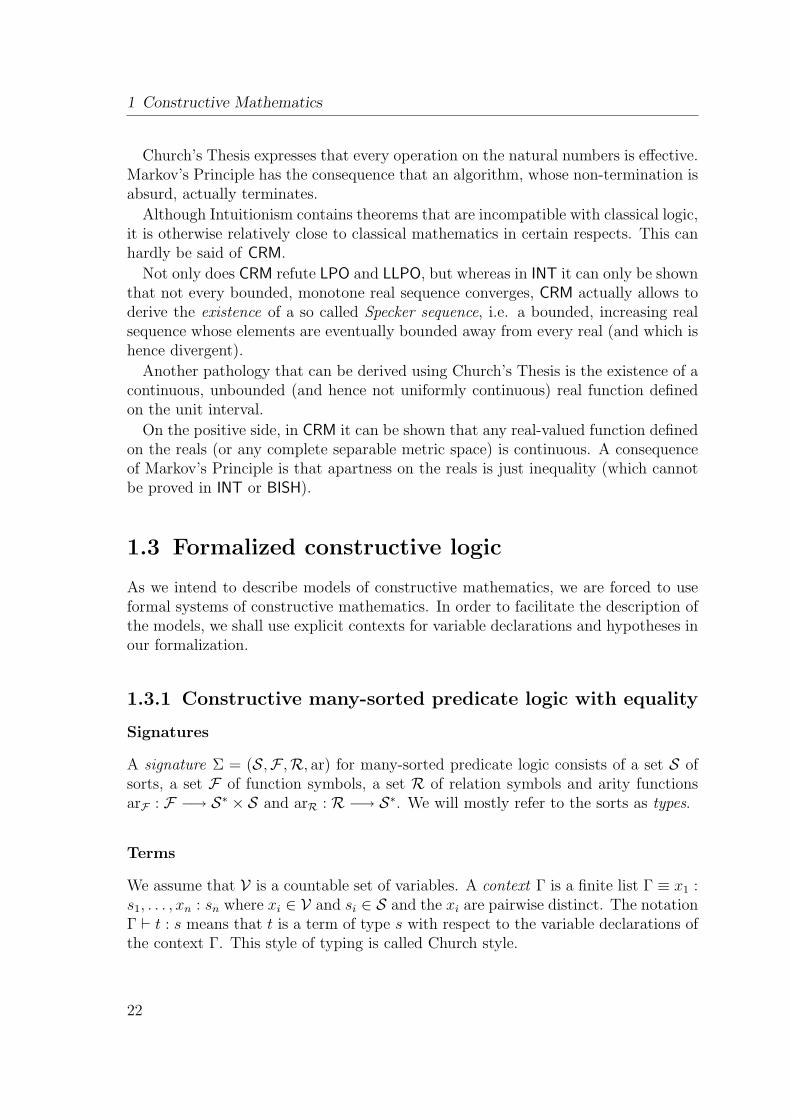
Church’s Thesis expresses that every operation on the natural numbers is effective.Markov’s Principle has the consequence that an algorithm, whose non-termination isabsurd, actually terminates.
Although Intuitionism contains theorems that are incompatible with classical logic,it is otherwise relatively close to classical mathematics in certain respects. This canhardly be said of CRM.
Not only does CRM refute LPO and LLPO, but whereas in INT it can only be shownthat not every bounded, monotone real sequence converges, CRM actually allows toderive the existence of a so called Specker sequence, i.e. a bounded, increasing realsequence whose elements are eventually bounded away from every real (and which ishence divergent).
Another pathology that can be derived using Church’s Thesis is the existence of acontinuous, unbounded (and hence not uniformly continuous) real function definedon the unit interval.
On the positive side, in CRM it can be shown that any real-valued function definedon the reals (or any complete separable metric space) is continuous. A consequenceof Markov’s Principle is that apartness on the reals is just inequality (which cannotbe proved in INT or BISH).
1.3 Formalized constructive logic
As we intend to describe models of constructive mathematics, we are forced to useformal systems of constructive mathematics. In order to facilitate the description ofthe models, we shall use explicit contexts for variable declarations and hypotheses inour formalization.
1.3.1 Constructive many-sorted predicate logic with equality
Signatures
A signature Σ = (S,F ,R, ar) for many-sorted predicate logic consists of a set S ofsorts, a set F of function symbols, a set R of relation symbols and arity functionsarF : F −→ S∗ × S and arR : R −→ S∗. We will mostly refer to the sorts as types.
Terms
We assume that V is a countable set of variables. A context Γ is a finite list Γ ≡ x1 :s1, . . . , xn : sn where xi ∈ V and si ∈ S and the xi are pairwise distinct. The notationΓ ` t : s means that t is a term of type s with respect to the variable declarations ofthe context Γ. This style of typing is called Church style.
22

1.3 Formalized constructive logic
The term formation rules are
(x : s ∈ Γ)Γ ` x : s
Γ ` t1 : s1 · · · Γ ` tn : sn(arF(f) = (s1, . . . , sn, s))
Γ ` f(t1, . . . , tn) : s
Formulae
The set of atomic formulae is defined by the following rules.
Γ ` t : s Γ ` t′ : s
Γ ` t =s t′ : Prop
Γ ` t1 : s1 · · · Γ ` tn : sn(arF(f) = (s1, . . . , sn))
Γ ` R(t1, . . . , tn) : Prop
The set of all formulae is defined by the above and the following rules.
Γ ` ϕ : Prop Γ ` ψ : Prop
Γ ` ϕ ∧ ψ : Prop Γ ` ⊥ : Prop
Γ ` ϕ : Prop Γ ` ψ : Prop
Γ ` ϕ→ ψ : Prop
Γ ` ϕ : Prop Γ ` ψ : Prop
Γ ` ϕ ∨ ψ : Prop
Γ, x : s ` ϕ : Prop
Γ ` ∀x : s. ϕ : Prop
Γ, x : s ` ϕ : Prop
Γ ` ∃x : s. ϕ : Prop
We use ¬ϕ as a shorthand for ϕ → ⊥ and ϕ ↔ ψ as a shorthand for (ϕ → ψ)∧(ψ → ϕ).
Sequents
A sequent is an expression of the form Γ | Θ ` ϕ where Γ is a context, Θ is a listof propositions and ϕ is a proposition, both with respect to the context Γ. Thesequent is to be interpreted as: under the variable declarations of Γ, the propositionϕ follows from the propositions enlisted in Θ. If Γ ` ϕ1 , . . . , Γ ` ϕn , Γ ` ϕ are wellformed propositions, then Γ | ϕ1 · · ·ϕn ` ϕ is a well formed sequent. Although oneis primarily interested in single sentences, sequents provide a convenient notationfor the fact that a proposition holds, subject to a set of variable declarations andhypotheses.
Proof rules
The set of provable sequents is defined inductively by the following rules.
The axiom rule:
(ax) (if ϕ ∈ Θ)Γ | Θ ` ϕ
23
1 Constructive Mathematics
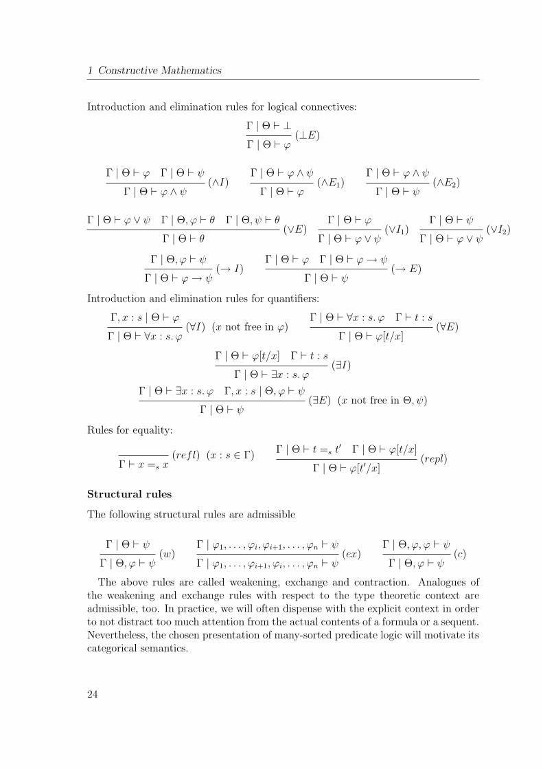
Introduction and elimination rules for logical connectives:
Γ | Θ ` ⊥(⊥E)
Γ | Θ ` ϕ
Γ | Θ ` ϕ Γ | Θ ` ψ(∧I)
Γ | Θ ` ϕ ∧ ψ
Γ | Θ ` ϕ ∧ ψ(∧E1)
Γ | Θ ` ϕ
Γ | Θ ` ϕ ∧ ψ(∧E2)
Γ | Θ ` ψ
Γ | Θ ` ϕ ∨ ψ Γ | Θ, ϕ ` θ Γ | Θ, ψ ` θ(∨E)
Γ | Θ ` θ
Γ | Θ ` ϕ(∨I1)
Γ | Θ ` ϕ ∨ ψ
Γ | Θ ` ψ(∨I2)
Γ | Θ ` ϕ ∨ ψ
Γ | Θ, ϕ ` ψ(→ I)
Γ | Θ ` ϕ→ ψ
Γ | Θ ` ϕ Γ | Θ ` ϕ→ ψ(→ E)
Γ | Θ ` ψ
Introduction and elimination rules for quantifiers:
Γ, x : s | Θ ` ϕ(∀I) (x not free in ϕ)
Γ | Θ ` ∀x : s. ϕ
Γ | Θ ` ∀x : s. ϕ Γ ` t : s(∀E)
Γ | Θ ` ϕ[t/x]
Γ | Θ ` ϕ[t/x] Γ ` t : s(∃I)
Γ | Θ ` ∃x : s. ϕ
Γ | Θ ` ∃x : s. ϕ Γ, x : s | Θ, ϕ ` ψ(∃E) (x not free in Θ, ψ)
Γ | Θ ` ψ
Rules for equality:
(refl) (x : s ∈ Γ)Γ ` x =s x
Γ | Θ ` t =s t′ Γ | Θ ` ϕ[t/x]
(repl)Γ | Θ ` ϕ[t′/x]
Structural rules
The following structural rules are admissible
Γ | Θ ` ψ(w)
Γ | Θ, ϕ ` ψ
Γ | ϕ1, . . . , ϕi, ϕi+1, . . . , ϕn ` ψ(ex)
Γ | ϕ1, . . . , ϕi+1, ϕi, . . . , ϕn ` ψ
Γ | Θ, ϕ, ϕ ` ψ(c)
Γ | Θ, ϕ ` ψ
The above rules are called weakening, exchange and contraction. Analogues ofthe weakening and exchange rules with respect to the type theoretic context areadmissible, too. In practice, we will often dispense with the explicit context in orderto not distract too much attention from the actual contents of a formula or a sequent.Nevertheless, the chosen presentation of many-sorted predicate logic will motivate itscategorical semantics.
24

1.3 Formalized constructive logic
1.3.2 Heyting arithmetic
A very basic system of arithmetic based on intuitionistic predicate logic with equalityis Heyting arithmetic (HA). Its signature consists of a single type whose inhabitantsare thought of as natural numbers. Furthermore, no relation symbols other thanequality occur. Finally, the set of function symbols holds an element for each defi-nition of a primitive recursive function. The set of axioms contains all definitionalequations for these functions.1 We shall denote by Fn the set of n-ary functionsymbols. The family (Fn)n∈N is defined inductively by the following rules.
1. 0 ∈ F0
2. S ∈ F1
3. p(m)k ∈ Fm for m, k ∈ N, k < m
4. If t ∈ Fn and s1, . . . , sn ∈ Fm then Comp[t, s1, . . . , sn] ∈ Fm for m,n ∈ N
5. If t ∈ Fn and s ∈ Fn+2 then R[t, s] ∈ Fn+1
As for the axioms of Heyting arithmetic, the following equations describe the be-haviour of the primitive recursive constructors.
p(m)k (x1, . . . , xm) = xk
Comp[t, s1, . . . , sn](x1, . . . , xm) = t(s1(x1, . . . , xm), . . . , sn(x1, . . . , xm))
R[t, s](x1, . . . , xn, 0) = t(x1, . . . , xn)
R[t, s](x1, . . . , xn, Sk) = s(x1, . . . , xn,R[t, s](x1, . . . , xn, k), k)
The following axiom expresses that zero is not a successor.
0 6= Sx
Finally, for every formula A(x) there is an instance of the induction principle.
A(0) ∧ (∀x. A(x)→ A(Sx))→ ∀x. A(x)
The classical version of Heyting arithmetic, i.e. Heyting arithmetic augmentedwith tertium non datur is called Peano arithmetic.
1Heyting arithmetic can be alternatively presented using only 0, S, + and ×, and the definitionalequations for + and ×. The presentation using symbols for all definitions of primitive recursivefunctions is a definitional extension of the former.
25
1 Constructive Mathematics
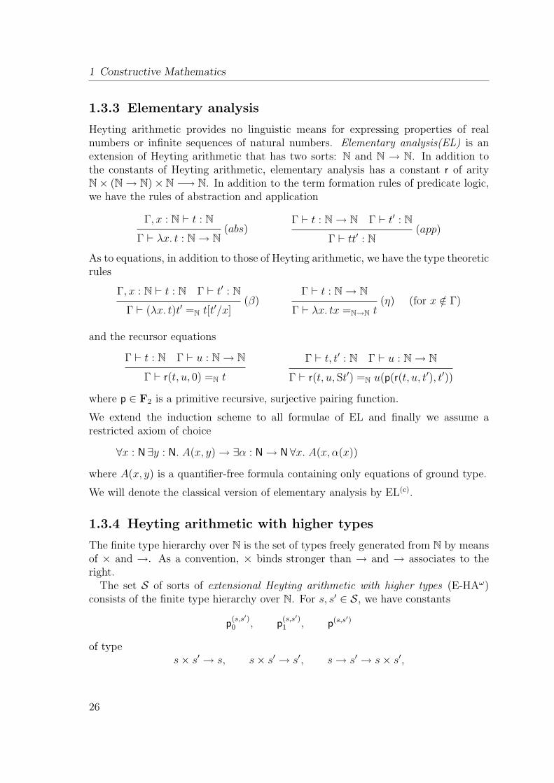
1.3.3 Elementary analysis
Heyting arithmetic provides no linguistic means for expressing properties of realnumbers or infinite sequences of natural numbers. Elementary analysis(EL) is anextension of Heyting arithmetic that has two sorts: N and N → N. In addition tothe constants of Heyting arithmetic, elementary analysis has a constant r of arityN× (N→ N)×N −→ N. In addition to the term formation rules of predicate logic,we have the rules of abstraction and application
Γ, x : N ` t : N(abs)
Γ ` λx. t : N→ N
Γ ` t : N→ N Γ ` t′ : N(app)
Γ ` tt′ : N
As to equations, in addition to those of Heyting arithmetic, we have the type theoreticrules
Γ, x : N ` t : N Γ ` t′ : N(β)
Γ ` (λx. t)t′ =N t[t′/x]
Γ ` t : N→ N(η) (for x /∈ Γ)
Γ ` λx. tx =N→N t
and the recursor equations
Γ ` t : N Γ ` u : N→ N
Γ ` r(t, u, 0) =N t
Γ ` t, t′ : N Γ ` u : N→ N
Γ ` r(t, u, St′) =N u(p(r(t, u, t′), t′))
where p ∈ F2 is a primitive recursive, surjective pairing function.
We extend the induction scheme to all formulae of EL and finally we assume arestricted axiom of choice
∀x : N ∃y : N. A(x, y)→ ∃α : N→ N ∀x. A(x, α(x))
where A(x, y) is a quantifier-free formula containing only equations of ground type.
We will denote the classical version of elementary analysis by EL(c).
1.3.4 Heyting arithmetic with higher types
The finite type hierarchy over N is the set of types freely generated from N by meansof × and →. As a convention, × binds stronger than → and → associates to theright.
The set S of sorts of extensional Heyting arithmetic with higher types (E-HAω)consists of the finite type hierarchy over N. For s, s′ ∈ S, we have constants
p(s,s′)0 , p
(s,s′)1 , p(s,s′)
of types× s′ → s, s× s′ → s′, s→ s′ → s× s′,
26

1.3 Formalized constructive logic
respectively. When the types are clear from the context or irrelevant, we feel free toomit the superscripts. Pairing and unpairing is governed by the equations
p0(p(x, y)) = x, p1(p(x, y)) = y, p(p0(z), p1(z)) = z.
As in the case of elementary analysis, we extend the term formation rules of pred-icate logic with rules for abstraction and application,
Γ, x : s ` t : s′
(abs)Γ ` λx : s. t : s→ s′
Γ ` t : s→ s′ Γ ` t′ : s(app)
Γ ` tt′ : s′
accompanied by the respective equations.
Γ, x : s ` t : s′ Γ ` t′ : s(β)
Γ ` (λx : s. t)t′ =s′ t[t′/x]
Γ ` t : s→ s′
(η) (for x /∈ Γ)Γ ` λx. tx =s→s′ t
In Heyting arithmetic and elementary analysis, all definitions of primitive recursivefunctions were introduced at the level of function symbols. In contrast, in E-HAω,we provide the constant 0 ∈ N, the the function symbol S ∈ N → N and for eachs ∈ S the function symbol rs : s × (s × N → s) → (N → s) . The constant rs is arecursor over type s, governed by the equations
Γ ` t : s Γ ` u : s× N→ s
Γ ` r(t, u)(0) =s t
Γ ` t : s Γ ` u : s× N→ s Γ ` t′ : N
Γ ` r(t, u)(St′) =s u(r(t, u)(t′), t′)
Finally we state the axiom that 0 is not a successor
0 6= Sx
and the induction scheme
A(0) ∧ (∀x. A(x)→ A(Sx))→ ∀x. A(x)
This finishes the definition of E-HAω. For the definition of HAω, we simply dropthe extensionality rule (η).
As previously mentioned, in our formulation of (E-)HAω (and EL) we have ex-tended the term language of multi-sorted predicate logic in that we allow λ-abstraction.If we wanted to stay strictly within the realm of traditional predicate calculus, atleast in the case of (E-)HAω, we could have used combinators instead. We havedecided not to do so, as λ-terms allow a more intuitive and natural notation. Notealso that extensionality is commonly formulated as an axiom stating that equalityon functions is equivalent to argumentwise equality. Our formulation featuring theη-rule of λ-calculus is easily seen to be equivalent.
27
1 Constructive Mathematics
The level of a type is inductively defined by
level(N) = 0 level(s× s′) = max(level(s), level(s′))
level(s→ s′) = max(level(s) + 1, level(s′))
Given some type s, we can introduce the type s∗ of finite sequences of elements ofs as a notational convenience. We set
level(s∗) = level(s).
Obviously, for each s, a bijection between s and s∗ can be defined.We could have defined elementary analysis to be the fragment of E-HAω that uses
only types of level 0 and 1. This would allow for a slightly more natural notationand presentation. However, in order not to complicate the description of the variousinterpretations of EL to be defined in the next chapter, it is more convenient to keepthe language as small as possible. As the extension of elementary analysis with alltypes of type level 0 and 1 is a definitional extension, we will freely use this extranotation.
The classical versions of E-HAω and HAω are called E-PAω and PAω
1.3.5 Higher order arithmetic
All previously mentioned extensions of Heyting arithmetic are conservative exten-sions, i.e., they prove the same theorems of Heyting arithmetic as Heyting arith-metic itself. This is not the case for higher order arithmetic. Higher order arithmetic(HAH) results from E-HAω by adding the kind Ω of propositions as a type and ex-tending the set of types to all types freely generated from N and Ω by means of ×and →. Functions and functional relations are linked by the axiom of unique choice.
(∀x : s ∃!y : s′. A(x, y)) −→ (∃f : s→ s′ ∀x : s. A(x, f(x)))
The extensionality of entailment axiom, which equates logical equivalence and equal-ity on the type of propositions, is not standardly assumed. Introducing propositionsas a type allows for quantification over truth values and predicates. In particular, itallows one to define a predicate by quantifying over all predicates. Hence, in contrastto HA, EL and (E-)HAω, the system HAH is impredicative.
1.4 Constructive Principles
In this section we are going to review some common priciples that are used in varioussystems of constructive mathematics. In section 1.4.4 we will examine the dependen-cies and inconsistencies between combinations of these principles.
28

1.4 Constructive Principles
1.4.1 Definitions
In the following, we will use the small greek letters to denote infinite sequencesof numbers, small roman letters from the beginning of the alphabet to denote finitesequences of numbers and small roman letters from the end of the alphabet to denotenatural numbers.
Notation
Let α, β : N→ N, a, b : N∗, n : N. Then
〈〉 : N∗ = the empty sequence.〈n〉 : N∗ = the sequence of length 1 with entry n.
a ∗ α : N→ N = the concatenation of a and α.a ∗ b : N∗ = the concatenation of a and b.a_n : N∗ = a ∗ 〈n〉.
lth(a) : N = the length of a.αn : N∗ = the initial segment of length n of α.
The statement α ∈ a means ∀k < lth(a). αk = ak. In other words, a finite sequenceis identified with its set of infinite extensions.
For a set A of finite sequences we write α ∈ A to express that all initial segmentsof α are elements of A, in other words, α ∈ A if and only if ∀k. αk ∈ A.
A function γ : N∗ → N describes a partial continuous operation from N→ N to Nin the following manner. We write
γ(α) = n for ∃k. γ(αk) = n+ 1 ∧ ∀i < k. γ(αi) = 0.
The meaning of γ( ) thus depends on whether the argument is a finite or infinitesequence. The value of γ(α), if it exists, depends only on some finite initial segmentof α. If γ(αk) = 0, then αk is not sufficiently long in order for γ to compute theresult. The formula γ(α) ↓ expresses that γ( ) terminates when applied to α, in otherwords, it expresses that there exists a k ∈ N such that γ(αk) > 0. The function γ iscalled a neighborhood function for the operation γ( ).
The definition of γ( ) can be used in order to let γ define a partial continuousoperation from N→ N to N→ N. We write
γ|α = β for ∀n. γ(〈n〉 ∗ α) = βn.
For e, n ∈ N, we denote by e.n the result of applying the eth partial recursivefunction (with respect to some fixed admissible numbering) to the argument n. Theformula e.n↓ expresses that the eth partial recursive function terminates when appliedto n. An alternative notation for e.n is the Kleene-bracket notation e(n).
29

1 Constructive Mathematics
Choice Principles
The axiom of choice
AC(X, Y ) (∀x : X ∃y : Y. A(x, y)) −→ ∃f : X → Y ∀x : X. R(x, f(x))
expresses that every total relation on X × Y admits a choice function. By AC(X)we denote that for all Y , AC(X, Y ) holds. The principle AC(N) is called countablechoice or number choice, the principle AC(N→ N) is called function choice.
The axiom of unique choice
AC!(X,Y ) (∀x : X ∃!y : Y. A(x, y)) −→ ∃f : X → Y ∀x : X. R(x, f(x))
expresses that every functional relation on X × Y is the graph of a function.The axiom of dependent choice
DC(X) (∀x : X ∃y : X. A(x, y))−→ ∀x : X ∃f : N→ X. f(0) = x ∧ ∀n : N. R(f(n), f(n+ 1))
allows to construct an infinite sequence of pairwise related elements of X startingwith an arbitrary x ∈ X. By DC we denote that for all X, DC(X) holds. Dependentchoice is more powerful than countable choice.
Continuity Principles
Continuity principles conflict with classical reasoning but are certainly compatiblewith constructive mathematics. Continuity principles state that every function oroperation between some specified (classes of) spaces is continuous.
Let (X, d) and (X ′, d′) be metric spaces. Then the continuity principles
CP(X,X ′) Every function from X to X ′ is ε-δ-continuous.
and
CPseq(X,X′) Every function from X to X ′ is sequentially continuous.
state the continuity (resp. sequential continuity) of all functions from X to X ′.For the particular case that X = N→ N and X ′ = N, the following combinations
of continuity with choice are widely used. The weak principle of continuity statesthat every operation from N→ N to N is continuous.
WC-N (∀α : N→ N ∃n : N. A(α, n))−→ (∀α : N→ N ∃m,n : N ∀β : N→ N. β ∈ αm −→ A(β, n))
The strong principle of continuity states that every operation from N → N to N isgiven by a neighborhood function.
30

1.4 Constructive Principles
CONT (∀α : N→ N ∃n : N. A(α, n))−→ (∃γ : N∗ → N ∀α : N→ N. γ(α) ↓ ∧A(α, γ(α)))
By [TvD88a, 4.1.4], the continuity principle for α ranging over an arbitrary spread isderivable from the respective continuity principle stated for the full spread. Clearly,the strong principle of continuity entails the weak principle of continuity. The strongprinciple of continuity enables one to actually decide whether a given finite sequencecontains enough information to compute the result for all its infinite extensions. Wewill meet a generalization of CONT in Theorem 2.1.18.
We shall now formulate two weakenings of WC-N. Let 2 be the two element set0, 1. The following principle of continuity states that every operation from the fullbinary fan N→ 2 to N is continuous.
WCcp-N (∀α : N→ 2 ∃n : N. A(α, n))−→ (∀α : N→ 2 ∃m,n : N ∀β : N→ 2. β ∈ αm −→ A(β, n))
By [TvD88a, 4.7.5], the continuity principle for α ranging over an arbitrary fan isderivable from the respective continuity principle stated for the full binary fan.
Now, let N+ = α : N→ 2 | ∀m,n. α(m) = 1∧m < n→ α(n) = 0, N+ is the onepoint compactification of N (in the sense of [BB85, (6.6)]). The following principleof continuity states that every operation from the fan N+ to N is continuous.2
WCseq-N (∀α : N+ ∃n : N. A(α, n))−→ (∀α : N+ ∃m,n : N ∀β : N+. β ∈ αm −→ A(β, n))
It is actually sufficient to require continuity at the constant zero sequence.
WCseq-N′ (∀α : N+ ∃n : N. A(α, n))−→ (∃m,n : N ∀β : N+. β ∈ 0m −→ A(β, n))
WC-N entails WCcp-N, as the full binary fan is a retract of the full spread. Likewise,WCcp-N entails WCseq-N, as N+ is a retract of the full binary fan. The relationshipbetween the variants of WC-N and CP will be further discussed in the sections 1.4.3and 2.3.
Church’s Thesis
In theoretical computer science, Church’s thesis referes to the observation that a greatmany different models of computation give rise to the same class of computablefunctions. In constructive mathematics, however, Church’s thesis is referred to asthe principle that all operations on the natural numbers are computable. Althoughregarded a misnomer by many, we will adhere to this terminology.
CT (∀n∃m. A(n,m))→ (∃e∀n. e.n ↓ ∧A(n, e.n))
We will meet a generalization of CT in Theorem 2.1.6.
2To our knowledge, the first reference in literature, where a continuity principle w.r.t. N+ is used,is [BS03].
31

1 Constructive Mathematics
Bar Induction
The principle of bar induction equates two notions of well foundedness for trees.Amongst the various possible formulations, we choose to present the principle ofmonotone bar induction. For a complete discussion see e.g. [Dum77, chapter 3].
BI Let P ⊆ N∗ such that(1) ∀a, b : N∗. P (a)→ P (a ∗ b)(2) ∀a : N∗. (∀x : N. P (a_x))→ P (a)(3) ∀α : N→ N ∃n : N. P (αn).Then P (〈〉).
As is the case for continuity principles, the principle of bar induction relativized toa spread follows from the principle of bar induction for the full spread.
The Fan Theorem
The fan theorem is a consequence of the principle of bar induction. It expresses theHeine-Borel compactness of Cantor space.
FAN (∀α : N→ 2 ∃n : N. A(αn))−→ ∃m : N ∀α : N→ 2 ∃n : N. n ≤ m ∧ A(αn)
Again, the fan theorem for α ranging over an arbitrary fan follows from the abovecase.
Markov’s Principle
One consequence of Markov’s principle
M ((∀n : N. A(n) ∨ ¬A(n)) ∧ ¬¬∃n : N. A(n)) −→ ∃n : N. A(n)
is that an algorithm that cannot diverge, actually terminates.
Double Negation Shift
The double negation shift schema is
DNS (∀x. ¬¬A(x)) −→ ¬¬∀x. A(x),
where x is a variable of arbitrary type. Its main use is that in (E-)HAω, one canderive the negative translation of some choice principle from that choice principleitself and DNS. This is due to the fact that the negative translation of a formula isequivalent to its double negation relative to DNS, see [Spe62].
32

1.4 Constructive Principles
Independence of Premise
The independence of premise schema is given by
IP (¬B → ∃x. A(x)) −→ ∃x. ¬B → A(x),
where x is a variable of arbitrary type not free in B.
Boundedness Principle
A set S ⊆ N is called pseudobounded whenever for each sequence γ : N → S thereexists an n ∈ N such that for all k ≥ n the inequality γ(k) < k holds. HajimeIshihara introduced the principles
BD Every inhabited pseudobounded subset of N is bounded
and
BD-N Every countable pseudobounded subset of N is bounded,
where a set is called countable if it is the image of a sequence. The notion wasintroduced in [Ish92].
1.4.2 Status with respect to classcial mathematics
The principles introduced in the previous section fall into three categories. The firstcategory is constituted by the continuity principles and Church’s thesis. All theseprinciples are incompatible with classical mathematics in that they refute instancesof the principle of the excluded middle.
The second category is constituted by the choice principles, the principle of barinduction and the fan theorem. The choice principles are not derivable in classicalmathematics, but compatible with classical mathematics. The principle of bar induc-tion (and hence the fan theorem) can be proved in classical mathematics augmentedwith dependent choice (see [HK66]).
The last category consists of Markov’s principle, double negation shift, indepen-dence of premise and the boundedness principle. These can be proven in (or rather,become trivial in the realm of) classical logic without choice.
1.4.3 Consequences of constructive principles in analysis
We shall now point out some of the consequences that the constructive principlesintroduced in section 1.4.1 have on constructive analysis.
33

1 Constructive Mathematics
Representations
In order to make these principles applicable to common mathematical objects, wehave to define representations of these objects in terms of spreads and fans. A metricspace (X, d) is a complete separable metric space (csm) if it is Cauchy-complete andthere exists a dense sequence of elements of X.
Proposition 1.4.1 (Representation of csm-spaces). Let (X, d) be a csm-space.Then there exist decidable predicates T ⊆ N∗ and R ⊆ N∗ × N∗ and a map ρ from(the set of infinite sequences defined by) T to X such that
1. T is a spread
2. For α, β ∈ T , ρ(α) = ρ(β) if and only if aRb for all finite initial segments aand b of α and β, respectively.
3. The map ρ : T → X is a quotient map with respect to the Baire-topology on T .
Proof. [TvD88b, 7.2.3] and [TvD88b, 7.2.4].
See example 1.2.2 for a representation of the space of real numbers equipped withthe euclidean topology meeting the properties stated in Proposition 1.4.1.
A metric space (X, d) is a complete totally bounded metric space (ctb) if it isCauchy-complete and for each ε > 0 there exists a finitely indexed ε-net, i.e. afinitely indexed cover by ε-balls. Classically, a metric space is complete and totallybounded if and only if it is compact. Amongst all classically equivalent characteri-zations, completeness and total boundedness proves to be the most useful notion forconstructive analysis. When (X, d) is a ctb-space, it can be represented by a fan.
Proposition 1.4.2 (Representation of ctb-spaces). Let (X, d) be a ctb-space.Then there exist decidable predicates T ⊆ N∗ and R ⊆ N∗ × N∗ and a map ρ from(the set of infinite sequences defined by) T to X such that
1. T is a fan
2. For α, β ∈ T , ρ(α) = ρ(β) if and only if aRb for all finite initial segments aand b of α and β, respectively.
3. The map ρ : T → X is a quotient map with respect to the Baire-topology on T .
Proof. [TvD88b, 7.4.2] and [TvD88b, 7.4.3].
See example 1.2.3 for a representation of the real unit interval equipped with theeuklidean topology meeting the properties stated in Proposition 1.4.2.
34
1.4 Constructive Principles
Continuity principles
Theorem 1.4.3.
(i) WC-N entails CP(X,X ′) for all complete separable metric spaces X.
(ii) WCcp-N entails CP(X,X ′) for all complete totally bounded metric spaces X
(iii) WCseq-N entails CPseq(X,X′) for all complete separable metric spaces X
Proof. (i) See [TvD88b, 7.2.7]. Actually, in the reference given, the separability ofX ′ is required. This requirement can be lifted by the following argument. As R isseparable, the validity of the principle CP(X,R) holds. Now, CP(X,X ′) for arbitraryX ′ follows, as for each f : X → X ′ and x0 ∈ X, the function x 7→ d′(f(x), f(x0)) iscontinuous by CP(X,R).). (ii) This follows from the proof of [TvD88b, 7.2.7] and thefact, that the representation can be defined on a fan, as shown in Proposition 1.4.2.(iii) One can use the proof for the implication 1⇒ 3 in [BS03, Proposition 4.4]. Theonly application of AC(N→ N,N) in that proof can be replaced by WCseq.
Conversely, AC(N → N,N) and CP(N → N,N) imply WC-N, AC(N → 2,N) andCP(N→ 2,N) imply WCcp-N, and AC(N+,N) and CP(N+,N) imply WCseq-N.
Church’s thesis and Markov’s principle
The famous Kreisel-Lacombe-Schoenfield-Tsejtin theorem states that
Theorem 1.4.4. CT and M entail CP(X,X ′) for all complete separable metricspaces.
Proof. See [TvD88b, 7.2.11].
Interestingly, the use of Markov’s principle is essential, here, as CT alone is notsufficient in order to derive this result, see [Bee75].
On the other hand, CT has some consequences that one might find pathological orat least counterintuitive.
Theorem 1.4.5. Under the assumption of CT it can be shown that there exist
(i) a uniformly continuous function f : [0, 1] → R such that ∀x : R. f(x) > 0 andinf(f) = 0.
(ii) a continuous function f : [0, 1] → R which is unbounded (and hence not uni-formly continuous).
Proof. See [TvD88a, 6.4.4]
A consequence of Markov’s principle is that in every metric space (X, d), if x, y ∈ Xare not equal (i.e. ¬x = y) then x and y are apart (i.e. d(x, y) > 0).
35

1 Constructive Mathematics
Bar induction and the fan theorem
The most notable consequences of the fan theorem (and hence of bar induction) inconstructive analysis are
Theorem 1.4.6. Under the assumption of the fan theorem
(i) Every complete totally bounded space is Heine-Borel compact (i.e. for everyopen cover of X there exists a finitely indexed subcover).
(ii) Every continuous function defined on a ctb space is uniformly continuous.
(iii) For every continuous real valued function f defined on a ctb space X, if ∀x :X. f(x) > 0 then inf(f) > 0.
Proof. (i) follows from the fact that by the fan theorem, the set of infinite sequencesdefined by any fan is Heine-Borel compact and from the fact that by Proposition1.4.2, X is a continuous image of a fan. (ii) and (iii) follow directly from (i).
The boundedness principle
The boundedness principle BD-N has a great number of interesting equivalents (seee.g. [Ish01]) in analysis such as
• Every sequentially continuous mapping of a separable metric space into a metricspace is continuous.
• Every sequentially continuous mapping of a complete separable metric spaceinto a metric space is continuous.
• Banach’s inverse mapping theorem
• The open mapping theorem
• The closed graph theorem
• The Banach-Steinhaus theorem
• The Hellinger-Toeplitz theorem
• The sequential completeness of the space of test-functions
Remark 1.4.7. Note that in the presence of BD-N, the principles CP(X, Y ) andCPseq(X, Y ) are equivalent for every separable metric space X.
36

1.5 Categorical Logic
1.4.4 Inconsistencies between constructive principles
Pure constructive mathematics can be extended with a variety of constructive prin-ciples. Some of these are, however, mutually incompatible. We will mention onlythose inconsistencies that are relevant for the rest of this thesis.
Theorem 1.4.8. In E-HAω, the following holds.
(i) CT + AC(N→ N,N) ` ⊥
(ii) CP(N→ N,N) + AC((N→ N)→ N,N) ` ⊥
(iii) FAN + CT ` ⊥
(iv) IP + CT + M ` ⊥
Proof. (i) see [TvD88b, 9.6.8], (ii) see [TvD88b, 9.6.11], (iii) see [TvD88a, 4.7.6] or1.4.5 (ii) and 1.4.6 (ii), (iv) see [Tro98, 1.13(iii)]
Remark 1.4.9. For (i) and (ii) in the previous theorem, the extensionality axiom isessential.
1.5 Categorical Logic
Although category theory [Mac71] has originated from algebra and topology, there isalso a strong link between category theory and constructive logic. On the one hand,categories with suitable properties are models for various flavors of logic, on the otherhand, syntactic entities can often be organized into a categorical structure.
Many-sorted predicate logic is interpreted by assigning to each sort s an objectJsK. A proposition
x1 : s1, . . . , xn : sn ` ϕ
is interpreted as a subobject JϕK of Js1K× · · · × JsnK. A sequence
x1 : s1, . . . , xn : sn | ϕ1, . . . , ϕm ` ϕ
is validated if and only if the infimum Jϕ1K ∧ · · · ∧ JϕmK of the interpretations ofsubobjects ϕ1, . . . , ϕm is contained in the subobject JϕK of Js1K × · · · × JsnK. Theinterpretations of the logical connectives and quantifiers and type theoretic construc-tions can be conveniently and stringently described in categorical terms by meansof limits, colimits and other adjoints. Therefore, if some category is suitable forthe interpretation of some logic or type theory, the interpretation is determined upto isomorphism. This allows for a very concise description of categorical models.See [Pit00] for a gentle introduction to categorical logic and [Jac99] for an extensivesource.
37

38

2 Realizability Interpretations
Realizability interpretations can be seen as concrete instantiation of the Brouwer-Heyting-Kolmogorov explanation of the intuitionistic meaning of the logical connec-tives. Although the BHK explanation leaves the basic notions of proof and con-struction open, one may instantiate these with concrete mathematical notions. See[Tro98] for an article on the state of the art in realizability and [Oos02] for a historicalessay.
2.1 Formalized realizability interpretation
Concrete instantiations of the BHK interpretation can be formalized in various sys-tems of constructive mathematics, thus giving rise to interesting metamathematicalinformation like the admissibility of certain rules and equiconsistency results.
2.1.1 Numerical realizability
In this section we recall the definition of Kleene’s numerical realizability as introducedin [Kle45] and some of its basic properties. In numerical realizability, the notionsof proof object and construction are instantiated as numbers and partial recursivefunction application, respectively.
Convention 2.1.1. In Heyting arithmetic, any disjunction A∨B can be equivalentlyexpressed as ∃x. (x = 0→ A)∧(x > 0→ B). As dropping ∨ as a primitive allows usto make some definitions more concise, we shall treat disjunction as a derived notionfor the rest of this section.
The underlying idea of the realizability interpretation is to declare a proof objectfor a disjunction to be a pair consisting of an indicator of which of the disjuncts isto be proved and a proof object for that disjunct. Likewise, the proof object foran existentially quantified statement is a pair consisting of an actual witness for theexistence statement and a proof object for the statement, instantiated with this verywitness.
Definition 2.1.2 (Numerical realizability).The numerical realizability interpretation is an inductively defined translation of for-mulas A of Heyting arithmetic into formulas e rn A of Heyting arithmetic, where eis a fresh variable not occuring in A,
39

2 Realizability Interpretations
e rn ⊥ ≡ ⊥e rn t = s ≡ t = se rn A ∧B ≡ p0 e rn A ∧ p1 e rn Be rn A→ B ≡ ∀a. a rn A → e.a ↓ ∧ e.a rn Be rn ∀x. A ≡ ∀x. e.x ↓ ∧ e.x rn Ae rn ∃x. A ≡ p1 e rn A[p0 e/x]
with p0, p1 being the primitive recursive projection functions w.r.t. some fixed prim-itive recursive paring function p.
Definition 2.1.3 (Numerical realizability combined with truth).The numerical realizability combined with truth interpretation translates a formulaA into a formula e rnt A. Its definition differs from that of rn only in the clause forimplication.
e rnt A→ B ≡ (∀a. a rnt A → e.a ↓ ∧ e.a rnt B) ∧ (A→ B)
We shall now single out some classes of formulas that have special properties withrespect to the numerical realizability interpretation.
Definition 2.1.4 (Special classes of formulae of HA).
1. A formula is negative if it does not contain ∃.
2. A formula is almost negative if it contains ∃ only directly in front of primeformulae.
3. A formula A is stable if HA ` ¬¬A→ A.
4. The rn-conservative class (CC(rn)) consists of all formulae A such that when-ever B → C is a subformula of A, then B is almost negative.
Negative formulas are equivalent to their negative translations. Therefore, Peanoarithmetic is conservative over Heyting arithmetic with respect to negative formulas.Almost negative formulas are equivalent to their realizability interpretations, i.e.they are self-realizing. Another important aspect of almost negative formulas is thefact that the realizability interpretation translates formulas into the almost negativefragment of arithmetic. A formula is stable if and only if it is equivalent to a negatedformula.
Proposition 2.1.5 (Self-realizing formulas).
(i) The formulae e rn A and ∃e. e rn A are equivalent to almost negative formulae.
(ii) If A is almost negative, then HA ` A↔ (∃e. e rn A).
40

2.1 Formalized realizability interpretation
Proof. See [Tro73, 3.2.10, 3.2.11]. The realizer for (ii) is essentially an unboundedsearch algorithm. It is crucial, that every prime formula of Heyting arithmetic isdecidable.
The class of realizable formulas exceeds the class of theorems of HA. In particular,even formulas that are inconsistent with classical logic can be realized. The followingaxiomatization of realizable formulas was found by Troelstra.
Theorem 2.1.6 (Soundness and characterization of rn).
(i) HA + ECT0 ` A ⇐⇒ HA ` ∃e. e rn A
(ii) If A is closed, then
HA + ECT0 ` A ⇐⇒ there exists n ∈ N such that HA ` n rn A,
where ECT0 is the extended Church’s thesis
ECT0 (∀x. D(x)→ ∃y. A(x, y))→ (∃e∀x. D(x)→ e.x ↓ ∧ A(x, e.x))
for almost negative D(x)
and n is the numeral associated with a natural number n. Moreover, the number ncan be computed from a derivation of A.
Proof. See [Tro98, 1.11]
We will now take a look at the properties of the realizability combined with truthinterpretation.
Proposition 2.1.7.
(i) HA ` (e rnt A)→ A
(ii) If A ∈ CC(rn) then HA ` e rn A ↔ e rnt A.
(iii) If A ∈ CC(rn) and HA + ECT0 ` A then HA ` A.
Proof. (i) is proved by induction on the structure of A. (ii) is proved by induction onthe structure of A. The crucial case is implication. We assume that HA ` e rn B ↔e rnt B and HA ` e rn C ↔ e rnt C. We must show that B → C followsfrom e rn (B → C). As A is in CC(rn), B is almost negative. From B we canconclude ∃x. x rn B. If x rn B then e.x ↓ ∧ e.x rn C. By the induction hypothesis,e.x ↓ ∧ e.x rnt C and by (i), C follows. (iii) By the axiomatization of realizability,HA ` ∃x. x rn A. By (ii), HA ` ∃x. x rnt A and by (i), HA ` A.
In the light of the previous proposition, the characterization part of the followingtheorem is of course trivial.
41

2 Realizability Interpretations
Theorem 2.1.8 (Soundness and characterization of rnt).
(i) HA ` A ⇐⇒ HA ` ∃e. e rnt A
(ii) If A is closed, then
HA ` A ⇐⇒ there exists n ∈ N such that HA ` n rnt A.
The number n can be computed from a derivation of A.
The soundness and characterization theorems hold also with respect to certainextensions of HA. In particular they hold for HA + M.
Proposition 2.1.9. The soundness and characterization theorems hold mutatis mu-tandis for HA + M instead of HA.
Proof. See [Tro98, 1.12].
Corollary 2.1.10. HA + M + ECT0 is conservative over HA + M with respect toCC(rn) formulas.
Proof. Assume HA + M + ECT0 ` A for A ∈ CC(rn). It follows from the soundnessand characterization theorem for HA+M that HA+M ` ∃e. e rn A. As A ∈ CC(rn),HA + M ` ∃e. e rnt A and thus HA + M ` A.
Corollary 2.1.11. HA + M + ECT0 is equiconsistent with HA.
Proof. Assume HA + M + ECT0 ` 0 = 1. As 0 = 1 is in CC(rn), by Corollary 2.1.10,HA + M ` 0 = 1. As 0 = 1 is negative, HA ` 0 = 1 follows from the negativetranslation (which validates M).
As we have seen, the rn-interpretation is a useful tool in order to obtain equiconsis-tency results. We shall now turn our attention to applications of the rnt-interpretation.The rnt-interpretation of a ∀∃ quantifier combination reads as follows.
e rnt ∀x∃y. A(x, y) ≡ ∀x. e.x ↓ ∧ p1(e.x) rnt A(x, p0(e.x))
As a consequence of the soundness theorem, if HA proves a sentence ∀x∃y. A(x, y),then there is an n ∈ N such that HA ` ∀x. n.x ↓ ∧ p1(n.x) rnt A(x, p0(n.x)) and ase rnt A entails A, HA proves ∀x. m.x ↓ ∧ A(x, m.x) for m = λ∗a. p0(n.a). One canview the formula A(x, y) as specifying the set of acceptable outputs y for the inputx. If one can prove constructively, that for each input x there exists an output ymeeting the specification A(x, y), then by the above reasoning there exists a programm together with a constructive correctness proof.
42

2.1 Formalized realizability interpretation
We summarize the direct consequences of the soundness of the rnt-interpretation.
Corollary 2.1.12 (Admissible rules of HA).
(i) For A containing at most x, y free, if HA ` ∀x∃y. A(x, y) then there is somen ∈ N such that HA ` ∀x. n.x ↓ ∧ A(x, n.x).
(ii) For A containing at most x free, if HA ` ∃x. A(x) then there is some n ∈ Nsuch that HA ` A(n).
(iii) For A,B closed, if HA ` A ∨B then HA ` A or HA ` B.
Proof. Immediate consequences of Theorem 2.1.8.
The properties (i), (ii) and (iii) of the above corollary are called Church’s rule,the explicit definability property (EDP) and the disjunction property (DP).1 As allformalizations of arithmetic considered in this thesis possess Rosser sentences R, nei-ther of these properties holds for their classical counterparts, as R∨¬R is classicallyprovable, but neither is R nor ¬R.
We could have as well used the rn-interpretation in order to derive Church’s rule forHA+ECT0. The correctness of the algorithm n would in that case be provable only inHA + ECT0 instead of HA. The provability of correctness in HA can be guaranteed,if we require A ∈ CC(rn). However, in that case ECT0 would not contribute tothe proof of ∀x∃y. A(x, y), as the latter formula is as well in CC(rn). We thereforeprefer the rnt-interpretation over the rn-interpretation for the purpose of extractingalgorithms from proofs, as it applies to general formulas A.
2.1.2 Function realizability
In this section we recall the definition of Kleene’s function realizability as introducedin [Kle65, Kle69] and some of its basic properties. We will omit those proofs whichparallel those of the previous section.
In function realizability, the notions of proof object and construction are instanti-ated as functions and partial continuous function application, respectively.
Convention 2.1.13. As in Heyting arithmetic, in elementary analysis ∨ is definablefrom ∃ and will be treated as a derived notion in this section. Furthermore, wewill regard equality on function type α = β as defined by ∀x. αx = βx. This hasthe advantage that the prime formulae of elementary analysis with respect to thispresentation are decidable. Finally, we will omit typing annotations and instead useroman letters for numbers and greek letters for infinite sequences.
1As disjunction can be defined from existence, DP follows from EDP. The converse is also true forrecursively enumerable extensions of HA, as shown in [Fri77].
43

2 Realizability Interpretations
Definition 2.1.14 (Function realizability).The function realizability interpretation is an inductively defined translation of aformula A of elementary analysis into a formula α rf A of elementary analysis,where α is a fresh variable not occuring in A,
α rf ⊥ ≡ ⊥α rf t = s ≡ t = sα rf A ∧B ≡ j0 α rf A ∧ j1 α rf Bα rf A→ B ≡ ∀β. β rf A→ α|β ↓ ∧ α|β rf Bα rf ∀x A ≡ ∀x. αx rf Aα rf ∃x A ≡ α+ rf A[α0/x]α rf ∀β A ≡ ∀β α|β ↓ ∧ α|β rf Aα rf ∃β A ≡ j1α rf A[j0α/β]
with j0, j1 being the projection functions w.r.t. some fixed paring function j on N→ Nand α+ being the tail of α (i.e. α = 〈α0〉 ∗ α+).
Definition 2.1.15 (Function realizability combined with truth).The function realizability combined with truth interpretation translates a formula Ainto a formula α rft A. Its definition differs from that of rf only in the clause forimplication.
α rft A→ B ≡ (∀β. β rft A→ α|β ↓ ∧ α|β rft B) ∧ (A→ B)
Definition 2.1.16 (Special classes of formulae of EL).
1. A formula is negative if it does not contain ∃.
2. A formula is almost negative if it contains ∃x and ∃α only directly in front ofprime formulae.
3. A formula A is stable if EL ` ¬¬A→ A.
4. The rf-conservative class (CC(rf)) consists of all formulae A such that when-ever B → C is a subformula of A, then B is almost negative.
Proposition 2.1.17 (Self realizing formulae).
(i) The formulae α rf A and ∃α. α rf A are equivalent to almost negative formu-lae.
(ii) If A is almost negative, then EL ` A↔ (∃α. α rf A).
Proof. In order to see (ii), it is essential to notice that firstly, prime formulas aredecidable and secondly, for every prime formula it is provable that if A(α) then thereexists an n ∈ N such that for all β ∈ αn, A(β) holds. If A is prime, then a realizerfor ∃α.A can be defined essentially via an unbounded search through all infinitesequences of the form a ∗ const0, where a ∈ N∗ and const0 is the infinite constantzero sequence.
44

2.1 Formalized realizability interpretation
Theorem 2.1.18 (Soundness and characterization of rf).
(i) EL + GC ` A ⇐⇒ EL ` ∃α. α rf A
(ii) If A is closed, then
EL+GC ` A ⇐⇒ there exists n ∈ N such that EL ` n total ∧ n rf A,
where GC is the generalized continuity principle
GC (∀α. D(α)→ ∃β. A(α, β))→ (∃γ ∀α. D(α)→ γ.α ↓ ∧ A(α, γ.α))
for almost negative D(α),
n is the numeral associated with the natural number n and k is the kth partialrecursive function. Moreover, the number n can be computed from a derivation of A.
Proposition 2.1.19.
(i) EL ` (α rft A)→ A
(ii) If A ∈ CC(rf) then EL ` α rf A ↔ α rft A.
(iii) If A ∈ CC(rf) and EL + GC ` A then EL ` A.
Theorem 2.1.20 (Soundness and characterization of rft).
(i) EL ` A ⇐⇒ EL ` ∃α. α rft A
(ii) If A is closed, then
EL ` A ⇐⇒ there exists n ∈ N such that EL ` n total ∧ n rft A.
The number n can be computed from a derivation of A.
The soundness and characterization theorems hold also with respect to certainextensions of EL, in particular for EL + BI.
Proposition 2.1.21. The soundness and characterization theorems hold mutatis mu-tandis for EL + BI instead of EL.
Proof. It is stated in [Tro98, 2.9] that soundness and characterization hold in presenceof BID (see loc. cit.). As on the one hand, BI implies BID, and on the other hand BIDand GC imply BI (see [Dum77, Theorem 3.8]), the claim follows.
We skip the equiconsistency results for intuitionism that can be obtained via therf-interpretation and summarize the direct consequences of the soundness of thernt-interpretation.
45

2 Realizability Interpretations
Corollary 2.1.22 (Admissible rules of EL).
(i) For A containing at most α, β free, if EL ` ∀α∃β. A(α, β) then there is somen ∈ N such that EL ` n total ∧ ∀α. n|α ↓ ∧ A(α, n|α).
(ii) For A containing at most α free, if EL ` ∃α. A(α) then there is some n ∈ Nsuch that EL ` A(n).
(iii) For A,B closed, if EL ` A ∨B then EL ` A or EL ` B.
Proof. Immediate consequences of Theorem 2.1.20.
2.1.3 Classically provably realizable formulas
In this section we will examine classes of formulas, whose realizability can be provedclassically.
Classically provably numerically realizable formulas of HA
The class of formulas whose rn-realizability can be proved constructively was axiom-atized in Theorem 2.1.6. The following proposition gives an answer to the question ofwhat more formulas can be proved realizable if we use classical arithmetic. As classi-cal arithmetic does not have the explicit definability property, two separate questionsarise.
Proposition 2.1.23.
(i) PA ` ∃n. n rn A if and only if HA + ECT0 + M ` ¬¬A
(ii) Let A be closed.Then PA ` n rn A for some n ∈ N if and only if HA + ECT0 + M ` A
Proof. (i) see [Tro73, 3.2.25]. (ii) The formula n rn A is almost negative, hencethere exists a negative formula B such that HA + M ` (n rn A) ↔ B. As PA isconservative over HA with respect to negative formulas, we have HA ` B and thusHA+M ` n rn A. By the axiomatization part of Proposition 2.1.9, this is equivalentto HA + ECT0 + M ` A. For the reverse direction, the existence of some n ∈ Nsuch that HA + M ` n rn A follows from the soundness part of Proposition 2.1.9.Consequently, PA ` n rn A.
The answer to (i) of the above question is not actually an axiomatization of theclass of provably realizable formulas but of the class of their double negations. We are,however, more interested in the case described in (ii), namely, the class of formulas,whose realizability can be proven for a concretely given realizer, as opposed to theclass of formulas for which the existence of a realizer is classically provable.
46

2.1 Formalized realizability interpretation
By definition, the rnt-interpretations entails truth, i.e.
HA ` (∃e. e rnt A)→ A
so asking for an axiomatization of rnt-realizable formulas is of course pointless, aslong as we interpret in HA. But this is no longer so if we interpret in PA. The classof those formulas, whose rnt-realizability can be proven classically has the propertythat ∀∃ quantifier combinations are required to be algorithmically tractable, yetthe corresponding correctness proof is only required to be classical. Put differently,the class of formulas is strictly larger than the class of theorems of HA, yet enjoysChurch’s rule, EDP and DP and stays within the bounds of PA. This property makesthis class of formulas interesting from a classical, recursion theoretic point of view.As far as we know, the following is an open problem.
Problem 2.1.24. Axiomatize the class of closed formulae A such that
PA ` n rnt A for some n ∈ N.
The axiomatization problem can be naturally extended to open formulas. We wish togive an axiomatization for the class of formulas such that
PA ` ∀~x. n.~x ↓ ∧ n.~x rnt A for some n ∈ N,
where ~x is the list of free variables in A.
In the following we shall give examples of realizable and non-realizable formulasand give axiomatization with respect to special classes of formulas.
Lemma 2.1.25. HA ` (e rnt ¬A)↔ ¬A
Proof. By definition, e rnt ¬A if and only if (∀a. (a rnt A)→ (e.a ↓ ∧ e.a rnt ⊥))∧¬A, which is equivalent to (∀a. (a rnt A) → ⊥) ∧ ¬A. As (a rnt A) → A, this isequivalent to ¬A.
Proposition 2.1.26.
(i) There exists an n ∈ N such that PA ` n rntM for each instance M of Markov’sprinciple.
(ii) There exists an n ∈ N such that PA ` n rnt D for each instance D of thedouble negation shift principle.2
2I would like to gratefully acknowledge helpful suggestions regarding the axiomatization problemmade by Jaap van Oosten and Dana Scott. Dana Scott suggested to add the double negationsof all theorems of Peano arithmetic as axioms, Jaap van Oosten suggested to add principles thatguarantee that every stable formula is equivalent to a negative formula. The double negationshift principle accomplishes the latter. The former is a direct consequence as, relative to DNS,the double negation of a formula is equivalent to its negative translation.
47
2 Realizability Interpretations
(iii) There is an instance I of IP such that for all k ∈ N, PA 6 ` k rnt I.
(iv) There is an instance L of LPO such that for all k ∈ N, PA 6 ` k rnt L.
Proof. (i) Let M ≡ ((∀x. A(n) ∨ ¬A(x)) ∧ ¬¬∃x. A(x)) → ∃x. A(x) and assumee1 rnt ∀x. A(x) ∨ ¬A(x) and e2 rnt ¬¬∃x. A(x). The former gives rise to somee such that ∀x. (p0(e.x) = 0 → p1(e.x) rnt A) ∧ (p0(e.x) > 0 → p1(e.x) rnt ¬A)and the latter is equivalent to ¬¬∃x. A(x) by Lemma 2.1.25. A realizer can beconstructed by unbounded search using e as a halting condition. The termination ofthis algorithm is provable in PA. Finally, M itself is provable in PA. Moreover, ncan be chosen independently of the particular instance of M.(ii) Let D ≡ (∀x. ¬¬A) → (¬¬∀x. A). As e rnt ¬¬∀x. A is equivalent to ¬¬∀x. Aby Lemma 2.1.25, and asD is a theorem of PA, any code for a provably total recursivefunction will do as a realizer.(iii) We can use the same instance of IP that is used in [Tro98, 1.13(iii)] in orderto show the inconsistency of CT + M + IP, namely ((¬¬∃y. Txxy) → ∃z. Txxz) →(∃z. (¬¬∃y. Txxy) → Txxz). As the hypothesis is an instance of M, the universalclosure of the conclusion, ∀x∃z. (¬¬∃y. Txxy) → Txxz) would be realizable. Arealizer would however give rise to a decision algorithm for the halting set, which isabsurd.(iv) The formula (∃y. Txxy) ∨ (¬∃y. Txxy) is an instance of LPO. A realizer for∀x. (∃y. Txxy) ∨ (¬∃y. Txxy) would again give rise to a decision algorithm for thehalting set.
Markov’s principle and the double negation shift principle are validated by theinterpretation under discussion. In HA, every negative formula is almost negativeand stable. Markov’s principle can be thought of as the principle responsible formaking every almost negative formula equivalent to a negative formula, while thedouble negation shift principle can be thought of as making every stable formulaequivalent to a negative formula. It is not known, whether these constitute a completeaxiomatization, although it seems very unlikely.
The axiomatization problem appears to be very hard. The main obstacle may bethat, whereas in the case of rn-realizability the formula x rn A is always almost neg-ative, we are not able to abstractly describe the class of formulas that are equivalentto a formula of the form x rnt A.
The following proposition states that HA+M+DNS is a complete axiomatizationfor two (however) very restricted classes of formulae.
Proposition 2.1.27. Let A be closed.
(i) If A is stable, then there exists n ∈ N such that PA ` n rnt A if and only ifPA ` A if and only if HA + DNS ` A.
(ii) If A ∈ CC(rn), then there exists n ∈ N such that PA ` n rnt A if and only ifHA + M ` A.
48

2.1 Formalized realizability interpretation
Proof. (i) The first equivalence follows immediately from Lemma 2.1.25, as A isequivalent to a negated formula. The second equivalence follows from the fact thatHA + DNS ` AG ↔ ¬¬A, where AG is the negative translation of A.(ii) As A ∈ CC(rn), PA ` n rnt A if and only if PA ` n rn A. By Proposition2.1.23, this is the case if and only if HA + M + ECT0 ` A. As HA + M + ECT0 isconservative over HA + M with respect to CC(rn) by Corollary 2.1.10, HA + M ` A.The reverse direction follows from the soundness of the rnt-interpretation and thefact that M is realized.
We have thus far examined, in how far theorems of PA are realized. As rnt-realizability entails truth, principles that are not theorems of PA are not realizable.In fact, by (i) of the previous proposition, negations of instances of principles thatare refuted by PA are realized. In particular, there are instances E of CT such that¬E is realized.
Classically provably function realizable formulas of EL
An analogous set of questions can be posed for the rf- and rft-interpretations. Wewill omit those proofs which closely resemble the respective proofs for numericalrealizability, which can be found in the previous section.
Proposition 2.1.28.
(i) EL(c) ` ∃α. α rf A if and only if EL + GC + M ` ¬¬A
(ii) Let A be closed.Then EL(c) ` n total ∧ n rf A for some n ∈ Nif and only if EL + GC + M ` A.
Proof. It is crucial to notice that also in EL, the principle M suffices to show that ev-ery almost negative formula is equivalent to a negative formula. The rest is analogousto the proof of Proposition 2.1.23.
Problem 2.1.29. Axiomatize the class of closed formulae A such that
EL(c) ` n total ∧ n rf A for some n ∈ N.
As in problem 2.1.24, the axiomatization problem can be naturally extended to openformulas.
Proposition 2.1.30.
(i) There exists an n ∈ N such that EL(c) ` n total ∧ n rft M for eachinstance M of Markov’s principle.
(ii) There exists an n ∈ N such that EL(c) ` n total ∧ n rft D for eachinstance D of the double negation shift principle.
49
2 Realizability Interpretations
(iii) There is an instance I of IP such that for all k ∈ N, EL(c) 6 ` k total ∧k rft I.
(iv) There is an instance L of LPO such that for all k ∈ N, EL(c) 6 ` k total ∧k rft L.
Proposition 2.1.31. Let A be closed.
(i) If A is stable, then EL(c) ` n rft A for some n ∈ N if and only if EL(c) ` Aif and only if EL + DNS ` A.
(ii) If A ∈ CC(rf), then EL(c) ` n rft A for some n ∈ N if and only if EL+M `A.
Again, the class of formulae under discussion here is strictly larger than EL, satisfiesChurch’s rule, the continuity rule, EDP and DP, but stays within the bounds of EL(c).It is worth noticing that it also includes BD-N.
Proposition 2.1.32. Every instance of the boundedness principles BD-N is classi-cally rft-realized.
Proof. The boundedness principle can be formalized as
(∀α∃n∀k > n. β(α(k)) < k)→ (∃N∀x. β(x) < N)
Let H ≡ ∀α∃n∀k > n. β(α(k)) < k and C ≡ ∃N∀x. β(x) < N . Note that theboundedness principle H → C is an implication between the two CC(rf) formulasH and C. By Proposition 2.1.19 (ii),
γ rft H → C≡ (∀δ. δ rft H → γ|δ ↓ ∧ γ|δ rft C) ∧ (H → C)⇔ (∀δ. δ rf H → γ|δ ↓ ∧ γ|δ rf C) ∧ (H → C)⇔ (γ rf (H → C)) ∧ (H → C)
By the above, there exists an n ∈ N such that EL(c) proves that n rft-realizes(the universal closure of) BD-N if and only if there exists an n ∈ N such that EL(c)
proves that n rf-realizes BD-N and EL(c) proves BD-N. By Proposition 2.1.28, theformer is the case if and only if EL + GC + M proves BD-N. As shown in [Ish92,Proposition 3], EL + WC-N suffices to prove BD-N. The latter is also the case, asBD-N is a theorem of EL(c). The classical proof of BD-N requires an instance of theaxiom of choice for prime formulas, which is contained in the definition of EL.
Corollary 2.1.33. Let A be a formula of the form B → C, where B and C arein CC(rf). Then there exists an n ∈ N such EL(c) proves that n rft-realizes theuniversal closure of A if and only if A is a theorem of both EL + GC + M and EL(c).
Proof. The claim follows from the proof of Proposition 2.1.32.
50
2.2 Categorical Realizability Semantics
2.2 Categorical Realizability Semantics
One might give realizability interpretations for E-HAω and higher order arithmeticin the same style as for HA and EL, now. We shall, however, take a different route.We define categories of sets equipped with a realizability structure. These categorieswill, as we shall observe, have good properties that allow for the interpretation ofconstructive arithmetic. The advantage is that, once we have defined the category,the rest of the interpretation is fixed up to isomorphism. This allows for a moreconcise description of realizability models, compared to those given in 2.1.2 and2.1.14, where we needed a clause for every logical connective and quantifier. If onewants to retain the metamathematical flavor of realizability interpretation one canexpress the validity in the categorical model in a sufficiently expressive logical system.
Mind that a complete change of paradigm happens, here. Whereas in the previoussection we described the interpretation of every feature of some formal system ofarithmetic, we will now define the categorical model first and then observe whichfeatures and hence which formal system of arithmetic finds an interpretation in thismodel. In particular, we will give a characterization of those categorical models thatallow for an interpretation of higher order arithmetic in Theorem 2.2.20.
We will also make an abstraction as to the notion of realizers. Whereas we haveused numbers and functions as models of computation in the previous section, wewill use the more abstract notion of a partial combinatory algebra (pca), here. Bothnotions of realizers employed in the previous section are pca’s. As an extension,we allow the realizers to have types, an idea that originates from Kreisel’s modifiedrealizability (see [Kre59]). While both typed combinatory algebra and partial com-binatory algebra are known for some time, their combination has been introducedonly recently by John Longley in [Lon99b].
2.2.1 Typed Partial Combinatory Algebras
In this section we review the notions of partial combinatory algebra and typed partialcombinatory algebra and give some examples.
Definition 2.2.1. A partial combinatory algebra (pca) is a set A equipped with apartial binary application that has elements s, k ∈ A such that for all a, b, c ∈ A
s a b ↓, s a b c a c (b c), k a b = b
Notice that e = e′ means that both sides are defined and equal and e e′ (as in[FS91]) means that whenever e is defined then e′ is defined and equal to e. As a con-vention, application associates to the left and is often denoted by mere juxtaposition,as above. In the following, for any expression e the statement e x is supposed toimply that e is defined.
51
2 Realizability Interpretations
Remark 2.2.2. Combinatory completeness holds for every pca A, i.e., for any poly-nomial e (a term built up from typed variables and constants) and any variable xthere is a polynomial λ∗x. e whose variables are those of e excluding x such thatλ∗x. e ↓ and (λ∗x. e) a e[a/x] for all a ∈ A and all valuations of the free variables.Conversely, every partial applicative structure that is combinatory complete is a pca.
Example 2.2.3.
(i) The set N, equipped with partial recursive application (x, y) 7→ x(y), where· is an admissible numbering of the set of partial recursive functions, is a pca.We denote this pca by K1 (for first Kleene algebra).
(ii) The set N → N equipped with partial continuous function application | asdefined in section 1.4.1 is a pca. We denote this pca by K2 (for second Kleenealgebra).
Remark 2.2.4. One often encounters a stronger definition of pca’s, with s a b c a c (b c) replaced by the requirement
s a b c ' a c (b c),
where e ' e′ means that e is defined if and only if e′ is defined, in which case bothare equal. Both K1 and K2 are also pca’s in this stronger sense, we will howevernot need this extra requirement for our results. Moreover, although an s combinatorfor K2 satisfying the stronger requirement exists, it has to be forced to diverge oncertain arguments, which unnecessarily complicates its definition.
Definition 2.2.5. A typed partial combinatory algebra (tpca) is a non-empty set Tof types together with
1. binary operations × and → on T ,
2. a set |T | of realizers of type T for every T ∈ T
3. a partial application function ·S,T : |S → T | × |S| −→ |T | for all S, T ∈ T
such that for all S, T, U ∈ T there are elements
kS,T ∈ |S → T → S|, sS,T,U ∈ |(S → T → U)→ (S → T )→ (S → U)|pairS,T ∈ |S → T → S × T |, fstS,T ∈ |S × T → S|, sndS,T ∈ |S × T → T |
satisfyingk a b = a, s a b ↓, s a b c a c (b c)fst (pair a b) = a, snd (pair a b) = b
for all appropriately typed a, b, c.As usual,→ associates to the right and × binds stronger than→, type annotations
are frequently omitted. In the following, for any expression e the statements e ∈ |T |and e x are supposed to imply that e is defined.
52

2.2 Categorical Realizability Semantics
Remark 2.2.6. The notion of typed pca was introduced by John Longley in [Lon99b]under the name partial combinatory type structure. Although typed combinators aswell as (untyped) partial combinatory algebra have been studied for a long time,surprisingly enough a combination of both had not been considered before. Ourdefinition differs from that given in [Lon99b] only in the respect that Longley requiresthat every type is inhabited, whereas we decided not to do so in view of some ofthe following examples. However, as soon as there is some type T there also is aninhabited type, as T → T is inhabited by i = skk.
The notion of tpca should be viewed as open, as it is possible to extend it withadditional features such as sum types, arithmetic, recursion etc.
Remark 2.2.7. A typed version of combinatory completeness holds for every tpca,i.e., for any polynomial e : T (a well-typed term built up from typed variables andconstants) and any variable x : S there is a polynomial λ∗x : S. e : S → T whosevariables are those of e excluding x such that λ∗x :S. e ↓ and (λ∗x :S. e) a e[a/x]for all a ∈ |T | and all valuations of the free variables.
Examples of tpca’s are abundant. First of all, any pca can be made into a tpca withone single type. Examples arising from typed functional programming languages arestudied in [Lon99a].
Example 2.2.8. Let A be a pca.
(i) We define the tpca P(A) as follows. The underlying set of types is the powerset of A and for any type S let |S| = S. For types S, T we define
|S × T | = a ∈ A | p0 a ∈ |S| and p1 a ∈ |T ||S → T | = a ∈ A | ∀b ∈ |S|. a b ∈ |T |
where p, p0, p1 ∈ A are appropriate combinators for pairing and projection.The typed application operations are defined as restrictions of the applicationoperation in A to the respective subsets and, therefore, are total.
(ii) If we restrict the set of types to the nonempty subsets of A we obtain anothertpca which we call P+(A).
(iii) Let a ∈ A be such that paa = a and ∀x ∈ A. ax = a. Then we can furtherrestrict the set of types to those subsets of A containing a and call the resultingtpca Pa(A).
(iv) Finally, we can restrict the set of types to the set of finite types over some chosenground type. For appropriate choices of A this gives rise to HRO (hereditaryrecursive operations) and ICF (intensional continuous functionals) as discussedin [Tro73]).
53

2 Realizability Interpretations
Example 2.2.9. Interesting examples arise from cartesian closed categories. Let Cbe a CCC. We obtain a tpca as follows. Define the set of types to be the set ofobjects3 of C and for any type T let |T | be the set C(1, T ) of global sections of T .For instance, the cartesian closed category of algebraic lattices gives rise to a notionof realizability investigated in [BBS98]. Other interesting examples arise from thecartesian closed category PER(A) of partial equivalence relations on a pca A. Inanalogy to Example 2.2.8 (ii) and (iii) one can consider the subcategory PER+(A)of nonempty per’s and the subcategory PERa(A) of those per’s containing somesuitable fixed element a in their carrier, as both are exponential ideals. Finallyone can restrict to subcategories of finite types over some chosen ground type thusobtaining HEO and ECF (see [Tro73]).
Example 2.2.10.
(i) Fix a set B of base types and define the set of types as the set freely generatedfrom B by × and →. For any type T define |T | to be the set of closed simplytyped λ–terms of type T modulo β or βη equality. Application is induced bythe application of λ–calculus.
(ii) Let the set of types be those of Godel’s system T (with product types) and foreach type T let |T | be the set of closed terms of system T of type T modulo anappropriate conversion equality or observational equivalence.
(iii) Similarly one may take the closed types of Girard’s system F (polymorphicλ–calculus) and for |T | the closed terms of type T modulo β or βη equality.
Remark 2.2.11. Notice that for example 2.2.8 (ii) and (iii) (but not (i)!) it sufficesto require that A is a conditional pca (see [HO93]), in which the axiom s a b ↓ neednot hold. In a sense, the introduction of types makes up for the lack of definednessof s a b in A. In Example 2.2.8(iii) instead of requiring that all types contain somefixed element a we can require that all types contain some fixed right–absorptive setΘ of A (see [HO93]).
Correspondingly, in Example 2.2.9 for the cases of PER+(A) and PERa(A) (butnot PER(A)!) it suffices that A is a conditional pca. Furthermore, instead of thecategory PERa(A) we can consider the cartesian closed category PERΘ(A) of thoseper’s R satisfying θRθ′ for all θ, θ′ ∈ Θ for some right–absorptive set Θ.
In Example 2.2.9 the category C need not be cartesian closed. Instead, one maytake for C a weak version of a partial cartesian closed category as in [Bir99].
2.2.2 Universal Types
Definition 2.2.12. Let T be a tpca. A type U ∈ T is called universal if forany type T ∈ T there are realizers eT ∈ |T → U | and rT ∈ |U → T | such that
3ignoring size matters for the moment
54
2.2 Categorical Realizability Semantics
∀x ∈ |T |. rT (eT x) = x i.e. every type is a partial4 retract of the type U .
A universal type U in a tpca gives rise to a pca as in particular U → U is a retractof U . The underlying set of the pca is |U | and for x, y ∈ |U | application is definedas rU→Uxy. This structure is combinatory complete. For any untyped U -polynomiale and variables x1, . . . , xn define λ∗x1 · · ·xn. e as eU→U λ
∗x1 :U. · · · eU→U λ∗xn :U. e′,
where e′ is e with applications MN replaced by rU→UMN . In particular, combinatorss and k can be defined for U in this way.
In [Lon99b] a 2-category of tpca’s and applicative morphisms is introduced, con-taining the 2-category of pca’s familiar from [Lon94] as a full subcategory. We willnot repeat the definition of the 2-category here but rather state the induced notionof equivalence for typed pca’s as a definition, although it is a bit lengthy.
Definition 2.2.13. Two tpca’s T and S are equivalent whenever there are functionsf : T → S and g : S → T together with a function uT : |T | → |f(T )| for every T ∈ Tand a function vS : |S| → |g(S)| for every S ∈ S satisfying the following properties.For every pair T, T ′ ∈ T there is some qT,T ′ ∈ |f(T → T ′) → f(T ) → f(T ′)| suchthat
qT,T ′ uT→T ′(a)uT (b) uT ′(ab) for all a ∈ |T → T ′|, b ∈ |T |.
Likewise, for every pair S, S ′ ∈ S there is some rS,S′ ∈ |g(S → S ′) → g(S) → g(S ′)|such that
rS,S′ vS→S′(a) vS(b) vS′(ab) for all a ∈ |S → S ′|, b ∈ |S|.
Furthermore, for every T ∈ T there are elements iT ∈ |T → g(f(T ))| and jT ∈|g(f(T ))→ T | satisfying
iT a = vf(T )(uT (a)) and a = jT vf(T )(uT (a))
for all a ∈ |T | and for every S ∈ S there are elements kS ∈ |S → f(g(S))| andlS ∈ |f(g(S))→ S| satisfying
kS a = ug(S)(vS(a)) and a = lS ug(S)(vS(a))
for all a ∈ |S|.
For instance, the tpca’s P0(K1) and P+(K1) are equivalent. The following propo-sition says that a tpca is equivalent to a pca if and only if it has a universal type.
Proposition 2.2.14. If a tpca T has a universal type U , then it is equivalent to theinduced pca on U . Conversely, if a tpca is equivalent to a pca, then it has a universaltype.
4meaning that rT may be partial although eT is still total
55

2 Realizability Interpretations
Proof. straightforward exercise.
One consequence of the existence of a universal type is the existence of fixpointcombinators for all types.
Proposition 2.2.15 (Shin-ya Katsumata). Let T be a tpca with a universal typeU ∈ T . Then for every type T ∈ T there is an element YT ∈ |(T → T ) → T |satisfying ∀f ∈ |T → T |. (YTf) f(YTf).
Proof. Since U is universal, U → (T → T ) → T is a retract of U with realizersr : U → (U → (T → T )→ T ) and e : ((U → (T → T )→ T )→ U . Let
A = λ∗x : Uλ∗y : T → T. y(rxxy) : U → (T → T )→ T )
and YT = A(eA) : (T → T )→ T . Then for any f : T → T ,
YTf = A(eA)f (by definition of YT )= (λ∗x : Uλ∗y : T → T. y(rxxy))(eA)f (by definition of A) f(r(eA)(eA)f) (by remark 2.2.7)= f(A(eA)f) (since r(e(x)) = x)= f(YTf) (by definition of YT again)
Corollary 2.2.16. Let T be a tpca with an s combinator satisfying s a b c ' a c (b c)with a universal type U ∈ T . Then for every type T ∈ T there is an elementYT ∈ |(T → T )→ T | satisfying ∀f ∈ |T → T |. f(YTf) ' (YTf).5
Proof. The claim follows from the proof of Proposition 2.2.15 and the fact that ifs a b c ' a c (b c) then (λ∗x : S. e) a ' t[a/x].
The existence of a universal type is a rather strong requirement for a tpca. Asshown in the following proposition, a lot of natural examples of tpca’s do not have auniversal type.
Proposition 2.2.17.
(i) The tpca P(A) has no universal type.
(ii) The tpca’s P+(A) and Pa(A) have no universal type unless A has only oneelement.
5At the time of writing the article [LS02], we were only able to prove this weaker statement aboutthe existence of fixpoint combinators and posed the existence of a fixpoint combinator with theproperties described in 2.2.15 as a question. Although it is well known that Turing’s fixpointcombinator has the desired property in the untyped case, it is not obvious how to transfer thisresult into the typed case. Upon reading our article, Shin-ya Katsumata communicated hissolution to us.
56

2.2 Categorical Realizability Semantics
(iii) The tpca PΘ(A) has no universal type unless A = Θ.
(iv) The tpca’s HRO and ICF have no universal type.
(v) The tpca induced by a well-pointed CCC has a universal type if and only if thereis an object U such that any object A in the category is a retract of U .
(vi) The tpca induced by the cartesian closed category of algebraic lattices has nouniversal type.
(vii) The tpca PER(A) has no universal type
(viii) The tpca’s PER+(A) and PERa(A) have no universal type unless A has onlyone element.
(ix) The tpca’s HEO and ECF have no universal type
(x) None of the tpca’s in example 2.2.10 has a universal type.
Proof. Statements (i), (ii) and (iii) hold for cardinality reasons. Let us suppose T isone of the tpca’s P(A), P+(A), Pa(A) or PΘ(A). Assume there exists a universaltype U ∈ T . Then for any T ∈ T , T = rT u |u ∈ U. Thus, the number of typeswere bounded by the cardinality of A which is not the case.
Similarly for (vii) and (viii). Statements (iv), (ix) and (x) hold because of Propo-sition 2.2.15. All application functions are total but there are realizable endomapswithout fixpoint. Statement (v) is only the expansion of the definition of universaltype. Finally, (vi) follows from (v) as there clearly is no universal algebraic latticefor cardinality reasons.
2.2.3 Realizability Models
Now we generalize various constructions of realizability models from pca’s to typedpca’s.
Definition 2.2.18. Let T be a tpca.
(i) The category Asm(T ) of assemblies over T is defined as follows. An object Xconsists of an underlying set I together with an underlying type T ∈ T and arealizability relation X⊆ |T | × I such that ∀i ∈ I.∃t ∈ |T |. t X i. For anyi ∈ I we define the set of realizers of i, ||i||X to be the set t ∈ |T | | t X i.A morphism from X to X ′ is a map f : I //I ′ which is tracked by somea ∈ |T → T ′|, i.e. ∀i ∈ I.∀b ∈ |T |. b X i→ a b X′ f(i).
57

2 Realizability Interpretations
(ii) The category D(T ) of discrete sets over T is the full subcategory of Asm(T )on those objects X = (I, T, X) which satisfy ∀t ∈ |T |.∀i, i′ ∈ I. t X i ∧ t X
i′ → i = i′.6
(iii) The fibration UFam(D(T )) over Asm(T ) of uniform families of discrete setsinduced by T is defined as follows. An object in the total category is an assem-bly X = (I, T, X) together with an I-indexed familiy of discrete sets (Di)i∈I
over one common type S. A morphism from (X,S, (Di)i∈I) to (X ′, S ′, (D′i)i∈I′)
consists of a morphism of assemblies f : X //X ′ together with a family of
morphisms of discrete sets (fi : Di//D′
f(i) )i∈I which is uniformly tracked, i.e.there is a realizer a ∈ |T → S → S ′| such that ∀i ∈ I.∀b ∈ |T |. b X i→ a b fi. The fibration itself is given by the projection functor sending (X,S, (Di)i∈I)to X and (f, (fi)i∈I) to f .
(iv) The hyperdoctrine H(T ) over Set is defined as follows. An element in the fibreover a set I is a type T ∈ T together with a function ϕ : I //P(|T |). Theentailment ϕ `I ϕ
′ holds if there is some a ∈ |T → T ′| such that ∀i ∈ I.∀b ∈ϕ(i). a b ∈ ϕ′(i). Reindexing is given by precomposition.
(v) The realizability category over T , RC(T ), is defined as Set[H(T )], i.e. thecategory whose objects are formal partial equivalence relations w.r.t. H(T )and whose morphisms are formal strict functional relations (see [Pit99] for theexact definition).
One can prove that all constructions of Definition 2.2.18 applied to equivalenttpca’s yield equivalent (fibred) categories. For tpca’s with just one type, the con-structions above coincide with the well known constructions for pca’s. Next wediscuss which of the properties of realizability models lift to the typed case.
The categories Asm(T ) and D(T ) are regular and locally cartesian closed. Theglobal sections functor Γ : Asm(T ) //Set has a right adjoint ∇ : Set //Asm(T )which can be described concretely as follows. Let T ∈ T be a type inhabited by∗ ∈ |T |. Then for any set I define ∇I as the assembly with underlying set I, un-derlying type T and ||i||∇I
= ∗ for all i ∈ I. An assembly X = (I, T, X) is calledcodiscrete iff it is isomorphic to ∇I, i.e. iff there exists a t ∈ |T | such that t X i forall i ∈ I. Note that an object of Asm(T ) is in D(T ) if and only if it is internallyorthogonal to ∇(2). Furthermore, the fibration UFam(D(T )) over Asm(T ) is asplit fibration equivalent to the fibration of discrete families in Asm(T ), i.e. thosefamilies that are internally orthogonal to ∇(2). Thus it follows immediately that thefibration is complete and a fibred CCC (see [HRR90]). However, there need not exist
6Note that this category is frequently called the category of modest sets in the untyped case. Incalling it the category of discrete sets we follow the argument given in [OS00, Section 2.2].
58
2.2 Categorical Realizability Semantics
a generic family.7
The hyperdoctrine H(T ) is a model for the (>,∧,→,∀,∃,=)–fragment of firstorder predicate logic. However, in general H(T ) need not be a tripos (see [HJP80,Pit81]) as there need not exist a generic predicate allowing for an interpretation ofhigher order logic. Moreover, the fibres need not have finite suprema allowing for aninterpretation of (⊥,∨).
The category RC(T ) is locally cartesian closed and exact. It contains Asm(T )as a full reflective subcategory closed under subobjects and the inclusion preservesthe locally cartesian closed structure. The category RC(T ) is the exact completionof the regular category Asm(T ) and was in fact defined this way in [Lon99b]. Everyobject of RC(T ) is covered via a regular epi by an object of Asm(T ) (see [FS91,Car95, CV98]). In general RC(T ) need not be a topos.
2.2.4 Impredicativity entails Untypedness
We will show now that a tpca T has a universal type, i.e. is essentially untyped,if and only if the ensuing realizability models of Definition 2.2.18 have the usualimpredicative features.
For this purpose we need the following somewhat technical lemma.
Lemma 2.2.19. Suppose there exists a morphism m : A //X in Asm(T ) suchthat for every subobject n : B //Y of a codiscrete Y there is a pullback diagram
B
n
//y A
m
Y // X
Then T has a universal type.
Proof. Let U be the type of A. We claim that U is universal. For an arbitrarytype T ∈ T let ∆T be the assembly with underlying set |T |, underlying type T and||t||∆T
= t for all t ∈ |T |. Let i : ∆T//∇|T | be the morphism whose underlying
map is the identity on |T |. As i is monic and ∇|T | is codiscrete there is a pullbackdiagram
∆T
i
f //y A
m
∇|T | u
// X
7Notice that we call an object X in the total category of a fibration generic whenever for eachobject Y in the total category there is a cartesian morphism from Y to X. We do not requireuniqueness in any form.
59

2 Realizability Interpretations
due to our assumption on m. Let eT ∈ |T → U | be a realizer of f . Note that eT isdefined for all t ∈ |T |. Let D be the assembly with underlying set |T |, underlyingtype U and ||t||D = eT t for all t ∈ |T |. Let i′ : D //∇|T | and f ′ : D //A bethe morphisms whose underlying maps are those of i and f , respectively. Therefore,u i′ = m f ′. Let g : D //∆T be the mediating morphism, i.e. i g = i′ andf g = f ′. Notice that g(t) = t for all t ∈ |T |, as i g = i′. Let rT be a realizer ofg. Then for all t ∈ |T | we have rT (eT t) ∆T
g(t) = t and, therefore, rT (eT t) = t, asdesired.
Theorem 2.2.20. Let T be a tpca. The following are equivalent.
(i) T has a universal type
(ii) Asm(T ) has a generic mono
(iii) H(T ) is a tripos
(iv) RC(T ) is a topos
(v) UFam(D(T )) over Asm(T ) has a generic family.
Proof. If T has a universal type then it is equivalent to a pca. As all constructionsconsidered in (ii) - (v) preserve equivalence, the induced structures are equivalentto ones induced by a pca. For these the properties (ii) - (v) are well known and,therefore, condition (i) implies conditions (ii) - (v).
Assume (ii) and let m be a generic mono. As any mono arises as a pullback of m,this holds in particular for subobjects of codiscrete objects. Therefore, condition (i)follows by Lemma 2.2.19.
Clearly (iii) implies (iv).Assume (iv). Let > : 1 //Ω be a subobject classifier in RC(T ). Then Ω is
covered by an assembly X via an epi e : X //Ω. Let m : A //X be the pullbackof > along e. As Asm(T ) is closed under subobjects A is an assembly, too. We showthat all subobjects of codiscrete objects arise as pullbacks of m. Let n : B //C bea subobject of a codiscrete assembly C. As C is projective in RC(T ) the classifyingmorphism χ : C //Ω for n factors through e and, therefore, in the diagram
B
n
//___ ((y A
m
//y 1
>
C //___
χ
55Xe // Ω
the left square is a pullback, too. Thus, by Lemma 2.2.19 the tpca T has a universaltype. Hence (iv) entails (i).
Finally, assume (v). Remember that the fibration UFam(D(T )) is equivalent tothe fibration of discrete families in Asm(T ). As any mono is a discrete family this
60
2.2 Categorical Realizability Semantics
implies that every mono appears as a pullback of a fixed morphism in Asm(T ). Thusby Lemma 2.2.19 condition (i) follows.
In the proof of (v) ⇒ (i) we have actually shown more. Whenever there is asubfibration of the codomain fibration of Asm(T ) that contains all monos and hasa generic family, then T has a universal type.
Moreover, whenever there is an arbitrary fibration over Asm(T ) that contains thesubobject fibration of Asm(T ) as a definable subfibration and has a generic family,then T has a universal type. This is because a definable subfibration as opposed toan arbitrary subfibration inherits the property of having a generic family. See [Bor94]for a treatment of definability in fibrations.
But, equally important, from Theorem 2.2.20 and Proposition 2.2.17 we get quitea few examples of realizability models which are not impredicative. We just discussthose examples which have already been considered in other contexts.
As the category ALat of algebraic lattices does not have a universal object theexact completion of the regular category Asm(ALat) is not a topos. Observe thatas Asm(ALat) is the regular completion of the category Sp of topological spaces(see [Ros99]) it follows immediately that the exact completion of Sp as a lex categoryis not a topos. Moreover, the fibration UFam(D(ALat)) has no generic family and,therefore, is not a model of polymorphic λ–calculus or even Calculus of Constructions.This confirms a conjecture raised in [BBS98].
Next notice that the category of ¬¬–separated objects of the modified realizabilitytopos Mod (see [Gra81, Oos97b]) is equivalent to the category Asm(P0(K1)) whereK1 is the 1st Kleene algebra and P0(K1) is the tpca defined in Example 2.2.8. In thiscase the underlying type of an assembly is called its set of potential realizers.
More generally, whenever A is a conditional pca and Θ ⊆ A is a right–absorptiveset then the category of ¬¬–separated objects in the modified realizability topos over(A,Θ) (see [HO93, OR94]) is equivalent to the category Asm(PΘ(A)) (see Remark2.2.11). As tpca’s of the form PΘ(A) do not have a universal type it follows fromTheorem 2.2.20 that there is no generic family for the fibration of discrete familiesin the category of ¬¬–separated objects of a modified realizability topos. Anotherconsequence of Theorem 2.2.20 is that a modified realizability topos does not ariseas the exact completion of its regular subcategory of ¬¬–separated objects as theexact completion is not a topos.
All these considerations apply as well to extensional versions of modified realiz-ability as considered in [Gra81] replacing P0(K1) by PER0(K1).
We have seen that one can build realizability models over arbitrary typed pca’s,i.e. typed models of computation, such as for example models of Godel’s system T .Traditional untyped pca’s can be considered as particular instances of typed pca’s,namely those with a universal type. It is well known that realizability over untypedpca’s gives rise to models of impredicative type theory. We have shown that thisimplication can be reversed in the sense that a realizability model over a typed pca
61

2 Realizability Interpretations
T is impredicative if and only if T admits a universal type, i.e. is essentially untyped.There are, however, examples of typed pca’s without a universal type whose cate-
gories of assemblies are nevertheless equivalent to categories of ¬¬–separated objectsof appropriate toposes. For example, the category of assemblies over P0(K1)) turnsout to be equivalent to the category of ¬¬–separated objects of the modified realiz-ability topos introduced independently by Hyland and Grayson in the early eightiesand studied in greater detail by van Oosten [Oos97b, Oos91]. Another example isthe category of assemblies over PER0(K1), which is equivalent to the category of¬¬–separated objects of the extensional modified realizability topos of [Gra81]. Butit is not clear in general when a category of assemblies over a tpca without a universaltype can be reconstructed as the category of ¬¬–separated objects for some topos.For instance, the categories of assemblies over the tpca’s listed in Example 2.2.10 arenot categories of ¬¬–separated objects of any topos. The category of assemblies overthe tpca described in Example 2.2.10 (i) has no NNO. The categories of assembliesover the tpca’s described in Example 2.2.10 (ii) and (iii) fail to validate sentences ofthe form ∀x : N∃y : N. T (e, x, y) for appropriately chosen e ∈ N, which hold in (thecategory of ¬¬–separated objects of) any topos.
2.2.5 Discussion of related work
L. Birkedal [Bir99] has proved a result analogous to ours but for his wcpc’s instead oftyped pca’s. Birkedal’s wcpc’s are a bit more general than tpca’s as the former coveralso the relative realizability toposes of [Bir99]. His proof relies on A. Pitts’ [Pit99]characterization of those hyperdoctrines which give rise to a topos when applyingthe “tripos–to–topos construction”. This use of Pitts’ characterization theorem wasinspired by discussions with the author of this thesis in the autumn of 1999 and anearly version of [LS02], in which we proved our result using Pitts’ result of [Pit99].
When reading a draft version of the paper “An abstract look at realizability”[dMRR99] and trying to understand some proof therein it appeared to us that wecan reuse an older result of ours, namely that a tpca T has a universal type if andonly if Asm(T ) has a generic mono, with almost no modification. The point wasthat we saw that firstly, a subobject classifier in RC(T ) gives rise to a mono min Asm(T ) from which one may obtain every subobject of a codiscrete object ∇Ivia pullback and secondly, that from such a mono m we can construct a universaltype in T in literally the same way as from a generic mono in Asm(T ). Using thismethod one can prove the respective results of [Bir99] and [dMRR99] in a simplerway even though these are formulated for more general settings than just tpca’s.In particular, the intensional notion of computation employed in [dMRR99] is givenby just a category C together with a faithful functor U from C to the category ofsets and partial functions both satisfying some elementary conditions but withoutany assumptions about the existence of weak partial function spaces. Using a resultfrom [CR98] it follows that C has weak dependent products whenever the ensuing
62

2.3 Separating models for continuity axioms
realizability category is locally cartesian closed.One also should mention the work of M. Menni. In [Men99] he gave a very nice char-
acterization of those finite limit categories C whose exact completion is a topos. Inthe subsequent paper [Men00] under the assumption that the global sections functorΓ : C→ Set has a full and faithful right adjoint ∇ (a so–called “chaotic situation”)he could simplify the characterization of [Men99] as follows: the exact completion ofC is a topos if and only if C has weak dependent products and a generic mono. Aspartitioned assemblies over a typed pca (or arising from the more general situationsconsidered in [Bir99, dMRR99]) are instances of a “chaotic situation” the result of[Men00] provides a conceptual explanation for the central role that generic monosplay—explicitly or implicitly—in our work and the above mentioned papers.
2.3 Separating models for continuity axioms
The dependencies between the continuity principles introduced in section 1.4.1 canbe charted as follows.
WC-N
+3 WCcp-N
+3 WCseq-N
CP(N→ N,N) +3 CP(N→ 2,N) +3 CP(N+,N)
We will demonstrate that all of these implications are strict by exhibiting separatingmodels. All of these models can be extend to toposes, which shows that even inhigher order arithmetic, none of the above implications can be reversed.
We start by giving a model that refutes all principles in the top row and satisfiesall principles in the bottom row.
Proposition 2.3.1.
(i) The category Asm(K1) validates Church’s thesis and (when interpreted with aclassical metalogic) Markov’s principle.
(ii) The category Asm(K1) validates CP(N→ N,N).
(iii) The category Asm(K1) refutes WCseq-N.
Proof. (i) follows from Proposition 2.1.23, as the rn-interpretation is the formalizedversion of the interpretation in Asm(K1). (ii) The principle CP(N → N,N) followsfrom CT and M by the KLST theorem (see Theorem 1.4.4). (iii) As a consequenceof Church’s thesis, ∀α : N+∃n : N. α = n. By applying WCseq-N we get ∃m,n :N ∀α : N+. α ∈ 0m → α = n. We conclude ∃m : N ∀α : N+. α ∈ 0m → α = 0ω,which is absurd.
63

2 Realizability Interpretations
As Asm(K1) validates the strongest of the principles in the bottom row and re-futes the weakest of the principles in the top row of the above diagram, the verticallydepicted implications can be seen to be strict. Moreover, as Asm(K1) is the subcate-gory of ¬¬-separated objects of the effective topos Eff (see [Hyl82]), the implicationscannot be reversed even in higher order arithmetic.
We will now give two models that both separate the principles in the leftmostcolumn from those in the middle column.
Definition 2.3.2.
(i) Let ωALat be the category of ω-algebraic lattices and continuous (with respectto the Scott-topology) maps.
(ii) Let Dom be the category of coherently complete Scott-domains, i.e. the cate-gory of ω-algebraic, coherently complete dcpo’s with a least element and con-tinuous (with respect to the Scott-topology) maps.
Proposition 2.3.3.
(i) The category Asm(Dom) validates AC(σ, τ) for all σ, τ in the finite type hier-archy over N.
(ii) The category Asm(Dom) validates WCcp-N.
(iii) The category Asm(Dom) refutes CP(N→ N,N).
Proof. (i) As the interpretations of the finite types over N in Asm(Dom) are dis-crete objects, these can be identified with the induced partial equivalence relationson the respective domains of realizers. The domain Dι of realizers for the type N isN⊥. For finite types σ, τ the domain Dσ→τ of realizers for σ → τ is the domain DDσ
τ .The induced partial equivalence relation on Dσ coincides with the binary totalityrelation ∼σ on Dσ. Let z ∈ Dσ→τ such that for all x ∈ Dσ, if x ∼σ x then zx ∼τ zx.By a result of Y.L. Ershov (see [Ers75] and also [LM84]), it is the case that for allx, y ∈ Dσ, if x ∼σ y then zx ∼τ zy. In other words, every a priori intensionaloperation from σ to τ is extensional and thus AC(σ, τ) holds in for all finite typesσ, τ over N in Asm(Dom).(ii) As AC(N → 2,N) holds in the model under discussion, it suffices to showCP(N→ 2,N). The interpretation of the finite type hierarchy in Asm(Dom) yieldsthe Kleene-Kreisel hierarchy of countable functionals. It is well known that in thehierarchy of countable functionals there exists a functional Φ : ((N→ 2)→ N)→ N)that has the property that for all F : (N→ 2)→ N and all α, β : N→ 2,
if α(Φ(F )) = β(Φ(F )) then F (α) = F (β),
in other words, Φ(F ) is a uniform modulus of continuity for F . Therefore, a fortioriCP(N→ 2,N) holds.
64

2.3 Separating models for continuity axioms
(iii) The principles CP(N → N,N) and AC((N → N) → N,N) entail the existence ofa “modulus of continuity at const0” functional Ψ : ((N → N) → N) → N), which isabsurd by [TvD88b, Corollary 6.11].
The category Dom is well-pointed and has Tω (and N→ N⊥) as universal objectsas shown in [Plo78]. Therefore, the category Asm(Dom) is the subcategory of ¬¬-separated objects of the topos RC(Dom) = RC(Tω), which demonstrates that theimplications cannot be reversed in higher order arithmetic, either. Note also thatthe use of typed realizability allowed for an easier and more transparent proof, here,compared to working with the (albeit equivalent) category Asm(Tω).
Proposition 2.3.4.
(i) The category Asm(ωALat) validates AC(σ, τ) for all σ, τ in the finite typehierarchy over N.
(ii) The category Asm(ωALat) validates WCcp-N.
(iii) The category Asm(ωALat) refutes CP(N→ N,N).
Proof. (i) See [TvD88b, 9.4.10–9.4.13].(ii) The interpretation of the finite type hierarchy in Asm(ωALat) yields the Kleene-Kreisel hierarchy of countable functionals. The rest of the argument follows the proofof Proposition 2.3.3 (ii).(iii) follows by the same argument as the proof of 2.3.3 (iii).
The category ωALat is well-pointed and has P(ω) as a universal object. Therefore,the category Asm(ωALat) is the subcategory of ¬¬-separated objects of the toposRC(ωALat) = RC(P(ω)), which demonstrates that the implications cannot bereversed in higher order arithmetic, either.
Remark 2.3.5. The subcategory D(ωALat) of discrete objects of the categoryAsm(ωALat) is equivalent to Scott’s category Equ of countably based equilogicalspaces. As the interpretation of HAω takes place in this subcategory, Proposition2.3.4 holds for the category of equilogical spaces, as well.
We will now give two models that both separate the principles in the middle columnfrom those in the rightmost column. For this purpose, we will make use of a form ofextensional realizability.
Proposition 2.3.6.
(i) The category Asm(PER0(K1)) validates AC(σ, τ) for all σ, τ in the finite typehierarchy over N.
(ii) The category Asm(PER0(K1)) validates WCseq-N.
65

2 Realizability Interpretations
(iii) The category Asm(PER0(K1)) refutes CP(N→ 2,N).
Proof. (i) By the very definition of extensional realizability, the intensional opera-tions from σ to τ coincide with the extensional operations and thus AC(σ, τ) holdsfor all finite types σ, τ over N in Asm(PER0(K1)).(ii) As AC(N+,N) holds in the model under discussion, it suffices to show CP(N+,N).As CT is not valid in extensional realizability, we have to argue “externally”. Bythe KLS theorem of recursion theory (see [Rog67]), there is an algorithm computingfrom every realizer of an effective operation F from N+ to N a modulus of continuityn at const0, i.e. an n ∈ N such that for all α ∈ 0n, Fα = F const0. The set const0 iscomplemented in N+ by the finite set C = 0k10ω | k < n. Therefore, the smallestmodulus of continuity of F at const0 can be computed by evaluating F on all ele-ments of C. Now, the smallest modulus of continuity functional is extensional andtherefore a realizer for CP(N+,N) in extensional realizability.(iii) By a theorem of Kleene, there exists a primitive recursive tree TK ⊆ 2∗ (theKleene tree) which is well-founded with respect to recursive branches (in the sensethat every recursive 01-valued function eventually leaves the tree), but contains ar-bitrarily long finite sequences (see e.g. [TvD88b, 4.7.6]). This result can be used toestablish the fact that N→ 2 and N→ N are homeomorphic (w.r.t. the product topol-ogy) in extensional realizability. Therefore, CP(N → 2,N) entails CP(N → N,N).But CP(N → N,N) is refuted by AC((N → N) → N,N), as shown in the proof ofProposition 2.3.3 (iii).
Although RC(PER0(K1)) is not a topos by Theorem 2.2.20, the categoryAsm(PER0(K1)) is the subcategory of ¬¬-separated objects of the extensional re-alizability topos introduced independently in [Gra81] and [Pit81], see also [Oos97a].Therefore, again, the implications can not be reversed in higher order arithmetic,either.
The idea of searching for a model with the properties described in Proposition 2.3.6was stimulated by reading an early version of [BS03] and discussions with the authors.Conversely, our Proposition 2.3.6 found a first application in [BS03, Example 4.12],which states the following.
Proposition 2.3.7. In the extensional realizability topos, the statement
all functions from R to R are sequentially continuous
holds, whereas the statement
all functions from R to R are ε-δ-continuous
does not hold.
As all models mentioned in this section except for Asm(K1) and Eff separate con-tinuity principles which are equivalent relative to Ishihara’s boundedness principle,all of these models falsify the latter.
66

2.3 Separating models for continuity axioms
Corollary 2.3.8. The boundedness principle BD-N does not hold in the categoriesAsm(Dom), Asm(ωALat), Asm(PER0(P(ω))) and Equ. Moreover, BD-N doesnot hold in the toposes RC(Dom), RC(ωALat) and the extensional realizabilitytopos.
Proof. BD-N and CP(N+,N) entail CP(N→ N,N).
The only previously known countermodel of BD-N in the literature was Beeson’s fp-realizability, a notion of realizability combined with formalized provability introducedin [Bee75]. Is is our hope that the further and above all simpler countermodelsexhibited here can be put to good use as a test bed for constructive mathematics inthe following sense: Ishihara has proved that a number of mathematical statementsare equivalent to BD-N, and thus not provable in pure constructive mathematics. Ifthe exact status of some new statement A with respect to BD-N is not yet settled,that is, neither has a purely constructive proof of A, nor a proof of BD-N fromA been found, then the interpretation in one of the models mentioned here wouldconstitute an alternative handle for the purpose of refuting the provability of A inpure constructive mathematics.
67

68

3 Computable Analysis
Computable Analysis is a branch of classical mathematics in which one studies thecomputability and complexity aspects of analytic theorems. One therefore has toextend classical recursion theory to structures with continuum cardinality. The be-ginnings of computable analysis can be traced back as far as [Tur36]. Although thereexist several non-equivalent approaches to computable analysis, in this thesis we willconcentrate on the Type–2 theory of effectivity (TTE) approach initiated by Kreitzand Weihrauch (see [Wei00] for a complete presentation).
3.1 Introduction
We shall briefly recall some basic notions and facts of computable analysis.
3.1.1 Numberings
Following Church’s thesis1, we call a function f : Nn /N computable if f is apartial recursive function. In order to extend the notion of computability to othercountable sets, we introduce numberings of these sets. A numbering of a set X isa partial surjection ν : N / /X . Given numbered sets (X1, ν1), . . . , (Xn, νn) and(Y, µ), a partial function f : X1 × · · · ×Xn
/Y is computable if and only if thereexists a partial recursive function r : Nn /N such that for all ~x = (x1, . . . , xn) ∈Nn, f(ν1(x1), . . . , νn(xn))) µ(r(~x)). This situation is depicted in the followingdiagram.
Nn
ν1×···×νn
r / Nµ
X1 × · · · ×Xn f
/ Y
For instance, let · : N // //PR be some standard numbering of the set of partialrecursive functions and let N be numbered by the identical function. Then thefunctions
eval : PR× N /N (ϕ, x) 7→ ϕ(x)
andabs : PR× N //PR (ϕ, x) 7→ λy. ϕ(p(x, y))
1not to be confused with the principle CT, introduced in Subsection 1.4.1
69

3 Computable Analysis
(where p is some primitive recursive pairing function) are computable, that is, thereexist partial recursive functions r, s : N2 //N such that
N2
·×id
r / N
PR× Neval
/ N
N2
·×id
s / N·
PR× N
abs// PR
Moreover, it is an elementary recursion theoretic fact that, if ϕ, ϕ′ are numberingsof PR such that the functions eval and abs are computable with respect to both ϕand ϕ′, then ϕ and ϕ′ are equivalent in the sense that there exist partial recursivefunctions r, s : N //N such that ϕ(x) ϕ′(r(x)) and ϕ′(x) ϕ(s(x)) for all x ∈ N.
N r /
ϕ ! !CCCC
CCCC
N
ϕ′
PR
N s /
ϕ′ ! !CCCC
CCCC
N
ϕ
PR
The same holds mutatis mutandis for numberings of the set of total recursive func-tions. A numbering meeting these requirement is called an admissible Gdel number-ing.
3.1.2 Representations
In order to study computability aspects in analysis, numberings can not be employed,as most interesting structures in analysis are of continuum cardinality. We thereforeuse the elements of Baire space B = N → N in order to represent elements ofspaces with continuum cardinality. As is to be expected, topology will play a greaterrole in the theory of representations than it does in the theory of numberings. Westandardly equip Baire space with the product topology, also referred to as initialsegment topology or simply Baire topology.
Definition 3.1.1 (Baire space). Baire space (B) is the set of all functions fromN to N, equipped with the initial segment topology, i.e. the subsets of the formaα | α ∈ B for a ∈ N∗ form a basis for the topology.
Even though Baire space is uncountable, there is a self-evident notion of com-putability for partial functions r : B /B . We call a partial function r : B /B(continuously) realizable if it is realized by some γ ∈ B, i.e. f(α) ' γ |α for allα ∈ B. The realizable functions are exactly the continuous functions with a Gδ do-main of definition. Every partial continuous function r : B /B has a realizableextension. We call a function r : B /B computably realizable if it is realized bysome computable function α ∈ B.
70

3.1 Introduction
Now that the notions are settled for Baire space, we can extend them to representedspaces.
Definition 3.1.2.
(i) A representation of a set X is a partial surjection ρ : B / /X .
(ii) An element x ∈ X is called computable with respect to the representation ρ ifthere is a computable function α ∈ B such that ρ(α) = x.
(iii) Let (X, ρ) and (X ′, ρ′) represented sets. Then a partial function f : X /X ′
is called (continuously) realizable if there is a a realizable function r : B /Bsuch that
Bρ
r / Bρ′
X
f/ X ′
(iv) In the above situation, the function is called computably realizable if there is acomputable funtion r : B /B such that the above diagram commutes.
(v) LetR ⊆ X×X ′. Then the relationR is called realizable / computably realizableif there is a realizable / computably realizable function r : B /B such thatR(ρα, ρ′(rα)) for all α ∈ dom(ρ).
(vi) Two representations ρ, ρ′ of the same set X are called topologically equiva-lent / computably equivalent if and only if idX : (X, ρ) //(X, ρ′) and idX :(X, ρ′) //(X, ρ) are both realizable / computably realizable.
3.1.3 Admissibility
The notion of representation is of course rather general. A goodness to fit criteriumthat in fact determines the representation of a topological space up to topologicalequivalence is admissibility. The notion of admissibility was introduced by Weihrauchfor countably based T0-spaces and extended to arbitrary spaces by Schrder in [Sch02].
Definition 3.1.3. Let X be a topological space. A representation ρ : B / /X iscalled admissible if
1. The map ρ : B / /X is partial continuous.
2. For every partial continuous ρ′ : B / /X , there is a partial continuous mapr : B /B such that ρ′(α) ρ(r(α)) for all α ∈ B.
B
ρ′ @@@
@@@@
r /
B
ρ~~~~
~~~
X
71
3 Computable Analysis
A signed digit representation of the real numbers is an example for an admissiblerepresentation. It is well known that with respect to the unsigned decimal digitrepresentation, multiplication by three is not realizable. By the following theorem,it follows that the unsigned digit representation is an example of a non-admissiblerepresentation.
Theorem 3.1.4. Let (X, ρX) and (Y, ρY ) be admissibly represented topological spaces.Then a function f : X /Y is continuously realizable if and only if it is sequentiallycontinuous.
Proof. See [Sch02].
A subset O of a topological space X is sequentially open if, whenever a sequence(xn) of elements of X converges to some x ∈ O, then all but finitely many elementsof the sequence (xn) are in O. The sequentially open sets of a topological spaceform a topology, which is (possibly) finer than the original topology. By seq(X) wedenote the sequentialization of X, that is the set X, equipped with the topologyof sequentially open sets. A topological space is sequential if it coincides with itssequentialization, i.e., if every sequentially open set is open.
Theorem 3.1.5. Given a partial surjection ρ : B / /X then
(i) The map ρ : B / /seq(X) is continuous if and only if ρ : B / /X is.
(ii) The map ρ : B / /seq(X) is an admissible representation if and only ifρ : B / /X is.
(iii) If ρ is admissible, then the topology seq(X) coincides with the final topologyinduced by ρ.
Proof. See [Sch02].
Remark 3.1.6. By the above theorem, the property of ρ being an admissible repre-sentation is independent of the topology on X in the following sense: if ρ : B / /Xis admissible, then ρ is admissible with respect to all topologies on X such that ρis continuous, that is, with respect to all topologies that are coarser than the finaltopology induced by ρ. Thus, the notion of admissibility makes sense even for repre-sented sets as opposed to represented spaces. Note also that, up to sequentialization,the original topology on X can be recovered from the final topology induced by ρ.
The class of admissible representations is closed under various constructions. Wecite the two closure properties needed in this thesis.
Theorem 3.1.7.
(i) Let (X, ρ) be an admissible representation. Then for every S ⊆ X the restric-tion (S, ρ|S) of ρ to S is an admissible representation.
72

3.2 Category theoretic approach to representations
(ii) Let (X, ρX), (Y, ρY ) be a admissible representations Then the representation[ρX , ρY ] of the cartesian product of X and Y (defined in [Wei00, Definition3.3.3]) is admissible.
(iii) Let (X, ρX), (Y, ρY ) be representations and assume that (Y, ρY ) is admissible.Then the representation [ρX → ρY ]X of the space of continuously realizablemaps (defined in [Wei00, Definition 3.3.13]) is admissible. The final topologyinduced by [ρX → ρY ]X is the sequential topology whose convergence relation isdefined as
(fn) −→ f for all (xn) ⊆ X if (xn) −→X x then (fn(xn)) −→Y f(x)
Proof. (i) and (ii) are trivial. (iii) see [Sch03, Proposition 4.2.5].
3.2 Category theoretic approach to
representations
In this section we will make use of the fact that the category of representations andcontinuously realizable maps has a rich logical structure. The standard constructionsknown from computable analysis can be rediscovered via their universal properties.An abstract proof of Schrder’s theorem that every T0–quotient of a subset of Bairespace has an admissible representation can be conducted. Finally, a logical charac-terization of admissible representations will be given.
3.2.1 The category of representations
Let us denote by Rep the category of represented sets and continuously realizablemaps. By Definition 3.1.2, a representation of a set X is defined to be a partialsurjection ρX : B / /X . Let us define the relation X⊆ B × X by α X x ρX(α) = x. Then (X, X) is a discrete set over the pca K2. Conversely, if (X, X) isa discrete set, then the inverse relation ρX of X is a partial surjection ρX : B / /X .
Now, let (X, ρX) and (Y, ρY ) be represented spaces, and let (X, X) and (Y, Y )be the corresponding discrete sets. Then a function f : X //Y is continuouslyrealizable with respect to ρX and ρY if and only if it is a morphism from (X, X) to(Y, Y ) in D(K2). That is, the categories Rep and D(K2) are equivalent. Categoriesof discrete sets are well known to have very pleasent logical properties. See [Bau00]for an extensive treatment. As we try to derive results for computable analysis, whichis a classical discipline, we use classical set theory with choice as our metalogic. Theinterpretation in Rep ' D(K2) validates the generalized continuity principle andMarkov’s principle by Proposition 2.1.28 and it validates bar induction by Proposition2.1.21. That is, Rep is in particular a model of Intuitionism as described in Section1.2.2.
73

3 Computable Analysis
The standard representations of N and R are the category theoretic natural numberobject and real number object, respectively.2 Standard representations of the productof two represented spaces and the space of continuously realizable maps betweentwo represented spaces have been defined in [Wei00, Definition 3.3.3] and [Wei00,Definition 3.3.13], respectively. These particular choices of representations are welljustified from a category theoretic point of view.
Proposition 3.2.1. Let (X, ρX) and (Y, ρY ) be represented sets. Then the stan-dard representation [ρX , ρY ] of the set-theoretic product X × Y is the category theo-retic product (Y, ρY ) × (X, ρX) and the standard representation [ρX → ρY ]X of thespace of continuously realizable maps from X to Y is the category theoretic exponent(Y, ρY )(X,ρX).
Proof. The universal property of the representation [ρX , ρY ] follows from [Wei00,Lemma 3.3.4]. The universal property of the representation [ρX → ρY ]X followsfrom [Wei00, Lemma 3.3.14 and Theorem 3.3.15].
Remark 3.2.2. In the light of the preceeding proposition, Theorem 3.1.7 (iii) statesthat the admissible representations form an exponential ideal in the category ofrepresentations.
In order to familiarize ourselves with the internal logic of the category of represen-tations, we shall have a look at what subobjects look like concretely. A subobjectof a represented space (X, ρ) is a represented space (S, δ) and a continuously realiz-able injection i : S // //X . Without loss of generality, we can (and will henceforth)assume that S is a subset of X and i is the subset inclusion of S into X.
B ∃ /
δ
Bρ
S
i// X
A subobject S of an object X is called stable if the sentence
∀x ∈ X. ¬¬(x ∈ S)→ (x ∈ S)
holds in the internal logic and dense if the sentence
∀x ∈ X. ¬¬(x ∈ S)
2By real number object, we refer to the Cauchy construction of the real numbers as opposed tothe Dedekind construction, as the category D(K2) provides no means to interpret higher orderarithmetic. Nevertheless, the Dedekind construction of the real numbers, interpreted in thetopos RC(K2), which contains the category D(K2) as the subcategory of discrete objects, willyield an object isomorphic to the Cauchy construction, as the axiom of countable choice holdsin RC(K2).
74

3.2 Category theoretic approach to representations
holds in the internal logic of the category. In the case of the category of representedsets, the stable subobjects of (X, ρ) are up to isomorphism exactly those subobjects(S, δ), S ⊆ X, where δ is the restriction ρ|S of ρ to S. The dense subobjects of (X, ρ)are exactly those subobjects (S, δ) where S = X.
For instance, the interpretation of
x ∈ R | x < 0 ∨ x ≥ 0 ⊆ R
is a dense subset of R, as ∀x ∈ R.¬¬(x < 0 ∨ x ≥ 0) holds in the category ofrepresentations (as it is provable constructively). On the other hand, the subobjectis not stable, as ∀x ∈ R. x < 0 ∨ x ≥ 0 does not hold. On the other hand, R>0 andR≥0 are stable subobjects of R (the proof of the stability of R>0 requires classicalmetalogic), but obviously not dense subobjects.
Remark 3.2.3. In the light of the preceeding comments, Theorem 3.1.7 (i) statesthat the class of admissible representations is closed under stable subobjects in thecategory of representations.
We will now define an admissible representation of a non T1-space that plays animportant role in the categorical approach to the theory of representations.
Definition 3.2.4. The Sierpinski space Σ is the set ⊥,>, equipped with thetopology ∅, >, ⊥,>.
The Sierpinski space has the important property that for every topological spaceX, the constinuous functions f : X //Σ correspond exactly to the open subsets ofX. An admissible representation of Σ can be defined by
ρ(α) =
> if ∃x : N. α(x) > 0⊥ if ∀x : N. α(x) = 0
The standard representation of Σ is definable in the internal logic of the category ofrepresentations as the quotient set
Σ = 2N/ ∼
where 2 = 0, 1 and α ∼ β is defined as (∀x : N. αx = 0)↔ (∀x : N. βx = 0). Thequotient exists, as the relation ∼ is ¬¬-stable. The object Σ is a dominance in thesense of Rosolini, see [Bau00, Section 5.3].
3.2.2 Logical aspects of admissibility
The following theorem by Schroder characterizes those topological spaces that havean admissible representation.
75

3 Computable Analysis
Theorem 3.2.5 (Schroder). A sequential space has an admissible representationif and only if it is T0 and is the topological quotient of a subset of Baire space.
Proof. See [Sch03, Theorem 3.2.4]. Actually, the cited theorem states that a se-quential space has an admissible representation if and only if it is T0 and is thetopological quotient of a countably based T0–space. As every countably based T0–space is a quotient of a subspace of Baire space, both statements are easily seen tobe equivalent.
By Remark 3.1.6, the admissibility of a representation does not depend on thetopology on X, but is a property of the represented set (X, ρX), alone. We willreprove the harder direction of Schroder’s theorem, using the internal logic of thecategory of represented sets and concepts of synthetic domain theory (cf. [Hyl91]).As a corollary, we obtain a logical characterization of the admissibile representations.
Theorem 3.2.6. Every T0–quotient of a subspace of Baire space has an admissiblerepresentation.
Proof. A quotient of a subset of Baire space is nothing but a represented set, equippedwith its final topology. For a represented set X, regardless of whether the repre-sentation is admissible, by the universal property of the final topology, the set ofmorphisms from X to Σ corresponds to the set of open sets of X with respect tothe final topology induced by ρX . Thus, the object ΣX is a representation of the setO(X) of open subsets of X which is admissible by Remark 3.2.2to be defined . Theconvergence relation on O(X) can be described as follows: a sequence (On) of opensubsets of X converges to O ∈ O(X) if for every sequence (xn) in X, whenever (xn)converges to x (with respect to the final topology on X induced by ρX) and x ∈ O,then there exists n0 ∈ N such that xn ∈ On for all n ≥ n0.
Let ηX : X //ΣΣXbe the transpose of the evaluation function εX : ΣX ×X //Σ .
For every x ∈ X, ηX(x)(O) = > if and only if x ∈ O. Therefore, the map ηX is amono if and only if the final topology on X is T0.
Given a represented set X, we can factor the map ηX as follows,
X
e?
????
???
ηX // ΣΣX
X==
ι
==
where X = ϕ ∈ ΣΣX | ¬¬∃x : X. ηXx = ϕ. As Σ is an admissible representationsand as admissible representations form an eponential ideal by Remark 3.2.2, ΣΣX
is admissible. Being a stable subobject of an admissible representation, X is anadmissible representation, too, by Remark 3.2.3. The morphism e : X //X isepic, as its image is dense. Moreover, it is monic if ηX is. Therefore, if X is T0, thenthe underlying map of the morphism e is a bijection.
76

3.2 Category theoretic approach to representations
It remains to be shown that e is also a homeomorphism from X to X with respectto the final topologies induced by ρX and ρX , respectively. This is tantamount to theunderlying map of Σe : ΣX //ΣX being a bijection. In fact, we can show that Σe is
always an isomorphism. A morphism f : A //B such that Σf is an isomorphism iscalled Σ-equable. We will demonstrate the Σ–equability of Σe by showing separatelythat Σe is monic and split epic.
As to the fact that Σe is monic, we prove in the internal logic of Rep that Σe isone–one. Let f, f ′ ∈ ΣX such that f e = f ′ e. We have to show that f = f ′. Letz ∈ X. Then
(∃x : X.e(x) = z)→ f(z) = f ′(z)
As equality on Σ is stable, it is also true that
(¬¬∃x : X.e(x) = z)→ f(z) = f ′(z)
But the above hypothesis is true by definition for all elements of X and so in partic-ular for z.
The fact that Σe is split epic follows by pure category theory. The contravariantfunctor Σ( ) is self–adjoint on the right. The triangular equation applied to thisadjunction yields
ΣηX ηΣX = idΣX
As ηX = ι e, by functoriality of Σ( ) it is the case that Σe Σι = ΣηX and thereforeBy the triangular equation of this adjunction
Σe Σι ηΣX = idΣX
which finishes the proof.
The real advantage of the purely logical description of the admissible representa-tion corresponding to some arbitrary representation is that we can now express theadmissibility of a representation in terms of the internal language of Rep.
Theorem 3.2.7. An object X in Rep is an admissible representation if and only if
∀ϕ : ΣΣX
. (¬¬∃x : X. ηXx = ϕ)→ (∃!x : X. ηXx = ϕ)
is satisfied in the internal logic of Rep.
Proof. The formula expresses that the morphism e : X //X is an iso. This is bothsufficient and (because of the uniqueness of admissible representations of a topologicalspace) necessary.
77

3 Computable Analysis
We will now describe the object ΣX more concretely for the case that X is acomplete separable metric space. Mind that in the presence of the continuity principleWC-N, any two metrics rendering X a complete separable metric space can be shownto be topologically equivalent. This means that with respect to the internal logicof Rep, being a csm is a property of the set X alone, and not a property of someadditional structure on X. We already know that the morphisms from X to Σcorrespond to the open subsets of X with respect to the final topology induced byρX . In the internal logic of the category of representations, we can prove that if Xis a csm, then the elements of ΣX can be identified with those subsets of X that arecountable unions of open balls.
Proposition 3.2.8. Let (X, d) be a csm with a dense sequence (qi) and let S ⊆ Xbe a subset of X. Consider the following two statements about the subset S.
(1) There exists α : N //N with
∀x : X. x ∈ S ←→ ∃n : N. αn > 0 ∧ x ∈ B(qp0(αn−1), 2−p1(αn−1)).
(2) There exists χ : X //Σ such that
∀x : X. x ∈ S ←→ χ(x) = >.
The implication (1) ⇒ (2) holds constructively. Moreover, χ is uniquely determinedby S. As to the reverse direction, under the additional assumption of CONT, theimplication (2)⇒ (1) holds constructively.
Proof. The membership of some x ∈ X in the union of the balls B(qp0(αn), 2−p1(αn))
can be expressed as a Σ01–statement, i.e., given x and α, one can construct a sequence
β auch that x ∈ S if and only if there is some n ∈ N such that β(n) > 0. This istedious, but straightforward. As to the converse direction, for the space (X, d) thereexists a representation ρ with the properties described in Proposition 1.4.1. ByCONT, we can find a neighborhood function for χ ρ. From such a neighborhoodfunction, one can construct an appropriate enumeration of open balls with the helpof [TvD88b, 7.2.4 (v)].
As a first application of the logical characterization of admissible representationswe show constructively that wheneverX is a csm, then it satisfies the characterizationformula for admissible representations.
Theorem 3.2.9. The statement
(X, d) is a csm → ∀ϕ : ΣΣX
. (¬¬∃x : X. ηXx = ϕ)→ (∃!x : X. ηXx = ϕ)
is constructively provable under the assumption of Markov’s principle.
78

3.2 Category theoretic approach to representations
Proof. For the sake of brevity, we will write η for ηX . Let ϕ ∈ ΣΣXand assume ¬¬∃x :
X. ηx = ϕ. Furthermore, let (qn)n∈N be a dense sequence in X. By Proposition3.2.8, every open ball B(c, r) in X induces an element of ΣX , to which we can applyϕ ∈ ΣΣX
. We will construct a sequence (xk)k∈N such that ϕ(B(xk, 2−k)) = > and
d(xk, xk+1) < 2−k for all k ∈ N.
We define the sequence (q(0)n )n∈N by setting q
(0)n = qn for all n ∈ N. The family
(B(q(0)n , 20))n∈N covers X. Hypothetically, from the assumption ∃x : X. ηx = ϕ we
can conclude
∃n : N. ϕ(B(q(0)n , 20)) = >,
as (ηx)(B(c, r)) = > ↔ x ∈ B(c, r). Therefore, our assumption ¬¬∃x : X. ηx = ϕentails
¬¬∃n : N. ϕ(B(q(0)n , 20)) = >,
which, however, by Markov’s principle yields
∃n : N. ϕ(B(q(0)n , 20)) = >.
Set x0 = q(0)n for the n found above.
Assume now that xk ∈ X has been found such that ϕ(B(xk, 2−k)) = >. In order
to find xk+1, first assume hypothetically that ∃x : X. ηx = ϕ. For such x one canshow (ηx)(B(xk, 2
−k)) = ϕ(B(xk, 2−k)) = >, which is equivalent to x ∈ B(xk, 2
−k).In particular, we can conclude ∃x : X. x ∈ B(x0, 2
−k) ∧ ηx = ϕ from the temporaryhypothesis. Thus, from the main assumption of this proof we can conclude
¬¬∃x : X. x ∈ B(xk, 2−k) ∧ ηx = ϕ
Let (q(k+1)n )n∈N be some enumeration of all elements of the sequence (qn)n∈N that
are in B(xk, 2−k). The family (B(q
(k+1)n , 2−(k+1)))n∈N covers B(xk, 2
−k). By the sameargument as before, we can conclude
∃n : N. ϕ(B(q(k+1)n , 2−(k+1))) = >.
Set xk+1 = q(k)n for the n found above.
By dependent choice, we obtain a sequence (xk) such that ϕ(B(xk, 2−k)) = >
and d(xk, xk+1) < 2−k for all k ∈ N. Set x = limk→∞ xk. We claim that ηx = ϕ.Assume ∃x : X. ηx = ϕ. For such x, as (ηx)(B(xk, 2
−k)) = ϕ(B(xk, 2−k)) = >, we
conclude x ∈ B(xk, 2−k), i.e. d(x, xk) < 2−k for all k ∈ N. Therefore x = x and thus
ηx = ηx = ϕ. As equality on ΣΣXis stable, ηx = ϕ and the unicity of x follow
simultaneously from the assumption ¬¬∃x : X. ηx = ϕ.
79

3 Computable Analysis
Remark 3.2.10. As a consequence of Theorem 3.2.7 and 3.2.9, whenever (the syn-tactic description of) a set can be shown to be a csm with respect to the internal logicof the category Rep, then its interpretation in Rep is an admissible representation.In particular, this is true for every set such that it is provable in Intuitionism thatthe set can be equipped with a metric rendering it a csm.
Many important spaces used in functional analysis are not metrizable but fall intothe following, more general class of spaces.
Definition 3.2.11 (Inductive Limit of CSMs). Let (X, d) be a metric space andlet (Xn)n∈N be a sequence of subsets of X such that
1. Xn ⊆ Xn+1
2. (Xn, d) is a complete separable metric space
for all n ∈ N. The inductive limit topology on X is defined as follows. A set O ⊆ Xis declared open if and only if O ∩Xn is open in (Xn, d) for all n ∈ N.
Note that in the above definition we assume that all subsets Xn are csm’s withrespect to the restriction of one and the same metric d on X. We will meet examplesof inductive limits of csm’s in Section 3.3.3. In the following proposition, we describethe object ΣX if X is an inductive limit of csm’s.
Proposition 3.2.12. Let (X, d) be a metric space and let (Xn)n∈N be an increasing
sequence of subsets of X such that (q(n)i )i∈N is a dense sequence in (Xn, d) and (Xn, d)
is complete for all n ∈ N. Let S ⊆ X be a subset of X. Consider the following twostatements about the subset S.
(1) There exists an α : N× N //N with
∀n : N ∀x : Xn. x ∈ S ∩Xn
←→ ∃k : N. α(n, k) > 0 ∧ x ∈ B(q(n)p0(α(n,k)−1), 2
−p1(α(n,k)−1)).
(2) There exists a χ : X //Σ such that
∀x : X. x ∈ S ←→ χ(x) = >.
The implication (1) ⇒ (2) holds constructively. Moreover, χ is uniquely determinedby S. As to the reverse direction, under the additional assumption of CONT, theimplication (2)⇒ (1) holds constructively.
Proof. From (1) we can conclude by Proposition 3.2.8 that there is a family of mapsχn : Xn
//Σ characterizing the sets S ∩ Xn. This family of maps gives rise toa unique χ : X //Σ such that each χn is the restrictions of χ to Xn. For theconverse direction, simply apply Proposition 3.2.8 to the family of restrictions of χto all Xn.
80

3.3 Categorical approach to computable analysis
It would be desirable to prove an extension of Theorem 3.2.9 to inductive limitsof csm’s. The proof is invariably harder in this case, as it would have to necessarilyinvolve to show the convergence of a net or a filter (as opposed to the convergenceof a sequence). For the time being, we therefore have to content ourselves with thefollowing theorem.
Theorem 3.2.13. Let X be an object of Rep. If (X, d) is an inductive limit ofcsm’s (Xn, d) with respect to the internal logic of Rep, then X is admissible.
Proof. The formula ∀x : X ∃n : N. x ∈ Xn holds with respect to the internal logic ofRep. The interpretation in Rep of the existential quantifier corresponds exactly tothe definition of the representation δ in line 3 of [Sch02, Theorem 19] if we let δn bethe interpretation of Xn.
3.3 Categorical approach to computable analysis
3.3.1 Motivation
In the previous two sections we have talked mainly about continuous realizability offunctions. In computable analysis, one examines which functions and operations inclassical analysis are computable with respect to the standard representations on thespaces involved. The standard representations are defined in such a way that thecanonical operations on these spaces are computable.
The standard representation ρR on the space of real numbers equipped with theeuclidean topology is defined as in example 1.2.2. Its domain of definition is (definedby) a spread. The standard representation ρC on the complex numbers is induced bythe product representation [ρR, ρR] on R2.
With respect to these representations, the computable elements of R are exactly thecomputable real numbers as defined by Turing. These form a real closed field, con-taining amongst others all algebraic numbers, π and e. As to computable functionsfrom R to R (or C to C) with respect to the standard representations, polynomialswith computable coefficients are computable functions, so is the exponential functionand hence so are the trigonometric functions. For n ∈ N, n > 0, define R ⊆ Cn × Cby
R(a0, . . . , an−1, a) a0a0 + a1a
1 + · · ·+ an−1an−1 + an = 0
The relation R is computably realizable, that is, there is a computable realizer whichcomputes a realizer for a zero of the polynomial from realizers of its coefficients.Different realizers for the same coefficients will possibly result in a realizer for adifferent zero of the polynomial.
We would like to achieve this type of result in an abstract way, by interpretingconstructive mathematics in categorical realizability models. Moreover, we wouldlike to systematically obtain representations of spaces with desirable properties by
81

3 Computable Analysis
interpreting an appropriate constructive description of the underlying set of the spacein a suitable realizability category. The connection between constructive analysis andcomputable analysis has already been pointed out in [Tro92].
3.3.2 Models
The categories we will use are variants of the category of assemblies over the secondKleene algebra K2.
Definition 3.3.1.
(i) An object of the category Asm(K2) is a set X together with a relation X⊆B×X such that for all x ∈ X there is an α ∈ B such that α X x. A morphismfrom (X, X) to (Y, Y ) is a function f : X //Y such that there exists γ ∈ Bsuch that if α X x then γ|α X f(x).
(ii) The objects of the category Asm(K2, Keff2 ) are those of Asm(K2). A morphism
from (X, X) to (Y, Y ) is a function f : X //Y such that there exists acomputable γ ∈ B such that if α X x then γ|α X f(x).
(iii) An object of the category Asmt(K2) is a set X together with a relation X⊆B ×X. A morphism from (X, X) to (Y, Y ) is a function f : X //Y suchthat there exists γ ∈ B such that if α X x then γ|α X f(x).
(iv) The objects of the category Asmt(K2, Keff2 ) are those of Asmt(K2). A mor-
phism from (X, X) to (Y, Y ) is a function f : X //Y such that there existsa computable γ ∈ B such that if α X x then γ|α X f(x).
The category Asm(K2) is the semantic version of the rf–interpretation. It isequivalent to the category of multirepresentations (cf. [Sch03]) and continuously re-alizable maps. Its full subcategory D(K2) is equivalent to the category of represen-tations. The category Asm(K2, K
eff2 ) is called the relative realizability category over
K2 and Keff2 (cf. [Bir99]). This category is equivalent to the category of multirepre-
sentations and computably realizable maps. The inclusion functor of Asm(K2, Keff2 )
into Asm(K2) is logical. The category Asmt(K2) is the semantic version of therft–interpretation. Its subcategory Asmt(K2, K
eff2 ) is a combination of relative and
truth–realizability. Again, the inclusion functor of Asmt(K2, Keff2 ) into Asmt(K2) is
logical.As computable analysis is a branch of classical mathematics, we must make sure
that the sets and functions we reason about correspond to actual sets and functionsin the world of classical mathematics. While the internal logics of Asm(K2) andAsm(K2, K
eff2 ) validate principles like the continuity principle, which are incompati-
ble with classical mathematics, this is not the case for their truth–variants Asmt(K2)and Asmt(K2, K
eff2 ). As the forgetful functor U : Asmt(K2) //Set is logical, the
82

3.3 Categorical approach to computable analysis
interpretation of the description of a set will result in just that set, equipped withsome realizability relation. On the other hand, the category Asm(K2) is well suitedfor reasoning about the intrinsic topology and the admissibility of some object. For-tunately, for many spaces of interest in analysis the interpretations in both categorieswill coincide.
Proposition 3.3.2. For a predicate R ⊆ B × B definable in elementary analysis(EL), assume that
1. R ∈ CC(rf)
2. EL proves that R is a partial equivalence relation.
3. EL proves ¬¬R(x, y)→ R(x, y).
Then the interpretations of the quotient set B/R in all categories of Definition 3.3.1yield computably equivalent realizability structures.
Proof. The proposition follows from the fact that the toposes in question are the se-mantic variants of the rf and rft interpretations and that these coincide for CC(rf)–formulas. Condition 3 guarantees that the subquotient can be interpreted in thesecategories.
Proposition 3.3.3. Assume that EL proves that (X, d) is a csm. Then the inter-pretations of (X, d) in all categories of Definition 3.3.1 yield computably equivalentrealizability structures.
Proof. As shown implicitly in [TvD88b, Proposition 7.2.4], there is a partial equiv-alence relation R on B which is negative such that X can be identified with B/R.Every negative formula in particular belongs to CC(rf). Moreover, every negativeformula is stable.
The previous proposition can be generalized to inductive limits of csm’s.
Proposition 3.3.4. Assume that EL proves that (X, d) is an inductive limit of csm’swith respect to the sequence of subsets (Xn)n∈N. Then the interpretations of (X, d) inall categories of Definition 3.3.1 yield computably equivalent realizability structures.
Proof. For all n ∈ N, let (q(n)i )i∈N be a dense sequence in Xn. Similar to Section 7.2.3
of [TvD88b], there is a function α : N5 //Q such that∣∣∣d(q(n)i , q
(n′)i′ )− α(n, i, n′, i′, k)
∣∣∣ < 2−k
A sequence β is in the domain |R| of R, the partial equivalence relation to be defined,if and only if
∀k > 0. α(β0, βk, β0, β(k + 1), k + 1) < 2−k+1
83

3 Computable Analysis
Two sequences β, β′ of |R| are equivalent with respect to R if
∀k > 0. α(β0, βk, β′0, β′k, k) < 2−k+3
The partial equivalence relation R is hence negative. Moreover, B/R can be identified
with X by associating with a sequence β ∈ |R| the limit of the sequence (q(β0)β(i+1))i∈N
in Xβ0.
We will summarize our results in the following theorem.
Theorem 3.3.5. Assume that EL proves that (X, d) is an inductive limit of csm’swith respect to the sequence of subsets (Xn)n∈N. Then
(i) The interpretations of X in all categories of Definition 3.3.1 yield computablyequivalent realizability structures. In particular, the underlying set of the in-terpretation of X in Asm(K2) and Asm(K2, K
eff2 ) coincides with the classical
interpretation.
(ii) The transpose of the realizability relation on the interpretation of X is an ad-missible representation.
(iii) The final topology induced by the representation is the inductive limit topology.
Proof. (i) is the contents of Proposition 3.3.4.(ii) As the interpretation of EL in Asm(K2) takes place in the subcategory of discreteobjects, the transpose of the realizability relation is a partial surjective function. ByTheorem 3.2.13, this function is an admissible representation.(iii) follows from Proposition 3.2.12.
The above theorem states that in many interesting cases, in particular for allseparable Banach spaces,3 we do not have to define a representation ad hoc, but therealizability interpretation systematically provides us with a good representation. Asall separable Banach spaces are csm’s, in the next section we shall have a closer lookat two examples of inductive limits of csm’s, which are not metrizable.
3.3.3 Examples of inductive limits of csm’s
Dual spaces
By the dual of a normed space we mean the set of all continuous linear functionals.In constructive analysis it cannot be proved that every such functional has a norm,as this would require bounded completeness of the real numbers, which is not con-structively true. We can, however, prove that the dual of a separable normed spaceis an inductive limit of csm’s. We take the following definition from [BB85, Section7.6].
3at least those where this property can be demonstrated constructively
84

3.3 Categorical approach to computable analysis
Definition 3.3.6. LetX be a separable normed space. For a dense sequence (xn)n∈N,we define the corresponding double norm on X∗ by
|||u||| =∞∑
n=1
|u(xn)|1 + ||xn||
While we cannot define a norm on the dual space X∗ of a normed space X, we canconstructively define the unit ball of X∗, i.e. the set of functionals that map the unitball of X into the unit ball of C. Now we make use of the fact that a constructiveversion of the Banach-Alaoglu theorem holds in Bishop’s mathematics.
Theorem 3.3.7. The unit ball B∗ of the dual X∗ of a separable normed space X iscomplete and totally bounded with respect to the double norm.
Proof. See [BB85, Chapter 7, Theorem (6.7)] for a constructive proof.
This means in particular that the dual of a separable normed space is the inductivelimit of a sequence of csm’s, as, if B∗ is the unit ball of X∗, then X∗ =
⋃n∈N nB
∗.The question arises whether the final topology induced by the admissible repre-
sentation (which coincides with the inductive limit topology induced by the sequenceof csm’s) is equal to the usual weak∗ topology on X. For infinite dimensional sep-arable Banach spaces this is never the case, as shown in [HS96]. A consequence ofTheorem 2.5 of loc. cit. is that the weak∗ topology on X∗ is not sequential if X hasinfinite dimension. However, as the application function X × X∗ −→ C is sequen-tially continuous with respect to the weak∗ topology on X∗ by the Banach–Steinhaustheorem (see [Rud73, Theorem 2.17]), the notions of sequential convergence of theweak∗-topology and the inductive limit topology coincide, and hence the latter is thesequentialization of the former.
Test functions
A similar situation arises in the case of the space of Schwartz test functions D, thatis the set of infinitely differentiable functions with compact support. It is easy tosee that this set is an inductive limit of csm’s, constructively. To this end, for everyk ∈ N one defines C∞
k ⊆ D to be the set of those test functions, whose supportis contained in the interval [−k, k]. Each C∞
k is a Frchet space and hence a csm.Furthermore, D is the union of all spaces C∞
k . Therefore, the function realizabilityinterpretation yields an admissible representation of D and the final topology inducedby this representation is the inductive limit topology on D. This topology is notidentical with the usual vector space topology on D, as the latter has been shown tobe non-sequential by T. Shirai. Nevertheless, the notions of sequential convergenceof the usual topology on D and the inductive limit topology coincide, and hence thelatter is the sequentialization of the former.
85
3 Computable Analysis
The space `p
As we have seen, if one can constructively prove that X is a Banach space or aninductive limit of csm’s, then the realizability interpretation of the description of theunderlying set alone will be interpreted as an admissible representation of that spacewith respect to the expected topology. How can this be, if one and the same set cancarry several meaningful vector space topologies? For instance, we can meaningfullyequipp the space `p with its norm, or with the weak topology. Can we define admis-sible representations for both spaces logically? The answer is yes. The crucial pointis that in constructive mathematics, classically indistinguishable variations in thedescription of a set can have a big impact. We will find an admissible representationof the Banach space `p as the result of the interpretation of the set
(xn)n∈N |∞∑
n=0
|xn|p is convergent
whereas we find an admissible representation of the space `p equipped with the weaktopology as the result of the interpretation of the set
(xn)n∈N |∞∑
n=0
|xn|p <∞.
By the constructive failure of the bounded completeness of the real numbers, a limitof the series
∑∞n=0 |xn|p need not exist, even if an upper bound for the sequence of
partial sums is known.
3.3.4 From constructive mathematics to computable analysis
We have already seen how one can obtain useful representations for a wide class ofspaces by applying realizability semantics. In this section we will obtain computabil-ity results from constructive existence proofs. Let (X, ρX) and (Y, ρY ) be representedsets. The representations give rise to objects (X, X) and (Y, Y ) of Asmt(K2, K
eff2 ).
Furthermore, every relation R ⊆ X × Y corresponds uniquely to a stable subobjectof (X, X) × (Y, Y ) which we will denote by R as well. In the above situation,the relation R is computably realizable with respect to ρX and ρY in the sense ofdefinition 3.1.2 if and only if the formula ∀x : X∃y : Y.R(x, y) holds with respect tothe internal logic of Asmt(K2, K
eff2 ).
This fact allows us to relate constructive mathematics and computable analysis.We can perform the proof of ∀x : X ∃y : Y.R(x, y) on an abstract level and donot have to manipulate realizers concretely. For instance, recall the example offinding a complex zero of a non-constant polynomial mentioned in section 3.3.1. Thecomputable realizability of the relation follows immediately from the existence ofconstructive proofs of the Fundamental Theorem of Algebra.
86

3.3 Categorical approach to computable analysis
On the other hand, it can be shown that a relation R is not computably realizableby deriving a statement from the assumption ∀x : X∃y : Y.R(x, y) which is knownto be false in Asmt(K2, K
eff2 ). Useful such statements are omniscience principles like
LPO or LLPO.We will now look at some mini-examples from basic numerical mathematics. We
use the following notations.
M(n) : real n× n matrices
O(n) : orthogonal n× n matrices
∆(n) : upper triangular n× n matrices
One can prove in classical mathematics that every matrix A can be written as aproduct A = QR of an orthogonal matrix Q and an upper triangular matrix R. Is itthe case that we can compute such matrices Q and R from A?
The set M(n) = Rn·n is interpreted as the standard representation of Rn·n. Itssubsets O(n) and ∆(n) are defined by equations and thus stable. Therefore, theirinterpretations are the corestrictions of the standard representation of Rn·n to therespective subsets, as expected. Finally, the relation R(A,Q,R)↔ A = QR is stable.
From the assumption
∀A ∈ M(n)∃Q ∈ O(n)∃R ∈ ∆(n). A = QR
we can infer∀x ∈ Rn∃H ∈ O(n). Hx ∈ Re1
by looking only at the first column of each matrix. The latter statement entails theprinciple LLPO for the following reason. Given a sequence α such that α(n) = 1 forat most one argument n, one can define the vector
∑∞n=0 an where an = 2−ne2 if n
is even and an = 2−ne1 if n is odd. Now H−1e1 is either off the line Re1 or off theline Re2, which gives us the information whether α is zero for all odd or all evenarguments.
On the other hand
∀A ∈ Gl(n)∃Q ∈ O(n)∃R ∈ ∆(n). A = QR
holds because∀x ∈ Rn \ 0∃H ∈ O(n). Hx ∈ Re1
holds and the whole decomposition can be assembled from this transformation. Fur-thermore, a version of the original theorem with the weaker conclusion that R isupper triangular only up to an arbitrary ε > 0 can be proved and hence computedby an algorithm.
A similar situation occurs for the Gauss factorization. It is not possible to computefrom an arbitrary matrix A a permutation matrix P , a lower diagonal matrix L and
87

3 Computable Analysis
an upper diagonal matrix U such that PA = LU . However, if we either require A tobe invertible or else allow the matrices L and U to be lower and upper diagonal upto ε, a decomposition can be computed.
Our last example will be concerned with the computability of eigenvectors. We canprove classically that every real symmetric matrix has an eigenvector. Nevertheless,the assumption
∀M ∈ Sym(2)∃v ∈ R2. v ∈ EV(M)
entails LLPO. This can be seen as follows. Let a, b ∈ R such that ab = 0. From
∃λ ∈ R∃v ∈ R2. ||v|| = 1,
(1 + a bb 1
)v = λv
it is not too hard to infer a = 0 or b = 0. The implication ab = 0→ (a = 0 ∨ b = 0)is an equivalent of LLPO. Accordingly, there exists no algorithm computing an eigen-value for an arbitrary symmetric matrix, and we were able to show this on a purelylogical level.
88
4 (Appendix) Semantic StrongNormalization
In order to get a semantic strong normalization proof for a type theory to workas proposed in [HO93, OR94], it is necessary to build a model of the respectivetype theory based on a right–absorptive conditionally partial combinatory algebra(SN∗,Θ) consisting of (equivalence classes of) strongly normalizing λ–terms with adistinguished constant ∗.
We recall the definition of a conditional pca.
Definition 4.0.8. A conditionally partial combinatory algebra (c-pca) is a set Aequipped with a partial binary application that has elements s, k ∈ A such that forall a, b, c ∈ A
s a b c ' a c (b c), k a b = b
Whereas we believe that one could relax the condition on s without any harm byrequiring merely s a b c a c (b c), we will refrain from doing so for now.
Remark 4.0.9. Conditional combinatory completeness holds for every c-pca A, i.e.,for any polynomial e (a term built up from typed variables and constants) and anyvariable x there is a polynomial λ∗x. e whose variables are those of e excluding x suchthat (λ∗x. e) a ' e[a/x] for all a ∈ A and all valuations of the free variables. Thatmeans, λ∗x. e is only guaranteed to exist if e[a/x] exists for some a.
Definition 4.0.10. A subset Θ ⊆ A of a c-pca is called an ideal if for all a ∈ Aand all θ ∈ Θ, the result θa exists and is an element of Θ. A c-pca equipped with adistinguished ideal is called right–absorptive.
As we have seen in section 2.2, there is no generic family for the fibration of discretefamilies in Asm(PΘ(A)) and, therefore, this fibration cannot be used for a semanticstrong normalization proof for an impredicative type theory. There are, however,fibrations built upon the notion of right–absorptive c-pca that do have a genericfamily. In [HO93] the fibration of PER–extension pairs over Set is introduced. Thisfibration is a complete fibred CCC with a generic family and gives rise to a semanticstrong normalization proof for system F.
In [OR94] this fibration is extended to the fibration of PER–extension pairs overAsm(PΘ(A)). Roughly, the difference between the fibration of PER–extension pairsover Asm(PΘ(A)) on the one hand and the fibration of uniform families of discrete
89
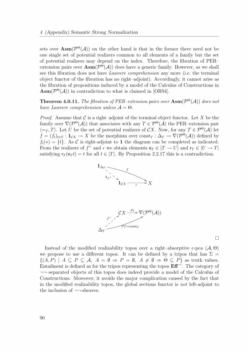
4 (Appendix) Semantic Strong Normalization
sets over Asm(PΘ(A)) on the other hand is that in the former there need not beone single set of potential realizers common to all elements of a family but the setof potential realizers may depend on the index. Therefore, the fibration of PER–extension pairs over Asm(PΘ(A)) does have a generic family. However, as we shallsee this fibration does not have Lawvere comprehension any more (i.e. the terminalobject functor of the fibration has no right–adjoint). Accordingly, it cannot arise asthe fibration of propositions induced by a model of the Calculus of Constructions inAsm(PΘ(A)) in contradiction to what is claimed in [OR94].
Theorem 4.0.11. The fibration of PER–extension pairs over Asm(PΘ(A)) does nothave Lawvere comprehension unless A = Θ.
Proof. Assume that C is a right–adjoint of the terminal object functor. Let X be thefamily over ∇(PΘ(A)) that associates with any T ∈ PΘ(A) the PER–extension pair〈=T , T 〉. Let U be the set of potential realizers of CX. Now, for any T ∈ PΘ(A) letf = (ft)t∈T : 1CX → X be the morphism over constT : ∆T → ∇(PΘ(A)) defined byft(∗) = t. As C is right-adjoint to 1 the diagram can be completed as indicated.From the realizers of f∨ and ε we obtain elements eT ∈ |T → U | and rT ∈ |U → T |satisfying rT (eT t) = t for all t ∈ |T |. By Proposition 2.2.17 this is a contradiction.
1∆Tf
&&1f∨ ""E
EE
E
1CX ε// X
CX Pε // ∇(PΘ(A))
∆T
Pf=constT
77f∨
<<zz
zz
z
Instead of the modified realizability topos over a right–absorptive c-pca (A,Θ)we propose to use a different topos. It can be defined by a tripos that has Σ =(A,P ) | A ⊆ P ⊆ A, A = ∅ ⇒ P = ∅, A 6= ∅ ⇒ Θ ⊆ P as truth values.Entailment is defined as for the tripos representing the topos Eff→. The category of¬¬–separated objects of this topos does indeed provide a model of the Calculus ofConstructions. Moreover, it avoids the major complication caused by the fact thatin the modified realizability topos, the global sections functor is not left-adjoint tothe inclusion of ¬¬-sheaves.
90
Bibliography
[Bau00] A. Bauer. The Realizability Approach to Computable Analysis and Topol-ogy. PhD thesis, School of Computer Science, Carnegie Mellon University,Pittsburgh, 2000.
[BB85] E. Bishop and D.S. Bridges. Constructive Analysis. Springer-Verlag,1985.
[BBS98] A. Bauer, L. Birkedal, and D.S. Scott. Equilogical spaces. Revised Febru-ary 2001. To appear in Theoretical Computer Science, September 1998.
[Bee75] M.J. Beeson. The nonderivability in intuitionistic formal systems of theo-rems on the continuity of effective operations. Journal of Symbolic Logic,40(3), 1975.
[Bee85] M.J. Beeson. Foundations of constructive mathematics. Springer Verlag,Berlin, 1985.
[Bir99] L. Birkedal. Developing Theories of Types and Computability. PhD thesis,School of Computer Science, Carnegie Mellon University, 1999.
[Bis67] E. Bishop. Foundations of Constructive Analysis. McGraw-Hill, NewYork, 1967.
[Bor94] F. Borceux. Handbook of Categorical Algebra 2, Categories and Struc-tures, volume 51 of Encyclopedia of Mathematics and its Applications.Cambridge University Press, 1994.
[Bou66] N. Bourbaki. Espaces vectorielles topologiques, volume XV. Hermann,1966.
[BR87] D.S. Bridges and F. Richman. Varieties of Constructive Mathematics,volume 97 of London Mathematical Society Lecture Note Series. Cam-bridge University Press, Cambridge, 1987.
[BS03] A. Bauer and A. Simpson. Two constructive embedding-extension the-orems with applications to continuity principles and to banach-mazurcomputability. submitted manuscript, 2003.
91
Bibliography
[BSV02] D.S. Bridges, P. Schuster, and L. Vıta. Apartness, topology, and uni-formity: a constructive view. Mathematical Logic Quarterly, 48(Suppl.1):16–28, 2002.
[Car95] A. Carboni. Some free constructions in realizability and proof theory.Journal of Pure and Applied Algebra, 103:117–148, 1995.
[CR98] A. Carboni and G. Rosolini. Locally cartesian closed exact completions.Journal of Pure and Applied Algebra, 1998. to appear.
[CV98] A. Carboni and E.M. Vitale. Regular and exact completions. Journal ofPure and Applied Algebra, 125:79–116, 1998.
[dMRR99] F. de Marchi, E.P. Robinson, and G. Rosolini. An abstract look at real-izability. Submitted for publication, November 1999.
[Dum77] M. Dummett. Elements of Intuitionism. Oxford University Press, Oxford,1977.
[Ers75] Y.L. Ershov. Theorie der numerierungen ii. Zeitschrift fur MathematischeLogik und Grundlagen der Mathematik, 21:473–584, 1975.
[Fri77] H. Friedman. On the derivability of instantiation properties. Journal ofSymbolic Logic, 42:506–514, 1977.
[FS91] P.J. Freyd and A. Scedrov. Categories, Allegories. North-Holland, 1991.
[Gra81] R. J. Grayson. Modified realizability toposes. Handwritten notes fromMunster University, July 1981.
[Hey30] A. Heyting. Die formalen regeln der intuitionistischen logik. In Sitzungs-berichte der Preußischen Akademie der Wissenschaften. Physikalisch-mathematische Klasse, pages 42–56, 1930.
[Hey56] A. Heyting. Intuitionism, An Introduction. North-Holland, 1956.
[HJP80] J.M.E. Hyland, P.T. Johnstone, and A.M. Pitts. Tripos theory. Math.Proc. Camb. Phil. Soc., 88:205–232, 1980.
[HK66] W.A. Howard and G. Kreisel. Transfinite induction and bar induction oftypes zero and one, and the role of continuity in intuitionistic analysis.Journal of Symbolic Logic, 31(3), 1966.
[HO93] J.M.E. Hyland and C.-H. L. Ong. Modified realizability toposes andstrong normalization proofs. In J.F. Groote and M. Bezem, editors, TypedLambda Calculi and Applications, volume 664 of Lecture Notes in Com-puter Science, pages 179–194. Springer-Verlag, 1993.
92
Bibliography
[HRR90] J.M.E. Hyland, E.P. Robinson, and G. Rosolini. The discrete objects inthe effective topos. Proceedings of the London Mathematical Society, 60,1990.
[HS96] A.J. Humphreys and S.G. Simpson. Separable banach space theory needsstrong set existence axioms. Transactions of the American MathematicalSociety, 348:4231–4255, 1996.
[Hyl82] J.M.E. Hyland. The effective topos. In A.S. Troelstra and D. vanDalen, editors, The L.E.J. Brouwer Centenary Symposium, pages 165–216. North-Holland, 1982.
[Hyl91] J.M.E. Hyland. First steps in synthetic domain theory. In A. Carboni,C. Pedicchio, and G. Rosolini, editors, Conference on Category The-ory 1990, volume 1488 of Lecture Notes in Mathematics, pages 131–156.Springer Verlag, 1991.
[Ish92] H. Ishihara. Continuity properties in constructive mathematics. Journalof Symbolic Logic, 57(2):557–565, 1992.
[Ish01] H. Ishihara. Sequentially continuity in constructive mathematics. In C.S.Calude, M.J. Dinneen, and S. Sburlan, editors, Combinatorics, Com-putability and Logic, Discrete Mathematics and Theoretical ComputerScience, pages 5–12, London, 2001. Springer. Proceedings of DMTCS2001.
[Jac99] B. Jacobs. Categorical logic and type theory. Studies in logic and foun-dations of mathematics. North-Holland, Amsterdam, 1999.
[Kle45] S.C. Kleene. On the interpretation of intuitionistic number theory. Jour-nal of Symbolic Logic, 10:109–124, 1945.
[Kle65] S.C. Kleene. Logical calculus and realizability. Acta Philosophica Fennica,18:71–80, 1965.
[Kle69] S.C. Kleene. Formalized Recursive Functionals and Formalized Relizabil-ity, volume 89 of Memoirs of the American Mathematical Society. Amer-ican Mathematical Society, 1969.
[Kre59] G. Kreisel. Interpretation of analysis by means of functionals of finitetype. In Constructivity in Mathematics. North Holland, Amsterdam,1959.
[LM84] G. Longo and E. Moggi. The hereditary partial effective functionals andrecursion theory in higher types. Journal of Symbolic Logic, 49:1319–1332,1984.
93

Bibliography
[Lon94] J. Longley. Realizability Toposes and Language Semantics. PhD thesis,University of Edinburgh, 1994.
[Lon99a] J. Longley. Matching typed and untyped realizability. InL. Birkedal, J. van Oosten, G. Rosolini, and D.S. Scott,editors, Workshop on Realizability Semantics and Applica-tions, volume 23 of Electronic Notes in Computer Science.Elsevier, 1999. Available from http://www.elsevier.nl/gej-ng/31/29/23/92/27/show/Products/notes/index.htt.
[Lon99b] J. Longley. Unifying typed and untyped realizability. Manuscript (avail-able from http://www.dcs.ed.ac.uk/home/jrl/unifying.txt), 1999.
[LS02] P. Lietz and T. Streicher. Impredicativity entails untypedness. Mathe-matical Structures in Computer Science, 12(3):335–347, 2002.
[Mac71] S. Mac Lane. Categories for the Working Mathematician. Springer Verlag,Berlin, 1971.
[Men99] M. Menni. A characterization of the left exact categories whose exactcompletions are toposes. Submitted for publication, 1999.
[Men00] M. Menni. Generic proofs and chaotic situations (extended abstract).Submitted for publication, 2000.
[Oos91] J. van Oosten. Exercises in realizability. PhD thesis, University of Ams-terdam, 1991.
[Oos97a] J. van Oosten. Extensional realizability. Annals of Pure and AppliedLogic, 84:317–349, 1997.
[Oos97b] J. van Oosten. The modified realizability topos. Journal of Pure andApplied Algebra, 116:273–289, 1997.
[Oos02] J. van Oosten. Realizability: A historical essay. Mathematical Structuresin Computer Science, 12(3):239–263, 2002.
[OR94] C.-H. L. Ong and E. Ritter. A generic strong normalization proof: appli-cation to the calculus of constructions (extended abstract). In ComputerScience Logic: 7th Workshop, CSL’93, Swansea, UK, Sep. 1993, SelectedPapers, volume 832 of Lecture Notes in Computer Science, pages 261–279.Springer Verlag, 1994.
[OS00] J. van Oosten and A. Simpson. Axioms and (counter)examples in syn-thetic domain theory. Annals of Pure and Applied Logic, 104(1–3):233–278, 2000.
94

Bibliography
[Pit81] A.M. Pitts. The Theory of Triposes. PhD thesis, Cambridge University,1981.
[Pit99] A.M. Pitts. Tripos theory in retrospect. In L. Birkedal, J. van Oosten,G. Rosolini, and D.S. Scott, editors, Workshop on Realizability Semanticsand Applications, volume 23 of Electronic Notes in Computer Science.Elsevier, 1999.
[Pit00] A.M. Pitts. Categorical logic. In S. Abramsky, D. M. Gabbay, and T. S. E.Maibaum, editors, Handbook of Logic in Computer Science, Volume 5. Al-gebraic and Logical Structures, chapter 2. Oxford University Press, 2000.
[Plo78] G.D. Plotkin. Tω as a universal domain. J. Computer and System Sci-ences, 17:209–236, 1978.
[Rog67] H. Rogers, Jr. Theory of Recursive Functions and Effective Computability.McGraw-Hill Book Company, 1967.
[Ros99] G. Rosolini. Equilogical spaces and filter spaces, 1999. to appear.
[Rud73] W. Rudin. Functional Analysis. McGraw Hill Series in Higher Mathe-matics. McGraw Hill, New York, 1973.
[Sch02] M. Schroder. Extended admissibility. Theoretical Computer Science,284(2):519–538, 2002.
[Sch03] M. Schroder. Admissible Representations for Continuous Computations.PhD thesis, FernUniversitat – Gesamthochschule Hagen, 2003.
[Spe62] C. Spector. Provably recursive functionals of analysis: a consistency proofof analysis by an extension of principles formulated in current intuition-istic mathematics. In J.C.E. Dekker, editor, Proceedings of Symposia inPure Mathematics, volume 5, pages 1–27. American Mathematical Soci-ety, 1962.
[Spi02] B. Spitters. Located operators. Mathematical Logic Quarterly, 48(Suppl.1):107–122, 2002.
[Tro73] A.S. Troelstra, editor. Metamathematical Investigation of IntuitionisticArithmetic and Analysis. Springer Verlag, 1973. With contributions byA.S. Troelstra, C.A. Smorynski, J.I. Zucker and W.A. Howard.
[Tro92] A.S. Troelstra. Comparing the theory of representations and construc-tive mathematics. In E. Borger, G. Jager, H. Kleine Buning, and M.M.Richter, editors, Computer Science Logic. 5th workshop, CSL ’91, pages382–395. Springer Verlag, 1992.
95
Bibliography
[Tro98] A.S. Troelstra. Realizability. In S.R. Buss, editor, Handbook of ProofTheory, pages 407–473. North-Holland, 1998.
[Tur36] A. Turing. On computable numbers with an application to the Entschei-dungsproblem. Proc. London Math. Soc., 42:230–265, 1936.
[TvD88a] A.S. Troelstra and D. van Dalen. Constructivism in mathematics. Anintroduction. Volume I. Number 121 in Studies in Logic and the Founda-tions of Mathematics. North-Holland, Amsterdam, 1988.
[TvD88b] A.S. Troelstra and D. van Dalen. Constructivism in mathematics. Anintroduction. Volume II. Number 123 in Studies in Logic and the Foun-dations of Mathematics. North-Holland, Amsterdam, 1988.
[Wei00] K. Weihrauch. Computable Analysis. Springer, Berlin, 2000.
96
Curriculum Vitae
Peter Lietz
geboren am 1. November 1970 in Mainz
1990 Allgemeine Hochschulreife,
Staatliches Gymnasium am Kurfurstlichen Schloß, Mainz
1991 – 1998 Studium der Mathematik mit Wahlpflichtfach Informatik,
Technische Universitat Darmstadt
1994 – 1995 Erasmus-Aufenthalt am Instituto Superior Tecnico
der Universidade Tecnica de Lisboa, Portugal
1998 Hochschulabschluss als Diplom-Mathematiker,
Diplomarbeit “A Fibrational Theory of Geometric Morphisms”
1998 – 2004 Doktorand am Fachbereich Mathematik der TU Darmstadt,
Arbeitsgruppe Logik und mathematische Grundlagen der Informatik
1998 – 1999 Teilnahme am Postgraduate Course in the Theory of Computation
des Laboratory for Foundations of Computer Science
an der University of Edinburgh
zeitweise gefordert durch ein Stipendium des Landes Hessen
zeitweise wissenschaftlicher Mitarbeiter
97


![A Formal and Constructive Theory of Computationforster/downloads/bsc-thesis.pdf · Chapter1 Introduction Computabilitytheoryisoneoftheoldestfieldsofcomputerscience. Itusuallyis taughtandcarriedoutusingclassicalmathematicalmethods,seeforinstance[10]](https://static.fdokument.com/doc/165x107/5ec9ea8675dc0534da69c2a8/a-formal-and-constructive-theory-of-computation-forsterdownloadsbsc-thesispdf.jpg)


![Mathematics by Experiment: Exploring Patterns of Integer ...users.rowan.edu/~nguyen/experimentalmath/... · experimental mathematics in [BB]: Experimental mathematics is the methodology](https://static.fdokument.com/doc/165x107/5f571ce9bdfe5b4c9e5c36bc/mathematics-by-experiment-exploring-patterns-of-integer-usersrowanedunguyenexperimentalmath.jpg)