![Das geometry Paket - mirrors.concertpass.commirrors.concertpass.com/tex-archive/macros/latex/contrib/geometry/... · Rand der Seite auf 2cm setzen möchten, können Sie einfach \usepackage[margin=2cm]{geometry}](https://static.fdokument.com/doc/165x107/60634a5762abad73cf640fa0/das-geometry-paket-rand-der-seite-auf-2cm-setzen-mchten-knnen-sie-einfach.jpg)
Geometry, Modelling and Control of Infinite Dimensional ... · Geometry, Modelling and Control of...
126
Technisch-Naturwissenschaftliche Fakultät Geometry, Modelling and Control of Infinite Dimensional Port-Hamiltonian Systems D ISSERTATION zur Erlangung des akademischen Grades D OKTOR DER T ECHNISCHEN W ISSENSCHAFTEN Angefertigt am Institut für Regelungstechnik und Prozessautomatisierung. Eingereicht von: Andreas Siuka Am Auring 14, 4533 Piberbach Betreuung: o.Univ.–Prof. Dipl.-Ing. Dr.techn. K. Schlacher Beurteilung: o.Univ.–Prof. Dipl.-Ing. Dr.techn. K. Schlacher Univ.–Prof. Dipl.-Ing. Dr.techn. A. Kugi Linz, Mai 2011. Johannes Kepler Universität Linz A-4040 Linz, Altenberger Str. 69, Internet: http://www.jku.at, DVR 0093696
Transcript of Geometry, Modelling and Control of Infinite Dimensional ... · Geometry, Modelling and Control of...
Technisch-NaturwissenschaftlicheFakultät
Geometry, Modelling and Control of
Infinite Dimensional Port-Hamiltonian Systems
DISSERTATION
zur Erlangung des akademischen Grades
DOKTOR DER TECHNISCHEN WISSENSCHAFTEN
Angefertigt am Institut für Regelungstechnik und Prozessautomatisierung.
Eingereicht von:
Andreas Siuka
Am Auring 14, 4533 Piberbach
Betreuung:
o.Univ.–Prof. Dipl.-Ing. Dr.techn. K. Schlacher
Beurteilung:
o.Univ.–Prof. Dipl.-Ing. Dr.techn. K. Schlacher
Univ.–Prof. Dipl.-Ing. Dr.techn. A. Kugi
Linz, Mai 2011.
Johannes Kepler Universität Linz
A-4040 Linz, Altenberger Str. 69, Internet: http://www.jku.at, DVR 0093696
Kurzfassung
Im konzentriert-parametrischen Fall hat sich in den letzten Jahren die Klasse der Tor-basierten Hamiltonschen Systeme besonders darin ausgezeichnet, eine strukturierte ma-thematische Systemdarstellung zu gewährleisten, welche die Anwendung sogenannter ener-giebasierter Regelungsentwürfe erlaubt. Diese Arbeit widmet sich nun der Analyse undweiteren Verallgemeinerung dieser Systemklasse hinsichtlich der Modellierung verteilt-parametrischer Systeme und der Übertragung energiebasierter Regelungsmethoden vomkonzentriert- auf den verteilt-parametrischen Fall basierend auf dem klassischen evolu-tionären Zugang. Die vorliegende Arbeit ist in drei Hauptteile gegliedert. Der erste Teilbehandelt die Analyse und Weiterentwicklung verteilt-parametrischer Tor-basierter Hamil-tonscher Systeme, wobei prinzipiell zwei Systemklassen untersucht werden, welcher in di-rekter Analogie zur Tor-basierten Hamiltonschen Darstellung konzentriert-parametrischerSysteme stehen. Um möglichst Koordinatensystem unabhängige und vor allem hinsicht-lich physikalischer Anwendungen allgemein gültige Systemklassen zu formulieren, werdenformale differentialgeometrische Konzepte genutzt, welche ein effektives mathematischesRahmenwerk für die Untersuchung verteilt-parametrischer Systeme darstellen.
Im zweiten Teil der Arbeit wird die Formulierung von Feldtheorien auf Basis des Tor-basierten Hamiltonschen Ansatzes behandelt. Dabei wird zuerst die Tor-basierte Hamil-tonsche Modellierung von Balkenmodellen untersucht, welche auf der bekannten Timos-henko Balkentheorie beruhen. Weiters werden fluiddynamische Anwendungen in Lagran-gescher Betrachtungsweise betrachtet, welche beispielsweise bei der Modellierung vonEinspritzprozessen auftreten können. Dabei wird zuerst die Tor-basierte HamiltonscheDarstellung eines bewegten, idealen Fluidkontinuums (keine viskosen Spannungen) un-tersucht, welche dann als Basis für die Tor-basierte Hamiltonsche Formulierung der be-kannten Navier-Stokes Gleichungen (in Lagrangescher Betrachtungsweise) dient. Daraufbasierend werden weiters elektrisch leitende Fluide untersucht, um so eine Tor-basierteHamiltonsche Formulierung der Grundgleichungen der Magnetohydrodynamik in Lagran-gescher Betrachtungsweise unter der Voraussetzung quasistationärer elektrodynamischerBeziehungen zu erhalten.
Der dritte Teil der Arbeit widmet sich der direkten Übertragung einer, aus dem kon-zentriert-parametrischen Fall wohl bekannten, energiebasierten Regelungsmethode – ba-sierend auf sogenannten strukturellen Invarianten – auf die verteilt-parametrische Tor-basierte Hamiltonsche Systemklasse. Dieses Konzept wird zur Regelung des Timoshenko-balkens mittels Randeingriff genutzt.
Abstract
With regard to the lumped-parameter case the Port-Hamiltonian framework has proveditself over the past years concerning a structured mathematical system description whichallows the application of so-called energy based control methods. This work focuses onthe analysis and further generalisation of this system class with respect to the modellingof distributed-parameter systems and the extension of energy based control concepts fromthe lumped- to the distributed-parameter case on the basis of the classical evolutionaryapproach. The instant work is structured in three main parts. The first part is dedicated tothe analysis and further development of distributed-parameter Port-Hamiltonian systems.In principle, two system classes will be investigated in detail, where the direct analogiesto the Port-Hamiltonian framework in the finite dimensional case will become apparent.In order to formulate a coordinate system independent and mainly general system class– with regard to physical applications – formal differential geometric concepts which re-present an effective mathematical framework for the investigation of infinite dimensionalsystems will be used.
The second part of this work deals with the formulation of field-theories based onthe Port-Hamiltonian framework. First of all, the Port-Hamiltonian formulation of beamsmodelled according to the Timoshenko beam theory is investigated. Furthermore, fluiddynamical applications in a Lagrangian setting are taken into account which may occur forthe modelling of injection processes, for instance. First, the Port-Hamiltonian formulationof an ideal fluid continuum (no viscous stresses) in motion which will serve as the basis forthe Port-Hamiltonian representation of the well-known Navier-Stokes equations (restric-ted to the Lagrangian point of view) is analysed. In addition, based on these investigationswe also take electrically conducting fluids into account leading to a Port-Hamiltonian for-mulation of the governing equations of magnetohydrodynamics in a Lagrangian setting onthe condition of quasi-stationary electrodynamic relations.
The third part of the thesis aims to directly generalise an energy based control conceptbased on so-called structural invariants – well-known in the lumped-parameter case – tothe infinite dimensional Port-Hamiltonian system class. This approach is applied to theenergy based boundary control of the Timoshenko beam.

To Sandra

Preface
This thesis was developed within my employment as a research assistant at the Institute ofAutomatic Control and Control Systems Technology which is part of the technical facultyof the Johannes Kepler University of Linz, Austria.
First of all, my deep respectfulness and my special gratitude with respect to ProfessorKurt Schlacher has to be emphasised since he encouraged me and, in particular, he arousedmy interests in control theory as well as in differential geometric issues with regard to con-trol purposes. I appreciated very much the inspiring working atmosphere at the instituteand the professional discussions; these and his never ending support contributed a lotto the growth of my work and my understanding of complex mathematical and physicalrelations.
Special thanks and deep acknowledgements go to Markus Schöberl for his scientificcomments and, especially, for his inspirations which have influenced my way of scientificthinking a lot. Furthermore, I want to thank all the colleagues and former staff at theinstitute, namely Bernhard Ramsebner, Harald Daxberger, Karl Rieger, Richard Stadlmayr,Paul Ludwig, Klaus Weichinger and Phillip Wieser as well as Julia Gabriel and ChristianHöfler for the excellent working atmosphere and the (not only scientific) discussions whichoften helped and encouraged me in continuing my research.
Finally, I want to express my thankfulness to my better half, Sandra, in particular forher understanding for my work and for all her love over the last few years. I also wantto thank my parents who have offered me the opportunity of a study, my friends and allthe persons who have supported me during the last few years. Last but not least I want tothank Stefan Söllradl for the proofreading of this thesis.
Over the past years my research was focused on the modelling and control of infi-nite dimensional Port-Hamiltonian systems. During this time-period I considered severalconcepts and I haved worked out some ideas; of course, these led to further interestingproblems which could not be completely addressed within my thesis. Finally, I hope thatthe results presented in the forthcoming chapters are useful and beneficial with respect tofurther control theoretic issues on distributed-parameter systems.
Linz, May 2011 Andreas Siuka
Contents
1 Introduction 1
2 Geometric Preliminaries 4
2.1 Bundles . . . . . . . . . . . . . . . . . . . . . . . . . . . . . . . . . . . . . . 42.1.1 Tangent, Cotangent and Vertical Bundles . . . . . . . . . . . . . . . . 42.1.2 Bundle Morphisms and Pull-back Bundles . . . . . . . . . . . . . . . 5
2.2 Jet Bundles . . . . . . . . . . . . . . . . . . . . . . . . . . . . . . . . . . . . 62.2.1 First-order Jet Bundles . . . . . . . . . . . . . . . . . . . . . . . . . . 62.2.2 Higher-order Jet Bundles . . . . . . . . . . . . . . . . . . . . . . . . 82.2.3 Integration on Manifolds . . . . . . . . . . . . . . . . . . . . . . . . . 9
2.3 Poisson Structures . . . . . . . . . . . . . . . . . . . . . . . . . . . . . . . . 10
3 Port-Hamiltonian Systems 133.1 Finite Dimensional Port-Controlled Hamiltonian Systems . . . . . . . . . . . 143.2 Infinite Dimensional Port-Controlled Hamiltonian Systems . . . . . . . . . . 17
3.2.1 The Geometry of Distributed-Parameter Systems . . . . . . . . . . . 173.2.2 First-order Hamiltonian Densities . . . . . . . . . . . . . . . . . . . . 193.2.3 Hamiltonian Evolution Equations I . . . . . . . . . . . . . . . . . . . 213.2.4 Hamiltonian Evolution Equations II . . . . . . . . . . . . . . . . . . . 293.2.5 Concluding Remarks . . . . . . . . . . . . . . . . . . . . . . . . . . . 33
4 Port-Hamiltonian Formulation of Field Theories 35
4.1 Port-Hamiltonian Modelling of the Timoshenko Beam . . . . . . . . . . . . . 364.2 Port-Hamiltonian Formulation of Fluid Dynamics . . . . . . . . . . . . . . . 40
4.2.1 The Geometry of Lagrangian Fluid Dynamics . . . . . . . . . . . . . 404.2.2 Conservation of Mass . . . . . . . . . . . . . . . . . . . . . . . . . . . 434.2.3 Stress Forms and Constitutive Relations in Fluid Dynamics . . . . . . 444.2.4 The Balance of Linear Momentum . . . . . . . . . . . . . . . . . . . 484.2.5 Port-Hamiltonian Formulation of the Ideal Fluid . . . . . . . . . . . . 504.2.6 Port-Hamiltonian Formulation of the Navier-Stokes Equations . . . . 55
4.3 Port-Hamiltonian Formulation of Magnetohydrodynamics . . . . . . . . . . 604.3.1 Electromagnetic Body Forces . . . . . . . . . . . . . . . . . . . . . . 61
I

CONTENTS CONTENTS II
4.3.2 Port-Hamiltonian Formulation of inductionless Magnetohydrodynam-ics . . . . . . . . . . . . . . . . . . . . . . . . . . . . . . . . . . . . . 68
5 Control of infinite dimensional Port-Hamiltonian Systems 735.1 Control of finite dimensional Port-Hamiltonian Systems based on Structural
Invariants . . . . . . . . . . . . . . . . . . . . . . . . . . . . . . . . . . . . . 745.2 Boundary Control of infinite dimensional Port-Hamiltonian Systems based
on Structural Invariants . . . . . . . . . . . . . . . . . . . . . . . . . . . . . 785.3 Boundary Control of the Timoshenko Beam based on Structural Invariants . 85
6 Summary and Outlook 94
A Proofs and Detailed Computations 96
A.1 The Application of the Horizontal Differential . . . . . . . . . . . . . . . . . 96A.2 The Rate of Deformation Tensors . . . . . . . . . . . . . . . . . . . . . . . . 96A.3 The Stored Energy Relation . . . . . . . . . . . . . . . . . . . . . . . . . . . 98A.4 Hamiltonian Formulation of the Ideal Fluid . . . . . . . . . . . . . . . . . . 99A.5 The first Viscous Piola-Kirchhoff Stress Form . . . . . . . . . . . . . . . . . . 101A.6 The Damping Tensor in iMHD . . . . . . . . . . . . . . . . . . . . . . . . . . 102A.7 Control of finite dimensional PCHD Systems . . . . . . . . . . . . . . . . . . 104A.8 The Equivalent Norm on Z . . . . . . . . . . . . . . . . . . . . . . . . . . . 105A.9 The Existence of the Inverse Operator A−1 . . . . . . . . . . . . . . . . . . . 108
Bibliography 111
Chapter 1Introduction
The basis for the analysis and control of complex physical systems provides a mathematicalmodel/description of the system which can be used not only for simulation purposes butalso for the stability investigations. In particular, for lumped-parameter systems the Port-Hamiltonian framework enjoys great popularity in the modelling and control communitysince it provides a structured mathematical system representation, where for many ap-plications the physics behind the governing equations becomes apparent in a remarkableway. Even this structured system description allows the application of so-called energybased control methods, see, e.g., [Gómez-Estern et al., 2001, Ortega et al., 2001, 2002,van der Schaft, 2000]. Over the past years the trend was – due to the physical interpreta-tion offered by the Port-Hamiltonian framework – to extend the Port-Hamiltonian systemclass to the distributed-parameter case, where the governing equations are represented bypartial differential equations – abbreviated as PDEs in the sequel. In this context thereexist several approaches (which are known to the author) for a possible generalisation ofthe (Port-)Hamiltonian framework to the infinite dimensional scenario;
• the polysymplectic approach going back to DeDonder/Weyl, see, e.g., [Giachettaet al., 1997, Kanatchikov, 1998] and references therein,
• a concept based on Stokes-Dirac structures, see [van der Schaft and Maschke, 2002],and references therein, and also the extensions for control purposes, e.g., [Macchelliand Melchiorri, 2004a,b, Macchelli et al., 2004c,d, Macchelli and Melchiorri, 2005,Rodriguez et al., 2001],
• and an approach based on the classical evolutionary approach, see, e.g., [Marsdenand Ratiu, 1994, Olver, 1993], and references therein, and also the extensions withregard to control purposes [Ennsbrunner and Schlacher, 2005, Ennsbrunner, 2006,Kugi, 2001, Schlacher, 2007, 2008, Schöberl et al., 2008].
Within this thesis the infinite dimensional Port-Hamiltonian system representation basedon the (classical) evolutionary approach is considered, where this work aims to analyseand further generalise this system class on the one hand with respect to the formulation ofHamiltonian field theories and on the other hand with regard to control purposes including
1
1 Introduction 2
the controller design based on the Port-Hamiltonian machinery. Roughly speaking, it is re-markable that this approach may be seen as a direct adaption of the classical evolutionaryapproach based on, e.g., [Marsden and Ratiu, 1994, Olver, 1993] and references therein,where the main difference lies in the fact that the adapted Port-Hamiltonian approach isable to consider non-trivial boundary conditions/terms. Therefore, for many applicationsit is possible to introduce so-called (energy) ports acting – besides the distributed ports –through the system boundary in order that the considered infinite dimensional system isable to interact with its environment. Even this fact is essential for concrete physical andengineering applications with regard to control purposes, where it often is of interest toinvestigate the coupling of such systems via their (energy) ports; this fact may be advanta-geously for the modelling of networks as well as for the design of controller systems whichact through the (energy) ports with the considered plant(s) – the well-known control byinterconnection methodology.
Particularly, with regard to the introduction, analysis and further development of theinfinite dimensional Port-Hamiltonian framework it is obvious that appropriate and effec-tive mathematical tools are necessary for the purpose of system formulations which shouldbe general enough in order that – besides the covering of a wide range of physical applica-tions – the system descriptions do not depend on the used coordinate system. In fact, weare interested in (a kind of) coordinate free introduction and formulation of the systemclasses; even this fact makes it, in principle, possible to specify and analyse the structuralproperties which are offered by the Port-Hamiltonian machinery in an intrinsic manner.
The thesis is organised as follows; In Chapter 2 the mathematical tools which arenecessary for a coordinate system independent treatment are briefly introduced and sum-marised, namely we will use formal differential geometric concepts. In fact, this chapterpresents only a brief survey of the geometric objects and basic concepts which are usedthroughout this work. For detailed proofs and more profound discussions concerning thegeometric machinery the interested reader is referred to [Giachetta et al., 1997, Saunders,1989], as most of the notion in this thesis is based on their work.
Chapter 3 deals with the geometric analysis of infinite dimensional Port-Hamiltoniansystems which are based on the classical evolutionary approach. Therefore, we recapit-ulate the port based system description such as in [Ennsbrunner, 2006], for instance,where it must be emphasised that we confine ourselves to the first-order case only (thehigher-order case can be found in [Ennsbrunner, 2006]). With regard to the formulationof (first-order) field theoretical applications the extension of this system representation bythe use of appropriate differential operators is illustrated.
The formulation of field theories in the Port-Hamiltonian context is the main focus ofChapter 4, where it is worth noting that, in this work, we confine ourselves to first-orderHamiltonian field theoretic applications only. First, the Port-Hamiltonian modelling ofbeam models based on the Timoshenko beam theory is presented, where specifically themain differences between the presented approach and the one on the basis of the Stokes-Dirac structures are illustrated. The main part of this chapter deals with the (Port-)Hamil-tonian formulation of the governing equations of fluid- and magnetohydrodynamics in aLagrangian setting. In fact, the motion of a fluid continuum is analysed in detail, wherethe (Port-)Hamiltonian representation of an ideal and a Newtonian fluid which lead to aPort-Hamiltonian formulation of the well-known Navier-Stokes equations in a Lagrangian
1 Introduction 3
setting is investigated. In fact, this point of view may be advantageously with respect tothe modelling and the treatment of injection processes, for instance. Furthermore, thisapproach is directly extended such that electrically conducting fluids in the presence ofexternal electromagnetic fields are taken into account which lead to a Port-Hamiltonianformulation of the governing equations of magnetohydrodynamics, however, on the con-dition of quasi-stationary electrodynamic relations.
Chapter 5 is dedicated to the controller design based on the illustrated Port-Hamilton-ian framework, where we are mainly interested in the stabilisation of so-called Hamilto-
nian boundary control systems. In fact, the well-known control via structural invariants
approach which is based on the control by interconnection methodology for finite dimen-sional Port-Hamiltonian systems is directly generalised to the presented infinite dimen-sional case, where specific criteria and conditions analogous to the lumped-parametercase which allow a systematic (boundary) controller design are derived. This approach isapplied to the energy based boundary control of the Timoshenko beam in order to demon-strate the effectiveness of this control concept.
Finally, some proofs and detailed computations can be found in the Appendix A; theseare omitted in the main parts of the thesis in order to enhance the readability. Nevertheless,the interested reader is asked to inspect these parts whenever they are referenced in thecorresponding chapters.
Chapter 2Geometric Preliminaries
The purpose of this chapter is to present the main notions of differential geometry and toillustrate the geometric objects which will be used in the sequel. It is assumed that thereader is familiar with the basic geometric concepts of manifolds, bundles and tensors.In the sequel, tensor notation and, especially, Einstein’s convention on sums will be usedto keep the formulas short and readable. We use the standard symbol ⊗ for the tensorproduct, d denotes the exterior derivative, c the natural contraction between tensor fieldsand ∧ the exterior product. Moreover, the partial derivatives are abbreviated by ∂BA withrespect to the coordinates with indices A
B and, e.g.,[mAB
]corresponds to the matrix re-
presentation of a (second-order) tensor m, for instance. The interested reader is referredto standard books dealing with differential geometry and Jet bundles such as [Boothby,1986, Giachetta et al., 1997, Saunders, 1989] for more detailed information.
2.1 Bundles
This subsection is dedicated to the introduction of the necessary bundle constructionswhich will be of essential use throughout this thesis.
2.1.1 Tangent, Cotangent and Vertical Bundles
Let us introduce the bundle π : E → B with local coordinates (X i), i = 1, . . . , m on B and(X i, xα), α = 1, . . . , n on E . A (local) section Φ : B → E , or equivalently Φ ∈ Γ (π), whichmeets π ◦ Φ = idB with respect to the identity map idB on B leads in local coordinates toxα = Φα(X i), where the set of all sections of the bundle π : E → B is denoted by Γ (π).The tangent bundle τE : T (E) → E (locally) equipped with coordinates (X i, xα, X i, xα)and the cotangent bundle τ ∗E : T ∗ (E) → E which possesses the coordinates (X i, xα, Xi, xα)can be introduced in a standard manner with respect to the holonomic bases {∂i, ∂α} and{dX i, dxα} for the tangent and cotangent spaces, respectively. Typical elements of thetangent bundle τE : T (E) → E are tangent vector fields v : E → T (E) taking in localcoordinates the form of v = vi(X i, xα)∂i + vα(X i, xα)∂α with X i = vi(X i, xα) as well asxα = vα(X i, xα) and elements of the cotangent bundle are 1-forms ω : E → T ∗ (E) =
4
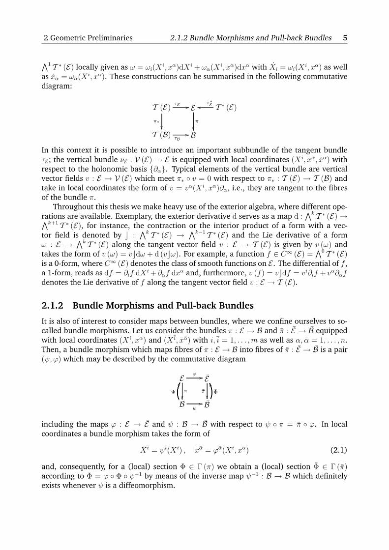
2 Geometric Preliminaries 2.1.2 Bundle Morphisms and Pull-back Bundles 5
∧1 T ∗ (E) locally given as ω = ωi(Xi, xα)dX i + ωα(X
i, xα)dxα with Xi = ωi(Xi, xα) as well
as xα = ωα(Xi, xα). These constructions can be summarised in the following commutative
diagram:
T (E)
π∗
��
τE // Eπ
��
T ∗ (E)τ∗Eoo
T (B) τB// B
In this context it is possible to introduce an important subbundle of the tangent bundleτE ; the vertical bundle νE : V (E) → E is equipped with local coordinates (X i, xα, xα) withrespect to the holonomic basis {∂α}. Typical elements of the vertical bundle are verticalvector fields v : E → V (E) which meet π∗ ◦ v = 0 with respect to π∗ : T (E) → T (B) andtake in local coordinates the form of v = vα(X i, xα)∂α, i.e., they are tangent to the fibresof the bundle π.
Throughout this thesis we make heavy use of the exterior algebra, where different ope-rations are available. Exemplary, the exterior derivative d serves as a map d :
∧k T ∗ (E) →∧k+1 T ∗ (E), for instance, the contraction or the interior product of a form with a vec-tor field is denoted by c :
∧k T ∗ (E) →∧k−1 T ∗ (E) and the Lie derivative of a form
ω : E →∧k T ∗ (E) along the tangent vector field v : E → T (E) is given by v (ω) and
takes the form of v (ω) = vcdω + d (vcω). For example, a function f ∈ C∞ (E) =∧0 T ∗ (E)
is a 0-form, where C∞ (E) denotes the class of smooth functions on E . The differential of f ,a 1-form, reads as df = ∂if dX i + ∂αf dxα and, furthermore, v (f) = vcdf = vi∂if + vα∂αf
denotes the Lie derivative of f along the tangent vector field v : E → T (E).
2.1.2 Bundle Morphisms and Pull-back Bundles
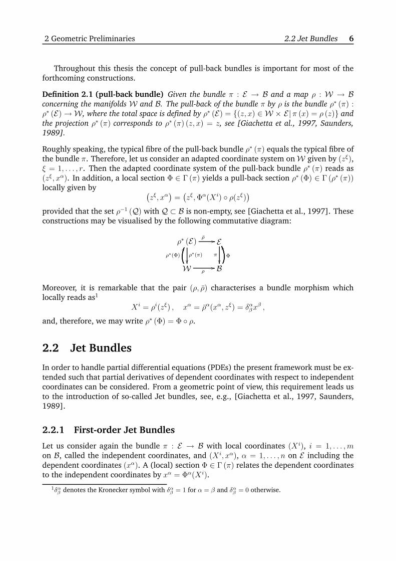
It is also of interest to consider maps between bundles, where we confine ourselves to so-called bundle morphisms. Let us consider the bundles π : E → B and π : E → B equippedwith local coordinates (X i, xα) and (X i, xα) with i, i = 1, . . . , m as well as α, α = 1, . . . , n.Then, a bundle morphism which maps fibres of π : E → B into fibres of π : E → B is a pair(ψ, ϕ) which may be described by the commutative diagram
Eπ
��
ϕ // Eπ
��B
ψ//
Φ
GG
BΦ
VV
including the maps ϕ : E → E and ψ : B → B with respect to ψ ◦ π = π ◦ ϕ. In localcoordinates a bundle morphism takes the form of
X i = ψi(X i) , xα = ϕα(X i, xα) (2.1)
and, consequently, for a (local) section Φ ∈ Γ (π) we obtain a (local) section Φ ∈ Γ (π)according to Φ = ϕ ◦ Φ ◦ ψ−1 by means of the inverse map ψ−1 : B → B which definitelyexists whenever ψ is a diffeomorphism.
2 Geometric Preliminaries 2.2 Jet Bundles 6
Throughout this thesis the concept of pull-back bundles is important for most of theforthcoming constructions.
Definition 2.1 (pull-back bundle) Given the bundle π : E → B and a map ρ : W → Bconcerning the manifolds W and B. The pull-back of the bundle π by ρ is the bundle ρ∗ (π) :ρ∗ (E) → W, where the total space is defined by ρ∗ (E) = {(z, x) ∈ W × E|π (x) = ρ (z)} and
the projection ρ∗ (π) corresponds to ρ∗ (π) (z, x) = z, see [Giachetta et al., 1997, Saunders,
1989].
Roughly speaking, the typical fibre of the pull-back bundle ρ∗ (π) equals the typical fibre ofthe bundle π. Therefore, let us consider an adapted coordinate system on W given by (zξ),ξ = 1, . . . , r. Then the adapted coordinate system of the pull-back bundle ρ∗ (π) reads as(zξ, xα). In addition, a local section Φ ∈ Γ (π) yields a pull-back section ρ∗ (Φ) ∈ Γ (ρ∗ (π))locally given by (
zξ, xα)
=(zξ,Φα(X i) ◦ ρ(zξ)
)
provided that the set ρ−1 (Q) with Q ⊂ B is non-empty, see [Giachetta et al., 1997]. Theseconstructions may be visualised by the following commutative diagram:
ρ∗ (E)
ρ∗(π)
��
ρ // Eπ
��W
ρ∗(Φ)
HH
ρ// B
Φ
WW
Moreover, it is remarkable that the pair (ρ, ρ) characterises a bundle morphism whichlocally reads as1
X i = ρi(zξ) , xα = ρα(xα, zξ) = δαβxβ ,
and, therefore, we may write ρ∗ (Φ) = Φ ◦ ρ.
2.2 Jet Bundles
In order to handle partial differential equations (PDEs) the present framework must be ex-tended such that partial derivatives of dependent coordinates with respect to independentcoordinates can be considered. From a geometric point of view, this requirement leads usto the introduction of so-called Jet bundles, see, e.g., [Giachetta et al., 1997, Saunders,1989].
2.2.1 First-order Jet Bundles
Let us consider again the bundle π : E → B with local coordinates (X i), i = 1, . . . , mon B, called the independent coordinates, and (X i, xα), α = 1, . . . , n on E including thedependent coordinates (xα). A (local) section Φ ∈ Γ (π) relates the dependent coordinatesto the independent coordinates by xα = Φα(X i).
1δαβ denotes the Kronecker symbol with δαβ = 1 for α = β and δαβ = 0 otherwise.
2 Geometric Preliminaries 2.2.1 First-order Jet Bundles 7
Definition 2.2 (1-jet of a section) Two sections Φ,Ψ ∈ Γ (π) are 1-equivalent at p ∈ B if
in some adapted coordinate system
Φα|p = Ψα|p , ∂iΦα|p = ∂iΨ
α|pare fulfilled, i.e., two sections may be identified by their values and their first-order partial
derivatives at p ∈ B. The equivalence class containing Φ is called the 1-jet j1pΦ of sections Φ
at p, see [Saunders, 1989].
The set of all the 1-jets of local sections of the bundle π possesses a natural structure asa differentiable manifold denoted by J 1 (E) called the first Jet manifold. Aside from thebundle π two additional bundles can be constructed which are given by
π1 : J 1 (E) → B , π10 : J 1 (E) → E .
It is worth mentioning that the adapted coordinate system (X i, xα) on E induces an adap-ted coordinate system on J 1 (E) given by (X i, xα, xαi ) involving the derivative coordinates
which are characterised byxαi(j1pΦ)
= ∂iΦα|p ,
where j1pΦ denotes the 1-jet of the section Φ at p ∈ B.
Definition 2.3 (first-order prolongation of sections) Given the bundle π : E → B. The
first-order prolongation of a section Φ ∈ Γ (π) is the section j1Φ : B → J 1 (E) defined by
j1Φ (p) = j1pΦ
at p ∈ B, see [Saunders, 1989].
In local coordinates a prolonged section j1Φ : B → J 1 (E) or, equivalently, j1Φ ∈ Γ (π1)reads as (
X i, xα, xαi)
=(X i,Φα(X i), ∂iΦ
α(X i)).
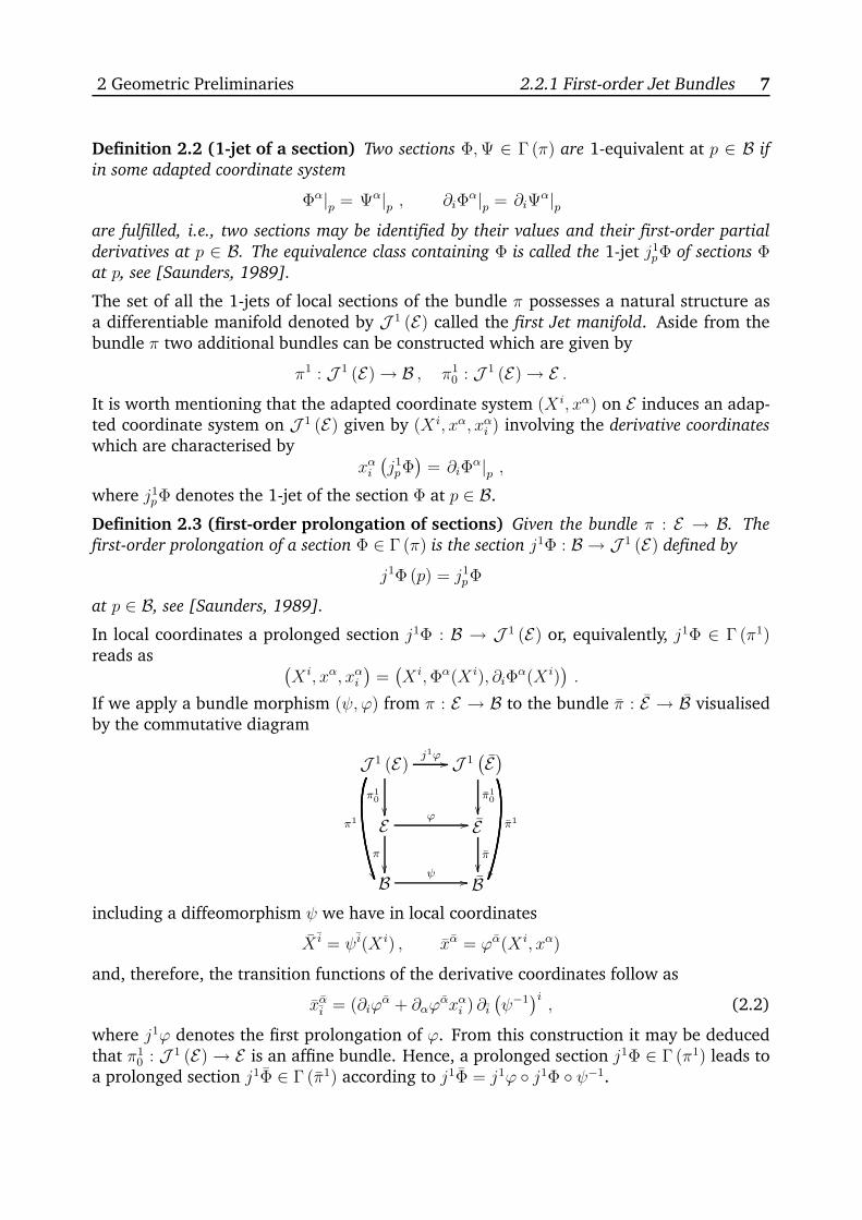
If we apply a bundle morphism (ψ, ϕ) from π : E → B to the bundle π : E → B visualisedby the commutative diagram
J 1 (E)j1ϕ //
π10
��π1
��
J 1(E)
π10
��π1
E ϕ //
π
��
Eπ
��B ψ // B
including a diffeomorphism ψ we have in local coordinates
X i = ψi(X i) , xα = ϕα(X i, xα)
and, therefore, the transition functions of the derivative coordinates follow as
xαi = (∂iϕα + ∂αϕ
αxαi ) ∂i(ψ−1
)i, (2.2)
where j1ϕ denotes the first prolongation of ϕ. From this construction it may be deducedthat π1
0 : J 1 (E) → E is an affine bundle. Hence, a prolonged section j1Φ ∈ Γ (π1) leads toa prolonged section j1Φ ∈ Γ (π1) according to j1Φ = j1ϕ ◦ j1Φ ◦ ψ−1.
2 Geometric Preliminaries 2.2.2 Higher-order Jet Bundles 8
2.2.2 Higher-order Jet Bundles
In order to take higher-order derivative coordinates into account we have to introducehigher-order Jet bundles which may be constructed in an analogous manner as the first-order ones, see [Giachetta et al., 1997, Saunders, 1989], for instance. To keep the formulasshort and readable we use the formal notion of an unordered multi-index J , where the kth-order partial derivative is denoted by
∂J = ∂jk ◦ . . . ◦ ∂j1 .
The unordered multi-index J denotes a collection of numbers according to (j1, . . . , jk)with jl = {1, . . . , m} for l = 1, . . . , k, i.e., it specifies which derivatives are taken intoaccount, and the order of the multi-index, denoted by #J = k, characterises the numberof derivatives which are needed (modulo permutations), see [Giachetta et al., 1997, Olver,1993]. Especially, the notation J, i is an abbreviation for (j1, . . . , jk, i) and for the case#J = 0 we have the identity ∂JΦ = Φ for Φ ∈ Γ (π).
Roughly speaking, we define the r-jet of a section Φ ∈ Γ (π) analogously to Definition2.2, where the set of all the r-jets of local sections Φ ∈ Γ (π) leads to the introductionof the r
th Jet manifold J r (E) which is equipped with adapted coordinates (X i, xαJ ) with0 ≤ #J ≤ r. In particular, for #J = 0 we set xαJ = xα. Therefore, it is clear that we areable to state
. . .πr+1r→ J r (E)
πrr−1→ J r−1 (E) → . . .→ J 2 (E)π21→ J 1 (E)
π10→ J 0 (E) = E π→ B ,
where the additional bundles
πr : J r (E) → B , πrs : J r (E) → J s (E) , s < r ,
can be constructed. In this context we can define the r-order prolongation of a (local)section Φ ∈ Γ (π) by jrΦ : B → J r (E) or, equivalently, jrΦ ∈ Γ (πr) which takes in localcoordinates the form of
(X i, xα, xαJ
)=(X i,Φα(X i), ∂JΦ
α(X i)), 1 ≤ #J ≤ r .
For the extension of a bundle morphism to higher-order Jet bundles a special operatormust be introduced.
Definition 2.4 (total derivative) The vector field di : J r+1 (E) → (πr+1r )
∗(T (J r (E))) which
reads as
di = ∂i + xαJ,i∂Jα , 0 ≤ #J ≤ r ,
is called the total derivative with respect to the independent coordinate X i and meets
di (f) ◦ jr+1Φ = ∂i (f ◦ jrΦ)
for f ∈ C∞ (J r (E)) and sections Φ ∈ Γ (π), see [Saunders, 1989].
2 Geometric Preliminaries 2.2.3 Integration on Manifolds 9
The introduction of the total derivative allows the extension of the bundle morphism (2.1)with respect to high-order cases, where the transition functions are given by (2.2) and
xαI ,j = dj (xαI ) ∂j(ψ−1
)j, 1 ≤ #I ≤ r , (2.3)
see [Giachetta et al., 1997]. If the bundle morphism (2.1) is induced by a 1-parametertransformation group then it is of particular interest to investigate the prolongation ofthe transformation group by defining the prolongation of the corresponding infinitesimalgenerators. In fact, we confine ourselves to the prolongation of infinitesimal generatorsrepresented by vertical vector fields only.
Definition 2.5 (prolongation of vertical vector fields) Given a vertical vector field v : E →V (E) with local representation v = vα(X i, xα)∂α. The r-order prolongation of this vector field
is given by jrv : J r (E) → V (J r (E)) and takes in local coordinates the form of
jrv = vα∂α + dJ (vα) ∂Jα , 1 ≤ #J ≤ r ,
with respect to dJ = djr ◦ . . . ◦ dj1, see [Olver, 1993].
2.2.3 Integration on Manifolds
In the sequel the integration on manifolds plays an important role. Therefore, we assumethat the base manifold B is an oriented compact manifold with (coherently oriented) boun-dary ∂B, where it is of interest to integrate over certain differential forms. Thus, we brieflyintroduce the well-known Theorem of Stokes which will be of essential use for all furtherconstructions. For more detailed information the reader is referred to, e.g., [Boothby,1986, Frankel, 2004].
Theorem 2.1 (Stokes’ Theorem) Let B be an oriented compact m-dimensional manifold
with coherently oriented boundary ∂B and ω : B →∧m−1 T ∗ (B) a continuously differentiable
(m− 1)-form on B. Then, we have2
ˆ
B
dω =
ˆ
∂B
ι∗ (ω)
with the inclusion mapping ι : ∂B → B, see [Boothby, 1986].
Having the total derivative at one’s disposal we are able to introduce the horizontal diffe-rential in this context.
Definition 2.6 (horizontal differential) Consider the form ω : J r (E) →∧
T ∗ (J r (E)).The horizontal differential is defined by
dh (ω) = dX i ∧ di (ω) ,
see [Giachetta et al., 1997, Saunders, 1989].
2The boundary is called coherently oriented if ∂B = (−1)m∂B is met, where ∂B denotes the boundary
with respect to the orientation induced by B see, e.g., [Boothby, 1986].
2 Geometric Preliminaries 2.3 Poisson Structures 10
The horizontal differential and the exterior derivative are linked by the following lemma.
Lemma 2.1 Given a section Φ ∈ Γ (π). The relation
d ◦(jkΦ
)∗=(jk+1Φ
)∗ ◦ dh
holds for every k ≥ 0, see [Saunders, 1989].
In particular, for integrals over the oriented compact manifold B involving horizontal dif-ferentials this result enables us to deduce
ˆ
B
(jr+1Φ
)∗(dh (ω)) =
ˆ
B
d ((jrΦ)∗ ω) =
ˆ
∂B
ι∗ ((jrΦ)∗ ω) .
Remark 2.1 It is worth noting that the application of the horizontal differential of (m− 1)-forms ω : J r (E) → (πr)∗
(∧m−1 T ∗ (B))
on B which take in local coordinates the form of
ω = ωi∂icdX , dX = dX1 ∧ . . . ∧ dXm , ωi ∈ C∞ (J r (E)) ,
is equivalent to the divergence theorem, see [Marsden and Hughes, 1994, Olver, 1993], for
instance.
2.3 Poisson Structures
Poisson structures play a prominent role for the characterisation and, especially, the ana-lysis of finite dimensional Hamiltonian systems, see, e.g., [Giachetta et al., 1997, Marsdenand Ratiu, 1994, Olver, 1993] and references therein. In this section we consider an n-dimensional (smooth) manifold M locally equipped with coordinates (xα), α = 1, . . . , n.
Definition 2.7 (Poisson bracket) A manifold M is called a Poisson manifold if it is equip-
ped with a Poisson bracket which is a bilinear map {·, ·} : C∞ (M) × C∞ (M) → C∞ (M)satisfying
1. Skew-Symmetry
{F,W} = −{W,F}2. Leibniz Rule
{F,W · P} = {F,W} · P +W · {F, P}3. Jacobi Identity
{{F,W} , P} + {{P, F} ,W} + {{W,P} , F} = 0
for F,W, P ∈ C∞ (M), i.e., {·, ·} is a derivation in each factor, see [Marsden and Ratiu, 1994,
Olver, 1993].
2 Geometric Preliminaries 2.3 Poisson Structures 11
Therefore, a Poisson bracket for F,W ∈ C∞ (M) can be uniquely defined as
{F,W} = (JcdW )cdF , (2.4)
where J is a contravariant skew-symmetric tensor called the structure tensor in local coor-dinates given by
J = Jαβ∂α ⊗ ∂β , Jαβ ∈ C∞ (M) , α, β = 1, . . . , n .
Moreover, in local coordinates (2.4) reads as
{F,W} = (∂αF ) Jαβ (∂βW ) .
The components of J are defined by the basic brackets Jαβ ={xα, xβ
}called the structure
functions satisfying the condition of skew-symmetry
Jαβ ={xα, xβ
}= −
{xβ , xα
}= −Jβα
and the Jacobi Identity
{{xα, xβ
}, xγ}
+{{xγ , xα} , xβ
}+{{xβ , xγ
}, xα}
= 0
which takes the equivalent form of
Jεγ(∂εJ
αβ)
+ Jεβ (∂εJγα) + Jεα
(∂εJ
βγ)
= 0 (2.5)
due to
{{xα, xβ
}, xγ}
={Jαβ , xγ
}=(∂εJ
αβ)Jεδ (∂δx
γ) =(∂εJ
αβ)Jεγ ,
{{xγ , xα} , xβ
}=
{Jγα, xβ
}= (∂εJ
γα)Jεδ(∂δx
β)
= (∂εJγα) Jεβ ,{{
xβ, xγ}, xα}
={Jβγ , xα
}=(∂εJ
βγ)Jεδ (∂δx
α) =(∂εJ
βγ)Jεα
with α, β, γ, δ, ε = 1, . . . , n, cf. [Olver, 1993], for instance. It is worth mentioning that theexterior derivative applied to functions on M serves as a map d : C∞ (M) → T ∗ (M) andthe structure tensor J is a skew-symmetric map of the form J : T ∗ (M) → T (M) sinceJcdW = Jαβ (∂βW ) ∂α.
In this context the notion of a Poisson bracket leads to the definition of a Hamilto-nian vector field, see [Giachetta et al., 1997, Marsden and Ratiu, 1994, Olver, 1993], forinstance.
Definition 2.8 (Hamiltonian vector field) Let us consider a Poisson manifold M together
with a smooth function H ∈ C∞ (M) called the Hamiltonian. A Hamiltonian vector field
vH : M → T (M) possesses the property
vH (F ) = {F,H} = (JcdH)cdF
for an arbitrary smooth function F ∈ C∞ (M), where vH (F ) denotes the Lie derivative of F
along vH .
2 Geometric Preliminaries 2.3 Poisson Structures 12
In local coordinates a Hamiltonian vector field reads as vH = vαH(xα)∂α with xα = vαH(xα)and, therefore, vH (F ) = vαH(xα)∂αF = {F,H}. Consequently, Hamilton’s equations can beformulated as
xα = vαH(xα) = Jαβ∂βH
or, equivalently, in a coordinate free manner
x = vH = JcdH . (2.6)
Remark 2.2 If J locally satisfies rank([Jαβ])
= 2k ≤ dim (M) = n then it is possible to find
(local) canonical coordinates such that the Poisson bracket for F,W ∈ C∞ (M) becomes
{F,W} = (∂iF )(∂iW
)−(∂iF
)(∂iW ) , ∂i =
∂
∂qi, ∂i =
∂
∂pi,
with respect to x = (q, p, z) and i = 1, . . . , k, j = 1, . . . , n− 2k whenever (2.5) is fulfilled. In
this case, the Hamiltonian vector field is given as
vH =(∂iH
)∂i − (∂iH) ∂i
and (2.6) takes (locally) the form of
qi = ∂iH , pi = −∂iH , zj = 0 .
Moreover, if 2k = n is (locally) fulfilled, i.e.,[Jαβ]
has full rank, then the standard Poisson
manifold becomes a symplectic manifold with even rank n and the equations are (locally)
given by
qi = ∂iH , pi = −∂iHwhich characterise the canonical form of Hamilton’s equations. For more detailed information
see, e.g., [Marsden and Ratiu, 1994, Olver, 1993].
Remark 2.3 If in Definition 2.7 the properties are relaxed such that the Jacobi Identity is
dropped then we speak about a generalised Poisson bracket on a generalised Poisson mani-
fold. This fact is rather essential for the introduction of the Port-Hamiltonian system repre-
sentation, see, e.g., [Dalsmo and van der Schaft, 1999, Stramigioli et al., 1998]. However, it
is worth noting that for the case of a generalised Poisson bracket it is, in general, not ensured
that a canonical representation exists.
Chapter 3Port-Hamiltonian Systems
In the finite dimensional case the Hamiltonian formalism is well-known, where the gover-ning equations are represented in an evolutionary first-order form. From a system theoreticpoint of view, whenever the Hamiltonian corresponds to the system’s total energy, the re-sulting system equations describe, in general, an autonomous, lossless system, where theHamiltonian serves as a conserved quantity. In order to generalise this framework withregard to dissipative effects and the definition of system in- and outputs the so-called Port-Controlled Hamiltonian system representation (with dissipation) was introduced. It hasbecome an essential tool not only for modelling, system analysis and simulation purposesbut also for the application of energy based control methods based on the underlying struc-tural properties of this system class, see [Ortega et al., 2001, 2002, van der Schaft, 2000],for instance.
With respect to the extension of the Hamiltonian framework to the infinite dimensio-nal case there exist several approaches; the polysymplectic approach going back to De-Donder/Weyl (e.g. [Giachetta et al., 1997, Kanatchikov, 1998] and references therein), aconcept based on Stokes-Dirac structures (see [van der Schaft and Maschke, 2002]) andthe classical evolutionary approach (see, e.g., [Marsden and Ratiu, 1994, Olver, 1993]and references therein). As mentioned before, in order to obtain a Port-Hamiltonian de-scription, we confine ourselves to an extension of the classical evolutionary approach withregard to control purposes based on [Ennsbrunner, 2006], where it must be emphasisedthat we restrict ourselves to the first-order case only, i.e., we mainly focus our interests onfirst-order Hamiltonian field theory (for control purposes) as in [Ennsbrunner and Schla-cher, 2005, Schlacher, 2007, 2008, Schöberl et al., 2008]. It is remarkable that this ap-proach may be seen as a direct adaption of the classical evolutionary approach, wherethe main difference lies in the fact that the extended approach is able to consider non-trivial boundary conditions/terms which is crucial for concrete physical and engineeringapplications concerning control aspects. Furthermore, according to [Ennsbrunner, 2006]an infinite dimensional Port-Hamiltonian system representation can be introduced on thebasis of specific multilinear maps by full analogy with the finite dimensional case.
Finally, it must be emphasised that we focus our interests on a geometric descriptionin a coordinate system independent manner in order that system and structural propertieswhich do not depend on the used coordinate system can be specified. This fact is rather
13
3 Port-Hamiltonian Systems 3.1 Finite Dimensional PCHD Systems 14
essential particularly with regard to subjects like physical based modelling and systemanalysis.
In Section 3.1 the well-known Port-Controlled Hamiltonian system class in the finitedimensional scenario is analysed in detail based on a geometric point of view. This partshould be seen as the basis for the forthcoming section since the introduced geometricobjects and concepts allow a generalisation to the distributed-parameter case; this topic isthe main focus of section 3.2, where the extension of this system class to the distributed-parameter case on the basis of specific multilinear maps is discussed and analysed in detailbased on [Ennsbrunner, 2006, Schlacher, 2007, 2008, Schöberl et al., 2008]. Particularly,with respect to the formulation of (first-order) field theoretical applications the extensionof this system representation by means of appropriate differential operators is illustrated.
3.1 Finite Dimensional Port-Controlled Hamiltonian Sys-
tems
Let us consider an n-dimensional (smooth) manifold M - called the state manifold - locallyequipped with coordinates (xα), α = 1, . . . , n and a Hamiltonian H ∈ C∞ (M) which des-cribes the total energy of the considered Hamiltonian system (2.6) for many applications.If we compute the total time change of the Hamiltonian along the solutions of (2.6) whichequals the Lie derivative of H along the Hamiltonian vector field vH we obtain vH (H) = 0in consideration of the skew-symmetry of the underlying Poisson structure. In this case,the Hamiltonian serves as a conserved quantity and, therefore, from a system theoreticpoint of view the equations (2.6) describe, in general, a lossless and autonomous system.Consequently, it is obvious to extend this system class with respect to dissipative effectsand the introduction of appropriate system in- and outputs which leads to the definitionof the Port-Controlled Hamiltonian system representation, see [van der Schaft, 2000].
Definition 3.1 (PCHD system) A Port-Controlled Hamiltonian System (with dissipation),
or PCH(D) system for short, is given as
x = v = (J − R)cdH + ucG (3.1)
y = G∗cdH
with the skew-symmetric interconnection map J , the symmetric positive semidefinite dissipa-
tion map R and the input map G as well as its adjoint map G∗ with respect to the system
input u and the collocated output y. Furthermore, the total change of the Hamiltonian along
the solutions of (3.1) reads as
v (H) = − (RcdH)cdH + ucy ≤ ucy . (3.2)
Of course, for this setting the total derivative serves as a map d : C∞ (M) → T ∗ (M)and the interconnection and the dissipation maps are maps of the form J,R : T ∗ (M) →T (M), where the interconnection map J is skew-symmetric, i.e., it fulfils for arbitraryfunctions W,F ∈ C∞ (M) the relation
(JcdW )cdF + (JcdF )cdW = 0 ,
3 Port-Hamiltonian Systems 3.1 Finite Dimensional PCHD Systems 15
and the dissipation map R is a symmetric and positive semidefinite map according to
(RcdW )cdF − (RcdF )cdW = 0 , (RcdW )cdW ≥ 0 .
Thus, these maps are appropriate tensors in local coordinates given by
J = Jαβ∂α ⊗ ∂β , R = Rαβ∂α ⊗ ∂β ,
where the components satisfy Jαβ = −Jβα, Rαβ = Rβα and Jαβ, Rαβ ∈ C∞ (M). Fur-thermore, we introduce the input vector bundle υ : U → M (locally) equipped withcoordinates (xα, uξ), ξ = 1, . . . , m, with respect to the holonomic basis {eξ} as well as thedual vector bundle υ∗ : Y = U∗ → M – called the output vector bundle – which (lo-cally) possesses the coordinates (xα, yξ) and the basis {eξ} for the fibres. In this contextthe input map is given by G : U → T (M) and its adjoint (dual) map corresponds toG∗ : T ∗ (M) → U∗ = Y . Therefore, the relation
(ucG)cdH = uc (G∗cdH) = ucy
is fulfilled characterising the port with respect to the system input u and the correspondingcollocated output y. Hence, the input map G as well as its adjoint map G∗ can be bothrepresented by an appropriate tensor which in local coordinates reads as
G = Gαξ e
ξ ⊗ ∂α , Gαξ ∈ C∞ (M) .
Finally, it must be emphasised that the vector field v is not a tangent vector field on T (M)any more since it depends on the input u. In fact, it is a vector field of the pull-backbundle1 υ∗ (τM) : υ∗ (T (M)) → U or, equivalently, it can be interpreted as a submanifoldof T (M) parameterised by u.
It is worth mentioning that (3.2) states nothing else than the balance of energy prin-ciple, whenever the Hamiltonian H corresponds to the total energy of the system. In thiscase the change of the system’s energy is equal to the difference of the power flow into thesystem characterised by the (energy) port ucy and the dissipated power (RcdH)cdH.
Remark 3.1 If the system (3.1) is modelled autonomous and no dissipation is considered
then the interconnection map induces a generalised Poisson structure. If, in addition, the
components Jαβ meet (2.5) then J is equivalent to the structure tensor and the vector field v
is defined as a Hamiltonian vector field vH in a classical manner, see Definition 2.8.
Finally, a PCHD system in local coordinates reads as
xα = vα(xα, uξ
)=
(Jαβ −Rαβ
)∂βH +Gα
ξ uξ
yξ = Gαξ ∂αH , (3.3)
and (3.2) takes the form of
v (H) = − (∂αH)Rαβ (∂βH) + yξuξ
with respect to the corresponding vector field v = vα(xα, uξ
)∂α.
1To enhance the readability the underlying pull-back structure is suppressed in the definition of therelevant maps.
3 Port-Hamiltonian Systems 3.1 Finite Dimensional PCHD Systems 16
Remark 3.2 It is worth noting that the structure of a PCHD system is preserved by diffeo-
morphisms of the form xα = ϕα(xα) with α = 1, . . . , n and the transition functions for the
input bundle read as uξ = ψξξ(x
α)uξ, ξ = 1, . . . , m, where [ψξξ(xα)] is invertible. For the case of
an affine input bundle which allows for affine input transformations see, e.g., [Schöberl and
Schlacher, 2007b].
Structural Invariants for PCHD Systems
Structural invariants or so-called Casimir functions play a prominent role for the analysisof Hamiltonian systems, see, e.g., [Marsden and Ratiu, 1994, Olver, 1993] and for thedevelopment of control concepts based on the Port-Hamiltonian framework, see [Ortegaet al., 2001, van der Schaft, 2000], for instance.
Definition 3.2 (structural invariant, PCHD system) A structural invariant C ∈ C∞ (M)for a PCHD system (3.1) satisfies in local coordinates the set of PDEs
∂αC(Jαβ −Rαβ
)= 0 (3.4)
implying that the total change of C along the solutions of (3.1) results in
v (C) = xcdC = (ucG)cdC
which holds independently of the Hamiltonian H. If, additionally, u = 0 or G∗cdC = 0 is met,
then the structural invariant serves as a conserved quantity for the PCHD system (3.1). In the
case of rank([Jαβ − Rαβ
])= n the structural invariant is called trivial, see [van der Schaft,
2000].
Consequently, in local coordinates Definition 3.2 implies
v (C) = ∂αC(Jαβ −Rαβ
)∂βH + (∂αC)Gα
ξ uξ = (∂αC)Gα
ξ uξ ,
where for uξ = 0 or (∂αC)Gαξ = 0 the total change of the structural invariant C along
the solutions of (3.1) vanishes, i.e., v (C) = 0 and in this case it serves as a conservedquantity for (3.1). It is worth mentioning that structural invariants are only characterisedby the underlying structural properties of the system; i.e., they are completely determinedby the interconnection and the dissipation map of the PCHD system and, thus, they do notdepend on the system’s Hamiltonian.
Remark 3.3 For the autonomous and non-dissipative case the structural invariants are com-
pletely determined by the underlying (generalised) Poisson structure. In this case a structural
invariant fulfils
{C,H} = 0 , ∀H ,
see, e.g., [Marsden and Ratiu, 1994, Olver, 1993], which locally implies (∂αC) Jαβ = 0.
3 Port-Hamiltonian Systems 3.2 Infinite Dimensional PCHD Systems 17
3.2 Infinite Dimensional Port-Controlled Hamiltonian Sys-
tems
This section is dedicated to the extension of the Port-Hamiltonian framework to the dis-tributed-parameter case, where we are interested in an evolutionary representation of thegoverning equations. In fact, the underlying geometric concepts of the state manifold,etc. which are introduced in order to characterise a finite dimensional PCHD system mustbe replaced by appropriate geometric objects. Therefore, we take the Jet machinery intoaccount, see section 2.2. Furthermore, we investigate the concept of an evolutionary vec-tor field which characterises a certain set of PDEs, where the main objective is to find aPort-Hamiltonian formulation of these equations by generalising the relevant geometricconcepts and objects from the finite dimensional scenario.
3.2.1 The Geometry of Distributed-Parameter Systems
The state of a distributed-parameter system is given by a certain set of functions on acompact manifold D (with coherently oriented boundary ∂D) locally equipped with coor-dinates (X i), i = 1, . . . , m, where the state may be described by a section of the bundleπ : X → D - called the state bundle - which locally possesses the coordinates (X i, xα),α = 1, . . . , n. For this setting (X i) denotes the independent spatial coordinates and (xα)the dependent coordinates. Moreover, the time t plays the role of the curve (evolution)parameter and, thus, it is no coordinate in this context. Therefore, a section of the statebundle Φ ∈ Γ (π) describes in local coordinates the state of the infinite dimensional systemby xα = Φα(X i).
In the sequel we need some important geometric structures which can be directlyconstructed from the state bundle. First of all, we introduce the rth Jet manifold J r (X )equipped with adapted coordinates (X i, xα, xαJ ), 1 ≤ #J ≤ r and all the required Jetbundles. Furthermore, we are able to construct the exterior pull-back bundle
(πr)∗(
m∧T ∗ (D)
)→ J r (X ) ,
with respect to the fibre basis {dX}, dX = dX1 ∧ . . . ∧ dXm, where the sections of thisbundle are r-order densities of the form F dX with F ∈ C∞ (J r (X )) and the (global)volume form dX, as well as the bundle
(πr0)∗ (T ∗ (X )) ∧ (πr)∗
(m∧
T ∗ (D)
)→ J r (X ) (3.5)
with the basis {dxα ∧ dX} for the fibres, whose sections are given by χα dxα ∧ dX withcomponents χα ∈ C∞ (J r (X )). These sections are covector valued forms which may beinterpreted as densities with directions. In this context the presented geometric frameworkallows to define a functional F as the integral over a r-order density on D. More precisely,it serves as a map F : Γ (π) → R and takes the form of
F (Φ) =
ˆ
D
(jrΦ)∗ (F dX) , F ∈ C∞ (J r (X )) .
3 Port-Hamiltonian Systems 3.2.1 Geometry of Distributed-Parameter Systems 18
Finally, we consider the vertical bundle νX : V (X ) → X which possesses the coordinates(X i, xα, xα) and which allows the introduction of a so-called evolutionary vector field.
Definition 3.3 (evolutionary vector field) The vector field v : J r (X ) → (πr0)∗ (V (X )) is
called an evolutionary vector field and is locally given by v = vα∂α with vα ∈ C∞ (J r (X ))which corresponds to the set of PDEs
X i = 0 , xα = vα , vα ∈ C∞ (J r (X )) , (3.6)
inclusive appropriate boundary conditions, see [Olver, 1993]. These equations describe a set
of r-order evolution equations, where the curve (evolution) parameter (of the solution) is the
time t.
It is worth noting that the evolutionary vector field does not generate a flow since it is notangent vector field. However, on a time interval [0, T ] ⊂ R
+0 together with appropriate
boundary conditions it may generate a semi group according to
γt : [0, T ] × Γ (π) → Γ (π) , t ∈ [0, T ] (3.7)
which maps sections to sections of the state bundle π : X → D such that
Φt = γt (Φ0) , Φt1+t2 = γt2 ◦ γt1 (Φ0)
hold with Φ0,Φt,Φt1+t2 ∈ Γ (π) and t, t1 + t2 ∈ [0, T ], where Φ0 ∈ Γ (π) denotes the initialstate/condition. In addition, the semi group satisfies
∂tγαt (Φ0) = vα ◦ jr (γt (Φ0))
and, especially,2
∂tγαt (Φ0)|t=0 = vα ◦ jrΦ0 .
Finally, it must be mentioned that an evolutionary vector field can also be extended to aprolonged evolutionary vector field, where according to Definition 2.5 the s-order prolon-gation of an evolutionary vector field v : J r (X ) → (πr0)
∗ (V (X )) is given by
jsv : J r+s (X ) →(πr+ss
)∗(V (J s (X ))) (3.8)
and takes in local coordinates the form of jsv = vα∂α + dJ (vα) ∂Jα with 1 ≤ #J ≤ s, seealso [Olver, 1993].
In the sequel, the main objective will be to investigate the concept of an evolutionaryvector field in more detail in order to find a Port-Hamiltonian representation of a set of(r-order) evolution equations which are characterised by such a vector field.
2In particular, it is assumed that the given problem is well-posed in the sense of Hadamard, i.e., thereexist suitable normed function spaces for the solution which is unique and varies continuously with the initialstate, see [Curtain and Zwart, 1995]. This (rather strong) assumption must usually be investigated for eachparticular application.
3 Port-Hamiltonian Systems 3.2.2 First-order Hamiltonian Densities 19
3.2.2 First-order Hamiltonian Densities
In the infinite dimensional case we deal with a Hamiltonian functional of the form
H (Φ) =
ˆ
D
(j1Φ)∗
(H dX) , H ∈ C∞(J 1 (X )
), (3.9)
where we confine ourselves in this thesis to the case of first-order Hamiltonian densitiesH dX with H ∈ C∞ (J 1 (X )) only. For the higher-order case the interested reader isreferred to [Ennsbrunner, 2006]. In the finite dimensional scenario the total change of theHamiltonian H ∈ C∞ (M) along the solutions of (3.1) – given by (3.2) – has turned outto play a crucial role on the one hand for the characterisation of the dissipative effects andon the other hand for the introduction of the (energy) ports. Therefore, in this subsectionwe are mainly interested in the analysis of the formal change of (3.9) along (3.7) in orderto obtain an analogous expression in terms of an evolutionary vector field which will allowthe characterisation of an infinite dimensional Port-Hamiltonian system afterwards.
Formal Change of the Hamiltonian Functional
The change of (3.9) along (3.7) is formally given by3,4
v (H (Φ)) =
ˆ
D
(jr+1Φ
)∗ (j1v (H dX)
)=
ˆ
D
(jr+1Φ
)∗ (j1vcd (H dX)
),
with respect to the first-order case and in consideration of the evolutionary vector field v :J r (X ) → (πr0)
∗ (V (X )) with r ≥ 2, where its first prolongation takes in local coordinatesthe form of
j1v = vα∂α + di (vα) ∂iα .
Consequently, we locally obtain
v (H (Φ)) =
ˆ
D
(jrΦ)∗ (vα∂αH dX) +
ˆ
D
(jr+1Φ
)∗ (di (v
α) ∂iαH dX)
and integration by parts leads to
v (H (Φ)) =
ˆ
D
(jrΦ)∗ (vαδαH dX) +
ˆ
D
(jr+1Φ
)∗ (di(vα∂iαH dX
)),
where we have introduced the variational derivative δα (·) = ∂α (·) − di (∂iα (·)), see, e.g.,
[Olver, 1993]. It is worth noting that, in this case, the variational derivative serves as amap
δ :(π1)∗(
m∧T ∗ (D)
)→(π2
0
)∗(T ∗ (X )) ∧
(π2)∗(
m∧T ∗ (D)
)(3.10)
3In the sequel, this construction will be called the formal change of the Hamiltonian functional.4If the semi group (3.7) parameterised in t exists, then the formal change of the Hamiltonian functional
(involving the pull-back of the Hamiltonian density by the semi group) equals the time derivative of thefunctional provided that all applied operations are admissible.
3 Port-Hamiltonian Systems 3.2.2 First-order Hamiltonian Densities 20
and its application takes in local coordinates the form of5
δ (H dX) = δαH dxα ∧ dX . (3.11)
In terms of the horizontal differential, see Appendix A.1, we are able to state
v (H (Φ)) =
ˆ
D
(jrΦ)∗ (vαδαH dX) +
ˆ
D
(jr+1Φ
)∗ (dh(vα∂iαH ∂icdX
))
which is equivalent to
v (H (Φ)) =
ˆ
D
(jrΦ)∗ (vαδαH dX) +
ˆ
∂D
ι∗((jrΦ)∗
(vα∂iαH ∂icdX
))
by applying Lemma 2.1 and Stokes’ Theorem. Therefore, it is obvious to introduce aboundary map, see, e.g., [Schlacher, 2007, Schöberl et al., 2008], of the form
δ∂ :(π1)∗(
m∧T ∗ (D)
)→(π1
0
)∗(T ∗ (X )) ∧
(π1)∗(m−1∧
T ∗ (D)
)(3.12)
whose application takes in local coordinates the form of
δ∂ (H dX) = ∂iαH dxα ∧ ∂icdX . (3.13)
Finally, we are able to end up with the formal change of the Hamiltonian functional (3.9)along (3.7) in a coordinate free manner
v (H (Φ)) =
ˆ
D
(jrΦ)∗ (vcδ (H dX)) +
ˆ
∂D
ι∗((jrΦ)∗
(vcδ∂ (H dX)
)). (3.14)
This important result is the basis for all further investigations with respect to the genera-lisation of the Port-Hamiltonian framework to the distributed-parameter case. In fact, theformal change of the Hamiltonian functional splits into two parts; the first part is definedinside the domain involving the variational derivative which serves as the map (3.10) andthe second part degenerates to a boundary term with respect to the introduced boundarymap (3.12). Furthermore, it is clear that both parts – on the domain as well as on theboundary – are characterised by certain pairings involving the evolutionary vector fieldand the terms (3.11), (3.13) respectively. Therefore, with regard to the introduction of aninfinite dimensional Port-Hamiltonian system representation it is obvious that by an ap-propriate choice of the evolution equations characterised by the evolutionary vector fieldit will be possible on the one hand to distinguish structural properties not only inside thedomain but also on the boundary and on the other hand these specific pairings will al-low the introduction of (energy) ports acting inside the domain as well as through theboundary. Before we proceed with the extension of the Port-Hamiltonian framework tothe considered distributed-parameter case we intend to investigate the boundary term inmore detail.
5In fact, these expressions are covector valued forms which are sections of the bundle (3.5) for r = 2.
3 Port-Hamiltonian Systems 3.2.3 Hamiltonian Evolution Equations I 21
Boundary Term
In order to find a more manageable expression for the boundary term in local coordinateswe introduce the boundary pull-back bundle ι∗ (π) : ι∗ (X ) → ∂D equipped with coordi-nates
(X i∂∂ , x
α), i∂ = 1, . . . , m− 1, where the inclusion mapping ι : ∂D → D is assumed to
be given by
ι :(X i∂∂
)→(X i∂ = X i∂
∂ , Xm = const.
), i∂ = 1, . . . , m− 1 , (3.15)
see, [Ennsbrunner and Schlacher, 2005, Ennsbrunner, 2006, Schöberl et al., 2008]. In thiscontext the coordinates
(X i∂∂
)on ∂D are called adapted to the boundary if (3.15) is met.
Therefore, we are able to introduce a corresponding boundary volume form
dX∂ = ∂mcdX = (−1)m−1 dX1∂ ∧ . . . ∧ dXm−1
∂
and a boundary section Φ∂ ∈ Γ (ι∗ (π)) which is related to a section Φ ∈ Γ (π) accordingto Φ∂ = ι∗ (Φ) = Φ ◦ ι or, equivalently, ι∗ ◦ Φ∗ = Φ∗
∂ . Furthermore, we are also able topull-back certain Jet bundles to the boundary. Therefore, we consider the bundle ι∗ (πr) :ι∗ (J r (X )) → ∂D with adapted coordinates
(X i∂∂ , x
α, xαJ), 1 ≤ #J ≤ r, where a prolonged
section jrΦ ∈ Γ (πr) leads to ι∗ (jrΦ) = jrΦ ◦ ι which is abbreviated by6 Φr∂ = ι∗ (jrΦ) or,
equivalently, (Φr∂)
∗ = ι∗ ◦ (jrΦ)∗.Having this machinery at one’s disposal the boundary term can be reformulated in local
coordinates asˆ
∂D
ι∗((jrΦ)∗
(vα∂iαH ∂icdX
))=
ˆ
∂D
(Φr∂)
∗ ((vα ◦ ι) (∂mα H ◦ ι) dX∂) ,
or, equivalently,ˆ
∂D
ι∗((jrΦ)∗
(vcδ∂ (H dX)
))=
ˆ
∂D
(Φr∂)
∗ (ι∗(vcδ∂ (H dX)
))(3.16)
withι∗ (v) = (vα ◦ ι) ∂α , (vα ◦ ι) ∈ C∞ (ι∗ (J r (X ))) ,
as well as
ι∗(δ∂ (H dX)
)= ι∗
(∂iαH dxα ∧ ∂icdX
)= (∂mα H ◦ ι) dxα ∧ dX∂
with(∂mα H ◦ ι) ∈ C∞
(ι∗(J 1 (X )
)).
3.2.3 Hamiltonian Evolution Equations I
The investigations from the last subsection and, especially, the important result (3.14) en-able us to propose a direct generalisation of Definition 3.1 to the distributed-parameter
6Note that Φr∂ 6= jrΦ∂ , in general, since the pull-back boundary bundles are not equipped with an under-lying Jet bundle structure.
3 Port-Hamiltonian Systems 3.2.3 Hamiltonian Evolution Equations I 22
case based on [Ennsbrunner, 2006, Schlacher, 2007, 2008], for instance. Therefore, weintroduce a coordinate-free version of an infinite dimensional PCHD system, where it isworth mentioning that we restrict ourselves to the case that the proposed system classmay describe a set of second-order evolution equations. In fact, for this case, the intercon-nection, the dissipation as well as the input map are represented by appropriate multilinearmaps by direct analogy with the finite dimensional case. It is worth noting that we willoften denote this case as the so-called non-differential operator case in order to avoidconfusions since in the next subsection we will further generalise this system class by re-placing the relevant multilinear maps by appropriate differential operators. Furthermore,it is remarkable that the proposed system class enables us to directly characterise the mainstructural properties known from the lumped-parameter case concerning the (physical)interpretation of the interconnection and the dissipation map and for the introduction ofthe (energy) ports we have two possibilities, i.e., we consider on the one hand distributedports and on the other hand so-called boundary ports which describe for many applica-tions the influence of the boundary conditions. Moreover, this system class also allows theintroduction of structural invariants together with the derivation of the necessary condi-tions in an analogous manner as in the finite dimensional case, where it is worth notingthat the variational derivative will play a crucial role.
The iPCHD System Class (the Non-Differential Operator Case)
Based on the investigations from the last subsection and, in particular, with respect to theformal change of the functional (3.14) we are able to introduce a direct generalisation ofDefinition 3.1 to the distributed-parameter case based on [Ennsbrunner, 2006, Schlacher,2007, 2008], for instance, by an appropriate choice of the considered evolution equations.
Definition 3.4 (iPCHD system, non-differential operator case) An infinite dimensional
PCHD system, or iPCHD system for short, with the Hamiltonian functional (3.9) is given
as
x = v = (J −R) (δ (H dX)) + ucGy = G∗cδ (H dX) (3.17)
inclusive appropriate boundary conditions together with X = 0 and with the skew-symmetric
interconnection map J , the symmetric positive semidefinite dissipation map R, the input
map G as well as its adjoint map G∗ with respect to the distributed system input u and the
distributed collocated output y. Furthermore, the formal change of the Hamiltonian functional
(3.9) along (3.7) takes the form of
v (H (Φ)) = −ˆ
D
(j2Φ)∗
(R (δ (H dX))cδ (H dX)) +
ˆ
D
(j2Φ)∗
(ucy)
+
ˆ
∂D
ι∗((j2Φ)∗ (
vcδ∂ (H dX))), (3.18)
3 Port-Hamiltonian Systems 3.2.3 Hamiltonian Evolution Equations I 23
with respect to the evolutionary vector field v7.
In this context the variational derivative which serves as a map according to (3.10) nowplays the analogous role of the exterior derivative in the lumped-parameter case and theinterconnection and the dissipation maps are maps of the form
J ,R :(π2
0
)∗(T ∗ (X )) ∧
(π2)∗(
m∧T ∗ (D)
)→(π2
0
)∗(V (X )) , (3.19)
where the interconnection map J serves as a skew-symmetric map according to
J (ω)c$ + J ($)cω = 0
for ω = ωαdxα ∧ dX and $ = $αdx
α ∧ dX with ωα, $α ∈ C∞ (J 2 (X )) and the dissipationmap R is symmetric and positive semidefinite, i.e.,
R (ω)c$ −R ($)cω = 0 , R (ω)cω ≥ 0 .
Furthermore, in local coordinates these maps read as
J (ω) = J αβωβ ∂α , R (ω) = Rαβωβ ∂α , β = 1, . . . , n ,
with respect to the components J αβ = −J βα, Rαβ = Rβα and J αβ ,Rαβ ∈ C∞ (J 2 (X )).Moreover, the input map G as well as its adjoint map G∗ are defined by
G : U →(π2
0
)∗(V (X )) , G∗ :
(π2
0
)∗(T ∗ (X )) ∧
(π2)∗(
m∧T ∗ (D)
)→ Y , (3.20)
where υ : U → J 2 (X ) denotes the input vector bundle (locally) equipped with coordinates(X i, xα, xαJ , u
ξ) with 1 ≤ #J ≤ 2 and ξ = 1, . . . , nu with respect to the holonomic basis{eξ}. Therefore, the output vector bundle can be defined as the dual bundle υ∗ : Y =U∗ → J 2 (X ) which possesses the local coordinates (X i, xα, xαJ , yξ) as well as the fibrebasis
{eξ ⊗ dX
}. Furthermore, it is dual to the input vector bundle with respect to the
bilinear map8
Y ×J 2(X ) U →m∧
T ∗ (D)
in local coordinates given by the interior product
ucy =(uξeξ
)c (yηe
η ⊗ dX) = yξuξ dX , η = 1, . . . , nu .
Consequently, we are able to derive the relation
(ucG)cδ (H dX) = uc (G∗cδ (H dX)) = ucy7It is remarkable that the evolutionary vector field v is not a tangent vector field on
(π2
0
)∗
(V (X )) anymore since it depends on the distributed input u. However, in order to enhance the readability we suppressthe underlying pull-back structure in the definition of the relevant maps in the sequel.
8In order to enhance the readability we suppress the underlying pull-back constructions in the definitionof the bilinear map.
3 Port-Hamiltonian Systems 3.2.3 Hamiltonian Evolution Equations I 24
characterising the port distributed over D. Thus, the input map G and its adjoint map G∗
can both be represented by the tensor
G = Gαξ eξ ⊗ ∂α , Gαξ ∈ C∞(J 2 (X )
),
and, therefore, in local coordinates we obtain
ucG =(uξeξ
)c(Gαη eη ⊗ ∂α
)= Gαξ uξ∂α
as well as
G∗cδ (H dX) =(Gαξ eξ ⊗ ∂α
)c(δβH dxβ ∧ dX
)= Gαξ δαH eξ ⊗ dX = yξ e
ξ ⊗ dX .
Hence, it is clear that in local coordinates the proposed iPCHD system representation(3.17) reads as
xα = vα =(J αβ −Rαβ
)δβH + Gαξ uξ
yξ = Gαξ δαH
and (3.18) locally takes the form of
v (H (Φ)) = −ˆ
D
(j2Φ)∗ (
(δαH)Rαβ (δβH) dX)
+
ˆ
D
(j2Φ)∗ (
yξuξ dX
)
+
ˆ
∂D
ι∗((j2Φ)∗ (
vα∂iαH ∂icdX)),
with respect to the evolutionary vector field v = vα∂α.
Remark 3.4 It is worth noting that the structure of an iPCHD system is preserved by bundle
morphisms of the form (2.1) which possess the transition functions (2.2) as well as (2.3)
and the transition functions for the input bundle read as uξ = φξξu
ξ, ξ = 1, . . . , nu, with
φξξ ∈ C∞ (J 2 (X )), where [φξξ] is invertible. For more detailed information see [Schlacher,
2008].
Remark 3.5 In order to emphasise the main differences between the presented Port-Hamil-
tonian framework and the classical evolutionary approach (e.g., [Marsden and Ratiu, 1994,
Olver, 1993]) it is worth noting that in the infinite dimensional case a Poisson bracket may
be defined as a bilinear map according to
{W,Q} (Φ) =
ˆ
D
(j2Φ)∗
(J (δ (Q dX))cδ (W dX)) =
ˆ
D
(j2Φ)∗ (
(δαW)J αβ (δβQ) dX)
for the functionals
W (Φ) =
ˆ
D
(j1Φ)∗
(W dX) , Q (Φ) =
ˆ
D
(j1Φ)∗
(Q dX)
with W,Q ∈ C∞ (J 1 (X )), satisfying the condition of skew-symmetry
{W,Q} (Φ) = −{Q,W} (Φ)
3 Port-Hamiltonian Systems 3.2.3 Hamiltonian Evolution Equations I 25
and the Jacobi Identity
{{W,Q} ,P} (Φ) + {{P,W} ,Q} (Φ) + {{Q,P} ,W} (Φ) = 0
for all functionals W,Q,P with P (Φ) =´
D(j1Φ)
∗(P dX), P ∈ C∞ (J 1 (X )), see, e.g.,
[Marsden and Ratiu, 1994, Olver, 1993]. Thus, the map J is defined according to (3.19). It
is worth mentioning that the Leibniz’ Rule has no counterpart in this setting. Furthermore, a
Hamiltonian (evolutionary) vector field vH may be defined by
vH (F (Φ)) = {F,H} (Φ) +
ˆ
∂D
ι∗((j2Φ)∗ (
vHcδ∂ (F dX)))
(3.21)
which in local coordinates reads as
vH (F (Φ)) =
ˆ
D
(j2Φ)∗ (
(δαF)J αβ (δβH) dX)
+
ˆ
∂D
ι∗((j2Φ)∗ (
vαH∂iαF ∂icdX
))
for an arbitrary functional F (Φ) =´
D(j1Φ)
∗(F dX), F ∈ C∞ (J 1 (X )), splitting into a
term defined on the domain and an appropriate boundary term, cf. (3.14), with respect
to the Hamiltonian functional (3.9). Therefore, Hamilton’s equations may be defined by
x = vH = J (δ (H dX)).These considerations may be seen as a direct link to the classical evolutionary approach
(applied to the non-differential operator case), see, e.g., [Marsden and Ratiu, 1994, Olver,
1993], where the classical approach is only able to consider trivial boundary conditions/terms
and, thus, no boundary term is necessary for the definition of a Hamiltonian (evolutionary)
vector field vH. Hence, if in (3.21) the boundary term vanishes, then vH corresponds to the
classical definition of a Hamiltonian (evolutionary) vector field as in [Marsden and Ratiu,
1994, Olver, 1993], for instance.
Remark 3.6 If in Remark 3.5 the Jacobi Identity is dropped then we may speak about a
generalised Poisson bracket. Therefore, if the system (3.17) is a lossless system, i.e., R = 0,
and we have no distributed port then the map J induces a generalised Poisson structure
and the evolutionary vector field v of Definition 3.4 may be interpreted as a Hamiltonian
(evolutionary) vector field vH according to (3.21).
Next, we intend to analyse the boundary term, where we are mainly interested in deter-mining appropriate boundary in- and outputs which will lead us to the introduction ofso-called boundary ports.
Boundary Ports
The remaining task will be to investigate the boundary term in more detail which allowsthe introduction of (energy) ports acting through the boundary ∂D for many applicationsprovided that the physical meaning is apparent. Thus, in consideration of (3.16) theboundary term can be reformulated as
ˆ
∂D
ι∗((j2Φ)∗ (
vcδ∂ (H dX)))
=
ˆ
∂D
(Φ2∂
)∗ (ι∗(vcδ∂ (H dX)
))(3.22)
3 Port-Hamiltonian Systems 3.2.3 Hamiltonian Evolution Equations I 26
which in local coordinates is equivalent toˆ
∂D
(Φ2∂
)∗((xα ◦ ι) (∂mα H ◦ ι) dX∂)
with Φ2∂ = j2Φ◦ ι. With regard to the introduction of the (energy) ports acting through the
boundary it must be emphasised that due to the pairing in (3.22) the determination of theboundary in- and outputs clearly is not unique. Therefore, we are interested in deriving arelation of the form9
(xα ◦ ι) (∂mα H ◦ ι) dX∂ = y∂,ξ∂ uξ∂∂ dX∂ = u∂ξ∂ y
∂,ξ∂ dX∂ ,
where it is clear that there are, in general, two main possibilities for the choices of theboundary in- and outputs (or even combinations of them). For the investigation of the firstpossibility we introduce the boundary input vector bundle ν∂ : U∂ → ι∗ (J 2 (X )) equippedwith local coordinates (X i∂
∂ , xα, xαJ , u
ξ∂∂ ) with 1 ≤ #J ≤ 2, ξ∂ = 1, . . . , n∂u and the holonomic
basis {e∂,ξ∂} as well as the dual boundary vector bundle ν∗∂ : Y∂ = U∗∂ → ι∗ (J 2 (X )) – the
boundary output vector bundle – which possesses the local coordinates (X i∂∂ , x
α, xαJ , y∂,ξ∂)
and the fibre basis {eξ∂∂ ⊗ dX∂} with respect to the bilinear map
Y∂ ×ι∗(J 2(X )) U∂ →m−1∧
T ∗ (D)
in local coordinates given by the interior product
u∂cy∂ =(uξ∂∂ e∂,ξ∂
)c (y∂,η∂ e
η∂∂ ⊗ dX∂) = y∂,ξ∂ u
ξ∂∂ dX∂ , η∂ = 1, . . . , n∂u .
Therefore, we introduce the boundary map G∂ as well as the adjoint boundary map G∗∂
both represented by the tensor
G∂ = Gα∂,ξ∂ eξ∂∂ ⊗ ∂α , Gα∂,ξ∂ ∈ C∞
(ι∗(J 2 (X )
)),
and choose u∂cG∂ = ι∗ (v) which in local coordinates reads as
u∂cG∂ =(uξ∂∂ e∂,ξ∂
)c(Gα∂,η∂ e
η∂∂ ⊗ ∂α
)= Gα∂,ξ∂ u
ξ∂∂ ∂α = (xα ◦ ι) ∂α .
Thus, we obtain the boundary port
(u∂cG∂)cι∗(δ∂ (H dX)
)= u∂c
(G∗∂cι∗
(δ∂ (H dX)
))= u∂cy∂ (3.23)
with respect to the collocated boundary output y∂ = G∗∂cι∗
(δ∂ (H dX)
)including the ad-
joint boundary map G∗∂ , where in local coordinates we obtain
G∗∂cι∗
(δ∂ (H dX)
)=(Gα∂,ξ∂ e
ξ∂∂ ⊗ ∂α
)c((∂mβ H ◦ ι
)dxβ ∧ dX∂
)
= Gα∂,ξ∂ (∂mα H ◦ ι) eξ∂∂ ⊗ dX∂ = y∂,ξ∂ eξ∂∂ ⊗ dX∂ .
9Note the abuse of notation. In the sequel, we write ∂D even when the boundary ports are only definedon a part of ∂D.
3 Port-Hamiltonian Systems 3.2.3 Hamiltonian Evolution Equations I 27
For the other choice of the boundary ports we introduce the boundary input vector bundleν∂ : U∂ → ι∗ (J 2 (X )) with local coordinates (X i∂
∂ , xα, xαJ , u
∂ξ∂
) and the holonomic basis{e∂,ξ∂} as well as the dual boundary vector bundle ν∂,∗ : Y∂ = U∂,∗ → ι∗ (J 2 (X )) equippedwith local coordinates (X i∂
∂ , xα, xαJ , y
∂,ξ∂) and the basis {dX∂ ⊗ e∂ξ∂} for the fibres withrespect to the bilinear map
U∂ ×ι∗(J 2(X )) Y∂ →m−1∧
T ∗ (D)
which is locally given by the interior product
y∂cu∂ =(y∂,ξ∂ dX∂ ⊗ e∂ξ∂
)c(u∂η∂ e
∂,η∂)
= u∂ξ∂ y∂,ξ∂ dX∂ .
Hence, the boundary map G∂ as well as its adjoint map G∂,∗ can be introduced which areboth given by the tensor
G∂ = G∂,ξ∂α dxα ∧ dX∂ ⊗ e∂ξ∂ , G∂,ξ∂α ∈ C∞(ι∗(J 2 (X )
)),
and we choose G∂cu∂ = ι∗(δ∂ (H dX)
)locally given as
G∂cu∂ =(G∂,ξ∂α dxα ∧ dX∂ ⊗ e∂ξ∂
)c(u∂η∂ e
∂,η∂)
= G∂,ξ∂α u∂ξ∂ dxα ∧ dX∂ = (∂mα H ◦ ι) dxα ∧ dX∂ .
Therefore, we obtain the boundary port
ι∗ (v)c(G∂cu∂
)=(ι∗ (v)cG∂,∗
)cu∂ = y∂cu∂ (3.24)
with respect to the collocated boundary output y∂ = ι∗ (v)cG∂,∗, where in local coordinateswe obtain
ι∗ (v)cG∂,∗ = (xα ◦ ι) ∂αc(G∂,ξ∂β dxβ ∧ dX∂ ⊗ e∂ξ∂
)
= G∂,ξ∂α (xα ◦ ι) dX∂ ⊗ e∂ξ∂ = y∂,ξ∂ dX∂ ⊗ e∂ξ∂ .
It is worth noting that we have only investigated the two main possibilities for the choiceof the boundary ports, although, a combination of them is possible since the exact choicedepends on the considered problem. For a more general discussion on this topic the inter-ested reader is referred to [Ennsbrunner, 2006].
In conclusion, it may be said that the formal change of the Hamiltonian functional (3.9)along (3.7) consists of the dissipative effects inside the domain, the distributed port andthe boundary port which may be defined by the relations (3.23) or (3.24) respectively (oreven combinations of them) and which characterises for many applications the influenceof the boundary conditions. Consequently, it is worth mentioning that (3.18) states no-thing else than the balance of energy principle, whenever the Hamiltonian functional (3.9)corresponds to the total energy of the system.
3 Port-Hamiltonian Systems 3.2.3 Hamiltonian Evolution Equations I 28
Structural Invariants for iPCHD Systems
Analogously to the lumped-parameter case we are also able to define structural invariantsfor the distributed-parameter case, where in the distributed-parameter scenario the defini-tion of the boundary ports play a crucial role. Therefore, we confine ourselves to the twomain parameterisations of the boundary ports stated in (3.23) as well as (3.24).
Definition 3.5 (structural invariant, iPCHD system) A structural invariant for an iPCHD
system (3.17) with H ∈ C∞ (J 1 (X )) is given by
C (Φ) =
ˆ
D
(j1Φ)∗
(C dX) , C ∈ C∞(J 1 (X )
).
First, for the boundary port parameterisation (3.23) it satisfies in local coordinates the set
of PDEs
δαC(J αβ −Rαβ
)= 0
implying that the formal change of C along (3.7) results in
v (C (Φ)) =
ˆ
D
(j2Φ)∗
((ucG)cδ (C dX)) +
ˆ
∂D
(Φ2∂
)∗ ((u∂cG∂)cι∗
(δ∂ (C dX)
)).
If, additionally, u = 0 or G∗cδ (C dX) = 0 as well as u∂ = 0 or G∗∂cι∗
(δ∂ (C dX)
)= 0, then the
structural invariant serves as a conserved quantity for the iPCHD system (3.17) concerning
the case (3.23).
Second, for the boundary port parameterisation (3.24) it satisfies the set of PDEs
δαC(J αβ −Rαβ
)= 0 , (xα ◦ ι) (∂mα C ◦ ι) = 0
and the formal change of C along (3.7) results in
v (C (Φ)) =
ˆ
D
(j2Φ)∗
((ucG)cδ (C dX)) .
If, additionally, u = 0 or G∗cδ (C dX) = 0 is met, then the structural invariant serves as a
conserved quantity for (3.17) with respect to the case (3.24).
In the case of rank([J αβ −Rαβ
])= n, C is a total derivative (for both cases) only.
These conditions follow by a direct computation and may be seen as a direct adaptionof Definition 3.2 to the introduced iPCHD system representation. Especially, for the caserank
([J αβ −Rαβ
])= n it is clear that δαC = 0 must be satisfied which is fulfilled for total
derivatives of the form C = di(Ci)
with Ci ∈ C∞ (X ) since
δα(di(Ci))
= ∂α(di(Ci))
− dj∂jα
(di(Ci))
= ∂α(di(Ci))
− di(∂α(Ci))
= 0 .
For this case, it is worth mentioning that a structural invariant simplifies to
C (Φ) =
ˆ
D
(j1Φ)∗ (
di(Ci)dX)
=
ˆ
∂D
ι∗(Ci ◦ Φ ∂icdX
)
by applying the horizontal differential.
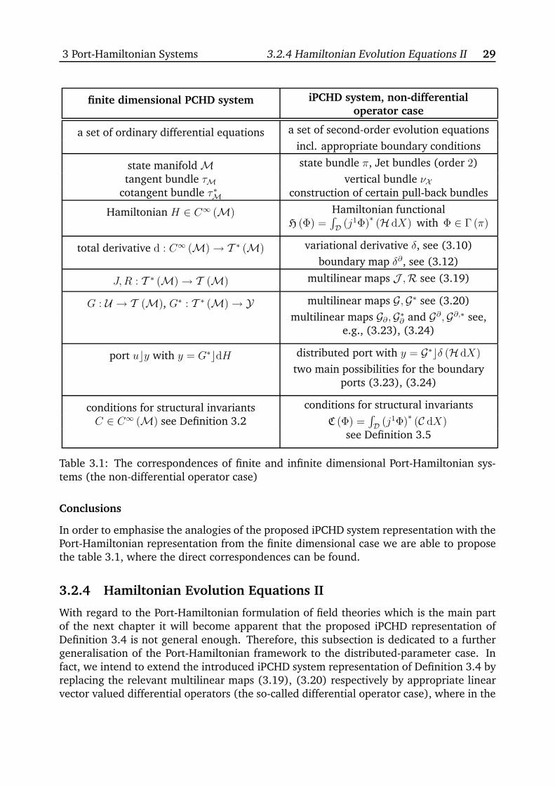
3 Port-Hamiltonian Systems 3.2.4 Hamiltonian Evolution Equations II 29
finite dimensional PCHD system iPCHD system, non-differentialoperator case
a set of ordinary differential equations a set of second-order evolution equations
incl. appropriate boundary conditions
state manifold M state bundle π, Jet bundles (order 2)
tangent bundle τM vertical bundle νXcotangent bundle τ ∗M construction of certain pull-back bundles
Hamiltonian H ∈ C∞ (M) Hamiltonian functionalH (Φ) =
´
D(j1Φ)
∗(H dX) with Φ ∈ Γ (π)
total derivative d : C∞ (M) → T ∗ (M) variational derivative δ, see (3.10)
boundary map δ∂, see (3.12)
J,R : T ∗ (M) → T (M) multilinear maps J ,R see (3.19)
G : U → T (M), G∗ : T ∗ (M) → Y multilinear maps G,G∗ see (3.20)
multilinear maps G∂ ,G∗∂ and G∂,G∂,∗ see,
e.g., (3.23), (3.24)
port ucy with y = G∗cdH distributed port with y = G∗cδ (H dX)
two main possibilities for the boundaryports (3.23), (3.24)
conditions for structural invariants conditions for structural invariants
C ∈ C∞ (M) see Definition 3.2 C (Φ) =´
D(j1Φ)
∗(C dX)
see Definition 3.5
Table 3.1: The correspondences of finite and infinite dimensional Port-Hamiltonian sys-tems (the non-differential operator case)
Conclusions
In order to emphasise the analogies of the proposed iPCHD system representation with thePort-Hamiltonian representation from the finite dimensional case we are able to proposethe table 3.1, where the direct correspondences can be found.
3.2.4 Hamiltonian Evolution Equations II
With regard to the Port-Hamiltonian formulation of field theories which is the main partof the next chapter it will become apparent that the proposed iPCHD representation ofDefinition 3.4 is not general enough. Therefore, this subsection is dedicated to a furthergeneralisation of the Port-Hamiltonian framework to the distributed-parameter case. Infact, we intend to extend the introduced iPCHD system representation of Definition 3.4 byreplacing the relevant multilinear maps (3.19), (3.20) respectively by appropriate linearvector valued differential operators (the so-called differential operator case), where in the
3 Port-Hamiltonian Systems 3.2.4 Hamiltonian Evolution Equations II 30
sequel both iPCHD representations and even combinations of them will turn out to be theadequate description for field theories based on the Port-Hamiltonian framework. Never-theless, it must be emphasised that the forthcoming iPCHD representation concerning thedifferential operator case is too general regarding the introduction of the boundary portsand, therefore, after the general definition of the system class we take two specific opera-tors which will play a crucial role for the applications in the next chapter into account.
Linear Vector Valued Differential Operators
Before we proceed we have to introduce the considered differential operators. Roughlyspeaking, a differential operator serves as a map from a jet bundle (or a specific pull-backbundle) to a manifold; in fact, we restrict ourselves to specific linear differential operatorswhich are maps from a pull-back bundle to a specific vector space.
Definition 3.6 (linear vector valued differential operator) An r-order linear vector va-
lued differential operator is a map of the form
D : (πp0)∗(T ∗ (X )) ∧ (πp)∗
(m∧
T ∗ (D)
)→(πp+r0
)∗(V (X )) , p ≥ 0 , r > 0 ,
which is locally given by
D (ω) = DαβJdJ (ωβ) ∂α , 0 ≤ #J ≤ r , dJ = djr ◦ . . . ◦ dj1 ,
with respect to ω = ωα dxα ∧ dX with ωα ∈ C∞ (J p (X )) and the components DαβJ ∈C∞ (J p (X )). Furthermore, its (formal) adjoint takes the form of
D∗ (ω) = (−1)#JdJ(DβαJωβ
)∂α .
It is worth mentioning that the adjoint operator can be easily obtained by integration byparts leading to
D (ω)c$ = D∗ ($)cω + dh (d) , (3.25)
with respect to ω = ωαdxα ∧ dX as well as $ = $αdx
α ∧ dX with ωα, $α ∈ C∞ (J p (X ))and d = di ∂icdX, where the components di are bilinear expressions involving the com-ponents ωα, $α and total derivatives of them up to order r − 1, see, e.g., [Olver, 1993].Furthermore, the specification of the adjoint operator allows an important characterisationof the operator itself.
Definition 3.7 (skew-, self-adjoint operator) An r-order linear vector valued differential
operator D is called skew-adjoint if D∗ = −D and it is self-adjoint if D∗ = D, respectively,
see [Olver, 1993].
In the sequel the objective is to extend the iPCHD system representation by means of appro-priate linear vector valued differential operators, where, in particular, the characterisationof the operators of Definition 3.7 plays an important role.
3 Port-Hamiltonian Systems 3.2.4 Hamiltonian Evolution Equations II 31
The iPCHD System Class (the Differential Operator Case)
Having this framework at one’s disposal the iPCHD system representation can be furthergeneralised, where the interconnection and the dissipation map are represented by r-orderlinear vector valued differential operators according to Definition 3.6 and the input mapalso serves as a linear differential operator in this context.
Definition 3.8 (iPCHD system, differential operator case) An iPCHD system with respect
to the differential operator case with the Hamiltonian functional (3.9) reads as
x = v = (J − R) (δ (H dX)) + G (u) (3.26)
y = G∗ (δ (H dX))
inclusive appropriate boundary conditions together with X = 0 and with the skew-adjoint
operator J, the self-adjoint non-negative operator R as well as the input operator G and
its (formal) adjoint G∗ with respect to the distributed input u and the distributed collocated
output y. Furthermore, the formal change of the Hamiltonian functional (3.9) along (3.7)
takes the form of
v (H (Φ)) =
ˆ
D
(j2+rΦ
)∗((J − R) (δ (H dX))cδ (H dX)) +
ˆ
D
(j2+rΦ
)∗(G (u)cδ (H dX))
+
ˆ
∂D
ι∗((j2+rΦ
)∗ (vcδ∂ (H dX)
)). (3.27)
For this case the operators J and R are r-order linear vector valued differential operatorswhich are maps of the form
J,R :(π2
0
)∗(T ∗ (X )) ∧
(π2)∗(
m∧T ∗ (D)
)→(π2+r
0
)∗(V (X )) , r > 0 , (3.28)
where J is a skew-adjoint operator according to
J (ω)c$ + J ($)cω = dh (j) , j = ji ∂icdX , (3.29)
with ω = ωαdxα ∧ dX, $ = $αdx
α ∧ dX as well as ωα, $α ∈ C∞ (J 2 (X )) and R is anon-negative self-adjoint operator, i.e.,
R (ω)c$ − R ($)cω = dh (r) , r = ri ∂icdX , R (ω)cω ≥ 0 . (3.30)
The input operator G and its adjoint operator G∗ are maps according to
G : U →(π2+r
0
)∗(V (X )) , G∗ :
(π2
0
)∗(T ∗ (X )) ∧
(π2)∗(
m∧T ∗ (D)
)→ Y (3.31)
and they are linear r-order differential operators with respect to the relation
G (u)cω = ucG∗ (ω) + dh (g) , g = gi ∂icdX , (3.32)
3 Port-Hamiltonian Systems 3.2.4 Hamiltonian Evolution Equations II 32
where G and its adjoint G∗ are locally given by
G (u) = GαJξ dJ
(uξ)∂α , G∗ (ω) = (−1)#J
dJ(GαJξ ωα
)eξ ⊗ dX .
These operators may also be interpreted as r-order linear vector valued differential ope-rators, though, with respect to the corresponding in- and output vector bundles10. In thiscontext the components ji and ri are bilinear expressions involving the components ωα, $α
and total derivatives of them up to order r − 1 as well as the components gi which arebilinear expressions, too, and which contain the components uξ, ωα and total derivativesof them up to order r − 1. Consequently, from (3.32) we are able to derive the relation
G (u)cδ (H dX) = ucG∗ (δ (H dX)) + dh (g) = ucy + dh (g)
characterising the port distributed over D. Hence, it is obvious that an iPCHD system ofthe form (3.26) may describe a set of (r + 2)-order evolution equations. Nevertheless, thedefinition of the boundary ports for this system class is, in general, more sophisticated thanfor the non-differential operator case (Definition 3.4) since (3.27) leads – besides (3.16) –to additional boundary terms due to the applications of the operators according to (3.29),(3.30) and (3.32). Thus, the definition of the boundary ports depends on the consideredapplication and cannot be explicitly defined for the general case which has been presen-ted so far. Furthermore, this fact has serious consequences for the determination of thestructural invariants for this system class, where due to the applications of the operators itis no longer possible to derive the necessary conditions for the structural invariants in thisgeneral setting11.
Specific Operators
As mentioned before, in the sequel we will consider two types of operators motivatedby the forthcoming applications. First of all, we introduce a second-order non-negativeself-adjoint operator R locally given by
R (ω) = di(Rαβij dj (ωβ)
)∂α , Rαβij = Rβαji , (3.33)
with, in general, Rαβij ∈ C∞ (J 3 (X )), which satisfies the relation
R (ω)c$ − R ($)cω = dh(R (ω)c$∂ − R ($)cω∂
)(3.34)
with respect to
ω = ωαdxα ∧ dX , $ = $αdx
α ∧ dX , ωα, $α ∈ C∞(J 2 (X )
),
and ω∂ = −∂icω, $∂ = −∂ic$ as well as
R (ω) = Rαβij dj (ωβ) ∂α .
10In fact, the in- and output vector bundles on the domain as well as on the boundary can be introducedin an analogous manner as before with respect to the corresponding bilinear maps concerning the specificduality properties, though, with respect to the higher-order case. Therefore, their introduction is omitted atthis stage.
11Therefore, the treatment of the structural invariants for the iPCHD system class concerning the differen-tial operator case is completely omitted.
3 Port-Hamiltonian Systems 3.2.5 Concluding Remarks 33
Thus, (3.34) locally reads as
$α di(Rαβij dj (ωβ)
)dX − ωα di
(Rαβij dj ($β)
)dX
= dh($α Rαβij dj (ωβ) ∂icdX − ωα Rαβij dj ($β) ∂icdX
).
The operator R is non-negative by means of the relation
R (ω)cω = ωα di(Rαβij dj (ωβ)
)dX =
− di (ωα) Rαβij dj (ωβ) dX + dh(ωα Rαβij dj (ωβ) ∂icdX
),
where the non-negativity of the operator follows if
− di (ωα) Rαβijdj (ωβ) ≥ 0 (3.35)
is met.Furthermore, we define a first-order input operator G which corresponds to
G (u)cω = ucG∗ (ω) + dh(G (u)cω∂
)(3.36)
withG (u) = G
(uξeξ
)= Gαi
ξ di(uξ)∂α (3.37)
and, in general, Gαiξ ∈ C∞ (J 2 (X )) as well as
G (u) = Gαiξ u
ξ ∂α , ω∂ = −∂icω ,
where (3.36) locally takes the form of
ωα Gαiξ di
(uξ)dX = −uξ di
(ωαGαi
ξ
)dX + dh
(ωα Gαi
ξ uξ ∂icdX
). (3.38)
Conclusions
In order to emphasise the analogies of the iPCHD system representation concerning thedifferential operator case with the Port-Hamiltonian representation from the finite dimen-sional case we are able to propose the table 3.2, where the direct correspondences can befound.
3.2.5 Concluding Remarks
Finally, it must be emphasised that the iPCHD system representations of Definition 3.4 and3.8 will be combined in the sequel, i.e., combinations of the maps (3.19), (3.20) as wellas (3.28), (3.31) will appear in the iPCHD formulation of certain applications. In fact,the Port-Hamiltonian framework has been introduced rather generally in order to cover awide range of applications concerning the formulation of field theories which is the mainpart of the next chapter.
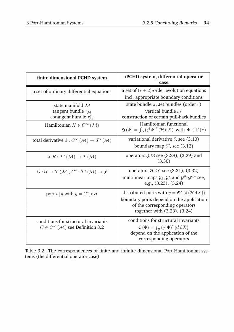
3 Port-Hamiltonian Systems 3.2.5 Concluding Remarks 34
finite dimensional PCHD system iPCHD system, differential operator
case
a set of ordinary differential equations a set of (r + 2)-order evolution equations
incl. appropriate boundary conditions
state manifold M state bundle π, Jet bundles (order r)
tangent bundle τM vertical bundle νXcotangent bundle τ ∗M construction of certain pull-back bundles
Hamiltonian H ∈ C∞ (M) Hamiltonian functionalH (Φ) =
´
D(j1Φ)
∗(H dX) with Φ ∈ Γ (π)
total derivative d : C∞ (M) → T ∗ (M) variational derivative δ, see (3.10)
boundary map δ∂, see (3.12)
J,R : T ∗ (M) → T (M) operators J,R see (3.28), (3.29) and(3.30)
G : U → T (M), G∗ : T ∗ (M) → Y operators G,G∗ see (3.31), (3.32)
multilinear maps G∂ ,G∗∂ and G∂,G∂,∗ see,
e.g., (3.23), (3.24)
port ucy with y = G∗cdH distributed ports with y = G∗ (δ (H dX))
boundary ports depend on the applicationof the corresponding operators
together with (3.23), (3.24)
conditions for structural invariants conditions for structural invariants
C ∈ C∞ (M) see Definition 3.2 C (Φ) =´
D(j1Φ)
∗(C dX)
depend on the application of thecorresponding operators
Table 3.2: The correspondences of finite and infinite dimensional Port-Hamiltonian sys-tems (the differential operator case)
Chapter 4Port-Hamiltonian Formulation of FieldTheories
In order to point out the effectiveness of the Port-Hamiltonian framework with respectto the formulation of field theories the main focus of this chapter is dedicated to the Port-Hamiltonian representation of three physical applications; namely, we investigate the Port-Hamiltonian description of the governing equations of beams modelled according to theTimoshenko theory and of fluid mechanical as well as magnetohydrodynamic applications.These applications have become established more and more in the control community overthe past years, see [Kim and Renardy, 1987, Luo et al., 1999, Macchelli and Melchiorri,2004a,b, Vazquez and Krstic, 2008, Zhang, 2007], for instance.
In section 4.1 we investigate the Port-Hamiltonian modelling of the Timoshenko beammainly based on [Schöberl and Schlacher, 2011, Siuka et al., 2011], where we motivatethe Port-Hamiltonian modelling task on the basis of the introduced system representationsof chapter 3. Afterwards, the gained formulation will be compared to another Port-Hamil-tonian representation based on the concept of the Stokes-Dirac structures, see [Macchelliand Melchiorri, 2004a,b], and the main differences concerning the mechanical aspectswill be discussed. Section 4.2 deals with the Port-Hamiltonian formulation of fluid dy-namical applications in a Lagrangian setting. Therefore, we will extensively analyse thegoverning equations from a geometric point of view in order to gain enough insights toachieve a Port-Hamiltonian formulation of the basic fluid equations – namely the Navier-Stokes equations in a Lagrangian setting. This point of view may be advantageously withrespect to the modelling of injection processes, for instance. On the basis of these consi-derations this formulation will be extended in order to also take the interaction of freecurrents and electromagnetic fields with fluid matter into account which will lead us tothe Port-Hamiltonian formulation of the governing equations of magnetohydrodynamics(in a Lagrangian setting) based on [Schöberl et al., 2010, Siuka et al., 2010]; this is themain focus of section 4.3, where we will investigate the so-called inductionless magneto-hydrodynamic case. Roughly speaking, in the inductionless magnetohydrodynamic casewe consider the macroscopic behaviour of an electrically conducting fluid (continuum) inthe presence of external electromagnetic fields, where it is assumed that the dynamic ofthe additionally induced electromagnetic parts can be neglected which is the case for many
35
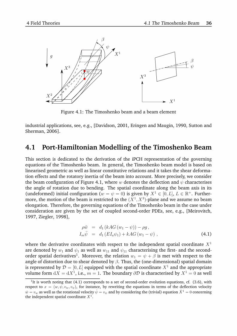
4 Field Theories 4.1 The Timoshenko Beam 36
g
X1
X1
X2
X3
X3 ψ
ψ
β
β
w
Figure 4.1: The Timoshenko beam and a beam element
industrial applications, see, e.g., [Davidson, 2001, Eringen and Maugin, 1990, Sutton andSherman, 2006].
4.1 Port-Hamiltonian Modelling of the Timoshenko Beam
This section is dedicated to the derivation of the iPCH representation of the governingequations of the Timoshenko beam. In general, the Timoshenko beam model is based onlinearised geometric as well as linear constitutive relations and it takes the shear deforma-tion effects and the rotatory inertia of the beam into account. More precisely, we considerthe beam configuration of Figure 4.1, where w denotes the deflection and ψ characterisesthe angle of rotation due to bending. The spatial coordinate along the beam axis in its(undeformed) initial configuration (w = ψ = 0) is given by X1 ∈ [0, L], L ∈ R
+. Further-more, the motion of the beam is restricted to the (X1, X3)-plane and we assume no beamelongation. Therefore, the governing equations of the Timoshenko beam in the case underconsideration are given by the set of coupled second-order PDEs, see, e.g., [Meirovitch,1997, Ziegler, 1998],
ρw = d1 (kAG (w1 − ψ)) − ρg ,
Imψ = d1 (EIaψ1) + kAG (w1 − ψ) , (4.1)
where the derivative coordinates with respect to the independent spatial coordinate X1
are denoted by w1 and ψ1 as well as w11 and ψ11 characterising the first- and the second-order spatial derivatives1. Moreover, the relation w1 = ψ + β is met with respect to theangle of distortion due to shear denoted by β. Thus, the (one-dimensional) spatial domainis represented by D = [0, L] equipped with the spatial coordinate X1 and the appropriatevolume form dX = dX1, i.e., m = 1. The boundary ∂D is characterised by X1 = 0 as well
1It is worth noting that (4.1) corresponds to a set of second-order evolution equations, cf. (3.6), withrespect to x = (w,ψ, vw , vψ), for instance, by rewriting the equations in terms of the deflection velocityw = vw as well as the rotational velocity ψ = vψ and by considering the (trivial) equation X1 = 0 concerningthe independent spatial coordinate X1.
4 Field Theories 4.1 The Timoshenko Beam 37
as X1 = L. The beam parameters are given by the mass per unit length 0 < ρ ∈ C∞ (D),the shear modulus 0 < G ∈ C∞ (D), the mass moment of inertia 0 < Im ∈ C∞ (D), thearea moment of inertia 0 < Ia ∈ C∞ (D), the gravitational constant g ∈ R
+, the numericalfactor k ∈ R
+ depending on the shape of the cross section as well as the cross-sectionalarea 0 < A ∈ C∞ (D) and the elasticity module 0 < E ∈ C∞ (D). For further details see[Meirovitch, 1997, Ziegler, 1998], for instance.
In order to obtain an equivalent iPCH representation of the governing equations wechoose the displacements w, ψ and the temporal momenta which read as
pw = ρ w , pψ = Im ψ
as dependent coordinates. In this context the state bundle π : X → D possesses thecoordinates (X1, xα), α = 1, . . . , 4, with x = (w, ψ, pw, pψ) and the required Jet bundles canbe constructed in a standard manner. Furthermore, the kinetic energy of the beam takesthe form of
T (Φ) =1
2
ˆ L
0
Φ∗
((1
ρ(pw)2 +
1
Im(pψ)2
)dX
), Φ ∈ Γ (π) ,
in terms of the temporal momenta and the potential energy reads as
V (Φ) =
ˆ L
0
(j1Φ)∗((
1
2EIa (ψ1)
2 +1
2kAG (w1 − ψ)2 + ρgw
)dX
), Φ ∈ Γ (π) ,
including a gravitational potential related to the initial configuration. The Hamiltonianfunctional is equivalent to the sum of the kinetic and the potential energy of the beam
H (Φ) = T (Φ) + V (Φ) =
ˆ L
0
(j1Φ)∗
(H dX) (4.2)
with respect to the first-order Hamiltonian density
H dX =
(1
2ρ(pw)2 +
1
2Im(pψ)2 +
1
2EIa (ψ1)
2 +1
2kAG (w1 − ψ)2 + ρgw
)dX (4.3)
which corresponds to the sum of the kinetic and the potential energy density.
Proposition 4.1 Consider the Hamiltonian functional (4.2) with the first-order Hamiltonian
density (4.3). The iPCH system representation of the Timoshenko beam takes (in matrix
representation) the form of
x = v =
w
ψ
pwpψ
=
0 0 1 00 0 0 1
−1 0 0 00 −1 0 0
δwHδψHδpwHδpψH
= J (δ (H dX)) , (4.4)
and the formal change of (4.2) reads as
v (H (Φ)) = ι∗L
((j1Φ)∗(
1
ρpw kAG (w1 − ψ) +
1
Impψ EIaψ1
))
− ι∗0
((j1Φ)∗(
1
ρpw kAG (w1 − ψ) +
1
Impψ EIaψ1
))(4.5)
with respect to the inclusion mappings ι0 : {0} → {X1 = 0} and ιL : {L} → {X1 = L}.
4 Field Theories 4.1 The Timoshenko Beam 38
In order to show the equivalence of (4.1) and (4.4) we consider the first set of the equa-tions (4.4) which read as
w = δpwH = ∂pwH =1
ρpw , ψ = δpψH = ∂pψH =
1
Impψ
since the variational derivatives with respect to the temporal momenta degenerate to par-tial ones. The second set of the equations follows by a direct computation to
pw = −δwH = −∂wH + d1
(∂1wH)
= −ρg + d1 (kAG (w1 − ψ)) ,
pψ = −δψH = −∂ψH + d1
(∂1ψH)
= kAG (w1 − ψ) + d1 (EIa (ψ1)) .
Substituting with the first set of the equations shows the equivalence with (4.1). Theformal change of the Hamiltonian functional follows by direct computation.
It is worth mentioning that the formal change of the Hamiltonian functional (4.5)allows for a clear physical interpretation since the formal change involves the collocationbetween the deflection velocity w and the shearing force kGA (w1 − ψ) as well as therotational velocity ψ due to bending and the bending moment EIaψ1 on the boundary.Therefore, the formal change of the functional is characterised by the geometric as wellas the natural boundary conditions which often appear in mechanics. Furthermore, it isobvious how to introduce the boundary ports which may be parameterised according tothe general cases (3.23) and (3.24) which allow to consider, e.g., the forces and momentsas boundary inputs and the velocities as appropriate boundary outputs or conversely.
Example 4.1 Let us consider a beam cantilevered at X1 = L with iPCH representation (4.4).
The boundary conditions at the clamped end (at X1 = L) are equivalent to the geometric
boundary conditions
ι∗L
(Φ∗
(1
ρpw
))= 0 , ι∗L
(Φ∗
(1
Impψ
))= 0
and the free end (at X1 = 0) is characterised by the natural boundary conditions
ι∗0((j1Φ)∗
(kAG (w1 − ψ)))
= 0 , ι∗0((j1Φ)∗
(EIaψ1))
= 0 ,
expressing the fact that the shearing force as well as the bending moment must vanish at the
free end. In this case (4.5) takes the form of v (H (Φ)) = 0 and the Hamiltonian functional
serves as a conserved quantity (the total energy is conserved).
With regard to Definition 3.5 it is clear that the structural invariants for this configuration
are total derivatives only since J has full rank resulting in
δwC = δψC = δpwC = δpψC = 0 .
Due to the free and the clamped end the remaining conditions are given by
∂1wC ◦ ι0 = 0
∂1ψC ◦ ι0 = 0
∂1pwC ◦ ι0 = ∂1
pwC ◦ ιL = 0
∂1pψC ◦ ι0 = ∂1
pψC ◦ ιL = 0
4 Field Theories 4.1 The Timoshenko Beam 39
together with arbitrary ∂1wC ◦ ιL as well as ∂1
ψC ◦ ιL. Therefore, it is easily verified that the two
structural invariants of the form
C1 (Φ) =1
L
ˆ L
0
(j1Φ)∗ ((
w +X1w1
)dX)
=1
L
ˆ L
0
(j1Φ)∗ (
d1
(X1w
)dX)
= ι∗L (w ◦ Φ) ,
C2 (Φ) =1
L
ˆ L
0
(j1Φ)∗ ((
ψ +X1ψ1
)dX)
=1
L
ˆ L
0
(j1Φ)∗ (
d1
(X1ψ
)dX)
= ι∗L (ψ ◦ Φ)
fulfil the conditions from above and, additionally, they serve as conserved quantities for the
considered beam configuration clearly reflecting the fact that the deflection and the angle of
rotation at the clamped end are fixed.
It must be emphasised that the iPCH representation of the Timoshenko beam is not unique.In [Macchelli and Melchiorri, 2004a,b] a Port-Hamiltonian formulation of the governingbeam equations is presented based on the concept of the Stokes-Dirac structures, wherefor the dependent coordinates, besides the temporal momenta, the deformations w1 − ψ,ψ1 are used in order to deal with the duality properties of the underlying Stokes-Diracstructures (so-called energy variables are used, see [van der Schaft and Maschke, 2002]).As a consequence, no derivative coordinates appear directly in the Hamiltonian density.Thus, in this case the variational derivative degenerates to a partial one, though, the in-terconnection map must be replaced by an appropriate differential operator, where theboundary ports are derived by the integration by parts methodology. Nevertheless, thechoice of the dependent coordinates has essential physical consequences. In [Macchelliand Melchiorri, 2004a,b] no displacement coordinates are used and, therefore, the gravityforce density may be considered by a distributed input only since no gravitational potentialcan be assigned. Furthermore, due to the choice of the deformations it is not possible todescribe the location of the beam with respect to an inertial system which could be a draw-back with regard to control purposes whenever position control is the objective. Moreover– with respect to the modelling of plates, etc. – this choice of the coordinates does notallow a direct application to (spatially) higher dimensional applications, where we dealwith more than one independent spatial coordinate, since restrictions appear as additionalPDEs which would lead to the class of restricted iPCH(D) systems. However, the choice ofthe displacements, as it is the case for the illustrated Port-Hamiltonian approach, can beapplied directly to higher dimensional cases.
Example 4.2 (continued) Consider again the configuration of the beam of Example 4.1 but
the clamped end is replaced by an actuated boundary and the shearing force and the bending
moment at X1 = L are considered as boundary system inputs with respect to the case (3.24),
i.e., the boundary map takes (in matrix representation) the form of
[G∂,ξ∂α
]=
[1 0 0 00 1 0 0
], G∂,ξ∂α = δξ∂α , ξ∂ = 1, 2 .
Then, (4.5) reads as
v (H (Φ)) =(Φ1∂L
)∗ (u∂1y
∂,1 + u∂2y∂,2), Φ1
∂L= j1Φ ◦ ιL ,
4 Field Theories 4.2 Fluid Dynamics 40
containing the boundary system inputs
u∂1 = (kGA (w1 − ψ)) ◦ ιL , u∂2 = (EIaψ1) ◦ ιL ,and the corresponding boundary outputs
y∂,1 =
(1
ρpw
)◦ ιL , y∂,2 =
(1
Impψ
)◦ ιL .
4.2 Port-Hamiltonian Formulation of Fluid Dynamics
In this section we will derive a Port-Hamiltonian representation of the governing equationsof fluid dynamical applications in a Lagrangian setting. First of all, we will investigate indetail the underlying concepts which are necessary for deriving the Navier-Stokes equa-tions based on a purely geometric point of view in order to obtain a formulation, where weswitch from the usual Eulerian description to a description on the basis of the Lagrangianpoint of view. This task will be essential for a Port-Hamiltonian representation based onthe former introduced approach. In this context we will make heavy use of the continuummechanical relationships concerning both descriptions. Therefore, in the Lagrangian pic-ture we are able to characterise the motion of a continuum with fluid matter, where we firstinvestigate the Port-Hamiltonian formulation of the so-called ideal fluid, where we consi-der no dissipative effects due to viscous stresses, in order to obtain an iPCH formulationof the governing equations. In the sequel, this framework will be extended with respectto the consideration of viscous stresses leading to an appropriate iPCHD representation ofthe Navier-Stokes equations in a Lagrangian view.
4.2.1 The Geometry of Lagrangian Fluid Dynamics
For Lagrangian fluid dynamics the concept of a reference manifold is important in contrastto fluid dynamics based on the Eulerian point of view. In this context the reference mani-fold serves as a label for the fluid particle positions at the initial point of time. Therefore,we introduce the (trivial) reference bundle πR : R → I with R = I ×B equipped with co-ordinates2 (t0, X i), where B denotes the reference manifold which possesses the so-calledmaterial coordinates (X i) and I is the time manifold with the coordinate (t0). The refe-rence manifold B is supposed to be a (compact) Riemannian manifold (with coherentlyoriented boundary ∂B) equipped with a (positive definite) metric
G = Gij dX i ⊗ dXj , Gij = Gji ∈ C∞ (B) , (4.6)
serving as a map G : T (B) → T ∗ (B). The inverse of the metric is a map G : T ∗ (B) →T (B) given by
G = Gij ∂i ⊗ ∂j , Gij = Gji ∈ C∞ (B) ,
where the components fulfil GijGjk = δik. Furthermore, the associated volume form readsas
VOL =√
det [Gij] dX1 ∧ . . . ∧ dXmx .
2In this section the Latin indices vary from 1 to mx and the Greek indices from 1 to nq.
4 Field Theories 4.2.1 The Geometry of Lagrangian Fluid Dynamics 41
In order to characterise a configuration of a continuum with fluid matter we introducea configuration manifold Q which possesses the local coordinates (qα) which may be in-terpreted as spatial coordinates, see, e.g., [Marsden and Hughes, 1994]. Since the confi-guration manifold is also a (compact) Riemannian manifold (with coherently orientedboundary) we equip it with the (positive definite) metric
g = gαβ dqα ⊗ dqβ , gαβ = gβα ∈ C∞ (Q) , (4.7)
with inverseg = gαβ ∂α ⊗ ∂β , gαβ = gβα ∈ C∞ (Q) ,
according to gαβgβγ = δαγ and the associated volume form reads as
vol =√
det [gαβ] dq1 ∧ . . . ∧ dqnq .
In this context we are able to introduce the (trivial) configuration bundle πC : C → Iwith C = I × Q equipped with coordinates (t0, qα) which can be extended to the bundleπL : E → R with E = C ×I R which possesses the coordinates (t0, X i, qα). A sectionΦ ∈ Γ (πL) (locally) leads to qα = Φα(t0, X i) which is called a motion in the Lagrangiansetting. Roughly speaking, the motion maps a reference state S ⊂ B – where an elementof S corresponds to a fluid particle in a unique manner – to a configuration Φ (t0,S) ⊂ Qat a certain point of time t0.
Remark 4.1 Since the reference manifold labels the fluid particle positions at the initial point
of time, all subsequent configurations of the fluid particles are described by the motion Φ ∈Γ (πL) which characterises the particle paths leading to a particle placement field. Thus, for
a particle labelled as X with coordinates (X i) the motion Φ (t0, X i) represents the position of
the particle at the time t0. In this context the spatial coordinates (qα) may be interpreted as the
fluid particle positions and Q characterises the region in which the fluid flows. In this context,
let us consider the reference state S. Then, Φ (t0,S) at a fixed point of time t0 characterises
the volume which is moving with the fluid. Therefore, for fluid dynamics we may identify the
labels and the initial positions for t0 = 0 and, hence, B and Q as well as G and g may coincide.
Nevertheless, we strictly distinguish between the reference and the configuration manifold in
order to separate the independent and dependent coordinates. For more detailed information
see [Aris, 1989, Bennett, 2006, Chorin and Marsden, 1990, Marsden et al., 2001].
Remark 4.2 For fluid dynamics it is also convenient to call the motion Φ ∈ Γ (πL) the fluidflow map, see [Chorin and Marsden, 1990].
It is worth mentioning that the special structure of the configuration bundle may be cha-racterised by the tensor
Λ = dt0 ⊗ ∂0
– a so-called (trivial) reference frame – which represents a trivial connection on C corres-ponding to an inertial frame, see, e.g., [Schöberl, 2007, Schöberl and Schlacher, 2007a]and references therein. In fact, all metric coefficients are time independent due to theconsidered case of the inertial frame. Furthermore, we are able to introduce the first Jet
4 Field Theories 4.2.1 The Geometry of Lagrangian Fluid Dynamics 42
manifold J 1 (E), where the first prolongation of a section Φ ∈ Γ (πL) leads to qα0 = ∂0Φα =
V α0 and qαi = ∂iΦ
α = F αi . Therefore, V α
0 denote the components of the material velo-city and F α
i represent the components of the deformation gradient which are well-knownquantities in elasticity theory, see [Marsden and Hughes, 1994]. In the sequel, we confineourselves to the case mx = nq and, therefore, we assume dimB = dimQ. In addition, it issupposed that the motion is smooth enough and, therefore, it is assumed that the motionis an invertible mapping in order that for an open set Φ (t0,B) at a fixed point of time t0
we are able to define the inverse of the motion by the map Φ : Φ (t0,B) → B leading toX i = Φi(t0, qα).
In this context we are able to define the velocity as the tangent vector field v : J 1 (C) →(π1C,0
)∗(V (C)) which takes the form of v = qα0 ∂α. In consideration of the motion this vector
field enables us to introduce two important concepts, see [Marsden and Hughes, 1994].On the one hand, by restricting v to the motion we obtain the material velocity v = V α
0 ∂αincluding the former introduced components V α
0 = ∂0Φα and on the other hand, since we
assume that the motion is invertible, we deduce
v = vα∂α =(V α
0 ◦ Φ)∂α
which is called the spatial velocity with components vα = V α0 ◦ Φ ∈ C∞ (C). It is worth
mentioning that the spatial velocity may be interpreted as a vertical tangent vector fieldv : C → V (C). In this context the corresponding connection on the vertical bundle V (C) →C reads as
Λc = dt0 ⊗ ∂0 + dqα ⊗(∂α − γβαγ q
γ∂β
), ∂β =
∂
∂qβ, (4.8)
including the Christoffel symbols of the second kind given by
γβαγ = γβγα =1
2gβδ (∂αgγδ + ∂γgαδ − ∂δgαγ) ∈ C∞ (Q) .
Remark 4.3 Roughly speaking, in mechanics the concept of connections is indispensable for
the formulation of velocities and accelerations in an intrinsic manner. For detailed information
see, e.g., [Giachetta et al., 1997, Schöberl, 2007, Schöberl and Schlacher, 2007a].
In the sequel, we will often pull-back certain forms such as ω vol with ω ∈ C∞ (Q) with thehelp of the motion according to
ˆ
Φ(t0,S)
ω vol =
ˆ
S
Φ∗ (ω vol) =
ˆ
S
J (ω ◦ Φ) VOL ,
where the integral has to be evaluated for a fixed time t0. The expression
J = det [F αi ]
√det [gαβ ◦ Φ]
det [Gij]∈ C∞ (R) (4.9)
is called the Jacobian of the motion, see [Marsden and Hughes, 1994], for instance.
4 Field Theories 4.2.2 Conservation of Mass 43
Remark 4.4 More precisely, when we pull-back the form ω vol with ω ∈ C∞ (Q) we obtain,
in general,
Φ∗ (vol) = J (ω ◦ Φ)(dX1 − Γ1
0dt0)∧ . . . ∧
(dXmx − Γmx0 dt0
), Γi0 ∈ C∞ (R) .
Since the reference bundle is used for labelling the fluid particle positions at a fixed initial point
of time the coefficients Γi0 ∈ C∞ (R) are not explicitly required for all further calculations.
In particular, when we integrate over such forms on the fibres of R at a fixed time t0 then
we have to consider the restriction dt0 = 0. Therefore, we do not consider these parts and
instead of the former expression we write Φ∗ (vol) = J VOL which corresponds to the Changeof Variables Theorem in [Marsden and Hughes, 1994]. For a more general discussion about
this topic the interested reader is referred to [Schöberl, 2007].
It is worth noting that the Jacobian describes the ratio of an elementary volume in theconfiguration to its initial volume in the reference state. The former assumption of theinvertibility of the motion now corresponds to the requirement 0 < J < ∞, see [Aris,1989].
4.2.2 Conservation of Mass
The Jacobian (4.9) plays an important role for the principle of conservation of mass. There-fore, we assume the existence of the mass density ρ ∈ C∞ (C). Then, the mass m (S) ∈ R
+
of a continuum filled with fluid matter is defined as
m (S) =
ˆ
Φ(t0,S)
ρ vol ,
where the integral has to be evaluated at a fixed time t0 for a configuration Φ (t0,S) ⊂ Q.The pull-back of this expression results in
m (S) =
ˆ
Φ(t0,S)
ρ vol =
ˆ
S
J (ρ ◦ Φ) VOL
and, consequently, the mass is conserved ifˆ
S
∂0 (J (ρ ◦ Φ) VOL) = 0 (4.10)
is met. Since this relation must hold for every domain of integration and every point oftime t0 the equation of continuity in the Lagrangian description takes the form of
∂0 (J (ρ ◦ Φ)) = ∂0 (ρR) = 0 , (4.11)
where we have introduced the mass density in the reference state ρR ∈ C∞ (B) accordingto ρR = J (ρ ◦ Φ). Otherwise, from (4.10) we obtain the equivalent result
ˆ
S
∂0 (J (ρ ◦ Φ) VOL) =
ˆ
Φ(t0,S)
vΦ (ρ vol) = 0
4 Field Theories 4.2 Stress Forms and Constitutive Relations 44
with3 vΦ = Φ∗ (∂0) = ∂0 + vα∂α, where Φ∗ denotes the Push-forward of Φ. The evaluationof the Lie derivative results in (for fixed t0)
ˆ
Φ(t0,S)
(vΦ (ρ) + ρ div (v)) vol = 0
with respect to
div (v) =1√
det [gαβ]∂α
(vα√
det [gαβ ]
)vol .
Hence, the equation of continuity in the Eulerian description takes the usual form of
vΦ (ρ) + ρ div (v) = 0 . (4.12)
4.2.3 Stress Forms and Constitutive Relations in Fluid Dynamics
For the investigation of the constitutive relations in fluid dynamics we introduce the cor-responding stress forms and stress tensors in the Eulerian as well as in the Lagrangiandescription based on [Frankel, 2004, Marsden and Hughes, 1994, Schlacher et al., 2004,Schöberl, 2007, Schöberl and Schlacher, 2007a].
Stress Forms
In the sequel the main object of interest will be the Cauchy stress form represented by thevector valued form
σ = σαβ ∂αcvol ⊗ ∂β , σαβ ∈ C∞ (C) ,
which characterises the effect of the surface forces; for fluid dynamics those are characte-rised by the hydrostatic pressure and viscous effects. Therefore, for a continuum with fluidmatter the Cauchy stress form reads as
σ = −Pgαβ ∂αcvol ⊗ ∂β + σ , (4.13)
see, e.g., [Aris, 1989, Chorin and Marsden, 1990], including the hydrostatic pressure P ∈C∞ (C) and the viscous stress form
σ = σαβ ∂αcvol ⊗ ∂β .
In order to obtain the corresponding expression in the Lagrangian setting we have to pull-back the form part by the motion Φ ∈ Γ (πL). Therefore, we carry out a so-called Piolatransformation leading to the first Piola-Kirchhoff stress form according to
P = Φ∗(σαβ∂αcvol
)⊗ ∂β = P iβ∂icVOL ⊗ ∂β , P iβ ∈ C∞ (R) , (4.14)
with the components
P iβ = J(F iασ
αβ)◦ Φ = J
(−PF i
αgαβ + F i
ασαβ)◦ Φ .
3This vector field can be interpreted as the infinitesimal generator of an isomorphism φτ : Q → Q whichmaps a configuration at t0 to a configuration at t0 + τ , see, e.g., [Schlacher et al., 2004].
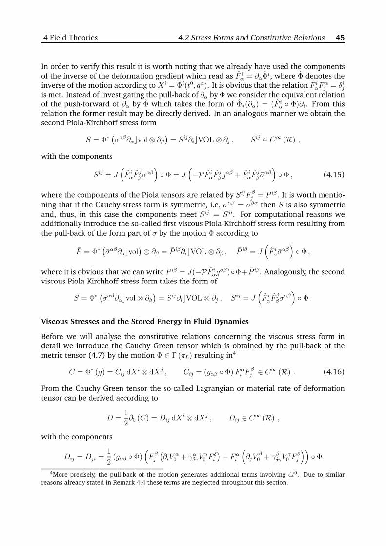
4 Field Theories 4.2 Stress Forms and Constitutive Relations 45
In order to verify this result it is worth noting that we already have used the componentsof the inverse of the deformation gradient which read as F i
α = ∂αΦi, where Φ denotes the
inverse of the motion according to X i = Φi(t0, qα). It is obvious that the relation F iαF
αj = δij
is met. Instead of investigating the pull-back of ∂α by Φ we consider the equivalent relationof the push-forward of ∂α by Φ which takes the form of Φ∗(∂α) = (F i
α ◦ Φ)∂i. From thisrelation the former result may be directly derived. In an analogous manner we obtain thesecond Piola-Kirchhoff stress form
S = Φ∗(σαβ∂αcvol ⊗ ∂β
)= Sij∂icVOL ⊗ ∂j , Sij ∈ C∞ (R) ,
with the components
Sij = J(F iαF
jβσ
αβ)◦ Φ = J
(−PF i
αFjβg
αβ + F iαF
jβ σ
αβ)◦ Φ , (4.15)
where the components of the Piola tensors are related by SijF βj = P iβ. It is worth mentio-
ning that if the Cauchy stress form is symmetric, i.e, σαβ = σβα then S is also symmetricand, thus, in this case the components meet Sij = Sji. For computational reasons weadditionally introduce the so-called first viscous Piola-Kirchhoff stress form resulting fromthe pull-back of the form part of σ by the motion Φ according to
P = Φ∗(σαβ∂αcvol
)⊗ ∂β = P iβ∂icVOL ⊗ ∂β , P iβ = J
(F iασ
αβ)◦ Φ ,
where it is obvious that we can write P iβ = J(−PF iαg
αβ)◦Φ+P iβ. Analogously, the secondviscous Piola-Kirchhoff stress form takes the form of
S = Φ∗(σαβ∂αcvol ⊗ ∂β
)= Sij∂icVOL ⊗ ∂j , Sij = J
(F iαF
jβ σ
αβ)◦ Φ .
Viscous Stresses and the Stored Energy in Fluid Dynamics
Before we will analyse the constitutive relations concerning the viscous stress form indetail we introduce the Cauchy Green tensor which is obtained by the pull-back of themetric tensor (4.7) by the motion Φ ∈ Γ (πL) resulting in4
C = Φ∗ (g) = Cij dX i ⊗ dXj , Cij = (gαβ ◦ Φ)F αi F
βj ∈ C∞ (R) . (4.16)
From the Cauchy Green tensor the so-called Lagrangian or material rate of deformationtensor can be derived according to
D =1
2∂0 (C) = Dij dX i ⊗ dXj , Dij ∈ C∞ (R) ,
with the components
Dij = Dji =1
2(gαβ ◦ Φ)
(Fβj
(∂iV
α0 + γαδγV
γ0 F
δi
)+ F α
i
(∂jV
β0 + γ
βδγV
γ0 F
δj
))◦ Φ
4More precisely, the pull-back of the motion generates additional terms involving dt0. Due to similarreasons already stated in Remark 4.4 these terms are neglected throughout this section.
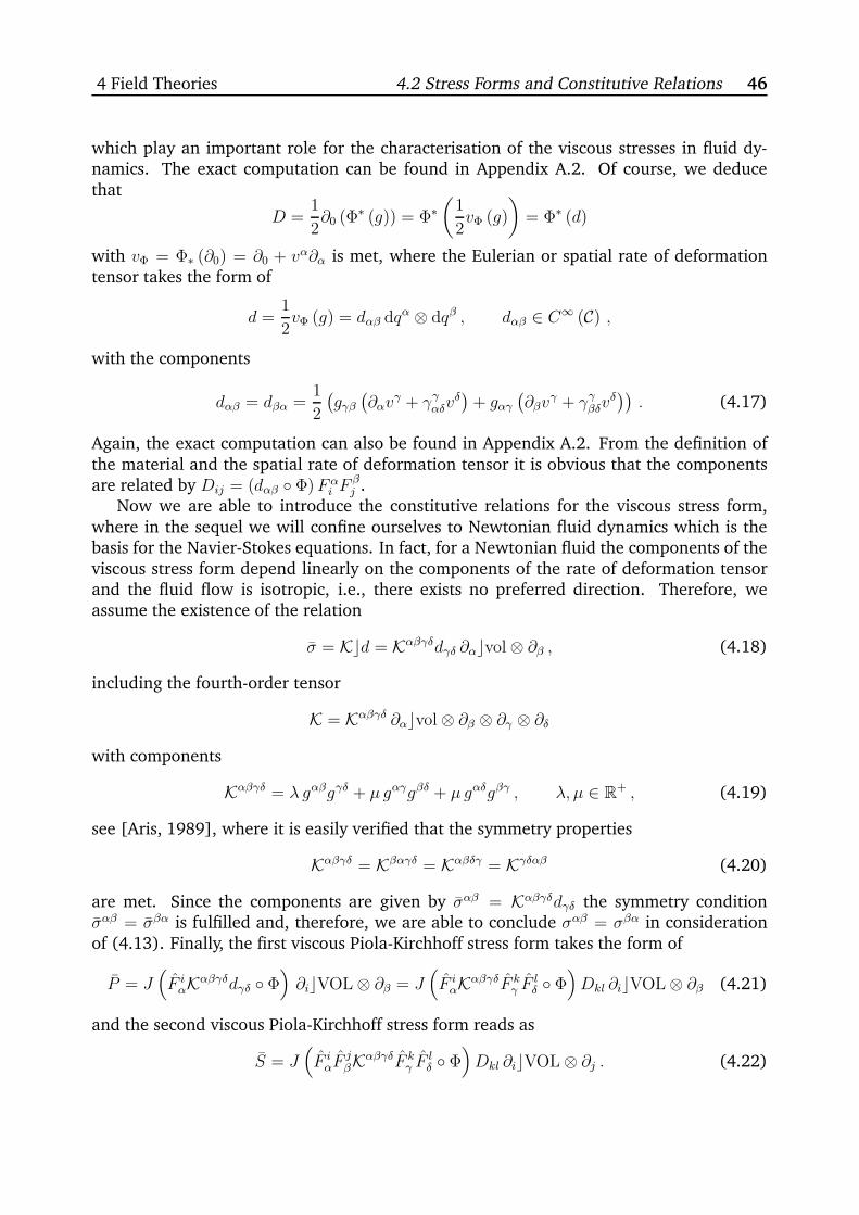
4 Field Theories 4.2 Stress Forms and Constitutive Relations 46
which play an important role for the characterisation of the viscous stresses in fluid dy-namics. The exact computation can be found in Appendix A.2. Of course, we deducethat
D =1
2∂0 (Φ∗ (g)) = Φ∗
(1
2vΦ (g)
)= Φ∗ (d)
with vΦ = Φ∗ (∂0) = ∂0 + vα∂α is met, where the Eulerian or spatial rate of deformationtensor takes the form of
d =1
2vΦ (g) = dαβ dqα ⊗ dqβ , dαβ ∈ C∞ (C) ,
with the components
dαβ = dβα =1
2
(gγβ(∂αv
γ + γγαδv
δ)
+ gαγ(∂βv
γ + γγβδv
δ)). (4.17)
Again, the exact computation can also be found in Appendix A.2. From the definition ofthe material and the spatial rate of deformation tensor it is obvious that the componentsare related by Dij = (dαβ ◦ Φ)F α
i Fβj .
Now we are able to introduce the constitutive relations for the viscous stress form,where in the sequel we will confine ourselves to Newtonian fluid dynamics which is thebasis for the Navier-Stokes equations. In fact, for a Newtonian fluid the components of theviscous stress form depend linearly on the components of the rate of deformation tensorand the fluid flow is isotropic, i.e., there exists no preferred direction. Therefore, weassume the existence of the relation
σ = Kcd = Kαβγδdγδ ∂αcvol ⊗ ∂β , (4.18)
including the fourth-order tensor
K = Kαβγδ ∂αcvol ⊗ ∂β ⊗ ∂γ ⊗ ∂δ
with components
Kαβγδ = λ gαβgγδ + µ gαγgβδ + µ gαδgβγ , λ, µ ∈ R+ , (4.19)
see [Aris, 1989], where it is easily verified that the symmetry properties
Kαβγδ = Kβαγδ = Kαβδγ = Kγδαβ (4.20)
are met. Since the components are given by σαβ = Kαβγδdγδ the symmetry conditionσαβ = σβα is fulfilled and, therefore, we are able to conclude σαβ = σβα in considerationof (4.13). Finally, the first viscous Piola-Kirchhoff stress form takes the form of
P = J(F iαKαβγδdγδ ◦ Φ
)∂icVOL ⊗ ∂β = J
(F iαKαβγδF k
γ Flδ ◦ Φ
)Dkl ∂icVOL ⊗ ∂β (4.21)
and the second viscous Piola-Kirchhoff stress form reads as
S = J(F iαF
jβKαβγδF k
γ Flδ ◦ Φ
)Dkl ∂icVOL ⊗ ∂j . (4.22)
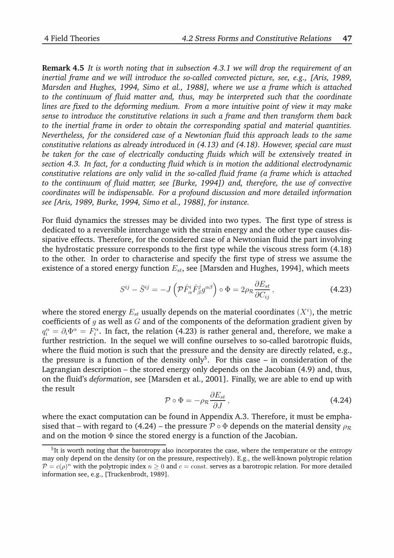
4 Field Theories 4.2 Stress Forms and Constitutive Relations 47
Remark 4.5 It is worth noting that in subsection 4.3.1 we will drop the requirement of an
inertial frame and we will introduce the so-called convected picture, see, e.g., [Aris, 1989,
Marsden and Hughes, 1994, Simo et al., 1988], where we use a frame which is attached
to the continuum of fluid matter and, thus, may be interpreted such that the coordinate
lines are fixed to the deforming medium. From a more intuitive point of view it may make
sense to introduce the constitutive relations in such a frame and then transform them back
to the inertial frame in order to obtain the corresponding spatial and material quantities.
Nevertheless, for the considered case of a Newtonian fluid this approach leads to the same
constitutive relations as already introduced in (4.13) and (4.18). However, special care must
be taken for the case of electrically conducting fluids which will be extensively treated in
section 4.3. In fact, for a conducting fluid which is in motion the additional electrodynamic
constitutive relations are only valid in the so-called fluid frame (a frame which is attached
to the continuum of fluid matter, see [Burke, 1994]) and, therefore, the use of convective
coordinates will be indispensable. For a profound discussion and more detailed information
see [Aris, 1989, Burke, 1994, Simo et al., 1988], for instance.
For fluid dynamics the stresses may be divided into two types. The first type of stress isdedicated to a reversible interchange with the strain energy and the other type causes dis-sipative effects. Therefore, for the considered case of a Newtonian fluid the part involvingthe hydrostatic pressure corresponds to the first type while the viscous stress form (4.18)to the other. In order to characterise and specify the first type of stress we assume theexistence of a stored energy function Est, see [Marsden and Hughes, 1994], which meets
Sij − Sij = −J(PF i
αFjβg
αβ)◦ Φ = 2ρR
∂Est
∂Cij, (4.23)
where the stored energy Est usually depends on the material coordinates (X i), the metriccoefficients of g as well as G and of the components of the deformation gradient given byqαi = ∂iΦ
α = F αi . In fact, the relation (4.23) is rather general and, therefore, we make a
further restriction. In the sequel we will confine ourselves to so-called barotropic fluids,where the fluid motion is such that the pressure and the density are directly related, e.g.,the pressure is a function of the density only5. For this case – in consideration of theLagrangian description – the stored energy only depends on the Jacobian (4.9) and, thus,on the fluid’s deformation, see [Marsden et al., 2001]. Finally, we are able to end up withthe result
P ◦ Φ = −ρR∂Est
∂J, (4.24)
where the exact computation can be found in Appendix A.3. Therefore, it must be empha-sised that – with regard to (4.24) – the pressure P ◦Φ depends on the material density ρRand on the motion Φ since the stored energy is a function of the Jacobian.
5It is worth noting that the barotropy also incorporates the case, where the temperature or the entropymay only depend on the density (or on the pressure, respectively). E.g., the well-known polytropic relationP = c(ρ)n with the polytropic index n ≥ 0 and c = const. serves as a barotropic relation. For more detailedinformation see, e.g., [Truckenbrodt, 1989].
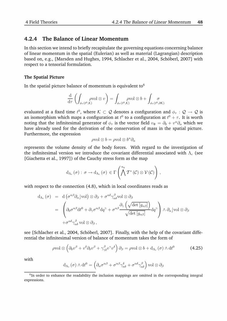
4 Field Theories 4.2.4 The Balance of Linear Momentum 48
4.2.4 The Balance of Linear Momentum
In this section we intend to briefly recapitulate the governing equations concerning balanceof linear momentum in the spatial (Eulerian) as well as material (Lagrangian) descriptionbased on, e.g., [Marsden and Hughes, 1994, Schlacher et al., 2004, Schöberl, 2007] withrespect to a tensorial formulation.
The Spatial Picture
In the spatial picture balance of momentum is equivalent to6
d
dτ
(ˆ
φτ (t0,K)
ρvol ⊗ v
)=
ˆ
φτ (t0,K)
ρvol ⊗ b+
ˆ
φτ (t0,∂K)
σ
evaluated at a fixed time t0, where K ⊂ Q denotes a configuration and φτ : Q → Q isan isomorphism which maps a configuration at t0 to a configuration at t0 + τ . It is worthnoting that the infinitesimal generator of φτ is the vector field vΦ = ∂0 + vα∂α which wehave already used for the derivation of the conservation of mass in the spatial picture.Furthermore, the expression
ρvol ⊗ b = ρvol ⊗ bα∂α
represents the volume density of the body forces. With regard to the investigation ofthe infinitesimal version we introduce the covariant differential associated with Λc (see[Giachetta et al., 1997]) of the Cauchy stress form as the map
dΛc (σ) : σ → dΛc (σ) ∈ Γ
(nq∧
T ∗ (C) ⊗ V (C)
),
with respect to the connection (4.8), which in local coordinates reads as
dΛc (σ) = d(σαβ∂αcvol
)⊗ ∂β + σαδγ
βαδvol ⊗ ∂β
=
∂0σ
αβdt0 + ∂γσαβdqγ + σαβ
∂γ
(√det [gαβ]
)
√det [gαβ ]
dqγ
∧ ∂αcvol ⊗ ∂β
+σαδγβαδ vol ⊗ ∂β ,
see [Schlacher et al., 2004, Schöberl, 2007]. Finally, with the help of the covariant diffe-rential the infinitesimal version of balance of momentum takes the form of
ρvol ⊗(∂0v
β + vδ∂δvβ + γ
βγδv
γvδ)∂β = ρvol ⊗ b+ dΛc (σ) ∧ dt0 (4.25)
withdΛc (σ) ∧ dt0 =
(∂ασ
αβ + σαβγδαδ + σαδγβαδ
)vol ⊗ ∂β
6In order to enhance the readability the inclusion mappings are omitted in the corresponding integralexpressions.
4 Field Theories 4.2.4 The Balance of Linear Momentum 49
where we have
γδαδ =1√
det [gαβ]∂α
(√det [gαβ]
).
Hence, the spatial form of balance of momentum (in local coordinates) is equivalent to
ρ(∂0v
β + vδ∂δvβ + γ
βγδv
γvδ)
= ρbβ + ∂ασαβ + σαβγδαδ + σαδγ
βαδ . (4.26)
The Material Picture
In order to obtain the material or Lagrangian counterpart to (4.25) we investigate thepull-back of the form part of dΛc (σ) by the motion Φ resulting in
Φ∗ (dΛc (σ)) = dΦΛc (P )
which includes
Φ∗(d(σαβ∂αcvol
))= d
(Φ∗(σαβ∂αcvol
))= d
(P iβ∂icVOL
)
as well as
Φ∗(σαδγ
βαδ vol
)= Φ∗
(σαεF i
εγβαδ
)JF δ
i VOL = P iαF δi
(γβαδ ◦ Φ
)VOL .
Therefore, we derive the covariant differential of the first Piola-Kichhoff stress form whichreads as
dΦΛc (P ) = d
(P iβ∂icVOL
)⊗ ∂β + P iαF δ
i
(γβαδ ◦ Φ
)VOL ⊗ ∂β
=
∂0P
iβdt0 + ∂kPiβdXk + P iβ
∂k
(√det [Gij]
)
√det [Gij]
dXk
∧ ∂icVOL ⊗ ∂β
+P iαF δi
(γβαδ ◦ Φ
)VOL ⊗ ∂β
and, furthermore, we are able to conclude
dΦΛc (P ) ∧ dt0 =
(∂iP
iβ + P iβΓkik + P iαF δi
(γβαδ ◦ Φ
))VOL ⊗ ∂β ,
where Γijk denote the components of the Christoffel symbols of the second kind with res-pect to the metric G leading to
Γkik =1√
det [Gij ]∂i
(√det [Gij ]
).
Consequently, the balance of momentum in the Lagrangian setting reads as
ρRVOL ⊗(∂0V
β0 +
(γβγδ ◦ Φ
)Vγ0 V
δ0
)∂β = ρRVOL ⊗ B + dΦ
Λc (P ) ∧ dt0 (4.27)
with B = (bα ◦ Φ) ∂α which locally corresponds to
ρR
(∂0V
β0 +
(γβγδ ◦ Φ
)Vγ0 V
δ0
)= ρR
(bβ ◦ Φ
)+ ∂iP
iβ + P iβΓkik + P iαF δi
(γβαδ ◦ Φ
). (4.28)
4 Field Theories 4.2.5 The Ideal Fluid 50
4.2.5 Port-Hamiltonian Formulation of the Ideal Fluid
This section is dedicated to the Hamiltonian representation of the (compressible) idealfluid based on the Lagrangian point of view. The ideal fluid characterises a so-calledinviscid fluid flow, where the Cauchy stress form takes the form of
σ = −Pgαβ∂αcvol ⊗ ∂β , (4.29)
i.e., σαβ = 0, see [Aris, 1989, Chorin and Marsden, 1990]. Of course, such a fluid flow hasno practical relevance, however, we intend to find an appropriate Hamiltonian formulationof the ideal fluid in a Lagrangian setting since a Newtonian fluid – which is the basis forthe Navier-Stokes equations – may be treated in an analogous manner by incorporatingthe viscous stresses.
First of all, we will introduce the well-known governing equations of an ideal fluid inthe usual Eulerian description, where we rewrite these equations by the use of the conceptof the motion in order to obtain the equivalent equations in the material or Lagrangianpicture based on the results of the former subsection, i.e., we will take the motion of anideal fluid continuum into account. On the basis of these computations the main objectiveis to find an infinite dimensional (Port-)Hamiltonian representation of the governing equa-tions which describe the ideal fluid continuum in motion, where we intend to representthese equations in the form
x = J (δ (H dX))
– restricting ourselves to the non-differential operator case – with respect to appropriatechoices of the dependent coordinates x, of the Hamiltonian density H dX and of the in-terconnection map J . Furthermore, we are interested in deriving the formal change ofthe considered Hamiltonian functional which leads to an appropriate boundary term only(i.e., a term defined on the surface of the fluid continuum).
The Ideal Fluid
In the spatial or Eulerian setting the covariant differential associated with Λc of the Cauchystress form simplifies to
dΛc (σ) ∧ dt0 = − (∂αP) gαβ vol ⊗ ∂β
for the case of an inviscid flow. Thus, the governing equations for a compressible idealfluid are given by7
ρ(∂0v
β + vδ∂δvβ + γ
βγδv
γvδ)
= − (∂αP) gαβ . (4.30)
– the well-known Euler equations – together with (4.12). In consideration of the motionwe are able to conclude
Φ∗ (dΛc (σ)) ∧ dt0 = dΦΛc (P ) ∧ dt0 = −J
(F iαg
αβ ◦ Φ)∂i (P ◦ Φ) VOL ⊗ ∂β (4.31)
7For simplicity the body force density is neglected.
4 Field Theories 4.2.5 The Ideal Fluid 51
and, consequently, the Lagrangian or material form of (4.30) reads as(ρ∂0V
β0 + ργ
βγδV
γ0 V
δ0
)◦ Φ = −
(F iαg
αβ ◦ Φ)∂i (P ◦ Φ) , (4.32)
together with (4.11), which characterises as set of PDEs for the motion since
Vβ0 = ∂0Φ
β , ∂0
(Vβ0
)= ∂00Φ
β , F iα = ∂αΦ
i = (∂iΦα)−1
.
For more detailed information the interested reader is referred to [Bennett, 2006, Marsdenet al., 2001], for instance.
Example 4.3 It is worth noting that the ideal fluid in the compressible case incorporates a
so-called isentropic (adiabatic reversible) flow, where the relation
P = A (ρ)κ , κ > 1 , A ∈ R+ ,
is met, i.e., P is clearly a function of the density ρ. Hence, an isentropic flow may be seen as
a special case of a barotropic flow with the adiabatic exponent κ > 1. Now, for this case we
intend to compute the stored energy function by evaluating the relation (4.24). First of all by
plugging in the motion Φ we are able to deduce
P ◦ Φ = (ρR)κA
(J)κ,
where P ◦ Φ clearly depends on the material density ρR and on the Jacobian J , i.e., on
the motion Φ. Due to the former results this expression must be equivalent to (4.24) and,
therefore, the stored energy function takes the form of
Est =(ρR)κ−1
A
κ− 1
1
(J)κ−1 + c , c ∈ R .
In terms of spatial quantities we obtain
Est =(ρ)κ−1
A
κ− 1+ c =
Pρ (κ− 1)
+ c
which corresponds to the well-known result as in [Chorin and Marsden, 1990, Eringen and
Maugin, 1990], for instance.
Port-Hamiltonian Formulation of the Ideal Fluid
As mentioned before, the objective is to represent the equations (4.32) in the (Port-) Ha-miltonian form
x = J (δ (H dX)) .
Before we clarify the choices for the dependent coordinates, the Hamiltonian density andthe interconnection map we have to introduce a bit more notation. So far, for the La-grangian picture it has turned out that the motion Φ ∈ Γ (πL) is the crucial fact for the
4 Field Theories 4.2.5 The Ideal Fluid 52
representation of the appropriate (material) quantities. Therefore, it is clear that the ma-terial quantities such as the first Piola-Kirchhoff stress form P or the material rate of thedeformation tensor D may only be derived if the solution or, equivalently, the motionΦ ∈ Γ (πL) of the considered application is known. Especially, with regard to the definitionof the Jacobian (4.9) we may introduce the expression
J = det [F αi ]
√det [gαβ ]
det [Gij ]∈ C∞
(J 1 (E)
),
where this expression does not incorporate the knowledge of the motion8. If the motion Φ– or equivalently the solution of the considered problem – is known then we deduce thatthe relation
J ◦ j1Φ = J
is met. In an analogous manner it is easily seen that we are able to state
P iβ ◦ j1Φ = P iβ , P iβ ∈ C∞(J 1 (E)
),
Sij ◦ j1Φ = Sij , Sij ∈ C∞(J 1 (E)
),
Cij ◦ j1Φ = Cij , Cij ∈ C∞(J 1 (E)
),
Dij ◦ j1Φ = Dij , Dij ∈ C∞(J 1 (E)
)
which also imply˘P iβ ◦ j1Φ = P iβ , ˘Sij ◦ j1Φ = Sij
in consideration of the definitions of the appropriate material quantities. In this context itis worth noting that we may write
SijFβj =
(Sijq
βj
)◦ j1Φ = P iβ ◦ j1Φ = P iβ .
In fact, the stored energy which fulfils (4.24) may be – without the knowledge of themotion – interpreted as a function of the metric coefficients Gij ∈ C∞ (B) as well asgαβ ∈ C∞ (Q) and the derivative coordinates (qαi ). Consequently, we formally have
P = −ρR∂Est
∂J
which is related to the hydrostatic pressure by
P ◦ j1Φ = P ◦ Φ .
With regard to a Hamiltonian representation of the ideal fluid we introduce the kineticenergy for a continuum with fluid matter according to
T =
ˆ
Φ(t0,S)
1
2(vcvcg) ρ vol ,
8In this context the components Fαi should be seen as a place holder for ∂iΦα(t0, X i
)whenever Φ ∈
Γ (πL) is known.
4 Field Theories 4.2.5 The Ideal Fluid 53
where the integral has to be evaluated at a fixed time t0 for the configuration Φ (t0,S) ⊂ Qwith respect to the reference state S ⊂ B. In consideration of the motion we obtain theequivalent expression
T =
ˆ
Φ(t0,S)
1
2ρ gαβ v
α vβ vol =
ˆ
S
1
2ρR (gαβ ◦ Φ)V α
0 Vβ0 VOL . (4.33)
The potential energy of the fluid continuum takes the form of
V =
ˆ
S
ρREst VOL (4.34)
including the stored energy Est.In order to cope with the Port-Hamiltonian framework we choose the material coordi-
nates (X i) which serve as the labelling coordinates as independent coordinates on D suchthat D and S coincide. As dependent coordinates we choose x = (qα, pα) including thefluid particle positions (qα) and the momenta with respect to time (pα) which correspondto
pα = ρR gαβ qβ
√det [Gij] . (4.35)
Therefore, the state bundle π : X → D = S is equipped with the coordinates (X i, qα, pα).It is worth noting that the time coordinate t0 only plays the role of the evolution parameterfor the presented Port-Hamiltonian framework and, therefore, the identification qα = qα0 ismet. Consequently, in consideration of the motion the momenta with respect to time maybe interpreted as so-called material momenta Pα according to
Pα = pα ◦ j1Φ =
(ρR gαβ q
β0
√det [Gij ]
)◦ j1Φ = ρR (gαβ ◦ Φ)V β
0
√det [Gij] .
Furthermore, if we compare the former introduced quantities we are able to conclude
ρR, Gij ∈ C∞ (D) ,
gαβ ∈ C∞ (X ) ,
P, J , Est ∈ C∞(J 1 (X )
).
The Hamiltonian functional is equivalent to the sum of the kinetic and the potential energyof the fluid continuum (4.33), (4.34) respectively and reads as9
H (Φ) = T (Φ) + V (Φ) =
ˆ
S
(j1Φ)∗
(H dX) (4.36)
with respect to the first-order Hamiltonian density
H dX =
(1
2ρR√
det [Gij ]gαβ pα pβ + ρR Est
√det [Gij]
)dX , (4.37)
9Since the identification qα = qα0
is met and in consideration of (4.35) the motion Φ ∈ Γ (πL) (and itsprolongation with respect to t0) may be identified with a section of the state bundle π : X → D for a fixedpoint of time t0. Therefore, in the sequel we will consider the motion instead of sections of π : X → D inthe relevant expressions in order to enhance the readability.
4 Field Theories 4.2.5 The Ideal Fluid 54
where we have used the relation
qβ =1
ρR√
det [Gij ]gαβpα
resulting from (4.35). Due to the former explanations we have H ∈ C∞ (J 1 (X )). It isworth noting that the Hamiltonian density corresponds to the sum of the kinetic and thepotential energy density of the fluid continuum.
Proposition 4.2 Consider the Hamiltonian functional (4.36) with the first-order Hamilto-
nian density (4.37). The Port-Hamiltonian representation of the governing equations of the
ideal fluid in a Lagrangian description (4.32) is given by
∂0Φα = δαH ◦ j1Φ =
(gαβ ◦ Φ
)
ρR√
det [Gij]Pβ ,
∂0Pα = −δαH ◦ j2Φ = −(∂αg
βγ)◦ Φ
2ρR√
det [Gij]PβPγ −
√det [Gij ]J
(F iα ◦ Φ
)∂i (P ◦ Φ)
and the formal change of (4.36) reads as10
v (H (Φ)) = −ˆ
∂S
J
(PgαβF i
α
ρR√
det [Gij]◦ Φ
)Pβ ∂icVOL . (4.38)
The exact computation can be found in the Appendix A.4. First of all, it can be easilyverified that the equations of Proposition 4.2 are equivalent to
x =
[qα
pα
]=
[0 δαβ
−δβα 0
] [δβHδβH
]= J (δ (H dX)) (4.39)
by suppressing the motion. In order to show that the equations of Proposition 4.2 and(4.32) coincide we substitute the first set into the second set of the equations leading to
ρR∂0
((gαβ ◦ Φ)V β
0
)= −1
2ρR(gδβ(∂αg
βγ)gεγ)◦ ΦV δ
0 Vε0 − J
(F iα ◦ Φ
)∂i (P ◦ Φ)
with V α0 = ∂0Φ
α. Furthermore, we obtain
ρR (gαβ ◦ Φ) ∂0
(Vβ0
)+ ρRV
β0 V
γ0 (∂γgαβ ◦ Φ)
= −1
2ρR(gδβ(∂αg
βγ)gεγ)◦ ΦV δ
0 Vε0 − J
(F iα ◦ Φ
)∂i (P ◦ Φ)
and in consideration of
∂α(gβδg
βγ)
= 0
gβδ∂α(gβγ)
= −gβγ∂α (gβδ)
gβδ∂α(gβγ)gγε = −∂α (gεδ)
10To enhance the readability the inclusion mapping is omitted.
4 Field Theories 4.2.6 The Navier-Stokes Equations 55
we are able to state
ρR (gαβ ◦ Φ) ∂0
(Vβ0
)+ ρRV
β0 V
γ0 (∂γgαβ ◦ Φ)
=1
2ρR (∂αgεδ) ◦ ΦV δ
0 Vε0 − J
(F iα ◦ Φ
)∂i (P ◦ Φ) .
Finally, we obtain
(ρ gαβ ◦ Φ) ∂0
(Vβ0
)+(ρ gαδγ
δβγ ◦ Φ
)Vβ0 V
γ0 = −
(F iα ◦ Φ
)∂i (P ◦ Φ)
from which the desired result follows directly.In the end, it is worth noting that (4.38) can be rewritten as
−ˆ
∂S
J(PF i
α ◦ Φ)V α
0 ∂icVOL = −ˆ
Φ(t0,∂S)
vαP ∂αcvol =
ˆ
Φ(t0,∂S)
σcvcg (4.40)
with respect to the inviscid case, where the Cauchy stress form is given by (4.29). Foran ideal fluid in a Lagrangian setting this term completely reflects the influence of theboundary conditions, cf. [Bennett, 2006].
4.2.6 Port-Hamiltonian Formulation of the Navier-Stokes Equations
This section is dedicated to the derivation of the Hamiltonian formulation of the Navier-Stokes equations in a Lagrangian setting, where the objective is to obtain a formal Port-Hamiltonian representation of these equations. In fact, to keep the forthcoming calcula-tions short and readable we confine ourselves to the case of a trivial metric, where we havegαβ = δαβ as well as Gij = δij; i.e., we intend to a find a Port-Hamiltonian representationof the Navier-Stokes equations restricted to Cartesian coordinates.
First of all, we will investigate the viscous stress forms in the Eulerian and Lagrangianpicture in order to obtain the governing equations, again, in the Eulerian and Lagrangianformulation. As we will see later on, the main objective of this subsection is to extendthe (Port-)Hamiltonian formulation of the ideal fluid (of course, restricted to the case ofa trivial metric) by means of the viscous stresses in order to obtain a formal iPCHD repre-sentation of the Navier-Stokes equations in a Lagrangian setting, i.e., we take a Newtonianfluid continuum in motion into account. It is worth noting that this point of view may beadvantageously with respect to the modelling of injection processes, for instance. In fact,we intend to represent the governing equations in the form
x = (J − R) (δ (H dX)) ,
where we extend the Hamiltonian formulation of the ideal fluid continuum by an appro-priate non-negative self-adjoint differential operator R according to (3.33), (3.34) res-pectively. Roughly speaking, in order to obtain a Port-Hamiltonian formulation of theNavier-Stokes equations restricted to the Lagrangian point of view we have to combineboth proposed iPCHD system representations of Definition 3.4 and 3.8.
4 Field Theories 4.2.6 The Navier-Stokes Equations 56
The Navier-Stokes Equations
In general, the Navier-Stokes equations characterise the flow of Newtonian fluids, wherewe consider the Cauchy stress form
σ = −Pgαβ∂αcvol ⊗ ∂β + σ , σ = Kcd ,
incorporating the viscous stress form σ which depend linearly on the components of therate of deformation tensor with respect to (4.17) and (4.19). Since we restrict ourselvesto the case of Cartesian coordinates the fourth-order tensor K reads as
K =(λ δαβδγδ + µ δαγδβδ + µ δαδδβγ
)∂αcvol ⊗ ∂β ⊗ ∂γ ⊗ ∂δ (4.41)
and the rate of deformation tensor d simplifies to
d =1
2(δεδ ∂γv
ε + δγε ∂δvε) dqγ ⊗ dqδ .
Therefore, (4.18) corresponds to
σ = Kcd =(λδαβ ∂γv
γ + µ(δαγ ∂γv
β + δβδ ∂δvα))∂αcvol ⊗ ∂β
and, thus, for the considered case of a Newtonian fluid the Cauchy stress form takes theform of
σ =(−Pδαβ + λδαβ ∂γv
γ + µ(δαγ ∂γv
β + δβδ ∂δvα))∂αcvol ⊗ ∂β .
Consequently, the covariant differential associated with Λc of the Cauchy stress form readsas
dΛc (σ) ∧ dt0 =(−∂αPδαβ + λ ∂α
(δαβ∂γv
γ)
+ µ∂α(δαγ∂γv
β)
+ µ∂α(δβδ∂δv
α))
vol ⊗ ∂β
=(−∂αPδαβ + (λ+ µ) ∂α
(δαβ∂γv
γ)
+ µ ∂α(δαγ∂γv
β))
vol ⊗ ∂β ,
and, thus, in the Eulerian setting the governing equations for a compressible Newtonianfluid (in Cartesian coordinates) are given by11
ρ(∂0v
β + vδ∂δvβ)
= −∂αPδαβ + (λ+ µ) ∂α(δαβ∂γv
γ)
+ µ ∂α(δαγ∂γv
β)
(4.42)
together with (4.12) representing the well-known Navier-Stokes equations (in Cartesiancoordinates).
In order to obtain the Lagrangian counterpart of these equations we consider the firstviscous Piola-Kichhoff stress form, see Appendix A.5,
P = J(F iαF
kγ ◦ Φ
)(λ δαβ∂kV
γ0 + µ δαγ∂kV
β0 + µ δβγ∂kV
α0
)∂icVOL ⊗ ∂β .
In consideration of (4.31) we finally obtain
dΦΛc (P ) ∧ dt0 = J
[−δαβ
(F iα◦Φ
)∂i (P◦Φ) + (λ+ µ) δαβ
(F iα◦Φ
)∂i
((F kγ ◦Φ
)∂kV
γ0
)
+µ δαγ(F iα◦Φ
)∂i
((F kγ ◦Φ
)∂kV
β0
)]VOL ⊗ ∂β ,
11Again, the body force density is neglected for simplicity.
4 Field Theories 4.2.6 The Navier-Stokes Equations 57
where the exact computation can also be found in Appendix A.5. Consequently, the La-grangian or material form of (4.42) reads as
(ρ∂0V
β0
)◦Φ = −δαβ
(F iα◦Φ
)∂i (P◦Φ) + (λ+ µ) δαβ
(F iα◦Φ
)∂i
((F kγ ◦Φ
)∂kV
γ0
)
+ µ δαγ(F iα ◦ Φ
)∂i
((F kγ ◦ Φ
)∂kV
β0
)(4.43)
and together with (4.11) these equations represent the Navier-Stokes equations in theLagrangian form (and in Cartesian coordinates).
Port-Hamiltonian Formulation of the Navier-Stokes Equations
As mentioned before, the main objective is to represent the governing equations (4.43) inthe Port-Hamiltonian form
x = (J − R) (δ (H dX)) ,
where we extend the Hamiltonian formulation of the ideal fluid with respect to the viscousstress terms by means of an appropriate differential operator R. Accordingly , in thefollowing part we will investigate the dissipation loss caused by the viscous stresses inmore detail. Therefore, we consider the resulting viscous force density f v which is definedby
f v =(dΦ
Λc
(P)c (g ◦ Φ)
)∧ dt0 ,
cf. (A.5), and, hence, the dissipation loss concerning the viscous forces – abbreviated byQv1
S – takes the form of
Qv1S =
ˆ
S
V cf v =
ˆ
S
(dΦ
Λc
(P)cV c (g ◦ Φ)
)∧ dt0 (4.44)
with respect to V = (v ◦ Φ) ∂α = V α0 ∂α and (g ◦ Φ) = (gαβ ◦ Φ) dqα⊗ dqβ. Since the compo-
nents of the viscous stresses depend linearly on the components of the rate of deformationtensor and, thus, on the components of the (material) velocity we mark this relationshipby P (V ) with respect to V = V α
0 ∂α for clarity (by a slight abuse of notation). According to[Schlacher et al., 2004, Schöberl, 2007], (4.44) can be rewritten as
Qv1S = −
ˆ
S
∧⊗(S(V )cD (V )
)+
ˆ
∂S
P (V )cV c (g ◦ Φ) = Q0S + Qv1
∂ , (4.45)
where∧⊗ (.) denotes the replacement of ⊗ by ∧ in the corresponding expression (.). Thus,
we have
Q0S = −
ˆ
S
∧⊗(S(V )cD (V )
)= −ˆ
S
Sij(V )Dij (V ) VOL (4.46)
as well as
Qv1∂ =
ˆ
∂S
P (V )cV c (g ◦ Φ) . (4.47)
4 Field Theories 4.2.6 The Navier-Stokes Equations 58
In consideration of the components of the second viscous Piola-Kichhoff stress form (4.22)we obtain
∧⊗(S(V )cD (V )
)= J Dij (V )
(F iαF
jβKαβγδF k
γ Flδ ◦ Φ
)Dkl(V )
= J Dkl (V )(F kγ F
lδKγδαβF i
αFjβ ◦ Φ
)Dij(V ) (4.48)
by relabelling the indices and, furthermore, we conclude that
Q0S = −
∧⊗(S(V )cD (V )
)≤ 0 (4.49)
is met due to the form of (4.48) involving the components Kαβγδ ≥ 0 of (4.19) and J > 0.With regard to the symmetry properties (4.20) we state the important result
∧⊗(S(V )cD (V )
)=
∧⊗(S (V )cD(V )
)
which enables us to write
Q0S = −
ˆ
S
∧⊗(S (V )cD(V )
)
=
ˆ
S
(dΦ
Λc
(P (V )
)cV c (g ◦ Φ)
)∧ dt0 −
ˆ
∂S
P (V )cV c (g ◦ Φ)
= Qv2S −Qv2
∂ . (4.50)
Finally, by combining (4.45) and (4.50) we are able to end up with the result
Qv1S −Qv2
S = Qv1∂ −Qv2
∂
which is equivalent toˆ
S
[dΦ
Λc
(P (V )
)cV c (g ◦ Φ) − dΦ
Λc
(P (V )
)cV c (g ◦ Φ)
]∧ dt0
=
ˆ
∂S
[P (V )cV c (g ◦ Φ) − P (V )cV c (g ◦ Φ)
]. (4.51)
As already mentioned, this remarkable result enables us to extend the Hamiltonian formu-lation of Proposition 4.2 via an appropriate differential operator according to
f v =(dΦ
Λc
(P)c (g ◦ Φ)
)∧ dt0 = −
(j3Φ)∗ (
di(Rijαβdj
(δβH
)))VOL ⊗ dqα (4.52)
withRijαβ = −J F i
τ δαεKτεγδ F jγ δβδ = Rji
βα (4.53)
which corresponds to the operator introduced in (3.33), though, with respect to the choiceof the dependent coordinates, cf. (A.5), too. In this context the Hamiltonian functionalis again given by the sum of the kinetic and the potential energy of the fluid continuum(4.33), (4.34) respectively – restricted to the case of trivial metric coefficients – and readsas
H (Φ) = T (Φ) + V (Φ) =
ˆ
S
(j1Φ)∗
(H dX) (4.54)
4 Field Theories 4.2.6 The Navier-Stokes Equations 59
with respect to the first-order Hamiltonian density12
H dX =
(1
2ρRδαβpαpβ + ρREst
)dX , H ∈ C∞
(J 1 (X )
). (4.55)
Obviously, the differential operator of (4.52) fulfils the relation (4.51) and, therefore, it isa self-adjoint operator since in this context (4.51) (formally) corresponds to (3.34).
Proposition 4.3 Consider the Hamiltonian functional (4.54) with the first-order Hamilto-
nian density (4.55). The Port-Hamiltonian formulation of the Navier-Stokes equations in a
Lagrangian description (4.43) is given by
∂0Φα = δαH ◦ j1Φ =
1
ρRδαβPβ ,
∂0Pα =(−δαH− di
(Rijαβdj
(δβH
)))◦ j3Φ
= −J(F iα◦Φ
)∂i (P ◦ Φ) + J
(F iτ ◦Φ
)∂i
(δαεKτεγδ
(F jγ ◦Φ
)δβδ ∂j
(1
ρRδµβPµ
))
and the formal change of (4.54) reads as13
v (H (Φ)) = −ˆ
S
(j3Φ)∗(
δαH di(Rijαβdj
(δβH
)))VOL −
ˆ
∂S
J
(1
ρRPδαβF i
α◦Φ
)Pβ ∂icVOL .
(4.56)
The equivalence of the equations of Proposition 4.3 and of (4.43) follows directly by sub-stituting the first set into the second set of the equations by considering the components of(4.41), also see Appendix A.5. Furthermore, it is obvious that the equations of Proposition4.3 are equivalent to
x =
[qα
pα
]=
([0 δαβ
−δβα 0
]−[
0 0
0 di(Rijαβdj (·)
)])[
δβHδβH
]= (J − R) (δ (H dX))
(4.57)with respect to the introduced self-adjoint operator (4.52) by suppressing the motion.
In the end we intend to analyse the formal change of the Hamiltonian functional. The-refore, the application of the adjoint operator leads to
v (H (Φ))=
ˆ
S
(j3Φ)∗(
di (δαH) R
ijαβdj
(δβH
))VOL−
ˆ
∂S
(j2Φ)∗(
δαHRijαβdj
(δβH
)∂icVOL
)
−ˆ
∂S
J
(1
ρRPδαβF i
α◦Φ
)Pβ ∂icVOL ,
where the term evaluated inside the domainˆ
S
(j3Φ)∗ (
di (δαH) Rij
αβdj(δβH
))VOL ≤ 0
12Note that in the case of Cartesian coordinates we clearly have VOL =√
det [δij ]dX = dX .13For readability purposes the inclusion mapping is omitted.
4 Field Theories 4.3 Magnetohydrodynamics 60
equals (4.46) and, thus, this expression is clearly non-positive due to (4.49), cf. (3.35).Thus, it is obvious that the operator of (4.52) is a non-negative self-adjoint differentialoperator. Combining the boundary terms we obtain
ˆ
∂S
V α0
[−J
(PF i
α◦Φ)
+ J F iτ δαεKτεγδ F j
γ δβδ ∂jVβ0
]∂icVOL
in terms of the material velocities and in consideration of (4.53). This expression is justequivalent to
ˆ
∂S
P cV c (g ◦ Φ) =
ˆ
Φ(t0,∂S)
σcvcg
with respect to (A.5) as well as (4.13) and (4.14). Hence, this term completely reflectsthe influence of the boundary conditions; i.e., they determine the values of the velocityand the stresses on the boundary. For more detailed information and a general discussionconcerning the physical interpretation of the boundary conditions for a viscous flow ina Lagrangian setting the interested reader is referred to [Bennett, 2006] and referencestherein.
4.3 Port-Hamiltonian Formulation of Magnetohydrodyna-
mics
Magnetohydrodynamics (abbreviated MHD) is a well-established and mainly challengingdiscipline since it combines two main field theories in physics: These two main field theo-ries are fluid mechanics, mostly represented by the Navier-Stokes equations, on the onehand and electrodynamics described by Maxwell’s equations on the other hand, both lin-ked together via Ohm’s law and Lorentz forces. Roughly speaking, it deals with the in-teraction of free currents and electromagnetic fields with fluid matter (liquids and gases),usually equipped with a high electrical conductivity. Furthermore, MHD finds practicaluse in many areas of engineering and pure science; e.g., pumping and levitation of li-quid metals in recasting and welding processes (as it is the case for remelting furnaces) ormagnetohydrodynamic drive concepts such as the magnetoplasmadynamic thruster. Fordetailed information the interested reader is referred to [Davidson, 2001, Eringen andMaugin, 1990, Sutton and Sherman, 2006], for instance.
In this section we will investigate the governing equations on the basis of the obtaineddescription of the last section, where it is worth noting that we restrict ourselves to theso-called inductionless MHD case – iMHD for short – meaning that that the dynamic ofthe additionally induced electromagnetic parts can be neglected with respect to the ex-ternal electromagnetic fields (at a low magnetic Reynold’s number). Hence, the purposeof this section which is mainly based on [Siuka et al., 2010] is to extend the frameworkfrom the last section in order to also take electrically conducting fluids in the presence ofexternal electromagnetic fields into account, where we are interested in deriving a Port-Hamiltonian representation of the governing iMHD equations based on the Lagrangianpoint of view. First of all, we have to introduce the main electromagnetic body forceswhich are important for the considered iMHD case.
4 Field Theories 4.3.1 Electromagnetic Body Forces 61
4.3.1 Electromagnetic Body Forces
For the specification of the resulting electromagnetic body forces concerning a conductingfluid in the presence of external electromagnetic fields we intend to make heavy use of theclassical MHD approximation, see, e.g., [Eringen and Maugin, 1990, Sutton and Sherman,2006]. Before we will investigate this important result we intend to analyse the relevantelectromagnetic objects and the constitutive relations in detail based on a purely geometricpoint of view.
The Electromagnetic Field Tensors
It is worth mentioning that the governing balance equations of electrodynamics are for-mulated in the configuration space. Therefore, let us introduce the electromagnetic fieldtensor F : C → ∧2 T ∗ (C) corresponding to
F = E ∧ dt0 +B
which meets dF = 0, see, e.g., [Burke, 1994, Frankel, 2004, Jadczyk et al., 1998], inclu-ding the electric field strength E : C → T ∗ (C) given by14
E = E0αdqα , E0α ∈ C∞ (C) , (4.58)
and the magnetic flux density B : C →∧2 T ∗ (C) which reads as
B =1
2Bαβdq
α ∧ dqβ , Bαβ = −Bαβ ∈ C∞ (C) . (4.59)
Remark 4.6 It is worth noting that the magnetic flux density has been introduced as a pure
two form for computational reasons. We may also write
B =1
2Bαβdq
α ∧ dqβ = Bγ∂γcvol ,
where the identification
Bαβ = εαβγBγ
√det [gαβ] , Bγ ∈ C∞ (C) , (4.60)
is met15. Furthermore, it is worth noting that the electromagnetic field strength tensor meets
the relation dF = 0 which is equivalent to the homogeneous Maxwell’s equations since we
obtain
dF =1
2(∂0Bαβ + ∂αE0β − ∂βE0α) dqα ∧ dqβ ∧ dt0 +
1
2(∂γBαβ) dqα ∧ dqβ ∧ dqγ = 0 ,
where the first term in brackets describes Faraday’s law and the second term in brackets the
Absence of Magnetic Charges. Especially, when we take the parameterisation (4.60) into
account we are able to conclude
1
2(∂γBαβ) dqα ∧ dqβ ∧ dqγ = div (B) vol = 0
14Throughout this section we consider the case mx = nq = 3., i.e., three-dimensional spatial domains.15We have ε123 = ε231 = ε312 = 1 with εαβγ = −εβαγ and εαβγ = 0 for α = β or β = γ or γ = α.
4 Field Theories 4.3.1 Electromagnetic Body Forces 62
with
div (B) =1√
det [gαβ]∂γ
(Bγ√
det [gαβ]
)
by considering the summation convention for the symbol εαβγ .
If the Lemma of Poincaré may be applied, see, e.g., [Burke, 1994, Frankel, 2004, Jadczyket al., 1998], it is convenient to introduce the electromagnetic potential A : C → T ∗ (C)which reads as
A = A0dt0 + Aαdq
α ,
where A0 ∈ C∞ (C) denotes the electrostatic potential and Aαdqα is the vector potential
with components Aα ∈ C∞ (C). The electromagnetic potential meets F = dA leading tothe parameterisation
E0α = ∂αA0 − ∂0Aα , Bαβ = ∂αAβ − ∂βAα .
Furthermore, we introduce the field tensor G : C → ∧2 T ∗ (C) corresponding to
G = D −H ∧ dt0 ,
see, e.g., [Burke, 1994, Frankel, 2004], which includes the magnetic field strength H :C → T ∗ (C) and the electric flux density D : C →
∧2 T ∗ (C) given by
H = H0αdqα , D =
1
2Dαβdq
α ∧ dqβ
with components H0α ∈ C∞ (C) as well as Dαβ = −Dβα ∈ C∞ (C) and which meets
dG = µ vol − j ∧ dt0 , (4.61)
see [Frankel, 2004], for instance, where we assume the existence of a (continuous) chargedensity µ ∈ C∞ (C) and where we have introduced the current density j = jγ∂γcvol withcomponents jγ ∈ C∞ (C). Hence, (4.61) yields the continuity equation for conservation ofcharge according to
d (dG) = (∂0µ+ div (j)) dt0 ∧ vol = 0 (4.62)
with
div (j) =1√
det [gαβ]∂γ
(jγ√
det [gαβ]
).
Remark 4.7 It is worth mentioning that the inhomogeneous Maxwell’s equations are equiva-
lent to (4.61), where we have
dG =1
2(∂0Dαβ − ∂αH0β + ∂βH0α) dqα ∧ dqβ ∧ dt0 +
1
2(∂γDαβ) dqα ∧ dqβ ∧ dqγ ,
and the comparison to (4.61) leads to the Ampère-Maxwell Law and to Gauss’s Law; by taking
the former introduced parameterisation applied to the electric flux densityD into account, i.e.,
D =1
2Dαβdq
α ∧ dqβ = Dγ∂γcvol , Dαβ = εαβγDγ
√det [gαβ] ,
4 Field Theories 4.3.1 Electromagnetic Body Forces 63
Gauss’s Law takes the form of
1
2(∂γDαβ) dqα ∧ dqβ ∧ dqγ = div (D) vol = µ vol
with
div (D) =1√
det [gαβ]∂γ
(Dγ√
det [gαβ]
).
Let the charge c (S) ∈ R of a continuum filled with fluid matter be defined as
c (S) =
ˆ
Φ(t0,S)
µ vol , (4.63)
where the integral has to be evaluated at a fixed time t0 for a configuration Φ (t0,S) ⊂ Q.Furthermore, from the electromagnetic field tensor F we are able to derive
f = −vΦcF = −vαE0αdt0 + (E0β − vαBαβ) dqβ
with respect to the vector field vΦ = ∂0 + vα∂α which we have already used before. Thisrelation enables us to introduce the force density
fL = µ vol ⊗ γccf = µ (E0β − vαBαβ) vol ⊗ dqβ
in consideration of γc = dqβ ⊗ ∂β. It is worth mentioning that the force density fL consistsof the sum of the electrostatic force density f es given by
f es = µ vol ⊗E = µE0β vol ⊗ dqβ (4.64)
and the resulting force density caused by the convective transport of charge f co whichtakes the form of
f co = µ vol ⊗ (−vcB) = − (µvαBαβ) vol ⊗ dqβ . (4.65)
In this context it is convenient to introduce the convective current density defined by
j = jα∂αcvol = µvα ∂αcvol (4.66)
with components jα = µvα ∈ C∞ (C), see [Frankel, 2004], for instance.
Remark 4.8 For the case of convective current densities only, we may introduce the charge
density in the reference state in an analogous manner as we have done for the mass density.
In fact, the pull-back of (4.63) by the motion leads to µR = J (µ ◦ Φ). Therefore, conservation
of charge in the material picture reads as ∂0 (µR) = 0 and in the spatial picture we obtain
vΦ (µ) + µ div (v) = 0 which is equivalent to (4.62) evaluated for jγ = µvγ. It must be
emphasised that these laws are the correct conservation laws in the case of convective current
densities (4.66) only, see [Schöberl et al., 2010, Siuka et al., 2010].
4 Field Theories 4.3.1 Electromagnetic Body Forces 64
The Convected Picture
Since in (i)MHD a conducting fluid in the presence of external electromagnetic fields istaken into account it is obvious that for the case of finite conductivity we have to consideran induced conductive current density which causes – in combination with the externalelectromagnetic fields – an electromagnetic force density. This force density may be in-terpreted as a body force which counteracts the motion of the fluid (according to Lenz’slaw) and, therefore, leads to dissipative effects. Before this force density will be intro-duced we intend to analyse in detail the constitutive relation for the conductive currentdensity which is given by Ohm’s law. There, special care must be taken since the consti-tutive relations for electrodynamics are only valid in the so-called fluid frame which maybe interpreted as a frame attached to the considered (fluid) continuum, see, e.g., [Burke,1994], for a more general discussion about this important topic.
In order to overcome this problem we intend to make heavy use in the sequel of the so-called convected picture, see [Aris, 1989, Marsden and Hughes, 1994, Simo et al., 1988],for instance, which allows us to introduce a frame whose coordinate lines are fixed tothe deforming medium (the reference frame of the continuum). Before we proceed, weconsider a bundle morphism (without time reparameterisation) from the configurationbundle πC : C → I to πC : C → I = I of the form
t0 = δ00t
0 , t0 = δ00 t
0 ,
qα = ϕα(t0, qα) , qα = ϕα(t0, qα) (4.67)
with respect to a diffeomorphism ϕ, where the inverse of ϕ is denoted by ϕ. Furthermore,for the derivative coordinates we obtain
qα0 = (∂0ϕα + ∂αϕ
αqα0 ) δ00 , (4.68)
by considering the prolongation j1ϕ of ϕ. Applying this bundle morphism the referenceframe takes the form of
Λ = dt0 ⊗(∂0 + δ0
0 (∂0ϕα ◦ ϕ) ∂α
), (4.69)
where in this context the components ∂0ϕα represent the components of the velocity of an
observer, see, e.g., [Giachetta et al., 1997, Schöberl, 2007] and references therein.
Remark 4.9 It is worth noting that by applying this bundle morphism the velocity which is
defined as the vector field v : J 1(C)→(π1C,0
)∗ (V(C))
takes the form of
v =(qα0 − δ0
0 (∂0ϕα ◦ ϕ)
)∂α
including the resulting transition functions of (4.69), see [Schöberl, 2007].
In order to obtain a reference frame that has coordinate lines fixed to the deforming me-dium leading to so-called convected coordinates, we consider the special bundle morphism
t0 = δ00t
0 , qα = ϕα(t0, qα) = δαi Φi(t0, qα) , (4.70)
4 Field Theories 4.3.1 Electromagnetic Body Forces 65
involving the inverse of the motion. In this context we are able to conclude16
qα ◦ Φ = δαi Xi ,
where it is clear that
∂0 (qα ◦ Φ) = d0 (qα) ◦ j1Φ = qα0 ◦ j1Φ = 0
is met. When this relation is applied to (4.68) we end up with
qα0 ◦ j1Φ = (∂0ϕα ◦ Φ) + (∂αϕ
α ◦ Φ)V α0 = 0
which results in∂0ϕ
α = −∂αϕα(V α
0 ◦ Φ)
= −δαi F iαv
α (4.71)
since with respect to (4.70) we have ∂αϕα = δαi ∂αΦi = δαi F
iα.
Remark 4.10 With regard to Remark 4.9 the corresponding velocity field reads as
v = −δ00 (∂0ϕ
α ◦ ϕ) ∂α = δ00δαi
(F iα ◦ Φ
)V α
0 ∂α
which is called the convective velocity, see [Simo et al., 1988].
Furthermore, with the help of
dqα = ∂0ϕαdt0 + ∂αϕ
αdqα ,
obtained via (4.70), we are able to compute the expression of the metric g (4.7) in theconvected picture due to g = ϕ∗ (g) resulting in17
g = gαβ(dqα − (∂0ϕ
α ◦ ϕ) dt0)⊗(dqβ −
(∂0ϕ
β ◦ ϕ)
dt0)
(4.72)
with respect to the components gαβ = (gαβ ◦ ϕ) ∂αϕα∂βϕ
β with gαβ ∈ C∞(C). In fact, these
components may be formally identified with the components of (4.16) in consideration of(4.70). The appropriate volume form can be derived similarly and reads as
vol =√
det[gαβ] (
dq1 −(∂0ϕ
1 ◦ ϕ)dt0)∧ . . . ∧
(dqnq − (∂0ϕ
nq ◦ ϕ) dt0)
(4.73)
which meets vol = ϕ∗(vol). It is worth mentioning that the metric (4.72) and the volume
form (4.73) in the convected picture are explicitly time dependent in contrast to the spatialpicture, where an inertial frame is used.
16Thus, the term convected coordinates should be obvious now.17In fact, we consider a bundle morphism without time reparameterisation and, therefore, we do not
distinguish between dt0 and dt0 since we have dt0 = δ00dt0.
4 Field Theories 4.3.1 Electromagnetic Body Forces 66
Ohm’s Law and the Conductive Force Density
As mentioned before we intend to derive the constitutive relation for the conductive cur-rent density represented by Ohm’s law. Therefore, we focus our interests on the derivationof the electromagnetic fields in the convected picture, then we use the classical relationsand transform them back in order to obtain the correct relations in the spatial picture withrespect to the inertial frame.
The electromagnetic field tensor in the convected picture is obtained by F = ϕ∗(F)
leading to
F = (E0α ◦ ϕ) ∂αϕα(dqα − (∂0ϕ
α ◦ ϕ) dt0)∧ dt0
+1
2(Bαβ ◦ ϕ) ∂αϕ
α∂βϕβ(dqα − (∂0ϕ
α ◦ ϕ) dt0)∧(dqβ −
(∂0ϕ
β ◦ ϕ)
dt0)
which results in
F = (E0α ◦ ϕ) ∂αϕαdqα ∧ dt0 − 1
2(Bαβ ◦ ϕ) ∂αϕ
α∂βϕβ(∂0ϕ
β ◦ ϕ)
dqα ∧ dt0
− 1
2(Bαβ ◦ ϕ) ∂αϕ
α∂βϕβ (∂0ϕ
α ◦ ϕ) dt0 ∧ dqβ +1
2(Bαβ ◦ ϕ) ∂αϕ
α∂βϕβ dqα ∧ dqβ .
By relabelling the indices and by considering the skew-symmetry condition for the compo-nents of the magnetic flux density we end up with
F = ∂αϕα(E0α −Bαβ∂βϕ
β∂0ϕβ)◦ ϕ dqα ∧ dt0 +
1
2(Bαβ ◦ ϕ) ∂αϕ
α∂βϕβ dqα ∧ dqβ .
In consideration of (4.71) we are able to obtain
F = ∂αϕα (E0α − vγBγα) ◦ ϕ dqα ∧ dt0 +
1
2(Bαβ ◦ ϕ) ∂αϕ
α∂βϕβdqα ∧ dqβ
= E ∧ dt0 + B , (4.74)
where in the convected picture the electric field strength reads as
E = E0αdqα = ∂αϕ
α (E0α − vγBγα) ◦ ϕdqα (4.75)
and the magnetic flux density takes the form of
B =1
2Bαβdq
α ∧ dqβ =1
2(Bαβ ◦ ϕ) ∂αϕ
α∂βϕβ dqα ∧ dqβ (4.76)
with respect to E0α ∈ C∞(C)
as well as Bαβ = −Bβα ∈ C∞(C). Therefore, we have
derived the well-known result that the electric field strength seen by the (moving) fluidcontinuum – given by (4.75) – consists of the applied electric field strength (4.58) and acontribution of the applied magnetic flux density (4.59) in combination with the velocityof the continuum.
Furthermore, we introduce the electrical conductivity form as a vector valued form inthe convected picture corresponding to
κ = καβ∂αcvol ⊗ ∂β , καβ ∈ C∞(C). (4.77)

4 Field Theories 4.3.1 Electromagnetic Body Forces 67
Thus, Ohm’s law can be formulated in the convected picture according to
j = −κc(∂0cF
)= κcE = καβE0β ∂αcvol ,
where the conductive current density j = jα∂αcvol results from the electric field whichthe continuum actually receives, i.e., this is the current density measured by an observermoving with the fluid continuum. For the equivalent expression in the spatial picture wehave to evaluate j = ϕ∗ (j) resulting in
j =(καβ∂αϕ
α∂βϕβ)◦ ϕ (E0β − vγBγβ) ∂αcvol = καβ (E0β − vγBγβ) ∂αcvol (4.78)
since from κ = ϕ∗ (κ) we obtain
κ =(καβ∂αϕ
α∂βϕβ)◦ ϕ∂αcvol ⊗ ∂β = καβ∂αcvol ⊗ ∂β ,
where the relation ϕ∗ (∂α) = (∂αϕα ◦ ϕ) ∂α has been used with respect to the push-forward
of ϕ denoted by ϕ∗.It is worth noting that (4.78) represents the simplest case of Ohm’s law in MHD, where
thermoelectric effects as well as the Hall current (reasonable approximation for conductingliquids) are neglected. For more detailed information see [Eringen and Maugin, 1990,Sutton and Sherman, 2006], for instance.
Remark 4.11 For the isotropic case the conductivity form in the convected picture may take
the form of
κ = η gαβ ∂αcvol ⊗ ∂β , η ∈ R+ ,
and, consequently, in the spatial picture we obtain
κ = η gαβ ∂αcvol ⊗ ∂β
in consideration of the components of (4.72).
Finally, the electromagnetic force density caused by the conductive current density takesthe form of
fD = −jcB = − (jαBαβ) vol ⊗ dqβ
= −καδ (E0δ − vγBγδ)Bαβ vol ⊗ dqβ (4.79)
since the conductive current density is represented by a vector valued form which is iso-morphic to vol ⊗ jα∂α. Therefore, with respect to the motion we are able to derive
FD = −J(καδE0δBαβ
)◦ Φ VOL ⊗ dqβ − JV
γ0
(καδBβαBγδ
)◦ Φ VOL ⊗ dqβ (4.80)
which represents the corresponding force density in the material picture.
Remark 4.12 As stated earlier, the former introduced Cauchy stress form (4.13) – including
the hydrostatic pressure and the viscous stress form (4.18) – is still valid if the corresponding
constitutive relations would be introduced in the convected picture and, afterwards, transfor-
med back to obtain the equivalent expression in the spatial picture. The interested reader is
referred to [Aris, 1989] (and references therein) for a profound discussion about this topic.
4 Field Theories 4.3.2 iMHD 68
MHD Approximation
Now, we are able to introduce the so-called MHD approximation. First of all, the MHDapproximation states that all electro- and magnetostrictive effects are negligible with res-pect to conductive force densities and viscous stresses as well as the hydrostatic pressure.Thus, it is convenient to consider the Cauchy stress form as we have already introducedin (4.13). Furthermore, by neglecting polarisation and magnetisation effects the relevantelectromagnetic body forces for the iMHD case – where the additionally induced electro-magnetic parts can be neglected with respect to the external electromagnetic fields (at alow magnetic Reynold’s number) – are given by the electrostatic body force (4.64), thebody force caused by the convective transport of charge (4.65) and the conductive forcedensity (4.79) which results from the induced conductive current in combination with theexternal electromagnetic fields (since we consider a conducting fluid with finite electricalconductivity). It is worth mentioning that the classical MHD approximation further statesthat the electrostatic force density as well as the force caused by the convective transportof charge are negligible in comparison with the conductive force density, i.e.,
fL = f es + f co � fD
is met18.
4.3.2 Port-Hamiltonian Formulation of inductionless Magnetohydro-
dynamics
This subsection mainly focuses on the Hamiltonian formulation of the governing equationsof the iMHD case in a Lagrangian setting, where the objective is dedicated to the deriva-tion of a formal Port-Hamiltonian representation of these equations. Roughly speaking, weintend to derive a Port-Hamiltonian formulation of an electrically conducting fluid conti-nuum in the presence of external electromagnetic fields with respect to the considerediMHD case together with the MHD approximation. First of all, we analyse the governingequations in the Eulerian and Lagrangian picture, where for simplicity we neglect the vis-cous stresses since they can be incorporated in the presented framework in an analogousmanner as before. In fact, we are interested in representing the governing equations in theform
x = (J −R) (δ (H dX)) + G (u) ,
y = G∗ (δ (H dX)) ,
where we again extend the Hamiltonian formulation of the ideal fluid continuum withan appropriate choice for the dissipation map R – represented by a multilinear map ac-cording to (3.19) – and we take an appropriate input operator G as well as its adjointoperator G∗ into account which corresponds to the operator introduced in (3.36), (3.37)respectively. As we will see later on, as distributed system input we choose the electrostatic
18In classical MHD this relation is equivalent to the assumption µ → 0, i.e., the charge density is set tozero leading to a vanishing convective current density.
4 Field Theories 4.3.2 iMHD 69
potential. Thus, in order to obtain a Port-Hamiltonian formulation of the governing equa-tions concerning the iMHD case in a Lagrangian setting we have to combine both proposediPCHD system representations.
The iMHD Case
In consideration of the former introduced MHD approximation and of (4.79) the governingequations of the iMHD case in the Eulerian or spatial picture take the form of
ρ(∂0v
β + vδ∂δvβ + γ
βγδv
γvδ)
= − (∂αP) gαβ + καδ (E0δ − vγBγδ)Bεαgεβ (4.81)
together with (4.12), where it is worth mentioning that we neglect the viscous stresses inorder to keep the forthcoming calculations short and readable. Nevertheless, they can betreated in an analogous manner as in section 4.2.6. The corresponding equations in theLagrangian or material picture read as
(ρ∂0V
β0 + ργ
βγδV
γ0 V
δ0
)◦ Φ = −
(F iαg
αβ ◦ Φ)∂i (P ◦ Φ) − V
γ0
(καδBεαBγδg
εβ)◦ Φ
+(καδE0δBεαg
εβ)◦ Φ (4.82)
together with (4.11) and characterise a set of PDEs for the motion as illustrated before.
Port-Hamiltonian Representation of iMHD
Particularly with regard to a Port-Hamiltonian representation of (4.82) we intend to ex-tend the Hamiltonian formulation of the ideal fluid of Proposition 4.2. Therefore, in consi-deration of (4.30) as well as (4.81) it is clear that we have to analyse the conductiveforce density (4.80) in detail. Since in the iMHD case the induced electromagnetic partsare negligible compared with the external electromagnetic fields we assume in the se-quel a (quasi-)stationary external magnetic field, i.e., ∂0Bαβ = 0 and, therefore, we haveBαβ ∈ C∞ (Q) as well as Aα ∈ C∞ (Q). In this case it is convenient to consider the elec-trostatic potential as the system input. Thus, we set u = A0 with A0 ∈ C∞ (Q). By takingthese considerations into account the conductive force density in the material picture canbe rewritten as
FD = −JV γ0
(καδBβαBγδ
)◦ Φ VOL ⊗ dqβ + J
(καδBβα∂δA0
)◦ Φ VOL ⊗ dqβ , (4.83)
where it is obvious that this force density splits into two parts; the first part consists ofa quadratic term with respect to the magnetic flux density and the second part containsthe chosen system input which acts on the domain. First, we analyse the quadratic term.With regard to the consideration of this expression in the Port-Hamiltonian context wehave to demand on the one hand that the components of the conductivity form satisfyκαβ = κβα ∈ C∞ (Q) and on the other hand we assume that the conductivity form servesas a positive definite map in order that the matrix representation
[καδBβαBγδ
]is positive
semidefinite. The exact computation can be found in Appendix A.6.
4 Field Theories 4.3.2 iMHD 70
Remark 4.13 Obviously, for the isotropic case, where we have καβ = η gαβ with η ∈ R+, it
is guaranteed that the conductivity form serves as a symmetric and positive definite map with
components καβ = η gαβ ∈ C∞ (Q).
Next we analyse the second part of the conductive force density (4.83) which contains thechosen system input. It is worth noting that the components of this part can be rewrittenin the form
J(καδBβα∂δA0
)◦ Φ VOL ⊗ dqβ = J
(καδBβαF
iδdiA0
)◦ j1Φ VOL ⊗ dqβ
since (F iδdiA0)◦j1Φ = ∂δA0◦Φ. Thus, it is clear that for the Port-Hamiltonian representation
of (4.82) we have to consider an appropriate input differential operator.
Proposition 4.4 Consider the Hamiltonian functional (4.36) with the first-order Hamilto-
nian density (4.37). The Port-Hamiltonian representation of the governing equations of the
iMHD case in a Lagrangian description (4.82) with the electrostatic potential as the system
input is given by
∂0Φα = δαH ◦ j1Φ ,
∂0Pα = −δαH ◦ j2Φ −(Rαβδ
βH)◦ j1Φ + Gi
αdi (A0) ◦ j1Φ
with
Rαβ = J
√det [Gij ]κ
γδBαγBβδ = Rβα ∈ C∞(J 1 (X )
), [Rαβ ] ≥ 0 ,
as well as
Giαdi (A0) = J
√det [Gij ]κ
βγBαβFiγdi (A0) , (4.84)
and the formal change of (4.36) reads as19
v (H (Φ)) = −ˆ
S
(j1Φ)∗ (
δαHRαβ δβH dX
)+
ˆ
S
(j1Φ)∗ (
δαHGiαdi (A0) dX
)
−ˆ
∂S
J
(PgαβF i
α
ρR√
det [Gij]◦ Φ
)Pβ ∂icVOL . (4.85)
The equivalence of the equations of Proposition 4.4 and of (4.82) follows directly since wehave only extended the formulation of Proposition 4.2 with respect to the conductive forcedensity (4.83). In fact, the introduced input operator (4.84) corresponds to the operatorintroduced in (3.37), though, with respect to the choice of the dependent coordinates.Therefore, it can be easily verified that the equations of Proposition 4.4 are equivalent to[qα
pα
]=
([0 δαβ
−δβα 0
]−[
0 00 Rαβ
])[δβHδβH
]+
[0
Giαdi (u)
]= (J −R) (δ (H dX)) + G (u) ,
y = G∗ (δ (H dX)) , (4.86)
by suppressing the motion, where the physical interpretation of the distributed collocatedoutput follows by the analysis of the formal change of the Hamiltonian functional.
19In order to enhance the readability the inclusion mapping is omitted.
4 Field Theories 4.3.2 iMHD 71
Remark 4.14 It is worth mentioning that this system representation can be extended directly
with respect to the consideration of the viscous stresses by combining this representation with
the one of Proposition 4.3 (restricted to the case of a trivial metric).
Concerning the formal change of the Hamiltonian functional given by (4.85) we investi-gate the term involving the input operator first. This term takes the form ofˆ
S
(j1Φ)∗ (
δαHGiαdi (A0) dX
)= −ˆ
S
(j2Φ)∗ (
A0di(Giαδ
αH)dX)
+
ˆ
∂S
(j1Φ)∗ (
δαHGiαA0 ∂icdX
)(4.87)
by applying the adjoint operator, cf (3.38). Hence, the term including the input operatorsplits into two parts; the first part is again a term acting inside the domain containing theadjoint operator – leading to the formal definition of the distributed collocated output –and the second part degenerates to a term on the boundary. The first part may be rewrittenas
−ˆ
S
(j2Φ)∗ (
A0di(Giαδ
αH)dX)
=
ˆ
S
(A0 ◦ Φ) DIV (S) VOL
with respect to
S = Si∂i = −J(F iγκ
βγBαβ ◦ Φ)V α
0 ∂i , DIV (S) =1√
det [Gij]∂i
(Si√
det [Gij]
),
since V α0 = δαH ◦ j1Φ. Furthermore, by introducing
s = sγ∂γ = −κβγvαBαβ∂γ (4.88)
it is clear that Si = J(F iγsγ ◦ Φ
)is met and, therefore, it can be shown that the relation
DIV (S) = J (div (s)) ◦ Φ
– which corresponds to the formal definition of the distributed collocated output – is ful-filled with20
div (s) =1√
det [gαβ]∂α
(sα√
det [gαβ]
).
It is worth noting that the components of s equal the components of the conductive currentdensity caused by the motion only, cf. (4.78). Consequently, we are able to conclude
ˆ
S
(A0 ◦ Φ) DIV (S) VOL =
ˆ
Φ(t0,S)
A0 div (s) vol . (4.89)
Finally, we analyse the second part of (4.87) which takes the form ofˆ
∂S
(j1Φ)∗ (
δαHGiαA0 ∂icdX
)= −ˆ
∂S
(A0 ◦ Φ)Si ∂icVOL = −ˆ
Φ(t0,∂S)
A0sγ ∂γcvol ,
(4.90)20More precisely, it can be shown that S corresponds to the Piola transform of s. For detailed information
the interested reader is referred to [Marsden and Hughes, 1994], for instance.
4 Field Theories 4.3.2 iMHD 72
including the components of (4.88), too.The remaining terms of (4.85) are given by the boundary term including the hydrostatic
pressure which is equivalent to (4.40) and by the term
−ˆ
S
(j1Φ)∗ (
δαHRαβ δβH dX
)= −ˆ
S
J (κγεsεsγ)◦Φ VOL = −
ˆ
Φ(t0,S)
κγεsεsγ vol , (4.91)
where we have κγεκεδ = δδγ since[κεδ]
is invertible due to the assumption of the positivedefiniteness of the conductivity form. Therefore, this term can be interpreted such thatit characterises the dissipation loss concerning the part of the conductive current densitycaused only by the motion.
Remark 4.15 It must be emphasised that in the expressions of (4.89), (4.90) and (4.91) no
electrostatic dissipation loss is contained directly. In fact, we have not yet considered the conti-
nuity equation for the conductive current density. However, by a rearrangement of the terms
in (4.85) it is possible to show that the formal change of the Hamiltonian functional consists
of a term describing the full Ohmic power loss inside the domain inclusive the electrostatic loss
and – besides the boundary term including the hydrostatic pressure – a boundary term which
contains the product of the electrostatic potential and the conductive current density restric-
ted to the boundary, provided that the continuity equation for the conductive current density
may be taken into account, i.e., we have not considered (4.62) restricted to the iMHD case
(µ → 0) and the components of (4.78). This fact is completely omitted in the representation
of Proposition 4.4.
Remark 4.16 It is worth noting that only for the case of convective currents of the form
(4.66) – i.e., we neglect the conductivity of the fluid (as well as the MHD approximation) –
we have to consider the electrostatic body force (4.64) and the force density caused by the
convective transport of charge (4.65). Therefore, we may extend the Hamiltonian functio-
nal – which has been corresponded so far to the sum of the kinetic and potential energy of
the continuum with fluid matter – by an electromagnetic energy density; this fact leads to
a redefinition of the temporal momenta which additionally consist of electromagnetic parts
in contrast to the pure mechanical momenta used so far in order to obtain a Hamiltonian
representation of the governing equations (in the material picture) for this setting. This case
is omitted in this thesis. For detailed information about this topic the interested reader is
referred to [Siuka et al., 2010].
Chapter 5Control of infinite dimensionalPort-Hamiltonian Systems
Due to the fact that in many applications the physics behind the governing equationsbecomes apparent by the Port-Hamiltonian framework it is now obvious to take advantageof the system representation with respect to control purposes. In the finite dimensionalcase a key benefit of the Port-Hamiltonian system class lies in the possibility of couplingPCHD systems via their (energy) ports which can be exploited not only for the modelling ofnetworks but also for the well-known control by interconnection methodology, see [Ortegaet al., 2001, van der Schaft, 2000], for instance. In particular, for the control via structural
invariants approach which is based on the control by interconnection concept the structuralinvariants of such coupled PCHD systems – interconnected by their ports – play a crucialrole. Of course, this control concept is not limited to the finite dimensional case andconcerning infinite dimensional systems an approach based on Stokes-Dirac structures wasproposed, see, e.g., [Macchelli and Melchiorri, 2004a,b, Macchelli et al., 2004d, Macchelliand Melchiorri, 2005, Rodriguez et al., 2001] and references therein. In particular, for thisapproach, where so-called energy variables are used – for the Timoshenko beam the strainis used instead of the displacements, cf. section 4.1 –, the PDEs are considered as a kindof transmission systems between two finite dimensional ones, i.e., the finite dimensionalcontroller system is interconnected to the finite dimensional plant via infinite dimensionaltransmission systems. However, by taking the presented Port-Hamiltonian framework intoaccount we directly consider the interconnection of a finite dimensional system with aninfinite dimensional one, i.e., the finite dimensional controller is interconnected to theinfinite dimensional plant. In fact, for infinite dimensional mechanical systems this pointof view seems to be advantageously whenever position control is the objective.
Due to the direct analogies of the iPCHD system class to finite dimensional PCHD sys-tems we intend to generalise the control via structural invariants method to the proposedPort-Hamiltonian framework for distributed-parameter systems, where we confine our-selves to the non-differential operator case only, cf. Definition 3.4, in order to obtain asystematic and a most general approach. More precisely, the objective of this chapter is todirectly adapt the approach from the finite dimensional case based on [Ortega et al., 2001,van der Schaft, 2000]; we mainly focus our interests on a systematic derivation of the ne-
73
5 Control of PCHD Systems 5.1 Control of PCHD Systems 74
cessary conditions for structural invariants of the considered closed-loop system whichconsists of the interconnection of the finite dimensional controller system and the infinitedimensional plant represented as an iPCHD system according to Definition 3.4, where werestrict our considerations to so-called Hamiltonian boundary control systems (we considerboundary ports only) with one-dimensional spatial domains (dim (D) = 1), i.e., the finitedimensional controller is interconnected to the infinite dimensional plant by means of theports of the controller system and of the boundary ports of the plant. In fact, it will beshown that in the infinite dimensional scenario we will obtain analogous conditions for thestructural invariants of the closed-loop system as in the lumped-parameter case dependingon the considered case of the boundary ports, i.e., we will take the parameterisations of(3.23) as well as (3.24) into account for a systematic derivation of these conditions.
This chapter which is mainly based on [Siuka et al., 2011] is organised as follows;in section 5.1 we recapitulate the well-known control via structural invariants method inthe finite dimensional case, where we intend to focus on the key ideas of this approachwhich will play a crucial role for the generalisation to the infinite dimensional scenario.Section 5.2 deals with the adaption of the method to the infinite dimensional case, wherethe coupling of a finite dimensional PCHD system (the controller) and an iPCHD system(the plant regarded as a Hamiltonian boundary control system) will be performed andanalysed in detail in order to systematically derive conditions for the structural invariantsof the coupled system (the closed-loop system) depending on the interconnection of thetwo (sub)systems. In section 5.3 the usability and the efficiency of the proposed approachis demonstrated, where the control concept is applied to the boundary control of the Ti-moshenko beam.
Finally, it is worth noting that other (energy based) control approaches dealing withthe boundary control of the Timoshenko beam can be found in, e.g., [Kim and Renardy,1987, Luo et al., 1999] for the case of pure damping injection control laws and/or (fi-nite dimensional) dynamic boundary controllers, in, e.g., [Zhang, 2007] for the case of astandard PD control law or in, e.g., [Macchelli and Melchiorri, 2004a,b] as already men-tioned, where the authors apply the control via structural invariants methodology to theinfinite dimensional Port-Hamiltonian representation of the Timoshenko beam based onthe Stokes-Dirac structures; more precisely, they focus on the interconnection of a (finitedimensional) boundary controller with the Timoshenko beam with an end mass, where themain objective is dedicated to the position control of the end mass, i.e., the partial diffe-rential equations of the Timoshenko beam characterise a transmission system as describedbefore.
5.1 Control of finite dimensional Port-Hamiltonian Sys-
tems based on Structural Invariants
The main purpose of this section is to recapitulate the well-known control via structural
invariants method based on the control by interconnection concept for finite dimensionalPCHD systems, see [Ortega et al., 2001, van der Schaft, 2000]. We intend to present thebasic ideas of this approach insofar as that we are able to directly adapt this method to theinfinite dimensional case in the next section.
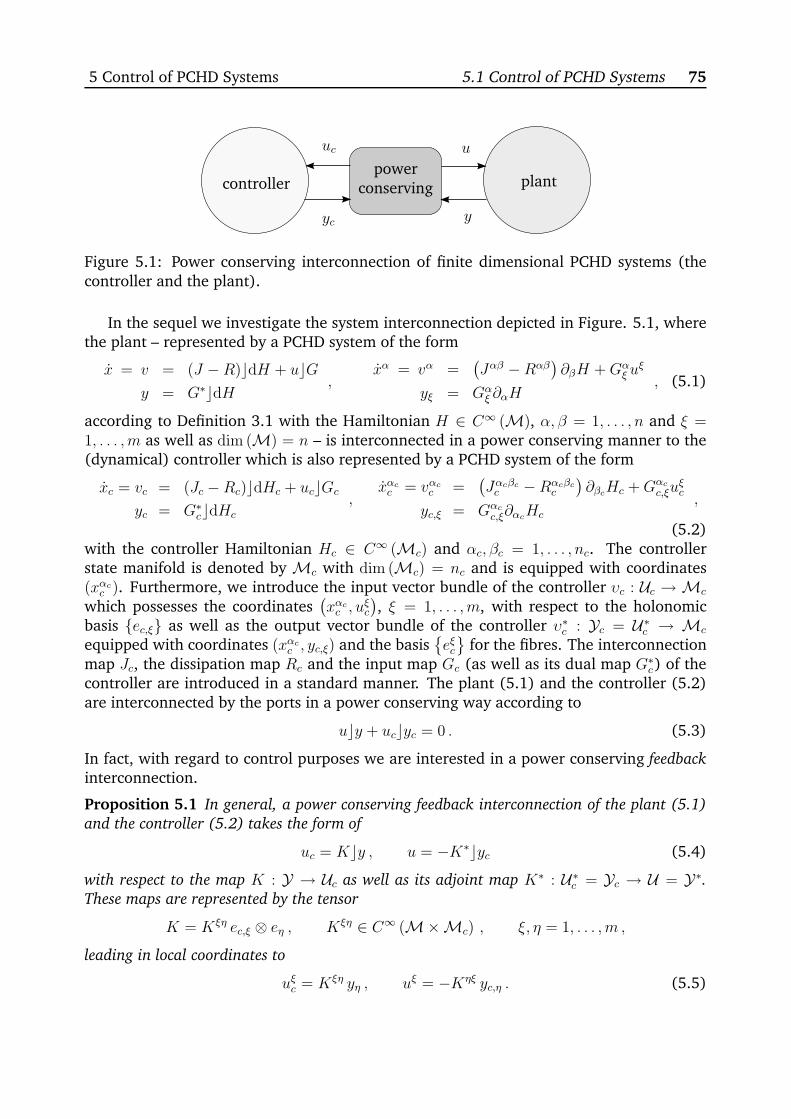
5 Control of PCHD Systems 5.1 Control of PCHD Systems 75
controllerpower
conserving plant
uc
yc
u
y
Figure 5.1: Power conserving interconnection of finite dimensional PCHD systems (thecontroller and the plant).
In the sequel we investigate the system interconnection depicted in Figure. 5.1, wherethe plant – represented by a PCHD system of the form
x = v = (J − R)cdH + ucGy = G∗cdH ,
xα = vα =(Jαβ − Rαβ
)∂βH +Gα
ξ uξ
yξ = Gαξ ∂αH
, (5.1)
according to Definition 3.1 with the Hamiltonian H ∈ C∞ (M), α, β = 1, . . . , n and ξ =1, . . . , m as well as dim (M) = n – is interconnected in a power conserving manner to the(dynamical) controller which is also represented by a PCHD system of the form
xc = vc = (Jc − Rc)cdHc + uccGc
yc = G∗ccdHc
,xαcc = vαcc =
(Jαcβcc − Rαcβc
c
)∂βcHc +Gαc
c,ξuξc
yc,ξ = Gαcc,ξ∂αcHc
,
(5.2)with the controller Hamiltonian Hc ∈ C∞ (Mc) and αc, βc = 1, . . . , nc. The controllerstate manifold is denoted by Mc with dim (Mc) = nc and is equipped with coordinates(xαcc ). Furthermore, we introduce the input vector bundle of the controller υc : Uc → Mc
which possesses the coordinates(xαcc , u
ξc
), ξ = 1, . . . , m, with respect to the holonomic
basis {ec,ξ} as well as the output vector bundle of the controller υ∗c : Yc = U∗c → Mc
equipped with coordinates (xαcc , yc,ξ) and the basis{eξc}
for the fibres. The interconnectionmap Jc, the dissipation map Rc and the input map Gc (as well as its dual map G∗
c) of thecontroller are introduced in a standard manner. The plant (5.1) and the controller (5.2)are interconnected by the ports in a power conserving way according to
ucy + uccyc = 0 . (5.3)
In fact, with regard to control purposes we are interested in a power conserving feedback
interconnection.
Proposition 5.1 In general, a power conserving feedback interconnection of the plant (5.1)
and the controller (5.2) takes the form of
uc = Kcy , u = −K∗cyc (5.4)
with respect to the map K : Y → Uc as well as its adjoint map K∗ : U∗c = Yc → U = Y∗.
These maps are represented by the tensor
K = Kξη ec,ξ ⊗ eη , Kξη ∈ C∞ (M×Mc) , ξ, η = 1, . . . , m ,
leading in local coordinates to
uξc = Kξη yη , uξ = −Kηξ yc,η . (5.5)
5 Control of PCHD Systems 5.1 Control of PCHD Systems 76
This result is easily verified by direct evaluation of (5.3) with respect to (5.4). Therefore,in consideration of (5.5) the closed-loop system serves as an overall PCHD system whichtakes in local coordinates the form of (in matrix representation)
[xα
xαcc
]=
([Jαβ −Gα
ξ Kηξ Gβc
c,η
Gαcc,ξK
ξηGβη Jαcβcc
]−[Rαβ 0
0 Rαcβcc
])[∂βH
∂βcHc
](5.6)
with the closed-loop Hamiltonian
Hd = H +Hc ∈ C∞ (M×Mc) , (5.7)
whose total time change along the trajectories of the closed-loop system (5.6) results in
vd (Hd) = − (∂αH)Rαβ (∂βH) − (∂αcHc)Rαcβcc (∂βcHc) ≤ 0 (5.8)
with respect to the corresponding vector field of the closed-loop system vd : M ×Mc →T (M×Mc) locally given by
vd = vα (xα, xαcc ) ∂α + vαcc (xα, xαcc ) ∂αc .
Due to the power-conserving interconnection it is clear that the total time change of Hd isonly characterised by the dissipative parts of the plant and of the controller and, hence, itis negative semidefinite. Consequently, with regard to control purposes the objective maybe formulated as follows; choose the controller Hamiltonian Hc such that the closed-loopHamiltonianHd possesses a minimum at the desired equilibrium – so-called energy shaping
– and, moreover, if the closed-loop Hamiltonian Hd is positive definite it can serve as aLyapunov function candidate for the investigation of the stability of the desired equilibriumin the sense of Lyapunov.
In order to fulfil these requirements it is of interest to analyse the relation of the plantand the controller coordinates in detail; this relation exists due to the power-conservinginterconnection and, therefore, the closed-loop dynamics is, in fact, restricted to a subma-nifold of M×Mc. In particular, one possibility for the characterisation of this relation isthe investigation of (non-trivial) structural invariants Cd ∈ C∞ (M×Mc) of the closed-loop system. Since the closed-loop system possesses no external inputs it is clear that thestructural invariants must serve as conserved quantities for the closed-loop system inde-pendently of the plant Hamiltonian H and the controller Hamiltonian Hc , cf. Definition3.2. Obviously, these requirements lead to the set of PDEs
[∂αCd ∂αcCd
]([
Jαβ −Gαξ K
ηξ Gβcc,η
Gαcc,ξK
ξηGβη Jαcβcc
]−[Rαβ 0
0 Rαcβcc
])= 0 , (5.9)
where the structural invariants are clearly determined by the interconnection and the dis-sipation map of the closed-loop system. In order to simplify these conditions we confineourselves to specific structural invariants which restrict the closed-loop dynamics to thesubmanifold given by{
(xα, xαcc ) ∈ M×Mc | xλc = −Cλ + κλ , Cλ ∈ C∞ (M) , κλ ∈ R , λ = 1, . . . , n ≤ nc},
5 Control of PCHD Systems 5.1 Control of PCHD Systems 77
see [Ortega et al., 2001, van der Schaft, 2000], where the constants κλ depend on theinitial conditions of the plant and the controller to the initial point of time t = t0 ∈ R
+0 .
In particular, we are interested in n (non-trivial) structural invariants of the closed-loopsystem of the specific form
Cλd = xλc + Cλ , Cλ ∈ C∞ (M) , (5.10)
which must fulfil the set of PDEs (5.9). Thus, provided that n such structural invariantsexist it is ensured that n coordinates of the controller are related to the plant coordinatesvia (by a slight abuse of notation)
xλc = −Cλ + κλ , κλ = Cλd
∣∣t=t0
, (5.11)
since the structural invariants (5.10) serve as conserved quantities for the closed-loopsystem and, therefore, they are constant along the trajectories of (5.6). Particularly, forstructural invariants of the specific form (5.10) it is possible to simplify the conditions of(5.9).
Proposition 5.2 The functions (5.10) are structural invariants of the closed-loop system
(5.6) if and only if the conditions
(∂αC
λ)Jαβ (∂βC
ρ) = Jλρc (5.12)
Rαβ(∂βC
λ)
= 0 (5.13)
Rλρc = 0 (5.14)(
∂αCλ)Jαβ = −Gλ
c,ξKξηGβ
η (5.15)
with λ, ρ = 1, . . . , n ≤ nc are fulfilled.
The exact computation can be found in Appendix A.7. For more detailed information aswell as modifications of these conditions concerning the control methodology the interes-ted reader is referred to [Ortega et al., 2001, van der Schaft, 2000].
It is worth noting that the order of the controller has not yet been determined and,thus, the order may be considered as an additional degree of freedom for the proposedapproach. Especially, for the case n < nc – i.e., not all controller coordinates are related tothe plant coordinates by (5.10), (5.11) respectively – it is obvious that certain componentsof Jc, Rc and Gc are not determined by the conditions of Proposition 5.2; hence, they canalso be considered as additional (free) design parameters in order to, e.g., (systematically)introduce additional damping in the closed-loop system by the controller. Therefore, in thecase of n < nc the closed-loop dynamics is restricted to the submanifold{
(xα, xαcc ) ∈ M×Mc | (xαcc ) =(−Cλ + κλ, xµc
), λ = 1, . . . , n , µ = n + 1, . . . , nc
},
where for(xλc)
the relation (5.11) is met and (xµc ) denote those controller coordinateswhich are not related to the plant coordinates by (5.10), (5.11) respectively. Hence, byan appropriate choice of the controller Hamiltonian Hc – which has not been determinedso far – the closed-loop Hamiltonian (5.7) may serve as an appropriate Lyapunov functioncandidate which can be used for the stability analysis of the desired equilibrium (of the
5 Control of PCHD Systems 5.2 Boundary Control of iPCHD Systems 78
closed-loop system) in the sense of Lyapunov. Provided that the closed-loop HamiltonianHd is positive definite and that it serves as an appropriate Lyapunov function the stabilityof the desired equilibrium in the sense of Lyapunov is clearly ensured because of (5.8).In this case, it is worth noting that for many applications the asymptotic stability of thedesired equilibrium can be mostly shown by applying LaSalle’s invariance principle, see[Khalil, 2002], for instance.
Remark 5.1 Let us consider the special case n = nc, i.e., all controller coordinates are related
to the plant coordinates by (5.10), (5.11) respectively. Then, the controlled plant which reads
as
xα =(Jαβ − Rαβ
)∂βH −Gα
ξ Kηξ Gβc
c,η (∂βcHc) ,
cf. (5.6), can be rewritten as
xα =(Jαβ − Rαβ
) (∂βH − ∂βC
βc ∂βcHc
)
in consideration of (5.14) as well as (5.15) since
−Gαξ K
ηξ Gβcc,η =
(∂βC
βc)Jβα = −∂βCβc
(Jαβ − Rαβ
).
Due to the fact that all controller coordinates are related to the plant coordinates we clearly
have(xβcc)
=(−Cβc + κβc
)with Cβc ∈ C∞ (M) and, therefore, by applying the chain rule
we deduce ∂βHc = −(∂βcHc)(∂βCβc). Finally, this result enables us to state
xα =(Jαβ − Rαβ
)(∂βH + ∂βHc) =
(Jαβ − Rαβ
)∂βHd ,
i.e., in the case of n = nc the controlled plant possesses the same interconnection and dis-
sipation maps as in the uncontrolled case but a shaped Hamiltonian – namely the desired
Hamiltonian Hd. For more detailed information see [van der Schaft, 2000], for instance.
5.2 Boundary Control of infinite dimensional Port-Hamil-
tonian Systems based on Structural Invariants
This section is dedicated to the extension of the former illustrated control via structural
invariants method to the infinite dimensional case. As mentioned before we consideriPCHD systems with a one-dimensional spatial domain – dim (D) = 1 with m = 1 – and, inaddition, we do not assume the existence of a distributed port, i.e., we confine ourselvesto so-called Hamiltonian boundary control systems. In fact, we are interested in a directextension of the control via structural invariants method based on the finite dimensionalcase and, therefore, with respect to the derivation of a systematic approach in the infinitedimensional scenario we treat iPCHD systems only, where the interconnection and thedissipation map are no differential operators; i.e., we only take iPCHD systems accordingto Definition 3.4 into account.
In the sequel we investigate the system interconnection depicted in Figure 5.2, wherethe plant is given by an iPCHD system of the form
x = v = (J −R) (δ (H dX)) , xα = vα =(J αβ −Rαβ
)δβH , (5.16)
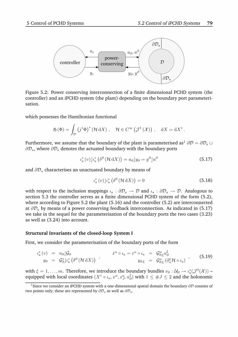
5 Control of PCHD Systems 5.2 Control of iPCHD Systems 79
controllerpower-
conserving D
uc
yc
u∂, u∂
y∂, y∂
∂Da
∂Du
Figure 5.2: Power conserving interconnection of a finite dimensional PCHD system (thecontroller) and an iPCHD system (the plant) depending on the boundary port parameteri-sation.
which possesses the Hamiltonian functional
H (Φ) =
ˆ
D
(j1Φ)∗
(H dX) , H ∈ C∞(J 1 (X )
), dX = dX1 .
Furthermore, we assume that the boundary of the plant is parameterised as1 ∂D = ∂Da ∪∂Du, where ∂Da denotes the actuated boundary with the boundary ports
ι∗a (v)cι∗a(δ∂ (H dX)
)= u∂cy∂ = y∂cu∂ (5.17)
and ∂Du characterises an unactuated boundary by means of
ι∗u (v)cι∗u(δ∂ (H dX)
)= 0 (5.18)
with respect to the inclusion mappings ιa : ∂Da → D and ιu : ∂Du → D. Analogous tosection 5.3 the controller serves as a finite dimensional PCHD system of the form (5.2),where according to Figure 5.2 the plant (5.16) and the controller (5.2) are interconnectedat ∂Da by means of a power conserving feedback interconnection. As indicated in (5.17)we take in the sequel for the parameterisation of the boundary ports the two cases (3.23)as well as (3.24) into account.
Structural Invariants of the closed-loop System I
First, we consider the parameterisation of the boundary ports of the form
ι∗a (v) = u∂cG∂y∂ = G∗
∂cι∗a(δ∂ (H dX)
) ,xα ◦ ιa = vα ◦ ιa = Gα∂,ξuξ∂
y∂,ξ = Gα∂,ξ (∂1αH ◦ ιa)
, (5.19)
with ξ = 1, . . . , m. Therefore, we introduce the boundary bundles ν∂ : U∂ → ι∗a(J 2(X )) –equipped with local coordinates (X1 ◦ ιa, xα, xαJ , uξ∂) with 1 ≤ #J ≤ 2 and the holonomic
1Since we consider an iPCHD system with a one-dimensional spatial domain the boundary ∂D consists oftwo points only; these are represented by ∂Da as well as ∂Du.
5 Control of PCHD Systems 5.2 Control of iPCHD Systems 80
basis {e∂,ξ} – as well as ν∗∂ : Y∂ = U∗∂ → ι∗a(J 2(X )) which possesses the local coordinates
(X1 ◦ ιa, xα, xαJ , y∂,ξ) and the basis {eξ∂} for the fibres2.In this case, the plant (5.16) and the controller (5.2) are interconnected by the ports
at ∂Da in a power-conserving way according to
uccyc +(Φ2∂a
)∗(u∂cy∂) = 0 , Φ2
∂a= j2Φ ◦ ιa , (5.20)
where we are interested in a power conserving feedback interconnection for this setting.
Proposition 5.3 In general, a power conserving feedback interconnection of the plant (5.16)
and the controller (5.2) takes the form of
uc = (K∂cy∂) ◦ Φ2∂a,
(u∂ ◦ Φ2
∂a
)= −
(K∗∂ ◦ Φ2
∂a
)cyc ,
for the parameterisation of the boundary ports (5.19) with respect to the map K∂ : Y∂ → Ucas well as its adjoint map K∗
∂ : U∗c = Yc → U∂ = Y∗
∂ . These maps are represented by the tensor
K∂ = Kξη∂ ec,ξ ⊗ e∂,η , Kξη
∂ ∈ C∞(Mc × ι∗a(J 2(X ))
), ξ, η = 1, . . . , m ,
leading in local coordinates to
uξc =(Kξη∂ y∂,η
)◦ Φ2
∂a,
(uξ∂ ◦ Φ2
∂a
)= −
(Kηξ∂ ◦ Φ2
∂a
)yc,η . (5.21)
This result can directly be verified by direct computation. Therefore, the closed-loop sys-tem serves as an overall mixed-dimensional PCHD system – which consists of the (power-conserving) interconnection of a finite and an infinite dimensional Port-Hamiltonian (sub)system – of the form
xα = vα =(J αβ −Rαβ
)δβH (5.22)
xαcc = vαcc =(Jαcβcc − Rαcβc
c
)∂βcHc +Gαc
c,ξ
(Kξη∂ y∂,η ◦ Φ2
∂a
)
with respect to the boundary ports/terms of the infinite dimensional subsystem
ι∗a (v)cι∗a(δ∂ (H dX)
)= y∂,ξ u
ξ∂ = −y∂,ξ Kηξ
∂ yc,η = −y∂,ξ Kηξ∂ Gαc
c,η (∂αcHc) ,
ι∗u (v)cι∗u(δ∂ (H dX)
)= 0 . (5.23)
The Hamiltonian functional of the closed-loop system takes the form of
Hd = H (Φ) +Hc =
ˆ
D
(j1Φ)∗
(H dX) +Hc , (5.24)
whose formal change results in
vd (Hd) = −ˆ
D
(j2Φ)∗ (
(δαH)Rαβ (δβH) dX)− (∂αcHc)R
αcβcc (∂βcHc) ≤ 0 (5.25)
2In fact, we have X1 ◦ ιa = const. and dX∂ = ∂1cdX = 1 with respect to the considered one-dimensionalspatial domains.
5 Control of PCHD Systems 5.2 Control of iPCHD Systems 81
with respect to the corresponding vector field of the closed-loop system vd = vα∂α+vαc∂αc .Due to the power conserving interconnection it is obvious that the formal change of Hd isonly characterised by the dissipative parts of the plant (inside the domain) and of thecontroller. With regard to control purposes the objective is – analogous to the finite di-mensional case – the stabilisation of a desired equilibrium of the closed-loop system (5.22),(5.23) respectively. Therefore, the controller Hamiltonian must be chosen such that theHamiltonian functional of the closed-loop system possesses a minimum at the desiredequilibrium and that it is positive definite due to (5.25) in order that Hd may serve as aLyapunov function candidate for the investigation of the stability of the desired equilibriumin the sense of Lyapunov.
Consequently, it is again of interest to analyse the relation of the plant and the control-ler coordinates in detail which exists due to the power conserving interconnection of thecontroller and of the plant at ∂Da. In particular, we intend to investigate the structu-ral invariants of the closed-loop system (5.22), (5.23) respectively. By analogy with thelumped-parameter case we are interested in n structural invariants of the specific form
Cλ = xλc +
ˆ
D
(j1Φ)∗ (Cλ dX
), Cλ ∈ C∞
(J 1 (X )
), λ = 1, . . . , n ≤ nc , (5.26)
where – since the closed-loop system possesses neither external distributed inputs nor ex-ternal boundary inputs – it is clear that the structural invariants must serve as conservedquantities for the closed-loop system independently of the closed-loop Hamiltonian func-tional Hd (i.e., independent of H and Hc), cf. Definition 3.5.
Proposition 5.4 The functionals (5.26) are structural invariants of the closed-loop system
(5.22), (5.23) respectively, with respect to the parameterisation of the boundary ports (5.19)
if and only if the conditions
δαCλ(J αβ −Rαβ
)= 0 (5.27)
Jλβcc − Rλβcc − Gα∂,ξ
(∂1αCλ ◦ ιa
)Kηξ∂ Gβc
c,η = 0 (5.28)(xα ∂1
αCλ)◦ ιu = 0 (5.29)
Gλc,ξKξη
∂ = 0 (5.30)
with λ = 1, . . . , n ≤ nc are fulfilled.
In order to prove this proposition let us compute the formal change of structural invariantsof the form (5.26) which reads as
vd(Cλ)
= xλc +
ˆ
D
(j2Φ)∗ (
δαCλ(J αβ −Rαβ
)δβH dX
)+(Φ2∂
)∗ ((xα∂1
αCλ)◦ ι),
with Φ2∂ = j2Φ ◦ ι, ι : ∂Da ∪ ∂Du = ∂D → D, where due to the requirement vd
(Cλ)
= 0and due to the fact that Cλ must be defined independently of the Hamiltonian functionalH of the plant and the controller Hamiltonian Hc we are able to conclude that
δαCλ(J αβ −Rαβ
)= 0
5 Control of PCHD Systems 5.2 Control of iPCHD Systems 82
must be met which corresponds to (5.27). Hence, the remaining expression in considera-tion of (5.19) as well as (5.22) reads as
vd(Cλ)
=(Jλβcc − Rλβc
c
)∂βcHc +Gλ
c,ξ
(Kξη∂ y∂,η ◦ Φ2
∂a
)+(Φ2∂u
)∗ ((xα ∂1
αCλ)◦ ιu)
+(Φ2∂a
)∗ (Gα∂,ξ uξ∂(∂1αCλ ◦ ιa
))= 0
– with Φ2∂u
= j2Φ ◦ ιu as well as Φ2∂a
= j2Φ ◦ ιa – and, consequently, we obtain
vd(Cλ)
=(Φ2∂a
)∗ (Gλc,ξKξη
∂
) (y∂,η ◦ Φ2
∂a
)+(Φ2∂u
)∗ ((xα∂1
αCλ)◦ ιu)
+(Φ2∂a
)∗ (Jλβcc − Rλβc
c − Gα∂,ξ(∂1αCλ ◦ ιa
)Kηξ∂ Gβc
c,η
)∂βcHc = 0 ,
with respect to (5.23), from which the remaining conditions of Proposition 5.4 directlyfollow.
Structural Invariants of the closed-loop System II
Now, we take the parameterisation of the boundary ports of the form
ι∗a(δ∂ (H dX)
)= G∂cu∂
y∂ = ι∗a (v)cG∂,∗ ,∂1αH ◦ ιa = G∂,ξα u∂ξ
y∂,ξ = G∂,ξα (xα ◦ ιa), (5.31)
into account with ξ = 1, . . . , m. Accordingly, for this case we consider the boundarybundles ν∂ : U∂ → ι∗a(J 2(X )) equipped with local coordinates (X1 ◦ ιa, xα, xαJ , u∂ξ ), with1 ≤ #J ≤ 2, and the holonomic basis {e∂,ξ} as well as ν∂,∗ : Y∂ = U∂,∗ → ι∗a(J 2(X )) whichpossesses the local coordinates (X1 ◦ ιa, xα, xαJ , y∂,ξ) and the basis {e∂ξ}.
In this case, the plant (5.16) and the controller (5.2) are interconnected by the portsat ∂Da in a power conserving manner according to
uccyc +(Φ2∂a
)∗ (y∂cu∂
)= 0 , Φ2
∂a= j2Φ ◦ ιa .
Again, we are interested in a power conserving feedback interconnection for this case.
Proposition 5.5 In general, a power conserving feedback interconnection of the plant (5.16)
and the controller (5.2) takes the form of
uc =(y∂cK∂
)◦ Φ2
∂a,
(u∂ ◦ Φ2
∂a
)= −
(K∂,∗ ◦ Φ2
∂a
)cyc ,
for the parameterisation of the boundary ports (5.31) with respect to the map K∂ : Y∂ → Ucas well as its adjoint map K∂,∗ : U∗
c = Yc → U∂ = Y∂,∗. These maps are represented by the
tensor
K∂ = K∂,ξη e∂,η ⊗ ec,ξ , K∂,ξ
η ∈ C∞(Mc × ι∗a(J 2(X ))
), ξ, η = 1, . . . , m ,
leading in local coordinates to
uξc =(K∂,ξη y∂,η
)◦ Φ2
∂a,
(u∂ξ ◦ Φ2
∂a
)= −
(K∂,ηξ ◦ Φ2
∂a
)yc,η . (5.32)
5 Control of PCHD Systems 5.2 Control of iPCHD Systems 83
This result can easily be verified by direct computation. The closed-loop system serves asan overall mixed-dimensional PCHD system of the form
xα = vα =(J αβ −Rαβ
)δβH (5.33)
xαcc = vαcc =(Jαcβcc −Rαcβc
c
)∂βcHc +Gαc
c,ξ
(K∂,ξη y∂,η ◦ Φ2
∂a
)
with respect to the boundary ports/terms of the infinite dimensional subsystem
ι∗a (v)cι∗a(δ∂ (H dX)
)= u∂ξ y
∂,ξ = −yc,ηK∂,ηξ y∂,ξ = − (∂αcHc)G
αcc,ηK∂,η
ξ y∂,ξ ,
ι∗u (v)cι∗u(δ∂ (H dX)
)= 0 . (5.34)
The Hamiltonian functional of the closed-loop system is again of the form (5.24) andits formal change corresponds to (5.25), of course. Therefore, we are again interestedin n structural invariants of the specific form (5.26) of the closed-loop system (5.33),(5.34) respectively. Since the closed-loop system possesses neither external distributednor external boundary inputs the structural invariants must serve as conserved quantitiesfor the closed-loop system independently of the Hamiltonian functional H of the plant andthe controller Hamiltonian Hc, cf. Definition 3.5.
Proposition 5.6 The functionals (5.26) are structural invariants of the closed-loop system
(5.33), (5.34) respectively, with respect to the parameterisation of the boundary ports (5.31)
if and only if the conditions
δαCλ(J αβ −Rαβ
)= 0 (5.35)
Gλc,ξK∂,ξ
η G∂,ηα +(∂1αCλ ◦ ιa
)= 0 (5.36)
(xα ∂1
αCλ)◦ ιu = 0 (5.37)
Jλβcc − Rλβcc = 0 (5.38)
with λ = 1, . . . , n ≤ nc are fulfilled.
In order to prove this proposition we compute the formal change of structural invariantsof the form (5.26) which takes the form of
vd(Cλ)
= xλc +
ˆ
D
(j2Φ)∗ (
δαCλ(J αβ −Rαβ
)δβH dX
)+(Φ2∂
)∗ ((xα ∂1
αCλ)◦ ι),
with Φ2∂ = j2Φ ◦ ι, where due to the fact vd
(Cλ)
= 0 and that Cλ must be independentlydefined of the Hamiltonian functional of the plant and the controller Hamiltonian wededuce
δαCλ(J αβ −Rαβ
)= 0
which equals (5.35). Furthermore, the remaining expression is given by
vd(Cλ)
=(Jλβcc − Rλβc
c
)∂βcHc +Gλ
c,ξ
(K∂,ξη y∂,η ◦ Φ2
∂a
)+(Φ2∂u
)∗ ((xα ∂1
αCλ)◦ ιu)
+(Φ2∂a
)∗ ((xα ∂1
αCλ)◦ ιa)
= 0
5 Control of PCHD Systems 5.2 Control of iPCHD Systems 84
– with respect to Φ2∂u
= j2Φ ◦ ιu as well as Φ2∂a
= j2Φ ◦ ιa – which is equivalent to
vd(Cλ)
=(Jλβcc − Rλβc
c
)∂βcHc +
(Φ2∂a
)∗ ((Gλc,ξ K∂,ξ
η G∂,ηα +(∂1αCλ ◦ ιa
))(xα ◦ ιa)
)
+(Φ2∂u
)∗ ((xα ∂1
αCλ)◦ ιu)
= 0 ,
in consideration of (5.31), from which the remaining conditions of Proposition 5.6 directlyfollow.
Boundary Control of iPCHD Systems based on Structural Invariants
By analogy with the finite dimensional case the order of the controller has not been de-termined yet and, therefore, the order may been seen again as an additional degree offreedom for the proposed approach. In particular, for the case n < nc – i.e., not all control-ler coordinates are considered by the relation (5.26) – it is clear that certain componentsof Jc, Rc and Gc are not determined by the conditions of the Propositions 5.4, 5.6 res-pectively; thus, they can also be considered as additional free design parameters in orderto, e.g., add additional damping in the closed-loop system by the controller which actsthrough the boundary port on ∂Da.
In order to find solutions of the set of the conditions (5.27) – (5.30) as well as (5.35)– (5.38) the following strategy may be performed:
1. For the parameterisation (5.19) choose Gc and K∂ in order to satisfy (5.30) or for(5.31) choose Jc and Rc in order to satisfy (5.38).
2. Solve (5.27) which equals (5.35) concerning the boundary conditions which are gi-ven for the parameterisation (5.19) by (5.28), (5.29) with respect to the design para-meters Jc and Rc or for (5.31) by (5.36), (5.37) with regard to the design parametersGc and K∂ .
Analogous to the finite dimensional case – provided that n structural invariants exist –the key feature of this approach is that n controller coordinates are related to the plantcoordinates via
xλc = −ˆ
D
(j1Φ)∗ (Cλ dX
)+ κλ , Cλ ∈ C∞
(J 1 (X )
), κλ ∈ R , (5.39)
with λ = 1, . . . , n in consideration of (5.26) since the structural invariants serve as conser-ved quantities for the closed-loop system. The constants κλ ∈ R depend on the initialconditions of the plant and the controller to the initial point of time t = t0 ∈ R
+0 and are
given by κλ = Cλ∣∣t=t0
by a slight abuse of notation. Therefore, it is clear that – in the caseof n < nc – the controller coordinates are split into
(xαcc ) =(xλc , x
µc
)=
(−ˆ
D
(j1Φ)∗ (Cλ dX
)+ κλ , xµc
)
with λ = 1, . . . , n and µ = n+ 1, . . . , nc, where for(xλc)
the relation (5.39) is met and (xµc )denote those coordinates which are not related to the plant coordinates by (5.26), (5.39)
5 Control of PCHD Systems 5.3 Control of the Timoshenko Beam 85
respectively. Consequently, if it is possible to choose the controller HamiltonianHc – whichhas not been yet determined – such that the closed-loop Hamiltonian functional Hd of(5.24) is positive definite, then it may serve as an appropriate Lyapunov function candidatefor the investigation of the stability of the desired equilibrium of the closed-loop system inthe sense of Lyapunov. It is worth noting that the negative semidefiniteness of the formalchange of the closed-loop Hamiltonian functional (5.25) is only a necessary conditionfor the stability of the desired equilibrium in the infinite dimensional case. In general,the proof of the stability in the infinite dimensional scenario is more sophisticated thanin the finite dimensional case, where advanced functional analytic investigations whichcan be found for the case of linear PDEs (with a one-dimensional spatial domain) in [Liuand Zheng, 1999, Luo et al., 1999, Michel et al., 2007], for instance, must be usuallyaccomplished. Therefore, the proof of the stability must be investigated for each particularapplication.
5.3 Boundary Control of the Timoshenko Beam based on
Structural Invariants
In order to emphasise the results of the last section we intend to apply the proposedapproach to the (energy based) boundary control of the Timoshenko beam.
Boundary Control via Structural Invariants
Let us consider a beam modelled according to the Timoshenko theory with the domainD = [0, L] and the spatial coordinate X1 ∈ [0, L], where for simplicity we neglect thegravitational potential and all beam parameters are assumed to be constant (and positive).According to section 4.1 the Hamiltonian functional – in this case – is given by
H (Φ) =1
2
ˆ L
0
(j1Φ)∗(
1
ρ(pw)2 +
1
Im(pψ)
2 + EIa (ψ1)2 + kGA (w1 − ψ)2
)dX (5.40)
with the first-order Hamiltonian density
H dX =1
2
(1
ρ(pw)2 +
1
Im(pψ)2 + EIa (ψ1)
2 + kGA (w1 − ψ)2
)dX
and the iPCH system representation reads as
x = v =
w
ψ
pwpψ
=
0 0 1 00 0 0 1
−1 0 0 00 −1 0 0
δwHδψHδpwHδpψH
= J (δ (H dX)) .
Furthermore, at X1 = 0 we consider a free end and at X1 = L the beam is actuated via a(shearing) force and a (bending) moment, i.e., the boundary conditions are given by
u∂1 = (kGA (w1 − ψ)) ◦ ιLu∂2 = (EIaψ1) ◦ ιL
,(kGA (w1 − ψ)) ◦ ι0 = 0
(EIaψ1) ◦ ι0 = 0,
5 Control of PCHD Systems 5.3 Control of the Timoshenko Beam 86
cf. Examples 4.1, 4.2 respectively. For this configuration it is obvious that X1 = 0 cha-racterises an unactuated boundary ∂Du and X1 = L represents an actuated boundary ∂Da
with the boundary map
[G∂,ξα
]=
[1 0 0 00 1 0 0
], G∂,ξα = δξα , ξ = 1, 2 ,
and the corresponding collocated boundary outputs
y∂,1 =
(1
ρpw
)◦ ιL , y∂,2 =
(1
Impψ
)◦ ιL , (5.41)
cf. Example 4.2. Furthermore, it is easily verified that for this setting the equilibria takethe form of
xd =
wdψdpw,dpψ,d
=
aX1 + b
a
00
(5.42)
with a, b ∈ R implying u∂1,d = u∂2,d = 0 at the equilibrium, of course.With regard to control purposes the objective can be stated as follows; design a boun-
dary controller via the proposed approach on the basis of structural invariants in consi-deration of the parameterisation (5.31) in order that a desired equilibrium xd for certain
values of a, b ∈ R can be stabilised. According to Proposition 5.5 we confine ourselves tothe (simple) choice of K∂,ξ
η = δξη concerning the components of the (power conserving)feedback interconnection represented by the map K∂. Furthermore, due to the form of(5.40) we intend to shape the potential energy of the beam only, i.e., the structural inva-riants of the closed-loop system should not depend on the temporal momenta as well astheir derivative coordinates.
Proposition 5.7 A possible choice for the structural invariants of the closed-loop system
which satisfy the conditions (5.35)–(5.38) with respect to K∂,ξη = δξη and G∂,ξα = δξα is gi-
ven by
C1 = x1c −
1
L
ˆ L
0
(j1Φ)∗ (
w +X1w1
)dX = x1
c − ι∗L (w ◦ Φ) , (5.43)
C2 = x2c −
1
L
ˆ L
0
(j1Φ)∗ (
ψ +X1ψ1
)dX = x2
c − ι∗L (ψ ◦ Φ) (5.44)
and for nc = 4 and m = 2 the controller maps are chosen to
[Jαcβcc −Rαcβc
c
]=
0 0 0 00 0 0 00 0 −R33
c J34c −R34
c
0 0 −J34c − R34
c −R44c
,
[Gαcc,ξ
]=
1 00 1G3c,1 G3
c,2
G4c,1 G4
c,2
with the (simple) choice Jαcβcc , Rαcβcc , Gαc
c,ξ ∈ R for the additional design parameters.
5 Control of PCHD Systems 5.3 Control of the Timoshenko Beam 87
In order to show that (5.43) as well as (5.44) together with the choices of the controllermaps fulfil the relations (5.35) – (5.38) we have to consider the condition (5.38) first of all.This condition is clearly fulfilled since for λ = 1, 2 and βc = 1, . . . , nc = 4 the componentsare given by Jλβcc = Rλβc
c = 0. The conditions (5.36) and (5.37) take the form of
Gλc,ξδ
ξα = −∂1
αCλ ◦ ιL , ∂1αCλ ◦ ι0 = 0
with respect to G∂,ξα = δξα, the choice K∂,ξη = δξη and the boundary conditions at the free
end. Since (5.43) depends only on the deflection w and its derivative coordinates and(5.44) only on the angle of rotation ψ and its derivative coordinates, the correspondingcomponents of Gc are chosen such that the former conditions can be rewritten as
G1c,1 = 1 = −∂1
wC1 ◦ ιL , G2c,2 = 1 = −∂1
ψC2 ◦ ιL , ∂1wC1 ◦ ι0 = 0 , ∂1
ψC2 ◦ ι0 = 0
with respect to G1c,2 = G2
c,1 = 0. These conditions represent the boundary conditions for(5.35). Due to the fact that the interconnection map J has full rank we deduce that Cλare total derivatives only and, thus, we are able to end up with
C1 = − 1
L
(w +X1w1
)= − 1
Ld1
(X1w
), C2 = − 1
L
(ψ +X1ψ1
)= − 1
Ld1
(X1ψ
)
which clearly satisfy the relations (5.35) – (5.37).In consideration of (5.39) the structural invariants (5.43), (5.44) enable us to obtain
for the first two controller coordinates the identities
x1c = ι∗L (w ◦ Φ) + κ1 , x2
c = ι∗L (ψ ◦ Φ) + κ2 (5.45)
with the constants κ1, κ2 ∈ R depending on the initial conditions of the plant and thecontroller.
Remark 5.2 If we take the influence of the gravity field into account, cf. Proposition 4.1, it is
worth mentioning that the choice of the structural invariants (5.43), (5.44) is still valid.
In the last step the controller Hamiltonian Hc must be chosen with regard to the require-ments. Therefore, we make the (simple) choice
Hc =1
2Mµνx
µcx
νc +
1
2c1(x1c − x1
c,d
)2+
1
2c2(x2c − x2
c,d
)2, µ, ν = 3, 4 , (5.46)
withMµν = Mνµ ∈ R , [Mµν ] > 0 , c1 > 0 , c2 > 0
as well as
x1c,d = ι∗L (wd ◦ Φ) + κ1 = aL+ b+ κ1 , x2
c,d = ι∗L (ψd ◦ Φ) + κ2 = a+ κ2 .
Therefore, the Hamiltonian functional of the closed-loop system Hd is given by the sumof (5.40) and (5.46) and it is easily verified that it possesses a minimum at the desired
5 Control of PCHD Systems 5.3 Control of the Timoshenko Beam 88
equilibrium (5.42) together with x3c,d = x4
c,d = 0. In order to show that Hd is positivedefinite we consider a bundle morphism Mc ×X → Mc × X of the form3
x3c
x4c
w
ψ
pwpψ
=
x3c − x3
c,d
x4c − x4
c,d
w − wdψ − ψdpw − pw,dpψ − pψ,d
=
x3c
x4c
w − aX1 − b
ψ − a
pwpψ
(5.47)
with respect to x3c,d = x4
c,d = 0, where this bundle morphism clearly transforms the desiredequilibrium of the closed-loop system into the origin according to
xd =
wdψdpw,dpψ,d
= 0 , x3
c,d = x4c,d = 0 (5.48)
in consideration of (5.47). Additionally, it is worth noting that from this bundle morphismwe deduce
ι∗L(w ◦ Φ
)= x1
c − x1c,d , ι∗L
(ψ ◦ Φ
)= x2
c − x2c,d
with respect to Φ : D → X . Thus, in consideration of (5.47) the closed-loop Hamiltonianfunctional reads as
Hd =1
2
ˆ L
0
(j1Φ)∗(
1
ρ(pw)2 +
1
Im(pψ)
2 + EIa(ψ1
)2+ kGA
(w1 − ψ
)2)
dX
+1
2Mµν x
µc x
νc +
1
2c1(ι∗L(w ◦ Φ
))2+
1
2c2(ι∗L(ψ ◦ Φ
))2(5.49)
which is positive definite and its formal change takes the form of
vd (Hd) = −xµc Mµν Rνζc Mζχ x
χc ≤ 0 , µ, ν, ζ, χ = 3, 4 , (5.50)
due to (5.25).
Proof of Stability
As mentioned before, for the proof concerning the stability of the desired equilibrium(of the closed-loop system) we have to investigate the well-posedness of the solution ofthe closed-loop system and the admissibleness of all the applied operations. Therefore,we intend to perform the stability analysis analogous to [Luo et al., 1999, Morgül, 1998,Thull, 2010, Zhang, 2007] (and references therein), where we first define the functionspace Z as4
Z ={z =
(x3c , x
4c , w, ψ, pw, pψ
) ∣∣ x3c , x
4c ∈ R , w, ψ ∈ H1 (0, L) , pw, pψ ∈ L2 (0, L)
}
3More precisely, we consider a bundle morphism on a submanifold of Mc × X due to the identities of(5.45).
4In fact, the particular sections of the infinite dimensional subsystem and their prolongations are limitedto this function space; at this stage and in the sequel they are not explicitly stated in order to enhance thereadability.
5 Control of PCHD Systems 5.3 Control of the Timoshenko Beam 89
with respect to the spaces
L2 (0, L) =
{h ∈ Γ (π)
∣∣∣∣ˆ L
0
(h)2 dX <∞},
Hk (0, L) ={h ∈ Γ (π) , h ∈ L2 (0, L)
∣∣ ∂Jh ∈ L2 (0, L) , 1 ≤ #J ≤ k}.
In Z we introduce the inner product
〈z, z〉Z = Mµν xµc˘xνc + c1 ι
∗L
((w ◦ Φ
) (˘w ◦ Φ
))+ c2 ι
∗L
((ψ ◦ Φ
) ( ˘ψ ◦ Φ))
+
ˆ L
0
(j1Φ)∗(
1
ρpw ˘pw +
1
Impψ ˘pψ + EIaψ1
˘ψ1 + kGA(w1 − ψ
) (˘w1 − ˘ψ
))dX (5.51)
which induces the (equivalent) norm
‖z‖2Z = 〈z, z〉Z = Mµν x
µc x
νc + c1 ι
∗L
(w ◦ Φ
)2+ c2 ι
∗L
(ψ ◦ Φ
)2ˆ L
0
(j1Φ)∗(
1
ρ(pw)2 +
1
Im(pψ)2 + EIa
(ψ1
)2+ kGA
(w1 − ψ
)2)
dX (5.52)
where, obviously, the relation
‖z‖2Z = 〈z, z〉Z = 2 Hd (5.53)
is met, i.e., the square of the norm just corresponds to the positive definite Hamiltonianfunctional of the closed-loop system (5.49) aside from a numerical factor. It can be shownthat Z serves as a proper Hilbert space with the equivalent inner product (5.51), seeAppendix A.8. In addition, we are able to rewrite the closed-loop system (5.33), (5.34) asa so-called Cauchy Problem of the form z = Az with the initial condition z (0) = z0 ∈ Zfor t0 = 0 and the linear operator A : D (A) → Z given by
A
x3c
x4c
w
ψ
pwpψ
=
−R33c (M33x
3c +M34x
4c) + (J34
c − R34c ) (M34x
3c +M44x
4c) +G3
c,1y∂,1 +G3
c,2y∂,2
(−J34c − R34
c ) (M33x3c +M34x
4c) − R44
c (M34x3c +M44x
4c) +G4
c,1y∂,1 +G4
c,2y∂,2
1ρpw
1Impψ
kAG(w11 − ψ1
)
EIaψ11 + kAG(w1 − ψ
)
including the boundary outputs (5.41), where the domain D (A) of the operator A isdefined as
D (A) ={z ∈ Z
∣∣ x3c , x
4c ∈ R , pw, pψ ∈ H1 (0, L) , w, ψ ∈ H2 (0, L) ,
kGA(w1 − ψ
)◦ ιL + c1 (w ◦ ιL) +G3
c,1
(M33x
3c +M34x
4c
)+G4
c,1
(M34x
3c +M44x
4c
)= 0 ,
EIa(ψ1 ◦ ιL
)+ c2
(ψ ◦ ιL
)+G3
c,2
(M33x
3c +M34x
4c
)+G4
c,2
(M34x
3c +M44x
4c
)= 0 ,
(w1 − ψ
)◦ ι0 = 0 ,
(ψ1 ◦ ι0
)= 0}.
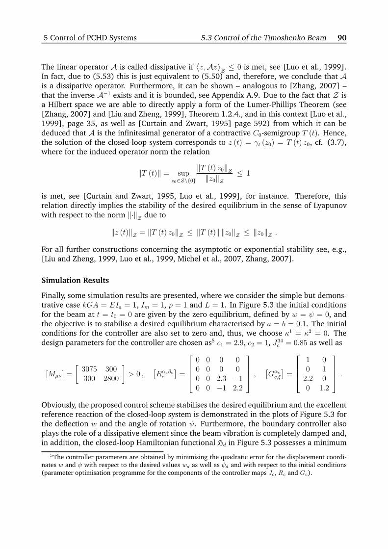
5 Control of PCHD Systems 5.3 Control of the Timoshenko Beam 90
The linear operator A is called dissipative if⟨z,Az
⟩Z≤ 0 is met, see [Luo et al., 1999].
In fact, due to (5.53) this is just equivalent to (5.50) and, therefore, we conclude that Ais a dissipative operator. Furthermore, it can be shown – analogous to [Zhang, 2007] –that the inverse A−1 exists and it is bounded, see Appendix A.9. Due to the fact that Z isa Hilbert space we are able to directly apply a form of the Lumer-Phillips Theorem (see[Zhang, 2007] and [Liu and Zheng, 1999], Theorem 1.2.4., and in this context [Luo et al.,1999], page 35, as well as [Curtain and Zwart, 1995] page 592) from which it can bededuced that A is the infinitesimal generator of a contractive C0-semigroup T (t). Hence,the solution of the closed-loop system corresponds to z (t) = γt (z0) = T (t) z0, cf. (3.7),where for the induced operator norm the relation
‖T (t)‖ = supz0∈Z\{0}
‖T (t) z0‖Z‖z0‖Z
≤ 1
is met, see [Curtain and Zwart, 1995, Luo et al., 1999], for instance. Therefore, thisrelation directly implies the stability of the desired equilibrium in the sense of Lyapunovwith respect to the norm ‖·‖Z due to
‖z (t)‖Z = ‖T (t) z0‖Z ≤ ‖T (t)‖ ‖z0‖Z ≤ ‖z0‖Z .
For all further constructions concerning the asymptotic or exponential stability see, e.g.,[Liu and Zheng, 1999, Luo et al., 1999, Michel et al., 2007, Zhang, 2007].
Simulation Results
Finally, some simulation results are presented, where we consider the simple but demons-trative case kGA = EIa = 1, Im = 1, ρ = 1 and L = 1. In Figure 5.3 the initial conditionsfor the beam at t = t0 = 0 are given by the zero equilibrium, defined by w = ψ = 0, andthe objective is to stabilise a desired equilibrium characterised by a = b = 0.1. The initialconditions for the controller are also set to zero and, thus, we choose κ1 = κ2 = 0. Thedesign parameters for the controller are chosen as5 c1 = 2.9, c2 = 1, J34
c = 0.85 as well as
[Mµν ] =
[3075 300300 2800
]> 0 ,
[Rαcβcc
]=
0 0 0 00 0 0 00 0 2.3 −10 0 −1 2.2
,
[Gαcc,ξ
]=
1 00 1
2.2 00 1.2
.
Obviously, the proposed control scheme stabilises the desired equilibrium and the excellentreference reaction of the closed-loop system is demonstrated in the plots of Figure 5.3 forthe deflection w and the angle of rotation ψ. Furthermore, the boundary controller alsoplays the role of a dissipative element since the beam vibration is completely damped and,in addition, the closed-loop Hamiltonian functional Hd in Figure 5.3 possesses a minimum
5The controller parameters are obtained by minimising the quadratic error for the displacement coordi-nates w and ψ with respect to the desired values wd as well as ψd and with respect to the initial conditions(parameter optimisation programme for the components of the controller maps Jc, Rc and Gc).
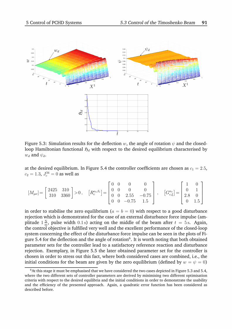
5 Control of PCHD Systems 5.3 Control of the Timoshenko Beam 91
00.2
0.40.6
0.81
05
1015
2025
300
0.05
0.1
0.15
0.2
0.25
0.3
X1t
w
wd
00.2
0.40.6
0.81
05
1015
2025
300
0.02
0.04
0.06
0.08
0.1
0.12
0.14
0.16
X1t
ψ
ψd
0 5 10 15 20 25 300
0.01
0.02
0.03
0.04
0.05
0.06
t
Hd
Figure 5.3: Simulation results for the deflection w, the angle of rotation ψ and the closed-loop Hamiltonian functional Hd with respect to the desired equilibrium characterised bywd and ψd.
at the desired equilibrium. In Figure 5.4 the controller coefficients are chosen as c1 = 2.5,c2 = 1.3, J34
c = 0 as well as
[Mµν ]=
[2425 310310 3360
]>0 ,
[Rαcβcc
]=
0 0 0 00 0 0 00 0 2.55 −0.750 0 −0.75 1.5
,
[Gαcc,ξ
]=
1 00 1
2.8 00 1.5
in order to stabilise the zero equilibrium (a = b = 0) with respect to a good disturbancerejection which is demonstrated for the case of an external disturbance force impulse (am-plitude 1 N
m, pulse width 0.1 s) acting on the middle of the beam after t = 5 s. Again,
the control objective is fulfilled very well and the excellent performance of the closed-loopsystem concerning the effect of the disturbance force impulse can be seen in the plots of Fi-gure 5.4 for the deflection and the angle of rotation6. It is worth noting that both obtainedparameter sets for the controller lead to a satisfactory reference reaction and disturbancerejection. Exemplary, in Figure 5.5 the later obtained parameter set for the controller ischosen in order to stress out this fact, where both considered cases are combined, i.e., theinitial conditions for the beam are given by the zero equilibrium (defined by w = ψ = 0)
6At this stage it must be emphasised that we have considered the two cases depicted in Figure 5.3 and 5.4,where the two different sets of controller parameters are derived by minimising two different optimisationcriteria with respect to the desired equilibria and the initial conditions in order to demonstrate the usabilityand the efficiency of the presented approach. Again, a quadratic error function has been considered asdescribed before.
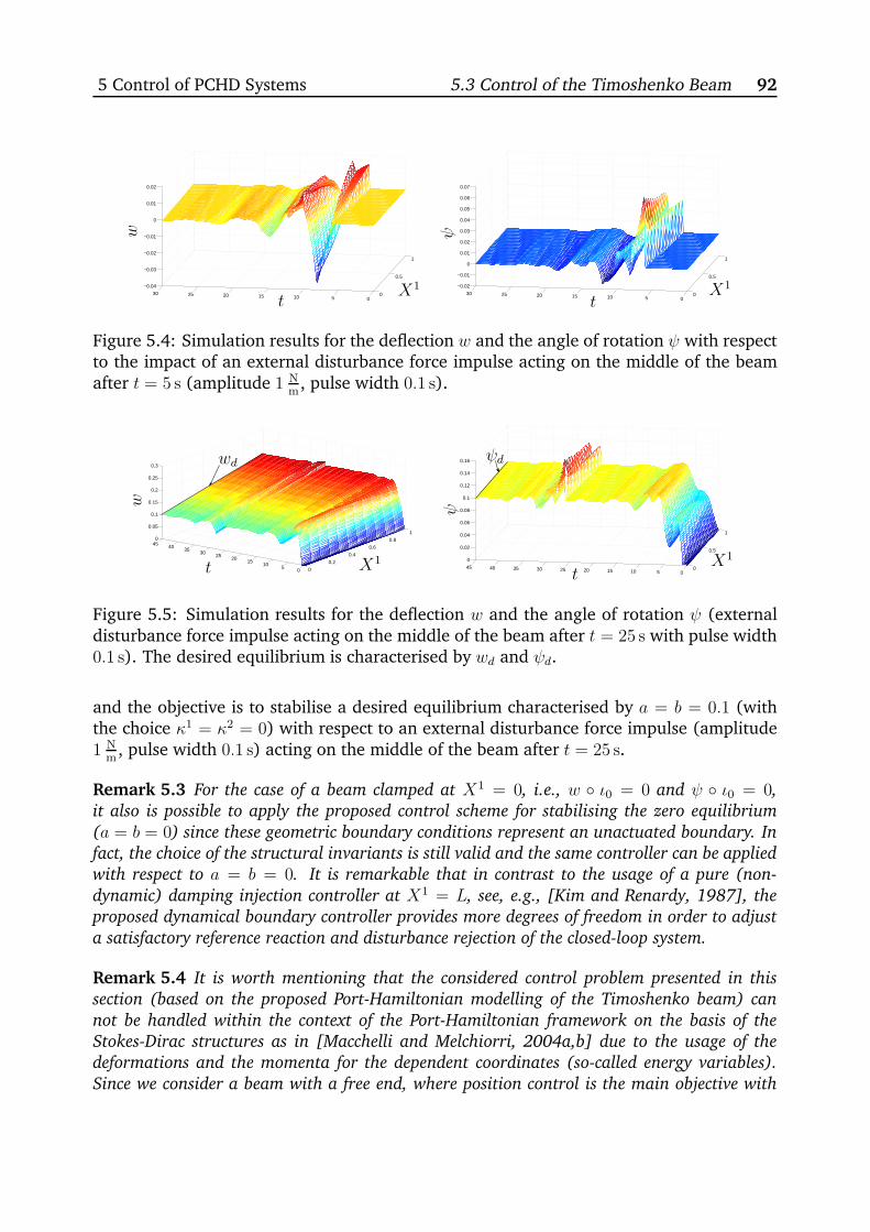
5 Control of PCHD Systems 5.3 Control of the Timoshenko Beam 92
0
0.5
1
051015202530
−0.04
−0.03
−0.02
−0.01
0
0.01
0.02
X1
t
w
0
0.5
1
051015202530
−0.02
−0.01
0
0.01
0.02
0.03
0.04
0.05
0.06
0.07
X1
t
ψ
Figure 5.4: Simulation results for the deflection w and the angle of rotation ψ with respectto the impact of an external disturbance force impulse acting on the middle of the beamafter t = 5 s (amplitude 1 N
m, pulse width 0.1 s).
0
0.2
0.4
0.6
0.8
1
05
1015
2025
3035
40450
0.05
0.1
0.15
0.2
0.25
0.3
X1t
w
wd
0
0.5
1
051015202530354045
0
0.02
0.04
0.06
0.08
0.1
0.12
0.14
0.16
X1
t
ψψd
Figure 5.5: Simulation results for the deflection w and the angle of rotation ψ (externaldisturbance force impulse acting on the middle of the beam after t = 25 s with pulse width0.1 s). The desired equilibrium is characterised by wd and ψd.
and the objective is to stabilise a desired equilibrium characterised by a = b = 0.1 (withthe choice κ1 = κ2 = 0) with respect to an external disturbance force impulse (amplitude1 N
m, pulse width 0.1 s) acting on the middle of the beam after t = 25 s.
Remark 5.3 For the case of a beam clamped at X1 = 0, i.e., w ◦ ι0 = 0 and ψ ◦ ι0 = 0,
it also is possible to apply the proposed control scheme for stabilising the zero equilibrium
(a = b = 0) since these geometric boundary conditions represent an unactuated boundary. In
fact, the choice of the structural invariants is still valid and the same controller can be applied
with respect to a = b = 0. It is remarkable that in contrast to the usage of a pure (non-
dynamic) damping injection controller at X1 = L, see, e.g., [Kim and Renardy, 1987], the
proposed dynamical boundary controller provides more degrees of freedom in order to adjust
a satisfactory reference reaction and disturbance rejection of the closed-loop system.
Remark 5.4 It is worth mentioning that the considered control problem presented in this
section (based on the proposed Port-Hamiltonian modelling of the Timoshenko beam) can
not be handled within the context of the Port-Hamiltonian framework on the basis of the
Stokes-Dirac structures as in [Macchelli and Melchiorri, 2004a,b] due to the usage of the
deformations and the momenta for the dependent coordinates (so-called energy variables).
Since we consider a beam with a free end, where position control is the main objective with

5 Control of PCHD Systems 5.3 Control of the Timoshenko Beam 93
respect to the control via structural invariants methodology, a Port-Hamiltonian formulation
of the beam with respect to the usage of the displacement coordinates is indispensable.
Chapter 6Summary and Outlook
This thesis is mainly dedicated to the geometry, modelling and control of infinite dimensio-nal Port-Hamiltonian systems (called iPCHD systems). It has turned out that the investiga-tion of the formal change of a Hamiltonian functional along a(n) (prolonged) evolutionaryvector field which characterises a certain set of evolution equations serves as the crucialaspect for the extension of the Port-Hamiltonian framework to the distributed-parametercase. Then, by a certain choice of these evolution equations it is possible to proposethe infinite dimensional Port-Hamiltonian system representation, where two main systemclasses can be introduced; namely the iPCHD system representations concerning the non-differential and the differential operator case which allow the analogous physical interpre-tation known from the lumped-parameter PCHD systems such as the characterisation ofthe dissipative effects (inside the domain) and the definition of the (energy) ports actinginside the domain as well as through the boundary. Particularly, with regard to the (Port-)Hamiltonian formulation of field theories the combination of these two system representa-tions has turned out to be an adequate tool. In fact, the proposed framework is applied tothe Port-Hamiltonian modelling of the Timoshenko beam and to the Port-Hamiltonian for-mulation of fluid dynamics including the Navier-Stokes equations and of (inductionless)magnetohydrodynamics – which incorporates electrically conducting fluids in the presenceof (quasi-)stationary electromagnetic fields – in a Lagrangian setting. The last part of thisthesis deals with the extension of the control via structural invariants method which is awell-known method for the control of lumped-parameter PCHD systems with regard to theproposed iPCHD systems restricted to the non-differential operator case, where specificcriteria and conditions analogous to the lumped-parameter case which allow a systematic(boundary) controller design are derived. This control approach is applied to the energybased boundary control of the Timoshenko beam.
With regard to further investigations and future work based on this thesis it will be ofinterest to apply and extend the proposed framework to the Port-Hamiltonian formulationof fully coupled field theories such as the full equations of magnetohydrodynamics inclu-ding – aside from the governing equations of fluid dynamics – the Maxwell’s equations.Particularly, with regard to control purposes it should be possible to extend the control via
structural invariants method to iPCHD systems with higher-dimensional domains (such asplates, etc.), where the demand concerning finite dimensional control laws will become
94

6 Summary and Outlook 95
a crucial aspect. Moreover, another main objective should be dedicated to the extensionof the (from the finite-dimensional case well-known) control method Interconnection and
Damping Assignment - Passivity based Control (IDA-PBC), see, e.g., [Ortega et al., 2002], tothe proposed iPCHD system class, where this method is of main interest concerning prac-tical applications. In particular, the application of non-linear control laws or non-linearboundary controllers should be investigated and analysed in detail with respect to the de-rivation of effective control concepts for iPCHD systems, where, especially for the (formal)stability analysis, the non-linear semigroup theory must be taken into account.
Appendix AProofs and Detailed Computations
Appendix A contains a few proofs and some exact computations which are omitted in theprevious chapters concerning the readability.
A.1 The Application of the Horizontal Differential
Exemplary, for all applications involving horizontal differentials we intend to proof therelation
ˆ
D
(jr+1Φ
)∗ (di(vα∂iαH dX
))=
ˆ
D
(jr+1Φ
)∗ (dh(vα∂iαH ∂icdX
)).
Therefore, we computeˆ
D
(jr+1Φ
)∗ (di(vα∂iαH dX
))=
ˆ
D
∂i((vα∂iαH
)◦ (jrΦ) dX
)
=
ˆ
D
d((vα∂iαH
)◦ (jrΦ) ∂icdX
)
due to the fact d ((vα∂iαH) ◦ (jrΦ) dX) = 0. Furthermore, we obtainˆ
D
(jr+1Φ
)∗ (di(vα∂iαH dX
))=
ˆ
D
dXj ∧ ∂j((vα∂iαH
)◦ (jrΦ) ∂icdX
)
=
ˆ
D
(jr+1Φ
)∗ (dXj ∧ dj
(vα∂iαH ∂icdX
)),
from which the desired result follows by considering the definition of the horizontal differ-ential.
A.2 The Rate of Deformation Tensors
We intend to compute the material rate of deformation tensor according to
D =1
2∂0 (C) =
1
2∂0
((gαβ ◦ Φ)F α
i Fβj
)dX i ⊗ dXj = Dij dX i ⊗ dXj .
96
A Proofs and Detailed Computations A.2 The Rate of Deformation Tensors 97
Therefore, we conclude
D =1
2
(∂γgαβV
γ0 F
αi F
βj + gαβ∂iV
α0 F
βj + gαβF
αi ∂jV
β0
)◦ Φ dX i ⊗ dXj
with respect to ∂0 (gαβ ◦ Φ) = ∂γ (gαβ ◦ Φ)V γ0 as well as ∂0F
αi = ∂iV
α0 . With the help of the
relation∂γgαβ = gδβγ
δαγ + gδαγ
δβγ , (A.1)
cf. [Marsden and Hughes, 1994], we derive the desired result
D =1
2
(gαβ∂iV
α0 F
βj + gδβγ
δαγV
γ0 F
αi F
βj + gαβF
αi ∂jV
β0 + gδαγ
δβγV
γ0 F
αi F
βj
)◦ Φ dX i ⊗ dXj
=1
2(gαβ ◦ Φ)
(Fβj
(∂iV
α0 + γαδγV
γ0 F
δi
)+ F α
i
(∂jV
β0 + γ
βδγV
γ0 F
δj
))◦ Φ dX i ⊗ dXj .
For the derivation of the spatial rate of deformation tensor we evaluate the expression
d =1
2vΦ
(gαβdq
α ⊗ dqβ)
= dαβdqα ⊗ dqβ , vΦ = ∂0 + vα∂α ,
with gαβ ∈ C∞ (Q) leading to
d =1
2vΦ (gαβ) dqα ⊗ dqβ +
1
2gαβvΦ (dqα) ⊗ dqβ +
1
2gαβdq
α ⊗ vΦ
(dqβ).
This expression includes the relations
vΦ (gαβ) = vγ∂γgαβ , vΦ
(dqβ)
= vγ∂γ(dqβ)
= dvβ = ∂γvβdqγ
and, therefore, we are able to write
d =1
2
(vγ∂γgαβ + gδβ∂αv
δ + gαδ∂βvδ)dqα ⊗ dqβ
Using (A.1) we obtain the desired result
d =1
2
(gαδ(∂βv
δ + γδβγvγ)
+ gβδ(∂αv
δ + γδαγvγ))
dqα ⊗ dqβ .
The pull-back of this expression by the motion leads to
D = Φ∗ (d) = (dαβ ◦ Φ)F αi F
βj dX i ⊗ dXj = Dij dX i ⊗ dXj
(by neglecting the terms involving dt0) with the components
Dij =1
2
(gαδ
(∂jV
δ0 + γδβγV
γ0 F
βj
)F αi + gβδ
(∂iV
δ0 + γδαγV
γ0 F
αi
)Fβj
)◦ Φ
=1
2(gαβ ◦ Φ)
(F αi
(∂jV
β0 + γ
βδγV
γ0 F
δj
)+ F
βj
(∂iV
α0 + γαδγV
γ0 F
δi
))◦ Φ .
A Proofs and Detailed Computations A.3 The Stored Energy Relation 98
A.3 The Stored Energy Relation
Based on the result
Sij − Sij = −J(PF i
αFjβg
αβ)◦ Φ = 2ρR
∂Est
∂Cij
we want to prove the relation
P ◦ Φ = −ρR∂Est
∂J.
Therefore, it is easily seen that in consideration of the components of the Cauchy Greentensor Cij = (gαβ ◦ Φ)F α
i Fβj the relation
det [Cij] = (det [gαβ] ◦ Φ) (det [F αi ])2
which allows to reparameterise the Jacobian (4.9) leading to
J = det [F αi ]
√det [gαβ ] ◦ Φ
det [Gij]=
√det [Cij]
det [Gij ]
is met. Due to the fact that the stored energy only depends on the Jacobian we are able toderive
Sij − Sij = 2ρR∂Est
∂J
∂J
∂Cij= ρR
∂Est
∂JJCij
since∂J
∂Cij=
1
2J
1
det [Gij ]
∂ (det [Cij ])
∂Cij=
1
2JCij ,
where we have used the components of the inverse Cauchy Green tensor which followfrom
C = Φ∗ (g) = Cij∂i ⊗ ∂j =(gαβF i
αFjβ ◦ Φ
)∂i ⊗ ∂j , CijCjk = δik ,
and the well-known relation
∂ (det [Mik])
∂Mik
Mjk = δij det [Mik] (A.2)
for an invertible matrix M = [Mik] with components Mik. Furthermore, we conclude
−J(PF i
αFjβg
αβ)◦ Φ = ρR
∂Est
∂JJ(gαβF i
αFJβ ◦ Φ
)
and, consequently, we obtain the desired result.
A Proofs and Detailed Computations A.4 The Ideal Fluid 99
A.4 Hamiltonian Formulation of the Ideal Fluid
We intend to prove the equations
∂0Φα = δαH ◦ j1Φ =
(gαβ ◦ Φ
)
ρR√
det [Gij]Pα ,
∂0Pα = −δαH ◦ j2Φ = −(∂αg
βγ)◦ Φ
2ρR√
det [Gij]PβPγ −
√det [Gij ]J
(F iα ◦ Φ
)∂i (P ◦ Φ)
with respect to the first-order Hamiltonian density
H dX =
(1
2ρR√
det [Gij ]gαβpαpβ + ρREst
√det [Gij ]
)dX .
The first part of the equations is easily verified since we obtain
qα = δαH = ∂αH =1
ρR√
det [Gij ]gαβpβ
and by plugging in the motion the desired result follows directly. For the second part ofthe equations we compute the variational derivative and obtain
pα = −∂αH + di(∂iαH
)(A.3)
with
∂αH =1
2ρR√
det [Gij ]∂α(gγβ)pγpβ + ρR∂α (Est)
√det [Gij] ,
di(∂iαH
)= di
(ρR∂
iα (Est)
√det [Gij]
).
Since the stored energy is a function of the Jacobian we are able to state
di(∂iαH
)= di
(ρR∂Est
∂J∂iα
(J)√
det [Gij ]
)
= −di(P ∂iα (det [F α
i ])√
det [gαβ]
)
= −di(P det [F α
i ] F iα
√det [gαβ]
)
with F iαF
αj = δij , where we have used the relation (A.2). Before we evaluate the expression
di(∂iαH
)= −J F i
αdi
(P)√
det [Gij] − P√
det [gαβ]di
(det [F α
i ] F iα
)
− P det [F αi ] F i
α di
(√det [gαβ]
)
A Proofs and Detailed Computations A.4 The Ideal Fluid 100
we investigate the relation
∂i
((F iα ◦ Φ
)F αj
)= 0
∂i
(F iα ◦ Φ
)F αj = −
(F iα ◦ Φ
)∂i(F αj
)
∂i
(F iα ◦ Φ
)= −
(F iβ ◦ Φ
)∂i
(Fβj
)(F jα ◦ Φ
)
= −(F iβ ◦ Φ
)∂j
(Fβi
)(F jα ◦ Φ
)
since∂i
(Fβj
)= ∂i
(∂jΦ
β)
= ∂j(∂iΦ
β)
= ∂j
(Fβi
).
Therefore, we conclude
di
(det [F α
i ] F iα
)= di (det [F α
i ]) F iα − det [F α
i ] F iβ dj
(Fβi
)F jα
= det[Fβj
]Fjβ di
(Fβj
)F iα − det [F α
i ] F iβ dj
(Fβi
)F jα
= det [F αi ](Fjβ di
(Fβj
)F iα − F
jβ di
(Fβj
)F iα
)
= 0 (A.4)
and, furthermore, we obtain
di
(√det [gαβ]
)= qαi ∂α
(√det [gαβ]
)= qαi
1
2
∂α (det [gαβ])√det [gαβ]
= qαi1
2
1√det [gαβ]
∂ (det [gαβ])
∂gβγ∂α (gβγ)
= qαi1
2
√det [gαβ]g
βγ ∂α (gβγ) .
Consequently, (A.3) takes the form of
pα = − 1
2ρR√
det [Gij]∂α(gγβ)pγpβ − ρR∂α (Est)
√det [Gij]
− J F iαdi
(P)√
det [Gij] −1
2P J
√det [Gij] g
βγ∂α (gβγ) .
The term which involves the stored energy reads as
ρR∂α (Est)√
det [Gij ] = ρR∂Est
∂J∂α
(J)√
det [Gij]
= −P det [F αi ] ∂α
(√det [gαβ]
)
= −1
2P det [F α
i ]√
det [gαβ]gγβ ∂α (gγβ)
= −1
2PJ√
det [Gij ]gγβ ∂α (gγβ)

A Proofs and Detailed Computations A.5 Viscous Stress Form 101
and, thus, we obtain
pα = − 1
2ρR√
det [Gij ]∂α(gγβ)pγpβ − J F i
αdi
(P)√
det [Gij] .
By plugging in the motion we have
∂0Pα = − ∂α(gγβ)◦ Φ
2ρR√
det [Gij]PγPβ − J
(F iα ◦ Φ
)(di
(P)◦ j2Φ
)√det [Gij ]
and, due to
di
(P)◦ j2Φ = ∂i
(P ◦ j1Φ
)= ∂i (P ◦ Φ) ,
we obtain the final result
∂0Pα = − ∂α(gγβ)◦ Φ
2ρR√
det [Gij ]PγPβ − J
(F iα ◦ Φ
)∂i (P ◦ Φ)
√det [Gij] .
A.5 The first Viscous Piola-Kirchhoff Stress Form
For the case of a Newtonian fluid the viscous stress form in Cartesian coordinates reads as
σ = Kcd =(λδαβ ∂γv
γ + µ(δαγ ∂γv
β + δβδ ∂δvα))∂αcvol ⊗ ∂β
and, therefore, we obtain
dΛc (σ) ∧ dt0 =((λ+ µ) ∂α
(δαβ∂γv
γ)
+ µ ∂α(δαγ∂γv
β))
vol ⊗ ∂β .
In order to obtain the Lagrangian counterpart we compute the first viscous Piola-Kichhoffstress form (4.21) which follows in Cartesian coordinates to
P =1
2J(F iαKαβγδF k
γ Flδ
)◦ Φ (δετF
τl ∂kV
ε0 + δετF
εk∂lV
τ0 ) ∂icVOL ⊗ ∂β
= J(F iαKαβγδF k
γ δεδ (∂kVε0 ))◦ Φ ∂icVOL ⊗ ∂β .
With regard toKαβγδ = λ δαβδγδ + µ δαγδβδ + µ δαδδβγ
we are able to conclude
P = J(F iαF
kγ ◦ Φ
)(λ δαβ∂kV
γ0 + µ δαγ∂kV
β0 + µ δβγ∂kV
α0
)∂icVOL ⊗ ∂β
and, therefore, we obtain
dΦΛc
(P)∧ dt0 = ∂i
(J(F iαKαβγδF k
γ δεδ (∂kVε0 ))◦ Φ)
VOL ⊗ ∂β (A.5)
A Proofs and Detailed Computations A.6 The Damping Tensor in iMHD 102
resulting in
dΦΛc
(P)∧ dt0 = J
[λ δαβ
(F iα◦Φ
)∂i
((F kγ ◦Φ
)∂kV
γ0
)+ µ δαγ
(F iα◦Φ
)∂i
((F kγ ◦Φ
)∂kV
β0
)
+ µ δβγ(F iα ◦ Φ
)∂i
((F kγ ◦ Φ
)∂kV
α0
)]VOL ⊗ ∂β
in consideration of (A.4). Before we proceed we inspect the expression(F iα◦Φ
)∂i
((F kγ ◦Φ
)∂kV
α0
)=(F iαF
kγ ◦Φ
)∂i (∂kV
α0 ) +
(F iα◦Φ
)∂i
(F kγ ◦Φ
)∂kV
α0
=(F iαF
kγ ◦Φ
)∂k (∂iV
α0 ) −
(F iαF
kδ ◦Φ
)∂i(F δj
) (F jγ ◦Φ
)∂kV
α0
by considering the relation
∂i
((F kγ ◦ Φ
)Fγj
)= 0
∂i
(F kγ ◦ Φ
)Fγj = −
(F kγ ◦ Φ
)∂i(Fγj
)
∂i
(F kγ ◦ Φ
)= −
(F kδ ◦ Φ
)∂i(F δj
) (F jγ ◦ Φ
).
Furthermore, we end up with the result(F iα◦Φ
)∂i
((F kγ ◦Φ
)∂kV
α0
)=(F iαF
kγ ◦Φ
)∂k (∂iV
α0 ) −
(F kα F
iδ ◦Φ
)∂k(F δj
) (F jγ ◦Φ
)∂iV
α0
=(F iαF
kγ ◦Φ
)∂k (∂iV
α0 ) −
(F jγ F
iδ ◦Φ
)∂j(F δk
) (F kα ◦Φ
)∂iV
α0
=(F iαF
kγ ◦ Φ
)∂k (∂iV
α0 ) +
(F jγ ◦ Φ
)∂j
(F iα ◦ Φ
)∂iV
α0
=(F kγ ◦ Φ
)∂k
((F iα ◦ Φ
)∂iV
α0
).
With the help of this relation we are able to state
dΦΛc
(P)∧ dt0 = J
[λ δαβ
(F iα◦Φ
)∂i
((F kγ ◦Φ
)∂kV
γ0
)+ µ δαγ
(F iα◦Φ
)∂i
((F kγ ◦Φ
)∂kV
β0
)
+ µ δβγ(F kγ ◦ Φ
)∂k
((F iα ◦ Φ
)∂i (V
α0 ))]
VOL ⊗ ∂β
leading to the final result
dΦΛc
(P)∧ dt0 = J
[(λ+ µ) δαβ
(F iα ◦ Φ
)∂i
((F kγ ◦ Φ
)∂kV
γ0
)
+µ δαγ(F iα ◦ Φ
)∂i
((F kγ ◦ Φ
)∂kV
β0
)]VOL ⊗ ∂β .
A.6 The Damping Tensor in iMHD
We want to prove that the matrix representation of
Rαβ = JκγδBαγBβδ
√det [Gij ] = Rβα ,
A Proofs and Detailed Computations A.6 The Damping Tensor in iMHD 103
which is denoted by [Rαβ ], is positive semidefinite provided that the matrix[κγδ]
is sym-metric and positive definite. Since J
√det [Gij ] is always positive we intend to investigate
the definiteness of the remaining expression[κγδBαγBβδ
].
First of all, we introduce the matrix representations
[Bαβ] =
0 B3 −B2
−B3 0 B1
B2 −B1 0
=
[b1 b2 b3
],
[καβ]
=
κ11 κ12 κ13
κ21 κ22 κ23
κ31 κ32 κ33
,
where bα denotes the αth-column of [Bαβ ]. Therefore, we obtain
[κγδBαγBβδ
]=
bT1bT2bT3
[καβ
] [b1 b2 b3
]=
bT1[καβ]b1 bT1
[καβ]b2 bT1
[καβ]b3
bT2[καβ]b1 bT2
[καβ]b2 bT2
[καβ]b3
bT3[καβ]b1 bT3
[καβ]b2 bT3
[καβ]b3
.
According to [Swamy, 1973], a matrix is positive semidefinite if and only if all principleminors of the matrix are non-negative. By applying this result we have to investigate
bT1[καβ]b1 ≥ 0 , bT2
[καβ]b2 ≥ 0 , bT3
[καβ]b3 ≥ 0 , det
[κγδBαγBβδ
]≥ 0
as well as
det
[bT1[καβ]b1 bT1
[καβ]b2
bT2[καβ]b1 bT2
[καβ]b2
]≥ 0 ,
det
[bT1[καβ]b1 bT1
[καβ]b3
bT3[καβ]b1 bT3
[καβ]b3
]≥ 0 ,
det
[bT2[καβ]b2 bT2
[καβ]b3
bT3[καβ]b2 bT3
[καβ]b3
]≥ 0 .
In particular, from the matrix representation [Bαβ] we deduce that det [Bαβ ] = 0 is metresulting in
det[κγδBαγBβδ
]= 0
and, therefore, the fourth condition from above is already fulfilled. With regard to theremaining conditions we make the assumption
[καβ]
=[κβα]> 0 . (A.6)
In order to show that this assumption guarantees the positive semidefiniteness of [Rαβ ]it is clear that the first three conditions are already fulfilled since these are pure quadra-tic forms. In consideration of the analysis of the last three conditions we rewrite theseexpressions in the form
[bT1[καβ]b1 bT1
[καβ]b2
bT2[καβ]b1 bT2
[καβ]b2
]=
[bT1bT2
] [καβ] [
b1 b2],
[bT1[καβ]b1 bT1
[καβ]b3
bT3[καβ]b1 bT3
[καβ]b3
]=
[bT1bT3
] [καβ] [
b1 b3],
[bT2[καβ]b2 bT2
[καβ]b3
bT3[καβ]b2 bT3
[καβ]b3
]=
[bT2bT3
] [καβ] [
b2 b3].
A Proofs and Detailed Computations A.7 Control of PCHD Systems 104
Since the matrices [bT1bT2
],
[bT1bT3
],
[bT2bT3
]
possess linearly independent rows it can be deduced that the relations[bT1bT2
] [καβ] [b1 b2
]>0 ,
[bT1bT3
] [καβ] [b1 b3
]>0 ,
[bT2bT3
] [καβ] [b2 b3
]> 0
are met due to (A.6) and, therefore, the former conditions are clearly fulfilled.
A.7 Control of finite dimensional PCHD Systems
We intend to prove the conditions of Proposition 5.2, where the forthcoming computationsare mainly based on [van der Schaft, 2000]. Since we consider n structural invariants ofthe specific form (5.10) the set of the PDEs (5.9) takes the form of
[∂αC
λ δλαc][Jαβ −Rαβ −Gα
ξ Kηξ Gβc
c,η
Gαcc,ξK
ξηGβη Jαcβcc −Rαcβc
c
]= 0
from which we obtain∂αC
λ(Jαβ − Rαβ
)+Gλ
c,ξKξηGβ
η = 0 (A.7)
as well as−(∂αC
λ)Gαξ K
ηξ Gβcc,η + Jλβcc − Rλβc
c = 0 . (A.8)
Multiplication of (A.7) with ∂βCρ, ρ = 1, . . . , n, leads to
∂αCλ(Jαβ−Rαβ
)∂βC
ρ=−Gλc,ξK
ξηGβη (∂βC
ρ)=−Gλc,ηK
ηξGβξ (∂βC
ρ)=− (∂αCρ)Gα
ξKηξGλ
c,η .
If we compare this result with (A.8) it can be deduced that
− (∂αCρ)Gα
ξ Kηξ Gλ
c,η = −Jρλc +Rρλc = Jλρc +Rλρ
c ,
is met which – together with the former result – leads to
∂αCλ(Jαβ −Rαβ
)∂βC
ρ = Jλρc +Rλρc .
In consideration of the skew-symmetric and the symmetric parts we obtain(∂αC
λ)Jαβ (∂βC
ρ) = Jλρc , (A.9)
−(∂αC
λ)Rαβ (∂βC
ρ) = Rλρc ,
and due to the fact that R and Rc are (by definition) positive semidefinite maps – note that(∂αC
λ)Rαβ (∂βC
ρ) ≥ 0 is met – it can be deduced that the conditions
Rλρc = 0 , (A.10)
Rαβ (∂βCρ) = 0 (A.11)
A Proofs and Detailed Computations A.8 The Equivalent Norm on Z 105
must be fulfilled. Therefore, it is easily seen that (A.9), (A.10) as well as (A.11) correspondto the first three conditions of Proposition 5.2, namely (5.12) – (5.14). Furthermore,(A.11) equals
Rαβ (∂βCρ) = (∂βC
ρ)Rβα = (∂αCρ)Rαβ = 0 =
(∂αC
λ)Rαβ
and, thus, (A.7) simplifies to
∂αCλ(Jαβ − Rαβ
)+Gλ
c,ξKξηGβ
η =(∂αC
λ)Jαβ +Gλ
c,ξKξηGβ
η = 0
from which (5.15) – which reads as(∂αC
λ)Jαβ = −Gλ
c,ξKξηGβ
η (A.12)
– follows directly.
A.8 The Equivalent Norm on ZWe intend to show that the function space Z given by
Z ={z =
(x3c , x
4c , w, ψ, pw, pψ
) ∣∣ x3c , x
4c ∈ R , w, ψ ∈ H1 (0, L) , pw, pψ ∈ L2 (0, L)
}
equipped with the natural inner product
〈z, z〉n = x3c˘x3c + x4
c˘x4c +
ˆ L
0
(j1Φ)∗ (
ψ ˘ψ + ψ1˘ψ1 + w ˘w + w1 ˘w1 + pw ˘pw + pψ ˘pψ
)dX
and the natural norm
‖z‖2n=〈z, z〉n=
(x3c
)2+(x4c
)2+
ˆ L
0
(j1Φ)∗((
ψ)2
+(ψ1
)2+(w)2+(w1)
2+(pw)2+(pψ)2)dX
defines a proper Hilbert space with the equivalent inner product 〈z, z〉Z of (5.51) and theinduced equivalent norm
‖z‖2Z = 〈z, z〉Z = Mµν x
µc x
νc + c1 ι
∗L
(w ◦ Φ
)2+ c2 ι
∗L
(ψ ◦ Φ
)2
+
ˆ L
0
(j1Φ)∗(
1
ρ(pw)2 +
1
Im(pψ)2 + EIa
(ψ1
)2+ kGA
(w1 − ψ
)2)
dX .
In fact, the equivalence of the norms must be shown according to
k1 ‖z‖2n ≤ ‖z‖2
Z ≤ k2 ‖z‖2n , k1, k2 > 0 , (A.13)
see, e.g., [Zeidler, 1990] as well as [Thull, 2010] and references therein. First of all,we intend to investigate the lower bound. Before we proceed we analyse the term (thepull-backs are omitted in order to enhance the readability)
ˆ L
0
(w1)2 =
ˆ L
0
(w1 − ψ
)2dX + 2
ˆ L
0
(w1ψ
)dX −
ˆ L
0
(ψ)2
dX .
A Proofs and Detailed Computations A.8 The Equivalent Norm on Z 106
In consideration of
0 ≤ˆ L
0
(ψ√ε1
± w1
√ε1
)2
dX =1
ε1
ˆ L
0
(ψ)2
dX ± 2
ˆ L
0
(w1ψ
)dX + ε1
ˆ L
0
(w1)2 dX
with ε1 > 0 leading to
∓ 2
ˆ L
0
(w1ψ
)dX ≤ 1
ε1
ˆ L
0
(ψ)2
dX + ε1
ˆ L
0
(w1)2 dX (A.14)
we obtain the relation
(1 − ε1)
ˆ L
0
(w1)2 dX ≤
ˆ L
0
(w1 − ψ
)2dX +
(1
ε1− 1
)ˆ L
0
(ψ)2
dX . (A.15)
Before we proceed we investigate the relationˆ L
0
(ψ)2
dX = ι∗(X1(ψ)2)− 2
ˆ L
0
X1ψψ1 dX = L ι∗L(ψ)2 − 2
ˆ L
0
Xψψ1 dX
which enables us to concludeˆ L
0
(ψ)2
dX ≤ L ι∗L(ψ)2
+1
2
ˆ L
0
(ψ)2
dX + 2
ˆ L
0
(X1ψ1
)2dX (A.16)
– by considering a similar result as (A.14) for ε1 = 2 – resulting inˆ L
0
(ψ)2
dX ≤ 2L ι∗L(ψ)2
+ 4
ˆ L
0
(X1ψ1
)2dX ≤ 2L ι∗L
(ψ)2
+ 4L2
ˆ L
0
(ψ1
)2dX
It is worth noting that this inequality corresponds to the well-known Poincaré inequality,see, e.g., [Vazquez and Krstic, 2008] and references therein. Therefore, from (A.15) wededuce
(1−ε1)
ˆ L
0
(w1)2dX ≤
ˆ L
0
(w1 − ψ
)2dX + 2L
(1
ε1
− 1
)ι∗L(ψ)2
+ 4L2
(1
ε1
− 1
)ˆ L
0
(ψ1
)2dX
which enables us to finally conclude
‖z‖2Z ≥ Mµν x
µc x
νc + c1 ι
∗L (w)2 +
(c2 − 2LkGA
(1
ε1− 1
))ι∗L(ψ)2
+
ˆ L
0
((EIa − 4L2kGA
(1
ε1
− 1
))(ψ1
)2+ kGA (1 − ε1) (w1)
2
)dX
+
ˆ L
0
(1
ρ(pw)2 +
1
Im(pψ)
2
)dX ,
where the inequalities
c2 − 2LkGA
(1
ε1− 1
)> 0
EIa − 4L2kGA
(1
ε1
− 1
)> 0
1 − ε1 > 0
A Proofs and Detailed Computations A.8 The Equivalent Norm on Z 107
must be satisfied. These inequalities can be subsumed as
max
{1
c22LkGA
+ 1,
1EIa
4L2kGA+ 1
}< ε1 < 1 , (A.17)
where it is always guaranteed that such a constant exists due to
c2
2LkGA> 0 ,
EIa
4L2kGA> 0 .
Furthermore, as in [Thull, 2010] it is also possible to find non-negative constants c1, c2such that the relations
c1 ι∗L (w)2 ≥ c1
ˆ L
0
(w)2 dX ,
(c2 − 2LkGA
(1
ε1
− 1
))ι∗L(ψ)2 ≥ c2
ˆ L
0
(ψ)2
dX
are (pointwise) met and, moreover, we are able to state
λmin ([Mµν ])((x3c
)2+(x4c
)2) ≤ Mµν xµc x
νc ≤ λmax ([Mµν ])
((x3c
)2+(x4c
)2), (A.18)
where λmin ([Mµν ]) as well as λmax ([Mµν ]) denote the smallest and largest positive realeigenvalue of the symmetric and positive definite matrix [Mµν ]. Therefore, it is guaranteedthat a positive constant k1 with respect to (A.17) exists such that
‖z‖2Z ≥ k1 ‖z‖2
n (A.19)
is (pointwise) met.Next, we intend to investigate the upper bound of (A.13). By considering (A.14) with
ε2 > 0 as well as (A.18) we are able to state
‖z‖2Z ≤ λmax ([Mµν ])
((x3c
)2+(x4c
)2)+ c1 ι
∗L (w)2 + c2 ι
∗L
(ψ)2
+
ˆ L
0
(EIa
(ψ1
)2+ kGA (1 + ε2) (w1)
2 + kGA
(1 +
1
ε2
)(ψ)2)
dX
+
ˆ L
0
(1
ρ(pw)2 +
1
Im(pψ)
2
)dX .
Furthermore, it is also possible to find positive constants c1, c2 such that the relations
c1 ι∗L (w)2 ≤ c1
ˆ L
0
((w)2 + (w1)
2) dX , c2 ι∗L
(ψ)2 ≤ c2
ˆ L
0
((ψ)2
+(ψ1
)2)dX
are met by applying the Sobolev embedding theorem, see [Zeidler, 1990], for instance.Therefore, it is guaranteed that a positive constant k2 for (arbitrary) ε2 > 0 exists such that
‖z‖2Z ≤ k2 ‖z‖2
n (A.20)
is (pointwise) met.Finally, from the relations (A.19) as well as (A.20) it can be concluded that the norms
‖z‖Z and ‖z‖n are equivalent and, thus, the function space Z defines a proper Hilbertspace with respect to the inner product 〈z, z〉Z of (5.51).
A Proofs and Detailed Computations A.9 The Inverse Operator A−1 108
A.9 The Existence of the Inverse Operator A−1
The existence of the inverse operator A−1 can be shown by solving the equations z = Azfor (arbitrary values of) z = (x3
c , x4c , w, ψ, pψ, pw) ∈ Z. To enhance the readability we
consider sections instead of the coordinate representations and for the restriction of therelevant terms to the boundary we suppress the inclusion mappings notation and directlyplug in the boundary points. In fact, we consider the set of equations
x3c
x4c
w
ψ
pwpψ
=
−R33c (M33x
3c+M34x
4c)+(J34
c −R34c )(M34x
3c+M44x
4c)+G
3c,1
1ρpw(L) +G3
c,21Impψ(L)
(−J34c −R34
c )(M33x3c+M34x
4c)−R44
c (M34x3c+M44x
4c)+G
4c,1
1ρpw(L)+G4
c,21Impψ(L)
1ρpw (X1)
1Impψ (X1)
kAG(∂11w (X1) − ∂1ψ (X1)
)
EIa∂11ψ (X1) + kAG(∂1w (X1) − ψ (X1)
)
with respect to ∂11 = ∂1 ◦ ∂1. From the third and fourth equation we conclude
pw(X1)
= ρw(X1), pψ
(X1)
= Imψ(X1). (A.21)
Therefore, from the first and the second equation we directly obtain[x3c
x4c
]=
([−R33
c J34c −R34
c
−J34c − R34
c −R44c
] [M33 M34
M34 M44
])−1 [x3c −G3
c,1w (L) −G3c,2ψ (L)
x4c −G4
c,1w (L) −G4c,2ψ (L)
],
(A.22)provided that – since [Mµν ] > 0 – the matrix [Jµνc − Rµν
c ] with µ, ν = 3, 4 is invertible.From now on, the forthcoming part is mainly based on [Zhang, 2007], where a Timo-
shenko beam with a free end and a standard PD control law at the actuated boundary isconsidered for stabilising the zero equilibrium. Integration of the fifth equation from 0 toX1 yields
kAG(∂1w
(X1)− ψ
(X1))
= kAG(∂1w (0) − ψ (0)
)︸ ︷︷ ︸
0
+
ˆ X1
0
pw (Z1) dZ1 (A.23)
in consideration of the free end condition at X1 = 0 and, consequently, the sixth equationcan be written as
EIa∂11ψ(X1)
= −ˆ X1
0
pw (Z1) dZ1 + pψ(X1).
Integration of this expression from 0 to X1 results in
EIa ∂1ψ(X1)
= EIa∂1ψ (0)︸ ︷︷ ︸0
−ˆ X1
0
ˆ Z2
0
pw (Z1) dZ1dZ2 +
ˆ X1
0
pψ (Z1) dZ1 (A.24)
in consideration of the free end at X1 = 0 or, equivalently,
∂1ψ(X1)
= − 1
EIa
ˆ X1
0
ˆ Z2
0
pw (Z1) dZ1dZ2 +1
EIa
ˆ X1
0
pψ (Z1) dZ1 .
A Proofs and Detailed Computations A.9 The Inverse Operator A−1 109
Integration of the last expression from X1 to L yields
ψ(X1)
= ψ (L) +1
EIa
ˆ L
X1
ˆ Z3
0
ˆ Z2
0
pw (Z1) dZ1dZ2dZ3 −1
EIa
ˆ L
X1
ˆ Z2
0
pψ (Z1) dZ1dZ2 .
(A.25)Before we proceed we evaluate (A.24) at X1 = L which reads as
EIa ∂1ψ (L) = −ˆ L
0
ˆ Z2
0
pw (Z1) dZ1dZ2 +
ˆ L
0
pψ (Z1) dZ1
= −c2ψ (L) −G3c,2
(M33x
3c +M34x
4c
)−G4
c,2
(M34x
3c +M44x
4c
)
from which we obtain
ψ (L) = −G3c,2
c2
(M33x
3c +M34x
4c
)−G4c,2
c2
(M34x
3c +M44x
4c
)
+1
c2
ˆ L
0
ˆ Z2
0
pw (Z1) dZ1dZ2 −1
c2
ˆ L
0
pψ (Z1) dZ1 .
Therefore, (A.25) finally takes the form of
ψ(X1)
= −G3c,2
c2
(M33x
3c +M34x
4c
)−G4c,2
c2
(M34x
3c +M44x
4c
)− 1
c2
ˆ L
0
pψ (Z1) dZ1
+1
c2
ˆ L
0
ˆ Z2
0
pw (Z1) dZ1dZ2 −1
EIa
ˆ L
X1
ˆ Z2
0
pψ (Z1) dZ1dZ2
+1
EIa
ˆ L
X1
ˆ Z3
0
ˆ Z2
0
pw (Z1) dZ1dZ2dZ3 . (A.26)
Furthermore, from (A.23) we conclude
kAG∂1w(X1)
= kAG ψ(X1)
+
ˆ X1
0
pw (Z1) dZ1
and integration of this expression from X1 to L yields
w(X1)
= w (L) −ˆ L
X1
ψ (Z1) dZ1 −1
kAG
ˆ L
X1
ˆ Z2
0
pw (Z1) dZ1dZ2 . (A.27)
Evaluation of (A.23) at X1 = L results in
kAG(∂1w (L) − ψ (L)
)=
ˆ L
0
pw (Z1) dZ1
= −c1w (L) −G3c,1
(M33x
3c +M34x
4c
)−G4
c,1
(M34x
3c +M44x
4c
)
which leads to
w (L) = −G3c,1
c1
(M33x
3c +M34x
4c
)−G4c,1
c1
(M34x
3c +M44x
4c
)− 1
c1
ˆ L
0
pw (Z1) dZ1 .

A Proofs and Detailed Computations A.9 The Inverse Operator A−1 110
Substituting this result in (A.27) enables us to finally obtain
w(X1)
= −G3c,1
c1
(M33x
3c +M34x
4c
)−G4c,1
c1
(M34x
3c +M44x
4c
)−ˆ L
X1
ψ (Z1) dZ1
− 1
c1
ˆ L
0
pw (Z1) dZ1 −1
kAG
ˆ L
X1
ˆ Z2
0
pw (Z1) dZ1dZ2 (A.28)
which is clearly a function of the z-components by plugging in the relations (A.22) and(A.26). Therefore, the relations (A.21), (A.22), (A.26) as well as (A.28) determine thecomponents of z for a given z and, thus, we have shown the existence of the inverseoperator A−1. Furthermore, it may be deduced that for a bounded z the components of zare also bounded.
Bibliography
R. Aris. Vectors, Tensors and the Basic Equations of Fluid Mechanics. Dover Publications,New York, 1989.
A. Bennett. Lagrangian Fluid Dynamics. Cambridge University Press, 2006.
W. M. Boothby. An Introduction to Differentiable Manifolds and Riemannian Geometry. Aca-demic Press Inc., Orlando, 1986.
W. L. Burke. Applied Differential Geometry. Cambridge University Press, 1994.
A. J. Chorin and J. E. Marsden. A Mathematical Introduction to Fluid Mechanics. Springer-Verlag, New York, 1990.
R. F. Curtain and H. J. Zwart. An Introduction to Infinite-Dimensional Linear Systems Theory.Springer-Verlag, New York, 1995.
M. Dalsmo and A. J. van der Schaft. On representation and integrability of mathematicalstructures in energy-conserving physical systems. SIAM Journal on Control and Optimi-
zation, 37:54–91, 1999.
P. A. Davidson. An Introduction to Magnetohydrodynamics. Cambridge University Press,2001.
H. Ennsbrunner. Infinite-dimensional Euler-Lagrange and Port Hamiltonian Systems. PhDthesis, Johannes Kepler University, Linz, Austria, 2006.
H. Ennsbrunner and K. Schlacher. On the Geometrical Representation and Interconnectionof Infinite Dimensional Port Controlled Hamiltonian Systems. In Proceedings, 44th IEEE
Conference on Decision and Control and the European Control Conference, Seville, Spain,2005.
A. C. Eringen and G. A. Maugin. Electrodynamics of Continua II: Fluids and Complex Media.Springer-Verlag, New York, 1990.
T. Frankel. The Geometry of Physics. Cambridge University Press, 2nd ed., 2004.
111
BIBLIOGRAPHY BIBLIOGRAPHY 112
G. Giachetta, L. Mangiarotti, and G. Sardanashvily. New Lagrangian and Hamiltonian Me-
thods in Field Theory. World Scientific, Singapore, 1997.
F. Gómez-Estern, R. Ortega, F. R. Rubio, and J. Aracil. Stabilization of a Class of Un-deractuated Mechanical Systems via Total Energy Shaping. In Proceedings, 40th IEEE
Conference on Decision and Control, Orlando, Florida, USA, 2001.
A. Jadczyk, J. Janyska, and M. Modugno. Galilei general relativistic quantum mechanicsrevisited. "Geometria, Física-Matemática e outros Ensaios", Homenagem a António Ribeiro
Gomes, pages 253–313, 1998.
I. V. Kanatchikov. Canonical structure of classical field theory in the polymomentum phasespace. Reports on Mathematical Physics, 41(1):49–90, 1998.
H. K. Khalil. Nonlinear Systems. Prentice Hall, 3rd ed., 2002.
J. U. Kim and Y. Renardy. Boundary Control of the Timoshenko Beam. SIAM Journal on
Control and Optimization, 25(6):1417–1429, 1987.
A. Kugi. Non-linear Control Based on Physical Models. Springer-Verlag, London, 2001.
Z. Liu and S. Zheng. Semigroups associated with dissipative systems. Chapman & Hall/CRC,1999.
Z. H. Luo, B. Z. Guo, and Ö. Morgül. Stability and Stabilization of Infinite Dimensional
Systems with Applications. Springer-Verlag, London, 1999.
A. Macchelli and C. Melchiorri. Modeling and Control of the Timoshenko Beam: TheDistributed Port Hamiltonian Approach. SIAM Journal on Control and Optimization, 43(2):743–767, 2004a.
A. Macchelli and C. Melchiorri. Control by Interconnection and Energy Shaping of theTimoshenko Beam. Mathematical and Computer Modelling of Dynamical Systems, 10(3-4):231–251, 2004b.
A. Macchelli and C. Melchiorri. Control by Interconnection of Mixed Port HamiltonianSystems. IEEE Transactions on Automatic Control, 50(11):1839–1844, 2005.
A. Macchelli, A. J. van der Schaft, and C. Melchiorri. Port Hamiltonian Formulation of Infi-nite Dimensional Systems i. Modelling. In Proceedings, 43rd IEEE Conference on Decision
and Control, Atlantis, Paradise Island, Bahamas, 2004c.
A. Macchelli, A. J. van der Schaft, and C. Melchiorri. Port Hamiltonian Formulation ofInfinite Dimensional Systems ii. Boundary Control by Interconnection. In Proceedings,
43rd IEEE Conference on Decision and Control, Atlantis, Paradise Island, Bahamas, 2004d.
J. E. Marsden and T. J. R. Hughes. Mathematical Foundations of Elasticity. Dover Publica-tions, New York, 1994.
BIBLIOGRAPHY BIBLIOGRAPHY 113
J. E. Marsden and T. S. Ratiu. Introduction to Mechanics and Symmetry. Springer-Verlag,New York, 1994.
J. E. Marsden, S. Pekarsky, S. Shkoller, and M. West. Variational methods, multisymplecticgeometry and continuum mechanics. Journal of Geometry and Physics, 38:253–284,2001.
L. Meirovitch. Principles and Techniques of Vibrations. Prentice Hall, 1997.
A. N. Michel, L. Hou, and D. Liu. Stability of Dynamical Systems - Continuous, Discontinuous
and Discrete Systems. Birkhäuser, Boston, 2007.
Ö. Morgül. Stabilization and Disturbance Rejection for the Wave Equation. IEEE Transac-
tions on Automatic Control, 43(1):89–95, 1998.
P. J. Olver. Applications of Lie Groups to Differential Equations. Springer-Verlag, New York,2nd ed., 1993.
R. Ortega, A. J. van der Schaft, I. Mareels, and B. Maschke. Putting energy back in control.IEEE Control Systems Magazine, 21(2):18–33, 2001.
R. Ortega, A. J. van der Schaft, B. Maschke, and G. Escobar. Interconnection and dampingassignment passivity-based control of port-controlled Hamiltonian systems. Automatica,38:585–596, 2002.
H. Rodriguez, A. J. van der Schaft, and R. Ortega. On Stabilization of Nonlinear DistributedParameter Port-Controlled Hamiltonian Systems via Energy Shaping. In Proceedings,
40th IEEE Conference on Decision and Control, Orlando, Florida, USA, 2001.
D. J. Saunders. The Geometry of Jet Bundles. Cambridge University Press, 1989.
K. Schlacher. Distributed PCHD-Systems, from the Lumped to the Distributed Parameter Case,pages 239–255. Advances in Control Theory and Applications, in Bonivento C., IsidoriA., Marconi L., Rossi C., Serie Lecture Notes in Control and Information Sciences 353,Springer Verlag, 2007.
K. Schlacher. Mathematical Modeling for Nonlinear Control: A Hamiltonian Approach.Mathematics and Computers in Simulation, 79(4):829–849, 2008.
K. Schlacher, G. Grabmair, H. Ennsbrunner, and R. Stadlmayr. Some Applications of Dif-
ferential Geometry in Mechanics, pages 261–281. CISM Courses and Lectures No. 444,Springer Verlag, Wien, 2004.
M. Schöberl. Geometry and Control of Mechanical Systems - An Eulerian, Lagrangian and
Hamiltonian Approach. PhD thesis, Johannes Kepler University, Linz, Austria, 2007.
M. Schöberl and K. Schlacher. Covariant formulation of the governing equations of conti-nuum mechanics in an Eulerian description. Journal of Mathematical Physics, 48(5):052902–1 – 052902–15, 2007a.
BIBLIOGRAPHY BIBLIOGRAPHY 114
M. Schöberl and K. Schlacher. Geometric Analysis of Time Variant Hamiltonian ControlSystems. In Proceedings, IFAC Symposium on Nonlinear Control Systems, Pretoria, South
Africa, 2007b.
M. Schöberl and K. Schlacher. First order Hamiltonian Field Theory and Mechanics. Ma-
thematical and Computer Modelling of Dynamical Systems, 17(1):105–121, 2011.
M. Schöberl, H. Ennsbrunner, and K. Schlacher. Modelling of piezoelectric structures - aHamiltonian approach. Mathematical and Computer Modelling of Dynamical Systems, 14(3):179–193, 2008.
M. Schöberl, A. Siuka, and K. Schlacher. Geometric Aspects of First Order Field Theoriesin Piezoelectricity and Magnetohydrodynamics. In Proceedings, International Conference
on Electromagnetics in Advanced Applications, Sydney, Australia, 2010.
J. C. Simo, J. E. Marsden, and P. S. Krishnaprasad. The Hamiltonian structure of nonli-near elasticity: The material and convective representations of solids, rods, and plates.Archive for Rational Mechanics and Analysis, 104(2):125–183, 1988.
A. Siuka, M. Schöberl, and K. Schlacher. Hamiltonian Evolution Equations of inductionlessMagnetohydrodynamics. In Proceedings, 19th International Symposium on Mathematical
Theory of Networks & Systems, Budapest, Hungary, 2010.
A. Siuka, M. Schöberl, K. Rieger, and K. Schlacher. Regelung verteilt-parametrischer Ha-miltonscher Systeme auf Basis struktureller Invarianten. at - Automatisierungstechnik,accepted for publication, 2011.
S. Stramigioli, B. Maschke, and A. J. van der Schaft. Passive Output Feedback and PortInterconnection. In Proceedings, 4th IFAC Nonlinear Control Systems Design Symposium,
Enschede, Netherlands, 1998.
G. W. Sutton and A. Sherman. Engineering Magnetohydrodynamics. Dover Publications,New York, 2006.
K. N. Swamy. On Sylvester’s Criterion for Positive-Semidefinite Matrices. IEEE Transactions
on Automatic Control, page 306, 1973.
D. Thull. Tracking Control of Mechanical Distributed Parameter Systems with Applications.Shaker Verlag, 2010.
E. Truckenbrodt. Fluidmechanik Band 1: Grundlagen und elementare Strömungsvorgänge
dichtebeständiger Fluide. Springer-Verlag, Berlin, 3rd ed., 1989.
A. J. van der Schaft. L2-Gain and Passivity Techniques in Nonlinear Control. Springer-Verlag,London, 2000.
A. J. van der Schaft and B. Maschke. Hamiltonian formulations of distributed parametersystems with boundary energy flow. Journal of Geometry and Physics, 42:166–194, 2002.

R. Vazquez and M. Krstic. Control of Turbulent and Magnetohydrodynamic Channel Flows:
Boundary Stabilization and State Estimation. Birkhäuser, Boston, 2008.
E. Zeidler. Nonlinear Functional Analysis and its Applications II/B. Springer-Verlag, NewYork, 1990.
C.-G. Zhang. Boundary feedback stabilization of the undamped Timoshenko beam withboth ends free. Journal of Mathematical Analysis and Applications, 326(1):488–499,2007.
F. Ziegler. Mechanics of Solids and Fluids. Springer-Verlag, Vienna, New York, 2nd ed.,1998.
115

Curriculum Vitae
Personal Data
Name Andreas Siuka
Address Am Auring 14, 4533 Piberbach
Date of Birth March 22nd, 1984
Place of Birth Linz
Nationality Austria
Email [email protected]
Education
since 11/2008 Work on Ph-.D. thesis. Supervisor: o.Univ.-Prof. Dr. KurtSchlacher, Institute of Automatic Control and Control SystemsTechnology, Johannes Kepler University Linz.
10/2003 – 10/2008 Study Mechatronics at the Johannes Kepler University Linz(finished with distinction). Specialisation on Automatic Control.
Diploma thesis: Analysis and Control of Underactuated Mechanical
Systems by Energy Shaping Methods, Supervisor: o.Univ.-Prof. Dr.Kurt Schlacher.
07/2002 – 08/2003 Military Service, Militärmusik Oberösterreich, Linz.
09/1994 – 06/2002 Grammar School Stift Schlierbach, Schlierbach.
09/1990 – 17/1994 Elementary School, Neuhofen an der Krems
116
Professional Experience
since 10/2009 Johannes Kepler University Linz, lecturer at the Institute ofAutomatic Control and Control Systems Technology.
since 11/2008 Johannes Kepler University Linz, temporary research assistant atthe Institute of Automatic Control and Control SystemsTechnology.
Further Education, Summer Schools and Workshops
05/2011 Workshop on Nonlinear Output Regulation held by Prof. LorenzoMarconi, Linz, Austria.
07/2009 Summer School on Algebraic Analysis and Computer Algebra - New
Perspectives for Applications (AACA ’09) held by Prof.Jean-Francois Pommaret, Hagenberg, Austria.
12/2008 Workshop on Identification and Model Free Control held by Prof.Michel Fliess, Linz, Austria.
Publications
Journal Articles
• Siuka A., Schöberl M., Rieger K., Schlacher K.: Regelung verteilt-parametrischer Ha-
miltonscher Systeme auf Basis struktureller Invarianten, In: at - Automatisierungstech-
nik, accepted for publication, 2011.
• Siuka A., Schöberl M.: Applications of energy based control methods for the inverted
pendulum on a cart, In: Robotics and Autonomous Systems, Vol. 57, No. 10, Elsevier,pp. 1012-1017, ISSN: 0921-8890, 2009.
Conference Papers
• Schöberl M., Siuka A., Schlacher K.: Geometric Aspects of First Order Field Theories
in Piezoelectricity and Magnetohydrodynamics, In: Proceedings of the InternationalConference on Electromagnetics in Advanced Applications (ICEAA ’10), pp. 55–58,2010, Sydney, Australia.
• Siuka A., Schöberl M., Schlacher K.: Hamiltonian Evolution Equations of inductionless
Magnetohydrodynamics, In: CD Proceedings of the 19th International Symposium onMathematical Theory of Networks & Systems (MTNS 2010), pp. 1889-1896, 2010,Budapest, Hungary.
117
• Siuka A., Schöberl M.: Applications of Energy based Control Methods for the Inverted
Pendulum on a Cart, In: Proceedings 5th International Conference on ComputationalIntelligence, Robotics and Autonomous Systems (CIRAS 2008), pp. 187-192, 2008,Linz, Austria.
Invited Talks
• Siuka A., Schöberl M., Schlacher K.: Modellierung und Regelung verteilt-parametrischer
Hamiltonscher Systeme, Control Colloquium at the Institute of Automatic Control(Technical University Munich), October 27, 2010, Garching/Munich, Germany.
• Rieger K., Siuka A.: An Introduction to PDE Control - The Infinite-Dimensional Backs-
tepping Approach, ACCM Lecture Series: Research and Education in Advanced Dy-namics and Model Based Control of Structures and Machines, June 2, 2010, Linz,Austria.
Talks
• Siuka A., Schöberl M., Schlacher K.: Zur Formulierung von Feldtheorien: Ein Tor-
basierter Hamiltonscher Ansatz, GAMM Fachausschuss Dynamik und Regelungstheo-rie, March 19, 2011, Linz, Austria.
• Siuka A., Schöberl M., Schlacher K.: Regelung Hamiltonscher Systeme in evolutionärer
Darstellung mittels strukturellen Invarianten, GMA Fachausschuss 1.40 (TheoretischeVerfahren der Regelungstechnik), September 22, 2010, Anif/Salzburg, Austria.
• Siuka A., Schöberl M., Schlacher K.: Hamiltonian Evolution Equations of inductionless
Magnetohydrodynamics, 19th International Symposium on Mathematical Theory ofNetworks & Systems (MTNS 2010), July 9, 2010, Budapest, Hungary.
• Siuka A., Schöberl M., Schlacher K.: Hamiltonsche Formulierung der Grundgleichun-
gen der Magnetohydrodynamik, GAMM Fachausschuss Dynamik und Regelungstheo-rie, October 13, 2009, Magdeburg, Germany.
• Siuka A., Schöberl M.: Applications of Energy based Control Methods for the Inverted
Pendulum on a Cart, International Conference on Computational Intelligence, Robo-tics and Autonomous Systems (CIRAS 2008), June 20, 2008, Linz, Austria.
Linz, May 2011
118

Eidesstattliche Erklärung
Ich erkläre an Eides statt, dass ich die vorliegende Dissertation selbstständig und ohnefremde Hilfe verfasst, andere als die angegebenen Quellen und Hilfsmittel nicht benutztbzw. die wörtlich oder sinngemäß entnommenen Stellen als solche kenntlich gemacht ha-be.
Linz, im Mai 2011
119