
Georg Job - KIT
187
Georg Job A New Concept of Thermodynamics Entropy as Heat Eduard-Job-Foundation for Thermal and Chemical Dynamics
Transcript of Georg Job - KIT
Georg Job
A New Concept of Thermodynamics
Entropy as Heat
Eduard-Job-Foundation for Thermal and Chemical Dynamics

Georg Job
A New Concept of Thermodynamics
Entropy as Heat
Eduard-Job-Foundation for Thermal and Chemical Dynamics
English Translation of
G. Job: “Neudarstellung der Wärmelehre”,
Akademische Verlagsgesellschaft
Frankfurt am Main, 1972
Translated by Harry Schmeichel, Timm Lankau, Hans Fuchs, Joel Rosenberg
Hamburg, July 2007
V
Preface
The presented book originated from a series of lectures presented during the 1970 summer semester in Hamburg with the title "Trial of a New Concept of Thermodynamics". The impetus for this series was a talk, which I gave in 1967, in the context of a seminar about physical metallurgy at the Institute of Physical Chemistry. My task was to give a short, two-hour overview of thermodynamics and the thermal properties of substances. Because of the shortness of time it was not possible to do it in a traditional way, starting with temperature and heat, con-tinuing with the main laws of thermodynamics, thermodynamic potentials, etc., and make it comprehensible for younger students on the one hand, and also inter-esting enough for my colleagues in the Institute. As a way out, it was not far-fetched to try as directly as possible to reach the most important core of thermo-dynamic concepts, and grab the devil by its horns, starting with a wanted poster of entropy. Surprisingly, it was shown that it is possible to build the complete theory easily and logically, without recourse to the results of the conventional theory. The resonance of the talk with the audience encouraged me to complete my approach, removing unnecessary additives and improving the foundation, and developing a mathematical apparatus, which fits to the new requirements. This consideration formed the basis of the lecture series mentioned above.
Here I want to thank Mr. F. Bruhn, M. Bühring, M. Deneke, J. Heesemann and W. Stränz who offered to rewrite my incomplete notes in a readable form. They have contributed to the quicker publication of the book; without their help I would barely have found the time for it. I must also not forget Mr. M. Melcher, who prepared many of the experiments in the lecture series, and my sister-in-law Mrs. Gd. Job, who with patience and accuracy did the typing. By Christmas 1970 the first draft was completed, then after a thorough revision in 1971, the book was produced first as a lecture script by the chemistry student association in Hamburg. In order to facilitate the transition to conventional textbook form, the usual terms and mathematical procedures were added, along with additional sections, to pro-duce the version presented here.
Hamburg, May 1972 Georg Job
VI
Preface to the English Edition
An English version of the German edition was planned long before, but I never found the time to start with this work. It was my brother, Eduard Job, who got the whole work going. It was his idea, to make this approach accessible for a broader readership. A strong motive was the possibility to protect others from the numerous severe obstacles he had met during his studies of this subject in Ham-burg and Chicago.
I have to mention Harry Schmeichel (California), Timm Lankau (Taiwan), Hans Fuchs (Switzerland) and Joel Rosenberg (Massachusetts). They helped to translate, proofread, correct and modify the given text, in order to express the basic ideas in a better comprehensible form. Since the new approach requires a number of new technical terms for which no standard translation exists it was rather hard to do this work.
Now the IUAPC Conference 2007 in Turin is a good reason for me to prepare at least a provisional version. I want to apologize for eventually incompleteness due to the short time for preparation. I am thankful for any suggestion for im-provement. Criticism of the readers are quite welcome.°)
Hamburg, July 2007 Georg Job
VII
CONTENTS
PREFACE .............................................................................................V
PREFACE TO THE ENGLISH EDITION .............................................VI
CONTENTS.........................................................................................VII
1. INTRODUCTION...............................................................................1
2. PURE THERMODYNAMICS ............................................................3
2.1. Heat ..........................................................................................................3 2.1.1. The Intuitive Interpretation of Heat....................................................3 2.1.2. Measure of Heat* ...............................................................................8 2.1.3. Heat* Measurement Procedure ........................................................11
2.2. Work and Temperature........................................................................14 2.2.1. Potential Energy and Energy Conservation......................................14 2.2.2. Heat* Potential .................................................................................16 2.2.3. Thermal Tension ..............................................................................17 2.2.4. Temperature .....................................................................................19 2.2.5. Heat Engines ....................................................................................19 2.2.6. Thermal Work ..................................................................................20 2.2.7. Heat* Capacity .................................................................................21 2.3.1. Absolute Temperature ......................................................................22 2.3.2. Prerequisites for Heat* Production...................................................23 2.3.3. Feasible and Unfeasible Processes ...................................................25 2.3.4. Lost Work ........................................................................................25 2.3.5. Heat* Conduction.............................................................................26
2.4. Heat* Content at the Absolute Zero of Temperature ........................29
2.5. Comparison with other Theories of Heat............................................30 2.5.1. Comparison with Traditional Thermodynamics...............................30 2.5.2. Historical Background .....................................................................35
VIII Contents
3. GENERAL THERMODYNAMICS...................................................39
3.1. Elastic Coupling ....................................................................................39 3.1.1. Elastic Behavior ...............................................................................39 3.1.2. Main Quantities ................................................................................41 3.1.3. Co- and Counter-Coupling ...............................................................42 3.1.4. Energy and Forces............................................................................43 3.1.5. Primary and Coupling Effects ..........................................................46 3.1.6. Unstable Behavior ............................................................................48
3.2. Mathematical Rules for Derivatives ....................................................49 3.2.1. Change of Variable...........................................................................49 3.2.2. Flip Rule...........................................................................................52 3.2.3. Application Guidelines.....................................................................57 3.2.4. Applications .....................................................................................59 3.2.5. Necessary Number of Known Coefficients ......................................61
3.3 Simple Examples of Mechanical-Thermal Coupling...........................62 3.3.1. Deformation of a Body.....................................................................62 3.3.2. Rubber Band.....................................................................................65 3.3.3. Steel Wire.........................................................................................67
3.4. Body Under Isotropic Pressure ............................................................70 3.4.1. Main Equation and Coupling ...........................................................70 3.4.2. Volume.............................................................................................72 3.4.3. Entropy Content ...............................................................................73 3.4.4 Compressibility, Coefficient of Expansion, and Specific Heat .......75
3.5 Other Systems.........................................................................................76 3.5.1. Galvanic Cell....................................................................................77 3.5.2. Piezoelectric and Pyroelectric Effects ..............................................78 3.5.3. Magneto-Caloric Effect....................................................................79 3.5.4. Bimetallic Strip ................................................................................81
3.6. Traditional Concepts.............................................................................83 3.6.1. Forms of Energy...............................................................................83 3.6.2. Heat, Work, and First Law of Thermodynamics ..............................85 3.6.3. Temperature, Entropy, and Second Law of Thermodynamics .........87 3.6.4. Enthalpy, Heat Functions .................................................................89 3.6.5. Maximum Useful Work....................................................................92
Contents IX
3.6.6. Free Energy, Thermodynamic Potentials .........................................93 3.6.7. Equilibrium Conditions ....................................................................97
3.7 Common Mathematical Procedures .....................................................99 3.7.1. Characteristic Functions, MAXWELL Relations ................................99 3.7.2. Reversible Cycles........................................................................... 101 3.7.3. Systematic Procedure for Calculations........................................... 104 3.7.4. Applications ................................................................................... 106
4. CHEMICAL THERMODYNAMICS ...............................................109
4.1. Introduction......................................................................................... 109
4.2. Amount of Substance .......................................................................... 111
4.3. Chemical Potential .............................................................................. 113 4.3.1 Energy and Potential ....................................................................... 113 4.3.2. The Tendency of Matter to Disperse.............................................. 116 4.3.3. Water as a Numerical Example ...................................................... 118
4.4. Coupling of Substance Transfer to Other Processes........................ 122 4.4.1. Volume and Entropy Demands of a Substance, "Molar Mass"...... 122 4.4.2. Main Equation and Coupling ......................................................... 124
4.5. Transformations of Substances.......................................................... 127 4.5.1. Conditions for Chemical Conversion ............................................. 127 4.5.2. Coupling of V, S and ξ ................................................................... 130 4.5.3. Phase Transitions ........................................................................... 132 4.5.4. λ –Transitions................................................................................. 134
4.6. Homogeneous Bodies .......................................................................... 135 4.6.1. Degree of a Quantity ...................................................................... 135 4.6.2. "Dissection" of a Quantity.............................................................. 137 4.6.3. Reduction of Coefficients............................................................... 139
4.7. Asymptotic Laws for Substances at High Dilution........................... 140 4.7.1. Chemical Potential at Low Concentration...................................... 140 4.7.2. Properties of Dilute Gases.............................................................. 141 4.7.3. Chemical Potentials in Mixtures .................................................... 144
X Contents
4.7.4. Osmosis, Boiling and Freezing Points of Dilute Solutions ............146 4.7.5. Law of Mass Action .......................................................................149 4.7.6. Solution Equilibria .........................................................................149
4.8. Effect of External Fields .....................................................................151
5. THERMODYNAMICS OF ENTROPY PRODUCING PROCESSES..153
5.1. Mechanical Example ...........................................................................153
5.2. ONSAGER's Theorem ...........................................................................156
5.3. Coupling of Electric Currents and Entropy Flows...........................157
....................................................................................161 5.4. More Examples
INDEX................................................................................................163
1
1. INTRODUCTION
Thermodynamics is generally considered a difficult and abstract subject, par-ticularly by beginners. Its development appears arbitrary and unrelated to such topics, as mechanics and electricity and its concepts are not easily clarified by making use of analogies to other areas of physics. If we attempt to apply intuition based on everyday experience, our understanding of thermodynamics becomes even more obscure. In thermodynamics, the variety of abstract concepts such as entropy, enthalpy, state function, cycles, free energy, reversibility, latent heat, etc. make it hard for the student to attain a comprehensive overview of the subject.
For example, the concept of "heat" already shows a noticeable contradiction between theory and intuition. Whereas in everyday experience heat is considered to be something that may be produced in an oven, contained in a heated room and escapes along with air through an open window, in physics heat is not something that is produced in an oven, contained in a room or escapes through an open win-dow. In theoretical physics heat refers strictly to the energy that is transferred to a body through random molecular motion or radiation rather than as something that is contained or created within matter. In physics, heat, similar to work, represents a form of energy that is transferred from one body to another and is not an inher-ent property of a body.1 Expressed mathematically, the quantity of heat Q, just like work, is not a function of state and its differential dQ is therefore incomplete. This conflict between theory and intuition is particularly evident when even scien-tifically educated people do not clearly understand the relationships. For example, many people insist that a body not only accepts heat but also possesses it. Such an opinion may be intuitively correct but is incorrect from a theoretical standpoint except under some very special conditions.
We successfully deal with our environment using a concept of heat that dif-fers from the one taught in physics. Even years of high school and university teaching have not changed this. Nevertheless, it was deemed worthwhile, even if only as an academic exercise, to try to construct a theory based on the intuitive
1 Even this description of heat is not uniform in different physics textbooks!
1. Introduction 2
concepts of heat. This attempt turned out to be successful and the familiar theory of thermodynamics has been developed from a completely different starting point. The resulting educational framework is built on a new foundation, conceptually rearranged and stripped of all unnecessary mathematical terms.
This new approach has the advantage of mathematical rigor, consistency of concepts and compatibility with intuitive understanding. On the other hand, devia-tion from common ways of thinking developed over more than a century is a defi-nite disadvantage. One can ameliorate resistance to this new interpretation of heat by avoiding the ambiguous word heat altogether. Although we cannot avoid its use in earlier chapters, later, for clarity, reference to the word heat is omitted de-spite certain statements becoming less intuitive as a result.
3
2. PURE THERMODYNAMICS
This chapter is addressed to thermodynamics in the narrow sense of heat phe-nomena. It describes measuring methods of the amount of heat, the flow and gen-eration of heat, energy turnover during heat transfer and clarifies basic concepts such as temperature, heat capacity and heat engines. Later chapters cover the laws describing the relationship between thermal and other physical phenomena such as thermal expansion, adiabatic cooling, heat of transition and thermoelectricity.
2.1. Heat
In physics, natural laws are usually presented as mathematical relationships between observed quantities defined by rules for their direct measurement or by an instruction for an indirect calculation from other measurable quantities. In order to make these definitions sensible, we first need a qualitative overview of the subject. Our objective is to choose a measurement process, which preserves those proper-ties familiar to us through everyday experience or common use of language, as-suming, of course, that nature allows us to do this successfully.
2.1.1. The Intuitive Interpretation of Heat
What are the everyday perceptions about heat? One can observe different con-ceptual levels, which may be characterized roughly as follows:
1st Level: Heat, like cold, is a property of a body. It can be caused by friction or fire. When the cause stops, the heated state gradually fades away. A hot body cools down slowly by itself whereas a cold body warms up slowly by itself.
2nd Level: Heat and cold exist in bodies in different amounts. The more heat con-tained in a body, the warmer it appears. In order to heat a large body, more heat is required than for a small one. When a body cools down, heat is not de-stroyed but flows into its surroundings. For example, by placing a hot pot in cold water, the surrounding water becomes warm. Heat and cold can be gener-
2. Pure Thermodynamics
4
ated, e.g., heat is produced by an electric hotplate and cold is produced by a re-frigerator.
3rd Level: A body feels hot because it contains heat. Cold reflects an absence of heat. Rather than cold being produced in a refrigerator, heat is extracted and passed to the outside environment. The extracted heat is not destroyed but spreads throughout the room, just as ripples on a lake after a stone is thrown or as sound waves within a room.
At Level 1 heat is only perceived as a kind of intensity, as hotness to be more precise. Level 2 introduces the concept of an amount of heat. On a first impres-sion, both heat and cold can be produced but not destroyed. At Level 3 this view is simplified by treating cold as the absence of heat while preserving the remaining content of Level 2.
Let us pursue these ideas further and consider the last and most advanced con-ceptual level. In summary, heat exists in every body in a greater or lesser amount it can be transferred to or extracted from a body, but the total amount of heat can be increased but never decreased. In order to complete this picture, we shall inter-pret the results of a few simple additional observations.
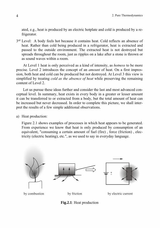
a) Heat production:
Figure 2.1 shows examples of processes in which heat appears to be generated. From experience we know that heat is only produced by consumption of an equivalent, "consuming a certain amount of fuel (fire) , force (friction) , elec-tricity (electric heating), etc.", as we used to say in everyday language.
by friction by electric current
Fig.2.1: Heat production
2. Pure Thermodynamics 5
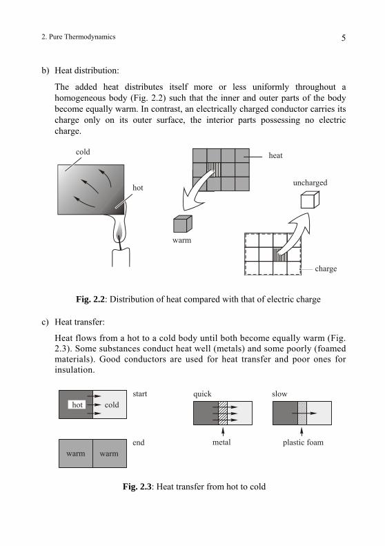
b) Heat distribution:
The added heat distributes itself more or less uniformly throughout a homogeneous body (Fig. 2.2) such that the inner and outer parts of the body become equally warm. In contrast, an electrically charged conductor carries its charge only on its outer surface, the interior parts possessing no electric charge.
hot
heat
uncharged
charge
warm
cold
Fig. 2.2: Distribution of heat compared with that of electric charge
c) Heat transfer:
Heat flows from a hot to a cold body until both become equally warm (Fig. 2.3). Some substances conduct heat well (metals) and some poorly (foamed materials). Good conductors are used for heat transfer and poor ones for insulation.
cold
warm
hot
warm
start
end
quick slow
metal plastic foam
Fig. 2.3: Heat transfer from hot to cold
2. Pure Thermodynamics
6
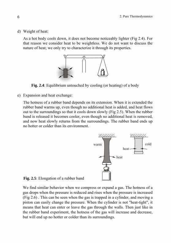
d) Weight of heat:
As a hot body cools down, it does not become noticeably lighter (Fig 2.4). For that reason we consider heat to be weightless. We do not want to discuss the nature of heat; we only try to characterize it through its properties.
Fig. 2.4: Equilibrium untouched by cooling (or heating) of a body
e) Expansion and heat exchange:
The hotness of a rubber band depends on its extension. When it is extended the rubber band warms up, even though no additional heat is added, and heat flows out to the surroundings so that it cools down slowly (Fig 2.5). When the rubber band is released it becomes cooler, even though no additional heat is removed, and now heat slowly returns from the surroundings. The rubber band ends up no hotter or colder than its environment.
warm
heat
heatcold
Fig. 2.5: Elongation of a rubber band
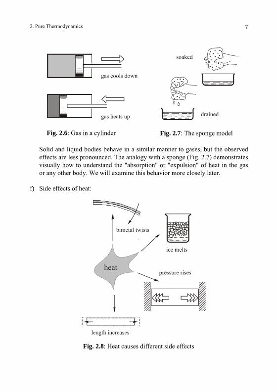
We find similar behavior when we compress or expand a gas. The hotness of a gas drops when the pressure is reduced and rises when the pressure is increased (Fig 2.6) . This can be seen when the gas is trapped in a cylinder, and moving a piston can easily change the pressure. When the cylinder is not "heat-tight", it means that heat can enter or leave the gas through the walls. Then just like in the rubber band experiment, the hotness of the gas will increase and decrease, but will end up no hotter or colder than its surroundings.
2. Pure Thermodynamics 7
soaked
drained
gas cools down
gas heats up
Fig. 2.6: Gas in a cylinder Fig. 2.7: The sponge model
Solid and liquid bodies behave in a similar manner to gases, but the observed effects are less pronounced. The analogy with a sponge (Fig. 2.7) demonstrates visually how to understand the "absorption" or "expulsion" of heat in the gas or any other body. We will examine this behavior more closely later.
f) Side effects of heat:
heat
ice melts
pressure rises
length increases
bimetal twists
Fig. 2.8: Heat causes different side effects
2. Pure Thermodynamics 8
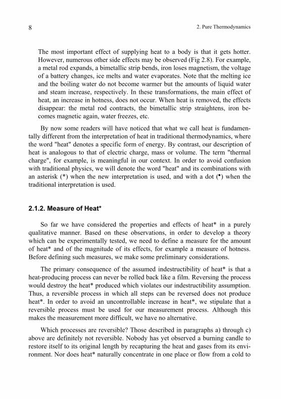
The most important effect of supplying heat to a body is that it gets hotter. However, numerous other side effects may be observed (Fig 2.8). For example, a metal rod expands, a bimetallic strip bends, iron loses magnetism, the voltage of a battery changes, ice melts and water evaporates. Note that the melting ice and the boiling water do not become warmer but the amounts of liquid water and steam increase, respectively. In these transformations, the main effect of heat, an increase in hotness, does not occur. When heat is removed, the effects disappear: the metal rod contracts, the bimetallic strip straightens, iron be-comes magnetic again, water freezes, etc.
By now some readers will have noticed that what we call heat is fundamen-tally different from the interpretation of heat in traditional thermodynamics, where the word "heat" denotes a specific form of energy. By contrast, our description of heat is analogous to that of electric charge, mass or volume. The term "thermal charge", for example, is meaningful in our context. In order to avoid confusion with traditional physics, we will denote the word "heat" and its combinations with an asterisk (*) when the new interpretation is used, and with a dot (•) when the traditional interpretation is used.
2.1.2. Measure of Heat*
So far we have considered the properties and effects of heat* in a purely qualitative manner. Based on these observations, in order to develop a theory which can be experimentally tested, we need to define a measure for the amount of heat* and of the magnitude of its effects, for example a measure of hotness. Before defining such measures, we make some preliminary considerations.
The primary consequence of the assumed indestructibility of heat* is that a heat-producing process can never be rolled back like a film. Reversing the process would destroy the heat* produced which violates our indestructibility assumption. Thus, a reversible process in which all steps can be reversed does not produce heat*. In order to avoid an uncontrollable increase in heat*, we stipulate that a reversible process must be used for our measurement process. Although this makes the measurement more difficult, we have no alternative.
Which processes are reversible? Those described in paragraphs a) through c) above are definitely not reversible. Nobody has yet observed a burning candle to restore itself to its original length by recapturing the heat and gases from its envi-ronment. Nor does heat* naturally concentrate in one place or flow from a cold to
2. Pure Thermodynamics 9
a warm body. In general, reversibility cannot be expected in a spontaneous process because it should then flow freely in either direction.
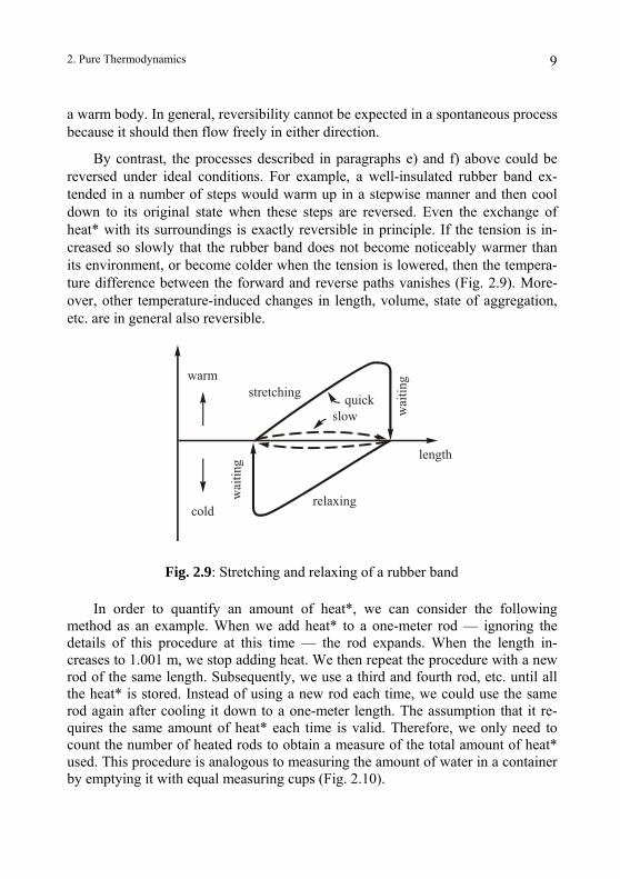
By contrast, the processes described in paragraphs e) and f) above could be reversed under ideal conditions. For example, a well-insulated rubber band ex-tended in a number of steps would warm up in a stepwise manner and then cool down to its original state when these steps are reversed. Even the exchange of heat* with its surroundings is exactly reversible in principle. If the tension is in-creased so slowly that the rubber band does not become noticeably warmer than its environment, or become colder when the tension is lowered, then the tempera-ture difference between the forward and reverse paths vanishes (Fig. 2.9). More-over, other temperature-induced changes in length, volume, state of aggregation, etc. are in general also reversible.
warm
cold
length
stretching
relaxing
quickslow w
aitin
g
wa i
ting
Fig. 2.9: Stretching and relaxing of a rubber band
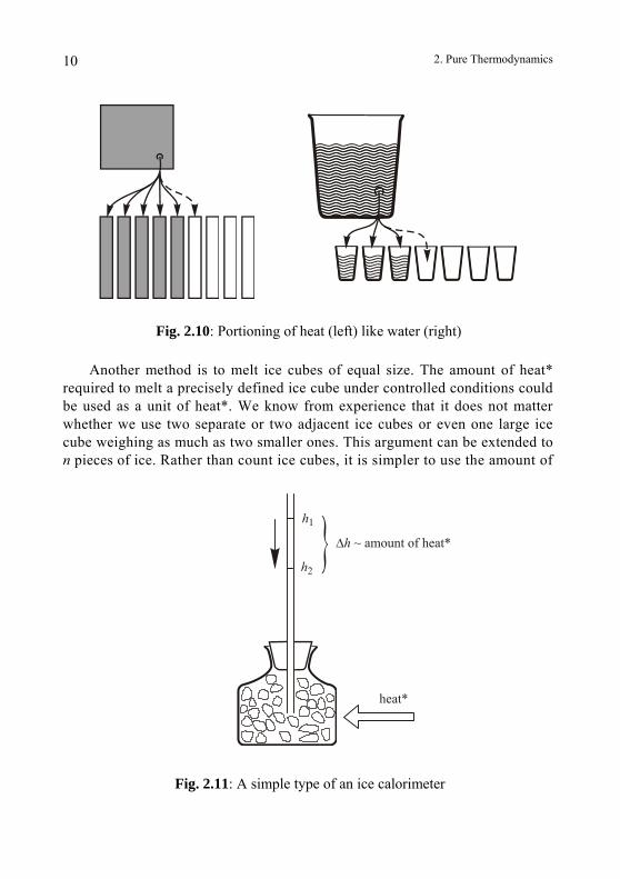
In order to quantify an amount of heat*, we can consider the following method as an example. When we add heat* to a one-meter rod — ignoring the details of this procedure at this time — the rod expands. When the length in-creases to 1.001 m, we stop adding heat. We then repeat the procedure with a new rod of the same length. Subsequently, we use a third and fourth rod, etc. until all the heat* is stored. Instead of using a new rod each time, we could use the same rod again after cooling it down to a one-meter length. The assumption that it re-quires the same amount of heat* each time is valid. Therefore, we only need to count the number of heated rods to obtain a measure of the total amount of heat* used. This procedure is analogous to measuring the amount of water in a container by emptying it with equal measuring cups (Fig. 2.10).
2. Pure Thermodynamics
10
Fig. 2.10: Portioning of heat (left) like water (right)
Another method is to melt ice cubes of equal size. The amount of heat* required to melt a precisely defined ice cube under controlled conditions could be used as a unit of heat*. We know from experience that it does not matter whether we use two separate or two adjacent ice cubes or even one large ice cube weighing as much as two smaller ones. This argument can be extended to n pieces of ice. Rather than count ice cubes, it is simpler to use the amount of
h2
h1
heat*
Fig. 2.11: A simple type of an ice calorimeter
2. Pure Thermodynamics 11
melted ice as measure of heat*. This allows us to construct a practical meas-urement procedure. Liquid water requires less volume than solid ice. The change in volume reflects the heat input. For example, we can use an ice water bottle with a capillary tube (Bunsen ice calorimeter) where we can monitor the water level, i.e., the change in volume of the water (Fig 2.11). With input of heat* the water level drops and with loss of heat* (formation of ice) it rises. This corresponds to a procedure to measure volume whereby water is poured from a given container into a calibrated cylinder.
2.1.3. Heat* Measurement Procedure
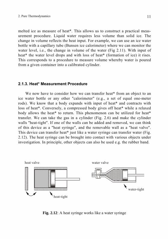
We now have to consider how we can transfer heat* from an object to an ice water bottle or any other "calorimeter" (e.g., a set of equal one-meter rods). We know that a body expands with input of heat* and contracts with loss of heat*. Conversely, a compressed body gives off heat* while a relaxed body allows the heat* to return. This phenomenon can be utilized for heat* transfer. We can take the gas in a cylinder (Fig. 2.6) and make the cylinder walls "heat-tight". If one of the walls can be added and removed, we can think of this device as a "heat syringe", and the removable wall as a "heat valve". This device can transfer heat* just like a water syringe can transfer water (Fig. 2.12). The heat syringe can be brought into contact with various objects under investigation. In principle, other objects can also be used e.g. the rubber band.
heat valve water valve
heat-tight
water-tight
Fig. 2.12: A heat syringe works like a water syringe
2. Pure Thermodynamics
12
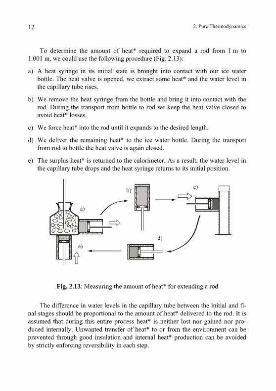
To determine the amount of heat* required to expand a rod from 1 m to 1.001 m, we could use the following procedure (Fig. 2.13):
a) A heat syringe in its initial state is brought into contact with our ice water bottle. The heat valve is opened, we extract some heat* and the water level in the capillary tube rises.
b) We remove the heat syringe from the bottle and bring it into contact with the rod. During the transport from bottle to rod we keep the heat valve closed to avoid heat* losses.
c) We force heat* into the rod until it expands to the desired length.
d) We deliver the remaining heat* to the ice water bottle. During the transport from rod to bottle the heat valve is again closed.
e) The surplus heat* is returned to the calorimeter. As a result, the water level in the capillary tube drops and the heat syringe returns to its initial position.
a)
b)
d)e)
c)
Fig. 2.13: Measuring the amount of heat* for extending a rod
The difference in water levels in the capillary tube between the initial and fi-nal stages should be proportional to the amount of heat* delivered to the rod. It is assumed that during this entire process heat* is neither lost nor gained nor pro-duced internally. Unwanted transfer of heat* to or from the environment can be prevented through good insulation and internal heat* production can be avoided by strictly enforcing reversibility in each step.
2. Pure Thermodynamics 13
How much success will we have in achieving the last condition in our proce-dure? We have shown that steps a), c) and e) can be made reversible if they are performed slowly enough. In addition, all friction between the piston and cylinder has to be eliminated in order to avoid producing heat*. However, steps b) and d) pose some difficulties. If we bring the heat syringe into contact with a warmer body, the piston moves; if we hold the piston in a fixed position, the gas pressure in the cylinder rises. This occurs because heat* flows from the warm body to the colder heat syringe causing the gas to expand. As mentioned above, we cannot allow spontaneous changes to occur in the measurement procedure. Before we bring the heat syringe into contact with a body, the gas in the cylinder has to be compressed and therefore made warmer, so that the piston remains at rest during the brief contact. We can then extract heat* from the hot body. A corresponding procedure applies when the body is colder than the heat syringe. With these pre-cautions, steps b) and d) become reversible.
Thus we have determined a useful measurement procedure that follows logi-cally from our previous assumptions. In summary, these are:
a) Every body contains a definite amount of heat* under specified conditions.
b) Heat* can be produced but not destroyed.
We are now in a position to examine these statements quantitatively. For as-sumption a) to be valid, the amount of heat* in a body, measured by the above procedure (or a similar one) relative to a standard state, must always be the same, independently of whether we use a heat syringe or a rubber band for the transfer of heat, or whether we count pieces of ice or one-meter rods, as long as the calibra-tion is correct. In order to test assumption b), we could extract heat* from a calo-rimeter and deliver it to a thermally insulated test device. For example, we could transfer the heat* to the boiler of a steam engine, to an incandescent bulb or to a thermocouple and then "collect" this scattered heat* with a heat syringe and return it to the calorimeter. When all bodies return to their initial state, then we know from assumption a) that they contain no more heat* than they had initially. Any additional heat* created in the process must now be in the calorimeter and can be measured directly. Statement b) is false if in any test the calorimeter indicates less heat* at the end than was recorded initially.
Experience shows us indirectly that our assumptions are valid. By the above measurement procedure, heat* is explained as a physical quantity. We will denote it by the symbol S. We used the word "indirectly" because later (section 2.5.1) it will transpire that heat* can be equated to entropy in traditional thermodynamics.
2. Pure Thermodynamics 14
Thus the properties of heat* can be deduced by comparison with those of entropy. We can rely on experience without actually having performed the measurements because the results, which the tests would deliver, are easily predictable.
2.2. Work and Temperature
Work is required for or may be gained by transferring heat*, because pushing a piston or stretching a rubber band demands work, for example. In the following sections we shall consider the energy exchanges in such processes.
2.2.1. Potential Energy and Energy Conservation
When a mass of water dm is moved from one container (I) to another (II) where the second container is higher by ∆h than the first one, the work performed is given by
dW = ∆h g dm, where g is the acceleration of free fall. The work performed in lifting the water is stored and is retrievable by reversing the process. We assume here that the process is carried out in a reversible manner. The stored work is called potential energy E. The mass of water dm in container II is said to have a potential energy greater by dW compared with container I:
dEII – dEI = dW.
Note that the mass of water dm in container I, compared with another container at a lower level, already possesses potential energy. The absolute value of energy cannot be determined but rather the difference compared with a conveniently chosen reference point.
Let us now consider the corresponding heat* transfer process. For example, it takes work to "lift" the amount of heat* dS from a cold (I) to a hot (II) body by means of a heat syringe. If carefully done, the associated work dW is retrievable because the process is basically reversible. We can assign a potential energy dEII to the heat* dS in body II that is greater than the corresponding amount dEI in body I by
dEII − dEI = dW.
2. Pure Thermodynamics 15
Similarly, it takes work dW to move a small amount of electric charge dq from one body (I) to another (II) which is more highly charged. Again, dW is recoverable if the charge transfer is reversible. As in the previous cases, the differ-ence of the potentially usable, stored work dE in body II relative to body I, is given by
dEII − dEI = dW. Numerous other methods exist for storing work e.g. a compressed steel
spring, a flying projectile, a rotating flywheel, a charged capacitor, a current-carrying inductor, etc. They all represent stored work, or in other words, a form of energy (elastic, kinetic, electric, magnetic, etc.). In all observed natural processes, work is converted from one stored form into another form. For example, when a steel ball is dropped on to a rigid floor, the initial potential energy (stored work done in overcoming gravity) is converted to kinetic energy (stored work done by the force of gravity) and then upon impact to elastic energy (stored work done by elastic deformation). The upward motion repeats the process in reverse order.
One of the most remarkable achievements in physics during the nineteenth century was the realization that work could be transformed from one stored form to another but the total amount remains constant. Work cannot be created nor destroyed. Consequently, if energy vanishes in one place, it has to reappear in another form elsewhere and vice versa. This realization is generally referred to as the law of conservation of energy.
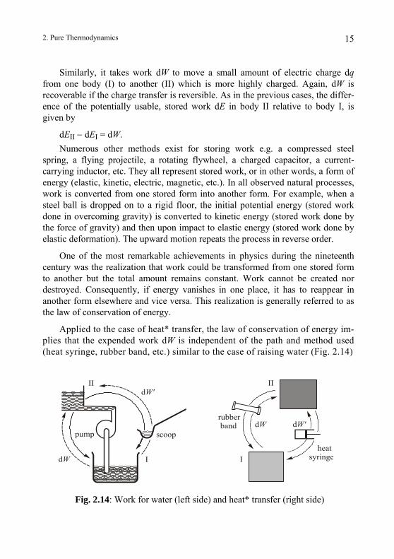
Applied to the case of heat* transfer, the law of conservation of energy im-plies that the expended work dW is independent of the path and method used (heat syringe, rubber band, etc.) similar to the case of raising water (Fig. 2.14)
dW
dW'
dW'dW
II II
I I
pump scoop
rubber band
heatsyringe
Fig. 2.14: Work for water (left side) and heat* transfer (right side)
2. Pure Thermodynamics 16
or moving an electric charge. Otherwise, in contradiction to this law, it would be possible to create work from nothing or make it disappear by delivering heat* by one path and returning it via another.
2.2.2. Heat* Potential
When we refer to a "potential" ψ at a given location, we generally mean the potential energy dE of a small amount da (of substance, charge, mass, heat*, etc.) at this location, divided by this amount:
ddEa
ψ = .
The change in potential ∆ψ between two locations is given by the quotient of the work dW — that is the work required to move da from one location to another — divided by da:
ddWa
∆ψ = .
Although ∆ψ can be determined, ψ cannot. While for small da the potential en-ergy is proportional to the amount da, the potential is only a function of its loca-tion. Thus, the potential ψ can be interpreted as a "work level" associated with the amount of water, electricity, heat*, etc. Storage of work or potential energy is the product of the level and the quantity located there. In other words, it is the energy required to raise the quantity to that level.
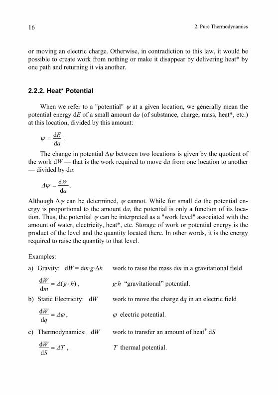
Examples:
a) Gravity: dW = dm·g·∆h work to raise the mass dm in a gravitational field
d ( )Wd
g h∆= ⋅ , g·h “gravitational” potential. m
b) Static Electricity: dW work to move the charge dq in an electric field
ddWq
∆ϕ= , ϕ electric potential.
c) Thermodynamics: dW work to transfer an amount of heat* dS
ddW TS
∆= , T thermal potential.
2. Pure Thermodynamics
17
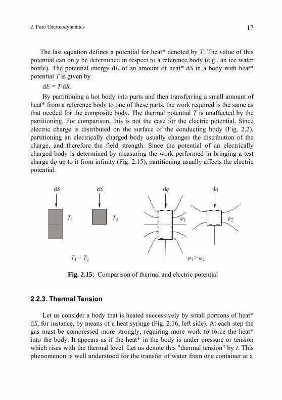
The last equation defines a potential for heat* denoted by T. The value of this potential can only be determined in respect to a reference body (e.g., an ice water bottle). The potential energy dE of an amount of heat* dS in a body with heat* potential T is given by
dE = T·dS. By partitioning a hot body into parts and then transferring a small amount of
heat* from a reference body to one of these parts, the work required is the same as that needed for the composite body. The thermal potential T is unaffected by the partitioning. For comparison, this is not the case for the electric potential. Since electric charge is distributed on the surface of the conducting body (Fig. 2.2), partitioning an electrically charged body usually changes the distribution of the charge, and therefore the field strength. Since the potential of an electrically charged body is determined by measuring the work performed in bringing a test charge dq up to it from infinity (Fig. 2.15), partitioning usually affects the electric potential.
Fig. 2.15: Comparison of thermal and electric potential
dS
T1 T2
dq
T T1 2 = φ φ1 2 >
φ1 φ2
dS dq
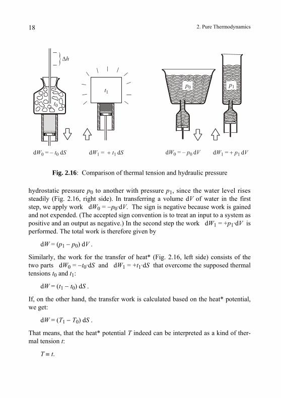
2.2.3. Thermal Tension
Let us consider a body that is heated successively by small portions of heat* dS, for instance, by means of a heat syringe (Fig. 2.16, left side). At each step the gas must be compressed more strongly, requiring more work to force the heat* into the body. It appears as if the heat* in the body is under pressure or tension which rises with the thermal level. Let us denote this "thermal tension" by t. This phenomenon is well understood for the transfer of water from one container at a
2. Pure Thermodynamics
18
p0
d = – dW t S0 0 d = dW t S1 + 1
∆h
t1
t0
p1
d = – dW p V0 0 d = dW p V1 + 1
Fig. 2.16: Comparison of thermal tension and hydraulic pressure
hydrostatic pressure p0 to another with pressure p1, since the water level rises steadily (Fig. 2.16, right side). In transferring a volume dV of water in the first step, we apply work dW0 = −p0·dV. The sign is negative because work is gained and not expended. (The accepted sign convention is to treat an input to a system as positive and an output as negative.) In the second step the work dW1 = +p1·dV is performed. The total work is therefore given by
dW = (p1 − p0) dV .
Similarly, the work for the transfer of heat* (Fig. 2.16, left side) consists of the two parts dW0 = −t0·dS and dW1 = +t1·dS that overcome the supposed thermal tensions t0 and t1:
dW = (t1 − t0) dS .
If, on the other hand, the transfer work is calculated based on the heat* potential, we get:
dW = (T1 − T0) dS .
That means, that the heat* potential T indeed can be interpreted as a kind of ther-mal tension t:
T ≡ t.
2. Pure Thermodynamics 19
2.2.4. Temperature
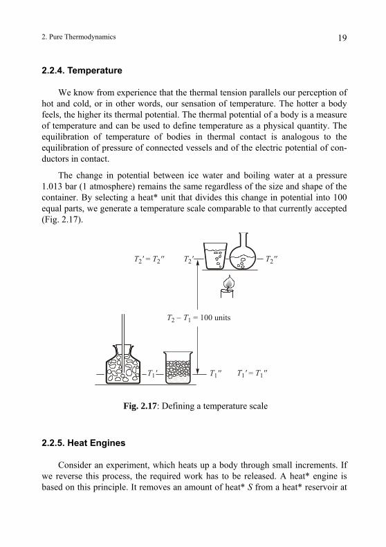
We know from experience that the thermal tension parallels our perception of hot and cold, or in other words, our sensation of temperature. The hotter a body feels, the higher its thermal potential. The thermal potential of a body is a measure of temperature and can be used to define temperature as a physical quantity. The equilibration of temperature of bodies in thermal contact is analogous to the equilibration of pressure of connected vessels and of the electric potential of con-ductors in contact.
The change in potential between ice water and boiling water at a pressure 1.013 bar (1 atmosphere) remains the same regardless of the size and shape of the container. By selecting a heat* unit that divides this change in potential into 100 equal parts, we generate a temperature scale comparable to that currently accepted (Fig. 2.17).
T T2 1 − = 100 units
T1' T1''
T T2 2' '' = T2' T2''
T T1 1' ''=
Fig. 2.17: Defining a temperature scale
2.2.5. Heat Engines
Consider an experiment, which heats up a body through small increments. If we reverse this process, the required work has to be released. A heat* engine is based on this principle. It removes an amount of heat* S from a heat* reservoir at
2. Pure Thermodynamics 20
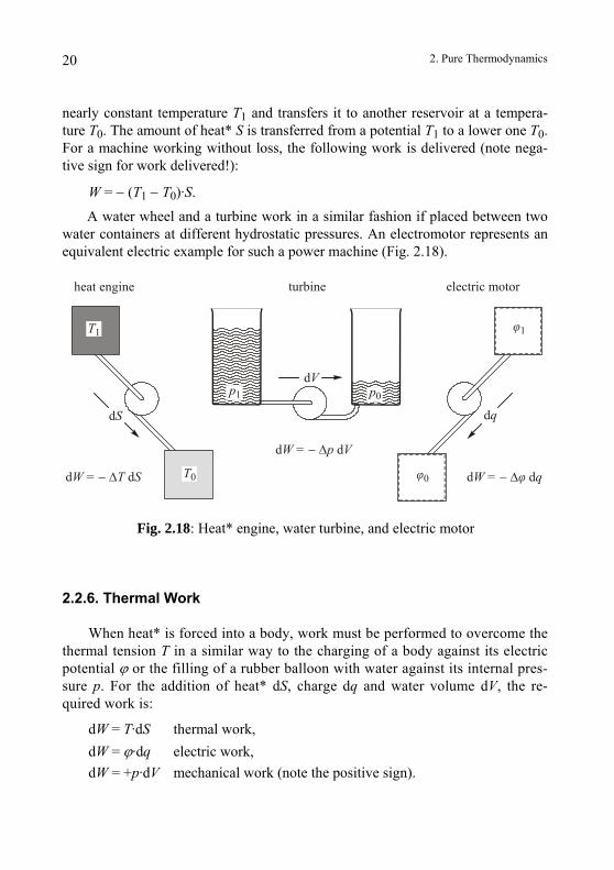
nearly constant temperature T1 and transfers it to another reservoir at a tempera-ture T0. The amount of heat* S is transferred from a potential T1 to a lower one T0. For a machine working without loss, the following work is delivered (note nega-tive sign for work delivered!):
W = − (T1 − T0)·S.
A water wheel and a turbine work in a similar fashion if placed between two water containers at different hydrostatic pressures. An electromotor represents an equivalent electric example for such a power machine (Fig. 2.18).
dW = q− ∆φ d
dW = p V− ∆ d
dW = T S− ∆ d T0 φ0
T1
dVp1 p0
φ1
heat engine turbine electric motor
dqdS
Fig. 2.18: Heat* engine, water turbine, and electric motor
2.2.6. Thermal Work
When heat* is forced into a body, work must be performed to overcome the thermal tension T in a similar way to the charging of a body against its electric potential ϕ or the filling of a rubber balloon with water against its internal pres-sure p. For the addition of heat* dS, charge dq and water volume dV, the re-quired work is:
dW = T·dS thermal work, dW = ϕ·dq electric work, dW = +p·dV mechanical work (note the positive sign).
2. Pure Thermodynamics 21
Thermal work should not be confused with the work required for "lifting" heat* (for example with a heat syringe to a higher level of temperature. When the body supplying the heat* is at the same temperature as that which receives it, the work required for "lifting" vanishes whereas the thermal work remains.
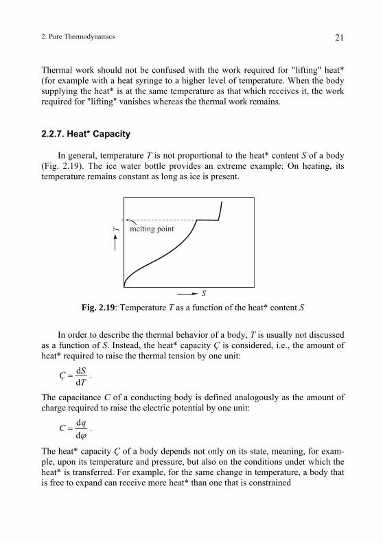
2.2.7. Heat* Capacity
In general, temperature T is not proportional to the heat* content S of a body (Fig. 2.19). The ice water bottle provides an extreme example: On heating, its temperature remains constant as long as ice is present.
T
S
melting point
Fig. 2.19: Temperature T as a function of the heat* content S
In order to describe the thermal behavior of a body, T is usually not discussed as a function of S. Instead, the heat* capacity Ç is considered, i.e., the amount of heat* required to raise the thermal tension by one unit:
dd
SÇT
= .
The capacitance C of a conducting body is defined analogously as the amount of charge required to raise the electric potential by one unit:
dd
qCϕ
= .
The heat* capacity Ç of a body depends not only on its state, meaning, for exam-ple, upon its temperature and pressure, but also on the conditions under which the heat* is transferred. For example, for the same change in temperature, a body that is free to expand can receive more heat* than one that is constrained
2. Pure Thermodynamics 22
2.3. Heat* Production
This section deals with conditions under which heat* is produced, and the consequences of this production which were excluded previously as bothersome side effects.
2.3.1. Absolute Temperature
Let us compare two simple experiments. In order to avoid corrupting the re-sults with an undesirable loss of heat to the surroundings, we must insulate the test body well or work sufficiently quickly.
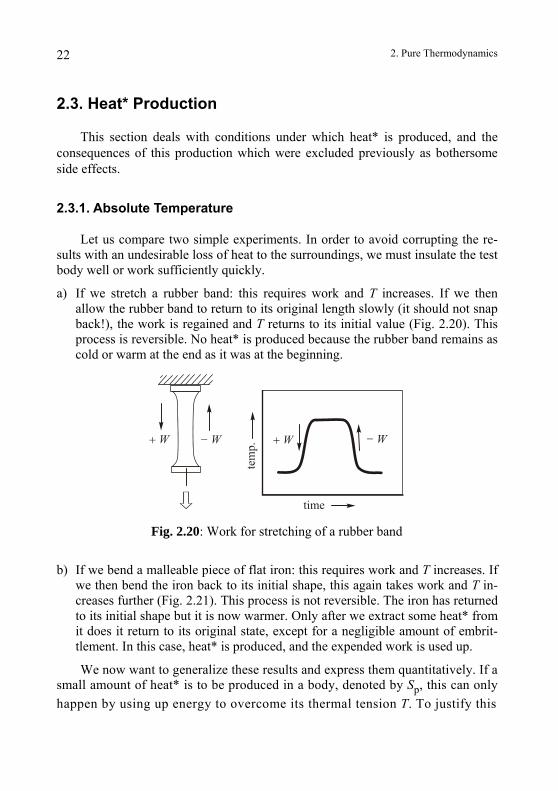
a) If we stretch a rubber band: this requires work and T increases. If we then allow the rubber band to return to its original length slowly (it should not snap back!), the work is regained and T returns to its initial value (Fig. 2.20). This process is reversible. No heat* is produced because the rubber band remains as cold or warm at the end as it was at the beginning.
+ W + W− W − W
tem
p.
time
Fig. 2.20: Work for stretching of a rubber band
b) If we bend a malleable piece of flat iron: this requires work and T increases. If we then bend the iron back to its initial shape, this again takes work and T in-creases further (Fig. 2.21). This process is not reversible. The iron has returned to its initial shape but it is now warmer. Only after we extract some heat* from it does it return to its original state, except for a negligible amount of embrit-tlement. In this case, heat* is produced, and the expended work is used up.
We now want to generalize these results and express them quantitatively. If a small amount of heat* is to be produced in a body, denoted by Sp, this can only happen by using up energy to overcome its thermal tension T. To justify this
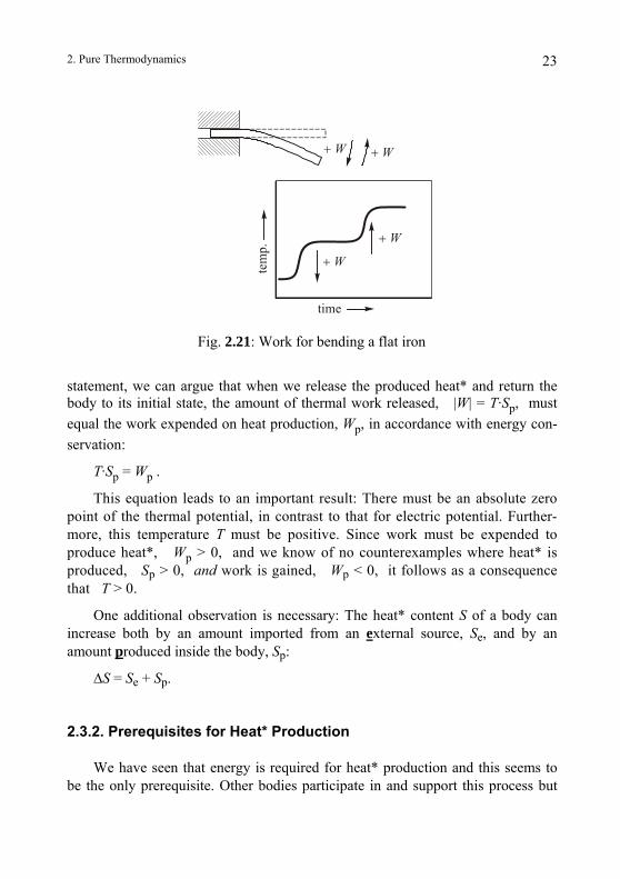
2. Pure Thermodynamics 23
+ W + W
+ W
+ W
tem
p.
time
Fig. 2.21: Work for bending a flat iron
statement, we can argue that when we release the produced heat* and return the body to its initial state, the amount of thermal work released, |W| = T·Sp, must equal the work expended on heat production, Wp, in accordance with energy con-servation:
T·Sp = Wp .
This equation leads to an important result: There must be an absolute zero point of the thermal potential, in contrast to that for electric potential. Further-more, this temperature T must be positive. Since work must be expended to produce heat*, Wp > 0, and we know of no counterexamples where heat* is produced, Sp > 0, and work is gained, Wp < 0, it follows as a consequence that T > 0.
One additional observation is necessary: The heat* content S of a body can increase both by an amount imported from an external source, Se, and by an amount produced inside the body, Sp:
∆S = Se + Sp.
2.3.2. Prerequisites for Heat* Production
We have seen that energy is required for heat* production and this seems to be the only prerequisite. Other bodies participate in and support this process but
2. Pure Thermodynamics 24
remain unaffected. For example, work is expended on bending the iron strip while nothing else important changes. The same conclusion applies when heat* is pro-duced in an electric resistor, by stirring a liquid or by friction in a bearing. Con-versely, one can suspect that heat* is always produced when the required energy is available. The following examples provide some justification for this statement.
a) When a rolling vehicle slows down, its kinetic energy is released. This energy can be stored as potential energy if the vehicle rolls uphill. There is no, or more accurately, only little heat* produced. This possibility is eliminated when the vehicle rolls on level ground and all of the released energy is used for heat* production.
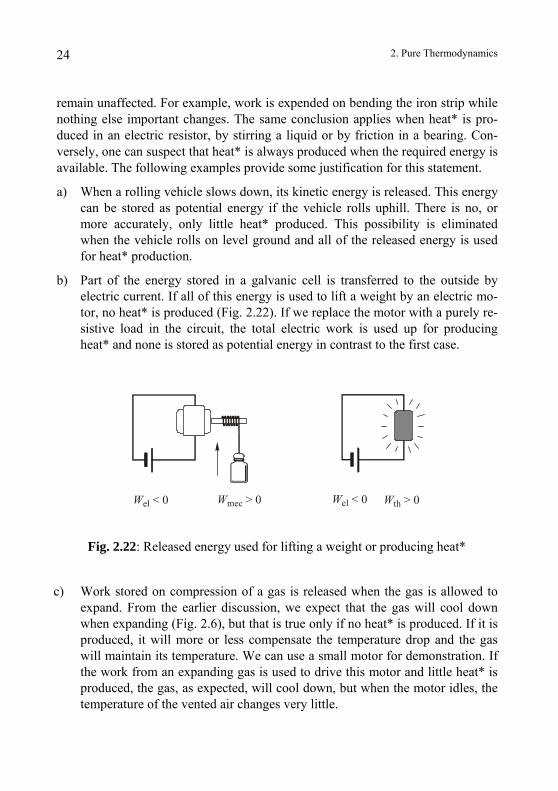
b) Part of the energy stored in a galvanic cell is transferred to the outside by electric current. If all of this energy is used to lift a weight by an electric mo-tor, no heat* is produced (Fig. 2.22). If we replace the motor with a purely re-sistive load in the circuit, the total electric work is used up for producing heat* and none is stored as potential energy in contrast to the first case.
Wel < 0 Wel < 0Wmec > 0 Wth > 0
Fig. 2.22: Released energy used for lifting a weight or producing heat*
c) Work stored on compression of a gas is released when the gas is allowed to expand. From the earlier discussion, we expect that the gas will cool down when expanding (Fig. 2.6), but that is true only if no heat* is produced. If it is produced, it will more or less compensate the temperature drop and the gas will maintain its temperature. We can use a small motor for demonstration. If the work from an expanding gas is used to drive this motor and little heat* is produced, the gas, as expected, will cool down, but when the motor idles, the temperature of the vented air changes very little.
2. Pure Thermodynamics 25
In summary we can state that heat* is produced in a process where excess en-ergy is neither used for work nor stored. This applies in particular to processes involving friction. Work used to overcome friction or some other resistance cannot be stored or captured in such a way that it can be reused.
2.3.3. Feasible and Unfeasible Processes
The insights gained above allow us to determine, on the basis of energy bal-ances, whether or not a process is feasible. A process whereby energy is released, i.e., where stored work is not fully converted from one form of storage into an-other, can run by itself. A process, which requires extra energy, cannot run by itself. It is assumed in both cases that these processes do not violate any laws of nature. The work released in the first case can be consumed by heat* production and hence complies with energy conservation. In the second case, by contrast, the missing energy has to be supplied externally.
Not every process that is capable of releasing energy will actually run its course. For example, a gaseous mixture of oxygen and hydrogen is stable at room temperature even though energy could be released in a chemical reaction. Simi-larly, the Alps are preserved although work could be gained by leveling them. The above processes are possible but inhibited. These natural inhibitions are extremely important for the world, as we know it. Without them, mountains would disappear and the oxygen in the air would destroy all organic matter and, with it, all living beings. Since the process of oxidation is too slow under normal circumstances, life can survive on earth
2.3.4. Lost Work
If work Wp is used up in a heat-producing process, then it is not possible to regain the full amount. This occurs because heat* cannot be destroyed and those places and reservoirs where heat* can be stored are at a positive temperature. Therefore, at least the potential energy, T·S that exists at the coldest accessible place is lost. We describe Wp as "lost", "wasted" or "devalued" work because it can only be partially restored through cumbersome procedures. The rate at which work is lost is called loss power.
2. Pure Thermodynamics 26
One of the most convenient ways to introduce heat* in a specified place is to utilize lost work. In order to heat up a room or a body, we produce heat* locally via a chemical reaction (fire, gas burner) or with an electric heater. In general, we do not transfer heat* from a reservoir or some distant source. After measuring the lost work and the temperature of the body that is being heated, we can easily cal-culate the amount of heat* produced, provided an appropriate thermometer is available.
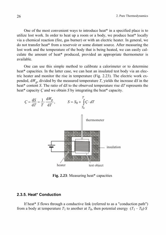
One can use this simple method to calibrate a calorimeter or to determine heat* capacities. In the latter case, we can heat an insulated test body via an elec-tric heater and monitor the rise in temperature (Fig. 2.23). The electric work ex-pended, dWp, divided by the measured temperature T, yields the increase dS in the heat* content S. The ratio of dS to the observed temperature rise dT represents the heat* capacity Ç and we obtain S by integrating the heat* capacity.
pdd 1 ,d d
WSÇT T T
= = ⋅0
0
T
TS S Ç dT= + ⋅∫
test object
thermometer
heater
insulation
2.3.5. Heat* Condu
If heat* S flows from a body at tempe
Fig. 2.23: Measuring heat* capacities
ction
through a conductive link (referred to as a "conduction path") rature T1 to another at T0, then potential energy (T1 – T0)·S
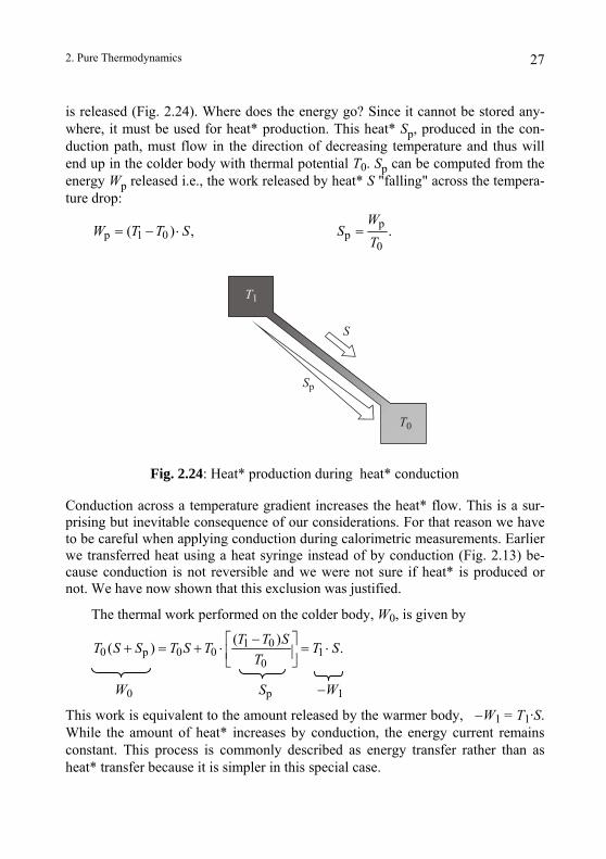
2. Pure Thermodynamics 27
is released (Fig. 2.24). Where does the energy go? Since it cannot be stored any-where, it must be used for heat* production. This heat* Sp, produced in the con-duction path, must flow in the direction of decreasing temperature and thus will end up in the colder body with thermal potential T0. Sp can be computed from the energy Wp released i.e., the work released by heat* S "falling" across the tempera-ture drop:
p0 p
0) , .
WT S S
T⋅ =p 1(W T= −
S
T1
T0
Sp
Fig. 2.24: Heat* production during heat* conduction
Conduction across a temperature gradient increases the heat* flow. This is a sur-prising but inevitable consequence of our considerations. For that reason we have to be careful when applying conduction during calorimetric measurements. Earlier we transferred heat using a heat syringe instead of by conduction (Fig. 2.13) be-cause conduction is not reversible and we were not sure if heat* is produced or not. We have now shown that this exclusion was justified.
The thermal work performed on the colder body, W0, is given by
1 00 p 0 0 1
0
( )( ) .T T ST S S T S T T ST−⎡ ⎤+ = + ⋅ = ⋅⎢ ⎥⎣ ⎦
W0 Sp −W1
This work is equivalent to the amount released by the warmer body, −W1 = T1·S. While the amount of heat* increases by conduction, the energy current remains constant. This process is commonly described as energy transfer rather than as heat* transfer because it is simpler in this special case.
2. Pure Thermodynamics 28
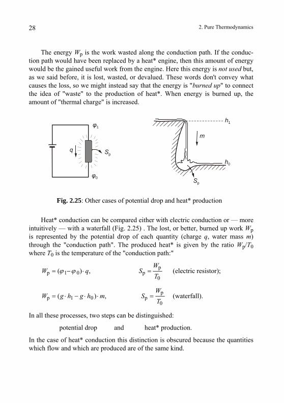
The energy Wp is the work wasted along the conduction path. If the conduc-tion path would have been replaced by a heat* engine, then this amount of energy would be the gained useful work from the engine. Here this energy is not used but, as we said before, it is lost, wasted, or devalued. These words don't convey what causes the loss, so we might instead say that the energy is "burned up" to connect the idea of "waste" to the production of heat*. When energy is burned up, the amount of "thermal charge" is increased.
φ0
φ1
q Sp
m
Sp
h1
h0
Fig. 2.25: Other cases of potential drop and heat* production
Heat* conduction can be compared either with electric conduction or — more intuitively — with a waterfall (Fig. 2.25) . The lost, or better, burned up work Wp is represented by the potential drop of each quantity (charge q, water mass m) through the "conduction path". The produced heat* is given by the ratio Wp/T0 where T0 is the temperature of the "conduction path:"
pp 1 0 p
0( ) ,
WW q S
Tϕ ϕ= − ⋅ = (electric resistor);
pp 1 0 p
0( ) ,
WW g h g h m S
T= ⋅ − ⋅ ⋅ = (waterfall).
In all these processes, two steps can be distinguished:
potential drop and heat* production.
In the ca e quantities which flo
se of heat* conduction this distinction is obscured because thw and which are produced are of the same kind.
2. Pure Thermodynamics 29
2.4. Heat* Content at the Absolute Zero of Temperature
If we remove all heat* S from a substance, we expect its temperature T to drop to zero. Actually we can make the temperature T approach zero as closely as desired by continuously extracting heat*. Since T can be measured, it is easy to observe this behavior. Expressed mathematically, we have:
T → 0 as S → 0 (more precisely: T → 0 for S sufficiently small).
It is more difficult to determine the amount of heat* remaining in a body. One could destroy the body chemically and thus release and measure the heat* which remains, since heat* cannot be destroyed. However, both the reactants and prod-ucts of the chemical reaction contain some heat*. Therefore, this method can only determine the difference ∆S of the heat* released by the initial materials and ab-sorbed by the final materials. Such investigations show that ∆S vanishes at very low temperatures (the procedures are described in chapter 4). This result and other empirical facts support the obvious assumption that bodies at zero absolute tem-perature contain no heat*:
S → 0 as T → 0.
These two relations formulated here have some peculiar exceptions. If a drop of water evaporates completely, then its heat* content goes to zero without a change in temperature. This is in violation of the first relation. If we allow a ther-mally insulated gas to expand continuously, then its temperature drops and ap-proaches zero although its heat* content remains constant. This is a violation of the second relation. We will apply the above relations to non-degenerate cases only, such that the volume of a body cannot vanish or become arbitrarily large. Furthermore, the amount of the substance used may approach zero — a vacuum is permissible in our considerations — but it may never approach infinity. The above discussion can be summarized as follows:
T → 0 if and only if S → 0 for finite systems.
Some materials, such as liquid glass for example, are observed to give off less heat* if they are cooled down quickly, than they would if they were cooled down slowly, although the initial and final temperatures are equal in the two cases. It is as if heat* is trapped or frozen into the body if it is cooled too quickly. In the case of glass, it is the heat* required to melt it (the heat* of fusion) which is frozen in.
2. Pure Thermodynamics 30
Melted glass crystallizes very slowly, and rapid cooling delays the process to the point that it stops and the heat* of fusion cannot be released. A further tempera-ture drop would slow down the crystallization even more, so this method cannot be used to extract the frozen heat*. These amounts of heat* are literally trapped in, as in a thermos flask. Since they cannot be released, they do not influence a ther-mometer and contribute nothing to the measured temperature of a body.
Some materials trap heat* even in an absolutely cold environment. By exclud-ing these exceptions, the above theorems remain valid for finite systems. Their consequences agree with our experience.
2.5. Comparison with other Theories of Heat
People familiar with other approaches to thermodynamics need to know how this new approach is related to traditional conceptual approaches. This knowledge is also necessary in order to use intelligently the tabulated data and knowledge available in the literature. Even for those not well versed in historical terminology, it should not be too difficult to understand the essential ideas.
2.5.1. Comparison with Traditional Thermodynamics
So far we have formulated several concepts to describe the observed thermal phenomena. The same processes can be described using the standard language of conventional thermodynamics. A comparison will yield the corresponding con-cepts of each approach. In this section only we will mark all variables as they are used in the new approach with an asterisk (*) as we have been doing with heat*. Variables from traditional thermodynamics will not be marked.
We mentioned earlier that heat* can be equated with entropy (see the end of section 2.1.3). Both quantities can be identified strictly from the following com-parison. Our procedure for heat* transfer from one body to another is very similar to a reversible CARNOT process. Section 2.1.3 gives the example of expanding a rod from 1.000 to 1.0001 m with a heat* input via a heat syringe from an ice water bottle. During this process the entropy decrease −∆S1 of the first body (ice calo-rimeter) equals the entropy increase ∆S2 of the second body (rod) because the
2. Pure Thermodynamics 31
entropy of the total system (ice calorimeter and rod) remains constant due to re-versibility:
−∆S1 = ∆S2 .
According to traditional theory, the mass m of freezing water in our heat* meas-urement process is proportional to the entropy loss of the calorimeter, −∆S1 In addition, m is by our definition a measure of the increase in heat* of the body under investigation:
∆S2* ~ m ~ −∆S1 = ∆S2 .
If we set the proportionality constant between ∆S2* and ∆S2 to unity by an appro-priate choice of units and select the zero of entropy properly, then the entropy S and the heat* content S* of a body are equal:
S = S* .
In traditional thermodynamics, "heat" is treated as a form of energy, repre-sented by Q. Entropy, S, is introduced as the integral ∫dQrev/T. Those who are familiar with this abstract introduction might wish a more detailed justification of the last equation in order to see how it fits in with previous concepts. The follow-ing comments might help: Entropy is a state function, which always increases for real processes in isolated systems. Since it is an extensive or substance-like quan-tity, one can assign a density to it for every region of space. It follows that entropy can be viewed as an entity distributed in space that may be added to or extracted from a body, and whose total amount always increases. Since dS = dQrev/T, the qualitative effects of an entropy increase are the same as a heat• input, Q. You can think of each increase dS, for either reversible or irreversible processes, to be caused by a reversible heat• input, dQrev, even if it is actually caused by an irre-versible process. Since we cannot tell whether the heat effects are due to entropy or the energy dQrev received by a body, we are free to interpret the quantity S as heat, rather than Q.
Now let us consider the determination of the absolute thermal potential T* of a piece of matter by producing a small amount of heat* Sp* inside it as described in section 2.3.1. The energy Wp expended for this purpose is supplied to the piece and then completely emitted as thermal work, W*. Conservation of energy re-quires that
Wp = −W* = T*·Sp*.
2. Pure Thermodynamics 32
Expressed in traditional terminology, the performed work Wp is expended in the first irreversible step and as a result, the entropy must increase by some — as yet undetermined — amount. In the subsequent reversible step, the heat• Q is released and simultaneously the entropy is decreased by Q/T, where T is the thermody-namic temperature of the material. Since the body returns to its initial state at the end, the total change in energy and entropy are zero. Expressed mathematically, we have Wp + Q = 0 and Sp + Q/T = 0, or
Wp = −Q = T·Sp.
Comparing both equations for Wp, we see that heat• in its traditional sense, Q, is equal to thermal work, W*, and since S = S*, the thermodynamic temperature, T, must be equal to heat* potential, T*:
Q = W*, T = T*. As a result, our heat* capacity Ç* = dS*/dT* = dS/dT = Ç. Usually the
quantity Ç = dS/dT is not used in traditional thermodynamics, but it could be called "entropy capacity". Our heat* capacity Ç* differs from the commonly used heat• capacity C = dQ/dT by the factor T, because T·dS = dQ. We can write
C = T·Ç* = T (dS/dT). Therefore, in our terminology traditional heat• capacity C may be referred to as "thermal work capacity". Except for the sake of this comparison, there is no reason to introduce a quantity C in our new interpretation. Similarly, there is no need to introduce a quantity Ç in the traditional view. In all cases, we can state that
Ç = Ç* C = C*.
entropy capacity = heat* capacity heat• capacity = thermal work capacity
Thus, the basic quantities and their derived variables are in one-to-one corre-spondence without requiring conversion. That has some practical consequences. We can measure the heat* potential with a common mercury thermometer and we can read off the heat* content of many bodies in the "entropy" column of pub-lished tables. If the quantities remain the same, what has really changed?
Briefly stated: It has been shown that the central concepts of thermodynamics can be introduced in a simple and intuitive way, although under different names. The discrepancies between the energetic interpretation of heat and our common language have been largely eliminated. Entropy, for most people a hard-to-grasp
2. Pure Thermodynamics 33
concept, has been given an adequate interpretation. Finally, we can make compari-sons with other areas of physics that facilitate our understanding of the conceptual framework and remove the abstractness of thermodynamics. Those who are un-comfortable that heat conduction is treated as a composite procedure (heat transfer from high to low temperature combined with heat production) may consider en-ergy flow instead of entropy flow and, in this way, retain traditional formulae without returning to the traditional interpretation.
In order to clarify these differences, let us contrast some analogous state-ments, in traditional and new terminology.
a) Energy Law (First Law) :
— Traditional: The internal energy of a system is a state function. Its change is due to the sum of all heat• and work inputs to the system received from its surroundings. The energy of an isolated system remains constant during all internal processes.
— New: Work can be stored in various ways and can be regained. It cannot be created or destroyed.
b) Entropy Law (Second Law):
— Traditional: The entropy of a system is a state function. Its change is due to the integral of all heat• inputs to the system received from its surroundings in a reversible way, dQrev, divided by the absolute temperature T at which the heat• is introduced. The entropy of an isolated system can increase but never decrease during all internal processes.
— New: Heat* is contained in larger or smaller amounts in a body depending on its state. It can be produced but cannot be destroyed.
c) NERNST Heat Law (Third Law):
— Traditional: The entropy of a system in equilibrium vanishes as its tempera-ture approaches absolute zero.
— New: Absolutely cold bodies contain no heat* unless some of it is trapped in.
d) Heat Engines:
— Traditional: The efficiency of an ideal heat engine, defined as the useful work divided by the expended heat•, Qin, is given by the temperature differ-ence between heat• input and output, ∆T = Tin − Tout, divided by the abso-lute temperature of the heat• input: W/Qin = ∆T/Tin.
2. Pure Thermodynamics 34
— New: The useful work of a lossless heat* engine is the product of the thermal potential drop, ∆T, and the amount S of the transferred heat*: W = ∆T·S.
The new interpretation treats work — or rather work storage — as synony-mous with energy, since there is no compelling reason to differentiate between stationary and moving forms of energy or work. On the contrary, one can avoid unnecessary explanations by not making this distinction. A good example is the treatment of electric charge. Certain important statements become almost self-explanatory with the new interpretation. For example, the statement that it is im-possible to build a perpetually running heat engine driven by a constant tempera-ture heat reservoir (W. THOMSON's version of the Second Law) is analogous to: "It is impossible to operate a water mill without a drop in elevation". Similarly, the statement that it is impossible to reach the absolute zero of temperature (the fre-quently used form of the Third Law), in other words to remove all the heat* con-tained in a body, is analogous to saying: "It is impossible to reach the absolute zero of pressure by removing all the gas from a tank".
We are faced with the curious fact that the choice of a single concept — namely, the "heat" concept — has decisively influenced the structure of an entire theoretical framework. This choice affects not only the immediacy of its state-ments, but also the conciseness of its computational methods, as we will see later. How is this possible?
In contrast to scientific description, common language is relatively imprecise. A single word can denote different concepts. For example, to an unbiased layman the word "force" conveys ideas and characteristics that correspond to physical quantities like pressure, force, energy, momentum or potential. There exists con-siderable leeway in establishing a correspondence between scientific and com-monly used concepts.
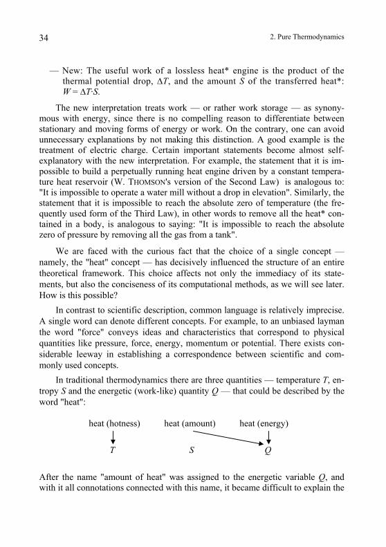
In traditional thermodynamics there are three quantities — temperature T, en-tropy S and the energetic (work-like) quantity Q — that could be described by the word "heat":
heat (hotness) heat (amount) heat (energy) T S Q
After the name "amount of heat" was assigned to the energetic variable Q, and with it all connotations connected with this name, it became difficult to explain the
2. Pure Thermodynamics 35
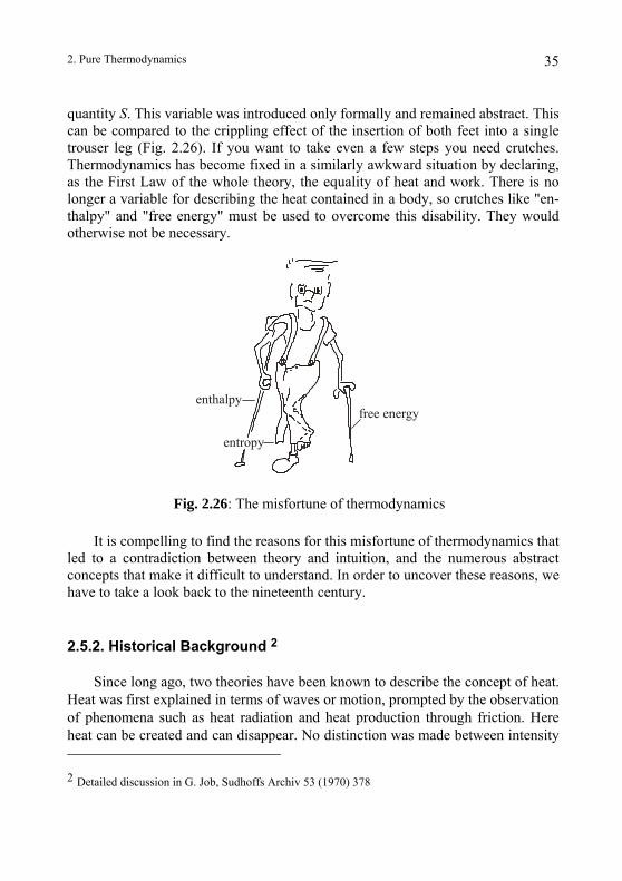
quantity S. This variable was introduced only formally and remained abstract. This can be compared to the crippling effect of the insertion of both feet into a single trouser leg (Fig. 2.26). If you want to take even a few steps you need crutches. Thermodynamics has become fixed in a similarly awkward situation by declaring, as the First Law of the whole theory, the equality of heat and work. There is no longer a variable for describing the heat contained in a body, so crutches like "en-thalpy" and "free energy" must be used to overcome this disability. They would otherwise not be necessary.
enthalpy
entropy
free energy
Fig. 2.26: The misfortune of thermodynamics
It is compelling to find the reasons for this misfortune of thermodynamics that led to a contradiction between theory and intuition, and the numerous abstract concepts that make it difficult to understand. In order to uncover these reasons, we have to take a look back to the nineteenth century.
2.5.2. Historical Background 2
Since long ago, two theories have been known to describe the concept of heat. Heat was first explained in terms of waves or motion, prompted by the observation of phenomena such as heat radiation and heat production through friction. Here heat can be created and can disappear. No distinction was made between intensity 2 Detailed discussion in G. Job, Sudhoffs Archiv 53 (1970) 378
2. Pure Thermodynamics 36
(temperature) and quantity (amount of heat), as you find in common language even today.
Later, during the 18th century, under the influence of the evolution of chemis-try, scholars tended to interpret heat as a kind of substance called caloric, which could neither be produced nor annihilated like a chemical element. As a result, the first quantitative statements could be made about heat. Transports of heat, as well as the changes of temperature when hot and cold bodies are in contact, were easily explained by making the temperature proportional to the concentration of heat. The processes of fusion and evaporation were viewed as a reaction of this "heat substance" with the heated body. Heat was not produced by friction; the substance was released by the worn down material like oil from pressed seeds. According to this substance theory, heat could not be produced, nor could it be destroyed. In order to explain the temperature balance achieved by bodies with different initial temperatures, J. H. LAMBERT (1779), M. A. PICTET (before 1800) and other con-temporaries assumed that heat was subjected to a kind of tension that increases more and more when a body becomes hot. This was assumed to be the cause of the tendency of heat to disperse.
In 1824, S. CARNOT, whose considerations laid the foundation for thermody-namics, compared a heat engine driven by cold and hot heat reservoirs with a water mill. He drew analogies between the temperature difference and the drop in elevation of the water, and between the heat transferred and the water flowing down, and then computed the work gained from such an engine. He did not obtain his results from the analogy but derived them from the well-known impossibility of a perpetual motion machine (perpetuum mobile) on the basis of the substance theory of heat. In essence, he used two assumptions:
a) Work cannot be created.
b) Heat is not producible and not destructible.
Building on CARNOT's ideas, E. CLAPEYRON (1834) introduced the relationship between steam pressure and heat of evaporation that became known as the CLAUSIUS-CLAPEYRON Equation because R. CLAUSIUS (1864) expressed it in its final form. In 1848 W. THOMSON suggested a definition of temperature that corre-sponds to the introduction of T as the potential of the heat substance.
This generally successful interpretation of heat was contradicted by results of different experiments that showed that heat seems to be produced, related to the amount of work expended. This indicated a connection between these two quanti-
2. Pure Thermodynamics 37
ties. B. THOMPSON, H. DAVY (about 1800) and especially J. P. JOULE, by his care-ful experiments after 1840, further refined the idea. JOULE measured the same heating effect when he expended a definite amount of work, regardless of the method he used. R. MAYER, J. P. JOULE and H. v. HELMHOLTZ then assumed that heat and work are interconvertible. Confusion spread when they tried to apply the principle of conservation of energy to all of physics, since formerly it was proven only for mechanical processes. Did heat in a steam engine behave like water in a mill according to CARNOT's explanation, or was it used up as MAYER and JOULE claimed?
In 1850, R. CLAUSIUS suggested a compromise between the conflicting inter-pretations. Heat was neither arbitrarily convertible into work, nor was its amount conserved in a steam engine during the transition from higher to lower tempera-ture. Both processes had to be considered as interconnected in a determined man-ner. He showed that one could arrive at the corresponding statements made by CARNOT and CLAPEYRON by changing the assumptions of the substance theory of heat as follows:
a) Work cannot be created nor destroyed without using up or creating an equivalent amount of heat.
b) Heat is not producible and not destructible cannot flow from a lower to a higher temperature by itself.
Although this theory was further developed by THOMSON in parallel with CLAUSIUS, it was not accepted initially because it lacked the simplicity and ele-gance of the old interpretation. Later, however, it replaced all other competing theories. It was helped by the fact that the discovery of the energy principle made an overwhelming impression on scientists of that time. They had exaggerated expectations from this law of nature. In some places it was considered as the "only formula required for the true knowledge of nature" (G. HELM, 1898). According to H. HERTZ, many of his contemporaries considered the reduction of all natural phenomena to the laws of energy conversion as the ultimate goal of physical re-search. It is understandable that in such an environment the CLAUSIUS-THOMSON theory of thermodynamics was treated as a kind of archetype theory because its heat quantity was not a quantity on its own, unlike electric charge, but was simply interpreted as a form of energy. Efforts were made to develop other disciplines according to this ideal, rather than making the framework of thermodynamics similar to that of its related areas. The hope of the "energetic advocates" was not realized, but they
left us their version of thermodynamics.
2. Pure Thermodynamics 38
What was overlooked is that a minimal change of CARNOT's basic assump-tions is sufficient to eliminate the contradictions between the old theory and ex-perience. In this way the switch to the energy interpretation, which has cost so much effort and controversy, could have been avoided:
a) Work cannot be created nor destroyed.
b) Heat is not producible and not destructible.
By striking out the one word "not" in the last sentence, we reject the substance theory just as CLAUSIUS did.
3. General Thermodynamics 39
3. GENERAL THERMODYNAMICS
On heating a body one can observe a temperature rise – the primary effect – as well as various secondary effects such as expansion, pressure increase, bending, charge increase (pyroelectric effect), chemical changes, etc. Conversely, mechani-cal, electrical and magnetic effects can cause thermal side effects like a tempera-ture change or a heat transfer to or from the environment. This chapter deals with the interactions and relationships between thermal and other physical quantities. However, chemical transformations are left until chapter 4.
3.1. Elastic Coupling
This term refers to a conceptual model that applies to many physical proc-esses. It is particularly suitable for describing conditions of thermodynamic equi-librium. First we shall clarify the conceptual and mathematical framework of this model with mechanical examples before applying it to thermal phenomena.
3.1.1. Elastic Behavior
If we stretch a rubber band (at constant temperature) from a length l0 to a length l, we observe an opposing force F which is uniquely determined by this extension, and which increases with length l:
F = F(l).
We refer to this behavior as elastic. We observe a steep increase in force at small extension, a somewhat reduced value on further extension and finally another increase at even larger extension. Figure 3.1 depicts the function F = F(l) graphi-cally in exaggerated form.
Let us define the "stiffness" of the rubber band at length l1 by dF/dl, which represents the slope of the curve at point P. The term "spring constant", commonly used for a linear relationship between F and l, namely F = a·(l − l0), is
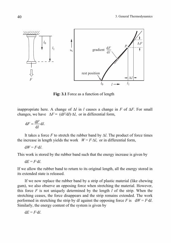
3. General Thermodynamics 40
l0
l0
l1
l1
F
dFd l
l
∆lrest position
∆F
F
gradientP
Fig: 3.1 Force as a function of length
inappropriate here. A change of ∆l in l causes a change in F of ∆F. For small changes, we have ∆F = (dF/dl)·∆l, or in differential form,
dd d .dFF ll
=
It takes a force F to stretch the rubber band by ∆l. The product of force times the increase in length yields the work W = F·∆l, or in differential form,
dW = F·d l.
This work is stored by the rubber band such that the energy increase is given by
dE = F·dl.
If we allow the rubber band to return to its original length, all the energy stored in its extended state is released.
If we now replace the rubber band by a strip of plastic material (like chewing gum), we also observe an opposing force when stretching the material. However, this force F is not uniquely determined by the length l of the strip. When the stretching ceases, the force disappears and the strip remains extended. The work performed in stretching the strip by dl against the opposing force F is dW = F·dl. Similarly, the energy content of the system is given by
dE = F·dl.
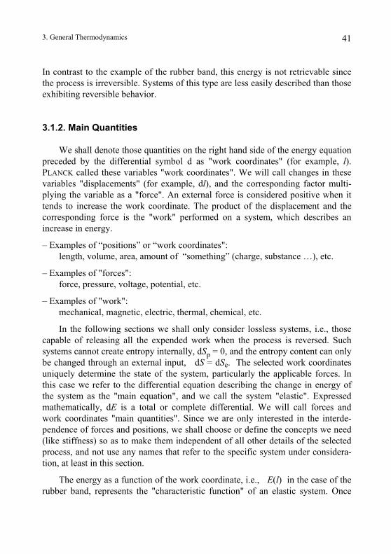
3. General Thermodynamics 41
In contrast to the example of the rubber band, this energy is not retrievable since the process is irreversible. Systems of this type are less easily described than those exhibiting reversible behavior.
3.1.2. Main Quantities
We shall denote those quantities on the right hand side of the energy equation preceded by the differential symbol d as "work coordinates" (for example, l). PLANCK called these variables "work coordinates". We will call changes in these variables "displacements" (for example, dl), and the corresponding factor multi-plying the variable as a "force". An external force is considered positive when it tends to increase the work coordinate. The product of the displacement and the corresponding force is the "work" performed on a system, which describes an increase in energy.
– Examples of “positions” or “work coordinates": length, volume, area, amount of “something” (charge, substance …), etc.
– Examples of "forces": force, pressure, voltage, potential, etc.
– Examples of "work": mechanical, magnetic, electric, thermal, chemical, etc.
In the following sections we shall only consider lossless systems, i.e., those capable of releasing all the expended work when the process is reversed. Such systems cannot create entropy internally, dSp = 0, and the entropy content can only be changed through an external input, dS = dSe. The selected work coordinates uniquely determine the state of the system, particularly the applicable forces. In this case we refer to the differential equation describing the change in energy of the system as the "main equation", and we call the system "elastic". Expressed mathematically, dE is a total or complete differential. We will call forces and work coordinates "main quantities". Since we are only interested in the interde-pendence of forces and positions, we shall choose or define the concepts we need (like stiffness) so as to make them independent of all other details of the selected process, and not use any names that refer to the specific system under considera-tion, at least in this section.
The energy as a function of the work coordinate, i.e., E(l) in the case of the rubber band, represents the "characteristic function" of an elastic system. Once
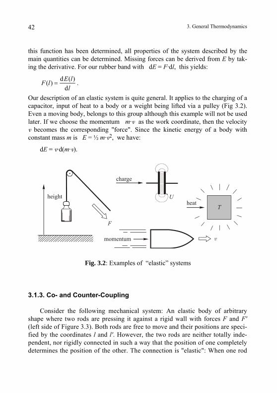
3. General Thermodynamics
42
this function has been determined, all properties of the system described by the main quantities can be determined. Missing forces can be derived from E by tak-ing the derivative. For our rubber band with dE = F·dl, this yields:
d ( )( )dE lF l
l= .
Our description of an elastic system is quite general. It applies to the charging of a capacitor, input of heat to a body or a weight being lifted via a pulley (Fig 3.2). Even a moving body, belongs to this group although this example will not be used later. If we choose the momentum m·v as the work coordinate, then the velocity v becomes the corresponding "force". Since the kinetic energy of a body with constant mass m is E = ½ m·v2, we have:
dE = v·d(m·v).
T
F
v
U
charge
momentum
heatheight
Fig. 3.2: Examples of “elastic” systems
3.1.3. Co- and Counter-Coupling
Consider the following mechanical system: An elastic body of arbitrary shape where two rods are pressing it against a rigid wall with forces F and F' (left side of Figure 3.3). Both rods are free to move and their positions are speci-fied by the coordinates l and l'. However, the two rods are neither totally inde-pendent, nor rigidly connected in such a way that the position of one completely determines the position of the other. The connection is "elastic": When one rod
3. General Thermodynamics 43
is pushed in, the other is pushed out. By holding one rod fixed its motion ceases, but the force, which pushes the rod out increases. We will refer to this kind of interdependence of two processes as counter-coupling, which describes the case where one process hinders the other. We call the opposite behavior, where one process reinforces the other, co-coupling. The right hand side of Figure 3.3 gives an example of the latter.
F
F
F'
F'l
l
l'
l'
.
Fig. 3.3: Counter- and Co-coupling of two rods
Instead of focusing on the rods, it is generally more convenient to monitor their work coordinates. Therefore we will introduce the following way of talking: We say that l and l' are elastically coupled, even though they are only mathemati-cal variables. This is either co- or counter-coupling, depending on whether an increase in l results in an increase or decrease in l'.
3.1.4. Energy and Forces
The systems, illustrated in Figure 3.3, have two possibilities for performing and storing work, that is by moving either one rod or the other:
dW = F·dl and dW' = F'·dl'. The energy differential — the increase in the work stored — depends on two pos-sible processes:
dE = F·dl + F'·dl'.
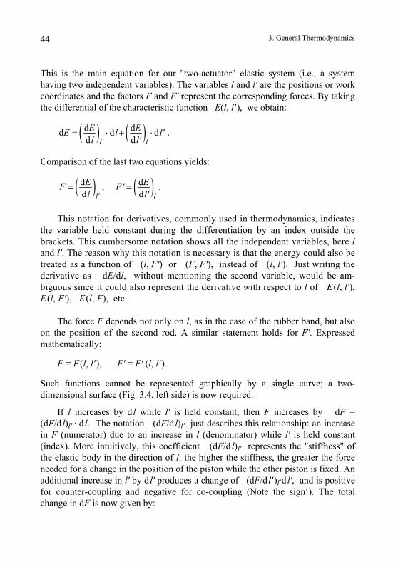
44 3. General Thermodynamics
This is the main equation for our "two-actuator" elastic system (i.e., a system having two independent variables). The variables l and l' are the positions or work coordinates and the factors F and F' represent the corresponding forces. By taking the differential of the characteristic function E(l, l' ), we obtain:
( ) ( )d dd d dd dl' l
E EE l l'l l'
= ⋅ + ⋅ .
Comparison of the last two equations yields:
( )dd l'
EFl
= ( )dd l
EF'l'
=, .
This notation for derivatives, commonly used in thermodynamics, indicates the variable held constant during the differentiation by an index outside the brackets. This cumbersome notation shows all the independent variables, here l and l'. The reason why this notation is necessary is that the energy could also be treated as a function of (l, F') or (F, F'), instead of (l, l'). Just writing the derivative as dE/dl, without mentioning the second variable, would be am-biguous since it could also represent the derivative with respect to l of E (l, l'), E (l, F'), E(l, F), etc.
The force F depends not only on l, as in the case of the rubber band, but also on the position of the second rod. A similar statement holds for F'. Expressed mathematically:
F = F(l, l' ), F' = F' (l, l' ).
Such functions cannot be represented graphically by a single curve; a two-dimensional surface (Fig. 3.4, left side) is now required.
If l increases by d l while l' is held constant, then F increases by dF = (dF/d l)l' · d l. The notation (dF/d l)l' just describes this relationship: an increase in F (numerator) due to an increase in l (denominator) while l' is held constant (index). More intuitively, this coefficient (dF/d l)l' represents the "stiffness" of the elastic body in the direction of l: the higher the stiffness, the greater the force needed for a change in the position of the piston while the other piston is fixed. An additional increase in l' by d l' produces a change of (dF/d l' )l·d l', and is positive for counter-coupling and negative for co-coupling (Note the sign!). The total change in dF is now given by:
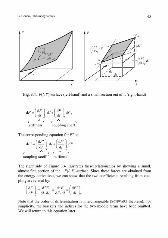
3. General Thermodynamics 45
F
P
l'
l'
l
F
P
l
dF
d l'd l
dFd l' d l'
l dFd l' l
dFd l d l
l'
dFd l l'
Fig. 3.4: F(l, l' )-surface (left-hand) and a small section out of it (right-hand)
d dd d dd dl' l
F FF l l'l l'
⎛ ⎞ ⎛ ⎞= +⎜ ⎟ ⎜ ⎟⎝ ⎠ ⎝ ⎠
,
stiffness coupling coeff.
The corresponding equation for F' is:
d dd d dd dl' l
F' F'F' l l'l l'
⎛ ⎞ ⎛ ⎞= +⎜ ⎟ ⎜ ⎟⎝ ⎠ ⎝ ⎠
.
coupling coeff.' stiffness'
The right side of Figure 3.4 illustrates these relationships by showing a small, almost flat, section of the F(l, l' )-surface. Since these forces are obtained from the energy derivatives, we can show that the two coefficients resulting from cou-pling are related by:
2 2d d d d=d d d d d dl l'
F E E F'l' l l' l' l l
⎛ ⎞ ⎛ ⎞= =⎜ ⎟ ⎜ ⎟⋅ ⋅⎝ ⎠ ⎝ ⎠.
Note that the order of differentiation is interchangeable (SCHWARZ theorem). For simplicity, the brackets and indices for the two middle terms have been omitted. We will return to this equation later.
3. General Thermodynamics 46
3.1.5. Primary and Coupling Effects
During the motion of the rods or, more generally, during a change in work coordinates, we observe various effects.
a) Primary effects and their coefficients:
The farther a rod is pushed in, or the larger l or l' becomes, the greater the cor-responding force F or F', respectively. This observation is also valid when no coupling occurs. Such an effect, one that exhibits the interdependence of cor-responding quantities, is called a primary effect. In our example it is ex-pressed quantitatively by the positive coefficients
d d d d, , , …d d d dF'l' l F
F l F' l'l F l' F'
⎛ ⎞ ⎛ ⎞ ⎛ ⎞⎛ ⎞⎜ ⎟⎜ ⎟ ⎜ ⎟ ⎜ ⎟⎝ ⎠⎝ ⎠ ⎝ ⎠ ⎝ ⎠
These consist of derivatives of the corresponding main quantities such as (F, l) or (F', l' ), and not (F', l) or (F, l' ) ; the index is unimportant here. We call these coefficients primary measures. In order to understand the sig-nificance of terms such as (d l/dF)F', one could investigate the functions l(F, F' ) and l ' (F, F' ), instead of considering the dependence of F and F' on the positions of the rods. For instance, the term (d l/dF)F' indicates the "soft-ness" of the elastic body in the direction l with F' held fixed.
b) Coupling effects and their coefficients:
The influence exerted by a change in position on the other positions and forces is called a coupling effect. The sign of a coupling effect depends on the type of coupling. In the absence of coupling this effect disappears, while the primary effects remain. Consider a system with counter-coupling, such as that illustrated by the left hand side of Figure 3.3. When one rod is pushed in, the other is pushed out, and vice versa. These coupling effects express themselves in two possible ways. If the right rod is held fixed (l' = const.) while the left rod is pushed in, then the force F' increases. If this rod is free to move (F' = const.), then its position l' decreases. This behavior may be described quanti-tatively by coefficients like
d d, , …d dl' F'
F' l'l l
⎛ ⎞ ⎛ ⎞⎜ ⎟ ⎜ ⎟⎝ ⎠ ⎝ ⎠
,
3. General Thermodynamics 47
where here the first term is positive and the second negative. In each case the quantity in the numerator and denominator are not corresponding main quan-tities, as seen here in (F', l) and (l', l). We call these kinds of derivatives coupling coefficients. The signs are reversed for co-coupling (right hand side of Figure 3.3). If one rod in that system is pushed in, the other tries to move in the same direction. If we push the rod on the left in and allow the rod on the right to move (F' = const.), its position l' increases. By holding this rod fixed (l' = const.), the force F' decreases. Note that the signs are reversed from those in our previous example.
c) Indirect effects:
It is clear that one rod is affected by the motion of the other rod in our two ex-amples. In both cases, it is harder to push in the left rod if the other rod is held fixed (l' = const.). Conversely, it becomes easier if the other is free to move (F' = const.). This result is independent of the type of coupling (co or counter). Mathematically, this condition is expressed as follows:
( ) ( ) ( ) ( )d d d d> , < .d d d dl' F' l' F'
F F l ll l F F
In the first case the body appears less elastic, or stiffer, than in the second case. Although the second rod is not directly involved in the primary effect we are looking at, it still affects the motion of the first rod. We will call ef-fects of these kind indirect effects. The coefficients differ, physically, because of the change of the constraints, formally, by the change of the index in the corresponding partial derivative.
n, (d ri-ca to thmtrMan
(dtww
One further comment about the equation from the end of the last sectioF/d l' )l = (dF'/d l)l'. The coupling effect described by the first term is numelly equal to that of the second term. This means that the first rod is coupled
e second as strongly as the second is coupled to the first. Stated concisely, the utual coupling is equally strong, or in other words it is symmetric! This symme-y will be used when we apply the flip rule, or the SCHWARZ theorem, or the AXWELL equations in traditional thermodynamics derivations (see sections 3.2.2 d 3.7.1).In conclusion, when we know that the symmetry condition (dF/d l' )l = F'/dl)l' is satisfied, then for an arbitrary system with two coordinates l, l', and o forces F(l, l' ), F' (l, l' ), the differential dE = F·d l + F'·d l' is complete, i.e.,
e can say that the energy is a function of the coordinates E = E(l, l' ). Physi-
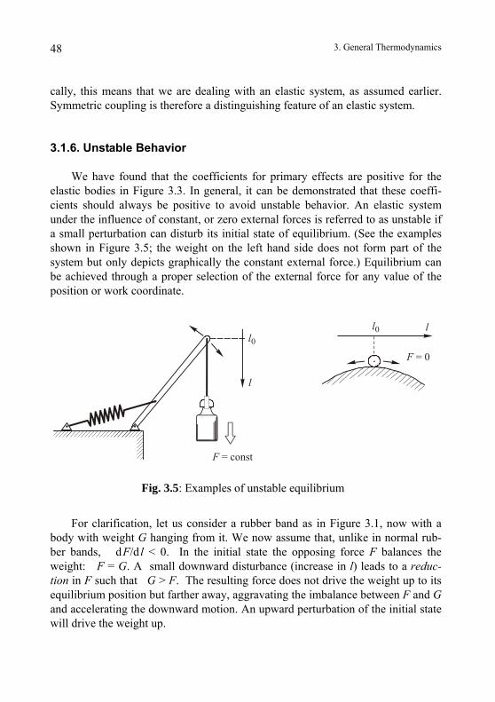
3. General Thermodynamics 48
cally, this means that we are dealing with an elastic system, as assumed earlier. Symmetric coupling is therefore a distinguishing feature of an elastic system.
3.1.6. Unstable Behavior
We have found that the coefficients for primary effects are positive for the elastic bodies in Figure 3.3. In general, it can be demonstrated that these coeffi-cients should always be positive to avoid unstable behavior. An elastic system under the influence of constant, or zero external forces is referred to as unstable if a small perturbation can disturb its initial state of equilibrium. (See the examples shown in Figure 3.5; the weight on the left hand side does not form part of the system but only depicts graphically the constant external force.) Equilibrium can be achieved through a proper selection of the external force for any value of the position or work coordinate.
F = const
F = 0
l
l
Fig. 3.5: Examples of unstable equilibrium
For clarification, let us consider a rubber band as in Figure 3.1, now with a body with weight G hanging from it. We now assume that, unlike in normal rub-ber bands, dF/d l < 0. In the initial state the opposing force F balances the weight: F = G. A small downward disturbance (increase in l) leads to a reduc-tion in F such that G > F. The resulting force does not drive the weight up to its equilibrium position but farther away, aggravating the imbalance between F and G and accelerating the downward motion. An upward perturbation of the initial state will drive the weight up.
3. General Thermodynamics 49
The reason for such unstable behavior is the assumption that dF/d l < 0. Clearly, we can expect unstable behavior in all cases where the force decreases with increasing work coordinate, or in other words, where the coefficient of the primary effect is negative.
So far statements regarding the sign and magnitude of the coefficients have been developed heuristically. These can be derived formally for a system, which is stable (which is almost always the case), and where the type of coupling between work coordinates is known. This means that the essential structure of a stable, elastic system is determined by the statements about coupling, independent of its mechanical, thermal, electrical or other properties. Structural conclusions can thus be extended from a familiar to a less familiar system with the same kind of cou-pling and stability. Therein lies the value of the current consideration.
3.2. Mathematical Rules for Derivatives
In this section we shall present some mathematical rules for expressing a derivative in terms of others, for example by derivatives that can be measured more conveniently. With an abundance of possible coefficients, any means of saving time is very useful. Although we are dealing with purely mathematical relationships here, we will highlight their physical significance. In the follow-ing, the variables u, v, w … describe the properties of the system, and the mutu-ally independent parameters z1, z2, … zn characterize the state of the system. Thus the quantities u, v, w … that can depend on each other in various ways are functions of zi.
3.2.1. Change of Variable
In thermodynamics, where many equations are conveniently expressed in differential form, a change of variables is sometimes required for the deriva-tives. To make such a change to a derivative (du/dv)v' v''… of a function u(v, v', v'' …), it is useful to apply the fact that a derivative can be written as a ratio of two differentials:
( ) ( )( )dd ,
d da
a a
uuv v
=
3. General Thermodynamics 50
provided that the denominator does not vanish. The index a indicates, here and subsequently, an abbreviation for the quantities that are unimportant for the current development. In this example, a stands for the unimportant quantities v', v''… The symbols (du)a and (dv)a denote differentials of u and v which can be functions of other variables — for instance, v, v', v'' … or the parameters z1, z2, … zn — while a is held constant. A typical procedure involves the following: the two differentials are separately computed, based on mathematical or thermo-dynamic relations, and divided by each other. The resulting ratio of differentials is again represented by the usual derivative notation (see section 3.7.3). As a simple example, if we choose v, v', v'' … as independent variables, then the total differential is given by
( ) ( ) ( )d d dd d d dd d dv' v'' vv'' vv'
u u uu v v' v''v v' v''
= + + + …… … …
( )
The requirement that a remains constant means that (dv)a = dv, (dv' )a = 0, (dv'' )a = 0, … , so that only the first term of the equation remains
( ) ( )dd dda a
a
uu vv
= .
By dividing by (dv)a, we regain the original expression.
In order to shorten the procedure further, it is useful to become familiar with some additional rules. Five simple operations will allow us to accomplish the task of changing derivatives to new variables. Section 3.2.2 discusses the fifth opera-tion, and section 3.2.3 discusses the detailed applications. For ease of reference we shall give names to these operations.
a) Inversion:
( ) ( )d d1dd aa
u vuv
=
( ) ( ) ( )d d dd d da a a
u u wv w v
=
b) Expansion:
Note that the same index is used in each term!
3. General Thermodynamics 51
c) Inserting an index:
( ) ( ) ( )d d dd d dwa va ua
u u wv w v
= −
Note the minus sign, and that each term contains the complete set of variables u, v, w, a!
d) Replacing an index
( ) ( ) ( ) ( )d d d dd d d dza wa va za
u u u wv v w v
= +
If we wish towe write dowadd the expanas a "correctinew independnal set v, z, a.
For these rules toequation exist, i.eof the variables re
For the follorepresented by a r
( )dd a
uv
=For a)
( )dd a
uv
=For b)
For c) By selecand dw o
d , d ,u v
replace the index z with w in the original derivative (du/dv)za, n the derivative with the new variable w in the index, and then sion of the original derivative with respect to the new variable w on term". The first factor in the "correction term" contains the ent variables w, v, a, while the second factor contains the origi-
be valid, we require that the derivatives on both sides of the ., the quantities in the numerator must be differentiable functions presented by the denominator and index.
wing derivations, we use the property that a derivative can be atio of differentials.
( )( )
( )( ) ( )d d d1 1d dd
a aaaa
u v vu uv
= = .
( )( )
( )( )
( )( ) ( ) ( )d d d d d
d d d d da a a
a aa a a
u u w u wv w v w v
= = .
ting u, v, a as independent variables, the differentials du, dv, da f the quantities contained in the original expression are
( ) ( ) ( )d d d d , d d d dd d dva ua uv
w w wa w u v au v a
= + + .
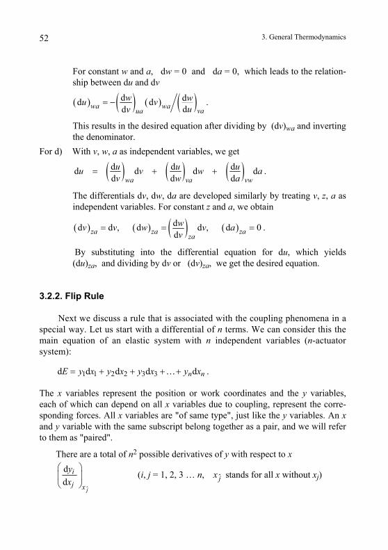
3. General Thermodynamics 52
For constant w and a, dw = 0 and da = 0, which leads to the relation-ship between du and dv
( ) ( ) ( ) ( )d dd dddwa wa vaua
w wu vuv
= − .
This results in the desired equation after dividing by (dv)wa and inverting the denominator.
For d) With v, w, a as independent variables, we get
( ) ( ) ( )d d dd d d dd d dwa va vw
u u uu v w av w a
= + +
( ) ( )
.
The differentials dv, dw, da are developed similarly by treating v, z, a as independent variables. For constant z and a, we obtain
( ) ( )dd d , d d , d 0dza za za
za
wv v w v av
= = =
3 3d d d dn nE y x y y x y x= + + + +…
.
By substituting into the differential equation for du, which yields (du)za, and dividing by dv or (dv)za, we get the desired equation.
3.2.2. Flip Rule
Next we discuss a rule that is associated with the coupling phenomena in a special way. Let us start with a differential of n terms. We can consider this the main equation of an elastic system with n independent variables (n-actuator system):
1 1 2 2dx .
The x variables represent the position or work coordinates and the y variables, each of which can depend on all x variables due to coupling, represent the corre-sponding forces. All x variables are "of same type", just like the y variables. An x and y variable with the same subscript belong together as a pair, and we will refer to them as "paired".
There are a total of n2 possible derivatives of y with respect to x
ˆ
dd
j
i
j x
yx
⎛ ⎞⎜ ⎟⎝ ⎠
j (i, j = 1, 2, 3 … n, x stands for all x without xj)
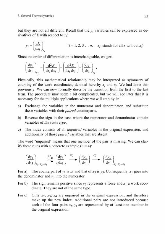
3. General Thermodynamics 53
but they are not all different. Recall that the yi variables can be expressed as de-rivatives of E with respect to xi:
ˆ
dd
i
ii x
Eyx
⎛ ⎞= ⎜ ⎟⎝ ⎠
(i = 1, 2, 3 … n, stands for all x without xi) ix
Since the order of differentiation is interchangeable, we get:
ˆ
2 2 dd dd d d d
i
j
j j i iˆ
dd d
j
i
j i xx
yx x
⎛ ⎞ ⎛⎜ ⎟ ⎜⎝ ⎠ ⎝
yE Ex x x x
⎞ ⎛ ⎞ ⎛ ⎞= = =⎟ ⎜ ⎟ ⎜ ⎟
⎝ ⎠⎠ ⎝ ⎠.
Physically, this mathematical relationship may be interpreted as symmetry of coupling of the work coordinates, denoted here by xi and xj. We had done this previously. We can now formally describe the transition from the first to the last term. The procedure may seem a bit complicated, but we will see later that it is necessary for the multiple applications where we will employ it:
a) Exchange the variables in the numerator and denominator, and substitute these variables with their paired counterparts.
b) Reverse the sign in the case where the numerator and denominator contain variables of the same type.
c) The index consists of all unpaired variables in the original expression, and additionally of those paired variables that are absent.
The word "unpaired" means that one member of the pair is missing. We can clar-ify these rules with a concrete example (n = 4):
1 2 43 , ,
1dd x x x
3
1ddy
x⎛⎜ ⎞
⎟⎝ ⎠
3
1
ddyx
⎛⎜ ⎟ ⎞⎝ ⎠ 2 3 4
3
1 , ,
dd x x x
yx⎝ ⎠
a) b) c) ⎛ ⎞⎜ ⎟ y
x⎛ ⎞⎜ ⎟⎝ ⎠
For a) The counterpart of y1 is x1 and that of x3 is y3. Consequently, x1 goes into the denominator and y3 into the numerator.
For b) The sign remains positive since y3 represents a force and x1 a work coor-dinate. They are not of the same type.
For c) Only x2, x3, x4 are unpaired in the original expression, and therefore make up the new index. Additional pairs are not introduced because each of the four pairs xi, yi are represented by at least one member in the original expression.
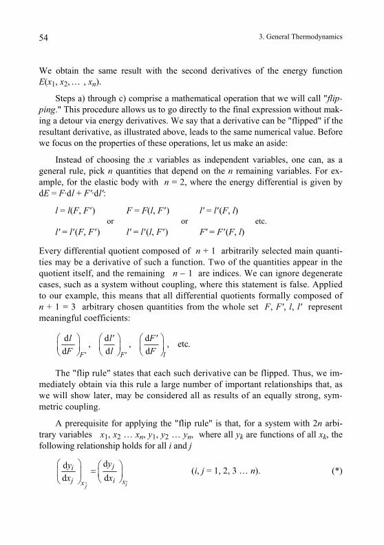
3. General Thermodynamics 54
We obtain the same result with the second derivatives of the energy function E(x1, x2, … , xn).
Steps a) through c) comprise a mathematical operation that we will call "flip-ping." This procedure allows us to go directly to the final expression without mak-ing a detour via energy derivatives. We say that a derivative can be "flipped" if the resultant derivative, as illustrated above, leads to the same numerical value. Before we focus on the properties of these operations, let us make an aside:
Instead of choosing the x variables as independent variables, one can, as a general rule, pick n quantities that depend on the n remaining variables. For ex-ample, for the elastic body with n = 2, where the energy differential is given by dE = F·dl + F'·dl':
l = l(F, F' ) F = F(l, F' ) l' = l' (F, l) or or etc. l' = l' (F, F' ) l' = l' (l, F' ) F' = F' (F, l)
Every differential quotient composed of n + 1 arbitrarily selected main quanti-ties may be a derivative of such a function. Two of the quantities appear in the quotient itself, and the remaining n − 1 are indices. We can ignore degenerate cases, such as a system without coupling, where this statement is false. Applied to our example, this means that all differential quotients formally composed of n + 1 = 3 arbitrary chosen quantities from the whole set F, F', l, l' represent meaningful coefficients:
d d d, , , etc.d d dF' F' l
l l' F'F l F
⎛ ⎞ ⎛ ⎞ ⎛ ⎞⎜ ⎟ ⎜ ⎟ ⎜ ⎟⎝ ⎠ ⎝ ⎠ ⎝ ⎠
The "flip rule" states that each such derivative can be flipped. Thus, we im-mediately obtain via this rule a large number of important relationships that, as we will show later, may be considered all as results of an equally strong, sym-metric coupling.
A prerequisite for applying the "flip rule" is that, for a system with 2n arbi-trary variables x1, x2 … xn, y1, y2 … yn, where all yk are functions of all xk, the following relationship holds for all i and j
ˆˆ
dd d
ij
ji
j i
d
xx
yx x
⎛ ⎞ ⎛ ⎞=⎜ ⎟ ⎜ ⎟⎝ ⎠⎝ ⎠
y (i, j = 1, 2, 3 … n). (*)
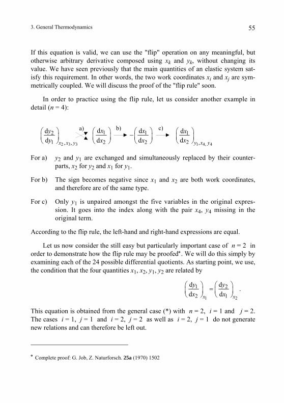
3. General Thermodynamics 55
If this equation is valid, we can use the "flip" operation on any meaningful, but otherwise arbitrary derivative composed using xk and yk, without changing its value. We have seen previously that the main quantities of an elastic system sat-isfy this requirement. In other words, the two work coordinates xi and xj are sym-metrically coupled. We will discuss the proof of the "flip rule" soon.
In order to practice using the flip rule, let us consider another example in detail (n = 4):
For a) y2 and y1 are exchanged and simultaneously replaced by their counter-parts, x2 for y2 and x1 for y1.
For b) The sign becomes negative since x1 and x2 are both work coordinates, and therefore are of the same type.
For c) Only y1 is unpaired amongst the five variables in the original expres-sion. It goes into the index along with the pair x4, y4 missing in the original term.
According to the flip rule, the left-hand and right-hand expressions are equal.
Let us now consider the still easy but particularly important case of n = 2 in order to demonstrate how the flip rule may be proofed∗. We will do this simply by examining each of the 24 possible differential quotients. As starting point, we use, the condition that the four quantities x1, x2, y1, y2 are related by
1 2
1 2
2 1
d dd dx x
y yx x
⎛ ⎞ ⎛ ⎞=⎜ ⎟ ⎜ ⎟⎝ ⎠ ⎝ ⎠
.
This equation is obtained from the general case (*) with n = 2, i = 1 and j = 2. The cases i = 1, j = 1 and i = 2, j = 2 as well as i = 2, j = 1 do not generate new relations and can therefore be left out.
∗ Complete proof: G. Job, Z. Naturforsch. 25a (1970) 1502
2 3 3
2
1 , ,
dd x x y
yy⎝ ⎠
1
2
dd
xx
⎛⎜ ⎞
⎟⎝ ⎠
1
2
dd
xx
⎛ ⎞⎜ ⎟⎝ ⎠
− a) b) c)
1 4, 4
1
2 ,
dd y x y
xx⎝ ⎠
⎛ ⎞⎜ ⎟ ⎛ ⎞
⎜ ⎟
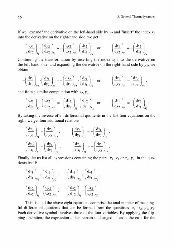
3. General Thermodynamics 56
If we "expand" the derivative on the left-hand side by y2 and "insert" the index x2 into the derivative on the right-hand side, we get
1 1 21
1 2 2 2
2 2 2 1
d d d dd d d dx x yx
y y y xy x x x
⎛ ⎞ ⎛ ⎞ ⎛ ⎞⋅ = − ⋅⎜ ⎟ ⎜ ⎟ ⎜ ⎟⎜ ⎟⎝ ⎠ ⎝ ⎠ ⎝ ⎠⎝ ⎠ 21
1 2
2 1
d dd d yx
y xy x
⎛ ⎞ ⎛ ⎞= −⎜ ⎟⎜ ⎟⎝ ⎠⎝ ⎠
⎛ ⎞ or .
Continuing the transformation by inserting the index x1 into the derivative on the left-hand side, and expanding the derivative on the right-hand side by y1, we obtain
2 21 21 2 1 1d d d dy yy yx y y x
− ⋅ = − ⋅⎜ ⎟ ⎜ ⎟⎜ ⎟ ⎜ ⎟⎝ ⎠ ⎝ ⎠⎝ ⎠ ⎝ ⎠
1 11 2d dd dy yx x⎛ ⎞ ⎛ ⎞⎛ ⎞ ⎛ ⎞
1 2
1 2
2 1
d dd dy y
x xy y
⎛ ⎞ ⎛ ⎞=⎜ ⎟ ⎜ ⎟⎝ ⎠ ⎝ ⎠
or ,
and from a similar computation with x2, y2
1 1 1 2
21 2 2
2 2 2 1
dd d dd d d dy y y x
yx x xx y y y
⎛ ⎞ ⎛ ⎞ ⎛ ⎞⎛ ⎞ ⋅ = − ⋅⎜ ⎟ ⎜ ⎟ ⎜ ⎟ ⎜ ⎟⎝ ⎠ ⎝ ⎠ ⎝ ⎠ ⎝ ⎠ 1 2
21
2 1
ddd dy x
yxx y
⎛ ⎞⎛ ⎞ = −⎜ ⎟ ⎜ ⎟⎝ ⎠ ⎝ ⎠
or .
By taking the inverse of all differential quotients in the last four equations on the right, we get four additional relations
21 2 1
22 1 1
1 2 1 2
dd d d, d d d d yx x x
yx x xy y y x
⎛ ⎞ ⎛ ⎞ ⎛ ⎞ ⎛ ⎞= = −⎜ ⎟⎜ ⎟ ⎜ ⎟ ⎜ ⎟⎝ ⎠⎝ ⎠ ⎝ ⎠ ⎝ ⎠
,
1 2 1 2
2 1 12
1 2 1 2
d d dd, d d d dy y y x
y y yxx x x y
⎛ ⎞⎛ ⎞ ⎛ ⎞ ⎛ ⎞= = −⎜ ⎟ ⎜ ⎟ ⎜ ⎟ ⎜ ⎟⎝ ⎠ ⎝ ⎠ ⎝ ⎠ ⎝ ⎠
.
Finally, let us list all expressions containing the pairs x1, y1 or x2, y2 in the quo-tients itself:
2 2 2 21 1 1 1d d d dx y
1 1 1 1d d d d, , , ,x yx x y y⎜ ⎟ ⎜ ⎟ ⎜ ⎟ ⎜ ⎟
⎝ ⎠ ⎝ ⎠ ⎝ ⎠ ⎝ ⎠
y y x x⎛ ⎞ ⎛ ⎞⎛ ⎞ ⎛ ⎞
1 1 1 12 2 2 2
d d, , .d d d dx y
2 2 2 2d d, x y
y y x xx x y y
⎛ ⎞ ⎛ ⎞⎛ ⎞ ⎛⎜ ⎟ ⎜ ⎜ ⎟ ⎜ ⎟⎝ ⎠ ⎝ ⎠ ⎝ ⎠ ⎝ ⎠
⎞⎟
This list and the above eight equations comprise the total number of meaning-ful differential quotients that can be formed from the quantities x1, x2, y1, y2. Each derivative symbol involves three of the four variables. By applying the flip-ping operation, the expression either remain unchanged — as is the case for the
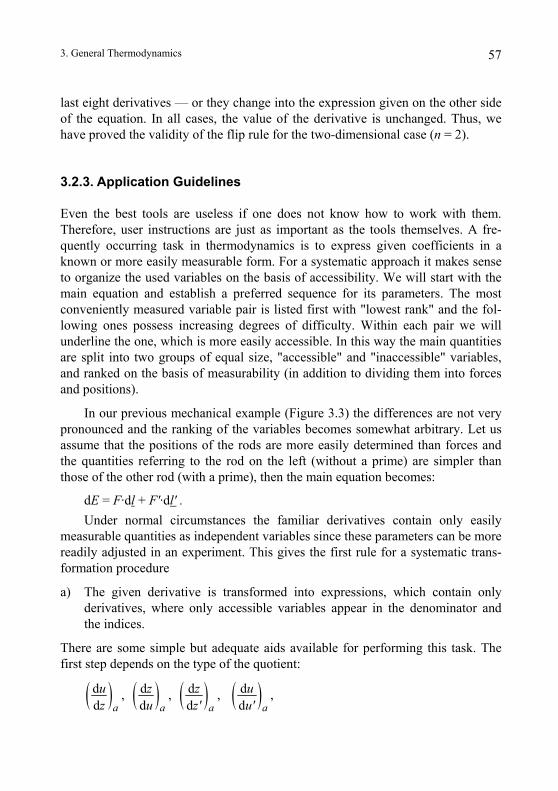
3. General Thermodynamics 57
last eight derivatives — or they change into the expression given on the other side of the equation. In all cases, the value of the derivative is unchanged. Thus, we have proved the validity of the flip rule for the two-dimensional case (n = 2).
3.2.3. Application Guidelines
Even the best tools are useless if one does not know how to work with them. Therefore, user instructions are just as important as the tools themselves. A fre-quently occurring task in thermodynamics is to express given coefficients in a known or more easily measurable form. For a systematic approach it makes sense to organize the used variables on the basis of accessibility. We will start with the main equation and establish a preferred sequence for its parameters. The most conveniently measured variable pair is listed first with "lowest rank" and the fol-lowing ones possess increasing degrees of difficulty. Within each pair we will underline the one, which is more easily accessible. In this way the main quantities are split into two groups of equal size, "accessible" and "inaccessible" variables, and ranked on the basis of measurability (in addition to dividing them into forces and positions).
In our previous mechanical example (Figure 3.3) the differences are not very pronounced and the ranking of the variables becomes somewhat arbitrary. Let us assume that the positions of the rods are more easily determined than forces and the quantities referring to the rod on the left (without a prime) are simpler than those of the other rod (with a prime), then the main equation becomes:
dE = F·dl + F'·dl' . Under normal circumstances the familiar derivatives contain only easily
measurable quantities as independent variables since these parameters can be more readily adjusted in an experiment. This gives the first rule for a systematic trans-formation procedure
a) The given derivative is transformed into expressions, which contain only derivatives, where only accessible variables appear in the denominator and the indices.
There are some simple but adequate aids available for performing this task. The first step depends on the type of the quotient:
( ) ( ) ( ) ( )d d d d, , , d d d da a a a
u z z uz u z' u'
,
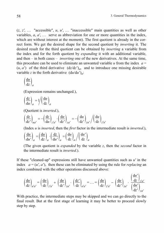
3. General Thermodynamics 58
(z, z', … "accessible", u, u', … "inaccessible" main quantities as well as other variables, a, a', … serve as abbreviation for one or more quantities in the index, which are without interest at the moment). The first quotient is already in the cor-rect form. We get the desired shape for the second quotient by inverting it. The desired result for the third quotient can be obtained by inserting a variable from the index and for the forth quotient by expanding it with an additional variable, and then – in both cases – inverting one of the new derivatives. At the same time, this procedure can be used to eliminate an unwanted variable u from the index a = (u, a' ) of the third derivative (dz/dz' )a, and to introduce one missing desirable variable z in the forth derivative (du/du' )a:
( )dd a
uz
(Expression remains unchanged.),
( ) ( )d d1z u= dd aa zu
(Quotient is inverted.),
( ) ( ) ( ) ( ) ( )d d d d dd dd d d za' z'a'ua' z'a' za'
z z u u uz' zz' u z'
= − ⋅ = −
(Index u is inserted, then the first factor in the intermediate result is inverted.),
( ) ( ) ( ) ( ) ( )d d d d dd dd d d a aa a a
u u z u u'z zu' z u'
= ⋅ =
(The given quotient is expanded by the variable z, then the second factor in the intermediate result is inverted.).
If these "cleaned-up" expressions still have unwanted quantities such as u' in the index a = (u', a' ), then these can be eliminated by using the rule for replacing an index combined with the other operations discussed above:
( ) ( ) ( ) ( ) ( ) ( ) ( )( )ddd d d d d d= = … = dd d d d d dd
z'a'
u'a' z'a' za' u'a' z'a' za'za'
u'zu u u z' u uu'z z z' z z z'z'
+ ⋅ − ⋅
With practice, the intermediate steps may be skipped and we can go directly to the final result. But at the first stage of learning it may be better to proceed slowly step by step.
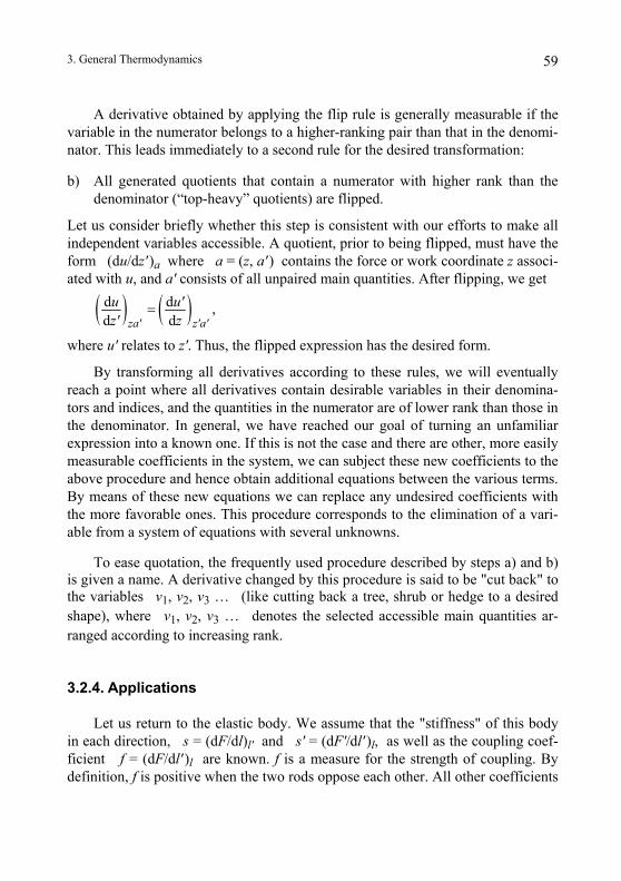
3. General Thermodynamics 59
A derivative obtained by applying the flip rule is generally measurable if the variable in the numerator belongs to a higher-ranking pair than that in the denomi-nator. This leads immediately to a second rule for the desired transformation:
b) All generated quotients that contain a numerator with higher rank than the denominator (“top-heavy” quotients) are flipped.
Let us consider briefly whether this step is consistent with our efforts to make all independent variables accessible. A quotient, prior to being flipped, must have the form (du/dz' )a where a = (z, a' ) contains the force or work coordinate z associ-ated with u, and a' consists of all unpaired main quantities. After flipping, we get
( ) ( )d dd dza' z'a'
u u'z' z
= ,
where u' relates to z'. Thus, the flipped expression has the desired form.
By transforming all derivatives according to these rules, we will eventually reach a point where all derivatives contain desirable variables in their denomina-tors and indices, and the quantities in the numerator are of lower rank than those in the denominator. In general, we have reached our goal of turning an unfamiliar expression into a known one. If this is not the case and there are other, more easily measurable coefficients in the system, we can subject these new coefficients to the above procedure and hence obtain additional equations between the various terms. By means of these new equations we can replace any undesired coefficients with the more favorable ones. This procedure corresponds to the elimination of a vari-able from a system of equations with several unknowns.
To ease quotation, the frequently used procedure described by steps a) and b) is given a name. A derivative changed by this procedure is said to be "cut back" to the variables v1, v2, v3 … (like cutting back a tree, shrub or hedge to a desired shape), where v1, v2, v3 … denotes the selected accessible main quantities ar-ranged according to increasing rank.
3.2.4. Applications
Let us return to the elastic body. We assume that the "stiffness" of this body in each direction, s = (dF/dl)l' and s' = (dF'/dl' )l, as well as the coupling coef-ficient f = (dF/dl' )l are known. f is a measure for the strength of coupling. By definition, f is positive when the two rods oppose each other. All other coefficients
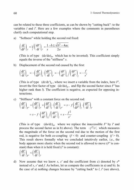
3. General Thermodynamics 60
can be related to these three coefficients, as can be shown by "cutting back": to the variables l and l'. Here are a few examples where the comments in parentheses clarify each computational step.
a) "Softness" while holding the second rod fixed:
( ) ( ) 2d 1 4d1dd 2l'l'
l b b acFlF s a
− ± −= =
(This is of type (dz/du)a, which has to be inverted). This coefficient simply equals the inverse of the "stiffness" s.
b) Displacement of the second rod caused by the first:
( ) ( ) ( ) ( ) ( )d d d d dd dd d d lF' l l' l
fl' l' F' F F'l' l'l F' l s'
= − ⋅ = − = −
(This is of type (dz/dz')a , where we insert a variable from the index, here F', invert the first factor of type (dz/du)a , and flip the second factor since F' has higher rank than l). The coefficient is negative, as expected for opposing in-teractions.
c) "Stiffness" with a constant force on the second rod:
( ) ( ) ( ) ( ) ( ) ( )( ) ( )
´2
d d d d ´ d dd d d d d d
d d d d
F' l' l F l l'
l l
F F F l l' F's fl l l' l F' l
fF F's f sl' l' s'
= + ⋅ = − ⋅
= − ⋅ = −
(This is of type (du/dz)a, where we replace the inaccessible F' by l' and process the second factor as in b) above). The term −f 2/s', which measures the magnitude of the force on the second rod due to the motion of the first rod, is negative for both co-coupling (f < 0) and counter-coupling (f > 0). This result shows formally what we concluded intuitively earlier, i.e., the body appears more elastic when the second rod is allowed to move (F' is con-stant) than when it is held fixed (l' is constant):
( ) ( )d dd dF' l'
F Fl l
<
d) Now assume that we know s, s' and the coefficient from c) denoted by s* instead of s, s' and f. As before, let us compute the coefficients in a) and b). In the case of a) nothing changes because by "cutting back" to l, l' (see above),
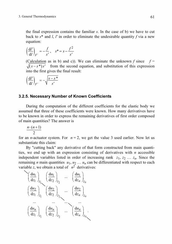
3. General Thermodynamics 61
the final expression contains the familiar s. In the case of b) we have to cut back to s* and l, l' in order to eliminate the undesirable quantity f via a new equation:
( ) 2
´
d , *d F
f fl' s sl s' s'
= − = −
( )
(Calculation as in b) and c)). We can eliminate the unknown f since f = *s s s'− from the second equation, and substitution of this expression
into the first gives the final result:
( )´
d *d F
l' s sl s'
−= −
3.2.5. Necessary Number of Known Coefficients
During the computation of the different coefficients for the elastic body we assumed that three of these coefficients were known. How many derivatives have to be known in order to express the remaining derivatives of first order composed of main quantities? The answer is
( 1)2
n n⋅ +
for an n-actuator system. For n = 2, we get the value 3 used earlier. Now let us substantiate this claim:
By "cutting back" any derivative of that form constructed from main quanti-ties, we end up with an expression consisting of derivatives with n accessible independent variables listed in order of increasing rank z1, z2 … zn. Since the remaining n main quantities u1, u2 … un can be differentiated with respect to each variable z, we obtain a total of n2 derivatives:
ˆ ˆ ˆ1 2
ˆ ˆ ˆ1 21 2d d d
... ... ... ...nnz z zz z z⎜ ⎟ ⎜ ⎟ ⎜ ⎟
⎝ ⎠ ⎝ ⎠ ⎝ ⎠
ˆ ˆ ˆ1 2
1 1 1
1 2
2 2 2
1 2
d d d...d d d
d d d...
d d d... .d d d
n
n
n
n n n
n
z z z
z z z
u u uz z z
u u u
u u uz z z
⎛ ⎞⎛ ⎞ ⎛ ⎞⎜ ⎟ ⎜ ⎟ ⎜ ⎟⎝ ⎠ ⎝ ⎠ ⎝ ⎠
⎛ ⎞⎛ ⎞ ⎛ ⎞
⎛ ⎞⎛ ⎞ ⎛ ⎞⎜ ⎟ ⎜ ⎟ ⎜ ⎟⎝ ⎠ ⎝ ⎠ ⎝ ⎠
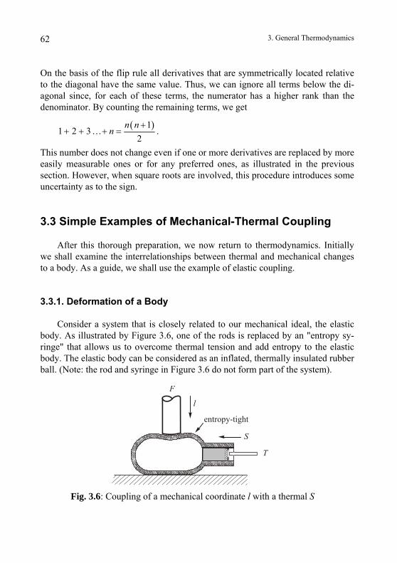
3. General Thermodynamics 62
On the basis of the flip rule all derivatives that are symmetrically located relative to the diagonal have the same value. Thus, we can ignore all terms below the di-agonal since, for each of these terms, the numerator has a higher rank than the denominator. By counting the remaining terms, we get
( )11 2 3…
2n n
n+
+ + + = .
This number does not change even if one or more derivatives are replaced by more easily measurable ones or for any preferred ones, as illustrated in the previous section. However, when square roots are involved, this procedure introduces some uncertainty as to the sign.
3.3 Simple Examples of Mechanical-Thermal Coupling
After this thorough preparation, we now return to thermodynamics. Initially we shall examine the interrelationships between thermal and mechanical changes to a body. As a guide, we shall use the example of elastic coupling.
3.3.1. Deformation of a Body
Consider a system that is closely related to our mechanical ideal, the elastic body. As illustrated by Figure 3.6, one of the rods is replaced by an "entropy sy-ringe" that allows us to overcome thermal tension and add entropy to the elastic body. The elastic body can be considered as an inflated, thermally insulated rubber ball. (Note: the rod and syringe in Figure 3.6 do not form part of the system).
S
F
T
l
entropy-tight
Fig. 3.6: Coupling of a mechanical coordinate l with a thermal S
3. General Thermodynamics 63
The processes of "pushing in a rod" and "adding entropy" are not independent but are mutually coupled. Qualitatively they bear the same relationship as counter-coupling in our mechanical example. This follows readily from our earlier discus-sions of entropy, or heat*. The observed effects can be classified the same way as in the case of the elastic mechanical body (here, we will not consider the coeffi-cients that describe quantitatively the individual effects).
a) Primary effects:
– The further the rod is pushed in, the greater the resistive force F becomes.
( ) , d 0d S
Fl
> ( )d 0 …d T
Fl
>
– The more entropy is added, the higher the thermal tension rises inside the rubber ball.
( )d 0d l
TS
> ( )d 0 …d F
TS
>,
b) Coupling effects:
– If we push in the rod, then entropy is forced out. If the entropy is sealed in, the temperature rises.
( )d 0d T
Sl
< ( )d 0 …d S
Tl
>,
– If we add entropy, the rod is pushed out. If we hold the rod fixed, the force acting on it increases.
( )d 0d F
lS
< ( )d 0 …d l
FS
>,
c) Indirect effects:
– It is easier to push in the rod if we allow entropy to escape; harder if en-tropy is sealed in.
( ) ( )d dd dS T
F Fl l
> .
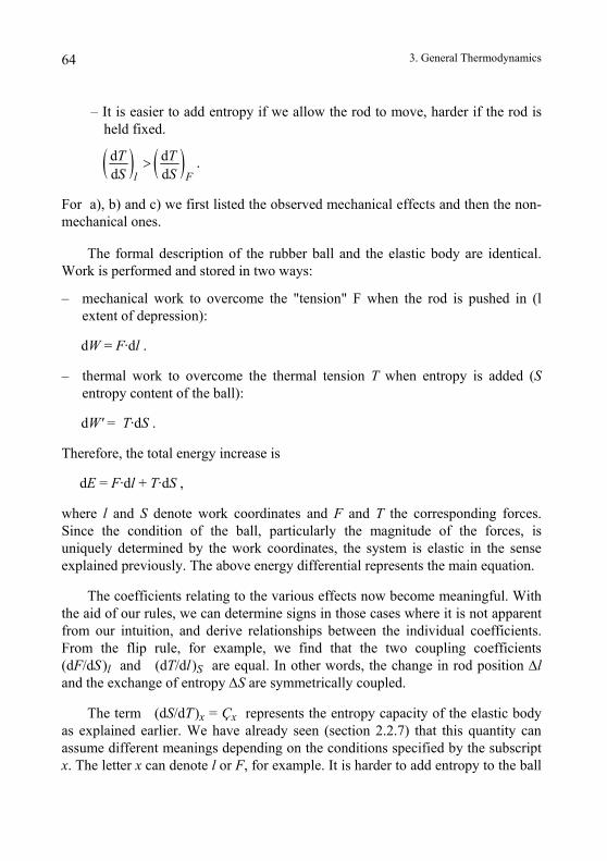
3. General Thermodynamics 64
– It is easier to add entropy if we allow the rod to move, harder if the rod is held fixed.
( ) ( )d dd dl F
T TS S
> .
For a), b) and c) we first listed the observed mechanical effects and then the non-mechanical ones.
The formal description of the rubber ball and the elastic body are identical. Work is performed and stored in two ways:
– mechanical work to overcome the "tension" F when the rod is pushed in (l extent of depression):
dW = F·dl .
– thermal work to overcome the thermal tension T when entropy is added (S entropy content of the ball):
dW' = T·dS .
Therefore, the total energy increase is
dE = F·dl + T·dS ,
where l and S denote work coordinates and F and T the corresponding forces. Since the condition of the ball, particularly the magnitude of the forces, is uniquely determined by the work coordinates, the system is elastic in the sense explained previously. The above energy differential represents the main equation.
The coefficients relating to the various effects now become meaningful. With the aid of our rules, we can determine signs in those cases where it is not apparent from our intuition, and derive relationships between the individual coefficients. From the flip rule, for example, we find that the two coupling coefficients (dF/dS )l and (dT/dl)S are equal. In other words, the change in rod position ∆l and the exchange of entropy ∆S are symmetrically coupled.
The term (dS/dT)x = Çx represents the entropy capacity of the elastic body as explained earlier. We have already seen (section 2.2.7) that this quantity can assume different meanings depending on the conditions specified by the subscript x. The letter x can denote l or F, for example. It is harder to add entropy to the ball
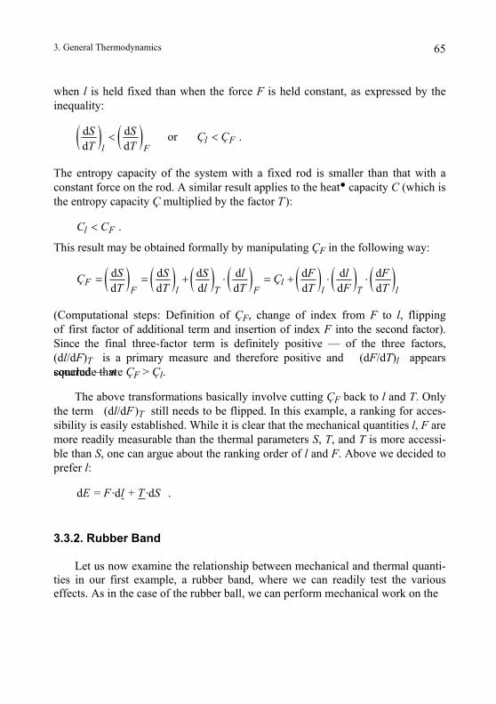
3. General Thermodynamics 65
when l is held fixed than when the force F is held constant, as expressed by the inequality:
( ) ( )d dd dl F
S ST T
< l FÇ or Ç < .
The entropy capacity of the system with a fixed rod is smaller than that with a constant force on the rod. A similar result applies to the heat capacity C (which is the entropy capacity Ç multiplied by the factor T ):
l FC C< .
This result may be obtained formally by manipulating ÇF in the following way:
( ) ( ) ( ) ( ) ( ) ( ) ( )d d d d d d dd d d d d d dF l
F l T F l T l
S S S l F l FÇ ÇT T l T T F T
= = + ⋅ = + ⋅ ⋅
(Computational steps: Definition of ÇF, change of index from F to l, flipping of first factor of additional term and insertion of index F into the second factor). Since the final three-factor term is definitely positive — of the three factors, (dl/dF)T is a primary measure and therefore positive and (dF/dT)l appears squared — we conclude that ÇF > Çl.
The above transformations basically involve cutting ÇF back to l and T. Only the term (dl/dF )T still needs to be flipped. In this example, a ranking for acces-sibility is easily established. While it is clear that the mechanical quantities l, F are more readily measurable than the thermal parameters S, T, and T is more accessi-ble than S, one can argue about the ranking order of l and F. Above we decided to prefer l:
d = ·d + ·d E F l T S .
3.3.2. Rubber Band
Let us now examine the relationship between mechanical and thermal quanti-ties in our first example, a rubber band, where we can readily test the various effects. As in the case of the rubber ball, we can perform mechanical work on the
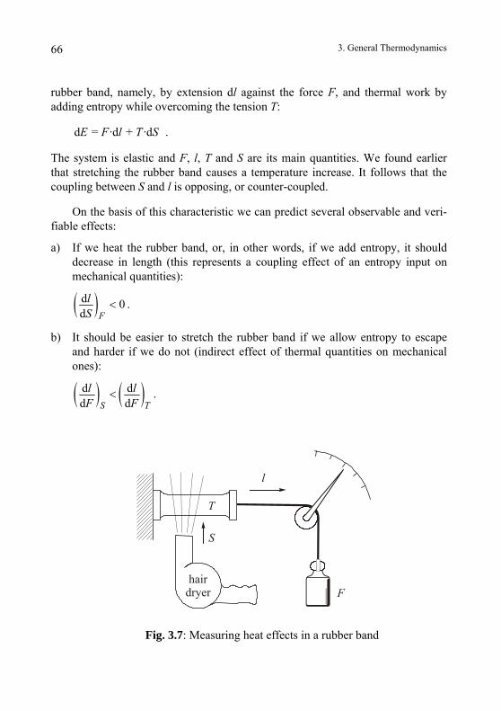
3. General Thermodynamics 66
rubber band, namely, by extension dl against the force F, and thermal work by adding entropy while overcoming the tension T:
d = ·d + ·d E F l T S .
The system is elastic and F, l, T and S are its main quantities. We found earlier that stretching the rubber band causes a temperature increase. It follows that the coupling between S and l is opposing, or counter-coupled.
On the basis of this characteristic we can predict several observable and veri-fiable effects:
a) If we heat the rubber band, or, in other words, if we add entropy, it shoulddecrease in length (this represents a coupling effect of an entropy input onmechanical quantities):
( )d 0l < . d FS
b) It should be easier to stretch the rubber band if we allow entropy to escapeand harder if we do not (indirect effect of thermal quantities on mechanicalones):
( ) ( )S T
d dd d
l lF F
< .
T
S
F
l
hairdryer
Fig. 3.7: Measuring heat effects in a rubber band
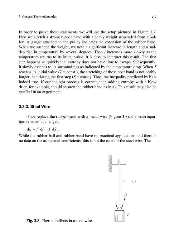
3. General Thermodynamics 67
In order to prove these statements we will use the setup pictured in Figure 3.7. First we stretch a strong rubber band with a heavy weight suspended from a pul-ley. A gauge attached to the pulley indicates the extension of the rubber band. When we suspend the weight, we note a significant increase in length and a sud-den rise in temperature by several degrees. Then l increases more slowly as the temperature returns to its initial value. It is easy to interpret this result. The first step happens so quickly that entropy does not have time to escape. Subsequently, it slowly escapes to its surroundings as indicated by the temperature drop. When T reaches its initial value (T = const.), the stretching of the rubber band is noticeably longer than during the first step (S = const.). Thus, the inequality predicted by b) is indeed true. If our thought process is correct, then adding entropy with a blow drier, for example, should shorten the rubber band as in a). This result may also be verified in an experiment.
3.3.3. Steel Wire
If we replace the rubber band with a metal wire (Figure 3.8), the main equa-tion remains unchanged:
d = ·d + ·d E F l T S . While the rubber ball and rubber band have no practical applications and there is no data on the associated coefficients, this is not the case for the steel wire. The
F
l
S T,
Fig. 3.8: Thermal effects in a steel wire
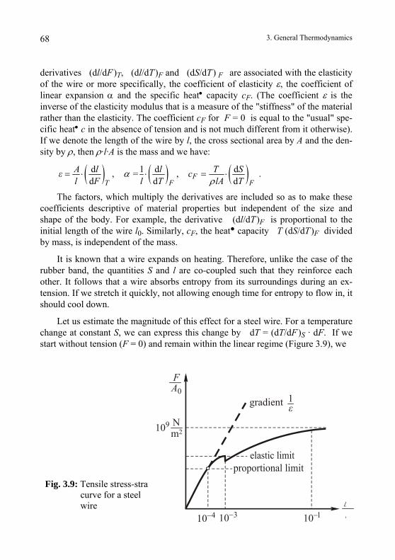
3. General Thermodynamics 68
derivatives (dl/dF )T, (dl/dT )F and (dS/dT ) F are associated with the elasticity of the wire or more specifically, the coefficient of elasticity ε, the coefficient of linear expansion α and the specific heat• capacity cF. (The coefficient ε is the inverse of the elasticity modulus that is a measure of the "stiffness" of the material rather than the elasticity. The coefficient cF for F = 0 is equal to the "usual" spe-cific heat• c in the absence of tension and is not much different from it otherwise). If we denote the length of the wire by l, the cross sectional area by A and the den-sity by ρ, then ρ·l·A is the mass and we have:
( ) ( ) ( )d 1 d d, = , d d dF
T F F
A l l T Sε cl F l T lA T
αρ
= ⋅ ⋅ = ⋅
curve for a steel
.
The factors, which multiply the derivatives are included so as to make these coefficients descriptive of material properties but independent of the size and shape of the body. For example, the derivative (dl/dT)F is proportional to the initial length of the wire l0. Similarly, cF, the heat capacity T (dS/dT)F divided by mass, is independent of the mass.
It is known that a wire expands on heating. Therefore, unlike the case of the rubber band, the quantities S and l are co-coupled such that they reinforce each other. It follows that a wire absorbs entropy from its surroundings during an ex-tension. If we stretch it quickly, not allowing enough time for entropy to flow in, it should cool down.
Let us estimate the magnitude of this effect for a steel wire. For a temperature change at constant S, we can express this change by dT = (dT/dF)S · dF. If we start without tension (F = 0) and remain within the linear regime (Figure 3.9), we
Fig. 3.9: Tensile stress-strain
wire
FA0
1
10−4 10−3 10−1
ε
l∆
109 Nm2
gradient
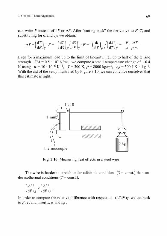
3. General Thermodynamics 69
can write F instead of dF or ∆F. After "cutting back" the derivative to F, T, and substituting for α and cF, we obtain:
( ) ( ) ( ) ( ) ( )d d d d dd dd d d F FTS F F
T T S F Tl ST F FT TF S F A c
αρ
∆ = ⋅ = − ⋅ = − = − ⋅
Even for a maximum load up to the limit of linearity, i.e., up to half of the tensile strength F/A = 0.5 · 109 N/m2, we compute a small temperature change of −0.4 K using α = 10 · 10−6 K−1, T = 300 K, ρ = 8000 kg/m3, cF = 500 J K−1 kg−1. With the aid of the setup illustrated by Figure 3.10, we can convince ourselves that this estimate is right.
1 : 10
1 mm2
thermocouple
Fig. 3.10: Measuring heat effects in a steel wire
The wire is harder to stretch under adiabatic conditions (S = const.) than un-der isothermal conditions (T = const.):
( ) ( )d dd dS T
l lF F
< .
In order to compute the relative difference with respect to (dl/dF )T, we cut back to F, T, and insert ε, α and cF :
3. General Thermodynamics 70
( ) ( )( )
( ) ( )( )
( ) ( ) ( )( )
( )( ) ( )
2
2
d d d d d d dd d d d d d d
d d dd d d
dd
.d dd d
F
T S F S F F T
T T T
FT F
l l l T l T SF F T F T S F
l l lF F F
lT T
l S cF T
αρε
− − ⋅ ⋅ ⋅= = =
= =⋅
Using the modulus of elasticity ε −1 = 0.2 ·1012 N/m2 for steel and the above values of coefficients, the relative difference is 0.0015. Since the difference caused by thermally indirect effects is less than one-tenth of a percent, it is usually neglected in mechanics. The elasticity modulus is generally given as l/A·dF/dl, although strictly we should distinguish between an isothermal and an adiabatic modulus.
3.4. Body Under Isotropic Pressure
The next example of mechanical-thermal coupling is for a uniform body subjected to isotropic ambient pressure. This body could be a wooden cube, a hollow iron ball or the liquid enclosed in a hydraulic cylinder. Since this last one is an espe-cially important case, we will cover it in detail.
3.4.1. Main Equation and Coupling
Mechanical work is required to compress a body. This work increases with increasing volume increment −dV, and with applied pressure p, and can be ex-pressed as
dW = −p · dV .
Figure 3.11 illustrates these relationships. Since p is the force acting on unit area, the total force applied to a flat area A is F = p · A. The work can now be written as
( )d = d = d dFW F l A l p VA
= − ,

3. General Thermodynamics 71
F = p·A
dl
l
A – V = A· ld d
– V = A ld di i i
liFi
Ai
dli
Fig. 3.11: Pressure, force, and work on an arbitrary body
since the area moves by an amount dl due to the external pressure. As a result, the volume decreases by A·dl. If the surface is curved, it can be divided into many small, nearly flat pieces. In order to obtain the total work, the contributions from all pieces must be summed:
( ) ( )d d d d dii i i i i
i
FW F l A l p V p VA
= = = − = −∑ ∑
d ´ d diW T S T S= =∑
.
Similarly, the energy added as a result of entropy inputs at different surface loca-tions can be computed as the sum of all individual contributions
.
The mechanical and thermal work performed on the body due to compression or heating is stored and can be regained in one form or another by letting the body relax or cool down. This is true for compact, heat-resistant materials over a wide pressure and temperature range, but decomposing, porous materials must be han-dled with care. By stipulating volume and entropy, V and S, the condition of the material is usually fully determined if we exclude all influences other than changes in pressure and temperature. Thus, we have an elastic system with main equation
dE = (–p)dV + TdS. If we select V and S as work coordinates, then −p and T become the corresponding forces. According to our sign convention (section 3.1.2), a positive external force
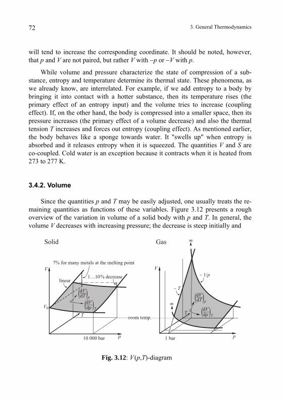
3. General Thermodynamics 72
will tend to increase the corresponding coordinate. It should be noted, however, that p and V are not paired, but rather V with −p or −V with p.
While volume and pressure characterize the state of compression of a sub-stance, entropy and temperature determine its thermal state. These phenomena, as we already know, are interrelated. For example, if we add entropy to a body by bringing it into contact with a hotter substance, then its temperature rises (the primary effect of an entropy input) and the volume tries to increase (coupling effect). If, on the other hand, the body is compressed into a smaller space, then its pressure increases (the primary effect of a volume decrease) and also the thermal tension T increases and forces out entropy (coupling effect). As mentioned earlier, the body behaves like a sponge towards water. It "swells up" when entropy is absorbed and it releases entropy when it is squeezed. The quantities V and S are co-coupled. Cold water is an exception because it contracts when it is heated from 273 to 277 K.
3.4.2. Volume
Since the quantities p and T may be easily adjusted, one usually treats the re-maining quantities as functions of these variables. Figure 3.12 presents a rough overview of the variation in volume of a solid body with p and T. In general, the volume V decreases with increasing pressure; the decrease is steep initially and
Solid Gas 8
V
~ T
V
p
dVd p T dV
d p T
dVd T p dV
d T p
T
V0
10 000 bar 1 bar
Troom temp.
linear~ 1/p
8
7% for many metals at the melting point
Fig. 3.12: V(p,T)-diagram
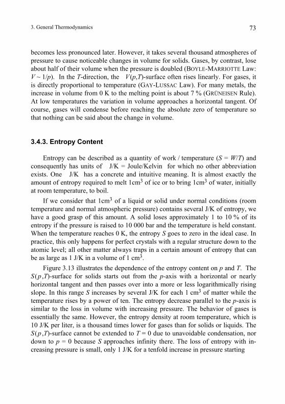
3. General Thermodynamics 73
becomes less pronounced later. However, it takes several thousand atmospheres of pressure to cause noticeable changes in volume for solids. Gases, by contrast, lose about half of their volume when the pressure is doubled (BOYLE-MARRIOTTE Law: V ~ 1/p). In the T-direction, the V (p,T)-surface often rises linearly. For gases, it is directly proportional to temperature (GAY-LUSSAC Law). For many metals, the increase in volume from 0 K to the melting point is about 7 % (GRÜNEISEN Rule). At low temperatures the variation in volume approaches a horizontal tangent. Of course, gases will condense before reaching the absolute zero of temperature so that nothing can be said about the change in volume.
3.4.3. Entropy Content
Entropy can be described as a quantity of work / temperature (S = W/T) and consequently has units of J/K = Joule/Kelvin for which no other abbreviation exists. One J/K has a concrete and intuitive meaning. It is almost exactly the amount of entropy required to melt 1cm3 of ice or to bring 1cm3 of water, initially at room temperature, to boil.
If we consider that 1cm3 of a liquid or solid under normal conditions (room temperature and normal atmospheric pressure) contains several J/K of entropy, we have a good grasp of this amount. A solid loses approximately 1 to 10 % of its entropy if the pressure is raised to 10 000 bar and the temperature is held constant. When the temperature reaches 0 K, the entropy S goes to zero in the ideal case. In practice, this only happens for perfect crystals with a regular structure down to the atomic level; all other matter always traps in a certain amount of entropy that can be as large as 1 J/K in a volume of 1 cm3.
Figure 3.13 illustrates the dependence of the entropy content on p and T. The S(p ,T)-surface for solids starts out from the p-axis with a horizontal or nearly horizontal tangent and then passes over into a more or less logarithmically rising slope. In this range S increases by several J/K for each 1 cm3 of matter while the temperature rises by a power of ten. The entropy decrease parallel to the p-axis is similar to the loss in volume with increasing pressure. The behavior of gases is essentially the same. However, the entropy density at room temperature, which is 10 J/K per liter, is a thousand times lower for gases than for solids or liquids. The S(p ,T)-surface cannot be extended to T = 0 due to unavoidable condensation, nor down to p = 0 because S approaches infinity there. The loss of entropy with in-creasing pressure is small, only 1 J/K for a tenfold increase in pressure starting
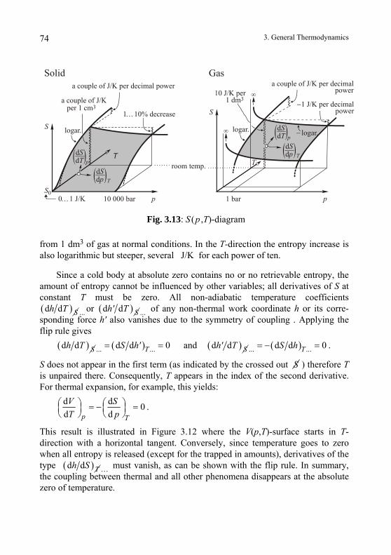
3. General Thermodynamics 74
from 1 dm3 of gas at normal conditions. In the T-direction the entropy increase is also logarithmic but steeper, several J/K for each power of ten.
Since a cold body at absolute zero contains no or no retrievable entropy, the amount of entropy cannot be influenced by other variables; all derivatives of S at constant T must be zero. All non-adiabatic temperature coefficients ( )d d Sh T ... or ( )d d Sh' T ... of any non-thermal work coordinate h or its corre-sponding force h' also vanishes due to the symmetry of coupling . Applying the flip rule gives
( )d d Sh T ( )... ...d d 0TS h'= = and ( )d d Sh' T ( )... ...d d 0TS h= − = .
S does not appear in the first term (as indicated by the crossed out S ) therefore T is unpaired there. Consequently, T appears in the index of the second derivative. For thermal expansion, for example, this yields:
d d 0d dp T
V ST p
⎛ ⎞ ⎛ ⎞= − =⎜ ⎟⎜ ⎟⎝ ⎠⎝ ⎠
.
This result is illustrated in Figure 3.12 where the V(p,T)-surface starts in T-direction with a horizontal tangent. Conversely, since temperature goes to zero when all entropy is released (except for the trapped in amounts), derivatives of the type ( )d dh S T… must vanish, as can be shown with the flip rule. In summary, the coupling between thermal and all other phenomena disappears at the absolute zero of temperature.
Fig. 3.13: S (p ,T)-diagram
p p0 1 J/K…
TT
S
S0
S
dSdp T
dSdp TdS
dT p
dSdT p
a couple of J/K per 1 cm3
1 10% decrease…
a couple of J/K per decimal power
10 000 bar
−1 J/K per decimal power
a couple of J/K per decimal power
logar.
Solid Gas
∞ logar. logar.−
1 bar
∞
room temp.
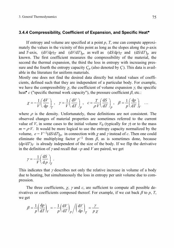
3. General Thermodynamics 75
3.4.4 Compressibility, Coefficient of Expansion, and Specific Heat
If entropy and volume are specified at a point p, T, one can compute approxi-mately the values in the vicinity of this point as long as the slopes along the p-axis and T-axis, (dV/dp)T and (dV/dT )p, as well as (dS/dp)T and (dS/dT)p are known. The first coefficient measures the compressibility of the material, the second the thermal expansion, the third the loss in entropy with increasing pres-sure and the fourth the entropy capacity Çp (also denoted by Ç). This data is avail-able in the literature for uniform materials. Mostly one does not find the desired data directly but related values of coeffi-cients, defined such that they are independent of a particular body. For example, we have the compressibility χ, the coefficient of volume expansion γ, the specific heat• c ("specific thermal work capacity"), the pressure coefficient β, etc.:
dd d d1 1 1, , , …
d d d dp p VT
pV V STcV p V T V T p T
χ γ βρ
⎛ ⎞⎛ ⎞ ⎛ ⎞⎛ ⎞= − = = =⎜ ⎟ ⎜ ⎟ ⎜ ⎟ ⎜ ⎟⎝ ⎠ ⎝ ⎠ ⎝ ⎠ ⎝ ⎠
where ρ is the density. Unfortunately, these definitions are not consistent. The observed changes of material properties are sometimes referred to the current value of V, in some cases to the initial volume V0 (typically for γ) or to the mass m = ρ·V. It would be more logical to use the entropy capacity normalized by the volume, e = V−1(dS/dT)p, in connection with χ and γ instead of c. Then one could eliminate the multiplying factor p−1 from β, as is sometimes done, because (dp/dT )V is already independent of the size of the body. If we flip the derivative in the definition of γ and recall that −p and V are paired, we get
d1d T
SV p
γ ⎛ ⎞= − ⎜ ⎟⎝ ⎠
.
This indicates that γ describes not only the relative increase in volume of a body due to heating, but simultaneously the loss in entropy per unit volume due to com-pression.
The three coefficients, χ, γ and c, are sufficient to compute all possible de-rivatives or coefficients composed thereof. For example, if we cut back β to p, T, we get
( ) ( ) ( )d1 1 d dd dd pV T
p V VT pp T p p
γβχ
= = − =
3. General Thermodynamics 76
The specific heat• at constant volume cV = Tρ –1V –1 · (dS/dT)V is smaller than that for constant pressure cp = c because adding entropy is more difficult when coupled volume changes, either positive or negative, are prevented. In order to compute the difference c − cV relative to c, that may be considered as a meas-ure of the indirect effect of mechanical behavior on thermal behavior, we cut back (c − cV)/c to p, T without flipping the derivative just this once:
( ) ( )( )
( ) ( )( )
( ) ( )( ) ( )
2
d d d d d d d dd d d d
d d d d .
d d d d
p VV T V
p p
T p
T p
S T S T S p p Tc cc S T S T
S p V T TV p S T c
γρ χ
− − ⋅−= = =
− ⋅= =
− ⋅
The same expression can be obtained by comparing the compressibility of the body with and without entropy exchange, similarly to the above. The compressi-bility is described by the usual isothermal χT = χ and adiabatic χS = −V−1(dV/dT)S definitions. Note that this is an indirect effect of thermal side on mechanical changes:
21V Sc c
c eγχ χ
χ χ− −
= = ≤ .
The more suitable density of entropy capacity "e" has been substituted for c in order to simplify the final expression. This result is not only valid for c and χ but also for the primary measures, entropy capacity (dS/dT ) x and compressibility –(dV/dp)x. Since primary measures cannot be negative for stable behavior, the expression γ 2/(e·χ) has to be less than one. The second to last equation indicates that the relative strength of the indirect effect is determined by a quotient of cou-pling and primary measures (formed from the same independent variables).
For solids under normal ambient conditions, typical values for χ are 10−5 … 10−6 /bar, γ lies in the range of 10−4 … 10−5 K−1 and e, including liquids, has a value near 10−2 (J/K)/K per cm3 of matter.
3.5 Other Systems
The above method can be applied qualitatively and quantitatively to com-pletely different systems and processes such as the magneto-thermal effect, piezo-
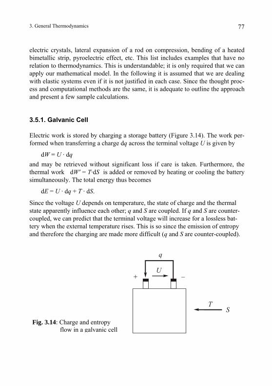
3. General Thermodynamics 77
electric crystals, lateral expansion of a rod on compression, bending of a heated bimetallic strip, pyroelectric effect, etc. This list includes examples that have no relation to thermodynamics. This is understandable; it is only required that we can apply our mathematical model. In the following it is assumed that we are dealing with elastic systems even if it is not justified in each case. Since the thought proc-ess and computational methods are the same, it is adequate to outline the approach and present a few sample calculations.
3.5.1. Galvanic Cell
Electric work is stored by charging a storage battery (Figure 3.14). The work per-formed when transferring a charge dq across the terminal voltage U is given by
dW = U · dq and may be retrieved without significant loss if care is taken. Furthermore, the thermal work dW' = T·dS is added or removed by heating or cooling the battery simultaneously. The total energy thus becomes
dE = U · dq + T · dS.
Since the voltage U depends on temperature, the state of charge and the thermal state apparently influence each other; q and S are coupled. If q and S are counter-coupled, we can predict that the terminal voltage will increase for a lossless bat-tery when the external temperature rises. This is so since the emission of entropy and therefore the charging are made more difficult (q and S are counter-coupled).
+ −U
T
q
S
Fig. 3.14: Charge and entropy flow in a galvanic cell
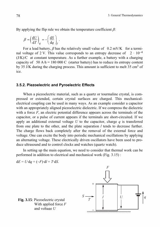
3. General Thermodynamics
78
By applying the flip rule we obtain the temperature coefficient β:
( )d dd dq T
U ST q
β ⎛ ⎞= = −⎜ ⎟⎝ ⎠
.
For a lead battery, β has the relatively small value of 0.2 mV/K for a termi-nal voltage of 2 V. This value corresponds to an entropy decrease of 2 · 10−4 (J/K)/C at constant temperature. As a further example, a battery with a charging capacity of 50 A·h = 180 000 C (starter battery) has to reduce its entropy content by 35 J/K during the charging process. This amount is sufficient to melt 35 cm3 of ice.
3.5.2. Piezoelectric and Pyroelectric Effects
When a piezoelectric material, such as a quartz or tourmaline crystal, is com-pressed or extended, certain crystal surfaces are charged. This mechanical-electrical coupling can be used in many ways. As an example consider a capacitor with an appropriately aligned piezoelectric dielectric. If we compress the dielectric with a force F, an electric potential difference appears across the terminals of the capacitor, or a pulse of current appears if the terminals are short-circuited. If we apply an additional external voltage U to the capacitor, charge q is transferred from one plate to the other, and the plate separation l tends to decrease further. The charge flows back completely after the removal of the external force and voltage. One can excite the body into periodic mechanical oscillations by applying an alternating voltage. These electrically driven oscillators have been used to pro-duce ultrasound and to control clocks and watches (quartz watch).
In setting up the main equation, we need to consider that thermal work can be performed in addition to electrical and mechanical work (Fig. 3.15) :
dE = U·dq + (−F)·dl + T·dS.
Fig. 3.15: Piezoelectric crystal With applied force F and voltage U
S
F
TqUl
+
−
3. General Thermodynamics 79
Furthermore, q and S may be coupled. Depending on the type of coupling, the capacitor is charged in one direction or the other (pyroelectric effect).
As a numerical example let us choose a 1 cm3 cube of "sintered" BaTiO3 which, following polarization at high temperatures in an electric field, becomes piezoelectric. The capacitor plates are made by plating two opposite sides perpen-dicular to the polarization direction. Since this is a three-actuator system (n = 3), we need (n + 1)·n/2 = 6 independent coefficients for a complete description. In addition to the elasticity modulus (1011 N/m2), the coefficient of expansion (10−5/K) and density of entropy capacity (104J/K2 · m3), we could select the electric capacitance in addition to the piezo- and pyroelectric charge coefficients:
10 10 9;, , ,
d d dC C C10 10 ; 10 .d V d N d KF T U T U F
q q qU F T
− − −⎛ ⎞ ⎛ ⎞ ⎛ ⎞= = =⎜ ⎟ ⎜ ⎟ ⎜ ⎟⎝ ⎠ ⎝ ⎠ ⎝ ⎠
Now let us squeeze our system slowly but strongly (F = 1000 N) by applying a pair of pliers to the metallic ends. Since the entropy has time to escape (T = const.), a voltage develops between the open electrodes (q = 0):
, ,,
d d d 1000Vd dd U T F Tq T
U q qU F FF UF
⎛ ⎞ ⎛ ⎞ ⎛ ⎞= = − = −⎜ ⎟ ⎜ ⎟⎜ ⎟⎝ ⎠ ⎝ ⎠⎝ ⎠
This is large enough to produce a 1/2 mm long spark. Similarly, a high voltage can be reached by heating (∆T = 100 K) instead of applying pressure:
( ), , ,
d dd 1000Vd dd q F U F F T
q qUU T TT UT
⎛ ⎞ ⎛ ⎞= ∆ = −∆ = −⎜ ⎟ ⎜ ⎟⎝ ⎠ ⎝ ⎠
.
Conversely, by applying a voltage of −1000 V to the electrodes while holding l and S constant, the resulting expansion force is 100 N with a temperature rise of 1.1 · 10−3 K.
3.5.3. Magneto-Caloric Effect
If we heat a piece of iron within a constant external magnetic field, then the induced magnetic dipole moment j decreases and vanishes almost completely at 1040 K (770 ºC), implying that S and j are coupled. In fact, a magnetized body can be treated as an elastic system provided it does not exhibit significant hysteresis.
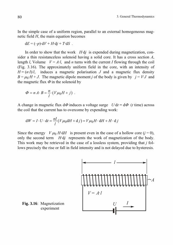
3. General Thermodynamics 80
In the simple case of a uniform region, parallel to an external homogeneous mag-netic field H, the main equation becomes
dE = (–p)·dV + H·dj + T·dS .
In order to show that the work H·dj is expended during magnetization, con-sider a thin resistanceless solenoid having a solid core. It has a cross section A, length l, Volume V = A·l, and n turns with the current I flowing through the coil (Fig. 3.16). The approximately uniform field in the core, with an intensity of H = (n·I)/l, induces a magnetic polarisation J and a magnetic flux density B = µ0·H + J. The magnetic dipole moment j of the body is given by j = V·J and the magnetic flux Φ in the solenoid by
( )0nn A B V H jl
Φ µ= ⋅ = ⋅ + .
A change in magnetic flux dΦ induces a voltage surge U·dt = dΦ (t time) across the coil that the current has to overcome by expending work:
( )0 0d d d d d dnIW I U t V H j V H H H jl
µ µ= ⋅ ⋅ = + = ⋅ + ⋅
Since the energy V µ0 H·dH is present even in the case of a hollow core (j = 0), only the second term H·dj represents the work of magnetization of the body. This work may be retrieved in the case of a lossless system, providing that j fol-lows precisely the rise or fall in field intensity and is not delayed due to hysteresis.
U I
V = A l⋅
A
l
Fig. 3.16: Magnetization experiment
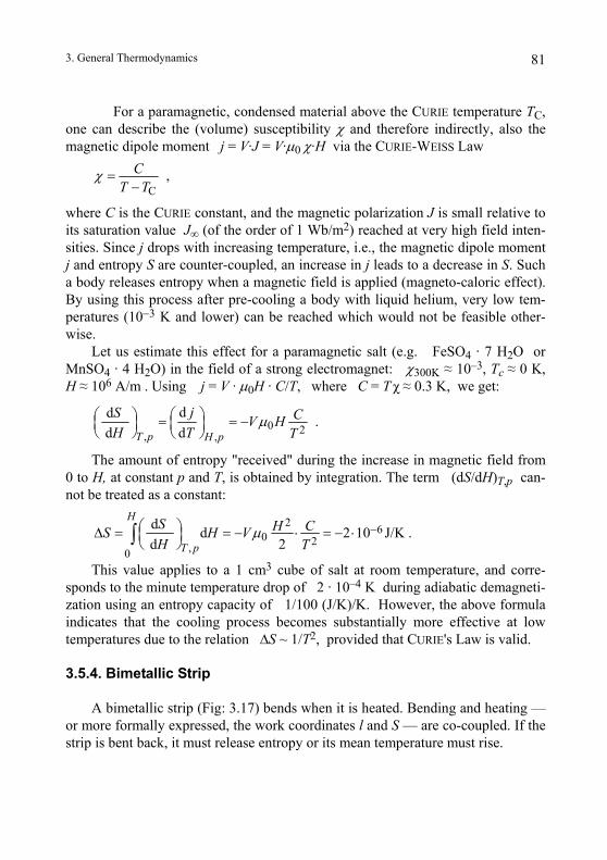
3. General Thermodynamics 81
For a paramagnetic, condensed material above the CURIE temperature TC, one can describe the (volume) susceptibility χ and therefore indirectly, also the magnetic dipole moment j = V·J = V·µ0 χ·H via the CURIE-WEISS Law
C
CT T
χ =−
,
where C is the CURIE constant, and the magnetic polarization J is small relative to its saturation value J∞ (of the order of 1 Wb/m2) reached at very high field inten-sities. Since j drops with increasing temperature, i.e., the magnetic dipole moment j and entropy S are counter-coupled, an increase in j leads to a decrease in S. Such a body releases entropy when a magnetic field is applied (magneto-caloric effect). By using this process after pre-cooling a body with liquid helium, very low tem-peratures (10−3 K and lower) can be reached which would not be feasible other-wise.
Let us estimate this effect for a paramagnetic salt (e.g. FeSO4 · 7 H2O or MnSO4 · 4 H2O) in the field of a strong electromagnet: χ300K ≈ 10–3, Tc ≈ 0 K, H ≈ 106 A/m . Using j = V · µ0H · C/T, where C = T χ ≈ 0.3 K, we get:
0 2, ,
d dd dT p H p
jS CV HH T T
µ⎛ ⎞⎛ ⎞ = = −⎜ ⎟ ⎜ ⎟⎝ ⎠ ⎝ ⎠ .
The amount of entropy "received" during the increase in magnetic field from 0 to H, at constant p and T, is obtained by integration. The term (dS/dH)T,p can-not be treated as a constant:
2 60 2,0
d d 2 10 J/Kd 2
H
T p
S H CS H VH T
µ −⎛ ⎞∆ = = − ⋅ = − ⋅⎜ ⎟⎝ ⎠∫ .
This value applies to a 1 cm3 cube of salt at room temperature, and corre-sponds to the minute temperature drop of 2 · 10–4 K during adiabatic demagneti-zation using an entropy capacity of 1/100 (J/K)/K. However, the above formula indicates that the cooling process becomes substantially more effective at low temperatures due to the relation ∆S ~ 1/T2, provided that CURIE's Law is valid.
3.5.4. Bimetallic Strip
A bimetallic strip (Fig: 3.17) bends when it is heated. Bending and heating — or more formally expressed, the work coordinates l and S — are co-coupled. If the strip is bent back, it must release entropy or its mean temperature must rise.
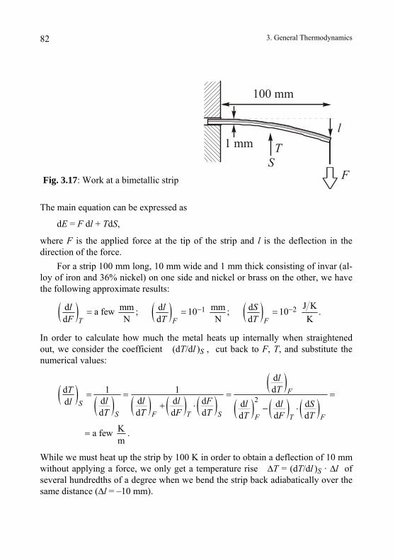
3. General Thermodynamics 82
100 mm
1 mm TS
l
F
Fig. 3.17: Work at a bimetallic strip
The main equation can be expressed as
dE = F dl + TdS,
where F is the applied force at the tip of the strip and l is the deflection in the direction of the force.
For a strip 100 mm long, 10 mm wide and 1 mm thick consisting of invar (al-loy of iron and 36% nickel) on one side and nickel or brass on the other, we have the following approximate results:
( ) ( ) ( )1 2 J Kd mm d mm da few ; 10 ; 10 .d N d N d KT F F
l l SF T T
− −= = =
In order to calculate how much the metal heats up internally when straightened out, we consider the coefficient (dT/dl )S , cut back to F, T, and substitute the numerical values:
( ) ( ) ( ) ( ) ( )( )
( ) ( ) ( )2
ddd 1 1
d d d dd d d dd d d d d d d
K a few .m
FS
S F T S F T F
lTT
l l l Fl l l ST T F T T F T
= = = =+ ⋅ − ⋅
=
While we must heat up the strip by 100 K in order to obtain a deflection of 10 mm without applying a force, we only get a temperature rise ∆T = (dT/dl )S · ∆l of several hundredths of a degree when we bend the strip back adiabatically over the same distance (∆l = –10 mm).
3. General Thermodynamics 83
3.6. Traditional Concepts
In addition to the quantities used so far, various other concepts are frequently utilized in thermodynamics, such as internal energy, enthalpy, useful work, free energy, etc., for the purpose of facilitating computation and theory. The reason for introducing these concepts goes back to the historical development of treating thermal work performed on a body as a measure of added heat. Heat became a special form of energy either transferred to or, under certain conditions, residing in a body and was grouped with other forms of energy. Since one could not interpret entropy intuitively — it was perceived as an abstract quantity derived from ther-mal work — computational methods that avoided this concept were preferred. As far as possible, entropy was expressed by energetic quantities in the final result. Therefore, the shortest and most reasonable approach to obtain the desired rela-tionships appeared to be energy considerations. The traditional framework of thermodynamics was developed with this goal in mind and, as a result, appears more akin to an energy theory than to a theory of heat.
In our presentation, in which entropy is introduced with more or less known and intuitive properties, we can dispense with many of these artificial aids without sacrificing anything. However, since the energy approach is widely used, it is difficult to avoid reference to some of its most important concepts. In the follow-ing sections these are explained within the context of our viewpoint.
3.6.1. Forms of Energy
If we bring a body from state I to II — some concrete examples are a stretched wire, a gas in a cylinder, a piezoelectric crystal — then the total work W expended is given as the difference in energy E between the two states:
W = EII – EI .
The form in which the energy is exchanged, such as mechanical or thermal, de-pends in general on the intermediate states in going from I to II. In Figure 3.18, we consider a gas in a cylinder. We can describe graphically different ways of moving from one state to another. Along the solid line in the diagram, the gas is easily compressed but heated up with difficulty, i.e., the required mechanical work W' is
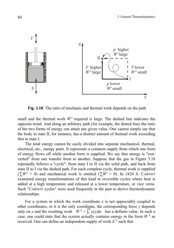
3. General Thermodynamics 84
S
V
V
I
II
S
TW
higherlarge''
TW
lowersmall''
pW
higher large'
pW
lower small'
Fig. 3.18: The ratio of mechanic and thermal work depends on the path
small and the thermal work W'' required is large. The dashed line indicates the opposite trend. And along an arbitrary path (for example, the dotted line) the ratio of the two forms of energy can attain any given value. One cannot simply say that the body in state II, for instance, has a distinct amount of thermal work exceeding that in state I.
The total energy cannot be easily divided into separate mechanical, thermal, electrical, etc., energy parts. It represents a common supply from which one form of energy flows off while another form is supplied. We say that energy is "con-verted" from one transfer form to another. Suppose that the gas in Figure 3.18 repeatedly follows a "cycle": from state I to II via the solid path, and back from state II to I via the dashed path. For each complete cycle, thermal work is supplied (∑W'' > 0) and mechanical work is emitted (∑W' > 0). In 1824 S. CARNOT examined energy transformations of this kind in reversible cycles where heat is added at a high temperature and released at a lower temperature, or vice versa. Such "CARNOT cycles" were used frequently in the past to derive thermodynamic relationships.
For a system in which the work coordinate x is not appreciably coupled to other coordinates, or it is the only coordinate, the corresponding force y depends only on x and the resulting work W † =
III has a definite value. In such a
case, one could state that the system actually contains energy in the form W † as received. One can define an independent supply of work E † such that
d( )y x x∫
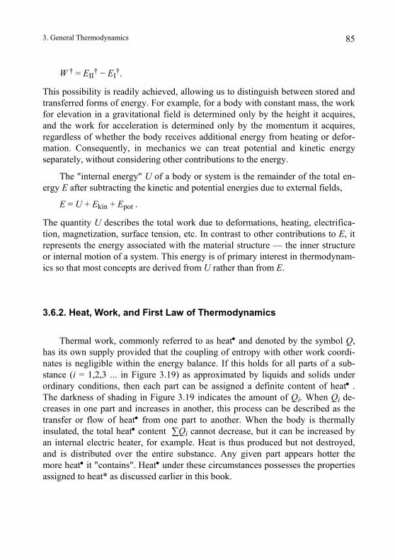
3. General Thermodynamics 85
W † = EII† − EI†.
This possibility is readily achieved, allowing us to distinguish between stored and transferred forms of energy. For example, for a body with constant mass, the work for elevation in a gravitational field is determined only by the height it acquires, and the work for acceleration is determined only by the momentum it acquires, regardless of whether the body receives additional energy from heating or defor-mation. Consequently, in mechanics we can treat potential and kinetic energy separately, without considering other contributions to the energy.
The "internal energy" U of a body or system is the remainder of the total en-ergy E after subtracting the kinetic and potential energies due to external fields,
E = U + Ekin + Epot .
The quantity U describes the total work due to deformations, heating, electrifica-tion, magnetization, surface tension, etc. In contrast to other contributions to E, it represents the energy associated with the material structure — the inner structure or internal motion of a system. This energy is of primary interest in thermodynam-ics so that most concepts are derived from U rather than from E.
3.6.2. Heat, Work, and First Law of Thermodynamics
Thermal work, commonly referred to as heat• and denoted by the symbol Q, has its own supply provided that the coupling of entropy with other work coordi-nates is negligible within the energy balance. If this holds for all parts of a sub-stance (i = 1,2,3 ... in Figure 3.19) as approximated by liquids and solids under ordinary conditions, then each part can be assigned a definite content of heat• . The darkness of shading in Figure 3.19 indicates the amount of Qi. When Qi de-creases in one part and increases in another, this process can be described as the transfer or flow of heat• from one part to another. When the body is thermally insulated, the total heat• content ∑Qi cannot decrease, but it can be increased by an internal electric heater, for example. Heat is thus produced but not destroyed, and is distributed over the entire substance. Any given part appears hotter the more heat• it "contains". Heat• under these circumstances possesses the properties assigned to heat* as discussed earlier in this book.
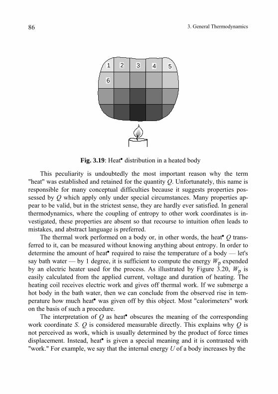
3. General Thermodynamics 86
1 2 3 4 5
6
Fig. 3.19: Heat• distribution in a heated body
This peculiarity is undoubtedly the most important reason why the term "heat" was established and retained for the quantity Q. Unfortunately, this name is responsible for many conceptual difficulties because it suggests properties pos-sessed by Q which apply only under special circumstances. Many properties ap-pear to be valid, but in the strictest sense, they are hardly ever satisfied. In general thermodynamics, where the coupling of entropy to other work coordinates is in-vestigated, these properties are absent so that recourse to intuition often leads to mistakes, and abstract language is preferred.
The thermal work performed on a body or, in other words, the heat• Q trans-ferred to it, can be measured without knowing anything about entropy. In order to determine the amount of heat• required to raise the temperature of a body — let's say bath water — by 1 degree, it is sufficient to compute the energy Wp expended by an electric heater used for the process. As illustrated by Figure 3.20, Wp is easily calculated from the applied current, voltage and duration of heating. The heating coil receives electric work and gives off thermal work. If we submerge a hot body in the bath water, then we can conclude from the observed rise in tem-perature how much heat• was given off by this object. Most "calorimeters" work on the basis of such a procedure.
The interpretation of Q as heat• obscures the meaning of the corresponding work coordinate S. Q is considered measurable directly. This explains why Q is not perceived as work, which is usually determined by the product of force times displacement. Instead, heat• is given a special meaning and it is contrasted with "work." For example, we say that the internal energy U of a body increases by the
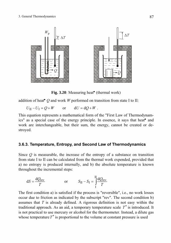
3. General Thermodynamics 87
Q
Wp
Q
∆T ∆T
Fig. 3.20: Measuring heat• (thermal work)
addition of heat• Q and work W performed on transition from state I to II:
II I or d dU U Q W U Q W− = + = + .
This equation represents a mathematical form of the "First Law of Thermodynam-ics" as a special case of the energy principle. In essence, it says that heat• and work are interchangeable, but their sum, the energy, cannot be created or de-stroyed.
3.6.3. Temperature, Entropy, and Second Law of Thermodynamics
Since Q is measurable, the increase of the entropy of a substance on transition from state I to II can be calculated from the thermal work expended, provided that a) no entropy is produced internally, and b) the absolute temperature is known throughout the incremental steps:
revdd QST
= or II
revII I
I
dQS ST
− = ∫
*
*
The first condition a) is satisfied if the process is "reversible", i.e., no work losses occur due to friction as indicated by the subscript "rev". The second condition b) assumes that T is already defined. A rigorous definition is not easy within the traditional approach. As an aid, a temporary temperature scale T is introduced. It is not practical to use mercury or alcohol for the thermometer. Instead, a dilute gas whose temperatureT is proportional to the volume at constant pressure is used
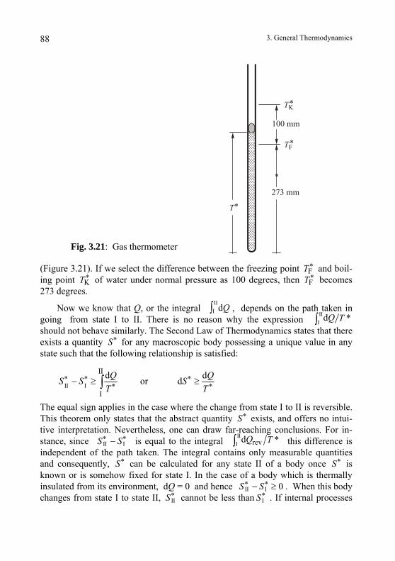
3. General Thermodynamics 88
100 mm
273 mm
T*
*
*TK
*TF
Fig. 3.21: Gas thermometer
(Figure 3.21). If we select the difference between the freezing point and boil-ing point KT of water under normal pressure as 100 degrees, then T becomes 273 degrees.
*FT*F
IIdQ
*
Now we know that Q, or the integral I∫ , depends on the path taken in going from state I to II. There is no reason why the expression
III
should not behave similarly. The Second Law of Thermodynamics states that there exists a quantity for any macroscopic body possessing a unique value in any state such that the following relationship is satisfied:
d *Q T∫*S
II I
II* *
*dQS ST
− ≥ ∫ or I
**
dd QST
≥
*S
* *S S−
The equal sign applies in the case where the change from state I to II is reversible. This theorem only states that the abstract quantity exists, and offers no intui-tive interpretation. Nevertheless, one can draw far-reaching conclusions. For in-stance, since II I is equal to the integral
III this difference is
independent of the path taken. The integral contains only measurable quantities and consequently, can be calculated for any state II of a body once is known or is somehow fixed for state I. In the case of a body which is thermally insulated from its environment, dQ = 0 and hence II
revd *Q T∫*S *S
I* * 0S S− ≥
II*S I
*S. When this body
changes from state I to state II, cannot be less than . If internal processes
3. General Thermodynamics 89
such as diffusion, electric currents, chemical transformations, etc. occur in such a body, can only increase and never decrease. And so on. *S
Later we will see that T is equivalent to T when we consider the properties of dilute gases (see section 4.7.2). As a result, and the now-familiar quantity S are also equivalent for the appropriate choice for the zero point. The abstractly formulated content and correspondences of the Second Law of Thermodynamics should become intuitively understandable. If we consider, for example, that dQ/T represents the entropy transferred into a system from the outside, and that some entropy can also be produced internally, then the inequality dS ≥ dQ/T becomes more meaningful.
**S
*U
* *II IQ U U= −
II I II IQ E E U U= − = −
3.6.4. Enthalpy, Heat Functions
For a system with coupled work coordinates, we can generally obtain the individ-ual contributions to work arising from a change in state by summing all contribu-tions along the path from state I to II. This applies in particular to thermal work Q. However, since Q is readily determined calorimetrically and is usually interpreted as a measure of heat•, we are inclined to look for the possibility of calculating Q by simpler methods. One possibility is to associate Q with other variables such as
which can represent a heat• content under certain conditions:
.
In fact, variables called "heat functions" or "enthalpy", from the Greek word for heat content, are easily declared. The simplest example is the total or internal energy for systems that can only exchange thermal work with their surroundings. Consequently, it follows that
.
A cylinder filled with gas reduces to such a system when the piston is fixed. As a result, no work arising from volume changes is performed. Even if the exter-nal pressure vanishes and the piston moves "blindly", the outward motion is only restrained by the friction between the piston and the cylinder wall. In this case, no mechanical work is done on the surroundings. Unlike our previous examples, this system is no longer lossless. The mechanical work due to the expansion of the gas is lost as heat• — in a sense via a detour because the regular path for mechanical work is blocked. Here the variable dQ consists of two parts arising from different
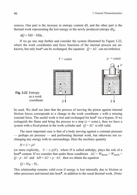
3. General Thermodynamics 90
sources. One part is the increase in entropy content dS, and the other part is the thermal work representing the lost energy or the newly produced entropy dSp:
pd d dQ T S T S= −
II IQ H H= −
.
If we go one step further and consider the system illustrated by Figure 3.22, where the work coordinates and force functions of the internal process are un-known, but only heat• can be exchanged, the equation Q = ∆U can nevertheless
Sp
S
V
V = const p = const
S
Sp
Fig. 3.22: Entropy as a work
coordinate
be used. We shall see later that the process of moving the piston against internal friction forces corresponds to a change in the work coordinate x with a missing external force. The useful work is lost and exchanged for heat• via a bypass. If we extinguish the flame and bring the process to a stop (x = const.), then we have a system with a fixed piston in the work cylinder and Q = ∆U is still valid.
The most important case is that of a body moving against a constant pressure — perhaps air pressure — and performing thermal work, but otherwise not ex-changing any energy with its surroundings. Here the auxiliary quantity
H ≡ U + pV (or more explicitly, U − (−p)V), where H is called enthalpy, plays the role of a heat content. If we consider that under these conditions ∆U = Wtherm + Wmech = Q − p · ∆V and ∆H = ∆U + p · ∆V, then we obtain the equation
.
This relationship remains valid even if energy is lost internally due to friction or other processes and turned into heat, in addition to the usual thermal work. (Note:
3. General Thermodynamics 91
the weight on the right side of Figure 3.22 is not part of the system but only helps to visualize the constant pressure).
The above result can be generalized to multi-actuator systems. If, besides x1 = S, all other work coordinates x2, x3, x4 … are fixed, then U is a heat function. By holding some of the corresponding forces y2, y3, y4 … fixed, say y2 and y4, but not the corresponding work coordinates x2 and x4, the following quantity
* 2 2 4 4U U y x y x= − −
assumes the role of the heat function. Under these circumstances
2 2 4 4U Q y x y x∆ = + ∆ + ∆ ,
and
* 2 2 4 4U U y x y x∆ = ∆ − ∆ − ∆*U∆
*
…U y y y y y yα β γ α α β β γ γ
,
yielding the result Q = . This equation is also valid in the case of "blind" coordinates as covered previously. For example, if we eliminate the external force y3 suddenly and x3 drifts "blindly" under the influence of opposing forces of fric-tion, the previously useful work produces entropy internally. "Blind" coordinates, those with a missing external force like x3, are sometimes called "internal parame-ters" and are not interpreted as work coordinates in the same sense as we use this notion.
It is apparent that we can introduce heat functions in numerous special cases. For each set of forces yα, yβ, yγ … ≠ T (T may be constant or variable), the fol-lowing is defined as the "associated" enthalpy U :
ψ = − − − −… .
If yα, yβ … are kept constant and heat and energy exchange are allowed only via the associated coordinates xα, xβ … , then ψαβγ… becomes a heat function. (There are many other functions such as ( )* , … ,f y yα β γ α βψ= +…
( ), , , … , …f T y y y x xα β γ α β γ µ νψ =…
U where f is an arbitrary function.) If not specified differently, the independent variables of ψ αβγ… include T, the forces named in the index yα, yβ, yγ …, and the work coordinates xµ, xν … which are neither associated with T nor the forces named in the index:
.
This equation reduces to the special form U = f(T,V) or H = f(T,p) for a body that can be compressed and heated (dU = TdS − pdV), and is often referred to
3. General Thermodynamics 92
as the "caloric equation of state", compared to the so-called "thermal equation of state" of a body, i.e., p = f(T,V) or V = f(T,p) where applicable. In section 3.4 we compared V(p,T) and S(p,T) for similar reasons, but were guided by differ-ent interpretations of heat. The most important heat capacities can be viewed as temperature coefficients of properly chosen enthalpy functions. For the case under consideration we have (dU )V = (dQ)V and also (dH ) p = (dQ)p which yields
( ) ( )( ) ( ) ( )
( )
ddd d, d d d d
pVV p
V pV p
QQU HC CT T T T
= = = = .
Since entropy is considered an abstract and not directly measurable quantity, it is understandable that this special representation of the coefficients Ca = T (dS/dT )a is preferred, where a denotes arbitrarily chosen conditions.
3.6.5. Maximum Useful Work
When a system is in equilibrium, all forces compensate, and therefore all work performed due to small changes of the work coordinates compensate for each other. There is no driving force for a spontaneous change. When the system is not balanced, a net force remains which can start a process that runs in one direction, even against some resistance. In the unbalanced system, the greater forces on one side perform more work (release more energy) than is gathered by the opposing forces on the other side. We will call the difference "free work" Wf, and consider it as emitted and therefore negative, Wf < 0. This free work is burned up (as far as not parts of it are stored as kinetic energy, intermediately or finally), by producing entropy in overcoming forces of friction. The lost work may be absorbed by the system together with the produced entropy or may be released to the environment as thermal work. In the first case Wf cancels in the energy balance of the system. In the second case it shows up as a smaller (more negative) term Q. Under some conditions it is possible to calculate the energy released in a desired change without knowing the individual forces. Therefore, one can identify the effective driving forces of a process and predict whether or not a process is feasible.
If one succeeds in counteracting the excess forces, for example by intervention with an external force, then one can stop or even reverse the processes running in the system. In doing so, the previously released free energy Wf has to be expended and it becomes positive. Such intervention allows us to make the free work, which
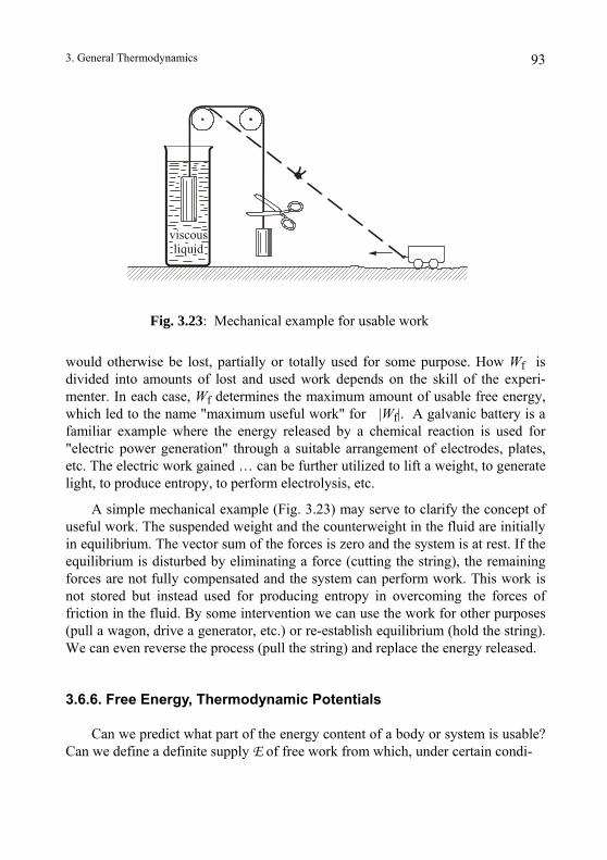
3. General Thermodynamics 93
viscousliquid
Fig. 3.23: Mechanical example for usable work
would otherwise be lost, partially or totally used for some purpose. How Wf is divided into amounts of lost and used work depends on the skill of the experi-menter. In each case, Wf determines the maximum amount of usable free energy, which led to the name "maximum useful work" for |Wf|. A galvanic battery is a familiar example where the energy released by a chemical reaction is used for "electric power generation" through a suitable arrangement of electrodes, plates, etc. The electric work gained … can be further utilized to lift a weight, to generate light, to produce entropy, to perform electrolysis, etc.
A simple mechanical example (Fig. 3.23) may serve to clarify the concept of useful work. The suspended weight and the counterweight in the fluid are initially in equilibrium. The vector sum of the forces is zero and the system is at rest. If the equilibrium is disturbed by eliminating a force (cutting the string), the remaining forces are not fully compensated and the system can perform work. This work is not stored but instead used for producing entropy in overcoming the forces of friction in the fluid. By some intervention we can use the work for other purposes (pull a wagon, drive a generator, etc.) or re-establish equilibrium (hold the string). We can even reverse the process (pull the string) and replace the energy released.
3.6.6. Free Energy, Thermodynamic Potentials
Can we predict what part of the energy content of a body or system is usable? Can we define a definite supply E of free work from which, under certain condi-
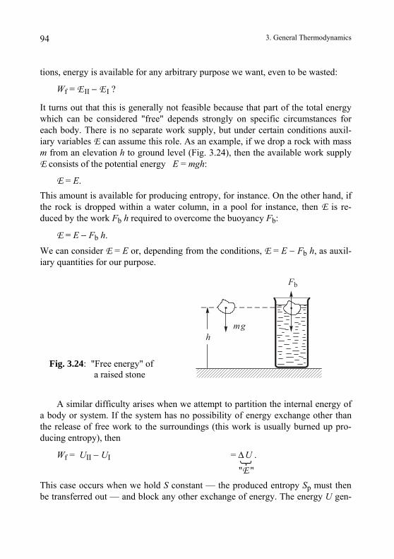
3. General Thermodynamics 94
tions, energy is available for any arbitrary purpose we want, even to be wasted:
Wf = E II − E I ?
It turns out that this is generally not feasible because that part of the total energy which can be considered "free" depends strongly on specific circumstances for each body. There is no separate work supply, but under certain conditions auxil-iary variables E can assume this role. As an example, if we drop a rock with mass m from an elevation h to ground level (Fig. 3.24), then the available work supply E consists of the potential energy E = mgh:
E = E. This amount is available for producing entropy, for instance. On the other hand, if the rock is dropped within a water column, in a pool for instance, then E is re-duced by the work Fb h required to overcome the buoyancy Fb:
E = E − Fb h.
We can consider E = E or, depending from the conditions, E = E − Fb h, as auxil-iary quantities for our purpose.
hmg
Fb
Fig. 3.24: "Free energy" of a raised stone
A similar difficulty arises when we attempt to partition the internal energy of a body or system. If the system has no possibility of energy exchange other than the release of free work to the surroundings (this work is usually burned up pro-ducing entropy), then
Wf = UII − UI = ∆ U .
"E " This case occurs when we hold S constant — the produced entropy Sp must then be transferred out — and block any other exchange of energy. The energy U gen-
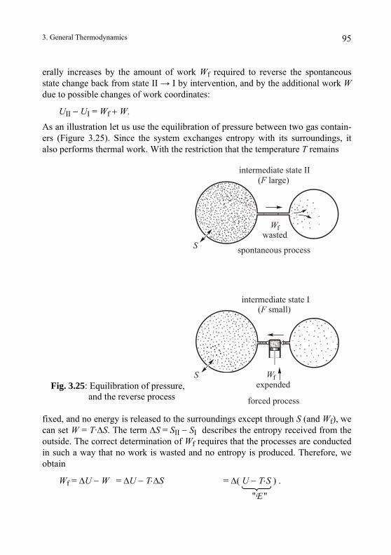
3. General Thermodynamics 95
erally increases by the amount of work Wf required to reverse the spontaneous state change back from state II → I by intervention, and by the additional work W due to possible changes of work coordinates:
UII − UI = Wf + W.
As an illustration let us use the equilibration of pressure between two gas contain-ers (Figure 3.25). Since the system exchanges entropy with its surroundings, it also performs thermal work. With the restriction that the temperature T remains
Fig. 3.25: Equilibration of pressure, and the reverse process
( large)Fintermediate state II
intermediate state I
wasted
S
S
Wf
Wf
spontaneous process
( small)F
forced process
expended
fixed, and no energy is released to the surroundings except through S (and Wf), we can set W = T·∆S. The term ∆S = SII − SI describes the entropy received from the outside. The correct determination of Wf requires that the processes are conducted in such a way that no work is wasted and no entropy is produced. Therefore, we obtain
Wf = ∆U − W = ∆U − T⋅∆S = ∆( U − T⋅S ) . "E "
3. General Thermodynamics 96
For this special case it is no longer U but a new quantity A whose change deter-mines the free work:
A = U − TS, Wf = AII − AI .
Similar auxiliary functions — different ones depending on the situation — are called "free energies" or "thermodynamic potentials" (or better, "thermodynamic potential energies"), because they have properties similar to the potential energy in mechanics. The quantity A, as introduced by H. V. HELMHOLTZ, is called "HELMHOLTZ free energy", "HELMHOLTZ energy" or simply "free energy".
In the more important practical case in which a body expands against a con-stant pressure p (perhaps air pressure) we have W = T·∆S + (−p)·∆V and
Wf = ∆U − W = ∆U − T⋅∆S − (−p)⋅∆V = ∆( U − T⋅S + p⋅V ) "E "
Here a new quantity G, introduced by W. J. GIBBS and called "GIBBS free energy", "GIBBS energy" or simply "free enthalpy”, assumes the role of A.
G = U − TS + pV, Wf = GII − GI .
If we hold S constant rather than T, then we have W = (−p)∆V. In this way we obtain
Wf = ∆U − W = ∆U − (−p)⋅∆V = ∆( U + p⋅V )
"E "
We remember U + p⋅V ≡ H. The quantity H that was previously got to know as enthalpy, now serves as a thermodynamic potential.
Just as in the case of the heat functions, we can immediately generalize these results. If we fix all work coordinates xi of a multi-actuator system, or allow the corresponding external forces yi to vanish, then U serves as thermodynamic poten-tial. Note that in addition to Wf (as thermal waste or dissipation heat ) no energy is exchanged with the surroundings in this system. However, if some forces, say y2 and y4, are held constant instead of the corresponding coordinates x2 and x4, then we have W = y2∆x2 + y4∆x4, and
Wf = ∆U − W = ∆U − y2∆x2 − y4∆x4 = ∆( U − y2x2 − y4x4 )
"E "
Thermodynamic potentials can be defined for numerous special cases. For each set of constant forces yα, yβ, yγ … (unlike the heat functions, T is included here), we
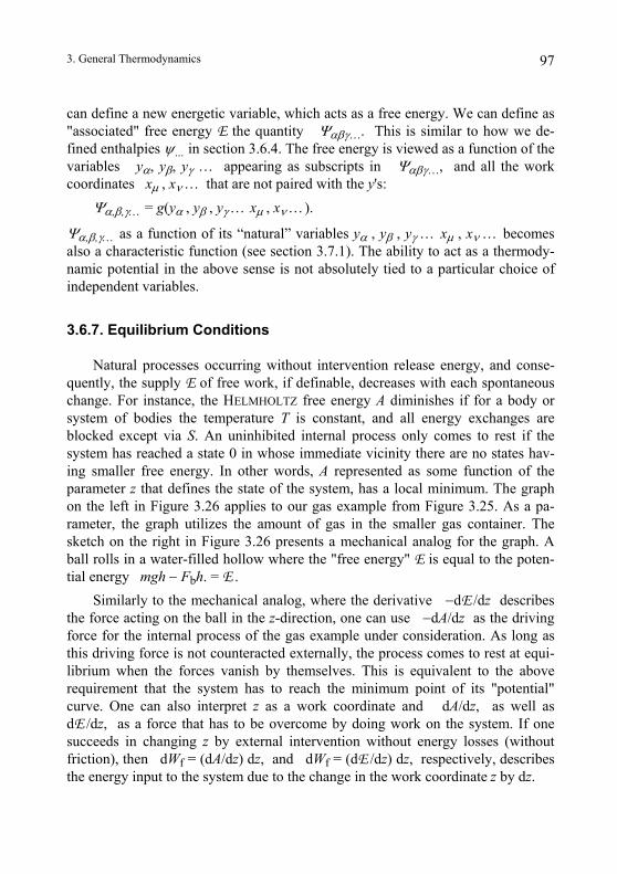
3. General Thermodynamics 97
can define a new energetic variable, which acts as a free energy. We can define as "associated" free energy E the quantity Ψαβγ…. This is similar to how we de-fined enthalpies ψ… in section 3.6.4. The free energy is viewed as a function of the variables yα, yβ, yγ … appearing as subscripts in Ψαβγ…, and all the work coordinates xµ , xν … that are not paired with the y's:
Ψα,β,γ… = g(yα , yβ , yγ … xµ , xν …).
Ψα,β,γ… as a function of its “natural” variables yα , yβ , yγ … xµ , xν … becomes also a characteristic function (see section 3.7.1). The ability to act as a thermody-namic potential in the above sense is not absolutely tied to a particular choice of independent variables.
3.6.7. Equilibrium Conditions
Natural processes occurring without intervention release energy, and conse-quently, the supply E of free work, if definable, decreases with each spontaneous change. For instance, the HELMHOLTZ free energy A diminishes if for a body or system of bodies the temperature T is constant, and all energy exchanges are blocked except via S. An uninhibited internal process only comes to rest if the system has reached a state 0 in whose immediate vicinity there are no states hav-ing smaller free energy. In other words, A represented as some function of the parameter z that defines the state of the system, has a local minimum. The graph on the left in Figure 3.26 applies to our gas example from Figure 3.25. As a pa-rameter, the graph utilizes the amount of gas in the smaller gas container. The sketch on the right in Figure 3.26 presents a mechanical analog for the graph. A ball rolls in a water-filled hollow where the "free energy" E is equal to the poten-tial energy mgh − Fbh. = E .
Similarly to the mechanical analog, where the derivative −dE /dz describes the force acting on the ball in the z-direction, one can use −dA/dz as the driving force for the internal process of the gas example under consideration. As long as this driving force is not counteracted externally, the process comes to rest at equi-librium when the forces vanish by themselves. This is equivalent to the above requirement that the system has to reach the minimum point of its "potential" curve. One can also interpret z as a work coordinate and dA/dz, as well as dE /dz, as a force that has to be overcome by doing work on the system. If one succeeds in changing z by external intervention without energy losses (without friction), then dWf = (dA/dz) dz, and dWf = (dE /dz) dz, respectively, describes the energy input to the system due to the change in the work coordinate z by dz.

3. General Thermodynamics 98
0Wf
z
z
0
h ~ A*
Fig. 3.26: Equilibrium at the minimum of the free energy
If we need further parameters zi in order to define the state of the system (as-suming T = const. and no energy transfer occurs except via S!), then the forces
ii must vanish in all directions in the final state of a completed process. The condition for equilibrium of the system at point (z1, z2 … ) is given by (d /d zA z )
( )ˆ
d 0 1, 2 d
ii z
A iz
⎛ ⎞ = = …⎜ ⎟⎝ ⎠
) d (d /d ) dA A z z A z z
.
Since ˆ ˆ1 21 1 2 2d z z = (d /d + +… , we can express the "equilibrium condition" in simpler form without referring to the parameters zi :
dA = 0 (T = const. and no energy transfer except via S). Under different conditions, A is replaced by other thermodynamic potentials
but nothing else is changed. Of particular interest are systems under constant pres-sure and temperature that are otherwise insulated, where the most frequently used equilibrium condition is
dG = 0 (p, T = const. and no energy transfer except via S,V).
3. General Thermodynamics 99
This condition is widely used in chemical thermodynamics. The equilibrium con-ditions discussed above make it possible to describe the equilibrium state of a system via energy balances as preferred by the energetic approach to thermody-namics.
3.7 Common Mathematical Procedures
Mathematical procedures used in traditional thermodynamics differ from those employed here in essentially two respects:
a) Instead of directly transforming the derivatives, one usually goes back to the differentials.
b) In place of the flip rule, one uses various characteristic functions or appropri-ately selected cycles.
Let us first consider the computational aids in b).
3.7.1. Characteristic Functions, MAXWELL Relations
It was noted in section 3.1.2 that the energy E as a function of the work coor-dinates x1, x2 … xn is the characteristic function for a lossless or elastic system. That means that all properties described by its main quantities can be computed as long as E(x1, x2 … xn) is known. In particular, one can find the missing forces Fi from the derivatives of E with respect to xi. A similar conclusion is valid for U.
This feature of E or U is lost on choosing other independent variables such as, for example, the forces y1 and y3 instead of the corresponding coordinates x1 and x3. However, in this case the already familiar intermediate variable ψ1,3 , known as the free energy with y1 and y3 held constant, assumes this role. By definition, we have ψ1,3 = U − y1 x1 − y3 x3 and its differential becomes:
13 1 1 1 1 3 3 3 3d d d d d dU y x y x y x y xψ = − ⋅ − ⋅ − ⋅ − ⋅
13 1 1 2 2 3 3 4 4d d d d dx y y x x y y x
.
By substituting this dU with the main equation dU = y1 dx1 + y2 dx2 …, we ob-tain the so-called "fundamental equation" of the quantity ψ1,3 :
ψ = − + − + +… .
3. General Thermodynamics 100
This equation differs from the energy differential in two respects. For the va-riables identified by the index of the quantity ψ (here 1 and 3), x and y are inter-changed and the sign is also changed. Now the differential of ψ1,3(y1 , x2 , y3 , x4 … ) can generally be expressed as:
1313ψ 13 13
1 2 31 2 3
d d dd d d dd d d
y x yy x y
ψ ψ ψ⎛ ⎞⎛ ⎞ ⎛ ⎞= + + +⎜ ⎟⎜ ⎟ ⎜ ⎟⎝ ⎠⎝ ⎠ ⎝ ⎠…… ……
Comparison of the coefficients in the last both equations shows an important re-sult. By taking the derivatives of ψ1,3(y1, x2, y3, x4 … ) with respect to any of the variables inside the brackets, we always get the corresponding main quantity with either positive or negative sign. This way we can compute the missing work coor-dinates and forces, and other expressions consisting of main quantities, as long as the function ψ1,3 (y1 , x2 , y3 , x4 … xn) is known. Therefore, we can consider ψ1,3 , just as U(x1 … xn), to be a characteristic function of the system under consideration. With a different choice of independent variables z1 … zn (zi = xi or yi), U(x1 … xn) is replaced by the corresponding function ψ(z1 … zn), which we have already met in our earlier discussion about thermodynamic potentials.
The real significance of the characteristic function lies in the fact that it en-ables us to perform, either directly or indirectly, those operations that we com-pleted by using the flip rule. For example, in order to carry out the transformation
d dd dyyw uw
v xu
⎛ ⎞⎛ ⎞ = −⎜ ⎟ ⎜ ⎟⎝ ⎠ ⎝ ⎠
for a system with the main equation dU = udx + vdy + wdz, we start with the fundamental equation of the function ψuw = U − ux − wz, where the independent variables u, y, w are the same as on the left side of the above equation. Then
dψuw = − x du + v dy − z dw .
From this equation, we get v = (dψuw/dy) uw and x = −(dψuw/du) yw. Then by changing the order of differentiation (SCHWARZ theorem), we obtain the final result:
d d dd d dd d d d d d
uw uw
ywyw uw uwyw uw
v xu u y y u y
ψ ψ⎛ ⎞⎛ ⎞⎛ ⎞ ⎛ ⎞⎛ ⎞ ⎛ ⎞= = = −⎜ ⎟⎜ ⎟⎜ ⎟ ⎜ ⎟⎜ ⎟ ⎜ ⎟⎝ ⎠⎝ ⎠ ⎝ ⎠ ⎝ ⎠⎝ ⎠ ⎝ ⎠ .
3. General Thermodynamics 101
If the index and numerator of the initial derivative contain paired variables, then this procedure fails. In this case, one has to make an appropriate transforma-tion of the original derivative.
Equations derived in this way are often called "MAXWELL relations". J. C. MAXWELL derived them originally by considering a reversible cycle for a body undergoing compression and heating. It is described by the main equation dU = −pdV + TdS. The characteristic functions are U(V,S), ψp = H(p,S), ψT = A(V,T) and ψpT = G(p,T) with corresponding fundamental equations:
dU = −pdV + TdS, dH = Vdp + TdS, dA = −pdV − SdT, dG = Vdp − SdT.
By taking derivatives "diagonally", i.e., −p with respect to S, and T with respect to V in the first equation, etc., and by using the SCHWARZ theorem, we obtain the following four equations:
d d d d,d d d dS pV S
p T V TS V S p
⎛ ⎞⎛ ⎞ ⎛ ⎞ ⎛ ⎞− = =⎜ ⎟ ⎜ ⎟⎜ ⎟ ⎜ ⎟⎝ ⎠ ⎝ ⎠⎝ ⎠ ⎝ ⎠,
d d d d,p S V S⎛ ⎞⎛ ⎞ ⎛ ⎞ ⎛ ⎞− = − = −⎜ ⎟ ⎜ ⎟⎜ ⎟ ⎜ ⎟d d d dT pV TT V T p⎝ ⎠ ⎝ ⎠⎝ ⎠ ⎝ ⎠.
These equations can be derived directly by flipping. In this sense the flip rule can be considered as a tool for deriving all possible MAXWELL relations.
3.7.2. Reversible Cycles
The same results can be obtained with energy balance equations applied to appropriate cycles, as MAXWELL himself did. As an example, consider a piece of wire of length l that is stretched by the force F and whose entropy content can be increased by adding entropy against the temperature T (Figure 3.27). In order to derive the MAXWELL Equation
( ) ( )d dd dT l
S Fl T
= − ,
we perform the following lossless procedure with the wire:
a. Stretch the wire by dl at constant temperature T as described by the first de-rivative, and thereby add the entropy dS = (dS/dl)T dl to the wire.
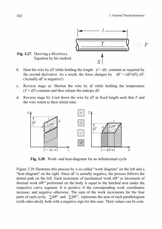
3. General Thermodynamics 102
S
T F
l
Fig. 3.27: Deriving a MAXWELL Equation by his method
b. Heat the wire by dT while holding the length (l + dl) constant as required by the second derivative. As a result, the force changes by dF = (dF/dT)l dT. (Actually dF is negative!)
c. Reverse stage a): Shorten the wire by dl while holding the temperature (T + dT) constant and thus release the entropy dS.
d. Reverse stage b): Cool down the wire by dT at fixed length such that F and the wire return to their initial state.
F
ddF
cb
ldl
a∑dW'
dT
S
T
d
dS
b
c
a∑dW''
d
a
b
c
Fig. 3.28: Work- and heat-diagrams for an infinitesimal cycle
Figure 3.28 illustrates this process by a so-called "work diagram" on the left and a "heat diagram" on the right. Since dF is actually negative, the process follows the dotted path on the left. Each increment of mechanical work dW' or increment of thermal work dW'' performed on the body is equal to the hatched area under the respective curve segment. It is positive if the corresponding work coordinates increase, and negative otherwise. The sum of the work increments for the four parts of each cycle, ∑dW' and ∑dW'', represents the area of each parallelogram (with sides abcd), both with a negative sign for this case. Their values can be com-
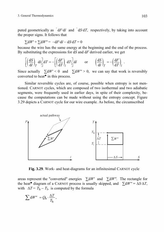
3. General Thermodynamics 103
puted geometrically as dF·dl and dS·dT, respectively, by taking into account the proper signs. It follows that
∑dW' + ∑dW'' = −dF·dl − dS·dT = 0 because the wire has the same energy at the beginning and the end of the process. By substituting the expressions for dS and dF derived earlier, we get
( ) ( ) ( ) ( )d d d dd d d d ord d d dT l T l
S F S Fl T T ll T l T
⎡ ⎤⎡ ⎤ = − = −⎢ ⎥⎢ ⎥⎣ ⎦ ⎣ ⎦ .
Since actually ∑dW' < 0 and ∑dW'' > 0, we can say that work is reversibly converted to heat in this process.
Similar reversible cycles are, of course, possible when entropy is not men-tioned. CARNOT cycles, which are composed of two isothermal and two adiabatic segments, were frequently used in earlier days, in spite of their complexity, be-cause the computations can be made without using the entropy concept. Figure 3.29 depicts a CARNOT cycle for our wire example. As before, the circumscribed
l
F
actual pathway
T
Th
Tl
S
∆T
∆S
∑W' ∑W''
Fig. 3.29. Work- and heat-diagrams for an infinitesimal CARNOT cycle
areas represent the "converted" energies ∑dW' and ∑dW''. The rectangle for the heat diagram of a CARNOT process is usually skipped, and ∑dW'' = ∆S·∆T, with ∆T = Th − Tl, is computed by the formula
hh
d TW'' QT∆= ⋅∑ ,
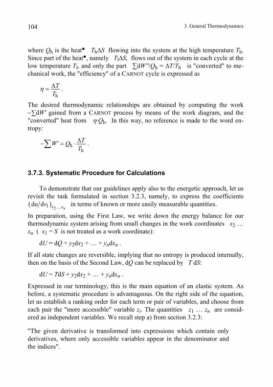
3. General Thermodynamics 104
where Qh is the heat Th∆S flowing into the system at the high temperature Th. Since part of the heat, namely Tl∆S, flows out of the system in each cycle at the low temperature Tl, and only the part ∑dW''/Qh = ∆T/Th is "converted" to me-chanical work, the "efficiency" of a CARNOT cycle is expressed as
h
TT
η ∆= .
The desired thermodynamic relationships are obtained by computing the work −∑dW' gained from a CARNOT process by means of the work diagram, and the "converted" heat from η·Qh. In this way, no reference is made to the word en-tropy:
hh
TW' QT∆− = ⋅∑ .
3.7.3. Systematic Procedure for Calculations
To demonstrate that our guidelines apply also to the energetic approach, let us revisit the task formulated in section 3.2.3, namely, to express the coefficients ( )
21d dnv vu v … in terms of known or more easily measurable quantities.
In preparation, using the First Law, we write down the energy balance for our thermodynamic system arising from small changes in the work coordinates x2 … xn ( x1 = S is not treated as a work coordinate):
dU = dQ + y2dx2 + … + yndxn .
If all state changes are reversible, implying that no entropy is produced internally, then on the basis of the Second Law, dQ can be replaced by T dS:
dU = TdS + y2dx2 + … + yndxn .
Expressed in our terminology, this is the main equation of an elastic system. As before, a systematic procedure is advantageous. On the right side of the equation, let us establish a ranking order for each term or pair of variables, and choose from each pair the "more accessible" variable zi. The quantities z1 … zn are consid-ered as independent variables. We recall step a) from section 3.2.3:
"The given derivative is transformed into expressions which contain only derivatives, where only accessible variables appear in the denominator and the indices".
3. General Thermodynamics 105
This procedure may be carried out in the following systematic way:
a) Write down the differentials of all variables appearing in the derivative ( )
21d dnv vu v … and select zi as the independent variables:
ˆ ˆ1
11
d dd d … dd d
n
nnz z
u uu z zz z
⎛ ⎞⎛ ⎞= + +⎜ ⎟ ⎜ ⎟⎝ ⎠ ⎝ ⎠,
ˆ ˆ1
1 11 1
1
d dd d … dd d
n
nnz z
v vv z zz z
⎛ ⎞⎛ ⎞= + +⎜ ⎟ ⎜ ⎟⎝ ⎠ ⎝ ⎠
…………………………………………
,
ˆ ˆ1
n 11
d d … dd d
n
nnz z
v z zz z
= + +⎜ ⎟ ⎜ ⎟⎝ ⎠ ⎝ ⎠
d dn nv v⎛ ⎞⎛ ⎞ .
b) The differentials dv2 … dvn vanish since the parameters v2 … vn are constant, resulting in n + 1 equations with n + 2 "unknowns", namely, du, dv1, dz1 … dzn . By eliminating dzi and solving for du, we obtain:
21
1 1
d dd d or d d
nv v
u uu B v Bv v
⎛ ⎞= = =⎜ ⎟⎝ ⎠ …
,
where B is composed of the coefficients from the system of equations, and therefore contains only derivatives with respect to zi as desired.
This procedure, explained above in general form, appears cumbersome, but often leads to the solution relatively quickly. We have already encountered one applica-tion during the derivation of the rule for "inserting an index" (see section 3.2.1). If the specified derivative contains auxiliary variables ψ (enthalpies, thermodynamic potentials, etc.), its total differentials are written with the help of the fundamental equation before being expanded in terms of zi .
We also recall step b) from section 3.2.3:
"All generated quotients that contain a numerator with higher rank than the denominator (top-heavy quotients) are flipped".
This procedure can be performed by utilizing the characteristic function for all zi or the corresponding MAXWELL relations. The procedure was explained in the previous section and will not be repeated here.
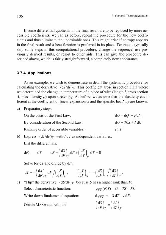
3. General Thermodynamics106
If some differential quotients in the final result are to be replaced by more ac-cessible coefficients, we can as before, repeat the procedure for the new coeffi-cients and thus eliminate the undesirable ones. This might arise if entropy appears in the final result and a heat function is preferred in its place. Textbooks typically skip some steps in this computational procedure, change the sequence, use pre-viously derived results, or resort to other aids. This can give the procedure de-scribed above, which is fairly straightforward, a completely new appearance.
3.7.4. Applications
As an example, we wish to demonstrate in detail the systematic procedure for calculating the derivative (dT/dF)S. This coefficient arose in section 3.3.3 where we determined the change in temperature of a piece of wire (length l, cross section A, mass density ρ) upon stretching. As before, we assume that the elasticity coef-ficient ε, the coefficient of linear expansion α and the specific heat cF are known.
a) Preparatory steps:
On the basis of the First Law: dU = dQ + Fdl .
By consideration of the Second Law: dU = TdS + Fdl.
Ranking order of accessible variables: F, T.
b) Express (dT/dF)S with F, T as independent variables:
List the differentials:
( ) ( )d dd d d 0d dT F
S SS F TF T
= + =dF, dT, .
Solve for dT and divide by dF:
( ) ( ) ( ) ( ) ( )d d d d dd d , = d d d dT F S F
S S T S ST FF T F T
= − −d TF
.
c) “Flip” the derivative (dS/dF)T because S has a higher rank than F:Select characteristic function: ψFT (F,T) = U − TS − Fl.
Write down fundamental equation: dψFT = − S dT − l dF.
( ) ( )d dd dT F
S lF T
=Obtain MAXWELL relation: .
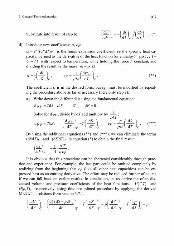
3. General Thermodynamics 107
( ) ( ) ( )d d dd dd F FS
T l ST TF
= − . (*) Substitute into result of step b):
d) Introduce new coefficients α, cF: α = l−1(dl/dT)F is the linear expansion coefficient, cF the specific heat ca-pacity, defined as the derivative of the heat function (or enthalpy) ψF(T, F) = U − Fl with respect to temperature, while holding the force F constant, and dividing the result by the mass m = ρ ⋅lA
d1d F
ll T
α ⎛ ⎞= ⎜ ⎟⎝ ⎠
, d1d
FF
Fc
lA Tψ
ρ⎛ ⎞= ⎜ ⎟⎝ ⎠
d d , d , d 0F T S l F T F
. (**)
The coefficient α is in the desired form, but cF must be modified by repeat-ing the procedure above as far as necessary (here only step a):
a') Write down the differentials using the fundamental equation:
dψ = − = . 1lAρ
Solve for dψF , divide by dT and multiply by : d d dd d , = , d d d
FF F
F F F
S STT S T cT T lA T
ψψρ
⎛ ⎞ ⎛ ⎞ ⎛ ⎞= =⎜ ⎟ ⎜ ⎟ ⎜ ⎟⎝ ⎠ ⎝ ⎠ ⎝ ⎠
. (***)
By using the additional equations (**) and (***), we can eliminate the terms (dl/dT)F and (dS/dT)F in equation (*) to obtain the final result:
( )d 1d S F
TTF A c
αρ
= − ⋅ .
It is obvious that this procedure can be shortened considerably through prac-tice and experience. For example, the last part could be omitted completely by realizing from the beginning that cF (like all other heat capacities) can be ex-pressed best as an entropy derivative. The effort may be reduced further of course if we can fall back on earlier results. In conclusion, let us derive the often dis-cussed volume and pressure coefficients of the heat functions U(V,T) and H(p,T), respectively, using this streamlined procedure by applying the derived MAXWELL relations from section 3.7.1.
( )d d d d d d dd d d d dT T T VT
T S p V pU S VT p T pV V V V T
−⎛ ⎞ ⎛ ⎞⎛ ⎞ ⎛ ⎞ ⎛ ⎞= = − = −⎜ ⎟ ⎜ ⎟ ⎜ ⎟ ⎜ ⎟⎜ ⎟⎝ ⎠ ⎝ ⎠ ⎝ ⎠ ⎝ ⎠⎝ ⎠,
3. General Thermodynamics 108
( )d d d d dd dd d d d d pT T T T
T S V p p VH ST V T Vp p p p T
+⎛ ⎞ ⎛ ⎞ ⎛ ⎞ ⎛ ⎞ ⎛ ⎞= = + = − +⎜ ⎟⎜ ⎟ ⎜ ⎟ ⎜ ⎟ ⎜ ⎟ ⎝ ⎠⎝ ⎠ ⎝ ⎠ ⎝ ⎠ ⎝ ⎠.
Collecting and numbering hundreds of formulas for later usage is a standard method in conventional textbooks. One aim of the new approach is to reduce this apparatus to a minimum.
4. Chemical Thermodynamic 109
4. CHEMICAL THERMODYNAMICS
The area of physics that deals with the macroscopic description of systems of reactive matter is called "chemical physics" or "chemical thermodynamics". This subject can be developed conceptually and formally in a manner similar to that used in Chapter 2 for pure thermodynamics. The most important quantities, the counterparts of entropy and temperature, are the amount of substance and its chemical potential, and we consider these quantities first.
The concept of chemical potential used here is a somewhat generalized ver-sion of that found in standard chemical thermodynamics. A more descriptive term might be substance potential (the potential of a substance, where substance can even refer to light), but here we shall use the well-known expression chemical potential.
4.1. Introduction
The term "substance" generally refers to a uniform substance described by a chemical formula and identified by certain properties such as color, density, solu-bility, melting point, emission and absorption spectra, reactivity, etc. Our sur-roundings comprise many different substances, distributed uniformly or non-uniformly. Rarely does an object consist of only one kind of substance such as a piece of pure sugar or a copper wire. Generally we find mixtures of substances.
In simple cases, bodies such as an air bubble, a water drop, a drinking glass and an emerald are uniform. Some bodies comprise a number of separate uniform parts, such as a granite block made up of feldspar, quartz and mica minerals, or a steel beam consisting of a microscopic mixture of iron and iron carbide crystals, or a copper coin having a structure of differently arranged crystals each with the same chemical composition. In addition, bodies such as a cell, a leaf or a wooden block are structured down to the submicroscopic scale. Others change continu-ously from place to place such as a colorful agate mineral, or the atmosphere that becomes thinner and contains relatively more hydrogen at higher elevations.
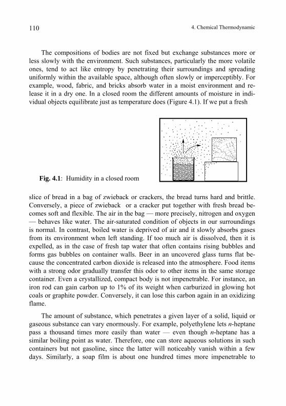
4. Chemical Thermodynamic 110
The compositions of bodies are not fixed but exchange substances more or less slowly with the environment. Such substances, particularly the more volatile ones, tend to act like entropy by penetrating their surroundings and spreading uniformly within the available space, although often slowly or imperceptibly. For example, wood, fabric, and bricks absorb water in a moist environment and re-lease it in a dry one. In a closed room the different amounts of moisture in indi-vidual objects equilibrate just as temperature does (Figure 4.1). If we put a fresh
Fig. 4.1: Humidity in a closed room
slice of bread in a bag of zwieback or crackers, the bread turns hard and brittle. Conversely, a piece of zwieback or a cracker put together with fresh bread be-comes soft and flexible. The air in the bag — more precisely, nitrogen and oxygen — behaves like water. The air-saturated condition of objects in our surroundings is normal. In contrast, boiled water is deprived of air and it slowly absorbs gases from its environment when left standing. If too much air is dissolved, then it is expelled, as in the case of fresh tap water that often contains rising bubbles and forms gas bubbles on container walls. Beer in an uncovered glass turns flat be-cause the concentrated carbon dioxide is released into the atmosphere. Food items with a strong odor gradually transfer this odor to other items in the same storage container. Even a crystallized, compact body is not impenetrable. For instance, an iron rod can gain carbon up to 1% of its weight when carburized in glowing hot coals or graphite powder. Conversely, it can lose this carbon again in an oxidizing flame.
The amount of substance, which penetrates a given layer of a solid, liquid or gaseous substance can vary enormously. For example, polyethylene lets n-heptane pass a thousand times more easily than water — even though n-heptane has a similar boiling point as water. Therefore, one can store aqueous solutions in such containers but not gasoline, since the latter will noticeably vanish within a few days. Similarly, a soap film is about one hundred times more impenetrable to
4. Chemical Thermodynamic 111
nitrogen than to carbon dioxide. There are large differences in the ability to pene-trate a layer of air above a salt solution: Water can easily cross this layer but the less volatile salt is almost completely blocked.
For a homogeneous body, a substance penetrating it distributes itself uni-formly over the entire volume after a sufficient amount of time. The capacity to absorb foreign substances varies over a wide range, just like the penetrability. One liter of water at room temperature can absorb an unlimited amount of ethanol since water and ethanol are miscible. On the other hand, 500 liters of hydrochloric acid gas at one bar pressure can dissolve only approximately 10 mm3 of limestone or only 10−10 mm3 of silver sulfide, an amount not perceptible with an optical microscope.
Amounts of substance are not constant since the substances can be converted into one another, or decomposed into their fundamental parts, the elements. They can also be rebuilt from the elements. During familiar chemical transformations the amount of elements remains unchanged, i.e., under the same conditions one obtains the same amount of elements when the mixture is analyzed before and after the transformation. However, processes in nuclear reactors and particle ac-celerators show that the elements themselves may be transformed and can be split into hydrogen (including the neutrons!), or reconstituted from it with the amount of hydrogen remaining constant. If we wish, we can interpret all transformations of substances as changes of state of a single kind of matter.
4.2. Amount of Substance
Since various measures are used to quantify amounts of substance, let us first consider what properties we should expect of such a quantity.
It is reasonable to assume that an amount of substance within a given space can only change by releasing or receiving substances to or from its environment. In addition, a chemical transformation can consume or create a substance. Its quantity cannot change simply by storing, heating, insulating or separating it from other substances. If we impose this property, certain measures are eliminated im-mediately, such as the volume used in everyday transactions — a liter of water, a cubic meter of gas, etc. — and in a strict sense also the mass m that increases whenever work is performed on a particular substance due to EINSTEIN's equation
E = m c2 .
4. Chemical Thermodynamic 112
E is the energy content and c is the speed of light. Because these changes in mass are far below the available accuracy of measurement under normal circumstances, this measure of quantity of substance, the mass m, has been widely accepted in science and in business. However, it is unsatisfactory when one considers that by increasing the temperature of 1 cm3 of water by 1º Celsius, its mass increases by 5 · 10–14 g. This corresponds to the mass of around one billion water molecules.
It is a convincing assumption that two amounts of the same substance are equal, provided they occupy the same volume or weigh the same under the same external conditions, such as the shape of the volume, pressure, temperature, field strength, etc.,. In order to measure the available amount of a substance, it is suffi-cient — as we did for entropy — to divide the substance into equal pieces or fill up equal containers with it under identical conditions, and then count the parts. Basically, any arbitrary quantity can serve as a unit, provided it can be uniquely identified for a given substance. The unit for an amount of gas as "standard cubic meter" is basically such a procedure.
Due to the atomic structure of matter, it seems natural to divide up a portion of substance into its component atoms or groups of atoms. It is therefore natural to use "particle" as a basic unit. By doing so, the concepts of the amount of substance and the number of particles overlap. The usual unit of measurement in chemistry, the "mole", is consistent with the above. The mole may be defined as
1 mol = 0.6023 · 1024 particles, where the right-hand side represents the so-called LOSCHMIDT or AVOGADRO
number. More accurately, the mole may be defined so that a portion with a mass m = 12 g of the pure carbon isotope with a mass number of 12 represents exactly an amount of substance n(12C) = 1 mol. Since it is possible to count directly or indirectly the atoms or groups of atoms, the amount of substance n defined by this rule is a measurable quantity. Nevertheless, our measurement procedure is appli-cable whether or not we know anything about the existence of atoms.
If we consider all matter to be of the same kind, then this definition is not adequate. Logically, all substances must be brought into a consistent material state, such as hydrogen for instance, whose quantity can be determined by count-ing atoms. The number of nuclear building blocks, in other words the nucleon number, becomes a measure of the amount of substance of a body. Expressed in "mol", the numerical value of this quantity agrees approximately with the mass given in grams. More precisely, a portion of n = 1 mol of matter in the form of hydrogen H weighs 1.008 g, as graphite C it weighs 1.000 g and as iron Fe it
4. Chemical Thermodynamic 113
weighs 0.999 g. According to this measurement procedure, there is a law of con-servation of substance (antimatter might be count as negative) similar to that for electric charge. If we identify the amount of substance by its mass, essentially a measure of energy, then matter and energy can be treated as interchangeable due to EINSTEIN's equation. Thus, we encounter relationships here that are similar to those we learned from heat concepts (entropy or energy).
4.3. Chemical Potential
As mentioned earlier, the dispersion of matter in space reminds us of thermal processes. Past researchers were guided by this similarity and spoke of heat as a fluid. It seems obvious that we should use the conceptual framework for thermal phenomena as a model for our current topic.
4.3.1 Energy and Potential
We are already familiar with the fact that a body can exchange various sub-stances with surrounding objects. In order to transfer substances in a controlled fashion, we can utilize a kind of syringe as we did for entropy. If we use this de-vice to deliver a small quantity dn of any substance from one body to another — for example, water in the form of steam from a dry wooden block to a moist brick (Figure 4.2) — it requires work. This work is totally retrievable if all losses due to friction or other entropy-producing processes are avoided. Losses can be avoided, at least in an idealized thought process, by ensuring that all steps are reversible.
In order to determine the work dW required for the substance under considera-tion, we must transfer only this amount and avoid any additional work. Specifi-cally, we should not transfer other substances simultaneously, nor produce any entropy, nor transfer any extra electric charge. Neither should the bodies be de-formed in the process. We are assured that no parameter or component was over-looked when a body ends up in its original state after returning the transferred amount of substance. In practice, this transfer can be carried out as follows: First the desired substance is extracted from a body through a rigid wall (the bottom) of the syringe that is permeable only to the substance. Then the syringe is used to inject the substance into the second body and the expended work is measured. Unfortunately, there is no such permeable wall that holds back entropy. However,
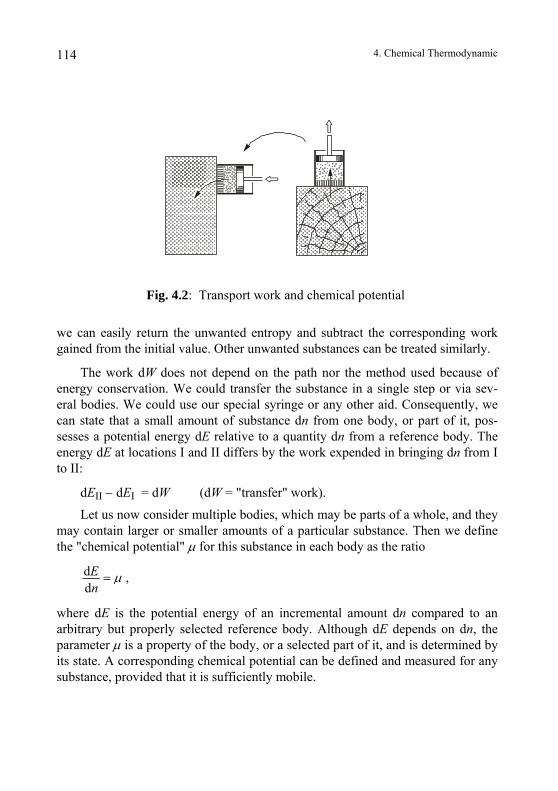
4. Chemical Thermodynamic 114
Fig. 4.2: Transport work and chemical potential
we can easily return the unwanted entropy and subtract the corresponding work gained from the initial value. Other unwanted substances can be treated similarly.
The work dW does not depend on the path nor the method used because of energy conservation. We could transfer the substance in a single step or via sev-eral bodies. We could use our special syringe or any other aid. Consequently, we can state that a small amount of substance dn from one body, or part of it, pos-sesses a potential energy dE relative to a quantity dn from a reference body. The energy dE at locations I and II differs by the work expended in bringing dn from I to II:
dEII − dEI = dW (dW = "transfer" work).
Let us now consider multiple bodies, which may be parts of a whole, and they may contain larger or smaller amounts of a particular substance. Then we define the "chemical potential" µ for this substance in each body as the ratio
ddEn
µ= ,
where dE is the potential energy of an incremental amount dn compared to an arbitrary but properly selected reference body. Although dE depends on dn, the parameter µ is a property of the body, or a selected part of it, and is determined by its state. A corresponding chemical potential can be defined and measured for any substance, provided that it is sufficiently mobile.
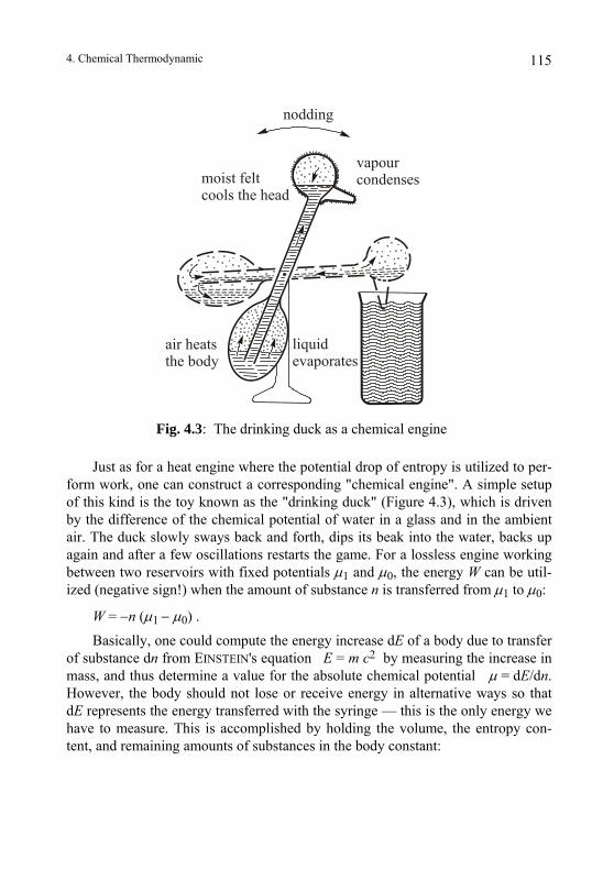
4. Chemical Thermodynamic 115
nodding
vapourcondenses
air heatsthe body
liquidevaporates
moist feltcools the head
Fig. 4.3: The drinking duck as a chemical engine
Just as for a heat engine where the potential drop of entropy is utilized to per-form work, one can construct a corresponding "chemical engine". A simple setup of this kind is the toy known as the "drinking duck" (Figure 4.3), which is driven by the difference of the chemical potential of water in a glass and in the ambient air. The duck slowly sways back and forth, dips its beak into the water, backs up again and after a few oscillations restarts the game. For a lossless engine working between two reservoirs with fixed potentials µ1 and µ0, the energy W can be util-ized (negative sign!) when the amount of substance n is transferred from µ1 to µ0:
W = −n (µ1 − µ0) .
Basically, one could compute the energy increase dE of a body due to transfer of substance dn from EINSTEIN's equation E = m c2 by measuring the increase in mass, and thus determine a value for the absolute chemical potential µ = dE/dn. However, the body should not lose or receive energy in alternative ways so that dE represents the energy transferred with the syringe — this is the only energy we have to measure. This is accomplished by holding the volume, the entropy con-tent, and remaining amounts of substances in the body constant:
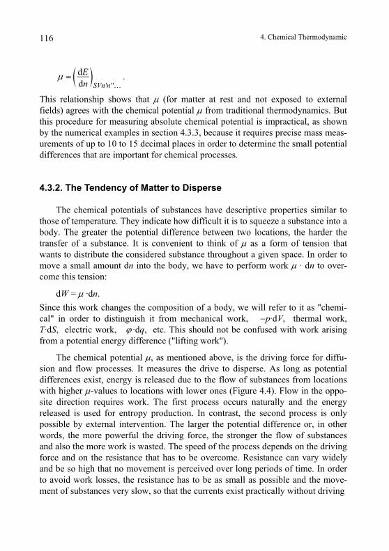
4. Chemical Thermodynamic 116
( )dd SVn'n''
En
µ =…
.
This relationship shows that µ (for matter at rest and not exposed to external fields) agrees with the chemical potential µ from traditional thermodynamics. But this procedure for measuring absolute chemical potential is impractical, as shown by the numerical examples in section 4.3.3, because it requires precise mass meas-urements of up to 10 to 15 decimal places in order to determine the small potential differences that are important for chemical processes.
4.3.2. The Tendency of Matter to Disperse
The chemical potentials of substances have descriptive properties similar to those of temperature. They indicate how difficult it is to squeeze a substance into a body. The greater the potential difference between two locations, the harder the transfer of a substance. It is convenient to think of µ as a form of tension that wants to distribute the considered substance throughout a given space. In order to move a small amount dn into the body, we have to perform work µ · dn to over-come this tension:
dW = µ ·dn. Since this work changes the composition of a body, we will refer to it as "chemi-cal" in order to distinguish it from mechanical work, −p·dV, thermal work, T·dS, electric work, ϕ ·dq, etc. This should not be confused with work arising from a potential energy difference ("lifting work").
The chemical potential µ, as mentioned above, is the driving force for diffu-sion and flow processes. It measures the drive to disperse. As long as potential differences exist, energy is released due to the flow of substances from locations with higher µ-values to locations with lower ones (Figure 4.4). Flow in the oppo-site direction requires work. The first process occurs naturally and the energy released is used for entropy production. In contrast, the second process is only possible by external intervention. The larger the potential difference or, in other words, the more powerful the driving force, the stronger the flow of substances and also the more work is wasted. The speed of the process depends on the driving force and on the resistance that has to be overcome. Resistance can vary widely and be so high that no movement is perceived over long periods of time. In order to avoid work losses, the resistance has to be as small as possible and the move-ment of substances very slow, so that the currents exist practically without driving
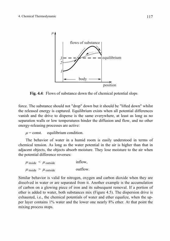
4. Chemical Thermodynamic 117
32
1
µ
positionbody
equilibrium
flows of substance
Fig. 4.4: Flows of substance down the of chemical potential slops
force. The substance should not "drop" down but it should be "lifted down" whilst the released energy is captured. Equilibrium exists when all potential differences vanish and the drive to disperse is the same everywhere, at least as long as no separation walls or low temperatures hinder the diffusion and flow, and no other energy-releasing processes are active:
µ = const. equilibrium condition.
The behavior of water in a humid room is easily understood in terms of chemical tension. As long as the water potential in the air is higher than that in adjacent objects, the objects absorb moisture. They lose moisture to the air when the potential difference reverses:
µ inside < µ outside inflow,
µ inside > µ outside outflow.
Similar behavior is valid for nitrogen, oxygen and carbon dioxide when they are dissolved in water or are separated from it. Another example is the accumulation of carbon on a glowing piece of iron and its subsequent removal. If a portion of ether is added to water, both substances mix (Figure 4.5). The dispersion drive is exhausted, i.e., the chemical potentials of water and ether equalize, when the up-per layer contains 1% water and the lower one nearly 8% ether. At that point the mixing process stops.
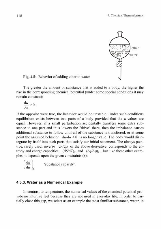
4. Chemical Thermodynamic 118
The greater the amount of substance that is added to a body, the higher the rise in the corresponding chemical potential (under some special conditions it may remain constant):
d 0dnµ ≥ .
If the opposite were true, the behavior would be unstable. Under such conditions equilibrium exists between two parts of a body provided that the µ-values are equal. However, if a small perturbation accidentally transfers some extra sub-stance to one part and thus lowers the "drive" there, then the imbalance causes additional substance to follow until all of the substance is transferred, or at some point the assumed behavior dµ/dn < 0 is no longer valid. The body would disin-tegrate by itself into such parts that satisfy our initial statement. The always posi-tive, rarely used, inverse dn/dµ of the above derivative, corresponds to the en-tropy and charge capacities, (dS/dT)x and (dq/dϕ)x. Just like these other exam-ples, it depends upon the given constraints (x):
dd x
nµ
⎛⎜⎝ ⎠
⎞⎟ "substance capacity".
4.3.3. Water as a Numerical Example
In contrast to temperature, the numerical values of the chemical potential pro-vide no intuitive feel because they are not used in everyday life. In order to par-tially close this gap, we select as an example the most familiar substance, water, in
Fig. 4.5: Behavior of adding ether to water
>1% ether
water<8%
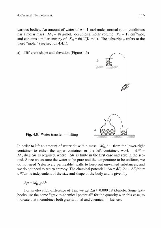
4. Chemical Thermodynamic 119
various bodies. An amount of water of n = 1 mol under normal room conditions has a molar mass Mm = 18 g/mol, occupies a molar volume Vm = 18 cm3/mol, and contains a molar entropy of Sm = 66 J/(K·mol). The subscript m refers to the word "molar" (see section 4.4.1).
a) Different shape and elevation (Figure 4.6)
h'
h
Fig. 4.6: Water transfer — lifting
In order to lift an amount of water dn with a mass Mm·dn from the lower-right container to either the upper container or the left container, work dW = Mm·dn·g·∆h is required, where ∆h is finite in the first case and zero in the sec-ond. Since we assume the water to be pure and the temperature to be uniform, we do not need "selectively permeable" walls to keep out unwanted substances, and we do not need to return entropy. The chemical potential ∆µ = dEII/dn − dEI/dn = dW/dn is independent of the size and shape of the body and is given by
∆µ = Mm·g·∆h.
For an elevation difference of 1 m, we get ∆µ ≈ 0.000 18 kJ/mole. Some text-books use the name "gravito-chemical potential" for the quantity µ in this case, to indicate that it combines both gravitational and chemical influences.
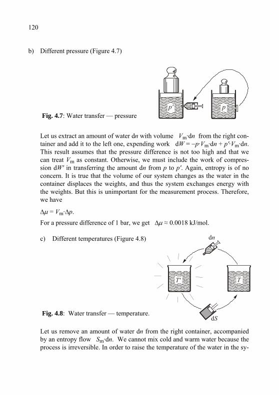
4. Chemical Thermodynamic 120
pp'
b) Different pressure (Figure 4.7)
Fig. 4.7: Water transfer — pressure
Let us extract an amount of water dn with volume Vm·dn from the right con-tainer and add it to the left one, expending work dW = −p·Vm·dn + p'·Vm·dn. This result assumes that the pressure difference is not too high and that we can treat Vm as constant. Otherwise, we must include the work of compres-sion dW' in transferring the amount dn from p to p'. Again, entropy is of no concern. It is true that the volume of our system changes as the water in the container displaces the weights, and thus the system exchanges energy with the weights. But this is unimportant for the measurement process. Therefore, we have
∆µ = Vm·∆p.
For a pressure difference of 1 bar, we get ∆µ ≈ 0.0018 kJ/mol.
c) Different temperatures (Figure 4.8)
Fig. 4.8: Water transfer — temperature.
dn
dS
T' T
Let us remove an amount of water dn from the right container, accompanied by an entropy flow Sm·dn. We cannot mix cold and warm water because the process is irreversible. In order to raise the temperature of the water in the sy-
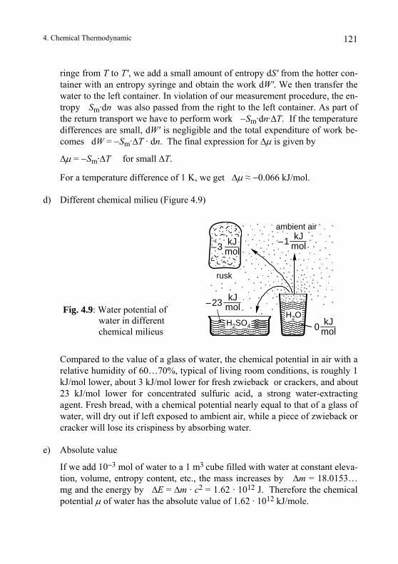
4. Chemical Thermodynamic 121
ringe from T to T', we add a small amount of entropy dS' from the hotter con-tainer with an entropy syringe and obtain the work dW'. We then transfer the water to the left container. In violation of our measurement procedure, the en-tropy Sm·dn was also passed from the right to the left container. As part of the return transport we have to perform work −Sm·dn·∆T. If the temperature differences are small, dW' is negligible and the total expenditure of work be-comes dW = −Sm·∆T · dn. The final expression for ∆µ is given by
∆µ = −Sm·∆T for small ∆T.
For a temperature difference of 1 K, we get ∆µ ≈ −0.066 kJ/mol.
d) Different chemical milieu (Figure 4.9)
kJmol–3
kJmol–1
kJmol–23
kJmol 0H SO2 4
H O2
ambient air
rusk
Fig. 4.9: Water potential of water in different chemical milieus
Compared to the value of a glass of water, the chemical potential in air with a relative humidity of 60…70%, typical of living room conditions, is roughly 1 kJ/mol lower, about 3 kJ/mol lower for fresh zwieback or crackers, and about 23 kJ/mol lower for concentrated sulfuric acid, a strong water-extracting agent. Fresh bread, with a chemical potential nearly equal to that of a glass of water, will dry out if left exposed to ambient air, while a piece of zwieback or cracker will lose its crispiness by absorbing water.
e) Absolute value
If we add 10−3 mol of water to a 1 m3 cube filled with water at constant eleva-tion, volume, entropy content, etc., the mass increases by ∆m = 18.0153… mg and the energy by ∆E = ∆m · c2 = 1.62 · 1012 J. Therefore the chemical potential µ of water has the absolute value of 1.62 · 1012 kJ/mole.
4. Chemical Thermodynamic 122
The result that cold water has a higher chemical potential than warm water, indicating a stronger tendency to disperse, seems to contradict our experience. We know that wet clothes dry out near the oven and water condenses on cold win-dowpanes. For those cases with a large temperature difference, a strong entropy flow dictates the flow of substances, and supplies sufficient energy to transfer substances against opposing potential drops.
4.4. Coupling of Substance Transfer to Other Processes
An object that receives substances increases its volume, energy and entropy content in most cases. However, it can also bend, distort, accept or reject another substance, change its state of charge and so on. The following sections present a description of such processes.
4.4.1. Volume and Entropy Demands of a Substance, "Molar Mass"
A gelatine cube, a wooden block and even a granite block swell when wet and shrink when dried. We can attribute these changes in volume to the space re-quirements of the water inside the respective bodies. If we add 1 cm3 of water to one liter of concentrated sulfuric acid and also to the same amount of half-concentrated sulfuric acid, then the volume increases by 0.48 cm3 in the first case and by 0.97 cm3 in the second. Evidently water does not always require the same space even when the temperature and pressure remain constant, so it becomes necessary to define this concept more precisely.
We will consider the volume required for a given amount of substance as the volume by which a body expands when the substance is added. For a more rigor-ous treatment, we will add only an incremental quantity dn in order to avoid sig-nificant changes to the composition of the body. The resulting volume increase dV can be computed for a convenient amount of substance, say a mole, as Vm = dV/dn. The quantity Vm is called the (partial) molar volume of the substance in the body. Let us now specify the conditions under which this procedure has to be performed. It is required that pressure, temperature, field strength, etc. remain constant in order to avoid errors due to thermal expansion, compressibility, elec-trostriction and similar effects. Simultaneously, no other substances can be intro-duced. Finally, we define
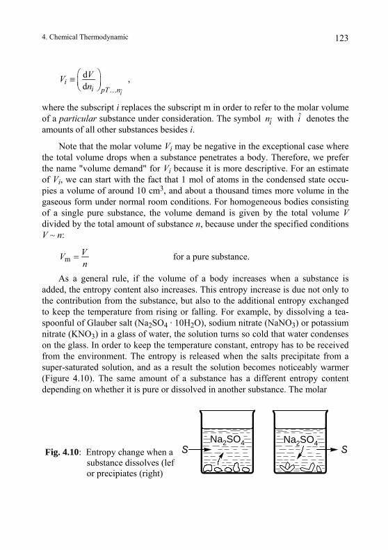
4. Chemical Thermodynamic 123
ˆ
dd
i
ii pT n
VVn
⎛ ⎞≡ ⎜ ⎟⎝ ⎠ …
in ˆ
,
where the subscript i replaces the subscript m in order to refer to the molar volume of a particular substance under consideration. The symbol with i denotes the amounts of all other substances besides i.
Note that the molar volume Vi may be negative in the exceptional case where the total volume drops when a substance penetrates a body. Therefore, we prefer the name "volume demand" for Vi because it is more descriptive. For an estimate of Vi, we can start with the fact that 1 mol of atoms in the condensed state occu-pies a volume of around 10 cm3, and about a thousand times more volume in the gaseous form under normal room conditions. For homogeneous bodies consisting of a single pure substance, the volume demand is given by the total volume V divided by the total amount of substance n, because under the specified conditions V ~ n:
mVVn
= for a pure substance.
As a general rule, if the volume of a body increases when a substance is added, the entropy content also increases. This entropy increase is due not only to the contribution from the substance, but also to the additional entropy exchanged to keep the temperature from rising or falling. For example, by dissolving a tea-spoonful of Glauber salt (Na2SO4 · 10H2O), sodium nitrate (NaNO3) or potassium nitrate (KNO3) in a glass of water, the solution turns so cold that water condenses on the glass. In order to keep the temperature constant, entropy has to be received from the environment. The entropy is released when the salts precipitate from a super-saturated solution, and as a result the solution becomes noticeably warmer (Figure 4.10). The same amount of a substance has a different entropy content depending on whether it is pure or dissolved in another substance. The molar
Fig. 4.10: Entropy change when a substance dissolves (left) or precipiates (right)
S SNa SO2 4 Na SO2 4
4. Chemical Thermodynamic 124
entropy of a pure substance Sm, or the (partial) molar entropy Si of a substance i, distributed in another substance, is defined in a similar fashion to Vm and Vi by the equation:
ˆ
dd
i
ii pT n
SSn
⎛ ⎞≡ ⎜ ⎟⎝ ⎠ …
For homogeneous bodies consisting of a single substance, Sm is computed simi-larly to Vm by dividing the total entropy S by the total amount of substance n:
mSSn
= for a pure substance.
It can be estimated from Vm and values of entropy density. If a substance is evapo-rated or mixed with other substances, then the entropy demand increases signifi-cantly.
Similarly we can describe the energy increase dE of a body due to the addi-tion of the incremental amount of substance dn, and define a (partial) molar en-ergy Ei of a substance in that body: Ei = ( )d d ˆ… ii pT n . This and a number of related quantities (partial molar enthalpy, free energy, free enthalpy, etc.) play an important role in traditional thermodynamics, but they are dispensable here. On the basis of EINSTEIN's equation m = E/c2, we can assign via Ei a (partial) molar mass to each substance (or more concisely, "molar mass") Mi = Ei/c2 =
E n
( ) …d d ipT nm ni . The relative changes of this quantity under different conditions are so small that Mm is considered constant for most applications. As such, we speak of the mass m = n · Mm of the amount n of a substance. If we know the elemental composition, i.e., the chemical formula of a substance, the molar mass can be calculated with sufficient accuracy by adding the Mi-values or "atomic weights" for the elements. Since masses can be easily and precisely determined from weight measurements, and the amounts of substance ni by dividing by the molar mass, this method tends to be used almost exclusively.
4.4.2. Main Equation and Coupling
If we change the volume, entropy or amount of substances in a body, then its energy content is modified by the mechanical, thermal and chemical work ex-pended in the process:
( ) 1 1 2 2d d d d d dk kE p V T S n n nµ µ µ= − + + + + +… .
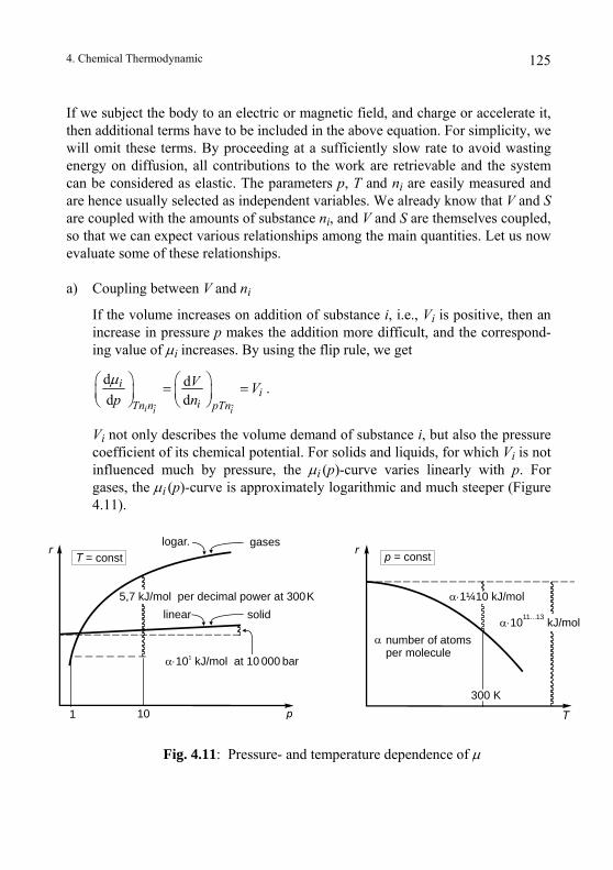
4. Chemical Thermodynamic 125
If we subject the body to an electric or magnetic field, and charge or accelerate it, then additional terms have to be included in the above equation. For simplicity, we will omit these terms. By proceeding at a sufficiently slow rate to avoid wasting energy on diffusion, all contributions to the work are retrievable and the system can be considered as elastic. The parameters p, T and ni are easily measured and are hence usually selected as independent variables. We already know that V and S are coupled with the amounts of substance ni, and V and S are themselves coupled, so that we can expect various relationships among the main quantities. Let us now evaluate some of these relationships.
a) Coupling between V and ni
If the volume increases on addition of substance i, i.e., Vi is positive, then an increase in pressure p makes the addition more difficult, and the correspond-ing value of µi increases. By using the flip rule, we get
ˆ ˆ
dd d
i i i
ii
iTn n pTn
V Vp n
⎛ ⎞⎛ ⎞ = =⎜ ⎟ ⎜ ⎟⎝ ⎠ ⎝ ⎠
dµ .
Vi not only describes the volume demand of substance i, but also the pressure coefficient of its chemical potential. For solids and liquids, for which Vi is not influenced much by pressure, the µi (p)-curve varies linearly with p. For gases, the µi (p)-curve is approximately logarithmic and much steeper (Figure 4.11).
1
T = const p = constr r
p T10300 K
number of atomsper molecule
α
α⋅10 kJ/mol at 10 000 bar1
α⋅1 0 kJ/mol¼1
α⋅10 kJ/mol11...13
5,7 kJ/mol per decimal power at 300K
gases
solid
logar.
linear
Fig. 4.11: Pressure- and temperature dependence of µ
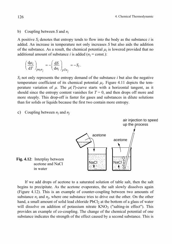
4. Chemical Thermodynamic 126
b) Coupling between S and ni
A positive Si denotes that entropy tends to flow into the body as the substance i is added. An increase in temperature not only increases S but also aids the addition of the substance. As a result, the chemical potential µi is lowered provided that no additional amount of substance i is added (ni = const.):
ˆ ˆ
d dd d
i i
ii
n i pTn
S ST nµ ⎛ ⎞⎛ ⎞ = − = −⎜ ⎟ ⎜ ⎟⎝ ⎠ ⎝ ⎠
. ipn
Si not only represents the entropy demand of the substance i but also the negative temperature coefficient of its chemical potential µi. Figure 4.11 depicts the tem-perature variation of µ. The µ( T)-curve starts with a horizontal tangent, as it should since the entropy content vanishes for T = 0, and then drops off more and more steeply. This drop-off is faster for gases and substances in dilute solutions than for solids or liquids because the first two contain more entropy.
c) Coupling between ni and nj
acetoneacetone
NaCl
up the process
NaCl
air injection to speed
Fig. 4.12: Interplay between acetone and NaCl in water
If we add drops of acetone to a saturated solution of table salt, then the salt begins to precipitate. As the acetone evaporates, the salt slowly dissolves again (Figure 4.12). This is an example of counter-coupling between two amounts of substance ni and nj, where one substance tries to drive out the other. On the other hand, a small amount of solid lead chloride PbCl2 at the bottom of a glass of water will dissolve on addition of potassium nitrate KNO3 ("salting-in effect"). This provides an example of co-coupling. The change of the chemical potential of one substance indicates the strength of the effect caused by a second substance. This is
4. Chemical Thermodynamic 127
( )d dexpressed more precisely by the coefficient ji j pT n . Due to the symme-
try of the coupling, the reverse effect of the second substance on the first, meas-ured by the coefficient
nµ
( ) ˆd dij i pT nnµ , is equally strong, as can be shown with
the flip rule:
ˆˆ
ddd d
ij
ji
j i pT npT nn nµµ⎛ ⎞ ⎛ ⎞
=⎜ ⎟ ⎜ ⎟⎝ ⎠⎝ ⎠
( )0 0
0 0 m m, d dp T
p Tp T V p S Tµ µ= + −∫ ∫
.
Qualitatively it is easy to demonstrate the inverse effect with our first example: By adding table salt to an acetone-water mixture with a 1:1 ratio, the acetone sepa-rates into a second layer above the solution ("salting-out effect").
For a substance that exists in pure form in a homogeneous body, it is possible to evaluate µ as a function of p and T compared to a reference value µ(p0, T0) since Vm and Sm can be measured readily:
.
Sometimes it is easier to investigate a simpler piece of matter that is in chemical equilibrium with the body in question, since both substances have the same chemical potential. For example, we can determine the potential of water in a cane sugar solution by evaluating the potential of the pure water vapor above the solution when isolated from the outside air. Its µ -value can be computed as that of a pure substance using the above equation.
4.5. Transformations of Substances
This section deals with the laws that govern the chemical conversions and transformations of different forms of substances.
4.5.1. Conditions for Chemical Conversion
So far we have ignored the fact that a substance penetrating a body may be changed chemically, either destroyed or produced. If a small amount of substance dn disappears in the process, its potential energy µ ·dn is released, provided that
4. Chemical Thermodynamic 128
it is not captured by the reaction products. Since this energy may be used to pro-duce entropy and cannot be recovered, the chemical potential µ in a way forces the substance to destroy or transform itself. The quantity µ therefore assumes a new meaning as a "self-destructive drive ". Without conservation of matter this drive would destroy the substance into nothing, or rather, radiate it away. Instead, the destruction of one substance leads to the formation of another. During chemical conversions, excluding element changes, the amounts of the participating elements must remain unchanged. In a chemical equation this requirement is met by ensur-ing that the total number of atoms of each kind is equal on both sides.
According to this idea the conversion A → B should only take place spon-taneously if the "destructive" or "transforming" drive µA of the reactant is greater than that of the product µ B. In other words, µA > µ B. Several substances may be involved in the reaction,
A + B → 2 C or more generally νA A + νB B + νC C … = 0 .
The above notation includes "stoichiometric coefficients" νi which are negative for the reactants and positive for the products (νA = –1, ν B = –1, νC = +2). Since the total "destructive drive" of the vanished substance must be greater than that of the newly formed ones, we impose the following requirement:
µA + µ B > µ C + µ C or more generally νAµ A + νBµ B + … < 0 .
In the opposite case, the drive of the reaction is reversed. Since chemical poten-tials vary with pressure, temperature, composition, etc., it is likely that the same chemical reaction can run in either direction depending on these conditions.
In order to confirm our assumption, let us consider what happens with the en-ergy. The p gress of a reaction is usually described by a variable ξ called "extent of reaction" hat is explained by the equation
∆ni = ν ,
where ∆ni is the change of the amount of the substance i. If νi is negative, ∆ni indicates a loss of the substance i. We can denote the common expression "unit conversion" more precisely by ξ = 1 mol. In our example, 1 mol of A and B each are used up to create 2 mol of C. If the reaction progresses by the small amount dξ and the components change by dn i = νi dξ, then the potential energy µA·dξ + µ B·dξ is released during the destruction of the reactants. Simultane-ously, energy 2µ C·dξ has to be supplied for the newly created products. The total expenditure of work or "chemical work" is therefore given by
ro t
iξ
4. Chemical Thermodynamic 129
)
m A B C ... f A B C ...BA Ca b c a b cW a b cµ µ µ µ µ= − − − − ≡ ∆…
i
dW = (−µA − µ B + 2µ C) dξ or more generally dW = (ν1µ1 + ν2µ2 + …) dξ.
The reaction can only run by itself (dξ > 0) if energy is released, or in other words dW is negative. The expression in parentheses in the equation above must be nega-tive, as we suspected earlier. This difference of the "chemical potentials of prod-ucts minus reactants", −µA − µ B + 2µ C or ∑νi ·µ i , is usually abbreviated by the symbol ∆Rµ where the general R (R for reaction) can be replaced with other symbols for a particular reaction. The term −∆Rµ represents the forward drive or so-called "affinity" A = −∆R µ of a reaction, while +∆R µ is the reverse drive. The conversion conditions can now be simply expressed as
∆R µ < 0 reaction driven forwards,
∆R µ = 0 equilibrium, (∆R µ ≡ ∑νi·µi)
∆R µ > 0 reaction driven backwards.
In order to describe the dispersion of a substance D, we can arbitrarily fix the zero point for its chemical potential since only the difference ∆µ D is important for the spread of D. That is convenient for many calculations. As soon as we in-clude chemical conversions, however, we only have this freedom for the elements. All other substances consist of combinations of the elements:
aA + bB + cC + … → Aa Bb Cc … .
During the formation (indicated by f) of a compound AaBbCc… from its ele-ments, which exist in some (well defined) standard state ( , the following work is expended for each mole produced:
By using the chemical potential µm f ,
of the elements in their standard states and measuring W µ= ∆ A B C ... a bµ µ µ µ= ∆ + + +…
…a bµ µ⋅ + ⋅ +-
the quantity BAa b c a b c becomes fixed and can no longer be freely chosen. Conversely, because the terms
BA drop out during affinity calculations, we are free to do what we want with the
f A B C ...
µ
-
values. The chemical potential of a pure substance at 1.013 bar pressure and 298 K temperature, compared to that of its elements in pure, stable form under the same pressure and temperature, is tabulated for many sub-stances (standard free enthalpies of formation). By setting the µ
f A B C ...
values of the elements to zero, we can identify the quantity a b cµ∆
A B C ...
for any compound using the chemical potential a b cµ of this compound, which simplifies the notation and evaluations. This possibility is removed if we allow changes to the
4. Chemical Thermodynamic 130
elements themselves (i.e., nuclear reactions) because differences in chemical po-tentials between them would become important.
4.5.2. Coupling of V, S and ξ
Let us now consider a homogeneous or non-homogeneous body consisting of various substances Ai. This body can be compressed and heated and has the reac-tion ∑ νi Ai = 0 running internally. The effect of such a chemical reaction is identical to that of an exchange of substance with the environment, except that the quantities ni are no longer independent, but are related by the extent of reaction ξ: dni = νi · dξ. As a result of this relation and R µ∆ = −A , the main equation has the form
dE = −pdV + TdS + ∑ µ i dni = (−p)dV + TdS + (−A)dξ .
On the basis of the above relation we can consider S, V and ξ as elastically coupled. We are already familiar with some of the possible primary and coupling effect indicators such as (dS/dT)pξ representing the entropy capacity Ç. The index ξ merely indicates that the substances of the body will not change. Other coefficients such as (dV/dξ)pT and (dS/dξ)pT that describe the change in vol-ume and entropy content during the reaction can easily be calculated. Applying the chain rule to the function V(p, T, n1(ξ), n2(ξ)… ) and its counterpart for S, we get:
ˆ ˆ1 2
1 21 1 2 2
1 2
d dd d dd d d d dpT pTn pTn
n nV V V V Vn n
ν νξ ξ ξ
⎛ ⎞ ⎛ ⎞⎛ ⎞ = + + = + +⎜ ⎟ ⎜ ⎟ ⎜ ⎟⎝ ⎠ ⎝ ⎠ ⎝ ⎠
… … .
The result can be summarized as follows:
R m R md d,d di i i i
pT pT
V SV V S Sν νξ ξ
⎛ ⎞ ⎛ ⎞= ≡ ∆ = ≡ ∆⎜ ⎟ ⎜ ⎟⎝ ⎠ ⎝ ⎠
∑ ∑ .
Here, the symbol ∆R is again used to simplify the notation. By further application of the flip rule, we get:
R m R m dd d d;
d d d dppT pTT
V SV Sp T ξξ ξ ξ
⎛ ⎞ ⎛ ⎞ ⎛ ⎞⎛ ⎞= − = −∆ = = ∆⎜ ⎟⎜ ⎟ ⎜ ⎟⎜ ⎟ ⎝ ⎠⎝ ⎠ ⎝ ⎠⎝ ⎠
AA .
These equations tell us what we could have predicted on the basis of the concept of coupling: If the reaction increases the volume (∆RVm > 0), then the reaction
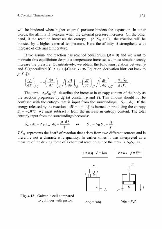
4. Chemical Thermodynamic 131
will be hindered when higher external pressure hinders the expansion. In other words, the affinity A weakens when the external pressure increases. On the other hand, if the reaction increases the entropy (∆RSm > 0), the reaction will be boosted by a higher external temperature. Here the affinity A strengthens with increase of external temperature.
If we assume the reaction has reached equilibrium (A = 0) and we want to maintain this equilibrium despite a temperature increase, we must simultaneously increase the pressure. Quantitatively, we obtain the following relation between p and T (generalized [CLAUSIUS]-CLAPEYRON Equation, derivation hint: cut back to p, T, ξ):
R m
R m
d d d d dd d d dd p pT pTT
p SS VT pT Vξξ ξ ξ ξ
∆⎛ ⎞ ⎛ ⎞ ⎛ ⎞⎛ ⎞ ⎛ ⎞= − = =⎜ ⎟⎜ ⎟ ⎜ ⎟ ⎜ ⎟⎜ ⎟⎝ ⎠ ∆⎝ ⎠ ⎝ ⎠ ⎝ ⎠⎝ ⎠A
A A .
The term ∆RSm·dξ describes the increase in entropy content of the body as the reaction progresses by dξ (at constant p and T). This amount should not be confused with the entropy that is input from the surroundings Śm · dξ. If the energy released by the reaction dW = −A · dξ is burned up producing the entropy Sp = −dW/T we must subtract it from the increase in entropy content. The total entropy input from the surroundings becomes:
m R mdd dŚ S
Tξξ ξ ⋅⋅ = ∆ ⋅ − A
m R mŚ ST
= ∆ − A or .
T·Śm represents the heat of reaction that arises from two different sources and is therefore not a characteristic quantity. In earlier times it was interpreted as a measure of the driving force of a chemical reaction. Since the term T·∆RSm is
A
A U qd dξ =
p
F
l
V p = Fd d l
V
U
q
V p F = = /α⋅ αlξ α⋅ α = = /q A U
Fig. 4.13: Galvanic cell compared to cylinder with piston
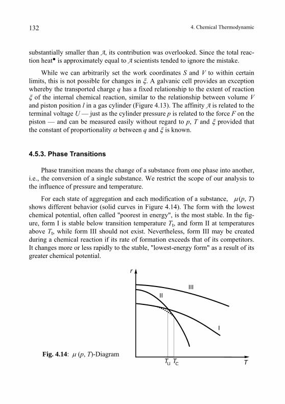
4. Chemical Thermodynamic 132
substantially smaller than A, its contribution was overlooked. Since the total reac-tion heat is approximately equal to A scientists tended to ignore the mistake.
While we can arbitrarily set the work coordinates S and V to within certain limits, this is not possible for changes in ξ. A galvanic cell provides an exception whereby the transported charge q has a fixed relationship to the extent of reaction ξ of the internal chemical reaction, similar to the relationship between volume V and piston position l in a gas cylinder (Figure 4.13). The affinity A is related to the terminal voltage U — just as the cylinder pressure p is related to the force F on the piston — and can be measured easily without regard to p, T and ξ provided that the constant of proportionality α between q and ξ is known.
4.5.3. Phase Transitions
Phase transition means the change of a substance from one phase into another, i.e., the conversion of a single substance. We restrict the scope of our analysis to the influence of pressure and temperature.
For each state of aggregation and each modification of a substance, µ(p, T) shows different behavior (solid curves in Figure 4.14). The form with the lowest chemical potential, often called "poorest in energy", is the most stable. In the fig-ure, form I is stable below transition temperature Tt, and form II at temperatures above Tt, while form III should not exist. Nevertheless, form III may be created during a chemical reaction if its rate of formation exceeds that of its competitors. It changes more or less rapidly to the stable, "lowest-energy form" as a result of its greater chemical potential.
TU TC
IIIII
I
r
TFig. 4.14: µ (p, T)-Diagram
friedrichherrmann
Bleistift
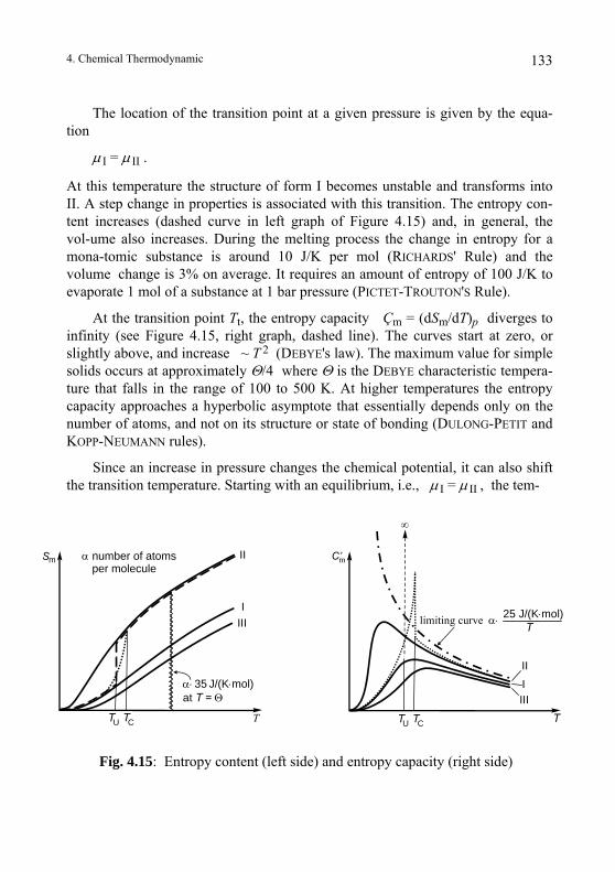
4. Chemical Thermodynamic 133
The location of the transition point at a given pressure is given by the equa-tion
µ I = µ II .
At this temperature the structure of form I becomes unstable and transforms into II. A step change in properties is associated with this transition. The entropy con-tent increases (dashed curve in left graph of Figure 4.15) and, in general, the vol-ume also increases. During the melting process the change in entropy for a mona-tomic substance is around 10 J/K per mol (RICHARDS' Rule) and the volume change is 3% on average. It requires an amount of entropy of 100 J/K to evaporate 1 mol of a substance at 1 bar pressure (PICTET-TROUTON'S Rule).
At the transition point Tt, the entropy capacity Çm = (dSm/dT)p diverges to infinity (see Figure 4.15, right graph, dashed line). The curves start at zero, or slightly above, and increase ~ T 2 (DEBYE's law). The maximum value for simple solids occurs at approximately Θ/4 where Θ is the DEBYE characteristic tempera-ture that falls in the range of 100 to 500 K. At higher temperatures the entropy capacity approaches a hyperbolic asymptote that essentially depends only on the number of atoms, and not on its structure or state of bonding (DULONG-PETIT and KOPP-NEUMANN rules).
Since an increase in pressure changes the chemical potential, it can also shift the transition temperature. Starting with an equilibrium, i.e., µ I = µ II , the tem-
- ∞
C’
T T
mII
II
I
I
III
III
T
number of atomsαper molecule
TU TC TU TC
Sm
α⋅ ⋅Θ
35 J/(K mol)at
T =
limiting curve α⋅ 25 J/(K mol)⋅
Fig. 4.15: Entropy content (left side) and entropy capacity (right side)
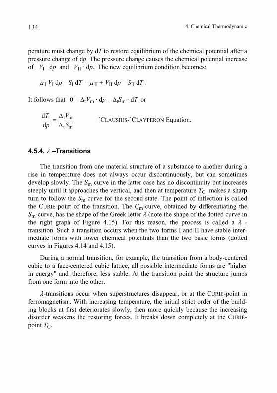
4. Chemical Thermodynamic 134
perature must change by dT to restore equilibrium of the chemical potential after a pressure change of dp. The pressure change causes the chemical potential increase of VI · dp and VII · dp. The new equilibrium condition becomes:
µ I VI dp – SI dT = µ II + VII dp − SII dT .
It follows that 0 = ∆tVm · dp − ∆tSm · dT or
t t m
t m
ddT Vp S
∆=
∆ [CLAUSIUS-]CLAYPERON Equation.
4.5.4. λ –Transitions
The transition from one material structure of a substance to another during a rise in temperature does not always occur discontinuously, but can sometimes develop slowly. The Sm-curve in the latter case has no discontinuity but increases steeply until it approaches the vertical, and then at temperature TC makes a sharp turn to follow the Sm-curve for the second state. The point of inflection is called the CURIE-point of the transition. The Çm-curve, obtained by differentiating the Sm-curve, has the shape of the Greek letter λ (note the shape of the dotted curve in the right graph of Figure 4.15). For this reason, the process is called a λ -transition. Such a transition occurs when the two forms I and II have stable inter-mediate forms with lower chemical potentials than the two basic forms (dotted curves in Figures 4.14 and 4.15).
During a normal transition, for example, the transition from a body-centered cubic to a face-centered cubic lattice, all possible intermediate forms are "higher in energy" and, therefore, less stable. At the transition point the structure jumps from one form into the other.
λ-transitions occur when superstructures disappear, or at the CURIE-point in ferromagnetism. With increasing temperature, the initial strict order of the build-ing blocks at first deteriorates slowly, then more quickly because the increasing disorder weakens the restoring forces. It breaks down completely at the CURIE-point TC.
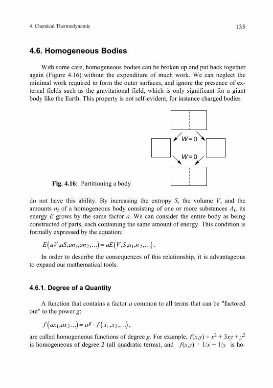
4. Chemical Thermodynamic 135
4.6. Homogeneous Bodies
With some care, homogeneous bodies can be broken up and put back together again (Figure 4.16) without the expenditure of much work. We can neglect the minimal work required to form the outer surfaces, and ignore the presence of ex-ternal fields such as the gravitational field, which is only significant for a giant body like the Earth. This property is not self-evident, for instance charged bodies
W = 0
W = 0
Fig. 4.16: Partitioning a body
do not have this ability. By increasing the entropy S, the volume V, and the amounts ni of a homogeneous body consisting of one or more substances Ai, its energy E grows by the same factor a. We can consider the entire body as being constructed of parts, each containing the same amount of energy. This condition is formally expressed by the equation:
( ) ( )1 2 1 2, , , ,… , , , ,…S an an aE V S n n=
( )
E aV a .
In order to describe the consequences of this relationship, it is advantageous to expand our mathematical tools.
4.6.1. Degree of a Quantity
A function that contains a factor a common to all terms that can be "factored out" to the power g:
( )1 2 1 2, … , ,…gf ax ax a f x x= ⋅ ,
are called homogeneous functions of degree g. For example, f(x,y) = x2 + 3xy + y2 is homogeneous of degree 2 (all quadratic terms), and f(x,y) = 1/x + 1/y is ho-
4. Chemical Thermodynamic 136
mogeneous of degree −1 (because 1/ax + 1/ay = a−1(1/x + 1/y)). The energy function from the last section is linearly homogeneous (g = 1).
Consider an elastic system with work coordinates x1, x2, … xn and a set of variables y, z ... that depend on xi. Although the following discussion deals with purely mathematical relationships, we will use physical terminology in order to make it easier for the mathematical novice to understand later applications. If we assume that for the quantity y = f (x1, … xn) the function f is homogeneous of degree g, then we will say that y itself has degree g. Since each xi increases by the factor a if multiplied by a, we have g =1 for xi.
In addition to x1, … xn it is useful to introduce the quantities z1, … zn having the degrees g1, … gn as independent variables. An arbitrary variable y = h(x1, … xn) of degree g can be written in the form y = F(z1, … zn) where F need not be a homogeneous function. But this function F satisfies the following equation:
( )1 ,…, ng g ( )1 1,…,gn nF a z a z a F z z= ⋅
( ) ( ) ( )( )
( ) ( ) ( )
1 1 1 1 1
1 1 1
… … ,…, …
… … … .
ng g n n n ng gn n n
. (+)
In order to prove this relation (if one is not interested in the proofs, skip the indented sections below) we express zi in terms of xi and consider the fact that the functions fi and h are homogeneous:
F a z a z F f ax ax f ax ax
h ax ax a h x x a F z z
=
= = ⋅ = ⋅
The degree of a quantity composed of several others can be determined im-mediately with rules similar to those of exponents. If u, v and w have degree s, s and t, then u + v, u · w and u/w have degree s, s + t and s − t, respectively. Constants have the degree 0 and the derivative ( )
ˆd d
ii zy z has the degree of the
ratio y/zi .
In order to prove the last statement about (iz , we take the derivative
of the above equation (+) with respect to zi and simultaneously divide both sides by
)d d iy z
iga . By using the shorthand notation Fi for ( , we get )ˆ
d di
i zF z
( ) ( )1 1 … n ig g g gi n i na z a F z z−= ⋅1 … F a z .
Finally, on replacing zi by fi(x1 … xn), we find that Fi has the degree g − gi as claimed.
Applied to our homogeneous body, this means that in addition to E, other quantities such as V, S, ni, m, etc., are "proportional to the size of a section of this
4. Chemical Thermodynamic 137
body" and are of degree 1. On the other hand, the forces derived from work coor-dinates ( )
ˆd d
ii i xy E x= have degree 0, and are "independent of the size of a
section". The last statement is most important, since it means that pressure, temperature
and chemical potential depend only on the relationship V : S : n1 : n2 :… Even if the section of the body under consideration is reduced almost to a point, and the composition (including entropy) of the surroundings of the section are changed arbitrarily, the values of p, T and µi in that section remain fixed as long as the relationship V : S : n1 : n2 :… is preserved there. In contrast, the electric potential exhibits completely different behavior, since its value is not determined only by local conditions but is also influenced by distant charges.
Therefore it seems reasonable to ignore the shape and size of a body and to introduce measures of the local composition (including entropy) of a body, and to express p, T and µi as functions of these variables. It is common to relate V, S, ni of a small section, as well as E and other parameters (all of degree 1) to the vol-ume or total amount of all substances n = ∑ ni of this section. In the first case, relating to the volume V, we obtain the entropy density cS , the energy density cE ,… and the concentrations ("substance densities") ci of the individual sub-stances. In the second case, relating to the total amount of all substances n, we get the average (molar) volume V , the average (molar) entropy S , ... and the mole fractions xi of the substances:
( )1 , , …, ;
, , …, .
iS i
ii
nV S c cV V V
nV SV S xn n n
≡ ≡ ≡
≡ ≡ ≡
All these quantities are of degree 0. Since the sum of all xi must be 1, they cannot be selected arbitrarily. The number of independent variables is therefore decreased by one in both cases.
4.6.2. "Dissection" of a Quantity
A variable y = F(z1 … zn) of degree g can be decomposed into separate terms in a distinct way, depending on the chosen set of independent variables:
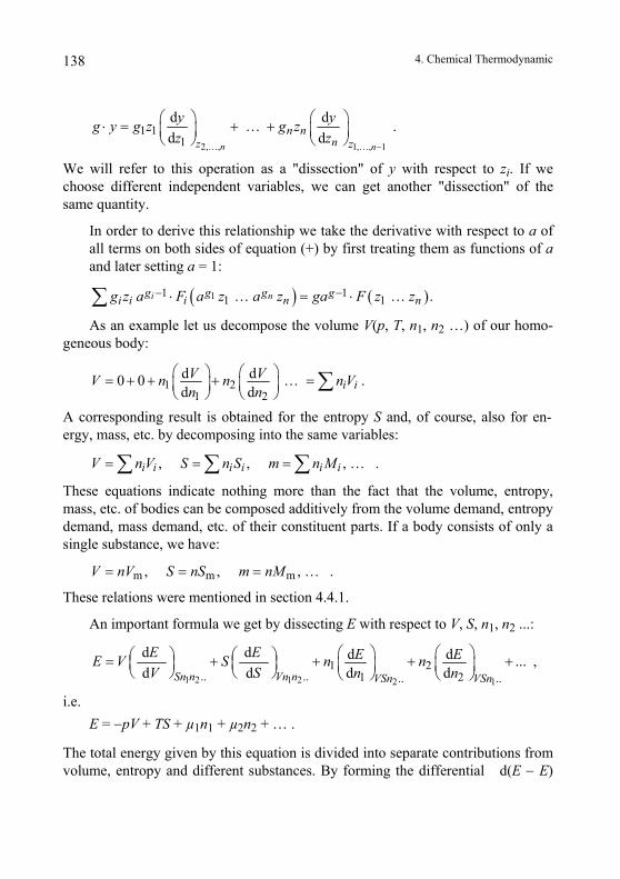
4. Chemical Thermodynamic 138
2,…, 1,…, 1
1 11
d d … d d
n n
n nnz z
y yg y g z g zz z
−
⎛ ⎞⎛ ⎞⋅ = + +⎜ ⎟ ⎜ ⎟⎝ ⎠ ⎝ ⎠
.
We will refer to this operation as a "dissection" of y with respect to zi. If we choose different independent variables, we can get another "dissection" of the same quantity.
In order to derive this relationship we take the derivative with respect to a of all terms on both sides of equation (+) by first treating them as functions of a and later setting a = 1:
( ) ( )11 11 1… … .i ng g g gi i i n ng z a F a z a z ga F z z− −⋅ = ⋅∑As an example let us decompose the volume V(p, T, n1, n2 …) of our homo-
geneous body:
1 21 2
d d0 0 …d d i i
V VV n n n Vn n
⎛ ⎞ ⎛ ⎞= + + + =⎜ ⎟ ⎜ ⎟⎝ ⎠ ⎝ ⎠
∑ .
A corresponding result is obtained for the entropy S and, of course, also for en-ergy, mass, etc. by decomposing into the same variables:
, , , … .i i i i i iV n V S n S m n M= = =∑ ∑ ∑
m m m, , , … .V nV S nS m nM= = =
These equations indicate nothing more than the fact that the volume, entropy, mass, etc. of bodies can be composed additively from the volume demand, entropy demand, mass demand, etc. of their constituent parts. If a body consists of only a single substance, we have:
These relations were mentioned in section 4.4.1.
An important formula we get by dissecting E with respect to V, S, n1, n2 ...:
1 2 1 2 2 11 2
.. .. 1 2.. ..
d d d d ... ,d d d dSn n Vn n VSn VSn
E E E EE V S n nV S n n
⎛ ⎞ ⎛ ⎞⎛ ⎞ ⎛ ⎞= + + + +⎜ ⎟ ⎜ ⎟ ⎜ ⎟ ⎜ ⎟⎝ ⎠ ⎝ ⎠ ⎝ ⎠ ⎝ ⎠
i.e. E = −pV + TS + µ1n1 + µ2n2 + … .
The total energy given by this equation is divided into separate contributions from volume, entropy and different substances. By forming the differential d(E − E)
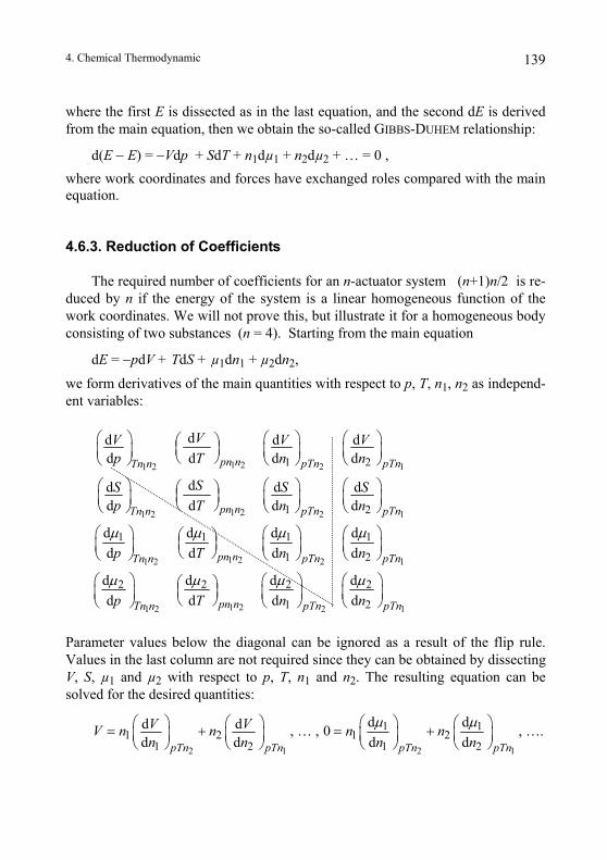
4. Chemical Thermodynamic 139
where the first E is dissected as in the last equation, and the second dE is derived from the main equation, then we obtain the so-called GIBBS-DUHEM relationship:
d(E − E) = −Vdp + SdT + n1dµ1 + n2dµ2 + … = 0 , where work coordinates and forces have exchanged roles compared with the main equation.
4.6.3. Reduction of Coefficients
The required number of coefficients for an n-actuator system (n+1)n/2 is re-duced by n if the energy of the system is a linear homogeneous function of the work coordinates. We will not prove this, but illustrate it for a homogeneous body consisting of two substances (n = 4). Starting from the main equation
dE = −pdV + TdS + µ1dn1 + µ2dn2,
we form derivatives of the main quantities with respect to p, T, n1, n2 as independ-ent variables:
dd d d1 2 2 11 2
1 2 2 11 2
1 2 2 11 2
1
1 2
1 2
1 1 1 1
1 2
2
d d d d
dd d dd d d d
d d d dd d d d
dd
pn n pTn pTnTn n
pn n pTn pTnTn n
pn n pTn pTnTn n
Tn
p T n n
SS S Sp T n n
p T n n
p
µ µ µ µ
µ
⎜ ⎟ ⎜ ⎟ ⎜ ⎟⎜ ⎟ ⎝ ⎠ ⎝ ⎠ ⎝ ⎠⎝ ⎠
⎛ ⎞ ⎛ ⎞ ⎛ ⎞⎛ ⎞⎜ ⎟ ⎜ ⎟ ⎜ ⎟⎜ ⎟ ⎝ ⎠ ⎝ ⎠ ⎝ ⎠⎝ ⎠
⎛ ⎞ ⎛ ⎞ ⎛ ⎞⎛ ⎞⎜ ⎟ ⎜ ⎟ ⎜ ⎟⎜ ⎟ ⎝ ⎠ ⎝ ⎠ ⎝ ⎠⎝ ⎠
⎛ ⎞⎜ ⎟⎝ ⎠
VV V V⎛ ⎞ ⎛ ⎞ ⎛ ⎞⎛ ⎞
1 2 2 12
2 2 2
1 2
d d dd d dpn n pTn pTnn T n nµ µ µ⎛ ⎞ ⎛ ⎞⎛ ⎞
⎜ ⎟ ⎜ ⎟ ⎜ ⎟⎝ ⎠ ⎝ ⎠ ⎝ ⎠
Parameter values below the diagonal can be ignored as a result of the flip rule. Values in the last column are not required since they can be obtained by dissecting V, S, µ1 and µ2 with respect to p, T, n1 and n2. The resulting equation can be solved for the desired quantities:
2 1 2 1
1 11 2 1 2
1 2 1 2
d dd d , … , 0 , …d d d dpTn pTn pTn pTn
V VV n n n nn n n n
µ µ⎛ ⎞ ⎛ ⎞ ⎛ ⎞ ⎛ ⎞= + = +⎜ ⎟ ⎜ ⎟ ⎜ ⎟ ⎜ ⎟⎝ ⎠ ⎝ ⎠ ⎝ ⎠ ⎝ ⎠
.
4. Chemical Thermodynamic 140
4.7. Asymptotic Laws for Substances at High Dilution
If all entropy is removed from a body, its temperature T becomes 0. What happens to the chemical potential of a substance if the amount of substance in the body becomes increasingly smaller? It will be shown that changes of the chemical potential are independent of the chosen substance and even independent of the body it is distributed in. It can be described by a general law that can be used for the analysis of dilute gases and solutions.
4.7.1. Chemical Potential at Low Concentration
We know that the chemical potential decreases as the amount of substance distributed in a body is reduced. Initially this drop in chemical potential is irregu-lar but approaches a regular trend with decreasing concentration. If n is reduced by a power of ten, µ drops by a constant amount regardless of the substance under consideration (Figure 4.17). On a logarithmic scale for n the µ(n) curves approach parallel straight lines, their asymptotes, for larger n. The slope of these lines is directly proportional to temperature, while the intersection point with the µ-axis is influenced by the composition and condition (p, T, etc.) of the body, as well as by the kind of substance distributed in the body. In general, we can describe chemical potentials by:
00
ln nRTn
µ µ= + ⋅ .
Here n0 is an arbitrary reference point and R is a universal constant, characteristic for the behavior of diluted substances with value
R = 8.314 J/(K·mol). Although the parameter µ0 depends on n, it always remains finite for "finite" sys-tems. "Finite" means the volume does not vanish, and neither the volume nor any amount of substance in the body becomes arbitrarily large.
As a special case of the above we can state that µ → −∞ as n → 0 for T > 0. This asymptotic rule reminds us of the behavior of entropy as the absolute zero of temperature is approached (see section 2.4). Similar exceptions also apply here. If a substance cannot diffuse within a body, it cannot be extracted from a body, and we can say it is "trapped in" even if the chemical potential outside drops to an arbitrary low value. The internal chemical potential cannot be obtained by meas-urement — just like temperature in the case of trapped entropy.
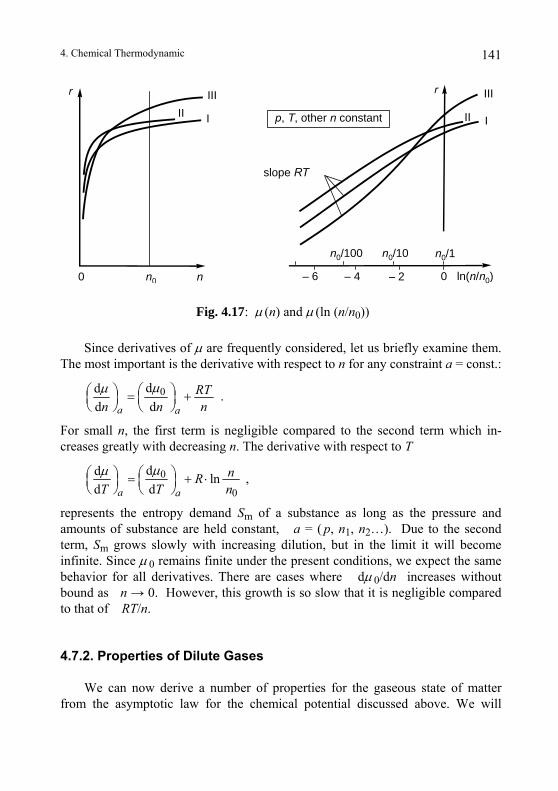
4. Chemical Thermodynamic 141
r
n
II III I
III III
n00 – 6 – 4 – 2 0
p T n , , other constant
slope RT
r
ln( /n n0
n0/1n0/10n0/100
)
Fig. 4.17: µ (n) and µ (ln (n/n0))
Since derivatives of µ are frequently considered, let us briefly examine them. The most important is the derivative with respect to n for any constraint a = const.:
0ddd da a
RTn n n
µµ ⎛ ⎞⎛ ⎞ = +⎜ ⎟ ⎜ ⎟⎝ ⎠ ⎝ ⎠ .
For small n, the first term is negligible compared to the second term which in-creases greatly with decreasing n. The derivative with respect to T
0
0
dd lnd da a
nRT T n
µµ ⎛ ⎞⎛ ⎞ = + ⋅⎜ ⎟ ⎜ ⎟⎝ ⎠ ⎝ ⎠ ,
represents the entropy demand Sm of a substance as long as the pressure and amounts of substance are held constant, a = ( p, n1, n2…). Due to the second term, Sm grows slowly with increasing dilution, but in the limit it will become infinite. Since µ 0 remains finite under the present conditions, we expect the same behavior for all derivatives. There are cases where dµ 0/dn increases without bound as n → 0. However, this growth is so slow that it is negligible compared to that of RT/n.
4.7.2. Properties of Dilute Gases
We can now derive a number of properties for the gaseous state of matter from the asymptotic law for the chemical potential discussed above. We will
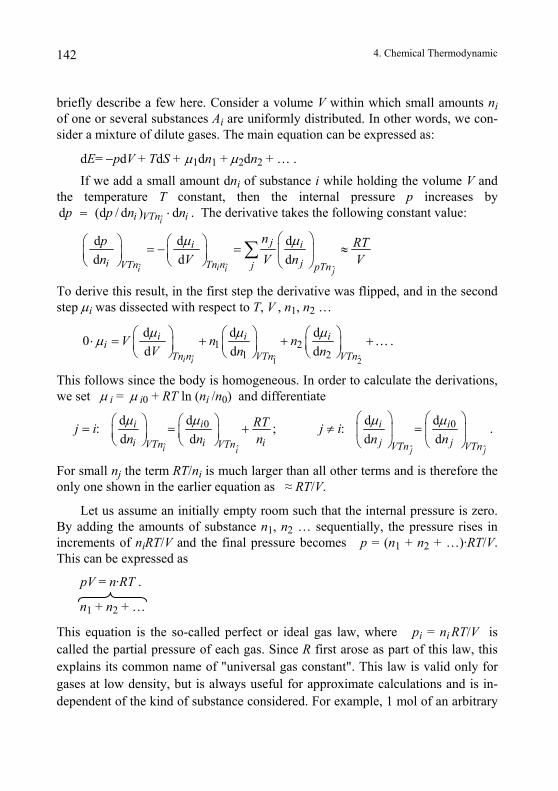
4. Chemical Thermodynamic 142
briefly describe a few here. Consider a volume V within which small amounts ni of one or several substances Ai are uniformly distributed. In other words, we con-sider a mixture of dilute gases. The main equation can be expressed as:
dE= −pdV + TdS + µ1dn1 + µ2dn2 + … .
If we add a small amount dni of substance i while holding the volume V and the temperature T constant, then the internal pressure p increases by
. The derivative takes the following constant value: ˆd (d / d ) dii VTn ip p n n= ⋅
ˆˆ ˆ
d d dd d d
i ii j
ji i
i jTn nVTn j pTn
np RTn V V n V
µ µ⎛ ⎞⎛ ⎞ ⎛ ⎞= − = ≈⎜ ⎟⎜ ⎟⎜ ⎟ ⎝ ⎠⎝ ⎠ ⎝ ⎠∑
To derive this result, in the first step the derivative was flipped, and in the second step µi was dissected with respect to T, V , n1, n2 …
ˆ ˆ ˆ1 2
1 21 2
d d d0 d d d
i i
i i ii
Tn n VTn VTnV n n
V n nµ µ µµ ⎛ ⎞ ⎛ ⎞ ⎛ ⎞⋅ = + + +⎜ ⎟ ⎜ ⎟ ⎜ ⎟
⎝ ⎠ ⎝ ⎠ ⎝ ⎠… .
This follows since the body is homogeneous. In order to calculate the derivations, we set µ i = µ i0 + RT ln (ni /n0) and differentiate
ˆ ˆ ˆ ˆ
0 0d d d d: ; : .d d d d
i i j j
i i i i
i i i j jVTn VTn VTn VTn
RTj i j in n n n nµ µ µ µ⎛ ⎞ ⎛ ⎞⎛ ⎞ ⎛ ⎞= = + ≠ =⎜ ⎟ ⎜ ⎟⎜ ⎟ ⎜ ⎟
⎝ ⎠ ⎝ ⎠ ⎝ ⎠ ⎝ ⎠
For small nj the term RT/ni is much larger than all other terms and is therefore the only one shown in the earlier equation as ≈ RT/V.
Let us assume an initially empty room such that the internal pressure is zero. By adding the amounts of substance n1, n2 … sequentially, the pressure rises in increments of niRT/V and the final pressure becomes p = (n1 + n2 + …)·RT/V. This can be expressed as
pV = n·RT .
n1 + n2 + …
This equation is the so-called perfect or ideal gas law, where pi = ni RT/V is called the partial pressure of each gas. Since R first arose as part of this law, this explains its common name of "universal gas constant". This law is valid only for gases at low density, but is always useful for approximate calculations and is in-dependent of the kind of substance considered. For example, 1 mol of an arbitrary
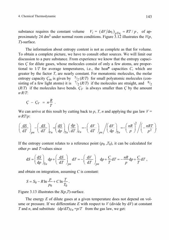
4. Chemical Thermodynamic 143
( )substance requires the constant volume Vi = ipTnd d /iV n RT p= , of ap-
proximately 24 dm3 under normal room conditions. Figure 3.12 illustrates the V(p, T)-surface.
The information about entropy content is not as complete as that for volume. To obtain a complete picture, we have to consult other sources. We will limit our discussion to a pure substance. From experience we know that the entropy capaci-ties Ç for dilute gases, whose molecules consist of only a few atoms, are propor-tional to 1/T for average temperatures, i.e., the heat• capacities C, which are greater by the factor T, are nearly constant. For monatomic molecules, the molar entropy capacity Çm is given by 5/2 (R/T) for small polyatomic molecules (con-sisting of a few light atoms) it is 7/2 (R/T) if the molecules are straight, and 8/2 (R/T) if the molecules have bends. ÇV is always smaller than Ç by the amount n·R/T:
VRÇ Ç nT
− = .
We can arrive at this result by cutting back to p, T, n and applying the gas law V = n·RT/p:
2
2dd d d d d .
d d d d d d Vn pn Tnpn Vn Tn
pS S S V V nR nRTT p pT T p T p
⎛ ⎞⎛ ⎞⎛ ⎞ ⎛ ⎞ ⎛ ⎞ ⎛ ⎞⎛ ⎞⎛ ⎞− = ⋅ =− =− −⎜ ⎟ ⎜ ⎟ ⎜ ⎟ ⎜ ⎟⎜ ⎟ ⎜ ⎟ ⎜ ⎟ ⎜ ⎟⎝ ⎠ ⎝ ⎠ ⎝ ⎠ ⎝ ⎠⎝ ⎠ ⎝ ⎠ ⎝ ⎠ ⎝ ⎠ If the entropy content relates to a reference point (p0 ,T0), it can be calculated for other p- and T-values since
d d dd d d d d d dd d dpn pnTn
S S V C nR CS p T p T p Tp T T T p T
⎛ ⎞ ⎛ ⎞ ⎛ ⎞= + = − + = − +⎜ ⎟ ⎜ ⎟⎜ ⎟⎝ ⎠ ⎝ ⎠⎝ ⎠
,
and obtain on integration, assuming C is constant:
00 0
ln lnp TS S R Cp T
= − + .
Figure 3.13 illustrates the S(p,T)-surface.
The energy E of dilute gases at a given temperature does not depend on vol-ume or pressure. If we differentiate E with respect to V (divide by dV) at constant T and n, and substitute (dp/dT)Vn =p/T from the gas law, we get:
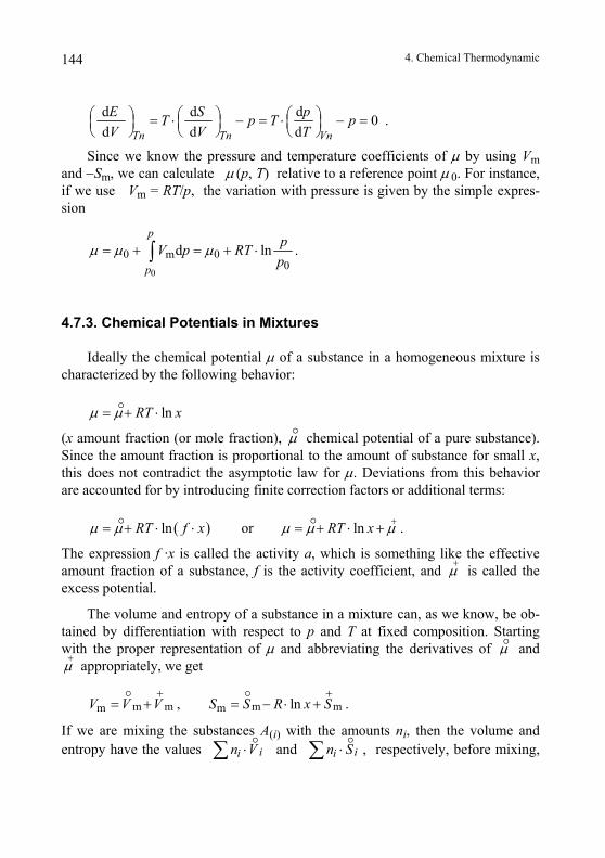
4. Chemical Thermodynamic 144
d d d 0d d dTn Tn Vn
pE ST p T pV V T
⎛ ⎞⎛ ⎞ ⎛ ⎞= ⋅ − = ⋅ − =⎜ ⎟ ⎜ ⎟ ⎜ ⎟⎝ ⎠ ⎝ ⎠ ⎝ ⎠
.
Since we know the pressure and temperature coefficients of µ by using Vm and −Sm, we can calculate µ (p, T) relative to a reference point µ 0. For instance, if we use Vm = RT/p, the variation with pressure is given by the simple expres-sion
0
0 m 00
d lnp
V p RTp
µ µ µ= + = + ⋅∫p p
lnRT xµ µ= + ⋅
.
4.7.3. Chemical Potentials in Mixtures
Ideally the chemical potential µ of a substance in a homogeneous mixture is characterized by the following behavior:
(x amount fraction (or mole fraction), µ
( )ln or lnRT f x RT x
chemical potential of a pure substance). Since the amount fraction is proportional to the amount of substance for small x, this does not contradict the asymptotic law for µ. Deviations from this behavior are accounted for by introducing finite correction factors or additional terms:
µ µ µ µ µ+= + ⋅ ⋅ = + ⋅ + .
The expression f ·x is called the activity a, which is something like the effective amount fraction of a substance, f is the activity coefficient, and µ
+ is called the
excess potential.
The volume and entropy of a substance in a mixture can, as we know, be ob-tained by differentiation with respect to p and T at fixed composition. Starting with the proper representation of µ and abbreviating the derivatives of µ and µ+
appropriately, we get
m m m mm m, lnV V V S S R x S+ +
= + = − ⋅ +
.
If we are mixing the substances A(i) with the amounts ni, then the volume and entropy have the values iin V⋅∑ and , respectively, before mixing,
iin S⋅∑
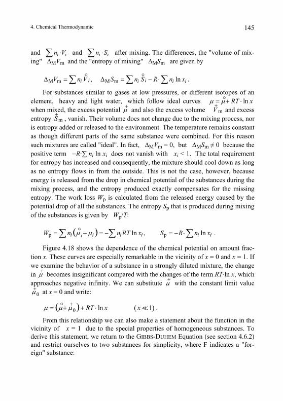
4. Chemical Thermodynamic 145
and ∑ and i in V⋅ i in S⋅∑ after mixing. The differences, the "volume of mix-ing" ∆MVm and the "entropy of mixing" ∆MSm are given by
M m M m, lnS R n x− ⋅∑i ii i i iV n V S n∆ = ∆ =∑ ∑
lnRT xµ µ= + ⋅
.
For substances similar to gases at low pressures, or different isotopes of an element, heavy and light water, which follow ideal curves when mixed, the excess potential µ+ and also the excess volume V m
+ and excess entropy
+, vanish. Their volume does not change due to the mixing process, nor
is entropy added or released to the envir ment. The temperature remains constant as though different parts of the same s bstance were combined. For this reason such mixtures are called "ideal". In fact, ∆MVm = 0, but ∆MSm ≠ 0 because the positive term −R·∑ ni ln xi does not vfor entropy has increased and consequenas no entropy flows in from the outsidenergy is released from the drop in chemmixing process, and the entropy produentropy. The work loss Wp is calculatepotential drop of all the substances. Theof the substances is given by Wp/T:
mS
p ln( )i i iiW n n RTµ µ= − = −∑ ∑
Figure 4.18 shows the dependence tion x. These curves are especially remawe examine the behavior of a substancein µ+ becomes insignificant compared wapproaches negative infinity. We can s
0µ+
(0 ln( ) RT x xµ µ µ+
= + + ⋅
at x = 0 and write:
From this relationship we can also vicinity of x = 1 due to the special pderive this statement, we return to the Gand restrict ourselves to two substanceseign" substance:
onu
anish with xi < 1. The total requirement tly, the mixture should cool down as longe. This is not the case, however, because ical potential of the substances during the
ced exactly compensates for the missing d from the released energy caused by the entropy Sp that is produced during mixing
pi i i, lnx S R n x= − ⋅∑ .
of the chemical potential on amount frac-rkable in the vicinity of x = 0 and x = 1. If in a strongly diluted mixture, the change ith the changes of the term RT·ln x, which
ubstitute µ+
with the constant limit value
)1 .
make a statement about the function in the roperties of homogeneous substances. To IBBS-DUHEM Equation (see section 4.6.2) for simplicity, where F indicates a "for-
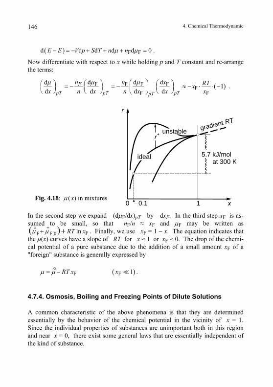
4. Chemical Thermodynamic 146
( ) F Fd d d d d 0E E V p S T n nµ µ− = − + + + = .
Now differentiate with respect to x while holding p and T constant and re-arrange the terms:
( )F F F FF
F F
d d dd 1d d d d
F
pT pT pTpT
n n x RTxx n x n x x x
µ µµ ⎛ ⎞⎛ ⎞ ⎛ ⎞⎛ ⎞ = − = − ≈ − ⋅ ⋅ −⎜ ⎟ ⎜ ⎟ ⎜ ⎟⎜ ⎟⎝ ⎠ ⎝ ⎠ ⎝ ⎠⎝ ⎠
ln( ) RT xµ µ++ +
( )F F 1RT x xµ µ= −
.
gradient RT
r
r+
x0 1
unstable
ideal 5.7 kJ/mol at 300 K
0.1Fig. 4.18: µ( x) in mixtures
In the second step we expand (dµF/dx)pT by dxF. In the third step xF is as-sumed to be small, so that nF/n ≈ xF and µF may be written as
FF F,0 . Finally, we use xF = 1 − x. The equation indicates that the µ(x) curves have a slope of RT for x ≈ 1 or xF ≈ 0. The drop of the chemi-cal potential of a pure substance due to the addition of a small amount xF of a "foreign" substance is generally expressed by
.
4.7.4. Osmosis, Boiling and Freezing Points of Dilute Solutions
A common characteristic of the above phenomena is that they are determined essentially by the behavior of the chemical potential in the vicinity of x = 1. Since the individual properties of substances are unimportant both in this region and near x = 0, there exist some general laws that are essentially independent of the kind of substance.
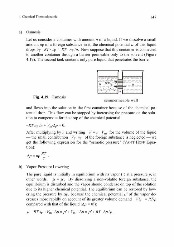
4. Chemical Thermodynamic 147
a) Osmosis
Let us consider a container with amount n of a liquid. If we dissolve a small amount nF of a foreign substance in it, the chemical potential µ of this liquid drops by RT · xF ≈ RT · nF /n. Now suppose that this container is connected to another container through a barrier permeable only to the solvent (Figure 4.19). The second tank contains only pure liquid that penetrates the barrier
µµ − FRTx
semipermeable wall
Fig. 4.19: Osmosis
and flows into the solution in the first container because of the chemical po-tential drop. This flow can be stopped by increasing the pressure on the solu-tion to compensate for the drop of the chemical potential:
−RT·nF /n + Vm·∆p = 0.
After multiplying by n and writing V = n · Vm for the volume of the liquid — the small contribution VF ·nF of the foreign substance is neglected — we get the following expression for the "osmotic pressure" (VAN'T HOFF Equa-tion):
FRTp nV
∆ = .
b) Vapor Pressure Lowering
The pure liquid is initially in equilibrium with its vapor (' ) at a pressure p, in other words, µ = µ'. By dissolving a non-volatile foreign substance, the equilibrium is disturbed and the vapor should condense on top of the solution due to its higher chemical potential. The equilibrium can be restored by low-ering the pressure by ∆p, because the chemical potential µ' of the vapor de-creases more rapidly on account of its greater volume demand V' = RT/p compared with that of the liquid (∆p < 0!):
m
F m m /RT x V p ' V' p ' RT p p µ µ µ− + ⋅ ∆ = + ⋅ ∆ = + ⋅ ∆ .
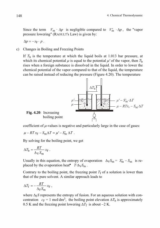
4. Chemical Thermodynamic 148
Since the term Vm · ∆p is negligible compared to V'm p⋅ ∆
Fp x p∆ = − ⋅
F m mRT x S T ' S' T
, the "vapor pressure lowering" (RAOULT's Law) is given by:
.
c) Changes in Boiling and Freezing Points
If Tb is the temperature at which the liquid boils at 1.013 bar pressure, at which its chemical potential µ is equal to the potential µ' of the vapor, then Tb rises when a foreign substance is dissolved in the liquid. In order to lower the chemical potential of the vapor compared to that of the liquid, the temperature can be raised instead of reducing the pressure (Figure 4.20). The temperature
coefficient of µ-values is negative and particularly large in the case of gases:
µ' µ
∆Tb
µ' 'm ⋅− ∆ S Tµ − ∆F S TRTx − ⋅m
Fig. 4.20: Increasing boiling point
µ µ− − ∆ = − ∆ .
By solving for the boiling point, we get
b FV m
RTT xS
∆ =∆
m mS' S
.
Usually in this equation, the entropy of evaporation ∆VSm = − is re-placed by the evaporation heat• T·∆VSm .
Contrary to the boiling point, the freezing point Tf of a solution is lower than that of the pure solvent. A similar approach leads to
f FF m
RTT xS
∆ = −∆
,
where ∆FS represents the entropy of fusion. For an aqueous solution with con-centration cF = 1 mol/dm3, the boiling point elevation ∆Tb is approximately 0.5 K and the freezing point lowering ∆Tf is about −2 K.
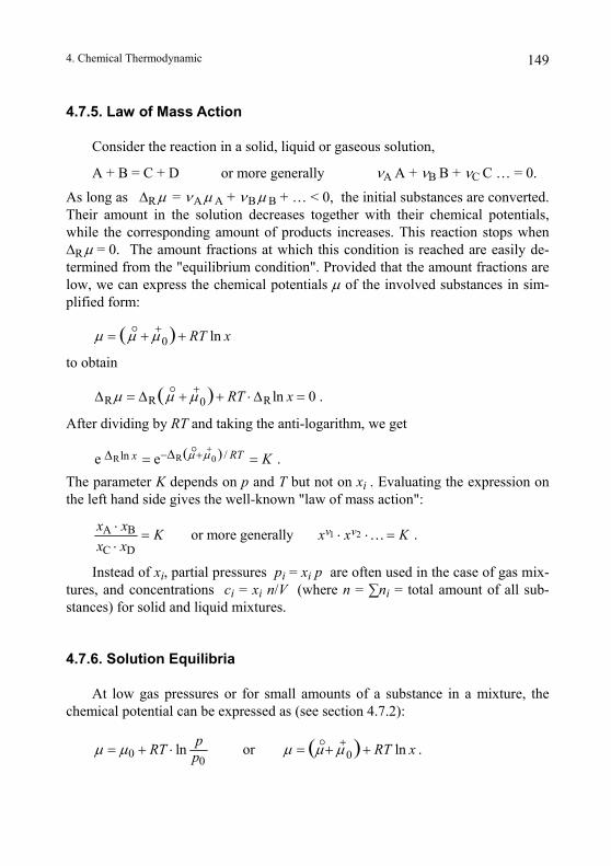
4. Chemical Thermodynamic 149
4.7.5. Law of Mass Action
Consider the reaction in a solid, liquid or gaseous solution,
A + B = C + D or more generally νA A + νB B + νC C … = 0.
As long as ∆R µ = νA µ A + νB µ B + … < 0, the initial substances are converted. Their amount in the solution decreases together with their chemical potentials, while the corresponding amount of products increases. This reaction stops when ∆R µ = 0. The amount fractions at which this condition is reached are easily de-termined from the "equilibrium condition". Provided that the amount fractions are low, we can express the chemical potentials µ of the involved substances in sim-plified form:
0 ln( ) RT xµ µ µ+= + +
R R R0 ln 0( ) RT xµ µ µ+∆ = ∆ + + ⋅ ∆ =
RR 0 / ln ( )e e RTx
to obtain
.
After dividing by RT and taking the anti-logarithm, we get
Kµ µ+− +∆∆ = =
. The parameter K depends on p and T but not on xi . Evaluating the expression on the left hand side gives the well-known "law of mass action":
1 2A B
C D or more generally v vx x K x x K
x x⋅ = ⋅ ⋅ =⋅
… .
Instead of xi, partial pressures pi = xi p are often used in the case of gas mix-tures, and concentrations ci = xi n/V (where n = ∑ni = total amount of all sub-stances) for solid and liquid mixtures.
4.7.6. Solution Equilibria
At low gas pressures or for small amounts of a substance in a mixture, the chemical potential can be expressed as (see section 4.7.2):
0 00ln or ln( )pRT RT xpµ µ µ µ µ+= + ⋅ = + + .
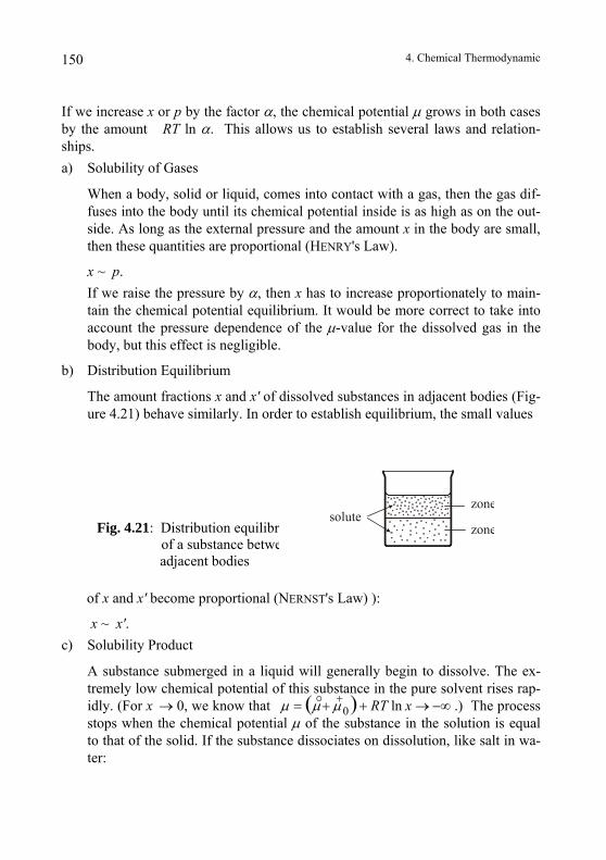
4. Chemical Thermodynamic 150
If we increase x or p by the factor α, the chemical potential µ grows in both cases by the amount RT ln α. This allows us to establish several laws and relation-ships. a) Solubility of Gases
When a body, solid or liquid, comes into contact with a gas, then the gas dif-fuses into the body until its chemical potential inside is as high as on the out-side. As long as the external pressure and the amount x in the body are small, then these quantities are proportional (HENRY's Law).
x ~ p. If we raise the pressure by α, then x has to increase proportionately to main-tain the chemical potential equilibrium. It would be more correct to take into account the pressure dependence of the µ-value for the dissolved gas in the body, but this effect is negligible.
b) Distribution Equilibrium
The amount fractions x and x' of dissolved substances in adjacent bodies (Fig-ure 4.21) behave similarly. In order to establish equilibrium, the small values
Fig. 4.21: Distribution equilibrium of a substance between
adjacent bodies
solutezone
zone
of x and x' become proportional (NERNST's Law) ):
x ~ x'. c) Solubility Product
A substance submerged in a liquid will generally begin to dissolve. The ex-tremely low chemical potential of this substance in the pure solvent rises rap-idly. (For x 0, we know that 0→ ln( ) RT xµ µ µ+= + + → −∞ .) The process stops when the chemical potential µ of the substance in the solution is equal to that of the solid. If the substance dissociates on dissolution, like salt in wa-ter:
4. Chemical Thermodynamic 151
AB = A+ + B−, then the products of the dissociation together compensate for the dissolution drive of the salt AB: µAB = µA + µB . If the amount fraction xA of one prod-uct is lowered by α, the amount fraction of the second product xB has to in-crease by α in order to maintain the equilibrium — assuming that the concen-trations are sufficiently low. The product
xA ·xB = K
must remain constant. K is here the so-called "solubility product constant" of the substance AB. If for some reason the product xA ·xB exceeds the value K, i.e., µ A + µ B > µ AB, the substance AB precipitates from the solution. If a substance dissociates into several ions, then K consists of the corresponding number of amount fractions.
d) Solubility and Temperature
The solubility of a substance is raised with increasing temperature if the chemical potential of the dissolved substance µ decreases faster than that in its pure state µ', and vice versa. This holds when Sm > , because the temperature coefficient of the chemical potential (dµ /dT)p…= −Sm. If the "molar entropy of solution" ∆L Sm = Sm − or the "molar solution heat" T·∆L Sm is positive, the solubility increases with temperature. In this case, en-tropy is received from the surroundings during dissolution. We obtain the same result if we interpret this process as a chemical reaction Apure → Adis-solved and assume that the extent of reaction and the entropy change are cou-pled.
mS'
mS'
4.8. Effect of External Fields
By considering the influence of external fields on the chemical potential, we can calculate the substance changes caused by these fields.
As an example, consider gas diffusion into the atmosphere. Since the work W = m·g·h = n·Mm·g·h required to raise an amount n of a substance from the ground (h = 0) to a height h at constant p and T, the chemical potential µ is greater than µ0 at ground level by Mm·g·h (see section 4.3.3):
µ = µ0 + Mm·g·h .
4. Chemical Thermodynamic 152
Equilibrium exists when the chemical potential ("gravito-chemical potential" would be more precise, see section 4.3.3) has the same value everywhere. In order to compensate for the increased chemical potential Mm·g·dh due to the increase in height dh, the pressure must drop. As a result, µ changes by Vm·dp, or (RT/p)·dp for gases:
mm
dd d 0, or dM gpRTM g h p hp p RT
⋅⋅ + = = − .
After integrating and taking the anti-logarithm, we obtain the "barometric height formula":
m
0 eM g h
RTp p⋅−
= ⋅
2I 2I
.
A magnetic field H boosts the dissociation of iodine vapour
,
since it lowers the chemical potential of the paramagnetic iodine atoms, attracted by the field, relative to the diamagnetic I2. To calculate this effect, we can start with the main equation dE = −pdV + HdM + TdS + µ1dn1 + µ2dn2 of the gas mixture, and then evaluate ( )
1 2d di pTn nHµ by using the flip rule, etc.
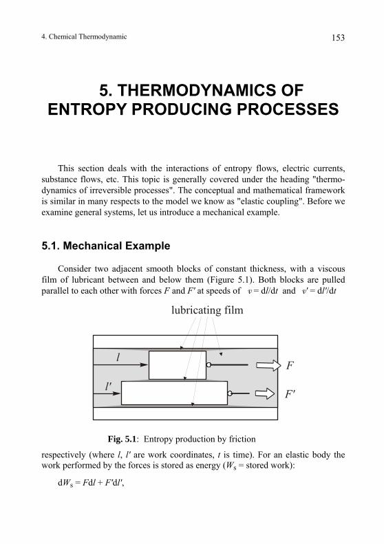
4. Chemical Thermodynamic 153
5. THERMODYNAMICS OF ENTROPY PRODUCING PROCESSES
This section deals with the interactions of entropy flows, electric currents, substance flows, etc. This topic is generally covered under the heading "thermo-dynamics of irreversible processes". The conceptual and mathematical framework is similar in many respects to the model we know as "elastic coupling". Before we examine general systems, let us introduce a mechanical example.
5.1. Mechanical Example
Consider two adjacent smooth blocks of constant thickness, with a viscous film of lubricant between and below them (Figure 5.1). Both blocks are pulled parallel to each other with forces F and F' at speeds of v = dl/dt and v' = dl'/dt
respectively (where l, l' are work coordinates, t is time). For an elastic body the work performed by the forces is stored as energy (Ws = stored work):
dWs = Fdl + F'dl',
Fig. 5.1: Entropy production by friction
F
lubricating film
l
F'l'
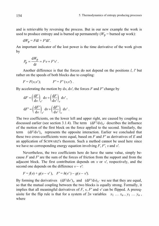
5. Thermodynamics of entropy producing processes 154
and is retrievable by reversing the process. But in our new example the work is used to produce entropy and is burned up permanently (Wp = burned up work):
dWp = Fdl + F'dl'.
An important indicator of the lost power is the time derivative of the work given by
pp
ddW
P F F' 't
= = +v v .
Another difference is that the forces do not depend on the positions l, l' but rather on the speeds of both blocks due to coupling:
F = F(v,v' ); F' = F' (v,v') .
By accelerating the motion by dv, dv', the forces F and F' change by
( ) ( )d dd d dd d'
F FF ''
= +v v
v vv v
,
( ) ( )d dd d dd d'
F' F'F' v ''
= +v v
vv v
.
The two coefficients, on the lower left and upper right, are caused by coupling as discussed earlier (see section 3.1.4). The term (dF'/dv)v' describes the influence of the motion of the first block on the force applied to the second. Similarly, the term (dF/dv' )v represents the opposite interaction. Earlier we concluded that these two cross-coefficients were equal, based on F and F' as derivatives of E and an application of SCHWARZ's theorem. Such a method cannot be used here since we have no corresponding energy equation involving F, F', v and v'.
Nevertheless, the two coefficients here do have the same value, simply be-cause F and F' are the sum of the forces of friction from the support and from the adjacent block. The first contribution depends on v or v', respectively, and the second one depends on the difference v − v':
F = f(v) + g(v − v' ), F' = h(v' ) − g(v − v').
By forming the derivatives (dF/dv' )v and (dF'/dv)v' we see that they are equal, so that the mutual coupling between the two blocks is equally strong. Formally, it implies that all meaningful derivatives of F, v, F' and v' can be flipped. A prereq-uisite for the flip rule is that for a system of 2n variables x1 … xn , y1 … yn , where
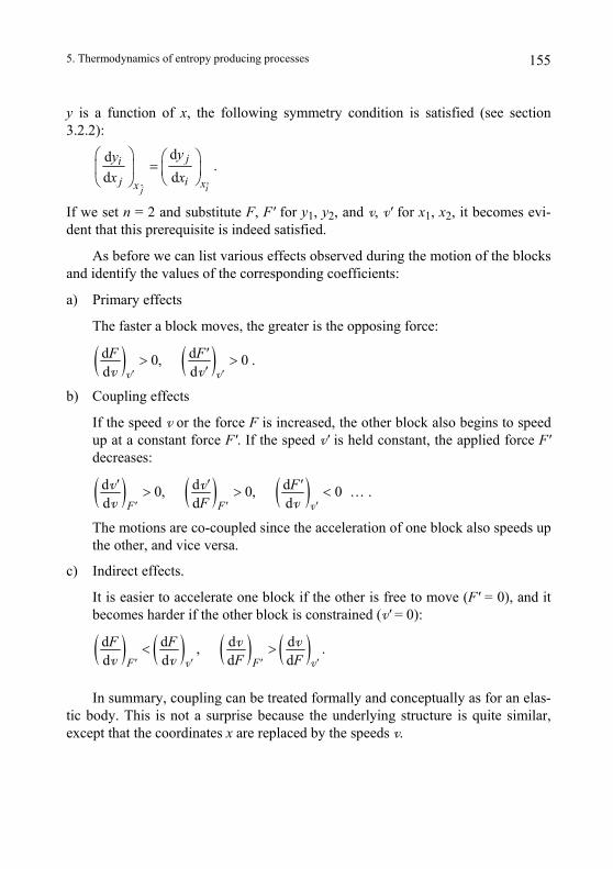
5. Thermodynamics of entropy producing processes 155
y is a function of x, the following symmetry condition is satisfied (see section 3.2.2):
ˆˆ
ddd d
ij
ji
j i xx
yyx x
⎛ ⎞ ⎛ ⎞=⎜ ⎟ ⎜ ⎟
⎝ ⎠⎝ ⎠.
If we set n = 2 and substitute F, F' for y1, y2, and v, v' for x1, x2, it becomes evi-dent that this prerequisite is indeed satisfied.
As before we can list various effects observed during the motion of the blocks and identify the values of the corresponding coefficients:
a) Primary effects
The faster a block moves, the greater is the opposing force:
( ) ( )d d0, 0d d' '
F F''
> >v vv v
.
b) Coupling effects
If the speed v or the force F is increased, the other block also begins to speed up at a constant force F'. If the speed v' is held constant, the applied force F' decreases:
( ) ( ) ( )d d d0, 0, 0 … .d d dF' F' '
' ' F'F
> > <v
v vv v
The motions are co-coupled since the acceleration of one block also speeds up the other, and vice versa.
c) Indirect effects.
It is easier to accelerate one block if the other is free to move (F' = 0), and it becomes harder if the other block is constrained (v' = 0):
( ) ( ) ( ) ( )d d d d, .d dd dF' 'v v F' '
F FF F
< >v v
v v
In summary, coupling can be treated formally and conceptually as for an elas-tic body. This is not a surprise because the underlying structure is quite similar, except that the coordinates x are replaced by the speeds v.
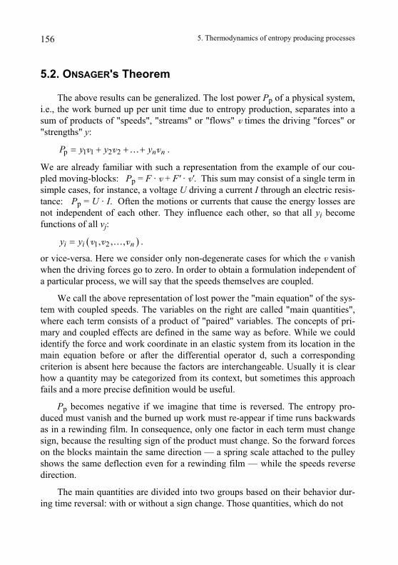
5. Thermodynamics of entropy producing processes 156
5.2. ONSAGER's Theorem
The above results can be generalized. The lost power Pp of a physical system, i.e., the work burned up per unit time due to entropy production, separates into a sum of products of "speeds", "streams" or "flows" v times the driving "forces" or "strengths" y:
p 1 1 2 2 n nP y y y= + + +v v v… .
We are already familiar with such a representation from the example of our cou-pled moving-blocks: Pp = F · v + F' · v'. This sum may consist of a single term in simple cases, for instance, a voltage U driving a current I through an electric resis-tance: Pp = U · I. Often the motions or currents that cause the energy losses are not independent of each other. They influence each other, so that all yi become functions of all vj:
( )1 2, , ,i i ny y= v v v… .
or vice-versa. Here we consider only non-degenerate cases for which the v vanish when the driving forces go to zero. In order to obtain a formulation independent of a particular process, we will say that the speeds themselves are coupled.
We call the above representation of lost power the "main equation" of the sys-tem with coupled speeds. The variables on the right are called "main quantities", where each term consists of a product of "paired" variables. The concepts of pri-mary and coupled effects are defined in the same way as before. While we could identify the force and work coordinate in an elastic system from its location in the main equation before or after the differential operator d, such a corresponding criterion is absent here because the factors are interchangeable. Usually it is clear how a quantity may be categorized from its context, but sometimes this approach fails and a more precise definition would be useful.
Pp becomes negative if we imagine that time is reversed. The entropy pro-duced must vanish and the burned up work must re-appear if time runs backwards as in a rewinding film. In consequence, only one factor in each term must change sign, because the resulting sign of the product must change. So the forward forces on the blocks maintain the same direction — a spring scale attached to the pulley shows the same deflection even for a rewinding film — while the speeds reverse direction.
The main quantities are divided into two groups based on their behavior dur-ing time reversal: with or without a sign change. Those quantities, which do not
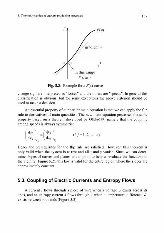
5. Thermodynamics of entropy producing processes 157
F
v
gradient m
F( )v
in this range F m≈ ⋅v
Fig. 5.2: Example for a F(v)-curve
change sign are interpreted as "forces" and the others are "speeds". In general this classification is obvious, but for some exceptions the above criterion should be used to make a decision.
An essential property of our earlier main equation is that we can apply the flip rule to derivatives of main quantities. The new main equation possesses the same property based on a theorem developed by ONSAGER, namely that the coupling among speeds is always symmetric:
ˆˆd d
ijj i⎝ ⎠⎝ ⎠ vvv v
dd ji yy⎛ ⎞ ⎛ ⎞=⎜ ⎟ ⎜ ⎟ (i, j = 1, 2, …, n).
Hence the prerequisites for the flip rule are satisfied. However, this theorem is only valid when the system is at rest and all v and y vanish. Since we can deter-mine slopes of curves and planes at this point to help us evaluate the functions in the vicinity (Figure 5.2), this law is valid for the entire region where the slopes are approximately constant.
5.3. Coupling of Electric Currents and Entropy Flows
A current I flows through a piece of wire when a voltage U exists across its ends, and an entropy current J flows through it when a temperature difference ϑ exists between both ends (Figure 5.3).
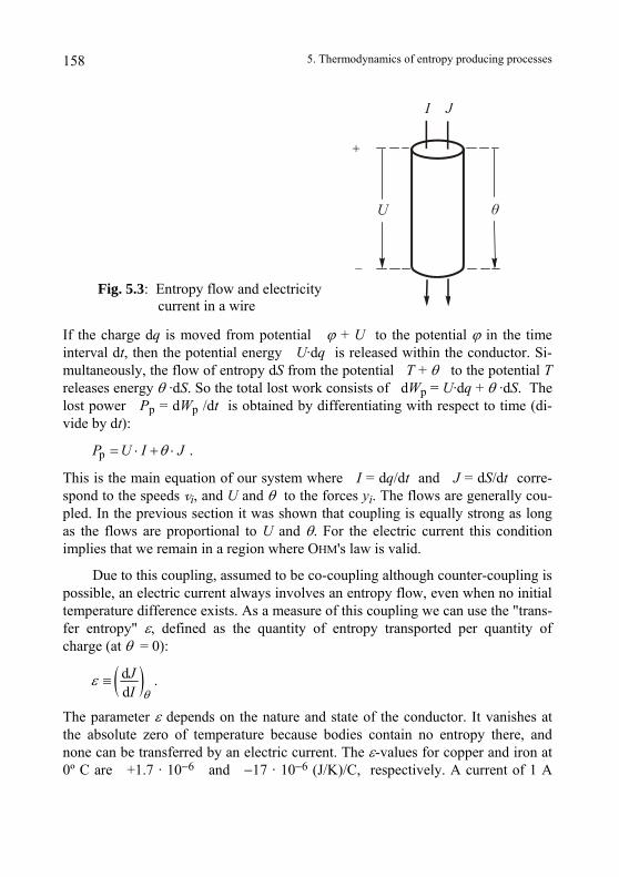
5. Thermodynamics of entropy producing processes 158
_
U
JI
+
θ
Fig. 5.3: Entropy flow and electricity current in a wire
If the charge dq is moved from potential ϕ + U to the potential ϕ in the time interval dt, then the potential energy U·dq is released within the conductor. Si-multaneously, the flow of entropy dS from the potential T + θ to the potential T releases energy θ ·dS. So the total lost work consists of dWp = U·dq + θ ·dS. The lost power Pp = dWp /dt is obtained by differentiating with respect to time (di-vide by dt):
pP U I Jθ= ⋅ + ⋅ .
This is the main equation of our system where I = dq/dt and J = dS/dt corre-spond to the speeds vi, and U and θ to the forces yi. The flows are generally cou-pled. In the previous section it was shown that coupling is equally strong as long as the flows are proportional to U and θ. For the electric current this condition implies that we remain in a region where OHM's law is valid.
Due to this coupling, assumed to be co-coupling although counter-coupling is possible, an electric current always involves an entropy flow, even when no initial temperature difference exists. As a measure of this coupling we can use the "trans-fer entropy" ε, defined as the quantity of entropy transported per quantity of charge (at θ = 0):
( )ddJI θ
ε ≡ .
The parameter ε depends on the nature and state of the conductor. It vanishes at the absolute zero of temperature because bodies contain no entropy there, and none can be transferred by an electric current. The ε-values for copper and iron at 0º C are +1.7 · 10−6 and −17 · 10−6 (J/K)/C, respectively. A current of 1 A
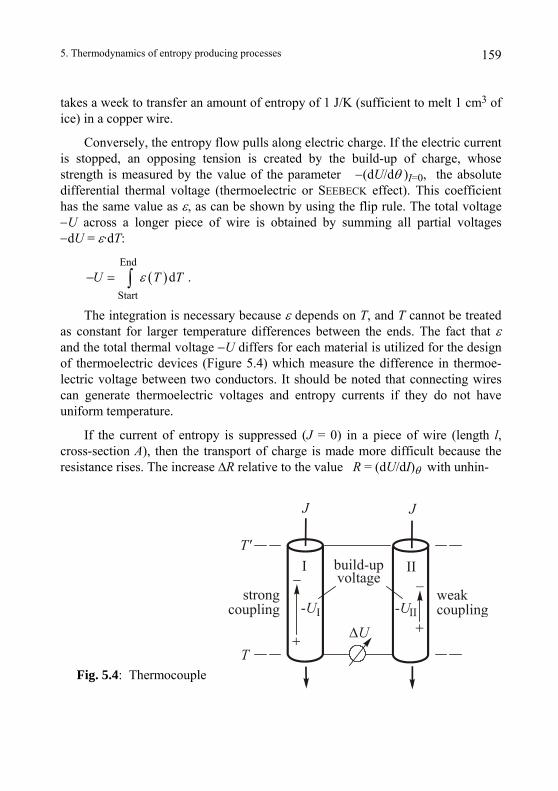
5. Thermodynamics of entropy producing processes 159
takes a week to transfer an amount of entropy of 1 J/K (sufficient to melt 1 cm3 of ice) in a copper wire.
Conversely, the entropy flow pulls along electric charge. If the electric current is stopped, an opposing tension is created by the build-up of charge, whose strength is measured by the value of the parameter −(dU/dθ )I=0, the absolute differential thermal voltage (thermoelectric or SEEBECK effect). This coefficient has the same value as ε, as can be shown by using the flip rule. The total voltage −U across a longer piece of wire is obtained by summing all partial voltages −dU = ε·dT:
( )Start
dU T Tε− = ∫End
.
The integration is necessary because ε depends on T, and T cannot be treated as constant for larger temperature differences between the ends. The fact that ε and the total thermal voltage −U differs for each material is utilized for the design of thermoelectric devices (Figure 5.4) which measure the difference in thermoe-lectric voltage between two conductors. It should be noted that connecting wires can generate thermoelectric voltages and entropy currents if they do not have uniform temperature.
If the current of entropy is suppressed (J = 0) in a piece of wire (length l, cross-section A), then the transport of charge is made more difficult because the resistance rises. The increase ∆R relative to the value R = (dU/dI)θ with unhin-
I− −
++
II
J J
T'
-UI -UII
∆U
strongcoupling
build-upvoltage
weakcoupling
Fig. 5.4: Thermocouple
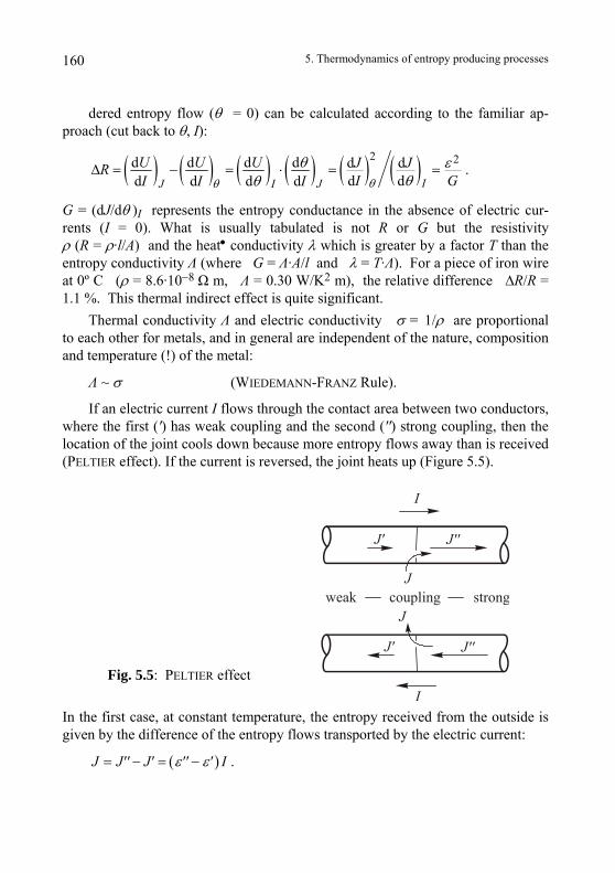
5. Thermodynamics of entropy producing processes 160
dered entropy flow (θ = 0) can be calculated according to the familiar ap-proach (cut back to θ, I):
( ) ( ) ( ) ( ) ( ) ( )2 2d d d d d dd dd d d d IJ I J
U U U J JRI GI I I θθ
θ εθθ
∆ = − = = =
( )
. ⋅
G = (dJ/dθ )I represents the entropy conductance in the absence of electric cur-rents (I = 0). What is usually tabulated is not R or G but the resistivity ρ (R = ρ·l/A) and the heat• conductivity λ which is greater by a factor T than the entropy conductivity Λ (where G = Λ·A/l and λ = T·Λ). For a piece of iron wire at 0º C (ρ = 8.6·10−8 Ω m, Λ = 0.30 W/K2 m), the relative difference ∆R/R = 1.1 %. This thermal indirect effect is quite significant.
Thermal conductivity Λ and electric conductivity σ = 1/ρ are proportional to each other for metals, and in general are independent of the nature, composition and temperature (!) of the metal:
Λ ~ σ (WIEDEMANN-FRANZ Rule).
If an electric current I flows through the contact area between two conductors, where the first (') has weak coupling and the second ('') strong coupling, then the location of the joint cools down because more entropy flows away than is received (PELTIER effect). If the current is reversed, the joint heats up (Figure 5.5).
In the first case, at constant temperature, the entropy received from the outside is given by the difference of the entropy flows transported by the electric current:
I
I
J
Jweak coupling strong
J''
J''
J'
J'
Fig. 5.5: PELTIER effect
J J'' J' '' ' Iε ε= − = − .
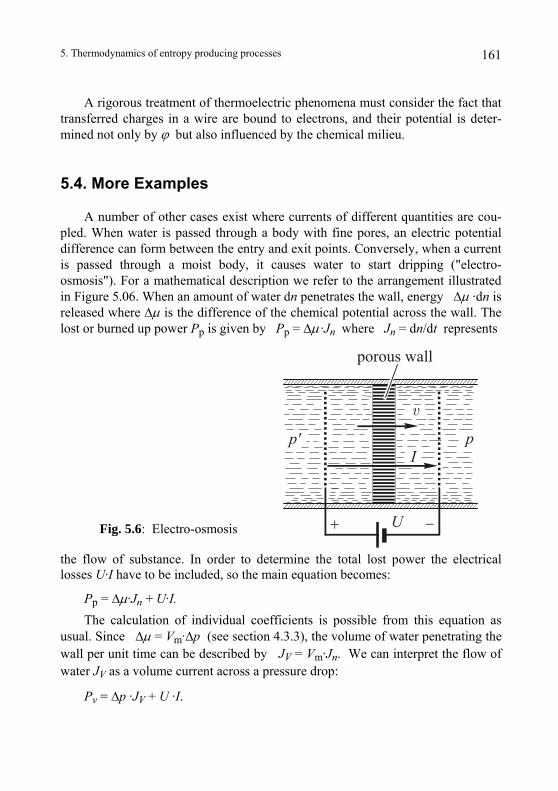
5. Thermodynamics of entropy producing processes 161
A rigorous treatment of thermoelectric phenomena must consider the fact that transferred charges in a wire are bound to electrons, and their potential is deter-mined not only by ϕ but also influenced by the chemical milieu.
5.4. More Examples
A number of other cases exist where currents of different quantities are cou-pled. When water is passed through a body with fine pores, an electric potential difference can form between the entry and exit points. Conversely, when a current is passed through a moist body, it causes water to start dripping ("electro-osmosis"). For a mathematical description we refer to the arrangement illustrated in Figure 5.06. When an amount of water dn penetrates the wall, energy ∆µ ·dn is released where ∆µ is the difference of the chemical potential across the wall. The lost or burned up power Pp is given by Pp = ∆µ ·Jn where Jn = dn/dt represents
the flow of substance. In order to determine the total lost power the electrical losses U·I have to be included, so the main equation becomes:
+ −U
Ip
v
Pp = ∆µ·Jn + U·I. The calculation of individual coefficients is possible from this equation as
usual. Since ∆µ = Vm·∆p (see section 4.3.3), the volume of water penetrating the wall per unit time can be described by JV = Vm·Jn. We can interpret the flow of water JV as a volume current across a pressure drop:
Pv = ∆p ·JV + U ·I.
Fig. 5.6: Electro-osmosis
porous wall
p'
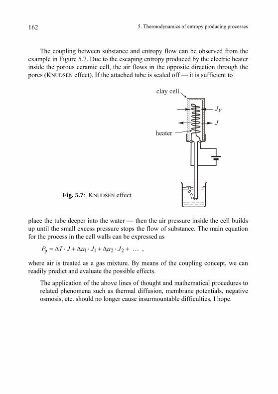
5. Thermodynamics of entropy producing processes 162
The coupling between substance and entropy flow can be observed from the example in Figure 5.7. Due to the escaping entropy produced by the electric heater inside the porous ceramic cell, the air flows in the opposite direction through the pores (KNUDSEN effect). If the attached tube is sealed off — it is sufficient to
JV
J
clay cell
heater
Fig. 5.7: KNUDSEN effect
place the tube deeper into the water — then the air pressure inside the cell builds up until the small excess pressure stops the flow of substance. The main equation for the process in the cell walls can be expressed as
p 1 1 2 2 … P T J J Jµ µ= ∆ ⋅ + ∆ ⋅ + ∆ ⋅ + ,
where air is treated as a gas mixture. By means of the coupling concept, we can readily predict and evaluate the possible effects.
The application of the above lines of thought and mathematical procedures to related phenomena such as thermal diffusion, membrane potentials, negative osmosis, etc. should no longer cause insurmountable difficulties, I hope.
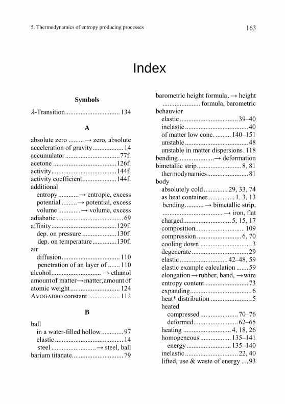
5. Thermodynamics of entropy producing processes 163
Index
barometric height formula.→ height Symbols ...................... formula, barometric behauvior λ-Transition................................ 134 elastic .................................. 39–40 inelastic .....................................40 A of matter low conc. ......... 140–151
absolute zero .........→ zero, absolute unstable .....................................48 acceleration of gravity.................. 14 unstable in matter dispersions.118 accumulator ................................77f. bending.....................→ deformation acetone .....................................126f. bimetallic strip.......................... 8, 81 activity......................................144f. thermodynamics........................81 activity coefficient....................144f. body additional absolutely cold .............. 29, 33, 74 entropy ............→ entropie, excess as heat container................ 1, 3, 13 potential .........→ potential, excess bending...........→ bimetallic strip, volume .............→ volume, excess ................................... → iron, flat adiabatic ....................................... 69 charged............................ 5, 15, 17 affinity......................................129f. composition............................. 109 dep. on pressure ....................130f. compression .......................... 6, 70 dep. on temperature..............130f. cooling down ..............................3 air degenerate .................................29 diffusion.................................. 110 elastic ............................ 42–48, 59 penetration of an layer of ....... 110 elastic example calculation .......59 alcohol............................. → ethanol elongation→ rubber, band, → wire amount of matter→ matter, amount of entropy content .........................73 atomic weight ............................. 124 expanding....................................6 AVOGADRO constant................... 112 heat* distribution ........................5
heated B compressed ...................... 70–76
deformed.......................... 62–65 ball heating ............................ 4, 18, 26 in a water-filled hollow............. 97 homogeneous .................. 135–141 elastic ........................................ 14 energy .......................... 135–140 steel ..........................→ steel, ball inelastic ............................... 22, 40 barium titanate.............................. 79 lifted, use & waste of energy ....93
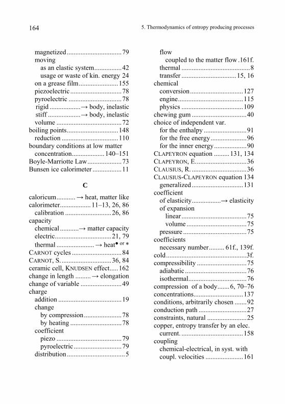
5. Thermodynamics of entropy producing processes 164
magnetized ................................79 flow moving coupled to the matter flow .161f. as an elastic system................42 thermal ........................................8 usage or waste of kin. energy 24 transfer ................................15, 16 on a grease film.......................155 chemical piezoelectric ..............................78 conversion...............................127 pyroelectric ...............................78 engine......................................115 rigid ..................→ body, inelastic physics ....................................109
stiff ...................→ body, inelastic chewing gum ................................40 volume ......................................72 choice of independent var. boiling points..............................148 for the enthalpy .........................91 reduction .................................110 for the free energy.....................96 boundary conditions at low matter for the inner energy...................90 concentration................... 140–151 CLAPEYRON equation .........131, 134 Boyle-Marriotte Law....................73 CLAPEYRON, E..............................36 Bunsen ice calorimeter .................11 CLAUSIUS, R. ................................36
CLAUSIUS-CLAPEYRON equation 134 generalized ..............................131 C coefficient caloricum...........→ heat, matter like of elasticity.................→ elasticity calorimeter.................. 11–13, 26, 86 of expansion calibration ...........................26, 86 linear ......................................75 capacity volume ...................................75 chemical ...........→ matter capacity pressure .....................................75 electric.................................21, 79 coefficients
thermal ......................→ heat or * necessary number......... 61f., 139f. CARNOT cycles .............................84 cold...............................................3f. CARNOT, S. .............................36, 84 compressibility .............................75 ceramic cell, KNUDSEN effect.....162 adiabatic ....................................76 change in length .........→ elongation isothermal..................................76 change of variable ........................49 compression of a body.......6, 70–76 charge concentrations.............................137 addition .....................................19 conditions, arbitrarily chosen .......92 change conduction path ............................27 by compression......................78 constraints, natural .......................25 by heating ..............................78 copper, entropy transfer by an elec. coefficient current. ....................................158 piezo ......................................79 coupling pyroelectric ............................79 chemical-electrical, in syst. with distribution..................................5 coupl. velocities ......................161
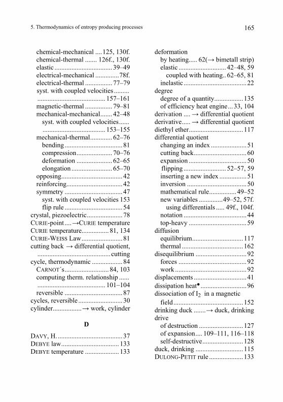
5. Thermodynamics of entropy producing processes 165
chemical-mechanical ....125, 130f. deformation chemical-thermal ....... 126f., 130f. by heating..... 62(→ bimetall strip) elastic .................................. 39–49 elastic ............................ 42–48, 59 electrical-mechanical ..............78f. coupled with heating.. 62–65, 81 electrical-thermal ................ 77–79 inelastic .....................................22 syst. with coupled velocities ......... degree ........................................ 157–161 degree of a quantity................. 135 magnetic-thermal ................ 79–81 of efficiency heat engine... 33, 104 mechanical-mechanical....... 42–48 derivation .... → differential quotient syst. with coupled velocities...... derivative..... → differential quotient ..................................... 153–155 diethyl ether................................ 117 mechanical-thermal............. 62–76 differential quotient bending .................................. 81 changing an index .....................51 compression..................... 70–76 cutting back...............................60 deformation ..................... 62–65 expansion ..................................50 elongation ........................ 65–70 flipping ......................... 52–57, 59 opposing.................................... 42 inserting a new index ................51 reinforcing................................. 42 inversion ...................................50 symmetry .................................. 47 mathematical rule................ 49–52 syst. with coupled velocities 153 new variables ..............49–52, 57f. flip rule .................................. 54 using differentials ..... 49f., 104f. crystal, piezoelectric..................... 78 notation .....................................44 CURIE-point ....→CURIE temperature top-heavy ..................................59
diffusion CURIE temperature................ 81, 134 equilibrium.............................. 117 CURIE-WEISS Law........................ 81 thermal .................................... 162 cutting back → differential quotient, disequilibrium ..............................92 ........................................... cutting forces ........................................92 cycle, thermodynamic .................. 84 work ..........................................92 CARNOT´s.......................... 84, 103 displacements ...............................41 computing therm. relationship ......
........................................ 101–104 dissipation heat ...........................96 reversible .................................. 87 dissociation of I2 in a magnetic cycles, reversible .......................... 30 field......................................... 152 cylinder.................→ work, cylinder drinking duck .......→ duck, drinking
drive D of destruction .......................... 127
of expansion.... 109–111, 116–118 DAVY, H. ...................................... 37 self-destructive........................ 128 DEBYE law.................................. 133 duck, drinking ............................ 115 DEBYE temperature .................... 133 DULONG-PETIT rule .................... 133
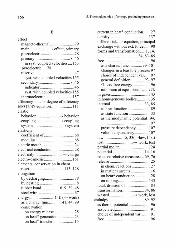
5. Thermodynamics of entropy producing processes 166
E current in heat* conduction.......27 density.....................................137 effect differential..→ equation, principal magneto-thermal .......................79 exchange without ext. force ......90 main ................. → effect, primary forms and transformation .....1, 14, piezoelectric ..............................78 ......................................34, 83–85 primary..................................8, 46 free ............................................96 in syst. coupled velocities ....153 as a charac. func.............99–101 pyroelectric 78 changes in a feasable process 97 reactive......................................47 choice of independent var......97 syst. with coupled velocities 155 general definition.............93–97 secondary ..............................8, 46 GIBBS' free energy .................96 indicator.................................46 minimum at equilibrium ......97f. syst. with coupled velocities 155 in gases....................................143 thermoelectric .........................157 in homogeneous bodies...........135 effciency.......→ degree of effciency internal ................................33, 85 EINSTEIN's equation ....................111 as heat function......................89 elastic as state function .....................33 behavior .....................→ behavior as thermodynamic potential..94, coupling .....................→ coupling ...............................................97 system ...........................→ system pressure dependency............107 elasticity volume dependency .............107 coefficient of .............................68 law.................. 15, 33(→law, first) modulus.....................................68 lost............................→ work, lost electric motor ...............................24 partial molar ............................124 electrical conduction ....................28 potential ..............................14–16 electricity.......................... → charge reactive relative measure.....69, 76 electro-osmosis...........................161 release .......................................25 elements, conservation in chem. in chem. reactions ................127 react................................. 113, 128 in matter currents .................116 elongation on heat* conduction...............28 by decharging............................78 on mixing.............................145 by heating....................................8 total, division of ........................84 rubber band ................. 6, 9, 39, 48 transformation.....................84, 86 steel wire ...................................67 wasted ......................→ work, lost energy........................14f. (→ work) enthalpy ..................................89–92 as a charac. func............ 41, 44, 99 as therm. potential .....................96 conservation associated ..................................91 on energy release ...................25 choice of independent var. ........91 on heat* generation................23 free ............................................96 on heat* transfer ....................15
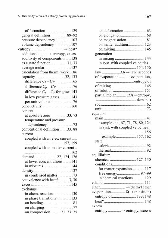
5. Thermodynamics of entropy producing processes 167
of formation......................... 129 on deformation ......................63 general definition ................ 89–92 on elongation .........................68 pressure dependency............... 107 on magnetisation....................81 volume dependency ................ 107 on matter addition................ 123 entropy ............................... → heat* on mixing............................. 145 additional .........→ entropy, excess generation additivity of components ........ 138 in mixing ............................. 144 as a state function................ 31, 33 in syst. with coupled velocities..
..................................... 154, 156 average molar.......................... 137 calculation from therm. work.... 86 law ..................33(→ law, second) capacity............................. 32, 133 of evaporation ......→ evaporation, difference Cl – CF.................. 65 ......................................entropy of
of mixing................................. 145 difference Cp – CV................. 76 of solution ............................... 151 difference Cp – CV for gases 143 partial molar..........123(→entropy, in low pressure gases ........... 143 ........................................ demand) per unit volume...................... 76 rod.............................................62 conductivity ............................ 160 unit ............................................73 content equation at absolute zero................ 33, 73 main ..........................................41 temperature and pressure example . 44, 67, 71, 78, 80, 124 dependency ......................... 73 in syst. with coupled velocities..
............................................. 156 conventional definition ....... 33, 88 current
example .................... 157, 162 coupled with an elec. current..... ..................................... 157, 159 state
caloric ....................................92 coupled with an matter current .. ............................................. 162 thermal...................................92
equilibrium demand.................... 122, 124, 126 chemical .......................... 127–130 at lower concentrations........ 141 conditions...................................... in mixtures........................... 144 for matter expansion ............ 117 density..................................... 137
free energy....................... 97–99 in condensed matter............... 73 in chemical reactions ........... 129 equivalence with heat*........ 13, 30 ethanol........................................ 111 excess...................................... 145 ether.........................→ diethyl ether exchange evaporation.............. 8(→ transition) in chem. reactions................ 130 entropy of........................ 133, 148 in phase transitions .............. 133 heat........................................ 148 on bending ............................. 81 excess on charging............................ 77 entropy .............→ entropy, excess on compression.......... 71, 73, 75
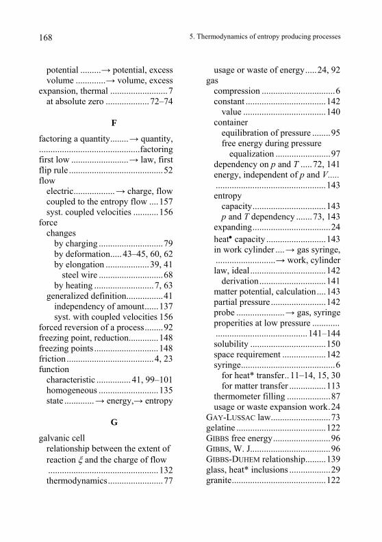
5. Thermodynamics of entropy producing processes 168
potential .........→ potential, excess usage or waste of energy.....24, 92 volume .............→ volume, excess gas expansion, thermal .........................7 compression ................................6 at absolute zero ...................72–74 constant ...................................142
value ....................................140 container F equilibration of pressure ........95 factoring a quantity........→ quantity, free energy during pressure
equalization ........................97 ............................................factoring first low .........................→ law, first dependency on p and T .....72, 141 flip rule .........................................52 energy, independent of p and V..... flow ................................................143 electric..................→ charge, flow entropy coupled to the entropy flow ....157 capacity................................143 syst. coupled velocities ...........156 p and T dependency .......73, 143 force expanding..................................24 changes
heat• capacity ..........................143 by charging ............................79 in work cylinder ....→ gas syringe, by deformation..... 43–45, 60, 62 ..........................→ work, cylinder by elongation ...................39, 41 law, ideal.................................142 steel wire ............................68 derivation.............................141 by heating ..........................7, 63 matter potential, calculation....143 generalized definition................41 partial pressure ........................142 independency of amount......137 probe .....................→ gas, syringe syst. with coupled velocities 156 properities at low pressure ............ forced reversion of a process........92 ........................................141–144 freezing point, reduction.............148 solubility .................................150 freezing points ............................148 space requirement ...................142 friction......................................4, 23 syringe.........................................6 function for heat* transfer..11–14, 15, 30 characteristic ............... 41, 99–101 for matter transfer ................113 homogeneous ..........................135 thermometer filling ...................87 state .............→ energy,→ entropy usage or waste expansion work.24 GAY-LUSSAC law..........................73 G gelatine .......................................122
galvanic cell GIBBS free energy.........................96 relationship between the extent of GIBBS, W. J...................................96
GIBBS-DUHEM relationship.........139 reaction ξ and the charge of flow glass, heat* inclusions ..................29 ................................................132 granite.........................................122 thermodynamics........................77
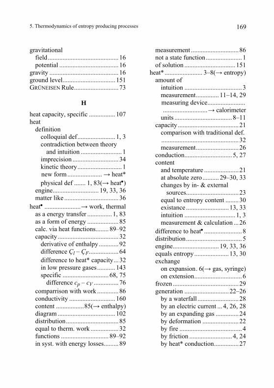
5. Thermodynamics of entropy producing processes 169
gravitational field........................................... 16 potential .................................... 16 gravity .......................................... 16 ground level................................ 151 GRÜNEISEN Rule........................... 73
H
heat capacity, specific ................ 107 heat definition colloquial def....................... 1, 3
contradiction between theory and intuition ......................... 1
imprecision ............................ 34 kinetic theory........................... 1
new form ..................... → heat* physical def ....... 1, 83(→ heat•) engine............................ 19, 33, 36 matter like ................................. 36 heat• ......................→ work, thermal as a energy transfer ............... 1, 83 as a form of energy ................... 85 calc. via heat functions........ 89–92 capacity..................................... 32 derivative of enthalpy............ 92 difference Çl – ÇF.................. 64 difference to heat* capacity... 32 in low pressure gases ........... 143 specific ............................ 68, 75
difference cp – cV ............... 76 comparrison with work ............. 86 conductivity ............................ 160 content .................85(→ enthalpy) diagram ................................... 102 distribution................................ 85 equal to therm. work ................. 32 functions ............................. 89–92 in syst. with energy losses......... 89
measurement .............................86 not a state function......................1 of solution ............................... 151 heat* ....................... 3–8(→ entropy) amount of intuition ...................................3 measurement.............. 11–14, 29
measuring device..................................................→ calorimeter
units ................................... 8–11 capacity .....................................21 comparison with traditional def.
...............................................32 measurement..........................26 conduction............................. 5, 27 content and temperature .....................21 at absolute zero .......... 29–30, 33
changes by in- & external sources................................23
equal to entropy content ........30 existance .......................... 13, 33 intuition ............................... 1, 3 measurement & calculation ...26 difference to heat• .......................8 distribution..................................5 engine............................ 19, 33, 36 equals entropy..................... 13, 30 exchange on expansion. 6(→ gas, syringe) on extension.............................6 frozen ........................................29 generation ........................... 22–26 by a waterfall .........................28 by an electric current ... 4, 26, 28 by an expanding gas ..............24 by deformation ......................22 by fire ......................................4 by friction .......................... 4, 24 by heat* conduction...............27
5. Thermodynamics of entropy producing processes 170
expended work.......................23 for heating..............................26 prerequisites.......................4, 23 inclusion..............................29, 33 indestructibility ............... 4, 13, 33 consequences ............... 8, 25, 29 potential .......... → potential, heat* producibility.................... 4, 13, 33 strength .....................................34 transfer ......................................11 as a therm. cycle ....................30 work.......................................14 unit ......................................10, 19 valve..........................................11 weight .........................................6 work ............ 34(→ work, thermal) height formula, barometric .........152 HELM, G. ......................................37 HELMHOLTZ free energy.........96, 97 HELMHOLTZ, H. V...................37, 96 HENRY's Law..............................150 HERTZ, H. .....................................37 history of thermodynamics.....35–38 homogeneous...→ body, → function hysteresis, magnetic .....................79
I
ice calorimeter ................................11 water bottle .........................11, 21 inhibition .....................→ constraint insertion of an index..→ differential .............................................quotient inversion, of a differential quotient .. ......................................................50 iodine..........................................152 iron bending .....................................22 carbon content.........................110 carburisation............................110
flat .............................................22 magnetic properties ...................79 strip ...........................................24 therm. effects on conductivity.160 transfer entropy .......................158 iron(II) sulfate ..............................81 irreversible...→ process, irreversible isothermal .....................................69
J
JOULE, J. P. ...................................37
K
KNUDSEN effect ..........................162 KOPP-NEUMANN rule..................133
L
LAMBERT, J. H..............................36 law first ......35, 85, 87(→ energy, law) of mass action .........................149 second ........... 87(→ entropy, law) THOMSON's version................34 third......34(→ NERNST's heat law) lead accumulator ..........................78 lead cell ............→ lead accumulator lead chloride ...............................126 level of work..............→ work, level lifting a weight .......................14, 16 linear expansion, coefficient of ....68 LOSCHMIDT number....................112 loss............→ performance, → work
M
machine, perpetual motion ...........36 magnetization influence of heat..............8, 79–81 of a body .............................79–81
5. Thermodynamics of entropy producing processes 171
magneto-thermal effect .....→ effect, ...............................magneto-thermal manganese(II) sulfate ................... 81 mass action law.. → law, of mass action change on heating ................... 112 measure of the amount of substance ............................. 112 molar ....................................... 124 partial molar............................ 124 transfer ..............................14, 16f. material, plastic ............................ 40 matter capacity................................... 118 conservation............................ 112 current...................→ matter, flow decomposition.............→ reaction definition................................. 109 density........137(→ concentration) distributed between 2 areas..... 150 drive of dispersion .......... 109–111 engine...................................... 115 flow against potential drop .......... 122 coupled to a charge flow...... 161 coupled to a entropy flow.... 162 drive and resistance ............. 116 inclusion.................................. 140 interchangeable with energy ... 113 potential ................................114f. absolut value........................ 115 as tension ............................. 116 change on matter addition ... 118 dependency on mole fraction.....
............................................. 144 driving mat. dispersion ........ 116 equals chemical potential .... 116 for different modifications... 132 for low concentrations ......... 140 in gases ................................ 144
in mixtures................... 144–146 influence of contaminants.......... ..................................... 126, 146 influence of gravity.............. 151 influence of magnetic fields 152 measurement........................ 127 numerical example, water.......... ..................................... 118–122 pressure dependency............ 125 self-destructive drive ........... 127 tabulated value..................... 129 temperature dependency...... 126 transfer.................................... 113 transformation......111(→ reaction ................................ or transition) uniform ................................... 109 unit .......................................... 112 MAXWELL relations..................... 99, 101, 107 thermodynamic cycles .... 101–104 MAXWELL, J. C. ......................... 101 MAYER, R.....................................37 melting .......... 7(→ phase transition) change in entropy.................... 133 change in volume .................... 133 membrane potential ......→ potential, ..................................... membrane mercury ........................................87 mixture entropy ..........→ entropy, of ...........................................mixing mixture volume ..........→ volume, of ...........................................mixing mixture ...........144–146(→ solution) entropy .................................... 145 ideal ........................................ 145 volume changes....................... 145 mole............................................ 112 fraction.................................... 137 mass ......................→ mass, molar volume ...........→ volume, demand
5. Thermodynamics of entropy producing processes 172
momentum as work coordinate ....42 motor, running on compressed air 24
N
natural constraints .....→ constraints, ...............................................natural NERNST heat law.. 33, 150(→heat* content ...................................at abs. zero)
O
odor transfer ...............................110 ONSAGER´s Theorem................156f. osmosis.......................................146 negative...................................162
P
parameters internal ......................................91 value necessary number ............61 partial pressure ...........→ gas,partial, .............................................pressure PELTIER effect ............................160 performance loss ..........................25 factorisation ............................156 permeability for matter...............110 perpetuum mobile......... → machine, ..............................perpetual. motion phase transition.....→ transformation PICTET, M. A. ...............................36 PICTET-TROUTON's Rule.............133 piezoelectric crystal......... → crystal, ..................................piezoelectric piezoelectric effect ............→ effect, ..................................piezoelectric polyethylene, permeability .........110 potassium nitrate ................ 123, 126
potential additional .......→ potential, excess definition.................................16f. drop ...........................................28 electric.......................................16 excess ......................................144 gravitational ..............................16 heat*....................................16, 17 as thermal tension ...............18, 19 identity with therm. temperature
..................................................31 membrane................................162 thermodynamic ...................93–97 conventional definition ..........96 pressure caused by an entropy current162 changes drop ..................................161 equilization between two gas containers........................95 on compression...................71 on heating...........................13 on equilibrium ..........131, 133 osmotic....................................146 primary effect ...... → effect, primary primary equation ..........→ equation, ............................................. primary principal equation.........→ equation, ............................................principal principal quantity............→quantity, ............................................principal procedure mathematical conventional......................99–108 examples .........................106–108 systematic............................57–59 examples ................................59 process contrained..................................25 feasible and unfeasible ..............25 forced reversion ..................92, 94
5. Thermodynamics of entropy producing processes 173
irreversible ............................ 8, 22 reversible ......... 8,13, 87(→ cycle, ....................................... therm.) spontaneous........................... 8, 25 change in free energy............. 97 properties.....................→ behaviour pyroelectric effect..............→ effect,
................................... pyroelectric
Q
quantity accessible .................................. 57 choice of independent var.57, 104 degree of a...→ degree of quantity extensive ................................... 31 factoring.................................. 137 inaccessible ............................... 57 independent of amount............ 137 paired ........................................ 52 consideration the sign ............... 71 partial molar.................... 122–124 principal degree of ................................. 135 in syst. with coupled velocity . 157 proportional to amount............ 137 rank of....................................... 57 unpaired .................................... 53 quartz, piezoelectric effect ........... 78 quotients, top-heavy ................... 105
R
rank of a quantity→quantity, rank of RAOULT's Law............................ 148 reaction(→transformation of matter) reaction conditions................................ 128 conversion number.→ progression ..........................................number energy changes................ 128, 130
entropy changes ...................... 130 equilibrium.............................. 129 heat of ................................... 131 numbers................................... 128 progression number................. 128 active changes......................... 131 unit conversion ....................... 128 work........................................ 128 reference state............................. 129 refrigerator .....................................4 resistance electric and entropy flow ........ 160 electronic component............ 4, 28 specific.................................... 160 reversible.........................→ process reversion, forced→ forced reversion RICHARDS' Rule.......................... 133 rod as calorimeter ...........................9 rubber ball ...................................... 62–65 band ...................................... 6, 39 reversibility of the process.... 9, 22 thermodynamics.................. 65–67 used for heat* transfer ........ 11, 15
S
salt ...................(→ sodium chloride) paramagnetic.............................81 salting-in effect........................... 126 salting-out effect......................... 127 saltpetre ............→ potassium nitrate SCHWARZ theorem................ 45, 100 second law................→ law, second secondary effect→ effect, secondary SEEBECK effect ........................... 159 side effect .........→ effect, secondary sign change in time reversion ......... 156 for matter flow ..........................18
5. Thermodynamics of entropy producing processes 174
of primary effects......................48 of secondary effects ..................46 of the free work.........................92 of the paired force ...............41, 71 reversal in the flip rule ..............53 soap film.....................................110 softness.................... ............46, 60 solubility of gases ................ ................150 product ..................................150f. temperature dependency .........151 solution entropy......... → entropy, of ......................................... solution solution equilibria ......................... 149–151 heat*.............→ heat*, of solution speed...............................→ velocity speeds in syst. with coupled velocities .... → ........................spontaneous ........spring..................squeezing a bodystability...............state function ......steam engine.......steel ball .............steel spring .........stiffness ..............stoichiometric coestreams in syst. w velocities .→ in ........................strength............... syst. with couplstretching ............strip bimetallic ........ iron..................substance, amoun
sulfuric acid matter potential of water .........121 volume increase on water add.122 susceptibility, temp. dependence..81 system elastic ........................................41 finite ..........................................29 lossless ......................................41 n-actuator ..................................52 two-actuator ..............................44 unstable .....................................48 with coupled velocities ...153–157 with losses, energy low .......89–92
T
table salt .....................................126 temperature
te .....................................22 at* content ......................21
e ending .......................22, 81
flow on syst. with ....coupled velocity .............→ process ......→ steel, spring
absolu and he chang by b
→....... →....................ffiith sy..........ed .....
.→
.....t of
...
...
compressibility .....................48 function, state
..→ heat engine
.....................15
.....................15
......... 39, 44, 59 cients .........128 coupled st. with coupled ......... velocities .....................41 velocities ...156 ...→ elongation
bimetallic strip ......→ ron, strip ..................111
by charging ......................77, 79 by compression..................6, 71 by deformation.......................63 by elongation ...........6, 9, 22, 68 by entropy exchange 4, 8, 63, 72 by heat* exchange →by entropy
....................................exchange by heat* generation....22, 23, 26 characteristic, DEBYE ..............133 coefficient .................................78 identity with convent. def..........31 scale ..........................................19 tension, thermal ......................18, 36 ........................... (→ temperature) thermal diffusion ...... → diffusion, thermal tension............ → tension, thermal voltage............→ voltage, thermal
5. Thermodynamics of entropy producing processes 175
thermodynamics chemical.......................... 109–152 comp. with convent. methods .... 8, ............................................ 30–35 energetic viewpoint................... 83 entropy generating processes ........ ........................................ 153–161 general .............................. 39–108 history ................................. 35–38 irreversible .............................. 153 problematic definitions ............... 8 pure ....................................... 3–38 thermometer ................................. 87 thermo couple...................................... 157 electricity ................................ 157 third law .......................→ law, third THOMPSON, B. .............................. 37 THOMSON, W................................ 36 second law ................................ 34 total energy..............→ energy, total tourmaline, piezoelectric effect .... 78 toy ........................→ duck, drinking transfer entropy .................................... 158 of charge ............................. 15, 16 of heat* .............. → heat* transfer of mass ................................ 14, 16 of matter.................................. 113 of volume.................................. 18 transformation of substances...... 127 transition................................. 7, 132 transition point ........................... 133 turbine .......................................... 20
U
useable work .........→ work, useable
V
VAN'T HOFF Equation................. 147 vapor pressure lowering ............. 147 variable...........................→ quantity vehicle, rolling downhill ..............24 velocity as a force ...................................42 generalized definition ............. 156 coupling............................... 156 voltage caused by a matter flow .......... 161 caused by an entropy flow ...... 159 change by compression.............78 temperature dependency . 8, 77, 79 thermal .................................... 159 differential ........................... 159 volume..........................................72 additional .........→ volume, excess average molar ......................... 137 change in mixture ............................ 145 in reactions .......................... 130 in transformations................ 133 on heating ..............................72 reduction ............................72 on increasing pressure ...........72 on matter addition................ 122 composition ............................ 138 demand ................................... 122 in mixtures........................... 144 of gases ................................ 142 excess...................................... 145 flow......................................... 161 of mixing ................................ 145 partial molar.......122f.(→ volume, ........................................ demand)
5. Thermodynamics of entropy producing processes 176
W
waste work w. missing ext. force .................................................89, 91
water as solvent ................................111 diffusion.......................... 110, 117 -fall............................................28 mass increase by heating.........112 matter potential , num. example
........................................ 118–122 mill ......................................20, 36 solvation of diethyl ether ........117 space requirement in H2SO4 ...122
temperature changes in solvation processes..............................122
to calibrate a calorimeter.............................. 9 thermometer...........................19 volume decrease on heating ......72 wheel................. 20(→ water mill) WIEDEMANN-FRANZ rule............160 wire live .................................. 157–161 thermodynamics..................67–70 comput. example..................106 reversible cycles .......... 101–104 wood...........................................122 work and energy..................... 14–16, 34 capacity, thermal .......................32 specific...................................75 chemical .......................... 116, 128 conversation of....................15, 33 coordinates ................................41 blind.......................................91 cylinder ..... 83, 89(→ gas syringe) diagram .................................102f. electric.......................................20 for charge transfer ...............15, 17 for chemical conversions ........128
for heat* generation ....... 22f., 25f. for heat* injection ...................20f. for heat* transfer .......................14 for magnetisation ......................80 for mass transfer................14, 16f. for matter injection..................116 for matter transfer .................113f. for volume injection................20f. for volume transfer....................18 free ..........................................92f. from free energy ..............93–97 loss.......................................92f. sign ........................................92 usage....................................92f. general definition ......................41 level...........................................16 lost.............................................26 on conduction ........................28 on matter currents ................116 on mixing.............................145 mechanical ................................20 of compression........................70f. opposing heat•...........................86 thermal ...................... 20(→ heat•) definite supply .......................85 identity with heat•..................32 to charge a body......................20f. to charge an accumulator ..........77 to deform a body .......................62 to increase length ......................40 to lift a weight ...........................14 useful.........................................34 maximum.......92(→ work, free)
Z
zero, absolute................................23 entropy content........ 29–30, 33, 73 heat* content ...→ entropy content impossible to reach ...................34
5. Thermodynamics of entropy producing processes 177
thermal expansion............... 72–74 vanishing of coupling................ 74
vanishing temp. dependency.....74 zwieback............................. 110, 121