Ground based UV/vis observations A) History B) Basic...
90
Ground based UV/vis observations A) History B) Basic viewing directions B) Spectroscopy C) Radiative transport modelling D) Results from different stations
Transcript of Ground based UV/vis observations A) History B) Basic...
Ground based UV/vis observations
A) History
B) Basic viewing directions
B) Spectroscopy
C) Radiative transport modelling
D) Results from different stations
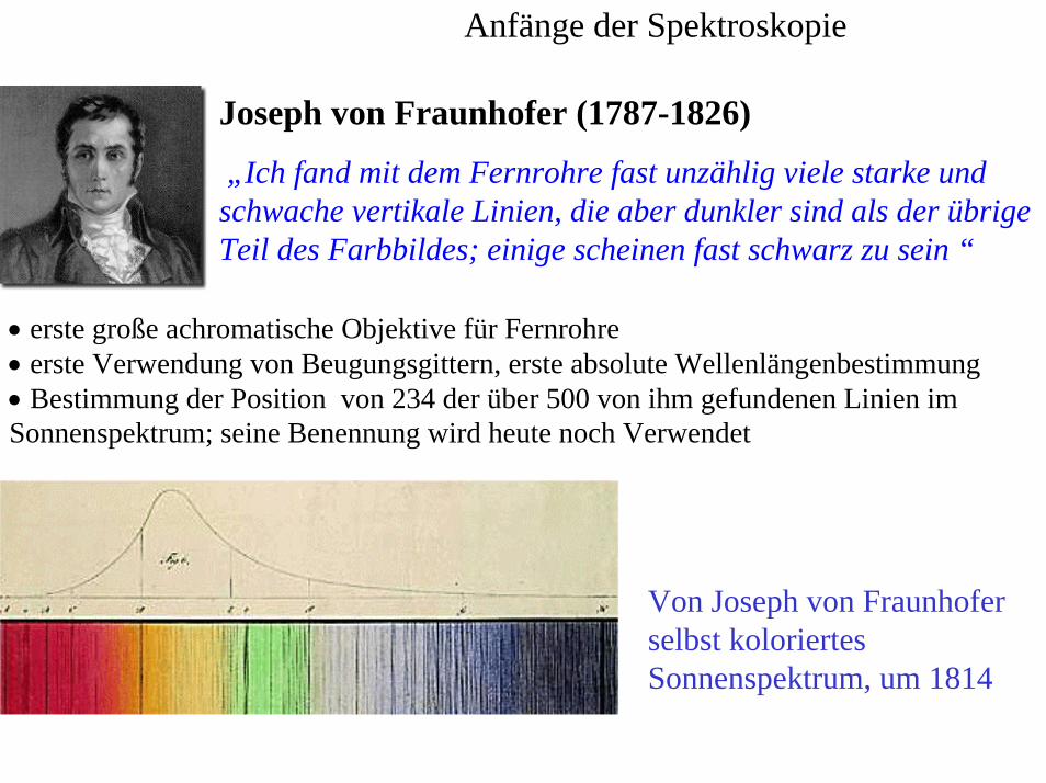
Anfänge der Spektroskopie
Joseph von Fraunhofer (1787-1826)
„Ich fand mit dem Fernrohre fast unzählig viele starke und schwache vertikale Linien, die aber dunkler sind als der übrige Teil des Farbbildes; einige scheinen fast schwarz zu sein “
• erste große achromatische Objektive für Fernrohre• erste Verwendung von Beugungsgittern, erste absolute Wellenlängenbestimmung• Bestimmung der Position von 234 der über 500 von ihm gefundenen Linien im Sonnenspektrum; seine Benennung wird heute noch Verwendet
Von Joseph von Fraunhofer selbst koloriertes Sonnenspektrum, um 1814
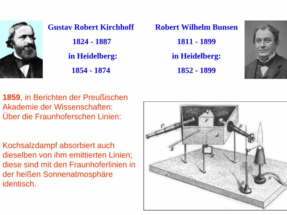
Gustav Robert Kirchhoff
1824 - 1887
in Heidelberg:
1854 - 1874
Robert Wilhelm Bunsen
1811 - 1899
in Heidelberg:
1852 - 1899
1859, in Berichten der Preußischen Akademie der Wissenschaften: Über die Fraunhoferschen Linien:
Kochsalzdampf absorbiert auch dieselben von ihm emittierten Linien; diese sind mit den Fraunhoferlinien in der heißen Sonnenatmosphäre identisch.

Ozon Wirkungsquerschnitt
1880, Hartley:
UV Ozonabsorption
1882, Chappuis:
vis Ozonabsorption
1890, Huggins
Liniengruppe Spektrum des Sirius (langwellige UV Absorption des Ozon)
200 400 600 800Wavelength [nm]
1E-23
1E-22
1E-21
1E-20
1E-19
1E-18
1E-17
[cm
]
Hartley Hug
gins
Chappuis
310 330 3501E-22
1E-21
1E-20
1E-19
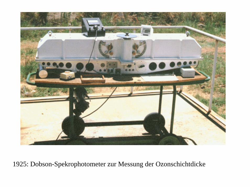
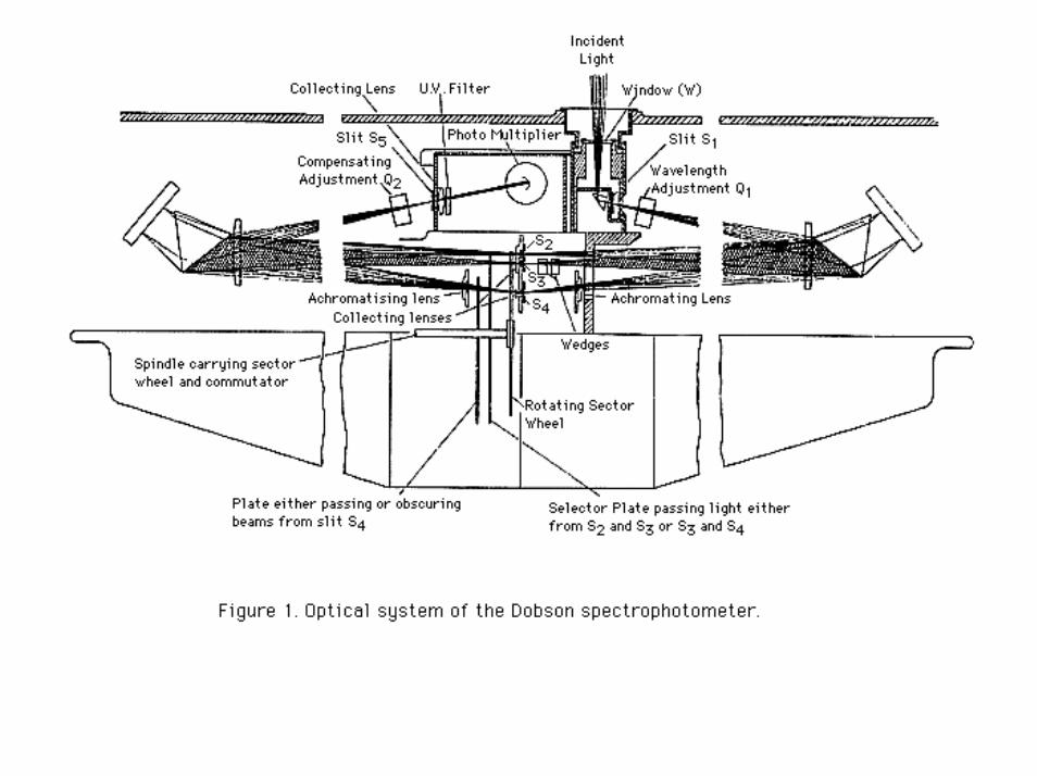
1925: Dobson-Spekrophotometer zur Messung der Ozonschichtdicke
300 310 320 330 340 350Wellenlänge [nm]
0E+0
1E-19
2E-19
3E-19O
3-Ab
sorp
tions
quer
schn
itt [c
m]
AB
CD
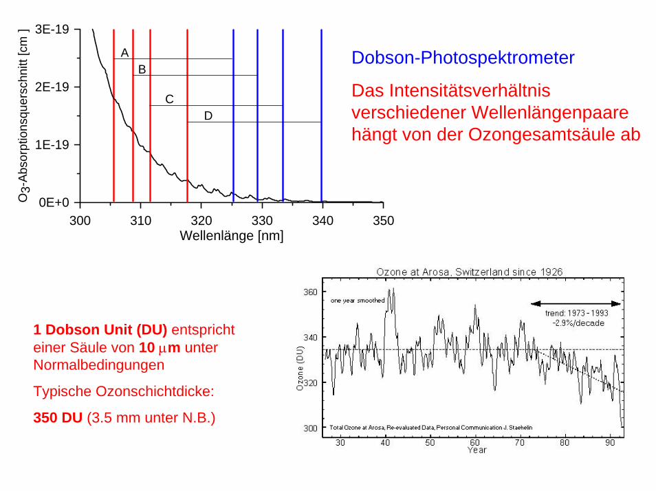
Dobson-Photospektrometer
Das Intensitätsverhältnis verschiedener Wellenlängenpaare hängt von der Ozongesamtsäule ab
1 Dobson Unit (DU) entspricht einer Säule von 10 µm unter Normalbedingungen
Typische Ozonschichtdicke:
350 DU (3.5 mm unter N.B.)
⎭⎬⎫
⎩⎨⎧
⋅⎟⎠
⎞⎜⎝
⎛+−⋅= ∫ ∑
l
si
ii dssII0
0 )()()(exp)()( λερλσλλ
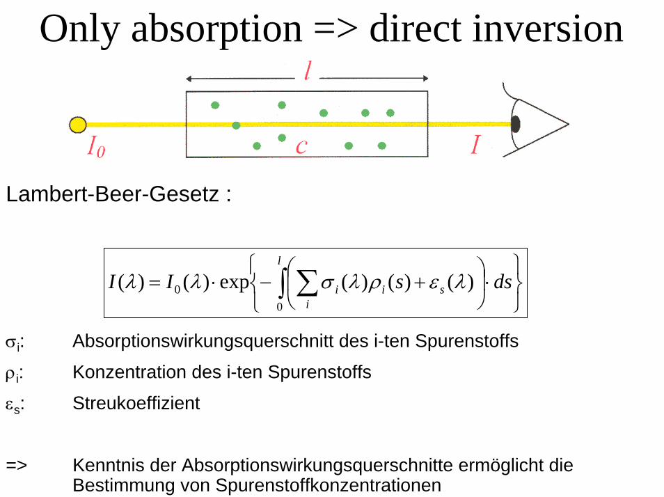
Lambert-Beer-Gesetz :
σi: Absorptionswirkungsquerschnitt des i-ten Spurenstoffs
ρi: Konzentration des i-ten Spurenstoffs
εs: Streukoeffizient
=> Kenntnis der Absorptionswirkungsquerschnitte ermöglicht die Bestimmung von Spurenstoffkonzentrationen
Only absorption => direct inversion
IC
I'0
I3
I1
λ3λ2λ1
I0
Inte
nsity
[arb
. Uni
ts]
Wavelength [arb. Units]
σ3
σ1
σ2
λ3λ2λ1
σdiff
Wavelength [arb. Units]
Cro
ss s
ectio
n [a
rb. U
nits
]
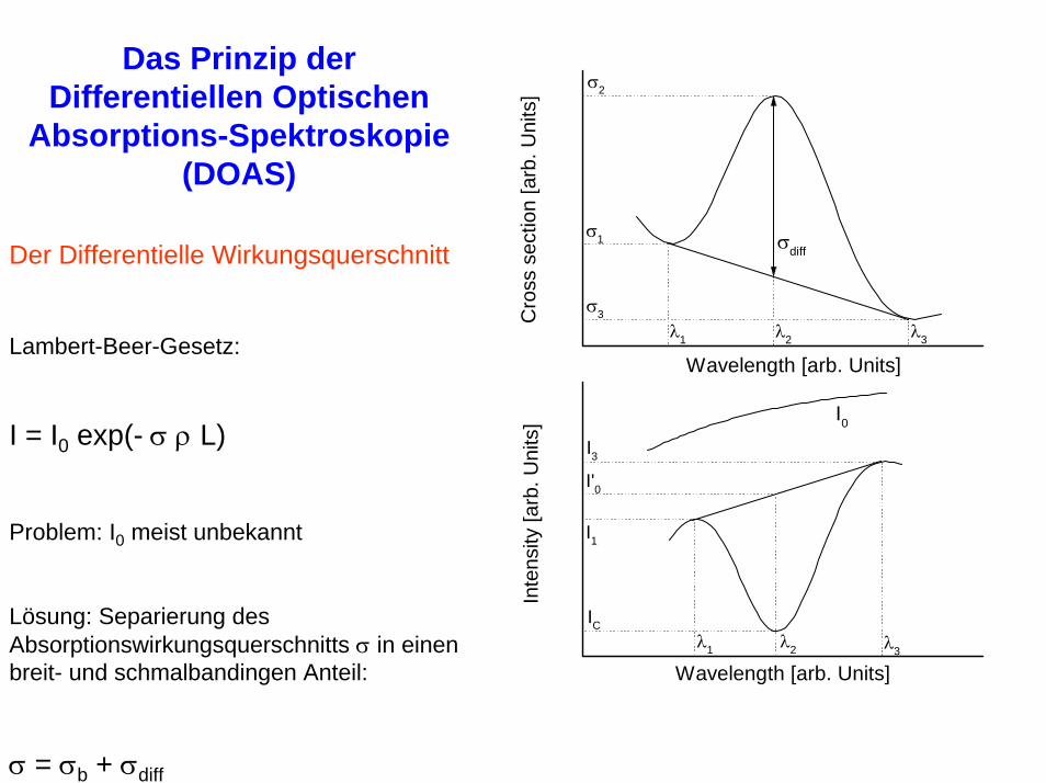
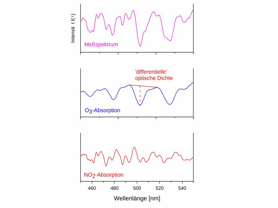
Der Differentielle Wirkungsquerschnitt
Lambert-Beer-Gesetz:
I = I0 exp(- σ ρ L)
Problem: I0 meist unbekannt
Lösung: Separierung des Absorptionswirkungsquerschnitts σ in einen breit- und schmalbandingen Anteil:
σ = σb + σdiff
Das Prinzip der Differentiellen Optischen
Absorptions-Spektroskopie(DOAS)
460 480 500 520 540
Wellenlänge [nm]
Inte
nsit
t I(
)
O3-Absorption
NO2-Absorption
Meßspektrum
'differentielle'optische Dichte
250 300 350 400 450 600 650 7000
100200
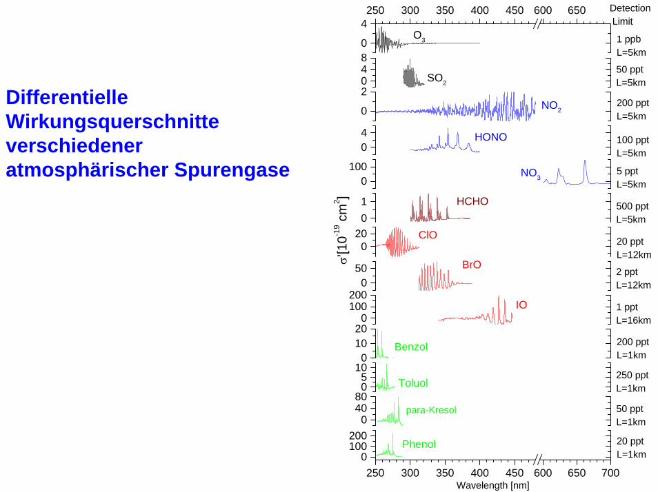
Detection Limit
200 pptL=1km
1 pptL=16km
2 pptL=12km
20 pptL=12km
500 pptL=5km
5 pptL=5km
100 pptL=5km
200 pptL=5km
1 ppbL=5km
Phenol
Wavelength [nm]
04080
20 pptL=1km
50 pptL=1km
250 pptL=1km
para-Kresol
05
10
Toluol
01020
Benzol
0100200
IO
050 BrO
020 ClO
01
HCHO
0100 NO3
04
HONO
0
2NO2
048
SO2
0
4250 300 350 400 450 600 650
50 pptL=5km
σ'[1
0-19 c
m2 ]
O3
Differentielle Wirkungsquerschnitte verschiedener atmosphärischer Spurengase
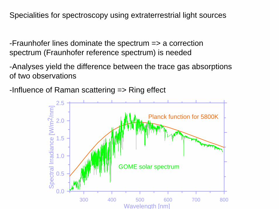
Specialities for spectroscopy using extraterrestrial light sources
-Fraunhofer lines dominate the spectrum => a correction spectrum (Fraunhofer reference spectrum) is needed
-Analyses yield the difference between the trace gas absorptions of two observations
-Influence of Raman scattering => Ring effect
300 400 500 600 700 800Wavelength [nm]
0.0
0.5
1.0
1.5
2.0
2.5
Spec
tral I
rradi
ance
[W/m
2 /nm
]
GOME solar spectrum
Planck function for 5800K
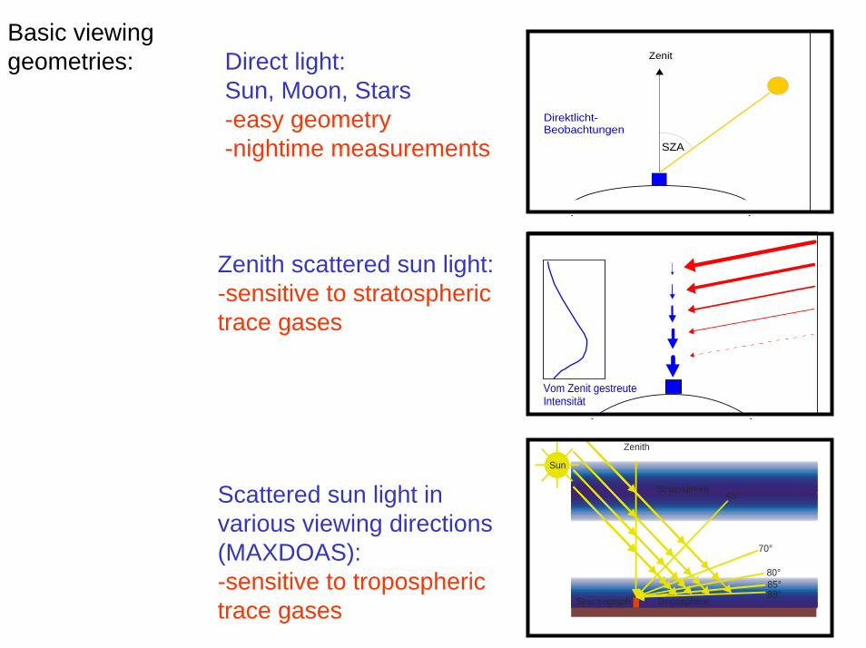
Basic viewing geometries: Zenit
SZA
Direktlicht-Beobachtungen
Vom Zenit gestreute Intensität
Direct light:Sun, Moon, Stars-easy geometry-nightime measurements
Zenith scattered sun light:-sensitive to stratospheric trace gases
Spectrograph
Zenith
Sun
Stratosphere
Troposphere
45°
70°
80°85°88°
Scattered sun light in various viewing directions(MAXDOAS):-sensitive to tropospheric trace gases
400 500 600 700
Wavelength [nm]
Inte
nsity
[arb
itr. u
nits
]
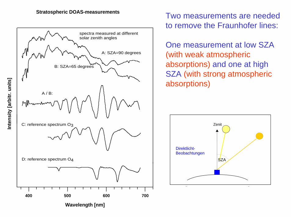
spectra measured at different solar zenith angles
A: SZA=90 degrees
B: SZA=65 degrees
A / B:
C: reference spectrum O3
D: reference spectrum O4
Stratospheric DOAS-measurements Two measurements are needed to remove the Fraunhofer lines:
One measurement at low SZA (with weak atmospheric absorptions) and one at high SZA (with strong atmospheric absorptions)
Zenit
SZA
Direktlicht-Beobachtungen
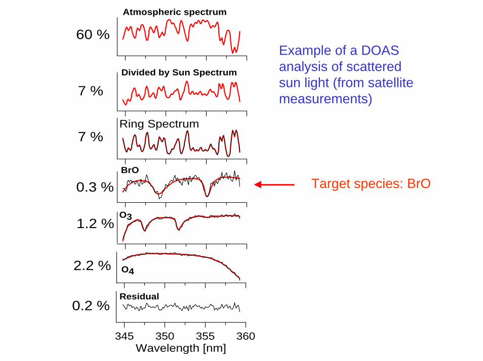
345 350 355 360Wavelength [nm]
BrO
O3
O4
Residual
Atmospheric spectrum
Divided by Sun Spectrum
60 %
Ring Spectrum
7 %
7 %
0.3 %
0.2 %
1.2 %
2.2 %
Example of a DOAS analysis of scattered sun light (from satellite measurements)
Target species: BrO
440 460 480 500 520 540 560-0.05
-0.03
-0.01
0.01
0.03
365 370 375 380 385 390-0.061
-0.059
-0.057
-0.055
-0.053
365 370 375 380 385 390-0.005
-0.003
-0.001
0.001
Opt
ical
den
sity
348 352 356 360Wavelength [nm]
-0.004
-0.003
-0.002
-0.001
0.000
0.001
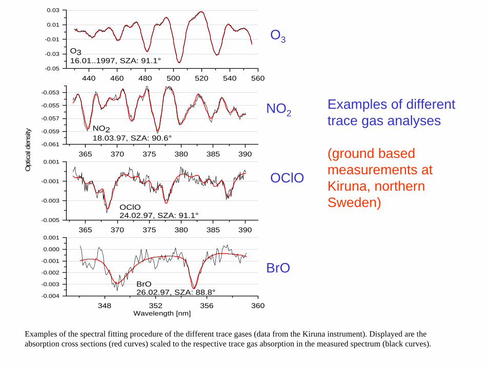
O316.01..1997, SZA: 91.1°
NO218.03.97, SZA: 90.6°
OClO24.02.97, SZA: 91.1°
BrO26.02.97, SZA: 88.8°
O3
NO2
OClO
BrO
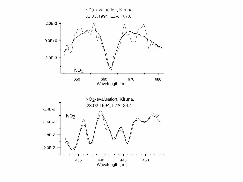
Examples of different trace gas analyses
(ground based measurements at Kiruna, northern Sweden)
Examples of the spectral fitting procedure of the different trace gases (data from the Kiruna instrument). Displayed are the absorption cross sections (red curves) scaled to the respective trace gas absorption in the measured spectrum (black curves).
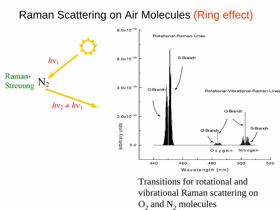
Raman Scattering on Air Molecules (Ring effect)
Transitions for rotational and vibrational Raman scattering on O2 and N2 molecules
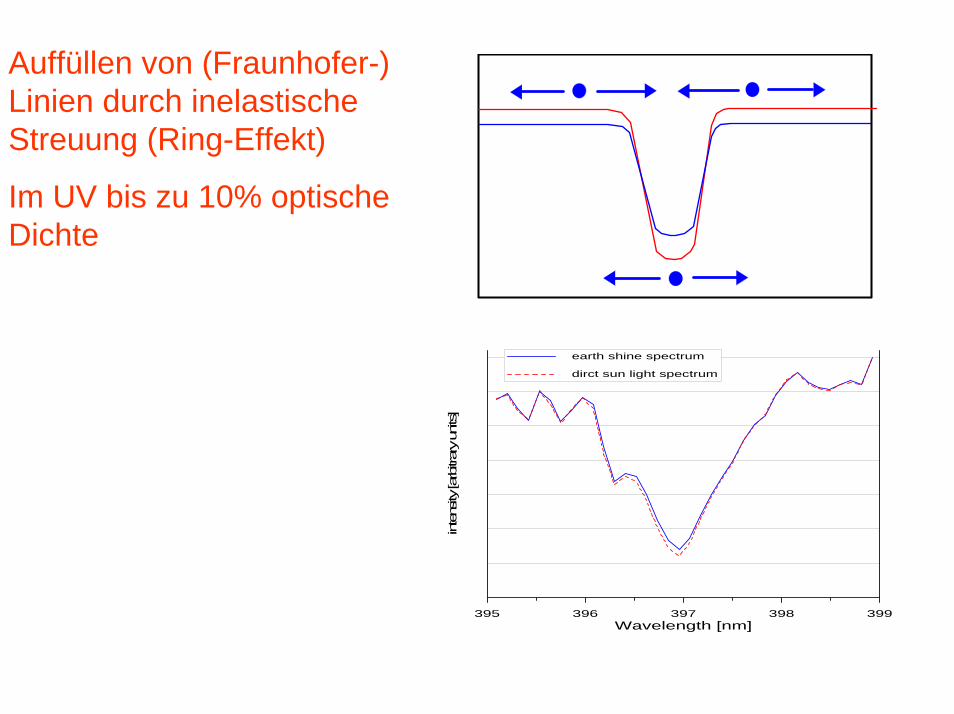
Auffüllen von (Fraunhofer-) Linien durch inelastischeStreuung (Ring-Effekt)
Im UV bis zu 10% optische Dichte
395 396 397 398 399Wavelength [nm]
intens
ity [a
rbitrar
y un
its]
earth shine spectrum
dirct sun light spectrum
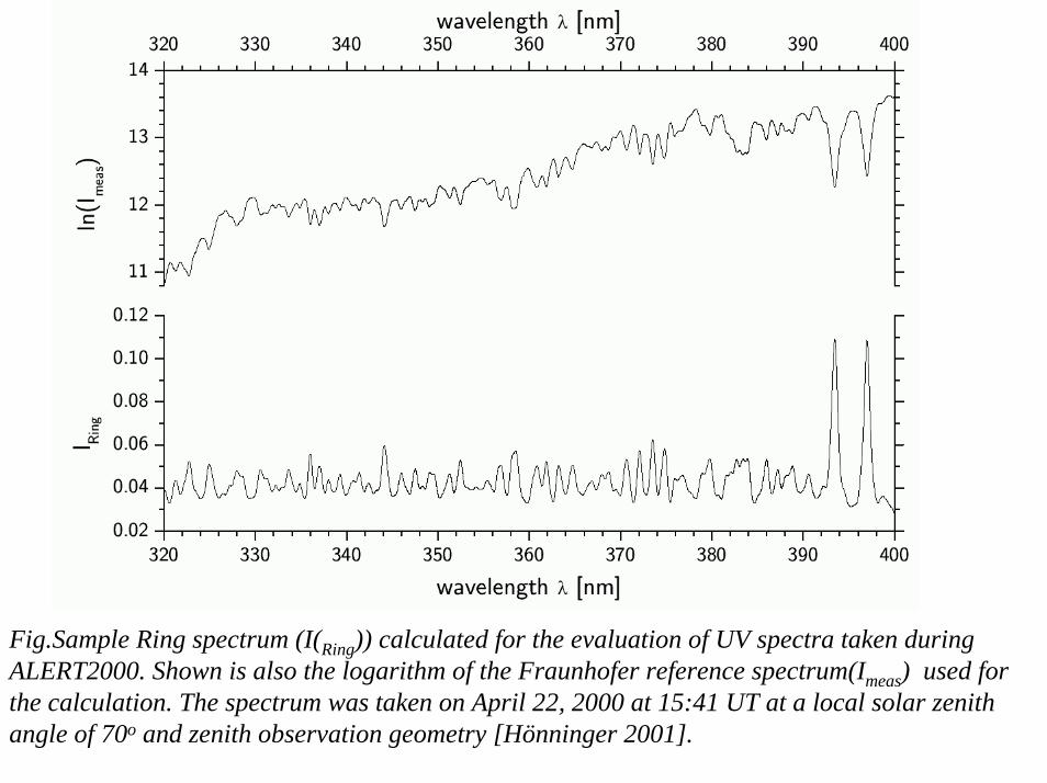
Fig.Sample Ring spectrum (I(Ring)) calculated for the evaluation of UV spectra taken during ALERT2000. Shown is also the logarithm of the Fraunhofer reference spectrum(Imeas) used for the calculation. The spectrum was taken on April 22, 2000 at 15:41 UT at a local solar zenith angle of 70o and zenith observation geometry [Hönninger 2001].

The DOAS spectroscopy yields the integrated concentration along the light path
τ−⋅= eII 0Lambert-Beer‘s law:
=>
with:
=>
if concentration c is constant along light path:
∫ ⋅⋅==⎟⎠⎞
⎜⎝⎛ dsc
II στ0ln
∫ ⋅= dscSCD
στ
=SCD
scSCD ⋅=
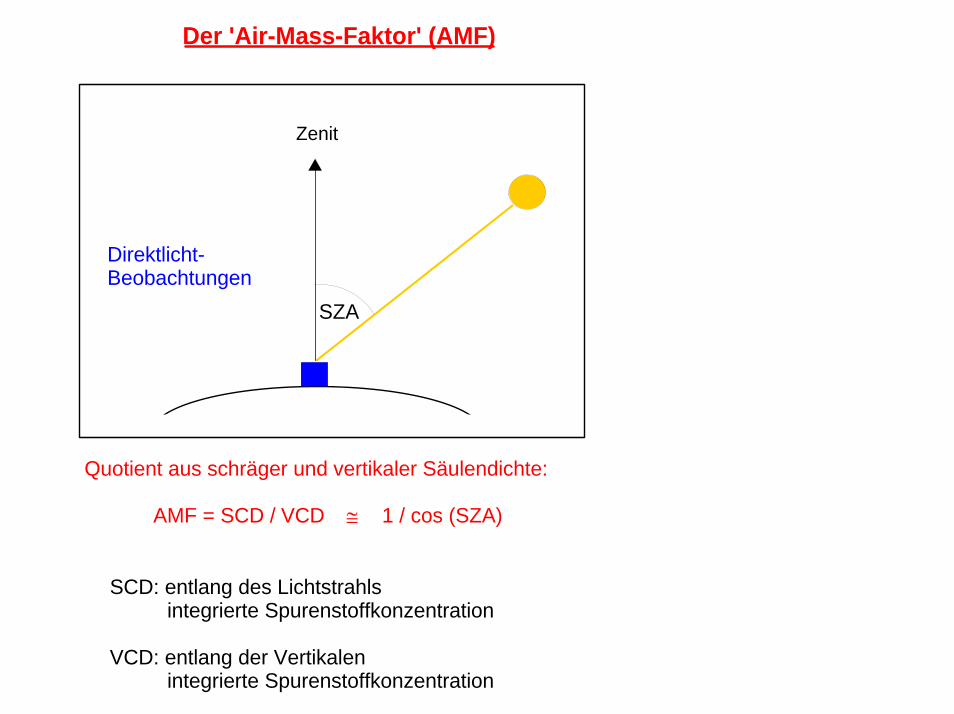
Der 'Air-Mass-Faktor' (AMF)
Zenit
SZA
SCD: entlang des Lichtstrahls integrierte Spurenstoffkonzentration
VCD: entlang der Vertikalen integrierte Spurenstoffkonzentration
Quotient aus schräger und vertikaler Säulendichte:
AMF = SCD / VCD 1 / cos (SZA)
Direktlicht-Beobachtungen

Zenit
SZA
Direktlicht-Beobachtungen
The measured SCD is the difference between both measurements:∆SCD = SCDmess – SCDref
= VCD*AMFmess – VCD*AMFref
=> VCD = ∆SCD / (AMFmess- AMFref)
0 5 10 15 20 25AMF
0
5000
10000
SCD
O3[
DU
]
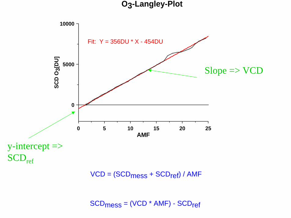
Fit: Y = 356DU * X - 454DU
O3-Langley-Plot
VCD = (SCDmess + SCDref) / AMF
SCDmess = (VCD * AMF) - SCDref
Slope => VCD
y-intercept => SCDref
Direct light observations
-light source: sun, moon or star
-direct light path, easy interpretation of the measurement
-complex instrumental set-up, tracking system
-night-time chemistry can be investigated
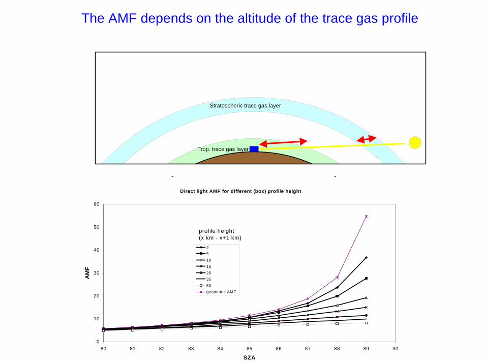
The AMF depends on the altitude of the trace gas profile
Direct light AMF for different (box) profile height
0
10
20
30
40
50
60
80 81 82 83 84 85 86 87 88 89 90
SZA
AM
F
251016263550geometric AMF
profile height(x km - x+1 km)
Stratospheric trace gas layer
Trop. trace gas layer
435 440 445 450Wavelength [nm]
-2.0E-2
-1.8E-2
-1.6E-2
-1.4E-2
650 660 670 680Wavelength [nm]
-2.0E-3
0.0E+0
2.0E-3
NO3
NO2
NO2-evaluation, Kiruna, 23.02.1994, LZA: 84.4°
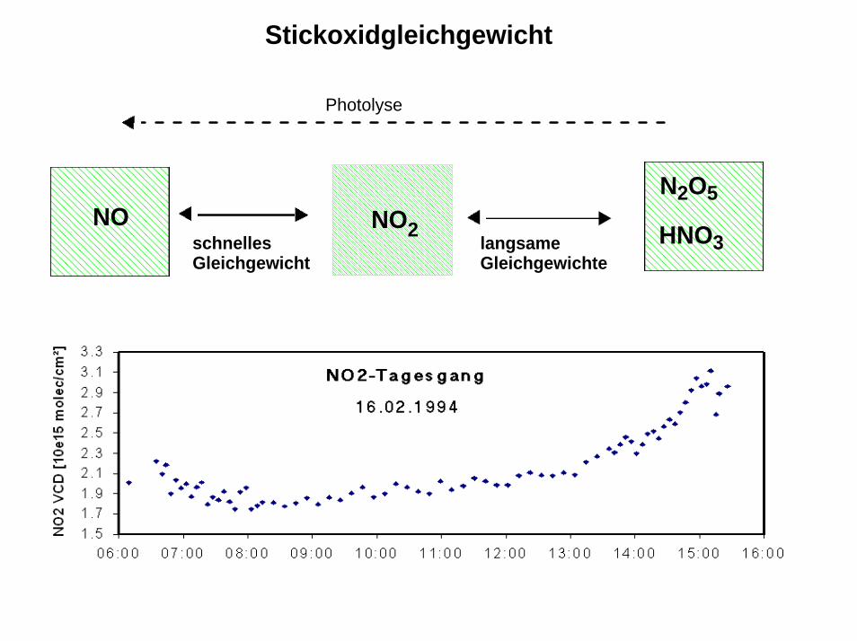
NO NO2
N2O5
HNO3langsameGleichgewichte
schnellesGleichgewicht
Stickoxidgleichgewicht
Photolyse
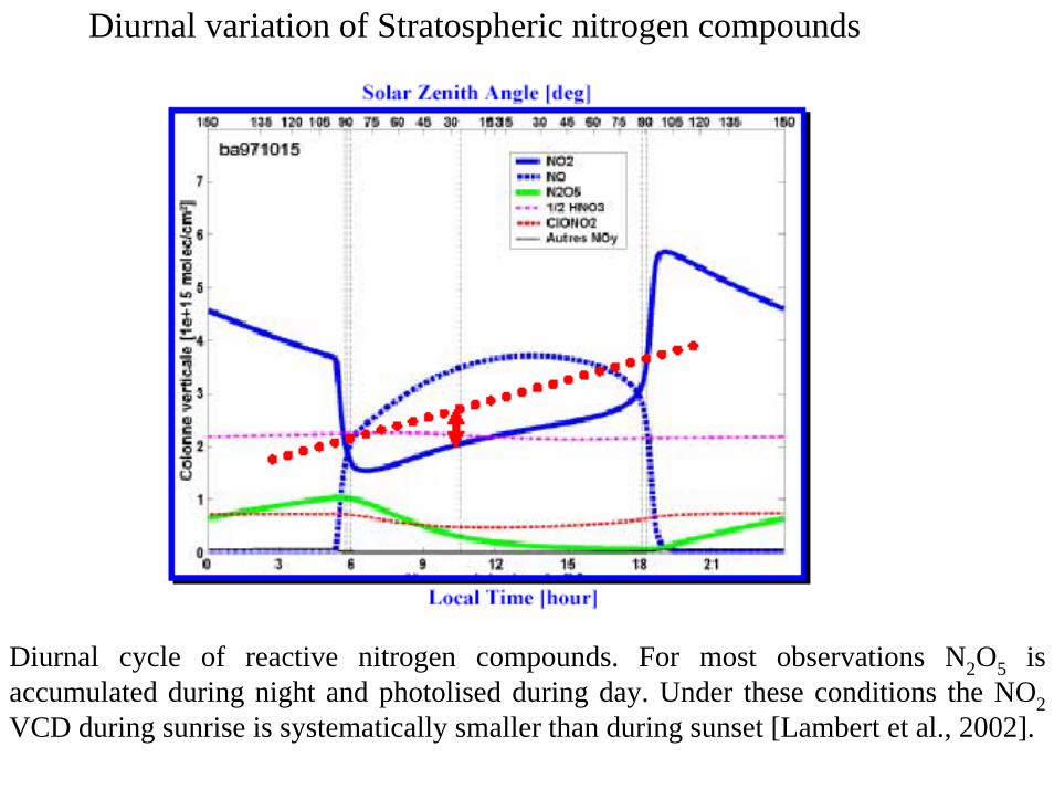
Diurnal variation of Stratospheric nitrogen compounds
Diurnal cycle of reactive nitrogen compounds. For most observations N2O5 is accumulated during night and photolised during day. Under these conditions the NO2VCD during sunrise is systematically smaller than during sunset [Lambert et al., 2002].
1/25/94 04:48 1/25/94 16:48 1/26/94 04:48 1/26/94 16:48
0
1
2
3
4
VCD
NO
3 [1
013 m
olec
/cm
]
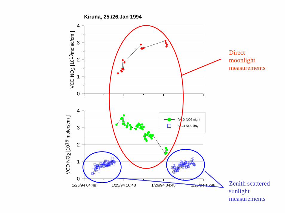
Kiruna, 25./26.Jan 1994
0
1
2
3
4
VCD
NO
2 [1
015
mol
ec/c
m]
VCD NO2 night
VCD NO2 day
Direct moonlight measurements
Zenith scattered sunlight measurements
0 10 20 30
0 4 8 12 16
0 4 8 12 16
SCD
NO
3
0 4 8 12
0 4 8 12AMF
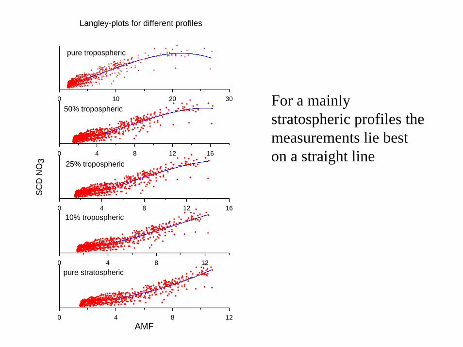
Langley-plots for different profiles
pure tropospheric
50% tropospheric
25% tropospheric
10% tropospheric
pure stratospheric
For a mainly stratospheric profiles the measurements lie best on a straight line

Langley-plot for different absorption bands
O4 moon light observations, Kiruna, 1994
O4 absorption, direct moon measurements, Kiruna, 29.01.1994
-0.1
-0.08
-0.06
-0.04
-0.02
0
340 390 440 490 540 590 640 690
Wavelength [nm]
Opt
ical
dep
th
Spectrum 1: 29.01., 5:46 UT, LZA: 81.8°Spectrum 2: 26.01., 23:40 UT, LZA: 53.1°
2 4 6 8 10 12AMF
0.00
0.01
0.02
0.000
0.005
0.010
0.015
0.00
0.04
0.08
0.12
-0.01
0.00
0.01
0.02
Opt
ical
dep
th0.00
0.06
0.12
0.18
0.00
0.04
0.08
0.12
630 nm, slope: 0.0121269R-squared = 0.997629
577 nm, slope: 0.0170016R-squared = 0.997599
530 nm, slope: 0.00218741R-squared = 0.937879
477 nm, slope: 0.00982482R-squared = 0.997355
380 nm, slope: 0.00307024R-squared = 0.909493
360 nm, slope: 0.00718113R-squared = 0.991984
Only little moon lightin the UV
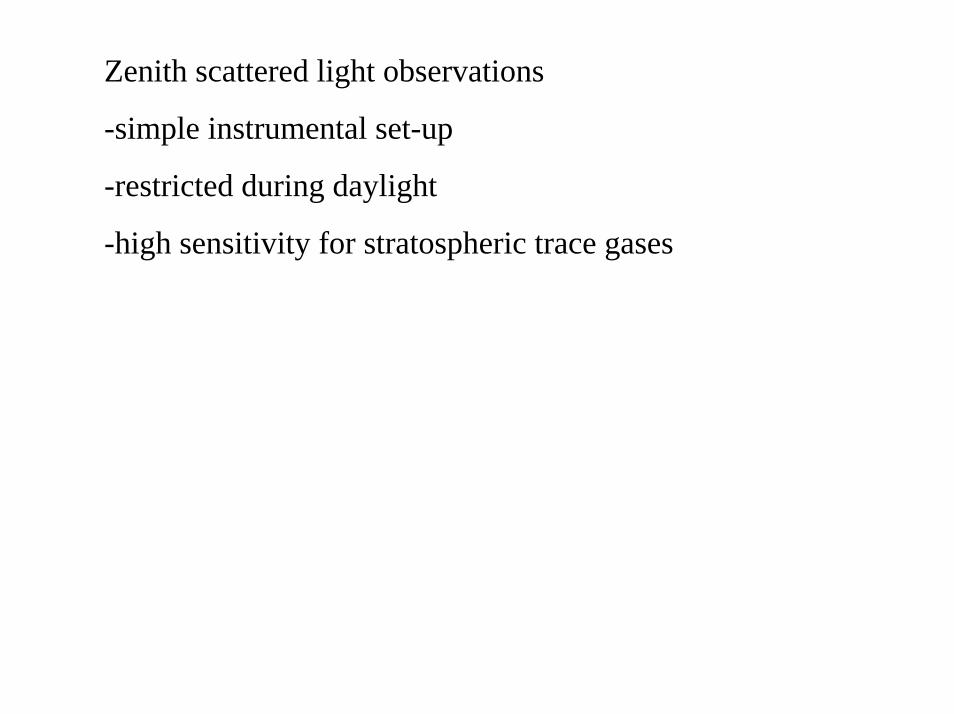
Zenith scattered light observations
-simple instrumental set-up
-restricted during daylight
-high sensitivity for stratospheric trace gases
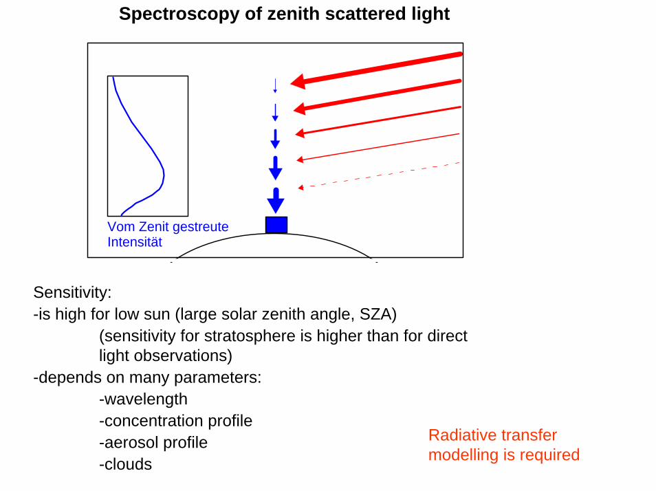
Spectroscopy of zenith scattered light
Vom Zenit gestreute Intensität
Radiative transfer modelling is required
Sensitivity:-is high for low sun (large solar zenith angle, SZA)
(sensitivity for stratosphere is higher than for direct light observations)
-depends on many parameters:-wavelength-concentration profile-aerosol profile-clouds
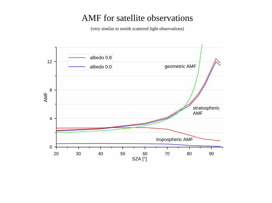
AMF for satellite observations (very similar to zenith scattered light observations)
20 30 40 50 60 70 80 90SZA [°]
0
4
8
12
AMF
albedo 0.8
albedo 0.0
stratospheric AMF
tropospheric AMF
geometric AMF
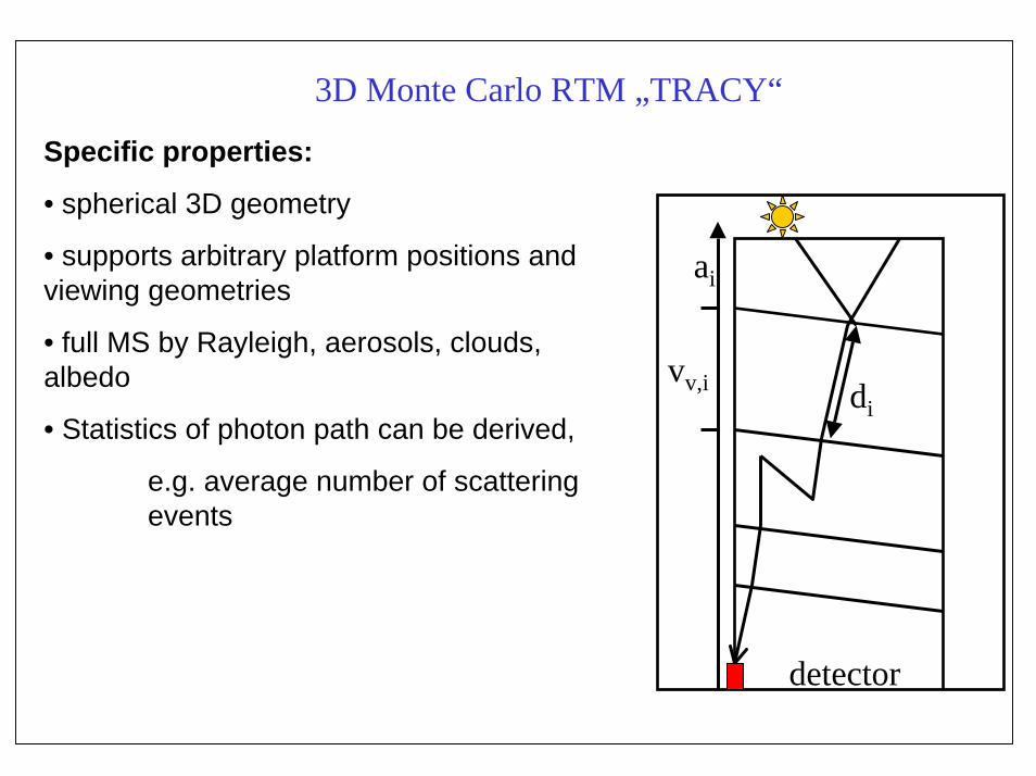
3D Monte Carlo RTM „TRACY“
di
ai
detector
Specific properties:
• spherical 3D geometry
• supports arbitrary platform positions and viewing geometries
• full MS by Rayleigh, aerosols, clouds, albedo
• Statistics of photon path can be derived,
e.g. average number of scattering events
vv,i
Instrument
Instrument
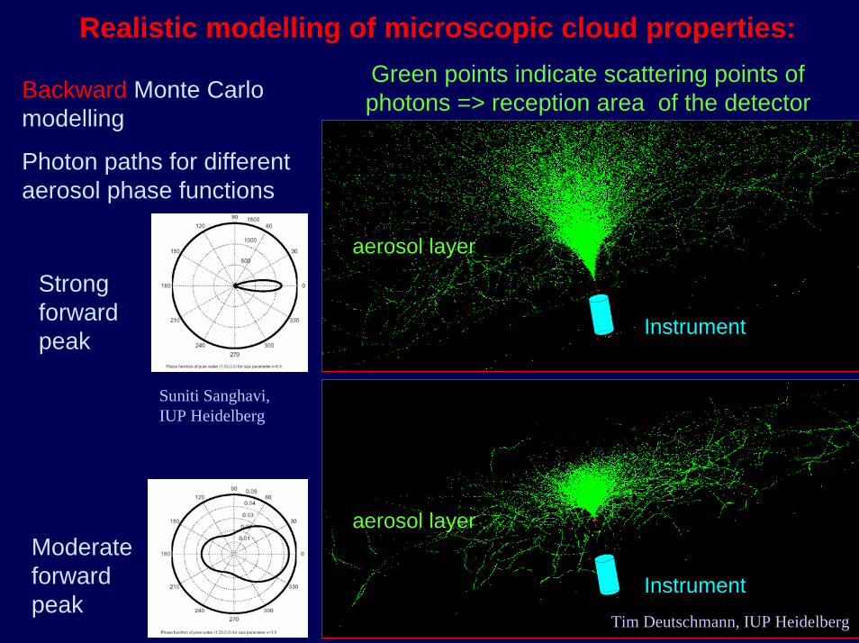
Green points indicate scattering points of photons => reception area of the detectorBackward Monte Carlo
modelling
Photon paths for different aerosol phase functions
Strong forward peak
Moderateforward peak
Suniti Sanghavi, IUP Heidelberg
Tim Deutschmann, IUP Heidelberg
Realistic modelling of microscopic cloud properties:
aerosol layer
aerosol layer
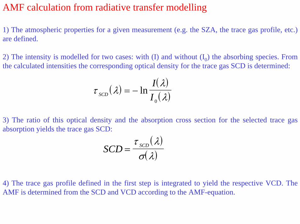
AMF calculation from radiative transfer modelling
1) The atmospheric properties for a given measurement (e.g. the SZA, the trace gas profile, etc.) are defined.
2) The intensity is modelled for two cases: with (I) and without (I0) the absorbing species. From the calculated intensities the corresponding optical density for the trace gas SCD is determined:
3) The ratio of this optical density and the absorption cross section for the selected trace gas absorption yields the trace gas SCD:
4) The trace gas profile defined in the first step is integrated to yield the respective VCD. The AMF is determined from the SCD and VCD according to the AMF-equation.
( )( )( )τ λλλSCD
II
= − ln0
( )( )SCD SCD=
τ λσ λ
Jan-01 Jan-02 Jan-03 Jan-04 Jan-05
Kiruna
Paramaribo
Neumayer
Arrival HeigtsMAXDOAS
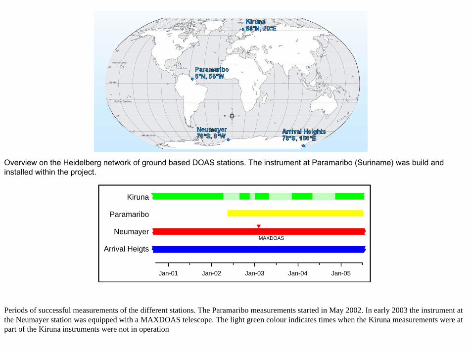
Overview on the Heidelberg network of ground based DOAS stations. The instrument at Paramaribo (Suriname) was build and installed within the project.
Periods of successful measurements of the different stations. The Paramaribo measurements started in May 2002. In early 2003 the instrument at the Neumayer station was equipped with a MAXDOAS telescope. The light green colour indicates times when the Kiruna measurements were at part of the Kiruna instruments were not in operation
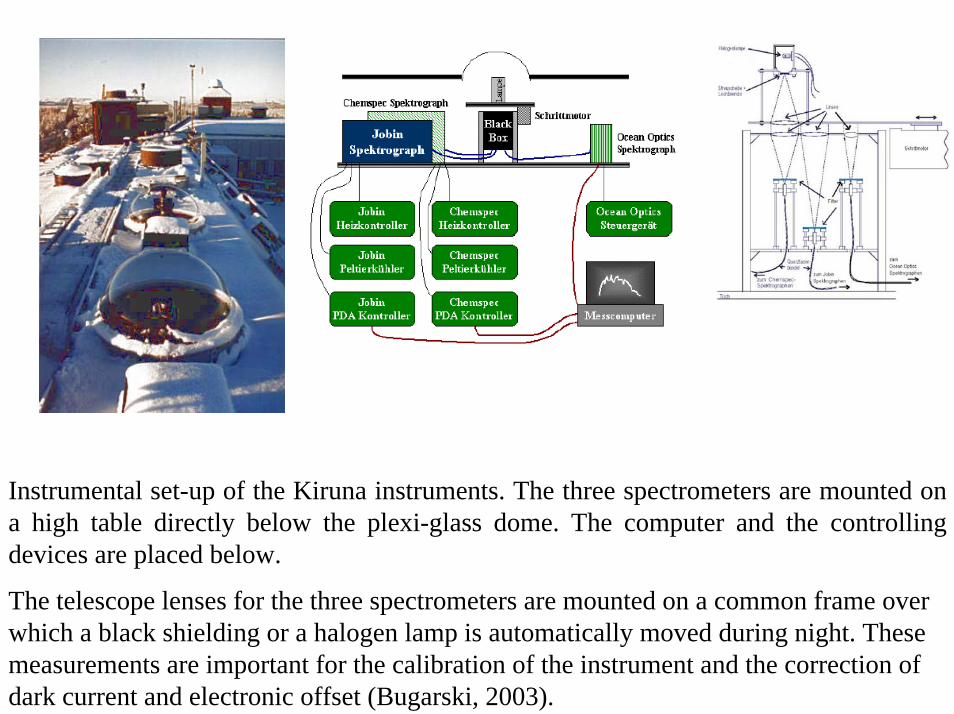
Instrumental set-up of the Kiruna instruments. The three spectrometers are mounted on a high table directly below the plexi-glass dome. The computer and the controlling devices are placed below.
The telescope lenses for the three spectrometers are mounted on a common frame over which a black shielding or a halogen lamp is automatically moved during night. These measurements are important for the calibration of the instrument and the correction of dark current and electronic offset (Bugarski, 2003).

4:48 7:12 9:36 12:00 14:24 16:48Zeit
0
4000
8000
SCD
O3
[DU
]
0
100
200
300
400
VCD
O3
[DU
]
O3-Auswertung
Opt
isch
e D
icht
e [
rel.
Einh
eite
n]
O3-Fitergebnis
Tagesgang, Kiruna, 11.03.1994
SCD O3
VCD O3
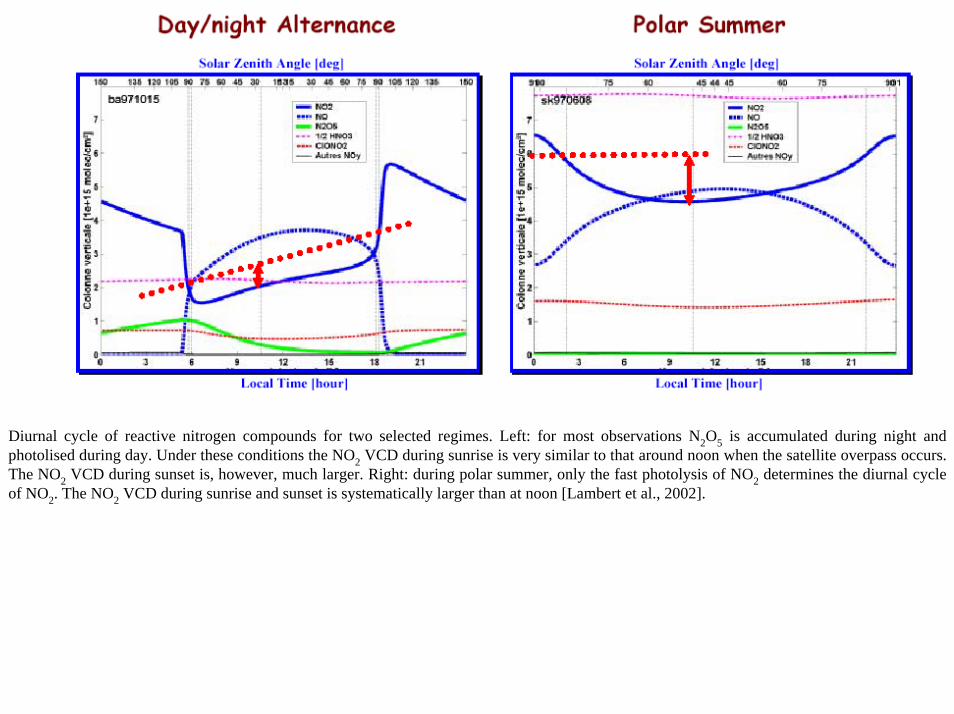
Diurnal cycle of reactive nitrogen compounds for two selected regimes. Left: for most observations N2O5 is accumulated during night and photolised during day. Under these conditions the NO2 VCD during sunrise is very similar to that around noon when the satellite overpass occurs. The NO2 VCD during sunset is, however, much larger. Right: during polar summer, only the fast photolysis of NO2 determines the diurnal cycle of NO2. The NO2 VCD during sunrise and sunset is systematically larger than at noon [Lambert et al., 2002].
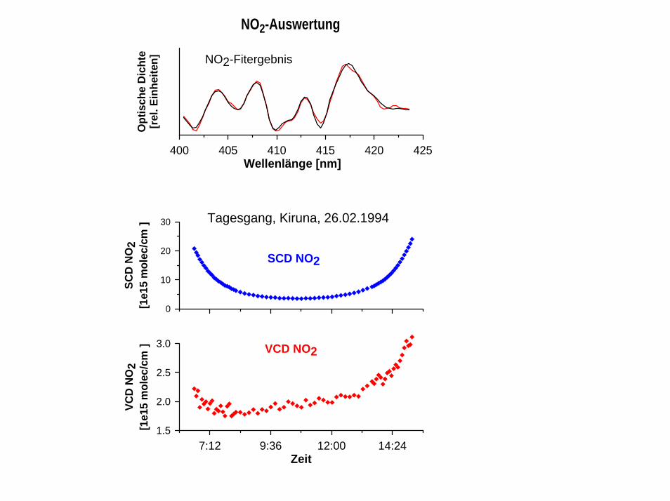
400 405 410 415 420 425Wellenlänge [nm]
Opt
isch
e D
icht
e[r
el. E
inhe
iten]
NO2-Auswertung
7:12 9:36 12:00 14:24Zeit
0
10
20
30
SCD
NO
2[1
e15
mol
ec/c
m]
1.5
2.0
2.5
3.0
VCD
NO
2[1
e15
mol
ec/c
m]
Tagesgang, Kiruna, 26.02.1994
SCD NO2
VCD NO2
NO2-Fitergebnis
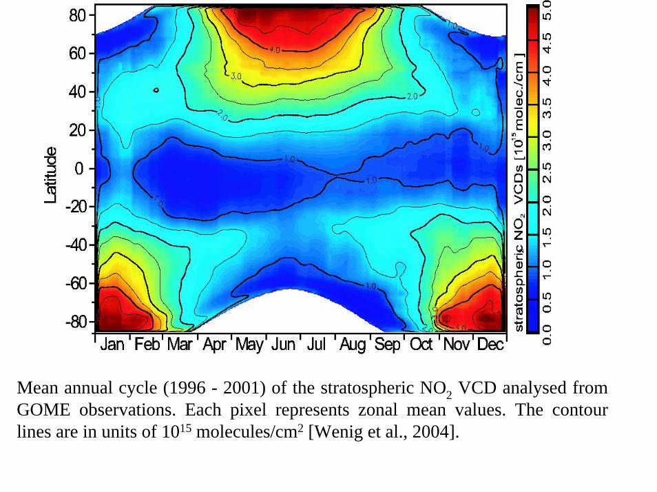
Mean annual cycle (1996 - 2001) of the stratospheric NO2 VCD analysed from GOME observations. Each pixel represents zonal mean values. The contour lines are in units of 1015 molecules/cm2 [Wenig et al., 2004].

0.0E+00
1.0E+15
2.0E+15
3.0E+15
4.0E+15
5.0E+15
6.0E+15
7.0E+15
8.0E+15
Nov. 96 Nov. 97 Nov. 98 Nov. 99 Nov. 00 Nov. 01 Nov. 02 Nov. 03 Nov. 04
Time
NO
2 VC
D [m
olec
/cm
²]
VCDReihe2Reihe3
Average NO2 VCD from SCIAMACHY at noonMAXDOAS NO2 VCD sunrise 90° SZAMAXDOAS NO2 VCD sunset 90° SZA
SCIAMACHY NO2 VCD © Andreas Richter
Time series of NO2 VCDs measured by the Kiruna instrument since December 1996. From 2002 to 2005 also the time series of average SCIAMACHY NO2 VCDs (within 200km, scientific product of the University of Bremen) are shown.
0.0E+00
1.0E+15
2.0E+15
3.0E+15
4.0E+15
5.0E+15
6.0E+15
7.0E+15
8.0E+15
Jan. 05 Feb. 05 Mrz. 05 Apr. 05 Mai. 05 Jun. 05
Time
NO
2 VC
D [m
olec
/cm
²]
VCDminReihe2Reihe3
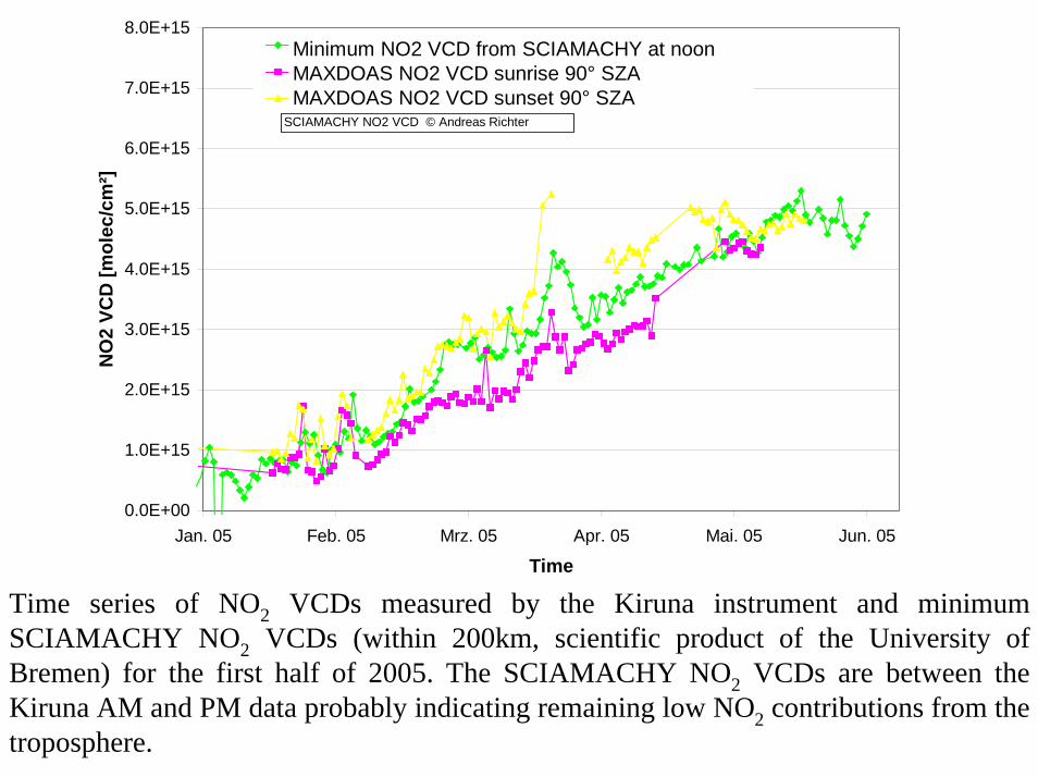
Minimum NO2 VCD from SCIAMACHY at noonMAXDOAS NO2 VCD sunrise 90° SZAMAXDOAS NO2 VCD sunset 90° SZA
SCIAMACHY NO2 VCD © Andreas Richter
Time series of NO2 VCDs measured by the Kiruna instrument and minimum SCIAMACHY NO2 VCDs (within 200km, scientific product of the University of Bremen) for the first half of 2005. The SCIAMACHY NO2 VCDs are between the Kiruna AM and PM data probably indicating remaining low NO2 contributions from the troposphere.
SpectrographUV
SpectrographVisible
Meteorological Office Building
ElectronicsComputer
Telescope
Quartz glassfiber bundles
Observation platform
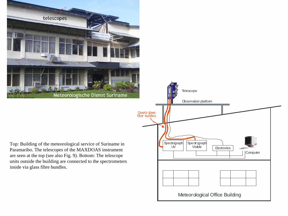
Top: Building of the meteorological service of Suriname in Paramaribo. The telescopes of the MAXDOAS instrument are seen at the top (see also Fig. 9). Bottom: The telescope units outside the building are connected to the spectrometers inside via glass fibre bundles.
SCIAMACHY NO2 VCD © Andreas Richter
0.0E+00
5.0E+14
1.0E+15
1.5E+15
2.0E+15
2.5E+15
3.0E+15
3.5E+15
4.0E+15
Apr. 02 Okt. 02 Apr. 03 Okt. 03 Apr. 04 Okt. 04 Apr. 05Time
NO
2 VC
D [m
olec
/cm
²]
VCDminReihe2Reihe3
Min NO2 VCD from SCIAMACHY at noonMAXDOAS NO2 VCD sunrise 90° SZAMAXDOAS NO2 VCD sunset 90° SZA
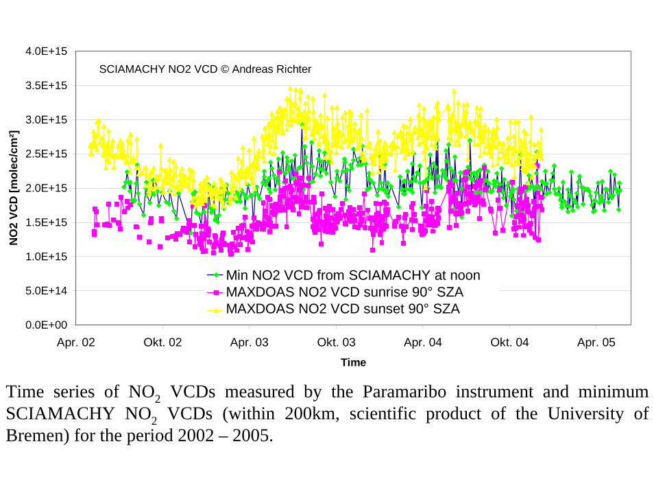
Time series of NO2 VCDs measured by the Paramaribo instrument and minimum SCIAMACHY NO2 VCDs (within 200km, scientific product of the University of Bremen) for the period 2002 – 2005.
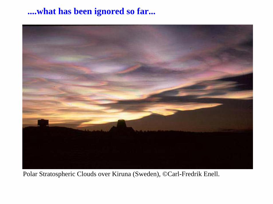
....what has been ignored so far...
Polar Stratospheric Clouds over Kiruna (Sweden), ©Carl-Fredrik Enell.
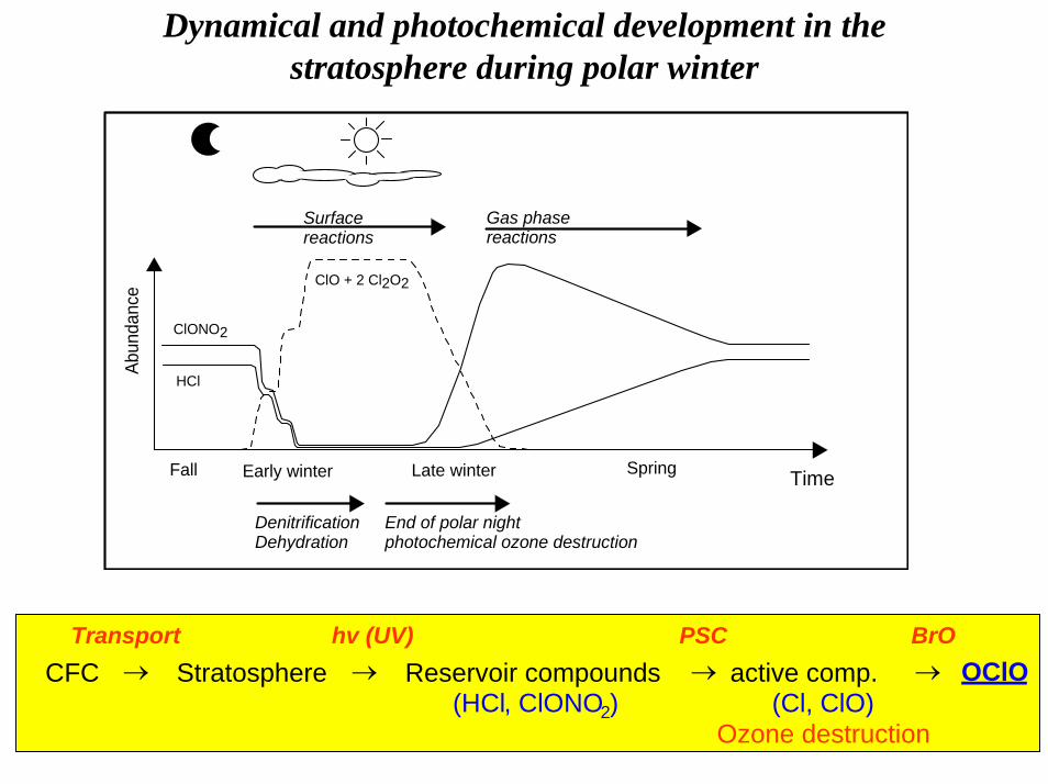
Dynamical and photochemical development in the stratosphere during polar winter
Abun
danc
e
Time
Surface reactions
Gas phasereactions
ClONO2
HCl
ClO + 2 Cl2O2
Fall Early winter Late winter Spring
End of polar nightphotochemical ozone destruction
DenitrificationDehydration
CFC → Stratosphere → Reservoir compounds → active comp. → OClO(HCl, ClONO2) (Cl, ClO)
Ozone destruction
Transport hv (UV) PSC BrO
-5 .0E +13
0.0E +00
5.0E +13
1.0E +14
1.5E +14
2.0E +14
2.5E +14
3.0E +14
Jan. 00 Jan. 01 Jan. 02 Jan. 03 Jan. 04 Jan. 05
Tim e
OC
lO D
SCD
[mol
ec/c
m²]
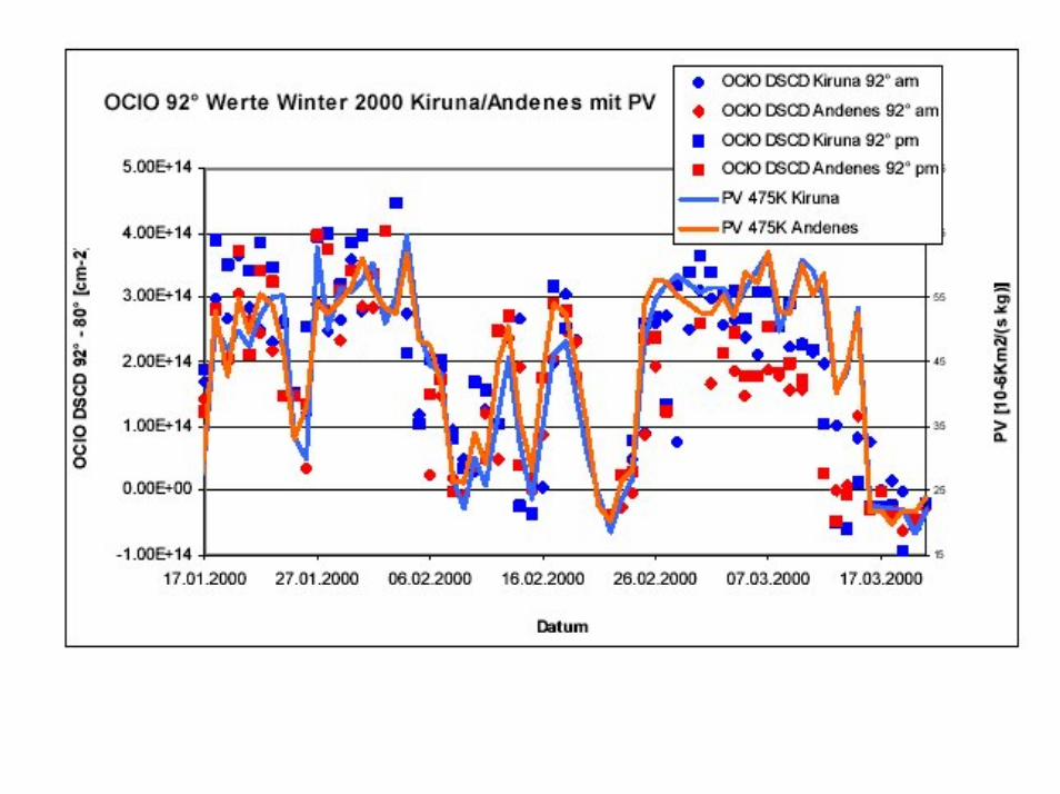
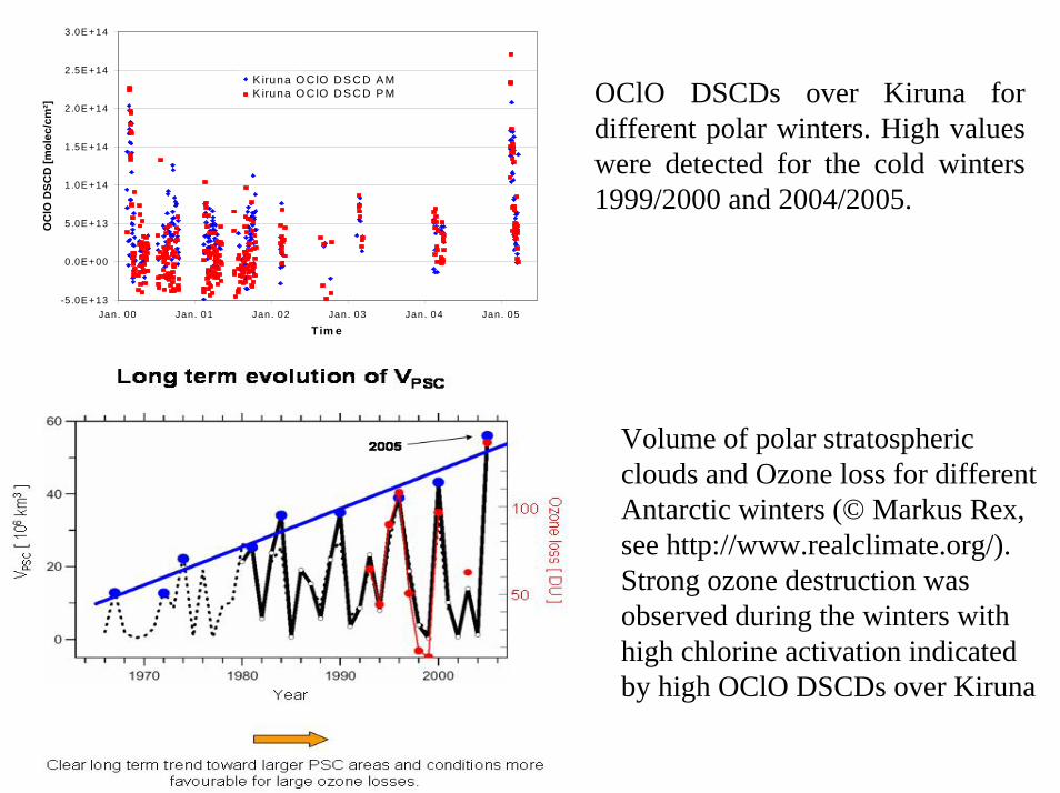
R eihe1R eihe2K iruna O C lO D S C D A MK iruna O C lO D S C D P M OClO DSCDs over Kiruna for
different polar winters. High values were detected for the cold winters 1999/2000 and 2004/2005.
Volume of polar stratospheric clouds and Ozone loss for different Antarctic winters (© Markus Rex, see http://www.realclimate.org/). Strong ozone destruction was observed during the winters with high chlorine activation indicated by high OClO DSCDs over Kiruna

01.01
.9901
.02.99
01.03
.9901
.04.99
01.05
.9901
.06.99
01.07
.9901
.08.99
01.09
.9901
.10.99
01.11
.9901
.12.99
01.01
.0001
.02.00
01.03
.0001
.04.00
01.05
.0001
.06.00
01.07
.0001
.08.00
01.09
.0001
.10.00
01.11
.0001
.12.00
01.01
.0101
.02.01
01.03
.0101
.04.01
01.05
.0101
.06.01
01.07
.0101
.08.01
01.09
.0101
.10.01
01.11
.0101
.12.01
01.01
.0201
.02.02
01.03
.0201
.04.02
01.05
.0201
.06.02
80100120140160180200220240260280300320340
DOAS (84°<=SZA<=90°) DOAS (88°<=SZA<=94°) Ozone soundings TOMS
VCD
O3 [
DU
]
Date
01.01
.9901
.02.99
01.03
.9901
.04.99
01.05
.9901
.06.99
01.07
.9901
.08.99
01.09
.9901
.10.99
01.11
.9901
.12.99
01.01
.0001
.02.00
01.03
.0001
.04.00
01.05
.0001
.06.00
01.07
.0001
.08.00
01.09
.0001
.10.00
01.11
.0001
.12.00
01.01
.0101
.02.01
01.03
.0101
.04.01
01.05
.0101
.06.01
01.07
.0101
.08.01
01.09
.0101
.10.01
01.11
.0101
.12.01
01.01
.0201
.02.02
01.03
.0201
.04.02
01.05
.0201
.06.02
0
1
2
3
4
5
6
7
am pmVC
D N
O2 [
1015
mol
ec/c
m2 ]
Date
180
190
200
210
220
230
240
250
Temperature @
50hPa [K]
01.01
.9901
.02.99
01.03
.9901
.04.99
01.05
.9901
.06.99
01.07
.9901
.08.99
01.09
.9901
.10.99
01.11
.9901
.12.99
01.01
.0001
.02.00
01.03
.0001
.04.00
01.05
.0001
.06.00
01.07
.0001
.08.00
01.09
.0001
.10.00
01.11
.0001
.12.00
01.01
.0101
.02.01
01.03
.0101
.04.01
01.05
.0101
.06.01
01.07
.0101
.08.01
01.09
.0101
.10.01
01.11
.0101
.12.01
01.01
.0201
.02.02
01.03
.0201
.04.02
01.05
.0201
.06.02
0
1
2
3
4
5
6
7
8
9
10 am, SZA = 90° pm, SZA = 90° am, SZA = 94° pm, SZA = 94°
SCD
OC
lO [1
014 m
olec
/cm
2 ]
Date
-20
-30
-40
-50
-60
-70
PV @ 475K (PVU
)
DOAS- Messungen auf der Neumayer- Station/Antarktis © Udo Frieß
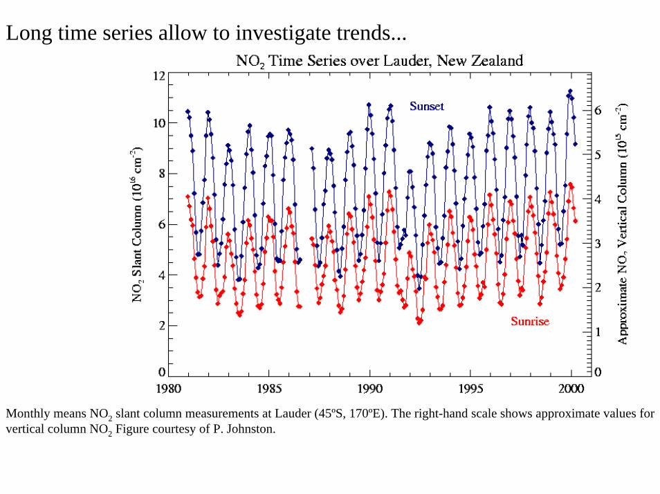
Long time series allow to investigate trends...
Monthly means NO2 slant column measurements at Lauder (45ºS, 170ºE). The right-hand scale shows approximate values for vertical column NO2 Figure courtesy of P. Johnston.

Effects of clouds I
-clouds change the colour of the sky
Example: influence of polar stratospheric clouds on the measured spectra
Colour index
Clouds make the sky more red88 90 92 94
SZA
0
4
8
12
Col
our i
ndex
January
March
blue
red
IICI =
Mie-Vielfach-Streuung
Spektrograph
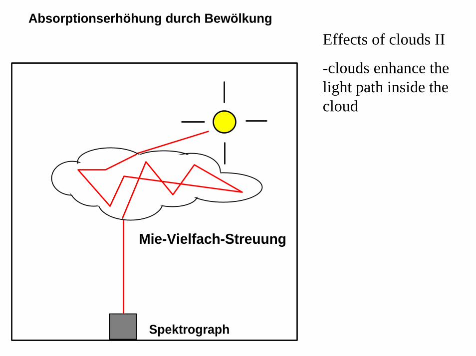
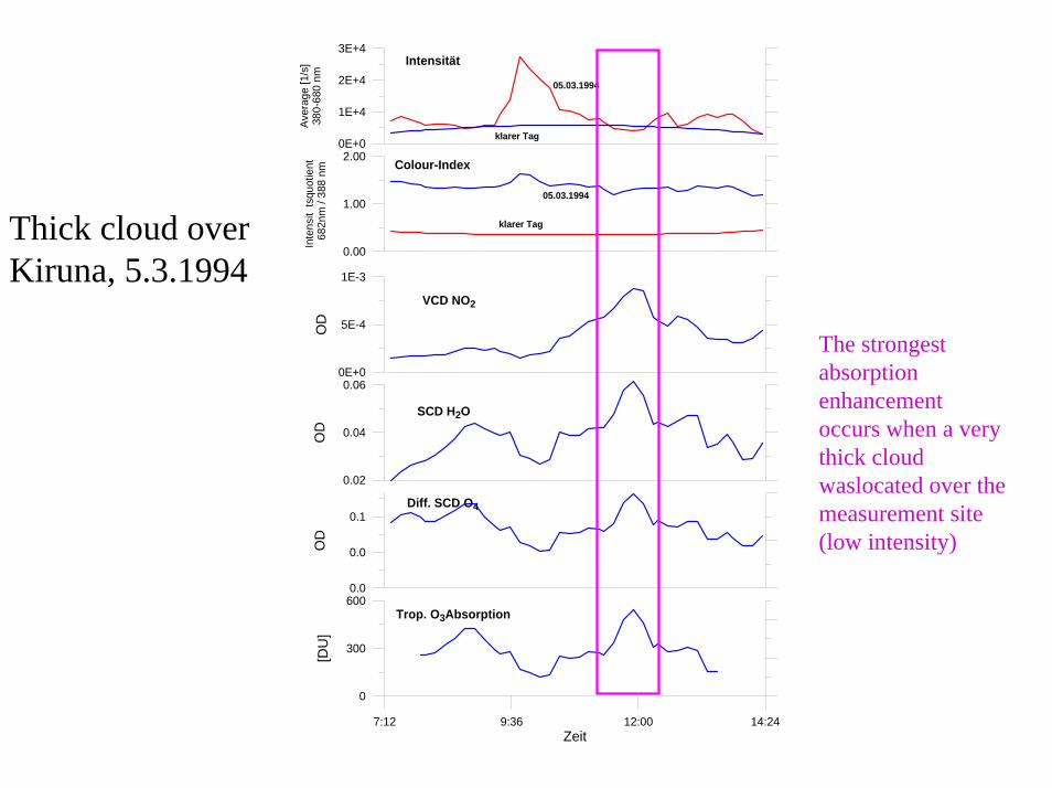
Absorptionserhöhung durch BewölkungEffects of clouds II
-clouds enhance the light path inside the cloud
400 450 500 550 600 6500E+0
1E+6
2E+6
inte
nsity
[cou
nts]
1
2
3
Quo
tient
A /
B
400 450 500 550 600 650
0.97
0.98
0.99
1.00
1.01
1.02
Quo
tient
C /
Poly
nom
ial
400 450 500 550 600 650l th [ ]
O4
H2O
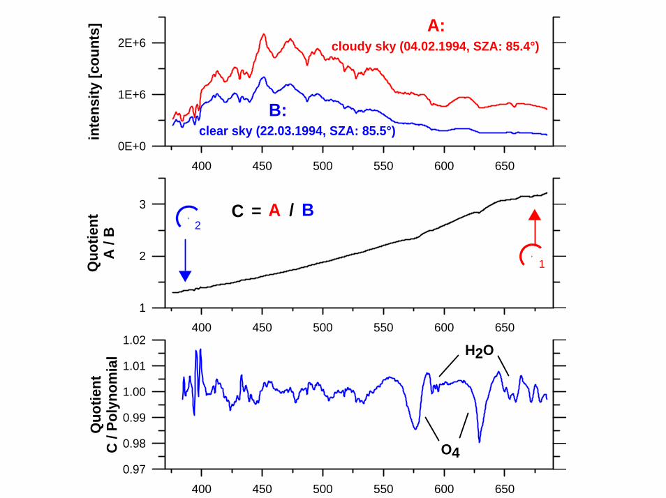
cloudy sky (04.02.1994, SZA: 85.4°)
clear sky (22.03.1994, SZA: 85.5°)
A:
B:
C = A / B2
1
7:12 9:36 12:00 14:24Zeit
0
300
600
[DU
]
0.0
0.0
0.1
OD
0.02
0.04
0.06
OD
0E+0
5E-4
1E-3
OD
0.00
1.00
2.00
Inte
nsit
tsqu
otie
nt 6
82nm
/ 38
8 nm
0E+0
1E+4
2E+4
3E+4
Aver
age
[1/s
]38
0-68
0 nm
VCD NO2
SCD H2O
Diff. SCD O4
Trop. O3Absorption
klarer Tag
05.03.1994
klarer Tag
05.03.1994
Colour-Index
Intensität
Thick cloud over Kiruna, 5.3.1994
The strongest absorption enhancement occurs when a very thick cloud waslocated over the measurement site (low intensity)
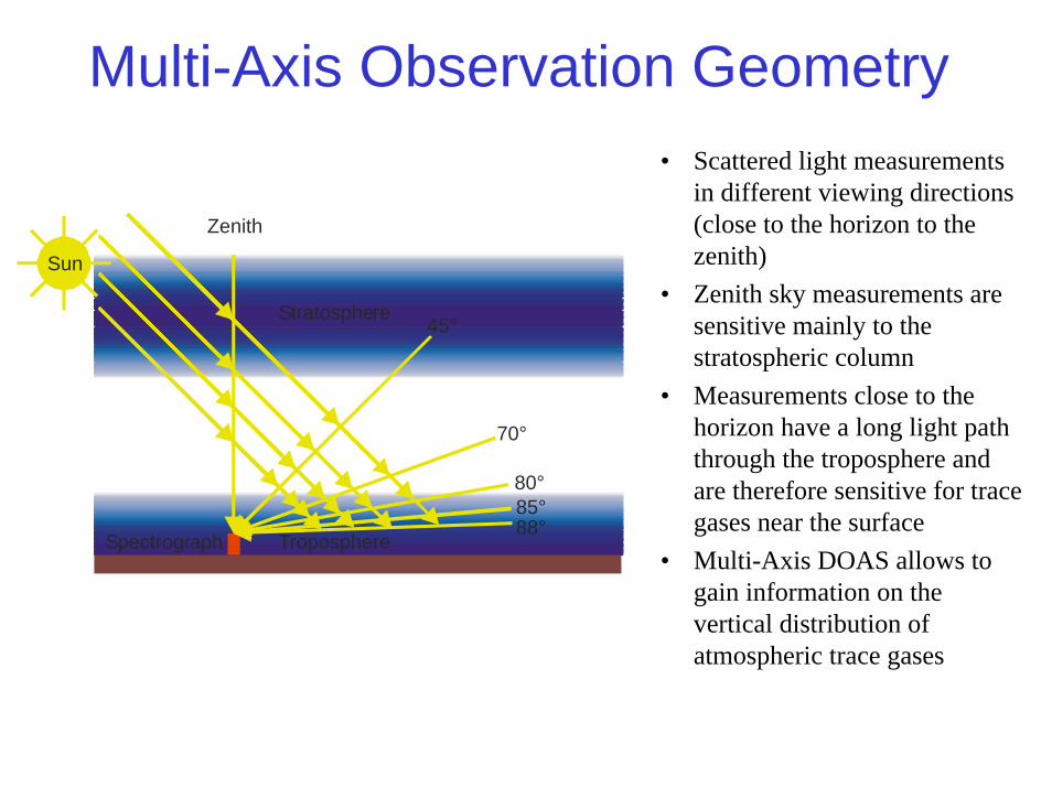
Multi-Axis Observation Geometry• Scattered light measurements
in different viewing directions (close to the horizon to the zenith)
• Zenith sky measurements are sensitive mainly to the stratospheric column
• Measurements close to the horizon have a long light path through the troposphere and are therefore sensitive for trace gases near the surface
• Multi-Axis DOAS allows to gain information on the vertical distribution of atmospheric trace gases
Spectrograph
Zenith
Sun
Stratosphere
Troposphere
45°
70°
80°85°88°

The path length through the boundary layer is mainly determined by the viewing angle of the telescopes.; from observations made at different viewing angles, the boundary layer trace gas absorption can be retrieved.

Three UV spectra on the CCD
Sophisticated MAX-DOAS setup with four independently moveable telescopes

Mini-MAX-DOAS
The whole spectrometer moves to the different elevation angles
On top of the Instituts für Umweltphysik, University of Heidelberg
Diploma thesis R. Sinreich, 2003
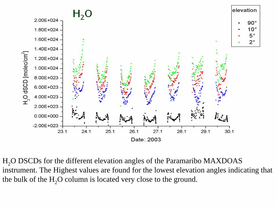
H2O DSCDs for the different elevation angles of the Paramaribo MAXDOAS instrument. The Highest values are found for the lowest elevation angles indicating that the bulk of the H2O column is located very close to the ground.

O4 DSCDs for the different elevation angles of the Paramaribo MAXDOAS instrument. In contrast to H2O, the DSCDs for the telescopes at 2° and 5° are very similar indicating that the O4 profile is not as closely located to the ground as the H2O profile. The scatter of the data indicates the presence of clouds.
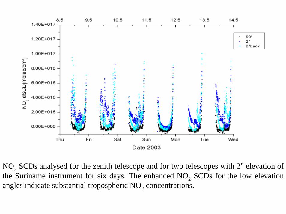
NO2 SCDs analysed for the zenith telescope and for two telescopes with 2° elevation of the Suriname instrument for six days. The enhanced NO2 SCDs for the low elevation angles indicate substantial tropospheric NO2 concentrations.
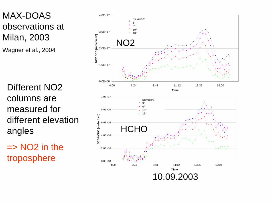
MAX-DOAS observations at Milan, 2003Wagner et al., 2004
0.0E+00
2.0E+16
4.0E+16
6.0E+16
8.0E+16
1.0E+17
4:00 6:24 8:48 11:12 13:36 16:00
Time
SCD
HC
HO
[mol
ec/c
m²]
Reihe1Reihe2Reihe3Reihe4
Elevation:3°6°10°18°
0.0E+00
1.0E+17
2.0E+17
3.0E+17
4.0E+17
4:00 6:24 8:48 11:12 13:36 16:00
Time
NO
2 SC
D [m
olec
/cm
²]
Reihe1Reihe2Reihe3Reihe4
Elevation:3°6°10°18°
HCHO
NO2
10.09.2003
Different NO2 columns aremeasured fordifferent elevationangles
=> NO2 in thetroposphere

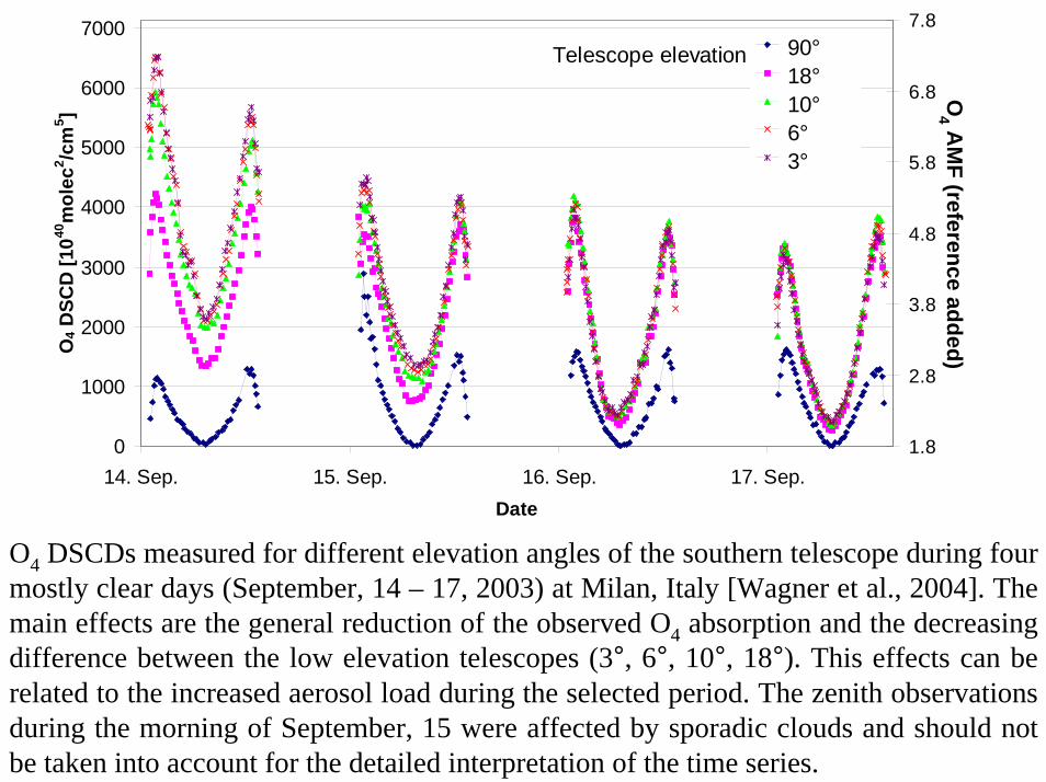
MAX-DOAS observations are sensitive to aerosols and clouds
Clear day with aerosols
The atmospheric O2 (and O4-) concentration is almost constant.
Changes in the measured O4 absorptions indicate variations in the atmospheric radiative transport
0
1000
2000
3000
4000
5000
6000
7000
14. Sep. 15. Sep. 16. Sep. 17. Sep.Date
O4 D
SCD
[1040
mol
ec2 /c
m5 ]
1.8
2.8
3.8
4.8
5.8
6.8
7.8Reihe1Reihe2Reihe3Reihe4Reihe5Reihe6
90°18°10°6°3°
Telescope elevation
O4 A
MF (reference added)
O4 DSCDs measured for different elevation angles of the southern telescope during four mostly clear days (September, 14 – 17, 2003) at Milan, Italy [Wagner et al., 2004]. The main effects are the general reduction of the observed O4 absorption and the decreasing difference between the low elevation telescopes (3°, 6°, 10°, 18°). This effects can be related to the increased aerosol load during the selected period. The zenith observations during the morning of September, 15 were affected by sporadic clouds and should not be taken into account for the detailed interpretation of the time series.
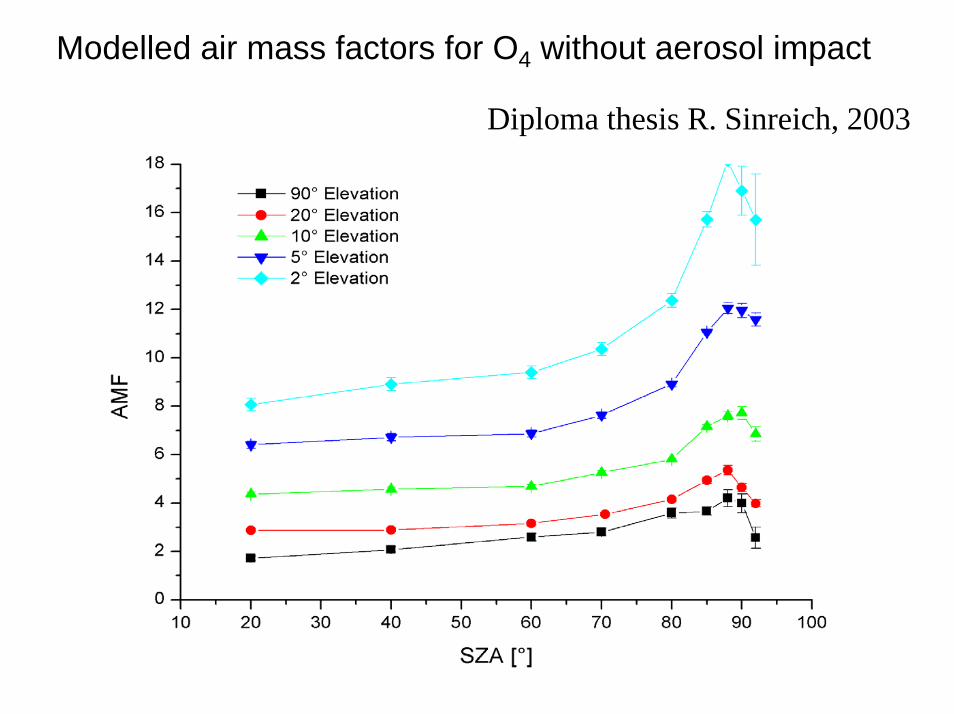
Modelled air mass factors for O4 without aerosol impact
Diploma thesis R. Sinreich, 2003
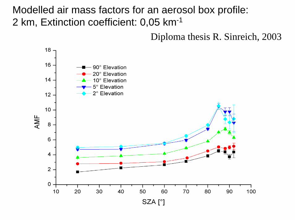
Modelled air mass factors for an aerosol box profile: 2 km, Extinction coefficient: 0,05 km-1
Diploma thesis R. Sinreich, 2003
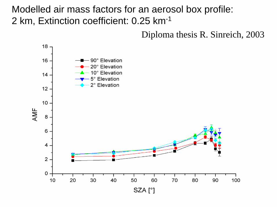
Modelled air mass factors for an aerosol box profile: 2 km, Extinction coefficient: 0.25 km-1
Diploma thesis R. Sinreich, 2003
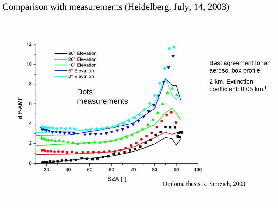
Comparison with measurements (Heidelberg, July, 14, 2003)
Dots: measurements
Diploma thesis R. Sinreich, 2003
Best agreement for anaerosol box profile:
2 km, Extinction coefficient: 0,05 km-1
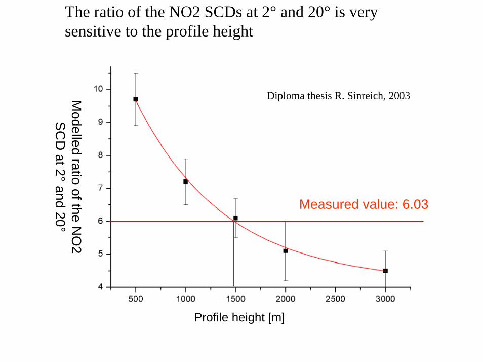
The ratio of the NO2 SCDs at 2° and 20° is verysensitive to the profile height
Measured value: 6.03
Diploma thesis R. Sinreich, 2003
Profile height [m]
Modelled
ratio of the NO
2 S
CD
at 2° and 20°
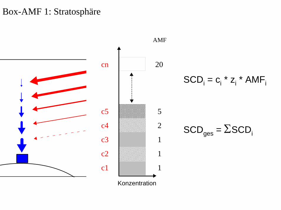
Box-AMF 1: Stratosphäre
AMF
5
2
1
1
1
20cn
SCDi = ci * zi * AMFi
c5
c4
c3
c2
c1
SCDges = ΣSCDi
Konzentration
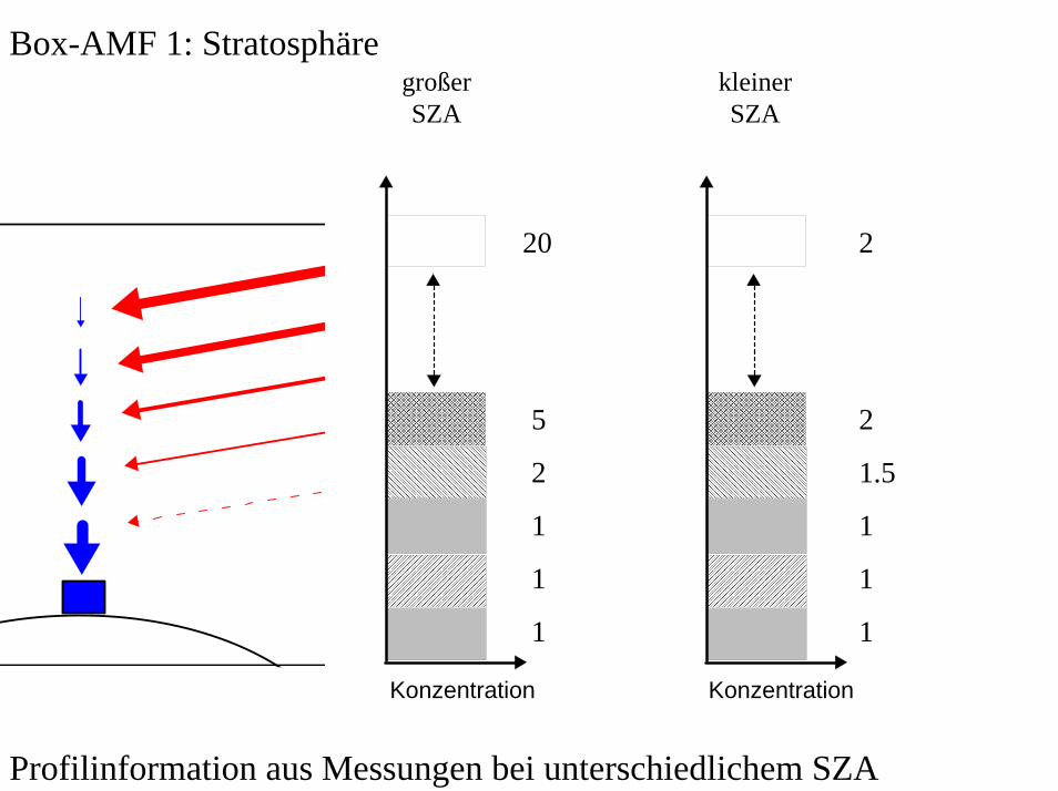
Box-AMF 1: Stratosphäregroßer SZA
kleiner SZA
2
5
2
1
1
1
20
2
1.5
1
1
1
Konzentration Konzentration
Profilinformation aus Messungen bei unterschiedlichem SZA
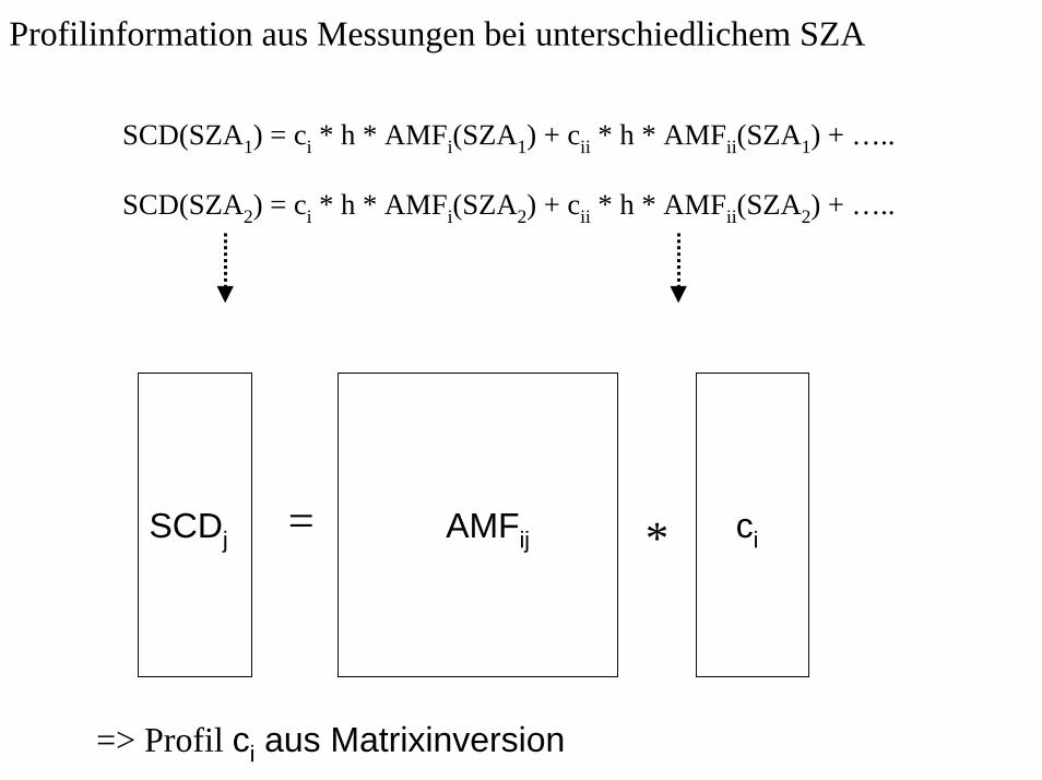
Profilinformation aus Messungen bei unterschiedlichem SZA
SCD(SZA1) = ci * h * AMFi(SZA1) + cii * h * AMFii(SZA1) + …..
SCD(SZA2) = ci * h * AMFi(SZA2) + cii * h * AMFii(SZA2) + …..
SCDj AMFij ci= *
=> Profil ci aus Matrixinversion

Box-AMF 2: Troposphäre
kleiner Elevations
winkel
großer Elevations
winkel
2
2
2
2
3
4
2
aph
Zenith
Stratosphere
Troposphere
45°
70°
80°85°88°
2
2
3
6
15
Konzentration
Konzentration

Figure 1: Sketch of the instrumental setup. Here 2x5 lines of sight are shown. The scattered sunlight is observed using small telescopes and is lead to two spectrographs via quartz fibres. Here it is analysed and the spectra are saved on a PC.
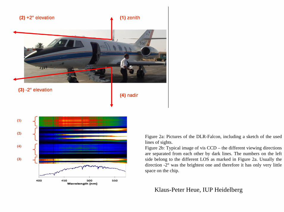
Figure 2a: Pictures of the DLR-Falcon, including a sketch of the used lines of sights.Figure 2b: Typical image of vis CCD – the different viewing directions are separated from each other by dark lines. The numbers on the left side belong to the different LOS as marked in Figure 2a. Usually the direction -2° was the brightest one and therefore it has only very little space on the chip.
Klaus-Peter Heue, IUP Heidelberg
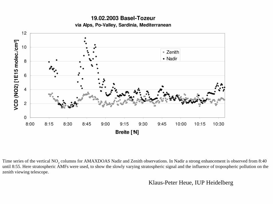
Time series of the vertical NO2 columns for AMAXDOAS Nadir and Zenith observations. In Nadir a strong enhancement is observed from 8:40 until 8:55. Here stratospheric AMFs were used, to show the slowly varying stratospheric signal and the influence of tropospheric pollution on the zenith viewing telescope.
Klaus-Peter Heue, IUP Heidelberg

Latitude
Longitude
12.512.011.511.010.510.09.59.0
Ostiligia
45.745.645.545.445.345.245.145.044.944.844.7
MI-Bresso
MI-Linate
Como
Pavia
LeccoAlzate
Rho
Saronno
Sannazano
SermidePorto Tolle
Mantova
20
10
0
-10
-20
2003.09.26 Nadir NO2 * 1015
Latitude
Longitude
12.512.011.511.010.510.09.59.0
Ostiligia
45.745.645.545.445.345.245.145.044.944.844.7
MI-Bresso
MI-Linate
Como
Pavia
LeccoAlzate
Rho
Saronno
Sannazano
SermidePorto Tolle
Mantova
20
10
0
-10
-20
2003.09.26 Nadir NO2 * 1015
Pundt et al., 2004
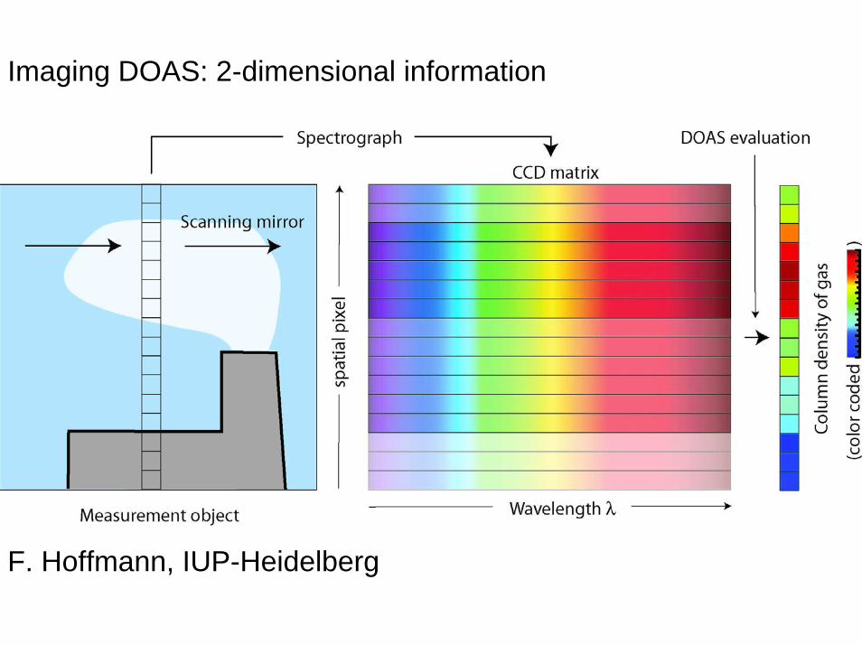
Imaging DOAS: 2-dimensional information
F. Hoffmann, IUP-Heidelberg
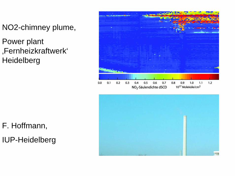
NO2-chimney plume,
Power plant ‚Fernheizkraftwerk‘ Heidelberg
F. Hoffmann,
IUP-Heidelberg
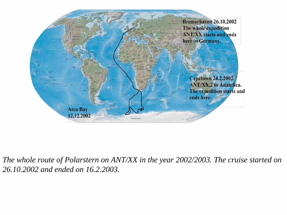
The whole route of Polarstern on ANT/XX in the year 2002/2003. The cruise started on 26.10.2002 and ended on 16.2.2003.

0.0E+00
1.0E+15
2.0E+15
3.0E+15
4.0E+15
5.0E+15
6.0E+15
-60 -40 -20 0 20 40 60
NO2 VCD [molec/cm²]
Latit
ude
morning NO2 VCD
afternoon NO2 VCD
Total VCDs of NO2 for the Atlantic traverse during May 2004 as a function of latitude. For all latitudes, PM values are clearly larger than the PM measurements.

1.5E+13
2.0E+13
2.5E+13
3.0E+13
3.5E+13
4.0E+13
4.5E+13
5.0E+13
5.5E+13
-70 -50 -30 -10 10 30 50 70
Latitude
BrO
VC
D [m
olec
/cm
²]
Polarstern BrO VCD AM 2004Polarstern BrO VCD PM 2004
Latitudinal mean VCDs of BrO in May 2005 for SZA between 84 and 86°.Compared to the values at 90° the BrO VCDs are substantially larger because ofthe photochemically reactivity of BrO.

Latitudinal cross section of the SCDs of H2O in the ANT/XX expedition [Halaisia, 2004]. The enhanced values of H2O in equatorial regions is because of the higher temperature of these regions (see Fig. 37).
Temperature distribution of ANT/XX cruise of Polarstern. The characteristic high temperature of the equatorial regions is shown with a maximumat 28 °C and the law temperature of the polar summer at –5 °C, the data is taken from the AWI internet site: www.ewoce.org.