Herstellung, Charakterisierung und mikromechanische ...

Herstellung, Charakterisierung und mikromechanische Modellierung von magneto-sensitiven Elastomeren

Von der Naturwissenschaftlichen Fakultät der

Gottfried Wilhelm Leibniz Universität Hannover zur Erlangung des Grades

Doktor der Naturwissenschaften

(Dr. rer. nat.)

genehmigte Dissertation

von

Dipl.-Phys. Sahbi Aloui

2018

ii

Referent: Hon. Prof. Dr. rer. nat. habil. Manfred Klüppel

Korreferent: Prof. Dr. rer. nat. Jürgen Caro

Tag der Promotion: 16 Oktober 2018

iii

Acknowledgement

The present thesis was prepared during my work as a research assistant in the years 2012 to

2017 at the German institute of rubber technology DIK. I would like to express my deep

appreciation to all those who were involved in this work.

First, to Prof. Dr. Manfred Klüppel, the head department of “Material concept and modelling”

department, for his highly professional support, valuable advice and the supervision of this

dissertation.

To Prof. Dr. Jürgen Caro who has kindly accepted to advise this Ph. D. thesis as a second

examiner.

To Prof. Dr. Ulrich Giese, managing director of DIK, and Prof. Dr. Paul Heitjans who had

kindly accepted to be members of the examination board.

My very special thanks go to all staff members of “Material concept and modelling”

department, who supported me on many topics with the greatest commitment and attention to

detail. I want to express my great gratitude to Markus Möwes for his support in the

experimental part of this thesis regarding the magnetorheology, to Frank Fleck for conducting

gas adsorption measurements in addition to inspiring discussions and to Andrej Lang for

assisting me by the evaluation of the dynamic-mechanical measurements.

I would further like to express my heartfelt thanks to Dr. Jens Meier as well as Peter Erren for

performing the multihysteresis measurements, to Mohammed El-Yaagoubi for helping me by

fitting the multihysteresis measurements data and to Dr. Astrid Diekmann for the SEM

examinations.

For the supply of magnetic fillers, without this work would not have been possible, I would

like to thank the companies BASF SE and Evonik Industries AG.

I would like to thank all my ex-colleagues at DIK for the extensive and valuable ideas

exchange and suggestions I have received. I appreciated very interesting discussions, which

did not deal only with rubber technology.

For the continuation of this work and clarification of the open questions, I wish all the

participants a lot of success.

Finally, I am very grateful to my wife Patrycja Anna, my daughters Emne and Esmeh El-

Manana, my son Muhammed, my parents and siblings. It is inconceivable to pretend to be the

man I am today without their immense trust and big support.

v

Kurzfassung

Magneto-sensitive Elastomere (MSE) gehören zur Klasse der „Smart Materials“. Sie zeigen

ein sich selbst anpassendes und adaptives Verhalten in zufälligen Ereignissen und werden

auch als intelligente Materialien bezeichnet. Sie zeichnen sich durch die Fähigkeit aus, in

einem zielgerichteten Handeln auf Veränderungen der Betriebs- oder Umweltbedingungen

ohne externe Regulierung zu reagieren.

MSE werden durch Mischen magnetischer Füllstoffe in der Kautschukmatrix hergestellt.

Mechanische und magnetorheologische Messungen zeigen, dass Partikelgröße, Füllstoffgehalt

und Haftvermittler die mechanische und die magnetische Eigenschaften von MSE erheblich

beeinflussen. Die Leistung von MSE kann durch die Herstellung anisotroper Proben mit

orientierten magnetischen Füllstoffpartikeln weiter verbessert werden. Das wird durch die

Vulkanisation in einem externen Magnetfeld erreicht.

Dieser Prozess kann online durch magnetorheologische Messungen der unvernetzten

Schmelzen untersucht werden. Die Orientierung der magnetischen Füllstoffpartikel in

Strängen entlang der Magnetfeldlinien äußert sich in einer sukzessiven Erhöhung des

Schubmoduls beim Einschalten des Magnetfeldes. Diese Schaltfähigkeit wird durch

mikrofeine magnetische Füllstoffe gefördert und kann einen Wert von 600 % erreichen.

Magnetische Füllstoffe im Nanogrößenbereich zeigen jedoch kaum einen Schalteffekt und

tragen hauptsächlich zur mechanischen Verstärkung von MSE bei. Die Vernetzung

gewährleistet die MSE höhere Modulwerte im Vergleich zu den Schmelzen, ein maximaler

Schalteffekt von 36 % für anisotrope Proben wird aber gemessen.

MSE zeigen ein ähnliches mechanisches Ermüdungs- und Alterungsverhalten im Vergleich zu

herkömmlichen Gummiproben.

Die Kopplung zwischen den magnetischen und mechanischen Eigenschaften von MSE wird

weiter untersucht, indem die Messdaten mit dem mikromechanischen dynamischen

Flokkulationsmodell modelliert werden. Es zeigt sich, dass die Fit-Parameter signifikant von

der Verteilung der magnetischen Füllstoffpartikel innerhalb der MSE-Proben abhängen.

Darüber hinaus werden einige Anpassungsparameter durch das angelegte Magnetfeld

bestimmt, was bestätigt, dass die Änderung der magnetischen Eigenschaften der Umgebung

die mechanischen Eigenschaften der Proben unvermeidlich beeinflusst.

Die Eigenschaftenoptimierung der MSE kann durch den Einsatz hybrider Füllstoffsysteme

erreicht werden. Die Verbindung verschiedener Füllstoffe ergibt einen Synergieeffekt

zwischen der Wirkung einzelner Füllstoffe und den Endeigenschaften von MSE. Ein zeitnaher

Einsatz von MSE in technischen Anwendungen erscheint derzeit nur auf dieser Basis

realistisch.

Schlüsselwörter: Smart materials, Magneto-sensitive Elastomere, Orientierung der magneti-

schen Füllstoffpartikel, Schalteffekt, magneto-mechanisches Verhalten, hybrid Füllsysteme.

vii

Abstract

Magneto-sensitive elastomers (MSE) belong to the class of smart materials. They show a self-

adjusting and adaptive behaviour in random occurrences and are also denoted as intelligent

materials. They are characterised by the ability to react in a target-oriented acting to changes

in operating or environmental conditions without external regulation.

MSE are prepared by mixing magnetic fillers within the rubber matrix. Mechanical and

magnetorheological measurements show that particle size, filler loading and coupling agent

considerably influence the mechanical and magnetic properties of MSE. The performance of

MSE can be further improved by preparing anisotropic samples with oriented magnetic filler

particles. This is achieved by curing in an external magnetic field.

This process can be examined online by magnetorheological measurements of the non-

crosslinked melts. The orientation of the magnetic filler particles in strings along the magnetic

field lines expresses itself in a successive increase of the shear modulus when the magnetic

field is turned on. This switching ability is promoted by microsized magnetic fillers and can

reach a value of 600 %. However, nanosized magnetic fillers show hardly any switching

effect and mainly contribute to the mechanical reinforcement of MSE. The crosslinking

ensures the MSE samples higher modulus values compared to the melts. But a maximal

switching effect of 36 % for anisotropic samples is measured.

MSE show similar mechanical fatigue and ageing behaviour compared with conventional

rubber samples.

The coupling between magnetic and mechanical properties of MSE is further investigated by

modelling the measurement data using the micromechanical dynamical flocculation model. It

is found that the fit parameters significantly depend on the distribution of magnetic filler

particles within the MSE samples. Moreover, some fit parameters are governed by the applied

magnetic field, thus confirming that changing the magnetic properties of the surroundings

inevitably influences the mechanical properties of the samples.

The optimization of MSE properties can be achieved by applying hybrid filler systems. The

association of different fillers provides a synergy effect between the action of single fillers

and the MSE final properties. Indeed, a prompt use of MSE in technical applications only

currently appears to be realistic on this basis.

Keywords: Smart materials, magneto-sensitive elastomers, orientation of magnetic filler

particles, switching effect, magneto-mechanical behaviour, hybrid magnetic filler systems.

ix

Table of content

Basic considerations ..................................................................................................... 1

1 Introduction .......................................................................................................... 1

2 Elastomer composites ............................................................................................. 7

2.1 Rubbers ......................................................................................................... 7

2.1.1 Natural rubber ...................................................................................................................... 8

2.1.2 Acrylonitrile butadiene rubber .............................................................................................. 9

2.1.1 Ethylene propylene diene terpolymer .................................................................................. 9

2.1.2 Hydrogenated acrylonitrile butadiene rubber .................................................................... 10

2.1.3 Carboxylated hydrogenated acrylonitrile butadiene rubber ............................................... 10

2.1.4 Styrene butadiene rubber .................................................................................................. 10

2.2 Vulcanisation ............................................................................................... 11

2.3 Functional fillers .......................................................................................... 12

2.4 Rubber additives .......................................................................................... 16

3 Magnetism and magnetic filler particles ................................................................ 19

3.1 Magnetism ................................................................................................... 19

3.2 Magnetic dipole interaction .......................................................................... 23

3.3 Magnetic materials ....................................................................................... 25

3.3.1 Iron ..................................................................................................................................... 27

3.3.2 Iron oxides ......................................................................................................................... 28

3.3.3 Ferrite ................................................................................................................................ 29

3.3.4 Magnetic fillers used in this study ...................................................................................... 30

4 Modelling and data treatment ............................................................................... 33

4.1 Dynamic-mechanical thermal Analysis ......................................................... 33

4.1.1 Generation of master curve ............................................................................................... 35

4.1.2 Evaluation of relaxation time spectra ................................................................................ 37

4.2 Dynamical Flocculation Model ..................................................................... 42

4.3 Fatigue crack growth .................................................................................... 47

5 Experimental methods .......................................................................................... 51

5.1 Static volumetric gas adsorption measurements ............................................ 51

5.2 Sample preparation ...................................................................................... 51

5.2.1 Mixing ................................................................................................................................ 51

5.2.2 Vulcanisation in a magnetic field ....................................................................................... 52

x

5.3 Physicals ...................................................................................................... 55

5.3.1 Stress-strain curves ........................................................................................................... 55

5.3.2 Multihysteresis measurements for fitting with the DFM ..................................................... 55

5.3.3 Shore A hardness .............................................................................................................. 56

5.3.4 Rebound ............................................................................................................................ 56

5.3.5 Abrasion ............................................................................................................................. 56

5.4 DMTA testing instruments ........................................................................... 56

5.5 Crack propagation behaviour: Tear fatigue analyser .................................... 58

5.6 Magnetorheological measurements ............................................................... 59

5.7 Combined rheological and dielectric measurements ...................................... 60

Results and discussion ................................................................................................ 63

6 Characterisation of filler particles by static volumetric gas adsorption technique...... 63

7 Mechanical properties and ageing behaviour ......................................................... 65

7.1 Physicals ...................................................................................................... 65

7.2 Stress-strain curves ...................................................................................... 66

7.2.1 Influence of particle size .................................................................................................... 67

7.2.2 Variation of filler loading .................................................................................................... 68

7.2.3 Influence of coupling agent ................................................................................................ 70

7.3 Dynamic-mechanical thermal analysis .......................................................... 71

7.3.1 Vulcanisation in a magnetic field ....................................................................................... 71

7.3.2 Influence of particle size .................................................................................................... 74

7.3.3 Variation of filler loading .................................................................................................... 76

7.3.4 Influence of coupling agent ................................................................................................ 79

7.4 Fatigue crack propagation and ageing behaviour .......................................... 81

7.4.1 Mechanical fatigue of magneto-sensitive elastomers........................................................ 81

7.4.2 Thermal Ageing of magneto-sensitive elastomers ............................................................ 85

8 Magnetorheology of melts .................................................................................... 89

8.1 Flocculation ................................................................................................. 89

8.2 Influence of coupling agent on the relative magnetorheological effect ............ 91

8.3 Influence of application temperature on the relative magnetorheological effect

93

9 Magnetorheology of crosslinked systems ............................................................... 95

9.1 Vulcanisation in a magnetic field .................................................................. 95

9.2 Internal microstructure of MSE ................................................................... 98

9.2.1 Magnetic anisotropy of MSE using scanning electron microscope ................................... 98

9.2.2 Magnetic anisotropy of MSE using magnetorheological testing ........................................ 99

9.3 Influence of particle size ............................................................................. 100

xi

9.4 Variation of filler loading ........................................................................... 102

9.5 Influence of coupling agent ......................................................................... 103

9.6 Magnetic induced relaxation behaviour of MSE .......................................... 105

9.7 Modelling of the magneto-mechanical response of the MSE ......................... 111

10 Optimization of viscoelastic properties of MSE by hybrid filler systems............... 121

10.1 Hybrid magnetic filler systems .................................................................... 122

10.1.1 Stress-strain behaviour ................................................................................................ 122

10.1.2 Dynamic-mechanical analysis ..................................................................................... 123

10.1.3 Magnetorheology of non-crosslinked melts ................................................................. 124

10.1.4 Magnetorheology of crosslinked samples ................................................................... 125

10.2 Hybrid filler systems .................................................................................. 127


10.2.2 Dynamic-mechanical analysis ..................................................................................... 129


10.3 Adaptive systems for active bearing platform .............................................. 132


10.3.2 Dynamic-mechanical thermal analysis ........................................................................ 135


10.3.4 Combined rheological and dielectric measurements ................................................... 137

10.3.5 Influence of the mechanical fatigue on MRE ............................................................... 139

10.4 Outlook: New hybrid filler systems for MSE composites ............................. 143

10.4.1 Iron–iron oxide matrix on graphene ............................................................................. 143

10.4.2 Magnetic Carbon Nanotubes ....................................................................................... 144

11 Summary and Conclusions .............................................................................. 147

Bibliography ............................................................................................................ 151

Annexe .................................................................................................................... 175

1

Basic considerations

1 Introduction

Engineering constructions like buildings, bridges and offshore drilling rigs are exposed to

dynamic loads. They arise naturally from strong earthquake excitations, extreme waves or

strong winds and considerably affect the survivability of such structures [1, 2]. Undesirable

vibrations occur also in a variety of technical and automotive systems as the consequence of a

temporally periodic movement of a body about a rest position. These vibrations are

disproportionately high in case of an unbalanced construction or special machines with high

rotational speeds. If such systems are connected to the ground, the vibrations propagate

further through mechanical waves affecting a reliable operation of machines placed nearby.

Those generated technical disruptions are often accompanied by disturbing noise, showing

that vibrations damping is not only survivability or reliable operation issue but also a comfort

topic.

Mechanical vibrations are reduced by decoupling the main structure from the ground through

elastic or viscoelastic elements. At each vibration, a part of the mechanical energy is

transformed into heat due to friction. As a result, the oscillation amplitude decreases

continuously until the vibrations are fully amortised. The attenuation of the structure

movements by dissipating the energy generated is highly desired. The physical basics of

mechanical vibrations were treated in-depth the last decades to become a better understanding

of how unwanted resonances phenomena occur. The following small excursion into this field

should give more insight in the subject by presenting the two major and easiest cases: the

simple and damped harmonic oscillator in classical mechanics.

The simple harmonic oscillator in classical mechanics consists of a spherical body with a

radius r and a mass m suspended on a spring with a spring constant D. For simplification

purposes, the spherical body is assumed as a point mass. If the body is deflected from its rest

position, a restoring force 𝑭 occurs in the area of validity of Hooke's law where the total

deformation 𝒙 is sufficiently small and has the following form:

𝑭 = −𝐷𝒙 . (1)

The associated angular frequency is given by

𝜔02 = 𝐷/𝑚. (2)

If the body is immersed in liquid, the friction can no longer be neglected, and the Stokes

friction force 𝑭𝒅 shall be added:

𝑭𝒅 = −6𝜋𝜂𝑟𝒗 (3)

where 𝜂 is the dynamic viscosity and 𝒗 is the velocity of body. The damping constant 𝛾 of the

damped harmonic oscillator depends on the ratio of resonance frequencies of the oscillating

system to the damping element and it is given by

2

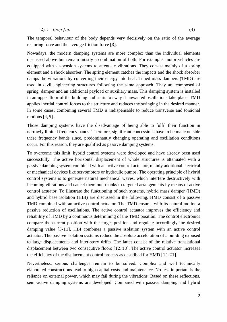
2𝛾 ∶= 6𝜋𝜂𝑟/𝑚. (4)

The temporal behaviour of the body depends very decisively on the ratio of the average

restoring force and the average friction force [3].

Nowadays, the modern damping systems are more complex than the individual elements

discussed above but remain mostly a combination of both. For example, motor vehicles are

equipped with suspension systems to attenuate vibrations. They consist mainly of a spring

element and a shock absorber. The spring element catches the impacts and the shock absorber

damps the vibrations by converting their energy into heat. Tuned mass dampers (TMD) are

used in civil engineering structures following the same approach. They are composed of

spring, damper and an additional payload or auxiliary mass. This damping system is installed

in an upper floor of the building and starts to sway if unwanted oscillations take place. TMD

applies inertial control forces to the structure and reduces the swinging in the desired manner.

In some cases, combining several TMD is indispensable to reduce transverse and torsional

motions [4, 5].

Those damping systems have the disadvantage of being able to fulfil their function in

narrowly limited frequency bands. Therefore, significant concessions have to be made outside

these frequency bands since, predominantly changing operating and oscillation conditions

occur. For this reason, they are qualified as passive damping systems.

To overcome this limit, hybrid control systems were developed and have already been used

successfully. The active horizontal displacement of whole structures is attenuated with a

passive damping system combined with an active control actuator, mainly additional electrical

or mechanical devices like servomotors or hydraulic pumps. The operating principle of hybrid

control systems is to generate natural mechanical waves, which interfere destructively with

incoming vibrations and cancel them out, thanks to targeted arrangements by means of active

control actuator. To illustrate the functioning of such systems, hybrid mass damper (HMD)

and hybrid base isolation (HBI) are discussed in the following. HMD consist of a passive

TMD combined with an active control actuator. The TMD ensures with its natural motion a

passive reduction of oscillations. The active control actuator improves the efficiency and

reliability of HMD by a continuous determining of the TMD position. The control electronics

compare the current position with the target position and regulate accordingly the desired

damping value [5-11]. HBI combines a passive isolation system with an active control

actuator. The passive isolation systems reduce the absolute acceleration of a building exposed

to large displacements and inter-story drifts. The latter consist of the relative translational

displacement between two consecutive floors [12, 13]. The active control actuator increases

the efficiency of the displacement control process as described for HMD [14-21].

Nevertheless, serious challenges remain to be solved. Complex and well technically

elaborated constructions lead to high capital costs and maintenance. No less important is the

reliance on external power, which may fail during the vibrations. Based on these reflections,

semi-active damping systems are developed. Compared with passive damping and hybrid

3

control systems, they offer a continuous control of the internal system features instead of

introducing mechanical energy from a third source. They require less electrical power supply

and earn more attention in the last years. Notable example is the variable orifice fluid damper.

It consists of a passive fluid damper equipped with an electromechanically controlled variable

orifice valve to regulate the fluid flow. The passive fluid damper, also referred to as hydraulic

damper, consists of a piston attached to a piston rod and a cylinder filled with an

incompressible fluid. The piston is permanently immersed in the cylinder. Together, they

form a closed cavity, the workroom of the damper. If the piston moves due to occurring

vibrations transmitted through the piston rod, the volume of the cavity varies forming a

variable pressure level, which is known as hydraulic resistance. In order to better adjust the

hydraulic resistance of the damping element, the fluid may be conducted in many balancing

chambers and through different valve systems. The variable pressure level is based on a

continuous transition between compression and decompression of the fluid. According to

fluid dynamics, this state transition is accompanied by a temperature change. As discussed

above, the operating principle of fluid damper remains also the same: the conversion of

kinetic energy into thermal energy. In the case of variable orifice fluid damper, the hydraulic

resistance is controlled solely by a valve having an orifice with variable opening degree [22-

24].

Despite the efforts made to reduce the manufacturing costs and the complexity degree of the

devices discussed above, the system reliability and especially the maintenance still remain a

major problem. The reason lies in the need to be controlled by an external unity even if it is

incorporated in the main structure.

It is highly recommended to consider systems, which can be controlled internally. They offer

a large flexibility and high degree of freedom, while taking into account simple structures.

Semi-active devices based on already developed controllable fluids represent a serious

alternative.

Electrorheological fluid (ERF) was the first contender. It consists of an electrically insulating

carrier liquid; such as water or mineral oil, in which electro-sensitive colloids; such as soft

iron particles, are suspended. In the presence of an external electrical field, the viscosity of

ERF changes significantly and hence the damping behaviour. These changes occur in the

milliseconds range and are reversible. ERF was first used in clutch systems. A US-patent was

registered in 1947 for ERF-based clutches by W. M. Winslow [25, 26]. The

electrorheological clutches have the advantages over conventional clutches in the simple

control of the transmitted torque, the fast response time and the low wear because the

electromagnetic information is transmitted without any mechanical intermediate step. In 1948,

J. Rabinow developed a clutch system based on magnetorheological fluid (MRF) [27]. MRF

is the magnetic analogue of ERF. MRF have prevailed as controllable fluid than ERF because

they are less sensitive to impurities and contaminants encountered during the production and

the operating processes. Furthermore, the maximum yield stress of MRF compared with ERF

is an order of magnitude larger, although their viscosities are similar [1].

4

The ability of ERF and MRF to vary in real time their dynamical and rheological properties in

order to ensure adaptability to changing circumstances is considered as inbuilt intelligence of

the system. This ability forms the basis for a new class in the area of material science, the so-

called smart materials.

However, those controllable fluids are exposed to a sedimentation problem of the filler

particles due to gravitation. A minor problem can occur, when the carrier liquid water comes

in contact with the surroundings since it could be evaporated. These deficiencies can be

reduced by adding antiwear and lubricity additives but are not completely eliminated. Those

limitations opened the door to further developments of new types of smart materials.

In order to overcome the sedimentation deficiency of controllable fluids, rubber materials

were considered. Compared to fluids, rubber materials have a higher molecular weight and

exhibit therefore a considerably higher viscosity. Due to interaction with long strongly

branched polymer chains, the mobility of filler particles is significantly restricted and the

possibility to sediment is not given any more. Furthermore, rubber materials still remain the

standard components of passive damping systems. Classical damping structures are made of

laminated steel plates and elastomer layers [28].

An adaptive damping behaviour with a continuous control of the elasticity modulus and an

ongoing adjustment of the resonance frequency is achieved by mixing magnetic fillers into

the rubber matrix. This gives rise to magneto-sensitive elastomers (MSE), which are able to

vary their mechanical properties and to adapt them to surroundings.

MSE are used in wide range of applications undergoing dynamic deformations as well as in

the state of rest for actuator and sensor technologies.

In the area of disaster resistant constructions, adaptive vibration control systems have been

successfully used in high-rise buildings [29-48]. Laminated MSE layers and steel plates are

surrounded with electromagnetic coils generating a strong magnetic field. The latter regulates

the vibration behaviour of the control systems, which react actively to strong vibrations by

changing the lateral stiffness and damping force up to 45 % [33]. In the automotive industry,

MSE are used in adaptive vehicle seat suspensions [49-51], in tuned engine mounts [52, 53],

in active vehicle bumpers [54] and are introduced in new crash systems [55].

In the sensors segment, MSE are used in wireless and passive temperature indicators [56-58].

The temperature indicator is based on the Villari effect, i.e. the inverse magnetostrictive

effect. This effect describes the change of magnetic susceptibility of a material when it is

subjected to a mechanical stress. Its novelty is that it functions without electric current. A

switch prepared from a magnetic shape memory alloy is placed between a permanent magnet

and a resonator made of a soft magnetic ribbon. As soon as the temperature reaches a critical

value, the switch undertakes a transition between the paramagnetic and ferromagnetic state.

By exceeding a material-specifically temperature, the magnetic flux is changed and, therefore,

the resonance frequency of the soft magnetic ribbon is shifted. This enables to determine

temperature variations and to record them.

5

MSE are also used in strain sensors [59-63], in touch-screen panel [64] and in

electromagnetic shielding systems [65, 66]. Electromagnetic radiations arise through different

electromagnetic field sources in the environment. They are generated from diverse electrical

devices on earth and they could come from the universe. The impact of some sunrays may

even be perceptible on earth. Considering the ejected plasma (ionizing radiation) during sun

eruptions, they may affect considerably the efficient work-flow of satellites and hence, our

communication and navigation systems. On earth they can cause immense damage, like

destroying current transformers. This was the case in North America in 1989. Millions of

human being stayed for about ten hours without electric current and the economic

repercussions were huge. In order to avoid such catastrophes, elastomer composites were used

as an electromagnetic shielding system. They enable masking the devices and reflecting the

electromagnetic radiations. MSE allow an effective absorbing of the electromagnetic

radiations, due to the interaction with the magnetic particles, and converting them to harmless

heat energy.

MSE are also used in actuators for valves [67] and in active noise barrier systems [68]. In

microelectromechanical systems, MSE are used successfully in magnetometers [69], in

microcantilevers [70], in tuned microvibration control systems [71] and in adaptive

micropumps [72, 73]. There are aspirations in medical field to use MSE in adjustable

prosthetic devices [74] and in artificial controllable lymphatic vessels [75].

Despite the successful use of the MSE in different technical structures, outstanding issues still

remain and need to be studied. The deficiency of basic knowledge for conception,

dimensioning and production impedes currently a global implementation of MSE in all

industrial sectors. In particular, the relationship between structural parameters like rubber or

filler type and technological properties is lacking in experience, guidelines and calculation

tools.

In the framework of this thesis, these relevant issues are considered. At the beginning, a

detailed overview on different aspects of the rubber technology and some relevant topics on

magnetism are given. The experimental findings are then presented and discussed. The first

part is devoted to characterisation and understanding of the key factors influencing

mechanical and magnetic properties of the finished MSE. In a second part, a physical

description of the coupling between magnetic and mechanical properties is discussed. This is

based on the physical fundamentals of the rubber elasticity supplemented by the magnetism.

In the last part, the optimization of dynamic-mechanical properties and magnetic sensitivity of

the MSE are closely examined.

7

2 Elastomer composites

Elastomeric materials are widely used in nearly all industrial and technical applications. The

carrier material is rubber. For application suitable products, supplementary components like

fillers, plasticizers, vulcanisation systems and other necessary additives are added. Due to a

large number of combinations of the different components, the properties of the finished

elastomer composite can be adapted as needed for the individual application. In this chapter,

the basics of rubber technology are highlighted. The different components used as well as the

methods applied for the preparation of elastomer composites are described.

2.1 Rubbers

Rubbers are noncrosslinked polymers with a glass transition temperature 𝑇𝑔 lower than the

operating temperature. The term “polymer” goes back to the Greek words “poly” and “meros”

which means many and parts respectively. Polymers are long molecular chains made from

one or more types of repeating units known as monomers. Rubbers are macromolecular

compounds usually composed of hydrocarbon polymer chains and can be natural or synthetic.

Natural rubber is obtained by conversion of natural products. Fully synthetic rubbers are

crude oil-derived and are produced synthetically through condensation reactions, in which the

atoms and molecules merge together to form the polymer chains. The polymerization

processes of the different monomers occur under different and controlled conditions. They

have been developed according to the diverse application fields and the expected properties of

the finished product [76]. Monomers with the chemical structure 𝑅 − 𝐻𝐶 = 𝐶𝐻2 form the so-

called vinyl group and are the basic component of all conventional rubbers. The vinyl-group

includes a carbon-carbon double bond and has a major role in the vulcanisation process of

long polymer chains. This point is discussed in detail in a later section of this chapter.

The most outstanding feature of rubber compared to other materials is its high deformation

rates when it is stretched. Rubber can show elongations up to 1000 % while solids cannot be

strained more than 50 % even if both elastic and plastic deformations are considered [76].

This behaviour is based on the different mechanism of energy storage during the deformation.

In the ideal solid state, the atoms occupy neighbouring lattice sites with predefined lattice

spacing and atoms conformation. In the case of an external deformation, atomic distances as

well as valence bond angles change, leading to a change in the internal energy of the ideal

solid. The stress and strain of ideal elastic solid are linear interrelated according to the

Hooke´s law. The wide-meshed polymer chains of rubber are organised in a rather flexible

way and are randomly arranged. Above the glass transition area, the whole polymer chains or

a part of it can undergo rotary and vibrational motions around chain segments. According to

second law of thermodynamics, the most probable statistical state of the polymer chains

corresponds to the state of maximum entropy The entropy is a quantity which measures the

disorder in a closed system to calculate the internal energy degradation. The molecular

statistical approach of the rubber elasticity is referred to the entropy elasticity. It is based on

8

the “random flight statistic” of the not deformed polymer chains, in which a Gaussian

distribution function of the end-to-end distance of the individual chains can be derived. The

deformation behaviour of rubber like materials is based on the change in entropy. If the

polymer chains are stretched in one direction, the degree of disorder along the load direction

decreases. Accordingly, the entropy decreases and the average end-to-end distance of the

individual polymer chains is deviated from its most probable value. A restoring force of the

deformed polymer network can then be determined. If the deformation is removed, the chain

segments may take different random arrangements and the entropy increases consequently.

When the polymer chains are completely unloaded, the system reaches the most statistically

probable state; the state of biggest disorder. Rubber materials behave non-linearly. They are

characterised by non-linear relationship between stress and deformation [76].

In the frame of this thesis, the following rubber types are considered.

2.1.1 Natural rubber

Natural rubber (NR) is a renewable raw material. It is produced by the coagulation of natural

latex, the milky juice of Hevea brasiliensis - a variety of tropical plants, which is cultivated in

large plantations in Africa, Asia and South America. The natural latex contains besides water

and polymers, proteins, carbohydrates, sterols, fats and minerals. To increase its shelf life,

ammonia 𝑁𝐻3 is usually added. In order to separate the polymer chains as a solid-like mass

from the water, the coagulation is achieved with the acetic acid 𝐶𝐻3𝐶𝑂𝑂𝐻 or formic

acid 𝐻𝐶𝑂𝑂𝐻. The coagulum is washed to remove undesired substances and dried in dry

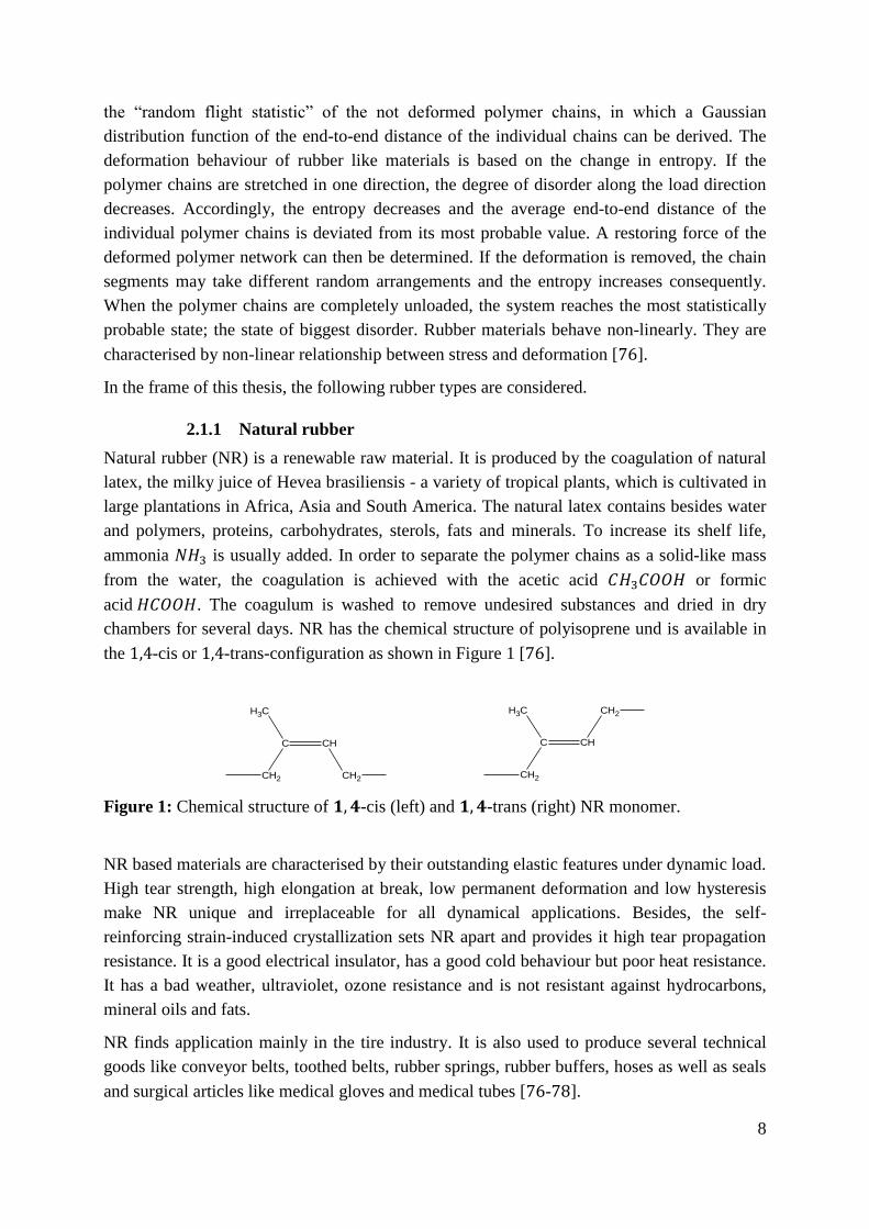
chambers for several days. NR has the chemical structure of polyisoprene und is available in

the 1,4-cis or 1,4-trans-configuration as shown in Figure 1 [76].

C CH

CH2 CH2

CH3

C CH

CH2

CH3 CH2

Figure 1: Chemical structure of 𝟏, 𝟒-cis (left) and 𝟏, 𝟒-trans (right) NR monomer.

NR based materials are characterised by their outstanding elastic features under dynamic load.

High tear strength, high elongation at break, low permanent deformation and low hysteresis

make NR unique and irreplaceable for all dynamical applications. Besides, the self-

reinforcing strain-induced crystallization sets NR apart and provides it high tear propagation

resistance. It is a good electrical insulator, has a good cold behaviour but poor heat resistance.

It has a bad weather, ultraviolet, ozone resistance and is not resistant against hydrocarbons,

mineral oils and fats.

NR finds application mainly in the tire industry. It is also used to produce several technical

goods like conveyor belts, toothed belts, rubber springs, rubber buffers, hoses as well as seals

and surgical articles like medical gloves and medical tubes [76-78].

9

2.1.2 Acrylonitrile butadiene rubber

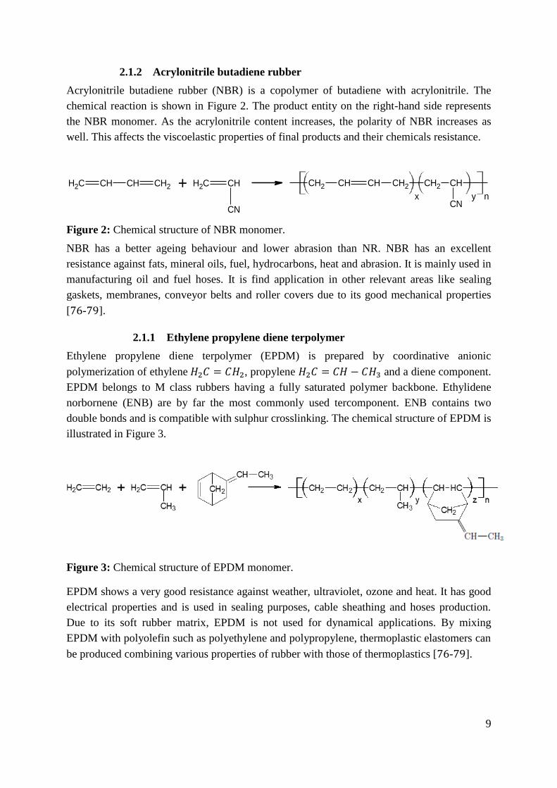
Acrylonitrile butadiene rubber (NBR) is a copolymer of butadiene with acrylonitrile. The

chemical reaction is shown in Figure 2. The product entity on the right-hand side represents

the NBR monomer. As the acrylonitrile content increases, the polarity of NBR increases as

well. This affects the viscoelastic properties of final products and their chemicals resistance.

CH2 CH CH CH2 + CH2 CH

CN

CH2 CH CH CH2 CH2 CH

CNx y n

Figure 2: Chemical structure of NBR monomer.

NBR has a better ageing behaviour and lower abrasion than NR. NBR has an excellent

resistance against fats, mineral oils, fuel, hydrocarbons, heat and abrasion. It is mainly used in

manufacturing oil and fuel hoses. It is find application in other relevant areas like sealing

gaskets, membranes, conveyor belts and roller covers due to its good mechanical properties

[76-79].

2.1.1 Ethylene propylene diene terpolymer

Ethylene propylene diene terpolymer (EPDM) is prepared by coordinative anionic

polymerization of ethylene 𝐻2𝐶 = 𝐶𝐻2, propylene 𝐻2𝐶 = 𝐶𝐻 − 𝐶𝐻3 and a diene component.

EPDM belongs to M class rubbers having a fully saturated polymer backbone. Ethylidene

norbornene (ENB) are by far the most commonly used tercomponent. ENB contains two

double bonds and is compatible with sulphur crosslinking. The chemical structure of EPDM is

illustrated in Figure 3.

Figure 3: Chemical structure of EPDM monomer.

EPDM shows a very good resistance against weather, ultraviolet, ozone and heat. It has good

electrical properties and is used in sealing purposes, cable sheathing and hoses production.

Due to its soft rubber matrix, EPDM is not used for dynamical applications. By mixing

EPDM with polyolefin such as polyethylene and polypropylene, thermoplastic elastomers can

be produced combining various properties of rubber with those of thermoplastics [76-79].

10

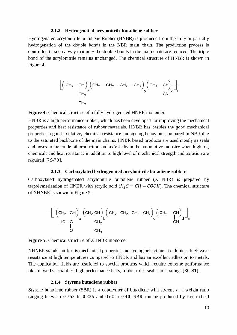
2.1.2 Hydrogenated acrylonitrile butadiene rubber

Hydrogenated acrylonitrile butadiene Rubber (HNBR) is produced from the fully or partially

hydrogenation of the double bonds in the NBR main chain. The production process is

controlled in such a way that only the double bonds in the main chain are reduced. The triple

bond of the acrylonitrile remains unchanged. The chemical structure of HNBR is shown in

Figure 4.

CH2 CH CH2 CH2 CH2 CH2 CH2 CH

CNCH2

CH3

x y z n

Figure 4: Chemical structure of a fully hydrogenated HNBR monomer.

HNBR is a high performance rubber, which has been developed for improving the mechanical

properties and heat resistance of rubber materials. HNBR has besides the good mechanical

properties a good oxidative, chemical resistance and ageing behaviour compared to NBR due

to the saturated backbone of the main chains. HNBR based products are used mostly as seals

and hoses in the crude oil production and as V-belts in the automotive industry when high oil,

chemicals and heat resistance in addition to high level of mechanical strength and abrasion are

required [76-79].

2.1.3 Carboxylated hydrogenated acrylonitrile butadiene rubber

Carboxylated hydrogenated acrylonitrile butadiene rubber (XHNBR) is prepared by

terpolymerization of HNBR with acrylic acid (𝐻2𝐶 = 𝐶𝐻 − 𝐶𝑂𝑂𝐻). The chemical structure

of XHNBR is shown in Figure 5.

CH2 CH CH2 CH CH2 CH2 CH2 CH2 CH2 CH

CNCH2

CH3

C

O

OHa b c d n

Figure 5: Chemical structure of XHNBR monomer

XHNBR stands out for its mechanical properties and ageing behaviour. It exhibits a high wear

resistance at high temperatures compared to HNBR and has an excellent adhesion to metals.

The application fields are restricted to special products which require extreme performance

like oil well specialities, high performance belts, rubber rolls, seals and coatings [80, 81].

2.1.4 Styrene butadiene rubber

Styrene butadiene rubber (SBR) is a copolymer of butadiene with styrene at a weight ratio

ranging between 0.765 to 0.235 and 0.60 to 0.40. SBR can be produced by free-radical

11

emulsion polymerization (E-SBR) or by ionic solution polymerization (S-SBR). The chemical

structure of SBR is shown in Figure 6.

CH2 CH CH CH2

CHCH2

CH2 CH CH CH2 CH CH2+x y n

Figure 6: Chemical structure of SBR monomer

SBR represents the best synthetic rubber due to its performance-processing-cost profile. SBR

is an excellent electrical insulating material. It has a lower elasticity but a better heat and

ageing resistance than NR. SBR is used for producing technical rubber articles, sealing

systems and conveyor belts [76-79]. Due to its high abrasion resistance, S-SBR enjoys a great

interest in the tire industry, especially after the huge development made for the production of

green tires [82, 83].

2.2 Vulcanisation

The vulcanisation refers to the production process of crosslinked high elastic elastomer

composites through energy rich radiation or chemical crosslinking. The latter is currently the

most used crosslinking method. The polymer chains are linked by covalent bonds, achieved

mainly by use of sulphur, peroxide or metal oxides when supplied with heat [76].

Diene rubbers possess double bonds in the main or the side chain and are mostly crosslinked

with sulphur. Sulphur is available as S8-rings. It has a dissociation energy of 226 kJ/mol and

it first has to be split off in order to contribute to vulcanisation process [84]. In addition, the

crosslinking system can also involve different vulcanisation accelerators, activators and

sulphur donors. Vulcanisation accelerators are organosulphur compounds or amine. Amines

are organic compounds containing one nitrogen atom with a lone pair. Zinc oxide (ZnO) and

stearic acid are used as activators. Together with the vulcanisation accelerators, the activators

generate an active activator complex. The latter forms with sulphur a sulphur transfer

complex. This reacts with the polymer chains and constitutes network sites in the form of

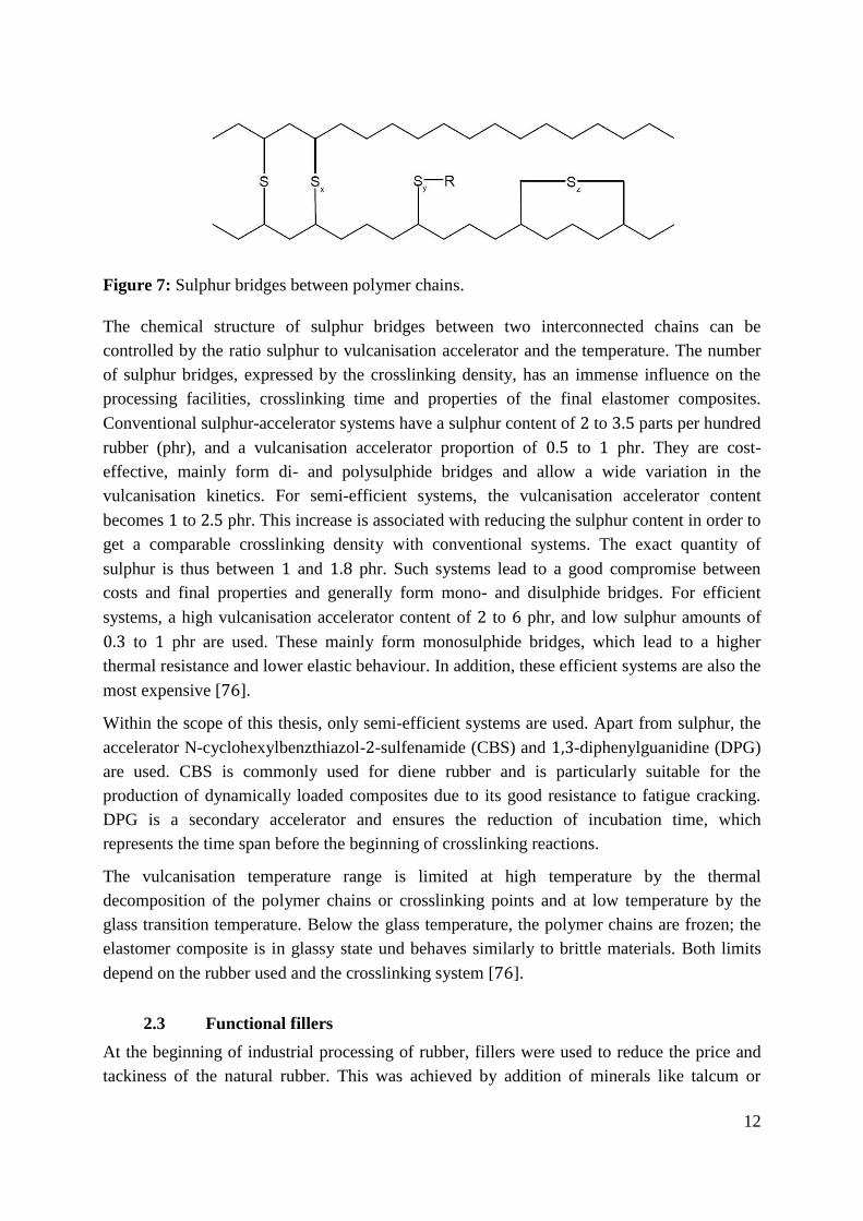
monosulphide, disulphide or polysulphide bridges (see Figure 7) [76].

12

Figure 7: Sulphur bridges between polymer chains.

The chemical structure of sulphur bridges between two interconnected chains can be

controlled by the ratio sulphur to vulcanisation accelerator and the temperature. The number

of sulphur bridges, expressed by the crosslinking density, has an immense influence on the

processing facilities, crosslinking time and properties of the final elastomer composites.

Conventional sulphur-accelerator systems have a sulphur content of 2 to 3.5 parts per hundred

rubber (phr), and a vulcanisation accelerator proportion of 0.5 to 1 phr. They are cost-

effective, mainly form di- and polysulphide bridges and allow a wide variation in the

vulcanisation kinetics. For semi-efficient systems, the vulcanisation accelerator content

becomes 1 to 2.5 phr. This increase is associated with reducing the sulphur content in order to

get a comparable crosslinking density with conventional systems. The exact quantity of

sulphur is thus between 1 and 1.8 phr. Such systems lead to a good compromise between

costs and final properties and generally form mono- and disulphide bridges. For efficient

systems, a high vulcanisation accelerator content of 2 to 6 phr, and low sulphur amounts of

0.3 to 1 phr are used. These mainly form monosulphide bridges, which lead to a higher

thermal resistance and lower elastic behaviour. In addition, these efficient systems are also the

most expensive [76].

Within the scope of this thesis, only semi-efficient systems are used. Apart from sulphur, the

accelerator N-cyclohexylbenzthiazol-2-sulfenamide (CBS) and 1,3-diphenylguanidine (DPG)

are used. CBS is commonly used for diene rubber and is particularly suitable for the

production of dynamically loaded composites due to its good resistance to fatigue cracking.

DPG is a secondary accelerator and ensures the reduction of incubation time, which

represents the time span before the beginning of crosslinking reactions.

The vulcanisation temperature range is limited at high temperature by the thermal

decomposition of the polymer chains or crosslinking points and at low temperature by the

glass transition temperature. Below the glass temperature, the polymer chains are frozen; the

elastomer composite is in glassy state und behaves similarly to brittle materials. Both limits

depend on the rubber used and the crosslinking system [76].

2.3 Functional fillers

At the beginning of industrial processing of rubber, fillers were used to reduce the price and

tackiness of the natural rubber. This was achieved by addition of minerals like talcum or

13

kaolin. Later, mineral fillers were used as extenders with the aim of improving the processing

and properties of final elastomer composites. Several investigations revealed that zinc oxide

(ZnO) assign the crosslinked samples a mechanical reinforcement and improves their heat

resistance. ZnO remained the most important reinforcing filler until the large-scale

development of carbon black (CB). From the late 1920s with the rapid development of the

automobile industry, CB became the main reinforcing filler in the rubber technology due to

realised improvements of the wear resistance of the tyre tread compounds. Particularly

important is the reinforcement potential of CB for amorphous synthetic rubbers like SBR

[76].

CB is an organic filler which is principally made of carbon. The CB particles are spherical

and may form chain-like aggregates. Regarding the morphology, it can be differentiated

between primary particles (particle microstructure), aggregates (primary structure) and

agglomerates (secondary structure). The primary particles used in the production of

elastomers have medium particle diameter between 10 𝑛𝑚 and 300 𝑛𝑚 and a N2-BET

specific surface area between 9 𝑚²/𝑔 and 138 𝑚²/𝑔. The aggregates have an anisotropic

structure and consist of several firmly connected primary particles. They represent the

smallest stable unit and have a size between 100 𝑛𝑚 and 800 𝑛𝑚. CB aggregates can be

bonded together via Van-der-Waals forces to form large agglomerates. The agglomerates can

only be broken apart under the influence of mechanical forces.

Considering the interaction with the rubber matrix, CB is divided into reinforcing and not

reinforcing fillers. The term reinforcement is understood as the sum of all rubber-filler

interactions, which are expressed in physical properties for both non-crosslinked and

crosslinked samples. Reinforcing, also called active, fillers are nanoparticles and have particle

diameters between 10 𝑛𝑚 and 100 𝑛𝑚. They change by interaction with the polymer chains

the viscoelastic properties of the rubber samples. They increase the viscosity of the rubbers

and improve the fracture behaviour of the vulcanisates, such as tear strength, tear propagation

resistance and abrasion. Not reinforcing or inactive fillers have particle diameters between

500 𝑛𝑚 and 1000 𝑛𝑚 and simply ensure that the rubber matrix become diluted. This causes

a decrease of tearing energy, although the process ability or gas tightness can be positively

influenced.

Due to its graphite-type crystalline structure, CB has an excellent electrical conductivity,

which ranges between 10−1 𝑆/𝑐𝑚 and 102 𝑆/𝑐𝑚. The electrical conductivity of CB depends

on the degree of graphitization, the impurities and the chemical groups on the surface. By

mixing CB in the rubber matrix, the dielectric conductivity of the prepared elastomer

composites can be changed by 15 powers of ten. The increase of the dielectric conductivity

mainly depends on the CB volume fraction when the percolation threshold is exceeded. The

percolation process describes the formation of connected filler clusters to establish a filler

network. It is the transition from isolated filler particles to linked filler clusters through

chemical reactions, so that continuous paths along the filler network arise for charge carriers.

The percolation threshold mainly depends on the properties of CB and their distribution in the

14

rubber matrix. The latter is strongly influenced by both the mixing and the curing process.

The polymer chains have with 10−13 𝑆 a tiny contribution to the dielectric properties of

elastomer composites. This is caused by molecular interactions.

Depending on the application field, the dielectric conductivity of elastomer composites is

highly relevant when it comes to electrostatic charging by friction. For rotating car tyres, an

electron transfer occurs between the tyre tread and the road because they have a different

dielectric constant. The car becomes electrically charged. To prevent the passengers an

electric shock, the electrostatic charge should continuously be discharged during the drive.

This is only achieved by using conductive CB to fill the elastomer composites.

In order to increase the performance, safety and lifetime of modern tyres, bio-based

alternatives to petrochemical materials and recycled raw materials are developed. No less

interesting is the environmental impact of mobility nowadays. Different studies show that the

mobility contributes to around 18 % of global CO2-emissions, whereby 75 % of them is

attributed to road transport. 24% of CO2-emissions from passenger cars and 40% of CO2-

emissions from trucks are directly attributed to the tyres [82, 83]. More precisely, these CO2-

emissions results from the rolling behaviour of tyre and the corresponding fuel consumption.

For sustainable mobility, new products are developed and intensively studied. Tyre labels

were also introduced in order to increase not only the safety and the profitability, but also the

ecological efficiency in the road traffic. This was successfully achieved by manufacturing the

so-called “Green tyres”. Green tyres are characterised by a low rolling resistance, outstanding

brake properties and a long lifetime. This success is mainly attributed to the new filler Silica.

Silica is an inorganic filler and consists of amorphous silicon dioxide. It is finely dispersed

colloids with N2-BET specific surface areas ranging between 25 𝑚²/𝑔 and 700 𝑚²/𝑔. There

are pyrogenic silica and precipitated silica. They differ by the structure of the aggregates and

the chemical composition of the surface. Pyrogenic silica has a chain-like aggregate structure.

The aggregates of the precipitated silica are substantially larger and consist of clusters with a

porous structure which also leads to an inner surface. On the silica surface there are silanol

groups (𝑅3𝑆𝑖 − 𝑂 − 𝐻) as well as siloxane groups (𝑅2𝑆𝑖 − [−𝑂 − 𝑆𝑖𝑅2]𝑛 − 𝑂 − 𝑆𝑖𝑅3) [85].

Precipitated silica has 5 to 6 silanol groups per 𝑛𝑚² on the surface. Pyrogenic silica has 2.5 to

3.5, mostly isolated silanol groups per 𝑛𝑚² on the surface. The silanol groups are responsible

for the acid and the strongly polar behaviour of silica. They are accessible for various

chemical reactions. Of great practical importance is the reaction of the silanol groups with

organic silanes. Reactive groups can be formed to initiate a covalent bonding between the

polymer chains and the silica surface area. Silanisation reactions can only take place if silanol

groups are present. Due to their polarity, the silica clusters tend to agglomerate via hydrogen

bond than to be bonded with the polymer chains. This effect is more pronounced for silica

than for CB filled elastomer composites.

Silica is used in the rubber industry as substitute or compliment to CB palette. A necessary

prerequisite is the use of a bifunctional organosilane. In contrast to CB, silica is not

15

electrically conductive. For tyre application, a CB amount above the dielectric percolation

threshold is always added [76]. Figure 8 depicts the two rubber fillers CB and silica.

Figure 8: Reinforcing rubber fillers: carbon black on the left and silica on the right.

In the scope of this thesis, two kinds of CB supplied by ORION Engineered Carbons GmbH

and one silica type supplied by Evonik Industries are used. N 550 is a semi-active CB [86].

Printex XE2-B is a high reinforcing and a super conductive CB [87]. Ultrasil 7000 GR

(U 7000) is a precipitated amorphous silicon dioxide [88]. U 7000 is one of the most used

silica in the rubber industry. Some of the physical properties of the two CB and silica are

summarized in Table 1.

Table 1: Physical properties of fillers

N 𝟓𝟓𝟎 Printex XE2-B U 𝟕𝟎𝟎𝟎

Average particle size [nm] 56 30 14

N2-BET specific surface area [m²/g] 40 1000 175

Density (20 °C) [g/cm³] 1.8 1.7– 1.9 2

Besides the mechanical reinforcement potential, rubber fillers can also be classified according

to their behaviour in an applied magnetic field. The conventional rubber fillers discussed

above, CB and silica, are non-magnetic materials and do not interact with an external

magnetic field. The magnetic field can flow such as in a vacuum or air. Regarding magnetism,

they can be considered as irrelevant. Other filler materials may be affected in various degrees

by magnetic fields. They can cause a considerable strengthening and bundling of magnetic

field lines. They may even magnetise themselves. It can be distinguished between

magnetically soft and magnetically hard materials. This distinction is particularly important in

terms of applications. Soft magnetic materials are mainly iron, nickel, cobalt and low alloy

steels. The magnetic field flows more easily through them und the magnetic flux density

becomes higher. By removing the magnetic field, a large part of the magnetisation gets lost. A

small material-dependent residual magnetism may remain. Hard magnetic materials possess a

permanent magnetic behaviour. After being magnetised, they retain their magnetic properties

and are marked by a high energy density. Such materials are characterised by a high

16

remanence and high coercivity. A general overview of different magnetic fillers is depicted in

Figure 9, adapted from [89].

Figure 9: Magnetic materials.

The origin of the different magnetisation behaviours is discussed in detail in the next chapter.

2.4 Rubber additives

Rubber additives are auxiliary materials that are added to rubber compounds in order to

facilitate the processing and to set better features of fully operational elastomer composites.

They are used for the designing of end products from mixing steps through control of

chemical reactions like curing process or salinization to achieving desired properties during

the service life, even if these properties are mainly supported by rubber type, fillers and

crosslinking systems.

In the processing of rubber compounds, plasticizers play an important role and have a large

influence on the properties of the finished products. Plasticizers are low viscous fluids and

should comply with different requirements. Basically, they should be readily soluble in the

rubber, oxidation resistant, have good ageing behaviour and do not disturb the crosslinking

systems. They increase the chain mobility and lower the viscosity as well as the glass

transition temperature. They are classified in two groups: mineral oil and synthetic

plasticizers. The ester plasticizers build the largest synthetic plasticizer group. The mineral oil

plasticizers comprise three categories: paraffinic, naphthenic and aromatic plasticizers.

Paraffinic plasticizers are more compatible with nonpolar rubber like EPDM. Weakly polar

rubber like NR and SBR interact well with naphthenic plasticizers. Aromatic and synthetic

plasticizers are suited for polar rubber. In the framework of this thesis, dioctyl phthalate

17

(DOP), a phthalic acid ester is used for polar rubbers. Treated distillate aromatic extract

(TDAE) is used for nonpolar rubber. The addition of plasticizers leads to a dilution of the

rubber matrix. The mixing ratios affect the viscoelastic plateau of finished elastomer

composites by shifting the range of glass transition towards higher or lower temperatures. The

desired thermal properties can then be set very precisely. Mechanical characteristics like

modulus of elasticity, stress value or hardness also change accordingly. They decrease with

increasing the plasticizer content.

Processing aids are used to promote principally the mixing process of components. However,

they influence in a similar manner the properties of the finished products as the plasticizers.

In order to attain application relevant properties, rubber compounds should be first

vulcanised. In the framework of this thesis, this is achieved by sulphur crosslinking during the

curing process. In addition to elementary sulphur, vulcanisation accelerators and activators are

added. Almost all vulcanisation accelerators are highly reactive only in the presence of metal

oxides. As seen in section 2.3, zinc oxide (ZnO) is used. Furthermore, the stearic acid is used

as activator. It forms with ZnO zinc stearates, a necessary preliminary stage for sulphur

crosslinking. Zinc stearates increase the solubility of the crosslinking system in the rubber by

forming soluble complexes. ZnO and stearic acid are present in the finished compounds at

very low levels.

Furthermore, antioxidants are used to inhibit the oxidation of the polymer chains by ozone or

oxygen. The oxidation reactions may have adverse changes of the properties and the life time

of the elastomer composites. Diene rubbers are particularly vulnerable to ageing processes

due to their double bonds. N-(1,3-dimethylbutyl)-N'-phenyl-p-phenylenediamine (6PPD) and

N-isopropyl-N'-phenyl-p-phenylenediamine (IPPD), supplied by Lanxess, are used.

Besides, coupling agents can be useful to enhance the adhesion of polymer chains to surface

area of filler particles. These are strictly necessary if the surface areas of both polymer chains

and filler particles have different polarities. In this case, the coupling agent silane bis-

(triethoxysilylpropyl)-tetrasulfide (TESPT), also known under the trade name Si69, is added.

It is used to functionalize the surface area of magnetic filler particles making them more

compatible with the polymer chains [76].

19

3 Magnetism and magnetic filler particles

This chapter is devoted to the theory of magnetism and magnetic fillers used in the rubber

technologies. The most important concepts of magnetism are presented. The different types of

magnetism are introduced and the reasons of their occurrence are discussed. The magnetic

dipole-dipole interaction is explained in more detail. Afterwards, different magnetic materials

are presented. This is followed by the magnetic fillers for rubber compounds.

3.1 Magnetism

Magnetism is one of the fundamental phenomena of solid-state physics. The Greeks

discovered that certain iron ores found in a city called Magnesia, now in Turkey, could attract

other pieces of iron. The ancient Chinese discovered that certain types of natural iron ore,

when suspended freely always points in a north-south direction. The Chinese use this property

to make a simple form of compass for navigational purposes. During a lecture demonstration

in 1819, the Danish scientist Hans Oersted found that compass needle has been deflected via

an electric current in a wire. This discovery brought for the first time the magnetic field and

the electrical current together. This milestone was the beginning of our understanding of the

origin of magnetism. James Clerk Maxwell was the first who describes that magnetism is a

property of a charged particle in motion. Otto Stern and Walther Gerlach succeeded in

explaining this phenomenon, which was not comprehensible within the framework of

classical physics. In the Stern-Gerlach experiment, named after the two researchers as

recognition of their findings, an electron gun shoots out a beam of electrically neutral silver

atoms across an evacuated tube. If a bar magnet is held at the side of the tube, the beam is

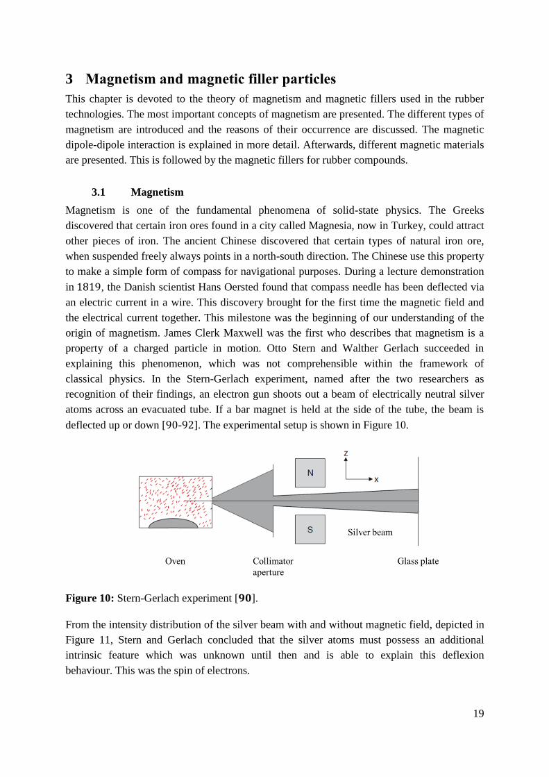
deflected up or down [90-92]. The experimental setup is shown in Figure 10.

Figure 10: Stern-Gerlach experiment [𝟗𝟎].

From the intensity distribution of the silver beam with and without magnetic field, depicted in

Figure 11, Stern and Gerlach concluded that the silver atoms must possess an additional

intrinsic feature which was unknown until then and is able to explain this deflexion

behaviour. This was the spin of electrons.

20

I(z)

z

Without B

With B

-z0 0 z

0

Figure 11: Intensity distribution of silver beam with and without magnetic field.

This concept implies that all magnetic phenomena are attributed to the spin state within the

atoms. The silver atoms occupied only two states when the magnetic field was switched on.

This means that the magnetic moments in atoms just occur in two spatial quantized states.

According to quantum theory, the spin of electron is 1

2. The corresponding magnetic moment

µ is defined as

µ = 𝑔𝑠𝑞

2𝑚 𝑺 (5)

where 𝑔𝑠 is the g-factor, 𝑞 is the charge of the particle, 𝑚 is its mass and 𝑺 is its spin angular

momentum.

When the electrons take different spin states, different form of magnetism can be observed.

Inside materials, the atoms are considered as tiny magnets and are arranged in groups called

domains. The size of these domains and their orientation affect strongly the magnetic

properties of magnetic materials. The magnetic materials can be classified in diamagnetic,

paramagnetic, ferromagnetic, antiferromagnetic and ferrimagnetic materials.

For diamagnetic materials like hydrogen (𝐻), copper (𝐶𝑢) and silver (𝐴𝑔), the individual

atoms do not possess any net magnetic moment. In the absence of external magnetic field, the

net magnetic dipole moment over each atom or molecule is zero due to the pairing of

electrons. When diamagnetic materials are brought in an external magnetic field, they get

feebly magnetised in the opposite direction of the magnetic field and experience a repelling

force.

21

For paramagnetic materials like aluminium (𝐴𝑙), calcium (𝐶𝑎), platinum (𝑃𝑡) and dioxygen

(𝑂2), each individual atom has a net non-zero magnetic moment. They possess a permanent

dipole moment due to some unpaired electrons. When they are placed in an external magnetic

field, they get weakly magnetised in the same direction as the magnetic field and experience a

feeble attractive force.

Ferromagnetism, antiferromagnetism and ferrimagnetism are macroscopic phenomena

associated with the so-called collective magnetism. Collective magnetism is a phenomenon in

which the magnetic moments mutually align themselves due to interaction of the electron

spins. This behaviour is based on the coupling of the magnetic moments. Depending on the

strength of the coupling and the ordering temperature (Curie or Néel temperature); below

which the interaction energy of the magnetic moments is greater than the thermal energy, a

spontaneous magnetic order occurs without the action of external magnetic fields.

For ferromagnetic materials like manganese (𝑀𝑛), iron (𝐹𝑒), cobalt (𝐶𝑜) and nickel (𝑁𝑖),

spontaneous magnetisation occurs below the Curie temperature 𝑇𝐶. At the temperature

absolute zero, all atomic magnetic moments are aligned in the same direction so that the

spontaneous magnetisation takes its maximum value. When the temperature increases, the

ferromagnetic ordering is gradually disturbed and disappears at the Curie point 𝑇𝐶. The

ferromagnetic materials experience a very strong attractive force when they get magnetised in

the presence of an external field. The magnetic domains, randomly oriented in the

unmagnetised material, become aligned in the same direction as the external field.

In the case of antiferromagnetism, there is no spontaneous magnetisation. The magnetic

moments are arranged in sublattices, which have opposite magnetisation. The negative

exchange energy between adjacent magnetic moments additionally leads to a vanishing of the

total magnetisation. At the temperature absolute zero, the spin chain within the material

consists of an alternating antiparallel position of the spins. If the temperature increases, the

thermal excitation turns over the individual spins, so that the spatial arrangement of magnetic

moments is disturbed. The antiferromagnetic ordering disappears above the antiferromagnetic

Néel temperature 𝑇𝑁 and becomes a paramagnetic ordering.

Ferrimagnetic materials have a spontaneous magnetisation below the Curie temperature TC

similar to the ferromagnetism. For ferrimagnetic materials like nickel (𝑁𝑖) and ferrite, any

two magnetic dipoles are aligned anti-parallel. Since the magnitudes of magnetic dipoles are

not equal, a net magnetisation remains. In some ferrimagnetics, the total magnetisation can be

reversed at a compensation temperature 𝑇𝑘. If the magnetisations of the sublattices are equal,

antiferromagnetism is observed [90-95].

The different forms of collective magnetism are displayed in Figure 12.

22

Figure 12: Form of magnetism in solids: ferromagnetic, antiferromagnetic and ferrimagnetic

domains. The thick lines represent the Bloch walls between the single domains.

In the case of ferrimagnetic particles, if the particle size falls below a critical value, no

magnetic domain can be built. The thermal energy is greater than the magnetocrystalline

anisotropy energy and the magnetisation direction follows the thermal fluctuation. Such

particles are one-domain particles and have no remanence. This phenomenon is called

superparamagnetism [93,95].

The magnetic field is a zero divergence field as already stated by James Clerk Maxwell. The

Gauss´s law for magnetism has the following form:

div 𝑩 = 0 (6)

This means that the source of magnetism is not the magnetic load carriers. In contrast to

electron in electricity, the source of magnetism is the moving electric charges or time varying

electric fields. The magnetic field is described by two different physical quantities: the

magnetic flux density or magnetic induction 𝑩 and the magnetic field strength 𝑯. 𝑩 describes

the spatial density of the magnetic flux 𝛷 and has the unit Tesla (𝑇). 𝑯 describes the strength

of the magnetic field generated by free currents and has the unit Ampere per meter (𝐴/𝑚). 𝑩

and 𝑯 are related in vacuum as follows:

𝑩 = µ0𝑯 (7)

where µ0 = 4𝜋. 10−7 V s

A m is the vacuum permeability.

If a material is placed in a magnetic field, the existing magnetic dipoles interact with it. The

material becomes magnetised and the magnetic flux density B changes to

𝑩 = µ0𝑚𝑟𝑯 (8)

where 𝑚𝑟 is the relative permeability of the material. The magnetic flux density can be also

expressed by

𝑩 = µ0(𝑯 + 𝑴) (9)

where M is the magnetisation. The magnetisation M indicates the magnetic field caused by

bound surface currents. Those microscopic ring currents are present in each molecule and are

the origin of the magnetism [94-97]. In general, the magnetisation M is location-dependent.

For homogeneous external magnetic field and isotropic samples, M is given by the spatial

means over all magnetic dipoles and takes the following form:

𝑴 =∑ 𝒎𝑖𝑖

𝑉≔

𝒎𝑟

𝑉 (10)

23

The magnetisation 𝑴 is defined as the density of the existing magnetic dipoles within the

material. For infinitesimal small volume, the sum operator can be changed to an integral and

the relative permeability of the sample becomes as follows:

𝒎𝑟 = ∫ 𝑴𝑑𝑉𝑉

(11)

From equation (8) and equation (9), a relation between H and M can be derived.

𝑴 = (µ𝑟 − 1)𝑯 (12)

𝑴 ≔ 𝜒𝑯 (13)

where the proportionality factor 𝜒 is the magnetic susceptibility [90-95]. It is a material

specific property and it is considered as the material response function to external magnetic

field. It represents with the relative permeability µ𝑟 the key features of magnetic materials.

Indeed 𝜒 and µ𝑟 take different values for different materials. The value ranges for

diamagnetic, paramagnetic and ferromagnetic materials are listed below

diamagnetic materials 𝜒 < 0 𝑚𝑟 < 1

paramagnetic materials 𝜒 > 0 𝑚𝑟 > 1

ferromagnetic materials 𝜒 ≫ 0 𝑚𝑟 > 1

3.2 Magnetic dipole interaction

In this section the stationary phenomena of the magnetic field are more closely treated.

According to quantum theory, every atom can have a non-zero magnetic moment and the

existing magnetic dipoles can occupy different quantum states. In the presence of an external

magnetic field, the coupling between individual magnetic moments induces a magnetically

ordered state, as described in the last section [90-95].

The magnetic energy of a magnetic dipole 𝒎 in an external magnetic field 𝑩 looks as follows:

𝐸 = − 𝒎 ∙ 𝑩 = −𝑚 𝐵 𝑐𝑜𝑠𝜃 (14)

where 𝜃 represents the angle between magnetic dipole and magnetic field direction as

pictured on Figure 13.

24

-1

0

1

E

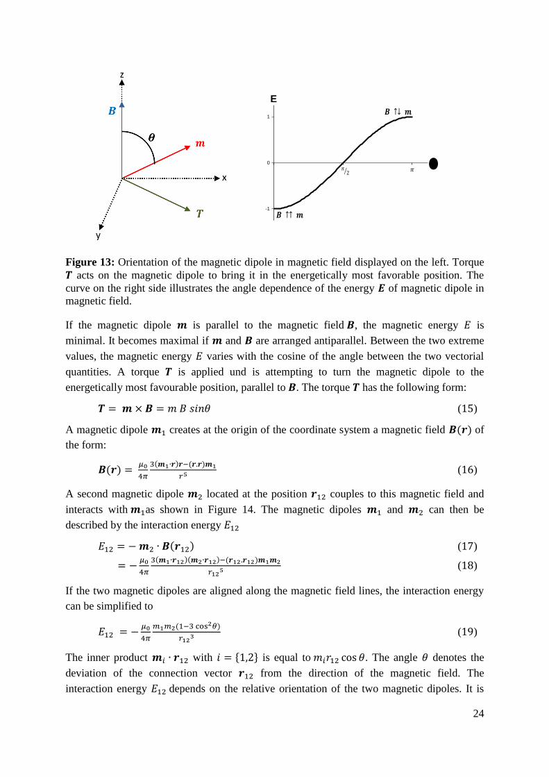
Figure 13: Orientation of the magnetic dipole in magnetic field displayed on the left. Torque

𝑻 acts on the magnetic dipole to bring it in the energetically most favorable position. The

curve on the right side illustrates the angle dependence of the energy 𝑬 of magnetic dipole in

magnetic field.

If the magnetic dipole 𝒎 is parallel to the magnetic field 𝑩, the magnetic energy 𝐸 is

minimal. It becomes maximal if 𝒎 and 𝑩 are arranged antiparallel. Between the two extreme

values, the magnetic energy 𝐸 varies with the cosine of the angle between the two vectorial

quantities. A torque 𝑻 is applied und is attempting to turn the magnetic dipole to the

energetically most favourable position, parallel to 𝑩. The torque 𝑻 has the following form:

𝑻 = 𝒎 × 𝑩 = 𝑚 𝐵 𝑠𝑖𝑛𝜃 (15)

A magnetic dipole 𝒎1 creates at the origin of the coordinate system a magnetic field 𝑩(𝒓) of

the form:

𝑩(𝒓) = 𝜇0

4𝜋

3(𝒎1∙𝒓)𝒓−(𝒓.𝒓)𝒎1

𝑟5 (16)

A second magnetic dipole 𝒎2 located at the position 𝒓12 couples to this magnetic field and

interacts with 𝒎1as shown in Figure 14. The magnetic dipoles 𝒎1 and 𝒎2 can then be

described by the interaction energy 𝐸12

𝐸12 = − 𝒎2 ∙ 𝑩(𝒓12) (17)

= −𝜇0

4𝜋

3(𝒎1∙𝒓12)(𝒎2∙𝒓12)−(𝒓12.𝒓12)𝒎1𝒎2

𝑟125 (18)

If the two magnetic dipoles are aligned along the magnetic field lines, the interaction energy

can be simplified to

𝐸12 = −𝜇0

4𝜋

𝑚1𝑚2(1−3 cos2𝜃)

𝑟123 (19)

The inner product 𝒎𝑖 ∙ 𝒓12 with 𝑖 = {1,2} is equal to 𝑚𝑖𝑟12 cos 𝜃. The angle 𝜃 denotes the

deviation of the connection vector 𝒓12 from the direction of the magnetic field. The

interaction energy 𝐸12 depends on the relative orientation of the two magnetic dipoles. It is

25

proportional to the product of the two magnetic moments and is inversely proportional to the

cube of their distance.

-1

0

1

2

E12

Figure 14: Dipole-dipole coupling in magnetic field is illustrated on the left. The angle

dependence of the dipole-dipole interaction energy 𝑬𝟏𝟐 in magnetic field is displayed on the

right.

The interaction energy 𝐸12 is at its largest when 𝒓12 is parallel to the direction of the magnetic

field [90-95].

3.3 Magnetic materials

The magnetic permeability µ𝑟 reveals the magnetic sensitivity of the examined material.

Different materials affect in various ways the pattern of the magnetic field lines. As long as

no external magnetic field is applied, even ferromagnetic materials seem to be not magnetic

from a certain temperature because the magnetic domains are spontaneously arranged. Due to

the disorder of elementary magnets, the material does not show outwards any magnetic

phenomena.

Applying an external magnetic field moves first the Bloch walls separating the single

magnetic domains (see Figure 12). Increasing the magnetic field change the size of the

magnetic domains and their orientation. If all magnetic domains are aligned, the

magnetisation attains its maximum and has the same direction as the magnetic field. Once this

state is reached, a further increase of the magnetisation is no longer possible even if the

magnitude of the external magnetic field increases. In other words, if all dipole moments are

parallel to the external magnetic field, the material is magnetically saturated. These processes

are reversible. When the external magnetic field is switched off, the magnetisation does not

disappear completely. It remains a residual magnetisation 𝐵𝑟, which disappears with an

opposite field at the level of the coercivity 𝐻𝐶. The magnetic flux density 𝑩 becomes zero.

The entire process of magnetisation can be determined by considering the evolution of the

magnetic flux density 𝑩 and the magnetic field strength 𝑯. The obtained relationship between

𝑩 and 𝑯 represents a characteristic curve for each material and is called the hysteresis loop.

Figure 15 displays the hysteresis loop of a ferromagnetic material [90].

26

If a ferromagnetic material is exposed to a magnetic field for the first time, both 𝑩 and 𝑯 are

equal zero because the material is completely unmagnetised. With increasing the magnetic

field strength 𝑯, the magnetic flux density 𝑩 increases also. From a certain magnetic field

strength 𝑯, 𝑩 increases slightly to reach a saturation state. This phenomenon corresponds to

the sub curve (a) in Figure 15 and is called initial magnetisation curve. By reducing the

magnetic field, the magnetic field strength 𝑯 decreases. The magnetic flux density 𝑩

decreases also, however, not according to the initial magnetisation curve but rather an upper

sub curve (b). Even at a zero magnetic field strength 𝑯, a non-zero magnetic flux density 𝑩

remains. This material dependent value is referred to as magnetic remanence or residual

magnetisation 𝐵𝑟. If the direction of the magnetic field is reversed, the magnetic flux density

𝑩 returns zero at a non-zero magnetic field strength 𝑯. This particular value corresponds to

the coercivity 𝐻𝐶. A further increasing of the magnetic field strength towards negative values

leads the material to reach again the saturation state. When this process is turned over, same

steps in reverse order are obtained according to sub curve (c).

bb

c

Hc

H [A/m]

B [

T]

Br

a

Figure 15: Hysteresis loop of a ferromagnetic material.

Ferromagnetic materials are divided into two groups, differing in the shape of the hysteresis

loop and the magnetisation energy. Hard magnetic materials need a strong external magnetic

field to become magnetised. But once magnetised, they do not readily lose their

magnetisation. They are characterised by a strong reluctance, which means that a high

magnetic energy is stored. The hysteresis loop has a rectangular shape with high coercivity

and remanence values. Hard magnetic materials are mainly used as a magnetic field source,

generating a continuous magnetic flux. Soft magnetic materials have a hysteresis loop with

small area and very small magnetic energies can be stored. The low coercivity and remanence

27

values are a hint for a low energy requirement for the magnetisation process. Their magnetism

is temporary and get lost as soon as the exciter field current stops. Soft magnetic materials are

characterised by a high permeability and are used in general for guiding the magnetic flux

[90-92].

In the following subsections, different magnetic materials will be examined more closely. On

this basis, the magnetic fillers used in this thesis are presented.

3.3.1 Iron

In the periodic table of elements, iron is the chemical element with the atomic number 26. It

is a part of transition metals and has the symbol 𝐹𝑒, coming from Latin for ferrum. It is the

fourth most common element in the earth's crust with a total amount of 6.2 %. Iron represents

the final stage of nuclear fusion in the stars, which is hurled into the environment by

supernova explosions. Already in antiquity, iron objects from meteorites were known. Due to

its origin, this type of iron is called meteoric iron and consists of an iron nickel alloy.

Historically, iron production was first carried out by the Hittites. Nowadays, the iron is

mainly obtained in the blast furnace by means of chemical reduction of the iron oxide of the

iron ores with carbon [85]. Pure iron can also be obtained in the laboratory by reduction of

iron oxides with hydrogen at temperature ranging from 400 to 700 °𝐶 or by pyrolysis of iron

pentacarbonyl 𝐹𝑒(𝐶𝑂)5 at 250 °𝐶. Pure iron has the highest saturation magnetisation, the

highest magnetic permeability and the lowest remanence of all elements. A summary of the

properties of iron is presented in Table 2 [90].

Table 2: Physical properties of iron.

Fe

Atomic number 26 Standard atomic weight (Ar) 55,847(3)

Electron configuration [Ar] 3d6 4s2

Density (at room temperature ) 8.874 𝑘𝑔/𝑚3 Electronegativity ( Allred-Rochow scale) 1.6 Most common isotope (natural abundance > 91%) 56Fe

Melting point 1539 °𝐶

Curie point 768 °𝐶

The crystal structure and magnetic ordering of iron are temperature dependent. They are listed

in

Table 3.

Table 3: Crystal structure and magnetic ordering of iron

Temperature

[°C]

Occurrence Crystal structure

Bravais lattice

Magnetic ordering

𝟗𝟎𝟔 -Fe body-centred cubic (bcc) ferromagnetic

𝟏𝟒𝟎𝟏 -Fe face-centred cubic (fcc) paramagnetic

𝟏𝟓𝟑𝟗 -Fe body-centred cubic (bcc) paramagnetic

28

-Fe is ferromagnetic up to the Curie point of 768 °𝐶. After that, it loses its spontaneous

magnetisation and remains ferromagnetic only in the presence of an external field [85].

3.3.2 Iron oxides

Naturally occurring iron oxides are wüstite (FeO), hematite (α-Fe2O3), maghemite (δ -Fe2O3)

and magnetite (Fe3O4). Figure 16 shows the iron-oxygen phase diagram [85].

Wüstite (FeO) is an iron monoxide known also as iron (II)-oxide or ferrous oxide. It has a

sodium chloride structure with an iron deficiency. It has a cations blanks/voids ranging

between 0.12 and 0.05, and hence a typical composition from Fe0.88O to Fe0.95O. The iron

deficiency is compensated by Fe3+ ions. Wüstite is stable as a non-stoichiometric compound

Fe1-xO only above 560 °𝐶. Below 560 °𝐶, FeO is metastable and contains a disproportionate

amount of -Fe and Fe3O4. At room temperature, wüstite is paramagnetic. It becomes

antiferromagnetic at a temperature range of −70 °𝐶 to −62 °𝐶. The Néel temperature 𝑇𝑁 is

not constant anymore and is within a certain range because it depends on the concentration of

defects in the structure [96-97].

Hematite and maghemite represent the two natural modifications of iron (III)-oxide. Hematite

(α-Fe2O3) crystallizes in corundum structure. It is weakly ferromagnetic at room temperature

and has a Currie temperature 𝑇𝐶 of 683 °𝐶. Below −13 °𝐶, hematite undergoes a spin-flop

transition and becomes antiferromagnetic. This temperature limit marks the so-called Morin

transition where the spin orientation is turned 90 degrees. Hematite can be superparamagnetic

at room temperature when the particles are smaller than 8 𝑛𝑚 [96-97].

Maghemite (δ-Fe2O3) crystallizes in spinel structure with blanks/voids and is ferrimagnetic at

room temperature. The Curie temperature 𝑇𝐶 of maghemite ranges between 547 °𝐶

and 713 °𝐶. 𝑇𝐶 is not well-defined because maghemite transforms to hematite at temperature

between – 267 °𝐶 and 527 °𝐶 [96-97]. The following chemical reactions can illustrate this

transition. Maghemite can be obtained by oxidation of magnetite at a temperature between

250 and 300 °𝐶.

2Fe3O4 + ½ O2 → 3 δ-Fe2O3

Above 300 °𝐶, δ-Fe2O3 changes to α-Fe2O3.

δ-Fe2O3 → α-Fe2O3

Maghemite can be superparamagnetic at room temperature when the particles are smaller

than 10 𝑛𝑚.

Magnetite (Fe3O4) is iron (II,III)-oxide and is considered as natural magnet. Fe3O4 crystallizes

in the inverse spinel structure Fe+3 [Fe+2Fe+3]O4. The tetrahedral sites are occupied by Fe3+.

The octahedral sites are occupied by Fe+3 and Fe+2. Magnetite is ferrimagnetic. Its Curie

temperature is 577 °𝐶 and its magnetic moment has a theoretical value of 4 µB. The

experimental magnetic moment of magnetite ranges between 4.0 and 4.2 due to contribution

29

of the angular momentum. Magnetite can be superparamagnetic at room temperature when the

particles are smaller than 6 𝑛𝑚. Moreover, Fe3O4 is a good electrical conductor because on

the octahedron sites occurs a rapid electron exchange between the Fe2+- and Fe3+- ions

[85, 96-97].

Figure 16: Iron-oxygen phase diagram [𝟖𝟓].

There are also two different artificial iron (III)-oxides: Beta phase (β-Fe2O3) and epsilon

phase (ε-Fe2O3), which do not play a major role in the framework of this thesis.

3.3.3 Ferrite

Ferrites are ferrimagnetic materials and are mostly composed of three components. Most

ferrites are a mixture of iron, manganese and zinc. Iron is the most important metal in the

ferrite with a share of 70 %. The manganese part is about 25 %. The remaining amount of

5 % is zinc. Every single iron atom generates its own small magnetic field just like any other

manganese atom. In an external magnetic field, the magnetisation fields are oriented in

different directions and partially cancel out one another. Therefore a ferrite is a weaker

magnet than pure iron [85].

The ferrites are produced from various oxides and occur in various structures. One illustration

can be the formula unit Me-Fe2O4, where Me represents a divalent metal. It crystallizes in the

spinel structure. The metal ions are located on the places of two sublattices A and B with a

tetrahedral or octahedral dioxygen (O2) environment. The A-lattice is occupied exclusively by

Fe3+ ions, while the sublattice B is occupied by Me2+ and the remaining Fe3+-ions

In the normal spinel structure, the sublattices are occupied by only one ion type, whereas in

the case of inverse spinel ferrites, the A lattice is occupied exclusively by Fe3+ and the B

lattice is statistically occupied by Fe3+ and Me2+. The metals and the oxygen form crystals

with differently sized crystallites. Since each crystallite is electrically isolated from its

neighbouring one, electric current can flow only within a crystallite. The ferrite shows almost

no electrical conductivity. In contrast to pure iron, a high-frequency magnetic field induces a

very small current in the ferrite. The AC losses are consequently low.

30

Ferrites can have different and mixed structures. The arrangement of the atoms in the crystals,

the oxygen content and the crystallite size determine the direction of the magnetic field in the

iron and manganese atoms. If some iron atoms are replace by manganese atoms, nickel is

used instead of zinc or the oxygen content is increased, the magnetic and the electrical

properties of the ferrite considerably change.

The ferrites are used in switching power supplies. They supply notebooks with electrical

energy. They transmit high-frequency signals from satellites and mobile phones and work as

an antenna in radio-controlled clocks [85].

3.3.4 Magnetic fillers used in this study

In order to prepare magneto-sensitive elastomers, soft magnetic filler were mixed into rubber

matrix. Earlier works have revealed that only MSE filled with magnetic fillers based on iron

or iron oxides show a sufficiently good sensitivity to external magnetic field [98-107].

In the framework of this thesis, pure iron based filler is used. It consists of carbonyl iron

particles SW-S (CIP) and is supplied by BASF SE. The second magnetic filler used is

MAGSILICA. It is based on iron oxides embedded in a silica matrix and is supplied by

Evonik Industries.

Iron carbonyl is a fine iron powder prepared from thermal decomposition of iron

pentacarbonyl 𝐹𝑒(𝐶𝑂)5. Iron (𝐹𝑒) and carbon monoxide (𝐶𝑂) are arranged in a trigonal

bipyramidal structure, in which five carbon monoxide ligands are coordinated to an iron atom.

The electrical charge carries are homogeneously distributed throughout the atoms so that iron

pentacarbonyl does not possess any molecular dipole.

Iron pentacarbonyl is prepared by direct reaction of iron with carbon monoxide. Finely

dispersed iron reacts at temperatures between 150 °𝐶 and 200 °𝐶 under a carbon monoxide

pressure of 50 to 200 bar according to the following chemical formula:

Fe + 5 CO Fe(CO)5

The prepared iron pentacarbonyl is available as yellow-red solution and contains impurities

such as nickel (𝑁𝑖), molybdenum (𝑀𝑜) and chromium (𝐶𝑟). The impurities are removed by

distillation. In a second step, the reverse reaction takes place at higher temperature according

to the following chemical formula:

Fe(CO)5 Fe + 5 CO

Iron (𝐹𝑒) is transported chemically through the gas phase of carbon monoxide (𝐶𝑂). This

process is known as chemical transport reaction and leads to separate pure iron 𝐹𝑒 from

gaseous carbon monoxide (𝐶𝑂) [108-113].

The grey-coloured iron carbonyl prepared represents the hard grade. It is the product from the

primary decomposition without further chemical processing. It has an onion skin structure as

pictured on the left of Figure 17. It contains up to 97,8 % iron 𝐹𝑒, a maximum of 1 %

carbon 𝐶, a maximum of 0.9 % nitrogen 𝑁 and a maximum of 0.5 % oxygen 𝑂. Soft grade

31

CIP is produced by annealing of hard grades under hydrogen 𝐻. In this process, the onion skin

structure becomes a polycrystalline structure as depicted on Figure 17. The iron 𝐹𝑒 content

increases at least to 99.8 %. 𝐶, 𝑁 and 𝑂 are strongly reduced [114-115].

Figure 17: Structure of carbonyl iron particles. Onion skin structure of hard grade CIP is

depicted on the left. The right picture illustrates the polycrystalline structure of soft grade CIP

[𝟏𝟏𝟒].

The CIP used in this thesis contain more than 99 % pure iron and less than 0.4 % carbon. The

relative permeability µ𝑟 of CIP is larger than 29. Additionally, the CIP particles are coated

with a thin layer of polyol containing multiple hydroxyl functional groups. The average

diameter of CIP lies in a range between 3 µ𝑚 to 4.5 µ𝑚 [114-115].

MAGSILICA is a rust-red nanoscaled magnetic filler. It consists of a mixture of different iron

oxides coated with a 3 𝑛𝑚 thick silica layer. The iron oxide content is 85 ± 5 % According

to the supplier, MAGSILICA contains 55 ± 5 % magnetite (Fe3O4), 35 ± 5 % maghemite

(γ-Fe2O3) and less than 15 % hematite (α-Fe2O3). The average diameter of MAGSILICA

particles ranges between 5 𝑛𝑚 to 30 𝑛𝑚. The special saturation magnetisation is more than

45 𝐴𝑚2/𝑘𝑔. The coercivity is between 8 𝑘𝐴/𝑚 and 11 𝑘𝐴/𝑚 [106, 116]. Below certain

size ranges, hematite, maghemite and magnetite show a superparamagnetic behaviour and

possess a higher magnetic moment than paramagnetic materials. At room temperature,

magnetite (Fe3O4) is ferrimagnetic. The magnetic moments have different magnitudes and are

arranged antiparallel within the Weiss domains. Maghemite (γ-Fe2O3) is a ferrimagnetic

material. The magnetic moments are parallel within the Weiss domains, so that the total

magnetisation is larger compared to magnetite [117-118]. Hematite (α-Fe2O3) is

antiferromagnetic below the temperature of Morin transition, otherwise weakly ferromagnetic.

The magnetic moments have the same magnitude and are arranged antiparallel within the

Weiss domains [119-121]. The size distribution of MAGSILICA particles and the structure

of MAGSILICA aggregates are shown in Figure 18.

32

Figure 18: Size distribution of MAGSILICA particles is shown on the left. The inset

illustrates the core-shell structure. On the right, the structure of MAGSILICA aggregates is

shown by means of transmission electron micrograph (TEM) [𝟏𝟏𝟔].

CIP mainly differs from MAGSILICA in the composition and size. Figure 19 shows a view of

MAGSILICA and CIP [114, 115].

Figure 19: Magnetic fillers used. MAGSILICA is on the left. CIP is on the right [𝟏𝟏𝟒].

The coating layers of MAGSILICA and CIP are magnetically dead layers. They do not

contribute to the magnetisation weather of the magnetic filler particle itself or subsequently to

MSE. The coating is highly relevant in order to protect the surrounding rubber matrix and to

provide electrical insulation for electrically conductive substances, which avoids eddy

currents. In addition, the coating enables a better chemical bonding of the filler particles to the

polymer chains with a silane [106, 107].

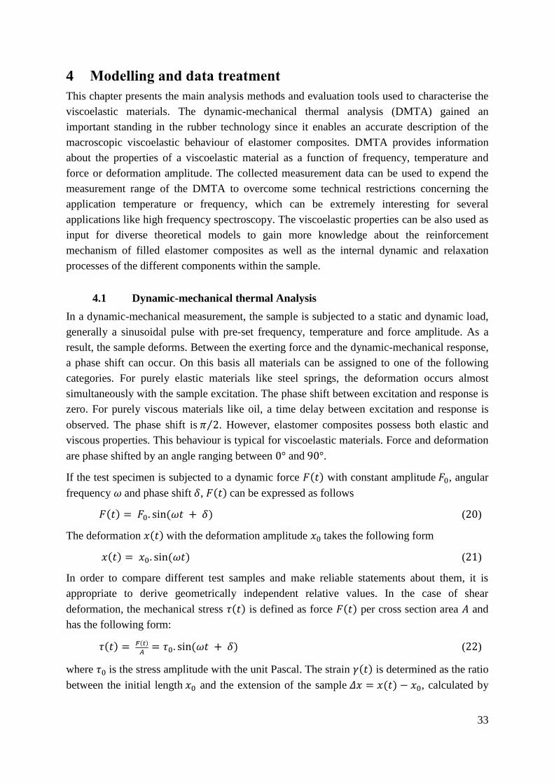
33

4 Modelling and data treatment

This chapter presents the main analysis methods and evaluation tools used to characterise the

viscoelastic materials. The dynamic-mechanical thermal analysis (DMTA) gained an

important standing in the rubber technology since it enables an accurate description of the

macroscopic viscoelastic behaviour of elastomer composites. DMTA provides information

about the properties of a viscoelastic material as a function of frequency, temperature and

force or deformation amplitude. The collected measurement data can be used to expend the

measurement range of the DMTA to overcome some technical restrictions concerning the

application temperature or frequency, which can be extremely interesting for several

applications like high frequency spectroscopy. The viscoelastic properties can be also used as

input for diverse theoretical models to gain more knowledge about the reinforcement

mechanism of filled elastomer composites as well as the internal dynamic and relaxation

processes of the different components within the sample.

4.1 Dynamic-mechanical thermal Analysis

In a dynamic-mechanical measurement, the sample is subjected to a static and dynamic load,

generally a sinusoidal pulse with pre-set frequency, temperature and force amplitude. As a

result, the sample deforms. Between the exerting force and the dynamic-mechanical response,

a phase shift can occur. On this basis all materials can be assigned to one of the following

categories. For purely elastic materials like steel springs, the deformation occurs almost

simultaneously with the sample excitation. The phase shift between excitation and response is

zero. For purely viscous materials like oil, a time delay between excitation and response is

observed. The phase shift is 𝜋 2⁄ . However, elastomer composites possess both elastic and

viscous properties. This behaviour is typical for viscoelastic materials. Force and deformation

are phase shifted by an angle ranging between 0° and 90°.

If the test specimen is subjected to a dynamic force 𝐹(𝑡) with constant amplitude 𝐹0, angular

frequency 𝜔 and phase shift 𝛿, 𝐹(𝑡) can be expressed as follows

𝐹(𝑡) = 𝐹0. sin(𝜔𝑡 + 𝛿) (20)

The deformation 𝑥(𝑡) with the deformation amplitude 𝑥0 takes the following form

𝑥(𝑡) = 𝑥0. sin(𝜔𝑡) (21)

In order to compare different test samples and make reliable statements about them, it is

appropriate to derive geometrically independent relative values. In the case of shear

deformation, the mechanical stress 𝜏(𝑡) is defined as force 𝐹(𝑡) per cross section area 𝐴 and

has the following form:

𝜏(𝑡) = 𝐹(𝑡)

𝐴= 𝜏0. sin(𝜔𝑡 + 𝛿) (22)

where 𝜏0 is the stress amplitude with the unit Pascal. The strain 𝛾(𝑡) is determined as the ratio

between the initial length 𝑥0 and the extension of the sample 𝛥𝑥 = 𝑥(𝑡) − 𝑥0, calculated by

34

subtracting the initial length 𝑥0 from the current distance 𝑥(𝑡). It is dimensionless and can be

expressed as

𝛾(𝑡) = 𝑥(𝑡)−𝑥0

𝑥0= 𝛥𝑥

𝑥0= 𝛾0. sin(𝜔𝑡) (23)

where 𝛾0 is the strain amplitude. Figure 20 illustrates the time-dependent curve progression of

both mechanical stress 𝜏(𝑡) and strain 𝛾(𝑡) of viscoelastic materials.

0

-0

0

(t

) [P

a]

t [s]

0

-0

0

(t

) [-

]

Figure 20: Time evolution of mechanical stress 𝜏(𝑡) and strain 𝛾(𝑡) of viscoelastic materials.

The phase shift 𝛿 between them is also displayed.

The relationship between exerting force and deformation can be further expressed by a

complex quantity to associate the mechanical stress with the strain. This is the shear modulus

𝐺∗(𝑡) in case of a shear or torsion deformation. The shear modulus 𝐺∗(𝑡) is calculated by

dividing the mechanical stress by the strain as follows:

𝐺∗(𝑡) = 𝜏(𝑡)

𝛾(𝑡) (24)

By inserting the previous equations (22) and (23) and developing the sum formula of the sine

function, 𝐺∗(𝑡) becomes

𝐺∗(𝑡) = 𝜏0.sin(𝜔𝑡 + 𝛿)

𝛾0.sin(𝜔𝑡) (25)

𝐺∗(𝑡) = 𝜏0.cos(𝛿) sin(𝜔𝑡)+ 𝜏0.sin(𝛿) cos(𝜔𝑡)


Using the identity cos(𝜔𝑡) = sin(𝜔𝑡 + 𝜋/2), 𝐺∗(𝑡) becomes

35

𝐺∗(𝑡) = 𝜏0.cos(𝛿) sin(𝜔𝑡)+ 𝜏0.sin(𝛿) sin(𝜔𝑡 + 𝜋/2)


𝐺∗(𝑡) = 𝜏0.cos(𝛿) sin(𝜔𝑡)

𝛾0.sin(𝜔𝑡)+

𝜏0.sin(𝛿) sin(𝜔𝑡 + 𝜋/2)


≔ 𝐺′ + 𝑖. 𝐺′′ (29)

where

𝐺′ = 𝜏0

𝛾0 cos(𝛿) (30)

𝐺′′ = 𝜏0

𝛾0 sin(𝛿) (31)

The complex shear modulus 𝐺∗(𝑡) is splitted into two parts. The real part at which stress and

strain are in phase is referred to as the storage modulus, denoted by 𝐺′. It describes the elastic

properties of the sample and it is a measure of the mechanical stored energy 𝑊𝑒𝑙. The

imaginary part at which the stress and the strain are shifted by 𝜋/2 is referred to as the loss

modulus, denoted by 𝐺′′. It refers to the viscous properties of the sample and it is a measure of

the mechanical dissipated energy 𝑊𝑑𝑖𝑠.

The quotient of loss and storage modulus describes geometrically the tangent of the phase

shift 𝛿 between sample excitation and response and it looks as follows

tan(𝛿) = 𝐺′′

𝐺′ = 1

2𝜋

𝑊𝑑𝑖𝑠

𝑊𝑒𝑙 (32)

The phase shift 𝛿 indicates the fraction of energy irreversibly dissipated. This is only a part of

the energy introduced during a deformation cycle and is transformed into heat. The larger the

phase shift between exciting force and resulting deformation, the larger the sample damping

[122, 123].

4.1.1 Generation of master curve

DMTA is designed to determine the rheological behaviour of test samples under a wide range

of practical conditions by varying frequency, temperature and load or strain amplitude. Due to

technical limitations, the material properties at high frequency are often not possible to be

characterised, although it is extremely interesting to better understand e.g. the behaviour of

tyre tread due to friction or during braking processes. To overcome these technical

restrictions, the collected measurement data can be evaluated according to the time-

temperature superposition principle [124].

This principle states that there is a time-temperature equivalence of the properties of

viscoelastic materials. The reason lays in the molecular processes and global molecular

rearrangements, which determine the relaxation behaviour of the material. These molecular

processes are thermally activated and will be much faster when the temperature increases.

However, the number of molecular processes or their type remains unchanged. The curve

shape of the relaxation spectrum and therefore the viscoelastic properties remain also

constant. Only the time or frequency position of the viscoelastic properties changes with the

temperature.

36

For elastomer composites, the time-temperature superposition principle has acquired a great

significance to predict long-term behaviour. If the curve progression of storage modulus

𝐺′(𝑡) is known at different temperatures, a master curve can be determined by horizontal

shifting the individual curves at a reference temperature 𝑇𝑟𝑒𝑓 according to the Williams-

Landel-Ferry law, known as WLF law after M. L. Williams, R. F. Landel and J. D. Ferry

[125]. The master curve covers therefore a time or frequency interval which is not accessible

by any experimental measurements. This procedure can be applied for rheological simple

systems. Figure 21 shows a generated master curve of the storage modulus according to WLF

at 20 °𝐶.

The shift factor log 𝑎𝑇 is temperature- dependent and it has the following form:

log 𝑎𝑇 = − 𝐶1(𝑇− 𝑇𝑟𝑒𝑓)

𝐶2+(𝑇− 𝑇𝑟𝑒𝑓) (33)

where 𝑇 is the measurement temperature and 𝑇𝑟𝑒𝑓 is the reference temperature. 𝐶1 and 𝐶2 are

intrinsic material coefficients. The WLF law can be also described on the basis of Arrhenius

equation

log 𝑎𝑇 = − 𝐸𝑎

2.303𝑅(

1

𝑇−

1

𝑇𝑟𝑒𝑓) (34)

where 𝐸𝑎 is the activation energy and 𝑅 is the gas constant.

10-4

10-2

100

102

104

106

108

1010

1012

1014

107

108

109

-70 °C

-60 °C

-50 °C

-45 °C

-40 °C

-35 °C

-30 °C

-25 °C

-20 °C

-15 °C

-10 °C

0 °C

10 °C

20 °C

30 °C

40 °C

G' [P

a]

f [Hz]

Figure 21: Single frequency sweeps at different temperatures are illustrated between the two

lines. The generated master curve according to WLF at 20 °C is the nearly continuous curve.

In order to shift the single frequency sweeps properly, the Kramers-Kronig relations are taken

in account [124]. The Kramers-Kronig relations, according to H. A. Kramers and R. Kronig,

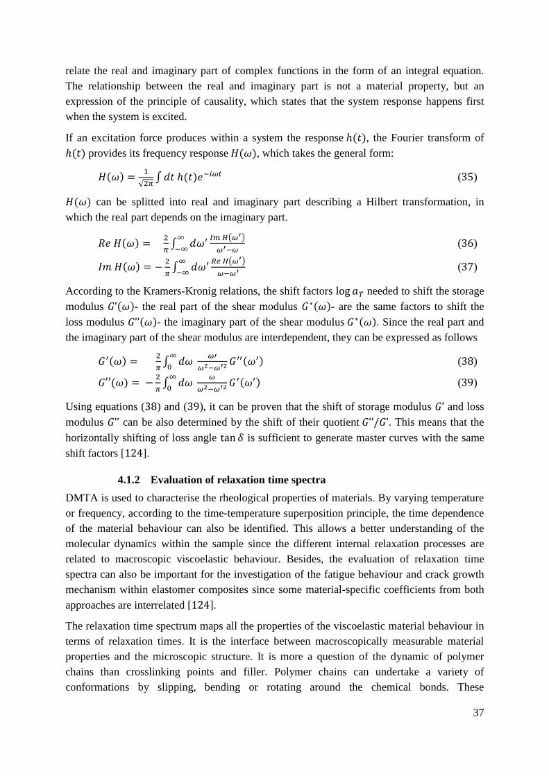
37

relate the real and imaginary part of complex functions in the form of an integral equation.

The relationship between the real and imaginary part is not a material property, but an

expression of the principle of causality, which states that the system response happens first

when the system is excited.

If an excitation force produces within a system the response ℎ(𝑡), the Fourier transform of

ℎ(𝑡) provides its frequency response 𝐻(𝜔), which takes the general form:

𝐻(𝜔) =1

√2𝜋∫ 𝑑𝑡 ℎ(𝑡)𝑒−𝑖𝜔𝑡 (35)

𝐻(𝜔) can be splitted into real and imaginary part describing a Hilbert transformation, in

which the real part depends on the imaginary part.

𝑅𝑒 𝐻(𝜔) = 2

𝜋∫ 𝑑𝜔′ 𝐼𝑚 𝐻(𝜔′)

𝜔′−𝜔

∞

−∞ (36)

𝐼𝑚 𝐻(𝜔) = −2

𝜋∫ 𝑑𝜔′ 𝑅𝑒 𝐻(𝜔′)

𝜔−𝜔′

∞

−∞ (37)

According to the Kramers-Kronig relations, the shift factors log 𝑎𝑇 needed to shift the storage

modulus 𝐺’(𝜔)- the real part of the shear modulus 𝐺∗(𝜔)- are the same factors to shift the

loss modulus 𝐺’’(𝜔)- the imaginary part of the shear modulus 𝐺∗(𝜔). Since the real part and

the imaginary part of the shear modulus are interdependent, they can be expressed as follows

𝐺′(𝜔) = 2

𝜋∫ 𝑑𝜔

𝜔′

𝜔2−𝜔′2 𝐺′′(𝜔′)∞

0 (38)

𝐺′′(𝜔) = −2

𝜋∫ 𝑑𝜔

𝜔

𝜔2−𝜔′2 𝐺′(𝜔′)∞

0 (39)

Using equations (38) and (39), it can be proven that the shift of storage modulus 𝐺’ and loss

modulus 𝐺’’ can be also determined by the shift of their quotient 𝐺’’/𝐺’. This means that the

horizontally shifting of loss angle tan 𝛿 is sufficient to generate master curves with the same

shift factors [124].

4.1.2 Evaluation of relaxation time spectra

DMTA is used to characterise the rheological properties of materials. By varying temperature

or frequency, according to the time-temperature superposition principle, the time dependence

of the material behaviour can also be identified. This allows a better understanding of the

molecular dynamics within the sample since the different internal relaxation processes are

related to macroscopic viscoelastic behaviour. Besides, the evaluation of relaxation time

spectra can also be important for the investigation of the fatigue behaviour and crack growth

mechanism within elastomer composites since some material-specific coefficients from both

approaches are interrelated [124].

The relaxation time spectrum maps all the properties of the viscoelastic material behaviour in

terms of relaxation times. It is the interface between macroscopically measurable material

properties and the microscopic structure. It is more a question of the dynamic of polymer

chains than crosslinking points and filler. Polymer chains can undertake a variety of

conformations by slipping, bending or rotating around the chemical bonds. These

38

conformations are constantly changing due to the Brownian motion and external deformation

of the material. The relaxation times spectra describe the transition rates at which this

conformational change takes place. Since different microscopic processes are associated with

different conformational changes, their characteristic relaxation times generally vary in a wide

range: from local changes, which sometimes take place very quickly, until changes in larger

chain segments associated with longer periods. As a result, the individual microscopic

processes can be identified in different areas of the relaxation spectrum [126-130].

To introduce the approach of relaxation spectrum, viscoelastic materials are assumed as

phenomenological Maxwell model. This rheological model maps well the complex behaviour

of viscoelastic materials only if the relationship between mechanical stress and deformation is

linear. The viscoelastic material is modelled by a series of Maxwell elements, which are

arranged parallel as shown in Figure 22. The Maxwell element consists of a Hook spring with

the modulus 𝐺𝑖, which is arranged in series with an ideal viscous damping element with the

Newtonian viscosity 𝜂𝑖 .

Figure 22: Maxwell model of viscoelastic materials.

The mechanical stress 𝜎(𝑡) is a time dependent variable. It is a sum of the contribution of

each individual Maxwell element and has the following form:

𝜎(𝑡) = 𝜎𝑒 + ∑ 𝜎𝑖(𝑡)𝑛𝑖=1 (40)

The relaxation modulus 𝐺(𝑡) is calculated by dividing the mechanical stress in equation (40)

by the elongation 휀(𝑡). 𝐺(𝑡) takes the following discrete form

𝐺(𝑡) = 𝐺𝑒 + ∑ 𝐺𝑖(𝑡)𝑛𝑖=1 (41)

: = 𝐺𝑒 + ∑ 𝐺𝑖𝑒−

𝑡

𝜏𝑖𝑛𝑖=1 (42)

where 𝐺𝑖(𝑡) is the 𝑖𝑡ℎ relaxation module of the 𝑖𝑡ℎ Maxwell element. Furthermore, the

relaxation moduli 𝐺𝑖(𝑡) can be expressed as a function of the relaxation times 𝜏𝑖. 𝐺𝑖

represents the amplitude of the relaxation modulus 𝐺𝑖(𝑡).

Since these relaxation times are very close together, it is appropriate to derive continuous

relaxation time spectra 𝐻(𝜏). The relaxation modulus 𝐺𝑖(𝑡) becomes

39

𝐺(𝑡) = 𝐺𝑒 + ∫ 𝑑𝑙𝑛(𝜏)+∞

−∞ 𝑒−

𝑡

𝜏 𝐻(𝜏) (43)

The Fourier transformation of the relaxation modulus yields to the following relationship

between the relaxation time spectrum and the experimentally available dynamic moduli:

𝐺′(𝜔) = 𝐺𝑒 + ∫ 𝑑𝑙𝑛(𝜏)+∞

−∞ 𝐻(𝜏)

𝜔2𝜏2

1+𝜔2𝜏2 (44)

𝐺′′(𝜔) = ∫ 𝑑𝑙𝑛(𝜏)+∞

−∞ 𝐻(𝜏)

𝜔𝜏

1+𝜔2𝜏2 (45)

The relaxation time spectra 𝐻(𝜏) are determined by an iterative approximation according to

Williams and Ferry [113-115]. 𝐻(𝜏) has the following form:

𝐻(𝜏) = 𝐴𝐺′(𝜔)𝑑 𝐺′(𝜔)

𝑑 𝑙𝑜𝑔𝜔 (46)

with

𝐴 =2−𝑝

2Γ(2−𝑝

2)Γ(1+

𝑝

2) (47)

where 𝑝 is the local slope of 𝐻(𝜏) at 1

𝜔= 𝜏. Γ is the gamma function.

In the frame of multiscale approach, 𝐺(𝑡) can be expressed as the superposition of high

frequency part of the glass transition zone, Rouse-like regime at the intermediate frequencies

and reptation regime at low frequencies [128-130]. For unfilled rubbers, the relaxation

modulus due to bending rigidity of chains follows a power-law asymptotic behaviour with the

exponent −3/4 according to

𝐺𝑔𝑙𝑎𝑠𝑠(𝑡) ∝ (𝑡

𝜏0)

−3 4⁄

(48)

The relaxation behaviour at the high frequency glass transition regime is caused by the

bending rigidity of the polymer chains and is similar to relaxation time of a Kuhn segment.

The Rouse-like regime describes the low frequency part of the glass transition zone. The

relaxation modulus decreases more slowly than in the glassy regime and it can be written as

follows

𝐺𝑅𝑜𝑢𝑠𝑒(𝑡) ∝ (𝑡

𝜏0)

−1 2⁄

(49)

𝐺𝑅𝑜𝑢𝑠𝑒(𝑡) follows a power-law asymptotic behaviour with the exponent −1/2. The reptation

regime describes the sliding motion of entangled network strands and it depends on the

crosslink density. The last relaxation mechanism occurs at very high frequencies. It describes

small vibrations of chain fragments comparable with the size of monomers. The exponent of

the power law can be derived from the right flank of the loss modulus curve. For the further

consideration within the framework of this thesis, only the glass transition is significant. The

focus will be put on the glassy and Rouse-like regime.

The generated master curve for unfilled NR sample is presented in Figure 23. The storage

modulus 𝐺′(𝜔) and loss modulus 𝐺′′(𝜔) are plotted against the frequency 𝜔. The different

40

slopes correspond to four relaxation mechanisms according to the four different microscopic

dynamics discussed above. The different slopes are drawn up in the graph.

-2 0 2 4 6 8 10 12 14 163

4

5

6

7

8

9

-0.29

log(G')

log(G'')

log

(G

'),

log

(G'')

[MP

a]

log() [Hz]

0.87

0.57

0.12

Figure 23: Viscoelastic master curves of an unfilled NR sample at reference temperature

of 𝟐𝟎 °𝑪. The different scaling ranges are indicated.

The different relaxation times do not exactly match with the theoretical values but remain in

the valid range. The corresponding relaxation time spectrum for unfilled NR sample can be

derived from the master curves according to equation (44) and (45). It is depicted in Figure

24.

The different relaxation behaviours still remain valid for filled samples. One precondition

must be fulfilled: no additional network exists besides the polymer chains network. It is to

note that the glassy and Rouse-like regime can no longer be distinguished. The relaxation

time spectrum for filled NR sample is depicted in Figure 25.

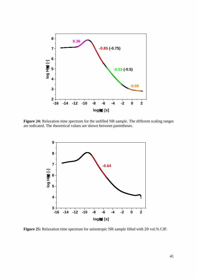
41

-16 -14 -12 -10 -8 -6 -4 -2 0 22

3

4

5

6

7

8

log

H(

) [-

]

log() [s]

0.36

-0.85 (-0.75)

-0.53 (-0.5)

-0.09

Figure 24: Relaxation time spectrum for the unfilled NR sample. The different scaling ranges

are indicated. The theoretical values are shown between parentheses.

-16 -14 -12 -10 -8 -6 -4 -2 0 23

4

5

6

7

8

9

log

H(

) [-

]

log() [s]

-0.64

Figure 25: Relaxation time spectrum for anisotropic NR sample filled with 20 vol.% CIP.

42

4.2 Dynamical Flocculation Model

The dynamical flocculation model (DFM) is a physical motivated micromechanical model for

the description of isotherm change in state of elastomers by a given deformation. DFM

provides an excellent agreement with the experimental stress-strain behaviour of elastomer

composites. It represents an extension of the non-affine tube model. A non-Gaussian length

distribution of the polymer chains is assumed. This means that the polymer chains have a

finite length; also qualified as finite chain extensibility. The extended tube model assumes

that polymer networks with high entanglement density are strongly hindered in their

fluctuation. This hindrance is described by fluctuation-limiting virtual tubes around the

network chains. Under deformation of the polymer network, these tubes do not deform affine

[131-146]. Figure 26 illustrates a schematic representation of a network chain in a virtual

tube. Graph is adapted from [132].

Figure 26: Schematic representation of a network chain in a virtual tube. The tube diameter is

given by the mean spacing of the topological constraint centre, i.e. crosslinks and

entanglements, indicated as crosses.

For an isothermal reversible deformation, the mechanical energy inducing a state change of an

unfilled elastomer is equal to the free energy function 𝑊(휀𝜇). According to Klüppel et al.

[132], the entropy-elastic rubber contribution 𝑊𝑅 has the constitutive form:

𝑊𝑅 = 𝐺𝑐

2{

(1−1

𝑛 )(∑ 𝜆𝜇

23𝜇=1 −3)

1−1

𝑛(∑ 𝜆𝜇

23𝜇=1 −3)

+ 𝑙𝑛 (1 −1

𝑛(∑ 𝜆𝜇

23𝜇=1 − 3))} + 2𝐺𝑒(∑ 𝜆𝜇

−13𝜇=1 − 3) (50)

where 𝐺𝑐 is the crosslink modulus, 𝐺𝑒 is the entanglement modulus, 𝜆𝜇 is the stretch ratio and

𝑛 is the finite extensibility parameter. 𝑛 ≔ 𝑛𝑒 𝑇𝑒⁄ where 𝑛𝑒 is a polymer specific quantity

representing the number of chain segments between two entanglements and 𝑇𝑒 is a crosslink-

dependent trapping factor indicating the proportion of elastically active entanglements. DFM

has the peculiarity that all free parameters are linked with molecular structure of the rubber

samples. The crosslink modulus 𝐺𝑐: = 𝜈𝑐𝑘𝐵𝑇 depends on the number density of mechanically

active network strands between the junctions 𝜈𝑐 and the absolute temperature 𝑇. 𝑘𝐵 is the

Boltzmann constant. The entanglement modulus 𝐺𝑒: = 𝜈𝑒𝑘𝐵𝑇 √6⁄ depends on the number

density of chain fragments between entanglements 𝜈𝑒. The finite extensibility parameter

43

𝑛𝑒 𝑇𝑒⁄ ≔ 𝜈𝑠𝑘𝐵𝑇 (√6 𝐺𝑒𝑇𝑒)⁄ gives the number of segments between two adjacent

entanglements. Here 𝜈𝑠 ≔ 𝑛𝑒𝜈𝑒 is the segment number density.

The polymer contribution to the total stress is defined as the first derivative of the free energy

function 𝑊𝑅with respect to the stretch ratio 𝜆𝜇 in the spatial direction 𝜇 ≔ 1, 2 and 3. 𝜆𝜇 is

defined as

𝜆𝜇 ≔ 1 + 휀𝜇 (51)

where 휀𝜇 is the strain in the direction 𝜇. The total stress takes the following form:

𝜎𝑅,𝜇: =𝑑𝑊𝑅

𝑑𝜆𝜇 (52)

The elastomer composites are assumed as incompressible materials. This means that the

volume of the sample remains constant independently of the load conditions. The following

applies:

Δ𝑉

Δ𝑉0= 𝜆1𝜆2𝜆3 ≡ 1 (53)

In other words, if the sample is sheared in direction 1, it will be compressed in direction 3 and

remains unaffected in direction 2. The principle stress axes 𝜂 and 𝜉 of the deformation

ellipsoid rotate with increasing amplitude in the direction of the shearing surfaces as shown in

Figure 27.

Figure 27: Variation of the angle 𝝌 between the principle stress axes 𝜼 and 𝝃. Sample is

sheared in direction 𝟏. Direction 𝟐 is perpendicular to plane (𝟏, 𝟑).

The principal stretch ratios in the main axes 𝜂 and 𝜉 take the following form:

𝜆1 = √1 +𝜒2

4+

𝜒

2 (54)

𝜆2 = 1 (55)

𝜆3 = √1 +𝜒2

4−

𝜒

2 (56)

44

𝜒 is the angle between the two principal axes 𝜂 and 𝜉. Taking into consideration the volume

constancy of the sample and redefining the stretch ratio in direction 1 as:

𝜆1 ≡ 𝜆 (57)

the following applies:

𝜆2 ≡ 1 (58)

𝜆3 ≡1

𝜆 (59)

The simple shear stress takes the following form:

𝜎𝑅 = 𝐺𝑐(𝜆 − 𝜆−3) {1−

1

𝑛

(1−1

𝑛 (𝜆2−2+

2

𝜆2))2 −

1

𝑛

1−1

𝑛 (𝜆2−2+

2

𝜆2)} + 2𝐺𝑒(1 − 𝜆−2) (60)

For filled elastomers, the free energy function 𝑊(휀𝜇) is the sum of the rubber and filler

energy functions, weighted by the effective filler volume fraction:

𝑊(휀𝜇) = (1 − Φ𝑒𝑓𝑓)𝑊𝑅(휀𝜇) + Φ𝑒𝑓𝑓𝑊𝐴(휀𝜇) (61)

where 𝑊𝐴(휀𝜇)is the energy-elastic contribution of filler and Φ𝑒𝑓𝑓 is the mechanical effective

filler volume fraction. If an unfilled sample is stretched, the polymer deformation in a small

local area corresponds to the global external deformation. In filled samples, the free polymeric

phase is subject to a greater mechanical stress than the overall filler clusters once a load is

applied. The reason is that the rigid filler clusters enclose parts of the polymers, which are no

longer accessible for the stress. The additional loads must be then intercepted by the free

polymer phase which implies that the local strain is greater than the global one. The

consideration of this effect is carried out through the hydrodynamic amplification factor 𝑋𝜇.

The local deformation described in terms of the internal stretch ratio κμ is then related to the

external strain εμ of the sample through:

𝜅𝜇 ∶= 1 + 𝑋𝜇휀𝜇 (62)

The hydrodynamic amplification factor 𝑋𝜇 depends on the principal strain history of the

sample and more precisely on the maximum load 휀𝑚𝑎𝑥. 𝑋𝜇 gives rise to stress softening effect

of filler-reinforced rubber, well known as Mullins effect [135]. For fractal filler clusters, 𝑋𝜇 is

formulated as follows:

𝑋( 휀𝜇,𝑚𝑎𝑥) ≔ 1 + 𝑐. Φ𝑒𝑓𝑓

2 (3−𝑑𝑓)⁄∑

1

𝑑

3𝜇=1 (𝑑 + ∫ 𝑑𝜉 (

𝜉𝜇

𝑑− 1)

𝑑𝑤−𝑑𝑓𝜉𝜇,𝑚𝑖𝑛

0𝜙(𝜉)) (63)

where 𝑐 ≈ 2.5 represents the Einstein coefficient for spherical inclusions [147]. 𝑑𝑓 is the

fractal dimension of the filler clusters, 𝑑 is the primary particle size, 𝑑𝑤 is the anomalous

diffusion exponent, 𝑥𝜇 = 𝜉𝜇 𝑑⁄ is the related filler cluster size and 𝜙(𝜉) is the filler cluster

size distribution.

45

According to the kinetics model of cluster-cluster aggregation (CCA), a Smoluchowski size

distribution of the filler cluster is taken into consideration:

𝜙(𝑥𝜇) =4𝑥

⟨𝑥𝜇⟩2 𝑒−2𝑥 ⟨𝑥𝜇⟩⁄ (64)

where ⟨𝑥𝜇⟩ is the mean filler cluster size. In the further handling, the size distribution of the

filler clusters is assumed to be isotropic. This means that

⟨𝑥1⟩ = ⟨𝑥2⟩ = ⟨𝑥3⟩ ≡ 𝑥0 (65)

Within this model and according to Meakin, the exponents take the following values [148].

𝑑𝑓 = 1.8 (66)

𝑑𝑤 = 3.1 (67)

Besides, the minimal filler cluster size is expressed as follows

𝑥𝜇,𝑚𝑖𝑛 =𝜉𝜇,𝑚𝑖𝑛

𝑑=

𝑄𝑣 𝑣,𝑏

𝑑3�̂�𝑅,𝜇( 𝜇,𝑚𝑖𝑛; 𝜇,𝑚𝑎𝑥) ≡

𝑠𝑣

�̂�𝑅,𝜇( 𝜇,𝑚𝑖𝑛; 𝜇,𝑚𝑎𝑥) (68)

where 𝑄𝑣 is the elastic constant due to deformation of virgin filler-filler bonds and 휀𝑣,𝑏 is the

final strain of the bonds under loading. �̂�𝑅,𝜇(휀𝑗; 휀𝑘) is the relative rubber stress according to

two given states of strain 휀𝑗 and 휀𝑘 and is defined as follows:

�̂�𝑅,𝜇(휀𝑗; 휀𝑘) ∶= 𝜎𝑅,𝜇(휀𝑗) − 𝜎𝑅,𝜇(휀𝑘) (69)

Furthermore, 𝑠𝑣 represents the strength of the virgin filler-filler bonds.

The stress-strain relationship of the rubber matrix 𝜎𝑅,𝜇 is defined as the first derivative of the

free energy function 𝑊𝑅with respect to the stretch ratio 𝜅𝜇, which takes into account the

hydrodynamic amplification factor 𝑋𝜇:

𝜎𝑅,𝜇: =𝑑𝑊𝑅

𝑑𝜅𝜇 (70)

Locally, large filler clusters carry more local stress than small clusters and break first. Two

different types of clusters arise. Increasing the deformation breaks the next largest clusters.

This process is continuous so that the boundary between unbroken hard filler clusters and

reaggregated soft clusters shifts to smaller values with increasing maximum deformation.

Figure 28 shows the distribution of filler cluster sizes within a test specimen. The filler cluster

size 𝑥𝑚𝑖𝑛 represents the borders between unbroken and broken filler clusters.

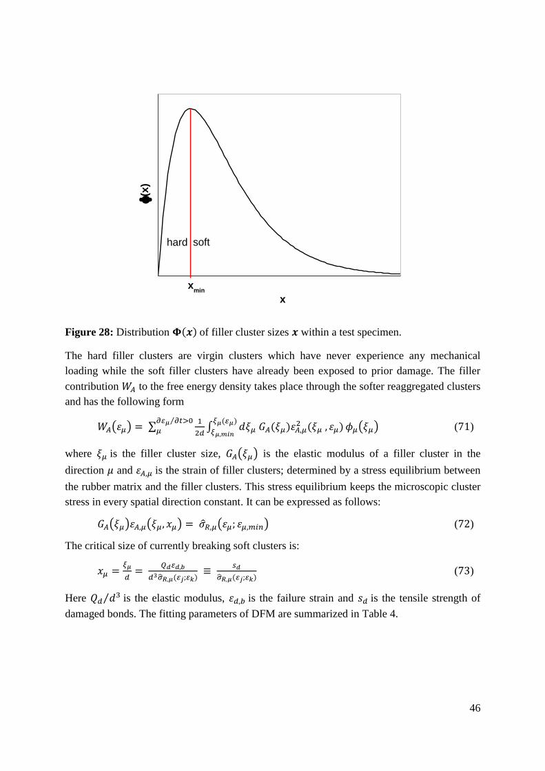
46

hard

(x

)

x

xmin

soft

Figure 28: Distribution 𝚽(𝒙) of filler cluster sizes 𝒙 within a test specimen.

The hard filler clusters are virgin clusters which have never experience any mechanical

loading while the soft filler clusters have already been exposed to prior damage. The filler

contribution 𝑊𝐴 to the free energy density takes place through the softer reaggregated clusters

and has the following form

𝑊𝐴(휀𝜇) = ∑1

2𝑑∫ 𝑑𝜉𝜇 𝐺𝐴(𝜉𝜇)휀𝐴,𝜇

2 (𝜉𝜇 , 휀𝜇)𝜉𝜇( 𝜇)

𝜉𝜇,𝑚𝑖𝑛

𝜕 𝜇 𝜕𝑡>0⁄

𝜇 𝜙𝜇(𝜉𝜇) (71)

where 𝜉𝜇 is the filler cluster size, 𝐺𝐴(𝜉𝜇) is the elastic modulus of a filler cluster in the

direction 𝜇 and 휀𝐴,𝜇 is the strain of filler clusters; determined by a stress equilibrium between

the rubber matrix and the filler clusters. This stress equilibrium keeps the microscopic cluster

stress in every spatial direction constant. It can be expressed as follows:

𝐺𝐴(𝜉𝜇)휀𝐴,𝜇(𝜉𝜇, 𝑥𝜇) = �̂�𝑅,𝜇(휀𝜇; 휀𝜇,𝑚𝑖𝑛) (72)

The critical size of currently breaking soft clusters is:

𝑥𝜇 =𝜉𝜇

𝑑=

𝑄𝑑 𝑑,𝑏

𝑑3�̂�𝑅,𝜇( 𝑗; 𝑘) ≡

𝑠𝑑

�̂�𝑅,𝜇( 𝑗; 𝑘) (73)

Here 𝑄𝑑 𝑑3⁄ is the elastic modulus, 휀𝑑,𝑏 is the failure strain and 𝑠𝑑 is the tensile strength of

damaged bonds. The fitting parameters of DFM are summarized in Table 4.

47

Table 4: DFM fitting parameters

Parameter Unit Designation

𝑮𝒄 MPa Crosslink modulus

𝑮𝒆 MPa Entanglement modulus

𝒏 - Finite extensibility parameter

𝒔𝒗 MPa Tensile strength of virgin bonds

𝒔𝒅 MPa Tensile strength of damaged bonds

𝒙𝟎 - Mean filler cluster size

𝚽𝒆𝒇𝒇 - Effective filler volume fraction

4.3 Fatigue crack growth

Technical elastomers suffer damages and some of them with disastrous consequences. This

happens despite the careful examinations and rigorous calculations to determine the material

lifetime and resistance to environmental crack formation. The most failures occur due to

mechanical fatigue. That is why elastomer composites have to fulfil increasingly high

requirements regarding loading and fatigue life. The damage is mainly caused by crystal

defects and micro-voids in the components, formed already during the manufacturing process.

Small imperfections are always present. But they must not lead to failure at any operating

time. In order to determine the conditions under which an elastomer fails in consequence of

long operating time, it seems to be necessary to focus on how fatigue cracks grow within the

sample. According to fracture mechanics, the conditions at the crack tip are essential for the

fatigue crack propagation process. A fatigue crack grows and propagates means exerting a

mechanical force. If the crack length reaches a critical value, the fatigue crack propagation

becomes unstable and happens with a high speed. The critical crack length and critical load

are therefore the principal characteristics governing the fatigue and damage behaviour of

elastomer composites [149].

Within the scope of this thesis, the principal emphasis is placed on describing how fatigue

cracks propagate within the rubber matrix. If the elastomer composite contains a crack of a

size 𝑐, the fatigue crack can propagate when the sample is subjected to mechanical stress. By

a tensile load, the crack propagates perpendicular to the crack plane. Such crack opening

mode corresponds to mode I of the fracture mechanics. A. A. Griffith developed a

thermodynamical approach for deformable bodies to describe how cracks propagate under the

effect of cyclic mechanical loading. He studied the energy balance in a cracked body during

crack propagation. He assumed that the plastic zone at the crack is small enough compared to

the crack length and the sample dimensions [150,151].

According to Griffith, the energetic break criterion states that in order to initiate and maintain

quasistatic crack propagation in a conservative system, the energy release rate provided must

be greater than the dissipated fracture energy per crack area. If a material under mechanical

stress starts deforming, it stores elastic energy. As a result, the breaking resistance can be

locally exceeded and thus a crack is initiated from crystal defects and micro-voids. A

transition from a stationary to a moving crack takes place. If the crack propagates further, it

48

further relieves the material under stress and releases energy to move forward the opening

edge. Beyond a certain limit, the energy released is sufficient to open more and more the

crack. The crack propagation continues until the material, in a catastrophic case scenario,

tears. The energy balance established by Griffith results from a balance between the elastic

strain energy relieved and the interfacial energy of the crack; the energy required to open it

[150,151].

The energy balance for the case of crack propagation in an infinitely extended plate of finite

thickness was first discussed by Griffith [150]. According to Griffith, the crack propagation

occurs when the elastic strain energy 𝑊𝑒, released by elongation of the crack, is equal to or

greater than the surface energy 𝑊0 required in order to create the fracture surfaces. This can

be expressed as follows:

𝑊𝑒 ≥ 𝑊0 (74)

The criterion of unstable crack propagation is

𝑑𝑊𝑒

𝑑𝑐 ≥

𝑑𝑊0

𝑑𝑐 (75)

The elastic strain energy 𝑊𝑒 is defined as

𝑊𝑒 ∶= 𝜋𝑐2

𝐸𝜎2 (76)

where 𝑐 is the crack size, 𝜎 is the mechanical stress and 𝐸 is the modulus of elasticity. The

surface energy 𝑊0 is

𝑊0 = 4𝑐𝛾0 (77)

where 𝛾0 is the surface tension [149, 152]. The crack grows if the elastic strain energy 𝑊𝑒 is

at least two times larger than the surface tension 𝛾0 [153]. The Griffith criterion of crack

propagation leads to the following relationship:

2𝜋𝑐

𝐸𝜎2 ≥ 4𝛾0 (78)

An existing fatigue crack can propagate without any external energy supply. According to the

equations (74), (76) and (77), the critical tension required for the crack propagation is

𝜎𝑐 ∶= √2𝐸𝛾0

𝜋𝑐 (79)

The associated critical crack length is

𝑐0 ∶= 2𝐸𝛾0

𝜋𝜎2 (80)

Fatigue crack growth curves and life prediction can be obtained from a cyclic fracture

mechanics tests. Test specimens can be examined under real conditions using a tear fatigue

analyser [154]. Figure 29 illustrates the experimental results. Paris et al. found that the crack

growth rate in elastomers was related to the magnitude of the tearing energy [155]. The crack

growth rate corresponds to the change in the crack length as a function of load change. It is

49

given in differential form 𝑑𝑐/𝑑𝑛, where 𝑑𝑐 is the crack propagation and 𝑛 is the number of

loading cycle. The Paris-Erdogan law is expressed as follows

𝑑𝑐

𝑑𝑛= 𝐵. 𝑇𝛽 (81)

𝐵 and 𝛽 are material-dependent constants. 𝑇 is the tearing energy and is calculated as follows

𝑇 =2𝜋

√𝜆 𝑐 𝑊𝑒 (82)

where 𝜆 is the stretching ration, 𝑐 is the crack length and 𝑊𝑒 is the elastic strain energy

available for the crack to propagate. A double logarithmic plot of a crack propagation curve is

shown in Figure 29. The crack growth rate is plotted against the tearing energy 𝑇.

T2

log

(dc/d

n)

[m/c

ycle

]

log(T) [N/m]

T1

Figure 29: Illustration of the Paris-Erdogan law. Fatigue crack growth in elastomer

composites

Three regions in the crack propagation curve can be discerned. The lower limit of the curve is

determined by the threshold value of the tearing energy 𝑇1. If the tearing energy is smaller

than 𝑇1, the fatigue crack cannot propagate. 𝑇1 represents the lower limit of the crack

propagation curve until which the sample is fatigue endurable. In the subsequent region II, the

influence of the mechanical stress dominates. In this area a linear progression of the crack

growth curve can be observed [156, 157]. It can be approximated by the Paris-Erdogan law

presented in equation (81). Region III marks the transition to brittle violent cracking. The

upper limit 𝑇2 indicates the stress at which the crack propagation becomes unstable.

51

5 Experimental methods

This chapter is devoted to the different experimental methods used for the preparation and

characterisation of MSE. In a pre-investigation phase the reinforcement potential of the

different magnetic fillers used have been determined using the static volumetric gas

adsorption. The sample preparation begins with mixing the different components and ends

after the curing process. The preparation of isotropic or anisotropic MSE additionally requires

the presence of an external magnetic field generated by a coil system during the vulcanisation.

Different testing methods are then conducted to characterise the viscoelastic properties of

MSE.

5.1 Static volumetric gas adsorption measurements

The method of static volumetric gas adsorption serves to characterise the surface of fine

particles and dispersed solids. This technique makes use of the fact that reference gas

molecules can be adsorbed onto the surfaces of the sample to be tested. At a constant

temperature, a pressure drop can then be measured. From the pressure difference, the

adsorbed gas volume can be determined. If more and more gas is gradually led to the

measurement cell, the pressure increases in turn. The dependence of the adsorbed gas

volume 𝑉(𝑝, 𝑇) on the partial gas pressure 𝑝 at a given temperature 𝑇 can be used to create

adsorption isotherms. For this purposes the gas adsorption measuring unit BELSORP-max

from BEL Japan Inc is used. Before starting a measurement, the magnetic filler was first pre-

treated. It was annealed in a controlled vacuum atmosphere at 100 °𝐶 for three hours in order

to remove any possible deposits like water and other impurities. During the gas adsorption

measurement, the classic BET gas nitrogen with a boiling point at 77 𝐾 was used [106].

5.2 Sample preparation

5.2.1 Mixing

The mixing process aims to ensure the finished product homogenous properties despite the

use of multiple components. The mixing process was carried out using the laboratory internal

mixer Haake PolyLab OS from Thermo Scientific. It consists of a motor unit connected to a

mixing chamber with a mixing volume of 60 𝑚𝑙 and a filling level of 70 %. The chamber is

electrically heated and the internal temperature can be partially regulated by means of air

cooling. The mixing geometry is two Banbury rotors that work tangentially. During the

mixing process, torque, rotational speed, mixing chamber temperature and the temperature of

the mixture are recorded.

The mixing process was performed on different steps. Rubber, magnetic filler and silane were

first mixed together to obtain a chemical bonding between polymer chains and filler particles.

The so-called silanisation process was carried out at a constant temperature ranging between

130 °𝐶 and 135 °𝐶 for 10 minutes by adapting the rotor speed. The other additives except the

curing system were than added. The crosslinker was mixed at the end on a roller mill by room

52

temperature to ensure that curing reactions only starts in the heat press and not during the

mixing process.

5.2.2 Vulcanisation in a magnetic field

Rubber became a valuable technical product only after the hot vulcanisation process,

introduced by the American Goodyear in 1839. It still remains the most important

vulcanisation process for standard and conventional rubbers [76].

The vulcanisation process is the thermally induced setting up of the filler network and

chemical crosslinking of the polymer chains. It was characterised by the vulcameter MDR

2000 from Alpha Technologies. The required torque is measured at a deflection angle

of 0.5 °, which corresponds approximately to a deformation of 6 %, and a frequency

of 1.67 𝐻𝑧. The curing temperature for all prepared samples was 150 °𝐶. The real part of the

torque 𝑆′ is evaluated and the so-called 𝑡90-time is determined. It is the time at which 𝑆′

reached 90 % of its maximum value. This time serves as basis for determining the

vulcanisation time of the samples to avoid any reversion, thermal ageing and/or over-

crosslinking. The effective vulcanisation time is the 𝑡90-time plus one minute for each one

millimetre sample thickness.

The samples were cured in an electrical heating press from Wickert & Söhne at 300 bar

pressure and a vulcanisation temperature of 150 °𝐶. The vulcanisation was achieved in the

presence of an external magnetic field delivering anisotropic MSE composites with filler

particles oriented in the direction of the magnetic field. Isotropic MSE composites having

homogenous filler dispersion were obtained when no magnetic field was applied. The

magnetic field was generated by two square-shaped magnetic coils enclosed by an iron core

as shown in Figure 30. A nearly uniform magnetic field of about 0.3 𝑇 was measured with an

unfilled vulcanisation mould at 23 °𝐶. The MSE melts were filled in a vulcanisation mould

made of aluminium plates 300 𝑚𝑚 x 300 𝑚𝑚 x 2 𝑚𝑚 with a central quadratic cavity of

100 𝑚𝑚 x 100 𝑚𝑚 x 2 𝑚𝑚. The field strength is set by the magnitude of the electrical

current flowing through the solenoids and is probably slightly modified during the

vulcanisation process taking place at 150 °𝐶. The magnetic field strength will be reduced at

this high temperature. However, an increasing magnetic field strength is expected due to the

bundling of magnetic field lines going through the magnetic rubber sample more readily than

the surrounding mould made of aluminium with low magnetic susceptibility 𝜒 = 2.4 ×

10−5. Due to this geometrical construction, the exact value of the magnetic field strength in

the rubber sample remains unknown [106-107].

53

Figure 30: Schematic of the curing setup for the preparation of anisotropic MSE during

vulcanisation in an electrical heating pres. Horizontal iron plates, 𝟏𝟎 𝒎𝒎 thick, and a vertical

iron block, 𝟑𝟎 𝒎𝒎 thick, form a closed magnetic core are coloured in grey. The magnetic

coils are shown in orange. The heating press is displayed in green. The vulcanisation mould is

labelled with a circle, its thickness is 𝟐 𝒎𝒎 and it is not true to scale.

The natural rubber used was a high-grade pale crepe rubber. The different synthetic rubbers

used were supplied by Lanxess AG Germany. Keltan 4450 is an amorphous EPDM

containing 52 wt.% ethylene and 4.3 wt.% ENB [158]. Perbunan 3945 is a medium-viscous

NBR with 39 wt.% acrylonitrile [159]. Therban 3467 is a partially saturated HNBR with 34

wt.% acrylonitrile. It has a residual double bonds content of 5.5 wt.%, which makes it suitable

for sulphur crosslinking [160]. Therban XT is a carboxylated HNBR (XHNBR). It contains

33 wt.% acrylonitrile and 3.5 wt.% residual double bonds [161]. A medium-viscous solution

SBR containing 25 wt.% styrene and 25 wt.% vinyl is used [162]. For sample identification,

the rubber designations are abbreviated as described in Table 5.

Table 5: Rubber abbreviation

Type Abbreviation

EPDM E

HNBR H

NBR N

NR NR

SBR S

XHNBR X

Further, the MSE samples are labelled “X𝑎Y𝑏Z”. X designates the rubber type as presented

in Table 5. Y and Z label the filler used in hybrid filler systems. “𝑎” and “𝑏” are natural

numbers representing the filler fraction in vol.% respectively. If just one filler is used, the

additional designation Y𝑏 is omitted. One sample is prepared without silane and received at

its end the additional term \Si. Depending on the orientation of the magnetic filler particles,

the letters A or I is added for anisotropic or isotropic samples respectively. A general

overview of the different compositions of the sample prepared is given in Table 6.

54

Table 6: Composition of the samples in vol.%

Sample Rubber TDAE Sunpar DOP CIP MAGSILICA CB Silica Si69 6PPD IPPD St.acid ZnO S CBS DPG

E20C 51 - 23 - 20 - - - 3.6 1.3 - 0.5 0.4 0.3 0.7 -

H20C 49 - - 24 20 - - - 3.8 1.4 - 0.5 0.4 0.2 0.7 -

N0 63 - - 33 0 - - - 0 1.9 - 0.7 0.6 0.3 1.0 -

N06C 58 - - 30 6 - - - 1.6 1.7 - 0.6 0.5 0.3 0.9 -

N13C 53 - - 28 13 - - - 2.9 1.6 - 0.6 0.5 0.3 0.8 -

N20C 48 - - 25 20 - - - 3.9 1.4 - 0.5 0.4 0.2 0.7 -

N28C 43 - - 22 28 - - - 4.6 1.3 - 0.4 0.4 0.2 0.6 -

N36C 37 - - 19 36 - - - 5 1.1 - 0.4 0.3 0.2 0.4 -

NR20C 49 - 24 - 20 - - - 3.7 1.4 - 0.5 0.4 0.2 0.7 -

NR20C03P 51 - 25 - 20 - 0.8 - 0.4 1.4 - 0.5 0.4 0.2 0.7

NR20C05P 50 - 25 - 20 - 1.3 - 0.4 1.4 - 0.5 0.4 0.2 0.7

NR20C07P 50 - 24 - 20 - 1.8 - 0.4 1.4 - 0.5 0.4 0.2 0.7

S0 72 22 - - 0 - - - 0 - 1.2 1.4 0.4 0.6 1 0.6

S05C 67 20 - - 5 - - - 3.5 - 1.2 1.3 0.3 0.5 1 0.5

S10C 63 19 - - 10 - - - 3.3 - 1.1 1.3 0.3 0.5 0.9 0.5

S10C 60 18 - - 15 - - - 3.1 - 1 1.2 0.3 0.5 0.9 0.5

S20C 56 17 - - 20 - - - 2.9 - 1 1.1 0.3 0.4 0.8 0.4

S20C\Si 58 18 - - 20 - - - 0 - 1 1 0.3 0.4 0.8 0.5

S20M 56 17 - - - 20 - - 3 - 1 1 0.3 0.4 0.8 0.5

S05C15M 56 17 - - 5 15 - - 3 - 1 1 0.3 0.4 0.8 0.5

S10C10M 56 17 - - 10 10 - - 3 - 1 1 0.3 0.4 0.8 0.5

S15C05M 56 17 - - 15 5 - - 3 - 1 1 0.3 0.4 0.8 0.5

S05C15S 56 17 - - 5 - - 15 3 - 1 1 0.3 0.4 0.8 0.5

S10C10S 56 17 - - 10 - - 10 3 - 1 1 0.3 0.4 0.8 0.5

S15C05S 56 17 - - 15 - - 5 3 - 1 1 0.3 0.4 0.8 0.5

X20C 48 - - 25 20 - - - 3.8 1.4 - 0.5 0.4 0.2 0.7 -

55

5.3 Physicals

The term Physicals is a collective term for different methods of material testing. It includes

the destructive stress-strain testing as well as non-destructive hardness, rebound and abrasion

tests.

5.3.1 Stress-strain curves

To measure the stress response as a function of strain, the universal tensile tester Zwick Z 010

from Zwick Roell materials testing systems was used. Tensile tests were carried out on S3A-

specimens according to DIN 53504. S3A-specimens were prepared from 2 𝑚𝑚 thick plates

of cured material, placed on sample holder and uniaxial elongated until they break. The

measurements were carried out at room temperature with a preload of 0.5 𝑁 and a cross-head

speed of 200 𝑚𝑚/𝑚𝑖𝑛. Due to sample fluctuations five samples per MSE were measured.

5.3.2 Multihysteresis measurements for fitting with the DFM

Multihysteresis measurements were carried out to complete the quasi-static tensile test. The

measurements were performed in a simple shear mode as shown in Figure 32. The sample

was measured uniaxial and quasi-static using a universal testing machine from MTS Systems

Corporation at a crosshead speed of 1 𝑚𝑚/𝑚𝑖𝑛 [163]. Five deformation cycles per

deformation step were performed with increasing deformation maxima. The force was

measured as a function of the deformation. This preconditioning leads to stress equilibrium of

the elastomer composite. These data can then be fitted and evaluated using the DFM. The

multihysteresis measurements were carried out in the presence of an external magnetic field.

The intrinsic mechanical properties can then be associated to magnetic properties of the test

specimens. Synergy effects were expected.

Figure 31: Multihysteresis measurements for fitting with the DFM. The dynamic mechanical

analyser MTS is shown on the left. The measurement setup is depicted on the right.

56

5.3.3 Shore A hardness

The measurements were carried out with the testing apparatus Frank 38230 from Karl Frank

GmbH according to the specifications in DIN 53505. The Shore A hardness represents a

characteristic value used for elastomer composites and rubbery materials. It is related to

penetration depth of an intender. A spring-loaded pin made of hardened steel is used as an

indenter and it has the shape of a truncated cone. It is pressed 3 seconds with a spring force of

12.5 ± 0.5 𝑁 into the specimen. The specimen is a 6 mm thick disc. Each sample is

measured at 5 different locations to reduce the sample fluctuations due to possible orientation

effects and several dispersion degrees.

5.3.4 Rebound

The rebound elasticity was carried out according to the specifications in DIN 53512 using the

Zwick 5109 rebound resilience tester. It is a measure of the elasticity of rubber samples. A

pendulum hammer fell free onto the specimen. When it came into contact with the sample, it

was deflected. The rebound is the relationship between the fall energy and the recovered

energy, derived from the quotient of rebound height to height of fall of the pendulum. Similar

to Shore A hardness measurements, the specimen is a 6 mm thick disc.

5.3.5 Abrasion

The abrasion tester from Karl Frank GmbH is used to determine the resistance of elastomers

regarding the friction loss according to the specifications in DIN 53516. Test sample moves

along a 40 𝑚 long path under a defined pressure with a constant speed. An abrasive sheet

with defined attack strength is used. The volume loss of the MSE samples determines the

abrasion resistance. The sample is a 6 𝑚𝑚 thick disc and has a diameter of 16 𝑚𝑚.

5.4 DMTA testing instruments

The DMTA testing instruments used are based on off-resonance forced oscillation method.

The sample is subjected to a static and dynamic load, generally a sinusoidal pulse. On the

basis of the measured force and deformation amplitudes, the phase angle and the complex

module can be determined. The measuring modes used for DMTA measurements are shown

in Figure 32. The tensile and/or compression mode is presented at the left. The picture at

centre shows the double shear mode. The torsion mode is depicted on the right.

Figure 32: Measuring modes used for dynamic-mechanical thermal analysis

57

Temperature-frequency sweeps were performed with the advanced rheometric expansion

system (ARES) from Rheometric Scientific TM on 30 𝑚𝑚 long, 10 𝑚𝑚 wide and 2 𝑚𝑚

thick strip samples. ARES is pictured in Figure 33. The samples were measured in torsion

under constant normal force of 1 𝑁. The deformation is controlled by a motor unit located at

the lower part of the device and the shear stress is recorded via a transducer located at the

upper part of the device [164]. The complex shear modulus 𝐺∗ and the loss factor tan 𝛿 are

determined as a function of the temperature and frequency. The deformation amplitude is kept

constant at 0.1 %. The temperature ramp was driven from low to high temperatures, from

−80 °𝐶 to 60 °𝐶 with temperature increment of 5 °𝐶 in the area of glass transition and 10 °𝐶

otherwise. Low temperatures were controlled by means of liquid nitrogen while high

temperatures are achieved by using heating elements. For each temperature step, a frequency

sweep from 0.01 𝐻𝑧 to 10 𝐻𝑧 was performed. For every test temperature, a soak time of

10 °𝐶 is maintained to attain thermal equilibrium of the sample with the ambient temperature.

Figure 33: The rotational rheometer ARES.

Strain sweeps were carried out with Eplexor® 500 𝑁 from Gabo Qualimeter Testanlagen

GmbH. The strain-sweeps were performed in a shear mode using a double sandwich sample

holder as shown in Figure 34. No static preload is needed and previous damage of the sample

is avoided. Dynamic deformation is generated by a separate electrodynamic oscillator [165].

The dynamic amplitude ranged between 0.01 % and 100 % at constant frequency of 1 𝐻𝑧

and room temperature. The specimens consist of two discs, 2 𝑚𝑚 thick with a diameter

of 20 𝑚𝑚, glued to the sample holders.

58

Figure 34: The dynamic mechanical analyser Eplexor® 500 N is shown on the left. The

measurement cell is shown on the right.

5.5 Crack propagation behaviour: Tear fatigue analyser

The fracture mechanics properties of MSE samples were investigated by analysing the

dynamic crack growth rate under cyclic loading. The measurements were performed with a

tear fatigue analyser (TFA) from Bayer/Coesfeld. The samples were analysed in tensile mode.

Strain amplitude of 15 % and frequency of 10 𝐻𝑧 were kept unchanged over the entire

measuring time. The investigations were carried out under pulsed loading with a pulse length

of 50 milliseconds. The TFA allows the simultaneous testing of up to 10 samples. Each

loading and unloading cycle is recorded separately for each sample. The detection of crack

length occurs automatically and is achieved over the entire period of the test by determining

the crack contour length 𝑐 with a CCD camera. For each individual measuring station, the

force 𝐹, the deformation 𝑥, the elastic strain energy 𝑊𝑒 and the crack contour length 𝑐 are

recorded separately [166]. The sample geometry used for fatigue tests is the 65 𝑚𝑚 long,

15 𝑚𝑚 wide and almost 1.7 𝑚𝑚 thick single notched tension sample (SENT). It is shown in

Figure 35.

Figure 35: Schematic representation of the single notched tension sample SENT used to

characterise the crack propagation behaviour of elastomers

59

5.6 Magnetorheological measurements

Magnetorheological investigations were carried out with the plate-plate rheometer Physica

MCR 501 from Anton Paar GmbH. The rheometer is equipped with a magnetic measuring

cell. Physica MCR 501 is able to simultaneously record the dynamic-mechanical and

magnetic properties of the samples. Figure 36 shows the setup for combined rheological and

magnetic testing as well as the measuring principle [167]. On the left, the picture shows the

device for rheological measurements. Magnetic investigations occur in general in closed

space in order to bundle the magnetic field lines through the test sample and prevent magnetic

losses. This is shown in the middle picture. The schematic picture on the right illustrates the

measuring principle.

The measurements were carried out in a shear mode using 2 𝑚𝑚 thick discs with a diameter

of 20 𝑚𝑚. Both melts and vulcanised samples can be characterised in the presence of a

magnetic field. While the melts measurements were strain-controlled, i.e. the gap distance

was kept constant, the measurements on vulcanised samples were controlled by a constant

normal force 𝐹𝑁 of 25 𝑁. The measurements were performed at a constant shear strain

of 0.1 % and a frequency of 10 𝐻𝑧.

Figure 36: Setup for combined rheological and magnetic testing of elastomer composites. On

the left, the device for rheological measurements is shown. Magnetic investigations occur in

closed space shown in the middle picture in order to prevent magnetic losses [𝟏𝟔𝟕]. On the

right, the measuring principle is schematically drawn.

The direction of shearing was perpendicular to direction of the magnetic field. To examine the

magnetorheological relaxation behaviour of the MSE, an on-and-off switching mode of the

magnetic field was applied. Measurements on melts were realised at a constant magnetic field

of about 0.74 𝑇. The magnetic field was switched on and off alternatingly for several times. It

was switched on for 150 𝑠 and then switched off for 30 𝑠. Measurements on vulcanisates

were achieved by a stepwise increase of the magnetic field from 0.2 𝑇 to 0.74 𝑇. The

magnetic field was alternatingly switched on for 100 𝑠 and then switched off for 20 𝑠 during

the total measurement period. During the measurement procedure, a moderate heating of the

magnetic cell was observed due to high electrical current controlling the magnetic field. A

temperature increase of about 10 °𝐶 for the melts and about 2 °𝐶 for the vulcanisates was

seen.

60

5.7 Combined rheological and dielectric measurements

The plate-plate rheometer Physica MCR 501 from Anton Paar GmbH can also be equipped

with a dielectric measuring cell. The mechanical settings were the same as discussed in the

previous section. The additional dielectric spectroscopy allows a frequency and temperature-

dependent characterisation of the polarization and conductivity behaviour of MSE samples in

the alternating electric field in order to describe their molecular kinetics. Dielectric

measurements were performed with a broadband dielectric spectrometer BDS 40 supplied by

Novocontrol GmbH. Figure 37 shows the setup for combined rheological and dielectric

testing of elastomer composites [168]. Unlike magnetorheological measurements, covering

the measurement cell is necessary just for temperature-dependent electrorheological analysis.

Figure 37: Setup for combined rheological and dielectric testing of elastomer composites

[𝟏𝟔𝟖]. The four thin cables connect the lower and upper plates of the measurement cell to

dielectric spectrometer in order to create a dielectric closed loop.

The structure of the dielectric analyzer is based on the measuring principle of the capacitive

electric field. The sample to be examined is located between two electrodes. This forms a

sample capacitor. The electrical field was a set parameter while the frequency and

temperature were free variables. The measured quantities were the amount of electrical

impedance and the phase between the alternating current and the AC voltage. A complex

conductivity and a complex permittivity can be derived for the sample in the plate capacitor.

In the impedance spectroscopy of materials, the AC voltage 𝑢(𝑡) with a frequency 𝑓 has the

following form:

𝑢(𝑡) = 𝑅𝑒 (𝑈∗ 𝑒𝑖𝜔𝑡) = 𝑈1 cos (𝜔𝑡) (83)

A phase-shifted current 𝑖(𝑡) with the same frequency 𝑓 and a phase angle 𝜑 is generated. It

looks as follows:

𝑖(𝑡) = 𝑅𝑒(𝐼∗ 𝑒𝑖𝜔𝑡) = 𝐼1 cos (𝜔𝑡 + 𝜑) (84)

At low voltage amplitude of 𝑈0 = 1 𝑉, the sample polarization remains linear and there is no

need to consider high harmonics since the response signal is a pure sine wave. The impedance

takes the following form:

61

𝑍∗ ≔ 𝑈∗

𝐼∗ (85)

The complex capacity 𝐶∗ can be then expressed as

𝐶∗(𝜔) = − 𝑖

𝜔𝑍∗(𝜔) (86)

The dielectric response of the sample is evaluated from the sample cell impedance and the

sample geometry. It can be expressed through the sample dielectric function

휀∗(𝜔) = 휀′ − 𝑖휀′′ (87)

or its specific conductivity

𝜎∗(𝜔) = 𝜎′ − 𝑖𝜎′′ (88)

The complex dielectric function is related to complex capacity 𝐶𝑝∗ by

휀∗(𝜔) = 휀′ − 𝑖휀′′ =𝐶∗(𝜔)

𝐶0= −

𝑖

𝜔𝑍∗(𝜔)

1

𝐶0 (89)

where 𝐶0 is the empty cell capacity. The specific conductivity is defined as

𝜎∗(𝜔) = 𝜎′ − 𝑖𝜎′′ = 𝑖𝜔휀0(휀∗(𝜔) − 1) (90)

where 휀0 is the vacuum permittivity [169].

63

Results and discussion

6 Characterisation of filler particles by static volumetric gas

adsorption technique

In order to identify the mechanical reinforcing potential of the filler in the final elastomer

composite, the polymer-filler interaction should be characterised. The static volumetric gas

adsorption technique enables the determination of interaction between filler particles and a

test gas. If a high surface activity of the filler particles is observed with the test gas, a high

interaction between polymer chains and filler particles in crosslinked samples is expected.

Static volumetric gas adsorption measurements have been carried out using the instrument

BELsorp max from BEL Japan Inc to characterise the morphological structure and surface

activity of filler particles. The standard test gas used here is nitrogen 𝑁2. The amount of gas

adsorbed on the surface of the magnetic filler particles is determined as a function of pressure.

Before starting a measurement, the test sample has been pretreated at 100 °𝐶 in a vacuum for

three hours. A pressure range between 𝑝/𝑝0 = 10−6 and 𝑝/𝑝0 = 1 was considered by

recording the adsorption isotherms. The surface activity of the filler was determined by

evaluating the adsorption isotherms at low pressure 𝑝/𝑝0 = 10−6. The low pressure area is

important in the analysis of heterogeneities on the surface of filler particles. Due to the small

number of gas molecules, the first molecules will attach to the sites of the surface that have

the highest interaction energies. The specific surface area is an additional parameter for the

characterisation of fillers and it is determined using the BET theory. The specific surface area

is mainly determined by the size of the primary particles at a pressure range between 𝑝/𝑝0 =

0.1 and 𝑝/𝑝0 = 0.3. The surface activity and the specific surface area are needed and mostly

sufficient to determine the mechanical reinforcing potential of the filler. In some cases, the

filler particles have a high specific surface area. But, they show a very low reinforcing

potential. This is then explained with a very low surface activity.

Figure 38 shows the N2-adsorption isotherms for the fillers MAGSILICA, CIP, N 550

(carbon black) and U 7000 (silica). The relative pressure-dependency of surface coverage is

shown in a double logarithmic plot. The surface coverage is defined as adsorbed N2-amount 𝑉

divided by the monolayer amount 𝑉𝑚 and is a measure of the surface wetting. The monolayer

volume 𝑉𝑚 is the volume which occupies exactly one monolayer on the filler surface and it is

obtained according to the Brunauer, Emmett and Teller model.

For a relative pressure of 𝑝/𝑝0 = 10−4, the surface coverage is around 6.7 % for CIP, 16.5 %

for MAGSILICA, 23 % for N 550 and 27.3 % for U 7000. Compared to the other fillers,

CIP shows the lowest amount of adsorbed nitrogen. This behaviour is also retained for the

entire measurement. This proves that CIP has the lowest surface activity in this filler pool.

This outcome is related to the surface finish of the different filler. The surface area of CIP is

covered by polyhydric alcohols. The surface area of MAGSILICA consists of a silicon

dioxide layer with the molecular formula 𝑆𝑖𝑂2. The surface area of N 550 consists mainly of

64

graphitic nano-crystallites. The surface area of U 7000 consists of siloxane (𝑆𝑖 − 𝑂 − 𝑆𝑖) and

a high amount of silanol groups (𝑆𝑖 − 𝑂𝐻) [106, 107].

10-7

10-6

10-5

10-4

10-3

10-2

10-1

100

101

10-2

10-1

100

101

CIP

MAGSILICA

N 550

U 7000

V/ V

m [

-]

p/p0 [-]

Figure 38: N2-adsorption isotherms of different fillers, as indicated. The surface coverage

𝑽/𝑽𝒎 is plotted as function of the relative pressure 𝒑/𝒑𝟎. The monolayer volume 𝑽𝒎 is

obtained according to BET theory.

The specific surface area of the different fillers is obtained using the BET model. It maps out

the ability of the filler particles to agglomerate, an important prerequisite to determine the

mechanical reinforcement of the samples. The specific surface area of CIP is 0.4 𝑚²/𝑔. It is

two orders of magnitude smaller than the specific surface area of MAGSILICA, which is by

almost 54 𝑚²/𝑔. Therefore, MAGSILICA particles have a larger tendency to agglomerate

than CIP particles. It may be expected at this point that the mechanical reinforcement

potential is high for MAGSILICA compared with CIP. The specific surface area of N 550

is 39 𝑚²/𝑔. The specific surface area of U 7000 is 162.5 𝑚²/𝑔 [106, 107].

65

7 Mechanical properties and ageing behaviour

7.1 Physicals

The mechanical properties of elastomer composites can be characterised by different

mechanical tests. This kind of testing is a punctual measurement and is used to measure and

observe material behaviour over a short period of time. The measuring parameters are fixed

and remain unchanged over the entire measuring time. Such measurements are often used for

first orientation to quickly get an idea of the sample reaction to an applied force or

deformation.

Figure 39 summarises the results obtained for anisotropic SBR samples filled with the

magnetic filler CIP. The CIP content varies from 5 vol. % to 20 vol.%. The amount of the

other components was kept constant. Hardness Shore A, Rebound and DIN abrasion are

considered.

S05C S10C S15C S20C35

40

45

50

55

60

65

Hard

nes

s S

ho

re A

45

50

55

60

65

Reb

ou

nd

[%

]

500

600

700

800

900

1000

DIN

Ab

ras

ion

[m

m3]

Figure 39: Mechanical testing for anisotropic SBR samples with different magnetic filler

content at room temperature.

The measure of the hardness Shore A is the penetration depth of an intender, a truncated cone,

by applying a constant force. The sample S05C with 5 vol.% CIP shows a hardness of about

38 Shore A. Increasing the magnetic filler content increases the hardness of the sample. It

reaches 60 Shore A for the anisotropic sample S20C with 20 vol.% CIP. This behaviour is

explained by the different hardness values of rubber and magnetic filler. The magnetic filler is

a solid body. The polymer chains of rubber are much softer by far. The more magnetic filler

in the sample is, the harder the MSE sample is.

66

This findings can also be connected to the elasticity of the samples. The more rubber in the

sample compared to filler is, the more elastic is the sample. This behaviour can be confirmed

by rebound measurements. The energy balance before and after the impact can be determined

using a rebound resilience tester. The potential energy of the pendulum hammer in the starting

position can be derivated from its height. After the impact, the pendulum hammer reaches a

lower height level. This process describes an inelastic collision, in which some kinetic energy

is dissipated. The rebound resilience is determined from the difference in the height. This

constitutes a qualitative measure of the elasticity of the material investigated. Figure 39 shows

that the anisotropic sample S20C reaches a rebound value of about 62 %. Decreasing the

magnetic filler content leads to more elastic samples. These findings are consistent with the

results obtained from previous hardness measurements

The analysis of wear behaviour of elastomer components is of high interest to manufacturers

in rubber industry. Several mechanisms are usually involved in the wear process at the same

time, but with different proportions. Elastomers show first the mechanisms of abrasion and

fatigue wear, followed by crack initiation and crack growth. The wear behaviour of

elastomers depends not only on the material properties and sample composition, but also on

the interactions that occur with another friction partner and the level of mechanical stress.

Wear is therefore a system property and not an intrinsic material property. The DIN abrasion

test is preferably used due to the simplicity of the sample preparation and the experimental

procedure. Abrasion is generally associated with fatigue, crack resistance and crack growth. It

has the advantage that the time required for testing is low compared to other methods. Figure

39 shows that the increasing of the magnetic filler content reduces the abrasion behaviour of

the MSE. Indeed, the DIN abrasion goes from 900 𝑚𝑚³ for the anisotropic SBR sample

S05C with 05 vol.% CIP to 540 𝑚𝑚³ for the SBR sample 20C with 20 vol.% CIP. This

behaviour is very similar to the rebound experiment. The magnetic filler stabilises the rubber

matrix and reduces the internal friction. The formation of stable bonds is attributed to multiple

contact points between the surface area of the magnetic filler particles and the polymer chains.

The elastomer composites become wear resistant.

7.2 Stress-strain curves

Tensile tests are among the most frequently performed static methods in mechanical material

testing. They are used to characterise the stiffness and deformation behaviour of a test sample

in uniaxial elongation. The material behaviour is examined with increasing load. The load is

usually applied slowly and steadily increasing until the specimen is broken. These formal

conditions are known as quasi-static tensile testing.

During a tensile test, the force 𝐹 and the sample deformation 𝑥 are registered simultaneously.

Plotting the measured force against the resulting deformation creates a force-elongation

diagram of the investigated material. If the geometric parameters of the specimen like initial

length and initial cross section are considered, a stress-strain curve can be derived.

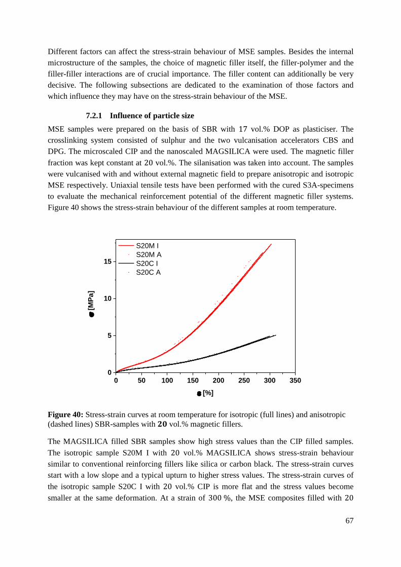
67

Different factors can affect the stress-strain behaviour of MSE samples. Besides the internal

microstructure of the samples, the choice of magnetic filler itself, the filler-polymer and the

filler-filler interactions are of crucial importance. The filler content can additionally be very

decisive. The following subsections are dedicated to the examination of those factors and

which influence they may have on the stress-strain behaviour of the MSE.

7.2.1 Influence of particle size

MSE samples were prepared on the basis of SBR with 17 vol.% DOP as plasticiser. The

crosslinking system consisted of sulphur and the two vulcanisation accelerators CBS and

DPG. The microscaled CIP and the nanoscaled MAGSILICA were used. The magnetic filler

fraction was kept constant at 20 vol.%. The silanisation was taken into account. The samples

were vulcanised with and without external magnetic field to prepare anisotropic and isotropic

MSE respectively. Uniaxial tensile tests have been performed with the cured S3A-specimens

to evaluate the mechanical reinforcement potential of the different magnetic filler systems.

Figure 40 shows the stress-strain behaviour of the different samples at room temperature.

0 50 100 150 200 250 300 3500

5

10

15

S20M I

S20M A

S20C I

S20C A

[

MP

a]

[%]

Figure 40: Stress-strain curves at room temperature for isotropic (full lines) and anisotropic

(dashed lines) SBR-samples with 𝟐𝟎 vol.% magnetic fillers.

The MAGSILICA filled SBR samples show high stress values than the CIP filled samples.

The isotropic sample S20M I with 20 vol.% MAGSILICA shows stress-strain behaviour

similar to conventional reinforcing fillers like silica or carbon black. The stress-strain curves

start with a low slope and a typical upturn to higher stress values. The stress-strain curves of

the isotropic sample S20C I with 20 vol.% CIP is more flat and the stress values become

smaller at the same deformation. At a strain of 300 %, the MSE composites filled with 20

68

vol.% MAGSILICA show a stress value of about 17 MPa while the samples filled with 20

vol.% CIP show a significantly smaller stress value of just 5 MPa. These stress values are

typical for nanoscaled and microscaled filler particles.

This difference is explained by a better filler networking of the nanoscaled MAGSILICA

particles compared to microscaled CIP particles. The mechanical reinforcement potential is

attributed to the formation of a physically bonded filler network and to strong polymer-filler

couplings. MAGSILICA with a specific surface area of 54 𝑚²/𝑔 provides the polymer

chains a larger surface area to adhere compared to CIP with a specific surface area of

0.4 𝑚²/𝑔. Additionally, the coupling reactions of the silane with the magnetic filler during

mixing and with the polymer chains during the vulcanisation establish a strong chemical

bonding at the polymer-filler interface. Due to the surface finish, the polymer-filler interface

is larger with MAGSILICA than with CIP. For these reasons, MAGSILICA provides better

networking features necessary for mechanical reinforcement than CIP [106, 107]. This

behaviour confirms the findings that the filler networking is promoted by the particle size as

discussed by Vilgis et al. [170].

No effect of the orientation of the magnetic filler particles is found on the stress and strain

values of the SBR samples because the loading direction was perpendicular to the magnetic

filler strings.

7.2.2 Variation of filler loading

MSE composites were prepared on the basis of NBR and the magnetic filler CIP. The

silanisation was taken into account. The silane content has been adjusted to magnetic filler

volume fraction. The plasticiser TDAE was used. The crosslinking system consists of sulphur

and the vulcanisation accelerator CBS. The samples were vulcanised with and without

external magnetic field in order to prepare anisotropic and isotropic MSE respectively.

Uniaxial tensile tests have been performed with the cured S3A-specimens to evaluate the

mechanical reinforcement potential of the different magnetic filler systems. The stress-strain

curves for the isotropic and anisotropic NBR samples with different filler volume fractions at

room temperature are depicted in Figure 41.

69

0 200 400 600 8000

1

2

3

4

5 N0

N06C I

N13C I

N20C I

N28C I

N36C I

[

MP

a]

[%]

0 200 400 600 8000

1

2

3

4

5 N0

N06C A

N13C A

N20C A

N28C A

N36C A

[

MP

a]

[%]

Figure 41: Stress-strain curves at room temperature for isotropic (right) and anisotropic (left)

NBR samples with different filler volume fractions.

Considering first the filler concentration, a systematic increase of stress values as well as

tensile strength with increasing CIP content for the isotropic MSE is observed until a critical

filler amount of about 20 vol.% is reached. A maximum stress value of about 5 MPa and a

maximum extensibility of 750 % were attained for the isotropic N20C. The anisotropic MSE

do not follow this tendency. They show the highest stress and extensibility values for the

sample N13C with 13 vol.% CIP.

Concerning the entire domain of the stress-strain curves for both isotropic and anisotropic

MSE, two different behaviours can be observed depending on the magnetic filler amount of

the samples. While the stress-strain curves for the unfilled MSE look quite usual, the stress-

strain curves for the filled MSE are rather uncommon for elastomer composites showing at

about 2 MPa a yield-like behaviour. Obviously, the filler morphology is not affecting this

significantly. Accordingly, the yielding behaviour is probably related to the formation of

voids due to a detachment of the polymer chains from the filler surfaces. The voids grow as

the strain increases and a more or less pronounced plateau with a constant stress arises [171].

Previous work has shown rather common stress-strain curves without yielding if non-polar

rubber were used [106, 107]. The present behaviour may thus be associated with the polarity

of the rubber matrix. Indeed, the polar acrylonitrile groups of polymer chains interact with the

polar hydroxyl group of the magnetic filler particles due to the available permanent dipoles. A

physical bonding between the polymer chains and the filler particles based on dipole-dipole

forces can be built. This is relatively weak in comparison to the chemical bonding between

the polymer chains and the filler particles due to the use of silane. Accordingly, it appears that

the silanisation reaction was not sufficient for getting a reasonable chemical bonding. One

reason could be the large number of the acrylonitrile groups (39 %) that cannot react with the

silane. Nevertheless the physical bonds may contribute to the established network and

improve the mechanical properties of the MSE. The yield point could, thus, indicate that the

interaction between the polar groups of polymer chains and the magnetic filler fails if a

critical stress of the samples is reached.

70

To investigate the influence of the polarity of rubber on stress-stress behaviour of MSE,

additional four different samples were prepared with a constant CIP concentration of 20

vol.%. The different rubbers show different polarities. A non-polar EPDM (E), a weakly polar

NR, a polar HNBR (H) and a very polar XHNBR (X) were used. The stress-strain curves for

the isotropic and anisotropic samples at room temperature are illustrated in Figure 42.

0 100 200 300 400 500 6000

5

10

15

E20C I

NR20C I

H20C I

X20C I

[

MP

a]

[%]

0 100 200 300 400 500 6000

5

10

15

E20C A

NR20C A

H20C A

X20C A

[

MP

a]

[%]


samples on the basis of different rubbers with different polarities. The CIP volume fraction is

kept constant at 𝟐𝟎 vol.% for all samples.

Figure 42 confirms the measurement findings for the polar NBR samples. It seems that the

polarity of rubber plays a crucial role in the stress-strain behaviour of the MSE composites.

7.2.3 Influence of coupling agent

MSE composites were prepared with an without silane on the basis of SBR and 20 vol.% CIP.

The plasticiser DOP was used. The crosslinking system consists of sulphur and the two

vulcanisation accelerators CBS and DPG. The samples were vulcanised with and without

external magnetic field in order to prepare anisotropic and isotropic MSE respectively.

Uniaxial tensile tests have been performed with the cured S3A-specimens to evaluate the

reinforcement potential of the different magnetic filler systems. The stress-strain curves for

the isotropic and anisotropic samples with and without silane at room temperature are

illustrated in Figure 43.

71

0 50 100 150 200 250 300 350 4000

1

2

3

4

5 S20C I

S20C no Silane I

S20C A

S20C no Silane A

[

MP

a]

[%]

Figure 43: Effect of silane on stress-strain curves at room temperature for silanized (full line)

and non-silanized (dashed line) SBR samples including the effect of particles orientation.

The silanized samples show higher stress values compared to non-silanized ones. This

indicates that a larger chemical polymer-filler coupling is realized with silane. The interaction

between the polymer chains and the polyol-coated CIP particles is enhanced. This leads to a

better distribution of magnetic filler particles in the sample and thus to a high mechanical

reinforcement.

The orientation of magnetic filler particles does not play a major role under uniaxial loading

because the columnar CIP strings are perpendicular to the tensile direction [106, 107].

7.3 Dynamic-mechanical thermal analysis

Dynamic-mechanical thermal analysis is used to characterise the rheological behaviour of

elastomer composites. Similar to the stress-strain behaviour of MSE, the dynamic-mechanical

behaviour of MSE is affected by several factors. In addition to the choice of magnetic filler,

the magnetic filler content and the filler-polymer interaction, the internal microstructure of

MSE plays for the dynamic-mechanical analysis a key role compared to quasistatic stress-

strain curves. All these aspects are evaluated in the following subsections.

7.3.1 Vulcanisation in a magnetic field

Elastomer composites are produced by curing the rubber component with a crosslinking

system in a heating press. The crosslinking is a chemical reaction in which the polymer chains

are linked by means of sulphur into a three-dimensional network. The vulcanisation process

substantially improves the stiffness values and it is aimed to meet the required mechanical

72

properties of elastomer composites. If the curing process takes place in the presence of an

external magnetic field, the internal distribution of the magnetic filler particles within the

rubber matrix can be strongly influenced. This depends on the strength of the magnetic field.

Anisotropic samples with oriented magnetic filler strings are then realised.

The analysis of the amplitude dependence of the storage modulus 𝐺’ at room temperature is

sufficient to provide insights in how the internal microstructure of elastomer composites looks

like. MSE composites were prepared on the basis of SBR and the magnetic filler CIP. The

samples were vulcanised with and without external magnetic field in order to prepare

anisotropic and isotropic MSE respectively. For the preparation of anisotropic samples, 3

different magnetic field strengths were applied: 0.08 𝑇, 0.11 𝑇 and 0.2 𝑇. Strain sweeps in

shear mode for SBR samples cured with different magnetic field strengths at room

temperature and a frequency of 1 𝐻𝑧 are shown in Figure 44. The orientation of the magnetic

filler particles was perpendicular to the shearing direction.

0,1 1 10 50

0,50

0,75

1,00

1,25

1,50 S0

S05C I

S10C I

S15C I

S20C I

G' [M

Pa

]

dyn

[%]

0,1 1 10 50

0,5

1,0

1,5

2,0

2,5

3,0B

curing = 0.08 T S0

S05C A

S10C A

S15C A

S20C A

G' [M

Pa

]

dyn

[%]

0,1 1 10 50

0,5

1,0

1,5

2,0

2,5

3,0

3,5B

curing = 0.11 T S0

S05C A

S10C A

S15C A

S20C A

G' [M

Pa

]

dyn

[%]

0,1 1 10 50

0,5

1,0

1,5

2,0

2,5

3,0

3,5

4,0

4,5B

curing = 0.2 T S0

S05C A

S10C A

S15C A

S20C A

G' [M

Pa

]

dyn

[%]

Figure 44: Amplitude dependence of the storage modulus at 𝟐𝟑 °𝑪 and a frequency of 𝟏 𝑯𝒛.

Measurement results for isotropic SBR-samples in the top left corner. Measurement results for

anisotropic SBR-samples cured with a magnetic field of 𝟎. 𝟎𝟖 𝑻, 𝟎. 𝟏𝟏 𝑻 and 𝟎. 𝟐 𝑻 are

shown in the top right, bottom left and bottom right corner respectively.

Obviously, all MSE samples show a Payne effect [172]. The strain storage modulus

continuously decreases with increasing the strain amplitude. This indicates a continuous

73

breakdown of the magnetic filler network. The storage modulus 𝐺′ increases systematically

with increasing the CIP content. The magnetic filler particles build together larger filler

clusters and create a stiffer magnetic filler network. This stabilises the polymer matrix and

delivers improved mechanical properties.

In order to examine the effect of orientation of the magnetic filler particles, the samples

containing the same filler concentration are compared. The isotropic MSE samples were cured

without magnetic field. A maximal storage modulus 𝐺’ of 1.3 MPa at a strain amplitude of

0.1 % is measured for the sample S20C I with 20 vol.% CIP. The storage modulus 𝐺’

increases significantly for anisotropic samples. It is quite obvious that the higher the magnetic

field during curing is, the higher is the storage modulus. The anisotropic sample S20C A with

20 vol. % CIP has a storage modulus 𝐺’ of 4.2 MPa at a strain amplitude of 0.1 %, when it is

cured at 0.2 𝑇.

The increase of the storage modulus of the MSE samples can be associated with the

interaction strength between the magnetic filler particles and the applied magnetic field during

curing. According to equation (19), increasing the strength of the magnetic field increases the

magnetic energy available. This leads to a better alignment of the magnetic filler particles

along the magnetic field lines. The magnetic filler particles within a string come closer to

each other. This increases the anisotropic shape of the filler network and promotes the

mechanical reinforcement of MSE samples. A columnar structure is created. The particle

distribution Φ of the magnetic filler depending on the strength of the magnetic field during

curing is depicted in Figure 45. The magnetic filler strings become narrower and longer when

the magnetic field during the vulcanisation 𝐵𝑧 increases.

74

x

Bz

Figure 45: The particle distribution of the magnetic filler depending on the strength of the

magnetic field during curing.

7.3.2 Influence of particle size

In order to evaluate the influence of the size of the magnetic filler particles on the dynamic-

mechanical properties of MSE, SBR based MSE samples with a constant magnetic filler

fraction of 20 vol.% were prepared on the same way as discussed in section (7.2.1). The

microscaled CIP and the nanoscaled MAGSILICA were used again. The samples were

vulcanised with and without external magnetic field to prepare anisotropic and isotropic MSE

respectively. Strain sweeps in shear mode have been performed. The orientation of the

magnetic filler particles was perpendicular to the shearing direction. Figure 46 shows the

amplitude dependence of the storage modulus of the different MSE samples at room

temperature and a frequency of 1 𝐻𝑧.

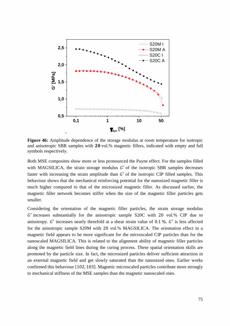
75

0,1 1 10 500,5

1,0

1,5

2,0

2,5 S20M I

S20M A

S20C I

S20C A

G' [M

Pa]

dyn

[%]

Figure 46: Amplitude dependence of the storage modulus at room temperature for isotropic

and anisotropic SBR samples with 𝟐𝟎 vol.% magnetic fillers, indicated with empty and full

symbols respectively.

Both MSE composites show more or less pronounced the Payne effect. For the samples filled

with MAGSILICA, the strain storage modulus 𝐺′ of the isotropic SBR samples decreases

faster with increasing the strain amplitude than 𝐺′ of the isotropic CIP filled samples. This

behaviour shows that the mechanical reinforcing potential for the nanosized magnetic filler is

much higher compared to that of the microsized magnetic filler. As discussed earlier, the

magnetic filler network becomes stiffer when the size of the magnetic filler particles gets

smaller.

Considering the orientation of the magnetic filler particles, the strain storage modulus

𝐺′ increases substantially for the anisotropic sample S20C with 20 vol.% CIP due to

anisotropy. 𝐺′ increases nearly threefold at a shear strain value of 0.1 %. 𝐺′ is less affected

for the anisotropic sample S20M with 20 vol.% MAGSILICA. The orientation effect in a

magnetic field appears to be more significant for the microscaled CIP particles than for the

nanoscaled MAGSILICA. This is related to the alignment ability of magnetic filler particles

along the magnetic field lines during the curing process. These spatial orientation skills are

promoted by the particle size. In fact, the microsized particles deliver sufficient attraction in

an external magnetic field and get slowly saturated than the nanosized ones. Earlier works

confirmed this behaviour [102, 103]. Magnetic microscaled particles contribute more strongly

to mechanical stiffness of the MSE samples than the magnetic nanoscaled ones.

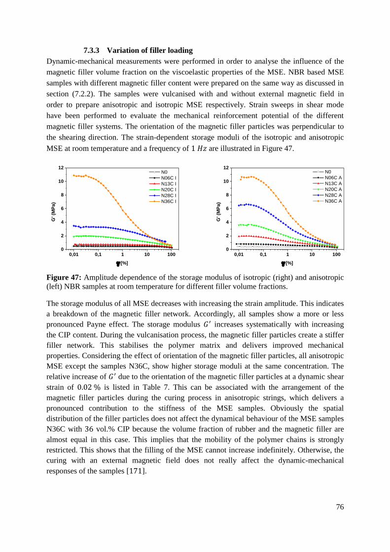
76

7.3.3 Variation of filler loading

Dynamic-mechanical measurements were performed in order to analyse the influence of the

magnetic filler volume fraction on the viscoelastic properties of the MSE. NBR based MSE

samples with different magnetic filler content were prepared on the same way as discussed in

section (7.2.2). The samples were vulcanised with and without external magnetic field in

order to prepare anisotropic and isotropic MSE respectively. Strain sweeps in shear mode

have been performed to evaluate the mechanical reinforcement potential of the different

magnetic filler systems. The orientation of the magnetic filler particles was perpendicular to

the shearing direction. The strain-dependent storage moduli of the isotropic and anisotropic

MSE at room temperature and a frequency of 1 𝐻𝑧 are illustrated in Figure 47.

0,01 0,1 1 10 1000

2

4

6

8

10

12

G' (M

Pa

)

[%]

N0

N06C I

N13C I

N20C I

N28C I

N36C I

0,01 0,1 1 10 1000

2

4

6

8

10

12

G' (M

Pa

)

[%]

N0

N06C A

N13C A

N20C A

N28C A

N36C A

Figure 47: Amplitude dependence of the storage modulus of isotropic (right) and anisotropic

(left) NBR samples at room temperature for different filler volume fractions.

The storage modulus of all MSE decreases with increasing the strain amplitude. This indicates

a breakdown of the magnetic filler network. Accordingly, all samples show a more or less

pronounced Payne effect. The storage modulus 𝐺′ increases systematically with increasing

the CIP content. During the vulcanisation process, the magnetic filler particles create a stiffer

filler network. This stabilises the polymer matrix and delivers improved mechanical

properties. Considering the effect of orientation of the magnetic filler particles, all anisotropic

MSE except the samples N36C, show higher storage moduli at the same concentration. The

relative increase of 𝐺′ due to the orientation of the magnetic filler particles at a dynamic shear

strain of 0.02 % is listed in Table 7. This can be associated with the arrangement of the

magnetic filler particles during the curing process in anisotropic strings, which delivers a

pronounced contribution to the stiffness of the MSE samples. Obviously the spatial

distribution of the filler particles does not affect the dynamical behaviour of the MSE samples

N36C with 36 vol.% CIP because the volume fraction of rubber and the magnetic filler are

almost equal in this case. This implies that the mobility of the polymer chains is strongly

restricted. This shows that the filling of the MSE cannot increase indefinitely. Otherwise, the

curing with an external magnetic field does not really affect the dynamic-mechanical

responses of the samples [171].

77

Table 7: Characteristic values of the storage modulus of the MSE samples due to orientation

of magnetic filler particles at a dynamic strain of 𝟎. 𝟎𝟐 %. The indices ‘𝑰’ and ‘𝑨’ stand for

isotropic and anisotropic samples, respectively.

𝑮𝑰′

[MPa]

𝑮𝑨′

[MPa]

Δ𝑮’ [MPa]

N0 0.42 0.42 0.00

N06C 0.49 0.80 0.31

N13C 0.75 1.95 1.20

N20C 1.94 3.60 1.66

N28C 3.37 6.53 3.16

N36C 10.70 10.70 0.00

Next, the response of the MSE samples regarding dynamic deformation at higher frequencies

is taken into consideration. Temperature-frequency sweeps at small deformation and different

temperatures within a limited frequency range were measured. These series of isothermal

branches of the frequency-dependent shear modulus were horizontally shifted along the

logarithmic frequency axis to generate master curves. The time-temperature superposition

principle according to the Williams, Landel and Ferry approach relating the frequency and

temperature dependency of viscoelastic materials above the glass transition temperature 𝑇𝑔 is

used.

The master curves of storage and loss moduli 𝐺’ and 𝐺’’ as well as loss factor tan 𝛿 for both

isotropic and anisotropic MSE samples are presented in Figure 48. The reference temperature

𝑇𝑟𝑒𝑓 was 20 °𝐶. The WLF parameters derived from the horizontal shifting have the following

values 𝐶1 = 4.64 and 𝐶2 = 88.89 °𝐶. The associated shift factors and the corresponding

WLF-fit are depicted in Figure 49, demonstrating that the WLF equation (33) fits well the

data for temperature 𝑇 higher than the glassy transition temperature 𝑇𝑔 ≈ −35 °𝐶.

Considering the frequency dependency of the storage moduli shown in Figure 48, the elastic

plateau, also known as the rubbery plateau, covers the low frequency or high temperature part

of the master curves. It reaches out over 5 frequency decades, which range between

3.6 10−4 𝐻𝑧 and 102 𝐻𝑧. The rubbery plateau is followed by the glass transition domain. This

covers the frequency range between 102 𝐻𝑧 and 108 𝐻𝑧. The slope of the master curves

below the glassy plateau increases with increasing frequency or decreasing temperature. At

lower temperature, the MSE samples become stiffer and begin to lose gradually their

elasticity. An important characteristic of the polymer dynamic within this frequency range is

the glass transition temperature. It stands at almost −35 °𝐶 and represents the lowest

conceivable operating temperature for the NBR based MSE [171].

78

10-4

10-2

100

102

104

106

108

1010

1012

1014

1016

105

106

107

108

109

1010

N0

N06C I

N13C I

N20C I

N28C I

N36C I

G' [P

a]

f [Hz]

10-4

10-2

100

102

104

106

108

1010

1012

1014

1016

105

106

107

108

109

1010

N0

N06C A

N13C A

N20C A

N28C A

N36C A

G' [P

a]

f [Hz]

10-4

10-2

100

102

104

106

108

1010

1012

1014

1016

102

103

104

105

106

107

108

109

N0

N06C I

N13C I

N20C I

N28C I

N36C I

G'' [

Pa

]

f [Hz]

10-4

10-2

100

102

104

106

108

1010

1012

1014

1016

102

103

104

105

106

107

108

109

N0

N06C A

N13C A

N20C A

N28C A

N36C A

G'' [

Pa

]

f [Hz]

10-4

10-2

100

102

104

106

108

1010

1012

1014

1016

10-3

10-2

10-1

100

N0

N06C I

N13C I

N20C I

N28C I

N36C I

tan [

-]

f [Hz]

10-4

10-2

100

102

104

106

108

1010

1012

1014

1016

10-3

10-2

10-1

100

N0

N06C A

N13C A

N20C A

N28C A

N36C A

tan [

-]

f [Hz]

Figure 48: Viscoelastic master curves of the MSE at a reference temperature 𝑇𝑟𝑒𝑓 = 20 °𝐶.

Isotropic samples are shown on the left and anisotropic samples on the right. Storage moduli

are shown at the top, loss moduli at the centre and loss factor at the bottom.

The master curves for both isotropic and anisotropic MSE samples show a similar behaviour

as conventional carbon black- or silica-filled samples. In the rubbery plateau, the slope of the

master curves of storage moduli 𝐺′ increases with increasing the filler loading. This is

characteristic for the networking potential of the filler particles. Regarding the effect of

orientation of the magnetic filler particles, slightly larger storage and loss moduli for the

79

anisotropic MSE samples are observed. This is related to the columnar structure of CIP,

which delivers an additional contribution to the stiffness and hysteresis of the samples.

The glass transition frequency at 20 °𝐶 is located at about 105 𝐻𝑧 as deduced from the

maximum of the loss factor tan 𝛿 = 𝐺′′ 𝐺′⁄ . It is important to note that the magnetic filler

content and the effect of orientation do not affect 𝑇𝑔. This behavior remains similar for the

maximum of tan 𝛿, since it is not shifted. The loss factor tan 𝛿 shows a pronounced increase

of energy dissipation with the filler loading in the rubbery plateau and less pronounced

increase in the glassy state while the maximum decreases. This behaviour is similar to

conventional carbon black- or silica-filled samples [171].

-80 -60 -40 -20 0 20 40 60

0

5

10

15

log

(aT)

[-]

T [°C]

Measurement

WLF-fit

Figure 49: Shift factors of the NBR samples obtained by horizontal shifting of the isothermal

branches of the frequency-dependent loss factor tan 𝛿 (symbols) and the corresponding WLF-

fit (line) according to equation (33)

7.3.4 Influence of coupling agent

In order to examine more closely the influence of silane on the magnetically induced

flocculation during the curing process, dynamic-mechanical investigations were performed.

The orientation of magnetic filler particles was perpendicular to the shearing direction. The

strain-dependent storage moduli of MSE composites with and without silane are presented in

Figure 50.

80

0,1 1 10 500,5

1,0

1,5

2,0

2,5

3,0 S20C I

S20C\Si I

S20C A

S20C\Si AG

' [M

Pa

]

dyn

[%]

Figure 50: Effect of silane on the amplitude dependence of the storage modulus (Payne

effect) at room temperature for silanized (closed symbols) and non-silanized (open symbols)

SBR samples including the effect of particles orientation.

All MSE samples show a more or less pronounced Payne effect. The storage modulus 𝐺’

decreases with increasing the shear strain due to continuous breakdown of the filler network.

Figure 50 shows that the storage moduli 𝐺’ are smaller for silanized MSE composites

compared with the non-silanized samples. These results are independent of the orientation of

the magnetic filler particles. In addition, 𝐺’ decreases slower for the silanized samples

compared with the non-silanized ones due to increasing strain amplitude. For the anisotropic

samples, this even leads to an intersection of the two curves at a dynamical strain of about

1 %.

The observed mechanical performance is explained by the fact that the silane layer at the filler

surface acts as a kind of space-holder. This prevents the filler particles to come in close

contact and delivers more flexible filler-filler bonds [170]. This is the main reason why the

samples with silane are less stiff than the non silanized samples, independently from their

orientations. Furthermore, the sulphur units of the silane react during the vulcanisation with

the polymer chains leading to a strong chemical coupling between the polymer matrix and the

magnetic filler particles. This improves the phase bonding and stabilises the filler network

The covalent chemical bonds make the magnetic filler network more stable. [106, 107].

81

7.4 Fatigue crack propagation and ageing behaviour

Ageing is the totality of chemical and physical changes over time that lead to a change in

mechanical properties of the elastomer composites so that their usefulness is reduced in time

[173, 174]. These changes can lead to sample failure and the finished product can no longer

fulfil its function [175]. The thermal ageing occurs at any time during the manufacturing and

operation processes. The fatigue happens when the samples are temporarily or constantly

exposed to diverse mechanical loads [176].

At a molecular level, irreversible physical and chemical processes caused by fatigue and

ageing occur. These processes include polymer chain scissions, post-crosslinking and

reformation of covalent bonds (re-combination). While the polymer chain scission causes a

decrease in the viscosity, a post-crosslinking of the material leads to an increase in the

stiffness. A combination of both mechanisms can eventually lead to the formation of

microcracks that limit the lifetime of the elastomer composites. Materials in which the chain

scission process occurs tend to form cracks on the surface. The degree of ageing-related

changes depends strongly on the material structure and the ageing conditions such as

temperature, time and mechanical stress. The ageing can be divided into an internal and an

external ageing. The internal ageing represents the degradation of residual stresses,

recrystallisation, phase separation in multicomponent systems (plasticizer migration e.g.). It is

caused by thermodynamically unstable states of the rubber material. External ageing

phenomena are stress cracking, fatigue cracking, thermo-oxidative degradation or swelling

and are caused by complex physical or chemical environmental effects. The fatigue and

ageing resistance can be characterised in the context of durability tests. Here, the elastomer

composites are subjected to artificial ageing under realistic conditions in order to evaluate the

effect of fatigue and ageing on the structure and properties [177].

7.4.1 Mechanical fatigue of magneto-sensitive elastomers

The fatigue crack growth is related to the microstructural inhomogeneity of the test samples

and the mechanical load applied. Each material contains microcracks due to manufacturing

tolerances. Applying mechanical stresses leads to a local exceeding of the breaking strength

and thus to crack initiation. The crack initiation is in principle the transition from an inactive

to a moving fracture. Depending on the available elastic energy, the fracture propagates or

stops.

As discussed earlier (see section 4.3), the crack propagation is labelled with the crack growth

rate. Stable crack propagation is characterised by a relatively low crack growth rate. The

cracks keep growing when more and more energy is externally supplied. At higher crack

growth rates, the cracks grow faster and can quickly turn into catastrophic regime. The crack

propagation becomes unstable.

In order to examine the fatigue crack growth of MSE, experimental measurements were

conducted using single notched tension sample SENT and were performed with the TFA. In

the fracture mechanical testing of rubber samples, initial cracks are manually introduced with

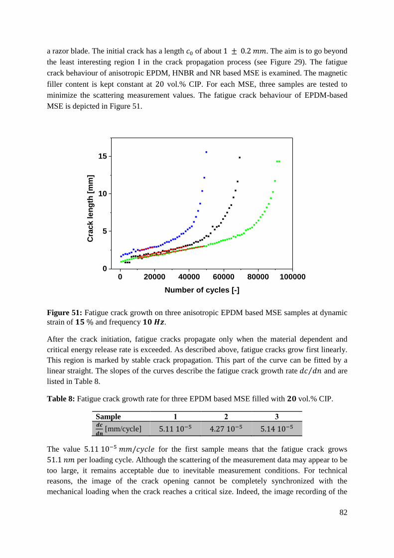
82

a razor blade. The initial crack has a length 𝑐0 of about 1 ± 0.2 𝑚𝑚. The aim is to go beyond

the least interesting region I in the crack propagation process (see Figure 29). The fatigue

crack behaviour of anisotropic EPDM, HNBR and NR based MSE is examined. The magnetic

filler content is kept constant at 20 vol.% CIP. For each MSE, three samples are tested to

minimize the scattering measurement values. The fatigue crack behaviour of EPDM-based

MSE is depicted in Figure 51.

0 20000 40000 60000 80000 1000000

5

10

15

Cra

ck len

gth

[m

m]

Number of cycles [-]

Figure 51: Fatigue crack growth on three anisotropic EPDM based MSE samples at dynamic

strain of 𝟏𝟓 % and frequency 𝟏𝟎 𝑯𝒛.

After the crack initiation, fatigue cracks propagate only when the material dependent and

critical energy release rate is exceeded. As described above, fatigue cracks grow first linearly.

This region is marked by stable crack propagation. This part of the curve can be fitted by a

linear straight. The slopes of the curves describe the fatigue crack growth rate 𝑑𝑐 𝑑𝑛⁄ and are

listed in Table 8.

Table 8: Fatigue crack growth rate for three EPDM based MSE filled with 𝟐𝟎 vol.% CIP.

Sample 1 2 3 𝒅𝒄

𝒅𝒏 [mm/cycle] 5.11 10−5 4.27 10−5 5.14 10−5

The value 5.11 10−5 𝑚𝑚/𝑐𝑦𝑐𝑙𝑒 for the first sample means that the fatigue crack grows

51.1 𝑛𝑚 per loading cycle. Although the scattering of the measurement data may appear to be

too large, it remains acceptable due to inevitable measurement conditions. For technical

reasons, the image of the crack opening cannot be completely synchronized with the

mechanical loading when the crack reaches a critical size. Indeed, the image recording of the

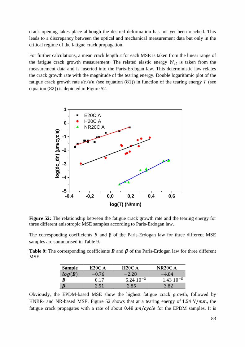
83

crack opening takes place although the desired deformation has not yet been reached. This

leads to a discrepancy between the optical and mechanical measurement data but only in the

critical regime of the fatigue crack propagation.

For further calculations, a mean crack length 𝑐 for each MSE is taken from the linear range of

the fatigue crack growth measurement. The related elastic energy 𝑊𝑒𝑙 is taken from the

measurement data and is inserted into the Paris-Erdogan law. This deterministic law relates

the crack growth rate with the magnitude of the tearing energy. Double logarithmic plot of the

fatigue crack growth rate 𝑑𝑐 𝑑𝑛⁄ (see equation (81)) in function of the tearing energy 𝑇 (see

equation (82)) is depicted in Figure 52.

-0,4 -0,2 0,0 0,2 0,4 0,6-5

-4

-3

-2

-1

0

1

E20C A

H20C A

NR20C A

log

(dc_d

n)

(µm

/cycle

)

log(T) (N/mm)

Figure 52: The relationship between the fatigue crack growth rate and the tearing energy for

three different anisotropic MSE samples according to Paris-Erdogan law.

The corresponding coefficients 𝐵 and β of the Paris-Erdogan law for three different MSE

samples are summarised in Table 9.

Table 9: The corresponding coefficients 𝑩 and 𝜷 of the Paris-Erdogan law for three different

MSE

Sample E20C A H20C A NR20C A

𝒍𝒐𝒈(𝑩) −0.76 −2.28 −4.84

𝑩 0.17 5.24 10−3 1.43 10−5

𝜷 2.51 2.85 3.82

Obviously, the EPDM-based MSE show the highest fatigue crack growth, followed by

HNBR- and NR-based MSE. Figure 52 shows that at a tearing energy of 1.54 𝑁/𝑚𝑚, the

fatigue crack propagates with a rate of about 0.48 µ𝑚/𝑐𝑦𝑐𝑙𝑒 for the EPDM samples. It is

84

around 8.06 10−3 µ𝑚/𝑐𝑦𝑐𝑙𝑒 for the HNBR-based MSE and 4.34 10−5 µ𝑚/𝑐𝑦𝑐𝑙𝑒 for NR

samples. Accordingly, the EPDM samples display the worst values of the fatigue crack

propagation compared to HNBR and NR ones. The large crack growth rate for EPDM rubber

is the main reason why is not suitable for any dynamic applications. NR confirms with its

small fatigue crack growth rate its standing as the most appropriate rubber for dynamic

applications. NR owes its outstanding resistance to crack growth to the strain-induced

crystallisation (SIC). SIC depends on the loading direction. When the amorphous NR gets

stretched at room temperature, the polymer chains become strongly oriented and many of

them remains partially immobilized. A lamellar structure emerges within the rubber matrix.

This forms additionally separate networks, which are perpendicular to the loading direction.

These crystallite networks reduce locally the crack formation and can inhibit the crack

propagation in the rubber matrix. SIC increases the stiffness and improves the resistance to

crack growth of the NR samples. The values of HNBR samples come somewhere in between.

Fatigue cracks in HNBR samples propagate 2 decades slower than in EPDM-based MSE and

2 decades quicker than in NR-based MSE. Nevertheless, HNBR is often used for dynamic

applications like NR. It is mainly used in high temperature applications where a good

mechanical stiffness is also required. This is the case for timing belts of automotive engines or

in the sealing technology.

According to Persson et al [178], the coefficient 𝑚 from the relaxation time spectra as well as

the coefficient 𝛽 from the Paris-Erdogan law are interrelated as follows:

𝑏 = 1−𝑚

2−𝑚∶=

1

𝛽 (91)

Klüppel showed that the last relationship (equation (91)) is also valid for viscoelastic

materials [179]. The coefficient 𝑚 from the relaxation time spectra as well as the coefficient

𝛽 from the Paris-Erdogan law are summarised in Table 10. The different models used to

describe the mechanical response of rubber and, consequently, to determine these coefficients

are mentioned again between the brackets.

Table 10: Summary of the coefficient 𝒎 from the relaxation time spectra as well as the

coefficient 𝜷 from the Paris-Erdogan law. The different models used are mentioned between

the brackets.

Sample E20C A H20C A NR20C A

𝒎 (𝑯(𝝉)) 0.37 0.56 0.64

𝒃 𝟎. 𝟑𝟖 𝟎. 𝟑𝟎 𝟎. 𝟐𝟓

𝜷 (Paris-Erdogan) 2.51 2.85 3.82

𝟏/𝜷 𝟎. 𝟑𝟗 𝟎. 𝟑𝟓 𝟎. 𝟐𝟔

Relative error [%] 3.16 14.84 0.80

Table 10 shows that the 𝑏-values of the different MSE samples, derived from the coefficient

𝑚 from the relaxation time spectra according to equation (91), are in good agreement with the

coefficient 𝛽 from the Paris-Erdogan law.

85

For the anisotropic NR and EPDM samples, the evaluation of the relaxation time spectra lead

to predict with almost good accuracy the coefficient 𝛽. This represents the principal factor to

determine the fatigue crack growth rate of the MSE samples. With a relative error of 0.81 %

and 3.17 %, the results for NR and EPDM samples are very good. However, the result for

HNBR samples show a lager discrepancy with a relative error of 14.84 %.

These relative errors still remain acceptable although the incorrect evaluation of lifetime or

crack propagation rate can lead to disastrous consequences for the MSE performance. Errors

during the TFA measurements are unavoidable due to the technical design. Errors can also

occur by generating the master curves and/or evaluating the relaxation time spectra.

7.4.2 Thermal Ageing of magneto-sensitive elastomers

Diene rubbers are irreplaceable for technical elastomer products exposed to high dynamic

loads. The reason lies in the typical molecular inner structure of rubber. Long chain molecules

with a very regular structure provide outstanding elastic properties. However, the unsaturated

chemical bonds in the polymer backbone make it susceptible to decomposition by ozone and

oxygen or a gradual post-crosslinking by radicals, ultraviolet radiation and heat. This leads in

the long term to crack formation and ultimately tearing of elastomer composites [76, 173].

Rubber materials degrade by heat treatment. This process may get worse when oxidative

reactions take place simultaneously. Rubber components and elastomer composites generally

undergo disadvantageous changes during prolonged storage under unfavourable air and

temperature conditions due to initiated post-crosslinking and oxidation reactions.

For the experimental analysis of the thermal ageing of MSE composites, SBR samples were

prepared with different magnetic filler content. The magnetic filler was the microscaled CIP.

Since atmospheric oxygen is a relatively aggressive environment for rubber materials, IPPD

was added to make MSE temporary ozone-resistant. Additives slow down the ageing process

but they cannot be a permanent solution. IPPD is one of the indispensable additives in the

rubber technology. It is used as an antioxidant and antiozonant for statically and dynamically

highly stressed elastomer composites like in the tyre sector and in technical rubber articles

such as hoses, vehicle moulded parts, cable sheaths and conveyor belts. IPPD continuously

accumulates on the rubber surface to prevent the oxidative degradation and crack formation.

The MSE samples were put under normal atmospheric conditions in an oven at a temperature

of 100 °𝐶 for a maximum term of 28 days. Ageing repercussions and changes in the internal

structure of the MSE samples can be reliably evaluated by considering the changes in the

elongation at break and tensile strength at break. The measurement results are depicted in

Figure 53 and Figure 54 respectively.

86

0 7 14 21 28

100

200

300

S0

S05C A

S10C A

S15C A

S20C A

Elo

ng

ati

on

at

bre

ak [

%]

Days

Figure 53: Elongation at break for thermally aged MSE samples with the anti-ageing agent

IPPD under air at atmospheric pressure.

The dynamic-mechanical behaviour of MSE can be explained by a shortening of the long

polymer chains and continuous post-crosslinking reactions during the ageing process. The

drop of the elongation at break for all MSE samples shows that the existing polymer network

is constantly destroyed. The reason is that the chemical and molecular bonds are thermally

activated. At high temperature, the polymer chains decompose. The MSE samples lose a large

part of their restoring force. The crosslinking is also a thermally activated process. If the

sulphur is not completely used during the vulcanisation or do not lead to a fully crosslinked

structure (see the chemical bond 𝑆𝑦 − 𝑅 and 𝑆𝑧 in Figure 7), the sulphur residues may react

with the polymer chains and form new crosslinking points. These post-crosslinking reactions

make the MSE samples stiffer. However, this often leads the samples to break at relatively

low strains [76, 173].

Figure 54 shows that the tensile strength at break increases for all samples. The anisotropic

samples S05C A and S10C A with 5 vol.% and 10 vol.% CIP respectively are broken after 7

days. For the sample S15C A and S20C A with 15 vol.% and 20 vol.% CIP respectively, the

tensile strength at break increases until the 21𝑠𝑡day and then decreases again. This results

from the polymer chain scissions and the subsequent softening of the MSE samples.

87

0 7 14 21 281

2

3

4

5

6

S0

S05C A

S10C A

S15C A

S20C ATen

sile s

tren

gth

at

bre

ak [

MP

a]

Days

Figure 54: Tensile strength at break for thermally aged MSE samples with the anti-ageing

agent IPPD under air at atmospheric pressure.

The changes of the tensile strength 𝜎50 at an elongation of 50 % give more insight into the

network structure due to post-crosslinking. This is shown in Figure 55. The tensile strength of

the anisotropic MSE samples increases with increasing the ageing time period. This indicates

that the network density has significantly increased. 𝜎50 of the sample S20C A with 20 vol.%

CIP tripled from 0.8 MPa to 2.5 MPa after 28 days of thermal ageing.

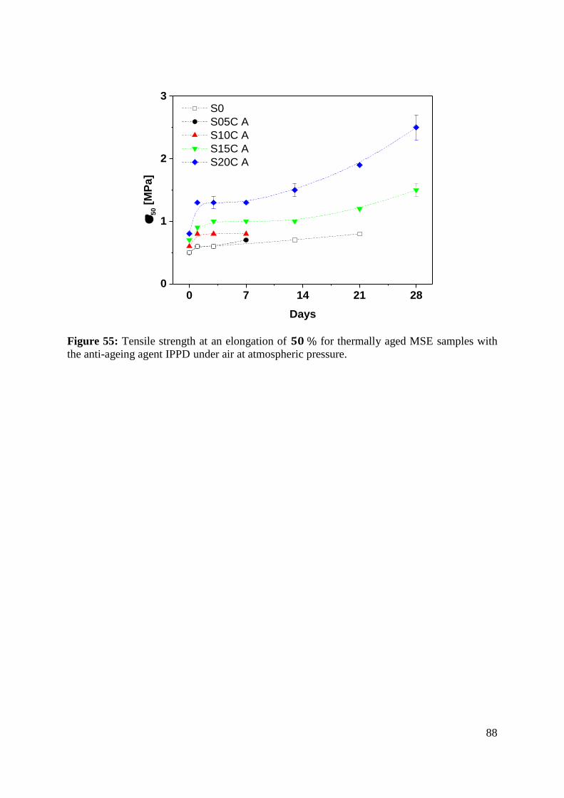
88

0 7 14 21 280

1

2

3 S0

S05C A

S10C A

S15C A

S20C A

5

0 [

MP

a]

Days

Figure 55: Tensile strength at an elongation of 𝟓𝟎 % for thermally aged MSE samples with

the anti-ageing agent IPPD under air at atmospheric pressure.

89

8 Magnetorheology of melts

The effect of particle orientation during the curing process can be observed online by

magnetorheological measurements in the non-crosslinked melts. The orientation of the

magnetic filler particles in strings along the magnetic field lines expresses itself in a

successive increase of the shear modulus, which is measured at small strain amplitudes to

avoid disturbance of the system. The storage modulus 𝐺′ monitors the magnetically induced

flocculation of the magnetic filler particles due to their interaction with the magnetic field. To

analyse the intensity of the interaction between the magnetic filler particles and an external

magnetic field, an on-off switching mode of the magnetic field with alternating polarity is

considered. The shearing direction in this experiment is perpendicular to the direction of the

magnetic field [106, 107].

The storage modulus 𝐺′of a non-crosslinked melt is caused by the physical entanglements of

the polymer chains. The crosslinking introduces chemical crosslinking points into the system.

In filled systems, the magnetic filler particles provide additional large surface areas in the raw

mixture. More stable bonds are formed because more contact points between the surface area

of the magnetic filler and the polymer chains are available. An increase in the magnetic filler

content thus represents an increase in the surface area offered and an increases of the number

of bound polymer chains in the system. In addition, the distances between the several

magnetic filler particles are significantly reduced and progressively loose chain ends are built

[106, 107].

8.1 Flocculation

The flocculation is a chemical process by which colloids come together to form a compact

and uniform mass. In the rubber technology, the flocculation can be understood as the process

by which a stable network is created [138, 146]. This is the result of the curing process. The

polymer chains, magnetic fillers and additives are linked together through crosslinking

systems and organofunctional silanes.

In order to examine the flocculation process, MSE samples were prepared with a constant

magnetic filler fraction of 20 vol.% on the same way as discussed in section (7.2.1). The

microscaled CIP and the nanoscaled MAGSILICA were used. The silanisation was taken into

account. Strain sweeps in shear mode were performed to evaluate the magnetorheological

response of the different samples. The magnetic flux density 𝑩 is 0.74 𝑇. Figure 56 shows the

magnetically induced flocculation during switching on and switching off the magnetic field at

a shear strain amplitude of 0.5 % and an initial temperature of 50 °𝐶.

90

0 200 400 600 800 1000 1200 14000,3

0,4

0,5

0,6

0,7

0,8 S20M

S20CG

' [M

Pa]

t [s]

-0,75

-0,50

-0,25

0,00

0,25

0,50

0,75

= 0.5 %, f = 10 Hz

B [

T]

Figure 56: Variation of the storage modulus at shear strain 𝜸 of 𝟎. 𝟓 % and initial temperature

of 𝟓𝟎 °𝑪 during the switching on and switching off the magnetic field for the SBR-melts with

𝟐𝟎 vol.% magnetic fillers.

The MSE sample S20C with 20 vol.% CIP shows a pronounced switching effect compared to

the sample S20M with 20 vol.% MAGSILICA. The storage modulus 𝐺′ increases by more

than 40 % once the magnetic field is turned on. The MAGSILICA-filled sample S20M shows

hardly any switching effect. Furthermore, S20M shows a continuous decrease of the storage

modulus with increasing flocculation time. This is the consequence of the unwanted heating

of the magnetic cell during the measurement by about 10 °𝐶 after 1400 seconds. This is the

general case for filled elastomer composites with nanoscaled fillers, the stiffness decreases

considerably with increasing temperature due to thermal activation of the filler-filler bonds.

The CIP-filled sample seems little affected by the increase in temperature because there exist

two effects, which influence each other. The increase in temperature reduces on the one hand

the sample viscosity and, correspondingly, its stiffness. On the other hand, it promotes the

orientation of the magnetic dipoles of the magnetic filler particles along the magnetic field

lines. Strings of magnetic filler particles are then formed. These structure contribute to an

additional mechanical reinforcement of the MSE sample and accordingly, high stiffness

values are obtained.

The large switching effect observed for the CIP-filled sample confirms the good interaction of

the microscaled magnetic filler particles with the external magnetic field. Obviously, the

magnetic moments of nanoscaled MAGSILICA are too small to sufficiently interact with the

external magnetic field. Additionally, switching on and off the magnetic field does not affect

the maximum of the storage modulus 𝐺′ of the CIP-filled MSE sample. Not even the polarity

91

change of the magnetic field leads to any improvement. It seems that the induced magnetic

dipole are fully saturated.

The MAGSILICA-filled sample shows a larger storage modulus 𝐺′ than the CIP-filled sample

during the entire measurement. This confirms the capacity of nanoscaled MAGSILICA to

build a stronger filler network than the microscaled CIP [106, 107].

The relative magnetorheological effect (MRE) represents a relative measure of the switching

effect of MSE samples. The MRE is defined as the difference between the initially storage

modulus 𝐺0′ when the magnetic field is turned off and the maximum of the storage modulus

𝐺𝑖𝑛𝑓′ once the magnetic field is turned on, divided by 𝐺0

′ . Mathematically, the MRE can then

be expressed as follows:

𝑀𝑅𝐸 = 𝐺𝑖𝑛𝑓

′ − 𝐺0′

𝐺0′ (92)

Figure 57 shows schematically how the MRE can be determined.

G'0

G' [M

Pa]

t [s]

G'inf

MRE

B [

T]

Figure 57: Schematic diagram to determine the magnetorheological effect MRE as a measure

of the switching ability of the MSE samples.

8.2 Influence of coupling agent on the relative magnetorheological effect

In order to examine the influence of silane on MSE, two different SBR samples were prepared

at a constant magnetic filler volume fraction of 20 vol.% with and without silane on the same

way as discussed in section (7.2.1). The effect of silane on the variation of the storage

modulus at a shear strain amplitude of 0.5 % and a start temperature of 50 °𝐶 is shown in

Figure 58.

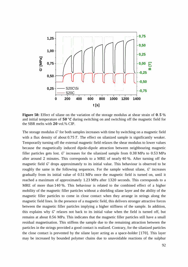
92

0 200 400 600 800 1000 1200 1400

0,25

0,50

0,75

1,00

1,25

S20C\Si

S20C

G' [M

Pa]

t [s]

-0,75

-0,50

-0,25

0,00

0,25

0,50

0,75

B [

T]

Figure 58: Effect of silane on the variation of the storage modulus at shear strain of 𝟎. 𝟓 %

and initial temperature of 𝟓𝟎 °𝑪 during switching on and switching off the magnetic field for

the SBR melts with 𝟐𝟎 vol.% CIP.

The storage modulus 𝐺’ for both samples increases with time by switching on a magnetic field

with a flux density of about 0.75 𝑇. The effect on silanized sample is significantly weaker.

Temporarily turning off the external magnetic field relaxes the shear modulus to lower values

because the magnetically induced dipole-dipole attraction between neighbouring magnetic

filler particles gets lost. 𝐺’ increases for the silanized sample from 0.38 MPa to 0.53 MPa

after around 2 minutes. This corresponds to a MRE of nearly 40 %. After turning off the

magnetic field 𝐺’ drops approximately to its initial value. This behaviour is observed to be

roughly the same in the following sequences. For the sample without silane, 𝐺’ increases

gradually from its initial value of 0.51 MPa once the magnetic field is turned on, until it

reached a maximum of approximately 1.23 MPa after 1320 seconds. This corresponds to a

MRE of more than 140 %. This behaviour is related to the combined effect of a higher

mobility of the magnetic filler particles without a shielding silane layer and the ability of the

magnetic filler particles to come in close contact when they arrange in strings along the

magnetic field lines. In the presence of a magnetic field, this delivers stronger attractive forces

between the magnetic filler particles implying a higher stiffness of the sample. In addition,

this explains why 𝐺’ relaxes not back to its initial value when the field is turned off, but

remains at about 0.56 MPa. This indicates that the magnetic filler particles still have a small

residual magnetisation. This stiffens the sample due to the remaining attraction between the

particles in the strings provided a good contact is realized. Contrary, for the silanized particles

the close contact is prevented by the silane layer acting as a space-holder [170]. This layer

may be increased by bounded polymer chains due to unavoidable reactions of the sulphur

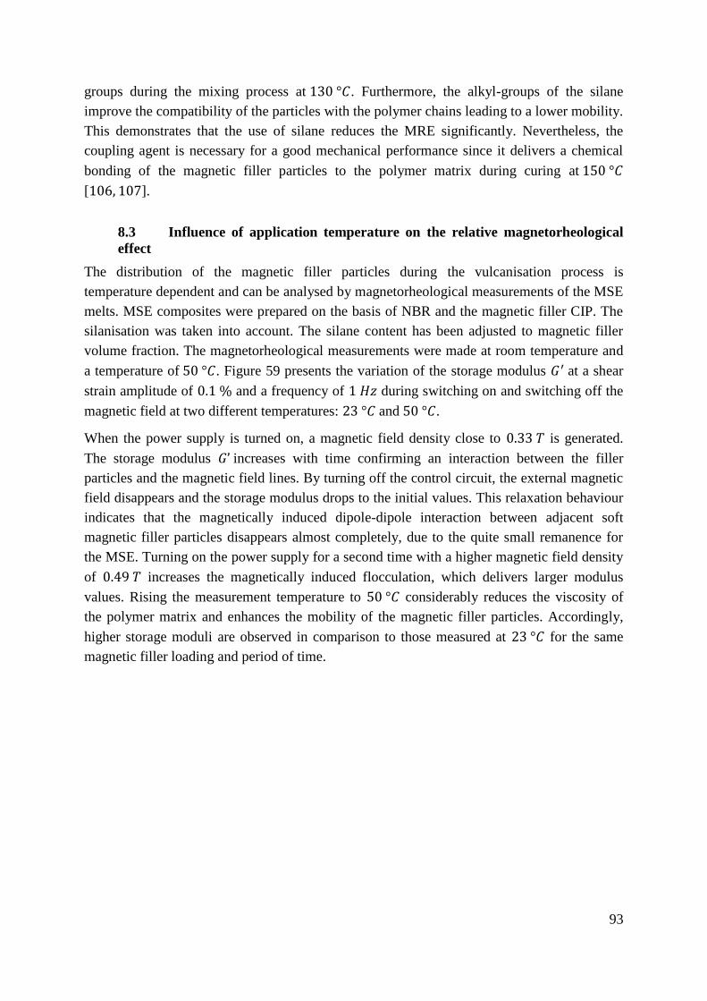
93

groups during the mixing process at 130 °𝐶. Furthermore, the alkyl-groups of the silane

improve the compatibility of the particles with the polymer chains leading to a lower mobility.

This demonstrates that the use of silane reduces the MRE significantly. Nevertheless, the

coupling agent is necessary for a good mechanical performance since it delivers a chemical

bonding of the magnetic filler particles to the polymer matrix during curing at 150 °𝐶

[106, 107].

8.3 Influence of application temperature on the relative magnetorheological

effect

The distribution of the magnetic filler particles during the vulcanisation process is

temperature dependent and can be analysed by magnetorheological measurements of the MSE

melts. MSE composites were prepared on the basis of NBR and the magnetic filler CIP. The

silanisation was taken into account. The silane content has been adjusted to magnetic filler

volume fraction. The magnetorheological measurements were made at room temperature and

a temperature of 50 °𝐶. Figure 59 presents the variation of the storage modulus 𝐺′ at a shear

strain amplitude of 0.1 % and a frequency of 1 𝐻𝑧 during switching on and switching off the

magnetic field at two different temperatures: 23 °𝐶 and 50 °𝐶.

When the power supply is turned on, a magnetic field density close to 0.33 𝑇 is generated.

The storage modulus 𝐺’ increases with time confirming an interaction between the filler

particles and the magnetic field lines. By turning off the control circuit, the external magnetic

field disappears and the storage modulus drops to the initial values. This relaxation behaviour

indicates that the magnetically induced dipole-dipole interaction between adjacent soft

magnetic filler particles disappears almost completely, due to the quite small remanence for

the MSE. Turning on the power supply for a second time with a higher magnetic field density

of 0.49 𝑇 increases the magnetically induced flocculation, which delivers larger modulus

values. Rising the measurement temperature to 50 °𝐶 considerably reduces the viscosity of

the polymer matrix and enhances the mobility of the magnetic filler particles. Accordingly,

higher storage moduli are observed in comparison to those measured at 23 °𝐶 for the same

magnetic filler loading and period of time.

94

0 200 400 600 8000

1

2

3

4

5

6 N0

N06C

N13C

N20C

N28C

N36C

G' [M

Pa

]

t [s]

0,0

0,2

0,4

0,6

B [

T]

0 200 400 600 8000

1

2

3

4

5

6 N0

N06C

N13C

N20C

N28C

N36C

G' [M

Pa

]

t [s]

0.0

0.2

0.4

0.6

B [

T]

Figure 59: Effect of temperature on the variation of the storage modulus at shear strain of

𝟎. 𝟏 % and a frequency of 𝟏 𝑯𝒛 during switching on and switching off the magnetic field for

the non-crosslinked melts at 𝟐𝟑 °𝑪 and 𝟓𝟎 °𝑪.

The MRE increases with time and with increasing magnetic field strength. It is more

pronounced with increasing magnetic filler content and measurement temperature. For the

sample N36C with 36 vol.% CIP, 𝐺′increases after 800 seconds from 0.875 MPa to 4.495

MPa at 23 °𝐶 and from 0.429 MPa to 4.726 MPa at 50 °𝐶, which means an absolute increase

by more than four or even ten times, respectively [171]. The MRE for MSE samples at both

temperatures is listed in Table 11.

Table 11: Maximal MRE for the non-cross-linked melts at 𝟐𝟑 °𝑪 and 𝟓𝟎 °𝑪 measured at a

shear strain of 𝟎. 𝟏 %.

N06C N13C N20C N28C N36C

𝟐𝟑 °𝑪 0.06 0.59 1.97 2.65 3.54

𝟓𝟎 °𝑪 0.27 2.16 4.35 4.69 6.09

95

9 Magnetorheology of crosslinked systems

Magnetorheological measurements were carried out with the crosslinked MSE composites,

which were vulcanised with and without magnetic field to get anisotropic and isotropic MSE

respectively. The curing aims to provide a high level of crosslinking between the polymer

chains and supports the building of the magnetic filler network. This new structure ensures a

larger stiffness for all MSE composites and higher moduli values in comparison to the melts,

because the magnetic filler particles are firmly tied to the polymer chains and can no longer

be moved along the magnetic field lines. The on-off switching mode was chosen and the

magnetic field strength was increased successively up to its maximum of about 0.75 𝑇. The

direction of the magnetic field was changed after every on-off cycle in order to examine if the

polarity of the magnetic field may influence the measured moduli [106, 107].

9.1 Vulcanisation in a magnetic field

In order to determine the influence of the magnetic field strength during the curing process,

MSE composites were prepared on the basis of SBR and the magnetic filler CIP. The samples

were vulcanised with and without external magnetic field in order to prepare anisotropic and

isotropic MSE respectively. For the preparation of anisotropic samples, 3 different magnetic

field strengths were applied: 0.08 𝑇, 0.11 𝑇 and 0.2 𝑇. In Figure 60 illustrates the

magnetorheological response of the isotropic as well as the anisotropic MSE composites.

Measurements were performed at a shear strain amplitude of 0.5 %, a frequency of 10 𝐻𝑧 and

an initial temperature of 53°𝐶.

Obviously, all MSE samples show a more or less pronounced switching effect. The storage

modulus abruptly increases when the external magnetic field is turned on and quickly

decreases when the external magnetic field is turned off. The switching effect observed for

MSE composites confirms the good interaction of the microscaled magnetic filler particles

with the external magnetic field.

The degree of change of storage modulus depends on the magnetic filler content, the magnetic

field strength during the curing process and the magnetic field strength during the

magnetorheological measurements. The anisotropic MSE sample S20C A with 20 vol.% CIP,

cured at a magnetic field of 0.2 𝑇, shows the largest switching effect compared to all other

samples. The storage modulus 𝐺′ increases by more than 40 % once the magnetic field is

turned on. For the isotropic sample S20C I, 𝐺’ only increases by nearly 5 %.

This is explained by the fact that, the magnetic filler contribute to the mechanical

reinforcement of the MSE sample. The more, the better. The magnetic field during the curing

enhances the orientation of the magnetic dipoles of the magnetic filler particles and promotes

their alignment along the magnetic field lines. Magnetic filler strings are formed within the

rubber matrix and an anisotropic inner structure arises . This anisotropic magnetic filler

network increases the stiffness of the MSE samples and improves their magnetic sensitivity.

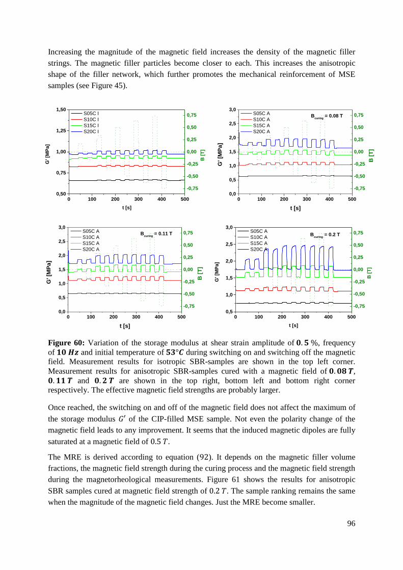
96

Increasing the magnitude of the magnetic field increases the density of the magnetic filler

strings. The magnetic filler particles become closer to each. This increases the anisotropic

shape of the filler network, which further promotes the mechanical reinforcement of MSE

samples (see Figure 45).

0 100 200 300 400 5000,50

0,75

1,00

1,25

1,50

G' [M

Pa

]

t [s]

S05C I

S10C I

S15C I

S20C I

-0,75

-0,50

-0,25

0,00

0,25

0,50

0,75

B [

T]

0 100 200 300 400 5000,0

0,5

1,0

1,5

2,0

2,5

3,0

G' [M

Pa

]

t [s]

S05C A

S10C A

S15C A

S20C A

Bcuring

= 0.08 T

-0,75

-0,50

-0,25

0,00

0,25

0,50

0,75

B [

T]

0 100 200 300 400 5000,0

0,5

1,0

1,5

2,0

2,5

3,0

G' [M

Pa

]

t [s]

S05C A

S10C A

S15C A

S20C A

Bcuring

= 0.11 T

-0,75

-0,50

-0,25

0,00

0,25

0,50

0,75

B [

T]

0 100 200 300 400 5000,5

1,0

1,5

2,0

2,5

3,0

G' [M

Pa

]

t [s]

S05C A

S10C A

S15C A

S20C A

Bcuring

= 0.2 T

-0,75

-0,50

-0,25

0,00

0,25

0,50

0,75

B [

T]

Figure 60: Variation of the storage modulus at shear strain amplitude of 𝟎. 𝟓 %, frequency

of 𝟏𝟎 𝑯𝒛 and initial temperature of 𝟓𝟑°𝑪 during switching on and switching off the magnetic

field. Measurement results for isotropic SBR-samples are shown in the top left corner.

Measurement results for anisotropic SBR-samples cured with a magnetic field of 𝟎. 𝟎𝟖 𝑻,

𝟎. 𝟏𝟏 𝑻 and 𝟎. 𝟐 𝑻 are shown in the top right, bottom left and bottom right corner

respectively. The effective magnetic field strengths are probably larger.

Once reached, the switching on and off of the magnetic field does not affect the maximum of

the storage modulus 𝐺′ of the CIP-filled MSE sample. Not even the polarity change of the

magnetic field leads to any improvement. It seems that the induced magnetic dipoles are fully

saturated at a magnetic field of 0.5 𝑇.

The MRE is derived according to equation (92). It depends on the magnetic filler volume

fractions, the magnetic field strength during the curing process and the magnetic field strength

during the magnetorheological measurements. Figure 61 shows the results for anisotropic

SBR samples cured at magnetic field strength of 0.2 𝑇. The sample ranking remains the same

when the magnitude of the magnetic field changes. Just the MRE become smaller.

97

-0,75 -0,50 -0,25 0,00 0,25 0,50 0,750,0

0,1

0,2

0,3

0,4

0,5

MR

E [

-]

B [T]

S05C A

S10C A

S15C A

S20C A

Figure 61: MRE dependency on the magnetic filler content for anisotropic SBR samples

cured at a magnetic field strength of 𝟎. 𝟐 𝑻.

Figure 62 shows the dependency of the MRE of the anisotropic MSE sample S20C A filled

with 20 vol.% CIP on the magnetic field during the curing process.

-0,75 -0,50 -0,25 0,00 0,25 0,50 0,750,0

0,1

0,2

0,3

0,4

0,5

MR

E [

-]

B [T]

0.20 T

0.11 T

0.08 T

0.00 T

Figure 62: MRE dependency on the magnetic field strength during the curing process for

MSE samples filled with 𝟐𝟎 vol.% CIP.

98

During the magnetorheological measurements, higher magnetic field magnitudes than 0.5 𝑇

impair the MRE because high magnetic fields are generally generated by high electrical

currents. This unnecessarily increases the temperature of the magnetic cell. This inevitably

increase in temperature decreases the viscosity of the samples and thus also the storage

modulus. Considering the relatives quantities, the MRE is then reduced.

The MRE depends on the magnetic filler content (see Figure 61) and the magnitude of the

magnetic field during the curing process (see Figure 62). It tends asymptotic to a threshold

value, which can be approximated with one of the following equations:

𝑀𝑅𝐸 (𝜙, 𝐵) = 𝑎(1 − 𝑒𝜙

𝐵

𝐵0) (93)

or

𝑀𝑅𝐸 (Β𝑐, 𝐵) = 𝑎(1 − 𝑒Β𝑐

𝐵

𝐵0) (94)

where 𝑎 is a scalar parameter, 𝐵0 is the magnitude of a constant magnetic field of 1 𝑇 and 𝐵 is

the magnitude of the magnetic field, by which the samples are tested. The magnetic filler

content 𝜙 in equation (92) and the magnitude of the magnetic field during the curing process

Β𝑐 in equation (93) represent the preparation criteria of the MSE composites.

9.2 Internal microstructure of MSE

The internal microstructure of MSE composites can be determined by performing microscopic

examinations or magnetorheological tests. The scanning electron microscope (SEM) is based

on the scanning of the sample surface by means of a very tightly focused electron beam.

When the electron beam hits the sample, elastic and inelastic collision processes take place.

The resulting deflections of the secondary electrons are recorded to reflect the quality of the

sample surface. Magnetorheological measurements point out the preferred direction of

magnetisation of the MSE composites. Depending on the direction of the applied magnetic

field, different magnetisation behaviour of the MSE composites can be observed. This spatial

dependency specifies the magnetic anisotropy of the MSE.

9.2.1 Magnetic anisotropy of MSE using scanning electron microscope

MSE composites were prepared on the basis of NBR and the magnetic filler CIP. The

magnetic filler content is 20 vol.%. The vulcanisation was carried out with and without an

external magnetic field. SEM images of a cross section of the samples N20C with 20 vol.%

CIP are depicted in Figure 63 [171].

The left image in Figure 63 shows that the magnetic filler particles are uniformly dispersed

within the rubber matrix. This is achieved when no magnetic field is applied during the

vulcanisation. If an external magnetic field is applied during the curing process, the magnetic

filler particles are lined up along the magnetic field lines in columnar structure. This

illustrates the right image in Figure 63. The orientation of the magnetic moments is caused by

a less restricted mobility of the magnetic filler particles within the rubber matrix during the

99

vulcanisation due to high temperatures. Besides the decrease of the sample viscosity during

curing, the mobility of the magnetic filler particles is further improved when plasticizers are

used. The MSE sample acquires anisotropic mechanical and magnetic properties.

Figure 63: SEM images of a cross section of the N20C samples cured without (left) and with

(right) magnetic field.

9.2.2 Magnetic anisotropy of MSE using magnetorheological testing

The magnetic anisotropy of MSE composites can be observed by magnetorheological

measurements. The measurement configuration consists of measuring the anisotropic MSE

sample at two different sides. With other terms, the orientation direction of the magnetic filler

particles can be chosen to be parallel or perpendicular to the external magnetic field, as

depicted in Figure 64. Note here that the direction of the applied force and the magnetic field

direction in this measurement configuration are the same. The anisotropic N20C was a 6 𝑚𝑚

long, 6 𝑚𝑚 wide and 6 𝑚𝑚 high cube. The electrical current governing the magnetic cell was

increased linearly from 0 𝑉 to 5 𝑉. This corresponds to a magnetic field strength from 0 𝑇 to

maximal 0.75 𝑇.

Figure 64: The orientation of the magnetic filler strings within the anisotropic sample N20C

during magnetorheological measurements. The magnetic field runs along the vertical z-axis.

100

The variation of the storage modulus 𝐺’ at a shear strain amplitude of 0.1 %, a frequency of

10 𝐻𝑧 and initial temperature of 50 °𝐶 during switching on and switching off the magnetic

field is shown in Figure 65.

0 50 100 150 200

20

40

60

80 B parallel to CIP strings

B perpendicular to CIP strings

G' [k

Pa]

t [s]

0

1

2

3

4

5

I [A

]

Figure 65: The variation of the storage modulus 𝑮’ of the anisotropic sample N20C at shear

strain amplitude of 𝟎. 𝟏 %, frequency of 𝟏𝟎 𝑯𝒛 and initial temperature of 𝟓𝟎 °𝑪. The

direction of the magnetic field is parallel or perpendicular to CIP strings.

The magnetic field was first turned off for 30 seconds. The anisotropic sample N20C shows

high storage modulus when the CIP strings within the sample are parallel and not

perpendicular to the applied force. This direction dependency indicates that the sample

stiffness is an anisotropic property. This behaviour is attributed to the columnar structure of

the magnetic filler particles within the rubber matrix.

Turning on the electric current and accordingly the magnetic field in the next 180 seconds

leads to great changes in the storage modulus 𝐺’. While 𝐺’ slightly increases for the sample

where the CIP strings are perpendicular to the direction of the magnetic field, 𝐺’ shows a

strong increase when the CIP strings are parallel to the direction of the magnetic field. A

higher magnetic sensitivity is observed when the CIP strings are parallel to the magnetic field

direction. When the magnetic field is switched off, 𝐺’ relaxes to its initial value.

9.3 Influence of particle size

As discussed earlier in sections (7.2.1) and (7.3.2), SBR samples were prepared with two

different magnetic fillers at constant volume fraction of 20 vol.%. The magnetic filler used

were the microscaled CIP and the nanoscaled MAGSILICA. Figure 66 illustrates the variation

of the storage modulus at a shear strain amplitude of 0.5 %, a frequency of 10 𝐻𝑧 and an

101

initial temperature of 50°𝐶 for the isotropic and anisotropic SBR samples. The magnetic field

is increased stepwise and the measurement period is reduced to 500 seconds in order to

minimise the thermal heating of the magnetic measurement cell.

0 100 200 300 400 5000,5

1,0

1,5

2,0

2,5

-0,75

-0,50

-0,25

0,00

0,25

0,50

0,75 S20M I S20M A S20C I S20C A

G' [M

Pa

]

t [s]

B [

T]

Figure 66: Variation of the storage modulus at shear strain amplitude of 𝟎. 𝟓 %, frequency of

𝟏𝟎 𝑯𝒛 and initial temperature of 𝟓𝟎°𝑪 during switching on and switching off the magnetic

field for isotropic and anisotropic SBR samples with two different magnetic fillers at constant

volume fraction of 𝟐𝟎 vol.%.

The isotropic samples S20C I with 20 vol.% CIP and S20M I with 20 vol.% MAGSILICA

show hardly any switching effect. Similar to the melts (see Figure 56), the sample S20M I

shows almost no switching effect but a slight decrease of the moduli values due to thermal

heating. The switching effect for the sample S20C I does not exceed 4 %. The MSE samples

are not sensitive enough to external magnetic field because the magnetic filler particles are

more or less homogeneously distributed within the rubber matrix.

The storage modulus 𝐺’ of the isotropic sample S20M I is about 1.22 MPa. For the isotropic

sample S20C I, it is around 0.68 MPa. This performance has to do with the large reinforcing

potential of the nanoscaled magnetic filler particles.

The anisotropic inner structure achieved during the vulcanisation with an external magnetic

field makes both samples stiffer because the columnar arrangement of the magnetic filler

particles significantly contribute to mechanical reinforcement of the samples. A tiny

switching effect is observed for the sample S20M A with 20 vol.% MAGSILICA. The

storage modulus 𝐺’ is hardly affected once the magnetic field is switched on. The change in

modulus is more pronounced for the sample S20C A with 20 vol.% CIP. A switching effect

of about 30 % is observed.

102

It is important to note that the magnetic field strength of about 0.75 𝑇 is not necessary for

reaching the maximum modulus values Gmax′ . This is already observed at about 0.5 𝑇 where

the induced magnetic dipoles become saturated. Furthermore, the switching effect of

vulcanisates is smaller than the switching effect of melts, because the mobility of the

magnetic filler particles in the rubber matrix is restricted by the crosslinking achieved during

the curing process [106, 107].

9.4 Variation of filler loading

Magnetorheological measurements were carried out with CIP-filled NBR samples with

different filler volume fractions. The curing was realized with and without magnetic field to

obtain isotropic and anisotropic MSE composites respectively. The variation of the storage

modulus at a shear strain amplitude of 0.1 %, a frequency of 10 𝐻𝑧 and an initial temperature

of 50°𝐶 for isotropic and anisotropic MSE are depicted in Figure 67.

0 500 1000 1500 2000 25000

2

4

6

8

10 N06C I

N13C I

N20C I

N28C I

N36C I

G' [M

Pa

]

t [s]

-0,50

-0,25

0,00

0,25

0,50

B [

T]

0 500 1000 1500 2000 25000

2

4

6

8

10 N06C A

N13C A

N20C A

N28C A

N36C A

G' [M

Pa

]

t [s]

-0,50

-0,25

0,00

0,25

0,50

B [

T]

Figure 67: Effect of orientation on the variation of the storage modulus at shear strain

amplitude of 𝟎. 𝟏 %, frequency of 𝟏𝟎 𝑯𝒛 and initial temperature of 𝟓𝟎°𝑪 during switching on

and switching off the magnetic field for the crosslinked vulcanisates. On the left the isotropic

samples are presented and on the right anisotropic samples are shown.

For isotropic MSE composites, the storage modulus 𝑮’ increases with increasing the magnetic

filler content. Only a slightly small switching effect is observed for all samples because the

magnetic filler particles are more or less homogeneously distributed within the rubber matrix.

They are not able to form columnar strings through the interaction with the applied magnetic

field because they are immobilized by the crosslinking. The maximum switching effect does

not exceed 𝟏𝟑 % and it is recorded for the sample N20C I with 𝟐𝟎 vol.% CIP.

All anisotropic MSE composites become stiffer due to an additional contribution of the

magnetic filler network. The arrangement of the magnetic filler particles along the magnetic

field lines is achieved during the curing process [𝟏𝟕𝟏]. This inner structure ensures all

samples larger stiffness and improves their magnetic sensitivity. A maximum switching effect

of 𝟑𝟔 % is recorded for the sample N13C A with 𝟏𝟑 vol.% CIP.

103

Obviously increasing the magnetic filler volume fraction is not followed by an increase of the

switching effect of both the isotropic and the anisotropic MSE composites. A maximum is

reached with a magnetic filler content of 20 vol.% for the isotropic sample and a magnetic

filler content of 13 vol.% for anisotropic samples. Above this CIP limit, only an increase in

stiffness is observed. It appears that despite the strong magnetic interaction between the

magnetic filler particles and the magnetic field, the magnetic ordering of the MSE composites

is increasingly disturbed.

Similar to dynamic-mechanical investigations in section 7.3.3, the magnetic filler content

seems to play a major role in setting the magnetorheological properties of the finished MSE

composites. The volume fraction of the magnetic filler should be optimised and exactly

adjusted in order to avoid considerable restriction on the maximum switching effect.

The switching effect for both isotropic and anisotropic MSE is summarized in Table 12.

Table 12: Maximum MRE for isotropic and anisotropic crosslinked MSE samples derived

from measurements at shear strain amplitude of 0.1 %, a frequency of 10 𝐻𝑧 and initial

temperature of 50°𝐶.

N06C N13C N20C N28C N36C

Anisotropic 0.23 0.36 0.26 0.12 0.03

Isotropic 0.004 0.03 0.13 0.09 0.05

9.5 Influence of coupling agent

Two different SBR samples were prepared at a constant CIP content of 20 vol.% with and

without silane on the same way as discussed in section (7.2.1) in order to examine the

influence of silane on the switching effect. Figure 68 illustrates the influence of silane on the

variation of the storage modulus at a shear strain amplitude of 0.5 %, a frequency of 10 𝐻𝑧

and an initial temperature of 50 °𝐶 during the switching on and the switching off of the

magnetic field for isotropic and anisotropic samples. The magnetic field is increased stepwise

and the measurement period is reduced to 500 seconds in order to minimise the thermal

heating of the magnetic measurement cell.

104

0 100 200 300 400 5000,5

1,0

1,5

2,0

2,5

-0,75

-0,50

-0,25

0,00

0,25

0,50

0,75

S20C I

S20C\Si I

S20C A

S20C\Si A

G' [M

Pa

]

t [s]

B [

T]

Figure 68: Effect of silane on the variation of the storage modulus at shear strain of 𝟎. 𝟓 %, ,

frequency of 𝟏𝟎 𝑯𝒛 and initial temperature of 𝟓𝟎 °𝑪 during switching on and switching off

the magnetic field for the SBR samples.

Independently of the particle orientations, smaller switching effect and storage moduli are

observed for the silanized SBR samples. This confirms that silane hinders the mobility and

prevents a close contact of the magnetic filler particles. Therefore, it reduces the magnetic

sensitivity of the silanized samples and, thus, the switching effect. Due to vulcanisation, the

rubber matrix becomes crosslinked and the magnetic filler particles are immobilized within

the composites. The additional silanisation leads to strong chemical bonding between the

polymer chains and the magnetic filler particles, making them less mobile. For the isotropic

samples, where the particles are more or less homogeneously distributed, the switching effect

has a maximal value of about 4 %. Obviously, the applied external magnetic field is not

strong enough to displace the magnetic filler particles sufficiently and make the composites

magnetically more sensitive. The magnetic sensitivity of the samples can be enhanced by

curing in the presence of an external magnetic field to obtain anisotropic MSE. The magnetic

filler particles arrange themselves thereby in oriented particle chains. The most pronounced

change of the modulus during switching on and switching off the magnetic field is observed

for the anisotropic sample S20C\Si A without silane and it is about 30 % [106, 107].

The same ranking is observed also here as the strain sweep data at 0.5 % strain amplitude

obtained with the DMA in Figure 50, despite different experimental setup.

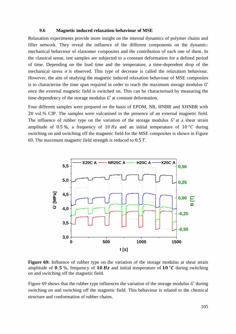
105

9.6 Magnetic induced relaxation behaviour of MSE

Relaxation experiments provide more insight on the internal dynamics of polymer chains and

filler network. They reveal the influence of the different components on the dynamic-

mechanical behaviour of elastomer composites and the contribution of each one of them. In

the classical sense, test samples are subjected to a constant deformation for a defined period

of time. Depending on the load time and the temperature, a time-dependent drop of the

mechanical stress 𝜎 is observed. This type of decrease is called the relaxation behaviour.

However, the aim of studying the magnetic induced relaxation behaviour of MSE composites

is to characterise the time span required in order to reach the maximum storage modulus 𝐺’

once the external magnetic field is switched on. This can be characterised by measuring the

time-dependency of the storage modulus 𝐺’ at constant deformation.

Four different samples were prepared on the basis of EPDM, NR, HNBR and XHNBR with

20 vol.% CIP. The samples were vulcanised in the presence of an external magnetic field.

The influence of rubber type on the variation of the storage modulus 𝐺‘ at a shear strain

amplitude of 0.5 %, a frequency of 10 𝐻𝑧 and an initial temperature of 10 °𝐶 during

switching on and switching off the magnetic field for the MSE composites is shown in Figure

69. The maximum magnetic field strength is reduced to 0.5 𝑇.

0 500 1000 15003,0

3,5

4,0

4,5

5,0

5,5

G' [M

Pa

]

t [s]

E20C A NR20C A H20C A X20C A

-0,50

-0,25

0,00

0,25

0,50

B [

T]

Figure 69: Influence of rubber type on the variation of the storage modulus at shear strain

amplitude of 𝟎. 𝟓 %, frequency of 𝟏𝟎 𝑯𝒛 and initial temperature of 𝟏𝟎 °𝑪 during switching

on and switching off the magnetic field.

Figure 69 shows that the rubber type influences the variation of the storage modulus 𝐺’ during

switching on and switching off the magnetic field. This behaviour is related to the chemical

structure and conformation of rubber chains.

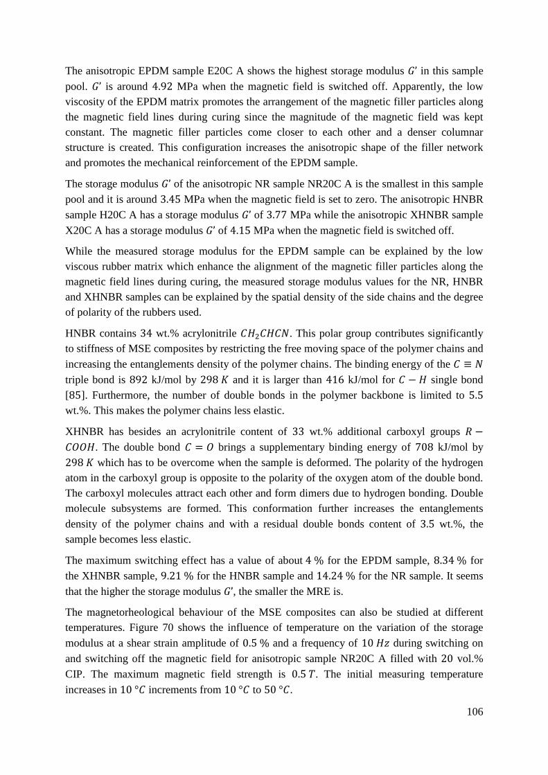
106

The anisotropic EPDM sample E20C A shows the highest storage modulus 𝐺’ in this sample

pool. 𝐺’ is around 4.92 MPa when the magnetic field is switched off. Apparently, the low

viscosity of the EPDM matrix promotes the arrangement of the magnetic filler particles along

the magnetic field lines during curing since the magnitude of the magnetic field was kept

constant. The magnetic filler particles come closer to each other and a denser columnar

structure is created. This configuration increases the anisotropic shape of the filler network

and promotes the mechanical reinforcement of the EPDM sample.

The storage modulus 𝐺’ of the anisotropic NR sample NR20C A is the smallest in this sample

pool and it is around 3.45 MPa when the magnetic field is set to zero. The anisotropic HNBR

sample H20C A has a storage modulus 𝐺’ of 3.77 MPa while the anisotropic XHNBR sample

X20C A has a storage modulus 𝐺’ of 4.15 MPa when the magnetic field is switched off.

While the measured storage modulus for the EPDM sample can be explained by the low

viscous rubber matrix which enhance the alignment of the magnetic filler particles along the

magnetic field lines during curing, the measured storage modulus values for the NR, HNBR

and XHNBR samples can be explained by the spatial density of the side chains and the degree

of polarity of the rubbers used.

HNBR contains 34 wt.% acrylonitrile 𝐶𝐻2𝐶𝐻𝐶𝑁. This polar group contributes significantly

to stiffness of MSE composites by restricting the free moving space of the polymer chains and

increasing the entanglements density of the polymer chains. The binding energy of the 𝐶 ≡ 𝑁

triple bond is 892 kJ/mol by 298 𝐾 and it is larger than 416 kJ/mol for 𝐶 − 𝐻 single bond

[85]. Furthermore, the number of double bonds in the polymer backbone is limited to 5.5

wt.%. This makes the polymer chains less elastic.

XHNBR has besides an acrylonitrile content of 33 wt.% additional carboxyl groups 𝑅 −

𝐶𝑂𝑂𝐻. The double bond 𝐶 = 𝑂 brings a supplementary binding energy of 708 kJ/mol by

298 𝐾 which has to be overcome when the sample is deformed. The polarity of the hydrogen

atom in the carboxyl group is opposite to the polarity of the oxygen atom of the double bond.

The carboxyl molecules attract each other and form dimers due to hydrogen bonding. Double

molecule subsystems are formed. This conformation further increases the entanglements

density of the polymer chains and with a residual double bonds content of 3.5 wt.%, the

sample becomes less elastic.

The maximum switching effect has a value of about 4 % for the EPDM sample, 8.34 % for

the XHNBR sample, 9.21 % for the HNBR sample and 14.24 % for the NR sample. It seems

that the higher the storage modulus 𝐺’, the smaller the MRE is.

The magnetorheological behaviour of the MSE composites can also be studied at different

temperatures. Figure 70 shows the influence of temperature on the variation of the storage

modulus at a shear strain amplitude of 0.5 % and a frequency of 10 𝐻𝑧 during switching on

and switching off the magnetic field for anisotropic sample NR20C A filled with 20 vol.%

CIP. The maximum magnetic field strength is 0.5 𝑇. The initial measuring temperature

increases in 10 °𝐶 increments from 10 °𝐶 to 50 °𝐶.

107

0 500 1000 15002,0

2,5

3,0

3,5

4,0

4,5G

' [M

Pa

]

t [s]

10 °C 20 °C 30 °C 40 °C 50 °C

-0,50

-0,25

0,00

0,25

0,50

B [

T]

Figure 70: The influence of temperature on the variation of the storage modulus of

anisotropic NR sample filled with 𝟐𝟎 vol.% CIP at shear strain amplitude of 𝟎. 𝟓 % and

frequency of 𝟏𝟎 𝑯𝒛 during switching on and switching off the magnetic field. The initial

temperature increases in 𝟏𝟎 °𝑪 increments from 𝟏𝟎 °𝑪 to 𝟓𝟎 °𝑪.

Figure 70 depicts a significant influence of the measuring temperature on the variation of the

storage moduli 𝐺’ of the anisotropic sample NR20C A. Considering first the initial values of

storage modulus, they increase with decreasing temperature. At 10 °𝐶, the NR20C A sample

has an initial storage modulus 𝐺’ of 3.45 MPa compared with 2.13 MPa at 50 °𝐶. This

behaviour is mainly related to the change in the sample viscosity. Rising the measurement

temperature considerably promotes the mobility of the polymer chains and thus reduces the

viscosity of the polymer matrix. This enhances the orientation of the magnetic dipoles of the

magnetic filler particles along the magnetic field lines and leads to a better switching ability.

When the magnetic field is switched off, then a spontaneous relaxation of the storage modulus

𝐺’ follows. However, 𝐺’ do not relax to its initial value because the magnetic filler particles do

not completely lose their magnetisation. A rest magnetisation of the magnetic filler still

remains. This contribute to a further stiffening of the sample still remains.

The magnetic relaxation time describes the occurrence of the magnetisation process of the

MSE composites. It corresponds to the time took to align the magnetic dipole moments along

the magnetic field lines and to reach in an ideal case the saturation magnetisation. The

magnetic induced relaxation behaviour of MSE composites can be derived from the time

evolution of the storage modulus 𝐺’ as shown in Figure 69. The curve range with the highest

switching effect is considered for further calculation and it is depicted in Figure 71.

108

E20C A

Fit

G' [M

Pa]

t [s]

Figure 71: Curve range with the highest switching effect recorded for anisotropic EPDM

sample filled with 𝟐𝟎 vol.% CIP at shear strain amplitude of 𝟎. 𝟓 %, frequency of 𝟏𝟎 𝑯𝒛 and

initial temperature of 𝟏𝟎 °𝑪 during switching on and switching off the magnetic field.

Once turned on, the magnetic field brings the magnetic dipole moments of the magnetic filler

particles to align themselves along the magnetic field lines. The magnetic dipole moments

distribution is no longer the same. As a result, the MSE composites become stiffer and show

high storage moduli. It can be seen in Figure 71 that the magnetisation process takes place at

two different time scales. The storage modulus 𝐺’ increases abruptly in the first few seconds

after switching on the external magnetic field. The quick response of the MSE composite is

followed by a gradual more slowly increase of 𝐺’. The first relaxation behaviour is attributed

to the magnetic filler dynamic due to the high magnetic affinity of the magnetic filler

particles. The second relaxation behaviour is attributed to the dynamic of polymer chains.

The storage modulus 𝐺’ can be expressed by the sum of two exponential functions as follows:

𝐺′(𝑡) = 𝐺′0 + Δ𝐺′

1 exp (−𝑡−𝑡0

𝜏1) + Δ𝐺′2 exp (−

𝑡−𝑡0

𝜏2) (94)

where 𝐺′0 is the initial storage modulus before the magnetic excitation, 𝑡0 is a shift factor on

the time axis, Δ𝐺′𝑖 represents the 𝑖th relaxation strength and 𝜏𝑖 is the magnetic induced

relaxation time.

Using equation (94), the magnetic induced relaxation times 𝜏1 and 𝜏2 can be derived. The

results for anisotropic EPDM samples with 20 vol.% CIP are presented in Figure 72.

109

-0,330 -0,165 0 0,165 0,3300,75

1,00

1,25

1,50

1,75

2,00

2,25

2,50

10 °C

20 °C

30 °C

40 °C

50 °C

1 [

s]

B [T]

-0,330 -0,165 0 0,165 0,330

10

20

30

40

50

60

70

80 10 °C

20 °C

30 °C

40 °C

50 °C

2 [

s]

B [T]

Figure 72: Magnetic induced relaxation times of anisotropic EPDM samples filled with 𝟐𝟎

vol.% CIP at different measurement temperatures as a function of the magnetic field. On the

right is plotted the short relaxation time 𝝉𝟏 related to magnetic filler dynamic. On the left is

plotted the long relaxation time 𝝉𝟐 related to polymer dynamic.

Regarding the magnetic filler dynamic, the relaxation time 𝜏1varies between 1 to 2 seconds.

𝜏1 depends on both the magnetic field and the measuring temperature. Increasing the

magnetic field flux improves the magnetic interaction between magnetic filler particles and

the external magnetic field. This promotes the orientation of the magnetic dipoles along the

magnetic field direction. By switching off the magnetic field, this inner microstructure is no

longer supported. The samples relax. By reversing the polarity of the magnetic field and

keeping its intensity constant, the relaxation time becomes rather smaller. This is explained by

the fact the magnetic filler particles are already magnetised but not to saturation. To be

subjected to a magnetic field during an additional time leads more magnetic dipoles to get

aligned and to have almost the same relaxation behaviour. Compared to initial distribution,

the energetically not equivalent magnetic dipoles within the sample become harmonised once

the magnetic field is turned on and point in the same direction. The totality of the magnetic

dipoles develops a similar relaxation behaviour, which reduces the relaxation time. The

relaxation time at high magnetic field strengths regardless of polarisation is not very large.

This indicates that the magnetic filler particles are slowly becoming saturated.

The increase of measurement temperature has as a consequence the decrease of the sample

viscosity. This promotes the aligning of the magnetic dipoles along the magnetic field lines.

The magnetic induced relaxation behaviour of the MSE composites is mainly due to magnetic

field but is also indirectly boosted by polymer chains dynamic. At any given magnetic field

strength, the relaxation time 𝜏2 is very large compared to 𝜏1. 𝜏2 ranges between 10 and 80

seconds depending on the dynamic of the polymer chains.

The temperature dependency of the magnetic induced relaxation times 𝜏1 and 𝜏2 can be

associated to the thermal activity the filler-filler and polymer-filler bonds. In Figure 73, the

magnetic induced relaxation times 𝜏1 (attributed to magnetic filler dynamic) and 𝜏2 (attributed

110

to dynamic of polymer chains) for an anisotropic EPDM sample with 20 vol.% CIP is plotted

against the inverse of the temperature.

3,1 3,2 3,3 3,4 3,5 3,61,00

1,25

1,50

1,75

2,00

2,25

2,50 0,165 T

-0,165 T

0,332 T

-0,332 T

1 [

s]

1000/T [1/K]

3,1 3,2 3,3 3,4 3,5 3,6

10

20

30

40

50

60

70

80 0,165 T

-0,165 T

0,332 T

-0,332 T

2 [

s]

1000/T [1/K]

Figure 73: Temperature dependency of the magnetic induced relaxation times 𝝉𝟏 and 𝝉𝟐 for

anisotropic EPDM sample filled with 𝟐𝟎 vol.% CIP.

Obviously, the magnetic induced relaxation times 𝜏1 and 𝜏2 show no clear temperature

dependency. This relaxation cannot be led back to the thermal activity of the filler-filler and

polymer-filler bonds. This is explained by the fact that the relaxation behaviour studied here is

magnetically induced and it is not the result of thermomechanical processes even if the

measuring temperature changes. The strength of the applied magnetic field is the key factor to

determine the time period of the magnetic induced relaxation. It appears clearly from Figure

73 that the magnetic induced relaxation time 𝜏1 becomes smaller with increasing the magnetic

field. The polarity change of the magnetic field can be considered as an additional time to get

the magnetic dipole moments of the not yet saturated magnetic filler particles aligned along

the magnetic field lines.

The same also applies for similar reasons to second magnetic induced relaxation time 𝜏2. No

similarity with the Arrhenius diagram for rubber materials is provided. The relaxation

behaviour of the polymer chains is directly dependent on magnetic processes although the

polymer chains are not magnetic. The decrease of the sample viscosity due to increasing the

measuring temperature induces new conformations of the polymer chains. The entanglements

density of the polymer chains decreases and the internal friction is reduced. This new

structural arrangements additionally promote the orientation of the magnetic dipoles of the

magnetic filler particles along the magnetic field lines. This results in a minimal increase of

the storage modulus 𝐺’ with increasing measuring time until the magnetic filler particles are

completely saturated.

The experimental findings shown in Figure 72 confirms that the magnetic induced relaxation

behaviour of the MSE composites is independent from temperature. Both magnetic induced

relaxation times 𝜏1 and 𝜏2 are the shortest at temperature between 20 °𝐶 and 30 °𝐶 and not

at 50 °𝐶.

111

9.7 Modelling of the magneto-mechanical response of the MSE

MSE composites combine high elasticity and a fast switching ability in the presence of an

external magnetic field. Both characteristics make them an attractive alternative to established

standard technical elastomers. MSE composites exhibit an additionally magnetic field-

induced reinforcement caused by the oriented magnetic filler particles within the rubber

matrix. The magneto-mechanical properties of the MSE composites are the result of the

coupling between the mechanical load and the external magnetic field. This section is devoted

to describe the magneto-mechanical behaviour of MSE composites and to model it using the

micromechanical dynamical flocculation model (DFM) for the description of isotherm state

change of MSE at a given deformation. Varying the magnetic properties of the surroundings

changes the mechanical properties of the samples and makes the fit parameters magnetic field

dependent.

The DFM is used for modelling the magneto-mechanical response of the MSE composites.

Compared with the Jolly [180], Ivaneyko [181, 182] or finite elements based models [183-

188], the DFM is based on physical principles of high viscous polymer chains and contains a

physical description of rubber characteristics like the Mullins effect. Therefore, the DFM fit

parameters map a more realistic picture of the inner dynamic of the elastomer composites.

With increasing the number of load cycles, rubber materials experience a stress softening.

This effect is referred to as Mullins effect [189, 190]. This is explained by the irreversible

break of local filler clusters and mechanically unstable crosslinks. Additionally, the stress

softening can be caused by the diffusion of adsorbed polymer chains on the surface of the

magnetic filler particles, the total desorption from the magnetic filler surface or the

entanglements sliding along the chain ends or between crosslinking sites after reaching a load

limit. The Mullins effect is considered in the DFM and it is described with the concept of

hydrodynamic amplification (see equation (63)).

The measurement were carried out with the dynamic-mechanical analyser MTS in simple

shear mode as shown in Figure 31. The influence of a constant magnetic field on mechanical

properties is investigated by multihysteresis experiments at room temperature. The material

behaviour under four load amplitudes was tested. Each step was repeated five times. The

magnetic field was switched off during the first three cycles and then switched on for the last

two cycles as illustrated in Figure 74. The third and fifth cycles of loading and unloading

curves form the respective reference curves and are displayed by lines. Here is assumed that a

quasistatic material state was established. Highly sensitive fluxgate sensor is set in close

proximity to the MSE composites to detect the magnetic field density.

112

B = 1 T

[-

]

Time [s]

B = 0 T

Figure 74: Multihysteresis measurement of MSE composites. In each deformation step, the

deformation cycle was repeated five times. The first 𝟑 cycles were performed without

magnetic field, while the last 𝟐 cycles with magnetic field. The third and fifth cycles of

loading and unloading curves represent the reference curves and are displayed by full lines.

During the measurement tests, several preload cycles are made in order to establish a quasi-

static material state. It is an important step to attain an equilibrium mechanical state for the

different samples. This pre-conditioning permits to compare the different MSE composites at

constant deformation history.

The raw data and the reference cycles from multihysteresis measurements for the anisotropic

EPDM samples with 20 vol.% CIP are presented in Figure 75 and Figure 76 respectively.

113

-0.4 -0.2 0.0 0.2 0.4

-1.0

-0.5

0.0

0.5

1.0

[M

Pa]

[-]

Figure 75: Raw data of multihysteresis measurements for anisotropic EPDM samples with

𝟐𝟎 vol.% CIP plots.

-0.4 -0.2 0.0 0.2 0.4

-1.0

-0.5

0.0

0.5

1.0

[

MP

a]

[-]

B = 0 T

B = 1 T

Figure 76: Reference cycles from multihysteresis measurements for anisotropic EPDM

samples with 𝟐𝟎 vol.% CIP plots.

Both isotropic and anisotropic samples show under cyclic load a hysteresis loop as seen in

Figure 76. The hysteresis loop is steeper and larger for the anisotropic MSE composite. This

114

indicates changing elastic material properties where elastic energy is dissipated. The stress

softening is mainly attributed to the destroy of magnetic filler clusters because the rupture of

the physical bonds between polymer chains and crosslinking points occurs very slowly and

only at high critical loads. However, The filler clusters can reaggregate during the rest phases

when the sample is unloaded.

More profound insight about the dynamic-mechanical behaviour of the MSE composites in

the presence of an external magnetic field can be achieved by fitting the experimental results

using the DFM. Two different MSE composites were prepared on the basis of two different

rubbers. EPDM was chosen for its soft matrix and HNBR for its ageing behaviour as well as

its weathering resistance. The magnetic filler is CIP with a content of 20 vol.% and all other

additives remain the same.

For the multihysteresis measurements shown below, first the third cycle describing the

mechanical behaviour of the MSE composites without magnet field is fitted with the DFM.

All fitting parameters were random numbers except the effective filler volume fraction. It was

set to the magnetic filler content 0.2. This is justified by the spherical shape of the magnetic

filler particles. In contrast to standard fillers in rubber technology like carbon black, there is

no need to consider any topological effects for CIP particles. When the fitting procedure of

the third cycle is finished, the fifth cycle describing the mechanical behaviour of the MSE

composites with magnet field is fitted taking into account the following. Since the magnetic

affinity of the magnetic filler particles is by far much larger than all components of the MSE

composite, only the magnetic filler particles are severely affected by the external magnetic

field. Therefore, the fit parameters related to mechanical behaviour of rubber are not

influenced by the applied magnetic field and remain unchanged. A significant result of this

assumption is that the stiffening observed in the experiments is assigned to the magnetic filler.

Further, the cured samples have a very large viscosity restricting the free mobility of the

magnetic filler particles even in the presence of an external magnetic field. The latter affects

only the orientation of the magnetic moments and do not induce any movement of the

magnetic filler particles within the rubber matrix. For this reason, the mean filler cluster size

𝑥0 remains also constant. To fit the fifth cycle describing the mechanical behaviour of the

MSE composite in the presence of a magnetic field, all fitting parameters are hold except the

tensile strength of virgin bonds 𝑠𝑣 and the tensile strength of damaged bonds 𝑠𝑑 because only

these parameters govern the shape of the hysteresis loop.

The reference cycles of multihysteresis measurements for both isotropic and anisotropic

EPDM samples are presented in Figure 77 and Figure 78 respectively. In addition, the DFM

fittings are displayed in red.

115

-0,4 -0,3 -0,2 -0,1 0,0 0,1 0,2 0,3 0,4

-0,6

-0,4

-0,2

0,0

0,2

0,4

0,6

Gc = 0.79

Ge = 0.30

n = 23.63

sd = 11.73

sv = 27.83

x0 = 8.30

eff

= 0.20

Set

= 0.00

Measurement

Fit

B = 0 T

[

MP

a]

[-]

-0,4 -0,3 -0,2 -0,1 0,0 0,1 0,2 0,3 0,4

-0,6

-0,4

-0,2

0,0

0,2

0,4

0,6

Gc = 0.79

Ge = 0.30

n = 23.63

sd = 12.93

sv = 28.92

x0 = 8.30

eff

= 0.20

Set

= 0.00

[M

Pa

]

[-]

Measurement

Fit

B = 1 T

Figure 77: Reference cycles of the multihysteresis measurements for isotropic EPDM

samples filled with 𝟐𝟎 vol.% CIP and the associated fit curves with DFM. The measurement

data were performed without (left) and with (right) magnetic field.

The shear stress 𝜏 of the isotropic EPDM sample reaches a peak value of about 0.65 MPa

independently of the magnitude of the applied magnetic field. The crosslink modulus 𝐺𝑐 is

0.79 MPa and the entanglement modulus 𝐺𝑒 is 0.30 MPa. The finite extensibility parameter

𝑛 amounts to 23.63, which indicate that almost 24 chain segments are between two adjacent

entanglements. The mean filler cluster size 𝑥0 is equal to 8.30. It is defined as the quotient of

the filler cluster 𝜉 to the primary particle size 𝑑. The magnetic filler cluster can be estimated

between 25 µ𝑚 to 37.4 µ𝑚 because the diameter of CIP particles ranges between 3 µ𝑚

and 4.5 µ𝑚. Without magnetic field, the tensile strength of virgin bonds 𝑠𝑣 is 27.83 MPa and

the tensile strength of damaged bonds 𝑠𝑑 is 11.73 MPa. That 𝑠𝑑 is smaller than 𝑠𝑣 is self-

evident, because the damage bonds cannot be stiffer than virgin bonds.

As mentioned above, turning on the magnetic field concerns only 𝑠𝑑 and 𝑠𝑣. The tensile

strength of virgin bonds 𝑠𝑣 goes from 27.83 MPa to 28.92 MPa and the tensile strength of

damaged bonds 𝑠𝑑 goes from 11.73 MPa to 12.93 MPa. This increase is attributed to

alignment of the magnetic moments of the magnetic filler particles. The orientation of the

magnetic moments increases the magnetic interaction between the magnetic filler particles.

These different contributions are rapidly summed up and cause a higher mechanical stress in

the core of the sample. This increase is accompanied with a small enlargement of the

hysteresis loop.

Figure 78 shows the reference cycles of the multihysteresis measurements for anisotropic

EPDM samples with 20 vol.% CIP and the associated fitting curves with the DFM. Due to the

anisotropic microstructure of the sample realised during the curing process in the presence of

an external magnetic field, absolute higher values for all fit parameters are achieved except

the finite extensibility parameter 𝑛. 𝑛 drops from 23.63 to 3.01 and points out that the

number of chain segments is reduced to an eighth. Only 3 chain segments are between two

adjacent entanglements for anisotropic EPDM samples. This can be explained by the new

distribution of the magnetic filler particles within the rubber matrix. Indeed, the magnetic

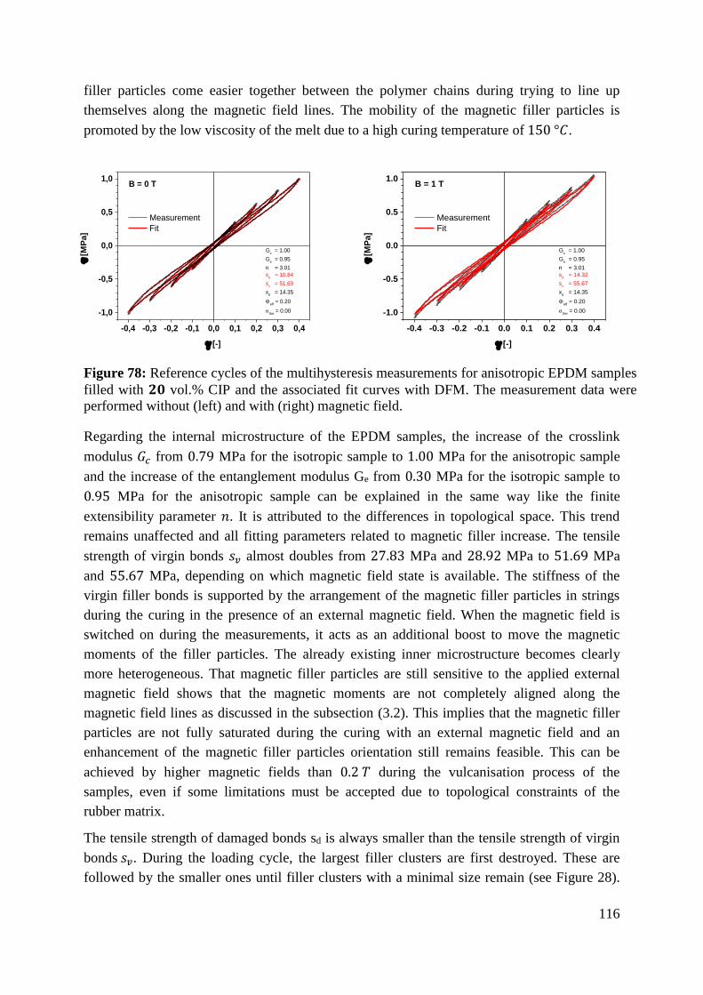
116

filler particles come easier together between the polymer chains during trying to line up

themselves along the magnetic field lines. The mobility of the magnetic filler particles is

promoted by the low viscosity of the melt due to a high curing temperature of 150 °𝐶.

-0,4 -0,3 -0,2 -0,1 0,0 0,1 0,2 0,3 0,4

-1,0

-0,5

0,0

0,5

1,0

Measurement

Fit

B = 0 T

Gc = 1.00

Ge = 0.95

n = 3.01

sd = 10.84

sv = 51.69

x0 = 14.35

eff

= 0.20

Set

= 0.00

[

MP

a]

[-]

-0.4 -0.3 -0.2 -0.1 0.0 0.1 0.2 0.3 0.4

-1.0

-0.5

0.0

0.5

1.0

Measurement

Fit

B = 1 T

Gc = 1.00

Ge = 0.95

n = 3.01

sd = 14.32

sv = 55.67

x0 = 14.35

eff

= 0.20

Set

= 0.00

[M

Pa

]

[-]

Figure 78: Reference cycles of the multihysteresis measurements for anisotropic EPDM samples

filled with 𝟐𝟎 vol.% CIP and the associated fit curves with DFM. The measurement data were

performed without (left) and with (right) magnetic field.

Regarding the internal microstructure of the EPDM samples, the increase of the crosslink

modulus 𝐺𝑐 from 0.79 MPa for the isotropic sample to 1.00 MPa for the anisotropic sample

and the increase of the entanglement modulus Ge from 0.30 MPa for the isotropic sample to

0.95 MPa for the anisotropic sample can be explained in the same way like the finite

extensibility parameter 𝑛. It is attributed to the differences in topological space. This trend

remains unaffected and all fitting parameters related to magnetic filler increase. The tensile

strength of virgin bonds 𝑠𝑣 almost doubles from 27.83 MPa and 28.92 MPa to 51.69 MPa

and 55.67 MPa, depending on which magnetic field state is available. The stiffness of the

virgin filler bonds is supported by the arrangement of the magnetic filler particles in strings

during the curing in the presence of an external magnetic field. When the magnetic field is

switched on during the measurements, it acts as an additional boost to move the magnetic

moments of the filler particles. The already existing inner microstructure becomes clearly

more heterogeneous. That magnetic filler particles are still sensitive to the applied external

magnetic field shows that the magnetic moments are not completely aligned along the

magnetic field lines as discussed in the subsection (3.2). This implies that the magnetic filler

particles are not fully saturated during the curing with an external magnetic field and an

enhancement of the magnetic filler particles orientation still remains feasible. This can be

achieved by higher magnetic fields than 0.2 𝑇 during the vulcanisation process of the

samples, even if some limitations must be accepted due to topological constraints of the

rubber matrix.

The tensile strength of damaged bonds sd is always smaller than the tensile strength of virgin

bonds 𝑠𝑣. During the loading cycle, the largest filler clusters are first destroyed. These are

followed by the smaller ones until filler clusters with a minimal size remain (see Figure 28).

117

When the strain amplitude is reduced after reaching its maximum, an almost complete

reaggregation of the magnetic filler clusters may take place. But these filler-filler bonds,

which were once destroyed, are significantly weaker than the filler-filler bonds in the virgin

sample. Comparison of the tensile strengths of damaged bonds 𝑠𝑑 for all EPDM samples

shows that they are a bit higher for anisotropic samples. However, they remain on the same

scale.

The mean filler cluster size 𝑥0 increases from 8.30 to 14.35. This validates the scanning

electron microscope images shown in Figure 63. The magnetic filler clusters are larger for the

anisotropic sample compared with the isotropic sample.

The maximum shear stress rises from 0.65 MPa for isotropic EPDM sample to 1 MPa for

anisotropic sample. This is explained by the fact that the hysteresis of filled elastomer

composites is mainly induced by the filler. This mechanism is based on the internal friction

within the rubber matrix and the local high stress values around the magnetic filler clusters.

The magnetic filler clusters stores mostly the mechanical energy when they are stretched in

the tension field of the elastomer matrix. But when the clusters get destroyed, the stored

mechanical energy is dissipated as heat.

The fit parameters of the DFM for the mechanical behaviour of the EPDM samples E20C A

with and without magnetic field are summarized in Table 13. The effective filler volume

fraction Φeff is set to 0.2.

Table 13: Fit parameters of the DFM for the EPDM samples with 𝟐𝟎 vol.% CIP.

Orientation B

[T]

Gc

[MPa]

Ge

[MPa]

n

[-]

sd

[MPa]

sv

[MPa]

x0

[-]

Isotropic 𝟎 0.79 0.30 23.63 𝟏𝟏. 𝟕𝟑 𝟐𝟕. 𝟖𝟑 8.30

𝟏 0.79 0.30 23.63 𝟏𝟐. 𝟗𝟑 𝟐𝟖. 𝟗𝟐 8.30

Anisotropic 𝟎 1.00 0.95 3.01 𝟏𝟎. 𝟖𝟒 𝟓𝟏. 𝟔𝟗 14.35

𝟏 1.00 0.95 3.01 𝟏𝟒. 𝟑𝟐 𝟓𝟓. 𝟔𝟕 14.35

The multihysteresis measurements and the associated fit curves using the DFM of HNBR

samples under the same measuring conditions as for EPDM samples are shown in Figure 79

and Figure 80. Regarding the curves shape, it is to note that the hysteresis as well as the

upturn is much more pronounced for the HNBR samples compared with the EPDM samples.

This behaviour is more evident for anisotropic samples. This indicates that the interaction of

the polymer chains with the surface area of the magnetic filler particles is much better.

However, the maximum value of the shear stress 𝜏 becomes smaller. An absolute maximum

value of 1 MPa is measured for anisotropic EPDM sample. 𝜏 is roughly 0.87 MPa for

anisotropic HNBR. A remarkable finding for the HNBR samples is that the maximum value

of the shear stress 𝜏 is almost the same for the isotropic and the anisotropic samples. For

EPDM samples, 𝜏 was 0.65 MPa for the isotropic sample and 1 MPa for the anisotropic

sample.

118

-0,4 -0,3 -0,2 -0,1 0,0 0,1 0,2 0,3 0,4-1,0

-0,5

0,0

0,5

1,0

Gc = 0.36

Ge = 1.26

n = 32.41

sd = 16.48

sv = 19.41

x0 = 7.61

eff

= 0.20

Set

= 0.00

B = 0 T

[M

Pa

]

[-]

-0,4 -0,3 -0,2 -0,1 0,0 0,1 0,2 0,3 0,4-1,0

-0,5

0,0

0,5

1,0

Gc = 0.36

Ge = 1.26

n = 32.41

sd = 23.01

sv = 26.25

x0 = 7.61

eff

= 0.20

Set

= 0.00

B = 1 T

[M

Pa

]

[-]

Figure 79: Reference cycles of the multihysteresis measurements for isotropic HNBR



-0,4 -0,3 -0,2 -0,1 0,0 0,1 0,2 0,3 0,4-1,0

-0,5

0,0

0,5

1,0

Gc = 1.73

Ge = 1.21

n = 1.80

sd = 21.84

sv = 45.85

x0 = 22.08

eff

= 0.20

Set

= 0.00

B = 0 T

[M

Pa

]

[-]

-0,4 -0,3 -0,2 -0,1 0,0 0,1 0,2 0,3 0,4-1,0

-0,5

0,0

0,5

1,0

B = 1 T

Gc = 1.73

Ge = 1.21

n = 1.80

sd = 28.54

sv = 50.21

x0 = 22.08

eff

= 0.20

Set

= 0.00

[M

Pa

]

[-]

Figure 80: Reference cycles of the multihysteresis measurements for anisotropic HNBR



The fit parameters of the DFM for the mechanical behaviour of the HNBR samples H20C A

with and without magnetic field are summarized in Table 14. The effective filler volume

fraction Φeff is set to 0.2.

Table 14: Fit parameters of the DFM for the HNBR samples with 𝟐𝟎 vol.% CIP

Orientation B

[T]

Gc

[MPa]

Ge

[MPa]

n

[-]

sd

[MPa]

sv

[MPa]

x0

[-]

Isotropic 𝟎 0.36 1.26 32.41 𝟏𝟔. 𝟒𝟖 𝟏𝟗. 𝟒𝟏 7.61

𝟏 0.36 1.26 32.41 𝟐𝟑. 𝟎𝟏 𝟐𝟔. 𝟐𝟓 7.61

Anisotropic 𝟎 1.73 1.21 1.80 𝟐𝟏. 𝟖𝟒 𝟒𝟓. 𝟖𝟓 22.08

𝟏 1.73 1.21 1.80 𝟐𝟖. 𝟓𝟒 𝟓𝟎. 𝟐𝟏 22.08

The DFM fitting shows that the reinforcement mechanism of the MSE composites is similar

although the rubber types are different. The fit parameters related to mechanical behaviour of

119

rubber were only affected by the molecular structure of the polymer chains as well as the

distribution of the magnetic filler particles within the rubber matrix and not by the applied

magnetic field during the measurement. However, the polymer-filler interaction is much

better for HNBR samples. This can be explained by the polarity of the rubber. HNBR is much

polar than EPDM.

121

10 Optimization of viscoelastic properties of MSE by hybrid filler

systems

The investigations accomplished on MSE composites with single magnetic filler have shown

that the magnetic filler used plays the major role for determining the magneto-mechanical

behaviour of the sample, when the mechanical performance is coupled to an external

magnetic field. Using the magnetic filler CIP or MAGSILICA revealed different mechanical

and magnetorheological characteristics, which are opposite to each other. Samples filled with

the magnetic filler CIP are associated with bad mechanical but good magnetorheological

properties. Exactly the inverse is observed for samples filled with the magnetic filler

MAGSILICA: good mechanical and bad magnetorheological properties.

The main reason of the different mechanical performances of the MSE composites is the

mechanical reinforcing potential of the magnetic filler used. From static volumetric gas

adsorption measurements, a specific surface area of 54 𝑚²/𝑔 for MAGSILICA and 0.4 𝑚²/𝑔

for CIP was determined. The specific surface area criterion suggests that MAGSILICA

possesses more high-energy sites on the surface area than CIP. This leads more polymer

chains to bond to the surface of the magnetic filler particles and hence to increase the

reinforcing potential of the magnetic filler. Besides the filler concentration, the pronounced

filler networking of the nanosized MAGSILICA particles is promoted by the particle size.

The smaller the size of filler particles is the larger becomes the specific surface area and

therefore the mechanical reinforcement of the filler.

The magnetorheological behaviour is explained by different magnetic interaction ranges

between the magnetic filler particles and the magnetic field applied. Due to different particle

sizes, the nanoscaled magnetic filler MAGSILICA becomes much earlier magnetically

saturated than the microscaled CIP. The saturation magnetisation is the maximum possible

magnetisation of a material, even if the external magnetic field increases. The saturation

magnetisation of magnetic particles is size dependent and can be estimated by the so-called

core-shell model [191]. It assumes that magnetic particles of diameter 𝑑 are surrounded by a

non-magnetic shell of thickness ℎ. The saturation magnetisation of the bulk material is related

to volume of the individual magnetic particle and it can be described by the following

equation:

𝑀𝑆𝑝

𝑀𝑆∞ =

𝑀𝑆(𝑝𝑎𝑟𝑡𝑖𝑐𝑙𝑒)

𝑀𝑆(𝑏𝑢𝑙𝑘)=

𝑉𝑐𝑜𝑟𝑒

𝑉𝑝= 1 − 6

ℎ

𝑑+ 12

ℎ2

𝑑2 − 8ℎ3

𝑑3 ≈ 1 − 6ℎ

𝑑+ Ο (

ℎ2

𝑑2) (95)

where 𝑀𝑆∞ is the saturation magnetisation of the bulk material, 𝑀𝑆

𝑝 is the saturation

magnetisation of the particle and 𝑉𝑝 is the volume of the magnetic particle.

To overcome these material dependent limitations and in order to enhance the dynamic-

mechanical as well as the magnetorheological properties of the finished samples, MSE

composites with hybrid filler systems were prepared. Hybrid filler systems permit to find a

compromise between the two extreme behaviours. Each filler type, for his part, will contribute

to the improvement of just one feature of the MSE composite.

122

10.1 Hybrid magnetic filler systems

SBR sample with hybrid magnetic filler systems at a constant magnetic filler volume fraction

of 20 vol.% were prepared in the same way as the MSE composites with one magnetic filler.

The microscaled magnetic filler CIP was replaced in intervals of 5 vol.% by the nanoscaled

magnetic MAGSILICA.

10.1.1 Stress-strain behaviour

The stress-strain curves for the SBR samples with 20 vol.% hybrid magnetic fillers system at

room temperature are shown in Figure 81.

0 50 100 150 200 250 300 350 4000

5

10

15

S05C15M I S05C15M A

S10C10M I S10C10M A

S15C05M I S15C05M A

[

MP

a]

[%]

Figure 81: Stress-strain curves for SBR samples with 𝟐𝟎 vol.% hybrid magnetic fillers with

gradual replacement in intervals of 𝟓 vol.% of CIP by MAGSILICA at room temperature.

Isotropic samples are represented by dashed lines. Anisotropic samples are displayed with full

lines.

The isotropic sample S05C15M I with 05 vol.% CIP and 15 vol.% MAGSILICA shows

stress-strain behaviour similar to conventional reinforcing fillers like silica or carbon black.

The stress-strain curves start with a low slope and a typical upturn to higher stress values. As

the CIP content increases, the stress-strain curves become more flat and the stress values

become smaller at the same deformation. As discussed earlier, the reason of such behaviour is

explained by the reinforcement potential of the respective magnetic filler. Regarding the SBR

samples with one magnetic filler system, S20C I with 20 vol.% CIP and S20M I with 20

vol.% MAGSILICA, the stress values of SBR samples with hybrid magnetic filler systems at

300 % ranges between a minimum of 5 MPa measured for S20C I and a maximum of 17 MPa

measured for S20M I. The current examination shows that the stress and strain values of the

123

MSE composites filled with hybrid magnetic filler systems can be precisely adjusted and a

compromise can be found.

The orientation of the magnetic filler particles within the samples does not play any

significant role for these measurements as seen before because it is perpendicular to tensile

direction [106, 107].

10.1.2 Dynamic-mechanical analysis

DMTA measurements were performed for the filled SBR samples with 20 vol.% hybrid

magnetic fillers system at room temperature and a frequency of 1 𝐻𝑧. The orientation of the

magnetic filler particles was perpendicular to the shearing direction. The experimental results

are shown in Figure 82.

0,1 1 10 500,5

1,0

1,5

2,0

2,5 S05C15M I S05C15M A

S10C10M I S10C10M A

S15C05M I S15C05M A

G' [M

Pa]

dyn

[%]

Figure 82: Amplitude dependence of the storage modulus for SBR samples with 𝟐𝟎 vol.%

hybrid magnetic fillers with gradual replacement in intervals of 𝟓 vol.% of CIP by

MAGSILICA at room temperature and a frequency of 𝟏 𝑯𝒛. Isotropic samples are

represented by open symbols. Anisotropic samples are displayed with closed symbols.

Figure 82 shows that the increasing of the MAGSILICA content in the isotropic MSE

composites is followed by a corresponding increase of the storage modulus 𝐺’. Additionally, a

similar trend as the stress-strain curves in Figure 81 is observed. The storage modulus of the

isotropic SBR samples with one magnetic filler system S20C I with 20 vol.% CIP and S20M I

with 20 vol.% MAGSILICA represent the external limits of the storage moduli of the

isotropic SBR samples with hybrid magnetic filler system (see Figure 46).

𝐺’ of the isotropic sample S15C05C I with 15 vol.% CIP and 05 vol.% MAGSILICA is 0.87

MPa at 0.1 %. This is larger than 0.4 MPa; the storage modulus 𝐺’ of the sample S20C I. In

124

addition, the isotropic sample S05C15M I with 05 vol.% CIP and 15 vol.% MAGSILICA has

a storage modulus 𝐺’ of about 1.27 MPa at 0.1 %. This is smaller than a storage modulus 𝐺’

of 1.8 MPa for the sample S20M I at the same strain amplitude. This behaviour is related to

the more pronounced filler networking of the nanosized MAGSILICA. The higher the

MAGSILICA volume fraction in the isotropic MSE composite, the higher is the storage

modulus.

Regarding the orientation of the magnetic filler particles, the strain storage modulus 𝐺’

increases significantly for the anisotropic samples. A magnetic filler content of 5 vol.% of the

microscaled CIP is enough to have a storage modulus 𝐺’ closer to 1.8 MPa at 0.1 %, the

maximal measured value of 𝐺’ for the anisotropic sample S20M A with 20 vol.%

MAGSILICA. The orientation of the microsized CIP particles in a magnetic field during

curing appears to contribute more significantly to storage moduli of the samples than the filler

networking potential of MAGSILICA. The higher the CIP content in the anisotropic MSE

composite, the higher is the storage modulus. The nanoscaled MAGSILICA particles cannot

form a pronounced anisotropic filler network due to its poor interaction with the external

magnetic field during the vulcanisation. No additional contribution of the anisotropic structure

to mechanical stiffening of the MSE composites filled with MAGSILICA can be

delivered [106, 107].

10.1.3 Magnetorheology of non-crosslinked melts

Magnetorheological measurements of filled SBR samples with 20 vol.% hybrid magnetic

fillers system were carried out. Variation of the storage modulus at a shear strain amplitude

of 0.5 %, a frequency of 10 𝐻𝑧 and an initial temperature of 50 °𝐶 during switching on and

switching off of the magnetic field for the SBR melts with hybrid magnetic fillers system is

shown in Figure 83.

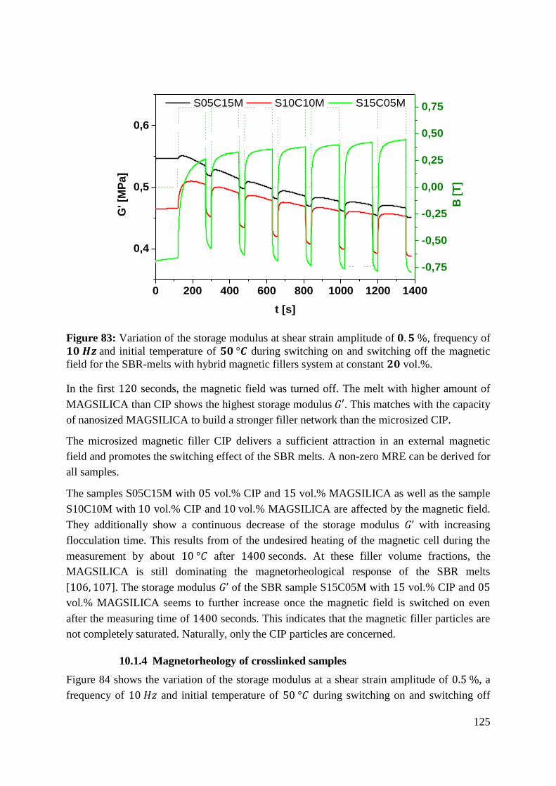
125

0 200 400 600 800 1000 1200 1400

0,4

0,5

0,6

S05C15M S10C10M S15C05M

G' [M

Pa]

t [s]

-0,75

-0,50

-0,25

0,00

0,25

0,50

0,75

B [

T]


𝟏𝟎 𝑯𝒛 and initial temperature of 𝟓𝟎 °𝑪 during switching on and switching off the magnetic

field for the SBR-melts with hybrid magnetic fillers system at constant 𝟐𝟎 vol.%.

In the first 120 seconds, the magnetic field was turned off. The melt with higher amount of

MAGSILICA than CIP shows the highest storage modulus 𝐺′. This matches with the capacity

of nanosized MAGSILICA to build a stronger filler network than the microsized CIP.

The microsized magnetic filler CIP delivers a sufficient attraction in an external magnetic

field and promotes the switching effect of the SBR melts. A non-zero MRE can be derived for

all samples.

The samples S05C15M with 05 vol.% CIP and 15 vol.% MAGSILICA as well as the sample

S10C10M with 10 vol.% CIP and 10 vol.% MAGSILICA are affected by the magnetic field.

They additionally show a continuous decrease of the storage modulus 𝐺’ with increasing

flocculation time. This results from of the undesired heating of the magnetic cell during the

measurement by about 10 °𝐶 after 1400 seconds. At these filler volume fractions, the

MAGSILICA is still dominating the magnetorheological response of the SBR melts

[106, 107]. The storage modulus 𝐺’ of the SBR sample S15C05M with 15 vol.% CIP and 05

vol.% MAGSILICA seems to further increase once the magnetic field is switched on even

after the measuring time of 1400 seconds. This indicates that the magnetic filler particles are

not completely saturated. Naturally, only the CIP particles are concerned.

10.1.4 Magnetorheology of crosslinked samples

Figure 84 shows the variation of the storage modulus at a shear strain amplitude of 0.5 %, a

frequency of 10 𝐻𝑧 and initial temperature of 50 °𝐶 during switching on and switching off

126

the magnetic field for isotropic and anisotropic SBR samples with hybrid magnetic fillers

system at constant 20 vol.%. To minimize the thermal heating, the magnetic field is increased

stepwise and the overall time is reduced to 500 seconds.

0 100 200 300 400 5000,5

1,0

1,5

2,0

2,5

-0,75

-0,50

-0,25

0,00

0,25

0,50

0,75 S05C15M I S10C10M I S15C05M I

S05C15M A S10C10M A S15C05M A

G' [M

Pa

]

t [s]

B [

T]


𝟏𝟎 𝑯𝒛 and initial temperature of 𝟓𝟎 °𝑪 during switching on and switching off the magnetic

field for isotropic and anisotropic SBR samples with hybrid magnetic fillers system at

constant 20 vol.%.

For isotropic samples, the SBR vulcanisates with higher amount of MAGSILICA than CIP

show the highest storage moduli 𝐺′ confirming the high mechanical reinforcing potential of

the nanosized MAGSILICA compared to the microsized CIP. The switching effect of all

isotropic MSE composites is very small independently of the CIP volume fraction because the

magnetic filler particles are not aligned but more or less homogeneously distributed within the

rubber matrix.

The columnar structure of the magnetic filler particles achieved during the curing in external

magnetic field to prepare anisotropic samples promotes the magnetorheological response of

MSE composites. All anisotropic SBR samples become stiffer and show a higher switching

effect. As discussed earlier, this behaviour is directly proportional to magnetic filler amount

of CIP.

To note is that the switching effect of vulcanisates is smaller than the switching effect of

melts, because the mobility of magnetic filler particles in the rubber matrix is constrained by

the crosslinking achieved during the curing process [106, 107].

127

10.2 Hybrid filler systems

Like all technical elastomeric materials, the MSE composites must have an application-related

property profile. In order to satisfy the requirements regarding the dynamic-mechanical as

well as the magnetorheological properties and to ensure optimum outcome, hybrid fillers

systems were used to overcome the deficiencies of MSE composites filled with one-filler

systems. While the microsized magnetic filler CIP contributes to switching ability, the

nanosized MAGSILICA promotes the filler networking of the MSE composites.

As shown in the last section, it was found appropriate to use hybrid magnetic filler systems to

achieve different dynamic-mechanical and magnetorheological results for several MSE

composites. Nevertheless, the mechanical reinforcing potential of such filler systems remains

not satisfactory. The MSE composites can be brought to application maturity by a new

approach for hybrid filler systems. The microscaled magnetic filler CIP should be maintained

as a carrier material for the switching ability of the MSE composites. However, a new

nanoscaled filler should be used to obtain a better filler networking than MAGSILICA.

The conventional rubber filler silica (U 7000) was chosen due to its structural and chemical

similarity to MAGSILICA to form with the microsized CIP the new hybrid filler system.

Silica is a nanosized filler with a specific surface area of 162.5 𝑚²/𝑔. A larger flocculation

and thus a better mechanical reinforcement potential is expected compared with

MAGSILICA. MAGSILICA has a specific surface area of 54 𝑚²/𝑔. Silica also represents the

coating layer of the MAGSILICA particles. The same chemical nature of the surface area

ensures the same binding between the polymer chains and the filler particles. The

renunciation of MAGSILICA and its iron oxides mixture hardly leads to a disadvantage

because the contribution of MAGSILICA to magnetorheological properties of the MSE

composites is negligible compared with CIP.

SBR samples with hybrid filler systems at a constant filler volume fraction of 20 vol.% were

prepared in the same way as the MSE composites with hybrid magnetic filler systems. The

microscaled magnetic filler CIP was replaced in intervals of 5 vol.% by the nanoscaled non-

magnetic silica.


The stress-strain curves for the SBR samples with 20 vol.% hybrid filler system with gradual

replacement in intervals of 5 vol.% of CIP by silica at room temperature are shown in Figure

85. For comparing the results of the silica-filled samples, the measured data obtained for MSE

composites with hybrid magnetic filler systems are additionally plotted in the same graph.

128

0 50 100 150 200 250 300 350 400 450 5000

5

10

15

S05C15M I S05C15S I

S10C10M I S10C10S I

S15C05M I S15C05S I

[

MP

a]

[%]

0 50 100 150 200 250 300 350 400 450 5000

5

10

15

05C/15M A 05C/15S A

10C/10M A 10C/10S A

15C/05M A 15C/05S A

[

MP

a]

[%]

Figure 85: Stress-strain curves for SBR samples with 𝟐𝟎 vol.% hybrid filler systems at room

temperature. Measured data obtained for MSE composites with hybrid magnetic filler system

are additionally plotted. Silica filled samples are represented by dashed lines. MAGSILICA

filled samples are displayed with full lines. Isotropic samples are depicted on the left.

Anisotropic samples are illustrated on the right.

The MSE composites with the different filler systems show an almost similar stress-strain

behaviour for the samples with a larger CIP content.

For the samples with equal shares S10C10S I and S10C10S A with 10 vol.% CIP and 10

vol.% silica as well as S10C10M I and S10C10M A with 10 vol.% CIP and 10 vol.%

MAGSILICA, the stress-strain curves have an almost identical curve progression. However,

changes were observed. They concern the tensile strength at break and the elongation at

break. The tensile strength at break is almost 2 MPa larger for the silica-filled sample. The

same behaviour is observed for the elongation at break. It is nearly 50 % higher.

The stress-strain curves of the samples S05C15S I and S05C15S A with 05 vol.% CIP and 15

vol.% silica show from a strain value of 180 % a significant deviation from the stress-strain

curves of the MAGSILICA-filled samples at the same filling ratio. This may be related to

different synergy effects achieved during the curing process between CIP particles from one

side and silica or MAGSILICA particles from the other side. The elongation at break is

approximately 100 % larger for the silica-filled sample. The tensile strength at break is 1

MPa larger for the isotropic silica-filled sample.

The observed increase in tensile strength at break and elongation at break of the silica filled

samples compared with the MAGSILICA filled samples is related to the high mechanical

reinforcement of silica. This evidence was anticipated from the static volumetric gas

adsorption measurements. A larger specific surface area of 162.5 𝑚²/𝑔 was derived for silica

instead of 54 𝑚²/𝑔 for MAGSILICA.

The orientation of the magnetic filler particles has hardly any effect because the tensile

direction is perpendicular to the magnetic filler strings.

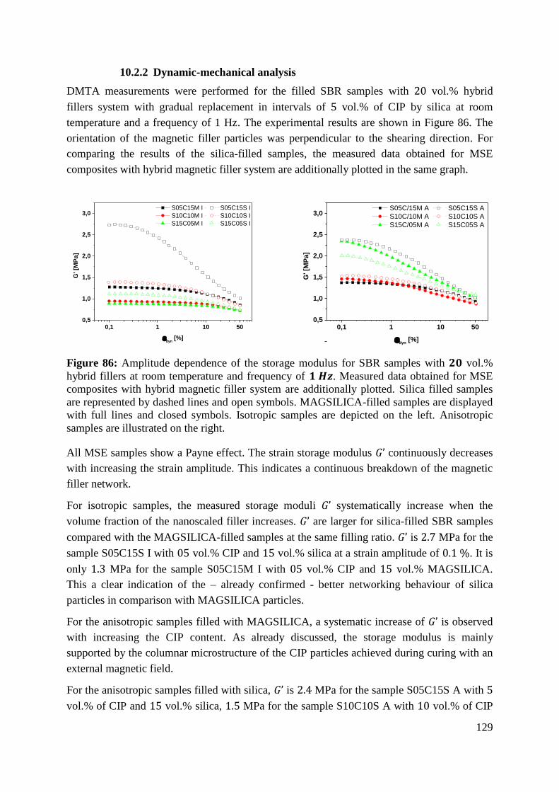
129

10.2.2 Dynamic-mechanical analysis

DMTA measurements were performed for the filled SBR samples with 20 vol.% hybrid

fillers system with gradual replacement in intervals of 5 vol.% of CIP by silica at room

temperature and a frequency of 1 Hz. The experimental results are shown in Figure 86. The

orientation of the magnetic filler particles was perpendicular to the shearing direction. For

comparing the results of the silica-filled samples, the measured data obtained for MSE

composites with hybrid magnetic filler system are additionally plotted in the same graph.

0,1 1 10 500,5

1,0

1,5

2,0

2,5

3,0 S05C15M I S05C15S I

S10C10M I S10C10S I

S15C05M I S15C05S I

G' [M

Pa

]

dyn

[%]

0,1 1 10 500,5

1,0

1,5

2,0

2,5

3,0 S05C/15M A S05C15S A

S10C/10M A S10C10S A

S15C/05M A S15C05S A

G' [M

Pa

]

dyn

[%]

Figure 86: Amplitude dependence of the storage modulus for SBR samples with 𝟐𝟎 vol.%

hybrid fillers at room temperature and frequency of 𝟏 𝑯𝒛. Measured data obtained for MSE

composites with hybrid magnetic filler system are additionally plotted. Silica filled samples

are represented by dashed lines and open symbols. MAGSILICA-filled samples are displayed

with full lines and closed symbols. Isotropic samples are depicted on the left. Anisotropic

samples are illustrated on the right.

All MSE samples show a Payne effect. The strain storage modulus 𝐺’ continuously decreases

with increasing the strain amplitude. This indicates a continuous breakdown of the magnetic

filler network.

For isotropic samples, the measured storage moduli 𝐺’ systematically increase when the

volume fraction of the nanoscaled filler increases. 𝐺’ are larger for silica-filled SBR samples

compared with the MAGSILICA-filled samples at the same filling ratio. 𝐺’ is 2.7 MPa for the

sample S05C15S I with 05 vol.% CIP and 15 vol.% silica at a strain amplitude of 0.1 %. It is

only 1.3 MPa for the sample S05C15M I with 05 vol.% CIP and 15 vol.% MAGSILICA.

This a clear indication of the – already confirmed - better networking behaviour of silica

particles in comparison with MAGSILICA particles.

For the anisotropic samples filled with MAGSILICA, a systematic increase of 𝐺’ is observed

with increasing the CIP content. As already discussed, the storage modulus is mainly

supported by the columnar microstructure of the CIP particles achieved during curing with an

external magnetic field.

For the anisotropic samples filled with silica, 𝐺’ is 2.4 MPa for the sample S05C15S A with 5

vol.% of CIP and 15 vol.% silica, 1.5 MPa for the sample S10C10S A with 10 vol.% of CIP

130

and 10 vol.% silica and 2.0 MPa for the sample S15C05S A with 15 vol.% of CIP and 5

vol.% silica at a strain amplitude of 0.1 %. This ranking remains unchanged until the end of

the measurement. The fact that the anisotropic sample S05C15S A with only 5 vol.% of CIP

has the largest storage modulus 𝐺’ among the anisotropic silica filled MSE composites shows

that 𝐺’ is not only supported by the columnar microstructure of the CIP particles achieved

during curing with an external magnetic field. The contribution of the network of the second

filler in the hybrid filler system to 𝐺’ can no longer be neglected. This behaviour confirms the

presence of different synergy effects between CIP particles from one side and silica or

MAGSILICA particles from the other side.

The existence of different synergy effects can also be verified when the two samples filled

with 5 vol.% of CIP and 15 vol.% silica are considered. The isotropic sample S05C15S I has

a storage modulus 𝐺’ of 2.75 MPa at a strain amplitude 0.1 %. However, 𝐺’ is only 2.4 MPa

for the anisotropic sample S05C15S A. It appears that the silica network is more dominant

than the CIP strings when the silica content is at least 15 vol.%. The CIP strings certainly

disturb the emergence of a stiff silica network within the rubber matrix but they cannot

prevent it.


Magnetorheological measurements were carried out for the filled SBR samples with 20 vol.%

hybrid fillers system with gradual replacement in intervals of 5 vol.% of CIP by silica at a

temperature of 50 °𝐶, a shear strain amplitude of 0.5 % and a frequency of 10 𝐻𝑧. The

experimental results are shown in Figure 87. The magnetic field, shown on the right axis, is

increased stepwise and the overall time is 500 seconds. For comparing the results of silica

filled samples, the measured data obtained for MSE composites with hybrid magnetic filler

system are additionally plotted in the same graph.

0 100 200 300 400 500

0.75

1.00

1.25

1.50

-0.75

-0.50

-0.25

0.00

0.25

0.50

0.75 S05C15M I S05C15S I

S10C10M I S10C10S I

S15C05M I S15C05S I

G' [M

Pa

]

t [s]

B [

T]

0 100 200 300 400 500

1,00

1,25

1,50

1,75

2,00

2,25

-0,75

-0,50

-0,25

0,00

0,25

0,50

0,75 S05C15M A S05C15S A

S10C10M A S10C10S A

S15C05M A S15C05S A

G' [M

Pa

]

t [s]

B [

T]

Figure 87: Variation of the storage modulus for SBR samples with 𝟐𝟎 vol.% hybrid at strain

amplitude of 𝟎. 𝟓 %, frequency of 𝟏𝟎 𝑯𝒛 and initial temperature of 𝟓𝟎°𝑪 during switching

on and switching off the magnetic field. Measured data obtained for MSE composites with

hybrid magnetic filler system are additionally plotted. Silica filled samples are represented by

131

dashed lines. MAGSILICA-filled samples are displayed with full lines. Isotropic samples are

depicted on the left. Anisotropic samples are illustrated on the right.

For isotropic samples, the achieved results confirm the earlier findings shown in Figure 86

despite the differences in test geometries and measurement conditions. The storage modulus

𝐺’ increases with increasing the volume fraction of the nanoscaled filler in the hybrid filler

system. Moreover, 𝐺’ is larger for the vulcanisates filled with silica than with MAGSILICA.

The silica filled samples additionally show a larger switching effect than the MAGSILICA

filled samples. The largest magnetorheological effect (MRE) of 7 % is calculated for the

sample S05C15S I with 5 vol.% of CIP and 15 vol.% silica and not for the MAGSILICA

filled samples.

For anisotropic samples, higher storage moduli 𝐺’ for all the samples are registered due to the

additional contribution of the CIP strings to mechanical reinforcement. However, the ranking

does not match with the previous DMTA results shown in Figure 86. This behaviour

manifests the presence of more complex synergy effects between CIP particles from one side

and silica or MAGSILICA particles from the other side

The MAGSILICA filled samples show a higher switching effect than the silica filled samples.

Despite the small saturation magnetisation of MAGSILICA, the MAGSILICA particles are

still affected by the applied magnetic field and support the improvement of the magnetic

sensitivity of the MSE composites. This results in a maximum MRE of 23 % for the sample

S15C05M A with 15 vol.% of CIP and 05 vol.% MAGSILICA and a maximum MRE of

18 % for the sample S15C05S A with 15 vol.% of CIP and 05 vol.% silica.

It can be recognised that the CIP - silica - systems can in general adjust the property profile of

the finished MSE composites. Technical silica can indeed better enhance the dynamic-

mechanical behaviour of the MSE composites than MAGSILICA. However, it should be

taken into account that the switching effect can be significantly reduced due to the

diamagnetic ordering of silica on the one side and due to the different synergy effects between

the filler particles during curing on the other side.

It additionally appears that independently of the hybrid filler system used, the largest

switching effect is realised by the one filler system CIP. A MRE of 30 % is observed for the

anisotropic sample S20C A with 20 vol.% CIP. A CIP content of 20 vol.% represents an

indispensable threshold value for optimising the magnetorheological response of the MSE

composites.

132

10.3 Adaptive systems for active bearing platform

MSE composites can be used in diverse industrial and technical application areas. They

consume less energy compared to other smart materials whilst ensuring safe operation

processes and thus reducing the environmental impacts. Besides, they prolong the lifetime of

elastomeric materials by optimizing the instantaneous usage to required property profile. They

are successfully implemented in the field of sensor technology. For dynamic applications, the

magneto-mechanical properties and ageing behaviour under mechanical load of MSE

composites is under development. An application-related property profile is not yet

completed.

Based on the results obtained so far, a simple draft for adaptive systems for an active bearing

platform is designed. An adaptive system can adjust its behaviour and adapt it to changing

surroundings through integrated sensors according to fixed control algorithms [192-194].

This new bearing platform should be able to detect the mechanical vibrations during operation

in one side. In the other side, it should be able to self-handle and to actively react to these

external circumstances. Within the framework of this thesis, an appropriate adaptive

elastomer composite is realised. Figure 88 shows the operational principle of the active

bearing platform.

Figure 88: Operational principle of the active bearing platform

To catch the mechanical vibrations, the operational principle of the active bearing platform is

based on the piezoresistive effect. A piezoresistive sensor is a pressure gauge. It is a

composite material comprising a pressure transducer and a signal converter. The elastic strain

gauge consists of a silicon membrane to which ohmic resistors are attached. The ohmic

resistors are arranged as Wheatstone bridge so that the electrical resistance linearly changes

with the elongation. The piezoresistive sensor measures the change in the electrical resistance

of the strain gauge caused by a mechanical deformation [195, 196].

The piezoresistive effect can also be observed in high viscous elastomer composites. A

necessary prerequisite is the existence of an electrically conductive filler network within the

rubber matrix. If the sample is deformed, the elasticity modulus decreases with increasing the

133

strain amplitude according to Payne effect. This behaviour is caused by the breaking of the

filler network. At high strain amplitudes, the desorption of adsorbed polymer chains at the

filler surface areas could also take place.

The upper graph in Figure 89 shows the structure of a virgin filler network with a mean filler

cluster size of 𝜉0. The red lines display the available paths for the charge carriers to move

freely. Placing the sample between two electrodes forms a sample capacitor according to the

measuring principle of the capacitive electric field. This arrangement forms an electrically

closed circuit and permits to measure the dielectric quantities of the test sample.

If the sample is deformed, the filler network gets broken. The corresponding structure is

illustrated in the lower graph in Figure 89. The available paths for the charge carriers become

longer because the path concentration is reduced. This results in a decrease of the elasticity

modulus and the dielectric conductivity. Accordingly, the resistance of the sample increases.

Figure 89: Breaking of the filler network during cyclic mechanical loading [𝟏𝟗𝟕]

To prepare adaptive systems for the active bearing platform, MSE composites with hybrid

fillers systems are used. As previously discussed, the nanoscaled fillers MAGSILICA and

silica are characterised by a high networking potential compared to the microscaled CIP. They

contribute as a part of hybrid filler system to improve the mechanical response of the MSE

composites despite the negative impact on the switching ability. Nevertheless, MAGSILICA

and silica are not appropriate for the development of adaptive systems for the active bearing

platform because they are electrically non conducting. Silica is a well-known electrical

insulator [88]. MAGSILICA particles are indeed produced on the basis of iron oxides but

they are coated by an insulating layer in order to prevent eddy currents [116].

Instead, the nanosized Printex XE2-B is used. It is an electrically super conductive carbon

black. Furthermore, it has a BET specific surface area of 1000 𝑚²/𝑔, which indicates a high

mechanical reinforcing potential (see Table 1). Both characteristics make Printex XE2-B

suitable for the development of adaptive systems for the active bearing platform.

In order to ensure the active bearing platform high adaptability, the microscaled magnetic

filler CIP is used for its large magnetic sensitivity. As described in the section 9.4, a wide

operational efficiency is realised by a CIP content of 20 vol.%. The anisotropic structure

134

achieved during curing with an external magnetic field further contributes to a higher

mechanical reinforcement of the MSE composites.

In this approach, the MSE composites take advantage of the microsized magnetic filler CIP to

increase the switching ability and benefit from the nanosized Printex XE2-B to create a stiff

and conductive filler network. The MSE composites were prepared on the basis of NR. The

Printex XE2-B filler content were varied between 0.8 vol.% and 1.8 vol.% in order to

determine the dielectric threshold at which an electrically conductive filler network is built.

An unnecessary increase of the sample viscosity can also be avoided. The increase in

viscosity can hinder the mobility of CIP particles during the vulcanisation and consequently

their orientation along the magnetic field lines. This would enormously affect the switching

effect of the MSE composites.


The stress-strain curves for the NR samples with hybrid filler systems at room temperature are

shown in Figure 90.

0 100 200 300 400 5000

2

4

6

8

10

NR20C03P I NR20C03P A



[

MP

a]

[%]

Figure 90: Stress-strain curves for NR samples with hybrid filler systems at room

temperature. Isotropic samples are represented by full lines. Anisotropic samples are

displayed with dashed lines.

The MSE composites with the different filler systems show an almost similar stress-strain

behaviour. The stress values of the samples increase with increasing the Printex XE2-B

content. The strain values remain almost unchanged at 430 %.

Larger stiffness values are measured for the MSE composites filled with the current hybrid

filler systems compared to the NR samples NR20C I and NR20C A with only 20 vol.% CIP

135

shown in Figure 42. Obviously, the nanosized Printex XE2-B enhances the stiffening of all

samples because a stable and reinforcing filler network is created. A Printex XE2-B content of

0.8 vol.% for the MSE composites NR20C03P I and NR20C03P A seems sufficient to attain

the mechanical threshold.

In contrast to earlier stress-strain measurements for weakly polar rubbers (see Figure 40 and

Figure 43), the anisotropic samples have significantly larger stress values than the isotropic

samples. The difference between the stress values due to different inner microstructures is

almost 2 MPa at a strain value of 400 %. This behaviour can also be attributed to the filler

network of the nanosized Printex XE2-B. The reason is the perpendicular orientation of the

columnar CIP strings within the samples to tensile direction.

10.3.2 Dynamic-mechanical thermal analysis

In order to determine the influence of the filler particle distribution on the dynamic

mechanical response of the MSE composites, DMTA measurements were performed for the

anisotropic NR samples with hybrid filler systems at room temperature and a frequency of

10 𝐻𝑧. The amplitude dependence of the storage modulus 𝐺’ is shown in Figure 91.

0,01 0,1 1 10

0,0

0,5

1,0

1,5

2,0

2,5

G' [M

Pa]

(%)

NR20C03P A

NR20C05P A

NR20C07P A

Figure 91: Amplitude dependence of the storage modulus for anisotropic NR samples with

hybrid filler systems at room temperature and frequency of 𝟏𝟎 𝑯𝒛.

Obviously, all MSE composites show an amplitude dependent storage modulus. The storage

modulus 𝐺’ continuously decreases with increasing the strain amplitude. This confirms the

findings of the last section. A stable filler network already exists. The decrease in 𝐺’ is the

result of the breaking of the hybrid filler network.

136

The storage modulus 𝐺′ increases with increasing the Printex XE2-B volume fraction. This

indicates that a reinforcing filler network is created from the nanosized Printex XE2-B

particles. This additional structure improves the sample stiffness, beside the contribution of

the oriented CIP strings. The mechanical threshold is reached by a Printex XE2-B content of

0.8 vol.%.


In order to determine the switching effect of the MSE composites, magnetorheological

measurements were carried out on anisotropic NR samples with hybrid filler systems at room

temperature, a frequency of 10 𝐻𝑧 and a shear strain amplitude of 0.5 %. The magnetic field

is increased stepwise until a maximum of 0.49 𝑇 without changing the polarity. The

measurement period is 1100 seconds. The experimental results are shown in Figure 92.

0 200 400 600 800 10001,0

1,5

2,0

2,5

3,0

3,5

NR20C03P A

NR20C05P A

NR20C07P A

G' [M

Pa]

t [s]

0,0

0,2

0,4

B [

T]

Figure 92: Variation of the storage modulus at room temperature, frequency of 𝟏𝟎 𝑯𝒛 and

shear strain amplitude of 𝟎. 𝟓 % during switching on and switching off the magnetic field for

anisotropic NR samples with hybrid filler systems.

Anisotropic NR samples were prepared during the vulcanisation in external magnetic field. As

mentioned earlier, the achieved columnar structure of the magnetic filler particles improves

the magnetic sensitivity of the MSE composites. A magnetorheological effect (MRE) of 35 %

is observed for the anisotropic sample NR20C07P A with 20 vol.% CIP and 1.8 vol.%

Printex XE2-B. The MRE of the anisotropic sample NR20C05P A with 20 vol.% CIP and 1.3

vol.% Printex XE2-B is 44 %. The MRE of the anisotropic sample NR20C03P A with 20

vol.% CIP and 0.8 vol.% Printex XE2-B is 43 %.

137

The increase in the Printex XE2-B content has contributed to the increase of the sample

viscosity. All NR samples become stiffer due to the enhanced filler networking. But this led to

the decrease of the switching effect because the orientation of the microscaled CIP particles

during curing along the magnetic field lines as well as the orientation of the magnetic dipoles

during the magnetorheological measurements become more difficult. The optimal Printex

XE2-B content for the best magnetorheological response seems to be at 1.3 vol.%. However,

it remains to examine if the dielectric threshold of the MSE composite is therefore reached.

10.3.4 Combined rheological and dielectric measurements

Combined dielectric and rheological investigations at room temperature and a frequency of

10 𝐻𝑧 were carried out. The strain history is depicted in Figure 93.

400 600 800 1000 1200

0,01

0,1

1

10

[%

]

t [s]

Figure 93: Strain history for combined rheological and dielectric measurements.

The MSE composites were first subjected to small shear amplitude 𝛾 of 0.02 % for 600

seconds. Afterward, 𝛾 was gradually increased from 0.02 % to 21 % to examine the

amplitude dependence of the storage modulus 𝐺’ and the real part of the impedance 𝑍𝑠′ . In the

last step, 𝛾 is abruptly reduced to 0.01 % for a short time and is then kept at 0.02 % for 300

seconds to determine the relaxation behaviour of the samples.

In order to determine the dielectric threshold of the adaptive systems for active bearing

platform, dielectric investigations have revealed that the samples are dielectric conductors

when the content of the nanosized Printex XE2-B is above 1.8 vol.%.

Figure 94 shows the amplitude-dependent variation of the storage modulus 𝐺’ and the real part

of the impedance 𝑍𝑠′ for the anisotropic sample NR20C07P A with 20 vol.% CIP and

1.8 vol.% Printex XE2-B.

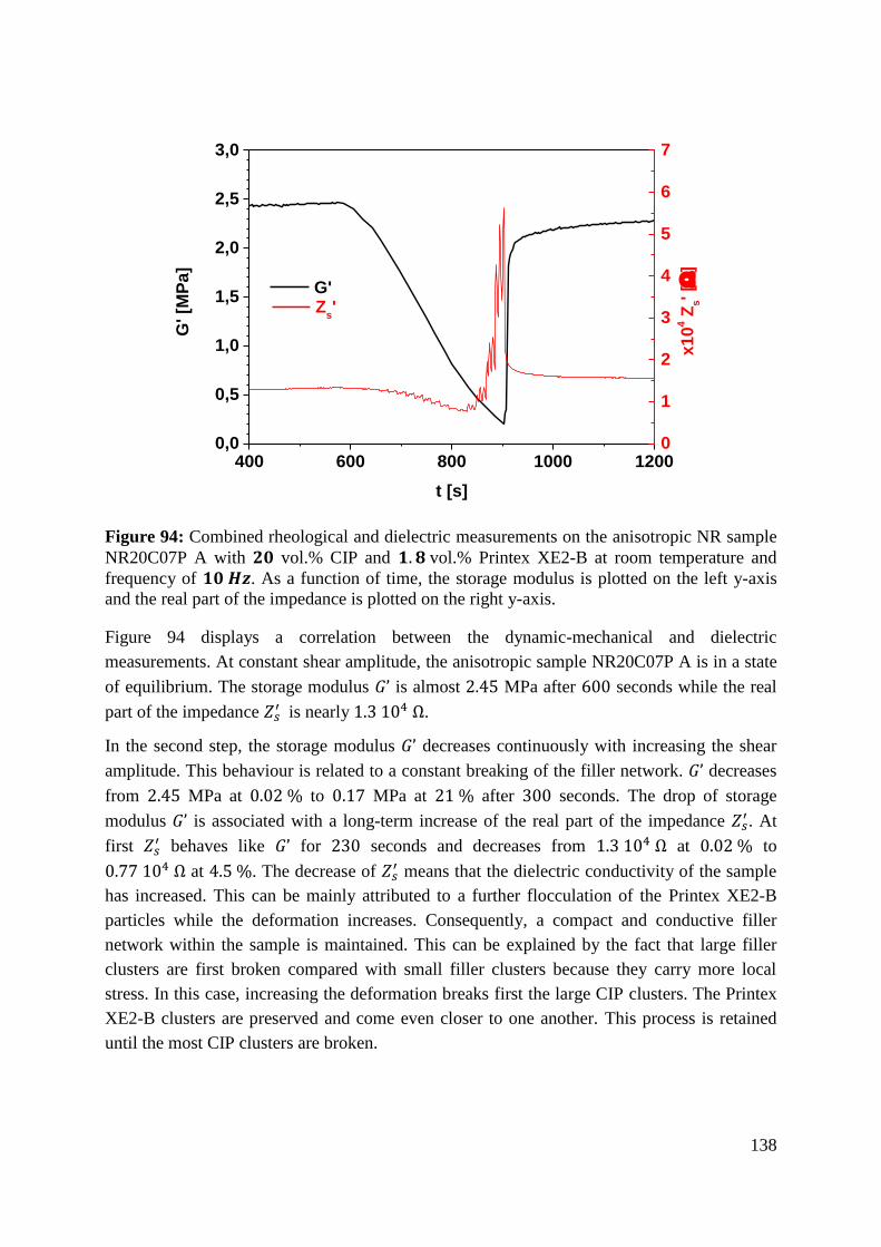
138

400 600 800 1000 12000,0

0,5

1,0

1,5

2,0

2,5

3,0

G' [M

Pa

]

t [s]

G'

0

1

2

3

4

5

6

7

Zs'

x10

4 Z

s' [

]

Figure 94: Combined rheological and dielectric measurements on the anisotropic NR sample

NR20C07P A with 𝟐𝟎 vol.% CIP and 𝟏. 𝟖 vol.% Printex XE2-B at room temperature and

frequency of 𝟏𝟎 𝑯𝒛. As a function of time, the storage modulus is plotted on the left y-axis

and the real part of the impedance is plotted on the right y-axis.

Figure 94 displays a correlation between the dynamic-mechanical and dielectric

measurements. At constant shear amplitude, the anisotropic sample NR20C07P A is in a state

of equilibrium. The storage modulus 𝐺’ is almost 2.45 MPa after 600 seconds while the real

part of the impedance 𝑍𝑠′ is nearly 1.3 104 Ω.

In the second step, the storage modulus 𝐺’ decreases continuously with increasing the shear

amplitude. This behaviour is related to a constant breaking of the filler network. 𝐺’ decreases

from 2.45 MPa at 0.02 % to 0.17 MPa at 21 % after 300 seconds. The drop of storage

modulus 𝐺’ is associated with a long-term increase of the real part of the impedance 𝑍𝑠′ . At

first 𝑍𝑠′ behaves like 𝐺’ for 230 seconds and decreases from 1.3 104 Ω at 0.02 % to

0.77 104 Ω at 4.5 %. The decrease of 𝑍𝑠′ means that the dielectric conductivity of the sample

has increased. This can be mainly attributed to a further flocculation of the Printex XE2-B

particles while the deformation increases. Consequently, a compact and conductive filler

network within the sample is maintained. This can be explained by the fact that large filler

clusters are first broken compared with small filler clusters because they carry more local

stress. In this case, increasing the deformation breaks first the large CIP clusters. The Printex

XE2-B clusters are preserved and come even closer to one another. This process is retained

until the most CIP clusters are broken.

139

After the slight decline, a disproportionate increase of 𝑍𝑠′ from 0.77 104 Ω at 4.5 % to

5.6 104 Ω at 21 % is observed within 70 seconds. This indicates that the Printex XE2-B

network already started to break apart.

In the last step of this measurement, the relaxation behaviour of the sample is examined. The

deformation is abruptly reduced to 0.01 % and is then kept at 0.02 % for 300 seconds.

Plateau values are observed. The storage modulus 𝐺’ is 2.28 MPa while the real part of the

impedance 𝑍𝑠′ is 1.52 104 Ω. The relaxation behaviour is related to reflocculation processes,

which are always associated with stress softening. This explains why the initial values of both

the storage modulus 𝐺’ and the real part of the impedance 𝑍𝑠′ are not reached.

10.3.5 Influence of the mechanical fatigue on MRE

The mechanical fatigue represents a main pillar of the property profile of the MSE

composites. For active bearing platform, it is useful to perform the mechanical tests in

compression mode in contrast to what was done in section 7.4.1.

The measurement sequence was as follows. The relative magnetorheological effect (MRE)

was first determined for all virgin MSE composites. Afterwards, the samples were subjected

to mechanical fatigue tests in compression mode using the dynamic-mechanical analyser

Eplexor. The MRE of the damaged samples is measured for the second time under the same

condition. The magnetorheological measurements were carried out at room temperature, a

shear strain amplitude of 0.5 % and a frequency of 10 𝐻𝑧.

The anisotropic sample NR20C07P A with 20 vol.% CIP and 1.8 vol.% Printex XE2-B was

subjected to a constant static load of 300 𝑁 and a variable dynamic load over 10.000 cycles.

The dynamic force was 50 𝑁, 100 𝑁, 150 𝑁 or 200 𝑁. A virgin sample was used for each

dynamic-mechanical measurement. The measurements were performed at room temperature

and a frequency of 10 𝐻𝑧.

Figure 95 shows the dynamic-mechanical behaviours of MSE composites after 10.000

loading. As a function of dynamic force, the storage modulus 𝐸’ is displayed on the left y-axis

and the dynamic strain 휀𝑑𝑦𝑛 is displayed on the right y-axis.

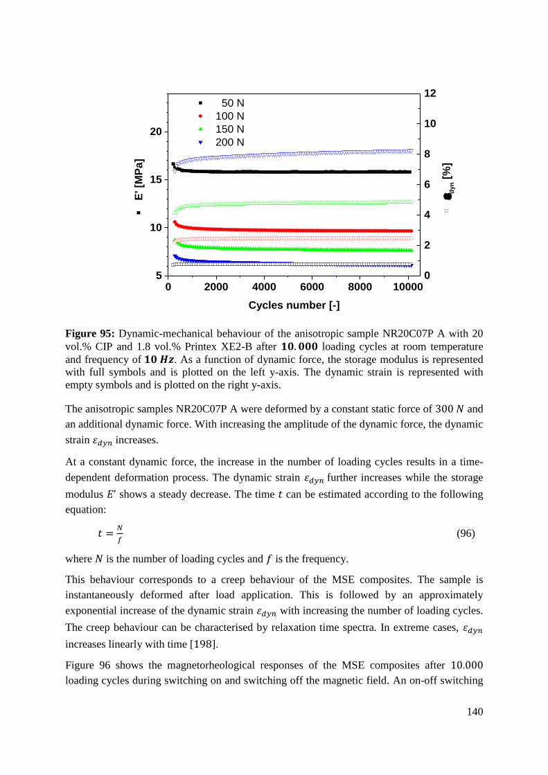
140

0 2000 4000 6000 8000 100005

10

15

20E

' [M

Pa]

Cycles number [-]

50 N

100 N

150 N

200 N

0

2

4

6

8

10

12

dy

n [

%]

Figure 95: Dynamic-mechanical behaviour of the anisotropic sample NR20C07P A with 20

vol.% CIP and 1.8 vol.% Printex XE2-B after 𝟏𝟎. 𝟎𝟎𝟎 loading cycles at room temperature

and frequency of 𝟏𝟎 𝑯𝒛. As a function of dynamic force, the storage modulus is represented

with full symbols and is plotted on the left y-axis. The dynamic strain is represented with

empty symbols and is plotted on the right y-axis.

The anisotropic samples NR20C07P A were deformed by a constant static force of 300 𝑁 and

an additional dynamic force. With increasing the amplitude of the dynamic force, the dynamic

strain 휀𝑑𝑦𝑛 increases.

At a constant dynamic force, the increase in the number of loading cycles results in a time-

dependent deformation process. The dynamic strain 휀𝑑𝑦𝑛 further increases while the storage

modulus 𝐸’ shows a steady decrease. The time 𝑡 can be estimated according to the following

equation:

𝑡 =𝑁

𝑓 (96)

where 𝑁 is the number of loading cycles and 𝑓 is the frequency.

This behaviour corresponds to a creep behaviour of the MSE composites. The sample is

instantaneously deformed after load application. This is followed by an approximately

exponential increase of the dynamic strain 휀𝑑𝑦𝑛 with increasing the number of loading cycles.

The creep behaviour can be characterised by relaxation time spectra. In extreme cases, 휀𝑑𝑦𝑛

increases linearly with time [198].

Figure 96 shows the magnetorheological responses of the MSE composites after 10.000

loading cycles during switching on and switching off the magnetic field. An on-off switching

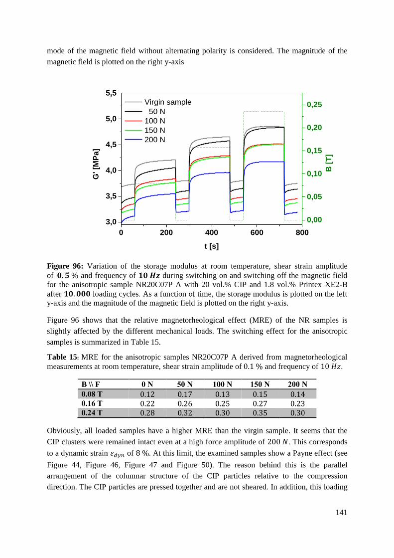
141

mode of the magnetic field without alternating polarity is considered. The magnitude of the

magnetic field is plotted on the right y-axis

0 200 400 600 800

3,0

3,5

4,0

4,5

5,0

5,5

Virgin sample

50 N

100 N

150 N

200 N

t [s]

G' [M

Pa]

0,00

0,05

0,10

0,15

0,20

0,25

B [

T]

Figure 96: Variation of the storage modulus at room temperature, shear strain amplitude

of 𝟎. 𝟓 % and frequency of 𝟏𝟎 𝑯𝒛 during switching on and switching off the magnetic field

for the anisotropic sample NR20C07P A with 20 vol.% CIP and 1.8 vol.% Printex XE2-B

after 𝟏𝟎. 𝟎𝟎𝟎 loading cycles. As a function of time, the storage modulus is plotted on the left

y-axis and the magnitude of the magnetic field is plotted on the right y-axis.

Figure 96 shows that the relative magnetorheological effect (MRE) of the NR samples is

slightly affected by the different mechanical loads. The switching effect for the anisotropic

samples is summarized in Table 15.

Table 15: MRE for the anisotropic samples NR20C07P A derived from magnetorheological

measurements at room temperature, shear strain amplitude of 0.1 % and frequency of 10 𝐻𝑧.

B \\ F 0 N 50 N 100 N 150 N 200 N

0.08 T 0.12 0.17 0.13 0.15 0.14

0.16 T 0.22 0.26 0.25 0.27 0.23

0.24 T 0.28 0.32 0.30 0.35 0.30

Obviously, all loaded samples have a higher MRE than the virgin sample. It seems that the

CIP clusters were remained intact even at a high force amplitude of 200 𝑁. This corresponds

to a dynamic strain 휀𝑑𝑦𝑛 of 8 %. At this limit, the examined samples show a Payne effect (see

Figure 44, Figure 46, Figure 47 and Figure 50). The reason behind this is the parallel

arrangement of the columnar structure of the CIP particles relative to the compression

direction. The CIP particles are pressed together and are not sheared. In addition, this loading

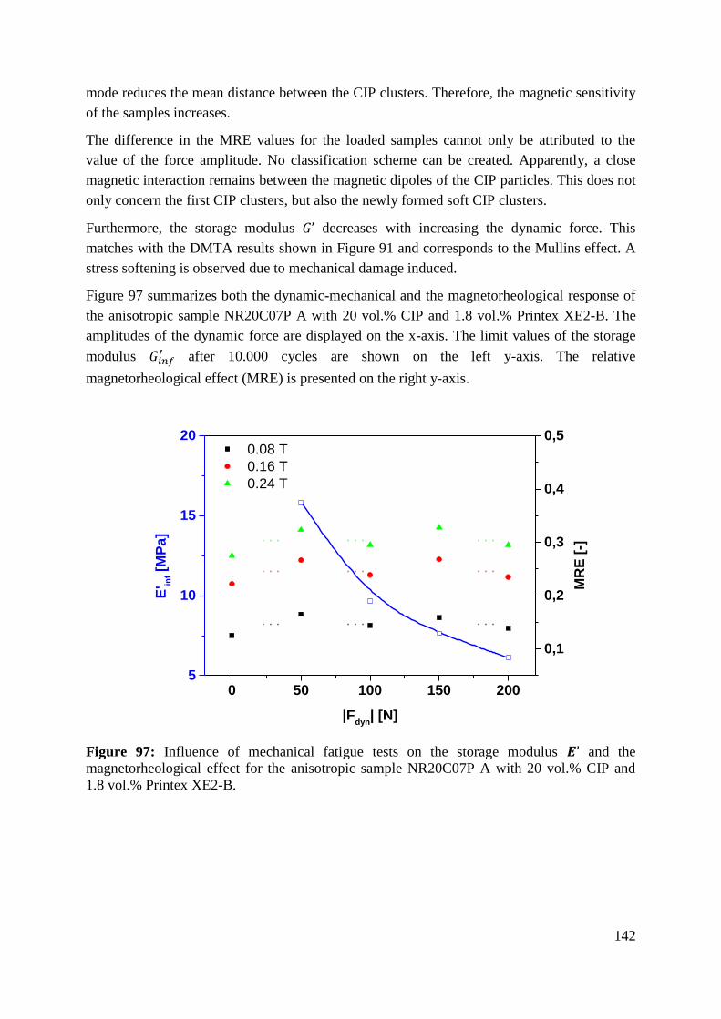
142

mode reduces the mean distance between the CIP clusters. Therefore, the magnetic sensitivity

of the samples increases.

The difference in the MRE values for the loaded samples cannot only be attributed to the

value of the force amplitude. No classification scheme can be created. Apparently, a close

magnetic interaction remains between the magnetic dipoles of the CIP particles. This does not

only concern the first CIP clusters, but also the newly formed soft CIP clusters.

Furthermore, the storage modulus 𝐺’ decreases with increasing the dynamic force. This

matches with the DMTA results shown in Figure 91 and corresponds to the Mullins effect. A

stress softening is observed due to mechanical damage induced.

Figure 97 summarizes both the dynamic-mechanical and the magnetorheological response of

the anisotropic sample NR20C07P A with 20 vol.% CIP and 1.8 vol.% Printex XE2-B. The

amplitudes of the dynamic force are displayed on the x-axis. The limit values of the storage

modulus 𝐺𝑖𝑛𝑓′ after 10.000 cycles are shown on the left y-axis. The relative

magnetorheological effect (MRE) is presented on the right y-axis.

0 50 100 150 2005

10

15

20 0.08 T

0.16 T

0.24 T

|Fdyn

| [N]

E' in

f [M

Pa]

0,1

0,2

0,3

0,4

0,5

MR

E [

-]

Figure 97: Influence of mechanical fatigue tests on the storage modulus 𝑬’ and the

magnetorheological effect for the anisotropic sample NR20C07P A with 20 vol.% CIP and

1.8 vol.% Printex XE2-B.

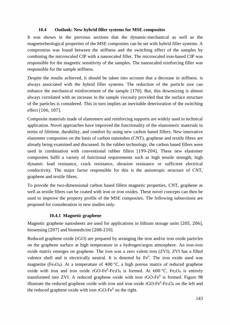
143

10.4 Outlook: New hybrid filler systems for MSE composites

It was shown in the previous sections that the dynamic-mechanical as well as the

magnetorheological properties of the MSE composites can be set with hybrid filler systems. A

compromise was found between the stiffness and the switching effect of the samples by

combining the microscaled CIP with a nanoscaled filler. The microscaled iron-based CIP was

responsible for the magnetic sensitivity of the samples. The nanoscaled reinforcing filler was

responsible for the sample stiffness.

Despite the results achieved, it should be taken into account that a decrease in stiffness. is

always associated with the hybrid filler systems. The reduction of the particle size can

enhance the mechanical reinforcement of the sample [170]. But, this downsizing is almost

always correlated with an increase in the sample viscosity provided that the surface structure

of the particles is considered. This in turn implies an inevitable deterioration of the switching

effect [106, 107].

Composite materials made of elastomers and reinforcing supports are widely used in technical

application. Novel approaches have improved the functionality of the elastomeric materials in

terms of lifetime, durability, and comfort by using new carbon based fillers. New innovative

elastomer composites on the basis of carbon nanotubes (CNT), graphene and textile fibres are

already being examined and discussed. In the rubber technology, the carbon based fillers were

used in combination with conventional rubber fillers [199-204]. These new elastomer

composites fulfil a variety of functional requirements such as high tensile strength, high

dynamic load resistance, crack resistance, abrasion resistance or sufficient electrical

conductivity. The major factor responsible for this is the anisotropic structure of CNT,

graphene and textile fibres.

To provide the two-dimensional carbon based fillers magnetic properties, CNT, graphene as

well as textile fibres can be coated with iron or iron oxides. These novel concepts can then be

used to improve the property profile of the MSE composites. The following subsections are

proposed for consideration in new studies only.

10.4.1 Magnetic graphene

Magnetic graphene nanosheets are used for applications in lithium storage units [205, 206],

biosensing [207] and biomedicine [208-210].

Reduced graphene oxide (rGO) are prepared by arranging the iron and/or iron oxide particles

on the graphene surface at high temperature in a hydrogen/argon atmosphere. An iron-iron

oxide matrix emerges on graphene. The iron was a zero valent iron (ZVI). ZVI has a filled

valence shell and is electrically neutral. It is denoted by Fe0. The iron oxide used was

magnetite (Fe3O4). At a temperature of 400 °𝐶, a high porous matrix of reduced graphene

oxide with iron and iron oxide rGO-Fe0-Fe3O4 is formed. At 600 °𝐶, Fe3O4 is entirely

transformed into ZVI. A reduced graphene oxide with iron rGO-Fe0 is formed. Figure 98

illustrate the reduced graphene oxide with iron and iron oxide rGO-Fe0-Fe3O4 on the left and

the reduced graphene oxide with iron rGO-Fe0 on the right.

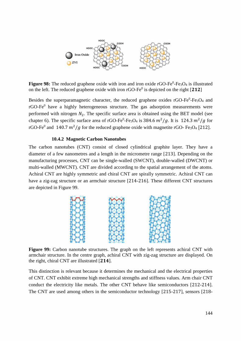
144

Figure 98: The reduced graphene oxide with iron and iron oxide rGO-Fe0-Fe3O4 is illustrated

on the left. The reduced graphene oxide with iron rGO-Fe0 is depicted on the right [𝟐𝟏𝟐]

Besides the superparamagnetic character, the reduced graphene oxides rGO-Fe0-Fe3O4 and

rGO-Fe0 have a highly heterogeneous structure. The gas adsorption measurements were

performed with nitrogen 𝑁2. The specific surface area is obtained using the BET model (see

chapter 6). The specific surface area of rGO-Fe0-Fe3O4 is 384.6 𝑚2/𝑔. It is 124.3 𝑚2/𝑔 for

rGO-Fe0 and 140.7 𝑚2/𝑔 for the reduced graphene oxide with magnetite rGO- Fe3O4 [212].

10.4.2 Magnetic Carbon Nanotubes

The carbon nanotubes (CNT) consist of closed cylindrical graphite layer. They have a

diameter of a few nanometres and a length in the micrometre range [213]. Depending on the

manufacturing processes, CNT can be single-walled (SWCNT), double-walled (DWCNT) or

multi-walled (MWCNT). CNT are divided according to the spatial arrangement of the atoms.

Achiral CNT are highly symmetric and chiral CNT are spirally symmetric. Achiral CNT can

have a zig-zag structure or an armchair structure [214-216]. These different CNT structures

are depicted in Figure 99.

Figure 99: Carbon nanotube structures. The graph on the left represents achiral CNT with

armchair structure. In the centre graph, achiral CNT with zig-zag structure are displayed. On

the right, chiral CNT are illustrated [𝟐𝟏𝟒].

This distinction is relevant because it determines the mechanical and the electrical properties

of CNT. CNT exhibit extreme high mechanical strengths and stiffness values. Arm chair CNT

conduct the electricity like metals. The other CNT behave like semiconductors [212-214].

The CNT are used among others in the semiconductor technology [215-217], sensors [218-

145

220] and biomedical applications [221-223]. CNT are also used in the rubber technology to

improve the mechanical and dielectric properties of elastomer composites [224, 225].

In order to realise versatile systems, CNT can be further optimised through functionalisation

with magnetic or superparamagnetic particles to obtain magnetic CNT (Mag-CNT). In the

following, a short list of already prepared Mag-CNT is presented, which can be considered for

use as hybrid filler systems in MSE composites.

To impart magnetic properties, CNT can be filled with metals or ferrofluids as shown in

Figure 100. Prepared with “nanostraws” technique, the ferrofluid – a suspension of magnetite

(Fe3O4) in hexane – is poured into CNT. An external magnetic field is used to promote the

penetration of Fe3O4 particles in the tubes. The solvent is later removed by evaporation [225].

Figure 100: Preparation of Mag-CNT by filling CNT with a ferrofluid – a suspension of

Fe3O4 in hexane [𝟐𝟐𝟓].

Mag-CNT can also be realised by coating the surface of CNT with single-molecule magnets

(Mn12O12(O2CCH3)16(H2O)4), spinel ferrites (Me-Fe2O4), cobalt-containing magnetic

polyoxometalate ((As2W20O68Co(H2O))8−) or iron nanoparticles.

The coating with iron nanoparticles can be achieved according to the Fenton´s reagent

synthetic scheme as shown in Figure 101. A Fe2O3-CNT composite is realised [225].

Figure 101: Preparation of Mag-CNT by coating the CNT with iron nanoparticles [𝟐𝟐𝟓].

Mag-CNT can be a very interesting alternative to hybrid filler systems discussed earlier

because they can additionally be coated with silica layer as shown in Figure 102 [226].

146

Figure 102: Preparation method of silica coated Mag-CNT [𝟐𝟐𝟔].

147

11 Summary and Conclusions

Magneto-sensitive elastomers (MSE) consist of an insulating rubber matrix in which magnetic

filler particles are embedded. They are able to vary in real time their rheological properties in

order to ensure adaptability to changing environmental conditions. This behaviour is achieved

by means of magnetic fields, which yield to a coupling between the dynamic-mechanical and

the magneto-rheological properties of MSE. In contrast to conventional elastomer composites,

the MSE responses can then be actively controlled according to the magnetic field settings.

Two different magnetic fillers were used. The carbonyl iron particles SW-S (CIP) is a

microscaled iron-based magnetic filler. MAGSILICA is a nanoscaled magnetic filler. It

consists of iron oxide mixture embedded in a silica matrix. Static volumetric gas adsorption

measurements were performed in order to determine the specific surface area of the magnetic

fillers according to the BET model. This constitutes an important tool for predicting the filler

networking. A specific surface area of 0.4 𝑚²/𝑔 was derived for CIP. MAGSILICA has a

specific surface area of 54 𝑚²/𝑔.

The vulcanisation was achieved in the presence of a magnetic coil system in order to

influence the setting up of the filler network within the rubber matrix. As soon as no magnetic

field was applied, the magnetic filler particles were homogenously dispersed and isotropic

MSE composites were obtained. But if the magnetic field was applied, the magnetic filler

particles aligned themselves along the magnetic field lines due to magnetic dipole-dipole

interactions. A columnar structure arose and the MSE composites became anisotropic. SEM

images confirmed the inner structure of the magnetic filler network.

From design and choice of the different components, through vulcanisation process until

applied magnetic field during application, different factors influence the properties of the final

MSE composites to different degrees.

Mechanical measurements showed that the mechanical reinforcement is mainly supported by

the nanoscaled magnetic filler. The mechanical reinforcement potential is attributed to the

networking capacity of the filler used, which can be evaluated through the formation of a

physically bonded filler network and a strong polymer-filler coupling. With a higher specific

surface area, MAGSILICA offers a larger surface area for the polymer chains to adhere

compared to CIP.

Stress-strain measurements provide the first evidence for the better networking potential of

MAGSILICA. The samples S20M A and S20M I with 20 vol.% MAGSILICA showed larger

stress values than the samples S20C A and S20C I with 20 vol.% CIP at the same strain

amplitude. Similar to conventional reinforcing fillers like silica or carbon black, the stress

values of the MSE composites increase with increasing the filler loading. Furthermore, it was

found that the polarity of rubber may play a non-negligible role in determining the stress-

strain behaviour of the samples.

148

The orientation of the magnetic filler particles did not really affect the stress-strain values of

the MSE composites. The reason for this lies in the fact that the loading direction was

perpendicular to the magnetic filler strings.

Dynamic-mechanical measurements showed that all MSE composites were subject to the

Payne effect. The storage modulus decreased with an increase in the strain amplitude.

Moreover, the distribution of the magnetic filler particles within the rubber matrix during

vulcanisation seems to play a key role. High storage moduli were obtained when the

magnitude of the magnetic field applied during curing were increased. This is the result of a

better magnetic dipole-dipole interaction between the magnetic filler particles and the applied

magnetic field during curing, which governs the distribution of the magnetic filler particles

within the rubber matrix and thus the degree of anisotropy of the MSE composites. This leads

to the creation of a distinctive columnar structure promoting the mechanical reinforcement of

MSE composites. However, the storage moduli of the filled samples N36C A and N36C I

with 36 vol.% CIP show no discernible difference due to anisotropy. Obviously, there is a

clear limitation to the filler volume fraction. This behaviour indicates that no magnetic filler

strings were formed during the curing process, even in a magnetic field. This can be related to

a strong reciprocal mobility restriction of the polymer chains and the magnetic filler particles,

which inhibits the orientation of the magnetic filler particles along the magnetic field lines.

The coupling agent silane was used to enhance the interaction between polymer chains and

the magnetic filler CIP as well as MAGSILICA. A strong chemical bonding at the polymer-

filler interface was established through the coupling reaction of the silane with the magnetic

filler during mixing and the rubber matrix during the vulcanisation. This led to a better

distribution of the magnetic filler particles in the sample and to a high mechanical

reinforcement.

Both mechanical and thermal ageing experiments showed a similar ageing behaviour of the

MSE composites to conventional rubber samples. There were no indications that the magnetic

filler particles lost their covering coating and react directly or indirectly with the polymer

chains even under high dynamic loading.

Magnetorheological measurements were performed on the non-crosslinked melts in order to

visualise the effect of particle orientation during the curing process. The MSE composites

filled with the microscaled CIP showed a pronounced switching effect once the magnetic field

is turned on. The relative magnetorheological effect (MRE) was more than 40 % for the

sample S20C filled with 20 vol.% CIP. However, the sample filled with the nanoscaled

MAGSILICA was hardly affected by the magnetic field. This indicates different interaction

strengths between the magnetic filler particles and the applied magnetic field. It was found

that the magnetic dipole-dipole was direct proportional to the particle size. Obviously, the

magnetic moments of the nanoscaled MAGSILICA were too small to deliver a satisfactory

attraction in an external magnetic field. The particles were relatively quickly saturated in

contrast to the microscaled CIP particles, which interacted well with the magnetic field by

aligning themselves along the magnetic field lines. Beside the particle size, the filler

149

composition played also a decisive role. Pure iron has a comparably large saturation

magnetisation than iron oxides.

Moreover, the switching effect has increased with increasing the magnitude of the magnetic

field. This trend was maintained until the magnetic filler particles became completely

saturated. The reason for this was a larger magnetic interaction between the magnetic filler

particles and the magnetic field. The additional increase in measurement temperature also led

to a larger switching effect. The MRE of the sample N36C with 36 vol.% CIP was 354 % at

room temperature and 609 % at a temperature of 50 °𝐶. This is explained by the fact that the

temperature increase has actively supported the mobility of the magnetic filler particles within

the rubber matrix and thus facilitated their orientation along the magnetic field lines.

It was seen, that the silanisation has a big influence on the MRE of the samples. A MRE of

more than 140 % was derived for the sample without silane S20C\Si while a significantly

weaker MRE of nearly 40 % was obtained for the silanized sample S20C. This behaviour was

related to the combined effect of a higher mobility of the magnetic filler particles without a

shielding silane layer and the ability of the magnetic filler particles to come in close contact

when they arrange in strings along the magnetic field lines.

Magnetorheological measurements were also carried out with the crosslinked MSE

composites. The curing was done with and without magnetic field to get anisotropic and

isotropic MSE respectively. This new structure ensures a larger stiffness for all MSE

composites and higher moduli values in comparison to the melts, because a high level of

crosslinking between the polymer chains was achieved and a magnetic filler network was

built. The switching effect remains proportional to the microscaled magnetic filler content and

the magnetic field strength during curing. However, the MRE of the vulcanised samples has

become smaller than the MRE of the non-crosslinked melts because the magnetic filler

particles are firmly tied to the polymer chains and can no longer be moved along the magnetic

field lines. The maximum MRE was recorded for the anisotropic sample N13C A with 13

vol.% CIP. It was 36 %.

Furthermore, it was shown that the size of the magnetic filler particle as well as the magnitude

of the magnetic field during curing determine the value of the MRE. The filler content cannot

also be infinitely increased. A CIP volume fraction of 20 vol.% seemed appropriate to have

an optimal property profile for almost all MSE composites. Similar to melts, the silane was

needed to establish a good polymer-filler interface and cannot be sacrificed due to its negative

impact on the switching effect.

It was shown that the magnetorheological response of the MSE composites can be described

by the magnetic induced relaxation behaviours of the magnetic filler and the polymer chains.

Short relaxation times of 1 to 2 seconds were observed for the magnetic filler while the

relaxation of the polymer chains took between 10 and 80 seconds.

150

Quasi-static measurements in the presence of external magnetic field showed a strong

coupling between the mechanical properties of MSE composites and the magnetic properties

of the surroundings. The dynamic flocculation model (DFM) gave a deep insight into the

inner structure of the samples and the ongoing measuring processes. Since the mechanical

stiffening of the MSE composites was assigned to the magnetic filler, the fit parameters

related to mechanical behaviour of rubber were only affected by the molecular structure of the

polymer chains as well as the distribution of the magnetic filler particles within the rubber

matrix and not by the applied magnetic field during the measurement. However, the tensile

strength of virgin bonds 𝑠𝑣 and the tensile strength of damaged bonds 𝑠𝑑 have been affected

by the applied magnetic field during the measurement. 𝑠𝑣 has increased from 27.83 MPa to

28.92 MPa for the isotropic EPDM sample once the magnetic field was applied. The same

happened for the anisotropic sample. The difference is significantly higher. 𝑠𝑣 has increased

from 51.69 MPa to 55.67 MPa when the magnetic field was turned on. The same behaviour

was observed for 𝑠𝑑. The difference between turned on or off magnetic field is less

pronounced.

The use of hybrid filler systems showed that the property profile of the finished MSE

composites can be accordingly adjusted. The dynamic-mechanical behaviour of the samples

can be indeed improved by using nanoscaled filler like MAGSILICA, technical silica or

carbon black. However, the 20 vol.% limit of magnetic filler CIP seems indispensable to

realise the highest switching effect. It was shown that the MSE composites with hybrid filler

systems could be in the near future a serious option for mature application fields. These

hybrid filler systems could be further extended to other types of nanoscaled fillers like

graphene or carbon nanotubes, which have also had a favourable impact on improving the

dynamic-mechanical properties of the finished elastomeric materials.

151

Bibliography

1. B. F. Spencer Jr., M. K. Sain, “Controlling buildings: a new frontier in feedback”, IEEE

Control Systems, pp. 19-35, December 1997.

2. B. F. Spencer Jr., S. Nagarajaiah, “State of the Art of Structural Control”, J. Struct. Eng.,

pp. 845-856, July 2003

3. W. Demtröder, Experimentalphysik 1, Springer-Verlag Berlin Heidelberg, pp. 353-363,

March 2008, ISBN 978-3-540-79294-9.

4. T. Kobori, “Future direction on research and development of seismic-response-controlled

structure,” Proc. 1st World Conf. on Struct. Control, Los Angeles, CA, Panel: 19-31,

August 1994.

5. M. Sakamoto, T. Kobori, T. Yamada, and M. Takahashi, “Practical applications of active

and hybrid response control systems and their verifications by earthquake and strong

wind observations,” Proc. 1st World Conf. on Struct. Control, Los Angeles, CA, pp.

WP2:90-99, August 1994.

6. K. Tanida, Y. Koike, K. Mutaguchi, and N. Uno, “Development of hybrid active-passive

damper,” Active and Passive Damping, ASME, PVP-vol. 211, pp. 21-26, 1991.

7. Y. Koike, T. Murata, K. Tanida, T. Kobori, K. Ishii, and Y. Takenaka, “Development of

V-shaped hybrid mass damper and its application to high-rise buildings,” Proc. 1st World

Conf. on Struct. Control, Los Angeles, CA, pp. FA2:3-12, August 1994.

8. J. Hirai, A. Hisanori, and E. Tsuji, “Study on tuned active damper for control tower of

Kansai International Airport,” Proc. Int. Workshop on Struct. Control, Honolulu, HI, pp.

206-13, 1993.

9. T. Suzuki, M. Kageyama, A. Nobata, S. Inaba, and O. Yoshida, “Active vibration control

system installed in a high-rise building,” Proc. 1st World Conf. on Struct. Control, Los

Angeles, CA, pp. FP3:3-11, August 1994.

10. Y. Fujino and H. Yamaguchi, “Implemented examples of structural response control for

civil structures with emphasis on active control,” Japan Soc. Steel Const., vol. 12, pp. 16-

22, 1994.

11. H. Iemura, A. Igarashi, Y. Inoue, and M. Sakamoto, “Nonlinear active control experiment

of a real size frame structure,” Proc. 2nd Int. Workshop on Struct. Control, Hong Kong,

pp. 241-252, December 1996.

12. J. Cai, G. Bu, C. Yang, Q. Chen and Z. Zuo, “Calculation methods for inter-story drifts of

building structures,” Advances in Structural Engineering, Vol 17, Issue 5, 2014

13. J. Zhou, G. B. Bu and K. N. Li, “Calculation methods for inter-story drifts of building

structures,” 15th World Conf. on Earthquake Engrg WCEE, Lisbon, September 2012

152

14. J. M. Kelly, “Aseismic base isolation: its history and prospects,” Proc. 1st World Cong.

on Joints and Bearings, ACI-SP-70, vol. 1, pp. 549-586, 1981.

15. J. M. Kelly, “Aseismic base isolation: review and bibliography,” Soil Dyn. and

Earthquake Engrg., vol. 5, no. 3, pp. 202-216, 1986.

16. I. G. Buckle and R. L. Mayes, “Seismic isolation history, application and performance-a

world view,” Earthquake Spectra, vol. 6, no. 2, pp.161-201, 1990.

17. T. T. Soong and M. C. Constantinou, Eds., Passive and active Structural Vibration

Control in Civil Engineering, Springer-Verlag, Wien and New York, 1994, ISBN 978-3-

211-82615-7.

18. A. M. Reinhorn, T. T. Soong, and C. Y. Wen, “Base isolated structures with active

control,” Proc. ASME PVP Conf, San Diego, CA, PVP-127, pp. 413-420, 1987.

19. J. M. Kelly, G. Leitmann and A. G. Soldatos, “Robust control of base isolated structures

under earthquake excitation,” J. Opt. Theory and App., vol. 53, no. 2, pp. 159-180, 1987.

20. W. E. Schmitendorf, F. Jabbari, J. N. Yang, “Robust control techniques for buildings

under earthquake excitation,” Earthquake Engrg. and Struct. Dyn., 23, pp. 539-552, 1994.

21. J. N. Yang, J. C. Wu, A. M. Reinhorn, M. Riley, “Control of sliding isolated buildings

using sliding mode control,” J. Struct. Engrg., ASCE, vol. 122, no. 2, pp. 179-186, 1996.

22. P. Causemann, “Moderne Schwingungsdämpfung,” ATZ 11/2003 Jahrgang 105

23. J. N. Yang, J. C. Wu, Z. Li, “Control of seismic-excited buildings using active variable

stiffness systems,” Engrg Struct , vol 18, no 8, pp.589-596, 1996

24. T. Kobori, M. Takahashi, T. Nasu, N. Niwa, K. Ogasawara, “Seismic response controlled

structure with active variable stiffness system,” Earthquake Engrg. and Struct. Dyn., vol

22, pp. 925-941, 1993

25. W. M. Winslow, ”Method and means for translating electrical impulses into mechanical

forces”, U.S. Patent No US2417850 A, 1947

26. W. M. Winslow, “Induced fibration of suspensions” J. Appl. Phys., vol 20, pp. 1137-

1140, 1949

27. J. Rabinow, “The magnetic fluid clutch”, AIEE Transactions, 67, pp 1308-1315, 1948

28. T. Nishi,”Elastomeric-Seismic Protection Isolators at the East Japan Giant Earthquake“,

Plenary speech, 10th Fall Rubber Colloqium, Hannover, 2012

29. H. Deng, X. Gong, L. Wang, ”Development of an adaptive tuned vibration absorber with

magnetorheological elastomer“, Smart Mater. Structure 15, 2006, 111

30. J. D. Carlson, M. R. Jolly, “MR Fluid, Foam and Elastomer Devices”, Mechatronics 10,

2000, pp 555-569

153

31. J. Ginder, M. Nichols, L. Elie, J. Tardiff, “Magnetorheological elastomers: properties and

applications, Smart structures and materials” Proc. SPIE, 3675, 1999, pp 131-138

32. K. Popp, M. Kröger, W. Li, X. Zhang, P. Kosasih, “MRE Properties under Shear and

Squeeze Modes and Applications”, J. Int. Mat. Sys. and Structure 21, 2010, 1471

33. Y. Li, J. Li, W. Li, B. Samali, “Development and characterisation of a

magnetorheological elastomer based adaptive seismic isolator“, Smart Materials and

Structure 22, 2013, 035005

34. M. K. Sethi, P. Kumar and A. Kumar, “Transient vibration reduction of a powertrain

using MRE based adaptive tuned vibration absorber”, Proc. Eng. 144, 2016, pp. 689–696

35. Z. Xu, X. Gong, G. Liao and X. Chen, “An active damping-compensated

magnetorheological elastomer adaptive tuned vibration absorber”, J. Intell. Mater. Syst.

Struct. 21, 2010, pp. 1039–1047

36. G. J. Liao, X. L. Gong, C. J. Kang and S. H. Xuan, “The design of an active–adaptive

tuned vibration absorber based on magnetorheological elastomer and its vibration

attenuation performance”, Smart Mater. Struct. 20, 2011, 075015

37. R. Sinko, M. Karnes, J. H. Koo, Y. K. Kim and K. S. Kim, “Design and test of an

adaptive tuned vibration absorber for reducing cryogenic cooler vibrations” ASME 2011

Conf. on Smart Materials, Adaptive Structures and Intelligent Systems, 2011, pp. 325–

331

38. S. Sun, J. Yang, W. Li, H. Deng, H. Du and G. Alici, “Development of an MRE adaptive

tuned vibration absorber with self-sensing capability” Smart Mater. Struct. 24, 2015,

095012

39. S. Sun, H. Deng, J. Yang, W. Li, H. Du, G. Alici and M. Nakano, “An adaptive tuned

vibration absorber based on multilayered MR elastomers”, Smart Mater. Struct. 24, 2015,

045045

40. H. Deng, X. Gong and L. Wang, “Development of an adaptive tuned vibration absorber

with magnetorheological elastomer”, Smart Mater. Struct. 15, 2006, pp. N111–116

41. N. Hoang, N. Zhang and H. Du, “A dynamic absorber with a soft magnetorheological

elastomer for powertrain vibration suppression” Smart Mater. Struct. 18, 2009, 074009

42. T. Komatsuzaki, T. Inoue and Y. Iwata, “Experimental investigation of an adaptively

tuned dynamic absorber incorporating magnetorheological elastomer with selfsensing

property”, Exp. Mech. 56, 2016, pp.871–880

43. M. Behrooz, X. Wang and F. Gordaninejad, “Performance of a new magnetorheological

elastomer isolation system”, Smart Mater. Struct. 23, 2014, 045014

44. C. Yang, J. Fu, M. Yu, X. Zheng and B. Ju, “A new magnetorheological elastomer

isolator in shear compression mixed mode”, J. Intell. Mater. Syst. Struct. 26, 2015, pp.

1290–1300

154

45. M. Behrooz, S. Yarra, D. Mar, N. Pinuelas, B. Muzinich, N. G. Publicover, G. Pekcan, A.

Itani and F. Gordaninejad, “A self-sensing magnetorheological elastomer-based adaptive

bridge bearing with a wireless data monitoring system”, Proc. SPIE 9803 98030D, 2016

46. G. Park, S. Chen, R. Li, Z. Zhang and X. Wang, “Multi-scale analysis and optimized

design of laminated-MRE bearings”, Proc. SPIE 9799 97993M, 2016

47. R. Li, X. Li, Y. Wu, S. Chen and X. Wang, “Analysis of longitudinal seismic response of

bridge with magnetorheological elastomeric bearings” Proc. SPIE 9803 98034I, 2016

48. Z. W. Xing, M. Yu, J. Fu, Y. Wang and L. J. Zhao, “A laminated magnetorheological

elastomer bearing prototype for seismic mitigation of bridge superstructures”, J. Intell.

Mater. Syst. Struct. 26, 2015, pp. 1818–1825

49. H. Du, W. Li and N. Zhang, “Semi-active variable stiffness vibration control of vehicle

seat suspension using an MR elastomer isolator”, Smart Mater. Struct. 20, 2011, 105003

50. S. Sun, J. Yang, H. Deng, H. Du, W. Li, G. Alici and M. Nakano, “Horizontal vibration

reduction of a seat suspension using negative changing stiffness magnetorheological

elastomer isolators”, Int. J. Veh. Des. 68, 2015, pp. 104–118

51. X. X. Bai and N. M. Wereley, “Magnetorheological impact seat suspensions for ground

vehicle crash mitigation” SPIE Smart Structures and Materials + Nondestructive

Evaluation and Health Monitoring (International Society for Optics and Photonics), 2014,

p 90570R

52. I. L. Ladipo, J. D. Fadly and W. F. Faris, “Characterisation of magnetorheological

elastomer (MRE) engine mounts”, Mater.Today Proc. 3, 2016, pp. 411–418

53. B. Kavlicoglu, B. Wallis, H. Sahin and Y. Liu, “Magnetorheological elastomer mount for

shock and vibration isolations”, Proc. SPIE 7977 79770Y, 2011

54. V. Bogdanov, D. Borin, G. Stepanov and A. Andruszkiewicz, “Usage of magneto-active

elastomers in a bumper of a vehicle for front impact protection”, J. Phys. 149, 2009, pp.

1–4

55. Adaptive linear Crash-Systems, ThyssenKrupp techforum 1, 2006, pp. 41-47

56. T. Huber, B. Bergmair, C. Vogler, F. Bruckner, G. Hrkac, D. Suess, “Magnetoelastic

resonance sensor for remote strain measurements“, App. Phys. Lett. 101, 2012, 042402

57. B. Bergmair, J. Liu, T. Huber, O. Gutfleisch, D. Suess, „Wireless and passive

temperature indicator utilizing the large hysteresis of magnetic shape memory alloys“,

App. Phys. Lett. 101, 2012, 042412

58. B. Bergmair, ”Sichere Kühlkette”, Physik Journal 12, Juni 2013, p. 14

59. T. I. Volkova, V. Böhm, T. Kaufhold, J. Popp, F. Becker, D. Yu. Borin, G. V. Stepanov,

K. Zimmermann, “Motion behaviour of magneto-sensitive elastomers controlled by an

external magnetic field for sensor applications”, J. Magn. Mater. 431, 2017 , pp. 262-265.

155

60. L. Ge, X. Gong, Y. Wang, S. Xuan, “The conductive three dimensional topological

structure enhanced magnetorheological elastomer towards a strain sensor”, Compos. Sci.

Technol. 135, 2016, pp. 92-99

61. N. Ghafoorianfar and F. Gordaninejad, “A magnetorheological elastomer compressive

and shear sensor”, Proc. SPIE 9435 94351E, 2015

62. I. Bica, “Magnetoresistor sensor with magnetorheological elastomers”, J. Indus. Eng.

Chem. 17, 2011, pp. 83–89

63. W. Li, K. Kostidis, X. Zhang and Y. Zhou, “Development of a force sensor working with

MR elastomers”, IEEE/ASME Int. Conf. on Advanced Intelligent Mechatronics, 2009,

AIM (Piscataway, NJ: IEEE) pp. 233–238

64. X. Wang, F. Gordaninejad, M. Calgar, Y. Liu, J. Sutrisno and A. Fuchs, “Sensing

behavior of magnetorheological elastomers”, J. Mech. Des. 131, 2009, 091004

65. R. Sykora, V. Babayan, M. Usakova, J. Kruzelak, I. Hudec, “Rubber Composite

Materials With the Effects of Electromagnetic Shielding”, Polym Compos. 2015,

doi:10.1002/pc.23490

66. R. Sykora, V. Babayan, M. Usakova, J. Kruzelak, I. Hudec, “Elastomer Composites With

the Effects of Electromagnetic Shielding”, 11th Fall Rubber Colloqium, Hannover, 26. –

28. Nov. 2014

67. H. Bose, R. Rabindranath and J. Ehrlich, “Soft magnetorheological elastomers as new

actuators for valves”, J. Intell. Mater. Syst. Struct. 23, 2012, pp. 989–94

68. M. Farshad and M. Le Roux, “A new active noise abatement barrier system”, Polym.

Test. 23, 2004, pp. 855–860

69. G. Du and X. Chen, “MEMS magnetometer based on magnetorheological elastomer

Measurement” 45, 2012, pp. 54–58

70. D. Lee, M. Lee, N. Jung, M. Yun, J. Lee, T. Thundat and S. Jeon, “Modulus-tunable

magnetorheological elastomer microcantilevers”, Smart Mater. Struct. 23, 2014, 055017

71. Y. Q. Ni, Z. G. Ying and Z. H. Chen, “Magneto-rheological elastomer (MRE) based

composite structures for microvibration control”, Earthq. Eng. Eng. Vib. 9, 2010, pp.

345–356

72. M. Behrooz and F. Gordaninejad, “Behavior of a flexible controllable micropump” Proc.

SPIE 9431 943109, 2015

73. M. Behrooz and F. Gordaninejad, “A flexible micro fluid transport system featuring

magnetorheological elastomer”, Smart Mater. Struct. 25, 2016, 025011

74. F. Jonsdottir, F. B. Gudmundsson, K. H. Gudmundsson and C. Lecomte, “Preparation

and characterisation of a prototype magnetorheological elastomer for application in

prosthetic devices”, 7th ECCOMAS Thematic Conf. on Smart Structures and Materials,

2015

75. M. Behrooz, “A controllable flexible micropump and a semi-active vibration absorber

using magnetorheological elastomers”, PhD Thesis University of Nevada, Reno, 2015

156

76. F. Röthmeyer; F. Sommer, “Kautschuktechnologie“,München; Wien: Hanser, 2001 ISBN

3-446-16169-4

77. R. H. Schuster, “Kautschuke”, Internal lecture for training seminars in DIK, 2007

78. GAK 12/1998, Jahrgang 51, p. 985

79. “Uhlmann’s Encyclopedia of Industrial Chemistry“, VCH Verlagsgesellschaft mbH,

1993

80. Therban.com, XHNBR

81. Arlanxeo, Product data sheet, XHNBR

82. Lanxess Green Mobilität

83. Lanxess Grüne Reifen

84. R. Steudel, “Eigenschaften von Schwefel-Schwefel Bindungen”, Angewandte Chemie,

87. Jahrgang 1975, Heft 19, pp 683-720

85. E. Riedel, C. Janiak, “Anorganische Chemie”, Walter de Gruyter GmbH & Co.KG, 2007

ISBN 978-3-11-018903-2

86. Orion Engineered Carbons, Product data sheet, N550

87. Orion Engineered Carbons, Product data sheet, Printex XE2-B

88. Evonik, Product data sheet, Ultrasil 7000 GR, short U7000

89. Magnetic materials, http://ruby.chemie.uni-freiburg.de/Vorlesung/angewandte.html,

Materials for the lecture “Applied solid state chemistry”

90. W. Demtröder, “Experimentlphysik 3“, Springer Verlag, 2005 ISBN 3-540-21473-9

91. D. Meschede, “Gerthsen Physik”, Springer Verlag, 2002, ISBN 678-3-662-07461-9

92. P. A. Tipler, G. Mosca, “Physik für Wissenschaftler und Ingenieure”, Spektrum

Akademischer Verlag, Auflage 6, 2009, ISBN 978-3827419453

93. M. Getzlaff, “Fundamentals of Magnetism”, Springer Berlin, 2007, ISBN 978-3-540-

31150-8

94. W. F. Brown Jr., “Micromagnetics”, John Wiley & Sons, Inc., 1963, Library of Congress

Catalog Card Number 63-18566

95. R. L. Carlin, “Magnetochemistry”, Springer Verlag, 1986, ISBN 3-540-15816-2

96. R. M. Cornell, U. Schwetmann, “The Iron Oxides: Structure, Properties, Reactions,

Occurrences and Uses”, WILEY-VCH Verlag GmbH & Co. KGaA, Weinheim, 2nd

Edition 2003, ISBN 3-527-30274-3

97. U. Schwetmann, R. M. Cornell, “Iron Oxides in the Laboratory”, WILEY-VCH Verlag

GmbH & Co. KGaA, Weinheim, 2nd Edition 2000, ISBN 3-527329669-7

98. E. Ürögiova, I. Hudec, D. Bellusova, “Magnetic and mechanical properties of strontium

ferrite rubber composites”, KGK Mai 2006, pp. 224-228

99. D. Bellusova, T. Alshuth, R. H. Schuster, M. Myndyk, V. Sepelak, I. Hudec, “Influence

of barium Ferrites on the performance of BR-elastomers”, KGK März 2008, pp. 118-123

100. J. Kruzelak, R. Szabova, D. Bellusova, G. Kysela, I. Hudec, “Elastomeric materials with

magnetic fillers for intelligent tyres construction”, KGK Januar/Februar 2010, pp. 20-24

157

101. D. Bellusova, T. Alshuth, R. Schuster, M. Myndyk, V. Sepelak, “The effect of

mechanical milling of co-precipitated barium hexaferrite on the properties of BR-

composites”, KGK November/Dezember 2011, pp. 22-28

102. Th. Alshuth, M. Ramspeck, R. H. Schuster, B. Halbedel, F. Zschunke,

“Magnetorheologische Elastomere”, KGK September 2007, pp. 448-455

103. C. W. Karl, J. McIntyre, T. Alshuth, M. Klüppel, “Magneto-rheological elastomers with

switchable mechanical properties”, KGK 1-2 2013, pp. 46-53

104. J. McIntyre, T. Alshuth, “Crack propagation in magnetorheological elastomers”, KGK

11-12 2013, pp. 29-35

105. P. Wagner, S. Robin, J. McIntyre, T. Alshuth, R. H. Schuster, U. Giese, P. Gaczynski, K.

D. Becker, D. Menzel, “Synthesis and characterisation of soft magnetic MnFe2O4

particles as a basis for magneto-active elastomers”, KGK 5 2014, pp. 40-46

106. S. Aloui, M. Klüppel, “Magneto-rheological response of elastomer composites with

hybrid-magnetic fillers”, Smart mater. Struct., 24, 2015, 025016

107. M. Klüppel, S. Aloui, “Optimization of mechanical properties of magneto-sensitive

elastomers by applying hybrid-magnetic fillers”, Constitutive Models for Rubber IX,

Marvalova & Petrikova (Eds), Taylor & Francis Group London, 2015, pp. 633-638,

ISBN 978-1-138-02873-9

108. L. Mond, C. Langer and F. Quincke, “Action of carbon monoxide on nickel”, J. Chem.

Soc., Trans., 57, 1890, pp. 749-753

109. L. Mond, C. Langer, “On iron carbonyls”, J. Chem. Soc., Trans., 59, 1891, pp. 1090-1093

110. J. Dewar, H. O. Jones, “The physical and chemical properties of iron carbonyl”,

Proceedings of the royal society A,76, 513, 1905, pp. 558- 577

111. A. Mittasch, “Über Eisencarbonyl und Carbonyleisen”, Zeitschrift für angewandte

Chemie, 41, 1928, pp- 827-850

112. J. E. Huheey, E. A. Keiter, R. L. Keiter, “Anorganische Chemie prinzipien von

Strukturen und Reaktivität”, Walter de Gruyter Berlin New York, 1995, ISBN 978-3-

110-13557-2

113. D. S. Terekhov, N. V. Emmanuel, “Direct extraction of nickel and iron from laterite ores

using the carbonyl process”, Minerals Engineering, 54, 2013, pp. 124-130

114. BASF SE, Carbonyl Iron Powder

115. BASF SE, CIP technical data sheet

116. Evonik Industries, MAGSILICA Technical data sheet

117. S.-J. Lee, J.-R. Jeong, S.-C. Shin, J.-C. Kim und J.-D. Kim, “Synthesis and

characterization of superparamagnetic maghemite nanoparticles prepared by

coprecipitation technique”, J. Magn. Magn. Mat., 282, 2004, pp. 147-150

118. S. Mornet, J. Portier und E. Duguet, “A method for synthesis and functionalization of

ultrasmall superparamagnetic covalent carriers based on maghemite and dextran”, J.

Magn. Magn. Mater., 293, 1, 2005, pp. 127-134

158

119. I. Dzyaloshinsky, “A thermodynamic theory of “weak” ferromagnetism of

antiferromagnetics”, J. Phys. Chem. Solids, 4, 4, 1958, pp. 241-255

120. T. Moriya, “Anisotropic superexchange interaction and weak ferromagnetism”, Phys.

Rev., 120, 1, 1960, pp. 91- 98

121. M. -Z. Dang, D. G. Rancourt, J. E. Dutrizac, G. Lamarche, R. Provencher, “Interplay of

surface conditions, particle size, stoichiometry, cell parameters, and magnetism in

synthetic hematite-like materials”, Hyperfine Interactions 117, 1-4, 1998, pp. 271–319

122. W. Grellmann, S. Seidler (Hrsg.), „Kunststoffprüfung“, Carl Hanser Verlag München, 3.

Auflage, 2015, ISBN 978-3-446-44350-1.

123. K. P. Menard, “Dynamic mechanical analysis: a practical introduction”, CRC Press, 2nd.

edition, 2008, ISBN 978-1-4200-5312-8

124. J. D. Ferry, “Viscoelastic Properties of Polymers”, 3rd ed., Wiley, New York, 1980, ISBN

978-0-471-04894-7

125. M. L. Williams, R. F. Landel, J. D. Ferry, J. Am. Chem. Soc. 77, 1955, 3701

126. M. L. Williams, J. D. Ferry, “Second approximation calculations of mechanical and

electrical relaxation and retardation distributions”, J. Polym. Sci 11, 2, 1953, pp. 169-175

127. M. Klüppel, “Evaluation of viscoelastic master curves of filled elastomers and

applications to fracture mechanics”, J. Phys.: Condesn. Matter, 21, 2009, 035104

128. M. Saphiannikova, V. Toshchevikov, I. Gazuz, F. Petry, S. Westermann, G. Heinrich,

“Multiscale Approach to Dynamic-Mechanical Analysis of Unfilled Rubbers”,

Macromolecules 47, 2014, pp. 4813-4823

129. I. Ivaneiko, V. Toshchevikov, M. Saphiannikova, K. W. Stöckelhuber, F. Petry, S.

Westermann, G. Heinrich, “Modeling of dynamic-mechanical behavior of reinforced

elastomers using a multiscale approach”, Polymer, 82, 2016, pp. 356-365

130. I. Ivaneiko, V. Toshchevikov, K. W. Stöckelhuber, M. Saphiannikova, G. Heinrich,

“Superposition approach to the dynamic-mechanical behaviour of reinforced rubbers”,

Polymer, 127, 2017, pp. 129-140

131. M. Klüppel, “Characterisation of nonideal networks by stress-strain measurements at

large extensions”, J. Appl. Polym. Sci. vol. 48, issue 7, 1993, pp 137-150

132. M. Klüppel, J. Schramm, “A generalized tube model of rubber elasticity and stress

softening of filler reinforced elastomer systems”, Macromol. Theory Simul. 9, 2000, pp.

742-754

133. M. Klüppel, J. Schramm, Proceedings: Kautschuk-Herbst-Kolloquium 98, Hannover

1998, p. 341

134. G. Heinrich, E. Straube, G. Helmis, “Rubber elasticity of polymer networks:theories“,

Springer Berlin/Heidelberg, Adv. Polym. Sci. 85, 1988, pp. 33-87

135. G. Heinrich, M. Kaliske, ”Theoretical and numerical formulation of a molecular based

constitutive tube-model of rubber elasticity”, Comput. Theor. Polym. Sci. 7 (3/4), 1997,

pp. 227-241

159

136. M. Klüppel, J. Schramm, “A generalized tube model of rubber elasticity and stress

softening of filler reinforced elastomer systems”, Macromol. Theory Simul. 9, 2000, pp.

742-754

137. M. Klüppel, H. Menge, H. Schmidt, H. Schneider, R. H. Schuster, “Influence of

Preparation Conditions on Network Parameters of Sulfur-Cured Natural Rubber”,

Macromolecules, 34 (23), 2001, pp. 8107-8116

138. M. Klüppel, “The role of disorder in filler reinforcement of elastomers on various length

scales”, Adv. Polym. Sci. 164, 2003, pp. 1–86

139. M. Klüppel, “Hyperelasticity and stress softening of filler reinforced polymer networks”,

Macromol. Symp., vol. 200, 2003, pp. 31–43

140. M. Klüppel, J. Meier, G. Heinrich, “Impact of pre-strain on dynamic-mechanical

properties of carbon black and silica filled rubbers”. Busfield, Muhr (Eds.) Constitutive

Models for Rubber III, Swets & Zeitlinger, Lisse, 2003, p. 333

141. M. Klüppel, J. Meier, M. Dämgen, “Modelling of stress softening and filler induced

hysteresis of elastomer materials”. Austrell, Kari (Eds.) Constitutive Models for Rubber

IV, Taylor & Francis, London 2005, p. 171.

142. H. Lorenz, J. Meier, M. Klüppel, “Micromechanics of internal friction of filler reinforced

elastomers”, Besdo D., Heimann B., Klüppel M., Kröger M., Wriggers P., Nackenhorst

U. (Eds.), Elastomere Friction: Theory, Experiment and Simulation, Lecture Notes in

Applied and Computational Mechanics, vol. 51. Springer, Berlin, Heidelberg, New York,

2010, pp. 27–52, ISBN: 978-3-642-10656-9

143. H. Lorenz, M. Freund, D. Juhre, J. Ihlemann, M. Klüppel, “Constitutive generalisation of

a microstructure-based model for filled elastomers”, Macromol. Theory Simul. 20, 2011,

pp 110–123

144. H. Lorenz, M. Klüppel, G. Heinrich, “Micro-structure based modelling and FE-

implementation of filler-induced stress softening and hysteresis of reinforced rubbers”, Z.

Angew. Math. Mech., 92, 8, 2012

145. H. Lorenz, M. Klüppel, “Microstructure-based modelling of arbitrary deformation

histories of filler-reinforced elastomers”, J. Mech. Phys. Solids 60, 2012, pp 1842-1861

146. H. Lorenz, “Mikrostruktur-basierte Modellierung des mechanischen Verhaltens gefüllter

Elastomere“, Dissertation at Technical University Dresden, 2012

147. A. Einstein, “Berichtigung zu meiner Arbeit :Eine neue Bestimmung der

Moleküldimensionen”, Ann. Phys. 34, 1911, pp 591-592

148. P. Meakin, “Fractal aggregates”, Adv. Colloid Interface Sci. 28, 1987, pp 249-331

149. H. Blumenauer, G. Pusch, “Technische Bruchmechanik“, VEB Deutscher Verlag für

Grundstoffindustrie Leipzig, 2. Auflage, 1987, ISBN: VLN 152-915/68/86

150. A. A. Griffith, “The phenomena of rupture and flow in solids”, Philosophical

Transactions of the Royal Society of London, Series A, vol. 221, 1921, pp 163–198

151. M. Kuna, „Numerische Beanspruchungsanalyse von Rissen“, Vieweg+Teubner, 2008,

ISBN 978-3-8351-0097-8

152. H. Blumenauer, G. Pusch, “Bruchmechanik. Grundlagen Prüfmethoden,

Anwendungsgebiete“, VEB Deutscher Verlag für Grundstoffindustrie Leipzig, 1.

Auflage, 1973, ISBN: VLN 152-915/62/73

160

153. S. Sähn, H. Göldner, “Bruch- und Beurteilungskriterien in der Festigkeitslehre“,

Fachbuchverlag Leipzig-Köln, 2. Auflage, 1993, ISBN: 3-343-00854-0

154. U. Eisele, S. Kelbch, H.-W. Engels, “The Tear Analyzer – A New Tool for Quantitative

Measurements of the Dynamic Crack Growth of Elastomers”, Kautsch. Gummi Kunstst.

45, 1992, pp. 1064–1069

155. P. Paris, F. Erdogan, “A critical analysis of crack propagation laws”, J. Basic Eng. 85,

1963, pp 528-534

156. H. Blumenauer, ”Werkstoffprüfung”, 6. Auflage, Deutscher Verlag für

Grundstoffindustrie, Leipzig, 1994, ISBN 3-342-00547-5

157. U. Eisele, “Introduction to Polymer Physics”, Springer Berlin Heidelberg, 1990

158. Arlanxeo, Product data sheet, Keltan 4450

159. Arlanxeo, Product data sheet, NBR 3945

160. Arlanxeo, Product data sheet, HNBR 3467

161. Arlanxeo, Product data sheet, XHNBR

162. Lanxess, Product data sheet, Buna VSL 2525-0

163. Operating instruction for MTS

164. ARES User´s Manual

165. Operating instruction for Eplexor®

166. Operating instruction for TFA

167. Operating instruction for Anton Paar: magnetic cell

168. Operating instruction for Anton Paar: dielectric cell

169. Novocontrol Owner´s Manual, Novocontrol User´s Manual

170. T. A. Vilgis, G. Heinrich, M. Klüppel, “Reinforcement of Polymer Nano-Composites”,

Cambridge University Press, Cambridge 2009

171. S. Aloui, M. Klüppel, Effect of Particles Orientation on Dynamic-Mechanical Response

and Switching-Ability of Magneto-Sensitive Elastomers, 2017 submitted

172. A. R. Payne, “The dynamic properties of carbon black loaded natural rubber

vulcanizates”, J. Appl. Polym Sci , 21, 1962, pp. 368-372

173. DIN 50035 (2012-09): Begriffe auf dem Gebiet der Alterung von Materialien – Polymere

Werkstoffe

174. G. W. Ehrenstein, S. Pongratz, “Beständigkeit von Kunststoffen“, Carl Hanser Verlag,

München Wien, 2007, ISBN 978-3-446-21851-2

175. A. R. Azura, S. Ghazali, M. Mariatti, “Effects of the Filler Loading and Ageing Time on

the Mechanical and Electrical Conductivity Properties of Carbon Black Filled Natural

Rubber”, J. Appl. Polym. Sci. 110, 2008, pp. 747–752

161

176. O. Claessen, T. Mang, H. G. Dikland, M. van Duin, “Helle Fensterprofilmaterialien:

Alterungsverhalten auf Basis von peroxidisch vernetztem EPDM“. Kautsch. Gummi

Kunstst. 63, 2010, pp. 350–360

177. K. Oßwald, K. Reincke, S. Döhler, U. Heuert, B. Langer, W. Grellmann, “Aspekte der

Alterung elastomerer Werkstoffe“, KGK Kautschuk Gummi Kunststoffe 70, 2017, 8, pp.

498–506

178. B. N. J. Persson, E. A. Brener, “Crack propagation in viscoelastic solids”, Phys. Rev. E,

71, 2005, 036123

179. M. Klüppel, “Evaluation of viscoelastic master curves of filled elastomers and

applications to fracture mechanics”, J. Phys.: Condens. Matter, 21, 2009, 035104

180. M. R. Jolly, J. D. Carlson and B. C. Munoz, “A model of the behaviour of

magnetorheological materials”, Smart Mater. Struct., 5, 1996, pp. 607–614

181. D. Ivaneyko, V. P. Toshchevikov, M. Saphiannikova and G. Heinrich, “Magneto-

sensitive elastomers in a homogeneous magnetic field: A regular rectangular lattice

model”, Macromol. Theory Simul., 20, 2011, pp. 411–424

182. D. Ivaneyko, V. Toshchevikov, M. Saphiannikova and G. Heinrich, “Effects of particle

distribution on mechanical properties of magneto-sensitive elastomers in a homogeneous

magnetic field”, Condens. Matter Phys., 15, 3, 2012, pp. 33601: 1-12

183. L. Borcea, and O. Bruno, “On the magneto-elastic properties of elastomer-ferromagnet

composites”, J. Mech. Phys. Solids, 49, 2001, pp. 2877–2919

184. J. Ginder, S. Clark, W. Schlotter and M. Nichols, “Magnetostrictive phenomena in

magnetorheological elastomers”, Int. J. Mod. Phys. B, 16, 2002, pp. 2412–2418

185. X. Guan, X. Dong and J. Ou, “Magnetostrictive effect of magnetorheological elastomer”,

J. Magn. Magn. Mater, 320, 2008, pp. 158–163

186. P. Ponte Castaneda and E. Galipeau, “Homogenization-based constitutive models for

magnetorheological elastomers at finites train”, J. Mech. Phys. Solids, 59, 2011, pp. 194–

215

187. K. Danas, S. V. Kankanala and N. Triantafyllidis, “Experiments and modelling of iron-

particle-filled magnetorheological elastomers”, J. Mech. Phys. Solids, 60, 2012, pp. 120–

138

188. E. Galipeau and P. Ponte Castaneda, “The effect of particle shape and distribution on the

macroscopic behavior of magnetoelastic composites”, Int. J. Solids Struct., 49, 2012, pp.

1-17

189. L. Mullins and N. R. Tobin, “Stress softening in rubber vulcanizates. Use of a strain

amplification factor to describe the elastic behavior of filler-reinforced vulcanized

rubber”, J. Appl. Polym Sci , 9, 1965, pp. 2993-3009

162

190. J. A. C. Harwood, L. Mullins, and A. R. Payne, “Stress Softening in Natural Rubber

Vulcanizates”, J. Appl. Polym Sci , 9, 1965, pp. 3011-3021

191. A. E. Berkowitz, W. J. Schuele , P. F. Flanders, “Permanent magnets and fine particles“,

J. Appl. Phys. 39, 1968, 1261

192. H. Blumenauer, “Werkstoffe und Diagnosemethoden für adaptive mechanische

Systeme“, In: G. Leps, H. Kausche (Eds) 40 Jahre Werkstofftechnik in Merseburg,

Selbstverlag, 1999, ISBN 3-86010-578-7

193. A. Ritter, “Smart materials – in Architektur, Innenarchitektur und Design“, Birkhäuser

Basel, 2007, ISBN 978-3-7643-7326-1

194. D. M. Addington, D. L. Schodek, “Smart Materials and Technologies – For the

Architecture and Design Professions”, Elsevier Science Publishers B. V. Amsterdam,

2007, ISBN 978-0-7506-6225-3

195. P. W. Bridgman, The Effect of Tension on the Electrical Resistance of Certain Abnormal

Metals, Proc. Amer. Acad. Arts Sci., 57, 3, 1922, pp. 41-66

196. H. R. Tränkler, “Taschenbuch der Meßtechnik: mit Schwerpunkt Sensortechnik”,

Oldenburg, 1996, ISBN 3-486-23670-9

197. D. Steinhauser, M. Möwes, M. Klüppel, “Carbon black networking in elastomers

monitored by simultaneous rheological and dielectric investigations”, J. Phys.: Condens.

Matter, 28, 2016, 495103

198. C. Wrana, “Polymerphysik”, Springer Spektrum, 2014, ISBN 978-3-642-45075-4

199. M. M. Möwes, F. Fleck, M. Klüppel, Effect of filler surface activity and morphology on

mechanical and dielectric properties of NBR/Graphene nanocomposites”, Rubber Chem.

Technol., 87, 1, 2014, pp. 70–85

200. A. Das, K.W. Stöckelhuber, R. Jurk, M. Saphiannikova, J. Fritzsche, H. Lorenz,M.

Klüppel and G. Heinrich, “Modified and unmodified multiwalled carbon nanotubes in

high performance solution-styrene–butadiene and butadiene rubber blends”, Polymer, 49,

2008, pp. 5276–5283

201. J. Fritzsche, H. Lorenz and Manfred Klüppel, “CNT based elastomer-hybrid-

nanocomposites with promising mechanical and electrical properties”, Macromol. Mater.

Eng., 294, 2009, pp. 551–560

202. D. Steinhauser, K. Subramaniam, A. Das, G. Heinrich and M. Klüppel, “Influence of

ionic liquids on the dielectric relaxation behavior of CNT based elastomer

nanocomposites”, eXPRESS Polym. Lett., 6, 11, 2012, pp. 927–936

203. J. Fritzsche, H. Lorenz and M. Klüppel, “Elastomer carbon nanotube composites“,

Polymer carbon nanotube composites: preparation, properties and applications, T.

McNally und P. Pötschke, Eds., Woodhead Publishing Limited, 2011, pp. 193-229, ISBN

978-1-84569-761-7

163

204. A. Das, K. W. Stöckelhuber, J. Fritzsche, R. Jurk, M. Klüppel and G. Heinrich,

“Coupling activity of ionic liquids between diene elastomers and multi-walled carbon

nanotubes“, Carbon, 47, 14, 2009, pp. 3313-3321

205. D. Yu and L. Dai, “Self-Assembled Graphene/Carbon Nanotube hybrid films for

supercapacitors”, J. Phys. Chem. Lett., 1, 2, 2010, pp. 467-470

206. S. Yang, Y. Sun, L. Chen, Y. Hernandez, X. Feng and K. Mullen, “Porous iron oxide

ribbons grown on graphene for high-performance lithium storage”, Sci. Rep., 2, 427,

2012, pp. 1-7

207. Y. He, Q. Sheng, J. Zheng, M. Wang and B. Liu, “Magnetite–graphene for the direct

electrochemistry of hemoglobin and its biosensing application”, Electrochim. Acta, 56, 5,

2011, pp. 2471-2476

208. Y. Gao, D. Ma, G. Hu, P. Zhai, X. Bao, B. Zhu, B. Zhang and D. S. Su, “Layered-carbon-

stabilized iron oxide nanostructures as oxidation catalysts”, Angew. Chem. Int. Ed. Engl.,

50, 43, 2011, pp. 10236-10240

209. V. Chandra, J. Park, Y. J. Chun, W. Lee, I. C. Hwang and K. S. Kim, “Water-dispersible

magnetite-reduced graphene oxide composites for arsenic removal”, ACS Nano, 4, 7,

2010, pp. 3979-3986

210. H. Jabeen, V. Chandra, S. J. Jung, W. Lee, K. S. Kim and S. B. Kim, “Enhanced Cr(VI)

removal using iron nanoparticle decorated graphene”, Nanoscale, 3, 2011, pp. 3583-3585

211. X. Yang, X. Zhang, Y. Ma, Y. Huang, Y. Wang and Y. Chen, “Superparamagnetic

graphene oxide–Fe3O4nanoparticles hybrid for controlled targeted drug carriers”, J.

Mater. Chem., 19, 2009, pp. 2710-2714

212. P. Bhunia, G. Kim, C. Baik and H. Lee, “A strategically designed porous iron–iron oxide

matrix on graphene for heavy metal adsorption”, Chem. Commun., 48, 2012, pp. 9888–

9890

213. S. Iijima, “Helical microtubules of graphitic carbon”, Nature, 354, 1991, pp. 56-58

214. H. P. Monner, S. Mühle, P. Wierach and J. Riemenschneider, “Carbon nanotubes- ein

multifunktionaler Leichtbauwerkstoff für die Adaptronik”, Adaptronic Congress 2003

215. J.F. Harris Peter, “Carbon Nanotubes and Related Structures – New Materials for the

Twenty-first Century”, Cambridge University Press, Cambridge, 1999, ISBN 978-0-511-

60581-9

216. B. I. Yakobson, C. J. Brabec, J. Bernholc, “Nanomechanics of carbon tubes: instabilities

beyond linear range”, Phys. Rev. Lett., 76, 14, 1996, pp. 2511-2514

217. M. S. Fuhrer, B. M. Kim, T. Dürkop and T. Brintlinger, “High-mobility nanotube

transistor memory,” Nano Lett., 2, 2002, pp. 755–759

164

218. M. Freitag, Y. Martin, J. A. Misewich, R. Martel and P. Avouris, “Photoconductivity of

single carbon nanotubes,” Nano Lett., 3, 2003, pp. 1067–1072

219. J. A. Misewich, R. Martel, P. Avouris, J. C. Tsang, S. Heinze, and J. Tersoff,

“Electrically induced optical emission from a carbon nanotube FET”, Science, 300, 5620,

2003, pp. 783–786

220. J. Kong, N. R. Franklin, C. Zhou, M. G. Chapline, S. Peng, K. Cho, and H. Dai,

“Nanotube molecular wires as chemical sensors,” Science, 287, 5453, 2000, pp. 622–625

221. A. Modi, N. Koratkar, E. Lass, B. Wei, and P. M. Ajayan, “Miniaturized gas ionization

sensors using carbon nanotubes,” Nature, 424, 2003, pp. 171–173

222. C. Staii, A. T. Johnson, M. Chen, and A. Gelperin, “Dna-decorated carbon nanotubes for

chemical sensing,” Nano Lett., 5, 2005, pp. 1774–1778

223. K. Kostarelos, A. Bianco and M. Prato, “Promises, facts and challenges for carbon

nanotubes in imaging and therapeutics”, Nat. Nanotechnol., 4, 2009, pp. 627–633

224. H. Wu, X. Chang, L. Liu, F. Zhao and Y. Zhao, “Chemistry of carbon nanotubes in

biomedical applications”, J. Mater. Chem., 20, 2010, pp. 1036–1052

225. A. Masotti and A. Caporali, “Preparation of magnetic carbon nanotubes (Mag-CNTs) for

biomedical and biotechnological applications”, Int. J. Mol. Sci., 14, 2013, pp. 24619-

24642

226. X. Lu, H. Liu, C. Deng and X. Yan, “Facile synthesis and application of mesoporous

silica coated magnetic carbon nanotubes”, Chem. Commun., 47, 2011, pp. 1210–1212

165

List of figure

Figure 1: Chemical structure of 1,4-cis (left) and 1,4-trans (right) NR monomer. ................... 8

Figure 2: Chemical structure of NBR monomer. ....................................................................... 9

Figure 3: Chemical structure of EPDM monomer. .................................................................... 9

Figure 4: Chemical structure of a fully hydrogenated HNBR monomer. ................................ 10

Figure 5: Chemical structure of XHNBR monomer ................................................................ 10

Figure 6: Chemical structure of SBR monomer ....................................................................... 11

Figure 7: Sulphur bridges between polymer chains. ................................................................ 12

Figure 8: Reinforcing rubber fillers: carbon black on the left and silica on the right. ............. 15

Figure 9: Magnetic materials. ................................................................................................... 16

Figure 10: Stern-Gerlach experiment [90]. .............................................................................. 19

Figure 11: Intensity distribution of silver beam with and without magnetic field. .................. 20

Figure 12: Form of magnetism in solids: ferromagnetic, antiferromagnetic and ferrimagnetic

domains. The thick lines represent the Bloch walls between the single domains. ................... 22

Figure 13: Orientation of the magnetic dipole in magnetic field displayed on the left. Torque

T acts on the magnetic dipole to bring it in the energetically most favorable position. The

curve on the right side illustrates the angle dependence of the energy E of magnetic dipole in

magnetic field. .......................................................................................................................... 24

Figure 14: Dipole-dipole coupling in magnetic field is illustrated on the left. The angle

dependence of the dipole-dipole interaction energy E12 in magnetic field is displayed on the

right. ......................................................................................................................................... 25

Figure 15: Hysteresis loop of a ferromagnetic material. .......................................................... 26

Figure 16: Iron-oxygen phase diagram [85]. ........................................................................... 29

Figure 17: Structure of carbonyl iron particles. Onion skin structure of hard grade CIP is

depicted on the left. The right picture illustrates the polycrystalline structure of soft grade CIP

[114]. ........................................................................................................................................ 31

Figure 18: Size distribution of MAGSILICA particles is shown on the left. The inset

illustrates the core-shell structure. On the right, the structure of MAGSILICA aggregates is

shown by means of transmission electron micrograph (TEM) [116]. ..................................... 32

Figure 19: Magnetic fillers used. MAGSILICA is on the left. CIP is on the right [114]. ....... 32

166

Figure 20: Time evolution of mechanical stress τt and strain γt of viscoelastic materials. The

phase shift δ between them is also displayed. .......................................................................... 34

Figure 21: Single frequency sweeps at different temperatures are illustrated between the two

lines. The generated master curve according to WLF at 20 °C is the nearly continuous curve.

.................................................................................................................................................. 36

Figure 22: Maxwell model of viscoelastic materials. .............................................................. 38

Figure 23: Viscoelastic master curves of an unfilled NR sample at reference temperature

of 20 °C. The different scaling ranges are indicated. ............................................................... 40

Figure 24: Relaxation time spectrum for the unfilled NR sample. The different scaling ranges

are indicated. The theoretical values are shown between parentheses. .................................... 41

Figure 25: Relaxation time spectrum for anisotropic NR sample filled with 20 vol.% CIP. .. 41

Figure 26: Schematic representation of a network chain in a virtual tube. The tube diameter is

given by the mean spacing of the topological constraint centre, i.e. crosslinks and

entanglements, indicated as crosses. ........................................................................................ 42

Figure 27: Variation of the angle χ between the principle stress axes η and ξ. Sample is

sheared in direction 1. Direction 2 is perpendicular to plane (1, 3). ........................................ 43

Figure 28: Distribution Φx of filler cluster sizes x within a test specimen. ............................. 46

Figure 29: Illustration of the Paris-Erdogan law. Fatigue crack growth in elastomer

composites ................................................................................................................................ 49

Figure 30: Schematic of the curing setup for the preparation of anisotropic MSE during

vulcanisation in an electrical heating pres. Horizontal iron plates, 10 mm thick, and a vertical

iron block, 30 mm thick, form a closed magnetic core are coloured in grey. The magnetic

coils are shown in orange. The heating press is displayed in green. The vulcanisation mould is

labelled with a circle, its thickness is 2 mm and it is not true to scale. ................................... 53

Figure 31: Multihysteresis measurements for fitting with the DFM. The dynamic mechanical

analyser MTS is shown on the left. The measurement setup is depicted on the right. ............ 55

Figure 32: Measuring modes used for dynamic-mechanical thermal analysis ........................ 56

Figure 33: The rotational rheometer ARES. ............................................................................ 57

Figure 34: The dynamic mechanical analyser Eplexor® 500 N is shown on the left. The

measurement cell is shown on the right. .................................................................................. 58

Figure 35: Schematic representation of the single notched tension sample SENT used to

characterise the crack propagation behaviour of elastomers .................................................... 58

Figure 36: Setup for combined rheological and magnetic testing of elastomer composites. On

the left, the device for rheological measurements is shown. Magnetic investigations occur in

167

closed space shown in the middle picture in order to prevent magnetic losses [167]. On the

right, the measuring principle is schematically drawn. ............................................................ 59

Figure 37: Setup for combined rheological and dielectric testing of elastomer composites

[168]. The four thin cables connect the lower and upper plates of the measurement cell to

dielectric spectrometer in order to create a dielectric closed loop. .......................................... 60

Figure 38: N2-adsorption isotherms of different fillers, as indicated. The surface coverage

V/Vm is plotted as function of the relative pressure p/p0. The monolayer volume Vm is

obtained according to BET theory. .......................................................................................... 64

Figure 39: Mechanical testing for anisotropic SBR samples with different magnetic filler

content at room temperature. .................................................................................................... 65

Figure 40: Stress-strain curves at room temperature for isotropic (full lines) and anisotropic

(dashed lines) SBR-samples with 20 vol.% magnetic fillers. .................................................. 67


NBR samples with different filler volume fractions. ............................................................... 69


samples on the basis of different rubbers with different polarities. The CIP volume fraction is

kept constant at 20 vol.% for all samples. ............................................................................... 70

Figure 43: Effect of silane on stress-strain curves at room temperature for silanized (full line)

and non-silanized (dashed line) SBR samples including the effect of particles orientation. ... 71

Figure 44: Amplitude dependence of the storage modulus at 23 °C and a frequency of 1 Hz.

Measurement results for isotropic SBR-samples in the top left corner. Measurement results

for anisotropic SBR-samples cured with a magnetic field of 0.08 T, 0.11 T and 0.2 T are

shown in the top right, bottom left and bottom right corner respectively. ............................... 72

Figure 45: The particle distribution of the magnetic filler depending on the strength of the

magnetic field during curing. ................................................................................................... 74

Figure 46: Amplitude dependence of the storage modulus at room temperature for isotropic

and anisotropic SBR samples with 20 vol.% magnetic fillers, indicated with empty and full

symbols respectively. ............................................................................................................... 75

Figure 47: Amplitude dependence of the storage modulus of isotropic (right) and anisotropic

(left) NBR samples at room temperature for different filler volume fractions. ....................... 76

Figure 48: Viscoelastic master curves of the MSE at a reference temperature Tref = 20 °C.

Isotropic samples are shown on the left and anisotropic samples on the right. Storage moduli

are shown at the top, loss moduli at the centre and loss factor at the bottom. ......................... 78

Figure 49: Shift factors of the NBR samples obtained by horizontal shifting of the isothermal

branches of the frequency-dependent loss factor tanδ (symbols) and the corresponding WLF-

fit (line) according to equation (33) ......................................................................................... 79

168

Figure 50: Effect of silane on the amplitude dependence of the storage modulus (Payne effect)

at room temperature for silanized (closed symbols) and non-silanized (open symbols) SBR

samples including the effect of particles orientation. ............................................................... 80

Figure 51: Fatigue crack growth on three anisotropic EPDM based MSE samples at dynamic

strain of 15 % and frequency 10 Hz. ....................................................................................... 82

Figure 52: The relationship between the fatigue crack growth rate and the tearing energy for

three different anisotropic MSE samples according to Paris-Erdogan law. ............................. 83

Figure 53: Elongation at break for thermally aged MSE samples with the anti-ageing agent

IPPD under air at atmospheric pressure. .................................................................................. 86

Figure 54: Tensile strength at break for thermally aged MSE samples with the anti-ageing

agent IPPD under air at atmospheric pressure. ........................................................................ 87

Figure 55: Tensile strength at an elongation of 50 % for thermally aged MSE samples with

the anti-ageing agent IPPD under air at atmospheric pressure. ................................................ 88

Figure 56: Variation of the storage modulus at shear strain γ of 0.5 % and initial temperature

of 50 °C during the switching on and switching off the magnetic field for the SBR-melts with

20 vol.% magnetic fillers. ........................................................................................................ 90

Figure 57: Schematic diagram to determine the magnetorheological effect MRE as a measure

of the switching ability of the MSE samples. ........................................................................... 91

Figure 58: Effect of silane on the variation of the storage modulus at shear strain of 0.5 % and

initial temperature of 50 °C during switching on and switching off the magnetic field for the

SBR melts with 20 vol.% CIP. ................................................................................................ 92

Figure 59: Effect of temperature on the variation of the storage modulus at shear strain of

0.1 % and a frequency of 1 Hz during switching on and switching off the magnetic field for

the non-crosslinked melts at 23 °C and 50 °C. ......................................................................... 94

Figure 60: Variation of the storage modulus at shear strain amplitude of 0.5 %, frequency

of 10 Hz and initial temperature of 53°C during switching on and switching off the magnetic

field. Measurement results for isotropic SBR-samples are shown in the top left corner.

Measurement results for anisotropic SBR-samples cured with a magnetic field of 0.08 T,

0.11 T and 0.2 T are shown in the top right, bottom left and bottom right corner respectively.

The effective magnetic field strengths are probably larger. ..................................................... 96

Figure 61: MRE dependency on the magnetic filler content for anisotropic SBR samples

cured at a magnetic field strength of 0.2 T. .............................................................................. 97

Figure 62: MRE dependency on the magnetic field strength during the curing process for

MSE samples filled with 20 vol.% CIP. .................................................................................. 97

Figure 63: SEM images of a cross section of the N20C samples cured without (left) and with

(right) magnetic field. ............................................................................................................... 99

169

Figure 64: The orientation of the magnetic filler strings within the anisotropic sample N20C

during magnetorheological measurements. The magnetic field runs along the vertical z-axis.

.................................................................................................................................................. 99

Figure 65: The variation of the storage modulus G’ of the anisotropic sample N20C at shear

strain amplitude of 0.1 %, frequency of 10 Hz and initial temperature of 50 °C. The direction

of the magnetic field is parallel or perpendicular to CIP strings. ........................................... 100

Figure 66: Variation of the storage modulus at shear strain amplitude of 0.5 %, frequency of

10 Hz and initial temperature of 50°C during switching on and switching off the magnetic

field for isotropic and anisotropic SBR samples with two different magnetic fillers at constant

volume fraction of 20 vol.%. ................................................................................................. 101

Figure 67: Effect of orientation on the variation of the storage modulus at shear strain

amplitude of 0.1 %, frequency of 10 Hz and initial temperature of 50°C during switching on

and switching off the magnetic field for the crosslinked vulcanisates. On the left the isotropic

samples are presented and on the right anisotropic samples are shown. ................................ 102

Figure 68: Effect of silane on the variation of the storage modulus at shear strain of 0.5 %, ,

frequency of 10 Hz and initial temperature of 50 °C during switching on and switching off the

magnetic field for the SBR samples. ...................................................................................... 104

Figure 69: Influence of rubber type on the variation of the storage modulus at shear strain

amplitude of 0.5 %, frequency of 10 Hz and initial temperature of 10 °C during switching on

and switching off the magnetic field. ..................................................................................... 105

Figure 70: The influence of temperature on the variation of the storage modulus of anisotropic

NR sample filled with 20 vol.% CIP at shear strain amplitude of 0.5 % and frequency of

10 Hz during switching on and switching off the magnetic field. The initial temperature

increases in 10 °C increments from 10 °C to 50 °C. .............................................................. 107

Figure 71: Curve range with the highest switching effect recorded for anisotropic EPDM

sample filled with 20 vol.% CIP at shear strain amplitude of 0.5 %, frequency of 10 Hz and

initial temperature of 10 °C during switching on and switching off the magnetic field. ....... 108

Figure 72: Magnetic induced relaxation times of anisotropic EPDM samples filled with 20

vol.% CIP at different measurement temperatures as a function of the magnetic field. On the

right is plotted the short relaxation time τ1 related to magnetic filler dynamic. On the left is

plotted the long relaxation time τ2 related to polymer dynamic. .......................................... 109

Figure 73: Temperature dependency of the magnetic induced relaxation times τ1 and τ2 for

anisotropic EPDM sample filled with 20 vol.% CIP. ............................................................ 110

Figure 74: Multihysteresis measurement of MSE composites. In each deformation step, the

deformation cycle was repeated five times. The first 3 cycles were performed without

magnetic field, while the last 2 cycles with magnetic field. The third and fifth cycles of

170

loading and unloading curves represent the reference curves and are displayed by full lines.

................................................................................................................................................ 112

Figure 75: Raw data of multihysteresis measurements for anisotropic EPDM samples with 20

vol.% CIP plots. ..................................................................................................................... 113

Figure 76: Reference cycles from multihysteresis measurements for anisotropic EPDM

samples with 20 vol.% CIP plots. .......................................................................................... 113

Figure 77: Reference cycles of the multihysteresis measurements for isotropic EPDM samples

filled with 20 vol.% CIP and the associated fit curves with DFM. The measurement data were

performed without (left) and with (right) magnetic field. ...................................................... 115

Figure 78: Reference cycles of the multihysteresis measurements for anisotropic EPDM

samples filled with 20 vol.% CIP and the associated fit curves with DFM. The measurement

data were performed without (left) and with (right) magnetic field. ..................................... 116

Figure 79: Reference cycles of the multihysteresis measurements for isotropic HNBR samples

filled with 20 vol.% CIP and the associated fit curves with DFM. The measurement data were

performed without (left) and with (right) magnetic field. ...................................................... 118

Figure 80: Reference cycles of the multihysteresis measurements for anisotropic HNBR

samples filled with 20 vol.% CIP and the associated fit curves with DFM. The measurement

data were performed without (left) and with (right) magnetic field. ..................................... 118

Figure 81: Stress-strain curves for SBR samples with 20 vol.% hybrid magnetic fillers with

gradual replacement in intervals of 5 vol.% of CIP by MAGSILICA at room temperature.

Isotropic samples are represented by dashed lines. Anisotropic samples are displayed with full

lines. ....................................................................................................................................... 122

Figure 82: Amplitude dependence of the storage modulus for SBR samples with 20 vol.%

hybrid magnetic fillers with gradual replacement in intervals of 5 vol.% of CIP by

MAGSILICA at room temperature and a frequency of 1 Hz. Isotropic samples are represented

by open symbols. Anisotropic samples are displayed with closed symbols. ......................... 123


10 Hz and initial temperature of 50 °C during switching on and switching off the magnetic

field for the SBR-melts with hybrid magnetic fillers system at constant 20 vol.%. .............. 125


10 Hz and initial temperature of 50 °C during switching on and switching off the magnetic

field for isotropic and anisotropic SBR samples with hybrid magnetic fillers system at

constant 20 vol.%. .................................................................................................................. 126

Figure 85: Stress-strain curves for SBR samples with 20 vol.% hybrid filler systems at room

temperature. Measured data obtained for MSE composites with hybrid magnetic filler system

are additionally plotted. Silica filled samples are represented by dashed lines. MAGSILICA

171

filled samples are displayed with full lines. Isotropic samples are depicted on the left.

Anisotropic samples are illustrated on the right. .................................................................... 128

Figure 86: Amplitude dependence of the storage modulus for SBR samples with 20 vol.%

hybrid fillers at room temperature and frequency of 1 Hz. Measured data obtained for MSE

composites with hybrid magnetic filler system are additionally plotted. Silica filled samples

are represented by dashed lines and open symbols. MAGSILICA-filled samples are displayed

with full lines and closed symbols. Isotropic samples are depicted on the left. Anisotropic

samples are illustrated on the right. ........................................................................................ 129

Figure 87: Variation of the storage modulus for SBR samples with 20 vol.% hybrid at strain

amplitude of 0.5 %, frequency of 10 Hz and initial temperature of 50°C during switching on

and switching off the magnetic field. Measured data obtained for MSE composites with

hybrid magnetic filler system are additionally plotted. Silica filled samples are represented by

dashed lines. MAGSILICA-filled samples are displayed with full lines. Isotropic samples are

depicted on the left. Anisotropic samples are illustrated on the right. ................................... 130

Figure 88: Operational principle of the active bearing platform ............................................ 132

Figure 89: Breaking of the filler network during cyclic mechanical loading [197] .............. 133

Figure 90: Stress-strain curves for NR samples with hybrid filler systems at room

temperature. Isotropic samples are represented by full lines. Anisotropic samples are

displayed with dashed lines. ................................................................................................... 134

Figure 91: Amplitude dependence of the storage modulus for anisotropic NR samples with

hybrid filler systems at room temperature and frequency of 10 Hz. ...................................... 135

Figure 92: Variation of the storage modulus at room temperature, frequency of 10 Hz and

shear strain amplitude of 0.5 % during switching on and switching off the magnetic field for

anisotropic NR samples with hybrid filler systems. ............................................................... 136

Figure 93: Strain history for combined rheological and dielectric measurements. ................ 137

Figure 94: Combined rheological and dielectric measurements on the anisotropic NR sample

NR20C07P A with 20 vol.% CIP and 1.8 vol.% Printex XE2-B at room temperature and

frequency of 10 Hz. As a function of time, the storage modulus is plotted on the left y-axis

and the real part of the impedance is plotted on the right y-axis. .......................................... 138

Figure 95: Dynamic-mechanical behaviour of the anisotropic sample NR20C07P A with 20

vol.% CIP and 1.8 vol.% Printex XE2-B after 10.000 loading cycles at room temperature and

frequency of 10 Hz. As a function of dynamic force, the storage modulus is represented with

full symbols and is plotted on the left y-axis. The dynamic strain is represented with empty

symbols and is plotted on the right y-axis. ............................................................................. 140

Figure 96: Variation of the storage modulus at room temperature, shear strain amplitude

of 0.5 % and frequency of 10 Hz during switching on and switching off the magnetic field

for the anisotropic sample NR20C07P A with 20 vol.% CIP and 1.8 vol.% Printex XE2-B

172

after 10.000 loading cycles. As a function of time, the storage modulus is plotted on the left

y-axis and the magnitude of the magnetic field is plotted on the right y-axis. ...................... 141

Figure 97: Influence of mechanical fatigue tests on the storage modulus E’ and the

magnetorheological effect for the anisotropic sample NR20C07P A with 20 vol.% CIP and

1.8 vol.% Printex XE2-B. ....................................................................................................... 142

Figure 98: The reduced graphene oxide with iron and iron oxide rGO-Fe0-Fe3O4 is illustrated

on the left. The reduced graphene oxide with iron rGO-Fe0 is depicted on the right [212] .. 144

Figure 99: Carbon nanotube structures. The graph on the left represents achiral CNT with

armchair structure. In the centre graph, achiral CNT with zig-zag structure are displayed. On

the right, chiral CNT are illustrated [214]. ............................................................................ 144

Figure 100: Preparation of Mag-CNT by filling CNT with a ferrofluid – a suspension of

Fe3O4 in hexane [225]. ........................................................................................................... 145

Figure 101: Preparation of Mag-CNT by coating the CNT with iron nanoparticles [225]. .. 145

Figure 102: Preparation method of silica coated Mag-CNT [226]. ....................................... 146

173

List of tables

Table 1: Physical properties of fillers ...................................................................................... 15

Table 2: Physical properties of iron. ........................................................................................ 27

Table 3: Crystal structure and magnetic ordering of iron ........................................................ 27

Table 4: DFM fitting parameters .............................................................................................. 47

Table 5: Rubber abbreviation ................................................................................................... 53

Table 6: Composition of the samples in vol.% ........................................................................ 54

Table 7: Characteristic values of the storage modulus of the MSE samples due to orientation

of magnetic filler particles at a dynamic strain of 0.02 %. The indices ‘𝐼’ and ‘𝐴’ stand for

isotropic and anisotropic samples, respectively. ...................................................................... 77

Table 8: Fatigue crack growth rate for three EPDM based MSE filled with 20 vol.% CIP. ... 82

Table 9: The corresponding coefficients 𝐵 and 𝛽 of the Paris-Erdogan law for three different

MSE .......................................................................................................................................... 83

Table 10: Summary of the coefficient 𝑚 from the relaxation time spectra as well as the

coefficient 𝛽 from the Paris-Erdogan law. The different models used are mentioned between

the brackets. .............................................................................................................................. 84

Table 11: Maximal MRE for the non-cross-linked melts at 23 °𝐶 and 50 °𝐶 measured at a

shear strain of 0.1 %. ................................................................................................................ 94

Table 12: Maximum MRE for isotropic and anisotropic crosslinked MSE samples derived

from measurements at shear strain amplitude of 0.1 %, a frequency of 10 𝐻𝑧 and initial

temperature of 50°𝐶. .............................................................................................................. 103

Table 13: Fit parameters of the DFM for the EPDM samples with 20 vol.% CIP. ............... 117

Table 14: Fit parameters of the DFM for the HNBR samples with 20 vol.% CIP ................ 118

Table 15: MRE for the anisotropic samples NR20C07P A derived from magnetorheological

measurements at room temperature, shear strain amplitude of 0.1 % and frequency of 10 𝐻𝑧.

................................................................................................................................................ 141

175

Annexe

Annexe A: List of abbreviations

TMD Tuned mass damper

HMD Hybrid mass damper

HBI Hybrid base isolation

MRF Magnetorheological fluids

ERF Electrorheological fluids

MSE Magneto-sensitive Elastomers

NR Natural rubber

EPDM Ethylene propylene diene terpolymers

SBR Styrene butadiene rubber

NBR Acrylonitrile butadiene rubber

HNBR Hydrogenated acrylonitrile butadiene rubber

XHNBR Carboxylate hydrogenated acrylonitrile butadiene Rubber

DMTA Dynamic-mechanical thermal analysis

MRE Magnetorheological effect

Fe Iron

FeO Wüstite

α-Fe2O3 Hematite

δ -Fe2O3 Maghemite

Fe3O4 Magnetite

A Anisotropic

I Isotropic

176

Annexe B: Symbol directory

m Mass [kg]

D Spring constant [N/m]

F Restoring force according to Hooke´s law [N]

Fd Frictional force, Stokes’ drag [N]

γ Shear amplitude [ - ]

T Temperature [°C]

T0 Initial temperature [°C]

TC Currie temperature [°C]

Tk Compensation temperature [°C]

TN Néel temperature [°C]

G* Complex shear modulus [MPa]

G’ Storage modulus [MPa]

G’’ Loss modulus [MPa]

η* Viscosity [Pa.s]

η’ Real part of η* [Pa.s]

η’’ Loss modulus [Pa.s]

tan Loss angle [ - ]

Gc Crosslink modulus [MPa]

Ge Entanglement modulus [MPa]

n Finite extensibility parameter [ - ]

sd Damaged/Soft bonds strength [MPa]

sv Virgin bonds strength [MPa]

x0 Average cluster size [ - ]

Sset Set stress [MPa]

휀0 Vacuum permittivity 8.85 10-12 [As/(Vm)]

µ Magnetic moment [A².m]

µB Bohr magneton [J/T]

177

𝑔𝑠 g-factor [-]

𝑞 Charge of the particle [C]

𝑆 Spin angular momentum [kg.m²/s]

µ0 Vaccum permeability 4.10-7 [Vs/(Am)]

χm Magnetic susceptibility [ - ]

B Magntic flux [Wb]

H Magnetic flux [A/m]

B Magnetic flux density [T]

M Magnetisation [T]

J Magnetic polarization [T]

𝑘𝐵 Boltzmann constant 1.38 10-23 [J/K]

R Gas constant 8.314 [J/(mol.K)]

Mathematical convention

A Vectorial quantity in bold

A Scalar quantity

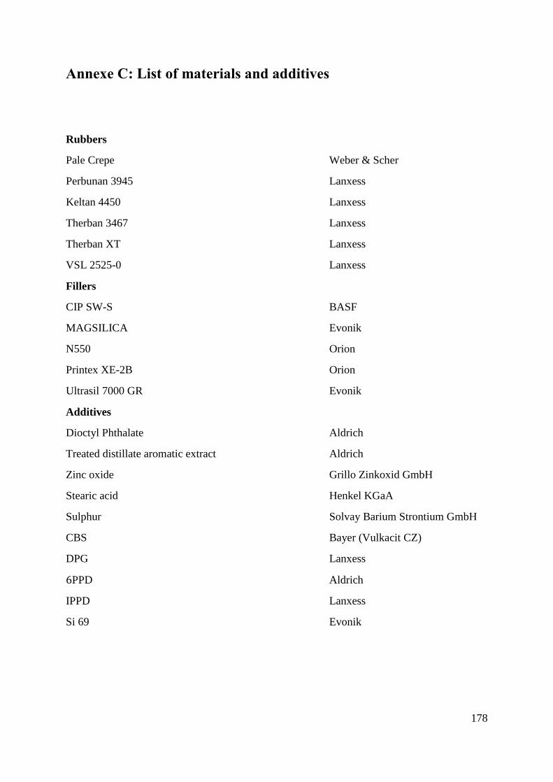
178

Annexe C: List of materials and additives

Rubbers

Pale Crepe Weber & Scher

Perbunan 3945 Lanxess

Keltan 4450 Lanxess

Therban 3467 Lanxess

Therban XT Lanxess

VSL 2525-0 Lanxess

Fillers

CIP SW-S BASF

MAGSILICA Evonik

N550 Orion

Printex XE-2B Orion

Ultrasil 7000 GR Evonik

Additives

Dioctyl Phthalate Aldrich

Treated distillate aromatic extract Aldrich

Zinc oxide Grillo Zinkoxid GmbH

Stearic acid Henkel KGaA

Sulphur Solvay Barium Strontium GmbH

CBS Bayer (Vulkacit CZ)

DPG Lanxess

6PPD Aldrich

IPPD Lanxess

Si 69 Evonik

179

Annexe D: Curriculum vitae

Name: Sahbi Aloui

Born on 24 Juni 1980 in Menzel Bourguiba, Tunisia

Professional experience

11.2017 - Netzsch Gabo Instruments GmbH

Application engineer

07.2012 – 06.2017 German Institute of Rubber Technology e. V. (DIK)

Research associate

Education

10.2014- Gottfried Wilhelm Leibniz University Hannover

Institute of Physical Chemistry and Electrochemistry

Target degree: Doctor of Natural Sciences (Dr. rer. nat.)

Dissertation: Preparation, Characterisation and Micromechanical

Modelling of Magneto-Sensitive Elastomers

10.2006 – 04.2011 Gottfried Wilhelm Leibniz University Hannover

Institute of Theoretical Physics

Degree: Diploma in Physics (Dipl.-Phys.)

Diploma thesis: Creation of Non-Abelian Gauge Potential in Ultracold

Quantum Gases

09.1998 – 06.2002 Ecole supérieure des sciences économiques et commerciales in Tunisia

Degree: „Maîtrise“ in Economics

Thesis: Functioning of a Trading Room

180

Annexe E: List of publications and conference contributions

Publications

1. S. Aloui, M. Klüppel, Magneto-rheological response of elastomer composites with

hybrid-magnetic fillers, Smart mater. Struct., 24, 2015, 025016

2. M. Klüppel, S. Aloui, Optimization of mechanical properties of magneto-sensitive

elastomers by applying hybrid-magnetic fillers, Constitutive Models for Rubber IX,

Marvalova & Petrikova (Eds), Taylor & Francis Group London, 2015, ISBN 978-1-

138-02873-9, pp. 633-638

3. S. Aloui, M. Klüppel, Effect of Particles Orientation on Dynamic-Mechanical

Response and Switching-Ability of Magneto-Sensitive Elastomers, Current smart

mater., 3, 2018, pp. 1-10

Conference contributions: Presentations

1. Sahbi Aloui, Manfred Klüppel, Introduction to magnetorheological response of

elastomers, Materiakonzepte und Modellierung Seminar Hannover (2013)

2. Sahbi Aloui, Manfred Klüppel, Magnetorheological response of elastomers: technical

basis, DIK Kolloquim Hannover (2013)

3. Sahbi Aloui, Manfred Klüppel, Introduction to magneto-sensitive elastomers,

Internationales ECEMP Kolloquium Dresden (2014)

4. Sahbi Aloui, Manfred Klüppel, Magneto-sensitive elastomers based on magnetic filler

hybrid systems, 11. Kautschuk Herbst Kolloquium (KHK) Hannover (2014)

5. Sahbi Aloui, Manfred Klüppel, Magneto-sensitive elastomers, Deutsche Physikalische

Gesellschaft (DPG) Frühjahrestagung Berlin (2015)

6. Sahbi Aloui, Manfred Klüppel, Magnetorheological elastomers for sensor

applications, 35. Mitgliederversammlung Deutsche Kautschuk Gesellschaft (DKG)

Hannover (2016)

7. Sahbi Aloui, Manfred Klüppel, Preparation and properties of magneto-sensitive

elastomers, European PhD Rubber Seminar Hannover (2016)

Conference contributions: Posters

1. Sahbi Aloui, Manfred Klüppel, Smart elastomers based on magneto-sensitive filler

systems, Zentrum für Festkörperchemie und neue Materialien, Summer school

Hannover „Energy Materials“ (2014)

2. Sahbi Aloui, Manfred Klüppel, Magneto-Sensitive Elastomers for Adaptive Vibration

Control Systems, DKT Nürnberg (2015)

181

3. Sahbi Aloui, Manfred Klüppel, Magnetorheological Elastomers for Adaptive Vibration

Control Systems, “Iron in functional materials” Symposium Hannover (2016)

Herstellung, Charakterisierung und mikromechanische ...

Documents

Transcript of Herstellung, Charakterisierung und mikromechanische ...