HIGHER MOMENTS RISK AND THE CROSS-SECTION OF STOCK RETURNS …
47
HIGHER MOMENTS RISK AND THE CROSS-SECTION OF STOCK RETURNS Garazi Elorza Iglesias Trabajo de investigación 016/007 Master en Banca y Finanzas Cuantitativas Tutores: Dr. Alfonso Novales Universidad Complutense de Madrid Universidad del País Vasco Universidad de Valencia Universidad de Castilla-La Mancha www.finanzascuantitativas.com
Transcript of HIGHER MOMENTS RISK AND THE CROSS-SECTION OF STOCK RETURNS …
HIGHER MOMENTS RISK AND THE CROSS-SECTION OF STOCK RETURNS
Garazi Elorza Iglesias
Trabajo de investigación 016/007
Master en Banca y Finanzas Cuantitativas
Tutores: Dr. Alfonso Novales
Universidad Complutense de Madrid
Universidad del País Vasco
Universidad de Valencia
Universidad de Castilla-La Mancha
www.finanzascuantitativas.com

Higher moments risk and
the cross-section of stock returns
Garazi Elorza
Director: Alfonso Novales
Master en Banca y Finanzas Cuantitativas
Madrid
Contents
1 Introduction 4
2 Data 6
3 The analytical framework 6
4 Market moments innovations 8
4.1 Estimation of higher moments . . . . . . . . . . . . . . . . . . . . . . . . . . . . . . 8
4.1.1 GARCHSK . . . . . . . . . . . . . . . . . . . . . . . . . . . . . . . . . . . . 9
4.1.2 NAGARCHSK . . . . . . . . . . . . . . . . . . . . . . . . . . . . . . . . . . 9
4.2 Innovations in market moments . . . . . . . . . . . . . . . . . . . . . . . . . . . . . 12
5 Portfolios sorted on market moments 15
5.1 Portfolios sorted on market volatility exposure . . . . . . . . . . . . . . . . . . . . 15
5.2 Portfolios sorted on market skewness exposure . . . . . . . . . . . . . . . . . . . . 17
5.3 Portfolios sorted on market kurtosis exposure . . . . . . . . . . . . . . . . . . . . . 18
5.4 NAGARCHSK model . . . . . . . . . . . . . . . . . . . . . . . . . . . . . . . . . . 21
5.5 Results on subperiods . . . . . . . . . . . . . . . . . . . . . . . . . . . . . . . . . . 21
5.6 Using rolling window . . . . . . . . . . . . . . . . . . . . . . . . . . . . . . . . . . . 22
6 Factor portfolios 23
7 Exploring the risk premiums 26
7.1 Fama and MacBeth regressions on the 81 factor portfolios . . . . . . . . . . . . . . 27
7.2 Fama and MacBeth regressions on the other portfolios . . . . . . . . . . . . . . . . 30
7.3 Interpreting the sign of the price of market moments risk . . . . . . . . . . . . . . 30
8 Sorting stock returns on different moments 33
9 Conclusion 35
A Appendix 1 38
B Appendix 2 39
B.1 Autocorrelation functions of market moments with GARCHSK . . . . . . . . . . . 39
C Appendix 3 40
C.1 Results for 10 portfolios . . . . . . . . . . . . . . . . . . . . . . . . . . . . . . . . . 40
2

D Appendix 4 41
D.1 Results for NAGARCHSK model . . . . . . . . . . . . . . . . . . . . . . . . . . . . 41
E Appendix 5 43
E.1 Results for rolling window . . . . . . . . . . . . . . . . . . . . . . . . . . . . . . . . 43
3
4
1 Introduction
It is well known that excess kurtosis and negative skewness are standard characteristics of the
stock return distributions. So it seems natural to take them into the account in asset pricing. The
presence of the excess kurtosis in an index means that the market gives more probability to extreme
observations than in normal distribution. Meanwhile, the appearance of negative skewness has the
effect of highlighting the left tail of the distribution. In that case, market gives higher probability
to decreases than increases in asset pricing.
It is by now well accepted that market skewness and kurtosis are important indicators of market
risk, so the goal of this thesis is twofold: i) to analyze whether market skewness and kurtosis risks
affect to the cross-section of stock returns, ii) to examine whether individual skewness and kurtosis
are priced in the market. We use daily closing prices from the Eurostoxx market for which, to the
best of our knoweledge, this analysis has not been done.
The estimation method for higher moments is based on Gram-Charlier series expansion of the
normal density function for the error term, as in Leon et al. (2004), where GARCH-type models
are used allowing for time-varying volatility, skewness and kurtosis. These authors find a significant
presence of conditional skewness and kurtosis in daily returns of stock indices and exchange rates.
We use a different estimation method for individual stocks, because estimating the parameters
of the Exponentially weighted moving average or GARCH models for each stock has a high compu-
tational cost. Thus, we decide to calculate higher moments series for each stock as in RiskMetrics
imposing a parameter λ = 0.94 for all the cases.
Nevertheless, there are many methods for calculating higher moments. For example, recent
studies by Chang et al. (2011) and Bams et al. (2015) show that such moments could be calculated
using out-of-the-money European call and put options prices. High-frequency returns of a single
day can also be used to compute the moments in a particular day as in Amaya et al. (2015). We
could use the traditional technique of rolling window of daily returns.
We perform two types of empirical exercises to analyze if market higher moments risks affect to
stocks’ risk premium. First, we sort all stocks in Eurostoxx from 2000 to 2016 in quintiles based on
their exposure of their returns to each moment’s innovation, as in Chang et al. (2011) and Bams
et al. (2015). These authors find that in down-markets, when investors are more risk-averse, the
market volatility risk is priced significantly negative, while the effect disappears in up-markets. As
for higher moments risk premium, skewness and kurtosis, they conclude that the risk premium for
these moments are significantly negative and positive, respectively, but only when the investors
risk aversion is low.
Similar results can be seen in Chang et al. (2011), where they also show that stocks with high
exposure to innovations in market skewness have low returns on average. Nonetheless, the results
are weaker for volatility and kurtosis, where stocks with high exposure in market volatility and

5
kurtosis exhibit somewhat lower and higher returns on average, respectively.
We can find in the literature different techniques for portfolio construction: either equal-
weighted portfolios, which are portfolios where all the stocks have the same weight, or value-
weighted portfolios that are constructed according to the value they have in relation to the total of
the portfolio. We use equal-weighted portfolios, and we find some evidence that market volatility
is priced in the cross section of stocks, where stocks with high exposure to innovations in market
volatility risk exhibit low returns on average. The results for market skewness and kurtosis are
not so clear, but they show that the stocks with high exposure to these moments exhibit higher
returns on average.
Therefore, factor portfolios for market volatility, skewness and kurtosis risk are constructed.
For that, firstly, all stocks of Eurostoxx are sorted in terciles based on their exposure of their
returns to innovations in either market moment (index return, volatility, skewness and kurtosis)
and then these 12 groups are combined. We obtain that the average return on the market skewness
and kurtosis risk factor portfolio are −0.10% and −0.08% per month, respectively, or −1.20% and
−0, 98% per year.
As a second approach, the prices of the market moment risks are also estimated, using Fama
and MacBeth regressions as in Fama and MacBeth (1973). This two-step estimation approach is
very popular. Amaya et al. (2015) use it to determine the significance on the cross-section of the
stock returns of each market high moment individually and jointly.
Chang et al. (2011) use this methodology to estimate the price of market high moments risks.
As in that work, we study whether market higher moments risks affect to the cross-section of stock
returns and we use Fama and MacBeth methodology for calculating risk premiums. We find that
the estimates of the premium for market volatility and kurtosis risk are negative and for market
skewness risk is positive.
The remainder of the work is organized as follows. In section 2 the data is discussed. In
section 3 the models used for computing the market moments’ risk premia are discussed. Section
4 presents the methods used to extract higher moments from Eurostoxx index returns, as well
as the extraction of the innovations. In section 5, there are presented the results for the stocks
that are sorted into quintiles based on their exposure to innovations in market moments. Section
6 constructs factor portfolios and in section 7 estimates the price of market moments risk using
Fama and MacBeth regressions. Section 8 presents the results for portfolios sorted on realized
moments. Section 9 concludes.

6
2 Data
We use individual stocks from Eurostoxx which is a stock index of the Eurozone and it is com-
pounded by 293 important firms. The data set includes daily closing prices from January 3, 2000
to April 7, 2016. If these period is considered there are just 203 companies because some of them
are newer and enter in the index later. We also need the Eurostoxx index prices and they are
obtained from DataStream, as well as the stocks data. The factor mimicking portfolio returns
for size, book-to-market and momentum factors are obtained from the online data library of Ken
French which can be found at http://mba.tuck.dartmouth.edu/pages/faculty/ken.french/
data_library.html.
On the other hand, we also need the return of the risk-free asset, which is considered German
10-year bond and it is also obtained from Datastream.
The study is going to focus on stock returns rather than with prices, so given a series of
asset prices P0, P1, · · · , PT continuously compounded returns for period t are defined as Rt =
ln(Pt/Pt−1), t = 1, 2, . . . , T .
3 The analytical framework
In this study, there are certain risk factors, which are market higher moments, namely volatility,
skewness and kurtosis and the goal is to study empirically their effect to the cross section of
stock returns. We use two strategies to investigate this and we use a multifactor representation of
equilibrium returns, with the moments of the market return as state variables.
The first strategy is based on univariate sorting. The factors are moments of market return.
So if we use a sample of returns and moments for a period t = 1, 2, . . . , T , the model is defined as:
Rit−Rf,t = βi0 +βi,MKT (Rm,t−Rf,t) +βi,∆V ol∆V olt+βi,∆Skew∆Skewt+βi,∆Kurt∆Kurtt+ εit
(3.1)
where Rit is the ith risky asset return, Rf,t is the return of the risk-free asset and Rm,t the market
portfolio return. Furthermore, ∆V olt = V olt − Et−1[V olt], ∆Skewt = Skewt − Et−1[Skewt] and
∆Kurtt = Kurtt − Et−1[Kurtt]. The coefficients βi,MKT , βi,∆V ol, βi,∆Skew and βi,∆Kurt are the
sensibilities or the measures of the ith risky asset’s exposures to market excess return, market
volatility, market skewness and market kurtosis risks, respectively. We also assume that εit is
homokedastic and independent of Rm,t −Rf,t, ∆V ol, ∆Skew and ∆Kurt.
There are different methods for the estimation of this model. A known alternative is rolling-
windows, for which a time window has to be selected. With the data we have in the first time
window, the coefficients with Ordinary Least Squares (OLS) method are estimated and then we
7
move the window forwards to obtain the next estimation. There are two ways to use rolling-
windows, overlapping or non-overlapping them. When we use overlapping windows we could arise
the risk of introducing too much autocorrelation, because the same data time and time again is
used. The second option could be useful in order to avoid this problem, but it requires a larger
sample.
To obtain ∆V ol, ∆Skew and ∆Kurt, we need an appropriate structure for the time series
of market moments that previously have been estimated and we can specific them observing the
autocorrelogramas.
During the empirical study we build different portfolios. On the one hand, portfolios sorted
on the stock’s exposure to innovations in one of the market moments will be used. However, it is
important to analyze the effects of each factor in pricing, so it would be convenient to study the
implication of each market moment separately. So, we use another different criteria to construct
different portfolios depending on the market moment, but in both cases would be required the
estimates of the regression coefficients, βi,MKT , βi,∆V ol, βi,∆Skew and βi,∆Kurt so 3.1 model will
be used.
The second set of results is based on multivariate sorts and cross-sectional regressions. In this
part, we use the coefficients estimated in the previous equation to estimate the prices of the market
moment risks, λ, from the cross-sectional relation:
Rjt −Rf,t = λ0t + λ∆MKT,tβj,MKT + λ∆V ol,tβj,∆V ol + λ∆Skew,tβj,∆Skew + λ∆Kurt,tβj,∆Kurt + ujt
(3.2)
The objective of this multifactor model is to analyze if the risk factors we are considering
in each model are able to explain the changes in the cross-section of the stocks returns. For
it, the parameters are obtained running Fama and MacBeth regressions, which is a well known
methodology of estimating by OLS in two steps.
Economic theory provides little guidance on the signs of the prices of the market volatility,
skewness and kurtosis risks obtained by this methodology. The volatility matters in the cross sec-
tion of stock returns because this allows investors to hedge against changes in future opportunities.
For instance, if high market volatility today is related with unfavourable investment tomorrow,
then the stock that is related positively to the innovation in market volatility provides a hedge
against a worsening in the investment opportunity set. In addition, previous studies have been
found that when the volatility is high the returns are low. So, it is expected the sign of the price
of market volatility risk to be negative.
However, for the case of the skewness and kurtosis theory does not provide much guidance, due
to the fact that determining the expected sign would be a large empirical exercise. There are works
that said the price of skewness risk is negative, while others conclude the opposite. Therefore, in
this study the expected sign of the volatility risk premium is negative while for the case of skewness
8
and kurtosis it is not clear.
Recent studies by Amaya, Christoffersen, Jacobs and Vasquez (2015) and Chang, Christoffersen
and Jacobs (2011) suggest the following. In the first one the authors determine that the relation
between stock returns and market volatility is positive but statistically not significant. Regarding
to skewness and kurtosis are statistically significant individually and jointly, and the signs are
negative and positive, respectively. Whereas in the second work the results differ slightly. The
authors show that market skewness risk indicate a robustly negative risk premium. However, the
results on market volatility and kurtosis risk are sensitive to variations in empirical setup and
across sample periods.
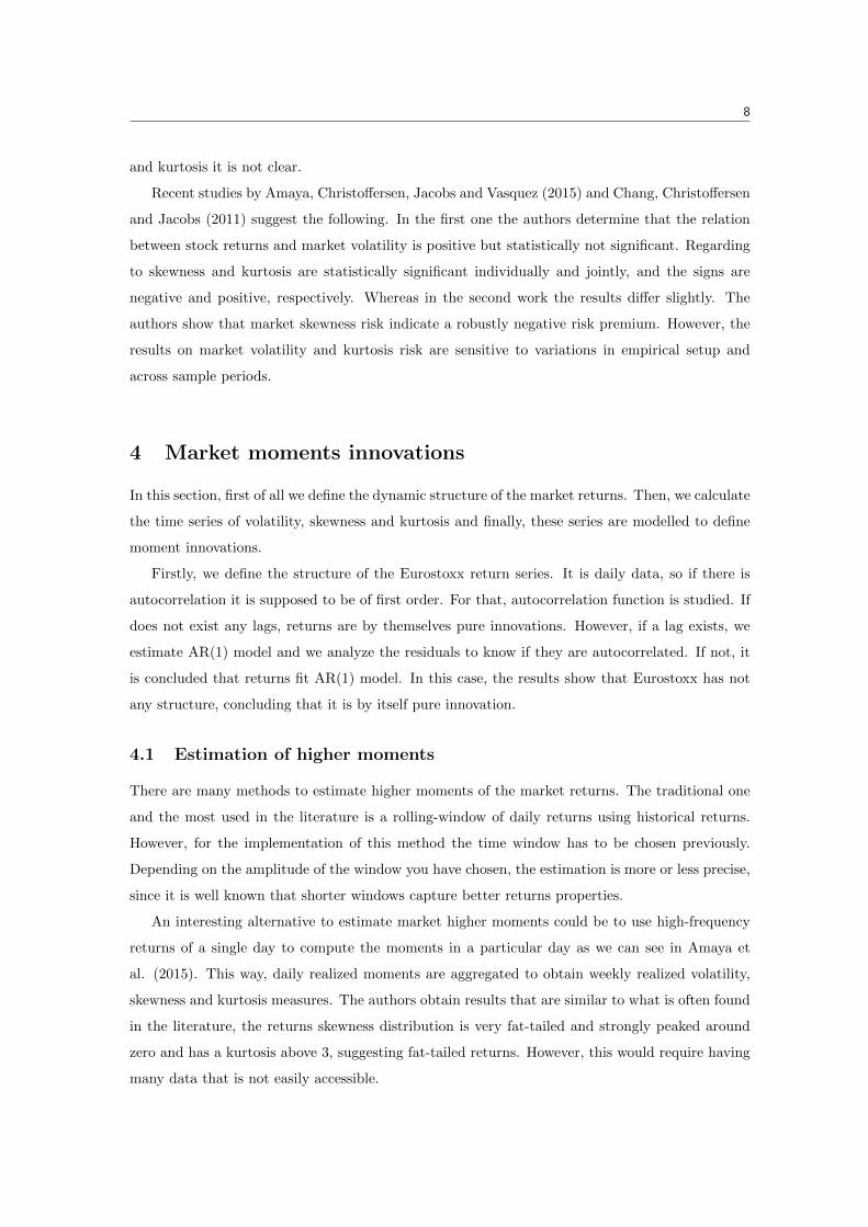
4 Market moments innovations
In this section, first of all we define the dynamic structure of the market returns. Then, we calculate
the time series of volatility, skewness and kurtosis and finally, these series are modelled to define
moment innovations.
Firstly, we define the structure of the Eurostoxx return series. It is daily data, so if there is
autocorrelation it is supposed to be of first order. For that, autocorrelation function is studied. If
does not exist any lags, returns are by themselves pure innovations. However, if a lag exists, we
estimate AR(1) model and we analyze the residuals to know if they are autocorrelated. If not, it
is concluded that returns fit AR(1) model. In this case, the results show that Eurostoxx has not
any structure, concluding that it is by itself pure innovation.
4.1 Estimation of higher moments
There are many methods to estimate higher moments of the market returns. The traditional one
and the most used in the literature is a rolling-window of daily returns using historical returns.
However, for the implementation of this method the time window has to be chosen previously.
Depending on the amplitude of the window you have chosen, the estimation is more or less precise,
since it is well known that shorter windows capture better returns properties.
An interesting alternative to estimate market higher moments could be to use high-frequency
returns of a single day to compute the moments in a particular day as we can see in Amaya et
al. (2015). This way, daily realized moments are aggregated to obtain weekly realized volatility,
skewness and kurtosis measures. The authors obtain results that are similar to what is often found
in the literature, the returns skewness distribution is very fat-tailed and strongly peaked around
zero and has a kurtosis above 3, suggesting fat-tailed returns. However, this would require having
many data that is not easily accessible.

4.1 Estimation of higher moments 9
In our thesis, we use GARCH-type models for the estimation of high moments as we can see
in Leon et al.(2004) work. These models allow for time-varying volatility, skewness and kurtosis
jointly. GARCHSK and NAGARCHSK are the models.
First, we present the models and the estimation procedure.
4.1.1 GARCHSK
This model resembles the model known as GARCH(1,1), but it also takes into account the con-
ditional skewness and kurtosis. These moments are calculated as the conditional variance, by the
GARCH(1,1) structure, but instead of using returns residuals, we need standardized residuals. The
model is defined as
rt = Et−1[rt] + εt where εt ∼ (0, σ2ε )
εt = h1/2t ηt; ηt ∼ (0, 1); εt | It−1 ∼ (0, ht)
ht = β0 + β1ε2t−1 + β2ht−1
st = γ0 + γ1η3t−1 + γ2st−1
kt = δ0 + δ1η4t−1 + δ2kt−1
where Et−1[ηt] = 0, Et−1[η2t ] = 1, Et−1[η3
t ] = st and Et−1[η4t ] = kt. ηt are standardized residuals
and Et−1[•] denotes the conditional expectation on an information set up to period t− 1.
4.1.2 NAGARCHSK
This model is very similar to the previous one, but presents an added difficulty at the time making
an estimation, as there is one additional parameter and when estimating eight or nine parameters
the difference is significative. It is defined as
rt = Et−1[rt] + εt where εt ∼ (0, σ2ε )
εt = h1/2t ηt; ηt ∼ (0, 1); εt | It−1 ∼ (0, ht)
ht = β0 + β1(εt−1 + β3h1/2t−1)2 + β2ht−1
st = γ0 + γ1η3t−1 + γ2st−1
kt = δ0 + δ1η4t−1 + δ2kt−1
where Et−1[ηt] = 0, Et−1[η2t ] = 1, Et−1[η3
t ] = st and Et−1[η4t ] = kt. ηt are standardized residuals
and Et−1[•] denotes the conditional expectation on an information set up to period t− 1.
Next, we study how these two models are estimated. First of all, we need an appropriate
structure for the market returns, so we observe the autocorrelogramas. Once we have the structure

4.1 Estimation of higher moments 10
of the market returns, we have to estimate the parameters, and it is assumed that the distribution
is based on a Gram-Charlier series expansion since we are considering skewness and kurtosis.
Using a Gram-Charlier series expansion of the normal density function and truncating at
the forth moment, we obtain the following density function for the standardized residuals, ηt,
conditional on the information available in t− 1:
g(ηt | It−1) =1√2πe−
η2
2
[1 +
st3!
(η3t − 3ηt) +
kt − 3
4!(η4t − 6η2
t + 3)
]= φ(ηt)ψ(ηt)
where φ(•) denotes the density function of the standard normal distribution.
However, we have to realize that this is not really a density function due to the integral in all R
is not equal to 1. So in Leon et al. (2004) [7] they suggest a new density function and they obtain
f(•), by transforming g(•). See in Appendix A the proof that this function is really a density
function that integrates to one.
f(ηt | It−1) =φ(ηt)ψ
2(ηt)
Γt(4.1)
where
Γt = 1 +s2t
3!+
(kt − 3)2
4!
Thus, this way we have a density function for standardized residuals, ηt, that will be used in
GARCHSK and NAGARCHSK models. Next, we need a likelihood function for the residuals, εt.
It is known that εt = h−1/2t ηt, so the density function is:
g(εt | It−1) = h−1/2f(ηt | It−1) = h−1/2 1
Γtφ(ηt)ψ
2(ηt)
Consequently, the likelihood function is given by:
L =
T∏i=1
g(εt | It−1) = h−T/2t (Γt)
−1φ(ηt)
T(ψ2(ηt)
)TTaking logarithms:
l = lnL = −T2ln(ht)− T ln(Γt) + T ln (φ(ηt)) + T ln
(ψ2(ηt)
)After omitting unessential constants, the logarithm of the likelihood function for the conditional
distribution εt is:
l = − ln(ht)
2− ln(Γt)−
η2t
2+ ln
(ψ2(ηt)
)
In fact, this likelihood function is similar to the standard normal case plus two terms where time-
varying skewness and kurtosis are considered. Moreover, note that the density function based on
Gram-Charlier series expansion (4.1) is like the normal density function when st = 0 and kt = 3.

4.1 Estimation of higher moments 11
After using this methodology for the calculation of market higher moments it is expected
to obtain results similar to the literature, heavy-tailed distributions with negative skewness and
kurtosis greater than 3.
To estimate GARCHSK model we impose variance targeting, since thus the number of param-
eters to be estimated is three less, one in the variance equation, another in the skewness and the
last from the kurtosis equation. The method for the variance equation consists in fixing a long
term volatility level (in this case the sample variance) and using its analytical expression, fixing
the constant of the model depending on the variance and the other two parameters, that is,
β0 = σ2(1− β1 − β2) (4.2)
As σ2 it is taken the variance of the whole sample, however, for the initial variance, h0, we use the
first subsample of 180 observations, and begins to extrapolate from the following observation on
181. The changes in the other equations are slightly different, but the idea is the same. For the
first case is,
γ0 = s(1− γ1σ3 − γ2) (4.3)
where s and σ are the long term skewness and standard deviation, respectively. For the kurtosis
the change is,
δ0 = k(1− δ1σ4 − δ2) (4.4)
where k and σ are long term kurtosis and standard deviation. To initiate these time series has
been used the same procedure as in the variance equation. The first value is calculated using 180
observations and then begins to extrapolate from the following observation on 181. The results for
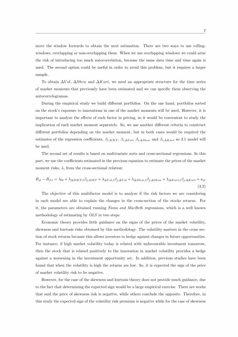
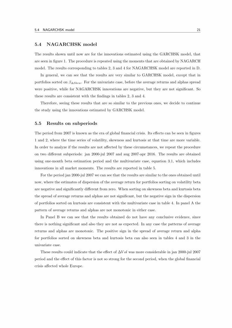
this model are shown in figure 1.
All three time series vary significantly through time, and specially at the beginning, in 2001
and around 2007. The period between 1997 and 2000 is known as the era of dot-com bubble or
Internet bubble. During this years, there was a strong growth of economic values of firms related
to Internet, causing a strong economic bubble that took to bankruptcy to a lot of companies. In
2001 the bubble went deflating rapidly, most of the firms stopped their activities when as there
were no profits and there was no source of investment available. This could be the reason for the
increases in volatility, skewness and kurtosis that can be seen in figure 1.
The changes observed around 2007 could be caused by the global financial crisis that started
in that year. It started by the collapse of the housing bubble in the United States in 2006, and
still continues in many countries.
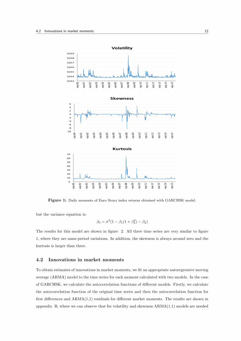
To continue, we estimate the second model, NAGARCHSK. In this model, we also impose
the condition of variance targeting, since otherwise the number of parameters to estimate would
increase considerably. For that, we use the equations (4.3) and (4.4) for skewness and kurtosis,
4.2 Innovations in market moments 12
0,013
0,014
0,015
0,016
0,017
0,018
0,019
sep-‐00
sep-‐01
sep-‐02
sep-‐03
sep-‐04
sep-‐05
sep-‐06
sep-‐07
sep-‐08
sep-‐09
sep-‐10
sep-‐11
sep-‐12
sep-‐13
sep-‐14
sep-‐15
Volatility
-‐10
-‐8
-‐6
-‐4
-‐2
0
2
4
6
sep-‐00
sep-‐01
sep-‐02
sep-‐03
sep-‐04
sep-‐05
sep-‐06
sep-‐07
sep-‐08
sep-‐09
sep-‐10
sep-‐11
sep-‐12
sep-‐13
sep-‐14
sep-‐15
Skewness
0
10
20
30
40
50
60
70
sep-‐00
sep-‐01
sep-‐02
sep-‐03
sep-‐04
sep-‐05
sep-‐06
sep-‐07
sep-‐08
sep-‐09
sep-‐10
sep-‐11
sep-‐12
sep-‐13
sep-‐14
sep-‐15
Kurtosis
Figure 1: Daily moments of Euro Stoxx index returns obtained with GARCHSK model.
but the variance equation is:
β0 = σ2(1− β1(1 + β23)− β2)
The results for this model are shown in figure 2. All three time series are very similar to figure
1, where they are same-period variations. In addition, the skewness is always around zero and the
kurtosis is larger than three.
4.2 Innovations in market moments
To obtain estimates of innovations in market moments, we fit an appropriate autoregressive moving
average (ARMA) model to the time series for each moment calculated with two models. In the case
of GARCHSK, we calculate the autocorrelation functions of different models. Firstly, we calculate
the autocorrelation function of the original time series and then the autocorrelation function for
first differences and ARMA(1,1) residuals for different market moments. The results are shown in
appendix B, where we can observe that for volatility and skewness ARMA(1,1) models are needed

4.2 Innovations in market moments 13
0,012
0,014
0,016
0,018
0,02
0,022
0,024
sep-‐00
sep-‐01
sep-‐02
sep-‐03
sep-‐04
sep-‐05
sep-‐06
sep-‐07
sep-‐08
sep-‐09
sep-‐10
sep-‐11
sep-‐12
sep-‐13
sep-‐14
sep-‐15
Volatility
-‐10
-‐8
-‐6
-‐4
-‐2
0
2
4
6
8
sep-‐00
sep-‐01
sep-‐02
sep-‐03
sep-‐04
sep-‐05
sep-‐06
sep-‐07
sep-‐08
sep-‐09
sep-‐10
sep-‐11
sep-‐12
sep-‐13
sep-‐14
sep-‐15
Skewness
0
10
20
30
40
50
60
sep-‐00
sep-‐01
sep-‐02
sep-‐03
sep-‐04
sep-‐05
sep-‐06
sep-‐07
sep-‐08
sep-‐09
sep-‐10
sep-‐11
sep-‐12
sep-‐13
sep-‐14
sep-‐15
Kurtosis
Figure 2: Daily moments of Euro Stoxx index returns obtained with NAGARCHSK model.
to remove the autocorrelation. However, for the kurtosis, taking the first difference remove most
of the autocorrelation in the data, but ARMA(1,1) is more suitable.
For NAGARCHSK model the results are very similar so they are not reported. The resulting
measures of innovations in market moments are obtained using the following models:
• GARCHSK model:
∆V olt = V olt − 0.002− 0.887V olt−1 + 0.147∆V olt−1 (4.5)
∆Skewt = Skewt + 0.013− 0.908Skewt−1 + 0.050∆Skewt−1 (4.6)
∆Kurtt = Kurtt − 0.312− 0.963Kurtt−1 + 0.026∆Kurtt−1 (4.7)
• NAGARCHSK model:
∆V olt = V olt − 0.003− 0.770V olt−1 + 0.140∆V olt−1 (4.8)

4.2 Innovations in market moments 14
∆Skewt = Skewt + 0.020− 0.802Skewt−1 + 0.019∆Skewt−1 (4.9)
∆Kurtt = Kurtt − 0.242− 0.972Kurtt−1 + 0.067∆Kurtt−1 (4.10)
The innovations of volatility we obtain from these equations are very small in magnitude com-
paring with the innovations of skewness and kurtosis. However, if we analyse the ratio between
the standard deviation of the innovations and the standard deviation of these series (volatility,
skewness and kurtosis), we see that in all three cases the proportion of total variation of outcomes
explained by the model is bigger than 60%. These small volatility innovations take us to estimate
β∆V ol much greater that β∆Skew and β∆Kurt, as we see later.
Once the ARMA(1,1) residuals for V ol, Skew and Kurt are estimated, in table 1 we present
the correlation between them, and also the correlations with Rm − Rf , SMB, HML and MOM
factors. The data for these factors are monthly, so the correlations are calculated with monthly
innovations.
In order to obtain monthly innovations, firstly, we consider the first and the last closing data
in each month and we calculate monthly market returns. Once we have them, we re-estimate
GARCHSK model to obtain time series for volatility, skewness and kurtosis. Then we detect their
structure, which coincide with daily data, ARMA(1,1), and we use the residuals of those.
Table 1: Correlations between monthly innovations for market moments and Rm − Rf , SMB, HML
and MOM factors.
Correlation
Risk factors ∆V ol ∆Skew ∆Kurt
∆V ol 1 -0.90 0.89
∆Skew 1 -0.98
∆Kurt 1
Rm −Rf -0.25 0.27 -0.25
SMB -0.07 0.10 -0.13
HML -0.08 0.08 -0.03
MOM 0.08 -0.11 0.07
In table 1 we can see that the correlation between all factors are very high, so to separate the
effect from one factor on the other, we decide to orthogonalized them. In this way any multicolin-
eality problem is avoided. ∆V ol will leave as it is and ∆Skew and ∆Kurt will be orthogonalized.
So, first we orrthogonalize ∆Skew regressing it on ∆V ol and after we regress ∆Kurt on ∆V ol
15
and ∆Skew. From now, throughout the work we use residuals from these regressions as ∆Skew
and ∆Kurt.
5 Portfolios sorted on market moments
In this section we show three similar empirical exercises. In each case, the stocks are sorted into
quintiles based on their exposure to innovations in market volatility, market skewness and kurtosis.
In this way, we test if stocks with different exposures to innovations in market volatility, skewness
or kurtosis exhibit different returns on average.
Portfolio construction can be done by different opinions. It is frequent to construct according
to market beta, nevertheless, in this study we are going to analyze other relevant factors that are
the higher moments of the market. So we are going to sort portfolios in different ways depending
on all these factors. In each case, we sort the cross-section of stock returns into quintiles based on
the stock’s exposure to innovations in one of the market moments.
Finally, we briefly report some robustness exercises.
5.1 Portfolios sorted on market volatility exposure
First, we construct portfolios based on stocks exposure to ∆V ol and then we compare the average
returns and alphas of these portfolios. To construct the portfolios we use the following equation,
Rit −Rf,t = βi0 + βi,MKT (Rm,t −Rf,t) + βi,∆V ol∆V olt + εit (5.1)
On the other hand, it is also interesting to investigate how different the results are when we consider
∆Skew and ∆Kurt, so in the second specification the model is
Rit−Rf,t = βi0 +βi,MKT (Rm,t−Rf,t) +βi,∆V ol∆V olt+βi,∆Skew∆Skewt+βi,∆Kurt∆Kurtt+ εit
(5.2)
We calculate betas using a non-overlapping one-month window, and because the data is daily
returns, we consider 21 days in a month.
Once we have the betas, the stocks are sorted into quintiles based on the coefficients of the
regression, β∆V ol. Thus, the first quintile contains stocks with the lowest beta, while in the fifth
quintile we find the ones with the highest beta. This way to construct portfolios we can see in
Chang et al. (2011) and Bams et al. (2015). In both works, the authors use one month time
window and the windows are non overlapping.
In this work, there are 203 stocks in total and 5 portfolios, so we decide that quintile 1 and 5
have 40 stocks and 41 rest of them. On the other hand, in Chang et al. (2011), the authors form
value-weighted portfolios using the capitalization of each stock as weighting in the portfolio, but
in this work this information was not available, so the portfolios are equal-weighted.
5.1 Portfolios sorted on market volatility exposure 16
After portfolio formation, we repeat the process for the next month moving the window forward
one month. At the end of the procedure, we obtain time series of daily returns and β∆V ol for each
quintile portfolio.
Then, monthly returns have been calculated and for that we consider the first and the last
closing data of each month. We obtain these information calculating the daily prices of portfolios,
where the price of the portfolio is the sum of the prices of different stocks.
We also compute Jensen’s Alpha using Carhart model, to assess if the effect of volatility persists
after controlling for other well known factors as excess return, size, book-to-market and momentum.
The Carhart four-factor model is an extension of Fama and French model, including Momentum
factor. Fama and French is also an extension of the CAPM, but it includes more common factors
which explain the asset’s expected return better.
Rit−Rf,t = αi0 +βi,MKT (Rm,t−Rf,t) +βi,SMBRSMB,t +βi,HMLRHML,t +βi,MOMRMOM,t + εit
where SMB (Small Minus Big) is the portfolio that replicates the risk factor associated with
the size understood as market capitalization, obtained as the difference between returns of small
market capitalization companies versus returns of big market capitalization companies. HML
(High Minus Low) is also a portfolio that replicates Book-to-Market (BM) 1 factor, and it can
be obtained as the difference between companies with high ratio versus companies with low ratio.
MOM (Momentum) is a factor that reflect the trend in differences between average return of
portfolios of high returns and low returns. In the formation of this variable, the price a year ago
has been considered as well as the fluctuation of the return of the previous month. So Momentum
in a stock is described as the tendency for a stock’s price to continue rising after an increase and
vice versa.
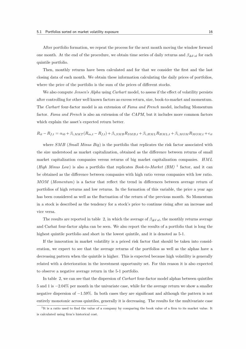
The results are reported in table 2, in which the average of β∆V ol, the monthly returns average
and Carhat four-factor alpha can be seen. We also report the results of a portfolio that is long the
highest quintile portfolio and short in the lowest quintile, and it is denoted as 5-1.
If the innovation in market volatility is a priced risk factor that should be taken into consid-
eration, we expect to see that the average returns of the portfolios as well as the alphas have a
decreasing pattern when the quintile is higher. This is expected because high volatility is generally
related with a deterioration in the investment opportunity set. For this reason it is also expected
to observe a negative average return in the 5-1 portfolio.
In table 2, we can see that the dispersion of Carhart four-factor model alphas between quintiles
5 and 1 is −2.04% per month in the univariate case, while for the average return we show a smaller
negative dispersion of −1.59%. In both cases they are significant and although the pattern is not
entirely monotonic across quintiles, generally it is decreasing. The results for the multivariate case
1It is a ratio used to find the value of a company by comparing the book value of a firm to its market value. It
is calculated using firm’s historical cost.
5.2 Portfolios sorted on market skewness exposure 17
Table 2: Sorting on β∆V ol for GARCHSK model. The table reports the average beta, average monthly
returns for each portfolio in percent and monthly alphas in percent. Univariate is referred to (5.1) and the
multivariate to (5.2). In parentheses the t-statistics are shown and the significant ones are bolded with
90% confidence.
Quintile portfolio
1 2 3 4 5 5-1
Volatility beta (univariate)-146.990
(-16.86)
-48.433
(-17.03)
-3.178
(-3.78)
41.954
(16.25)
137.871
(17.19)
Average return0.39
(0.60)
0.68
(1.43)
0.00
(0.00)
-0.17
(-0.43)
-1.20
(-1.75)
-1.59
(-2.63)
Carhart four-factor alpha0.13
(0.19)
0.13
(0.25)
-0.54
(-1.20)
-0.63
(-1.46)
-1.91
(-2.60)
-2.04
(-3.11)
Volatility beta (multivariate)-7145.4
(-7.06)
-2140.6
(-6.87)
173.9
(2.28)
2443.4
(6.78)
7388.9
(7.34)
Average return0.00
(-0.01)
0.47
(1.01)
-0.07
(-0.15)
-0.24
(-0.51)
-0.34
(-0.52)
-0.34
(-0.56)
Carhart four-factor alpha-0.69
(-1.03)
0.23
(0.44)
-0.73
(-1.39)
-0.76
(-1.51)
-0.86
(-1.30)
-0.17
(-0.24)
are slightly different, since the dispersion of average return and the alphas are also negative, as was
expected, but they are not significant. In addition, the pattern for the alphas is almost monotonic
decreasing across quintiles as well as for the average returns.
In general, some evidence exists about ∆V ol being a price risk factor with a negative price of
risk, but the estimates are significant when ∆Skew and ∆Kurt are not added.
5.2 Portfolios sorted on market skewness exposure
In this subsection the strategy for portfolio construction is the same as for the volatility, except
that stocks are sorted on βSkew. So the regression (5.1) is replaced by the following,
Rit −Rf,t = βi0 + βi,MKT (Rm,t −Rf,t) + βi,∆Skew∆Skewt + εit (5.3)
The results of these portfolios are reported in table 3. The multivariate case is refered to results
obtained by equation (5.2).
The results from table 3 show that the dispersion of the alphas and the average return between
quintiles 5 and 1 are negative for the multivariate case and positive for the univariate. In both
cases they are not significant, but for the univariate case the alpha is significantly different from
zero. Although the average return dispersion is not significant, we can observe that is not zero.
5.3 Portfolios sorted on market kurtosis exposure 18
Table 3: Sorting on β∆Skew for GARCHSK model. The table reports the average beta, average monthly
returns for each portfolio in percent and monthly alphas in percent. Univariate is referred to (5.3) and the
multivariate to (5.2). In parentheses the t-statistics are shown and the significant ones are bolded with
90% confidence.
Quintile portfolio
1 2 3 4 5 5-1
Skewness beta (univariate)-0.336
(-10.86)
-0.106
(-10.18)
0.003
(1.06)
0.113
(10.27)
0.354
(10.14)
Average return-1.03
(-1.57)
0.36
(0.78)
0.17
(0.38)
0.26
(0.61)
-0.13
(-0.20)
0.91
(1.48)
Carhart four-factor alpha-1.74
(-2.47)
-0.17
(-0.35)
-0.35
(-0.70)
-0.07
(-0.16)
-0.53
(-0.80)
1.20
(1.71)
Skewness beta (multivariate)-0.886
(-8.40)
-0.263
(-8.13)
0.025
(3.10)
0.308
(8.33)
0.939
(8.76)
Average return-0.46
(-0.71)
0.18
(0.38)
0.23
(0.59)
0.39
(0.80)
-0.80
(-1.24)
-0.34
(-0.54)
Carhart four-factor alpha-1.20
(-1.71)
-0.36
(-0.67)
-0.14
(-0.33)
-0.09
(-0.17)
-1.23
(-1.85)
-0.03
(-0.04)
The pattern of the returns and alphas across quintiles are not monotonic, because it seem to be
increasing but in the last quintile decrease a lot, specially for the multivariate case.
Overall, it is concluded that little evidence exists that ∆Skew is a priced risk factor.
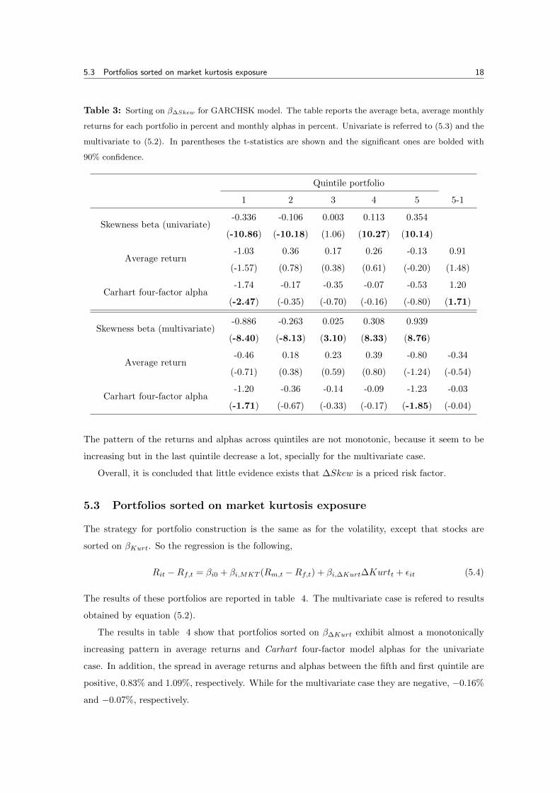
5.3 Portfolios sorted on market kurtosis exposure
The strategy for portfolio construction is the same as for the volatility, except that stocks are
sorted on βKurt. So the regression is the following,
Rit −Rf,t = βi0 + βi,MKT (Rm,t −Rf,t) + βi,∆Kurt∆Kurtt + εit (5.4)
The results of these portfolios are reported in table 4. The multivariate case is refered to results
obtained by equation (5.2).
The results in table 4 show that portfolios sorted on β∆Kurt exhibit almost a monotonically
increasing pattern in average returns and Carhart four-factor model alphas for the univariate
case. In addition, the spread in average returns and alphas between the fifth and first quintile are
positive, 0.83% and 1.09%, respectively. While for the multivariate case they are negative, −0.16%
and −0.07%, respectively.

5.3 Portfolios sorted on market kurtosis exposure 19
Table 4: Sorting on β∆Kurt for GARCHSK model. The table reports the average beta, average monthly
returns for each portfolio in percent and monthly alphas in percent. Univariate is referred to (5.4) and the
multivariate to (5.2). In parentheses are shown the t-statistics and the significant ones are bolded with
90% confidence.
Quintile portfolio
1 2 3 4 5 5-1
Kurtosis beta (univariate)-0.024
(-20.78)
-0.007
(-19.49)
0.001
(3.74)
0.008
(20.33)
0.026
(20.20)
Average return-0.94
(-1.54)
-0.15
(-0.33)
0.34
(0.86)
0.53
(1.23)
-0.11
(-0.15)
0.83
(1.34)
Carhart four-factor alpha-1.65
(-2.52)
-0.57
(-1.22)
-0.14
(-0.35)
0.12
(0.26)
-0.56
(-0.73)
1.09
(1.66)
Kurtosis beta (multivariate)-1.111
(-7.28)
-0.334
(-7.11)
0.026
(2.27)
0.379
(6.97)
1.150
(7.56)
Average return0.01
(0.02)
0.09
(0.17)
0.07
(0.17)
-0.26
(-0.61)
-0.15
(-0.24)
-0.16
(-0.30)
Carhart four-factor alpha-0.61
(-0.98)
-0.36
(-0.57)
-0.43
(-0.96)
-0.73
(-1.66)
-0.68
(-0.99)
-0.07
(-0.11)
In addition, the alpha spread in the univariate case is the only significative one, since for
the spread of average returns are not. However, in spite of the average return spread not being
significant, we can see that it is not equal to zero in the univariate case.
In general, little evidence exist to support that ∆Kurt is a priced risk factor.
Comparing the results in tables 2, 3 and 4, the exposure to volatility risk seems quantitatively
larger than the exposure to skewness and kurtosis risk.
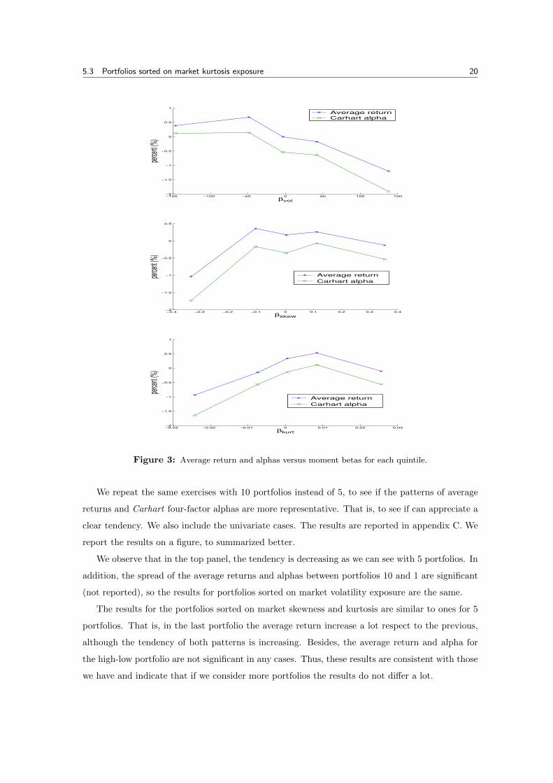
The results from tables 2, 3 and 4 are summarized in figure 3. There, it is only the univariate
case where the average monthly returns and the monthly alphas of each portfolio are on the vertical
axis and the monthly betas in the horizontal axis. The top panel shows the results for the quintiles
that are sorted on ∆V ol, the middle panel portfolios sorted on ∆Skew and the bottom panel shows
the results for the portfolios sorted on ∆Kurt.
The figure 3 exhibits that the results for volatility are stronger than for skewness and kurtosis,
due to the fact that in the top panel the results are as expected and in the others the pattern is
no monotonic.
In these empirical exercises, we decide to have 5 portfolios to continue with Chang et al. (2011)
work, but we know that if we consider more portfolios the pattern of the average returns and
alphas could be more representative or accurate.
5.3 Portfolios sorted on market kurtosis exposure 20
−150 −100 −50 0 50 100 150−2
−1.5
−1
−0.5
0
0.5
1
βvol
perce
nt (%
)
Average return
Carhart alpha
−0.4 −0.3 −0.2 −0.1 0 0.1 0.2 0.3 0.4−2
−1.5
−1
−0.5
0
0.5
βskew
perce
nt (%
)
Average return
Carhart alpha
−0.03 −0.02 −0.01 0 0.01 0.02 0.03−2
−1.5
−1
−0.5
0
0.5
1
βkurt
perce
nt (%
)
Average return
Carhart alpha
Figure 3: Average return and alphas versus moment betas for each quintile.
We repeat the same exercises with 10 portfolios instead of 5, to see if the patterns of average
returns and Carhart four-factor alphas are more representative. That is, to see if can appreciate a
clear tendency. We also include the univariate cases. The results are reported in appendix C. We
report the results on a figure, to summarized better.
We observe that in the top panel, the tendency is decreasing as we can see with 5 portfolios. In
addition, the spread of the average returns and alphas between portfolios 10 and 1 are significant
(not reported), so the results for portfolios sorted on market volatility exposure are the same.
The results for the portfolios sorted on market skewness and kurtosis are similar to ones for 5
portfolios. That is, in the last portfolio the average return increase a lot respect to the previous,
although the tendency of both patterns is increasing. Besides, the average return and alpha for
the high-low portfolio are not significant in any cases. Thus, these results are consistent with those
we have and indicate that if we consider more portfolios the results do not differ a lot.
5.4 NAGARCHSK model 21
5.4 NAGARCHSK model
The results shown until now are for the innovations estimated using the GARCHSK model, that
are seen in figure 1. The procedure is repeated using the moments that are obtained by NAGARCH
model. The results corresponding to tables 2, 3 and 4 for NAGARCHSK model are reported in D.
In general, we can see that the results are very similar to GARCHSK model, except that in
portfolios sorted on β∆Skew. For the univariate case, before the average returns and alphas spread
were positive, while for NAGARCHSK innovations are negative, but they are not significant. So
these results are consistent with the findings in tables 2, 3 and 4.
Therefore, seeing these results that are so similar to the previous ones, we decide to continue
the study using the innovations estimated by GARCHSK model.
5.5 Results on subperiods
The period from 2007 is known as the era of global financial crisis. Its effects can be seen in figures
1 and 2, where the time series of volatility, skewness and kurtosis at that time are more variable.
In order to analyze if the results are not affected by these circumstances, we repeat the procedure
on two different subperiods: jan 2000-jul 2007 and aug 2007-apr 2016. The results are obtained
using one-month beta estimation period and the multivariate case, equation 3.1, which includes
innovations in all market moments. The results are reported in table 5.
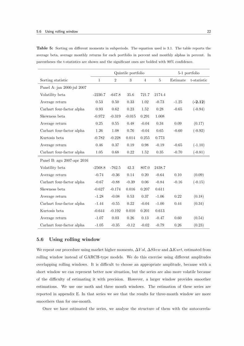
For the period jan 2000-jul 2007 we can see that the results are similar to the ones obtained until
now, where the estimates of dispersion of the average return for portfolios sorting on volatility beta
are negative and significantly different from zero. When sorting on skewness beta and kurtosis beta
the spread of average returns and alphas are not significant, but the negative sign in the dispersion
of portfolios sorted on kurtosis are consistent with the multivariate case in table 4. In panel A the
pattern of average returns and alphas are not monotonic in either case.
In Panel B we can see that the results obtained do not have any conclusive evidence, since
there is nothing significant and also they are not as expected. In any case the patterns of average
returns and alphas are monotonic. The positive sign in the spread of average return and alpha
for portfolios sorted on skewness beta and kurtosis beta can also seen in tables 4 and 3 in the
univariate case.
These results could indicate that the effect of ∆V ol was more considerable in jan 2000-jul 2007
period and the effect of this factor is not so strong for the second period, when the global financial
crisis affected whole Europe.
5.6 Using rolling window 22
Table 5: Sorting on different moments in subperiods. The equation used is 3.1. The table reports the
average beta, average monthly returns for each portfolio in percent and monthly alphas in percent. In
parentheses the t-statistics are shown and the significant ones are bolded with 90% confidence.
Quintile portfolio 5-1 portfolio
Sorting statistic 1 2 3 4 5 Estimate t-statistic
Panel A: jan 2000-jul 2007
Volatility beta -2230.7 -647.8 35.6 721.7 2174.4
Average return 0.53 0.50 0.33 1.02 -0.73 -1.25 (-2.12)
Carhart four-factor alpha 0.93 0.62 0.23 1.52 0.28 -0.65 (-0.94)
Skewness beta -0.972 -0.319 -0.015 0.291 1.008
Average return 0.25 0.55 0.48 -0.04 0.34 0.09 (0.17)
Carhart four-factor alpha 1.26 1.08 0.76 -0.04 0.65 -0.60 (-0.92)
Kurtosis beta -0.782 -0.228 0.014 0.255 0.773
Average return 0.46 0.37 0.19 0.98 -0.19 -0.65 (-1.10)
Carhart four-factor alpha 1.05 0.68 0.22 1.52 0.35 -0.70 (-0.81)
Panel B: agu 2007-apr 2016
Volatility beta -2568.8 -762.5 42.3 807.0 2438.7
Average return -0.74 -0.36 0.14 0.20 -0.64 0.10 (0.09)
Carhart four-factor alpha -0.67 -0.88 -0.39 0.06 -0.84 -0.16 (-0.15)
Skewness beta -0.627 -0.174 0.016 0.207 0.611
Average return -1.28 -0.08 0.53 0.37 -1.06 0.22 (0.18)
Carhart four-factor alpha -1.44 -0.55 0.22 -0.04 -1.00 0.44 (0.34)
Kurtosis beta -0.644 -0.192 0.010 0.201 0.613
Average return -1.07 0.03 0.26 0.13 -0.47 0.60 (0.54)
Carhart four-factor alpha -1.05 -0.35 -0.12 -0.02 -0.79 0.26 (0.23)
5.6 Using rolling window
We repeat our procedure using market higher moments, ∆V ol, ∆Skew and ∆Kurt, estimated from
rolling window instead of GARCH-type models. We do this exercise using different amplitudes
overlapping rolling windows. It is difficult to choose an appropriate amplitude, because with a
short window we can represent better now situation, but the series are also more volatile because
of the difficulty of estimating it with precision. However, a larger window provides smoother
estimations. We use one moth and three month windows. The estimation of these series are
reported in appendix E. In that series we see that the results for three-month window are more
smoothers than for one-month.
Once we have estimated the series, we analyse the structure of them with the autocorrela-
23
tion functions, where we see that for the estimates of one-month windows all the moments fit
to ARMA(1,1) model. But for the estimates of three-month windows, for volatility ARMA(1,1)
model is needed to remove the autocorrelation, while for the skewness and kurtosis, taking the
AR(1) model is enough. We repeat the same procedure of tables 2, 3 and 4 to construct portfolios.
The results are reported in appendix E.
In general, we have not reached any robust conclusions. The signs of average returns and alphas
for the high-low portfolios are the expected, but almost in no case are significant. For portfolios
sorted on βV ol, the results for one or three rolling window do not change. In both cases the patterns
across quintiles are not monotonic, but the tendency is increasing.
For the portfolios sorted on βSkew and βKurt, there is any clear tendency for average returns and
alphas across quintiles, and only the results for three-month window for the kurtosis are significant
with negative signs. Thus, whereas some results are consistent with the findings in tables 2, 3 and
4, such findings are hardly meaningful given the lack of robustness.
6 Factor portfolios
Results from the previous section show the effect of ∆V ol on the cross section of the stock returns
maintained across different sample periods. However, the effect of ∆Kurt when different periods
are considered changed as well as for the ∆Skew effect.
As we can see in Chang et al. (2011), the results obtained until now could be difficult to interpret
because of the correlation between different market moments, so it is important to analyze factors’
implications individually. In addition, it is important to analyze the effects of each factor in pricing,
so it would be convenient to study the implication of each market moment separately.
To this end, we consider another sorting criterion, which depends on the market moment and
that also requires the betas estimated in equation 3.1. At the end of each month, we calculate
betas and construct tercile portfolios based on βMKT , β∆V ol, β∆Skew and β∆Kurt (the lowest in
tercile 1 and the highest in tercile 3). In that way there are 3 portfolios for each risk factors, which
are four, and using the intersection of these four sorting criteria, we construct 81 portfolios. Thus,
in each of the 81 portfolios, there is a tercile of each of the four market moment factors. Therefore,
with all possible combinations we have 81 portfolios.
As in the previous section, there are 203 stocks in total and 3 portfolios, so we decide that tercile
1 and 3 have 68 stocks and 67 the second tercile. On the other hand, in Chang et al. (2011) value-
weighted portfolios are formed using the capitalization of each stock as weighing in the portfolio,
but in this work this information was not available, therefore the portfolios are equal-weighted.
After portfolio formation, we employ the procedure used in section 5 again to obtain the time
series of beta, daily average returns and Carhart four-factor model alphas for each of the 81

24
portfolios. We also calculate monthly returns and for that, we consider the first and the last
closing data of each month. We obtain these information calculating the daily prices of portfolios,
where the price of the portfolio is the sum of the prices of different stocks.
This could be a great amount of information to process, consequently, we make groups to
summarize all details. We construct these groups according to high (H), medium (M) or low (L)
exposure to each of the factors one at a time and averaging over the 27 portfolios in each group.
That is, when we combine the 81 portfolios, each tercile is in 27 of the portfolios. So, to simplify the
results, we construct equal-weighted portfolios with these 27 portfolios. In this way, H portfolios
show the terciles with the stocks with high exposure to a factor, M the terciles with stocks with
medium exposure to a factor and L the ones with low exposure. This method of grouping allows
to differ portfolios in exposure to one factor but are neutral in other factors.
The results are reported in table 6. We also bring out outcomes of H-L portfolios. That
indicates portfolios which are long 27 high exposure portfolios and short 27 low exposure portfolios
with regard to a given factor.
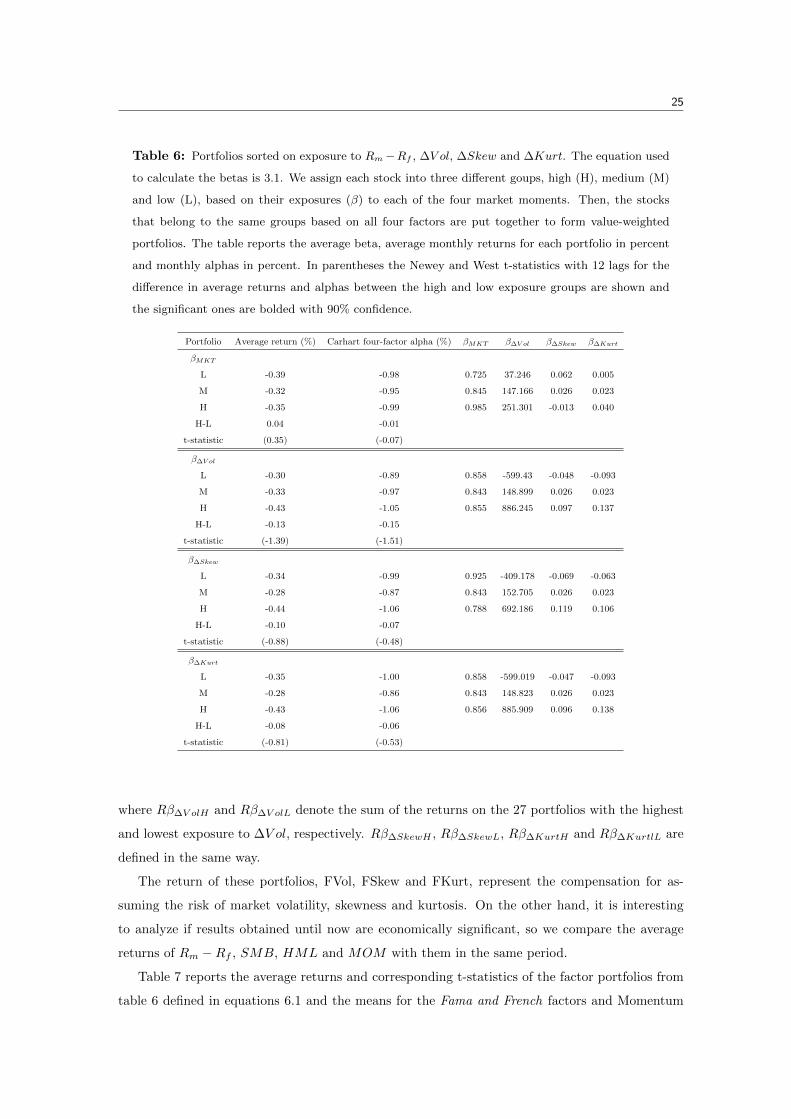
In table 6 we can see that the average return of the β∆V ol high-low portfolio is −0.13% per
month but it is not significantly different from zero, as well as for the monthly alpha. These
results are similar to table 2 where the signs for the alphas and average returns dispersion were
also negative. In addition, the patterns are decreasing, consistent with earlier results.
The estimate of average return and Carhart four-factor model alpha of the β∆Skew and β∆Kurt
high-low portfolios are negatives and not significant in all cases. In addition, no monotonic pattern
is detected in any case, as in earlier results, in all cases they first increase and then decrease.
In these two last cases, the spread in average return and alpha between the high and low
portfolios are negative and not significant in either case, but it could not be deduced that they are
equal to zero, because their value has changed across portfolios.
In summary, these results are quite similar to earlier results observed in tables 2, 3 and 4, where
we see that market higher moments are considered in asset pricing.
Continuing with the work, we use the returns of factor portfolios constructed above as proxies
for risk factors, ∆V ol, ∆Skew and ∆Kurt. So we consider volatility factor portfolio, skewness
factor portfolio and kurtosis factor portfolio. They correspond to the high-low portfolios in table
6 and are defined as follows
FV ol =1
27(Rβ∆V olH −Rβ∆V olL)
FSkew =1
27(Rβ∆SkewH −Rβ∆SkewL) (6.1)
FKurt =1
27(Rβ∆KurtH −Rβ∆KurtL)
25
Table 6: Portfolios sorted on exposure to Rm −Rf , ∆V ol, ∆Skew and ∆Kurt. The equation used
to calculate the betas is 3.1. We assign each stock into three different goups, high (H), medium (M)
and low (L), based on their exposures (β) to each of the four market moments. Then, the stocks
that belong to the same groups based on all four factors are put together to form value-weighted
portfolios. The table reports the average beta, average monthly returns for each portfolio in percent
and monthly alphas in percent. In parentheses the Newey and West t-statistics with 12 lags for the
difference in average returns and alphas between the high and low exposure groups are shown and
the significant ones are bolded with 90% confidence.
Portfolio Average return (%) Carhart four-factor alpha (%) βMKT β∆V ol β∆Skew β∆Kurt
βMKT
L -0.39 -0.98 0.725 37.246 0.062 0.005
M -0.32 -0.95 0.845 147.166 0.026 0.023
H -0.35 -0.99 0.985 251.301 -0.013 0.040
H-L 0.04 -0.01
t-statistic (0.35) (-0.07)
β∆V ol
L -0.30 -0.89 0.858 -599.43 -0.048 -0.093
M -0.33 -0.97 0.843 148.899 0.026 0.023
H -0.43 -1.05 0.855 886.245 0.097 0.137
H-L -0.13 -0.15
t-statistic (-1.39) (-1.51)
β∆Skew
L -0.34 -0.99 0.925 -409.178 -0.069 -0.063
M -0.28 -0.87 0.843 152.705 0.026 0.023
H -0.44 -1.06 0.788 692.186 0.119 0.106
H-L -0.10 -0.07
t-statistic (-0.88) (-0.48)
β∆Kurt
L -0.35 -1.00 0.858 -599.019 -0.047 -0.093
M -0.28 -0.86 0.843 148.823 0.026 0.023
H -0.43 -1.06 0.856 885.909 0.096 0.138
H-L -0.08 -0.06
t-statistic (-0.81) (-0.53)
where Rβ∆V olH and Rβ∆V olL denote the sum of the returns on the 27 portfolios with the highest
and lowest exposure to ∆V ol, respectively. Rβ∆SkewH , Rβ∆SkewL, Rβ∆KurtH and Rβ∆KurtlL are
defined in the same way.
The return of these portfolios, FVol, FSkew and FKurt, represent the compensation for as-
suming the risk of market volatility, skewness and kurtosis. On the other hand, it is interesting
to analyze if results obtained until now are economically significant, so we compare the average
returns of Rm −Rf , SMB, HML and MOM with them in the same period.
Table 7 reports the average returns and corresponding t-statistics of the factor portfolios from
table 6 defined in equations 6.1 and the means for the Fama and French factors and Momentum
26
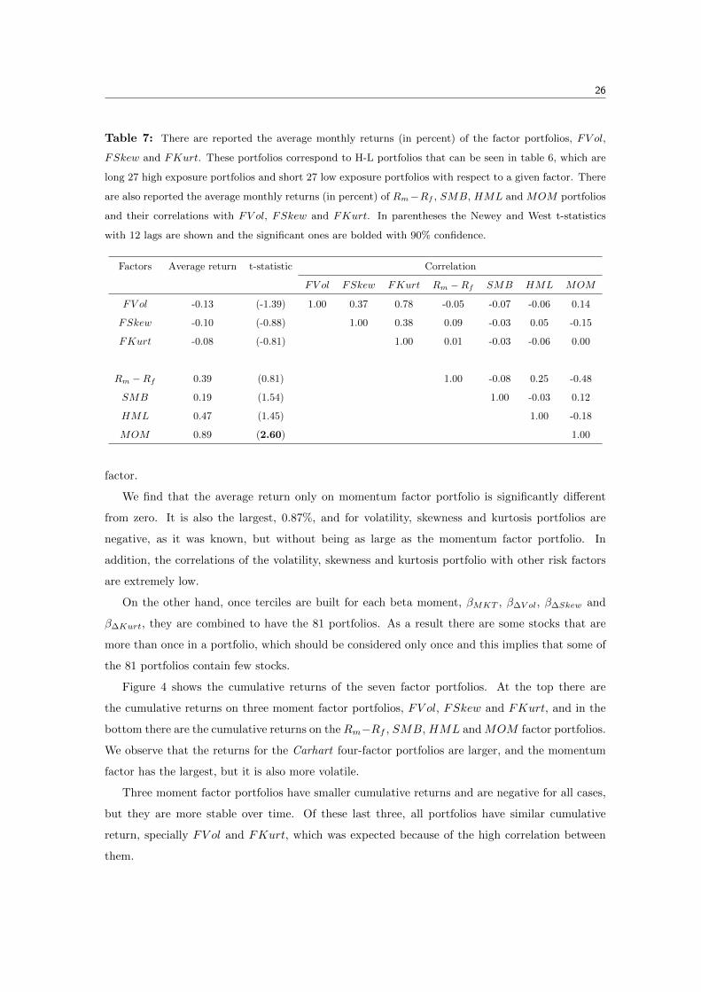
Table 7: There are reported the average monthly returns (in percent) of the factor portfolios, FV ol,
FSkew and FKurt. These portfolios correspond to H-L portfolios that can be seen in table 6, which are
long 27 high exposure portfolios and short 27 low exposure portfolios with respect to a given factor. There
are also reported the average monthly returns (in percent) of Rm−Rf , SMB, HML and MOM portfolios
and their correlations with FV ol, FSkew and FKurt. In parentheses the Newey and West t-statistics
with 12 lags are shown and the significant ones are bolded with 90% confidence.
Factors Average return t-statistic Correlation
FV ol FSkew FKurt Rm −Rf SMB HML MOM
FV ol -0.13 (-1.39) 1.00 0.37 0.78 -0.05 -0.07 -0.06 0.14
FSkew -0.10 (-0.88) 1.00 0.38 0.09 -0.03 0.05 -0.15
FKurt -0.08 (-0.81) 1.00 0.01 -0.03 -0.06 0.00
Rm −Rf 0.39 (0.81) 1.00 -0.08 0.25 -0.48
SMB 0.19 (1.54) 1.00 -0.03 0.12
HML 0.47 (1.45) 1.00 -0.18
MOM 0.89 (2.60) 1.00
factor.
We find that the average return only on momentum factor portfolio is significantly different
from zero. It is also the largest, 0.87%, and for volatility, skewness and kurtosis portfolios are
negative, as it was known, but without being as large as the momentum factor portfolio. In
addition, the correlations of the volatility, skewness and kurtosis portfolio with other risk factors
are extremely low.
On the other hand, once terciles are built for each beta moment, βMKT , β∆V ol, β∆Skew and
β∆Kurt, they are combined to have the 81 portfolios. As a result there are some stocks that are
more than once in a portfolio, which should be considered only once and this implies that some of
the 81 portfolios contain few stocks.
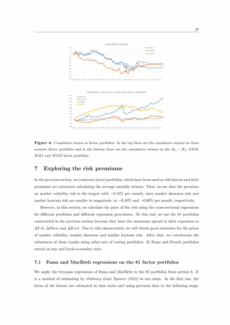
Figure 4 shows the cumulative returns of the seven factor portfolios. At the top there are
the cumulative returns on three moment factor portfolios, FV ol, FSkew and FKurt, and in the
bottom there are the cumulative returns on the Rm−Rf , SMB, HML and MOM factor portfolios.
We observe that the returns for the Carhart four-factor portfolios are larger, and the momentum
factor has the largest, but it is also more volatile.
Three moment factor portfolios have smaller cumulative returns and are negative for all cases,
but they are more stable over time. Of these last three, all portfolios have similar cumulative
return, specially FV ol and FKurt, which was expected because of the high correlation between
them.
27
-‐40
-‐35
-‐30
-‐25
-‐20
-‐15
-‐10
-‐5
0
5
10
jul-‐00 jul-‐01 jul-‐02 jul-‐03 jul-‐04 jul-‐05 jul-‐06 jul-‐07 jul-‐08 jul-‐09 jul-‐10 jul-‐11 jul-‐12 jul-‐13 jul-‐14 jul-‐15
Cumulative returnsFVol
FSkew
FKurt
-‐100
-‐50
0
50
100
150
200
250
300
350
400
jul-‐00 jul-‐01 jul-‐02 jul-‐03 jul-‐04 jul-‐05 jul-‐06 jul-‐07 jul-‐08 jul-‐09 jul-‐10 jul-‐11 jul-‐12 jul-‐13 jul-‐14 jul-‐15
Cumulative returns on Carhart four-‐factor portfolios
MOM
R_m-‐R_f
SMB
HML
Figure 4: Cumulative return on factor portfolios. In the top there are the cumulative returns on three
moment factor portfolios and in the bottom there are the cumulative returns on the Rm − Rf , SMB,
HML and MOM factor portfolios.
7 Exploring the risk premiums
In the previous section, we construct factor portfolios, which have been used as risk factors and their
premiums are estimated calculating the average monthly returns. Thus, we see that the premium
on market volatility risk is the largest with −0.13% per month, since market skewness risk and
market kurtosis risk are smaller in magnitude, at −0.10% and −0.08% per month, respectively.
However, in this section, we calculate the price of the risk using the cross-sectional regressions
for different portfolios and different regression procedures. To this end, we use the 81 portfolios
constructed in the previous section because they have the maximum spread in their exposures to
∆V ol, ∆Skew and ∆Kurt. Due to this characteristic we will obtain good estimates for the prices
of market volatility, market skewness and market kurtosis risk. After that, we corroborate the
robustness of these results using other sets of testing portfolios: 25 Fama and French portfolios
sorted on size and book-to-market ratio.
7.1 Fama and MacBeth regressions on the 81 factor portfolios
We apply the two-pass regressions of Fama and MacBeth to the 81 portfolios from section 6. It
is a method of estimating by Ordinary Least Squares (OLS) in two steps. In the first one, the
betas of the factors are estimated in time series and using previous data to the following stage.

7.1 Fama and MacBeth regressions on the 81 factor portfolios 28
For example, if we consider all factors, in this step the model to estimate is,
Rit −Rf,t = βi0 + βi,MKT (Rm,t −Rf,t) + βi,∆V ol∆V olt + βi,∆Skew∆Skewt + βi,∆Kurt∆Kurtt
+ βi,SMBSMBt + βi,HMLHMLt + βi,MOMMOMt + εit(7.1)
In the second step, a cross-sectional regression is done to explain assets return for every moment
of the time. To do this the betas we have estimated in the previous step are used as regressors.
The model for this second step is defined as,
Rit −Rf,t = λ0t + λMKT,tβi,MKT + λ∆V ol,tβi,∆V ol + λ∆Skew,tβi,∆Skew + λ∆Kurt,tβi,∆Kurt
+ λSMB,tβi,SMB + λHML,tβi,HML + λMOM,tβi,MOM + uit(7.2)
After the second stage, a monthly time series of the price of risk is estimated and the final
estimate is obtained by averaging the series.
We run Fama and MacBeth regressions for different models. We consider Rm − Rf , SMB,
HML, MOM , ∆V ol, ∆Skew and ∆Kurt as factors, but they are combined in different ways. The
factor models considered are (i) CAPM + ∆V ol, (ii) CAPM + ∆Skew, (iii) CAPM + ∆Kurt, (iv)
CAPM + ∆V ol + ∆Skew, (v) CAPM + ∆V ol + ∆Kurt, (vi) CAPM + ∆Skew + ∆Kurt, (vii)
CAPM + ∆V ol + ∆Skew + ∆Kurt, (viii) Carhart four-factor + ∆V ol, (ix) Carhart four-factor
+ ∆Skew, (x) Carhart four-factor + ∆Kurt, (xi) Carhart four-factor + ∆V ol + ∆Skew, (xii)
Carhart four-factor + ∆V ol + ∆Kurt, (xiii) Carhart four-factor + ∆Skew + ∆Kurt and (xiv)
Carhart four-factor + ∆V ol + ∆Skew + ∆Kurt.
We estimate these models differently, because for the SMB, HML and MOM factors, the
data is monthly, whereas the other factors are daily. Therefore, in models where both types of
data are found, first we obtain monthly innovations of market moments.
For this, the GARCHSK model must be re-estimated with monthly market returns. Once we
have obtained the time series of market volatility, skewness and kurtosis, their dynamic structure
has to be detected. In this case, it coincides with daily data, ARMA(1, 1), so we use the residuals
of those.
After that, in the first stage of the method, we calculate the betas using an overlapping rolling
window of 5 years. To finish with, in the second stage, we use those series of beta to estimate
monthly prices of risk.
In the first 7 models, where the factors included are daily data, the estimation differs. In the
first stage, we estimate the betas using non overlapping rolling windows of one month of daily
returns. Thus, we obtain monthly betas and these series are used for monthly estimates of the
price of risk. Then, those are averaged to get the final estimate. The results of Fama and MacBeth
regressions are reported in table 8.
After the estimation, we see that the estimate of the price of market skewness risk, λ∆Skew, is
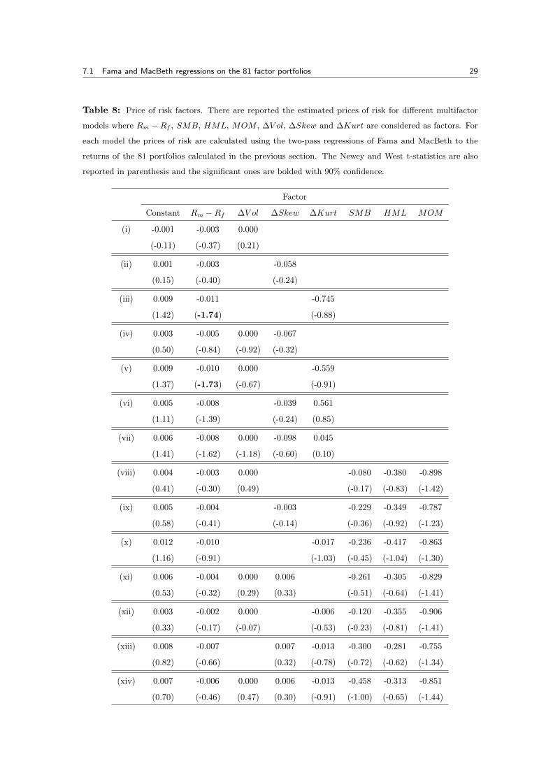
7.1 Fama and MacBeth regressions on the 81 factor portfolios 29
Table 8: Price of risk factors. There are reported the estimated prices of risk for different multifactor
models where Rm − Rf , SMB, HML, MOM , ∆V ol, ∆Skew and ∆Kurt are considered as factors. For
each model the prices of risk are calculated using the two-pass regressions of Fama and MacBeth to the
returns of the 81 portfolios calculated in the previous section. The Newey and West t-statistics are also
reported in parenthesis and the significant ones are bolded with 90% confidence.
Factor
Constant Rm −Rf ∆V ol ∆Skew ∆Kurt SMB HML MOM
(i) -0.001 -0.003 0.000
(-0.11) (-0.37) (0.21)
(ii) 0.001 -0.003 -0.058
(0.15) (-0.40) (-0.24)
(iii) 0.009 -0.011 -0.745
(1.42) (-1.74) (-0.88)
(iv) 0.003 -0.005 0.000 -0.067
(0.50) (-0.84) (-0.92) (-0.32)
(v) 0.009 -0.010 0.000 -0.559
(1.37) (-1.73) (-0.67) (-0.91)
(vi) 0.005 -0.008 -0.039 0.561
(1.11) (-1.39) (-0.24) (0.85)
(vii) 0.006 -0.008 0.000 -0.098 0.045
(1.41) (-1.62) (-1.18) (-0.60) (0.10)
(viii) 0.004 -0.003 0.000 -0.080 -0.380 -0.898
(0.41) (-0.30) (0.49) (-0.17) (-0.83) (-1.42)
(ix) 0.005 -0.004 -0.003 -0.229 -0.349 -0.787
(0.58) (-0.41) (-0.14) (-0.36) (-0.92) (-1.23)
(x) 0.012 -0.010 -0.017 -0.236 -0.417 -0.863
(1.16) (-0.91) (-1.03) (-0.45) (-1.04) (-1.30)
(xi) 0.006 -0.004 0.000 0.006 -0.261 -0.305 -0.829
(0.53) (-0.32) (0.29) (0.33) (-0.51) (-0.64) (-1.41)
(xii) 0.003 -0.002 0.000 -0.006 -0.120 -0.355 -0.906
(0.33) (-0.17) (-0.07) (-0.53) (-0.23) (-0.81) (-1.41)
(xiii) 0.008 -0.007 0.007 -0.013 -0.300 -0.281 -0.755
(0.82) (-0.66) (0.32) (-0.78) (-0.72) (-0.62) (-1.34)
(xiv) 0.007 -0.006 0.000 0.006 -0.013 -0.458 -0.313 -0.851
(0.70) (-0.46) (0.47) (0.30) (-0.91) (-1.00) (-0.65) (-1.44)

7.2 Fama and MacBeth regressions on the other portfolios 30
negative in some models, but it is not significant in any case. The price of market kurtosis risk,
λ∆Kurt, is not significant in none of the models, moreover, in most of the models is negative.
In the case of the estimate of the price of market volatility risk, it is not significant in any
model. But we can see that in all cases the estimate is 0.000 in spite of the t-statistics are not
equal to 0. This implies that the standard deviation of the price of risk are very reduced, so the
estimation precision is very high.
For SMB, HML and MOM factors all price of risk have negative price but they are not
significant.
7.2 Fama and MacBeth regressions on the other portfolios
In this subsection, we check the robustness of the previous section estimates running the same Fama
and MacBeth regression on other portfolios, namely, 25 Fama and French portfolios sorted on size
and book-to-market ratio and distinguished according to value weighted and equal weighted. This
exercise is interesting for analysis, because as said before, some of the 81 portfolios used until now
are composed of few stocks, what can lead to confusing estimations.
In this case, the estimated model is only the last one (xiv), where we consider all factors. The
results for these regressions are reported in table 9. There, in Panel A, we report the results using
5 years’ (60 months) window to calculate the betas, while in Panel B, the betas are calculated
using a 90 months window.
For the 25 portfolios sorted on size and book-to-market, the price of risk estimated are not very
significant. We find that the estimate of λ∆V ol is significantly negative in four cases, consistent
with the results in Chang et al. (2011). In other two cases, it is not significant, but as said before,
although the estimate is small the t-statistic is high, so the estimation precision is very high.
The estimate of the price of skewness is significant when the window is 60 months. In addition,
it is positive, different from most of the models in table 8, where the estimated price was negative,
but they were not significant.
In relation to λ∆Kurt, it is not significant in any case, but we see that the estimate sign is
negative in all cases, consistent with the results in table 8.
The traditional pricing factors such as SMB, HML and MOM are not estimated significantly,
even when we use 25 size and book-to-market portfolios, which should give an advantage to SMB
and HML factors, as they are built considering these factors. So the estimates of the price of risk
for the moment factors must be interpreted carefully.
7.3 Interpreting the sign of the price of market moments risk
In previous works, such as in Chang et al. (2011), the authors find that the price of market volatility
risk is negative, and suggest that an increase in the market volatility indicate a deterioration on

7.3 Interpreting the sign of the price of market moments risk 31
Table 9: Price of risk factors. There are reported the estimated prices of risk for different multifactor
models where Rm −Rf , SMB, HML, MOM , ∆V ol, ∆Skew and ∆Kurt are considered as factors. The
prices of risk are calculated using the two-pass regressions of Fama and MacBeth to the 25 Fama and
French portfolios sorted on size and book-to-market and distinguished according to value weighted (VW)
and equal weighted (EW). In Panel A the λs are estimated by running a time series regression of 5 years
(60 months) of monthly returns and in Panel B, the rolling window is 90 months. The Newey and West
t-statistics are also reported in parenthesis and the significant ones are bolded with 90% confidence.
Price of risk
λMKT λ∆V ol λ∆Skew λ∆Kurt λSMB λHML λMOM
Panel A: 60 months beta
81 portfolios -0.006 0.000 0.006 -0.013 -0.458 -0.313 -0.851
(-0.46) (0.47) (0.30) (-0.91) (-1.00) (-0.65) (-1.44)
25 size and book-to-market 0.006 -0.001 0.083 -0.025 0.234 -0.360 -1.25
portfolios (VW) (0.79) (-2.22) (2.77) (-1.00) (1.48) (-1.08) (-1.83)
25 size and book-to-market 0.011 -0.002 0.063 -0.013 0.152 -0.453 -0.963
portfolios (EW) (0.85) (-2.70) (3.67) (-0.53) (0.91) (-1.16) (-1.33)
Panel B: 90 months beta
81 portfolios -0.004 0.000 -0.009 -0.003 0.167 -0.369 -0.229
(-0.37) (-0.62) (-0.73) (-0.34) (0.64) (-1.10) (-0.84)
25 size and book-to-market 0.006 -0.001 0.031 -0.011 0.121 -0.518 -1.192
portfolios (VW) (0.80) (-1.94) (0.62) (-0.34) (0.56) (-1.03) (-1.56)
25 size and book-to-market 0.019 -0.002 0.035 -0.002 0.072 -0.632 -0.382
portfolios (EW) (1.84) (-2.26) (1.37) (-0.08) (0.33) (-1.07) (-0.76)
the future investment opportunities. Because investors want to hedge against future risks, they
prefer stocks with high return when the market volatility is higher than expected. So it is said
that the price of market volatility risk is negative.
In addition, this negative relation we can see in table 1, where we observe that the correlation
between the market excess and ∆V ol is negative. In addition, during the thesis we observe that in
some cases it seems to be also negative, but in other cases the estimations of the price of market
volatility risk are very small, so the sign is not very well appreciated.
As for the skewness, we observe that the estimation of the price of the market skewness risk
is negative and not significantly different from zero in most of the models. While for 25 Fama
and French portfolios sorted on size and book-to-market the estimation of λ∆Skew is positive and
significant for 60 months window.
However, the first results are not consistent with the table 1, where the correlation between the
7.3 Interpreting the sign of the price of market moments risk 32
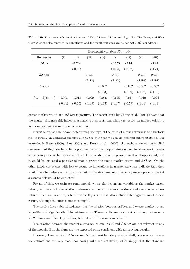
Table 10: Time series relationship between ∆V ol, ∆Skew, ∆Kurt and Rm −Rf . The Newey and West
t-statistics are also reported in parenthesis and the significant ones are bolded with 90% confidence.
Dependent variable: Rm −RfRegressors (i) (ii) (iii) (iv) (v) (vi) (vii) (viii)
∆V ol -3.764 -3.959 -3.74 -3.94
(-0.65) (-0.86) (-0.62) (-0.74)
∆Skew 0.030 0.030 0.030 0.030
(7.82) (7.83) (7.58) (7.54)
∆Kurt -0.002 -0.002 -0.002 -0.002
(-1.13) (-1.09) (-1.02) (-0.96)
Rm −Rf (t− 1) -0.008 -0.012 -0.020 -0.006 -0.025 -0.011 -0.019 -0.024
(-0.41) (-0.65) (-1.20) (-1.13) (-1.47) (-0.59) (-1.21) (-1.41)
excess market return and ∆Skew is positive. The recent work by Chang et al. (2011) shows that
the market skewness risk indicates a negative risk premium, while the results on market volatility
and kurtosis risk are sensitive to variations.
Nevertheless, as said above, determining the sign of the price of market skewness and kurtosis
risk is largely an empirical exercise due to the fact that we can do different interpretations. For
example, in Bates (2000), Pan (2002) and Doran et al. (2007), the authors use option-implied
skewness, but they conclude that a positive innovation in option-implied market skewness indicates
a decreasing risk in the stocks, which would be related to an improved investment opportunity. So
it would be expected a positive relation between the excess market return and ∆Skew. On the
other hand, the stocks with low exposure to innovations in market skewness indicate that they
would have to hedge against downside risk of the stock market. Hence, a positive price of market
skewness risk would be expected.
For all of this, we estimate some models where the dependent variable is the market excess
return, and we check the relation between the market moments residuals and the market excess
return. The results are reported in table 10, where it is also included the lagged market excess
return, although its effect is not meaningful.
The results from table 10 indicate that the relation between ∆Skew and excess market return
is positive and significantly different from zero. These results are consistent with the previous ones
for 25 Fama and French portfolios, but not with the results in table 8.
The relation between the market excess return and ∆V ol and ∆Kurt are not relevant in any
of the models. But the signs are the expected ones, consistent with all previous results.
However, these results of ∆Skew and ∆Kurt must be interpreted carefully, since as we observe
the estimations are very small comparing with the t-statistic, which imply that the standard
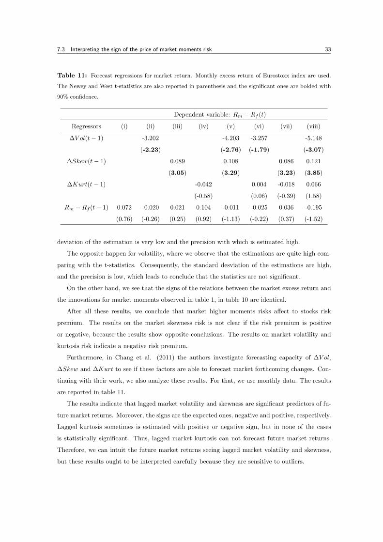
7.3 Interpreting the sign of the price of market moments risk 33
Table 11: Forecast regressions for market return. Monthly excess return of Eurostoxx index are used.
The Newey and West t-statistics are also reported in parenthesis and the significant ones are bolded with
90% confidence.
Dependent variable: Rm −Rf (t)
Regressors (i) (ii) (iii) (iv) (v) (vi) (vii) (viii)
∆V ol(t− 1) -3.202 -4.203 -3.257 -5.148
(-2.23) (-2.76) (-1.79) (-3.07)
∆Skew(t− 1) 0.089 0.108 0.086 0.121
(3.05) (3.29) (3.23) (3.85)
∆Kurt(t− 1) -0.042 0.004 -0.018 0.066
(-0.58) (0.06) (-0.39) (1.58)
Rm −Rf (t− 1) 0.072 -0.020 0.021 0.104 -0.011 -0.025 0.036 -0.195
(0.76) (-0.26) (0.25) (0.92) (-1.13) (-0.22) (0.37) (-1.52)
deviation of the estimation is very low and the precision with which is estimated high.
The opposite happen for volatility, where we observe that the estimations are quite high com-
paring with the t-statistics. Consequently, the standard desviation of the estimations are high,
and the precision is low, which leads to conclude that the statistics are not significant.
On the other hand, we see that the signs of the relations between the market excess return and
the innovations for market moments observed in table 1, in table 10 are identical.
After all these results, we conclude that market higher moments risks affect to stocks risk
premium. The results on the market skewness risk is not clear if the risk premium is positive
or negative, because the results show opposite conclusions. The results on market volatility and
kurtosis risk indicate a negative risk premium.
Furthermore, in Chang et al. (2011) the authors investigate forecasting capacity of ∆V ol,
∆Skew and ∆Kurt to see if these factors are able to forecast market forthcoming changes. Con-
tinuing with their work, we also analyze these results. For that, we use monthly data. The results
are reported in table 11.
The results indicate that lagged market volatility and skewness are significant predictors of fu-
ture market returns. Moreover, the signs are the expected ones, negative and positive, respectively.
Lagged kurtosis sometimes is estimated with positive or negative sign, but in none of the cases
is statistically significant. Thus, lagged market kurtosis can not forecast future market returns.
Therefore, we can intuit the future market returns seeing lagged market volatility and skewness,
but these results ought to be interpreted carefully because they are sensitive to outliers.

34
8 Sorting stock returns on different moments
In previous sections we investigate that the behaviour of market higher moments affect to the
cross-section of the stocks. Thus, in this section we analyze the importance of higher moments of
the own stocks. We examine whether the higher order moments of each stock are priced in the
Eurostoxx market. We follow Amaya et al. (2015), where portfolios are formed according to their
realized volatility, skewness and kurtosis. In fact, we analyze the relation between stock returns
for the current month and the previous month’s realized volatility, skewness and kurtosis.
First of all, we need estimates of time series of volatility, skewness and kurtosis of each stock.
It might be appropriate to estimate the parameters of the Exponentially weighted moving average
or GARCH models for each stock, but this has a high computational cost and it is left for further
research. So, we decide to calculate those series as in RiskMetrics imposing a parameter λ = 0.94
for all the cases. Therefore, the time series of variance, skewness and kurtosis are calculated with
the following models,
rt = Et−1[rt] + εt where εt ∼ (0, σ2ε )
εt = σtηt; ηt ∼ (0, 1); εt | It−1 ∼ (0, σ2t )
σ2t = λσ2
t−1 + (1− λ)ε2t−1
st = λst−1 + (1− λ)η3t−1
kt = λkt−1 + (1− λ)η4t−1
where Et−1[ηt] = 0, Et−1[η2t ] = 1, Et−1[η3
t ] = st and Et−1[η4t ] = kt. ηt are standardized residuals
and Et−1[•] denotes the conditional expectation on an information set up to period t− 1.
After analyzing autocorrelogramas for each return series, we conclude that for each stock, they
either follow an AR(1) model or they are by themselves a pure innovation. We use the sample
moments computed with the subsample of the first 180 observations as initial conditions, and we
begin to extrapolate over time starting with observation 181.
After calculating the time series of the moments of each stock, every month stocks are ranked
into quintiles according to their realized moment at the beginning of the month. As in section
5, there are 203 stocks in total, so we decide that quintile 1 and 5 have 40 stocks and 41 rest of
them. We construct value-weighted portfolios, so we calculate daily prices of portfolios, where the
price of the portfolio is the sum of the prices of different stocks. Then, monthly returns have been
calculated using the first and the last closing data of each month.
We also report the Carhart four-factor alphas, and we calculate them as in the previous sections.
The results of different portfolios are reported in table 12, where panel A shows the results for
the realized volatility, panel B for realized skewness and panel C for realized kurtosis.
We observe that the volatility and the skewness of the own stocks is more valued in the asset
pricing, as we see in both cases the results are significant and the t-statistics are relatively high. We
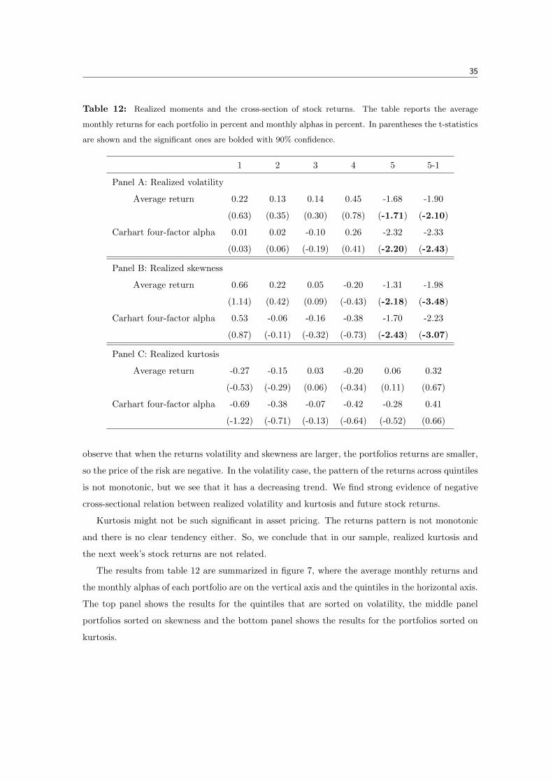
35
Table 12: Realized moments and the cross-section of stock returns. The table reports the average
monthly returns for each portfolio in percent and monthly alphas in percent. In parentheses the t-statistics
are shown and the significant ones are bolded with 90% confidence.
1 2 3 4 5 5-1
Panel A: Realized volatility
Average return 0.22 0.13 0.14 0.45 -1.68 -1.90
(0.63) (0.35) (0.30) (0.78) (-1.71) (-2.10)
Carhart four-factor alpha 0.01 0.02 -0.10 0.26 -2.32 -2.33
(0.03) (0.06) (-0.19) (0.41) (-2.20) (-2.43)
Panel B: Realized skewness
Average return 0.66 0.22 0.05 -0.20 -1.31 -1.98
(1.14) (0.42) (0.09) (-0.43) (-2.18) (-3.48)
Carhart four-factor alpha 0.53 -0.06 -0.16 -0.38 -1.70 -2.23
(0.87) (-0.11) (-0.32) (-0.73) (-2.43) (-3.07)
Panel C: Realized kurtosis
Average return -0.27 -0.15 0.03 -0.20 0.06 0.32
(-0.53) (-0.29) (0.06) (-0.34) (0.11) (0.67)
Carhart four-factor alpha -0.69 -0.38 -0.07 -0.42 -0.28 0.41
(-1.22) (-0.71) (-0.13) (-0.64) (-0.52) (0.66)
observe that when the returns volatility and skewness are larger, the portfolios returns are smaller,
so the price of the risk are negative. In the volatility case, the pattern of the returns across quintiles
is not monotonic, but we see that it has a decreasing trend. We find strong evidence of negative
cross-sectional relation between realized volatility and kurtosis and future stock returns.
Kurtosis might not be such significant in asset pricing. The returns pattern is not monotonic
and there is no clear tendency either. So, we conclude that in our sample, realized kurtosis and
the next week’s stock returns are not related.
The results from table 12 are summarized in figure 7, where the average monthly returns and
the monthly alphas of each portfolio are on the vertical axis and the quintiles in the horizontal axis.
The top panel shows the results for the quintiles that are sorted on volatility, the middle panel
portfolios sorted on skewness and the bottom panel shows the results for the portfolios sorted on
kurtosis.

36
1 1.5 2 2.5 3 3.5 4 4.5 5−2.5
−2
−1.5
−1
−0.5
0
0.5
perce
nt (%
)
Average return
Carhart alpha
1 1.5 2 2.5 3 3.5 4 4.5 5−2
−1.5
−1
−0.5
0
0.5
1
perce
nt (%
)
Average return
Carhart alpha
1 1.5 2 2.5 3 3.5 4 4.5 5−0.7
−0.6
−0.5
−0.4
−0.3
−0.2
−0.1
0
0.1
perce
nt (%
)
Average return
Carhart alpha
Figure 5: Average return and alphas in each quintile.
9 Conclusion
We examine how the cross section of stock returns is affected by the behaviour of the higher
moments of the market returns. To do so, we estimate market volatility, skewness and kurtosis
using GARCHSK and NAGARCHSK models. We use individual stocks from Eurostoxx as well as
the Eurostoxx index and the data sample contains daily closing prices from 2000 to 2016.
We use two different strategies, so our thesis is divided in two parts. The first one is based
on the univariate sorting, where we construct different portfolios depending on the exposure of
stocks returns to innovations in one of the market moments. Additionally, we also construct factor
portfolios to separate the pricing effects of different factors. The risk premium of these portfolios
is estimated by computing their average return.
The second part of our analysis is based on the multivariate sorting and cross-sectional regres-
sions. Here, we compute the price of market volatility, skewness and kurtosis risk using Fama and
MacBeth regressions to different test portfolios.
37
We find that the stocks with high exposure to innovations in market volatility have low returns
on average. This suggest that market volatility risk receives a negative risk premium, consistent
with the results in the second part of our analysis.
The results for skewness and kurtosis are not so evident. Average returns and alphas of port-
folios with different sensitivity to skewness and kurtosis do not display a strictly monotonic pat-
tern, although stocks with higher exposure to innovations in market skewness and kurtosis exhibit
somewhat higher returns on average. The risk premium associated to market kurtosis risk is also
negative, although it does not seem to be statistically significant, possibly because of the difficulty
of estimating it with precision. The evidence on market skewness risk is not very clear, although
it seems to receive a positive and statistically significant risk premium, although this type of risk
seems to receive a positive and statistically significant premium, as shown by the analysis on 25
Fama and French portfolios sorted on size and book-to-market ratio.
Similar work was done by Chang, Christoffersen and Jacobs (2011) using the stocks included in
the Center for Research in Securities Prices NYSE/Amex/Nasdaq file, reaching somewhat different
results. These authors find that stocks with high exposure to innovations in implied market
skewness exhibit low returns on average and they also conclude that market skewness risk indicate
a robustly negative risk premium. In our case, the results for the market skewness risk are not so
evident.
For the case of volatility and kurtosis, their results are weaker and more sensitive to variations
in the empirical and setup and across sample periods. However, they also conclude that the price of
volatility and kurtosis risk are negative and positive, respectively. Hence, our results only coincide
with those of Chang, Christoffersen and Jacobs (2011) just in the negative sign of volatility risk
premium.
On the other hand, we also analyze whether the higher moments of each stock are priced in
the Eurostoxx market. To do so, we calculate the series of these higher moments with RiskMetrics
imposing a parameter λ = 0.94 for all cases. Once we have the series, we construct portfolios
sorting stocks according to their value at the beginning of the month to each higher moment, in
that way, we re-calculate the portfolios every month.
The results show that higher moments of each stock are priced in the Eurostoxx market, even
more than higher moments of market returns. Specially, stocks volatility and skewness, where we
find a significant negative relation between these moments and the next week’s stock returns, so
it is important to consider them in asset pricing.
Similar work was done by Amaya et al. (2015) using every listed stock in the Trade and Quote
database, and they reach somewhat different results. This authors find a reliable and significant
negative relation between realized skewness and next week’s stock, consistent with our findings.
However, they find a little evidence of a reliable relation between realized volatility and the cross-

38
section of next week’s stock returns.
The general conclusion is that to fully understand the behaviour of the cross section of stock
returns it is necessary to consider the time evolution of the higher moments of market returns and
each stock returns.

39
A Appendix 1
Here we show that the function f(ηt | It−1) is really a density function, and its integral in all R is
equal to one.In order to obtain that, we rewrite ψ(ηt) as:
ψ(ηt) = 1 +st√3!H3(ηt) +
kt − 3√4!
H4(ηt)
where {Hi(x)}i∈N represent some polynomials such that H0(x) = 1, H1(x) = x and for i ≥ 2
follow the next expression:
Hi(x) =xHi−1(x)−
√i− 1Hi−2(x)√i
Therefore, it is verified that the family of polynomials {Hi(x)}i∈N is an orthonormal basis
satisfying that: ∫ ∞−∞
Hi(x)φ(x)dx = 1 (A.1)
∫ ∞−∞
Hi(x)Hj(x)φ(x)dx = 0 ∀i 6= j (A.2)
where φ(•) is a density function of N(0, 1) distribution. So if we integrate the function (4.1), using
(A.1) and (A.2) conditions:
(1
Γt
)∫ ∞∞
φ(ηt)
[1 +
st√3!H3(ηt) +
kt − 3√4!
H4(ηt)
]2
=
(1
Γt
)[∫ ∞−∞
φ(ηt)dηt +s2t
3!
∫ ∞−∞
H23 (ηt)φ(ηt)dηt +
(kt − 3)2
4!
∫ ∞−∞
H24 (ηt)φ(ηt)dηt
]=
(1
Γt
)[1 +
s2t
3!+
(kt − 3)2
4!
]= 1
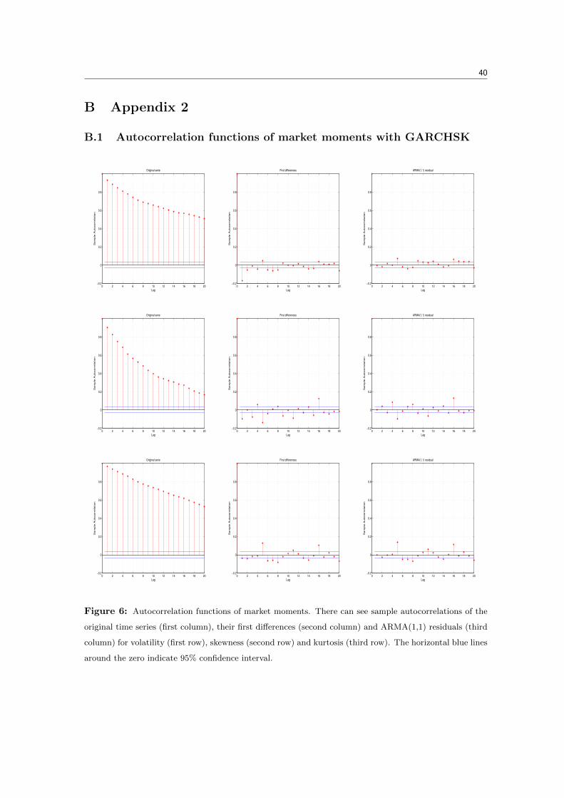
40
B Appendix 2
B.1 Autocorrelation functions of market moments with GARCHSK
0 2 4 6 8 10 12 14 16 18 20−0.2
0
0.2
0.4
0.6
0.8
Lag
Sa
mp
le A
uto
co
rre
latio
n
Original serie
0 2 4 6 8 10 12 14 16 18 20−0.2
0
0.2
0.4
0.6
0.8
Lag
Sa
mp
le A
uto
co
rre
latio
n
First differences
0 2 4 6 8 10 12 14 16 18 20−0.2
0
0.2
0.4
0.6
0.8
Lag
Sa
mp
le A
uto
co
rre
latio
n
ARMA(1,1) residual
0 2 4 6 8 10 12 14 16 18 20−0.2
0
0.2
0.4
0.6
0.8
Lag
Sa
mp
le A
uto
co
rre
latio
n
Original serie
0 2 4 6 8 10 12 14 16 18 20−0.2
0
0.2
0.4
0.6
0.8
Lag
Sa
mp
le A
uto
co
rre
latio
n
First differences
0 2 4 6 8 10 12 14 16 18 20−0.2
0
0.2
0.4
0.6
0.8
Lag
Sa
mp
le A
uto
co
rre
latio
n
ARMA(1,1) residual
Figure 6: Autocorrelation functions of market moments. There can see sample autocorrelations of the
original time series (first column), their first differences (second column) and ARMA(1,1) residuals (third
column) for volatility (first row), skewness (second row) and kurtosis (third row). The horizontal blue lines
around the zero indicate 95% confidence interval.
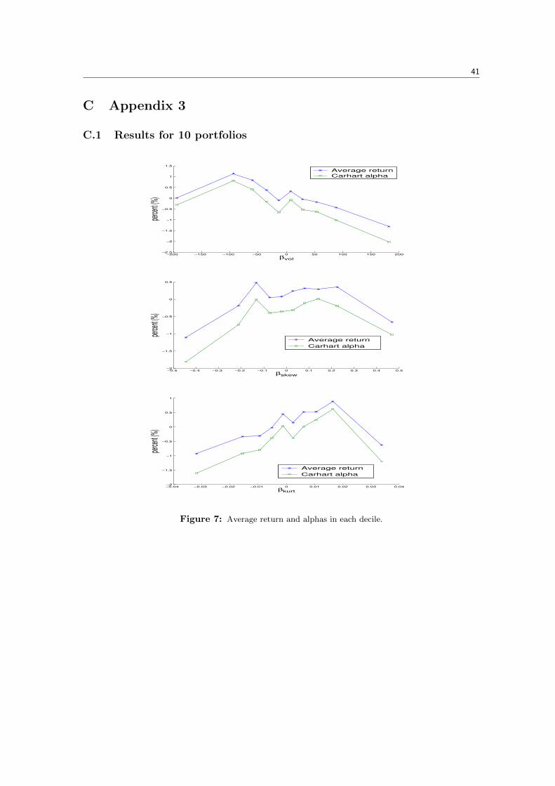
41
C Appendix 3
C.1 Results for 10 portfolios
−200 −150 −100 −50 0 50 100 150 200−2.5
−2
−1.5
−1
−0.5
0
0.5
1
1.5
βvol
perce
nt (%
)
Average return
Carhart alpha
−0.5 −0.4 −0.3 −0.2 −0.1 0 0.1 0.2 0.3 0.4 0.5−2
−1.5
−1
−0.5
0
0.5
βskew
perce
nt (%
)
Average return
Carhart alpha
−0.04 −0.03 −0.02 −0.01 0 0.01 0.02 0.03 0.04−2
−1.5
−1
−0.5
0
0.5
1
βkurt
perce
nt (%
)
Average return
Carhart alpha
Figure 7: Average return and alphas in each decile.
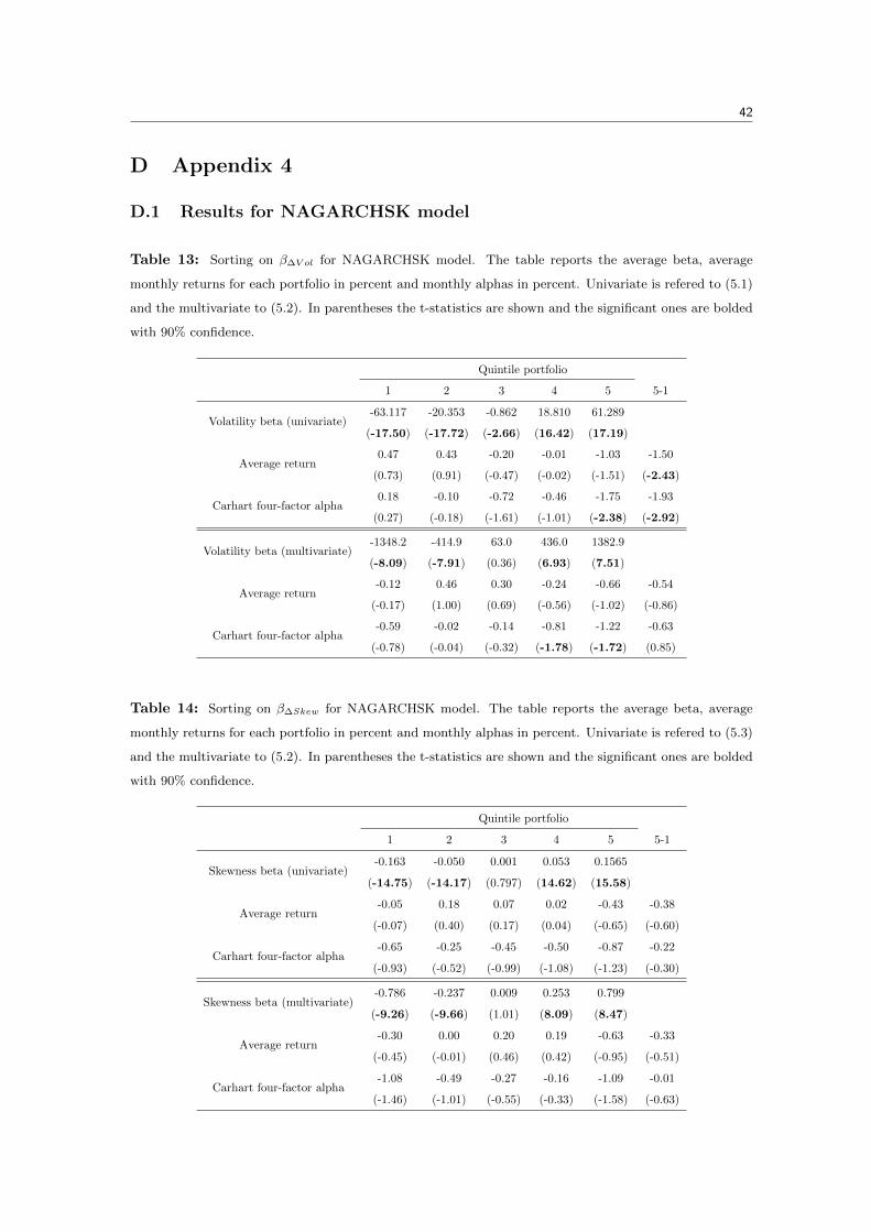
42
D Appendix 4
D.1 Results for NAGARCHSK model
Table 13: Sorting on β∆V ol for NAGARCHSK model. The table reports the average beta, average
monthly returns for each portfolio in percent and monthly alphas in percent. Univariate is refered to (5.1)
and the multivariate to (5.2). In parentheses the t-statistics are shown and the significant ones are bolded
with 90% confidence.
Quintile portfolio
1 2 3 4 5 5-1
Volatility beta (univariate)-63.117
(-17.50)
-20.353
(-17.72)
-0.862
(-2.66)
18.810
(16.42)
61.289
(17.19)
Average return0.47
(0.73)
0.43
(0.91)
-0.20
(-0.47)
-0.01
(-0.02)
-1.03
(-1.51)
-1.50
(-2.43)
Carhart four-factor alpha0.18
(0.27)
-0.10
(-0.18)
-0.72
(-1.61)
-0.46
(-1.01)
-1.75
(-2.38)
-1.93
(-2.92)
Volatility beta (multivariate)-1348.2
(-8.09)
-414.9
(-7.91)
63.0
(0.36)
436.0
(6.93)
1382.9
(7.51)
Average return-0.12
(-0.17)
0.46
(1.00)
0.30
(0.69)
-0.24
(-0.56)
-0.66
(-1.02)
-0.54
(-0.86)
Carhart four-factor alpha-0.59
(-0.78)
-0.02
(-0.04)
-0.14
(-0.32)
-0.81
(-1.78)
-1.22
(-1.72)
-0.63
(0.85)
Table 14: Sorting on β∆Skew for NAGARCHSK model. The table reports the average beta, average
monthly returns for each portfolio in percent and monthly alphas in percent. Univariate is refered to (5.3)
and the multivariate to (5.2). In parentheses the t-statistics are shown and the significant ones are bolded
with 90% confidence.
Quintile portfolio
1 2 3 4 5 5-1
Skewness beta (univariate)-0.163
(-14.75)
-0.050
(-14.17)
0.001
(0.797)
0.053
(14.62)
0.1565
(15.58)
Average return-0.05
(-0.07)
0.18
(0.40)
0.07
(0.17)
0.02
(0.04)
-0.43
(-0.65)
-0.38
(-0.60)
Carhart four-factor alpha-0.65
(-0.93)
-0.25
(-0.52)
-0.45
(-0.99)
-0.50
(-1.08)
-0.87
(-1.23)
-0.22
(-0.30)
Skewness beta (multivariate)-0.786
(-9.26)
-0.237
(-9.66)
0.009
(1.01)
0.253
(8.09)
0.799
(8.47)
Average return-0.30
(-0.45)
0.00
(-0.01)
0.20
(0.46)
0.19
(0.42)
-0.63
(-0.95)
-0.33
(-0.51)
Carhart four-factor alpha-1.08
(-1.46)
-0.49
(-1.01)
-0.27
(-0.55)
-0.16
(-0.33)
-1.09
(-1.58)
-0.01
(-0.63)
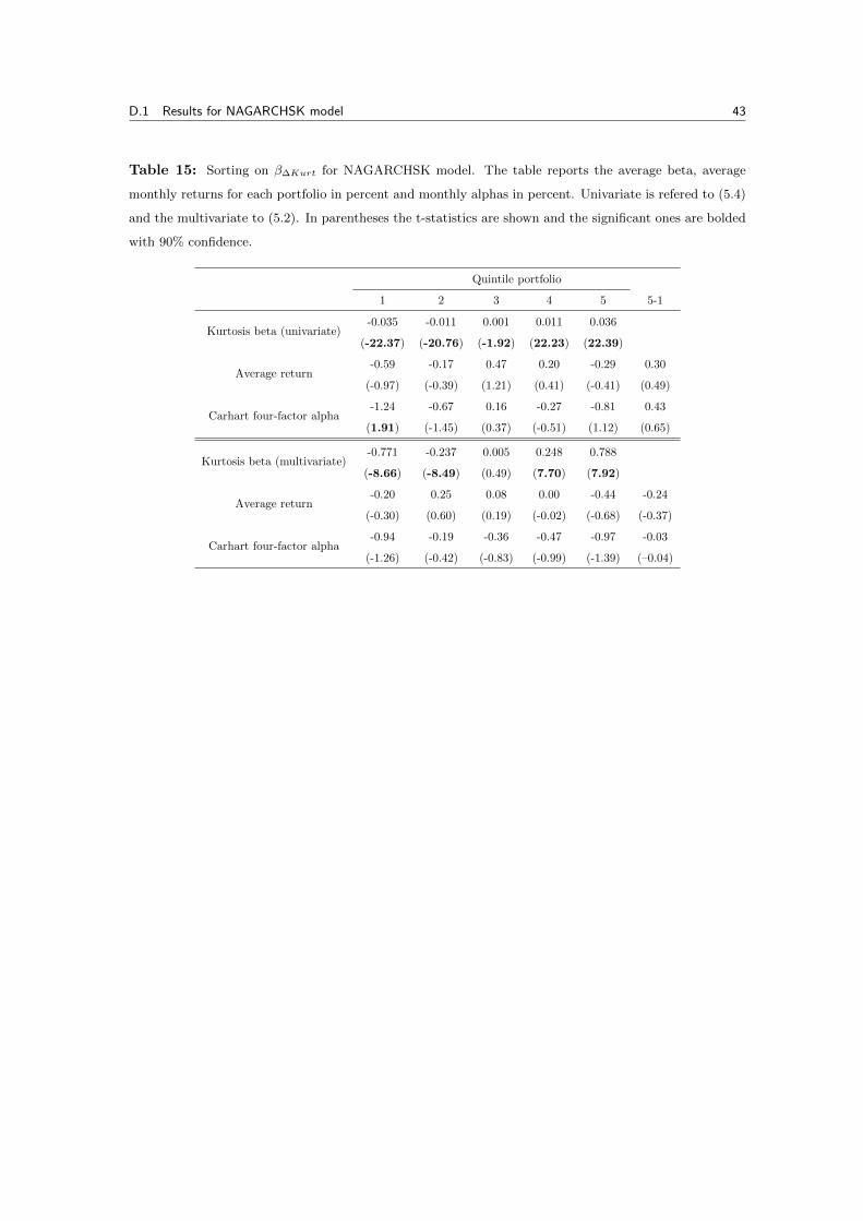
D.1 Results for NAGARCHSK model 43
Table 15: Sorting on β∆Kurt for NAGARCHSK model. The table reports the average beta, average
monthly returns for each portfolio in percent and monthly alphas in percent. Univariate is refered to (5.4)
and the multivariate to (5.2). In parentheses the t-statistics are shown and the significant ones are bolded
with 90% confidence.
Quintile portfolio
1 2 3 4 5 5-1
Kurtosis beta (univariate)-0.035
(-22.37)
-0.011
(-20.76)
0.001
(-1.92)
0.011
(22.23)
0.036
(22.39)
Average return-0.59
(-0.97)
-0.17
(-0.39)
0.47
(1.21)
0.20
(0.41)
-0.29
(-0.41)
0.30
(0.49)
Carhart four-factor alpha-1.24
(1.91)
-0.67
(-1.45)
0.16
(0.37)
-0.27
(-0.51)
-0.81
(1.12)
0.43
(0.65)
Kurtosis beta (multivariate)-0.771
(-8.66)
-0.237
(-8.49)
0.005
(0.49)
0.248
(7.70)
0.788
(7.92)
Average return-0.20
(-0.30)
0.25
(0.60)
0.08
(0.19)
0.00
(-0.02)
-0.44
(-0.68)
-0.24
(-0.37)
Carhart four-factor alpha-0.94
(-1.26)
-0.19
(-0.42)
-0.36
(-0.83)
-0.47
(-0.99)
-0.97
(-1.39)
-0.03
(–0.04)
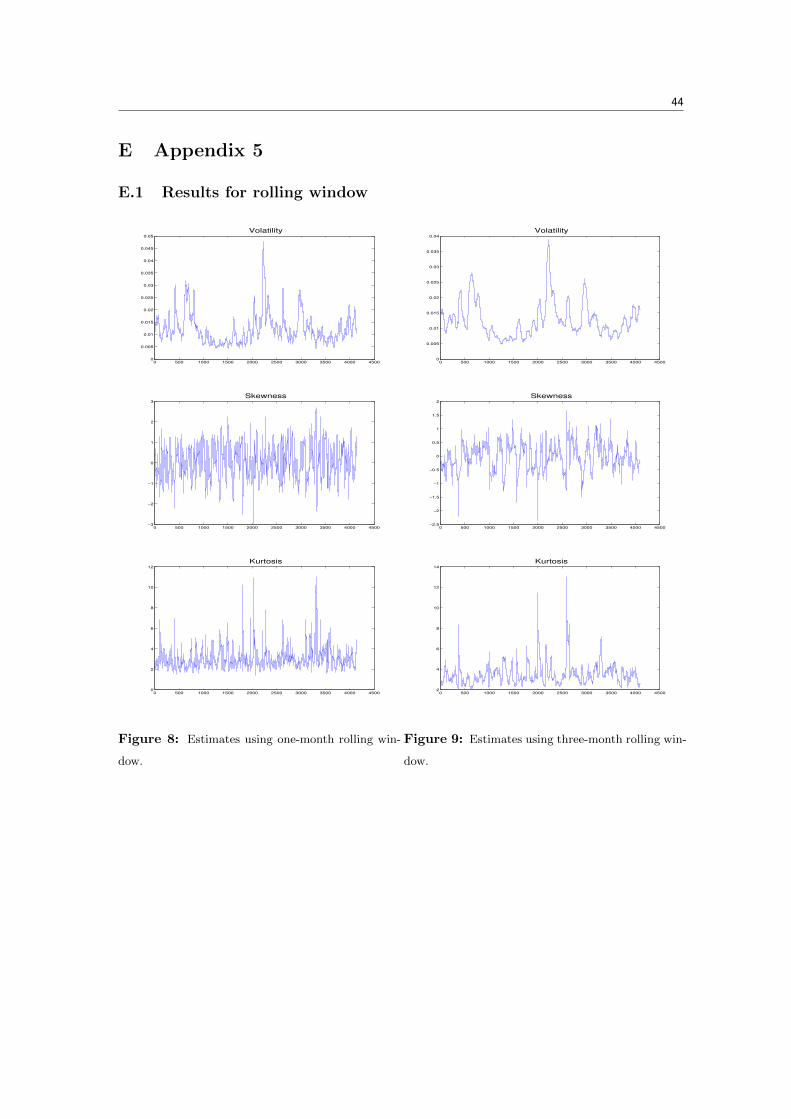
44
E Appendix 5
E.1 Results for rolling window
0 500 1000 1500 2000 2500 3000 3500 4000 45000
0.005
0.01
0.015
0.02
0.025
0.03
0.035
0.04
0.045
0.05
Volatility
0 500 1000 1500 2000 2500 3000 3500 4000 4500−3
−2
−1
0
1
2
3
Skewness
0 500 1000 1500 2000 2500 3000 3500 4000 45000
2
4
6
8
10
12
Kurtosis
Figure 8: Estimates using one-month rolling win-
dow.
0 500 1000 1500 2000 2500 3000 3500 4000 45000
0.005
0.01
0.015
0.02
0.025
0.03
0.035
0.04
Volatility
0 500 1000 1500 2000 2500 3000 3500 4000 4500−2.5
−2
−1.5
−1
−0.5
0
0.5
1
1.5
2
Skewness
0 500 1000 1500 2000 2500 3000 3500 4000 45002
4
6
8
10
12
14
Kurtosis
Figure 9: Estimates using three-month rolling win-
dow.
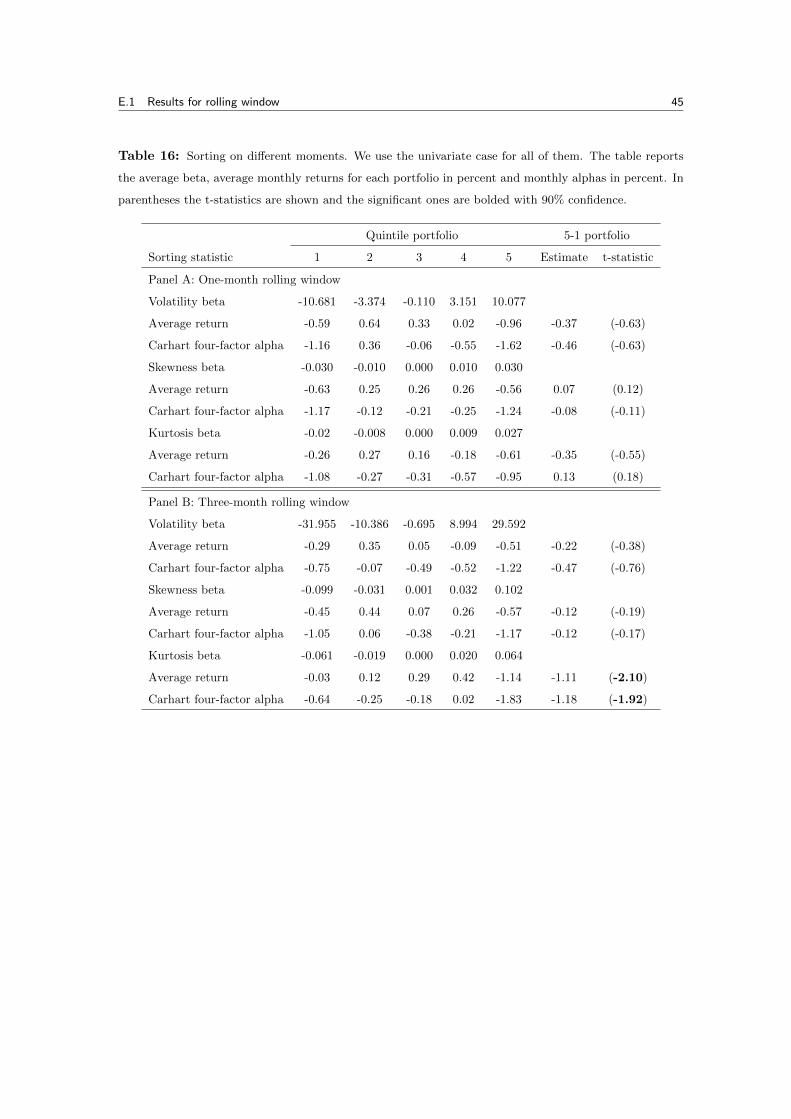
E.1 Results for rolling window 45
Table 16: Sorting on different moments. We use the univariate case for all of them. The table reports
the average beta, average monthly returns for each portfolio in percent and monthly alphas in percent. In
parentheses the t-statistics are shown and the significant ones are bolded with 90% confidence.
Quintile portfolio 5-1 portfolio
Sorting statistic 1 2 3 4 5 Estimate t-statistic
Panel A: One-month rolling window
Volatility beta -10.681 -3.374 -0.110 3.151 10.077
Average return -0.59 0.64 0.33 0.02 -0.96 -0.37 (-0.63)
Carhart four-factor alpha -1.16 0.36 -0.06 -0.55 -1.62 -0.46 (-0.63)
Skewness beta -0.030 -0.010 0.000 0.010 0.030
Average return -0.63 0.25 0.26 0.26 -0.56 0.07 (0.12)
Carhart four-factor alpha -1.17 -0.12 -0.21 -0.25 -1.24 -0.08 (-0.11)
Kurtosis beta -0.02 -0.008 0.000 0.009 0.027
Average return -0.26 0.27 0.16 -0.18 -0.61 -0.35 (-0.55)
Carhart four-factor alpha -1.08 -0.27 -0.31 -0.57 -0.95 0.13 (0.18)
Panel B: Three-month rolling window
Volatility beta -31.955 -10.386 -0.695 8.994 29.592
Average return -0.29 0.35 0.05 -0.09 -0.51 -0.22 (-0.38)
Carhart four-factor alpha -0.75 -0.07 -0.49 -0.52 -1.22 -0.47 (-0.76)
Skewness beta -0.099 -0.031 0.001 0.032 0.102
Average return -0.45 0.44 0.07 0.26 -0.57 -0.12 (-0.19)
Carhart four-factor alpha -1.05 0.06 -0.38 -0.21 -1.17 -0.12 (-0.17)
Kurtosis beta -0.061 -0.019 0.000 0.020 0.064
Average return -0.03 0.12 0.29 0.42 -1.14 -1.11 (-2.10)
Carhart four-factor alpha -0.64 -0.25 -0.18 0.02 -1.83 -1.18 (-1.92)

References 46
References
[1] Amaya, D., Christoffersen, P., Jacobs, K. and Vasquez, A., 2015. Does realized skewness predict
the cross-section of equity returns? Journal of Financial Economics.
[2] Bams, D., Honarvar, I. and Lehnert, T., 2015. From time varying risk-aversion to market
anomalies in market moments’ risk premia.
[3] Bates, D. S., 2000. Post-’87 crash fears in S&P 500 futures option market. Journal of Econo-
metrics.
[4] Chang, B. Y., Christoffersen, P. and Jacobs, K., 2011. Market skewness risk and the cross
section of stock returns. Journal of Financial Economics.
[5] Doran, J. S., Peterson, D. R. and Tarrant, B. C., 2007. Is there information in the volatility
skew? Journal of Futures Markets
[6] Fama, E.F. and MacBeth, J.D., 1973. Risk, return, and equilibrium: empirical tests. Journal
of Political Economy.
[7] Leon, A., Rubio, G. and Serna, G., 2004. Autoregresive conditional volatility, skewness and
kurtosis. The Quarterly Review of Economics and Finance.
[8] Pan, J., 2002. The jump-risk premia implicit in options: evidence from an integrated time series
study. Journal of Financial Economics.