HYBRID COHERENT LIGHTtuprints.ulb.tu-darmstadt.de/8527/1/Dissertation_FriedrichFranziska_v2.pdf ·...
187
HYBRID COHERENT LIGHT Modeling light-emitting quantum dot superluminescent diodes Dem Fachbereich Physik der Technischen Universität Darmstadt zur Erlangung des Grades eines Doktors der Naturwissenschaften (Dr. rer. nat.) genehmigte Dissertation von M. Sc. Franziska Friedrich aus Weiterstadt 1. Gutachten: Prof. Dr. Reinhold Walser 2. Gutachten: Prof. Dr. Wolfgang Elsäßer Darmstadt 2019 D 17
Transcript of HYBRID COHERENT LIGHTtuprints.ulb.tu-darmstadt.de/8527/1/Dissertation_FriedrichFranziska_v2.pdf ·...
HYBRID COHERENT LIGHTModeling light-emitting quantum dot superluminescent diodes
Dem Fachbereich Physikder Technischen Universität Darmstadt
zur Erlangung des Gradeseines Doktors der Naturwissenschaften (Dr. rer. nat.)
genehmigte Dissertation vonM. Sc. Franziska Friedrich
aus Weiterstadt
1. Gutachten: Prof. Dr. Reinhold Walser2. Gutachten: Prof. Dr. Wolfgang Elsäßer
Darmstadt 2019D 17
Hybrid coherent light – Modeling light-emitting quantum dot superluminescent diodesHybrid-kohärentes Licht – Modellierung von lichtemittierenden Quantenpunkt-Superlumineszenzdioden
Genehmigte Dissertation von Franziska Friedrich aus Weiterstadt
1. Gutachten: Prof. Dr. Reinhold Walser2. Gutachten: Prof. Dr. Wolfgang Elsäßer
Tag der Einreichung: 17. Dezember 2018Tag der Prüfung: 19. Februar 2019
Darmstadt – D17
Bitte zitieren Sie dieses Dokument als:URN: urn:nbn:de:tuda-tuprints-85278URI: https://tuprints.ulb.tu-darmstadt.de/id/eprint/8527
Dieses Dokument wird bereitgestellt von tuprints,E-Publishing-Service der TU Darmstadthttp://[email protected]
Die Veröffentlichung steht unter folgender Creative Commons Lizenz:Namensnennung - Nicht kommerziell - Keine Bearbeitungen4.0 Internationalhttps://creativecommons.org/licenses/by-nc-nd/4.0/
A B S T R AC T
Commercial devices for optical coherence tomography greatly benefit from the exceptionalfeatures of broadband light-emitting quantum dot superluminescent diodes (QDSLDs). Here,light generation occurs at the transition from spontaneous to stimulated emission, the regimeof the amplified spontaneous emission. In this context, initially spontaneously emitted photonsare amplified by stimulated emission processes when traversing through the QDSLD, whichleads to strong light amplification. The suitable choice of the waveguide geometry and the gainmedium formed by quantum dots, enables large spectral widths of some terahertz combinedwith a rather higher degree of spatial coherence. Modern measurement methods based on two-photon absorption processes provide a temporal resolution of some femtoseconds and thusallow correlation studies of the emitted QDSLD light. Also from a theoretical point of view,the characterization of the amplified spontaneous emission generated by QDSLDs and theirassociated photon statistics represents an interesting and challenging research topic. Especiallyin a particular temperature regime these devices exhibit uncommon properties with regard tothe temporal field and intensity correlations g(1)(τ) and g(2)(τ): While g(1)(τ) reflects therather highly incoherent nature of light emitted by QDSLDs due to its spectral width of severalTHz, a reduction of g(2)(0) from 2 to 1.33 at a temperature of T = 190 K was observed in theSemiconductor Optics group of Prof. W. Elsäßer at the Technical University of Darmstadt in2011 [1]. The understanding of the occurrence of these hybrid coherent light states, which aresimultaneously incoherent in g(1)(τ) and coherent in g(2)(τ) is the subject of this thesis.
In a first step we find the quantum mechanical light state associated with the QDSLD to be welldescribed by a multimode phase-randomized Gaussian state by comparison with experimentalresults. In the second step we present a microscopic theory of the amplified spontaneous emission,which allows an explanation of the temperature-dependent noise suppression of broadbandQDSLDs. For this purpose we consider distinguishable quantum dots, which are embedded ina strongly absorptive bulk material that defines a waveguide. Tilted and anti-reflection coatedoutput facets, leading to a suppression of longitudinal modes, are modeled by beam splittersthat couple the internal field to the surroundings. Regarding the spectral properties of QDSLDs,the broadband light generated inside the diode is described by a multimode electric field. Thismultimode quantum field theory yields rate equations for the optical power densities and the leveloccupation of the inhomogeneous ensemble of quantum dots within the diode. With the help ofthe input-output formalism, we determine the optical power spectrum. As a main result, we findthe broadband external power spectrum to be a convolution of the intra-diode photon spectrumwith a Lorentzian response. This finding corresponds with experimentally available spectra.Furthermore, based on the quantum theory of QDSLDs we determine the central second-orderdegree of coherence g(2)(0). It reveals a reduction within a special detuning regime and thereforeallows the interpretation of the hybrid coherent light phenomenon from a quantum optical pointof view.
iii

Z U S A M M E N FA S S U N G
Kommerzielle Messapparaturen für die optische Kohärenztomographie profitieren von deneinzigartigen Eigenschaften von breitbandigen Quantenpunkt-Superlumineszenzdioden (engl.quantum dot superluminescent diodes (QDSLDs)). Die Lichterzeugung tritt hier am Übergangvon spontaner zu stimulierter Emission auf, welches dem Bereich der verstärkt-spontanen Emis-sion entspricht. Die zu Beginn spontan emittierten Photonen werden bei ihrer Propagation imWellenleiter durch stimulierte Emissionsprozesse verstärkt. Mittels geeigneter Wahl von Wel-lenleitergeometrie und Gewinnmedium, hier Quantenpunkte, werden große spektrale Breitenvon einigen Terahertz mit gleichzeitig hoher, räumlicher Kohärenz realisiert. Der Einsatz vonsogenannten Zwei-Photonen Absorptionsdetektoren zur Messung von zeitlichen Korrelationenermöglicht Auflösungen von einigen Femtosekunden und erlaubt somit auch Korrelationsstudienvon terahertz-breiten QDSLDs. Aber auch aus theoretischer Sicht stellt die Charakterisierung derverstärkt spontanen Emission von QDSLDs und deren photon-statistischen Eigenschaften eininteressantes und herausforderndes Forschungsprojekt dar. Gerade im Hinblick auf einen ganzbestimmten Temperaturbereich zeigen diese Bauelemente ein ungewöhnliches Verhalten bzgl.der zeitlichen Feld- und Intensitätskorrelation, g(1)(τ) und g(2)(τ). Während g(1)(τ) hochgradiginkohärent mit einer spektralen Breite von einigen THz ist, lässt sich eine Reduktion von g(2)(0)von 2 nach 1.33 bei einer Temperatur von T = 190 K im Labor beobachten. Dieses Experimentwurde in der AG Halbleiteroptik von Prof. W. Elsäßer an der Technischen Universität Darmstadtdurchgeführt. Das Auffinden einer physikalischen Erklärung für die Beobachtung dieses hybrid-kohärenten Lichtes, welches gleichzeitig inkohärent in g(1)(τ) und kohärent in g(2)(τ) ist, stelltdas Ziel dieser Dissertation dar.
Im ersten Schritt postulieren wir zunächst einen Quantenzustand des emittierten Lichts einerQDSLD und vergleichen die theoretischen mit den experimentellen Ergebnissen. Es zeigt sich,dass der multimodige, phasenverschmierte, gaußsche Zustand die experimentellen Daten sehrgut wiederspiegelt. Im zweiten Schritt stellen wir eine mikroskopische Theorie der verstärkt-spontanen Emission vor um eine Erklärung für die temperaturabhängige Rauschunterdrückungvon breitbandigen QDSLDs zu finden. Diese berücksichtigt unterscheidbare Quantenpunkte, diesich in einem stark absorbierenden Bulk-Material, dem Wellenleiter, befinden. Geneigte undantireflexbeschichtete Austrittsfacetten sorgen für eine Unterdrückung longitudinaler Moden. Siewerden durch Strahlteiler modelliert, welche das interne Feld an die äußere Umgebung koppeln.Aufgrund der spektralen Eigenschaften von QDSLDs wird das breitbandige Licht innerhalb desWellenleiters durch ein multimodales, elektrisches Feld beschrieben. Diese multimodale Quan-tentheorie liefert Ratengleichungen für die optischen Leistungsdichten sowie Niveaubesetzungendes inhomogenen Ensembles der Quantenpunkte. Mit Hilfe des Input-Output Formalismus be-stimmen wir das optische Spektrum, welches durch eine Faltung des internen Photonenspektrumsmit einer Lorentz’schen Antwort gegeben ist. Ein Vergleich dieses wichtigen Ergebnisses mit denexperimentellen Daten zeigt gute Übereinstimmung. Des Weiteren untersuchen wir den zentralenKohärenzgrad zweiter Ordnung, g(2)(0), mit Hilfe unserer Quantentheorie. Dabei wird eineReduktion innerhalb eines bestimmten Bereiches der Verstimmung beobachtet. Die gewonnenenErgebnisse lassen die Interpretation des Phänomens von hybrid-kohärenten Licht aus einer reinquantenoptischen Perspektive zu.
v

C O N T E N T S
1 I N T RO D U C T I O N 12 Q UA N T U M E L E C T RO DY NA M I C S 3
2.1 Quantization in an inhomogeneous dielectric . . . . . . . . . . . . . . . . . . 32.1.1 Homogeneous dielectric medium . . . . . . . . . . . . . . . . . . . 52.1.2 Poynting vector and intensity . . . . . . . . . . . . . . . . . . . . . 10
2.2 Quantum states of light . . . . . . . . . . . . . . . . . . . . . . . . . . . . . 112.2.1 Coherent states . . . . . . . . . . . . . . . . . . . . . . . . . . . . . 112.2.2 Thermal states . . . . . . . . . . . . . . . . . . . . . . . . . . . . . 13
2.3 Spectral and statistical properties of light . . . . . . . . . . . . . . . . . . . . 152.3.1 First-order autocorrelation and power spectrum . . . . . . . . . . . . 162.3.2 Second-order autocorrelation . . . . . . . . . . . . . . . . . . . . . . 202.3.3 Temporal autocorrelation of coherent states . . . . . . . . . . . . . . 202.3.4 Temporal autocorrelation of thermal states . . . . . . . . . . . . . . 21
2.3.4.1 Temporal first-order autocorrelation . . . . . . . . . . . . . 212.3.4.2 Temporal second-order correlation function . . . . . . . . . 22
2.4 Photon statistics of light sources . . . . . . . . . . . . . . . . . . . . . . . . 243 H Y B R I D C O H E R E N T L I G H T 27
3.1 Quantum dot superluminescent diodes . . . . . . . . . . . . . . . . . . . . . 273.2 First observation of hybrid coherent light . . . . . . . . . . . . . . . . . . . . 30
4 L I G H T S TAT E S O F Q UA N T U M D OT S U P E R L U M I N E S C E N T D I O D E S 354.1 Phase-randomized Gaussian state . . . . . . . . . . . . . . . . . . . . . . . . 354.2 First-order correlation function . . . . . . . . . . . . . . . . . . . . . . . . . 394.3 Second-order correlation function . . . . . . . . . . . . . . . . . . . . . . . . 404.4 Comparison with a feedback experiment . . . . . . . . . . . . . . . . . . . . 424.5 Mixing light from two sources . . . . . . . . . . . . . . . . . . . . . . . . . 44
4.5.1 Example of a Gaussian shaped diode spectrum . . . . . . . . . . . . 464.5.2 Comparison with experimental results . . . . . . . . . . . . . . . . . 48
5 M I C RO S C O P I C T H E O RY O F Q UA N T U M D OT S U P E R L U M I N E S C E N T D I O D E S 535.1 Quantum dots . . . . . . . . . . . . . . . . . . . . . . . . . . . . . . . . . . 56
5.1.1 Pumping of quantum dots at room temperature . . . . . . . . . . . . 585.1.2 Response, gain and inversion of a quantum dot at room temperature . 60
5.2 Waveguide geometry . . . . . . . . . . . . . . . . . . . . . . . . . . . . . . 635.2.1 Empty superluminescent diode . . . . . . . . . . . . . . . . . . . . . 635.2.2 Output coupling through tilted end facets . . . . . . . . . . . . . . . 675.2.3 Virtual cavity system . . . . . . . . . . . . . . . . . . . . . . . . . . 73
5.2.3.1 Input-output formalism from scattering theory . . . . . . . . 745.2.3.2 Input-output relation by effective point interaction . . . . . . 79
5.2.4 Emission of the empty waveguide . . . . . . . . . . . . . . . . . . . 845.2.4.1 Response to white noise input . . . . . . . . . . . . . . . . 885.2.4.2 Response to phase-randomized Gaussian noise input . . . . 90
5.3 Intrawaveguide quantum dot superluminescent diode system . . . . . . . . . 905.3.1 On the nature of the QDSLD quantum state . . . . . . . . . . . . . . 935.3.2 Rate equations . . . . . . . . . . . . . . . . . . . . . . . . . . . . . 94
5.3.2.1 Single-mode ASE field and identical quantum dots . . . . . 96
vii
viii Contents
5.3.2.2 Multimode ASE field . . . . . . . . . . . . . . . . . . . . . 1006 S P E C T RU M O F Q UA N T U M D OT S U P E R L U M I N E S C E N T D I O D E S 107
6.1 Theory of the optical power spectrum emitted by QDSLDs . . . . . . . . . . 1076.2 Comparison with a measured power spectrum . . . . . . . . . . . . . . . . . 111
7 P H OT O N S TAT I S T I C S O F Q UA N T U M D OT S U P E R L U M I N E S C E N T D I O D E S 1177.1 Temporal second-order correlation of QDSLDs . . . . . . . . . . . . . . . . 1177.2 Central second-order degree of coherence . . . . . . . . . . . . . . . . . . . 118
7.2.1 Single-mode QDSLD with identical quantum dots . . . . . . . . . . 1217.2.2 Physical explanation of the occurrence of hybrid coherent light . . . . 123
8 C O N C L U S I O N A N D O U T L O O K 125Appendix A W I C K T H E O R E M F O R B O S O N I C G AU S S I A N S TAT E S 127Appendix B T E M P O R A L C O R R E L AT I O N S O F P R AG & M I X E D L I G H T S TAT E S 129
B.1 PRAG states . . . . . . . . . . . . . . . . . . . . . . . . . . . . . . . . . . . 129B.1.1 First- and second-order moments . . . . . . . . . . . . . . . . . . . 129B.1.2 First-order correlation and power spectrum . . . . . . . . . . . . . . 130B.1.3 Second-order correlation . . . . . . . . . . . . . . . . . . . . . . . . 131
B.2 Mixed light states . . . . . . . . . . . . . . . . . . . . . . . . . . . . . . . . 133B.2.1 First-order correlation and power spectrum . . . . . . . . . . . . . . 133B.2.2 Second-order correlation . . . . . . . . . . . . . . . . . . . . . . . . 134
Appendix C E U L E R - M AC L AU R I N S E R I E S 135Appendix D DA M P I N G I N T H E S C H R Ö D I N G E R P I C T U R E 137Appendix E N O I S E I N P U T A N D O U T P U T 143Appendix F Q UA N T U M S T O C H A S T I C P RO C E S S E S : I T Ô V S . S T R AT O N OV I C H 147
F.1 Itô calculus . . . . . . . . . . . . . . . . . . . . . . . . . . . . . . . . . . . . 148F.2 Stratonovich calculus . . . . . . . . . . . . . . . . . . . . . . . . . . . . . . 149
F.2.1 Connection between Itô and Stratonovich stochastic integral . . . . . 149F.3 Formulation of Itô QSDEs . . . . . . . . . . . . . . . . . . . . . . . . . . . . 151F.4 Comparison between Itô and Stratonovich . . . . . . . . . . . . . . . . . . . 151
Appendix G D I FF E R E N T I A L E Q UAT I O N O F T H E F O U RT H - O R D E R M O M E N T
O F T H E Q D S L D FI E L D A M P L I T U D E S 153Appendix H S E C O N D - O R D E R D E G R E E O F C O H E R E N C E O F Q D S L D S 155
H.1 Single-mode QDSLD . . . . . . . . . . . . . . . . . . . . . . . . . . . . . . 157Bibliography 159L I S T O F P U B L I C AT I O N S 171C O N F E R E N C E S , W O R K S H O P S & S E M I NA R S 173DA N K S AG U N G 175
1I N T RO D U C T I O N
The concept of ’coherence’ is inevitably associated with the concept of the laser (light amplifi-cation by stimulated emission of radiation). The invention of the laser in 1960 by T. Maiman [2]represents a milestone in modern physics and provides novel opportunities in the field of researchand development until this day. A complete description of its working principle can only beensured by a quantum theory, which allows to differentiate between a light bulb and a laser.The theoretical foundations were laid by R. Glauber in his optical coherence theory [3–6] forwhich he was awarded the Nobel Prize in 2005 [7]. Detailed laser theories were establishedi.a. by the schools of M. Lax [8, 9], H. Haken [10–12] and W. Lamb [13, 14]. In the context ofGlauber’s theory of coherence, correlations play a central role. Especially, field and intensitycorrelations are relevant, since they provide statements about the power spectral density andthe photon statistics of light sources. The first experiment that measured intensity correlationswas performed by R. Hanbury Brown and R. Q. Twiss in 1956 [15] with the goal to measure thesize of stars. The observed bunching effect of these thermal light sources could be explained byclassical considerations. However, based on Glauber’s theory there exists a further, pure quantumoptical phenomenon, today known as antibunching, which was theoretically predicted by H. J.Carmichael and D. F. Walls [16] and experimentally confirmed by L. Mandel, H. J. Kimble andM. Dagenais in atomic resonance fluorescence [17]. Until this day, antibunching was observedin further single-photon emitters like quantum dots [18–20], single dye molecules trapped in asolid [21] or single nitrogen-vacancy centers in diamonds [22]. Currently, the structural engineer-ing of such single-photon sources operating as qubits, that form the basis of quantum information,represents a big challenge [23].
While this field of research is addressed to such a single- or few-body problem for building aquantum computer, further groups are primary concerned with light sources composed of manydegrees of freedom. Among other things, optical properties of semiconductor devices play animportant role due to their wide applicability in research and development but also in commercialtechnologies. Especially, broadband superluminescent diodes with light emission characteristicsthat are spatially directed and additionally possess a considerable spectral width are relevantfor industrial applications – for fiber-sensor technologies [24–27], medical diagnostics [28],to only name a few. But also from the aspect of fundamental research, these semiconductordevices are of major interest regarding their coherence properties in first- and second-order. Theirbroad bandwidths are accompanied by femtosecond coherence times, that are too short for usualdetectors with a temporal resolution of some picoseconds. Thus, measuring intensity correlationsof such broadband light sources was long time not possible until F. Boitier developed a noveldetector, based on the two-photon absorption process [29, 30]. This pioneering progress in thedetection process offered new insights to the quantum nature of light-emitting broadband sources.
In this context a key experiment was performed in 2011 by M. Blazek and W. Elsäßer at theTechnical University of Darmstadt [1]. Their investigation of field and intensity correlations ofthe amplified spontaneous emission of quantum dot superluminescent diodes highlighted a newclass of light states. These novel states of light exhibit an optical spectrum with a spectral widthof about several THz. This means that the radiation is incoherent in first-order of correlation.
1
2 I N T RO D U C T I O N
Simultaneously, a reduction of the equal-time, second-order degree of coherence from 2 to 1.33within a special temperature regime of about T = 190 K was observed, which in return impliesthat the amplified spontaneous emission became coherent in second-order. The formulation ofa theory of the so-called hybrid coherent light, which is incoherent in first- and coherent insecond-order of correlation function represents an interesting and simultaneously challengingtopic of research. The following thesis is dedicated to this phenomenon and is structured asfollows:
In chapter 2 we study some basics of quantum electrodynamics, which are relevant to clar-ify the concept of correlations. Starting with the quantization procedure in isotropic media, weend up in an expression for the quantized electric field inside the diode system. With regard tohybrid coherent light, coherent and thermal states are studied in more detail. Subsequently, wesummarize fundamental aspects of Glauber’s coherence theory, in particular the definition ofcorrelations of first- and second-order which allows a classification of light in terms of theircoherence properties.
Chapter 3 is addressed to the working principle and the main characteristics of a quantum dotsuperluminescent diode. Special attention is paid to the gain medium formed by quantum dots aswell as the geometry of the waveguide. Furthermore, the main facts of the central hybrid coherentlight experiment is shortly summarized. Accordingly, chapter 2 and chapter 3 lay the necessaryfoundations to characterize the amplified spontaneous emission of the broadband semiconductordevice.
For modeling light emission of the diode under investigation, we postulate a quantum statedescribed in chapter 4. It turns out that the multimode phase-randomized Gaussian state is anexcellent choice. In this connection, we determine first- and second-order correlations. Thetheoretical results are compared with two experiments conducted by S. Blumenstein from theSemiconductor Optics group at the Technical University of Darmstadt. Both, a feedback and amixed light experiment, in which the emitted radiation of the quantum dot superluminescent diodeis superimposed with the emission of a single-mode laser, fits the experimental data remarkablywell.
In chapter 5 we propose a microscopic theory of the amplified spontaneous emission of thediode system. This model considers inhomogeneously broadened quantum dots forming the gainmedium. In addition, the special geometry of the waveguide is taken into account. Based onstochastic equations of the system operators we find rate equations which allow a detailed studyof the intrawaveguide system. In this context, we concentrate on the special cases of a transversalsingle-mode as well as a multimode quantum dot superluminescent diode composed of identicalquantum dots.
By the help of the input-output formalism, we calculate the output spectrum measured by asingle photon-detector and compare it with the experimental data in chapter 6.
Due to the unusual light behavior of broadband quantum dot superluminescent diodes weinvestigate their photon statistics in chapter 7. Starting from our microscopic, multimode theorywe examine the equal-time, also called central, second-order correlation. The special case of asingle-mode diode highlights a reduction of this measure as a function of detuning, which againpermits an explanation of the occurrence of hybrid coherent light from a theoretical perspective.
A summary of the results as well as an outlook is provided in chapter 8.
2Q UA N T U M E L E C T RO DY NA M I C S
Hybrid coherent light reveals unusual behavior when studying its temporal correlation func-tions. In a particular temperature regime, a reduction of the temporal central second-order degreeof coherence from 2 to 1.33 was observed in the lab whereas the optical power spectrum remainsbroadband with a spectral width of some THz [1]. How can we interpret these measurementdata? And how do first- and second-order correlations provide information about the coherenceor incoherence of light sources in general? Is it possible to fully characterize radiation fieldsby considering their spectral and statistical characteristics? This chapter is devoted to thesequestions.
Motivated by the experimental results of hybrid coherent light emitted by a quantum dotsuperluminescent diode, we choose a pure quantum mechanical description of the emitted lightand consider correlations in the quantum world. In doing so, we first quantize the electromagneticfield in the presence of an isotropic, inhomogeneous, dielectric medium for investigating theradiation field inside the diode system composed of semiconductor materials of high refractiveindex. After that, two classes of quantum states, coherent and thermal states, are characterizedto classify hybrid coherent light as a coherent and simultaneously incoherent radiation sourcewith regard to their first- and second-order correlation function. The chapter closes with a shortoverview of classical and non-classical light sources and clarifies the concept of photon bunchingand antibunching.
2.1 Q UA N T I Z AT I O N I N A N I N H O M O G E N E O U S D I E L E C T R I C
Quantum effects can be strongly modified by the presence of macroscopic dielectric bodies.E.g. optical instruments in which the electromagnetic field under study propagates or the sur-rounding semiconductor material of quantum dot superluminescent diodes, in which the gainmedia (quantum dots) are embedded, influence the emission and photon statistical properties. Insuch cases it is necessary to consider the quantization of the electromagnetic field in presenceof a polarizable medium. In the following we study a non-relativistic quantum description ofthe electromagnetic field in a linear, isotropic, nonmagnetic, nondispersive, nonabsorptive andinhomogeneous dielectric medium with frequency-independent polarizability and position depen-dent dielectric constant. This section about the quantization in the presence of dielectric matter isbased on the theory of R. Glauber and M. Lewenstein [31–33], which is a generalization of thefamiliar canonical field quantization concepts.
3
4 Q UA N T U M E L E C T RO DY NA M I C S
M AC RO S C O P I C M A X W E L L E Q UAT I O N S The starting point are the classical, source-free(i.e. no free charges ρ = 0 and displacement currents j = 0) macroscopic Maxwell equations invector calculus formulation1 that read in SI units [35, 36]
∇ ·D(r, t) = 0 (Gauss’s law of electricity), (2.1a)
∇ ·B(r, t) = 0 (Gauss’s law of magnetism), (2.1b)
∇×E(r, t) = −∂tB(r, t) (Faraday’s law), (2.1c)
∇×H(r, t) = ∂tD(r, t) (Ampére’s law). (2.1d)
Here, E and H are the electric and magnetic field and D and B are the electric displacement andthe magnetic induction field.
Generally, the dielectric medium is described by the phenomenological quantity ε knownas dielectric function. For an isotropic, linear, nonabsorptive 2 and nondispersive dielectric, εbecomes a real, frequency independent scalar and the dielectric displacement is related to theelectric field according to [32]
D(r, t) = ε(r)E(r, t). (2.2)
Assuming a nonmagnetic medium, the magnetic induction field B,
B(r, t) = µ0H(r, t), (2.3)
is proportional to the magnetic field H with vacuum permeability µ0.The quantization procedure of the canonical field theory includes (1) the definition of a scalar
and a vector potential as well as the choice of an appropriate gauge, (2) the formulation ofa Lagrangian density for the dynamical variables and finally (3) the quantization process byreplacing the canonical variables by operators.
V E C T O R P OT E N T I A L A N D C H O I C E O F G AU G E We define a vector potential, which isrelated to the electric field and the magnetic induction field by
B(r, t) = ∇×A(r, t), (2.4)
E(r, t) = −∂tA(r, t). (2.5)
In general, one expects an additional contribution in (2.5) arising from a scalar potential Φ.However, due to the assumption of absent charges, we set this scalar potential equal to zero andchoose the generalized Coulomb gauge3,
∇ · (ε(r)A(r, t)) = 0, (2.6)
which is obviously in agreement with the Gauss law (2.1a) or rather the generalized transversalitycondition, ∇ · (ε(r)∂tA(r, t)) = 0. We can rewrite the Maxwell equation (2.1d) in terms of thevector potential A under consideration of the definition (2.4). As a main result, we find anequation of motion for the vector potential,
∇× (∇×A(r, t))+ε(r)ε0c2
0∂ 2
t A(r, t) = 0, (2.7)
that depends on the vacuum permittivity ε0 and the speed of light in vacuum
c0 = (µ0ε0)−1/2. (2.8)
1 The vector calculus formulation of the original Maxwell equations was introduced by O. Heaviside [34].2 Clearly, for modeling a quantum dot superluminescent diode, the assumption of a nonabsorptive medium sounds
doubtful. However, the absorption effect of the semiconductor is included in our quantum theory by coupling the gainmedium to a large reservoir, leading to damping effects in the diode system.
3 Equation (2.6) is a generalization of the well-known Coulomb gauge ∇ ·A = 0 in free space.
2.1 Q UA N T I Z AT I O N I N A N I N H O M O G E N E O U S D I E L E C T R I C 5
L AG R A N G I A N F O R M A L I S M Clearly, equation (2.7) can also be derived by the help of theLagrangian formalism. The Lagrangian for the electromagnetic field propagating in an inho-mogeneous dielectric in terms of the dynamical variables 4 (A,∂tA) and the position dependentpermittivity ε(r) is specified by [31]
L =12
∫d3r[ε(r)E2(r, t)− B2(r, t)
µ0
]=
12
∫d3r[ε(r)(∂tA(r, t))2− (∇×A(r, t))2
µ0
]. (2.9)
The vector potential A represents the canonical field variable and its corresponding canoni-cally conjugate, the canonical momentum ΠΠΠ, is defined by the functional derivative of theLagrangian (2.9) according to
ΠΠΠ(r, t) =δL
δ (∂tA)= ε(r)∂tA(r, t) = −ε(r)E(r, t) = −D(r, t). (2.10)
Because the canonical momentum is the negative electric displacement, the divergence of ΠΠΠ iszero as a consequence of the Gauss’s law of electricity (2.1a), i.e.
∇ ·ΠΠΠ = −∇ ·D = 0, (2.11)
and therefore purely transversal.The Hamilton function of the classical electromagnetic field in the presence of an inhomoge-
neous dielectric reads
H [A,ΠΠΠ] =∫
d3r ΠΠΠ(r, t)∂tA(r, t)−L =12
∫d3r[
ΠΠΠ2(r, t)ε(r)
+(∇×A(r, t))2
µ0
](2.12)
=12
∫d3r[
ε(r)E2(r, t)+1µ0
B2(r, t)]
(2.13)
and the Hamilton field equations or rather the canonical equations are defined by the derivativeof the Hamilton function in terms of the canonical variables, that is
∂tA(r, t) =δH
δΠΠΠ=
ΠΠΠ(r, t)ε(r)
, (2.14)
∂tΠΠΠ(r, t) = −δH
δA= −∇× (∇×A(r, t))
µ0. (2.15)
Taking the time derivative of (2.14), the solution can be directly inserted into the Hamiltonequation (2.15) which again yields to the predicted equation of motion (2.7).
2.1.1 Homogeneous dielectric medium
This more general consideration of an inhomogeneous medium, in which the dielectric functiondepends on position r simplifies in case of a bulk material with dielectric function
ε(r) = ε . (2.16)
A quantum dot superluminescent diode in absence of a gain material corresponds to such abulk medium. Therefore, we restrict the quantization process of the electromagnetic field to the
4 In classical physics, a system is described by a set of dynamical variables. Knowing their equations of motion as wellas their initial values, the system’s evolution is uniquely defined.
6 Q UA N T U M E L E C T RO DY NA M I C S
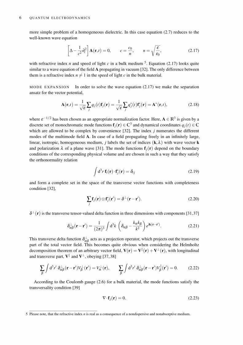
more simple problem of a homogeneous dielectric. In this case equation (2.7) reduces to thewell-known wave equation[
∆− 1c2 ∂ 2
t
]A(r, t) = 0, c =
c0
n, n =
√εε0
, (2.17)
with refractive index n and speed of light c in a bulk medium 5. Equation (2.17) looks quitesimilar to a wave equation of the field A propagating in vacuum [32]. The only difference betweenthem is a refractive index n 6= 1 in the speed of light c in the bulk material.
M O D E E X PA N S I O N In order to solve the wave equation (2.17) we make the separationansatz for the vector potential,
A(r, t) =1√ε ∑
jq j(t)f j(r) =
1√ε ∑
jq∗j(t)f
∗j(r) = A∗(r, t), (2.18)
where ε−1/2 has been chosen as an appropriate normalization factor. Here, A ∈R3 is given by adiscrete set of monochromatic mode functions f j(r) ∈ C3 and dynamical coordinates q j(t) ∈ C
which are allowed to be complex by convenience [32]. The index j numerates the differentmodes of the multimode field A. In case of a field propagating freely in an infinitely large,linear, isotropic, homogeneous medium, j labels the set of indices (k,λ ) with wave vector kand polarization λ of a plane wave [31]. The mode functions f j(r) depend on the boundaryconditions of the corresponding physical volume and are chosen in such a way that they satisfythe orthonormality relation ∫
d3r fi(r) · f∗j(r) = δi j (2.19)
and form a complete set in the space of the transverse vector functions with completenesscondition [32],
∑j
f j(r)⊗ f∗j(r′) = δ⊥(r− r′). (2.20)
δ⊥(r) is the transverse tensor-valued delta function in three dimensions with components [31,37]
δ⊥αβ (r− r′) =1
(2π)3
∫d3k
(δαβ −
kαkβ
k2
)eik(r−r′). (2.21)
This transverse delta function δ⊥αβ acts as a projection operator, which projects out the transversepart of the total vector field. This becomes quite obvious when considering the Helmholtzdecomposition theorem of an arbitrary vector field, V(r) = V‖(r)+V⊥(r), with longitudinaland transverse part, V‖ and V⊥, obeying [37, 38]
∑β
∫d3r′ δ⊥αβ (r− r′)V⊥β (r′) = V⊥α (r), ∑
β
∫d3r′ δ⊥αβ (r− r′)V ‖β (r
′) = 0. (2.22)
According to the Coulomb gauge (2.6) for a bulk material, the mode functions satisfy thetransversality condition [39]
∇ · f j(r) = 0. (2.23)
5 Please note, that the refractive index n is real as a consequence of a nondispersive and nonabsorptive medium.
2.1 Q UA N T I Z AT I O N I N A N I N H O M O G E N E O U S D I E L E C T R I C 7
Considering the completeness condition (2.20), the complex conjugate mode function f∗i (r) isrelated with the mode function itself by
f∗i (r) =∫
d3r′ δ⊥(r− r′) · f∗i (r′) = ∑j
U∗i jf j(r), (2.24)
with expansion coefficients given by the integral of the scalar product of mode function fi and f j,
Ui j =∫
d3r fi(r) · f j(r). (2.25)
Obviously, the matrix U is symmetric [31],
Ui j =U ji. (2.26)
Furthermore, U is a unitary matrix, which can be shown by utilizing the orthonormality con-dition (2.19) as well as the relation between the mode function and its corresponding complexconjugate (2.24). There holds
∑k
UikU∗jk = ∑
k,lUikU
∗jl
∫d3r f∗k(r) · fl(r) =
∫d3r∑
k,lUikf∗k(r) ·U∗jlfl(r)
=∫
d3r fi(r) · f∗j(r) = δi j.(2.27)
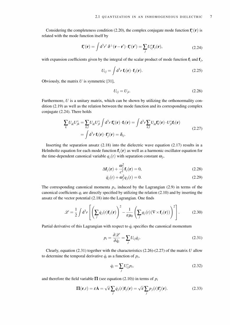
Inserting the separation ansatz (2.18) into the dielectric wave equation (2.17) results in aHelmholtz equation for each mode function f j(r) as well as a harmonic oscillator equation forthe time-dependent canonical variable q j(t) with separation constant ω j,
∆f j(r)+ω2
j
c2 f j(r) = 0, (2.28)
q j(t)+ω2j q j(t) = 0. (2.29)
The corresponding canonical momenta pi, induced by the Lagrangian (2.9) in terms of thecanonical coefficients qi are directly specified by utilizing the relation (2.10) and by inserting theansatz of the vector potential (2.18) into the Lagrangian. One finds
L =12
∫d3r
(∑j
q j(t)f j(r)
)2
− 1εµ0
(∑
jq j(t)(∇× f j(r))
)2 . (2.30)
Partial derivative of this Lagrangian with respect to qi specifies the canonical momentum
pi =∂L
∂ qi= ∑
jUi jq j. (2.31)
Clearly, equation (2.31) together with the characteristics (2.26)-(2.27) of the matrix U allowto determine the temporal derivative qi as a function of pi,
qi = ∑j
U∗i j pi, (2.32)
and therefore the field variable ΠΠΠ (see equation (2.10)) in terms of pi
ΠΠΠ(r, t) = εA =√
ε ∑j
q j(t)f j(r) =√
ε ∑j
p j(t)f∗j(r). (2.33)
8 Q UA N T U M E L E C T RO DY NA M I C S
Q UA N T I Z AT I O N P RO C E S S A quantization in Coulomb gauge is based on a set of canonicalvariables which exhibit operator character after quantization,
q j(t) → q j(t), p j(t) → p j(t), (2.34)
and whose commutators are given by
[qi, p j ] = ihδi j, [qi, q j ] = [ pi, p j ] = 0. (2.35)
Furthermore, we can calculate the hermitian conjugated variables q†j and p†
j by taking into
account that the canonical field operators are hermitian, i.e. A = A† and ΠΠΠ = ΠΠΠ†. Utilizing the
orthonormality relation (2.19) we end up with the expressions
q†i = ∑
jUi jq j, p†
i = ∑j
U∗i j p j, (2.36)
which allow to evaluate the commutators
[qi , q†j ] = [ pi , p†
j ] = 0, [qi , p†j ] = ihU∗i j. (2.37)
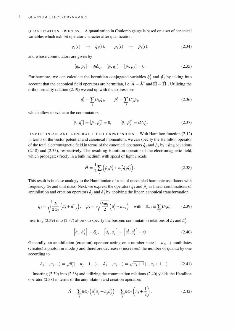
H A M I LT O N I A N A N D G E N E R A L FI E L D E X P R E S S I O N S With Hamilton function (2.12)in terms of the vector potential and canonical momentum, we can specify the Hamilton operatorof the total electromagnetic field in terms of the canonical operators q j and p j by using equations(2.18) and (2.33), respectively. The resulting Hamilton operator of the electromagnetic field,which propagates freely in a bulk medium with speed of light c reads
H =12 ∑
j
(p j p†
j +ω2j q j q
†j
). (2.38)
This result is in close analogy to the Hamiltonian of a set of uncoupled harmonic oscillators withfrequency ω j and unit mass. Next, we express the operators q j and p j as linear combinations ofannihilation and creation operators a j and a†
j by applying the linear, canonical transformation
q j =
√h
2ω j
(a j + a†
− j
), p j = i
√hω j
2
(a†
j − a− j
)with a− j ≡∑
iUi jai. (2.39)
Inserting (2.39) into (2.37) allows to specify the bosonic commutation relations of a j and a†j ,[
ai , a†j
]= δi j,
[ai , a j
]=[a†
i , a†j
]= 0. (2.40)
Generally, an annihilation (creation) operator acting on a number state |...,n j, ...〉 annihilates(creates) a photon in mode j and therefore decreases (increases) the number of quanta by oneaccording to
a j |...,n j, ...〉=√n j |...,n j−1, ...〉 , a†j |...,n j, ...〉=
√n j + 1 |...,n j + 1, ...〉 . (2.41)
Inserting (2.39) into (2.38) and utilizing the commutation relations (2.40) yields the Hamiltonoperator (2.38) in terms of the annihilation and creation operators
H = ∑j
hω j
(a†
j a j + a j a†j
)= ∑
jhω j
(n j +
12
). (2.42)
2.1 Q UA N T I Z AT I O N I N A N I N H O M O G E N E O U S D I E L E C T R I C 9
Here,
n j = a†j a j (2.43)
denotes the photon number operator of the jth mode. The last term in equation (2.42) correspondsto an infinite sum of zero point energies of the harmonic oscillators. However, this vacuum energydistribution can be omitted by an appropriate renormalization so that the Hamiltonian reduces to
H = ∑j
hω ja†j a j. (2.44)
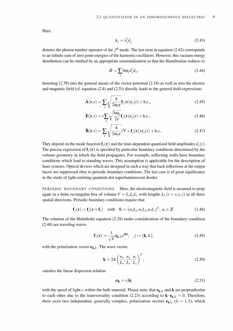
Inserting (2.39) into the general ansatz of the vector potential (2.18) as well as into the electricand magnetic field (cf. equation (2.4) and (2.5)) directly leads to the general field expressions
A(r, t) = ∑j
√h
2ω jεf j(r)a j(t)+ h.c., (2.45)
E(r, t) = i∑j
√hω j
2εf j(r)a j(t)+ h.c., (2.46)
B(r, t) = ∑j
√h
2ω jε(∇× f j(r))a j(t)+ h.c.. (2.47)
They depend on the mode function f j(r) and the time-dependent quantized field amplitudes a j(t).The precise expression of f j(r) is specified by particular boundary conditions determined by thevolume geometry in which the field propagates. For example, reflecting walls have boundaryconditions which lead to standing waves. This assumption is applicable for the description oflaser systems. Optical devices which are designed in such a way that back reflections at the outputfacets are suppressed obey to periodic boundary conditions. The last case is of great significancein the study of light-emitting quantum dot superluminescent diodes.
P E R I O D I C B O U N DA RY C O N D I T I O N S Here, the electromagnetic field is assumed to prop-agate in a finite rectangular box of volume V = LxLyLz with lengths Li (i = x,y,z) in all threespatial directions. Periodic boundary conditions require that
f j(r) = f j(r+L) with L = (nxLx,nyLy,nzLz)T , ni ∈Z. (2.48)
The solution of the Helmholtz equation (2.28) under consideration of the boundary condition(2.48) are traveling waves
f j(r) =1√V
ek,λ eikr, j 7→ (k,λ ), (2.49)
with the polarization vector ek,λ . The wave vector,
k = 2π(
nx
Lx,ny
Ly,nz
Lz
)T
, (2.50)
satisfies the linear dispersion relation
ωk = c|k| (2.51)
with the speed of light c within the bulk material. Please note, that ek,λ and k are perpendicularto each other due to the transversality condition (2.23) according to k ·ek,λ = 0. Therefore,there exist two independent, generally complex, polarization vectors ek,λ (λ = 1,2), which
10 Q UA N T U M E L E C T RO DY NA M I C S
again are perpendicular to each other, that is ek,λ ·ek,λ ′ = δλλ ′ . Thus, the set of unit vectorsk/|k|,ek,1,ek,2 forms a trihedron. In this context, inserting equation (2.49) into (2.46), theelectric field in a bulk medium of permittivity ε can be written as
E(r, t) = E(+)(r, t)+ E(−)(r, t) (2.52)
with positive frequency part
E(+)(r, t) =[E(−)(r, t)
]†= ∑
jvk(r)ak,λ (t)ek,λ (2.53)
and mode function
vk(r) = Ekeikr, Ek = i
√hωk
2εV. (2.54)
Analogical considerations yield a similar expression for the magnetic flux
B(r, t) = B(+)(r, t)+ B(−)(r, t), B(+)(r, t) = ∑j
wk(r)ak,λ (t)(k× ek,λ ) (2.55)
with mode function
wk(r) = Bkeikr, Bk = i
√h
2εωkV. (2.56)
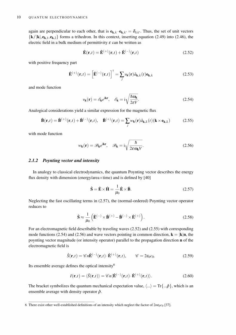
2.1.2 Poynting vector and intensity
In analogy to classical electrodynamics, the quantum Poynting vector describes the energyflux density with dimension (energy/area×time) and is defined by [40]
S = E× H =1µ0
E× B. (2.57)
Neglecting the fast oscillating terms in (2.57), the (normal-ordered) Poynting vector operatorreduces to
S≈ 1µ0
(E(−)× B(+)− B(−)× E(+)
). (2.58)
For an electromagnetic field describable by traveling waves (2.52) and (2.55) with correspondingmode functions (2.54) and (2.56) and wave vectors pointing in common direction, k = |k|n, thepoynting vector magnitude (or intensity operator) parallel to the propagation direction n of theelectromagnetic field is
S(r, t) = C nE(−)(r, t) · E(+)(r, t), C = 2ε0c0. (2.59)
Its ensemble average defines the optical intensity6
I(r, t) = 〈S(r, t)〉= C n〈E(−)(r, t) · E(+)(r, t)〉. (2.60)
The bracket symbolizes the quantum mechanical expectation value, 〈...〉= Tr...ρ, which is anensemble average with density operator ρ .
6 There exist other well-established definitions of an intensity which neglect the factor of 2nε0c0 [37].
2.2 Q UA N T U M S TAT E S O F L I G H T 11
L I N E A R P O L A R I Z E D L I G H T In case of an electromagnetic field with a single linear polar-ization parallel to the unit vector e7,
E(r, t) = E(r, t)e, (2.61)
the intensity is determined by the equal space-time, ensemble average
I(r, t) = C n〈E(−)(r, t)E(+)(r, t)〉 (2.62)
with the scalar field E(r, t). Please note (2.62) corresponds to the intensity inside the bulk mediumwith refractive index n. Clearly, an intensity of a radiation field under study is measured outsidethe light source and the refractive index in equation (2.62) is set equal to one.
Up to now, we quantized the electromagnetic field in the presence of a bulk medium. Thisdescription is more general compared to the quantization process in vacuum and in particularrelevant for an accurate description of the electric field propagating inside the considered semi-conductor device of a superluminescent diode, which represents the central object of this thesis.In the following we study some important quantum states of the electromagnetic field which arerelevant in the context of the hybrid coherent light phenomenon.
2.2 Q UA N T U M S TAT E S O F L I G H T
Generally, there exist numerous classes of important quantum states, which form a quantummechanical basis for relevant observables like correlation functions [32]. Especially in the contextof hybrid coherent light, so-called coherent and thermal states play a fundamental role as we willsee later in this thesis. In the following, we briefly summarize the main characteristics of both lightstates. For more information we refer the reader to standard quantum optics textbooks [32,41–43].
2.2.1 Coherent states
Coherent states were invented by E. Schrödinger [44] in 1926 as the most "classical" quantumstates [41] with a minimum allowed uncertainty in amplitude and phase. Their physical meaningbecomes apparent in the context of laser physics: the radiation field emitted by a stabilized laseroperating well above its threshold is in a coherent state.
There exist a number of possible options to introduce coherent states. Here, we follow thedefinition by R. Glauber [4] in 1963, in which a coherent state |α〉 is described by an unitarydisplacement operator D(α) [45] acting on the vacuum state |0〉,
|α〉= D(α) |0〉 , with D(α) = eα a†−α∗a. (2.63)
Simultaneously, from equation (2.63) it follows that |α〉 is an eigenstate of the annihilationoperator a with complex eigenvalue α = |α|eiφ ,
a |α〉= α |α〉 . (2.64)
Applying the Baker-Campbell Hausdorff formula [46] to the definition (2.63) allows to determinethe coherent state in Fock representation |n〉,
|α〉=∞
∑n=0
αn√
n!e−
|α|22 |n〉 . (2.65)
7 Practically, a radiation of type (2.61) can be realized by implementing a polarization filter into the detection setup.
12 Q UA N T U M E L E C T RO DY NA M I C S
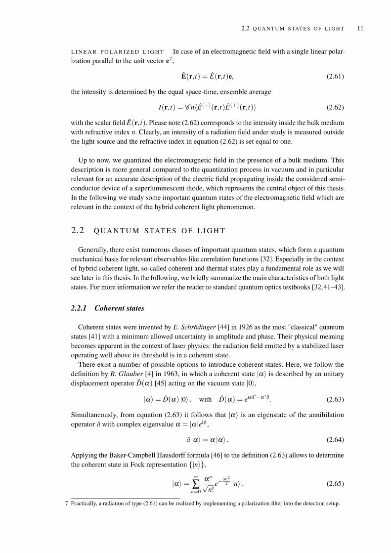
The probability to measure n photons in state α ,
Pn(α) = |〈n|α〉|2 = |α|2n
n!e−|α|
2, (2.66)
corresponds to a Poissonian distribution with mean photon number n = |α|2 as depicted infigure 2.1 for |α = 2〉 (blue), |α = 4〉 (red) and |α = 6〉 (green).
0 10 20 30 40 50 60
0.00
0.05
0.10
0.15
0.20
n
Pn(α)
Figure 2.1: Poissonian distribution of a coherent state |α〉 describing the probability to measuren photons in state |α = 2〉 (blue), |α = 4〉 (red) and |α = 6〉 (green).
Coherent states are not orthogonal. They form an overcomplete set and satisfy the completenessrelation
1π
∫d2α |α〉〈α|= 1. (2.67)
An illustration of quantum states provides the one-dimensional Wigner function invented byE. Wigner [47] in 1932. It refers to a phase-space distribution of an arbitrary quantum state withdensity operator ρ [47,48] and is defined by the ordinary two-dimensional integral (d2ξ = dξrdξi
with ξ = ξr + iξi)
W (α) = 〈δ (s=0)(a†−α∗, a−α)〉 with δ (s)(a†, a) =∫ ∞
−∞
d2ξπ2 eξ a†−ξ ∗a+ s
2 |ξ |2 . (2.68)
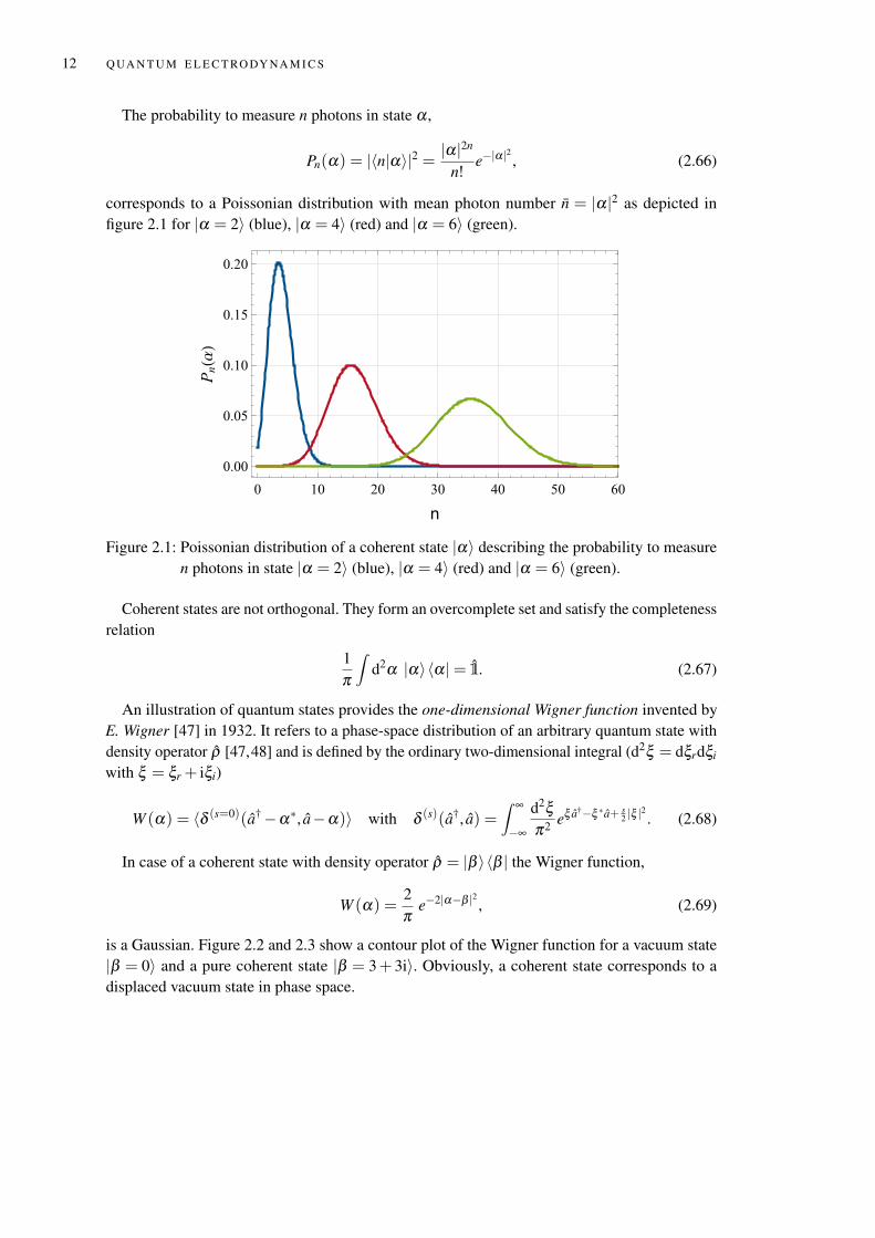
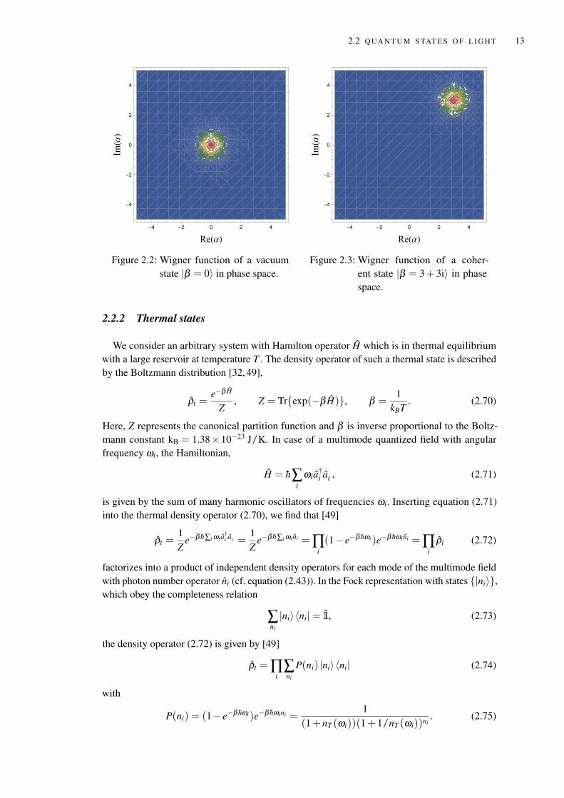
In case of a coherent state with density operator ρ = |β 〉〈β | the Wigner function,
W (α) =2π
e−2|α−β |2 , (2.69)
is a Gaussian. Figure 2.2 and 2.3 show a contour plot of the Wigner function for a vacuum state|β = 0〉 and a pure coherent state |β = 3+ 3i〉. Obviously, a coherent state corresponds to adisplaced vacuum state in phase space.
2.2 Q UA N T U M S TAT E S O F L I G H T 13
-4 -2 0 2 4
-4
-2
0
2
4
Re(α)
Im(α)
Figure 2.2: Wigner function of a vacuumstate |β = 0〉 in phase space.
-4 -2 0 2 4
-4
-2
0
2
4
Re(α)
Im(α)
Figure 2.3: Wigner function of a coher-ent state |β = 3+ 3i〉 in phasespace.
2.2.2 Thermal states
We consider an arbitrary system with Hamilton operator H which is in thermal equilibriumwith a large reservoir at temperature T . The density operator of such a thermal state is describedby the Boltzmann distribution [32, 49],
ρt =e−β H
Z, Z = Trexp(−β H), β =
1kBT
. (2.70)
Here, Z represents the canonical partition function and β is inverse proportional to the Boltz-mann constant kB = 1.38×10⁻²³ J/K. In case of a multimode quantized field with angularfrequency ωi, the Hamiltonian,
H = h∑i
ωia†i ai , (2.71)
is given by the sum of many harmonic oscillators of frequencies ωi. Inserting equation (2.71)into the thermal density operator (2.70), we find that [49]
ρt =1Z
e−β h∑i ωia†i ai =
1Z
e−β h∑i ωini = ∏i(1− e−β hωi)e−β hωini = ∏
iρi (2.72)
factorizes into a product of independent density operators for each mode of the multimode fieldwith photon number operator ni (cf. equation (2.43)). In the Fock representation with states |ni〉,which obey the completeness relation
∑ni
|ni〉〈ni|= 1, (2.73)
the density operator (2.72) is given by [49]
ρt = ∏i
∑ni
P(ni) |ni〉〈ni| (2.74)
with
P(ni) = (1− e−β hωi)e−β hωini =1
(1+ nT (ωi))(1+ 1/nT (ωi))ni. (2.75)
14 Q UA N T U M E L E C T RO DY NA M I C S
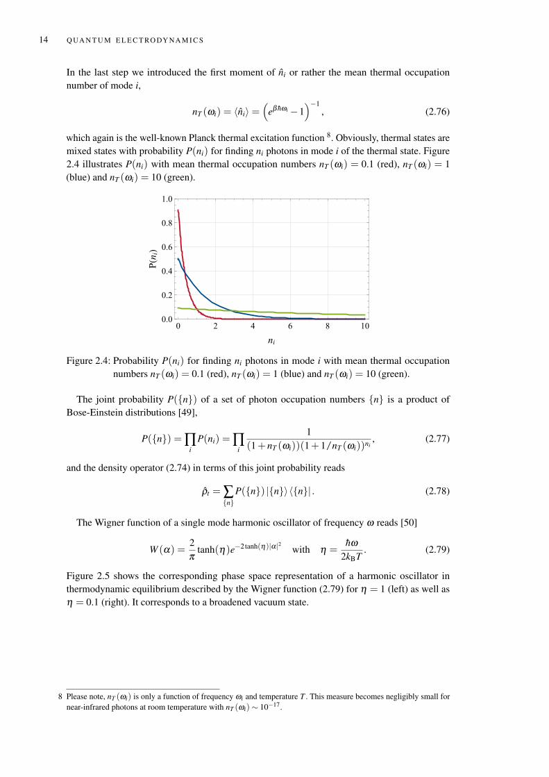
In the last step we introduced the first moment of ni or rather the mean thermal occupationnumber of mode i,
nT (ωi) = 〈ni〉=(
eβ hωi−1)−1
, (2.76)
which again is the well-known Planck thermal excitation function 8. Obviously, thermal states aremixed states with probability P(ni) for finding ni photons in mode i of the thermal state. Figure2.4 illustrates P(ni) with mean thermal occupation numbers nT (ωi) = 0.1 (red), nT (ωi) = 1(blue) and nT (ωi) = 10 (green).
0 2 4 6 8 100.0
0.2
0.4
0.6
0.8
1.0
ni
P(ni)
Figure 2.4: Probability P(ni) for finding ni photons in mode i with mean thermal occupationnumbers nT (ωi) = 0.1 (red), nT (ωi) = 1 (blue) and nT (ωi) = 10 (green).
The joint probability P(n) of a set of photon occupation numbers n is a product ofBose-Einstein distributions [49],
P(n) = ∏i
P(ni) = ∏i
1(1+ nT (ωi))(1+ 1/nT (ωi))ni
, (2.77)
and the density operator (2.74) in terms of this joint probability reads
ρt = ∑n
P(n) |n〉〈n| . (2.78)
The Wigner function of a single mode harmonic oscillator of frequency ω reads [50]
W (α) =2π
tanh(η)e−2tanh(η)|α|2 with η =hω
2kBT. (2.79)
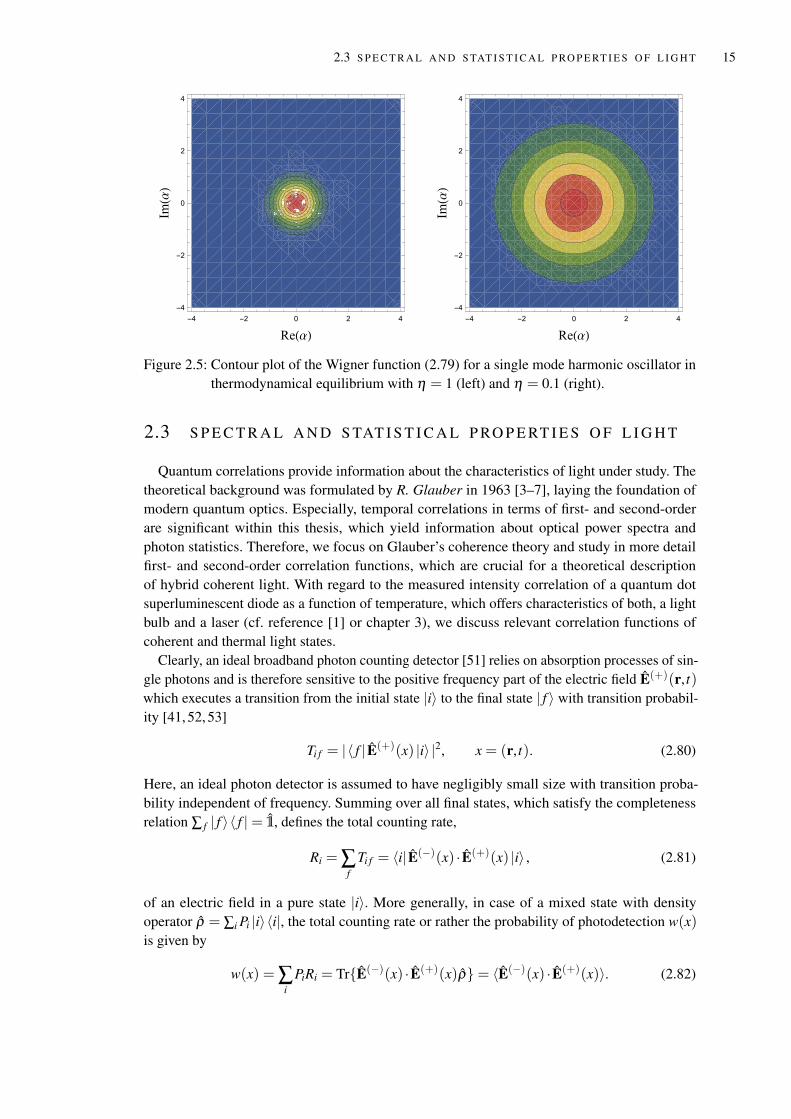
Figure 2.5 shows the corresponding phase space representation of a harmonic oscillator inthermodynamic equilibrium described by the Wigner function (2.79) for η = 1 (left) as well asη = 0.1 (right). It corresponds to a broadened vacuum state.
8 Please note, nT (ωi) is only a function of frequency ωi and temperature T . This measure becomes negligibly small fornear-infrared photons at room temperature with nT (ωi) ∼ 10−17.
2.3 S P E C T R A L A N D S TAT I S T I C A L P RO P E RT I E S O F L I G H T 15
-4 -2 0 2 4
-4
-2
0
2
4
Re(α)
Im(α)
-4 -2 0 2 4
-4
-2
0
2
4
Re(α)
Im(α)
Figure 2.5: Contour plot of the Wigner function (2.79) for a single mode harmonic oscillator inthermodynamical equilibrium with η = 1 (left) and η = 0.1 (right).
2.3 S P E C T R A L A N D S TAT I S T I C A L P RO P E RT I E S O F L I G H T
Quantum correlations provide information about the characteristics of light under study. Thetheoretical background was formulated by R. Glauber in 1963 [3–7], laying the foundation ofmodern quantum optics. Especially, temporal correlations in terms of first- and second-orderare significant within this thesis, which yield information about optical power spectra andphoton statistics. Therefore, we focus on Glauber’s coherence theory and study in more detailfirst- and second-order correlation functions, which are crucial for a theoretical descriptionof hybrid coherent light. With regard to the measured intensity correlation of a quantum dotsuperluminescent diode as a function of temperature, which offers characteristics of both, a lightbulb and a laser (cf. reference [1] or chapter 3), we discuss relevant correlation functions ofcoherent and thermal light states.
Clearly, an ideal broadband photon counting detector [51] relies on absorption processes of sin-gle photons and is therefore sensitive to the positive frequency part of the electric field E(+)(r, t)which executes a transition from the initial state |i〉 to the final state | f 〉 with transition probabil-ity [41, 52, 53]
Ti f = | 〈 f | E(+)(x) |i〉 |2, x = (r, t). (2.80)
Here, an ideal photon detector is assumed to have negligibly small size with transition proba-bility independent of frequency. Summing over all final states, which satisfy the completenessrelation ∑ f | f 〉〈 f |= 1, defines the total counting rate,
Ri = ∑f
Ti f = 〈i| E(−)(x) · E(+)(x) |i〉 , (2.81)
of an electric field in a pure state |i〉. More generally, in case of a mixed state with densityoperator ρ = ∑i Pi |i〉〈i|, the total counting rate or rather the probability of photodetection w(x)is given by
w(x) = ∑i
PiRi = TrE(−)(x) · E(+)(x)ρ= 〈E(−)(x) · E(+)(x)〉. (2.82)
16 Q UA N T U M E L E C T RO DY NA M I C S
This result can be extended to a more general expression in which the electric field is evaluatedat different space time events in the sense
G(1)(x;x′) = 〈E(−)(x) · E(+)(x′)〉. (2.83)
It defines the so-called first-order correlation function that is relevant and sufficient to inter-pret classical interference setups. In order to characterize the nature of light sources [42], thedifference between classical and quantum fields [40] or experiments which measure intensitycorrelations [15], higher-order correlations have to be taken into account.
AU T O C O R R E L AT I O N F U N C T I O N S We consider autocorrelation functions which describecorrelations between the same electric field E. Correlations between different electrical fields arenot relevant within this thesis due to common experimental setups to measure optical spectraor photon statistics which again are related to first- and second-order autocorrelations. For thisreason, we always mean autocorrelation functions when talking about correlation functions.
Generally, the nth-order autocorrelation function (tensor) with space-time event x = (r, t) isdefined by the tensor product [4, 6]
G(n)(x1, ...,xn;xn+1, ...,x2n) = 〈E(−)(x1)⊗ ...⊗ E(−)(xn)⊗ E(+)(xn+1)⊗ ...⊗ E(+)(x2n)〉.(2.84)
It is a normally ordered function, which means that all creation operators lie on the left-hand sideof all annihilation operators. The general normalized nth-order correlation function [40],
g(n)(x1, ...,xn;xn+1, ...,x2n) =G(n)(x1, ...,xn;xn+1, ...,x2n)
∏2ni=1
√TrG(1)(xi;xi)
, (2.85)
is called the nth-order degree of coherence. It characterizes the measured response in experiments,in which n photons are detected, simultaneously [40].
Both, first- and second-order correlation functions play essential roles in the study of hybridcoherent light and will be analyzed in more detail in the following section. In this context weget more specific and consider in the following traveling electric fields E(r, t) = E(r, t)e with asingle linear polarization e of type (2.61), which allows to describe correlation functions in termsof scalar-valued ensemble averages
G(n)(x1, ...,xn;xn+1, ...,x2n) = 〈E(−)(x1)...E(−)(xn)E(+)(xn+1)...E(+)(x2n)〉. (2.86)
Clearly, the correlation function itself becomes a scalar, physical measure.
2.3.1 First-order autocorrelation and power spectrum
According to equation (2.84), the first-order correlation function is defined by the ensembleaverage of the electric field at different space-time events x1 and x2 (cf. equation (2.83)) [54],
G(1)(x1;x2) = 〈E(−)(x1)E(+)(x2)〉. (2.87)
The first-order degree of coherence is specified by this first-order correlation normalized by thesquare root of the electric field product at equal events (cf. equation (2.85)) with
g(1)(x1;x2) =G(1)(x1;x2)√
G(1)(x1;x1)G(1)(x2;x2). (2.88)
2.3 S P E C T R A L A N D S TAT I S T I C A L P RO P E RT I E S O F L I G H T 17
With the help of the Cauchy-Schwarz inequality9 one can show that the absolute value ofg(1)(x1;x2) has an upper and lower bound,
0≤ |g(1)(x1;x2)| ≤ 1, (2.89)
and is fully matching classical considerations 10 [40]. According to equation (2.62), the first-ordercorrelation function for equal space-time events, G(1)(x;x), is proportional to the intensity
I(x) = C nG(1)(x;x). (2.90)
As an application, we consider a multimode electric field of type (2.61) with scalar positivefrequency component
E(+)(r, t) = ∑j
v j(r)a j(t). (2.91)
Inserting (2.91) into the definition of the first-order correlation function ends up in an expression,
G(1)(r1, t1;r2, t2) = ∑i j
v∗i (r1)v j(r2)〈a†i (t1)a j(t2)〉, (2.92)
that is proportional to the two-time expectation value of creation and annihilation operator ofmodes i and j. Thus, knowing this expectation value and the mode function, we can specify thefirst-order correlation function.
Within this thesis, only temporal correlations of stationary fields, describing the correlations atthe same position but at different time events, t1 and t2, are relevant.
P OW E R S P E C T RU M Consider again an electric field of type (2.61), E(r, t) = E(r, t)e, de-scribed by a plane wave propagating parallel to the z-direction, which is measured by a photo-detector at position zd with cross-section area A perpendicular to z. Its Fourier transform as wellas its inverse Fourier transform is defined by
E(r,ω) =1
2π
∫ ∞
−∞dt E(r, t)eiωt , E(r, t) =
∫ ∞
−∞dω E(r,ω)e−iωt . (2.93)
The power spectral density is proportional to the square of the absolute value of the electricfield in frequency space,
S(ω) = C 〈E(−)(ω)E(+)
(ω)〉 ∝ ns(ω), E(+)(ω) =
∫dxdyE(+)
(r,ω), (2.94)
and therefore directly related to the stationary photon number ns(ω) of the light field. TheFourier transform of the temporal first-order correlation function G(1)(r, t;r, t + τ) with timedelay τ = t2− t1 > 0 is related to the power spectral density of the stationary electric field E atposition r = (x,y,z) according to the Wiener-Khintchine theorem [55, 56],
S (r,ω) = limt→∞
C
2πRe
∞∫−∞
dτ eiωτG(1)(r, t;r, t + τ) =C
πRe
∞∫0
dτ eiωτG(1)(r,τ). (2.95)
9 The Cauchy Schwarz inequality for a scalar product 〈x,y〉 with x,y ∈ C reads |〈x,y〉|2 ≤ 〈x,x〉〈y,y〉.10 As the classical and the quantum first-order degree of coherence exhibit the same range of values, first-order
interference experiments are not suitable to measure quantum effects. Thus, higher-order correlations have to be takeninto account.
18 Q UA N T U M E L E C T RO DY NA M I C S
In the last step, we utilized that the first-order temporal correlation function of the free stationaryfield possesses time-symmetry
G(1)(r,τ) = limt→∞〈E(−)(r, t)E(+)(r, t + τ)〉= G(1)(r,−τ)∗. (2.96)
Integration of equation (2.95) over the total detector area A provides the experimentally availablepower spectral density (PSD) or power spectrum
S(ω) =∫
Adxdy S (r,ω) =
C
πRe∫ ∞
0dτ eiωτ G(1)(τ), (2.97)
with the spatially averaged temporal first-order correlation function
G(1)(τ) ≡ limt→∞
∫A
dxdy G(1)(r, t;r, t + τ). (2.98)
Please note, G(1)(τ) is only a function of time delay τ , that is independent of position r andtime t, due to the assumption of a stationary electromagnetic field described by traveling waves.
Usually, an optical power spectrum is measured by an optical spectrum analyzer. In chapter 6,we will see that the power spectrum of a quantum dot superluminescent diode is Gaussian shapedwith a central frequency in the near-infrared regime and a broad spectral width of several THz.
For stationary fields, the temporal first-order degree of coherence as a function of time de-lay τ > 0 is determined by
g(1)(r,τ) = limt→∞
〈E(−)(r, t)E(+)(r, t + τ)〉〈E(−)(r, t)E(+)(r, t)〉 = g(1)(r,−τ)∗, (2.99)
In general, g(1)(r,τ) is complex. Its absolute value describes the correlation strength between thesame electric field measured at different times with time delay τ and is therefore a quantitativemeasure of coherence. For g(1)(r,τ) = 1 the light field is said to be temporal coherent, whereasg(1)(r,τ → ∞) = 0 it looses coherence at some point in time. The light field is called incoherent[57]. As a consequence of the inequality (2.89), the temporal first-order degree of coherence isbounded by
0≤ |g(1)(r,τ)| ≤ |g(1)(r,τ = 0)|= 1. (2.100)
C H A R AC T E R I Z I N G S H A P E S O F D I S T R I B U T I O N S A power spectral density is charac-terized by some essential quantities: the central frequency, bandwidth and coherence time. In thiscontext, we define the probability normalized power spectral density
s(ω) =S(ω)∫ ∞
−∞ dω S(ω). (2.101)
The resulting first and second moments,
ω =∫ ∞
−∞dω ω s(ω), (2.102)
and
σ2 =∫ ∞
−∞dω (ω− ω)2 s(ω), (2.103)
define the central angular frequency and the variance of s(ω).
2.3 S P E C T R A L A N D S TAT I S T I C A L P RO P E RT I E S O F L I G H T 19
An unambiguously definition of the spectral width and the coherence time does not exist. Onecan find a number of different specifications, depending on the shape of S(ω) [49,58]. It becomesapparent that the spectral profile determines the validity of the single definitions. For example, awell-established definition of the spectral width b is given by the twofold standard deviation
b = 2σ . (2.104)
However, for fat-tailed distributions like Lorentzian spectra, the definition of a width written inequation (2.104) is not applicable. Therefore, we use an alternative definition for the frequencyspectral width
b =1∫ ∞
−∞ dω s2(ω), (2.105)
introduced by L. Mandel11 [59] and also known as Süssmann measure [48]. Based on the relationbetween frequency and wavelength, ν = c/λ , the frequency spectral width b in terms of thewavelength spectral width ∆λ and central wavelength λ is given by [49]
b = 2π∆ν ' 2πcλ 2
∆λ . (2.106)
Clearly, a strict declaration of the definition of a spectral width is necessary 12 , which becomesquite obvious in case of a single normalized Gaussian spectrum s(ω) with standard deviation σ .According to definition (2.105) the spectral width for the light beam is
bgauss = 2√
πσ . (2.107)
A direct comparison with the definition (2.104) reveals a discrepancy of a factor√
π ≈ 1.77.The coherence time is defined by the integral
τc =∫ ∞
−∞dτ |g(1)(τ)|2, (2.108)
which reflects the timescales at which |g(1)(τ)| vanishes. To be specific, on timescales τ < τc
the correlation of the fluctuations is strong, whereas for τ > τc the correlation becomes weak. Inaddition, the spectral width and the coherence time are related by [49]
τc ∼1b
. (2.109)
11 The definition (2.105) of a spectral width by L. Mandel was firstly introduced in the context of a study of the extent ofa unit cell of the photon phase space.
12 A superluminescent diode spectrum described by equation (4.5) and parameters listed in table 4.1 shows a spectralwidth of about b = 2π ·13 THz according to the definition (2.105). A comparison with the spectral width definition inequation (2.104), b = 2π ·7.5 THz exhibits a significant systematic bias.
20 Q UA N T U M E L E C T RO DY NA M I C S
2.3.2 Second-order autocorrelation
The second-order autocorrelation function provides information about the photon statistics oflight under consideration. It describes the photon counting probability to detect a photon at space-time event x1 = (r1, t1) and a second one at x2 = (r2, t2). This corresponds to the expectationvalue
G(2)(x1;x2) = 〈E(−)(x1)E(−)(x2)E(+)(x2)E(+)(x1)〉. (2.110)
The second-order degree of coherence is defined by
g(2)(x1;x2) =G(2)(x1;x2)
G(1)(x1;x1)G(1)(x2;x2). (2.111)
We consider again the general electric field described by equation (2.91). Obviously, G(2)(x1;x2)
is proportional to the fourth-order moment of annihilation and creation operators,
G(2)(x1;x2) = ∑i jlm
v∗i (r1)v∗j(r2)vl(r2)vm(r1)〈a†i (t1)a
†j(t2)al(t2)am(t1)〉, (2.112)
evaluated at different space-time events (r1, t1) and (r2, t2). Again, we only need to specify themode functions and the quantum expectation value of annihilation and creation operators todetermine the temporal second-order autocorrelation function of a radiation field described by anarbitrary quantum state.
Generally, the temporal second-order degree of coherence with time delay τ > 0 is given by
g(2)(r,τ) = limt→∞
〈E(−)(r, t)E(−)(r, t + τ)E(+)(r, t + τ)E(+)(r, t)〉〈E(−)(r, t)E(+)(r, t)〉〈E(−)(r, t + τ)E(+)(r, t + τ)〉 , g(2) ∈R. (2.113)
This experimentally available measure is real, symmetric and has no upper bound [57],
g(2)(r,τ) = g(2)(r,−τ), 0≤ g(2)(r,τ) ≤ ∞, (2.114)
in contrast to the first-order degree of coherence (cf. equation (2.100)). An equal-time, second-order degree of coherence defines the central second-order degree of coherence g(2)(0). Thisphysical quantity plays a central role in the context of hybrid coherent light as we will see laterin this thesis.
2.3.3 Temporal autocorrelation of coherent states
Regarding the general expression for a multimode, transverse electric field in equation (2.91),the nth-order degree of coherence of a coherent state is [60]
|g(n)(x1, ...,xn;xn, ...,x1)|= 1, ∀n ∈N\0. (2.115)
In general, the state of a radiation field is said to be nth-order coherent, if
|g( j)(x1, ...,x j;x j, ...,x1)|= 1, ∀ j ≤ n. (2.116)
In particular, first- and second-order temporal correlations in terms of coherent states with timedelay τ satisfy
|g(1)(τ)|= g(2)(τ) = 1. (2.117)
2.3 S P E C T R A L A N D S TAT I S T I C A L P RO P E RT I E S O F L I G H T 21
2.3.4 Temporal autocorrelation of thermal states
2.3.4.1 Temporal first-order autocorrelation
We consider a free radiation field E of type (2.91) with ai(t) = aie−iωit , described by a thermalstate with density operator (2.72). As already shown in equation (2.92), the first-order correlationfunction G(1)(r, t;r, t + τ) depends on
〈a†i (t)a j(t + τ)〉= 〈a†
i a j〉ei(ωi−ω j)te−iω jτ . (2.118)
The average on the right-hand side of equation (2.118) is given by the mean thermal occupationnumber already defined in equation (2.76),
〈a†i a j〉= Tra†
i a j ρt= nT (ωi)δi j. (2.119)
Therefore, the temporal first-order correlation function and the first-order degree of coherence ofa free thermal radiation field reduces to
G(1)(r, t;r, t + τ) = ∑i|vi(r)|2e−iωiτnT (ωi), g(1)(r,τ) = ∑i |vi(r)|2nT (ωi)e−iωiτ
∑i |vi(r)|2nT (ωi). (2.120)
1 D WAV E G U I D E In the following, we assume that the considered radiation field is linearlypolarized in y-direction with running waves propagating along the z-axis which are subjectedto periodic boundary conditions (cf. section 2.1.1). The mode function of the electric field inequation (2.91) is written by
v j(r) = i
√hω j
2εVχ(x,y)eik jz. (2.121)
Here, V is the physical volume and χ(x,y) is an additional spatial component. With such aspecific mode function, the normalized first-order correlation (2.120) reads
g(1)(τ) = ∑i ωinT (ωi)e−iωiτ
∑i ωinT (ωi), g(1)(0) = 1. (2.122)
Please note, g(1)(τ) is independent of position z and has a maximum at vanishing time delay.In [60] (see also [49]), we already discussed temporal correlations of thermal light sources. Bycalculating the real part of the first-order correlation function in the continuum limit, it turnedout that the first-order degree of coherence is specified by
g(1)(τ) = −3csch2(
πkBT τh
)+ 3(
hπkBT
)2 1τ2 . (2.123)
Furthermore, in case of time delays much smaller (bigger) than the thermal coherence time
τc =h
2πkBT, (2.124)
the absolute value |g(1)(τ)| is determined by
|g(1)(τ)|=
1, τ τc
0, τ τc. (2.125)
22 Q UA N T U M E L E C T RO DY NA M I C S
T = 0.09 K
T = 0.9 K
T = 1.9 K
T = 190 K
-4 -2 0 2 40.0
0.2
0.4
0.6
0.8
1.0
τ ((Ks)-1)
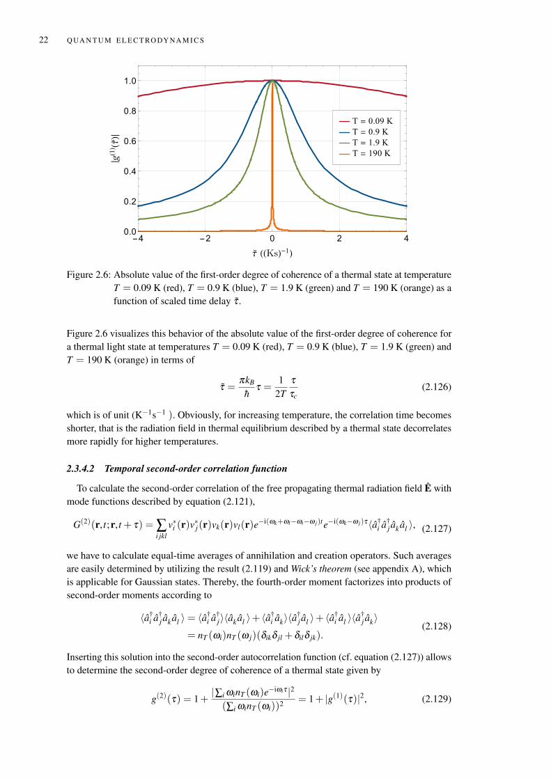
|g(1) (τ)|
Figure 2.6: Absolute value of the first-order degree of coherence of a thermal state at temperatureT = 0.09 K (red), T = 0.9 K (blue), T = 1.9 K (green) and T = 190 K (orange) as afunction of scaled time delay τ .
Figure 2.6 visualizes this behavior of the absolute value of the first-order degree of coherence fora thermal light state at temperatures T = 0.09 K (red), T = 0.9 K (blue), T = 1.9 K (green) andT = 190 K (orange) in terms of
τ =πkB
hτ =
12T
ττc
(2.126)
which is of unit (K−1s−1 ). Obviously, for increasing temperature, the correlation time becomesshorter, that is the radiation field in thermal equilibrium described by a thermal state decorrelatesmore rapidly for higher temperatures.
2.3.4.2 Temporal second-order correlation function
To calculate the second-order correlation of the free propagating thermal radiation field E withmode functions described by equation (2.121),
G(2)(r, t;r, t + τ) = ∑i jkl
v∗i (r)v∗j(r)vk(r)vl(r)e−i(ωk+ωl−ωi−ω j)te−i(ωk−ω j)τ〈a†
i a†j ak al 〉, (2.127)
we have to calculate equal-time averages of annihilation and creation operators. Such averagesare easily determined by utilizing the result (2.119) and Wick’s theorem (see appendix A), whichis applicable for Gaussian states. Thereby, the fourth-order moment factorizes into products ofsecond-order moments according to
〈a†i a†
j ak al 〉= 〈a†i a†
j〉〈ak al 〉+ 〈a†i ak〉〈a†
j al 〉+ 〈a†i al 〉〈a†
j ak〉= nT (ωi)nT (ω j)(δikδ jl + δilδ jk).
(2.128)
Inserting this solution into the second-order autocorrelation function (cf. equation (2.127)) allowsto determine the second-order degree of coherence of a thermal state given by
g(2)(τ) = 1+|∑i ωinT (ωi)e−iωiτ |2
(∑i ωinT (ωi))2 = 1+ |g(1)(τ)|2, (2.129)
2.3 S P E C T R A L A N D S TAT I S T I C A L P RO P E RT I E S O F L I G H T 23
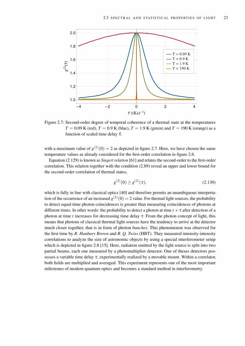
T = 0.09 K
T = 0.9 K
T = 1.9 K
T = 190 K
-4 -2 0 2 4
1.0
1.2
1.4
1.6
1.8
2.0
τ ((Ks)-1)
g(2) (τ)
Figure 2.7: Second-order degree of temporal coherence of a thermal state at the temperaturesT = 0.09 K (red), T = 0.9 K (blue), T = 1.9 K (green) and T = 190 K (orange) as afunction of scaled time delay τ .
with a maximum value of g(2)(0) = 2 as depicted in figure 2.7. Here, we have chosen the sametemperature values as already considered for the first-order correlation in figure 2.6.
Equation (2.129) is known as Siegert relation [61] and relates the second-order to the first-ordercorrelation. This relation together with the condition (2.89) reveal an upper and lower bound forthe second-order correlation of thermal states,
g(2)(0) ≥ g(2)(τ), (2.130)
which is fully in line with classical optics [40] and therefore permits an unambiguous interpreta-tion of the occurrence of an increased g(2)(0) = 2 value. For thermal light sources, the probabilityto detect equal-time photon coincidences is greater than measuring coincidences of photons atdifferent times. In other words: the probability to detect a photon at time t + τ after detection of aphoton at time t increases for decreasing time delay τ . From the photon concept of light, thismeans that photons of classical thermal light sources have the tendency to arrive at the detectormuch closer together, that is in form of photon bunches. This phenomenon was observed forthe first time by R. Hanbury Brown and R. Q. Twiss (HBT). They measured intensity-intensitycorrelations to analyze the size of astronomic objects by using a special interferometer setupwhich is depicted in figure 2.8 [15]. Here, radiation emitted by the light source is split into twopartial beams, each one measured by a photomultiplier detector. One of theses detectors pos-sesses a variable time delay τ , experimentally realized by a movable mount. Within a correlator,both fields are multiplied and averaged. This experiment represents one of the most importantmilestones of modern quantum optics and becomes a standard method in interferometry.
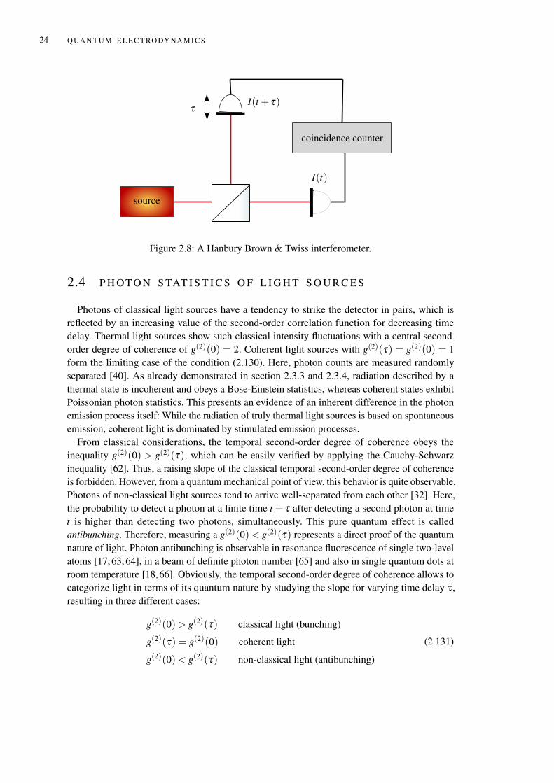
24 Q UA N T U M E L E C T RO DY NA M I C S
coincidence counter
τ
source
I(t)
I(t + τ)
Figure 2.8: A Hanbury Brown & Twiss interferometer.
2.4 P H OT O N S TAT I S T I C S O F L I G H T S O U R C E S
Photons of classical light sources have a tendency to strike the detector in pairs, which isreflected by an increasing value of the second-order correlation function for decreasing timedelay. Thermal light sources show such classical intensity fluctuations with a central second-order degree of coherence of g(2)(0) = 2. Coherent light sources with g(2)(τ) = g(2)(0) = 1form the limiting case of the condition (2.130). Here, photon counts are measured randomlyseparated [40]. As already demonstrated in section 2.3.3 and 2.3.4, radiation described by athermal state is incoherent and obeys a Bose-Einstein statistics, whereas coherent states exhibitPoissonian photon statistics. This presents an evidence of an inherent difference in the photonemission process itself: While the radiation of truly thermal light sources is based on spontaneousemission, coherent light is dominated by stimulated emission processes.
From classical considerations, the temporal second-order degree of coherence obeys theinequality g(2)(0) > g(2)(τ), which can be easily verified by applying the Cauchy-Schwarzinequality [62]. Thus, a raising slope of the classical temporal second-order degree of coherenceis forbidden. However, from a quantum mechanical point of view, this behavior is quite observable.Photons of non-classical light sources tend to arrive well-separated from each other [32]. Here,the probability to detect a photon at a finite time t + τ after detecting a second photon at timet is higher than detecting two photons, simultaneously. This pure quantum effect is calledantibunching. Therefore, measuring a g(2)(0) < g(2)(τ) represents a direct proof of the quantumnature of light. Photon antibunching is observable in resonance fluorescence of single two-levelatoms [17, 63, 64], in a beam of definite photon number [65] and also in single quantum dots atroom temperature [18, 66]. Obviously, the temporal second-order degree of coherence allows tocategorize light in terms of its quantum nature by studying the slope for varying time delay τ ,resulting in three different cases:
g(2)(0) > g(2)(τ) classical light (bunching)
g(2)(τ) = g(2)(0) coherent light
g(2)(0) < g(2)(τ) non-classical light (antibunching)
(2.131)
2.4 P H OT O N S TAT I S T I C S O F L I G H T S O U R C E S 25
Regarding the concept of hybrid coherent light, showing both coherent and incoherent character-istics in terms of g(2)(0), we have a closer look at the central second-order degree of coherence.Again, light sources are classified in the following categories [40]:
g(2)(0) > 2 superbunched light
g(2)(0) = 2 incoherent (thermal) light
1 < g(2)(0) < 2 partially coherent light
g(2)(0) = 1 coherent light
0≤ g(2)(0) < 1 antibunched light
(2.132)
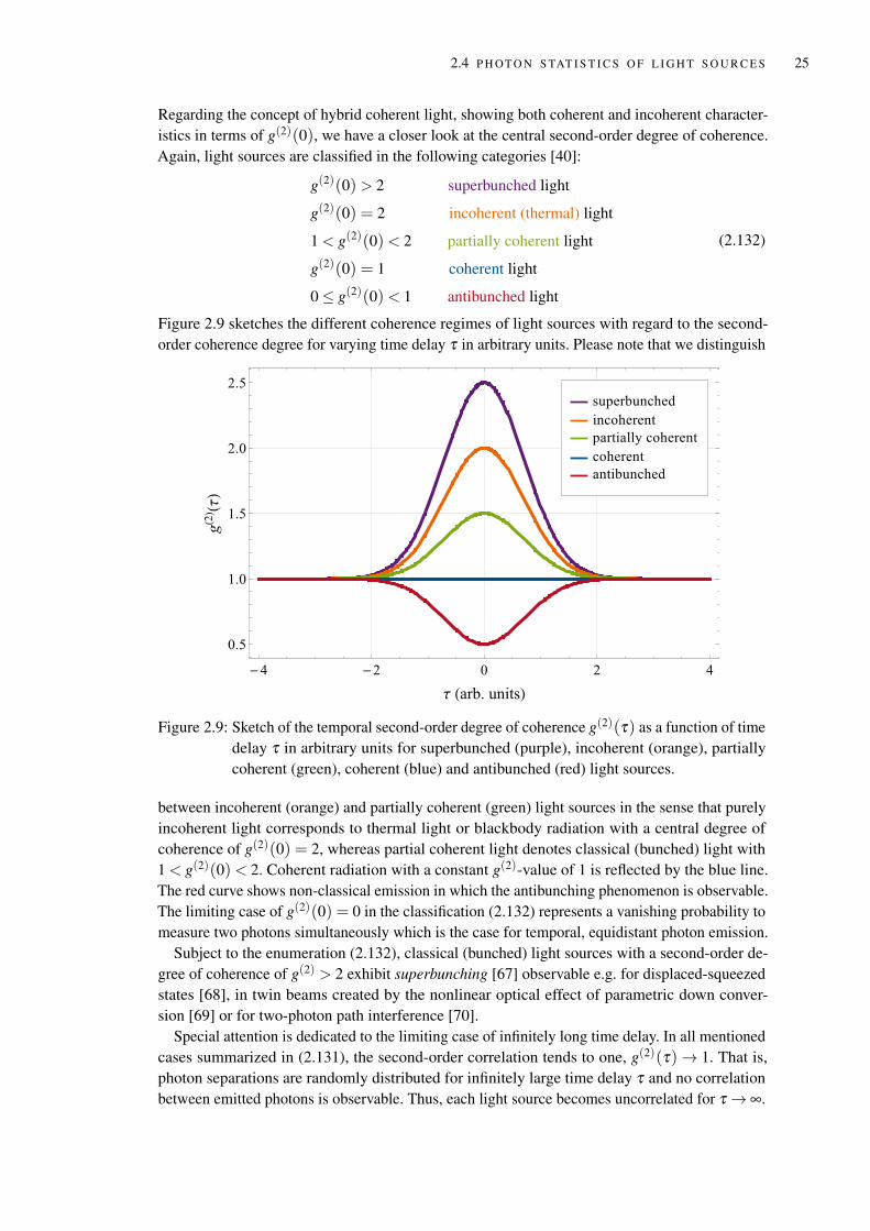
Figure 2.9 sketches the different coherence regimes of light sources with regard to the second-order coherence degree for varying time delay τ in arbitrary units. Please note that we distinguish
superbunched
incoherent
partially coherent
coherent
antibunched
-4 -2 0 2 4
0.5
1.0
1.5
2.0
2.5
τ (arb. units)
g(2) (τ)
Figure 2.9: Sketch of the temporal second-order degree of coherence g(2)(τ) as a function of timedelay τ in arbitrary units for superbunched (purple), incoherent (orange), partiallycoherent (green), coherent (blue) and antibunched (red) light sources.
between incoherent (orange) and partially coherent (green) light sources in the sense that purelyincoherent light corresponds to thermal light or blackbody radiation with a central degree ofcoherence of g(2)(0) = 2, whereas partial coherent light denotes classical (bunched) light with1 < g(2)(0)< 2. Coherent radiation with a constant g(2)-value of 1 is reflected by the blue line.The red curve shows non-classical emission in which the antibunching phenomenon is observable.The limiting case of g(2)(0) = 0 in the classification (2.132) represents a vanishing probability tomeasure two photons simultaneously which is the case for temporal, equidistant photon emission.
Subject to the enumeration (2.132), classical (bunched) light sources with a second-order de-gree of coherence of g(2) > 2 exhibit superbunching [67] observable e.g. for displaced-squeezedstates [68], in twin beams created by the nonlinear optical effect of parametric down conver-sion [69] or for two-photon path interference [70].
Special attention is dedicated to the limiting case of infinitely long time delay. In all mentionedcases summarized in (2.131), the second-order correlation tends to one, g(2)(τ)→ 1. That is,photon separations are randomly distributed for infinitely large time delay τ and no correlationbetween emitted photons is observable. Thus, each light source becomes uncorrelated for τ→ ∞.
26 Q UA N T U M E L E C T RO DY NA M I C S
In this section, we determined the quantized electric field in the presence of a dielectric mediumand introduced temporal correlations. We mentioned the main characteristics of coherent andthermal states and analyzed their temporal first- and second-order correlations. Furthermore,we studied the photon statistics of light sources by having a closer look at the central second-order degree of coherence. For the sake of completeness, one should mention the other feasiblecounterpart, namely the spatial autocorrelations, e.g. relevant for ghost imaging techniques13
[71–73]. In the context of hybrid coherent light, these spatial correlations are irrelevant from atheoretical as well as an experimental point of view. Therefore, the whole thesis is dedicatedentirely to the description of temporal first-and second-order autocorrelation functions of lightemitted by a quantum dot superluminescent diode. However, this becomes quite challengingwithout the knowledge of the working principle, structure and performance of the specialsemiconductor device. The next chapter deals with these open questions and outlines the keycharacteristics of quantum dot superluminescent diodes.
13 Here, an arbitrary object is imaged by spatially correlating information of two detectors. One detector measures alight beam which passes the object, the other one detects light which never interacts with the object.
3
H Y B R I D C O H E R E N T L I G H T
A detailed experimental study of the light characteristics of quantum dot superluminescentdiodes in terms of first- and second-order temporal autocorrelations by M. Blazek and W. Elsäßer[1] in 2011 highlighted a new class of light states, neither observed in natural photon sourcesnor in experimentally manipulated systems so far. These novel states of light are incoherentin first and simultaneously coherent in second-order correlation function. Understanding thegeneration of this hybrid coherent light represents an interesting and challenging field of research,giving more insights to the quantum nature of light-emitting semiconductor devices. This thesis isdedicated to find an explanation for the hybrid coherent light phenomenon. Therefore, this chapteris of high importance as it delivers a brief summary of the significant characteristics of quantumdot superluminescent diodes as well as all relevant information about the hybrid-coherent lightexperiment, necessary to study the occurrence of these novel states of light from a theoreticalpoint of view. More details of the correlation measurements can be found in reference [1, 74, 75].
3.1 Q UA N T U M D OT S U P E R L U M I N E S C E N T D I O D E S
Superluminescent diodes (SLDs) are opto-electronic, edge-emitting semiconductor devices,which emit spatial directed light with spectral widths of several THz [74, 76–78]. Figure 3.1shows such a diode.
Figure 3.1: Image of a quantum dot superluminescent diode. With kind permission of S. Blumen-stein [75].
The setup of the device is comparable with standard laser diodes (LDs). The active mediuminside the optical waveguide is embedded in a forward biased p-n junction [76, 78]. Electronsof the n-doped and holes of the p-doped material relax in the active region due to diffusionprocesses and recombine under the emission of photons. But in contrast to typical laser diodes orlight-emitting diodes (LEDs), a SLDs exhibits neither purely spontaneous nor purely stimulatedemission; it generates amplified spontaneous emission (ASE). Here, initially spontaneous emitted
27
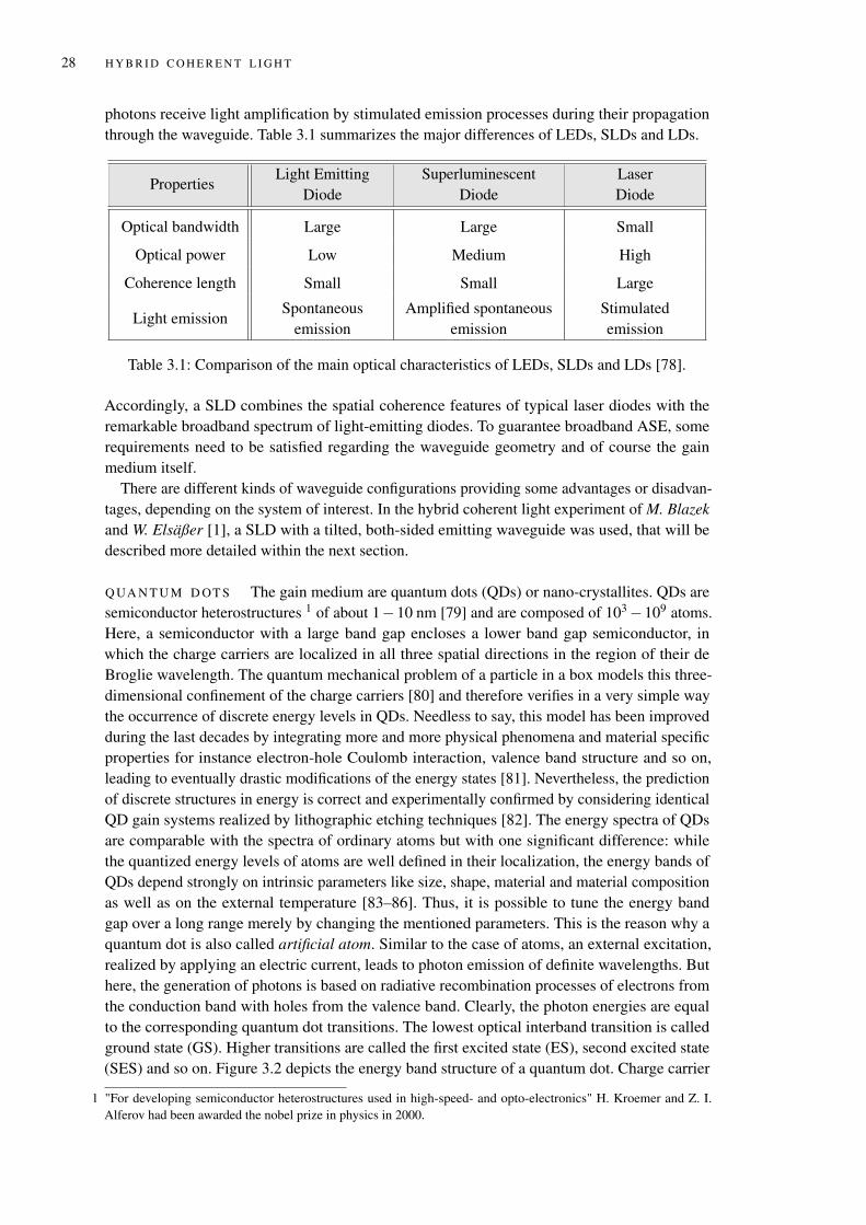
28 H Y B R I D C O H E R E N T L I G H T
photons receive light amplification by stimulated emission processes during their propagationthrough the waveguide. Table 3.1 summarizes the major differences of LEDs, SLDs and LDs.
PropertiesLight Emitting
DiodeSuperluminescent
DiodeLaserDiode
Optical bandwidth Large Large Small
Optical power Low Medium High
Coherence length Small Small Large
Light emissionSpontaneous
emissionAmplified spontaneous
emissionStimulatedemission
Table 3.1: Comparison of the main optical characteristics of LEDs, SLDs and LDs [78].
Accordingly, a SLD combines the spatial coherence features of typical laser diodes with theremarkable broadband spectrum of light-emitting diodes. To guarantee broadband ASE, somerequirements need to be satisfied regarding the waveguide geometry and of course the gainmedium itself.
There are different kinds of waveguide configurations providing some advantages or disadvan-tages, depending on the system of interest. In the hybrid coherent light experiment of M. Blazekand W. Elsäßer [1], a SLD with a tilted, both-sided emitting waveguide was used, that will bedescribed more detailed within the next section.
Q UA N T U M D OT S The gain medium are quantum dots (QDs) or nano-crystallites. QDs aresemiconductor heterostructures 1 of about 1−10 nm [79] and are composed of 103−109 atoms.Here, a semiconductor with a large band gap encloses a lower band gap semiconductor, inwhich the charge carriers are localized in all three spatial directions in the region of their deBroglie wavelength. The quantum mechanical problem of a particle in a box models this three-dimensional confinement of the charge carriers [80] and therefore verifies in a very simple waythe occurrence of discrete energy levels in QDs. Needless to say, this model has been improvedduring the last decades by integrating more and more physical phenomena and material specificproperties for instance electron-hole Coulomb interaction, valence band structure and so on,leading to eventually drastic modifications of the energy states [81]. Nevertheless, the predictionof discrete structures in energy is correct and experimentally confirmed by considering identicalQD gain systems realized by lithographic etching techniques [82]. The energy spectra of QDsare comparable with the spectra of ordinary atoms but with one significant difference: whilethe quantized energy levels of atoms are well defined in their localization, the energy bands ofQDs depend strongly on intrinsic parameters like size, shape, material and material compositionas well as on the external temperature [83–86]. Thus, it is possible to tune the energy bandgap over a long range merely by changing the mentioned parameters. This is the reason why aquantum dot is also called artificial atom. Similar to the case of atoms, an external excitation,realized by applying an electric current, leads to photon emission of definite wavelengths. Buthere, the generation of photons is based on radiative recombination processes of electrons fromthe conduction band with holes from the valence band. Clearly, the photon energies are equalto the corresponding quantum dot transitions. The lowest optical interband transition is calledground state (GS). Higher transitions are called the first excited state (ES), second excited state(SES) and so on. Figure 3.2 depicts the energy band structure of a quantum dot. Charge carrier
1 "For developing semiconductor heterostructures used in high-speed- and opto-electronics" H. Kroemer and Z. I.Alferov had been awarded the nobel prize in physics in 2000.
3.1 Q UA N T U M D OT S U P E R L U M I N E S C E N T D I O D E S 29
λGS
λES
λSES
WL
CB
VB
GS
ESSES
Position
Ener
gy
Figure 3.2: Energy band structure of a quantum dot in position space. Electrons from the con-duction band (CB) of the bulk medium relax into the wetting layer (WL) and fromthe WL to the ground (GS), first excited (ES) and second excited state (SES). TheGS, ES and SES electrons recombine with holes from the valence band (VB) andsimultaneously emit photons of wavelength λGS, λES and λSES.
relaxation from the conduction band of the bulk medium into the wetting layer (WL) and fromthe wetting layer into the energy levels (GS, ES, SES) are symbolized by black arrows. Therecombination process of the lowest, first and second excited state and the simultaneously emittedphotons of wavelength λGS ≥ λES ≥ λSES are visualized by red, green and blue arrows. Thepossibility to produce such artificial atoms with desired opto-electronic properties opens a widefield of applications for commercial purposes like solar cells [87] or biological diagnostic toolsfor discerning cellular function at the molecular level [88]. But also for the field of quantuminformation, QDs became indispensable as single-photon emitters [89] or qubits [90, 91].
A widely-used fabrication technique of self-assembled QD gain media is epitaxially grownbased on the Stranski-Krastanow method [92, 93]. This technique is much cheaper and morerapid compared to lithographic techniques [94]. The QDs nucleate spontaneously on the growthsurface driven by the strain of lattice mismatch between epitaxial layer and the substrate whenusing molecular beam epitaxy or metal-organic vapor phase epitaxy techniques [78]. Due tothis self-organized growth, the dots are not identical but rather show an approximately Gaussiandistribution in their sizes [95]. Therefore, the single energy levels of the complete set of QDs arebroadened. This inhomogeneous broadening of the gain medium is utilized in a quantum dotsuperluminescent diode (QDSLD) which is the central object of this thesis.
Figure 3.3 shows a typical measured optical power spectrum of a QDSLD with purely GSemission (black line). The green line is a Gaussian fit,
S(ω) =S0√
2πσ2e−(ω−ω)2/(2σ2), (3.1)
of central frequency ω = 2π ·0.24 PHz (λ =1249.14 nm), standard deviation σ = 2π ·1.16 THzand amplitude S0 = 0.113/
√2πσ2. The spectral width is given by b = 2π ·4.11 THz or in terms
of wavelength ∆λ =21.39 nm.In order to obtain such smooth THz broad radiation spectra and spatial directed ASE, more
than one layer of the gain medium are used [96]. Typically, 5−15 layers guarantee the desirablelight behavior. They are spatially separated by another semiconductor material, the so-calledbuffer layers.

30 H Y B R I D C O H E R E N T L I G H T
Data
Gaussian fit
1.48 1.49 1.50 1.51 1.52 1.53
0.0
0.2
0.4
0.6
0.8
1.0
ω (1015/s)
S(ω
)(arb.units)
Figure 3.3: The measured optical power spectrum S(ω) of a QDSLD in arbitrary units shows GSemission. The experimental data (black) are fitted with a Gaussian function (green)with a central frequency ω = 2π ·0.24 PHz (λ =1249.14 nm), a standard deviationσ = 2π ·1.16 THz and an amplitude S0 = 0.113/
√2πσ2. The spectral width is given
by b = 2π ·4.11 THz (∆λ =21.39 nm).
In summary, the delicate choice of waveguide geometry and gain medium results in high outputpowers, high efficiency, spatial coherence and a very broad spectral width. These features of theemitted radiation field together with the remarkable fabrication characteristics of an adaptable,compact and robust semiconductor device, are in great demand for industrial applications likeoptical coherence tomography (OCT) [28, 97–100], telecommunication [101], fiber-optic sensorsand gyroscopes [24, 25, 102], etc. Also fundamental research such as ghost imaging techniques[73,103–105] or the analysis of fundamental quantum optical questions on the photon statistics ofbroadband emitting semiconductor devices [1, 106, 107] takes advantage of these semiconductordevices. The last mentioned experiment performed by M. Blazek and W. Elsäßer measuredtemporal hybrid coherent light for the first time with the help of a QDSLD.
3.2 FI R S T O B S E RVAT I O N O F H Y B R I D C O H E R E N T L I G H T
The QDSLD, studied by M. Blazek and W. Elsäßer [1], was commercially fabricated by theUniversity of Sheffield and the III-V Labs in Palaiseau (series VN1035). This diode possesseda gain medium containing indium arsenide (InAs) quantum dots embedded in indium galliumarsenide (InGaAs) quantum wells (dot-in-well structure). The optical waveguide had a lengthof L = 6 mm and was slightly tilted under an angle of 5− 8 with respect to the longitudinalaxes. In addition, the emission facets where anti-reflection coated to suppress the formation oflongitudinal modes [108]. To obtain high efficient light amplifications with broad spectral rangessix layers of the gain medium were utilized, whereas each layer consisted of about 400 quantumdots per µm2 . They were spatially separated by buffer layers with refractive index nm ≈ 3.5slightly smaller than the index of the single gain layers nc ≈ 3.505. The diode emitted on bothsides.
The emitted light of the QDSLD had an optical output power of P = 50 mW and a centralwavelength of λ= 1220±110 nm at room temperature. The device emitted transverse-electric
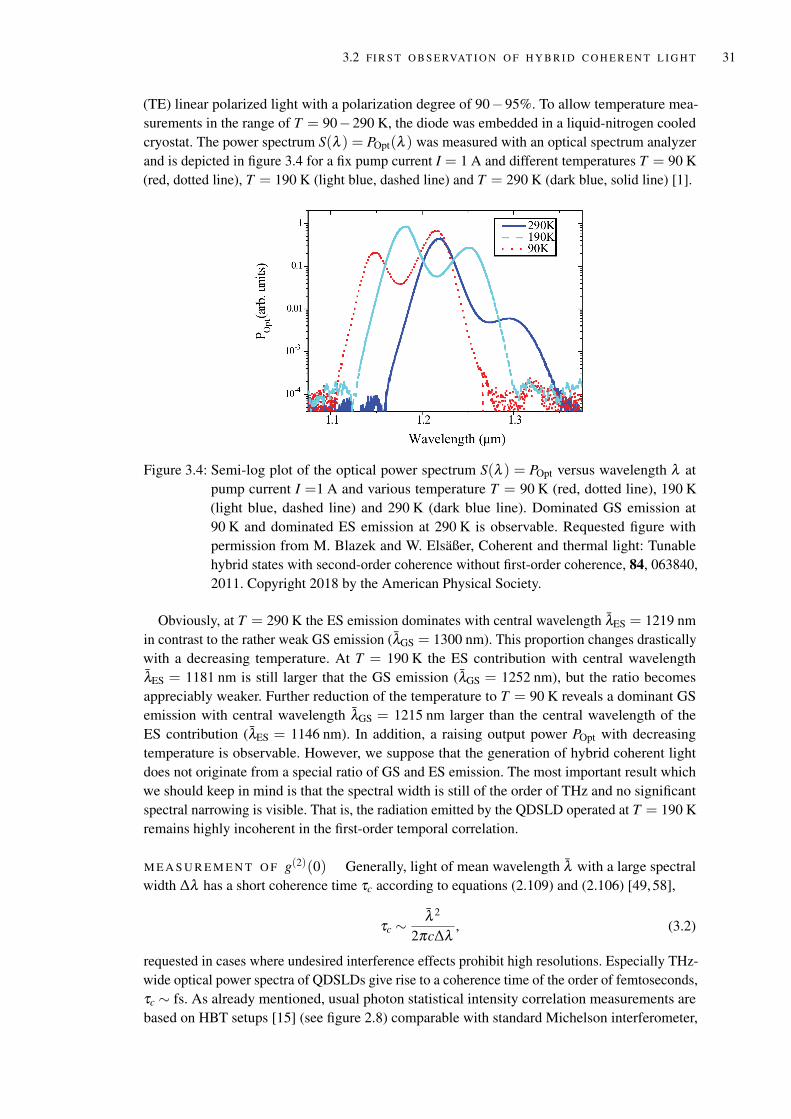
3.2 FI R S T O B S E RVAT I O N O F H Y B R I D C O H E R E N T L I G H T 31
(TE) linear polarized light with a polarization degree of 90−95%. To allow temperature mea-surements in the range of T = 90−290 K, the diode was embedded in a liquid-nitrogen cooledcryostat. The power spectrum S(λ ) = POpt(λ ) was measured with an optical spectrum analyzerand is depicted in figure 3.4 for a fix pump current I = 1 A and different temperatures T = 90 K(red, dotted line), T = 190 K (light blue, dashed line) and T = 290 K (dark blue, solid line) [1].
Figure 3.4: Semi-log plot of the optical power spectrum S(λ ) = POpt versus wavelength λ atpump current I =1 A and various temperature T = 90 K (red, dotted line), 190 K(light blue, dashed line) and 290 K (dark blue line). Dominated GS emission at90 K and dominated ES emission at 290 K is observable. Requested figure withpermission from M. Blazek and W. Elsäßer, Coherent and thermal light: Tunablehybrid states with second-order coherence without first-order coherence, 84, 063840,2011. Copyright 2018 by the American Physical Society.
Obviously, at T = 290 K the ES emission dominates with central wavelength λES = 1219 nmin contrast to the rather weak GS emission (λGS = 1300 nm). This proportion changes drasticallywith a decreasing temperature. At T = 190 K the ES contribution with central wavelengthλES = 1181 nm is still larger that the GS emission (λGS = 1252 nm), but the ratio becomesappreciably weaker. Further reduction of the temperature to T = 90 K reveals a dominant GSemission with central wavelength λGS = 1215 nm larger than the central wavelength of theES contribution (λES = 1146 nm). In addition, a raising output power POpt with decreasingtemperature is observable. However, we suppose that the generation of hybrid coherent lightdoes not originate from a special ratio of GS and ES emission. The most important result whichwe should keep in mind is that the spectral width is still of the order of THz and no significantspectral narrowing is visible. That is, the radiation emitted by the QDSLD operated at T = 190 Kremains highly incoherent in the first-order temporal correlation.
M E A S U R E M E N T O F g(2)(0) Generally, light of mean wavelength λ with a large spectralwidth ∆λ has a short coherence time τc according to equations (2.109) and (2.106) [49, 58],
τc ∼λ 2
2πc∆λ, (3.2)
requested in cases where undesired interference effects prohibit high resolutions. Especially THz-wide optical power spectra of QDSLDs give rise to a coherence time of the order of femtoseconds,τc ∼ fs. As already mentioned, usual photon statistical intensity correlation measurements arebased on HBT setups [15] (see figure 2.8) comparable with standard Michelson interferometer,
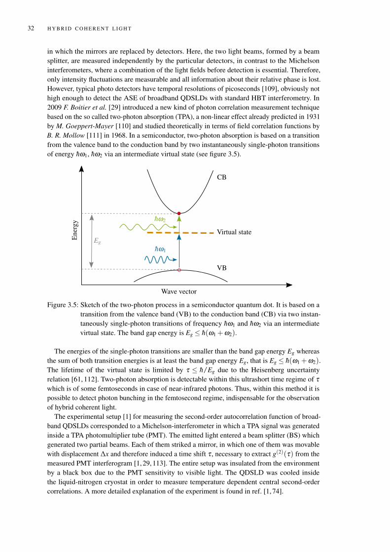
32 H Y B R I D C O H E R E N T L I G H T
in which the mirrors are replaced by detectors. Here, the two light beams, formed by a beamsplitter, are measured independently by the particular detectors, in contrast to the Michelsoninterferometers, where a combination of the light fields before detection is essential. Therefore,only intensity fluctuations are measurable and all information about their relative phase is lost.However, typical photo detectors have temporal resolutions of picoseconds [109], obviously nothigh enough to detect the ASE of broadband QDSLDs with standard HBT interferometry. In2009 F. Boitier et al. [29] introduced a new kind of photon correlation measurement techniquebased on the so called two-photon absorption (TPA), a non-linear effect already predicted in 1931by M. Goeppert-Mayer [110] and studied theoretically in terms of field correlation functions byB. R. Mollow [111] in 1968. In a semiconductor, two-photon absorption is based on a transitionfrom the valence band to the conduction band by two instantaneously single-photon transitionsof energy hω1, hω2 via an intermediate virtual state (see figure 3.5).
Wave vector
Ener
gy
CB
VB
Virtual state
hω1
hω2
Eg
Figure 3.5: Sketch of the two-photon process in a semiconductor quantum dot. It is based on atransition from the valence band (VB) to the conduction band (CB) via two instan-taneously single-photon transitions of frequency hω1 and hω2 via an intermediatevirtual state. The band gap energy is Eg ≤ h(ω1 +ω2).
The energies of the single-photon transitions are smaller than the band gap energy Eg whereasthe sum of both transition energies is at least the band gap energy Eg, that is Eg ≤ h(ω1 +ω2).The lifetime of the virtual state is limited by τ ≤ h/Eg due to the Heisenberg uncertaintyrelation [61, 112]. Two-photon absorption is detectable within this ultrashort time regime of τwhich is of some femtoseconds in case of near-infrared photons. Thus, within this method it ispossible to detect photon bunching in the femtosecond regime, indispensable for the observationof hybrid coherent light.
The experimental setup [1] for measuring the second-order autocorrelation function of broad-band QDSLDs corresponded to a Michelson-interferometer in which a TPA signal was generatedinside a TPA photomultiplier tube (PMT). The emitted light entered a beam splitter (BS) whichgenerated two partial beams. Each of them striked a mirror, in which one of them was movablewith displacement ∆x and therefore induced a time shift τ , necessary to extract g(2)(τ) from themeasured PMT interferogram [1, 29, 113]. The entire setup was insulated from the environmentby a black box due to the PMT sensitivity to visible light. The QDSLD was cooled insidethe liquid-nitrogen cryostat in order to measure temperature dependent central second-ordercorrelations. A more detailed explanation of the experiment is found in ref. [1, 74].
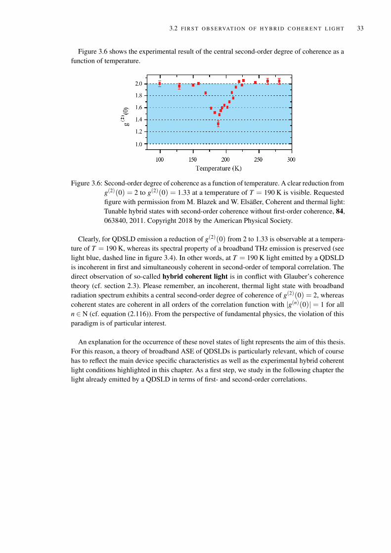
3.2 FI R S T O B S E RVAT I O N O F H Y B R I D C O H E R E N T L I G H T 33
Figure 3.6 shows the experimental result of the central second-order degree of coherence as afunction of temperature.
Figure 3.6: Second-order degree of coherence as a function of temperature. A clear reduction fromg(2)(0) = 2 to g(2)(0) = 1.33 at a temperature of T = 190 K is visible. Requestedfigure with permission from M. Blazek and W. Elsäßer, Coherent and thermal light:Tunable hybrid states with second-order coherence without first-order coherence, 84,063840, 2011. Copyright 2018 by the American Physical Society.
Clearly, for QDSLD emission a reduction of g(2)(0) from 2 to 1.33 is observable at a tempera-ture of T = 190 K, whereas its spectral property of a broadband THz emission is preserved (seelight blue, dashed line in figure 3.4). In other words, at T = 190 K light emitted by a QDSLDis incoherent in first and simultaneously coherent in second-order of temporal correlation. Thedirect observation of so-called hybrid coherent light is in conflict with Glauber’s coherencetheory (cf. section 2.3). Please remember, an incoherent, thermal light state with broadbandradiation spectrum exhibits a central second-order degree of coherence of g(2)(0) = 2, whereascoherent states are coherent in all orders of the correlation function with |g(n)(0)| = 1 for alln ∈ N (cf. equation (2.116)). From the perspective of fundamental physics, the violation of thisparadigm is of particular interest.
An explanation for the occurrence of these novel states of light represents the aim of this thesis.For this reason, a theory of broadband ASE of QDSLDs is particularly relevant, which of coursehas to reflect the main device specific characteristics as well as the experimental hybrid coherentlight conditions highlighted in this chapter. As a first step, we study in the following chapter thelight already emitted by a QDSLD in terms of first- and second-order correlations.

4
L I G H T S TAT E S O F Q UA N T U M D OT S U P E R L U M I N E S C E N TD I O D E S
The analysis of hybrid coherent light enforces a detailed study on the photon statistics of theamplified spontaneous emission which was first studied by L. Allen and G. I. Peters classically[114–117]. However, photon statistics is the footprint of the quantum nature of light, which isdirectly related to the emission spectral density and mathematically quantified by the centralsecond-order degree of coherence (see chapter 2). Therefore, already existing, well-establishedtheories of SLD emission, based on rate equations or traveling wave approaches [118–120], haveto be extended to the quantum world, which has not been done yet to the best of our knowledge.The high complex material semiconductor structure can be directly embedded within a quantumfield theoretical ansatz. However, this leads to many degrees of freedom.
As a first step, we want to postulate a quantum state describing ASE of the diode system,allowing us to implement the emission and photon statistical properties by disregarding additionalmaterial or geometric specific characteristics of the device. Thus, at this point of the thesis, weclaim that it is so far unnecessary to study the light creation and propagation in the semiconductorwaveguide structure.
In this chapter, first- and second-order correlation functions of the chosen light state arestudied in detail, the validity which is proven by two experiments [121, 122] at room temperatureconducted by S. Blumenstein (name of birth Hartmann) et al.. All pictures showing measurementsare adapted or taken from ref. [122], generated in a collaborative way. The first measurementis based on optical feedback, whereas the second one considers the convolution of coherentlight with the SLD broadband radiation. We will see that both experiments exhibit remarkableagreement with our theoretical predictions.
4.1 P H A S E - R A N D O M I Z E D G AU S S I A N S TAT E
In order to model a THz broadband radiation spectrum of a QDSLD, we choose a quantizedtransversal electric field E(r, t) evaluated at position r = (x,y,z)T and time t. The observedradiation field outside the quantum dot superluminescent diode is highly multimode. Therefore,we consider a free electric field given by a superposition of a large number of N longitudinalmodes with positive frequency part
E(+)(r, t) = E(+)(x,y, t− zc0) = E(+)(r, t)ey, E(+)(r, t) =
N
∑j=1
u j(r, t)a j. (4.1)
We require a linear polarization in y-direction due to the structural composition of the device (seechapter 3.2) [123]. Although the diode system emits both-sided, we consider a mono-directional
35
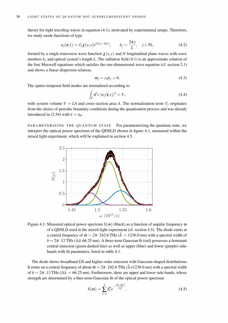
36 L I G H T S TAT E S O F Q UA N T U M D OT S U P E R L U M I N E S C E N T D I O D E S
theory for right traveling waves in equation (4.1), motivated by experimental setups. Therefore,we study mode functions of type
u j(r, t) = E jχ(x,y)ei(k jz−ω jt), k j =2π j
L, j ∈N, (4.2)
formed by a single transverse wave function χ(x,y) and N longitudinal plane waves with wavenumbers k j and optical system’s length L. The radiation field (4.1) is an approximate solution ofthe free Maxwell equations which satisfies the one-dimensional wave equation (cf. section 2.1)and shows a linear dispersion relation,
ω j = c0k j > 0. (4.3)
The spatio-temporal field modes are normalized according to∫V
d3r |u j(r, t)|2 = V , (4.4)
with system volume V = LA and cross-section area A. The normalization term E j originatesfrom the choice of periodic boundary conditions during the quantization process and was alreadyintroduced in (2.54) with ε = ε0.
PA R A M E T E R I Z I N G T H E Q UA N T U M S TAT E For parameterizing the quantum state, weinterpret the optical power spectrum of the QDSLD shown in figure 4.1, measured within themixed light experiment, which will be explained in section 4.5.
ω (1015/s)
S(ω
)
1.45 1.5 1.55 1.60
0.5
1
1.5
2
2.5
Figure 4.1: Measured optical power spectrum S(ω) (black) as a function of angular frequency ωof a QDSLD used in the mixed-light experiment (cf. section 4.5). The diode emits ata central frequency of ω = 2π ·242.6 THz (λ = 1236.0 nm) with a spectral width ofb = 2π ·13 THz (∆λ 66.25 nm). A three-term Gaussian fit (red) possesses a dominantcentral emission (green dashed line) as well as upper (blue) and lower (purple) side-bands with fit parameters, listed in table 4.1.
The diode shows broadband GS and higher-order emission with Gaussian-shaped distributions.It emits on a central frequency of about ω = 2π ·242.6 THz (λ=1236.0 nm) with a spectral widthof b = 2π ·13 THz (∆λ = 66.25 nm). Furthermore, there are upper and lower side-bands, whosestrength are determined by a thee-term Gaussian fit of the optical power spectrum
S(ω) =3
∑i=1
S0i e− (ω−ωi)
2
2σ2i . (4.5)
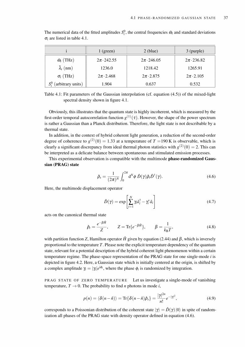
4.1 P H A S E - R A N D O M I Z E D G AU S S I A N S TAT E 37
The numerical data of the fitted amplitudes S0i , the central frequencies ωi and standard deviations
σi are listed in table 4.1.
i 1 (green) 2 (blue) 3 (purple)
ωi (THz) 2π ·242.55 2π ·246.05 2π ·236.82
λi (nm) 1236.0 1218.42 1265.91
σi (THz) 2π ·2.468 2π ·2.875 2π ·2.105
S0i (arbitrary units) 1.904 0.637 0.532
Table 4.1: Fit parameters of the Gaussian interpolation (cf. equation (4.5)) of the mixed-lightspectral density shown in figure 4.1.
Obviously, this illustrates that the quantum state is highly incoherent, which is measured by thefirst-order temporal autocorrelation function g(1)(τ). However, the shape of the power spectrumis rather a Gaussian than a Planck distribution. Therefore, the light state is not describable by athermal state.
In addition, in the context of hybrid coherent light generation, a reduction of the second-orderdegree of coherence to g(2)(0) = 1.33 at a temperature of T =190 K is observable, which isclearly a significant discrepancy from ideal thermal photon statistics with g(2)(0) = 2. This canbe interpreted as a delicate balance between spontaneous and stimulated emission processes.
This experimental observation is compatible with the multimode phase-randomized Gaus-sian (PRAG) state
ρs =1
(2π)N
∫ 2π
0dNφ D(γ)ρtD†(γ). (4.6)
Here, the multimode displacement operator
D(γ) = exp
[N
∑i=1
γia†i − γ∗i ai
](4.7)
acts on the canonical thermal state
ρt =e−β H
Z, Z = Tre−β H, β =
1kBT
, (4.8)
with partition function Z, Hamilton operator H given by equation (2.44) and β , which is inverselyproportional to the temperature T . Please note the explicit temperature dependency of the quantumstate, relevant for a potential description of the hybrid coherent light phenomenon within a certaintemperature regime. The phase-space representation of the PRAG state for one single-mode i isdepicted in figure 4.2. Here, a Gaussian state which is initially centered at the origin, is shifted bya complex amplitude γi = |γi|eiφi , where the phase φi is randomized by integration.
P R AG S TAT E O F Z E RO T E M P E R AT U R E Let us investigate a single-mode of vanishingtemperature, T → 0. The probability to find n photons in mode i,
p(n) = 〈δ (n− n)〉= Trδ (n− n)ρs=|γ|2n
n!e−|γ|
2, (4.9)
corresponds to a Poissonian distribution of the coherent state |γ〉= D(γ) |0〉 in spite of random-ization all phases of the PRAG state with density operator defined in equation (4.6).
38 L I G H T S TAT E S O F Q UA N T U M D OT S U P E R L U M I N E S C E N T D I O D E S
φi
Im(γ)
Re(γ)
|γi|
DisplacedGaussian state
Figure 4.2: Phase-space representation of the PRAG state. We depict the mode i, which isprepared in a Gaussian (thermal) state, displaced by γi = |γi|eiφi , and the phase angleis randomized (cf. equation (4.6)).
Field and intensity correlations are evaluable using beneficial Lie algebraic similarity trans-formations, more precisely the harmonic oscillator algebra [124] with
D†(γ)a jD(γ) = a j + γ j. (4.10)
As a relevant result, we find first and second moments of the PRAG state, given by
〈ai〉= 0, 〈a†j ai〉= nS(ωi)δi j with nS(ωi) = nC(ωi)+ nT (ωi), nC(ωi) = |γi|2. (4.11)
A detailed derivation of equation (4.11) is elaborated in appendix B. Furthermore, higher-ordermoments are expressible by these lowest moments using Wick’s theorem (see appendix A),which is a powerful tool to facilitate the determination of the second-order autocorrelationfunction. One should notice that the mean thermal occupation number nT (cf. equation (2.76))explicitly arises in the second moment (see equation (4.11)) which corresponds to a Bose-Einsteindistribution referred in section 2. Therefore, in case of near-infrared (NIR) photons at roomtemperature possessing a central angular frequency of ω = 2π ·0.24 PHz, the thermal occupationnT (ω)≈ 10−17 is negligibly small. However, we are dealing with a driven semiconductor system,so that the temperature of the photons must not be the same as the environmental temperature.
As shown in section 2.1.2, a common definition of the field intensity I(r, t) (see equation (2.62))of the emitted QDSLD light is proportional to the expectation value of the electric field at equalspace-time events,
I(r, t) = I(x,y) = C 〈E(−)(r, t)E(+)(r, t)〉, (4.12)
and therefore directly related to the second-order moment (4.11). Obviously, I(x,y) is independentof time t and position z, resulting from the stationarity of the state itself as well as the translationalinvariance of the traveling radiation field described by equation (4.1). This physical variable is ofunit W m−2 in fully agreement to the radiometric definition of an intensity [125].
4.2 FI R S T- O R D E R C O R R E L AT I O N F U N C T I O N 39
The optical power P, measured by a standard single-photon detector at a fix position z is givenby this intensity integrated over the full detector area A,
P =∫
Adxdy I(x,y) =
N
∑i=1
psi =
N
∑i=1
pci + pt
i ≡ Pc +Pt with (4.13)
pci = pc(ωi) ≡
hωic0
LnC(ωi), pt
i = pt(ωi) ≡hωic0
LnT (ωi), ps
i = pci + pt
i . (4.14)
As shown in figure 4.1, the optical power spectrum S(ω) is Gaussian distributed over thefrequency bandwidth [ω1,ωN ]. Clearly, integration of S(ω) over this bandwidth corresponds tothe optical power itself, ∫ ωN
ω1
dω S(ω) = P. (4.15)
Thus, a definition of frequency averages and variances,
〈〈p〉〉 ≡ 1N
N
∑i=1
pi, ∆2 p≡N
∑i=1
(pi−〈〈p〉〉)2
N, (4.16)
is inevitable for the interpretation of spectra. The total optical power in terms of power averagesand variances (4.16), is given by the sum of the average of the incoherent field 〈〈pc〉〉 and theaverage of the thermal field 〈〈pt〉〉 multiplied by the number of modes N,
P = Pc +Pt = N (〈〈pc〉〉+ 〈〈pt〉〉) . (4.17)
In the following, we will show that field and intensity correlations are expressible by thesephysical quantities.
4.2 FI R S T- O R D E R C O R R E L AT I O N F U N C T I O N
We already showed that, by definition of Glauber’s coherence theory, the first-order autocorre-lation function of the QDSLD emission is given by the average value of the positive and negativefrequency parts of the electric field (4.1) for different space-time events x ≡ (r, t) (cf. equa-tion (2.87)). Scale invariant properties can be achieved by introducing the normalized first-orderautocorrelation function described by (2.88), in which the denominator corresponds to a productof intensities (see equation (2.90)). The Wiener-Khintchine theorem (cf. equation (2.95)) relatesthe temporal field correlation to the optical power spectrum by a Fourier-transformation, whichis experimentally accessible using a spectrum analyzer. The measured signal is proportional tothe spatially averaged temporal first-order correlation function (cf. equation (2.98)). The integralover the total detector area A can be evaluated by utilizing the normalization condition (4.4) andthe solution of the second moment given in equation (4.11). The corresponding calculation canbe found in appendix B. As a main result we find that the temporal first-order autocorrelationfunction of PRAG states is given by
G(1)(τ) =1C
N
∑i=1
e−iωiτ psi . (4.18)
In case of vanishing time delay, τ = 0, the correlation function is proportional to the total opticalpower P,
G(1)(0) =PC
. (4.19)
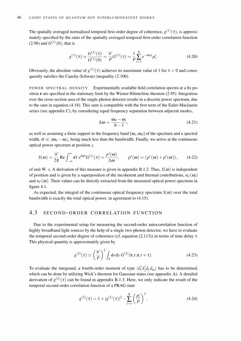
40 L I G H T S TAT E S O F Q UA N T U M D OT S U P E R L U M I N E S C E N T D I O D E S
The spatially averaged normalized temporal first-order degree of coherence, g(1)(τ), is approxi-mately specified by the ratio of the spatially averaged temporal first-order correlation function(2.98) and G(1)(0), that is
g(1)(τ) ' G(1)(τ)G(1)(0)
=C
PG(1)(τ) =
1P
N
∑i=1
e−iωiτ psi . (4.20)
Obviously, the absolute value of g(1)(τ) achieves its maximum value of 1 for τ = 0 and conse-quently satisfies the Cauchy-Schwarz inequality (2.100).
P OW E R S P E C T R A L D E N S I T Y Experimentally available field correlation spectra at a fix po-sition r are specified in the stationary limit by the Wiener-Khintchine theorem (2.95). Integrationover the cross-section area of the single-photon detector results in a discrete power spectrum, dueto the sum in equation (4.18). This sum is compatible with the first term of the Euler-Maclaurinseries (see appendix C), by considering equal frequency separation between adjacent modes,
∆ω =ωN−ω1
N−1, (4.21)
as well as assuming a finite support in the frequency band [ω1,ωN] of the spectrum and a spectralwidth, σ |ωN−ω1|, being much less than the bandwidth. Finally, we arrive at the continuousoptical power spectrum at position z,
S(ω) =C
2πRe∫ ∞
−∞dτ eiωτG(1)(τ) =
ps(ω)
∆ω, ps(ω) = (pc(ω)+ pt(ω)) , (4.22)
of unit W ·s. A derivation of this measure is given in appendix B.1.2. Thus, S(ω) is independentof position and is given by a superposition of the incoherent and thermal contributions, nC(ωi)
and nT (ω). Their values can be directly extracted from the measured optical power spectrum infigure 4.1.
As expected, the integral of the continuous optical frequency spectrum S(ω) over the totalbandwidth is exactly the total optical power, in agreement to (4.15).
4.3 S E C O N D - O R D E R C O R R E L AT I O N F U N C T I O N
Due to the experimental setup for measuring the second-order autocorrelation function ofhighly broadband light sources by the help of a single two-photon detector, we have to evaluatethe temporal second-order degree of coherence (cf. equation (2.113)) in terms of time delay τ .This physical quantity is approximately given by
g(2)(τ) '(
C
P
)2 ∫A
dxdy G(2)(r, t;r, t + τ). (4.23)
To evaluate the integrand, a fourth-order moment of type 〈a†i a†
j al am〉 has to be determined,which can be done by utilizing Wick’s theorem for Gaussian states (see appendix A). A detailedderivation of g(2)(τ) can be found in appendix B.1.3. Here, we only indicate the result of thetemporal second-order correlation function of a PRAG state
g(2)(τ) = 1+ |g(1)(τ)|2−N
∑i=1
(pc
iP
)2
. (4.24)
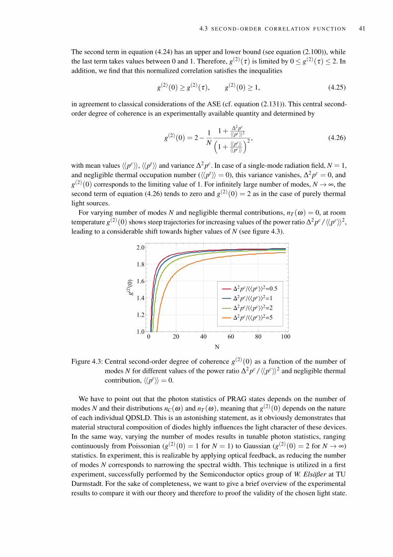
4.3 S E C O N D - O R D E R C O R R E L AT I O N F U N C T I O N 41
The second term in equation (4.24) has an upper and lower bound (see equation (2.100)), whilethe last term takes values between 0 and 1. Therefore, g(2)(τ) is limited by 0≤ g(2)(τ) ≤ 2. Inaddition, we find that this normalized correlation satisfies the inequalities
g(2)(0) ≥ g(2)(τ), g(2)(0) ≥ 1, (4.25)
in agreement to classical considerations of the ASE (cf. equation (2.131)). This central second-order degree of coherence is an experimentally available quantity and determined by
g(2)(0) = 2− 1N
1+ ∆2 pc
〈〈pc〉〉2(1+ 〈〈pt〉〉
〈〈pc〉〉
)2 , (4.26)
with mean values 〈〈pc〉〉, 〈〈pt〉〉 and variance ∆2 pc. In case of a single-mode radiation field, N = 1,and negligible thermal occupation number (〈〈pt〉〉 = 0), this variance vanishes, ∆2 pc = 0, andg(2)(0) corresponds to the limiting value of 1. For infinitely large number of modes, N→ ∞, thesecond term of equation (4.26) tends to zero and g(2)(0) = 2 as in the case of purely thermallight sources.
For varying number of modes N and negligible thermal contributions, nT (ω) = 0, at roomtemperature g(2)(0) shows steep trajectories for increasing values of the power ratio ∆2 pc/〈〈pc〉〉2,leading to a considerable shift towards higher values of N (see figure 4.3).
Δ2pc/⟨⟨pc⟩⟩2=0.5
Δ2pc/⟨⟨pc⟩⟩2=1
Δ2pc/⟨⟨pc⟩⟩2=2
Δ2pc/⟨⟨pc⟩⟩2=5
0 20 40 60 80 1001.0
1.2
1.4
1.6
1.8
2.0
N
g(2) (0)
Figure 4.3: Central second-order degree of coherence g(2)(0) as a function of the number ofmodes N for different values of the power ratio ∆2 pc/〈〈pc〉〉2 and negligible thermalcontribution, 〈〈pt〉〉= 0.
We have to point out that the photon statistics of PRAG states depends on the number ofmodes N and their distributions nC(ω) and nT (ω), meaning that g(2)(0) depends on the natureof each individual QDSLD. This is an astonishing statement, as it obviously demonstrates thatmaterial structural composition of diodes highly influences the light character of these devices.In the same way, varying the number of modes results in tunable photon statistics, rangingcontinuously from Poissonian (g(2)(0) = 1 for N = 1) to Gaussian (g(2)(0) = 2 for N → ∞)statistics. In experiment, this is realizable by applying optical feedback, as reducing the numberof modes N corresponds to narrowing the spectral width. This technique is utilized in a firstexperiment, successfully performed by the Semiconductor optics group of W. Elsäßer at TUDarmstadt. For the sake of completeness, we want to give a brief overview of the experimentalresults to compare it with our theory and therefore to proof the validity of the chosen light state.
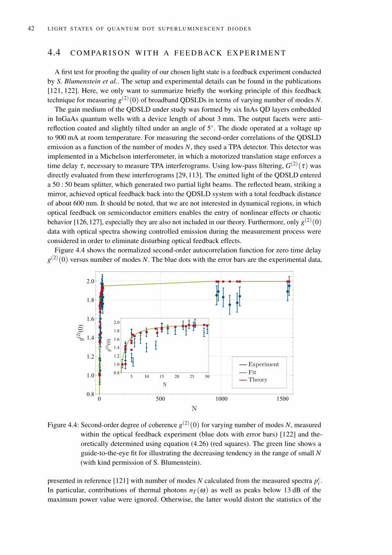
42 L I G H T S TAT E S O F Q UA N T U M D OT S U P E R L U M I N E S C E N T D I O D E S
4.4 C O M PA R I S O N W I T H A F E E D BAC K E X P E R I M E N T
A first test for proofing the quality of our chosen light state is a feedback experiment conductedby S. Blumenstein et al.. The setup and experimental details can be found in the publications[121, 122]. Here, we only want to summarize briefly the working principle of this feedbacktechnique for measuring g(2)(0) of broadband QDSLDs in terms of varying number of modes N.
The gain medium of the QDSLD under study was formed by six InAs QD layers embeddedin InGaAs quantum wells with a device length of about 3 mm. The output facets were anti-reflection coated and slightly tilted under an angle of 5. The diode operated at a voltage upto 900 mA at room temperature. For measuring the second-order correlations of the QDSLDemission as a function of the number of modes N, they used a TPA detector. This detector wasimplemented in a Michelson interferometer, in which a motorized translation stage enforces atime delay τ , necessary to measure TPA interferograms. Using low-pass filtering, G(2)(τ) wasdirectly evaluated from these interferograms [29, 113]. The emitted light of the QDSLD entereda 50 : 50 beam splitter, which generated two partial light beams. The reflected beam, striking amirror, achieved optical feedback back into the QDSLD system with a total feedback distanceof about 600 mm. It should be noted, that we are not interested in dynamical regions, in whichoptical feedback on semiconductor emitters enables the entry of nonlinear effects or chaoticbehavior [126,127], especially they are also not included in our theory. Furthermore, only g(2)(0)data with optical spectra showing controlled emission during the measurement process wereconsidered in order to eliminate disturbing optical feedback effects.
Figure 4.4 shows the normalized second-order autocorrelation function for zero time delayg(2)(0) versus number of modes N. The blue dots with the error bars are the experimental data,
Experiment
FitTheory
5 10 15 20 25 300.8
1.0
1.2
1.4
1.6
1.8
2.0
N
g(2) (0)
0 500 1000 15000.8
1.0
1.2
1.4
1.6
1.8
2.0
N
g(2) (0)
Figure 4.4: Second-order degree of coherence g(2)(0) for varying number of modes N, measuredwithin the optical feedback experiment (blue dots with error bars) [122] and the-oretically determined using equation (4.26) (red squares). The green line shows aguide-to-the-eye fit for illustrating the decreasing tendency in the range of small N(with kind permission of S. Blumenstein).
presented in reference [121] with number of modes N calculated from the measured spectra pci .
In particular, contributions of thermal photons nT (ω) as well as peaks below 13 dB of themaximum power value were ignored. Otherwise, the latter would distort the statistics of the

4.4 C O M PA R I S O N W I T H A F E E D BAC K E X P E R I M E N T 43
light state. The red squares are the theoretical values, specified by equation (4.26) for the givenexperimental values of N, 〈〈pc〉〉 and ∆2 pc, to reflect experimental requirements of the coherencetransition. In addition, table 4.2 lists some theoretical and experimental values for g(2)(0) withexperimentally determined number of modes N and power ratio ∆2 pc/〈〈pc〉〉2. To avoid confusion,
N∆2 pc
〈〈pc〉〉2 g(2)exp(0) g(2)th (0)
3 1.31 1.18 1.23
10 1.12 1.78 1.74
30 1.08 1.83 1.931
1945 0.57 1.84 1.999
Table 4.2: Experimental and theoretical values of g(2)(0) with experimentally determined param-eters N and ∆2 pc/〈〈pc〉〉2. The number of modes N were varied by applying opticalfeedback. The experimental data were kindly supplied by S. Blumenstein.
we denote the temporal second-order correlation function, determined experimentally by g(2)exp(τ)and theoretically by g(2)th (τ).
A comparison between theory and experiment highlights an overall good agreement. For alarge number of modes, N > 1000, i.e. weak optical feedback, the QDSLD shows ultra-broadbandemission with a second-order correlation function of about g(2)th (0)≈ 1.999 in theory. From the
experimental point of view, g(2)exp(0) can not be determined within this regime simply by countingthe number of spectral peaks, due to the formation of smooth Gaussian power spectra as shownin figure 4.1.
In the experiment, N was determined by fitting modes with spacing according to the freespectral range in terms of angular frequency,
∆ω =2πc0
2nGaAsL≈ 2π ·1.465 ·1010 Hz, nGaAs ≈ 3.41, (4.27)
representing a lower-bound estimate [122]. Within this mode regime, a second-order correlationaround g(2)exp(0) = 1.85 was measured, which reveals an appreciable deviation from the calcu-lated value of 1.999. This discrepancy between theory and experiment is caused by technicalchallenges during the measurement process (see ref. [122]) leading to experimental data lyingbelow the predicted theoretical values for large number of modes, N > 1000. With increasingoptical feedback, spectral peaks became more and more visible, so that N are experimentallydetermined by just counting the peaks. In the range of N = 30 down to N = 15 we observe aslight decreasing tendency of g(2)(0) both in experiment (g(2)exp(0) = 1.83 for N = 30) as well as
in theory (g(2)th (0) = 1.931 for N = 30). For N < 15 a fast transition in coherence is observabledue to a reduction of g(2)(0) from 1.8 to 1 in both theory and experiment.
Indeed, optical feedback offers a dramatic change of the statistical behavior of photons emittedby QDSLDs. However, a coherence transition is observable even for small number of modes,where the smooth THz-wide Gaussian character disappear. Therefore, the precision of ourtheory, especially formulated for broadband QDSLD emission, has to be confirmed by a furtherexperiment, retaining the broadband character of emitting QDSLDs. It becomes apparent that amixed-light experiment, in which coherent light is superimposed with the radiation of a QDSLD,represents an ideal candidate for this challenging examination of the PRAG state quality fordescribing light emitted by these semiconductor devices.
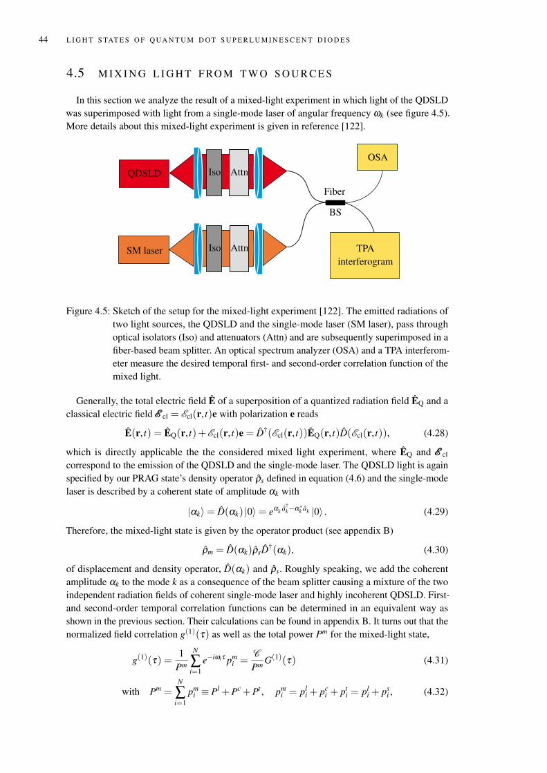
44 L I G H T S TAT E S O F Q UA N T U M D OT S U P E R L U M I N E S C E N T D I O D E S
4.5 M I X I N G L I G H T F RO M T W O S O U R C E S
In this section we analyze the result of a mixed-light experiment in which light of the QDSLDwas superimposed with light from a single-mode laser of angular frequency ωk (see figure 4.5).More details about this mixed-light experiment is given in reference [122].
source
QDSLD
SM laser
Fiber
BS
AttnIso
AttnIso
OSA
TPAinterferogram
Figure 4.5: Sketch of the setup for the mixed-light experiment [122]. The emitted radiations oftwo light sources, the QDSLD and the single-mode laser (SM laser), pass throughoptical isolators (Iso) and attenuators (Attn) and are subsequently superimposed in afiber-based beam splitter. An optical spectrum analyzer (OSA) and a TPA interferom-eter measure the desired temporal first- and second-order correlation function of themixed light.
Generally, the total electric field E of a superposition of a quantized radiation field EQ and aclassical electric field EEE cl = Ecl(r, t)e with polarization e reads
E(r, t) = EQ(r, t)+Ecl(r, t)e = D†(Ecl(r, t))EQ(r, t)D(Ecl(r, t)), (4.28)
which is directly applicable the the considered mixed light experiment, where EQ and EEE cl
correspond to the emission of the QDSLD and the single-mode laser. The QDSLD light is againspecified by our PRAG state’s density operator ρs defined in equation (4.6) and the single-modelaser is described by a coherent state of amplitude αk with
|αk〉= D(αk) |0〉= eαk a†k−α∗k ak |0〉 . (4.29)
Therefore, the mixed-light state is given by the operator product (see appendix B)
ρm = D(αk)ρsD†(αk), (4.30)
of displacement and density operator, D(αk) and ρs. Roughly speaking, we add the coherentamplitude αk to the mode k as a consequence of the beam splitter causing a mixture of the twoindependent radiation fields of coherent single-mode laser and highly incoherent QDSLD. First-and second-order temporal correlation functions can be determined in an equivalent way asshown in the previous section. Their calculations can be found in appendix B. It turns out that thenormalized field correlation g(1)(τ) as well as the total power Pm for the mixed-light state,
g(1)(τ) =1
Pm
N
∑i=1
e−iωiτ pmi =
C
Pm G(1)(τ) (4.31)
with Pm =N
∑i=1
pmi ≡ Pl +Pc +Pt , pm
i = pli + pc
i + pti = pl
i + psi , (4.32)
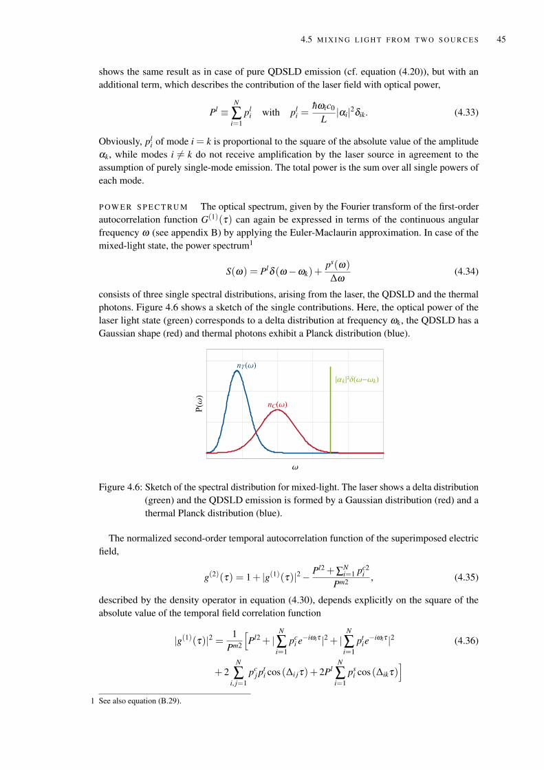
4.5 M I X I N G L I G H T F RO M T W O S O U R C E S 45
shows the same result as in case of pure QDSLD emission (cf. equation (4.20)), but with anadditional term, which describes the contribution of the laser field with optical power,
Pl ≡N
∑i=1
pli with pl
i =hωic0
L|αi|2δik. (4.33)
Obviously, pli of mode i = k is proportional to the square of the absolute value of the amplitude
αk, while modes i 6= k do not receive amplification by the laser source in agreement to theassumption of purely single-mode emission. The total power is the sum over all single powers ofeach mode.
P OW E R S P E C T RU M The optical spectrum, given by the Fourier transform of the first-orderautocorrelation function G(1)(τ) can again be expressed in terms of the continuous angularfrequency ω (see appendix B) by applying the Euler-Maclaurin approximation. In case of themixed-light state, the power spectrum1
S(ω) = Plδ (ω−ωk)+ps(ω)
∆ω(4.34)
consists of three single spectral distributions, arising from the laser, the QDSLD and the thermalphotons. Figure 4.6 shows a sketch of the single contributions. Here, the optical power of thelaser light state (green) corresponds to a delta distribution at frequency ωk, the QDSLD has aGaussian shape (red) and thermal photons exhibit a Planck distribution (blue).
nT(ω)
nC(ω)
|αk|²δ(ω-ωk)
ω
P(ω
)
Figure 4.6: Sketch of the spectral distribution for mixed-light. The laser shows a delta distribution(green) and the QDSLD emission is formed by a Gaussian distribution (red) and athermal Planck distribution (blue).
The normalized second-order temporal autocorrelation function of the superimposed electricfield,
g(2)(τ) = 1+ |g(1)(τ)|2− Pl2 +∑Ni=1 pc2
iPm2 , (4.35)
described by the density operator in equation (4.30), depends explicitly on the square of theabsolute value of the temporal field correlation function
|g(1)(τ)|2 = 1Pm2
[Pl2 + |
N
∑i=1
pci e−iωiτ |2 + |
N
∑i=1
ptie−iωiτ |2 (4.36)
+ 2N
∑i, j=1
pcj p
ti cos (∆i jτ)+ 2Pl
N
∑i=1
psi cos (∆ikτ)
]1 See also equation (B.29).

46 L I G H T S TAT E S O F Q UA N T U M D OT S U P E R L U M I N E S C E N T D I O D E S
with frequency difference ∆i j = ωi−ω j. Clearly, the last term in equation (4.36) oscillates withbeat frequency ∆ik = ωi−ωk, resulting from the frequency difference of the QDSLD mode i andthe laser frequency. This leads to the occurrence of sidebands in the spectrum and finally in thesecond-order degree of coherence g(2)(τ).
S P E C I A L C A S E : S I N G L E - M O D E M I X E D - L I G H T E M I S S I O N (N = 1) It is interestingto study the intensity correlation for the special case of a single-mode mixed-light state. Here,the last term in equation (4.35) is equal to one and the square of the absolute value of the first-order degree of coherence (4.36) reduces to |g(1)(τ)|= 1. Therefore, the second-order degree ofcoherence of a single-mode mixed-light state is
g(2)(τ) = 1, (4.37)
in agreement to purely coherent light sources.
S P E C I A L C A S E : T H E R M A L M I X E D - L I G H T E M I S S I O N For negligible laser and QD-SLD emission, that is we are dealing with a purely thermal light source, the last term in (4.35)vanishes and g(2)(τ) reduces to
g(2)(τ) = 1+ |g(1)(τ)|2, (4.38)
which is the well-known Siegert relation (cf. equation (2.129)). Equation (4.38) shows a maxi-mum value of 2 for time delay τ = 0, which provides an evidence for the occurrence of bunchingas expected.
The second-order correlation function of the mixed-light state for zero time delay is givenby
g(2)(0) = 2− Pl2 +∑Ni=1 pc2
iPm2 , (4.39)
or alternative in terms of variances and mean values using equation (4.14), (4.16) and (4.33),
g(2)(0) = 2− 1N
1+ ∆2 pc
〈〈pc〉〉2 +Pl2
N〈〈pc〉〉2(1+ 〈〈pt〉〉
〈〈pc〉〉 +Pl
N〈〈pc〉〉
)2 . (4.40)
The photon statistics depends on the number of modes N, as in case of pure QDSLD emission,but is also affected by the optical power of the laser.
4.5.1 Example of a Gaussian shaped diode spectrum
Regarding the spectral shape of typical measured spectral densities, a single Gaussian spectrumof type
pc(ω) = Pc0
ω∆ω√2πσω
e−(ω−ω)2
2σ2 (4.41)
with mean frequency ω , standard deviation σ and frequency separation ∆ω (cf. equation (4.21))represents obviously an interesting and informative example. The normalization constant Pc
0 isspecified by the discrete summation of the powers,
Pc =N
∑i=1
pc(ωi) '1
∆ω
∫ ωN
ω1
dω pc(ω) = Pc0 . (4.42)
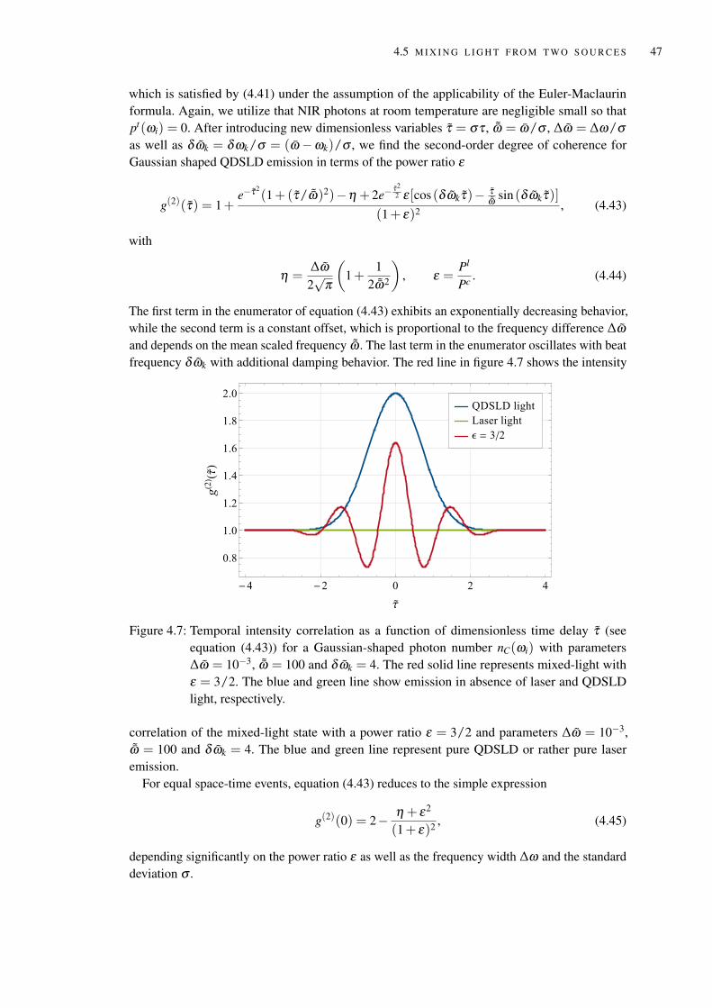
4.5 M I X I N G L I G H T F RO M T W O S O U R C E S 47
which is satisfied by (4.41) under the assumption of the applicability of the Euler-Maclaurinformula. Again, we utilize that NIR photons at room temperature are negligible small so thatpt(ωi) = 0. After introducing new dimensionless variables τ = στ , ˜ω = ω/σ , ∆ω = ∆ω/σas well as δωk = δωk/σ = (ω −ωk)/σ , we find the second-order degree of coherence forGaussian shaped QDSLD emission in terms of the power ratio ε
g(2)(τ) = 1+e−τ2
(1+(τ/ ˜ω)2)−η + 2e−τ22 ε [cos (δωkτ)− τ
˜ω sin (δωkτ)](1+ ε)2 , (4.43)
with
η =∆ω
2√
π
(1+
12 ˜ω2
), ε =
Pl
Pc . (4.44)
The first term in the enumerator of equation (4.43) exhibits an exponentially decreasing behavior,while the second term is a constant offset, which is proportional to the frequency difference ∆ωand depends on the mean scaled frequency ˜ω . The last term in the enumerator oscillates with beatfrequency δωk with additional damping behavior. The red line in figure 4.7 shows the intensity
QDSLD light
Laser light
ϵ = 3/2
-4 -2 0 2 4
0.8
1.0
1.2
1.4
1.6
1.8
2.0
τ
g(2) (τ)
Figure 4.7: Temporal intensity correlation as a function of dimensionless time delay τ (seeequation (4.43)) for a Gaussian-shaped photon number nC(ωi) with parameters∆ω = 10−3, ˜ω = 100 and δωk = 4. The red solid line represents mixed-light withε = 3/2. The blue and green line show emission in absence of laser and QDSLDlight, respectively.
correlation of the mixed-light state with a power ratio ε = 3/2 and parameters ∆ω = 10−3,˜ω = 100 and δωk = 4. The blue and green line represent pure QDSLD or rather pure laser
emission.For equal space-time events, equation (4.43) reduces to the simple expression
g(2)(0) = 2− η + ε2
(1+ ε)2 , (4.45)
depending significantly on the power ratio ε as well as the frequency width ∆ω and the standarddeviation σ .
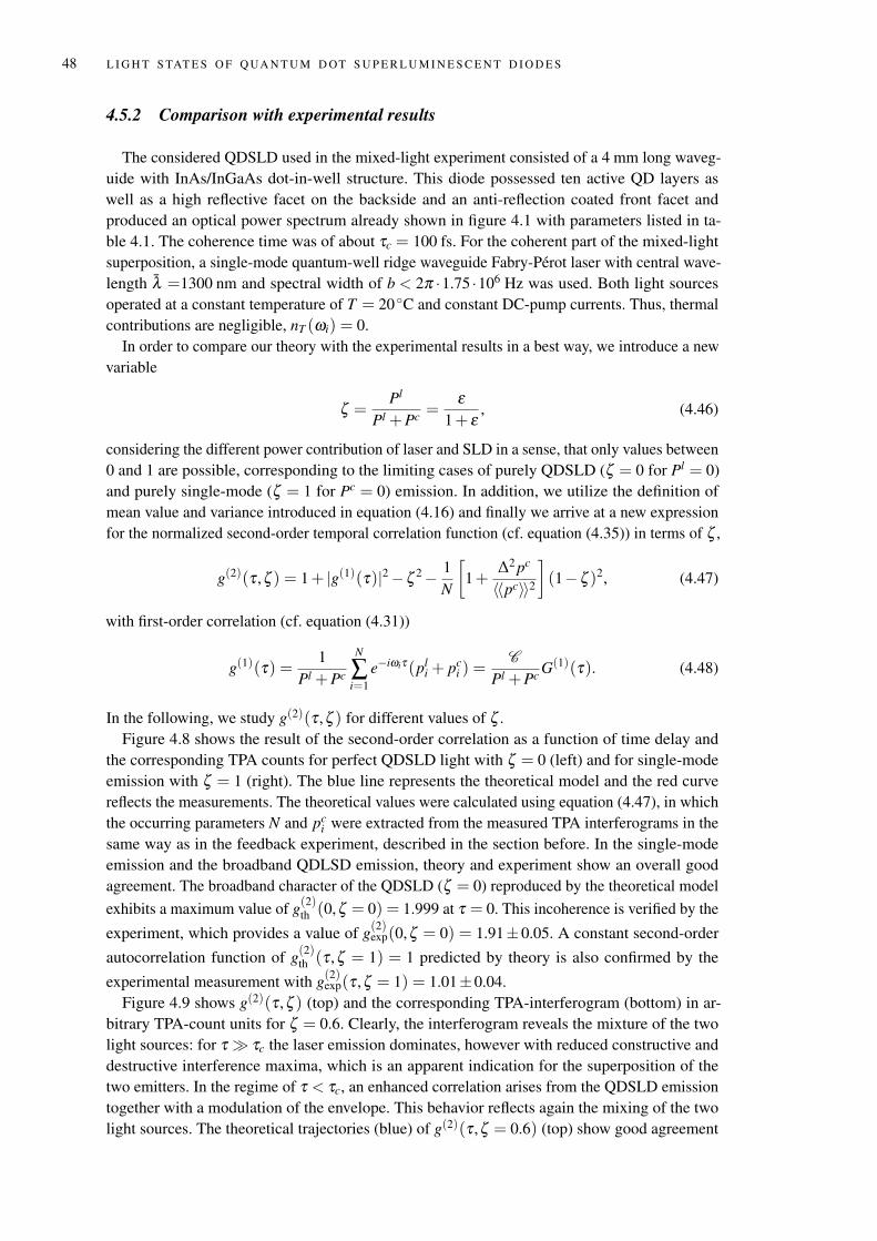
48 L I G H T S TAT E S O F Q UA N T U M D OT S U P E R L U M I N E S C E N T D I O D E S
4.5.2 Comparison with experimental results
The considered QDSLD used in the mixed-light experiment consisted of a 4 mm long waveg-uide with InAs/InGaAs dot-in-well structure. This diode possessed ten active QD layers aswell as a high reflective facet on the backside and an anti-reflection coated front facet andproduced an optical power spectrum already shown in figure 4.1 with parameters listed in ta-ble 4.1. The coherence time was of about τc = 100 fs. For the coherent part of the mixed-lightsuperposition, a single-mode quantum-well ridge waveguide Fabry-Perot laser with central wave-length λ =1300 nm and spectral width of b < 2π ·1.75 ·106 Hz was used. Both light sourcesoperated at a constant temperature of T = 20 C and constant DC-pump currents. Thus, thermalcontributions are negligible, nT (ωi) = 0.
In order to compare our theory with the experimental results in a best way, we introduce a newvariable
ζ =Pl
Pl +Pc =ε
1+ ε, (4.46)
considering the different power contribution of laser and SLD in a sense, that only values between0 and 1 are possible, corresponding to the limiting cases of purely QDSLD (ζ = 0 for Pl = 0)and purely single-mode (ζ = 1 for Pc = 0) emission. In addition, we utilize the definition ofmean value and variance introduced in equation (4.16) and finally we arrive at a new expressionfor the normalized second-order temporal correlation function (cf. equation (4.35)) in terms of ζ ,
g(2)(τ ,ζ ) = 1+ |g(1)(τ)|2−ζ 2− 1N
[1+
∆2 pc
〈〈pc〉〉2](1−ζ )2, (4.47)
with first-order correlation (cf. equation (4.31))
g(1)(τ) =1
Pl +Pc
N
∑i=1
e−iωiτ(pli + pc
i ) =C
Pl +Pc G(1)(τ). (4.48)
In the following, we study g(2)(τ ,ζ ) for different values of ζ .Figure 4.8 shows the result of the second-order correlation as a function of time delay and
the corresponding TPA counts for perfect QDSLD light with ζ = 0 (left) and for single-modeemission with ζ = 1 (right). The blue line represents the theoretical model and the red curvereflects the measurements. The theoretical values were calculated using equation (4.47), in whichthe occurring parameters N and pc
i were extracted from the measured TPA interferograms in thesame way as in the feedback experiment, described in the section before. In the single-modeemission and the broadband QDLSD emission, theory and experiment show an overall goodagreement. The broadband character of the QDSLD (ζ = 0) reproduced by the theoretical modelexhibits a maximum value of g(2)th (0,ζ = 0) = 1.999 at τ = 0. This incoherence is verified by the
experiment, which provides a value of g(2)exp(0,ζ = 0) = 1.91±0.05. A constant second-order
autocorrelation function of g(2)th (τ ,ζ = 1) = 1 predicted by theory is also confirmed by the
experimental measurement with g(2)exp(τ ,ζ = 1) = 1.01±0.04.Figure 4.9 shows g(2)(τ ,ζ ) (top) and the corresponding TPA-interferogram (bottom) in ar-
bitrary TPA-count units for ζ = 0.6. Clearly, the interferogram reveals the mixture of the twolight sources: for τ τc the laser emission dominates, however with reduced constructive anddestructive interference maxima, which is an apparent indication for the superposition of thetwo emitters. In the regime of τ < τc, an enhanced correlation arises from the QDSLD emissiontogether with a modulation of the envelope. This behavior reflects again the mixing of the twolight sources. The theoretical trajectories (blue) of g(2)(τ ,ζ = 0.6) (top) show good agreement
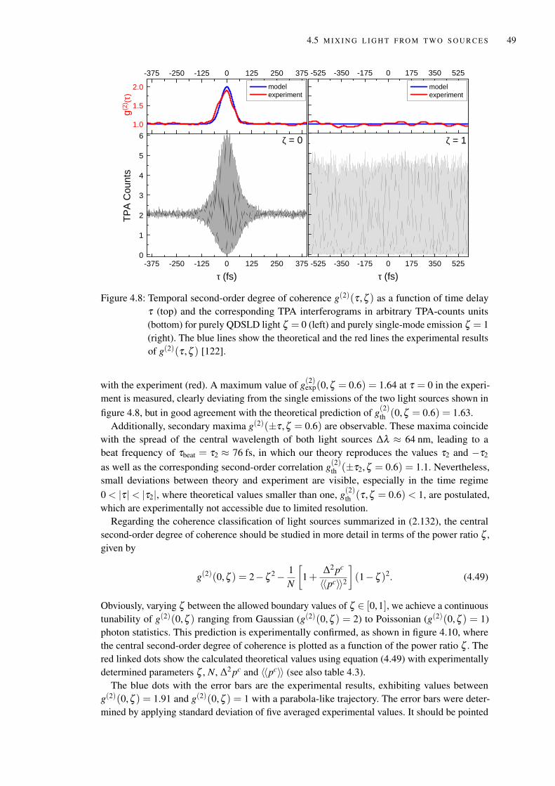
4.5 M I X I N G L I G H T F RO M T W O S O U R C E S 49
- 3 7 5 - 2 5 0 - 1 2 5 0 1 2 5 2 5 0 3 7 50
1
2
3
4
5
61 . 01 . 52 . 0
- 3 7 5 - 2 5 0 - 1 2 5 0 1 2 5 2 5 0 3 7 5
- 5 2 5 - 3 5 0 - 1 7 5 0 1 7 5 3 5 0 5 2 5
- 5 2 5 - 3 5 0 - 1 7 5 0 1 7 5 3 5 0 5 2 5
τ ( f s )
ζ = 0g(2)
(τ)
m o d e l e x p e r i m e n t
TPA C
ounts
τ ( f s )
ζ = 1
m o d e l e x p e r i m e n t
Figure 4.8: Temporal second-order degree of coherence g(2)(τ ,ζ ) as a function of time delayτ (top) and the corresponding TPA interferograms in arbitrary TPA-counts units(bottom) for purely QDSLD light ζ = 0 (left) and purely single-mode emission ζ = 1(right). The blue lines show the theoretical and the red lines the experimental resultsof g(2)(τ ,ζ ) [122].
with the experiment (red). A maximum value of g(2)exp(0,ζ = 0.6) = 1.64 at τ = 0 in the experi-ment is measured, clearly deviating from the single emissions of the two light sources shown infigure 4.8, but in good agreement with the theoretical prediction of g(2)th (0,ζ = 0.6) = 1.63.
Additionally, secondary maxima g(2)(±τ ,ζ = 0.6) are observable. These maxima coincidewith the spread of the central wavelength of both light sources ∆λ ≈ 64 nm, leading to abeat frequency of τbeat = τ2 ≈ 76 fs, in which our theory reproduces the values τ2 and −τ2
as well as the corresponding second-order correlation g(2)th (±τ2,ζ = 0.6) = 1.1. Nevertheless,small deviations between theory and experiment are visible, especially in the time regime0 < |τ| < |τ2|, where theoretical values smaller than one, g(2)th (τ ,ζ = 0.6) < 1, are postulated,which are experimentally not accessible due to limited resolution.
Regarding the coherence classification of light sources summarized in (2.132), the centralsecond-order degree of coherence should be studied in more detail in terms of the power ratio ζ ,given by
g(2)(0,ζ ) = 2−ζ 2− 1N
[1+
∆2 pc
〈〈pc〉〉2](1−ζ )2. (4.49)
Obviously, varying ζ between the allowed boundary values of ζ ∈ [0,1], we achieve a continuoustunability of g(2)(0,ζ ) ranging from Gaussian (g(2)(0,ζ ) = 2) to Poissonian (g(2)(0,ζ ) = 1)photon statistics. This prediction is experimentally confirmed, as shown in figure 4.10, wherethe central second-order degree of coherence is plotted as a function of the power ratio ζ . Thered linked dots show the calculated theoretical values using equation (4.49) with experimentallydetermined parameters ζ , N, ∆2 pc and 〈〈pc〉〉 (see also table 4.3).
The blue dots with the error bars are the experimental results, exhibiting values betweeng(2)(0,ζ ) = 1.91 and g(2)(0,ζ ) = 1 with a parabola-like trajectory. The error bars were deter-mined by applying standard deviation of five averaged experimental values. It should be pointed
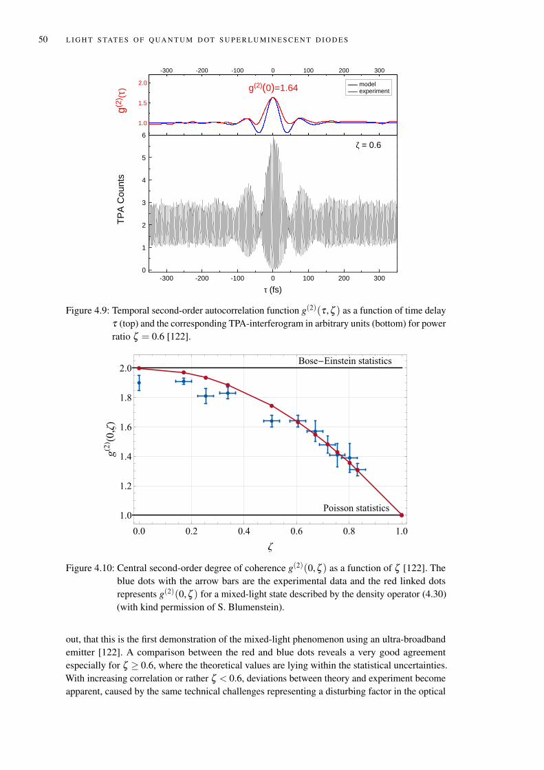
50 L I G H T S TAT E S O F Q UA N T U M D OT S U P E R L U M I N E S C E N T D I O D E S
- 3 0 0 - 2 0 0 - 1 0 0 0 1 0 0 2 0 0 3 0 00
1
2
3
4
5
61 . 0
1 . 5
2 . 0- 3 0 0 - 2 0 0 - 1 0 0 0 1 0 0 2 0 0 3 0 0
g ( 2 ) ( 0 ) = 1 . 6 4
τ ( f s )
ζ = 0 . 6
m o d e l e x p e r i m e n t
TPA C
ounts
g(2) (τ
)
Figure 4.9: Temporal second-order autocorrelation function g(2)(τ ,ζ ) as a function of time delayτ (top) and the corresponding TPA-interferogram in arbitrary units (bottom) for powerratio ζ = 0.6 [122].
Bose-Einstein statistics
Poisson statistics
0.0 0.2 0.4 0.6 0.8 1.0
1.0
1.2
1.4
1.6
1.8
2.0
ζ
g(2) (0,ζ)
Figure 4.10: Central second-order degree of coherence g(2)(0,ζ ) as a function of ζ [122]. Theblue dots with the arrow bars are the experimental data and the red linked dotsrepresents g(2)(0,ζ ) for a mixed-light state described by the density operator (4.30)(with kind permission of S. Blumenstein).
out, that this is the first demonstration of the mixed-light phenomenon using an ultra-broadbandemitter [122]. A comparison between the red and blue dots reveals a very good agreementespecially for ζ ≥ 0.6, where the theoretical values are lying within the statistical uncertainties.With increasing correlation or rather ζ < 0.6, deviations between theory and experiment becomeapparent, caused by the same technical challenges representing a disturbing factor in the optical
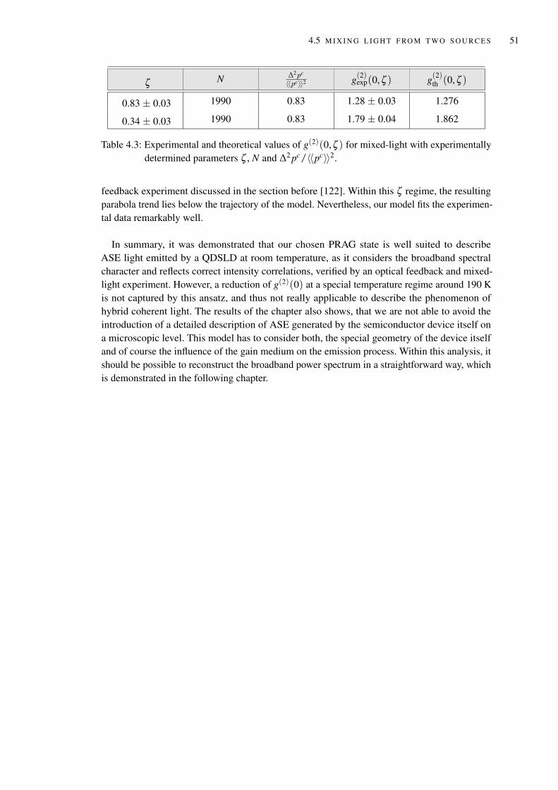
4.5 M I X I N G L I G H T F RO M T W O S O U R C E S 51
ζ N ∆2 pc
〈〈pc〉〉2 g(2)exp(0,ζ ) g(2)th (0,ζ )
0.83 ± 0.03 1990 0.83 1.28 ± 0.03 1.276
0.34 ± 0.03 1990 0.83 1.79 ± 0.04 1.862
Table 4.3: Experimental and theoretical values of g(2)(0,ζ ) for mixed-light with experimentallydetermined parameters ζ , N and ∆2 pc/〈〈pc〉〉2.
feedback experiment discussed in the section before [122]. Within this ζ regime, the resultingparabola trend lies below the trajectory of the model. Nevertheless, our model fits the experimen-tal data remarkably well.
In summary, it was demonstrated that our chosen PRAG state is well suited to describeASE light emitted by a QDSLD at room temperature, as it considers the broadband spectralcharacter and reflects correct intensity correlations, verified by an optical feedback and mixed-light experiment. However, a reduction of g(2)(0) at a special temperature regime around 190 Kis not captured by this ansatz, and thus not really applicable to describe the phenomenon ofhybrid coherent light. The results of the chapter also shows, that we are not able to avoid theintroduction of a detailed description of ASE generated by the semiconductor device itself ona microscopic level. This model has to consider both, the special geometry of the device itselfand of course the influence of the gain medium on the emission process. Within this analysis, itshould be possible to reconstruct the broadband power spectrum in a straightforward way, whichis demonstrated in the following chapter.

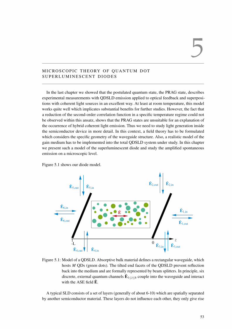
5
M I C RO S C O P I C T H E O RY O F Q UA N T U M D OTS U P E R L U M I N E S C E N T D I O D E S
In the last chapter we showed that the postulated quantum state, the PRAG state, describesexperimental measurements with QDSLD emission applied to optical feedback and superposi-tions with coherent light sources in an excellent way. At least at room temperature, this modelworks quite well which implicates substantial benefits for further studies. However, the fact thata reduction of the second-order correlation function in a specific temperature regime could notbe observed within this ansatz, shows that the PRAG states are unsuitable for an explanation ofthe occurrence of hybrid coherent light emission. Thus we need to study light generation insidethe semiconductor device in more detail. In this context, a field theory has to be formulatedwhich considers the specific geometry of the waveguide structure. Also, a realistic model of thegain medium has to be implemented into the total QDSLD system under study. In this chapterwe present such a model of the superluminescent diode and study the amplified spontaneousemission on a microscopic level.
Figure 5.1 shows our diode model.
E
E2,inE5,in
E6,out E1,out
E1,in
z
E6,in
E4,in
E2,outE5,out
0-LE4,out
E3,in E3,out
Figure 5.1: Model of a QDSLD. Absorptive bulk material defines a rectangular waveguide, whichhosts M QDs (green dots). The tilted end facets of the QDSLD prevent reflectionback into the medium and are formally represented by beam splitters. In principle, sixdiscrete, external quantum channels E1≤i≤6 couple into the waveguide and interactwith the ASE field E.
A typical SLD consists of a set of layers (generally of about 6-10) which are spatially separatedby another semiconductor material. These layers do not influence each other, they only give rise
53
54 M I C RO S C O P I C T H E O RY O F Q UA N T U M D OT S U P E R L U M I N E S C E N T D I O D E S
to an even more inhomogeneously broadened gain medium visible in the optical power spectrum(see figure 3.3). Therefore, for simplicity we only consider one layer of the gain medium. Thegain medium is composed of M QDs, which are embedded in a strongly absorptive bulk materialthat defines a waveguide. This waveguide is assumed to be rectangular, which results in a lineardispersion relation [60].
I N T R AWAV E G U I D E R A D I AT I O N Clearly, the light generated inside the diode is broadbandand must be described by a multimode electrical field [37, 51],
E(r, t) = E(+)(r, t)+ E(−)(r, t). (5.1)
For the positive frequency part we consider a superposition of waves propagating along thez-direction,
E(+)(r, t) = E(+)(r, t)ey = ∑ki
ui(r)ai(t)ey, (5.2)
formed by a superposition of N polarized modes
ui(r) = Ei χ(x,y)eikiz (5.3)
which factorize into a single transverse wave function χ(x,y) and longitudinal plane waveswith wave vector ki = kiez. Here, ki = 2πi/L with i ∈ [−N/2, N/2−1 ] and N/2 ∈N dependson the length of the waveguide L. Due to the rectangular geometry of the QDSLD [123], thefield is linearly polarized. Without loss of generality, we chose a linear polarization ey in y-direction. The transverse mode function is normalized to the cross section area of the waveguideA =
∫A dxdy |χ|2. If the system’s volume is V = AL, then the normalization factor of the electric
fields reads Ei = i√
hωi/2εV . There is a linear intrawaveguide dispersion relation betweenfrequency ω and wave number |kz|,
ω = c |kz| , c = c0/nc, (5.4)
with the speed of light c in the bulk medium of refractive index nc. This is in contrast to theconsideration of chapter 4 where we studied propagation in free space with vacuum velocity c0.
As we want to pursue a quantum theory, we need to consider bosonic amplitudes ai, whichsatisfy the commutation relations (2.40). Due to energy conservation, a non-vanishing couplingbetween left- and right-propagating modes of the same ki inside the diode system is conceivable.However, the presence of a bulk material suppresses possible interference effects between anyfield modes inside the waveguide system, in fact also between modes of the same frequency,but with opposite propagation direction. Therefore, in good approximation we can neglect thisintrawaveguide coupling.
WAV E G U I D E G E O M E T RY Tilted end facets on the left- and right-hand side prevent backreflections, experimentally realized by tilting the emission facets as well as using anti-reflectioncoatings (cf. chapter 3). These end facets are modeled by beam splitters enclosing the activemedium. In theory, a lossless beam splitter can be considered as a device which couples aparticular set of input modes to a set of particular output modes. As shown in figure 5.2 thebeam splitter has four input and four output ports with corresponding bosonic annihilation vectoroperator bin/out = (b1,in/out, b2,in/out, b3,in/out, b4,in/out)T being related by the S-matrix [32,128–131],
bout = S bin. (5.5)
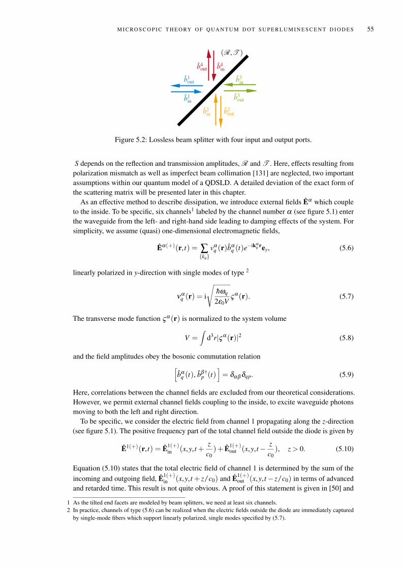
M I C RO S C O P I C T H E O RY O F Q UA N T U M D OT S U P E R L U M I N E S C E N T D I O D E S 55
(R,T )
b4in
b1out
b1in b3
out
b3in
b2outb2
in
b4out
Figure 5.2: Lossless beam splitter with four input and output ports.
S depends on the reflection and transmission amplitudes, R and T . Here, effects resulting frompolarization mismatch as well as imperfect beam collimation [131] are neglected, two importantassumptions within our quantum model of a QDSLD. A detailed deviation of the exact form ofthe scattering matrix will be presented later in this chapter.
As an effective method to describe dissipation, we introduce external fields Eα which coupleto the inside. To be specific, six channels1 labeled by the channel number α (see figure 5.1) enterthe waveguide from the left- and right-hand side leading to damping effects of the system. Forsimplicity, we assume (quasi) one-dimensional electromagnetic fields,
Eα(+)(r, t) = ∑kq
vαq (r)b
αq (t)e
−ikαq rey, (5.6)
linearly polarized in y-direction with single modes of type 2
ναq (r) = i
√hωq
2ε0Vςα(r). (5.7)
The transverse mode function ςα(r) is normalized to the system volume
V =∫
d3r|ςα(r)|2 (5.8)
and the field amplitudes obey the bosonic commutation relation[bα
q (t), bβ†p (t)
]= δαβ δqp. (5.9)
Here, correlations between the channel fields are excluded from our theoretical considerations.However, we permit external channel fields coupling to the inside, to excite waveguide photonsmoving to both the left and right direction.
To be specific, we consider the electric field from channel 1 propagating along the z-direction(see figure 5.1). The positive frequency part of the total channel field outside the diode is given by
E1(+)(r, t) = E1(+)in (x,y, t +
zc0)+ E1(+)
out (x,y, t− zc0), z > 0. (5.10)
Equation (5.10) states that the total electric field of channel 1 is determined by the sum of theincoming and outgoing field, E1(+)
in (x,y, t + z/c0) and E1(+)out (x,y, t− z/c0) in terms of advanced
and retarded time. This result is not quite obvious. A proof of this statement is given in [50] and
1 As the tilted end facets are modeled by beam splitters, we need at least six channels.2 In practice, channels of type (5.6) can be realized when the electric fields outside the diode are immediately captured
by single-mode fibers which support linearly polarized, single modes specified by (5.7).
56 M I C RO S C O P I C T H E O RY O F Q UA N T U M D OT S U P E R L U M I N E S C E N T D I O D E S
summarized in appendix E. Thus, there exist two kinds of field modes; incoming and outgoing.The former influences the dynamics of the internal system of the QDSLD by producing randomnoise effects and providing an amount of energy, carried away by the outgoing modes leadingto damping effects. Therefore, we are dealing with radiation damping which is usually the casewhenever a field interpretation of the bath is possible and this is again always possible accordingto reference [50]. Please note, in contrast to the ASE field inside the waveguide of the QDSLD(see equation (5.1)), the single electromagnetic channel fields outside the diode propagate invacuo with dispersion relation ωi = c0|ki|. The other optical channels Eα of figure 5.1 can bedescribed in an analogous fashion, but are not required for this discussion. Nevertheless, we willgive a detailed expression for each individual channel field later in this chapter.
G A I N M E D I U M The active gain medium is formed by an ensemble of M QDs embedded inan opaque semiconductor material. Due to their spectral properties, each dot can be modeledby a multi-level system. In order to receive light amplification, we need to consider at leastthree energy levels [18]. Each quantum dot interacts with the multimode ASE field (5.2) and isincoherently pumped with rate R due to the injected current. As we are dealing with a solid, theemitted light experiences a high rate of absorption loss. Therefore, the generated light which isamplified by the dots is absorbed, profoundly. This can be modeled by coupling each transition sof the quantum dot j to a one-dimensional reservoir,
H jb = ∑
s∑k
hω jskb j†
sk b jsk, s ∈ (21), (20), (10) | (mn) : |m〉 → |n〉. (5.11)
They satisfy the bosonic commutation relation[bi
sk(t), b j†sk′(t)
]= δi jδkk′ . (5.12)
As a further consequence of a high absorption coefficient of solids, interactions between QDs areassumed to be negligible.
5.1 Q UA N T U M D OT S
Up to now, we have sketched the main ingredients for our microscopic model of a quantum dotsuperluminescent diode. In the following we have to elaborate this model by having a closer lookat the quantum mechanical formulation of the gain medium and the geometry of the waveguidestructure, separately. The resulting equations of motion allow to determine emission and photonstatistical properties or rather first- and second-order moments, which will be studied in chapter 6and 7.
Before calculating the electrical output field measured by the detector to determine first-and second-order autocorrelation functions, we have a look at the generation and amplificationprocesses of light inside the gain medium of a quantum dot superluminescent diode. First weexamine the interaction of the ASE field with the gain medium inside the QDSLD system.Figure 5.3 shows one of the quantum dot systems under consideration with energy hωm of the mth
level and transition frequency ωmn = ωm−ωn between level m and n and corresponding decayrates γmn. Here, the ASE field (5.2) acts on the transition |1〉 ↔ |2〉 leading to a broad Gaussianpower spectrum (see figure 3.3) arising from purely ground state (GS) emission. Higher-orderradiation (excited state (ES), second excited state (SES), etc.) is easily implemented within thistheoretical model by just incorporating additional levels forming the quantum dot. However,as a first step we want to keep our theory as simple as possible and as we do not believe that
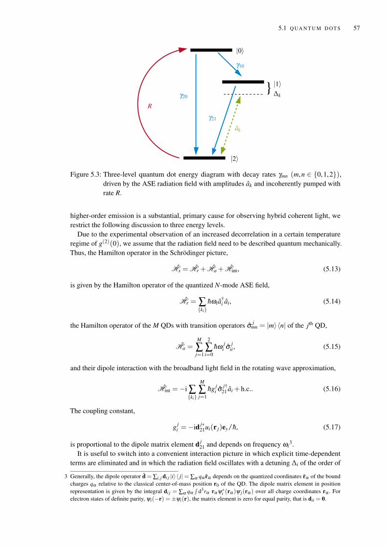
5.1 Q UA N T U M D OT S 57
|0〉
γ10
|1〉
|2〉
R
ak
∆kγ20
γ21
Figure 5.3: Three-level quantum dot energy diagram with decay rates γmn (m,n ∈ 0,1,2),driven by the ASE radiation field with amplitudes ak and incoherently pumped withrate R.
higher-order emission is a substantial, primary cause for observing hybrid coherent light, werestrict the following discussion to three energy levels.
Due to the experimental observation of an increased decorrelation in a certain temperatureregime of g(2)(0), we assume that the radiation field need to be described quantum mechanically.Thus, the Hamilton operator in the Schrödinger picture,
Hs = Hr + Ha + Hint, (5.13)
is given by the Hamilton operator of the quantized N-mode ASE field,
Hr = ∑ki
hωia†i ai, (5.14)
the Hamilton operator of the M QDs with transition operators σ jmn = |m〉〈n| of the jth QD,
Ha =M
∑j=1
2
∑i=0
hω ji σ j
ii , (5.15)
and their dipole interaction with the broadband light field in the rotating wave approximation,
Hint = −i ∑ki
M
∑j=1
hg ji σ j†
21 ai + h.c.. (5.16)
The coupling constant,
g ji = −id j∗
21ui(r j)ey/h, (5.17)
is proportional to the dipole matrix element d j21 and depends on frequency ωi
3.It is useful to switch into a convenient interaction picture in which explicit time-dependent
terms are eliminated and in which the radiation field oscillates with a detuning ∆i of the order of
3 Generally, the dipole operator d = ∑i, j di j |i〉〈 j|= ∑α qα rα depends on the quantized coordinates rα of the boundcharges qα relative to the classical center-of-mass position r0 of the QD. The dipole matrix element in positionrepresentation is given by the integral di j = ∑α qα
∫d3rα rα ψ∗i (rα )ψ j(rα ) over all charge coordinates rα . For
electron states of definite parity, ψi(−r) = ±ψi(r), the matrix element is zero for equal parity, that is dii = 0.
58 M I C RO S C O P I C T H E O RY O F Q UA N T U M D OT S U P E R L U M I N E S C E N T D I O D E S
THz. Here, the interaction state |ψ(t)〉I is related with the state vector in the Schrödinger picture|ψ(t)〉S,
|ψ(t)〉I = U†(t) |ψ(t)〉S , (5.18)
by the transformation operator
U(t) = e−iGt , G = ∑ki
ω12a†i ai +
M
∑j=1
[ω j
0 σ j00 +(ω j
1−δω j12)σ
j11 +ω j
2 σ j22
]. (5.19)
Thus, the system Hamilton operator in the interaction picture reads
Hs = ih ˙U†U +U†HsU
= ∑ki
h∆ia†i ai +
M
∑j=1
hδω j12σ j
11−∑ki
M
∑j=1
[ihg j
i (∆i)σ j†21 ai + h.c.
]. (5.20)
In this interaction picture, the ASE field oscillates with detuning ∆i and depends on the meantransition frequency ω12 of the QDs defined by
∆i = ωi− ω12, ω12 =1N ∑ki
ωi. (5.21)
Accordingly, the frequency δω j12 = ω j
12− ω12 occurring in equation (5.20) represents a smalldeviation of the jth quantum dot from the mean value ω12.
To generate light amplification, the dots are incoherently pumped. In theory, this can beimplemented by introducing a pumping rate R acting on transition |2〉→ |0〉 as shown in figure 5.3.This represents an accurate description for the pumping mechanism inside semiconductor diodes,receiving light amplification by applying a voltage I on the pn-junction. As already mentioned,each driven quantum dot system inside the superluminescent diode is strongly damped due to thesurrounding semiconductor material, which can be described by a coupling to a large reservoir.The next subsection is dedicated to this relevant aspect.
5.1.1 Pumping of quantum dots at room temperature
Dissipation processes play a significant role in the context of QDs embedded in a semiconductorbulk material, which we have to take into account when describing light generation in QDSLDs.For the sake of simplicity, we first consider a single quantum dot, M = 1, inside the QDSLDdriven by the ASE radiation field, specified by the Hamiltonian (5.20). Obviously, the energycorrection term in this Hamiltonian in the interaction picture, describing small deviations fromthe mean frequency of several QDs vanishes in case of a single dot and equation (5.20) reduces to
Hs = ∑ki
h∆ia†i ai −∑
ki
[ihgiσ†
21ai + h.c.]
. (5.22)
Naturally, also the index j in equation (5.20), labeling the single QD systems, becomes superflu-ous and was therefore eliminated. In order to describe a damped, incoherently driven quantumdot, the microscopic model has to be extended by adding an external incoherent pumping rate Ras well as coupling the small system to the environment specified by many harmonic oscillatorswith Hamilton operator introduced in equation (5.11).
In general, for describing a damped quantum system, we consider a small system (S) ofoperators S, S† with Hamilton operator HS, weakly coupled to a large reservoir (R) with
5.1 Q UA N T U M D OT S 59
a huge number of unobserved degrees of freedom, described by a Hamiltonian composed ofmany harmonic oscillators (see equation (5.11)). Please note, that we are only interested in thedynamics of the small system (S) so that the exact form of both, the environment and the couplingconstant, is not relevant. This physical problem can be studied in detail in the Schrödinger orHeisenberg picture. The resulting equations of motion are called master equation or quantumLangevin equation, respectively. The former describes the dynamics of the reduced densityoperator of the small system whereas the quantum Langevin equations specify the time evolutionof the dynamical variables of this subsystem. Here, we concentrate on the description of dampingin the Schrödinger picture in which all operators possess at most an explicit time dependency.A detailed derivation of the master equation is given in appendix D4. In the following we justhighlight the main assumptions and approximations necessary to achieve this density operatorequation of motion.
M A S T E R E Q UAT I O N The dynamics of a quantum system described by the temporal deriva-tive of the density operator ρ is determined by the Liouville von Neumann equation,
˙ρ(t) = − ih
[H, ρ
], (5.23)
given by the commutator of ρ and the total system Hamiltonian
H= HS + HR + HI (5.24)
in the Schrödinger picture. Here, HS is the Hamiltonian of the small system whose interactionis described by the system’s deexcitation and excitation operators S†, S5. HR is the reservoirHamilton operator and the interaction between system and environment is described by HI. At theinitial time t = 0, the environment, consisting of many harmonic oscillators with Hamiltonian HR,is assumed to be in a stationary state and decorrelated with the small system. The coupling energybetween the system and its environment is supposed to be weak, so that the system’s actionon the dynamics of the environment is negligible. The state of the total system approximatelyfactorizes into a tensor product of the time-dependent system’s density operator and the stationarydensity operator of the reservoir (Born approximation). Taking the trace over the reservoirdegrees of freedom and applying the iteration method to the Liouville equation results in anintegro-differential equation for the reduced system’s density operator ρS(t) = TrRρ(t). Thetime scales over which the correlation functions of the environment decay, are assumed to bemuch smaller than the evolution time scales of the system. The environment loses its memoryon time scales larger than the correlation time of the reservoir fluctuations. Within the Markovapproximation reservoir correlation functions are replaceable by delta distributions. Taking intoaccount all mentioned assumptions and approximations we end up in a master equation for thedensity matrix of the open system in Lindblad form [132]
ddt
ρS(t) = (LS +LR)ρS(t). (5.25)
4 The derivation of the master equation in appendix D considers a continuum version of the reservoir Hamiltonian(5.11). A formulation in terms of discrete modes is analogous.
5 E.g. the operators S, S† could be annihilation and creation operators of a cavity mode or the excitation and deexcitationoperators of a two-level system.
60 M I C RO S C O P I C T H E O RY O F Q UA N T U M D OT S U P E R L U M I N E S C E N T D I O D E S
Here, the system Liouville operator LS ρS(t) = − ih
[HS, ρS
], describes the unperturbed system
and the damping Liouvillian,
LR ρS(t) =Γ( N(0)︸ ︷︷ ︸stim. emission
+ 1︸︷︷︸spon. emission
)(2SρS(t)S†− S†SρS(t)− ρS(t)S†S)
+ ΓN(0)︸ ︷︷ ︸stim. absoption
(2S†ρS(t)S− SS†ρS(t)− ρS(t)SS†)
− i[δω S†S+ δωth
[S†, S
], ρS(t)
], δωth = P
∫d∆ |W (∆)|2N(∆)/∆,
(5.26)
considers the coupling between environment and system, leading to dissipation captured bya relaxation rate Γ, energy shift δω as well as thermal energy shift δωth depending on thethermal occupation number N(∆). The first term in the damping Liouvillian (cf. equation (5.26))characterizes spontaneous and stimulated emission whereas the second one specifies stimulatedabsorption processes. The last term includes the mentioned energy shifts which can be eliminatedby appropriate renormalization.
More generally, for a set of system operators Si, S†i the master equation is extendable by
summing over all these system operators with corresponding damping rates Γi and occupationnumbers Ni. For adaptable renormalization of the energy shifts, the multicomponent masterequation for the reduced density operator reads
ddt
ρS(t) =−ih
[HS, ρS
]+∑
iΓi(Ni + 1)(2Si ρS(t)S
†i − S†
i Si ρS(t)− ρS(t)S†i Si )
+∑i
ΓiNi(2S†i ρS(t)Si − ρS(t)Si S†
i − Si S†i ρS(t)).
(5.27)
This important equation of motion for the system’s density operator ρS can be directly applied toour problem of a single quantum dot embedded in the isolated semiconductor waveguide depictedin figure 5.1. What we find is nothing else but Bloch equations, characterizing the temporaldynamics of the quantum dot populations and coherences which will be explicitly demonstratedin the next section.
5.1.2 Response, gain and inversion of a quantum dot at room temperature
Regarding the results of the two mentioned experiments in chapter 4 performed at roomtemperature, the temporal autocorrelation properties in first- and second-order of QDSLDsare very similar to usual diodes, showing broad Gaussian shaped spectral densities as well asincoherent photon statistics with a central second-order correlation function of approximately 2.Thus, at a first glance it does not seem to be necessary to treat the ASE light field quantummechanically. In order to analyze optimal response and gain of a driven single quantum dot withclassical center-of-mass position r0 in the diode system at room temperature, we first investigatea single-mode, time-harmonic ASE field with space dependent amplitude E(r) and angularfrequency ω
E(r, t) = E(r)e−iωt + c.c.. (5.28)
Please remember, usual atoms moving with a certain velocity induce a Doppler-shift in theclassical single-mode field frequency. However, a QD is a static system and the dependency ofthe position variable in the general expression of field amplitude in (5.28) can be eliminated.Thus, E(r) only depends on the constant center-of-mass position r0 of the considered QD,E(r) = E(r0).
5.1 Q UA N T U M D OT S 61
The total Hamilton operator of this three-level system interacting with a classical light field inrotating wave approximation is given by
Hcl =2
∑i=0
hωiσii− hΩe−iωt σ†21− hΩ∗eiωt σ21. (5.29)
Here, we introduced the characteristic physical quantity known as Rabi frequency,
Ω(r0) =d∗21E(r0)
h, (5.30)
depending on the dipole matrix element d21 and the field amplitude E(r0) at the QD’s posi-tion r0. Again, we switch into a suitable interaction picture according to equation (5.18) withtransformation operator
U(t) = e−iGt , G = hω0σ00 + h(ω1 +∆)σ11 + hω2σ22, ∆ = ω−ω12. (5.31)
Thus, the Hamiltonian in this interaction picture oscillating with frequency detuning ∆ is deter-mined by
Hcl(t) = −h∆σ11(t)− hΩ∗σ21(t)− hΩσ†21(t). (5.32)
Applying the multicomponent master equation (5.27), we find the equation of motion for the re-duced density operator considering coherent evolution of the system described by the commutatorof the density operator with the system Hamiltonian (5.32) and irreversible damping effects. Thesum in equation (5.27) extends over all possible quantum dot transitions i ∈ (21), (20), (10)with system operators corresponding to the quantum dot lowering operators, Si = σi. Introducingan incoherent pumping rate [133–135] R = γ20N20 proportional to the photon number N20, we findoptical Bloch equations [51] for a driven quantum dot interacting with a single-mode classicalradiation field
ρ00(t) = −2(R+ γ20 + γ10)ρ00 + 2Rρ22, (5.33)
ρ11(t) = −iΩ∗ρ12 + iΩρ11−2γ21ρ11 + 2γ10ρ00, (5.34)
ρ22(t) = −2Rρ22 + iΩ∗ρ12− iΩρ21 + 2γ21ρ11 + 2(R+ γ20)ρ00, (5.35)
ρ10(t) = (i∆− γ21−R− γ20− γ10)ρ10 + iΩρ20, (5.36)
ρ12(t) = (i∆− γ21−R)ρ12 + iΩ(ρ22−ρ11), (5.37)
ρ20(t) = −(2R+ γ20 + γ10)ρ20 + iΩ∗ρ10, (5.38)
with ρi j = 〈i| ρS | j〉, ρi j = ρ∗ji, γi j = γ ji and vanishing thermal occupation numbers, N21 = N10 = 0.Figure 5.4 visualizes the time evolution of the populations for a QD system initially in its groundstate with zero coherences (ρ22(0) = 1, ρ00(0) = ρ11(0) = 0 and ρi j(0) = 0 with i 6= j).
The quantum dot is incoherently pumped with rate R = 5γ21, driven by a single-mode radiationfield of Rabi frequency Ω = γ21 and zero detuning, ∆ = 0. The damping rate from the highest tothe lowest state in both cases is assumed to be negligibly small, γ20 = 0. In figure 5.4 (left) wehave chosen an upper decay rate of γ10 = 0.1γ21. The ground state population indeed decreasesbut is always higher than the population for the upper energy states, that is no inversion betweenlevel |1〉 and |2〉 (w = ρ11−ρ22 < 0) or no amplification of the system is observable, respectively.For γ10 = 10γ21 depicted in figure 5.4 (right), the population of the ground state decreases muchfaster. Furthermore, for γ21t > 0.14 the ground state population is below the population of theintermediate level |1〉, that is inversion (w > 0) arises.
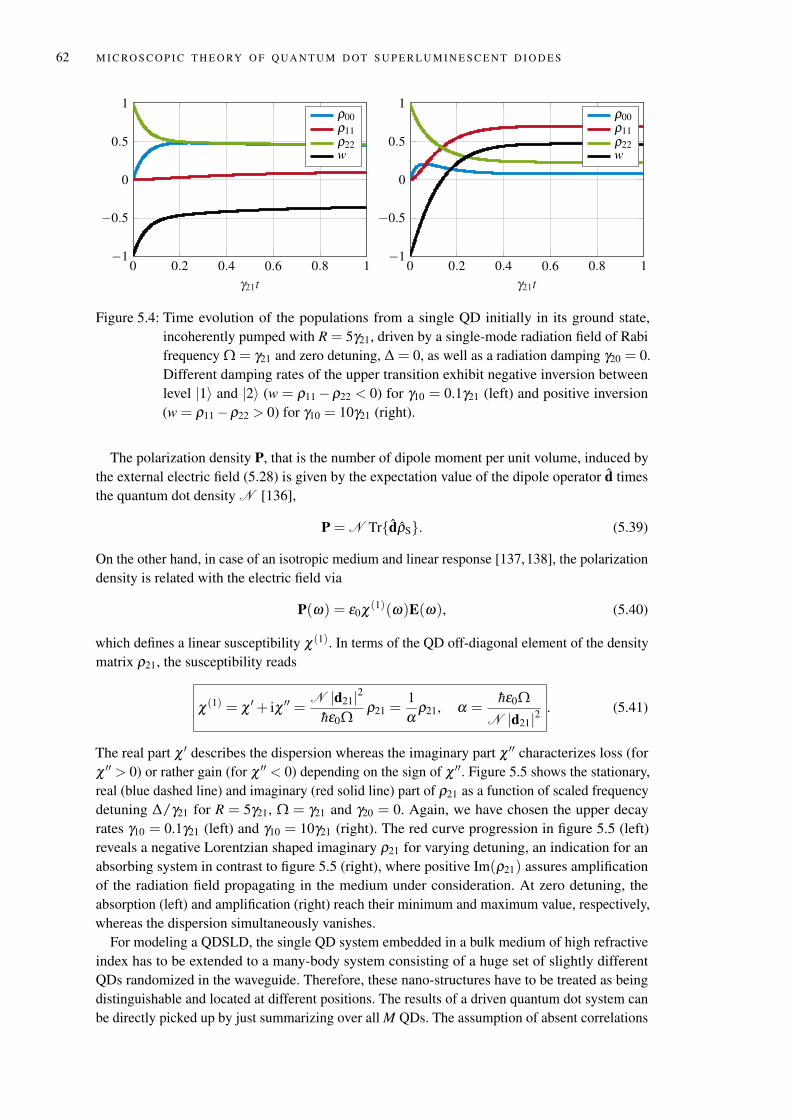
62 M I C RO S C O P I C T H E O RY O F Q UA N T U M D OT S U P E R L U M I N E S C E N T D I O D E S
0 0.2 0.4 0.6 0.8 1−1
−0.5
0
0.5
1
γ21t
ρ00ρ11ρ22w
0 0.2 0.4 0.6 0.8 1−1
−0.5
0
0.5
1
γ21t
ρ00ρ11ρ22w
Figure 5.4: Time evolution of the populations from a single QD initially in its ground state,incoherently pumped with R = 5γ21, driven by a single-mode radiation field of Rabifrequency Ω = γ21 and zero detuning, ∆ = 0, as well as a radiation damping γ20 = 0.Different damping rates of the upper transition exhibit negative inversion betweenlevel |1〉 and |2〉 (w = ρ11−ρ22 < 0) for γ10 = 0.1γ21 (left) and positive inversion(w = ρ11−ρ22 > 0) for γ10 = 10γ21 (right).
The polarization density P, that is the number of dipole moment per unit volume, induced bythe external electric field (5.28) is given by the expectation value of the dipole operator d timesthe quantum dot density N [136],
P = N TrdρS. (5.39)
On the other hand, in case of an isotropic medium and linear response [137,138], the polarizationdensity is related with the electric field via
P(ω) = ε0χ (1)(ω)E(ω), (5.40)
which defines a linear susceptibility χ (1). In terms of the QD off-diagonal element of the densitymatrix ρ21, the susceptibility reads
χ (1) = χ ′+ iχ ′′ =N |d21|2
hε0Ωρ21 =
1α
ρ21, α =hε0Ω
N |d21|2. (5.41)
The real part χ ′ describes the dispersion whereas the imaginary part χ ′′ characterizes loss (forχ ′′ > 0) or rather gain (for χ ′′ < 0) depending on the sign of χ ′′. Figure 5.5 shows the stationary,real (blue dashed line) and imaginary (red solid line) part of ρ21 as a function of scaled frequencydetuning ∆/γ21 for R = 5γ21, Ω = γ21 and γ20 = 0. Again, we have chosen the upper decayrates γ10 = 0.1γ21 (left) and γ10 = 10γ21 (right). The red curve progression in figure 5.5 (left)reveals a negative Lorentzian shaped imaginary ρ21 for varying detuning, an indication for anabsorbing system in contrast to figure 5.5 (right), where positive Im(ρ21) assures amplificationof the radiation field propagating in the medium under consideration. At zero detuning, theabsorption (left) and amplification (right) reach their minimum and maximum value, respectively,whereas the dispersion simultaneously vanishes.
For modeling a QDSLD, the single QD system embedded in a bulk medium of high refractiveindex has to be extended to a many-body system consisting of a huge set of slightly differentQDs randomized in the waveguide. Therefore, these nano-structures have to be treated as beingdistinguishable and located at different positions. The results of a driven quantum dot system canbe directly picked up by just summarizing over all M QDs. The assumption of absent correlations
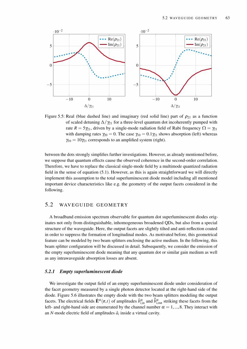
5.2 WAV E G U I D E G E O M E T RY 63
−10 0 10
−5
0
5
·10−2
∆/γ21
Re(ρ21)
Im(ρ21)
−10 0 10
−5
0
5
·10−2
∆/γ21
Re(ρ21)
Im(ρ21)
Figure 5.5: Real (blue dashed line) and imaginary (red solid line) part of ρ21 as a functionof scaled detuning ∆/γ21 for a three-level quantum dot incoherently pumped withrate R = 5γ21, driven by a single-mode radiation field of Rabi frequency Ω = γ21
with damping rates γ20 = 0. The case γ10 = 0.1γ21 shows absorption (left) whereasγ10 = 10γ21 corresponds to an amplified system (right).
between the dots strongly simplifies further investigations. However, as already mentioned before,we suppose that quantum effects cause the observed coherence in the second-order correlation.Therefore, we have to replace the classical single-mode field by a multimode quantized radiationfield in the sense of equation (5.1). However, as this is again straightforward we will directlyimplement this assumption to the total superluminescent diode model including all mentionedimportant device characteristics like e.g. the geometry of the output facets considered in thefollowing.
5.2 WAV E G U I D E G E O M E T RY
A broadband emission spectrum observable for quantum dot superluminescent diodes orig-inates not only from distinguishable, inhomogeneous broadened QDs, but also from a specialstructure of the waveguide. Here, the output facets are slightly tilted and anti-reflection coatedin order to suppress the formation of longitudinal modes. As motivated before, this geometricalfeature can be modeled by two beam splitters enclosing the active medium. In the following, thisbeam splitter configuration will be discussed in detail. Subsequently, we consider the emission ofthe empty superluminescent diode meaning that any quantum dot or similar gain medium as wellas any intrawaveguide absorption losses are absent.
5.2.1 Empty superluminescent diode
We investigate the output field of an empty superluminescent diode under consideration ofthe facet geometry measured by a single photon detector located at the right-hand side of thediode. Figure 5.6 illustrates the empty diode with the two beam splitters modeling the outputfacets. The electrical fields Eα(r, t) of amplitudes bα
i,in and ˆbαi,out striking these facets from the
left- and right-hand side are enumerated by the channel number α = 1, ...,8. They interact withan N-mode electric field of amplitudes ai inside a virtual cavity.
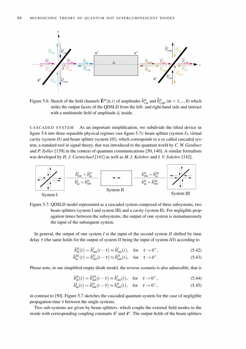
64 M I C RO S C O P I C T H E O RY O F Q UA N T U M D OT S U P E R L U M I N E S C E N T D I O D E S
b3i,in
b6i,in
b4i,in
b5i,in
b7i,in
b1i,in
ˆb8i,out
ˆb4i,out
ˆb5i,out
bri,out
ˆb7i,out
ˆb2iout
b2i,in
ˆb3i,out
bli,out br
i,inˆb1
i,out
κrκ l
κrκ l
z0
x
bli,in
ˆb6i,out ai
b8i,in−L
Figure 5.6: Sketch of the field channels Eα(r, t) of amplitudes bαi,in and ˆbα
i,out (α = 1, ...,8) whichstrike the output facets of the QDSLD from the left- and right-hand side and interactwith a multimode field of amplitude ai inside.
C A S C A D E D S Y S T E M As an important simplification, we subdivide the tilted device infigure 5.6 into three separable physical regimes (see figure 5.7): beam splitter (system I), virtualcavity (system II) and beam splitter (system III), which corresponds to a so called cascaded sys-tem, a standard tool in signal theory, that was introduced to the quantum world by C. W. Gardinerand P. Zoller [139] in the context of quantum communications [50, 140]. A similar formalismwas developed by H. J. Carmichael [141] as well as M. I. Kolobov and I. V. Sokolov [142].
System IISystem I System III
bIout = bII
in bIIout = bIII
in
bIin = bII
out bIIin = bIII
out
Figure 5.7: QDSLD model represented as a cascaded system composed of three subsystems, twobeam splitters (system I and system III) and a cavity (system II). For negligible prop-agation times between the subsystems, the output of one system is instantaneouslythe input of the subsequent system.
In general, the output of one system I is the input of the second system II shifted by timedelay τ (the same holds for the output of system II being the input of system III) according to
bIIin(t) = bI
out(t− τ) ≈ bIout(t), for τ → 0+, (5.42)
bIIIin (t) = bII
out(t− τ) ≈ bIIout(t), for τ → 0+. (5.43)
Please note, in our simplified empty diode model, the reverse scenario is also admissible, that is
bIIin(t) = bIII
out(t− τ) ≈ bIout(t), for τ → 0+, (5.44)
bIin(t) = bII
out(t− τ) ≈ bIIout(t), for τ → 0+, (5.45)
in contrast to [50]. Figure 5.7 sketches the cascaded quantum system for the case of negligiblepropagation time τ between the single systems.
Two sub-systems are given by beam splitters, which couple the external field modes to theinside with corresponding coupling constants κ l and κr. The output fields of the beam splitters
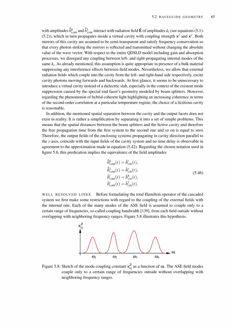
5.2 WAV E G U I D E G E O M E T RY 65
with amplitudes ˆb6i,out and ˆb1
i,out interact with radiation field E of amplitudes ai (see equations (5.1)-(5.2)), which in turn propagates inside a virtual cavity with coupling strength κ l and κr. Bothmirrors of this cavity are assumed to be semi-transparent and satisfy frequency conservation sothat every photon striking the mirrors is reflected and transmitted without changing the absolutevalue of the wave vector. With respect to the entire QDSLD model including gain and absorptionprocesses, we disregard any coupling between left- and right-propagating internal modes of thesame ki. As already mentioned, this assumption is quite appropriate in presence of a bulk materialsuppressing any interference effects between field modes. Nevertheless, we allow that externalradiation fields which couple into the cavity from the left- and right-hand side respectively, excitecavity photons moving forwards and backwards. At first glance, it seems to be unnecessary tointroduce a virtual cavity instead of a dielectric slab, especially in the context of the existent modesuppression caused by the special end facet’s geometry modeled by beam splitters. However,regarding the phenomenon of hybrid coherent light highlighting an increasing coherence in termsof the second-order correlation at a particular temperature regime, the choice of a fictitious cavityis reasonable.
In addition, the mentioned spatial separation between the cavity and the output facets does notexist in reality. It is rather a simplification by separating it into a set of simple problems. Thismeans that the spatial distances between the beam splitters and the fictive cavity and thereforethe free propagation time from the first system to the second one and so on is equal to zero.Therefore, the output fields of the enclosing systems propagating in cavity direction parallel tothe z-axis, coincide with the input fields of the cavity system and no time delay is observable inagreement to the approximation made in equation (5.42). Regarding the chosen notation used infigure 5.6, this predication implies the equivalence of the field amplitudes
ˆb6i,out(t) = bl
i,in(t),ˆb1
i,out(t) = bri,in(t),
bli,out(t) = b8
i,in(t),
bri,out(t) = b7
i,in(t).
(5.46)
W E L L R E S O LV E D L I N E S Before formulating the total Hamilton operator of the cascadedsystem we first make some restrictions with regard to the coupling of the external fields withthe internal one. Each of the many modes of the ASE field is assumed to couple only to acertain range of frequencies, so-called coupling bandwidth [139], from each field outside withoutoverlapping with neighboring frequency ranges. Figure 5.8 illustrates this hypothesis.
ω4ω3ω2ω1
ωi
κβiq
Figure 5.8: Sketch of the mode coupling constant κβiq as a function of ωi. The ASE field modes
couple only to a certain range of frequencies outside without overlapping withneighboring frequency ranges.
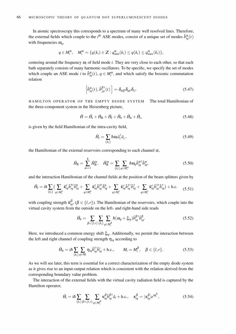
66 M I C RO S C O P I C T H E O RY O F Q UA N T U M D OT S U P E R L U M I N E S C E N T D I O D E S
In atomic spectroscopy this corresponds to a spectrum of many well resolved lines. Therefore,the external fields which couple to the ith ASE modes, consist of a unique set of modes bα
iq(t)with frequencies ωq,
q ∈Mαi , Mα
i = q(ki) ∈Z : qαmin(ki) ≤ q(ki) ≤ qα
max(ki),
centering around the frequency ωi of field mode i. They are very close to each other, so that eachbath separately consists of many harmonic oscillators. To be specific, we specify the set of modeswhich couple an ASE mode i to bα
iq(t), q ∈ Mαi , and which satisfy the bosonic commutation
relation [bα
iq(t), bβ†jp (t)
]= δαβ δqpδi j. (5.47)
H A M I LT O N O P E R AT O R O F T H E E M P T Y D I O D E S Y S T E M The total Hamiltonian ofthe three-component system in the Heisenberg picture,
H = Hr + HB + HI + Hb + Hlr + Hi, (5.48)
is given by the field Hamiltonian of the intra-cavity field,
Hr = ∑ki
hωia†i ai , (5.49)
the Hamiltonian of the external reservoirs corresponding to each channel α ,
HB =8
∑α=1
HαB , Hα
B = ∑ki
∑q∈Mα
i
hωqbα†iq bα
iq, (5.50)
and the interaction Hamiltonian of the channel fields at the position of the beam splitters given by
HI = ih ∑ki
(∑
q∈M5i
κ liqb5†
iq b8iq + ∑
q∈M4i
κ liqb4†
iq b6iq + ∑
q∈M1i
κriqb1†
iq b2iq + ∑
q∈M3i
κriqb3†
iq b7iq)+ h.c. (5.51)
with coupling strength κβiq, (β ∈ l,r). The Hamiltonian of the reservoirs, which couple into the
virtual cavity system from the outside on the left- and right-hand side reads
Hb = ∑β∈l,r
∑ki
∑q∈Mβ
i
h(ωq + ξiq)bβ†iq bβ
iq. (5.52)
Here, we introduced a common energy shift ξiq. Additionally, we permit the interaction betweenthe left and right channel of coupling strength ηiq according to
Hlr = ih ∑ki
∑q∈Mi
ηiqbl†iq br
iq + h.c., Mi = Mβi , β ∈ l,r. (5.53)
As we will see later, this term is essential for a correct characterization of the empty diode systemas it gives rise to an input-output relation which is consistent with the relation derived from thecorresponding boundary value problem.
The interaction of the external fields with the virtual cavity radiation field is captured by theHamilton operator,
Hi = ih ∑ki
∑β∈l,r
∑q∈Mβ
i
κβiqbβ†
iq ai + h.c., κβiq = |κ
βiq|eiφ β
i , (5.54)
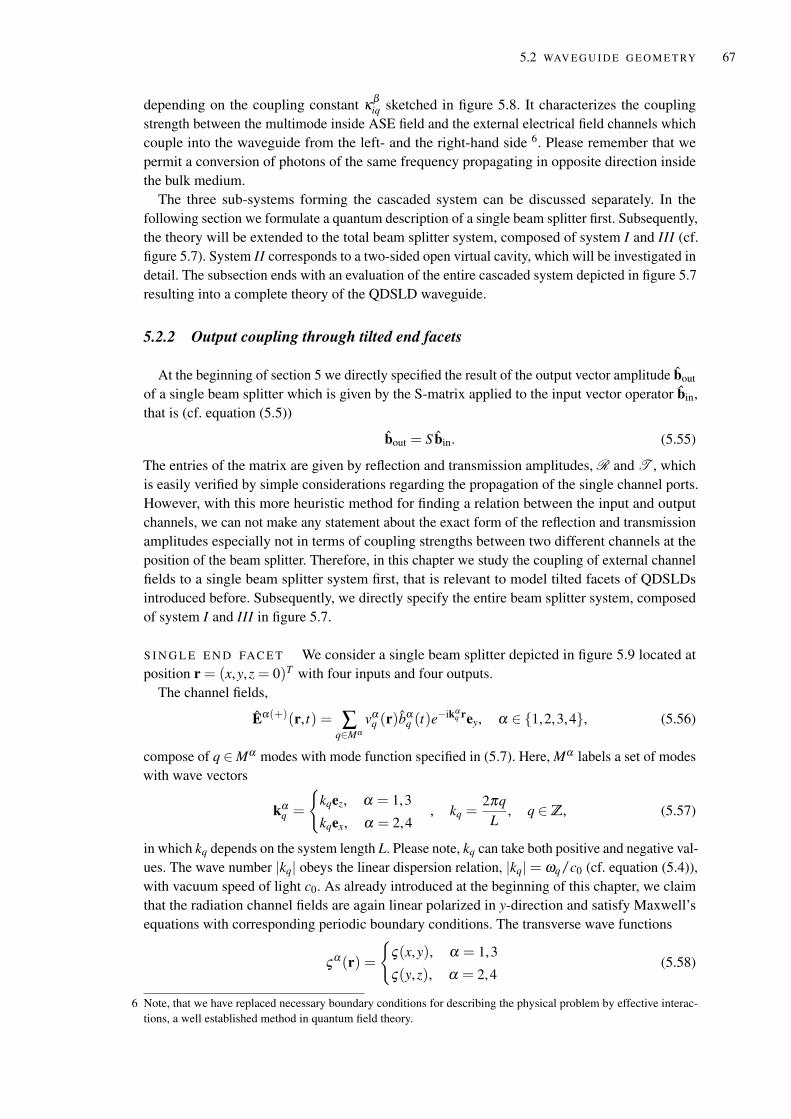
5.2 WAV E G U I D E G E O M E T RY 67
depending on the coupling constant κβiq sketched in figure 5.8. It characterizes the coupling
strength between the multimode inside ASE field and the external electrical field channels whichcouple into the waveguide from the left- and the right-hand side 6. Please remember that wepermit a conversion of photons of the same frequency propagating in opposite direction insidethe bulk medium.
The three sub-systems forming the cascaded system can be discussed separately. In thefollowing section we formulate a quantum description of a single beam splitter first. Subsequently,the theory will be extended to the total beam splitter system, composed of system I and III (cf.figure 5.7). System II corresponds to a two-sided open virtual cavity, which will be investigated indetail. The subsection ends with an evaluation of the entire cascaded system depicted in figure 5.7resulting into a complete theory of the QDSLD waveguide.
5.2.2 Output coupling through tilted end facets
At the beginning of section 5 we directly specified the result of the output vector amplitude bout
of a single beam splitter which is given by the S-matrix applied to the input vector operator bin,that is (cf. equation (5.5))
bout = S bin. (5.55)
The entries of the matrix are given by reflection and transmission amplitudes, R and T , whichis easily verified by simple considerations regarding the propagation of the single channel ports.However, with this more heuristic method for finding a relation between the input and outputchannels, we can not make any statement about the exact form of the reflection and transmissionamplitudes especially not in terms of coupling strengths between two different channels at theposition of the beam splitter. Therefore, in this chapter we study the coupling of external channelfields to a single beam splitter system first, that is relevant to model tilted facets of QDSLDsintroduced before. Subsequently, we directly specify the entire beam splitter system, composedof system I and III in figure 5.7.
S I N G L E E N D FAC E T We consider a single beam splitter depicted in figure 5.9 located atposition r = (x,y,z = 0)T with four inputs and four outputs.
The channel fields,
Eα(+)(r, t) = ∑q∈Mα
vαq (r)b
αq (t)e
−ikαq rey, α ∈ 1,2,3,4, (5.56)
compose of q ∈Mα modes with mode function specified in (5.7). Here, Mα labels a set of modeswith wave vectors
kαq =
kqez, α = 1,3
kqex, α = 2,4, kq =
2πqL
, q ∈Z, (5.57)
in which kq depends on the system length L. Please note, kq can take both positive and negative val-ues. The wave number |kq| obeys the linear dispersion relation, |kq|= ωq/c0 (cf. equation (5.4)),with vacuum speed of light c0. As already introduced at the beginning of this chapter, we claimthat the radiation channel fields are again linear polarized in y-direction and satisfy Maxwell’sequations with corresponding periodic boundary conditions. The transverse wave functions
ςα(r) =
ς(x,y), α = 1,3
ς(y,z), α = 2,4(5.58)
6 Note, that we have replaced necessary boundary conditions for describing the physical problem by effective interac-tions, a well established method in quantum field theory.
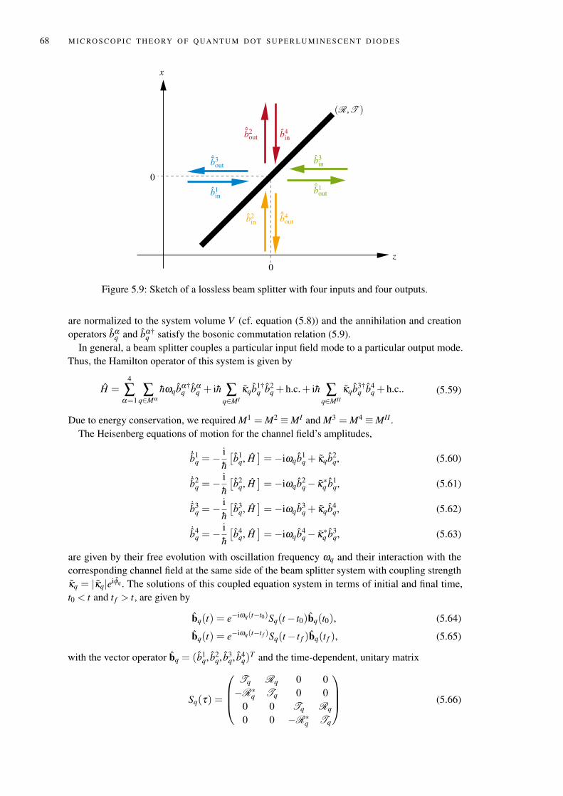
68 M I C RO S C O P I C T H E O RY O F Q UA N T U M D OT S U P E R L U M I N E S C E N T D I O D E S
z
x
0
0
b3in
(R,T )
ˆb3out
ˆb4out
b4in
ˆb1out
ˆb2out
b1in
b2in
Figure 5.9: Sketch of a lossless beam splitter with four inputs and four outputs.
are normalized to the system volume V (cf. equation (5.8)) and the annihilation and creationoperators bα
q and bα†q satisfy the bosonic commutation relation (5.9).
In general, a beam splitter couples a particular input field mode to a particular output mode.Thus, the Hamilton operator of this system is given by
H =4
∑α=1
∑q∈Mα
hωqbα†q bα
q + ih ∑q∈MI
κqb1†q b2
q + h.c.+ ih ∑q∈MII
κqb3†q b4
q + h.c.. (5.59)
Due to energy conservation, we required M1 = M2 ≡MI and M3 = M4 ≡MII .The Heisenberg equations of motion for the channel field’s amplitudes,
˙b1q = −
ih
[b1
q, H]= −iωqb1
q + κqb2q, (5.60)
˙b2q = −
ih
[b2
q, H]= −iωqb2
q− κ∗q b1q, (5.61)
˙b3q = −
ih
[b3
q, H]= −iωqb3
q + κqb4q, (5.62)
˙b4q = −
ih
[b4
q, H]= −iωqb4
q− κ∗q b3q, (5.63)
are given by their free evolution with oscillation frequency ωq and their interaction with thecorresponding channel field at the same side of the beam splitter system with coupling strengthκq = |κq|eiφq . The solutions of this coupled equation system in terms of initial and final time,t0 < t and t f > t, are given by
bq(t) = e−iωq(t−t0)Sq(t− t0)bq(t0), (5.64)
bq(t) = e−iωq(t−t f )Sq(t− t f )bq(t f ), (5.65)
with the vector operator bq = (b1q, b2
q, b3q, b4
q)T and the time-dependent, unitary matrix
Sq(τ) =
Tq Rq 0 0−R∗q Tq 0 0
0 0 Tq Rq
0 0 −R∗q Tq
(5.66)
5.2 WAV E G U I D E G E O M E T RY 69
with matrix elements
Rq(τ) = eiφq sin(|κq|τ), Tq(τ) = cos(|κq|τ). (5.67)
Please note, a sharply localized coupling constant in space results in an approximately flatfrequency independent coupling strength which is valid for Markovian systems. Therefore,we make the approximation κ(ωq) ≈ κ , so that Sq is independent of frequency ωq, that isSq(t) ≈ S(t).
Next, we define input and output operators in terms of initial and final time respectively,
bαin(t) =
√∆ν ∑
q∈Mαe−iωq(t−t0)bα
q (t0), (5.68)
ˆbαout(t) =
√∆ν ∑
q∈Mαe−iωq(t−t f )bα
q (t f ), ∆ν =∆ω2π
, (5.69)
with equally spaced frequency interval ∆ω = ωi+1−ωi. They satisfy the commutation relation[bα
in(t), bβ†in (t ′)
]= ∆ν ∑
q∈Mα∑
p∈Mβ
e−iωq(t−t0)eiωp(t ′−t0)[bα
q (t0), bβ†p (t0)
]= δαβ δqp∆ν ∑
q∈Mαe−iωq(t−t ′).
(5.70)
In the continuum limit, ∆ω → 0, the sum approaches a delta distribution
lim∆ω→0
∆ω2π ∑
q∈Mαe−iωq(t−t ′) = δ (t− t ′). (5.71)
Therefore, we find the central commutation relation of the input noise[bα
in(t), bβ†in (t ′)
]= δαβ δ (t− t ′) . (5.72)
The same holds for the output amplitudes ˆbαi,out. Obviously, the field amplitudes have the di-
mension of s−1/2 in contrast to the dimensionless field operators bαq (t) (cf. commutation rela-
tion (5.9)). Equating the right-hand side of equation (5.64) and (5.65), summing both sides overall modes q, multiplying by
√∆ν and finally utilizing the unitarity of the matrix (5.66), we find
a relation between the input and output operators
bout(t) = S(t f − t0) bin(t) , (5.73)
with bin = (b1in, b2
in, b3in, b4
in)T and bout = (b1
out, b2out, b
3out, b
4out)
T ≡ ( ˆb3out,
ˆb4out,
ˆb1out,
ˆb2out)
T . Pleasenote, to allow for the concept of channel fields in analogy to scattering theory, in which the totalelectromagnetic field of each channel is given by in- and outgoing electromagnetic fields withopposite propagation direction in the sense of figure 5.10, we applied an appropriate permutationof the output vector operator.
U N I TA RY S - M AT R I X Equation (5.73) shows that the input and output operators are con-nected by the S-matrix, (cf. equation (5.66))
S≡ limt f−t0→∞
κ→0κ(t f−t0)=const.
S(t f − t0) =
0 0 T R
0 0 −R∗ T
T R 0 0−R∗ T 0 0
(5.74)
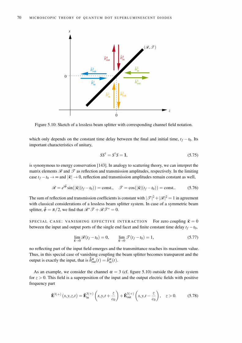
70 M I C RO S C O P I C T H E O RY O F Q UA N T U M D OT S U P E R L U M I N E S C E N T D I O D E S
z
x
0
0
b1out
b3in
b4in
b2out
(R,T )
b1in
b3out
b2in
b4out
Figure 5.10: Sketch of a lossless beam splitter with corresponding channel field notation.
which only depends on the constant time delay between the final and initial time, t f − t0. Itsimportant characteristics of unitary,
SS† = S†S = 1, (5.75)
is synonymous to energy conservation [143]. In analogy to scattering theory, we can interpret thematrix elements R and T as reflection and transmission amplitudes, respectively. In the limitingcase t f − t0→ ∞ and |κ| → 0, reflection and transmission amplitudes remain constant as well,
R = eiφ sin(|κ|(t f − t0)) = const., T = cos(|κ|(t f − t0)) = const.. (5.76)
The sum of reflection and transmission coefficients is constant with |T |2+ |R|2 = 1 in agreementwith classical considerations of a lossless beam splitter system. In case of a symmetric beamsplitter, φ = π/2, we find that R∗T +RT ∗ = 0.
S P E C I A L C A S E : VA N I S H I N G E FF E C T I V E I N T E R AC T I O N For zero coupling κ = 0between the input and output ports of the single end facet and finite constant time delay t f − t0,
limκ→0
R(t f − t0) = 0, limκ→0
T (t f − t0) = 1, (5.77)
no reflecting part of the input field emerges and the transmittance reaches its maximum value.Thus, in this special case of vanishing coupling the beam splitter becomes transparent and theoutput is exactly the input, that is ˆbα
out(t) = bαin(t).
As an example, we consider the channel α = 3 (cf. figure 5.10) outside the diode systemfor z > 0. This field is a superposition of the input and the output electric fields with positivefrequency part
E3(+) (x,y,z, t) = E3(+)in
(x,y, t +
zc0
)+ E3(+)
out
(x,y, t− z
c0
), z > 0. (5.78)
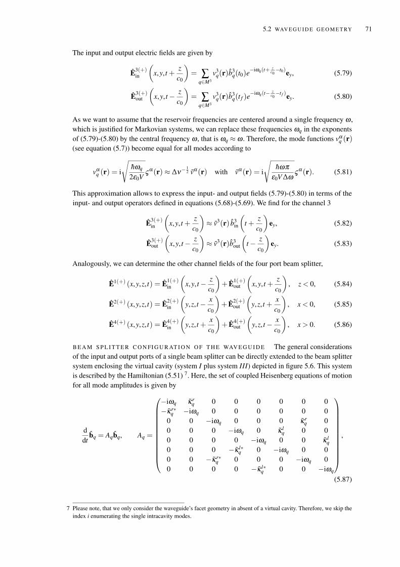
5.2 WAV E G U I D E G E O M E T RY 71
The input and output electric fields are given by
E3(+)in
(x,y, t +
zc0
)= ∑
q∈M3
v3q(r)b
3q(t0)e
−iωq(t+ zc0−t0)ey, (5.79)
E3(+)out
(x,y, t− z
c0
)= ∑
q∈M3
v3q(r)b
3q(t f )e
−iωq(t− zc0−t f )ey. (5.80)
As we want to assume that the reservoir frequencies are centered around a single frequency ω ,which is justified for Markovian systems, we can replace these frequencies ωq in the exponentsof (5.79)-(5.80) by the central frequency ω , that is ωq ≈ ω . Therefore, the mode functions vα
q (r)(see equation (5.7)) become equal for all modes according to
vαq (r) = i
√hωq
2ε0Vςα(r) ≈ ∆ν−
12 vα(r) with vα(r) = i
√hωπ
ε0V ∆ωςα(r). (5.81)
This approximation allows to express the input- and output fields (5.79)-(5.80) in terms of theinput- and output operators defined in equations (5.68)-(5.69). We find for the channel 3
E3(+)in
(x,y, t +
zc0
)≈ v3(r) b3
in
(t +
zc0
)ey, (5.82)
E3(+)out
(x,y, t− z
c0
)≈ v3(r)b3
out
(t− z
c0
)ey. (5.83)
Analogously, we can determine the other channel fields of the four port beam splitter,
E1(+) (x,y,z, t) = E1(+)in
(x,y, t− z
c0
)+ E1(+)
out
(x,y, t +
zc0
), z < 0, (5.84)
E2(+) (x,y,z, t) = E2(+)in
(y,z, t− x
c0
)+ E2(+)
out
(y,z, t +
xc0
), x < 0, (5.85)
E4(+) (x,y,z, t) = E4(+)in
(y,z, t +
xc0
)+ E4(+)
out
(y,z, t− x
c0
), x > 0. (5.86)
B E A M S P L I T T E R C O N FI G U R AT I O N O F T H E WAV E G U I D E The general considerationsof the input and output ports of a single beam splitter can be directly extended to the beam splittersystem enclosing the virtual cavity (system I plus system III) depicted in figure 5.6. This systemis described by the Hamiltonian (5.51) 7. Here, the set of coupled Heisenberg equations of motionfor all mode amplitudes is given by
ddt
bq = Aqbq, Aq =
−iωq κrq 0 0 0 0 0 0
−κr∗q −iωq 0 0 0 0 0 0
0 0 −iωq 0 0 0 κrq 0
0 0 0 −iωq 0 κ lq 0 0
0 0 0 0 −iωq 0 0 κ lq
0 0 0 −κ l∗q 0 −iωq 0 0
0 0 −κr∗q 0 0 0 −iωq 0
0 0 0 0 −κ l∗q 0 0 −iωq
,
(5.87)
7 Please note, that we only consider the waveguide’s facet geometry in absent of a virtual cavity. Therefore, we skip theindex i enumerating the single intracavity modes.
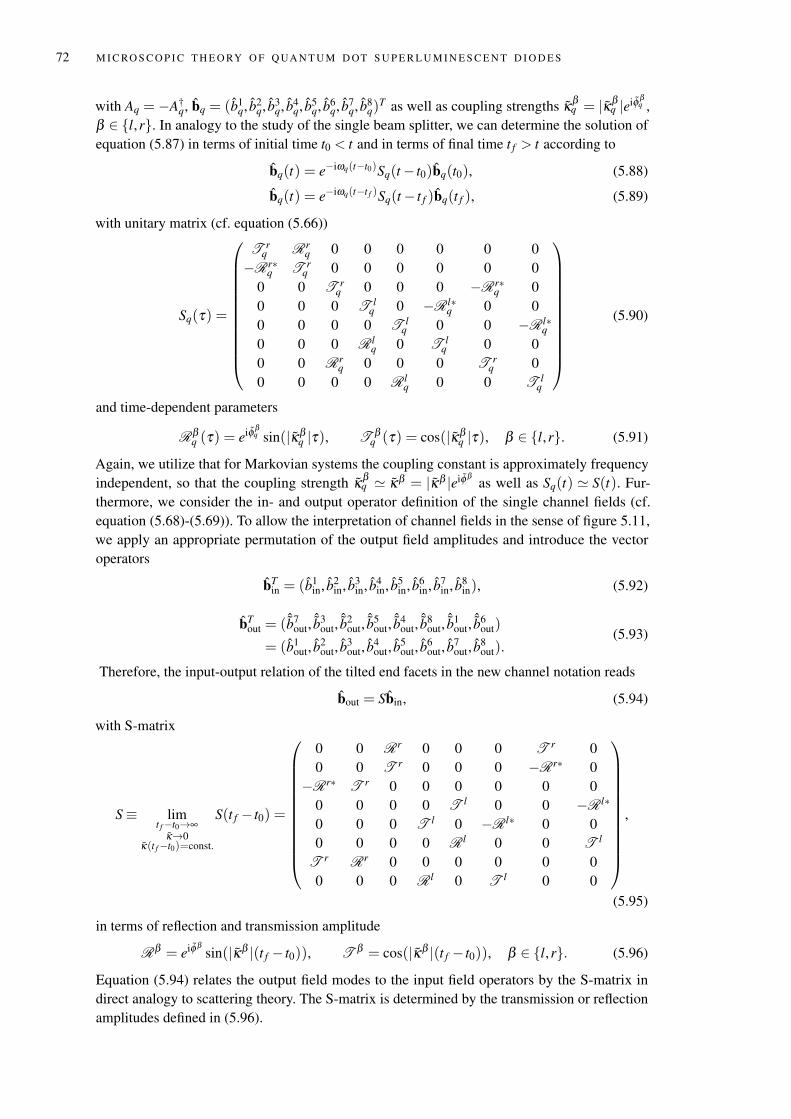
72 M I C RO S C O P I C T H E O RY O F Q UA N T U M D OT S U P E R L U M I N E S C E N T D I O D E S
with Aq = −A†q, bq = (b1
q, b2q, b3
q, b4q, b5
q, b6q, b7
q, b8q)
T as well as coupling strengths κβq = |κβ
q |eiφ βq ,
β ∈ l,r. In analogy to the study of the single beam splitter, we can determine the solution ofequation (5.87) in terms of initial time t0 < t and in terms of final time t f > t according to
bq(t) = e−iωq(t−t0)Sq(t− t0)bq(t0), (5.88)
bq(t) = e−iωq(t−t f )Sq(t− t f )bq(t f ), (5.89)
with unitary matrix (cf. equation (5.66))
Sq(τ) =
T rq Rr
q 0 0 0 0 0 0−Rr∗
q T rq 0 0 0 0 0 0
0 0 T rq 0 0 0 −Rr∗
q 00 0 0 T l
q 0 −R l∗q 0 0
0 0 0 0 T lq 0 0 −R l∗
q0 0 0 R l
q 0 T lq 0 0
0 0 Rrq 0 0 0 T r
q 00 0 0 0 R l
q 0 0 T lq
(5.90)
and time-dependent parameters
Rβq (τ) = eiφ β
q sin(|κβq |τ), T β
q (τ) = cos(|κβq |τ), β ∈ l,r. (5.91)
Again, we utilize that for Markovian systems the coupling constant is approximately frequencyindependent, so that the coupling strength κβ
q ' κβ = |κβ |eiφ βas well as Sq(t) ' S(t). Fur-
thermore, we consider the in- and output operator definition of the single channel fields (cf.equation (5.68)-(5.69)). To allow the interpretation of channel fields in the sense of figure 5.11,we apply an appropriate permutation of the output field amplitudes and introduce the vectoroperators
bTin = (b1
in, b2in, b3
in, b4in, b5
in, b6in, b7
in, b8in), (5.92)
bTout = ( ˆb7
out,ˆb3
out,ˆb2
out,ˆb5
out,ˆb4
out,ˆb8
out,ˆb1
out,ˆb6
out)
= (b1out, b
2out, b
3out, b
4out, b
5out, b
6out, b
7out, b
8out).
(5.93)
Therefore, the input-output relation of the tilted end facets in the new channel notation reads
bout = Sbin, (5.94)
with S-matrix
S≡ limt f−t0→∞
κ→0κ(t f−t0)=const.
S(t f − t0) =
0 0 Rr 0 0 0 T r 00 0 T r 0 0 0 −Rr∗ 0−Rr∗ T r 0 0 0 0 0 0
0 0 0 0 T l 0 0 −R l∗
0 0 0 T l 0 −R l∗ 0 00 0 0 0 R l 0 0 T l
T r Rr 0 0 0 0 0 00 0 0 R l 0 T l 0 0
,
(5.95)
in terms of reflection and transmission amplitude
Rβ = eiφ βsin(|κβ |(t f − t0)), T β = cos(|κβ |(t f − t0)), β ∈ l,r. (5.96)
Equation (5.94) relates the output field modes to the input field operators by the S-matrix indirect analogy to scattering theory. The S-matrix is determined by the transmission or reflectionamplitudes defined in (5.96).
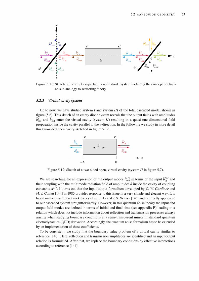
5.2 WAV E G U I D E G E O M E T RY 73
b3i,in
b6i,in
b4i,in
b2i,in
κrκ l
κ l
b1i,out
b2i,out
κr
b8i,out bl
i,in
ai
x
−L b1i,in
0b8i,inb6
i,out b7i,out
b7i,in
bli,out
zbr
i,out
bri,in
b4i,out
b5i,inb5
i,out
b3i,out
Figure 5.11: Sketch of the empty superluminescent diode system including the concept of chan-nels in analogy to scattering theory.
5.2.3 Virtual cavity system
Up to now, we have studied system I and system III of the total cascaded model shown infigure (5.6). This sketch of an empty diode system reveals that the output fields with amplitudesˆb6
out and ˆb1out enter the virtual cavity (system II) resulting in a quasi one-dimensional field
propagation inside the cavity parallel to the z-direction. In the following we study in more detailthis two-sided open cavity sketched in figure 5.12.
abl
in
blout
κ l
brin
brout
z
κr
0−L
Figure 5.12: Sketch of a two-sided open, virtual cavity (system II in figure 5.7).
We are searching for an expression of the output modes bl/rout in terms of the input bl/r
in andtheir coupling with the multimode radiation field of amplitudes a inside the cavity of couplingconstants κ l/r. It turns out that the input-output formalism developed by C. W. Gardiner andM. J. Collett [144] in 1985 provides response to this issue in a very simple and elegant way. It isbased on the quantum network theory of B. Yurke and J. S. Denker [145] and is directly applicableto our cascaded system straightforwardly. However, in this quantum noise theory the input andoutput field modes are defined in terms of initial and final time (see appendix E) leading to arelation which does not include information about reflection and transmission processes alwaysarising when studying boundary conditions at a semi-transparent mirror in standard quantumelectrodynamics (QED) derivation. Accordingly, the quantum noise formalism has to be extendedby an implementation of these coefficients.
To be consistent, we study first the boundary value problem of a virtual cavity similar toreference [146]. Here, reflection and transmission amplitudes are identified and an input-outputrelation is formulated. After that, we replace the boundary conditions by effective interactionsaccording to reference [144].
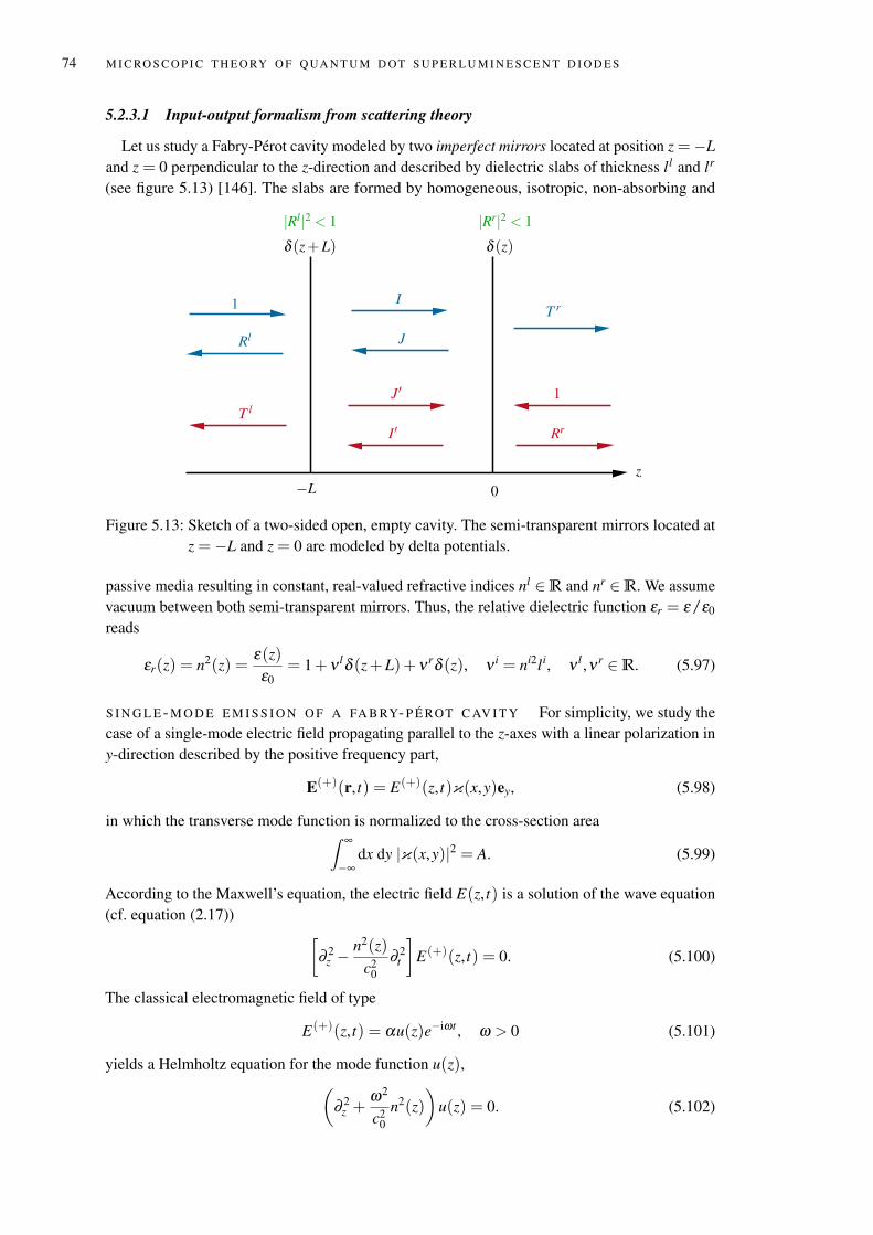
74 M I C RO S C O P I C T H E O RY O F Q UA N T U M D OT S U P E R L U M I N E S C E N T D I O D E S
5.2.3.1 Input-output formalism from scattering theory
Let us study a Fabry-Pérot cavity modeled by two imperfect mirrors located at position z =−Land z = 0 perpendicular to the z-direction and described by dielectric slabs of thickness ll and lr
(see figure 5.13) [146]. The slabs are formed by homogeneous, isotropic, non-absorbing and
z
δ (z)
1
0−L
δ (z+L)
I
J
J′
I′
1 T r
Rr
Rl
T l
|Rl|2 < 1 |Rr|2 < 1
Figure 5.13: Sketch of a two-sided open, empty cavity. The semi-transparent mirrors located atz = −L and z = 0 are modeled by delta potentials.
passive media resulting in constant, real-valued refractive indices nl ∈R and nr ∈R. We assumevacuum between both semi-transparent mirrors. Thus, the relative dielectric function εr = ε/ε0
reads
εr(z) = n2(z) =ε(z)ε0
= 1+ν lδ (z+L)+νrδ (z), ν i = ni2li, ν l ,νr ∈R. (5.97)
S I N G L E - M O D E E M I S S I O N O F A FA B RY- P É ROT C AV I T Y For simplicity, we study thecase of a single-mode electric field propagating parallel to the z-axes with a linear polarization iny-direction described by the positive frequency part,
E(+)(r, t) = E(+)(z, t)κ(x,y)ey, (5.98)
in which the transverse mode function is normalized to the cross-section area∫ ∞
−∞dx dy |κ(x,y)|2 = A. (5.99)
According to the Maxwell’s equation, the electric field E(z, t) is a solution of the wave equation(cf. equation (2.17)) [
∂ 2z −
n2(z)c2
0∂ 2
t
]E(+)(z, t) = 0. (5.100)
The classical electromagnetic field of type
E(+)(z, t) = αu(z)e−iωt , ω > 0 (5.101)
yields a Helmholtz equation for the mode function u(z),(∂ 2
z +ω2
c20
n2(z))
u(z) = 0. (5.102)
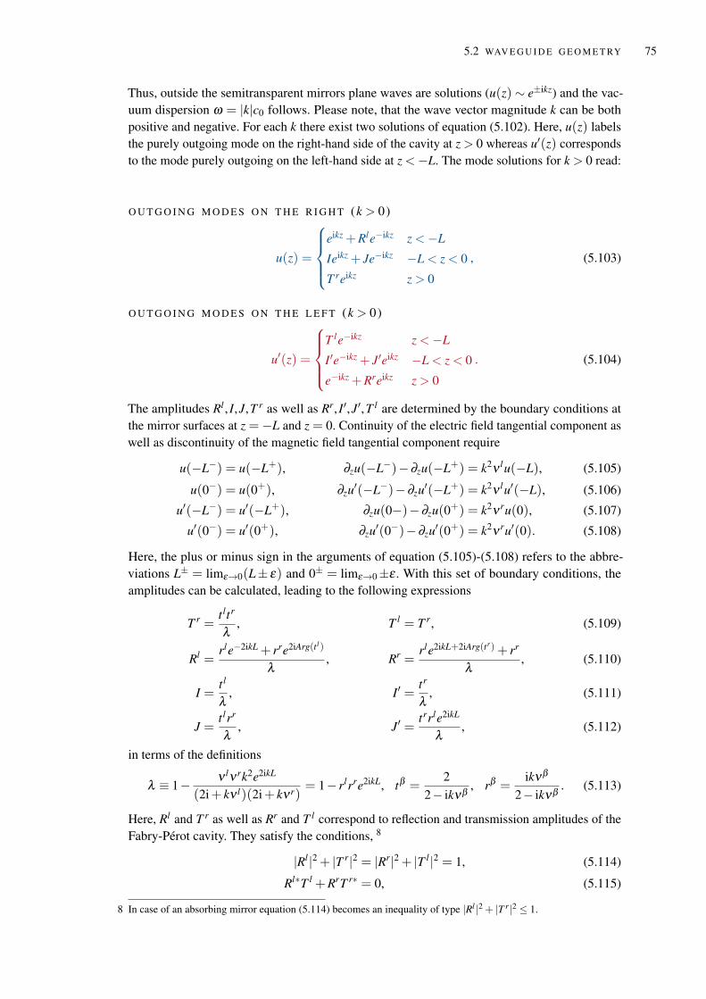
5.2 WAV E G U I D E G E O M E T RY 75
Thus, outside the semitransparent mirrors plane waves are solutions (u(z)∼ e±ikz) and the vac-uum dispersion ω = |k|c0 follows. Please note, that the wave vector magnitude k can be bothpositive and negative. For each k there exist two solutions of equation (5.102). Here, u(z) labelsthe purely outgoing mode on the right-hand side of the cavity at z > 0 whereas u′(z) correspondsto the mode purely outgoing on the left-hand side at z <−L. The mode solutions for k > 0 read:
O U T G O I N G M O D E S O N T H E R I G H T (k > 0)
u(z) =
eikz +Rle−ikz z <−L
Ieikz + Je−ikz −L < z < 0
T reikz z > 0
, (5.103)
O U T G O I N G M O D E S O N T H E L E F T (k > 0)
u′(z) =
T le−ikz z <−L
I′e−ikz + J′eikz −L < z < 0
e−ikz +Rreikz z > 0
. (5.104)
The amplitudes Rl , I,J,T r as well as Rr, I′,J′,T l are determined by the boundary conditions atthe mirror surfaces at z = −L and z = 0. Continuity of the electric field tangential component aswell as discontinuity of the magnetic field tangential component require
u(−L−) = u(−L+), ∂zu(−L−)−∂zu(−L+) = k2ν lu(−L), (5.105)
u(0−) = u(0+), ∂zu′(−L−)−∂zu′(−L+) = k2ν lu′(−L), (5.106)
u′(−L−) = u′(−L+), ∂zu(0−)−∂zu(0+) = k2νru(0), (5.107)
u′(0−) = u′(0+), ∂zu′(0−)−∂zu′(0+) = k2νru′(0). (5.108)
Here, the plus or minus sign in the arguments of equation (5.105)-(5.108) refers to the abbre-viations L± = limε→0(L± ε) and 0± = limε→0±ε . With this set of boundary conditions, theamplitudes can be calculated, leading to the following expressions
T r =t ltr
λ, T l = T r, (5.109)
Rl =rle−2ikL + rre2iArg(t l)
λ, Rr =
rle2ikL+2iArg(tr)+ rr
λ, (5.110)
I =t l
λ, I′ =
tr
λ, (5.111)
J =t lrr
λ, J′ =
trrle2ikL
λ, (5.112)
in terms of the definitions
λ ≡ 1− ν lνrk2e2ikL
(2i+ kν l)(2i+ kνr)= 1− rlrre2ikL, tβ =
22− ikνβ , rβ =
ikνβ
2− ikνβ . (5.113)
Here, Rl and T r as well as Rr and T l correspond to reflection and transmission amplitudes of theFabry-Pérot cavity. They satisfy the conditions, 8
|Rl|2 + |T r|2 = |Rr|2 + |T l|2 = 1, (5.114)
Rl∗T l +RrT r∗ = 0, (5.115)
8 In case of an absorbing mirror equation (5.114) becomes an inequality of type |Rl |2 + |T r|2 ≤ 1.

76 M I C RO S C O P I C T H E O RY O F Q UA N T U M D OT S U P E R L U M I N E S C E N T D I O D E S
0 2 4 6 8 10 12 14
0.0
0.2
0.4
0.6
0.8
1.0
νrk
|Tr |² |Rr |²
(a) ν l = νr
0 2 4 6 8 10 12 14
0.0
0.2
0.4
0.6
0.8
1.0
νrk
|Tr |² |Rr |²
(b) ν l = 0.5νr
0 2 4 6 8 10 12 14
0.0
0.2
0.4
0.6
0.8
1.0
νrk
|Tr |² |Rr |²
(c) ν l = 0.1νr
0 2 4 6 8 10 12 14
0.0
0.2
0.4
0.6
0.8
1.0
νrk
|Tr |² |Rr |²
(d) ν l = 0.001νr
Figure 5.14: Reflection and transmission coefficient, |Rr|2 and |T r|2, of an open cavity of lengthL = νr as a function of the scaled wave number νrk for characteristic function (a)ν l = νr, (b) ν l = 0.5νr, (c) ν l = 0.1νr, (d) ν l = 0.001νr.
due to energy conservation. Figure 5.14 shows the transmission |T r|2 (red) and the reflection |Rr|2(blue) coefficient on the right-hand side of the cavity of length L = νr as a function of scaled wavenumber νrk. For a smaller ratio ν l/νr, reflection and transmission reveal resonances observablein figure 5.14(a) for ν l = νr and figure 5.14(b) for ν l = 0.5νr. These resonances are smearedout with decreasing ratio ν l/νr visible in figure 5.14(c) and figure 5.14(d) for ν l = 0.1νr andν l = 0.001νr, respectively. In addition, for decreasing the ratio ν l/νr, an increasing reflectionand a decreasing transmission coefficient are observable until they reach their maximum andminimum value of 1 and 0, respectively 9. At the same time, the sum of both coefficients remainsconstant according to condition (5.114).
The mode function (5.103) is normalized by [146]∫dz n2(z)u(k,z)u∗(k′,z) = 2πδ (k− k′). (5.116)
The same is valid for the mode function u′(z). Furthermore, the mode functions obey theorthogonality condition [146] ∫
dz n2(z)u(k,z)u′∗(k′,z) = 0. (5.117)
9 Figure 5.14(d) corresponds to the bad cavity limit.
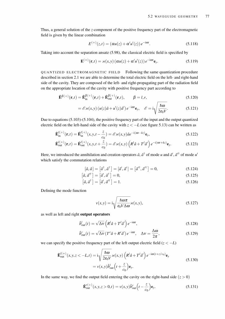
5.2 WAV E G U I D E G E O M E T RY 77
Thus, a general solution of the z-component of the positive frequency part of the electromagneticfield is given by the linear combination
E(+)(z, t) = (αu(z)+α ′u′(z))e−iωt . (5.118)
Taking into account the separation ansatz (5.98), the classical electric field is specified by
E(+)(r, t) = κ(x,y) (αu(z)+α ′u′(z))e−iωtey. (5.119)
Q UA N T I Z E D E L E C T RO M AG N E T I C FI E L D Following the same quantization proceduredescribed in section 2.1 we are able to determine the total electric field on the left- and right-handside of the cavity. They are composed of the left- and right-propagating part of the radiation fieldon the appropriate location of the cavity with positive frequency part according to
Eβ (+)(r, t) = Eβ (+)in (r, t)+ Eβ (+)
out (r, t), β = l,r, (5.120)
= Eκ(x,y) (u(z)a+ u′(z)a′)e−iωtey, E = i
√hω
2ε0V. (5.121)
Due to equations (5.103)-(5.104), the positive frequency part of the input and the output quantizedelectric field on the left-hand side of the cavity with z <−L (see figure 5.13) can be written as
El(+)in (r, t) = El(+)
in (x,y, t− zc0) = Eκ(x,y)ae−i(ωt−kz)ey, (5.122)
El(+)out (r, t) = El(+)
out (x,y, t +zc0) = Eκ(x,y)
(Rl a+T l a′
)e−i(ωt+kz)ey. (5.123)
Here, we introduced the annihilation and creation operators a, a† of mode u and a′, a′† of mode u′
which satisfy the commutation relations
[a, a ] =[a†, a† ]= [a′, a′ ] =
[a′†, a′†
]= 0, (5.124)[
a, a′†]=[a′, a† ]= 0, (5.125)[
a, a† ]= [a′, a′†]= 1. (5.126)
Defining the mode function
v(x,y) = i
√hωπ
ε0V ∆ωκ(x,y), (5.127)
as well as left and right output operators
blout(t) =
√∆ν(
Rl a+T l a′)
e−iωt , (5.128)
brout(t) =
√∆ν (T ra+Rra′)e−iωt , ∆ν =
∆ω2π
, (5.129)
we can specify the positive frequency part of the left output electric field (z <−L)
El(+)out (x,y,z <−L, t) = i
√hω
2ε0Vκ(x,y)
(Rl a+T l a′
)e−iω(t+z/c0)ey
= v(x,y)blout
(t +
zc0
)ey.
(5.130)
In the same way, we find the output field entering the cavity on the right-hand side (z > 0)
Er(+)out (x,y,z > 0, t) = v(x,y)br
out
(t− z
c0
)ey. (5.131)
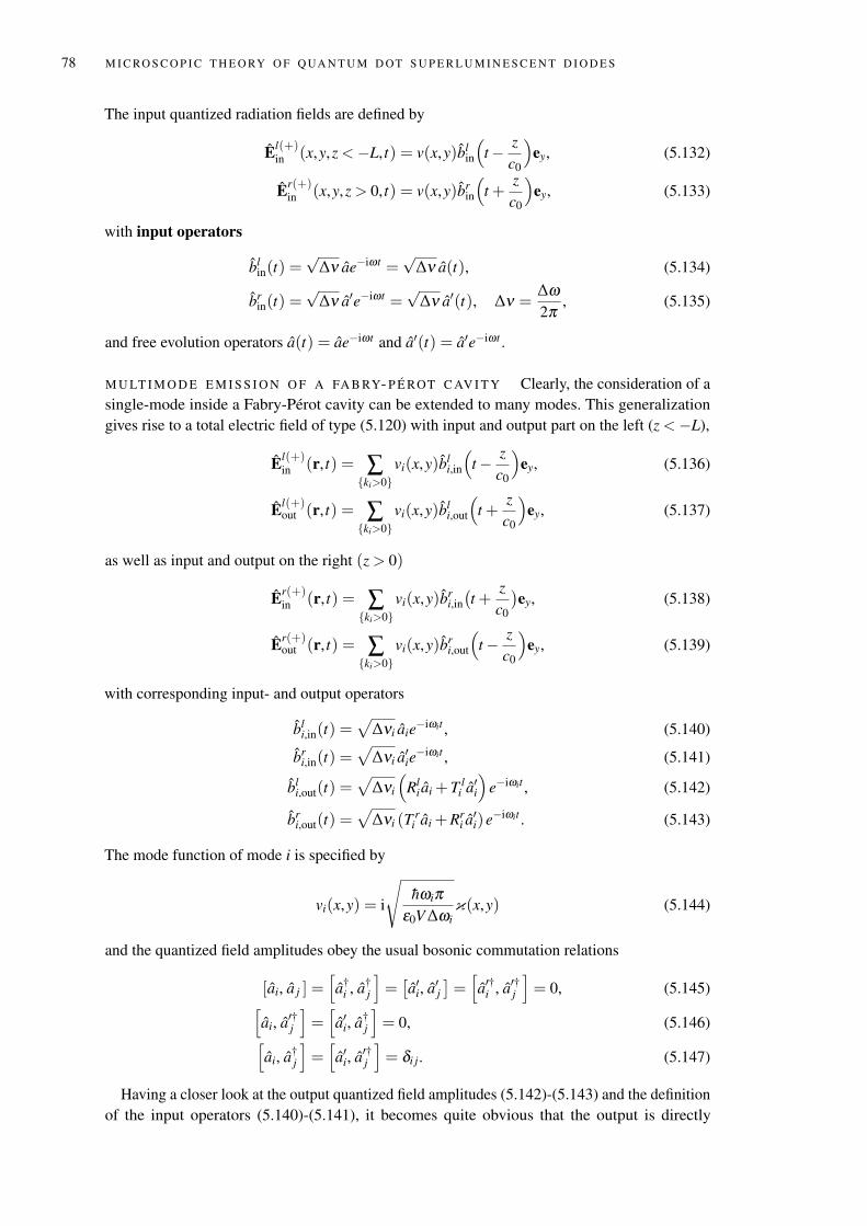
78 M I C RO S C O P I C T H E O RY O F Q UA N T U M D OT S U P E R L U M I N E S C E N T D I O D E S
The input quantized radiation fields are defined by
El(+)in (x,y,z <−L, t) = v(x,y)bl
in
(t− z
c0
)ey, (5.132)
Er(+)in (x,y,z > 0, t) = v(x,y)br
in
(t +
zc0
)ey, (5.133)
with input operators
blin(t) =
√∆ν ae−iωt =
√∆ν a(t), (5.134)
brin(t) =
√∆ν a′e−iωt =
√∆ν a′(t), ∆ν =
∆ω2π
, (5.135)
and free evolution operators a(t) = ae−iωt and a′(t) = a′e−iωt .
M U LT I M O D E E M I S S I O N O F A FA B RY- P É ROT C AV I T Y Clearly, the consideration of asingle-mode inside a Fabry-Pérot cavity can be extended to many modes. This generalizationgives rise to a total electric field of type (5.120) with input and output part on the left (z <−L),
El(+)in (r, t) = ∑
ki>0vi(x,y)bl
i,in
(t− z
c0
)ey, (5.136)
El(+)out (r, t) = ∑
ki>0vi(x,y)bl
i,out
(t +
zc0
)ey, (5.137)
as well as input and output on the right (z > 0)
Er(+)in (r, t) = ∑
ki>0vi(x,y)br
i,in(t +
zc0
)ey, (5.138)
Er(+)out (r, t) = ∑
ki>0vi(x,y)br
i,out
(t− z
c0
)ey, (5.139)
with corresponding input- and output operators
bli,in(t) =
√∆νi aie−iωit , (5.140)
bri,in(t) =
√∆νi a′ie
−iωit , (5.141)
bli,out(t) =
√∆νi
(Rl
i ai +T li a′i)
e−iωit , (5.142)
bri,out(t) =
√∆νi (T r
i ai +Rri a′i)e−iωit . (5.143)
The mode function of mode i is specified by
vi(x,y) = i
√hωiπ
ε0V ∆ωiκ(x,y) (5.144)
and the quantized field amplitudes obey the usual bosonic commutation relations
[ai, a j ] =[a†
i , a†j
]=[a′i, a′j
]=[a′†i , a′†j
]= 0, (5.145)[
ai, a′†j]=[a′i, a†
j
]= 0, (5.146)[
ai, a†j
]=[a′i, a′†j
]= δi j. (5.147)
Having a closer look at the output quantized field amplitudes (5.142)-(5.143) and the definitionof the input operators (5.140)-(5.141), it becomes quite obvious that the output is directly
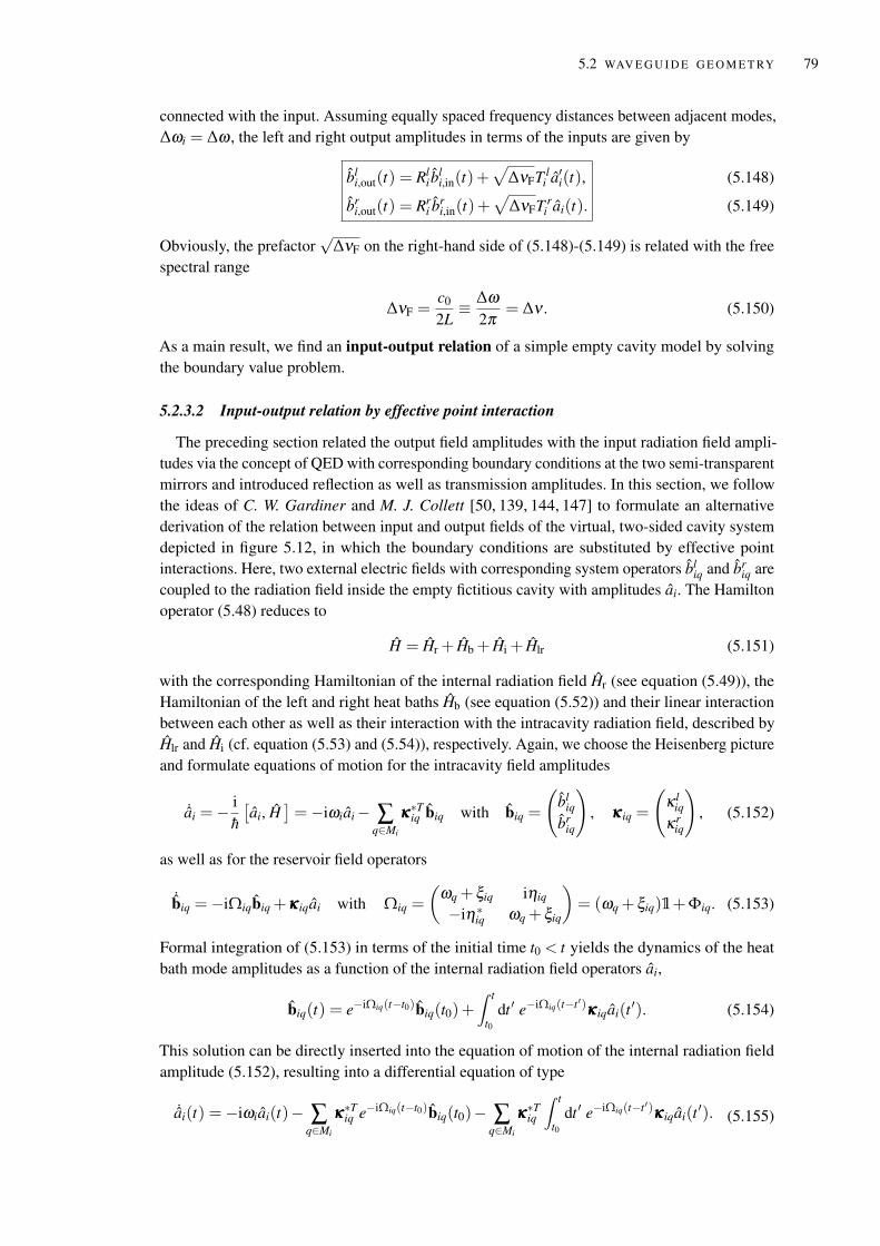
5.2 WAV E G U I D E G E O M E T RY 79
connected with the input. Assuming equally spaced frequency distances between adjacent modes,∆ωi = ∆ω , the left and right output amplitudes in terms of the inputs are given by
bli,out(t) = Rl
i bli,in(t)+
√∆νFT l
i a′i(t),
bri,out(t) = Rr
i bri,in(t)+
√∆νFT r
i ai(t).
(5.148)
(5.149)
Obviously, the prefactor√
∆νF on the right-hand side of (5.148)-(5.149) is related with the freespectral range
∆νF =c0
2L≡ ∆ω
2π= ∆ν . (5.150)
As a main result, we find an input-output relation of a simple empty cavity model by solvingthe boundary value problem.
5.2.3.2 Input-output relation by effective point interaction
The preceding section related the output field amplitudes with the input radiation field ampli-tudes via the concept of QED with corresponding boundary conditions at the two semi-transparentmirrors and introduced reflection as well as transmission amplitudes. In this section, we followthe ideas of C. W. Gardiner and M. J. Collett [50, 139, 144, 147] to formulate an alternativederivation of the relation between input and output fields of the virtual, two-sided cavity systemdepicted in figure 5.12, in which the boundary conditions are substituted by effective pointinteractions. Here, two external electric fields with corresponding system operators bl
iq and briq are
coupled to the radiation field inside the empty fictitious cavity with amplitudes ai. The Hamiltonoperator (5.48) reduces to
H = Hr + Hb + Hi + Hlr (5.151)
with the corresponding Hamiltonian of the internal radiation field Hr (see equation (5.49)), theHamiltonian of the left and right heat baths Hb (see equation (5.52)) and their linear interactionbetween each other as well as their interaction with the intracavity radiation field, described byHlr and Hi (cf. equation (5.53) and (5.54)), respectively. Again, we choose the Heisenberg pictureand formulate equations of motion for the intracavity field amplitudes
˙ai = −ih
[ai, H
]= −iωiai− ∑
q∈Mi
κκκ∗Tiq biq with biq =
(bl
iqbr
iq
), κκκ iq =
(κ l
iqκr
iq
), (5.152)
as well as for the reservoir field operators
˙biq = −iΩiqbiq +κκκ iqai with Ωiq =
(ωq + ξiq iηiq
−iη∗iq ωq + ξiq
)= (ωq + ξiq)1+Φiq. (5.153)
Formal integration of (5.153) in terms of the initial time t0 < t yields the dynamics of the heatbath mode amplitudes as a function of the internal radiation field operators ai,
biq(t) = e−iΩiq(t−t0)biq(t0)+∫ t
t0dt ′ e−iΩiq(t−t ′)κκκ iqai(t ′). (5.154)
This solution can be directly inserted into the equation of motion of the internal radiation fieldamplitude (5.152), resulting into a differential equation of type
˙ai(t) = −iωiai(t)− ∑q∈Mi
κκκ∗Tiq e−iΩiq(t−t0)biq(t0)− ∑q∈Mi
κκκ∗Tiq
∫ t
t0dt ′ e−iΩiq(t−t ′)κκκ iqai(t ′). (5.155)
80 M I C RO S C O P I C T H E O RY O F Q UA N T U M D OT S U P E R L U M I N E S C E N T D I O D E S
In the next step, we introduce the Langevin force operator f βi and the memory kernel Kβ
iaccording to
∑β∈l,r
f βi (t) ≡ ∑
q∈Mi
κκκ∗Tiq e−iΩiq(t−t0)biq(t0), (5.156)
∑β∈l,r
Kβi (τ) ≡ ∑
q∈Mi
κκκ∗Tiq e−iΩiqτκκκ iq, (5.157)
so that equation (5.155) simplifies to
˙ai(t) = −iωiai(t)− ∑β∈l,r
∫ t
t0dt ′ Kβ
i (t− t ′)ai(t ′)− ∑β∈l,r
f βi (t). (5.158)
M A R KOV A P P ROX I M AT I O N In analogy to the derivation of the master equation (see ap-pendix D) we utilize the sharpness of the memory kernel Kβ
i at t = t ′ for Markovian systems. Here,the convolution integral of Kβ
i (t− t ′) and an arbitrary system operator c(t) can be approximatedby
∫ t
t0dt ′ Kβ
i (t− t ′)c(t ′) ≈∫ t
t0dt ′ Kβ
i (t− t ′)c(t)tτc≈
(γβ
i2+ iδω
)c(t), (5.159)
for times t much bigger than the correlation time τc of the reservoir fluctuations. γ defines a decayrate and is related with the coupling constant via γ = 2π|κ|2/∆ω . The line shift δω will beneglected in the following. Please note, that in the Markov approximation, the coupling constantsare only a function of frequency ωi that is independent of frequency ωq,
κβiq ≈ κβ
i = |κβi |eiφ β
i , β ∈ l,r. (5.160)
Therefore the damping rates read
γβi ≡
1∆νi|κβ
i |2, β ∈ l,r. (5.161)
The temporal derivative of the mode field amplitude i is of Langevin type,
˙ai = −(
iωi +γ l
i + γri
2
)ai− ∑
β∈l,rf βi , (5.162)
including both a damping as well as a randomizing term. Therefore, f βi corresponds to a Langevin
operator, describing fluctuations of ai around its average.We define an input operator in terms of the initial time t0 < t,
bβi,in(t) ≡
√∆νi ∑
q∈Mβi
e−iωq(t−t0)bβiq(t0), β ∈ l,r. (5.163)
In the Markov approximation, also the coupling constants ηiq are flat around a certain centralfrequency ωi so that we can make the replacement ηiq ' ηi = |ηi|eiϕi and the Langevin force isrelated to the input field amplitude by
∑β∈l,r
f βi (t) '−
κκκ∗Ti√∆νi
Si(t− t0) bi,in(t), Si(τ) =(
Ti(τ) Rri (τ)
Rli(τ) Ti(τ)
), bi,in =
(bl
i,inbr
i,in
). (5.164)
5.2 WAV E G U I D E G E O M E T RY 81
Again, we identify the matrix elements of Si(τ) as reflection and transmission amplitudes definedby10
Ti(τ) = e−iξi(t) cos(|ηi|τ), (5.165)
Rri (τ) = e−i(ξi(t)−ϕi) sin(|ηi|τ), (5.166)
Rli(τ) = −e−i(ξi(t)+ϕi) sin(|ηi|τ). (5.167)
This result can be utilized to formulate the equation of motion for the field amplitude ai in termsof the input operator according to
ddt
ai(t) = −(
iωi +γ l
i + γri
2
)ai(t)− bL
i,in(t)− bRi,in(t) . (5.168)
Here, we introduced the abbreviations
bLi,in(t) ≡ X l
i (t− t0)bli,in(t), (5.169)
bRi,in(t) ≡ X r
i (t− t0)bri,in(t) (5.170)
with
Xβi (τ) = Dβ∗
i Ti(τ)+Dα∗i Rβ
i (τ) and Dβi =
√γβ
i eiφ βi , α ,β ∈ l,r, α 6= β . (5.171)
The first term in (5.168) describes the free evolution and considers damping effects resulting fromthe left and right mirrors of the virtual cavity. Please note, that this damping term is Markovianas it is only a function of the system operator evaluated at time t and not at earlier times. Thelast two terms, which are proportional to the input field operators bl/r
i,in can be interpreted as noisecontributions provided that the state of the total system at initial time t0 factorizes and the stateof the noise input is incoherent [50]. Thus, equation (5.168) represents a quantum stochasticdifferential equation (QSDE) for the quantized intracavity field amplitude ai also known asquantum Langevin equation named after Langevin who invented a heuristic formulation ofBrownian motion in classical physics [148], which became a standard method for describingstochastic processes.
In analogy to (5.154) the solution of the Heisenberg equation of the bath modes in terms ofthe final time t f > t is
biq(t) = e−iΩiq(t−t f )biq(t f )−∫ t f
tdt ′ e−iΩiq(t−t ′)κκκ iqai(t ′). (5.172)
Applying the same calculations as before, we can specify the equation of motion for the internalradiation field amplitude
˙ai(t) = −(
iωi−γ l
i + γri
2
)ai(t)− bL
i,out(t)− bRi,out(t) , (5.173)
with
bLi,out(t) = X l
i (t− t f )bli,out(t), (5.174)
bRi,out(t) = X r
i (t− t f )bri,out(t) (5.175)
10 Here, the matrix Si(τ) and its coefficients are equal to (5.66)-(5.67) except for a phase e−iξi(τ).
82 M I C RO S C O P I C T H E O RY O F Q UA N T U M D OT S U P E R L U M I N E S C E N T D I O D E S
as a function of the output operators depending on final time t f > t, which are defined by
bβi,out(t) ≡
√∆νi ∑
q∈Mβi
e−iωq(t−t f )bβiq(t f ), β ∈ l,r. (5.176)
It must be pointed out that both, input and output operator (see equation (5.163) and (5.176))have a dimension of s−1/2 in contrast to the dimensionless field amplitudes bβ
iq resulting incommutation relations [
bαi,in(t), bβ†
j,in(t′)]= δαβ δi jδ (t− t ′),[
bαi,out(t), bβ†
j,out(t′)]= δαβ δi jδ (t− t ′), αβ ∈ l,r
(5.177)
(5.178)
of unit s−1. Please note, that the commutator of the input as well as the output amplitudes are deltafunctions resulting in a temporal delta correlation or rather a flat spectrum when transforming intothe frequency regime. Thus equations (5.177)-(5.178) reflects the quantum white noise characterof the input and output.
I N P U T- O U T P U T R E L AT I O N A relation between the input and output field amplitudes isobtained by equating the right-hand side of equation (5.154) and the right-hand side of (5.172)which yields
e−iΩiq(t−t f )biq(t f ) = e−iΩiq(t−t0)biq(t0)+∫ t f
t0dt ′ e−iΩiq(t−t ′)κκκ iqai(t ′). (5.179)
We multiply both sides of (5.179) with√
∆νi and sum over all q modes. Under consideration ofthe Markov approximation (ηiq ' ηi, κiq ' κi) and the definition of the input and output operators(5.163) and (5.176), we get
e−iΦi(t−t f )bi,out(t) ' e−iΦi(t−t0)bi,in(t)+√
∆νi
∫ t f
t0dt ′ ∑
q∈Mi
e−iΩiq(t−t ′)κκκ iai(t ′). (5.180)
In the continuum limit, the summation term in the integrand corresponds to a delta distribution11.Due to the locality of the interaction at the output facets of the virtual cavity, we can expand theremote past and the remote future time, t0 and t f , to ±∞. Multiplying both sides of (5.180) witheiΦi(t−t f ), we find an input-output relation for the virtual cavity system
bi,out(t) = Sibi,in(t)+ΓΓΓi(t f − t)ai(t) (5.181)
with
Si ≡ limt f−t0→∞
ηi→0ηi(t f−t0)=const.
Si(t f − t0) =(
Ti Rri
Rli Ti
), ΓΓΓi(τ) = Si(τ)
(D l
iD r
i
), bi,out =
(br
i,outbl
i,out
).
(5.182)
Again, we introduced the useful channel notation in agreement to figure 5.12. Here, the elementsof the resulting S-matrix correspond to constant transmission and reflection amplitudes,
Ti ≡ Ti(t f − t0), Rβi = Rβ
i (t f − t0), (5.183)
respectively, which are a direct result of the coupling mechanism between the left and rightexternal fields at the single semi-transparent mirrors in analogy to the beam splitter systemdiscussed in a previous section. Obviously, the output field is described by the input field plus theinteraction with the internal radiation field in agreement to the previous section. Equation (5.181)represents a boundary condition which relates the output field modes to the internal cavity modes.
11 We utilized the integral representation of a delta function δ (t) =∫ ∞−∞
dω2π e−iωt .
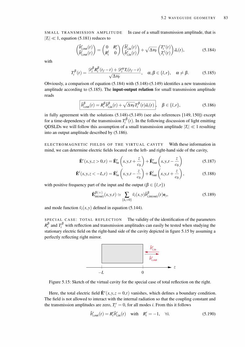
5.2 WAV E G U I D E G E O M E T RY 83
S M A L L T R A N S M I S S I O N A M P L I T U D E In case of a small transmission amplitude, that is|Ti| 1, equation (5.181) reduces to(
bri,out(t)
bli,out(t)
)=
(0 Rr
iRl
i 0
)(bl
i,in(t)br
i,in(t)
)+√
∆νF
(T r
i (t)T l
i (t)
)ai(t), (5.184)
with
T βi (t) =
Dβi Rβ
i (t f − t)+Dαi Ti(t f − t)√
∆νF, α ,β ∈ l,r, α 6= β . (5.185)
Obviously, a comparison of equation (5.184) with (5.148)-(5.149) identifies a new transmissionamplitude according to (5.185). The input-output relation for small transmission amplitudereads
bβi,out(t) = Rβ
i bβi,in(t)+
√∆νFT β
i (t)ai(t) , β ∈ l,r, (5.186)
in fully agreement with the solutions (5.148)-(5.149) (see also references [149, 150]) exceptfor a time-dependency of the transmission T β
i (t). In the following discussion of light emittingQDSLDs we will follow this assumption of a small transmission amplitude |Ti| 1 resultinginto an output amplitude described by (5.186).
E L E C T RO M AG N E T I C FI E L D S O F T H E V I RT UA L C AV I T Y With these information inmind, we can determine electric fields located on the left- and right-hand side of the cavity,
Er(x,y,z > 0, t) = Erin
(x,y, t +
zc0
)+ Er
out
(x,y, t− z
c0
)(5.187)
El(x,y,z <−L, t) = Elin
(x,y, t− z
c0
)+ El
out
(x,y, t +
zc0
), (5.188)
with positive frequency part of the input and the output (β ∈ l,r)
Eβ (+)in(out)(x,y, t) ' ∑
ki>0vi(x,y)bβ
i,in(out)(t)ey, (5.189)
and mode function vi(x,y) defined in equation (5.144).
S P E C I A L C A S E : T OTA L R E FL E C T I O N The validity of the identification of the parametersRβ
i and T βi with reflection and transmission amplitudes can easily be tested when studying the
stationary electric field on the right-hand side of the cavity depicted in figure 5.15 by assuming aperfectly reflecting right mirror.
bri,in
bri,out
z0−L
Figure 5.15: Sketch of the virtual cavity for the special case of total reflection on the right.
Here, the total electric field Er(x,y,z = 0, t) vanishes, which defines a boundary condition.The field is not allowed to interact with the internal radiation so that the coupling constant andthe transmission amplitudes are zero, T r
i = 0, for all modes i. From this it follows
bri,out(t) = Rr
i bri,in(t) with Rr
i = −1, ∀i. (5.190)
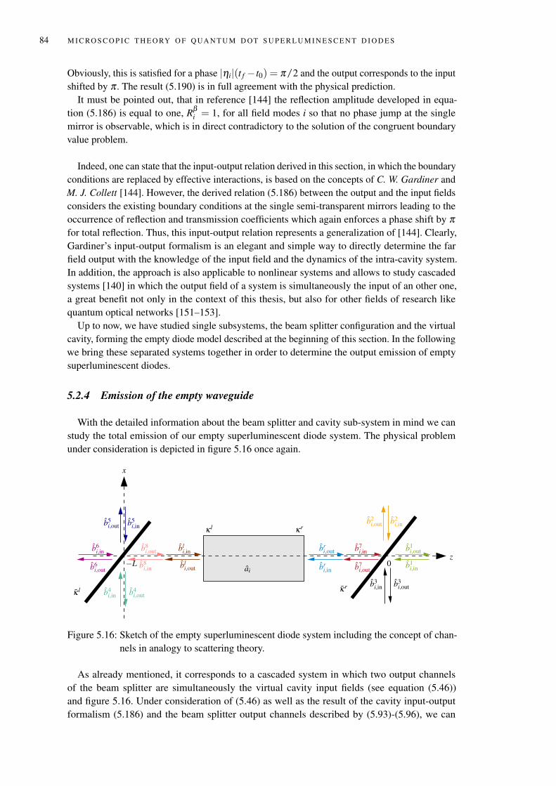
84 M I C RO S C O P I C T H E O RY O F Q UA N T U M D OT S U P E R L U M I N E S C E N T D I O D E S
Obviously, this is satisfied for a phase |ηi|(t f − t0) = π/2 and the output corresponds to the inputshifted by π . The result (5.190) is in full agreement with the physical prediction.
It must be pointed out, that in reference [144] the reflection amplitude developed in equa-tion (5.186) is equal to one, Rβ
i = 1, for all field modes i so that no phase jump at the singlemirror is observable, which is in direct contradictory to the solution of the congruent boundaryvalue problem.
Indeed, one can state that the input-output relation derived in this section, in which the boundaryconditions are replaced by effective interactions, is based on the concepts of C. W. Gardiner andM. J. Collett [144]. However, the derived relation (5.186) between the output and the input fieldsconsiders the existing boundary conditions at the single semi-transparent mirrors leading to theoccurrence of reflection and transmission coefficients which again enforces a phase shift by πfor total reflection. Thus, this input-output relation represents a generalization of [144]. Clearly,Gardiner’s input-output formalism is an elegant and simple way to directly determine the farfield output with the knowledge of the input field and the dynamics of the intra-cavity system.In addition, the approach is also applicable to nonlinear systems and allows to study cascadedsystems [140] in which the output field of a system is simultaneously the input of an other one,a great benefit not only in the context of this thesis, but also for other fields of research likequantum optical networks [151–153].
Up to now, we have studied single subsystems, the beam splitter configuration and the virtualcavity, forming the empty diode model described at the beginning of this section. In the followingwe bring these separated systems together in order to determine the output emission of emptysuperluminescent diodes.
5.2.4 Emission of the empty waveguide
With the detailed information about the beam splitter and cavity sub-system in mind we canstudy the total emission of our empty superluminescent diode system. The physical problemunder consideration is depicted in figure 5.16 once again.
b3i,in
b6i,in
b4i,in
b2i,in
κrκ l
κ l
b1i,out
b2i,out
κr
b8i,out bl
i,in
ai
x
−L b1i,in
0b8i,inb6
i,out b7i,out
b7i,in
bli,out
zbr
i,out
bri,in
b4i,out
b5i,inb5
i,out
b3i,out
Figure 5.16: Sketch of the empty superluminescent diode system including the concept of chan-nels in analogy to scattering theory.
As already mentioned, it corresponds to a cascaded system in which two output channelsof the beam splitter are simultaneously the virtual cavity input fields (see equation (5.46))and figure 5.16. Under consideration of (5.46) as well as the result of the cavity input-outputformalism (5.186) and the beam splitter output channels described by (5.93)-(5.96), we can
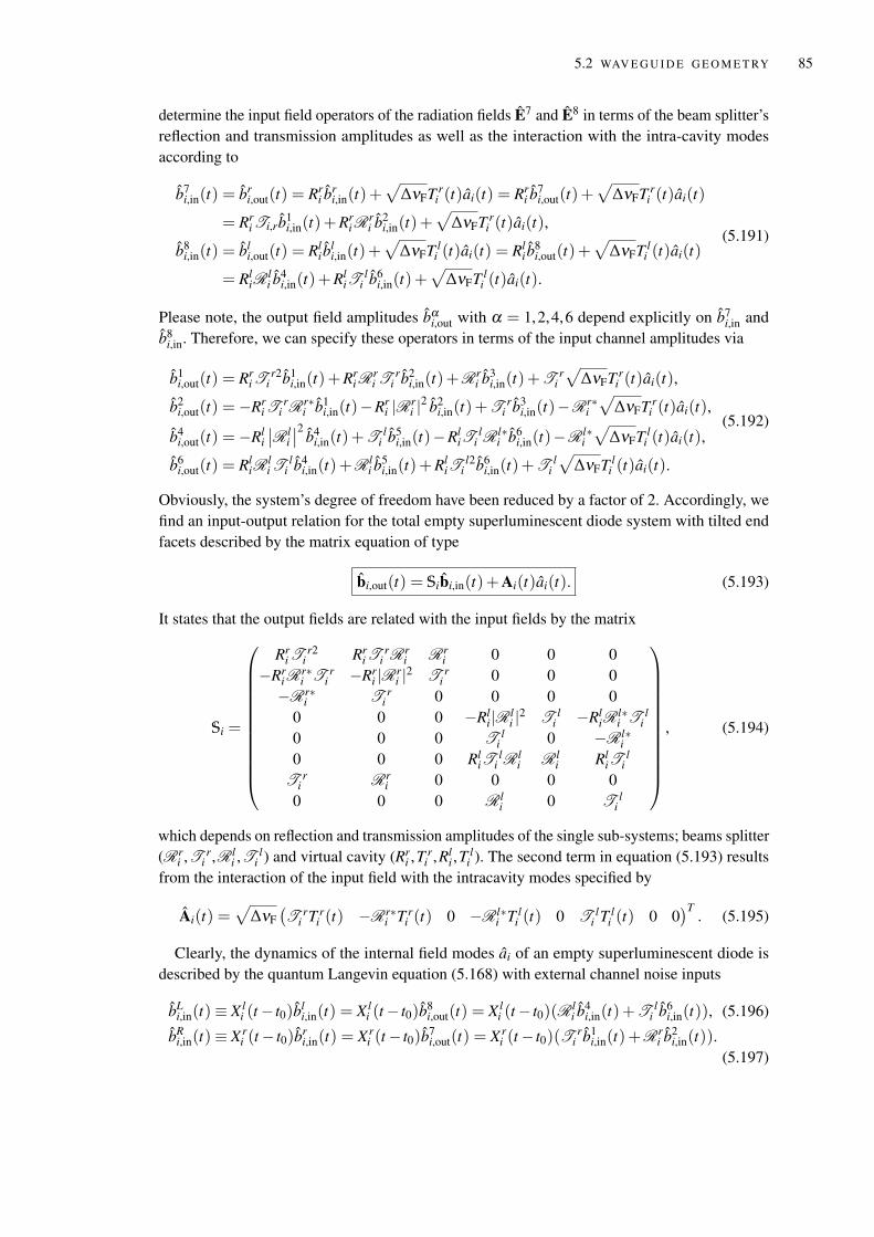
5.2 WAV E G U I D E G E O M E T RY 85
determine the input field operators of the radiation fields E7 and E8 in terms of the beam splitter’sreflection and transmission amplitudes as well as the interaction with the intra-cavity modesaccording to
b7i,in(t) = br
i,out(t) = Rri b
ri,in(t)+
√∆νFT r
i (t)ai(t) = Rri b
7i,out(t)+
√∆νFT r
i (t)ai(t)
= Rri Ti,rb1
i,in(t)+Rri R
ri b2
i,in(t)+√
∆νFT ri (t)ai(t),
b8i,in(t) = bl
i,out(t) = Rli b
li,in(t)+
√∆νFT l
i (t)ai(t) = Rli b
8i,out(t)+
√∆νFT l
i (t)ai(t)
= RliR
li b
4i,in(t)+Rl
iTl
i b6i,in(t)+
√∆νFT l
i (t)ai(t).
(5.191)
Please note, the output field amplitudes bαi,out with α = 1,2,4,6 depend explicitly on b7
i,in andb8
i,in. Therefore, we can specify these operators in terms of the input channel amplitudes via
b1i,out(t) = Rr
i Tr2
i b1i,in(t)+Rr
i Rri T
ri b2
i,in(t)+Rri b3
i,in(t)+T ri
√∆νFT r
i (t)ai(t),
b2i,out(t) = −Rr
i Tr
i Rr∗i b1
i,in(t)−Rri |Rr
i |2 b2i,in(t)+T r
i b3i,in(t)−Rr∗
i
√∆νFT r
i (t)ai(t),
b4i,out(t) = −Rl
i
∣∣R li
∣∣2 b4i,in(t)+T l
i b5i,in(t)−Rl
iTl
i R l∗i b6
i,in(t)−R l∗i
√∆νFT l
i (t)ai(t),
b6i,out(t) = Rl
iRli T
li b4
i,in(t)+R li b
5i,in(t)+Rl
iTl2
i b6i,in(t)+T l
i
√∆νFT l
i (t)ai(t).
(5.192)
Obviously, the system’s degree of freedom have been reduced by a factor of 2. Accordingly, wefind an input-output relation for the total empty superluminescent diode system with tilted endfacets described by the matrix equation of type
bi,out(t) = Sibi,in(t)+Ai(t)ai(t). (5.193)
It states that the output fields are related with the input fields by the matrix
Si =
Rri T
r2i Rr
i Tr
i Rri Rr
i 0 0 0−Rr
i Rr∗i T r
i −Rri |Rr
i |2 T ri 0 0 0
−Rr∗i T r
i 0 0 0 00 0 0 −Rl
i|R li |2 T l
i −RliR
l∗i T l
i0 0 0 T l
i 0 −R l∗i
0 0 0 RliT
li R l
i R li Rl
iTl
iT r
i Rri 0 0 0 0
0 0 0 R li 0 T l
i
, (5.194)
which depends on reflection and transmission amplitudes of the single sub-systems; beams splitter(Rr
i ,T ri ,R l
i ,Tl
i ) and virtual cavity (Rri ,T
ri ,Rl
i ,Tl
i ). The second term in equation (5.193) resultsfrom the interaction of the input field with the intracavity modes specified by
Ai(t) =√
∆νF(T r
i T ri (t) −Rr∗
i T ri (t) 0 −R l∗
i T li (t) 0 T l
i T li (t) 0 0
)T. (5.195)
Clearly, the dynamics of the internal field modes ai of an empty superluminescent diode isdescribed by the quantum Langevin equation (5.168) with external channel noise inputs
bLi,in(t) ≡ X l
i (t− t0)bli,in(t) = X l
i (t− t0)b8i,out(t) = X l
i (t− t0)(R li b
4i,in(t)+T l
i b6i,in(t)), (5.196)
bRi,in(t) ≡ X r
i (t− t0)bri,in(t) = X r
i (t− t0)b7i,out(t) = X r
i (t− t0)(T ri b1
i,in(t)+Rri b2
i,in(t)).(5.197)
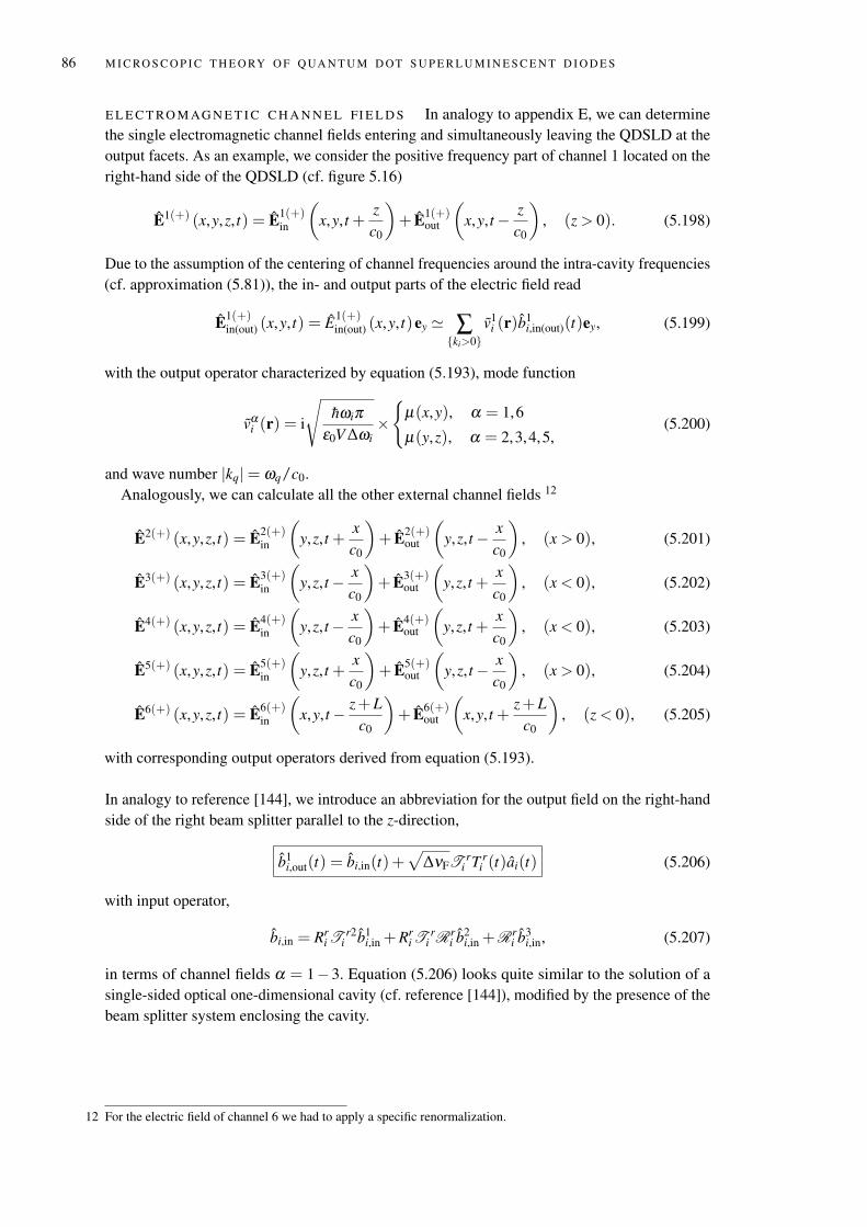
86 M I C RO S C O P I C T H E O RY O F Q UA N T U M D OT S U P E R L U M I N E S C E N T D I O D E S
E L E C T RO M AG N E T I C C H A N N E L FI E L D S In analogy to appendix E, we can determinethe single electromagnetic channel fields entering and simultaneously leaving the QDSLD at theoutput facets. As an example, we consider the positive frequency part of channel 1 located on theright-hand side of the QDSLD (cf. figure 5.16)
E1(+) (x,y,z, t) = E1(+)in
(x,y, t +
zc0
)+ E1(+)
out
(x,y, t− z
c0
), (z > 0). (5.198)
Due to the assumption of the centering of channel frequencies around the intra-cavity frequencies(cf. approximation (5.81)), the in- and output parts of the electric field read
E1(+)in(out) (x,y, t) = E1(+)
in(out) (x,y, t)ey ' ∑ki>0
v1i (r)b
1i,in(out)(t)ey, (5.199)
with the output operator characterized by equation (5.193), mode function
vαi (r) = i
√hωiπ
ε0V ∆ωi×
µ(x,y), α = 1,6
µ(y,z), α = 2,3,4,5,(5.200)
and wave number |kq|= ωq/c0.Analogously, we can calculate all the other external channel fields 12
E2(+) (x,y,z, t) = E2(+)in
(y,z, t +
xc0
)+ E2(+)
out
(y,z, t− x
c0
), (x > 0), (5.201)
E3(+) (x,y,z, t) = E3(+)in
(y,z, t− x
c0
)+ E3(+)
out
(y,z, t +
xc0
), (x < 0), (5.202)
E4(+) (x,y,z, t) = E4(+)in
(y,z, t− x
c0
)+ E4(+)
out
(y,z, t +
xc0
), (x < 0), (5.203)
E5(+) (x,y,z, t) = E5(+)in
(y,z, t +
xc0
)+ E5(+)
out
(y,z, t− x
c0
), (x > 0), (5.204)
E6(+) (x,y,z, t) = E6(+)in
(x,y, t− z+L
c0
)+ E6(+)
out
(x,y, t +
z+Lc0
), (z < 0), (5.205)
with corresponding output operators derived from equation (5.193).
In analogy to reference [144], we introduce an abbreviation for the output field on the right-handside of the right beam splitter parallel to the z-direction,
b1i,out(t) = bi,in(t)+
√∆νFT
ri T r
i (t)ai(t) (5.206)
with input operator,
bi,in = Rri T
r2i b1
i,in +Rri T
ri Rr
i b2i,in +Rr
i b3i,in, (5.207)
in terms of channel fields α = 1−3. Equation (5.206) looks quite similar to the solution of asingle-sided optical one-dimensional cavity (cf. reference [144]), modified by the presence of thebeam splitter system enclosing the cavity.
12 For the electric field of channel 6 we had to apply a specific renormalization.
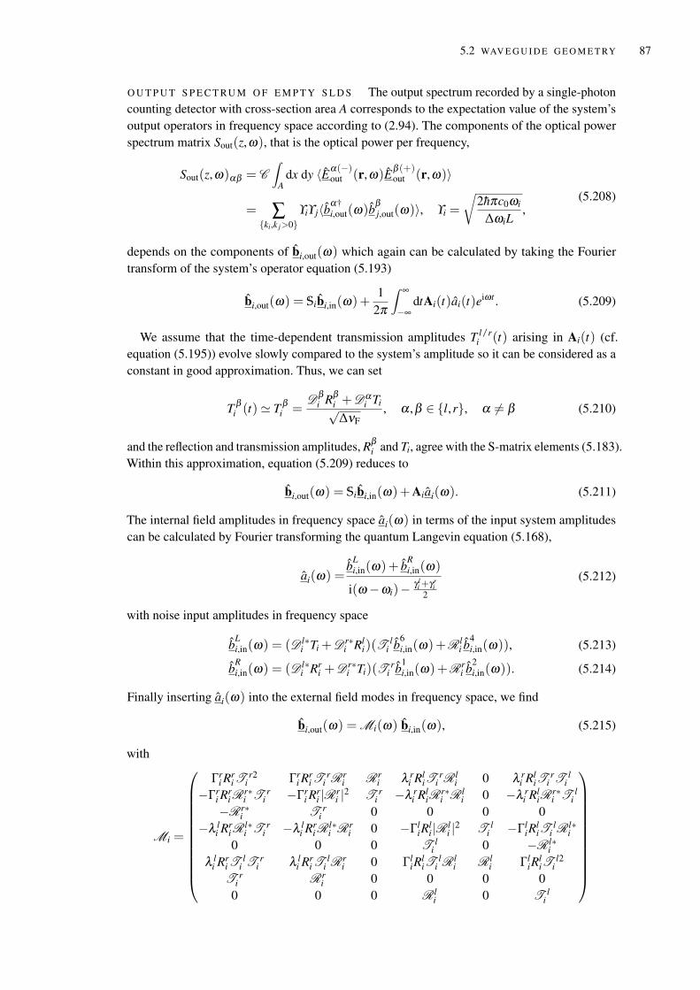
5.2 WAV E G U I D E G E O M E T RY 87
O U T P U T S P E C T RU M O F E M P T Y S L D S The output spectrum recorded by a single-photoncounting detector with cross-section area A corresponds to the expectation value of the system’soutput operators in frequency space according to (2.94). The components of the optical powerspectrum matrix Sout(z,ω), that is the optical power per frequency,
Sout(z,ω)αβ = C∫
Adx dy 〈Eα(−)
out (r,ω)Eβ (+)out (r,ω)〉
= ∑ki,k j>0
ϒiϒj〈bα†i,out(ω)b
βj,out(ω)〉, ϒi =
√2hπc0ωi
∆ωiL,
(5.208)
depends on the components of bi,out(ω) which again can be calculated by taking the Fouriertransform of the system’s operator equation (5.193)
bi,out(ω) = Sibi,in(ω)+1
2π
∫ ∞
−∞dtAi(t)ai(t)eiωt . (5.209)
We assume that the time-dependent transmission amplitudes T l/ri (t) arising in Ai(t) (cf.
equation (5.195)) evolve slowly compared to the system’s amplitude so it can be considered as aconstant in good approximation. Thus, we can set
T βi (t) ' T β
i =Dβ
i Rβi +Dα
i Ti√∆νF
, α ,β ∈ l,r, α 6= β (5.210)
and the reflection and transmission amplitudes, Rβi and Ti, agree with the S-matrix elements (5.183).
Within this approximation, equation (5.209) reduces to
bi,out(ω) = Sibi,in(ω)+Aiai(ω). (5.211)
The internal field amplitudes in frequency space ai(ω) in terms of the input system amplitudescan be calculated by Fourier transforming the quantum Langevin equation (5.168),
ai(ω) =b
Li,in(ω)+ b
Ri,in(ω)
i(ω−ωi)− γ li +γr
i2
(5.212)
with noise input amplitudes in frequency space
bLi,in(ω) = (D l∗
i Ti +D r∗i Rl
i)(Tl
i b6i,in(ω)+R l
i b4i,in(ω)), (5.213)
bRi,in(ω) = (D l∗
i Rri +D r∗
i Ti)(Tr
i b1i,in(ω)+Rr
i b2i,in(ω)). (5.214)
Finally inserting ai(ω) into the external field modes in frequency space, we find
bi,out(ω) = Mi(ω) bi,in(ω), (5.215)
with
Mi =
Γri R
ri T
r2i Γr
i Rri T
ri Rr
i Rri λ r
i RliT
ri R l
i 0 λ ri Rl
iTr
i T li
−Γri R
ri R
r∗i T r
i −Γri R
ri |Rr
i |2 T ri −λ r
i RliR
r∗i R l
i 0 −λ ri Rl
iRr∗i T l
i−Rr∗
i T ri 0 0 0 0
−λ li Rr
i Rl∗i T r
i −λ li Rr
i Rl∗i Rr
i 0 −ΓliR
li|R l
i |2 T li −Γl
iRliT
li R l∗
i0 0 0 T l
i 0 −R l∗i
λ li Rr
i Tl
i T ri λ l
i Rri T
li Rr
i 0 ΓliR
liT
li R l
i R li Γl
iRliT
l2i
T ri Rr
i 0 0 0 00 0 0 R l
i 0 T li
88 M I C RO S C O P I C T H E O RY O F Q UA N T U M D OT S U P E R L U M I N E S C E N T D I O D E S
and
λ βi =
Dαi Dβ∗
iεi
, Γβi = 1+
γαiεi
, εi = i(ω−ωi)−γr
i + γ li
2, α ,β ∈ l,r, α 6= β .
Thus, the output vector operator bi,out depends linearly on the input vector operator bi,in, revealingthat the power spectrum depends significantly on the choice of the input field. It is preciselya convolution of the input field with the response function of the beam splitters. The nextsubsections deal with the white noise and phase-randomized Gaussian noise input.
5.2.4.1 Response to white noise input
Quantum white noise is characterized by its spectral density independent of frequency,
S(ω) = S. (5.216)
As in the case of white light, all frequencies appear equally. Clearly, the choice of quantum whitenoise as an input, having infinite energy densities, is an idealization and therefore not observablein real physical systems. It is rather the thermal state which describes the truly physical nature ofthe input resulting into a Planck distribution for the mean thermal occupation number.
According to the Wiener-Khintchine theorem, the first-order autocorrelation function is speci-fied by the Fourier transform of the spectral density, resulting into a delta-function, meaning thatwhite noise fluctuations are uncorrelated in case of different time events. In summary, for whitenoise input with the number of quanta N, the following correlations hold
〈b†in(t)bin(t ′)〉= Nδ (t− t ′), (5.217)
〈bin(t)b†in(t′)〉= (N + 1)δ (t− t ′). (5.218)
Therefore, bin is Markovian. Please note, N is constant compared to thermal noise, in which thephoton number is described by a Planck distribution, N(ω) = nT (ω) (cf. equation (2.76)).
In this section, we study the simple case of white noise input entering the empty cavity systemfrom both sides. The concept of white noise discussed above can be directly applied to ourcomplex input-output cavity setup. Denoting Nα as the mean occupation number of channel α ,the frequency correlation of the input mode i is given by
〈bα†i,in(ω)b
βj,in(ω
′)〉= (Si j,in)αβ δ (ω−ω ′), (Si j,in)αβ = Nαδαβ δi j, α ,β = 1, ...,6, (5.219)
with input spectral density matrix element (Si j,in)αβ [139]. Here, we claimed that differentchannel modes are uncorrelated. In addition, we neglected correlations between different modesof the same channel.
A single-photon counting detector of finite cross-section area is assumed to be located onthe right-hand side and far away from of the empty SLD perpendicular to the z-direction.Consequently, only the output of channel 1 is recorded and contributes to the spectral density,because output fields propagate perpendicular to the z direction as well as the field on the left-handside, are not striking the detector, i.e. Eout = E1
out. The output of channel 1 is exactly specified bythe first element of the spectrum matrix Sout(ω).
In case of white noise input and equal damping rates, γ l = γr = γ , we find
S(ω) ≡ (Sout(ω))11 =πγ ∑ki
ϒ 2i |Rr
i |2T r2i ×
[(N1T
r2i + N2|Rr
i |2)( 1
πγ−L (ω−ωi)
)+ N3
|Rri |2
πγT r2i |Rr
i |2+(N4|R l
i |2 + N6Tl2
i )L (ω−ωi)] (5.220)
5.2 WAV E G U I D E G E O M E T RY 89
with the Lorentzian function
L (ω) =1π
γγ2 +ω2 . (5.221)
For N1 = N2 = N3 = N4 = 0 and N6 = N, the output spectrum,
S(ω) = p ∑ki
ωi
∆ωi|Rr
i |2T l2i T r2
i L (ω−ωi), p =2π2hc0γN
L, (5.222)
is a sum of Lorentzians with maximum value at ω = ωi and a full width at half maximum of√
2γ .Making the continuum transition we find a continuous power spectrum,
S(ω) = e
ωN/2−1∫ω−N/2
dω ω|Rr(ω)|2T l2(ω)T r2(ω) L (ω− ω), e =p
∆ω2 , (5.223)
with ∆ω = (ωN/2−1−ω−N/2)/(N − 1), given by a convolution of a Lorentzian curve andthree transfer functions (spectra) weighted by frequency ω . Here, we supposed equal frequencyseparation between adjacent modes, i.e. ∆ωi = ∆ω . Please note, that these transfer functionsvary slowly as a function of angular frequency ω as a result of the Markovian system’s dynamics.
L I M I T I N G C A S E γ 1 Consider the power spectral density (5.223) having a sharp Lorentzianwith γ much smaller than any other relevant system frequency. In this case we can write
limγ1
L (ω) =1π
limγ1
γγ2 +ω2 =
12iπ
limγ1
[1
ω− iγ− 1
ω + iγ
]. (5.224)
The single terms in the brackets are evaluable using the Sokhotski–Plemelj formula [154]
limγ→0
1ω± iγ
= P
(1ω
)∓ iπδ (ω), (5.225)
which results into the power spectral density
S(ω) = e
ωN/2−1∫ω−N/2
dω ω|Rr(ω)|2T l2(ω)T r2(ω)δ (ω− ω). (5.226)
For a natural line width γ much smaller than the frequency bandwidth b, we can extend theintegration limits to ±∞ leading to a constant optical power spectrum,
S(ω) ≈ eω|Rr(ω)|2T l2(ω)T r2(ω), (5.227)
of unit W ·s. Obviously, for a narrow line width γ , the output spectrum of an empty QDSLDfor white noise as an input depends on the pointwise multiplication of the three single spectra|Rr(ω)|2, T l2(ω) and T r2(ω). However, as already mentioned, these spectra vary slowly as afunction of frequency.
We consider again the convolution integral (5.226) and eliminate the explicit frequency depen-dency in the integrand by setting ω approximately equal to the mean value, ω ' ω . Therefore, incase of constant reflection and transmission amplitudes, the output spectrum is independent offrequency suggesting that the output is again quantum white noise.
90 M I C RO S C O P I C T H E O RY O F Q UA N T U M D OT S U P E R L U M I N E S C E N T D I O D E S
5.2.4.2 Response to phase-randomized Gaussian noise input
Obviously, the choice of noise input influences the shape of the optical power spectrumsignificantly in case of an empty SLD. According to the investigation of light emitted by QDSLDsin chapter 4, it is interesting to study phase-randomized Gaussian noise input with a densityoperator defined in equation (4.6). Here, the mean photon number N in (5.219) becomes afunction of frequency ω ,
N(ω) =C [ps(ω)+ pt(ω)] , C =L
hωc0, (5.228)
depending on the distributions ps(ω) and pt(ω) introduced in equation (4.14). Please note, incase of near-infrared photons, pt(ω) is negligible, as already shown in chapter 4. Motivatedby the measured optical power spectrum, we assume again a Gaussian distribution for ps(ω)
equivalent to equation (4.41) in section 4.5.1. Regarding the Markovian character of the systemunder study, reflection and transmission amplitudes are slowly varying in terms of frequency ωand we can extract these functions out of the integral according to the mean value theorem. Theintegration limits are extended to ±∞ in analogy to the studied case of white noise input. Finally,we get a simple expression for the power spectrum
S(ω) ' 2π2γ(∆ω)2 |R
r(ω)|2T l2(ω)T r2(ω)∫ ∞
−∞dω ps(ω)L (ω− ω). (5.229)
Equation (5.229) corresponds to a convolution of a Lorentzian and a Gaussian curve. Accordingly,the power spectrum of an empty SLD with PRAG input noise exhibits a Voigt profile multipliedwith the flat spectra T l2(ω), T r2(ω) and |Rr(ω)|2. Please note, that these spectral densitieshave upper bounds due to their definition in (5.96) and (5.183).
5.3 I N T R AWAV E G U I D E Q UA N T U M D OT S U P E R L U M I N E S C E N T
D I O D E S Y S T E M
The last two sections dealt with a quantum mechanical description of the components formingthe special QDSLD system: the gain medium composed of M QDs and the semiconductorwaveguide with tilted end facets. The model of the total diode system was already introduced atthe beginning of this chapter. Now we have reached a point at which we are able to determinethe full intrawaveguide dynamics, relevant to obtain knowledge about crucial physical processeslike gain, absorption, saturation etc., which again affect the spectral density and the photonstatistics of the QDSLD. In addition, we will observe amplified spontaneous emission as a naturalconsequence of a microscopic description of this semiconductor device.
In order to describe the total QDSLD intrawaveguide system, we follow the concepts intro-duced by C. W. Gardiner and M. J. Collett in 1985 [144] to deal with open quantum systemsas motivated in the section before. The resulting input-output formalism allows to determinethe output electric field, necessary to calculate first- and second-order temporal autocorrelationfunctions of the radiation field recorded by detectors far away from the small system under study.Pursuant to their definition (see section 2.3.1 and 2.3.2), two-time averages have to be calculated.It turns out, that the determination of these correlations in terms of quantum Langevin equations,describing the dynamics of the dissipative and fluctuating system, becomes a quite gratuitouscomplex challenge. As a consequence, we introduce a further well established formulation ofa stochastic differential equation (SDE) having some more mathematical advantages whichallows to calculate first- and second-order correlations in a very simple and elegant way. This
5.3 I N T R AWAV E G U I D E Q UA N T U M D OT S U P E R L U M I N E S C E N T D I O D E S Y S T E M 91
formalism is referred to the Japanese mathematician K. Itô, who invented a classical formulationof stochastic processes. Another, more physical, alternative classical description was developedby the Russian physicist R. Stratonovich. For someone who is not familiar with both formalisms,appendix F summarizes the main characteristics and differences of Itô’s and Stratonovich’s SDEsapplied to quantum mechanics. As a main result we show in this appendix that the Itô form of aquantum stochastic differential equation (QSDE) is equivalent to the Stratonovich one whichagain corresponds to the quantum Langevin equation. Thus, knowing the quantum Langevinequation we can directly deduce the corresponding Itô QSDE.
The Itô differential of the ith ASE field mode in terms of the input noise operators reads13
dai(t) = −[
i∆i +12(γ l
i + γri)]
ai(t) dt +M
∑j=1
g j∗i σ j
21(t) dt−dBLi (t)−dBR
i (t). (5.230)
The first term in equation (5.230) describes the free evolution of the mode i with frequency ∆i andincludes the external damping rates γ l
i , γri resulting from the left and right input noise fields leading
to damping effects of the system. The second term includes the coupling constant between mode iand quantum dot j defined in equation (5.17) as well as the lowering operator σ j
21. Therefore, thiscontribution describes the interaction of ASE field mode i with all M QDs. The last two termsconsider noise fluctuations described by the noise differentials (cf. equations (5.196)-(5.197))
dBLi (t) = X l
i (t− t0)(T li dB6
i (t)+R li dB4
i (t)), (5.231)
dBRi (t) = X r
i (t− t0)(T ri dB1
i (t)+Rri dB2
i (t)), (5.232)
depending on the Itô increments of the external channels α ∈ 1, ...,6 labeled by dBαi . They
have the dimension of the square root of reciprocal time and obey the commutation relation andItô rules (cf. equation (5.71) and appendix F),[
dBαi (t), dBβ†
j (t ′)]= δαβ δi jδ (t− t ′)dtdt ′, α ,β ∈ 1, ...,6, (5.233)
dBβi (t)dBβ†
i (t) = (Nβi + 1)dt, (5.234)
dBβ†i (t)dBβ
i (t) = Nβi dt, (5.235)
with and mean occupation numbers Nβi . Clearly, the rescaled noise operators introduced in
(5.231)-(5.232) have to satisfy the commutation relation and Itô rules[dBα
i (t), dBβ†j (t ′)
]= ϑ α
i (t)δ (t− t ′)δi jδαβ dtdt ′, α ,β ∈ L,R, (5.236)
dBβi (t)dBβ†
i (t) = (Nβi (t)+ 1)dt, (5.237)
dBβ†i (t)dBβ
i (t) = Nβi (t)dt, (5.238)
which obviously shows slight deviations compared to (5.233)-(5.235). Here, we introduced theabbreviations
ϑ Li (t) = γ l
i |Ti(t− t0)|2|T li |2 + γr
i |Rli(t− t0)|2|R l
i |2, (5.239)
ϑ Ri (t) = γ l
i |Rri (t− t0)|2|T r
i |2 + γri |Ti(t− t0)|2|Rr
i |2 (5.240)
and
NLi (t) = X l
i (t− t0)Nli , NR
i (t) = X ri (t− t0)Nr
i (5.241)
13 In contrast to appendix F, we omit the notation (I) labeling the Itô formulation of a QSDE.
92 M I C RO S C O P I C T H E O RY O F Q UA N T U M D OT S U P E R L U M I N E S C E N T D I O D E S
with mean occupation numbers
Nli = |T l
i |2N6i + |R l
i |2N4i , (5.242)
Nri = |T r
i |2N1i + |Rr
i |2N2i . (5.243)
Thus, dBβi , β ∈ L,R should not be confused with the Ito increments in the sense of quantum
white noise (5.233)-(5.235).Please note that the input fields of channel 3 and 5 never enter the waveguide. Therefore, the
corresponding damping rates γ3i and γ5
i , which are proportional to the coupling strength betweenreservoir and ASE field, are equal to zero.In the same way, we can derive QSDEs for all atomic coherences and populations of each quan-tum dot depending on pumping rate R≡ R j = N j
20γ j20, acting equally strong on each individual
nanostructure (cf. section 5.1 and figure 5.3), as well as on the Itô increments dB jm/D j
m, where mrepresents the dot transitions m ∈ (21), (20), (10) | (i j) : |i〉 → | j〉. They are given by:
Populations
dσ j00 = −(Γ
j00 +R)σ j
00 dt + γ j10N j
10σ j11 dt +Rσ j
22 dt− (σ j†10 dB j
10 + σ j†20 dB j
20 + h.c.) (5.244a)
dσ j11 =−Γ j
11σ j11 dt−∑
ki
(g j∗
i a†i σ j
21 dt + h.c.)+ γ j
10(Nj
10 + 1)σ j00 dt
+ γ j21N j
21σ j22 dt− (σ j†
21 dB j21− σ j†
10 dB j10 + h.c.)
(5.244b)
dσ22 =− (Γ j22 +R)σ j
22 dt + ∑ki
(g j∗
i a†i σ j
21 dt + h.c.)+ γ j
21(Nj
21 + 1)σ j11 dt
+(R+ γ j20)σ
j00 dt +(σ j†
21 dB j21 + σ j†
20 dB j20 + h.c.)
(5.244c)
Coherences
dσ j21 =−
(iδω j
12 +12(Γ j
21 +R))
σ j21 dt−∑
kig j
i (σj
22− σ j11)ai dt
− (σ j22− σ j
11) dB j21 + dB j†
10σ j20 + σ j†
10 dB j20
(5.245a)
dσ j20 =−
(Γ j202
+R)
σ j20 dt + ∑
kig j
i σ j10ai dt
+ σ j10 dB j
21− (σ j22− σ j
00) dB j20− σ j
21 dB j10
(5.245b)
dσ j10 =
(iδω j
12−12(Γ j
10 +R))
σ j10 dt−∑
kig j∗
i a†i σ j
20 dt
−dB j†21σ j
20− σ j†21 dB j
20− (σ j11− σ j
00) dB j10
(5.245c)
5.3 I N T R AWAV E G U I D E Q UA N T U M D OT S U P E R L U M I N E S C E N T D I O D E S Y S T E M 93
Decay and excitation rates
Γ j00 = γ j
10(Nj
10 + 1)+ γ j20 (5.246a)
Γ j11 = γ j
21(Nj
21 + 1)+ γ j10N j
10 (5.246b)
Γ j22 = γ j
21N j21 (5.246c)
Γ j21 = γ j
21(2N j21 + 1)+ γ j
10N j10 (5.246d)
Γ j20 = γ j
21N j21 + γ j
20 + γ j10
(N j
10 + 1)
(5.246e)
Γ j10 = +γ j
21
(N j
21 + 1)+ γ j
20 + γ j10
(2N j
10 + 1)
(5.246f)
5.3.1 On the nature of the QDSLD quantum state
Up to now, we are left with a set of coupled nonlinear Itô quantum stochastic differentialequations for all multiple radiation ASE modes as well as all populations and coherences for eachquantum dot system. This system of differential equations can be studied numerically in more de-tail. However, at this point of the thesis, it is reasonable to incorporate experimental observationsof the quantum state of the QDSLD system in order to limit the following considerations to amore specific physical problem by making some assumptions and approximations motivated bythe observed characteristics of the amplified spontaneous emission.
Due to the experimental measurements of the spectrum of highly incoherent broadbandradiation fields (see figure 3.3), we assume a vanishing expectation value, i.e. no coherentamplitude of the ith ASE mode,
〈ai〉= 0. (5.247)
Furthermore, we assume that there are no correlations between different ASE field modes at thesame space-time event, so that the average value
〈a†i a j〉= niδi j (5.248)
is given by the photon number ni of mode i. We disregard correlations between the differentexternal channel radiation field modes as well as interactions between these external modes withthe intrawaveguide quantum dot bath modes. The occupation numbers as well as the decay ratesof the left- and right-hand side of the waveguide are assumed to be equal for all ASE field modes,i.e. Nβ
i = Nβ with (β ∈ L,R) and γβi = γβ with β ∈ l,r.
D E C O R R E L AT I O N A P P ROX I M AT I O N Since the influence of a single quantum dot on theith mode of the multimode ASE radiation field is small, higher-order corrections are negligible bydecorrelating field and atomic operator [155], e.g.
〈a†i
(σ j
22− σ j11
)a j〉 ≈ 〈a†
i a j〉〈σ j22− σ j
11〉 (decorrelation approximation). (5.249)
This separation into a product of second-order quantum dot and field variables is of course anapproximation, but nevertheless more realistic compared to a mean-field theory [156].
In addition, correlations between different QDs are negligible, so that in good approximation
〈σ j†21 σ j′
21〉= 〈σj
11〉δ j j′ (5.250)
holds.
94 M I C RO S C O P I C T H E O RY O F Q UA N T U M D OT S U P E R L U M I N E S C E N T D I O D E S
A D I A BAT I C E L I M I NAT I O N We adiabatically eliminate coherences as dynamical variablesin the averaged QSDEs by replacing 〈σ j†
21 ai〉 by its stationary solution 〈σ j†21 ai〉s. In doing so, we
apply the Ito product rule according to
d〈σ j†21 ai〉= 〈(dσ j†
21 )ai〉+ 〈σ j†21 dai〉+ 〈(dσ j†
21 )(dai)〉. (5.251)
Under consideration of equations (5.230) and (5.245a) as well as the mentioned decorrelationapproximation, we end up in an equation of motion
d〈σ j†21 ai〉dt
= −(
i∆ ji +
Γ j
2
)〈σ j†
21 ai〉+ g j∗i
(ni(〈σ j
11〉−〈σj
22〉)+ 〈σj
11〉)
, (5.252)
with
Γ j ≡ R+ γ l + γr +Γ j21, (5.253)
where Γ j21 is defined in equation (5.246d) and detuning ∆ j
i = ∆i−δω j12 = ωi−ω j
12, which againresults into a stationary solution of type
〈σ j†21 ai〉s =
g j∗i
(ni(〈σ j
11〉−〈σj
22〉)+ 〈σj
11〉)
i∆ ji +
12 Γ j
≈ 〈σ j†21 ai〉 (adiabatic elimination). (5.254)
This approximation states, that the evolution of 〈σ j†21 ai〉 is slaved to that of the photon number ni
[157, 158]. Please note, that adiabatic elimination of the artificial atom coherences is appropriatein case of good cavities. In general QDSLDs, having inhomogeneous gain medium and tiltedend facets, operate far away from the good-cavity regime. However, experimental results of thesecond-order degree of coherence in terms of temperature highlight a considerable increase incoherence, generally not expected in bad cavities. Therefore, as a first step we assume that theconcept of atomic adiabatic elimination is applicable.
5.3.2 Rate equations
A measured power spectrum reflects the behavior of the optical power as a function ofangular frequency. The power itself is directly related to the stationary photon number (seeequation (2.94)). Its dynamics is determined again by the rate equations of the system, whosederivation is straightforward within the Itô formalism. Here, we only have to investigate theaverage value of the QSDE of creation and annihilation operator products from the ASE fieldmode according to (5.248) as well as the populations of the jth quantum dot, utilizing theproperties of the Itô increments (see appendix F). Applying all mentioned assumptions andapproximations introduced in section 5.3.1 as well as regarding the fact that the Itô incrementscommute with the system operators at the same time, we find the rate equations of the QDSLDsystem
ni =M
∑j=1
γG ji
(niw j +σ j
11
)−(γ l + γr)ni + NL + NR,
σ j22 = ∑
kiγG j
i
(niw j +σ j
11
)− (Γ j
22 +R)σ j22 + γ j
21
(N j
21 + 1)σ j
11 +(R+ γ j
20
)σ j
00,
σ j11 = −∑
kiγG j
i
(niw j +σ j
11
)−Γ j
11σ j11 + γ j
10
(N j
10 + 1)σ j
00 + γ j21N j
21σ j22,
σ j00 = −(Γ
j00 +R)σ j
00 + γ j10N j
10σ j11 +Rσ j
22,
(5.255)
(5.256)
(5.257)
(5.258)
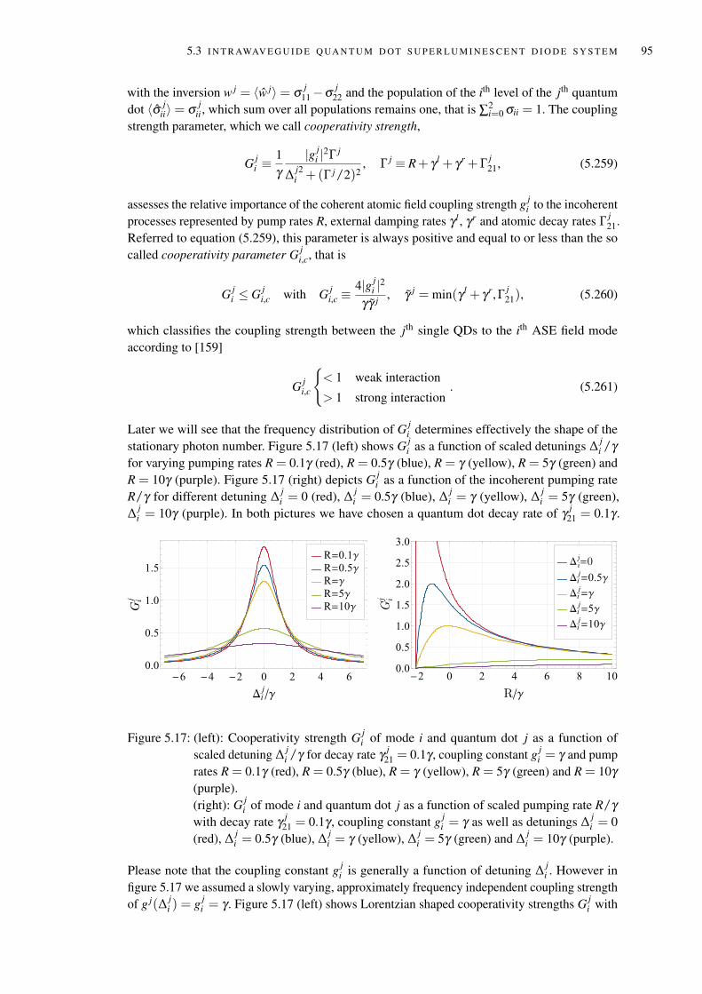
5.3 I N T R AWAV E G U I D E Q UA N T U M D OT S U P E R L U M I N E S C E N T D I O D E S Y S T E M 95
with the inversion w j = 〈w j〉= σ j11−σ j
22 and the population of the ith level of the jth quantumdot 〈σ j
ii〉= σ jii , which sum over all populations remains one, that is ∑2
i=0 σii = 1. The couplingstrength parameter, which we call cooperativity strength,
G ji ≡
1γ
|g ji |2Γ j
∆ j2i +(Γ j/2)2
, Γ j ≡ R+ γ l + γr +Γ j21, (5.259)
assesses the relative importance of the coherent atomic field coupling strength g ji to the incoherent
processes represented by pump rates R, external damping rates γ l , γr and atomic decay rates Γ j21.
Referred to equation (5.259), this parameter is always positive and equal to or less than the socalled cooperativity parameter G j
i,c, that is
G ji ≤ G j
i,c with G ji,c ≡
4|g ji |2
γγ j , γ j = min(γ l + γr,Γ j21), (5.260)
which classifies the coupling strength between the jth single QDs to the ith ASE field modeaccording to [159]
G ji,c
< 1 weak interaction
> 1 strong interaction. (5.261)
Later we will see that the frequency distribution of G ji determines effectively the shape of the
stationary photon number. Figure 5.17 (left) shows G ji as a function of scaled detunings ∆ j
i /γfor varying pumping rates R = 0.1γ (red), R = 0.5γ (blue), R = γ (yellow), R = 5γ (green) andR = 10γ (purple). Figure 5.17 (right) depicts G j
i as a function of the incoherent pumping rateR/γ for different detuning ∆ j
i = 0 (red), ∆ ji = 0.5γ (blue), ∆ j
i = γ (yellow), ∆ ji = 5γ (green),
∆ ji = 10γ (purple). In both pictures we have chosen a quantum dot decay rate of γ j
21 = 0.1γ .
R=0.1γR=0.5γR=γR=5γR=10γ
-6 -4 -2 0 2 4 6
0.0
0.5
1.0
1.5
Δij/γ
Gij
Δij=0
Δij=0.5γ
Δij=γ
Δij=5γ
Δij=10γ
-2 0 2 4 6 8 100.0
0.5
1.0
1.5
2.0
2.5
3.0
R/γ
Gij
Figure 5.17: (left): Cooperativity strength G ji of mode i and quantum dot j as a function of
scaled detuning ∆ ji /γ for decay rate γ j
21 = 0.1γ , coupling constant g ji = γ and pump
rates R = 0.1γ (red), R = 0.5γ (blue), R = γ (yellow), R = 5γ (green) and R = 10γ(purple).(right): G j
i of mode i and quantum dot j as a function of scaled pumping rate R/γwith decay rate γ j
21 = 0.1γ , coupling constant g ji = γ as well as detunings ∆ j
i = 0(red), ∆ j
i = 0.5γ (blue), ∆ ji = γ (yellow), ∆ j
i = 5γ (green) and ∆ ji = 10γ (purple).
Please note that the coupling constant g ji is generally a function of detuning ∆ j
i . However infigure 5.17 we assumed a slowly varying, approximately frequency independent coupling strengthof g j(∆ j
i ) = g ji = γ . Figure 5.17 (left) shows Lorentzian shaped cooperativity strengths G j
i with
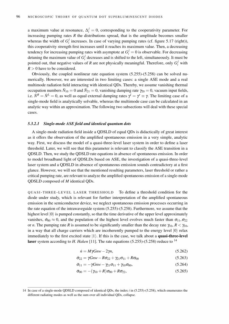
96 M I C RO S C O P I C T H E O RY O F Q UA N T U M D OT S U P E R L U M I N E S C E N T D I O D E S
a maximum value at resonance, ∆ ji = 0, corresponding to the cooperativity parameter. For
increasing pumping rates R the distributions spread, that is the amplitude becomes smallerwhereas the width of G j
i increases. In case of varying pumping rates (cf. figure 5.17 (right)),this cooperativity strength first increases until it reaches its maximum value. Then, a decreasingtendency for increasing pumping rates with asymptote at G j
i = 0 is observable. For decreasingdetuning the maximum value of G j
i decreases and is shifted to the left, simultaneously. It must bepointed out, that negative values of R are not physically meaningful. Therefore, only G j
i withR > 0 have to be considered.
Obviously, the coupled nonlinear rate equation system (5.255)-(5.258) can be solved nu-merically. However, we are interested in two limiting cases: a single ASE mode and a realmultimode radiation field interacting with identical QDs. Thereby, we assume vanishing thermaloccupation numbers N10 = 0 and N21 = 0, vanishing damping rate γ20 = 0, vacuum input fields,i.e. NR = NL = 0, as well as equal external damping rates γ l = γr ≡ γ . The limiting case of asingle-mode field is analytically solvable, whereas the multimode case can be calculated in ananalytic way within an approximation. The following two subsections will deal with these specialcases.
5.3.2.1 Single-mode ASE field and identical quantum dots
A single-mode radiation field inside a QDSLD of equal QDs is didactically of great interestas it offers the observation of the amplified spontaneous emission in a very simple, analyticway. First, we discuss the model of a quasi-three-level laser system in order to define a laserthreshold. Later, we will see that this parameter is relevant to classify the ASE transition in aQDSLD. Then, we study the QDSLD rate equations in absence of spontaneous emission. In orderto model broadband light of QDSLDs based on ASE, the investigation of a quasi-three-levellaser system and a QDSLD in absence of spontaneous emission sounds contradictory at a firstglance. However, we will see that the mentioned resulting parameters, laser threshold or rather acritical pumping rate, are relevant to analyze the amplified spontaneous emission of a single-modeQDSLD composed of M identical QDs.
Q UA S I - T H R E E - L E V E L L A S E R T H R E S H O L D To define a threshold condition for thediode under study, which is relevant for further interpretation of the amplified spontaneousemission in the semiconductor device, we neglect spontaneous emission processes occurring inthe rate equation of the intrawaveguide system (5.255)-(5.258). Furthermore, we assume that thehighest level |0〉 is pumped constantly, so that the time derivative of the upper level approximatelyvanishes, σ00 ≈ 0, and the population of the highest level evolves much faster than σ11,σ22
or n. The pumping rate R is assumed to be significantly smaller than the decay rate γ10, R < γ10,in a way that all charge carriers which are incoherently pumped to the energy level |0〉 relaximmediately to the first excited state |1〉. If this is the case, we talk about a quasi-three-levellaser system according to H. Haken [11]. The rate equations (5.255)-(5.258) reduce to 14
n = MγGnw−2γn, (5.262)
σ22 = γGnw−Rσ22 + γ21σ11 +Rσ00 (5.263)
σ11 = −γGnw− γ21σ11 + γ10σ00, (5.264)
σ00 = −(γ10 +R)σ00 +Rσ22, (5.265)
14 In case of a single-mode QDSLD composed of identical QDs, the index i in (5.255)-(5.258), which enumerates thedifferent radiating modes as well as the sum over all individual QDs, collapse.
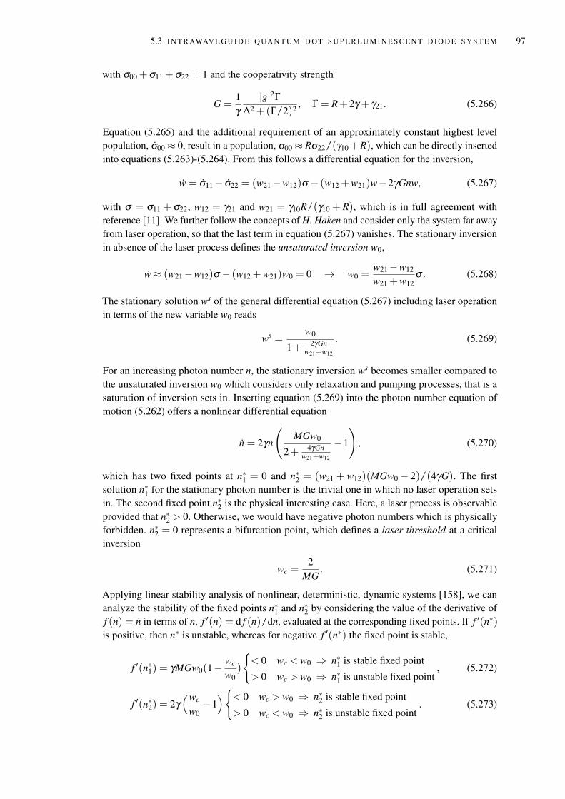
5.3 I N T R AWAV E G U I D E Q UA N T U M D OT S U P E R L U M I N E S C E N T D I O D E S Y S T E M 97
with σ00 +σ11 +σ22 = 1 and the cooperativity strength
G =1γ
|g|2Γ∆2 +(Γ/2)2 , Γ = R+ 2γ + γ21. (5.266)
Equation (5.265) and the additional requirement of an approximately constant highest levelpopulation, σ00 ≈ 0, result in a population, σ00 ≈ Rσ22/(γ10 +R), which can be directly insertedinto equations (5.263)-(5.264). From this follows a differential equation for the inversion,
w = σ11− σ22 = (w21−w12)σ − (w12 +w21)w−2γGnw, (5.267)
with σ = σ11 + σ22, w12 = γ21 and w21 = γ10R/(γ10 + R), which is in full agreement withreference [11]. We further follow the concepts of H. Haken and consider only the system far awayfrom laser operation, so that the last term in equation (5.267) vanishes. The stationary inversionin absence of the laser process defines the unsaturated inversion w0,
w≈ (w21−w12)σ − (w12 +w21)w0 = 0 → w0 =w21−w12
w21 +w12σ . (5.268)
The stationary solution ws of the general differential equation (5.267) including laser operationin terms of the new variable w0 reads
ws =w0
1+ 2γGnw21+w12
. (5.269)
For an increasing photon number n, the stationary inversion ws becomes smaller compared tothe unsaturated inversion w0 which considers only relaxation and pumping processes, that is asaturation of inversion sets in. Inserting equation (5.269) into the photon number equation ofmotion (5.262) offers a nonlinear differential equation
n = 2γn
(MGw0
2+ 4γGnw21+w12
−1
), (5.270)
which has two fixed points at n∗1 = 0 and n∗2 = (w21 + w12)(MGw0 − 2)/(4γG). The firstsolution n∗1 for the stationary photon number is the trivial one in which no laser operation setsin. The second fixed point n∗2 is the physical interesting case. Here, a laser process is observableprovided that n∗2 > 0. Otherwise, we would have negative photon numbers which is physicallyforbidden. n∗2 = 0 represents a bifurcation point, which defines a laser threshold at a criticalinversion
wc =2
MG. (5.271)
Applying linear stability analysis of nonlinear, deterministic, dynamic systems [158], we cananalyze the stability of the fixed points n∗1 and n∗2 by considering the value of the derivative off (n) = n in terms of n, f ′(n) = d f (n)/dn, evaluated at the corresponding fixed points. If f ′(n∗)is positive, then n∗ is unstable, whereas for negative f ′(n∗) the fixed point is stable,
f ′(n∗1) = γMGw0(1−wc
w0)
< 0 wc < w0 ⇒ n∗1 is stable fixed point
> 0 wc > w0 ⇒ n∗1 is unstable fixed point, (5.272)
f ′(n∗2) = 2γ(wc
w0−1)< 0 wc > w0 ⇒ n∗2 is stable fixed point
> 0 wc < w0 ⇒ n∗2 is unstable fixed point. (5.273)
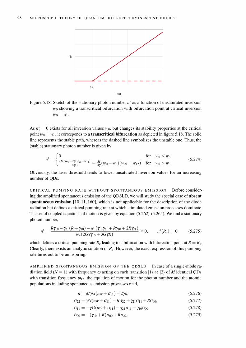
98 M I C RO S C O P I C T H E O RY O F Q UA N T U M D OT S U P E R L U M I N E S C E N T D I O D E S
wc
w0
ns
Figure 5.18: Sketch of the stationary photon number ns as a function of unsaturated inversionw0 showing a transcritical bifurcation with bifurcation point at critical inversionw0 = wc.
As n∗1 = 0 exists for all inversion values w0, but changes its stability properties at the criticalpoint w0 = wc, it corresponds to a transcritical bifurcation as depicted in figure 5.18. The solidline represents the stable path, whereas the dashed line symbolizes the unstable one. Thus, the(stable) stationary photon number is given by
ns =
0 for w0 ≤ wc(MGw0−2)(w21+w12)
4γG = M4γ (w0−wc)(w21 +w12) for w0 > wc
. (5.274)
Obviously, the laser threshold tends to lower unsaturated inversion values for an increasingnumber of QDs.
C R I T I C A L P U M P I N G R AT E W I T H O U T S P O N TA N E O U S E M I S S I O N Before consider-ing the amplified spontaneous emission of the QDSLD, we will study the special case of absentspontaneous emission [10, 11, 160], which is not applicable for the description of the dioderadiation but defines a critical pumping rate at which stimulated emission processes dominate.The set of coupled equations of motion is given by equation (5.262)-(5.265). We find a stationaryphoton number,
ns =Rγ10− γ21(R+ γ10)−wc(γ10γ21 +Rγ10 + 2Rγ21)
wc(2Gγγ10 + 3GγR)≥ 0, ns(Rc) = 0 (5.275)
which defines a critical pumping rate Rc leading to a bifurcation with bifurcation point at R = Rc.Clearly, there exists an analytic solution of Rc. However, the exact expression of this pumpingrate turns out to be uninspiring.
A M P L I FI E D S P O N TA N E O U S E M I S S I O N O F T H E Q D S L D In case of a single-mode ra-diation field (N = 1) with frequency ω acting on each transition |1〉 ↔ |2〉 of M identical QDswith transition frequency ω12, the equation of motion for the photon number and the atomicpopulations including spontaneous emission processes read,
n = MγG(nw+σ11)−2γn, (5.276)
σ22 = γG(nw+σ11)−Rσ22 + γ21σ11 +Rσ00, (5.277)
σ11 = −γG(nw+σ11)− γ21σ11 + γ10σ00, (5.278)
σ00 = −(γ10 +R)σ00 +Rσ22. (5.279)
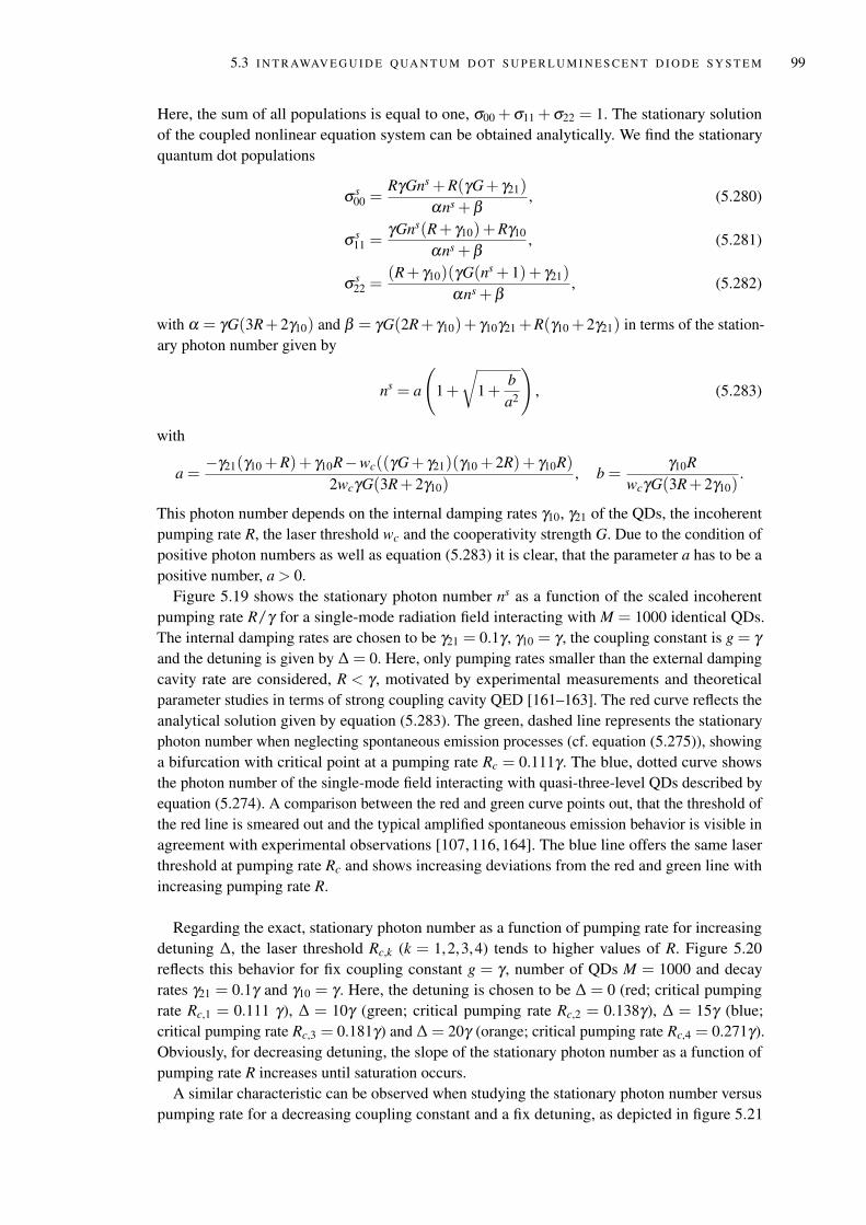
5.3 I N T R AWAV E G U I D E Q UA N T U M D OT S U P E R L U M I N E S C E N T D I O D E S Y S T E M 99
Here, the sum of all populations is equal to one, σ00 +σ11 +σ22 = 1. The stationary solutionof the coupled nonlinear equation system can be obtained analytically. We find the stationaryquantum dot populations
σ s00 =
RγGns +R(γG+ γ21)
αns +β, (5.280)
σ s11 =
γGns(R+ γ10)+Rγ10
αns +β, (5.281)
σ s22 =
(R+ γ10)(γG(ns + 1)+ γ21)
αns +β, (5.282)
with α = γG(3R+2γ10) and β = γG(2R+ γ10)+ γ10γ21 +R(γ10 +2γ21) in terms of the station-ary photon number given by
ns = a
(1+
√1+
ba2
), (5.283)
with
a =−γ21(γ10 +R)+ γ10R−wc((γG+ γ21)(γ10 + 2R)+ γ10R)
2wcγG(3R+ 2γ10), b =
γ10RwcγG(3R+ 2γ10)
.
This photon number depends on the internal damping rates γ10, γ21 of the QDs, the incoherentpumping rate R, the laser threshold wc and the cooperativity strength G. Due to the condition ofpositive photon numbers as well as equation (5.283) it is clear, that the parameter a has to be apositive number, a > 0.
Figure 5.19 shows the stationary photon number ns as a function of the scaled incoherentpumping rate R/γ for a single-mode radiation field interacting with M = 1000 identical QDs.The internal damping rates are chosen to be γ21 = 0.1γ , γ10 = γ , the coupling constant is g = γand the detuning is given by ∆ = 0. Here, only pumping rates smaller than the external dampingcavity rate are considered, R < γ , motivated by experimental measurements and theoreticalparameter studies in terms of strong coupling cavity QED [161–163]. The red curve reflects theanalytical solution given by equation (5.283). The green, dashed line represents the stationaryphoton number when neglecting spontaneous emission processes (cf. equation (5.275)), showinga bifurcation with critical point at a pumping rate Rc = 0.111γ . The blue, dotted curve showsthe photon number of the single-mode field interacting with quasi-three-level QDs described byequation (5.274). A comparison between the red and green curve points out, that the threshold ofthe red line is smeared out and the typical amplified spontaneous emission behavior is visible inagreement with experimental observations [107, 116, 164]. The blue line offers the same laserthreshold at pumping rate Rc and shows increasing deviations from the red and green line withincreasing pumping rate R.
Regarding the exact, stationary photon number as a function of pumping rate for increasingdetuning ∆, the laser threshold Rc,k (k = 1,2,3,4) tends to higher values of R. Figure 5.20reflects this behavior for fix coupling constant g = γ , number of QDs M = 1000 and decayrates γ21 = 0.1γ and γ10 = γ . Here, the detuning is chosen to be ∆ = 0 (red; critical pumpingrate Rc,1 = 0.111 γ), ∆ = 10γ (green; critical pumping rate Rc,2 = 0.138γ), ∆ = 15γ (blue;critical pumping rate Rc,3 = 0.181γ) and ∆ = 20γ (orange; critical pumping rate Rc,4 = 0.271γ).Obviously, for decreasing detuning, the slope of the stationary photon number as a function ofpumping rate R increases until saturation occurs.
A similar characteristic can be observed when studying the stationary photon number versuspumping rate for a decreasing coupling constant and a fix detuning, as depicted in figure 5.21
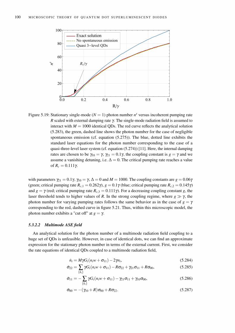
100 M I C RO S C O P I C T H E O RY O F Q UA N T U M D OT S U P E R L U M I N E S C E N T D I O D E S
Rc/γ
Exact solutionNo spontaneous emission
Quasi 3-level QDs
0.0 0.2 0.4 0.6 0.8 1.00
20
40
60
80
100
R/γ
ns
Figure 5.19: Stationary single-mode (N = 1) photon number ns versus incoherent pumping rateR scaled with external damping rate γ . The single-mode radiation field is assumed tointeract with M = 1000 identical QDs. The red curve reflects the analytical solution(5.283), the green, dashed line shows the photon number for the case of negligiblespontaneous emission (cf. equation (5.275)). The blue, dotted line exhibits thestandard laser equations for the photon number corresponding to the case of aquasi-three-level laser system (cf. equation (5.274)) [11]. Here, the internal dampingrates are chosen to be γ10 = γ , γ21 = 0.1γ , the coupling constant is g = γ and weassume a vanishing detuning, i.e. ∆ = 0. The critical pumping rate reaches a valueof Rc = 0.111γ .
with parameters γ21 = 0.1γ , γ10 = γ , ∆ = 0 and M = 1000. The coupling constants are g = 0.06γ(green; critical pumping rate Rc,1 = 0.262γ), g = 0.1γ (blue; critical pumping rate Rc,2 = 0.145γ)and g = γ (red; critical pumping rate Rc,3 = 0.111γ). For a decreasing coupling constant g, thelaser threshold tends to higher values of R. In the strong coupling regime, where g γ , thephoton number for varying pumping rates follows the same behavior as in the case of g = γcorresponding to the red, dashed curve in figure 5.21. Thus, within this microscopic model, thephoton number exhibits a "cut off" at g = γ .
5.3.2.2 Multimode ASE field
An analytical solution for the photon number of a multimode radiation field coupling to ahuge set of QDs is unfeasible. However, in case of identical dots, we can find an approximateexpression for the stationary photon number in terms of the external current. First, we considerthe rate equations of identical QDs coupled to a multimode radiation field,
ni = MγGi(niw+σ11)−2γni, (5.284)
σ22 = ∑ki
γGi(niw+σ11)−Rσ22 + γ21σ11 +Rσ00, (5.285)
σ11 = −∑ki
γGi(niw+σ11)− γ21σ11 + γ10σ00, (5.286)
σ00 = −(γ10 +R)σ00 +Rσ22. (5.287)
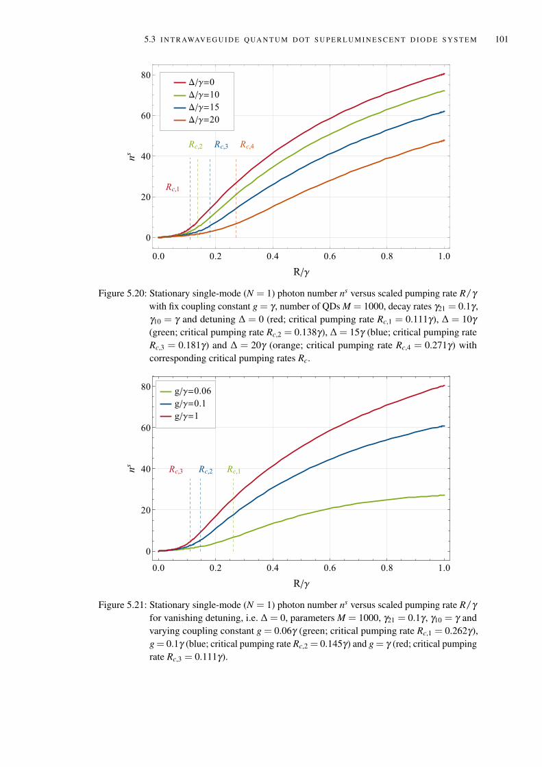
5.3 I N T R AWAV E G U I D E Q UA N T U M D OT S U P E R L U M I N E S C E N T D I O D E S Y S T E M 101
Rc,1
Rc,2 Rc,3 Rc,4
Δ/γ=0
Δ/γ=10
Δ/γ=15
Δ/γ=20
0.0 0.2 0.4 0.6 0.8 1.0
0
20
40
60
80
R/γ
ns
Figure 5.20: Stationary single-mode (N = 1) photon number ns versus scaled pumping rate R/γwith fix coupling constant g = γ , number of QDs M = 1000, decay rates γ21 = 0.1γ ,γ10 = γ and detuning ∆ = 0 (red; critical pumping rate Rc,1 = 0.111γ), ∆ = 10γ(green; critical pumping rate Rc,2 = 0.138γ), ∆ = 15γ (blue; critical pumping rateRc,3 = 0.181γ) and ∆ = 20γ (orange; critical pumping rate Rc,4 = 0.271γ) withcorresponding critical pumping rates Rc.
Rc,1Rc,2Rc,3
g/γ=0.06
g/γ=0.1
g/γ=1
0.0 0.2 0.4 0.6 0.8 1.0
0
20
40
60
80
R/γ
ns
Figure 5.21: Stationary single-mode (N = 1) photon number ns versus scaled pumping rate R/γfor vanishing detuning, i.e. ∆ = 0, parameters M = 1000, γ21 = 0.1γ , γ10 = γ andvarying coupling constant g = 0.06γ (green; critical pumping rate Rc,1 = 0.262γ),g = 0.1γ (blue; critical pumping rate Rc,2 = 0.145γ) and g = γ (red; critical pumpingrate Rc,3 = 0.111γ).
102 M I C RO S C O P I C T H E O RY O F Q UA N T U M D OT S U P E R L U M I N E S C E N T D I O D E S
The photon number n is given by the sum of the N mode photon numbers ni,
n = ∑ki
ni. (5.288)
In detailed balance [165], the stationary total photon number is determined by its zero temporalderivatives formed by each mode, n = 0 ↔ ni = 0. In order to solve the multimode problemunder consideration, we introduce an order parameter,
ϕ ≡ γ ∑ki
Ginsi , (5.289)
corresponding to the stationary number of photons for the diode system ns = ∑ki nsi , weighted
with the cooperativity strength Gi. According to equation (5.284), the ith mode photon number nsi
itself,
nsi (ϕ) =
σ s11(ϕ)
wci −ws(ϕ)
, wci =
2MGi
, (5.290)
is a function of the order parameter ϕ with the stationary excited state and the inversion,
σ s11(ϕ) =
ϕ(γ10 +R)+ γ10Rαϕ +β
, ws(ϕ) =γ10R− (γG+ γ21)(γ10 +R)
αϕ +β. (5.291)
They depend significantly on the incoherent pumping rate R due to the definitions
G = ∑ki
Gi, α = 3R+ 2γ10, β = (γG+ γ21)(γ10 + 2R)+ γ10R, (5.292)
where G is the sum over all N cooperativity strengths, Gi. By inserting equation (5.290) intoequation (5.289), we find a closed relation for the order parameter,
ϕ = ∑ki
γGiσ s11(ϕ)
wci −ws(ϕ)
=σ s
11(ϕ)ws(ϕ)
[−γG+ ∑
ki
γGiwci
wci −ws(ϕ)
]. (5.293)
The solution of ϕ and therefore the stationary photon number can be calculated numerically.However, as a good approximation we can replace wc
i in the enumerator of the second term in thebrackets of equation (5.293) by the constant minimum laser threshold wc
min = 2/(MGmax) (cf.equation (5.271)) with Gmax ≡ G(gi = 2/3 ·gmax,R) which is inverse proportional to the squareof the absolute maximum value of the coupling constant gmax. Equation (5.293) reduces to theanalytic expression
ϕ '− γGσ s
11(ϕ)ws(ϕ)
+wcmin
ϕws(ϕ)
=γ10R− γ21(γ10 +R)−wc
minβ2wc
minα
+
√(γ10R− γ21(γ10 +R)−wc
minβ2wc
minα
)2
+γGγ10Rwc
minα.
(5.294)
Thus, knowing all experimentally available parameters, we can specify the intrawaveguide photonnumber (cf. equation (5.290)) of a light emitting QDSLD from microscopic considerations withinour approximation. It is not surprising that in case of equal cooperativity strength, Gi = G, theanalytic solution is exact.
5.3 I N T R AWAV E G U I D E Q UA N T U M D OT S U P E R L U M I N E S C E N T D I O D E S Y S T E M 103
S M A L L C O O P E R AT I V I T Y S T R E N G T H : wci |ws(ϕ)| Consider again the exact expres-
sion of the stationary photon number of mode i (see equation (5.290)) in terms of the orderparameter
nsi (ϕ) =
σ s11(ϕ)
wci −ws(ϕ)
=σ s
11(ϕ)
wci (1−
ws(ϕ)wc
i)
. (5.295)
In case of wci |ws(ϕ)|, that is the cooperativity strength is very small with Gi 2/(M|ws(ϕ)|),
the right-hand side of equation (5.295) corresponds to a geometric series as
nsi (ϕ) =
σ s11(ϕ)wc
i
∞
∑k=0
(ws(ϕ)
wci
)k
=σ s
11(ϕ)ws(ϕ)
∞
∑k=1
(Mws(ϕ)
2
)k
Gki =
∞
∑k=1
ck(ϕ)Gki . (5.296)
In the first-order perturbation theory in Gi, all stationary quantum dot populations are independentof ϕ , which in turn implies a coefficient ck independent of ϕ . Thus, the stationary photon numberof mode i reads
nsi (ϕ) ≈
∞
∑k=1
ckGki . (5.297)
Within the regime of a small cooperativity strength, the stationary photon number of the ASE fieldmodes inside the diode system is specified by a polynomial in Gi and multiple ck. This solution isnot quite obvious. Concerning the set of coupled nonlinear differential equations (5.284)-(5.287),one would expect a much more complex system behavior. In summary, small cooperativitystrengths result in stationary photon numbers in terms of angular frequency whose distributionsare dominated by the shape of Gi.
I N H O M O G E N E O U S C O U P L I N G Motivated by the experimental Gaussian power spectrum,we study the stationary photon number ns as a function of the scaled incoherent pumping rate R/γfor the special case of a radiation field composed of N = 10 modes interacting with M = 1000identical QDs for a Gaussian shaped coupling constant with
g(∆i) = γ exp(−(∆i− ∆)2
2σ2
). (5.298)
This photon number is plotted in figure 5.22 for a Gaussian coupling amplitude γ , expectationvalue ∆ = 0 and width σ = γ . The damping rates and detuning are given by γ21 = 0.1γ , γ10 = γand ∆i = γi. The red line shows the numerical solution and the blue line is the approximated pho-ton number (cf. equation (5.290)) depending on the order parameter ϕ given by equation (5.294).The green line represents the stationary number of photons ns for negligible spontaneous emis-sion in the sense of reference [10] with a critical pumping rate, Rc = 0.112γ . Obviously, theapproximate photon number agrees well with the exact solution for smaller values of R. ForR > 0.4γ , the deviation between the approximated and the exact solution increases in contrast tothe case of absent spontaneous emission processes (green line) approximating the exact solution.Furthermore, depending on the values of the Gaussian distributed coupling constants gi of themultimode radiation field, the deviation between the multimode and single-mode photon number(black line) as a function of the pumping rate R is more or less significant. Here, the photonnumber of the single-mode radiation field for increasing Rγ > 0.4γ becomes lager than in theapproximate multimode case. All four cases show saturation for sufficiently large pumping rate.
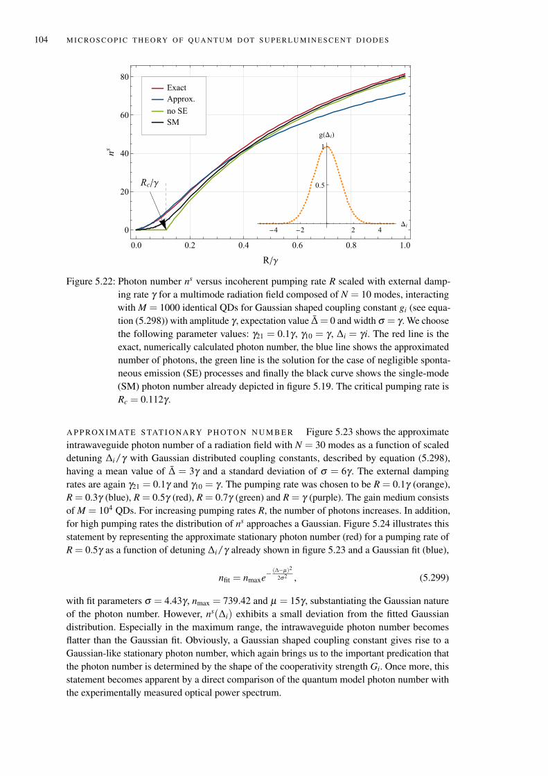
104 M I C RO S C O P I C T H E O RY O F Q UA N T U M D OT S U P E R L U M I N E S C E N T D I O D E S
Rc/γ
Exact
Approx.
no SE
SM
0.0 0.2 0.4 0.6 0.8 1.0
0
20
40
60
80
R/γ
ns
-4 -2 2 4Δi
0.5
1
g(Δi)
Figure 5.22: Photon number ns versus incoherent pumping rate R scaled with external damp-ing rate γ for a multimode radiation field composed of N = 10 modes, interactingwith M = 1000 identical QDs for Gaussian shaped coupling constant gi (see equa-tion (5.298)) with amplitude γ , expectation value ∆ = 0 and width σ = γ . We choosethe following parameter values: γ21 = 0.1γ , γ10 = γ , ∆i = γi. The red line is theexact, numerically calculated photon number, the blue line shows the approximatednumber of photons, the green line is the solution for the case of negligible sponta-neous emission (SE) processes and finally the black curve shows the single-mode(SM) photon number already depicted in figure 5.19. The critical pumping rate isRc = 0.112γ .
A P P ROX I M AT E S TAT I O NA RY P H OT O N N U M B E R Figure 5.23 shows the approximateintrawaveguide photon number of a radiation field with N = 30 modes as a function of scaleddetuning ∆i/γ with Gaussian distributed coupling constants, described by equation (5.298),having a mean value of ∆ = 3γ and a standard deviation of σ = 6γ . The external dampingrates are again γ21 = 0.1γ and γ10 = γ . The pumping rate was chosen to be R = 0.1γ (orange),R = 0.3γ (blue), R = 0.5γ (red), R = 0.7γ (green) and R = γ (purple). The gain medium consistsof M = 104 QDs. For increasing pumping rates R, the number of photons increases. In addition,for high pumping rates the distribution of ns approaches a Gaussian. Figure 5.24 illustrates thisstatement by representing the approximate stationary photon number (red) for a pumping rate ofR = 0.5γ as a function of detuning ∆i/γ already shown in figure 5.23 and a Gaussian fit (blue),
nfit = nmaxe−(∆−µ)2
2σ2 , (5.299)
with fit parameters σ = 4.43γ , nmax = 739.42 and µ = 15γ , substantiating the Gaussian natureof the photon number. However, ns(∆i) exhibits a small deviation from the fitted Gaussiandistribution. Especially in the maximum range, the intrawaveguide photon number becomesflatter than the Gaussian fit. Obviously, a Gaussian shaped coupling constant gives rise to aGaussian-like stationary photon number, which again brings us to the important predication thatthe photon number is determined by the shape of the cooperativity strength Gi. Once more, thisstatement becomes apparent by a direct comparison of the quantum model photon number withthe experimentally measured optical power spectrum.
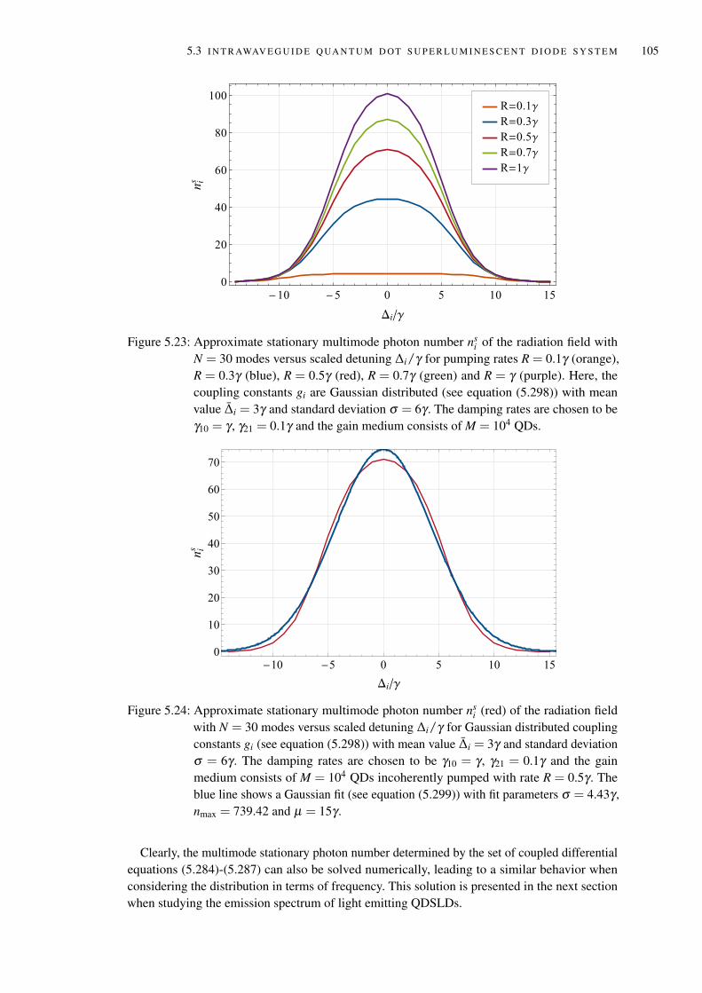
5.3 I N T R AWAV E G U I D E Q UA N T U M D OT S U P E R L U M I N E S C E N T D I O D E S Y S T E M 105
R=0.1γ
R=0.3γ
R=0.5γ
R=0.7γ
R=1γ
-10 -5 0 5 10 15
0
20
40
60
80
100
Δi/γ
nis
Figure 5.23: Approximate stationary multimode photon number nsi of the radiation field with
N = 30 modes versus scaled detuning ∆i/γ for pumping rates R = 0.1γ (orange),R = 0.3γ (blue), R = 0.5γ (red), R = 0.7γ (green) and R = γ (purple). Here, thecoupling constants gi are Gaussian distributed (see equation (5.298)) with meanvalue ∆i = 3γ and standard deviation σ = 6γ . The damping rates are chosen to beγ10 = γ , γ21 = 0.1γ and the gain medium consists of M = 104 QDs.
-10 -5 0 5 10 15
0
10
20
30
40
50
60
70
Δi/γ
nis
Figure 5.24: Approximate stationary multimode photon number nsi (red) of the radiation field
with N = 30 modes versus scaled detuning ∆i/γ for Gaussian distributed couplingconstants gi (see equation (5.298)) with mean value ∆i = 3γ and standard deviationσ = 6γ . The damping rates are chosen to be γ10 = γ , γ21 = 0.1γ and the gainmedium consists of M = 104 QDs incoherently pumped with rate R = 0.5γ . Theblue line shows a Gaussian fit (see equation (5.299)) with fit parameters σ = 4.43γ ,nmax = 739.42 and µ = 15γ .
Clearly, the multimode stationary photon number determined by the set of coupled differentialequations (5.284)-(5.287) can also be solved numerically, leading to a similar behavior whenconsidering the distribution in terms of frequency. This solution is presented in the next sectionwhen studying the emission spectrum of light emitting QDSLDs.
106 M I C RO S C O P I C T H E O RY O F Q UA N T U M D OT S U P E R L U M I N E S C E N T D I O D E S
In summary, we presented a microscopic theory of QDSLDs which considers the specificgain medium, formed by an inhomogeneous ensemble of QDs, as well as the special geometry ofthe end facets. The former is modeled by M distinguishable three-level systems, incoherentlypumped with rate R and interacting with a multimode radiation field, which couples to the outsideby two beam splitters enclosing the active medium. The resulting rate equations of the systemwere studied in detail for the special cases of a single-mode as well as a truly multimode radia-tion field interacting with equal QDs inside the waveguide. The stationary photon number as afunction of pumping rate exhibited the typical ASE transition. Furthermore, assuming a Gaussiancooperativity strength, the spectrum also showed a Gaussian-like distribution for varying angularfrequency, suggesting that the shape of this cooperativity strength dictates the shape of the powerspectral density. To proof this statement or rather our microscopic theory itself, the next sectiondeals with the theoretically predicted power spectrum measured by a single-photon detectorwhich allows a direct comparison with experimentally available data.
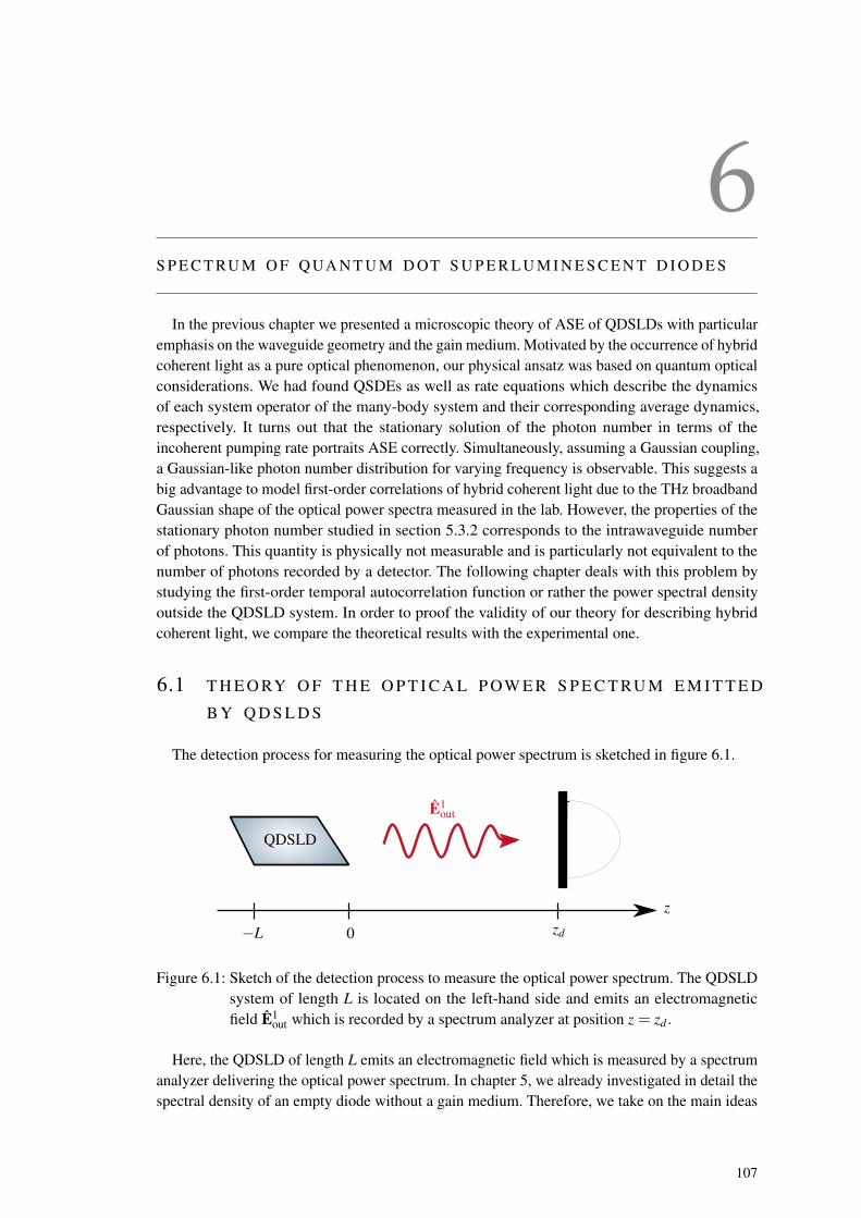
6S P E C T RU M O F Q UA N T U M D OT S U P E R L U M I N E S C E N T D I O D E S
In the previous chapter we presented a microscopic theory of ASE of QDSLDs with particularemphasis on the waveguide geometry and the gain medium. Motivated by the occurrence of hybridcoherent light as a pure optical phenomenon, our physical ansatz was based on quantum opticalconsiderations. We had found QSDEs as well as rate equations which describe the dynamicsof each system operator of the many-body system and their corresponding average dynamics,respectively. It turns out that the stationary solution of the photon number in terms of theincoherent pumping rate portraits ASE correctly. Simultaneously, assuming a Gaussian coupling,a Gaussian-like photon number distribution for varying frequency is observable. This suggests abig advantage to model first-order correlations of hybrid coherent light due to the THz broadbandGaussian shape of the optical power spectra measured in the lab. However, the properties of thestationary photon number studied in section 5.3.2 corresponds to the intrawaveguide numberof photons. This quantity is physically not measurable and is particularly not equivalent to thenumber of photons recorded by a detector. The following chapter deals with this problem bystudying the first-order temporal autocorrelation function or rather the power spectral densityoutside the QDSLD system. In order to proof the validity of our theory for describing hybridcoherent light, we compare the theoretical results with the experimental one.
6.1 T H E O RY O F T H E O P T I C A L P OW E R S P E C T RU M E M I T T E D
B Y Q D S L D S
The detection process for measuring the optical power spectrum is sketched in figure 6.1.
QDSLD
E1out
−L 0 zd
z
Figure 6.1: Sketch of the detection process to measure the optical power spectrum. The QDSLDsystem of length L is located on the left-hand side and emits an electromagneticfield E1
out which is recorded by a spectrum analyzer at position z = zd .
Here, the QDSLD of length L emits an electromagnetic field which is measured by a spectrumanalyzer delivering the optical power spectrum. In chapter 5, we already investigated in detail thespectral density of an empty diode without a gain medium. Therefore, we take on the main ideas
107
108 S P E C T RU M O F Q UA N T U M D OT S U P E R L U M I N E S C E N T D I O D E S
and proceedings made in the previous sections and apply them to the case of a truly incoherentQDSLD amplified by many quantum dots. According to the orientation of the output facetsshown in figure 5.11, channel 1 enters the diode system on the right hand side at z = 0. Theelectric output field E1
out is assumed to be guided in a single-mode fiber yielding to an radiationfield propagating along the z-direction in the sense of equation (5.199). It strikes the detector atposition z = zd .
Clearly, for calculating the temporal correlation function of the emitted QDSLD light, we needthe entire information about the dynamics of the single ASE modes as well as the populations andcoherences of the single QDs described by the QSDEs (5.230) and (5.244a)-(5.245c), respectively.According to the Wiener-Khintchine theorem (cf. equation (2.95) and (2.97)), the output spectrumcorresponds to the Fourier transform of the temporal first-order autocorrelation function
G(1)(τ) = limt→∞
∫Ad
dxdy 〈E1(−)out (x,y, t− zd/c0)E
1(+)out (x,y, t− zd/c0 + τ)〉. (6.1)
The output radiation field E1out is specified in equation (5.199) with mode function defined
in (5.200). Regarding the expression of electric field (5.199), the first-order correlation func-tion (6.1) is only a function of time difference τ [4, 49, 122] and the integrand is proportional tothe two-time correlation 〈b†
i,out(t)b j,out(t ′)〉 with t < t ′ = t + τ .Relying on the concept of the input-output formalism introduced in the previous chapter, the
output is related with the input and the internal field modes according to equation (5.206) or interms of Itô increments,
dB1i,out(t) = dBi(t)+
√∆νFT r
i T ri (t)ai(t)dt, (6.2)
respectively, in which the input (cf. equation (5.207)),
dBi(t) = Rri T
r2i dB1
i (t)+Rri T
ri Rr
i dB2i (t)+Rr
i dB3i (t), (6.3)
is given by a sum of the single input channels α = 1,2,3.Thus, the two-time output average at time events t, t ′ with t < t ′ = t + τ reads
〈dB†i,out(t)dB j,out(t
′)〉=〈dB†i (t)dB j(t
′)〉+∆νFTr
i T rj T r∗
i (t)T rj (t′)〈a†
i (t)a j(t′)〉dt dt ′
+√
∆νFTr
i T r∗i (t)〈a†
i (t)dB j(t ′)〉dt
+√
∆νFTrj T r
j (t′)〈dB†
i (t)a j(t ′)〉dt ′.
(6.4)
It corresponds to the sum of two-time correlations of the input and the internal field operators aswell as correlations between the input and the intrawaveguide field amplitudes. Obviously, equa-tion (6.4) depends significantly on the choice of the input. For example, input noise describableby thermal states possesses an explicit temperature dependency. However, we suppose that thechoice of the input is not relevant for observing hybrid coherent light. For simplicity we choosevacuum as an input. Therefore, the output field is directly related to the first-order autocorrelationfunction of the ASE field modes at different time events t, t ′, according to
〈dB†i,out(t)dB j,out(t
′)〉= ∆νFTr
i T rj T r∗
i (t)T rj (t′)〈a†
i (t)a j(t′)〉dt dt ′, t ′ > t. (6.5)
To evaluate the second-order moment of the intrawaveguide field modes on the right-hand side ofequation (6.5), we utilize the Itô QSDE (5.230) in terms of t ′. Multiplying from the left with thecreation operator a†
i (t) and taking the ensemble average results in
d〈a†i (t)am(t
′)〉t ′ =−[i∆m +
12(γ l
m + γrm)]〈a†
i (t)am(t′)〉dt ′+
M
∑j=1
g j∗m 〈a†
i (t)σj
21(t′)〉dt ′
−〈a†i (t)dBL
m(t′)〉−〈a†
i (t)dBRm(t′)〉,
(6.6)
6.1 T H E O RY O F T H E O P T I C A L P OW E R S P E C T RU M E M I T T E D B Y Q D S L D S 109
with the input noise operators (5.231)-(5.232). Due to causality (cf. equation (F.3)) the last twoterms in equation (6.6), describing correlations between the internal field amplitude at time t andthe input noise increments at future time t ′ > t, are equal to zero and the second-order momentof the internal field amplitudes reduces to
d〈a†i (t)am(t
′)〉t ′ = −[i∆m +
12(γ l
m + γrm)]〈a†
i (t)am(t′)〉dt ′+
M
∑j=1
g j∗m 〈a†
i (t)σj
21(t′)〉dt ′. (6.7)
We can express the two-time correlation of the intrawaveguide amplitude and the ASE transitionoperator of the jth quantum dot (last term in equation (6.7)) in terms of the average of the internalradiation amplitudes at different time events by applying the decorrelation approximation and theadiabatic elimination in analogy to section 5.3.1. Within these approximations the last term inequation (6.7) reads
〈a†i (t)σ
j21(t
′)〉 ≈ ∑kr
g jrw j(t ′)
(Γ j21 +R)/2+ iδω j
12
〈a†i (t)ar(t ′)〉. (6.8)
This approximate solution can be directly inserted into equation (6.7) and the QSDE of thetwo-time internal field modes is given by
d〈a†i (t)am(t
′)〉t ′ =−[i∆m +
γ lm + γr
m
2−
M
∑j=1
|g jm|2w j(t ′)
(Γ j21 +R)/2+ iδω j
12
]〈a†
i (t)am(t′)〉dt ′
+M
∑j=1
∑krr 6=m
g jrg j∗
m w j(t ′)
(Γ j21 +R)/2+ iδω j
12
〈a†i (t)ar(t
′)〉dt ′. (6.9)
Regarding the coupling matrix elements, we claim that off-diagonal elements are small comparedto the diagonal one. Accordingly, we neglect the last term in equation (6.9) in first-order pertur-bation theory. Furthermore, we consider the last term in the brackets, which is proportional to thetime-dependent inversion w j(t ′) = w j(t + τ). For t→ ∞ this inversion tends to a constant value,i.e. limt→∞〈w j(t + τ)〉= w js = const.. As we are interested in the stationary power spectrum ofa QDSLD, we replace the time-dependent inversion in equation (6.9) by its stationary value w js
in good approximation. Equation (6.9) reduces to the expression
d〈a†i (t)am(t ′)〉t ′ ≈− (iχi +ηi) 〈a†
i (t)am(t ′)〉dt ′, (6.10)
with the following abbreviations
χi = ∆i +M
∑j=1
|g ji |2w jsδω j
12
((Γ j21 +R)/2)2 + δω j2
12
= ∆i +O(δω j12) ≈ ∆i, (6.11)
ηi =γ l
i + γri
2−
M
∑j=1
|g ji |2w js(Γ j
21 +R)
(Γ j21 +R)2/2+ 2δω j2
12
=γ l
i + γri
2−2
M
∑j=1
|g ji |2w js
Γ j21 +R
+O(δω j12)
≈ γ li + γr
i −ξi
2, ξi = 4
M
∑j=1
|g ji |2w js
Γ j21 +R
.
(6.12)
In the last step of equations (6.11) and (6.12) we assumed a small frequency discrepancy δω j12 of
the jth quantum dot from the mean value ω12 so that all terms of the order O(δω j12) are negligible.
A central assumption of broadband ASE was presented in section 5.3.1, in which we requiredvanishing correlations between different field modes at equal time with 〈a†
i (t)am(t)〉= ni(t)δim
110 S P E C T RU M O F Q UA N T U M D OT S U P E R L U M I N E S C E N T D I O D E S
(cf. equation (5.248)). In this context we can formally integrate equation (6.10) so that theintrawaveguide field correlation function is determined by
〈a†i (t)am(t
′)〉= ni(t)e−(iχi+ηi)(t ′−t)δim, t ′ > t. (6.13)
Finally, the correlation function of the output increments dBi,out (see equation (6.5)) at differenttime events t, t ′ reads
〈dB†i,out(t)dB j,out(t ′)〉= ∆νFT
r2i T r∗
i (t)T ri (t′)ni(t)e−(iχi+ηi)(t ′−t)δi j dt dt ′. (6.14)
Please note, that equation (6.14) corresponds to a two-time correlation function of the Itôincrements. In order to determine the optical power spectral density measured by the detector,we have to calculate the second-order moment of the Heisenberg system operator bout at differenttime events. However, this transition is quite obvious when considering the definition of aquantum Wiener process (see equation (F.8)), where the Langevin-type temporal correlation canbe directly determined from the corresponding Itô equation (6.14) according to [139]
〈dB†i,out(t)dB j,out(t ′)〉= 〈b†
i,out(t)b j,out(t ′)〉dt dt ′ (6.15)
⇒ 〈b†i,out(t)b j,out(t ′)〉= ∆νFT
r2i T r∗
i (t)T ri (t′)ni(t)e−(iχi+ηi)(t ′−t)δi j. (6.16)
We assume a slowly varying transmission amplitude T βi (t) compared to the system’s amplitudes,
so that T βi (t) can be replaced by a constant T β
i that is
T βi (t) ' T β
i . (6.17)
Finally back-transformation to the original Heisenberg picture yields the discrete stationaryoptical power spectrum
S(ω) =C
πRe∫ ∞
0dτ G(1)(τ)eiωτ = ∑
ki,k j>0ϒiϒj Re
∫ ∞
0dτeiωτ〈b†
i,out(t)b j,out(t + τ)〉t→∞
= ∑ki>0
Piηi nsi
η2i +(ω−ωi)2 , ϒi =
√2hc0ωi
∆ωiL, Pi =
2hωi∆νFc0T r2i |T r
i |2∆ωiL
(6.18)
with optical power Pi. Again, we consider equal external decay rates and transmission amplitudesfor all modes, that is γβ
i = γβ , T βi =T β and T β
i = T β with β ∈ l,r. Furthermore, we demandthat the angular frequency appearing in the enumerator of equation (6.18) differs only slightlyfrom a mean value ω so that we can set ωi ≈ ω in good approximation. We suppose equalfrequency separation between adjacent modes, i.e. ∆ωi = ∆ω = (ωN/2−1−ω−N/2)/(N−1).Within these approximations we find an optical spectrum,
S(ω) ≈ P ∑ki>0
LΓi(ω−ωi) ns(ωi), P =2hω∆νFc0T r2|T r|2
∆ωL, (6.19)
given by a convolution of a Lorentzian curve,
LΓ(ω) =1π
Γ(Γ/2)2 +ω2 , Γ = γ l + γr−ξ ,
6.2 C O M PA R I S O N W I T H A M E A S U R E D P OW E R S P E C T RU M 111
with the stationary intrawaveguide photon number ns(ωi), which in turn was studied in detailin section 5.3. In the continuous limit, the sum in equation (6.19) is replaced by an integral,resulting into a continuous power spectrum of type1
S(ω) ≈ P∆ω
∞∫−∞
dω ′LΓ(ω−ω ′) ns(ω ′) . (6.20)
This closed expression of the power spectral density corresponds to a convolution of a Lorentziancurve with the stationary internal number of photons. It permits a direct comparison with theexperimentally available power spectrum, which is examined in the following section.
6.2 C O M PA R I S O N W I T H A M E A S U R E D P OW E R S P E C T RU M
In theory, the spectral density is directly related to the internal stationary photon number of theQDSLD under study. This result is of great relevance and allows a direct comparison with theexperimental data. In this section we will demonstrate that the experimentally measured opticalpower spectrum is basically reflected by the intrawaveguide photon number described in detail inchapter 5.
Figure 6.2 shows again the experimental power spectrum S(ω) (black) (cf. figure 3.3) togetherwith a Gaussian interpolation (green line),
Sfit(ω) =S0√2πσ
e−(ω−ω)2
2σ2 ,∫ ∞
−∞dω Sfit = S0, (6.21)
and the numerical solution of the stationary internal photon number ns = ∑ki nsi (red, dashed
line) resulting from the rate equations (5.284)-(5.287) under the assumption of M = 104 identicalquantum dots. In addition, we use a Gaussian profile for the cooperativity strength2,
G(ω) = G0e−(ω−ω)2
2σ2 . (6.22)
Other parameters which are included in this multimode theory are assumed to be well-knownand given by R = 0.5γ , γ10 = γ , γ21 = 0.1γ and γ l = γr = γ . Please note, that the fit parametersof both, the Gaussian fit as well as the multimode stationary photon number, are effected by thechoice of this set of parameters, more precisely on the pumping rate R, the number of QDs Mand the damping rates γ10, γ21, γ l and γr.
FI T T I N G T H E O P T I C A L P OW E R S P E C T RU M The available experimental data providedby S. Blumenstein were uncalibrated, that is information about the absolute values of the opticalpower at different frequencies are lost. Only the spectral shape or rather the relative change in theoptical spectrum is available. Therefore, the main challenge is to fit the shape of S(ω) withoutknowing the absolute values.
To be specific, we consider the change in the optical power spectrum of two adjacent frequen-cies [166], ∆S(ωi), which is related to the differences of the logarithm. To demonstrate this, weset
S(ωi+1) = S(ωi)+∆S(ωi) (6.23)
1 Here, the integration limits were extended to ±∞ which is valid regarding the frequency band [ω−N/2,ωN/2−1] inwhich ns(ω) = 0 for ω > ωN/2−1 and ω < ω−N/2.
2 Please note, that the dimension of the amplitude S0 of the power spectral density fit and the cooperativity strength G0are different. However, as the experimental data are not calibrated we choose arbitrary units.
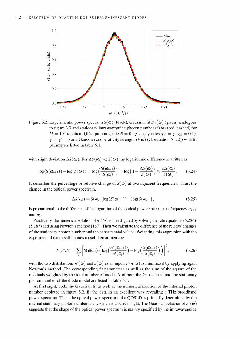
112 S P E C T RU M O F Q UA N T U M D OT S U P E R L U M I N E S C E N T D I O D E S
S(ω)Sfit(ω)ns(ω)
1.48 1.49 1.50 1.51 1.52 1.53
0.0
0.2
0.4
0.6
0.8
1.0
ω (1015/s)
S(ω
)(arb.units)
Figure 6.2: Experimental power spectrum S(ω) (black), Gaussian fit Sfit(ω) (green) analogousto figure 3.3 and stationary intrawaveguide photon number ns(ω) (red, dashed) forM = 104 identical QDs, pumping rate R = 0.5γ , decay rates γ10 = γ , γ21 = 0.1γ ,γ l = γr = γ and Gaussian cooperativity strength G(ω) (cf. equation (6.22)) with fitparameters listed in table 6.1.
with slight deviation ∆S(ωi). For ∆S(ωi) S(ωi) the logarithmic difference is written as
log(S(ωi+1))− log(S(ωi)) = log(S(ωi+1)
S(ωi)
)= log
(1+
∆S(ωi)
S(ωi)
)≈ ∆S(ωi)
S(ωi). (6.24)
It describes the percentage or relative change of S(ω) at two adjacent frequencies. Thus, thechange in the optical power spectrum,
∆S(ωi) = S(ωi) [log(S(ωi+1))− log(S(ωi))] , (6.25)
is proportional to the difference of the logarithm of the optical power spectrum at frequency ωi+1
and ωi.Practically, the numerical solution of ns(ω) is investigated by solving the rate equations (5.284)-
(5.287) and using Newton’s method [167]. Then we calculate the difference of the relative changesof the stationary photon number and the experimental values. Weighting this expression with theexperimental data itself defines a useful error measure
F(ns,S) = ∑i
[S(ωi+1)
(log(ns(ωi+1)
ns(ωi)
)− log
(S(ωi+1)
S(ωi)
))]2
, (6.26)
with the two distributions ns(ω) and S(ω) as an input. F(ns,S) is minimized by applying againNewton’s method. The corresponding fit parameters as well as the sum of the square of theresiduals weighted by the total number of modes N of both the Gaussian fit and the stationaryphoton number of the diode model are listed in table 6.1.
At first sight, both, the Gaussian fit as well as the numerical solution of the internal photonnumber depicted in figure 6.2, fit the data in an excellent way revealing a THz broadbandpower spectrum. Thus, the optical power spectrum of a QDSLD is primarily determined by theinternal stationary photon number itself, which is a basic insight. The Gaussian behavior of ns(ω)
suggests that the shape of the optical power spectrum is mainly specified by the intrawaveguide
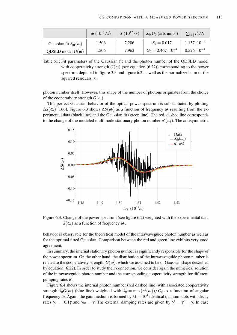
6.2 C O M PA R I S O N W I T H A M E A S U R E D P OW E R S P E C T RU M 113
ω (1015/s) σ (1012/s) S0,G0 (arb. units ) ∑ki r2i /N
Gaussian fit Sfit(ω) 1.506 7.286 S0 = 0.017 1.137 ·10−4
QDSLD model G(ω) 1.506 7.962 G0 = 2.467 ·10−4 0.526 ·10−4
Table 6.1: Fit parameters of the Gaussian fit and the photon number of the QDSLD modelwith cooperativity strength G(ω) (see equation (6.22)) corresponding to the powerspectrum depicted in figure 3.3 and figure 6.2 as well as the normalized sum of thesquared residuals, ri.
photon number itself. However, this shape of the number of photons originates from the choiceof the cooperativity strength G(ω).
This perfect Gaussian behavior of the optical power spectrum is substantiated by plotting∆S(ωi) [166]. Figure 6.3 shows ∆S(ωi) as a function of frequency ωi resulting from the ex-perimental data (black line) and the Gaussian fit (green line). The red, dashed line correspondsto the change of the modeled multimode stationary photon number ns(ωi). The antisymmetric
Data
Sfit(ωi)ns(ωi)
1.48 1.49 1.50 1.51 1.52 1.53-0.15
-0.10
-0.05
0.00
0.05
0.10
0.15
ω i (1015/s)
ΔS(ωi)
Figure 6.3: Change of the power spectrum (see figure 6.2) weighted with the experimental dataS(ωi) as a function of frequency ωi.
behavior is observable for the theoretical model of the intrawaveguide photon number as well asfor the optimal fitted Gaussian. Comparison between the red and green line exhibits very goodagreement.
In summary, the internal stationary photon number is significantly responsible for the shape ofthe power spectrum. On the other hand, the distribution of the intrawaveguide photon number isrelated to the cooperativity strength, G(ω), which we assumed to be of Gaussian shape describedby equation (6.22). In order to study their connection, we consider again the numerical solutionof the intrawaveguide photon number and the corresponding cooperativity strength for differentpumping rates R.
Figure 6.4 shows the internal photon number (red dashed line) with associated cooperativitystrength S0G(ω) (blue line) weighted with S0 = max(ns(ω))/G0 as a function of angularfrequency ω . Again, the gain medium is formed by M = 104 identical quantum dots with decayrates γ21 = 0.1γ and γ10 = γ . The external damping rates are given by γ l = γr = γ . In case
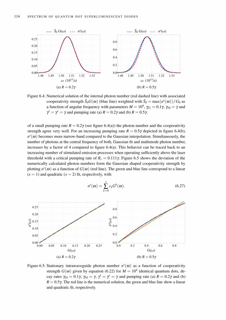
114 S P E C T RU M O F Q UA N T U M D OT S U P E R L U M I N E S C E N T D I O D E S
1.48 1.49 1.50 1.51 1.52 1.53
0.00
0.05
0.10
0.15
0.20
0.25
ω (1015/s)
S0 G(ω) ns(ω)
(a) R = 0.2γ
1.48 1.49 1.50 1.51 1.52 1.53
0.0
0.2
0.4
0.6
0.8
ω (1015/s)
S0 G(ω) ns(ω)
(b) R = 0.5γ
Figure 6.4: Numerical solution of the internal photon number (red dashed line) with associatedcooperativity strength S0G(ω) (blue line) weighted with S0 = max(ns(ω))/G0 asa function of angular frequency with parameters M = 104, γ21 = 0.1γ , γ10 = γ andγ l = γr = γ and pumping rate (a) R = 0.2γ and (b) R = 0.5γ .
of a small pumping rate R = 0.2γ (see figure 6.4(a)) the photon number and the cooperativitystrength agree very well. For an increasing pumping rate R = 0.5γ depicted in figure 6.4(b),ns(ω) becomes more narrow-band compared to the Gaussian interpolation. Simultaneously, thenumber of photons at the central frequency of both, Gaussian fit and multimode photon number,increases by a factor of 4 compared to figure 6.4(a). This behavior can be traced back to anincreasing number of stimulated emission processes when operating sufficiently above the laserthreshold with a critical pumping rate of Rc = 0.111γ . Figure 6.5 shows the deviation of thenumerically calculated photon numbers form the Gaussian shaped cooperativity strength byplotting ns(ω) as a function of G(ω) (red line). The green and blue line correspond to a linear(x = 1) and quadratic (x = 2) fit, respectively, with
ns(ω) =x
∑k=0
ckGk(ω). (6.27)
0.00 0.05 0.10 0.15 0.20 0.25
0.00
0.05
0.10
0.15
0.20
0.25
G(ω)
ns(ω
)
(a) R = 0.2γ
0.0 0.2 0.4 0.6 0.8
0.0
0.2
0.4
0.6
0.8
G(ω)
ns(ω
)
(b) R = 0.5γ
Figure 6.5: Stationary intrawaveguide photon number ns(ω) as a function of cooperativitystrength G(ω) given by equation (6.22) for M = 104 identical quantum dots, de-cay rates γ10 = 0.1γ , γ10 = γ , γ l = γr = γ and pumping rate (a) R = 0.2γ and (b)R = 0.5γ . The red line is the numerical solution, the green and blue line show a linearand quadratic fit, respectively.
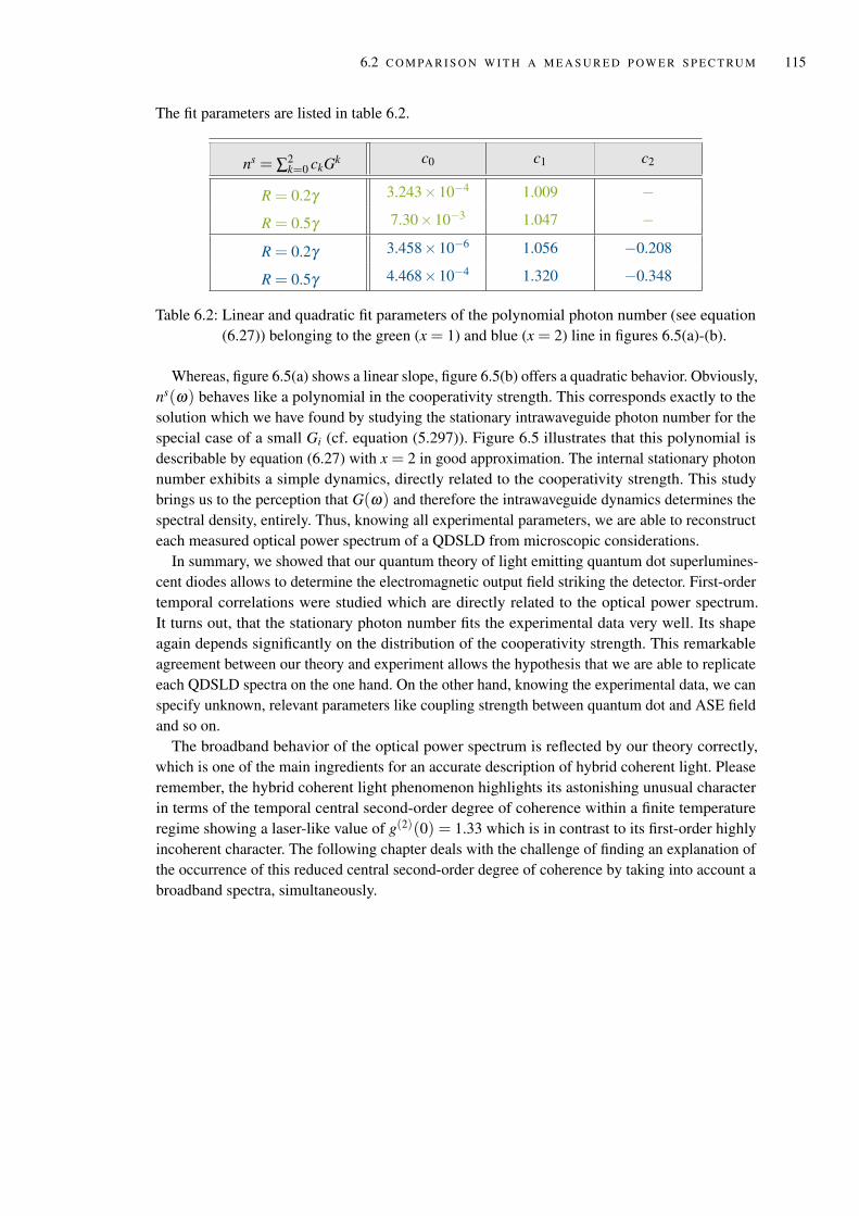
6.2 C O M PA R I S O N W I T H A M E A S U R E D P OW E R S P E C T RU M 115
The fit parameters are listed in table 6.2.
ns = ∑2k=0 ckGk c0 c1 c2
R = 0.2γ 3.243×10⁻⁴ 1.009 −
R = 0.5γ 7.30×10⁻³ 1.047 −
R = 0.2γ 3.458×10⁻⁶ 1.056 −0.208
R = 0.5γ 4.468×10⁻⁴ 1.320 −0.348
Table 6.2: Linear and quadratic fit parameters of the polynomial photon number (see equation(6.27)) belonging to the green (x = 1) and blue (x = 2) line in figures 6.5(a)-(b).
Whereas, figure 6.5(a) shows a linear slope, figure 6.5(b) offers a quadratic behavior. Obviously,ns(ω) behaves like a polynomial in the cooperativity strength. This corresponds exactly to thesolution which we have found by studying the stationary intrawaveguide photon number for thespecial case of a small Gi (cf. equation (5.297)). Figure 6.5 illustrates that this polynomial isdescribable by equation (6.27) with x = 2 in good approximation. The internal stationary photonnumber exhibits a simple dynamics, directly related to the cooperativity strength. This studybrings us to the perception that G(ω) and therefore the intrawaveguide dynamics determines thespectral density, entirely. Thus, knowing all experimental parameters, we are able to reconstructeach measured optical power spectrum of a QDSLD from microscopic considerations.
In summary, we showed that our quantum theory of light emitting quantum dot superlumines-cent diodes allows to determine the electromagnetic output field striking the detector. First-ordertemporal correlations were studied which are directly related to the optical power spectrum.It turns out, that the stationary photon number fits the experimental data very well. Its shapeagain depends significantly on the distribution of the cooperativity strength. This remarkableagreement between our theory and experiment allows the hypothesis that we are able to replicateeach QDSLD spectra on the one hand. On the other hand, knowing the experimental data, we canspecify unknown, relevant parameters like coupling strength between quantum dot and ASE fieldand so on.
The broadband behavior of the optical power spectrum is reflected by our theory correctly,which is one of the main ingredients for an accurate description of hybrid coherent light. Pleaseremember, the hybrid coherent light phenomenon highlights its astonishing unusual characterin terms of the temporal central second-order degree of coherence within a finite temperatureregime showing a laser-like value of g(2)(0) = 1.33 which is in contrast to its first-order highlyincoherent character. The following chapter deals with the challenge of finding an explanation ofthe occurrence of this reduced central second-order degree of coherence by taking into account abroadband spectra, simultaneously.

7
P H OT O N S TAT I S T I C S O F Q UA N T U M D OT S U P E R L U M I N E S C E N TD I O D E S
Photon statistics is a study about the statistical properties of radiation, which classifies lightsources in terms of their coherence properties and provides evidence to the quantum nature ofthe considered radiation. The photon statistics is related to the second-order correlation functionas indicated in chapter 2. In general, this correlation is measured by standard HBT experiments.As already mentioned, for the THz broad emission of QDSLDs with a coherence length ofsome femtoseconds, this measurement technique is not available due to the finite temporalresolution of commercial detectors. The invention of the two-photon detector by F. Boitier etal. [29] circumvents this problem and delivers a competitive feasibility for measuring broadbandradiation. In particular, it allows for the analysis of the photon statistical properties of hybridcoherent light, which exhibits a reduction of g(2)(0) at an external temperature T = 190 K (seesection 3.2).
To find an explanation of this unusual characteristic, this chapter is dedicated to the determina-tion of the second-order correlation function of QDSLDs resulting from the microscopic fieldtheory studied in section 5. Within this context we analyze the central second-order degree ofcoherence. The chapter ends with a discussion of the photon statistics of a single-mode QDSLDwith identical QDs.
7.1 T E M P O R A L S E C O N D - O R D E R C O R R E L AT I O N O F Q D S L D S
In this section we formally calculate the temporal second-order correlation function of lightemitted by a QDSLD, which is described by our microscopic theory presented in chapter 5. Atwo-photon detector of finite cross-section area Ad is assumed to be located at the right-hand sideof the semiconductor device with distance zd in analogy to the previous chapter where we studiedthe power spectrum (see figure 6.1). The electric field emitted by the QDSLD on the right-handside parallel to the z-direction is assumed to be guided into a single-mode fiber till it enters thedetector.
The positive frequency part of the electric field, which is measured by the two-photon detectorat z = zd 0, is given by (cf. equation (5.199))
E(+)out (r, t) = E(+)
out (r, t)ey ≡ E1(+)out (x,y, t− zd
c0) ' ∑
ki>0vi(x,y)b1
i,out(t−zd
c0)ey, (7.1)
with the mode functions (cf. equation (5.200))
vi(x,y) = i
√hπωi
ε0V ∆ωiµ(x,y). (7.2)
117
118 P H OT O N S TAT I S T I C S O F Q UA N T U M D OT S U P E R L U M I N E S C E N T D I O D E S
As discussed in section 2.3.2 the temporal second-order correlation function G(2)(r, t;r, t ′) andthe second-order degree of coherence g(2)(r, t;r, t ′) of the output radiation field with t < t ′
correspond to the fourth-order moments
G(2)(r, t;r, t ′) = 〈E(−)out (r, t)E(−)
out (r, t ′)E(+)out (r, t ′)E(+)
out (r, t)〉, (7.3)
g(2)(r, t;r, t ′) =〈E(−)
out (r, t)E(−)out (r, t ′)E(+)
out (r, t ′)E(+)out (r, t)〉
〈E(−)out (r, t)E(+)
out (r, t)〉〈E(−)out (r, t ′)E(+)
out (r, t ′)〉. (7.4)
To find an explicit expression of these physical quantities we utilize the input-output formalismin equation (5.206). In the following, we choose vacuum as an input in analogy to the previouschapter. It turns out, that the two-time correlation of the output operators only depends on thecorrelation of the intrawaveguide field amplitudes as
〈b1†i,out(t)b
1†k,out(t
′)b1m,out(t
′)b1n,out(t)〉= Ξikmn(t, t ′)〈a†
i (t)a†k(t′)am(t
′)an(t)〉 (7.5)
with
Ξikmn(t, t ′) ≡ (∆νF)2T r∗
i T r∗k T r
mT rn T r∗
i (t)T r∗k (t ′)T r
m(t′)T r
n (t). (7.6)
The dynamics of the intrawaveguide field operators is described by the stochastic differentialequation (5.230). Inserting the solution (7.5) into the definition (7.3) and integrating over the totalcross-section of the detector Ad finally results into an expression of the temporal second-ordercorrelation function
G(2)(t; t ′) = ∑ki,kk ,km,kn>0
wikmn(t, t ′)〈a†i (t)a
†k(t′)am(t
′)an(t)〉, (7.7)
in which
wikmn(t, t ′) =(
hπε0L
)2√ ωiωkωmωn
∆ωi∆ωk∆ωm∆ωnΞikmn(t, t ′). (7.8)
Only stationary situations will be considered. Thus, the physical quantity of interest
G(2)(τ) = limt→∞
G(2)(t; t ′ = t + τ) (7.9)
is only a function of time delay τ = t ′− t > 0. In analogy to the previous section we assumethat the time-dependent transmission amplitude T r
i (t) evolves slowly compared to the system’samplitudes, which results into an approximately constant transmission contribution so that,
Ξikmn(t, t + τ) ' Ξsikmn = (∆νF)
2T r∗i T r∗
k T rmT r
n T r∗i T r∗
k T rmT r
n = const., (7.10)
wikmn(t, t + τ) ' wsikmn = const.. (7.11)
Thus, knowing the two-time, fourth-order moment of the internal field operators we can specifythe second-order correlation explicitly.
7.2 C E N T R A L S E C O N D - O R D E R D E G R E E O F C O H E R E N C E
In this section, we study the central second-order degree of coherence of a QDSLD with the helpof our microscopic model. The theoretical result could provide an explanation of the experimentalobservation of the g(2)(0) reduction at a special temperature, which again grants more insightinto the quantum nature of light emitting diodes. Simultaneously, an explanation of the observed
7.2 C E N T R A L S E C O N D - O R D E R D E G R E E O F C O H E R E N C E 119
coherence properties of broadband QDSLDs could enable the establishment of novel light sourcespossessing a wide range of applications for both commercial and fundamental purposes. It shouldbe noted that the general measure of the second-order degree of coherence g(2)(τ) as a function oftime delay τ , is also determinable (see appendix H). However, with regard to the hybrid coherentlight effect, we are focused on the analysis of the central second-order correlation function.
To specify this physical quantity of interest, we set up an Itô QSDE for the average of theintrawaveguide field operators 〈a†
i a†k aman〉. This differential equation can be determined by the
help of the QSDE of a single field amplitude given in equation (5.230) together with the Itôproduct rule (F.20) or directly from the definition of an Itô QSDE (see equation (F.16)). In thefollowing we assume vacuum as an input, identical external decay rates for each mode i, γ l
i = γ l
and γri = γr, as well as uncorrelated input modes of different reservoirs, 〈dBL(†)dBR(†)〉 = 0.
Due to quantum causality and the fact that the increments commute with and are statisticallyindependent of the system operators at the same time [50], the stochastic differential equationreads
ddt〈a†
i a†k aman〉=−αikmn〈a†
i a†k aman〉+
M
∑j=1
(g j
i 〈σj†
21 a†k aman〉+ g j
k〈a†i σ j†
21 aman〉
+ g j∗m 〈a†
i a†kσ j
21an〉+ g j∗n 〈a†
i a†k amσ j
21〉)
,
(7.12)
with
αikmn = i(∆m +∆n−∆i−∆k)+ 2(γ l + γr). (7.13)
We are left with the determination of correlations between quantum dot transitions and multimoderadiation field amplitudes of type 〈σ j†
21 a†k aman〉. First, we consider the second correlation term on
the right hand side of equation (7.12). With the help of the QSDE (5.230), equation (5.245a) andthe Itô rule (F.20) we get
ddt〈σ j†
21 a†k aman〉=−ϑ j
kmn〈σj†
21 a†k aman〉+ ∑
krg j∗
r 〈w ja†r a†
k aman〉
+M
∑j′=1
(g j′
k 〈σj†
21 σ j′†21 aman〉+ g j′∗
m 〈σ j†21 a†
kσ j′21an〉+ g j′∗
n 〈σ j†21 a†
k amσ j′21〉)
,(7.14)
with
ϑ jkmn = −i(δω j
12 +∆k−∆m−∆n)+12(Γ j
21 +R)+32(γ l + γr). (7.15)
Approximations that were already introduced in connection with the rate equations (cf. sec-tion 5.3.1) allow to simplify this first-order differential equation. We apply the decorrelationapproximation and neglect correlations between different QDs, so that 〈σ j†
21 σ j′21〉= σ j
11δ j j′ holds(cf. equation (5.250)). Furthermore, we neglect squeezing effects, that is 〈aia j〉 = 〈a†
i a†j〉 = 0
as well as counter-propagating contributions like 〈σ j†21 a†
k〉= 〈σj
21ak〉= 0. The single correlationterms in equation (7.14) factorize to
〈w ja†s a†
k aman〉 ≈ w j〈a†s a†
k aman〉, (7.16)
〈σ j†21 σ j′†
21 aman〉 ≈ 〈σ j†21 am〉〈σ j′†
21 an〉+ 〈σ j†21 an〉〈σ j′†
21 am〉, (7.17)
〈σ j†21 a†
kσ j′21an〉 ≈ σ j
11nkδ j j′δkn + 〈σ j†21 an〉〈a†
kσ j′21〉. (7.18)
According to section 5.3.1 we adiabatically eliminate correlations of the quantum dot tran-sition and the radiation field by setting the right-hand side of equation (7.14) equal to zero,
120 P H OT O N S TAT I S T I C S O F Q UA N T U M D OT S U P E R L U M I N E S C E N T D I O D E S
ddt 〈σ
j†
21a†k aman〉 ≈ 0 and finally replacing the correlation by its stationary value. We obtain an
expression for the expectation value
〈σ j†21 a†
k aman〉 ≈1
ϑ jkmn
∑kr>0
g j∗r w j〈a†
r a†k aman〉+(g j∗
m δkn + g j∗n δkm)nkσ j
11
+ g jkg j∗
m g j∗n
[2(nmw j +σ j11)(nnw j +σ j
11)
(i∆ jm +Γ j/2)(i∆ j
n +Γ j/2)
+nkw j +σ j
11
−i∆ jk +Γ j/2
( nnw j +σ j11
i∆ jn +Γ j/2
+nmw j +σ j
11
i∆ jm +Γ j/2
)](7.19)
in terms of 〈a†i a†
k aman〉 and lower-order moments. All other correlations arising in equation (7.14)can be investigated in the same way. The differential equation of the fourth-order moment forthe radiation field amplitudes 〈a†
i a†k aman〉 is listed in appendix G. However, we only consider
terms which are at most quadratic in the coupling constant which provides the major contributionfor weak coupling strengths. Accordingly, we neglect terms of the order of |g|4. Furthermore,we claim that off-diagonal elements of type g j
i g j∗j with i 6= j are small compared to the diagonal
ones. As a main result we find that the first-order differential equation of the internal expectationvalue 〈a†
i a†k aman〉 is determined by
ddt〈a†
i a†k aman〉 ≈
[−αikmn +α (2)
ikmn
]〈a†
i a†k aman〉
+M
∑j=1
g ji
(g j∗
m
ϑ jkmk
+g j∗
n
ϑ jkkn
)σ j
11nk +M
∑j=1
g jk
(g j∗
m
ϑ jimi
+g j∗
n
ϑ jiin
)σ j
11ni
+M
∑j=1
g j∗m
(g j
k
ϑ j∗nkn
+g j
i
ϑ j∗nni
)σ j
11nn +M
∑j=1
g j∗n
(g j
k
ϑ j∗mkm
+g j
i
ϑ j∗mmi
)σ j
11nm,
(7.20)
with second-order energy shift
α (2)ikmn =
M
∑j=1
(|g j
i |2ϑ j
kmn
+|g j
k|2
ϑ jimn
+|g j
m|2ϑ j∗
nki
+|g j
n|2ϑ j∗
mki
)w j. (7.21)
The resulting stationary solution of the fourth-order moment of the internal field amplitudes reads
〈a†i a†
k aman〉s =∑M
j=1 β jikmn
αikmn−α (2)sikmn
, α (2)sikmn =
M
∑j=1
(|g j
i |2ϑ j
kmn
+|g j
k|2
ϑ jimn
+|g j
m|2ϑ j∗
nki
+|g j
n|2ϑ j∗
mki
)w js (7.22)
with
β jikmn =g j
i
(g j∗
m
ϑ jkmk
+g j∗
n
ϑ jkkn
)σ js
11nsk + g j
k
(g j∗
m
ϑ jimi
+g j∗
n
ϑ jiin
)σ js
11nsi
+ g j∗m
(g j
k
ϑ j∗nkn
+g j
i
ϑ j∗nni
)σ js
11nsn + g j∗
n
(g j
k
ϑ j∗mkm
+g j
i
ϑ j∗mmi
)σ js
11nsm.
(7.23)
Here, the labeling s emphasized the corresponding stationary solution of the considered physicalmeasure. Therefore, the temporal second-order correlation function and the temporal second-order degree of coherence of a QDSLD with zero time delay are given by
G(2)(0) = ∑ki,kk ,km,kn>0
wsikmn〈a†
i a†k aman〉s, (7.24)
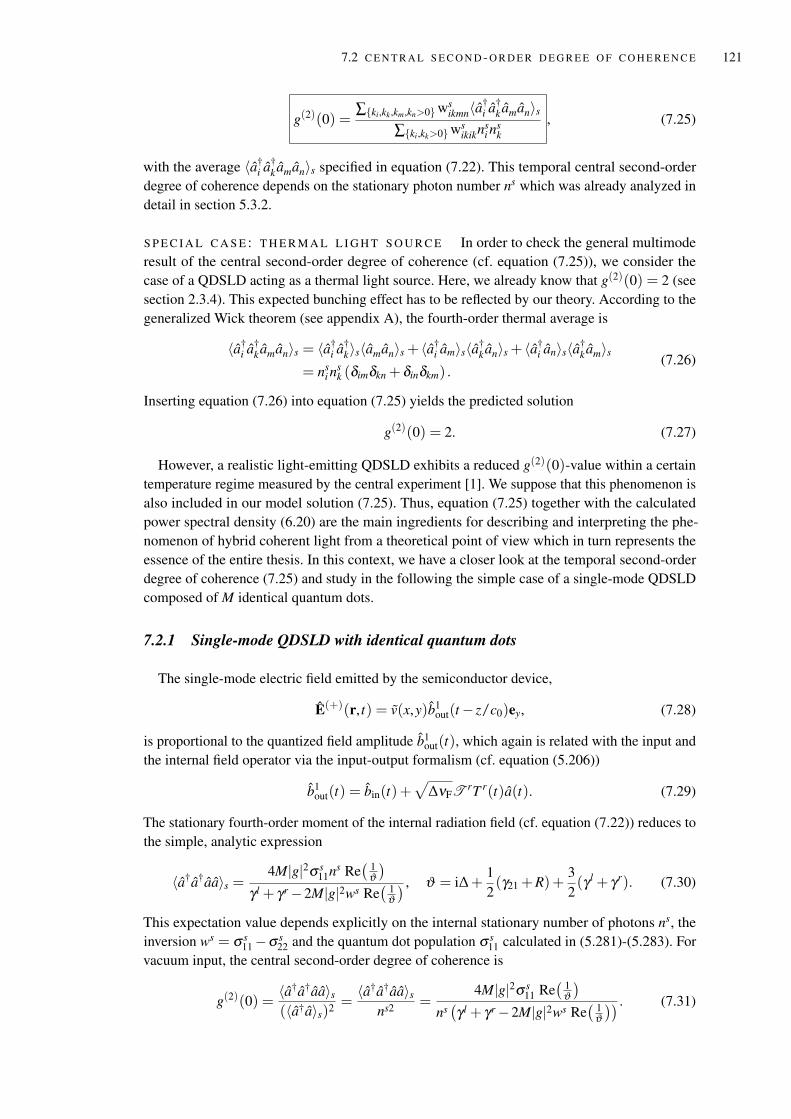
7.2 C E N T R A L S E C O N D - O R D E R D E G R E E O F C O H E R E N C E 121
g(2)(0) =∑ki,kk ,km,kn>0ws
ikmn〈a†i a†
k aman〉s∑ki,kk>0ws
ikiknsi n
sk
, (7.25)
with the average 〈a†i a†
k aman〉s specified in equation (7.22). This temporal central second-orderdegree of coherence depends on the stationary photon number ns which was already analyzed indetail in section 5.3.2.
S P E C I A L C A S E : T H E R M A L L I G H T S O U R C E In order to check the general multimoderesult of the central second-order degree of coherence (cf. equation (7.25)), we consider thecase of a QDSLD acting as a thermal light source. Here, we already know that g(2)(0) = 2 (seesection 2.3.4). This expected bunching effect has to be reflected by our theory. According to thegeneralized Wick theorem (see appendix A), the fourth-order thermal average is
〈a†i a†
k aman〉s = 〈a†i a†
k〉s〈aman〉s + 〈a†i am〉s〈a†
k an〉s + 〈a†i an〉s〈a†
k am〉s= ns
i nsk (δimδkn + δinδkm) .
(7.26)
Inserting equation (7.26) into equation (7.25) yields the predicted solution
g(2)(0) = 2. (7.27)
However, a realistic light-emitting QDSLD exhibits a reduced g(2)(0)-value within a certaintemperature regime measured by the central experiment [1]. We suppose that this phenomenon isalso included in our model solution (7.25). Thus, equation (7.25) together with the calculatedpower spectral density (6.20) are the main ingredients for describing and interpreting the phe-nomenon of hybrid coherent light from a theoretical point of view which in turn represents theessence of the entire thesis. In this context, we have a closer look at the temporal second-orderdegree of coherence (7.25) and study in the following the simple case of a single-mode QDSLDcomposed of M identical quantum dots.
7.2.1 Single-mode QDSLD with identical quantum dots
The single-mode electric field emitted by the semiconductor device,
E(+)(r, t) = v(x,y)b1out(t− z/c0)ey, (7.28)
is proportional to the quantized field amplitude b1out(t), which again is related with the input and
the internal field operator via the input-output formalism (cf. equation (5.206))
b1out(t) = bin(t)+
√∆νFT
rT r(t)a(t). (7.29)
The stationary fourth-order moment of the internal radiation field (cf. equation (7.22)) reduces tothe simple, analytic expression
〈a†a†aa〉s =4M|g|2σ s
11ns Re( 1
ϑ)
γ l + γr−2M|g|2ws Re( 1
ϑ) , ϑ = i∆+
12(γ21 +R)+
32(γ l + γr). (7.30)
This expectation value depends explicitly on the internal stationary number of photons ns, theinversion ws = σ s
11−σ s22 and the quantum dot population σ s
11 calculated in (5.281)-(5.283). Forvacuum input, the central second-order degree of coherence is
g(2)(0) =〈a†a†aa〉s(〈a†a〉s)2 =
〈a†a†aa〉sns2 =
4M|g|2σ s11 Re
( 1ϑ)
ns(γ l + γr−2M|g|2ws Re
( 1ϑ)) . (7.31)
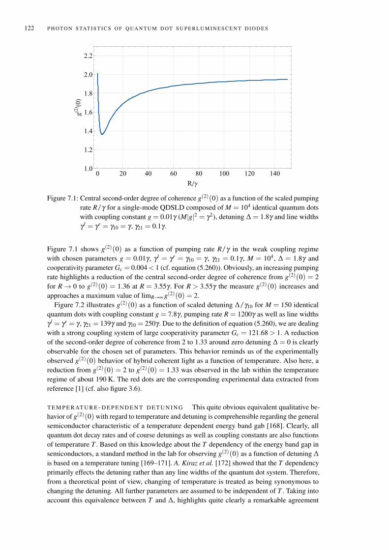
122 P H OT O N S TAT I S T I C S O F Q UA N T U M D OT S U P E R L U M I N E S C E N T D I O D E S
0 20 40 60 80 100 120 1401.0
1.2
1.4
1.6
1.8
2.0
2.2
R/γ
g(2) (0)
Figure 7.1: Central second-order degree of coherence g(2)(0) as a function of the scaled pumpingrate R/γ for a single-mode QDSLD composed of M = 104 identical quantum dotswith coupling constant g = 0.01γ (M|g|2 = γ2), detuning ∆ = 1.8γ and line widthsγ l = γr = γ10 = γ , γ21 = 0.1γ .
Figure 7.1 shows g(2)(0) as a function of pumping rate R/γ in the weak coupling regimewith chosen parameters g = 0.01γ , γ l = γr = γ10 = γ , γ21 = 0.1γ , M = 104, ∆ = 1.8γ andcooperativity parameter Gc = 0.004 < 1 (cf. equation (5.260)). Obviously, an increasing pumpingrate highlights a reduction of the central second-order degree of coherence from g(2)(0) = 2for R→ 0 to g(2)(0) = 1.36 at R = 3.55γ . For R > 3.55γ the measure g(2)(0) increases andapproaches a maximum value of limR→∞ g(2)(0) = 2.
Figure 7.2 illustrates g(2)(0) as a function of scaled detuning ∆/γ10 for M = 150 identicalquantum dots with coupling constant g = 7.8γ , pumping rate R = 1200γ as well as line widthsγ l = γr = γ , γ21 = 139γ and γ10 = 250γ . Due to the definition of equation (5.260), we are dealingwith a strong coupling system of large cooperativity parameter Gc = 121.68 > 1. A reductionof the second-order degree of coherence from 2 to 1.33 around zero detuning ∆ = 0 is clearlyobservable for the chosen set of parameters. This behavior reminds us of the experimentallyobserved g(2)(0) behavior of hybrid coherent light as a function of temperature. Also here, areduction from g(2)(0) = 2 to g(2)(0) = 1.33 was observed in the lab within the temperatureregime of about 190 K. The red dots are the corresponding experimental data extracted fromreference [1] (cf. also figure 3.6).
T E M P E R AT U R E - D E P E N D E N T D E T U N I N G This quite obvious equivalent qualitative be-havior of g(2)(0) with regard to temperature and detuning is comprehensible regarding the generalsemiconductor characteristic of a temperature dependent energy band gab [168]. Clearly, allquantum dot decay rates and of course detunings as well as coupling constants are also functionsof temperature T . Based on this knowledge about the T dependency of the energy band gap insemiconductors, a standard method in the lab for observing g(2)(0) as a function of detuning ∆is based on a temperature tuning [169–171]. A. Kiraz et al. [172] showed that the T dependencyprimarily effects the detuning rather than any line widths of the quantum dot system. Therefore,from a theoretical point of view, changing of temperature is treated as being synonymous tochanging the detuning. All further parameters are assumed to be independent of T . Taking intoaccount this equivalence between T and ∆, highlights quite clearly a remarkable agreement
7.2 C E N T R A L S E C O N D - O R D E R D E G R E E O F C O H E R E N C E 123
50 100 150 200 250 300 350
T (K)
-2000 -1000 0 1000 2000
1.0
1.2
1.4
1.6
1.8
2.0
Δ/γ
g(2) (0)
Figure 7.2: (Blue): Central second-order degree of coherence g(2)(0) as a function of the scaleddetuning ∆/γ for a single-mode QDSLD composed of M = 150 identical quantumdots with coupling constant g = 7.8γ (M|g|2 = 9126γ2), pumping rate R = 1200γ andline widths γ l = γr = γ , γ21 = 139γ and γ10 = 250γ . (Red): Experimental data [1] ofcentral second-oder degree of coherence g(2)(0) versus temperature T (cf. figure 3.6).
between the experimental observation [1] and our quantum theory of QDSLDs (see figure 7.2). Italso implies that the physical effect provoking the occurrence of hybrid coherent light is includedwithin our microscopic model.
Please note, that we considered here a single-mode emitting QDSLD system. The fact thathere a reduced second-order degree of coherence is observable reveals that the physical effect ofnoise suppression at a particular temperature regime is also included in the limiting single-modecase. Nevertheless, a reduction of g(2)(0) is also theoretically predicted for the full multimodetheory. Thus, the hybrid coherent light phenomenon of being incoherent in first- and simultane-ously coherent in second-order of correlation is presumably not a purely collective mode effect.Naturally, the broadband spectral density of hybrid coherent light as visualized in figure 6.2originates from the multimode character of the amplified spontaneous emission.
7.2.2 Physical explanation of the occurrence of hybrid coherent light
Our quantum theory reflects the key measurements of hybrid coherent light: a broadbandoptical power spectrum (see figure 6.2) as well as a reduction of the central second-order degreeof coherence (see figure 7.2). Our modeling ansatz presented in chapter 5 is based on quantumoptical considerations. Semiconductor effects like the formation of excitons, polaritons etc. aredisregarded within our field theory. This essential fact suggests that hybrid coherent light is
124 P H OT O N S TAT I S T I C S O F Q UA N T U M D OT S U P E R L U M I N E S C E N T D I O D E S
essentially a purely optical effect, which again permits the speculation that these novel states oflight are also reproducible in other optical devices. It is even conceivable that gas lasers operatedin the regime of the amplified spontaneous emission exhibit a reduced g(2)(0)-value, that is noisesuppression. A direct measurement of hybrid coherent light with other, suitable light sourceswould prove our hypothesis.
Obviously, a reduction of g(2)(0) is observable for small coupling strengths and large incoher-ent pumping rates. Due to this strong pumping mechanism, the system at resonance gets ’stiff’.This effect is also observable in non-linear systems (cf. Van der Pol oscillator model [173]).The system passes into saturation leading to a reduction of intensity fluctuations, which againis noticeable in a reduced central second-order degree of coherence. Such a noise reductioncorresponds to classical squeezing [174]. Simultaneously, the power spectrum, determined bythe first-order temporal autocorrelation function, remains broadband.
Clearly, this single-mode discussion of g(2)(0) should be extended to the more realistic andmore exciting case of a truly multimode QDSLD for which a suppression of noise fluctuation isalso predicted.
In this section, we analyzed the central second-order degree of coherence of a light emittingQDSLD. As a result of our microscopic theory, we found a general expression of g(2)(0) in termsof the stationary photon number, excited state population and inversion. For the special case of asingle-mode QDSLD composed of identical quantum dots and a particular set of parameters a re-duction of g(2)(0) as a function of detuning appeared. A direct comparison with the experimentaldata highlighted a very good agreement, quantitatively. This fact illustrates that hybrid coherentlight is describable in the context of our quantum theory which again allows an interpretation ofthe observed noise suppression of broadband QDSLDs at a particular temperature. It turns outthat the hybrid coherent light phenomenon is attributable to a saturation effect.
8C O N C L U S I O N A N D O U T L O O K
Motivated by the unusual behavior at a special temperature regime observed in the experiment[1], we investigated the emission and photon statistical properties of light emitting quantum dotsuperluminescent diodes (QDSLDs). At about T = 190 K the field-correlation g(1)(τ) remainedhighly incoherent with a spectral width of several THz, whereas the second-order correlationg(2)(τ) reduced from 2 to 1.33. Thus, so-called hybrid coherent light is simultaneously incoherentin first- and coherent in second-order correlation function.
To find an explanation of the occurrence of these novel states of light, we studied the amplifiedspontaneous emission of the QDSLD [122]. We postulated a quantum state, a multimode phase-randomized Gaussian (PRAG) state, which corresponds to a superposition of Gaussian stateswith shifted complex amplitudes and randomized phases. This multimode quantum state reflectedthe incoherent character of the broadband semiconductor device and revealed correct intensitycorrelations. We determined temporal correlations analytically in terms of first- and second-order, g(1)(τ) and g(2)(τ). A comparison with a feedback [121] and a mixed light experiment,conducted by the Semiconductor Optics group of W. Elsäßer at TU Darmstadt highlighted anoverall good match. As a main result, we found that the second-order correlation depends on thenumber of modes of the multimode amplified spontaneous emission field. Furthermore, mixinglight from a QDSLD with light emitted by a single-mode laser revealed tunable photon statisticsranging from Poissonian to Gaussian distributions.
In the second part of the thesis, a microscopic theory of the amplified spontaneous emissionof broadband QDLSDs was formulated. This model of the diode considered the gain mediumto be composed of many distinguishable quantum dots, each one described by a three-levelsystem. They are embedded in a strong absorptive bulk material, which defines a waveguide.In this context, the dissipative dynamics as well as gain and absorption of a single quantumdot at room temperature was analyzed. The waveguide itself was represented by a cavity. Thewaveguide’s output facets of typical QDSLDs are tilted and anti-reflection coated to guaranteethe suppression of longitudinal modes. This special geometry of the device was modeled by beamsplitters enclosing the active medium, which couples the internal field to the environment at thesame time. This three-component model of beam splitter - cavity - beam splitter was treated as acascaded system [139] in which the input of one system is simultaneously the output of the otherone. The broadband radiation inside the waveguide itself was described by a multimode quantizedelectric field. We established quantum stochastic differential equations for the field amplitudesand quantum dot operators as well as rate equations for the spectral densities and quantum dotpopulations. We studied in detail the amplified spontaneous emission of a single-mode as well asa multimode QDSLD in terms of the external pumping rate and frequency for the special caseof identical quantum dots. We applied the input-output formalism [144] under considerationof boundary conditions to specify the output radiation field and the optical power spectrumrecorded by a single-photon detector. We found that this spectral density is a convolution ofthe internal stationary photon number with a Lorentzian. A comparison with experimental datahighlighted good agreement. Therefore, our microscopic theory allows to reproduce measured
125
126 C O N C L U S I O N A N D O U T L O O K
QDSLD spectra. Also knowing the experimental data, we can specify relevant parameters whichare in general unavailable for these broadband semiconductor devices.
Based on our quantum theory of the QDSLD, we calculated the central second-order degreeof coherence g(2)(0). We found an explicit expression of this measure, which depends on theinternal spectra and the stationary quantum dot populations. Also in this context, we studiedthe limiting case of a single-mode QDSLD with identical quantum dots. For a special set ofparameters we observed a reduction of g(2)(0) from 2 to 1.33 when the detuning has beenvaried. Notice that changing the detuning is equivalent to changing the temperature [172]. Thisquantitative agreement with experimental observations allowed an interpretation of the hybridcoherent light phenomenon from a theoretical perspective. The occurrence of these novel statesof light can be traced back to a saturation effect resulting in noise suppression. Therefore, by thehelp of our microscopic theory, we found an explanation for the observation of hybrid coherentlight of broadband emitting QDSLDs.
The presented microscopic description of the amplified spontaneous emission of QDSLDs isbased on pure quantum optical considerations. The semiconductor properties of the device weredisregarded within our theory. Considering these characteristics makes our theory more realistic.Additionally, it could provide a precise connection between the detuning and the temperature.Knowing this fundamental relation of these physical quantities allows to predict theoretically thecritical temperature at which hybrid coherent light is observable for an arbitrary QDSLD.
Up to now, we only observed a reduction of the second-order degree of coherence for thespecial case of a single-mode QDSLD composed of identical QDs. For the multimode QDSLDemission we expect the same behavior. However, g(2)(0) and of course g(2)(τ) as a function ofdetuning for a broadband, multimode QDSLD described by our quantum theory has not beenstudied yet. Naturally, this more realistic case should be necessarily analyzed in the context ofhybrid coherent light.
Our general quantum optical ansatz, which reflects a reduction of the g(2)(0)-value in terms oftemperature is extensible or even directly applicable to further commercial devices. It is evenconceivable, that such a noise suppression is also observable in multimode gas lasers operatedin the regime of the amplified spontaneous emission. This would encourage our hypothesis ofhybrid coherent light as a purely optical phenomenon and provides new insights into the quantumnature of light emitting semiconductor devices.
Clearly, higher-order correlations are theoretically available and could be studied in detailwithin the context of our quantum theory.
Especially for ghost imaging in which broadband, highly incoherent light sources are essential,QDSLDs are a good choice [105]. In this context, beside the investigation of the temporalproperties of QDSLDs, the spatial correlations are also of interest which are predictable with ourquantum theory of light emitting QDSLDs.
AW I C K T H E O R E M F O R B O S O N I C G AU S S I A N S TAT E S
The estimation of equal-time higher-order moments can become quite challenging. However,for Gaussian states, there exists a useful mathematical rule which allows to overcome a directevaluation of these expectation values, known as generalized Wick theorem [175]. It states thatmultiple operator averages factorize into a sum of (two-point) pairwise averages, which in turnare more easy to handle. In particular, with regard to this thesis, we restrict our study to bosonicoperators.
Consider a set of operators X1, X2, ..., X2n corresponding to either bosonic annihilation, ai, orcreation operators, a†
i , of a set of harmonic oscillators with Hamilton operator
H = ∑i
hωia†i ai . (A.1)
In thermal equilibrium the density operator of the system is given by
ρt =e−β H
Z, (A.2)
with partition function Z = Trexp(−β H) and β = 1/(kBT ). The generalized Wick theoremfor equal-time multi-operator Gaussian averages with characteristic properties,
〈ai〉= 〈a†i 〉= 〈aia j〉= 〈a†
i a†j〉= 0, (A.3)
〈a†i a j〉= niδi j, 〈aia
†j〉= (1+ ni)δi j, (A.4)
reads [176]
〈X1X2...X2n〉= 〈X1X2〉〈X3X4...X2n〉+ 〈X1X3〉〈X2X4...X2n〉+ ...+ 〈X1X2n〉〈X2X3...X2n−1〉. (A.5)
127

BT E M P O R A L C O R R E L AT I O N S O F P R AG & M I X E D L I G H T S TAT E S
In this appendix we represent detailed calculations of first-, second- and fourth-order moments,first- and second-order temporal autocorrelation functions and the optical power spectrum ofthe multimode phase-randomized Gaussian (PRAG) state. Finally, we study temporal first- andsecond-order correlations of the mixed light state, introduced in chapter 4.
B.1 P R AG S TAT E S
B.1.1 First- and second-order moments
A multimode PRAG state is defined by the integral (cf. equation (4.6))
ρs =1
(2π)N
∫ 2π
0dφ N D(γ)ρtD†(γ), D(γ) = e∑N
i=1(γia†i−γ∗i ai), γi = |γi|eiφi . (B.1)
Here, D(γ) is the multimode displacement operator acting on the thermal state,
ρt =e−β H
Tre−β H, H =
N
∑i=1
hωia†i ai . (B.2)
Applying the harmonic oscillator algebra [124],
D†(γ)a jD(γ) = a j + γ j, (B.3)
the quantum mechanical average of the operator ai is given by
〈ai〉= Traiρs=∫ 2π
0
dφ N
(2π)N TraiD(γ)ρtD†(γ)=∫ 2π
0
dφ N
(2π)N TrD†(γ)aiD(γ)ρt
=∫ 2π
0
dφ N
(2π)N Tr(ai + γi)ρt= 〈ai〉t +|γi|
(2π)N
∫ 2π
0dφ Neiφi = 0.
(B.4)
Here, we utilized the cyclical permutability of the operators within the trace and a vanishingfirst-order moment of the thermal state
〈ai〉t = 0 (B.5)
with new notation 〈...〉t = Tr...ρt.In the same way, we can calculate the second moment under consideration of the unitarity of
the displacement operator
〈a†i a j〉= Tra†
i a jρs=∫ 2π
0
dφ N
(2π)N Tra†i a jD(γ)ρtD†(γ)
=∫ 2π
0
dφ N
(2π)N TrD†(γ)a†i D(γ)D†(γ)a jD(γ)ρt.
(B.6)
129
130 T E M P O R A L C O R R E L AT I O N S O F P R AG & M I X E D L I G H T S TAT E S
Again, we use the harmonic oscillator algebra in equation (B.3) and consider a zero first momentof a thermal state. Additionally, we have to keep in mind that the second-order moment of athermal state defines a mean thermal occupation number with 〈a†
i a j〉t = nT (ωi)δi j.Thus, we find that the second moment of the PRAG state,
〈a†i a j〉=
∫ 2π
0
dφ N
(2π)N Tr(a†i + γ∗i )(a j + γ j)ρt
=∫ 2π
0
dφ N
(2π)N (〈a†i a j〉t + γ j〈a†
i 〉t + γ∗i 〈a j〉t + γ∗i γ j)
(B.5)=∫ 2π
0
dφ N
(2π)N (nT (ωi)δi j + |γi||γ j|ei(φ j−φi))
= nS(ωi)δi j with nS(ωi) = nT (ωi)+ nC(ωi),
(B.7)
corresponds to the sum of the occupation number nT (ωi) and the distribution nC(ωi) = |γi|2 ofmode i.
B.1.2 First-order correlation and power spectrum
The first-order temporal autocorrelation function with time delay τ is given by the electricfield average
G(1)(τ) =∫
dxdy〈E(−)(r, t)E(+)(r, t + τ)〉=∫
dxdyN
∑i, j=1
u∗i (r)u j(r)〈a†i (t)a j(t + τ)〉
=N
∑i, j=1
h√ωiω j
2ε0Lei(k j−ki)ze−i(ω j−ωi)te−iω jτ〈a†
i a j〉.(B.8)
In the last step we considered the definition of the mode function (4.2) as well as the normalizationcondition (4.4). Under consideration of the solution of the second moment derived in the previoussection (cf. equation (B.7)), we get
G(1)(τ) =N
∑i=1
hωi
2ε0Le−iωiτnS(ωi) =
1C
N
∑i=1
psi e−iωiτ , ps
i = pci + pt
i , (B.9)
with C and optical power pci , pt
i defined in (2.59) and (4.14), respectively.The spatially averaged temporal first-order degree of coherence is approximately given by the
ratio of the first-order temporal correlation and the equal-space-time first-order correlation
g(1)(τ) ' G(1)(τ)G(1)(0)
=1P
N
∑i=1
psi e−iωiτ , P = ∑
ips
i = ∑i
pci + pt
i , (B.10)
with total optical power P.The power spectrum can be easily calculated by Fourier transforming the first-order temporal
autocorrelation function (B.8) according to
S(ω) =C
2πRe∫ ∞
−∞dτ eiωτG(1)(τ) =
N
∑i=1
12π
∫ ∞
−∞dτ ei(ω−ωi)τ ps
i =N
∑i=1
psi δ (ω−ωi). (B.11)
In the last step we utilized the integral representation of the delta function
δ (ω) =1
2π
∫ ∞
−∞dt eiωt . (B.12)
B.1 P R AG S TAT E S 131
With the help of the Euler-Maclaurin formula (see appendix C), we can approximate the sumover all modes of the discrete spectrum by an integral,
S(ω) =N
∑i=1
psi δ (ω−ωi) '
1∆ω
∫ ωN
ω1
dω ps(ω)δ (ω− ω), ps(ω) = pc(ω)+ pt(ω). (B.13)
Here,
∆ω =ωN−ω1
N−1(B.14)
describes the equal frequency separation between adjacent modes. An expansion of the lower andupper integration limits [ω1, ωN ] to (−∞,∞) yields the optical power spectrum of light describedby a multimode PRAG state,
S(ω) ' 1∆ω
∫ ∞
−∞dω ps(ω)δ (ω− ω) =
ps(ω)
∆ω=
1∆ω
(pc(ω)+ pt(ω)), (B.15)
which depends only on the contribution of the optical power pc(ω) ∝ nC(ω) and pt(ω) ∝ nT (ω).
B.1.3 Second-order correlation
The temporal second-order correlation function,
G(2)(τ) =∫ ∫
dxdy〈E(−)(r, t)E(−)(r, t + τ)E(+)(r, t + τ)E(+)(r, t)〉
=N
∑i jlm=1
h2√ωiω jωlωm
4ε20 L2 ei(kl+km−ki−k j)ze−i(ωl+ωm−ωi−ω j)te−i(ωl−ω j)τ〈a†
i a†j al am〉,
(B.16)
is proportional to the fourth-order moment 〈a†i a†
j al am〉. In analogy to the previous subsection, weutilize the permutation rule of the trace as well as the properties of the harmonic oscillator Liealgebra (B.3). We find that the average is given by
〈a†i a†
j al am〉= Tra†i a†
j al amρs=∫ 2π
0
dφ N
(2π)N Tra†i a†
j al amD(γ)ρtD†(γ)
=∫ 2π
0
dφ N
(2π)N TrD†(γ)a†i D(γ)D†(γ)a†
jD(γ)D†(γ)alD(γ)D†(γ)amD(γ)ρt
=∫ 2π
0
dφ N
(2π)N Tr(a†i + γ∗i )(a
†j + γ∗j )(al + γl)(am + γm)ρt
(B.5)=∫ 2π
0
dφ N
(2π)N (〈a†i a†
j al am〉t + γlγm〈a†i a†
j〉t + γ∗i γ∗j 〈al am〉t + γ∗j γm〈a†i al〉t
+ γ∗j γl〈a†i am〉t + γ∗i γm〈a†
j al〉t + γ∗i γl〈a†j am〉t + γ∗i γ∗j γlγm).
(B.17)
In the last step, we utilized vanishing expectation values for an odd amount of operators, whichis a consequence of the generalized Wick theorem (see appendix A). Additionally, we apply thistheorem to the fourth-order average of the field operators which results into a sum of products ofsecond-order moments according to
〈a†i a†
j al am〉t = 〈a†i a†
j〉t〈al am〉t + 〈a†i al〉t〈a†
j am〉t + 〈a†i am〉t〈a†
j al〉t . (B.18)
132 T E M P O R A L C O R R E L AT I O N S O F P R AG & M I X E D L I G H T S TAT E S
Using the thermal characteristics of a second-order moment 〈aia j〉t = 〈a†i a†
j〉t = 0 as well as〈a†
i a j〉t = nT (ωi)δi j we end up in a simple expression for the PRAG state fourth-order moment,
〈a†i a†
j al am〉=nT (ωi)nT (ω j)(δilδ jm + δimδ jl)+ nT (ωi)δil
∫ dφ N
(2π)N |γ j||γm|ei(φm−φ j)
+ nT (ωi)δim
∫ dφ N
(2π)N |γ j||γl|ei(φl−φ j)
+ nT (ω j)δ jl
∫ dφ N
(2π)N |γi||γm|ei(φm−φi)
+ nT (ω j)δ jm
∫ dφ N
(2π)N |γi||γl|ei(φl−φi)
+∫ dφ N
(2π)N |γi||γ j||γl||γm|ei(φl+φm−φi−φ j).
(B.19)
Inserting this solution into the second-order temporal correlation function (B.16) results in
G(2)(τ) =N
∑i j=1
h2ωiω j
4ε20 L2
[(nT (ωi)nT (ω j)+ nT (ωi)|γ j|2 + nT (ω j)|γi|2 + |γi|2|γ j|2)
· (1+ e−i(ωi−ω j)τ)−|γi|4δi j
]=∣∣∣ N
∑i=1
hωi
2ε0LnS(ωi)
∣∣∣2 + ∣∣∣ N
∑i=1
hωi
2ε0LnS(ωi)e−iωiτ
∣∣∣2− N
∑i=1
( hωi
2ε0LnC(ωi)
)2. (B.20)
Finally, the normalized second-order temporal correlation function reads
g(2)(τ) ' G(2)(τ)G(2)(0)
=
∣∣∣∑Ni=1
hωi2ε0L nS(ωi)
∣∣∣2 + ∣∣∣∑Ni=1
hωi2ε0L nS(ωi)e−iωiτ
∣∣∣2−∑Ni=1
(hωi2ε0L nC(ωi)
)2
∣∣∣∑Ni=1
hωi2ε0L nS(ωi)
∣∣∣2= 1+
∣∣∣∑Ni=1 ps
i e−iωiτ
∣∣∣2P2 − ∑N
i=1 pc2i
P2 = 1+ |g(1)(τ)|2− ∑Ni=1 pc2
iP2 .
(B.21)
B.2 M I X E D L I G H T S TAT E S 133
B.2 M I X E D L I G H T S TAT E S
Consider a superposition of light emitted by an incoherent radiation with density operator (4.6)and a laser, described by a coherent state with displacement operator D(α) obeying the harmonicoscillator algebra
D†(α)a jD(α) = a j +α j. (B.22)
Clearly, from (B.3) and (B.22) it follows the harmonic algebra of this mixed light
D†(γ +α)a jD(γ +α) = a j +α j + γ j = D†(α)a jD(α)+ γ j
= D†(γ)D†(α)a jD(α)D(γ).(B.23)
Therefore, the mixed light density operator considered in section 4.5 is determined by a productof displacement operators according to
ρm =1
(2π)N
∫ 2π
0dφ ND(α)D(γ)ρtD†(γ)D†(α) = D(α)ρsD†(α). (B.24)
B.2.1 First-order correlation and power spectrum
Some experimentally available measures like intensities or first-order correlations are relatedto the first-order moment
〈a†i a j〉= Tra†
i a jρm=1
(2π)N
∫ 2π
0dφ N Tra†
i a jD(αk)D(γ)ρtD†(γ)D†(αk)
=∫ 2π
0
dφ N
(2π)N TrD†(γ)D†(αk)a†i D(αk)D(γ)D†(γ)D†(αk)a jD(αk)D(γ)ρt
(B.23)=
∫ 2π
0
dφ N
(2π)N Tr(a∗i + γ∗i +α∗i δik)(a j + γ j +α jδ jk)ρt
(B.5)=∫ 2π
0
dφ N
(2π)N (〈aia j〉t + γ∗i γ j + γ∗i α jδ jk +α∗i γ jδik + |αi|2δikδ jk)
= nS(ωi)δi j + |αi|2δikδ jk.
(B.25)
Obviously, this ensemble average is given by the sum of a thermal, incoherent and coherentcontribution, nT (ω), nC(ω), and |α|2. Thus, the first-order autocorrelation function of the mixed-light state is determined by
G(1)(τ) =N
∑i=1
hωi
2ε0L(nS(ωi)δi j + |αi|2δikδ jk)e−iωiτ
=1C
N
∑i=1
pmi e−iωiτ , pm
i = pti + pc
i + pli = ps
i + pli
(B.26)
with laser power pli defined in (4.33). The temporal first-order degree of coherence in terms of
the total optical power Pm (see equation (4.32)) reads
g(1)(τ) ' G(1)(τ)G(1)(0)
=C
Pm G(1)(τ) =1
Pm
N
∑i=1
pmi e−iωiτ . (B.27)
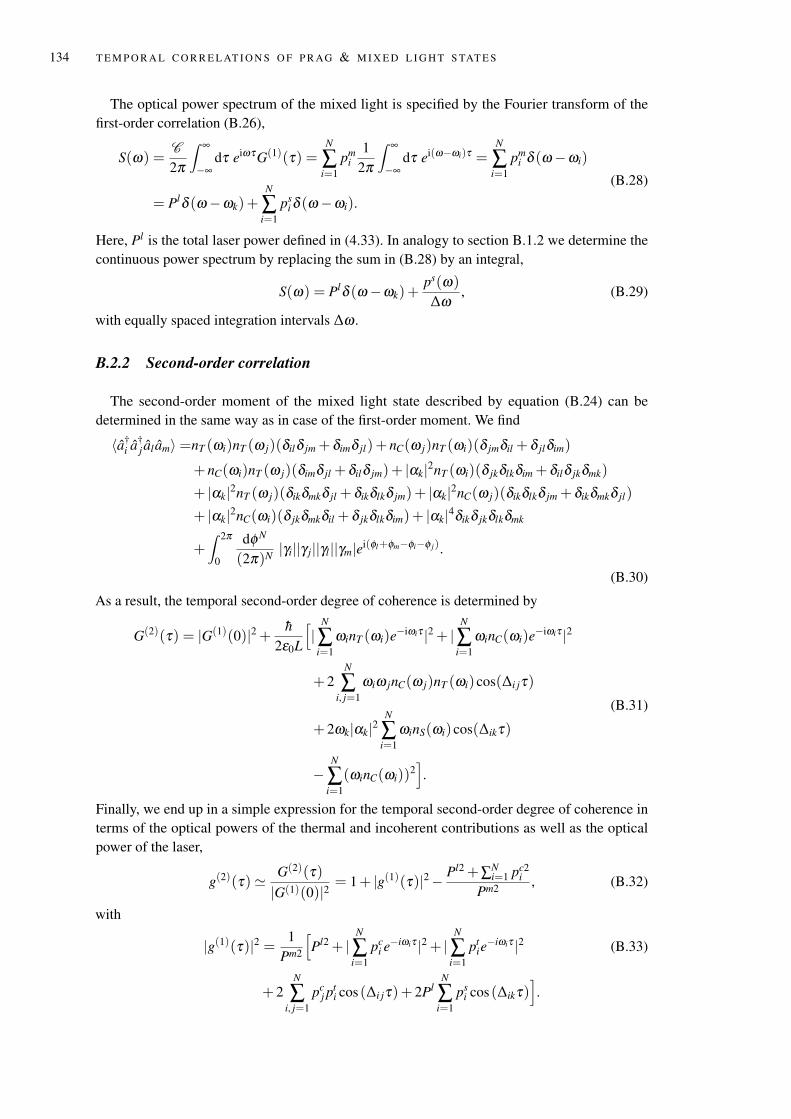
134 T E M P O R A L C O R R E L AT I O N S O F P R AG & M I X E D L I G H T S TAT E S
The optical power spectrum of the mixed light is specified by the Fourier transform of thefirst-order correlation (B.26),
S(ω) =C
2π
∫ ∞
−∞dτ eiωτG(1)(τ) =
N
∑i=1
pmi
12π
∫ ∞
−∞dτ ei(ω−ωi)τ =
N
∑i=1
pmi δ (ω−ωi)
= Plδ (ω−ωk)+N
∑i=1
psi δ (ω−ωi).
(B.28)
Here, Pl is the total laser power defined in (4.33). In analogy to section B.1.2 we determine thecontinuous power spectrum by replacing the sum in (B.28) by an integral,
S(ω) = Plδ (ω−ωk)+ps(ω)
∆ω, (B.29)
with equally spaced integration intervals ∆ω .
B.2.2 Second-order correlation
The second-order moment of the mixed light state described by equation (B.24) can bedetermined in the same way as in case of the first-order moment. We find
〈a†i a†
j al am〉=nT (ωi)nT (ω j)(δilδ jm + δimδ jl)+ nC(ω j)nT (ωi)(δ jmδil + δ jlδim)
+ nC(ωi)nT (ω j)(δimδ jl + δilδ jm)+ |αk|2nT (ωi)(δ jkδlkδim + δilδ jkδmk)
+ |αk|2nT (ω j)(δikδmkδ jl + δikδlkδ jm)+ |αk|2nC(ω j)(δikδlkδ jm + δikδmkδ jl)
+ |αk|2nC(ωi)(δ jkδmkδil + δ jkδlkδim)+ |αk|4δikδ jkδlkδmk
+∫ 2π
0
dφ N
(2π)N |γi||γ j||γl||γm|ei(φl+φm−φi−φ j).
(B.30)
As a result, the temporal second-order degree of coherence is determined by
G(2)(τ) = |G(1)(0)|2 + h2ε0L
[|
N
∑i=1
ωinT (ωi)e−iωiτ |2 + |N
∑i=1
ωinC(ωi)e−iωiτ |2
+ 2N
∑i, j=1
ωiω jnC(ω j)nT (ωi)cos(∆i jτ)
+ 2ωk|αk|2N
∑i=1
ωinS(ωi)cos(∆ikτ)
−N
∑i=1
(ωinC(ωi))2].
(B.31)
Finally, we end up in a simple expression for the temporal second-order degree of coherence interms of the optical powers of the thermal and incoherent contributions as well as the opticalpower of the laser,
g(2)(τ) ' G(2)(τ)|G(1)(0)|2 = 1+ |g(1)(τ)|2− Pl2 +∑N
i=1 pc2i
Pm2 , (B.32)
with
|g(1)(τ)|2 = 1Pm2
[Pl2 + |
N
∑i=1
pci e−iωiτ |2 + |
N
∑i=1
ptie−iωiτ |2 (B.33)
+ 2N
∑i, j=1
pcj p
ti cos (∆i jτ)+ 2Pl
N
∑i=1
psi cos (∆ikτ)
].
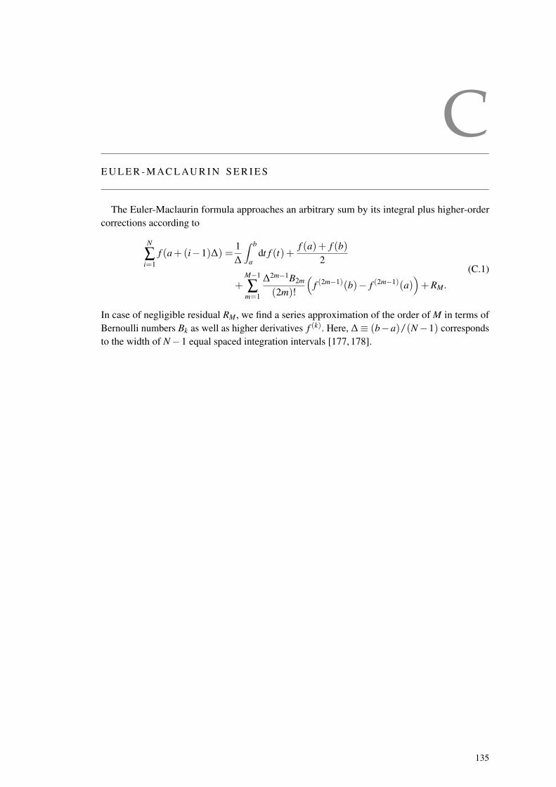
CE U L E R - M AC L AU R I N S E R I E S
The Euler-Maclaurin formula approaches an arbitrary sum by its integral plus higher-ordercorrections according to
N
∑i=1
f (a+(i−1)∆) =1∆
∫ b
adt f (t)+
f (a)+ f (b)2
+M−1
∑m=1
∆2m−1B2m
(2m)!
(f (2m−1)(b)− f (2m−1)(a)
)+RM.
(C.1)
In case of negligible residual RM, we find a series approximation of the order of M in terms ofBernoulli numbers Bk as well as higher derivatives f (k). Here, ∆≡ (b−a)/(N−1) correspondsto the width of N−1 equal spaced integration intervals [177, 178].
135

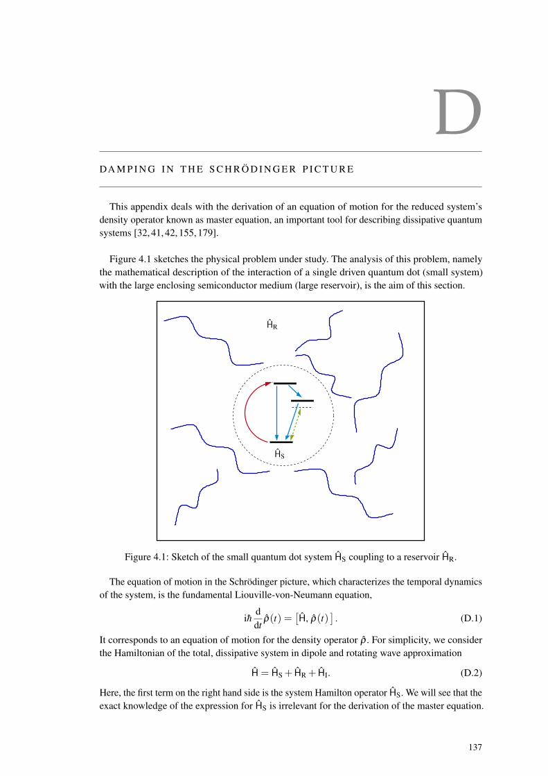
DDA M P I N G I N T H E S C H R Ö D I N G E R P I C T U R E
This appendix deals with the derivation of an equation of motion for the reduced system’sdensity operator known as master equation, an important tool for describing dissipative quantumsystems [32, 41, 42, 155, 179].
Figure 4.1 sketches the physical problem under study. The analysis of this problem, namelythe mathematical description of the interaction of a single driven quantum dot (small system)with the large enclosing semiconductor medium (large reservoir), is the aim of this section.
HR
HS
Figure 4.1: Sketch of the small quantum dot system HS coupling to a reservoir HR.
The equation of motion in the Schrödinger picture, which characterizes the temporal dynamicsof the system, is the fundamental Liouville-von-Neumann equation,
ihddt
ρ(t) =[H, ρ(t)
]. (D.1)
It corresponds to an equation of motion for the density operator ρ . For simplicity, we considerthe Hamiltonian of the total, dissipative system in dipole and rotating wave approximation
H= HS + HR + HI. (D.2)
Here, the first term on the right hand side is the system Hamilton operator HS. We will see that theexact knowledge of the expression for HS is irrelevant for the derivation of the master equation.
137
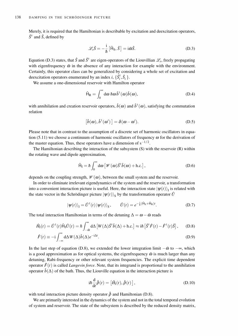
138 DA M P I N G I N T H E S C H R Ö D I N G E R P I C T U R E
Merely, it is required that the Hamiltonian is describable by excitation and deexcitation operators,S† and S, defined by
LsS = − ih
[HS, S
]= iω S. (D.3)
Equation (D.3) states, that S and S† are eigen-operators of the Liouvillian Ls, freely propagatingwith eigenfrequency ω in the absence of any interaction for example with the environment.Certainly, this operator class can be generalized by considering a whole set of excitation anddeexcitation operators enumerated by an index i, S†
i , Si .We assume a one-dimensional reservoir with Hamilton operator
HR =∫ ∞
0dω hω b†(ω)b(ω), (D.4)
with annihilation and creation reservoir operators, b(ω) and b†(ω), satisfying the commutationrelation [
b(ω), b†(ω ′)]= δ (ω−ω ′). (D.5)
Please note that in contrast to the assumption of a discrete set of harmonic oscillators in equa-tion (5.11) we choose a continuum of harmonic oscillators of frequency ω for the derivation ofthe master equation. Thus, these operators have a dimension of s−1/2.
The Hamiltonian describing the interaction of the subsystem (S) with the reservoir (R) withinthe rotating wave and dipole approximation,
HI = h∫ ∞
0dω[W (ω)S†b(ω)+ h.c.
], (D.6)
depends on the coupling strength, W (ω), between the small system and the reservoir.In order to eliminate irrelevant eigendynamics of the system and the reservoir, a transformation
into a convenient interaction picture is useful. Here, the interaction state |ψ(t)〉I is related withthe state vector in the Schrödinger picture |ψ(t)〉S by the transformation operator U
|ψ(t)〉I = U†(t) |ψ(t)〉S , U(t) = e−ih (HS+HR)t . (D.7)
The total interaction Hamiltonian in terms of the detuning ∆ = ω− ω reads
HI(t) = U†(t)HIU(t) = h∫ ∞
−ωd∆[W (∆)S†b(∆)+ h.c.
]≈ ih
[S†F(t)− F†(t)S
], (D.8)
F(t) ≡−i∫ ∞
−∞d∆W (∆)b(∆)e−i∆t . (D.9)
In the last step of equation (D.8), we extended the lower integration limit −ω to −∞, whichis a good approximation as for optical systems, the eigenfrequency ω is much larger than anydetuning, Rabi-frequency or other relevant system frequencies. The explicit time dependentoperator F(t) is called Langevin force. Note, that its integrand is proportional to the annihilationoperator b(∆) of the bath. Thus, the Liouville equation in the interaction picture is
ihddt
ˆρ(t) =[HI(t), ˆρ(t)
], (D.10)
with total interaction picture density operator ˆρ and Hamiltonian (D.8).We are primarily interested in the dynamics of the system and not in the total temporal evolution
of system and reservoir. The state of the subsystem is described by the reduced density matrix,
DA M P I N G I N T H E S C H R Ö D I N G E R P I C T U R E 139
ρS, defined by the partial trace over all reservoir degrees of freedom of the Hilbert space HR,ρS(t) = Tr Rρ(t). At the initial time t = 0, the system ρS and the reservoir ρR are assumedto be decorrelated. Thus, the state factorizes, ρ(0) = ρS(0)⊗ ρR(0). Taking the partial traceover the reservoir degrees of freedom of equation (D.10) the resulting Liouville equation for thesystem density operator is
ihddt
ˆρS(t) = TrR
[HI(t), ˆρ(t)
]. (D.11)
This differential equation, depending on the density operator ˆρS as well as ˆρR, is not closedand can therefore not be solved directly. In order to evaluate the trace on the right hand side ofequation (D.11), the evolution of ˆρR under the influence of the coupling has to be determined.
Assuming a weak coupling between the system and the reservoir, the total density operatorcan be evolved perturbatively by iterating the formal solution of its equation of motion (D.10)with t ≥ t ′,
ˆρ(t) = ˆρ(0)− ih
∫ t
0dt ′[HI(t ′), ˆρ(t ′)
]. (D.12)
Due to the weak interaction, we can stop after the second iteration process. Subsequently,resubstitution solution (D.12) into the equation of motion for the reduced density operator (D.11)yields
ddt
ˆρS(t) = −ih
TrR
[HI(t), ˆρ(0)
]− 1
h2
∫ t
0dt ′ TrR
[HI(t),
[HI(t ′), ˆρ(t ′)
]], (D.13)
in which the first term on the right hand side is proportional to the mean value of the Langevinforce operator, 〈F(t)〉, and therefore equal to zero.
For finding a closed first-order differential equation for the subsystem, we rewrite the totaldensity operator according to
ρ(t) = ρS(t)⊗ ρR +(ρ(t)− ρS(t)⊗ ρR)︸ ︷︷ ︸=δ ρ(t)
= ρS(t)⊗ ρR + δ ρ(t). (D.14)
As we consider subsystems that are much smaller than the surrounding reservoir, their interactionamong each other do not really affect the dynamics of the large environment. For a reservoirbeing in thermodynamic equilibrium, δ ρ(t) ρS(t)⊗ ρR holds and the total density operator indecorrelation approximation reads
ρ(t) = ρS(t)⊗ ρR (decorrelation approximation), (D.15)
leading to a closed differential equation when inserting this ansatz into equation (D.13),
ddt
ˆρS(t) =∫ t
0dt ′[(S ˆρS(t ′)S†− S†S ˆρS(t ′))〈F(t)F†(t ′)〉
+(S ˆρS(t ′)S†− ˆρS(t ′)S†S)〈F(t ′)F†(t)〉+(S† ˆρS(t ′)S− SS† ˆρS(t ′))〈F†(t)F(t ′)〉
+(S† ˆρS(t ′)S− ˆρS(t ′)SS†)〈F†(t ′)F(t)〉].
(D.16)
Here, terms proportional to 〈F(t)F(t ′)〉 or 〈F†(t)F†(t ′)〉 vanished in equation (D.16) due to theassumption of a non-squeezed reservoir.
140 DA M P I N G I N T H E S C H R Ö D I N G E R P I C T U R E
To evaluate the force averages in equation (D.16), further assumptions regarding the reservoirstate have to be formulated. The choice of a canonical ensemble in thermodynamic equilibriumwith density operator
ρR(t) =1Z
e−β HR , Z = Tr
e−β HR
, β =1
kBT, (D.17)
is convenient. The Hamiltonian in the exponent, HR =∫ ∞
0 d∆ h∆b†(∆)b(∆), corresponds toequation (D.4) transformed in the considered interaction picture. Such a canonical reservoir hasno mean-field component, no correlation between the modes and of course no squeezing, but anon-vanishing lowest-order moment proportional to the mean-thermal occupation number (cf.equation (2.76))
N(∆) = (eβ h(ω+∆)−1)−1, (D.18)
that is
〈b(∆)〉= 〈b(∆)b(∆′)〉= 〈b†(∆)b†(∆′)〉= 0, (D.19)
〈b†(∆)b(∆′)〉= N(∆)δ (∆−∆′), 〈b(∆)b†(∆′)〉= (N(∆)+ 1)δ (∆−∆′). (D.20)
Therefore, the Langevin force averages occurring in equation (D.16) are given by
〈F(t)F†(t ′)〉=∫ ∞
−∞d∆ |W (∆)|2e−i∆(t−t ′)(N(∆)+ 1), (D.21)
〈F†(t)F(t ′)〉=∫ ∞
−∞d∆ |W (∆)|2e−i∆(t−t ′)N(∆). (D.22)
Inserting these correlations into the equation of motion for the system density operator (cf.equation (D.16)) results into an integro-differential equation, which still remains difficult to solvewithout further simplifications regarding the time integration.
The Markov approximation enables a conversion to a relatively simple expression. In order toexplain the main idea behind this important approximation, we introduce the complex memorykernel,
K(t− t ′) ≡∫ ∞
−∞d∆ |W (∆)|2e−i∆(t−t ′) =
[F(t), F†(t ′)
], (D.23)
equivalent to the Fourier transform of the square of the absolute value of the coupling con-stant W (∆). Because W (∆) is a slowly varying function of detuning ∆, the memory kernel K(τ)is sharply peaked at τ = 0 and vanishes rapidly for times t larger than the correlation time τc
of the reservoir fluctuations. In contrast, the system density operator ˆρS varies slowly for times|t− t ′|< τc, so that the replacement ˆρS(t ′) ≈ ˆρS(t) is justified within the Markov approximation.Therefore we can write for the integral∫ t
0dt ′ K(t− t ′) ˆρS(t ′) ≈
∫ t
0dt ′ K(t− t ′) ˆρS(t) = γ(t) ˆρS(t), γ(t) =
∫ t
0dτ K(τ), (D.24)
with rate γ reaching its complex limiting value very quickly, so that the upper integration limitcan be extended to infinity in good approximation. Applying methods of complex analysis, it canbe shown, that the integral [155]
γ∞ = limtτc
γ(t) =∫ ∞
0dτ K(τ) = Γ+ iδω , (D.25)
is the sum of a damping rate Γ = π|W (ω)|2 and an energy shift δω . Applying the Markovapproximation to the integro-differential equation (D.16) and subsequently back transforming
DA M P I N G I N T H E S C H R Ö D I N G E R P I C T U R E 141
into the initial Schrödinger picture results in a birth-death process [180], the master equation inLindblad form [132]
ddt
ρS(t) = (LS +LR)ρS(t) . (D.26)
Here, the system Liouville operator,
LS ρS(t) = −ih
[HS, ρS
], (D.27)
describes the unperturbed system. The damping Liouville operator,
LR ρS(t) = Γ( N(0)︸ ︷︷ ︸stim. emission
+ 1︸︷︷︸spon. emission
)(2SρS(t)S†− S†SρS(t)− ρS(t)S†S)
+ ΓN(0)︸ ︷︷ ︸stim. absoption
(2S†ρS(t)S− SS†ρS(t)− ρS(t)SS†)
− i[δω S†S+ δωth
[S†, S
], ρS(t)
], (D.28)
considers the coupling between the environment and the system, leading to dissipation capturedby relaxation rate Γ, energy shift δω as well as thermal energy shift δωth. These energy shiftsare defined by the principle part integrals
δω = −P∫
d∆ |W (∆)|2/∆, (D.29)
δωth = −P∫
d∆ |W (∆)|2N(∆)/∆. (D.30)
The latter depends on the thermal occupation number N(∆). The first term in the dampingLiouvillian (D.28) characterizes stimulated and spontaneous emission whereas the second onespecifies stimulated absorption processes.
For a set of system operators Si, S†i equation (D.26) can be generalized by just summing over
all system operators with corresponding damping rates Γi and occupation numbers Ni. Choosingan appropriate renormalization of the energy shifts, the master equation for the reduced densityoperator with several system operator components reads
ddt
ρS(t) = −ih
[HS, ρS
]︸ ︷︷ ︸
LSρS(t)
+∑i
Γi(Ni + 1)(2Si ρS(t)S†i − S†
i Si ρS(t)− ρS(t)S†i Si )
+∑i
ΓiNi(2S†i ρS(t)Si − Si S†
i ρS(t)− ρS(t)Si S†i ). (D.31)

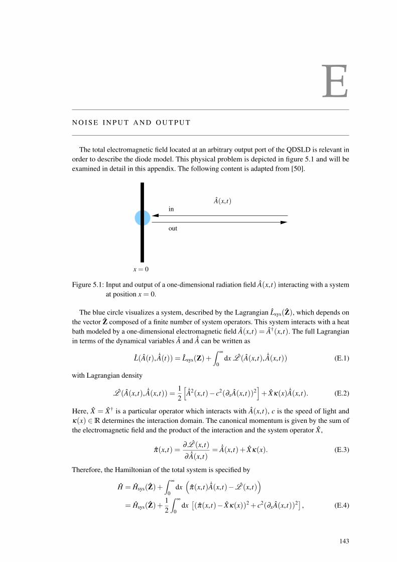
EN O I S E I N P U T A N D O U T P U T
The total electromagnetic field located at an arbitrary output port of the QDSLD is relevant inorder to describe the diode model. This physical problem is depicted in figure 5.1 and will beexamined in detail in this appendix. The following content is adapted from [50].
A(x, t)
x = 0
out
in
Figure 5.1: Input and output of a one-dimensional radiation field A(x, t) interacting with a systemat position x = 0.
The blue circle visualizes a system, described by the Lagrangian Lsys(Z), which depends onthe vector Z composed of a finite number of system operators. This system interacts with a heatbath modeled by a one-dimensional electromagnetic field A(x, t) = A†(x, t). The full Lagrangianin terms of the dynamical variables A and ˙A can be written as
L(A(t), ˙A(t)) = Lsys(Z)+∫ ∞
0dx L (A(x, t), ˙A(x, t)) (E.1)
with Lagrangian density
L (A(x, t), ˙A(x, t)) =12
[˙A2(x, t)− c2(∂xA(x, t))2
]+ Xκ(x) ˙A(x, t). (E.2)
Here, X = X† is a particular operator which interacts with A(x, t), c is the speed of light andκ(x) ∈R determines the interaction domain. The canonical momentum is given by the sum ofthe electromagnetic field and the product of the interaction and the system operator X ,
π(x, t) =∂L (x, t)
∂ ˙A(x, t)= ˙A(x, t)+ Xκ(x). (E.3)
Therefore, the Hamiltonian of the total system is specified by
H = Hsys(Z)+∫ ∞
0dx(
π(x, t) ˙A(x, t)− L (x, t))
= Hsys(Z)+12
∫ ∞
0dx[(π(x, t)− Xκ(x))2 + c2(∂xA(x, t))2] , (E.4)
143
144 N O I S E I N P U T A N D O U T P U T
with system Hamiltonian Hsys corresponding to the system Lagrangian Lsys. Introducing Fouriertransform variables,
A(x, t) =
√2
πc
∫ ∞
0dω q(ω , t)cos (ωx/c), (E.5)
π(x, t) =
√2
πc
∫ ∞
0dω p(ω , t)cos (ωx/c), (E.6)
κ(x) =√
2πc
∫ ∞
0dω κ(ω)cos (ωx/c), (E.7)
equation (E.4) can be written as
H− Hsys(Z) =12
∫ ∞
0dω
[( p(ω , t)− κ(ω)X)2 +ω2q(ω , t)2] . (E.8)
The new variables satisfy the commutation relation
[q(ω , t), p(ω ′, t) ] = ihδ (ω−ω ′). (E.9)
As a solution of the Lagrange equation,
ddt
∂L
∂ ˙q− ∂L
∂ q= 0, (E.10)
we obtain an equation of motion for the heat bath operator A(x, t),
¨A(x, t)− c2∂ 2x A(x, t) = −κ(x) ˙X , (E.11)
corresponding to a wave equation in the presence of a source. To solve this differential equation,destruction and creation operators are defined,
a(ω , t) =ω q(ω , t)+ i p(ω , t)√
2hω, a†(ω , t) =
ω q(ω , t)− i p(ω , t)√2hω
, (E.12)
in terms of continuous canonical operators,
p(ω , t) = i
√hω2(a†(ω , t)− a(ω , t)), q =
√h
2ω(a(ω , t)+ a†(ω , t)). (E.13)
We differentiate the annihilation operator (cf. equation (E.12)) with respect to time t and considerthe Heisenberg equation of motion for the radiation field operators,
˙q(ω , t) = p(ω , t)−κ(ω)X , (E.14)˙p(ω , t) = −ω2q(ω , t). (E.15)
Inserting equations (E.14)-(E.15) into the temporal derivatives of the annihilation operator resultsin
˙a(ω , t) =ω ˙q(ω , t)+ i ˙p(ω , t)√
2hω= −iω a(ω , t)−κ(ω)
√ω2h
X . (E.16)
This differential equation is solvable by formal integration in terms of initial, t0 < t, and analogousof final time, t f > t > t0,
a(ω , t) = a(ω , t0)e−iω(t−t0)−κ(ω)
√ω2h
∫ t
t0dt ′ e−iω(t−t ′)X(t ′). (E.17)
N O I S E I N P U T A N D O U T P U T 145
The first term on the right-hand side describes the free oscillating behavior of the radiationfield and the second term characterizes the interaction with the system. Next, we introduce thedefinition of input and output field operators,
Ain(t) ≡12
∫ ∞
0dω√
hπωc
[a(ω , t0)e−iω(t−t0)+ a†(ω , t0)eiω(t−t0)
], (E.18)
Aout(t) ≡12
∫ ∞
0dω√
hπωc
[a(ω , t f )e−iω(t−t f )+ a†(ω , t f )eiω(t−t f )
]. (E.19)
Obviously, the input operator is a function of the initial time t0 whereas the output operatordepends on the final time t f . By rewriting q(ω , t) in equation (E.5) with respect to the annihilationand creation operator (cf. equation (E.13)) and subsequently applying equation (E.17) as well asits Hermitian conjugate, the canonical operator in terms of the input field operator reads 1
A(x, t) =
√h
πc
∫ ∞
0dω
a(ω , t)+ a†(ω , t)√ω
cos(ωx
c
)= Ain
(t +
xc
)+ Ain
(t− x
c
)−∫ t
t0dt ′X(t ′)
√2
πc
∫ ∞
0dωκ(ω)cos(ω(t− t ′))cos
(ωxc
)= Ain
(t +
xc
)+ Ain
(t− x
c
)− 1
2
∫ t
t0dt ′X(t ′)
√2
πc
∫ ∞
0dωκ(ω)cos
(ωxc−ω(t− t ′)
)− 1
2
∫ t
t0dt ′X(t ′)
√2
πc
∫ ∞
0dωκ(ω)cos
(ωxc
+ω(t− t ′))
= Ain
(t +
xc
)+ Ain
(t− x
c
)− 1
2
∫ t
t0dt ′X(t ′) [κ(x− c(t− t ′))+κ(x+ c(t− t ′))]
− 12
∫ t
t0dt ′X(t ′)κ(x+ c(t− t ′)). (E.20)
In the last step, we used the definition of the Fourier transform of the coupling constant (seeequation (E.7)). Suitable substitution with cτ = x−c(t−t ′) in the upper first and cτ = x+c(t−t ′)in the second integral of (E.20) yields
A(x, t) = Ain
(t +
xc
)+ Ain
(t− x
c
)− 1
2
∫ xc
xc−(t−t0)
dτ κ(cτ)X(
t +(τ− x
c
))− 1
2
∫ xc+(t−t0)
xc
dτ κ(cτ)X(
t−(τ− x
c
))= Ain
(t +
xc
)+ Ain
(t− x
c
)− 1
2
∫ xc+(t−t0)
xc−(t−t0)
dτ κ(cτ)X(
t−|τ− xc|)
.
(E.21)
In the same way, we can find an expression in terms of the output field,
A(x, t) = Ain
(t +
xc
)+ Ain
(t− x
c
)− 1
2
∫ xc+(t−t0)
xc−(t−t0)
dτ κ(cτ)X(
t−|τ− xc|)
(E.22)
= Aout
(t +
xc
)+ Aout
(t− x
c
)− 1
2
∫ xc−(t−t f )
xc+(t−t f )
dτ κ(cτ)X(
t + |τ− xc|)
. (E.23)
For x lying outside the interaction regime, τ < x/c for κ(cτ) 6= 0, the argument of X in theintegrand can be replaced by |τ − x/c| = x/c− τ . Additionally, we can set t0 and t f equal
1 A similar expression of A(x, t) in terms of the output operator can be found by using the solution of the annihilationoperator as a function of future time t f , following the same calculation as in case of initial time t0.
146 N O I S E I N P U T A N D O U T P U T
to ±∞, provided that t0 is in the remote past and t f is in the remote future so that equation (E.22)and (E.23) are simplified to
A(x, t) = Ain
(t +
xc
)+ Ain
(t− x
c
)− 1
2
∫ ∞
−∞dτ κ(cτ)X
(t− x
c+ τ)
(E.24)
= Aout
(t +
xc
)+ Aout
(t− x
c
)− 1
2
∫ ∞
−∞dτ κ(cτ)X
(t +
xc− τ)
. (E.25)
Obviously, the canonical operator A(x, t) is given by the input and the output field operators atretarded and advanced time, t− x/c and t + x/c, plus a convolution integral with an integranddepending on κ and the system operator X . Equating the right-hand sides of (E.24) and (E.25)and sorting it according to the two arguments t− x/c and t + x/c, we find a relation between theinput and output operator with respect to advanced time,
Aout
(t +
xc
)= Ain
(t +
xc
)− 1
2
∫ ∞
−∞dτ κ(cτ)X
(t +
xc− τ)
. (E.26)
The solution is valid for a finite time t even if x are lying outside the interaction regime. Thus, wecan make the replacement t + x/c→ t and equation (E.26) simplifies to
Aout(t) = Ain(t)−12
∫ ∞
−∞dτ κ(cτ)X(t− τ). (E.27)
This result implies, that the output field is the sum of the incoming field and a radiating fielddescribed by the integral expression, which depends explicitly on the system operator and istherefore specified by the equation of motion of X . Thus, in case of x lying outside the interactionregime, that is outside the range of κ(x), equation (E.24) can be written as
A(x, t) = Ain
(t +
xc
)+ Aout
(t− x
c
). (E.28)
The total field A(x, t) is given by the sum of the incoming field Ain(t + x/c) at advanced timet + x/c and the outgoing field Aout(t− x/c) at retarded time t− x/c.
P O I N T W I S E L O C A L I Z E D I N T E R AC T I O N Consider the case of a negligibly small systemlocalized at position x = 0 which interacts with the electromagnetic field A(x, t) within a smallε-region (such a system could be e.g. an atom). The pointwise localized coupling can be describedby a delta distribution
κ(x) = 2√
γcδ (x). (E.29)
Its Fourier transform corresponds to a constant, frequency-independent coupling strength
κ(ω) =√
2γ/π , (E.30)
Equation (E.30) is the Markov approximation, discussed in appendix D. Inserting equation (E.29)into the output relation (E.27) leads to the simple expression
Aout(t) = Ain(t)−√
γc
X(t). (E.31)
The input field Ain(t) can be interpreted as noise input. The type of noise depends on the statisticsof the field amplitudes a(ω , t0) and a†(ω , t0) (see equation (E.18)). Obviously, their dependencyon the initial time t0 reveals that the choice of the input field is arbitrary, that is, Ain is not affectedby the system itself. In contrast, the output field described by equation (E.31) is specified by theinput noise and the small system.
FQ UA N T U M S T O C H A S T I C P RO C E S S E S : I T Ô V S . S T R AT O N OV I C H
This appendix deals with the quantum white noise concept for quantum systems clearly for-mulated by C. W. Gardiner and M. J. Collett [144]. After its formulation we define quantumstochastic integral equations in terms of the quantum Wiener process corresponding to quantumwhite noise. In close analogy to classical considerations, one can define two different integralsnamed after their inventors K. Itô and R. Stratonovich, which again result into different quantumstochastic differential equations (QSDEs) directly related with the quantum Langevin equation.Additionally, we will study the relation between the Itô and Stratonovich QSDE and summarizethe main differences between them. We will see that the Itô version has some more mathematicaladvantages compared to Stratonovich which in turn has more in common with physical consider-ations. A detailed analysis of classical stochastic processes as well as the quantum mechanicalanalog is written in reference [181] and [50, 144].
Consider an open, noisy system described by the system Hamilton operator Hs which linearlycouples to a heat bath of harmonic oscillators Hr described by the interaction Hamiltonian Hi,that is the total Hamiltonian is given by
H = Hs + Hr + Hi. (F.1)
From the knowledge of this Hamiltonian, we can specify the quantum Langevin equation byformal integration (in terms of initial time) of the Heisenberg equations of motion for eachsystem operator and assuming an approximately constant coupling between system and reservoir(Markov approximation). A detailed derivation of the quantum Langevin equation of an arbitrarysystem operator a with system Hamiltonian Hs in terms of the system operators c, decay rates γand noise terms bin can be found in reference [50]. Here, we only will give the result
˙a = − ih
[a, Hs
]−[a, c† ](γ
2c+√
γ bin
)+(γ
2c† +√
γ b†in
)[a, c ] . (F.2)
Please note, the noise operators depend explicitly on initial time t0 < t (see equation (5.163)).With the help of the input-output relation, the quantum Langevin equation can also be expressedin terms of the output operator bout depending on the final time t f > t (see equation (5.176)).Due to causality, the system operator a(t) is independent of bin(t ′) for t ′ > t. Vice versa, a(t) isindependent of bout(t ′) for t ′ < t, captured by the commutation relations[
a(t), bin(t ′)]= −Θ(t− t ′)
√γ [a(t), c(t ′) ] , (F.3)[
a(t), bout(t ′)]= Θ(t ′− t)
√γ [a(t), c(t ′) ] , (F.4)
which depend on the Heaviside function
Θ(t) =
1, t > 012 , t = 0
0, t < 0
. (F.5)
147
148 Q UA N T U M S T O C H A S T I C P RO C E S S E S : I T Ô V S . S T R AT O N OV I C H
Q UA N T U M W I E N E R P RO C E S S The quantum state of the operator bin determines the kindof noise input of a system with Hamiltonian Hs. Quantum mechanically, there always existsquantum noise due to zero-point fluctuations of the external input field. Depending on the systemunder study, additional noises contributing to the total spectrum have to be considered. Asalready mentioned, the idealized white noise input will be studied in detail within this appendix.Compared to classical white noise theory, quantum white noise can be described by a densityoperator resulting in delta-correlated expectation values,
〈b†in(t)bin(t ′)〉= Nδ (t− t ′), (F.6)
〈bin(t)b†in(t′)〉= (N + 1)δ (t− t ′), (F.7)
depending on the constant value N. In analogy to classical stochastic methods one can define aquantum Wiener process1 by the integral
B(t, t0) =∫ t
t0dt ′bin(t ′). (F.8)
From this definition, we find the commutation relation and expectation values for the Wienerprocess [
B(t, t0), B†(t, t0)]= t− t0, (F.9)
〈B†(t, t0)B(t, t0)〉= N(t− t0), (F.10)
〈B(t, t0)B†(t, t0)〉= (N + 1)(t− t0). (F.11)
Furthermore, the operators B(t, t0) have to reveal a Gaussian distribution with density operator
ρ(t, t0) = (1− e−β )exp(−β B†(t, t0)B(t, t0)
t− t0
)(F.12)
and mean occupation number
N = (eβ −1)−1. (F.13)
The basic principles are established for formulating quantum stochastic integrations in terms ofItô and Stratonovich which will be discussed in the next subsections.
F.1 I T Ô C A L C U L U S
Generally, for an arbitrary system operator X(t), the quantum Itô integral with time orderingt0 < t1 < ... < tn = t is defined by
(I)∫ t
t0X(t ′)dB(t ′) = lim
n→∞
n
∑i=0
X(ti)[B(ti+1, t0)− B(ti, t0)
]. (F.14)
For notational convenience we introduced the abbreviation (I) in order to distinguish between theItô and the Stratonovich formulation of stochastic integrals. One can verify that the incrementsdB(t), dB†(t) commute with the system operator X(t),
(I)∫ t
t0X(t ′)dB(t ′) = (I)
∫ t
t0dB(t ′)X(t ′), (F.15)
1 Classically, a Wiener process is described by a Fokker Planck equation with constant diffusion and zero drift term.
F.2 S T R AT O N OV I C H C A L C U L U S 149
as a result of equation (F.14) and quantum causality (F.3).The Itô quantum stochastic differential equation (QSDE) of a system operator a(t) in terms
of an arbitrary system operator c with system Hamiltonian Hs is defined by
(I) da = − ih
[a, Hs
]dt +
γ2(N + 1)(2c†ac− ac†c− c†ca)dt
+γ2
N(2cac†− acc†− cc†a)dt−√γ[a, c† ]dB(t)+
√γ dB†(t) [a, c ]
(F.16)
with N described by equation (F.13).The Itô increments satisfy the identities
(dB(t))2 = (dB†(t))2 = 0, (F.17)
dB(t)dB†(t) = (N + 1)dt, (F.18)
dB†(t)dB(t) = Ndt. (F.19)
Furthermore, terms like dtdB, dtdB†, dt2 and higher orders are negligible, in direct analogy toclassical considerations. By the help of these relations, one can derive the Itô rules of calculus
d(ab) = adb+(da)b+(da)(db), (F.20)
which obviously does not agree with the ordinary calculus.
F.2 S T R AT O N OV I C H C A L C U L U S
The Stratonovich quantum stochastic integral is defined by
(S)∫ t
t0X(t ′)dB(t ′) = lim
n→∞
n
∑i=0
X(ti)+ X(ti+1)
2[B(ti+1, t0)− B(ti, t0)
], (F.21)
where (S) labels the Stratonovich version of a stochastic integral for an arbitrary system opera-tor X . Please note, that this increment does not commute with X , which can be directly verifiedby calculating the difference of the integrals under considerations of the causality condition (F.3)
(S)∫ t
t0X(t ′)dB(t ′)− (S)
∫ t
t0dB(t ′)X(t ′) =
√γ2
∫ t
t0dt ′[X(t ′), c(t ′)
]. (F.22)
F.2.1 Connection between Itô and Stratonovich stochastic integral
In order to formulate the Stratonovich version of a quantum stochastic differential equation, itis quite reasonable to study the connection between the integral definitions of Itô and Stratonovich.In doing so, we rewrite equation (F.21) in terms of the mean time ti = (ti + ti+1)/2, leading tothe integral equation
(S)∫ t
t0X(t ′)dB(t ′) = lim
n→∞
[n
∑i=0
X(ti)(B(ti+1)− B(ti)
)+
n
∑i=0
X(ti)(B(ti)− B(ti)
)]. (F.23)
In addition, we set
X(ti) = X(ti)+ dX(ti), (F.24)
150 Q UA N T U M S T O C H A S T I C P RO C E S S E S : I T Ô V S . S T R AT O N OV I C H
where dX(ti) is specified by equation (F.16) and
dti = ti− ti, (F.25)
dB(ti) = B(ti)− B(ti), (F.26)
which will be valid to lowest order [144]. Thus, the Stratonovich stochastic integral (F.23) can bewritten as
(S)∫ t
t0X(t ′)dB(t ′) = lim
n→∞
[n
∑i=0
X(ti)(B(ti+1)− B(ti)
)+
n
∑i=0
X(ti)(B(ti)− B(ti)
)−√γ
n
∑i=0
[X(ti), c†(ti)
](B(ti)− B(ti)
)(B(ti)− B(ti)
)+√
γn
∑i=0
[X(ti), c(ti)
](B†(ti)− B†(ti)
)(B(ti)− B(ti)
)].
(F.27)
Considering the identities (F.17)-(F.19), one can express the Stratonovich integral in terms of theItô integral (cf. equation (F.14)) via
(S)∫ t
t0X(t ′)dB(t ′) = (I)
∫ t
t0X(t ′)dB(t ′)+
12√
γ N∫ t
t0
[X(t ′), c(t ′)
]dt ′. (F.28)
In the same way, we find
(S)∫ t
t0X(t ′)dB†(t ′) = (I)
∫ t
t0X(t ′)dB†(t ′)− 1
2√
γ(N + 1)∫ t
t0
[X(t ′), c†(t ′)
]dt ′, (F.29)
(S)∫ t
t0dB(t ′)X(t ′) = (I)
∫ t
t0X(t ′)dB(t ′)+
12√
γ(N + 1)∫ t
t0
[X(t ′), c(t ′)
]dt ′, (F.30)
(S)∫ t
t0dB†(t ′)X(t ′) = (I)
∫ t
t0X(t ′)dB†(t ′)− 1
2√
γN∫ t
t0
[X(t ′), c†(t ′)
]dt ′. (F.31)
With these connections between the integral representations of both, Stratonovich and Itô, wecan specify the Stratonovich version of a quantum stochastic differential equation
(S) da =− ih
[a, Hs
]dt− γ
2([
a, c† ] c− c† [a, c ])
dt−√γ[a, c† ]dB(t)
+√
γdB†(t) [a, c ](F.32)
This can be proven by inserting the integral representation implicitly into equation (F.32), thatis
(S)∫ t
t0da =− i
h(S)
∫ t
t0
[a, Hs
]dt− γ
2(S)
∫ t
t0
([a, c† ] c− c† [a, c ]
)dt
−√γ (S)∫ t
t0
[a, c† ]dB(t)+
√γ (S)
∫ t
t0dB†(t) [a, c ] .
(F.33)
Using equation (F.28) and (F.31) in the second line of the Stratonovich equation (F.33) andevaluating the commutators, we find
(I) da =− ih
[a, Hs
]dt +
γ2(N + 1)(2c†ac− ac†c− c†ca)dt
+γ2
N(2cac†− acc†− cc†a)dt−√γ[a, c† ]dB(t)+
√γ dB†(t) [a, c ] .
(F.34)
F.3 F O R M U L AT I O N O F I T Ô Q S D E S 151
The solution corresponds exactly to the Itô quantum stochastic differential equation (cf. equa-tion (F.16)). Please note, that the Stratonovich QSDE (F.32) is again exactly the quantumLangevin equation form [148] and therefore justifies Itô’s QSDE definition (F.16).
Furthermore, as a result of the Itô formalism, one can easily show that the Stratonovich versionobeys the usual rules of calculus according to
(S) d(ab) = (da)b+ adb. (F.35)
F.3 F O R M U L AT I O N O F I T Ô Q S D E S
Upon introducing Itô and Stratonovich QSDEs we are left with the technical problem ofsetting up an Itô QSDE from the knowledge of the total system described by the Hamiltonian(F.1). Former considerations of this section highlights the equivalent form of the Stratonovichequation and the quantum Langevin equation. Thus, from the knowledge of the quantum Langevinequation (F.2) we can directly specify the Stratonovich QSDE with increment dB = bindt yieldingexactly equation (F.32). On the other hand, we are allowed to directly determine the Itô QSDE(F.16) from the knowledge of the Stratonovich form.
F.4 C O M PA R I S O N B E T W E E N I T Ô A N D S T R AT O N OV I C H
Table A1 summarizes relevant differences between the Itô and Stratonovich quantum stochasticdifferential equations. For further information, please have a look at [50].
Itô QSDE (F.16) Stratonovich QSDE (F.32)
No natural physically motivated choiceNatural physical choice (equivalent to
Langevin equation)
Increments commute with systemoperators
Increments do not commute with systemoperators
Special calculus Ordinary calculus
No QSDE definition without knowledgeabout N and bath statistics
No integral equation definition withoutknowledge about QSDE
A quantum white noise theory Also valid for non-white noise
Table A1: Comparison of Itô and Stratonovich QSDE [50].

GD I F F E R E N T I A L E Q UAT I O N O F T H E F O U RT H - O R D E R M O M E N TO F T H E Q D S L D F I E L D A M P L I T U D E S
In section 7.2 we analyzed the central second-order degree of coherence of light-emittingQDLSDs based on our microscopic theory introduced in chapter 5. In this context, we set upa differential equation for the internal field amplitudes 〈a†
i a†k aman〉 (cf. equation (7.12)). This
equation of motion itself depends on further fourth-order moments in terms of quantum dotcoherences and field amplitudes. Their solutions are determined within the approximations listedin section 5.3.1. In general these approximations result in the factorization of averages (seeequations (7.16)-(7.18)). The application of adiabatic elimination delivers the desired results,which can be inserted directly into the first-order differential equation (7.12). We find the generalexpression
ddt〈a†
i a†k aman〉 ≈−αikmn〈a†
i a†k aman〉+
M
∑j=1
g ji g j
kg j∗m g j∗
n ξ jikmn
+M
∑j=1
∑ks
w j
[g ji g j∗
s
ϑ jkmn
〈a†s a†
k aman〉+g j
kg j∗s
ϑ jimn
〈a†i a†
s aman〉
+g j∗
m g js
ϑ j∗nki
〈a†i a†
k as an〉+g j∗
n g js
ϑ j∗mki
〈a†i a†
k amas 〉]
+M
∑j=1
[ g ji
ϑ jkmn
(g j∗m δkn + g j∗
n δkm)nk +g j
k
ϑ jimn
(g j∗m δin + g j∗
n δim)ni
+g j∗
m
ϑ j∗nki
(g jkδin + g j
i δkn)nn +g j∗
n
ϑ j∗mki
(g jkδmi + g j
i δkm)nm
]σ j
11
(G.1)
with
ξ jikmn =2λ j
mλ jn
(1
ϑ jkmn
+1
ϑ jimn
)+ 2λ j∗
k λ j∗i
(1
ϑ j∗nki
+1
ϑ j∗mki
)+λ j∗
k λ jn
(1
ϑ jkmn
+1
ϑ j∗nki
)
+λ j∗k λ j
m
(1
ϑ jkmn
+1
ϑ j∗mki
)+λ j∗
i λ jn
(1
ϑ jimn
+1
ϑ j∗nki
)+λ j∗
i λ jm
(1
ϑ jimn
+1
ϑ j∗mki
) (G.2)
and
λ ji =
niw j +σ j11
Γ j/2+ i∆ ji
. (G.3)
153

HS E C O N D - O R D E R D E G R E E O F C O H E R E N C E O F Q D S L D S
In this appendix we specify the temporal second-order degree of coherence g(2)(τ) of ourmodeled QDSLD. In doing so, we first set up a fourth-order moment QSDE for the field operatorswith regard to time t ′ > t, 〈a†
i (t)a†k(t′)am(t
′)an(t)〉t ′ , emphasized by the index t ′ at the bottomright of the quantum average bracket, 〈...〉t ′ . We apply the Itô derivation rule with respect to t ′
(see equation (F.20)) and find
d〈a†i (t)a
†k(t′)am(t
′)an(t)〉t ′ =〈a†i (t)da†
k(t′)am(t
′)an(t)〉+ 〈a†i (t)a
†k(t′)dam(t
′)an(t)〉+ 〈a†
i (t)(da†k(t′))(dam(t
′))an(t)〉.(H.1)
Considering quantum causality and the fact that the increments commute with and are statisticallyindependent of the system operators at the same time [50], the first term on the right-hand side ofequation (H.1) under the assumption of vacuum input reads
〈a†i (t)da†
k(t′)am(t
′)an(t)〉=[
i∆k−γ l + γr
2
]〈a†
i (t)a†k(t′)am(t
′)an(t)〉dt ′
+M
∑j=1
g jk〈a†
i (t)σj†
21 (t′)am(t
′)an(t)〉dt ′.(H.2)
The second term in equation (H.1) is determined in the same way whereas the last term vanishesunder consideration of absent correlations between left and right bath modes, 〈dBL(†)dBR(†)〉= 0,as well as vacuum input. Equation (H.1) can be written as
d〈a†i (t)a
†k(t′)am(t
′)an(t)〉t ′ =−[i(∆m−∆k)+ γ l + γr
]〈a†
i (t)a†k(t′)am(t
′)an(t)〉dt ′
+M
∑j=1
[g j
k〈a†i (t)σ
j†21 (t
′)am(t′)an(t)〉
+ g j∗m 〈a†
i (t)a†k(t′)σ j
21(t′)an(t)〉
]dt ′.
(H.3)
This solution includes averages between quantum dot transitions and field operators. We considerthe second correlation term in equation (H.3), which is described by the QSDE
d〈a†i (t)σ
j†21 (t
′)am(t′)an(t)〉t ′ =−
(i∆ j
m +Γ j
2
)〈a†
i (t)σj†
21 (t′)am(t
′)an(t)〉dt ′
+ ∑kr
g j∗r 〈a†
i (t)wj(t ′)a†
r (t′)am(t ′)an(t)〉dt ′
+M
∑j=1
g j∗m 〈a†
i (t)σj
11(t′)an(t)〉dt ′
(H.4)
with
∆ jm = ∆m−δω j
12, Γ j = Γ j21 +R+ γ l + γr. (H.5)
155
156 S E C O N D - O R D E R D E G R E E O F C O H E R E N C E O F Q D S L D S
We follow the assumptions made in section 5.3.1 and decorrelate quantum dot populations andinternal waveguide modes by making the replacements,
〈a†i (t)w
j(t ′)a†k(t′)am(t ′)an(t)〉 ≈ w j(t ′)〈a†
i (t)a†k(t′)am(t ′)an(t)〉, (H.6)
〈a†i (t)σ
j†21 (t
′)σ j′21(t
′)an(t)〉 ≈σ j11(t
′)〈a†i (t)an(t)〉δ j j′+ 〈a†
i (t)σj′
21(t′)〉〈σ j†
21 (t′)an(t)〉, (H.7)
with 〈a†i (t)σ
j′21(t
′)〉 specified in equation (6.8). Finally, we adiabatically eliminate the average〈a†
i (t)σj†
21 (t′)am(t ′)an(t)〉. In the same way we can calculate the last correlation term on the
right-hand side of equation (H.3). Again, we only consider coupling strength terms which are atmost of the order of 2. Therefore, the Itô QSDE (H.3) reduces to
ddt ′〈a†
i (t)a†k(t′)am(t
′)an(t)〉=−[i(∆m−∆k)+ γ l + γr
]〈a†
i (t)a†k(t′)am(t
′)an(t)〉
+M
∑j=1
∑kr g jkg j∗
r w j(t ′)〈a†i (t)a
†r (t′)am(t ′)an(t)〉
Λ jm
+M
∑j=1
∑kr g j∗m g j
rw j(t ′)〈a†i (t)a
†k(t′)ar(t ′)an(t)〉
Λ j∗k
+M
∑j=1
g jkg j∗
m σ j11(t
′)ni(t)δin
( 1
Λ jm+
1
Λ j∗k
)(H.8)
with
Λ ji = Γ j/2+ i∆ j
i . (H.9)
This equation can be separated into diagonal and off-diagonal elements in terms of the couplingstrength. We assume that the off-diagonal ones weakly contribute compared to the diagonalelements in direct analogy to the assumption made in section 7. Thus, in first-order perturbationtheory, we can neglect the off-diagonal terms. Furthermore, we replace the inversion w j(t ′) byits stationary solution w js, w j(t ′) ≈ w js, analog to the calculation of g(2)(0) in section 7.2. Theequation of motion for the fourth-order moment reads
limt→∞
ddt ′〈a†
i (t)a†k(t′)am(t
′)an(t)〉= −αkm〈a†i (t)a
†k(t′)am(t
′)an(t)〉+βikmδin (H.10)
with
αkm = i(∆m−∆k)+ γ l + γr−M
∑j=1
w js
(|g j
k|2
Λ jm
+|g j
m|2Λ j∗
k
), (H.11)
βikm =M
∑j=1
g jkg j∗
m σ js11ns
ii(∆m−∆k)+Γ j
Λ jmΛ j∗
k
. (H.12)
This differential equation is solvable by the method of variation of constants with τ = t ′− t > 0,which leads to
limt→∞〈a†
i (t)a†k(t + τ)am(t + τ)an(t)〉=
βikm
αkmδin + e−αkmτ
(〈a†
i a†k aman〉s−
βikm
αkmδin
). (H.13)
The resulting temporal second-order correlation function is given by
g(2)(τ) ' G(2)(τ)|G(1)(0)|2 =
∑ki,kk ,km,kn>0wsikmn
βikmαkm
δin(1− e−αkm|τ|
)∑ki,kk>0ws
ikiknsi n
sk
+ g(2)(0)e−αkm|τ|, (H.14)
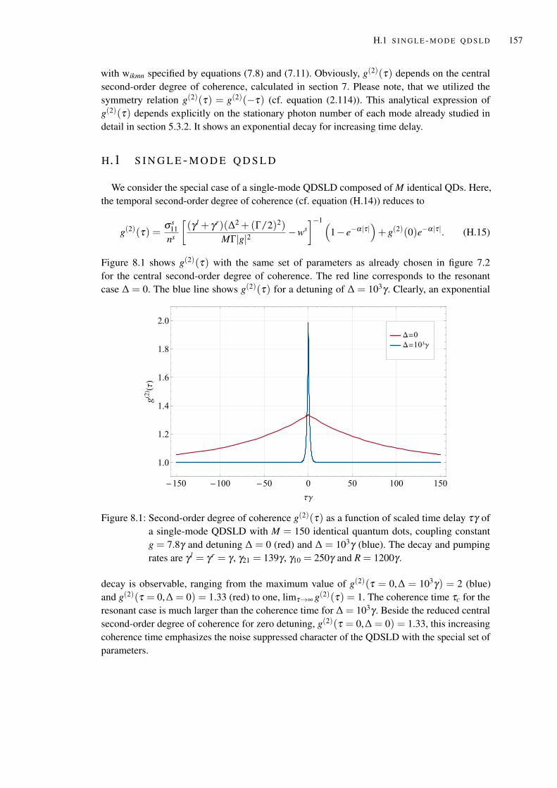
H.1 S I N G L E - M O D E Q D S L D 157
with wikmn specified by equations (7.8) and (7.11). Obviously, g(2)(τ) depends on the centralsecond-order degree of coherence, calculated in section 7. Please note, that we utilized thesymmetry relation g(2)(τ) = g(2)(−τ) (cf. equation (2.114)). This analytical expression ofg(2)(τ) depends explicitly on the stationary photon number of each mode already studied indetail in section 5.3.2. It shows an exponential decay for increasing time delay.
H.1 S I N G L E - M O D E Q D S L D
We consider the special case of a single-mode QDSLD composed of M identical QDs. Here,the temporal second-order degree of coherence (cf. equation (H.14)) reduces to
g(2)(τ) =σ s
11ns
[(γ l + γr)(∆2 +(Γ/2)2)
MΓ|g|2 −ws]−1(
1− e−α|τ|)+ g(2)(0)e−α|τ|. (H.15)
Figure 8.1 shows g(2)(τ) with the same set of parameters as already chosen in figure 7.2for the central second-order degree of coherence. The red line corresponds to the resonantcase ∆ = 0. The blue line shows g(2)(τ) for a detuning of ∆ = 103γ . Clearly, an exponential
Δ=0Δ=10³γ
-150 -100 -50 0 50 100 150
1.0
1.2
1.4
1.6
1.8
2.0
τγ
g(2) (τ)
Figure 8.1: Second-order degree of coherence g(2)(τ) as a function of scaled time delay τγ ofa single-mode QDSLD with M = 150 identical quantum dots, coupling constantg = 7.8γ and detuning ∆ = 0 (red) and ∆ = 103γ (blue). The decay and pumpingrates are γ l = γr = γ , γ21 = 139γ , γ10 = 250γ and R = 1200γ .
decay is observable, ranging from the maximum value of g(2)(τ = 0,∆ = 103γ) = 2 (blue)and g(2)(τ = 0,∆ = 0) = 1.33 (red) to one, limτ→∞ g(2)(τ) = 1. The coherence time τc for theresonant case is much larger than the coherence time for ∆ = 103γ . Beside the reduced centralsecond-order degree of coherence for zero detuning, g(2)(τ = 0,∆ = 0) = 1.33, this increasingcoherence time emphasizes the noise suppressed character of the QDSLD with the special set ofparameters.

B I B L I O G R A P H Y
[1] M. Blazek and W. Elsäßer, “Coherent and thermal light: Tunable hybrid states withsecond-order coherence without first-order coherence,” Phys. Rev. A, vol. 84, p. 063840,2011.
[2] T. H. Maiman, “Stimulated optical radiation in ruby,” Nature, vol. 187, pp. 493–494, 1960.
[3] R. J. Glauber, “Photon correlations,” Phys. Rev. Lett., vol. 10, pp. 84–86, 1963.
[4] R. J. Glauber, “The quantum theory of optical coherence,” Phys. Rev., vol. 130, pp. 2529–2539, 1963.
[5] R. J. Glauber, “Coherent and incoherent states of the radiation field,” Phys. Rev., vol. 131,pp. 2766–2788, 1963.
[6] R. J. Glauber, The quantum theory of optical coherence. Wiley-VCH Verlag GmbH & Co.KGaA, 2007.
[7] R. J. Glauber, “One hundred years of light quanta,” Nobel Lecture, 2005.
[8] M. Lax, “Quantum noise. X. density-matrix treatment of field and population-differencefluctuations,” Phys. Rev., vol. 157, pp. 213–231, 1967.
[9] M. Lax and W. H. Louisell, “Quantum noise. XII. Density-operator treatment of field andpopulation fluctuations,” Phys. Rev., vol. 185, pp. 568–591, 1969.
[10] H. Haken, Laser theory. Springer-Verlag, 1984.
[11] H. Haken, Light: Laser light dynamics. No. Bd. 2, North-Holland Publishing Company,1985.
[12] R. Graham and H. Haken, “Quantum theory of light propagation in a fluctuating laser-active medium,” Zeitschrift für Physik A Hadrons and Nuclei, vol. 213, no. 5, pp. 420–450,1968.
[13] M. O. Scully and W. E. Lamb, “Quantum theory of an optical maser. I. General theory,”Phys. Rev., vol. 159, pp. 208–226, 1967.
[14] M. Sargent, M. Scully, and W. Lamb, Laser physics. Addison-Wesley Pub. Co., 1976.
[15] R. Hanbury Brown and R. Q. Twiss, “Correlation between photons in two coherent beamsof light,” Nature, vol. 177, pp. 27–29, 1956.
[16] H. J. Carmichael and D. F. Walls, “Proposal for the measurement of the resonant Starkeffect by photon correlation techniques,” J. Phys. B: Atom. Molec. Phys., vol. 9, no. 4,p. L43, 1976.
[17] H. J. Kimble, M. Dagenais, and L. Mandel, “Photon antibunching in resonance fluores-cence,” Phys. Rev. Lett., vol. 39, pp. 691–695, 1977.
159
160 Bibliography
[18] P. Michler, A. Imamoglu, M. D. Mason, P. J. Carson, G. F. Strouse, and S. K. Buratto,“Quantum correlation among photons from a single quantum dot at room temperature,”Nature, vol. 406, pp. 968–970, 2000.
[19] T. H. Stievater, X. Li, D. G. Steel, D. Gammon, D. S. Katzer, D. Park, C. Piermarocchi,and L. J. Sham, “Rabi oscillations of excitons in single quantum dots,” Phys. Rev. Lett.,vol. 87, p. 133603, 2001.
[20] A. Wallraff, D. I. Schuster, A. Blais, L. Frunzio, R. S. Huang, J. Majer, S. Kumar, S. M.Girvin, and R. J. Schoelkopf, “Strong coupling of a single photon to a superconductingqubit using circuit quantum electrodynamics,” Nature, vol. 431, pp. 162–167, 2004.
[21] T. Basché, W. E. Moerner, M. Orrit, and H. Talon, “Photon antibunching in the fluorescenceof a single dye molecule trapped in a solid,” Phys. Rev. Lett., vol. 69, pp. 1516–1519, 1992.
[22] R. Brouri, A. Beveratos, J.-P. Poizat, and P. Grangier, “Photon antibunching in the fluores-cence of individual color centers in diamond,” Opt. Lett., vol. 25, no. 17, pp. 1294–1296,2000.
[23] M. A. Nielsen and I. L. Chuang, Quantum computation and quantum information: 10thanniversary edition. Cambridge University Press, 2010.
[24] M. C. Amann and J. Boeck, “High-efficiency superluminescent diodes for optical-fibretransmission,” Electronics Letters, vol. 15, no. 2, pp. 41–42, 1979.
[25] K. Böhm, R. Ulrich, P. Russer, and E. Weidel, “Low-noise fiber-optic rotation sensing,”Opt. Lett., vol. 6, no. 2, pp. 64–66, 1981.
[26] X. Li, Q. Sun, J. Wo, M. Zhang, and D. Liu, “Hybrid TDM/WDM-based fiber-opticpticsensor network for perimeter intrusion detection,” Journal of Lightwave Technology,vol. 30, no. 8, pp. 1113–1120, 2012.
[27] R. Slavík and J. Homola, “Ultrahigh resolution long range surface plasmon-based sensor,”Sensors and Actuators B: Chemical, vol. 123, no. 1, pp. 10 – 12, 2007.
[28] D. Huang, E. A. Swanson, C. P. Lin, J. S. Schuman, W. G. Stinson, W. Chang, M. R. Hee,T. Flotte, K. Gregory, C. A. Puliafito, and J. G. Fujimoto, “Optical coherence tomography,”Science, vol. 254, no. 5035, pp. 1178–1181, 1991.
[29] F. Boitier, A. Godard, E. Rosencher, and C. Fabre, “Measuring photon bunching atultrashort timescale by two-photon absorption in semiconductors,” Nature Physics, vol. 5,pp. 267–270, 2009.
[30] F. Boitier, Absorption à deux photons et effets de correlation quantique dans les semicon-ducteurs. PhD thesis, Office Nat. d’études et de Recherchers Aérospat., Châtillon Cedex,2011.
[31] R. J. Glauber and M. Lewenstein, “Quantum optics of dielectric media,” Phys. Rev. A,vol. 43, pp. 467–491, 1991.
[32] W. Vogel and D. G. Welsch, Quantum optics. Wiley, 2006.
[33] M. Wubs, L. G. Suttorp, and A. Lagendijk, “Multipole interaction between atoms andtheir photonic environment,” Phys. Rev. A, vol. 68, p. 013822, 2003.
Bibliography 161
[34] O. Heaviside, Electrical Papers. No. Bd. 1 in AMS Chelsea Publishing Series, AmericanMathematical Society, 2003.
[35] J. C. Maxwell, “A dynamical theory of the elektromagnetic field,” Philos. Trans. Roy. Soc.London, vol. 155, pp. 459–512, 1865.
[36] J. D. Jackson, Classical electrodynamics. Wiley, 2012.
[37] C. C. Tannoudji, J. D. Roc, and G. Grynberg, Photons and atoms: Introduction to quantumelectrodynamics. New York: Wiley, 1989.
[38] R. Loudon, The quantum theory of light. OUP Oxford, 2000.
[39] W. H. Louisell, Quantum statistical properties of radiation. John Wiley & Sons Canada,Limited, 1973.
[40] R. Loudon, The quantum theory of light. Oxford university press, 1978.
[41] D. F. Walls and G. J. Milburn, Quantum optics. Springer Berlin Heidelberg, 2012.
[42] M. O. Scully and M. S. Zubairy, Quantum optics. Cambridge University Press, 1997.
[43] J. Garrison and R. Chiao, Quantum optics. OUP Oxford, 2008.
[44] E. Schrödinger, “Der stetige Übergang von der Mikro- zur Makromechanik,” Naturwis-senschaften, vol. 14, pp. 664–666, 1926.
[45] H. Weyl, The theory of groups and quantum mechanics. Dover books on advancedmathematics, Dover Publications, 1950.
[46] R. M. Wilcox, “Exponential operators and parameter differentiation in quantum physics,”J. Math. Phys., vol. 8, no. 4, pp. 962–982, 1967.
[47] E. Wigner, “On the quantum correction for thermodynamic equilibrium,” Phys. Rev.,vol. 40, pp. 749–759, 1932.
[48] W. P. Schleich, Quantum optics in phase space. Berlin: Wiley-VCH Verlag GmbH & Co,2001.
[49] L. Mandel and E. Wolf, Optical coherence and quantum optics. Cambridge UniversityPress, 1995.
[50] C. Gardiner and P. Zoller, Quantum noise. Springer, 2000.
[51] C. C. Tannoudji, J. D. Roc, and G. Grynberg, Atom - photon interactions: Basic processand appilcations. WILEY-VCH Verlag GmbH & Co, 2008.
[52] R. J. Glauber, “The quantum theory of optical coherence,” Phys. Rev., vol. 130, pp. 2529–2539, 1963.
[53] M. D. Srinivas and E. B. Davies, “Photon counting probabilities in quantum optics,” OpticaActa: International Journal of Optics, vol. 28, no. 7, pp. 981–996, 1981.
[54] P. Lambropoulos and D. Petrosyan, Fundamentals of quantum optics and quantum infor-mation. Springer Berlin Heidelberg, 2007.
[55] N. Wiener, “Generalized harmonic analysis,” Acta Math., vol. 55, pp. 117–258, 1930.
162 Bibliography
[56] A. Khintchine, “Korrelationstheorie der stationären stochastischen Prozesse,” Mathematis-che Annalen, vol. 109, pp. 604–615, 1934.
[57] I. Hertel and C. Schulz, Atoms, molecules and optical physics 2: Molecules and photons -Spectroscopy and collisions. Springer Berlin Heidelberg, 2014.
[58] L. Mandel and E. Wolf, “The measures of bandwidth and coherence time in optics,”Proceedings of the Physical Society, vol. 80, no. 4, p. 894, 1962.
[59] L. Mandel, “Fluctuations of photon beam: The distribution of the photo-electrons,” Proc.Phys. Soc., vol. 74, pp. 233–243, 1959.
[60] F. Friedrich, “Hybrid coherent light: Modeling quantum-dot superluminescent diodes,”Master’s thesis, Technische Universität Darmstadt, 2013.
[61] F. Jahnke, Quantum optics with semiconductor nanostructures. Elsevier, 2012.
[62] L. Gao-xiang and P. Jin-sheng, Introduction to modern quantum optics. World ScientificPublishing Company, 1998.
[63] H. J. Kimble and L. Mandel, “Theory of resonance fluorescence,” Phys. Rev. A, vol. 13,pp. 2123–2144, 1976.
[64] H. Paul, “Photon antibunching,” Rev. Mod. Phys., vol. 54, pp. 1061–1102, 1982.
[65] J. R. Klauder, M. R. Strayer, and D. Feng, Coherent states: Past, present and future -Proceedings of the international symposium. World Scientific Publishing Company, 1994.
[66] Z. Yuan, B. E. Kardynal, R. M. Stevenson, A. J. Shields, C. J. Lobo, K. Cooper, N. S.Beattie, D. A. Ritchie, and M. Pepper, “Electrically driven single-photon source,” Science,vol. 295, no. 5552, pp. 102–105, 2002.
[67] K. J. McNeil and D. F. Walls, “Possibility of observing enhanced photon bunching fromtwo photon emission,” Physics Letters A, vol. 51, no. 4, pp. 233 – 234, 1975.
[68] N. B. Grosse, T. Symul, M. Stobinska, T. C. Ralph, and P. K. Lam, “Measuring photonantibunching from continuous variable sideband squeezing,” Phys. Rev. Lett., vol. 98,p. 153603, 2007.
[69] F. Boitier, A. Godard, N. Dubreuil, P. Delaye, C. Fabre, and R. Rosencher, “Photon extra-bunching in ultrabright twin beams measured by two-photon counting in a semiconductor,”Nat. Comm., vol. 2, 2011.
[70] P. Hong, J. Liu, and G. Zhang, “Two-photon superbunching of thermal light via multipletwo-photon path interference,” Phys. Rev. A, vol. 86, p. 013807, 2012.
[71] A. Gatti, E. Brambilla, M. Bache, and L. A. Lugiato, “Ghost imaging with thermal light:Comparing entanglement and classical correlation,” Phys. Rev. Lett., vol. 93, p. 093602,2004.
[72] D. V. Strekalov, A. V. Sergienko, D. N. Klyshko, and Y. H. Shih, “Observation of two-photon “ghost” interference and diffraction,” Phys. Rev. Lett., vol. 74, pp. 3600–3603,1995.
Bibliography 163
[73] S. Hartmann, A. Molitor, and W. Elsäßer, “Ultrabroadband ghost imaging exploitingoptoelectronic amplified spontaneous emission and two-photon detection,” Opt. Lett.,vol. 40, no. 24, pp. 5770–5773, 2015.
[74] M. Blazek, Thermisch und kohärent: Erzeugung neuartiger Lichtzustände mittelsQuantenpunkt-Superlumineszenzdioden. PhD thesis, Technische Universität Darmstadt,2011.
[75] S. Blumenstein, Classical ghost imaging with opto-electronic light sources: novel andhighly incoherent concepts. PhD thesis, Technische Universität Darmstadt, 2017.
[76] T. Lee, C. A. J. Burrus, and B. I. Miller, “A stripe-geometry double-heterostructureamplified-spontaneous-emission (superluminescent) diode,” IEEE J. Quantum Electron.,vol. QE-9, pp. 820–828, 1973.
[77] C. K. Hitzenberger, M. Danner, W. Drexler, and A. F. Fercher, “Measurement of the spatialcoherence of superluminescent diodes,” J. Mod. Opt., vol. 46, no. 12, pp. 1763–1774,1999.
[78] Z. Y. Zhang, R. A. Hogg, X. Q. Lv, and Z. G. Wang, “Self-assembled quantum-dotsuperluminescent light-emitting diodes,” Adv. Opt. Photon., vol. 2, no. 2, pp. 201–228,2010.
[79] B. E. A. Saleh and M. C. Teich, Fundamentals of photonics. Wiley, 2007.
[80] P. Michler, Quantum qots for quantum information technologies. Springer, 2017.
[81] U. Woggon, Optical properties of semiconductor quantum dots. Springer, 1997.
[82] J. Cibert, P. M. Petroff, G. J. Dolan, S. J. Pearton, A. C. Gossard, and J. H. English,“Optically detected carrier confinement to one and zero dimension in GaAs quantum wellwires and boxes,” Applied Physics Letters, vol. 49, no. 19, pp. 1275–1277, 1986.
[83] O. Stier, M. Grundmann, and D. Bimberg, “Electronic and optical properties of strainedquantum dots modeled by 8-band k ·p theory,” Phys. Rev. B, vol. 59, pp. 5688–5701, 1999.
[84] W. E. Buhro and V. L. Colvin, “Semiconductor nanocrystals: Shape matters,” Nat Mater,vol. 2, pp. 138–139, 2003.
[85] Y. Arakawa and H. Sakaki, “Multidimensional quantum well laser and temperature de-pendence of its threshold current,” Applied Physics Letters, vol. 40, no. 11, pp. 939–941,1982.
[86] M. Grundmann, Nano-optoelectronics. Berlin: Springer, 2002.
[87] J. Lee, D. Son, T. K. Ahn, H. Shin, I. Y. Kim, S. Hwang, M. J. Ko, S. Sul, H. Han, andN. Park, “Quantum-dot-sensitized solar cell with unprecedentedly high photocurrent,”Scientific Reports, vol. 3, no. 1050, 2013.
[88] S. J. Rosenthal, J. C. Chang, O. Kovtun, J. R. McBride, and I. D. Tomlinson, “Biocompati-ble quantum dots for biological applications,” Chemistry & Biology, vol. 18, no. 1, pp. 10 –24, 2011.
[89] J. C. Blakesley, P. See, A. J. Shields, B. E. Kardynał, P. Atkinson, I. Farrer, and D. A.Ritchie, “Efficient single photon detection by quantum dot resonant tunneling diodes,”Phys. Rev. Lett., vol. 94, p. 067401, 2005.
164 Bibliography
[90] M. Bayer, P. Hawrylak, K. Hinzer, S. Fafard, M. Korkusinski, Z. R. Wasilewski, O. Stern,and A. Forchel, “Coupling and entangling of quantum states in quantum dot molecules,”Science, vol. 291, no. 5503, pp. 451–453, 2001.
[91] M. Veldhorst, J. C. C. Hwang, C. H. Yang, A. W. Leenstra, B. de Ronde, J. P. Dehollain,J. T. Muhonen, F. E. Hudson, K. M. Itoh, A. Morello, and A. S. Dzurak, “An addressablequantum dot qubit with fault-tolerant control-fidelity,” Nature Nanotechnology, vol. 9,p. 981–985, 2014.
[92] I. N. Stranski and L. Krastanow, “Zur Theorie der orientierten Ausscheidung von Io-nenkristallen aufeinander,” Monatshefte für Chemie und verwandte Teile anderer Wis-senschaften, vol. 71, no. 1, pp. 351–364, 1937.
[93] M. Grundmann, J. Christen, N. N. Ledentsov, J. Böhrer, D. Bimberg, S. S. Ruvimov, ‡,P. Werner, U. Richter, U. Gösele, J. Heydenreich, V. M. Ustinov, A. Y. Egorov, A. E.Zhukov, P. S. Kop’ev, and Z. I. Alferov, “Ultranarrow luminescence lines from singlequantum dots,” Phys. Rev. Lett., vol. 74, pp. 4043–4046, 1995.
[94] A. L. Efros, D. J. Lockwood, and L. Tsybeskov, Semiconductor nanocrystals: From basicprinciples to applications. Nanostructure Science and Technology, Springer US, 2013.
[95] L. A. Banyai and S. W. Koch, Semiconductor quantum dots. World Scientific PublishingCompany, 1993.
[96] Z. Y. Zhang, X. Q. Meng, P. Jin, C. M. Li, S. C. Qu, B. Xu, X. L. Ye, and Z. G. Wang,“A novel application to quantum dot materials to the active region of superluminescentdiodes,” Journal of Crystal Growth, vol. 243, no. 1, pp. 25 – 29, 2002.
[97] A. F. Fercher, “Optical coherence tomography,” Journal of Biomedical Optics, vol. 1, no. 2,pp. 157–173, 1996.
[98] V. R. Shidlovski and J. Wei, “Superluminescent diodes for optical coherence tomography,”Proc. SPIE, vol. 4648, pp. 139–147, 2002.
[99] C. Velez, L. Occhi, and M. B. Raschle, “Superluminescent LEDs enter the mainstream,”Phot. Spectra, vol. 39, 2005.
[100] P. D. L. Judson, K. M. Groom, D. T. D. Childs, M. Hopkinson, N. Krstajic, and R. A. Hogg,“Maximising performance of optical coherence tomography systems using a multi-sectionchirped quantum dot superluminescent diode,” Microelectron. J., vol. 40, no. 3, pp. 588 –591, 2009. Workshop of Recent Advances on Low Dimensional Structures and Devices(WRA-LDSD).
[101] P. Urquhart, O. G. Lopez, G. Boyen, and A. Bruckmann, “Optical amplifiers for telecom-munications,” Int. Signal Processing, pp. 1–6, 2007.
[102] O. Çelikel and S. E. San, “Design details and characterization of all digital closed-loopinterferometric fiber optic gyroscope with superluminescent light emitting diode,” OpticalReview, vol. 16, no. 1, pp. 35–43, 2009.
[103] T. B. Pittman, Y. H. Shih, D. V. Strekalov, and A. V. Sergienko, “Optical imaging by meansof two-photon quantum entanglement,” Phys. Rev. A, vol. 52, pp. R3429–R3432, 1995.
[104] S. Kuhn, S. Hartmann, and W. Elsäßer, “Photon-statistics-based classical ghost imagingwith one single detector,” Opt. Lett., vol. 41, no. 12, pp. 2863–2866, 2016.
Bibliography 165
[105] S. Hartmann and W. Elsäßer, “A novel semiconductor-based, fully incoherent amplifiedspontaneous emission light source for ghost imaging,” Sci. Rep., vol. 7, p. 41866, 2017.
[106] M. Blazek, S. Hartmann, A. Molitor, and W. Elsäßer, “Unifying intensity noise and second-order coherence properties of amplified spontaneous emission sources,” Opt. Lett., vol. 36,no. 17, pp. 3455–3457, 2011.
[107] M. Blazek and W. Elsäßer, “Emission state hierarchy governed coherence and intensitynoise properties of quantum dot superluminescent diodes,” IEEE J. Quantum Electron.,vol. 48, p. 1578, 2012.
[108] G. A. Alphonse, D. B. Gilbert, M. G. Harvey, and M. Ettenberg, “High-power superlumi-nescent diodes,” IEEE Journal of Quantum Electronics, vol. 24, no. 12, pp. 2454–2457,1988.
[109] H. A. M. Leymann, C. Hopfmann, F. Albert, A. Foerster, M. Khanbekyan, C. Schneider,S. Höfling, A. Forchel, M. Kamp, J. Wiersig, and S. Reitzenstein, “Intensity fluctuationsin bimodal micropillar lasers enhanced by quantum-dot gain competition,” Phys. Rev. A,vol. 87, p. 053819, 2013.
[110] M. Göppert-Mayer, “Über Elementarakte mit zwei Quantensprüngen,” Annalen der Physik,vol. 401, no. 3, pp. 273–294, 1931.
[111] B. R. Mollow, “Two-photon absorption and field correlation functions,” Phys. Rev.,vol. 175, pp. 1555–1563, 1968.
[112] F. Boitier, A. Godard, N. Dubreuil, P. Delaye, C. Fabre, and E. Rosencher, “Two-photon-counting interferometry,” Phys. Rev. A, vol. 87, p. 013844, 2013.
[113] K. Mogi, K. Naganuma, and H. Yamada, “A novel real-time chirp measurement methodfor ultrashort optical pulses,” Jpn. J. Appl. Phys., vol. 27, no. 11R, p. 2078, 1988.
[114] L. Allen and G. I. Peters, “Amplified spontaneous emission I. The threshold condition,”Journal of Physics A: General Physics, vol. 4, no. 2, p. 238, 1971.
[115] L. Allen and G. I. Peters, “Amplified spontaneous emission. II. The connection with lasertheory,” J. Phys. A, vol. 4, no. 3, p. 377, 1971.
[116] L. Allen and G. I. Peters, “Amplified spontaneous emission III. Intensity and saturation,”J. Phys. A, vol. 4, no. 4, p. 564, 1971.
[117] L. Allen and G. I. Peters, “Amplified spontaneous emission. IV. Beam divergence andspatial coherence,” J. Phys. A, vol. 5, no. 4, p. 546, 1972.
[118] A. Uskov, T. Berg, and J. Mørk, “Theory of pulse-train amplification without patterningeffects in quantum-dot semiconductor optical amplifiers,” IEEE J. Quantum Electron.,vol. 40, no. 3, pp. 306–320, 2004.
[119] M. Rossetti, P. Bardella, and I. Montrosset, “Time-domain travelling-wave model forquantum dot passively mode-locked lasers,” IEEE J. Quantum Electron., vol. 47, no. 2,pp. 139–150, 2011.
[120] M. Gioannini, P. Bardella, and I. Montrosset, “A fast time domain travelling wave methodfor simulation of quantum dot lasers and amplifiers,” 23. CLEO Europe 2013, Munich,CB_3.2 Mon, p. 1, 2013.
166 Bibliography
[121] S. Hartmann, A. Molitor, M. Blazek, and W. Elsäßer, “Tailored first- and second-ordercoherence properties of quantum dot superluminescent diodes via optical feedback,” Opt.Lett., vol. 38, no. 8, pp. 1334–1336, 2013.
[122] S. Hartmann, F. Friedrich, A. Molitor, M. Reichert, W. Elsäßer, and R. Walser, “Tailoredquantum statistics from broadband states of light,” New Journal of Physics, vol. 17, no. 4,p. 043039, 2015.
[123] Z. Y. Zhang, I. J. Luxmoore, C. Y. Jin, H. Y. Liu, Q. Jiang, K. M. Groom, D. T. Childs,M. Hopkinson, A. G. Cullis, and R. A. Hogg, “Effect of facet angle on effective facetreflectivity and operating characteristics of quantum dot edge emitting lasers and superlu-minescent light-emitting diodes,” Appl. Phys. Lett., vol. 91, no. 8, p. 081112, 2007.
[124] R. R. Puri, Mathematical methods of quantum optics. Springer, 2001.
[125] H. Gross, Radiometry, handbook of optical systems, fundamentals of technical optics, vol.1. Wiley-VCH, Weinheim, 2005.
[126] T. Heil, I. Fischer, W. Elsäßer, B. Krauskopf, K. Green, and A. Gavrielides, “Delaydynamics of semiconductor lasers with short external cavities: Bifurcation scenarios andmechanisms,” Phys. Rev. E, vol. 67, p. 066214, 2003.
[127] F. Albert, C. Hopfmann, S. Reitzenstein, C. Schneider, S. Höfling, L. Worschech, M. Kamp,W. Kinzel, A. Forchel, and I. Kanter, “Observing chaos for quantum-dot microlasers withexternal feedback,” Nature communications, vol. 2, p. 366, 2011.
[128] J. A. Wheeler, “On the mathematical description of light nuclei by the method of resonatinggroup structure,” Phys. Rev., vol. 52, pp. 1107–1122, 1937.
[129] P. Sudhakar, M. O. Scully, and W. Martienssen, “A quantum description of the beamsplitter,” Opt. Commun., vol. 62, pp. 139–145, 1987.
[130] H. Fearn and R. Loudon, “Quantum theory of the lossless beam splitter,” Opt. Commun.,vol. 64, pp. 485–490, 1987.
[131] R. A. Campos, B. E. A. Saleh, and M. C. Teich, “Quantum-mechanical lossless beamsplitter: SU(2) symmetry and photon statistics,” Phys. Rev. A, vol. 40, pp. 1371–1384,1989.
[132] G. Lindblad, “On the generators of quantum dynamical semigroups,” Comm. Math. Phys.,vol. 48, no. 2, pp. 119–130, 1976.
[133] L. Tian and H. J. Carmichael, “Incoherent excitation of the Jaynes-Cummings system,”Quantum Optics: Journal of the European Optical Society Part B, vol. 4, no. 2, p. 131,1992.
[134] T. Tawara, H. Kamada, T. Tanabe, T. Sogawa, H. Okamoto, P. Yao, P. K. Pathak, andS. Hughes, “Cavity-qed assisted attraction between a cavity mode and an exciton mode ina planar photonic-crystal cavity,” Opt. Express, vol. 18, no. 3, pp. 2719–2728, 2010.
[135] M. R. Sturm, B. Rein, T. Walther, and R. Walser, “Feasibility of UV lasing withoutinversion in mercury vapor,” J. Opt. Soc. Am. B, vol. 31, no. 8, pp. 1964–1974, 2014.
[136] N. B. Delone, Basics of interaction of laser radiation with matter. Editions Frontières,1993.

Bibliography 167
[137] R. Kubo, “Statistical-mechanical theory of irreversible processes. I. general theory andsimple applications to magnetic and conduction problems,” Journal of the Physical Societyof Japan, vol. 12, no. 6, pp. 570–586, 1957.
[138] P. Meystre and M. Sargent III, Elements of quantum optics. Berlin: Springer, 1990.
[139] C. Gardiner and P. Zoller, The quantum world of ultra-cold atoms and light book II: Thephysics of quantum-optical devices. World Scientific, 2015.
[140] C. W. Gardiner, “Driving a quantum system with the output field from another drivenquantum system,” Phys. Rev. Lett., vol. 70, pp. 2269–2272, 1993.
[141] H. J. Carmichael, “Quantum trajectory theory for cascaded open systems,” Phys. Rev. Lett.,vol. 70, pp. 2273–2276, 1993.
[142] M. I. Kolobov and I. V. Sokolov, “Quantum theory of light interaction with an opticalamplifier,” Opt. Spektrosk., vol. 62, p. 112, 1987.
[143] G. S. Agarwal, Quantum optics. Cambridge University Press, 2013.
[144] C. W. Gardiner and M. J. Collett, “Input and output in damped quantum systems: Quantumstochastic differential equations and the master equation,” Phys. Rev. A, vol. 31, pp. 3761–3774, 1985.
[145] B. Yurke and J. S. Denker, “Quantum network theory,” Phys. Rev. A, vol. 29, pp. 1419–1437, 1984.
[146] M. Ley and R. Loudon, “Quantum theory of high-resolution length measurement with aFabry-Perot interferometer,” Journal of Modern Optics, vol. 34, no. 2, pp. 227–255, 1987.
[147] M. J. Collett and C. W. Gardiner, “Squeezing of intracavity and traveling-wave light fieldsproduced in parametric amplification,” Phys. Rev. A, vol. 30, pp. 1386–1391, 1984.
[148] P. Langevin, “Sur la theorie du mouvement brownien,” Comptes Rendus, vol. 146, p. 530,1906.
[149] M. Khanbekyan, L. Knöll, A. A. Semenov, W. Vogel, and D.-G. Welsch, “Quantum-stateextraction from high-Q cavities,” Phys. Rev. A, vol. 69, p. 043807, 2004.
[150] L. Knöll, W. Vogel, and D.-G. Welsch, “Resonators in quantum optics: A first-principlesapproach,” Phys. Rev. A, vol. 43, pp. 543–553, 1991.
[151] J. Gough and M. R. James, “Quantum feedback networks: Hamiltonian formulation,”Communications in Mathematical Physics, vol. 287, no. 3, pp. 1109–1132, 2009.
[152] J. Gough and M. R. James, “The series product and its application to quantum feedfor-ward and feedback networks,” IEEE Transactions on Automatic Control, vol. 54, no. 11,pp. 2530–2544, 2009.
[153] J. Combes, J. Kerckhoff, and M. Sarovar, “The SLH framework for modeling quantuminput-output networks,” Advances in Physics: X, vol. 2, no. 3, pp. 784–888, 2017.
[154] F. Constantinescu, J. E. G. Farina, and G. H. Fullerton, Distributions and their applicationsin physics: International series in natural philosophy. Elsevier Science, 2017.
168 Bibliography
[155] S. M. Barnett and P. M. Radmore, Methods in theoretical quantum optics. Oxford Seriesin Optical and Imaging Sciences, Clarendon Press, 2002.
[156] J. H. Eberly, “Atomic relaxation in the presence of intense partially coherent radiationfields,” Phys. Rev. Lett., vol. 37, pp. 1387–1390, 1976.
[157] H. Haken, Synergetics: An introduction: Nonequilibrium phase transitions and self-organization in physics, chemistry and biology. Springer series in synergetics, Springer,1978.
[158] S. H. Strogatz, Nonlinear dynamics and chaos: With applications to physics, biology,chemistry, and engineering. Studies in Nonlinearity, Avalon Publishing, 2014.
[159] P. R. Berman, E. Arimondo, and C. C. Lin, Advances in atomic, molecular, and opticalphysics. No. Bd. 60 in Advances In Atomic, Molecular, and Optical Physics, ElsevierScience, 2011.
[160] I. Protsenko, P. Domokos, V. Lefèvre-Seguin, J. Hare, J. M. Raimond, and L. Davidovich,“Quantum theory of a thresholdless laser,” Phys. Rev. A, vol. 59, pp. 1667–1682, 1999.
[161] S. Münch, S. Reitzenstein, P. Franeck, A. Löffler, T. Heindel, S. Höfling, L. Worschech,and A. Forchel, “The role of optical excitation power on the emission spectra of a stronglycoupled quantum dot-micropillar system,” Opt. Express, vol. 17, no. 15, pp. 12821–12828,2009.
[162] A. Laucht, N. Hauke, J. M. Villas-Bôas, F. Hofbauer, G. Böhm, M. Kaniber, and J. J.Finley, “Dephasing of exciton polaritons in photoexcited InGaAs quantum dots in GaAsnanocavities,” Phys. Rev. Lett., vol. 103, p. 087405, 2009.
[163] P. Yao, P. K. Pathak, E. Illes, S. Hughes, S. Münch, S. Reitzenstein, P. Franeck, A. Löffler,T. Heindel, S. Höfling, L. Worschech, and A. Forchel, “Nonlinear photoluminescencespectra from a quantum-dot–cavity system: Interplay of pump-induced stimulated emissionand anharmonic cavity QED,” Phys. Rev. B, vol. 81, p. 033309, 2010.
[164] C. Z. Ning, “What is laser threshold,” IEEE J Sel Top Quantum Electron, vol. 19, 2013.
[165] K. J. McNeil and D. F. Walls, “Quantum theory of multiphoton lasers. I. Systems indetailed balance,” Journal of Physics A: Mathematical and General, vol. 8, no. 1, p. 104,1975.
[166] F. C. Pampel, Logistic regression: A primer. SAGE Publications, 2000.
[167] A. Galántai, “The theory of Newton’s method,” Journal of Computational and AppliedMathematics, vol. 124, no. 1, pp. 25 – 44, 2000.
[168] E. Grilli, M. Guzzi, R. Zamboni, and L. Pavesi, “High-precision determination of thetemperature dependence of the fundamental energy gap in gallium arsenide,” Phys. Rev. B,vol. 45, pp. 1638–1644, 1992.
[169] K. H. Madsen, S. Ates, T. Lund-Hansen, A. Löffler, S. Reitzenstein, A. Forchel, and P. Lo-dahl, “Observation of non-Markovian dynamics of a single quantum dot in a micropillarcavity,” Phys. Rev. Lett., vol. 106, p. 233601, 2011.
[170] K. H. Madsen and P. Lodahl, “Quantitative analysis of quantum dot dynamics and emissionspectra in cavity quantum electrodynamics,” New Journal of Physics, vol. 15, no. 2,p. 025013, 2013.
Bibliography 169
[171] E. Gallardo, L. J. Martínez, A. K. Nowak, H. P. van der Meulen, J. M. Calleja, C. Tejedor,I. Prieto, D. Granados, A. G. Taboada, J. M. García, and P. A. Postigo, “Emission polariza-tion control in semiconductor quantum dots coupled to a photonic crystal microcavity,”Opt. Express, vol. 18, no. 12, pp. 13301–13308, 2010.
[172] A. Kiraz, P. Michler, C. Becher, B. Gayral, A. Imamoglu, L. Zhang, E. Hu, W. V. Schoen-feld, and P. M. Petroff, “Cavity-quantum electrodynamics using a single InAs quantum dotin a microdisk structure,” Applied Physics Letters, vol. 78, no. 25, pp. 3932–3934, 2001.
[173] J. W. Goodman, Statistical optics. Wiley, 2015.
[174] R. Boyd, Contemporary nonlinear optics. Quantum Electronics–Principles and Applica-tions, Elsevier Science, 2012.
[175] M. Gaudin, “Une démonstration simplifiée du théorème de Wick en mécanique statistique,”Nuclear Physics, vol. 15, pp. 89 – 91, 1960.
[176] W. H. Louisell, Quantum statistical properties of radiation. Wiley, 1990.
[177] E. T. Whittaker and G. N. Watson, A course of modern analysis. Cambridge universitypress, 1927.
[178] M. Abramowitz and I. A. Stegun, Handbook of mathematical functions with formulas,graphs, and mathematical tables. Dover, 1964.
[179] H. Carmichael, Statistical methods in quantum optics 1: Master equations and Fokker-Planck equations. Springer, 1999.
[180] A. Auffèves, D. Gerace, M. Richard, L. C. Kwek, S. Portolan, M. F. Santos, andC. Miniatura, Strong light-matter coupling: From atoms to solid-state systems. WorldScientific, 2013.
[181] C. Gardiner, Stochastic methods - A handbook for the natural and social sciences. SpringerBerlin Heidelberg, 2009.

L I S T O F P U B L I C AT I O N S
• S. Hartmann, F. Friedrich, A. Molitor, M. Reichert, W. Elsäßer and R. Walser,Tailored quantum statistics from broadband states of light,New J. Phys. 17, 043039 (2015)
• F. Friedrich and R. Walser,Emission spectrum of broadband quantum dot superluminescent diodes,to be published
• F. Friedrich and R. Walser,Silent white light: Photon statistics of light emitting quantum dot superluminescent diodes,to be published
171

C O N F E R E N C E S , W O R K S H O P S & S E M I NA R S
C O N F E R E N C E C O N T R I B U T I O N S
• Talk (Q 20.2),Emission properties and photon statistics of quantum-dot superluminescent diodes,DPG Frühjahrstagung 2018, Erlangen, Germany, 2018
• Poster (EA-P.28),Hybrid coherent light: modeling quantum-dot superluminescent diodes,CLEO Europe 2017, München, Germany, 2017
• Poster (Q 40.61),From incoherent to coherent: modeling quantum-dot superluminescent diodes,DPG Frühjahrstagung 2017, Mainz, Germany, 2017
• Talk,Emission spectrum of quantum-dot superluminescent diodes,Matariki Workshop on Quantum Science, Dunedin, New Zealand, 2016
• Poster (Q 58.35),Photon statistics of QDSLDs,DPG Frühjahrstagung 2016, Hannover, Germany, 2016
• Poster,Photon statistics of QDSLDs,Frontiers of Quantum Optics: 600 Willhelm & Else Heraeus-Seminar, Bad Honnef, Ger-many, 2015
• Poster (EA-P.16),Coherence of broadband light emitted by quantum-dot superluminescent diodes,CLEO Europe 2015, München, Germany, 2015
• Talk (Q 8.4),Coherence studies of light emitting quantum-dot superluminescent diodes,DPG Frühjahrstagung 2015, Heidelberg, Germany, 2015
• Poster (Q 30.70),Light characteristics of quantum dot SLEDs,DPG Frühjahrstagung 2014, Berlin, Germany, 2014
• Poster (Q 35.98),Hybrid coherent light: modeling quantum dot superluminescent diodes,DPG Frühjahrstagung 2013, Hannover, Germany, 2013
• Poster,Amplified spontaneous emission in superluminescent diodes,Highlights of quantum optics: 500 Willhelm & Else Heraeus-Seminar, Bad Honnef, Ger-many, 2012
173

174 C O N F E R E N C E S , W O R K S H O P S & S E M I NA R S
W O R K S H O P S , S E M I NA R S & P RO G R A M M I N G C O U R S E S
• Project Management basics,Ingenium-Seminar, TU Darmstadt, Germany, 2016
• Fortran for Scientific Computing,Programming course, HLRS, University of Stuttgart, Germany, 2013
• ZKI-Tagung Supercomputing,TU Darmstadt, Germany, 2013
DA N K S AG U N G
Die letzten Zeilen möchte ich nutzen, um mich bei einigen Menschen zu bedanken.
Insbesondere möchte ich mich bei meinem Doktorvater Herrn Prof. Dr. Reinhold Walser be-danken, der mir die Möglichkeit bot innerhalb seiner Arbeitsgruppe an dem Thema meinerDissertation zu forschen. Ich habe seine Anmerkungen und die gemeinsamen Diskussionenimmer sehr geschätzt. Auch seine Unterstützung bzgl. Workshops und Konferenzen haben michnicht nur auf wissenschaftlicher Basis vorangebracht sondern auch in meiner Persönlichkeitpositiv beeinflusst. Vielen Dank für die nette, hilfsbereite und kompetente Betreuung.
Ein großer Dank gilt auch Herrn Prof. Dr. Wolfgang Elsäßer, aus dessen Forschung sich dieFragestellung ergab, die letztlich zu dem Thema meiner Dissertation führte und mir somit einedirekte Zusammenarbeit zwischen Theorie und Experiment ermöglichte. Vielen Dank für dieDiskussionen und der Gelegenheit, einen etwas tieferen Einblick in die experimentelle Forschungzu gewinnen.
Bei Herrn Prof. Dr. Gernot Alber und Herrn Prof. Dr. Robert Roth bedanke ich mich dafür,dass sie sich als Prüfer bei meiner Disputation zur Verfügung stellen.
Besonderer Dank geht an Sébastien Blumenstein für die gute Zusammenarbeit zwischen Theorieund Experiment. Auch für seine generelle Hilfsbereitschaft bei experimentellen Fragen möchteich danke sagen.
Ein großer Dank geht an Antje Neumann, Polina Mironova, Jan Teske und Martin Sturm für dasKorrekturlesen meiner Arbeit und die interessanten Gespräche. Vielen Dank für die aufmuntern-den Worte gegen Ende der Abgabefrist und für die Freundschaften, die entstanden sind.
Natürlich möchte ich mich noch beim gesamten Sekretariat, Christine Schütze und DagmarKutschera, sowie bei allen noch nicht genannten AG Walser Mitarbeitern Oliver Gabel, KaiHansmann, Bastian Zapf und Florian Grewe für das sehr angenehme Arbeitsklima bedanken.
Abschließend bedanke ich mich noch bei meinen Eltern Rita und Helmut Friedrich, meinerSchwester Yvonne Partsch und meinem Schwager Florian Partsch sowie meinem Freund MariusDommermuth für die jahrelange Unterstützung und ihren bedingungslosen Beistand, was ichihnen über die gesamte Zeit sicherlich nicht immer leicht gemacht habe.
175

L E B E N S L AU F
Franziska Friedrichgeboren am 17. Juni 1986 in DarmstadtEmail: [email protected]
Hochschullaufbahn
06 .2013 B I S H E U T E Doktorand/wissenschaftliche MitarbeiterinAG theoretische QuantendynamikProf. Dr. Reinhold WalserInstitut für Angewandte Physik, TU Darmstadt
10 .2010 B I S 03 .2013 Masterstudium Physik, TU Darmstadt
10 .2005 B I S 04 .2010 Bachelorstudium Physik, TU Darmstadt
Schulbildung
08 .2002 B I S 06 .2005 Gymnasiale OberstufeBertolt-Brecht-Schule, Darmstadt
09 .1996 B I S 06 .2002 GymnasialzweigHessenwaldschule, Weiterstadt
08 .1992 B I S 07 .1996 GrundschuleSchloss-Schule, Gräfenhausen
177

D E C L A R AT I O N
Hiermit versichere ich, dass ich die vorliegende Dissertation selbstständig angefertigt und keineanderen als die angegebenen Quellen und Hilfsmittel verwendet habe. Alle wörtlichen undparaphrasierten Zitate wurden angemessen kenntlich gemacht. Die Arbeit hat bisher noch nichtzu Prüfungszwecken gedient.
Darmstadt, 17. Dezember 2018
Franziska Friedrich