Modelling Contact Mechanics with improved Green's Function ...
Fakultat fur Wirtschaftsinformatik und Wirtschaftsmathematik
Improved Tracking with IEEE 802.11and Location Fingerprinting
Inauguraldissertation
zur Erlangung des akademischen Gradeseines Doktors der Naturwissenschaften
der Universitat Mannheim
vorgelegt von
Dipl.-Wirtsch.-Inf. Hendrik Lemelsonaus Heidelberg
Mannheim, 2012
Hendrik, Lemelson (Dipl.-Wirtsch.-Inf.)Improved Tracking with IEEE 802.11and Location FingerprintingDissertation, Universitat Mannheim
Dekan:Referent:Korreferent:
Professor Dr. Heinz Jurgen Muller, Universitat MannheimProfessor Dr. Wolfgang Effelsberg, Universitat MannheimProfessor Dr. Dr. h. c. Kurt Rothermel, Universitat Stuttgart
Tag der mundlichen Prufung: 15. Februar 2013
Abstract
In recent years, we have seen a proliferation of powerful mobile devices like smartphones andtablet computers. This development was accompanied by considerable improvements in themobile communication infrastructure and resulted in an increased use of many different typesof network-based services by mobile users. Among these services, the so-called Location-based Services take a special position. These services make use of knowledge about the user’swhereabouts to improve their delivered service. To estimate the user’s position, several differentapproaches can be used. Outdoors, often the Global Positioning System is the method of choice.However, as GPS cannot be used inside buildings and also often fails in urban environmentswhere large buildings shade the mobile device from satellite signals, the position estimationwith the help of IEEE 802.11 and location fingerprinting has emerged as a viable alternative.It offers a reasonably good accuracy and has the advantage that existing infrastructure canbe re-used. But there are still several aspects with respect to using IEEE 802.11 for locationestimation that impede a widespread use of this technique beyond an academic setting. Thecontribution of this thesis are solutions to these issues.
In the first part of this thesis, we identify these limiting aspects and give an overview on howother researchers have approached them in the past. The major limiting factors we identifiedare: a still improvable accuracy, the high effort needed to set up a positioning system based onfingerprints, and the lack of means to estimate the error inherent in a given position estimate.
Subsequently, we present our solutions to the different aspects. We first introduce each so-lution, followed by giving an overview of the evaluation, then present the achieved results, anddiscuss issues that are connected to our findings.
As a first algorithm, we present Quick Fingerprinting: An algorithm that, while consider-ably reducing the necessary effort, additionally increases the positioning accuracy by takingmeasurements from several adjacent positions into account when creating location fingerprints.
This is followed by the Region-based Location Estimation algorithm. With this algorithm,the effort necessary for setting up a location fingerprinting system with IEEE 802.11 is reducedeven further to a mere walk of the area of operation at the cost of minor reductions in theachieved accuracy.
i
We then present four different algorithms that can be used to estimate the error that is imma-nent in any given position estimation with a high degree of precision: Fingerprint Clustering,Leave Out Fingerprint, Best Candidates Set, and Signal Strength Variance.
In the second part of this thesis, we analyze how a tracking approach can be used as a solutionto the identified problems. We present a tracking algorithm we have developed and give anoverview of our thorough evaluation of the system and the obtained results. Our algorithmmakes use of different types of contextual information to improve the positioning results.
We subsequently analyze how to make sure that the best possible positioning system is alwayschosen from a set of available systems if the user is moving. We introduce different approacheson how to select the optimal system and analyze their performance.
Before the thesis is finally concluded, we give several application examples to allow thereader to get an impression for which scenarios our findings are especially applicable.
ii
Zusammenfassung
In den letzten Jahren ist die Verbreitung leistungsstarker mobiler Endgerate, wie zum BeispielSmartphones und Tablet-Computer, stetig gewachsen. Diese Entwicklung ging einher mitder ebenfalls deutlich verbesserten Verfugbarkeit mobiler Breitbandverbindungen und hattezur Folge, dass die Verwendung Netzwerk-basierter Dienste von unterwegs stark zugenom-men hat. Als Teilmenge dieser Dienste nehmen die sogenannten ortsabhangigen Dienste einebesondere Rolle ein. Diese Dienste variieren ihre angebotene Dienstleistung abhangig vomaktuellen Aufenthaltsort des Benutzers. Um dabei die Position des Benutzers zu ermitteln,gibt es verschiedene Moglichkeiten. Im Freien wird haufig das Global Positioning Systemverwendet. Dieses funktioniert allerdings innerhalb von Gebauden nicht und ist auch in in-nerstadtischen Umgebungen, in denen großere Gebaude die Ausbreitung der Satellitensignalebehindern, nur eingeschrankt nutzbar. Als besonders geeignete Alternative zu GPS hat sich inden letzten Jahren die Positionsbestimmung mit Hilfe von IEEE 802.11 und Location Finger-printing etabliert. Dieses Verfahren bietet eine in vielen Fallen ausreichende Genauigkeit undhat den Vorteil, dass die bestehende IEEE 802.11 Infrastruktur weiter verwendet werden kann.Allerdings gibt es trotz der Vorteile auch einige negative Aspekte, die eine weite Verbreitungdieser Technik uber das akademische Umfeld hinaus bisher verhindert haben. Diese Arbeitbietet nachfolgend Losungen zu diesen Problemen.
Im ersten Teil der Arbeit werden die einzelnen Problembereiche identifiziert, und es wird einUberblick uber Losungsansatze anderer Wissenschaftler gegeben. Die Problembereiche sindeine weiter verbesserungswurdige Genauigkeit, ein inakzeptabel hoher Aufwand bei der Instal-lation eines solchen Systems und das Fehlen einer Moglichkeit zur zuverlassigen Schatzung desPositionierungsfehlers.
Anschließend stellen wir unsere Losungen zu den einzelnen Problembereichen vor. Zunachstwird jeweils der einzelne Losungsansatz eingefuhrt. Darauffolgend geben wir einen Uberblickuber die Evaluation des Ansatzes und prasentieren dann die Ergebnisse. Schließlich gehen wirauf besondere Aspekte ein, auf die wir wahrend unserer Arbeit gestoßen sind.
Der erste Algorithmus, denn wir prasentieren, ist Quick Fingerprinting, ein Algorithmus, dereine nennenswerte Reduktion des Aufwandes bei der Installation eines Location FingerprintingSystems ermoglicht und gleichzeitig eine Verbesserung der Genauigkeit erreicht. Dies wird
iii
durch die Verwendung von Messungen erzielt, die an benachbarten Referenzpunkten gesam-melt wurden.
Als nachstes stellen wir den Region-based Location Estimation Algorithmus vor. DieserAlgorithmus reduziert den Aufwand fur das Sammeln der Trainingsdaten bei der Installationeines Location Fingerprinting Systems noch weiter. Dies wird mit leichten Einbußen bei derGenauigkeit erkauft.
Anschließend stellen wir vier verschiedene Algorithmen vor, die zur Abschatzung des zuerwartenden Fehlers bei der Positionsbestimmung verwendet werden konnen. Diese vier Al-gorithmen sind Fingerprint Clustering, Leave Out Fingerprint, Best Candidates Set und SignalStrength Variance.
Im zweiten Teil der Arbeit untersuchen wir die Verwendung eines Tracking-Ansatzes zurVerbesserung der Positionsbestimmung mit Hilfe von IEEE 802.11 und Location Fingerprint-ing. Wir stellen ein von uns entwickeltes System vor und bieten einen Uberblick uber die bei derEvaluation dieses Systems erzielten Ergebnisse. Unser System verwendet dabei verschiedeneArten von Kontextinformationen, um die Positionsbestimmung zu verbessern.
Im Anschluss daran geben wir dann einen Uberblick uber verschiedene Ansatze, die dasProblem der Wahl des optimalen Positionierungssystems fur einen mobilen Benutzer behan-deln. Die einzelnen Moglichkeiten werden erklart und ihre Leistungsfahigkeit untersucht.
Bevor wir die Arbeit abschließen, geben wir einige Beispiele, die illustrieren, in welchenSzenarien die entwickelten Techniken Vorteile im Vergleich zum aktuellen Stand der Technikbringen.
iv
Acknowledgements
Being a member of the Lehrstuhl fur Praktische Informatik IV at the University of Mannheimhas always been a pleasure for me. I really had a great time there and have lots of reason to bethankful.
First of all, I want to deeply thank my supervisor Prof. Dr. Wolfang Effelsberg. His thoroughreviews of my work and his well placed objections gave me the opportunity to learn a lot and tosharpen my own view for details and particular aspects that I had not seen before. Furthermore,Prof. Effelsberg always had an open ear for all my matters, regardless of whether they wereresearch related, concerning the university’s bureaucracy, or were about rather personal issueslike traveling.
I also honestly thank Prof. Dr. Dr. h. c. Kurt Rothermel for being so kind to co-examinethis dissertation and my former colleagues: Thomas Haenselmann, Thomas King, SaschaSchnaufer, Stephan Kopf, Benjamin Guthier, Tonio Triebel, Philipp Schaber, Philip Mildner,Johannes Kiess, Daniel Schon, and Fleming Lampi. It was a pleasure to work together withall of you and I also enjoyed our regular coffee breaks and the inspiring and also challengingdiscussions we had on our research topics as well as also on many other interesting issues. Iwill keep this time in good memory.
Honest thank also goes to Ursula Eckle and Walter Muller, the two good souls of the Lehrstuhlfur Praktische Informatik IV. You always helped me out when I could not resolve problems onmy own, and you have become good friends for me.
Last but not least, my deep gratitude goes to my family. I thank my parents, who during allmy life supported me in any matter and helped me out both with words and deeds whenevernecessary. Without you, I would not be the man I am today. Thank you. Most of all, I thankmy wife Claudia. Whenever I lost track, you covered my back and motivated me to keep going.You always believed in me and never had a doubt. Thank you! You bring out the best in me!
v

vi
Contents
List of Abbreviations xi
List of Figures xv
List of Tables xvii
1 Introduction 11.1 Location-based Services . . . . . . . . . . . . . . . . . . . . . . . . . . . . . 31.2 Location Providers . . . . . . . . . . . . . . . . . . . . . . . . . . . . . . . . 4
2 Basic Techniques for Location Estimation 92.1 Lateration . . . . . . . . . . . . . . . . . . . . . . . . . . . . . . . . . . . . . 92.2 Angulation . . . . . . . . . . . . . . . . . . . . . . . . . . . . . . . . . . . . 92.3 Proximity . . . . . . . . . . . . . . . . . . . . . . . . . . . . . . . . . . . . . 102.4 Dead Reckoning . . . . . . . . . . . . . . . . . . . . . . . . . . . . . . . . . . 112.5 Scene Analysis . . . . . . . . . . . . . . . . . . . . . . . . . . . . . . . . . . 112.6 Location Fingerprinting . . . . . . . . . . . . . . . . . . . . . . . . . . . . . . 12
3 A Brief History of Location Estimation 133.1 Active Badge . . . . . . . . . . . . . . . . . . . . . . . . . . . . . . . . . . . 133.2 Active Bats . . . . . . . . . . . . . . . . . . . . . . . . . . . . . . . . . . . . 143.3 Ubisense . . . . . . . . . . . . . . . . . . . . . . . . . . . . . . . . . . . . . . 143.4 The Global Positioning System . . . . . . . . . . . . . . . . . . . . . . . . . . 15
4 Location Estimation with IEEE 802.11 174.1 Location Estimation without Fingerprints . . . . . . . . . . . . . . . . . . . . 174.2 Location Estimation with Fingerprints . . . . . . . . . . . . . . . . . . . . . . 18
4.2.1 RADAR . . . . . . . . . . . . . . . . . . . . . . . . . . . . . . . . . . 194.2.2 Rice . . . . . . . . . . . . . . . . . . . . . . . . . . . . . . . . . . . . 20
vii
Contents
5 Improvements for IEEE 802.11-LF 235.1 Research Questions . . . . . . . . . . . . . . . . . . . . . . . . . . . . . . . . 235.2 Research Methodology . . . . . . . . . . . . . . . . . . . . . . . . . . . . . . 245.3 Areas for Improvements . . . . . . . . . . . . . . . . . . . . . . . . . . . . . 25
5.3.1 Increasing the Positioning Accuracy . . . . . . . . . . . . . . . . . . . 275.3.2 Estimating the Error . . . . . . . . . . . . . . . . . . . . . . . . . . . 305.3.3 Reducing the Effort . . . . . . . . . . . . . . . . . . . . . . . . . . . . 315.3.4 Discussion . . . . . . . . . . . . . . . . . . . . . . . . . . . . . . . . 335.3.5 Conclusions . . . . . . . . . . . . . . . . . . . . . . . . . . . . . . . . 35
5.4 Quick Fingerprinting . . . . . . . . . . . . . . . . . . . . . . . . . . . . . . . 355.4.1 Algorithms . . . . . . . . . . . . . . . . . . . . . . . . . . . . . . . . 365.4.2 Evaluation Setup . . . . . . . . . . . . . . . . . . . . . . . . . . . . . 405.4.3 Evaluation . . . . . . . . . . . . . . . . . . . . . . . . . . . . . . . . 415.4.4 Conclusions . . . . . . . . . . . . . . . . . . . . . . . . . . . . . . . . 45
5.5 Region-based Location Estimation . . . . . . . . . . . . . . . . . . . . . . . . 465.5.1 Positioning Algorithm . . . . . . . . . . . . . . . . . . . . . . . . . . 485.5.2 Experimental Setup . . . . . . . . . . . . . . . . . . . . . . . . . . . . 515.5.3 Experimental Results . . . . . . . . . . . . . . . . . . . . . . . . . . . 545.5.4 Discussion . . . . . . . . . . . . . . . . . . . . . . . . . . . . . . . . 585.5.5 Conclusion . . . . . . . . . . . . . . . . . . . . . . . . . . . . . . . . 63
5.6 Error Estimation for IEEE 802.11-LF . . . . . . . . . . . . . . . . . . . . . . 635.6.1 Error Estimation . . . . . . . . . . . . . . . . . . . . . . . . . . . . . 655.6.2 Experimental Setup and Methodology . . . . . . . . . . . . . . . . . . 705.6.3 Experimental Results . . . . . . . . . . . . . . . . . . . . . . . . . . . 735.6.4 Discussion of Additional Factors . . . . . . . . . . . . . . . . . . . . . 765.6.5 Conclusions . . . . . . . . . . . . . . . . . . . . . . . . . . . . . . . . 78
6 Context, Tracking, and IEEE 802.11-LF 816.1 Context Information . . . . . . . . . . . . . . . . . . . . . . . . . . . . . . . . 81
6.1.1 Motion Mode . . . . . . . . . . . . . . . . . . . . . . . . . . . . . . . 826.1.2 Motion Direction . . . . . . . . . . . . . . . . . . . . . . . . . . . . . 856.1.3 Topology Information . . . . . . . . . . . . . . . . . . . . . . . . . . 86
6.2 Tracking with Particle Filters . . . . . . . . . . . . . . . . . . . . . . . . . . . 876.2.1 Particle Motion Model . . . . . . . . . . . . . . . . . . . . . . . . . . 886.2.2 Sensor Model . . . . . . . . . . . . . . . . . . . . . . . . . . . . . . . 89
6.3 Evaluation . . . . . . . . . . . . . . . . . . . . . . . . . . . . . . . . . . . . . 906.3.1 Motion Mode . . . . . . . . . . . . . . . . . . . . . . . . . . . . . . . 906.3.2 Particle Filter . . . . . . . . . . . . . . . . . . . . . . . . . . . . . . . 90
6.4 Results . . . . . . . . . . . . . . . . . . . . . . . . . . . . . . . . . . . . . . . 936.4.1 Motion Mode . . . . . . . . . . . . . . . . . . . . . . . . . . . . . . . 93
viii
Contents
6.4.2 Particle Filter . . . . . . . . . . . . . . . . . . . . . . . . . . . . . . . 946.5 Discussion . . . . . . . . . . . . . . . . . . . . . . . . . . . . . . . . . . . . . 100
6.5.1 Motion Mode . . . . . . . . . . . . . . . . . . . . . . . . . . . . . . . 1006.5.2 Compass . . . . . . . . . . . . . . . . . . . . . . . . . . . . . . . . . 101
6.6 Conclusions . . . . . . . . . . . . . . . . . . . . . . . . . . . . . . . . . . . . 101
7 Roaming between Positioning Technologies 1037.1 Error Estimation . . . . . . . . . . . . . . . . . . . . . . . . . . . . . . . . . . 103
7.1.1 Error Estimation for IEEE 802.11-LF . . . . . . . . . . . . . . . . . . 1047.1.2 Error Estimation for GPS . . . . . . . . . . . . . . . . . . . . . . . . . 1047.1.3 Error Estimation for GSM . . . . . . . . . . . . . . . . . . . . . . . . 105
7.2 Data Collection . . . . . . . . . . . . . . . . . . . . . . . . . . . . . . . . . . 1067.3 Evaluation . . . . . . . . . . . . . . . . . . . . . . . . . . . . . . . . . . . . . 108
7.3.1 Basic Selection Algorithm . . . . . . . . . . . . . . . . . . . . . . . . 1087.3.2 Functional Selection Algorithm . . . . . . . . . . . . . . . . . . . . . 109
7.4 Discussion . . . . . . . . . . . . . . . . . . . . . . . . . . . . . . . . . . . . . 1117.4.1 Systematic Differences . . . . . . . . . . . . . . . . . . . . . . . . . . 1117.4.2 Application Requirements . . . . . . . . . . . . . . . . . . . . . . . . 1137.4.3 Postponed IEEE 802.11-LF . . . . . . . . . . . . . . . . . . . . . . . 1137.4.4 Satellite Motion . . . . . . . . . . . . . . . . . . . . . . . . . . . . . . 113
7.5 Conclusions . . . . . . . . . . . . . . . . . . . . . . . . . . . . . . . . . . . . 115
8 Selected Application Scenarios 1178.1 Educational Media . . . . . . . . . . . . . . . . . . . . . . . . . . . . . . . . 1178.2 Paper Chase . . . . . . . . . . . . . . . . . . . . . . . . . . . . . . . . . . . . 1188.3 Automatic Handover . . . . . . . . . . . . . . . . . . . . . . . . . . . . . . . 119
9 Conclusions and Outlook 1219.1 Conclusions . . . . . . . . . . . . . . . . . . . . . . . . . . . . . . . . . . . . 1219.2 Outlook . . . . . . . . . . . . . . . . . . . . . . . . . . . . . . . . . . . . . . 123
Bibliography 125
ix

x
List of Abbreviations
AOA . . . . . . . . . . . Angle Of Arrival
AP . . . . . . . . . . . . Access Point
CDF . . . . . . . . . . Cumulative Distribution Function
COA . . . . . . . . . . . Cell Of Origin
CPU . . . . . . . . . . . Central Processing Unit
DGPS . . . . . . . . . Differential GPS
DOP . . . . . . . . . . Dilution Of Precision
E911 . . . . . . . . . . . Enhanced 911
FAF . . . . . . . . . . . Floor Attenuation Factor
FCC . . . . . . . . . . . Federal Communications Commission
GDOP . . . . . . . . . Geometric Dilution Of Precision
GHz . . . . . . . . . . . Gigahertz
GPS . . . . . . . . . . . Global Positioning System
GSM . . . . . . . . . . Global System for Mobile Communications
HDD . . . . . . . . . . Hard Disk Drive
HMM . . . . . . . . . Hidden Markov Model
LBS . . . . . . . . . . . Location-based Service
LF . . . . . . . . . . . . . Location Fingerprinting
LOS . . . . . . . . . . . Line Of Sight
xi
List of Abbreviations
LTE . . . . . . . . . . . Long-Term Evolution
MAC . . . . . . . . . . Medium Access Control
MHz . . . . . . . . . . Megahertz
NIC . . . . . . . . . . . Network Interface Card
NLOS . . . . . . . . . No Line Of Sight
NNSS . . . . . . . . . Nearest Neighbor in Signal Space
OTS . . . . . . . . . . . Off-The-Shelf
PDA . . . . . . . . . . . Personal Digital Assistant
PF . . . . . . . . . . . . Particle Filter
POI . . . . . . . . . . . Point Of Interest
POI . . . . . . . . . . . Point Of Interest
PSAP . . . . . . . . . Public Safety Answering Point
RFID . . . . . . . . . Radio-Frequency Identification
RSSI . . . . . . . . . . Received Signal Strength Indicator
RTT . . . . . . . . . . . Round-Trip Time
SIR . . . . . . . . . . . . Sampling Importance Re-sampling
SIS . . . . . . . . . . . . Sequential Importance Sampling
SMC . . . . . . . . . . Sequential Monte-Carlo Method
TDOA . . . . . . . . . Time Difference Of Arrival
TDOP . . . . . . . . . Time Dilution Of Precision
TOA . . . . . . . . . . . Time Of Arrival
TOF . . . . . . . . . . . Time Of Flight
TSS . . . . . . . . . . . Training Set Size
UDP . . . . . . . . . . . User Datagram Protocol
UMTS . . . . . . . . . Universal Mobile Telecommunications System
xii
List of Abbreviations
USB . . . . . . . . . . . Universal Serial Bus
UWB . . . . . . . . . . Ultra-Wideband
WGS − 84 . . . . . World Geodetic System 1984
WLAN . . . . . . . . Wireless Local Area Network
xiii

xiv
List of Figures
1.1 Difference between location-based push- and pull-services . . . . . . . . . . . 41.2 Examples how to anonymize user queries in an LBS . . . . . . . . . . . . . . . 7
2.1 Example for a position estimation with the help of angulation . . . . . . . . . . 10
5.1 Classification of different IEEE 802.11-LF-based systems . . . . . . . . . . . . 265.2 Influence of the user’s orientation on the received signal strength . . . . . . . . 295.3 Selection of the fingerprints based on the user’s orientation . . . . . . . . . . . 305.4 Example for a cumulative error distribution of an LF system . . . . . . . . . . 325.5 Visualized probability for a given signal strength . . . . . . . . . . . . . . . . 375.6 Combination of measurements from different reference spots . . . . . . . . . . 395.7 Overview of the reference and live spots at which we collected data to evaluate
our Quick Fingerprinting algorithms . . . . . . . . . . . . . . . . . . . . . . . 415.8 Selection of a proper offset for a grid size of 2.5 m . . . . . . . . . . . . . . . 425.9 The avg. positioning error of our Unequal Weighting algorithm for different
training set sizes and grid sizes . . . . . . . . . . . . . . . . . . . . . . . . . . 435.10 The Equal Weighting algorithm compared to the Rice algorithm . . . . . . . . 445.11 Optimal weights for different grid sizes . . . . . . . . . . . . . . . . . . . . . 455.12 The Unequal Weighting algorithm compared to the Equal Weighting algorithm
and the Rice algorithm . . . . . . . . . . . . . . . . . . . . . . . . . . . . . . 465.13 Cumulative error distribution for the Rice algorithm compared to that of our
novel unequal weighting algorithm . . . . . . . . . . . . . . . . . . . . . . . . 475.14 Example for a set of regions automatically identified by our algorithm . . . . . 495.15 Example for the calculation of the similarity measure . . . . . . . . . . . . . . 505.16 Reference and position determination spots and moving paths . . . . . . . . . . 535.17 Influence of the similarity threshold on the region size . . . . . . . . . . . . . . 555.18 An example for the result of the clustering process using a high threshold for
the similarity . . . . . . . . . . . . . . . . . . . . . . . . . . . . . . . . . . . 565.19 Influence of the region size on the rate of correct region estimates . . . . . . . 57
xv
List of Figures
5.20 Comparison of the performance of our algorithm being given training measurementsthat were collected when standing still or when moving . . . . . . . . . . . . . 58
5.21 The results of our own algorithm compared to those of the algorithm fromHaeberlen et al. . . . . . . . . . . . . . . . . . . . . . . . . . . . . . . . . . . 59
5.22 Overview of the influence of the similarity threshold on the estimation of thecorrect region . . . . . . . . . . . . . . . . . . . . . . . . . . . . . . . . . . . 61
5.23 The use of information about expected errors by users, inference algorithms,and operators . . . . . . . . . . . . . . . . . . . . . . . . . . . . . . . . . . . 64
5.24 Example for a region map created for the Mannheim test bed . . . . . . . . . . 675.25 The two test environments . . . . . . . . . . . . . . . . . . . . . . . . . . . . 715.26 Overview of the performance of the different algorithms for the Aarhus as well
as for the Mannheim dataset using the positioning algorithm by Haeberlen et al. 745.27 Distributions of the difference between estimated and real error . . . . . . . . . 77
6.1 Accelerometer readings for different motion modes . . . . . . . . . . . . . . . 836.2 Acceleration spread for different motion modes . . . . . . . . . . . . . . . . . 846.3 Difference between the accelerometer readings for different device orientations 856.4 Motion speed and direction influence the probability of future locations . . . . 866.5 Difference between Euclidean and topological distance . . . . . . . . . . . . . 876.6 Overview of the collected training data for the PF-based WLAN-LF system . . 916.7 Overview of the four paths that we used to collect the live data for our PF-based
IEEE 802.11-FP algorithm . . . . . . . . . . . . . . . . . . . . . . . . . . . . 926.8 Distribution of particle weights . . . . . . . . . . . . . . . . . . . . . . . . . . 946.9 Positioning accuracy with different particle drop thresholds . . . . . . . . . . . 966.10 Positioning accuracy when performing a sanity check . . . . . . . . . . . . . . 976.11 Positioning accuracy when performing a sanity check and using floor plan
information . . . . . . . . . . . . . . . . . . . . . . . . . . . . . . . . . . . . 986.12 Overview of areas within our test bed that are especially susceptible to large errors 99
7.1 Influence of the satellite constellation on the DOP . . . . . . . . . . . . . . . . 1057.2 Overview of the roaming scenarios . . . . . . . . . . . . . . . . . . . . . . . . 1067.3 Picture of the A5-B underpass scenario . . . . . . . . . . . . . . . . . . . . . . 1077.4 Error difference for GPS, GSM, and IEEE 802.11 during our measurements . . 1097.5 Results of our basic selection algorithm . . . . . . . . . . . . . . . . . . . . . 1107.6 Functional approximation of the real positioning error based on the estimated
error of GPS . . . . . . . . . . . . . . . . . . . . . . . . . . . . . . . . . . . . 1117.7 Examples for different representations of the shape of the earth . . . . . . . . . 1127.8 Influence of the temporal satellite constellation on the accuracy . . . . . . . . . 114
8.1 Example for the augmented reality view of our paper chase application . . . . . 119
xvi
List of Tables
5.1 Time needed for measuring the training data for the area of operation . . . . . . 625.2 Computation times . . . . . . . . . . . . . . . . . . . . . . . . . . . . . . . . 635.3 Position estimation accuracy for positioning algorithms and test environments . 735.4 Average error difference for the Aarhus and the Mannheim dataset using the
positioning algorithm by Haeberlen et al. . . . . . . . . . . . . . . . . . . . . . 755.5 Results for different combinations of the proposed algorithms as well as test
and training data for the positioning algorithm by Haeberlen et al. . . . . . . . 755.6 Comparison of the space and time complexity for the proposed algorithms . . . 77
6.1 Performance of our motion mode detection algorithm . . . . . . . . . . . . . . 936.2 Distribution of particle weights for selected thresholds . . . . . . . . . . . . . 95
7.1 Properties of the different measurement scenarios . . . . . . . . . . . . . . . . 107
xvii

xviii
CH
AP
TE
R
1 Introduction
In the last years, we have seen an ongoing trend of customers moving away from classicaldesktop computers and towards laptops and other mobile devices like tablet computers or smartphones. The reasons for this behavior were and still are mainly the fast-paced developments thatare taking place in the market for mobile electronic consumer products as well as an increasingsaturation of households with regard to classical desktop computers.
Furthermore, so-called mobile devices in the past were rarely portable in the literal meaningof the word or were lightweight but lacked the processing power and memory to do seriouswork. However, today’s mobile devices offer small and light form factors, high processingpower paired with lots of memory and, furthermore, long lasting batteries for untroubled andinfrastructure-independent usage on the move. These days, even cellular phones offer centralprocessing units (CPUs) in the range of one Gigahertz (GHz) and above and amounts of memorythat were subject to much larger devices in the past.
This change in the type of devices used for computing and communication also fostered animpressive change in the users’ behavior. Whereas users of computing devices or services inthe past were mainly stationary when using their devices, this is not necessarily true nowadays.Today, users often use mobile devices like laptops or smart phones while being on the move,for example while commuting to work or when they are out in the evening. The changed userbehavior also induced a change in the type of applications and services used.
In the past, services that were offered over a network connection were most often only usedat home or in the office due to the lack of mobile network access or other restrictions like insuf-ficient bandwidth and high fees. Nowadays, consumers are able to access such services almostanywhere by using modern mobile devices and fast next-generation wireless networks based onthe Universal Mobile Telecommunications System (UMTS), Long-Term Evolution (LTE), orIEEE 802.11 and Wireless Local Area Networks (WLANs). For further information on thesenetworks, please refer to [HT00] for UMTS, [DPSB08, STB09] for LTE, and, for example,[Gas05] for IEEE 802.11 and WLAN.
As a reaction to these major developments, existing services were adapted to the changingusage paradigms and new services were created to better support especially mobile users in
1
1 Introduction
many different ways. A good example to demonstrate these developments is Google Maps1. Inits early days, Google Maps offered the possibility to view the schematic map or a bird’s eyeview of a city or region. This initial version soon was extended by the possibility to also supplydriving or walking directions between different locations. Of course, these two features areuseful, especially when using a stationary computer at home where one can eventually print themap or the directions and take them along. For a mobile scenario, though - where even the ownlocation might be uncertain - supplying the user with an overview map or driving directionsbetween fixed locations is not optimal. Thus, the next logical step was to extend the applicationby a navigation function. As such, the user’s current location is now taken into account toprovide up-to-date navigation information from the current location to the target.
Another example for an exiting new service that was created due to the new possibilitiesnomadic users nowadays have is Foursquare2. Foursquare offers its users the possibility todisclose their actual location to their friends and the foursquare community. Furthermore, userscan write reviews about places, recommend them to other users and earn points and so-calledbadges, for instance for repeatedly visiting the same place or visiting many different placeswithin a certain time frame. For example, considering a bar, the foursquare user who has mostoften logged into the systems while being at that bar is awarded a major badge for the location.When using such a system, it is easy for people visiting an unknown city to get an overviewof sights and locations that might be worth visiting. Additionally, they can get in touch withother similar minded people that eventually are at the same location right at the same time. Thisallows to easily meet locals and make new friends.
The Enhanced 9113 (E911) initiative of the Federal Communications Commission (FCC) ofthe United States of America is yet another proof for the changed usage paradigms. In thepast, whenever a customer of a telephone company dialed the emergency number 911 from afixed telephone line, the call routing system of the telephone company could – based on thecustomer record and the caller id – route the call to the Public Safety Answering Point (PSAP)responsible for the area from which it originated. With the increasing use of cellular phones,such an automatic routing is of course also desirable for mobile users. Thus, the E911 initiativedemands from operators of mobile communication networks – like the ones that are used forcellular phones – that they, in case of an emergency call, are able to perform the same automaticcall routing based on the caller’s location as in wired telephone networks. Additionally, thelocation of the caller has to be transmitted automatically to the PSAP. This approach guaranteesthat, in case of an emergency, help can be dispatched in a fast end efficient manner without theneed for lengthy investigations for the caller’s location.
1http://maps.google.com2http://www.foursquare.com3http://www.fcc.gov/guides/wireless-911-services
2
1.1 Location-based Services
1.1 Location-based Services
All these kinds of applications are generally subsumed under the term location-based services(LBSs). An LBS is defined as an application or service that uses information about a user’s ordevice’s current whereabouts to adapt the delivered service accordingly. As we have seen, LBSscan be found in almost every area where users make use of mobile devices in their everydaylife.
Types of Services
But of course, not all LBSs are the same. There exist several features that are used to differenti-ate between different types of LBSs [SV04, Ku05]. These features also have a major influenceon how we interact with an LBS and how the LBS affects us when using it. The most importantaspect that can be used to divide the group of LBSs is the interaction model. We distinguishbetween two major groups:
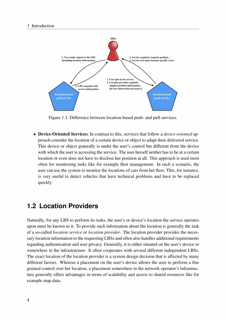
• Pull-Services: The first part is comprised of the so-called pull-services. These kinds ofapplications only act upon a direct request from the user. As such, the user formulatesa query containing her current location, and that query is sent to the application or LBS.The user then waits until the application has processed the request and the answer is sentback. This is depicted on the left in Figure 1.1. Using a location-aware search engine andperforming a search for a gas station in one’s own proximity is a good example for thiskind of service.
• Push-Services: The second group of services is made up of the so-called push-services.These services require the user to once register or opt in for the service. This can, forexample, be done by creating an account on a website or by downloading an applicationto a mobile device and then starting it. After the opt-in, the service is allowed to regularlyor even continuously monitor the user’s location. Upon the occurrence of a certain event– like the user entering a defined area or getting close to a point of interest (POI) – theservice takes action. Actions can, for example, be to notify the user of special offeringsof shops in her proximity. This approach is shown on the right-hand side of Figure 1.1.
In addition to the interaction model of LBSs, there exists also another way to differentiatebetween such services. While not as important as the first aspect, this type of differentiationshould not be neglected and is therefore mentioned here for completeness.
• Person-Oriented Services: If a service’s mode of operation is person oriented, thismeans that it operates on the user’s current location and uses this location to adapt thedelivered service. This is the more common way of operation for most LBSs. The justmentioned example of a shopping alert is a good example for a person-oriented LBS, too.The user’s location is the relevant factor to select which shops should be considered forhaving their special offers sent to the user.
3
1 Introduction
Figure 1.1: Difference between location-based push- and pull-services.
• Device-Oriented Services: In contrast to this, services that follow a device-oriented ap-proach consider the location of a certain device or object to adapt their delivered service.This device or object generally is under the user’s control but different from the devicewith which the user is accessing the service. The user herself neither has to be at a certainlocation or even does not have to disclose her position at all. This approach is used mostoften for monitoring tasks like for example fleet management. In such a scenario, theuser can use the system to monitor the locations of cars from her fleet. This, for instance,is very useful to detect vehicles that have technical problems and have to be replacedquickly.
1.2 Location Providers
Naturally, for any LBS to perform its tasks, the user’s or device’s location the service operatesupon must be known to it. To provide such information about the location is generally the taskof a so-called location service or location provider. The location provider provides the neces-sary location information to the requesting LBSs and often also handles additional requirementsregarding authentication and user privacy. Generally, it is either situated on the user’s device orsomewhere in the infrastructure. It often cooperates with several different independent LBSs.The exact location of the location provider is a system design decision that is affected by manydifferent factors. Whereas a placement on the user’s device allows the user to perform a finegrained control over her location, a placement somewhere in the network operator’s infrastruc-ture generally offers advantages in terms of scalability and access to shared resources like forexample map data.
4
1.2 Location Providers
Types of Locations
The information about the user’s whereabouts provided by location providers can generallyhave one of two different types [BD05]:
• Geometric Locations: On the one hand, the location provider can provide a geometriclocation or coordinate. Such a location is a fixed point or area defined by coordinates in agiven coordinate system. As such, the coordinate system and its properties must be knownto make use of the location information. If the coordinate system is known, though, thelocation can be easily set into relationship with other locations in the same coordinatesystem. This includes the computation of distances between different locations as well asother spatial relationships. Position is another name that is often used in the meaning ofgeometric locations. A frequently used coordinate system is the World Geodetic System1984 (WGS-84) [WGS04] and its longitudes and latitudes that are widely used to exactlypinpoint positions on the surface of the earth.
• Symbolic Locations: On the other hand, a location provider can alternatively or addition-ally provide so-called symbolic locations. In comparison to the former type of geometriclocations, a symbolic location is not necessarily bound to a coordinate system. Instead,it is merely a description for a certain place that – without further knowledge – does notdisclose any relationship like the distance or the containment status with regard to othersymbolic or geometric locations. The name of a certain restaurant is a suitable exam-ple for a symbolic location. While it quite exactly describes the whereabouts of a user tothose knowing the restaurant and its address, this information is useless for others withoutthis knowledge.
Privacy and Authentication
Of course, being able to access such sensitive information as a user’s position raises privacyconcerns. This is especially true for push-services that are allowed to constantly monitor theuser’s position. Therefore, an important task of the location service is the proper handlingof the authentication of requesting services. It has to make sure that only those services towhich the user has granted access are allowed to access the user’s context information. Inaddition, also privacy is a very important issue when looking at LBS and location services.Generally, not every service needs precise information about the user’s location. Sometimes,also a rough estimate is sufficient, or it may be the case that a user wants to temporarily restrictthe granularity by which her position is submitted to requesting services. To provide for thisissue, many solutions have been proposed in literature in the past.
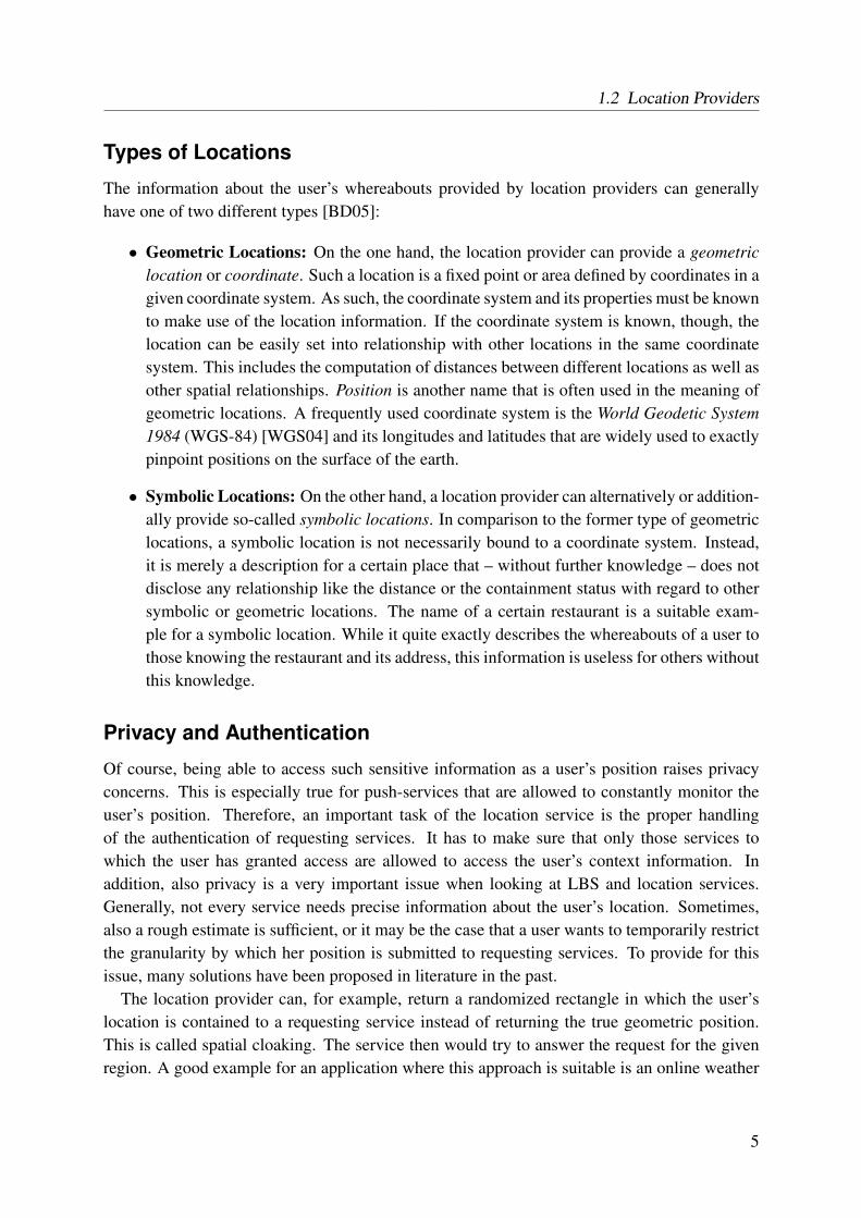
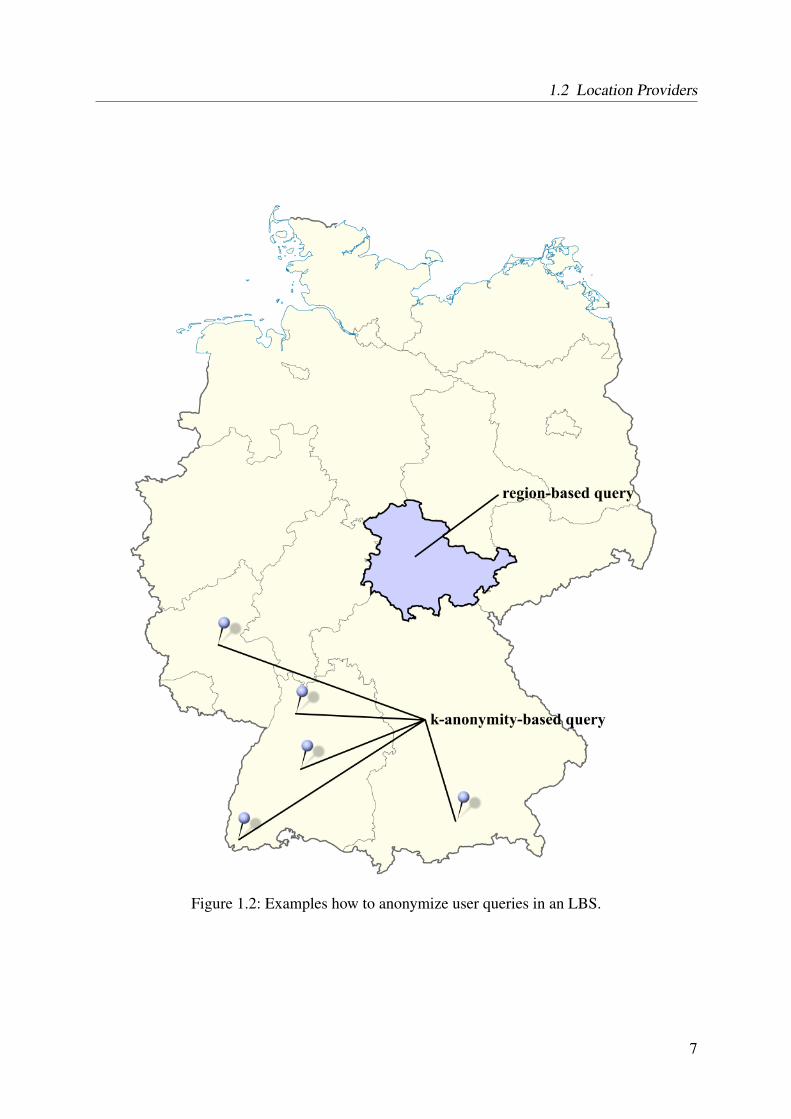
The location provider can, for example, return a randomized rectangle in which the user’slocation is contained to a requesting service instead of returning the true geometric position.This is called spatial cloaking. The service then would try to answer the request for the givenregion. A good example for an application where this approach is suitable is an online weather
5
1 Introduction
service. In cases where spatial cloaking is not feasible, the location provider can also returna set of different locations. In this case, the LBS processes and returns the results for all thesupplied locations, and the user or – depending on the system design – the location providerhas to filter out the inappropriate answers. In the literature, this approach is often referred toas k-Anonymity, where k refers to the total number of possible locations [Swe02, SS98]. Bothapproaches are exemplarily depicted in Figure 1.2.
6
1.2 Location Providers
Figure 1.2: Examples how to anonymize user queries in an LBS.
7

8
CH
AP
TE
R
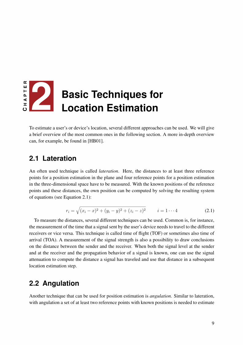
2 Basic Techniques forLocation Estimation
To estimate a user’s or device’s location, several different approaches can be used. We will givea brief overview of the most common ones in the following section. A more in-depth overviewcan, for example, be found in [HB01].
2.1 Lateration
An often used technique is called lateration. Here, the distances to at least three referencepoints for a position estimation in the plane and four reference points for a position estimationin the three-dimensional space have to be measured. With the known positions of the referencepoints and these distances, the own position can be computed by solving the resulting systemof equations (see Equation 2.1):
ri =√
(xi − x)2 + (yi − y)2 + (zi − z)2 i = 1 · · · 4 (2.1)
To measure the distances, several different techniques can be used. Common is, for instance,the measurement of the time that a signal sent by the user’s device needs to travel to the differentreceivers or vice versa. This technique is called time of flight (TOF) or sometimes also time ofarrival (TOA). A measurement of the signal strength is also a possibility to draw conclusionson the distance between the sender and the receiver. When both the signal level at the senderand at the receiver and the propagation behavior of a signal is known, one can use the signalattenuation to compute the distance a signal has traveled and use that distance in a subsequentlocation estimation step.
2.2 Angulation
Another technique that can be used for position estimation is angulation. Similar to lateration,with angulation a set of at least two reference points with known positions is needed to estimate
9
2 Basic Techniques for Location Estimation
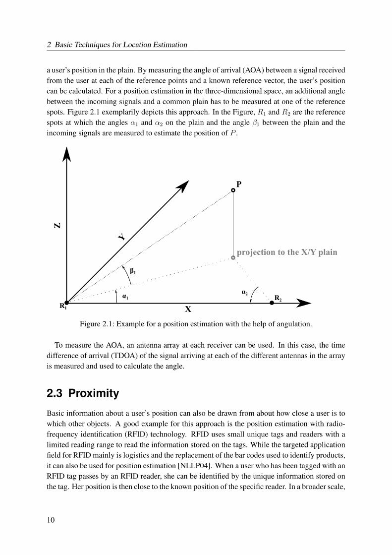
a user’s position in the plain. By measuring the angle of arrival (AOA) between a signal receivedfrom the user at each of the reference points and a known reference vector, the user’s positioncan be calculated. For a position estimation in the three-dimensional space, an additional anglebetween the incoming signals and a common plain has to be measured at one of the referencespots. Figure 2.1 exemplarily depicts this approach. In the Figure, R1 and R2 are the referencespots at which the angles α1 and α2 on the plain and the angle β1 between the plain and theincoming signals are measured to estimate the position of P .
Figure 2.1: Example for a position estimation with the help of angulation.
To measure the AOA, an antenna array at each receiver can be used. In this case, the timedifference of arrival (TDOA) of the signal arriving at each of the different antennas in the arrayis measured and used to calculate the angle.
2.3 Proximity
Basic information about a user’s position can also be drawn from about how close a user is towhich other objects. A good example for this approach is the position estimation with radio-frequency identification (RFID) technology. RFID uses small unique tags and readers with alimited reading range to read the information stored on the tags. While the targeted applicationfield for RFID mainly is logistics and the replacement of the bar codes used to identify products,it can also be used for position estimation [NLLP04]. When a user who has been tagged with anRFID tag passes by an RFID reader, she can be identified by the unique information stored onthe tag. Her position is then close to the known position of the specific reader. In a broader scale,
10
2.4 Dead Reckoning
the same effect can also be achieved when using WLAN. The most common mode of operationthat WLANs are operated in is the so-called infrastructure mode. In this mode, clients usingthe network do not communicate with each other directly (ad-hoc). Instead, all messages areforwarded by an infrastructure formed by a set of access points (APs). These APs typicallyhave a radio range of roughly 300 m in a completely open environment and outdoors, 150 m insemi-open environments like open-plan offices, and up to 50 m in closed indoor environments.Given these numbers, the known position of the AP a user is currently connected to thus can beused as a good indication of where she approximately is currently located.
2.4 Dead Reckoning
Using dead reckoning is another possible technique to estimate a user’s position. Based ona known start position and local sensor measurements from, e.g., accelerometers, one tries todraw conclusions about the user’s motion speed and motion direction and thus her current andupcoming positions. This technique is often used by navigation systems in cases where theirnormally used techniques are temporarily not available. If, for example, a car equipped with anin-car navigation system enters a tunnel or otherwise loses the connection to the normally usedsatellite-based positioning system, the available data from the speedometer, wheel-mountedsensors, and sensors that measure the steering angle can be used to extrapolate the car’s posi-tion by dead reckoning. Also, some approaches exist that try to transfer this technique to thedomain of human-centered indoor applications. Here, generally highly precise accelerometersand gyroscopes are, for example, mounted on the user’s shoe or leg. Based on the data fromthese devices, the positioning system at first tries to draw conclusions on the step number, steplength, and direction of a user and then uses this information to extrapolate the path a user takesfrom a given start position [Fox05, CSG05, SFL05].
2.5 Scene Analysis
A further method that can be used to estimate a user’s position is called scene analysis. Rely-ing on local observations, too, scene analysis also takes further knowledge into account forposition estimation. Easy Living is a system designed by Microsoft Research that followsthis [BMK+00].
In the statical scene analysis, an analysis of only current local measurements is performedto estimate the user’s position. This can be done by, for instance, matching the data to anavailable knowledge base. As an example, a system might try to identify a user on the imageof a surveillance camera. Based on the known position of the camera and the field of view,the system is then able to conclude on the current whereabouts of the user. Opposed to this, inthe differential scene analysis, the differences between several consecutive local measurementsare used. Once more considering a system based on camera images, it would, for example,
11
2 Basic Techniques for Location Estimation
be possible to draw information about the user’s motion from changes like pans in subsequentcamera image frames.
2.6 Location Fingerprinting
The last possibility mentioned here to estimate a user’s position is the so-called location fin-gerprinting (LF) technique. Closely related to scene analysis, location fingerprinting also relieson local measurements at the time of the position estimation and on a knowledge base withadditional information.
Fingerprinting algorithms are split into two phases. In a first phase, called training phase, aset of fingerprints is collected throughout the area the positioning system shall cover. A finger-print may contain any type of data that is characteristic for a certain position. The fingerprintsthen are stored in a fingerprint database together with the positions where they were collected.
In the second, so-called position determination phase, another fingerprint is collected at theuser’s yet unknown position. This fingerprint again contains the same type of data and measure-ments as those collected during the training phase. The fingerprint, sometimes also referred toas online fingerprint or live data, is then compared to all the fingerprints stored in the fingerprintdatabase. The position of the best matching fingerprint from the database is returned as the posi-tion estimate for the user. As especially location fingerprinting with the help of WLAN signalsis a key concept used in this thesis, we will look into that topic in more detail in Chapter 4.
12
CH
AP
TE
R
3 A Brief History of LocationEstimation
Most of the just presented techniques to estimate a position date back to ancient times. Angu-lation was, for instance, already used by sailors in ancient times to estimate their position andis still a valid approach today. However, besides the basic positioning techniques, also the ideaof estimating a user’s position and using it to enhance services offered to the user is alreadyquite old – at least in terms of information technology. In its history, many different techniquesand systems to estimate a user’s position have been developed and tested by the scientific com-munity and by industry. In the following, a brief overview of some positioning systems thatwere developed in the past is given without intending to be exhaustive. The main goal of thisoverview is to give the reader an idea of what systems have been used for location estimationin the past, how they worked, and what their main drawbacks were.
3.1 Active Badge
Even as early as 1990, the Active Badge system was developed at the Olivetti Research Lab-oratories in Cambridge [WHFaG92]. Its main purpose was to allow for an efficient automaticcall forwarding, and it was one of the first LBSs at all. The system uses badges attached tothe users that regularly emit a unique infrared light signal. This signal is received by receiversplaced in each room. The receivers then transmit the received signals to a central system wherea mapping of which badge – and thus which user – is located within the proximity of whichreceiver and therefore located in which room can be created. Subsequently, phone calls for thatuser can be forwarded to the room she is currently in.
Due to the technological solutions used for Active Badge, the system suffers from somemajor problems. Generally, systems using infrared light often are very sensitive to sunlight.This is also true for Active Badge. Thus, sunny days and large window panes severely affectthe operation of the system in such a way that the signals from the transmitters can no longerbe received. Furthermore, Active Badge needs a dedicated infrastructure made up of at leastone receiver in every room together with the necessary installation. Additionally, it requires the
13
3 A Brief History of Location Estimation
personnel to carry the transmitters just for the purpose of location estimation. Finally, havingonly an accuracy at room granularity is probably not sufficient for many types of LBSs.
3.2 Active Bats
Active Bats is another positioning system that was developed in Cambridge around the year2000 [HHS+99]. Instead of infrared light, it uses ultrasonic sound signals and additionally a433 Megahertz (MHz) radio as a control channel. Small units attached to the user regularly emitsound pulses. At the same time, a reset signal is sent to receivers placed in a grid fashion on theceiling of each room via the radio channel. Upon the reception of the reset signal, the receiversstart a high precision timer and measure the time till the reception of the sound pulse. Based onthese TOF measurements, the known locations of the receivers, and lateration, the position ofthe user can be computed very accurately. Active Bats achieves an average positioning accuracyin the range of a few centimeters.
However, similar to the Active Badge system, also the Active Bats system has some draw-backs. Again, a dedicated infrastructure is necessary and, in the case of Active Bats, this in-frastructure even has much higher installation requirements than the one needed for ActiveBadge. Additionally, the use of ultra sonic sound pulses is controversial as this kind of noisecan severely distract both people sensitive to high frequencies and also animals that are nearby.These problems were reasons why the system was not adopted by the community at a largescale.
3.3 Ubisense
Another quite new system used for position estimation is offered by a company called Ubisense1.It relies on a combination of lateration and angulation and uses ultra-wideband (UWB) radiopulses to estimate a user’s position. The user carries a small badge that is triggered by receiversplaced in the corners of each room to emit UWB pulses. The receivers are connected to a centralinstance by a dedicated infrastructure and communicate the reception of the pulse together withfurther information, like the reception angle, to the central unit. There, based on knowledgeabout the time that messages need to travel from each of the receivers to the central instance,the TDOA between the different receivers is measured. Together with the known positions ofthe receivers and the reception angles, this information is used to compute the exact locationof the user’s badge. The accuracy that can be achieved with this approach is similar to theone achieved by Active Bats and is close to 15 cm. Compared to other systems that use signalsbound to a small frequency range, the use of UWB signals offers several advantages. Especiallyin indoor scenarios, radio signals often suffer from a bad propagation behavior. This includesdiffraction, scattering, multi-path propagation, and attenuation of the signals [Rap01]. While
1http://www.ubisense.net
14

3.4 The Global Positioning System
these restrictions are also true for UWB signals, due to the wide range of frequencies used,a UWB signal is only partially affected by them. If, for example, an obstacle attenuates thesignal in a certain frequency range, the remaining parts of the UWB signal stay mainly unaf-fected. Considering the problem of multi-path propagation and small-scale fading, the systemoffered by Ubisense further has the advantage that it uses very short pulses. These pulses havea physical dimension of only roughly 30 cm and as such avoid the problem of interfering withthemselves if the signal takes several different paths to the receiver.
Similar to the other systems mentioned earlier, the most limiting problem for the systemoffered by Ubisense is the very high effort in terms of costly infrastructure, cabling, and initialcalibration that is needed to set it up. Furthermore, our own experiences with the system haveshown a high sensitivity to metal objects in the proximity of both the transmitter carried by theuser as well as the receivers mounted on the walls. In our own offices that are separated bymetal walls, we did not even manage to get the system working for position estimation at all.
3.4 The Global Positioning System
The Global Positioning System (GPS) is a satellite-based system for position estimation thatwas developed under the guidance of the American Department of Defense starting as early as1970. It uses at least 24 satellites placed in a medium earth orbit of about 20, 200 km height.Each satellite constantly sends out data transmissions containing a precise time stamp of thetime the transmission is sent, precise orbital information about the sending satellite, and an al-manac containing rough information about the system health and the orbits of all other GPSsatellites. To avoid interference between the signals of different satellites at the receiver, GPSuses a spread spectrum approach and different chipping sequences for each satellite. Once areceiver receives the signals of at least four satellites, it can compute its own position includinglongitude, latitude, and elevation. Although it would be possible to compute this informationwith the signals from only three satellites (as one estimated position would generally be some-where in space), GPS uses a fourth one to handle the imprecise local time as another unknownin the equation to solve (also refer to Equation 3.1). When available, GPS offers a good posi-tioning accuracy of up to ten meters on average.
Ri =√
(xr − xi)2 + (yr − yi)2 + (zr − zi)2 + ∆t ∗ c (3.1)
To further improve the positioning accuracy of GPS, different additions to the system exist.For instance, the accuracy can be improved up to a few centimeters by using additional localtransmitters as reference data sources. However, as the local transmitters are very expensive,this approach is only feasible for a limited set of applications.
Another possibility is the use of Differential GPS (DGPS). DGPS used stationary local re-ceivers that, due to their fixed location, can compute a very precise estimate of their own posi-tion over time. This knowledge together with the currently estimated position is used to identifythe error immanent in the currently received satellite signals. After the local DGPS station has
15
3 A Brief History of Location Estimation
estimated the error, correction information is broadcasted to all DGPS-enabled devices in thesurrounding which in the following can use it to correct their own received signals and, thus,improve their positioning accuracy.
The major problem GPS faces is that it is hardly available inside buildings and that it oftenfails in situations where obstacles like buildings block the line of sight (LOS) between thereceiver and the satellites. Unfortunately, this is quite often the case, especially indoors andin urban and suburban areas. In these situations, the position estimation with GPS is eitherimprecise or even impossible. While the complete failure is caused by the satellite signals notreaching the receiver at all, the – from a user’s perspective – even worse case is caused by thesignals reaching the receiver on indirect paths. Due to the incorrect estimation of the TOF forthese signals, this leads to large errors in the position estimation.
16
CH
AP
TE
R
4 Location Estimation withIEEE 802.11
This chapter gives an overview of related work in the area of position estimation with the help ofIEEE 802.11. The first section begins by presenting systems that use this networking technologyfor position estimation without using location fingerprinting. This is followed by a section thatintroduces several systems in the area of location fingerprinting with the help of IEEE 802.11that are directly related to the topics of this thesis. In the third section, the research questionsfor which this thesis provides solutions are stated. Finally, Section 5.2 introduces our researchmethodology.
4.1 Location Estimation without Fingerprints
In the past, several approaches were made to reuse the existing infrastructure of WLANs forthe purpose of location estimation and positioning. Of these, some use other techniques thanfingerprinting to estimate a user’s position. In the following, we give an introduction to some ofthese systems and point out what their advantages and disadvantages are compared to systemsthat follow a fingerprinting approach.
In the year 2000, an early system using existing WLAN infrastructure for position estimationwas introduced. It was part of the GUIDE project [CDMF00]. The overall system was designedas a mobile, context-aware tourist guide. It uses a built-in IEEE 802.11 network interface card tocommunicate with content servers and also to determine the proximity of nearby APs. As such,it is one of the first IEEE 802.11-based positioning systems. Of course, using the proximity to asingle AP for location estimation can only offer a coarse accuracy. Furthermore, depending onenvironmental factors like the weather, the shape of the region in which an AP can be receivedmight change. Thus, following this approach is only suitable for a limited set of applicationswhere the just mentioned drawbacks do not prohibit its use.
Another common approach for location estimation is, as shown in Chapter 1, lateration. Thistechnique has also been used to estimate positions with IEEE 802.11 in the past. For example, in[PBM+09a], Prieto et al. describe a system that measures the round-trip times (RTT) of signals
17
4 Location Estimation with IEEE 802.11
from a mobile station to at least three APs. Based on the propagation speed of the signals andthese times, the authors then calculate the distances between the station and the APs and usethem and the known coordinates of the APs to estimate the user’s position.
This kind of system has several disadvantages, though. One major disadvantage is the prob-lem of the signals taking many and unpredictable paths within an indoor environment. Espe-cially in no line of sight (NLOS) scenarios, this multipath propagation leads to signals needing alonger time to propagate from the sender to the receiver and thus to wrong distance estimations.Prieto et al. deal with this problem in a follow-up paper by modeling the NLOS component ofthe signals with a probability distribution and dynamically estimated parameters [PBM+09b].While they are able to improve the accuracy with their addition, it also highly increases thesystem’s complexity.
Furthermore, their approach has a second major disadvantage. Special hardware or at leastmodifications to the used standard hardware is needed. The protocol that is used on the data linklayer of WLANs defines several random backoff times. The network interface card waits sucha random backoff time frame if, for instance, a collision occurred while sending a data frame.If no special hardware or drivers are used, then the length of this time is not easily accessiblefrom user-space and thus cannot be separately considered upon the estimation of the RTT. Thisinduces a high inaccuracy in the position estimation.
4.2 Location Estimation with Fingerprints
Both the systems mentioned in Chapter 1 as well as the ones just introduced fulfill their taskof estimating a user’s position. However, all of them also have major drawbacks. They requirespecialized hardware or dedicated infrastructure, are very costly and hard to set up, or onlyoffer a coarse positioning accuracy except for special conditions.
In many regards, estimating a user’s position with the help of location fingerprinting andIEEE 802.11 can overcome these issues. WLAN infrastructure is already available almost ev-erywhere where people live or work in the developed countries these days [LCC+05, BHM+06].And, as commodity or off-the-shelf (OTS) hardware can be used, the hardware cost when ex-tending an existing positioning system based on IEEE 802.11 is moderate. Furthermore, theaccuracy that is achievable with IEEE 802.11-LF is sufficient for many types of LBSs. CurrentIEEE 802.11-LF systems achieve an average accuracy of about three meters.
But of course, location estimation with IEEE 802.11-LF is not perfect either. The achievedaccuracy and precision can still hardly compete with systems like Active Bats or UWB posi-tioning where the accuracy is in the range of few decimeters. These systems need an expen-sive infrastructure for the sole purpose of location estimation, though. An IEEE 802.11-LFsystem can reuse the existing WLAN infrastructure that is already in place for communica-tion purposes. Additionally, most mobile devices ranging from cellular phones over laptops totablet computers these days are already equipped with IEEE 802.11 interfaces. So, to use anIEEE 802.11-LF system, there is no need to attach or carry additional hardware. Compared
18
4.2 Location Estimation with Fingerprints
to GPS functionality that is also built into many modern mobile devices, IEEE 802.11-LF hasthe major advantage that it can be used both indoors and outdoors to estimate a user’s positionwhere APs are nearby. GPS and IEEE 802.11 thus complement each other very well.
4.2.1 RADAR
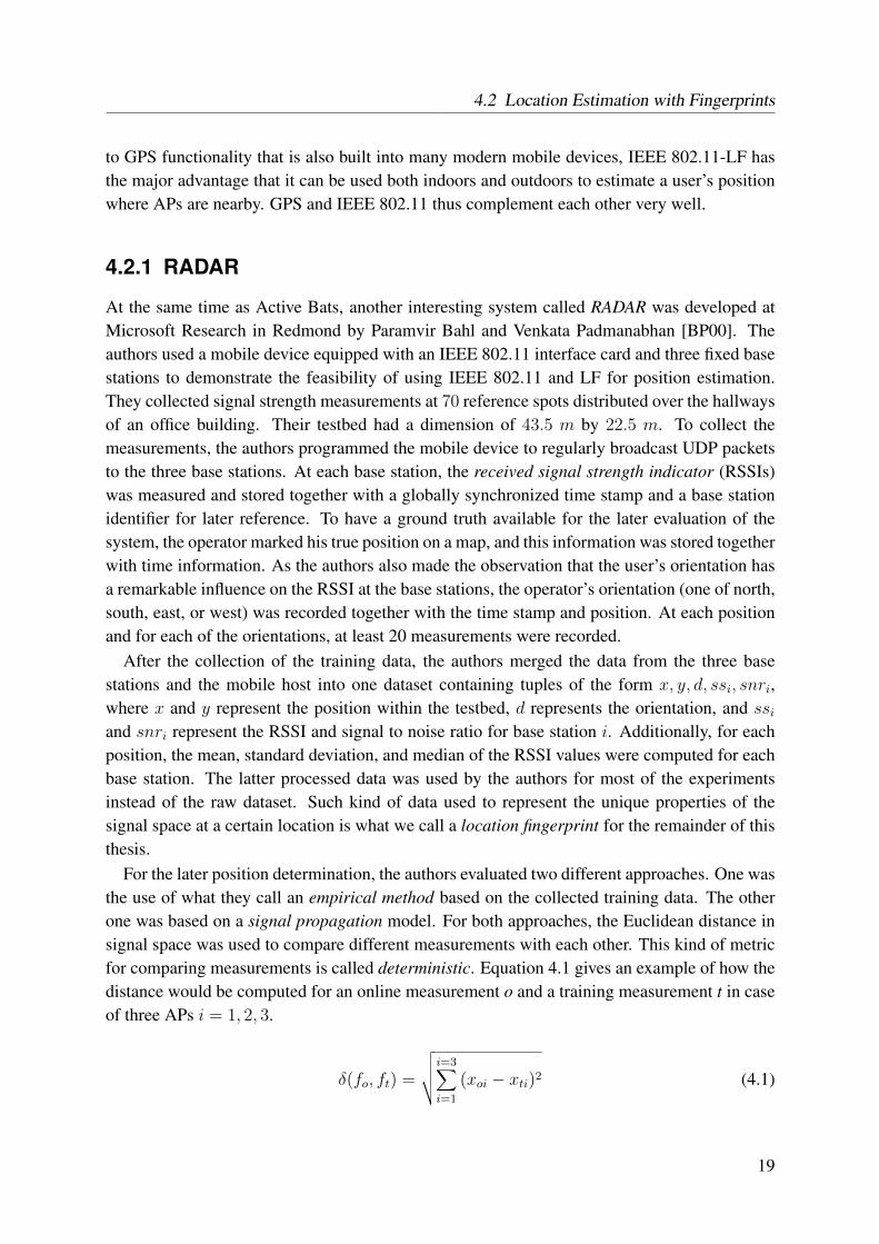
At the same time as Active Bats, another interesting system called RADAR was developed atMicrosoft Research in Redmond by Paramvir Bahl and Venkata Padmanabhan [BP00]. Theauthors used a mobile device equipped with an IEEE 802.11 interface card and three fixed basestations to demonstrate the feasibility of using IEEE 802.11 and LF for position estimation.They collected signal strength measurements at 70 reference spots distributed over the hallwaysof an office building. Their testbed had a dimension of 43.5 m by 22.5 m. To collect themeasurements, the authors programmed the mobile device to regularly broadcast UDP packetsto the three base stations. At each base station, the received signal strength indicator (RSSIs)was measured and stored together with a globally synchronized time stamp and a base stationidentifier for later reference. To have a ground truth available for the later evaluation of thesystem, the operator marked his true position on a map, and this information was stored togetherwith time information. As the authors also made the observation that the user’s orientation hasa remarkable influence on the RSSI at the base stations, the operator’s orientation (one of north,south, east, or west) was recorded together with the time stamp and position. At each positionand for each of the orientations, at least 20 measurements were recorded.
After the collection of the training data, the authors merged the data from the three basestations and the mobile host into one dataset containing tuples of the form x, y, d, ssi, snri,where x and y represent the position within the testbed, d represents the orientation, and ssiand snri represent the RSSI and signal to noise ratio for base station i. Additionally, for eachposition, the mean, standard deviation, and median of the RSSI values were computed for eachbase station. The latter processed data was used by the authors for most of the experimentsinstead of the raw dataset. Such kind of data used to represent the unique properties of thesignal space at a certain location is what we call a location fingerprint for the remainder of thisthesis.
For the later position determination, the authors evaluated two different approaches. One wasthe use of what they call an empirical method based on the collected training data. The otherone was based on a signal propagation model. For both approaches, the Euclidean distance insignal space was used to compare different measurements with each other. This kind of metricfor comparing measurements is called deterministic. Equation 4.1 gives an example of how thedistance would be computed for an online measurement o and a training measurement t in caseof three APs i = 1, 2, 3.
δ(fo, ft) =
√√√√i=3∑i=1
(xoi − xti)2 (4.1)
19
4 Location Estimation with IEEE 802.11
For the evaluation of the empirical approach, the authors randomly selected one of the 70
reference positions and one orientation and used the processed data to find the best matchingcounterpart among the remaining 69 positions with regard to the distance in signal space. Theycall this the Nearest Neighbor in Signal Space (NNSS). As a benchmark, the authors used analgorithm that uses the position of the strongest base station as a position estimate as well as analgorithm that randomly picked one of the 70 possible positions.
Their results show that using such an approach can well be used to estimate a user’s positionand is superior to both other algorithms described above. The authors report an accuracy of2.94 m in more than 50% of all cases opposed to, e.g., 8.16 m for the strongest base stationapproach.
The results were even further improved by using not only the best match from the trainingdata but by selecting the k best matches and averaging their positions. This is advantageous, asthe error vectors of the different matches in physical space often point in different directions.Thus, averaging the coordinates leads to a better overall estimate. In their experiments, by usinga k of five, the authors improved their results by 9% for the 50%-percentile compared to onlyusing the best match.
Another improvement was made by mitigating the influence of the user’s body. The authorscreated another processed dataset that, for each position, contained only the strongest RSSIvalues for each AP. Using this dataset, the results were further improved by 9% for the 50%-percentile.
Regarding their approach with a radio propagation model, the authors used the Floor Atten-uation Factor (FAF) propagation model by Seidel and Rappaport [SRF+92] and modified it tosuit their needs. They replaced the original FAF by a wall attenuation factor to compensatefor walls and other obstructions in the signal path. Using that model, they then computationallycreated a training dataset containing fingerprints for a grid of positions on the floor and used thatset as a search space for the NNSS algorithm. While being significantly better than the strongestbase station algorithm, this approach cannot compete with the results of the fingerprinting-basedsystem.
4.2.2 Rice
Another system – we are going to call it Rice from now on – that uses location fingerprintingand IEEE 802.11 was introduced by Haeberlen et al. in the year 2004 [HFL+04]. Compared toRADAR, this system introduced a new type of metric to match the online measurements withthe fingerprints stored in the database. Instead of using the deterministic Euclidean distance,the new system uses a Bayesian inference algorithm to model the state space of possible userpositions and the emission probabilities for a certain measurement. In the model, each positionand thus each fingerprint stored in the fingerprint database corresponds to a possible state theuser can be in. During the position determination phase, for each online measurement andfingerprint in the database, a probability of the user being at the position of the fingerprint is
20
4.2 Location Estimation with Fingerprints
computed. This is done by, for each position, combining the emission probabilities for themeasured signal strengths of each AP. The probabilities are computed from the measured signalstrength histograms stored in the fingerprints. After the computation of the probabilities for allstates, the state with the highest overall probability is selected as a position estimate. This typeof metric is called probabilistic, and it has even been shown by Youssef and Agrawala that thistype of metric generally offers a better accuracy than deterministic metrics [YA04].
In order to verify the use of their system when tracking a mobile user, the authors furthermoreimplemented what they call a sensor fusion approach by using a Hidden Markov Model (HMM)to handle transitions between different states. Following this approach, the state space and thusthe probability distribution over it is transferred between subsequent position estimations. Thisincreased the accuracy by 8%.
In a subsequent step, the authors of RICE furthermore modified their system to use Gaussiansignal strength distributions instead of signal strength histograms. This was done because theGaussian distribution allows the system to perform more robustly in case of suboptimal signalconditions. They also extended their testbed from some floors on a single story to an entirethree-story building and changed the collection of the fingerprints: Instead of using a grid ofreference spots where to collect the training data, the authors switched to a cell-based approachwith manually defined cells for each single fingerprint. The typical size of a cell was approx-imately 15 m2. They furthermore extended their system by a topological map of the regions.This map was used in a later step to increase the system’s performance during the trackingoperation.
While this probabilistic approach – especially when using Gaussian distributions – is morecomplex than the deterministic one taken by RADAR, it offers several advantages. First, it ismore robust to variations in the RSSI that are inherent when working with IEEE 802.11. Whenusing a normal distribution, even values that did not occur during the training data collectionare covered by the distribution. Thus, if such values occur during the position determinationphase, they still can be used. Second, the algorithm is more easily able to handle the case wherethe signals of access points are missing in the collected online measurement. In such a case, theprobability of the user being at the position of the fingerprint is multiplied with a small penaltyvalue and is thereby reduced to indicate the missing AP.
Using their second approach, the authors were able to achieve good results with regard toboth the positioning accuracy as well as the reliability. When using the Bayesian inferencealgorithm together with the signal strength histograms, the system achieved an accuracy of lessthan 1.5 m in 77% of all cases within the – admittedly – limited scenario of eleven referencespots and two orientations used. Incorporating the last two online measurements increased thisvalue to 83%. A further experiment with the HMM showed additional improvements in somesituations but decreased the accuracy in others, especially in areas with large open spaces. Theauthors explain this result with the dilution of the signal due to the open spaces and a suboptimalplacement of the base stations.
21
4 Location Estimation with IEEE 802.11
Another important aspect covered by Haeberlen et al. is the problem of different devicecharacteristics. As different devices generally have different antenna designs and chipsets, themeasured signal strengths at one position may vary between devices. The authors identifiedthis problem and found that a linear model can be used to create a mapping between differentdevices. These results were used by Kjaergaard et al. in a subsequent work on signal strengthnormalization over different devices [Kjæ06]. There, they could be confirmed, and an evenbetter normalization method was introduced [KM08] later.
22
CH
AP
TE
R
5 Improvements forIEEE 802.11-LF
As we have seen in Chapter 4, position estimation with IEEE 802.11-LF is a viable alternativeto other techniques. It is accurate enough for most types of LBSs, it can be used indoors aswell as outdoors, and an additional installation of dedicated infrastructure is not necessary inmost cases. Thus, it seems like this is an ideal solution to all positioning tasks. Unfortunately,most approaches that use IEEE 802.11-LF still suffer from several drawbacks. The followingsection gives an overview of the three major problems from which IEEE 802.11-LF systemssuffer. After presenting our research methodology, we then present our own solutions to eachof these single challenges in the subsequent sections.
5.1 Research Questions
As shown, in the past, the position estimation with IEEE 802.11 has already been an extensivelystudied field of research. Nevertheless, there are still many open problems that need to be solvedbefore positioning systems based on IEEE 802.11-LF become conveniently usable products.
In order to give an overview to the reader, we, in this Chapter, will show some urgent fieldsfor the improvement of IEEE 802.11-LF in general and also approaches targeting these issues.The problems are:
• A still improvable accuracy.
• The huge effort needed to initially set up a WLAN-LF system and to maintain the finger-print database.
• The lack of an error estimation for WLAN-LF.
In the following, our own developments to deal with these issues are presented. This in-cludes what we call Quick Fingerprinting, an approach that, at the same time, can deliver bothan increased accuracy and a largely reduced amount of time needed for the collection of the
23
5 Improvements for IEEE 802.11-LF
training data. We then present and evaluate a system that goes even further by replacing thefixed reference spots and uses pre-defined trajectories instead. This allows for the fast and effi-cient collection of training data at the cost of only minor degradations in accuracy. And, finally,several different algorithms to estimate the error for a given position estimate are introducedand thoroughly evaluated.
All these systems deal with a static scenario. But of course, in reality, a user will be movingaround most of the time. Therefore, in the second half of this thesis, we deal with the questionhow the position estimation could be further improved for tracking. While the simple reuseof existing techniques for static position estimation does not yet yield major improvements,tracking – the continuous estimation of a user’s position – offers several advantages over theindependent estimation of subsequent positions. Firstly, a new position estimate can incorpo-rate information from a history of former position estimates. Secondly, information about thecurrent motion state of the user can be used. And thirdly, also information about other context,like for instance an available building map, can be used to verify position estimates and anestimated movement.
5.2 Research Methodology
Several different ways exist to evaluate the performance of positioning algorithms. Of course,the best one is to perform a large number of position measurements in the true environmentwhere the system will be used. However, this unfortunately is not manageable for many settingsdue to the high amount of time and effort needed for such an evaluation.
Another possibility to evaluate positioning algorithms is by simulation. Here, the algorithmis provided with artificially created information and uses this information to estimate a posi-tion. This approach stands or falls with the quality of the created input. If it reflects the trueenvironment well, then also the achieved results for the positioning algorithm are valuable. Inthe case of position estimation with IEEE 802.11-LF, though, the latter approach is not usable,either. The reason is once more the complex propagation behavior of the radio signals in indoorenvironments. As these cannot be precisely modeled, it is also not possible to predict whatsignals a mobile station would measure at a specific position.
Thus, to evaluate positioning algorithms that use the signals of IEEE 802.11 APs, the com-mon approach is emulation. Emulation is a combination of the former two techniques. Atfirst, the data that the system would normally use to estimate a position are collected for theevaluation environment. Then, instead of using artificially created input, this collected data isprovided to the positioning algorithms in simulation runs.
For the evaluation of our own algorithms, we used emulation for the just mentioned reasons.We have collected several different datasets at the premises of our department at the Universityof Mannheim. The collection of different datasets became necessary for several reasons. Ourfirst dataset covers a single floor with a high density of reference spots. The dimensions ofthis dataset were limited by the effort needed to collect it, and it was used to analyze, for
24
5.3 Areas for Improvements
instance, the influence of the distance between different reference spots on several aspects ofthe position estimation. Over time, we realized that for our novel algorithms, like the region-based position estimation, a larger dataset containing both the floor from the first dataset andanother less cluttered floor would allow for a better evaluation of the algorithm in differentsettings. We therefore collected another dataset covering a much larger area with differentcharacteristics. This dataset was also used to evaluate the error estimation for IEEE 802.11-LF. To estimate the performance of our tracking approach, we once more extended the areacovered by the large dataset to also include several offices and lecture halls. This was necessaryto be able to also consider the influence of available building information on the positioningresults. In addition to the dimensions, the third dataset is also special considering the mode ofdata collection: Whereas the first two datasets were collected over a period during the weekendwhen the building was almost empty to assure a very high quality of the collected data, thethird dataset was collected during normal office hours over a longer timespan. This results ina poorer data quality but gives an even more realistic impression of what an IEEE 802.11-LF-based positioning system can provide.
As a result of using these different datasets, our single results for the different algorithms areonly partly comparable. To compensate for this, we – when needed – also performed perfor-mance evaluations of the RICE system with the corresponding datasets. These can serve as acommon baseline between the different systems.
5.3 Areas for Improvements
The first aspect we take a look at is the overall positioning accuracy. These days, IEEE 802.11-LF systems offer an average positioning accuracy of less than three meters. Compared toRADAR, this is already an improvement, and it is sufficiently accurate for many applicationsand types of LBSs. But still, there exist cases in which a higher accuracy would be desirableor is even necessary. Just consider a museum guide application for an art museum: In such ascenario, a positioning accuracy better than half the spacing between the exhibited images orobjects would be necessary for the guide to function optimally.
Another even more important aspect that still is a problem for IEEE 802.11-LF systems isthe following: Even though especially IEEE 802.11-LF systems that are based on probabilisticalgorithms offer a competitive average positioning accuracy, a remaining major problem is theuncertainty that is inherent in the position estimation most of the time. Besides their good aver-age accuracy, there are situations where the conditions are suboptimal. In these situations, theaccuracy decreases rapidly. However, as most IEEE 802.11-LF systems do not offer any meansto estimate the error that has to be expected, in these cases, the user or subsequent systems arenot notified that the currently estimated position might be far from the real whereabouts. Thus,a major improvement for these systems are means to estimate the error that has to be expectedfor a given position estimation.
25
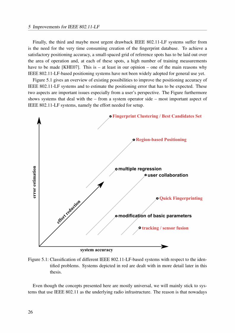
5 Improvements for IEEE 802.11-LF
Finally, the third and maybe most urgent drawback IEEE 802.11-LF systems suffer fromis the need for the very time consuming creation of the fingerprint database. To achieve asatisfactory positioning accuracy, a small-spaced grid of reference spots has to be laid out overthe area of operation and, at each of these spots, a high number of training measurementshave to be made [KHE07]. This is – at least in our opinion – one of the main reasons whyIEEE 802.11-LF-based positioning systems have not been widely adopted for general use yet.
Figure 5.1 gives an overview of existing possibilities to improve the positioning accuracy ofIEEE 802.11-LF systems and to estimate the positioning error that has to be expected. Thesetwo aspects are important issues especially from a user’s perspective. The Figure furthermoreshows systems that deal with the – from a system operator side – most important aspect ofIEEE 802.11-LF systems, namely the effort needed for setup.
Figure 5.1: Classification of different IEEE 802.11-LF-based systems with respect to the iden-tified problems. Systems depicted in red are dealt with in more detail later in thisthesis.
Even though the concepts presented here are mostly universal, we will mainly stick to sys-tems that use IEEE 802.11 as the underlying radio infrastructure. The reason is that nowadays
26
5.3 Areas for Improvements
IEEE 802.11 is the most ubiquitous radio technology that offers the possibility of a positioningaccuracy sufficient for most indoor scenarios, a sufficient coverage, and that is easy to use. Ex-tending our approaches to other radio systems (for example Zigbee) should be straightforward.
At first, Section 5.3.1 introduces current methods from other researchers as well as from our-selves to improve the positioning accuracy. This is followed by Section 5.3.2 where we presenttechniques to estimate the error of common IEEE 802.11-LF systems. Subsequently, Sec-tion 5.3.3 introduces new approaches to reduce the effort for creating the fingerprint database.In Section 5.3.4, we discuss the presented solutions from a more general perspective before we,in Section 5.3.5, finally conclude this section.
5.3.1 Increasing the Positioning Accuracy
There are many different aspects that affect the performance of a positioning system with regardto the positioning accuracy. As stated before, the class of systems that use a probabilistic metricgenerally offers a better positioning accuracy in most cases [YA04]. The Rice system introducedby Haeberlen et al. [HFL+04] is a typical representative of this class. However, besides avariation of the metric, several other aspects exist that can be used to improve the positioningaccuracy of LF systems based on IEEE 802.11. The possibilities range from advanced pre- orpost-processing steps of the sensor data over the consideration of the position or measurementhistory to the use of sensor fusion techniques.
Basic System Parameters
The easiest way to improve the positioning accuracy of LF systems is to modify basic setupparameters. As shown in [KHE07], a reduction of the grid spacing between the reference spots –in case a grid is used – has a major influence on the achievable accuracy. When, for example, thegrid spacing is reduced form 4 m to 2 m, the average accuracy of the studied system increasesfrom roughly 3 m to 2.5 m. In addition, both the number of measurements used to create eachsingle fingerprint during the training phase as well as the number of measurements used duringthe position determination phase have a large impact on the positioning accuracy. If the numberof the latter is increased from one to three, the achieved accuracy increases by 11%. Finally,also the number of APs which can be received throughout the coverage area matters for theachievable accuracy.
Measurement Processing
Inspired by fundamental research on this topic, other systems have been proposed that extendthe basic IEEE 802.11-LF approach by measurement pre- or post-processing steps to increasethe accuracy. An example for such an advanced system is Horus [YA05]. Horus uses an algo-rithm to detect and eliminate small-scale signal variations as they often occur when measuringthe signal strength of an IEEE 802.11 access point at a fixed position.
27
5 Improvements for IEEE 802.11-LF
Another often suggested possibility to improve the position accuracy of IEEE 802.11-basedLF systems is the use of advanced machine learning algorithms. In [WKB08], for instance,a particle filter approach is chosen to estimate the position of a user based on signal strengthmeasurements. Particle filters are part of the sequential Monte-Carlo methods and quite similarto Kalman filters. They are very well suited to deal with data and measurements that do notadhere to standardized distributions, like e.g., Gaussian distributions, as it is the case for indoorsignal strength measurements. Also, particle filters are computationally less expensive thanmany other methods. This makes them especially suitable for the use on mobile devices, beingless powerful compared to stationary computers. Widyawan et al. use a variation of the generalparticle filter approach called backtracking particle filter to increase the positioning accuracyof the underlying IEEE 802.11-LF system.
Feature Selection
Another approach is used by a system called SkyLoc [VLHdL07]. SkyLoc is a localizationsystem designed to run on cellular phones and is used to reliably determine the floor on whicha user is located in tall multi-story buildings. It uses the radio signals from base stations – orso-called cell towers – of the Global System for Mobile Communications (GSM) and locationfingerprints created for each floor of a building. To find the best-matching fingerprint in thedatabase, SkyLoc relies on a deterministic approach – namely the Euclidean distance in signalspace. To additionally improve the estimation accuracy, SkyLoc incorporates a method calledfeature selection. Instead of using data for all GSM cells from which a signal was receivedat the user’s current position, only a subset of these is used for matching against each of thefingerprints in the database. To identify the subset that offers the highest position accuracy inadvance of the deployment, the authors of [VLHdL07] suggest three different methods: The firstone is called Forward Selection. Starting with an empty set, the feature that offers the highestincrease in average position accuracy is added to the set of used features until it has reachedits final size. The second alternative is Backward Elimination. It proceeds in the oppositeway. From the full set of all available features, those features are removed successively fromthe set of which their removal offers the highest increase in the average position accuracy.Finally, the third method, namely Per-Floor Feature Selection, tries to find not one optimalfeature set to be used for the whole database but optimizes the set for each story separately.Additionally, the third method also uses weights for the single features to further increase theperformance. Transferring this approach to IEEE 802.11-LF would, for instance, suggest toonly use an optimized subset of the APs available at each reference position for an optimizedpositioning performance.
Sensor Fusion
Sensor fusion is another possibility to improve the accuracy of IEEE 802.11-LF systems. Sensorfusion means to not only use the readings from a single data source, in our case for instance
28
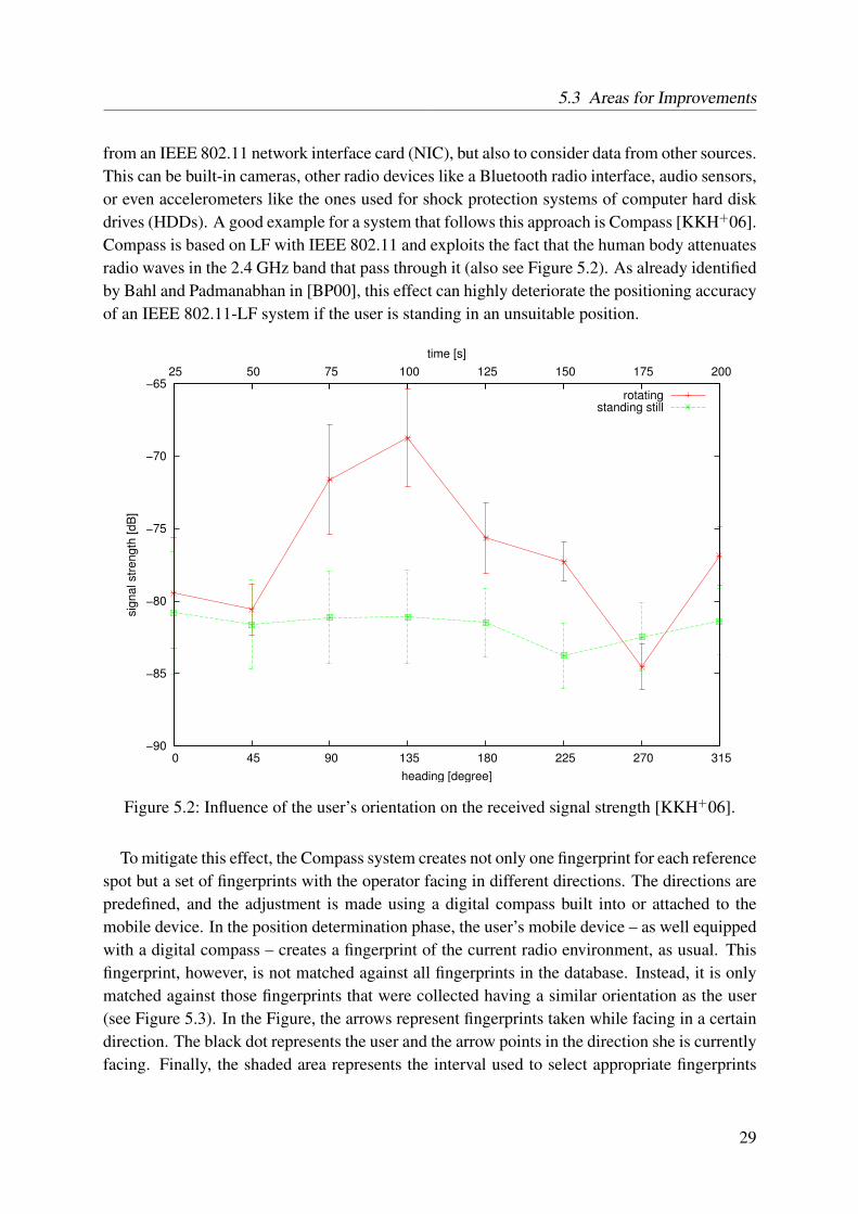
5.3 Areas for Improvements
from an IEEE 802.11 network interface card (NIC), but also to consider data from other sources.This can be built-in cameras, other radio devices like a Bluetooth radio interface, audio sensors,or even accelerometers like the ones used for shock protection systems of computer hard diskdrives (HDDs). A good example for a system that follows this approach is Compass [KKH+06].Compass is based on LF with IEEE 802.11 and exploits the fact that the human body attenuatesradio waves in the 2.4 GHz band that pass through it (also see Figure 5.2). As already identifiedby Bahl and Padmanabhan in [BP00], this effect can highly deteriorate the positioning accuracyof an IEEE 802.11-LF system if the user is standing in an unsuitable position.
−90
−85
−80
−75
−70
−65
0 45 90 135 180 225 270 315
25 50 75 100 125 150 175 200
sig
na
l str
en
gth
[d
B]
heading [degree]
time [s]
rotatingstanding still
Figure 5.2: Influence of the user’s orientation on the received signal strength [KKH+06].
To mitigate this effect, the Compass system creates not only one fingerprint for each referencespot but a set of fingerprints with the operator facing in different directions. The directions arepredefined, and the adjustment is made using a digital compass built into or attached to themobile device. In the position determination phase, the user’s mobile device – as well equippedwith a digital compass – creates a fingerprint of the current radio environment, as usual. Thisfingerprint, however, is not matched against all fingerprints in the database. Instead, it is onlymatched against those fingerprints that were collected having a similar orientation as the user(see Figure 5.3). In the Figure, the arrows represent fingerprints taken while facing in a certaindirection. The black dot represents the user and the arrow points in the direction she is currentlyfacing. Finally, the shaded area represents the interval used to select appropriate fingerprints
29
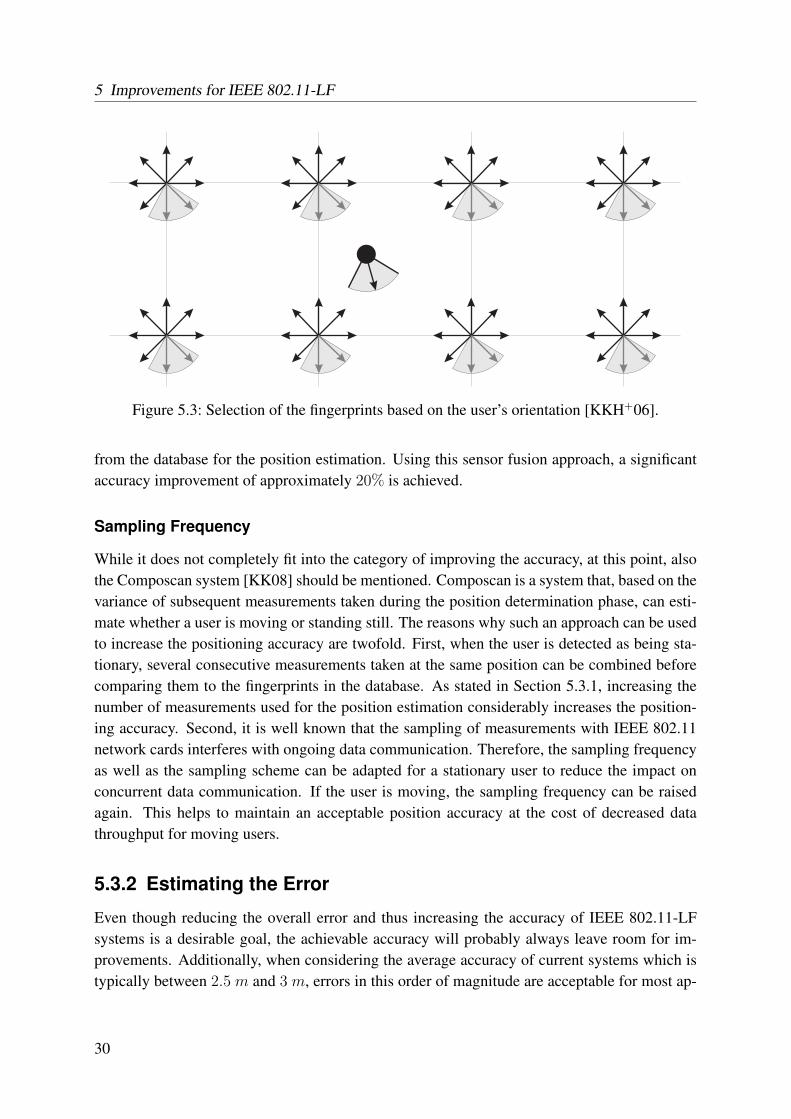
5 Improvements for IEEE 802.11-LF
Figure 5.3: Selection of the fingerprints based on the user’s orientation [KKH+06].
from the database for the position estimation. Using this sensor fusion approach, a significantaccuracy improvement of approximately 20% is achieved.
Sampling Frequency
While it does not completely fit into the category of improving the accuracy, at this point, alsothe Composcan system [KK08] should be mentioned. Composcan is a system that, based on thevariance of subsequent measurements taken during the position determination phase, can esti-mate whether a user is moving or standing still. The reasons why such an approach can be usedto increase the positioning accuracy are twofold. First, when the user is detected as being sta-tionary, several consecutive measurements taken at the same position can be combined beforecomparing them to the fingerprints in the database. As stated in Section 5.3.1, increasing thenumber of measurements used for the position estimation considerably increases the position-ing accuracy. Second, it is well known that the sampling of measurements with IEEE 802.11network cards interferes with ongoing data communication. Therefore, the sampling frequencyas well as the sampling scheme can be adapted for a stationary user to reduce the impact onconcurrent data communication. If the user is moving, the sampling frequency can be raisedagain. This helps to maintain an acceptable position accuracy at the cost of decreased datathroughput for moving users.
5.3.2 Estimating the Error
Even though reducing the overall error and thus increasing the accuracy of IEEE 802.11-LFsystems is a desirable goal, the achievable accuracy will probably always leave room for im-provements. Additionally, when considering the average accuracy of current systems which istypically between 2.5 m and 3 m, errors in this order of magnitude are acceptable for most ap-
30
5.3 Areas for Improvements
plications. However, one of the remaining problems with the position estimation is the so-calledlong-tail error: the quite unlike but still existing occurrence of a very large error. An estimationof the positioning error would be of high value to both the user and the system operator. In thissection, we therefore introduce different approaches that deal with the error of IEEE 802.11-LFsystems.
Error Distribution
The most basic approach of error estimation is to supply the user with general information aboutthe positioning error that has to be expected when using a certain positioning system. This canbe achieved by, for instance, supplying her with a cumulative distribution function (CDF) forthe error of the positioning system. Figure 5.4 gives an example for such a CDF. Here, forinstance, the error is smaller than 3 m in 80% of all cases. In this case, the user herself has toestimate the probability of a certain error to happen, and to adapt her behavior accordingly.
Even this very simple way of dealing with error information already has a remarkable impacton the user perception of an LBS. As a study by Dearman et al. [DVDLT07] has shown, eventhis situation-unspecific knowledge of the error distribution helps users of an LBS to performbetter when solving location-specific tasks. The main drawback of this approach is that it onlyoffers a general and not a situation-specific error estimation and as such might reduce the overalltrust a user has in her positioning system.
Multiple Regression
The authors of [DVDLT07] also introduced the use of multiple regression to estimate the posi-tioning error. Using the training data and a small number of test measurements for the referencespots, the system operator computes a linear model of the error that is expected based on a de-fined set of signal features. This set can contain the receivable APs or GSM cells, the signalstrengths, properties of the noise floor or other information available in the measurements. Dur-ing the position determination phase, the user then can apply the linear model to his currentlycollected data and compute an appropriate error estimate. Even though this approach still usesquite basic features to estimate the error, it already offers promising results. Therefore, we willintroduce several techniques using more advanced features to estimate the error in Section 5.6.
5.3.3 Reducing the Effort
The major reason why IEEE 802.11-LF is still only rarely adopted for position estimation be-yond academic settings is the need for the very time-consuming setup of the system. As an-alyzed in [KK08], a fine-grained grid of reference spots has to be used, and at least 20 mea-surements have to be collected at each reference spot to achieve a sufficient accuracy for mostLBSs. The following sections will present techniques on how this cumbersome process can becircumvented and how the overall effort can be reduced.
31
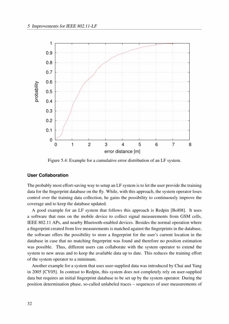
5 Improvements for IEEE 802.11-LF
0
0.1
0.2
0.3
0.4
0.5
0.6
0.7
0.8
0.9
1
0 1 2 3 4 5 6 7 8
pro
ba
bili
ty
error distance [m]
Figure 5.4: Example for a cumulative error distribution of an LF system.
User Collaboration
The probably most effort-saving way to setup an LF system is to let the user provide the trainingdata for the fingerprint database on the fly. While, with this approach, the system operator losescontrol over the training data collection, he gains the possibility to continuously improve thecoverage and to keep the database updated.
A good example for an LF system that follows this approach is Redpin [Bol08]. It usesa software that runs on the mobile device to collect signal measurements from GSM cells,IEEE 802.11 APs, and nearby Bluetooth-enabled devices. Besides the normal operation wherea fingerprint created from live measurements is matched against the fingerprints in the database,the software offers the possibility to store a fingerprint for the user’s current location in thedatabase in case that no matching fingerprint was found and therefore no position estimationwas possible. Thus, different users can collaborate with the system operator to extend thesystem to new areas and to keep the available data up to date. This reduces the training effortof the system operator to a minimum.
Another example for a system that uses user-supplied data was introduced by Chai and Yangin 2005 [CY05]. In contrast to Redpin, this system does not completely rely on user-supplieddata but requires an initial fingerprint database to be set up by the system operator. During theposition determination phase, so-called unlabeled traces – sequences of user measurements of
32
5.3 Areas for Improvements
which the positions are unknown – are used to refine the data in the fingerprint database. Toidentify the corresponding fingerprints, the authors apply an algorithm introduced by Dempsteret al. [DLR77] called Expectation Maximization algorithm. This algorithm iteratively computesmaximum likelihood estimates from a given set of incomplete observations. It is split into twosteps, an expectation step and a maximization step. The advantage of using unlabeled tracescompared to Redpin is that the operator can offer a guaranteed basic coverage of the area theinitial fingerprint database covers. However, this also shows the limits of this approach asthe unlabeled traces can only be used to refine existing data. Thus, the users cannot extendthe coverage area of the system on their own. An optimized solution could therefore use acombination of both approaches.
Generated Fingerprints
It is also possible to create the fingerprint database computationally. This approach reducesthe effort to set up an LF system very effectively. Most common here is the use of a radiopropagation model in combination with a few or even only one reference measurement. Basedon the measurement and the model, a radio map for the area to cover is computed. With valuestaken from this computed radio map, fingerprints are created for each reference spot in the area,and are then stored in the fingerprint database. For example, the system introduced by Ji etal. [JBPA06] follows this concept.
Whereas such an approach reduces the effort effectively, it is questionable how usable sucha system really is in practice. Considering the unpredictable behavior that radio signals showinside buildings, the performance of such a system strongly depends on the quality of the radiomodel in use. For instance, it has to incorporate factors like building materials or furniture at ahigh level of detail. If the model does not reflect the real radio propagation correctly, the entiresystem is unusable.
5.3.4 Discussion
As we have shown in the previous sections, several different solutions exist to mitigate thedrawbacks of 802.11-based LF systems. Each of these solutions fulfills its purpose when con-sidering its specific area. However, a look at the complete picture shows that not all solutionsare equally well suited for a real-world deployment.
Positioning Accuracy
For example, if we consider the Compass system mentioned in Section 5.3.1, we can see thatit offers a very competitive accuracy. But because one fingerprint has to be created for eachconsidered direction, the effort to set up the system would be even larger than it already is for abasic LF system.
33
5 Improvements for IEEE 802.11-LF
Exactly the opposite is true for the feature selection system presented in Section 5.3.1. Asthis system relies on data that is available anyway, and as its usage should have no negativeinfluence on other system parameters like the effort needed for setup, it can well be adopted forwidespread usage in LF systems.
Error Estimation
As mentioned in Section 5.3.2, the estimation of the expected error is mainly desirable to beable to provide the user with information in case of possibly large errors. This helps to increasethe user’s trust in the system. Because this is only possible with situation-specific knowledge,using only a distribution function like the one presented in Section 5.3.2 seems inappropriate.Algorithms that are able to use situation-specific information are better suited. This can eitherbe the training data, the online measurements, or even a combination of both. Such algorithmswere developed by us, and will be presented in Section 5.6.
Effort Reduction
Regarding the algorithms presented in Section 5.3.3, they have both advantages and disadvan-tages. Whereas the system presented in Section 5.3.3 that uses generated fingerprints veryconsequently reduces the effort necessary to set up the system, this comes at the cost of a heav-ily degraded accuracy if the selected radio model is not realistic. The system Redpin describedin Section 5.3.3 seems to be much better suited. The effort is effectively reduced while theaccuracy of the system is only influenced in terms of missing coverage. This comes at the costof lost control over the coverage area and the quality of the fingerprints, though.
Application-specific Requirements
As we have seen, not all presented solutions are equally well-suited to solve their correspond-ing problems and also the combination of different approaches is not always easily possible.Therefore, for a real deployment, the application requirements have to be considered as well inorder to identify features that need special consideration.
Let us think of, for instance, a friend finder application that is used on a university campus.On the one hand, the accuracy requirement could very well be reduced to room level as friendswould easily recognize each other if they were inside the same room. The same is true for theerror estimation where only errors beyond the size of a room would matter to the user. On theother hand, as the campus of a university generally covers a large area, a reduction of the effortto set up the system and to maintain the fingerprint database is a very important factor for thisscenario.
In contrast, when considering a warehouse navigation system, the situation is different. Tolocate items on the storage shelves, a high accuracy is necessary. Also the estimation of thepositioning error is of a higher importance in such a case: If the system is unsure about thecurrent estimate, it should inform the user in order to avoid the frustrating search for a stored
34
5.4 Quick Fingerprinting
item that might have been placed somewhere else. Therefore, such a system should obviouslyonly consider position estimates with a very low estimated error to avoid giving false directionsto the user. Compared to the first two properties, however, the effort necessary for setup andoperation is generally only of secondary importance in such a limited scenario.
5.3.5 Conclusions
Up to now, we gave a brief overview of techniques used to address the major issues that stillare obstacles to the wide adoption of IEEE 802.11-LF as a pervasive localization technology.Firstly, we have presented different techniques that can be used to increase the positioningaccuracy of 802.11-based LF systems. Increasing the accuracy is a prerequisite to be able toalso allow the use of advanced LBSs. Secondly, several possibilities to handle the problemof error estimation for IEEE 802.11-LF systems have been introduced. While this field ofresearch is still quite new, it nevertheless is of high importance – especially to the users ofLBSs. Finally, we have presented techniques that system operators can use to reduce the effortthat is necessary to set up a location fingerprinting database. This can help system operatorsto deploy and maintain IEEE 802.11-LF systems at a reasonable cost and, thus, to make theirusage more feasible. During our discussion, we have shown that, while suitable solutions existfor the single problems, a combination of these is neither always possible nor always necessary.Which of the different parameters should be optimized is highly dependent on the targetedapplication. We will now introduce our own contributions in the three mentioned fields.
5.4 Quick Fingerprinting
The time-consuming training phase is one of the major reasons why IEEE 802.11-based posi-tioning systems are still struggling to make their step from a scientific prototype to a conve-nience product. In this section, we therefore propose novel algorithms to set up a fingerprintingsystem. Our algorithms reduce the time needed to collect the necessary data during the trainingphase considerably without losing positioning accuracy. To accomplish this task, our algorithmspre-process the data that has been collected during the training phase. To create a fingerprint,not only the samples that have been collected at a single reference position are considered. In-stead, also samples that have been collected at positions adjacent to the position we create thefingerprint for are taken into account. With this approach, we can reduce both the amount ofdata that needs to be collected at each reference position and the time needed to collect the databy about 80% without losing positioning accuracy. In fact, our algorithms even increase thepositioning accuracy in most cases.
35
5 Improvements for IEEE 802.11-LF
5.4.1 Algorithms
In this section, we introduce the techniques used by our algorithms as well as by the algorithmwhich was taken as a benchmark during our evaluation.
Probabilistic Fingerprinting
When the Rice system is used, samples of the signal strengths of all receivable access pointsare collected at each reference position during the training phase. For each access point con-tained in the samples of one reference position, the average and the standard deviation of thesignal strength measurements are computed. These values are stored in the fingerprint of thecorresponding reference position. As a result, each fingerprint contains a pair of average signalstrength and standard deviation for each access point of which signals have been received atthe reference position. During the position determination phase, samples of the signal strengthof each receivable access point are collected. These samples are compared to the values storedin each of the fingerprints. By computing a normalized probability for each reference positionand selecting the position with the highest probability, the system comes up with a positionestimate.
In the following, we describe the computation of the probabilities in a more detailed fashion.For each fingerprint and each access point ap contained in the live samples, we compute a
probability P (sap). This probability states how probable it is to receive a signal of access pointap with a signal strength sap at the reference position r to which the fingerprint belongs.
To compute the probability, the live measured signal strength for access point ap is matchedwith the density function of a normal distribution with the parameters for access point ap takenfrom the current fingerprint. As the probability for a single value and a given continuous prob-ability distribution is zero per definition, the probability for an interval of s ± 0.5 is computedinstead (also refer to Equation 5.1).
While another value could also be used for the width of the interval, we decided to use thevalue introduced in [HFL+04] to map the discrete signal strength values the hardware delivers(−102 dB to 0 dB) to the continuous number space of the normal distribution.
Pr,ap(sap) =∫ s+0.5
s−0.5df(µr,ap, σr,ap) (5.1)
For access point ap, df is the density function of the normal distribution with an average ofµr,ap and a standard deviation of σr,ap. These values are taken from the fingerprint of referenceposition r (see Figure 5.5).
The latter step is repeated for all access points contained in the live samples. This, finally,leads to one overall value Pr per reference spot (see Equation 5.2) which – after a normaliza-tion step considering the sum of the values for all reference spots – can be interpreted as theprobability of the user being at reference position r.
Pr(s) = Πni=1Pr,api(sapi) (5.2)
36
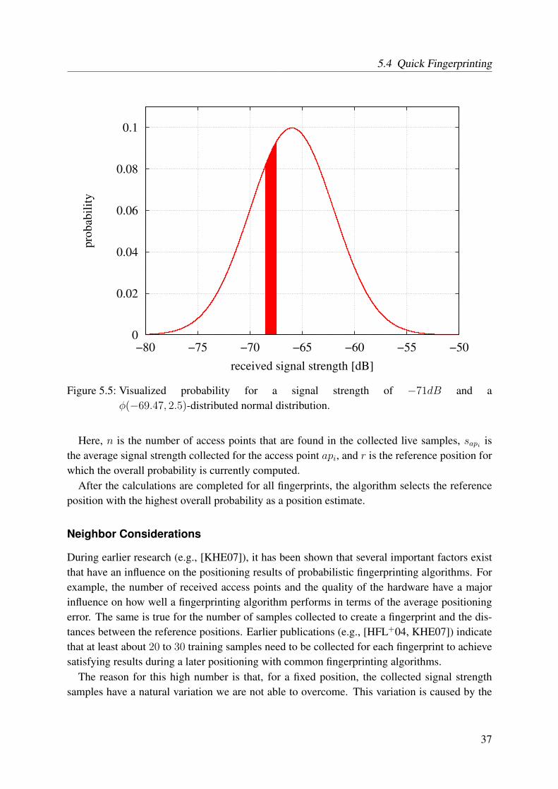
5.4 Quick Fingerprinting
0
0.02
0.04
0.06
0.08
0.1
−80 −75 −70 −65 −60 −55 −50
pro
bab
ilit
y
received signal strength [dB]
Figure 5.5: Visualized probability for a signal strength of −71dB and aφ(−69.47, 2.5)-distributed normal distribution.
Here, n is the number of access points that are found in the collected live samples, sapi isthe average signal strength collected for the access point api, and r is the reference position forwhich the overall probability is currently computed.
After the calculations are completed for all fingerprints, the algorithm selects the referenceposition with the highest overall probability as a position estimate.
Neighbor Considerations
During earlier research (e.g., [KHE07]), it has been shown that several important factors existthat have an influence on the positioning results of probabilistic fingerprinting algorithms. Forexample, the number of received access points and the quality of the hardware have a majorinfluence on how well a fingerprinting algorithm performs in terms of the average positioningerror. The same is true for the number of samples collected to create a fingerprint and the dis-tances between the reference positions. Earlier publications (e.g., [HFL+04, KHE07]) indicatethat at least about 20 to 30 training samples need to be collected for each fingerprint to achievesatisfying results during a later positioning with common fingerprinting algorithms.
The reason for this high number is that, for a fixed position, the collected signal strengthsamples have a natural variation we are not able to overcome. This variation is caused by the
37
5 Improvements for IEEE 802.11-LF
adverse propagation behavior of radio signals in indoor environments where we have to facesignal attenuation, signal diffraction, scattering, and multi-path propagation. To compensatefor these variations, a sufficiently large number of samples is generally needed to allow theaverage signal strength value to stabilize when creating a fingerprint. Having in mind the time-consuming task of collecting these samples for each single reference spot, the goal of our workis to reduce the required effort in a transparent and easy implementable way.
Furthermore, from a user’s perspective, a user who is located somewhere in a building duringthe position determination phase generally does not remain still while waiting for the collectionof enough samples to let the measurement values stabilize. As a result, even fewer signalstrength measurements will be taken during the position determination phase and, thus, themeasured values will scatter around the values stored in the fingerprints that were collected atthe reference positions close to the user’s current whereabouts.
Additionally, the user will almost never be located exactly at a reference position. Instead,she will stand or move somewhere between several reference positions in most cases. Therefore,often more than one fingerprint of adjacent reference spots around the user will give a suitablematch to the live data collected at the user’s real position.
Considering that the user will be located in between several reference spots most of the timeand that the signal strength of an access point at a given position has an inevitable fluctuationindoors, we propose new algorithms that take these insights into account in order to increasethe positioning accuracy on the one hand, while reducing the amount of needed samples to becollected at each reference position on the other hand.
Equal Weighting
At first, we present an algorithm that not only considers the samples that have been collected ata certain reference position itself but also the samples that have been collected at all adjacentreference spots in order to create the fingerprint. If the current reference position hasm adjacentreference positions and n samples are available for each position, this leads to m ∗ n samplesused to compute the fingerprint for the current position. The samples in this case are equallyweighted in the created fingerprint, which means that all the samples from the reference positionitself as well as those from the adjacent positions have an equal influence on the resultingfingerprint. This leads to a fingerprint that no longer represents only a single reference positionbut instead represents an area that is defined by the adjacent reference positions. Figure 5.6depicts this. The area C is – amongst others – covered by both the fingerprints for referencepositions A and B.
At this point, we want to point out that, even though we use more samples to create a singlefingerprint, we do not need to collect more samples. The essence of what we do is to re-use theexisting samples several times for different fingerprints.
38
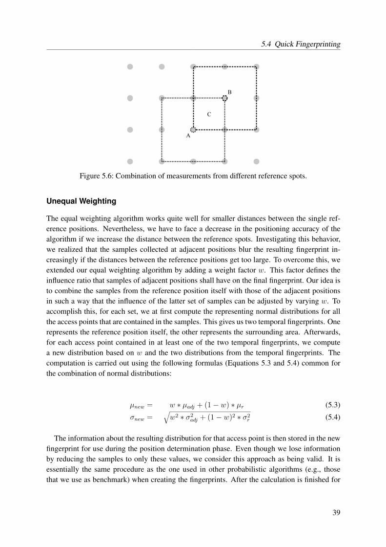
5.4 Quick Fingerprinting
Figure 5.6: Combination of measurements from different reference spots.
Unequal Weighting
The equal weighting algorithm works quite well for smaller distances between the single ref-erence positions. Nevertheless, we have to face a decrease in the positioning accuracy of thealgorithm if we increase the distance between the reference spots. Investigating this behavior,we realized that the samples collected at adjacent positions blur the resulting fingerprint in-creasingly if the distances between the reference positions get too large. To overcome this, weextended our equal weighting algorithm by adding a weight factor w. This factor defines theinfluence ratio that samples of adjacent positions shall have on the final fingerprint. Our idea isto combine the samples from the reference position itself with those of the adjacent positionsin such a way that the influence of the latter set of samples can be adjusted by varying w. Toaccomplish this, for each set, we at first compute the representing normal distributions for allthe access points that are contained in the samples. This gives us two temporal fingerprints. Onerepresents the reference position itself, the other represents the surrounding area. Afterwards,for each access point contained in at least one of the two temporal fingerprints, we computea new distribution based on w and the two distributions from the temporal fingerprints. Thecomputation is carried out using the following formulas (Equations 5.3 and 5.4) common forthe combination of normal distributions:
µnew = w ∗ µadj + (1 − w) ∗ µr (5.3)
σnew =√w2 ∗ σ2
adj + (1 − w)2 ∗ σ2r (5.4)
The information about the resulting distribution for that access point is then stored in the newfingerprint for use during the position determination phase. Even though we lose informationby reducing the samples to only these values, we consider this approach as being valid. It isessentially the same procedure as the one used in other probabilistic algorithms (e.g., thosethat we use as benchmark) when creating the fingerprints. After the calculation is finished for
39
5 Improvements for IEEE 802.11-LF
the current reference position, the newly computed fingerprint embodies two values (µnew andσnew) for each access point that was contained in the original set of samples for that position.
5.4.2 Evaluation Setup
The following section briefly describes the environment in which we collected the data for ourevaluation. Additionally, an overview is given of the data themselves as well as the hard- andsoftware used for collecting them.
Evaluation Environment
The environment where we conducted the data collection for the evaluation of our algorithmsis the second floor of the building A5-B at the University of Mannheim in Germany, wherethe offices of our group are located. The story is split up into two hallways, several offices,and three smaller rooms in the middle of the larger hallway (see Figure 5.7). The two hallwaysmeasure 30 m times 6 m and 15 m times 4 m respectively, covering an area of approximately240 m2.
Data Collection
To get a sufficient amount of data for the evaluation, 612 reference positions were laid out inthe evaluation environment using a grid of 0.5 m side length (see the blue dots in Figure 5.7).The samples collected at these positions are the foundation for the fingerprint databases usedduring our evaluation.
Additionally, 70 points were spread randomly over the hallways (the pink dots in Figure 5.7)to which we will refer to as live positions or live spots from now on. The samples collected atthese positions are used to emulate a user requesting a position estimation during the followingemulation of the position determination phase.
110 samples were collected at each reference position and each live position during the datacollection process. The collected samples contain a time stamp, the medium access control(MAC) address of the collecting IEEE 802.11 interface card, the current position, and, for eachreceived access point, the MAC address, the channel, and the RSSI. All samples were loggedto a file for easy reference during the following evaluation.
Hard- and Software
To collect the samples, we used an IBM Thinkpad R51 laptop computer running Suse Linux10.1. The laptop computer was equipped with a plug-in Lucent Silver PCMCIA card.
On the software side, the samples were collected with the LocEva framework [KBH07]. Theapplication to collect the samples uses the Java Native Interface and a wrapper written in C tointeract with the operating system kernel’s wireless extensions interface. This makes it possible
40
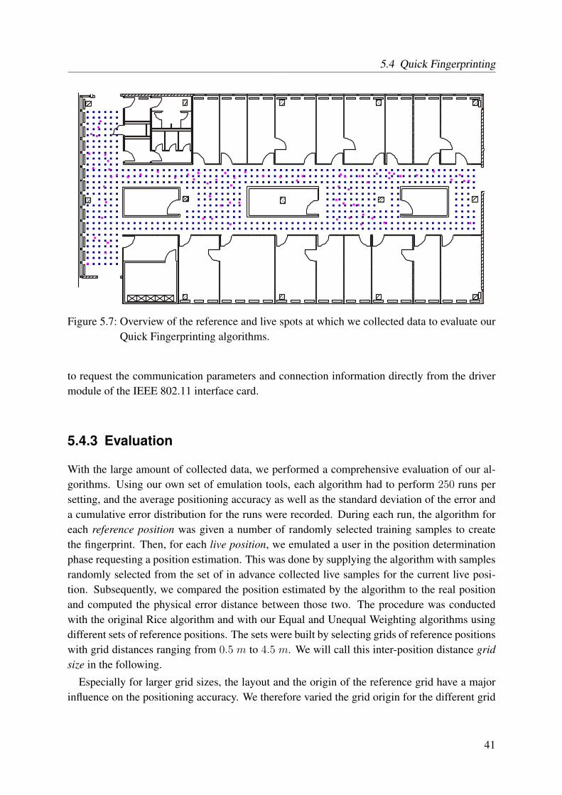
5.4 Quick Fingerprinting
Figure 5.7: Overview of the reference and live spots at which we collected data to evaluate ourQuick Fingerprinting algorithms.
to request the communication parameters and connection information directly from the drivermodule of the IEEE 802.11 interface card.
5.4.3 Evaluation
With the large amount of collected data, we performed a comprehensive evaluation of our al-gorithms. Using our own set of emulation tools, each algorithm had to perform 250 runs persetting, and the average positioning accuracy as well as the standard deviation of the error anda cumulative error distribution for the runs were recorded. During each run, the algorithm foreach reference position was given a number of randomly selected training samples to createthe fingerprint. Then, for each live position, we emulated a user in the position determinationphase requesting a position estimation. This was done by supplying the algorithm with samplesrandomly selected from the set of in advance collected live samples for the current live posi-tion. Subsequently, we compared the position estimated by the algorithm to the real positionand computed the physical error distance between those two. The procedure was conductedwith the original Rice algorithm and with our Equal and Unequal Weighting algorithms usingdifferent sets of reference positions. The sets were built by selecting grids of reference positionswith grid distances ranging from 0.5 m to 4.5 m. We will call this inter-position distance gridsize in the following.
Especially for larger grid sizes, the layout and the origin of the reference grid have a majorinfluence on the positioning accuracy. We therefore varied the grid origin for the different grid
41
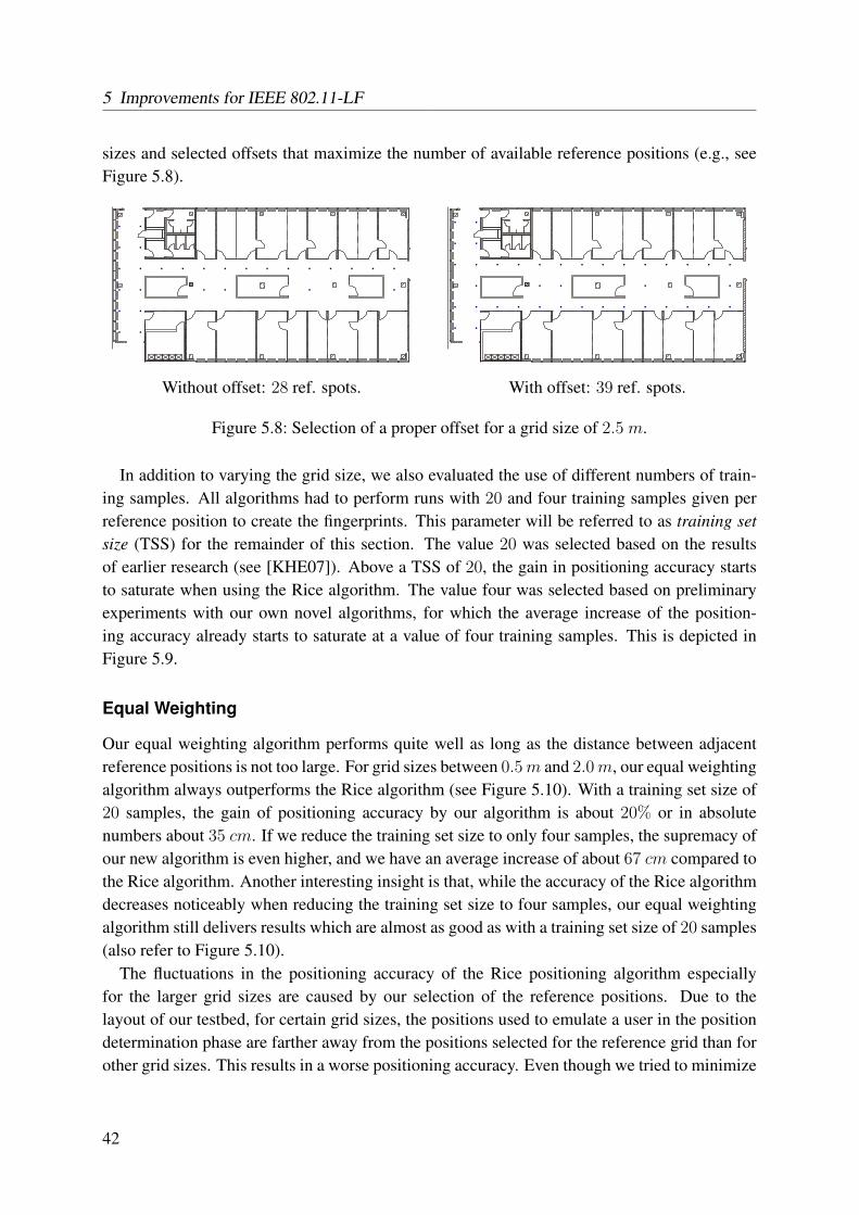
5 Improvements for IEEE 802.11-LF
sizes and selected offsets that maximize the number of available reference positions (e.g., seeFigure 5.8).
Without offset: 28 ref. spots. With offset: 39 ref. spots.
Figure 5.8: Selection of a proper offset for a grid size of 2.5 m.
In addition to varying the grid size, we also evaluated the use of different numbers of train-ing samples. All algorithms had to perform runs with 20 and four training samples given perreference position to create the fingerprints. This parameter will be referred to as training setsize (TSS) for the remainder of this section. The value 20 was selected based on the resultsof earlier research (see [KHE07]). Above a TSS of 20, the gain in positioning accuracy startsto saturate when using the Rice algorithm. The value four was selected based on preliminaryexperiments with our own novel algorithms, for which the average increase of the position-ing accuracy already starts to saturate at a value of four training samples. This is depicted inFigure 5.9.
Equal Weighting
Our equal weighting algorithm performs quite well as long as the distance between adjacentreference positions is not too large. For grid sizes between 0.5m and 2.0m, our equal weightingalgorithm always outperforms the Rice algorithm (see Figure 5.10). With a training set size of20 samples, the gain of positioning accuracy by our algorithm is about 20% or in absolutenumbers about 35 cm. If we reduce the training set size to only four samples, the supremacy ofour new algorithm is even higher, and we have an average increase of about 67 cm compared tothe Rice algorithm. Another interesting insight is that, while the accuracy of the Rice algorithmdecreases noticeably when reducing the training set size to four samples, our equal weightingalgorithm still delivers results which are almost as good as with a training set size of 20 samples(also refer to Figure 5.10).
The fluctuations in the positioning accuracy of the Rice positioning algorithm especiallyfor the larger grid sizes are caused by our selection of the reference positions. Due to thelayout of our testbed, for certain grid sizes, the positions used to emulate a user in the positiondetermination phase are farther away from the positions selected for the reference grid than forother grid sizes. This results in a worse positioning accuracy. Even though we tried to minimize
42
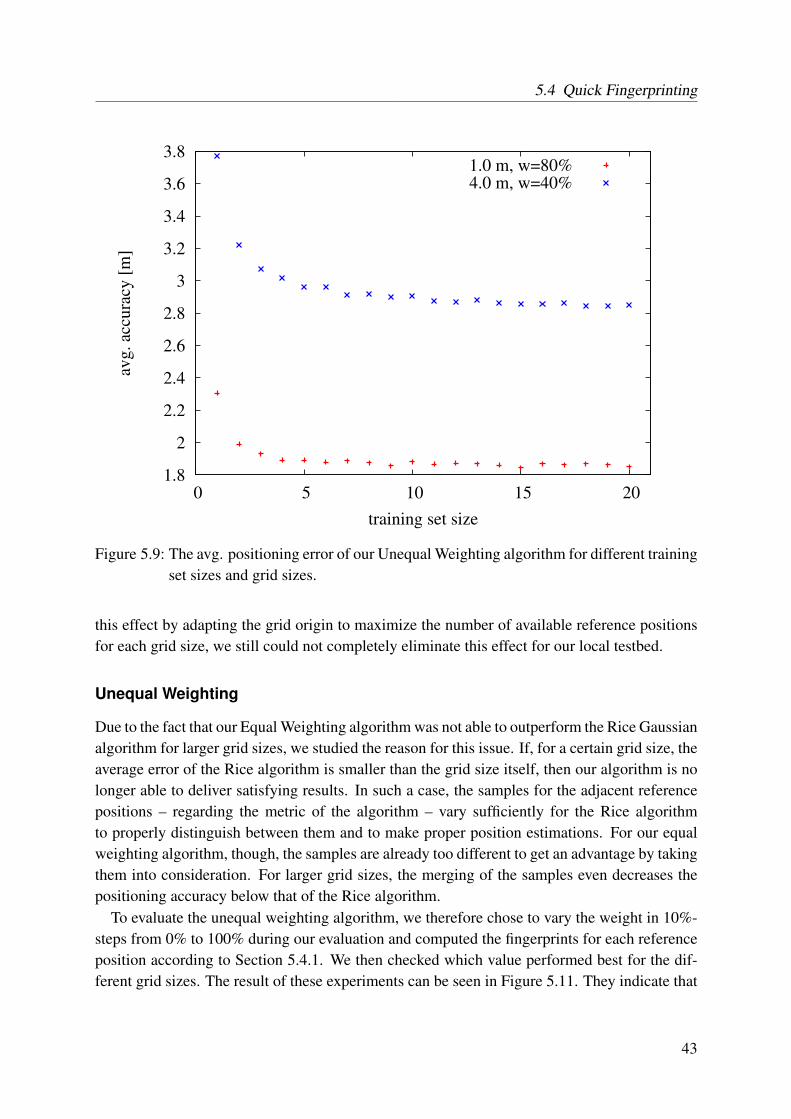
5.4 Quick Fingerprinting
1.8
2
2.2
2.4
2.6
2.8
3
3.2
3.4
3.6
3.8
0 5 10 15 20
avg
. ac
cura
cy [
m]
training set size
1.0 m, w=80%4.0 m, w=40%
Figure 5.9: The avg. positioning error of our Unequal Weighting algorithm for different trainingset sizes and grid sizes.
this effect by adapting the grid origin to maximize the number of available reference positionsfor each grid size, we still could not completely eliminate this effect for our local testbed.
Unequal Weighting
Due to the fact that our Equal Weighting algorithm was not able to outperform the Rice Gaussianalgorithm for larger grid sizes, we studied the reason for this issue. If, for a certain grid size, theaverage error of the Rice algorithm is smaller than the grid size itself, then our algorithm is nolonger able to deliver satisfying results. In such a case, the samples for the adjacent referencepositions – regarding the metric of the algorithm – vary sufficiently for the Rice algorithmto properly distinguish between them and to make proper position estimations. For our equalweighting algorithm, though, the samples are already too different to get an advantage by takingthem into consideration. For larger grid sizes, the merging of the samples even decreases thepositioning accuracy below that of the Rice algorithm.
To evaluate the unequal weighting algorithm, we therefore chose to vary the weight in 10%-steps from 0% to 100% during our evaluation and computed the fingerprints for each referenceposition according to Section 5.4.1. We then checked which value performed best for the dif-ferent grid sizes. The result of these experiments can be seen in Figure 5.11. They indicate that
43
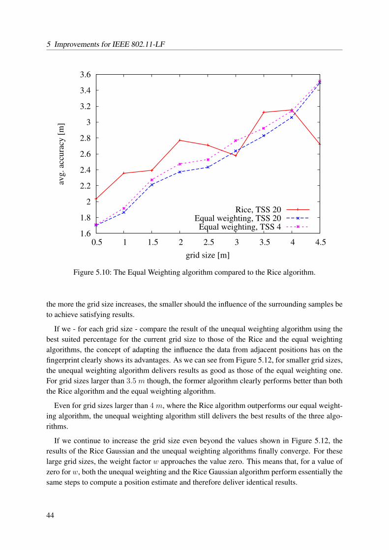
5 Improvements for IEEE 802.11-LF
1.6
1.8
2
2.2
2.4
2.6
2.8
3
3.2
3.4
3.6
0.5 1 1.5 2 2.5 3 3.5 4 4.5
avg
. ac
cura
cy [
m]
grid size [m]
Rice, TSS 20Equal weighting, TSS 20
Equal weighting, TSS 4
Figure 5.10: The Equal Weighting algorithm compared to the Rice algorithm.
the more the grid size increases, the smaller should the influence of the surrounding samples beto achieve satisfying results.
If we - for each grid size - compare the result of the unequal weighting algorithm using thebest suited percentage for the current grid size to those of the Rice and the equal weightingalgorithms, the concept of adapting the influence the data from adjacent positions has on thefingerprint clearly shows its advantages. As we can see from Figure 5.12, for smaller grid sizes,the unequal weighting algorithm delivers results as good as those of the equal weighting one.For grid sizes larger than 3.5 m though, the former algorithm clearly performs better than boththe Rice algorithm and the equal weighting algorithm.
Even for grid sizes larger than 4 m, where the Rice algorithm outperforms our equal weight-ing algorithm, the unequal weighting algorithm still delivers the best results of the three algo-rithms.
If we continue to increase the grid size even beyond the values shown in Figure 5.12, theresults of the Rice Gaussian and the unequal weighting algorithms finally converge. For theselarge grid sizes, the weight factor w approaches the value zero. This means that, for a value ofzero for w, both the unequal weighting and the Rice Gaussian algorithm perform essentially thesame steps to compute a position estimate and therefore deliver identical results.
44
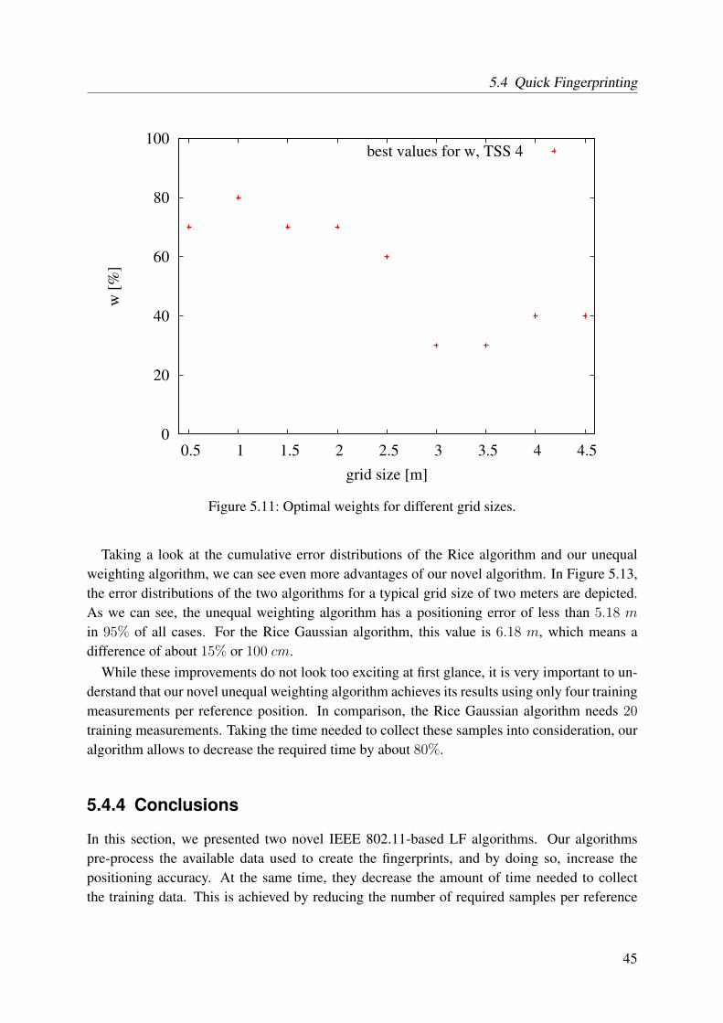
5.4 Quick Fingerprinting
0
20
40
60
80
100
0.5 1 1.5 2 2.5 3 3.5 4 4.5
w [
%]
grid size [m]
best values for w, TSS 4
Figure 5.11: Optimal weights for different grid sizes.
Taking a look at the cumulative error distributions of the Rice algorithm and our unequalweighting algorithm, we can see even more advantages of our novel algorithm. In Figure 5.13,the error distributions of the two algorithms for a typical grid size of two meters are depicted.As we can see, the unequal weighting algorithm has a positioning error of less than 5.18 m
in 95% of all cases. For the Rice Gaussian algorithm, this value is 6.18 m, which means adifference of about 15% or 100 cm.
While these improvements do not look too exciting at first glance, it is very important to un-derstand that our novel unequal weighting algorithm achieves its results using only four trainingmeasurements per reference position. In comparison, the Rice Gaussian algorithm needs 20
training measurements. Taking the time needed to collect these samples into consideration, ouralgorithm allows to decrease the required time by about 80%.
5.4.4 Conclusions
In this section, we presented two novel IEEE 802.11-based LF algorithms. Our algorithmspre-process the available data used to create the fingerprints, and by doing so, increase thepositioning accuracy. At the same time, they decrease the amount of time needed to collectthe training data. This is achieved by reducing the number of required samples per reference
45
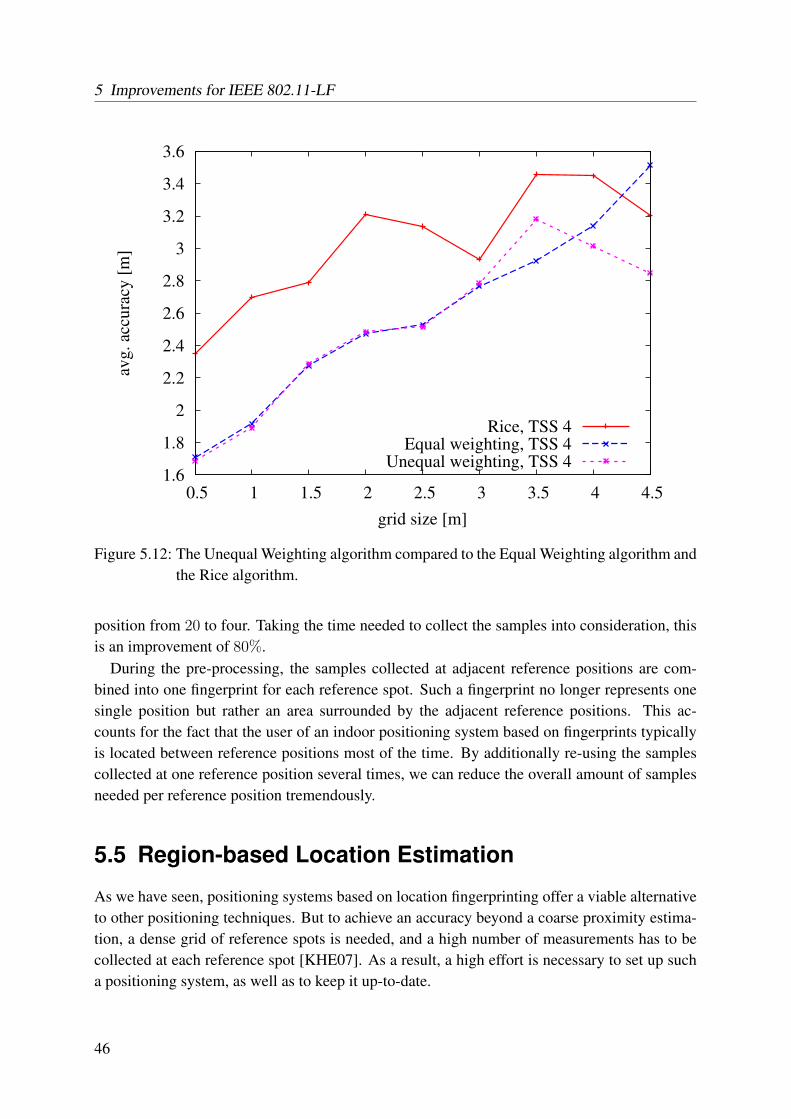
5 Improvements for IEEE 802.11-LF
1.6
1.8
2
2.2
2.4
2.6
2.8
3
3.2
3.4
3.6
0.5 1 1.5 2 2.5 3 3.5 4 4.5
avg
. ac
cura
cy [
m]
grid size [m]
Rice, TSS 4Equal weighting, TSS 4
Unequal weighting, TSS 4
Figure 5.12: The Unequal Weighting algorithm compared to the Equal Weighting algorithm andthe Rice algorithm.
position from 20 to four. Taking the time needed to collect the samples into consideration, thisis an improvement of 80%.
During the pre-processing, the samples collected at adjacent reference positions are com-bined into one fingerprint for each reference spot. Such a fingerprint no longer represents onesingle position but rather an area surrounded by the adjacent reference positions. This ac-counts for the fact that the user of an indoor positioning system based on fingerprints typicallyis located between reference positions most of the time. By additionally re-using the samplescollected at one reference position several times, we can reduce the overall amount of samplesneeded per reference position tremendously.
5.5 Region-based Location Estimation
As we have seen, positioning systems based on location fingerprinting offer a viable alternativeto other positioning techniques. But to achieve an accuracy beyond a coarse proximity estima-tion, a dense grid of reference spots is needed, and a high number of measurements has to becollected at each reference spot [KHE07]. As a result, a high effort is necessary to set up sucha positioning system, as well as to keep it up-to-date.
46
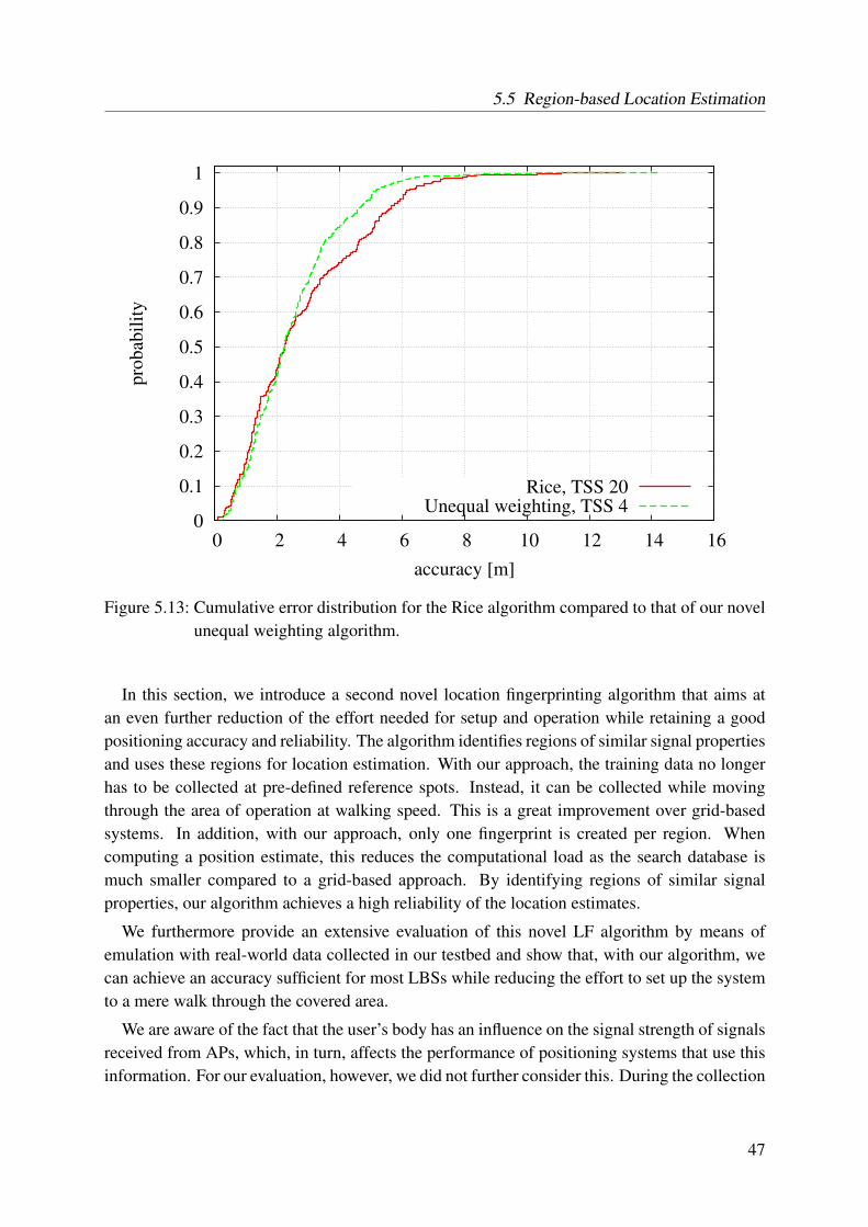
5.5 Region-based Location Estimation
0
0.1
0.2
0.3
0.4
0.5
0.6
0.7
0.8
0.9
1
0 2 4 6 8 10 12 14 16
pro
bab
ilit
y
accuracy [m]
Rice, TSS 20Unequal weighting, TSS 4
Figure 5.13: Cumulative error distribution for the Rice algorithm compared to that of our novelunequal weighting algorithm.
In this section, we introduce a second novel location fingerprinting algorithm that aims atan even further reduction of the effort needed for setup and operation while retaining a goodpositioning accuracy and reliability. The algorithm identifies regions of similar signal propertiesand uses these regions for location estimation. With our approach, the training data no longerhas to be collected at pre-defined reference spots. Instead, it can be collected while movingthrough the area of operation at walking speed. This is a great improvement over grid-basedsystems. In addition, with our approach, only one fingerprint is created per region. Whencomputing a position estimate, this reduces the computational load as the search database ismuch smaller compared to a grid-based approach. By identifying regions of similar signalproperties, our algorithm achieves a high reliability of the location estimates.
We furthermore provide an extensive evaluation of this novel LF algorithm by means ofemulation with real-world data collected in our testbed and show that, with our algorithm, wecan achieve an accuracy sufficient for most LBSs while reducing the effort to set up the systemto a mere walk through the covered area.
We are aware of the fact that the user’s body has an influence on the signal strength of signalsreceived from APs, which, in turn, affects the performance of positioning systems that use thisinformation. For our evaluation, however, we did not further consider this. During the collection
47
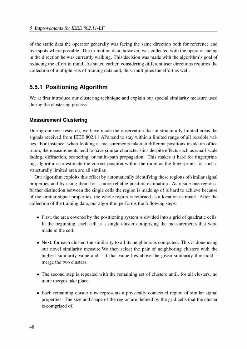
5 Improvements for IEEE 802.11-LF
of the static data the operator generally was facing the same direction both for reference andlive spots where possible. The in-motion data, however, was collected with the operator facingin the direction he was currently walking. This decision was made with the algorithm’s goal ofreducing the effort in mind. As stated earlier, considering different user directions requires thecollection of multiple sets of training data and, thus, multiplies the effort as well.
5.5.1 Positioning Algorithm
We at first introduce our clustering technique and explain our special similarity measure usedduring the clustering process.
Measurement Clustering
During our own research, we have made the observation that in structurally limited areas thesignals received from IEEE 802.11 APs tend to stay within a limited range of all possible val-ues. For instance, when looking at measurements taken at different positions inside an officeroom, the measurements tend to have similar characteristics despite effects such as small-scalefading, diffraction, scattering, or multi-path propagation. This makes it hard for fingerprint-ing algorithms to estimate the correct position within the room as the fingerprints for such astructurally limited area are all similar.
Our algorithm exploits this effect by automatically identifying these regions of similar signalproperties and by using them for a more reliable position estimation. As inside one region afurther distinction between the single cells the region is made up of is hard to achieve becauseof the similar signal properties, the whole region is returned as a location estimate. After thecollection of the training data, our algorithm performs the following steps:
• First, the area covered by the positioning system is divided into a grid of quadratic cells.In the beginning, each cell is a single cluster comprising the measurements that weremade in the cell.
• Next, for each cluster, the similarity to all its neighbors is computed. This is done usingour novel similarity measure.We then select the pair of neighboring clusters with thehighest similarity value and – if that value lies above the given similarity threshold –merge the two clusters.
• The second step is repeated with the remaining set of clusters until, for all clusters, nomore merges take place.
• Each remaining cluster now represents a physically connected region of similar signalproperties. The size and shape of the region are defined by the grid cells that the clusteris comprised of.
48
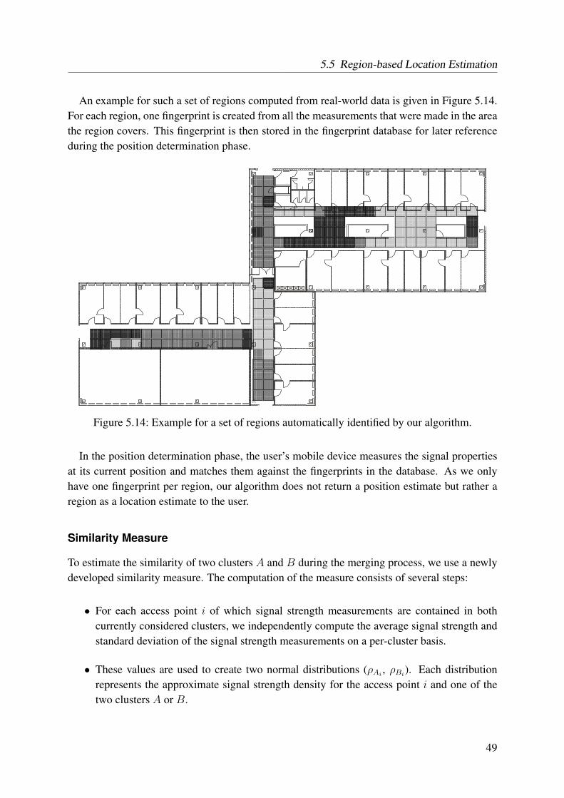
5.5 Region-based Location Estimation
An example for such a set of regions computed from real-world data is given in Figure 5.14.For each region, one fingerprint is created from all the measurements that were made in the areathe region covers. This fingerprint is then stored in the fingerprint database for later referenceduring the position determination phase.
Figure 5.14: Example for a set of regions automatically identified by our algorithm.
In the position determination phase, the user’s mobile device measures the signal propertiesat its current position and matches them against the fingerprints in the database. As we onlyhave one fingerprint per region, our algorithm does not return a position estimate but rather aregion as a location estimate to the user.
Similarity Measure
To estimate the similarity of two clusters A and B during the merging process, we use a newlydeveloped similarity measure. The computation of the measure consists of several steps:
• For each access point i of which signal strength measurements are contained in bothcurrently considered clusters, we independently compute the average signal strength andstandard deviation of the signal strength measurements on a per-cluster basis.
• These values are used to create two normal distributions (ρAi, ρBi
). Each distributionrepresents the approximate signal strength density for the access point i and one of thetwo clusters A or B.
49
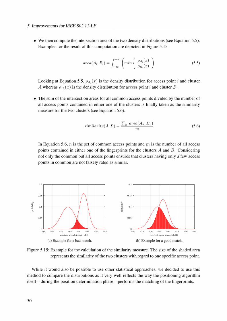
5 Improvements for IEEE 802.11-LF
• We then compute the intersection area of the two density distributions (see Equation 5.5).Examples for the result of this computation are depicted in Figure 5.15.
area(Ai, Bi) =
∫ +∞
−∞
(min
{ρAi(x)
ρBi(x)
)(5.5)
Looking at Equation 5.5, ρAi(x) is the density distribution for access point i and cluster
A whereas ρBi(x) is the density distribution for access point i and cluster B.
• The sum of the intersection areas for all common access points divided by the number ofall access points contained in either one of the clusters is finally taken as the similaritymeasure for the two clusters (see Equation 5.6).
similarity(A,B) =
∑n area(An, Bn)
m(5.6)
In Equation 5.6, n is the set of common access points and m is the number of all accesspoints contained in either one of the fingerprints for the clusters A and B. Consideringnot only the common but all access points ensures that clusters having only a few accesspoints in common are not falsely rated as similar.
0
0.05
0.1
0.15
0.2
−80 −75 −70 −65 −60 −55 −50 −45
pro
bab
ilit
y
received signal strength [dB]
(a) Example for a bad match.
0
0.05
0.1
0.15
0.2
−80 −75 −70 −65 −60 −55 −50 −45
pro
bab
ilit
y
received signal strength [dB]
(b) Example for a good match.
Figure 5.15: Example for the calculation of the similarity measure. The size of the shaded arearepresents the similarity of the two clusters with regard to one specific access point.
While it would also be possible to use other statistical approaches, we decided to use thismethod to compare the distributions as it very well reflects the way the positioning algorithmitself – during the position determination phase – performs the matching of the fingerprints.
50
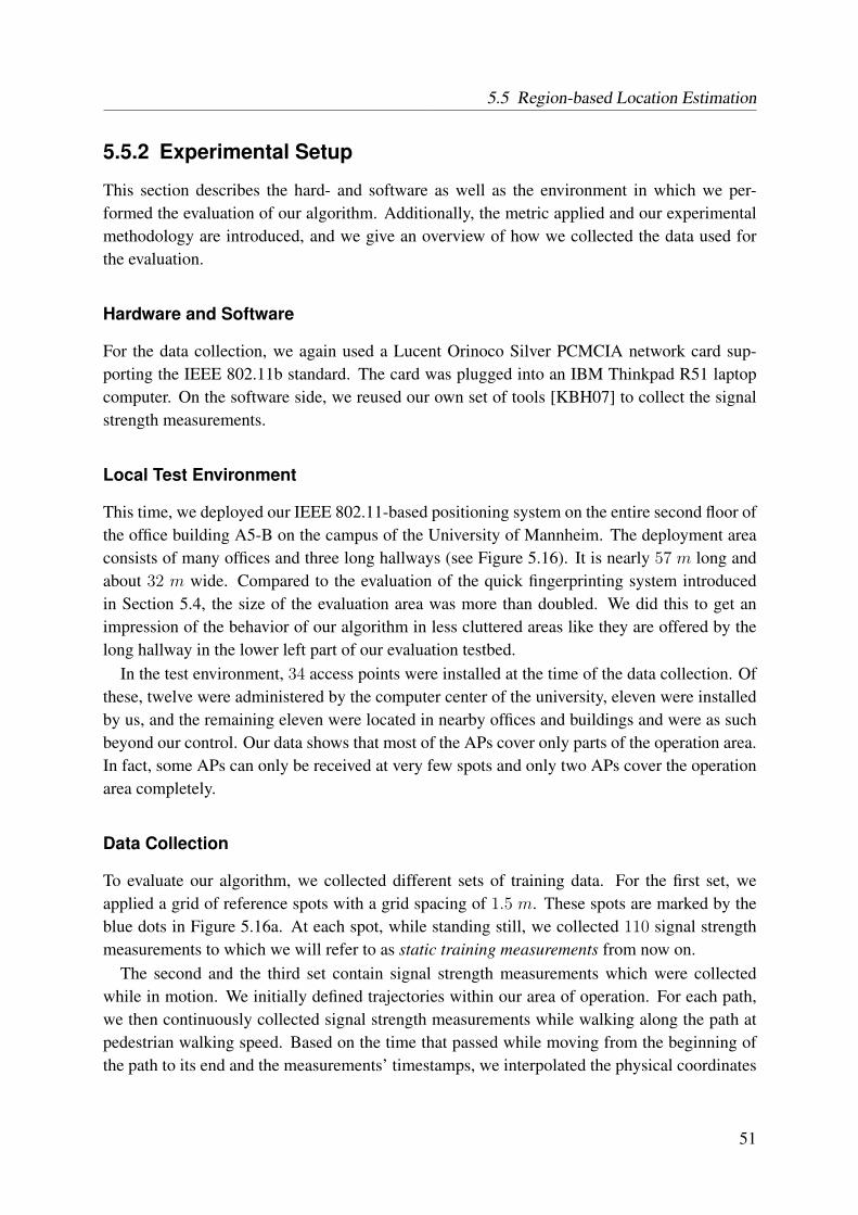
5.5 Region-based Location Estimation
5.5.2 Experimental Setup
This section describes the hard- and software as well as the environment in which we per-formed the evaluation of our algorithm. Additionally, the metric applied and our experimentalmethodology are introduced, and we give an overview of how we collected the data used forthe evaluation.
Hardware and Software
For the data collection, we again used a Lucent Orinoco Silver PCMCIA network card sup-porting the IEEE 802.11b standard. The card was plugged into an IBM Thinkpad R51 laptopcomputer. On the software side, we reused our own set of tools [KBH07] to collect the signalstrength measurements.
Local Test Environment
This time, we deployed our IEEE 802.11-based positioning system on the entire second floor ofthe office building A5-B on the campus of the University of Mannheim. The deployment areaconsists of many offices and three long hallways (see Figure 5.16). It is nearly 57 m long andabout 32 m wide. Compared to the evaluation of the quick fingerprinting system introducedin Section 5.4, the size of the evaluation area was more than doubled. We did this to get animpression of the behavior of our algorithm in less cluttered areas like they are offered by thelong hallway in the lower left part of our evaluation testbed.
In the test environment, 34 access points were installed at the time of the data collection. Ofthese, twelve were administered by the computer center of the university, eleven were installedby us, and the remaining eleven were located in nearby offices and buildings and were as suchbeyond our control. Our data shows that most of the APs cover only parts of the operation area.In fact, some APs can only be received at very few spots and only two APs cover the operationarea completely.
Data Collection
To evaluate our algorithm, we collected different sets of training data. For the first set, weapplied a grid of reference spots with a grid spacing of 1.5 m. These spots are marked by theblue dots in Figure 5.16a. At each spot, while standing still, we collected 110 signal strengthmeasurements to which we will refer to as static training measurements from now on.
The second and the third set contain signal strength measurements which were collectedwhile in motion. We initially defined trajectories within our area of operation. For each path,we then continuously collected signal strength measurements while walking along the path atpedestrian walking speed. Based on the time that passed while moving from the beginning ofthe path to its end and the measurements’ timestamps, we interpolated the physical coordinates
51
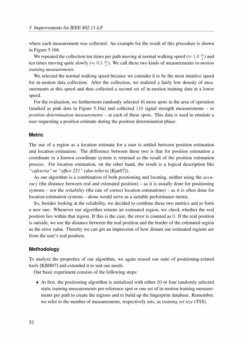
5 Improvements for IEEE 802.11-LF
where each measurement was collected. An example for the result of this procedure is shownin Figure 5.16b.
We repeated the collection ten times per path moving at normal walking speed (≈ 1.0 ms
) andten times moving quite slowly (≈ 0.5 m
s). We call these two kinds of measurements in-motion
training measurements.We selected the normal walking speed because we consider it to be the most intuitive speed
for in-motion data collection. After the collection, we realized a fairly low density of mea-surements at this speed and thus collected a second set of in-motion training data at a lowerspeed.
For the evaluation, we furthermore randomly selected 46 more spots in the area of operation(marked as pink dots in Figure 5.16a) and collected 110 signal strength measurements – orposition determination measurements – at each of these spots. This data is used to emulate auser requesting a position estimate during the position determination phase.
Metric
The use of a region as a location estimate for a user is settled between position estimationand location estimation. The difference between these two is that for position estimation acoordinate in a known coordinate system is returned as the result of the position estimationprocess. For location estimation, on the other hand, the result is a logical description like“cafeteria” or “office 221” (also refer to [Kjæ07]).
As our algorithm is a combination of both positioning and locating, neither using the accu-racy (the distance between real and estimated position) – as it is usually done for positioningsystems – nor the reliability (the rate of correct location estimations) – as it is often done forlocation estimation systems – alone would serve as a suitable performance metric.
So, besides looking at the reliability, we decided to combine these two metrics and to forma new one: Whenever our algorithm returns an estimated region, we check whether the realposition lies within that region. If this is the case, the error is counted as 0. If the real positionis outside, we use the distance between the real position and the border of the estimated regionas the error value. Thereby we can get an impression of how distant our estimated regions arefrom the user’s real position.
Methodology
To analyze the properties of our algorithm, we again reused our suite of positioning-relatedtools [KBH07] and extended it to suit our needs.
Our basic experiment consists of the following steps:
• At first, the positioning algorithm is initialized with either 20 or four randomly selectedstatic training measurements per reference spot or one set of in-motion training measure-ments per path to create the regions and to build up the fingerprint database. Remember,we refer to the number of measurements, respectively sets, as training set size (TSS).
52
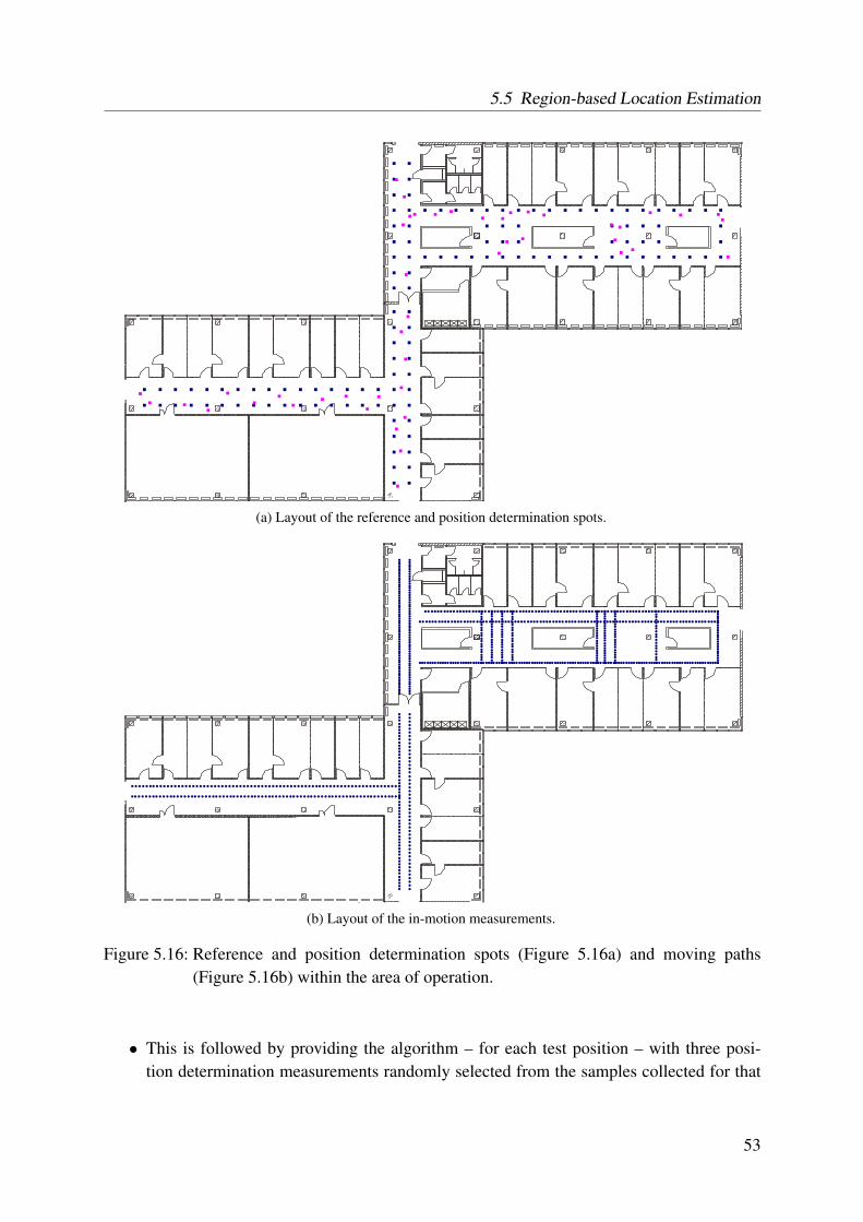
5.5 Region-based Location Estimation
(a) Layout of the reference and position determination spots.
(b) Layout of the in-motion measurements.
Figure 5.16: Reference and position determination spots (Figure 5.16a) and moving paths(Figure 5.16b) within the area of operation.
• This is followed by providing the algorithm – for each test position – with three posi-tion determination measurements randomly selected from the samples collected for that
53
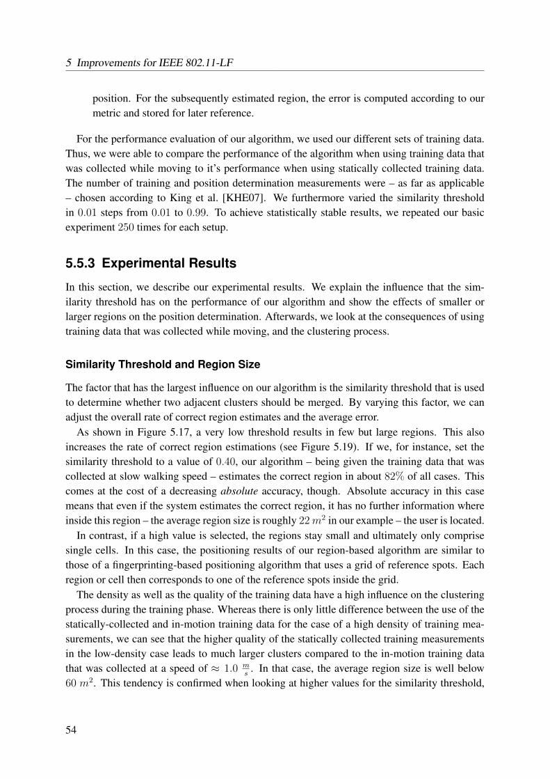
5 Improvements for IEEE 802.11-LF
position. For the subsequently estimated region, the error is computed according to ourmetric and stored for later reference.
For the performance evaluation of our algorithm, we used our different sets of training data.Thus, we were able to compare the performance of the algorithm when using training data thatwas collected while moving to it’s performance when using statically collected training data.The number of training and position determination measurements were – as far as applicable– chosen according to King et al. [KHE07]. We furthermore varied the similarity thresholdin 0.01 steps from 0.01 to 0.99. To achieve statistically stable results, we repeated our basicexperiment 250 times for each setup.
5.5.3 Experimental Results
In this section, we describe our experimental results. We explain the influence that the sim-ilarity threshold has on the performance of our algorithm and show the effects of smaller orlarger regions on the position determination. Afterwards, we look at the consequences of usingtraining data that was collected while moving, and the clustering process.
Similarity Threshold and Region Size
The factor that has the largest influence on our algorithm is the similarity threshold that is usedto determine whether two adjacent clusters should be merged. By varying this factor, we canadjust the overall rate of correct region estimates and the average error.
As shown in Figure 5.17, a very low threshold results in few but large regions. This alsoincreases the rate of correct region estimations (see Figure 5.19). If we, for instance, set thesimilarity threshold to a value of 0.40, our algorithm – being given the training data that wascollected at slow walking speed – estimates the correct region in about 82% of all cases. Thiscomes at the cost of a decreasing absolute accuracy, though. Absolute accuracy in this casemeans that even if the system estimates the correct region, it has no further information whereinside this region – the average region size is roughly 22m2 in our example – the user is located.
In contrast, if a high value is selected, the regions stay small and ultimately only comprisesingle cells. In this case, the positioning results of our region-based algorithm are similar tothose of a fingerprinting-based positioning algorithm that uses a grid of reference spots. Eachregion or cell then corresponds to one of the reference spots inside the grid.
The density as well as the quality of the training data have a high influence on the clusteringprocess during the training phase. Whereas there is only little difference between the use of thestatically-collected and in-motion training data for the case of a high density of training mea-surements, we can see that the higher quality of the statically collected training measurementsin the low-density case leads to much larger clusters compared to the in-motion training datathat was collected at a speed of ≈ 1.0 m
s. In that case, the average region size is well below
60 m2. This tendency is confirmed when looking at higher values for the similarity threshold,
54
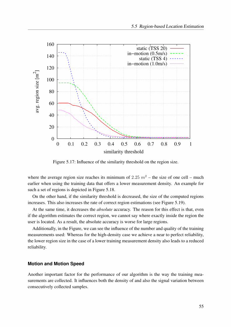
5.5 Region-based Location Estimation
0
20
40
60
80
100
120
140
160
0 0.1 0.2 0.3 0.4 0.5 0.6 0.7 0.8 0.9 1
avg
. re
gio
n s
ize
[m2]
similarity threshold
static (TSS 20)in−motion (0.5m/s)
static (TSS 4)in−motion (1.0m/s)
Figure 5.17: Influence of the similarity threshold on the region size.
where the average region size reaches its minimum of 2.25 m2 – the size of one cell – muchearlier when using the training data that offers a lower measurement density. An example forsuch a set of regions is depicted in Figure 5.18.
On the other hand, if the similarity threshold is decreased, the size of the computed regionsincreases. This also increases the rate of correct region estimations (see Figure 5.19).
At the same time, it decreases the absolute accuracy. The reason for this effect is that, evenif the algorithm estimates the correct region, we cannot say where exactly inside the region theuser is located. As a result, the absolute accuracy is worse for large regions.
Additionally, in the Figure, we can see the influence of the number and quality of the trainingmeasurements used: Whereas for the high-density case we achieve a near to perfect reliability,the lower region size in the case of a lower training measurement density also leads to a reducedreliability.
Motion and Motion Speed
Another important factor for the performance of our algorithm is the way the training mea-surements are collected. It influences both the density of and also the signal variation betweenconsecutively collected samples.
55
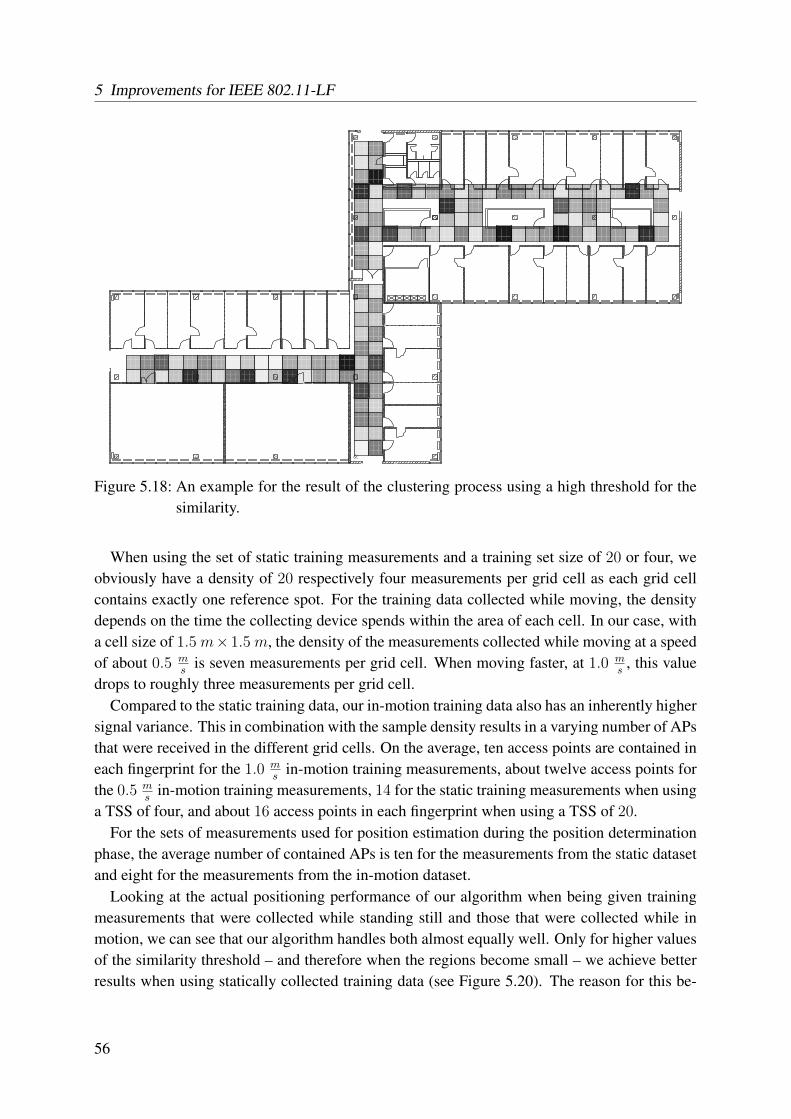
5 Improvements for IEEE 802.11-LF
Figure 5.18: An example for the result of the clustering process using a high threshold for thesimilarity.
When using the set of static training measurements and a training set size of 20 or four, weobviously have a density of 20 respectively four measurements per grid cell as each grid cellcontains exactly one reference spot. For the training data collected while moving, the densitydepends on the time the collecting device spends within the area of each cell. In our case, witha cell size of 1.5 m×1.5 m, the density of the measurements collected while moving at a speedof about 0.5 m
sis seven measurements per grid cell. When moving faster, at 1.0 m
s, this value
drops to roughly three measurements per grid cell.Compared to the static training data, our in-motion training data also has an inherently higher
signal variance. This in combination with the sample density results in a varying number of APsthat were received in the different grid cells. On the average, ten access points are contained ineach fingerprint for the 1.0 m
sin-motion training measurements, about twelve access points for
the 0.5 ms
in-motion training measurements, 14 for the static training measurements when usinga TSS of four, and about 16 access points in each fingerprint when using a TSS of 20.
For the sets of measurements used for position estimation during the position determinationphase, the average number of contained APs is ten for the measurements from the static datasetand eight for the measurements from the in-motion dataset.
Looking at the actual positioning performance of our algorithm when being given trainingmeasurements that were collected while standing still and those that were collected while inmotion, we can see that our algorithm handles both almost equally well. Only for higher valuesof the similarity threshold – and therefore when the regions become small – we achieve betterresults when using statically collected training data (see Figure 5.20). The reason for this be-
56
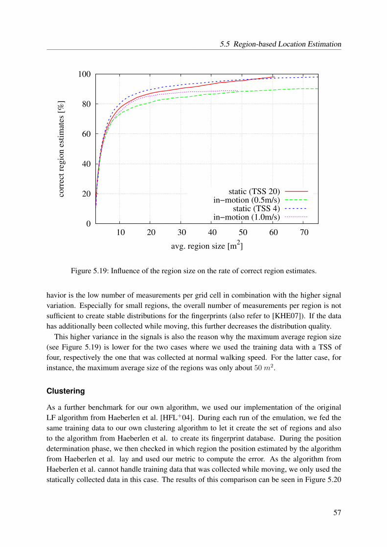
5.5 Region-based Location Estimation
0
20
40
60
80
100
10 20 30 40 50 60 70
corr
ect
reg
ion
est
imat
es [
%]
avg. region size [m2]
static (TSS 20)in−motion (0.5m/s)
static (TSS 4)in−motion (1.0m/s)
Figure 5.19: Influence of the region size on the rate of correct region estimates.
havior is the low number of measurements per grid cell in combination with the higher signalvariation. Especially for small regions, the overall number of measurements per region is notsufficient to create stable distributions for the fingerprints (also refer to [KHE07]). If the datahas additionally been collected while moving, this further decreases the distribution quality.
This higher variance in the signals is also the reason why the maximum average region size(see Figure 5.19) is lower for the two cases where we used the training data with a TSS offour, respectively the one that was collected at normal walking speed. For the latter case, forinstance, the maximum average size of the regions was only about 50 m2.
Clustering
As a further benchmark for our own algorithm, we used our implementation of the originalLF algorithm from Haeberlen et al. [HFL+04]. During each run of the emulation, we fed thesame training data to our own clustering algorithm to let it create the set of regions and alsoto the algorithm from Haeberlen et al. to create its fingerprint database. During the positiondetermination phase, we then checked in which region the position estimated by the algorithmfrom Haeberlen et al. lay and used our metric to compute the error. As the algorithm fromHaeberlen et al. cannot handle training data that was collected while moving, we only used thestatically collected data in this case. The results of this comparison can be seen in Figure 5.20
57
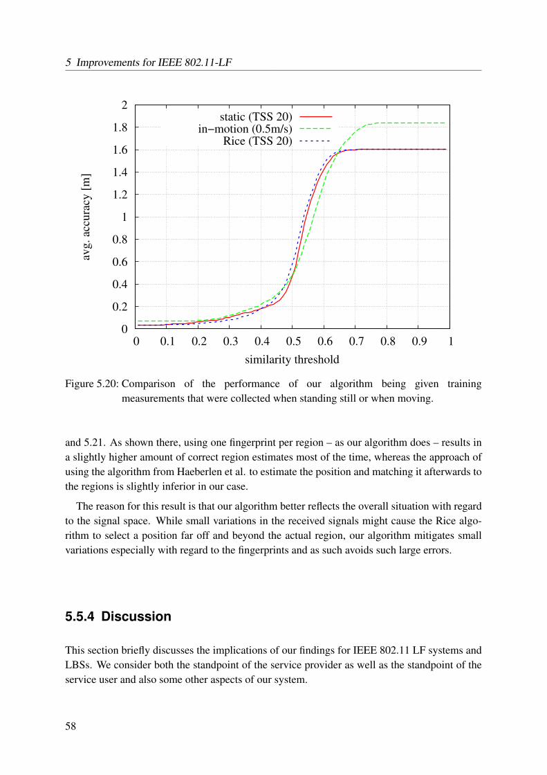
5 Improvements for IEEE 802.11-LF
0
0.2
0.4
0.6
0.8
1
1.2
1.4
1.6
1.8
2
0 0.1 0.2 0.3 0.4 0.5 0.6 0.7 0.8 0.9 1
avg
. ac
cura
cy [
m]
similarity threshold
static (TSS 20)in−motion (0.5m/s)
Rice (TSS 20)
Figure 5.20: Comparison of the performance of our algorithm being given trainingmeasurements that were collected when standing still or when moving.
and 5.21. As shown there, using one fingerprint per region – as our algorithm does – results ina slightly higher amount of correct region estimates most of the time, whereas the approach ofusing the algorithm from Haeberlen et al. to estimate the position and matching it afterwards tothe regions is slightly inferior in our case.
The reason for this result is that our algorithm better reflects the overall situation with regardto the signal space. While small variations in the received signals might cause the Rice algo-rithm to select a position far off and beyond the actual region, our algorithm mitigates smallvariations especially with regard to the fingerprints and as such avoids such large errors.
5.5.4 Discussion
This section briefly discusses the implications of our findings for IEEE 802.11 LF systems andLBSs. We consider both the standpoint of the service provider as well as the standpoint of theservice user and also some other aspects of our system.
58
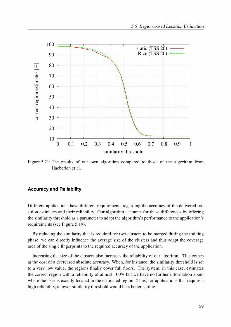
5.5 Region-based Location Estimation
10
20
30
40
50
60
70
80
90
100
0 0.1 0.2 0.3 0.4 0.5 0.6 0.7 0.8 0.9 1
corr
ect
reg
ion
est
imat
es [
%]
similarity threshold
static (TSS 20)Rice (TSS 20)
Figure 5.21: The results of our own algorithm compared to those of the algorithm fromHaeberlen et al.
Accuracy and Reliability
Different applications have different requirements regarding the accuracy of the delivered po-sition estimates and their reliability. Our algorithm accounts for these differences by offeringthe similarity threshold as a parameter to adapt the algorithm’s performance to the application’srequirements (see Figure 5.19).
By reducing the similarity that is required for two clusters to be merged during the trainingphase, we can directly influence the average size of the clusters and thus adapt the coveragearea of the single fingerprints to the required accuracy of the application.
Increasing the size of the clusters also increases the reliability of our algorithm. This comesat the cost of a decreased absolute accuracy. When, for instance, the similarity threshold is setto a very low value, the regions finally cover full floors. The system, in this case, estimatesthe correct region with a reliability of almost 100% but we have no further information aboutwhere the user is exactly located in the estimated region. Thus, for applications that require ahigh reliability, a lower similarity threshold would be a better setting.
59
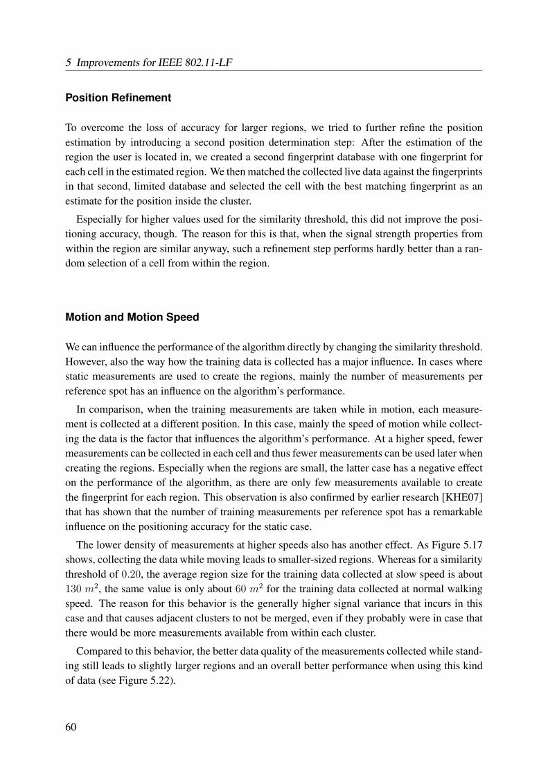
5 Improvements for IEEE 802.11-LF
Position Refinement
To overcome the loss of accuracy for larger regions, we tried to further refine the positionestimation by introducing a second position determination step: After the estimation of theregion the user is located in, we created a second fingerprint database with one fingerprint foreach cell in the estimated region. We then matched the collected live data against the fingerprintsin that second, limited database and selected the cell with the best matching fingerprint as anestimate for the position inside the cluster.
Especially for higher values used for the similarity threshold, this did not improve the posi-tioning accuracy, though. The reason for this is that, when the signal strength properties fromwithin the region are similar anyway, such a refinement step performs hardly better than a ran-dom selection of a cell from within the region.
Motion and Motion Speed
We can influence the performance of the algorithm directly by changing the similarity threshold.However, also the way how the training data is collected has a major influence. In cases wherestatic measurements are used to create the regions, mainly the number of measurements perreference spot has an influence on the algorithm’s performance.
In comparison, when the training measurements are taken while in motion, each measure-ment is collected at a different position. In this case, mainly the speed of motion while collect-ing the data is the factor that influences the algorithm’s performance. At a higher speed, fewermeasurements can be collected in each cell and thus fewer measurements can be used later whencreating the regions. Especially when the regions are small, the latter case has a negative effecton the performance of the algorithm, as there are only few measurements available to createthe fingerprint for each region. This observation is also confirmed by earlier research [KHE07]that has shown that the number of training measurements per reference spot has a remarkableinfluence on the positioning accuracy for the static case.
The lower density of measurements at higher speeds also has another effect. As Figure 5.17shows, collecting the data while moving leads to smaller-sized regions. Whereas for a similaritythreshold of 0.20, the average region size for the training data collected at slow speed is about130 m2, the same value is only about 60 m2 for the training data collected at normal walkingspeed. The reason for this behavior is the generally higher signal variance that incurs in thiscase and that causes adjacent clusters to not be merged, even if they probably were in case thatthere would be more measurements available from within each cluster.
Compared to this behavior, the better data quality of the measurements collected while stand-ing still leads to slightly larger regions and an overall better performance when using this kindof data (see Figure 5.22).
60
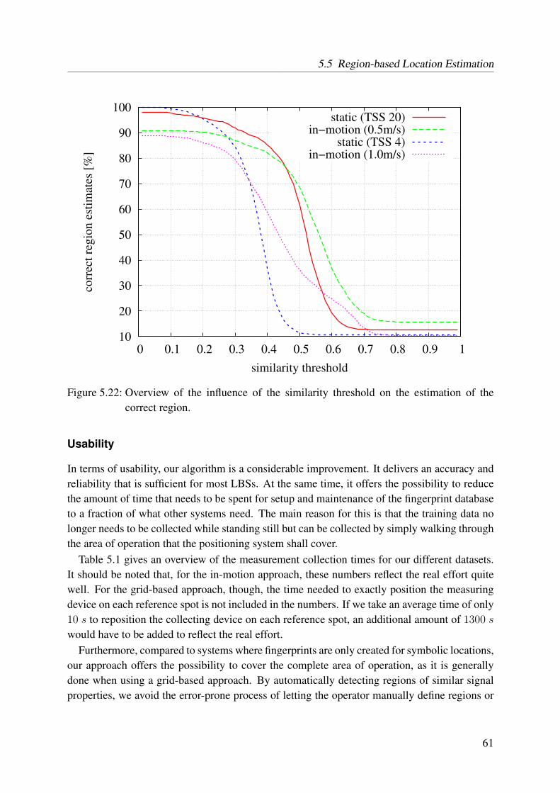
5.5 Region-based Location Estimation
10
20
30
40
50
60
70
80
90
100
0 0.1 0.2 0.3 0.4 0.5 0.6 0.7 0.8 0.9 1
corr
ect
reg
ion
est
imat
es [
%]
similarity threshold
static (TSS 20)in−motion (0.5m/s)
static (TSS 4)in−motion (1.0m/s)
Figure 5.22: Overview of the influence of the similarity threshold on the estimation of thecorrect region.
Usability
In terms of usability, our algorithm is a considerable improvement. It delivers an accuracy andreliability that is sufficient for most LBSs. At the same time, it offers the possibility to reducethe amount of time that needs to be spent for setup and maintenance of the fingerprint databaseto a fraction of what other systems need. The main reason for this is that the training data nolonger needs to be collected while standing still but can be collected by simply walking throughthe area of operation that the positioning system shall cover.
Table 5.1 gives an overview of the measurement collection times for our different datasets.It should be noted that, for the in-motion approach, these numbers reflect the real effort quitewell. For the grid-based approach, though, the time needed to exactly position the measuringdevice on each reference spot is not included in the numbers. If we take an average time of only10 s to reposition the collecting device on each reference spot, an additional amount of 1300 s
would have to be added to reflect the real effort.Furthermore, compared to systems where fingerprints are only created for symbolic locations,
our approach offers the possibility to cover the complete area of operation, as it is generallydone when using a grid-based approach. By automatically detecting regions of similar signalproperties, we avoid the error-prone process of letting the operator manually define regions or
61
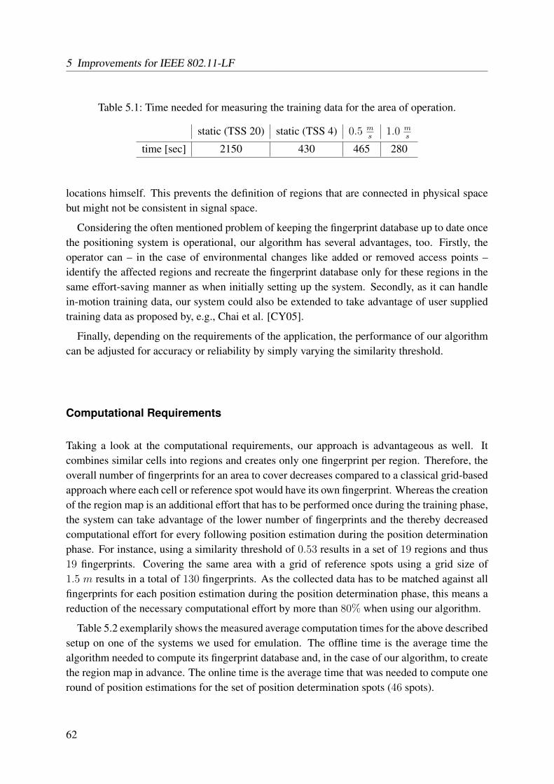
5 Improvements for IEEE 802.11-LF
Table 5.1: Time needed for measuring the training data for the area of operation.
static (TSS 20) static (TSS 4) 0.5 ms
1.0 ms
time [sec] 2150 430 465 280
locations himself. This prevents the definition of regions that are connected in physical spacebut might not be consistent in signal space.
Considering the often mentioned problem of keeping the fingerprint database up to date oncethe positioning system is operational, our algorithm has several advantages, too. Firstly, theoperator can – in the case of environmental changes like added or removed access points –identify the affected regions and recreate the fingerprint database only for these regions in thesame effort-saving manner as when initially setting up the system. Secondly, as it can handlein-motion training data, our system could also be extended to take advantage of user suppliedtraining data as proposed by, e.g., Chai et al. [CY05].
Finally, depending on the requirements of the application, the performance of our algorithmcan be adjusted for accuracy or reliability by simply varying the similarity threshold.
Computational Requirements
Taking a look at the computational requirements, our approach is advantageous as well. Itcombines similar cells into regions and creates only one fingerprint per region. Therefore, theoverall number of fingerprints for an area to cover decreases compared to a classical grid-basedapproach where each cell or reference spot would have its own fingerprint. Whereas the creationof the region map is an additional effort that has to be performed once during the training phase,the system can take advantage of the lower number of fingerprints and the thereby decreasedcomputational effort for every following position estimation during the position determinationphase. For instance, using a similarity threshold of 0.53 results in a set of 19 regions and thus19 fingerprints. Covering the same area with a grid of reference spots using a grid size of1.5 m results in a total of 130 fingerprints. As the collected data has to be matched against allfingerprints for each position estimation during the position determination phase, this means areduction of the necessary computational effort by more than 80% when using our algorithm.
Table 5.2 exemplarily shows the measured average computation times for the above describedsetup on one of the systems we used for emulation. The offline time is the average time thealgorithm needed to compute its fingerprint database and, in the case of our algorithm, to createthe region map in advance. The online time is the average time that was needed to compute oneround of position estimations for the set of position determination spots (46 spots).
62
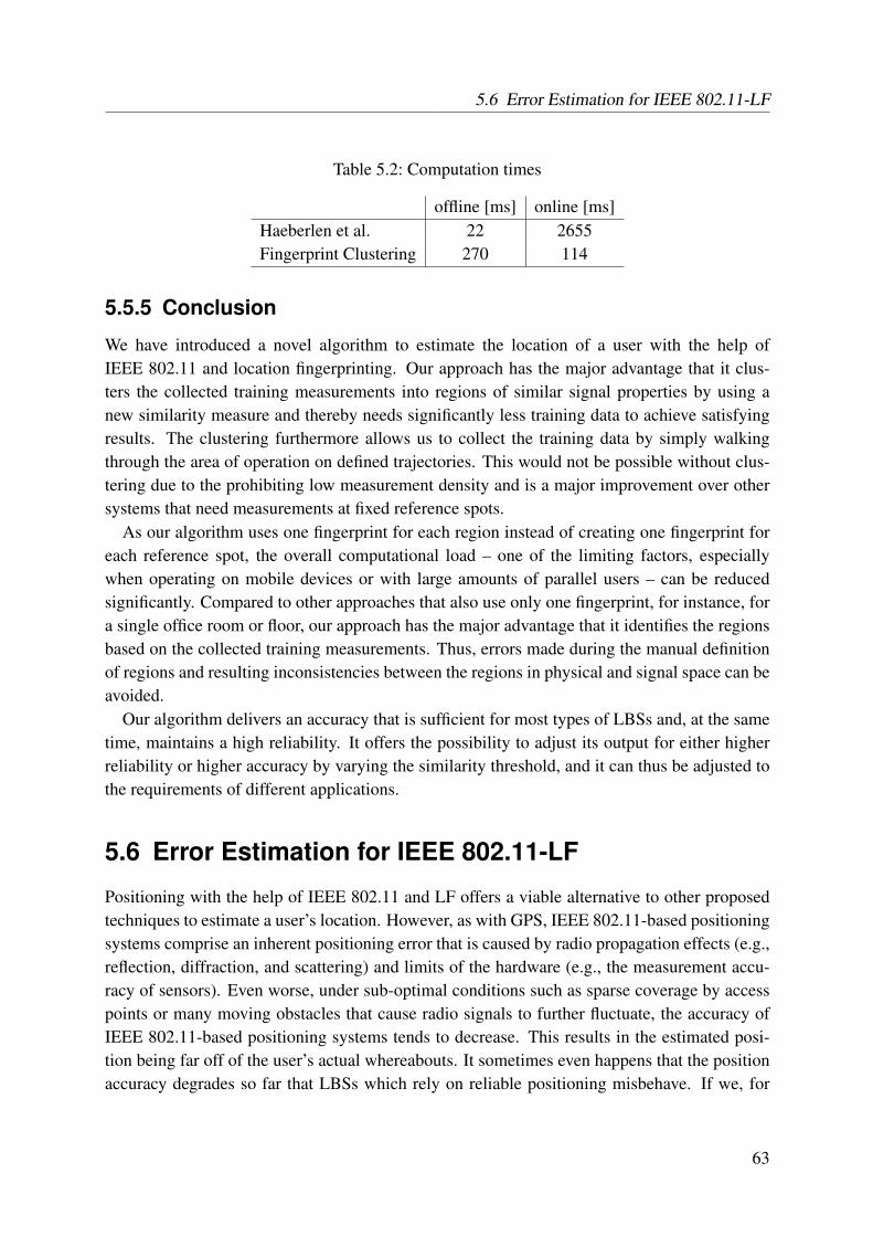
5.6 Error Estimation for IEEE 802.11-LF
Table 5.2: Computation times
offline [ms] online [ms]Haeberlen et al. 22 2655Fingerprint Clustering 270 114
5.5.5 Conclusion
We have introduced a novel algorithm to estimate the location of a user with the help ofIEEE 802.11 and location fingerprinting. Our approach has the major advantage that it clus-ters the collected training measurements into regions of similar signal properties by using anew similarity measure and thereby needs significantly less training data to achieve satisfyingresults. The clustering furthermore allows us to collect the training data by simply walkingthrough the area of operation on defined trajectories. This would not be possible without clus-tering due to the prohibiting low measurement density and is a major improvement over othersystems that need measurements at fixed reference spots.
As our algorithm uses one fingerprint for each region instead of creating one fingerprint foreach reference spot, the overall computational load – one of the limiting factors, especiallywhen operating on mobile devices or with large amounts of parallel users – can be reducedsignificantly. Compared to other approaches that also use only one fingerprint, for instance, fora single office room or floor, our approach has the major advantage that it identifies the regionsbased on the collected training measurements. Thus, errors made during the manual definitionof regions and resulting inconsistencies between the regions in physical and signal space can beavoided.
Our algorithm delivers an accuracy that is sufficient for most types of LBSs and, at the sametime, maintains a high reliability. It offers the possibility to adjust its output for either higherreliability or higher accuracy by varying the similarity threshold, and it can thus be adjusted tothe requirements of different applications.
5.6 Error Estimation for IEEE 802.11-LF
Positioning with the help of IEEE 802.11 and LF offers a viable alternative to other proposedtechniques to estimate a user’s location. However, as with GPS, IEEE 802.11-based positioningsystems comprise an inherent positioning error that is caused by radio propagation effects (e.g.,reflection, diffraction, and scattering) and limits of the hardware (e.g., the measurement accu-racy of sensors). Even worse, under sub-optimal conditions such as sparse coverage by accesspoints or many moving obstacles that cause radio signals to further fluctuate, the accuracy ofIEEE 802.11-based positioning systems tends to decrease. This results in the estimated posi-tion being far off of the user’s actual whereabouts. It sometimes even happens that the positionaccuracy degrades so far that LBSs which rely on reliable positioning misbehave. If we, for
63
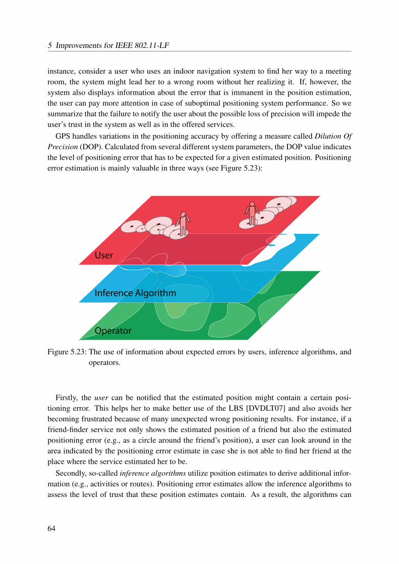
5 Improvements for IEEE 802.11-LF
instance, consider a user who uses an indoor navigation system to find her way to a meetingroom, the system might lead her to a wrong room without her realizing it. If, however, thesystem also displays information about the error that is immanent in the position estimation,the user can pay more attention in case of suboptimal positioning system performance. So wesummarize that the failure to notify the user about the possible loss of precision will impede theuser’s trust in the system as well as in the offered services.
GPS handles variations in the positioning accuracy by offering a measure called Dilution OfPrecision (DOP). Calculated from several different system parameters, the DOP value indicatesthe level of positioning error that has to be expected for a given estimated position. Positioningerror estimation is mainly valuable in three ways (see Figure 5.23):
User
Inference Algorithm
Operator
Figure 5.23: The use of information about expected errors by users, inference algorithms, andoperators.
Firstly, the user can be notified that the estimated position might contain a certain posi-tioning error. This helps her to make better use of the LBS [DVDLT07] and also avoids herbecoming frustrated because of many unexpected wrong positioning results. For instance, if afriend-finder service not only shows the estimated position of a friend but also the estimatedpositioning error (e.g., as a circle around the friend’s position), a user can look around in thearea indicated by the positioning error estimate in case she is not able to find her friend at theplace where the service estimated her to be.
Secondly, so-called inference algorithms utilize position estimates to derive additional infor-mation (e.g., activities or routes). Positioning error estimates allow the inference algorithms toassess the level of trust that these position estimates contain. As a result, the algorithms can
64
5.6 Error Estimation for IEEE 802.11-LF
give a higher priority to estimates with a low estimated error. This helps to deliver an overallhigher service quality.
Thirdly, operators of 802.11-based positioning systems can utilize positioning error esti-mates to optimize their system to the precision required by the application. For instance, anoperator might add additional APs to those parts of the operation area that show positioningerror estimates above a certain threshold.
In this section, we propose several algorithms to estimate the expected positioning error of802.11-based positioning systems. We focus on the static case of position estimation withoutany knowledge of spatial or temporal history. We have selected two well-studied systems pro-posed by Bahl et al. [BP00] and Haeberlen et al. [HFL+04] as our positioning systems. Weselected these two systems because they represent the two main types of location fingerprintingalgorithms, i.e., a probabilistic and a deterministic approach. Our setup and both algorithms aresufficiently easy to understand and therefore – with their own complexity – do not blur the viewfor the mechanisms used by our own error prediction algorithms.
We propose positioning error estimation algorithms that are able to predict the expected po-sitioning error in advance, using only the collected training data as well as algorithms that inferthe expected positioning error from live measurements in the position determination phase. Thisinformation can then be used to inform the user in an appropriate way (also see [LKE08]) andto allow dependent services to adapt their decisions.
5.6.1 Error Estimation
In this section, we propose our four novel algorithms for positioning error estimation. Thefollowing two algorithms can predict the expected positioning error in advance, using only thedata collected in the training phase:
A. Fingerprint Clustering B. Leave Out Fingerprint
The other two algorithms infer the expected positioning error from live measurements in theposition determination phase:
C. Best Candidates Set D. Signal Strength Variance
A. Fingerprint Clustering
The Fingerprint Clustering algorithm uses the idea that, inside structurally limited areas, thesignals received from an access point – despite inevitable small-scale fading effects – tend to bewithin a certain range. For instance, the signal strength measurements collected in one singleoffice room often cover only a quite limited range of the generally possible values. As in sucha case all the fingerprints collected in this office room are very similar, a positioning algorithmwill hardly be able to estimate the position precisely. Instead, it will probably select one of theother fingerprints collected somewhere else in the room.
65
5 Improvements for IEEE 802.11-LF
If such an area of similar signal properties has large physical dimensions, we expect thepositioning error to be larger because, generally, the number of similar fingerprints is higherand also their physical distribution space is larger. We exploit this behavior in the followingway. Our novel algorithm lays out a grid of cells over the complete covered area of operationof the IEEE 802.11-based positioning system. Then, the following steps are performed in orderto find regions of similar signal properties:
1. Initially, each grid cell represents a single cluster containing all the training samples col-lected inside the physical area of the cell.
2. After that, the algorithm randomly selects a cluster. By using a similarity measure, thealgorithm then checks whether the similarity to adjacent clusters lies above a given thresh-old. If this is the case for any adjacent cluster, the two clusters are merged into one.
3. The previous step is repeated until, for all remaining clusters, no further clusters can bemerged.
4. As a next step, the set of clusters is checked for clusters that only comprise one single cell.If such a cluster is found, it is merged with its most similar adjacent cluster disregardingthe threshold. The reason for this procedure is that the single cell clusters most oftenare a result of time and space constrained disturbances during the collection phase of thetraining data. If the fingerprints at these positions are selected by the positioning systemduring the position determination phase, this quite frequently results in large errors thatwould not be reflected by the small size of a single-cell cluster. Thus, eliminating theseclusters helps the error estimation algorithm to deliver better and more stable results.
5. In the end, each remaining cluster represents a region of similar signal properties in thearea of operation. The size and shape of the region is defined by the grid cells the clusteris comprised of. The estimated error for an estimated position is deduced from the sizeof the region that the estimated position is located in.
An example for a region map resulting from the Fingerprint Clustering algorithm is shownin Figure 5.24.
The similarity measure for a pair of clusters is calculated by comparing the distributions ofsignal strengths in the clusters using a similar function to the one used for the region-based po-sition estimation in Section 5.5.1. For each access point of which signal strength measurementsare contained in the samples of both clusters, and for each of the two clusters, the mean andthe standard deviation of the measured signal strengths are computed. These values are thenused to create two normal distributions, each one representing the signal strength distributionof the specific access point and cluster. Afterwards, the intersection area of these two normaldistributions is calculated. This step is repeated for all access points until, finally, the averagesize of all intersection areas is computed and interpreted as the similarity of the two clusters.Access points of which signal strength measurements are only contained in the samples of one
66
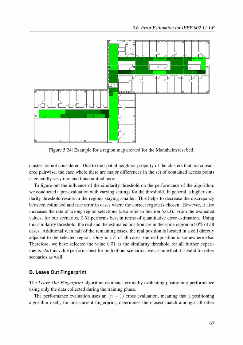
5.6 Error Estimation for IEEE 802.11-LF
Figure 5.24: Example for a region map created for the Mannheim test bed.
cluster are not considered. Due to the spatial neighbor property of the clusters that are consid-ered pairwise, the case where there are major differences in the set of contained access pointsis generally very rare and thus omitted here.
To figure out the influence of the similarity threshold on the performance of the algorithm,we conducted a pre-evaluation with varying settings for the threshold. In general, a higher sim-ilarity threshold results in the regions staying smaller. This helps to decrease the discrepancybetween estimated and true error in cases where the correct region is chosen. However, it alsoincreases the rate of wrong region selections (also refer to Section 5.6.3). From the evaluatedvalues, for our scenarios, 0.51 performs best in terms of quantitative error estimation. Usingthis similarity threshold, the real and the estimated position are in the same region in 90% of allcases. Additionally, in half of the remaining cases, the real position is located in a cell directlyadjacent to the selected region. Only in 5% of all cases, the real position is somewhere else.Therefore, we have selected the value 0.51 as the similarity threshold for all further experi-ments. As this value performs best for both of our scenarios, we assume that it is valid for otherscenarios as well.
B. Leave Out Fingerprint
The Leave Out Fingerprint algorithm estimates errors by evaluating positioning performanceusing only the data collected during the training phase.
The performance evaluation uses an (n − 1) cross evaluation, meaning that a positioningalgorithm itself, for one current fingerprint, determines the closest match amongst all other
67
5 Improvements for IEEE 802.11-LF
fingerprints (the other (n − 1) folds). The result is a good indicator of the error that can occurif the data collected during the position determination phase is noisy.
The positioning error result from this evaluation is used to compute an error map where eachfingerprinted position is assigned an error estimate. In the position determination phase, theposition estimated by the positioning algorithm is looked up in the error map, and the errorestimate stored for the corresponding position is returned. For each fingerprinted position p, theerror map contains an error estimate that is created by the following four steps:
1. Create a radio map using all fingerprints except the one for position p.
2. Run an emulation using m samples as test data taken randomly from the fingerprint forposition p.
3. Calculate the observed errors for the position estimates from the emulation.
4. Calculate the error estimate for position p as the average plus two times the standarddeviation of all the observed m errors. This method for computing the error estimate wasselected because initial experiments showed that this type of conservative estimate givesthe best results.
As a final step, when all error estimates have been calculated, the error map is averagedto filter out local variations. This is performed by assigning a new estimate to each position.The new estimate is calculated as 66% of the original estimate and 33% as the average of theestimates for all neighboring fingerprints. We chose these parameters for the weights becausethey provide a good balance between the error estimates for the different fingerprint positions.In our evaluation, this interpolation step increases the accuracy of the algorithm by almost fivepercent.
C. Best Candidates Set
When an IEEE 802.11-based positioning algorithm estimates a position, it generally returnsonly the position of the fingerprint that offers the best match to the data collected in the positiondetermination phase. However, the Best Candidates Set algorithm exploits the fact that posi-tioning algorithms can return information about the second, third etc. best matches. The BestCandidates Set algorithm uses the n best estimates returned from a positioning algorithm toestimate the expected positioning error. The rationale for using the n best estimates is based onthe observation that positioning algorithms will often estimate a user to be at any of the nearbypositions to his actual position. This is a result of the fact that adjacent fingerprinted positionswill often exhibit overlapping signal strength properties while online samples similarly havesufficient signal strength variance to choose at random between close locations.
The Best Candidates Set algorithm deduces an error estimate by computing the average dis-tance between the best estimate and the next (n− 1) best estimates. The algorithm contains thefollowing steps:
68
5.6 Error Estimation for IEEE 802.11-LF
1. Form the set of the n best estimates as outputted from an IEEE 802.11-based positioningalgorithm.
2. Compute the distance between the position of the best estimate and all the other (n− 1)
best estimates.
3. Return the average distance as the estimated error.
In addition to using the average distance between the best and the (n−1) next best estimates,we also tried two other options to compute an error estimate from the Best Candidates Set. Thefirst option was to use the maximum distance between the best estimate and any of the (n− 1)
next best estimates. The second option was to compute the maximum distance between anytwo of the n best estimates. Both options led to more conservative error estimates but they werealso more sensitive to large errors and to an increased n. In effect, both options produced ahigher proportion of large over-estimations when the performance of the positioning algorithmdegraded or when the size of the Best Candidates Set was increased. In contrast, the average-distance approach handled these situations better. Using the average distance, it was found thatn set to three gave the best overall performance, although the performance was only marginallybetter than with n set anywhere between four and seven. Higher values of n made the errorestimates more conservative while gradually decreasing performance due to the inclusion ofmore faraway positions.
D. Signal Strength Variance
Like most IEEE 802.11-based positioning systems, the systems selected for this paper are error-prone to signal strength variations because the position estimation process depends on proba-bilities or average values calculated on the signal strength samples.
The reasons for the variation of signal strength samples are two fold: Firstly, small-scaleeffects and multi-path radio propagation cause signal strength values to vary significantly if themobile device moves within the wavelength (for IEEE 802.11b, the wavelength is ≈ 12.5 cen-timeters). So, both during the training phase as well as during the position determination phase,even if the mobile device is supposed to be static, small movements can have a big impact onthe measured signal strength. Secondly, movements in the surrounding of the mobile device inquestion (e.g., persons moving around or doors being opened or closed) cause radio signals totravel over different paths which in consequence causes the signal strength to fluctuate.
If the variance between different signal strength samples is high, the probability that theactual closest fingerprint is selected is rather small, as a fingerprint far away might reach ahigher probability. The same is true for the average calculation because the average value mightdiffer if the variance between different signal strength samples is high. Therefore, an increasein variance also increases the probability of positioning errors.
69
5 Improvements for IEEE 802.11-LF
The idea of the Signal Strength Variance algorithm is to estimate the positioning error basedon the signal strength variance of the samples that are used in the position determination phaseto compute a position estimate. The algorithm can be described as follows:
1. For each access point that is part of the signal strength samples, find the largest signalstrength value (in dB).
2. Based on the largest signal strength value that is specific for a certain access point, sub-tract this value from all signal strength samples that are available for this given accesspoint.
3. For each access point, calculate the signal strength variance for the calculated values.
4. Average the signal strength variance values calculated for each access point to get an over-all variance value. This variance value can be perceived as an indicator of the expectedpositioning error similar to the DOP measure used by GPS.
We also tried several other ways to calculate an overall signal strength variance value. How-ever, this did not lead to an algorithm with better results than those achieved with the algorithmpresented above.
Random Value
As a baseline and to give the reader a better understanding of our results, we also implemented asimple random error estimation algorithm. This algorithm returns uniformly distributed randomerror estimates between 0 and ten meters independent of the supplied data.
5.6.2 Experimental Setup and Methodology
In this section, we describe the experimental setup and the measurement methodology used toevaluate the proposed algorithms.
Local Test Environments
We deployed our IEEE 802.11-based positioning systems in two different environments: Onthe second floor of the Hopper building on the campus of the University of Aarhus and on thesecond floor of the office building A5-B on the campus of the University of Mannheim.
The former one is a newly built office building consisting of many offices and a long hall (seeFigure 5.25a). The area is covered by 23 access points from different vendors; only five of theseaccess points can be detected in at least half of the measurements. Nine far-off access pointsare even only detectable in less than ten percent of all measurements. The average number ofaccess points contained in the fingerprints for this environment is 6.9, while the average number
70
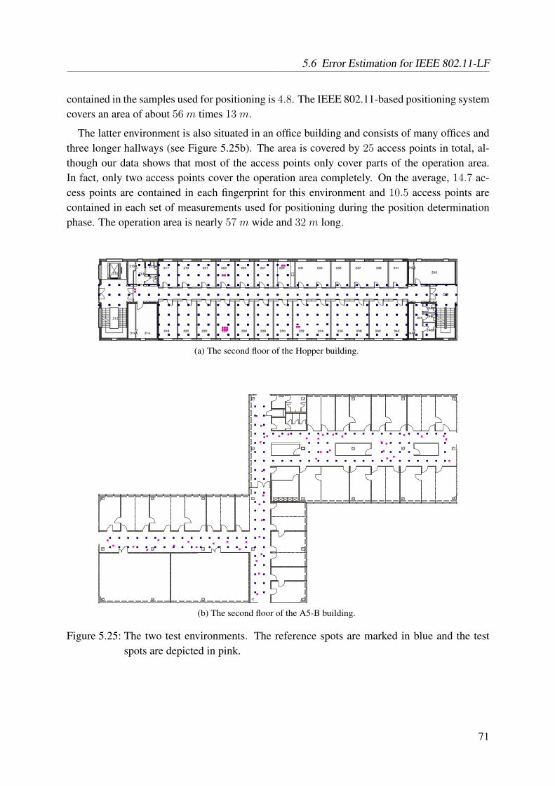
5.6 Error Estimation for IEEE 802.11-LF
contained in the samples used for positioning is 4.8. The IEEE 802.11-based positioning systemcovers an area of about 56 m times 13 m.
The latter environment is also situated in an office building and consists of many offices andthree longer hallways (see Figure 5.25b). The area is covered by 25 access points in total, al-though our data shows that most of the access points only cover parts of the operation area.In fact, only two access points cover the operation area completely. On the average, 14.7 ac-cess points are contained in each fingerprint for this environment and 10.5 access points arecontained in each set of measurements used for positioning during the position determinationphase. The operation area is nearly 57 m wide and 32 m long.
(a) The second floor of the Hopper building.
(b) The second floor of the A5-B building.
Figure 5.25: The two test environments. The reference spots are marked in blue and the testspots are depicted in pink.
71
5 Improvements for IEEE 802.11-LF
Hardware and Software Setup
As a client, we used a Lucent Orinoco Silver PCMCIA network card supporting 802.11b. Thiscard was plugged into an IBM Thinkpad R51 laptop computer. To collect signal strength sam-ples, we used our own set of tools [KBH07].
Data Collection
For both environments, we applied a grid of reference spots with a spacing of 1.5m to the oper-ation areas. For the Hopper building, this resulted in 225 reference spots, while the Mannheimenvironment comprised 130 reference spots (see the blue markers in Figures 5.25a and 5.25b).For the former environment, 120 signal strength measurements and, for the latter one, 110 sig-nal strength measurements were subsequently collected at each reference spot. The reason forthe difference in the number of measurements per spot is, that we were able to use datasets thathad been collected independently of each other in advance.
For the position determination phase, we then selected 14 spots in the Hopper building and46 spots in the A5-B building. At each of these spots, we collected 110 signal strength samplesas well. In Figure 5.25a and Figure 5.25b, these spots are marked by pink dots.
Metrics
Regarding the metric used to compare our error estimation algorithms, we use the error differ-ence. For each position estimate, we compute the physical distance between the real and theestimated position (the real error) and then subtract the result from the value that our error esti-mation algorithms return as the expected error. By using the error difference, it is, for instance,easy for us to analyze whether our algorithms tend to estimate the positioning error too high ortoo low.
Experimental Methodology
We performed an evaluation of our four error estimation algorithms. To keep the results com-parable, we examined the four algorithms in parallel. To achieve this, we used our suite ofpositioning-related tools [KBH07] and extended them to suit our special needs.
The basic experiment consisted of the following steps: At first, one of the two used position-ing algorithms is initialized with 25 randomly selected samples per reference spot to build up itsfingerprint database. Subsequently, our four different error estimation algorithms are initializedas well. Those that make use of the training data are additionally provided with exactly thesame data as the positioning algorithm itself. The same is then done with the data for the posi-tion determination phase. At first, the positioning algorithm – for each test position – is givenfive online samples to estimate a position. Afterwards, the same samples used for the positiondetermination as well as the estimated position are provided to our error estimation algorithms.
72
5.6 Error Estimation for IEEE 802.11-LF
Each of the algorithms then solely computes an error estimate which is recorded and stored forlater reference.
The values used for the number of training and position determination samples were chosenaccording to [KHE07]. To achieve statistically stable results, we repeated our basic experiment100 times. We ran our basic experiment using the positioning algorithm proposed by Bahl etal. [BP00] and the one proposed by Haeberlen at el. [HFL+04] on data collected from both ofour test environments.
As listed in Table 5.3, the position accuracy of the positioning algorithms by Bahl et al.[BP00] and Haeberlen at el. [HFL+04] is quite different when considering the data for each ofour two test environments. The main reasons are the number of access points, the properties ofthe environments, and the overall quality of the positioning algorithms themselves.
Table 5.3: True position estimation accuracy for positioning algorithms and test environments.
Positioning Algorithm Aarhus [m] Mannheim [m]Bahl et al. [BP00] 8.10 2.90Haeberlen et al. [HFL+04] 3.79 2.56
5.6.3 Experimental Results
In this section, we present our evaluation results focusing on the results for the more accurateRice positioning algorithm. We omitted the results for Radar as they are overall very similar tothose for the Rice algorithm and presenting them would only offer little additional informationto the reader.
Estimation Accuracy
The proposed error estimation algorithms show noticeable differences in their performancesas well as in their reactions to different environmental conditions and to the used positioningalgorithms.
Overall, for the Aarhus dataset and with the Haeberlen et al. positioning algorithm, the Fin-gerprint Clustering approach delivers the best results (e.g., 1.13 m at the median) even thoughthe second best algorithm, the Best Candidates Set, is quite close regarding the 95th percentile(see Figure 5.26a).
Looking at the Mannheim dataset, the situation is different. Considering the 25th, 50th,and 75th percentiles, the Best Candidates Set algorithm now takes the lead with 1.10 m at themedian (see Figure 5.26b). This impression is also confirmed when taking a look at the averagevalues for the error difference of the four algorithms and the two environments (see Table 5.4).Here as well, the Best Candidates Set algorithm performs best for the Mannheim dataset at1.45 m, while the Fingerprint Clustering algorithm is ahead for the Aarhus dataset at 2.24 m.
73
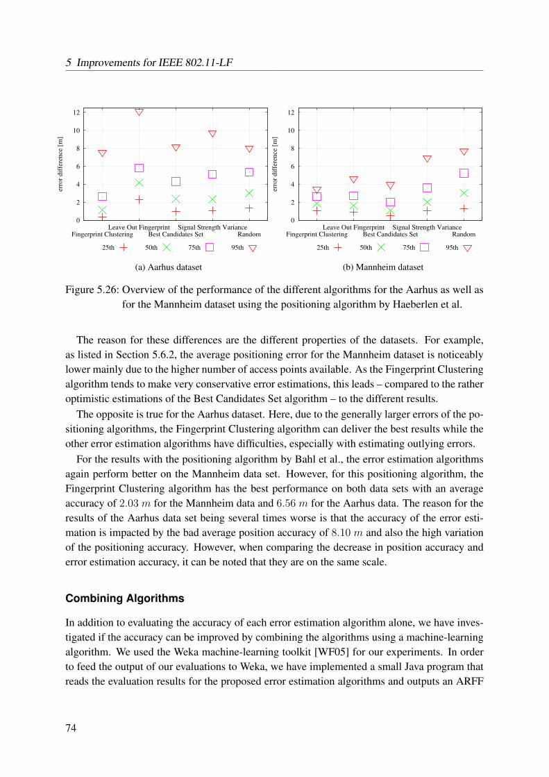
5 Improvements for IEEE 802.11-LF
0
2
4
6
8
10
12
Fingerprint ClusteringLeave Out Fingerprint
Best Candidates SetSignal Strength Variance
Random
erro
r dif
fere
nce
[m
]
25th 50th 75th 95th
(a) Aarhus dataset
0
2
4
6
8
10
12
Fingerprint ClusteringLeave Out Fingerprint
Best Candidates SetSignal Strength Variance
Random
erro
r dif
fere
nce
[m
]
25th 50th 75th 95th
(b) Mannheim dataset
Figure 5.26: Overview of the performance of the different algorithms for the Aarhus as well asfor the Mannheim dataset using the positioning algorithm by Haeberlen et al.
The reason for these differences are the different properties of the datasets. For example,as listed in Section 5.6.2, the average positioning error for the Mannheim dataset is noticeablylower mainly due to the higher number of access points available. As the Fingerprint Clusteringalgorithm tends to make very conservative error estimations, this leads – compared to the ratheroptimistic estimations of the Best Candidates Set algorithm – to the different results.
The opposite is true for the Aarhus dataset. Here, due to the generally larger errors of the po-sitioning algorithms, the Fingerprint Clustering algorithm can deliver the best results while theother error estimation algorithms have difficulties, especially with estimating outlying errors.
For the results with the positioning algorithm by Bahl et al., the error estimation algorithmsagain perform better on the Mannheim data set. However, for this positioning algorithm, theFingerprint Clustering algorithm has the best performance on both data sets with an averageaccuracy of 2.03 m for the Mannheim data and 6.56 m for the Aarhus data. The reason for theresults of the Aarhus data set being several times worse is that the accuracy of the error esti-mation is impacted by the bad average position accuracy of 8.10 m and also the high variationof the positioning accuracy. However, when comparing the decrease in position accuracy anderror estimation accuracy, it can be noted that they are on the same scale.
Combining Algorithms
In addition to evaluating the accuracy of each error estimation algorithm alone, we have inves-tigated if the accuracy can be improved by combining the algorithms using a machine-learningalgorithm. We used the Weka machine-learning toolkit [WF05] for our experiments. In orderto feed the output of our evaluations to Weka, we have implemented a small Java program thatreads the evaluation results for the proposed error estimation algorithms and outputs an ARFF
74
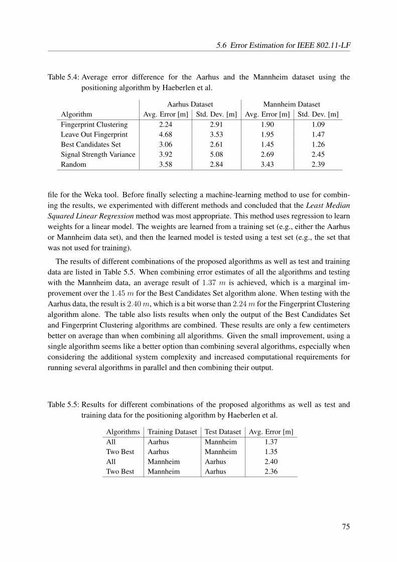
5.6 Error Estimation for IEEE 802.11-LF
Table 5.4: Average error difference for the Aarhus and the Mannheim dataset using thepositioning algorithm by Haeberlen et al.
Aarhus Dataset Mannheim DatasetAlgorithm Avg. Error [m] Std. Dev. [m] Avg. Error [m] Std. Dev. [m]Fingerprint Clustering 2.24 2.91 1.90 1.09Leave Out Fingerprint 4.68 3.53 1.95 1.47Best Candidates Set 3.06 2.61 1.45 1.26Signal Strength Variance 3.92 5.08 2.69 2.45Random 3.58 2.84 3.43 2.39
file for the Weka tool. Before finally selecting a machine-learning method to use for combin-ing the results, we experimented with different methods and concluded that the Least MedianSquared Linear Regression method was most appropriate. This method uses regression to learnweights for a linear model. The weights are learned from a training set (e.g., either the Aarhusor Mannheim data set), and then the learned model is tested using a test set (e.g., the set thatwas not used for training).
The results of different combinations of the proposed algorithms as well as test and trainingdata are listed in Table 5.5. When combining error estimates of all the algorithms and testingwith the Mannheim data, an average result of 1.37 m is achieved, which is a marginal im-provement over the 1.45 m for the Best Candidates Set algorithm alone. When testing with theAarhus data, the result is 2.40m, which is a bit worse than 2.24m for the Fingerprint Clusteringalgorithm alone. The table also lists results when only the output of the Best Candidates Setand Fingerprint Clustering algorithms are combined. These results are only a few centimetersbetter on average than when combining all algorithms. Given the small improvement, using asingle algorithm seems like a better option than combining several algorithms, especially whenconsidering the additional system complexity and increased computational requirements forrunning several algorithms in parallel and then combining their output.
Table 5.5: Results for different combinations of the proposed algorithms as well as test andtraining data for the positioning algorithm by Haeberlen et al.
Algorithms Training Dataset Test Dataset Avg. Error [m]All Aarhus Mannheim 1.37Two Best Aarhus Mannheim 1.35All Mannheim Aarhus 2.40Two Best Mannheim Aarhus 2.36
75
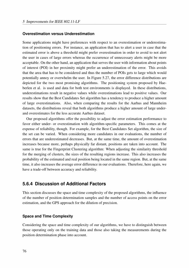
5 Improvements for IEEE 802.11-LF
Overestimation versus Underestimation
Some applications might have preferences with respect to an overestimation or underestima-tion of positioning errors. For instance, an application that has to alert a user in case that theestimated error is above a threshold might prefer overestimation in order to avoid to not alertthe user in cases of large errors whereas the occurrence of unnecessary alerts might be moreacceptable. On the other hand, an application that serves the user with information about pointsof interest (POI) in her proximity might prefer an underestimation of the error. This avoidsthat the area that has to be considered and thus the number of POIs gets to large which wouldpotentially annoy or overwhelm the user. In Figure 5.27, the error difference distributions aredepicted for the two most promising algorithms. The positioning system proposed by Hae-berlen et al. is used and data for both test environments is displayed. In these distributions,underestimations result in negative values while overestimations lead to positive values. Ourresults show that the Best Candidates Set algorithm has a tendency to produce a higher amountof large overestimations. Also, when comparing the results for the Aarhus and Mannheimdatasets, the distributions reveal that both algorithms produce a higher amount of large under-and overestimates for the less accurate Aarhus dataset.
Our proposed algorithms offer the possibility to adjust the error estimation performance tofavor either under- or overestimation with algorithm-specific parameters. This comes at theexpense of reliability, though. For example, for the Best Candidates Set algorithm, the size ofthe set can be varied. When considering more candidates in our evaluations, the number oferrors that are underestimated decreases. But, at the same time, the amount of overestimationincreases because more, perhaps physically far distant, positions are taken into account. Thesame is true for the Fingerprint Clustering algorithm: When adjusting the similarity thresholdfor the merging of clusters, the sizes of the resulting regions increase. This also increases theprobability of the estimated and real position being located in the same region. But, at the sametime, it also increases the average error difference in our evaluations. Therefore, here again, wehave a trade-off between accuracy and reliability.
5.6.4 Discussion of Additional Factors
This section discusses the space and time complexity of the proposed algorithms, the influenceof the number of position determination samples and the number of access points on the errorestimation, and the GPS approach for the dilution of precision.
Space and Time Complexity
Considering the space and time complexity of our algorithms, we have to distinguish betweenthose operating only on the training data and those also taking the measurements during theposition determination phase into account.
76
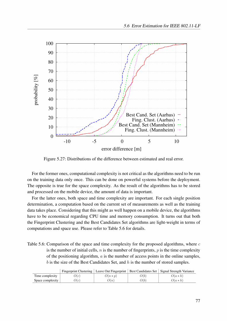
5.6 Error Estimation for IEEE 802.11-LF
0
10
20
30
40
50
60
70
80
90
100
-10 -5 0 5 10
pro
bab
ilit
y [
%]
error difference [m]
Best Cand. Set (Aarhus)Fing. Clust. (Aarhus)
Best Cand. Set (Mannheim)Fing. Clust. (Mannheim)
Figure 5.27: Distributions of the difference between estimated and real error.
For the former ones, computational complexity is not critical as the algorithms need to be runon the training data only once. This can be done on powerful systems before the deployment.The opposite is true for the space complexity. As the result of the algorithms has to be storedand processed on the mobile device, the amount of data is important.
For the latter ones, both space and time complexity are important. For each single positiondetermination, a computation based on the current set of measurements as well as the trainingdata takes place. Considering that this might as well happen on a mobile device, the algorithmshave to be economical regarding CPU time and memory consumption. It turns out that boththe Fingerprint Clustering and the Best Candidates Set algorithms are light-weight in terms ofcomputations and space use. Please refer to Table 5.6 for details.
Table 5.6: Comparison of the space and time complexity for the proposed algorithms, where cis the number of initial cells, n is the number of fingerprints, p is the time complexityof the positioning algorithm, a is the number of access points in the online samples,b is the size of the Best Candidates Set, and h is the number of stored samples.
Fingerprint Clustering Leave Out Fingerprint Best Candidates Set Signal Strength VarianceTime complexity O(c) O(n ∗ p) O(b) O(a ∗ h)
Space complexity O(c) O(n) O(b) O(a ∗ h)
77
5 Improvements for IEEE 802.11-LF
Number of Position Determination Samples and Number of Access Points
From experimental results, King et al. [KHE07] conclude that the IEEE 802.11-LF positioningerror is mainly determined by the number of access points and the number of signal strengthsamples used in the position determination phase. In this work, we do not present any algorithmthat takes this fact explicitly into account. However, the previously presented algorithms indi-rectly adhere to this fact. For instance, the Fingerprint Clustering algorithm (see Section 5.6.1),when comparing similarity between clusters, iterates over the set of access points and, thus,handles the number of access points. The number of position determination samples is coveredby the Signal Strength Variance algorithm (see Section 5.6.1) as the variance value stabilizes ifthe number of signal strength samples increases. However, it would be an interesting path offuture work to analyze if the proposed algorithms could be extended to use such results moreexplicitly.
Dilution of Precision
In addition to the proposed algorithms, we also implemented an algorithm that computes aGPS-like DOP value based on the geometry of APs. The algorithm uses the equations for DOPvalues described in Borre et al. [BAB+07]. However, a DOP value is not an error estimate inmeters but a factor that has to be combined with an error estimate.
Therefore, we have evaluated if the accuracy of the proposed algorithms can be improvedby combining their output with this GPS-like DOP value by multiplication. However, for allalgorithms, the combination with the DOP value strongly reduces their accuracy. This suggeststhat GPS-like DOP values do not seem to be a promising error estimation approach for indoorIEEE 802.11-based positioning. The main reason is that the complex indoor propagation en-vironment makes the geometry of the access points less important for the positioning accuracythan it is in the case of outdoor satellite-based positioning. This result is consistent with the ana-lytical results for the impact of the geometry of access points on the position accuracy presentedby Wallbaum et al. [Wal07].
5.6.5 Conclusions
In this section, we have introduced four novel algorithms to estimate the positioning error ofIEEE 802.11-based positioning systems. Our algorithms exploit several different features tofulfill their task. We have proposed error estimation algorithms that only use training data aswell as algorithms that only take the data available during the position determination phase intoaccount.
All our algorithms deliver good results for estimating the positioning error for both environ-ments and for the different positioning algorithms. The Fingerprint Clustering algorithm and theBest Candidates Set algorithm perform especially well. With either of these two algorithms, itis possible to estimate the positioning error of an IEEE 802.11-based positioning system up to a
78
5.6 Error Estimation for IEEE 802.11-LF
high degree of accuracy and with sufficient reliability. This is in contrast to the geometry-basedalgorithms used for GPS.
We have evaluated if using a machine-learning technique to combine several of the proposedalgorithms can improve the precision of the error estimates. In our case, though, the gain isvery small or the results even get worse. We therefore do not suggest to use a combination ofthe different algorithms but to rather use one algorithm alone. If the collected data has a goodquality, we suggest to use the Best Candidates Set algorithm whereas in situations where thecollected data is of lower quality, the Fingerprint Clustering algorithm should be used. Lookingat the targeted use of the algorithms on mobile devices, this suggestion makes even more senseas the use of multiple algorithms – even though each single one is economical in terms ofprocessing and storage demands – would waste precious resources.
79

80
CH
AP
TE
R
6 Context, Tracking, andIEEE 802.11-LF
Up to now, we have presented an overview of different problems that have to be dealt with whenusing IEEE 802.11-LF for position estimation, and we have contributed our own solutions tothese problems. In the following section, we will present another approach to help solve someof these issues, namely the use of tracking. All algorithms presented until here only use staticdata. This means that they consider a fixed set of training measurements that is used to buildthe fingerprint database, and a single or only few consecutive measurements during the positiondetermination phase to estimate a user’s position.
Tracking extends this by furthermore considering the measurement and position history andpossibly other available context information, and it is not limited to IEEE 802.11-LF. For in-stance, a navigation system in a car can further increase the accuracy of the position estimationby cross-validating the satellite-based estimates using available odometric data to extrapolatefrom former known positions. If the estimate of the satellite-based system and the extrapo-lated estimate differ, the system can omit using the latter or try to mitigate the error by using acombination of both systems.
If tracking is possible, it is generally preferable over the static approach as it yields the oppor-tunity for higher accuracy and better update rates. The following Chapter describes our effortsto transfer the tracking approach into the domain of IEEE 802.11-LF. Furthermore, togetherwith the use of fingerprinting techniques, we investigated the use of other possible context in-formation sources that are available on modern mobile devices and can be used to improve theposition estimation.
6.1 Context Information
Modern mobile devices offer a large number of sensors. Among these, we find accelerometers,temperature sensors, light sensors, magnetic compasses, microphones, and sometimes evenmore. As it has been shown by earlier research, for instance, the use of directional fingerprints
81
6 Context, Tracking, and IEEE 802.11-LF
and a compass can improve the positioning accuracy considerably [KKH+06]. However, thiscomes at the cost of an increase of the effort needed for setup and maintenance.
We therefore reconsidered the alternative use of a compass and furthermore how other sensorscan be used to support the position estimation of a moving user. Regarding the informationfrom most of the other sensors, we had to face the problem that – in distinction from using acompass – the information that can be gathered from these sensors built into mobile devicesis highly varying. For instance, it does not really make sense to store information about thebrightness at a certain position in a fingerprint as the brightness value is most probably subjectto change throughout the day. Thus, we also restricted ourselves to the use of additional contextinformation only during the position determination phase. In this phase, the most importantinformation is the one about the user’s motion. We therefore decided to use accelerometers andmagnetic compasses.
6.1.1 Motion Mode
When considering a moving user, information about the user’s mode of motion is an importanthelp when trying to extrapolate the user’s future path. If we are somehow able to identifywhether a user is standing still or walking at a certain speed, we can – based on past positionestimations – prioritize areas that can more likely be reached within the time between twoconsecutive position estimations and leave other areas that might be out of reach unconsidered.
In the past, much research has already been done in this area. Most often, dead reckoningwith the help of low-cost but still specialized devices is used. These devices generally containan accelerometer for every dimension, a gyroscope to detect rotation, and an interface to com-municate the sensor readings. By mounting such a device on a person’s foot, single strides,their length, and also their direction can be detected quite accurately. Using this informationfor dead reckoning, a positioning system can extrapolate a user’s location from a known startposition (e.g., see [RDML05, PEK+06, WKB08]).
This approach has several major flaws, though. Firstly, the used sensors normally have acertain drift. This leads to increasingly bad results for longer times without a reinitialization ata known position. Whereas – to a certain degree – this problem can be mitigated by the use ofmaps, the second problem is not as easily solved. As such a systems needs information from afoot- or leg-mounted high quality sensor system, a user needs to carry the sensor unit at her legor shoe. While this might be feasible for certain specialized application scenarios, it is not anacceptable approach for everyday usage.
Despite these problems, to us, motion information still seems like a valuable addition fromwhich a positioning system can benefit. Thus, we relaxed the requirements to fit our targetedapplication scenario of positioning usable in everyday life. Instead of using specialized sensorunits to detect single steps or even steps at all, we confined ourselves to using the accelerometersthat are built into modern devices to only detect the motion mode a user is in.
82
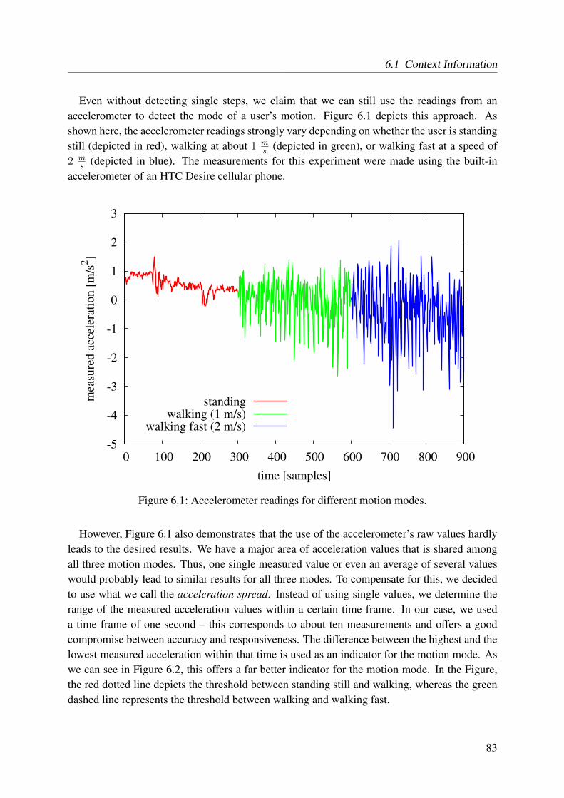
6.1 Context Information
Even without detecting single steps, we claim that we can still use the readings from anaccelerometer to detect the mode of a user’s motion. Figure 6.1 depicts this approach. Asshown here, the accelerometer readings strongly vary depending on whether the user is standingstill (depicted in red), walking at about 1 m
s(depicted in green), or walking fast at a speed of
2 ms
(depicted in blue). The measurements for this experiment were made using the built-inaccelerometer of an HTC Desire cellular phone.
-5
-4
-3
-2
-1
0
1
2
3
0 100 200 300 400 500 600 700 800 900
mea
sure
d a
ccel
erat
ion
[m
/s2]
time [samples]
standingwalking (1 m/s)
walking fast (2 m/s)
Figure 6.1: Accelerometer readings for different motion modes.
However, Figure 6.1 also demonstrates that the use of the accelerometer’s raw values hardlyleads to the desired results. We have a major area of acceleration values that is shared amongall three motion modes. Thus, one single measured value or even an average of several valueswould probably lead to similar results for all three modes. To compensate for this, we decidedto use what we call the acceleration spread. Instead of using single values, we determine therange of the measured acceleration values within a certain time frame. In our case, we useda time frame of one second – this corresponds to about ten measurements and offers a goodcompromise between accuracy and responsiveness. The difference between the highest and thelowest measured acceleration within that time is used as an indicator for the motion mode. Aswe can see in Figure 6.2, this offers a far better indicator for the motion mode. In the Figure,the red dotted line depicts the threshold between standing still and walking, whereas the greendashed line represents the threshold between walking and walking fast.
83
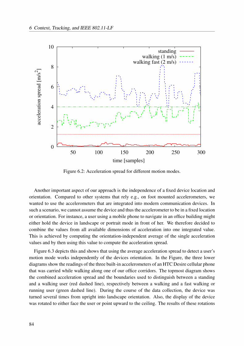
6 Context, Tracking, and IEEE 802.11-LF
0
2
4
6
8
10
50 100 150 200 250 300
acce
lera
tio
n s
pre
ad [
m/s
2]
time [samples]
standingwalking (1 m/s)
walking fast (2 m/s)
Figure 6.2: Acceleration spread for different motion modes.
Another important aspect of our approach is the independence of a fixed device location andorientation. Compared to other systems that rely e.g., on foot mounted accelerometers, wewanted to use the accelerometers that are integrated into modern communication devices. Insuch a scenario, we cannot assume the device and thus the accelerometer to be in a fixed locationor orientation. For instance, a user using a mobile phone to navigate in an office building mighteither hold the device in landscape or portrait mode in front of her. We therefore decided tocombine the values from all available dimensions of acceleration into one integrated value.This is achieved by computing the orientation-independent average of the single accelerationvalues and by then using this value to compute the acceleration spread.
Figure 6.3 depicts this and shows that using the average acceleration spread to detect a user’smotion mode works independently of the devices orientation. In the Figure, the three lowerdiagrams show the readings of the three built-in accelerometers of an HTC Desire cellular phonethat was carried while walking along one of our office corridors. The topmost diagram showsthe combined acceleration spread and the boundaries used to distinguish between a standingand a walking user (red dashed line), respectively between a walking and a fast walking orrunning user (green dashed line). During the course of the data collection, the device wasturned several times from upright into landscape orientation. Also, the display of the devicewas rotated to either face the user or point upward to the ceiling. The results of these rotations
84
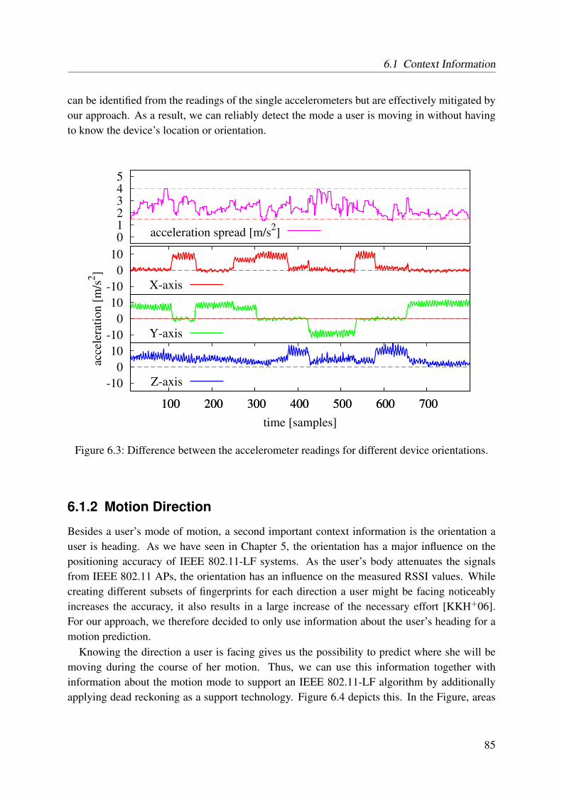
6.1 Context Information
can be identified from the readings of the single accelerometers but are effectively mitigated byour approach. As a result, we can reliably detect the mode a user is moving in without havingto know the device’s location or orientation.
0 1 2 3 4 5
acceleration spread [m/s2]
-10
0
10
X-axis
-10
0
10
Y-axis
-10
0
10
100 200 300 400 500 600 700
Z-axis
100 200 300 400 500 600 700
acce
lera
tio
n [
m/s
2]
time [samples]
Figure 6.3: Difference between the accelerometer readings for different device orientations.
6.1.2 Motion Direction
Besides a user’s mode of motion, a second important context information is the orientation auser is heading. As we have seen in Chapter 5, the orientation has a major influence on thepositioning accuracy of IEEE 802.11-LF systems. As the user’s body attenuates the signalsfrom IEEE 802.11 APs, the orientation has an influence on the measured RSSI values. Whilecreating different subsets of fingerprints for each direction a user might be facing noticeablyincreases the accuracy, it also results in a large increase of the necessary effort [KKH+06].For our approach, we therefore decided to only use information about the user’s heading for amotion prediction.
Knowing the direction a user is facing gives us the possibility to predict where she will bemoving during the course of her motion. Thus, we can use this information together withinformation about the motion mode to support an IEEE 802.11-LF algorithm by additionallyapplying dead reckoning as a support technology. Figure 6.4 depicts this. In the Figure, areas
85
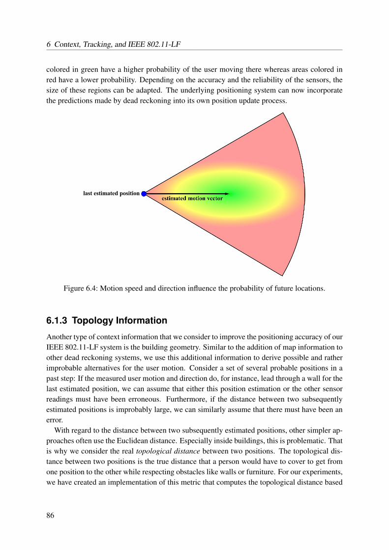
6 Context, Tracking, and IEEE 802.11-LF
colored in green have a higher probability of the user moving there whereas areas colored inred have a lower probability. Depending on the accuracy and the reliability of the sensors, thesize of these regions can be adapted. The underlying positioning system can now incorporatethe predictions made by dead reckoning into its own position update process.
Figure 6.4: Motion speed and direction influence the probability of future locations.
6.1.3 Topology Information
Another type of context information that we consider to improve the positioning accuracy of ourIEEE 802.11-LF system is the building geometry. Similar to the addition of map information toother dead reckoning systems, we use this additional information to derive possible and ratherimprobable alternatives for the user motion. Consider a set of several probable positions in apast step: If the measured user motion and direction do, for instance, lead through a wall for thelast estimated position, we can assume that either this position estimation or the other sensorreadings must have been erroneous. Furthermore, if the distance between two subsequentlyestimated positions is improbably large, we can similarly assume that there must have been anerror.
With regard to the distance between two subsequently estimated positions, other simpler ap-proaches often use the Euclidean distance. Especially inside buildings, this is problematic. Thatis why we consider the real topological distance between two positions. The topological dis-tance between two positions is the true distance that a person would have to cover to get fromone position to the other while respecting obstacles like walls or furniture. For our experiments,we have created an implementation of this metric that computes the topological distance based
86
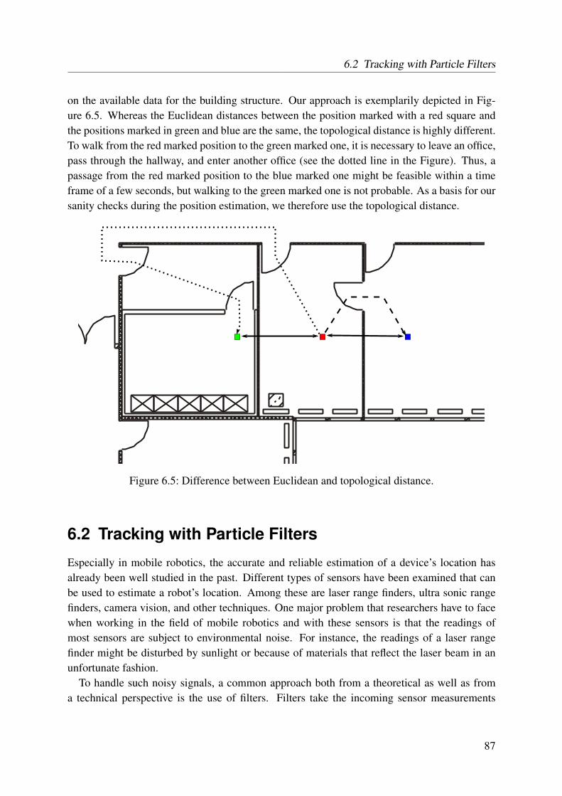
6.2 Tracking with Particle Filters
on the available data for the building structure. Our approach is exemplarily depicted in Fig-ure 6.5. Whereas the Euclidean distances between the position marked with a red square andthe positions marked in green and blue are the same, the topological distance is highly different.To walk from the red marked position to the green marked one, it is necessary to leave an office,pass through the hallway, and enter another office (see the dotted line in the Figure). Thus, apassage from the red marked position to the blue marked one might be feasible within a timeframe of a few seconds, but walking to the green marked one is not probable. As a basis for oursanity checks during the position estimation, we therefore use the topological distance.
Figure 6.5: Difference between Euclidean and topological distance.
6.2 Tracking with Particle Filters
Especially in mobile robotics, the accurate and reliable estimation of a device’s location hasalready been well studied in the past. Different types of sensors have been examined that canbe used to estimate a robot’s location. Among these are laser range finders, ultra sonic rangefinders, camera vision, and other techniques. One major problem that researchers have to facewhen working in the field of mobile robotics and with these sensors is that the readings ofmost sensors are subject to environmental noise. For instance, the readings of a laser rangefinder might be disturbed by sunlight or because of materials that reflect the laser beam in anunfortunate fashion.
To handle such noisy signals, a common approach both from a theoretical as well as froma technical perspective is the use of filters. Filters take the incoming sensor measurements
87
6 Context, Tracking, and IEEE 802.11-LF
and try to mitigate the effects of the environmental noise on the signals. Especially importantamong these filters is the Kalman filter introduced by R. E. Kalman in the year 1960 [Kal60].With a Kalman filter, it is possible to predict the state a system is in if not the state itself butonly emissions depending on the state and disturbed by noise can be measured. The filter hassome restrictions, though. The most important one is that it can only be used if the underlyingproblem can be modeled in a linear fashion.
To compensate for this limitation another class of filters has been introduced in the past (e.g.,refer to [RAG04]). This class is made up of the so-called Particle filters (PF). Particle filters– or Sequential Monte-Carlo Methods (SMCs) – are also used to e.g., predict the hidden stateof a system from which only noisy signal emissions can be measured. But, in contrast to theKalman filters, particle filters can also handle problems which cannot be modeled linearly.
This is achieved by not using a formal representation of the posterior probability density (theprobability for the different possible states at a certain point in time) . Instead, the density isrepresented by a large set of so-called particles. Each particle has a weight that is computedbased on properties of the underlying system. The sum of all particles – with their weight andtheir position in the state space – is used as the representation of the posterior.
Often called a Sequential Importance Sampling (SIS) filter, a PF is a sequential filter and thusevolves over time as more and more measured samples become available. As such, the progressof a particle filter is generally modeled in a cycle of several consecutive steps that are precededby a bootstrapping process. In the beginning, an initial distribution of the particles is assumed.This, in many cases, is a uniform random distribution in the state space. Upon the reception ofa new measurement, the particles are moved within the state space. For this, different types ofmotion models can be used. By using a sensor model subsequently, the weight of each particleis updated depending on its new position and the measurement. Then, the particle weights arenormalized, and the particles in their entirety represent the posterior after that measurement.As this type of PF does also have some limitations, e.g., the continuous degeneration of theparticle cloud, variations of the basic PF approach use a resampling step. This type of filter isgenerally referred to as Sampling Importance Re-sampling (SIR) filter and can help to avoid thedegeneration. In case of such an SIR PF, particles with a very low weight are eliminated andnew particles are re-sampled from the posterior distribution.
Especially for position estimation with the use of noisy sensor data, particle filters haveshown to be very effective, and they are widely used for this purpose nowadays. We thereforedecided to base our own tracking algorithm on an SIR filter, too.
6.2.1 Particle Motion Model
The motion model as part of the ongoing progress of a PF is used to move particles withinthe state space. This can generally be done in several different ways. Our basic mode is asimple Gaussian random motion. In the beginning, all particles are randomly distributed overthe covered area using an uniform distribution and are given a weight of one divided by the
88
6.2 Tracking with Particle Filters
number of particles. The, for each round of the PF and each particle, at first, a direction israndomly chosen. This direction is used together with a randomly chosen distance to advancethe particle to a new position. Whereas the direction is drawn from a uniform distribution ofvalues between 0◦ and 360◦, for the distance, we use a normal distribution with parameterschosen to represent a walking person.
Of course, with this basic approach, particles are able to leave the area that is covered byour training data. For this case, we have implemented two different behaviors: One choice isto restrain oneself from moving the particle if it otherwise moves outside the covered area. Inthis case, the particle simply stays at its current position. The second possibility is to let theparticle move. This results in the particle being removed during the next weight update as nonew weight can be assigned to it due to the lack of fingerprint information.
We also extended our motion model to make use of additional context information. Oneaddition is the consideration of information about the true motion of a user. Knowing the user’sspeed and her direction of motion, we can use this information to adapt the particle motionaccordingly. If the user is moving fast or if a longer time has passed between two consecutiveupdates, particles are allowed to advance farther from their current position. Furthermore, if thedirection in which a user is moving is known, the particle motion is adapted to let the particlesmove only in this direction. To gather information about the user motion, we have consideredseveral different approaches. One is the use of external sensors and a compass, as it was alreadydescribed in the earlier part of this chapter. Another possibility is the use of historic informationabout the user’s positions. From these, we try to extrapolate both a motion direction and thespeed.
A second major addition to the motion model is the incorporation of information about thetopology of a building. The particle cloud can be seen as a probability distribution of the user’swhereabouts. Furthermore, the movement of each single particle can be seen as a possibleuser motion that could have happened in the covered area. This is especially true when we usethe additional context information to decide on the particle motion. As a user is not able topass through obstacles like walls, we apply these constraints to the particles, too. If a particlemovement leads to crossing a wall, that movement is canceled. Similar to when a particle leavesthe covered area, we, in this case, either let the particle stay at its current position, or we removeit from the particle set.
6.2.2 Sensor Model
As stated in the former sections, another important step in the progress of a PF is the compu-tation of the particle weights. Generally, an importance density is used for this purpose. Inour case, we had to face a special design difficulty when implementing the weight update forthe particles. We wanted to improve the performance of IEEE 802.11-LF by the use of a par-ticle filter. Thus, we also wanted to stick to the general LF approach, and use the informationfrom an underlying fingerprint database for the weight update of the particles. The difficulty
89
6 Context, Tracking, and IEEE 802.11-LF
in this case is that, in general, each fingerprint only represents one single point within the two-or three-dimensional state space. But we obviously do not want to limit the particles to thislimited set of available positions.
We therefore continued our earlier work and used our grid cell representation of the infor-mation in the fingerprint database to create what we call an importance density grid. With thisapproach, we can use the information from the fingerprints to cover the whole area for whichfingerprint information is available. During the weight update phase of the PF, we, for each par-ticle, identify the cell in which the particle is located. Then, the information of the fingerprintthat owns that cell is used to compute the new particle weight.
Compared to the motion model, the possibilities to influence the performance of the particlefilter are rather limited with this type of sensor model. As it mimics the Gaussian process usedby the Rice LF system to compute the weight for the single particles, the parameters to adjustthe sensor model are very limited. For the cases where settings had to be made, we used thevalues that have been recommended in the literature or the ones that are properties of the usedhardware.
6.3 Evaluation
We now give an overview of the methodology we used to evaluate our tracking algorithm.At first, we will introduce the details about the evaluation of the sources for context informa-tion, especially the motion detection algorithm, before we continue with presenting informationabout the overall tracking system.
6.3.1 Motion Mode
To evaluate the motion detection algorithm, we collected short data sequences of about 30 s
length and also longer sequences of about 100 s for each motion mode. Whereas the formersequences were used to identify the thresholds to distinguish between the different modes, weused the latter ones to evaluate the algorithm. The devices used for collecting the data were anHTC Desire smartphone running Android 2.2 and an HTC Hero smartphone running Android1.5. The phones were held in a natural fashion in front of the user during the collection. Fur-thermore, during the collection of the longer data sets, the device was rotated several times indifferent directions. For each motion mode, we randomly selected sequences of ten measure-ments from the evaluation data sets, computed the acceleration spread, and – from that value –determined the motion mode. This experiment was repeated 1000 times for each motion mode.
6.3.2 Particle Filter
For the evaluation of the particle filter-based IEEE 802.11-LF system, we collected a new set ofmeasurements within the hallways, two lecture halls, and several offices located on the second
90
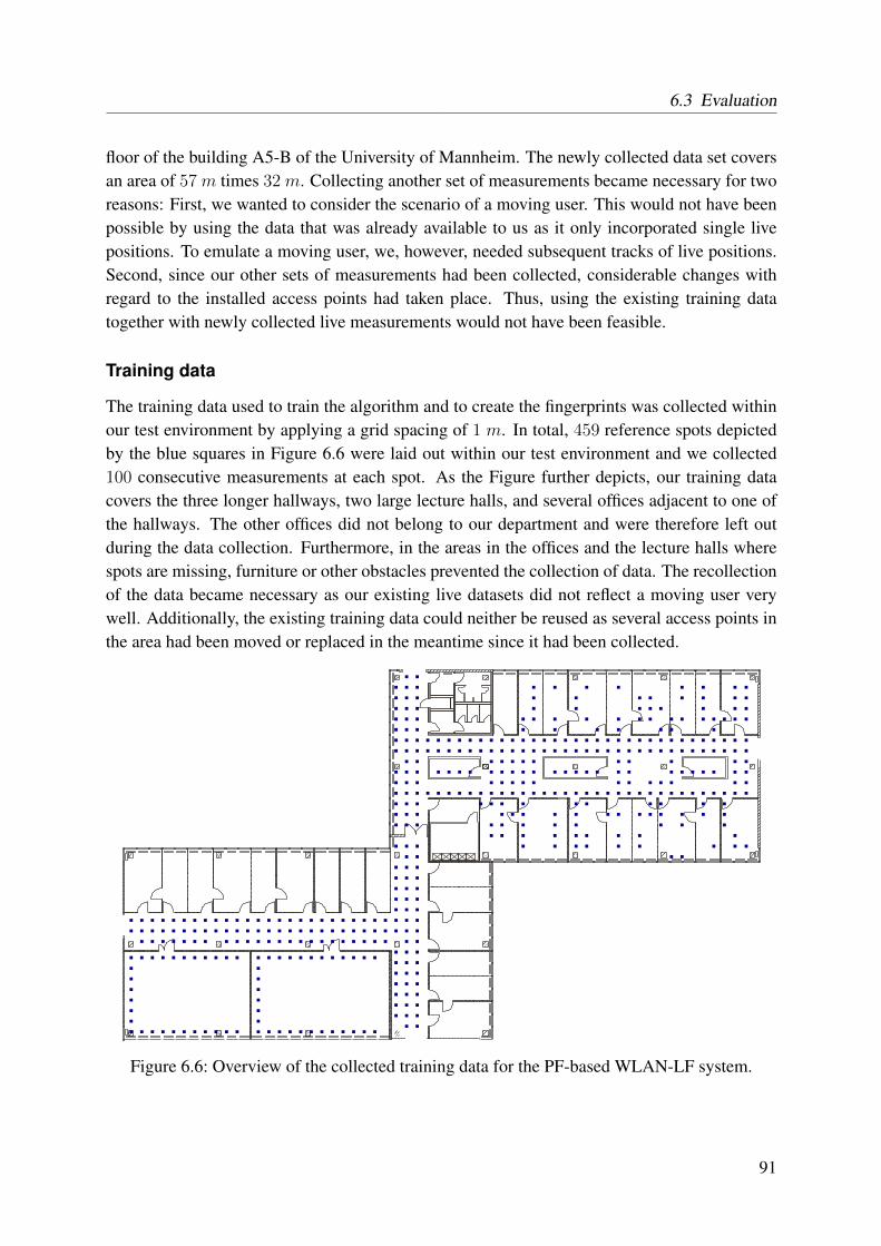
6.3 Evaluation
floor of the building A5-B of the University of Mannheim. The newly collected data set coversan area of 57 m times 32 m. Collecting another set of measurements became necessary for tworeasons: First, we wanted to consider the scenario of a moving user. This would not have beenpossible by using the data that was already available to us as it only incorporated single livepositions. To emulate a moving user, we, however, needed subsequent tracks of live positions.Second, since our other sets of measurements had been collected, considerable changes withregard to the installed access points had taken place. Thus, using the existing training datatogether with newly collected live measurements would not have been feasible.
Training data
The training data used to train the algorithm and to create the fingerprints was collected withinour test environment by applying a grid spacing of 1 m. In total, 459 reference spots depictedby the blue squares in Figure 6.6 were laid out within our test environment and we collected100 consecutive measurements at each spot. As the Figure further depicts, our training datacovers the three longer hallways, two large lecture halls, and several offices adjacent to one ofthe hallways. The other offices did not belong to our department and were therefore left outduring the data collection. Furthermore, in the areas in the offices and the lecture halls wherespots are missing, furniture or other obstacles prevented the collection of data. The recollectionof the data became necessary as our existing live datasets did not reflect a moving user verywell. Additionally, the existing training data could neither be reused as several access points inthe area had been moved or replaced in the meantime since it had been collected.
Figure 6.6: Overview of the collected training data for the PF-based WLAN-LF system.
91
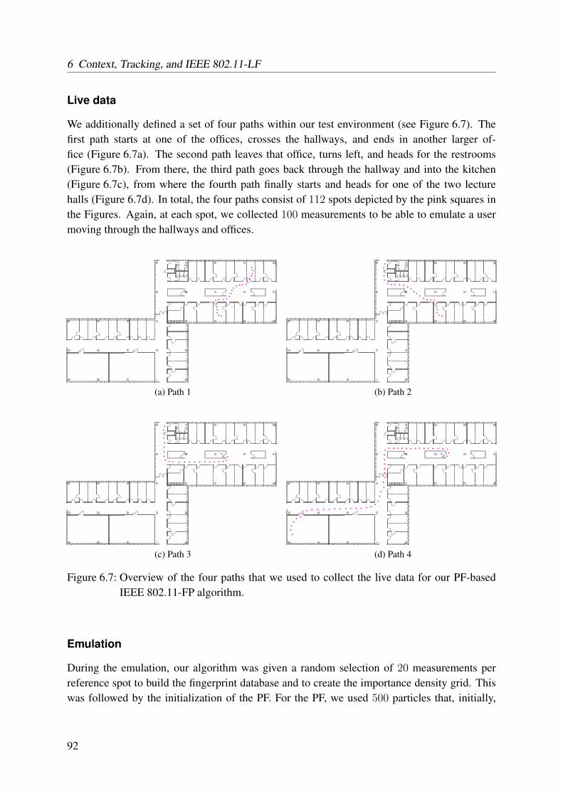
6 Context, Tracking, and IEEE 802.11-LF
Live data
We additionally defined a set of four paths within our test environment (see Figure 6.7). Thefirst path starts at one of the offices, crosses the hallways, and ends in another larger of-fice (Figure 6.7a). The second path leaves that office, turns left, and heads for the restrooms(Figure 6.7b). From there, the third path goes back through the hallway and into the kitchen(Figure 6.7c), from where the fourth path finally starts and heads for one of the two lecturehalls (Figure 6.7d). In total, the four paths consist of 112 spots depicted by the pink squares inthe Figures. Again, at each spot, we collected 100 measurements to be able to emulate a usermoving through the hallways and offices.
(a) Path 1 (b) Path 2
(c) Path 3 (d) Path 4
Figure 6.7: Overview of the four paths that we used to collect the live data for our PF-basedIEEE 802.11-FP algorithm.
Emulation
During the emulation, our algorithm was given a random selection of 20 measurements perreference spot to build the fingerprint database and to create the importance density grid. Thiswas followed by the initialization of the PF. For the PF, we used 500 particles that, initially,
92
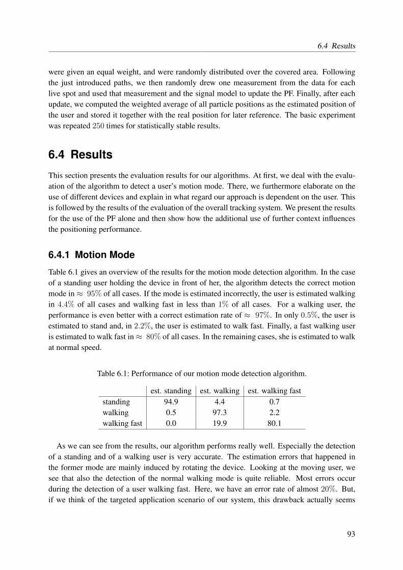
6.4 Results
were given an equal weight, and were randomly distributed over the covered area. Followingthe just introduced paths, we then randomly drew one measurement from the data for eachlive spot and used that measurement and the signal model to update the PF. Finally, after eachupdate, we computed the weighted average of all particle positions as the estimated position ofthe user and stored it together with the real position for later reference. The basic experimentwas repeated 250 times for statistically stable results.
6.4 Results
This section presents the evaluation results for our algorithms. At first, we deal with the evalu-ation of the algorithm to detect a user’s motion mode. There, we furthermore elaborate on theuse of different devices and explain in what regard our approach is dependent on the user. Thisis followed by the results of the evaluation of the overall tracking system. We present the resultsfor the use of the PF alone and then show how the additional use of further context influencesthe positioning performance.
6.4.1 Motion Mode
Table 6.1 gives an overview of the results for the motion mode detection algorithm. In the caseof a standing user holding the device in front of her, the algorithm detects the correct motionmode in ≈ 95% of all cases. If the mode is estimated incorrectly, the user is estimated walkingin 4.4% of all cases and walking fast in less than 1% of all cases. For a walking user, theperformance is even better with a correct estimation rate of ≈ 97%. In only 0.5%, the user isestimated to stand and, in 2.2%, the user is estimated to walk fast. Finally, a fast walking useris estimated to walk fast in ≈ 80% of all cases. In the remaining cases, she is estimated to walkat normal speed.
Table 6.1: Performance of our motion mode detection algorithm.
est. standing est. walking est. walking faststanding 94.9 4.4 0.7walking 0.5 97.3 2.2walking fast 0.0 19.9 80.1
As we can see from the results, our algorithm performs really well. Especially the detectionof a standing and of a walking user is very accurate. The estimation errors that happened inthe former mode are mainly induced by rotating the device. Looking at the moving user, wesee that also the detection of the normal walking mode is quite reliable. Most errors occurduring the detection of a user walking fast. Here, we have an error rate of almost 20%. But,if we think of the targeted application scenario of our system, this drawback actually seems
93
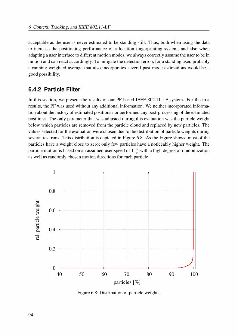
6 Context, Tracking, and IEEE 802.11-LF
acceptable as the user is never estimated to be standing still. Thus, both when using the datato increase the positioning performance of a location fingerprinting system, and also whenadapting a user interface to different motion modes, we always correctly assume the user to be inmotion and can react accordingly. To mitigate the detection errors for a standing user, probablya running weighted average that also incorporates several past mode estimations would be agood possibility.
6.4.2 Particle Filter
In this section, we present the results of our PF-based IEEE 802.11-LF system. For the firstresults, the PF was used without any additional information. We neither incorporated informa-tion about the history of estimated positions nor performed any post-processing of the estimatedpositions. The only parameter that was adjusted during this evaluation was the particle weightbelow which particles are removed from the particle cloud and replaced by new particles. Thevalues selected for the evaluation were chosen due to the distribution of particle weights duringseveral test runs. This distribution is depicted in Figure 6.8. As the Figure shows, most of theparticles have a weight close to zero; only few particles have a noticeably higher weight. Theparticle motion is based on an assumed user speed of 1 m
swith a high degree of randomization
as well as randomly chosen motion directions for each particle.
0
0.2
0.4
0.6
0.8
1
40 50 60 70 80 90 100
rel.
par
ticl
e w
eig
ht
particles [%]
Figure 6.8: Distribution of particle weights.
94
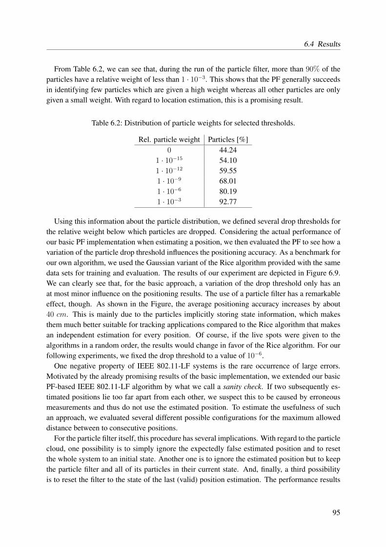
6.4 Results
From Table 6.2, we can see that, during the run of the particle filter, more than 90% of theparticles have a relative weight of less than 1 · 10−3. This shows that the PF generally succeedsin identifying few particles which are given a high weight whereas all other particles are onlygiven a small weight. With regard to location estimation, this is a promising result.
Table 6.2: Distribution of particle weights for selected thresholds.
Rel. particle weight Particles [%]0 44.24
1 · 10−15 54.101 · 10−12 59.551 · 10−9 68.011 · 10−6 80.191 · 10−3 92.77
Using this information about the particle distribution, we defined several drop thresholds forthe relative weight below which particles are dropped. Considering the actual performance ofour basic PF implementation when estimating a position, we then evaluated the PF to see how avariation of the particle drop threshold influences the positioning accuracy. As a benchmark forour own algorithm, we used the Gaussian variant of the Rice algorithm provided with the samedata sets for training and evaluation. The results of our experiment are depicted in Figure 6.9.We can clearly see that, for the basic approach, a variation of the drop threshold only has anat most minor influence on the positioning results. The use of a particle filter has a remarkableeffect, though. As shown in the Figure, the average positioning accuracy increases by about40 cm. This is mainly due to the particles implicitly storing state information, which makesthem much better suitable for tracking applications compared to the Rice algorithm that makesan independent estimation for every position. Of course, if the live spots were given to thealgorithms in a random order, the results would change in favor of the Rice algorithm. For ourfollowing experiments, we fixed the drop threshold to a value of 10−6.
One negative property of IEEE 802.11-LF systems is the rare occurrence of large errors.Motivated by the already promising results of the basic implementation, we extended our basicPF-based IEEE 802.11-LF algorithm by what we call a sanity check. If two subsequently es-timated positions lie too far apart from each other, we suspect this to be caused by erroneousmeasurements and thus do not use the estimated position. To estimate the usefulness of suchan approach, we evaluated several different possible configurations for the maximum alloweddistance between to consecutive positions.
For the particle filter itself, this procedure has several implications. With regard to the particlecloud, one possibility is to simply ignore the expectedly false estimated position and to resetthe whole system to an initial state. Another one is to ignore the estimated position but to keepthe particle filter and all of its particles in their current state. And, finally, a third possibilityis to reset the filter to the state of the last (valid) position estimation. The performance results
95
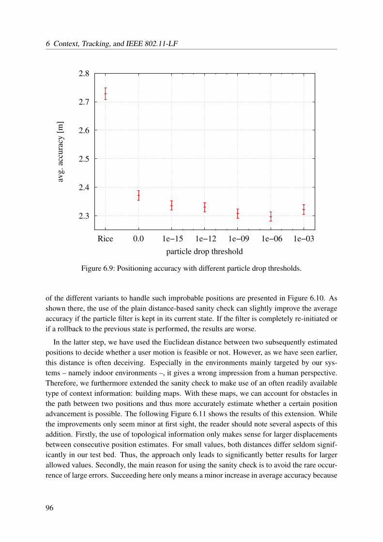
6 Context, Tracking, and IEEE 802.11-LF
2.3
2.4
2.5
2.6
2.7
2.8
Rice 0.0 1e−15 1e−12 1e−09 1e−06 1e−03
avg
. ac
cura
cy [
m]
particle drop threshold
Figure 6.9: Positioning accuracy with different particle drop thresholds.
of the different variants to handle such improbable positions are presented in Figure 6.10. Asshown there, the use of the plain distance-based sanity check can slightly improve the averageaccuracy if the particle filter is kept in its current state. If the filter is completely re-initiated orif a rollback to the previous state is performed, the results are worse.
In the latter step, we have used the Euclidean distance between two subsequently estimatedpositions to decide whether a user motion is feasible or not. However, as we have seen earlier,this distance is often deceiving. Especially in the environments mainly targeted by our sys-tems – namely indoor environments –, it gives a wrong impression from a human perspective.Therefore, we furthermore extended the sanity check to make use of an often readily availabletype of context information: building maps. With these maps, we can account for obstacles inthe path between two positions and thus more accurately estimate whether a certain positionadvancement is possible. The following Figure 6.11 shows the results of this extension. Whilethe improvements only seem minor at first sight, the reader should note several aspects of thisaddition. Firstly, the use of topological information only makes sense for larger displacementsbetween consecutive position estimates. For small values, both distances differ seldom signif-icantly in our test bed. Thus, the approach only leads to significantly better results for largerallowed values. Secondly, the main reason for using the sanity check is to avoid the rare occur-rence of large errors. Succeeding here only means a minor increase in average accuracy because
96
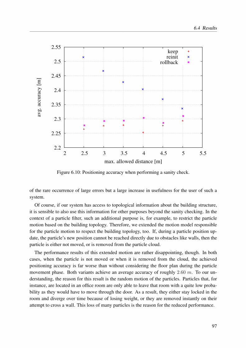
6.4 Results
2.2
2.25
2.3
2.35
2.4
2.45
2.5
2.55
2 2.5 3 3.5 4 4.5 5 5.5
avg
. ac
cura
cy [
m]
max. allowed distance [m]
keepreinit
rollback
Figure 6.10: Positioning accuracy when performing a sanity check.
of the rare occurrence of large errors but a large increase in usefulness for the user of such asystem.
Of course, if our system has access to topological information about the building structure,it is sensible to also use this information for other purposes beyond the sanity checking. In thecontext of a particle filter, such an additional purpose is, for example, to restrict the particlemotion based on the building topology. Therefore, we extended the motion model responsiblefor the particle motion to respect the building topology, too. If, during a particle position up-date, the particle’s new position cannot be reached directly due to obstacles like walls, then theparticle is either not moved, or is removed from the particle cloud.
The performance results of this extended motion are rather disappointing, though. In bothcases, when the particle is not moved or when it is removed from the cloud, the achievedpositioning accuracy is far worse than without considering the floor plan during the particlemovement phase. Both variants achieve an average accuracy of roughly 2.60 m. To our un-derstanding, the reason for this result is the random motion of the particles. Particles that, forinstance, are located in an office room are only able to leave that room with a quite low proba-bility as they would have to move through the door. As a result, they either stay locked in theroom and diverge over time because of losing weight, or they are removed instantly on theirattempt to cross a wall. This loss of many particles is the reason for the reduced performance.
97
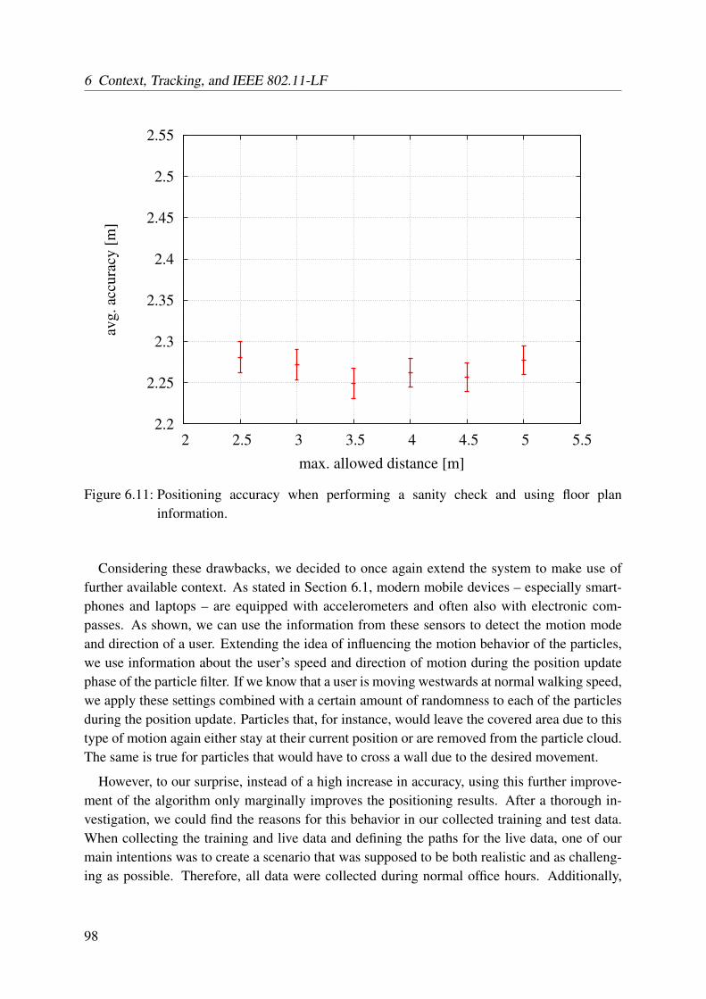
6 Context, Tracking, and IEEE 802.11-LF
2.2
2.25
2.3
2.35
2.4
2.45
2.5
2.55
2 2.5 3 3.5 4 4.5 5 5.5
avg
. ac
cura
cy [
m]
max. allowed distance [m]
Figure 6.11: Positioning accuracy when performing a sanity check and using floor planinformation.
Considering these drawbacks, we decided to once again extend the system to make use offurther available context. As stated in Section 6.1, modern mobile devices – especially smart-phones and laptops – are equipped with accelerometers and often also with electronic com-passes. As shown, we can use the information from these sensors to detect the motion modeand direction of a user. Extending the idea of influencing the motion behavior of the particles,we use information about the user’s speed and direction of motion during the position updatephase of the particle filter. If we know that a user is moving westwards at normal walking speed,we apply these settings combined with a certain amount of randomness to each of the particlesduring the position update. Particles that, for instance, would leave the covered area due to thistype of motion again either stay at their current position or are removed from the particle cloud.The same is true for particles that would have to cross a wall due to the desired movement.
However, to our surprise, instead of a high increase in accuracy, using this further improve-ment of the algorithm only marginally improves the positioning results. After a thorough in-vestigation, we could find the reasons for this behavior in our collected training and test data.When collecting the training and live data and defining the paths for the live data, one of ourmain intentions was to create a scenario that was supposed to be both realistic and as challeng-ing as possible. Therefore, all data were collected during normal office hours. Additionally,
98
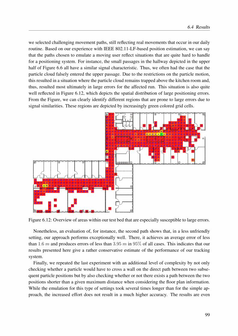
6.4 Results
we selected challenging movement paths, still reflecting real movements that occur in our dailyroutine. Based on our experience with IEEE 802.11-LF-based position estimation, we can saythat the paths chosen to emulate a moving user reflect situations that are quite hard to handlefor a positioning system. For instance, the small passages in the hallway depicted in the upperhalf of Figure 6.6 all have a similar signal characteristic. Thus, we often had the case that theparticle cloud falsely entered the upper passage. Due to the restrictions on the particle motion,this resulted in a situation where the particle cloud remains trapped above the kitchen room and,thus, resulted most ultimately in large errors for the affected run. This situation is also quitewell reflected in Figure 6.12, which depicts the spatial distribution of large positioning errors.From the Figure, we can clearly identify different regions that are prone to large errors due tosignal similarities. These regions are depicted by increasingly green colored grid cells.
Figure 6.12: Overview of areas within our test bed that are especially susceptible to large errors.
Nonetheless, an evaluation of, for instance, the second path shows that, in a less unfriendlysetting, our approach performs exceptionally well. There, it achieves an average error of lessthan 1.6 m and produces errors of less than 3.95 m in 95% of all cases. This indicates that ourresults presented here give a rather conservative estimate of the performance of our trackingsystem.
Finally, we repeated the last experiment with an additional level of complexity by not onlychecking whether a particle would have to cross a wall on the direct path between two subse-quent particle positions but by also checking whether or not there exists a path between the twopositions shorter than a given maximum distance when considering the floor plan information.While the emulation for this type of settings took several times longer than for the simple ap-proach, the increased effort does not result in a much higher accuracy. The results are even
99
6 Context, Tracking, and IEEE 802.11-LF
worse than when using the simple approach to restrict the particle motion. Considering thesource of information that is used to decide where particles should be moving, this is not sur-prising. The direct check represents the user much better, as she herself is moving in a certaindirection and at a certain speed. The alternate path a particle could have taken, for example,around corners, would have caused different sensor measurements if the user had taken thatpath. Thus, this type of indirect movements reflects the user behavior worse and consequentlyyields to worse results.
6.5 Discussion
The following section briefly discusses several aspects of our work that, despite the alreadypromising results of our algorithms, influence the results, and, thus, deserve further attention.
6.5.1 Motion Mode
At first, we will cover the user and device dependability of our motion mode detection algorithmand discuss the influence of the measurement window size.
Influence of the User
Of course, different users can have a different motion profile. During the course of our experi-ments, we have seen that the thresholds used for one user do not necessarily fit for another user.Therefore, it would be infeasible to use the same thresholds for everybody.
The system we have developed offers the possibility for a short user-based calibration step.The user is asked to stand still, walk, or walk fast for a timespan of 30 s each. Based on the datacollected in this time, the system then computes user-specific threshold values for the differentmotion modes and stores them for later reference. At first, the measurements for each motionmode pass a high- and lowpass filter that eliminates the topmost and bottommost one percentof the measurements. We do so to filter out outliers. Then, for the threshold between standingand walking, we calculate the difference between the measured acceleration spreads and usethe value of a standing user plus one third of the difference as the threshold. For the thresholdbetween a walking and a fast walking user, we use the average of the values measured for thetwo modes. The reason for the different handling of the thresholds is our insight that a standinguser is easier to detect and thus allows for a more rigid selection of the threshold.
This calibration step helps us to maintain the high accuracy of our system for different users.While it at first might seem cumbersome to have to calibrate a device for every user, we havemade the observation that mobile devices like smartphones are rarely shared between peopleand, thus, this step generally has to be performed only once for each device.
100
6.6 Conclusions
Influence of the Device
For our measurements, we used two different devices: An HTC Desire smartphone and anHTC Hero smartphone. Whereas we only presented the results for the HTC Desire smartphonein Section 6.3.1, the estimation results for the HTC Hero smartphone are almost identical.Even the values that were learned as thresholds for a single user were almost identical on bothdevices. This suggests that, at least for a given device class, for instance the smartphones fromone manufacturer, it might be sufficient to only have the user calibrate one device and thentransfer the calibration information to other devices belonging to the same class.
Measurement Window
We used a time frame of about one second or ten measurements for the sliding window fromwhich the acceleration spread was computed by our system. During our experiments, we alsotried other values. However, the chosen ones performed best. For lower numbers, we facedthe problem of not covering a complete motion cycle of at least one step. When reducing thewindow further, we even ended with values close to zero for all types of motion as only singlepoints with constant acceleration were detected in the motion cycle. For larger values, singlespikes in the measurements had a long-lasting effect on the detected spread and thus decreasedthe achieved accuracy, especially when changes in the motion mode occurred.
6.5.2 Compass
During our work, we used the integrated compass of the smartphones as well as a digital com-pass attached to a laptop computer via a universal serial bus (USB) connection. However, asour test environment has metal walls, one major problem we had to face was a high deviationoff the measured angles. When, for instance, walking in one direction along one of the hall-ways, the compasses measured arbitrary values. When performing the same kind of test in asecond building with walls made up of less inducing materials, we observed a much friendlierbehavior of the compasses. To still allow for a proper evaluation, we measured the behavior ofthe compass devices under normal operation, created a simulation model, and used that modelinstead of measured data during the emulation of our algorithms.
6.6 Conclusions
Using a particle filter as an underlying algorithm for the tracking of a user with the help ofIEEE 802.11 and LF has clearly proven to be a suitable approach. Even without the use ofadditional context, the PF offers an already increased positioning accuracy. This is achievedby explicitly considering the history of both the particle positions and the measurements. Ifadditional context information is incorporated as well, the results can be further improved. Theuse of map information and a sanity check of subsequent positions mainly helps to reduce the
101
6 Context, Tracking, and IEEE 802.11-LF
occurrence of rare large errors. From a usability perspective, this is an important improvementeven though it only results in a minor increase in the average positioning accuracy. Regardingthe metric used for the sanity check, we have seen that the use of the topological distance yieldsto better results. This is not surprising as it represents the possible user motion far better thanthe use of a simple Euclidean distance.
The additional use of motion information, on the other hand, offers the potential for muchbigger improvements. To gain the data necessary for a motion mode estimation, accelerometersand digital compasses, as they are already built into many modern mobile devices, can be used.Our results show that data from these sensors offers the possibility for a robust and reliableestimation of the user’s motion mode. As we have seen during our experiments, using thisinformation can reduce the average error to values of far less than two meters. However, wehave also made the observation that adverse conditions result in much smaller increases of theaccuracy. An analysis of our training data showed problematic similarities between certainareas in our test bed that resulted in a reduced performance. In a practical deployment, wewould resolve this by relocating the APs to create more distinctive characteristics for theseareas.
There are also some other aspects that would allow for a further tweaking of the system’sperformance in case of a productive use. For instance, while using the idea of an importancedensity grid helped us to combine the concepts of LF and PFs, it also introduces a new sourceof errors. During the resampling phase of the PF, particles are randomly placed in the grid cellsaccording to the importance density grid. However, as the layout of the grid does not take thebuilding topology into account, this can result in a new particle being placed on one side of awall while a particle responsible for the grid cell’s total weight is located on the other side. Asthis obviously leads to a degradation of the accuracy, such a behavior should be mitigated forfuture use.
A second aspect that offers some room for future work could be the occurrence of splitparticle clouds. Here, for example, a k-means clustering would offer a good solution to detectsuch a situation, and to handle it. While we did not follow this idea in favor of other interestingfeatures, this would be a worthwhile path for future activity.
102
CH
AP
TE
R
7 Roaming betweenPositioning Technologies
The previous chapter has discussed tracking – and thus the use of additional information likea position history and motion information – to improve the overall quality and accuracy of theposition estimation. As we have seen, the use of this additional information available due to theconsideration of the user’s motion yields to noticeable improvements. However, it also causesnew problems. This chapter deals with one of the most urging ones: the problem of choice. Auser who is roaming around will most probably find herself in situations where more than onepositioning system is available. While GPS generally can only be used outdoors, the preciselocation estimation with IEEE 802.11-LF is most often only used indoors and in areas closeto buildings. Furthermore, also the signals from GSM cell towers can be used for locationestimation in many situations. Thus, when entering or leaving a building or in the surroundingareas, more than one system might often be available. The following chapter deals with thequestion when to automatically choose which system. Considering the definition of suitable, inour case, we consider the most accurate system to be the most suitable one.
This definition, of course, is not necessarily valid under all circumstances. Depending onthe application scenario, other factors like, for example, the energy consumption of differentpositioning systems, privacy considerations, or the required use of the communication infras-tructure can be additional decisive factors. If, for instance, a user wants to keep informationabout her whereabouts private, she would rather use GPS for a position estimation instead of anIEEE 802.11-LF system or GSM positioning, which probably both rely on a central server forthe matching of the live measurements and fingerprints or aggregation of the data from differentbase stations.
7.1 Error Estimation
We base our decision on which system to use on the accuracy that can be expected from thedifferent available systems. As such, we need information about how much trust we can spendon a given position estimate. On the one hand, if the position estimate is uncertain, we better
103
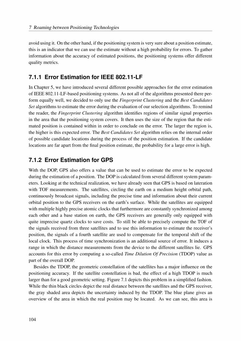
7 Roaming between Positioning Technologies
avoid using it. On the other hand, if the positioning system is very sure about a position estimate,this is an indicator that we can use the estimate without a high probability for errors. To gatherinformation about the accuracy of estimated positions, the positioning systems offer differentquality metrics.
7.1.1 Error Estimation for IEEE 802.11-LF
In Chapter 5, we have introduced several different possible approaches for the error estimationof IEEE 802.11-LF-based positioning systems. As not all of the algorithms presented there per-form equally well, we decided to only use the Fingerprint Clustering and the Best CandidatesSet algorithms to estimate the error during the evaluation of our selection algorithms. To remindthe reader, the Fingerprint Clustering algorithm identifies regions of similar signal propertiesin the area that the positioning system covers. It then uses the size of the region that the esti-mated position is contained within in order to conclude on the error. The larger the region is,the higher is this expected error. The Best Candidates Set algorithm relies on the internal orderof possible candidate locations during the process of the position estimation. If the candidatelocations are far apart from the final position estimate, the probability for a large error is high.
7.1.2 Error Estimation for GPS
With the DOP, GPS also offers a value that can be used to estimate the error to be expectedduring the estimation of a position. The DOP is calculated from several different system param-eters. Looking at the technical realization, we have already seen that GPS is based on laterationwith TOF measurements. The satellites, circling the earth on a medium height orbital path,continuously broadcast signals, including the precise time and information about their currentorbital position to the GPS receivers on the earth’s surface. While the satellites are equippedwith multiple highly precise atomic clocks that furthermore are constantly synchronized amongeach other and a base station on earth, the GPS receivers are generally only equipped withquite imprecise quartz clocks to save costs. To still be able to precisely compute the TOF ofthe signals received from three satellites and to use this information to estimate the receiver’sposition, the signals of a fourth satellite are used to compensate for the temporal shift of thelocal clock. This process of time synchronization is an additional source of error. It induces arange in which the distance measurements from the device to the different satellites lie. GPSaccounts for this error by computing a so-called Time Dilution Of Precision (TDOP) value aspart of the overall DOP.
Besides the TDOP, the geometric constellation of the satellites has a major influence on thepositioning accuracy. If the satellite constellation is bad, the effect of a high TDOP is muchlarger than for a good geometric setting. Figure 7.1 depicts this problem in a simplified fashion.While the thin black circles depict the real distance between the satellites and the GPS receiver,the gray shaded area depicts the uncertainty induced by the TDOP. The blue plane gives anoverview of the area in which the real position may be located. As we can see, this area is
104
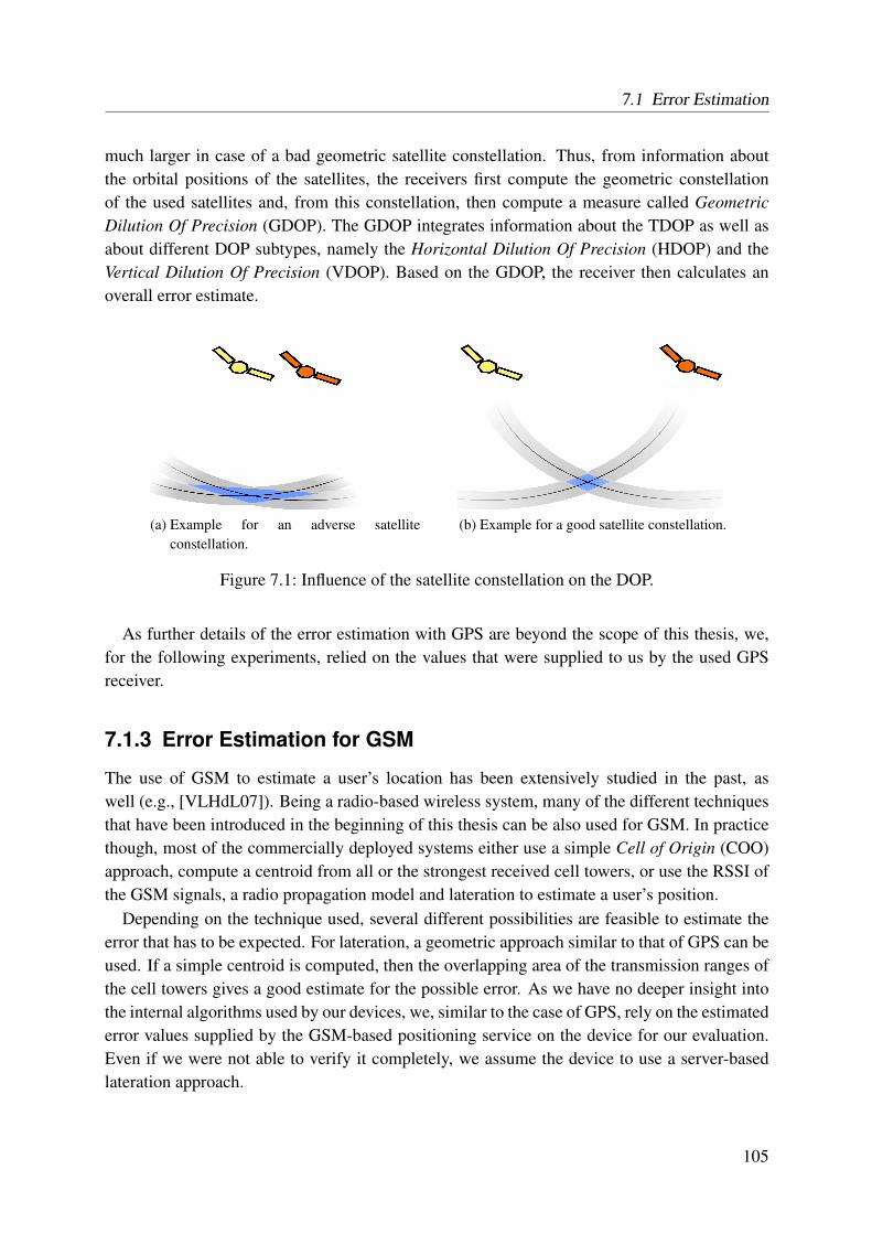
7.1 Error Estimation
much larger in case of a bad geometric satellite constellation. Thus, from information aboutthe orbital positions of the satellites, the receivers first compute the geometric constellationof the used satellites and, from this constellation, then compute a measure called GeometricDilution Of Precision (GDOP). The GDOP integrates information about the TDOP as well asabout different DOP subtypes, namely the Horizontal Dilution Of Precision (HDOP) and theVertical Dilution Of Precision (VDOP). Based on the GDOP, the receiver then calculates anoverall error estimate.
(a) Example for an adverse satelliteconstellation.
(b) Example for a good satellite constellation.
Figure 7.1: Influence of the satellite constellation on the DOP.
As further details of the error estimation with GPS are beyond the scope of this thesis, we,for the following experiments, relied on the values that were supplied to us by the used GPSreceiver.
7.1.3 Error Estimation for GSM
The use of GSM to estimate a user’s location has been extensively studied in the past, aswell (e.g., [VLHdL07]). Being a radio-based wireless system, many of the different techniquesthat have been introduced in the beginning of this thesis can be also used for GSM. In practicethough, most of the commercially deployed systems either use a simple Cell of Origin (COO)approach, compute a centroid from all or the strongest received cell towers, or use the RSSI ofthe GSM signals, a radio propagation model and lateration to estimate a user’s position.
Depending on the technique used, several different possibilities are feasible to estimate theerror that has to be expected. For lateration, a geometric approach similar to that of GPS can beused. If a simple centroid is computed, then the overlapping area of the transmission ranges ofthe cell towers gives a good estimate for the possible error. As we have no deeper insight intothe internal algorithms used by our devices, we, similar to the case of GPS, rely on the estimatederror values supplied by the GSM-based positioning service on the device for our evaluation.Even if we were not able to verify it completely, we assume the device to use a server-basedlateration approach.
105
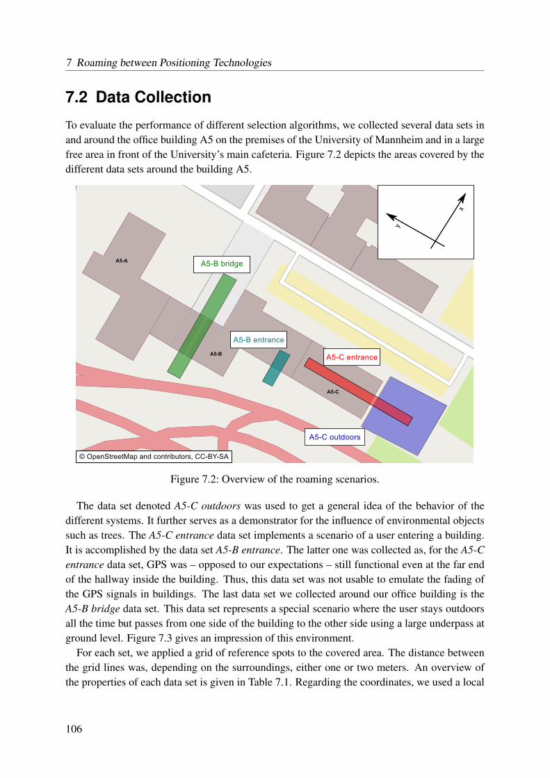
7 Roaming between Positioning Technologies
7.2 Data Collection
To evaluate the performance of different selection algorithms, we collected several data sets inand around the office building A5 on the premises of the University of Mannheim and in a largefree area in front of the University’s main cafeteria. Figure 7.2 depicts the areas covered by thedifferent data sets around the building A5.
Figure 7.2: Overview of the roaming scenarios.
The data set denoted A5-C outdoors was used to get a general idea of the behavior of thedifferent systems. It further serves as a demonstrator for the influence of environmental objectssuch as trees. The A5-C entrance data set implements a scenario of a user entering a building.It is accomplished by the data set A5-B entrance. The latter one was collected as, for the A5-Centrance data set, GPS was – opposed to our expectations – still functional even at the far endof the hallway inside the building. Thus, this data set was not usable to emulate the fading ofthe GPS signals in buildings. The last data set we collected around our office building is theA5-B bridge data set. This data set represents a special scenario where the user stays outdoorsall the time but passes from one side of the building to the other side using a large underpass atground level. Figure 7.3 gives an impression of this environment.
For each set, we applied a grid of reference spots to the covered area. The distance betweenthe grid lines was, depending on the surroundings, either one or two meters. An overview ofthe properties of each data set is given in Table 7.1. Regarding the coordinates, we used a local
106
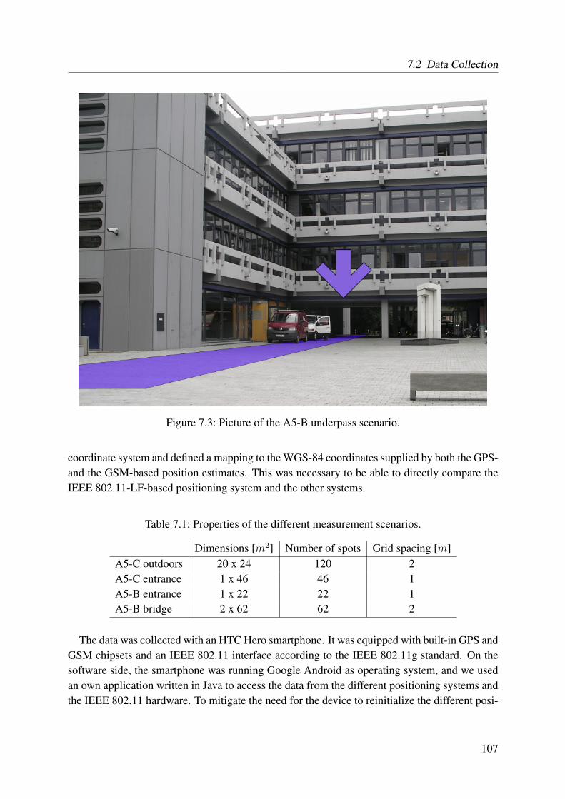
7.2 Data Collection
Figure 7.3: Picture of the A5-B underpass scenario.
coordinate system and defined a mapping to the WGS-84 coordinates supplied by both the GPS-and the GSM-based position estimates. This was necessary to be able to directly compare theIEEE 802.11-LF-based positioning system and the other systems.
Table 7.1: Properties of the different measurement scenarios.
Dimensions [m2] Number of spots Grid spacing [m]A5-C outdoors 20 x 24 120 2A5-C entrance 1 x 46 46 1A5-B entrance 1 x 22 22 1A5-B bridge 2 x 62 62 2
The data was collected with an HTC Hero smartphone. It was equipped with built-in GPS andGSM chipsets and an IEEE 802.11 interface according to the IEEE 802.11g standard. On thesoftware side, the smartphone was running Google Android as operating system, and we usedan own application written in Java to access the data from the different positioning systems andthe IEEE 802.11 hardware. To mitigate the need for the device to reinitialize the different posi-
107
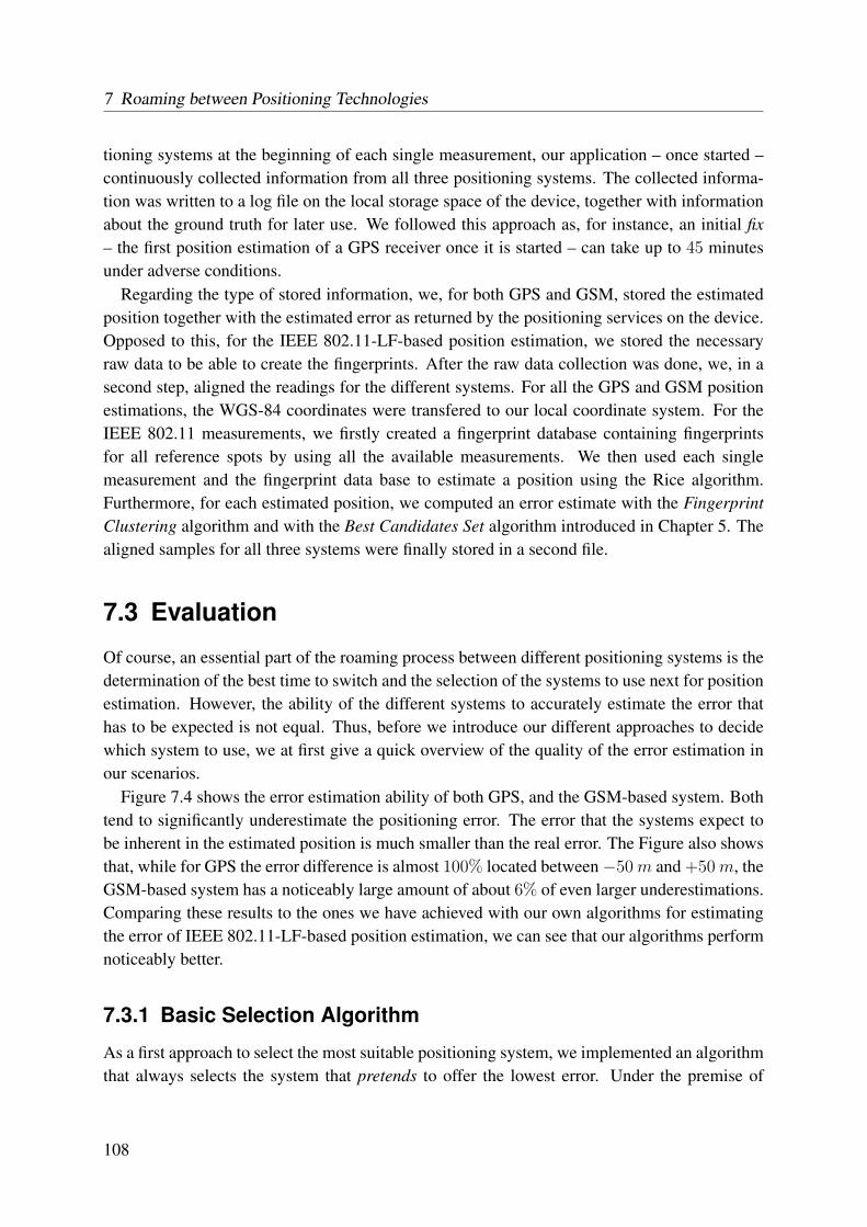
7 Roaming between Positioning Technologies
tioning systems at the beginning of each single measurement, our application – once started –continuously collected information from all three positioning systems. The collected informa-tion was written to a log file on the local storage space of the device, together with informationabout the ground truth for later use. We followed this approach as, for instance, an initial fix– the first position estimation of a GPS receiver once it is started – can take up to 45 minutesunder adverse conditions.
Regarding the type of stored information, we, for both GPS and GSM, stored the estimatedposition together with the estimated error as returned by the positioning services on the device.Opposed to this, for the IEEE 802.11-LF-based position estimation, we stored the necessaryraw data to be able to create the fingerprints. After the raw data collection was done, we, in asecond step, aligned the readings for the different systems. For all the GPS and GSM positionestimations, the WGS-84 coordinates were transfered to our local coordinate system. For theIEEE 802.11 measurements, we firstly created a fingerprint database containing fingerprintsfor all reference spots by using all the available measurements. We then used each singlemeasurement and the fingerprint data base to estimate a position using the Rice algorithm.Furthermore, for each estimated position, we computed an error estimate with the FingerprintClustering algorithm and with the Best Candidates Set algorithm introduced in Chapter 5. Thealigned samples for all three systems were finally stored in a second file.
7.3 Evaluation
Of course, an essential part of the roaming process between different positioning systems is thedetermination of the best time to switch and the selection of the systems to use next for positionestimation. However, the ability of the different systems to accurately estimate the error thathas to be expected is not equal. Thus, before we introduce our different approaches to decidewhich system to use, we at first give a quick overview of the quality of the error estimation inour scenarios.
Figure 7.4 shows the error estimation ability of both GPS, and the GSM-based system. Bothtend to significantly underestimate the positioning error. The error that the systems expect tobe inherent in the estimated position is much smaller than the real error. The Figure also showsthat, while for GPS the error difference is almost 100% located between −50m and +50m, theGSM-based system has a noticeably large amount of about 6% of even larger underestimations.Comparing these results to the ones we have achieved with our own algorithms for estimatingthe error of IEEE 802.11-LF-based position estimation, we can see that our algorithms performnoticeably better.
7.3.1 Basic Selection Algorithm
As a first approach to select the most suitable positioning system, we implemented an algorithmthat always selects the system that pretends to offer the lowest error. Under the premise of
108
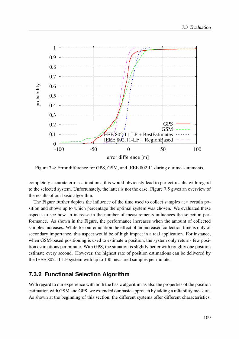
7.3 Evaluation
0
0.1
0.2
0.3
0.4
0.5
0.6
0.7
0.8
0.9
1
-100 -50 0 50 100
pro
bab
ilit
y
error difference [m]
GPSGSM
IEEE 802.11-LF + BestEstimatesIEEE 802.11-LF + RegionBased
Figure 7.4: Error difference for GPS, GSM, and IEEE 802.11 during our measurements.
completely accurate error estimations, this would obviously lead to perfect results with regardto the selected system. Unfortunately, the latter is not the case. Figure 7.5 gives an overview ofthe results of our basic algorithm.
The Figure further depicts the influence of the time used to collect samples at a certain po-sition and shows up to which percentage the optimal system was chosen. We evaluated theseaspects to see how an increase in the number of measurements influences the selection per-formance. As shown in the Figure, the performance increases when the amount of collectedsamples increases. While for our emulation the effect of an increased collection time is only ofsecondary importance, this aspect would be of high impact in a real application. For instance,when GSM-based positioning is used to estimate a position, the system only returns few posi-tion estimations per minute. With GPS, the situation is slightly better with roughly one positionestimate every second. However, the highest rate of position estimations can be delivered bythe IEEE 802.11-LF system with up to 100 measured samples per minute.
7.3.2 Functional Selection Algorithm
With regard to our experience with both the basic algorithm as also the properties of the positionestimation with GSM and GPS, we extended our basic approach by adding a reliability measure.As shown at the beginning of this section, the different systems offer different characteristics.
109
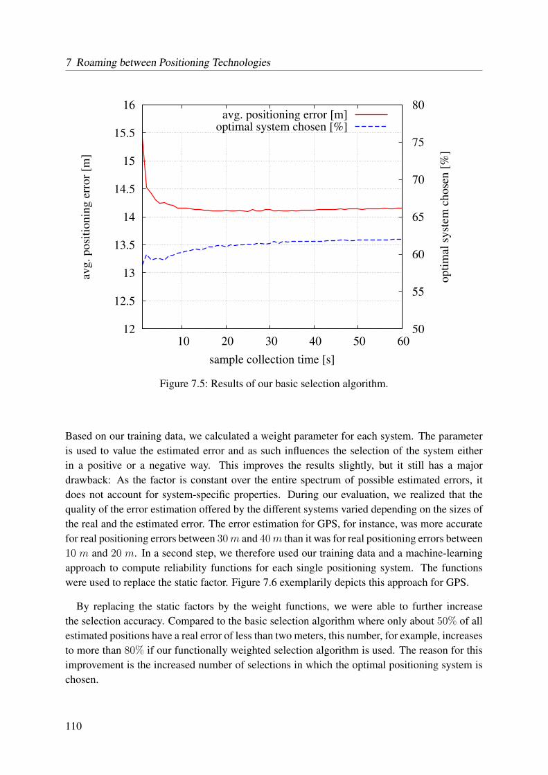
7 Roaming between Positioning Technologies
12
12.5
13
13.5
14
14.5
15
15.5
16
10 20 30 40 50 60 50
55
60
65
70
75
80
avg
. p
osi
tio
nin
g e
rro
r [m
]
op
tim
al s
yst
em c
ho
sen
[%
]
sample collection time [s]
avg. positioning error [m]optimal system chosen [%]
Figure 7.5: Results of our basic selection algorithm.
Based on our training data, we calculated a weight parameter for each system. The parameteris used to value the estimated error and as such influences the selection of the system eitherin a positive or a negative way. This improves the results slightly, but it still has a majordrawback: As the factor is constant over the entire spectrum of possible estimated errors, itdoes not account for system-specific properties. During our evaluation, we realized that thequality of the error estimation offered by the different systems varied depending on the sizes ofthe real and the estimated error. The error estimation for GPS, for instance, was more accuratefor real positioning errors between 30m and 40m than it was for real positioning errors between10 m and 20 m. In a second step, we therefore used our training data and a machine-learningapproach to compute reliability functions for each single positioning system. The functionswere used to replace the static factor. Figure 7.6 exemplarily depicts this approach for GPS.
By replacing the static factors by the weight functions, we were able to further increasethe selection accuracy. Compared to the basic selection algorithm where only about 50% of allestimated positions have a real error of less than two meters, this number, for example, increasesto more than 80% if our functionally weighted selection algorithm is used. The reason for thisimprovement is the increased number of selections in which the optimal positioning system ischosen.
110
7.4 Discussion
0
10
20
30
40
50
60
0 5 10 15 20 25 30 35 40
tru
e ac
cura
cy [
m]
est. accuracy [m]
measurement dataf(x)
Figure 7.6: Functional approximation of the real positioning error based on the estimated errorof GPS.
7.4 Discussion
During our work, we had to overcome numerous problems. The most prominent ones arediscussed in the following.
7.4.1 Systematic Differences
The position estimates returned by GPS and GSM positioning services on the Android platformare, as already mentioned earlier, longitude, latitude, and elevation values in the WGS-84 coor-dinate system. WGS-84 is one of several possible coordinate systems that are used in scienceand by industry to pinpoint locations on the earth’s surface. A specially defined coordinate sys-tem is necessary, as, opposed to common meaning, our earth is not a perfect ball. As depictedin Figure 7.7, the earth’s true shape is instead more or less similar to an ellipsoid.
Whereas WGS-84 is well suited when large areas are considered, Cartesian coordinate sys-tems are a better choice in case of mapping tasks within a limited scope. To map WGS-84longitude and latitude values to a Cartesian plain, several different approaches have been pro-posed in the past (e.g., refer to [HBD89]). However, due to the limited extent of our test bed, wedecided to take an even simpler approach. At first, we, for each position, calculate the distances
111
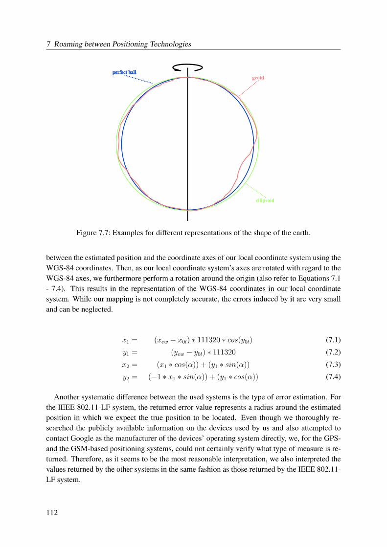
7 Roaming between Positioning Technologies
Figure 7.7: Examples for different representations of the shape of the earth.
between the estimated position and the coordinate axes of our local coordinate system using theWGS-84 coordinates. Then, as our local coordinate system’s axes are rotated with regard to theWGS-84 axes, we furthermore perform a rotation around the origin (also refer to Equations 7.1- 7.4). This results in the representation of the WGS-84 coordinates in our local coordinatesystem. While our mapping is not completely accurate, the errors induced by it are very smalland can be neglected.
x1 = (xew − x0l) ∗ 111320 ∗ cos(y0l) (7.1)
y1 = (yew − y0l) ∗ 111320 (7.2)
x2 = (x1 ∗ cos(α)) + (y1 ∗ sin(α)) (7.3)
y2 = (−1 ∗ x1 ∗ sin(α)) + (y1 ∗ cos(α)) (7.4)
Another systematic difference between the used systems is the type of error estimation. Forthe IEEE 802.11-LF system, the returned error value represents a radius around the estimatedposition in which we expect the true position to be located. Even though we thoroughly re-searched the publicly available information on the devices used by us and also attempted tocontact Google as the manufacturer of the devices’ operating system directly, we, for the GPS-and the GSM-based positioning systems, could not certainly verify what type of measure is re-turned. Therefore, as it seems to be the most reasonable interpretation, we also interpreted thevalues returned by the other systems in the same fashion as those returned by the IEEE 802.11-LF system.
112
7.4 Discussion
7.4.2 Application Requirements
During our work with the positioning systems on the HTC smartphone, we have also learnedvaluable lessons with regard to the application requirements. For GPS, the most important factis the initial delay that one has to wait until the GPS receiver will deliver the first positionestimation – the so-called initial fix. The reason for this delay is that the receiver at first has toidentify the signals of the available GPS satellites from the received signal spectrum. In casethat no further information is available, this can take a long time.
If the receiver already has a local version of the so-called satellite almanac, it can look upwhich satellites should be receivable at the current time and place. This, of course, requiresboth a rather good estimate for the current time and at least a rough estimate of the receiver’sgeographic region. But it also significantly speeds up the process of obtaining an initial fix.On a smartphone that generally also has a wireless data connection, the almanac and the otherinformation could be obtained quite easily, for instance, from an Internet data base. This in turnoffers the major advantage that the application and especially the GPS positioning service donot have to be running in the background at all times. Instead, both can be started on demandand still offer a first fix in an acceptable time. This helps to save precious battery time, CPUcycles, and memory at the cost of a required Internet connection.
7.4.3 Postponed IEEE 802.11-LF
In a real setting, the IEEE 802.11-LF system should – at least with regard to the positioning ser-vice – also reside on the mobile device. For our evaluation, though, we decided to only collectthe necessary information with the mobile device and to use that information afterwards for anevaluation with the help of emulation. This has several advantages. One is the heavily reducedsoftware development effort. Using this approach, we could keep the size of the software run-ning on the mobile device rather small and use existing tools for the evaluation of algorithms onour desktop computers. But the more important advantage is the increased flexibility. Whereasfor the GPS- and GSM-based systems the position estimation on the device acts as a black box,the position estimation with IEEE 802.11-LF is an open book to us. By collecting the raw data,we could easily experiment with different amounts of data used for creating the fingerprints, forestimating the position, or for supplying to the error estimation algorithm. This gave us a betterinsight into these areas compared to the other systems where such insights were not possible.
7.4.4 Satellite Motion
We have identified another both interesting and important aspect during our studies: The influ-ence of the satellite motion when using GPS. The GPS satellites are not geostationary but circlethe earth once every twelve hours. Our measurements for the different scenarios took betweenone and two hours each. Thus, during the run of the single measurements, the constellation ofthe receivable satellites changed.
113
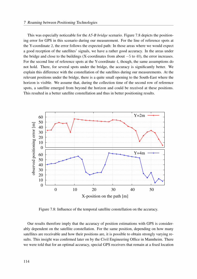
7 Roaming between Positioning Technologies
This was especially noticeable for the A5-B bridge scenario. Figure 7.8 depicts the position-ing error for GPS in this scenario during our measurement. For the line of reference spots atthe Y-coordinate 2, the error follows the expected path: In those areas where we would expecta good reception of the satellites’ signals, we have a rather good accuracy. In the areas underthe bridge and close to the buildings (X-coordinates from about −5 to 40), the error increases.For the second line of reference spots at the Y-coordinate 4, though, the same assumptions donot hold. There, for several spots under the bridge, the accuracy is significantly better. Weexplain this difference with the constellation of the satellites during our measurements. At therelevant positions under the bridge, there is a quite small opening to the South-East where thehorizon is visible. We assume that, during the collection time of the second row of referencespots, a satellite emerged from beyond the horizon and could be received at these positions.This resulted in a better satellite constellation and thus in better positioning results.
0 10 20 30 40 50
ob
serv
ed p
osi
tio
nin
g e
rro
r [m
]
X-position on the path [m]
0
10
20
30
40
50
60 Y=2m
0
10
20
30
40
50
60 Y=4m
Figure 7.8: Influence of the temporal satellite constellation on the accuracy.
Our results therefore imply that the accuracy of position estimations with GPS is consider-ably dependent on the satellite constellation. For the same position, depending on how manysatellites are receivable and how their positions are, it is possible to obtain strongly varying re-sults. This insight was confirmed later on by the Civil Engineering Office in Mannheim. Therewe were told that for an optimal accuracy, special GPS receivers that remain at a fixed location
114
7.5 Conclusions
for at least twelve hours have to be used. These devices consider all position estimations duringthat time-frame to allow for a very precise final estimate.
7.5 Conclusions
In this chapter, we have presented a solution how to select the best suitable positioning systemin case that several systems are available. We have shown that the simple use of the estimatederror values returned by the different systems already yields to usable results. However, whenadditionally using a static weight factor or, even better, a function to further evaluate the re-turned error estimates, the performance of the selection process can be further increased. Forthe latter approach, we achieved a selection accuracy of more than 80% even under the adverseconditions that our scenarios offer. We have further shown that environmental factors have alarge influence on the accuracy of the used positioning systems and, thus, also on our selectionprocess. For instance, when GPS is considered, the constellation of the satellites has a major in-fluence on the achievable positioning accuracy. Even in situations where one would expect GPSto deliver bad results, the system can still perform well due to a fortunate satellite constellation.Finally, we have identified several different aspects that are related to the used application thatcan have an influence on the choice of the used positioning system. Especially restrictions withregard to the user’s privacy can require an adapted selection mechanism. This also points out aprobable path for future work. Especially the use of additional context information as the onewe used for our IEEE 802.11-based tracking system could offer an even better and foresightfulselection of the best positioning systems for every situation.
115

116
CH
AP
TE
R
8 Selected ApplicationScenarios
In this chapter, we give the reader a brief impression of what the introduced techniques can beused for in practice. For each application domain, we first describe the application and thenpoint out how our novel techniques offer valuable contributions to it.
8.1 Educational Media
These days, the recording of lectures is common and a widely accepted procedure among teach-ers at universities and other educational institutions worldwide [OL02]. To allow for an easyrecording of the lecture, only audio, the slides, and, in rare cases, the image of the lecturerare recorded. This type of recordings tends to get rather boring to watch over time, no matterhow interesting the original presentation was. For professional video productions, the solutionto this problem is to hire a camera team that concurrently records different perspectives of thelecture (e.g., the lecturer, the audience, persons asking questions, and a total view). In a post-processing step, the different streams are cut together according to video production rules. Thiscreates a diversified video that is more interesting to watch. For everyday usage at a university,though, this approach is far too expensive.
Therefore, a solution that was developed in our department is an automatic lecture recordingsystem [LLKE09]. The system consists of several remotely adjustable cameras, a screen capturecomponent for the lecturer’s slides, at least one audio capture component, and a central instancethat aggregates the collected data and directs all other components (the director). The centraldirector follows a set of implemented video production rules to automatically cut together thevideo streams from the different sources to create a final recording of the lecture, without theneed for further manual processing. It uses a random function to switch between the differentsources, and supports different sensory inputs that can be used to influence the decisions.
One situation that often occurs in recorded lectures is a question coming from the audience.If a student asks a question during a recorded lecture, it is desirable to take her in the focusof at least one camera. There are several reasons for this: Firstly, if the camera is equipped
117
8 Selected Application Scenarios
with a directional microphone, taking the student into focus helps to record the audio of thequestion properly. Secondly, for the viewer of a recording, this helps to keep the video moreinteresting. Of course, for this to work, the camera has to know the position of the studentasking the question. To achieve this, we extended the director component of our system with anadditional sensory interface to an IEEE 802.11-LF based positioning system. Students takingpart in the lecture were equipped with Asus MyPal Personal Digital Assistants (PDAs) to allowthem to give feedback and to take part in quizzes during the lecture. On these PDAs, weinstalled two additional software components. One is used to allow for a localization of thePDA in the lecture hall. The second component has the purpose to allow students to announcetheir intent to ask a question, similar to raising their hand. Upon such a question event, thelocalization component – the IEEE 802.11-LF client – estimates the position of the PDA andcommunicates this position to the automatic director. The director can then point and zoom oneof the cameras in on the student. Once the lecturer gives the floor to the student, the imagesfrom that camera can be used in the lecture video to show the questioner, and, depending onthe overall camera setup, to even allow for advanced video recording techniques like a shot andcountershot scenario where both face each other.
As such, the use of our positioning techniques allows for the creation of more versatile andinteresting recordings and ultimately helps to increase the learning impact of such recordings.
8.2 Paper Chase
In the area of leisure activities, LBSs have gained increasing importance during the last fewyears. For instance, these days, the continuous collection of information about ones own posi-tion is common when being out for skiing or snowboarding, hiking, on bike trips, or even whensimply being out for a walk. Afterwards, this information can be used to gain further data likethe traveled distance, the mastered height difference, or the achieved top speed. Furthermore,due to the availability of inexpensive devices, new activities have been invented that not onlycollect position information for later reference and replay but where the position plays a centralrole in the activity itself. Geo Caching is a good example for such an activity. In this activ-ity, someone hides an object (e.g., a box containing a message or a goody) and publishes theexact coordinates where to find it on the Internet. Other people can then try to find the hiddenobject and are asked to replace it with something else. Inspired by this, during our research,we developed a virtual Paper Chase game. Similar to the classic children’s game, one playerdeploys hints and the other players have to follow these hints to a final goal. Traditionally, chalkmarkings or colored tapes act as hints; in our version, we completely rely on virtual marks. Oneplayer places the marks at selected positions using a software on her mobile device. The posi-tions are then communicated to a game server via a mobile data connection and can afterwardsbe accessed by the client software running on the other players’ mobile devices. The softwareon the hunters’ devices now constantly checks whether hints are in the proximity of the player.If this is the case, the mark is either displayed on a map or, if the player is aiming the device’s
118
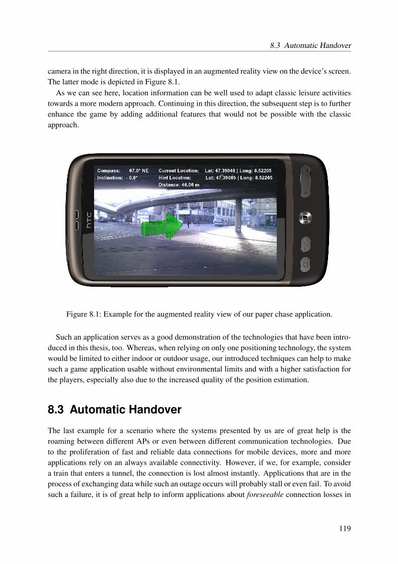
8.3 Automatic Handover
camera in the right direction, it is displayed in an augmented reality view on the device’s screen.The latter mode is depicted in Figure 8.1.
As we can see here, location information can be well used to adapt classic leisure activitiestowards a more modern approach. Continuing in this direction, the subsequent step is to furtherenhance the game by adding additional features that would not be possible with the classicapproach.
Figure 8.1: Example for the augmented reality view of our paper chase application.
Such an application serves as a good demonstration of the technologies that have been intro-duced in this thesis, too. Whereas, when relying on only one positioning technology, the systemwould be limited to either indoor or outdoor usage, our introduced techniques can help to makesuch a game application usable without environmental limits and with a higher satisfaction forthe players, especially also due to the increased quality of the position estimation.
8.3 Automatic Handover
The last example for a scenario where the systems presented by us are of great help is theroaming between different APs or even between different communication technologies. Dueto the proliferation of fast and reliable data connections for mobile devices, more and moreapplications rely on an always available connectivity. However, if we, for example, considera train that enters a tunnel, the connection is lost almost instantly. Applications that are in theprocess of exchanging data while such an outage occurs will probably stall or even fail. To avoidsuch a failure, it is of great help to inform applications about foreseeable connection losses in
119
8 Selected Application Scenarios
advance in order to give them the possibility for a proper preparation. In case of a train and itslimited degrees of freedom regarding the motion direction, such a concept can be implementedquite easily. However, it is by far more complex for a freely roaming user.
Our technologies target to provide help in this case. Especially the tracking system intro-duced in Chapter 6 can help to provide the information that is necessary to notify affectedapplications in advance of a possible connectivity loss. Based on the estimation of the motionmode and direction, applications can be given a grace time to finish network related tasks until,as known from topological information, the network connectivity is lost or a roaming betweendifferent systems takes place. This highly increases the usability of applications and, thus, re-sults in a better user satisfaction. Without the knowledge about the user’s position and motion,such an proactive behavior would not be possible.
120
CH
AP
TE
R
9 Conclusions and Outlook
The following concluding chapter sums up the findings of this thesis, gives an overview oflessons learned, and points out topics that are still open for further consideration.
9.1 Conclusions
As we have seen, the position estimation with IEEE 802.11 and LF is still a field of activeresearch and has the potential to highly influence the direction in which future mobile andlocation-based services will develop. As a viable alternative in situations where GPS is unavail-able, the position estimation with IEEE 802.11-LF would already today be a suitable solutionfor many different LBSs if the effort necessary for the setup and maintenance of the fingerprintdatabase was not too large. For this problem, we have presented two solutions in this thesis,that can effectively help to reduce the effort and thus allow for an easier and faster deploymentof IEEE 802.11-LF-based position estimation.
The first approach presented is Quick Fingerprinting. It relies on the observation that thetraining data that is collected at adjacent reference spots can be used to increase the quality ofthe fingerprints for other neighboring positions. We have presented two different schemes tomerge the training data, the more promising one depending on a weight factor. The merging ofdata from adjacent reference positions results in a noticeable improvement of the positioningaccuracy. However, the even more important aspect is that, even when reducing the amountof training data by up to 80%, our approach still retains almost the same average accuracyas without a reduction. This is a major improvement considering the cumbersome task ofcollecting the training data.
Furthermore, we have presented an alternative that reduces the effort even more effectively.This method is called Region-based Location Estimation. As shown in this thesis, the signalsof single IEEE 802.11 APs tend to have a similar characteristic as long as one stays within astructurally limited area like an office room. As a result, fingerprints created for reference spotslying in such an area also tend to be rather similar. Our algorithm exploits this by automatically
121
9 Conclusions and Outlook
identifying regions of similar signal properties. Then, it creates only one single fingerprintfor each region. This has two major advantages. Firstly, the overall number of fingerprintsis reduced. This helps to reduce the computational and storage requirements of an LF-basedsystem. Secondly, the training data can be collected for a region and no longer needs to becollected on the basis of numerous single spots. Thus, it is no longer necessary to stay at fixedpositions during the collection. Instead, we can move along predefined trajectories through ourarea of operation while collecting the training data. Compared to the approach of using a grid ofreference spots, this is another major improvement that helps to reduce the overall time neededfor data collection to a fraction, at the cost of only minor reductions in the achieved averageaccuracy.
Additionally, we used the regional property of the IEEE 802.11 signals to solve a secondurging problem that IEEE 802.11-LF-based positioning systems generally have. While theyoffer a competitive positioning accuracy, they also suffer from the rare occurrence of very largeerrors. To avoid users getting frustrated when using an IEEE 802.11-LF-based positioningsystem, we therefore have developed and evaluated several different methods to estimate thepositioning error that has to be expected for a given position estimate. Of the four proposedalgorithms, two performed especially well. One of them is Fingerprint Clustering which alsorelies on the regional signal properties and the idea that, if a user collects measurements withinsuch an area, it is quite probable that small scale variations of the signal lead to a selection ofany of the fingerprints that also lie in the appropriate region. We therefore developed a measureto estimate the error that has to be expected based on the size of the region the estimated positionlies in. The second algorithm that also performed very well is called Best Candidates Set. Ituses internal information from the IEEE 802.11-LF system to estimate the error. During theestimation of a position, such a system normally creates a ranking of all fingerprints in thedatabase. Based on the geographical distribution of the n best candidate fingerprints, the BestCandidates Set algorithm calculates an error estimate. While both algorithms perform reallywell in estimating the error, it depends on the quality of the collected input data which algorithmis superior. The Fingerprint Clustering algorithm with its more conservative error estimation isbetter suited for input data with a lower quality. The Best Candidates Set algorithm performsbetter if the collected data has a higher quality.
While the position estimation of users inside buildings can already be improved a lot withthese techniques, it is still not sufficient for all types of applications. Instead, the widespreadavailability of a precise tracking of users within buildings offers an even larger amount of pos-sible new applications, equally in the private, the commercial, and the scientific sector. There-fore, in the second part of this thesis, we have presented an algorithm that uses a Sampling-Importance-Resampling particle filter to track users with the help of IEEE 802.11-LF. Even thesimple use of a particle filter without any additional information already improves the achiev-able positioning accuracy. However, we furthermore extended the system to make use of ad-ditional context information that can be gathered on a mobile device like a smartphone. Wehave implemented an algorithm that can monitor the accelerometer built into mobile devices
122
9.2 Outlook
and is thus able to accurately determine a user’s motion mode. Furthermore, our system makesuse of information about the user’s motion direction. This information can be gathered by, forinstance, reading a digital compass built into many modern devices. Finally, we have extendedthe system to also allow for the use of topological information: Our system uses the informa-tion from a map to allow for a sanity check of subsequent position estimates. Whereas generallythe Euclidean distance is used for this purpose, we instead use the topological distance. Thisoffers a much better representation of possible user motions. While our system is also able toapply map-based motion restrictions on the particle motion, it has turned out that this does notimprove the accuracy significantly.
Of course, moving users are not limited to the coverage area of a single system and also asingle position may be covered by different positioning systems. Thus, we further investigatedpossibilities to allow for a proper selection of the best suited positioning system for a particularsituation - and compared the behavior of the error estimation of three different positioningsystems, namely GPS, GSM-based positioning, and IEEE 802.11-LF-based positioning usingan extensive set of collected data. From the results of this comparison, we derived differentalgorithms that can be used to select the best suitable system based on the estimated errorsfrom all three systems. From our algorithms, the one that performs best uses a set of differentfunctions to weight the reliability of the error estimation of each system before selecting thebest suitable one. This approach increases the rate of selecting the optimal system noticeably.
Finally, we presented several applications that act as showcases of how position estimationtechniques in general and the techniques introduced in this thesis in particular can be used tocreate interesting applications that are fun, helpful, attractive, and informative to the user andoffer a high added value over non-location-based applications from the same realm.
9.2 Outlook
While we have thoroughly investigated the algorithmic side of tracking users and devices withthe help of IEEE 802.11-LF during our work, there are still open questions that should further beconsidered in the future. For example, one major open topic for IEEE 802.11-LF-based positionestimation still is the device dependability of the collected measurements. Even though therehave already been promising efforts in the past to create mappings between different devicesor device classes [Kjæ06], there is still much room left for improvement. In addition, alsothe consideration of environmental and situation specific effects like humidity, the number ofpeople present, or open doors are a field that still offers the possibility to further improve thepositioning with IEEE 802.11-LF.
Similar to our own approach of considering the motion context of a user, another interestingidea is to incorporate even further context to increase the accuracy of LF with IEEE 802.11. Forexample, a mobile device that is equipped with a camera can easily determine the brightnessaround itself. This information can be matched with information from a building managementsystem. Based on the time of day, whether a device measures a high brightness, and if the
123
9 Conclusions and Outlook
light in a given room or area is known to be on or off, it is rather easy to check that the usercannot be located within a certain room. With regard to LF, fingerprints for that room thuswould not have to be considered during the position estimation. Consequently following thisapproach, the amount of context can almost infinitely be increased as long as mobile devices areequipped with the necessary sensors and information about that context can be mapped to thestored fingerprints. As a result, this gives interesting possibilities for further interdisciplinaryresearch.
Of course, this is only a selection of topics that allow for a further engagement in the area ofposition estimation with IEEE 802.11 and LF. Also, other technologies arising these days aredefinitely worth to be considered for their suitability with regard to position estimation. Amongthese, especially LTE should be mentioned that, in combination with so-called pico- or femto-cells, seems to be a promising candidate for an upcoming ubiquitous networking infrastructurethat could also be leveraged for a precise position estimation.
124
Bibliography
[BAB+07] K. Borre, D.M. Akos, N. Bertelsen, P. Rinder, and S.H. Jensen. A software-definedGPS and Galileo receiver: A Single-Frequency Approach. Birkhauser, 2007.
[BD05] Christian Becker and Frank Durr. On location models for ubiquitous computing.Personal and Ubiquitous Computing, 9(1):20–31, January 2005.
[BHM+06] Vladimir Bychkovsky, Bret Hull, Allen Miu, Hari Balakrishnan, and SamuelMadden. A measurement study of vehicular internet access using in situ wi-finetworks. In Proceedings of the 12th international conference on Mobile Com-puting and networking, MobiCom ’06, pages 50–61, Los Angeles, CA, USA,September 2006. ACM Press.
[BMK+00] Barry Brumitt, Brian Meyers, John Krumm, Amanda Kern, and Steven A. Shafer.Easyliving: Technologies for intelligent environments. In Proceedings of the2nd international symposium on Handheld and Ubiquitous Computing, HUC ’00,pages 12–29, Bristol, UK, September 2000. Springer-Verlag.
[Bol08] Philipp Bolliger. Redpin - adaptive, zero-configuration indoor localizationthrough user collaboration. In Proceedings of the 1st ACM international work-shop on Mobile Entity Localization and Tracking in GPS-less environments,MELT ’08, pages 55–60, San Francisco, CA, USA, September 2008. ACM Press.
[BP00] Paramvir Bahl and Venkata N. Padmanabhan. Radar: An in-building rf-baseduser location and tracking system. In Proceedings of the 19th IEEE internationalConference on Computer Communications, InfoCom ’00, pages 775–784, TelAviv, Israel, March 2000. IEEE Computer Society.
[CDMF00] Keith Cheverst, Nigel Davies, Keith Mitchell, and Adrian Friday. Experiencesof developing and deploying a context-aware tourist guide: the guide project.In Proceedings of the 6th international conference on Mobile Computing andnetworking, MobiCom ’00, pages 20–31, Boston, MA, USA, August 2000. ACMPress.
125
Bibliography
[CSG05] F. Cavallo, A.M. Sabatini, and V. Genovese. A step toward gps/ins personal nav-igation systems: real-time assessment of gait by foot inertial sensing. In Pro-ceedings of the international conference on Intelligent Robots and Systems, IROS’05, pages 1187–1191, Edmonton, AB, Canada, August 2005. IEEE ComputerSociety.
[CY05] Xiaoyong Chai and Qiang Yang. Reducing the calibration effort for locationestimation using unlabeled samples. In Proceedings of the 3rd IEEE internationalconference on Pervasive Computing and Communications, PERCOM ’05, pages95–104, Hawaii, USA, March 2005. IEEE Computer Society.
[DLR77] A. P. Dempster, N. M. Laird, and D. B. Rubin. Maximum likelihood from incom-plete data via the em algorithm. Journal of the Royal Statistical Society. Series B(Methodological), 39(1):1–38, 1977.
[DPSB08] Erik Dahlman, Stefan Parkvall, Johan Skold, and Per Beming. 3G Evolution:HSPA and LTE for Mobile Broadband. Academic Press, 2 edition, 2008.
[DVDLT07] David Dearman, Alex Varshavsky, Eyal De Lara, and Khai N. Truong. An ex-ploration of location error estimation. In Proceedings of the 9th internationalconference on Ubiquitous Computing, UbiComp ’07, pages 181–198, Innsbruck,Austria, September 2007. Springer-Verlag.
[Fox05] Eric Foxlin. Pedestrian tracking with shoe-mounted inertial sensors. IEEE Com-puter Graphics and Applications, 25(6):38–46, November 2005.
[Gas05] Matthew S Gast. 802.11 Wireless Networks: The Definitive Guide, Second Edi-tion. O’Reilly Media, Inc., 2005.
[HB01] Jeffrey Hightower and Gaetano Borriello. Location sensing techniques. UWCSE 01-07-01, University of Washington, Department of Computer Science andEngineering, Seattle, WA, USA, July 2001.
[HBD89] John W. Hager, James F. Behensky, and Brad W. Drew. The universal grids: Uni-versal transverse mercator (utm) and universal polar stereographic (ups). Techni-cal report, Defense Technical Information Center, Ft. Belvoir, Fairfax, VA, USA,1989.
[HFL+04] Andreas Haeberlen, Eliot Flannery, Andrew M. Ladd, Algis Rudys, Dan S. Wal-lach, and Lydia E. Kavraki. Practical robust localization over large-scale 802.11wireless networks. In Proceedings of the 10th international conference on MobileComputing and networking, MobiCom ’04, pages 70–84, Philadelphia, PA, USA,September 2004. ACM Press.
126
Bibliography
[HHS+99] Andy Harter, Andy Hopper, Pete Steggles, Andy Ward, and Paul Webster. Theanatomy of a context-aware application. In Proceedings of the 5th annualACM/IEEE international conference on Mobile computing and networking, Mo-biCom ’99, pages 59–68, Seattle, WA, USA, August 1999. ACM Press.
[HT00] Harri Holma and Antti Toskala. WCDMA for UMTS: Radio Access for ThirdGeneration Mobile Communications. John Wiley & Sons, Inc., New York, NY,USA, 1st edition, 2000.
[JBPA06] Yiming Ji, Saad Biaz, Santosh Pandey, and Prathima Agrawal. Ariadne: a dy-namic indoor signal map construction and localization system. In Proceedingsof the 4th international conference on Mobile Systems, applications and services,MobiSys ’06, pages 151–164, Uppsala, Sweden, June 2006. ACM Press.
[Kal60] Rudolph Emil Kalman. A new approach to linear filtering and prediction prob-lems. Transactions of the ASME – Journal of Basic Engineering, 82(SeriesD):35–45, 1960.
[KBH07] Thomas King, Thomas Butter, and Thomas Haenselmann. Loclib,trace,eva,ana:research tools for 802.11-based positioning systems. In Proceedings of the 2ndACM international workshop on Wireless Network Testbeds, Experimental evalu-ation and Characterization, WinTECH ’07, pages 67–74, Montreal, QC, Canada,September 2007. ACM Press.
[KHE07] Thomas King, Thomas Haenselmann, and Wolfgang Effelsberg. Deployment,calibration, and measurement factors for position errors in 802.11-based indoorpositioning systems. In Proceedings of the 3rd international conference onLocation-and Context-Awareness, LoCA ’07, pages 17–34, Oberpfaffenhofen,Germany, September 2007. Springer-Verlag.
[Kjæ06] Mikkel Baun Kjærgaard. Automatic mitigation of sensor variations for signalstrength based location systems. In Proceedings of the 2nd international con-ference on Location- and Context-Awareness, LoCA ’06, pages 30–47, Dublin,Ireland, May 2006. Springer-Verlag.
[Kjæ07] Mikkel Baun Kjærgaard. A taxonomy for radio location fingerprinting. InProceedings of the 3rd international conference on Location-and Context-Awareness, LoCA ’07, pages 139–156, Oberpfaffenhofen, Germany, September2007. Springer-Verlag.
[KK08] Thomas King and Mikkel Baun Kjærgaard. Composcan: Adaptive scanning forefficient concurrent communications and positioning with 802.11. In Proceedingsof the 6th ACM international conference on Mobile Systems, Applications, and
127
Bibliography
Services, MobiSys ’08, pages 67–80, Breckenridge, CO, USA, June 2008. ACMPress.
[KKH+06] Thomas King, Stephan Kopf, Thomas Haenselmann, Christian Lubberger, andWolfgang Effelsberg. Compass: A probabilistic indoor positioning system basedon 802.11 and digital compasses. In Proceedings of the 1st international work-shop on Wireless network testbeds, experimental evaluation & characterization,WiNTECH ’06, pages 34–40, Los Angeles, CA, USA, September 2006. ACMPress.
[KM08] Mikkel Baun Kjærgaard and Carsten Valdemar Munk. Hyperbolic location fin-gerprinting: A calibration-free solution for handling differences in signal strength(concise contribution). In Proceedings of the 6th IEEE international conferenceon Pervasive Computing and Communications, PERCOM ’08, pages 110–116,Hong Kong, March 2008. IEEE Computer Society.
[Ku05] Axel Kupper. Location-based Services: Fundamentals and Operation. JohnWiley & Sons, 2005.
[LCC+05] Anthony LaMarca, Yatin Chawathe, Sunny Consolvo, Jeffrey Hightower, IanSmith, James Scott, Timothy Sohn, James Howard, Jeff Hughes, Fred Potter,Jason Tabert, Pauline Powledge, Gaetano Borriello, and Bill Schilit. Place lab:device positioning using radio beacons in the wild. In Proceedings of the 3rdinternational conference on Pervasive Computing, PERVASIVE ’05, pages 116–133, Munich, Germany, May 2005. Springer-Verlag.
[LKE08] Hendrik Lemelson, Thomas King, and Wolfgang Effelsberg. A study on user ac-ceptance of error visualization techniques. In Proceedings of the 5th internationalconference on Mobile and Ubiquitous Systems: Computing, Networking, and Ser-vices, Mobiquitous ’08, pages 53:1–53:6, Dublin, Ireland, July 2008. ICST.
[LLKE09] Fleming Lampi, Hendrik Lemelson, Stephan Kopf, and Wolfgang Effelsberg. Aquestion managing suite for automatic lecture recording. Interactive Technologyand Smart Education, 6(2):108–118, 2009.
[NLLP04] Lionel M. Ni, Yunhao Liu, Yiu Cho Lau, and Abhishek P. Patil. Landmarc: indoorlocation sensing using active rfid. Wireless Networks, 10(6):701–710, November2004.
[OL02] Thomas Ottmann and Tobias Lauer. Means and methods in automatic course-ware production: Experienceand technical challenges. In Proceedings of WorldConference on E-Learning in Corporate, Government, Healthcare, and HigherEducation, pages 553–560, Montreal, QC, Canada, October 2002. AACE.
128
Bibliography
[PBM+09a] J. Prieto, A. Bahillo, S. Mazuelas, R. M. Lorenzo, J. Blas, and P. Fernandez.Adding indoor location capabilities to an ieee 802.11 wlan using real-time rttmeasurements. In Proceedings of the Wireless Telecommunications Symposium,WTS ’09, pages 113–119, Prague, Czech Republic, April 2009. IEEE ComputerSociety.
[PBM+09b] J. Prieto, A. Bahillo, S. Mazuelas, R.M. Lorenzo, J. Blas, and P. Fernandez. Nlosmitigation based on range estimation error characterization in an rtt-based ieee802.11 indoor location system. In IEEE International Symposium on IntelligentSignal Processing, WISP ’09, pages 61 –66, Budapest, Hungary, August 2009.IEEE Computer Society.
[PEK+06] J. Parkka, M. Ermes, P. Korpipaa, J. Mantyjarvi, J. Peltola, and I. Korhonen. Ac-tivity classification using realistic data from wearable sensors. IEEE Transactionson Information Technology in Biomedicine, 10(1):119 –128, January 2006.
[RAG04] Branko Ristic, Sanjeev Arulampalm, and Neil Gordon. Beyond the Kalman filter:particle filters for tracking applications. Artech House, 2004.
[Rap01] Theodore S. Rappaport. Wireless Communications: Principles and Practice.Prentice Hall PTR, second edition, December 2001.
[RDML05] Nishkam Ravi, Nikhil Dandekar, Preetham Mysore, and Michael L. Littman. Ac-tivity recognition from accelerometer data. In Proceedings of the 17th conferenceon Innovative Applications of Artificial Intelligence, IAAI ’05, pages 1541–1546,Pittsburgh, Pennsylvania, July 2005. AAAI Press.
[SFL05] Ross Stirling, Ken Fyfe, and Gérard Lachapelle. Evaluation of a newmethod of heading estimation for pedestrian dead reckoning using shoe mountedsensors. The Journal of Navigation, 58(01):31–45, 2005.
[SRF+92] S.Y. Seidel, T.S. Rappaport, M.J. Feuerstein, K.L. Blackard, and L. Grindstaff.The impact of surrounding buildings on propagation for wireless in-building per-sonal communications system design. In Proceedings of the 42nd IEEE Vehicu-lar Technology Conference, pages 814–818, Denver, CO , USA, May 1992. IEEEComputer Society.
[SS98] P. Samarati and L. Sweeney. Protecting privacy when disclosing information:k-anonymity and its enforcement through generalization and suppression. In Pro-ceedings of the IEEE Symposium on Research in Security and Privacy, Oakland,CA, USA, May 1998. IEEE Computer Society.
[STB09] Stefania Sesia, Issam Toufik, and Matthew Baker. LTE, The UMTS Long TermEvolution: From Theory to Practice. Wiley Publishing, 2009.
129
Bibliography
[SV04] Jochen H. Schiller and Agnes Voisard. Location-Based Services. Morgan Kauf-mann, 2004.
[Swe02] Latanya Sweeney. K-anonymity: a model for protecting privacy. InternationalJournal of Uncertainty, Fuzziness and Knowledge-Based Systems, 10(5):557–570, October 2002.
[VLHdL07] Alex Varshavsky, Anthony LaMarca, Jeffrey Hightower, and Eyal de Lara. Theskyloc floor localization system. In Proceedings of the 5th IEEE internationalconference on Pervasive Computing and Communications, PERCOM ’07, pages125–134, White Plains, NY, USA, March 2007. IEEE Computer Society.
[Wal07] Michael Wallbaum. A priori error estimates for wireless local area network posi-tioning systems. Pervasive and Mobile Computing, 3(5):560–580, October 2007.
[WF05] Ian H. Witten and Eibe Frank. Data Mining: Practical Machine Learning Toolsand Techniques, Second Edition (Morgan Kaufmann Series in Data ManagementSystems). Morgan Kaufmann Publishers Inc., San Francisco, CA, USA, 2005.
[WGS04] Department of defense world geodetic system 1984 – its definition and relation-ships with local geodetic systems. Nima technical report, 2004.
[WHFaG92] Roy Want, Andy Hopper, Veronica Falcao, and Jonathan Gibbons. The activebadge location system. ACM Transactions on Information Systems, 10(1):91–102, January 1992.
[WKB08] Widyawan, Martin Klepal, and Stephane Beauregard. A novel backtracking par-ticle filter for pattern matching indoor localization. In Proceedings of the 1stACM international workshop on Mobile Entity Localization and Tracking in GPS-less environments, MELT ’08, pages 79–84, San Francisco, CA, USA, September2008. ACM Press.
[YA04] Moustafa Youssef and Ashok Agrawala. On the optimality of wlan location de-termination systems. In Proceedings of the Communication Networks and Dis-tributed Systems Modeling and Simulation Conference, CNDS ’04, Seattle, Wash-ington, January 2004. ACM Press.
[YA05] Moustafa Youssef and Ashok Agrawala. The horus wlan location determinationsystem. In Proceedings of the 3rd international conference on Mobile Systems,applications, and services, MobiSys ’05, pages 205–218, Seattle, Washington,June 2005. ACM Press.
130