Improving and upscaling the diagnostics of genetic ...
136
Fakult ¨ at f ¨ ur Informatik Technische Universit¨ at M ¨ unchen Improving and upscaling the diagnostics of genetic diseases via gene expression and functional assays Vicente A. Y´ epez Mora Vollst¨andiger Abdruck der von der Fakult¨at f¨ ur Informatik der Technischen Universit¨ at M¨ unchen zur Erlangung des akademischen Grades eines Doktor der Naturwissenschaften (Dr. rer. nat.) genehmigten Dissertation. Vorsitzender: Prof. Dr. Burkhard Rost Pr¨ ufende der Dissertation: 1. Prof. Dr. Julien Gagneur 2. Prof. Dr. Juliane Winkelmann Die Dissertation wurde am 01.10.2020 bei der Technischen Universit¨at M¨ unchen eingereicht und durch die Fakult¨ at f¨ ur Informatik am 09.03.2021 angenommen.
Transcript of Improving and upscaling the diagnostics of genetic ...
Fakultat fur InformatikTechnische Universitat Munchen
Improving and upscaling the diagnostics ofgenetic diseases via gene expression and
functional assays
Vicente A. Yepez Mora
Vollstandiger Abdruck der von der Fakultat fur Informatik der TechnischenUniversitat Munchen zur Erlangung des akademischen Grades eines
Doktor der Naturwissenschaften (Dr. rer. nat.)
genehmigten Dissertation.
Vorsitzender:Prof. Dr. Burkhard Rost
Prufende der Dissertation:1. Prof. Dr. Julien Gagneur2. Prof. Dr. Juliane Winkelmann
Die Dissertation wurde am 01.10.2020 bei der Technischen Universitat Muncheneingereicht und durch die Fakultat fur Informatik am 09.03.2021 angenommen.

Acknowledgments
My most sincere gratitude goes to Prof. Julien Gagneur who trusted me since the be-ginning of this journey and guided me through it. Being part of his lab has been anawesome experience, in which I met not just colleagues, but friends. Among them, spe-cial thanks go to Chris for always being available to answer my (many!) questions of alltypes, from how to match a DNA with an RNA sample, to which parts of the GrandCanyon to visit. Also to Daniel for his patience, Juri for explaining the world, Ziga foracademic advice, Jun for knowing everything, Leo for (without knowing) teaching meto never complain, Felix for keeping the bar high, Flo for his computational support,Ines for fruitful outlier discussions, Xueqi for her proactivity, and Nils and Vangelis forcontributing to the amazing atmosphere we have developed in the lab. You make thelab a very special place. Also, to my students, especially Michaela for everything andthe Danielas for helping me keep the much-needed latin spirit. Finally, I’d like to ac-knowledge all the other members of the Gagneurlab and the different people that I’vemet and have influenced my PhD from the Technical University of Munich and GeneCenter.
The collaborators from the HelmholtzZentrum Munchen were crucial for my PhD.Specially, I’d like to thank Dr. Holger Prokisch, who always made time to meet meand gave promptly and precise feedback. From his group, many thanks goes to Laura,my first collaborator, who taught me about cellular respiration and that “everyone canparty, but few can party and work”. Also, to Mirjana, co-author in many finished,on-going, and hopefully future projects, not just for the smooth collaboration, but alsofriendship. Last, but not least, to Robert for his fast and accurate replies, as well asSarah, Agnieszka, and the rest of the Prokisch lab. Also, to all my other collaborators,including the clinicians who gathered the samples.
I cannot thank enough my graduate school, QBM. Without it, I wouldn’t have evenapplied, much less landed in Munich. Filiz and Mara did a great job with it. Also,through it, I got to know wonderful people with whom I shared science and laughterthese years: Andrea, Laia, Rahmi, Linda, Madlin, and Ellie.
Lastly, I’d like to thank all the friends with whom I traveled and partied during theseyears, thus keeping balance in life. To my parents, sister, niece, grandparents, uncles, andwhole family. Talking to you regularly makes me feel like home. This thesis is dedicatedto my niece so that when she reads it, she becomes proud and inspired. Finally, to mygirlfriend Gosia for her love, and the Fijo lek family for their selfless support and care.
iii

Summary
Pinpointing the genetic cause of a rare disorder is crucial for diagnosis and developingtreatments. However, DNA sequencing alone leaves most individuals with a suspectedrare disorder undiagnosed. In this thesis, I will present algorithms that I developed in-tegrating DNA sequencing, RNA sequencing, and robustly assessing cellular respirationto increase the diagnostic rate of genetic disorders.
I developed an end-to-end workflow that implements state-of-the-art statistical meth-ods to detect aberrant expression, splicing, and mono-allelic expression to support RNAsequencing-based diagnostics. The workflow includes preprocessing and quality controlsteps, as well as plots and advice, to further analyze the individual results. It alsoassesses if DNA and RNA samples originated from the same individual do match. Itincludes guidance on the minimum number of samples, sequencing depth, and how sam-ples from different centres can be combined to robustly detect outliers. The workflow isavailable online.
Oxygen consumption rates (OCR) provide quantification of cellular respiration whichis a widely-used metric to evaluate individuals with mitochondrial disorders. I developeda novel statistical method, OCR-Stats, that robustly estimates OCR levels and testsbetween the levels of two samples across multiple within and between-assays replicates. Ishowcased how it served as a functional assay to delineate a new disease-gene associationand diagnose patients.
Altogether, this work has directly helped to diagnose 37 patients and to discover sev-eral new disease-gene associations. Moreover, the software is increasingly being adoptedby various genetic centres across the world.
v

Publications
OCR-Stats: Robust estimation and statistical testing of mito-chondrial respiration activities using Seahorse XF Analyzer
Ref. [1]Vicente A. Yepez, Laura S. Kremer, Arcangela Iuso, Mirjana Gusic, Robert Kopa-jtich, Eliska Konarikova, Agnieszka Nadel, Leonhard Wachutka, Holger Prokisch, andJulien Gagneur(2018) PLoS ONE, DOI:10.1371/journal.pone.0199938
Author contribution Conceptualization: V.A.Y., L.S.K., A.I., M.G., R.K., E.K.,A.N., H.P., J.G.. Data curation: L.S.K., A.I., M.G., R.K., E.K., A.N.. Formal analysis:V.A.Y., H.P., J.G.. Investigation: V.A.Y., J.G.. Software: V.A.Y., L.W.. Supervision:H.P., J.G.. Visualization: V.A.Y., J.G.. Writing - original draft: V.A.Y., H.P., J.G..Writing - review and editing: all authors.
Detection of aberrant events in RNA sequencing data
Ref. [2]Vicente A. Yepez, Christian Mertes, Michaela F. Muller, Daniela S. Andrade, Leon-hard Wachutka, Laure Fresard, Mirjana Gusic, Ines Scheller, Patricia F. Goldberg, Hol-ger Prokisch, Julien Gagneur(2021) Nature Protocols, DOI: 10.1038/s41596-020-00462-5
Author contribution Participated in the design of the workflow: V.A.Y., C.M.,M.F.M., and J.G.. Contributed to the computational workflow: V.A.Y., C.M., M.F.M.,D.S.A., I.S., and P.F.G.. Implemented the candidate prioritization workflow: L.F.. De-signed and implemented wBuild: L.W.. Wrote the manuscript: V.A.Y. and J.G.. Allauthors revised the manuscript.
Bi-Allelic UQCRFS1 Variants Are Associated with Mitochon-drial Complex III Deficiency, Cardiomyopathy, and Alopecia To-talis
vii
Publications
Ref. [3]
Mirjana Gusic, Gudrun Schottmann, Rene G. Feichtinger, Chen Du, Caroline Scholz,Matias Wagner, Johannes A. Mayr, Chae-Young Lee, Vicente A. Yepez, NorbertLorenz, Susanne Morales-Gonzalez, Daan M. Panneman, Agnes Rotig, Richard J.T.Rodenburg, Saskia B. Wortmann, Holger Prokisch, and Markus Schuelke.
(2020) American Journal of Human Genetics, DOI: 10.1016/j.ajhg.2019.12.005.
Author contribution V.A.Y. did the cellular respiration statistical analysis. All au-thors revised the manuscript.
Transcriptome-directed analysis for Mendelian disease diagnosisovercomes limitations of conventional genomic testing
Ref. [4]
David R. Murdock, Hongzheng Dai, Lindsay C. Burrage, Jill A. Rosenfeld, ShamikaKetkar, Michaela F. Muller, Vicente A. Yepez, Julien Gagneur, Pengfei Liu, ShanChen, Mahim Jain, Gladys Zapata, Carlos A. Bacino, Hsiao-Tuan Chao, Paolo Moretti,William J. Craigen, Neil A. Hanchard, Undiagnosed Diseases Network, and BrendanLee.
(2021) Journal of Clinical Investigation, DOI: 10.1172/JCI141500
Author contribution Conceived and designed the experiments: D.R.M. and B.L.. An-alyzed RNA-seq data: D.R.M., H.D., S.C., and M.J.. Provided clinical support: J.A.R..Analyzed exome and genome data: H.D., L.C.B., S.C., M.J.. Performed validation ex-periments: P.L.. Provided patient samples and clinical information: C.A.B., H.C., P.M.,W.C,. N.A.H., and B.L.. Performed RNA-seq: G.Z. and N.A.H.. Performed statisticalanalyses: S.K.. Developed RNA-seq analysis tools: M.M., V.A.Y., and J.G.. Criticallyreviewed the manuscript: L.C.B., H.D., J.A.R., M.M., V.A.Y., J.G., C.A.B., H.C., P.M.,W.C., N.A.H., B.L.. Wrote the manuscript: D.R.M..
OUTRIDER: A Statistical Method for Detecting AberrantlyExpressed Genes in RNA Sequencing Data
Ref. [5]
Felix Brechtmann, Christian Mertes, Agne Matuseviciute, Vicente A. Yepez, ZigaAvsec, Maximilian Herzog, Daniel M. Bader, Holger Prokisch, and Julien Gagneur.
(2018) American Journal of Human Genetics, DOI: 10.1016/j.ajhg.2018.10.025
viii
Author contribution J.G. conceived the project and overviewed the research with thehelp of Z.A., H.P., and V.A.Y.. F.B., A.M., C.M. analyzed the data. F.B., C.M. andA.M. developed the software. D.M.B. M.H contributed to the software developmentand early stage data analysis. J.G. and Z.A. devised the statistical analysis. F.B.,V.A.Y., C.M., and J.G. made the figures. F.B., C.M., A.M., V.A.Y. and J.G. wrote themanuscript. All authors performed critical revision of the manuscript.
Detection of aberrant splicing events in RNA-Seq data withFRASER
Ref. [6]Christian Mertes, Ines Scheller, Vicente A. Yepez, Muhammed H. Celik, YingjiqiongLiang, Laura S. Kremer, Mirjana Gusic, Holger Prokisch, and Julien Gagneur.(2021) Nature Communications, DOI: 10.1038/ncomms15824
Author contribution C.M. and J.G conceived the method. C.M and I.S implementedthe package and performed the full analysis. V.A.Y. contributed to the package devel-opment and to the analysis. M.H.C. performed the MMSplice analysis of GTEx. C.M.and Y.L. performed the rare variant enrichment analysis. L.S.K. and M.G. analyzed theresults of the rare disease cohort. J.G and H.P. supervised the research. C.M., I.S, andJ.G. wrote the manuscript with the help of V.A.Y. All authors revised the manuscript.
ix

Contents
Acknowledgments iii
Summary v
Publications vii
1 Introduction 11.1 Rare and mitochondrial diseases . . . . . . . . . . . . . . . . . . . . . . . 1
1.1.1 Rare diseases . . . . . . . . . . . . . . . . . . . . . . . . . . . . . 11.1.2 Genetic diagnosis of rare disorders . . . . . . . . . . . . . . . . . . 11.1.3 DNA sequencing . . . . . . . . . . . . . . . . . . . . . . . . . . . 31.1.4 RNA sequencing . . . . . . . . . . . . . . . . . . . . . . . . . . . 51.1.5 Aberrant Expression . . . . . . . . . . . . . . . . . . . . . . . . . 71.1.6 Aberrant Splicing . . . . . . . . . . . . . . . . . . . . . . . . . . . 81.1.7 Mono-allelic expression . . . . . . . . . . . . . . . . . . . . . . . . 91.1.8 Mitochondrial disorders . . . . . . . . . . . . . . . . . . . . . . . 101.1.9 Quantifying oxygen consumption rates . . . . . . . . . . . . . . . 12
1.2 Aims and scope of this thesis . . . . . . . . . . . . . . . . . . . . . . . . 13
2 Background 152.1 Biological Background . . . . . . . . . . . . . . . . . . . . . . . . . . . . 15
2.1.1 DNA . . . . . . . . . . . . . . . . . . . . . . . . . . . . . . . . . . 152.1.2 Variant calling and annotation . . . . . . . . . . . . . . . . . . . . 162.1.3 RNA-sequencing . . . . . . . . . . . . . . . . . . . . . . . . . . . 182.1.4 Denoising autoencoders to detect outliers . . . . . . . . . . . . . . 192.1.5 Cellular respiration . . . . . . . . . . . . . . . . . . . . . . . . . . 212.1.6 Mitochondrial stress test . . . . . . . . . . . . . . . . . . . . . . . 21
2.2 Computational Background . . . . . . . . . . . . . . . . . . . . . . . . . 232.2.1 Snakemake . . . . . . . . . . . . . . . . . . . . . . . . . . . . . . 232.2.2 wBuild . . . . . . . . . . . . . . . . . . . . . . . . . . . . . . . . . 24
3 Detection of RNA outliers Pipeline 253.1 Motivation . . . . . . . . . . . . . . . . . . . . . . . . . . . . . . . . . . . 253.2 Workflow . . . . . . . . . . . . . . . . . . . . . . . . . . . . . . . . . . . 26
3.2.1 Input files . . . . . . . . . . . . . . . . . . . . . . . . . . . . . . . 283.2.2 Modules . . . . . . . . . . . . . . . . . . . . . . . . . . . . . . . . 28
3.2.2.1 Aberrant expression . . . . . . . . . . . . . . . . . . . . 293.2.2.2 Aberrant splicing . . . . . . . . . . . . . . . . . . . . . . 30
xi
Contents
3.2.2.3 MAE . . . . . . . . . . . . . . . . . . . . . . . . . . . . 313.2.3 DNA-RNA matching . . . . . . . . . . . . . . . . . . . . . . . . . 31
3.3 Dataset design . . . . . . . . . . . . . . . . . . . . . . . . . . . . . . . . . 333.3.1 Dealing with external count matrices . . . . . . . . . . . . . . . . 35
3.4 Application to a rare disease cohort . . . . . . . . . . . . . . . . . . . . . 36
4 Using RNA-seq to diagnose genetic disorders 434.1 Motivation . . . . . . . . . . . . . . . . . . . . . . . . . . . . . . . . . . . 434.2 Results . . . . . . . . . . . . . . . . . . . . . . . . . . . . . . . . . . . . . 44
4.2.1 Cohort description . . . . . . . . . . . . . . . . . . . . . . . . . . 444.2.2 Aberrant expression analysis . . . . . . . . . . . . . . . . . . . . . 444.2.3 Aberrant splicing analysis . . . . . . . . . . . . . . . . . . . . . . 464.2.4 Mono-allelic expression analysis . . . . . . . . . . . . . . . . . . . 484.2.5 RNA-seq variant calling . . . . . . . . . . . . . . . . . . . . . . . 504.2.6 Overall overview . . . . . . . . . . . . . . . . . . . . . . . . . . . 524.2.7 Analysis of expressed genes . . . . . . . . . . . . . . . . . . . . . 53
4.3 Aberrant expression analysis in COVID-19 patients . . . . . . . . . . . . 54
5 Statistical testing and application of OCR 595.1 OCR-stats . . . . . . . . . . . . . . . . . . . . . . . . . . . . . . . . . . . 59
5.1.1 Motivation . . . . . . . . . . . . . . . . . . . . . . . . . . . . . . . 595.1.2 Estimating OCRs within plates . . . . . . . . . . . . . . . . . . . 605.1.3 Outlier detection . . . . . . . . . . . . . . . . . . . . . . . . . . . 625.1.4 Inter and intraplate variations . . . . . . . . . . . . . . . . . . . . 625.1.5 Statistical testing of OCR . . . . . . . . . . . . . . . . . . . . . . 645.1.6 Benchmark . . . . . . . . . . . . . . . . . . . . . . . . . . . . . . 655.1.7 Power analysis . . . . . . . . . . . . . . . . . . . . . . . . . . . . 675.1.8 Other normalization considerations . . . . . . . . . . . . . . . . . 67
5.2 Application of OCR-stats . . . . . . . . . . . . . . . . . . . . . . . . . . 675.2.1 Background . . . . . . . . . . . . . . . . . . . . . . . . . . . . . . 685.2.2 Patients’ description . . . . . . . . . . . . . . . . . . . . . . . . . 695.2.3 Using functional assays to validate the genetic findings . . . . . . 695.2.4 Using gene expression to validate the genetic findings . . . . . . . 70
6 Conclusion 756.1 Conclusion . . . . . . . . . . . . . . . . . . . . . . . . . . . . . . . . . . . 756.2 Discussion . . . . . . . . . . . . . . . . . . . . . . . . . . . . . . . . . . . 76
A Appendix 83A.1 Appendix: Additional Methods . . . . . . . . . . . . . . . . . . . . . . . 83
A.1.1 Counting reads . . . . . . . . . . . . . . . . . . . . . . . . . . . . 83A.1.2 Obtaining set of positions not in linkage disequilibrium . . . . . . 83A.1.3 Variant calling in RNA-seq . . . . . . . . . . . . . . . . . . . . . . 84A.1.4 Variant annotation and handling . . . . . . . . . . . . . . . . . . 84
xii

Contents
A.1.5 Measure of extracellular fluxes using Seahorse XF96 . . . . . . . . 84A.1.6 Cell number quantification . . . . . . . . . . . . . . . . . . . . . . 84A.1.7 Seahorse method to compute OCR . . . . . . . . . . . . . . . . . 84
A.2 Appendix: Datasets . . . . . . . . . . . . . . . . . . . . . . . . . . . . . . 85A.2.1 Mitochondrial diseases dataset . . . . . . . . . . . . . . . . . . . . 85A.2.2 COVID-19 dataset . . . . . . . . . . . . . . . . . . . . . . . . . . 85
A.3 Appendix: Additional Figures . . . . . . . . . . . . . . . . . . . . . . . . 85
List of Figures 93
List of Tables 103
References 105
xiii

1 Introduction
1.1 Rare and mitochondrial diseases
This thesis describes how to use gene expression and functional assays to help diagnos-ing individuals with rare disorders which were inconclusive after DNA sequencing. Ishowcase this by using a cohort of individuals with a suspected mitochondrial disorder.This chapter describes what are rare disorders, how DNA has been used to diagnoseindividuals suffering from them, the current advances in RNA-seq in the field, whatdefines a mitochondrial disorder, and how to quantify cellular respiration.
1.1.1 Rare diseases
In Europe, a rare disease is defined as a life-threatening, chronically debilitating condi-tion affecting less than 1 in 2,000 people [7]. There exist between 6,000 and 8,000 rarediseases [8]. Between 6 and 8% of the European population is affected by a one of them,of which presumably 80% have a genetic cause [9]. Therefore, though individually rare,collectively they are common. Two-thirds of rare diseases are disabling, three-quartersaffect children, over half are life-limiting, most have no treatment, and almost all havean enormous negative impact on the individual well-being [10].
One of the main goals of rare disease research is to find the genetic cause, whichconsists of pinpointing the variant(s) that are originating the disease in the affectedindividual. It is estimated that the genetic cause of at least one-third of rare diseases hasnot been discovered yet [11]. Discovering the genetic cause can then lead to establishinga treatment. The treatments can be of various types, for example, drugs, vitamins,coenzymes, and even transplants [12]. So far, treatments have been developed for only6% of rare diseases, of which fewer than 1% are curative [13]. As the ultimate goal ofrare disease research is to reach a 100% diagnosis rate and provide treatment for eachdisease, there are still a lot of research opportunities in this field.
1.1.2 Genetic diagnosis of rare disorders
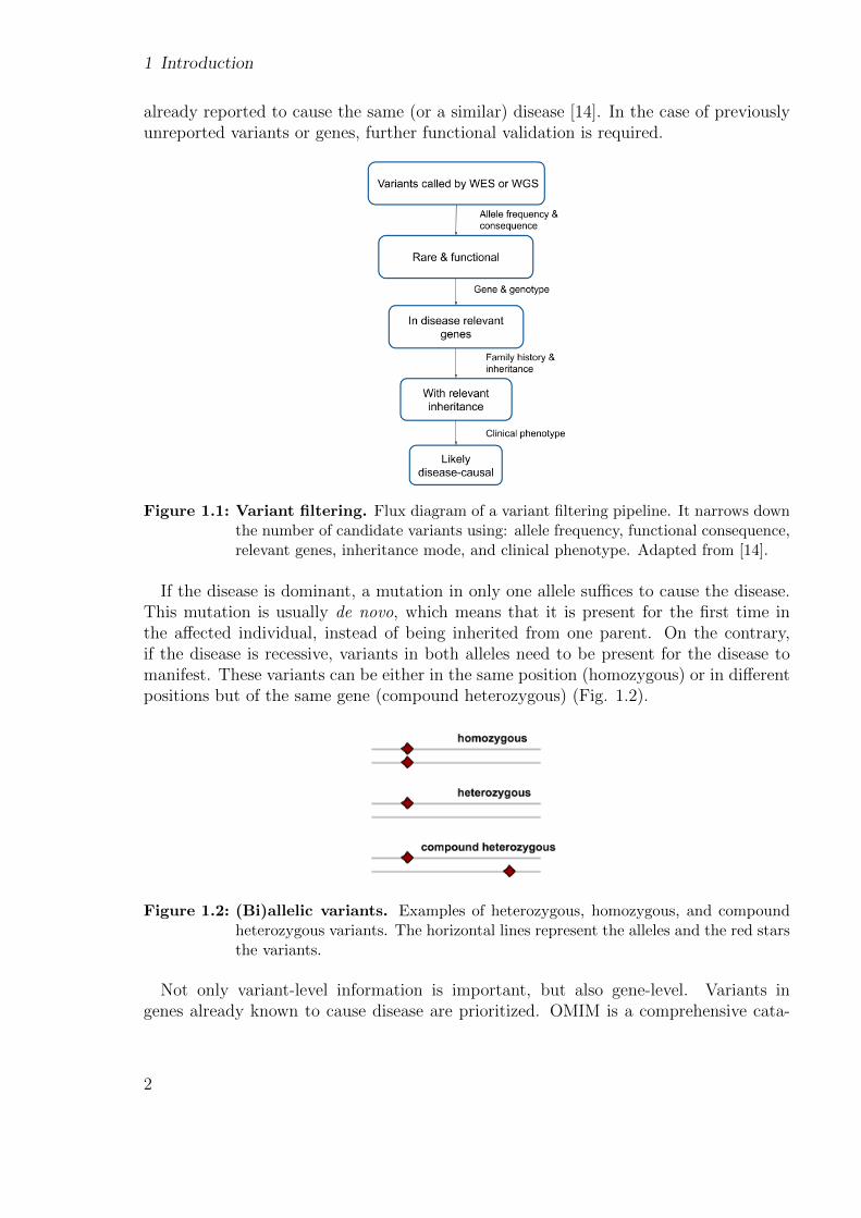
One of the first steps in genetic diagnosis (also known as molecular diagnosis) is tosequence the DNA of the affected individual, in order to detect the variants. Thenthe variants go through a scoring process that takes into account their frequency inthe population, predicted consequence, known pathogenicity, or inheritance mode (Fig.1.1). The ideal scenario is to obtain rare, high-impact, biallelic variants, whose mode ofinheritance and gene matches the affected individual’s phenotypes, and that have been
1
1 Introduction
already reported to cause the same (or a similar) disease [14]. In the case of previouslyunreported variants or genes, further functional validation is required.
Figure 1.1: Variant filtering. Flux diagram of a variant filtering pipeline. It narrows downthe number of candidate variants using: allele frequency, functional consequence,relevant genes, inheritance mode, and clinical phenotype. Adapted from [14].
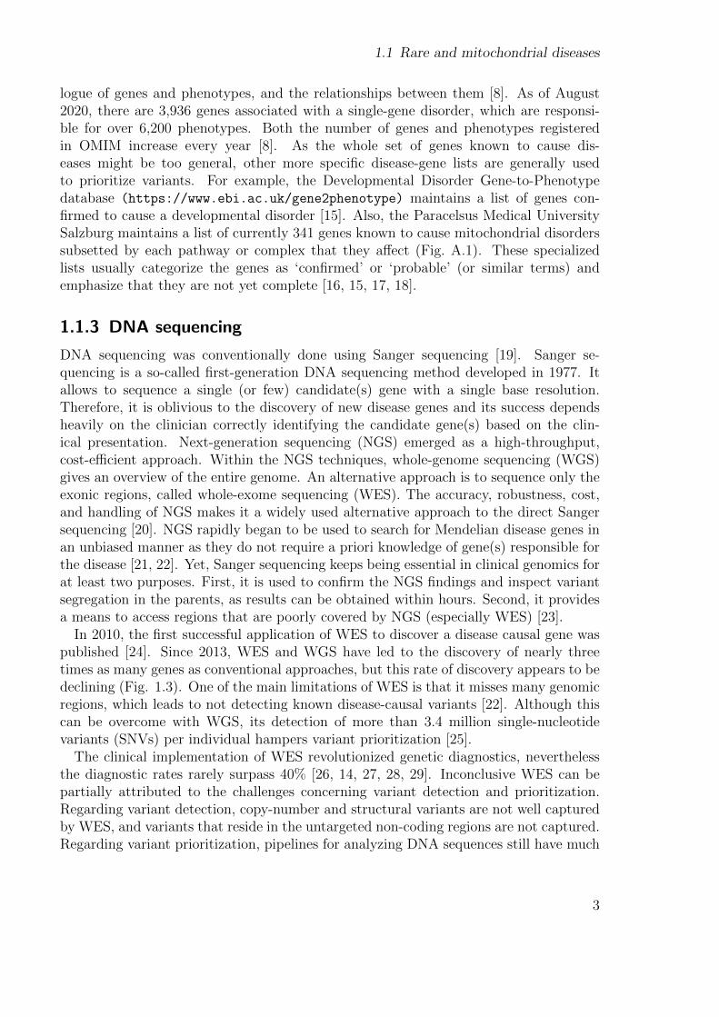
If the disease is dominant, a mutation in only one allele suffices to cause the disease.This mutation is usually de novo, which means that it is present for the first time inthe affected individual, instead of being inherited from one parent. On the contrary,if the disease is recessive, variants in both alleles need to be present for the disease tomanifest. These variants can be either in the same position (homozygous) or in differentpositions but of the same gene (compound heterozygous) (Fig. 1.2).
Figure 1.2: (Bi)allelic variants. Examples of heterozygous, homozygous, and compoundheterozygous variants. The horizontal lines represent the alleles and the red starsthe variants.
Not only variant-level information is important, but also gene-level. Variants ingenes already known to cause disease are prioritized. OMIM is a comprehensive cata-
2
1.1 Rare and mitochondrial diseases
logue of genes and phenotypes, and the relationships between them [8]. As of August2020, there are 3,936 genes associated with a single-gene disorder, which are responsi-ble for over 6,200 phenotypes. Both the number of genes and phenotypes registeredin OMIM increase every year [8]. As the whole set of genes known to cause dis-eases might be too general, other more specific disease-gene lists are generally usedto prioritize variants. For example, the Developmental Disorder Gene-to-Phenotypedatabase (https://www.ebi.ac.uk/gene2phenotype) maintains a list of genes con-firmed to cause a developmental disorder [15]. Also, the Paracelsus Medical UniversitySalzburg maintains a list of currently 341 genes known to cause mitochondrial disorderssubsetted by each pathway or complex that they affect (Fig. A.1). These specializedlists usually categorize the genes as ‘confirmed’ or ‘probable’ (or similar terms) andemphasize that they are not yet complete [16, 15, 17, 18].
1.1.3 DNA sequencing
DNA sequencing was conventionally done using Sanger sequencing [19]. Sanger se-quencing is a so-called first-generation DNA sequencing method developed in 1977. Itallows to sequence a single (or few) candidate(s) gene with a single base resolution.Therefore, it is oblivious to the discovery of new disease genes and its success dependsheavily on the clinician correctly identifying the candidate gene(s) based on the clin-ical presentation. Next-generation sequencing (NGS) emerged as a high-throughput,cost-efficient approach. Within the NGS techniques, whole-genome sequencing (WGS)gives an overview of the entire genome. An alternative approach is to sequence only theexonic regions, called whole-exome sequencing (WES). The accuracy, robustness, cost,and handling of NGS makes it a widely used alternative approach to the direct Sangersequencing [20]. NGS rapidly began to be used to search for Mendelian disease genes inan unbiased manner as they do not require a priori knowledge of gene(s) responsible forthe disease [21, 22]. Yet, Sanger sequencing keeps being essential in clinical genomics forat least two purposes. First, it is used to confirm the NGS findings and inspect variantsegregation in the parents, as results can be obtained within hours. Second, it providesa means to access regions that are poorly covered by NGS (especially WES) [23].
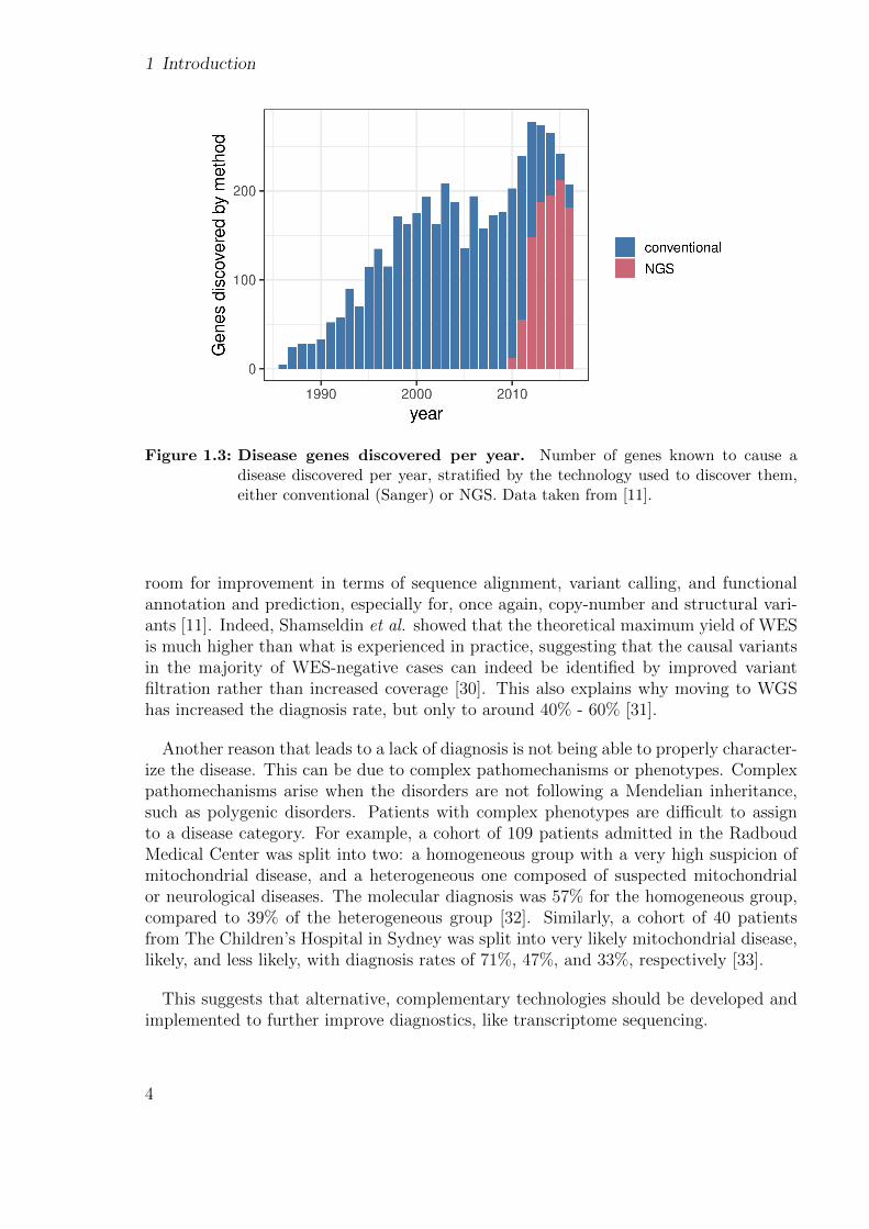
In 2010, the first successful application of WES to discover a disease causal gene waspublished [24]. Since 2013, WES and WGS have led to the discovery of nearly threetimes as many genes as conventional approaches, but this rate of discovery appears to bedeclining (Fig. 1.3). One of the main limitations of WES is that it misses many genomicregions, which leads to not detecting known disease-causal variants [22]. Although thiscan be overcome with WGS, its detection of more than 3.4 million single-nucleotidevariants (SNVs) per individual hampers variant prioritization [25].
The clinical implementation of WES revolutionized genetic diagnostics, neverthelessthe diagnostic rates rarely surpass 40% [26, 14, 27, 28, 29]. Inconclusive WES can bepartially attributed to the challenges concerning variant detection and prioritization.Regarding variant detection, copy-number and structural variants are not well capturedby WES, and variants that reside in the untargeted non-coding regions are not captured.Regarding variant prioritization, pipelines for analyzing DNA sequences still have much
3
1 Introduction
Figure 1.3: Disease genes discovered per year. Number of genes known to cause adisease discovered per year, stratified by the technology used to discover them,either conventional (Sanger) or NGS. Data taken from [11].
room for improvement in terms of sequence alignment, variant calling, and functionalannotation and prediction, especially for, once again, copy-number and structural vari-ants [11]. Indeed, Shamseldin et al. showed that the theoretical maximum yield of WESis much higher than what is experienced in practice, suggesting that the causal variantsin the majority of WES-negative cases can indeed be identified by improved variantfiltration rather than increased coverage [30]. This also explains why moving to WGShas increased the diagnosis rate, but only to around 40% - 60% [31].
Another reason that leads to a lack of diagnosis is not being able to properly character-ize the disease. This can be due to complex pathomechanisms or phenotypes. Complexpathomechanisms arise when the disorders are not following a Mendelian inheritance,such as polygenic disorders. Patients with complex phenotypes are difficult to assignto a disease category. For example, a cohort of 109 patients admitted in the RadboudMedical Center was split into two: a homogeneous group with a very high suspicion ofmitochondrial disease, and a heterogeneous one composed of suspected mitochondrialor neurological diseases. The molecular diagnosis was 57% for the homogeneous group,compared to 39% of the heterogeneous group [32]. Similarly, a cohort of 40 patientsfrom The Children’s Hospital in Sydney was split into very likely mitochondrial disease,likely, and less likely, with diagnosis rates of 71%, 47%, and 33%, respectively [33].
This suggests that alternative, complementary technologies should be developed andimplemented to further improve diagnostics, like transcriptome sequencing.
4
1.1 Rare and mitochondrial diseases
1.1.4 RNA sequencing
NGS also allowed the advent of RNA sequencing (RNA-seq). This technology allowsus to quantify mRNAs and alternative splicing events for gene expression analysis anddiscover novel RNA variants and splice sites [34]. It quickly replaced its predecessortechnology, microarrays [35], which relied upon existing knowledge of genomic sequence,had high background levels due to cross-hybridization, and had limited dynamic rangeof detection and challenging comparison of results across experiments [34].
One reason to study the transcriptome is that up to 30% of disease-causing variantsimpact the RNA and fall within the non-coding regions [36, 37]. Of those, aroundone third affects splicing [38]. Although many in silico tools have been developed topredict the effect of a variant on splicing, functional validation is required for diagnostics.Similarly, even though stop and frameshift variants that are not located in either thefirst or last exon are predicted to truncate the resulting mRNA and protein, this isnot always the case [39, 40]. Finally, half of the synonymous variants of conservedalternatively spliced exons are under selection pressure, suggesting a functional role onthe transcript [41]. Without conclusive validation, the identified variants remain asvariants of unknown significance (VUS). Almost 2,000 VUS are located in direct splicesites [42]. A form of validation can be to detect whether the variant causes aberrantexpression or splicing, which can be done via RNA-seq.
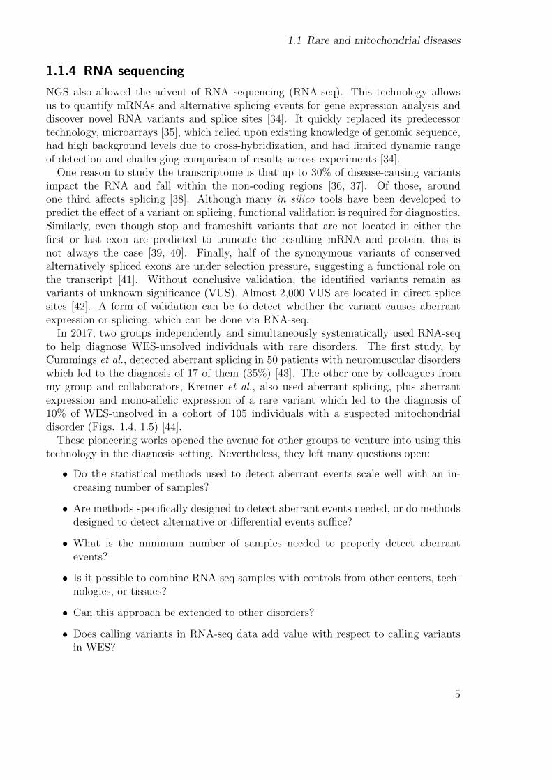
In 2017, two groups independently and simultaneously systematically used RNA-seqto help diagnose WES-unsolved individuals with rare disorders. The first study, byCummings et al., detected aberrant splicing in 50 patients with neuromuscular disorderswhich led to the diagnosis of 17 of them (35%) [43]. The other one by colleagues frommy group and collaborators, Kremer et al., also used aberrant splicing, plus aberrantexpression and mono-allelic expression of a rare variant which led to the diagnosis of10% of WES-unsolved in a cohort of 105 individuals with a suspected mitochondrialdisorder (Figs. 1.4, 1.5) [44].
These pioneering works opened the avenue for other groups to venture into using thistechnology in the diagnosis setting. Nevertheless, they left many questions open:
• Do the statistical methods used to detect aberrant events scale well with an in-creasing number of samples?
• Are methods specifically designed to detect aberrant events needed, or do methodsdesigned to detect alternative or differential events suffice?
• What is the minimum number of samples needed to properly detect aberrantevents?
• Is it possible to combine RNA-seq samples with controls from other centers, tech-nologies, or tissues?
• Can this approach be extended to other disorders?
• Does calling variants in RNA-seq data add value with respect to calling variantsin WES?
5
1 Introduction
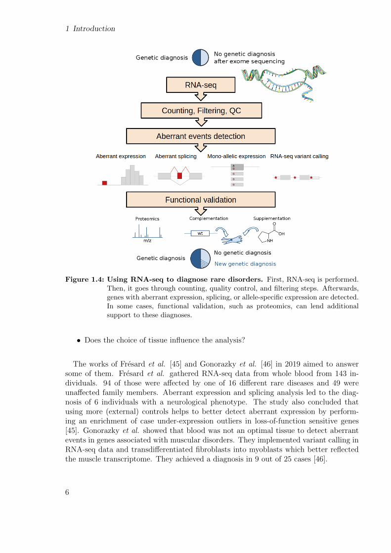
Figure 1.4: Using RNA-seq to diagnose rare disorders. First, RNA-seq is performed.Then, it goes through counting, quality control, and filtering steps. Afterwards,genes with aberrant expression, splicing, or allele-specific expression are detected.In some cases, functional validation, such as proteomics, can lend additionalsupport to these diagnoses.
• Does the choice of tissue influence the analysis?
The works of Fresard et al. [45] and Gonorazky et al. [46] in 2019 aimed to answersome of them. Fresard et al. gathered RNA-seq data from whole blood from 143 in-dividuals. 94 of those were affected by one of 16 different rare diseases and 49 wereunaffected family members. Aberrant expression and splicing analysis led to the diag-nosis of 6 individuals with a neurological phenotype. The study also concluded thatusing more (external) controls helps to better detect aberrant expression by perform-ing an enrichment of case under-expression outliers in loss-of-function sensitive genes[45]. Gonorazky et al. showed that blood was not an optimal tissue to detect aberrantevents in genes associated with muscular disorders. They implemented variant calling inRNA-seq data and transdifferentiated fibroblasts into myoblasts which better reflectedthe muscle transcriptome. They achieved a diagnosis in 9 out of 25 cases [46].
6
1.1 Rare and mitochondrial diseases
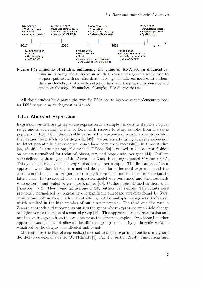
Figure 1.5: Timeline of studies enhancing the value of RNA-seq in diagnostics.Timeline showing the 4 studies in which RNA-seq was systematically used todiagnose patients with rare disorders, including their different novel contributions,the 2 methodological studies to detect outliers, and the protocol to describe andautomate the steps. N: number of samples, DR: diagnostic rate.
All these studies have paved the way for RNA-seq to become a complementary toolfor DNA sequencing in diagnostics [47, 48].
1.1.5 Aberrant Expression
Expression outliers are genes whose expression in a sample lies outside its physiologicalrange and is aberrantly higher or lower with respect to other samples from the samepopulation (Fig. 1.6). One possible cause is the existence of a premature stop codonthat causes the mRNA to be degraded [49]. Systematically using aberrant expressionto detect potentially disease-causal genes have been used successfully in three studies[44, 45, 46]. In the first one, the method DESeq [50] was used in a 1 vs. rest fashionon counts normalized for technical biases, sex, and biopsy site, per gene [44]. Outlierswere defined as those genes with | Z-score | > 3 and Hochberg-adjusted P value < 0.05.This yielded a median of one expression outlier per sample. The limitations of thatapproach were that DESeq is a method designed for differential expression and thecorrection of the counts was performed using known confounders, therefore oblivious tolatent ones. In the second one, a regression model was performed and then residualswere centered and scaled to generate Z-scores [45]. Outliers were defined as those with| Z-score | ≥ 2. They found an average of 343 outliers per sample. The counts werepreviously normalized by regressing out significant surrogate variables found by SVA.This normalization accounts for latent effects, but no multiple testing was performed,which resulted in the high number of outliers per sample. The third one also used aZ-score approach and reported as outliers the genes whose expression was 2-fold changeor higher versus the mean of a control group [46]. This approach lacks normalization andneeds a control group from the same tissue as the affected samples. Even though neitherapproach was optimal, it allowed the different groups to identify pathogenic variantswhich led to the diagnosis of affected individuals.
Motivated by the lack of a specialized method to detect expression outliers, my groupdecided to develop one called OUTRIDER [5] (Fig. 1.5, section 2.1.4). Simulations and
7
1 Introduction
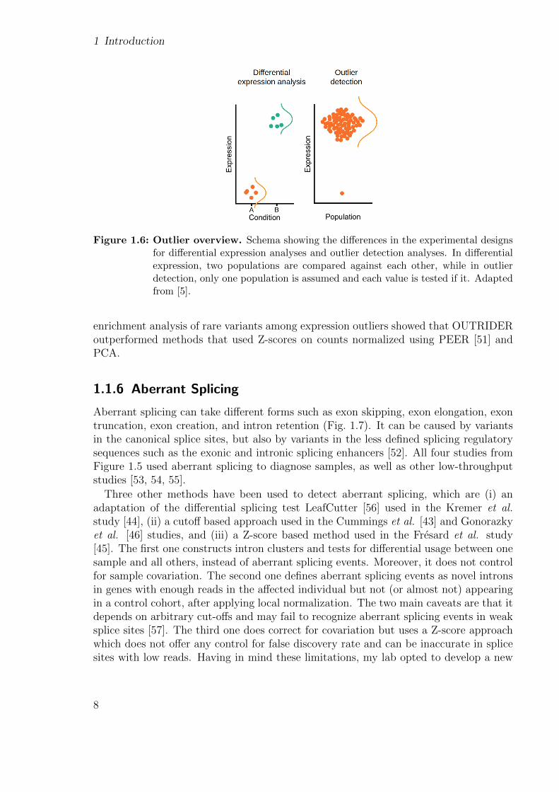
Figure 1.6: Outlier overview. Schema showing the differences in the experimental designsfor differential expression analyses and outlier detection analyses. In differentialexpression, two populations are compared against each other, while in outlierdetection, only one population is assumed and each value is tested if it. Adaptedfrom [5].
enrichment analysis of rare variants among expression outliers showed that OUTRIDERoutperformed methods that used Z-scores on counts normalized using PEER [51] andPCA.
1.1.6 Aberrant Splicing
Aberrant splicing can take different forms such as exon skipping, exon elongation, exontruncation, exon creation, and intron retention (Fig. 1.7). It can be caused by variantsin the canonical splice sites, but also by variants in the less defined splicing regulatorysequences such as the exonic and intronic splicing enhancers [52]. All four studies fromFigure 1.5 used aberrant splicing to diagnose samples, as well as other low-throughputstudies [53, 54, 55].
Three other methods have been used to detect aberrant splicing, which are (i) anadaptation of the differential splicing test LeafCutter [56] used in the Kremer et al.study [44], (ii) a cutoff based approach used in the Cummings et al. [43] and Gonorazkyet al. [46] studies, and (iii) a Z-score based method used in the Fresard et al. study[45]. The first one constructs intron clusters and tests for differential usage between onesample and all others, instead of aberrant splicing events. Moreover, it does not controlfor sample covariation. The second one defines aberrant splicing events as novel intronsin genes with enough reads in the affected individual but not (or almost not) appearingin a control cohort, after applying local normalization. The two main caveats are that itdepends on arbitrary cut-offs and may fail to recognize aberrant splicing events in weaksplice sites [57]. The third one does correct for covariation but uses a Z-score approachwhich does not offer any control for false discovery rate and can be inaccurate in splicesites with low reads. Having in mind these limitations, my lab opted to develop a new
8
1.1 Rare and mitochondrial diseases
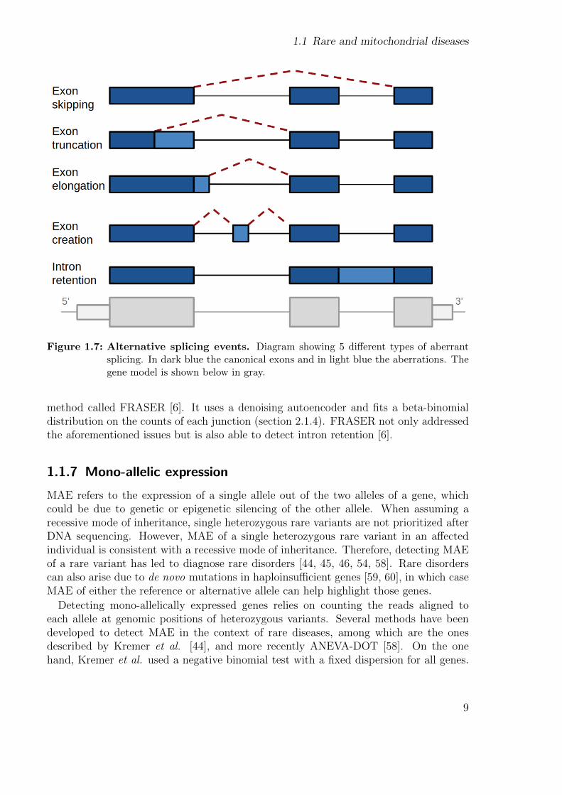
Figure 1.7: Alternative splicing events. Diagram showing 5 different types of aberrantsplicing. In dark blue the canonical exons and in light blue the aberrations. Thegene model is shown below in gray.
method called FRASER [6]. It uses a denoising autoencoder and fits a beta-binomialdistribution on the counts of each junction (section 2.1.4). FRASER not only addressedthe aforementioned issues but is also able to detect intron retention [6].
1.1.7 Mono-allelic expression
MAE refers to the expression of a single allele out of the two alleles of a gene, whichcould be due to genetic or epigenetic silencing of the other allele. When assuming arecessive mode of inheritance, single heterozygous rare variants are not prioritized afterDNA sequencing. However, MAE of a single heterozygous rare variant in an affectedindividual is consistent with a recessive mode of inheritance. Therefore, detecting MAEof a rare variant has led to diagnose rare disorders [44, 45, 46, 54, 58]. Rare disorderscan also arise due to de novo mutations in haploinsufficient genes [59, 60], in which caseMAE of either the reference or alternative allele can help highlight those genes.
Detecting mono-allelically expressed genes relies on counting the reads aligned toeach allele at genomic positions of heterozygous variants. Several methods have beendeveloped to detect MAE in the context of rare diseases, among which are the onesdescribed by Kremer et al. [44], and more recently ANEVA-DOT [58]. On the onehand, Kremer et al. used a negative binomial test with a fixed dispersion for all genes.
9
1 Introduction
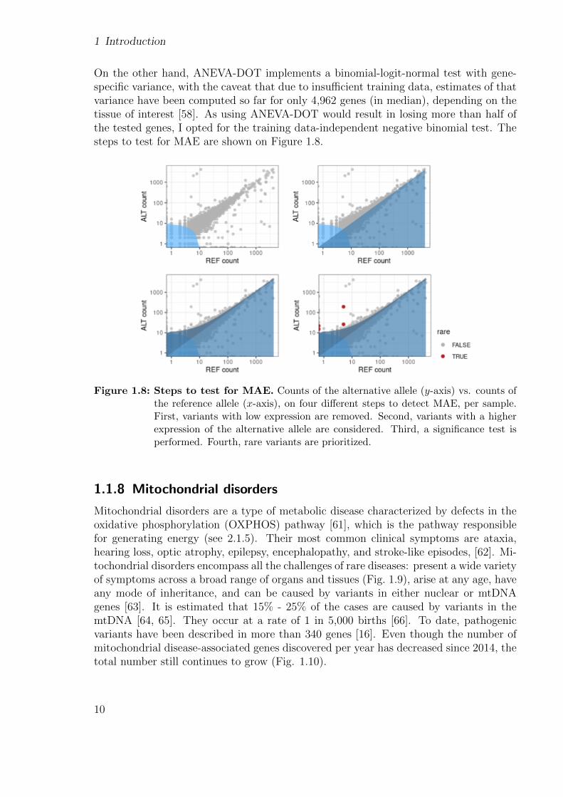
On the other hand, ANEVA-DOT implements a binomial-logit-normal test with gene-specific variance, with the caveat that due to insufficient training data, estimates of thatvariance have been computed so far for only 4,962 genes (in median), depending on thetissue of interest [58]. As using ANEVA-DOT would result in losing more than half ofthe tested genes, I opted for the training data-independent negative binomial test. Thesteps to test for MAE are shown on Figure 1.8.
Figure 1.8: Steps to test for MAE. Counts of the alternative allele (y-axis) vs. counts ofthe reference allele (x-axis), on four different steps to detect MAE, per sample.First, variants with low expression are removed. Second, variants with a higherexpression of the alternative allele are considered. Third, a significance test isperformed. Fourth, rare variants are prioritized.
1.1.8 Mitochondrial disorders
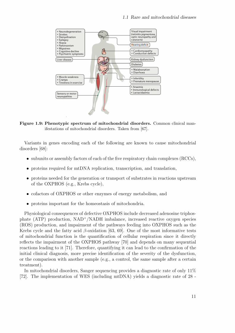
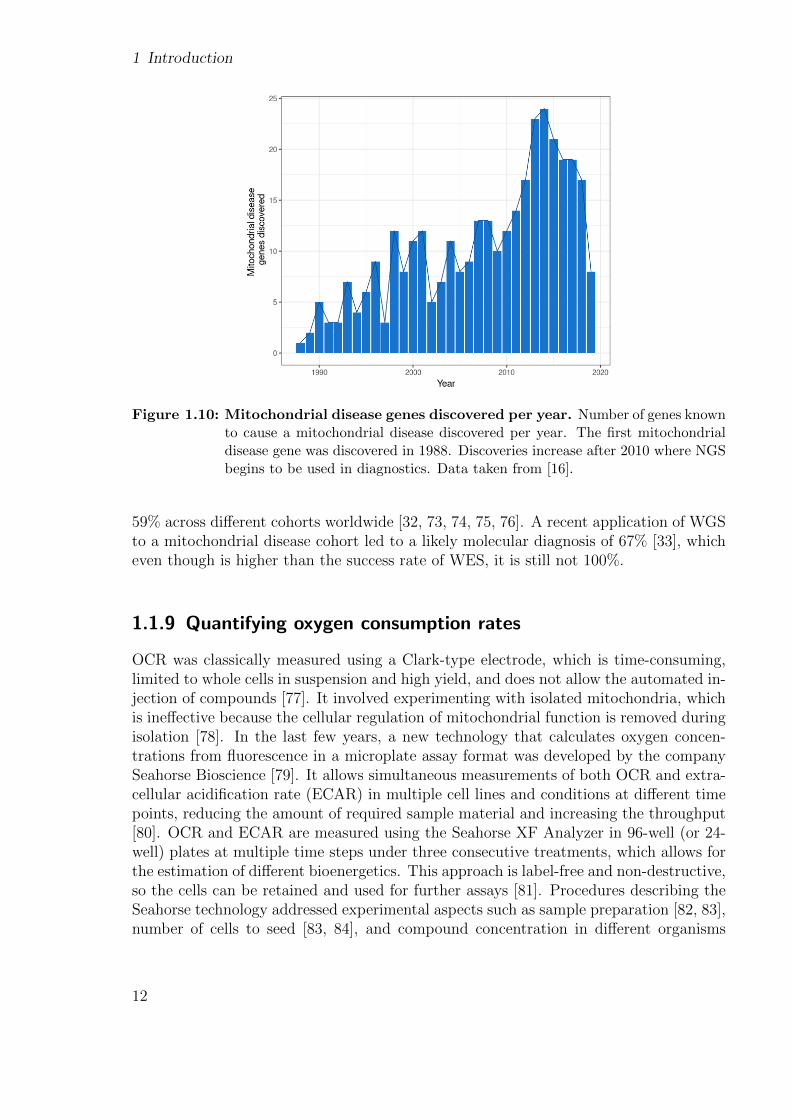
Mitochondrial disorders are a type of metabolic disease characterized by defects in theoxidative phosphorylation (OXPHOS) pathway [61], which is the pathway responsiblefor generating energy (see 2.1.5). Their most common clinical symptoms are ataxia,hearing loss, optic atrophy, epilepsy, encephalopathy, and stroke-like episodes, [62]. Mi-tochondrial disorders encompass all the challenges of rare diseases: present a wide varietyof symptoms across a broad range of organs and tissues (Fig. 1.9), arise at any age, haveany mode of inheritance, and can be caused by variants in either nuclear or mtDNAgenes [63]. It is estimated that 15% - 25% of the cases are caused by variants in themtDNA [64, 65]. They occur at a rate of 1 in 5,000 births [66]. To date, pathogenicvariants have been described in more than 340 genes [16]. Even though the number ofmitochondrial disease-associated genes discovered per year has decreased since 2014, thetotal number still continues to grow (Fig. 1.10).
10
1.1 Rare and mitochondrial diseases
Figure 1.9: Phenotypic spectrum of mitochondrial disorders. Common clinical man-ifestations of mitochondrial disorders. Taken from [67].
Variants in genes encoding each of the following are known to cause mitochondrialdisorders [68]:
• subunits or assembly factors of each of the five respiratory chain complexes (RCCs),
• proteins required for mtDNA replication, transcription, and translation,
• proteins needed for the generation or transport of substrates in reactions upstreamof the OXPHOS (e.g., Krebs cycle),
• cofactors of OXPHOS or other enzymes of energy metabolism, and
• proteins important for the homeostasis of mitochondria.
Physiological consequences of defective OXPHOS include decreased adenosine triphos-phate (ATP) production, NAD+/NADH imbalance, increased reactive oxygen species(ROS) production, and impairment of the pathways feeding into OXPHOS such as theKrebs cycle and the fatty acid β-oxidation [63, 69]. One of the most informative testsof mitochondrial function is the quantification of cellular respiration since it directlyreflects the impairment of the OXPHOS pathway [70] and depends on many sequentialreactions leading to it [71]. Therefore, quantifying it can lead to the confirmation of theinitial clinical diagnosis, more precise identification of the severity of the dysfunction,or the comparison with another sample (e.g., a control, the same sample after a certaintreatment).
In mitochondrial disorders, Sanger sequencing provides a diagnostic rate of only 11%[72]. The implementation of WES (including mtDNA) yields a diagnostic rate of 28 -
11
1 Introduction
Figure 1.10: Mitochondrial disease genes discovered per year. Number of genes knownto cause a mitochondrial disease discovered per year. The first mitochondrialdisease gene was discovered in 1988. Discoveries increase after 2010 where NGSbegins to be used in diagnostics. Data taken from [16].
59% across different cohorts worldwide [32, 73, 74, 75, 76]. A recent application of WGSto a mitochondrial disease cohort led to a likely molecular diagnosis of 67% [33], whicheven though is higher than the success rate of WES, it is still not 100%.
1.1.9 Quantifying oxygen consumption rates
OCR was classically measured using a Clark-type electrode, which is time-consuming,limited to whole cells in suspension and high yield, and does not allow the automated in-jection of compounds [77]. It involved experimenting with isolated mitochondria, whichis ineffective because the cellular regulation of mitochondrial function is removed duringisolation [78]. In the last few years, a new technology that calculates oxygen concen-trations from fluorescence in a microplate assay format was developed by the companySeahorse Bioscience [79]. It allows simultaneous measurements of both OCR and extra-cellular acidification rate (ECAR) in multiple cell lines and conditions at different timepoints, reducing the amount of required sample material and increasing the throughput[80]. OCR and ECAR are measured using the Seahorse XF Analyzer in 96-well (or 24-well) plates at multiple time steps under three consecutive treatments, which allows forthe estimation of different bioenergetics. This approach is label-free and non-destructive,so the cells can be retained and used for further assays [81]. Procedures describing theSeahorse technology addressed experimental aspects such as sample preparation [82, 83],number of cells to seed [83, 84], and compound concentration in different organisms
12
1.2 Aims and scope of this thesis
[71, 82, 85]. However, studies regarding statistical best practices for determining OCRlevels and testing them against others are lacking.
1.2 Aims and scope of this thesis
The contributions of this thesis are improved diagnostics rates using omics profiling andquantitative cellular phenotyping. This is showcased on mitochondrial disorders with i)advanced RNA-seq based diagnostics workflows and ii) quantitative cellular respirationassays.
Development of a computational pipeline to detect aberrant events inRNA-seq data
Pipelines to compute aberrant events from RNA-seq data are lacking. Also, as it isa new field, best practices regarding the preprocessing of raw data are missing. Settingthem up can take many months in which patients are awaiting diagnosis.
I created a modular, scalable pipeline able to robustly generate expression outliers fromraw sequencing files. It integrates state-of-the-art methods to detect aberrant expressionand includes quality control steps. It includes a protocol to guide the user throughoutall the steps. I showcase an example of the application of the pipeline into a cohortof hundreds of patients from the Undiagnosed Diseases Network where it drasticallyreduced the time to process the samples from months to days.
Assess the added value of RNA-seq over WESIn the study of Kremer et al., 5 out of 48 WES-negative patients with mitochondrial
disorders (10%) were solved with the help of RNA-seq. This cohort grew in size andcomplexity by adding other tissues, diseases, switching to strand-specific technology, andreceiving samples from different countries.
Integrating new samples, expertise, specialized methods to detect expression and splic-ing outliers, implementing a more precise method to perform allelic counting, and callingvariants in RNA-seq data we were able to diagnose 28 new samples, yielding a total of33 out of 217 WES-unsolved. This translated into a diagnosis rate of 15%. Finally, Istudy the gene expression of various disease gene lists in different tissues from the GTExcohort to aid researchers in selecting the best tissue.
Development of a statistical method to compute and test OCR on a multi-assay cohort
One of the main advantages of the Seahorse technology is that it allows us to measurethe same cell line in multiple well replicates inside a plate. Nevertheless, the variationbetween plates is larger than the one within. Most studies where it is used reportcomparisons inside plates only.
I developed a statistical method that takes into account both the intra- and inter-plate variation to compute OCR and test between samples and benchmark it againstthe method provided by Seahorse. I show an application of OCR testing to functionallyvalidate the candidate gene in two patients with mitochondrial disorders.
13

2 Background
This chapter describes the basics of DNA and RNA, in order to later explain howvariants are called and prioritized, and how gene expression can be used in the contextof diagnostics. It includes a mathematical section on how outliers are computed fromcount data. It also describes cellular respiration and the mitochondrial stress test used toquantify it. Finally, it presents the computational frameworks Snakemake and wBuild.
2.1 Biological Background
2.1.1 DNA
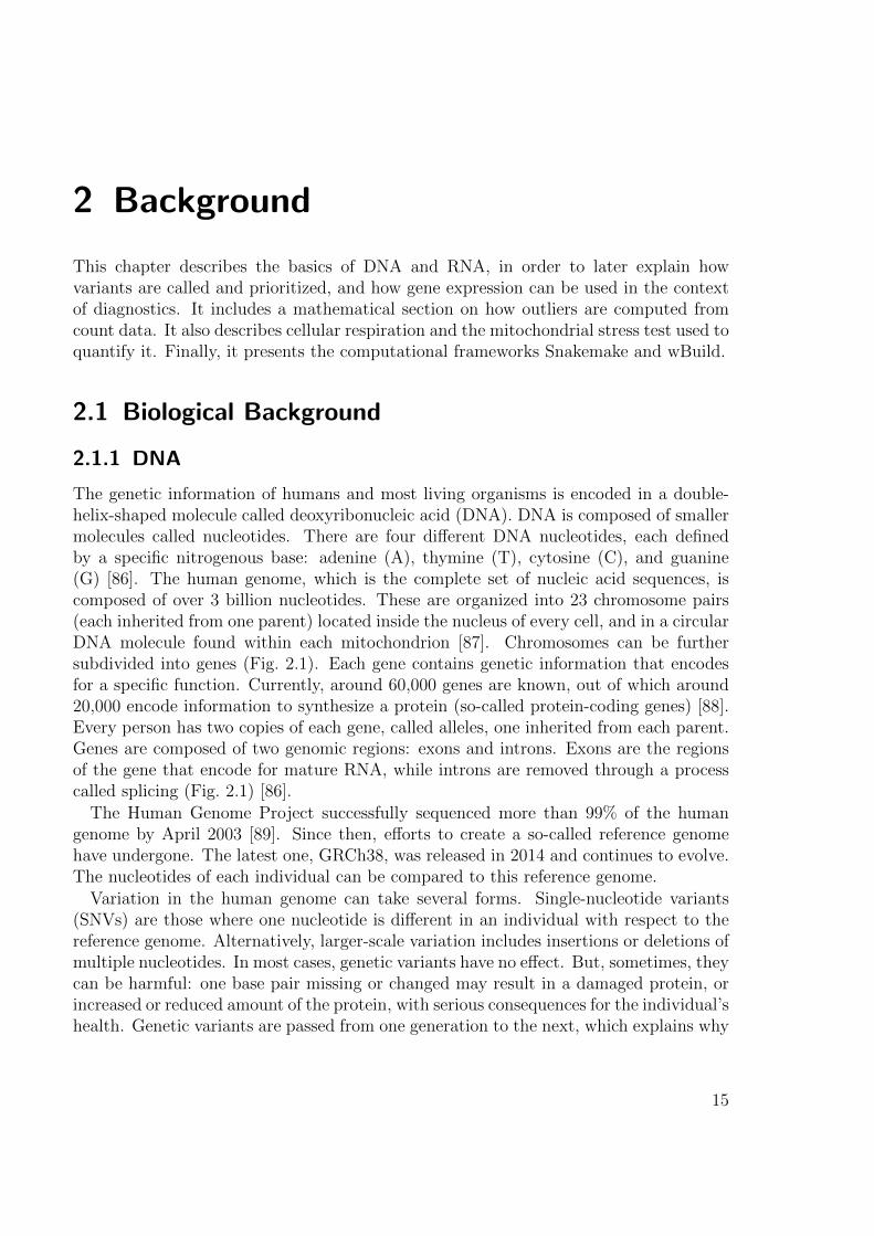
The genetic information of humans and most living organisms is encoded in a double-helix-shaped molecule called deoxyribonucleic acid (DNA). DNA is composed of smallermolecules called nucleotides. There are four different DNA nucleotides, each definedby a specific nitrogenous base: adenine (A), thymine (T), cytosine (C), and guanine(G) [86]. The human genome, which is the complete set of nucleic acid sequences, iscomposed of over 3 billion nucleotides. These are organized into 23 chromosome pairs(each inherited from one parent) located inside the nucleus of every cell, and in a circularDNA molecule found within each mitochondrion [87]. Chromosomes can be furthersubdivided into genes (Fig. 2.1). Each gene contains genetic information that encodesfor a specific function. Currently, around 60,000 genes are known, out of which around20,000 encode information to synthesize a protein (so-called protein-coding genes) [88].Every person has two copies of each gene, called alleles, one inherited from each parent.Genes are composed of two genomic regions: exons and introns. Exons are the regionsof the gene that encode for mature RNA, while introns are removed through a processcalled splicing (Fig. 2.1) [86].
The Human Genome Project successfully sequenced more than 99% of the humangenome by April 2003 [89]. Since then, efforts to create a so-called reference genomehave undergone. The latest one, GRCh38, was released in 2014 and continues to evolve.The nucleotides of each individual can be compared to this reference genome.
Variation in the human genome can take several forms. Single-nucleotide variants(SNVs) are those where one nucleotide is different in an individual with respect to thereference genome. Alternatively, larger-scale variation includes insertions or deletions ofmultiple nucleotides. In most cases, genetic variants have no effect. But, sometimes, theycan be harmful: one base pair missing or changed may result in a damaged protein, orincreased or reduced amount of the protein, with serious consequences for the individual’shealth. Genetic variants are passed from one generation to the next, which explains why
15
2 Background
Figure 2.1: Central dogma of molecular biology. DNA is packed in chromosomes. Eachchromosome is composed of genes. Genes are transcribed into precursor mRNA.Afterwards, only exonic regions (in blue) are kept, and intronic regions (in red) arespliced out forming messenger RNA (mRNA). This mRNA is later translated intoa protein. Adapted from: https://frank.itlab.us/photo_essays/wrapper.
php?nephila_2002_dna.html.
some families are more susceptible to certain diseases. If both alleles have a variantin the same position, the variant is called homozygous. If only one allele harbors thevariant, then it is called heterozygous.
2.1.2 Variant calling and annotation
Variant calling refers to the process of identifying an individual’s variants derived fromeither DNA or RNA sequencing. SAMtools [90] or GATK [91] offer functions for thispurpose. Amplification biases, software errors, and mapping artifacts can lead to manyfalse-positive calls. It is important, therefore, to filter variants according to their qualityscores, number of reads supporting the alternative allele, and whether they belong to aSNP cluster or repeat masked region [92]. They are stored in standardized (variant callformat, VCF) files [93]. They can be annotated (using, e.g., the Variant Effect Predictor(VEP) [94]) according to their:
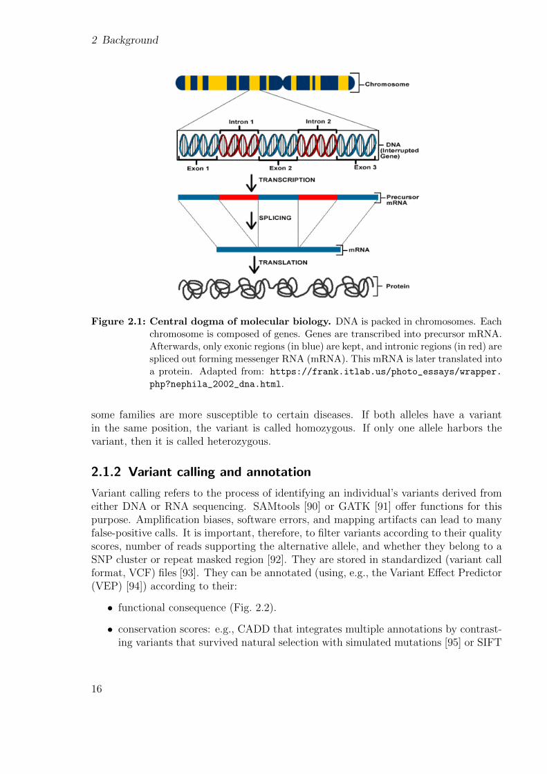
• functional consequence (Fig. 2.2).
• conservation scores: e.g., CADD that integrates multiple annotations by contrast-ing variants that survived natural selection with simulated mutations [95] or SIFT
16
2.1 Biological Background
which uses sequence homology to predict whether a substitution affects proteinfunction [96].
• frequency in the population using scores from, e.g., The Genome AggregationDatabase (gnomAD) [97] or the 1000 Genomes Project [98].
Figure 2.2: Variant consequences. Gene model showing different locations and conse-quences of variants. Adapted from: https://m.ensembl.org/info/genome/
variation/prediction/predicted_data.html. Not all consequences areshown.
Regarding pathogenicity, a variant can be classified as ‘pathogenic’, ‘likely pathogenic’,‘of unknown significance’, ‘likely benign’, or ‘benign’, depending on a certain series ofevidence scores described in the ACMG standards and guidelines for the interpretationof sequence variants [99]. ClinVar, the most widely used public archive of reports of therelationships among human variations and phenotypes [42], uses these terms.
Variants can also be classified according to their consequence, as proposed by Ensemble[100]. The consequences are split into 4 categories depending on their impact: high,moderate, low, or modifier. The following will be mentioned throughout this thesis:
• splice-site: variant changing the 2 base region at either end of the intron
• stop (also called nonsense): variant changing at least one base of a codon, resultingin a premature stop codon
• frameshift: insertion or deletion which is not a multiple of 3, causing a disruptionof the translational reading frame
• missense: variant changing at least one base, resulting in a different amino acidsequence
• splice-region: variant either within 1-3 bases of the exon or 3-8 bases of the intron
• synonymous: variant where there is no change in the encoded amino acid
• UTR: variant either in the 5’ or 3’ untranslated regions (UTRs)
• intronic: variant in the intronic region
17
2 Background
• intergenic: variant upstream or downstream of genes
Protein-truncating variants (PTVs) are variants predicted to shorten the coding se-quence of genes [101]. They include stop, splice-site, frameshift variants, as well as largedeletions. They are expected to have large effects on transcription and, therefore, ongene function [101].
2.1.3 RNA-sequencing
Genes are transcribed (i.e., converted) into single-stranded RNA molecules known asmessenger RNA (mRNA). The full range of mRNAs is called the transcriptome. RNA-seq has emerged as a technique to quantify the transcriptome by deeply sequencing itand recording how frequently each gene is represented in the sequenced sample [102].RNA is isolated from the cell and converted into a library of fragmented complemen-tary DNA (cDNA) using reverse polymerase [34]. These fragments are sequenced usinghigh-throughput techniques (e.g., Illumina sequencing) that are able to generate severalmillion reads in one run [34]. Subsequently, the reads are mapped to a reference genome,allowing the identification of transcribed regions and their expression levels [34].
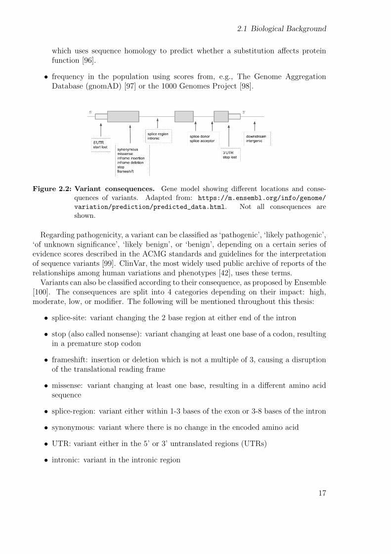
The mapped reads can be assigned to genomic regions. Reads that fully overlapexonic regions (A and B from Fig. 2.3) are aggregated by gene, which results in a genes× samples matrix composed of counts ki,j. These are the input for the statistical methodto detect expression outliers, OUTRIDER.
Figure 2.3: Types of RNA-seq reads. Schematic of a gene model showing how RNA-seqreads can either: be fully aligned to an exon (A), span two exons via splicing (B),or be aligned to an exon-intron boundary (C). Exons are represented as boxesand introns as lines.
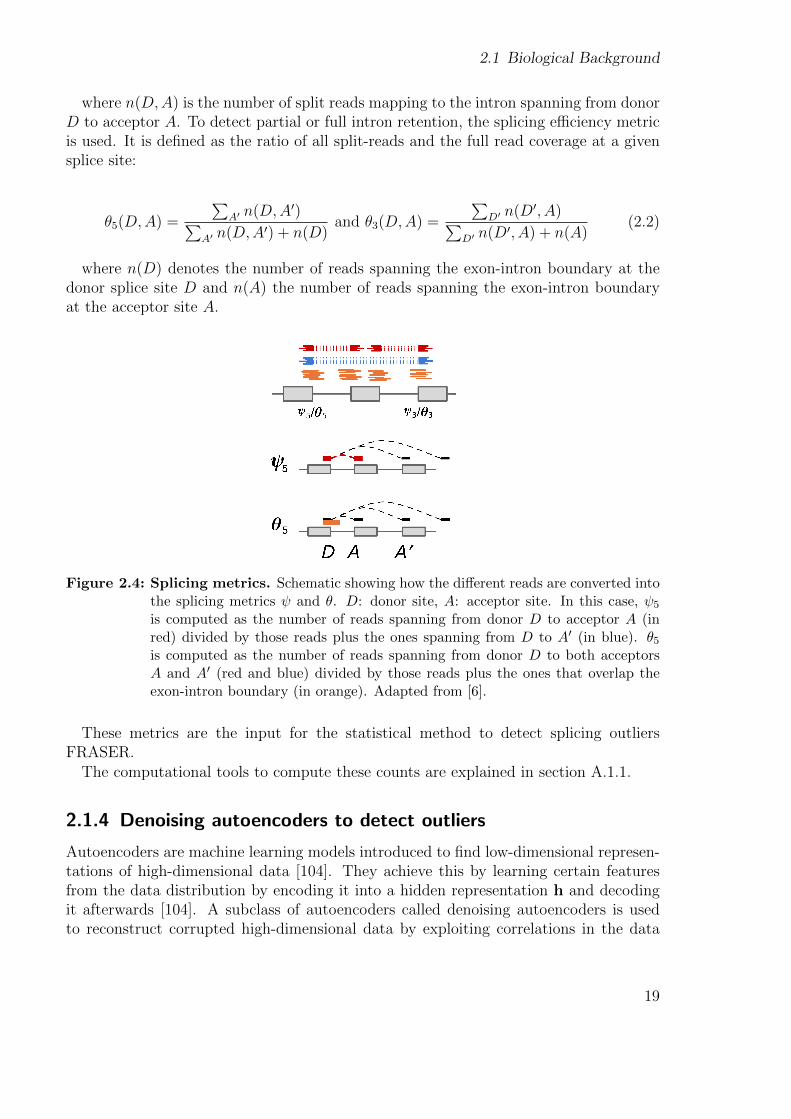
Reads spanning from one exon to another (split reads), and reads overlapping an exon-intron boundary (non-split reads) can also be quantified and aggregated by junction (Fig.2.3). These are then converted into the intron-centric metrics percent-spliced-in (Ψ) andsplicing efficiency (θ) shown in Figure 2.4 [103]. The Ψ index is computed as the ratiobetween reads mapping to the given intron and all split-reads sharing the same donoror acceptor site, respectively:
ψ5(D,A) =n(D,A)∑A′ n(D,A′)
and ψ3(D,A) =n(D,A)∑D′ n(D′, A)
(2.1)
18
2.1 Biological Background
where n(D,A) is the number of split reads mapping to the intron spanning from donorD to acceptor A. To detect partial or full intron retention, the splicing efficiency metricis used. It is defined as the ratio of all split-reads and the full read coverage at a givensplice site:
θ5(D,A) =
∑A′ n(D,A′)∑
A′ n(D,A′) + n(D)and θ3(D,A) =
∑D′ n(D′, A)∑
D′ n(D′, A) + n(A)(2.2)
where n(D) denotes the number of reads spanning the exon-intron boundary at thedonor splice site D and n(A) the number of reads spanning the exon-intron boundaryat the acceptor site A.
Figure 2.4: Splicing metrics. Schematic showing how the different reads are converted intothe splicing metrics ψ and θ. D: donor site, A: acceptor site. In this case, ψ5
is computed as the number of reads spanning from donor D to acceptor A (inred) divided by those reads plus the ones spanning from D to A′ (in blue). θ5is computed as the number of reads spanning from donor D to both acceptorsA and A′ (red and blue) divided by those reads plus the ones that overlap theexon-intron boundary (in orange). Adapted from [6].
These metrics are the input for the statistical method to detect splicing outliersFRASER.
The computational tools to compute these counts are explained in section A.1.1.
2.1.4 Denoising autoencoders to detect outliers
Autoencoders are machine learning models introduced to find low-dimensional represen-tations of high-dimensional data [104]. They achieve this by learning certain featuresfrom the data distribution by encoding it into a hidden representation h and decodingit afterwards [104]. A subclass of autoencoders called denoising autoencoders is usedto reconstruct corrupted high-dimensional data by exploiting correlations in the data
19
2 Background
[105]. This property is used by OUTRIDER and FRASER to control for the commoncovariation observed in gene expression [5, 6].
OUTRIDER detects expression outliers from gene-level counts [5]. The gene countsare assumed to follow a negative binomial (NB) distribution. Specifically, we assumethat the count ki,j of gene j = 1, . . . , p in sample i = 1, . . . , n follows a NB distributionwith a mean µi,j equal to the expected count ci,j and dispersion θj:
P (ki,j = NB(ki,j|µi,j = ci,j, θj).
The expected count ci,j is the product of the sample-specific size factor si and theexponential of the factor yi,j. Size factors are robust estimates of the variations insequencing depth [106]. The yi,j factor captures covariations across samples and ismodeled using the following autoencoder:
yi = hiWd + b,
hi = xiWe
(2.3)
where We is the encoding matrix and Wd is the decoding matrix, hi is the encodedrepresentation of dimension q, and b is a bias term.
The input of the autoencoder are the gene-centered, log-centered, size-factor normal-ized counts, i.e.,
xi,j = xi,j − xj
xi,j = logki,j + 1
si
The encoder and decoder matrices are initialized using principal component analysis,the bias is set to the mean of the log-transformed, size-factor normalized counts, and thedispersions are estimated using the method of moments. The autoencoder is then fittedby iterating the following 3 steps: first the encoder matrix updated, second the decodermatrix is updated, and third the dispersions are refitted per gene. The final encoder anddecoder matrices are then used to compute the expected counts ci,j. Having estimatedthe expected counts and the dispersions, one can then test the null hypothesis that thecount ki,j follows a NB distribution. This can be done using the following formula thatcomputes two-sided P -values:
Pi,j = 2 min{1
2,
kij∑k=0
NB(k|µi,j = ci,j, θj),∞∑
k=kij
NB(k|µi,j = ci,j, θj)} (2.4)
Multiple testing is then performed using Benjamini Yekutieli false discovery rate(FDR) method [107], which holds under positive dependence caused by gene co-expression.Expression outliers are defined as the gene-sample combinations with a FDR ≤ 0.05.
20
2.1 Biological Background
FRASER detects aberrant splicing using the intron-centric metrics ψ5, ψ3, and θ(Fig. 2.4) [6]. For each of them, the distribution of the numerator, conditioned thedenominator, is modeled using the beta-binomial (BB) distribution. Specifically, forψ5, the split read count ki,j of the intron j = 1, . . . , p in sample i = 1, . . . , N follows aBB distribution with a sample-intron-specific proportion expectation µi,j and an intron-specific correlation parameter ρj:
P (ki,j) = BB(ki,j|ni,j, µi,j, ρj),
where ni,j corresponds to the total number of split reads having the same donor site(acceptor site for ψ3) as intron j. The parameters µi,j and ρi,j are fitted following asimilar autoencoder procedure as done for aberrant expression fully described in Merteset al. [6]. P -values are computed using a similar formula as eq. 2.4, but adapted toa BB distribution. Two multiple testing steps are performed, one at the junction levelusing Holm’s method, and another at the gene level using Benjamini-Yekutieli’s method[107]. ∆Ψ values are calculated as the difference between the observed ψi,j and theexpectations µi,j. Splicing outliers are defined as the gene-sample combinations with aFDR ≤ 0.10 and |∆Ψ| ≥ 0.3.
2.1.5 Cellular respiration
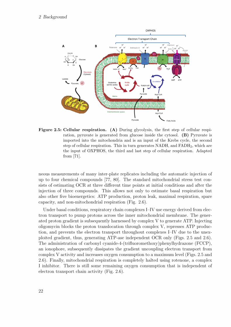
Cellular respiration is a metabolic process that converts the energy derived from sugars,carbohydrates, fats, and proteins into a high-energy molecule called adenosine triphos-phate (ATP) [86]. It is composed of three subprocesses: glycolysis, Krebs cycle, andoxidative phosphorylation (OXPHOS). Figure 2.5 gives an overview of it.
During glycolysis, a glucose molecule is converted into pyruvate [86]. Also, twomolecules of ATP and two molecules of NADH (a compound capable of storing highenergy electrons) are produced. This process occurs in the cytosol. No molecular oxy-gen is used during glycolysis.
Pyruvate is then imported into the mitochondrion where it is decarboxylated to pro-duce acetyl-CoA, which is needed for the second step. Krebs cycle (also known as citricacid or tricarboxylic acid) comprises nine enzymatic conversions that produce NADHand FADH2 (a compound similar to NADH) [86].
NADH and FADH2 transfer electrons to the electron transport chain. The electrontransport chain is composed of four complexes located in the inner mitochondrial mem-brane through which electrons flow horizontally, while pumping protons into the inter-membrane space (Fig. 2.5). These protons are then pumped into the mitochondrialmatrix via complex V (or ATP synthase) generating 32 molecules of ATP. After theprotons flow to the matrix, they are combined with oxygen. This last process is referredto as oxidative phosphorylation [86].
2.1.6 Mitochondrial stress test
Upon its introduction, the Seahorse XF Analyzer swiftly replaced its predecessor meth-ods to quantify oxygen consumption rates (OCR) because it allowed real-time simulta-
21
2 Background
Figure 2.5: Cellular respiration. (A) During glycolysis, the first step of cellular respi-ration, pyruvate is generated from glucose inside the cytosol. (B) Pyruvate isimported into the mitochondria and is an input of the Krebs cycle, the secondstep of cellular respiration. This in turn generates NADH, and FADH2, which arethe input of OXPHOS, the third and last step of cellular respiration. Adaptedfrom [71].
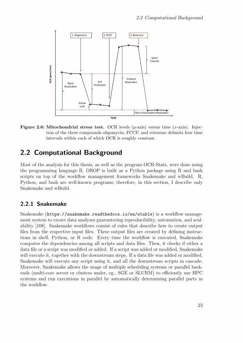
neous measurements of many inter-plate replicates including the automatic injection ofup to four chemical compounds [77, 80]. The standard mitochondrial stress test con-sists of estimating OCR at three different time points at initial conditions and after theinjection of three compounds. This allows not only to estimate basal respiration butalso other five bioenergetics: ATP production, proton leak, maximal respiration, sparecapacity, and non-mitochondrial respiration (Fig. 2.6).
Under basal conditions, respiratory chain complexes I–IV use energy derived from elec-tron transport to pump protons across the inner mitochondrial membrane. The gener-ated proton gradient is subsequently harnessed by complex V to generate ATP. Injectingoligomycin blocks the proton translocation through complex V, represses ATP produc-tion, and prevents the electron transport throughout complexes I–IV due to the unex-ploited gradient, thus, generating ATP-ase independent OCR only (Figs. 2.5 and 2.6).The administration of carbonyl cyanide-4-(trifluoromethoxy)phenylhydrazone (FCCP),an ionophore, subsequently dissipates the gradient uncoupling electron transport fromcomplex V activity and increases oxygen consumption to a maximum level (Figs. 2.5 and2.6). Finally, mitochondrial respiration is completely halted using rotenone, a complexI inhibitor. There is still some remaining oxygen consumption that is independent ofelectron transport chain activity (Fig. 2.6).
22
2.2 Computational Background
Figure 2.6: Mitochondrial stress test. OCR levels (y-axis) versus time (x-axis). Injec-tion of the three compounds oligomycin, FCCP, and rotenone delimits four timeintervals within each of which OCR is roughly constant.
2.2 Computational Background
Most of the analysis for this thesis, as well as the program OCR-Stats, were done usingthe programming language R. DROP is built as a Python package using R and bashscripts on top of the workflow management frameworks Snakemake and wBuild. R,Python, and bash are well-known programs; therefore, in this section, I describe onlySnakemake and wBuild.
2.2.1 Snakemake
Snakemake (https://snakemake.readthedocs.io/en/stable) is a workflow manage-ment system to create data analyses guaranteeing reproducibility, automation, and scal-ability [108]. Snakemake workflows consist of rules that describe how to create outputfiles from the respective input files. These output files are created by defining instruc-tions in shell, Python, or R code. Every time the workflow is executed, Snakemakecomputes the dependencies among all scripts and data files. Then, it checks if either adata file or a script was modified or added. If a script was added or modified, Snakemakewill execute it, together with the downstream steps. If a data file was added or modified,Snakemake will execute any script using it, and all the downstream scripts in cascade.Moreover, Snakemake allows the usage of multiple scheduling systems or parallel back-ends (multi-core server or clusters under, eg., SGE or SLURM) to efficiently use HPCsystems and run executions in parallel by automatically determining parallel parts inthe workflow.
23
2 Background
2.2.2 wBuild
wBuild (https://wbuild.readthedocs.io) is a framework that automatically createsSnakemake dependencies, workflow rules based on R markdown scripts and compilesthe analysis results into a navigable HTML page. All information needed such as input,output, number of threads, and even Python code is specified in a YAML header insidethe R script file, thereby keeping code and dependencies together.
24
3 Detection of RNA outliers Pipeline
The methodology, results, and figures presented in this chapter are part of the manuscript“Detection of RNA Outliers pipeline” from Yepez et al. 2020 [2]. The author’s contribu-tions are included in it. In short, I conceived the idea with the help of Christian Mertesand Julien Gagneur. Christian Mertes, Michaela Muller, Ines Scheller, and DanielaAndrade helped with the computational pipeline.
We already saw how RNA-seq is becoming increasingly used for diagnostics of geneticdiseases by detecting aberrant events. This chapter describes a protocol that I developedto automate the preprocessing and counting of raw sequencing files and subsequentapplication of the statistical methods to detect aberrant RNA events on them. I alsodescribe a procedure to assess the correct assignment of BAM files derived from RNA-seq and VCF files derived from DNA sequencing from the same individual. Moreover,I discuss whether it is possible to combine samples from different origins (e.g., cohorts,tissues, or sequencing depths), which is a big concern for diagnostic centers venturinginto RNA-seq for diagnostics but with a low initial number of samples. I conclude withan example of an external user who was already using RNA-seq for diagnostics, but afteradopting this pipeline was able to reduce the time for diagnostics from months to days.
3.1 Motivation
Unlike DNA sequencing with well-established pipelines to map, align, or call variantslike GATK [91] or Ensembl [100], the field of RNA-seq in diagnostics of rare disordersis new and lacks established workflows. Therefore, each group must develop their owntools to preprocess and analyze data in this context.
The pilot study from my group consisted of 105 fibroblast samples derived from mito-chondrial disease patients and controls [44]. Since then, the cohort (from now on referredto as Prokisch and fully described in section A.2.1) has increased by:
• sequencing more samples from different countries in batches of unequal sizes
• including other tissues, mostly blood
• growing samples in galactose (besides the original glucose)
• experimenting with transduced genes
• switching to a strand-specific protocol
25
3 Detection of RNA outliers Pipeline
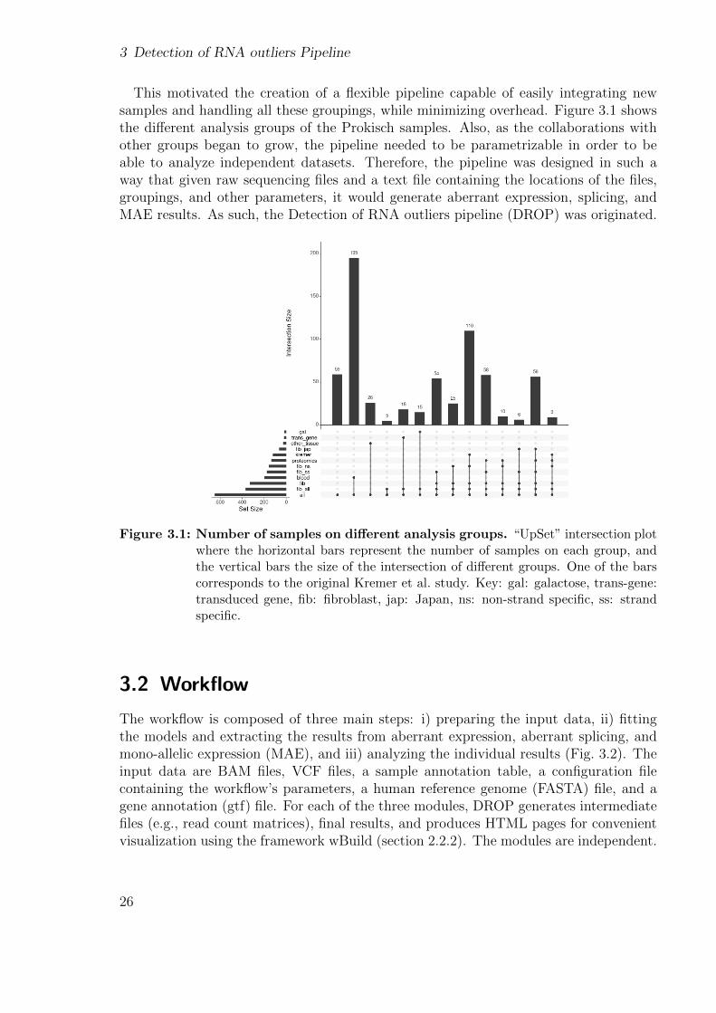
This motivated the creation of a flexible pipeline capable of easily integrating newsamples and handling all these groupings, while minimizing overhead. Figure 3.1 showsthe different analysis groups of the Prokisch samples. Also, as the collaborations withother groups began to grow, the pipeline needed to be parametrizable in order to beable to analyze independent datasets. Therefore, the pipeline was designed in such away that given raw sequencing files and a text file containing the locations of the files,groupings, and other parameters, it would generate aberrant expression, splicing, andMAE results. As such, the Detection of RNA outliers pipeline (DROP) was originated.
Figure 3.1: Number of samples on different analysis groups. “UpSet” intersection plotwhere the horizontal bars represent the number of samples on each group, andthe vertical bars the size of the intersection of different groups. One of the barscorresponds to the original Kremer et al. study. Key: gal: galactose, trans-gene:transduced gene, fib: fibroblast, jap: Japan, ns: non-strand specific, ss: strandspecific.
3.2 Workflow
The workflow is composed of three main steps: i) preparing the input data, ii) fittingthe models and extracting the results from aberrant expression, aberrant splicing, andmono-allelic expression (MAE), and iii) analyzing the individual results (Fig. 3.2). Theinput data are BAM files, VCF files, a sample annotation table, a configuration filecontaining the workflow’s parameters, a human reference genome (FASTA) file, and agene annotation (gtf) file. For each of the three modules, DROP generates intermediatefiles (e.g., read count matrices), final results, and produces HTML pages for convenientvisualization using the framework wBuild (section 2.2.2). The modules are independent.
26
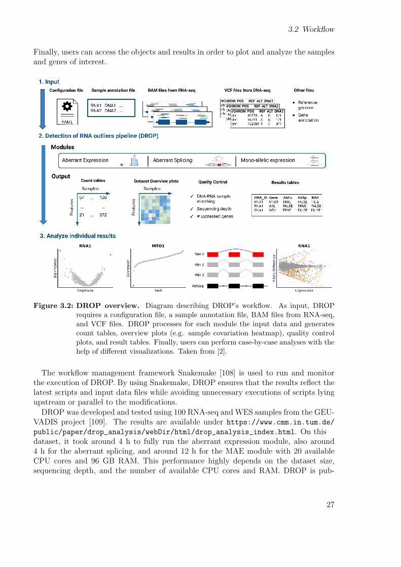
3.2 Workflow
Finally, users can access the objects and results in order to plot and analyze the samplesand genes of interest.
Figure 3.2: DROP overview. Diagram describing DROP’s workflow. As input, DROPrequires a configuration file, a sample annotation file, BAM files from RNA-seq,and VCF files. DROP processes for each module the input data and generatescount tables, overview plots (e.g. sample covariation heatmap), quality controlplots, and result tables. Finally, users can perform case-by-case analyses with thehelp of different visualizations. Taken from [2].
The workflow management framework Snakemake [108] is used to run and monitorthe execution of DROP. By using Snakemake, DROP ensures that the results reflect thelatest scripts and input data files while avoiding unnecessary executions of scripts lyingupstream or parallel to the modifications.
DROP was developed and tested using 100 RNA-seq and WES samples from the GEU-VADIS project [109]. The results are available under https://www.cmm.in.tum.de/
public/paper/drop_analysis/webDir/html/drop_analysis_index.html. On thisdataset, it took around 4 h to fully run the aberrant expression module, also around4 h for the aberrant splicing, and around 12 h for the MAE module with 20 availableCPU cores and 96 GB RAM. This performance highly depends on the dataset size,sequencing depth, and the number of available CPU cores and RAM. DROP is pub-
27
3 Detection of RNA outliers Pipeline
licly available as a Python package under https://github.com/gagneurlab/drop, andits documentation is under https://gagneurlab-drop.readthedocs.io/en/latest/
installation.html. A screenshot of DROP’s index HTML page is found on FigureA.2.
3.2.1 Input files
The following are the input files needed by DROP:
• BAM files from RNA-seq: The BAM files contain reads that will be used inall of the modules to generate the read count matrices [90]. They are created byaligning FASTA files derived from RNA-seq to a reference genome. They mustbe aligned using STAR [110] with the default parameters and twopassMode =
‘Basic’ to detect novel splice junctions. The BAM files must be sorted by positionand indexed.
• VCF files from either WES or WGS: VCF files are standardized text filescontaining a sample’s variants [93]. They are generated through calling variantson a BAM file. The VCF files must be compressed and indexed. The genome buildused to align the files derived from DNA sequencing and RNA sequencing must bethe same.
• Config file: file containing different parameters in YAML format [111]. A detaileddescription can be found in the DROP documentation.
• Sample annotation: table containing the samples’ information. Each row cor-responds to a unique pair of RNA and DNA samples derived from the same in-dividual. An RNA assay can belong to one or more DNA assays, and vice versa.If so, they must be specified in different rows. Further instructions and examplescan be found in the DROP documentation.
• Reference genome: human reference genome (FASTA) file. It must match thegenome build of the BAM and VCF files. An index (.fai) file must be created inthe same directory where the FASTA file is located.
• Gene annotation: gene annotation (.gtf) file. The latest release from GENCODE[88], with the right genome build (https://www.gencodegenes.org/human/) isrecommended.
3.2.2 Modules
DROP is composed of three independent modules. In each of them, BAM files areconverted into counts (either whole gene, split, non-split, and allelic). Then, thesecounts are merged according to analysis groups, in which the statistical methods areapplied.
28
3.2 Workflow
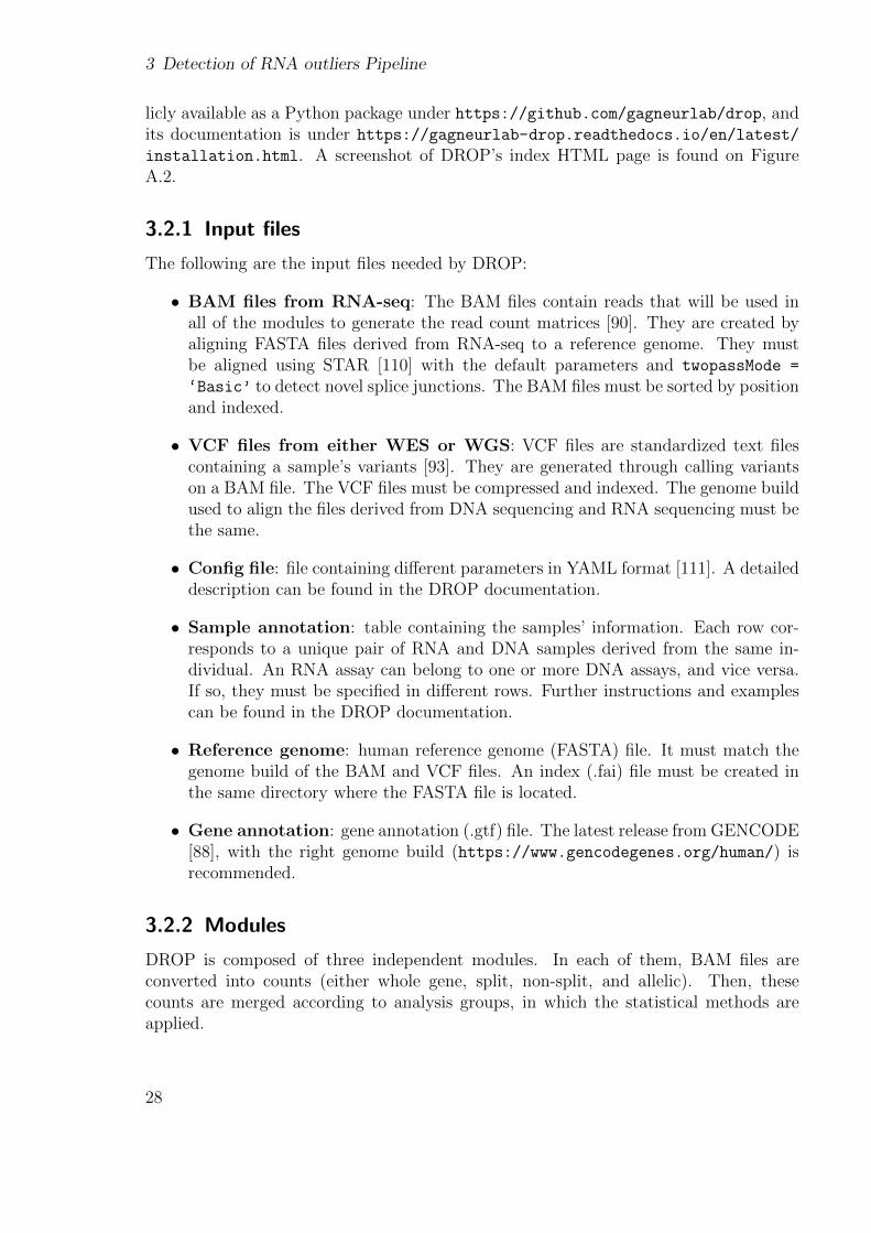
Figure 3.3: Files processing from individual samples to results by groups. Flowdiagram showing how the results are generated for each analysis group. First,the counting is performed only once per sample. Afterwards, they are mergedand filtered by each group. The statistical modelling is then performed on eachgroup.
3.2.2.1 Aberrant expression
This module computes expression outliers from BAM files. First, reads fully overlappinggenes are counted for each sample and stored individually. Then, the counts are mergedfor each gene annotation and analysis group combination. Genes with low expression arefiltered out. Afterwards, the OUTRIDER fit is run per group, which includes optimiza-tion of the encoding dimension [5]. Finally, the results are extracted and saved as textfiles (Fig. 3.4). The user can specify parameters to control the way reads are counted,filtered out, and an FDR cutoff. If HPO-encoded phenotypes [112] were provided in thesample annotation, a column stating whether the outlier genes overlap with the HPOterms is included in the results table.
To visualize the counting and OUTRIDER fit, two HTML reports are generated.The first one contains plots summarizing the number of reads counted per sample, sizefactors, genes FPKM (Fragments Per Kilobase of transcript per Million) before and afterfiltering, and number of expressed genes per sample. The second one contains plotswith the hyperparameter optimization search, number of expression outliers per sample,heatmaps of the count correlation before and after correction, biological coefficient ofvariation; plus the results table. The results table contains different values from the fitfor each sample-gene combination (Table 3.1).
29
3 Detection of RNA outliers Pipeline
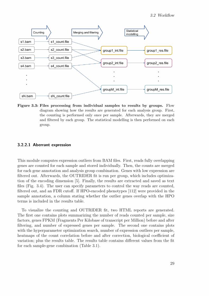
Figure 3.4: Aberrant expression workflow. Directed acyclic graph of the Snakemake rulesconstituting the aberrant expression module. The two main steps are countingand running the OUTRIDER fit and results.
3.2.2.2 Aberrant splicing
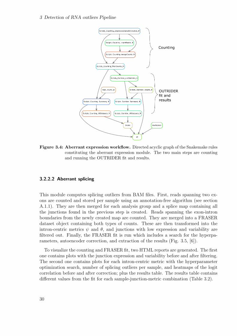
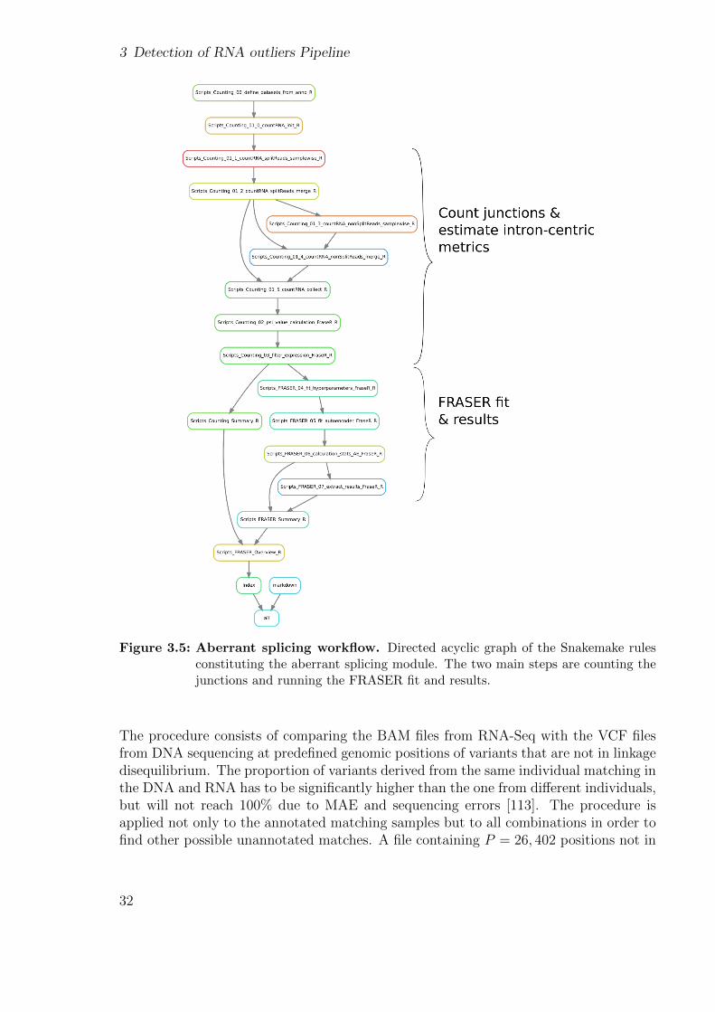
This module computes splicing outliers from BAM files. First, reads spanning two ex-ons are counted and stored per sample using an annotation-free algorithm (see sectionA.1.1). They are then merged for each analysis group and a splice map containing allthe junctions found in the previous step is created. Reads spanning the exon-intronboundaries from the newly created map are counted. They are merged into a FRASERdataset object containing both types of counts. These are then transformed into theintron-centric metrics ψ and θ, and junctions with low expression and variability arefiltered out. Finally, the FRASER fit is run which includes a search for the hyperpa-rameters, autoencoder correction, and extraction of the results (Fig. 3.5, [6]).
To visualize the counting and FRASER fit, two HTML reports are generated. The firstone contains plots with the junction expression and variability before and after filtering.The second one contains plots for each intron-centric metric with the hyperparameteroptimization search, number of splicing outliers per sample, and heatmaps of the logitcorrelation before and after correction; plus the results table. The results table containsdifferent values from the fit for each sample-junction-metric combination (Table 3.2).
30
3.2 Workflow
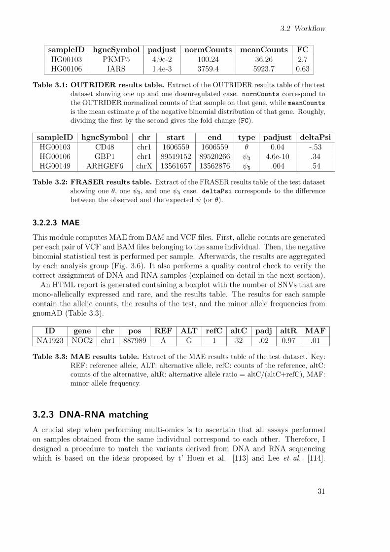
sampleID hgncSymbol padjust normCounts meanCounts FCHG00103 PKMP5 4.9e-2 100.24 36.26 2.7HG00106 IARS 1.4e-3 3759.4 5923.7 0.63
Table 3.1: OUTRIDER results table. Extract of the OUTRIDER results table of the testdataset showing one up and one downregulated case. normCounts correspond tothe OUTRIDER normalized counts of that sample on that gene, while meanCountsis the mean estimate µ of the negative binomial distribution of that gene. Roughly,dividing the first by the second gives the fold change (FC).
sampleID hgncSymbol chr start end type padjust deltaPsiHG00103 CD48 chr1 1606559 1606559 θ 0.04 -.53HG00106 GBP1 chr1 89519152 89520266 ψ3 4.6e-10 .34HG00149 ARHGEF6 chrX 13561657 13562876 ψ5 .004 .54
Table 3.2: FRASER results table. Extract of the FRASER results table of the test datasetshowing one θ, one ψ3, and one ψ5 case. deltaPsi corresponds to the differencebetween the observed and the expected ψ (or θ).
3.2.2.3 MAE
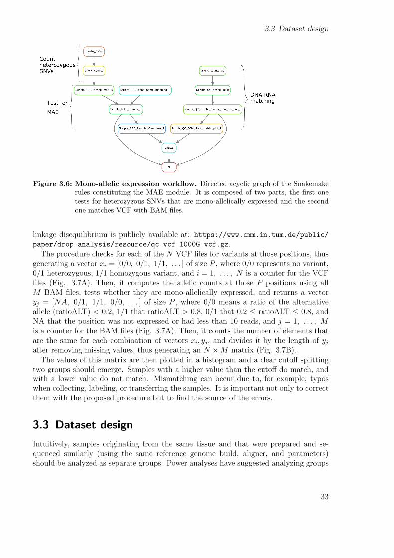
This module computes MAE from BAM and VCF files. First, allelic counts are generatedper each pair of VCF and BAM files belonging to the same individual. Then, the negativebinomial statistical test is performed per sample. Afterwards, the results are aggregatedby each analysis group (Fig. 3.6). It also performs a quality control check to verify thecorrect assignment of DNA and RNA samples (explained on detail in the next section).
An HTML report is generated containing a boxplot with the number of SNVs that aremono-allelically expressed and rare, and the results table. The results for each samplecontain the allelic counts, the results of the test, and the minor allele frequencies fromgnomAD (Table 3.3).
ID gene chr pos REF ALT refC altC padj altR MAFNA1923 NOC2 chr1 887989 A G 1 32 .02 0.97 .01
Table 3.3: MAE results table. Extract of the MAE results table of the test dataset. Key:REF: reference allele, ALT: alternative allele, refC: counts of the reference, altC:counts of the alternative, altR: alternative allele ratio = altC/(altC+refC), MAF:minor allele frequency.
3.2.3 DNA-RNA matching
A crucial step when performing multi-omics is to ascertain that all assays performedon samples obtained from the same individual correspond to each other. Therefore, Idesigned a procedure to match the variants derived from DNA and RNA sequencingwhich is based on the ideas proposed by t’ Hoen et al. [113] and Lee et al. [114].
31
3 Detection of RNA outliers Pipeline
Figure 3.5: Aberrant splicing workflow. Directed acyclic graph of the Snakemake rulesconstituting the aberrant splicing module. The two main steps are counting thejunctions and running the FRASER fit and results.
The procedure consists of comparing the BAM files from RNA-Seq with the VCF filesfrom DNA sequencing at predefined genomic positions of variants that are not in linkagedisequilibrium. The proportion of variants derived from the same individual matching inthe DNA and RNA has to be significantly higher than the one from different individuals,but will not reach 100% due to MAE and sequencing errors [113]. The procedure isapplied not only to the annotated matching samples but to all combinations in order tofind other possible unannotated matches. A file containing P = 26, 402 positions not in
32
3.3 Dataset design
Figure 3.6: Mono-allelic expression workflow. Directed acyclic graph of the Snakemakerules constituting the MAE module. It is composed of two parts, the first onetests for heterozygous SNVs that are mono-allelically expressed and the secondone matches VCF with BAM files.
linkage disequilibrium is publicly available at: https://www.cmm.in.tum.de/public/
paper/drop_analysis/resource/qc_vcf_1000G.vcf.gz.The procedure checks for each of the N VCF files for variants at those positions, thus
generating a vector xi = [0/0, 0/1, 1/1, . . . ] of size P , where 0/0 represents no variant,0/1 heterozygous, 1/1 homozygous variant, and i = 1, . . . , N is a counter for the VCFfiles (Fig. 3.7A). Then, it computes the allelic counts at those P positions using allM BAM files, tests whether they are mono-allelically expressed, and returns a vectoryj = [NA, 0/1, 1/1, 0/0, . . . ] of size P , where 0/0 means a ratio of the alternativeallele (ratioALT) < 0.2, 1/1 that ratioALT > 0.8, 0/1 that 0.2 ≤ ratioALT ≤ 0.8, andNA that the position was not expressed or had less than 10 reads, and j = 1, . . . , Mis a counter for the BAM files (Fig. 3.7A). Then, it counts the number of elements thatare the same for each combination of vectors xi, yj, and divides it by the length of yjafter removing missing values, thus generating an N ×M matrix (Fig. 3.7B).
The values of this matrix are then plotted in a histogram and a clear cutoff splittingtwo groups should emerge. Samples with a higher value than the cutoff do match, andwith a lower value do not match. Mismatching can occur due to, for example, typoswhen collecting, labeling, or transferring the samples. It is important not only to correctthem with the proposed procedure but to find the source of the errors.
3.3 Dataset design
Intuitively, samples originating from the same tissue and that were prepared and se-quenced similarly (using the same reference genome build, aligner, and parameters)should be analyzed as separate groups. Power analyses have suggested analyzing groups
33
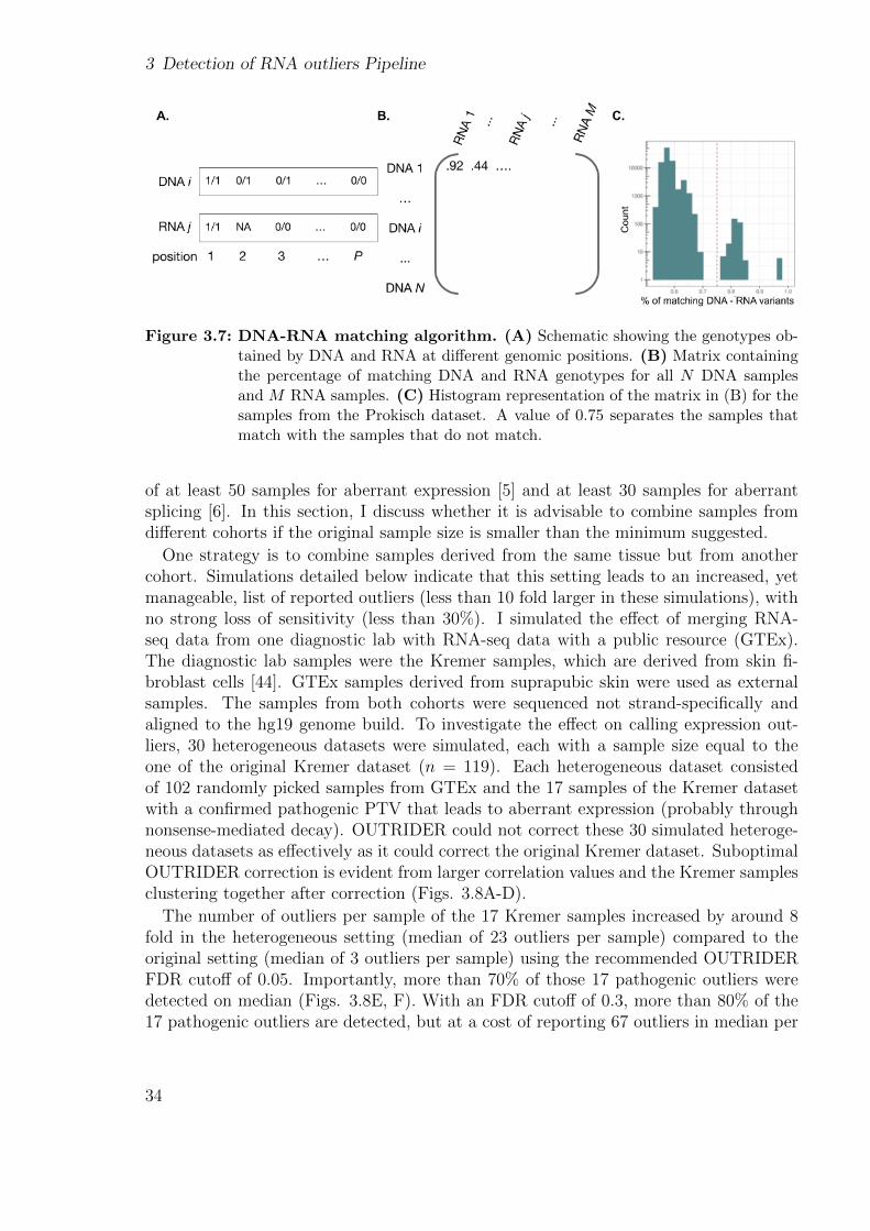
3 Detection of RNA outliers Pipeline
Figure 3.7: DNA-RNA matching algorithm. (A) Schematic showing the genotypes ob-tained by DNA and RNA at different genomic positions. (B) Matrix containingthe percentage of matching DNA and RNA genotypes for all N DNA samplesand M RNA samples. (C) Histogram representation of the matrix in (B) for thesamples from the Prokisch dataset. A value of 0.75 separates the samples thatmatch with the samples that do not match.
of at least 50 samples for aberrant expression [5] and at least 30 samples for aberrantsplicing [6]. In this section, I discuss whether it is advisable to combine samples fromdifferent cohorts if the original sample size is smaller than the minimum suggested.
One strategy is to combine samples derived from the same tissue but from anothercohort. Simulations detailed below indicate that this setting leads to an increased, yetmanageable, list of reported outliers (less than 10 fold larger in these simulations), withno strong loss of sensitivity (less than 30%). I simulated the effect of merging RNA-seq data from one diagnostic lab with RNA-seq data with a public resource (GTEx).The diagnostic lab samples were the Kremer samples, which are derived from skin fi-broblast cells [44]. GTEx samples derived from suprapubic skin were used as externalsamples. The samples from both cohorts were sequenced not strand-specifically andaligned to the hg19 genome build. To investigate the effect on calling expression out-liers, 30 heterogeneous datasets were simulated, each with a sample size equal to theone of the original Kremer dataset (n = 119). Each heterogeneous dataset consistedof 102 randomly picked samples from GTEx and the 17 samples of the Kremer datasetwith a confirmed pathogenic PTV that leads to aberrant expression (probably throughnonsense-mediated decay). OUTRIDER could not correct these 30 simulated heteroge-neous datasets as effectively as it could correct the original Kremer dataset. SuboptimalOUTRIDER correction is evident from larger correlation values and the Kremer samplesclustering together after correction (Figs. 3.8A-D).
The number of outliers per sample of the 17 Kremer samples increased by around 8fold in the heterogeneous setting (median of 23 outliers per sample) compared to theoriginal setting (median of 3 outliers per sample) using the recommended OUTRIDERFDR cutoff of 0.05. Importantly, more than 70% of those 17 pathogenic outliers weredetected on median (Figs. 3.8E, F). With an FDR cutoff of 0.3, more than 80% of the17 pathogenic outliers are detected, but at a cost of reporting 67 outliers in median per
34
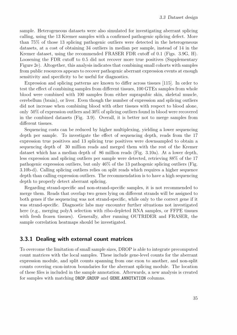
3.3 Dataset design
sample. Heterogeneous datasets were also simulated for investigating aberrant splicingcalling, using the 13 Kremer samples with a confirmed pathogenic splicing defect. Morethan 75% of those 13 splicing pathogenic outliers were detected in the heterogeneousdatasets, at a cost of obtaining 34 outliers in median per sample, instead of 14 in theKremer dataset, using the recommended FRASER FDR cutoff of 0.1 (Figs. 3.9G, H).Loosening the FDR cutoff to 0.5 did not recover more true positives (SupplementaryFigure 2e). Altogether, this analysis indicates that combining small cohorts with samplesfrom public resources appears to recover pathogenic aberrant expression events at enoughsensitivity and specificity to be useful for diagnostics.
Expression and splicing patterns are known to differ across tissues [115]. In order totest the effect of combining samples from different tissues, 100 GTEx samples from wholeblood were combined with 100 samples from either suprapubic skin, skeletal muscle,cerebellum (brain), or liver. Even though the number of expression and splicing outliersdid not increase when combining blood with other tissues with respect to blood alone,only 50% of expression outliers and 30% of splicing outliers found in blood were recoveredin the combined datasets (Fig. 3.9). Overall, it is better not to merge samples fromdifferent tissues.
Sequencing costs can be reduced by higher multiplexing, yielding a lower sequencingdepth per sample. To investigate the effect of sequencing depth, reads from the 17expression true positives and 13 splicing true positives were downsampled to obtain asequencing depth of 30 million reads and merged them with the rest of the Kremerdataset which has a median depth of 86 million reads (Fig. 3.10a). At a lower depth,less expression and splicing outliers per sample were detected, retrieving 88% of the 17pathogenic expression outliers, but only 46% of the 13 pathogenic splicing outliers (Fig.3.10b-d). Calling splicing outliers relies on split reads which requires a higher sequencedepth than calling expression outliers. The recommendation is to have a high sequencingdepth to properly detect aberrant splicing.
Regarding strand-specific and non-strand-specific samples, it is not recommended tomerge them. Reads that overlap two genes lying on different strands will be assigned toboth genes if the sequencing was not strand-specific, while only to the correct gene if itwas strand-specific. Diagnostic labs may encounter further situations not investigatedhere (e.g., merging polyA selection with ribo-depleted RNA samples, or FFPE tissueswith fresh frozen tissues). Generally, after running OUTRIDER and FRASER, thesample correlation heatmaps should be investigated.
3.3.1 Dealing with external count matrices
To overcome the limitation of small sample sizes, DROP is able to integrate precomputedcount matrices with the local samples. These include gene-level counts for the aberrantexpression module, and split counts spanning from one exon to another, and non-splitcounts covering exon-intron boundaries for the aberrant splicing module. The locationof these files is included in the sample annotation. Afterwards, a new analysis is createdfor samples with matching DROP GROUP and GENE ANNOTATION columns.
35
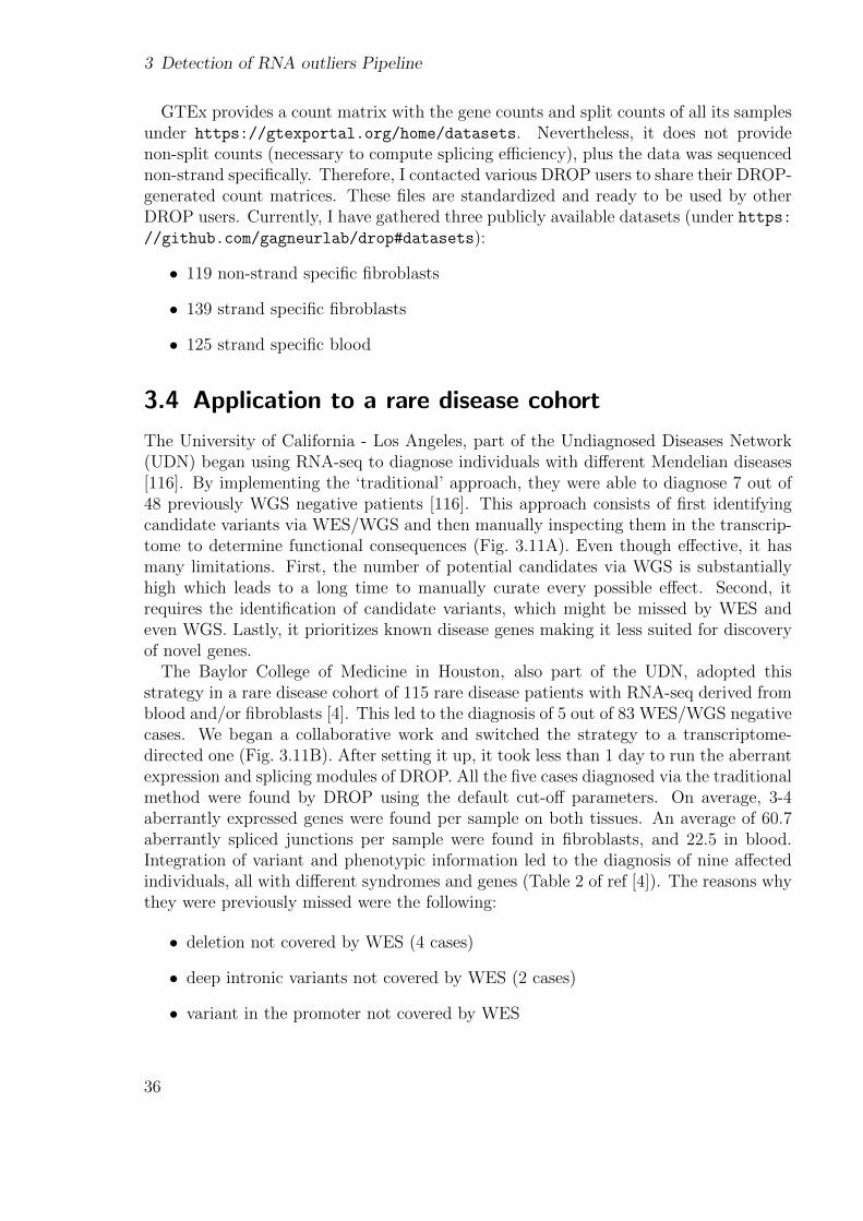
3 Detection of RNA outliers Pipeline
GTEx provides a count matrix with the gene counts and split counts of all its samplesunder https://gtexportal.org/home/datasets. Nevertheless, it does not providenon-split counts (necessary to compute splicing efficiency), plus the data was sequencednon-strand specifically. Therefore, I contacted various DROP users to share their DROP-generated count matrices. These files are standardized and ready to be used by otherDROP users. Currently, I have gathered three publicly available datasets (under https://github.com/gagneurlab/drop#datasets):
• 119 non-strand specific fibroblasts
• 139 strand specific fibroblasts
• 125 strand specific blood
3.4 Application to a rare disease cohort
The University of California - Los Angeles, part of the Undiagnosed Diseases Network(UDN) began using RNA-seq to diagnose individuals with different Mendelian diseases[116]. By implementing the ‘traditional’ approach, they were able to diagnose 7 out of48 previously WGS negative patients [116]. This approach consists of first identifyingcandidate variants via WES/WGS and then manually inspecting them in the transcrip-tome to determine functional consequences (Fig. 3.11A). Even though effective, it hasmany limitations. First, the number of potential candidates via WGS is substantiallyhigh which leads to a long time to manually curate every possible effect. Second, itrequires the identification of candidate variants, which might be missed by WES andeven WGS. Lastly, it prioritizes known disease genes making it less suited for discoveryof novel genes.
The Baylor College of Medicine in Houston, also part of the UDN, adopted thisstrategy in a rare disease cohort of 115 rare disease patients with RNA-seq derived fromblood and/or fibroblasts [4]. This led to the diagnosis of 5 out of 83 WES/WGS negativecases. We began a collaborative work and switched the strategy to a transcriptome-directed one (Fig. 3.11B). After setting it up, it took less than 1 day to run the aberrantexpression and splicing modules of DROP. All the five cases diagnosed via the traditionalmethod were found by DROP using the default cut-off parameters. On average, 3-4aberrantly expressed genes were found per sample on both tissues. An average of 60.7aberrantly spliced junctions per sample were found in fibroblasts, and 22.5 in blood.Integration of variant and phenotypic information led to the diagnosis of nine affectedindividuals, all with different syndromes and genes (Table 2 of ref [4]). The reasons whythey were previously missed were the following:
• deletion not covered by WES (4 cases)
• deep intronic variants not covered by WES (2 cases)
• variant in the promoter not covered by WES
36
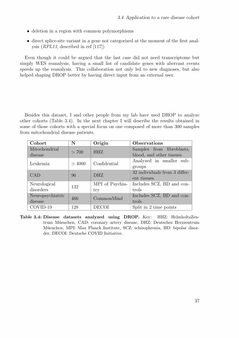
3.4 Application to a rare disease cohort
• deletion in a region with common polymorphisms
• direct splice-site variant in a gene not categorized at the moment of the first anal-ysis (RPL13, described in ref [117])
Even though it could be argued that the last case did not need transcriptome butsimply WES reanalysis, having a small list of candidate genes with aberrant eventsspeeds up the reanalysis. This collaboration not only led to new diagnoses, but alsohelped shaping DROP better by having direct input from an external user.
Besides this dataset, I and other people from my lab have used DROP to analyzeother cohorts (Table 3.4). In the next chapter I will describe the results obtained insome of those cohorts with a special focus on one composed of more than 300 samplesfrom mitochondrial disease patients.
Cohort N Origin ObservationsMitochondrialdisease
> 700 HHZSamples from fibroblasts,blood, and other tissues
Leukemia > 4000 ConfidentialAnalyzed in smaller sub-groups
CAD 96 DHZ32 individuals from 3 differ-ent tissues
Neurologicaldisorders
132MPI of Psychia-try
Includes SCZ, BD and con-trols
Neuropsychiatricdisease
466 CommonMindIncludes SCZ, BD and con-trols
COVID-19 128 DECOI Split in 2 time points
Table 3.4: Disease datasets analyzed using DROP. Key: HHZ: HelmholtzZen-trum Muenchen, CAD: coronary artery disease, DHZ: Deutsches HerzzentrumMuenchen, MPI: Max Planck Institute, SCZ: schizophrenia, BD: bipolar disor-der, DECOI: Deutsche COVID Initiative.
37
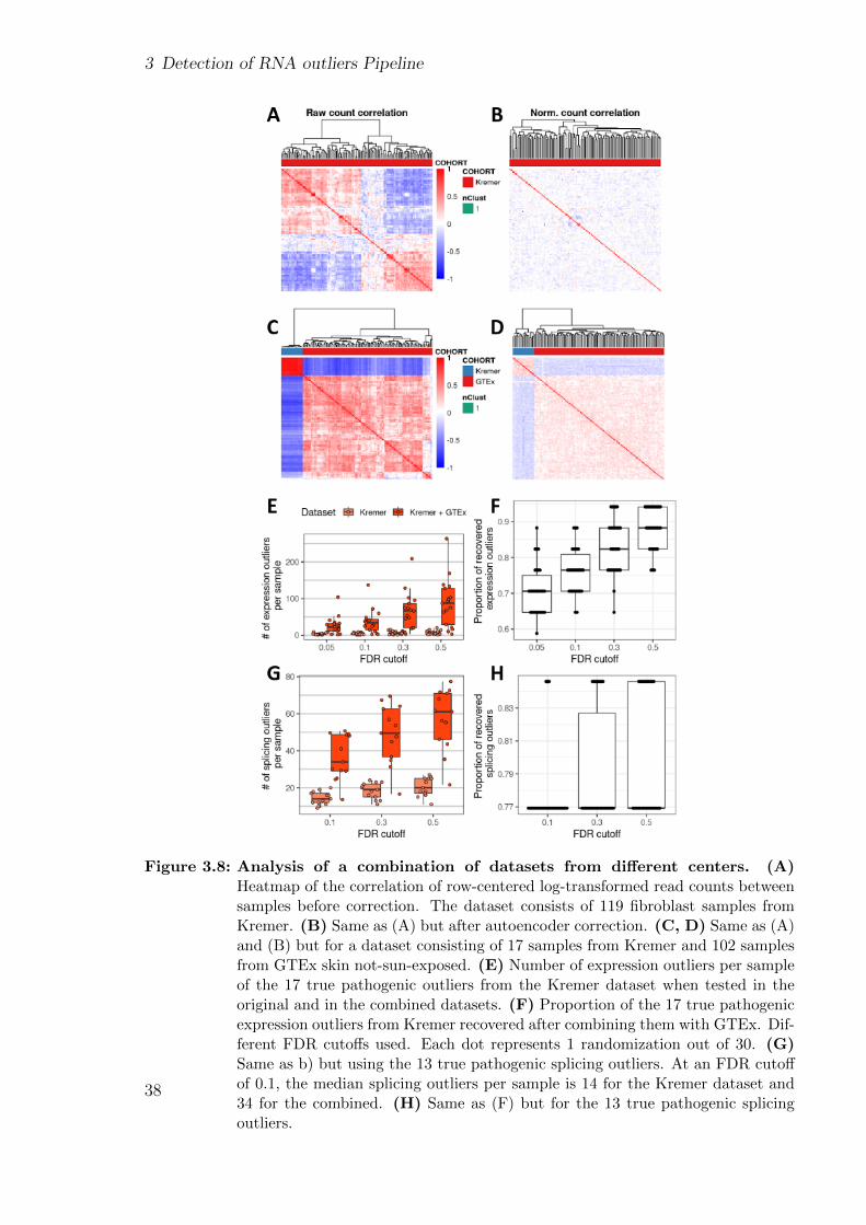
3 Detection of RNA outliers Pipeline
Figure 3.8: Analysis of a combination of datasets from different centers. (A)Heatmap of the correlation of row-centered log-transformed read counts betweensamples before correction. The dataset consists of 119 fibroblast samples fromKremer. (B) Same as (A) but after autoencoder correction. (C, D) Same as (A)and (B) but for a dataset consisting of 17 samples from Kremer and 102 samplesfrom GTEx skin not-sun-exposed. (E) Number of expression outliers per sampleof the 17 true pathogenic outliers from the Kremer dataset when tested in theoriginal and in the combined datasets. (F) Proportion of the 17 true pathogenicexpression outliers from Kremer recovered after combining them with GTEx. Dif-ferent FDR cutoffs used. Each dot represents 1 randomization out of 30. (G)Same as b) but using the 13 true pathogenic splicing outliers. At an FDR cutoffof 0.1, the median splicing outliers per sample is 14 for the Kremer dataset and34 for the combined. (H) Same as (F) but for the 13 true pathogenic splicingoutliers.
38
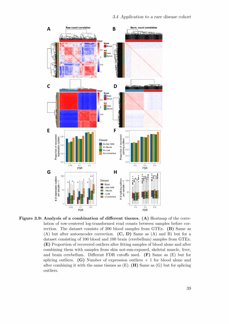
3.4 Application to a rare disease cohort
Figure 3.9: Analysis of a combination of different tissues. (A) Heatmap of the corre-lation of row-centered log-transformed read counts between samples before cor-rection. The dataset consists of 200 blood samples from GTEx. (B) Same as(A) but after autoencoder correction. (C, D) Same as (A) and B) but for adataset consisting of 100 blood and 100 brain (cerebellum) samples from GTEx.(E) Proportion of recovered outliers after fitting samples of blood alone and aftercombining them with samples from skin not-sun-exposed, skeletal muscle, liver,and brain cerebellum. Different FDR cutoffs used. (F) Same as (E) but forsplicing outliers. (G) Number of expression outliers + 1 for blood alone andafter combining it with the same tissues as (E). (H) Same as (G) but for splicingoutliers.
39
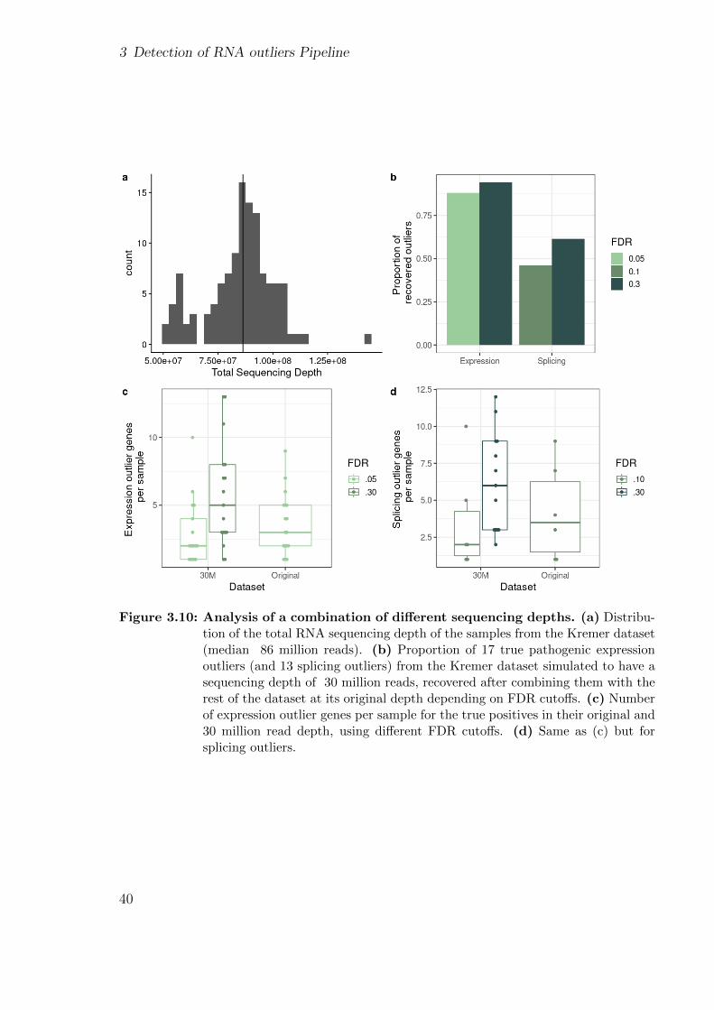
3 Detection of RNA outliers Pipeline
Figure 3.10: Analysis of a combination of different sequencing depths. (a) Distribu-tion of the total RNA sequencing depth of the samples from the Kremer dataset(median 86 million reads). (b) Proportion of 17 true pathogenic expressionoutliers (and 13 splicing outliers) from the Kremer dataset simulated to have asequencing depth of 30 million reads, recovered after combining them with therest of the dataset at its original depth depending on FDR cutoffs. (c) Numberof expression outlier genes per sample for the true positives in their original and30 million read depth, using different FDR cutoffs. (d) Same as (c) but forsplicing outliers.
40
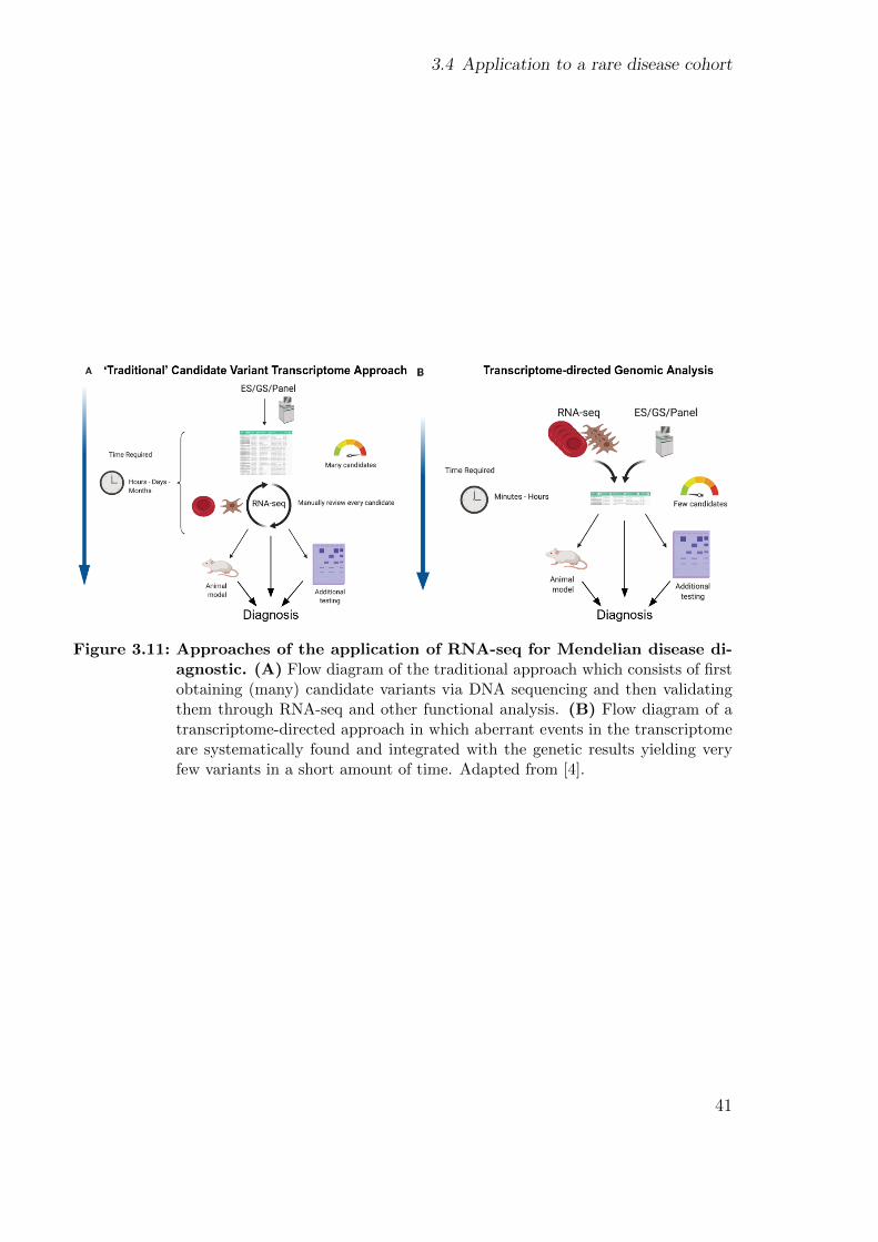
3.4 Application to a rare disease cohort
Figure 3.11: Approaches of the application of RNA-seq for Mendelian disease di-agnostic. (A) Flow diagram of the traditional approach which consists of firstobtaining (many) candidate variants via DNA sequencing and then validatingthem through RNA-seq and other functional analysis. (B) Flow diagram of atranscriptome-directed approach in which aberrant events in the transcriptomeare systematically found and integrated with the genetic results yielding veryfew variants in a short amount of time. Adapted from [4].
41

4 Using RNA-seq to diagnose geneticdisorders
Most of the content of this chapter is based on a study done jointly with Mirjana Gusic,with the guidance of Julien Gagneur and Holger Prokisch. The study is yet unpublished.Clinicians from different institutes helped to gather the data. Mirjana Gusic, RobertKopajtich, and Agnieszka Nadel prepared and sequenced the samples. Christian Merteshelped to obtain and interpret the results. Nicholas Smith developed the RNA-seq variantcalling pipeline.
4.1 Motivation
The study of Kremer et al. led to the diagnose of 5 out of 48 individuals with inconclusiveWES [44]. That means that 43 remained unsolved. Afterwards, variant reprioritizationand WGS led to the diagnosis of two other samples with disease-causal genes NDUFA10and LPIN1 (Table 4.1). NDUFA10 was found to be aberrantly expressed in one samplewhich harboured a homozygous variant in the 5’UTR region that was not prioritizedat that time. Aberrant splicing analysis found an exon to be skipped in LPIN1 in onesample. Nevertheless no variant was found by WES. WGS revealed a 2 kbp deletionspanning the aforementioned exon.
Gene Kremer et al. status Current statusTIMMDC1 x2 Diagnosed, AS, AE SameALDH18A1 Diagnosed AE, MAE SameCLPP Diagnosed, AS only AS, AEMCOLN1 Diagnosed, borderline significant AS, AETAZ AS but syn var not prioritized DiagnosedNDUFA10 AE but UTR var not prioritized DiagnosedLPIN1 AS but no var found Diagnosed after WGSSFXN4 – Diagnosed, ASNDUFAF5 x2 – Diagnosed, AS
Table 4.1: Diagnoses from the Kremer et al. dataset using RNA-seq. Table showingall the current diagnosed samples from the Kremer et al. cohort using RNA-seq.Each row corresponds to a gene. It includes the status at the time of that study andnow. Key: AE: significant aberrant expression, AS: significant aberrant splicing,var: variant, syn: synonymous
43
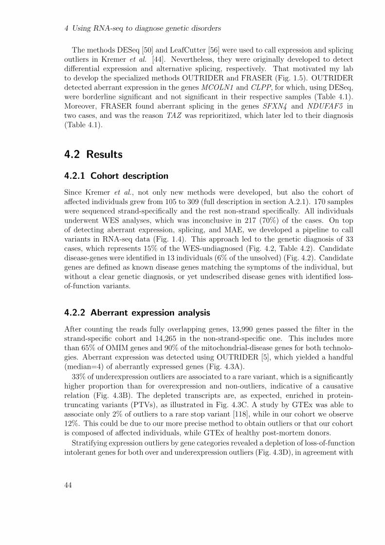
4 Using RNA-seq to diagnose genetic disorders
The methods DESeq [50] and LeafCutter [56] were used to call expression and splicingoutliers in Kremer et al. [44]. Nevertheless, they were originally developed to detectdifferential expression and alternative splicing, respectively. That motivated my labto develop the specialized methods OUTRIDER and FRASER (Fig. 1.5). OUTRIDERdetected aberrant expression in the genes MCOLN1 and CLPP, for which, using DESeq,were borderline significant and not significant in their respective samples (Table 4.1).Moreover, FRASER found aberrant splicing in the genes SFXN4 and NDUFAF5 intwo cases, and was the reason TAZ was reprioritized, which later led to their diagnosis(Table 4.1).
4.2 Results
4.2.1 Cohort description
Since Kremer et al., not only new methods were developed, but also the cohort ofaffected individuals grew from 105 to 309 (full description in section A.2.1). 170 sampleswere sequenced strand-specifically and the rest non-strand specifically. All individualsunderwent WES analyses, which was inconclusive in 217 (70%) of the cases. On topof detecting aberrant expression, splicing, and MAE, we developed a pipeline to callvariants in RNA-seq data (Fig. 1.4). This approach led to the genetic diagnosis of 33cases, which represents 15% of the WES-undiagnosed (Fig. 4.2, Table 4.2). Candidatedisease-genes were identified in 13 individuals (6% of the unsolved) (Fig. 4.2). Candidategenes are defined as known disease genes matching the symptoms of the individual, butwithout a clear genetic diagnosis, or yet undescribed disease genes with identified loss-of-function variants.
4.2.2 Aberrant expression analysis
After counting the reads fully overlapping genes, 13,990 genes passed the filter in thestrand-specific cohort and 14,265 in the non-strand-specific one. This includes morethan 65% of OMIM genes and 90% of the mitochondrial-disease genes for both technolo-gies. Aberrant expression was detected using OUTRIDER [5], which yielded a handful(median=4) of aberrantly expressed genes (Fig. 4.3A).
33% of underexpression outliers are associated to a rare variant, which is a significantlyhigher proportion than for overexpression and non-outliers, indicative of a causativerelation (Fig. 4.3B). The depleted transcripts are, as expected, enriched in protein-truncating variants (PTVs), as illustrated in Fig. 4.3C. A study by GTEx was able toassociate only 2% of outliers to a rare stop variant [118], while in our cohort we observe12%. This could be due to our more precise method to obtain outliers or that our cohortis composed of affected individuals, while GTEx of healthy post-mortem donors.
Stratifying expression outliers by gene categories revealed a depletion of loss-of-functionintolerant genes for both over and underexpression outliers (Fig. 4.3D), in agreement with
44
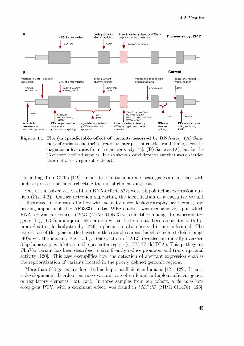
4.2 Results
Figure 4.1: The (un)predictable effect of variants assessed by RNA-seq. (A) Sum-mary of variants and their effect on transcript that enabled establishing a geneticdiagnosis in five cases from the pioneer study [44]. (B) Same as (A), but for the33 currently solved samples. It also shows a candidate variant that was discardedafter not observing a splice defect.
the findings from GTEx [119]. In addition, mitochondrial disease genes are enriched withunderexpression outliers, reflecting the initial clinical diagnosis.
Out of the solved cases with an RNA-defect, 82% were pinpointed as expression out-liers (Fig. 4.2). Outlier detection supporting the identification of a causative variantis illustrated in the case of a boy with neonatal-onset leukodystrophy, nystagmus, andhearing impairment (ID: AF6383). Initial WES analysis was inconclusive, upon whichRNA-seq was performed. UFM1 (MIM: 610553) was identified among 11 downregulatedgenes (Fig. 4.3E), a ubiquitin-like protein whose depletion has been associated with hy-pomyelinating leukodystrophy [120], a phenotype also observed in our individual. Theexpression of this gene is the lowest in this sample across the whole cohort (fold change-40% wrt the median, Fig. 4.3F). Reinspection of WES revealed an initially overseen3-bp homozygous deletion in the promoter region (c.-273-271delTCA). This pathogenicClinVar variant has been described to significantly reduce promoter and transcriptionalactivity [120]. This case exemplifies how the detection of aberrant expression enablesthe reprioritization of variants located in the poorly defined genomic regions.
More than 660 genes are described as haploinsufficient in humans [121, 122]. In neu-rodevelopmental disorders, de novo variants are often found in haploinsufficient genes,or regulatory elements [123, 124]. In three samples from our cohort, a de novo het-erozygous PTV, with a dominant effect, was found in MEPCE (MIM: 611478) [125],
45
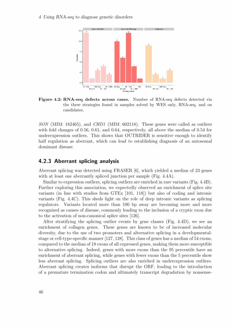
4 Using RNA-seq to diagnose genetic disorders
Figure 4.2: RNA-seq defects across cases. Number of RNA-seq defects detected viathe three strategies found in samples solved by WES only, RNA-seq, and oncandidates.
SON (MIM: 182465), and CHD1 (MIM: 602118). These genes were called as outlierswith fold changes of 0.56, 0.61, and 0.64, respectively, all above the median of 0.54 forunderexpression outliers. This shows that OUTRIDER is sensitive enough to identifyhalf regulation as aberrant, which can lead to establishing diagnosis of an autosomaldominant disease.
4.2.3 Aberrant splicing analysis
Aberrant splicing was detected using FRASER [6], which yielded a median of 23 geneswith at least one aberrantly spliced junction per sample (Fig. 4.4A).
Similar to expression outliers, splicing outliers are enriched in rare variants (Fig. 4.4B).Further exploring this association, we expectedly observed an enrichment of splice sitevariants (in line with studies from GTEx [101, 118]) but also of coding and intronicvariants (Fig. 4.4C). This sheds light on the role of deep intronic variants as splicingregulators. Variants located more than 100 bp away are becoming more and morerecognized as causes of disease, commonly leading to the inclusion of a cryptic exon dueto the activation of non-canonical splice sites [126].
After stratifying the splicing outlier events by gene classes (Fig. 4.4D), we see anenrichment of collagen genes. These genes are known to be of increased moleculardiversity, due to the use of two promoters and alternative splicing in a developmental-stage or cell-type-specific manner [127, 128]. This class of genes has a median of 54 exons,compared to the median of 18 exons of all expressed genes, making them more susceptibleto alternative splicing. Indeed, genes with more exons than the 95 percentile have anenrichment of aberrant splicing, while genes with fewer exons than the 5 percentile showless aberrant splicing. Splicing outliers are also enriched in underexpression outliers.Aberrant splicing creates isoforms that disrupt the ORF, leading to the introductionof a premature termination codon and ultimately transcript degradation by nonsense-
46
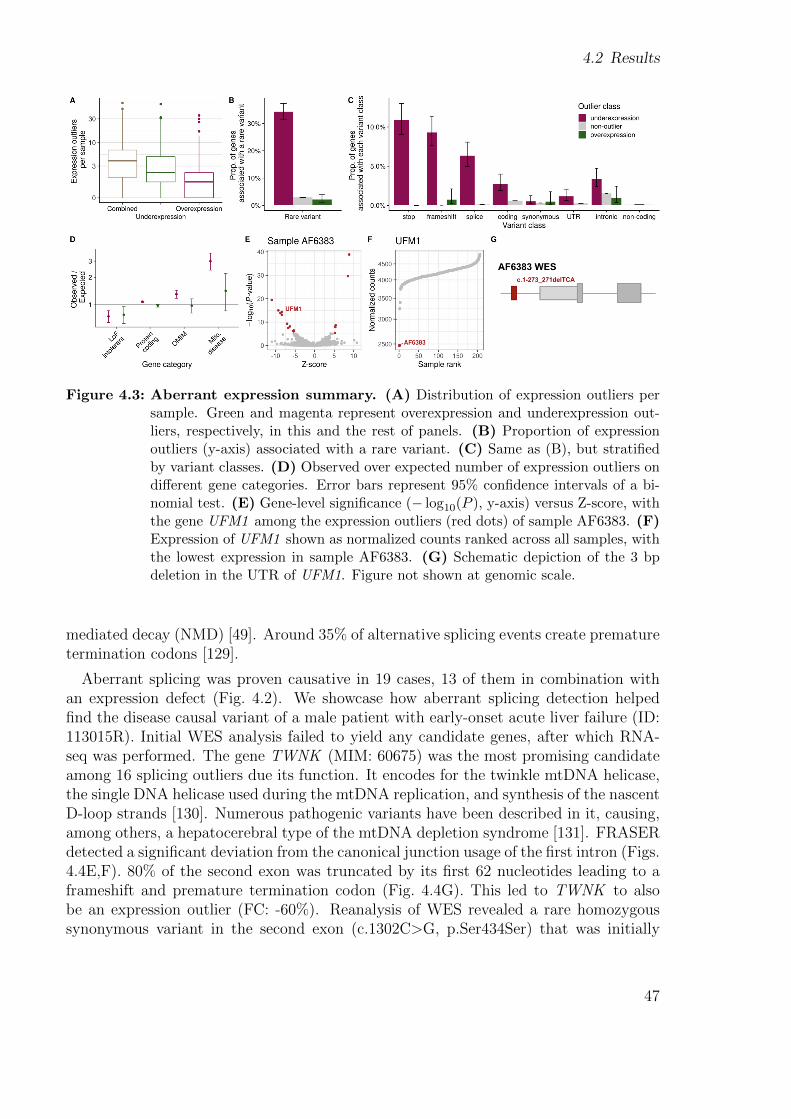
4.2 Results
Figure 4.3: Aberrant expression summary. (A) Distribution of expression outliers persample. Green and magenta represent overexpression and underexpression out-liers, respectively, in this and the rest of panels. (B) Proportion of expressionoutliers (y-axis) associated with a rare variant. (C) Same as (B), but stratifiedby variant classes. (D) Observed over expected number of expression outliers ondifferent gene categories. Error bars represent 95% confidence intervals of a bi-nomial test. (E) Gene-level significance (− log10(P ), y-axis) versus Z-score, withthe gene UFM1 among the expression outliers (red dots) of sample AF6383. (F)Expression of UFM1 shown as normalized counts ranked across all samples, withthe lowest expression in sample AF6383. (G) Schematic depiction of the 3 bpdeletion in the UTR of UFM1. Figure not shown at genomic scale.
mediated decay (NMD) [49]. Around 35% of alternative splicing events create prematuretermination codons [129].
Aberrant splicing was proven causative in 19 cases, 13 of them in combination withan expression defect (Fig. 4.2). We showcase how aberrant splicing detection helpedfind the disease causal variant of a male patient with early-onset acute liver failure (ID:113015R). Initial WES analysis failed to yield any candidate genes, after which RNA-seq was performed. The gene TWNK (MIM: 60675) was the most promising candidateamong 16 splicing outliers due its function. It encodes for the twinkle mtDNA helicase,the single DNA helicase used during the mtDNA replication, and synthesis of the nascentD-loop strands [130]. Numerous pathogenic variants have been described in it, causing,among others, a hepatocerebral type of the mtDNA depletion syndrome [131]. FRASERdetected a significant deviation from the canonical junction usage of the first intron (Figs.4.4E,F). 80% of the second exon was truncated by its first 62 nucleotides leading to aframeshift and premature termination codon (Fig. 4.4G). This led to TWNK to alsobe an expression outlier (FC: -60%). Reanalysis of WES revealed a rare homozygoussynonymous variant in the second exon (c.1302C>G, p.Ser434Ser) that was initially
47
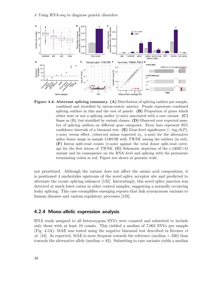
4 Using RNA-seq to diagnose genetic disorders
Figure 4.4: Aberrant splicing summary. (A) Distribution of splicing outliers per sample,combined and stratified by intron-centric metrics. Purple represents combinedsplicing outliers in this and the rest of panels. (B) Proportion of genes whicheither were or not a splicing outlier (y-axis) associated with a rare variant. (C)Same as (B), but stratified by variant classes. (D) Observed over expected num-ber of splicing outliers on different gene categories. Error bars represent 95%confidence intervals of a binomial test. (E) Gene-level significance (− log1 0(P ),y-axis) versus effect, (observed minus expected ψ5, x-axis) for the alternativesplice donor usage in sample 113015R with TWNK among the outliers (in red).(F) Intron split-read counts (y-axis) against the total donor split-read cover-age for the first intron of TWNK. (G) Schematic depiction of the c.1302C>Gvariant and its consequence on the RNA level and splicing with the prematureterminating codon in red. Figure not shown at genomic scale.
not prioritized. Although the variant does not affect the amino acid composition, itis positioned 4 nucleotides upstream of the novel splice acceptor site and predicted toalternate the exonic splicing enhancer [132]. Interestingly, this novel splice junction wasdetected at much lower ratios in other control samples, suggesting a normally occurringleaky splicing. This case exemplifies emerging reports that link synonymous variants tohuman diseases and various regulatory processes [133].
4.2.4 Mono-allelic expression analysis
RNA reads assigned to all heterozygous SNVs were counted and subsetted to includeonly those with at least 10 counts. This yielded a median of 7,062 SNVs per sample(Fig. 4.5A). MAE was tested using the negative binomial test described in Kremer etal. [44]. As expected, MAE is more frequent towards the reference (median = 330) thantowards the alternative allele (median = 82). Subsetting to rare variants yields a median
48
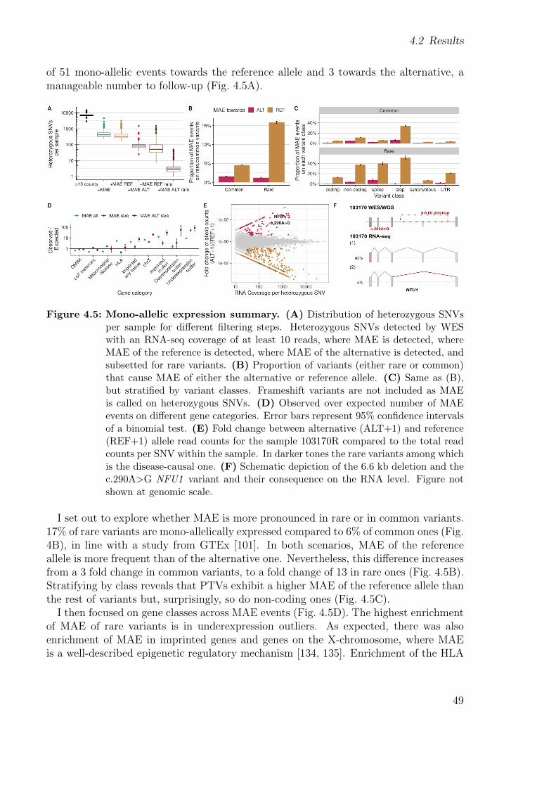
4.2 Results
of 51 mono-allelic events towards the reference allele and 3 towards the alternative, amanageable number to follow-up (Fig. 4.5A).
Figure 4.5: Mono-allelic expression summary. (A) Distribution of heterozygous SNVsper sample for different filtering steps. Heterozygous SNVs detected by WESwith an RNA-seq coverage of at least 10 reads, where MAE is detected, whereMAE of the reference is detected, where MAE of the alternative is detected, andsubsetted for rare variants. (B) Proportion of variants (either rare or common)that cause MAE of either the alternative or reference allele. (C) Same as (B),but stratified by variant classes. Frameshift variants are not included as MAEis called on heterozygous SNVs. (D) Observed over expected number of MAEevents on different gene categories. Error bars represent 95% confidence intervalsof a binomial test. (E) Fold change between alternative (ALT+1) and reference(REF+1) allele read counts for the sample 103170R compared to the total readcounts per SNV within the sample. In darker tones the rare variants among whichis the disease-causal one. (F) Schematic depiction of the 6.6 kb deletion and thec.290A>G NFU1 variant and their consequence on the RNA level. Figure notshown at genomic scale.
I set out to explore whether MAE is more pronounced in rare or in common variants.17% of rare variants are mono-allelically expressed compared to 6% of common ones (Fig.4B), in line with a study from GTEx [101]. In both scenarios, MAE of the referenceallele is more frequent than of the alternative one. Nevertheless, this difference increasesfrom a 3 fold change in common variants, to a fold change of 13 in rare ones (Fig. 4.5B).Stratifying by class reveals that PTVs exhibit a higher MAE of the reference allele thanthe rest of variants but, surprisingly, so do non-coding ones (Fig. 4.5C).
I then focused on gene classes across MAE events (Fig. 4.5D). The highest enrichmentof MAE of rare variants is in underexpression outliers. As expected, there was alsoenrichment of MAE in imprinted genes and genes on the X-chromosome, where MAEis a well-described epigenetic regulatory mechanism [134, 135]. Enrichment of the HLA
49
4 Using RNA-seq to diagnose genetic disorders
group of genes reflects their origin in the most polymorphic region of the human genome,which, as expected, only exists in common but not rare variants causing MAE [136].
Detection of MAE helped diagnosing four samples, all in combination with aberrantexpression (Fig. 4.2). One of those is a 13-year old boy with a severe Leigh disease andcomplex I deficiency (ID: 103170R). The initial WES analysis was negative. Among76 aberrant transcriptome events, the gene NFU1 (MIM:608100) was pinpointed as themost promising to cause the disease. NFU1 encodes for an iron-sulfur cluster scaf-fold that facilitates their insertion into the subunits of the respiratory chain complexes[137, 138]. Patients harboring pathogenic biallelic NFU1 variants can present with early-onset failure to thrive, pulmonary hypertension, encephalopathy, and neurological regres-sion [139]. MAE analysis found that this sample harbored a mono-allelically expressedmissense variant (c.290A>G (p.Val91Ala)) not previously reported (Figs. 4.5E,F). More-over, NFU1 was detected as an expression outlier, with a fold change of -40% comparedto the median, confirming the half-regulation. WGS was performed in order to elucidatethe genetic cause of the second allele depletion. This revealed a 6.6 kbp heterozygousdeletion spanning the complete exon 6 (Fig. 4.5G). Segregation analysis revealed thatthe missense variant was inherited from the father and the deletion from the mother.Altogether, this case is a model example of the implementation of different omics toolsto establish a genetic diagnosis.
4.2.5 RNA-seq variant calling
Transcriptome variant discovery can serve as a complementary approach to WES as itcan provide information about UTRs and intronic regions that are usually not coveredby exome-capturing kits [140]. This approach was used to diagnose a sample with a raremuscular disorder whose variant in the 5’ UTR was not detected by WES [46]. Therefore,we decided to call variants in our RNA-Seq data following GATK’s best practices [91].Precision-recall analyses were performed using variants called on WGS and RNA-Seqon GTEx samples derived from suprapubic skin. The best precision-recall balance wasobtained when excluding regions that have ≥ 3 variants within a 35 bp window, andvariants with less than 3 reads supporting the alternative allele (Fig. A.4). This yieldeda median of 44,183 variants per sample, in comparison to a median of 63,632 variantscalled by WES (Fig. 4.6A).
First, I set out to explore whether the variants discovered on the transcriptome differedsubstantially from those detected by WES. More variants are called in RNA-seq datathan in WES in the intergenic and the 3’ UTR region (Fig. 4.6B). Moreover, variantsmissed by WES are called in RNA-seq data in each region, even coding (Fig. 4.6B),indicating that RNA-seq can help overcome technical limitations in the detection ofcertain variants by WES. Afterwards, I counted the genes that did not pass the bi-allelicrare variant filter after WES but did pass after combining the WES and RNA-seq variantcalls. A total of 123 mitochondrial disease genes passed this filter (Fig. 4.6C).
RNA-seq variant calling identified the causative variant in nine cases missed by WES,all deep intronic (Table 4.2). Although these variants could have been detected by
50
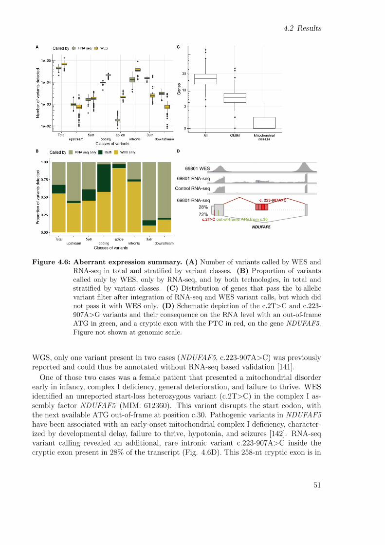
4.2 Results
Figure 4.6: Aberrant expression summary. (A) Number of variants called by WES andRNA-seq in total and stratified by variant classes. (B) Proportion of variantscalled only by WES, only by RNA-seq, and by both technologies, in total andstratified by variant classes. (C) Distribution of genes that pass the bi-allelicvariant filter after integration of RNA-seq and WES variant calls, but which didnot pass it with WES only. (D) Schematic depiction of the c.2T>C and c.223-907A>G variants and their consequence on the RNA level with an out-of-frameATG in green, and a cryptic exon with the PTC in red, on the gene NDUFAF5.Figure not shown at genomic scale.
WGS, only one variant present in two cases (NDUFAF5, c.223-907A>C) was previouslyreported and could thus be annotated without RNA-seq based validation [141].
One of those two cases was a female patient that presented a mitochondrial disorderearly in infancy, complex I deficiency, general deterioration, and failure to thrive. WESidentified an unreported start-loss heterozygous variant (c.2T>C) in the complex I as-sembly factor NDUFAF5 (MIM: 612360). This variant disrupts the start codon, withthe next available ATG out-of-frame at position c.30. Pathogenic variants in NDUFAF5have been associated with an early-onset mitochondrial complex I deficiency, character-ized by developmental delay, failure to thrive, hypotonia, and seizures [142]. RNA-seqvariant calling revealed an additional, rare intronic variant c.223-907A>C inside thecryptic exon present in 28% of the transcript (Fig. 4.6D). This 258-nt cryptic exon is in
51
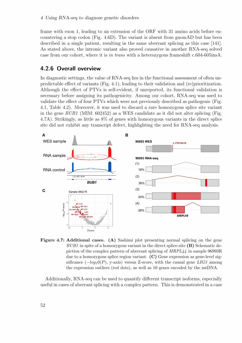
4 Using RNA-seq to diagnose genetic disorders
frame with exon 1, leading to an extension of the ORF with 31 amino acids before en-countering a stop codon (Fig. 4.6D). The variant is absent from gnomAD but has beendescribed in a single patient, resulting in the same aberrant splicing as this case [141].As stated above, the intronic variant also proved causative in another RNA-seq solvedcase from our cohort, where it is in trans with a heterozygous frameshift c.604-605insA.
4.2.6 Overall overview
In diagnostic settings, the value of RNA-seq lies in the functional assessment of often un-predictable effect of variants (Fig. 4.1), leading to their validation and (re)prioritization.Although the effect of PTVs is self-evident, if unreported, its functional validation isnecessary before assigning its pathogenicity. Among our cohort, RNA-seq was used tovalidate the effect of four PTVs which were not previously described as pathogenic (Fig.4.1, Table 4.2). Moreover, it was used to discard a rare homozygous splice site variantin the gene BUB1 (MIM: 602452) as a WES candidate as it did not alter splicing (Fig.4.7A). Strikingly, as little as 8% of genes with homozygous variants in the direct splicesite did not exhibit any transcript defect, highlighting the need for RNA-seq analysis.
Figure 4.7: Additional cases. (A) Sashimi plot presenting normal splicing on the geneBUB1 in spite of a homozygous variant in the direct splice-site (B) Schematic de-piction of the complex pattern of aberrant splicing of MRPL44 in sample 96993Rdue to a homozygous splice region variant. (C) Gene expression as gene-level sig-nificance (−log10(P ), y-axis) versus Z-score, with the causal gene LIG3 amongthe expression outliers (red dots), as well as 10 genes encoded by the mtDNA.
Additionally, RNA-seq can be used to quantify different transcript isoforms, especiallyuseful in cases of aberrant splicing with a complex pattern. This is demonstrated in a case
52
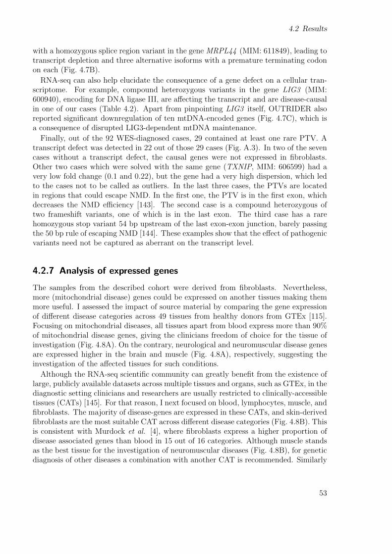
4.2 Results
with a homozygous splice region variant in the gene MRPL44 (MIM: 611849), leading totranscript depletion and three alternative isoforms with a premature terminating codonon each (Fig. 4.7B).
RNA-seq can also help elucidate the consequence of a gene defect on a cellular tran-scriptome. For example, compound heterozygous variants in the gene LIG3 (MIM:600940), encoding for DNA ligase III, are affecting the transcript and are disease-causalin one of our cases (Table 4.2). Apart from pinpointing LIG3 itself, OUTRIDER alsoreported significant downregulation of ten mtDNA-encoded genes (Fig. 4.7C), which isa consequence of disrupted LIG3-dependent mtDNA maintenance.
Finally, out of the 92 WES-diagnosed cases, 29 contained at least one rare PTV. Atranscript defect was detected in 22 out of those 29 cases (Fig. A.3). In two of the sevencases without a transcript defect, the causal genes were not expressed in fibroblasts.Other two cases which were solved with the same gene (TXNIP, MIM: 606599) had avery low fold change (0.1 and 0.22), but the gene had a very high dispersion, which ledto the cases not to be called as outliers. In the last three cases, the PTVs are locatedin regions that could escape NMD. In the first one, the PTV is in the first exon, whichdecreases the NMD efficiency [143]. The second case is a compound heterozygous oftwo frameshift variants, one of which is in the last exon. The third case has a rarehomozygous stop variant 54 bp upstream of the last exon-exon junction, barely passingthe 50 bp rule of escaping NMD [144]. These examples show that the effect of pathogenicvariants need not be captured as aberrant on the transcript level.
4.2.7 Analysis of expressed genes
The samples from the described cohort were derived from fibroblasts. Nevertheless,more (mitochondrial disease) genes could be expressed on another tissues making themmore useful. I assessed the impact of source material by comparing the gene expressionof different disease categories across 49 tissues from healthy donors from GTEx [115].Focusing on mitochondrial diseases, all tissues apart from blood express more than 90%of mitochondrial disease genes, giving the clinicians freedom of choice for the tissue ofinvestigation (Fig. 4.8A). On the contrary, neurological and neuromuscular disease genesare expressed higher in the brain and muscle (Fig. 4.8A), respectively, suggesting theinvestigation of the affected tissues for such conditions.
Although the RNA-seq scientific community can greatly benefit from the existence oflarge, publicly available datasets across multiple tissues and organs, such as GTEx, in thediagnostic setting clinicians and researchers are usually restricted to clinically-accessibletissues (CATs) [145]. For that reason, I next focused on blood, lymphocytes, muscle, andfibroblasts. The majority of disease-genes are expressed in these CATs, and skin-derivedfibroblasts are the most suitable CAT across different disease categories (Fig. 4.8B). Thisis consistent with Murdock et al. [4], where fibroblasts express a higher proportion ofdisease associated genes than blood in 15 out of 16 categories. Although muscle standsas the best tissue for the investigation of neuromuscular diseases (Fig. 4.8B), for geneticdiagnosis of other diseases a combination with another CAT is recommended. Similarly
53
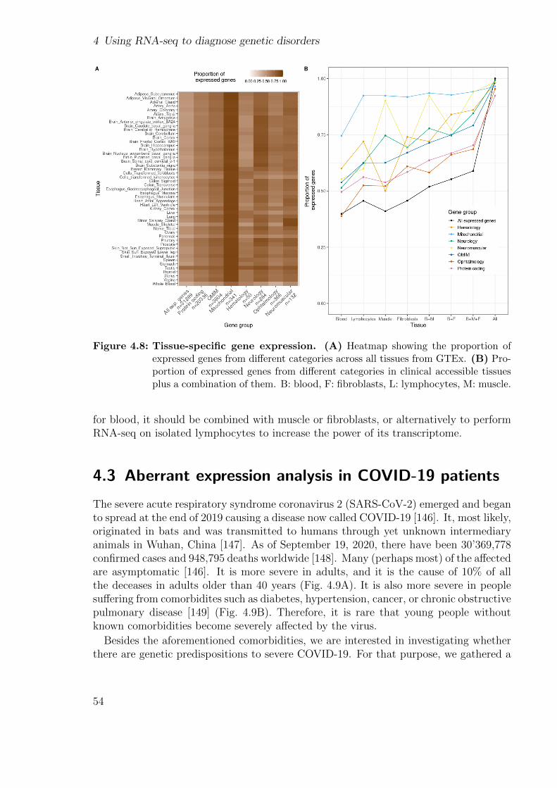
4 Using RNA-seq to diagnose genetic disorders
Figure 4.8: Tissue-specific gene expression. (A) Heatmap showing the proportion ofexpressed genes from different categories across all tissues from GTEx. (B) Pro-portion of expressed genes from different categories in clinical accessible tissuesplus a combination of them. B: blood, F: fibroblasts, L: lymphocytes, M: muscle.
for blood, it should be combined with muscle or fibroblasts, or alternatively to performRNA-seq on isolated lymphocytes to increase the power of its transcriptome.
4.3 Aberrant expression analysis in COVID-19 patients
The severe acute respiratory syndrome coronavirus 2 (SARS-CoV-2) emerged and beganto spread at the end of 2019 causing a disease now called COVID-19 [146]. It, most likely,originated in bats and was transmitted to humans through yet unknown intermediaryanimals in Wuhan, China [147]. As of September 19, 2020, there have been 30’369,778confirmed cases and 948,795 deaths worldwide [148]. Many (perhaps most) of the affectedare asymptomatic [146]. It is more severe in adults, and it is the cause of 10% of allthe deceases in adults older than 40 years (Fig. 4.9A). It is also more severe in peoplesuffering from comorbidites such as diabetes, hypertension, cancer, or chronic obstructivepulmonary disease [149] (Fig. 4.9B). Therefore, it is rare that young people withoutknown comorbidities become severely affected by the virus.
Besides the aforementioned comorbidities, we are interested in investigating whetherthere are genetic predispositions to severe COVID-19. For that purpose, we gathered a
54
4.3 Aberrant expression analysis in COVID-19 patients
Figure 4.9: Age and comorbidities predispose the impact of SARS-CoV-2. (A)COVID-19-related deaths among all deaths in United States in the period01.02.2020 - 05.09.2020 on different age groups. Data from ref [148] (B) Co-morbidities significantly associated with SARS-CoV-2 impact. HR: hazard ratio,adjusted with age and smoking status. Taken from ref [149].
set of 106 human RNA-seq samples, out of which 96 were affected by COVID-19 and10 were unaffected controls. The dataset is fully described in section A.2.2. From thesesamples, 79 passed quality control. Running OUTRIDER and FRASER on them ledto a total of 30 expression and 1,043 splicing outliers (Figs. 4.10A,B). The autoencoderwas able to remove the sample covariation (from, e.g., sex, hospital, and affected status,Figs. 4.10C,D).
Aberrant expression analysis revealed that patient ID: 9109, a 64 year-old male, had 2underexpression outliers (Fig. 4.11A). One was an antisense gene and the other one genePDK3 with a -70% fold change in normalized expression (Figs. 4.11A,B). The proteinencoded by this gene provides the primary link between glycolysis and Krebs cycle. It isassociated with abnormal gait due to lower limb muscle weakness and atrophy [150]. Novariant was found in his transcriptome. Muscle weakness can affect the muscles asso-ciated with breathing. Many individuals suffering from muscular dystrophy eventuallyneed to use a breathing assistance device, with respiratory failure being the main causeof death [151]. Therefore, individuals with (or susceptible to) muscle disorders are likelyto be more severely affected by COVID-19.
Aberrant splicing analysis revealed that patient ID:9088 had one splicing defect (Figs.4.11C,D). It consisted in skipping exon 9 (out of 10) in half of the reads in the geneTOR1AIP1 (Fig. 4.11E). Out of the 79 samples, only this showed this exon skippingevent (Fig. 4.11D). This gene is associated with muscular dystrophy [152], making it apotential candidate. A very poorly covered variant was found in the donor site whichrequires further confirmation. We found other splicing outliers in genes potentiallyrelated to the severity of COVID-19, but are not discussed here.
These promising results encourage us to gather more clinical information to betterunderstand the pathways in which the candidate genes are involved, as well as moretranscriptome data to better model gene expression and obtain new findings.
55
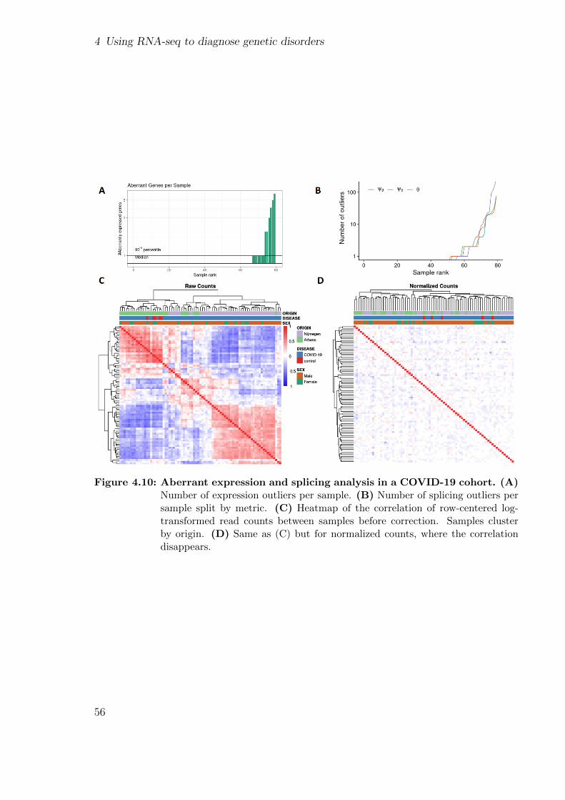
4 Using RNA-seq to diagnose genetic disorders
Figure 4.10: Aberrant expression and splicing analysis in a COVID-19 cohort. (A)Number of expression outliers per sample. (B) Number of splicing outliers persample split by metric. (C) Heatmap of the correlation of row-centered log-transformed read counts between samples before correction. Samples clusterby origin. (D) Same as (C) but for normalized counts, where the correlationdisappears.
56
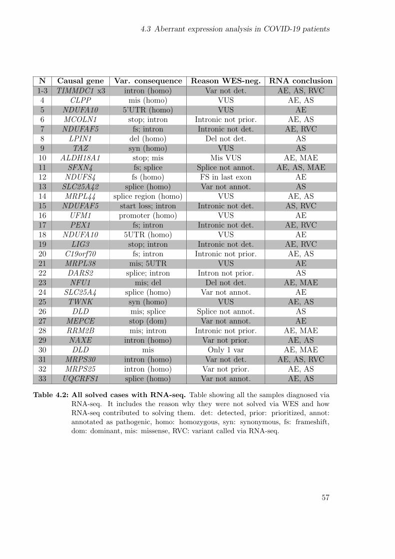
4.3 Aberrant expression analysis in COVID-19 patients
N Causal gene Var. consequence Reason WES-neg. RNA conclusion1-3 TIMMDC1 x3 intron (homo) Var not det. AE, AS, RVC4 CLPP mis (homo) VUS AE, AS5 NDUFA10 5’UTR (homo) VUS AE6 MCOLN1 stop; intron Intronic not prior. AE, AS7 NDUFAF5 fs; intron Intronic not det. AE, RVC8 LPIN1 del (homo) Del not det. AS9 TAZ syn (homo) VUS AS10 ALDH18A1 stop; mis Mis VUS AE, MAE11 SFXN4 fs; splice Splice not annot. AE, AS, MAE12 NDUFS4 fs (homo) FS in last exon AE13 SLC25A42 splice (homo) Var not annot. AS14 MRPL44 splice region (homo) VUS AE, AS15 NDUFAF5 start loss; intron Intronic not det. AS, RVC16 UFM1 promoter (homo) VUS AE17 PEX1 fs; intron Intronic not det. AE, RVC18 NDUFA10 5UTR (homo) VUS AE19 LIG3 stop; intron Intronic not det. AE, RVC20 C19orf70 fs; intron Intronic not prior. AE, AS21 MRPL38 mis; 5UTR VUS AE22 DARS2 splice; intron Intron not prior. AS23 NFU1 mis; del Del not det. AE, MAE24 SLC25A4 splice (homo) Var not annot. AE25 TWNK syn (homo) VUS AE, AS26 DLD mis; splice Splice not annot. AS27 MEPCE stop (dom) Var not annot. AE28 RRM2B mis; intron Intronic not prior. AE, MAE29 NAXE intron (homo) Var not prior. AE, AS30 DLD mis Only 1 var AE, MAE31 MRPS30 intron (homo) Var not det. AE, AS, RVC32 MRPS25 intron (homo) Var not prior. AE, AS33 UQCRFS1 splice (homo) Var not annot. AE, AS
Table 4.2: All solved cases with RNA-seq. Table showing all the samples diagnosed viaRNA-seq. It includes the reason why they were not solved via WES and howRNA-seq contributed to solving them. det: detected, prior: prioritized, annot:annotated as pathogenic, homo: homozygous, syn: synonymous, fs: frameshift,dom: dominant, mis: missense, RVC: variant called via RNA-seq.
57
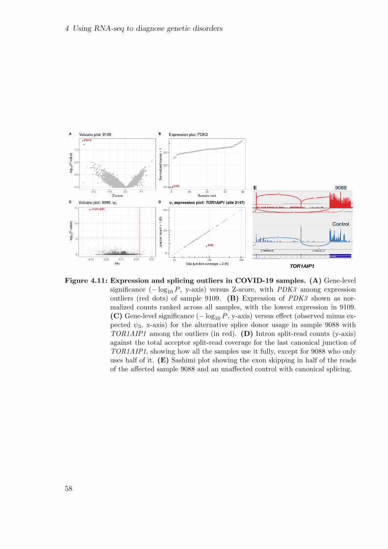
4 Using RNA-seq to diagnose genetic disorders
Figure 4.11: Expression and splicing outliers in COVID-19 samples. (A) Gene-levelsignificance (− log10 P , y-axis) versus Z-score, with PDK3 among expressionoutliers (red dots) of sample 9109. (B) Expression of PDK3 shown as nor-malized counts ranked across all samples, with the lowest expression in 9109.(C) Gene-level significance (− log10 P , y-axis) versus effect (observed minus ex-pected ψ3, x-axis) for the alternative splice donor usage in sample 9088 withTOR1AIP1 among the outliers (in red). (D) Intron split-read counts (y-axis)against the total acceptor split-read coverage for the last canonical junction ofTOR1AIP1, showing how all the samples use it fully, except for 9088 who onlyuses half of it. (E) Sashimi plot showing the exon skipping in half of the readsof the affected sample 9088 and an unaffected control with canonical splicing.
58
5 Statistical testing and application ofOCR
In the Introduction, I described the Seahorse technology to measure oxygen consumptionrates (OCR). Then, I discussed how although many procedures were written describingit, they mostly addressed experimental aspects instead of data analysis. This chapterdescribes OCR-stats, the statistical method I developed to robustly determine OCRlevels and test between samples. It includes best practices of how to seed cells and theminimum number of well and plate replicates to obtain confident results. The chapterends which an application of how different functional assays including cellular respirationwere used to characterize UQCRFS1 as a new disease gene.
5.1 OCR-stats
The methodology, results, and figures presented in this section are part of the manuscript“OCR-Stats: Robust estimation and statistical testing of mitochondrial respiration ac-tivities using Seahorse XF Analyzer” from Yepez et al. 2018 [1].
5.1.1 Motivation
As we saw in the Background, the mitochondrial stress test allows us to measure 6different bioenergetics in 96-well plates at various consecutive time points. Nevertheless,the sole definition of bioenergetic measures varies between authors, as well as the numberof time points in each interval (usually three time points, but in some cases one [153],two [154], or four or more [155]), and whether differences [71, 156], ratios [157, 158], orboth [84, 85] should be computed. Consequently, the comparison of results across studiesis difficult. Moreover, statistical power analyses for experimental design are often notprovided. The differences in OCR between biological samples (e.g. patient vs. control,or gene knockout vs. WT) can be as low as 12%–30% [159, 160, 161]. Therefore, todesign experiments with appropriate power to significantly detect such differences, it isimportant to know the source and amplitude of the variation within each sample and toreduce it as much as possible.
A large dataset of 126 mitochondrial stress tests in 96-well plates was generated bymy collaborators from the Helmholtz Zentrum. They included 203 different fibroblastcell lines, from which 26 were seeded in more than one plate (Table S1 of ref [1]).Between 3 and 7 biological samples per plate (median = 4) were seeded. A control
59
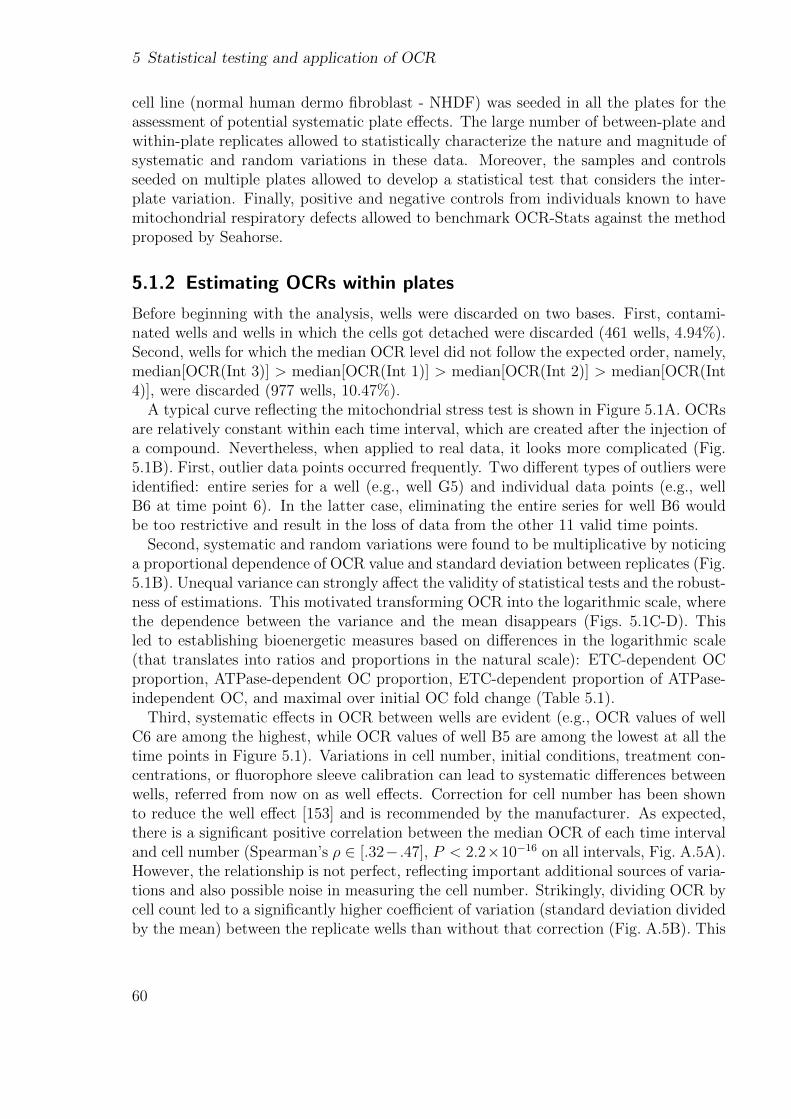
5 Statistical testing and application of OCR
cell line (normal human dermo fibroblast - NHDF) was seeded in all the plates for theassessment of potential systematic plate effects. The large number of between-plate andwithin-plate replicates allowed to statistically characterize the nature and magnitude ofsystematic and random variations in these data. Moreover, the samples and controlsseeded on multiple plates allowed to develop a statistical test that considers the inter-plate variation. Finally, positive and negative controls from individuals known to havemitochondrial respiratory defects allowed to benchmark OCR-Stats against the methodproposed by Seahorse.
5.1.2 Estimating OCRs within plates
Before beginning with the analysis, wells were discarded on two bases. First, contami-nated wells and wells in which the cells got detached were discarded (461 wells, 4.94%).Second, wells for which the median OCR level did not follow the expected order, namely,median[OCR(Int 3)] > median[OCR(Int 1)] > median[OCR(Int 2)] > median[OCR(Int4)], were discarded (977 wells, 10.47%).
A typical curve reflecting the mitochondrial stress test is shown in Figure 5.1A. OCRsare relatively constant within each time interval, which are created after the injection ofa compound. Nevertheless, when applied to real data, it looks more complicated (Fig.5.1B). First, outlier data points occurred frequently. Two different types of outliers wereidentified: entire series for a well (e.g., well G5) and individual data points (e.g., wellB6 at time point 6). In the latter case, eliminating the entire series for well B6 wouldbe too restrictive and result in the loss of data from the other 11 valid time points.
Second, systematic and random variations were found to be multiplicative by noticinga proportional dependence of OCR value and standard deviation between replicates (Fig.5.1B). Unequal variance can strongly affect the validity of statistical tests and the robust-ness of estimations. This motivated transforming OCR into the logarithmic scale, wherethe dependence between the variance and the mean disappears (Figs. 5.1C-D). Thisled to establishing bioenergetic measures based on differences in the logarithmic scale(that translates into ratios and proportions in the natural scale): ETC-dependent OCproportion, ATPase-dependent OC proportion, ETC-dependent proportion of ATPase-independent OC, and maximal over initial OC fold change (Table 5.1).
Third, systematic effects in OCR between wells are evident (e.g., OCR values of wellC6 are among the highest, while OCR values of well B5 are among the lowest at all thetime points in Figure 5.1). Variations in cell number, initial conditions, treatment con-centrations, or fluorophore sleeve calibration can lead to systematic differences betweenwells, referred from now on as well effects. Correction for cell number has been shownto reduce the well effect [153] and is recommended by the manufacturer. As expected,there is a significant positive correlation between the median OCR of each time intervaland cell number (Spearman’s ρ ∈ [.32− .47], P < 2.2×10⁻¹⁶ on all intervals, Fig. A.5A).However, the relationship is not perfect, reflecting important additional sources of varia-tions and also possible noise in measuring the cell number. Strikingly, dividing OCR bycell count led to a significantly higher coefficient of variation (standard deviation dividedby the mean) between the replicate wells than without that correction (Fig. A.5B). This
60
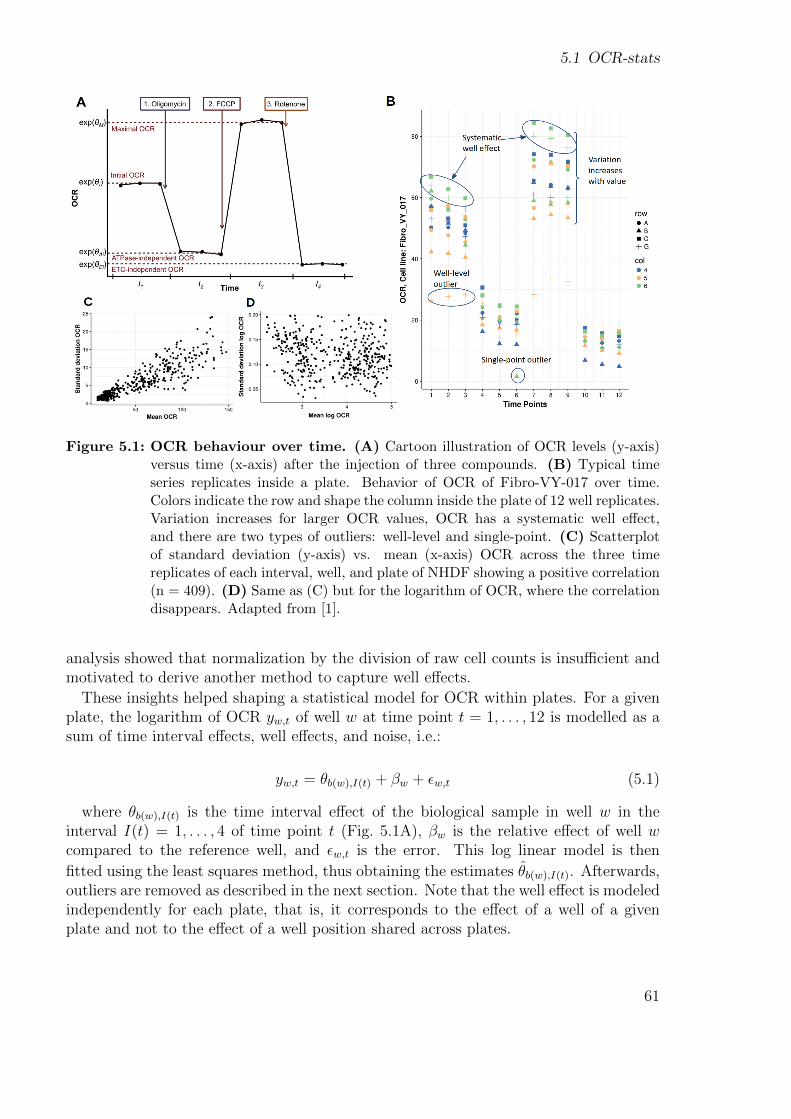
5.1 OCR-stats
Figure 5.1: OCR behaviour over time. (A) Cartoon illustration of OCR levels (y-axis)versus time (x-axis) after the injection of three compounds. (B) Typical timeseries replicates inside a plate. Behavior of OCR of Fibro-VY-017 over time.Colors indicate the row and shape the column inside the plate of 12 well replicates.Variation increases for larger OCR values, OCR has a systematic well effect,and there are two types of outliers: well-level and single-point. (C) Scatterplotof standard deviation (y-axis) vs. mean (x-axis) OCR across the three timereplicates of each interval, well, and plate of NHDF showing a positive correlation(n = 409). (D) Same as (C) but for the logarithm of OCR, where the correlationdisappears. Adapted from [1].
analysis showed that normalization by the division of raw cell counts is insufficient andmotivated to derive another method to capture well effects.
These insights helped shaping a statistical model for OCR within plates. For a givenplate, the logarithm of OCR yw,t of well w at time point t = 1, . . . , 12 is modelled as asum of time interval effects, well effects, and noise, i.e.:
yw,t = θb(w),I(t) + βw + εw,t (5.1)
where θb(w),I(t) is the time interval effect of the biological sample in well w in theinterval I(t) = 1, . . . , 4 of time point t (Fig. 5.1A), βw is the relative effect of well wcompared to the reference well, and εw,t is the error. This log linear model is then
fitted using the least squares method, thus obtaining the estimates θb(w),I(t). Afterwards,outliers are removed as described in the next section. Note that the well effect is modeledindependently for each plate, that is, it corresponds to the effect of a well of a givenplate and not to the effect of a well position shared across plates.
61
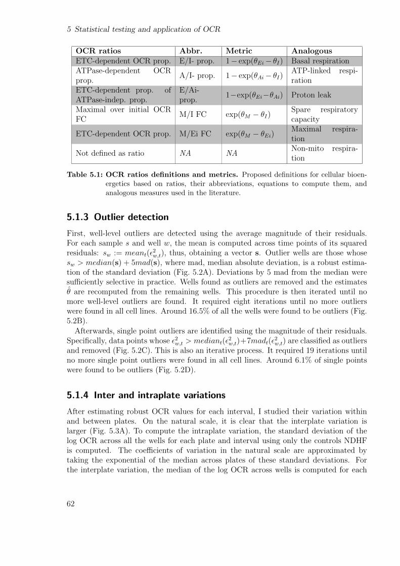
5 Statistical testing and application of OCR
OCR ratios Abbr. Metric AnalogousETC-dependent OCR prop. E/I- prop. 1− exp(θEi− θI) Basal respirationATPase-dependent OCRprop.
A/I- prop. 1− exp(θAi− θI)ATP-linked respi-ration
ETC-dependent prop. ofATPase-indep. prop.
E/Ai-prop.
1−exp(θEi−θAi) Proton leak
Maximal over initial OCRFC
M/I FC exp(θM − θI)Spare respiratorycapacity
ETC-dependent OCR prop. M/Ei FC exp(θM − θEi)Maximal respira-tion
Not defined as ratio NA NANon-mito respira-tion
Table 5.1: OCR ratios definitions and metrics. Proposed definitions for cellular bioen-ergetics based on ratios, their abbreviations, equations to compute them, andanalogous measures used in the literature.
5.1.3 Outlier detection
First, well-level outliers are detected using the average magnitude of their residuals.For each sample s and well w, the mean is computed across time points of its squaredresiduals: sw := meant(ε
2w,t), thus, obtaining a vector s. Outlier wells are those whose
sw > median(s) + 5mad(s), where mad, median absolute deviation, is a robust estima-tion of the standard deviation (Fig. 5.2A). Deviations by 5 mad from the median weresufficiently selective in practice. Wells found as outliers are removed and the estimatesθ are recomputed from the remaining wells. This procedure is then iterated until nomore well-level outliers are found. It required eight iterations until no more outlierswere found in all cell lines. Around 16.5% of all the wells were found to be outliers (Fig.5.2B).
Afterwards, single point outliers are identified using the magnitude of their residuals.Specifically, data points whose ε2w,t > mediant(ε
2w,t)+7madt(ε
2w,t) are classified as outliers
and removed (Fig. 5.2C). This is also an iterative process. It required 19 iterations untilno more single point outliers were found in all cell lines. Around 6.1% of single pointswere found to be outliers (Fig. 5.2D).
5.1.4 Inter and intraplate variations
After estimating robust OCR values for each interval, I studied their variation withinand between plates. On the natural scale, it is clear that the interplate variation islarger (Fig. 5.3A). To compute the intraplate variation, the standard deviation of thelog OCR across all the wells for each plate and interval using only the controls NDHFis computed. The coefficients of variation in the natural scale are approximated bytaking the exponential of the median across plates of these standard deviations. Forthe interplate variation, the median of the log OCR across wells is computed for each
62
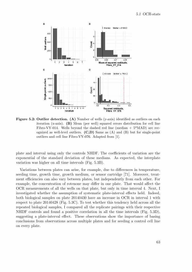
5.1 OCR-stats
Figure 5.2: Outlier detection. (A) Number of wells (y-axis) identified as outliers on eachiteration (x-axis). (B) Mean (per well) squared errors distribution for cell lineFibro-VY-014. Wells beyond the dashed red line (median + 5*MAD) are rec-ognized as well-level outliers. (C,D) Same as (A) and (B) but for single-pointoutliers and cell line Fibro-VY-076. Adapted from [1].
plate and interval using only the controls NHDF. The coefficients of variation are theexponential of the standard deviation of these medians. As expected, the interplatevariation was higher on all time intervals (Fig. 5.3B).
Variations between plates can arise, for example, due to differences in temperature,seeding time, growth time, growth medium, or sensor cartridge [71]. Moreover, treat-ment efficiencies can also vary between plates, but independently from each other. Forexample, the concentration of rotenone may differ in one plate. That would affect theOCR measurements of all the wells on that plate, but only in time interval 4. Next, Iinvestigated whether the assumption of systematic plate-interval effects held. Indeed,both biological samples on plate 20140430 have an increase in OCR in interval 1 withrespect to plate 20140428 (Fig. 5.3C). To test whether this tendency held across all therepeated biological samples, I compared all the replicate pairings with their respectiveNHDF controls and found a positive correlation in all the time intervals (Fig. 5.3D),suggesting a plate-interval effect. These observations show the importance of basingconclusions from observations across multiple plates and for seeding a control cell lineon every plate.
63
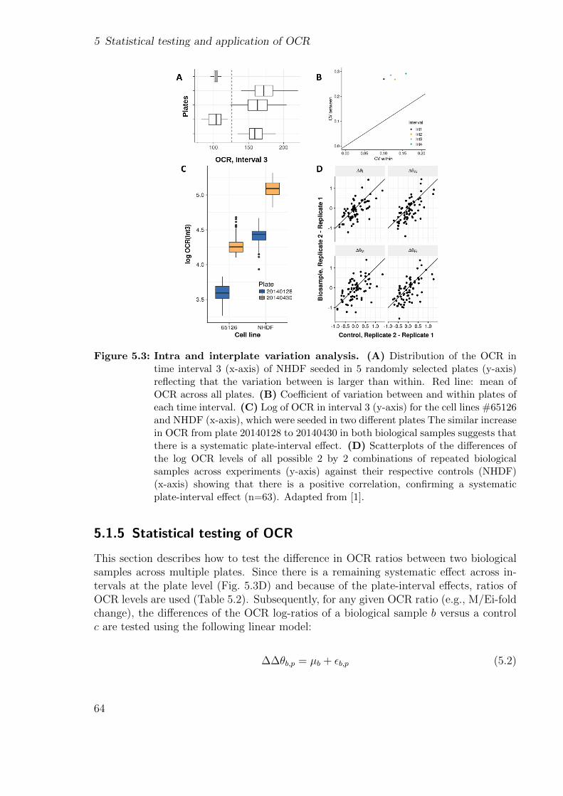
5 Statistical testing and application of OCR
Figure 5.3: Intra and interplate variation analysis. (A) Distribution of the OCR intime interval 3 (x-axis) of NHDF seeded in 5 randomly selected plates (y-axis)reflecting that the variation between is larger than within. Red line: mean ofOCR across all plates. (B) Coefficient of variation between and within plates ofeach time interval. (C) Log of OCR in interval 3 (y-axis) for the cell lines #65126and NHDF (x-axis), which were seeded in two different plates The similar increasein OCR from plate 20140128 to 20140430 in both biological samples suggests thatthere is a systematic plate-interval effect. (D) Scatterplots of the differences ofthe log OCR levels of all possible 2 by 2 combinations of repeated biologicalsamples across experiments (y-axis) against their respective controls (NHDF)(x-axis) showing that there is a positive correlation, confirming a systematicplate-interval effect (n=63). Adapted from [1].
5.1.5 Statistical testing of OCR
This section describes how to test the difference in OCR ratios between two biologicalsamples across multiple plates. Since there is a remaining systematic effect across in-tervals at the plate level (Fig. 5.3D) and because of the plate-interval effects, ratios ofOCR levels are used (Table 5.2). Subsequently, for any given OCR ratio (e.g., M/Ei-foldchange), the differences of the OCR log-ratios of a biological sample b versus a controlc are tested using the following linear model:
∆∆θb,p = µb + εb,p (5.2)
64
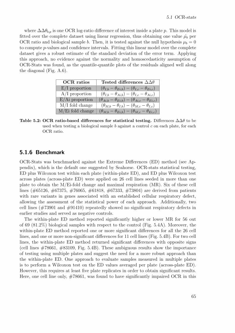
5.1 OCR-stats
where ∆∆θb,p is one OCR log-ratio difference of interest inside a plate p. This model isfitted over the complete dataset using linear regression, thus obtaining one value µb perOCR ratio and biological sample b. Then, it is tested against the null hypothesis µb = 0to compute p-values and confidence intervals. Fitting this linear model over the completedataset gives a robust estimate of the standard deviation of the error term. Applyingthis approach, no evidence against the normality and homoscedasticity assumption ofOCR-Stats was found, as the quantile-quantile plots of the residuals aligned well alongthe diagonal (Fig. A.6).
OCR ratios Tested differences ∆∆θE/I proportion (θI,b − θEi,b)− (θI,c − θEi,c)A/I proportion (θI,b − θAi,b)− (θI,c − θAi,c)
E/Ai proportion (θAi,b − θEi,b)− (θAi,c − θEi,c)M/I fold change (θM,b − θI,b)− (θM,c − θI,c)
M/Ei fold change (θM,b − θEi,b)− (θM,c − θEi,c)
Table 5.2: OCR ratio-based differences for statistical testing. Differences ∆∆θ to beused when testing a biological sample b against a control c on each plate, for eachOCR ratio.
5.1.6 Benchmark
OCR-Stats was benchmarked against the Extreme Differences (ED) method (see Ap-pendix), which is the default one suggested by Seahorse. OCR-stats statistical testing,ED plus Wilcoxon test within each plate (within-plate ED), and ED plus Wilcoxon testacross plates (across-plate ED) were applied on 26 cell lines seeded in more than oneplate to obtain the M/Ei-fold change and maximal respiration (MR). Six of these celllines (#65126, #67375, #76065, #61818, #67333, #73804) are derived from patientswith rare variants in genes associated with an established cellular respiratory defect,allowing the assessment of the statistical power of each approach. Additionally, twocell lines (#73901 and #91410) repeatedly showed no significant respiratory defects inearlier studies and served as negative controls.
The within-plate ED method reported significantly higher or lower MR for 56 outof 69 (81.2%) biological samples with respect to the control (Fig. 5.4A). Moreover, thewithin-plate ED method reported one or more significant differences for all the 26 celllines, and one or more non-significant differences for 11 cell lines (Fig. 5.4B). For two celllines, the within-plate ED method returned significant differences with opposite signs(cell lines #78661, #83109, Fig. 5.4B). These ambiguous results show the importanceof testing using multiple plates and suggest the need for a more robust approach thanthe within-plate ED. One approach to evaluate samples measured in multiple platesis to perform a Wilcoxon test on the ED values averaged per plate (across-plate ED).However, this requires at least five plate replicates in order to obtain significant results.Here, one cell line only, #78661, was found to have significantly impaired OCR in this
65
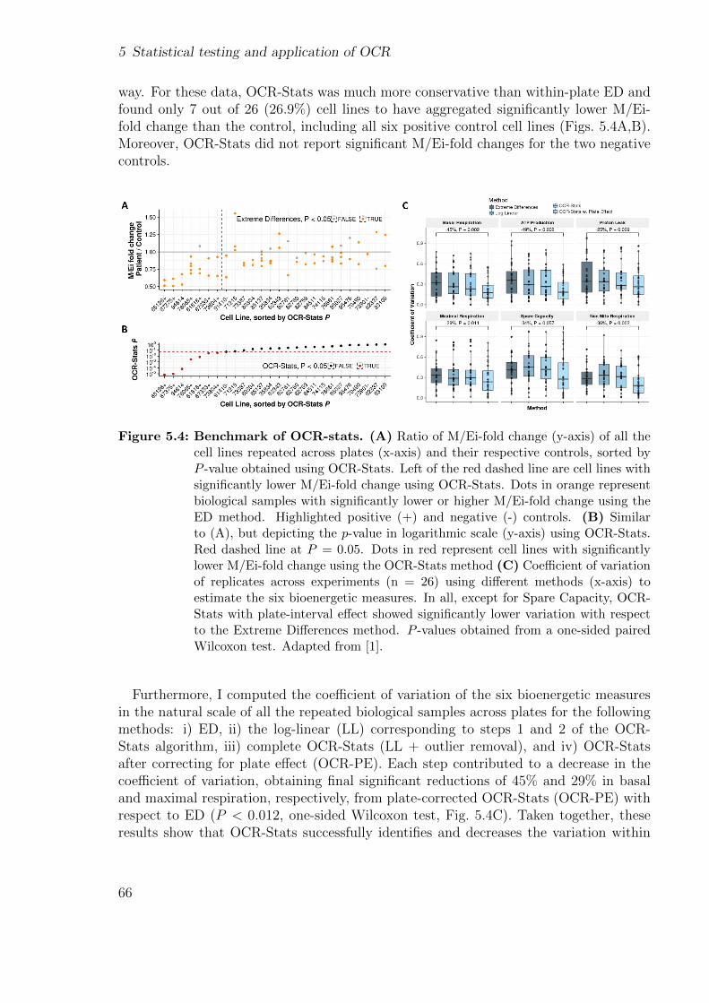
5 Statistical testing and application of OCR
way. For these data, OCR-Stats was much more conservative than within-plate ED andfound only 7 out of 26 (26.9%) cell lines to have aggregated significantly lower M/Ei-fold change than the control, including all six positive control cell lines (Figs. 5.4A,B).Moreover, OCR-Stats did not report significant M/Ei-fold changes for the two negativecontrols.
Figure 5.4: Benchmark of OCR-stats. (A) Ratio of M/Ei-fold change (y-axis) of all thecell lines repeated across plates (x-axis) and their respective controls, sorted byP -value obtained using OCR-Stats. Left of the red dashed line are cell lines withsignificantly lower M/Ei-fold change using OCR-Stats. Dots in orange representbiological samples with significantly lower or higher M/Ei-fold change using theED method. Highlighted positive (+) and negative (-) controls. (B) Similarto (A), but depicting the p-value in logarithmic scale (y-axis) using OCR-Stats.Red dashed line at P = 0.05. Dots in red represent cell lines with significantlylower M/Ei-fold change using the OCR-Stats method (C) Coefficient of variationof replicates across experiments (n = 26) using different methods (x-axis) toestimate the six bioenergetic measures. In all, except for Spare Capacity, OCR-Stats with plate-interval effect showed significantly lower variation with respectto the Extreme Differences method. P -values obtained from a one-sided pairedWilcoxon test. Adapted from [1].
Furthermore, I computed the coefficient of variation of the six bioenergetic measuresin the natural scale of all the repeated biological samples across plates for the followingmethods: i) ED, ii) the log-linear (LL) corresponding to steps 1 and 2 of the OCR-Stats algorithm, iii) complete OCR-Stats (LL + outlier removal), and iv) OCR-Statsafter correcting for plate effect (OCR-PE). Each step contributed to a decrease in thecoefficient of variation, obtaining final significant reductions of 45% and 29% in basaland maximal respiration, respectively, from plate-corrected OCR-Stats (OCR-PE) withrespect to ED (P < 0.012, one-sided Wilcoxon test, Fig. 5.4C). Taken together, theseresults show that OCR-Stats successfully identifies and decreases the variation within
66
5.2 Application of OCR-stats
and between plates, providing more stable testing results, which translates into fewerfalse positives.
5.1.7 Power analysis
Afterwards, the statistical power of OCR-Stats was investigated in this dataset to de-termine the minimum relative differences that the method is able to significantly detect,and the minimal number of well replicates needed. The number of wells of the repeatedbiological samples were subsetted to 4, 6, 8, 10, 12, 14, and 16 on each plate, after whichthe OCR-Stats algorithm and statistical testing were applied to obtain the residuals εb,pand their standard deviation (Fig. 5.5). These were converted to detectable differencesusing the following equation:
exp (1.96sd(εb,p)√
n)− 1 (5.3)
Assuming three plates per comparison and 16 wells per plate, these standard devi-ations allow detecting relative differences of 10% to 15% depending on the consideredlog OCR ratios differences for a significance level of 5% (Fig. 5.5, right y-axis). Rela-tive differences of 10% to 15% are in line with reported detected variations which areas low as 12% to 30% [159, 160, 161]. This analysis also suggests to seed at least 12wells per biological sample per plate, since increased standard deviations of the residualsfor numbers of wells smaller than 12 are observed. This power calculation is based onmeasurements performed in the Helmholtz Zentrum Munich only. Other laboratoriesmight have larger or smaller measurement variations. Nonetheless, this procedure couldbe used as a guideline for power calculation.
5.1.8 Other normalization considerations
The same number of cells were seeded in all the wells from all the assays the assaysdescribed here. Hence, the variations across wells observed in the cell number at theend of the experiments are largely overestimated by noise in the measurements. Inother experimental settings in which different numbers of cells are seeded, an offset termto the model in Eq. 5.1 should be included equal to the logarithm of the seeded cellnumber to control for this variation by design. In addition, the Seahorse XF Analyzercan be used on isolated mitochondria and on isolated enzymes, where a normalizationapproach is to divide OCR by mitochondrial proteins or enzyme concentration [80].However, as described here for cellular assays, robust normalization procedures requirecareful analysis.
5.2 Application of OCR-stats
This section is based on the publication by Gusic et al. [3], in which I was involved.After receiving the OCR measurements from Mirjana Gusic, I performed the statistical
67
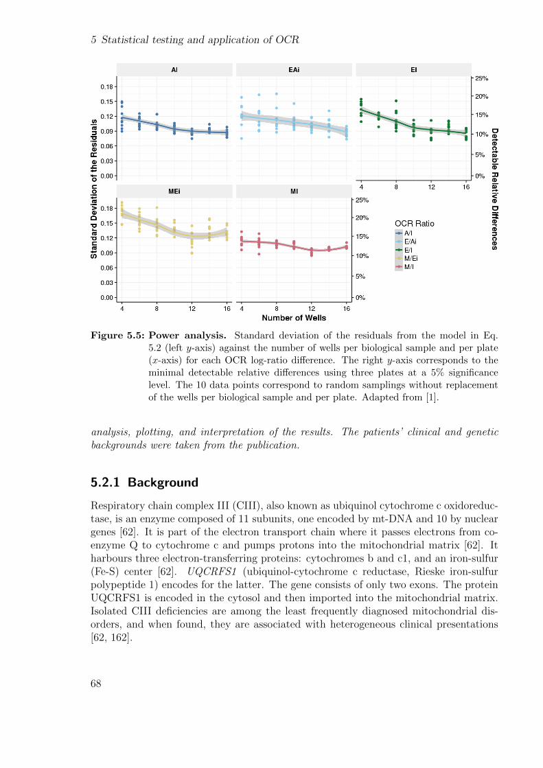
5 Statistical testing and application of OCR
Figure 5.5: Power analysis. Standard deviation of the residuals from the model in Eq.5.2 (left y-axis) against the number of wells per biological sample and per plate(x-axis) for each OCR log-ratio difference. The right y-axis corresponds to theminimal detectable relative differences using three plates at a 5% significancelevel. The 10 data points correspond to random samplings without replacementof the wells per biological sample and per plate. Adapted from [1].
analysis, plotting, and interpretation of the results. The patients’ clinical and geneticbackgrounds were taken from the publication.
5.2.1 Background
Respiratory chain complex III (CIII), also known as ubiquinol cytochrome c oxidoreduc-tase, is an enzyme composed of 11 subunits, one encoded by mt-DNA and 10 by nucleargenes [62]. It is part of the electron transport chain where it passes electrons from co-enzyme Q to cytochrome c and pumps protons into the mitochondrial matrix [62]. Itharbours three electron-transferring proteins: cytochromes b and c1, and an iron-sulfur(Fe-S) center [62]. UQCRFS1 (ubiquinol-cytochrome c reductase, Rieske iron-sulfurpolypeptide 1) encodes for the latter. The gene consists of only two exons. The proteinUQCRFS1 is encoded in the cytosol and then imported into the mitochondrial matrix.Isolated CIII deficiencies are among the least frequently diagnosed mitochondrial dis-orders, and when found, they are associated with heterogeneous clinical presentations[62, 162].
68
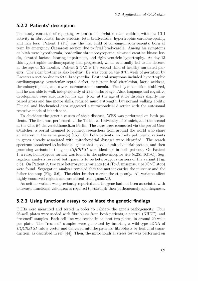
5.2 Application of OCR-stats
5.2.2 Patients’ description
The study consisted of reporting two cases of unrelated male children with low CIIIactivity in fibroblasts, lactic acidosis, fetal bradycardia, hypertrophic cardiomyopathy,and hair loss. Patient 1 (P1) was the first child of consanguineous parents, born atterm by emergency Caesarean section due to fetal bradycardia. Among his symptomsat birth were hypothermia, borderline thrombocytopenia, elevated creatine kinase lev-els, elevated lactate, hearing impairment, and right ventricle hypertrophy. At day 13this hypertrophic cardiomyopathy had progressed, which eventually led to his deceaseat the age of 3.5 months. Patient 2 (P2) is the second child of healthy unrelated par-ents. The elder brother is also healthy. He was born on the 37th week of gestation byCaesarean section due to fetal bradycardia. Postnatal symptoms included hypertrophiccardiomyopathy, ventricular septal defect, persistent fetal circulation, lactic acidosis,thrombocytopenia, and severe normochromic anemia. The boy’s condition stabilized,and he was able to walk independently at 23 months of age. Also, language and cognitivedevelopment were adequate for his age. Now, at the age of 9, he displays slightly im-paired gross and fine motor skills, reduced muscle strength, but normal walking ability.Clinical and biochemical data suggested a mitochondrial disorder with the autosomalrecessive mode of inheritance.
To elucidate the genetic causes of their diseases, WES was performed on both pa-tients. The first was performed at the Technical University of Munich, and the secondat the Charite Universitatsmedizin Berlin. The cases were connected via the portal Gen-eMatcher, a portal designed to connect researchers from around the world who sharean interest in the same gene(s) [163]. On both patients, no likely pathogenic variantsin genes already associated with mitochondrial diseases were identified. The searchspectrum broadened to include all genes that encode a mitochondrial protein, and thenpromising variants in the gene UQCRFS1 were identified in both patients. On Patient1, a rare, homozygous variant was found in the splice-acceptor site (c.251-1G>C). Seg-regation analysis revealed both parents to be heterozygous carriers of the variant (Fig.5.6). On Patient 2, two rare heterozygous variants (c.41T>A missense, c.610C>T stop)were found. Segregation analysis revealed that the mother carries the missense and thefather the stop (Fig. 5.6). The elder brother carries the stop only. All variants affecthighly conserved regions and are absent from gnomAD.
As neither variant was previously reported and the gene had not been associated witha disease, functional validation is required to establish their pathogenicity and diagnosis.
5.2.3 Using functional assays to validate the genetic findings
OCRs were measured and tested in order to validate the gene’s pathogenicity. Four96-well plates were seeded with fibroblasts from both patients, a control (NHDF), and“rescued” samples. Each cell line was seeded in at least two plates, in around 20 wellsper plate. The “rescued” samples were generated by inserting a wild-type cDNA ofUQCRSFS1 into a vector and delivered into the patients’ fibroblasts by lentiviral trans-duction, as described in ref. [44]. Then, the mitochondrial stress test was performed on
69
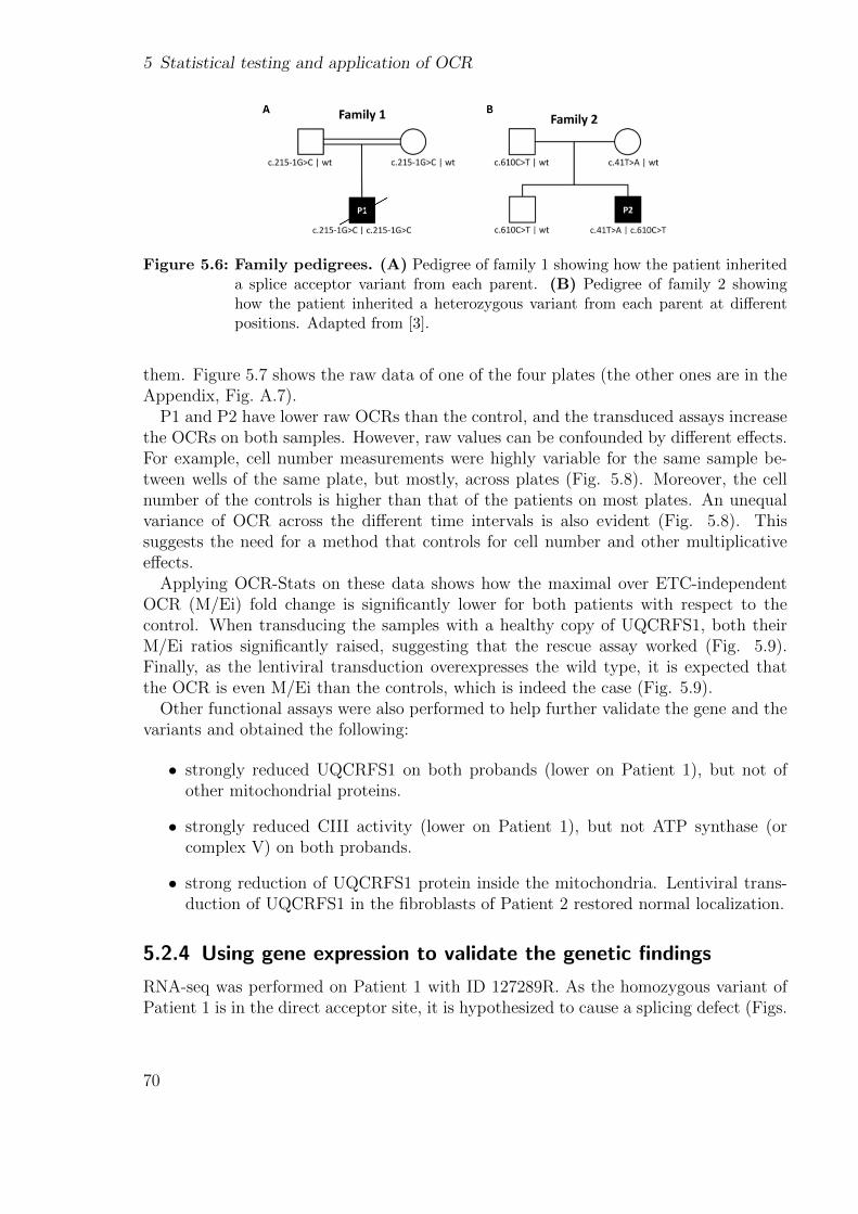
5 Statistical testing and application of OCR
Figure 5.6: Family pedigrees. (A) Pedigree of family 1 showing how the patient inheriteda splice acceptor variant from each parent. (B) Pedigree of family 2 showinghow the patient inherited a heterozygous variant from each parent at differentpositions. Adapted from [3].
them. Figure 5.7 shows the raw data of one of the four plates (the other ones are in theAppendix, Fig. A.7).
P1 and P2 have lower raw OCRs than the control, and the transduced assays increasethe OCRs on both samples. However, raw values can be confounded by different effects.For example, cell number measurements were highly variable for the same sample be-tween wells of the same plate, but mostly, across plates (Fig. 5.8). Moreover, the cellnumber of the controls is higher than that of the patients on most plates. An unequalvariance of OCR across the different time intervals is also evident (Fig. 5.8). Thissuggests the need for a method that controls for cell number and other multiplicativeeffects.
Applying OCR-Stats on these data shows how the maximal over ETC-independentOCR (M/Ei) fold change is significantly lower for both patients with respect to thecontrol. When transducing the samples with a healthy copy of UQCRFS1, both theirM/Ei ratios significantly raised, suggesting that the rescue assay worked (Fig. 5.9).Finally, as the lentiviral transduction overexpresses the wild type, it is expected thatthe OCR is even M/Ei than the controls, which is indeed the case (Fig. 5.9).
Other functional assays were also performed to help further validate the gene and thevariants and obtained the following:
• strongly reduced UQCRFS1 on both probands (lower on Patient 1), but not ofother mitochondrial proteins.
• strongly reduced CIII activity (lower on Patient 1), but not ATP synthase (orcomplex V) on both probands.
• strong reduction of UQCRFS1 protein inside the mitochondria. Lentiviral trans-duction of UQCRFS1 in the fibroblasts of Patient 2 restored normal localization.
5.2.4 Using gene expression to validate the genetic findings
RNA-seq was performed on Patient 1 with ID 127289R. As the homozygous variant ofPatient 1 is in the direct acceptor site, it is hypothesized to cause a splicing defect (Figs.
70
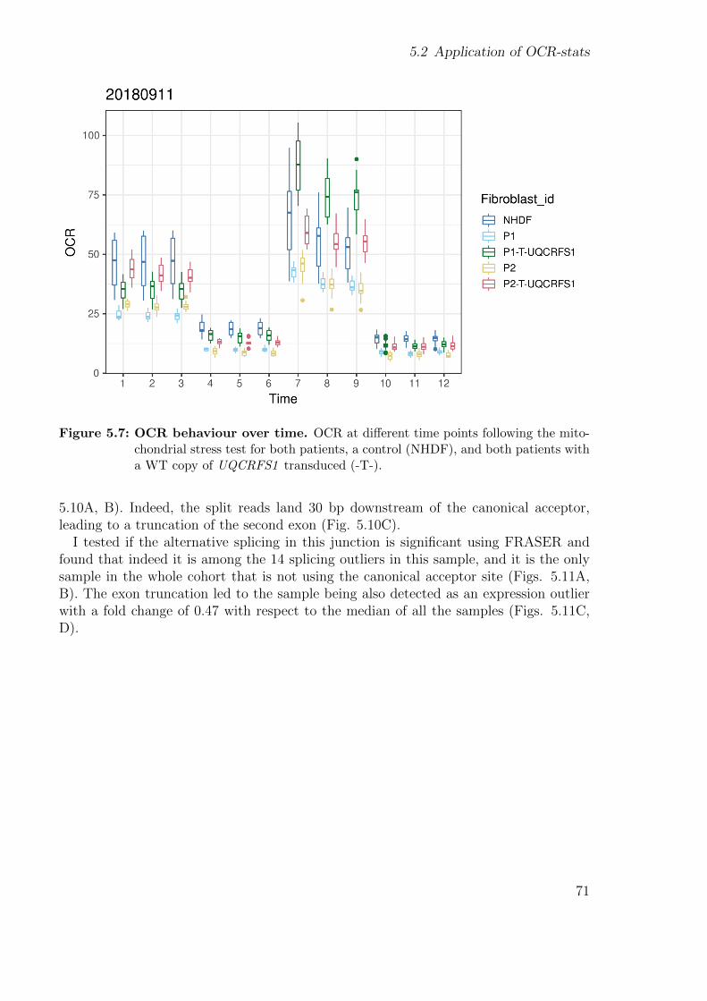
5.2 Application of OCR-stats
Figure 5.7: OCR behaviour over time. OCR at different time points following the mito-chondrial stress test for both patients, a control (NHDF), and both patients witha WT copy of UQCRFS1 transduced (-T-).
5.10A, B). Indeed, the split reads land 30 bp downstream of the canonical acceptor,leading to a truncation of the second exon (Fig. 5.10C).
I tested if the alternative splicing in this junction is significant using FRASER andfound that indeed it is among the 14 splicing outliers in this sample, and it is the onlysample in the whole cohort that is not using the canonical acceptor site (Figs. 5.11A,B). The exon truncation led to the sample being also detected as an expression outlierwith a fold change of 0.47 with respect to the median of all the samples (Figs. 5.11C,D).
71
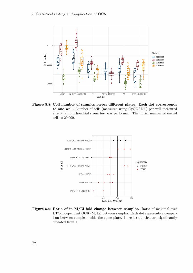
5 Statistical testing and application of OCR
Figure 5.8: Cell number of samples across different plates. Each dot correspondsto one well. Number of cells (measured using CyQUANT) per well measuredafter the mitochondrial stress test was performed. The initial number of seededcells is 20,000.
Figure 5.9: Ratio of in M/Ei fold change between samples. Ratio of maximal overETC-independent OCR (M/Ei) between samples. Each dot represents a compar-ison between samples inside the same plate. In red, tests that are significantlydeviated from 1.
72
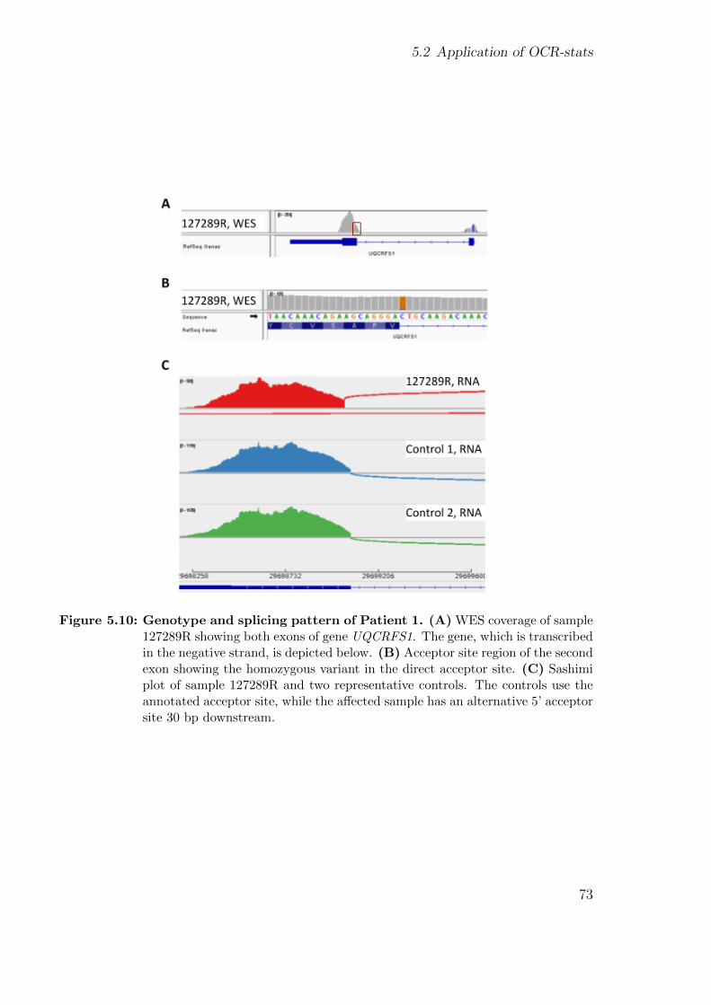
5.2 Application of OCR-stats
Figure 5.10: Genotype and splicing pattern of Patient 1. (A) WES coverage of sample127289R showing both exons of gene UQCRFS1. The gene, which is transcribedin the negative strand, is depicted below. (B) Acceptor site region of the secondexon showing the homozygous variant in the direct acceptor site. (C) Sashimiplot of sample 127289R and two representative controls. The controls use theannotated acceptor site, while the affected sample has an alternative 5’ acceptorsite 30 bp downstream.
73
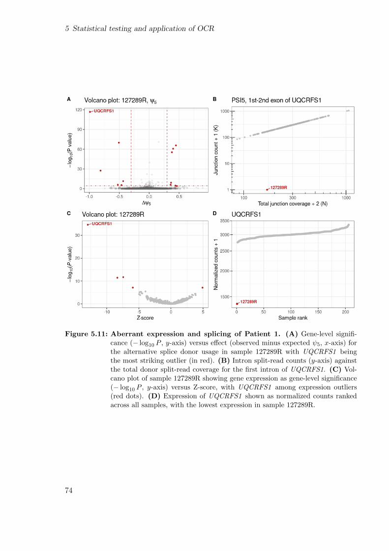
5 Statistical testing and application of OCR
Figure 5.11: Aberrant expression and splicing of Patient 1. (A) Gene-level signifi-cance (− log10 P , y-axis) versus effect (observed minus expected ψ5, x-axis) forthe alternative splice donor usage in sample 127289R with UQCRFS1 beingthe most striking outlier (in red). (B) Intron split-read counts (y-axis) againstthe total donor split-read coverage for the first intron of UQCRFS1. (C) Vol-cano plot of sample 127289R showing gene expression as gene-level significance(− log10 P , y-axis) versus Z-score, with UQCRFS1 among expression outliers(red dots). (D) Expression of UQCRFS1 shown as normalized counts rankedacross all samples, with the lowest expression in sample 127289R.
74
6 Conclusion
6.1 Conclusion
WES and WGS have accelerated the diagnostics of known genetic disorders, plus led tothe discovery of new diseases and disease-causal genes. Nevertheless, the rates of newdiscoveries are stalling, while at the same time not all individuals receive a diagnosis.This opened the road for functional assays such as RNA-seq and cellular respirationto become a complementary companion and increase diagnostic rates. In this thesis, Ipresent a workflow
I developed DROP, end-to-end workflow composed of three independent modulesto detect aberrant expression, splicing, and mono-allelic expression to support RNAsequencing-based diagnostics. The workflow includes preprocessing of raw sequencingfiles, quality control steps, and the state-of-the-art statistical methods to compute out-liers. It outputs results tables containing the outliers of each module plus webpagereports. By leveraging parallel computing infrastructures, results from cohorts of hun-dreds of samples can be obtained in a few days. DROP is available online and itsimplementation by external users has already led to diagnoses.
I addressed the issue of combining samples from different origins. Large sample sizes(at least 50 per analysis group) are required to properly detect expression outliers. Usingsamples from affected individuals and controls from GTEx, I showed that it is possibleto combine samples from different cohorts as long as they were sequenced and processedin the same manner and originated from the same tissue. Hence, combining differenttissues is not recommended. The input of DROP can either be raw sequencing files,external count matrices, or a combination of both. Using publicly available data toboost the effective cohort size will allow centers to venture into RNA sequencing fordiagnostics with a low number of samples. Additionally, I showed that fibroblasts are agood clinically accessible tissue as most disease genes are expressed there and provideguidance on how to a priori investigate which tissue expresses the highest amount ofgenes of interest.
In the datasets that I have analyzed, the median number of expression outliers rarelysurpasses five per sample. These expression outliers should be interpreted accordingto their fold changes. A strong down-regulation (fold-changes < 0.2) probably impliesimpaired gene function. Fold-changes of weaker amplitudes should further be investi-gated. In particular, a fold-change of 0.5 often reflects the loss of expression of oneallele. Inspecting the MAE results may further reveal mono-allelic expression of a rarevariant harbored by the other allele. Similarly, among the different analyzed datasets,the median number of aberrantly spliced genes per sample is around 25. These aber-
75
6 Conclusion
rant splicing events should be visualized as sashimi plots to detect the nature of themis-splicing. The next step is to search for splice-site and splice-region variants thatcan explain the defect. However, other variants such as synonymous and deep intronic,have also been described to activate new splice sites potentially originating from crypticexons.
I showcased how to use RNA-seq in interpreting variants in a cohort of 309 individualsaffected with a rare mitochondrial disorder. Analyzing the cohort using DROP andcalling variants in RNA-seq led to the diagnosis of 33 individuals, which represents15% of the 217 WES-unsolved cases. RNA-seq variant calling was deemed very usefulas it helped identify the disease-causal intronic variants missed by WES in 9 out ofthe 33 solved cases. An enrichment of protein-truncating variants was found in bothunderexpression and splicing outliers, in agreement with a similar study done by theGTEx consortium. In addition, loss-of-function intolerant genes were depleted withexpression outliers but mitochondrial disease genes were enriched.
Mitochondrial studies using extracellular fluxes, specifically the XF Analyzer fromSeahorse, are gaining popularity and are finding their way into diagnostics; therefore, it isof paramount importance to have an appropriate statistical method to estimate the OCRlevels from the raw data. I have developed such a model, the OCR-Stats algorithm, whichincludes approaches to control for well and plate-interval effects, and automatic outlieridentification. I demonstrated that OCR comparisons should be performed using ratiosrather than using differences and that the cell lines must be seeded on the same plate, asthis eliminates sources of variation like cell number and well positional and plate-intervaleffects. I introduced a linear model, the OCR-Stats statistical testing, and showedthat the results agree with previous results of patients diagnosed with mitochondrialdisorders. The variation in differences of OCR log-ratios for the same biological sampleacross plates is large and, consequently, samples should be seeded in multiple plates.Power analyses showed that OCR-stats can detect relative differences of 10% - 15% andthat the minimum number of well replicates per biological sample in a 96-well plateshould be 12. Different benchmarks showed that OCR-stats outperforms other methodsby reducing the coefficient of variation of the OCR estimates across replicates, andvalidating all samples with a confirmed mitochondrial defect. Cellular respiration wasused as another source of functional validation to confirm the pathogenicity of a gene intwo unrelated individuals suffering from a mitochondrial disorder.
6.2 Discussion
With decreasing costs of sequencing, WES, and eventually WGS, are expected to beadopted in routine diagnostics. For example, the NHS in England plans to increasethe provision of WGS-based diagnostics from 8,000 to 30,000 samples per month start-ing 2020 [164]. With more readily sequencing plus integration with other omics andfunctional assays, the future of diagnostics of rare disorders seems optimistic. In fact,the goals of the International Rare Diseases Research Consortium until 2027 are quitepromising [165]:
76
6.2 Discussion
1. all patients coming to medical attention with a suspected rare disease will bediagnosed within 1 year if their disorder is known in the medical literature; allcurrently undiagnosable individuals will enter a globally coordinated diagnosticand research pipeline
2. 1,000 new therapies for rare diseases will be approved
3. methodologies will be developed to assess the impact of diagnoses and therapieson rare disease patient
Nevertheless, there are still some clinical challenges that need to be improved [11]:
• non-specific clinical presentations (e.g., developmental delay)
• ultra-rare and unrecognized genetic diseases
• lack of ontology encompassing the complete spectrum of human phenotypes
• inconsistent, multidisciplinary approaches to patient evaluation
• inability to account for and compare age-specific or population-specific diseasepresentations
• standardization of data-sharing (e.g. for drug development, gene matching)
• biological insight into the function of most genes
• expertise in the analysis of non-coding variants
This thesis aimed at tackling some of them by providing robust methods and pipelinesto compute expression outliers, creating standard count matrices to share across cohorts,and showcasing how RNA-seq can be used to interpret (non-coding) variants.
Integration of other omicsRNA-seq for diagnostics has its limitations. One of them is the gene of interest not
being expressed in the probed tissue. Another one is that not all disease-causal variants(e.g. missense) affect the transcript. Proteomics can be used to identify protein-levelchanges brought about by these (missense) variants that affect protein stability or post-translational modifications [47]. Our collaborators from the Helmholtz Zentrum havebegun using large-scale proteomics on the Prokisch dataset described in this thesis whichhas led to clarifying the pathological consequence of missense variants. This could giverise to the development of a statistical method that jointly models gene expression withprotein intensities.
Metabolomics can also be used in diagnostics as they are likely to be very close to thephenotype [47]. The Undiagnosed Diseases Network (UDN) in the United States has
77
6 Conclusion
incorporated metabolomics to DNA sequencing and has obtained an overall diagnosticrate of 35% among 382 rare disorder patients with a complete clinical evaluation [12].
Growth of genome assemblies and databasesBetter assembly of reference genomes will help to increase the effectiveness of both
DNA and RNA-seq in diagnostics. For DNA, a more precise assembly can help to assignthe right consequence to a variant. This, combined with better variant-effect predictivemodels will also help prioritization. Regarding RNA, using a newer version to countgenes (#29 instead of #19) of the annotation provided by Gencode [88] led to 5% moreof OMIM genes being detected in the Prokisch dataset.
Improvements and updates to variant databases like ClinVar or gnomAD are also ofextreme importance. By 2016, the predecessor of gnomAD, the Exome AggregationConsortium (ExAC), had gathered WES from over 60,000 individuals of diverse an-cestries to compute allele frequencies [166]. These frequencies were adopted to definerare variants. Since then, it has duplicated the number of WES and, more importantly,now includes more than 15,000 WGS [97]. This led to a higher number of estimatedallele frequencies, especially in intronic regions. Gathering more samples from differentethnicities will make these frequencies more accurate and cover more genomic positions.
A meta-analysis on ClinVar showed that in the period between May 2016 and Septem-ber 2017, 179,432 new variants were added to ClinVar [167]. Moreover, 7,615 variantschanged classification, in all possible combinations between pathogenic, benign, VUS,and conflicting interpretations [167]. Yang et al. tested the classification of the variantsand concluded that 0.5% of ClinVar classifications are erroneous [168]. Nevertheless,they also show that this misclassification rate is decreasing over time, reflecting a betterunderstanding of pathogenicity and large sequencing efforts [168].
Extension to common diseasesRNA-seq has been applied to cohorts of rare disorders by calling outliers that can lead
to finding rare variants. Its application in a similar fashion to common diseases remain.Unlike rare diseases, common diseases are usually caused by a combination of variantsacross multiple genes [169]. For example, schizophrenia pathology is hypothesized to bedriven by the interplay of many common and rare genetic variants that act in concertin neural cell populations [170]. In collaboration with the Max Planck Institute ofPsychiatry, we have analyzed RNA-seq samples derived from individuals suffering fromschizophrenia and bipolar disorder. We found an enrichment of neurodevelopmentaldisease genes [17] among the expression outliers, but interpretation and validation ofthese results are still pending.
Aberrations in the genome like mutations and karyotype changes are the direct geneticcauses of leukemia and other types of cancer. Common driver mutations in leukemiahave been identified [171]. Yet, rare driver mutations and their pathological mechanism
78
6.2 Discussion
are not well understood [171, 172]. Our autoencoder approach to detect outliers accountsfor gene co-expression and focuses on detecting strong effects, which, in this context, canlead to detecting the driver mutations. In this respect, we have begun analyzing a cohortof more than 4,000 blood samples derived from individuals suffering from leukemia.
Potential role of on-coding RNAs
Generally, non-protein-coding RNAs (ncRNAs) are discarded by standard WES anal-yses as potential disease-causal genes. Nevertheless, some have been found to playcritical roles in various biological processes and their dysfunctions have been associatedwith a wide range of diseases [173, 174]. For example, recently, nine ncRNAS haveemerged as potent regulators of mitochondrial metabolism [175]. Among them, ncRNALINC00116 was found to interact with several complexes to influence mitochondrialmembrane potential, respiration, Ca2+ retention capacity, ROS, and supercomplex lev-els [176]. Inspired by these cases, on a project not mentioned in this thesis, I correlatedthe gene expression of ncRNAs with that of mitochondrial localized genes [177] andmitochondrial disease genes and oxygen consumption rates from the Prokisch cohort.LINC00493, later renamed SMIM26, had the highest correlation suggesting a potentialmitochondrial-related function. On-going research on the function of ncRNAs will likelylead to discovering their roles in disease.
Other uses of RNA-seq
RNA-seq data can be used in diagnostics for other two purposes not discussed in thisthesis. The first one is variant phasing. Due to splicing, variants can be phased overlonger distances than WES or WGS. Phasing is useful in the clinical setting by allowingto distinguish between compound heterozygotes from variants on the same allele [178].Variant phasing can greatly be benefited from longer RNA reads. The second one isgene fusion. Gene fusion happens when, due to chromosomal translocation, inversion,deletion, or duplication, genetic material from different genes are merged and transcribedtogether. Even though gene fusion has been used more extensively in cancer [179, 180],it has also been recently applied to diagnose patients with congenital [181] and rarediseases [182]. The integration of these and other tools as DROP modules could beconsidered in the future.
All the RNA-seq data presented in this thesis came from bulk RNA-seq. Single-cellRNA-seq (scRNA-seq) data can help to identify cell-type-specific outliers, especially dueto differentially expressed genes. Statistical methods and software to detect aberrantexpression on scRNA-seq data have already been carried by my lab with promisingresults. These could later be introduced as a new module in DROP.
79
6 Conclusion
Data standardizationBAM and VCF files have established themselves as optimal file formats to store se-
quencing and variant data, respectively. This has enabled the easy sharing betweencollaborators and the application of the same tools to access or process them. Neverthe-less, publicly sharing them is usually not straightforward because they contain variantdata. Count matrices do not contain variant data, making them easier to share. How-ever, for count data, there is still not one global file format. In this thesis, I have tackledthis problem in three ways. First, by designing DROP to allow the user to export thegene-level, split, and non-split counts (section 2.1.3) in a standard format, alongsidemetadata describing the cohort. Second, by designing DROP to be able to take as in-put these standardized matrices alongside BAM files. Third, by gathering and sharingthree datasets, each of >100 samples, online for download via Zenodo. Research centresaround the world have already used this functionality which will hopefully help themdiagnose cases.
Future of DROPOne of the goals of this thesis was to build a scalable pipeline able to handle hundreds
of RNA-seq samples. The modifications in the pipeline allowed FRASER to handleup to 900 samples. Nevertheless, it is still not able to handle thousands. Also, theexact sample size limits of both OUTRIDER and FRASER have not been tested. Itis important to increase the performance and capacity of both methods as cohorts areexpected to grow. Also, GATK’s function to perform the allelic counts [91] takes around2 h per sample on variants derived from WES, which translates into around 16 h onvariants derived from WGS. Further adaptations to DROP can be made to subset theWGS to expressed genes or exonic regions before counting.
We plan to establish a community of researchers and clinicians that use RNA-seq fordiagnostics. DROP has already been improved with feedback from external users. Acommunity will further help to shape DROP to the user’s requirements. Moreover, itwill boost count data sharing.
Finding the right tissueGonorazky et al. transformed fibroblasts into myoblasts which better reflected the
muscle transcriptome and led to detecting aberrant splicing events missed by fibroblastsor blood [46]. Another approach could be to reprogram accessible cells into inducedpluripotent stem cells, where as many as 27,046 genes are expressed [183]. However, suchprocedures are more laborious, expensive, and time-consuming than simply extractingblood.
The usefulness of each tissue to detect the causal aberration needs to be further inves-tigated. In this thesis, I discussed the percentage of different groups of genes expressedin various tissues. A study from GTEx comparing the outliers across tissues found that
80
6.2 Discussion
only 5% of expression outliers and 8% of splicing outliers are reproduced across thedifferent tissues [118]. A systematic aberrant expression and splicing analysis acrossvarious tissues from affected samples needs to be carried to determine in which tissuesthe causal aberration was detected. For example, in Murdock et al., 6 solved cases weresequenced both in fibroblasts and blood. RNA-seq from blood failed to identify thecausative defect in half, while none were missed with fibroblasts [4].
81

A Appendix
A.1 Appendix: Additional Methods
A.1.1 Counting reads
Counting reads that are paired with mates from the opposite strands (singleEnd =
FALSE) was performed using the summarizeOverlaps function from the GenomicAlign-ments package [184]. Only reads that fall completely within an exon or span two exonsfrom the same gene via splicing were considered (mode = intersectionStrict). Readsthat overlap more than one feature were assigned to each of those features instead ofbeing removed (inter.feature = FALSE). Genes with a 95th percentile FPKM < 1 wereconsidered to be not sufficiently expressed and filtered out. The used reference genomewas the GRCh37 primary assembly, release 29, of the GENCODE project [185] whichcontains 60,829 genes.
Split reads are counted using the summarizeJunctions function from the Genom-icAlignments package [184], and non-split reads overlapping splice sites are countedusing the featureCounts function from the Rsubread package [186]. Then, they areconverted into the intron-centric metrics percent-spliced-in and splicing efficiency [103].Afterwards, introns with less than 20 reads in all samples and introns for which the totalnumber of reads at the donor and acceptor splice site is zero in more than 95% of thesamples are filtered out.
In order to get the allelic counts, first, VCF files from either WES or WGS are subset-ted to obtain only SNVs using the view command from bcftools [93]. Then, the alleliccounting is performed using the ASEReadCounter function from GATK [91]. A negativebinomial test is applied to the reads using the DESeq2 package [106] fixing the dispersionparameter to 0.05 as done in Kremer et al. [44].
A.1.2 Obtaining set of positions not in linkage disequilibrium
In order to obtain a set of positions not in linkage disequilibrium, all the variants fromthe samples in the test dataset were pooled and subsetted to consider only the onesin autosomal chromosomes that are not in linkage disequilibrium using the functionsnpgdsLDpruning from the R/Bioconductor package SNPRelate [187]. Applying a link-age disequilibrium threshold of 0.2, we obtained a set of P = 26, 402 variants and theirgenomic positions.
83
A Appendix
A.1.3 Variant calling in RNA-seq
Variants were called on RNA-Seq data using GATK best practices for RNAseq short vari-ant discovery (https://gatk.broadinstitute.org/hc/RNAseq-short-variant-discovery-SNPs-Indels-).Variants with a ratio of quality to depth of coverage < 2, that were strand biased (Phredscaled fisher exact score > 30), or belonging to a SNP cluster (if 3 or more SNPs arefound within a 35 base window) were filtered out, as suggested by GATK. Furthermore,variants not contained in a repeat masked region (as defined by RepeatMasker [92]), andwith 3 or more reads supporting the alternative allele were prioritized.
A.1.4 Variant annotation and handling
Variants were annotated for consequence, location, minor allele frequencies (from the1000 Genomes Project [98], gnomAD [97], and the UK Biobank [188]) and deleteriousnessscores using the Variant Effect Predictor [94] from ensembl. For variants that fell onmultiple transcripts and had therefore multiple consequences, the one with the highestimpact was selected [100]. A variant is considered to be rare if the maximum minorallele frequency across all cohorts is less than 0.001. ACMG variant (re)classificationwas done with the InterVar software tool [189].
A.1.5 Measure of extracellular fluxes using Seahorse XF96
20,000 fibroblast cells were seeded in each well of a XF 96-well cell culture microplate in80 ml of culture medium, and incubated them overnight at 37◦C in 5% CO2. The fourcorners were left only with medium for background correction. Cells were incubatedat 37◦C for 30 min before measurement. OCR were measured an XF96 ExtracellularFlux Analyzer. OCR was determined at four levels: with no additions, and after addingoligomycin (1 µM), carbonyl cyanide 4-(trifluoromethoxy) phenylhydrazone (FCCP, 0.4µM), and rotenone (2 µM). After each assay, manual inspection was performed on allwells using a conventional light microscope.
A.1.6 Cell number quantification
The cell number was quantified using the CyQuant Cell Proliferation Kit (Thermo FisherScientific, Waltham, MA, USA), according to the manufacturer’s protocol. In brief, thecells were washed with 200 µL PBS per well and frozen in the microplate at -80◦Cto ensure subsequent cell lysis. The cells were thawed and resuspended vigorously in200 µL of 1x cell-lysis buffer supplemented with 1x CyQUANT GR dye per well. Theresuspended cells were incubated in the dark for 5 min at RT, whereupon fluorescencewas measured (excitation: 480 nm, emission: 520 nm).
A.1.7 Seahorse method to compute OCR
On every plate independently, for each well, in interval 1 take the OCR correspondingto the last measurement, in intervals 2 and 4 take the minimum, and in interval 3 the
84
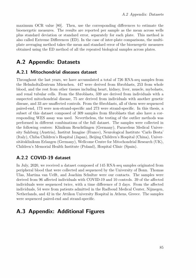
A.2 Appendix: Datasets
maximum OCR value [80]. Then, use the corresponding differences to estimate thebioenergetic measures. The results are reported per sample as the mean across wellsplus standard deviation or standard error, separately for each plate. This method isalso called Extreme Differences (ED). In the case of inter-plate comparisons, the multi-plate averaging method takes the mean and standard error of the bioenergetic measuresobtained using the ED method of all the repeated biological samples across plates.
A.2 Appendix: Datasets
A.2.1 Mitochondrial diseases dataset
Throughout the last years, we have accumulated a total of 726 RNA-seq samples fromthe HelmholtzZentrum Muenchen. 447 were derived from fibroblasts, 253 from wholeblood, and the rest from other tissues including heart, kidney, liver, muscle, mybolasts,and renal tubular cells. From the fibroblasts, 339 are derived from individuals with asuspected mitochondrial disease, 75 are derived from individuals with another geneticdisease, and 33 are unaffected controls. From the fibroblasts, all of them were sequencedpaired-end, 173 were non-strand-specific and 273 were strand-specific. In this thesis, asubset of this dataset composed of 309 samples from fibroblasts that also have a cor-responding WES assay was used. Nevertheless, the testing of the outlier methods wasperformed in different combinations of the full dataset. The samples were collected inthe following centers: Klinikum Reuchtlingen (Germany), Paracelsus Medical Univer-sity Salzburg (Austria), Institut Imagine (France), Neurological Institute ‘Carlo Besta’(Italy), Chiba Children’s Hospital (Japan), Beijing Children’s Hospital (China), Univer-sitatsklinikum Erlangen (Germany), Wellcome Centre for Mitochondrial Research (UK),Children’s Memorial Health Institute (Poland), Hospital Clınic (Spain).
A.2.2 COVID-19 dataset
In July, 2020, we received a dataset composed of 145 RNA-seq samples originated fromperipheral blood that were collected and sequenced by the University of Bonn. ThomasUlas, Martina van Uelft, and Joachim Schultze were our contacts. The samples werederived from 96 affected individuals with COVID-19 and 10 controls. 39 of the affectedindividuals were sequenced twice, with a time difference of 3 days. From the affectedindividuals, 54 were from patients admitted in the Radboud Medical Center, Nijmegen,Netherlands, and 42 in the Attikon University Hospital in Athens, Greece. The sampleswere sequenced paired-end and strand-specific.
A.3 Appendix: Additional Figures
85
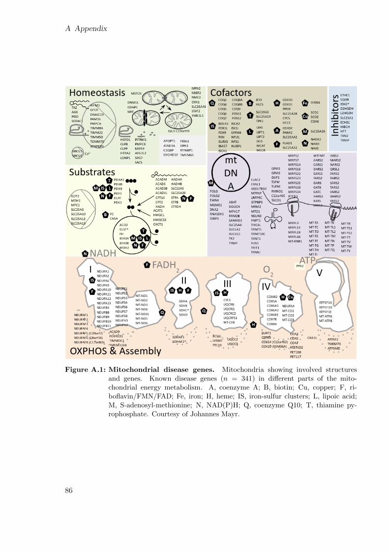
A Appendix
Figure A.1: Mitochondrial disease genes. Mitochondria showing involved structuresand genes. Known disease genes (n = 341) in different parts of the mito-chondrial energy metabolism. A, coenzyme A; B, biotin; Cu, copper; F, ri-boflavin/FMN/FAD; Fe, iron; H, heme; IS, iron-sulfur clusters; L, lipoic acid;M, S-adenosyl-methionine; N, NAD(P)H; Q, coenzyme Q10; T, thiamine py-rophosphate. Courtesy of Johannes Mayr.
86
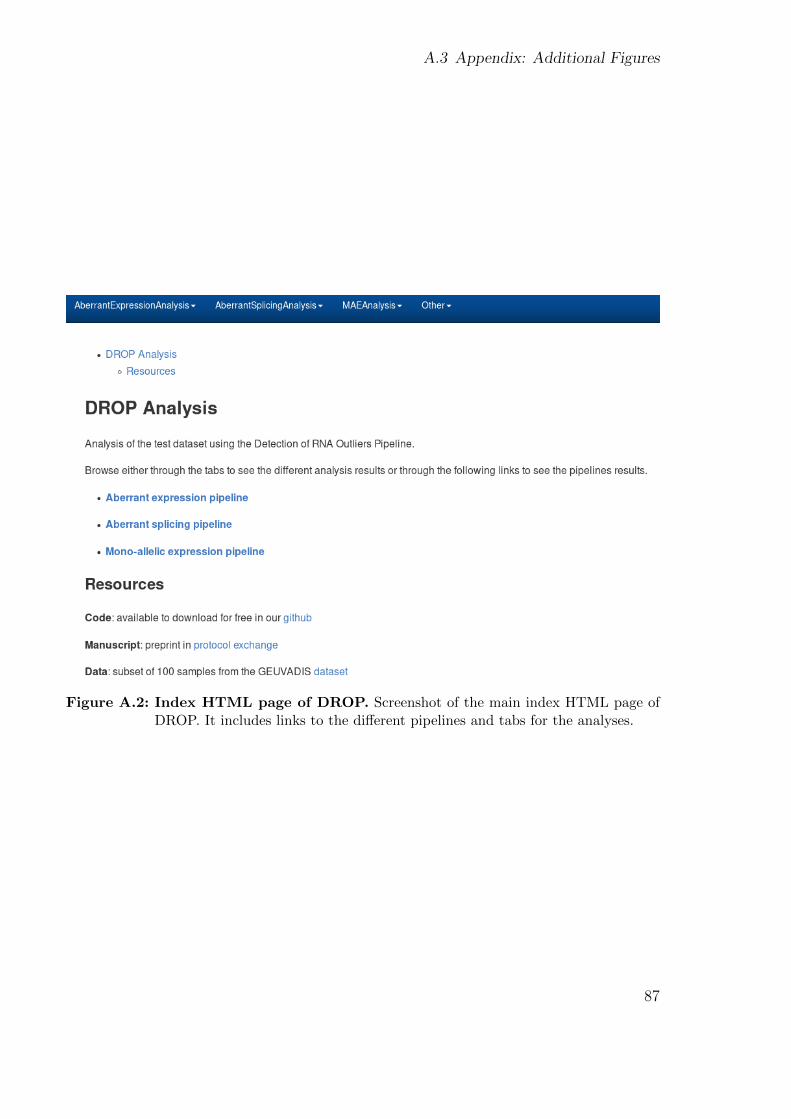
A.3 Appendix: Additional Figures
Figure A.2: Index HTML page of DROP. Screenshot of the main index HTML page ofDROP. It includes links to the different pipelines and tabs for the analyses.
87

A Appendix
Figure A.3: RNA-seq study cohort and workflow. RNA-seq was performed on skin-derived fibroblasts from 309 patients suspected to suffer from a rare disease.All patients have undergone the WES analysis beforehand, which was inconclu-sive for 217. Systematic detection of aberrant events and consequent analysisled to genetic diagnosis in 15% of the WES-undiagnosed cases by establish-ing a genotype-phenotype association, and pinpoint a candidate gene in 6% ofthe WES-undiagnosed cases, suggesting the discovery of novel disease-genes andmore complex pathomechanisms. A transcript defect was also detected in 76%of the WES-diagnosed cases carrying pathogenic protein-truncating variants.
88
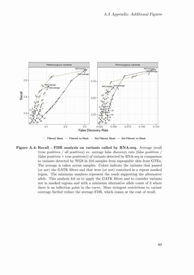
A.3 Appendix: Additional Figures
Figure A.4: Recall - FDR analysis on variants called by RNA-seq. Average recall(true positives / all positives) vs. average false discovery rate (false positives /(false positives + true positives)) of variants detected by RNA-seq in comparisonto variants detected by WGS in 210 samples from suprapubic skin from GTEx.The average is taken across samples. Colors indicate the variants that passed(or not) the GATK filters and that were (or not) contained in a repeat maskedregion. The minimum numbers represent the reads supporting the alternativeallele. This analysis led us to apply the GATK filters and to consider variantsnot in masked regions and with a minimum alternative allele count of 3 wherethere is an inflection point in the curve. More stringent restrictions to variantcoverage further reduce the average FDR, which comes at the cost of recall.
89
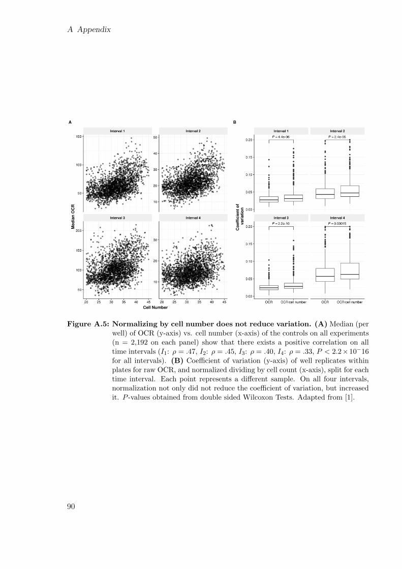
A Appendix
Figure A.5: Normalizing by cell number does not reduce variation. (A) Median (perwell) of OCR (y-axis) vs. cell number (x-axis) of the controls on all experiments(n = 2,192 on each panel) show that there exists a positive correlation on alltime intervals (I1: ρ = .47, I2: ρ = .45, I3: ρ = .40, I4: ρ = .33, P < 2.2×10⁻¹⁶for all intervals). (B) Coefficient of variation (y-axis) of well replicates withinplates for raw OCR, and normalized dividing by cell count (x-axis), split for eachtime interval. Each point represents a different sample. On all four intervals,normalization not only did not reduce the coefficient of variation, but increasedit. P -values obtained from double sided Wilcoxon Tests. Adapted from [1].
90
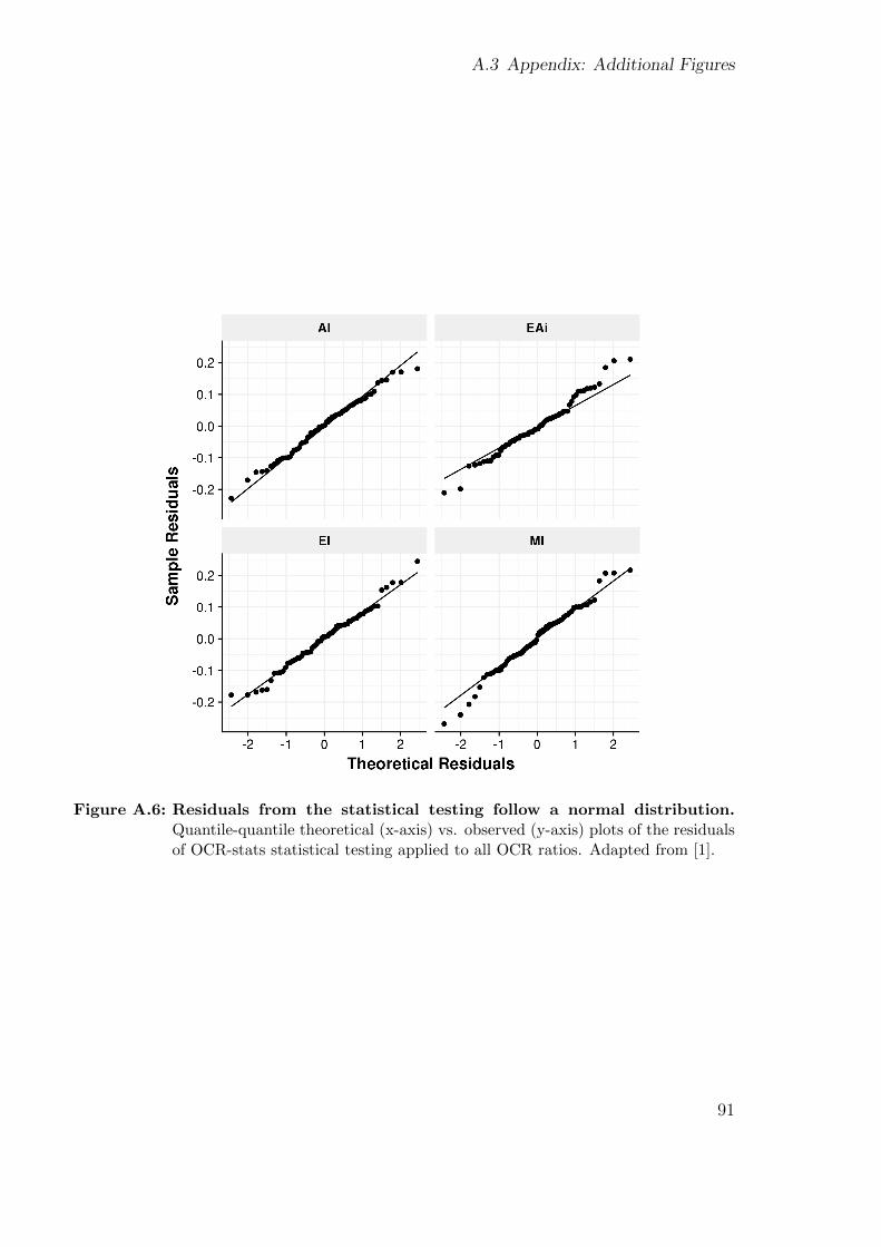
A.3 Appendix: Additional Figures
Figure A.6: Residuals from the statistical testing follow a normal distribution.Quantile-quantile theoretical (x-axis) vs. observed (y-axis) plots of the residualsof OCR-stats statistical testing applied to all OCR ratios. Adapted from [1].
91
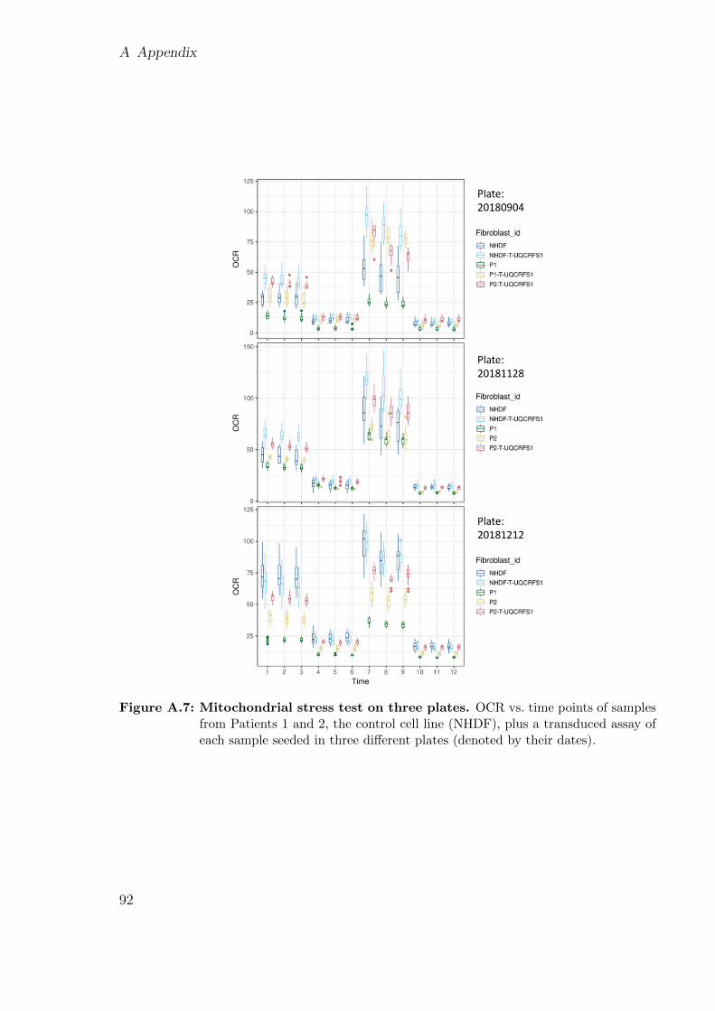
A Appendix
Figure A.7: Mitochondrial stress test on three plates. OCR vs. time points of samplesfrom Patients 1 and 2, the control cell line (NHDF), plus a transduced assay ofeach sample seeded in three different plates (denoted by their dates).
92
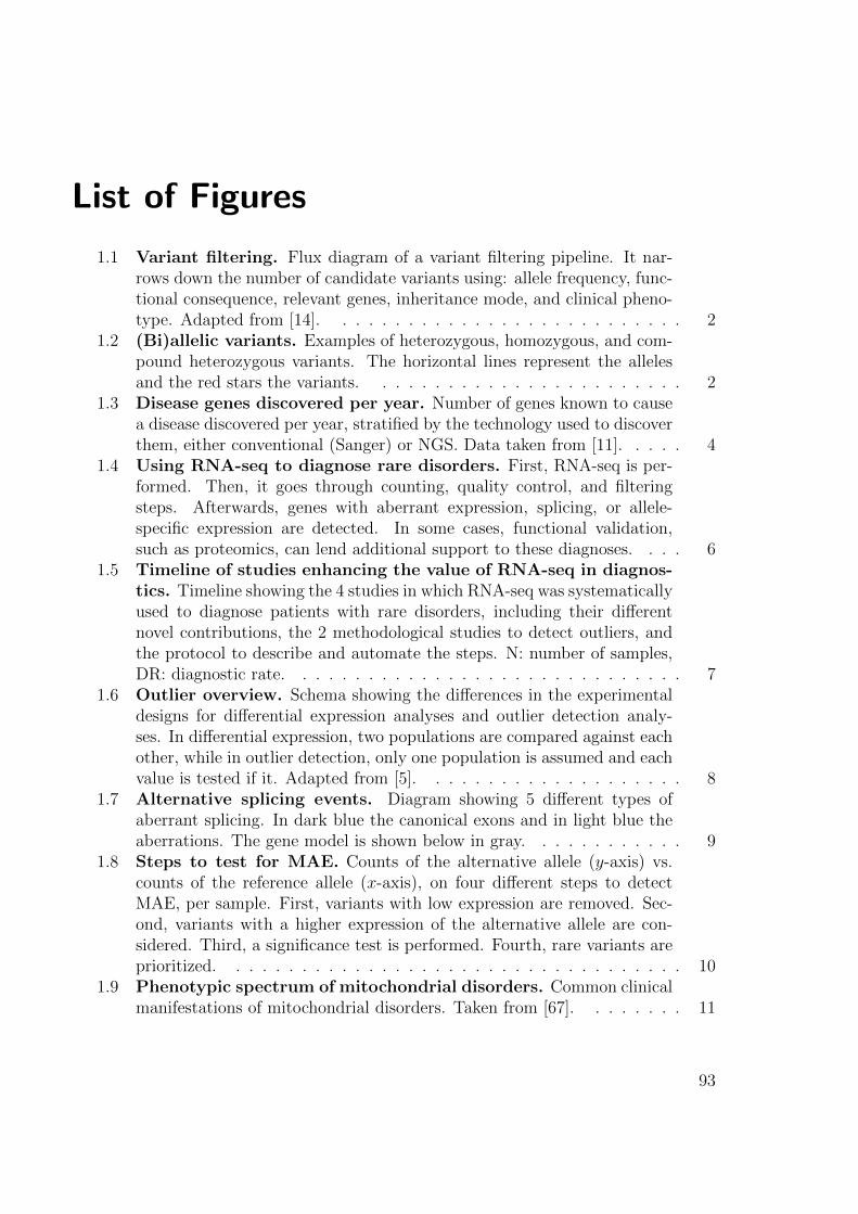
List of Figures
1.1 Variant filtering. Flux diagram of a variant filtering pipeline. It nar-rows down the number of candidate variants using: allele frequency, func-tional consequence, relevant genes, inheritance mode, and clinical pheno-type. Adapted from [14]. . . . . . . . . . . . . . . . . . . . . . . . . . . 2
1.2 (Bi)allelic variants. Examples of heterozygous, homozygous, and com-pound heterozygous variants. The horizontal lines represent the allelesand the red stars the variants. . . . . . . . . . . . . . . . . . . . . . . . 2
1.3 Disease genes discovered per year. Number of genes known to causea disease discovered per year, stratified by the technology used to discoverthem, either conventional (Sanger) or NGS. Data taken from [11]. . . . . 4
1.4 Using RNA-seq to diagnose rare disorders. First, RNA-seq is per-formed. Then, it goes through counting, quality control, and filteringsteps. Afterwards, genes with aberrant expression, splicing, or allele-specific expression are detected. In some cases, functional validation,such as proteomics, can lend additional support to these diagnoses. . . . 6
1.5 Timeline of studies enhancing the value of RNA-seq in diagnos-tics. Timeline showing the 4 studies in which RNA-seq was systematicallyused to diagnose patients with rare disorders, including their differentnovel contributions, the 2 methodological studies to detect outliers, andthe protocol to describe and automate the steps. N: number of samples,DR: diagnostic rate. . . . . . . . . . . . . . . . . . . . . . . . . . . . . . 7
1.6 Outlier overview. Schema showing the differences in the experimentaldesigns for differential expression analyses and outlier detection analy-ses. In differential expression, two populations are compared against eachother, while in outlier detection, only one population is assumed and eachvalue is tested if it. Adapted from [5]. . . . . . . . . . . . . . . . . . . . 8
1.7 Alternative splicing events. Diagram showing 5 different types ofaberrant splicing. In dark blue the canonical exons and in light blue theaberrations. The gene model is shown below in gray. . . . . . . . . . . . 9
1.8 Steps to test for MAE. Counts of the alternative allele (y-axis) vs.counts of the reference allele (x-axis), on four different steps to detectMAE, per sample. First, variants with low expression are removed. Sec-ond, variants with a higher expression of the alternative allele are con-sidered. Third, a significance test is performed. Fourth, rare variants areprioritized. . . . . . . . . . . . . . . . . . . . . . . . . . . . . . . . . . . 10
1.9 Phenotypic spectrum of mitochondrial disorders. Common clinicalmanifestations of mitochondrial disorders. Taken from [67]. . . . . . . . 11
93
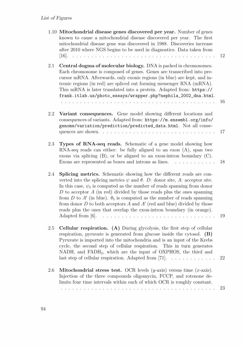
List of Figures
1.10 Mitochondrial disease genes discovered per year. Number of genesknown to cause a mitochondrial disease discovered per year. The firstmitochondrial disease gene was discovered in 1988. Discoveries increaseafter 2010 where NGS begins to be used in diagnostics. Data taken from[16]. . . . . . . . . . . . . . . . . . . . . . . . . . . . . . . . . . . . . . . 12
2.1 Central dogma of molecular biology. DNA is packed in chromosomes.Each chromosome is composed of genes. Genes are transcribed into pre-cursor mRNA. Afterwards, only exonic regions (in blue) are kept, and in-tronic regions (in red) are spliced out forming messenger RNA (mRNA).This mRNA is later translated into a protein. Adapted from: https://
frank.itlab.us/photo_essays/wrapper.php?nephila_2002_dna.html.. . . . . . . . . . . . . . . . . . . . . . . . . . . . . . . . . . . . . . . . . 16
2.2 Variant consequences. Gene model showing different locations andconsequences of variants. Adapted from: https://m.ensembl.org/info/genome/variation/prediction/predicted_data.html. Not all conse-quences are shown. . . . . . . . . . . . . . . . . . . . . . . . . . . . . . . 17
2.3 Types of RNA-seq reads. Schematic of a gene model showing howRNA-seq reads can either: be fully aligned to an exon (A), span twoexons via splicing (B), or be aligned to an exon-intron boundary (C).Exons are represented as boxes and introns as lines. . . . . . . . . . . . 18
2.4 Splicing metrics. Schematic showing how the different reads are con-verted into the splicing metrics ψ and θ. D: donor site, A: acceptor site.In this case, ψ5 is computed as the number of reads spanning from donorD to acceptor A (in red) divided by those reads plus the ones spanningfrom D to A′ (in blue). θ5 is computed as the number of reads spanningfrom donor D to both acceptors A and A′ (red and blue) divided by thosereads plus the ones that overlap the exon-intron boundary (in orange).Adapted from [6]. . . . . . . . . . . . . . . . . . . . . . . . . . . . . . . 19
2.5 Cellular respiration. (A) During glycolysis, the first step of cellularrespiration, pyruvate is generated from glucose inside the cytosol. (B)Pyruvate is imported into the mitochondria and is an input of the Krebscycle, the second step of cellular respiration. This in turn generatesNADH, and FADH2, which are the input of OXPHOS, the third andlast step of cellular respiration. Adapted from [71]. . . . . . . . . . . . . 22
2.6 Mitochondrial stress test. OCR levels (y-axis) versus time (x-axis).Injection of the three compounds oligomycin, FCCP, and rotenone de-limits four time intervals within each of which OCR is roughly constant.. . . . . . . . . . . . . . . . . . . . . . . . . . . . . . . . . . . . . . . . . 23
94
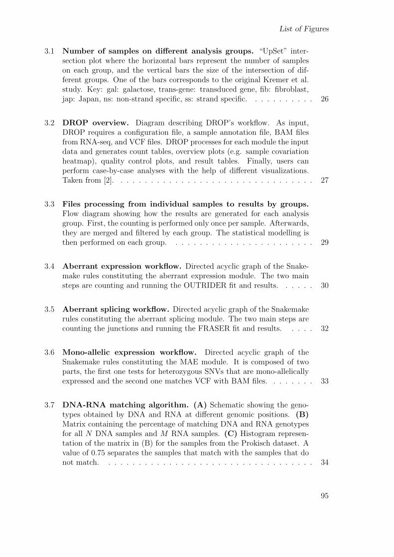
List of Figures
3.1 Number of samples on different analysis groups. “UpSet” inter-section plot where the horizontal bars represent the number of sampleson each group, and the vertical bars the size of the intersection of dif-ferent groups. One of the bars corresponds to the original Kremer et al.study. Key: gal: galactose, trans-gene: transduced gene, fib: fibroblast,jap: Japan, ns: non-strand specific, ss: strand specific. . . . . . . . . . . 26
3.2 DROP overview. Diagram describing DROP’s workflow. As input,DROP requires a configuration file, a sample annotation file, BAM filesfrom RNA-seq, and VCF files. DROP processes for each module the inputdata and generates count tables, overview plots (e.g. sample covariationheatmap), quality control plots, and result tables. Finally, users canperform case-by-case analyses with the help of different visualizations.Taken from [2]. . . . . . . . . . . . . . . . . . . . . . . . . . . . . . . . . 27
3.3 Files processing from individual samples to results by groups.Flow diagram showing how the results are generated for each analysisgroup. First, the counting is performed only once per sample. Afterwards,they are merged and filtered by each group. The statistical modelling isthen performed on each group. . . . . . . . . . . . . . . . . . . . . . . . 29
3.4 Aberrant expression workflow. Directed acyclic graph of the Snake-make rules constituting the aberrant expression module. The two mainsteps are counting and running the OUTRIDER fit and results. . . . . . 30
3.5 Aberrant splicing workflow. Directed acyclic graph of the Snakemakerules constituting the aberrant splicing module. The two main steps arecounting the junctions and running the FRASER fit and results. . . . . 32
3.6 Mono-allelic expression workflow. Directed acyclic graph of theSnakemake rules constituting the MAE module. It is composed of twoparts, the first one tests for heterozygous SNVs that are mono-allelicallyexpressed and the second one matches VCF with BAM files. . . . . . . . 33
3.7 DNA-RNA matching algorithm. (A) Schematic showing the geno-types obtained by DNA and RNA at different genomic positions. (B)Matrix containing the percentage of matching DNA and RNA genotypesfor all N DNA samples and M RNA samples. (C) Histogram represen-tation of the matrix in (B) for the samples from the Prokisch dataset. Avalue of 0.75 separates the samples that match with the samples that donot match. . . . . . . . . . . . . . . . . . . . . . . . . . . . . . . . . . . 34
95
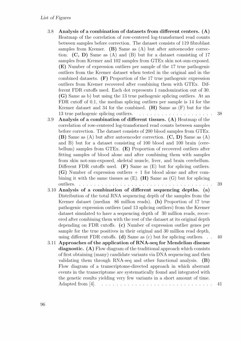
List of Figures
3.8 Analysis of a combination of datasets from different centers. (A)Heatmap of the correlation of row-centered log-transformed read countsbetween samples before correction. The dataset consists of 119 fibroblastsamples from Kremer. (B) Same as (A) but after autoencoder correc-tion. (C, D) Same as (A) and (B) but for a dataset consisting of 17samples from Kremer and 102 samples from GTEx skin not-sun-exposed.(E) Number of expression outliers per sample of the 17 true pathogenicoutliers from the Kremer dataset when tested in the original and in thecombined datasets. (F) Proportion of the 17 true pathogenic expressionoutliers from Kremer recovered after combining them with GTEx. Dif-ferent FDR cutoffs used. Each dot represents 1 randomization out of 30.(G) Same as b) but using the 13 true pathogenic splicing outliers. At anFDR cutoff of 0.1, the median splicing outliers per sample is 14 for theKremer dataset and 34 for the combined. (H) Same as (F) but for the13 true pathogenic splicing outliers. . . . . . . . . . . . . . . . . . . . . 38
3.9 Analysis of a combination of different tissues. (A) Heatmap of thecorrelation of row-centered log-transformed read counts between samplesbefore correction. The dataset consists of 200 blood samples from GTEx.(B) Same as (A) but after autoencoder correction. (C, D) Same as (A)and B) but for a dataset consisting of 100 blood and 100 brain (cere-bellum) samples from GTEx. (E) Proportion of recovered outliers afterfitting samples of blood alone and after combining them with samplesfrom skin not-sun-exposed, skeletal muscle, liver, and brain cerebellum.Different FDR cutoffs used. (F) Same as (E) but for splicing outliers.(G) Number of expression outliers + 1 for blood alone and after com-bining it with the same tissues as (E). (H) Same as (G) but for splicingoutliers. . . . . . . . . . . . . . . . . . . . . . . . . . . . . . . . . . . . . 39
3.10 Analysis of a combination of different sequencing depths. (a)Distribution of the total RNA sequencing depth of the samples from theKremer dataset (median 86 million reads). (b) Proportion of 17 truepathogenic expression outliers (and 13 splicing outliers) from the Kremerdataset simulated to have a sequencing depth of 30 million reads, recov-ered after combining them with the rest of the dataset at its original depthdepending on FDR cutoffs. (c) Number of expression outlier genes persample for the true positives in their original and 30 million read depth,using different FDR cutoffs. (d) Same as (c) but for splicing outliers. . . 40
3.11 Approaches of the application of RNA-seq for Mendelian diseasediagnostic. (A) Flow diagram of the traditional approach which consistsof first obtaining (many) candidate variants via DNA sequencing and thenvalidating them through RNA-seq and other functional analysis. (B)Flow diagram of a transcriptome-directed approach in which aberrantevents in the transcriptome are systematically found and integrated withthe genetic results yielding very few variants in a short amount of time.Adapted from [4]. . . . . . . . . . . . . . . . . . . . . . . . . . . . . . . 41
96
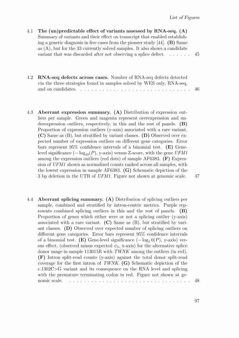
List of Figures
4.1 The (un)predictable effect of variants assessed by RNA-seq. (A)Summary of variants and their effect on transcript that enabled establish-ing a genetic diagnosis in five cases from the pioneer study [44]. (B) Sameas (A), but for the 33 currently solved samples. It also shows a candidatevariant that was discarded after not observing a splice defect. . . . . . . 45
4.2 RNA-seq defects across cases. Number of RNA-seq defects detectedvia the three strategies found in samples solved by WES only, RNA-seq,and on candidates. . . . . . . . . . . . . . . . . . . . . . . . . . . . . . . 46
4.3 Aberrant expression summary. (A) Distribution of expression out-liers per sample. Green and magenta represent overexpression and un-derexpression outliers, respectively, in this and the rest of panels. (B)Proportion of expression outliers (y-axis) associated with a rare variant.(C) Same as (B), but stratified by variant classes. (D) Observed over ex-pected number of expression outliers on different gene categories. Errorbars represent 95% confidence intervals of a binomial test. (E) Gene-level significance (− log10(P ), y-axis) versus Z-score, with the gene UFM1among the expression outliers (red dots) of sample AF6383. (F) Expres-sion of UFM1 shown as normalized counts ranked across all samples, withthe lowest expression in sample AF6383. (G) Schematic depiction of the3 bp deletion in the UTR of UFM1. Figure not shown at genomic scale. 47
4.4 Aberrant splicing summary. (A) Distribution of splicing outliers persample, combined and stratified by intron-centric metrics. Purple rep-resents combined splicing outliers in this and the rest of panels. (B)Proportion of genes which either were or not a splicing outlier (y-axis)associated with a rare variant. (C) Same as (B), but stratified by vari-ant classes. (D) Observed over expected number of splicing outliers ondifferent gene categories. Error bars represent 95% confidence intervalsof a binomial test. (E) Gene-level significance (− log1 0(P ), y-axis) ver-sus effect, (observed minus expected ψ5, x-axis) for the alternative splicedonor usage in sample 113015R with TWNK among the outliers (in red).(F) Intron split-read counts (y-axis) against the total donor split-readcoverage for the first intron of TWNK. (G) Schematic depiction of thec.1302C>G variant and its consequence on the RNA level and splicingwith the premature terminating codon in red. Figure not shown at ge-nomic scale. . . . . . . . . . . . . . . . . . . . . . . . . . . . . . . . . . 48
97
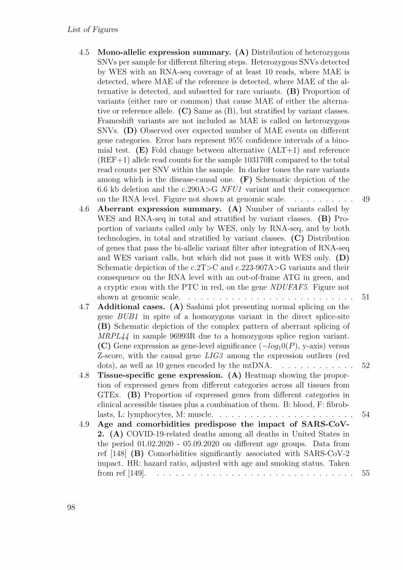
List of Figures
4.5 Mono-allelic expression summary. (A) Distribution of heterozygousSNVs per sample for different filtering steps. Heterozygous SNVs detectedby WES with an RNA-seq coverage of at least 10 reads, where MAE isdetected, where MAE of the reference is detected, where MAE of the al-ternative is detected, and subsetted for rare variants. (B) Proportion ofvariants (either rare or common) that cause MAE of either the alterna-tive or reference allele. (C) Same as (B), but stratified by variant classes.Frameshift variants are not included as MAE is called on heterozygousSNVs. (D) Observed over expected number of MAE events on differentgene categories. Error bars represent 95% confidence intervals of a bino-mial test. (E) Fold change between alternative (ALT+1) and reference(REF+1) allele read counts for the sample 103170R compared to the totalread counts per SNV within the sample. In darker tones the rare variantsamong which is the disease-causal one. (F) Schematic depiction of the6.6 kb deletion and the c.290A>G NFU1 variant and their consequenceon the RNA level. Figure not shown at genomic scale. . . . . . . . . . . 49
4.6 Aberrant expression summary. (A) Number of variants called byWES and RNA-seq in total and stratified by variant classes. (B) Pro-portion of variants called only by WES, only by RNA-seq, and by bothtechnologies, in total and stratified by variant classes. (C) Distributionof genes that pass the bi-allelic variant filter after integration of RNA-seqand WES variant calls, but which did not pass it with WES only. (D)Schematic depiction of the c.2T>C and c.223-907A>G variants and theirconsequence on the RNA level with an out-of-frame ATG in green, anda cryptic exon with the PTC in red, on the gene NDUFAF5. Figure notshown at genomic scale. . . . . . . . . . . . . . . . . . . . . . . . . . . . 51
4.7 Additional cases. (A) Sashimi plot presenting normal splicing on thegene BUB1 in spite of a homozygous variant in the direct splice-site(B) Schematic depiction of the complex pattern of aberrant splicing ofMRPL44 in sample 96993R due to a homozygous splice region variant.(C) Gene expression as gene-level significance (−log10(P ), y-axis) versusZ-score, with the causal gene LIG3 among the expression outliers (reddots), as well as 10 genes encoded by the mtDNA. . . . . . . . . . . . . 52
4.8 Tissue-specific gene expression. (A) Heatmap showing the propor-tion of expressed genes from different categories across all tissues fromGTEx. (B) Proportion of expressed genes from different categories inclinical accessible tissues plus a combination of them. B: blood, F: fibrob-lasts, L: lymphocytes, M: muscle. . . . . . . . . . . . . . . . . . . . . . . 54
4.9 Age and comorbidities predispose the impact of SARS-CoV-2. (A) COVID-19-related deaths among all deaths in United States inthe period 01.02.2020 - 05.09.2020 on different age groups. Data fromref [148] (B) Comorbidities significantly associated with SARS-CoV-2impact. HR: hazard ratio, adjusted with age and smoking status. Takenfrom ref [149]. . . . . . . . . . . . . . . . . . . . . . . . . . . . . . . . . 55
98
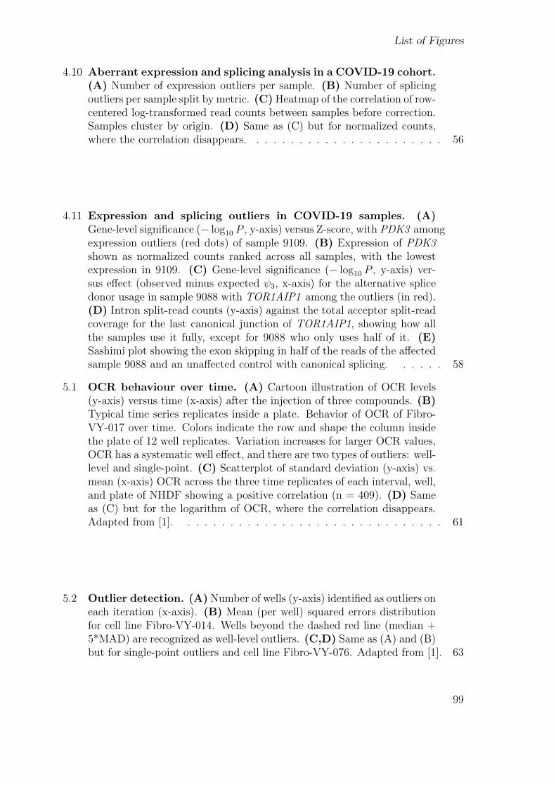
List of Figures
4.10 Aberrant expression and splicing analysis in a COVID-19 cohort.(A) Number of expression outliers per sample. (B) Number of splicingoutliers per sample split by metric. (C) Heatmap of the correlation of row-centered log-transformed read counts between samples before correction.Samples cluster by origin. (D) Same as (C) but for normalized counts,where the correlation disappears. . . . . . . . . . . . . . . . . . . . . . . 56
4.11 Expression and splicing outliers in COVID-19 samples. (A)Gene-level significance (− log10 P , y-axis) versus Z-score, with PDK3 amongexpression outliers (red dots) of sample 9109. (B) Expression of PDK3shown as normalized counts ranked across all samples, with the lowestexpression in 9109. (C) Gene-level significance (− log10 P , y-axis) ver-sus effect (observed minus expected ψ3, x-axis) for the alternative splicedonor usage in sample 9088 with TOR1AIP1 among the outliers (in red).(D) Intron split-read counts (y-axis) against the total acceptor split-readcoverage for the last canonical junction of TOR1AIP1, showing how allthe samples use it fully, except for 9088 who only uses half of it. (E)Sashimi plot showing the exon skipping in half of the reads of the affectedsample 9088 and an unaffected control with canonical splicing. . . . . . 58
5.1 OCR behaviour over time. (A) Cartoon illustration of OCR levels(y-axis) versus time (x-axis) after the injection of three compounds. (B)Typical time series replicates inside a plate. Behavior of OCR of Fibro-VY-017 over time. Colors indicate the row and shape the column insidethe plate of 12 well replicates. Variation increases for larger OCR values,OCR has a systematic well effect, and there are two types of outliers: well-level and single-point. (C) Scatterplot of standard deviation (y-axis) vs.mean (x-axis) OCR across the three time replicates of each interval, well,and plate of NHDF showing a positive correlation (n = 409). (D) Sameas (C) but for the logarithm of OCR, where the correlation disappears.Adapted from [1]. . . . . . . . . . . . . . . . . . . . . . . . . . . . . . . 61
5.2 Outlier detection. (A) Number of wells (y-axis) identified as outliers oneach iteration (x-axis). (B) Mean (per well) squared errors distributionfor cell line Fibro-VY-014. Wells beyond the dashed red line (median +5*MAD) are recognized as well-level outliers. (C,D) Same as (A) and (B)but for single-point outliers and cell line Fibro-VY-076. Adapted from [1]. 63
99
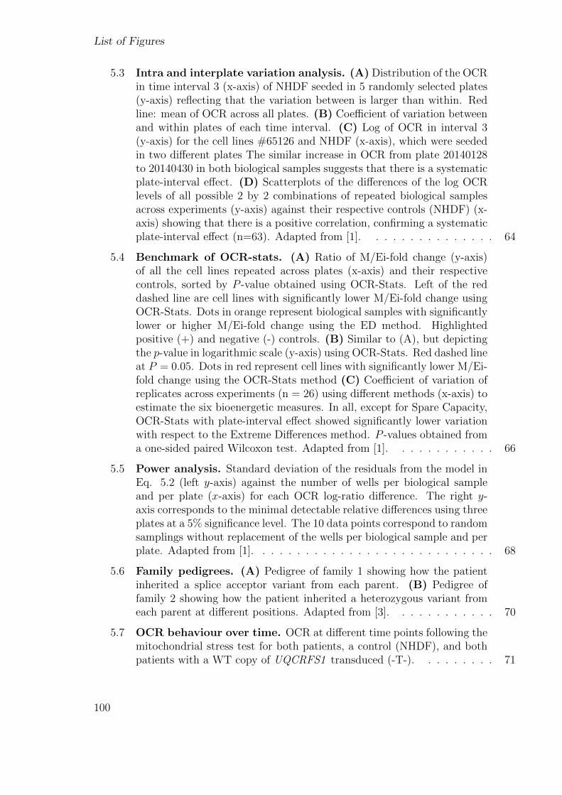
List of Figures
5.3 Intra and interplate variation analysis. (A) Distribution of the OCRin time interval 3 (x-axis) of NHDF seeded in 5 randomly selected plates(y-axis) reflecting that the variation between is larger than within. Redline: mean of OCR across all plates. (B) Coefficient of variation betweenand within plates of each time interval. (C) Log of OCR in interval 3(y-axis) for the cell lines #65126 and NHDF (x-axis), which were seededin two different plates The similar increase in OCR from plate 20140128to 20140430 in both biological samples suggests that there is a systematicplate-interval effect. (D) Scatterplots of the differences of the log OCRlevels of all possible 2 by 2 combinations of repeated biological samplesacross experiments (y-axis) against their respective controls (NHDF) (x-axis) showing that there is a positive correlation, confirming a systematicplate-interval effect (n=63). Adapted from [1]. . . . . . . . . . . . . . . 64
5.4 Benchmark of OCR-stats. (A) Ratio of M/Ei-fold change (y-axis)of all the cell lines repeated across plates (x-axis) and their respectivecontrols, sorted by P -value obtained using OCR-Stats. Left of the reddashed line are cell lines with significantly lower M/Ei-fold change usingOCR-Stats. Dots in orange represent biological samples with significantlylower or higher M/Ei-fold change using the ED method. Highlightedpositive (+) and negative (-) controls. (B) Similar to (A), but depictingthe p-value in logarithmic scale (y-axis) using OCR-Stats. Red dashed lineat P = 0.05. Dots in red represent cell lines with significantly lower M/Ei-fold change using the OCR-Stats method (C) Coefficient of variation ofreplicates across experiments (n = 26) using different methods (x-axis) toestimate the six bioenergetic measures. In all, except for Spare Capacity,OCR-Stats with plate-interval effect showed significantly lower variationwith respect to the Extreme Differences method. P -values obtained froma one-sided paired Wilcoxon test. Adapted from [1]. . . . . . . . . . . . 66
5.5 Power analysis. Standard deviation of the residuals from the model inEq. 5.2 (left y-axis) against the number of wells per biological sampleand per plate (x-axis) for each OCR log-ratio difference. The right y-axis corresponds to the minimal detectable relative differences using threeplates at a 5% significance level. The 10 data points correspond to randomsamplings without replacement of the wells per biological sample and perplate. Adapted from [1]. . . . . . . . . . . . . . . . . . . . . . . . . . . . 68
5.6 Family pedigrees. (A) Pedigree of family 1 showing how the patientinherited a splice acceptor variant from each parent. (B) Pedigree offamily 2 showing how the patient inherited a heterozygous variant fromeach parent at different positions. Adapted from [3]. . . . . . . . . . . . 70
5.7 OCR behaviour over time. OCR at different time points following themitochondrial stress test for both patients, a control (NHDF), and bothpatients with a WT copy of UQCRFS1 transduced (-T-). . . . . . . . . 71
100
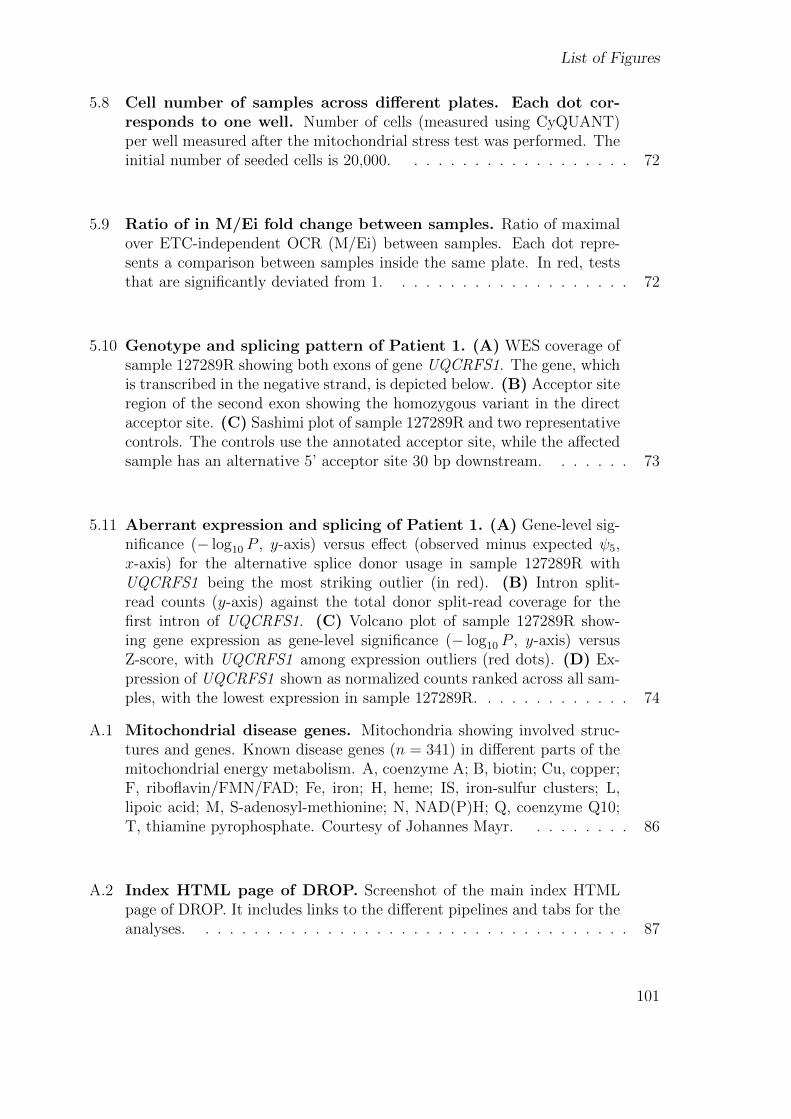
List of Figures
5.8 Cell number of samples across different plates. Each dot cor-responds to one well. Number of cells (measured using CyQUANT)per well measured after the mitochondrial stress test was performed. Theinitial number of seeded cells is 20,000. . . . . . . . . . . . . . . . . . . 72
5.9 Ratio of in M/Ei fold change between samples. Ratio of maximalover ETC-independent OCR (M/Ei) between samples. Each dot repre-sents a comparison between samples inside the same plate. In red, teststhat are significantly deviated from 1. . . . . . . . . . . . . . . . . . . . 72
5.10 Genotype and splicing pattern of Patient 1. (A) WES coverage ofsample 127289R showing both exons of gene UQCRFS1. The gene, whichis transcribed in the negative strand, is depicted below. (B) Acceptor siteregion of the second exon showing the homozygous variant in the directacceptor site. (C) Sashimi plot of sample 127289R and two representativecontrols. The controls use the annotated acceptor site, while the affectedsample has an alternative 5’ acceptor site 30 bp downstream. . . . . . . 73
5.11 Aberrant expression and splicing of Patient 1. (A) Gene-level sig-nificance (− log10 P , y-axis) versus effect (observed minus expected ψ5,x-axis) for the alternative splice donor usage in sample 127289R withUQCRFS1 being the most striking outlier (in red). (B) Intron split-read counts (y-axis) against the total donor split-read coverage for thefirst intron of UQCRFS1. (C) Volcano plot of sample 127289R show-ing gene expression as gene-level significance (− log10 P , y-axis) versusZ-score, with UQCRFS1 among expression outliers (red dots). (D) Ex-pression of UQCRFS1 shown as normalized counts ranked across all sam-ples, with the lowest expression in sample 127289R. . . . . . . . . . . . . 74
A.1 Mitochondrial disease genes. Mitochondria showing involved struc-tures and genes. Known disease genes (n = 341) in different parts of themitochondrial energy metabolism. A, coenzyme A; B, biotin; Cu, copper;F, riboflavin/FMN/FAD; Fe, iron; H, heme; IS, iron-sulfur clusters; L,lipoic acid; M, S-adenosyl-methionine; N, NAD(P)H; Q, coenzyme Q10;T, thiamine pyrophosphate. Courtesy of Johannes Mayr. . . . . . . . . 86
A.2 Index HTML page of DROP. Screenshot of the main index HTMLpage of DROP. It includes links to the different pipelines and tabs for theanalyses. . . . . . . . . . . . . . . . . . . . . . . . . . . . . . . . . . . . 87
101
List of Figures
A.3 RNA-seq study cohort and workflow. RNA-seq was performed onskin-derived fibroblasts from 309 patients suspected to suffer from a raredisease. All patients have undergone the WES analysis beforehand, whichwas inconclusive for 217. Systematic detection of aberrant events and con-sequent analysis led to genetic diagnosis in 15% of the WES-undiagnosedcases by establishing a genotype-phenotype association, and pinpoint acandidate gene in 6% of the WES-undiagnosed cases, suggesting the dis-covery of novel disease-genes and more complex pathomechanisms. Atranscript defect was also detected in 76% of the WES-diagnosed casescarrying pathogenic protein-truncating variants. . . . . . . . . . . . . . 88
A.4 Recall - FDR analysis on variants called by RNA-seq. Averagerecall (true positives / all positives) vs. average false discovery rate (falsepositives / (false positives + true positives)) of variants detected by RNA-seq in comparison to variants detected by WGS in 210 samples fromsuprapubic skin from GTEx. The average is taken across samples. Colorsindicate the variants that passed (or not) the GATK filters and that were(or not) contained in a repeat masked region. The minimum numbersrepresent the reads supporting the alternative allele. This analysis ledus to apply the GATK filters and to consider variants not in maskedregions and with a minimum alternative allele count of 3 where there isan inflection point in the curve. More stringent restrictions to variantcoverage further reduce the average FDR, which comes at the cost ofrecall. . . . . . . . . . . . . . . . . . . . . . . . . . . . . . . . . . . . . . 89
A.5 Normalizing by cell number does not reduce variation. (A) Me-dian (per well) of OCR (y-axis) vs. cell number (x-axis) of the controlson all experiments (n = 2,192 on each panel) show that there exists apositive correlation on all time intervals (I1: ρ = .47, I2: ρ = .45, I3:ρ = .40, I4: ρ = .33, P < 2.2 × 10⁻¹⁶ for all intervals). (B) Coefficientof variation (y-axis) of well replicates within plates for raw OCR, andnormalized dividing by cell count (x-axis), split for each time interval.Each point represents a different sample. On all four intervals, normal-ization not only did not reduce the coefficient of variation, but increasedit. P -values obtained from double sided Wilcoxon Tests. Adapted from[1]. . . . . . . . . . . . . . . . . . . . . . . . . . . . . . . . . . . . . . . 90
A.6 Residuals from the statistical testing follow a normal distribu-tion. Quantile-quantile theoretical (x-axis) vs. observed (y-axis) plots ofthe residuals of OCR-stats statistical testing applied to all OCR ratios.Adapted from [1]. . . . . . . . . . . . . . . . . . . . . . . . . . . . . . . 91
A.7 Mitochondrial stress test on three plates. OCR vs. time pointsof samples from Patients 1 and 2, the control cell line (NHDF), plus atransduced assay of each sample seeded in three different plates (denotedby their dates). . . . . . . . . . . . . . . . . . . . . . . . . . . . . . . . . 92
102
List of Tables
3.1 OUTRIDER results table. Extract of the OUTRIDER results table ofthe test dataset showing one up and one downregulated case. normCountscorrespond to the OUTRIDER normalized counts of that sample on thatgene, while meanCounts is the mean estimate µ of the negative binomialdistribution of that gene. Roughly, dividing the first by the second givesthe fold change (FC). . . . . . . . . . . . . . . . . . . . . . . . . . . . . . 31
3.2 FRASER results table. Extract of the FRASER results table of thetest dataset showing one θ, one ψ3, and one ψ5 case. deltaPsi corre-sponds to the difference between the observed and the expected ψ (or θ).. . . . . . . . . . . . . . . . . . . . . . . . . . . . . . . . . . . . . . . . . 31
3.3 MAE results table. Extract of the MAE results table of the testdataset. Key: REF: reference allele, ALT: alternative allele, refC: countsof the reference, altC: counts of the alternative, altR: alternative alleleratio = altC/(altC+refC), MAF: minor allele frequency. . . . . . . . . . 31
3.4 Disease datasets analyzed using DROP. Key: HHZ: HelmholtzZen-trum Muenchen, CAD: coronary artery disease, DHZ: Deutsches Herzzen-trum Muenchen, MPI: Max Planck Institute, SCZ: schizophrenia, BD:bipolar disorder, DECOI: Deutsche COVID Initiative. . . . . . . . . . . 37
4.1 Diagnoses from the Kremer et al. dataset using RNA-seq. Tableshowing all the current diagnosed samples from the Kremer et al. cohortusing RNA-seq. Each row corresponds to a gene. It includes the status atthe time of that study and now. Key: AE: significant aberrant expression,AS: significant aberrant splicing, var: variant, syn: synonymous . . . . . 43
4.2 All solved cases with RNA-seq. Table showing all the samples di-agnosed via RNA-seq. It includes the reason why they were not solvedvia WES and how RNA-seq contributed to solving them. det: detected,prior: prioritized, annot: annotated as pathogenic, homo: homozygous,syn: synonymous, fs: frameshift, dom: dominant, mis: missense, RVC:variant called via RNA-seq. . . . . . . . . . . . . . . . . . . . . . . . . . 57
5.1 OCR ratios definitions and metrics. Proposed definitions for cellularbioenergetics based on ratios, their abbreviations, equations to computethem, and analogous measures used in the literature. . . . . . . . . . . . 62
103
List of Tables
5.2 OCR ratio-based differences for statistical testing. Differences∆∆θ to be used when testing a biological sample b against a control c oneach plate, for each OCR ratio. . . . . . . . . . . . . . . . . . . . . . . . 65
104
References
[1] Yepez, V. A. et al. OCR-Stats: Robust estimation and statistical testing of mi-tochondrial respiration activities using Seahorse XF Analyzer. PLOS ONE 13,e0199938 (2018). URL https://dx.plos.org/10.1371/journal.pone.0199938.
[2] Yepez, V. A. et al. Detection of aberrant gene expression events in RNA sequencingdata. Nature Protocols 16, 1276–1296 (2021). URL http://www.nature.com/
articles/s41596-020-00462-5.
[3] Gusic, M. et al. Bi-Allelic UQCRFS1 Variants Are Associated with MitochondrialComplex III Deficiency, Cardiomyopathy, and Alopecia Totalis. The AmericanJournal of Human Genetics 106, 102–111 (2020). URL https://linkinghub.
elsevier.com/retrieve/pii/S0002929719304690.
[4] Murdock, D. R. et al. Transcriptome-directed analysis for Mendelian disease di-agnosis overcomes limitations of conventional genomic testing. Journal of ClinicalInvestigation 131, e141500 (2021). URL https://www.jci.org/articles/view/
141500.
[5] Brechtmann, F. et al. OUTRIDER: A Statistical Method for Detecting Aber-rantly Expressed Genes in RNA Sequencing Data. The American Journal of Hu-man Genetics 103, 907–917 (2018). URL https://linkinghub.elsevier.com/
retrieve/pii/S0002929718304014.
[6] Mertes, C. et al. Detection of aberrant splicing events in RNA-seq data usingFRASER. Nature Communications 12, 529 (2021). URL http://www.nature.
com/articles/s41467-020-20573-7.
[7] Baldovino, S., Moliner, A. M., Taruscio, D., Daina, E. & Roccatello, D. RareDiseases in Europe: from a Wide to a Local Perspective 18, 5 (2016).
[8] Amberger, J. S., Bocchini, C. A., Scott, A. F. & Hamosh, A. OMIM.org: leverag-ing knowledge across phenotype–gene relationships. Nucleic Acids Research 47,D1038–D1043 (2019). URL https://academic.oup.com/nar/article/47/D1/
D1038/5184722.
[9] EURORDIS. Rare Diseases: Understanding this Public Health Priority. RareDiseases 14 (2005). URL https://www.eurordis.org.
105
References
[10] Boycott, K. M. & Ardigo, D. Addressing challenges in the diagnosis and treatmentof rare genetic diseases. Nature Reviews Drug Discovery 17, 151–152 (2018). URLhttp://www.nature.com/articles/nrd.2017.246.
[11] Boycott, K. M. et al. International Cooperation to Enable the Diagnosis of All RareGenetic Diseases. The American Journal of Human Genetics 100, 695–705 (2017).URL https://linkinghub.elsevier.com/retrieve/pii/S0002929717301477.
[12] Splinter, K. et al. Effect of Genetic Diagnosis on Patients with Previously Undi-agnosed Disease. New England Journal of Medicine 379, 2131–2139 (2018). URLhttp://www.nejm.org/doi/10.1056/NEJMoa1714458.
[13] Dawkins, H. J. et al. Progress in Rare Diseases Research 2010-2016: An IRDiRCPerspective: Progress in Rare Diseases Research 2010-2016: An IRDiRC Per-spective. Clinical and Translational Science 11, 11–20 (2018). URL http:
//doi.wiley.com/10.1111/cts.12501.
[14] Wright, C. F. et al. Making new genetic diagnoses with old data: iterativereanalysis and reporting from genome-wide data in 1,133 families with devel-opmental disorders. Genetics in Medicine 20, 1216–1223 (2018). URL http:
//www.nature.com/articles/gim2017246.
[15] Wright, C. F. et al. Genetic diagnosis of developmental disorders in the DDDstudy: a scalable analysis of genome-wide research data. The Lancet 385,1305–1314 (2015). URL https://linkinghub.elsevier.com/retrieve/pii/
S0140673614617050.
[16] Stenton, S. L. & Prokisch, H. Genetics of mitochondrial diseases: Identifyingmutations to help diagnosis. EBioMedicine 56, 102784 (2020). URL https:
//linkinghub.elsevier.com/retrieve/pii/S2352396420301596.
[17] Coe, B. P. et al. Neurodevelopmental disease genes implicated by de novo mutationand copy number variation morbidity. Nature Genetics 51, 106–116 (2019). URLhttp://www.nature.com/articles/s41588-018-0288-4.
[18] Niemi, M. E. K. et al. Common genetic variants contribute to risk of rare severeneurodevelopmental disorders. Nature 562, 268–271 (2018). URL http://www.
nature.com/articles/s41586-018-0566-4.
[19] Sanger, F., Nicklen, S. & Coulson, A. R. DNA sequencing with chain-terminatinginhibitors. Proceedings of the National Academy of Sciences 74, 5463–5467 (1977).URL http://www.pnas.org/cgi/doi/10.1073/pnas.74.12.5463.
[20] Sikkema-Raddatz, B. et al. Targeted Next-Generation Sequencing can ReplaceSanger Sequencing in Clinical Diagnostics. Human Mutation 34, 1035–1042 (2013).URL http://doi.wiley.com/10.1002/humu.22332.
106
References
[21] Bamshad, M. J. et al. Exome sequencing as a tool for Mendelian disease gene dis-covery. Nature Reviews Genetics 12, 745–755 (2011). URL http://www.nature.
com/articles/nrg3031.
[22] Gilissen, C., Hoischen, A., Brunner, H. G. & Veltman, J. A. Disease gene identifi-cation strategies for exome sequencing. European Journal of Human Genetics 20,490–497 (2012). URL http://www.nature.com/articles/ejhg2011258.
[23] Hagemann, I. S. Overview of Technical Aspects and Chemistries of Next-Generation Sequencing. In Clinical Genomics, 3–19 (Elsevier, 2015). URLhttps://linkinghub.elsevier.com/retrieve/pii/B9780124047488000010.
[24] Ng, S. B. et al. Exome sequencing identifies the cause of a mendelian disorder.Nature Genetics 42, 30–35 (2010). URL http://www.nature.com/articles/ng.
499.
[25] Natarajan, P. et al. Deep-coverage whole genome sequences and blood lipids among16,324 individuals. Nature Communications 9, 3391 (2018). URL http://www.
nature.com/articles/s41467-018-05747-8.
[26] Yang, Y. et al. Clinical Whole-Exome Sequencing for the Diagnosis of MendelianDisorders. New England Journal of Medicine 369, 1502–1511 (2013). URL http:
//www.nejm.org/doi/10.1056/NEJMoa1306555.
[27] Farwell, K. D. et al. Enhanced utility of family-centered diagnostic exome sequenc-ing with inheritance model–based analysis: results from 500 unselected familieswith undiagnosed genetic conditions. Genetics in Medicine 17, 578–586 (2015).URL http://www.nature.com/articles/gim2014154.
[28] Stark, Z. et al. A prospective evaluation of whole-exome sequencing as a first-tiermolecular test in infants with suspected monogenic disorders. Genetics in Medicine18, 1090–1096 (2016). URL http://www.nature.com/articles/gim20161.
[29] Retterer, K. et al. Clinical application of whole-exome sequencing across clinicalindications. Genetics in Medicine 18, 696–704 (2016). URL http://www.nature.
com/articles/gim2015148.
[30] Shamseldin, H. E. et al. Increasing the sensitivity of clinical exome sequencingthrough improved filtration strategy. Genetics in Medicine 19, 593–598 (2017).URL http://www.nature.com/articles/gim2016155.
[31] Mattick, J. S., Dinger, M., Schonrock, N. & Cowley, M. Whole genome se-quencing provides better diagnostic yield and future value than whole exomesequencing. Medical Journal of Australia 209, 197–199 (2018). URL https:
//onlinelibrary.wiley.com/doi/abs/10.5694/mja17.01176.
107
References
[32] Wortmann, S. B., Koolen, D. A., Smeitink, J. A., van den Heuvel, L. & Rodenburg,R. J. Whole exome sequencing of suspected mitochondrial patients in clinicalpractice. Journal of Inherited Metabolic Disease 38, 437–443 (2015). URL http:
//doi.wiley.com/10.1007/s10545-015-9823-y.
[33] Riley, L. G. et al. The diagnostic utility of genome sequencing in a pediatric cohortwith suspected mitochondrial disease. Genetics in Medicine (2020).
[34] Wang, Z., Gerstein, M. & Snyder, M. RNA-Seq: a revolutionary tool for transcrip-tomics. Nature Reviews Genetics 10, 57–63 (2009). URL http://www.nature.
com/articles/nrg2484.
[35] Schena, M., Shalon, D., Davis, R. W. & Brown, P. O. Quantitative Monitoring ofGene Expression Patterns with a Complementary DNA Microarray. Science 270,467–470 (1995).
[36] Stenson, P. D. et al. The Human Gene Mutation Database: towards a comprehen-sive repository of inherited mutation data for medical research, genetic diagnosisand next-generation sequencing studies. Human Genetics 136, 665–677 (2017).URL http://link.springer.com/10.1007/s00439-017-1779-6.
[37] Ma, M. et al. Disease-associated variants in different categories of disease locatedin distinct regulatory elements. BMC Genomics 16, S3 (2015). URL http://
bmcgenomics.biomedcentral.com/articles/10.1186/1471-2164-16-S8-S3.
[38] Soemedi, R. et al. Pathogenic variants that alter protein code often disruptsplicing. Nature Genetics 49, 848–855 (2017). URL http://www.nature.com/
articles/ng.3837.
[39] Lykke-Andersen, S. & Jensen, T. H. Nonsense-mediated mRNA decay: an intricatemachinery that shapes transcriptomes. Nature Reviews Molecular Cell Biology 16,665–677 (2015). URL http://www.nature.com/articles/nrm4063.
[40] Nickless, A., Bailis, J. M. & You, Z. Control of gene expression throughthe nonsense-mediated RNA decay pathway. Cell & Bioscience 7, 26(2017). URL http://cellandbioscience.biomedcentral.com/articles/10.
1186/s13578-017-0153-7.
[41] Xing, Y. & Lee, C. Evidence of functional selection pressure for alternativesplicing events that accelerate evolution of protein subsequences. Proceedingsof the National Academy of Sciences 102, 13526–13531 (2005). URL http:
//www.pnas.org/cgi/doi/10.1073/pnas.0501213102.
[42] Landrum, M. J. et al. ClinVar: improving access to variant interpretations andsupporting evidence. Nucleic Acids Research 46, D1062–D1067 (2018). URLhttp://academic.oup.com/nar/article/46/D1/D1062/4641904.
108
References
[43] Cummings, B. B. et al. Improving genetic diagnosis in Mendelian disease withtranscriptome sequencing. SCIENCE TRANSLATIONAL MEDICINE 12 (2017).
[44] Kremer, L. S. et al. Genetic diagnosis of Mendelian disorders via RNA sequenc-ing. Nature Communications 8, 15824 (2017). URL http://www.nature.com/
articles/ncomms15824.
[45] Fresard, L. et al. Identification of rare-disease genes using blood transcriptomesequencing and large control cohorts. Nature Medicine 25, 911–919 (2019). URLhttp://www.nature.com/articles/s41591-019-0457-8.
[46] Gonorazky, H. D. et al. Expanding the Boundaries of RNA Sequencing as a Diag-nostic Tool for Rare Mendelian Disease. The American Journal of Human Genetics104, 466–483 (2019). URL https://linkinghub.elsevier.com/retrieve/pii/
S0002929719300126.
[47] Karczewski, K. J. & Snyder, M. P. Integrative omics for health and disease. NatureReviews Genetics 19, 299–310 (2018). URL http://www.nature.com/articles/
nrg.2018.4.
[48] Kremer, L. S., Wortmann, S. B. & Prokisch, H. “Transcriptomics”: moleculardiagnosis of inborn errors of metabolism via RNA-sequencing. Journal of InheritedMetabolic Disease 41, 525–532 (2018). URL http://doi.wiley.com/10.1007/
s10545-017-0133-4.
[49] Popp, M. W.-L. & Maquat, L. E. Organizing Principles of Mam-malian Nonsense-Mediated mRNA Decay. Annual Review of Genetics47, 139–165 (2013). URL http://www.annualreviews.org/doi/10.1146/
annurev-genet-111212-133424.
[50] Love, M. I., Huber, W. & Anders, S. Moderated estimation of fold changeand dispersion for RNA-seq data with DESeq2. Genome Biology 15, 550(2014). URL http://genomebiology.biomedcentral.com/articles/10.1186/
s13059-014-0550-8.
[51] Stegle, O., Parts, L., Piipari, M., Winn, J. & Durbin, R. Using probabilisticestimation of expression residuals (PEER) to obtain increased power and inter-pretability of gene expression analyses. Nature Protocols 7, 500–507 (2012). URLhttp://www.nature.com/articles/nprot.2011.457.
[52] Wang, Y., Ma, M., Xiao, X. & Wang, Z. Intronic splicing enhancers, cognate splic-ing factors and context-dependent regulation rules. Nature Structural & MolecularBiology 19, 1044–1052 (2012). URL http://www.nature.com/articles/nsmb.
2377.
[53] Kernohan, K. D. et al. Whole-transcriptome sequencing in blood provides a diag-nosis of spinal muscular atrophy with progressive myoclonic epilepsy. Human Mu-tation 38, 611–614 (2017). URL http://doi.wiley.com/10.1002/humu.23211.
109
References
[54] Hamanaka, K. et al. RNA sequencing solved the most common but unrec-ognized NEB pathogenic variant in Japanese nemaline myopathy. Geneticsin Medicine 21, 1629–1638 (2019). URL http://www.nature.com/articles/
s41436-018-0360-6.
[55] Wang, K. et al. Whole-genome DNA/RNA sequencing identifies truncating mu-tations in RBCK1 in a novel Mendelian disease with neuromuscular and cardiacinvolvement. Genome Medicine 5, 67 (2013). URL http://genomemedicine.
biomedcentral.com/articles/10.1186/gm471.
[56] Li, Y. I. et al. Annotation-free quantification of RNA splicing using LeafCutter.Nature Genetics 50, 151–158 (2018). URL http://www.nature.com/articles/
s41588-017-0004-9.
[57] Kapustin, Y. et al. Cryptic splice sites and split genes. Nucleic Acids Research39, 5837–5844 (2011). URL https://academic.oup.com/nar/article-lookup/
doi/10.1093/nar/gkr203.
[58] Mohammadi, P. et al. Genetic regulatory variation in populations informs tran-scriptome analysis in rare disease. Science 366, 351–356 (2019). URL http:
//www.sciencemag.org/lookup/doi/10.1126/science.aay0256.
[59] van Haelst, M. M. et al. Further confirmation of the MED13L haploinsufficiencysyndrome. European Journal of Human Genetics 23, 135–138 (2015). URL http:
//www.nature.com/articles/ejhg201469.
[60] Lindstrand, A. et al. Different mutations in PDE4D associated with developmentaldisorders with mirror phenotypes. Journal of Medical Genetics 51, 45–54 (2014).URL http://jmg.bmj.com/lookup/doi/10.1136/jmedgenet-2013-101937.
[61] Gorman, G. S. et al. Mitochondrial diseases. Nature Reviews Disease Primers 2,16080 (2016). URL http://www.nature.com/articles/nrdp201680.
[62] Koene, S. & Smeitink, J. Mitochondrial medicine (Khondion BV, Nijmegen, 2011),first edn.
[63] Munnich, A. & Rustin, P. Clinical spectrum and diagnosis of mitochondrialdisorders. American Journal of Medical Genetics 106, 4–17 (2001). URLhttp://doi.wiley.com/10.1002/ajmg.1391.
[64] Thorburn, D. R. Mitochondrial disorders: Prevalence, myths and advances. Jour-nal of Inherited Metabolic Disease 27, 349–362 (2004). URL http://doi.wiley.
com/10.1023/B:BOLI.0000031098.41409.55.
[65] DiMauro, S. & Davidzon, G. Mitochondrial DNA and disease. Annals of Medicine37, 222–232 (2005). URL http://www.tandfonline.com/doi/full/10.1080/
07853890510007368.
110
References
[66] Skladal, D., Halliday, J. & Thorburn, D. R. Minimum birth prevalenceof mitochondrial respiratory chain disorders in children. Brain 126, 1905–1912 (2003). URL https://academic.oup.com/brain/article-lookup/doi/
10.1093/brain/awg170.
[67] Suomalainen, A. & Battersby, B. J. Mitochondrial diseases: the contribution oforganelle stress responses to pathology. Nature Reviews Molecular Cell Biology19, 77–92 (2018). URL http://www.nature.com/articles/nrm.2017.66.
[68] Mayr, J. A. et al. Spectrum of combined respiratory chain defects. Journal ofInherited Metabolic Disease 38, 629–640 (2015). URL http://doi.wiley.com/
10.1007/s10545-015-9831-y.
[69] Reinecke, F., Smeitink, J. A. & van der Westhuizen, F. H. OXPHOS gene ex-pression and control in mitochondrial disorders. Biochimica et Biophysica Acta(BBA) - Molecular Basis of Disease 1792, 1113–1121 (2009). URL https:
//linkinghub.elsevier.com/retrieve/pii/S0925443909000921.
[70] Titov, D. V. et al. Complementation of mitochondrial electron transport chainby manipulation of the NAD+/NADH ratio. Science 352, 231–235 (2016). URLhttps://www.sciencemag.org/lookup/doi/10.1126/science.aad4017.
[71] Koopman, M. et al. A screening-based platform for the assessment of cellularrespiration in Caenorhabditis elegans. Nature Protocols 11, 1798–1816 (2016).URL http://www.nature.com/articles/nprot.2016.106.
[72] Neveling, K. et al. A Post-Hoc Comparison of the Utility of Sanger Sequencing andExome Sequencing for the Diagnosis of Heterogeneous Diseases. Human Mutation34, 1721–1726 (2013). URL http://doi.wiley.com/10.1002/humu.22450.
[73] Kohda, M. et al. A Comprehensive Genomic Analysis Reveals the Genetic Land-scape of Mitochondrial Respiratory Chain Complex Deficiencies. PLOS Genet-ics 12, e1005679 (2016). URL https://dx.plos.org/10.1371/journal.pgen.
1005679.
[74] Pronicka, E. et al. New perspective in diagnostics of mitochon-drial disorders: two years’ experience with whole-exome sequencing ata national paediatric centre. Journal of Translational Medicine 14,174 (2016). URL http://translational-medicine.biomedcentral.com/
articles/10.1186/s12967-016-0930-9.
[75] Taylor, R. W. et al. Use of Whole-Exome Sequencing to Determine the GeneticBasis of Multiple Mitochondrial Respiratory Chain Complex Deficiencies. JAMA312, 68 (2014). URL http://jama.jamanetwork.com/article.aspx?doi=10.
1001/jama.2014.7184.
111
References
[76] Fang, F. et al. The clinical and genetic characteristics in children with mitochon-drial disease in China. Science China Life Sciences 60, 746–757 (2017). URLhttp://link.springer.com/10.1007/s11427-017-9080-y.
[77] Brand, M. & Nicholls, D. Assessing mitochondrial dysfunc-tion in cells. Biochemical Journal 435, 297–312 (2011). URLhttps://portlandpress.com/biochemj/article/435/2/297/45704/
Assessing-mitochondrial-dysfunction-in-cells.
[78] Hill, B. G. et al. Integration of cellular bioenergetics with mitochon-drial quality control and autophagy. Biological Chemistry 393, 1485–1512(2012). URL http://www.degruyter.com/view/j/bchm.2012.393.issue-12/
hsz-2012-0198/hsz-2012-0198.xml.
[79] Gerencser, A. A. et al. Quantitative Microplate-Based Respirometry with Cor-rection for Oxygen Diffusion. Analytical Chemistry 81, 6868–6878 (2009). URLhttps://pubs.acs.org/doi/10.1021/ac900881z.
[80] Divakaruni, A. S., Paradyse, A., Ferrick, D. A., Murphy, A. N. & Jastroch, M.Analysis and Interpretation of Microplate-Based Oxygen Consumption and pHData. In Methods in Enzymology, vol. 547, 309–354 (Elsevier, 2014). URL https:
//linkinghub.elsevier.com/retrieve/pii/B9780128014158000163.
[81] Ferrick, D. A., Neilson, A. & Beeson, C. Advances in measuring cellular bioener-getics using extracellular flux. Drug Discovery Today 13, 268–274 (2008). URLhttps://linkinghub.elsevier.com/retrieve/pii/S1359644608000044.
[82] Dranka, B. P. et al. Assessing bioenergetic function in response to oxidative stressby metabolic profiling. Free Radical Biology and Medicine 51, 1621–1635 (2011).URL https://linkinghub.elsevier.com/retrieve/pii/S0891584911004990.
[83] Zhang, J. et al. Measuring energy metabolism in cultured cells, including humanpluripotent stem cells and differentiated cells. Nature Protocols 7, 1068–1085(2012). URL http://www.nature.com/articles/nprot.2012.048.
[84] Zhou, W. et al. HIF1 induced switch from bivalent to exclusively glycolyticmetabolism during ESC-to-EpiSC/hESC transition: Metabolic switch in ESC-to-EpiSC/hESC transition. The EMBO Journal 31, 2103–2116 (2012). URLhttp://emboj.embopress.org/cgi/doi/10.1038/emboj.2012.71.
[85] Shah-Simpson, S., Pereira, C. F., Dumoulin, P. C., Caradonna, K. L. &Burleigh, B. A. Bioenergetic profiling of Trypanosoma cruzi life stages usingSeahorse extracellular flux technology. Molecular and Biochemical Parasitology208, 91–95 (2016). URL https://linkinghub.elsevier.com/retrieve/pii/
S0166685116300901.
112
References
[86] Alberts, B. et al. Molecular biology of the cell (Garland Science, Taylor and FrancisGroup, New York, NY, 2015), sixth edition edn.
[87] Minchin, S. & Lodge, J. Understanding biochemistry: structure and func-tion of nucleic acids. Essays in Biochemistry 63, 433–456 (2019). URLhttps://portlandpress.com/essaysbiochem/article/63/4/433/220684/
Understanding-biochemistry-structure-and-function.
[88] Frankish, A. et al. GENCODE reference annotation for the human and mousegenomes. Nucleic Acids Research 47, D766–D773 (2019). URL https://
academic.oup.com/nar/article/47/D1/D766/5144133.
[89] International Human Genome Sequencing Consortium. Finishing the euchromaticsequence of the human genome. Nature 431, 931–945 (2004). URL http://www.
nature.com/articles/nature03001.
[90] Li, H. et al. The Sequence Alignment/Map format and SAMtools. Bioinformat-ics 25, 2078–2079 (2009). URL https://academic.oup.com/bioinformatics/
article-lookup/doi/10.1093/bioinformatics/btp352.
[91] Van der Auwera, G. A. et al. From FastQ Data to High-Confidence Variant Calls:The Genome Analysis Toolkit Best Practices Pipeline. In Current Protocols inBioinformatics, 11.10.1–11.10.33 (John Wiley & Sons, Inc., Hoboken, NJ, USA,2013).
[92] Smit, A., Hubley, R. & Green, P. RepeatMasker Open (2013). URL http://www.
repeatmasker.org.
[93] Danecek, P. et al. The variant call format and VCFtools. Bioinformat-ics 27, 2156–2158 (2011). URL https://academic.oup.com/bioinformatics/
article-lookup/doi/10.1093/bioinformatics/btr330.
[94] McLaren, W. et al. The Ensembl Variant Effect Predictor. Genome Biology 17, 122(2016). URL http://genomebiology.biomedcentral.com/articles/10.1186/
s13059-016-0974-4.
[95] Rentzsch, P., Witten, D., Cooper, G. M., Shendure, J. & Kircher, M. CADD:predicting the deleteriousness of variants throughout the human genome. NucleicAcids Research 47, D886–D894 (2019). URL https://academic.oup.com/nar/
article/47/D1/D886/5146191.
[96] Ng, P. C. & Henikoff, S. Predicting Deleterious Amino Acid Substitutions. GenomeResearch 11, 863–874 (2001). URL http://genome.cshlp.org/cgi/doi/10.
1101/gr.176601.
[97] Karczewski, K. J. et al. The mutational constraint spectrum quantified fromvariation in 141,456 humans. Nature 581, 434–443 (2020). URL http://www.
nature.com/articles/s41586-020-2308-7.
113
References
[98] The 1000 Genomes Project Consortium. A global reference for human geneticvariation. Nature 526, 68–74 (2015). URL http://www.nature.com/articles/
nature15393.
[99] Richards, S. et al. Standards and guidelines for the interpretation of sequencevariants: a joint consensus recommendation of the American College of Medi-cal Genetics and Genomics and the Association for Molecular Pathology. Genet-ics in Medicine 17, 405–423 (2015). URL http://www.nature.com/articles/
gim201530.
[100] Zerbino, D. R. et al. Ensembl 2018. Nucleic Acids Research 46, D754–D761(2018). URL http://academic.oup.com/nar/article/46/D1/D754/4634002.
[101] Rivas, M. A. et al. Effect of predicted protein-truncating genetic variants onthe human transcriptome. Science 348, 666–669 (2015). URL https://www.
sciencemag.org/lookup/doi/10.1126/science.1261877.
[102] Mortazavi, A., Williams, B. A., McCue, K., Schaeffer, L. & Wold, B. Mapping andquantifying mammalian transcriptomes by RNA-Seq. Nature Methods 5, 621–628(2008). URL http://www.nature.com/articles/nmeth.1226.
[103] Pervouchine, D. D., Knowles, D. G. & Guigo, R. Intron-centric estima-tion of alternative splicing from RNA-seq data. Bioinformatics 29, 273–274(2013). URL https://academic.oup.com/bioinformatics/article-lookup/
doi/10.1093/bioinformatics/bts678.
[104] Hinton, G. E. & Zemel, R. S. Autoencoders, Minimum Description Length andHelmholtz Free Energy. Proceedings of the 6th International Conference on NeuralInformation Processing 8 (1993).
[105] Vincent, P., Larochelle, H., Bengio, Y. & Manzagol, P.-A. Extracting and com-posing robust features with denoising autoencoders. In Proceedings of the 25th in-ternational conference on Machine learning - ICML ’08, 1096–1103 (ACM Press,Helsinki, Finland, 2008). URL http://portal.acm.org/citation.cfm?doid=
1390156.1390294.
[106] Anders, S. & Huber, W. Differential expression analysis for sequence count data12 (2010).
[107] Benjamini, Y. & Yekutieli, D. The Control of the False Discovery Rate in MultipleTesting Under Dependency. The Annals of Statistics 29, 24 (2001).
[108] Koster, J. & Rahmann, S. Snakemake–a scalable bioinformatics workflow en-gine. Bioinformatics 28, 2520–2522 (2012). URL https://academic.oup.com/
bioinformatics/article-lookup/doi/10.1093/bioinformatics/bts480.
114
References
[109] Lappalainen, T. et al. Transcriptome and genome sequencing uncovers functionalvariation in humans. Nature 501, 506–511 (2013). URL http://www.nature.
com/articles/nature12531.
[110] Dobin, A. et al. STAR: ultrafast universal RNA-seq aligner. Bioinformat-ics 29, 15–21 (2013). URL https://academic.oup.com/bioinformatics/
article-lookup/doi/10.1093/bioinformatics/bts635.
[111] Ben-Kiki, O. & Evans, C. YAML Ain’t Markup Language (YAMLTM) Version 1.280. URL https://yaml.org/spec/1.2/spec.pdf.
[112] Kohler, S. et al. Expansion of the Human Phenotype Ontology (HPO) knowledgebase and resources. Nucleic Acids Research 47, D1018–D1027 (2019). URL https:
//academic.oup.com/nar/article/47/D1/D1018/5198478.
[113] ’t Hoen, P. A. C. et al. Reproducibility of high-throughput mRNA and small RNAsequencing across laboratories. Nature Biotechnology 31, 1015–1022 (2013). URLhttp://www.nature.com/articles/nbt.2702.
[114] Lee, S. et al. NGSCheckMate: software for validating sample identity in next-generation sequencing studies within and across data types. Nucleic Acids Research45, e103–e103 (2017). URL https://academic.oup.com/nar/article/45/11/
e103/3079509.
[115] GTEx Consortium. Genetic effects on gene expression across human tis-sues. Nature 550, 204–213 (2017). URL http://www.nature.com/articles/
nature24277.
[116] Lee, H. et al. Diagnostic utility of transcriptome sequencing for rare Mendeliandiseases. Genetics in Medicine (2019). URL http://www.nature.com/articles/
s41436-019-0672-1.
[117] Le Caignec, C. et al. RPL13 Variants Cause Spondyloepimetaphyseal Dyspla-sia with Severe Short Stature. The American Journal of Human Genetics 105,1040–1047 (2019). URL https://linkinghub.elsevier.com/retrieve/pii/
S0002929719303647.
[118] Ferraro, N. M. et al. Transcriptomic signatures across human tissues identifyfunctional rare genetic variation. Science 369, eaaz5900 (2020). URL https:
//www.sciencemag.org/lookup/doi/10.1126/science.aaz5900.
[119] Li, X. et al. The impact of rare variation on gene expression across tissues. Nature550, 239–243 (2017). URL http://www.nature.com/articles/nature24267.
[120] Hamilton, E. M. et al. UFM1 founder mutation in the Roma population causesrecessive variant of H-ABC. Neurology 89, 1821–1828 (2017). URL http://www.
neurology.org/lookup/doi/10.1212/WNL.0000000000004578.
115
References
[121] Dang, V. T., Kassahn, K. S., Marcos, A. E. & Ragan, M. A. Identification of humanhaploinsufficient genes and their genomic proximity to segmental duplications.European Journal of Human Genetics 16, 1350–1357 (2008). URL http://www.
nature.com/articles/ejhg2008111.
[122] Matharu, N. et al. CRISPR-mediated activation of a promoter or enhancer rescuesobesity caused by haploinsufficiency. Science 363, eaau0629 (2019). URL https:
//www.sciencemag.org/lookup/doi/10.1126/science.aau0629.
[123] Heyne, H. O. et al. De novo variants in neurodevelopmental disorders withepilepsy. Nature Genetics 50, 1048–1053 (2018). URL http://www.nature.com/
articles/s41588-018-0143-7.
[124] Short, P. J. et al. De novo mutations in regulatory elements in neurodevelop-mental disorders. Nature 555, 611–616 (2018). URL http://www.nature.com/
articles/nature25983.
[125] Schneeberger, P. E., Bierhals, T., Neu, A., Hempel, M. & Kutsche, K. denovo MEPCE nonsense variant associated with a neurodevelopmental disordercauses disintegration of 7SK snRNP and enhanced RNA polymerase II activation.Scientific Reports 9, 12516 (2019). URL http://www.nature.com/articles/
s41598-019-49032-0.
[126] Vaz-Drago, R., Custodio, N. & Carmo-Fonseca, M. Deep intronic mutations andhuman disease. Human Genetics 136, 1093–1111 (2017). URL http://link.
springer.com/10.1007/s00439-017-1809-4.
[127] McAlinden, A., Havlioglu, N. & Sandell, L. J. Regulation of protein diversityby alternative pre-mRNA splicing with specific focus on chondrogenesis. BirthDefects Research Part C: Embryo Today: Reviews 72, 51–68 (2004). URL http:
//doi.wiley.com/10.1002/bdrc.20004.
[128] Ricard-Blum, S. The Collagen Family. Cold Spring Harbor Perspectives in Biology3, a004978–a004978 (2011). URL http://cshperspectives.cshlp.org/lookup/
doi/10.1101/cshperspect.a004978.
[129] Lewis, B. P., Green, R. E. & Brenner, S. E. Evidence for the widespread coupling ofalternative splicing and nonsense-mediated mRNA decay in humans. Proceedingsof the National Academy of Sciences 100, 189–192 (2003). URL http://www.
pnas.org/cgi/doi/10.1073/pnas.0136770100.
[130] Milenkovic, D. et al. TWINKLE is an essential mitochondrial helicase requiredfor synthesis of nascent D-loop strands and complete mtDNA replication. HumanMolecular Genetics 22, 1983–1993 (2013). URL https://academic.oup.com/
hmg/article-lookup/doi/10.1093/hmg/ddt051.
116
References
[131] El-Hattab, A. W., Craigen, W. J. & Scaglia, F. Mitochondrial DNA mainte-nance defects. Biochimica et Biophysica Acta (BBA) - Molecular Basis of Disease1863, 1539–1555 (2017). URL https://linkinghub.elsevier.com/retrieve/
pii/S0925443917300583.
[132] Desmet, F.-O. et al. Human Splicing Finder: an online bioinformatics tool topredict splicing signals. Nucleic Acids Research 37, e67–e67 (2009). URL https:
//academic.oup.com/nar/article-lookup/doi/10.1093/nar/gkp215.
[133] Hunt, R. C., Simhadri, V. L., Iandoli, M., Sauna, Z. E. & Kimchi-Sarfaty, C.Exposing synonymous mutations. Trends in Genetics 30, 308–321 (2014). URLhttps://linkinghub.elsevier.com/retrieve/pii/S0168952514000687.
[134] Wutz, A. Gene silencing in X-chromosome inactivation: advances in understand-ing facultative heterochromatin formation. Nature Reviews Genetics 12, 542–553(2011). URL http://www.nature.com/articles/nrg3035.
[135] Baran, Y. et al. The landscape of genomic imprinting across diverse adult humantissues. Genome Research 25, 927–936 (2015). URL http://genome.cshlp.org/
lookup/doi/10.1101/gr.192278.115.
[136] Robinson, J. et al. Distinguishing functional polymorphism from random varia-tion in the sequences of >10,000 HLA-A, -B and -C alleles. PLOS Genetics 13,e1006862 (2017). URL https://dx.plos.org/10.1371/journal.pgen.1006862.
[137] Melber, A. et al. Role of Nfu1 and Bol3 in iron-sulfur cluster transfer to mito-chondrial clients. eLife 5, e15991 (2016). URL https://elifesciences.org/
articles/15991.
[138] Uzarska, M. A. et al. Mitochondrial Bol1 and Bol3 function as assembly fac-tors for specific iron-sulfur proteins. eLife 5, e16673 (2016). URL https:
//elifesciences.org/articles/16673.
[139] Ahting, U. et al. Clinical, biochemical, and genetic spectrum of seven patientswith NFU1 deficiency. Frontiers in Genetics 06 (2015). URL http://journal.
frontiersin.org/article/10.3389/fgene.2015.00123/abstract.
[140] Piskol, R., Ramaswami, G. & Li, J. Reliable Identification of GenomicVariants from RNA-Seq Data. The American Journal of Human Genetics93, 641–651 (2013). URL https://linkinghub.elsevier.com/retrieve/pii/
S0002929713003832.
[141] Simon, M. T. et al. Novel mutations in the mitochondrial complex I assembly geneNDUFAF5 reveal heterogeneous phenotypes. Molecular Genetics and Metabolism126, 53–63 (2019). URL https://linkinghub.elsevier.com/retrieve/pii/
S1096719218305961.
117
References
[142] Sugiana, C. et al. Mutation of C20orf7 Disrupts Complex I Assembly and CausesLethal Neonatal Mitochondrial Disease. The American Journal of Human Genetics83, 468–478 (2008). URL https://linkinghub.elsevier.com/retrieve/pii/
S0002929708004990.
[143] Lindeboom, R. G. H., Supek, F. & Lehner, B. The rules and impact of nonsense-mediated mRNA decay in human cancers. Nature Genetics 48, 1112–1118 (2016).URL http://www.nature.com/articles/ng.3664.
[144] Nagy, E. & Maquat, L. E. A rule for termination-codon position within intron-containing genes: when nonsense affects RNA abundance. Trends in Biochem-ical Sciences 23, 198–199 (1998). URL https://linkinghub.elsevier.com/
retrieve/pii/S0968000498012080.
[145] Aicher, J. K., Jewell, P., Vaquero-Garcia, J., Barash, Y. & Bhoj, E. J. MappingRNA splicing variations in clinically accessible and nonaccessible tissues to facil-itate Mendelian disease diagnosis using RNA-seq. Genetics in Medicine (2020).URL http://www.nature.com/articles/s41436-020-0780-y.
[146] Wang, Q. et al. Landscape of multi-nucleotide variants in 125,748 human exomesand 15,708 genomes. Nature Communications 11, 2539 (2020). URL http://
www.nature.com/articles/s41467-019-12438-5.
[147] Singhal, T. A Review of Coronavirus Disease-2019 (COVID-19). The IndianJournal of Pediatrics 87, 281–286 (2020). URL http://link.springer.com/10.
1007/s12098-020-03263-6.
[148] Organization, W. H. WHO Coronavirus Disease (COVID-19) Dashboard. URL https://covid19.who.int/?gclid=
CjwKCAjw2Jb7BRBHEiwAXTR4jZQ7O6I5k-3G8cBnP8JysOA1Om8q3hKeXEhRorZe1i3K-N_
TdWzeRhoCUgUQAvD_BwE.
[149] Guan, W.-j. et al. Comorbidity and its impact on 1590 patients with COVID-19 in China: a nationwide analysis. European Respiratory Journal 55, 2000547(2020). URL http://erj.ersjournals.com/lookup/doi/10.1183/13993003.
00547-2020.
[150] Kennerson, M. L. et al. A new locus for X-linked dominant Charcot-Marie-Toothdisease (CMTX6) is caused by mutations in the pyruvate dehydrogenase kinaseisoenzyme 3 (PDK3) gene. Human Molecular Genetics 22, 1404–1416 (2013). URLhttps://academic.oup.com/hmg/article-lookup/doi/10.1093/hmg/dds557.
[151] Lo Mauro, A. & Aliverti, A. Physiology of respiratory disturbances in musculardystrophies. Breathe 12, 319–327 (2016).
[152] Ghaoui, R. et al. TOR1AIP1 as a cause of cardiac failure and recessive limb-girdle muscular dystrophy. Neuromuscular Disorders 26, 500–503 (2016). URLhttps://linkinghub.elsevier.com/retrieve/pii/S0960896616300931.
118
References
[153] Dranka, B. P., Hill, B. G. & Darley-Usmar, V. M. Mitochondrial reserve capacityin endothelial cells: The impact of nitric oxide and reactive oxygen species. FreeRadical Biology and Medicine 48, 905–914 (2010). URL https://linkinghub.
elsevier.com/retrieve/pii/S0891584910000201.
[154] Chacko, B. et al. The Bioenergetic Health Index: a new conceptin mitochondrial translational research. Clinical Science 127, 367–373(2014). URL https://portlandpress.com/clinsci/article/127/6/367/
70836/The-Bioenergetic-Health-Index-a-new-concept-in.
[155] Dunham-Snary, K. J., Sandel, M. W., Westbrook, D. G. & Ballinger, S. W. Amethod for assessing mitochondrial bioenergetics in whole white adipose tissues.Redox Biology 2, 656–660 (2014). URL https://linkinghub.elsevier.com/
retrieve/pii/S2213231714000585.
[156] Invernizzi, F. et al. Microscale oxygraphy reveals OXPHOS impairment in MRCmutant cells. Mitochondrion 12, 328–335 (2012). URL https://linkinghub.
elsevier.com/retrieve/pii/S1567724912000190.
[157] Zhang, J. et al. UCP2 regulates energy metabolism and differentiation potential ofhuman pluripotent stem cells: UCP2 regulates hPSC metabolism and differentia-tion. The EMBO Journal 30, 4860–4873 (2011). URL http://emboj.embopress.
org/cgi/doi/10.1038/emboj.2011.401.
[158] Yao, J. et al. Mitochondrial bioenergetic deficit precedes Alzheimer’s pathology infemale mouse model of Alzheimer’s disease. Proceedings of the National Academyof Sciences 106, 14670–14675 (2009). URL http://www.pnas.org/cgi/doi/10.
1073/pnas.0903563106.
[159] Stroud, D. A. et al. Accessory subunits are integral for assembly and functionof human mitochondrial complex I. Nature 538, 123–126 (2016). URL http:
//www.nature.com/articles/nature19754.
[160] Mitsopoulos, P. et al. Stomatin-Like Protein 2 Is Required for In Vivo Mito-chondrial Respiratory Chain Supercomplex Formation and Optimal Cell Func-tion. Molecular and Cellular Biology 35, 1838–1847 (2015). URL https:
//mcb.asm.org/content/35/10/1838.
[161] Almontashiri, N. et al. SPG7 Variant Escapes Phosphorylation-Regulated Pro-cessing by AFG3L2, Elevates Mitochondrial ROS, and Is Associated with MultipleClinical Phenotypes. Cell Reports 7, 834–847 (2014). URL https://linkinghub.
elsevier.com/retrieve/pii/S2211124714002484.
[162] Fernandez-Vizarra, E. & Zeviani, M. Nuclear gene mutations as the cause ofmitochondrial complex III deficiency. Frontiers in Genetics 6 (2015). URL http:
//journal.frontiersin.org/article/10.3389/fgene.2015.00134/abstract.
119
References
[163] Sobreira, N., Schiettecatte, F., Valle, D. & Hamosh, A. GeneMatcher: A MatchingTool for Connecting Investigators with an Interest in the Same Gene. Human Mu-tation 36, 928–930 (2015). URL http://doi.wiley.com/10.1002/humu.22844.
[164] Turro, E. et al. Whole-genome sequencing of patients with rare diseases in anational health system. Nature 583, 96–102 (2020). URL http://www.nature.
com/articles/s41586-020-2434-2.
[165] Austin, C. P. et al. Future of Rare Diseases Research 2017-2027: An IRDiRC Per-spective: Future of Rare Diseases Research 2017-2027. Clinical and TranslationalScience 11, 21–27 (2018). URL http://doi.wiley.com/10.1111/cts.12500.
[166] Lek, M. et al. Analysis of protein-coding genetic variation in 60,706 hu-mans. Nature 536, 285–291 (2016). URL http://www.nature.com/articles/
nature19057.
[167] Shah, N. et al. Identification of Misclassified ClinVar Variants via Disease Popula-tion Prevalence. The American Journal of Human Genetics 102, 609–619 (2018).URL https://linkinghub.elsevier.com/retrieve/pii/S0002929718300879.
[168] Yang, S. et al. Sources of discordance among germ-line variant classifications inClinVar. Genetics in Medicine 19, 1118–1126 (2017). URL http://www.nature.
com/articles/gim201760.
[169] Claussnitzer, M. et al. A brief history of human disease genetics. Nature 577,179–189 (2020). URL http://www.nature.com/articles/s41586-019-1879-7.
[170] Huo, Y., Li, S., Liu, J., Li, X. & Luo, X.-J. Functional genomics reveal generegulatory mechanisms underlying schizophrenia risk. Nature Communications10, 670 (2019). URL http://www.nature.com/articles/s41467-019-08666-4.
[171] Dancey, J., Bedard, P., Onetto, N. & Hudson, T. The Genetic Basis for CancerTreatment Decisions. Cell 148, 409–420 (2012). URL https://linkinghub.
elsevier.com/retrieve/pii/S0092867412000207.
[172] Papaemmanuil, E. et al. Genomic Classification and Prognosis in Acute MyeloidLeukemia. New England Journal of Medicine 374, 2209–2221 (2016). URL http:
//www.nejm.org/doi/10.1056/NEJMoa1516192.
[173] de Almeida, R., Fraczek, M., Parker, S., Delneri, D. & O’Keefe, R.Non-coding RNAs and disease: the classical ncRNAs make a come-back. Biochemical Society Transactions 44, 1073–1078 (2016). URLhttps://portlandpress.com/biochemsoctrans/article/44/4/1073/65412/
Noncoding-RNAs-and-disease-the-classical-ncRNAs.
[174] Mallory, A. C. & Shkumatava, A. LncRNAs in vertebrates: Advances and chal-lenges. Biochimie 117, 3–14 (2015). URL https://linkinghub.elsevier.com/
retrieve/pii/S0300908415000838.
120
References
[175] De Paepe, B., Lefever, S. & Mestdagh, P. How long noncoding RNAs enforcetheir will on mitochondrial activity: regulation of mitochondrial respiration, reac-tive oxygen species production, apoptosis, and metabolic reprogramming in can-cer. Current Genetics 64, 163–172 (2018). URL http://link.springer.com/
10.1007/s00294-017-0744-1.
[176] Stein, C. S. et al. Mitoregulin: A lncRNA-Encoded Microprotein that Sup-ports Mitochondrial Supercomplexes and Respiratory Efficiency. Cell Reports 23,3710–3720.e8 (2018). URL https://linkinghub.elsevier.com/retrieve/pii/
S2211124718308970.
[177] Calvo, S. E., Clauser, K. R. & Mootha, V. K. MitoCarta2.0: an updated inventoryof mammalian mitochondrial proteins. Nucleic Acids Research 44, D1251–D1257(2016). URL https://academic.oup.com/nar/article-lookup/doi/10.1093/
nar/gkv1003.
[178] Castel, S. E., Mohammadi, P., Chung, W. K., Shen, Y. & Lappalainen, T.Rare variant phasing and haplotypic expression from RNA sequencing withphASER. Nature Communications 7, 12817 (2016). URL http://www.nature.
com/articles/ncomms12817.
[179] Mitelman, F., Johansson, B. & Mertens, F. The impact of translocations andgene fusions on cancer causation. Nature Reviews Cancer 7, 233–245 (2007). URLhttp://www.nature.com/articles/nrc2091.
[180] Dai, X., Theobard, R., Cheng, H., Xing, M. & Zhang, J. Fusion genes: A promisingtool combating against cancer. Biochimica et Biophysica Acta (BBA) - Reviewson Cancer 1869, 149–160 (2018). URL https://linkinghub.elsevier.com/
retrieve/pii/S0304419X1730183X.
[181] van Heesch, S. et al. Genomic and Functional Overlap between Somatic andGermline Chromosomal Rearrangements. Cell Reports 9, 2001–2010 (2014). URLhttps://linkinghub.elsevier.com/retrieve/pii/S2211124714009887.
[182] Oliver, G. R. et al. A tailored approach to fusion transcript identification increasesdiagnosis of rare inherited disease. PLOS ONE 14, e0223337 (2019). URL http:
//dx.plos.org/10.1371/journal.pone.0223337.
[183] Bonder, M. J. et al. Systematic assessment of regulatory effects of human diseasevariants in pluripotent cells. preprint, Genomics (2019). URL http://biorxiv.
org/lookup/doi/10.1101/784967.
[184] Lawrence, M. et al. Software for Computing and Annotating Genomic Ranges.PLoS Computational Biology 9, e1003118 (2013). URL https://dx.plos.org/
10.1371/journal.pcbi.1003118.
121
References
[185] Harrow, J. et al. GENCODE: The reference human genome annotation forThe ENCODE Project. Genome Research 22, 1760–1774 (2012). URL http:
//genome.cshlp.org/cgi/doi/10.1101/gr.135350.111.
[186] Liao, Y., Smyth, G. K. & Shi, W. The R package Rsubread is easier, faster,cheaper and better for alignment and quantification of RNA sequencing reads.Nucleic Acids Research 47, e47 (2019).
[187] Zheng, X. et al. A high-performance computing toolset for relatedness andprincipal component analysis of SNP data. Bioinformatics 28, 3326–3328(2012). URL https://academic.oup.com/bioinformatics/article-lookup/
doi/10.1093/bioinformatics/bts606.
[188] Bycroft, C. et al. The UK Biobank resource with deep phenotyping and genomicdata. Nature 562, 203–209 (2018). URL http://www.nature.com/articles/
s41586-018-0579-z.
[189] Li, Q. & Wang, K. InterVar: Clinical Interpretation of Genetic Variants bythe 2015 ACMG-AMP Guidelines. The American Journal of Human Genetics100, 267–280 (2017). URL https://linkinghub.elsevier.com/retrieve/pii/
S0002929717300046.
122