Industrial wind tunnel analysis based on current modeling ...€¦ · Industrial wind tunnel...

Industrial wind tunnel analysis based on current modeling

and future outlook

Rafael José Mateus Vicente

Thesis to obtain the Master of Science Degree in

Mechanical Engineering

Supervisors: Dr. José Manuel da Silva Chaves Ribeiro Pereira

Prof. José Carlos Fernandes Pereira

Eng. João Rodrigues Lima Carvalho

Examination Committee

Chairperson: Prof. Viriato Sérgio de Almeida Semião

Supervisor: Dr. José Manuel da Silva Chaves Ribeiro Pereira

Member of the Committee: Prof. Filipe Szolnoky Ramos Pinto Cunha

June 2015

To my Family, Friends and Sara C.

And to our beloved Professors J. Toste Azevedo and J. Mendes Lopes

“Be the change you want to see in the world”

Mahatma Gandhi

“When something does not exist, design it”

Sir Henry Royce

“The improvement of understanding is for two ends: First, our own increase of knowledge; secondly to

enable us to deliver that knowledge to others.”

John Locke

i

Acknowledgements

Looking back to a journey shows us all the steps that were made to reach a certain objective. It is nice

to look back and sense the difficulties and joys of the past, remember who were there and gave their

unconditional support. A journey is not always made by one person, there is always someone by ones’

side to give support and be a part of our team. Thus, I am grateful to many people who helped me in

the course of this work.

First, I would like to thank my two supervisors, José Manuel Chaves Pereira and Professor José Carlos.

It was them who helped me when I got stuck in my thoughts and did not know which path to follow. All

those meetings where we debated and new ideas came to mind, were really important to me, and even

with time shortage, there was always a little moment for us to meet. To João de Deus, S.A. research

and development (R&D) department by helping me and trust me during the course of this project.

To Professor Luís Gonçalves de Sousa who assisted me on understanding faster ways to obtain the

required Star-CCM geometry from Solidworks 3D CAD.

To all wonderful colleagues and professionals that I met during this academic journey that will for sure

become future scientists and engineers bringing innovation and knowledge to the world.

To all my LASEF colleagues by their positive impact on some important steps throughout the bachelor

and specially during this master on understanding the beautiful world of applied sciences.

I also want to thank my family, who gave me all so that I could be writing this dissertation.

Last, but not least, to all my friends. Without whom my academic journey would be a lot more painful,

and for those who inspire me, do not ever stop being who you are.

iii

Abstract

The purpose of this work is to study the wind tunnel used by JDEUS, a Portuguese company part of the

Denso Corporation. JDEUS produces and develops intercoolers and radiators in their factory unit lo-

cated in Samora Correia, Portugal where a closed circuit wind tunnel is used to support both certification

and R&D activities. Given the amount of different geometries that JDEUS has in his portfolio the wind

tunnel is required to accommodate a wide range of applications reason, hence having a variable geom-

etry and therefore being a challenge for the main goal of this work that is to uniformize the flow reaching

the testing area where the intercooler is located during the test.

To study the existing air flow a number of Computational Fluid Dynamics (CFD) simulations of the wind

tunnel have been performed focused on three main cases representing different intercooler categories:

box, down face and full face. A special case of the box category was also included because of already

existing data.

Through misalignment correction, geometrical simplifications, settling chamber volume increase, duct

diameter reduction and pressure loss in addition to the flow path have resulted in an overall improvement

of the air flow in the wind tunnel. In addition, two solutions (one based on spheres and another one

based on fabric or cloth filters) are also presented to uniformize the air flow reaching the test area.

Keywords: Computational Fluid Dynamics, Wind Tunnel, Aerodynamics, Intercooler.

v

Resumo

O propósito deste trabalho é estudar o túnel de vento utilizado pela JDEUS, uma empresa portuguesa

que é parte integrante da Denso Corporation. A JDEUS produz e desenvolve intercoolers e radiadores

na sua unidade fabril localizada em Samora Correia, Portugal, onde um túnel de vento é utilizado para

dar suporte a actividades de certificação e I&D. Devido à quantidade de geometrias existentes

no portfolio da JDEUS o túnel de vento necessita de acomodar várias aplicações, pelo que tem uma

geometria variável, representando assim um desafio para o objectivo principal deste trabalho que é

uniformizar o escoamento que chega à zona de testes onde o intercooler está localizado durante o

ensaio.

Por forma a estudar o escoamento de ar efectuaram-se simulações CFD do túnel de vento em três

casos representando diferentes categorias de intercoolers: box, down face e full face. Para isso utilizou-

se também um caso especial da categoria box uma vez que este tinha dados disponíveis.

Após correcção de desalinhamentos, simplificações geométricas, aumento do volume da câmara de

estabilização e com a adição de perdas de carga ao longo do percurso do escoamento foi possível

melhorar a qualidade do escoamento de ar no túnel de vento. Ainda assim duas soluções (uma baseada

em esferas e outra baseada em filtros de tecido) são também apresentadas para uniformizar o

escoamento de ar utilizado na área de testes.

Palavras-chave: Dinâmica de fluidos computacional, Túnel de Vento, Aerodinâmica, Intercooler.

vii

Contents

Acknowledgements i

Abstract ii

Resumo iii

Contents iv

List of Figures vii

List of Tables viii

Nomenclature ix

1 Introduction .............................................................................................................. 1

1.1 Objective ................................................................................................................................ 1

1.2 Background ............................................................................................................................ 1

1.3 Limitations .............................................................................................................................. 6

1.4 Dissertation outline ............................................................................................................... 6

2 Methodology ............................................................................................................. 7

2.1 Geometry ............................................................................................................................... 7

2.1.1 Wind tunnel geometry A .............................................................................................. 7

2.1.2 Wind tunnel geometry A2 ............................................................................................ 9

2.1.3 Intercooler geometries ............................................................................................... 10

2.1.4 Wind tunnel testing section ....................................................................................... 10

2.1.5 Geometric issues ........................................................................................................ 12

2.2 Physical Properties and relevant non-dimensional Numbers ...................................... 13

2.2.1 Physical Properties ..................................................................................................... 13

2.2.2 Reynolds number ........................................................................................................ 13

2.3 Mathematical and Numerical Model ................................................................................ 14

2.3.1 Governing equations .................................................................................................. 14

2.3.2 SIMPLE algorithm ....................................................................................................... 15

2.3.3 Turbulence Modeling .................................................................................................. 16

2.3.4 Boundary conditions ................................................................................................... 17

2.3.5 The near wall flow ....................................................................................................... 18

2.3.6 Additional physics models ......................................................................................... 19

2.4 Discretization ....................................................................................................................... 22

2.5 Star CCM+ and the CFD Methodology................................................................................... 25

2.5.1 Pre-processing ............................................................................................................ 25

2.5.2 Simulation .................................................................................................................... 25

viii

2.5.3 Verification and validation of the solution ................................................................ 26

2.5.4 Post-processing .......................................................................................................... 26

3 Error Analysis ........................................................................................................ 27

3.1 Realizability .......................................................................................................................... 27

3.2 Estimating errors ................................................................................................................. 27

3.3 Validation ............................................................................................................................. 28

3.3.1 Modeling errors ........................................................................................................... 28

3.3.2 Compare CFD results to experimental data ........................................................... 28

3.4 Verification ........................................................................................................................... 30

3.4.1 Compare CFD results to highly accurate solutions ............................................... 30

3.4.2 Examine Iterative Convergence ............................................................................... 30

3.4.3 Examine Consistency ................................................................................................. 32

3.4.4 Discretization errors ................................................................................................... 32

3.5 Conclusion ........................................................................................................................... 38

4 Results and Discussion ........................................................................................ 39

4.1 Geometry A2 ....................................................................................................................... 39

4.1.1 Central .......................................................................................................................... 39

4.2 Geometry A .......................................................................................................................... 41

4.2.1 Computational domain and boundary conditions .................................................. 41

4.2.2 Central .......................................................................................................................... 42

4.3 Conclusions so far .............................................................................................................. 44

4.4 Geometry changes ............................................................................................................. 44

4.5 Geometry B .......................................................................................................................... 45

4.6 Wind tunnel test section ..................................................................................................... 46

4.7 Filter 1 and Filter 2 .............................................................................................................. 47

4.8 Results and discussion ...................................................................................................... 47

4.8.1 Computational domain and boundary conditions .................................................. 47

4.8.2 Box ................................................................................................................................ 48

4.8.3 Down Face ................................................................................................................... 50

4.8.4 Conclusions ................................................................................................................. 52

5 Flow homogenization ............................................................................................ 53

5.1 Results .................................................................................................................................. 54

5.1.1 Box ................................................................................................................................ 54

5.1.2 Down Face ................................................................................................................... 56

ix

5.2 Packed bed solution ........................................................................................................... 57

5.3 Fabric filter ........................................................................................................................... 55

5.4 Conclusions ......................................................................................................................... 56

6 Conclusions ............................................................................................................ 57

6.1 Achievements ...................................................................................................................... 57

6.2 Further work ........................................................................................................................ 60

7 References .............................................................................................................. 62

8 Attachments ........................................................................................................... 66

8.1 Packed bed solution ........................................................................................................... 66

8.2 Packed bed for BOX flow homogenization ..................................................................... 66

x

List of Figures

Figure 1.1 - Closed loop (left) vs open loop (right) wind tunnel [1] ............................................... 1

Figure 1.2- 3D model of the JDEUS closed circuit wind tunnel (this 3D representation was

produced as part of this work) ............................................................................................................ 2

Figure 1.3- Inner side view of the JDEUS wind tunnel 3D model where it is possible to

identify the Settling Chamber (A) Test Section (B and Cyan colored), the Air Cooler (C) and

the Drive Section (D and Magenta colored)) (this 3D representation was produced as part of

this work) ................................................................................................................................................ 2

Figure 1.4 –JDEUS portfolio sample, an Intercooler on the left and a radiator on the right [2] 3

Figure 1.5 - A Subaru Impresa geared with a box intercooler mounted on top. ......................... 3

Figure 1.6 - A Ford F250 geared with a full face intercooler mounted at the very front of the

vehicle. ................................................................................................................................................... 3

Figure 1.7 - A Volskwagen Beettle geared with a down face intercooler mounted on the front

bumper. .................................................................................................................................................. 4

Figure 1.8 - A Fiat 500 Abarth geared with a box intercooler mounted close to the wheels.

(Figure supplied by JDEUS) ............................................................................................................... 4

Figure 1.9 - Intercooler nomenclature ............................................................................................... 4

Figure 1.10 – Test section apparatus (a picture on the left and the CAD model on the right)

(both 3D representation and the picture were produced as part of this work) ............................ 5

Figure 2.1 – Geometry side view perspective of the settling chamber and the testing area. 3D

geometry to the left and corresponding pictures to the right. ........................................................ 7

Figure 2.2 – Geometry top view, heat exchangers.......................................................................... 8

Figure 2.3 – Wind tunnel geometry front view, detailed view of the ceiling heat exchangers

and internal deflectors.......................................................................................................................... 8

Figure 2.4 – Wind tunnel geometry top view, detailed view of the settling chamber inlet duct. 8

Figure 2.5- Sketch of the air flow, the Drive Section (colored in Magenta) ................................. 9

Figure 2.6- Sketch of the air flow ....................................................................................................... 9

Figure 2.7 – Front view of the test section apparatus (a picture on the left and the CAD model

on the right) .......................................................................................................................................... 11

Figure 2.8 – Test section geometry configuration. (Clockwise starting from top left) Box,

Central, Full-face and Down face. It is also possible to see the outlet duct through the testing

area. ...................................................................................................................................................... 11

Figure 2.9 – Detailed side view of the test section with the intercooler colored in cyan the

arrows represent the air flow. ........................................................................................................... 12

Figure 2.10 - Wind tunnel back view, outlet and inlet duct. .......................................................... 12

Figure 2.11 –Side view of the wind tunnel geometry A2 (inlet, outlet and Intercooler) ........... 17

Figure 2.12 – Mean velocity magnitude plotted on the longitudinal plane ................................. 18

Figure 2.13 –Side view of the wind tunnel geometry B (D-fan) ................................................... 18

Figure 2.14 – Near Wall formulation (on the left) and a fine mesh (on the right) ..................... 19

Figure 2.15 – Pressure loss and velocity data points obtained from the apparatus using a

central geometry (presented in section 2.1.3 and 2.1.4) .............................................................. 20

Figure 2.16 – Example of a tetrahedral mesh ................................................................................ 23

Figure 2.17 - Example of a polyhedral mesh ................................................................................. 24

Figure 2.18 – Example of a trimmed mesh ..................................................................................... 25

xi

Figure 3.1 – Sources of error ............................................................................................................ 27

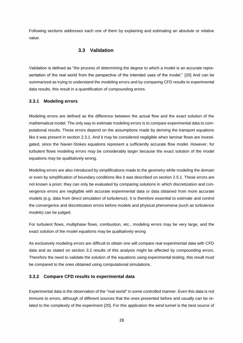
Figure 3.2 – Detailed view of testing area pressure magnitude plotted on the longitudinal

plane presenting the wind tunnel in a box configuration. ............................................................. 29

Figure 3.3 –Geometry B1 with box geometry incident velocity magnitude on intercooler’s

upstream face. .................................................................................................................................... 29

Figure 3.4 - Convergence workflow using L2 norm error ............................................................. 32

Figure 3.5 - Cell quality example, good cell to the left and a bad cell to the right (image from

[4]) ......................................................................................................................................................... 33

Figure 3.6 –Cell quality parameter on a polyhedral mesh with 4 Million cell geometry

(Geometry B) ....................................................................................................................................... 34

Figure 3.7 – Detail of a trimmed mesh of around 4Milliion cells on the left and the

corresponding cell quality parameter on the right (Geometry B) ................................................ 34

Figure 3.8 - Cell quality parameter on a trimmed mesh with 4 Million cells (Geometry B) ..... 34

Figure 3.9 – Based on the already presented trimmed mesh of around 4 Million cells with a

further refined area with 25% base cell volume reduction to increase results detail on the test

section duct (Geometry B)................................................................................................................. 35

Figure 3.10 – Velocity value along test duct, intercooler is positioned at from x cord 1,6 up to

x cord 1,8 ............................................................................................................................................. 36

Figure 3.11 – Pressure value along test duct, intercooler is positioned at from x cord 1,6 up

to x cord 1,8 ......................................................................................................................................... 36

Figure 3.12 - Velocity vector plotted on already presented coarse mesh. ................................. 37

Figure 3.13 - Velocity vector plotted on mesh 1M ......................................................................... 37

Figure 3.14 - Velocity vector plotted on already presented 4M mesh ........................................ 37

Figure 3.15 - Velocity vector plotted on already presented 4M25 mesh .................................... 38

Figure 3.16 - Velocity vector plotted on already presented 9M mesh ........................................ 38

Figure 4.1 – The mean pressure field plotted on the cross section plane presenting the wind

tunnel in a central configuration ....................................................................................................... 39

Figure 4.2 – Detailed view of testing area mean pressure magnitude plotted on the cross

section presenting the wind tunnel in a central configuration. ..................................................... 39

Figure 4.3 – Incident mean pressure magnitude on intercooler’s upstream face ..................... 40

Figure 4.4 – Mean velocity magnitude plotted on the longitudinal plane ................................... 40

Figure 4.5 – Mean velocity magnitude plotted on the longitudinal plane (Detailed view of

testing area with central configuration) ........................................................................................... 40

Figure 4.6 – Mean Velocity profile 50mm upstream of the intercooler position (on the left) and

at the intercooler’s face (on the right) .............................................................................................. 41

Figure 4.7 –Side view of the wind tunnel geometry A. .................................................................. 41

Figure 4.8 – The mean pressure field plotted on the cross section plane presenting the wind

tunnel in a central configuration ....................................................................................................... 42

Figure 4.9 – Detailed view of testing area mean pressure magnitude plotted on the cross

section presenting the wind tunnel in a central configuration. ..................................................... 42

Figure 4.10 – Incident mean pressure magnitude on intercooler’s upstream face .................. 43

Figure 4.11 – Detailed view of testing area average velocity magnitude plotted on the

longitudinal plane presenting the wind tunnel in a central configuration the scale is used in

Figure 4.23 ........................................................................................................................................... 43

xii

Figure 4.12 –Geometry A with central geometry mean velocity profile 50 mm of the testing

duct (On the left); Incident mean velocity magnitude on intercooler’s upstream face (on the

right) ...................................................................................................................................................... 43

Figure 4.13 – Wind tunnel outlet duct (E1-Filter 1, E2-Filter 2, V-Vortex and ventilator) ........ 44

Figure 4.14 – Wind tunnel cross section where it is possible to identify the Settling Chamber

(A), the Test Section (B and Cyan colored), the Air Cooler (C), the Drive Section (D and

Magenta colored)) and two additional pressure losses (E1 and E2) .......................................... 45

Figure 4.15 – Wind tunnel top view, ceiling heat exchangers and inlet duct. ........................... 45

Figure 4.16 – Wind tunnel geometry front view, ceiling heat exchangers (A) and cable tray

(B). ........................................................................................................................................................ 46

Figure 4.17- Sketch of the air flow the Drive Section is colored in Magenta ............................. 46

Figure 4.18 – Test section geometry configuration (clockwise starting from top left: central,

box, full-face and down face) ............................................................................................................ 46

Figure 4.19 - Cross section of the wind tunnel geometry B with the proposed extra filters (1

and 2).................................................................................................................................................... 47

Figure 4.20 - Pressure magnitude plotted on the longitudinal plane presenting the wind

tunnel in a box configuration ............................................................................................................. 48



Figure 4.22 – Incident pressure magnitude on intercooler’s upstream face ............................. 48

Figure 4.23 - Velocity magnitude plotted on the longitudinal plane presenting the wind tunnel

in a box configuration ......................................................................................................................... 49

Figure 4.24 – Detailed view of testing area velocity magnitude plotted on the longitudinal

plane presenting the wind tunnel in a box configuration the scale is used in Figure 4.23 ...... 49

Figure 4.25 –Geometry B1 with box geometry velocity profile 50 mm of the testing duct (On

the left); Incident velocity magnitude on intercooler’s upstream face (on the right) ................. 49

Figure 4.26 – Pressure magnitude plotted on the longitudinal plane presenting the wind

tunnel in a down face configuration ................................................................................................. 50


plane presenting the wind tunnel in a down face configuration. .................................................. 50

Figure 4.28 - Geometry B1 with down face geometry velocity profile 50 mm of the testing

duct (On the left); Incident velocity magnitude on intercooler’s upstream face (on the right). 50

Figure 4.29 – Detail of Geometry B1 testing duct with down face configuration ...................... 51

Figure 4.30 - Geometry B1 with down face geometry velocity profile 50 mm of the testing

duct (On the left); Incident velocity magnitude at the intercooler’s upstream face (on the

right). ..................................................................................................................................................... 51

Figure 4.31 - Geometry B1 with down face geometry incident velocity magnitude at the

intercooler’s upstream face. .............................................................................................................. 52

Figure 5.1 – Test section detail of the wind tunnel geometry B cross section, a screen placed

at the test section entrance as a possible solution to increase flow homogenization. ............. 53

Figure 5.2 - Geometry B2 with box configuration, testing area detail. ....................................... 54

Figure 5.3 - Geometry B2 with box configuration, testing area detail. ....................................... 54

Figure 5.4 - Geometry B1 with box configuration, velocity profile at 50 mm away from the

testing duct (On the left); Incident velocity magnitude on intercooler’s upstream face (on the

right). ..................................................................................................................................................... 55

xiii

Figure 5.5 - Pressure magnitude plotted on the longitudinal plane presenting the wind tunnel

in a box configuration ......................................................................................................................... 55



Figure 5.7 - Geometry B2 with down face configuration, testing area detail. ............................ 56

Figure 5.8 – Geometry B2 with down face geometry velocity profile 50 mm of the testing duct

(On the left); Incident velocity magnitude on intercooler’s upstream face (on the right). ........ 56

Figure 5.9 – Test section detail of the wind tunnel geometry B cross section, a packed bed of

spheres is represented as a possible solution to increase flow homogenization. .................... 57

Figure 5.10 – Ergum correlation computed for a wide range of spheres and compared with

the CFD simulation (a packing bed with a length of 150mm was considered (blue dots) CFD

data in red. ........................................................................................................................................... 55

Figure 5.11 - Test section detail of the wind tunnel geometry B cross section, a piece of

fabric/cloth is represented as a possible solution to increase flow homogenization. ............... 55

Figure 5.12 – Test section detail of the wind tunnel geometry B cross section, a packed bed

of spheres is represented as a possible solution to increase flow homogenization................. 56

Figure 6.1- Initial wind tunnel geometry .......................................................................................... 57

Figure 6.2- Improved wind tunnel geometry ................................................................................... 58

Figure 6.3 –Geometry A with central geometry mean velocity profile 50 mm of the testing

duct (On the left); Incident mean velocity magnitude on intercooler’s upstream face (on the

right) ...................................................................................................................................................... 58

Figure 6.4 –Geometry B1 with box geometry velocity profile 50 mm of the testing duct (On

the left); Incident velocity magnitude on intercooler’s upstream face (on the right) ................. 58

Figure 6.5 – Two possible solutions (a cloth based solution on the left and a spheres based

solution at the right) ............................................................................................................................ 59

Figure 6.6 - Geometry B1 with box configuration, velocity profile at 50 mm away from the

testing duct (On the left); Incident velocity magnitude on intercooler’s upstream face (on the

right). ..................................................................................................................................................... 59


spheres is represented as a possible solution to increase flow homogenization. .................... 60

xiv

List of Tables

Table 1.1 - Intercooler geometries ..................................................................................................... 5

Table 2.1 - Central geometry, also included in the analysis ........................................................ 10

Table 2.2 - Constant physical properties of the air ........................................................................ 13

Table 2.3 – Central case pressure loss experimental data (kindly supplied by JDEUS) ........ 20

Table 3.1 – Mesh characterization for the grid refinement study ................................................ 35

Table 4.1 - Geometry B2 with down face configuration ................................................................ 51

Table 5.1 - Geometry B2 with down face configuration. ............................................................... 56

Table 5.2 - Ergum equation by Zou and Yu ................................................................................... 58

Table 8.1 - List of commercially available spheres ........................................................................ 66

Table 8.2 – Corrected Ergum equation results for commercially available spheres. .............. 67

xv

Nomenclature

Acronyms

CFD Computational Fluid Dynamics

3D Three Dimensions

2D Two Dimensions

IC Intercooler

CAD Computer Aided Design

Symbols

𝑐𝑝 Pressure coefficient

𝑟 Compression ratio

Dh Hydraulic diameter

µ Viscosity

ρ density

Re Reynolds Number

P Absolute Pressure

𝑢𝑟𝑓 Under-relaxation factor for pressure.

Subscripts

𝑥, 𝑦, 𝑧 Cartesian components

𝑖, 𝑗, 𝑘 Computational indexes

𝑎𝑖𝑟 Air

𝑔𝑒𝑜𝑚 A particular intercooler geometry

1

1 Introduction

1.1 Objective

The main goal for this dissertation is to understand the air flow and provide a better understanding of

the wind tunnel through the use of Computational Fluid Dynamics (CFD) simulations, obtained results

analyzed and then validated against experimental data so that relevant conclusions can be withdrawn

and, eventually, propose changes to improve the wind tunnel performance.

This study is in the Mechanical Engineering interest as it requires information from several disciplines

ranging from Thermodynamics to Aerodynamics, Fluid Mechanics and also Computational Fluid Me-

chanics.

1.2 Background

JDEUS is a thermal equipment manufacturer focused on the automotive market part of the Denso

Corporation. In JDEUS facilities in Samora Correia Portugal a closed circuit wind tunnel is used to sup-

port both certification and R&D activities

A wind tunnel is an apparatus with air moving inside used in aerodynamic research to study the effect

of air moving pass solid objects. Due to a wide range of existing applications to be studied by wind

tunnels there are different geometries and technologies that can be combined to create different families

of wind tunnels such as:

Low speed wind tunnels

High speed wind tunnels

Supersonic wind tuunels

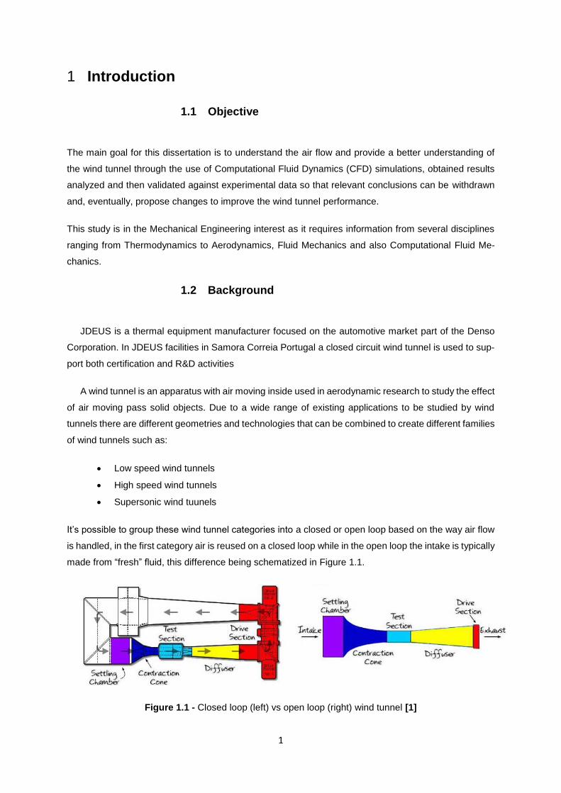
It’s possible to group these wind tunnel categories into a closed or open loop based on the way air flow

is handled, in the first category air is reused on a closed loop while in the open loop the intake is typically

made from “fresh” fluid, this difference being schematized in Figure 1.1.

Figure 1.1 - Closed loop (left) vs open loop (right) wind tunnel [1]

2

The JDEUS wind tunnel is a closed loop wind tunnel which geometry can be found in Figure 1.2. The

wind tunnel is divided into two distinct rooms: the first one containing the chamber on the left and the

second one contains the drive section and ducts (often called the machine room).

Figure 1.2- 3D model of the JDEUS closed circuit wind tunnel (this 3D representation was produced

as part of this work)

As presented before in Figure 1.1 a closed loop wind tunnel has identified areas such as the settling

chamber, a test section and a drive section Figure 1.3 identifies the JDEUS wind tunnel key sections.

Figure 1.3- Inner side view of the JDEUS wind tunnel 3D model where it is possible to identify the Set-

tling Chamber (A) Test Section (B and Cyan colored), the Air Cooler (C) and the Drive Section (D and

Magenta colored)) (this 3D representation was produced as part of this work)

This wind tunnel is used to study air flow passing through intercoolers and radiators similar to the ones

presented in Figure 1.4.

A

B

D

C

3

Figure 1.4 –JDEUS portfolio sample, an Intercooler on the left and a radiator on the right [2]

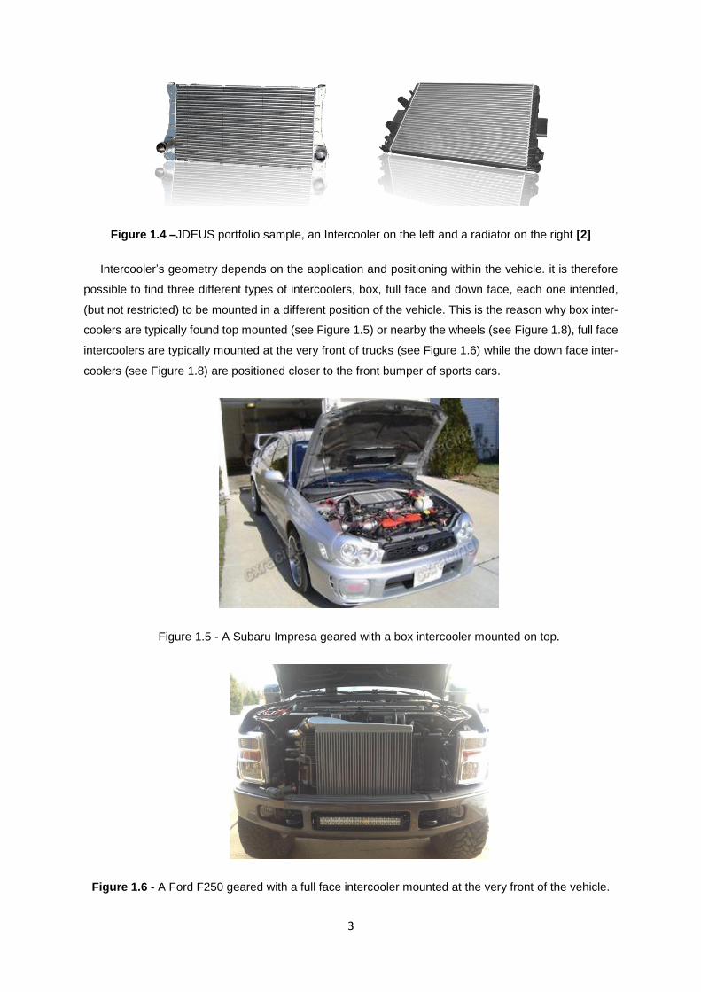
Intercooler’s geometry depends on the application and positioning within the vehicle. it is therefore

possible to find three different types of intercoolers, box, full face and down face, each one intended,

(but not restricted) to be mounted in a different position of the vehicle. This is the reason why box inter-

coolers are typically found top mounted (see Figure 1.5) or nearby the wheels (see Figure 1.8), full face

intercoolers are typically mounted at the very front of trucks (see Figure 1.6) while the down face inter-

coolers (see Figure 1.8) are positioned closer to the front bumper of sports cars.

Figure 1.5 - A Subaru Impresa geared with a box intercooler mounted on top.

Figure 1.6 - A Ford F250 geared with a full face intercooler mounted at the very front of the vehicle.

4

Figure 1.7 - A Volskwagen Beettle geared with a down face intercooler mounted on the front bumper.

Figure 1.8 - A Fiat 500 Abarth geared with a box intercooler mounted close to the wheels. (Figure

supplied by JDEUS)

These types are given according to the intercooler geometric characteristics such as width and height

following the automobile industry nomenclature, see Figure 1.9.

Figure 1.9 - Intercooler nomenclature

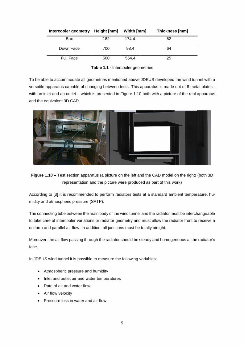
Table 1.1 describes the dimensions of covered geometries in this work, where differences between

intercooler types are clear.

5

Intercooler geometry Height [mm] Width [mm] Thickness [mm]

Box 182 174.4 62

Down Face 700 98.4 64

Full Face 500 554.4 25

Table 1.1 - Intercooler geometries

To be able to accommodate all geometries mentioned above JDEUS developed the wind tunnel with a

versatile apparatus capable of changing between tests. This apparatus is made out of 8 metal plates -

with an inlet and an outlet – which is presented in Figure 1.10 both with a picture of the real apparatus

and the equivalent 3D CAD.

Figure 1.10 – Test section apparatus (a picture on the left and the CAD model on the right) (both 3D

representation and the picture were produced as part of this work)

According to [3] it is recommended to perform radiators tests at a standard ambient temperature, hu-

midity and atmospheric pressure (SATP).

The connecting tube between the main body of the wind tunnel and the radiator must be interchangeable

to take care of intercooler variations or radiator geometry and must allow the radiator front to receive a

uniform and parallel air flow. In addition, all junctions must be totally airtight.

Moreover, the air flow passing through the radiator should be steady and homogeneous at the radiator’s

face.

In JDEUS wind tunnel it is possible to measure the following variables:

Atmospheric pressure and humidity

Inlet and outlet air and water temperatures

Rate of air and water flow

Air flow velocity

Pressure loss in water and air flow.

6

1.3 Limitations

This work will focus on the air flow reaching the test section (upstream of the intercooler), this flow will

be considered adiabatic as heat transfers between the intercooler body and the air passing through will

not be accounted for.

There is a room temperature control mechanism installed at the settling chamber ceiling, it’s a set of

heat exchangers and fans to force the air passing through while cools, this mechanism is only activated

when room temperature is outside the test bottom and top temperature thresholds, while at work this

cause secondary flows inside the settling chamber and works for short periods of time, reason why this

forced motion of the air will not be accounted.

The 3D-model of the wind tunnel is simplified to only include objects of at least approximately 40mm,

which means that small objects for example cables and pipes are not modeled.

Each geometry of the wind tunnel has at least 4 different variations based on the test section configura-

tion, and it was not possible to simulate all of them.

1.4 Dissertation outline

This dissertation is structured in 6 chapters, with the following content:

Chapter 1 – In chapter 1, an introduction to the subject is made.

Chapter 2 – In chapter 2, the methodology used to create the mathematical and numerical

model is presented along with essential concepts behind the CFD process.

Chapter 3 – In chapter 3 common CFD errors will be presented along with the method used to

verify and validate the results will also be present the results, still in this chapter the mesh con-

vergence procedure is described along with the validation of simulated results compared against

the ones obtained on the real wind tunnel.

Chapter 4 – In chapter 4, results will be presented and some conclusions will be made in order

to propose changes to the existing wind tunnel geometry leading, a new geometry based on

remarks made on chapters 2 and 4, CFD results will be presented for this new geometry are

also included in this chapter along with

Chapter 5 – In chapter 5 flow homogenization will be discussed and three different techniques

will be presented.

Chapter 6 – In chapter 6 conclusions and final remarks will be presented along with some ideas

for future works.

7

2 Methodology

2.1 Geometry

In this sub-section, the wind tunnel and the different intercooler geometries will be presented. All these

geometries are based on the real apparatus except for the simplified version (geometry A2) that was

created for validation purposes only.

2.1.1 Wind tunnel geometry A

The 3D wind tunnel geometry was created based on measurements and observations performed on site

using both laser and standard measuring tools, considerations must be made because as stated in

section 1.3 the wind tunnel geometry is simplified to only include objects that are at least approximately

40mm, which means that small objects for example cables are not modeled.. A comparison between

the 3D model and the real apparatus can be found in Figure 2.1.

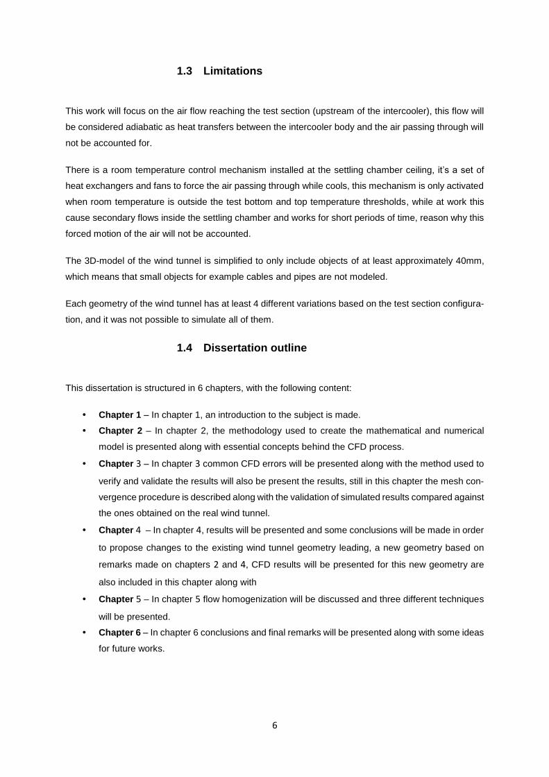
Figure 2.1 – Geometry side view perspective of the settling chamber and the testing area. 3D geome-

try to the left and corresponding pictures to the right.

The ceiling of the apparatus consists of a complex set of heat exchangers (coolers) and fans to control

the air temperature, these are presented in Figure 2.2 and Figure 2.3. These heat exchangers are made

of the same material as the geometries of the intercoolers and use a cold water circuit while the fans

are set in motion, so that air is forced to pass through the heat exchangers while cooling therefore the

existence of these coolers caused secondary flows to appear inside the settling chamber.

8

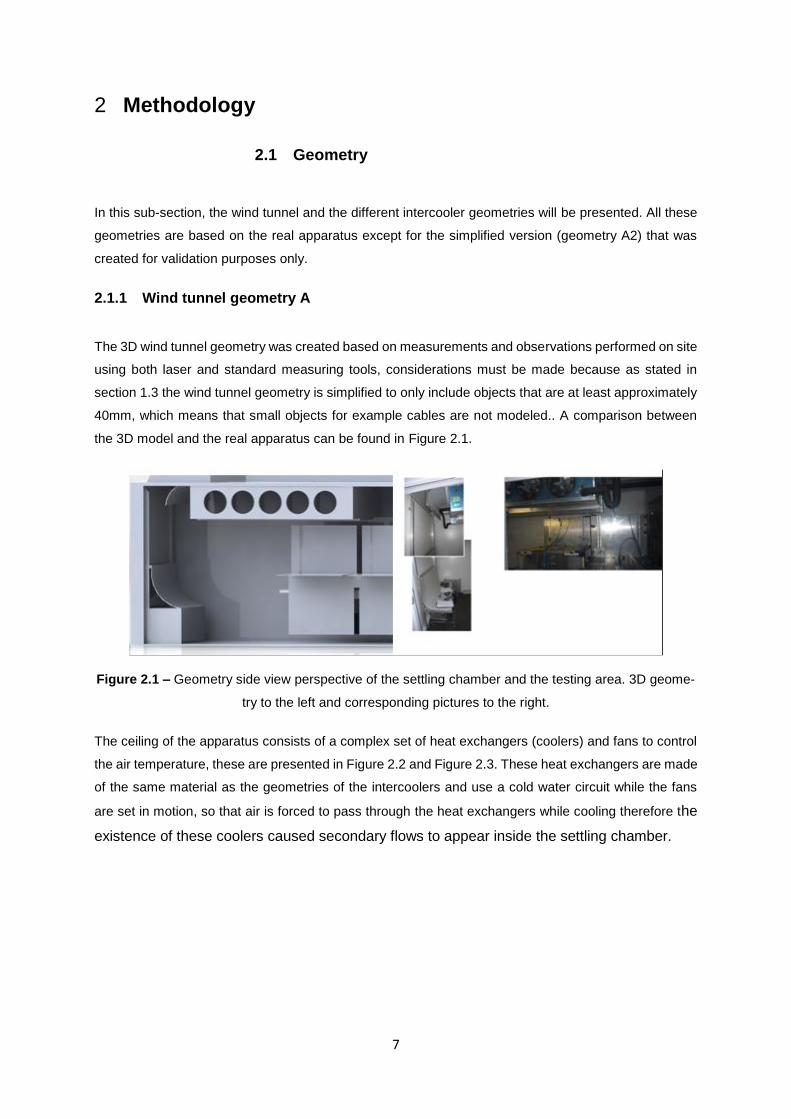
Figure 2.2 – Geometry top view, heat exchangers

Between the two sets of heat exchangers, there are two deflectors that can be seen in Figure 2.3.

Figure 2.3 – Wind tunnel geometry front view, detailed view of the ceiling heat exchangers and internal

deflectors.

Above the ceiling is located the settling chamber inlet duct, which is presented in Figure 2.4.

Figure 2.4 – Wind tunnel geometry top view, detailed view of the settling chamber inlet duct.

As already presented in section 1.2 the JDEUS uses a closed loop wind tunnel, the complete geometry

is presented in Figure 2.5 where the air flow motion is also sketched.

9

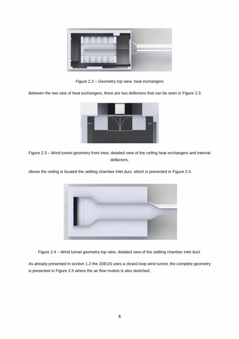
Figure 2.5- Sketch of the air flow, the Drive Section (colored in Magenta)

As a first geometry to be simulated this would represent a huge effort and therefore the wind tunnel

geometry A2 was proposed as a first geometry for CFD simulations. This geometry will be presented in

the next sub-section.

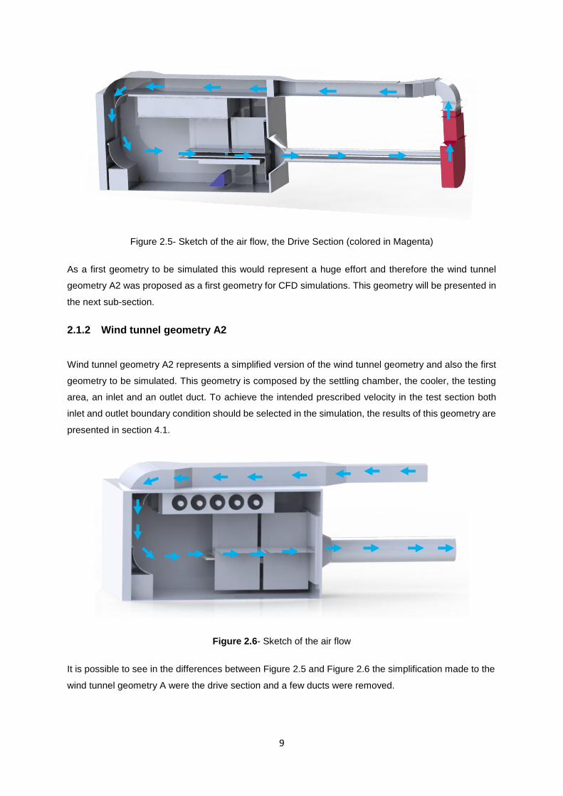
2.1.2 Wind tunnel geometry A2

Wind tunnel geometry A2 represents a simplified version of the wind tunnel geometry and also the first

geometry to be simulated. This geometry is composed by the settling chamber, the cooler, the testing

area, an inlet and an outlet duct. To achieve the intended prescribed velocity in the test section both

inlet and outlet boundary condition should be selected in the simulation, the results of this geometry are

presented in section 4.1.

Figure 2.6- Sketch of the air flow

It is possible to see in the differences between Figure 2.5 and Figure 2.6 the simplification made to the

wind tunnel geometry A were the drive section and a few ducts were removed.

10

2.1.3 Intercooler geometries

As stated in section 1.2 there is a wide variety of products developed and produced by JDEUS, this

section will introduce the reader to the reason behind the wide range of geometries. As specific appli-

cations require different intercooler’s output such as the required heat to be exchanged and not less

important the available space and positioning for the intercooler to be mounted therefore it exists a vast

range of products to provide tailored solutions for each set of requirements.

It is possible to encounter three different types of intercoolers: box, full face and down face, each one

of each is intended, but not restricted to be mounted in a different position of the vehicle. Reason why

box intercoolers are typically founded in top mounted or nearby the wheels, full face intercoolers are

typically mounted at the very front of trucks, the down face intercoolers (similar to the one presented

below) are positioned closer to the front bumper of sports cars.

These requirements can be translated into geometric parameters such as 𝐻 x 𝑊 x T according to the

terminology used across the automotive industry, this definition is presented in Figure 1.9.

For this study particular intercoolers were selected and can be found on the table Table 1.1

In addition to these models a central case with a Box type geometry was also selected for this study

because experimental data was available when this study was conducted, the central case geometry is

presented in Table 2.1.

Intercooler geometry Height [mm] Width [mm] Thickness [mm]

Central 300 144 80

Table 2.1 - Central geometry, also included in the analysis

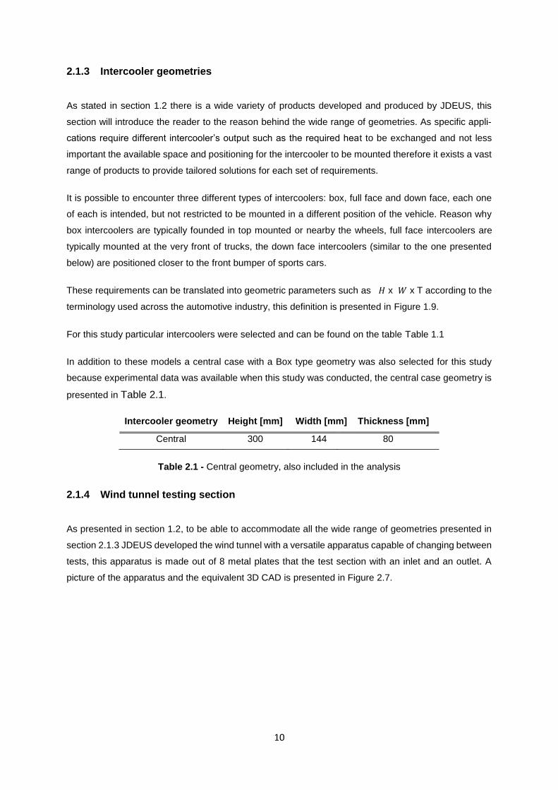
2.1.4 Wind tunnel testing section

As presented in section 1.2, to be able to accommodate all the wide range of geometries presented in

section 2.1.3 JDEUS developed the wind tunnel with a versatile apparatus capable of changing between

tests, this apparatus is made out of 8 metal plates that the test section with an inlet and an outlet. A

picture of the apparatus and the equivalent 3D CAD is presented in Figure 2.7.

11

Figure 2.7 – Front view of the test section apparatus (a picture on the left and the CAD model on the

right)

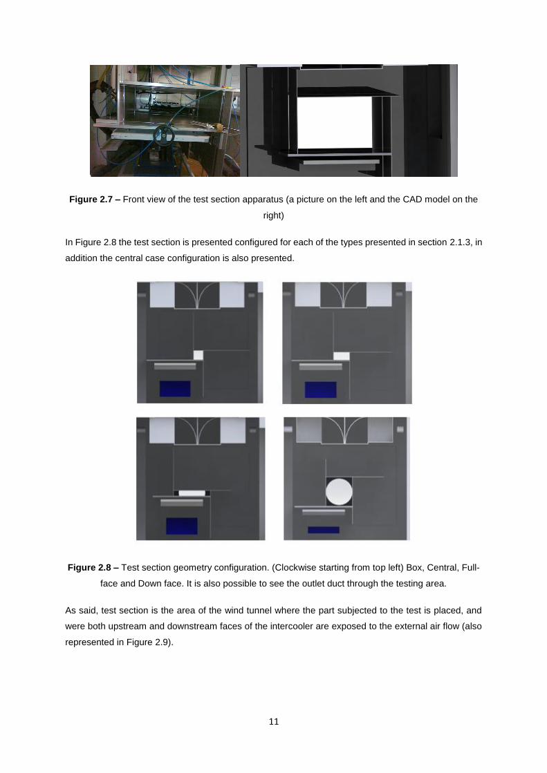
In Figure 2.8 the test section is presented configured for each of the types presented in section 2.1.3, in

addition the central case configuration is also presented.

Figure 2.8 – Test section geometry configuration. (Clockwise starting from top left) Box, Central, Full-

face and Down face. It is also possible to see the outlet duct through the testing area.

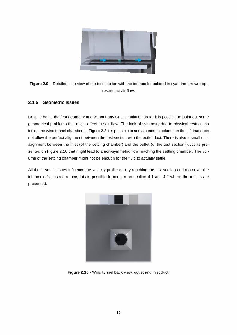
As said, test section is the area of the wind tunnel where the part subjected to the test is placed, and

were both upstream and downstream faces of the intercooler are exposed to the external air flow (also

represented in Figure 2.9).

12

Figure 2.9 – Detailed side view of the test section with the intercooler colored in cyan the arrows rep-

resent the air flow.

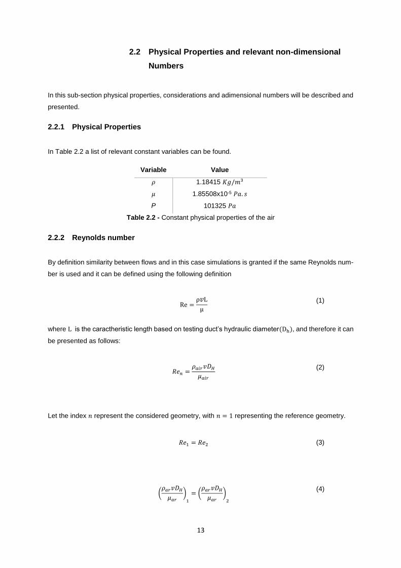
2.1.5 Geometric issues

Despite being the first geometry and without any CFD simulation so far it is possible to point out some

geometrical problems that might affect the air flow. The lack of symmetry due to physical restrictions

inside the wind tunnel chamber, in Figure 2.8 it is possible to see a concrete column on the left that does

not allow the perfect alignment between the test section with the outlet duct. There is also a small mis-

alignment between the inlet (of the settling chamber) and the outlet (of the test section) duct as pre-

sented on Figure 2.10 that might lead to a non-symmetric flow reaching the settling chamber. The vol-

ume of the settling chamber might not be enough for the fluid to actually settle.

All these small issues influence the velocity profile quality reaching the test section and moreover the

intercooler’s upstream face, this is possible to confirm on section 4.1 and 4.2 where the results are

presented.

Figure 2.10 - Wind tunnel back view, outlet and inlet duct.

13

2.2 Physical Properties and relevant non-dimensional

Numbers

In this sub-section physical properties, considerations and adimensional numbers will be described and

presented.

2.2.1 Physical Properties

In Table 2.2 a list of relevant constant variables can be found.

Variable Value

𝜌 1.18415 𝐾𝑔/𝑚3

𝜇 1.85508x10-5 𝑃𝑎. 𝑠

P 101325 𝑃𝑎

Table 2.2 - Constant physical properties of the air

2.2.2 Reynolds number

By definition similarity between flows and in this case simulations is granted if the same Reynolds num-

ber is used and it can be defined using the following definition

Re =

ρ𝑣L

µ

(1)

where L is the caractheristic length based on testing duct’s hydraulic diameter(Dh), and therefore it can

be presented as follows:

𝑅𝑒𝑛 =

𝜌𝑎𝑖𝑟𝑣𝐷𝐻

𝜇𝑎𝑖𝑟

(2)

Let the index 𝑛 represent the considered geometry, with 𝑛 = 1 representing the reference geometry.

𝑅𝑒1 = 𝑅𝑒2 (3)

(𝜌𝑎𝑟𝑣𝐷𝐻

𝜇𝑎𝑟

)1

= (𝜌𝑎𝑟𝑣𝐷𝐻

𝜇𝑎𝑟

)2

(4)

14

where 𝐷𝐻 stands for the hydraulic diameter.

Considering an incompressible and isothermal regime:

𝑣1𝐷𝐻1 = 𝑣2𝐷𝐻2 (5)

Hence

𝑣1𝐷𝐻1

𝐷𝐻2

= 𝑣2 (6)

where index 1 and 2 stands for a given simulation.

2.3 Mathematical and Numerical Model

In this sub-section the theory behind the numerical simulations performed in this dissertation is briefly

stated and explained. For more detailed information one is directed to the STAR-CCM user’s Manual

[4]. Some important aspects of this work will also be addressed.

2.3.1 Governing equations

In this section only essential modeling aspects of this work will be covered, further information can be

obtained from [5] [6] and [7].

This work, much like all CFD, is based on the three fundamental governing equations – continuity

(Mass conservation), momentum (Newton’s second law) and energy (Energy conservation). This sec-

tion will briefly address those equations and the complementary models (i.e. turbulence) required to fully

understand this work.

The equation that express mass and momentum balance in the flow, latter being named as the Navier-

Stokes equations, are expressed equation (7) and equation (8) in their tensorial form [6] [7],

𝜕𝜌

𝜕𝑡+

𝜕

𝜕𝑥𝑖

(𝜌𝑢𝑗) = 𝑠𝑚 (7)

𝜕(𝜌 𝑢𝑖)

𝜕𝑡+

𝜕

𝜕𝑥𝑗

(𝜌 𝑢𝑗 − 𝜏𝑖𝑗) = −𝜕𝑝

𝜕𝑥𝑖

+ 𝑠𝑖 (8)

15

where 𝑡 stands for time; 𝑥𝑖 the Cartesian coordinates (𝑖=1,2,3,); 𝑢𝑖 is the velocity component in the 𝑥𝑖

direction; 𝑝 represents the static pressure; 𝜌 the density; 𝜏𝑖𝑗 the components of the stress tensor; 𝑠𝑚 the

mass source and 𝑠𝑖 the momentum sources. In this case 𝑠𝑚 = 0 since there are no mass sources.

As suggested by [8] and [9] air can be considered incompressible for these CFD simulations, in addition

and as stated in section 1.4, no account for temperature effects are being taken into account, hence

density (ρ) can be considered constant both in space and time. It is therefore possible to simplify equa-

tions (7) and (8) and present them as follows:

𝜕𝑢𝑖

𝜕𝑥𝑖

= 0 (9)

𝜌

𝜕( 𝑢𝑖)

𝜕𝑡+ 𝜌

𝜕 𝑢𝑗

𝜕𝑥𝑗

− 𝜕 𝜏𝑖𝑗

𝜕𝑥𝑗

= −𝜕𝑝

𝜕𝑥𝑖

+ 𝑠𝑖 (10)

Cast in discrete form, this forms the basis for finite element computations. Since the segregated flow

approach is used, flow equations (velocity and pressure) will be solved in a segregated or uncoupled

manner. The link between the momentum and continuity equations is achieved with a predictor-corrector

approach and with a SIMPLE solver algorithm [6].

2.3.2 SIMPLE algorithm

As stated in 2.3.1 the model will make use of a SIMPLE solver algorithm [4] whose basics steps in the

solution update are as follows:

1. Set the boundary conditions

2. Compute the gradients of velocity and pressure

3. Solve the discretized momentum equation to compute the intermediate velocity field.

4. Compute the uncorrected mass fluxes at cell faces

5. Solve the pressure correction equation to produce cell values of the pressure correction.

6. Update the pressure field 𝑝𝑘+1 = 𝑝𝑘 + 𝑢𝑟𝑓 ∙ 𝑝′, where 𝑢𝑟𝑓 is the under-relaxation factor for pres-

sure.

7. Update boundary pressure corrections 𝑝𝑏′.

8. Correct the cell face mass fluxes: �̇�𝑓𝑘+1 − �̇�𝑓

∗ + �̇�𝑓′

9. Correct cell velocities: �⃗⃗� 𝑘+1 − �⃗� ∗ −𝑉∆𝑝′

𝑎𝑃𝑣 ; where ∆𝑝′ is the pressure corrections gradient, 𝑎𝑃

𝑣 is

the central coefficients vector for discretized linear system representing the velocity equations

and V is the cell volume.

16

2.3.3 Turbulence Modeling

Turbulence is present in the almost every flows encountered in nature and among several industrial

applications. Turbulent flows are characterized by fluctuating velocity fields. These fluctuations mixes

transported quantities such as momentum, energy causing transported quantities to fluctuate as well.

[10]

Instead of directly compute governing equations (DNS) these can be time-averaged (RANS), ensemble-

averaged, or otherwise manipulated to remove small scales (LES), resulting in a modified set of equa-

tions that are computationally less expensive to solve [6], that said one conclude that RANS and LES

are less computational expensive than DNS but RANS is still less expensive than LES. However,

modified equations contain additional unknown variables, and turbulence models are needed to deter-

mine these variables in terms of known quantities.

In this work, as will be seen, there was the need to investigate some turbulence models in order to obtain

a good agreement between computational results and experiments. All models considered throughout

this work are available in STAR-CCM.

2.3.3.1 Reynolds Average Navier Stokes (RANS)

Due to the computationally expensive DNS and LES for most geophysical and engineering applications,

modelers are restricted to RANS approaches commonly based on turbulent kinetic energy (TKE) closure

schemes. The most widely used RANS models today are two equation models which solve two transport

equations for the properties of the turbulence from which the eddy viscosity can be computed. The best

known of these models is the k- ε model which requires the solutions of the turbulent kinetic energy

equation and dissipation of turbulent kinetic energy equation [11]. The other model addressed in this

work is the k − ω model.

2.3.3.1.1 𝐤 − 𝛆

This turbulence model is a two-equation model in which transport equations are solved to the turbulence.

The values of k and ε come from transport equations for turbulent kinetic energy k and turbulent dissi-

pation rate ε. And although STAR-CCM+ has the most significant improvements made so far to this

model [6] it is not suitable to solve adverse gradient flows [12] reason why this model was not selected

for the present analysis.

2.3.3.1.2 𝐤 − 𝛚

Commonly addressed as the standard k − ω is also a two-equation model. A transport equation for the

turbulence kinetic energy k and a quantity ω defined as the specific dissipation rate.

17

One reported advantage of the k − ω model over the k − ε is its performance for boundary layers under

adverse pressure gradients [6], it was also formulated to better compute low-Reynolds number effects,

compressibility and shear flow spreading [13].

The biggest disadvantage of the k − ω model, in its original form, is that boundary layer computations

are sensitive to the values of ω in the free stream [6] However, for this analysis free stream boundary

layer condition is not used (boundary conditions are addressed in section 2.3.4)

2.3.4 Boundary conditions

Apart from the geometry definition and a consequent mesh, there is the need to for boundary conditions.

In closed wind tunnels, air flows by the action of a ventilator, represented in these simulations as a

constant pressure increase on momentum equation.

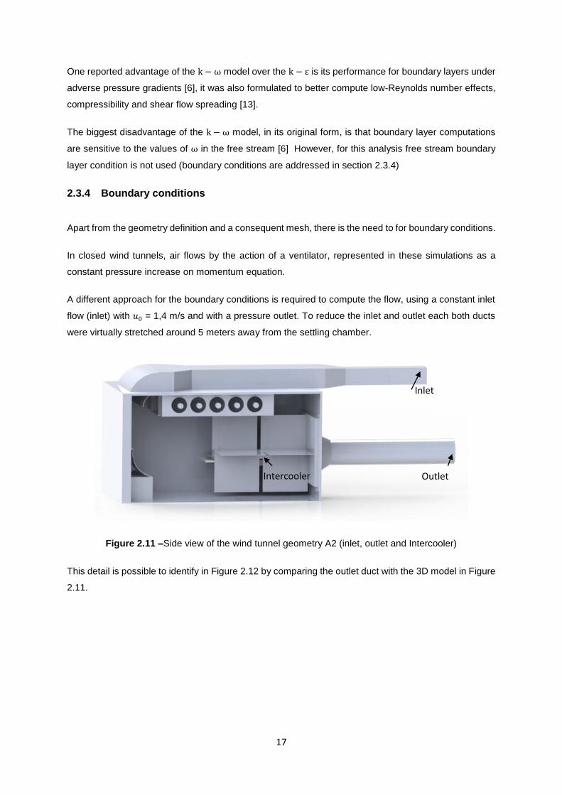
A different approach for the boundary conditions is required to compute the flow, using a constant inlet

flow (inlet) with 𝑢0 = 1,4 m/s and with a pressure outlet. To reduce the inlet and outlet each both ducts

were virtually stretched around 5 meters away from the settling chamber.

Figure 2.11 –Side view of the wind tunnel geometry A2 (inlet, outlet and Intercooler)

This detail is possible to identify in Figure 2.12 by comparing the outlet duct with the 3D model in Figure

2.11.

Inlet

Intercooler Outlet

18

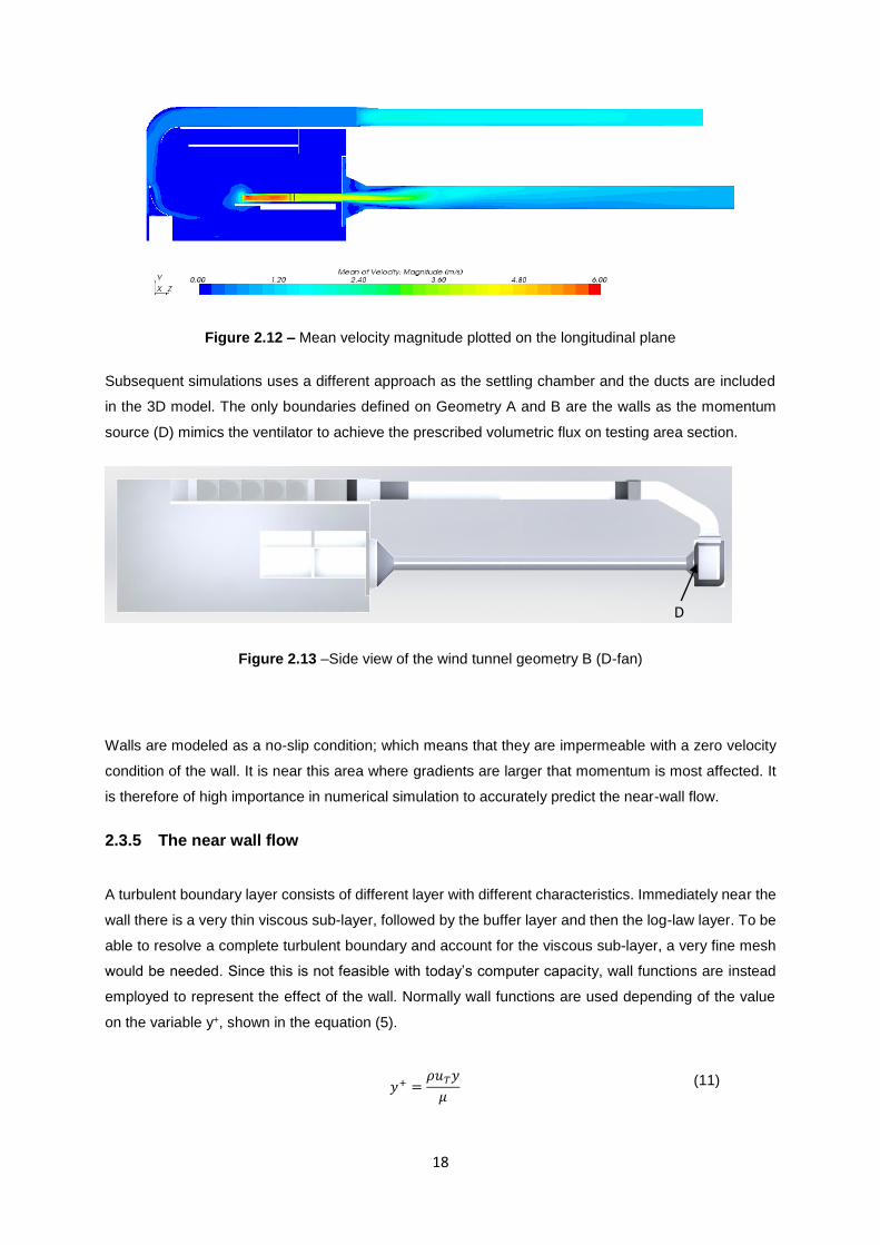
Figure 2.12 – Mean velocity magnitude plotted on the longitudinal plane

Subsequent simulations uses a different approach as the settling chamber and the ducts are included

in the 3D model. The only boundaries defined on Geometry A and B are the walls as the momentum

source (D) mimics the ventilator to achieve the prescribed volumetric flux on testing area section.

Figure 2.13 –Side view of the wind tunnel geometry B (D-fan)

Walls are modeled as a no-slip condition; which means that they are impermeable with a zero velocity

condition of the wall. It is near this area where gradients are larger that momentum is most affected. It

is therefore of high importance in numerical simulation to accurately predict the near-wall flow.

2.3.5 The near wall flow

A turbulent boundary layer consists of different layer with different characteristics. Immediately near the

wall there is a very thin viscous sub-layer, followed by the buffer layer and then the log-law layer. To be

able to resolve a complete turbulent boundary and account for the viscous sub-layer, a very fine mesh

would be needed. Since this is not feasible with today’s computer capacity, wall functions are instead

employed to represent the effect of the wall. Normally wall functions are used depending of the value

on the variable y+, shown in the equation (5).

𝑦+ =𝜌𝑢𝑇𝑦

𝜇 (11)

D

19

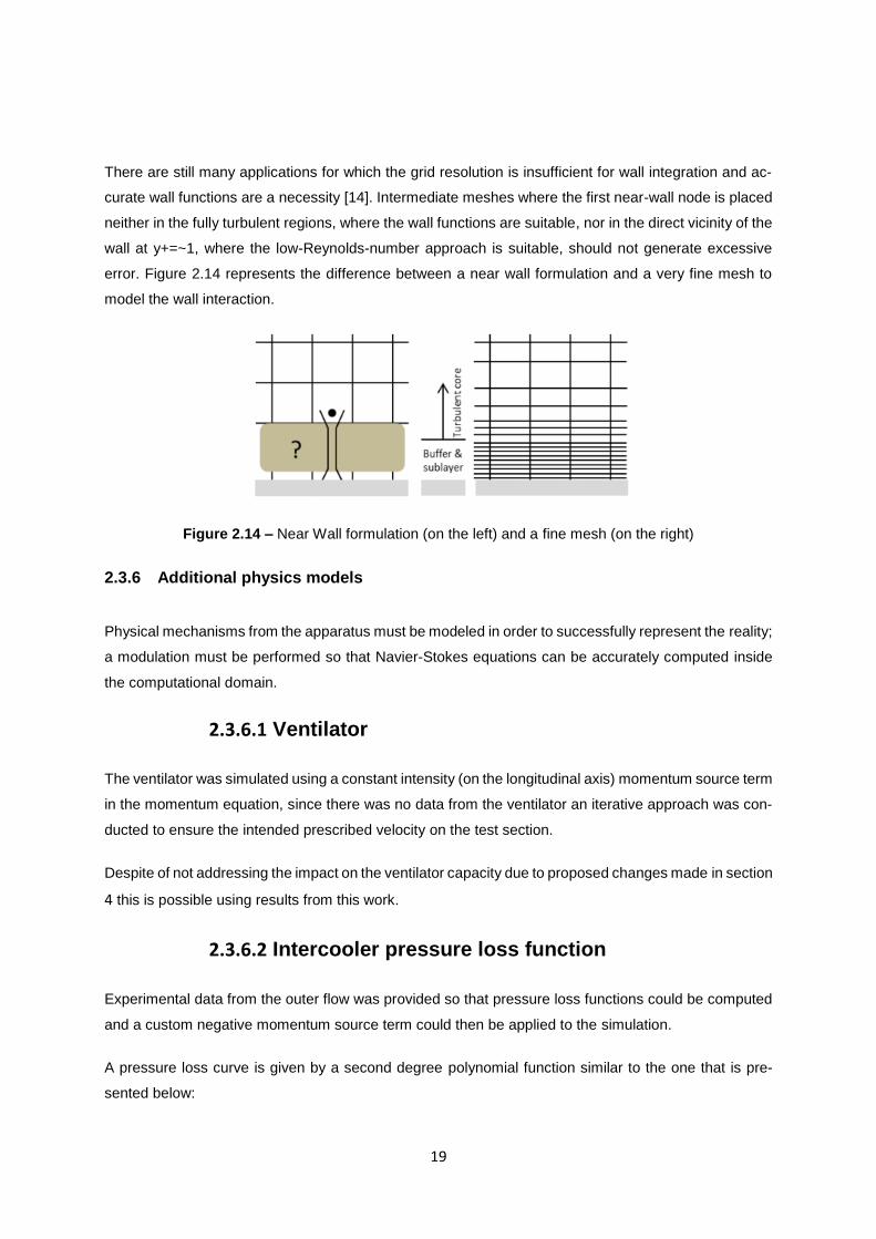
There are still many applications for which the grid resolution is insufficient for wall integration and ac-

curate wall functions are a necessity [14]. Intermediate meshes where the first near-wall node is placed

neither in the fully turbulent regions, where the wall functions are suitable, nor in the direct vicinity of the

wall at y+=~1, where the low-Reynolds-number approach is suitable, should not generate excessive

error. Figure 2.14 represents the difference between a near wall formulation and a very fine mesh to

model the wall interaction.

Figure 2.14 – Near Wall formulation (on the left) and a fine mesh (on the right)

2.3.6 Additional physics models

Physical mechanisms from the apparatus must be modeled in order to successfully represent the reality;

a modulation must be performed so that Navier-Stokes equations can be accurately computed inside

the computational domain.

2.3.6.1 Ventilator

The ventilator was simulated using a constant intensity (on the longitudinal axis) momentum source term

in the momentum equation, since there was no data from the ventilator an iterative approach was con-

ducted to ensure the intended prescribed velocity on the test section.

Despite of not addressing the impact on the ventilator capacity due to proposed changes made in section

4 this is possible using results from this work.

2.3.6.2 Intercooler pressure loss function

Experimental data from the outer flow was provided so that pressure loss functions could be computed

and a custom negative momentum source term could then be applied to the simulation.

A pressure loss curve is given by a second degree polynomial function similar to the one that is pre-

sented below:

20

∆𝑃 = 𝑎𝑉2 + 𝑏𝑉 (12)

Experimental data from an intercooler model of the box type with the following geometry [H x W] = 300

x 144 are listed in Table 2.3:

Case 𝑣𝑖−𝑒𝑥𝑡𝑒𝑟𝑛𝑎𝑙 𝑎𝑖𝑟 𝑓𝑙𝑜𝑤

[m/s]

ΔPext [Pa]

1 2 95

2 4 275

3 6 534

4 8 848

5 10 1340

Table 2.3 – Central case pressure loss experimental data (kindly supplied by JDEUS)

One can approximate intercooler longitudinal pressure loss to

−

𝜕𝑃𝑖,𝑗,𝑘

𝜕𝑥𝑖,𝑗,𝑘

= 𝑎𝑣𝑖,𝑗,𝑘2 + 𝑏𝑣𝑖,𝑗,𝑘

(13)

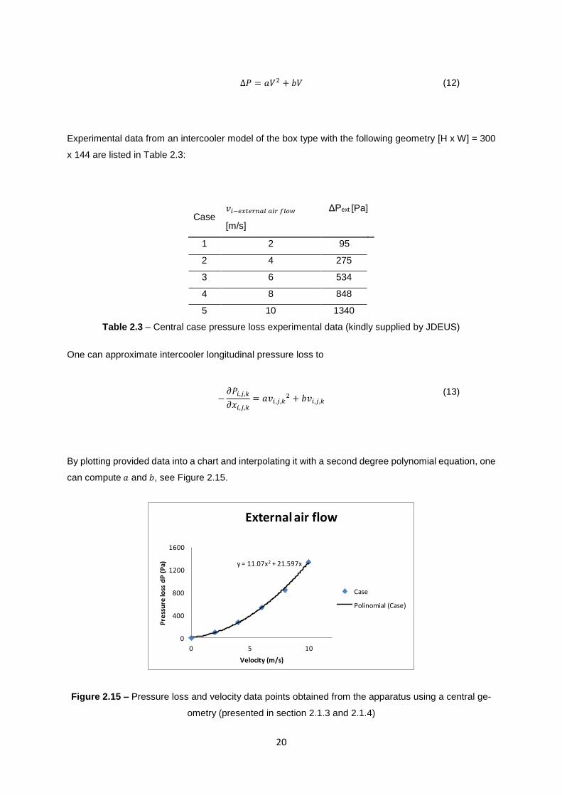
By plotting provided data into a chart and interpolating it with a second degree polynomial equation, one

can compute 𝑎 and 𝑏, see Figure 2.15.

y = 11.07x2 + 21.597x

0

400

800

1200

1600

0 5 10

Pre

ssu

re lo

ss d

P (

Pa)

Velocity (m/s)

External air flow

Case

Polinomial (Case)

Figure 2.15 – Pressure loss and velocity data points obtained from the apparatus using a central ge-

ometry (presented in section 2.1.3 and 2.1.4)

21

The polynomial data interpolation provides required coefficients with a maximum error of 6.14% (for V

= 2𝑚

𝑠) and an average error of 2.98%:

𝑎 = 11,07 𝑘𝑔

𝑚5𝑠

𝑏 = 21,597 𝑘𝑔

𝑚2𝑠

Replacing coefficient 𝑎 and 𝑏 on equation (13), one gets an equation to describe the pressure loss for

the central geometry.

∆𝑃𝑖(𝑣) = 11,07 𝑣𝑖2 + 21,697𝑣𝑖 (14)

Equation (14) was written for the total pressure drop the following linearization for the pressure per

length unit will be used:

∆𝑃𝑖

∆𝑥𝑐𝑒𝑛𝑡𝑟𝑎𝑙

(𝑣, 𝑥𝑔𝑒𝑜𝑚) =11,07 𝑣𝑖

2 + 21,697 𝑣𝑖

∆𝑥𝑐𝑒𝑛𝑡𝑟𝑎𝑙

𝑥𝑔𝑒𝑜𝑚 (15)

where 𝑥𝑔𝑒𝑜𝑚 is the thickness of the intercooler geometry.

Please note that a total pressure drop will depend on both air stream velocity and thickness of the

pressure loss (intercooler or filter), resulting in equation (10)

∆𝑃𝑖(𝑣, 𝑥𝑔𝑒𝑜𝑚) =

11,07 𝑣𝑖2 + 21,697 𝑣𝑖

80 × 10−3∆𝑥𝑖−𝑔𝑒𝑜𝑚𝑒𝑡𝑟𝑦

(16)

As there are no available data regarding the pressure loss other directions a homogeneous pressure

drop will be assumed and therefore the following relation applies:

𝜕𝑃𝑖

𝜕𝑥𝑖

= 𝑐𝑡𝑒 (17)

This data set was the only one available and therefore no available data for other intercooler geometries,

the following approximation will be applied to extrapolate this dataset for other geometries presented in

section 2.1.3.

22

(𝜕𝑃𝑖,𝑗,𝑘


) (𝑣)𝐶𝑒𝑛𝑡𝑟𝑎𝑙

= (𝜕𝑃𝑖,𝑗,𝑘


) (𝑣)𝐵𝑜𝑥



) (𝑣)𝐷𝑜𝑤𝑛 𝐹𝑎𝑐𝑒



) (𝑣)𝐹𝑢𝑙𝑙 𝐹𝑎𝑐𝑒

(18)

Approximation (17) will also be applied across each geometry.

2.4 Discretization

STAR-CCM+ uses the finite volume method to discretize the volume into smaller volumes (control vol-

umes or cells) where equations are solved, the following advantages and disadvantages can be pointed

out for the this method.

Advantages:

Can accommodate any type of grid, so it is suitable for complex geometries as the one addressed in

this work. [15]

The grid defines the control volume boundaries [15] and there is no need of a given cell to be related to

a coordinate system.

The method is conservative by construction and preserves the mass to the machine precision [16]

Disadvantages:

Methods of higher than second order are more difficult to develop in 3D, due to the fact that the finite

volume approach requires three levels of approximation (interpolation, differentiation, and integration),

however all terms that need to be approximated have physical meaning [17].

It is therefore easy to understand that meshing is a vital step for CFD simulation because in this step

individual cells are created on model geometry to be solved by mathematical methods connected and

formed within the boundary region of the model. STAR-CCM+ volume mesher contain three different

types of grids:

Tetrahedral

Polyhedral

Trimmed

Each of which offers advantages and disadvantages, some of them are presented below:

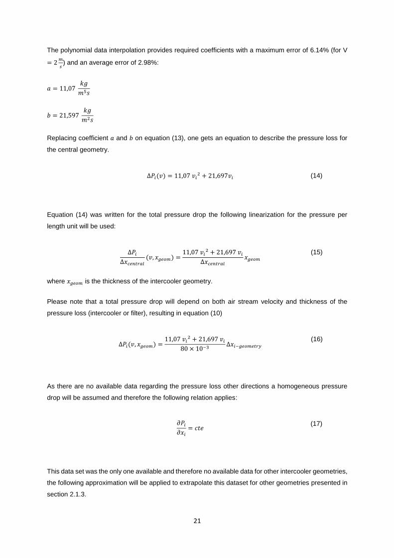
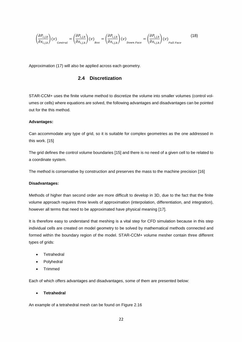
Tetrahedral

An example of a tetrahedral mesh can be found on Figure 2.16

23

Advantages:

o Relatively easy to generate automatically [18]

o Simple volume elements having plane segment faces and therefore both face and volume

centroid locations are well defined. [18]

Disadvantages:

o Tetrahedral meshes typically require 4-10 times more elements than a hexahedral mesh to

obtain the same level of accuracy [19]

o Volume mesh quality is very dependent on surface mesh quality.

o Requires a larger number of control volumes

o Have only four neighbors, and computing gradients at cell centers using standard approxi-

mations (linear shape functions) can be problematic.

o One problem is linked with the spatial position of neighbor nodes, because they may all lie

in nearly one plane, making it impossible to evaluate the gradient in the direction normal to

that plane.

o Another problem is encountered for cells next to boundaries: even when only one face is a

boundary face, the remaining three neighbors may be unfavorably distributed, moreover

along edges or at corners, one may end up with only one or two neighbor’s cell, which can

cause serious numerical problems, let alone reduced accuracy the fact that, for a hexahe-

dral cell, there are three optimal flow directions which lead to the maximum accuracy (nor-

mal to each of the three sets of parallel faces); for a polyhedron with 12 faces, there are six

optimal directions which, together with the large number of neighbors, lead to a more accu-

rate solution with a lower cell count.

Figure 2.16 – Example of a tetrahedral mesh

24

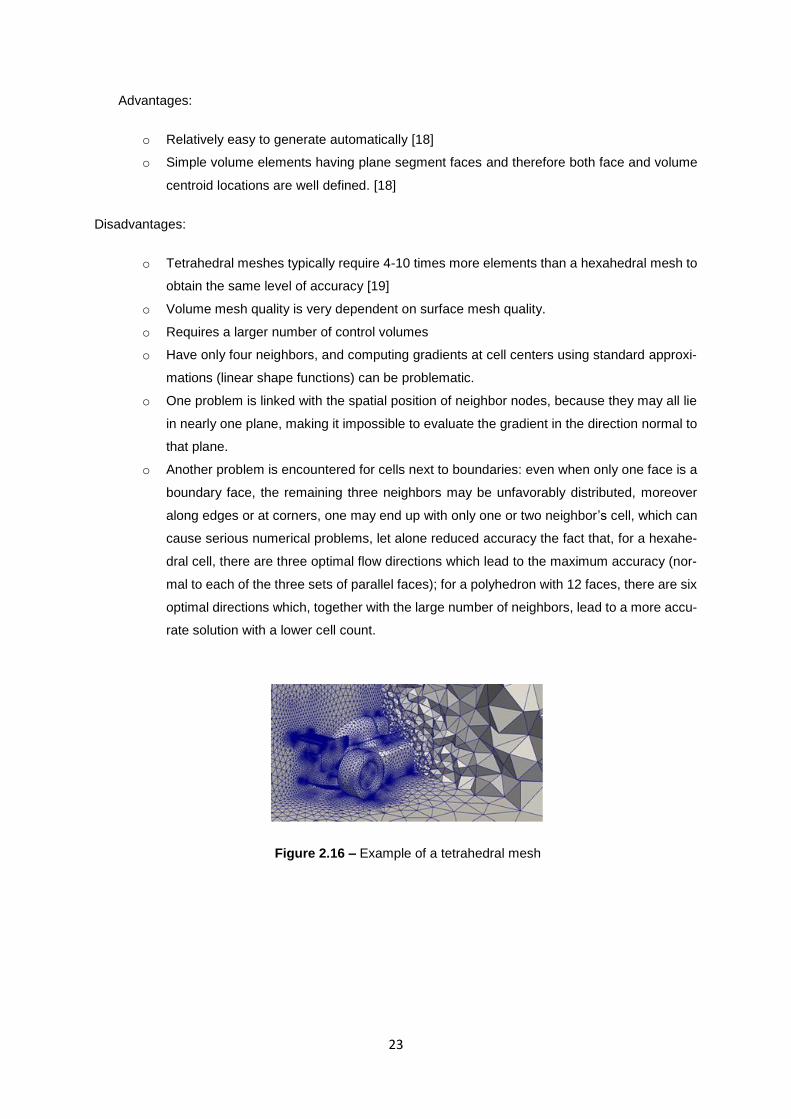
Polyhedral

An example of a polyhedral mesh can be found on Figure 2.17

Advantages:

o Contains many neighbors (typically of order 10) and therefore gradients can be much better

approximated (using linear shape functions and the information from nearest neighbors

only) when compared to tetrahedral cells.

o Likely to have a couple of neighbors, even along wall edges and corners, thus allowing for

a reasonable prediction of both gradient and local flow distribution.

o Although requiring more storage and computing operations per cell, it’s compensated by a

higher accuracy.

Disadvantages:

o Volume mesh quality is very dependent on surface mesh quality

Figure 2.17 - Example of a polyhedral mesh

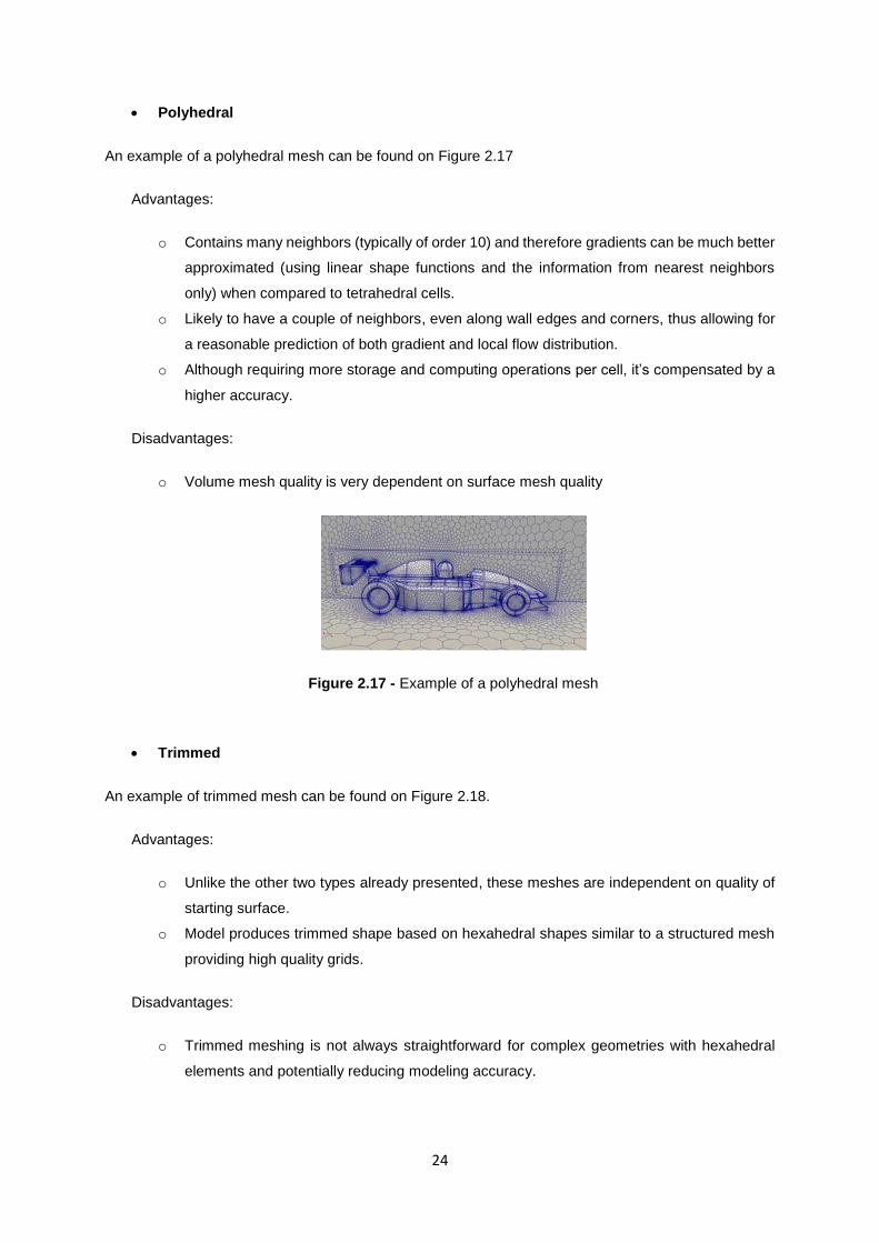
Trimmed

An example of trimmed mesh can be found on Figure 2.18.

Advantages:

o Unlike the other two types already presented, these meshes are independent on quality of

starting surface.

o Model produces trimmed shape based on hexahedral shapes similar to a structured mesh

providing high quality grids.

Disadvantages:

o Trimmed meshing is not always straightforward for complex geometries with hexahedral

elements and potentially reducing modeling accuracy.

25

Figure 2.18 – Example of a trimmed mesh

2.5 Star CCM+ and the CFD Methodology

In this sub-section the used methodology will be addressed along with STAR-CCM procedure presen-

tations because CFD flow simulation process follows a procedures hierarchy in order to be completed.

In fact, it can be decomposed in three main tasks:

Pre-processing

Simulation

Verification and validation of the solution

Post-processing.

STAR-CCM does all the pre-processing, including mesh generation, processing and post-processing

each one of each will be addressed with more care in the following sections. Only geometric models

were created previously using SolidWorks.

2.5.1 Pre-processing

Real geometry must be approximated by a CAD geometric model, the closer this model represents the

actual geometry the most accurate results are likely to be. Nevertheless, it’s mandatory to reduce the

level of detail so that only surfaces with impact on the flow are left. This is done in order to decrease the

amount of cells, enabling a better mesh quality and therefore reducing the simulation time.

Then it is necessary to identify the expected physical flow phenomena (turbulence, compressible flow,

combustion, multiphase flow, mixing, etc.) Star-CCM includes a vast range of physical models available

by default so that the grid generated is suitable to capture these phenomena.

Moreover boundary conditions are defined, which means that fluid behavior is specified at geometry

boundaries, in transient problems initial conditions are also specified.

2.5.2 Simulation

With the computational domain all set, it is possible to begin the second main task, on which the actual

fluid behavior is simulated.

26

CFD simulations are performed using an algorithm to solve equations with an iterative method, once the

solution is complete, it must be verified and validated against experimental data (if there is any availa-

ble). If this cannot be completed successfully, re-simulation may be required, with different assumptions

and/or grid improvements to the grid, models and boundary conditions used.

2.5.3 Verification and validation of the solution

Discretization yields a large number of algebraic equations (one set for each cell). These equations are

then generally solved using an iterative method, starting with a first guess value for all variables and

completing a computational cycle. Error or residual values are computed from the discredited equations

and the calculations are repeated many times, reducing the residual values, until a sufficiently converged

solution is judged to have been reached.

The final stage in the solution process is to determine when the solution has reached a sufficient level

of convergence. When the sum of the residual values around the system becomes sufficiently small, the

calculations are stopped and the solution is considered converged.

A further check is that additional iterations produce negligible changes in the variable values.

This subject is going to be addressed in more detail on section

2.5.4 Post-processing

Once a converged solution has been calculated, the results can be presented as numerical values or

pictures, such as velocity vectors and contours of constant values for instance pressure or velocity.

Visualization of numerical solutions using vector, contour or other kind of plots or movies (videos) of

unsteady flows is important for results interpretations. It’s also the more effective way of interpreting the

huge amount of data produced by a simulation. However there is always the risk of interpreting a bad

result as physical phenomena.

At the final stage, a post-processor organizes the output such that it is easily understandable whether

the solution is acceptable or not. After the data is organized it is possible to analyze the solution and

see, for example, the velocity and pressure fields.

27

3 Error Analysis

This chapter is devoted to the importance of being aware of existing errors, and even more to try to

distinguish each one of them. A small review of different errors is made, so that one understands all

steps taken in order to validate and verify that simulation results in use are representing the reality and

are trustworthy.

3.1 Realizability

It is necessary to verify if obtained results are actually a solution for the equations that it is being solved

and if obtained values are truthful. Typically, intended simulations are based on phenomena which are

too complex to treat directly (for example: turbulence, combustion, or multiphase flow), therefore models

should be designed to guarantee physically realistic solutions. This is not a numerical issue per si but

models that are not realizable may result in unphysical solutions or cause numerical methods to diverge.

In order to ensure that a realizable model is in use, results and data from duct flows were used to validate

the velocity and the pressure value, non-sense simulations were discarded.

3.2 Estimating errors

Numerical solutions of fluid flow and heat transfer problems are only approximate solutions. In addition

to the errors that might be introduced by setting up boundary conditions (as seen on section 2.3.4),

numerical solutions always include three kinds of systematic errors:

Modeling

Discretization

Iteration

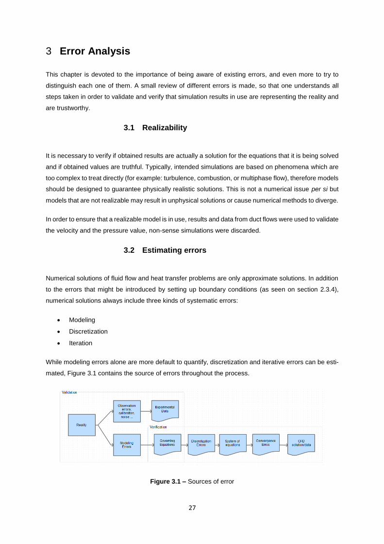
While modeling errors alone are more default to quantify, discretization and iterative errors can be esti-

mated, Figure 3.1 contains the source of errors throughout the process.

Figure 3.1 – Sources of error

28

Following sections addresses each one of them by explaining and estimating an absolute or relative

value.

3.3 Validation

Validation is defined as “the process of determining the degree to which a model is an accurate repre-

sentation of the real world from the perspective of the intended uses of the model.” [20] And can be

summarized as trying to understand the modeling errors and by comparing CFD results to experimental

data results, this result in a quantification of compounding errors.

3.3.1 Modeling errors

Modeling errors are defined as the difference between the actual flow and the exact solution of the

mathematical model. The only way to estimate modeling errors is to compare experimental data to com-

putational results. These errors depend on the assumptions made by deriving the transport equations

like it was present in section 2.3.1. And it may be considered negligible when laminar flows are investi-

gated, since the Navier-Stokes equations represent a sufficiently accurate flow model. However, for

turbulent flows modeling errors may be considerably larger because the exact solution of the model

equations may be qualitatively wrong.

Modeling errors are also introduced by simplifications made to the geometry while modeling the domain

or even by simplification of boundary conditions like it was described on section 2.5.1. These errors are

not known a priori; they can only be evaluated by comparing solutions in which discretization and con-

vergence errors are negligible with accurate experimental data or data obtained from more accurate

models (e.g. data from direct simulation of turbulence). It is therefore essential to estimate and control

the convergence and discretization errors before models and physical phenomena (such as turbulence

models) can be judged.

For turbulent flows, multiphase flows, combustion, etc., modeling errors may be very large, and the

exact solution of the model equations may be qualitatively wrong

As exclusively modeling errors are difficult to obtain one will compare real experimental data with CFD

data and as stated on section 3.2 results of this analysis might be affected by compounding errors.

Therefore the need to validate the solution of the equations using experimental testing, this result must

be compared to the ones obtained using computational simulations.

3.3.2 Compare CFD results to experimental data

Experimental data is the observation of the "real world" in some controlled manner. Even this data is not

immune to errors, although of different sources that the ones presented before and usually can be re-

lated to the complexity of the experiment [20]. For this application the wind tunnel is the best source of

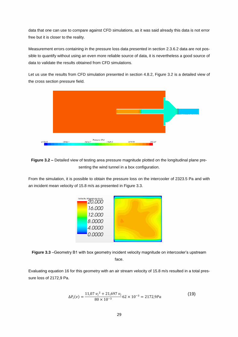
29

data that one can use to compare against CFD simulations, as it was said already this data is not error

free but it is closer to the reality.

Measurement errors containing in the pressure loss data presented in section 2.3.6.2 data are not pos-

sible to quantify without using an even more reliable source of data, it is nevertheless a good source of

data to validate the results obtained from CFD simulations.

Let us use the results from CFD simulation presented in section 4.8.2, Figure 3.2 is a detailed view of

the cross section pressure field.

Figure 3.2 – Detailed view of testing area pressure magnitude plotted on the longitudinal plane pre-

senting the wind tunnel in a box configuration.

From the simulation, it is possible to obtain the pressure loss on the intercooler of 2323.5 Pa and with

an incident mean velocity of 15.8 m/s as presented in Figure 3.3.

Figure 3.3 –Geometry B1 with box geometry incident velocity magnitude on intercooler’s upstream

face.

Evaluating equation 16 for this geometry with an air stream velocity of 15.8 m/s resulted in a total pres-

sure loss of 2172,9 Pa.

∆𝑃𝑖(𝑣) =

11,07 𝑣𝑖2 + 21,697 𝑣𝑖

80 × 10−362 × 10−3 = 2172,9𝑃𝑎

(19)

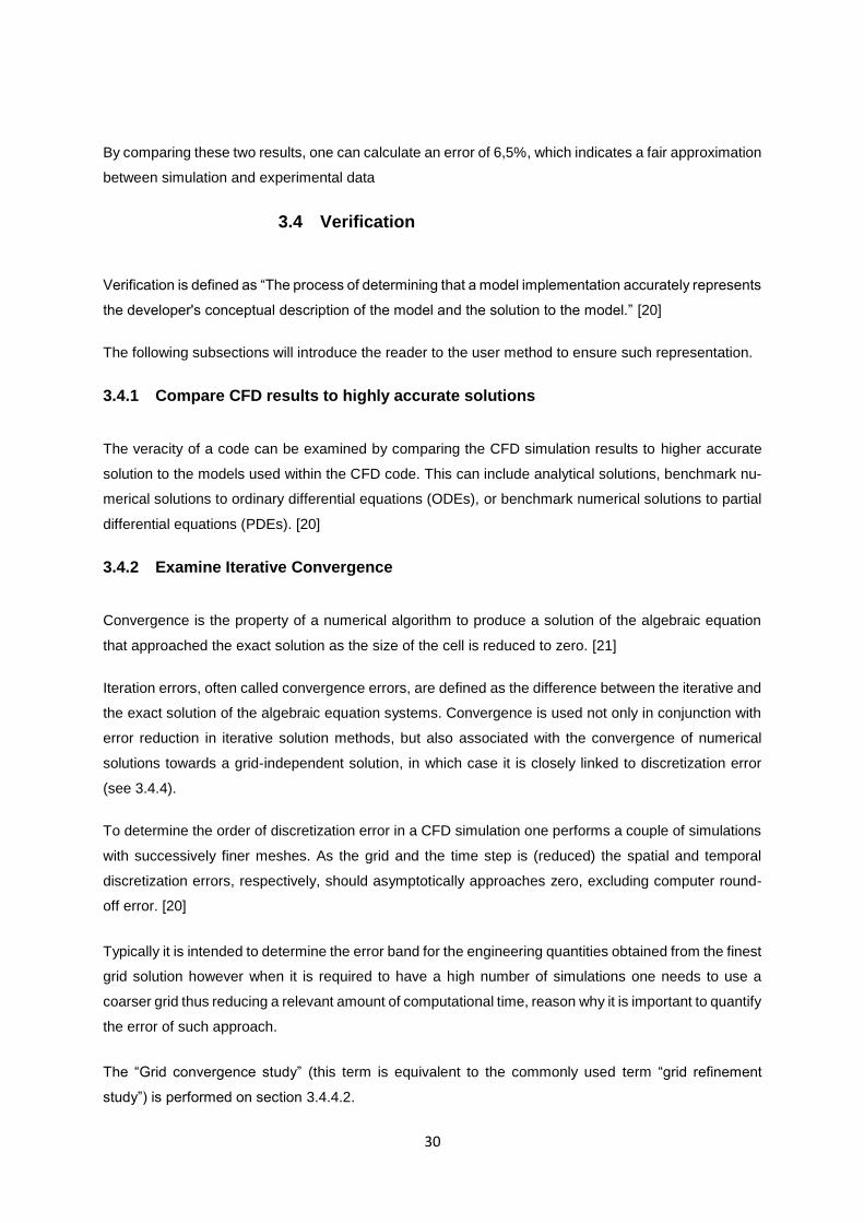
30

By comparing these two results, one can calculate an error of 6,5%, which indicates a fair approximation

between simulation and experimental data

3.4 Verification

Verification is defined as “The process of determining that a model implementation accurately represents

the developer's conceptual description of the model and the solution to the model.” [20]

The following subsections will introduce the reader to the user method to ensure such representation.

3.4.1 Compare CFD results to highly accurate solutions

The veracity of a code can be examined by comparing the CFD simulation results to higher accurate

solution to the models used within the CFD code. This can include analytical solutions, benchmark nu-

merical solutions to ordinary differential equations (ODEs), or benchmark numerical solutions to partial

differential equations (PDEs). [20]

3.4.2 Examine Iterative Convergence

Convergence is the property of a numerical algorithm to produce a solution of the algebraic equation

that approached the exact solution as the size of the cell is reduced to zero. [21]

Iteration errors, often called convergence errors, are defined as the difference between the iterative and

the exact solution of the algebraic equation systems. Convergence is used not only in conjunction with

error reduction in iterative solution methods, but also associated with the convergence of numerical

solutions towards a grid-independent solution, in which case it is closely linked to discretization error

(see 3.4.4).

To determine the order of discretization error in a CFD simulation one performs a couple of simulations

with successively finer meshes. As the grid and the time step is (reduced) the spatial and temporal

discretization errors, respectively, should asymptotically approaches zero, excluding computer round-

off error. [20]

Typically it is intended to determine the error band for the engineering quantities obtained from the finest

grid solution however when it is required to have a high number of simulations one needs to use a

coarser grid thus reducing a relevant amount of computational time, reason why it is important to quantify

the error of such approach.

The “Grid convergence study” (this term is equivalent to the commonly used term “grid refinement

study”) is performed on section 3.4.4.2.

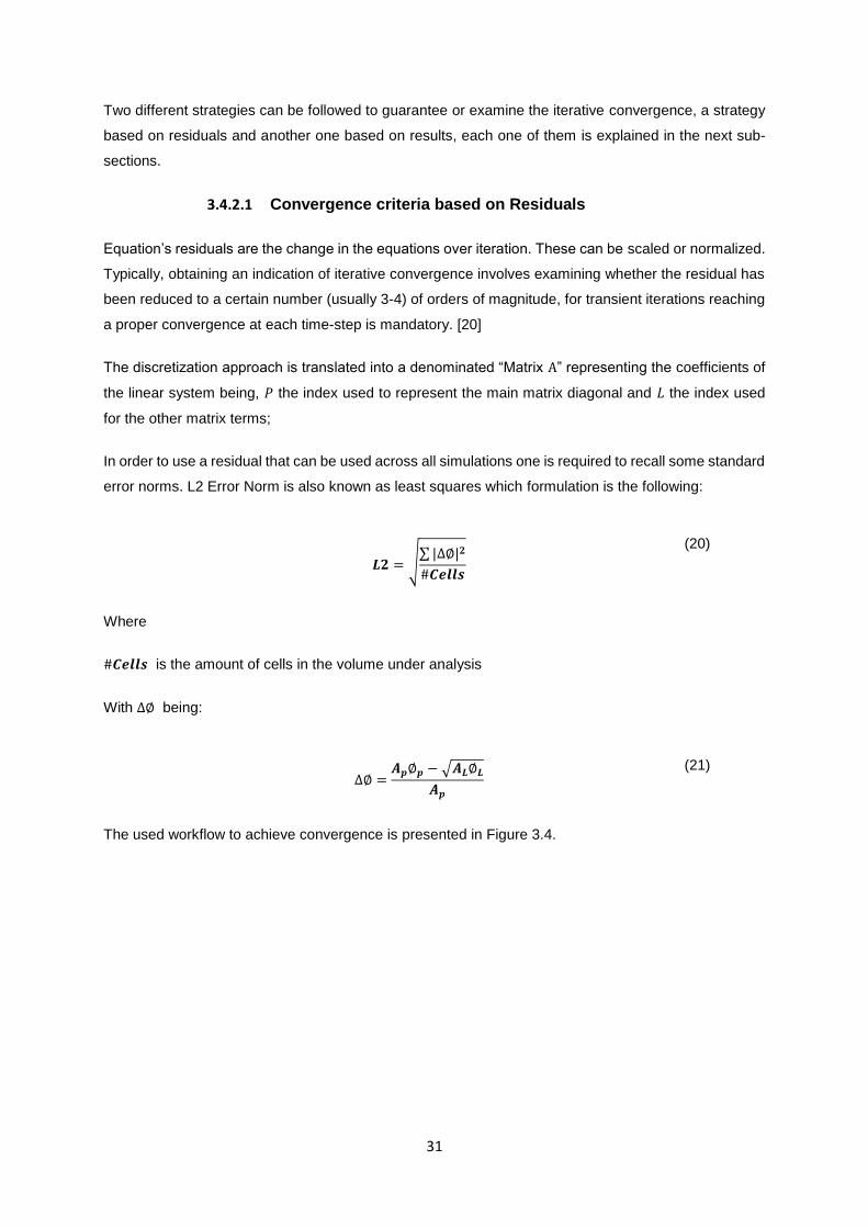
31

Two different strategies can be followed to guarantee or examine the iterative convergence, a strategy

based on residuals and another one based on results, each one of them is explained in the next sub-

sections.

3.4.2.1 Convergence criteria based on Residuals

Equation’s residuals are the change in the equations over iteration. These can be scaled or normalized.

Typically, obtaining an indication of iterative convergence involves examining whether the residual has

been reduced to a certain number (usually 3-4) of orders of magnitude, for transient iterations reaching

a proper convergence at each time-step is mandatory. [20]

The discretization approach is translated into a denominated “Matrix A” representing the coefficients of

the linear system being, 𝑃 the index used to represent the main matrix diagonal and 𝐿 the index used

for the other matrix terms;

In order to use a residual that can be used across all simulations one is required to recall some standard

error norms. L2 Error Norm is also known as least squares which formulation is the following:

𝑳𝟐 = √∑ |∆∅|𝟐

#𝑪𝒆𝒍𝒍𝒔

(20)

Where

#𝑪𝒆𝒍𝒍𝒔 is the amount of cells in the volume under analysis

With ∆∅ being:

∆∅ =

𝑨𝒑∅𝒑 − √𝑨𝑳∅𝑳

𝑨𝒑

(21)

The used workflow to achieve convergence is presented in Figure 3.4.

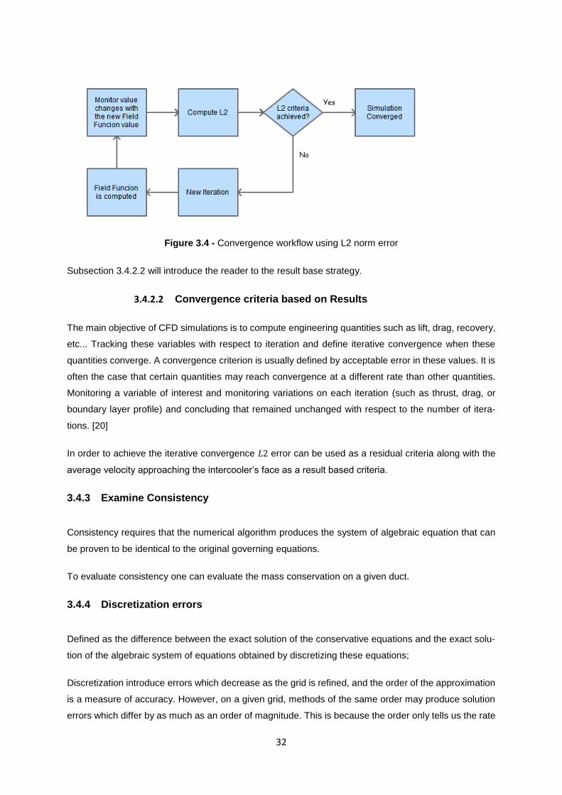
32

Figure 3.4 - Convergence workflow using L2 norm error

Subsection 3.4.2.2 will introduce the reader to the result base strategy.

3.4.2.2 Convergence criteria based on Results

The main objective of CFD simulations is to compute engineering quantities such as lift, drag, recovery,

etc... Tracking these variables with respect to iteration and define iterative convergence when these

quantities converge. A convergence criterion is usually defined by acceptable error in these values. It is

often the case that certain quantities may reach convergence at a different rate than other quantities.

Monitoring a variable of interest and monitoring variations on each iteration (such as thrust, drag, or

boundary layer profile) and concluding that remained unchanged with respect to the number of itera-

tions. [20]

In order to achieve the iterative convergence 𝐿2 error can be used as a residual criteria along with the

average velocity approaching the intercooler’s face as a result based criteria.

3.4.3 Examine Consistency

Consistency requires that the numerical algorithm produces the system of algebraic equation that can

be proven to be identical to the original governing equations.

To evaluate consistency one can evaluate the mass conservation on a given duct.

3.4.4 Discretization errors

Defined as the difference between the exact solution of the conservative equations and the exact solu-

tion of the algebraic system of equations obtained by discretizing these equations;

Discretization introduce errors which decrease as the grid is refined, and the order of the approximation

is a measure of accuracy. However, on a given grid, methods of the same order may produce solution

errors which differ by as much as an order of magnitude. This is because the order only tells us the rate

33

at which the error decreases at the mesh spacing is reduced; it gives no information about the error on

as single grid [22]

Discretization errors can be reduced by using more accurate interpolations or by applying the approxi-

mations to smaller regions but this will increase both time and cost of a solution. Compromise is always

needed as the ultimate goal is to obtain a compromise between maximum desired accuracy and with

the available resources and effort required.

However it’s important to have in mind that various errors may cancel each other, so that sometimes a

solution obtained on a course grid may agree better with the experiment than a solution on a finer grid

- which, by definition, should be more accurate, or the maximum accuracy with the available resources.

To ensure that a given solution is not affected by the prescribed mesh it requires to evaluate how does

the solution change with a mesh parameter, another important parameter aspect for time dependent

simulations is that errors might be affected by stopping the iteration process to soon.

3.4.4.1 Cell Quality

Cell quality in Star-CCM is based on a metric algorithm based on a both Gauss and least squares

methods. It is a function not only of the relative geometric distribution of the cell centroids of the neighbor

cells, but also on cell face’s orientation. Based on this criterion a cell quality with 1.0 is considered

perfect, and a degenerated cell will have a cell quality close to zero. One needs to take into account that

depending on the physics the cell quality can be fairly low and still provide a valid solution. It is also

possible to use weight functions to reduce the negative impact of lower quality cells. Figure 3.5 repre-

sents the difference between a good quality and a bad quality cell according to the STAR-CCM user’s

manual.

Figure 3.5 - Cell quality example, good cell to the left and a bad cell to the right (image from [4])

Figure 3.6 represents the wind tunnel geometry with a polyhedral grid where it is possible to conclude

that it is far from having an overall high quality mesh parameter moreover, this parameter is not constant

along the domain thus increasing the difficulty of reaching a stable solution.

34

Figure 3.6 –Cell quality parameter on a polyhedral mesh with 4 Million cell geometry (Geometry B)

Taking into consideration the advantages of a trimmed grid in terms of quality a trimmed mesh is pre-

sented in Figure 3.7.

Figure 3.7 – Detail of a trimmed mesh of around 4Milliion cells on the left and the corresponding cell

quality parameter on the right (Geometry B)

An overall view of the wind tunnel geometry is presented in Figure 3.8

Figure 3.8 - Cell quality parameter on a trimmed mesh with 4 Million cells (Geometry B)

35

That said the trimmed mesh was selected to discretize the computational domain, however, given the

reduced amount of cells on testing area, a local grid refinement was made with the cell size 25% smaller

than the original. Resulting mesh and quality parameter is presented in Figure 3.9.

Figure 3.9 – Based on the already presented trimmed mesh of around 4 Million cells with a further re-

fined area with 25% base cell volume reduction to increase results detail on the test section duct (Ge-

ometry B)

3.4.4.2 Mesh size

Since refining the entire grid does not add any advantage to the test area a characteristic length in

combination with pressure and velocity values along the test duct will be used to evaluate a set of 5

different grids, results will then be evaluated in order to obtain a grid to be used in further simulations.

Evaluating quantities of interest, namely pressure and velocity at the intercooler’s upstream face while

decreasing a mesh parameter ℎ (representing cell base size) allows to understand how solution is being

affected by the selected grid and let N be the number of cells in use by a refined grid this study is

presented in Table 3.1.

Grid N Characteristic cell length #Total grid cells

Corse

~N/12

0,060 360.467

1M ~N/6 0,040 1.072.396

4M ~N/2 0,025 4.075.258

4M 25 ~N/2 0,025 4.325.708

9M N 0,019 9.190.977

Table 3.1 – Mesh characterization for the grid refinement study

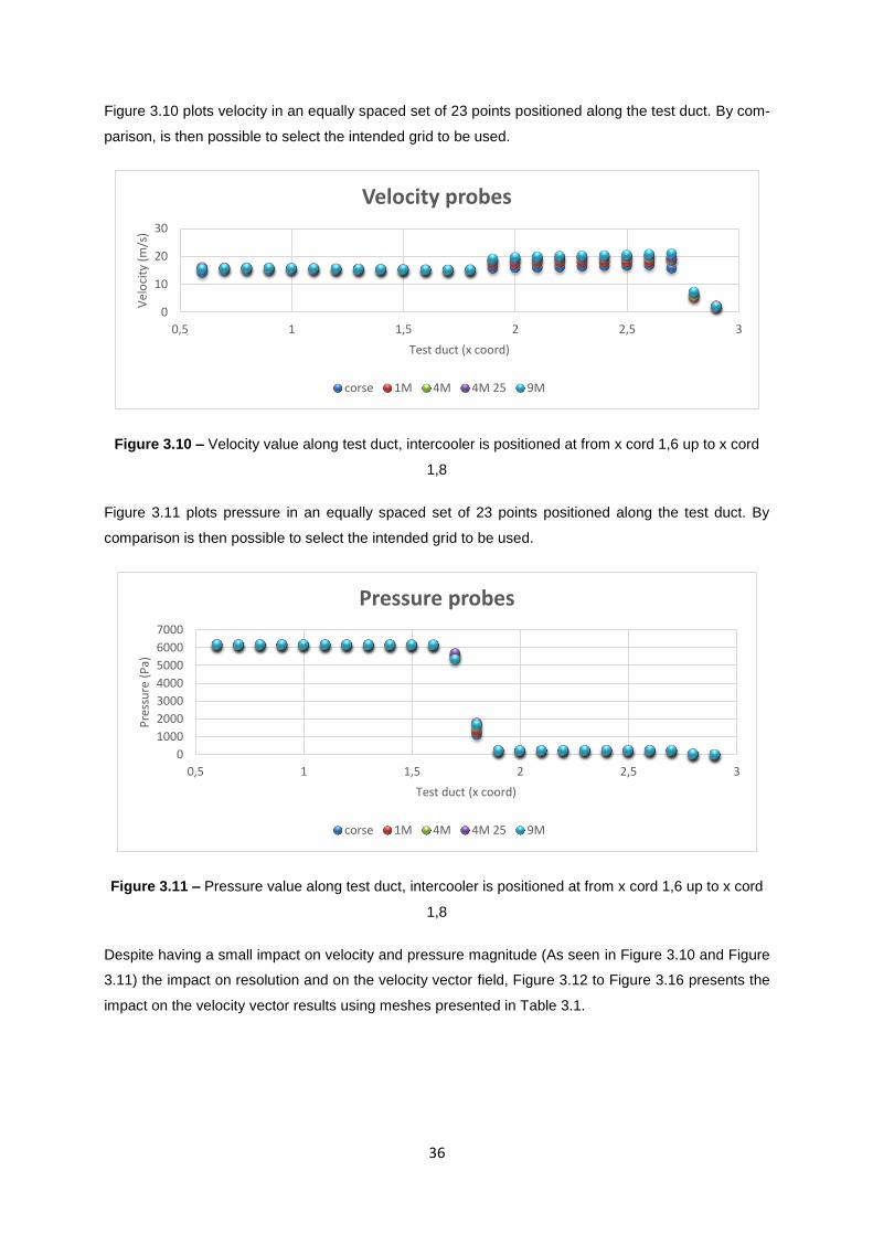
36

Figure 3.10 plots velocity in an equally spaced set of 23 points positioned along the test duct. By com-

parison, is then possible to select the intended grid to be used.

Figure 3.10 – Velocity value along test duct, intercooler is positioned at from x cord 1,6 up to x cord

1,8

Figure 3.11 plots pressure in an equally spaced set of 23 points positioned along the test duct. By

comparison is then possible to select the intended grid to be used.

Figure 3.11 – Pressure value along test duct, intercooler is positioned at from x cord 1,6 up to x cord

1,8

Despite having a small impact on velocity and pressure magnitude (As seen in Figure 3.10 and Figure

3.11) the impact on resolution and on the velocity vector field, Figure 3.12 to Figure 3.16 presents the

impact on the velocity vector results using meshes presented in Table 3.1.

0

10

20

30

0,5 1 1,5 2 2,5 3

Vel

oci

ty (

m/s

)

Test duct (x coord)

Velocity probes

corse 1M 4M 4M 25 9M

0

1000

2000

3000

4000

5000

6000

7000

0,5 1 1,5 2 2,5 3

Pre

ssu

re (

Pa)

Test duct (x coord)

Pressure probes

corse 1M 4M 4M 25 9M

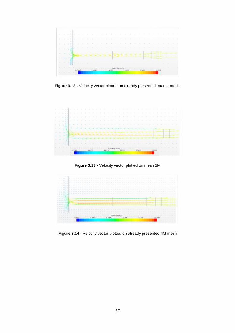
37

Figure 3.12 - Velocity vector plotted on already presented coarse mesh.

Figure 3.13 - Velocity vector plotted on mesh 1M

Figure 3.14 - Velocity vector plotted on already presented 4M mesh

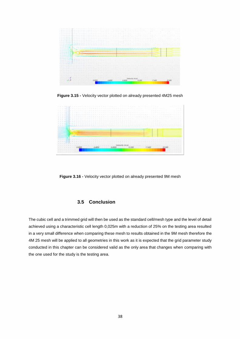
38

Figure 3.15 - Velocity vector plotted on already presented 4M25 mesh

Figure 3.16 - Velocity vector plotted on already presented 9M mesh

3.5 Conclusion

The cubic cell and a trimmed grid will then be used as the standard cell/mesh type and the level of detail

achieved using a characteristic cell length 0,025m with a reduction of 25% on the testing area resulted

in a very small difference when comparing these mesh to results obtained in the 9M mesh therefore the

4M 25 mesh will be applied to all geometries in this work as it is expected that the grid parameter study

conducted in this chapter can be considered valid as the only area that changes when comparing with

the one used for the study is the testing area.

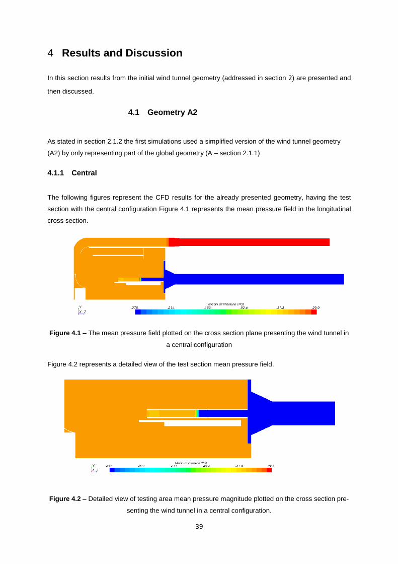
39

4 Results and Discussion

In this section results from the initial wind tunnel geometry (addressed in section 2) are presented and

then discussed.

4.1 Geometry A2

As stated in section 2.1.2 the first simulations used a simplified version of the wind tunnel geometry

(A2) by only representing part of the global geometry (A – section 2.1.1)

4.1.1 Central

The following figures represent the CFD results for the already presented geometry, having the test

section with the central configuration Figure 4.1 represents the mean pressure field in the longitudinal

cross section.

Figure 4.1 – The mean pressure field plotted on the cross section plane presenting the wind tunnel in

a central configuration

Figure 4.2 represents a detailed view of the test section mean pressure field.

Figure 4.2 – Detailed view of testing area mean pressure magnitude plotted on the cross section pre-

senting the wind tunnel in a central configuration.

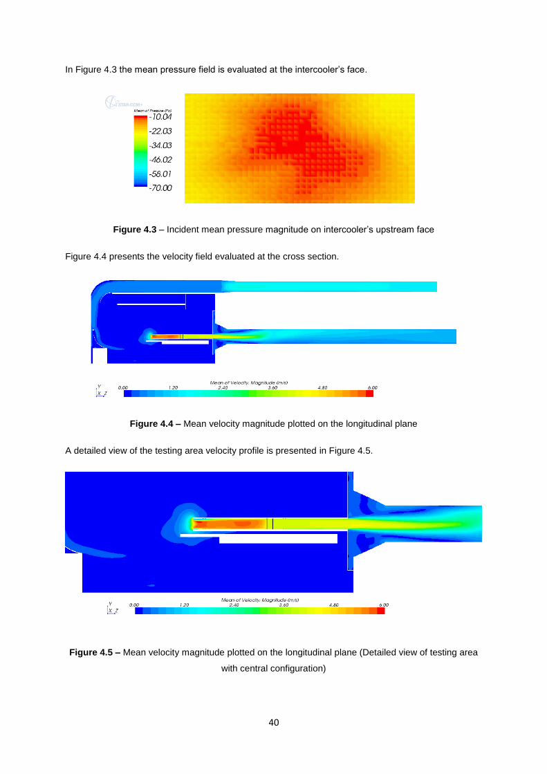
40

In Figure 4.3 the mean pressure field is evaluated at the intercooler’s face.

Figure 4.3 – Incident mean pressure magnitude on intercooler’s upstream face

Figure 4.4 presents the velocity field evaluated at the cross section.

Figure 4.4 – Mean velocity magnitude plotted on the longitudinal plane

A detailed view of the testing area velocity profile is presented in Figure 4.5.

Figure 4.5 – Mean velocity magnitude plotted on the longitudinal plane (Detailed view of testing area

with central configuration)

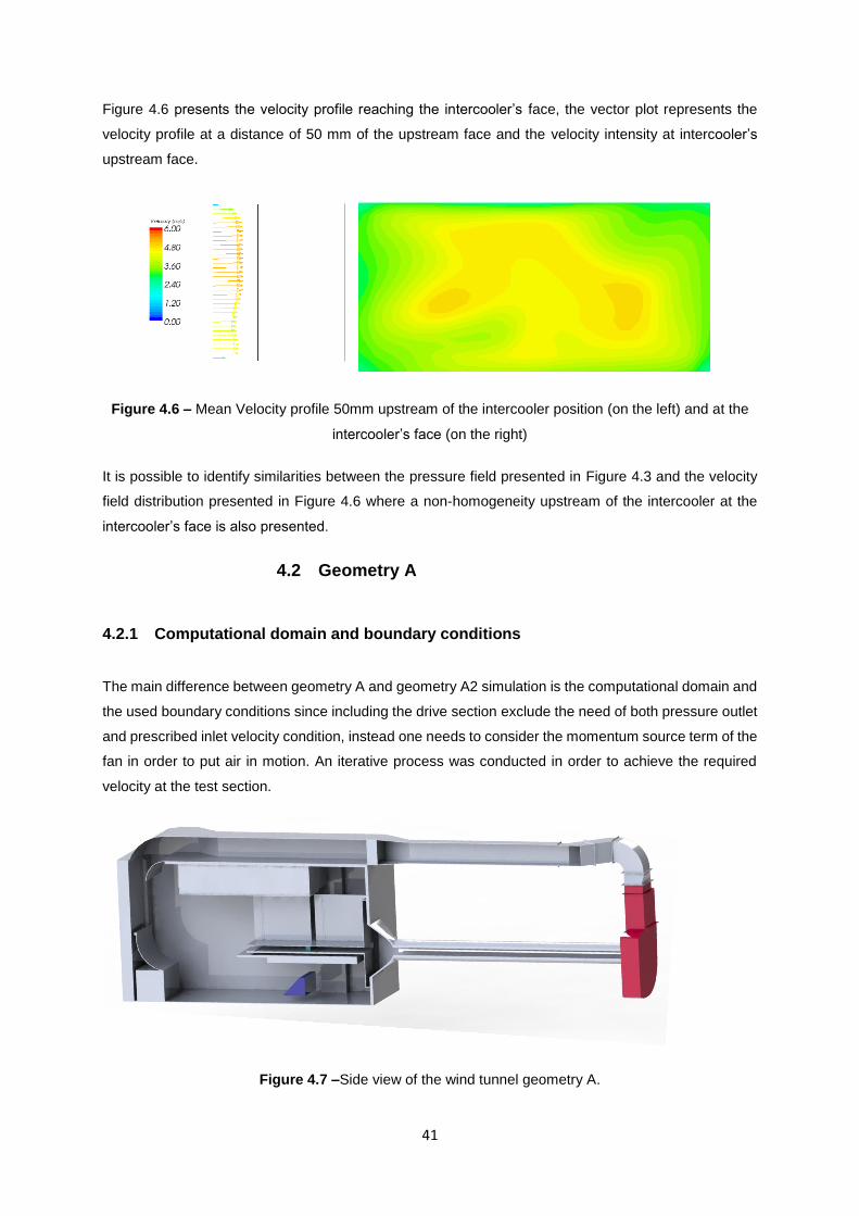
41

Figure 4.6 presents the velocity profile reaching the intercooler’s face, the vector plot represents the

velocity profile at a distance of 50 mm of the upstream face and the velocity intensity at intercooler’s

upstream face.

Figure 4.6 – Mean Velocity profile 50mm upstream of the intercooler position (on the left) and at the

intercooler’s face (on the right)

It is possible to identify similarities between the pressure field presented in Figure 4.3 and the velocity

field distribution presented in Figure 4.6 where a non-homogeneity upstream of the intercooler at the

intercooler’s face is also presented.

4.2 Geometry A

4.2.1 Computational domain and boundary conditions

The main difference between geometry A and geometry A2 simulation is the computational domain and

the used boundary conditions since including the drive section exclude the need of both pressure outlet

and prescribed inlet velocity condition, instead one needs to consider the momentum source term of the

fan in order to put air in motion. An iterative process was conducted in order to achieve the required

velocity at the test section.

Figure 4.7 –Side view of the wind tunnel geometry A.

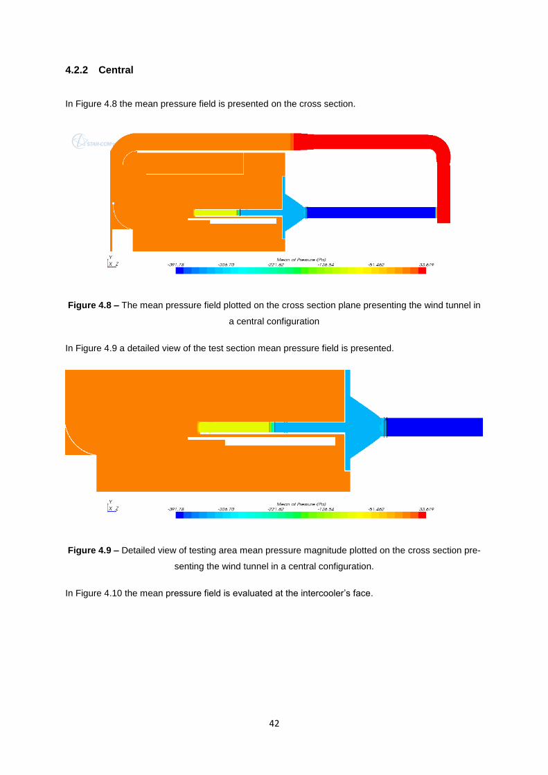
42

4.2.2 Central

In Figure 4.8 the mean pressure field is presented on the cross section.

Figure 4.8 – The mean pressure field plotted on the cross section plane presenting the wind tunnel in

a central configuration

In Figure 4.9 a detailed view of the test section mean pressure field is presented.

Figure 4.9 – Detailed view of testing area mean pressure magnitude plotted on the cross section pre-

senting the wind tunnel in a central configuration.

In Figure 4.10 the mean pressure field is evaluated at the intercooler’s face.

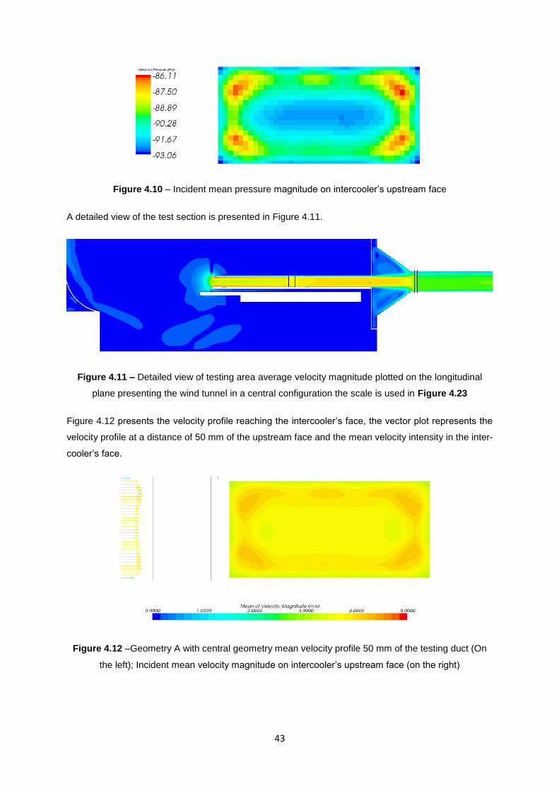
43

Figure 4.10 – Incident mean pressure magnitude on intercooler’s upstream face

A detailed view of the test section is presented in Figure 4.11.

Figure 4.11 – Detailed view of testing area average velocity magnitude plotted on the longitudinal

plane presenting the wind tunnel in a central configuration the scale is used in Figure 4.23


velocity profile at a distance of 50 mm of the upstream face and the mean velocity intensity in the inter-

cooler’s face.

Figure 4.12 –Geometry A with central geometry mean velocity profile 50 mm of the testing duct (On

the left); Incident mean velocity magnitude on intercooler’s upstream face (on the right)

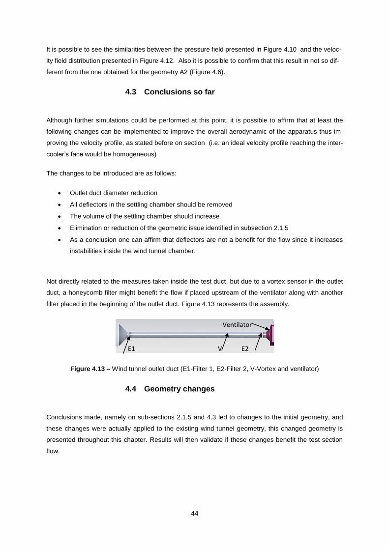
44

It is possible to see the similarities between the pressure field presented in Figure 4.10 and the veloc-

ity field distribution presented in Figure 4.12. Also it is possible to confirm that this result in not so dif-

ferent from the one obtained for the geometry A2 (Figure 4.6).

4.3 Conclusions so far

Although further simulations could be performed at this point, it is possible to affirm that at least the

following changes can be implemented to improve the overall aerodynamic of the apparatus thus im-

proving the velocity profile, as stated before on section (i.e. an ideal velocity profile reaching the inter-

cooler’s face would be homogeneous)

The changes to be introduced are as follows:

Outlet duct diameter reduction

All deflectors in the settling chamber should be removed

The volume of the settling chamber should increase

Elimination or reduction of the geometric issue identified in subsection 2.1.5

As a conclusion one can affirm that deflectors are not a benefit for the flow since it increases

instabilities inside the wind tunnel chamber.

Not directly related to the measures taken inside the test duct, but due to a vortex sensor in the outlet

duct, a honeycomb filter might benefit the flow if placed upstream of the ventilator along with another

filter placed in the beginning of the outlet duct. Figure 4.13 represents the assembly.

Figure 4.13 – Wind tunnel outlet duct (E1-Filter 1, E2-Filter 2, V-Vortex and ventilator)

4.4 Geometry changes

Conclusions made, namely on sub-sections 2.1.5 and 4.3 led to changes to the initial geometry, and

these changes were actually applied to the existing wind tunnel geometry, this changed geometry is

presented throughout this chapter. Results will then validate if these changes benefit the test section

flow.

E1 E2 V

Ventilator

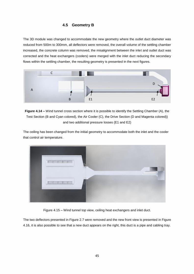
45

4.5 Geometry B

The 3D module was changed to accommodate the new geometry where the outlet duct diameter was

reduced from 500m to 300mm, all deflectors were removed, the overall volume of the settling chamber

increased, the concrete column was removed, the misalignment between the inlet and outlet duct was

corrected and the heat exchangers (coolers) were merged with the inlet duct reducing the secondary

flows within the settling chamber, the resulting geometry is presented in the next figures.

Figure 4.14 – Wind tunnel cross section where it is possible to identify the Settling Chamber (A), the

Test Section (B and Cyan colored), the Air Cooler (C), the Drive Section (D and Magenta colored))

and two additional pressure losses (E1 and E2)

The ceiling has been changed from the initial geometry to accommodate both the inlet and the cooler

that control air temperature.

Figure 4.15 – Wind tunnel top view, ceiling heat exchangers and inlet duct.

The two deflectors presented in Figure 2.7 were removed and the new front view is presented in Figure

4.16, it is also possible to see that a new duct appears on the right, this duct is a pipe and cabling tray.

D

B

A

C

E1 E2

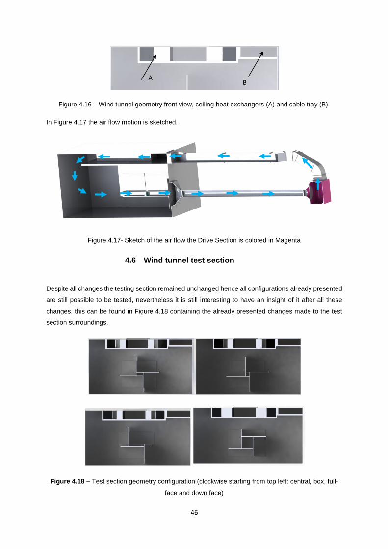
46

Figure 4.16 – Wind tunnel geometry front view, ceiling heat exchangers (A) and cable tray (B).

In Figure 4.17 the air flow motion is sketched.

Figure 4.17- Sketch of the air flow the Drive Section is colored in Magenta

4.6 Wind tunnel test section

Despite all changes the testing section remained unchanged hence all configurations already presented

are still possible to be tested, nevertheless it is still interesting to have an insight of it after all these

changes, this can be found in Figure 4.18 containing the already presented changes made to the test

section surroundings.

Figure 4.18 – Test section geometry configuration (clockwise starting from top left: central, box, full-

face and down face)

A B

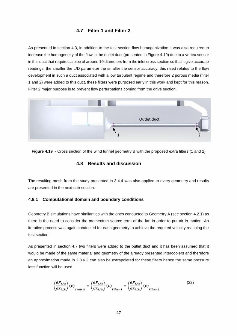
47

4.7 Filter 1 and Filter 2

As presented in section 4.3, in addition to the test section flow homogenization it was also required to

increase the homogeneity of the flow in the outlet duct (presented in Figure 4.19) due to a vortex sensor

in this duct that requires a pipe of around 10 diameters from the inlet cross section so that it give accurate

readings, the smaller the L/D parameter the smaller the sensor accuracy, this need relates to the flow

development in such a duct associated with a low turbulent regime and therefore 2 porous media (filter

1 and 2) were added to this duct, these filters were purposed early in this work and kept for this reason.

Filter 2 major purpose is to prevent flow perturbations coming from the drive section.

Figure 4.19 - Cross section of the wind tunnel geometry B with the proposed extra filters (1 and 2)

4.8 Results and discussion

The resulting mesh from the study presented in 3.4.4 was also applied to every geometry and results

are presented in the next sub-section.

4.8.1 Computational domain and boundary conditions

Geometry B simulations have similarities with the ones conducted to Geometry A (see section 4.2.1) as

there is the need to consider the momentum source term of the fan in order to put air in motion. An

iterative process was again conducted for each geometry to achieve the required velocity reaching the

test section

As presented in section 4.7 two filters were added to the outlet duct and it has been assumed that it

would be made of the same material and geometry of the already presented intercoolers and therefore

an approximation made in 2.3.6.2 can also be extrapolated for these filters hence the same pressure

loss function will be used.

(𝝏𝑷𝒊,𝒋,𝒌

𝝏𝒙𝒊,𝒋,𝒌

) (𝒗)𝑪𝒆𝒏𝒕𝒓𝒂𝒍

= (𝝏𝑷𝒊,𝒋,𝒌


) (𝒗)𝑭𝒊𝒍𝒕𝒆𝒓 𝟏

= (𝝏𝑷𝒊,𝒋,𝒌


) (𝒗)𝑭𝒊𝒍𝒕𝒆𝒓 𝟐

(22)

Outlet duct

1 2

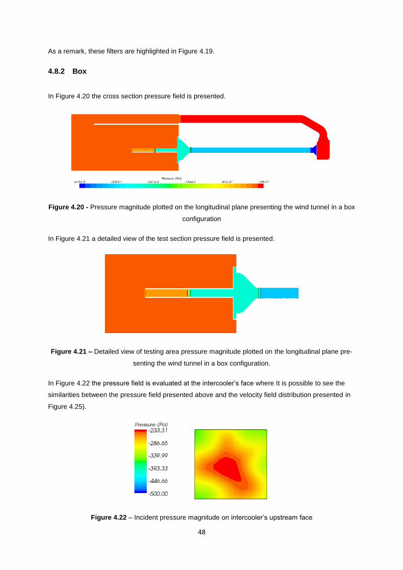
48

As a remark, these filters are highlighted in Figure 4.19.

4.8.2 Box

In Figure 4.20 the cross section pressure field is presented.

Figure 4.20 - Pressure magnitude plotted on the longitudinal plane presenting the wind tunnel in a box

configuration

In Figure 4.21 a detailed view of the test section pressure field is presented.



In Figure 4.22 the pressure field is evaluated at the intercooler’s face where It is possible to see the

similarities between the pressure field presented above and the velocity field distribution presented in

Figure 4.25).

Figure 4.22 – Incident pressure magnitude on intercooler’s upstream face

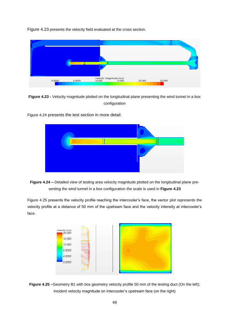
49


Figure 4.23 - Velocity magnitude plotted on the longitudinal plane presenting the wind tunnel in a box

configuration

Figure 4.24 presents the test section in more detail.

Figure 4.24 – Detailed view of testing area velocity magnitude plotted on the longitudinal plane pre-

senting the wind tunnel in a box configuration the scale is used in Figure 4.23



face.

Figure 4.25 –Geometry B1 with box geometry velocity profile 50 mm of the testing duct (On the left);

Incident velocity magnitude on intercooler’s upstream face (on the right)

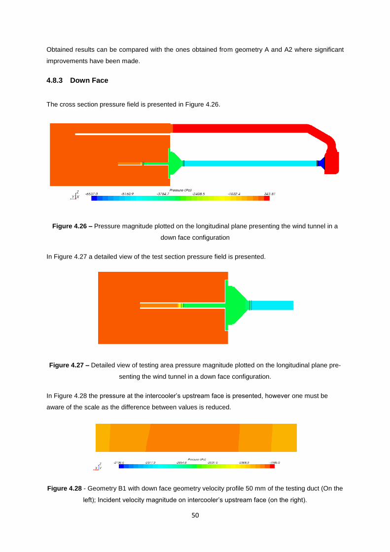
50

Obtained results can be compared with the ones obtained from geometry A and A2 where significant

improvements have been made.

4.8.3 Down Face

The cross section pressure field is presented in Figure 4.26.

Figure 4.26 – Pressure magnitude plotted on the longitudinal plane presenting the wind tunnel in a

down face configuration



senting the wind tunnel in a down face configuration.

In Figure 4.28 the pressure at the intercooler’s upstream face is presented, however one must be

aware of the scale as the difference between values is reduced.

Figure 4.28 - Geometry B1 with down face geometry velocity profile 50 mm of the testing duct (On the

left); Incident velocity magnitude on intercooler’s upstream face (on the right).

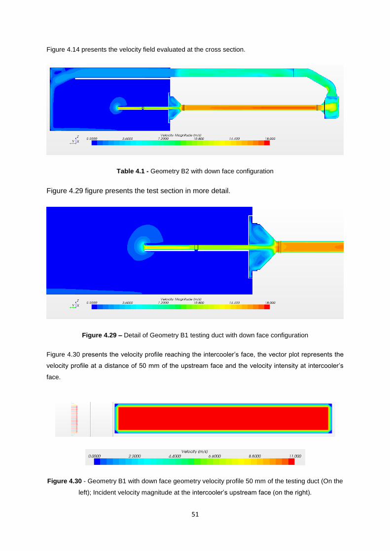
51


Table 4.1 - Geometry B2 with down face configuration

Figure 4.29 figure presents the test section in more detail.

Figure 4.29 – Detail of Geometry B1 testing duct with down face configuration



face.

Figure 4.30 - Geometry B1 with down face geometry velocity profile 50 mm of the testing duct (On the

left); Incident velocity magnitude at the intercooler’s upstream face (on the right).

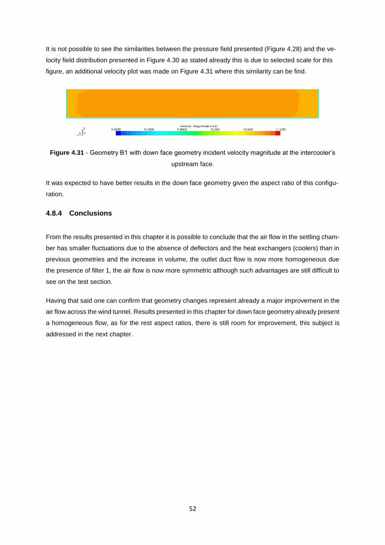
52

It is not possible to see the similarities between the pressure field presented (Figure 4.28) and the ve-

locity field distribution presented in Figure 4.30 as stated already this is due to selected scale for this

figure, an additional velocity plot was made on Figure 4.31 where this similarity can be find.

Figure 4.31 - Geometry B1 with down face geometry incident velocity magnitude at the intercooler’s

upstream face.

It was expected to have better results in the down face geometry given the aspect ratio of this configu-

ration.

4.8.4 Conclusions

From the results presented in this chapter it is possible to conclude that the air flow in the settling cham-

ber has smaller fluctuations due to the absence of deflectors and the heat exchangers (coolers) than in

previous geometries and the increase in volume, the outlet duct flow is now more homogeneous due

the presence of filter 1, the air flow is now more symmetric although such advantages are still difficult to

see on the test section.

Having that said one can confirm that geometry changes represent already a major improvement in the

air flow across the wind tunnel. Results presented in this chapter for down face geometry already present

a homogeneous flow, as for the rest aspect ratios, there is still room for improvement, this subject is

addressed in the next chapter.

53

5 Flow homogenization

In this section flow homogenization will be addressed and possible solutions will be presented. One

must be aware of the limitations that a solution for this apparatus must accommodate, such as the

variable geometry with the already presented range (on section 1.2, 2.1.3, 2.1.4 and 4.6).

To increase flow homogenization on test section the idea of having a pressure loss upstream of the

intercooler was studied in three different ways.

The first approach consisted of a screen (pressure loss) positioned at the test section entrance as

presented in Figure 5.1.

Figure 5.1 – Test section detail of the wind tunnel geometry B cross section, a screen placed at the

test section entrance as a possible solution to increase flow homogenization.

Early in this approach it became clear that this would not deliver any remarkable flow homogenization

as the flow profile recovers before reaching the intercooler’s face and therefore different solutions should

be proposed. A pressure loss closer to the intercooler was then proposed, reducing the benefit of having

the screen at the inlet and therefore no simulation will be presented for this geometry.

Hence the idea of only use a single porous media closer to the intercooler appeared to be a feasible

solution, however, one must have in consideration that this porous media must be versatile enough to

accommodate several geometries and yet having a known pressure loss function.

There might be a vast number of possible solutions to solve this homogenization two of them will be

addressed in more detail in the next subsections. One solution will make use of a random packed bed

with a constant diameter (this is a typical solution to homogenize air and fuel flow in burners), the other

solution will be a fabric or cloth filter widely used in industry as particle filters. To evaluate which filter

can solve the homogenization issue, it is required to compute the intended pressure drop, CFD simula-

tions can be of a good use to avoid costly iterations on the apparatus.

Screen

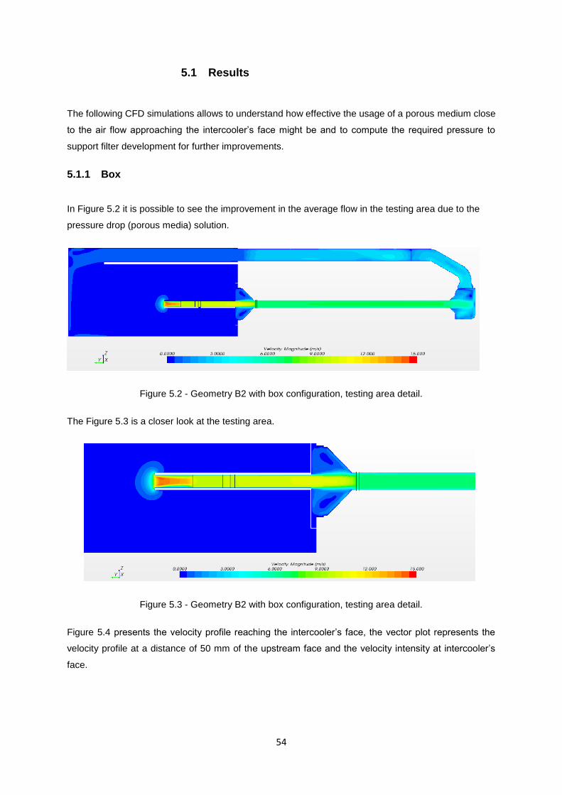
54

5.1 Results

The following CFD simulations allows to understand how effective the usage of a porous medium close

to the air flow approaching the intercooler’s face might be and to compute the required pressure to

support filter development for further improvements.

5.1.1 Box

In Figure 5.2 it is possible to see the improvement in the average flow in the testing area due to the

pressure drop (porous media) solution.

Figure 5.2 - Geometry B2 with box configuration, testing area detail.

The Figure 5.3 is a closer look at the testing area.

Figure 5.3 - Geometry B2 with box configuration, testing area detail.



face.

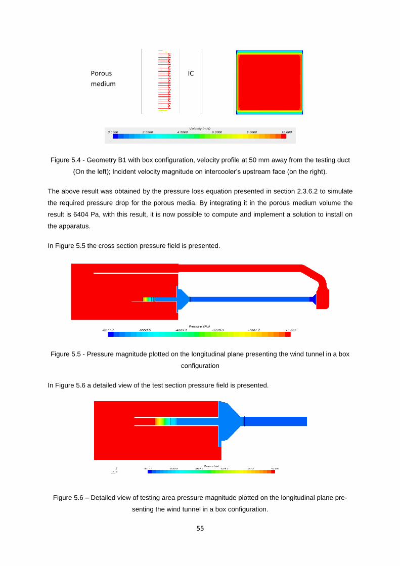
55

Figure 5.4 - Geometry B1 with box configuration, velocity profile at 50 mm away from the testing duct

(On the left); Incident velocity magnitude on intercooler’s upstream face (on the right).

The above result was obtained by the pressure loss equation presented in section 2.3.6.2 to simulate

the required pressure drop for the porous media. By integrating it in the porous medium volume the

result is 6404 Pa, with this result, it is now possible to compute and implement a solution to install on

the apparatus.

In Figure 5.5 the cross section pressure field is presented.

Figure 5.5 - Pressure magnitude plotted on the longitudinal plane presenting the wind tunnel in a box

configuration




Porous

medium

IC

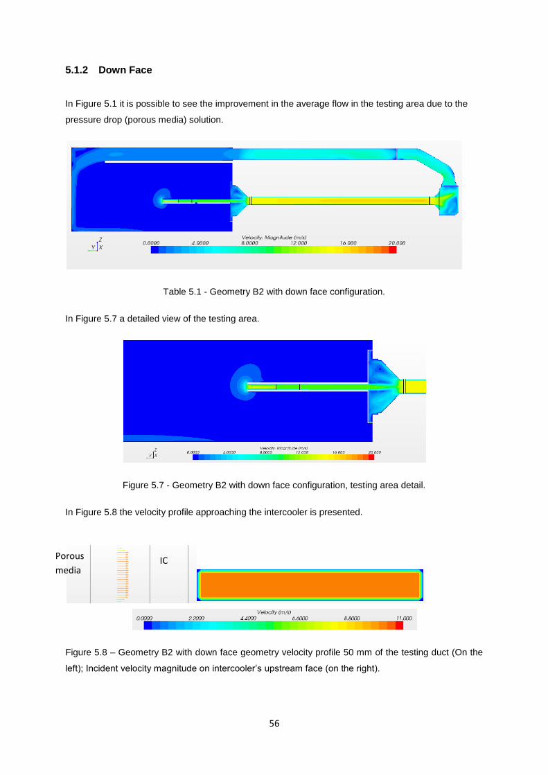
56

5.1.2 Down Face

In Figure 5.1 it is possible to see the improvement in the average flow in the testing area due to the

pressure drop (porous media) solution.

Table 5.1 - Geometry B2 with down face configuration.

In Figure 5.7 a detailed view of the testing area.

Figure 5.7 - Geometry B2 with down face configuration, testing area detail.

In Figure 5.8 the velocity profile approaching the intercooler is presented.

Figure 5.8 – Geometry B2 with down face geometry velocity profile 50 mm of the testing duct (On the

left); Incident velocity magnitude on intercooler’s upstream face (on the right).

Porous

media IC

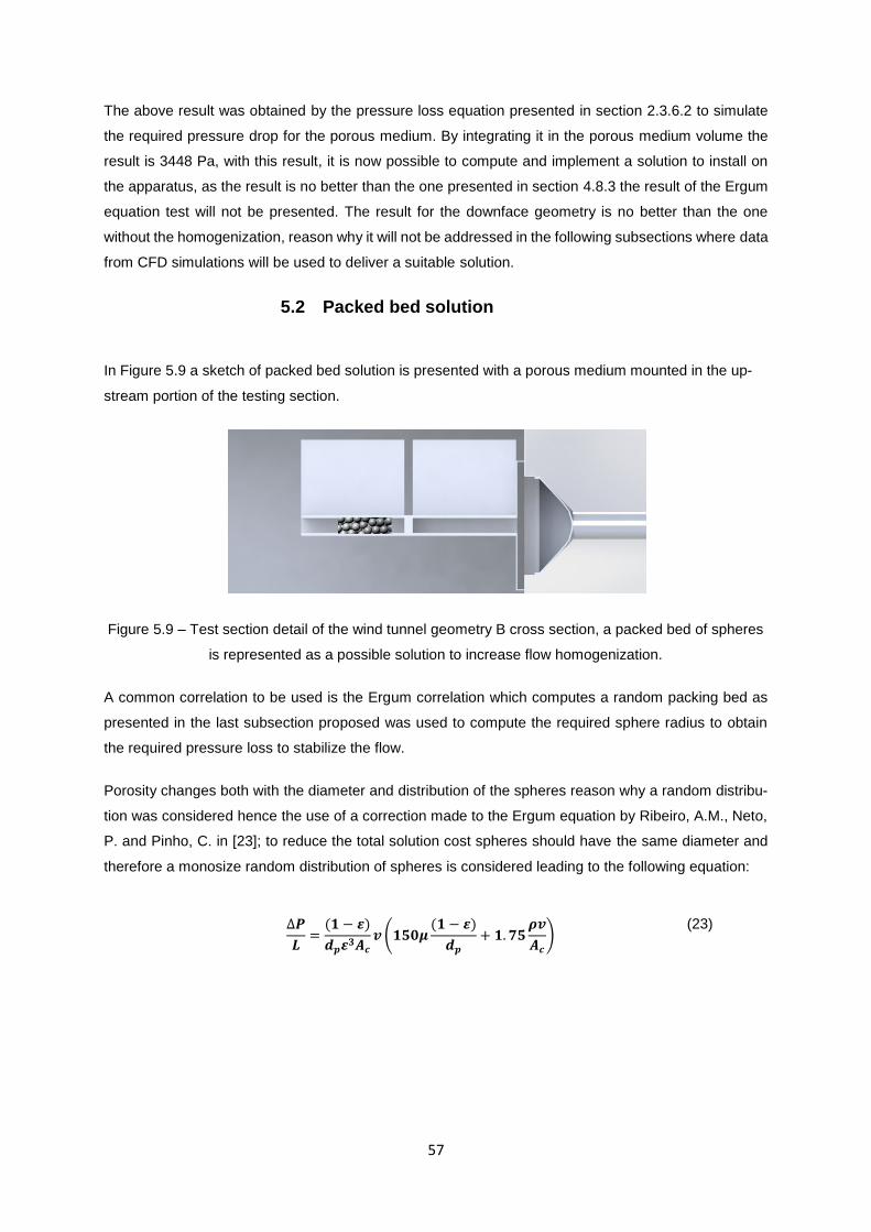
57

The above result was obtained by the pressure loss equation presented in section 2.3.6.2 to simulate

the required pressure drop for the porous medium. By integrating it in the porous medium volume the

result is 3448 Pa, with this result, it is now possible to compute and implement a solution to install on

the apparatus, as the result is no better than the one presented in section 4.8.3 the result of the Ergum

equation test will not be presented. The result for the downface geometry is no better than the one

without the homogenization, reason why it will not be addressed in the following subsections where data

from CFD simulations will be used to deliver a suitable solution.

5.2 Packed bed solution

In Figure 5.9 a sketch of packed bed solution is presented with a porous medium mounted in the up-

stream portion of the testing section.

Figure 5.9 – Test section detail of the wind tunnel geometry B cross section, a packed bed of spheres

is represented as a possible solution to increase flow homogenization.

A common correlation to be used is the Ergum correlation which computes a random packing bed as

presented in the last subsection proposed was used to compute the required sphere radius to obtain

the required pressure loss to stabilize the flow.

Porosity changes both with the diameter and distribution of the spheres reason why a random distribu-

tion was considered hence the use of a correction made to the Ergum equation by Ribeiro, A.M., Neto,

P. and Pinho, C. in [23]; to reduce the total solution cost spheres should have the same diameter and

therefore a monosize random distribution of spheres is considered leading to the following equation:

∆𝑷

𝑳=

(𝟏 − 𝜺)

𝒅𝒑𝜺𝟑𝑨𝒄

𝒗(𝟏𝟓𝟎𝝁(𝟏 − 𝜺)

𝒅𝒑

+ 𝟏. 𝟕𝟓𝝆𝒗

𝑨𝒄

) (23)

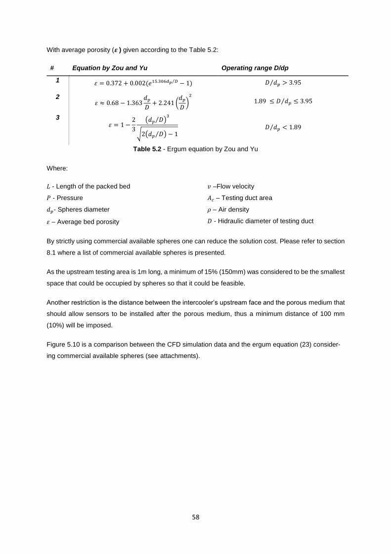
58

With average porosity (𝜺 ) given according to the Table 5.2:

# Equation by Zou and Yu Operating range D/dp

1 𝜀 = 0.372 + 0.002(𝑒15.306𝑑𝑝 𝐷⁄ − 1) 𝐷 𝑑𝑝⁄ > 3.95

2 𝜀 ≈ 0.68 − 1.363

𝑑𝑝

𝐷+ 2.241 (

𝑑𝑝

𝐷)

2

1.89 ≤ 𝐷 𝑑𝑝⁄ ≤ 3.95

3 𝜀 = 1 −

2

3

(𝑑𝑝 𝐷⁄ )3

√2(𝑑𝑝 𝐷⁄ ) − 1

𝐷 𝑑𝑝⁄ < 1.89

Table 5.2 - Ergum equation by Zou and Yu

Where:

𝐿 - Length of the packed bed

𝑃 - Pressure

𝑑𝑝- Spheres diameter

𝜀 – Average bed porosity

𝑣 –Flow velocity

𝐴𝑐 – Testing duct area

𝜌 – Air density

𝐷 - Hidraulic diameter of testing duct

By strictly using commercial available spheres one can reduce the solution cost. Please refer to section

8.1 where a list of commercial available spheres is presented.

As the upstream testing area is 1m long, a minimum of 15% (150mm) was considered to be the smallest

space that could be occupied by spheres so that it could be feasible.

Another restriction is the distance between the intercooler’s upstream face and the porous medium that

should allow sensors to be installed after the porous medium, thus a minimum distance of 100 mm

(10%) will be imposed.

Figure 5.10 is a comparison between the CFD simulation data and the ergum equation (23) consider-

ing commercial available spheres (see attachments).

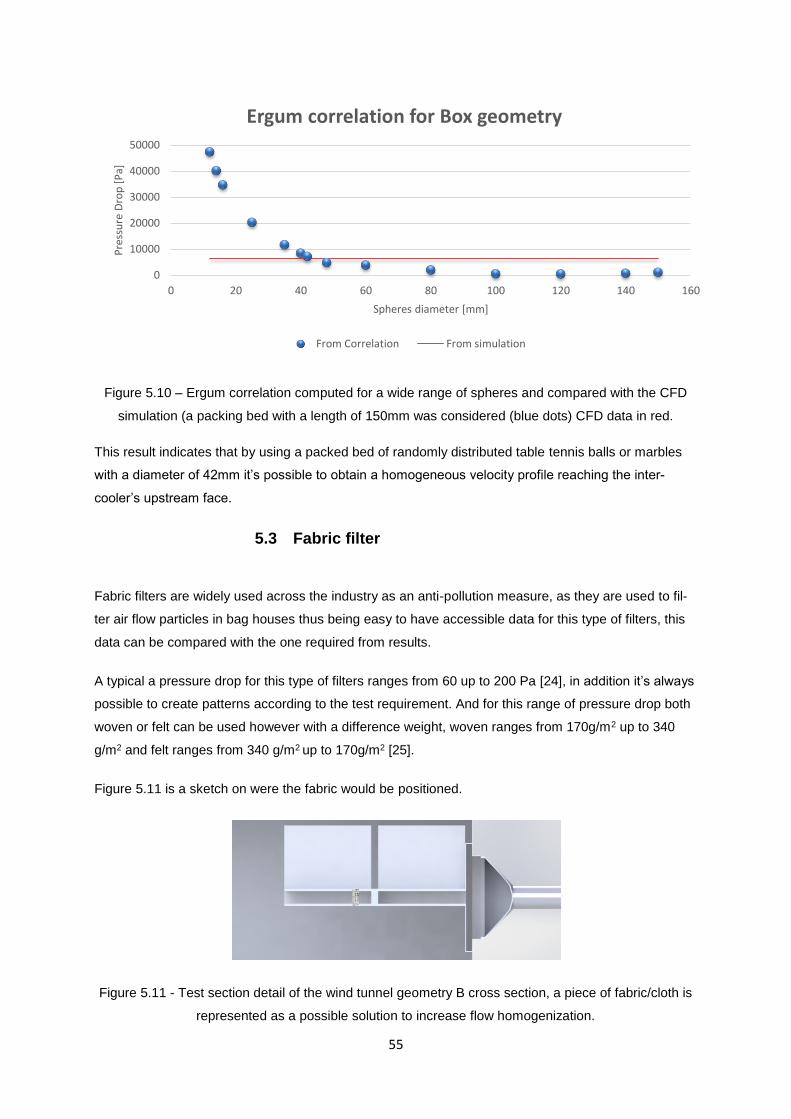
55

Figure 5.10 – Ergum correlation computed for a wide range of spheres and compared with the CFD

simulation (a packing bed with a length of 150mm was considered (blue dots) CFD data in red.

This result indicates that by using a packed bed of randomly distributed table tennis balls or marbles

with a diameter of 42mm it’s possible to obtain a homogeneous velocity profile reaching the inter-

cooler’s upstream face.

5.3 Fabric filter

Fabric filters are widely used across the industry as an anti-pollution measure, as they are used to fil-

ter air flow particles in bag houses thus being easy to have accessible data for this type of filters, this

data can be compared with the one required from results.

A typical a pressure drop for this type of filters ranges from 60 up to 200 Pa [24], in addition it’s always

possible to create patterns according to the test requirement. And for this range of pressure drop both

woven or felt can be used however with a difference weight, woven ranges from 170g/m2 up to 340

g/m2 and felt ranges from 340 g/m2 up to 170g/m2 [25].

Figure 5.11 is a sketch on were the fabric would be positioned.

Figure 5.11 - Test section detail of the wind tunnel geometry B cross section, a piece of fabric/cloth is

represented as a possible solution to increase flow homogenization.

0

10000

20000

30000

40000

50000

0 20 40 60 80 100 120 140 160

Pre

ssu

re D

rop

[P

a]

Spheres diameter [mm]

Ergum correlation for Box geometry

From Correlation From simulation

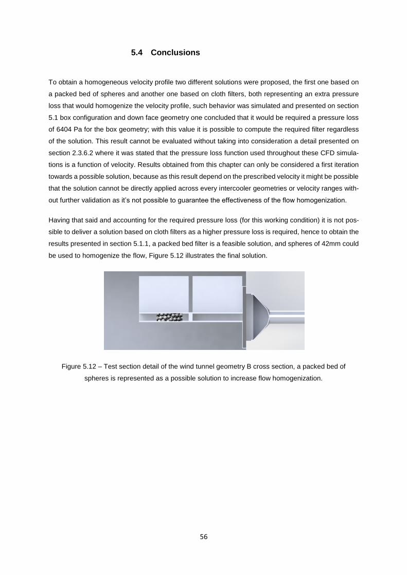
56

5.4 Conclusions

To obtain a homogeneous velocity profile two different solutions were proposed, the first one based on

a packed bed of spheres and another one based on cloth filters, both representing an extra pressure

loss that would homogenize the velocity profile, such behavior was simulated and presented on section

5.1 box configuration and down face geometry one concluded that it would be required a pressure loss

of 6404 Pa for the box geometry; with this value it is possible to compute the required filter regardless

of the solution. This result cannot be evaluated without taking into consideration a detail presented on

section 2.3.6.2 where it was stated that the pressure loss function used throughout these CFD simula-

tions is a function of velocity. Results obtained from this chapter can only be considered a first iteration

towards a possible solution, because as this result depend on the prescribed velocity it might be possible

that the solution cannot be directly applied across every intercooler geometries or velocity ranges with-

out further validation as it’s not possible to guarantee the effectiveness of the flow homogenization.

Having that said and accounting for the required pressure loss (for this working condition) it is not pos-

sible to deliver a solution based on cloth filters as a higher pressure loss is required, hence to obtain the

results presented in section 5.1.1, a packed bed filter is a feasible solution, and spheres of 42mm could

be used to homogenize the flow, Figure 5.12 illustrates the final solution.


spheres is represented as a possible solution to increase flow homogenization.

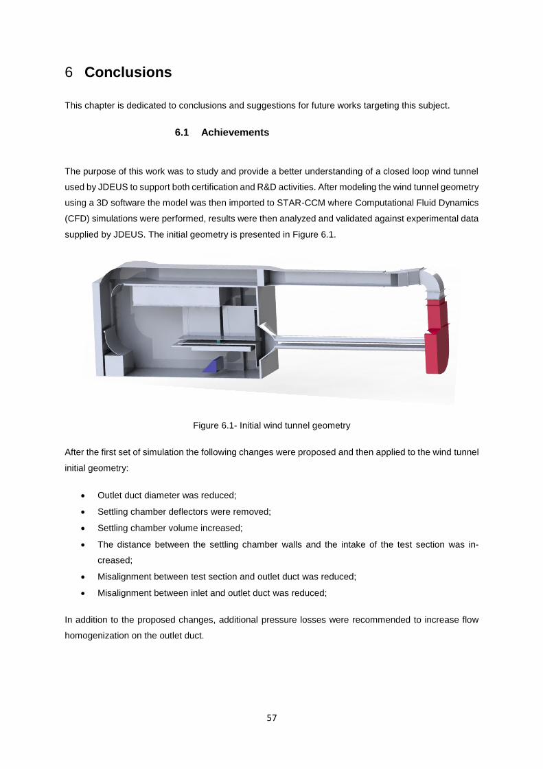
57

6 Conclusions

This chapter is dedicated to conclusions and suggestions for future works targeting this subject.

6.1 Achievements

The purpose of this work was to study and provide a better understanding of a closed loop wind tunnel

used by JDEUS to support both certification and R&D activities. After modeling the wind tunnel geometry

using a 3D software the model was then imported to STAR-CCM where Computational Fluid Dynamics

(CFD) simulations were performed, results were then analyzed and validated against experimental data

supplied by JDEUS. The initial geometry is presented in Figure 6.1.

Figure 6.1- Initial wind tunnel geometry

After the first set of simulation the following changes were proposed and then applied to the wind tunnel

initial geometry:

Outlet duct diameter was reduced;

Settling chamber deflectors were removed;

Settling chamber volume increased;

The distance between the settling chamber walls and the intake of the test section was in-

creased;

Misalignment between test section and outlet duct was reduced;

Misalignment between inlet and outlet duct was reduced;

In addition to the proposed changes, additional pressure losses were recommended to increase flow

homogenization on the outlet duct.

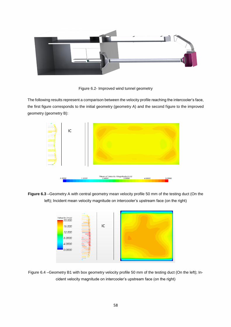
58

Figure 6.2- Improved wind tunnel geometry

The following results represent a comparison between the velocity profile reaching the intercooler’s face,

the first figure corresponds to the initial geometry (geometry A) and the second figure to the improved

geometry (geometry B):

Figure 6.3 –Geometry A with central geometry mean velocity profile 50 mm of the testing duct (On the

left); Incident mean velocity magnitude on intercooler’s upstream face (on the right)

Figure 6.4 –Geometry B1 with box geometry velocity profile 50 mm of the testing duct (On the left); In-

cident velocity magnitude on intercooler’s upstream face (on the right)

IC

IC

59

Although still having room for improvements with the understanding of all the geometrical variables of

the wind tunnel JDEUS decided to implement the same changes that were presented throughout this

work and implemented them in the actual wind tunnel geometry, after testing this improved geometry it

was possible to validate that the above mentioned approach as the overall air flow improved also the

instrument readings improved accordingly, namely the pitot tubes, thermocouples and the vortex sensor

readings, presenting less fluctuations that it was presenting prior to these geometrical changes.

To obtain the intended homogeneous velocity profile at the test section two different solutions were

proposed, the first one based on a packed bed of spheres and another one based on cloth filters.

Figure 6.5 – Two possible solutions (a cloth based solution on the left and a spheres based solution at

the right)

Both solutions represent an extra pressure loss that might homogenize the velocity profile. The wind

tunnel geometry containing this additional pressure loss was simulated where the following results were

obtained.

Figure 6.6 - Geometry B1 with box configuration, velocity profile at 50 mm away from the testing duct

(On the left); Incident velocity magnitude on intercooler’s upstream face (on the right).

Results proven to be as good as intended from the beginning of this work, knowing the pressure drop

value and positioning capabilities of homogenize the flow it was then possible to deliver a solution that

can be implemented on the real apparatus. Given the pressure value required (6404 Pa) the cloth based

solution is not feasible and therefore after applying the corrected form of the Ergum equation a feasible

solution for the wind tunnel homogenization problem was then presented, a packed bed of table tennis

balls (42mm) can be installed in the upstream area as presented in Figure 6.7

Porous

medium

IC

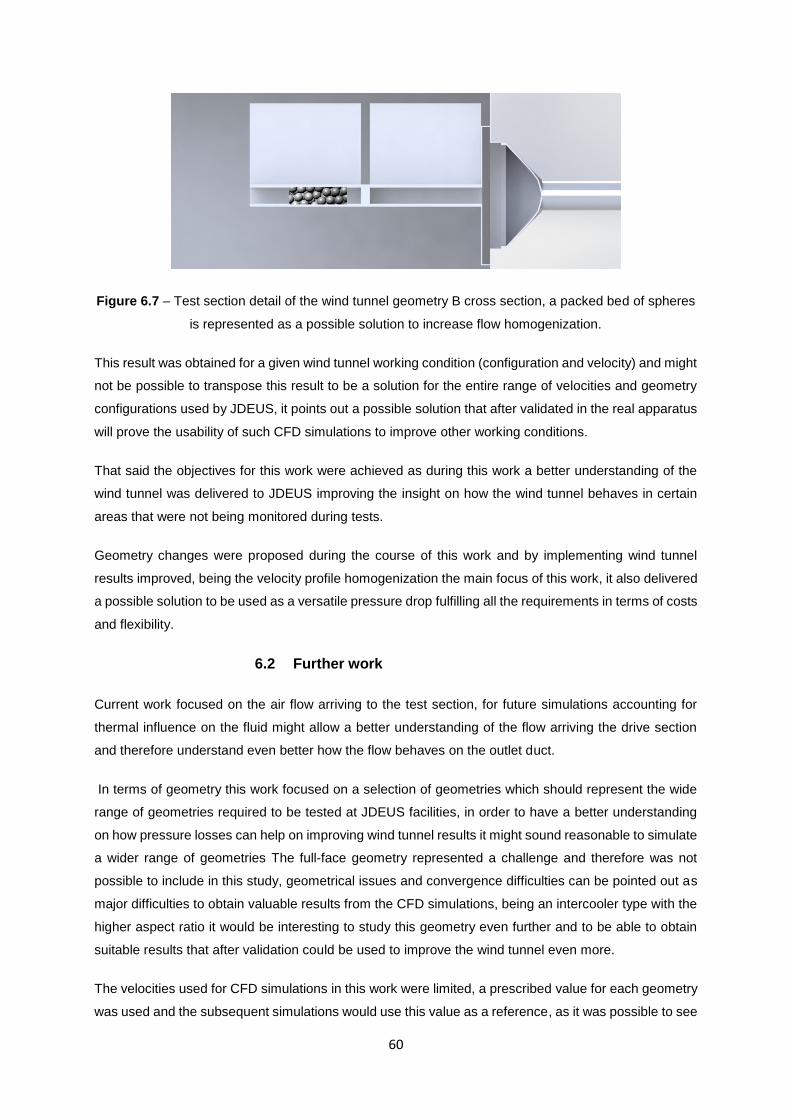
60

Figure 6.7 – Test section detail of the wind tunnel geometry B cross section, a packed bed of spheres

is represented as a possible solution to increase flow homogenization.

This result was obtained for a given wind tunnel working condition (configuration and velocity) and might

not be possible to transpose this result to be a solution for the entire range of velocities and geometry

configurations used by JDEUS, it points out a possible solution that after validated in the real apparatus

will prove the usability of such CFD simulations to improve other working conditions.

That said the objectives for this work were achieved as during this work a better understanding of the

wind tunnel was delivered to JDEUS improving the insight on how the wind tunnel behaves in certain

areas that were not being monitored during tests.

Geometry changes were proposed during the course of this work and by implementing wind tunnel

results improved, being the velocity profile homogenization the main focus of this work, it also delivered

a possible solution to be used as a versatile pressure drop fulfilling all the requirements in terms of costs

and flexibility.

6.2 Further work

Current work focused on the air flow arriving to the test section, for future simulations accounting for

thermal influence on the fluid might allow a better understanding of the flow arriving the drive section

and therefore understand even better how the flow behaves on the outlet duct.

In terms of geometry this work focused on a selection of geometries which should represent the wide

range of geometries required to be tested at JDEUS facilities, in order to have a better understanding

on how pressure losses can help on improving wind tunnel results it might sound reasonable to simulate

a wider range of geometries The full-face geometry represented a challenge and therefore was not

possible to include in this study, geometrical issues and convergence difficulties can be pointed out as

major difficulties to obtain valuable results from the CFD simulations, being an intercooler type with the

higher aspect ratio it would be interesting to study this geometry even further and to be able to obtain

suitable results that after validation could be used to improve the wind tunnel even more.

The velocities used for CFD simulations in this work were limited, a prescribed value for each geometry

was used and the subsequent simulations would use this value as a reference, as it was possible to see

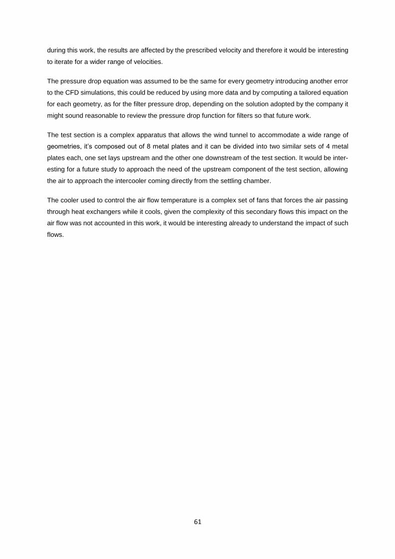
61

during this work, the results are affected by the prescribed velocity and therefore it would be interesting

to iterate for a wider range of velocities.

The pressure drop equation was assumed to be the same for every geometry introducing another error

to the CFD simulations, this could be reduced by using more data and by computing a tailored equation

for each geometry, as for the filter pressure drop, depending on the solution adopted by the company it

might sound reasonable to review the pressure drop function for filters so that future work.

The test section is a complex apparatus that allows the wind tunnel to accommodate a wide range of

geometries, it’s composed out of 8 metal plates and it can be divided into two similar sets of 4 metal

plates each, one set lays upstream and the other one downstream of the test section. It would be inter-

esting for a future study to approach the need of the upstream component of the test section, allowing

the air to approach the intercooler coming directly from the settling chamber.

The cooler used to control the air flow temperature is a complex set of fans that forces the air passing

through heat exchangers while it cools, given the complexity of this secondary flows this impact on the

air flow was not accounted in this work, it would be interesting already to understand the impact of such

flows.

62

7 References

[1] "Wind Tunnel open loop vs closed loop," The Franklin Institute, [Online]. Available:

http://www.fi.edu/flight/first/tunnelparts/tunnel_loop.html. [Accessed 17 03 2014].

[2] "JDEUS," [Online]. Available: http://www.jdeus.com/. [Accessed 17 01 2015].

[3] A. R. Khot, D. G. Thombare and S. P. Gaikwad, "An Overview of Radiator Performance

Evaluation and Testing".

[4] Adapco, STAR-CCM user's manual version 7.04.011.

[5] F. M. White, Fluid Mechanics, Rhode Island: McGraw-Hill, 1998.

[6] StarCCm+ User Guide, CD-Adapco.

[7] V. Brederode, Fundamentos de Aerodinâmica Incompressível, Lisboa: Vasco de Brederode,

1997.

[8] U. Kulshrestha, G. Kumar, M. Augustine and S. Mittal, "CFD Analysis of Automobile Radiator – A

Review," International Journal of Engineering Research and Applications (IJERA) , pp. 321-323,

2014.

[9] B. Shome, V. Kumar, S. V. R. Kumar and G. Arora, "CFD Prediction to Optimize Front End Cooling

Module of a Passenger Vehicle," Purdue, 2006.

[10] R. Schiestel, Modeling and Simulation of Turbulent Flows, Hoboken: WILEY, 2008.

[11] S. K. Venayagamoorthy, J. R. Koseff, J. H. Ferziger and L. H. Shih, "Testing of RANS turbulence

models for stratified," CENTER FOR TURBULENCE RESEARCH, 23 August 2012. [Online].

Available: http://ctr.stanford.edu/ResBriefs03/. [Accessed 2015 January 10].

[12] B. Mohammade and O. Pironneau, Analysis of the K-Epsilon TURBULENCE MODEL, Paris: Wiley,

1993.

[13] M. Cable, "An Evaluation of Turbulence Models for the Numerical," Department of Mechanical

and Materials from Queen's University, Kingston, 2009.

[14] G. Kalitzin, G. Medic, G. Iaccarino and P. Durbin, "Near-wall behavior of RANS turbulence

models," Journal of Computational Physics, no. 204, 2004.

[15] J. Tu, G. H. Yeoh and C. Liu, Computational Fluid Dynamics: A Practical Approach, Kidlington:

Butterworth-Heinemann, 2013.

63

[16] E. Audusse, F. Benkhaldoun, S. Sari, M. Seaid and P. Tassi, "A fast finite volume solver for multi-

layered shallow water flows," Journal of Computational Physics, vol. 272, p. 23–45, 2014.

[17] V. V. Ranade, Computational Flow Modeling for Chemical Reactor Engineering, vol. IV, London:

Academic Press, 2002.

[18] M. Peric and S. Ferguson, "The advantage of polyhedral meshes," CD-Adapco, [Online].

Available: http://www.plmmarketplace.com/upload/Temp/The_Advantage_of_polyhedral.pdf.

[Accessed 30 01 01].

[19] J. F. Shepherd and C. R. Johnson, "Hexahedral Mesh Generation Constraints," Sandia National

Laboratories, [Online]. Available: https://cfwebprod.sandia.gov/cfdocs/CompResearch/.

[Accessed 5 January 2015].

[20] NPARC, "NPARC Alliance & Wind-US CFD Code," NASA, [Online]. Available:

http://www.grc.nasa.gov/WWW/wind/. [Accessed 11 06 2014].

[21] D.-W. Sun, Computational Fluid Dynamics in Food Processing, CRC Press, 2007.

[22] S. Gorlin and I. Slezinger, Wind Tunnels and their instrumentation, Jerusalem: Israel Program

for Scientific Translations, 1966.

[23] A.M.Ribeiro, P. Neto and C. Pinho, "Mean porosity and pressure drop measurements in packed

beds of monosized spheres: Side wall effects," International Review of Chemical Engineering,

vol. 2, pp. 40-46.

[24] A. S. Mujumdar, Handbook of Industrial Drying, Fourth Edition, Boca Raton: CRC Press, 2014.

[25] L. K. Wang, N. C. Pereira and Y.-T. Hung, Air Pollution Control Engineering, vol. I, Totowa: The

Humana Press, Inc., 2004.

[26] [Online]. Available:

http://web.mit.edu/16.unified/www/SPRING/propulsion/notes/node25.html. [Accessed

January 2014].

[27] J. H. Ferziger and M. PeriC, Computacional Methods for Fluid Dynamics, Springer, 2002, p. 3.

[28] D. P. DeWitt, T. L. Bergman, F. P. Incropera and A. S. Lavine, Fundamentals ofHeat and Mass

Transfer, John Wiley & Sons, 2006.

[29] "Power for Land, Sea and Air," 2009.

[30] "Uses of intercooler," [Online]. Available:

http://www.mechanicalengineeringblog.com/tag/uses-of-intercooler/. [Accessed December

2013].

64

[31] P. Steinberg, N. Deussen, W. Sebbesse, Schlenz and Dieter, "Engine cooling," vol. Aerodynamics

of Road Vehicles, p. 533–576, 1998.

[32] "Concentration variations within pipe cross-sections in a dilute phase pneumatic conveying

system".

[33] A. K. Oppenheim, Combustion in Piston Engines: Technology, Evolution, Diagnosis and Control,

2004.

[34] [Online]. Available: http://auto.howstuffworks.com/engine1.htm. [Accessed January 2014].

[35] [Online]. Available: http://inventors.about.com/library/inventors/blotto.htm. [Accessed

January 2014].

[36] "Mechanical Engineering Blog," Janeiro 2014. [Online]. Available:

http://www.mechanicalengineeringblog.com/tag/uses-of-intercooler/.

[37] "http://gearheadbanger.wordpress.com/2012/02/17/como-funciona-oturbo/," [Online].

[Accessed September 2013].

[38] "http://www.autospeed.com/cms/article.html?&A=112608," [Online]. [Accessed 23 February

2014].

[39] P. Patel and P. P. Rathod, "International Journal of Emerging Technology and Advanced

Engineering," vol. 3, no. Performance Analysis Of Four Stroke Internal Combustion Engine With

Supercharger - Review Study , 2013.

[40] T. V. K. Institute, "LOW SPEED WIND TUNNELS," [Online]. Available:

https://www.vki.ac.be//index.php?option=com_content&view=category&id=48:low-speed-

wind-tunnels&layout=blog&Itemid=151&layout=default. [Accessed 17 03 2014].

[41] F. Steinle and E. Stanewsky, "Wind Tunnel Flow Quality and Data Accuracy Requirements,"

R.O.Dietz, Manchester, Tennessee 37355 - USA, 1982.

[42] S. Okamoto, Wind Tunnels, Rijeka: Intech, 2011.

[43] C. Matsubara, T. Kuo and H. Wu, "Comparison of the Effects of k-ϵ, k-ω, and Zero Equation

Models on Characterization of Turbulent Permeability of Porous Medi," Journal of Water

Resource and Hydraulic Engineering, vol. 2, no. CFD, 2013.

[44] N. Magalhães, "CFD Fire Simulation in Enclosures," Instituto Superior Técnico, Lisboa, 2007.

[45] A. d. Souza, How to – Understand Computational Fluid Dynamics, NAFEMS Ltd , 2005.

[46] M. d. M. Torrecilla, Introduction to numerical simulation of fluid flow, St. Petersburg: Technical

University of Munich, 2004.

65

[47] F. Juretic, "Error Analysis in Finite Volume CFD," Department of Mechanical Engineering,

Imperial College London, 2004.

[48] H. F. Schiefer and A. S. Best, "A PORTABLE INSTRUMENT FOR MEASURING AIR," Bureau of

Standards Journal Research, vol. VI, no. RP261, pp. 51-61, 1930.

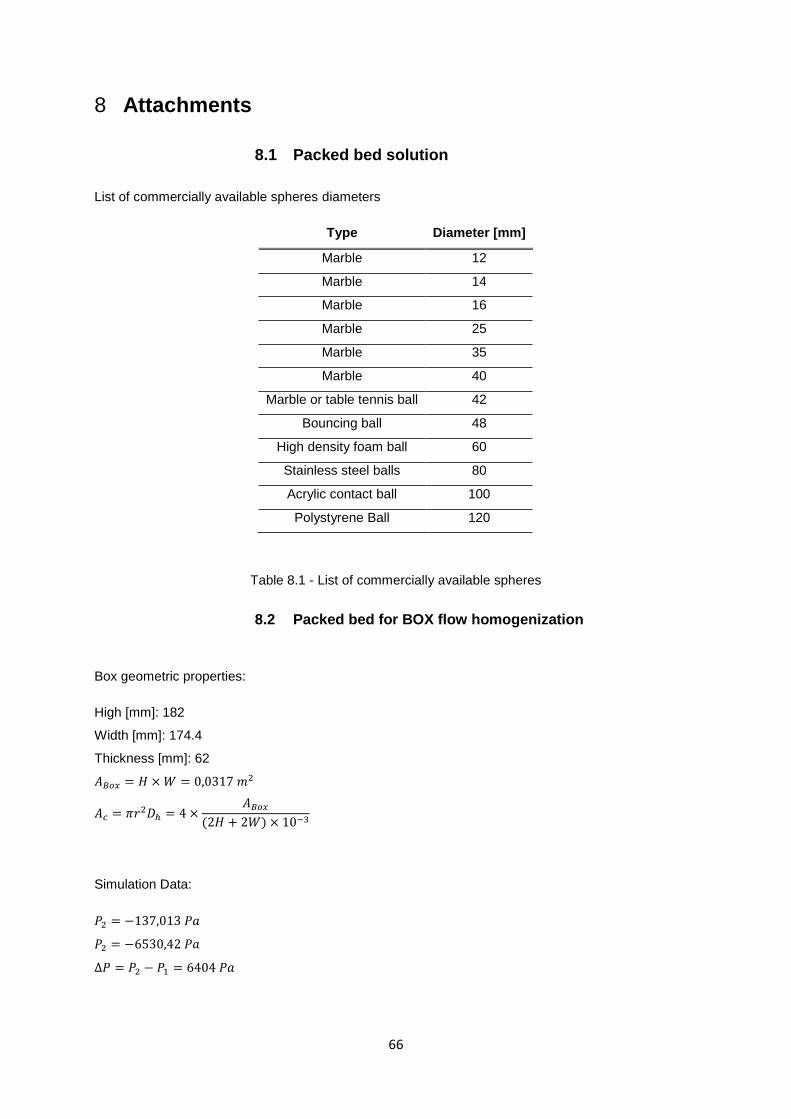
66

8 Attachments

8.1 Packed bed solution

List of commercially available spheres diameters

Type Diameter [mm]

Marble 12

Marble 14

Marble 16

Marble 25

Marble 35

Marble 40

Marble or table tennis ball 42

Bouncing ball 48

High density foam ball 60

Stainless steel balls 80

Acrylic contact ball 100

Polystyrene Ball 120

Table 8.1 - List of commercially available spheres

8.2 Packed bed for BOX flow homogenization

Box geometric properties:

High [mm]: 182

Width [mm]: 174.4

Thickness [mm]: 62

𝐴𝐵𝑜𝑥 = 𝐻 × 𝑊 = 0,0317 𝑚2

𝐴𝑐 = 𝜋𝑟2𝐷ℎ = 4 ×𝐴𝐵𝑜𝑥

(2𝐻 + 2𝑊) × 10−3

Simulation Data:

𝑃2 = −137,013 𝑃𝑎

𝑃2 = −6530,42 𝑃𝑎

∆𝑃 = 𝑃2 − 𝑃1 = 6404 𝑃𝑎

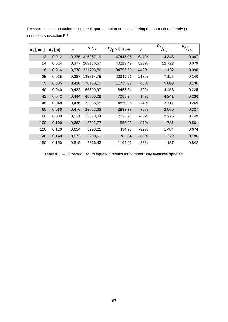
67

Pressure loss computation using the Ergum equation and considering the correction already pre-

sented in subsection 5.2.

𝒅𝒑 [mm] 𝒅𝒑 [m] 𝜺 ∆𝑷

𝑳⁄ ∆𝑷𝑳⁄ × 𝟎, 𝟏𝟓𝒎 ∆

𝑫𝒉𝒅𝒑

⁄ 𝒅𝒑

𝑫𝒉⁄

12 0,012 0,376 316287,19 47443,08 641% 14,843 0,067

14 0,014 0,377 268156,57 40223,49 528% 12,723 0,079

16 0,016 0,378 231703,86 34755,58 443% 11,132 0,090

25 0,025 0,387 135664,75 20349,71 218% 7,125 0,140

35 0,035 0,410 78133,13 11719,97 83% 5,089 0,196

40 0,040 0,432 56390,97 8458,64 32% 4,453 0,225

42 0,042 0,444 48558,29 7283,74 14% 4,241 0,236

48 0,048 0,476 32335,65 4850,35 -24% 3,711 0,269

60 0,060 0,476 25922,22 3888,33 -39% 2,969 0,337

80 0,080 0,521 13578,04 2036,71 -68% 2,226 0,449

100 0,100 0,663 3692,77 553,92 -91% 1,781 0,561

120 0,120 0,654 3298,21 494,73 -92% 1,484 0,674

140 0,140 0,572 5233,61 785,04 -88% 1,272 0,786

150 0,150 0,519 7366,43 1104,96 -83% 1,187 0,842

Table 8.2 – Corrected Ergum equation results for commercially available spheres.

Industrial wind tunnel analysis based on current modeling ...€¦ · Industrial wind tunnel...

Documents

Transcript of Industrial wind tunnel analysis based on current modeling ...€¦ · Industrial wind tunnel...