Working PaperInstitut für Makroökonomie

und KonjunkturforschungMacroeconomic Policy Institute

Thomas I. Palley1

Monetary policy in the liquidity trap and after: A reassessment of quantitative easing and critique of the Federal Reserve’s proposed exit strategyMay 2013

Abstract

This paper provides a novel analysis of quantitative easing (QE) that focu-ses on its implicit fiscal dimension. The first segment examines the theory of the liquidity trap and introduces a distinction between a “weak” and “strong” liquidity trap. The second segment analyzes the impact of QE under con-ditions of a weak and strong liquidity trap. In a weak liquidity trap QE is expansionary but subject to diminishing returns. As QE involves purchasing assets from the public, it transfers the income streams associated with tho-se assets to the fiscal authority. This transfer generates a form of fiscal drag that can theoretically eventually render QE contractionary. In an open economy, exchange rate effects of QE also need to be taken account of and those tend to be expansionary. The third segment explores how to exit QE. The current suggestion of raising the policy interest rate and paying interest on reserves to check inflationary pressures is contradicted because paying interest constitutes an implicit tax cut. Instead, the paper suggests adopting a system of asset based reserve requirements. Requiring banks to hold increased reserves would permanently deactivate liquidity created by QE without recourse to interest payments and the implicit tax cut they represent.

JEL ref.: E43, E44, E50, E52, E58.

Keywords: quantitative easing, fiscal drag, interest on reserves, exit strategy, asset based reserve requirements.

1 Thomas I. Palley, Independent Analyst, Washington, D.C.E-mail: mail@thomaspalley.com

113May 2013

1  

Monetary policy in the liquidity trap and after: A reassessment of quantitative easing and critique of the Federal Reserve’s proposed exit strategy

Abstract

This paper provides a novel analysis of quantitative easing (QE) that focuses on its implicit fiscal dimension. The first segment examines the theory of the liquidity trap and introduces a distinction between a “weak” and “strong” liquidity trap. The second segment analyzes the impact of QE under conditions of a weak and strong liquidity trap. In a weak liquidity trap QE is expansionary but subject to diminishing returns. As QE involves purchasing assets from the public, it transfers the income streams associated with those assets to the fiscal authority. This transfer generates a form of fiscal drag that can theoretically eventually render QE contractionary. In an open economy, exchange rate effects of QE also need to be taken account of and those tend to be expansionary. The third segment explores how to exit QE. The current suggestion of raising the policy interest rate and paying interest on reserves to check inflationary pressures is contradicted because paying interest constitutes an implicit tax cut. Instead, the paper suggests adopting a system of asset based reserve requirements. Requiring banks to hold increased reserves would permanently deactivate liquidity created by QE without recourse to interest payments and the implicit tax cut they represent. Keywords: quantitative easing, fiscal drag, interest on reserves, exit strategy, asset based reserve requirements. JEL reference: E43, E44, E50, E52, E58.

Thomas I. Palley Independent Economist

Washington, D.C. mail@thomaspalley.com

May 2013

1. Introduction

The theory of the liquidity trap has traditionally been interpreted through the lens of the

neo-Keynesian ISLM model. This paper explores liquidity trap theory within the context

of a Post-Keynesian model of endogenous money in which bank lending drives the

money supply. The paper then uses the new model to examine both the policy of

quantitative easing (QE) and the Federal Reserve’s proposed exit strategy from QE.

2  

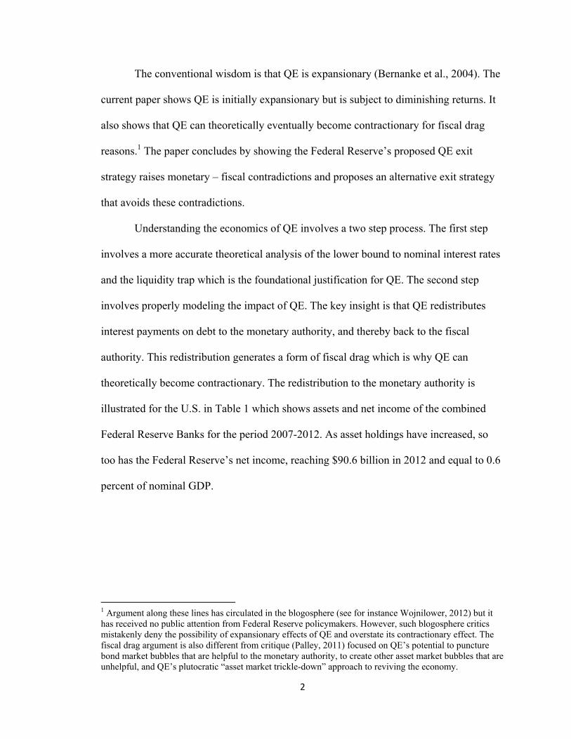
The conventional wisdom is that QE is expansionary (Bernanke et al., 2004). The

current paper shows QE is initially expansionary but is subject to diminishing returns. It

also shows that QE can theoretically eventually become contractionary for fiscal drag

reasons.1 The paper concludes by showing the Federal Reserve’s proposed QE exit

strategy raises monetary – fiscal contradictions and proposes an alternative exit strategy

that avoids these contradictions.

Understanding the economics of QE involves a two step process. The first step

involves a more accurate theoretical analysis of the lower bound to nominal interest rates

and the liquidity trap which is the foundational justification for QE. The second step

involves properly modeling the impact of QE. The key insight is that QE redistributes

interest payments on debt to the monetary authority, and thereby back to the fiscal

authority. This redistribution generates a form of fiscal drag which is why QE can

theoretically become contractionary. The redistribution to the monetary authority is

illustrated for the U.S. in Table 1 which shows assets and net income of the combined

Federal Reserve Banks for the period 2007-2012. As asset holdings have increased, so

too has the Federal Reserve’s net income, reaching $90.6 billion in 2012 and equal to 0.6

percent of nominal GDP.

                                                            1 Argument along these lines has circulated in the blogosphere (see for instance Wojnilower, 2012) but it has received no public attention from Federal Reserve policymakers. However, such blogosphere critics mistakenly deny the possibility of expansionary effects of QE and overstate its contractionary effect. The fiscal drag argument is also different from critique (Palley, 2011) focused on QE’s potential to puncture bond market bubbles that are helpful to the monetary authority, to create other asset market bubbles that are unhelpful, and QE’s plutocratic “asset market trickle-down” approach to reviving the economy.

3  

Table 1. Combined Federal Reserve Banks’ assets and net income, 2007-20012 ($ billions).

90.678.580.252.034.337.7Net income*

2,917.02,919.02,428.02,235.02,246.0915.0Assets

201220112010200920082007

Source: Board of Governors of the Federal Reserve, Independent auditors’ report.*Author’s calculations: net income = retained profits + interest paid to Treasury.

2. Preliminaries

The Great Recession and great stagnation that have followed the financial crisis of 2008

have seen the Federal Reserve and other central banks push their short-term policy

interest rate to zero or near so. After hitting the nominal lower bound (often referred to as

the zero lower bound) to nominal interest rates, central banks have engaged in a policy of

quantitative easing (QE) whereby they have purchased government bonds and private

sector debts. For instance, in the U.S. the Federal Reserve has purchased both Treasury

bonds and mortgage backed securities (MBS) issued by the government sponsored

mortgage finance entities, Fannie Mae and Freddie Mac.

The rationale for QE is twofold. First, by buying government bonds, the central

bank is effectively helping finance the deficit by monetizing it. Second, by buying

government bonds and selected private sector securities, the central bank is helping drive

down interest rates on those bonds and securities and drive up their price. Thus, even

though the short-term policy interest rate is constrained by the nominal lower bound

(NLB), rates on longer-term securities can still be pushed lower. That supposedly confers

a double stimulus. First, it lowers interest rates for borrowers: second, it generates a

4  

positive portfolio wealth effect for owners of such securities. Furthermore, those interest

rate and wealth effects may ripple into other segments of financial markets to the extent

that low rates in one segment induce wealth holders to engage in portfolio adjustments

and substitute into other segments. In this fashion, QE can reach rates and prices in parts

of the financial spectrum that policymakers are unable to access either because of

prohibitions or from reluctance owing to fear of distorting the market process and

favoring some participants over others.2

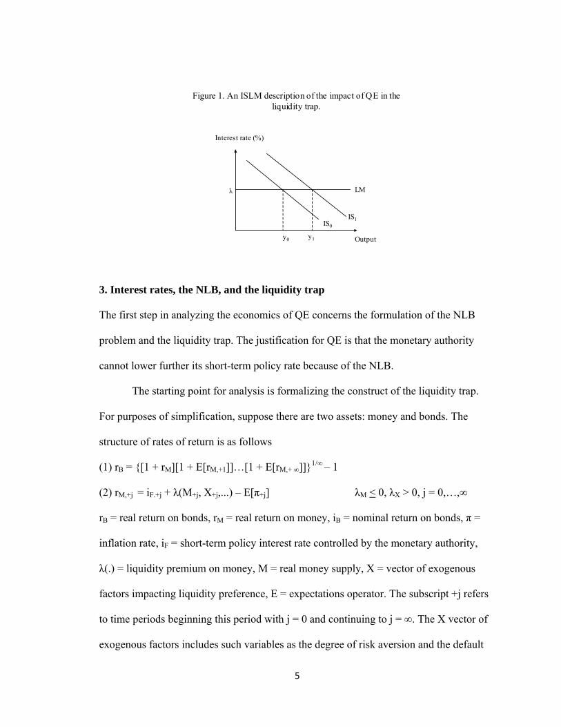
The conventional economic logic rationalizing QE can be illustrated using the

standard ISLM framework. For simplicity inflation is assumed equal to zero so that the

real and nominal interest rates are the same. The monetary authority is assumed to set the

interest rate and its policy interest rate is assumed to be constrained by a zero NLB.

Consequently, the LM schedule is horizontal at an interest rate slightly above zero

representing the liquidity premium (λ) required to hold bonds. Non-money assets must

pay just enough to compensate for giving up the liquidity benefits of holding money. QE

is assumed to bid up the price of financial assets, creating a wealth effect that shifts the IS

right as illustrated in Figure 1. The result is AD and income increase.

                                                            2 As discussed later, QE can also have real exchange rate effects that impact aggregate demand.

5  

Figure 1. An ISLM description of the impact of QE in the liquidity trap.

λ

Interest rate (%)

LM

IS0

IS1

Outputy0 y1

3. Interest rates, the NLB, and the liquidity trap

The first step in analyzing the economics of QE concerns the formulation of the NLB

problem and the liquidity trap. The justification for QE is that the monetary authority

cannot lower further its short-term policy rate because of the NLB.

The starting point for analysis is formalizing the construct of the liquidity trap.

For purposes of simplification, suppose there are two assets: money and bonds. The

structure of rates of return is as follows

(1) rB = {[1 + rM][1 + E[rM,+1]]…[1 + E[rM,+ ∞]]}1/∞ – 1

(2) rM,+j = iF.+j + λ(M+j, X+j,...) – E[π+j] λM < 0, λX > 0, j = 0,…,∞

rB = real return on bonds, rM = real return on money, iB = nominal return on bonds, π =

inflation rate, iF = short-term policy interest rate controlled by the monetary authority,

λ(.) = liquidity premium on money, M = real money supply, X = vector of exogenous

factors impacting liquidity preference, E = expectations operator. The subscript +j refers

to time periods beginning this period with j = 0 and continuing to j = ∞. The X vector of

exogenous factors includes such variables as the degree of risk aversion and the default

6  

risk on bonds and other assets. To simplify the analysis, henceforth it is assumed that the

current and future inflation rate is zero so that rB = iB and rM = iF + λ(M, X,..).

Equation (1) determines the real return on bonds. It embodies an expectations

theory of the term structure of interest rates whereby the return on long bonds is equal to

the expected return from a strategy of rolling-over a sequence of one-period investments

in money. The current period bond rate depends positively on the current and expected

future federal funds rate and the current and expected future liquidity premium. Equation

(2) determines the real return on money which is equal to the short-term policy rate plus

the liquidity premium from holding money less expected inflation. Money receives an

extra implicit return, over and above the explicit interest rate paid on money balances,

which reflects its liquidity property. This liquidity premium is a negative function of the

real money supply which represents the supply of liquidity, and a positive function of the

liquidity preference factors. As the supply of liquidity increases, the liquidity premium

falls (λM < 0) owing to diminished marginal utility of money holdings.

Substituting equation (2) into (1) then determines the nominal return on bonds

which is given by

(3) iB = {[1 + iF + λ(M, X,...)][1 + E[iF,+1 + λ+1]…[1 + E[iF,+n + λ+∞]]}1/∞ – 1

Equation (3) has the long bond rate being a function of the current and expected future

short-term interest rate and liquidity premium.3 If expected future short-term interest rates

and liquidity premiums are the same as current settings, equation (3) simplifies to

(4) iB = iF + λ(M, X,...)

                                                            3 Equation (2) is derived under the assumption of zero expected current and future inflation.

7  

There are three regimes to be considered: a normal regime, a NLB or weak

liquidity trap regime, and a strong liquidity trap regime. The normal regime is

characterized by:

(5.1) iB = iF + λ(M, X,..) > 0

(5.2) iF > iF,MIN

(5.3) λM < 0

iF,MIN = nominal lower bound to the policy rate.4 In normal times the central bank’s short-

term policy interest rate is above the NLB and the liquidity premium is sensitive to the

supply of money. Despite the fact that iF > iF,MIN there may still be a case for QE that

increases the supply of liquidity (M). For instance, suppose the monetary authority deems

iF to be appropriate given existing economic conditions. Now, let there be a large increase

in one of the elements of the X vector that raises the liquidity premium. In this case the

monetary authority may want to increase the supply of liquidity to offset the liquidity

shock while leaving the policy interest rate unchanged.

The NLB or weak liquidity trap is described as follows:

(6.1) iB = λ(M, X,…) > 0

(6.2) iF = iF,MIN

(6.3) λM < 0

Now, the short-term policy rate is at its nominal lower bound, but the liquidity premium

remains sensitive to the supply of liquidity because the marginal utility of liquidity is

                                                            4 The nominal lower bound (iF,MIN) is normally assumed to be zero. However, this is not necessarily the case and it may be positive and institutionally determined. For instance, the monetary authority may want to maintain a small positive short-term interest rate to prevent disruptive disintermediation that puts an end to short-term money market financing via arrangements such as money market funds.

8  

above its floor. This situation can be thought of as corresponding to the Federal Reserve’s

second round of quantitative easing implemented in 2010 that is now referred to as QE2.

Finally, the strong liquidity trap is described as follows:

(7.1) iB = λ(M, X,…) > 0

(7.2) iF = iF,MIN

(7.3) λM = 0

The critical feature is that the liquidity premium is now insensitive to the supply of

liquidity. This is because money and bonds have become perfect substitutes in agents’

portfolios as agents are saturated with liquidity. This situation corresponds to the liquidity

trap as defined by Keynes (1936) in his General Theory:

“There is the possibility, for the reasons discussed above, that, after the rate of interest has fallen to a certain level, liquidity-preference may become virtually absolute in the sense that almost everyone prefers cash to holding a debt which yields so low a rate of interest (p.207).”

4. The financial sector in an excess reserve regime

The next step involves modeling the financial sector. For simplicity, the model presented

below includes only a bond market and QE is conducted via bond purchases. The

appendix contains notes on the implications of including a mortgage market and housing,

the principal effect of which is to introduce additional channels of impact on AD via

housing related spending. The appendix shows that QE conducted via mortgage

purchases is analytically similar to QE conducted via bond purchases and the finding that

QE can become contractionary also holds for mortgage based QE.

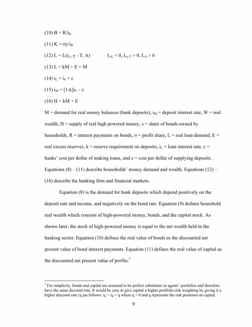
The financial sector is described by the following nine equations:

(8) M = M(iM, iB, y - T, W, X) MiM > 0, MiB < 0, My-T >0, MW > 0, MX >0

(9) W = H + sB + K 0 < s < 1

9  

(10) B = R/iB

(11) K = σy/iB

(12) L = L(iL, y - T, A) LiL < 0, Ly-T > 0, LA > 0

(13) L + kM + E = M

(14) iL = iF + c

(15) iM = [1-k]iF – z

(16) H = kM + E

M = demand for real money balances (bank deposits), iM = deposit interest rate, W = real

wealth, H = supply of real high powered money, s = share of bonds owned by

households, R = interest payments on bonds, σ = profit share, L = real loan demand, E =

real excess reserves, k = reserve requirement on deposits, iL = loan interest rate, c =

banks’ cost per dollar of making loans, and z = cost per dollar of supplying deposits.

Equations (8) – (11) describe households’ money demand and wealth. Equations (12) –

(16) describe the banking firm and financial markets.

Equation (8) is the demand for bank deposits which depend positively on the

deposit rate and income, and negatively on the bond rate. Equation (9) defines household

real wealth which consists of high-powered money, bonds, and the capital stock. As

shown later, the stock of high-powered money is equal to the net wealth held in the

banking sector. Equation (10) defines the real value of bonds as the discounted net

present value of bond interest payments. Equation (11) defines the real value of capital as

the discounted net present value of profits.5

                                                            5 For simplicity, bonds and capital are assumed to be perfect substitutes in agents’ portfolios and therefore have the same discount rate. It would be easy to give capital a higher portfolio risk weighting by giving it a higher discount rate (iK)as follows: iK = iB + q where q > 0 and q represents the risk premium on capital.

10  

Equation (12) defines real loan demand which is a negative function of the loan

rate and a positive function of income. Equation (13) is the banking sector’s balance

sheet identity. Assets consist of loans (L), required reserves (kD), and excess reserves

(E): liabilities consist of deposits. Equations (14) and (15) determine the loan and deposit

rates: the loan rate is a mark-up over the money market cost of funds, while the deposit

rate is a mark-down over the money market cost of funds that takes account of the costs

of administering deposits (z) and holding reserve requirements (k). Equation (16) is the

money market equilibrium condition in which the supply of high-powered money equals

demand. The demand for high-powered money consists of required reserves and excess

reserves.

Rearranging equation (10) and using equations (8), (9), (11), and (12) yields

(17) M([1-k]iF - z, iB, y, W, X) = [L(iF + c, y, A) + E]/[1 – k]

Substituting equation (14) in equation (13) yields

(18) H = [kL(iF + c, y, A) + E]/[1 – k]

Equation (17) shows that the deposit money supply is determined by a combination of

bank lending and excess reserve creation by the central bank. Given the deposit money

supply, the bond rate must adjust so that agents willingly hold the amount of deposits

banks have created. Equation (18) has the supply of high powered money being allocated

between required and excess reserves.

The model is illustrated in Figure 2. The north east panel shows the loan demand

and deposit supply schedules. The latter is determined from the banking sector’s balance

sheet constraint via equation (17). The level of bank lending is determined by the loan

rate, which is a mark-up over the money market rate. In an excess reserve regime bank

11  

deposits greatly exceed loans as a significant portion of deposits are held by banks as

excess reserves. The northwest panel determines the supply of high-powered money

supply. In effect, the monetary authority can be thought as targeting H. When it buys

assets, it pumps reserves into the economy, increasing H. Since lending is constrained by

loan demand at the floor interest rate, the increase in reserves is deposited in banks and

held as excess reserves. The Southeast panel determines the bond rate needed for deposits

so created to be willingly held.6

Figure 2. Determination of the supply of high-powered money, the money supply, bank lending, and interest rates.

High-poweredmoney, h

iF

iF + c

iF - z L(.)

M(.)

Loans, LDeposits, M

M=[L(.)+E]/[1-k]

Loan rate, iLDeposit rate, iMMoney market rate, iF

Bond rate, iB

L* M*

iB

[kL(.)+E]/[1-k]

H*

Figure 2 can be used to illustrate the meaning of a liquidity trap. In a liquidity trap

iF = iF,Min. In a weak liquidity trap the equilibrium is still on a portion of the money

demand function that is negatively sloped with regard to the bond rate (iB). In a strong

liquidity trap it is on a portion of the money demand function that is perfectly elastic with

respect to the bond rate.

                                                            6 The liquidity premium function described in equation (2) is obtained from the inverse of the money demand function. The structure of interest rates is therefore intimately connected to the state of liquidity preference as reflected in the state of money demand.

12  

Figure 2 can also be used to illustrate the instantaneous financial market effect of

QE operations. Such operations have the monetary authority buy bonds and pay for those

purchases by issuing high powered money. That creates deposits which are held as excess

reserves because bank lending is constrained by loan demand. In terms of Figure 2, the

demand for reserves shifts left in the northwest panel while the deposit supply schedule

shifts right in the northeast panel. The loan demand schedule is unchanged. The effect on

bond interest rates depends on whether the economy is in a weak or strong liquidity trap.

In the weak liquidity trap (λM < 0) an increase in the money supply induces a fall

in the bond rate. In the strong liquidity trap (λM = 0) money and bonds are perfect

substitutes so that the money demand function is perfectly elastic at the going bond rate.

The QE open market operation therefore has no impact on the bond rate.

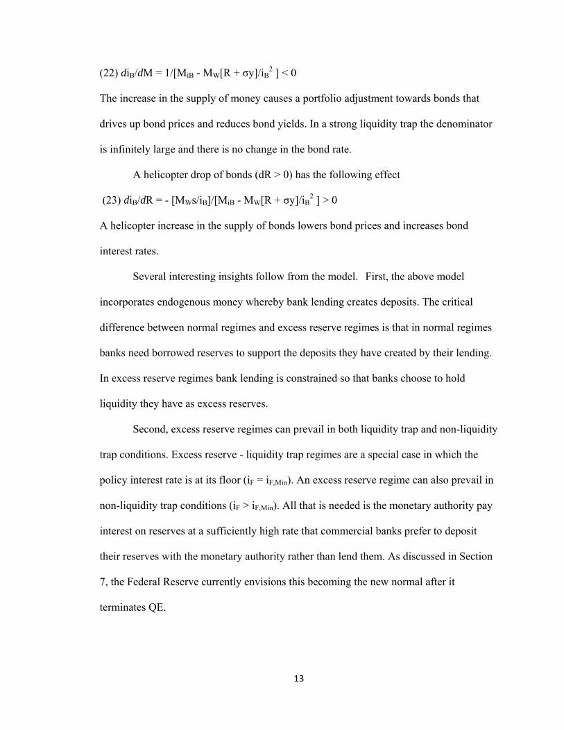
Analytically, the effect of a QE open market operation is as follows:

(19) dE + Rds/iB = 0

(20) dE = dM

(21) dM = MiBdiB + MW[dE + Rds/iB - RdiB/iB2 - σydiB/iB

2]

Equation (19) describes the open market operation whereby high-powered money is

exchanged for bonds. Note that QE operations do not change the stock of debt: they

change the distribution of ownership, increasing the monetary authority’s ownership

share. This is a critical point, the importance of which is explored below. Equation (20)

has the increase in excess reserves equal to the increase in the money supply. Equation

(21) is the differential of the money market equilibrium condition and determines the

change in the bond rate needed to induce agents to hold the increased supply of money.

Substituting equation (19) into (21) yields

13  

(22) diB/dM = 1/[MiB - MW[R + σy]/iB2 ] < 0

The increase in the supply of money causes a portfolio adjustment towards bonds that

drives up bond prices and reduces bond yields. In a strong liquidity trap the denominator

is infinitely large and there is no change in the bond rate.

A helicopter drop of bonds (dR > 0) has the following effect

(23) diB/dR = - [MWs/iB]/[MiB - MW[R + σy]/iB2 ] > 0

A helicopter increase in the supply of bonds lowers bond prices and increases bond

interest rates.

Several interesting insights follow from the model. First, the above model

incorporates endogenous money whereby bank lending creates deposits. The critical

difference between normal regimes and excess reserve regimes is that in normal regimes

banks need borrowed reserves to support the deposits they have created by their lending.

In excess reserve regimes bank lending is constrained so that banks choose to hold

liquidity they have as excess reserves.

Second, excess reserve regimes can prevail in both liquidity trap and non-liquidity

trap conditions. Excess reserve - liquidity trap regimes are a special case in which the

policy interest rate is at its floor (iF = iF,Min). An excess reserve regime can also prevail in

non-liquidity trap conditions (iF > iF,Min). All that is needed is the monetary authority pay

interest on reserves at a sufficiently high rate that commercial banks prefer to deposit

their reserves with the monetary authority rather than lend them. As discussed in Section

7, the Federal Reserve currently envisions this becoming the new normal after it

terminates QE.

14  

Third, excess reserve regimes subtly change the money supply creation process.

In normal times (borrowed reserve regimes) banks are short of reserves and the money

supply is created by the endogenous process of loans creating deposits: reserves are in

short supply and are used as required reserves. In excess reserve regimes the money

supply has a component that is created exogenously by the central bank. When a central

bank buys assets via QE operations, it pays for those assets by issuing high-powered

money. Those payments get deposited with banks, creating deposits: hence, the direct

creation of money by the central bank.

5. A simple macroeconomic model

The previous section provided a model of the financial sector in an excess reserve

regime. The model showed how QE impacts financial markets. It also made clear how

open market operations, including QE operations, do not change the stock of debt.

Instead, they change the distribution of debt ownership.

This section presents a model of the real economy that, together with the model of

the financial sector, provides a macroeconomic model for analyzing the real effects of

QE. The innovation of the model is it shows how QE generates fiscal drag effects that

may run counter to its financial market effects, which is why QE can become

contractionary.

The equations of the model are given by:

(24) y = E(y - T, G, iL, iM, iB, W, A)

Ey-T > 0, EG > 0, EiL < 0, EiM < 0, EiL < 0, EiB < 0, EW > 0, EA > 0

(25) T = ty – R + P

(26) P = [1-s]R - iFH

15  

(27) D = G – T

(28) R = R-1 + iB,-1D-1

Equation (24) is the goods market clearing condition and has output equal to aggregate

demand (AD). The only novelty here is the inclusion of the arguments iL and A from the

loan demand function. The negative partial with regard to the loan rate (EiL < 0) reflects

the assumption that a lower loan rate strengthens loan demand and increases AD.7

Equation (25) is the tax function in which tax revenues are a positive function of income

and profits of the central bank. The latter term is the novelty in the tax function. The

central bank is assumed to pay its profits to the fiscal authority so that these profits

constitute a form of tax. Equation (26) defines the central bank’s profits as interest

received on its bond holdings less interest paid on reserves. Equations (25) and (26) are

of critical importance for understanding why QE can theoretically eventually become

contractionary. Equation (27) defines the government deficit which is financed initially

by the sale of bonds, though subsequent QE purchases of bonds may result in de facto

monetization of the deficit. Lastly, equation (28) defines the evolution of debt interest

payments which equals last period’s payments plus the interest on last period’s debt

issuance. Bonds are perpetuities so they are never repaid. Last period’s bond issuance is

equal to last period’s budget deficit since the deficit is entirely bond financed by the

fiscal authority.8

                                                            7 Modeling the AD effects of private sector credit is difficult. The above simple formulation assumes a lower loan rate increases AD, the background assumption being increased borrowing increases AD. Additionally, a lower loan rate lowers interest payments of existing debtors and, if debtors have a higher propensity to spend than creditors, that too will increase AD. 8 Dividend payments on government owned private sector assets also constitute a form of tax leakage. For instance, at the height of the financial crisis the U.S. government effectively nationalized Fannie Mae and Freddie Mac, the mortgage securitizers. Now, dividends on those stakes paid to government are macro economically akin to a tax.

16  

Substituting equations (25) and (26) into (27) yields an expression for the budget

deficit given by:

(29) D = G - ty + sR + iFH = dR/iB

Equation (25) makes clear that the budget deficit is reduced by profits of the central bank.

Debt interest paid to the central bank increases central bank profit, which is in turn paid

to the fiscal authority and thereby reduces the budget deficit. Interest on reserves paid by

the central bank increases the deficit by reducing central bank profit. An increase in the

public’s ownership share of the debt also increases the deficit. The logic is it implicitly

reduces the central bank’s ownership share, which reduces the central bank’s interest

received and profit paid over to the fiscal authority.

Substituting the tax function and the loan demand function into equation (24)

yields

+ - - + + + + -/? - - - +/? + (30) y = E(y, iB, t, s, R, G, H, iF, k, z, c, σ, A) Signs above arguments represent signs of partial derivatives. AD is a positive function of

income (y), the share of the debt owned by the public (s), interest payments on the debt

(R), government spending (G), the high-powered money stock (H), the profit share (σ),

and the loan demand animal spirits variable (A). AD is a negative function of the bond

rate (iB), the tax rate (t), the central bank’s policy interest rate (iF), the reserve

requirement ratio (k), the cost of administering deposits (z), and the loan rate mark-up

over the policy rate (c).

The positive effects of income and government spending are standard. The

positive debt ownership share effect reflects the fact that government debt is household

wealth and a higher debt ownership share also increases household interest income. The

17  

bond interest rate effect is negative reflecting the negative household wealth effect.9 The

positive effect of high-powered money reflects the wealth effect as net private wealth in

the banking sector is D - L = kD + E = H. The positive effect of the loan demand shift

factor reflects the fact that increased borrowing increases spending. Finally, the positive

effect of the profit share reflects its effect on the wealth value of equities.10

AD is a negative function of the bond rate, the tax rate, and the loan rate mark-up

over the policy rate, and the central bank’s policy interest rate. The negative effect of the

bond rate and tax rate are both standard. The negative impact of the loan rate mark-up

reflects the assumption that a higher mark-up reduces borrowing. The negative effect of

the required reserve ratio and deposit administration cost reflect the fact that these

variables lower the deposit rate, which reduces household saving and increases AD. The

effect of the policy interest rate (iF) is formally ambiguous. On one hand, a lower policy

rate lowers the loan rate which increases loan demand and bank lending, in turn

stimulating AD. It also lowers the deposit rate which reduces household saving. On the

other hand, a lower policy rate lowers interest payments on reserves and constitutes a

form of analogue tax increase. This can be seen from inspection of equation (29), which

shows how payment of interest on reserves by the monetary authority increases the

budget deficit by reducing the central bank’s profit payment to the fiscal authority. If this

tax effect dominates the loan demand effect, a lower policy rate can be contractionary.

6. Model solution and comparative statics

                                                            9 Recall, interest payments on previously issued government debt are pre-determined. If government debt were floating rate there would be an income effect that could reverse the sign. 10 In Post Keynesian macroeconomic models, the profit share can have a negative effect if profit income accrues to higher income households with a lower propensity to consume. Introducing such an effect requires disaggregating the household sector by level and type of income, a feature that is absent in the current model.

18  

The model can now be solved and used to analyze the economic effects of QE policy.

Appropriate substitution reduces the model to a three equation system given by

(33) y = E(y, iB, t, s, R, G, H, iF, k, z, c, σ, A)

(34) M([1-k]iF – z, iB, y, σ, s, X) = [L(iF + c, y, A) + E]/[1- k]

(35) H =kM + E

Equation (33) is the familiar goods market equilibrium or IS condition. Equation (34) is

the financial sector equilibrium condition.11 Equation (35) determines the division of the

high-powered money supply between required and excess reserves. Substituting equation

(35) into equation (34) then yields

(36) M([1 - k]iF - z, iB, y, σ, s, X) = L(iF + c, y, A) + H

The reduced form model consists of equations (33) and (36). There are two endogenous

variables: output (y) and the bond rate (iB). There are two exogenous policy variables: the

policy interest rate (iF) and the supply of high-powered money (H). In a regime with

excess reserves the monetary authority can set both the federal funds rate and the supply

of high powered money.

Figure 3 provides an analogue representation of the model in [y, iB] space. The IS

schedule represents equation (33) and its slope is given by

diB/dy|IS = [1 - Ey]/EiB < 0

Assuming the Keynesian expenditure multiplier stability condition holds, the numerator

is positive. The sign of the IS then depends on the sign of the denominator which is

negative. The FS schedule represents equation (36) and its slope is given by

diB/dy|FS = [Ly - My]/MiB >< 0

                                                            11 Equation (34) is obtained by substituting the components of wealth into money demand in equation (17), which then generates a reduced form for money demand as shown in equation (34).

19  

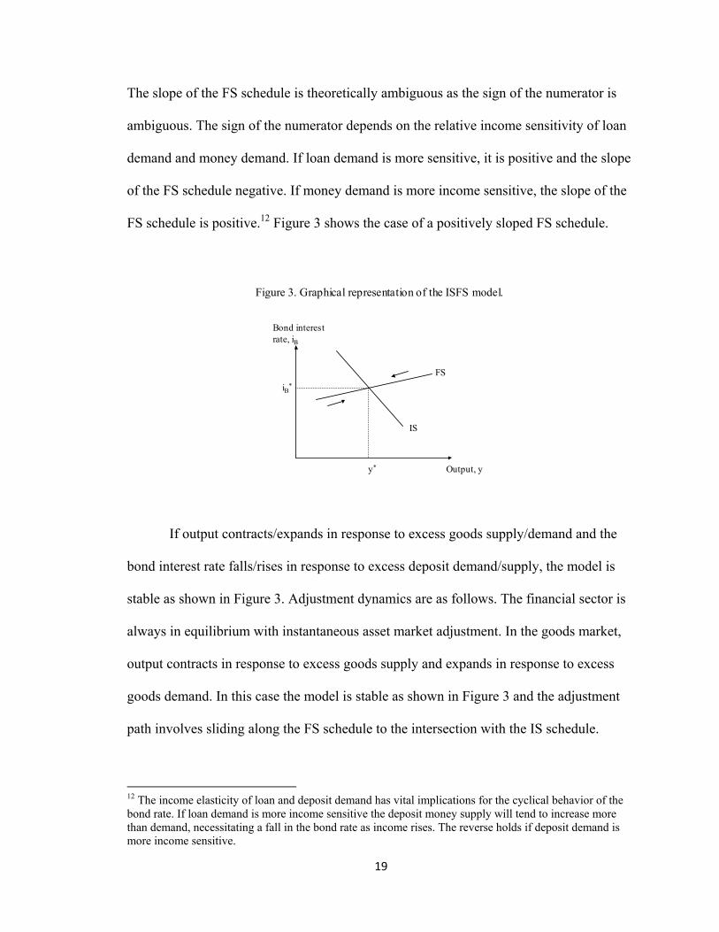
The slope of the FS schedule is theoretically ambiguous as the sign of the numerator is

ambiguous. The sign of the numerator depends on the relative income sensitivity of loan

demand and money demand. If loan demand is more sensitive, it is positive and the slope

of the FS schedule negative. If money demand is more income sensitive, the slope of the

FS schedule is positive.12 Figure 3 shows the case of a positively sloped FS schedule.

Figure 3. Graphical representation of the ISFS model.

Output, y

Bond interestrate, iB

FS

IS

y*

iB*

If output contracts/expands in response to excess goods supply/demand and the

bond interest rate falls/rises in response to excess deposit demand/supply, the model is

stable as shown in Figure 3. Adjustment dynamics are as follows. The financial sector is

always in equilibrium with instantaneous asset market adjustment. In the goods market,

output contracts in response to excess goods supply and expands in response to excess

goods demand. In this case the model is stable as shown in Figure 3 and the adjustment

path involves sliding along the FS schedule to the intersection with the IS schedule.

                                                            12 The income elasticity of loan and deposit demand has vital implications for the cyclical behavior of the bond rate. If loan demand is more income sensitive the deposit money supply will tend to increase more than demand, necessitating a fall in the bond rate as income rises. The reverse holds if deposit demand is more income sensitive.

20  

The model has graphical similarities with the neo-Keynesian ISLM model in that

it conducts macroeconomic analysis in output (y) – interest rate (iB) space. However,

there are two critical differences. First, there are two interest rates as the short-term rate is

distinguished from the bond rate. The former is exogenously set by policy while the latter

is endogenous. Second, the representation of financial market equilibrium is

fundamentally different. The ISLM model constructs financial sector equilibrium in

terms of a fictional money market in which the money supply is determined by the

money multiplier. The current model constructs financial sector equilibrium in terms of

the banking sector and the supply of deposit money balances is endogenously determined

by bank lending.

That said, in an excess reserve regime such as characterizes liquidity trap

conditions, the money supply becomes a hybrid of endogenous and exogenous money

supply determination. Bank lending endogenously determines a significant portion of the

money supply via the “loans create deposits” mechanism. However, lending is

constrained by loan demand. QE injects additional reserves into the financial system via

asset purchases. These purchases create deposits that are held as excess reserves by

banks. That portion of the money supply is therefore exogenously created. In an excess

reserve regime the monetary authority effectively picks the quantity of high-powered

money it wishes to supply, and the banking system then allocates that quantity between

required and excess reserves.

There are three comparative static experiments regarding monetary policy to

consider. The first is a lowering of the policy interest rate in normal times when the

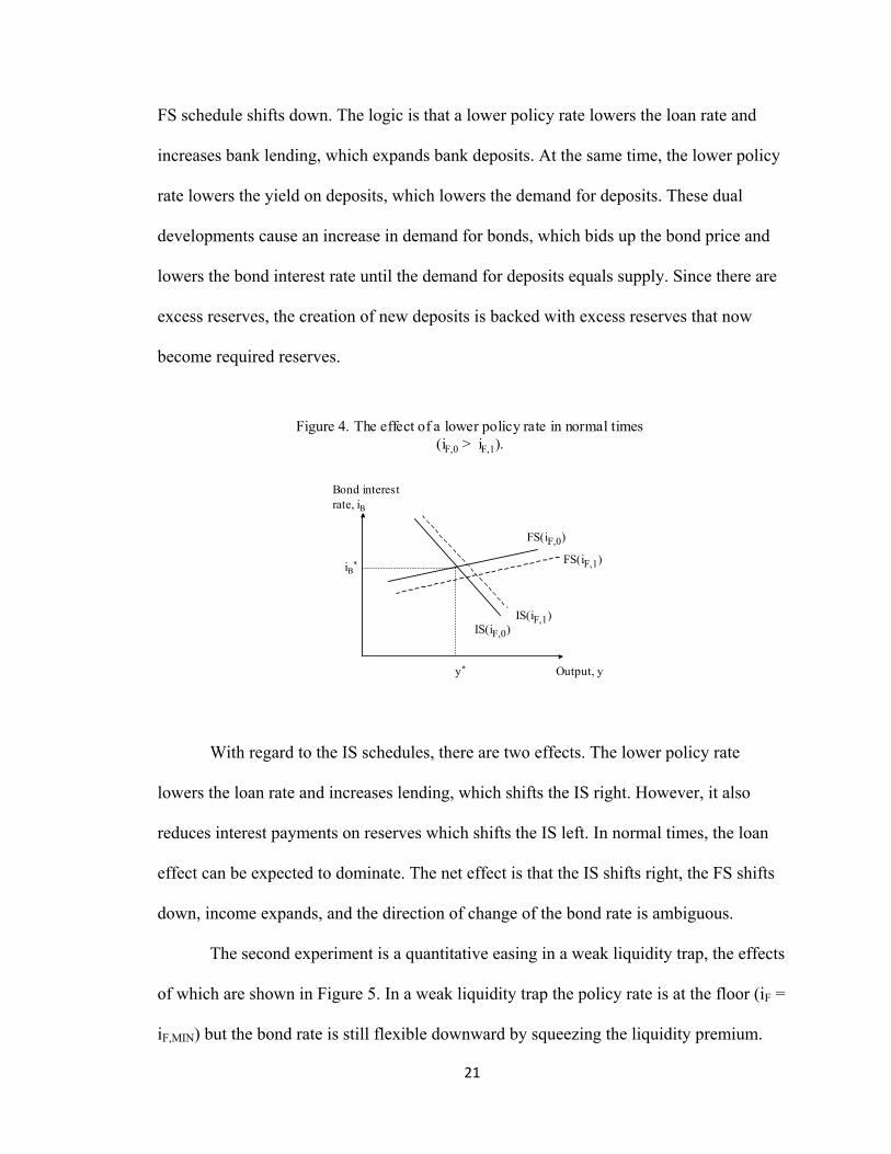
monetary authority has space to lower it (iF > iF,MIN). The effect is shown in Figure 4. The

21  

FS schedule shifts down. The logic is that a lower policy rate lowers the loan rate and

increases bank lending, which expands bank deposits. At the same time, the lower policy

rate lowers the yield on deposits, which lowers the demand for deposits. These dual

developments cause an increase in demand for bonds, which bids up the bond price and

lowers the bond interest rate until the demand for deposits equals supply. Since there are

excess reserves, the creation of new deposits is backed with excess reserves that now

become required reserves.

Figure 4. The effect of a lower policy rate in normal times (iF,0 > iF,1).

Output, y

Bond interestrate, iB

FS(iF,0)

IS(iF,0)

y*

iB*

IS(iF,1)

FS(iF,1)

With regard to the IS schedules, there are two effects. The lower policy rate

lowers the loan rate and increases lending, which shifts the IS right. However, it also

reduces interest payments on reserves which shifts the IS left. In normal times, the loan

effect can be expected to dominate. The net effect is that the IS shifts right, the FS shifts

down, income expands, and the direction of change of the bond rate is ambiguous.

The second experiment is a quantitative easing in a weak liquidity trap, the effects

of which are shown in Figure 5. In a weak liquidity trap the policy rate is at the floor (iF =

iF,MIN) but the bond rate is still flexible downward by squeezing the liquidity premium.

22  

The monetary authority therefore purchases bonds which it pays for by issuing high-

powered money. The bond purchase reduces the public’s ownership share (s) of the debt

and increases the supply of high powered money and holdings of excess reserves. Since

the policy rate is fixed, the loan rate is fixed and there is no benefit to AD from the loan

market. However, the purchase of assets transfers debt ownership and interest payments

to the central bank, acting as a form of tax increase. The IS schedule therefore shifts left.

In the financial sector, the purchase of bonds increases bank deposits and creates an

excess supply of money. That triggers a portfolio readjustment process that bids up the

price of bonds and lowers the bond rate, which is captured by the downward shift of the

FS schedule. The net result is the bond rate falls so that asset prices increase

unambiguously. However, the direction of change in income is theoretically ambiguous

and depends on the relative size of the shifts of the IS and FS schedules. Figure 5 shows

income as increasing.

Figure 5. The effect of quantitative easing in a weak liquidity trap (s0 > s1).

Output, y

Bond interestrate, iB

FS(s0)

IS(s1)

y*

iB*

IS(s0)

FS(s1)

An important feature of the above analysis is that the more QE policies are tried,

the less effective they are likely to become. That is because the liquidity premium is

23  

gradually squeezed out of the bond rate, meaning there is less and less room for the bond

rate to fall in response to increased liquidity. In terms of Figure 5, QE operations in a

weak liquidity trap continue to shift the IS left, but the FS becomes flatter and flatter.

That explains why there are likely to be diminishing returns to QE.13

The third comparative static experiment concerns QE in a strong liquidity trap. In

this case, the liquidity premium has been squeezed to the minimum and can fall no

further because bonds and money are now perfect substitutes. This situation is illustrated

in Figure 6. QE shifts the IS left but the relevant portion of the FS is now horizontal and

pegged at the bond rate floor. Consequently the bond interest rate is unchanged; there is

no wealth effect from QE; and output falls unambiguously because QE imposes a de

facto tax increase by draining interest payments out of the economy.

                                                            13 There are two important caveats to this argument about the leftward shift of the IS. First, the extent of the leftward shift depends on the marginal propensity to consume out of interest income, which may be very low given that most interest income on bonds and mortgage backed securities (the assets the Fed is buying) accrue to wealthy households. Second, QE may facilitate refinancing of existing debt (especially mortgage debt) at a lower interest. Debtors may thereby save interest payments, while the tax effect is equal to the interest on bonds purchased by the Federal Reserve. If the former is large, this refinancing effect might dominate the tax effect so that the IS shifts right. Such an outcome is most likely in the initial stages of QE, but it is also likely to fade away as the bond rate becomes increasingly inflexible downward and the pool of old debt for refinancing is used up.

24  

Figure 6. The effect of quantitative easing in a strong liquidity trap (s0 > s1).

Output, y

Bond interestrate, iB

FS(s0)

IS(s1)

y*

iB*

IS(s0)

FS(s1)

Once in the strong liquidity trap the monetary authority cannot lower the market

interest rate, as long as there is private sector market participation, because money and

bonds have become perfect substitutes, However, the monetary authority can lower the

interest rate if it decides to become the market and forego private sector participation so

that it becomes the exclusive holder of bonds. In that case, the private sector liquidity

premium (λ) is no longer relevant and the interest rate can fall to any level at which the

monetary authority is willing to buy new debt.

A final caveat to the above analysis concerns exchange rate effects. If QE causes

a country’s real exchange rate to depreciate, the exchange rate effect may dominate the

above interest payment effect so that the IS shifts right and output expands. This

exchange rate effect will operate in both a weak and strong liquidity trap, and it means

QE can still be expansionary even in a strong liquidity trap.14 However, if all countries

are pursuing QE so that it produces competitive devaluation, the real exchange rate may

                                                            14 This is the “currency war” fear alluded to by Brazil’s Finance Minister Guido Mantega in September 2010.

25  

be unchanged. In that case, the interest payment effect will dominate in all countries. The

implication is global QE will not work in a global strong liquidity trap.

7. Problems of exiting QE: an alternative suggestion

Thus far, the analysis has focused on whether QE is expansionary in the liquidity trap.

This section turns to the question of exit from QE. QE increases the supply of high-

powered money and bank holdings of excess reserves. The fear is when private sector

AD recovers those reserves could be activated to finance increased lending, potentially

causing inflation and asset bubble problems.

The Federal Reserve currently envisages dealing with this by raising its policy

interest rate and increasing the rate paid on banks’ holdings of reserves. That will do two

things. First, it will raise the loan rate, tamping down loan demand and lending. Second,

banks will have an incentive to hold reserves with the Federal Reserve rather than lend

them out.

The problem with this strategy is it ignores the fiscal implications of paying

interest on reserves. Increased interest payments on reserves will reduce the central

bank’s profits and constitute a form of tax cut, which will increase AD. Thus, the interest

rate exit strategy promises to have monetary policy pulling in opposite directions. On one

hand, a higher policy rate (iF) will lower loan demand and shift the IS left: on the other

hand, it will increase interest payments to the public and shift the IS right.

Moreover, even if the contractionary loan demand effect dominates, the strategy

still has risks. That is because to restrain AD the policy interest rate must be pushed

higher to offset the expansionary impact of interest payments on reserves and this

increase could be very large given the Federal Reserve’s balance sheet is close to two

26  

trillion dollars. Raising the interest rate significantly in this fashion will push up the

deposit interest rate, prompting a shift out of bonds and equities and risking major asset

market dislocation. For all of these reasons, there are significant risks to the Federal

Reserve’s proposed exit strategy.

An alternative exit strategy is for the Federal Reserve to implement a system of

asset based reserve requirements (ABRR). Imposing a system of ABRR would have two

policy advantages. First, it would strengthen the system of monetary control and expand

monetary policy options. Second, it would provide a superior QE exit strategy by

avoiding the problems with the current strategy described above.

ABRR require financial firms to hold reserves against different classes of assets,

with the regulatory authority setting reserve requirements on the basis of its concerns

with each asset class. By forcing financial firms to hold reserves, the system requires that

they retain some of their funds in the form of non-interest-bearing deposits with the

central bank. The implicit cost of forgone interest must be charged against investing in a

particular asset category, and it reduces the marginal revenue from that asset type. By

varying the requirement on each asset class, monetary authorities can vary the return on

each asset class and thereby manage demands, prices, and yields across asset classes.

Given this, the loan rate would become

(37) iL = [1 + ψ]iF + c

ψ = asset based reserve requirement on loans.

With regard to conduct of monetary policy, ABRR add policy instruments that

supplement and strengthen interest rate policy, thereby enhancing the ability of

policymakers to stabilize and manage financial markets. Most importantly, policy can

27  

target specific asset classes by varying the reserve requirement on that class. That enables

policymakers to address concerns regarding specific asset classes without raising the

general level of interest rates.

With regard to QE, ABRR would compel financial firms to hold additional

reserves against assets. Consequently, ABRR provide a way of deactivating the liquidity

created by QE, and it does so at no cost to the central bank. By not having to pay interest

on reserves required by ABRR, the central bank avoids giving an implicit expansionary

tax cut just when it is trying to rein in AD. Moreover, ABRR raise the cost of lending

which would push up the loan rate, thereby restraining AD as intended in the exit

strategy.15

8. Conclusion

This paper has provided a novel analysis of QE that focuses on its implicit fiscal

dimension. The paper involved three segments. The first segment examined the theory of

the liquidity trap and introduced a distinction between a weak and strong liquidity trap. A

weak liquidity trap occurs when the policy interest rate is at its lower nominal bound but

the liquidity premium on money is above its minimum. A strong liquidity trap occurs

when the policy interest rate is at its lower nominal bound and the liquidity premium on

money is at its minimum.

The second segment of the paper analyzed the impact of QE under conditions of a

weak and strong liquidity trap. In a weak liquidity trap QE is initially expansionary but it

is subject to diminishing returns. As QE involves purchasing assets from the public, it

transfers the income streams associated with those assets to the fiscal authority. This

transfer exerts a form of fiscal drag and it can theoretically eventually render QE                                                             15 See Palley (2000, 2003, 2004, 2010) for a discussion of the full policy advantages and benefits of ABRR. 

28  

contractionary. QE is unambiguosusly contractionary in a strong liquidity trap in a closed

economy. In an open economy, exchange rate effects of QE also need to be taken account

of and those effects tend to be expansionary.

The third segment of the paper explored the issue of how to exit QE. The current

suggestion of raising the policy interest rate and paying interest on reserves to check

inflationary pressures is contradicted because the payment of interest constitutes an

implicit tax cut. Instead, the paper suggests that the Federal Reserve adopt a system of

asset based reserve requirements. That would require banks to hold increased reserves,

which would permanently deactivate the liquidity created by QE without recourse to

interest payments and the implicit tax cut that such payments represent.

29  

Appendix: some notes on mortgage finance, housing, and QE The model in the main text shows how QE in the government bond market fits into a macroeconomic model with endogenous money. However, the model does not address housing and mortgage finance which are important aspects of QE policy. This appendix provides some notes on mortgage finance and housing that show how central bank purchases of mortgages also have both positive and negative effects on AD. Once again, the fact that interest service payment streams are transferred to the central bank is a critical channel whereby QE can negatively impact AD. There are three principal channels whereby lower mortgage rates can affect AD. These are via a house price wealth effect; a house construction and furnishing expenditure effect; and via reduced interest service payments from mortgage debtors to mortgage creditors. Modeling mortgages is complicated because mortgages can be refinanced, giving rise to repayment risk that affects the mortgage interest rate. For current purposes, suppose mortgages are interest only contracts, which means they constitute perpetual debt. However, the perpetual stream of interest service payments can be reduced by refinancing. The mortgage interest rate is given by (A.1) iN = iB + γ γ > 0 iN = mortgage interest rate, iB = bond rate, γ = pre-payment premium. The mortgage interest rate is therefore equal to the bond rate plus an exogenous pre-payment premium, reflecting the fact that households may refinance at a future date at a lower interest rate. A lower bond rate lowers the mortgage rate. The value of housing wealth is a function of the mortgage rate and is given by (A.2) V = V(iN,….) ViN < 0 V = value of housing wealth. An increase in the mortgage rate reduces demand for houses, lowering their prices and lowering housing wealth. New mortgage borrowing to finance home purchases is a negative function of the mortgage rate, and new borrowing is used to purchase both existing homes and new homes. Purchases of existing homes are asset transfers and have no impact on AD.16 Purchases of new homes add to AD via new construction (i.e. residential investment spending). Purchases of all homes, new and existing, also add to AD via their impact on spending on furnishings. These impacts are captured as follows (A.3) D = D(iN,….) DiN < 0, (A.4) I = αD 0 < α < 1 (A.5) S = εD ε > 0

                                                            16 For both purchases of existing and new homes there will be a small income effect via sales commissions. This income effect is ignored for simplicity.

30  

D = new mortgage borrowing, I = new residential construction, α = share of new mortgage borrowing used for purchase of new homes, S = spending on home furnishings. Furnishing spending is driven by both new and existing home purchases. The final and most difficult aspect of housing finance concerns mortgage debt service and its impact on AD. The evolution of mortgage debt service is described by (A.6) R = δR-1 + iND 0 < δ < 1 (A.7) δ = 1 + θMin[0, iN – iN,-1] 0 < θ < 1 R = current period mortgage interest payments, δ = refinancing effect. Equation (A.6) has this period’s mortgage interest payments equal to the interest on the stock of previously incurred mortgage debt after refinancing (δR-1) plus the interest on this period’s new mortgage borrowing (iND). Refinancing does not extinguish mortgage debt: it just reduces the amount of interest service payments. Equation (A.7) describes the refinancing effect. If interest rates are unchanged (iN = iN,-1) there is no refinancing so that δ = 1. The same is true if interest rates rise ((iN > iN,-1). However, there is refinancing if interest rates fall (iN < iN,-1) so that δ = 1 + θ[iN - iN,-1] < 1. That in turn reduces interest payments on the prior stock of existing mortgage debt (δR-1). The effect of lowering the mortgage interest rate via QE on mortgage debt servicing payments is given by dR/diN|ΔiN < 0 = - θR-1+ [D+ iNDiN] The first term reflects reduced payments on the stock of existing mortgages due to refinancing and it is negative. The second term reflects the change in interest payments on new mortgage loans and its sign depends on the interest elasticity of mortgage loan demand. It is positive if the elasticity is greater than unity and negative if less than unity. The general assumption is that the stock effect dominates so that dR/diN|ΔiN < 0 < 0. Mortgage interest payments are paid by mortgage debtors to mortgage creditors. The impact on aggregate consumption is given by (A.8) CR = β1[1- μ]R - β2[1 - μ]R - β2μR β1 < β2 = [β1 - β2][1- μ]R - β2μR = β1[1 - μ]R - β2R < 0 CR = aggregate consumption effect of mortgage interest payments, β1 = propensity to consume of creditor households, β2= propensity to consume of debtor households, μ = share of mortgages owned by the central bank, 1 - μ = share of mortgages owned by creditor households. Mortgage interest payments reduce aggregate consumption because they transfer income from debtors with a high marginal propensity to consume (MPC) to creditors with a low MPC. This negative transfer effect is particularly pronounced for mortgages owned by the central bank since it has a MPC of zero. QE purchases of mortgages by the central bank inject excess reserves into the banking system, creating deposits that in turn cause a lower bond rate. The effect on consumption via mortgage interest payments is given by - + + - dCR/dμ = - β1R + {β1[1 - μ] - β2}dR/diN.diN/diB.diB/dμ >< 0

31  

The sign is ambiguous. The first term is negative (-β1R) and reflects increased aggregate saving from increasing the central bank’s ownership share of the stock of mortgages. The second term is positive and reflects increased consumption from reducing interest service payments from high MPC debtor households to low MPC creditor households and the central bank. In a strong liquidity trap it is unambiguously negative since diB/dμ = 0. The effect of mortgage finance and housing on AD is captured by the following augmented AD function given by (A.9) E = E(y, iB,…) + β1[1 - μ]R - β2R + β3V(iN,….) + εD + αD The AD function consists of the AD function in the main body of the paper given by equation (30); the effect of mortgage interest transfers on debtor and creditor household consumption; the house purchase furnishing effect; and the new house construction effect. The initial impact effect of mortgage purchases on AD is given by - - + - - - - dE/dμ = {EiB + {β1[1 - μ] - β2}RiN + β3ViN + εDiN + αDiN}diB/dμ - β1R >< 0 The lower bond rate increases AD via a wealth effect, a reduced interest transfer effect on consumption, a house price wealth effect, a house purchase furnishing effect, and a new residential construction effect. It reduces AD via increased saving that results from increasing the central bank’s ownership of the stock of mortgages. The magnitude of diB/dμ is critical. As this declines, the magnitude of dE/dμ declines. Moreover, dE/dμ is unambiguously negative in the strong liquidity trap since diB/dμ = 0. QE conducted via purchases of mortgages has structural similarities with QE conducted via purchases of bonds. In both cases there is a saving leakage that results from increasing the central bank’s ownership share. In both cases the sign of the QE effect depends critically on the responsiveness of the relevant interest rate to the QE purchase. As that response falls, the beneficial impact of QE diminishes and can become negative because of the saving leakage effect. In the strong liquidity trap the effect is unambiguously negative. In the above analysis the bond market and mortgage market are perfectly integrated via equation (A.1). Why then would a central bank engage in QE via the mortgage market? If equation (A.1) holds and there is perfect integration there is no reason to do so. However, there is reason if the mortgage market is segmented from the bond market or if the arbitrage mechanism between the two markets has broken down. In that case, direct intervention in the mortgage market is the way to have the greatest impact on mortgage finance and housing driven spending.

32  

References Bernanke, B.S., Reinhart, V.R., and Sack, B.P. (2004), “Monetary policy alternatives at the zero bound: An empirical assessment”, Finance and Economics Discussion Series No.48, Divisions of Research & Statistics and Monetary Affairs, Federal Reserve Board, Washington, D.C., 2004. Palley, T.I. (2000), “Stabilizing finance: The case for asset-based reserve requirements”, Report issued by the Financial Markets Center, Philomont, VA, August, available at http://www.thomaspalley.com/docs/articles/macro_policy/stabilizing_finance.pdf. ---------------- (2003), “Asset price bubbles and the case for asset based reserve requirements,” Challenge, 46 (May – June), 53 – 72. ---------------- (2004), “Asset based reserve requirements: Reasserting domestic monetary control in an era of financial innovation and instability,” Review of Political Economy, 16 (January), 43 – 58. --------------- (2010), “Asset price bubbles and monetary policy: Why central banks have been wrong and what should be done,” Intervention, 7(1), 91 – 107.  --------------- (2011), “Quantitative Easing: A Keynesian Critique,” Investigacion Economica, (Julio – Septiembre) LXX, 69 - 86. Wojnilower, J. (2012), “ZIRP and QE remove private sector income,” Bubbles and Busts, Wednesday, 26 December.       

Publisher: Hans-Böckler-Stiftung, Hans-Böckler-Str. 39, 40476 Düsseldorf, Germany Phone: +49-211-7778-331, IMK@boeckler.de, http://www.imk-boeckler.de

IMK Working Paper is an online publication series available at: http://www.boeckler.de/imk_5016.htm

ISSN: 1861-2199 The views expressed in this paper do not necessarily reflect those of the IMK or the Hans-Böckler-Foundation. All rights reserved. Reproduction for educational and non-commercial purposes is permitted provided that the source is acknowledged.