Integrating Generic Sensor Fusion Algorithms with

Sound State Representations through Encapsulation of Manifolds

Christoph Hertzberga,b, Rene Wagnerc,b, Udo Fresea,b,c, Lutz Schroderc,b

aSFB/TR 8 – Spatial Cognition. Reasoning, Action, InteractionbFachbereich 3 – Mathematik und Informatik, Universitat Bremen, Postfach 330 440, 28334 Bremen, Germany

cDeutsches Forschungszentrum fur Kunstliche Intelligenz (DFKI), Sichere Kognitive Systeme,Enrique-Schmidt-Str. 5, 28359 Bremen, Germany

Abstract

Common estimation algorithms, such as least squares estimation or the Kalman filter, operate on astate in a state space S that is represented as a real-valued vector. However, for many quantities, mostnotably orientations in 3D, S is not a vector space, but a so-called manifold, i.e. it behaves like a vectorspace locally but has a more complex global topological structure. For integrating these quantities,several ad-hoc approaches have been proposed.

Here, we present a principled solution to this problem where the structure of the manifold S isencapsulated by two operators, state displacement : S × Rn → S and its inverse : S × S → Rn.These operators provide a local vector-space view δ 7→ xδ around a given state x. Generic estimationalgorithms can then work on the manifold S mainly by replacing +/− with/ where appropriate. Weanalyze these operators axiomatically, and demonstrate their use in least-squares estimation and theUnscented Kalman Filter. Moreover, we exploit the idea of encapsulation from a software engineeringperspective in the Manifold Toolkit, where the / operators mediate between a “flat-vector” viewfor the generic algorithm and a “named-members” view for the problem specific functions.

Key words: estimation, least squares, Unscented Kalman Filter, manifold, 3D orientation,boxplus-method, Manifold Toolkit2010 MSC: 93E10, 93E24, 5704

1. Introduction

Sensor fusion is the process of combining infor-mation obtained from a variety of different sensorsinto a joint belief over the system state. In the de-sign of a sensor fusion system, a key engineeringtask lies in finding a state representation that (a)adequately describes the relevant aspects of real-ity and is (b) compatible with the sensor fusionalgorithm in the sense that the latter yields mean-ingful or even optimal results when operating onthe state representation.

Email address: chtz@informatik.uni-bremen.de

(Christoph Hertzberg)

Satisfying both these goals at the same timehas been a long-standing challenge. Standard sen-sor fusion algorithms typically operate on realvalued vector state representations (Rn) whilemathematically sound representations often formmore complex, non-Euclidean topological spaces.A very common example of this comes up, e.g.within the context of inertial navigation systems(INS) where a part of the state space is SO(3),the group of orientations in R3. To estimate vari-ables in SO(3), there are generally two differentapproaches. The first uses a parameterizationof minimal dimension, i.e. with three parameters(e.g. Euler angles), and operates on the param-eters like on R3. This parameterization has sin-

arX

iv:1

107.

1119

v1 [

cs.R

O]

6 J

ul 2

011

x

x δ

0

δ

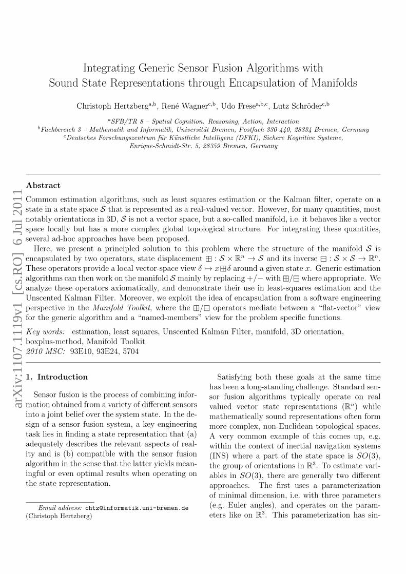
Figure 1: Mapping a local neighborhood in the state space(here: on the unit sphere S2) into Rn (here: the plane) al-lows for the use of standard sensor fusion algorithms with-out explicitly encoding the global topological structure.

gularities, i.e. a situation analogous to the well-known gimbal lock problem in gimbaled INS [13]can occur where very large changes in the parame-terization are required to represent small changesin the state space. Workarounds for this exist thattry to avoid these parts of the state space, as wasmost prominently done in the guidance system ofthe Apollo Lunar Module [22], or switch betweenalternative orderings of the parameterization eachof which exhibit singularities in different areas ofthe state space. The second alternative is to over-parameterize states with a non-minimal represen-tation such as unit quaternions or rotation matri-ces which are treated as R4 or R3×3 respectivelyand re-normalized as needed [45, 30]. This hasother disadvantages such as redundant parame-ters or degenerated, non-normalized variables.

Both approaches require representation-specificmodifications of the sensor fusion algorithm andtightly couple the state representation and thesensor fusion algorithm, which is then no longera generic black box but needs to be adjusted forevery new state representation.

Our approach is based on the observation thatsensor fusion algorithms employ operations whichare inherently local, i.e. they compare and mod-ify state variables in a local neighborhood aroundsome reference. We thus arrive at a generic solu-tion that bridges the gap between the two goalsabove by viewing the state space as a mani-fold. Informally speaking, every point of a mani-

fold has a neighborhood that can be mapped bi-directionally to Rn. This enables us to use anarbitrary manifold S as the state representationwhile the sensor fusion algorithm only sees a lo-cally mapped part of S in Rn at any point in time.For the unit sphere S2 this is illustrated in fig-ure 1.

We propose to implement the mapping bymeans of two encapsulation operators (“box-plus”) and (“boxminus”) where

: S × Rn → S, (1)

: S × S → Rn. (2)

Here, takes a manifold state and a small changeexpressed in the mapped local neighborhood inRn and applies this change to the state to yielda new, modified state. Conversely, determinesthe mapped difference between two states.

The encapsulation operators capture an impor-tant duality: The generic sensor fusion algorithmuses and in place of the corresponding vectoroperations − and + to compare and to modifystates, respectively – based on flattened pertur-bation vectors – and otherwise treats the statespace as a black box. Problem-specific code suchas measurement models, on the other hand, canwork inside the black box, and use the most nat-ural representation for the state space at hand.The operators and translate between thesealternative views. We will later show how thiscan be modeled in an implementation frameworksuch that manifold representations (with match-ing operators) even of very sophisticated com-pound states can be generated automatically froma set of manifold primitives (in our C++ imple-mentation currently Rn, SO(2), SO(3), and S2).

This paper extends course material [11] andseveral master’s theses [25, 5, 16, 43]. It startswith a discussion of related work in Section 2.Section 3 then introduces the -method and 3Dorientations as the most important application,and Section 4 lays out how least squares opti-mization and Kalman filtering can be modifiedto operate on these so-called -manifolds. Sec-tion 5 introduces the aforementioned softwaretoolkit, and Section 6 shows practical experi-

2

ments. Finally, the appendices prove the proper-ties of -manifolds claimed in Section 3 and give

-manifold representations of the most relevantmanifolds R/2πZ, SO(n), Sn and Pn along withproofs.

2. Related Work

2.1. Ad-hoc Solutions

Several ad-hoc methods are available to inte-grate manifolds into estimation algorithms work-ing on Rn [37, 42]. All of them have some draw-backs, as we now discuss using 3D orientations asa running example.

The most common workaround is to use a min-imal parameterization (e.g. Euler angles) [37] [42,p. 6] and place the singularities in some part ofthe workspace that is not used (e.g. facing 90

upwards). This, however, creates an unnecessaryconstraint between the application and the repre-sentation leading to a failure mode that is easilyforgotten. If it is detected, it requires a recoverystrategy, in the worst case manual intervention asin the aforementioned Apollo mission [22].

Alternatively, one can switch between severalminimal parameterizations with different singu-larities. This works but is more complicated.

For overparameterizations (e.g. quaternions),a normalization constraint must be maintained(unit length), e.g. by normalizing after eachstep [45, 30]. The step itself does not know aboutthe constraint, and tries to improve the fit by vi-olating the constraint, which is then undone bynormalization. This kind of counteracting up-dates is inelegant and at least slows down con-vergence. Lagrange multipliers could be used toenforce the constraint exactly [42, p.40] but leadto a more difficult equation system. Alternatively,one could add the normalization constraint as a“measurement” but this is only an approximation,since it would need to have uncertainty zero [42,p.40].

Instead, one could allow non-normalized statesand apply a normalization function every time be-fore using them [27, 42]. Then the normalizationdegree of freedom is redundant having no effect onthe cost function and the algorithm does not try

to change it. Some algorithms can handle this(e.g. Levenberg-Marquardt [35, Chap. 15]) butmany (e.g. Gauss-Newton [35, Chap. 15]) fail dueto singular equations. This problem can be solvedby adding the normalization constraint as a “mea-surement” with some arbitrary uncertainty. [42,p.40]. Still, the estimated state has more dimen-sions than necessary and computation time is in-creased.

2.2. Reference State with Perturbations

Yet another way is to set a reference state andwork relative to it with a minimal parameteri-zation [37, 42, p.6]. Whenever the parameter-ization becomes too large, the reference systemis changed accordingly [1, 7]. This is practicallysimilar to the -method, where in s δ the ref-erence state is s and δ is the minimal parameteri-zation. In particular [7] has triggered our investi-gation, so we compare to their SPmap in detail inApp. D. The vague idea of applying perturbationsin a way more specific than by simply adding hasbeen around in the literature for some time:

“We write this operation [the state up-date] as x → x + δx, even though itmay involve considerable more than vec-tor addition.” W. Triggs [42, p. 7]

Very recently, Strasdat et al. [39, Sec. II.C] havesummarized this technique for SO(3) under thelabel Lie group/algebra representation. Thismeans the state is viewed as an element of theLie group SO(3), i.e. an orthonormal matrix orquaternion but every step of the estimation algo-rithm operates in the Lie group’s tangential space,i.e. the Lie algebra. The Lie’s group’s exponentialmaps a perturbation δ from the Lie algebra to theLie group. For Lie groups this is equivalent to ourapproach, with s δ = s · exp δ (Sec. A.6).

Our contribution here compared to [7, 42, 39] isto embed this idea into a mathematical and algo-rithmic framework by means of an explicit axiom-atization, where the operators and make iteasy to adapt algorithms operating on Rn. More-over, our framework is more generic, being appli-cable also to manifolds which fail to be Lie groups,such as S2.

3

In summary, the discussion shows the need fora principled solution that avoids singularities andneeds neither normalization constraints nor re-dundant degrees of freedom in the estimation al-gorithm.

2.3. Quaternion-Based Unscented Kalman Filter

A reasonable ad-hoc approach for handlingquaternions in an EKF/UKF is to normalize, up-dating the covariance with the Jacobian of thenormalization as in the EKF’s dynamic step [8].This is problematic, because it makes the covari-ance singular. Still the EKF operates as the inno-vation covariance remains positive definite. Nev-ertheless, it is unknown if this phenomen causesproblems, e.g. the zero-uncertainty degree of free-dom could create overconfidence in another degreeof freedom after a non-linear update.

With a similar motivation, van der Merwe [33]included a dynamic, q = η(1 − |q|2)q that drivesthe quaternion q towards normalization. In thiscase the measurement update can still violate nor-malization, but the violation decays over time.

Kraft [24] and Sipos [38] propose a methodof handling quaternions in the state space of anUnscented Kalman Filter (UKF). Basically, theymodify the unscented transform to work withtheir specific quaternion state representation us-ing a special operation for adding a perturbationto a quaternion and for taking the difference oftwo quaternions.

Our approach is related to Kraft’s work in so faras we perform the same computations for statescontaining quaternions. It is more general in thatwe work in a mathematical framework where thespecial operations are encapsulated in the /-operators. This allows us to handle not justquaternions, but general manifolds as represen-tations of both states and measurements, and toroutinely adapt estimation algorithms to mani-folds without sacrificing their genericity.

2.4. Distributions on Unit Spheres

The above-mentioned methods as well as thepresent work treat manifolds locally as Rn andtake care to accumulate small steps in a way thatrespects the global manifold structure. This is an

approximation as most distributions, e.g. Gaus-sians, are strictly speaking not local but extendto infinity. In view of this problem, several gener-alizations of normal distributions have been pro-posed that are genuinely defined on a unit sphere.

The von Mises-Fisher distribution on Sn−1 wasproposed by Fisher [10] and is given by

p(x) = Cn(κ) exp(κµ>x

), (3)

with µ, x ∈ Sn−1 ⊂ Rn, κ > 0 and a normalizationconstant Cn(κ). µ is called the mean direction andκ the concentration parameter.

For the unit-circle S1 this reduces to the vonMises distribution

p(x) = C2(κ) exp(κ cos(x− µ)) , (4)

with x, µ ∈ [−π, π).The von Mises-Fisher distribution locally looks

like a normal distribution N(0, 1

κIn−1

)(viewed in

the tangential space), where In−1 is the (n − 1)-dimensional unit matrix. As only a single param-eter exists to model the covariance, only isotropicdistributions can be modeled, i.e. contours of con-stant probability are always circular. Especiallyfor posterior distributions arising in sensor fusionthis is usually not the case.

To solve this, i.e. to represent general multi-variate normal distributions, Kent proposed theFisher-Bingham distribution on the sphere [21].It is defined as:

p(x) = 1c(κ,β)

exp(κγ>1 x+ β[(γ>2 x)2 − (γ>3 x)2]

).

It requires γi to be a system of orthogonal unitvectors, with γ1 denoting the mean direction (asµ in the von Mises-Fisher case), γ2 and γ3 describ-ing the semi-major and semi-minor axis of the co-variance. κ and β describe the concentration andeccentricity of the covariance.

Though being mathematically more profound,these distributions have the big disadvantage thatthey can not be easily combined with other nor-mal distributions. Presumably, a completely newestimation algorithm would be needed to compen-sate for this, whereas our approach allows us toadapt established algorithms.

4

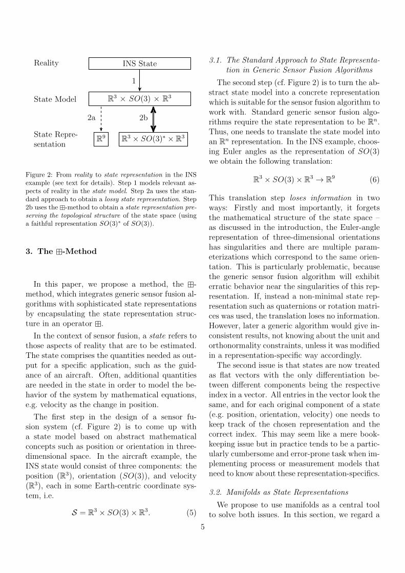
Reality INS State

1

State Model R3 × SO(3) × R3

2a 2b

State Repre-sentation

R9 R3 × SO(3)∗ × R3

Figure 2: From reality to state representation in the INSexample (see text for details). Step 1 models relevant as-pects of reality in the state model. Step 2a uses the stan-dard approach to obtain a lossy state representation. Step2b uses the -method to obtain a state representation pre-serving the topological structure of the state space (usinga faithful representation SO(3)∗ of SO(3)).

3. The -Method

In this paper, we propose a method, the -method, which integrates generic sensor fusion al-gorithms with sophisticated state representationsby encapsulating the state representation struc-ture in an operator .

In the context of sensor fusion, a state refers tothose aspects of reality that are to be estimated.The state comprises the quantities needed as out-put for a specific application, such as the guid-ance of an aircraft. Often, additional quantitiesare needed in the state in order to model the be-havior of the system by mathematical equations,e.g. velocity as the change in position.

The first step in the design of a sensor fu-sion system (cf. Figure 2) is to come up witha state model based on abstract mathematicalconcepts such as position or orientation in three-dimensional space. In the aircraft example, theINS state would consist of three components: theposition (R3), orientation (SO(3)), and velocity(R3), each in some Earth-centric coordinate sys-tem, i.e.

S = R3 × SO(3)× R3. (5)

3.1. The Standard Approach to State Representa-tion in Generic Sensor Fusion Algorithms

The second step (cf. Figure 2) is to turn the ab-stract state model into a concrete representationwhich is suitable for the sensor fusion algorithm towork with. Standard generic sensor fusion algo-rithms require the state representation to be Rn.Thus, one needs to translate the state model intoan Rn representation. In the INS example, choos-ing Euler angles as the representation of SO(3)we obtain the following translation:

R3 × SO(3)× R3 → R9 (6)

This translation step loses information in twoways: Firstly and most importantly, it forgetsthe mathematical structure of the state space –as discussed in the introduction, the Euler-anglerepresentation of three-dimensional orientationshas singularities and there are multiple param-eterizations which correspond to the same orien-tation. This is particularly problematic, becausethe generic sensor fusion algorithm will exhibiterratic behavior near the singularities of this rep-resentation. If, instead a non-minimal state rep-resentation such as quaternions or rotation matri-ces was used, the translation loses no information.However, later a generic algorithm would give in-consistent results, not knowing about the unit andorthonormality constraints, unless it was modifiedin a representation-specific way accordingly.

The second issue is that states are now treatedas flat vectors with the only differentiation be-tween different components being the respectiveindex in a vector. All entries in the vector look thesame, and for each original component of a state(e.g. position, orientation, velocity) one needs tokeep track of the chosen representation and thecorrect index. This may seem like a mere book-keeping issue but in practice tends to be a partic-ularly cumbersome and error-prone task when im-plementing process or measurement models thatneed to know about these representation-specifics.

3.2. Manifolds as State Representations

We propose to use manifolds as a central toolto solve both issues. In this section, we regard a

5

manifold as a black box encapsulating a certain(topological) structure. In practice it will be asubset of Rs subject to constraints such as the or-thonormality of a 3 × 3 rotation matrix that canbe used as a representation of SO(3).

As for the representation of states, in the sim-ple case where a state consists of a single com-ponent only, e.g. a three-dimensional orientation(SO(3)), we can represent a state as a single man-ifold. If a state consists of multiple different com-ponents we can also represent it as a manifoldsince the Cartesian product (Section A.7) of themanifolds representing each individual compo-nent yields another, compound manifold. Essen-tially, we can build sophisticated compound mani-folds starting with a set of manifold primitives. Aswe will discuss in Section 5, this mechanism canbe used as the basis of an object-oriented softwaretoolkit which automatically generates compoundmanifold classes from a concise specification.

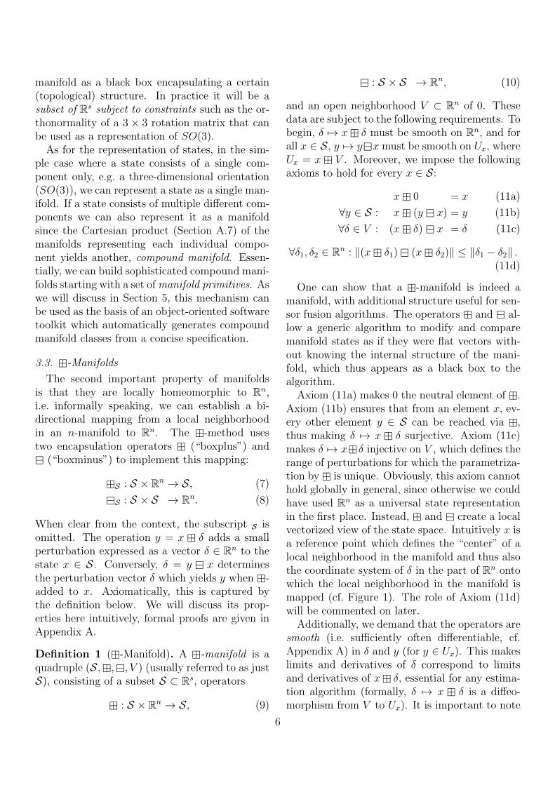
3.3. -Manifolds

The second important property of manifoldsis that they are locally homeomorphic to Rn,i.e. informally speaking, we can establish a bi-directional mapping from a local neighborhoodin an n-manifold to Rn. The -method usestwo encapsulation operators (“boxplus”) and

(“boxminus”) to implement this mapping:

S : S × Rn → S, (7)

S : S × S → Rn. (8)

When clear from the context, the subscript S isomitted. The operation y = x δ adds a smallperturbation expressed as a vector δ ∈ Rn to thestate x ∈ S. Conversely, δ = y x determinesthe perturbation vector δ which yields y when -added to x. Axiomatically, this is captured bythe definition below. We will discuss its prop-erties here intuitively, formal proofs are given inAppendix A.

Definition 1 (-Manifold). A -manifold is aquadruple (S,,, V ) (usually referred to as justS), consisting of a subset S ⊂ Rs, operators

: S × Rn → S, (9)

: S × S → Rn, (10)

and an open neighborhood V ⊂ Rn of 0. Thesedata are subject to the following requirements. Tobegin, δ 7→ x δ must be smooth on Rn, and forall x ∈ S, y 7→ yx must be smooth on Ux, whereUx = x V . Moreover, we impose the followingaxioms to hold for every x ∈ S:

x 0 = x (11a)

∀y ∈ S : x (y x) = y (11b)

∀δ ∈ V : (x δ) x = δ (11c)

∀δ1, δ2 ∈ Rn : ‖(x δ1) (x δ2)‖ ≤ ‖δ1 − δ2‖ .(11d)

One can show that a -manifold is indeed amanifold, with additional structure useful for sen-sor fusion algorithms. The operators and al-low a generic algorithm to modify and comparemanifold states as if they were flat vectors with-out knowing the internal structure of the mani-fold, which thus appears as a black box to thealgorithm.

Axiom (11a) makes 0 the neutral element of .Axiom (11b) ensures that from an element x, ev-ery other element y ∈ S can be reached via ,thus making δ 7→ x δ surjective. Axiom (11c)makes δ 7→ xδ injective on V , which defines therange of perturbations for which the parametriza-tion by is unique. Obviously, this axiom cannothold globally in general, since otherwise we couldhave used Rn as a universal state representationin the first place. Instead, and create a localvectorized view of the state space. Intuitively x isa reference point which defines the “center” of alocal neighborhood in the manifold and thus alsothe coordinate system of δ in the part of Rn ontowhich the local neighborhood in the manifold ismapped (cf. Figure 1). The role of Axiom (11d)will be commented on later.

Additionally, we demand that the operators aresmooth (i.e. sufficiently often differentiable, cf.Appendix A) in δ and y (for y ∈ Ux). This makeslimits and derivatives of δ correspond to limitsand derivatives of x δ, essential for any estima-tion algorithm (formally, δ 7→ x δ is a diffeo-morphism from V to Ux). It is important to note

6

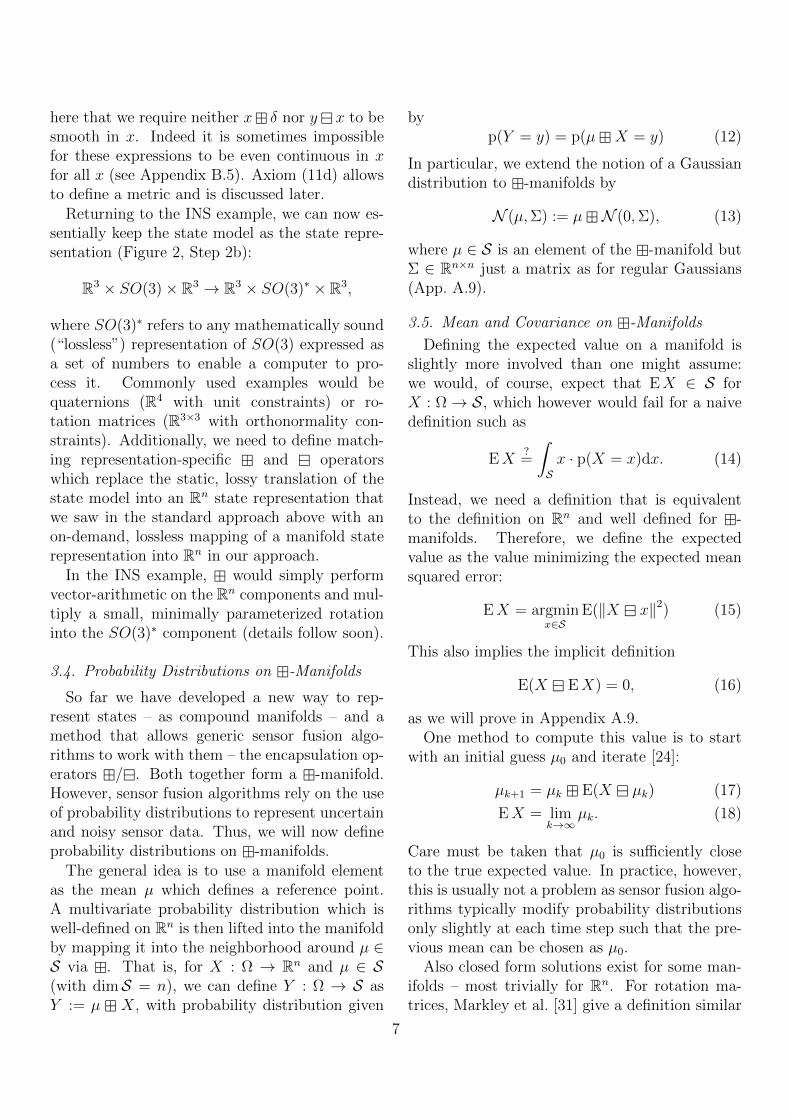
here that we require neither x δ nor y x to besmooth in x. Indeed it is sometimes impossiblefor these expressions to be even continuous in xfor all x (see Appendix B.5). Axiom (11d) allowsto define a metric and is discussed later.

Returning to the INS example, we can now es-sentially keep the state model as the state repre-sentation (Figure 2, Step 2b):

R3 × SO(3)× R3 → R3 × SO(3)∗ × R3,

where SO(3)∗ refers to any mathematically sound(“lossless”) representation of SO(3) expressed asa set of numbers to enable a computer to pro-cess it. Commonly used examples would bequaternions (R4 with unit constraints) or ro-tation matrices (R3×3 with orthonormality con-straints). Additionally, we need to define match-ing representation-specific and operatorswhich replace the static, lossy translation of thestate model into an Rn state representation thatwe saw in the standard approach above with anon-demand, lossless mapping of a manifold staterepresentation into Rn in our approach.

In the INS example, would simply performvector-arithmetic on the Rn components and mul-tiply a small, minimally parameterized rotationinto the SO(3)∗ component (details follow soon).

3.4. Probability Distributions on -Manifolds

So far we have developed a new way to rep-resent states – as compound manifolds – and amethod that allows generic sensor fusion algo-rithms to work with them – the encapsulation op-erators /. Both together form a -manifold.However, sensor fusion algorithms rely on the useof probability distributions to represent uncertainand noisy sensor data. Thus, we will now defineprobability distributions on -manifolds.

The general idea is to use a manifold elementas the mean µ which defines a reference point.A multivariate probability distribution which iswell-defined on Rn is then lifted into the manifoldby mapping it into the neighborhood around µ ∈S via . That is, for X : Ω → Rn and µ ∈ S(with dimS = n), we can define Y : Ω → S asY := µ X, with probability distribution given

byp(Y = y) = p(µX = y) (12)

In particular, we extend the notion of a Gaussiandistribution to -manifolds by

N (µ,Σ) := µN (0,Σ), (13)

where µ ∈ S is an element of the -manifold butΣ ∈ Rn×n just a matrix as for regular Gaussians(App. A.9).

3.5. Mean and Covariance on -Manifolds

Defining the expected value on a manifold isslightly more involved than one might assume:we would, of course, expect that EX ∈ S forX : Ω→ S, which however would fail for a naivedefinition such as

EX?=

∫Sx · p(X = x)dx. (14)

Instead, we need a definition that is equivalentto the definition on Rn and well defined for -manifolds. Therefore, we define the expectedvalue as the value minimizing the expected meansquared error:

EX = argminx∈S

E(‖X x‖2) (15)

This also implies the implicit definition

E(X EX) = 0, (16)

as we will prove in Appendix A.9.One method to compute this value is to start

with an initial guess µ0 and iterate [24]:

µk+1 = µk E(X µk) (17)

EX = limk→∞

µk. (18)

Care must be taken that µ0 is sufficiently closeto the true expected value. In practice, however,this is usually not a problem as sensor fusion algo-rithms typically modify probability distributionsonly slightly at each time step such that the pre-vious mean can be chosen as µ0.

Also closed form solutions exist for some man-ifolds – most trivially for Rn. For rotation ma-trices, Markley et al. [31] give a definition similar

7

x δ2

x δ1

x

δ1

δ2

Figure 3: Axiom (11d): The d-distance between xδ1 andx δ2 (dashed line) is less or equal to the distance in theparameterized around x (dotted line).

to (15) but use Frobenius distance. They derivean analytical solution. Lemma 9 shows that bothdefinitions are roughly equivalent, so this can beused to compute an initial guess for rotations.

The same method can be applied to calculatea weighted mean value of a number of values, be-cause in vector spaces the weighted mean

x =∑i

wixi with∑i

wi = 1 (19)

can be seen as the expected value of a discretedistribution with P(X = xi) = wi.

The definition of the covariance of a -manifolddistribution, on the other hand, is straightfor-ward. As in the Rn case, it is an n × n matrix.Specifically, given a mean value EX of a distri-bution X : Ω→ S, we define its covariance as

CovX = E((X EX)(X EX)>

), (20)

becauseXEX ∈ Rn and the standard definitioncan be applied.

The -operator induces a metric (proof inApp. A)

d(x, y) := ‖y x‖ (21)

that is important in interpreting CovX. First,

tr CovX = E(d(X,EX)2

). (22)

i.e.√

tr CovX is the rms d-distance of X to themean. Second, the states y ∈ S with d(µ, y) = σ

are the 1σ contour of N (µ, σ2 I). Hence, to in-terpret the state covariance or to define measure-ment or dynamic noise for a sensor fusion algo-rithm intuitively it is important that the metricinduced by has an intuitive meaning. For the

-manifold representing orientation in the INSexample, d(x, y) will be the angle between twoorientations x and y.

In the light of (21), axiom (11d) means that theactual distance d(x δ1, x δ2) is less or equalto the distance ‖δ1 − δ2‖ in the parametrization(Fig. 3), i.e. the map x 7→ x δ is 1-Lipschitz.This axiom is needed for all concepts explainedin this subsection, as can be seen in the proofs inAppendix A. In so far, (11d) is the deepest insightin the axiomatization (11).

Appendix A also discusses a slight inconsis-tency in the definitions above, where the co-variance of N (µ,Σ) defined by (13) and (20) isslightly smaller than Σ. For the usual case thatΣ is significantly smaller than the range of uniqueparameters V (i.e. for angles π), these incon-sistencies are very small and can be practicallyignored.

3.6. Practically Important -Manifolds

We will now define -operators for the prac-tically most relevant manifolds Rn as well as 2Dand 3D orientations. Appendix B proves the oneslisted here to fulfill the axioms (11), AppendicesA.5 and A.6 derive general techniques for con-structing a -operator.

3.6.1. Vectorspace (Rn)

For S = Rn, the - and -operators are, ofcourse, simple vector addition and subtraction

x δ = x+ δ, y x = y − x. (23)

3.6.2. 2D Orientation as Angles Modulo 2π

A planar rotation is the simplest case that re-quires taking its manifold structure into account.It can be represented by the rotation angle in-terpreted modulo 2π. Mathematically, this isS = R/2πZ, a set of equivalence classes. Prac-tically, simply a real number α ∈ R is stored, andperiodic equivalents α + 2πk, k ∈ Z are treatedas the same. is, then, simply plus. It could be

8

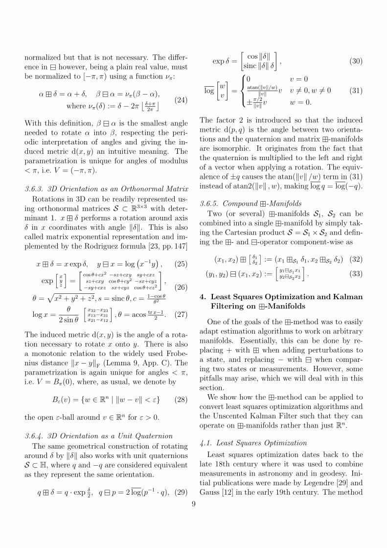
normalized but that is not necessary. The differ-ence in however, being a plain real value, mustbe normalized to [−π, π) using a function νπ:

α δ = α + δ, β α = νπ(β − α),

where νπ(δ) := δ − 2π⌊δ+π2π

⌋ (24)

With this definition, β α is the smallest angleneeded to rotate α into β, respecting the peri-odic interpretation of angles and giving the in-duced metric d(x, y) an intuitive meaning. Theparametrization is unique for angles of modulus< π, i.e. V = (−π, π).

3.6.3. 3D Orientation as an Orthonormal Matrix

Rotations in 3D can be readily represented us-ing orthonormal matrices S ⊂ R3×3 with deter-minant 1. x δ performs a rotation around axisδ in x coordinates with angle ‖δ‖. This is alsocalled matrix exponential representation and im-plemented by the Rodriguez formula [23, pp. 147]

x δ = x exp δ, y x = log(x−1y

), (25)

exp[xyz

]=

[cos θ+cx2 −sz+cxy sy+cxzsz+cxy cos θ+cy2 −sx+cyz−sy+cxz sx+cyz cos θ+cz2

],

θ =√x2 + y2 + z2, s = sinc θ, c = 1−cos θ

θ2

(26)

log x =θ

2 sin θ

[x32−x23x13−x31x21−x12

], θ = acos trx−1

2. (27)

The induced metric d(x, y) is the angle of a rota-tion necessary to rotate x onto y. There is alsoa monotonic relation to the widely used Frobe-nius distance ‖x− y‖F (Lemma 9, App. C). Theparametrization is again unique for angles < π,i.e. V = Bπ(0), where, as usual, we denote by

Bε(v) = w ∈ Rn | ‖w − v‖ < ε (28)

the open ε-ball around v ∈ Rn for ε > 0.

3.6.4. 3D Orientation as a Unit Quaternion

The same geometrical construction of rotatingaround δ by ‖δ‖ also works with unit quaternionsS ⊂ H, where q and −q are considered equivalentas they represent the same orientation.

q δ = q · exp δ2, q p = 2 log(p−1 · q), (29)

exp δ =

[cos ‖δ‖

sinc ‖δ‖ δ

], (30)

log

[wv

]=

0 v = 0atan(‖v‖/w)‖v‖ v v 6= 0, w 6= 0

±π/2‖v‖v w = 0.

(31)

The factor 2 is introduced so that the inducedmetric d(p, q) is the angle between two orienta-tions and the quaternion and matrix -manifoldsare isomorphic. It originates from the fact thatthe quaternion is multiplied to the left and rightof a vector when applying a rotation. The equiv-alence of ±q causes the atan(‖v‖ /w) term in (31)instead of atan2(‖v‖ , w), making log q = log(−q).

3.6.5. Compound -Manifolds

Two (or several) -manifolds S1, S2 can becombined into a single -manifold by simply tak-ing the Cartesian product S = S1×S2 and defin-ing the - and -operator component-wise as

(x1, x2)[δ1δ2

]:= (x1 S1 δ1, x2 S2 δ2) (32)

(y1, y2) (x1, x2) :=[y1S1

x1y2S2

x2

]. (33)

4. Least Squares Optimization and KalmanFiltering on -Manifolds

One of the goals of the -method was to easilyadapt estimation algorithms to work on arbitrarymanifolds. Essentially, this can be done by re-placing + with when adding perturbations toa state, and replacing − with when compar-ing two states or measurements. However, somepitfalls may arise, which we will deal with in thissection.

We show how the -method can be applied toconvert least squares optimization algorithms andthe Unscented Kalman Filter such that they canoperate on -manifolds rather than just Rn.

4.1. Least Squares Optimization

Least squares optimization dates back to thelate 18th century where it was used to combinemeasurements in astronomy and in geodesy. Ini-tial publications were made by Legendre [29] andGauss [12] in the early 19th century. The method

9

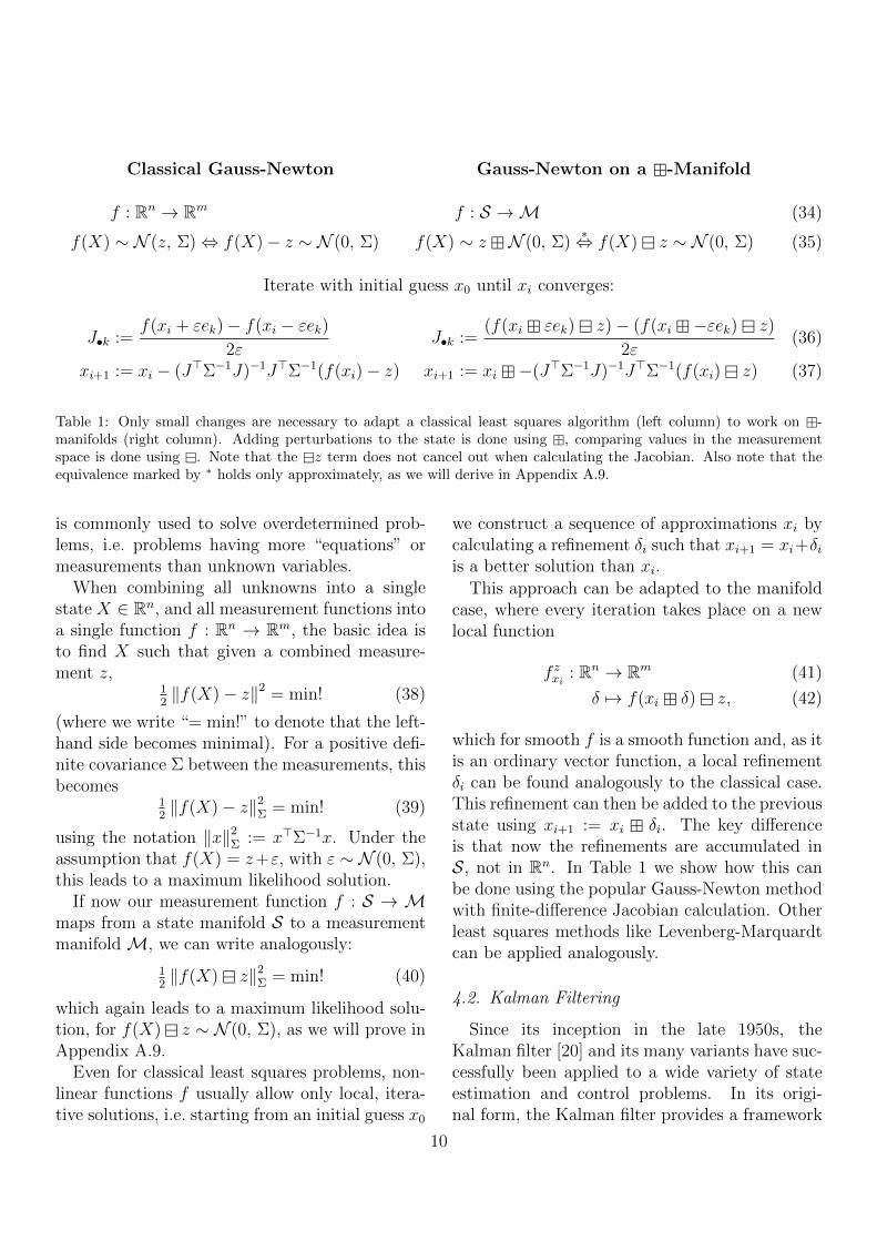
Classical Gauss-Newton Gauss-Newton on a -Manifold

f : Rn → Rm f : S →M (34)

f(X) ∼ N (z, Σ)⇔ f(X)− z ∼ N (0, Σ) f(X) ∼ z N (0, Σ)∗⇔ f(X) z ∼ N (0, Σ) (35)

Iterate with initial guess x0 until xi converges:

J•k :=f(xi + εek)− f(xi − εek)

2εJ•k :=

(f(xi εek) z)− (f(xi −εek) z)

2ε(36)

xi+1 := xi − (J>Σ−1J)−1J>Σ−1(f(xi)− z) xi+1 := xi −(J>Σ−1J)−1J>Σ−1(f(xi) z) (37)

Table 1: Only small changes are necessary to adapt a classical least squares algorithm (left column) to work on -manifolds (right column). Adding perturbations to the state is done using , comparing values in the measurementspace is done using . Note that the z term does not cancel out when calculating the Jacobian. Also note that theequivalence marked by ∗ holds only approximately, as we will derive in Appendix A.9.

is commonly used to solve overdetermined prob-lems, i.e. problems having more “equations” ormeasurements than unknown variables.

When combining all unknowns into a singlestate X ∈ Rn, and all measurement functions intoa single function f : Rn → Rm, the basic idea isto find X such that given a combined measure-ment z,

12‖f(X)− z‖2 = min! (38)

(where we write “= min!” to denote that the left-hand side becomes minimal). For a positive defi-nite covariance Σ between the measurements, thisbecomes

12‖f(X)− z‖2

Σ = min! (39)

using the notation ‖x‖2Σ := x>Σ−1x. Under the

assumption that f(X) = z+ε, with ε ∼ N (0, Σ),this leads to a maximum likelihood solution.

If now our measurement function f : S → Mmaps from a state manifold S to a measurementmanifold M, we can write analogously:

12‖f(X) z‖2

Σ = min! (40)

which again leads to a maximum likelihood solu-tion, for f(X) z ∼ N (0, Σ), as we will prove inAppendix A.9.

Even for classical least squares problems, non-linear functions f usually allow only local, itera-tive solutions, i.e. starting from an initial guess x0

we construct a sequence of approximations xi bycalculating a refinement δi such that xi+1 = xi+δiis a better solution than xi.

This approach can be adapted to the manifoldcase, where every iteration takes place on a newlocal function

f zxi : Rn → Rm (41)

δ 7→ f(xi δ) z, (42)

which for smooth f is a smooth function and, as itis an ordinary vector function, a local refinementδi can be found analogously to the classical case.This refinement can then be added to the previousstate using xi+1 := xi δi. The key differenceis that now the refinements are accumulated inS, not in Rn. In Table 1 we show how this canbe done using the popular Gauss-Newton methodwith finite-difference Jacobian calculation. Otherleast squares methods like Levenberg-Marquardtcan be applied analogously.

4.2. Kalman Filtering

Since its inception in the late 1950s, theKalman filter [20] and its many variants have suc-cessfully been applied to a wide variety of stateestimation and control problems. In its origi-nal form, the Kalman filter provides a framework

10

for continuous state and discrete time state esti-mation of linear Gaussian systems. Many real-world problems, however, are intrinsically non-linear, which gives rise to the idea of modifyingthe Kalman filter algorithm to work with non-linear process models (mapping old to new state)and measurement models (mapping state to ex-pected measurements) as well.

The two most popular extensions of thiskind are the Extended Kalman Filter (EKF)[4, Chap. 5.2] and more recently the UnscentedKalman Filter (UKF) [18]. The EKF linearizesthe process and measurement models through firstorder Taylor series expansion. The UKF, onthe other hand, is based on the unscented trans-form which approximates the respective proba-bility distributions through deterministically cho-sen samples, so-called sigma points , propagatesthese directly through the non-linear process andmeasurement models and recovers the statisticsof the transformed distribution from the trans-formed samples. Thus, intuitively, the EKF re-lates to the UKF as a tangent to a secant.

We will focus on the UKF here since it isgenerally better at handling non-linearities anddoes not require (explicit or numerically approxi-mated) Jacobians of the process and measurementmodels, i.e. it is a derivative-free filter. Althoughthe UKF is fairly new, it has been used success-fully in a variety of robotics applications rangingfrom ground robots [41] to unmanned aerial vehi-cles (UAVs) [33].

The UKF algorithm has undergone an evo-lution from early publications on the unscentedtransform [36] to the work by Julier and Uhlmann[17, 18] and by van der Merwe et al. [32, 33]. Thefollowing is based on the consolidated UKF for-mulation by Thrun, Burgard & Fox [40] with pa-rameters chosen as discussed in [43]. The modi-fication of the UKF algorithm for use with mani-folds is based on [11], [25], [5] and [43].

4.2.1. Non-Linear Process and MeasurementModels

UKF process and measurement models neednot be linear but are assumed to be subject to

additive white Gaussian noise, i.e.

xt = g(ut, xt−1) + εt (43)

zt = h(xt) + δt (44)

where g : T × Rn → Rn and h : Rn → Rm arearbitrary (but sufficiently nice) functions, T is thespace of controls, εt ∼ N (0, Rt), δt ∼ N (0, Qt),and all εt and δt are independent.

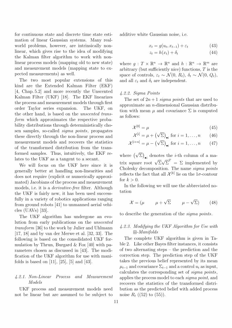
4.2.2. Sigma Points

The set of 2n+ 1 sigma points that are used toapproximate an n-dimensional Gaussian distribu-tion with mean µ and covariance Σ is computedas follows:

X [0] = µ (45)

X [i] = µ+(√

Σ)•i for i = 1, . . . , n (46)

X [i+n] = µ−(√

Σ)•i for i = 1, . . . , n (47)

where(√

Σ)•i denotes the i-th column of a ma-

trix square root√

Σ√

ΣT

= Σ implemented byCholesky decomposition. The name sigma pointsreflects the fact that all X [k] lie on the 1σ-contourfor k > 0.

In the following we will use the abbreviated no-tation

X = (µ µ+√

Σ µ−√

Σ) (48)

to describe the generation of the sigma points .

4.2.3. Modifying the UKF Algorithm for Use with

-Manifolds

The complete UKF algorithm is given in Ta-ble 2. Like other Bayes filter instances, it consistsof two alternating steps – the prediction and thecorrection step. The prediction step of the UKFtakes the previous belief represented by its meanµt−1 and covariance Σt−1 and a control ut as input,calculates the corresponding set of sigma points ,applies the process model to each sigma point, andrecovers the statistics of the transformed distri-bution as the predicted belief with added processnoise Rt ((52) to (55)).

11

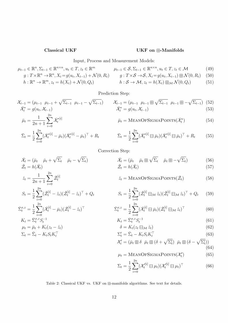
Classical UKF UKF on -Manifolds

Input, Process and Measurement Models:

µt−1 ∈ Rn,Σt−1 ∈ Rn×n, ut ∈ T, zt ∈ Rm µt−1 ∈ S,Σt−1 ∈ Rn×n, ut ∈ T, zt ∈M (49)

g : T×Rn →Rn, Xt=g(ut, Xt−1) +N (0, Rt) g : T×S →S, Xt=g(ut, Xt−1)N (0, Rt) (50)

h : Rn → Rm, zt = h(Xt) +N (0, Qt) h : S →M, zt = h(Xt)M N (0, Qt) (51)

Prediction Step:

Xt−1 = (µt−1 µt−1 +√

Σt−1 µt−1 −√

Σt−1) Xt−1 = (µt−1 µt−1 √

Σt−1 µt−1 −√

Σt−1) (52)

X ∗t = g(ut,Xt−1) X ∗t = g(ut,Xt−1) (53)

µt =1

2n+ 1

2n∑i=0

X ∗[i]t µt = MeanOfSigmaPoints(X ∗t ) (54)

Σt =1

2

2n∑i=0

(X ∗[i]t − µt)(X ∗[i]t − µt)> +Rt Σt =1

2

2n∑i=0

(X ∗[i]t µt)(X ∗[i]t µt)> +Rt (55)

Correction Step:

Xt = (µt µt +√

Σt µt −√

Σt) Xt = (µt µt √

Σt µt −√

Σt) (56)

Zt = h(Xt) Zt = h(Xt) (57)

zt =1

2n+ 1

2n∑i=0

Z [i]t zt = MeanOfSigmaPoints(Zt) (58)

St =1

2

2n∑i=0

(Z [i]t − zt)(Z [i]

t − zt)> +Qt St =1

2

2n∑i=0

(Z [i]t M zt)(Z [i]

t M zt)> +Qt (59)

Σx,zt =

1

2

2n∑i=0

(X [i]t − µt)(Z [i]

t − zt)> Σx,zt =

1

2

2n∑i=0

(X [i]t µt)(Z [i]

t M zt)> (60)

Kt = Σx,zt S−1

t Kt = Σx,zt S−1

t (61)

µt = µt +Kt(zt − zt) δ = Kt(zt M zt) (62)

Σt = Σt −KtStK>t Σ′t = Σt −KtStK

>t (63)

X ′t = (µt δ µt (δ +√

Σ′t) µt (δ −√

Σ′t))(64)

µt = MeanOfSigmaPoints(X ′t ) (65)

Σt =1

2

2n∑i=0

(X ′[i]t µt)(X ′[i]t µt)> (66)

Table 2: Classical UKF vs. UKF on -manifolds algorithms. See text for details.

12

-Manifold-MeanOfSigmaPoints

Input:

Y [i], i = 0, . . . , 2n (67)

Determine mean µ′:

µ′0 = Y [0] (68)

µ′k+1 = µ′k 1

2n+ 1

2n∑i=0

Y [i] µ′k (69)

µ′ = limk→∞

µ′k (70)

Table 3: MeanOfSigmaPoints computes the mean of aset of -manifold sigma points Y. In practice, the limitin (70) can be implemented by an iterative loop that isterminated if the norm of the most recent summed errorvector is below a certain threshold. The number of sigmapoints is not necessarily the same as the dimension of each.

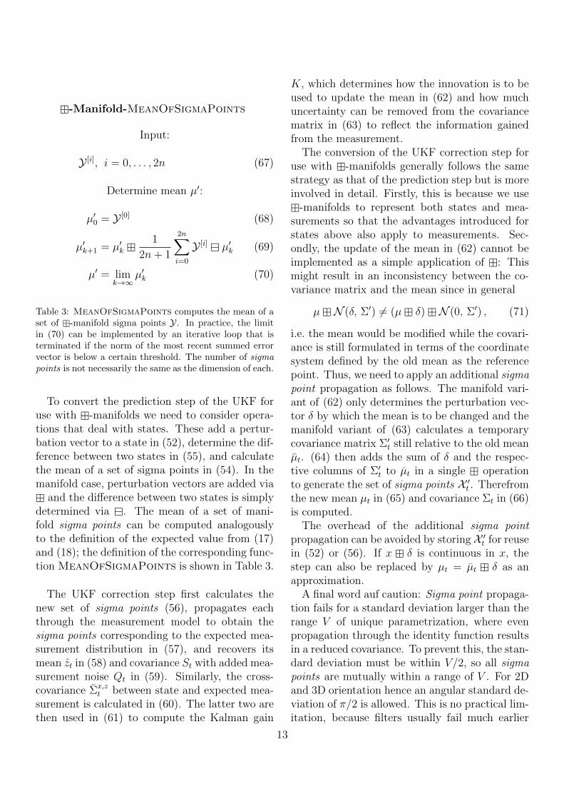
To convert the prediction step of the UKF foruse with -manifolds we need to consider opera-tions that deal with states. These add a pertur-bation vector to a state in (52), determine the dif-ference between two states in (55), and calculatethe mean of a set of sigma points in (54). In themanifold case, perturbation vectors are added via

and the difference between two states is simplydetermined via . The mean of a set of mani-fold sigma points can be computed analogouslyto the definition of the expected value from (17)and (18); the definition of the corresponding func-tion MeanOfSigmaPoints is shown in Table 3.

The UKF correction step first calculates thenew set of sigma points (56), propagates eachthrough the measurement model to obtain thesigma points corresponding to the expected mea-surement distribution in (57), and recovers itsmean zt in (58) and covariance St with added mea-surement noise Qt in (59). Similarly, the cross-covariance Σx,z

t between state and expected mea-surement is calculated in (60). The latter two arethen used in (61) to compute the Kalman gain

K, which determines how the innovation is to beused to update the mean in (62) and how muchuncertainty can be removed from the covariancematrix in (63) to reflect the information gainedfrom the measurement.

The conversion of the UKF correction step foruse with -manifolds generally follows the samestrategy as that of the prediction step but is moreinvolved in detail. Firstly, this is because we use

-manifolds to represent both states and mea-surements so that the advantages introduced forstates above also apply to measurements. Sec-ondly, the update of the mean in (62) cannot beimplemented as a simple application of : Thismight result in an inconsistency between the co-variance matrix and the mean since in general

µN (δ, Σ′) 6= (µ δ)N (0, Σ′) , (71)

i.e. the mean would be modified while the covari-ance is still formulated in terms of the coordinatesystem defined by the old mean as the referencepoint. Thus, we need to apply an additional sigmapoint propagation as follows. The manifold vari-ant of (62) only determines the perturbation vec-tor δ by which the mean is to be changed and themanifold variant of (63) calculates a temporarycovariance matrix Σ′t still relative to the old meanµt. (64) then adds the sum of δ and the respec-tive columns of Σ′t to µt in a single operationto generate the set of sigma points X ′t . Therefromthe new mean µt in (65) and covariance Σt in (66)is computed.

The overhead of the additional sigma pointpropagation can be avoided by storing X ′t for reusein (52) or (56). If x δ is continuous in x, thestep can also be replaced by µt = µt δ as anapproximation.

A final word auf caution: Sigma point propaga-tion fails for a standard deviation larger than therange V of unique parametrization, where evenpropagation through the identity function resultsin a reduced covariance. To prevent this, the stan-dard deviation must be within V/2, so all sigmapoints are mutually within a range of V . For 2Dand 3D orientation hence an angular standard de-viation of π/2 is allowed. This is no practical lim-itation, because filters usually fail much earlier

13

because of nonlinearity.

5. -Manifolds as aSoftware Engineering Tool

As discussed in Section 3, the -method simul-taneously provides two alternative views of a -manifold. On the one hand, generic algorithmsaccess primitive or compound manifolds via flat-tened perturbation vectors, on the other hand,the user implementing process and measurementmodels needs direct access to the underlying staterepresentation (such as a quaternion) and for com-pound manifolds wants to access individual com-ponents by a descriptive name.

In this section we will use our ManifoldToolkit (MTK ) to illustrate how the -methodcan be modeled in software. The current versionof MTK is implemented in C++ and uses theBoost Preprocessor library [2] and the Eigen Ma-trix library [15]. A port to MATLAB is also avail-able [44]. Similar mechanisms can be applied inother (object-oriented) programming languages.

5.1. Representing Manifolds in Software

In MTK, we represent -manifolds as C++classes and require every manifold to provide acommon interface to be accessed by the genericsensor fusion algorithm, i.e. implementations of and . The corresponding C++ interface is fairlystraight-foward. Defining a manifold requires anenum DOF and two methods

struct MyManifold

enum DOF = n;typedef double scalar;

void boxplus(vectview <const double , DOF > delta ,

double scale =1);

void boxminus(vectview <double , DOF > delta ,

const MyManifold& other) const;

;

where n is the degrees of freedom, x.boxplus(

delta, s) implements x := x (s · δ) and y

.boxminus(delta, x) implements δ := y x.vectview maps a double array of size DOF to anexpression directly usable in Eigen expressions.The scaling factor in boxplus can be set to −1 toconveniently implement x (−δ).

Additionally, a -manifold class can providearbitrary member variables and methods (which,

e.g. rotate vectors in the case of orientation) thatare specific to the particular manifold.

MTK already comes with a library of readilyavailable manifold primitive implementations ofRn as vect<n>, SO(2) and SO(3) as SO2 and SO3

respectively, and S2 as S2. It is possible to pro-vide alternative implementations of these or toadd new implementations of other manifolds ba-sically by writing appropriate and methods.

5.2. Automatically Generated Compound Mani-fold Representations

In practice, a single manifold primitive is usu-ally insufficient to represent states (or measure-ments). Thus, we also need to cover compound

-manifolds consisting of several manifold com-ponents in software.

A user-friendly approach would encapsulate themanifold in a class with members for each indi-vidual submanifold which, mathematically, cor-responds to a Cartesian product. Following thisapproach, / operators on the compound man-ifold are needed, which use the / operatorsof the components as described in Section 3.6.5.Using this method, the user can access membersof the manifold by name, and the algorithm justsees the compound manifold.

This can be done by hand in principle, butbecomes quite error-prone when there are manycomponents. Therefore, MTK provides a prepro-cessor macro which generates a compound mani-fold from a list of simple manifolds. The way howMTK does this automatically and hides all detailsfrom the user is a main contribution of MTK.

Returning to the INS example from the intro-duction where we need to represent a state con-sisting of a position, an orientation, and a velocity,we would have a nine-degrees-of-freedom state

S = R3 × SO(3)× R3. (72)

Using our toolkit this can be constructed as:MTK_BUILD_MANIFOLD(state ,

((vect <3>, pos))

((SO3 , orient))

((vect <3>, vel))

)

Given this code snippet the preprocessor will gen-erate a class state, having public members pos,

14

orient, and vel. Also generated are the mani-fold operations boxplus and boxminus as well asthe total degrees of freedom state::DOF = 9 ofthe compound manifold.

The macro also addresses another technicalproblem: Kalman filters in particular require co-variance matrices to be specified which representprocess and measurement noise. Similarly, indi-vidual parts of covariance matrices often need tobe analyzed. In both cases the indices of indi-vidual components in the flattened vector viewneed to be known. MTK makes this possible bygenerating an enum IDX reflecting the index cor-responding to the start of the respective part ofthe vector view. In the above example, the startof the vectorized orientation can be determinedusing e.g. s.orient.IDX for a state s. The sizeof this part is given by s.orient.DOF. MTK alsoprovides convenience methods to access and mod-ify corresponding sub-vectors or sub-matrices us-ing member pointers.

// state covariance matrix:

Matrix <double , state ::DOF , state ::DOF > cov;

cov.setZero ();

// set diagonal of covariance block of pos part:

setDiagonal(cov , &state ::pos , 1);

// fill entire orient -pos - covariance block:

subblock(cov , &state::orient , &state ::pos).fill

(0.1);

5.3. Generic Least Squares Optimization andUKF Implementations

Based on MTK, we have developed a genericleast squares optimization framework calledSLoM (Sparse Least Squares on Manifolds) [16]according to Table 1 and UKFoM [43], a genericUKF on manifolds implementation according toTable 2. Apart from handling manifolds, SLoMautomatically infers sparsity, i.e. which measure-ment depends on which variables, and exploitsthis in computing the Jacobian in (36), and inrepresenting, and inverting it in (37).

MTK, SLoM and UKFoM are already availableonline on www.openslam.org/mtk under an opensource license.

6. Experiments

We now illustrate the advantages of the -method in terms of both ease of use and algo-rithmic performance.

6.1. Worked Example: INS-GPS Integration

In a first experiment, we show how MTK andUKFoM can be used to implement a minimalistic,but working INS-GPS filter in about 50 lines ofC++ code. The focus is on how the frameworkallows to concisely write down such a filter. Itintegrates accelerometer and gyroscope readingsin the prediction step and fuses a global positionmeasurement (e.g. loosely coupled GPS) in themeasurement update. The first version assumeswhite noise. We then show how the frameworkallows for an easy extension to colored noise.

6.1.1. IMU Process Model

Reusing the state manifold definition from Sec-tion 5.2, the process model implements xt =g(ut, xt−1) (cf. Section 4.2.1) where the control utin this case comprises acceleration a as measuredby a three-axis accelerometer and angular velocityw as measured by a three-axis gyroscope.

state process_model(const state &s,

const vect <3> &a, const vect <3> &w)

state s2;

// apply rotation

vect <3> scaled_axis = w * dt;

SO3 rot = SO3::exp(scaled_axis);

s2.orient = s.orient * rot;

// accelerate with gravity

s2.vel = s.vel + (s.orient * a + gravity) * dt;

// translate

s2.pos = s.pos + s.vel * dt;

return s2;

The body of the process model uses Euler inte-gration of the motion described by a and w overa short time interval dt. Note how individualcomponents of the manifold state are accessed byname and how they can provide non-trivial meth-ods (overloaded operators).

Further, we need to implement a function thatreturns the process noise term Rt.

15

010

2030

4050

−5

0

5

0

5

10

15

x[m]y[m]

z[m

]

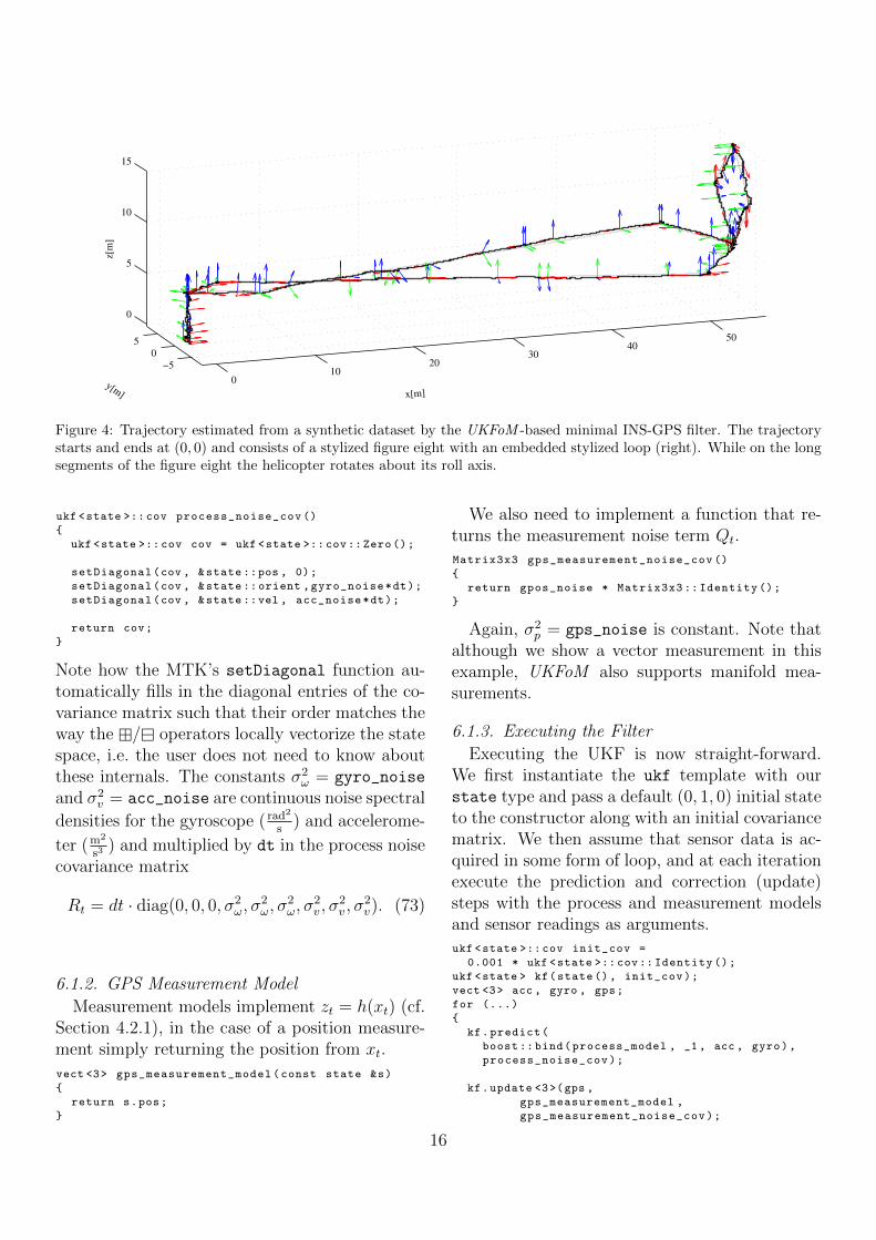
Figure 4: Trajectory estimated from a synthetic dataset by the UKFoM -based minimal INS-GPS filter. The trajectorystarts and ends at (0, 0) and consists of a stylized figure eight with an embedded stylized loop (right). While on the longsegments of the figure eight the helicopter rotates about its roll axis.

ukf <state >:: cov process_noise_cov ()

ukf <state >:: cov cov = ukf <state >::cov::Zero();

setDiagonal(cov , &state ::pos , 0);

setDiagonal(cov , &state ::orient ,gyro_noise*dt);

setDiagonal(cov , &state ::vel , acc_noise*dt);

return cov;

Note how the MTK’s setDiagonal function au-tomatically fills in the diagonal entries of the co-variance matrix such that their order matches theway the / operators locally vectorize the statespace, i.e. the user does not need to know aboutthese internals. The constants σ2

ω = gyro_noise

and σ2v = acc_noise are continuous noise spectral

densities for the gyroscope ( rad2

s) and accelerome-

ter (m2

s3) and multiplied by dt in the process noise

covariance matrix

Rt = dt · diag(0, 0, 0, σ2ω, σ

2ω, σ

2ω, σ

2v , σ

2v , σ

2v). (73)

6.1.2. GPS Measurement Model

Measurement models implement zt = h(xt) (cf.Section 4.2.1), in the case of a position measure-ment simply returning the position from xt.

vect <3> gps_measurement_model(const state &s)

return s.pos;

We also need to implement a function that re-turns the measurement noise term Qt.

Matrix3x3 gps_measurement_noise_cov ()

return gpos_noise * Matrix3x3 :: Identity ();

Again, σ2p = gps_noise is constant. Note that

although we show a vector measurement in thisexample, UKFoM also supports manifold mea-surements.

6.1.3. Executing the Filter

Executing the UKF is now straight-forward.We first instantiate the ukf template with ourstate type and pass a default (0, 1, 0) initial stateto the constructor along with an initial covariancematrix. We then assume that sensor data is ac-quired in some form of loop, and at each iterationexecute the prediction and correction (update)steps with the process and measurement modelsand sensor readings as arguments.

ukf <state >:: cov init_cov =

0.001 * ukf <state >::cov:: Identity ();

ukf <state > kf(state (), init_cov);

vect <3> acc , gyro , gps;

for (...)

kf.predict(

boost::bind(process_model , _1, acc , gyro),

process_noise_cov);

kf.update <3>(gps ,

gps_measurement_model ,

gps_measurement_noise_cov);

16

0 10 20 30 40 50

−5

0

5

0 20 40 60 80 100 120 140 1600

0.2

0.4

0.6

0.8

Time (s)

RM

S E

rror

Norm

s

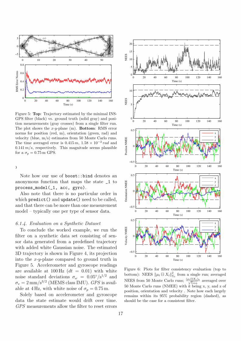
Figure 5: Top: Trajectory estimated by the minimal INS-GPS filter (black) vs. ground truth (solid gray) and posi-tion measurements (gray crosses) from a single filter run.The plot shows the x-y-plane (m). Bottom: RMS errornorms for position (red, m), orientation (green, rad) andvelocity (blue, m/s) estimates from 50 Monte Carlo runs.The time averaged error is 0.415m, 1.58 × 10−2 rad and0.141m/s, respectively. This magnitude seems plausiblefor a σp = 0.75 m GPS.

Note how our use of boost::bind denotes ananonymous function that maps the state _1 toprocess_model(_1, acc, gyro).

Also note that there is no particular order inwhich predict() and update() need to be called,and that there can be more than one measurementmodel – typically one per type of sensor data.

6.1.4. Evaluation on a Synthetic Dataset

To conclude the worked example, we run thefilter on a synthetic data set consisting of sen-sor data generated from a predefined trajectorywith added white Gaussian noise. The estimated3D trajectory is shown in Figure 4, its projectioninto the x-y-plane compared to ground truth inFigure 5. Accelerometer and gyroscope readingsare available at 100 Hz (dt = 0.01) with whitenoise standard deviations σω = 0.05/s1/2 andσv = 2 mm/s3/2 (MEMS class IMU). GPS is avail-able at 4 Hz, with white noise of σp = 0.75 m.

Solely based on accelerometer and gyroscopedata the state estimate would drift over time.GPS measurements allow the filter to reset errors

0 20 40 60 80 100 120 140 1600

5

10

15

20

Time (s)

NE

ES

0 20 40 60 80 100 120 140 1600

5

10

Time (s)N

EE

S

0 20 40 60 80 100 120 140 160

−0.5

0

0.5

Time (s)

Posi

tion N

ME

E

x

y

z

0 20 40 60 80 100 120 140 160

−0.5

0

0.5

Time (s)

Ori

enta

tion N

ME

E

x

y

z

0 20 40 60 80 100 120 140 160

−0.5

0

0.5

Time (s)

Vel

oci

ty N

ME

E

x

y

z

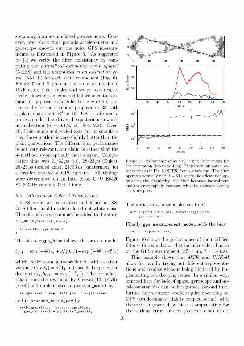
Figure 6: Plots for filter consistency evaluation (top to

bottom): NEES ‖µt Xt‖2Σtfrom a single run; averaged

NEES from 50 Monte Carlo runs; (µtXt)k√Σtkk

averaged over

50 Monte Carlo runs (NMEE) with k being x, y, and z ofposition, orientation and velocity . Note how each largelyremains within its 95% probability region (dashed), asshould be the case for a consistent filter.

17

stemming from accumulated process noise. How-ever, over short time periods accelerometer andgyroscope smooth out the noisy GPS measure-ments as illustrated in Figure 5. As suggestedby [4] we verify the filter consistency by com-puting the normalized estimation error squared(NEES) and the normalized mean estimation er-ror (NMEE) for each state component (Fig. 6).Figure 7 and 8 present the same results for aUKF using Euler angles and scaled axis respec-tively, showing the expected failure once the ori-entation approaches singularity. Figure 9 showsthe results for the technique proposed in [33] witha plain quaternion R4 in the UKF state and aprocess model that drives the quaternion towardsnormalization (η = 0.1/s, cf. Sec. 2.3). Over-all, Euler-angle and scaled axis fail at singulari-ties, the -method is very slightly better than theplain quaternion. The difference in performanceis not very relevant, our claim is rather that the

-method is conceptually more elegant. Compu-tation time was 21/32µs (), 28/23µs (Euler),25/23µs (scaled axis), 21/33µs (quaternion) fora predict-step/for a GPS update. All timingswere determined on an Intel Xeon CPU E5420@2.50GHz running 32bit Linux.

6.2. Extension to Colored Noise Errors

GPS errors are correlated and hence a INS-GPS filter should model colored not white noise.Therefor, a bias vector must be added to the state:

MTK_BUILD_MANIFOLD(state ,

...

((vect <3>, gps_bias))

)

The bias b =gps_bias follows the process model

bt+1 = exp(−dt

T

)bt +N

(0,(1−exp

(−2dt

T

))σ2b I3

)which realizes an autocorrelation with a givenvariance Cov(bt) = σ2

b I3 and specified exponentialdecay cor(bt, bt+k) = exp

(−k·dt

T

). The formula is

taken from the textbook by Grewal [13, (8.76),(8.78)] and implemented in process_model by

s2.gps_bias = exp(-dt/T_pos) * s.gps_bias;

and in process_noise_cov by

setDiagonal(cov , &state ::gps_bias ,

gps_cnoise *(1-exp(-2*dt/T_pos)));

0 10 20 30 40 50

−5

0

5

0 20 40 60 80 100 120 140 1600

200

400

600

Time (s)

Err

or

Norm

s

0 20 40 60 80 100 120 140 160

100

105

1010

Time (s)

NE

ES

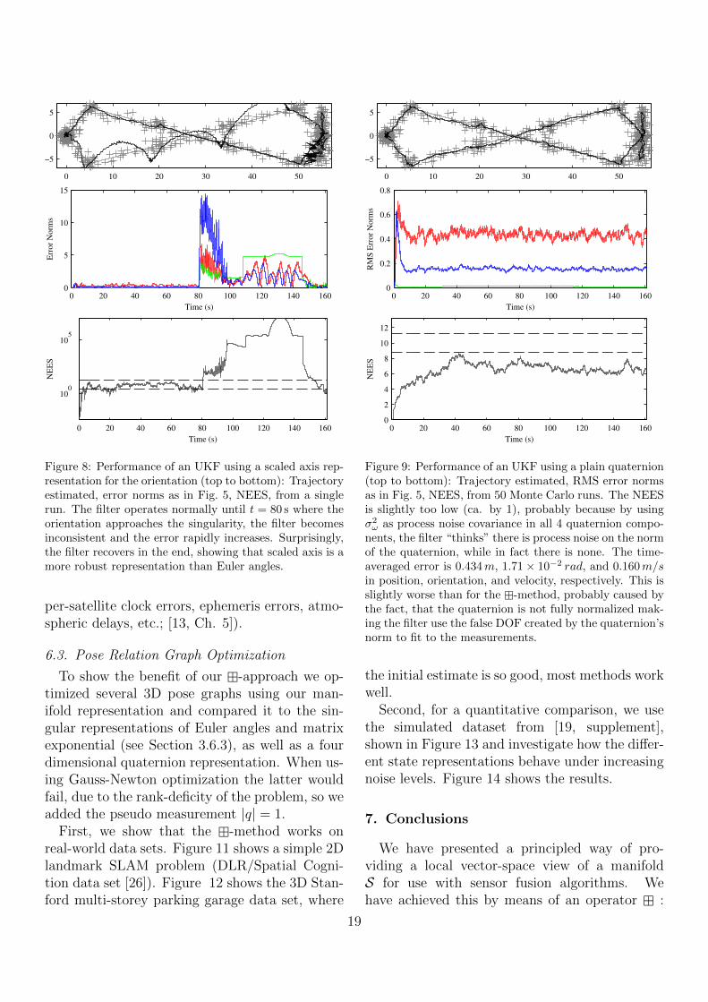
Figure 7: Performance of an UKF using Euler angles forthe orientation (top to bottom): Trajectory estimated, er-ror norms as in Fig. 5, NEES, from a single run. The filteroperates normally until t = 60 s where the orientation ap-proaches the singularity, the filter becomes inconsistentand the error rapidly increases with the estimate leavingthe workspace.

The initial covariance is also set to σ2b :

setDiagonal(init_cov , &state ::gps_bias ,

gps_cnoise);

Finally, gps_measurement_model adds the bias:

return s.pos+s.bias;

Figure 10 shows the performance of the modifiedfilter with a simulation that includes colored noiseon the GPS measurement (σ2

b = 5m, T = 1800s).This example shows that MTK and UKFoM

allow for rapidly trying out different representa-tions and models without being hindered by im-plementing bookkeeping issues. In a similar way,omitted here for lack of space, gyroscope and ac-celerometer bias can be integrated. Beyond that,further improvement would require operating onGPS pseudo-ranges (tightly coupled setup), withthe state augmented by biases compensating forthe various error sources (receiver clock error,

18

0 10 20 30 40 50

−5

0

5

0 20 40 60 80 100 120 140 1600

5

10

15

Time (s)

Err

or

Norm

s

0 20 40 60 80 100 120 140 160

100

105

Time (s)

NE

ES

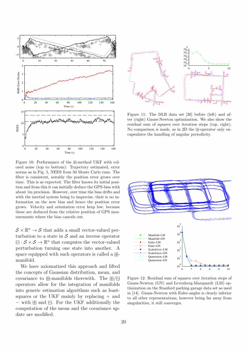
Figure 8: Performance of an UKF using a scaled axis rep-resentation for the orientation (top to bottom): Trajectoryestimated, error norms as in Fig. 5, NEES, from a singlerun. The filter operates normally until t = 80 s where theorientation approaches the singularity, the filter becomesinconsistent and the error rapidly increases. Surprisingly,the filter recovers in the end, showing that scaled axis is amore robust representation than Euler angles.

per-satellite clock errors, ephemeris errors, atmo-spheric delays, etc.; [13, Ch. 5]).

6.3. Pose Relation Graph Optimization

To show the benefit of our -approach we op-timized several 3D pose graphs using our man-ifold representation and compared it to the sin-gular representations of Euler angles and matrixexponential (see Section 3.6.3), as well as a fourdimensional quaternion representation. When us-ing Gauss-Newton optimization the latter wouldfail, due to the rank-deficity of the problem, so weadded the pseudo measurement |q| = 1.

First, we show that the -method works onreal-world data sets. Figure 11 shows a simple 2Dlandmark SLAM problem (DLR/Spatial Cogni-tion data set [26]). Figure 12 shows the 3D Stan-ford multi-storey parking garage data set, where

0 10 20 30 40 50

−5

0

5

0 20 40 60 80 100 120 140 1600

0.2

0.4

0.6

0.8

Time (s)

RM

S E

rror

Norm

s

0 20 40 60 80 100 120 140 1600

2

4

6

8

10

12

Time (s)

NE

ES

Figure 9: Performance of an UKF using a plain quaternion(top to bottom): Trajectory estimated, RMS error normsas in Fig. 5, NEES, from 50 Monte Carlo runs. The NEESis slightly too low (ca. by 1), probably because by usingσ2ω as process noise covariance in all 4 quaternion compo-

nents, the filter “thinks” there is process noise on the normof the quaternion, while in fact there is none. The time-averaged error is 0.434m, 1.71× 10−2 rad, and 0.160m/sin position, orientation, and velocity, respectively. This isslightly worse than for the -method, probably caused bythe fact, that the quaternion is not fully normalized mak-ing the filter use the false DOF created by the quaternion’snorm to fit to the measurements.

the initial estimate is so good, most methods workwell.

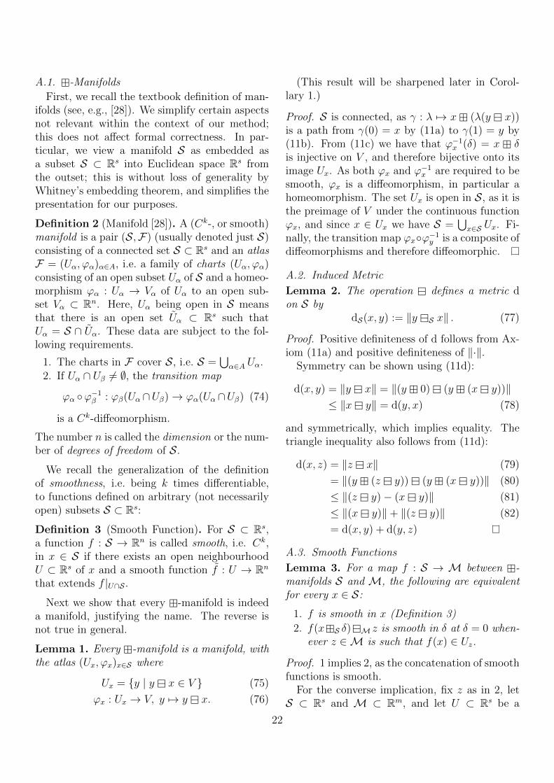
Second, for a quantitative comparison, we usethe simulated dataset from [19, supplement],shown in Figure 13 and investigate how the differ-ent state representations behave under increasingnoise levels. Figure 14 shows the results.

7. Conclusions

We have presented a principled way of pro-viding a local vector-space view of a manifoldS for use with sensor fusion algorithms. Wehave achieved this by means of an operator :

19

0 10 20 30 40 50

−5

0

5

0 20 40 60 80 100 120 140 1600

1

2

3

4

Time (s)

RM

S E

rror

Norm

s

0 20 40 60 80 100 120 140 1600

5

10

15

Time (s)

NE

ES

Figure 10: Performance of the -method UKF with col-ored noise (top to bottom): Trajectory estimated, errornorms as in Fig. 5, NEES from 50 Monte Carlo runs. Thefilter is consistent, notably the position error grows overtime. This is as expected: The filter knows its initial posi-tion and from this it can initially deduce the GPS-bias withabout 1m precision. However, over time the bias drifts andwith the inertial system being to imprecise, their is no in-formation on the new bias and hence the position errorgrows. Velocity and orientation error keep low, becausethese are deduced from the relative position of GPS mea-surements where the bias cancels out.

S ×Rn → S that adds a small vector-valued per-turbation to a state in S and an inverse operator

: S ×S → Rn that computes the vector-valuedperturbation turning one state into another. Aspace equipped with such operators is called a -manifold.

We have axiomatized this approach and liftedthe concepts of Gaussian distribution, mean, andcovariance to -manifolds therewith. The /operators allow for the integration of manifoldsinto generic estimation algorithms such as least-squares or the UKF mainly by replacing + and− with and . For the UKF additionally thecomputation of the mean and the covariance up-date are modified.

0 5 10

104

105

106

107

108

109

Figure 11: The DLR data set [26] before (left) and af-ter (right) Gauss-Newton optimization. We also show theresidual sum of squares over iteration steps (top, right).No comparison is made, as in 2D the -operator only en-capsulates the handling of angular periodicity.

Manifold−LM

Manifold−GN

Euler−LM

Euler−GN

ScaledAxis−LM

ScaledAxis−GN

Quaternion−LM

Quaternion−GN

0 2 4 6 8 10

100

101

102

103

104

105

Figure 12: Residual sum of squares over iteration steps ofGauss-Newton (GN) and Levenberg-Marquardt (LM) op-timization on the Stanford parking garage data set as usedin [14]. Gauss-Newton with Euler-angles is clearly inferiorto all other representations, however being far away fromsingularities, it still converges.

20

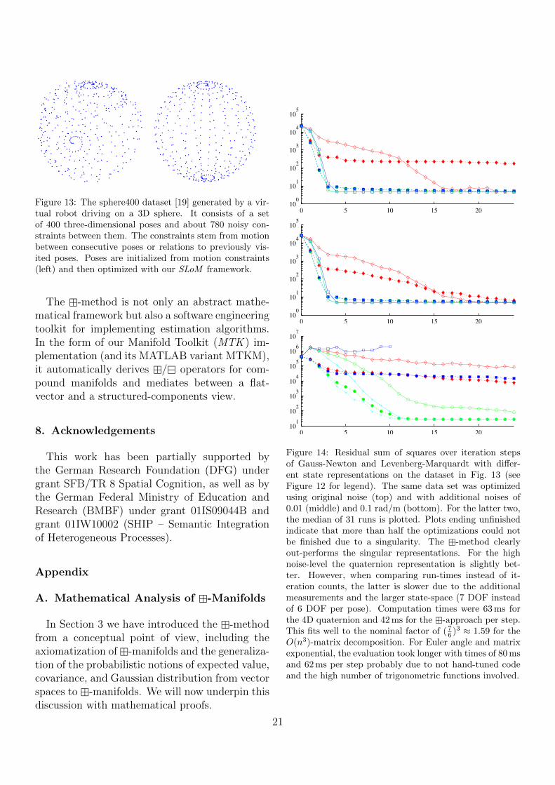
Figure 13: The sphere400 dataset [19] generated by a vir-tual robot driving on a 3D sphere. It consists of a setof 400 three-dimensional poses and about 780 noisy con-straints between them. The constraints stem from motionbetween consecutive poses or relations to previously vis-ited poses. Poses are initialized from motion constraints(left) and then optimized with our SLoM framework.

The -method is not only an abstract mathe-matical framework but also a software engineeringtoolkit for implementing estimation algorithms.In the form of our Manifold Toolkit (MTK ) im-plementation (and its MATLAB variant MTKM),it automatically derives / operators for com-pound manifolds and mediates between a flat-vector and a structured-components view.

8. Acknowledgements

This work has been partially supported bythe German Research Foundation (DFG) undergrant SFB/TR 8 Spatial Cognition, as well as bythe German Federal Ministry of Education andResearch (BMBF) under grant 01IS09044B andgrant 01IW10002 (SHIP – Semantic Integrationof Heterogeneous Processes).

Appendix

A. Mathematical Analysis of -Manifolds

In Section 3 we have introduced the -methodfrom a conceptual point of view, including theaxiomatization of-manifolds and the generaliza-tion of the probabilistic notions of expected value,covariance, and Gaussian distribution from vectorspaces to -manifolds. We will now underpin thisdiscussion with mathematical proofs.

0 5 10 15 20

100

101

102

103

104

105

0 5 10 15 20

100

101

102

103

104

105

0 5 10 15 20

101

102

103

104

105

106

107

Figure 14: Residual sum of squares over iteration stepsof Gauss-Newton and Levenberg-Marquardt with differ-ent state representations on the dataset in Fig. 13 (seeFigure 12 for legend). The same data set was optimizedusing original noise (top) and with additional noises of0.01 (middle) and 0.1 rad/m (bottom). For the latter two,the median of 31 runs is plotted. Plots ending unfinishedindicate that more than half the optimizations could notbe finished due to a singularity. The -method clearlyout-performs the singular representations. For the highnoise-level the quaternion representation is slightly bet-ter. However, when comparing run-times instead of it-eration counts, the latter is slower due to the additionalmeasurements and the larger state-space (7 DOF insteadof 6 DOF per pose). Computation times were 63 ms forthe 4D quaternion and 42 ms for the -approach per step.This fits well to the nominal factor of ( 7

6 )3 ≈ 1.59 for theO(n3)-matrix decomposition. For Euler angle and matrixexponential, the evaluation took longer with times of 80 msand 62 ms per step probably due to not hand-tuned codeand the high number of trigonometric functions involved.

21

A.1. -Manifolds

First, we recall the textbook definition of man-ifolds (see, e.g., [28]). We simplify certain aspectsnot relevant within the context of our method;this does not affect formal correctness. In par-ticular, we view a manifold S as embedded asa subset S ⊂ Rs into Euclidean space Rs fromthe outset; this is without loss of generality byWhitney’s embedding theorem, and simplifies thepresentation for our purposes.

Definition 2 (Manifold [28]). A (Ck-, or smooth)manifold is a pair (S,F) (usually denoted just S)consisting of a connected set S ⊂ Rs and an atlasF = (Uα, ϕα)α∈A, i.e. a family of charts (Uα, ϕα)consisting of an open subset Uα of S and a homeo-morphism ϕα : Uα → Vα of Uα to an open sub-set Vα ⊂ Rn. Here, Uα being open in S meansthat there is an open set Uα ⊂ Rs such thatUα = S ∩ Uα. These data are subject to the fol-lowing requirements.

1. The charts in F cover S, i.e. S =⋃α∈A Uα.

2. If Uα ∩ Uβ 6= ∅, the transition map

ϕα ϕ−1β : ϕβ(Uα ∩Uβ)→ ϕα(Uα ∩Uβ) (74)

is a Ck-diffeomorphism.

The number n is called the dimension or the num-ber of degrees of freedom of S.

We recall the generalization of the definitionof smoothness, i.e. being k times differentiable,to functions defined on arbitrary (not necessarilyopen) subsets S ⊂ Rs:

Definition 3 (Smooth Function). For S ⊂ Rs,a function f : S → Rn is called smooth, i.e. Ck,in x ∈ S if there exists an open neighbourhoodU ⊂ Rs of x and a smooth function f : U → Rn

that extends f |U∩S .

Next we show that every -manifold is indeeda manifold, justifying the name. The reverse isnot true in general.

Lemma 1. Every -manifold is a manifold, withthe atlas (Ux, ϕx)x∈S where

Ux = y | y x ∈ V (75)

ϕx : Ux → V, y 7→ y x. (76)

(This result will be sharpened later in Corol-lary 1.)

Proof. S is connected, as γ : λ 7→ x (λ(y x))is a path from γ(0) = x by (11a) to γ(1) = y by(11b). From (11c) we have that ϕ−1

x (δ) = x δis injective on V , and therefore bijective onto itsimage Ux. As both ϕx and ϕ−1

x are required to besmooth, ϕx is a diffeomorphism, in particular ahomeomorphism. The set Ux is open in S, as it isthe preimage of V under the continuous functionϕx, and since x ∈ Ux we have S =

⋃x∈S Ux. Fi-

nally, the transition map ϕxϕ−1y is a composite of

diffeomorphisms and therefore diffeomorphic.

A.2. Induced Metric

Lemma 2. The operation defines a metric don S by

dS(x, y) := ‖y S x‖ . (77)

Proof. Positive definiteness of d follows from Ax-iom (11a) and positive definiteness of ‖·‖.

Symmetry can be shown using (11d):

d(x, y) = ‖y x‖ = ‖(y 0) (y (x y))‖≤ ‖x y‖ = d(y, x) (78)

and symmetrically, which implies equality. Thetriangle inequality also follows from (11d):

d(x, z) = ‖z x‖ (79)

= ‖(y (z y)) (y (x y))‖ (80)

≤ ‖(z y)− (x y)‖ (81)

≤ ‖(x y)‖+ ‖(z y)‖ (82)

= d(x, y) + d(y, z)

A.3. Smooth Functions

Lemma 3. For a map f : S → M between -manifolds S and M, the following are equivalentfor every x ∈ S:

1. f is smooth in x (Definition 3)

2. f(xS δ)M z is smooth in δ at δ = 0 when-ever z ∈M is such that f(x) ∈ Uz.

Proof. 1 implies 2, as the concatenation of smoothfunctions is smooth.

For the converse implication, fix z as in 2, letS ⊂ Rs and M ⊂ Rm, and let U ⊂ Rs be a

22

neighbourhood of x such that extends smoothlyto U × x. Then we extend f smoothly to f :U → Rm by

f(y) = z M (f(xS (y S x))M z).

Replacing / in δ 7→ f(x δ) z by the in-duced charts as in Lemma 1, we see that smooth-ness corresponds to the classical definition ofsmooth functions on manifolds [28, p. 32]:

f(x δ) z = ϕz(f(ϕ−1x (δ))), (83)

with the right hand side required to be smooth inδ at δ = ϕx(x) = 0.

A direct consequence of this fact is

Corollary 1. Every -manifold S ⊂ Rs is anembedded submanifold of Rs.

(Recall that this means that the embeddingS → Rs is an immersion, i.e. a smooth map ofmanifolds that induces an injection of tangentspaces, and moreover that the topology of themanifold S is the subspace topology in Rs [28].)

Proof. S carries the subspace topology by con-struction. Clearly, the injection S → Rs issmooth according to Definition 3, and hence asa map of manifolds by the above argument. Sincetangent spaces are spaces of differential opera-tors on smooth real-valued functions and more-over have a local nature [28], the immersion prop-erty amounts to every smooth real-valued func-tion on an open subset of S extending to a smoothfunction on an open subset of Rs, which is pre-cisely the content of Definition 3.

A.4. Isomorphic -Manifolds

For every type of structure, one has a notion ofhomomorphism, which describes mappings thatpreserve the relevant structure. The natural no-tion of morphism ϕ : S → M of -manifolds isa smooth map ϕ : S → M that is homomorphicw.r.t. the algebraic operations and , i.e.

ϕ(xS δ) = ϕ(x)M δ (84)

ϕ(xS y) = ϕ(x)M ϕ(y). (85)

As usual, an isomorphism is a bijective homomor-phism whose inverse is again a homomorphism.Compatibility of inverses of homomorphisms withalgebraic operations as above is automatic, sothat an isomorphism ϕ : S → M of -manifoldsis just a diffeomorphism ϕ : S → M (i.e. an in-vertible smooth map with smooth inverse) thatis homomorphic w.r.t. and . If such a ϕ ex-ists, S and M are isomorphic. It is clear thatisomorphic -manifolds are indistinguishable assuch, i.e. differ only w.r.t. the representation oftheir elements. We will give examples of isomor-phic -manifolds in Appendix B; e.g. orthonor-mal matrices and unit quaternions form isomor-phic -manifolds.

A.5. Defining Symmetric -ManifoldsMost -manifolds arising in practice are man-

ifolds with inherent symmetries. This can be ex-ploited by defining at one reference element andpulling this structure back to the other elementsalong the symmetry.

Formally, we describe the following procedurefor turning an n-dimensional manifold S with suf-ficient symmetry into a -manifold. The firststep is to define a smooth and surjective functionψ : Rn → S which is required to be locally dif-feomorphic, i.e. for a neighborhood V of 0 ∈ Rn

it must have a smooth inverse ϕ := ψ−1. As ψ issurjective, ϕ can be extended globally to a (notnecessarily smooth) function ϕ : S → Rn suchthat ψ ϕ = idS .

The next step is to define, for every x ∈ S, adiffeomorphic transformation Rx : S → S (visu-ally a “rotation”) such that Rx(ψ(0)) = x. Wecan then define

x δ := Rx(ψ(δ)), y x := ϕ(R−1x (y)). (86)

Since x0 = Rx(ψ(0)) = x, Axiom (11a) holdsunder this construction. Axiom (11b) holds as werequire ψϕ = idS globally. Finally, as ϕψ = idVAxiom (11c) is fulfilled for δ ∈ V as required.Axiom (11d) depends on ψ and Rx and needs tobe established on a case-by-case basis.

A.6. Lie-Groups as -ManifoldsFor connected Lie-groups [28, Chap. 20], i.e.

manifolds with a diffeomorphic group structure,

23

the above steps are very simple. On the one handthe mapping ψ : Rn → S can be defined usingthe exponential map [28, p. 522], which is a lo-cally diffeomorphic map from a 0-neighborhoodin the Lie-algebra (a vector space diffeomorphicto Rn) to a neighborhood of the unit element inS. For compact Lie-groups, the exponential mapis also surjective, with global inverse log.

The transformation Rx can be simply definedas Rx(y) := x · y (or alternatively Rx(y) := y · x)using the group’s multiplication:

x δ := x · exp(δ), y x := log(x−1 · y). (87)

Again (11a)-(11c) follow from the construction inAppendix A.5. Axiom (11d) reduces to whether

‖(x δ1) (x δ2)‖ (88)

=∥∥log

((x · exp δ2)−1 · (x · exp δ1)

)∥∥ (89)

= ‖log (exp(−δ2) · exp δ1)‖ (90)

?

≤ ‖δ1 − δ2‖ . (91)

We do not know of a result that would establishthis fact in general, and instead prove the inequal-ity individually for each case.

A.7. Cartesian Product of Manifolds

Lemma 4. The Cartesian product of two -manifolds S1 and S2 is a -manifold S = S1×S2,with V = V1 × V2 and

(x1, x2)[δ1δ2

]= (x1 S1 δ1, x2 S2 δ2) (92)

(y1, y2) (x1, x2) =[y1S1

x1y2S2

x2

](93)

for (x1, x2), (y1, y2) ∈ S := S1 × S2 and[δ1δ2

]∈

Rn1 × Rn2.

Proof. Smoothness of and as well as Axioms(11a), (11b) and (11c) hold componentwise. ForAxiom (11d), we see that

‖(x δ) (x ε)‖2 = ‖(x1 δ1) (x1 ε1)‖2

+ ‖(x2 δ2) (x2 ε2)‖2

≤ ‖δ1 − ε1‖2 + ‖δ2 − ε2‖2

= ‖δ − ε‖2 .

A.8. Expected Value on -Manifolds

Also using Axiom (11d), we prove that the def-inition of the expected value by a minimizationproblem in (15) implies the implicit definition(16):

Lemma 5. For a random variable X : Ω → Sand µ ∈ S,

E ‖X µ‖2 = minµ∈S

!⇒ E(X µ) = 0. (94)

Proof. Let µ := argminµ E ‖X µ‖2. Then

E ‖X µ‖2 ≤ E ‖X (µ E(X µ))‖2 (95)

= E ‖(µ (X µ)) (µ E(X µ))‖2 (96)

≤ E ‖(X µ)− E(X µ)‖2 (97)

= E ‖X µ‖2 − ‖E(X µ)‖2 (98)

Hence, E(X µ) = 0.

A.9. (Gaussian) Distributions on -Manifolds

The basic idea of (12) in Section 3.4 was tomap a distribution X : Ω→ Rn to a distributionY : Ω→ S by defining Y := µX for some µ ∈ S.The problem is that in general is not injective.Thus (infinitely) many X are mapped to the sameY , which makes even simple things such as com-puting p(Y = y) for a given y ∈ S complicated,not to mention maximizing likelihoods.

A pragmatic approach is to “cut off” the distri-bution X where becomes ambiguous, i.e. definea distribution X with

p(X = x) := p(X = x | X ∈ V ) (99)

This can be justified because, if V is large com-pared to the covariance, P (X /∈ V ) is small andthe cut-off error is negligible. In practice, the factthat noise usually does not really obey a normaldistribution leads to a much bigger error.

Now (12) simplifies to

p(µ X = y) = p(X = y µ), (100)

because is bijective for X ∈ V . We also findthat for normal distributed noise, the maximumlikelihood solution is the least squares solution.

24

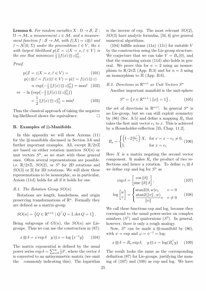
Lemma 6. For random variables X : Ω→ S, Z :Ω→M, a measurement z ∈M, and a measure-ment function f : S →M, with f(X) = z ε andε ∼ N (0, Σ) under the precondition ε ∈ V , the xwith largest likelihood p(Z = z|X = x, ε ∈ V ) isthe one that minimizes 1

2‖f(x) z‖2

Σ.

Proof.

p(Z = z|X = x, ε ∈ V ) = (101)

p(z ε = f(x)|ε ∈ V ) = p(ε = f(x) z)

∝ exp(−1

2‖f(x) z‖2

Σ

)= max! (102)

⇔ − ln(exp(−1

2‖f(x) z‖2

Σ

))=

1

2‖f(x) z‖2

Σ = min! (103)

Thus the classical approach of taking the negativelog-likelihood shows the equivalence.

B. Examples of -Manifolds

In this appendix we will show Axioms (11)for the -manifolds discussed in Section 3.6 andfurther important examples. All, except R/2πZare based on either rotation matrices SO(n) orunit vectors Sn, so we start with these generalones. Often several representations are possible,i.e. R/2πZ, SO(2), or S1 for 2D rotations andSO(3) or H for 3D rotations. We will show theserepresentations to be isomorphic, so in particular,Axiom (11d) holds for all if it holds for one.

B.1. The Rotation Group SO(n)

Rotations are length, handedness, and originpreserving transformations of Rn. Formally theyare defined as a matrix-group

SO(n) =Q ∈ Rn×n | Q>Q = I, detQ = 1

.

Being subgroups of Gl(n), the SO(n) are Lie-groups. Thus we can use the construction in (87):

x δ = x exp δ y x = log(x−1y

)(104)

The matrix exponential is defined by the usualpower series exp δ =

∑∞i=0

1i!δi, where the vector δ

is converted to an antisymmetric matrix (we omitthe ˆ commonly indicating this). The logarithm

is the inverse of exp. The most relevant SO(2),SO(3) have analytic formulas, [34, 6] give generalnumerical algorithms.

(104) fulfills axioms (11a)–(11c) for suitable Vby the construction using the Lie-group structure.We conjecture that we can take V = Bπ(0), andthat the remaining axiom (11d) also holds in gen-eral. We prove this for n = 2 using an isomor-phism to R/2πZ (App. B.3) and for n = 3 usingan isomorphism to H (App. B.6).

B.2. Directions in Rn+1 as Unit Vectors Sn

Another important manifold is the unit-sphere

Sn =x ∈ Rn+1 | ‖x‖ = 1

, (105)

the set of directions in Rn+1. In general Sn isno Lie-group, but we can still exploit symmetryby (86) (Sec. A.5) and define a mapping Rx thattakes the first unit vector e1 to x. This is achievedby a Householder-reflection [35, Chap. 11.2].

Rx =

(I−2vv

>

v>v

)X, for v = x− e1 6= 0,

I, for x = e1

(106)

Here X is a matrix negating the second vectorcomponent. It makes Rx the product of two re-flections and hence a rotation. To define e1 δwe define exp and log for Sn as

exp δ =

[cos ‖δ‖

sinc ‖δ‖ δ

], (107)

log

[wv

]=

atan2(0, w)e1 v = 0atan2(‖v‖ , w)

‖v‖ v v 6= 0(108)

We call these functions exp and log, because theycorrespond to the usual power-series on complexnumbers (S1) and quaternions (S3). In general,however, there is only a rough analogy.

Now, Sn can be made a -manifold by (86),with ψ = exp and ϕ = ψ−1 = log:

x δ = Rx exp δ, y x = log(R>x y) (109)

The result looks the same as the correspondingdefinition (87) for Lie-groups, justifying the nam-ing of (107) and (108) as exp and log. We have

25

that exp is left inverse to log, and log is left inverseto exp on ‖δ‖ < π. As proved in Lemma 7 (Ap-pendix C), exp and log are smooth. Hence Ax-ioms (11a), (11b), and (11c) hold for V = Bπ(0)(Sec.A.5). Axiom (11d) is proved as Lemma 11 inAppendix C.

The induced metric d(x, y) corresponds to theangle between x and y (Lemma 10).

Note that the popular stereographic projectioncannot be extended to a -manifold, because itviolates Axiom (11b).

Equipped with -manifolds for SO(n) and Sn,we now discuss the most important special cases,first for n = 2, then n = 3.

B.3. 2D Orientation as an Orthonormal Matrix

For planar rotations, exp in (104) takes an anti-symmetric 2×2 matrix, i.e. a number and returnsthe well-known 2D rotation matrix

x δ = x exp δ, y x = log(x−1y

)(110)

exp δ =[

cos δ − sin δsin δ cos δ

], log x = atan2(x21, x11).

The function exp is also an isomorphism betweenR/2πZ (24) and SO(2) (111), because the 2π-periodicity of exp as a function matches the pe-riodicity of R/2πZ as a set of equivalence classesand exp x ·exp δ = exp(x+δ). The latter holds asmultiplication in SO(2) commutes. From this ar-gument we see that R/2πZ (Sec. 3.6.2) and SO(2)are isomorphic -manifolds and also that axiom(11d) holds for the latter.

B.4. 2D Orientation as a Complex Number

Using complex multiplication, SO(2) is isomor-phic to the complex numbers of unit-length, i.e.S2 ⊂ C. For n = 2, (107) and (108) simplify to

expS1 δ = [ cos δsin δ ] , logS1 [ xy ] = atan2(y, x). (111)

R[xy ] equals complex multiplication with [ xy ] or,

as a matrix, [ x −yy x ]. This is because R[xy ] it is a

rotation mapping e1 to [ xy ] and there is only onesuch rotation on S1. With these prerequisites, S1

is isomorphic to SO(2) by Lemma 14 as is R/2πZ.

B.5. Directions in 3D Space as S2

The unit sphere is the most important exampleof a manifold that is not a Lie-group. This is aconsequence of the “hairy ball theorem” [9], whichstates that on S2 every continuous vector-field hasa zero – if S2 was a Lie-group, one could takethe derivative of x · δ for every x and some fixedδ to obtain a vector field on S2 without zeroes.With the same argument applied to x δ, it isalso impossible to give S2 a -structure that iscontinuous in x. This is one reason why we didnot demand continuity in x for . It also showsthat the discontinuity in (106) cannot be avoidedin general (although it can for S1 and S3).

However, we can give a simpler analytical for-mula for Rx in S2:

R[xyz

] :=[x −r 0y xc −sz xs c

], α = atan2(z, y),

c = cosα, s = sinα, r =√x2 + z2

(112)

x δ = Rx exp δ, y x = log(R>x y) (113)

The formula is discontinuous for r = 0, but anyvalue for α leads to a proper rotation matrix Rx.Therefore, neither nor are continuous in x,but they are smooth with respect to δ or y.

B.6. 3D Orientation as a Unit Quaternion

The -manifold for quaternions H presented inSec. 3.6.4, (29)-(31) is a special case of (107)-(109)for the unit sphere S3. In the construction Rq

from (106) is conveniently replaced by q−1·, be-cause H is a Lie-group. Also, exp and log cor-respond again to the usual functions for H. TheAxioms (11a)-(11c) are fulfilled for V = Bπ(0).Axiom (11d) is proved in Lemma 12.

The metric d(x, y) is the angle between x andy, and also monotonically related to the simpleEuclidean metric ‖x− y‖ (Lemma 8).

Orthonormal matrices SO(3) and unit quater-nions S3/±1 are two different representationsof rotations. Topologically this is called a univer-sal covering [3, §12]. Hence, their -manifolds areisomorphic with the usual conversion operation

ϕ[ wxyz

]=

[1−2(y2+z2) −2wz+2xy −2wy+2xy

2wz+2xy 1−2(x2+z2) −2wx+2yz

−2wy+2xz 2wx+2yz 1−2(x2+y2)

]. (114)

26

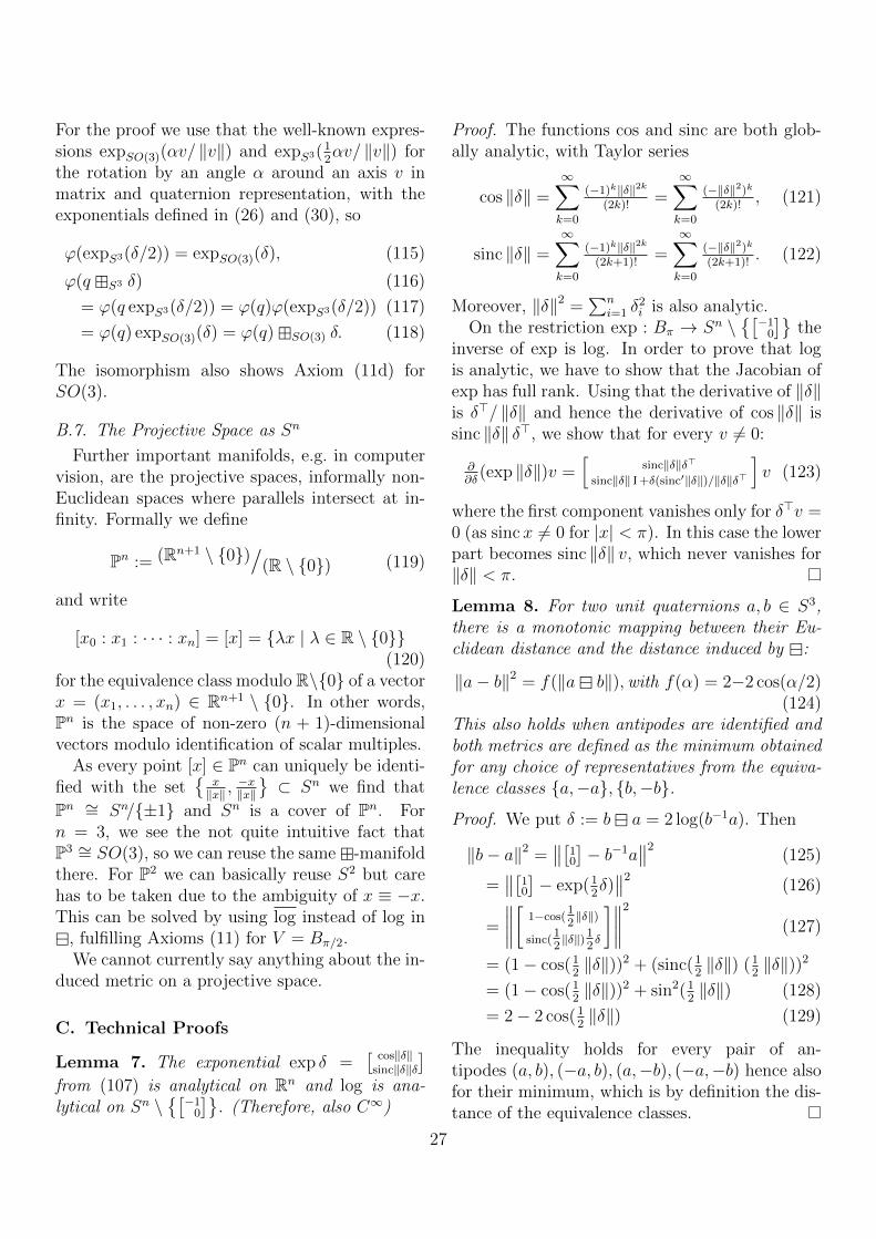
For the proof we use that the well-known expres-sions expSO(3)(αv/ ‖v‖) and expS3(1

2αv/ ‖v‖) for

the rotation by an angle α around an axis v inmatrix and quaternion representation, with theexponentials defined in (26) and (30), so

ϕ(expS3(δ/2)) = expSO(3)(δ), (115)

ϕ(q S3 δ) (116)

= ϕ(q expS3(δ/2)) = ϕ(q)ϕ(expS3(δ/2)) (117)

= ϕ(q) expSO(3)(δ) = ϕ(q)SO(3) δ. (118)

The isomorphism also shows Axiom (11d) forSO(3).

B.7. The Projective Space as Sn

Further important manifolds, e.g. in computervision, are the projective spaces, informally non-Euclidean spaces where parallels intersect at in-finity. Formally we define

Pn := (Rn+1 \ 0)/(R \ 0) (119)

and write

[x0 : x1 : · · · : xn] = [x] = λx | λ ∈ R \ 0(120)

for the equivalence class modulo R\0 of a vectorx = (x1, . . . , xn) ∈ Rn+1 \ 0. In other words,Pn is the space of non-zero (n + 1)-dimensionalvectors modulo identification of scalar multiples.

As every point [x] ∈ Pn can uniquely be identi-fied with the set

x‖x‖ ,

−x‖x‖⊂ Sn we find that

Pn ∼= Sn/±1 and Sn is a cover of Pn. Forn = 3, we see the not quite intuitive fact thatP3 ∼= SO(3), so we can reuse the same -manifoldthere. For P2 we can basically reuse S2 but carehas to be taken due to the ambiguity of x ≡ −x.This can be solved by using log instead of log in

, fulfilling Axioms (11) for V = Bπ/2.We cannot currently say anything about the in-

duced metric on a projective space.

C. Technical Proofs

Lemma 7. The exponential exp δ =[ cos‖δ‖

sinc‖δ‖δ]

from (107) is analytical on Rn and log is ana-lytical on Sn \

[−10

]. (Therefore, also C∞)

Proof. The functions cos and sinc are both glob-ally analytic, with Taylor series

cos ‖δ‖ =∞∑k=0

(−1)k‖δ‖2k(2k)!

=∞∑k=0

(−‖δ‖2)k

(2k)!, (121)

sinc ‖δ‖ =∞∑k=0

(−1)k‖δ‖2k(2k+1)!

=∞∑k=0

(−‖δ‖2)k

(2k+1)!. (122)

Moreover, ‖δ‖2 =∑n

i=1 δ2i is also analytic.

On the restriction exp : Bπ → Sn \[−1

0

]the

inverse of exp is log. In order to prove that logis analytic, we have to show that the Jacobian ofexp has full rank. Using that the derivative of ‖δ‖is δ>/ ‖δ‖ and hence the derivative of cos ‖δ‖ issinc ‖δ‖ δ>, we show that for every v 6= 0:

∂∂δ

(exp ‖δ‖)v =[

sinc‖δ‖δ>sinc‖δ‖ I +δ(sinc′‖δ‖)/‖δ‖δ>

]v (123)

where the first component vanishes only for δ>v =0 (as sincx 6= 0 for |x| < π). In this case the lowerpart becomes sinc ‖δ‖ v, which never vanishes for‖δ‖ < π.

Lemma 8. For two unit quaternions a, b ∈ S3,there is a monotonic mapping between their Eu-clidean distance and the distance induced by :

‖a− b‖2 = f(‖a b‖),with f(α) = 2−2 cos(α/2)(124)

This also holds when antipodes are identified andboth metrics are defined as the minimum obtainedfor any choice of representatives from the equiva-lence classes a,−a, b,−b.Proof. We put δ := b a = 2 log(b−1a). Then

‖b− a‖2 =∥∥[1

0

]− b−1a

∥∥2(125)

=∥∥[1

0

]− exp(1

2δ)∥∥2

(126)

=

∥∥∥∥[ 1−cos(12‖δ‖)

sinc(12‖δ‖) 1

2δ

]∥∥∥∥2

(127)

= (1− cos(12‖δ‖))2 + (sinc(1

2‖δ‖) (1

2‖δ‖))2

= (1− cos(12‖δ‖))2 + sin2(1

2‖δ‖) (128)

= 2− 2 cos(12‖δ‖) (129)

The inequality holds for every pair of an-tipodes (a, b), (−a, b), (a,−b), (−a,−b) hence alsofor their minimum, which is by definition the dis-tance of the equivalence classes.

27

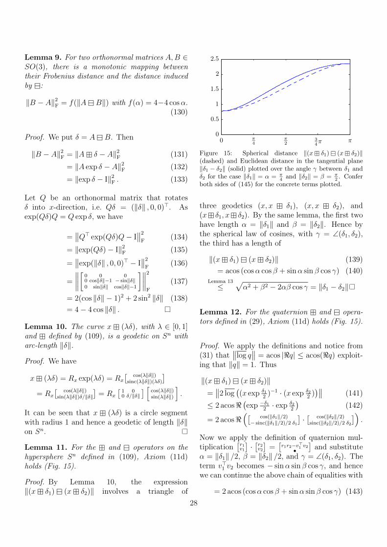
Lemma 9. For two orthonormal matrices A,B ∈SO(3), there is a monotonic mapping betweentheir Frobenius distance and the distance inducedby :

‖B − A‖2F = f(‖AB‖) with f(α) = 4−4 cosα.

(130)

Proof. We put δ = AB. Then

‖B − A‖2F = ‖A δ − A‖2

F (131)

= ‖A exp δ − A‖2F (132)

= ‖exp δ − I‖2F . (133)

Let Q be an orthonormal matrix that rotatesδ into x-direction, i.e. Qδ = (‖δ‖ , 0, 0)>. Asexp(Qδ)Q = Q exp δ, we have

=∥∥Q> exp(Qδ)Q− I

∥∥2

F(134)

= ‖exp(Qδ)− I‖2F (135)

=∥∥exp(‖δ‖ , 0, 0)> − I

∥∥2

F(136)

=

∥∥∥∥[ 0 0 00 cos‖δ‖−1 − sin‖δ‖0 sin‖δ‖ cos‖δ‖−1

]∥∥∥∥2

F

(137)

= 2(cos ‖δ‖ − 1)2 + 2 sin2 ‖δ‖ (138)

= 4− 4 cos ‖δ‖ .

Lemma 10. The curve x (λδ), with λ ∈ [0, 1]and defined by (109), is a geodetic on Sn witharc-length ‖δ‖.

Proof. We have

x (λδ) = Rx exp(λδ) = Rx

[ cos(λ‖δ‖)sinc(λ‖δ‖)(λδ)

]= Rx

[ cos(λ‖δ‖)sin(λ‖δ‖)δ/‖δ‖

]= Rx

[1 00 δ/‖δ‖

] [ cos(λ‖δ‖)sin(λ‖δ‖)

].

It can be seen that x (λδ) is a circle segmentwith radius 1 and hence a geodetic of length ‖δ‖on Sn.

Lemma 11. For the and operators on thehypersphere Sn defined in (109), Axiom (11d)holds (Fig. 15).

Proof. By Lemma 10, the expression‖(x δ1) (x δ2)‖ involves a triangle of

0 π4

π2

34π π

0

0.5

1

1.5

2

2.5

Figure 15: Spherical distance ‖(x δ1) (x δ2)‖(dashed) and Euclidean distance in the tangential plane‖δ1 − δ2‖ (solid) plotted over the angle γ between δ1 andδ2 for the case ‖δ1‖ = α = π

4 and ‖δ2‖ = β = π2 . Confer

both sides of (145) for the concrete terms plotted.

three geodetics (x, x δ1), (x, x δ2), and(x δ1, x δ2). By the same lemma, the first twohave length α = ‖δ1‖ and β = ‖δ2‖. Hence bythe spherical law of cosines, with γ = ∠(δ1, δ2),the third has a length of

‖(x δ1) (x δ2)‖ (139)

= acos (cosα cos β + sinα sin β cos γ) (140)

Lemma 13

≤√α2 + β2 − 2αβ cos γ = ‖δ1 − δ2‖

Lemma 12. For the quaternion and opera-tors defined in (29), Axiom (11d) holds (Fig. 15).

Proof. We apply the definitions and notice from(31) that

∥∥log q∥∥ = acos |<q| ≤ acos(<q) exploit-

ing that ‖q‖ = 1. Thus

‖(x δ1) (x δ2)‖=∥∥2 log

((x exp δ1

2)−1 · (x exp δ2

2))∥∥ (141)

≤ 2 acos<(exp −δ1

2· exp δ2

2

)(142)

= 2 acos<([ cos(‖δ1‖/2)− sinc(‖δ1‖/2)/2 δ1

]·[ cos(‖δ2‖/2)

sinc(‖δ2‖/2)/2 δ2

]).

Now we apply the definition of quaternion mul-tiplication

[r1v1

]·[r2v2

]=[r1r2−v>1 v2•

]and substitute

α = ‖δ1‖ /2, β = ‖δ2‖ /2, and γ = ∠(δ1, δ2). Theterm v>1 v2 becomes − sinα sin β cos γ, and hencewe can continue the above chain of equalities with

= 2 acos (cosα cos β + sinα sin β cos γ) (143)

28

Lemma 13

≤ 2√α2 + β2 − 2αβ cos γ (144)

= ‖δ1 − δ2‖ .Lemma 13. The distance on a sphere is less orequal to the Euclidean distance in the tangentialplane (Fig. 15). Formally, for all α, β ≥ 0, γ ∈ R

acos(cosα cos β + sinα sin β cos γ

)≤√α2 + β2 − 2αβ cos γ.

(145)

Proof. If the right-hand side exceeds π, the in-equality is trivial. Otherwise we substitute λ :=cos γ and take the cosine:

cosα cos β + sinα sin βλ

≥ cos√α2 + β2 − 2αβλ.

(146)

The proof idea is that the left-hand side of (146)is linear in λ, the right-hand side is convex in λ,and both are equal for λ = ±1. Formally, fromthe cosine addition formula we get

cosα cos β − sinα sin β = cos(α + β) (147)

= cos√α2 + β2 + 2αβ, (148)

cosα cos β + sinα sin β = cos(α− β) (149)

= cos√α2 + β2 − 2αβ. (150)

Taking a 1−λ2

: 1+λ2

convex combination of (147)and (149) we get the left-hand side of (146):

cosα cos β + sinα sin βλ (151)

= cosα cos β + sinα sin β(

1−λ2

(−1) + 1+λ2

(+1))

= 1−λ2

cos√α2 + β2 − 2αβ

+ 1+λ2

cos√α2 + β2 + 2αβ

≥ cos√α2 + β2 + 2αβ

(1−λ

2(−1) + 1+λ

2(+1)

)= cos

√α2 + β2 + 2αβλ. (152)

The inequality comes from the convexity of theright-hand side of (146) in λ. We prove this bycalculating its derivative

− sin√α2 + β2 + 2αβλ

1

2√α2 + β2 + 2αβλ

2αβ

= − sinc√α2 + β2 + 2αβλ αβ (153)

and observing that (153) increases monotonicallyuntil the square root exceeds π.

Lemma 14. The following function ϕ is an -isomorphism between S1 and SO(2):

ϕ : S1 → SO(2), ϕ [ xy ] = [ x −yy x ] . (154)

Proof. The map is bijective, because all matricesin SO(2) are of the form (111). It also commuteswith , since

ϕ([ xy ]S1 δ) = ϕ(R>[xy ] exp δ) (155)

= ϕ ([ x −yy x ] [ cos δsin δ ]) (156)

= ϕ([

x cos δ−y sin δy cos δ+x sin δ

])(157)

=[x cos δ−y sin δ −y cos δ−x sin δy cos δ+x sin δ x cos δ−y sin δ

](158)

= [ x −yy x ][

cos δ − sin δsin δ cos δ

](159)

= [ x −yy x ] exp δ (160)

= ϕ ([ xy ])SO2 δ.

D. Comparison to SPMap

In an SPMap [7] (originally 2D but extendedto 3D) every geometric entity is represented by areference pose (SE(3)) in an arbitrary, potentiallyoverparametrized representation, and a perturba-tion vector parametrizing the entity relative to itsreference pose in minimal parametrization. Theestimation algorithm operates solely on the per-turbation vector. This corresponds to s δ, withs being the reference pose and δ the perturbationvector. Actually, this concept and the idea thatin most algorithms can simply replace + mo-tivated the axiomatization of -systems we pro-pose. Our contribution is to give this idea, whichhas been around for a while, a thorough mathe-matical framework more general than geometricentities.

If a geometric entity is “less than a pose”, e.g.a point, SPMap still uses a reference pose but theredundant DOFs, e.g. rotation, are removed fromthe perturbation vector. In our axiomatizationthe pose would simply be an overparametrizationof a point. Using the notation of [7]

s δ = s⊕ (B>δ), (161)

29

where B is the so-called binding matrix that mapsentries of δ to the DOF of a pose, and ⊕ is theconcatenation of poses.

Analogously, the SPMap represents, e.g. a lineas the pose’s x-axis with x-rotation and trans-lation being redundant DOFs removed from theperturbation vector. Here lies a theoretical dif-ference. Consider two such poses differing by anx-rotation. They represent the same line but dif-fer in the effect of the perturbation vector, as y-and z-axes point into different directions. For us,the -system S would be a space of equivalenceclasses of poses. However, maps from S × Rn

to S, so s δ must formally be the equivalentfor equivalent poses s. The SPMap representa-tion has the advantage that it is continuous bothin the pose and the perturbation vector, which isnot possible with our axiomatization due to thehairy ball theorem as discussed in Sec. B.5.

Overall, our contribution is the axiomatizedand more general view, not limited to quotientsof SE(3) as with the SPMap. We currently in-vestigate axiomatization of SPMap’s idea to al-low different representatives of the same equiva-lence class to define different -co-ordinate sys-tems. We avoided this here, because it adds an-other level of conceptual complexity.

References

[1] P. Abbeel, Apprenticeship Learning and Reinforce-ment Learning with Application to Robotic Control,Ph.D. thesis, Department of Computer Science. Stan-ford University, 2008.

[2] D. Abrahams, A. Gurtovoy, C++ Template Metapro-gramming, Pearson Education, 2005.

[3] S.L. Altmann, Rotations, Quaternions and DoubleGroups, Oxford University Press, 1986.

[4] Y. Bar-Shalom, X. Li, T. Kirubarajan, Estimationwith Applications to Tracking and Navigation, JohnWiley & Sons, Inc., 2001.

[5] O. Birbach, Accuracy Analysis of Camera-InertialSensor Based Ball-Trajectory Prediction, Master’sthesis, Universitat Bremen, 2008.

[6] J. Cardosoa, F. Leitec, Exponentials of skew-symmetric matrices and logarithms of orthogonal ma-trices, Journal of Computational and Applied Math-ematics 233 (2010) 2867–2875.

[7] J.A. Castellanos, J. Montiel, J. Neira, J.D. Tards,The SPmap: A probablistic framework for simulta-neous localization and map building, IEEE Transac-

tions on Robotics and Automation 15 (1999) 948 –952.

[8] A. Davison, Real-time simultaneous localisation andmapping with a single camera, in: Proceedings of theInternational Conference on Computer Vision, 2003.

[9] M. Eisenberg, R. Guy, A proof of the hairy ball theo-rem, The American Mathematical Monthly 86 (1979)571–574.

[10] R. Fisher, Dispersion on a sphere, Proceedings of theRoyal Society of London. Series A, Mathematical andPhysical Sciences 217 (1953) 295–305.

[11] U. Frese, L. Schroder, Theorie der Sensorfusion 2006,2006. Universitat Bremen, lecture notes #03-05-H-699.55.

[12] C.F. Gauss, Theoria combinationis observationum er-roribus minimis obnoxiae, Commentationes societatisregiae scientiarum Gottingensis recentiores 5 (1821)6–93.

[13] M.S. Grewal, L.R. Weill, A.P. Andrews, Global Posi-tioning Systems, Inertial Navigation, and Integration,John Wiley, 2nd edition, 2007.

[14] G. Grisetti, C. Stachniss, W. Burgard, NonlinearConstraint Network Optimization for Efficient MapLearning, IEEE Transactions on Intelligent Trans-portation Systems 10 (2009) 428–439.

[15] G. Guennebaud, B. Jacob, et al., Eigen 2.0.15,eigen.tuxfamily.org, 2010.

[16] C. Hertzberg, A Framework for Sparse, Non-LinearLeast Squares Problems on Manifolds, Master’s the-sis, Universitat Bremen, 2008.

[17] S.J. Julier, J.K. Uhlmann, A General Method for Ap-proximating Nonlinear Transformations of Probabil-ity Distributions, Technical Report, University of Ox-ford, 1996.

[18] S.J. Julier, J.K. Uhlmann, A new extension of theKalman filter to nonlinear systems, in: Int. Symp.Aerospace/Defense Sensing, Simul. and Controls, Or-lando, FL, 1997, pp. 182–193.

[19] M. Kaess, A. Ranganathan, F. Dellaert, iSAM: In-cremental smoothing and mapping, IEEE Transac-tions on Robotics 24 (2008) 1365–1378. openslam.

org/iSAM.[20] R.E. Kalman, A new approach to linear filtering

and prediction problems, Transactions of the ASME–Journal of Basic Engineering 82 (1960) 35–45.

[21] J.T. Kent, The fisher-bingham distribution on thesphere, Journal of the Royal Statistical Society. Se-ries B (Methodological) 44 (1982) 71–80.

[22] A.R. Klumpp, Apollo lunar-descent guidance, Auto-matica 10 (1974) 133–146.

[23] D. Koks, Explorations in Mathematical Physics,Springer, 2006.

[24] E. Kraft, A quaternion-based unscented Kalman filterfor orientation tracking, in: Proceedings of the SixthInternational Conference of Information Fusion, vol-ume 1, 2003, pp. 47–54.

30

[25] J. Kurlbaum, Verfolgung von Ballflugbahnen miteinem frei beweglichen Kamera-Inertialsensor, Mas-ter’s thesis, Universitat Bremen, 2007.

[26] J. Kurlbaum, U. Frese, A Benchmark Dataset forData Association, Technical Report 017-02/2009,SFB TR/8, 2009.

[27] J.J. LaViola Jr., A comparison of unscented and ex-tended Kalman filtering for estimating quaternionmotion, in: Proceedings of the 2003 American Con-trol Conference, volume 6, 2003, pp. 2435–2440.

[28] J.M. Lee, Introduction to Smooth Manifolds, volume218 of Graduate Texts in Mathematics, Springer Ver-lag, 2003.

[29] A.M. Legendre, Nouvelles methodes pour ladetermination des orbites des cometes, Courcier,Paris, 1805.

[30] J.L. Marins, X. Yun, E.R. Bachmann, R.B. Mcghee,M.J. Zyda, An extended Kalman filter for quaternion-based orientation estimation using MARG sensors, in:Engineer’s Thesis, Naval Postgraduate School, 2001,pp. 2003–2011.

[31] F.L. Markley, Y. Cheng, J.L. Crassidis, Y. Oshman,Quaternion Averaging, Technical Report, NASAGoddard Space Flight Center, 2007. #20070017872.

[32] R. van der Merwe, E. Wan, Sigma-point Kalman fil-ters for probabilistic inference in dynamic state-spacemodels, in: Proceedings of the Workshop on Ad-vances in Machine Learning, 2003, Montreal, Canada.

[33] R. van der Merwe, E. Wan, S. Julier, Sigma-pointKalman filters for nonlinear estimation and sensor-fusion: Applications to integrated navigation, in:AIAA Guidance, Navigation, and Control Conferenceand Exhibit, 2004, Providence, Rhode Island.

[34] C. Moler, C.F. Van Loan, Nineteen dubious waysto compute the exponential of a matrix, twenty-fiveyears later, SIAM Review 45 (2003) 3–49.

[35] W.H. Press, S.A. Teukolsky, W.T. Vetterling, B.P.Flannery, Numerical recipes, second edition, Numer-ical Recipes, Second Edition, Cambridge UniversityPress, Cambridge, 1992, pp. 656 – 661, 681 – 699.

[36] B. Quine, J. Uhlmann, H. Durrant-Whyte, ImplicitJacobians for linearised state estimation in nonlinearsystems, in: Proc. of the American Control Confer-ence, Seattle, WA, 1995, pp. 1645–1646.

[37] J. Schmidt, H. Niemann, Using quaternions forparametrizing 3D rotations in unconstrained nonlin-ear optimization, in: Proceedings of the Vision, Mod-elling and Visualization, 2001.

[38] B.J. Sipos, Application of the manifold-constrainedunscented Kalman filter, in: Position, Location andNavigation Symposium, 2008 IEEE/ION, 2008, pp.30–43.

[39] H. Strasdat, J. Montiel, A. Davison, Scale drift-awarelarge scale monocular slam, in: Proceedings of theRobotics Science and Systems Conference, 2010.

[40] S. Thrun, W. Burgard, D. Fox, Probabilistic

Robotics, MIT Press, Cambridge, MA, 2005.[41] S. Thrun, et al., Stanley: The robot that won the

DARPA Grand Challenge, Journal of Field Robotics23 (2006).

[42] W. Triggs, P. McLauchlan, R. Hartley, A. Fitzgib-bon, Bundle adjustment – a modern synthesis, in:W. Triggs, A. Zisserman, R. Szeliski (Eds.), VisionAlgorithms: Theory and Practice, LNCS, SpringerVerlag, 2000, pp. 298–375.

[43] R. Wagner, Autonomous Outdoor Navigation with aRobotic R/C Car, Master’s thesis, Universitat Bre-men, 2010.

[44] R. Wagner, O. Birbach, U. Frese, Rapid developmentof manifold-based graph optimization for multi-sensorcalibration and SLAM, in: Proceedings of the Inter-national Conference on Intelligent Robots and Sys-tems, 2011. (under review).

[45] M.D. Wheeler, K. Ikeuchi, Iterative estimation of ro-tation and translation using the quaternion, Techni-cal Report, Carnegie Mellon University, Pittsburgh,PA, 1995.

31