econstor www.econstor.eu

Der Open-Access-Publikationsserver der ZBW – Leibniz-Informationszentrum WirtschaftThe Open Access Publication Server of the ZBW – Leibniz Information Centre for Economics

Standard-Nutzungsbedingungen:

Die Dokumente auf EconStor dürfen zu eigenen wissenschaftlichenZwecken und zum Privatgebrauch gespeichert und kopiert werden.

Sie dürfen die Dokumente nicht für öffentliche oder kommerzielleZwecke vervielfältigen, öffentlich ausstellen, öffentlich zugänglichmachen, vertreiben oder anderweitig nutzen.

Sofern die Verfasser die Dokumente unter Open-Content-Lizenzen(insbesondere CC-Lizenzen) zur Verfügung gestellt haben sollten,gelten abweichend von diesen Nutzungsbedingungen die in der dortgenannten Lizenz gewährten Nutzungsrechte.

Terms of use:

Documents in EconStor may be saved and copied for yourpersonal and scholarly purposes.

You are not to copy documents for public or commercialpurposes, to exhibit the documents publicly, to make thempublicly available on the internet, or to distribute or otherwiseuse the documents in public.

If the documents have been made available under an OpenContent Licence (especially Creative Commons Licences), youmay exercise further usage rights as specified in the indicatedlicence.

zbw Leibniz-Informationszentrum WirtschaftLeibniz Information Centre for Economics

Guner, Nezih; Kulikova, Yuliya; Llull, Joan

Working Paper

Does Marriage Make You Healthier?

IZA Discussion Papers, No. 8633

Provided in Cooperation with:Institute for the Study of Labor (IZA)

Suggested Citation: Guner, Nezih; Kulikova, Yuliya; Llull, Joan (2014) : Does Marriage MakeYou Healthier?, IZA Discussion Papers, No. 8633

This Version is available at:http://hdl.handle.net/10419/106571

DI

SC

US

SI

ON

P

AP

ER

S

ER

IE

S

Forschungsinstitut zur Zukunft der ArbeitInstitute for the Study of Labor

Does Marriage Make You Healthier?

IZA DP No. 8633

November 2014

Nezih GunerYuliya KulikovaJoan Llull

Does Marriage Make You Healthier?

Nezih Guner ICREA-MOVE, Universitat Autònoma de Barcelona,

Barcelona GSE and IZA

Yuliya Kulikova Universitat Autònoma de Barcelona

and Barcelona GSE

Joan Llull MOVE, Universitat Autònoma de Barcelona

and Barcelona GSE

Discussion Paper No. 8633 November 2014

IZA

P.O. Box 7240 53072 Bonn

Germany

Phone: +49-228-3894-0 Fax: +49-228-3894-180

E-mail: iza@iza.org

Any opinions expressed here are those of the author(s) and not those of IZA. Research published in this series may include views on policy, but the institute itself takes no institutional policy positions. The IZA research network is committed to the IZA Guiding Principles of Research Integrity. The Institute for the Study of Labor (IZA) in Bonn is a local and virtual international research center and a place of communication between science, politics and business. IZA is an independent nonprofit organization supported by Deutsche Post Foundation. The center is associated with the University of Bonn and offers a stimulating research environment through its international network, workshops and conferences, data service, project support, research visits and doctoral program. IZA engages in (i) original and internationally competitive research in all fields of labor economics, (ii) development of policy concepts, and (iii) dissemination of research results and concepts to the interested public. IZA Discussion Papers often represent preliminary work and are circulated to encourage discussion. Citation of such a paper should account for its provisional character. A revised version may be available directly from the author.

IZA Discussion Paper No. 8633 November 2014

ABSTRACT

Does Marriage Make You Healthier?* We use the Panel Study of Income Dynamics (PSID) and the Medical Expenditure Panel Survey (MEPS) to study the relationship between marriage and health for working-age (20 to 64) individuals. In both data sets married agents are healthier than unmarried ones, and the health gap between married and unmarried agents widens by age. After controlling for observables, a gap of about 12 percentage points in self-reported health persists for ages 55-59. We estimate the marriage health gap non-parametrically as a function of age. If we allow for unobserved heterogeneity in innate permanent health, potentially correlated with timing and likelihood of marriage, we find that the effect of marriage on health disappears at younger (20-39) ages, while about 6 percentage points difference between married and unmarried individuals, about half of the total gap, remains at older (55-59) ages. These results indicate that association between marriage and health is mainly driven by selection into marriage at younger ages, while there might be a protective effect of marriage at older ages. We analyze how selection and protective effects of marriage show up in the data. JEL Classification: I10, I12, J10 Keywords: health, marriage, selection Corresponding author: Nezih Guner MOVE (Markets, Organizations and Votes in Economics) Facultat d’Economia, Universitat Autònoma de Barcelona Edifici B – Campus de Bellaterra 08193 Bellaterra Cerdanyola del Vallès (Spain) E-mail: nezih.guner@movebarcelona.eu

* We would like to thank Matt Delventhal, Giacomo De Giorgi, Francesco Fasani, Ada Ferrer-i-Carbonell, and workshop and conference participants at the European Meeting of the Econometric Society in Toulouse, the Annual Meetings of the Spanish Economic Association in Santander, Barcelona GSE Winter Workshop, CINCH Summer Academy at the University of Duisburg-Essen, Koç University (Istanbul), Universitat Autònoma de Barcelona for comments. Guner and Llull acknowledge financial support from European Research Council (ERC) through Starting Grant n.263600, and from the Spanish Ministry of Economy and Competitiveness, through the Severo Ochoa Programme for Centers of Excellence in R&D (SEV-2011-0075).

I. Introduction

Married individuals are healthier and live longer than unmarried ones. This fact

was first documented by British epidemiologist William Farr more than 150 years

ago, and has been established by many studies since then.1 The question is, of

course, why? Does the association between marriage and health indicate a causal

effect of marriage on health (what is termed in the literature as the protective

effect of marriage), or is it simply an artifact of selection as healthier people are

more likely to get married in the first place?2 The answer to this question is

critical as it has important implications for public policy.3 Recent studies on the

link between public policy and health suggest that “upstream social and economic

determinants of health are of major health importance, and hence that social and

economic policy and practice may be the major route to improving population

health.” (House, Schoeni, Kaplan and Pollack, 2008, p.22). Marriage is often

portrayed as a solution for many social problems in the U.S., see e.g. Waite

and Gallagher (2000), and the effectiveness of pro-marriage policies depends on

whether marriage indeed makes individuals healthy, wealthy and happy.

In this paper we study the relationship between health and marriage using data

from the Panel Study of Income Dynamics (PSID) and the Medical Expenditure

Panel Survey (MEPS). In both data sets married individuals report to be healthier

than unmarried ones, and they do so in remarkably similar levels. The gap in self-

reported health persists after we control for observable characteristics such as

education, income, race, gender and the presence of children: the marriage health

gap starts at about 3 percentage points at younger ages (20 to 39), and increases

continuously for older ages, reaching a peak of 12 percentage points around ages

55 to 59. A similar picture emerges when we consider objective, instead of self-

reported, measures of health, or when we use the occurrence of chronic conditions

as an indicator of poor health.

Our definition of the marriage health gap is the difference between age-dependent

health curves for married and single individuals. These health curves are identified

non-parametrically. Different studies in evolutionary biology suggest that several

physical and personality traits that define a person as attractive for mating are

1 On Farr’s study, see Parker-Pope (2010).2 A similar question arises for the well-known married male wage premium.3 “Between 1950 and 2011, real GDP per capita grew at an average of 2.0% per year, while

real national health care expenditures per capita grew at 4.4% per year. The gap between thetwo rates of growth —2.4% per year— resulted in the share of the GDP related to health carespending increasing from 4.4% in 1950 to 17.9% in 2011.” (Fuchs, 2013, p.108).

2

associated with youth and health, and, as a result, with reproductive capacity.4

As a result, individuals with better innate health tend to be more attractive in

the marriage market. If individuals with better innate health are more attractive

marriage partners, and, as a result, more likely to get married in the first place,

least squares estimates will be upward biased.

Using the panel structure of the PSID, we overcome this selection bias by ac-

counting for individual-specific innate permanent health, potentially correlated

with the timing and likelihood of marriage. With a within-groups estimation,

the effect of marriage on health disappears for younger (20-39) ages, while about

a 6 percentage point gap between married and unmarried individuals remains

for older (55-59) ages. This is half of the total difference for this age group (12

percentage points). These results suggest that association between marriage and

health at younger ages is likely to be driven by selection of healthier individuals

into marriage, while there might be a protective effect of marriage that shows up

at older ages. We also find that the marriage health gap is similar for males and

females, blacks and whites, and for individuals with and without a college degree.

The marriage health gap is, however, larger for poorer individuals.

Next we investigate how selection and protection might show up in the data.

First, we show that individuals who are ever married by age 30 (or 40) have better

average innate permanent health than those individuals who are never married

by that age. The variance of permanent health, on the other hand, is larger for

those who are never married. These facts are consistent with a world in which

individuals look for healthy partners in the marriage market. In such a world,

individuals would mate assortatively in terms of innate permanent health, and in-

nate health should be a good predictor of marriage probabilities. We find evidence

supporting both predictions. The correlation between our recovered measure of

innate permanent health of husbands and wives is about 40%, and remains large

and significant (about 33%) even after controlling for college, race, and a measure

of permanent income. Furthermore, among individuals who are never-married by

age 25, a one standard deviation in innate permanent health is associated with an

increase in the probability of being married at some point between ages 30 and

40 of about 4 percentage points. After accounting for innate permanent health,

however, past health is uncorrelated with marriage probabilities, and, if anything,

the association is negative. This suggests that our estimates of the protective

effect of marriage may be even conservative.

4 For instance, see Buss (1994) and Dawkins (1989).

3

We then turn our focus to positive effects of marriage on health that are not

captured by selection. We first show that the effect of marriage on health is

cumulative. At a given age, the total number of years that an individual lives

as married, what we call marriage capital, has a positive and significant effect

on health. Given the importance of marriage capital, we estimate the effect of

marriage on health innovations, estimating a dynamic model for current health

that controls for lagged health. The estimated effect of marriage on health is then

even larger, about twice as large as the within-group estimates. This is consistent

with our previous result that, after accounting for innate permanent health, past

health is, if anything, negatively correlated with marriage prospects.

Our results also show that married individuals are more likely to engage in pre-

ventive medical care than singles are, even after controlling for observable char-

acteristics (including health expenditures, health insurance, and socio-economic

variables). Married individuals around ages 50 to 54, for example, are about 6%

more likely to check their cholesterol or have a prostate or breast examination.

Marriage also promotes healthy habits. We focus on smoking, a major health risk.

Our results show that a single individual is about 13 percentage points more likely

to quit smoking if he/she gets married than if he/she stays single. Furthermore,

a majority (about 72%) of singles who get married and quit do so while they are

married. The importance of healthy behavior also shows up in health expenditure

patterns. While married agents spend more on their health when they are young

and healthy, singles end up spending more than married ones in later years when

they are older and less healthy. A possible important factor behind these dif-

ferences is health insurance: while about 10% of married individuals do not have

any, public or private, insurance, 20% of unmarried females and 25% of unmarried

males lack health insurance.

This paper is related to the large literature on the relation between socioeco-

nomic status and health (Stowasser, Heiss, McFadden and Winter, 2012). It is

well documented that marriage is associated with positive health outcomes. Wood,

Avellar and Goesling (2009) and Wilson and Oswald (2005) provide reviews of ex-

isting evidence. There is also a large and positive effect of education on health

(e.g. Lleras-Muney, 2005; Cutler and Lleras-Muney, 2010), which goes beyond the

higher financial resources that it brings (Gardner and Oswald, 2004; Smith, 2007).

The existing literature on marriage and health mainly focuses on mortality

as key physical health outcome. The effect of marital status on mortality is

often studied by regressing mortality on marital status at a given age, and the

health status at that age is added as a control to mitigate the fact that healthier

4

individuals might have a higher likelihood of getting married in the first place.

Murray (2000), who follow a sample of male graduates from Amherst College

in Massachusetts, finds evidence for selection into marriage by health as well as

protective effect of marriage on health outcomes. An alternative approach is to

find valid instruments that generate exogenous variation in health or marriage

outcomes. However, finding such instruments in not an easy task (Adams et

al., 2003). Lillard and Panis (1996), using data only on males from the PSID

and taking a simultaneous equations (instrumental variables) approach, find that

there might be negative selection into marriage as less healthy men have more to

gain from marriage. Pijoan-Mas and Rıos-Rull (2012) estimate, using the Health

and Retirement Study (HRS), age-specific survival probabilities conditional upon

socio-economic characteristics and show that married females (males) are expected

to live 1.2 (2.2) years longer than their single counterparts. In this paper, we

study self-reported health status for younger (20 to 64) individuals, we identify

non-parametrically the marriage health gap as a function of age, and we account

for self-selection into marriage based on innate permanent health.

There is also a growing literature in labor economics and macroeconomics that

introduce health shocks and expenditures into life-cycle models with heteroge-

neous agents. French (2005), De Nardi, French and Jones (2010), Ozkan (2013),

and Kopecky and Koreshkova (2014) are recent examples from this literature.

II. Data and Descriptive Statistics

We use two data sources to document the relationship between marriage and

health. The first data source is the Panel Study of Income Dynamics (PSID).

The PSID began in 1968 with a nationally representative sample of over 18,000

individuals living in 5,000 families in the United States. Extensive demographic

and economic data on these individuals and their descendants have been collected

continuously since then. Starting in 1984, the PSID has been collecting data on

self-reported health of individuals. We use data from 1984 to 2011. The data is

annual until 1997 and biannual afterward. Panel A of Table B1 in Appendix B

shows descriptive statistics for the PSID sample.

The main health variable we use in this analysis is self-rated health.5 Each

respondent is asked to rate their health as excellent, very good, good, fair, or

poor. We consider those with excellent, very good or good health as healthy and

others as unhealthy. As Table B1 shows, throughout the sample period, about

89% of individuals are healthy according to this definition. Likewise, about 65%

5 Bound (1991) discusses the implications of using subjective and objective health measures.

5

Table 1—Marriage Ratios and Transitions In and Out of Marriage by Age

A. Marriage Ratios

Married Divorced/Sep. Widowed Never Married

PSID MEPS PSID MEPS PSID MEPS PSID MEPS

20-24 37.4 16.4 7.3 2.5 0.1 0.0 55.1 81.125-29 52.9 43.4 11.0 7.3 0.2 0.2 35.9 49.130-34 63.5 60.3 14.5 10.8 0.5 0.2 21.5 28.735-39 69.2 65.2 16.1 14.9 0.7 0.6 14.0 19.440-44 70.8 66.2 17.8 18.4 0.9 1.1 10.5 14.445-49 71.0 68.0 19.3 19.8 1.2 1.8 8.5 10.550-54 72.9 68.8 17.5 20.2 2.5 2.8 7.1 8.255-59 74.9 69.1 15.9 19.3 3.8 5.0 5.4 6.560-64 75.4 68.2 13.9 17.1 6.4 9.7 4.2 4.9

B. Transitions In and Out of Marriage

Married toUnmarried

Unmarriedto Married

20-24 5.7 14.325-29 4.7 12.430-34 3.6 10.835-39 2.8 8.040-44 2.3 6.945-49 1.8 5.250-54 1.7 4.955-59 1.5 2.360-64 1.7 2.1

Note: The table presents the weighted proportion of individual-year observations in each of four maritalsituations (A), and the proportion of married individuals getting unmarried in the following year and ofunmarried individuals transiting into marriage (B), within five-year age groups. Panel A is computedusing the PSID and the MEPS as indicated; in Panel B, the PSID is used. PSID sample covers 1984-2011, annually until 1997, biannually since then; MEPS sample covers 1996-2009 annually. One-yeartransitions in Panel B are computed for the period in which yearly observations are available. Dataconstruction and variable definitions are described in Appendix A.

of individuals are married. We consider those who declare themselves married in

the surveys as married and others (never married, divorced or widowed, separated,

as well as cohabitants) as unmarried. In the sample, about 38% of individuals have

a college degree. Per-adult household income is about 38,000 in 2005 U.S. dollars.

The second data source is the Medical Expenditure Panel Survey (MEPS). The

MEPS is a set of surveys of families and individuals, their medical providers,

and employers across the U.S. and is the most complete source of data on the

cost and use of health care and health insurance coverage. The MEPS has two

major components: the Household Component and the Insurance Component.

The Household Component, which is used in the current analysis, provides data

from individual households and their members, which is supplemented by data

6

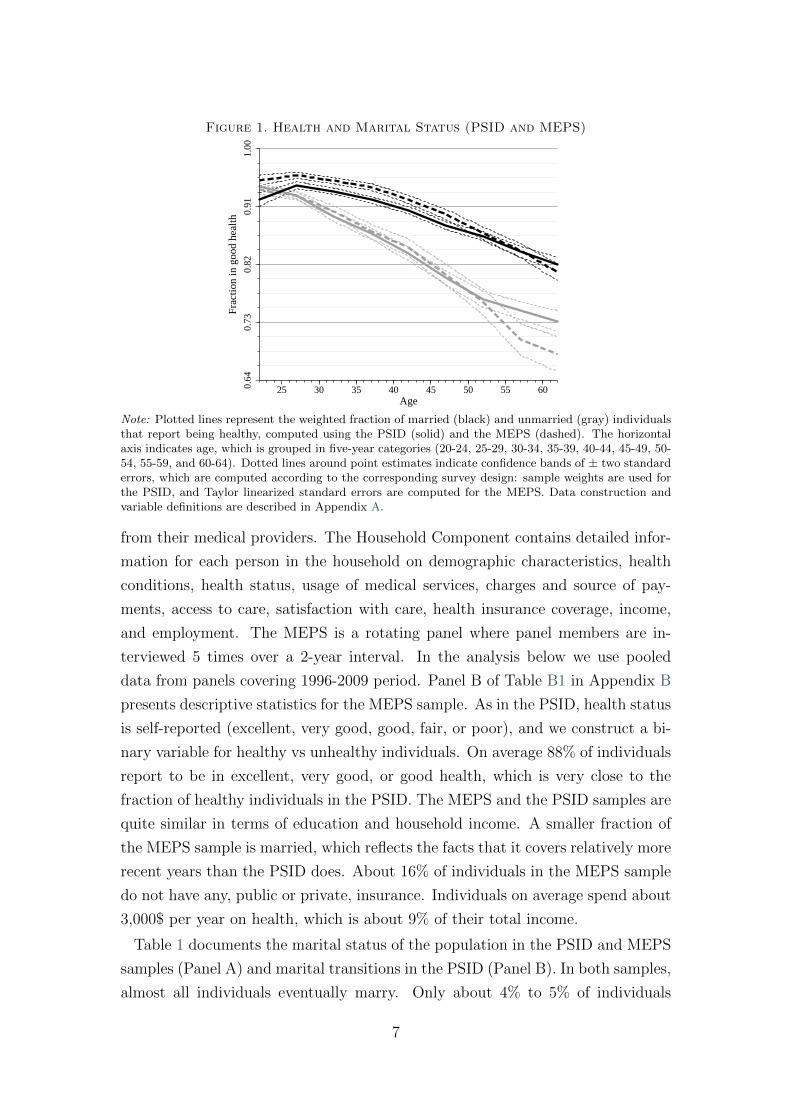
Figure 1. Health and Marital Status (PSID and MEPS)

0.64

0.73

0.82

0.91

1.00

25 30 35 40 45 50 55 60Age

Frac

tion

in g

ood

heal

th

Note: Plotted lines represent the weighted fraction of married (black) and unmarried (gray) individualsthat report being healthy, computed using the PSID (solid) and the MEPS (dashed). The horizontalaxis indicates age, which is grouped in five-year categories (20-24, 25-29, 30-34, 35-39, 40-44, 45-49, 50-54, 55-59, and 60-64). Dotted lines around point estimates indicate confidence bands of ± two standarderrors, which are computed according to the corresponding survey design: sample weights are used forthe PSID, and Taylor linearized standard errors are computed for the MEPS. Data construction andvariable definitions are described in Appendix A.

from their medical providers. The Household Component contains detailed infor-

mation for each person in the household on demographic characteristics, health

conditions, health status, usage of medical services, charges and source of pay-

ments, access to care, satisfaction with care, health insurance coverage, income,

and employment. The MEPS is a rotating panel where panel members are in-

terviewed 5 times over a 2-year interval. In the analysis below we use pooled

data from panels covering 1996-2009 period. Panel B of Table B1 in Appendix B

presents descriptive statistics for the MEPS sample. As in the PSID, health status

is self-reported (excellent, very good, good, fair, or poor), and we construct a bi-

nary variable for healthy vs unhealthy individuals. On average 88% of individuals

report to be in excellent, very good, or good health, which is very close to the

fraction of healthy individuals in the PSID. The MEPS and the PSID samples are

quite similar in terms of education and household income. A smaller fraction of

the MEPS sample is married, which reflects the facts that it covers relatively more

recent years than the PSID does. About 16% of individuals in the MEPS sample

do not have any, public or private, insurance. Individuals on average spend about

3,000$ per year on health, which is about 9% of their total income.

Table 1 documents the marital status of the population in the PSID and MEPS

samples (Panel A) and marital transitions in the PSID (Panel B). In both samples,

almost all individuals eventually marry. Only about 4% to 5% of individuals

7

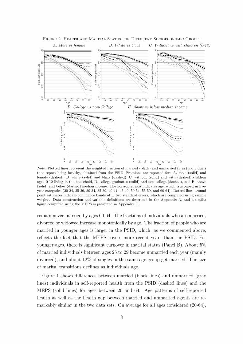
Figure 2. Health and Marital Status for Different Socioeconomic Groups

A. Male vs female B. White vs black C. Without vs with children (0-12)0.

600.

700.

800.

901.

00

25 30 35 40 45 50 55 60Age

Frac

tion

in g

ood

heal

th

0.44

0.58

0.72

0.86

1.00

25 30 35 40 45 50 55 60Age

Frac

tion

in g

ood

heal

th

0.52

0.64

0.76

0.88

1.00

25 30 35 40 45 50 55 60Age

Frac

tion

in g

ood

heal

th

D. College vs non-College E. Above vs below median income

0.52

0.64

0.76

0.88

1.00

25 30 35 40 45 50 55 60Age

Frac

tion

in g

ood

heal

th

0.52

0.64

0.76

0.88

1.00

25 30 35 40 45 50 55 60Age

Frac

tion

in g

ood

heal

th

Note: Plotted lines represent the weighted fraction of married (black) and unmarried (gray) individualsthat report being healthy, obtained from the PSID. Fractions are reported for: A. male (solid) andfemale (dashed), B. white (solid) and black (dashed), C. without (solid) and with (dashed) childrenaged 0-12 living in the household, D. college graduates (solid) and non-college (dashed), and E. above(solid) and below (dashed) median income. The horizontal axis indicates age, which is grouped in five-year categories (20-24, 25-29, 30-34, 35-39, 40-44, 45-49, 50-54, 55-59, and 60-64). Dotted lines aroundpoint estimates indicate confidence bands of ± two standard errors, which are computed using sampleweights. Data construction and variable definitions are described in the Appendix A, and a similarfigure computed using the MEPS is presented in Appendix C.

remain never-married by ages 60-64. The fractions of individuals who are married,

divorced or widowed increase monotonically by age. The fraction of people who are

married in younger ages is larger in the PSID, which, as we commented above,

reflects the fact that the MEPS covers more recent years than the PSID. For

younger ages, there is significant turnover in marital status (Panel B). About 5%

of married individuals between ages 25 to 29 become unmarried each year (mainly

divorced), and about 12% of singles in the same age group get married. The size

of marital transitions declines as individuals age.

Figure 1 shows differences between married (black lines) and unmarried (gray

lines) individuals in self-reported health from the PSID (dashed lines) and the

MEPS (solid lines) for ages between 20 and 64. Age patterns of self-reported

health as well as the health gap between married and unmarried agents are re-

markably similar in the two data sets. On average for all ages considered (20-64),

8

91% of married individuals indicate that they are healthy, while only 86% of un-

married ones do so. Not surprisingly, in very early ages most individuals (more

than 90%) are in good health and the marriage health gap is small. For older ages

the marriage health gap widens, and among those who are 40 to 64 years old, 88%

of married individuals are healthy in contrast to 78% of unmarried ones.

The fact that married agents are healthier than single ones could be due to a

host of factors. Figure 2 reproduces Figure 1 conditional on a few observable char-

acteristics for the PSID sample.6 In each sub-panel, black lines indicate married

individuals while gray lines are for unmarried ones, and solid and dashed lines in-

dicate different sub-populations. As Panel A of Figure 2 shows, males and females

report very similar levels of health when they are married or single. According

to Panel B, blacks have on average worse health than whites and the marriage

health gap vanishes for blacks at older ages. In Panel C, the marriage health gap

is visible and comparable whether or not one conditions on the presence of young

(ages 0 to 12) children (estimates become imprecise at older ages, because few

of those individuals have young children). Consistent with findings from the pre-

vious literature, individuals with better education and income have much better

health. While the marriage health gap is similar conditional on college education

(Panel D), the gap is larger for poorer individuals (Panel E).

III. Model Specification and Identification

In this section we describe our empirical strategy and discuss briefly how we

identify the effect of marriage on health. The equation that we estimate is given by

hit = α(ait) + β(ait)mit + x′itγ + δt + (ηi + εit), (1)

for i = 1, ..., N and t = 1, ..., T , where hit is the health status of individual i in

year t, α(ait) is the health curve for this individual when single, as a function of

her age ait, mit is an indicator variable that equals one whenever the individual is

married, α(ait) +β(ait) is, thus, the health curve for the individual when married,

xit is a vector that includes a set of control variables, δt indicates year dummies,

and (ηi + εit) is the error term, unobserved by the econometrician. Our main

object of interest is the marriage health gap β(a).

The unobserved error term includes an individual-specific innate permanent

component ηi, which is potentially correlated with marital status at different

ages. This correlation can be generated by self-selection into marriage. Stud-

ies in evolutionary biology suggest that individuals with better innate health are

6The results for the MEPS sample are in Figure C1 in Appendix C.

9

more attractive mates in the marriage market, as better health is a clear indica-

tion of reproductive success. This is summarized in Buss (1994) as follows: “Our

ancestors had access to two types of observable evidence of a woman’s health

and youth: features of physical appearance, such as full lips, clear skin, smooth

skin, clear eyes, lustrous hair and good muscle tone, and features of behavior,

such as bouncy, youthful gait, and animated facial expression, and a high energy

level. These physical cues to youth and health, and hence reproductive capacity,

constitute the ingredients of male standards of female beauty” (p.53).7 In the

presence of such selection, least squares estimates for equation (1) would deliver

an overestimate of the marriage health gap. Furthermore, the size of the bias

would differ at different ages. Since almost all individuals eventually get married

at some point, the bias is likely to be larger at younger ages.

We illustrate this bias in Figure 3. Consider the data generating process de-

scribed in Figure 3A, which shows health curves for married (black line) and single

(gray line) individuals. The curves are drawn with x = x, η = 0, and ε = 0. As

Figure 3A shows, this process does not generate a marriage health gap at younger

ages, while it generates a marriage gap in later years. Our choice for particular

health curves in Figure 3A is not random; they reproduce the marriage health gap

we obtain from a within-groups estimation of equation (1) on the PSID sample.

Note that, in equation (1), innate health η enters as an additive shifter. Therefore,

for given xit and εit, different individuals are represented by health curves that

are parallel to those in Figure 3A, and shifted by the corresponding ηi.

Figure 3B shows a simulated sample of 10 individuals generated by the process

just described. Each individual is indicated by a different marker. There is, for

example, an individual with the highest value of η who is always married (marked

by black squares at the top), and another individual with the lowest value of

η who is always single (marked by empty gray diamonds at the bottom). In

between, there are individuals with different marital histories. The individual,

who is indicated by empty circles, for example, is single before age 45 and then

he/she gets married. In the generated sample, there is positive self-selection as

individuals with higher η are more likely to get married and do so earlier.

If we average observed health of married and of singles (or, equivalently, we

fit equation (1) to those data by ordinary least squares (OLS)), we obtain the

health curves depicted in Figure 3C. Given the selection into marriage by high η

7 Pointing in the same direction: “From the point of view of a female trying to pick goodgenes with which to ally her own, what is she looking for? One thing she wants is evidence ofability to survive” (Dawkins, 1989, p.157).

10

Figure 3. Unobserved Heterogeneity and the Self-Selection Bias: An Example

A. Data generating process

0.68

0.76

0.84

0.92

1.00

20 25 30 35 40 45 50 55 60 65

Frac

tion

in g

ood

heal

th

Age

Married, � � 0,

� � ��, � � 0

Single, � � 0,

� � ��, � � 0

B. A sample of 10 individuals

0.68

0.76

0.84

0.92

1.00

20 25 30 35 40 45 50 55 60 65

Frac

tion

in g

ood

heal

th

Age

C. OLS estimates

0.68

0.76

0.84

0.92

1.00

20 25 30 35 40 45 50 55 60 65

Frac

tion

in g

ood

heal

th

Age

Note: Panel A presents married (black) and single (gray) health curves that constitute the data gener-ating process. Panel B plots a sample of 10 observations simulated from the data generating process.Each marker identifies an individual. Health curves are plotted in gray when the individual is single,and in black when married. Panel C presents OLS estimates of the married and single health curves.Covariates x and i.i.d. shocks ε are normalized to averages.

individuals, OLS overestimates the underlying marriage health gap. The health

curves obtained in Figure 3C intentionally replicate the average health curves by

marital status obtained from the PSID, depicted in Figure 1 in Section II.

In the empirical analysis below, we identify the single’s health curve α(a) and

the marriage health gap β(a) non-parametrically. A within-groups estimation of

equation (1) provides consistent estimates of the health curves, as long as our

assumption of additive separability of η is satisfied. It is very important to note

that since α(a) and β(a) are time-varying for a given individual, as he/she is

observed over different ages, identification does not rely exclusively on individuals

who change their marital status. Individuals contribute to the identification of

the married health curve whenever they are married, even if they never switch

marital status, up to a normalization of the intercept. Likewise, whenever they

are single, individuals contribute to the identification of the single health curve

up to the intercept. Marital status changes thus identify the gap between single

and married intercepts.8 Consequently, identification of the marriage health gap

at a given age, say 60 to 64, is not identified exclusively by individuals who switch

marital status within that age range.

We also estimate heterogeneous health curves that depend on socioeconomic

characteristics. In particular, we estimate the following version of equation (1):

hit = α(ait, qit) + β(ait, qit)mit + x′itγ + δt + (ηi + εit), (2)

8 Therefore, individuals who are, for example, always married (like the individual with thehighest η in Figure 3B) contribute to the identification of the shape of the married health curve,despite not contributing to the identification of the gap between married and single intercepts.

11

for i = 1, ..., N and t = 1, ..., T , where the health curves α(a, q) and α(a, q)+β(a, q)

are now allowed to vary across different socioeconomic groups, denoted by q. In

particular, motivated by the results in Figure 2, we estimate equation (2) for males

vs females, blacks vs whites, individuals with vs without children, individuals with

vs without a college degree, and individuals whose household income lies above

vs below the median household income.

IV. Results

In this section we present our estimates of the marriage health gap, β(a) in equa-

tion (1). We first present OLS and within-groups estimates. We also show that

the main results are robust to different definitions of two key variables, health and

marriage. Finally, we report the marriage health gap conditional on observable

characteristics, β(a, q) in equation (2).

A. Main Results

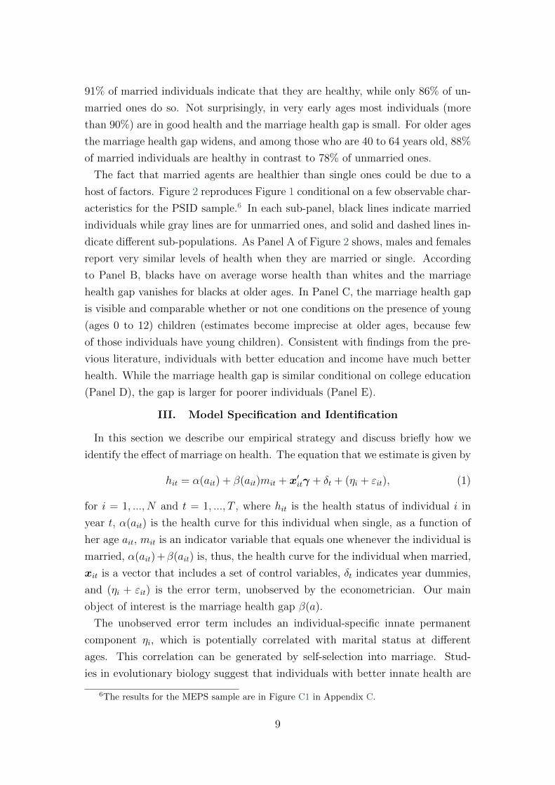
Figure 4 presents OLS estimates of β(a) from the PSID (black) and the MEPS

(gray) samples.9 In the estimation of equation (1), we use five-year age bins, from

20-24 to 60-64.10 Health, h, is an indicator variable that takes a value of one

whenever the individual is healthy. Control variables, x, include income, gender

(female dummy), race (black dummy), education (college dummy), and children

(dummies for presence of children ages 0-3, 4-12, and 13-18 in the household).

The results show that after controlling for observable characteristics, there is

a positive and significant difference between the reported health of married and

unmarried individuals. The gap is about 1 percentage point for younger (20-24)

ages, and increases monotonically to around 12 percentage points for 55 to 59 age

group in the PSID sample. Similar results are obtained from the MEPS sample

when we estimate the model with the same controls. The gap is initially small

and grows to about 8 percentage points for 55 to 59 age group.

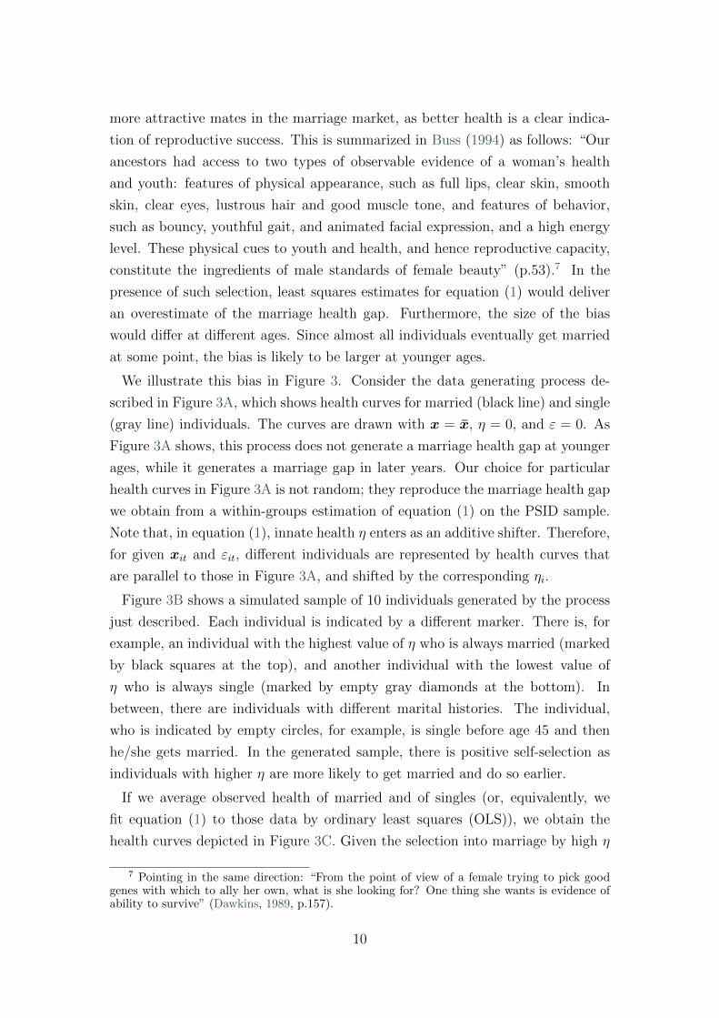
Figure 5 shows within-groups estimates (black line) together with OLS estimates

from Figure 4 (gray line) for the PSID sample. Within-groups estimation reduces

the size of the marriage health gap substantially. Indeed for ages up to 40 the

marriage health gap disappears completely. After age 40, however, the positive

effect of marriage on health starts to show up. At the peak of the gap (between

ages 55 and 59), married individuals are about 6 percentage points more likely

9 The full set of regression coefficients are shown in Table B2 in Appendix B.10 Results shown below are robust across different bin widths. Whenever they are presented

in figures, the mid point of the age interval is plotted.

12

Figure 4. Health and Marital Status: OLS Estimation Results

−0.

060.

000.

060.

120.

18

25 30 35 40 45 50 55 60Age

Prob

abili

ty g

ap m

arri

ed v

s si

ngle

, β(a

)

Note: Solid lines are OLS estimated marriage health gaps, β(a). The regression is fitted to the PSID(black) and the MEPS (gray). The dependent variable, h, is an indicator variable that takes a valueof one whenever the agent is healthy. Control variables, x, include income, gender (female dummy),race (black dummy), education (college dummy), children (dummies for 0-3, 4-12, and 13-18 year-oldchildren), and survey year (year dummies); regressions also estimate α(a). The horizontal axis indicatesage. In estimation, five-year age bins (20-24, 25-29, 30-34, 35-39, 40-44, 45-49, 50-54, 55-59, and 60-64)are considered. The center point of the bin is represented in the figure. Cross-sectional weights are usedin estimation. Dotted lines indicate ± two standard errors confidence bands around point estimates,which are clustered at the household level in the PSID, and Taylor linearized using survey stratificationdesign in the MEPS. Data construction and variable definitions are described in Appendix A.

Figure 5. Health and Marital Status: Within-Groups Estimation Results

−0.

060.

000.

060.

120.

18

25 30 35 40 45 50 55 60Age

Prob

abili

ty g

ap m

arri

ed v

s si

ngle

, β(a

)

Note: Solid lines are within-groups (black) and OLS (gray) estimated marriage health gaps, β(a). Theregression is fitted to the PSID. The dependent variable, h, is an indicator variable that takes a valueof one whenever the agent is healthy. Control variables, x, include income, gender (female dummy),race (black dummy), education (college dummy), children (dummies for 0-3, 4-12, and 13-18 year-oldchildren), and survey year (year dummies); regressions also estimate α(a). The horizontal axis indicatesage. In estimation, five-year age bins (20-24, 25-29, 30-34, 35-39, 40-44, 45-49, 50-54, 55-59, and 60-64)are considered. The center point of the bin is represented in the figure. Weights are used in estimation.Dotted lines indicate ± two standard errors confidence bands around point estimates, which are clusteredat the household level. Data construction and variable definitions are described in Appendix A.

13

to be healthy than unmarried ones. This is about half of the OLS estimated

gap. These results suggests that there is an important role for self-selection in

explaining the observed marriage health gap, especially at earlier ages, while some

protective effects of marriage on health remain at older ages. We explore both

self-selection patterns and the potential remaining effect of marriage on health in

further detail in Section V.

B. Robustness

The results in Figure 4 and Figure 5 are based on self-reported measures of

health. The MEPS contains another measure, SF12v2 (short form 12 version 2),

that is constructed as an index by the interviewers from answers that respondents

give to a set of health-related questions. The left panel of Figure 6 replicates the

OLS estimates from the MEPS sample with this objective measure of health, and

show that the basic qualitative picture remains the same. Another measure of

health is the presence of chronic conditions (such as cancer, hypertension, dia-

betes, stroke, hearth attack, etc.), which is provided in the PSID. The right panel

of Figure 6 shows the within-groups estimates of the marriage gap on the number

of different chronic conditions an individual ever had by any given age. Consis-

tent with other two measures of health, the difference between married and single

individuals is very small for younger ages, but as individuals age, married individ-

uals have a much smaller number of chronic conditions than singles do. Around

ages 50 to 54, for example, being married is associated with 0.1 fewer chronic

conditions. As we document in Table B1, on average individuals have about 0.65

chronic conditions. Hence, the marriage gap is about 15% of the mean.

We also check whether the way we define married and unmarried individuals

affect the results. In our first check, we would like to understand whether divorce

(in contrast to being never married) has a particularly adverse effect on health.

To this end, we drop divorced agents from the pool of unmarried, and compare

married individuals with those who are never married or widowed. Results, shown

in Panel A of Figure 7, are very much in line with our basic results. Indeed, the

marriage health gap is now slightly larger, which suggests that divorced individuals

have better, not worse, health than those who are never married or widowed. As

we discuss below, this possibly reflects the positive effects of marriage capital

(measured as the total number of years one is married) on health. Next, we

exclude widows from the pool of single agents (Panel B). In this case, results

are similar to our baseline results. As a final check, we consider all cohabitants

as married (Panel C). As documented in Table B1, this increases the fraction of

14

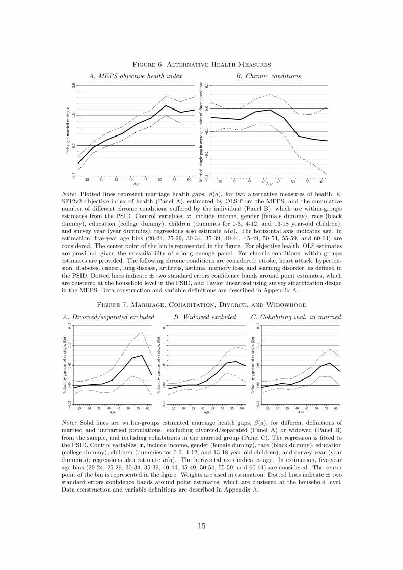
Figure 6. Alternative Health Measures

A. MEPS objective health index−

1.5

0.0

1.5

3.0

25 30 35 40 45 50 55 60Age

Inde

x ga

p m

arri

ed v

s si

ngle

B. Chronic conditions

−0.

3−

0.2

−0.

10.

00.

1

25 30 35 40 45 50 55 60Age

Mar

ried

−si

ngle

gap

in a

vera

ge n

umbe

r of

chr

onic

con

dito

nsNote: Plotted lines represent marriage health gaps, β(a), for two alternative measures of health, h:SF12v2 objective index of health (Panel A), estimated by OLS from the MEPS, and the cumulativenumber of different chronic conditions suffered by the individual (Panel B), which are within-groupsestimates from the PSID. Control variables, x, include income, gender (female dummy), race (blackdummy), education (college dummy), children (dummies for 0-3, 4-12, and 13-18 year-old children),and survey year (year dummies); regressions also estimate α(a). The horizontal axis indicates age. Inestimation, five-year age bins (20-24, 25-29, 30-34, 35-39, 40-44, 45-49, 50-54, 55-59, and 60-64) areconsidered. The center point of the bin is represented in the figure. For objective health, OLS estimatesare provided, given the unavailability of a long enough panel. For chronic conditions, within-groupsestimates are provided. The following chronic conditions are considered: stroke, heart attack, hyperten-sion, diabetes, cancer, lung disease, arthritis, asthma, memory loss, and learning disorder, as defined inthe PSID. Dotted lines indicate ± two standard errors confidence bands around point estimates, whichare clustered at the household level in the PSID, and Taylor linearized using survey stratification designin the MEPS. Data construction and variable definitions are described in Appendix A.

Figure 7. Marriage, Cohabitation, Divorce, and Widowhood

A. Divorced/separated excluded B. Widowed excluded C. Cohabiting incl. in married

−0.

050.

000.

050.

100.

15

25 30 35 40 45 50 55 60Age

Prob

abili

ty g

ap m

arri

ed v

s si

ngle

, β(a

)

−0.

050.

000.

050.

100.

15

25 30 35 40 45 50 55 60Age

Prob

abili

ty g

ap m

arri

ed v

s si

ngle

, β(a

)

−0.

050.

000.

050.

100.

15

25 30 35 40 45 50 55 60Age

Prob

abili

ty g

ap m

arri

ed v

s si

ngle

, β(a

)

Note: Solid lines are within-groups estimated marriage health gaps, β(a), for different definitions ofmarried and unmarried populations: excluding divorced/separated (Panel A) or widowed (Panel B)from the sample, and including cohabitants in the married group (Panel C). The regression is fitted tothe PSID. Control variables, x, include income, gender (female dummy), race (black dummy), education(college dummy), children (dummies for 0-3, 4-12, and 13-18 year-old children), and survey year (yeardummies); regressions also estimate α(a). The horizontal axis indicates age. In estimation, five-yearage bins (20-24, 25-29, 30-34, 35-39, 40-44, 45-49, 50-54, 55-59, and 60-64) are considered. The centerpoint of the bin is represented in the figure. Weights are used in estimation. Dotted lines indicate ± twostandard errors confidence bands around point estimates, which are clustered at the household level.Data construction and variable definitions are described in Appendix A.

15

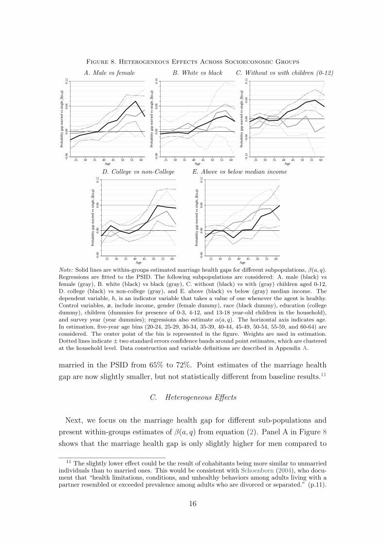
Figure 8. Heterogeneous Effects Across Socioeconomic Groups

A. Male vs female B. White vs black C. Without vs with children (0-12)−

0.06

0.00

0.06

0.12

25 30 35 40 45 50 55 60Age

Prob

abili

ty g

ap m

arri

ed v

s si

ngle

, β(a

,q)

−0.

080.

000.

080.

1625 30 35 40 45 50 55 60

Age

Prob

abili

ty g

ap m

arri

ed v

s si

ngle

, β(a

,q)

−0.

12−

0.06

0.00

0.06

0.12

25 30 35 40 45 50 55 60Age

Prob

abili

ty g

ap m

arri

ed v

s si

ngle

, β(a

,q)

D. College vs non-College E. Above vs below median income

−0.

060.

000.

060.

12

25 30 35 40 45 50 55 60Age

Prob

abili

ty g

ap m

arri

ed v

s si

ngle

, β(a

,q)

−0.

060.

000.

060.

12

25 30 35 40 45 50 55 60Age

Prob

abili

ty g

ap m

arri

ed v

s si

ngle

, β(a

,q)

Note: Solid lines are within-groups estimated marriage health gaps for different subpopulations, β(a, q).Regressions are fitted to the PSID. The following subpopulations are considered: A. male (black) vsfemale (gray), B. white (black) vs black (gray), C. without (black) vs with (gray) children aged 0-12,D. college (black) vs non-college (gray), and E. above (black) vs below (gray) median income. Thedependent variable, h, is an indicator variable that takes a value of one whenever the agent is healthy.Control variables, x, include income, gender (female dummy), race (black dummy), education (collegedummy), children (dummies for presence of 0-3, 4-12, and 13-18 year-old children in the household),and survey year (year dummies); regressions also estimate α(a, q). The horizontal axis indicates age.In estimation, five-year age bins (20-24, 25-29, 30-34, 35-39, 40-44, 45-49, 50-54, 55-59, and 60-64) areconsidered. The center point of the bin is represented in the figure. Weights are used in estimation.Dotted lines indicate ± two standard errors confidence bands around point estimates, which are clusteredat the household level. Data construction and variable definitions are described in Appendix A.

married in the PSID from 65% to 72%. Point estimates of the marriage health

gap are now slightly smaller, but not statistically different from baseline results.11

C. Heterogeneous Effects

Next, we focus on the marriage health gap for different sub-populations and

present within-groups estimates of β(a, q) from equation (2). Panel A in Figure 8

shows that the marriage health gap is only slightly higher for men compared to

11 The slightly lower effect could be the result of cohabitants being more similar to unmarriedindividuals than to married ones. This would be consistent with Schoenborn (2004), who docu-ment that “health limitations, conditions, and unhealthy behaviors among adults living with apartner resembled or exceeded prevalence among adults who are divorced or separated.” (p.11).

16

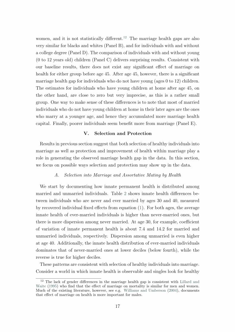
women, and it is not statistically different.12 The marriage health gaps are also

very similar for blacks and whites (Panel B), and for individuals with and without

a college degree (Panel D). The comparison of individuals with and without young

(0 to 12 years old) children (Panel C) delivers surprising results. Consistent with

our baseline results, there does not exist any significant effect of marriage on

health for either group before age 45. After age 45, however, there is a significant

marriage health gap for individuals who do not have young (ages 0 to 12) children.

The estimates for individuals who have young children at home after age 45, on

the other hand, are close to zero but very imprecise, as this is a rather small

group. One way to make sense of these differences is to note that most of married

individuals who do not have young children at home in their later ages are the ones

who marry at a younger age, and hence they accumulated more marriage health

capital. Finally, poorer individuals seem benefit more from marriage (Panel E).

V. Selection and Protection

Results in previous section suggest that both selection of healthy individuals into

marriage as well as protection and improvement of health within marriage play a

role in generating the observed marriage health gap in the data. In this section,

we focus on possible ways selection and protection may show up in the data.

A. Selection into Marriage and Assortative Mating by Health

We start by documenting how innate permanent health is distributed among

married and unmarried individuals. Table 2 shows innate health differences be-

tween individuals who are never and ever married by ages 30 and 40, measured

by recovered individual fixed effects from equation (1). For both ages, the average

innate health of ever-married individuals is higher than never-married ones, but

there is more dispersion among never married. At age 30, for example, coefficient

of variation of innate permanent health is about 7.4 and 14.2 for married and

unmarried individuals, respectively. Dispersion among unmarried is even higher

at age 40. Additionally, the innate health distribution of ever-married individuals

dominates that of never-married ones at lower deciles (below fourth), while the

reverse is true for higher deciles.

These patterns are consistent with selection of healthy individuals into marriage.

Consider a world in which innate health is observable and singles look for healthy

12 The lack of gender differences in the marriage health gap is consistent with Lillard andWaite (1995) who find that the effect of marriage on mortality is similar for men and women.Much of the existing literature, however, see e.g. Williams and Umberson (2004), documentsthat effect of marriage on health is more important for males.

17

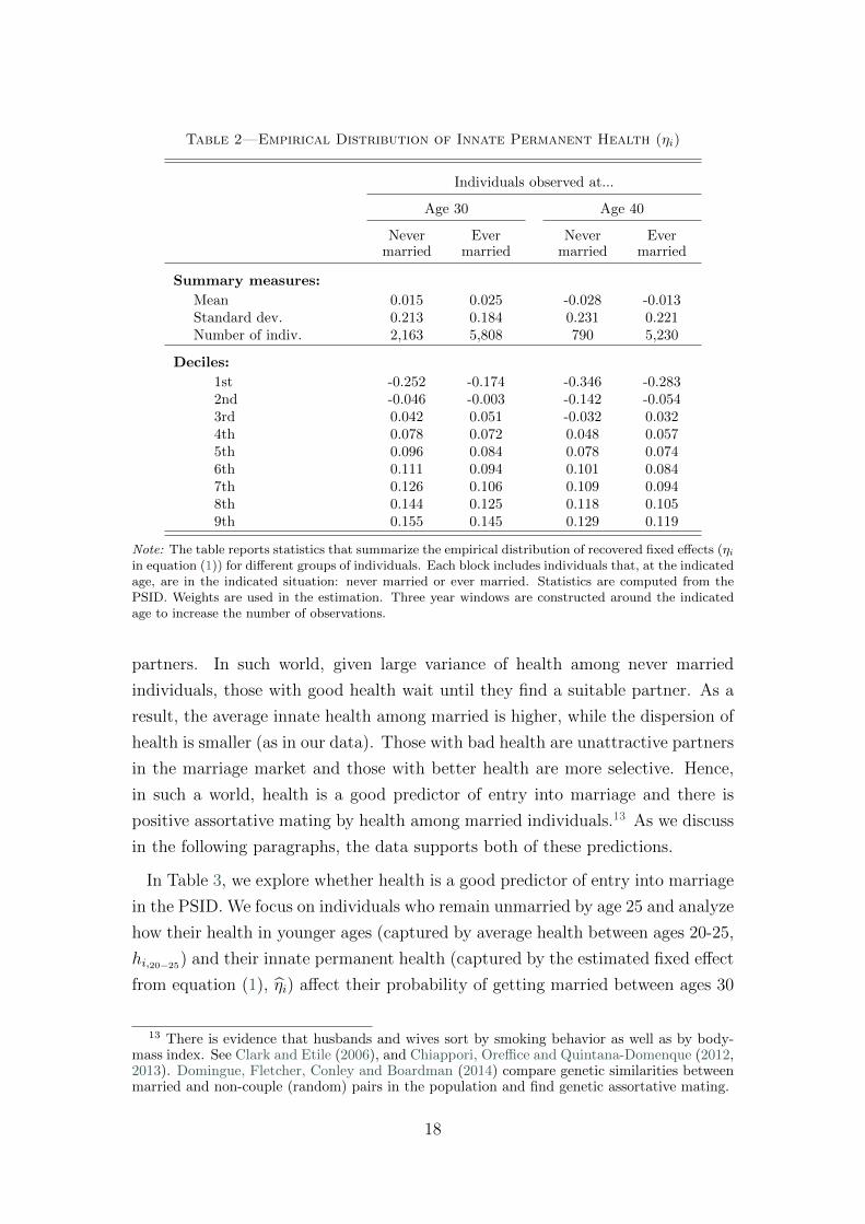
Table 2—Empirical Distribution of Innate Permanent Health (ηi)

Individuals observed at...

Age 30 Age 40

Nevermarried

Evermarried

Nevermarried

Evermarried

Summary measures:

Mean 0.015 0.025 -0.028 -0.013Standard dev. 0.213 0.184 0.231 0.221Number of indiv. 2,163 5,808 790 5,230

Deciles:

1st -0.252 -0.174 -0.346 -0.2832nd -0.046 -0.003 -0.142 -0.0543rd 0.042 0.051 -0.032 0.0324th 0.078 0.072 0.048 0.0575th 0.096 0.084 0.078 0.0746th 0.111 0.094 0.101 0.0847th 0.126 0.106 0.109 0.0948th 0.144 0.125 0.118 0.1059th 0.155 0.145 0.129 0.119

Note: The table reports statistics that summarize the empirical distribution of recovered fixed effects (ηiin equation (1)) for different groups of individuals. Each block includes individuals that, at the indicatedage, are in the indicated situation: never married or ever married. Statistics are computed from thePSID. Weights are used in the estimation. Three year windows are constructed around the indicatedage to increase the number of observations.

partners. In such world, given large variance of health among never married

individuals, those with good health wait until they find a suitable partner. As a

result, the average innate health among married is higher, while the dispersion of

health is smaller (as in our data). Those with bad health are unattractive partners

in the marriage market and those with better health are more selective. Hence,

in such a world, health is a good predictor of entry into marriage and there is

positive assortative mating by health among married individuals.13 As we discuss

in the following paragraphs, the data supports both of these predictions.

In Table 3, we explore whether health is a good predictor of entry into marriage

in the PSID. We focus on individuals who remain unmarried by age 25 and analyze

how their health in younger ages (captured by average health between ages 20-25,

hi,20−25) and their innate permanent health (captured by the estimated fixed effect

from equation (1), ηi) affect their probability of getting married between ages 30

13 There is evidence that husbands and wives sort by smoking behavior as well as by body-mass index. See Clark and Etile (2006), and Chiappori, Oreffice and Quintana-Domenque (2012,2013). Domingue, Fletcher, Conley and Boardman (2014) compare genetic similarities betweenmarried and non-couple (random) pairs in the population and find genetic assortative mating.

18

Table 3—The Effect of Health on the Probability of Getting Married

(1) (2) (3) (4) (5)

Health at age 20-25 0.196 0.013 -0.137 -0.149 -0.099(0.079) (0.110) (0.106) (0.109) (0.103)

Innate permanent health 0.299 0.479 0.259 0.163(0.128) (0.123) (0.128) (0.116)

College 0.209 0.216(0.031) (0.028)

Black -0.226 -0.276(0.035) (0.033)

Female -0.027 -0.058(0.028) (0.026)

Income (average 30-40) 0.001(0.000)

Presence of kids (30-40) 0.423(0.029)

Constant 0.396 0.555(0.076) (0.101)

Cohort dummies: No No Yes Yes Yes

Observations 1,700 1,700 1,700 1,700 1,700Adj. R-squared 0.005 0.010 0.611 0.644 0.705

Note: The dependent variable takes the value of one if the individual is married at some point betweenage 30 and 40. The sample is restricted to individuals who have never been married by age 25. Healthat age 20-25 is the average health of the individual at that age range. Innate permanent health is therecovered fixed effect (ηi) from equation (1); its standard deviation is 0.243. Cohort of birth dummiesare included when indicated. Robust standard errors in parenthesis.

and 40. In particular, we estimate the following regression:

mi,30−40 = φhi,20−25 + θηi + z′i,30−40λ+ υi,30−40 , (3)

where mi,30−40 equals one if individual (never married by age 25) is married at some

point between ages 30 and 40, hi,20−25 is individual’s average health at ages 20 to 25,

ηi is the recovered fixed effect from equation (1), and zi,30−40 is a vector of controls.

Column 1 in Table 3 shows that an unmarried individual who is in good health

between ages 20-25 has about 20 percentage points higher chances of being mar-

ried at some point between ages 30 and 40 than someone whose health is poor.

When we include innate permanent health in the regression, the latter absorbs

all the positive association with marriage probability (column 2). In particular, a

one standard deviation increase in innate permanent health is associated with a

7 percentage points increase in the probability of getting married before age 40;

in this case, the remaining effect of being in good health at ages 20 to 25 is only

1 percentage point, and is not significant. When we add further controls (edu-

cation, gender, race and income) the effect of innate permanent health remains

19

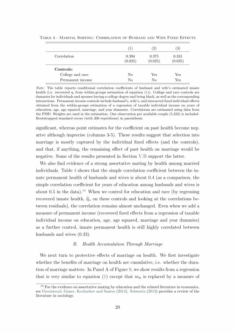
Table 4—Marital Sorting: Correlation of Husband and Wife Fixed Effects

(1) (2) (3)

Correlation 0.394 0.375 0.331(0.025) (0.025) (0.025)

Controls:

College and race No Yes Yes

Permanent income No No Yes

Note: The table reports conditional correlation coefficients of husband and wife’s estimated innatehealth (i.e. recovered ηi from within-groups estimation of equation (1)). College and race controls aredummies for individuals and spouses having a college degree and being black, as well as the correspondinginteractions. Permanent income controls include husband’s, wife’s, and interacted fixed individual effectsobtained from the within-groups estimation of a regression of taxable individual income on years ofeducation, age, age squared, marriage, and year dummies. Correlations are estimated using data fromthe PSID. Weights are used in the estimation. One observation per available couple (5,323) is included.Bootstrapped standard errors (with 200 repetitions) in parenthesis.

significant, whereas point estimates for the coefficient on past health become neg-

ative although imprecise (columns 3-5). These results suggest that selection into

marriage is mostly captured by the individual fixed effects (and the controls),

and that, if anything, the remaining effect of past health on marriage would be

negative. Some of the results presented in Section V.B support the latter.

We also find evidence of a strong assortative mating by health among married

individuals. Table 4 shows that the simple correlation coefficient between the in-

nate permanent health of husbands and wives is about 0.4 (as a comparison, the

simple correlation coefficient for years of education among husbands and wives is

about 0.5 in the data).14 When we control for education and race (by regressing

recovered innate health, ηi, on these controls and looking at the correlations be-

tween residuals), the correlation remains almost unchanged. Even when we add a

measure of permanent income (recovered fixed effects from a regression of taxable

individual income on education, age, age squared, marriage and year dummies)

as a further control, innate permanent health is still highly correlated between

husbands and wives (0.33).

B. Health Accumulation Through Marriage

We next turn to protective effects of marriage on health. We first investigate

whether the benefits of marriage on health are cumulative, i.e. whether the dura-

tion of marriage matters. In Panel A of Figure 9, we show results from a regression

that is very similar to equation (1) except that mit is replaced by a measure of

14 For the evidence on assortative mating by education and the related literature in economics,see Greenwood, Guner, Kocharkov and Santos (2014). Schwartz (2013) provides a review of theliterature in sociology.

20

Figure 9. Health Accumulation Through Marriage

A. Marriage capital−

0.03

0.00

0.03

0.06

0.09

25 30 35 40 45 50 55 60Age

Prob

abili

ty g

ap p

er 1

0 ex

tra

year

s of

mar

riag

e

B. Dynamic model

−0.

060.

000.

060.

120.

18

25 30 35 40 45 50 55 60Age

Prob

abili

ty g

ap m

arri

ed v

s si

ngle

, β(a

)

Note: The figure presents estimates of β(a) from two modified versions of equation (1): one (Panel A)in which the married dummy, m is replaced by the number of years an individual have been married(zero if never married); the other (Panel B) in which the model is expanded to include the laggeddependent variable ht−1 as an additional control. Left figure is estimated using the within-groupsestimator, right figure is estimated using System-GMM. Both models are estimated using data from thePSID. Control variables, x, include income, gender (female dummy), race (black dummy), education(college dummy), children (dummies for 0-3, 4-12, and 13-18 year-old children), and survey year (yeardummies); regressions also estimate α(a). The horizontal axis indicates age. In estimation, five-yearage bins (20-24, 25-29, 30-34, 35-39, 40-44, 45-49, 50-54, 55-59, and 60-64) are considered. Dotted linesare ± two standard errors confidence bands around point estimates, clustered at the household level.

marriage capital (defined as the total number of years an individual has been mar-

ried by year t).15 Hence β(a) now measures the effect of one extra year of being

married at a given age a on the probability of being healthy. The effect of an

extra year of marriage has a positive and significant effect on being healthy that

is roughly constant after ages 35-39: 10 extra years of marriage capital increase

the probability of being healthy by about 3 percentage points.

Given the importance of marriage health capital, we also estimate equation (1)

with past health as an additional control variable. In this case, a within-groups es-

timation does not deliver consistent estimates (Arellano and Bond, 1991). There-

fore, we use a generalized method of moments approach, in the way described in

Arellano and Bover (1995) (often known as System-GMM). The results are pre-

sented in Panel B of Figure 9. While the overall pattern of the marriage health gap

is similar to what we obtain from within-groups estimates, the marriage health

gap is now larger. As we have shown in Table 3, after we net out individual fixed

effects, there is a negative correlation between lagged health and the probability

of getting married. As a result, by not including lagged health in equation (1), we

underestimate the effect of marriage on health. Once this bias is corrected, the

effect of marriage on health is estimated to be even larger. In Panel B of Figure 9,

15 Independent of whether the person is married to the same partner.

21

marriage heath gap is about 6% for ages 40 to 49 and increases up to 12% for later

years. These results suggest that the baseline within-groups results in Figure 5,

are, if anything, conservative estimates of the effect of marriage on health.

C. Healthy Behavior

What factors can explain the protective effect of marriage on health? In this

section, we document that married individuals are much more likely to engage

in healthy behavior than unmarried ones. Figure 10 shows differences between

married and unmarried individuals in preventive health checks. The figure shows

coefficients form regressions similar to equation (1), where the dependent variable

is whether an individual performs a particular preventive check at a given age.

The results show that there are significant differences between married and

single individuals for all categories of preventive care. Married individuals around

ages 50 to 54, for example, are about 6% more likely to check their cholesterol

or have a prostate or breast examination. Note that these differences come from

regressions that control for education and income. Hence, the effect of marriage

on healthy behavior goes beyond the well documented effect (see e.g. Cutler and

Lleras-Muney, 2010) of education on healthy behavior.

Why would married individuals be more likely to do preventive care? One

possible factor, which is well documented in the medical literature, is that having

a partner encourages individuals to follow up on medical appointments, check-

ups, etc.16 Another factor, which we focus on in the next section, is the fact that

married individuals are more likely to have health insurance than unmarried are.

Differences between married and unmarried individuals in healthy behavior are

also reflected in their medical expenditures. To analyze differences in medical

expenditures, we model the conditional median of the total medical expenditure

in a way similar to equation (1) except that the dependent variable is now total

medical expenditure.17 Panel A of Figure 11 shows our estimates of the marriage

gap in median health expenditure estimated from the MEPS. Results suggest that

median health expenditure of married individuals aged below 40 is around 40-60$

larger per year than that of unmarried individuals at the same age range. At

16 There is a large medical literature that documents the link between marriage and specifichealth outcomes. In an interview to CNN, Dr. Paul L. Nguyen, summarizing research by Aizeret al. (2013), states that “You are going to nag your wife to go get her mammograms. Youare going to nag your husband to go get his colonoscopy.... If you are on your own, nobody isgoing to nag you.” In interview available at http://thechart.blogs.cnn.com/2013/09/23/marriage-may-improve-cancer-survival-odds/?hpt=he_c2, accessed on December 6, 2013.See Waite and Gallagher (2000) for further evidence on what they call “the virtues of nagging”.

17 Similarly, we consider regressions for mean expenditures as opposed to median, whichdeliver very similar results, with a different scale.

22

Figure 10. Preventive Health Checks and Marital Status

A. Dental check

−0.

12−

0.06

0.00

0.06

0.12

25 30 35 40 45 50 55 60Age

Prob

abili

ty g

ap b

etw

een

mar

ried

and

sin

gle

B. Cholesterol check

−0.

060.

000.

060.

120.

18

25 30 35 40 45 50 55 60Age

Prob

abili

ty g

ap b

etw

een

mar

ried

and

sin

gle

C. Complete check

−0.

060.

000.

060.

120.

18

25 30 35 40 45 50 55 60Age

Prob

abili

ty g

ap b

etw

een

mar

ried

and

sin

gle

D. Flu shot

−0.

060.

000.

060.

120.

18

25 30 35 40 45 50 55 60Age

Prob

abili

ty g

ap b

etw

een

mar

ried

and

sin

gle

E. Prostate exam

−0.

060.

000.

060.

120.

18

25 30 35 40 45 50 55 60Age

Prob

abili

ty g

ap b

etw

een

mar

ried

and

sin

gle

F. Pap smear

−0.

060.

000.

060.

120.

18

25 30 35 40 45 50 55 60Age

Prob

abili

ty g

ap b

etw

een

mar

ried

and

sin

gle

G. Breast examination

−0.

060.

000.

060.

120.

18

25 30 35 40 45 50 55 60Age

Prob

abili

ty g

ap b

etw

een

mar

ried

and

sin

gle

H. Mammography

−0.

060.

000.

060.

120.

18

25 30 35 40 45 50 55 60Age

Prob

abili

ty g

ap b

etw

een

mar

ried

and

sin

gle

Note: Plotted lines represent OLS estimates of β(a) from an equation similar to (1) in which thedependent variable is now an indicator variable that takes the value of one if the individual did the cor-responding preventive check. The following preventive checks are considered: dental check at least onceevery year; cholesterol check, general physical examination, flu shot, prostate examination, Pap smear,breast examination, and mammography at least once in the last two years. The equation is fitted to datafrom the MEPS. Control variables, x, include income, gender (female dummy), race (black dummy),education (college dummy), children (dummies for 0-3, 4-12, and 13-18 year-old children), and surveyyear (year dummies), as well as current health, health insurance (public and private insurance dummies)and total health expenditures; regressions also estimate α(a). Weights are used in the estimation. Thehorizontal axis indicates age. In estimation, five-year age bins (20-24, 25-29, 30-34, 35-39, 40-44, 45-49,50-54, 55-59, and 60-64) are considered. Dotted lines indicate ± two standard errors confidence bandsaround point estimates, which are Taylor linearized using survey stratification design in the MEPS.Data construction and variable definitions are described in Appendix A.

older ages, though, unmarried individuals spend more than married ones; at ages

50-59, median expenditure of unmarried individuals is around 100-110$ larger.

This higher expenditure by married individuals at earlier ages may due to pre-

ventive motives, while the higher expenditure by unmarried at older ages may be

due to curative motives, as a result of worse health. To further explore this hy-

pothesis, we estimate marriage expenditure gaps for different health statuses. In

particular, we extend the median expenditure model to account for heterogeneous

curves depending on health, in the spirit of the heterogeneous effects described in

equation (2). Panel B of Figure 11 presents median regression estimates of the

marriage health expenditure gap for healthy and unhealthy individuals. Married

individuals spend slightly more when they are healthy, which is consistent with

23

Figure 11. Median Health Expenditures and Marital Status

A. Expenditure gap−

1.2

−0.

8−

0.4

0.0

0.4

25 30 35 40 45 50 55 60Age

Hea

lth e

xpen

ditu

re g

ap m

arri

ed v

s si

ngle

(in

1,0

00s)

B. Heterogeneous effects by health level

−1.

2−

0.8

−0.

40.

00.

4

25 30 35 40 45 50 55 60Age

Hea

lth e

xpen

ditu

re g

ap m

arri

ed v

s si

ngle

(in

1,0

00s)

Note: Plotted solid line in Panel A represents median regression estimates of β(a) from a model similarto (1), in which total health expenditures is the dependent variable. Plotted solid lines in the Panel Bare median regression estimates of β(a, q) from an equation similar to (2), where the dependent variableis total health expenditures, and qit = hit is an indicator on whether the individual is healthy (black)in that period or not (gray). Control variables, x, include income, gender (female dummy), race (blackdummy), education (college dummy), children (dummies for 0-3, 4-12, and 13-18 year-old children),and survey year (year dummies), as well as health insurance (public and private insurance dummies);regressions also estimate α(a) and α(a, q) respectively. The equations are fitted to data from the MEPS.The horizontal axis indicates age. In estimation, five-year age bins (20-24, 25-29, 30-34, 35-39, 40-44,45-49, 50-54, 55-59, and 60-64) are considered. Dotted lines are ± two standard error bands, obtained bybootstrap with 30 repetitions. Data construction and variable definitions are described in Appendix A.

the fact they they are more likely to do preventive checks. In contrast, unmarried

individuals spend substantially more than married ones when they are unhealthy,

which suggests that when the unmarried are unhealthy, they are more likely to

face serious (and expensive) conditions.

Finally, we check whether entry into marriage is associated with healthy habits.

We focus on smoking, a key health factor. In particular, we look at all individuals

who were smokers in 1999 and document how many of them quit smoking between

1999 and 2011 conditional on their marital transitions. As Table 5 shows, a

single individual is about 13% points more likely to quit smoking if he/she gets

married than if he/she stays single (42% versus 29%); additionally, a majority

(about 72%) of singles who get married and quit smoking do so while they are

married. Likewise, a married individual is more likely to quit smoking if he/she

stays married than if he/she becomes single (40% versus 32%).

Overall, these results seem to suggest that marriage goes together with healthy

behavior. Even after controlling for observables, most importantly income, educa-

tion and health insurance, preventive health care, measured both by frequency of

preventive medical checks and by health expenditure while healthy, is more preva-

lent among married individuals than it is among singles. Marriage also increases

the probability of quitting smoking.

24

Table 5—Probability of Quitting Smoking and Marital Transitions

Probability of Probability of quitting smoking...

quitting smoking while married while single

Single → Single 0.286 0.009 0.277(0.028) (0.006) (0.027)

Single → Married 0.415 0.298 0.116(0.052) (0.048) (0.033)

Married → Single 0.318 0.052 0.266(0.057) (0.026) (0.055)

Married → Married 0.395 0.389 0.006(0.030) (0.030) (0.004)

Note: The table presents the probability that an individual quits smoking between 1999 and 2011conditional on smoking in 1999, by type of marital status transition. These probabilities are calculatedusing data from the PSID. Weights are used. In the left column, the numerator is the number ofindividuals in the corresponding marital transition that were not smoking in 2011 and were smokingin 1999, and the denominator is the number of individuals in the marital transition group that weresmoking in 1999. In the right panel, the numerator is changed to include only the individuals that weremarried/single in the first year we observe them not smoking after their last smoking spell. The totalnumber of observations is 1,007. Standard errors are in parenthesis.

D. Health Insurance

Health insurance status is a key determinant of health care utilization in the

U.S.18 In the MEPS sample, about 16% of individuals, who are between 20 and

64 years old, do not have any, public or private, health insurance. Panel A in

Figure 12 shows how health insurance status differ by marital status for males and

females. For both genders, unmarried individuals are more likely to be uninsured

than married ones. The gap is, however, larger for males. At ages 45 to 49,

for example, about 10% of married individuals, male or female, do not have any

health insurance. The fraction of uninsured among the unmarried of the same age

is less than 20% for females, while it is higher than 25% for males.19 The larger

gap for males reflects the effect of Medicaid that provides health insurance for

children and their parents in low-income families. In the MEPS sample, 9.0% and

17.6% of unmarried males and females have public health insurance, respectively.

Panel B in Figure 12 documents how medical insurance affect the marriage

health gap. We report OLS estimates of equation (2) for individuals with (black

line) and without (gray line) health insurance. For individuals with health in-

18 See e.g. Anderson, Dobkin and Gross (2012) and Finkelstein, Taubman, Wright, Bernstein,Gruber, Newhouse, Allen, Baicker and the Oregon Health Study Group (2012). Both papersdocument that changes in health insurance status has a large effect on health care utilization.

19 Bernstein, Cohen, Brett and Bush (2008), using, National Health Interview Survey, reportthat 13% of married women between ages 25 and 64 were uninsured in contrast to 21% ofunmarried women of the same age in 2007. For characteristics of uninsured population in theU.S., see Kaiser Family Foundation (2012).

25

Figure 12. Health Insurance, Health, and Marital Status

A. Fraction uninsured0.

00.

10.

20.

30.

4

25 30 35 40 45 50 55 60Age

Frac

tion

of in

divi

dual

s un

insu

red

B. Health gap conditional on insurance

−0.

070.

000.

070.

14

25 30 35 40 45 50 55 60Age

Prob

abili

ty g

ap m

arri

ed v

s si

ngle

, β(a

,q)

Note: Plotted lines in Panel A represent the weighted fraction of married (black) and unmarried (gray)males (solid) and females (dashed) that are covered by health insurance (public or private). Plottedlines in Panel B are OLS estimates for differential health curves for married individuals compared tosingle for insured (black) and uninsured (gray), β(a, q) from equation (2), where q indicates whether theindividual is insured or not. Results are obtained from the MEPS. In the right figure, control variables,x, include income, gender (female dummy), race (black dummy), education (college dummy), children(dummies for 0-3, 4-12, and 13-18 year-old children), and survey year (year dummies); regressions alsoestimate α(a, q). The horizontal axis indicates age. In estimation, five-year age bins (20-24, 25-29, 30-34, 35-39, 40-44, 45-49, 50-54, 55-59, and 60-64) are considered. Dotted lines indicate ± two standarderrors confidence bands around point estimates, which are Taylor liniarized computed following thesurvey stratification design. Data construction and variable definitions are described in Appendix A.

surance, the results are similar to what we document in Figure 4 for the MEPS

sample. Married individuals are healthier and the marriage health gap grows by

age. For uninsured individuals, however, we do not find any significant marriage

health gap. These results suggest that the availability of health insurance is an

important facilitator for a positive effect of health on marriage.

VI. Conclusions

We use data from the Medical Expenditure Panel Survey (MEPS) and the Panel

Study of Income Dynamics (PSID) to document differences in health between

married and unmarried individuals. After controlling for observables (education,

income, race and gender), there exists a marriage health gap of about 12 percent-

age points in both data sets. We non-parametrically identify health curves for

married and single individuals, estimating the marriage health gap as a function

of age. Allowing for heterogeneity in innate permanent health, our results suggest

that the marriage health gap disappears for younger (20-39) ages, while a positive

gap of 6 percentage points remains for older (50-59) ages. We interpret these

results as evidence that self-selection into marriage drives the observed marriage

health gap at younger ages, while, at older ages, an important fraction of the

observed gap is explained by protective effects of marriage on health.

26

We provide detailed evidence of self-selection patterns in the data, and on dif-

ferent mechanisms through which marriage exerts a beneficial effect on health.

We observe that the distribution of innate permanent health of married individu-

als is shifted to the right, and less dispersed than that of unmarried individuals.

This would be consistent with a marriage search model in which innate health

is observable. Such model implies assortative mating in innate health, and that

innate health is a good predictor of marriage probabilities, which we find in the

data. On the other hand, we document that married individuals are much more

likely to engage in preventive care and that the total years of being married (not

just current marital status) has a positive effect on health. We interpret these

results as indicators of better health production within marriage. We find that

health insurance plays an important role in this difference.

REFERENCES

Adams, Peter, Michael D. Hurd, Daniel McFadden, Angela Merrill,

and Tiago Ribeiro, “Healthy, wealthy, and wise? Tests for direct causal paths

between health and socioeconomic status,” Journal of Econometrics, January

2003, 112 (1), 356.

Aizer, Ayal A., Ming-Hui Chen, Ellen P. McCarthy, Mallika L. Mendu,

Sophia Koo, Tyler J. Wilhite, Powell L. Graham, Toni K. Choueiri,

Karen E. Hoffman, Neil E. Martin, Jim C. Hu, and Paul L. Nguyen,

“Marital Status and Survival in Patients With Cancer,” Journal of Clinical

Oncology, November 2013, 31 (31), 3869–3876.

Anderson, Michael, Carlos Dobkin, and Tal Gross, “The Effect of Health

Insurance Coverage on the Use of Medical Services,” American Economic Jour-

nal: Economic Policy, February 2012, 4 (1), 1–27.

Arellano, Manuel and Olympia Bover, “Another Look at the Instrumental

Variable Estimation of Error-Components Models,” Journal of Econometrics,

July 1995, 68 (1), 29–51.

and Stephen Bond, “Some Tests of Specification for Panel Data: Monte

Carlo Evidence and an Application to Employment Equations,” Review of Eco-

nomic Studies, April 1991, 58 (2), 277–297.

Bernstein, Amy B., Robin A. Cohen, Kate M. Brett, and Mary Ann

Bush, “Marital Status is Associated With Health Insurance Coverage for

Working-age Women at all Income Levels, 2007,” National Center for Health

Statistics Data Brief 11, U.S. Department of Health and Human Services, Cen-

27

ter for Disease Control and Prevention December 2008.

Bound, John, “Self-Reported Versus Objective Measures of Health in Retire-

ment Models,” Journal of Human Resources, 1991, 26 (1), 106–138.

Buss, David M., The Evolution of Desire: Strategies of Human Mating, New

York: Basic Books, 1994.

Chiappori, Pierre-Andre, Sonia Oreffice, and Climent Quintana-

Domenque, “Fatter Attraction: Anthropometric and Socioeconomic Matching

on the Marriage Market,” Journal of Political Economy, August 2012, 120 (4),

659–695.

, , and , “Bidimensional Matching with Heterogeneous Preferences: Smok-

ing in the Marriage Market,” IZA Discussion Paper 5392, November 2013.

Clark, Andrew E. and Fabrice Etile, “Don’t Give up on Me Baby: Spousal

Correlation in Smoking behaviour,” Journal of Health Economics., September

2006, 25 (5), 958–978.

Cutler, David M. and Adriana Lleras-Muney, “Understanding Differences

in Health Behaviors by Education,” Journal of Health Economics, January 2010,

29 (1), 1–28.

Dawkins, Richard, The Selfish Gene, second ed., New York City: Oxford Uni-

versity Press, 1989.

De Nardi, Mariacristina, Eric French, and John Bailey Jones, “Why

Do the Elderly Save? The Role of Medical Expenses,” Journal of Political

Economy, February 2010, 118 (1), 39–75.

Domingue, Benjamin W., Jason Fletcher, Dalton Conley, and Ja-

son D. Boardman, “Genetics and Educational Assortative Mating Among

US Adults,” Proceedings of the National Academy of Sciences of the United

States of America, June 2014, 111 (22), 7996–8000.

Finkelstein, Amy, Sarah Taubman, Bill Wright, Mira Bernstein,

Jonathan Gruber, Joseph P. Newhouse, Heidi Allen, Katherine

Baicker, and the Oregon Health Study Group, “The Oregon Health

Insurance Experiment: Evidence from the First Year,” Quarterly Journal of

Economics, August 2012, 127 (3), 1057–1106.

French, Eric, “The Effects of Health, Wealth and Wages on Labor Supply and

Retirement Behavior,” Review of Economic Studies, April 2005, 72 (2), 395–

427.

Fuchs, Victor R., “The Gross Domestic Product and Health Care Spending,”

28

The New England Journal of Medicine, July 2013, 369 (2), 107–109.

Gardner, Jonathan and Andrew J. Oswald, “How is mortality affected by

money, marriage, and stress?,” Journal of Health Economics, November 2004,

23 (6), 1181–1207.

Greenwood, Jeremy, Nezih Guner, Georgi Kocharkov, and Cezar San-

tos, “Marry Your Like: Assortative Mating and Income Inequality,” American

Economic Review: Papers and Proceedings, May 2014, 104 (5), 348353.

House, James S., Robert F. Schoeni, George A. Kaplan, and Harold

Pollack, “The Health Effects of Social and Economic Policy: The Promise and

Challenge for Research and Policy,” in James S. House, Robert F. Schoeni,

George A. Kaplan, and Harold Pollack, eds., Making Americans Healthier: So-

cial and Economic Policy as Health Policy, Russell Sage Foundation, 2008.

Kaiser Family Foundation, “The Uninsured: A Primer. Key Facts About

Americans Without Health Insurance,” Technical Report, October 2012.

Kopecky, Karen A. and Tatyana Koreshkova, “The Impact of Medical and

Nursing Home Expenses on Savings,” American Economic Journal: Macroeco-

nomics, July 2014, 6 (3), 29–72.

Lillard, Lee A. and Constantijn W. A. Panis, “Marital Status and Mortality:

The Role of Health,” Demography, August 1996, 33 (3), 313–327.

and Linda J. Waite, “’Til Death Do Us Apart: Marital Distruption and

Mortality,” American Journal of Sociology, March 1995, 100 (5), 1131–1156.

Lleras-Muney, Adriana, “The Relationship Between Education and Adult

Mortality in the United States,” Review of Economic Studies, January 2005,

72 (1), 189–221.

Murray, John E., “Marital Protection and Marital Selection: Evidence from

a Historical-Prospective Sample of American Men,” Demography, November

2000, 37 (4), 511–521.

Ozkan, Serdar, “Preventive vs. Curative Medicine: A Macroeconomic Analysis

of Health Care over the Life Cycle,” mimeo, Federal Reserve Board, July 2013.

Parker-Pope, Tara, “Is Marriage Good for Your Health,” The New York Times

Magazine, April 14 2010.

Pijoan-Mas, Josep and Jose-Vıctor Rıos-Rull, “Heterogeneity in Expected

Longevities,” CEPR Discussion Paper No. 9123, September 2012.

Schoenborn, Charlotte A., “Marital Status and Health: United States, 1999-

29

2002,” Advance Data from Vital and Health Statistics 351, U.S. Department

of Health and Human Services, Center for Disease Control and Prevention De-

cember 2004.

Schwartz, Christine R., “Trends and Variation in Assortative Mating: Causes

and Consequences,” The Annual Review of Sociology, 2013, 39, 45170.

Smith, James P., “The Impact of Socioeconomic Status on Health over the

Life-Course,” Journal of Human Resources, Fall 2007, XLII (4), 739–764.

Stowasser, Till, Florian Heiss, Daniel McFadden, and Joachim Winter,

“Healthy, Wealthy and Wise? Revisited: An Analysis of the Causal Pathways

from Socioeconomic Status to Health,” in David A. Wise, ed., Investigations in

the Economics of Aging, Chicago: University of Chicago Press, 2012.

Waite, Linda J. and Maggie Gallagher, The Case for Marriage: Why Mar-

ried People are Happier, Healthier and Better Off Financially, New York: Dou-

bleday, 2000.

Williams, Kristi and Debra Umberson, “Marital Status, Marital Transitions,

and Health: A Gendered Life Course Perspective,” Journal of Health and Social

Behavior, March 2004, 45 (1), 81–98.

Wilson, Chris M. and Andrew J. Oswald, “How Does Marriage Affect Phys-

ical and Psychological Health? A Survey of the Longitudinal Evidence,” IZA

Discussion Paper n. 1619, May 2005.

Wood, Robert G., Sarah Avellar, and Brian Goesling, The Effects of

Marriage on Health: A Synthesis of Recent Research Evidence, New York: Nova

Science Publishers Inc., 2009.

30

Appendix A: Data Description and Variable Definitions

A1. Sample Selection

Panel Survey of Income Dynamics (PSID) The Panel Study of Income

Dynamics (PSID) is administered by the Survey Research Center in the Institute

for Social Research at the University of Michigan. The study began in 1968

with a nationally representative sample of over 18,000 individuals living in 5,000

families in the United States. Extensive demographic and economic data on these

individuals and their descendants have been collected continuously since then,

yearly until 1997 and biannually after that. The PSID started to collect data on

health in 1984. We use data from 1984 to 2011 (the latest year of the survey).

The analysis is based on the core PSID sample. While the PSID has extensive

data on heads and spouses, available data for other household members is limited.

Our analysis focuses on heads and spouses based on “sequence number” 1 (head)

or 2 (wife).

Medical Expenditure Panel Survey (MEPS) The Medical Expenditure Panel

Survey began in 1996 and it is the most complete source of data on the cost and

use of health care and health insurance coverage in the United States. The survey

has two major components: the Household Component and the Insurance Com-

ponent. We use the Household Component, which contains extensive information

on demographic characteristics, health conditions, health status, usage of medical

services, access to care, satisfaction with care, health insurance coverage, income,

and employment, at both individual and household levels, supplemented by infor-

mation from their medical providers. The survey has a rotating panel structure

in which each individual is interviewed 5 times during a 2-year period and then

replaced. The sample includes about 31,000 individuals per year, with some vari-

ance across years, and it is representative of the U.S. population. As we do not

exploit the short panel dimension of the data set, for each year we consider the

cross-section of available individuals. Some of the variables are only available at a

yearly basis. Others are available at each of the five interviews over the two-year

period. In the latter case, for each individual, we consider his/her first interview

of the year. We use survey years 1996 to 2009.

Both in the PSID and in the MEPS, we clean our samples by dropping obser-

vations that have no compete information on self-reported health, marital status,

gender, race, or income. We focus on working-age individuals, so we consider

individuals aged 20 to 64.

31

A2. Variable Definitions

Self-Reported Health Our main health variable is constructed from the re-

ported self-rated health. Individuals rate their health as “excellent”, “very good”,

“good”, “fair” or “poor”. We create a health dummy where 1 (healthy) corre-

sponds to the first three grades, and 0 (unhealthy) to the other two.

Marital Status Marital status is defined as one of four possible status as re-

ported by individuals: “married”, “divorced/separated”, “widowed”, “separated”

and “never married”. In the PSID, if a respondent reported to be widowed,

divorced or separated in a previous period, but reports to be never married in

current one, he/she is assigned his/her previously-reported marital status. The

MEPS contains two questions on marital status: “what is your current marital

status?” and “what was your marital status in previous round” (which means

after the previous interview, but before the current one). Whenever available,

marital status is determined based on the first question; the second question is

used otherwise.

Age We create five-year age bins: 20-24, 25-29, 30-34, etc.

Gender Gender is self-reported.

Race Based on self-reported race, we create a “black” dummy, which we use as a

control in most of the regressions. Additionally, we also create a “white” dummy

that is used when we compute heterogeneous health gaps by race (Figures 2 and 8).

Education Our main education variable is a dummy that takes the value of

one if the individual received a college degree, based on the responses to “did you

receive a college degree?” or “did your wife receive a college degree?” in the PSID

or “highest degree attained” in the MEPS (in which case, college degree is defined

as bachelor’s degree or more). In the PSID, if a person reported that he/she has

a college degree in a previous year, but the answer to this question is missing in

a later year, we use previous answer to fill the missing observation. In the last

column of Table 4, we use the number of years of education of the individual

to compute our measure of permanent income. This information is based on the

response to the question “what is the highest grade or year of school that you have

completed?”. For that particular exercise, observations with DK/NA codes are

dropped. Whenever possible, missing or zero observations are imputed from valid

answers to this questions from preceding or following interviews. If a respondent

reports a lower completed grade in an interview after he/she reports a higher one

in a previous interview, we consider the higher value.

32

Children Presence of children in the household is identified from the question

“children under 18 in the family unit”. From the record of each child in the

household, we identify their age and create dummy variables for the presence of

children of the ages 0 to 3, 4 to 12, and 13 to 18.

Income Our definition of income is “taxable income” in the PSID or “total

person’s income” in the MEPS. For couples (married or cohabiting), we calculate

household taxable income by summing the total taxable incomes of the head

and the spouse and then divide the total taxable income by 2. This variable is

deflated using 2005 Consumer Price Index (CPI), obtained from the Bureau of

Labor Statistics.

Marital capital (PSID) Marital capital is defined as the sum of the durations

of all (past and present) marriages. Duration of a given marriage is calculated

as the difference between either the year of divorce/separation/widowhood or the

current year (depending on whether the marriage ended or is ongoing), and the

starting year of the marriage. This information is obtained from the Marriage

History Supplement of the PSID.

Chronic conditions (PSID) We consider the following chronic conditions:

stroke, hypertension, diabetes, cancer, lung disease, heart attack, heart disease,

arthritis, asthma, memory loss, and learning disorder. For each of them, we cre-

ate a dummy that equals one if you ever suffered that condition. Our chronic

conditions variable is defined as the sum of these dummies across all conditions.

Hence, it measures the number of different conditions the individual ever suffered.

Smoking (PSID) An individual is classified as a smoker if he answered the

question “do you smoke cigarettes?” affirmatively or the household head did so for

the question “does your wife smoke cigarettes?”. Smoking transitions conditional

on marital transitions are then computed as described in the main text.

Cohabitation (PSID) Cohabitants are identified from the variable “relation-

ship to head”. This variable takes the following values: 10 (head), 20 (legal wife),

90 (legal husband of head, if in rare cases the head is a female), 22 (female cohabi-

tant who has lived with the head for 12 months or more), 88 (first-year cohabitant,

boyfriend or girlfriend, of head). To identify cohabitants we use codes 22 and 88.

Objective Health Index (MEPS) We use the Physical Summary Component

of the Short Form 12 version 2 (SF-12v2) as an objective index of health. In

2000, 2001, and 2002, MEPS used Version 1 of the SF-12. Therefore for these

years, Version 1 scores are converted to Version 2 scores by adding 1.07897.

33

Further details are available at http://meps.ahrq.gov/data_stats/download_

data/pufs/h147/h147doc.pdf.

Preventive checks (MEPS) For each preventive check (dental, cholesterol,

general, flu shot, prostate check, pap smear, breast examination and mammog-

raphy), we create a dummy variable that is equal to 1 if a person did the corre-

sponding check within the preceding two years and zero otherwise.

Medical expenditure (MEPS) We use total medical (health care) expendi-

tures. Expenditures are defined as the sum of direct payments for care provided

during the year, including out-of-pocket payments and payments by private in-

surance, Medicaid, Medicare, and other sources. Payments for over the counter

drugs and for alternative care services are not. Indirect payments not related

to specific medical events, such as Medicaid Disproportionate Share and Medi-

care Direct Medical Education subsidies, are also not included either. When-

ever medical expenditure is used, we drop observations with unavailable medi-

cal expenditure. Expenditures are deflated by 2005 medical CPI, available at

http://data.bls.gov/cgi-bin/surveymost?cu.

Insurance (MEPS) We use the insurance coverage variable and distinguish

between “any private insurance”, “any public insurance” and “no insurance”.

Whenever indicated, we create two dummies, public or private, which take the

value of one if the individual holds the corresponding insurance (public and pri-

vate insurance are not mutually exclusive). Otherwise, we create an indicator

variable that equals one if the individual holds any insurance, public or private.

Whenever insurance information is used, observations with unavailable insurance

are dropped.

34

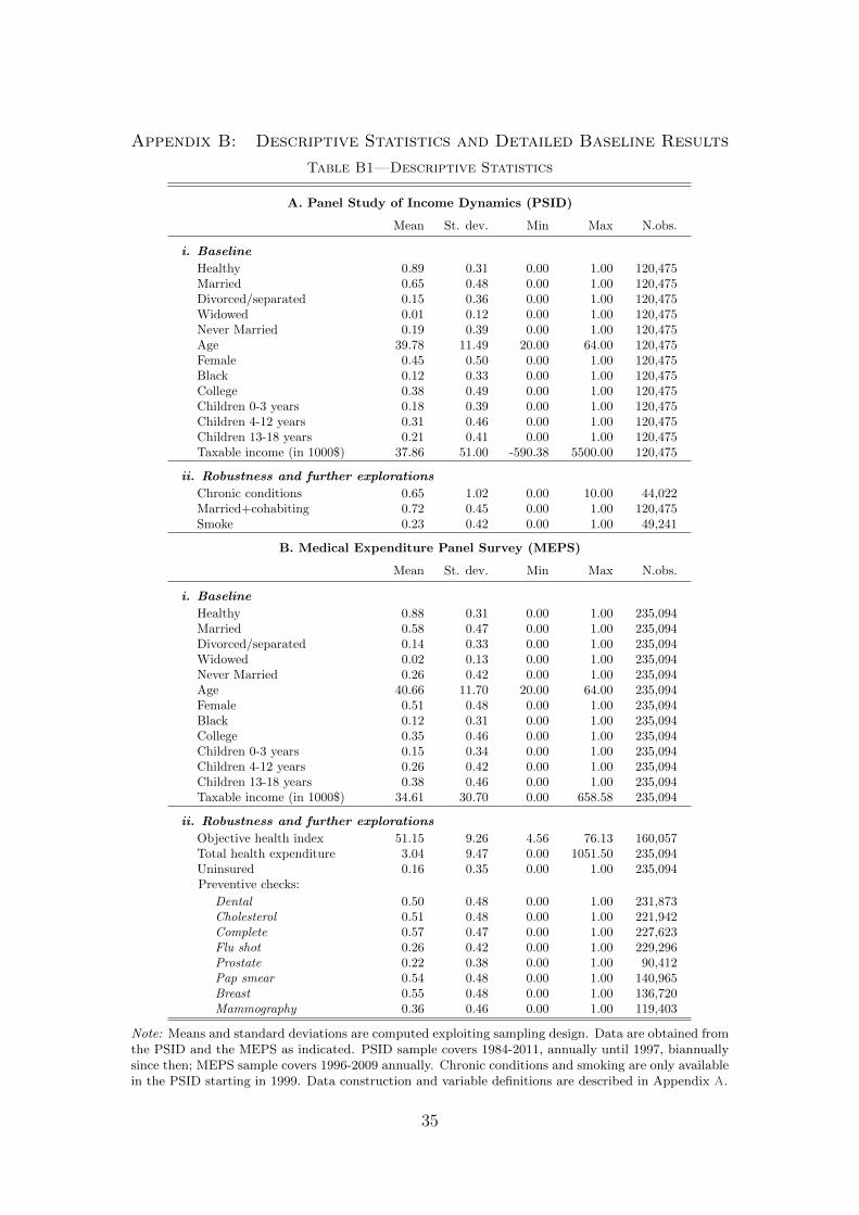
Appendix B: Descriptive Statistics and Detailed Baseline Results

Table B1—Descriptive Statistics

A. Panel Study of Income Dynamics (PSID)

Mean St. dev. Min Max N.obs.

i. Baseline

Healthy 0.89 0.31 0.00 1.00 120,475Married 0.65 0.48 0.00 1.00 120,475Divorced/separated 0.15 0.36 0.00 1.00 120,475Widowed 0.01 0.12 0.00 1.00 120,475Never Married 0.19 0.39 0.00 1.00 120,475Age 39.78 11.49 20.00 64.00 120,475Female 0.45 0.50 0.00 1.00 120,475Black 0.12 0.33 0.00 1.00 120,475College 0.38 0.49 0.00 1.00 120,475Children 0-3 years 0.18 0.39 0.00 1.00 120,475Children 4-12 years 0.31 0.46 0.00 1.00 120,475Children 13-18 years 0.21 0.41 0.00 1.00 120,475Taxable income (in 1000$) 37.86 51.00 -590.38 5500.00 120,475

ii. Robustness and further explorations

Chronic conditions 0.65 1.02 0.00 10.00 44,022Married+cohabiting 0.72 0.45 0.00 1.00 120,475Smoke 0.23 0.42 0.00 1.00 49,241

B. Medical Expenditure Panel Survey (MEPS)

Mean St. dev. Min Max N.obs.

i. Baseline

Healthy 0.88 0.31 0.00 1.00 235,094Married 0.58 0.47 0.00 1.00 235,094Divorced/separated 0.14 0.33 0.00 1.00 235,094Widowed 0.02 0.13 0.00 1.00 235,094Never Married 0.26 0.42 0.00 1.00 235,094Age 40.66 11.70 20.00 64.00 235,094Female 0.51 0.48 0.00 1.00 235,094Black 0.12 0.31 0.00 1.00 235,094College 0.35 0.46 0.00 1.00 235,094Children 0-3 years 0.15 0.34 0.00 1.00 235,094Children 4-12 years 0.26 0.42 0.00 1.00 235,094Children 13-18 years 0.38 0.46 0.00 1.00 235,094Taxable income (in 1000$) 34.61 30.70 0.00 658.58 235,094

ii. Robustness and further explorations

Objective health index 51.15 9.26 4.56 76.13 160,057Total health expenditure 3.04 9.47 0.00 1051.50 235,094Uninsured 0.16 0.35 0.00 1.00 235,094Preventive checks:

Dental 0.50 0.48 0.00 1.00 231,873Cholesterol 0.51 0.48 0.00 1.00 221,942Complete 0.57 0.47 0.00 1.00 227,623Flu shot 0.26 0.42 0.00 1.00 229,296Prostate 0.22 0.38 0.00 1.00 90,412Pap smear 0.54 0.48 0.00 1.00 140,965Breast 0.55 0.48 0.00 1.00 136,720Mammography 0.36 0.46 0.00 1.00 119,403

Note: Means and standard deviations are computed exploiting sampling design. Data are obtained fromthe PSID and the MEPS as indicated. PSID sample covers 1984-2011, annually until 1997, biannuallysince then; MEPS sample covers 1996-2009 annually. Chronic conditions and smoking are only availablein the PSID starting in 1999. Data construction and variable definitions are described in Appendix A.

35

Table B2—Detailed Estimation Results for Figures 4 and 5

MEPS PSID

OLS OLS Within-groups

Marriage gap β(a):

20-24 -0.027 (0.006) 0.009 (0.007) -0.010 (0.007)25-29 0.014 (0.004) 0.024 (0.006) -0.006 (0.005)30-34 0.030 (0.004) 0.027 (0.006) -0.001 (0.006)35-39 0.039 (0.005) 0.043 (0.009) -0.001 (0.007)40-44 0.051 (0.006) 0.054 (0.011) 0.010 (0.008)45-49 0.063 (0.006) 0.071 (0.013) 0.023 (0.010)50-54 0.085 (0.007) 0.083 (0.015) 0.048 (0.012)55-59 0.078 (0.008) 0.120 (0.020) 0.054 (0.017)60-64 0.078 (0.009) 0.107 (0.022) 0.037 (0.017)

Singles health curve α(a):

20-24 0.917 (0.004) 0.922 (0.007) 0.028 (0.026)25-29 0.873 (0.004) 0.898 (0.007) 0.037 (0.024)30-34 0.835 (0.005) 0.877 (0.009) 0.041 (0.023)35-39 0.807 (0.006) 0.845 (0.011) 0.045 (0.021)40-44 0.778 (0.006) 0.811 (0.012) 0.036 (0.020)45-49 0.741 (0.006) 0.768 (0.014) 0.021 (0.019)50-54 0.704 (0.007) 0.724 (0.015) -0.001 (0.017)55-59 0.691 (0.007) 0.662 (0.020) -0.012 (0.016)60-64 0.682 (0.009) 0.646 (0.021)

Controls:

College 0.055 (0.002) 0.073 (0.006) 0.009 (0.009)Female 0.000 (0.002) -0.005 (0.005)Black -0.020 (0.003) -0.069 (0.010)Children 0-3 years 0.001 (0.000) 0.001 (0.000) 0.000 (0.000)Children 4-12 years 0.001 (0.002) -0.004 (0.003) 0.003 (0.003)Children 13-18 years 0.001 (0.003) 0.000 (0.004) 0.006 (0.003)Taxable income (in 1000$) 0.001 (0.003) -0.013 (0.004) 0.006 (0.003)

Year dummies: Yes Yes Yes

Note: The table reports point estimates and standard errors from regressions presented in Figures 4and 5. OLS and Within-groups estimates are obtained from the PSID and the MEPS as indicated.

36

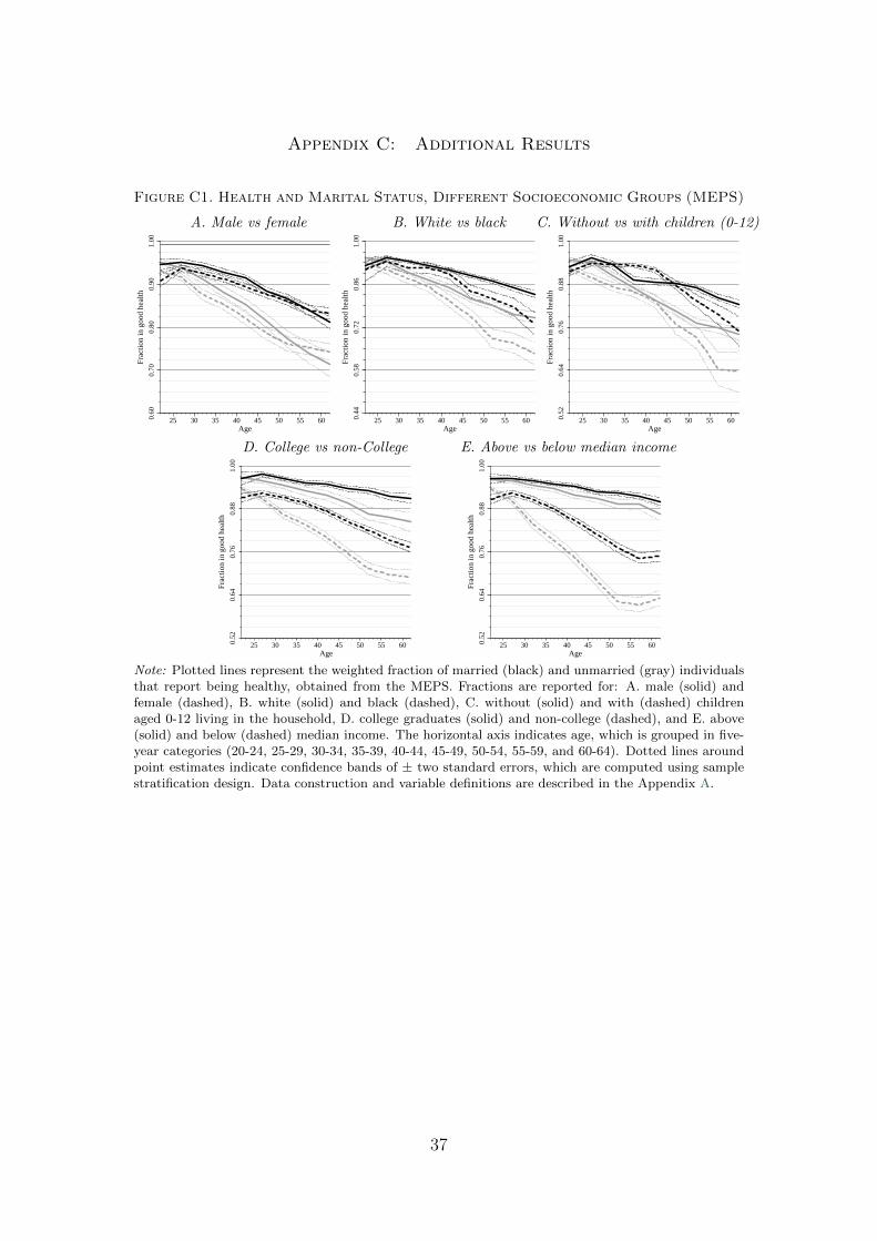
Appendix C: Additional Results

Figure C1. Health and Marital Status, Different Socioeconomic Groups (MEPS)

A. Male vs female B. White vs black C. Without vs with children (0-12)

0.60

0.70

0.80

0.90

1.00

25 30 35 40 45 50 55 60Age

Frac

tion

in g

ood

heal

th

0.44

0.58

0.72

0.86

1.00

25 30 35 40 45 50 55 60Age

Frac

tion

in g

ood

heal

th

0.52

0.64

0.76

0.88

1.00

25 30 35 40 45 50 55 60Age

Frac

tion

in g

ood

heal

th

D. College vs non-College E. Above vs below median income

0.52

0.64

0.76

0.88

1.00

25 30 35 40 45 50 55 60Age

Frac

tion

in g

ood

heal

th

0.52

0.64

0.76

0.88

1.00

25 30 35 40 45 50 55 60Age

Frac

tion

in g

ood

heal

th

Note: Plotted lines represent the weighted fraction of married (black) and unmarried (gray) individualsthat report being healthy, obtained from the MEPS. Fractions are reported for: A. male (solid) andfemale (dashed), B. white (solid) and black (dashed), C. without (solid) and with (dashed) childrenaged 0-12 living in the household, D. college graduates (solid) and non-college (dashed), and E. above(solid) and below (dashed) median income. The horizontal axis indicates age, which is grouped in five-year categories (20-24, 25-29, 30-34, 35-39, 40-44, 45-49, 50-54, 55-59, and 60-64). Dotted lines aroundpoint estimates indicate confidence bands of ± two standard errors, which are computed using samplestratification design. Data construction and variable definitions are described in the Appendix A.

37