econstor www.econstor.eu

Der Open-Access-Publikationsserver der ZBW – Leibniz-Informationszentrum WirtschaftThe Open Access Publication Server of the ZBW – Leibniz Information Centre for Economics

Standard-Nutzungsbedingungen:

Die Dokumente auf EconStor dürfen zu eigenen wissenschaftlichenZwecken und zum Privatgebrauch gespeichert und kopiert werden.

Sie dürfen die Dokumente nicht für öffentliche oder kommerzielleZwecke vervielfältigen, öffentlich ausstellen, öffentlich zugänglichmachen, vertreiben oder anderweitig nutzen.

Sofern die Verfasser die Dokumente unter Open-Content-Lizenzen(insbesondere CC-Lizenzen) zur Verfügung gestellt haben sollten,gelten abweichend von diesen Nutzungsbedingungen die in der dortgenannten Lizenz gewährten Nutzungsrechte.

Terms of use:

Documents in EconStor may be saved and copied for yourpersonal and scholarly purposes.

You are not to copy documents for public or commercialpurposes, to exhibit the documents publicly, to make thempublicly available on the internet, or to distribute or otherwiseuse the documents in public.

If the documents have been made available under an OpenContent Licence (especially Creative Commons Licences), youmay exercise further usage rights as specified in the indicatedlicence.

zbw Leibniz-Informationszentrum WirtschaftLeibniz Information Centre for Economics

Jalava, Nina; Schrøter Joensen, Juanna; Pellas, Elin

Working Paper

Grades and Rank: Impacts of Non-FinancialIncentives on Test Performance

IZA Discussion Papers, No. 8412

Provided in Cooperation with:Institute for the Study of Labor (IZA)

Suggested Citation: Jalava, Nina; Schrøter Joensen, Juanna; Pellas, Elin (2014) : Grades andRank: Impacts of Non-Financial Incentives on Test Performance, IZA Discussion Papers, No.8412

This Version is available at:http://hdl.handle.net/10419/101900

DI

SC

US

SI

ON

P

AP

ER

S

ER

IE

S

Forschungsinstitut zur Zukunft der ArbeitInstitute for the Study of Labor

Grades and Rank: Impacts of Non-Financial Incentives on Test Performance

IZA DP No. 8412

August 2014

Nina JalavaJuanna Schrøter JoensenElin Pellas

Grades and Rank: Impacts of Non-Financial

Incentives on Test Performance

Nina Jalava Stockholm School of Economics

Juanna Schrøter Joensen

Stockholm School of Economics and IZA

Elin Pellas

Stockholm School of Economics

Discussion Paper No. 8412 August 2014

IZA

P.O. Box 7240 53072 Bonn

Germany

Phone: +49-228-3894-0 Fax: +49-228-3894-180

E-mail: iza@iza.org

Any opinions expressed here are those of the author(s) and not those of IZA. Research published in this series may include views on policy, but the institute itself takes no institutional policy positions. The IZA research network is committed to the IZA Guiding Principles of Research Integrity. The Institute for the Study of Labor (IZA) in Bonn is a local and virtual international research center and a place of communication between science, politics and business. IZA is an independent nonprofit organization supported by Deutsche Post Foundation. The center is associated with the University of Bonn and offers a stimulating research environment through its international network, workshops and conferences, data service, project support, research visits and doctoral program. IZA engages in (i) original and internationally competitive research in all fields of labor economics, (ii) development of policy concepts, and (iii) dissemination of research results and concepts to the interested public. IZA Discussion Papers often represent preliminary work and are circulated to encourage discussion. Citation of such a paper should account for its provisional character. A revised version may be available directly from the author.

IZA Discussion Paper No. 8412 August 2014

ABSTRACT

Grades and Rank: Impacts of Non-Financial Incentives on Test Performance1

How does effort respond to being graded and ranked? This paper examines the effects of non-financial incentives on test performance. We conduct a randomized field experiment on more than a thousand sixth graders in Swedish primary schools. Extrinsic non-financial incentives play an important role in motivating highly skilled students to exert more effort. We find significant differences in test scores between the intrinsically motivated control group and three of four extrinsically motivated treatment groups. The only treatment not increasing test performance is criterion-based grading on an A-F scale, which is the typical grading method. Test performance is significantly higher if employing rank-based grading or giving students a symbolic reward. The motivational strengths of the non- financial incentives differ across the test score distribution, across the skill distribution, with peer familiarity, and with respect to gender. Boys are only motivated by rank-based incentives, while girls are also motivated by receiving a symbolic reward. Rank-based grading and symbolic rewards tend to crowd out intrinsic motivation for students with low skills, while girls also respond less to rank-based incentives if tested with less familiar peers. JEL Classification: I20, I21, D03, C93 Keywords: test-taking, performance incentives, effort, extrinsic and intrinsic motivation,

randomized experiment Corresponding author: Juanna Schrøter Joensen Department of Economics Stockholm School of Economics Sveavägen 65 Box 6501 SE 113 83 Stockholm Sweden E-mail: Juanna.Joensen@hhs.se

1 We would like to express our gratitude to the teachers and students who made this project possible through participating in the experiment - thanks for your time and collaboration. This paper also benefited from discussions with José Araújo, Ghazala Azmat, Tore Ellingsen, David Figlio, Jonathan Guryan, Krista Jonvør Schrøter Joensen, and participants at the workshop on Self-Control, Self-Regulation and Education in Aarhus. The usual disclaimer applies.

1 Introduction

Student performance is tightly linked to student motivation and effort. Improving student

performance is a key educational policy issue to which much time and resources are de-

voted. Student quality is typically assessed by the performance on various tests, yet little

is known about student motivation and effort in test situations. A better understanding

of how students respond to different test setups and different incentives can benefit the

equity and efficiency of the educational system, as test performance only reflects true

student quality if incentives are appropriately aligned. Low student test effort among

some students could thus create substantial biases in the measure of student quality of-

ten underlying high-powered incentive schemes such as school accountability systems, the

distribution of school resources, as well as teacher value added and performance pay.

Grading students is used as a screening device in school admission procedures. Grad-

ing may ensure effective communication of student performance between schools and

families, so students may be more efficiently tracked and students who require additional

assistance are identified and can receive necessary support. But what are the short-term

consequences of grading on student motivation and effort? How does student effort re-

spond to being graded - particularly on a test that is low-stake for the students but

can carry high stakes for the teachers and schools administrating the test? What if we

introduce alternative ways of incentivizing students?

In this paper, we analyze the effects of grading and non-financial extrinsic incentives

on student effort on a math test. A field experiment is conducted on 1,045 sixth grade

students to evaluate how short term effort can be affected by students receiving different

information on the assessment of the test. We focus exclusively on evaluating non-financial

means of incentivizing students, since these are relatively uncontroversial and widespread

in many grading schemes and educational settings. Additionally, primary school students

are found to respond strongly to immediate non-financial incentives (Levitt et al., 2012). It

is, however, not known which non-financial incentives are most effective at raising student

effort. The incentives we analyze are: (1) students receiving criterion-based grades A-F,

2

(2) students receiving grade A if they are among the top three performing students in

their class, (3) students receiving a certificate if they exceed the criterion-based score

for A-B, and (4) students receiving a prize if they are among the top three performing

students in their class. We randomize within the classroom and provide students with

information regarding the nature of the test immediately before they start. However,

the true purpose of the test is revealed only afterwards. Student treatment assignment

is private information. As the students have no possibility to prepare for the test, we

are able to isolate the role of effort from other factors affecting test performance. Tests

are conducted in the students’ natural learning environment to resemble the low-stake

tests students are taking at several schooling stages; e.g. widespread national school

accountability tests and international tests like the Programme for International Student

Assessment (PISA) and the Trends in International Mathematics and Science Study

(TIMSS). As these tests may be high-stake for schools and teachers, it is important that

students exert effort in order for the test to reflect student ability. We also compare these

different non-financial incentive designs in different school settings - spanning low and high

performing schools, as well as schools with diverse student socioeconomic backgrounds.

To the best of our knowledge, this is the first paper to directly evaluate and compare

the incentive effects of the standard criterion-based grades A-F, as well as the incentive

effects of introducing rank-based grading through tournaments within the classroom.

We find that the impacts vary substantially by student skill level.2 For highly skilled

students, the intrinsically motivated students in the control group provide as much test

effort as those graded according to the typical A-F grading scale; i.e. treatment (1). Test

performance is, however, significantly higher if employing rank based grading or giving

students symbolic rewards; i.e. treatments (2)-(4). We further find that motivational

strengths of the non-financial incentives differ across the test score distribution and with

respect to gender. Boys only increase their performance when facing rank-based grading.

Girls respond as strongly to rank-based grading, but they also respond strongly to being

2Note that skill level denotes student placement on the learning trajectory, while ability denotes stu-dent placement in the underlying math ability distribution at any given point on the learning trajectory.Highly skilled students are thus those who have been exposed to more math teaching, while lower skilledstudents have learned less math.

3

rewarded a certificate. The average treatment effects are between a third and half a

standard deviation. The non-financial incentives primarily work by making the students

in the two middle quartiles of the ability distribution exert more effort on the test.

For students with lower skill levels, however, there is no significant effect of non-financial

incentives. We observe the tendency that rank-based grading and symbolic rewards crowd

out intrinsic motivation, as the extrinsic incentives significantly decrease test scores for

the students in the bottom decile of the ability distribution where more students do not

exert any effort on the test. This effect is somewhat mitigated if students have been with

the same peer group for at least a school year.

By approaching the issue of student motivation and performance from a behavioral

economics perspective, we are able to achieve a better understanding of student motiva-

tion and effort in test situations and understand how students react to different incentives.

Our results call into question the current structure of the educational system in motivat-

ing highly skilled students in test situations and suggest that alternative non-financial

incentives may increase student effort and lead to better educational outcomes. Another

aspect to consider is familiarity with peers and their skills, as students tend to respond

differently when they are tested at an earlier stage of their learning trajectory and with

a new peer group. This has considerable policy implications, as it suggests that it is piv-

otal to take peer familiarity, the student skill level, and the student ability distribution

into account when implementing incentives and evaluating their effectiveness. Otherwise,

distributing resources based on test scores may lead to inefficient allocation of resources

as some students exert low effort and test scores do not reflect true student ability and

quality.

The remainder of this paper is organized as follows: Section 2 relates our paper to

previous literature. Section 3 sets up the theoretical framework and testable predictions.

Section 4 lays out the experimental design and implementation. Sections 5 and 6 present

the experimental data and the empirical results. Finally, sections 7 and 8 provide a

discussion and conclusion.

4

2 Background

The distinction between intrinsic and extrinsic motivation is fundamental in an educa-

tional setting. Intrinsic motivation refers to motivation coming from within the students

themselves and is driven by an interest in, or enjoyment of, the task itself. Extrinsic

motivation relies on external factors as a driving force for motivating the students. Many

studies on motivating students extrinsically have used financial means as a method of

motivating; paying students has been shown to result in better performance (Bettinger

and Slonim, 2007; Eisenkopf, 2011; Fryer, 2011; Bettinger, 2012; Levitt et al., 2012).

Opponents worry that the introduction of extrinsic incentives can have a detrimental

effect on students’ future performance, as extrinsic motivation may crowd out intrin-

sic motivation. Especially for young students, tangible rewards seem to have a stronger

detrimental effect on intrinsic motivation than for college students (Deci et al., 1999).

However, neither Levitt et al. (2012) nor Bettinger and Slonim (2007) find evidence that

extrinsic incentives are detrimental to primary school students’ intrinsic motivation and

test performance.

Extrinsic motivation can come in many different forms. While a majority of research

has focused on the implementation of financial rewards, there is evidence that the effect of

non-financial rewards can be considerable. Kosfeld and Neckermann (2011) find that non-

financial rewards such as awards or trophies can have significant motivational power in

the workplace, since awards yield non-material benefits in the form of social recognition,

status, and improved self-esteem (Weiss and Fershtman, 1998; Ellingsen and Johannesson,

2007). Besley and Ghatak (2008) find that status incentives increase effort while reducing

the optimal level of financial incentives. Levitt et al. (2012) directly compare the effects of

financial and non-financial rewards on short-term student effort and performance. They

find that giving primary school students a trophy leads to as large an increase in test

performance as financial rewards in the range of USD 10-20. However, how do the effects

of different non-financial incentives on test effort compare?

Ranking students by their performance is another tool that can be used as a source

5

of motivation, as rank in itself may work as a major motivator. Tran and Zeckhauser

(2012) confirm that the desire to rank highly has a measurable impact on behavior, while

Delfgaauw et al. (2013) find a high symbolic value of winning a tournament and a mea-

surable increase in retail store sales when tournament incentives are in place. Rank can

be used by students to impress friends and family and to earn respect and admiration,

which can be seen as tangible benefits. Students may also be directly psychologically

rewarded by higher rank without the need for any tangible benefits. Students who receive

rank publicly outperform those who receive their rank privately, but even when ranking

information cannot be reliably communicated Tran and Zeckhauser (2012) find an effect

on performance. Rank as a motivator in school can often be seen in the form of norm-

referenced grading, where students are assigned grades relative to the performance of

other students. Azmat and Iriberri (2010) show that high school students receiving rela-

tive rank feedback increase short-term performance, while Murphy and Weinhardt (2013)

also show an increase in secondary school performance by having a higher primary school

rank. However, it is still an open question whether rank-based grading incentives in the

form of a tournament affect student test effort.

Wise and DeMars (2005) discuss a number of potential assessment practices for man-

aging the problems posed by low student motivation leading to lower test performance.

The issue of students not exerting full effort on a test is of critical importance to assess-

ment practitioners, as the results will tend to underestimate the students’ true ability.

Wise and DeMars (2005) show that motivation is an essential factor in test performance

and that higher motivation is associated with higher test scores. Motivation is therefore

an important factor in eliciting test results that accurately reflect a student’s true ability

and knowledge.

Students tend to exert low effort on standardized tests in the absence of immediate

incentives (Attali et al., 2011; Levitt et al., 2012). These standardized tests are often of

little importance to the students (i.e. low-stake tests) but may have important conse-

quences for the teachers and schools (e.g. in the form of allocation of resources) and are

as such high-stake tests for the teachers and the schools. Attali et al. (2011) show that

6

males exhibit a larger difference in performance between low and high-stake tests than

females, and also find that students with a higher socioeconomic status showed larger dif-

ferences in performance. Levitt et al. (2012) find that the effects of introducing extrinsic

motivators are larger for boys than for girls; i.e. boys are more responsive to short-term

incentives than girls. This suggests that girls may be more intrinsically motivated, and

therefore also be at a higher risk of crowding out. In their experiment of around 6,500

primary and high school students, Levitt et al. (2012) examine various types of moti-

vators; including financial and non-financial incentives, immediate rewards and rewards

handed out with a delay, as well as rewards framed as losses. They find that incentives

framed as losses - giving the reward before the test and taking it back if test scores are not

improved - have a stronger effect than other incentives, and that non-financial incentives

are effective on primary school students but have little effect on older students. They also

find that delayed rewards have no motivational power. This has important implications

for the way the educational system is currently set up, with almost all feedback coming

with a delay. Our study complements Levitt et al. (2012) as they only evaluate one non-

financial incentive - a trophy for improved test performance - whereas we compare the

impacts of four non-financial incentives representing different ways of grading and dif-

ferent immediate rewards. Our estimated average treatment effects range from being as

large or larger (0.33 - 0.45 standard deviations) for highly skilled students to smaller than

theirs for low-skilled students. This could both be due to the nature of the incentives,

the element of competition relative to one’s peers inherent in two of our treatments, and

as highlighted by the theoretical framework in the following section and in Section 6 -

which part of the students’ learning trajectory the test is administered at.3

In a related paper, Baumert and Demmrich (2001) aim at increasing around 500

German ninth grade students’ stake on a shorter version of the PISA test through both

financial and non-financial incentives. Their three non-financial incentives entail getting

information on the importance of the test, later performance feedback from their math

3Their tests are administered in the fall, winter, and spring, and their outcome is test score im-provement relative to baseline test score one or two trimesters earlier. Our outcome is the test score,benchmarked by the control group test score at the same test occasion. This way we avoid issues of noisytest scores and regression to the mean (Kane and Staiger, 2002; Chay et al., 2005).

7

teacher, and making the test count towards their math course grade. They do not find

any significant average treatment effects. This could be because rewards are experienced

with a delay (Levitt et al., 2012), but our results suggest that this could also be because

the students were unfamiliar with the test tasks or because their treatment is based on a

criterion-based grading scale.

Lastly, our paper is also related to the literature on educational and grading stan-

dards (Becker and Rosen, 1992; Costrell, 1994; Betts, 1998; Betts and Grogger, 2003;

Figlio and Lucas, 2004) and the timing of grading (Sjogren, 2010; Facchinello, 2014)

focusing on the longer-term impacts of grading (standards) on educational choices and

labor market performance. We contribute to this literature by isolating the short-term

test effort effect and providing internally valid estimates of the differential impacts of

criterion- and reference-based grading methods on test performance.

This background motivates and formulates our research question: How can students be

incentivized to exert higher effort on tests without crowding out intrinsic motivation? We

contribute to the literature by evaluating different non-financial methods of incentivizing

primary school students, comprising different grading methods and symbolic rewards.

Even if students are being tested and graded increasingly often, there is a prominent gap

in research on student test-taking motivation. We analyze how test scores of extrinsically

incentivized students differ from those of intrinsically motivated students, both on average

and across the distribution. We focus exclusively on non-financial incentives. We also

analyze how the incentive effects differ with respect to skill level, gender, and peers. To

the best of our knowledge, this is the first paper to (i) directly evaluate test effort induced

by standard A-F criterion-based grading, (ii) evaluate test effort responses to rank-based

grading through tournaments, as well as (iii) directly compare these grading methods.

3 Theoretical Framework

Our experimental results can be interpreted through the lens of a simple version of

Becker’s Woytinsky lecture model (Becker, 1967). Students are endowed with ability

8

(reflecting actual math knowledge) and have to decide how much effort to put into the

low-stake test. Test scores are determined by ability, ai, effort, ei, and a random term, εi,

capturing how sharp and lucky the student is when taking the test:

TSi = γ0 + γ1ai + γ2ei + εi (1)

Test scores are increasing in ability and effort, hence γ1 > 0 and γ2 > 0. Ability is fixed

in the test situation, since the teachers are not informed about the exact nature of the

test and the students are not informed about the test taking place until the outset of

the class in which it is conducted. Students have no participation decision, as all of them

have to sit at their desk during the ten minutes of the test duration. This enables us to

isolate the impacts of extrinsic incentives on test performance through effort.

Students care about the effort they have to put into the test, as it may be inherently

costly to exert effort. Let c(e) denote the cost of effort. We assume the cost function

is twice continuously differentiable, increasing, and convex: c′(e) ≥ 0 and c′′(e) ≥ 0,

implying that increasing marginal effort is even more costly when already exerting a high

effort. We set c(0) = 0, c′(0) = 0, and c′′(0) = 0. Students also care about the reward they

get from the test, R. To provide a simple example of how extrinsic incentives work in this

model, we assume this reward is only achieved if the test score exceeds a predetermined

cut-off, TSi ≥ TS.4 Let Fε denote the cumulative distribution function (CDF) and fε the

probability density function (pdf) of ε. Students choose effort to maximize utility:

maxei

{(1− Fε

(TS − γ0 − γ1ai − γ2ei

))R− c(ei)

}(2)

subject to ei ≥ 0. Optimal effort, e∗i , equates marginal benefits with marginal costs and

is characterized by:

e∗i[fε(TS − γ0 − γ1ai − γ2e

∗i

)γ2R− c′(e∗i )

]= 0, (3)

4Allowing students to care about their test scores would not change the insights from this simplemodel. Caring about learning and test performance will be captured in the cost function in this statictest setting.

9

c′(e∗i ) ≥ fε(TS − γ0 − γ1ai − γ2e

∗i

)γ2R, (4)

and e∗i ≥ 0. The marginal benefit here comes exclusively from the probability of receiving

the reward for achieving a test score higher than TS, while the marginal cost comes from

increasing effort. If the marginal benefit is too low or the marginal cost is too high, then

the student will optimally exert no effort on the test, e∗i = 0.

A reduction in intrinsic motivation can be interpreted as an increase in the cost of

effort. If student effort cost is increased, students will exert less effort on the test and

more students will exert no effort.

A more valuable reward (increased R) means that it will be worth it to increase ef-

fort for some students, while a less valuable reward (decreased R) similarly will decrease

effort for some students. This is easy to illustrate: Ability is fixed in the test setting,

but students choose how much effort to exert. How does optimal effort depend on abil-

ity? What happens if we introduce (or increase) rewards for high performance? Assume

for simplicity that both the random term and ability are normally distributed. Firstly,

students with very high ability, ai ≥ a, will not be affected by the increased reward as

they still do not have to change their optimal effort in order to attain the reward. Their

optimal effort will still be positive though, e∗i > 0. Secondly, students at the margin,

a ≤ ai ≤ a, will increase their effort in response to the increased reward, e∗i > 0. Lastly,

low ability students, ai ≤ a, with too low ability to have a positive probability of attaining

the reward will choose not to exert any effort on the test, e∗i = 0. This is illustrated in

Figure 1.

3.1 Reward Threshold and Skills

A more interesting situation in our experimental setting is what happens if we increase

the cut-off for attaining the reward. Increasing competitiveness can be seen as making

the reward harder to attain; increase TS > TS. This means that there will still be

some students with very high ability, ai ≥ a, for which optimal effort stays the same,

e∗∗i = e∗i > 0, while students with ability, a ≤ ai ≤ a, will have to exert more effort

in order to attain the reward, e∗∗i > e∗i > 0, students with ability, a ≤ ai ≤ a, exert

10

the same positive effort as before, and students with ability below a will exert minimal

effort, e∗∗i = 0. Some of these also exerted minimal effort before the increase, but some of

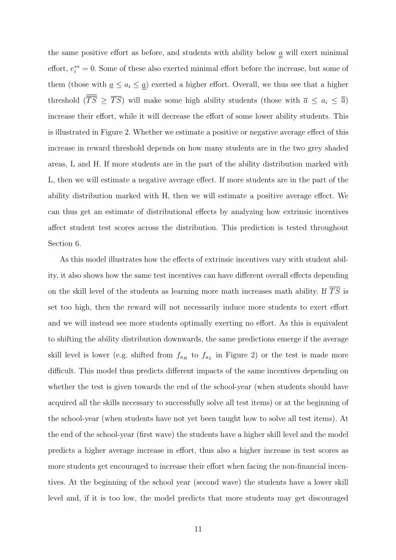
them (those with a ≤ ai ≤ a) exerted a higher effort. Overall, we thus see that a higher

threshold (TS ≥ TS) will make some high ability students (those with a ≤ ai ≤ a)

increase their effort, while it will decrease the effort of some lower ability students. This

is illustrated in Figure 2. Whether we estimate a positive or negative average effect of this

increase in reward threshold depends on how many students are in the two grey shaded

areas, L and H. If more students are in the part of the ability distribution marked with

L, then we will estimate a negative average effect. If more students are in the part of the

ability distribution marked with H, then we will estimate a positive average effect. We

can thus get an estimate of distributional effects by analyzing how extrinsic incentives

affect student test scores across the distribution. This prediction is tested throughout

Section 6.

As this model illustrates how the effects of extrinsic incentives vary with student abil-

ity, it also shows how the same test incentives can have different overall effects depending

on the skill level of the students as learning more math increases math ability. If TS is

set too high, then the reward will not necessarily induce more students to exert effort

and we will instead see more students optimally exerting no effort. As this is equivalent

to shifting the ability distribution downwards, the same predictions emerge if the average

skill level is lower (e.g. shifted from faH to faL in Figure 2) or the test is made more

difficult. This model thus predicts different impacts of the same incentives depending on

whether the test is given towards the end of the school-year (when students should have

acquired all the skills necessary to successfully solve all test items) or at the beginning of

the school-year (when students have not yet been taught how to solve all test items). At

the end of the school-year (first wave) the students have a higher skill level and the model

predicts a higher average increase in effort, thus also a higher increase in test scores as

more students get encouraged to increase their effort when facing the non-financial incen-

tives. At the beginning of the school year (second wave) the students have a lower skill

level and, if it is too low, the model predicts that more students may get discouraged

11

compared to how many get encouraged. If this is the case, we may actually estimate an

average decrease in test scores. The model thus illustrates that the size and direction of

incentive effects is closely linked to the student skill level. This prediction is tested in

Section 6.1 exploiting the fact that we test students at different points in their learning

trajectory.

3.2 Rank-Based Rewards and Peer Familiarity

A simple extension of the model also illustrates how the incentive effects of rank-based

grading depend on peer familiarity. The illustration above assumes an exogenously set

criterion-based (or absolute) threshold similar to our treatments 1 and 3. The model is

easily adapted to a rank-based (or relative) grading scheme, where the threshold will

be endogenously determined as it depends on the ability and effort of peers. Even if

the solution becomes more involved, all the basic predictions go through.5 We simply

illustrate this assuming there are only two students in the class, i and j, and the reward

is only received by the highest ranked student. Student i thus only receives the reward

if performing better than student j, i.e. if TSi ≥ TSj, and seeks to choose effort to

maximize utility given by:

maxei{(1− F2ε (γ1(aj − ai) + γ2(ej − ei)))R− c(ei)} (5)

subject to ei ≥ 0. Student j solves the mirror image of this maximization problem. First,

note that the rank-based grading problem in (5) is equivalent to the criterion-based

grading problem in (2), but with the exogenous threshold, TS, replaced by γ1aj + γ2ej.

In this sense the new threshold for receiving the reward is endogenous, as it depends on

the other student’s ability and effort choice. Each student’s effort choice thus becomes

a best response to what the other student will do. Second, note that the constant γ0

cancels out when only students’ relative performance on the test matters. Third, note

that uncertainty is higher with rank-based grading as Fε in (2) is replaced by F2ε which

5This setup is similar to the rank-order tournament model introduced by Lazear and Rosen (1981)

12

is the CDF of εi− εj. Assuming that the random terms are independently and identically

normally distributed with mean 0 and variance σ2, the difference between the random

terms will also be normally distributed with mean 0 and variance 2σ2. The increased

uncertainty simply means that increasing effort with rank-based grading does not increase

the probability of receiving the reward by as much as increasing effort with criterion-based

grading. Otherwise, all the basic insights from the solution (3) above go through. The

only caveats are that as uncertainty increases, the reward threshold becomes endogenous,

γ1aj + γ2ej, and information about one’s peers’ ability therefore becomes important with

rank-based grading similar to our treatments 2 and 4. Just to give a brief overview: If

students have the same ability, ai = aj, and also face the same effort cost, then the

noncooperative solution implies that both choose the same optimal effort, ei = ej. Rank-

based grading with identical ability students amounts to a zero sum game, where both

ex-ante choose to exert equally much test effort and the ex-post outcome is like flipping

a fair coin. If ability is heterogeneous, however, the student with higher ability has a

higher probability of being the highest ranked. This is equivalent to the case with an

exogenous threshold, TS, where the higher ability students do not have to increase effort

to be above the threshold and receive the reward. There will again be some students

with very low ability relative to their peers who will have a zero probability to be highest

ranked, even if exerting maximal effort, and will therefore exert minimal effort, ei = 0.

This prediction that the expectation of peer ability is important for effort responses to

rank-based grading is tested in Section 6.2 by exploiting the fact that some students have

more information about the peers they are competing with than others. We hypothesize

that those who have spent at least a school year in the same classroom as their peers

will have a more precise estimate of their peers’ ability, thus they face less uncertainty

about the endogenous threshold and their effort will respond more strongly to rank-based

grading incentives.

13

4 Empirical Strategy

In this section we explain the experimental design and its implementation, the school

environment, and the construction of treatment variables.

4.1 Experimental Design

We conducted a randomized field experiment to investigate the motivational power of non-

financial incentives on primary school students. Students in the experiment were assigned

to one out of five groups; either to an unincentivized control group or to an incentivized

treatment group. By randomly allocating the control and four different treatments within

each class, we are able to examine the effect of one incentivizing factor at a time, and

minimize the impact of endogenous variables such as family, school, and class-specific

factors. Students were offered no choice in whether to participate or not, and therefore we

eliminate the potential sample selection bias that could arise with voluntary participation

and self-selection. The randomization process means that we obtain groups that are

statistically equivalent to each other, and we can thereby simply compare the difference

between the means of the treatment groups and the control group to obtain internally

valid estimates of the average causal effect of treatment (ATE).

Although the experimental approach circumvents the problem of selection bias and

offers the virtue of internal validity, it does bring some potential issues regarding envi-

ronmental dependence and replicability. We can not guarantee that our results would

hold if the experiment were to be repeated in a different context. As our experimental

design poses a threat to external validity, its results should best be interpreted as what

can happen but not necessarily what will happen in an external environment where other

variables are free to operate without being tightly controlled.

To ensure the robustness of our results, we also present estimates where we control

for factors differing at the time of the test, gender, peer familiarity, class size, and school-

specific factors. These are factors that may causally affect the outcome variable. To

assess heterogeneity of treatment effects and external validity we also present estimates

14

separately by gender, skill level, and peer familiarity.

4.2 Implementation and School Environment

The experiment was conducted on Swedish primary school students. We chose to include

sixth graders because it is the last year of primary school in Sweden. Primary school

is made up of grades one through six, with secondary school following for grades seven

through nine. These grades all comprise compulsory schooling. Another reason for choos-

ing sixth graders is the recent (in 2012) reintroduction of grading for sixth graders in

Sweden.6 Previously, students received grades only once they reached eighth grade of sec-

ondary school. Now a comprehensive Swedish national exam is administered to all sixth

grade students in order to assure uniform and fair grading. The test is administered by the

Swedish National Agency for Education (Skolverket) and provides a basis for evaluating

the extent to which knowledge requirements are met at the teacher level, the principal

level, the school level, and the national level. The test is also meant to assure that the cur-

riculum is fostering the desired knowledge requirements and learning outcomes. Students

are typically 12 years old when entering sixth grade and most become teenagers during

this school year. Sixth grade is thus considered a critical stage in the student transition

from primary to secondary school.

The experiment was carried out on 1,045 sixth grade students in a total of 47 classes

in 17 schools in the Stockholm municipality. Each school in the City of Stockholm’s direc-

tory of compulsory schools was given a number, and with the aid of an online randomizer,

we randomly selected the set of schools to contact. Teachers were contacted by telephone

and asked to participate in our experiment. The sessions were usually carried out one to

two weeks after the phone call was made. Out of 22 contacted schools in total, 10 accepted

in the first wave and all schools accepted in the second wave. The only expressed reason

for not participating was the heavy student workload, however we assess that this would

have been more or less equivalent irrespective of school. We do not suspect that the teach-

ers’ choice of participating should have led to a biased sample, as all participating and

6Swedish sixth graders have not been graded since 1982. Sjogren (2010) and Facchinello (2014) analyzethe impacts of the gradual abolishment of grades for younger students.

15

non-participating schools showed a similar wide variety of school-specific characteristics.

Furthermore, teachers received limited information on the specifics of the experiment.

We therefore see the choice of accepting or declining as random, or at the very least not

correlated with the nature of the experiment. Schools accepting the study are represented

both on the high-performing and low-performing ends of the spectrum, and are diverse

with respect to geographic location and socioeconomic factors.

The first wave of the experiment took place in April 2013 and the second wave of

the experiment took place at the end of August and beginning of September 2013. The

experiment was carried out during scheduled lecture hours and consisted of a standardized

mathematical test containing four tasks giving a maximum of 22 points in total. The

tasks matched the level of difficulty of tasks in the Swedish national tests for sixth grade.

Furthermore, they were designed with support from educated primary school teachers not

present at any of the schools where the experiment was conducted. They were formulated

in such a way as to allow efficient and impartial grading. The students in the two waves

were presented with identical tests and we verify that there was no grade retention. Thus

it was primarily student preparation relative to the fixed test difficulty that changed

between the two waves and no student took the test twice.

All sessions were introduced and conducted by us while in the presence of the teacher,

thus encouraging students to perceive the experiment as formal. This was done to establish

commitment to the task and to encourage students to take the test seriously. Special care

was taken to ensure that the experiment was presented in an equal, or at least in a very

similar, way for all classes. The aim was for the experiment to be perceived equally by all

participating students. Some students may have viewed the test as more important than

others and as such applied more effort, but overall, no systematic deviations should exist

between the groups.

In each class, we randomly assigned students to control and treatment groups by hand-

ing out tests with differing information concerning the assessment of their performance.

We did this in a randomized fashion. To prevent any kind of preparation, teachers had

received limited information regarding the formalities of the test. Just before the test

16

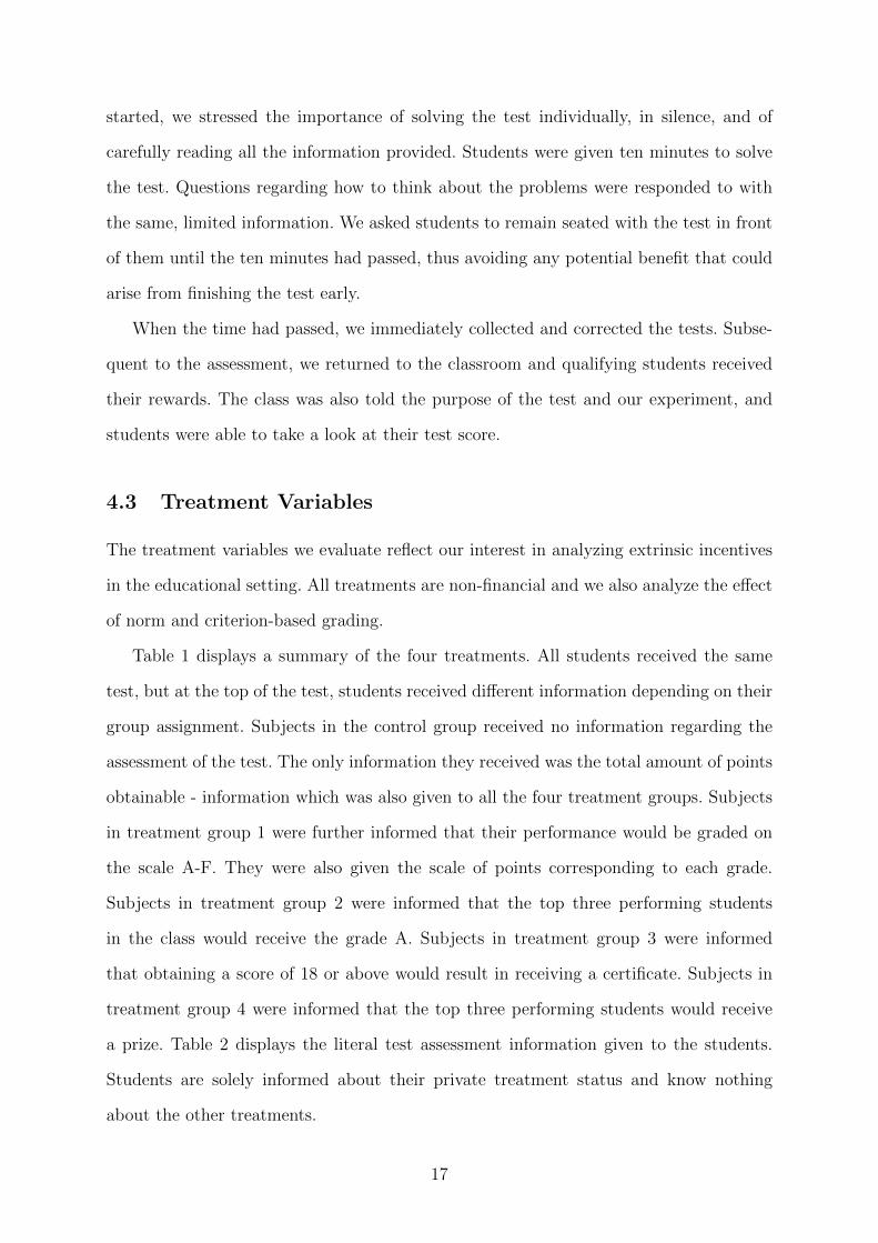
started, we stressed the importance of solving the test individually, in silence, and of

carefully reading all the information provided. Students were given ten minutes to solve

the test. Questions regarding how to think about the problems were responded to with

the same, limited information. We asked students to remain seated with the test in front

of them until the ten minutes had passed, thus avoiding any potential benefit that could

arise from finishing the test early.

When the time had passed, we immediately collected and corrected the tests. Subse-

quent to the assessment, we returned to the classroom and qualifying students received

their rewards. The class was also told the purpose of the test and our experiment, and

students were able to take a look at their test score.

4.3 Treatment Variables

The treatment variables we evaluate reflect our interest in analyzing extrinsic incentives

in the educational setting. All treatments are non-financial and we also analyze the effect

of norm and criterion-based grading.

Table 1 displays a summary of the four treatments. All students received the same

test, but at the top of the test, students received different information depending on their

group assignment. Subjects in the control group received no information regarding the

assessment of the test. The only information they received was the total amount of points

obtainable - information which was also given to all the four treatment groups. Subjects

in treatment group 1 were further informed that their performance would be graded on

the scale A-F. They were also given the scale of points corresponding to each grade.

Subjects in treatment group 2 were informed that the top three performing students

in the class would receive the grade A. Subjects in treatment group 3 were informed

that obtaining a score of 18 or above would result in receiving a certificate. Subjects in

treatment group 4 were informed that the top three performing students would receive

a prize. Table 2 displays the literal test assessment information given to the students.

Students are solely informed about their private treatment status and know nothing

about the other treatments.

17

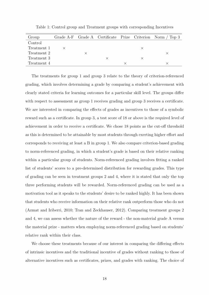
Table 1: Control group and Treatment groups with corresponding Incentives

Group Grade A-F Grade A Certificate Prize Criterion Norm / Top 3

ControlTreatment 1 × ×Treatment 2 × ×Treatment 3 × ×Treatment 4 × ×

The treatments for group 1 and group 3 relate to the theory of criterion-referenced

grading, which involves determining a grade by comparing a student’s achievement with

clearly stated criteria for learning outcomes for a particular skill level. The groups differ

with respect to assessment as group 1 receives grading and group 3 receives a certificate.

We are interested in comparing the effects of grades as incentives to those of a symbolic

reward such as a certificate. In group 3, a test score of 18 or above is the required level of

achievement in order to receive a certificate. We chose 18 points as the cut-off threshold

as this is determined to be attainable by most students through exerting higher effort and

corresponds to receiving at least a B in group 1. We also compare criterion-based grading

to norm-referenced grading, in which a student’s grade is based on their relative ranking

within a particular group of students. Norm-referenced grading involves fitting a ranked

list of students’ scores to a pre-determined distribution for rewarding grades. This type

of grading can be seen in treatment groups 2 and 4, where it is stated that only the top

three performing students will be rewarded. Norm-referenced grading can be used as a

motivation tool as it speaks to the students’ desire to be ranked highly. It has been shown

that students who receive information on their relative rank outperform those who do not

(Azmat and Iriberri, 2010; Tran and Zeckhauser, 2012). Comparing treatment groups 2

and 4, we can assess whether the nature of the reward - the non-material grade A versus

the material prize - matters when employing norm-referenced grading based on students’

relative rank within their class.

We choose these treatments because of our interest in comparing the differing effects

of intrinsic incentives and the traditional incentive of grades without ranking to those of

alternative incentives such as certificates, prizes, and grades with ranking. The choice of

18

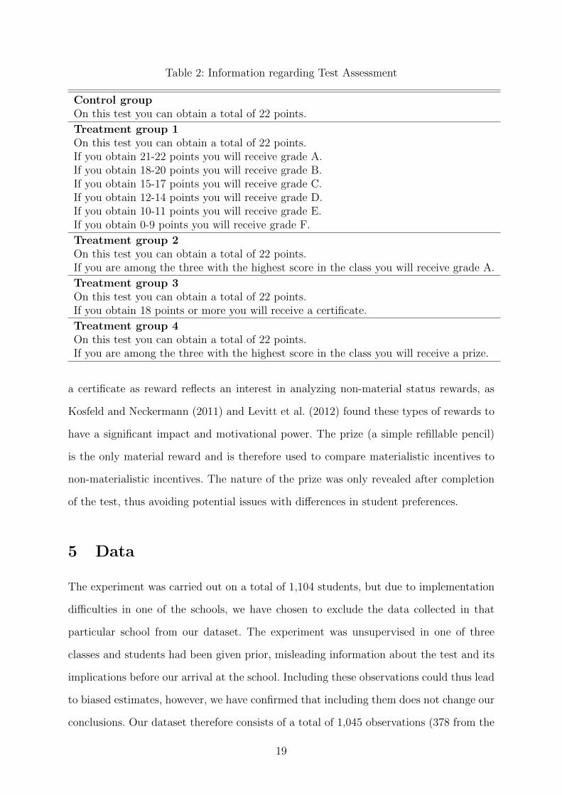
Table 2: Information regarding Test Assessment

Control groupOn this test you can obtain a total of 22 points.

Treatment group 1On this test you can obtain a total of 22 points.If you obtain 21-22 points you will receive grade A.If you obtain 18-20 points you will receive grade B.If you obtain 15-17 points you will receive grade C.If you obtain 12-14 points you will receive grade D.If you obtain 10-11 points you will receive grade E.If you obtain 0-9 points you will receive grade F.

Treatment group 2On this test you can obtain a total of 22 points.If you are among the three with the highest score in the class you will receive grade A.

Treatment group 3On this test you can obtain a total of 22 points.If you obtain 18 points or more you will receive a certificate.

Treatment group 4On this test you can obtain a total of 22 points.If you are among the three with the highest score in the class you will receive a prize.

a certificate as reward reflects an interest in analyzing non-material status rewards, as

Kosfeld and Neckermann (2011) and Levitt et al. (2012) found these types of rewards to

have a significant impact and motivational power. The prize (a simple refillable pencil)

is the only material reward and is therefore used to compare materialistic incentives to

non-materialistic incentives. The nature of the prize was only revealed after completion

of the test, thus avoiding potential issues with differences in student preferences.

5 Data

The experiment was carried out on a total of 1,104 students, but due to implementation

difficulties in one of the schools, we have chosen to exclude the data collected in that

particular school from our dataset. The experiment was unsupervised in one of three

classes and students had been given prior, misleading information about the test and its

implications before our arrival at the school. Including these observations could thus lead

to biased estimates, however, we have confirmed that including them does not change our

conclusions. Our dataset therefore consists of a total of 1,045 observations (378 from the

19

first wave and 667 from the second wave) from 47 classes and 17 schools. Of the 1,045

students, 493 are boys and 552 are girls. The gender distribution across the groups can

be seen in Table 3. The number of students in each group spans from 205 to 212.

As a result of randomization within each class, we obtained a balanced number of stu-

dents across treatment and control groups. Randomization also implies that the groups

are balanced with regard to other factors such as gender, class size, and school-specific

factors such as socioeconomic background. This is corroborated by Hotelling’s T 2 tests

and in Tables 4 to 6. We have chosen to include a set of control variables in our dataset

to increase the precision of our estimates and to certify that our findings are robust. The

only individual control variable is an indicator for gender. The class-level control variables

include class size, wave, learning weeks, and peer familiarity. First, class size could have

an indirect effect on student learning and skill level through teacher-student time and

attention.7 Class size further determines how many students are competing for the top

three positions in treatments 2 and 4. Second, Section 3.1 shows that the student skill

level plays an important role. This is proxied by wave and learning weeks; i.e. how many

weeks the student has been learning math in sixth grade. Third, Section 3.2 shows that

peer familiarity also plays an important role in student accuracy of assessing peer ability

and the probability of winning the tournaments in T2 and T4. This is proxied by an

indicator of whether the student is in a classroom with mostly new peers.8 Lastly, we also

include four school-level controls: a measure of average GPA at ninth grade graduation

(end of compulsory schooling) to proxy school quality, the percentage of foreign-born

students present at the school, and the percentage of students born in Sweden with both

parents being foreign-born, and a measure of average parental education level. Gender is

naturally measured at the individual level, while the class-level variables are collected via

the field experiment. All information on the last four control variables were obtained at

7There is a large literature testifying the importance of class size. Closest to our setting and usingSwedish data, Fredriksson et al. (2013) show that a smaller class size in fourth to sixth grade increasescognitive and non-cognitive skills at the end of sixth grade, as well as longer term education and labormarket outcomes.

8We have also estimated the treatment effects including detailed controls for factors varying at thetime of the test (temperature, rainfall, hour-of-the-day and day-of-the-week specific effects) to furthercertify the robustness of our results; see the accompanying online Appendix.

20

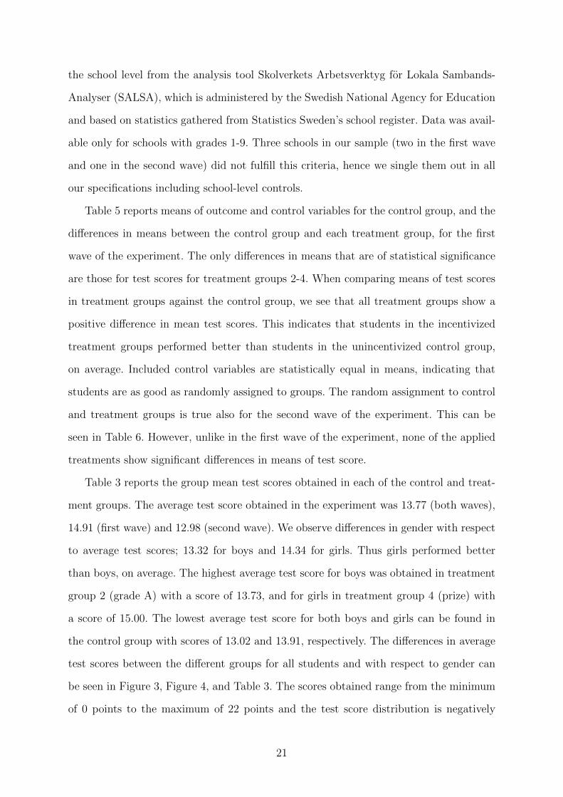
the school level from the analysis tool Skolverkets Arbetsverktyg for Lokala Sambands-

Analyser (SALSA), which is administered by the Swedish National Agency for Education

and based on statistics gathered from Statistics Sweden’s school register. Data was avail-

able only for schools with grades 1-9. Three schools in our sample (two in the first wave

and one in the second wave) did not fulfill this criteria, hence we single them out in all

our specifications including school-level controls.

Table 5 reports means of outcome and control variables for the control group, and the

differences in means between the control group and each treatment group, for the first

wave of the experiment. The only differences in means that are of statistical significance

are those for test scores for treatment groups 2-4. When comparing means of test scores

in treatment groups against the control group, we see that all treatment groups show a

positive difference in mean test scores. This indicates that students in the incentivized

treatment groups performed better than students in the unincentivized control group,

on average. Included control variables are statistically equal in means, indicating that

students are as good as randomly assigned to groups. The random assignment to control

and treatment groups is true also for the second wave of the experiment. This can be

seen in Table 6. However, unlike in the first wave of the experiment, none of the applied

treatments show significant differences in means of test score.

Table 3 reports the group mean test scores obtained in each of the control and treat-

ment groups. The average test score obtained in the experiment was 13.77 (both waves),

14.91 (first wave) and 12.98 (second wave). We observe differences in gender with respect

to average test scores; 13.32 for boys and 14.34 for girls. Thus girls performed better

than boys, on average. The highest average test score for boys was obtained in treatment

group 2 (grade A) with a score of 13.73, and for girls in treatment group 4 (prize) with

a score of 15.00. The lowest average test score for both boys and girls can be found in

the control group with scores of 13.02 and 13.91, respectively. The differences in average

test scores between the different groups for all students and with respect to gender can

be seen in Figure 3, Figure 4, and Table 3. The scores obtained range from the minimum

of 0 points to the maximum of 22 points and the test score distribution is negatively

21

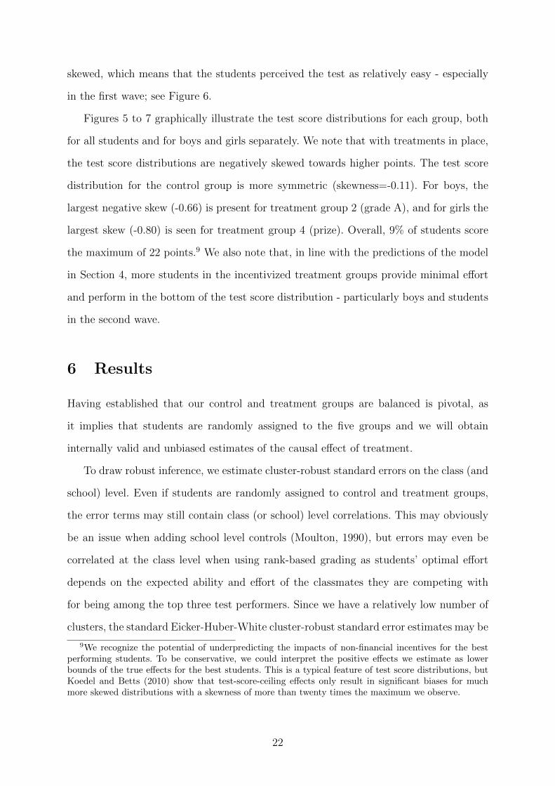
skewed, which means that the students perceived the test as relatively easy - especially

in the first wave; see Figure 6.

Figures 5 to 7 graphically illustrate the test score distributions for each group, both

for all students and for boys and girls separately. We note that with treatments in place,

the test score distributions are negatively skewed towards higher points. The test score

distribution for the control group is more symmetric (skewness=-0.11). For boys, the

largest negative skew (-0.66) is present for treatment group 2 (grade A), and for girls the

largest skew (-0.80) is seen for treatment group 4 (prize). Overall, 9% of students score

the maximum of 22 points.9 We also note that, in line with the predictions of the model

in Section 4, more students in the incentivized treatment groups provide minimal effort

and perform in the bottom of the test score distribution - particularly boys and students

in the second wave.

6 Results

Having established that our control and treatment groups are balanced is pivotal, as

it implies that students are randomly assigned to the five groups and we will obtain

internally valid and unbiased estimates of the causal effect of treatment.

To draw robust inference, we estimate cluster-robust standard errors on the class (and

school) level. Even if students are randomly assigned to control and treatment groups,

the error terms may still contain class (or school) level correlations. This may obviously

be an issue when adding school level controls (Moulton, 1990), but errors may even be

correlated at the class level when using rank-based grading as students’ optimal effort

depends on the expected ability and effort of the classmates they are competing with

for being among the top three test performers. Since we have a relatively low number of

clusters, the standard Eicker-Huber-White cluster-robust standard error estimates may be

9We recognize the potential of underpredicting the impacts of non-financial incentives for the bestperforming students. To be conservative, we could interpret the positive effects we estimate as lowerbounds of the true effects for the best students. This is a typical feature of test score distributions, butKoedel and Betts (2010) show that test-score-ceiling effects only result in significant biases for muchmore skewed distributions with a skewness of more than twenty times the maximum we observe.

22

downward biased.10 The fact that our clusters are of similar size should, however, reduce

the potential bias due to the small number of clusters. According to Rogers (1987) we

should not expect this potential bias to be large in our sample, since none of the classes

are larger than 5 percent of the total sample. This implies that the standard errors will

not be too far off because each term will be off by less than 1 in 400. This implies that the

standard cluster-robust standard error estimator with only 19-28 clusters of similar size

in the first-second wave should suffer minimal bias. We expect this bias to be extremely

close to zero in the total sample with 47 classes, but slightly higher when also clustering at

the school level with only 7-17 schools, where 7 of 17 schools in the total sample comprise

less than 5 percent of the sample. Cameron et al. (2008) report that a wild bootstrap

cluster-robust estimator performs well when the number of clusters is smaller than 50.

We confirm that the OLS and standard cluster-robust error estimates are very similar to

the adjustment for school and class level common shocks suggested by Cameron et al.

(2011) as well as their wild bootstrap (Cameron et al., 2008). In no cases do inference and

our conclusions change. In all tables we thus simply report the standard cluster-robust

standard errors.

Tables 7 and 8 present ATE estimates of the four non-financial incentives on stan-

dardized test scores. Table 7 reveals that we find positive, but insignificant ATE of all

four treatments. Table 8 reveals that this is true for both boys and girls.

We can also examine the treatment effects across the test score distribution. Ran-

domization within each classroom assures that - in the absence of treatment - all groups

of students would be equally likely to be observed in each of the percentiles of the test

score distribution. Hence, movements up (or down) in the test score distribution can be

attributed to the increased (or decreased) effort caused by the extrinsic incentive (treat-

ment) as both the ability and skill level are fixed in the test situation. Table 9 reveals

that there is a significant increase in the probability of scoring above the median for

treatments 3 and 4 (certificate and prize) and on the probability of scoring above the top

quartile for treatments 1 and 3 (grade A-F and certificate). Treatments 3 and 4 increase

10Wooldridge (2003) provides a more comprehensive discussion of these issues.

23

the probability of scoring above the median by 7-8 percentage points and treatments 1

and 3 increase the probability of scoring above the top quartile by 7-8 percentage points.

This is consistent with the predictions of the model in Section 4 that effort will increase

most for students at the margin for which the threshold for a performance reward is

within reach if they put more effort into the test. These students who increase their effort

when incentivized by rank-based grading and rewards are in the upper-middle part of the

ability distribution in our full sample of sixth graders. Table 9 further shows that adding

all individual, class, and school level controls does not change these conclusions.11 It also

reveals that the reason girls’ average test scores are higher on average is that they have

a lower probability to score in the lower half of the distribution. Finally, we also esti-

mate the distributional impacts by gender. Table 10 shows that only treatment 2 (grade

A) significantly increases the probability of scoring above the median by 10 percentage

points for boys. Table 11 shows that for girls, treatment 4 (prize) increases the probability

of scoring above the lower quartile by 9 percentage points and treatment 3 (certificate)

increases the probability of scoring above the upper quartile by 11-14 percentage points,

while it also decreases the probability of scoring above the lowest decile by 5 percentage

points. This is also consistent with the theory in Section 4 and indicates that the girls

around the upper quartile of the test score distribution are those increasing their effort

with the outlook of a certificate for high performance, while the girls around the lowest

decile are those getting demotivated by the too high threshold being out of reach. Overall,

it seems like boys get most motivated by competing for the grade A, while girls get most

motivated by competing for a prize or receiving a certificate for high performance.

6.1 Heterogeneous Treatment Effects by Skill level

We exploit that the preparation for the test is different for students in the two waves.

Students in the first wave are tested in April 2013, which is towards the end of the school-

year and around the time they will be taking the national test. The students should

11We verify that this is also true when we restrict our attention only to the students at schools withcomplete information on school-specific variables in the first two specifications. We further verify thatestimating a probit model instead of the linear probability model leads to the same conclusions.

24

therefore be in their comfort zone according to one of the leading theories of optimal

learning (Vygotsky, 1978) and be able to solve all the test tasks on their own if they

provide enough effort. The students in the second wave are tested in August-September

2013, which is at the beginning of sixth grade. As the test is designed to be a broad test

of the math skills acquired during their first six school years, some of the test tasks may

be too difficult for the students in the second wave to solve unassisted.12 On an optimal

learning trajectory (Vygotsky, 1978) these students should therefore be in their zone of

proximal development or if the tasks are way too hard even in their frustration zone.

The incentives may therefore unintentionally reduce their effort. Through the lens of the

model in Section 4, we interpret this as the students in the first wave being more skilled

than those in the second wave. In Figure 2 the distribution of ability in the first wave

is represented by faH , while faL represents the ability distribution of the second wave

students. The model predicts a lower increase in effort (or even more students exerting

no effort) in the second wave, as more students have a lower ability, a ≤ ai ≤ a, while

the model predicts a larger increase in effort by incentivized students in the first wave as

more students have a higher ability, a ≤ ai ≤ a.

Table 12 shows that we cannot reject this prediction, as the ATE is significant for

three of the four treatments among first wave students - with the exception of treatment

group 1 (grade A-F). Treatment group 4 (prize) tends to have the largest ATE, followed

by treatment group 2 (grade A), and treatment group 3 (certificate). Receiving the in-

formation that the performance on the test may lead to being rewarded with a prize

leads to almost half a standard deviation higher test score on average than when only

intrinsically motivated. Receiving a certificate for scoring above the cut-off for receiving

at least a B results in an average increase in test scores of about a third of a standard

deviation. This indicates that rank-based grading increases performance most, however,

the ATE of treatments 2, 3, and 4 are not statistically different; i.e. we cannot reject the

null hypothesis δ2 = δ3 = δ4. Being assigned to treatment group 1 (grade A-F) shows

no significant difference in average test scores. For the second wave, the ranking is re-

12After seeing the test, some of the teachers also pointed out that they had not yet taught the studentshow to solve some of the tasks.

25

versed, but not statistically significant. These results remain robust to including control

variables.

Table 13 presents ATEs separately by gender for the first wave. It reveals that boys

tend to be motivated only by rank-based grading singling out the top three test scorers

in the class: treatments 2 and 4 (grade A, prize). The size of these increases are about

half a standard deviation. We do not find statistically different responses to treatments

by gender, apart from the fact that only girls are induced to exert more effort by treat-

ment 3 (certificate). Girls and boys are equally motivated by the two rank-based grading

treatments and the effects are in the range of a third to half a standard deviation.13

We further analyze the distributional effects in the each wave. Table 14 reveals that

among the students in the first wave, the probability of scoring above the median is sig-

nificantly increased by treatments 2-4 (grade A, certificate, prize). P (TSi ≥ P50TS) is

increased by 19-21 percentage points. Treatment 2 (grade A) also increases the probability

of scoring above P25TS and P75TS by 19-21 percentage points, while treatment 3 (cer-

tificate) seems to have more motivational power at the upper quartile, and treatment 4

has more motivational power at the lower quartile. Examining these distributional effects

separately by gender, Table 15 presents the results for boys and Table 16 presents the

results for girls. For boys, treatment 2 (grade A) has a large effect higher up in the distri-

bution as it increases the probability of scoring above P25TS by 17, and above P50TS and

P75TS by 25-26 percentage points. The other rank-based grading treatment 4 (prize) has

an effect lower in the distribution as it increases the probability of scoring above P10TS

and P25TS by 12-29 percentage points, while treatment 3 (certificate) increases the prob-

ability of scoring above P10TS by 15 percentage points. For girls, treatment 2 (grade A)

has a similar effect at the lower quartile and median, although the motivational power is

only as strong at the lower quartile. Treatments 4 (prize) has a significant effect higher

up in the distribution, as does treatment 3 (certificate) by increasing girls’ probability

of scoring above the median and the top quartile by 28-30 percentage points. Treatment

13We have also estimated class-specific fixed effects specifications as an additional test of whetherthe class-level randomization was successful. These estimates are displayed in Table A.16 in the onlineAppendix and corroborate the robustness of our results to adding class FE - both overall and in theindividual waves.

26

1 (grade A-F) also significantly raises girls’ probability of scoring above the median by

24-26 percentage points and above P90TS by 9 percentage points.

Table 17 reveals that among the students in the second wave, the probability of

scoring above the tenth percentile, P (TSi ≥ P10TS), is lowered by 3-5 percentage points

when facing the non-financial incentives. This is consistent with the model prediction

that more students will optimally exert zero effort when the bar is set too high. Finally,

we corroborate that these conclusions are also robust to adding class and school-level

controls.

All in all, we find that while non-financial incentives increase test performance more for

students in the middle-upper part of the distribution among the highly skilled students,

the same incentives also decrease performance in the bottom of the distribution of low-

skilled students.

Finally, we test the impact of student placement on the learning trajectory more

directly. Is it really differences in student skill levels that drive the differences in treatment

responses between the first and the second wave? To answer this question, we employ a

more finely measured proxy for student skill level: learning weeks, denoting the number

of weeks the student has been learning math in sixth grade at the time of the test. The

results from adding interactions between learning weeks and the four treatment indicators

are presented in Table 18. We first note that adding learning weeks as a control does not

change any of our conclusions, but strongly diminishes the correlation between wave and

baseline test scores. This would be expected if wave mainly picks up the differences in

weeks the students have been learning math in sixth grade. More importantly, interacting

learning weeks with the four treatment indicators reveals that students respond more

strongly to T2-T4 when having been exposed to more weeks of sixth grade math classes.

This corroborates that the main factor determining the different impacts of treatment in

the two waves is student skill level at the time of the test.

27

6.2 Heterogeneous Treatment Effects by Peer Familiarity

The model in Section 3.2 shows that expectations about peer ability are important for

effort responses to rank-based grading incentives. We now turn to testing this model

prediction. We exploit the fact that some students have more information about the

peers they are competing with than others. We hypothesize that those who have spent at

least a school year in the same classroom as their peers will have a more precise estimate

of their peers’ ability; they thus face less uncertainty about the endogenous threshold and

their effort will respond more strongly to rank-based grading incentives. Table 19 presents

a direct test of this hypothesis, by separately presenting ATEs for students who have been

taught at least a school year in the classroom with the same peers and whether the ATEs

are different for those who just started with new peers within the last six weeks. Our

estimates support this hypothesis, as test score responses to treatments 2 and 4 (grade

A, prize) are significantly lower for those who are with new peers. Test scores are on

average increased by 0.35-0.37 standard deviations less by treatment 2 (grade A) and

by 0.48 standard deviations less by treatment 4 (prize) if tested in a new peer group.14

We also note that treatment 4 (prize) significantly increases test scores by 0.22 standard

deviations if in a familiar peer group. The last four columns of Table 19 reveal that this

is due to girls responding very strongly and raising their test scores by about a third of a

standard deviation if receiving a prize for being among the top three performers. Table 19

also shows that only girls respond significantly less to the rank-based grading incentives

when tested with unfamiliar peers.

Table 20 presents the distributional effects of non-financial incentives for the students

who have been with the same peers for at least a school year. We find that incentives

increase effort in the middle of the distribution. Treatment 3 (certificate) increases the

probability to score above both P50TS and P75TS by 8-11 percentage points, while the two

14Responses also tend to be lower for treatment 3 (certificate), but only significantly lower whenadding school-level controls. This is not predicted by the model in Section 3, since expectations aboutpeer ability should not be important for the individual reward on a criterion-based grading scale. Thiscould be because of some psychological factors related to uncertainty, self-confidence, self-evaluation ofmath ability, or because students dislike being singled out to receive a certificate in front of their newpeers.

28

rank-based treatments 2 and 4 (grade A, prize) increase performance lower in the ability

distribution. Table 21 shows that the incentives motivate lower in the distribution for

boys, where treatment 2 (grade A) increases the probability of scoring above P10TS and

by 11 percentage points and treatment 3 (certificate) increases the probability of scoring

above P10TS by 10 percentage points. Table 22 reveals that treatment 4 (prize) has a

large and significant effect throughout the test score distribution for girls, while treatment

3 (certificate) has a similarly large effect in the middle-upper part of the distribution by

increasing the probability of scoring above P50TS and P75TS by 13-19 percentage points.

Overall, we find strong empirical support for the model prediction that increased

uncertainty about peer ability - and consequently own winning probability - decreases the

motivational effect of tournament incentives. This motivational decrease is particularly

strong for girls. Our field experiment is not directly designed to distinguish between

competing theories of this observation. This could be done by introducing gender-specific

preference (Croson and Gneezy, 2009) and cost parameters in the model in Section 3.

For example, girls’ effort response under competition would be lowered when facing more

uncertainty about peers’ ability if girls expect their actual winning probabilities to be

lower than boys with the same math ability. This could occur if girls are less overconfident

(Alpert and Raiffa, 1982; Svenson, 1981), and could be a credible explanation as many

studies find boys to be more overconfident (Niederle and Vesterlund, 2010). Specifying and

estimating such a structural model to directly quantify the gender-specific differences in

parameters and their implications for behavior would be an interesting avenue for future

research.

7 Discussion

The results from our field experiment show that non-financial extrinsic incentives have a

motivational effect on highly skilled students’ performance in a test situation. Ranking

students by distinguishing the top three performers has particularly large motivational

power. However, the motivational power of evaluated incentives differs with respect to

29

gender. Boys only increase their effort if offered to compete, whereas girls also increase

their effort if offered a certificate for criterion-based grades A-B. Girls’ responses to rank-

based grading incentives are also significantly lower if they are in a class with new peers.

This indicates that girls’ responses to a competitive environment are particularly sensitive

to their knowledge about the ability of the peers they are competing with.

Why would we expect gender differences in the responses to the rank-based test as-

sessments? Boys are most responsive to being ranked with respect to grades, whereas

girls react most strongly to the incentive of receiving a prize for high rank. Receiving a

prize may offer a more public form of competition, and most studies find that boys exhibit

more competitive behavior (Gneezy et al., 2003; Gneezy and Rustichini, 2004; Croson and

Gneezy, 2009; Niederle and Vesterlund, 2010).15 However, we find no significant difference

in the performance response to competition among these sixth grade students.16 This is

consistent with Lavy (2012) who estimates no gender difference in teacher effort under

performance pay even if the female teachers are more pessimistic about the performance

pay scheme, and with Joensen and Nielsen (2014) who find that girls are less likely to

choose competitive advanced math classes in high school - even if the expected financial

reward is at least as high as for boys. It may thus be that the competitive environment

lowers girls’ utility (e.g. because they find it more unpleasant) even if they increase their

performance as much (or more) under the rank-based grading.17

Why do only girls respond to the symbolic reward? This could be because girls at-

tach relatively more importance to reflected appraisals, whereas boys attach relatively

15Note that all these studies use financial incentives. We cannot be certain of how the incentives wereperceived by the students. Thus we cannot conclude that prize was the most worthy of competition.Therefore, boys may still have displayed the most competitive behavior, but have valued grade A higherthan prize. As prize is the only materialistic reward, girls’ strong reaction to this incentive may indicatethat they are more materialistic than boys.

16Some studies even find the opposite to be true. Cardenas et al. (2012) find that the competitiveperformance increase in math is higher for girls than for boys in Sweden. However, they find that girlsare less likely to choose to compete on the math task.

17There does not seem to be a consensus on the nature and emergence of gender differences in com-petitiveness. Gneezy et al. (2009) show that culture matters as men (women) are more competitive in apatriarchal (matrilineal) society, while Andersen et al. (2010) suggest that girls become less competitivearound puberty in a patriarchal society and Booth and Nolen (2012) find that social learning mattersas girls from single-sex schools are more competitive at age 15 than girls from coed schools in the UK.Contrary to this Sutter and Rutzler (2010) find that boys are already more competitive around age threein Austria, whereas Dreber et al. (2011) find no evidence of differences in competitiveness among Swedishchildren aged 7 to 10.

30

more importance to social comparisons (Schwalbe and Staples, 1991).18 Both rank-based

incentives and receiving a symbolic reward offer sources of reflected appraisals, while

rank-based incentives offer a more direct form of competition and social comparison.

This could explain why we find a considerable impact on girls’ performance as soon as

rank-based incentives or a symbolic reward is in place, but for boys this impact is only

prevalent when facing competition. It is possible that boys do not view the symbolic re-

ward (and criterion-based grades more generally) as a strong enough social comparison.

If girls are more motivated by reflected appraisals they will, however, be motivated both

by the top three competition and by a symbolic reward. Josephs et al. (1992) also stresses

that males are more likely to individuate themselves from others in areas of importance

and value, whereas separation from others is not as important for females. If so, boys

would be more motivated by the possibility of successfully separating themselves from

others through individuating attainments by being top of their class. This could reflect

our results as boys tend to be motivated by wanting to stand out in competition, while

girls are motivated even though the reward is symbolic and many classmates also may

receive it by meeting the criteria.

Could social comparisons be important in other ways? We present additional evidence

indicating that boys (girls) tend to be more sensitive to the performance of other boys

(girls) in their class.19 We estimate (i) a significantly higher baseline performance and (ii)

a significantly lower response to all treatments if the same-gender average performance in

the class is higher, while there is no significant differential response to the other-gender

average performance in the class. These results suggest that gender is a salient feature of

identity and students tend to compare themselves to their same-gender classmates; i.e.

boys (girls) are more likely to have other boys (girls) as their reference group and make

within-gender social comparisons. These results also suggest that it is harder to increase

your social reward through higher test effort if your reference-peers are higher ability. The

lower treatment responses could be due to lower self-esteem if having more upward social

18Reflected appraisals (Cooley, 1902) refer to how others react to us - their image of us and howwe reflect it - and social comparisons (Festinger, 1954) refer to using others as references for our self-evaluations, self-enhancements, and self-improvements.

19See Tables A.17-A.19 in the accompanying Online Appendix for these results.

31

comparison possibilities in the relevant gender-specific reference group (Dijkstra et al.,

2008). These social comparisons do not seem particularly sensitive to peer familiarity. In

future research, it would be interesting to test these hypotheses on a sample with larger

control groups, as well as to open the black box of how students make social comparisons,

how it affects their performance, and how it affects their responses to extrinsic incentives.

Given the differences in placement in the test score distribution and the fact that

responses to extrinsic incentives vary considerably over the skill and ability distribution,

we cannot draw strong conclusions on the economic significance of these gender differences

without introducing more structure. Boys have a higher variance of test scores compared

to girls, since boys are much more likely to score in the bottom of the distribution.

There is also a gender level difference in which girls outperform boys with an average of

0.87 standardized points. This tells us either that girls have higher intrinsic motivation,

apply more effort in the test situation, or are simply better at solving the mathematical

tasks presented in the experiment. There is a growing literature addressing the issue that

boys are lagging behind in schools and having worse average educational achievement

because of low motivation, low self-discipline, or low non-cognitive skills in general (Jacob,

2002; Duckworth and Seligman, 2006; Fortin et al., 2013; Cornwell et al., 2013).20 This

could have longer-term detrimental effects as an early skill deficit lowers later educational

attainment and the returns to education (Cunha et al., 2006; Cunha and Heckman, 2007;

Oreopoulos and Salvanes, 2011). Our results suggest that one way of incentivizing boys to

be more engaged and put forth more effort in school would be to include more competition

into the assessment of their tests. This could be equally beneficial for both highly skilled

boys’ and girls’ math achievement.

Our results also highlight that the diverging results in the literature on responses

to, and emergence of, competitiveness may not only be due to differences in the gender

stereotypicality of the task (Dreber et al., 2011) and the implementation environments,

but also due to failing to appropriately take the skill levels relative to task difficulty and

20This could be because boys’ non-cognitive skills are more sensitive to parental inputs as they, forexample, become relatively more disadvantaged if growing up in a broken home (Bertrand and Pan,2013).

32

peer familiarity into account. Particularly, girls’ responses to competition seem to be very

sensitive to how well they know their peers. Our results therefore call for more research

to pin down how skills and peers affect responses to competition and other extrinsic

incentives.

8 Conclusions

The educational system is built upon a sequence of tests to measure student performance.

The results of these tests often lay the foundation for the distribution of school resources

and spur considerable public debates, but how do test incentives affect student motivation

and effort? For tests to be a useful measure of students’ knowledge and quality, they

need to accurately reflect students’ skill levels. This can only be the case if students are

motivated to perform well when taking tests and if they exert enough effort in the test

situation.

Measures of student quality, achievement gaps, teacher value added, and school quality

will be biased if some groups of students are not motivated to exert effort on achievement

tests and large scale national standardized tests carrying low stakes for the students, but

potentially high stakes for teachers and schools. Policy decisions based on such biased

measures could be seriously misguided and have unintended consequences. Two exam-

ples of high-powered and widespread incentive systems based on student test scores are

school accountability systems and performance pay based on teacher value added. First,

Kane and Staiger (2002) lay out the promises and pitfalls for using school accountability

systems based on imprecise school-level test score measures, while Figlio and Winicki

(2005) provide an example of unintended consequences of school accountability as some

schools feed their students with more calories just before the test in order to boost their

test performance. Second, Hanushek and Rivkin (2010) and Neal (2011) highlight sev-

eral reasons why using teacher value-added measures as a basis for performance pay,

employment, promotion, and assignment decisions may be problematic: e.g. they capture

very short-term rather than longer-term learning gains (Rothstein, 2010; Jacob et al.,

33

2010).21 Measures of school quality could even have important consequences for sorting

of students across schools if these are widely publicized (Rivkin et al., 2005; Rothstein,

2010). Our results further highlight that these measures are highly dependent on student

preparation for the test, peer familiarity, and the implicit incentives in the grading of the

test. It could therefore be easy for teachers and principals to manipulate such measures

by simply giving a symbolic reward or singling out the top performers on the day of the

test. Future research will hopefully reveal whether these non-financial test incentives have

longer-term effects.

Our results also have implications for grading design and the organization of schools,

as they show there is cause to question the current incentives being used to motivate

highly skilled students. We show that grading highly skilled students on an A-F scale ac-

cording to a pre-specified set of criteria does not motivate students to increase test effort.

To grade with criteria - without a corresponding distribution - is the most commonly used

method of student assessment in primary schools.22 Norm-referenced assessment methods

would be more effective in increasing highly skilled students’ test effort. However, intro-

ducing tournaments within the classroom will potentially lower test effort of students

with lower skill levels. Thus norm-referenced grading can have unintended consequences

if applied in a learning environment where students are not fully mastering the learning

requirements. This demotivating effect for low skilled students should, however, not be

large for students who are well prepared for their final exam or (inter)national tests.

This suggests the importance of choosing the appropriate grading method for the test to

accurately reflect the knowledge level it is intended to measure on the students’ learning

trajectory. If teacher pay depends on students’ test scores, they may be induced to teach-

to-the-test by shifting their attention away from those who are lagging behind to those

who are more skilled (Lazear, 2006). This is exactly what happened when Chicago Public

Schools changed their proficiency requirements and teachers shifted their attention to

those close to this requirement (Neal and Schanzenbach, 2010). Our results suggest that

21Lavy (2009) shows that teacher performance pay can sometimes lead to improved student perfor-mance through better teaching methods, which may potentially lead to positive longer-term effects.

22Note that even if this is also the typical grading method in Swedish schools, it is still novel - like theother evaluated grading methods - to the sixth grade students participating in the experiment.

34

norm-referenced grading could lead to similar polarization in a heterogeneous learning

environment.

Our results also suggest some interesting avenues for future research: Is is better to use

criterion-based grading with more or fewer grades? How important are the exact cut-offs

in criterion-based grading? How important is the degree of competitiveness in rank-based

grading? Does the nature of non-financial rewards matter? By further analyzing other

non-financial incentives, one could find even more efficient methods for increasing student

effort and performance. In this paper, we isolate the effort effect in the test situation,

while we plan to also evaluate other incentive effects and the importance of sorting when

evaluating longer-term impacts.23 Among the four non-financial incentives we evaluate,

we find those involving norm-referenced assessment to be the most effective in increasing

test effort of highly skilled students, but not for students with too low skill level. Such

rank-based grading is often prevalent at later educational stages. Our results indicate that

an earlier implementation could have positive effects on student effort and performance,

thus could lead to more efficient tracking and sorting across skill levels. A deeper analysis

of these issues and the longer-term effects of grading and reward schemes could be a

fruitful avenue for future research.

23Leuven et al. (2011) show that such distinctions may be crucial when comparing different financialtournament incentives for university students.

35

References

Alpert, M. and H. Raiffa (1982). A progress report on the training of probability assessors.

In D. Kahneman, P. Slovic, and A. Tversky (Eds.), Judgment Under Uncertainty:

Heuristics and Biases, pp. 294–305. Cambridge University Press.

Andersen, S., S. Ertac, U. Gneezy, J. A. List, and S. Maximiano (2010). Gender, competi-

tiveness and socialization at a young age: evidence from a matrilineal and a patriarchal

society. Review of Economics and Statistics .

Attali, Y., Z. Neeman, and A. Schlosser (2011). Rise to the challenge or not give a damn:

differential performance in high vs. low stakes tests. IZA Discussion Paper No. 5693 .

Azmat, G. and N. Iriberri (2010). The importance of relative performance feedback

information: Evidence from a natural experiment using high school students. Journal

of Public Economics 94 (7), 435–452.

Baumert, J. and A. Demmrich (2001). Test motivation in the assessment of student

skills: The effects of incentives on motivation and performance. European Journal of

Psychology of Education 16 (3), 441–462.

Becker, G. S. (1967). Human capital and the personal distribution of income: An analytical

approach, Volume 1. Woytinsky lecture. Institute of Public Administration Ann Arbor,

MI.

Becker, W. E. and S. Rosen (1992). The learning effect of assessment and evaluation in

high school. Economics of Education Review 11 (2), 107–118.

Bertrand, M. and J. Pan (2013). The trouble with boys: Social influences and the gender

gap in disruptive behavior. American Economic Journal: Applied Economics 5 (1),

32–64.

Besley, T. and M. Ghatak (2008). Status incentives. American Economic Review 98 (2),

206–211.

36

Bettinger, E. and R. Slonim (2007). Patience among children. Journal of Public Eco-

nomics 91 (1), 343–363.

Bettinger, E. P. (2012). Paying to learn: The effect of financial incentives on elementary

school test scores. Review of Economics and Statistics 94 (3), 686–698.

Betts, J. R. (1998). The impact of educational standards on the level and distribution of

earnings. American Economic Review , 266–275.

Betts, J. R. and J. Grogger (2003). The impact of grading standards on student achieve-

ment, educational attainment, and entry-level earnings. Economics of Education Re-

view 22 (4), 343–352.

Booth, A. and P. Nolen (2012). Choosing to compete: How different are girls and boys?

Journal of Economic Behavior & Organization 81 (2), 542–555.

Cameron, A. C., J. B. Gelbach, and D. L. Miller (2008). Bootstrap-based improvements

for inference with clustered errors. The Review of Economics and Statistics 90 (3),

414–427.

Cameron, A. C., J. B. Gelbach, and D. L. Miller (2011). Robust inference with multiway

clustering. Journal of Business & Economic Statistics 29 (2).

Cardenas, J.-C., A. Dreber, E. Von Essen, and E. Ranehill (2012). Gender differences in

competitiveness and risk taking: Comparing children in colombia and sweden. Journal

of Economic Behavior & Organization 83 (1), 11–23.

Chay, K. Y., P. J. McEwan, and M. Urquiola (2005). The central role of noise in evaluating

interventions that use test scores to rank schools. American Economic Review , 1237–

1258.

Cooley, C. H. (1902). Human Nature and the Social Order. New York: Schocken.

Cornwell, C., D. B. Mustard, and J. Van Parys (2013). Noncognitive skills and the

gender disparities in test scores and teacher assessments: Evidence from primary school.

Journal of Human Resources 48 (1), 236–264.

37

Costrell, R. M. (1994). A simple model of educational standards. The American Economic

Review , 956–971.

Croson, R. and U. Gneezy (2009). Gender differences in preferences. Journal of Economic

Literature, 448–474.

Cunha, F. and J. Heckman (2007). The technology of skill formation. American Economic

Review 97 (2), 31–47.

Cunha, F., J. J. Heckman, L. Lochner, and D. V. Masterov (2006). Interpreting the

evidence on life cycle skill formation. Handbook of the Economics of Education 1,

697–812.

Deci, E. L., R. Koestner, and R. M. Ryan (1999). A meta-analytic review of experi-

ments examining the effects of extrinsic rewards on intrinsic motivation. Psychological

Bulletin 125 (6), 627.

Delfgaauw, J., R. Dur, J. Sol, and W. Verbeke (2013). Tournament incentives in the field:

Gender differences in the workplace. Journal of Labor Economics 31 (2), 305–326.

Dijkstra, P., H. Kuyper, G. van der Werf, A. P. Buunk, and Y. G. van der Zee (2008).

Social comparison in the classroom: A review. Review of Educational Research 78 (4),

828–879.

Dreber, A., E. Von Essen, and E. Ranehill (2011). Outrunning the gender gap - boys and

girls compete equally. Experimental Economics 14 (4), 567–582.

Duckworth, A. L. and M. E. Seligman (2006). Self-discipline gives girls the edge: Gender

in self-discipline, grades, and achievement test scores. Journal of Educational Psychol-

ogy 98 (1), 198.

Eisenkopf, G. (2011). Paying for better test scores. Education Economics 19 (4), 329–339.

Ellingsen, T. and M. Johannesson (2007). Paying respect. The Journal of Economic

Perspectives 21 (4), 135–150.

38

Facchinello, L. (2014). The impact of grading on academic choices: Mechanisms and

social implications. Manuscript, Stockholm School of Economics.

Festinger, L. (1954). A theory of social comparison processes. Human relations 7 (2),

117–140.

Figlio, D. N. and M. E. Lucas (2004). Do high grading standards affect student perfor-

mance? Journal of Public Economics 88 (9), 1815–1834.

Figlio, D. N. and J. Winicki (2005). Food for thought: the effects of school accountability

plans on school nutrition. Journal of Public Economics 89 (2), 381–394.

Fortin, N. M., P. Oreopoulos, and S. Phipps (2013). Leaving boys behind: Gender dis-

parities in high academic achievement. NBER Working Paper (19331).

Fredriksson, P., B. Ockert, and H. Oosterbeek (2013). Long-term effects of class size. The

Quarterly Journal of Economics 128 (1), 249–285.

Fryer, R. G. (2011). Financial incentives and student achievement: Evidence from ran-

domized trials. The Quarterly Journal of Economics 126 (4), 1755–1798.

Gneezy, U., K. L. Leonard, and J. A. List (2009). Gender differences in competition:

Evidence from a matrilineal and a patriarchal society. Econometrica 77 (5), 1637–1664.

Gneezy, U., M. Niederle, and A. Rustichini (2003). Performance in competitive environ-

ments: Gender differences. The Quarterly Journal of Economics 118 (3), 1049–1074.

Gneezy, U. and A. Rustichini (2004). Gender and competition at a young age. The

American Economic Review 94 (2), 377–381.

Hanushek, E. A. and S. G. Rivkin (2010). Generalizations about using value-added

measures of teacher quality. The American Economic Review 100 (2), 267–271.

Jacob, B. A. (2002). Where the boys aren’t: non-cognitive skills, returns to school and

the gender gap in higher education. Economics of Education Review 21 (6), 589–598.

39

Jacob, B. A., L. Lefgren, and D. P. Sims (2010). The persistence of teacher-induced

learning. Journal of Human Resources 45 (4), 915–943.

Joensen, J. S. and H. S. Nielsen (2014). Math and gender: Heterogeneity in causes and

consequences of math. forthcoming in the Economic Journal .

Josephs, R. A., H. R. Markus, and R. W. Tafarodi (1992). Gender and self-esteem.

Journal of personality and social psychology 63 (3), 391.

Kane, T. J. and D. O. Staiger (2002). The promise and pitfalls of using imprecise school

accountability measures. The Journal of Economic Perspectives 16 (4), 91–114.

Koedel, C. and J. Betts (2010). Value added to what? how a ceiling in the testing

instrument influences value-added estimation. Education 5 (1), 54–81.

Kosfeld, M. and S. Neckermann (2011). Getting more work for nothing? symbolic awards

and worker performance. American Economic Journal: Microeconomics 3 (3), 86–99.

Lavy, V. (2009). Performance pay and teachers’ effort, productivity, and grading ethics.

American Economic Review 99 (5), 1979–2011.

Lavy, V. (2012). Gender differences in market competitiveness in a real workplace: Evi-

dence from performance-based pay tournaments among teachers. The Economic Jour-

nal .

Lazear, E. P. (2006). Speeding, terrorism, and teaching to the test. The Quarterly Journal

of Economics , 1029–1061.

Lazear, E. P. and S. Rosen (1981). Rank-order tournaments as optimum labor contracts.

The Journal of Political Economy , 841–864.

Leuven, E., H. Oosterbeek, J. Sonnemans, and B. Van der Klaauw (2011). Incentives

versus sorting in tournaments: Evidence from a field experiment. Journal of Labor

Economics 29 (3), 637–658.

40

Levitt, S. D., J. A. List, S. Neckermann, and S. Sadoff (2012). The behavioralist goes to

school: Leveraging behavioral economics to improve educational performance. NBER

Working Paper (18165).

Moulton, B. R. (1990). An illustration of a pitfall in estimating the effects of aggregate

variables on micro units. The Review of Economics and Statistics , 334–338.

Murphy, R. and F. Weinhardt (2013). Top of class: the importance of ordinal rank

position. CEP Discussion Paper No 1241 .

Neal, D. (2011). The design of performance pay in education. Handbook of the Economics

of Education 4, 495–550.

Neal, D. and D. W. Schanzenbach (2010). Left behind by design: Proficiency counts and

test-based accountability. The Review of Economics and Statistics 92 (2), 263–283.

Niederle, M. and L. Vesterlund (2010). Explaining the gender gap in math test scores:

The role of competition. The Journal of Economic Perspectives 24 (2), 129–144.

Oreopoulos, P. and K. G. Salvanes (2011). Priceless: The nonpecuniary benefits of school-

ing. The Journal of Economic Perspectives 25 (1), 159–184.

Rivkin, S. G., E. A. Hanushek, and J. F. Kain (2005). Teachers, schools, and academic

achievement. Econometrica 73 (2), 417–458.

Rogers, W. (1987). Regression standard errors in clustered samples. Stata Technical

Bulletin 3 (13).

Rothstein, J. (2010). Teacher quality in educational production: Tracking, decay, and

student achievement. The Quarterly Journal of Economics 125 (1), 175–214.

Schwalbe, M. L. and C. L. Staples (1991). Gender differences in sources of self-esteem.

Social Psychology Quarterly , 158–168.

Sjogren, A. (2010). Graded children: Evidence of longrun consequences of school grades

from a nationwide reform. Technical report, Working paper//IFAU-Institute for Labour

Market Policy Evaluation.

41

Sutter, M. and D. Rutzler (2010). Gender differences in competition emerge early in life.

IZA Discussion Paper No. 5015 .

Svenson, O. (1981). Are we all less risky and more skillful than our fellow drivers? Acta

Psychologica 47 (2), 143–148.

Tran, A. and R. Zeckhauser (2012). Rank as an inherent incentive: Evidence from a field

experiment. Journal of Public Economics 96 (9), 645–650.

Vygotsky, L. L. S. (1978). Mind in society: The development of higher psychological

processes. Harvard University Press.

Weiss, Y. and C. Fershtman (1998). Social status and economic performance: A survey.

European Economic Review 42 (3-5), 801–820.

Wise, S. L. and C. E. DeMars (2005). Low examinee effort in low-stakes assessment:

Problems and potential solutions. Educational Assessment 10 (1), 1–17.

Wooldridge, J. M. (2003). Cluster-sample methods in applied econometrics. The Ameri-

can Economic Review 93 (2), 133–138.

42

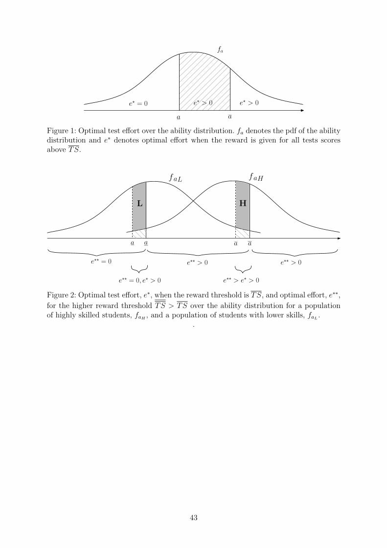
a a

e⋆ = 0 e⋆ > 0e⋆ > 0

fa

Figure 1: Optimal test effort over the ability distribution. fa denotes the pdf of the abilitydistribution and e∗ denotes optimal effort when the reward is given for all tests scoresabove TS.

a a

e⋆⋆ = 0

a a

e⋆⋆ > 0e⋆⋆ > 0

faL faH

e⋆⋆ = 0, e⋆ > 0 e⋆⋆ > e⋆ > 0

L H

Figure 2: Optimal test effort, e∗, when the reward threshold is TS, and optimal effort, e∗∗,

for the higher reward threshold TS > TS over the ability distribution for a populationof highly skilled students, faH , and a population of students with lower skills, faL .

.

43

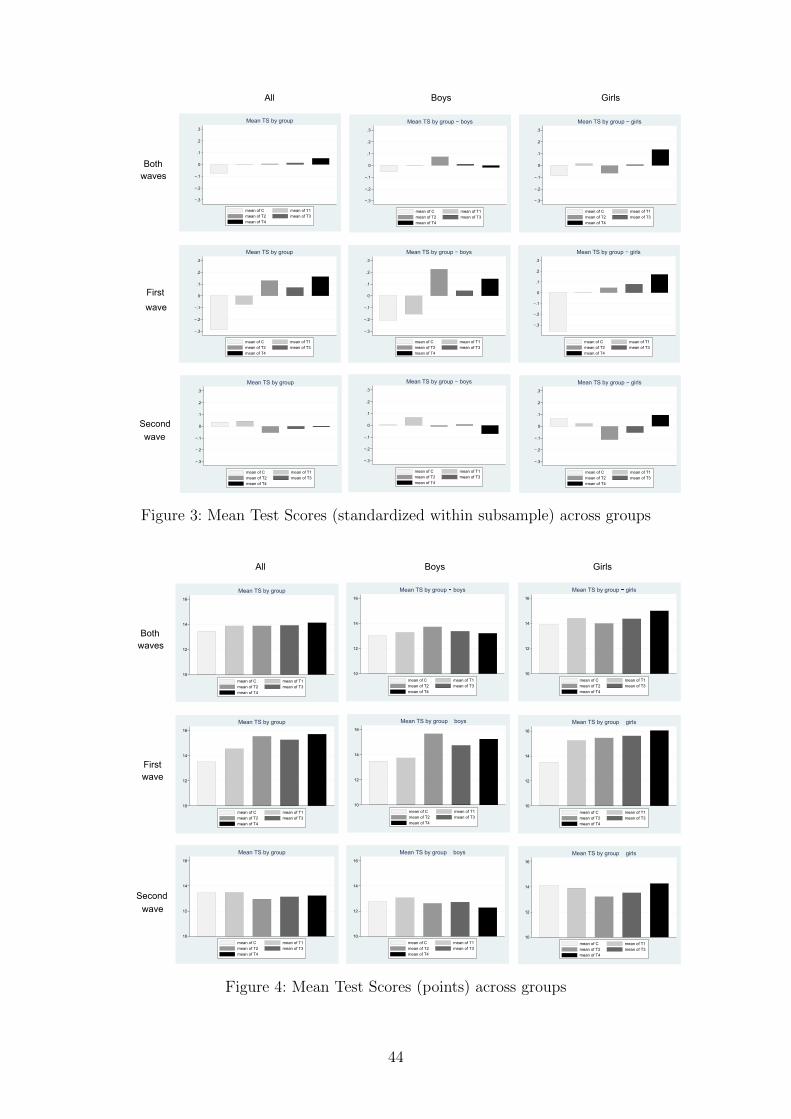
−.3

−.2

−.1

0

.1

.2

.3

Mean TS by group

mean of C mean of T1

mean of T2 mean of T3

mean of T4

All Boys Girls

Both

waves

First

wave

Second

wave

−.3

−.2

−.1

0

.1

.2

.3

Mean TS by group − boys

mean of C mean of T1

mean of T2 mean of T3

mean of T4

−.3

−.2

−.1

0

.1

.2

.3

Mean TS by group − girls

mean of C mean of T1

mean of T2 mean of T3

mean of T4

−.3

−.2

−.1

0

.1

.2

.3

Mean TS by group

mean of C mean of T1

mean of T2 mean of T3

mean of T4

−.3

−.2

−.1

0

.1

.2

.3

Mean TS by group − boys

mean of C mean of T1

mean of T2 mean of T3

mean of T4

−.3

−.2

−.1

0

.1

.2

.3

Mean TS by group − girls

mean of C mean of T1

mean of T2 mean of T3

mean of T4

−.3

−.2

−.1

0

.1

.2

.3

Mean TS by group

mean of C mean of T1

mean of T2 mean of T3

mean of T4

−.3

−.2

−.1

0

.1

.2

.3

Mean TS by group − boys

mean of C mean of T1

mean of T2 mean of T3

mean of T4

−.3

−.2

−.1

0

.1

.2

.3

Mean TS by group − girls

mean of C mean of T1

mean of T2 mean of T3

mean of T4

Figure 3: Mean Test Scores (standardized within subsample) across groups

10

12

14

16

Mean TS by group

mean of C mean of T1

mean of T2 mean of T3

mean of T4

10

12

14

16

Mean TS by group boys

mean of C mean of T1

mean of T2 mean of T3

mean of T4

10

12

14

16

Mean TS by group girls

mean of C mean of T1

mean of T2 mean of T3

mean of T4

10

12

14

16

Mean TS by group

mean of C mean of T1

mean of T2 mean of T3

mean of T4

10

12

14

16

Mean TS by group boys

mean of C mean of T1

mean of T2 mean of T3

mean of T4

10

12

14

16

Mean TS by group girls

mean of C mean of T1

mean of T2 mean of T3

mean of T4

10

12

14

16

Mean TS by group

mean of C mean of T1

mean of T2 mean of T3

mean of T4

10

12

14

16

Mean TS by group boys

mean of C mean of T1

mean of T2 mean of T3

mean of T4

10

12

14

16

Mean TS by group girls

mean of C mean of T1

mean of T2 mean of T3

mean of T4

All Boys Girls

Both

waves

First

wave

Second

wave

Figure 4: Mean Test Scores (points) across groups

44

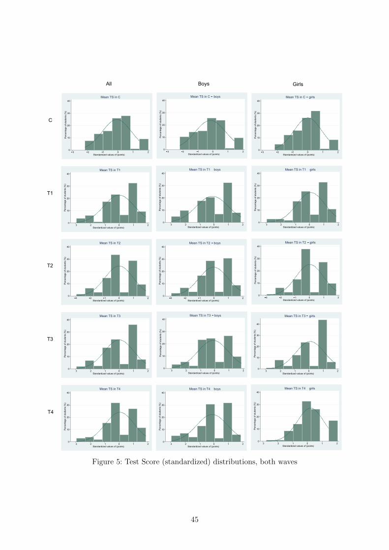
C

T1

T2

T3

T4

All Boys Girls

0

10

20

30

40

Perc

enta

ge o

f stu

dents

(%

)

3 2 1 0 1 2Standardized values of (points)

Mean TS in C

0

10

20

30

40

Perc

enta

ge o

f stu

dents

(%

)

3 2 1 0 1 2Standardized values of (points)

Mean TS in C boys

0

10

20

30

40

Perc

enta

ge o

f stu

dents

(%

)

3 2 1 0 1 2Standardized values of (points)

Mean TS in C girls

0

10

20

30

40

Perc

enta

ge o

f stu

dents

(%

)

3 2 1 0 1 2Standardized values of (points)

Mean TS in T1

0

10

20

30

40

Perc

enta

ge o

f stu

dents

(%

)

3 2 1 0 1 2Standardized values of (points)

Mean TS in T1 boys

0

10

20

30

40

Perc

enta

ge o

f stu

dents

(%

)

3 2 1 0 1 2Standardized values of (points)

Mean TS in T1 girls

0

10

20

30

40

Perc

enta

ge o

f stu

dents

(%

)

3 2 1 0 1 2Standardized values of (points)

Mean TS in T2

0

10

20

30

40

Perc

enta

ge o

f stu

dents

(%

)

3 2 1 0 1 2Standardized values of (points)

Mean TS in T2 boys

0

10

20

30

40

Perc

enta

ge o

f stu

dents

(%

)

3 2 1 0 1 2Standardized values of (points)

Mean TS in T2 girls

0

10

20

30

40

Perc

enta

ge o

f stu

dents

(%

)

3 2 1 0 1 2Standardized values of (points)

Mean TS in T3

0

10

20

30

40

Perc

enta

ge o

f stu

dents

(%

)

3 2 1 0 1 2Standardized values of (points)

Mean TS in T3 boys

0

10

20

30

40

Perc

enta

ge o

f stu

dents

(%

)

3 2 1 0 1 2Standardized values of (points)

Mean TS in T3 girls

0

10

20

30

40

Perc

enta

ge o

f stu

dents

(%

)

3 2 1 0 1 2Standardized values of (points)

Mean TS in T4

0

10

20

30

40

Perc

enta

ge o

f stu

dents

(%

)

3 2 1 0 1 2Standardized values of (points)

Mean TS in T4 boys

0

10

20

30

40

Perc

enta

ge o

f stu

dents

(%

)

3 2 1 0 1 2Standardized values of (points)

Mean TS in T4 girls

Figure 5: Test Score (standardized) distributions, both waves

45

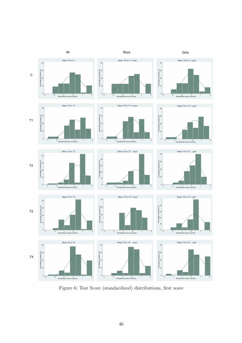
C

T1

T2

T3

T4

All Boys Girls

0

10

20

30

40

Perc

enta

ge o

f stu

dents

(%

)

3 2 1 0 1 2Standardized values of (points)

Mean TS in C

0

10

20

30

40

Perc

enta

ge o

f stu

dents

(%

)

3 2 1 0 1 2Standardized values of (points)

Mean TS in C boys

0

10

20

30

40

Perc

enta

ge o

f stu

dents

(%

)

3 2 1 0 1 2Standardized values of (points)

Mean TS in C girls

0

10

20

30

40

Perc

enta

ge o

f stu

dents

(%

)

3 2 1 0 1 2Standardized values of (points)

Mean TS in T1

0

10

20

30

40

Perc

enta

ge o

f stu

dents

(%

)

3 2 1 0 1 2Standardized values of (points)

Mean TS in T1 boys

0

10

20

30

40

Perc

enta

ge o

f stu

dents

(%

)

3 2 1 0 1 2Standardized values of (points)

Mean TS in T1 girls

0

10

20

30

40

Perc

enta

ge o

f stu

dents

(%

)

3 2 1 0 1 2Standardized values of (points)

Mean TS in T2

0

10

20

30

40

Perc

enta

ge o

f stu

dents

(%

)

3 2 1 0 1 2Standardized values of (points)

Mean TS in T2 boys

0

10

20

30

40

Perc

enta

ge o

f stu

dents

(%

)

3 2 1 0 1 2Standardized values of (points)

Mean TS in T2 girls

0

10

20

30

40

Perc

enta

ge o

f stu

dents

(%

)

3 2 1 0 1 2Standardized values of (points)

Mean TS in T3

0

10

20

30

40

Perc

enta

ge o

f stu

dents

(%

)

3 2 1 0 1 2Standardized values of (points)

Mean TS in T3 boys

0

10

20

30

40

Perc

enta

ge o

f stu

dents

(%

)

3 2 1 0 1 2Standardized values of (points)

Mean TS in T3 girls

0

10

20

30

40

Perc

enta

ge o

f stu

dents

(%

)

3 2 1 0 1 2Standardized values of (points)

Mean TS in T4

0

10

20

30

40

Perc

enta

ge o

f stu

dents

(%

)

3 2 1 0 1 2Standardized values of (points)

Mean TS in T4 boys

0

10

20

30

40

Perc

enta

ge o

f stu

dents

(%

)

3 2 1 0 1 2Standardized values of (points)

Mean TS in T4 girls

Figure 6: Test Score (standardized) distributions, first wave

46

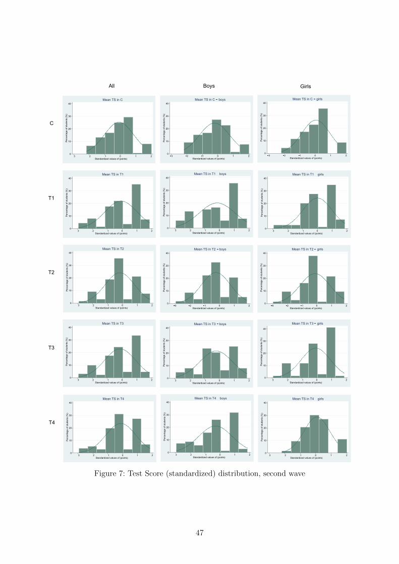
C

T1

T2

T3

T4

All Boys Girls

0

10

20

30

40

Perc

enta

ge o

f stu

dents

(%

)

3 2 1 0 1 2Standardized values of (points)

Mean TS in C

0

10

20

30

40

Perc

enta

ge o

f stu

dents

(%

)

3 2 1 0 1 2Standardized values of (points)

Mean TS in C boys

0

10

20

30

40

Perc

enta

ge o

f stu

dents

(%

)

3 2 1 0 1 2Standardized values of (points)

Mean TS in C girls

0

10

20

30

40

Perc

enta

ge o

f stu

dents

(%

)

3 2 1 0 1 2Standardized values of (points)

Mean TS in T1

0

10

20

30

40

Perc

enta

ge o

f stu

dents

(%

)

3 2 1 0 1 2Standardized values of (points)

Mean TS in T1 boys

0

10

20

30

40

Perc

enta

ge o

f stu

dents

(%

)

3 2 1 0 1 2Standardized values of (points)

Mean TS in T1 girls

0

10

20

30

40

Perc

enta

ge o

f stu

dents

(%

)

3 2 1 0 1 2Standardized values of (points)

Mean TS in T2

0

20

10

30

40

Perc

enta

ge o

f stu

dents

(%

)

3 2 1 0 1 2Standardized values of (points)

Mean TS in T2 boys

0

10

20

30

40

Perc

enta

ge o

f stu

dents

(%

)

3 2 1 0 1 2Standardized values of (points)

Mean TS in T2 girls

0

10

20

30

40

Perc

enta

ge o

f stu

dents

(%

)

3 2 1 0 1 2Standardized values of (points)

Mean TS in T3

0

10

20

30

40

Perc

enta

ge o

f stu

dents

(%

)

3 2 1 0 1 2Standardized values of (points)

Mean TS in T3 boys

0

10

20

30

40

Perc

enta

ge o

f stu

dents

(%

)

3 2 1 0 1 2Standardized values of (points)

Mean TS in T3 girls

0

10

20

30

40

Perc

enta

ge o

f stu

dents

(%

)

3 2 1 0 1 2Standardized values of (points)

Mean TS in T4

0

10

20

30

40

Perc

enta

ge o

f stu

dents

(%

)

3 2 1 0 1 2Standardized values of (points)

Mean TS in T4 boys

0

10

20

30

40

Perc

enta

ge o

f stu

dents

(%

)

3 2 1 0 1 2Standardized values of (points)

Mean TS in T4 girls

Figure 7: Test Score (standardized) distribution, second wave

47

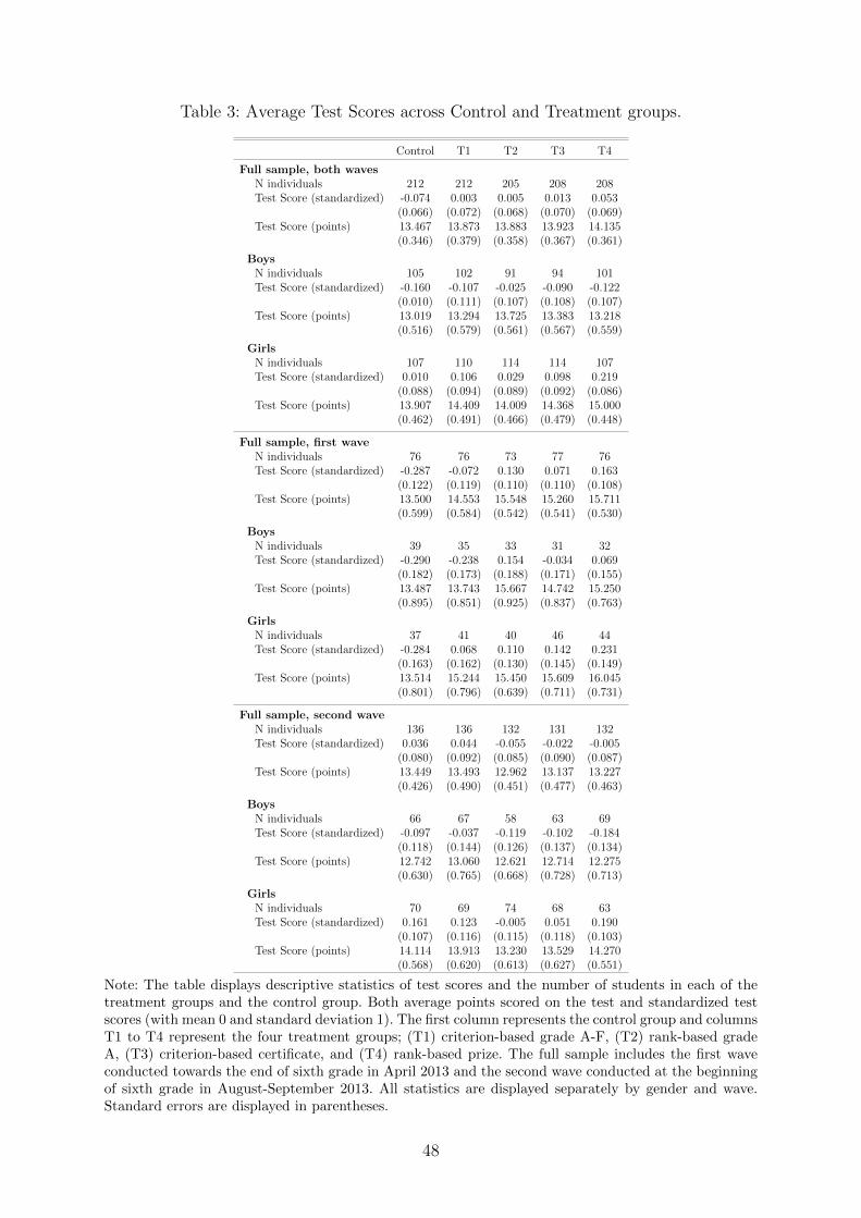
Table 3: Average Test Scores across Control and Treatment groups.

Control T1 T2 T3 T4

Full sample, both wavesN individuals 212 212 205 208 208Test Score (standardized) -0.074 0.003 0.005 0.013 0.053

(0.066) (0.072) (0.068) (0.070) (0.069)Test Score (points) 13.467 13.873 13.883 13.923 14.135

(0.346) (0.379) (0.358) (0.367) (0.361)

BoysN individuals 105 102 91 94 101Test Score (standardized) -0.160 -0.107 -0.025 -0.090 -0.122

(0.010) (0.111) (0.107) (0.108) (0.107)Test Score (points) 13.019 13.294 13.725 13.383 13.218

(0.516) (0.579) (0.561) (0.567) (0.559)

GirlsN individuals 107 110 114 114 107Test Score (standardized) 0.010 0.106 0.029 0.098 0.219

(0.088) (0.094) (0.089) (0.092) (0.086)Test Score (points) 13.907 14.409 14.009 14.368 15.000

(0.462) (0.491) (0.466) (0.479) (0.448)

Full sample, first waveN individuals 76 76 73 77 76Test Score (standardized) -0.287 -0.072 0.130 0.071 0.163

(0.122) (0.119) (0.110) (0.110) (0.108)Test Score (points) 13.500 14.553 15.548 15.260 15.711

(0.599) (0.584) (0.542) (0.541) (0.530)

BoysN individuals 39 35 33 31 32Test Score (standardized) -0.290 -0.238 0.154 -0.034 0.069

(0.182) (0.173) (0.188) (0.171) (0.155)Test Score (points) 13.487 13.743 15.667 14.742 15.250

(0.895) (0.851) (0.925) (0.837) (0.763)

GirlsN individuals 37 41 40 46 44Test Score (standardized) -0.284 0.068 0.110 0.142 0.231

(0.163) (0.162) (0.130) (0.145) (0.149)Test Score (points) 13.514 15.244 15.450 15.609 16.045

(0.801) (0.796) (0.639) (0.711) (0.731)

Full sample, second waveN individuals 136 136 132 131 132Test Score (standardized) 0.036 0.044 -0.055 -0.022 -0.005

(0.080) (0.092) (0.085) (0.090) (0.087)Test Score (points) 13.449 13.493 12.962 13.137 13.227

(0.426) (0.490) (0.451) (0.477) (0.463)

BoysN individuals 66 67 58 63 69Test Score (standardized) -0.097 -0.037 -0.119 -0.102 -0.184

(0.118) (0.144) (0.126) (0.137) (0.134)Test Score (points) 12.742 13.060 12.621 12.714 12.275

(0.630) (0.765) (0.668) (0.728) (0.713)

GirlsN individuals 70 69 74 68 63Test Score (standardized) 0.161 0.123 -0.005 0.051 0.190

(0.107) (0.116) (0.115) (0.118) (0.103)Test Score (points) 14.114 13.913 13.230 13.529 14.270

(0.568) (0.620) (0.613) (0.627) (0.551)

Note: The table displays descriptive statistics of test scores and the number of students in each of thetreatment groups and the control group. Both average points scored on the test and standardized testscores (with mean 0 and standard deviation 1). The first column represents the control group and columnsT1 to T4 represent the four treatment groups; (T1) criterion-based grade A-F, (T2) rank-based gradeA, (T3) criterion-based certificate, and (T4) rank-based prize. The full sample includes the first waveconducted towards the end of sixth grade in April 2013 and the second wave conducted at the beginningof sixth grade in August-September 2013. All statistics are displayed separately by gender and wave.Standard errors are displayed in parentheses.

48

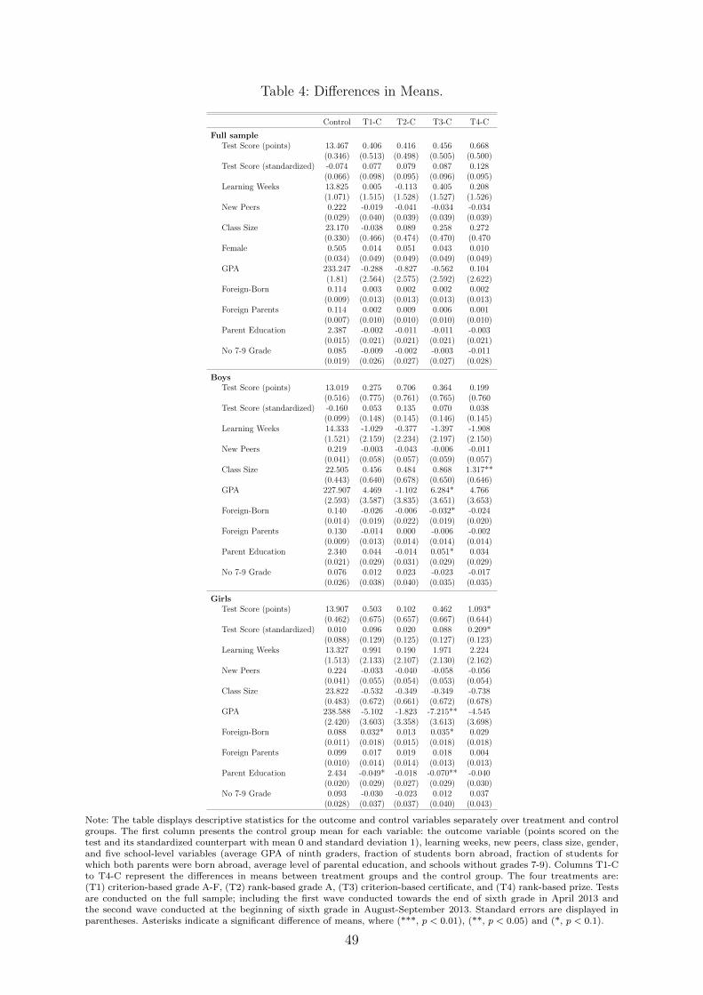
Table 4: Differences in Means.

Control T1-C T2-C T3-C T4-C

Full sampleTest Score (points) 13.467 0.406 0.416 0.456 0.668

(0.346) (0.513) (0.498) (0.505) (0.500)Test Score (standardized) -0.074 0.077 0.079 0.087 0.128

(0.066) (0.098) (0.095) (0.096) (0.095)Learning Weeks 13.825 0.005 -0.113 0.405 0.208

(1.071) (1.515) (1.528) (1.527) (1.526)New Peers 0.222 -0.019 -0.041 -0.034 -0.034

(0.029) (0.040) (0.039) (0.039) (0.039)Class Size 23.170 -0.038 0.089 0.258 0.272

(0.330) (0.466) (0.474) (0.470) (0.470Female 0.505 0.014 0.051 0.043 0.010

(0.034) (0.049) (0.049) (0.049) (0.049)GPA 233.247 -0.288 -0.827 -0.562 0.104

(1.81) (2.564) (2.575) (2.592) (2.622)Foreign-Born 0.114 0.003 0.002 0.002 0.002

(0.009) (0.013) (0.013) (0.013) (0.013)Foreign Parents 0.114 0.002 0.009 0.006 0.001

(0.007) (0.010) (0.010) (0.010) (0.010)Parent Education 2.387 -0.002 -0.011 -0.011 -0.003

(0.015) (0.021) (0.021) (0.021) (0.021)No 7-9 Grade 0.085 -0.009 -0.002 -0.003 -0.011

(0.019) (0.026) (0.027) (0.027) (0.028)

BoysTest Score (points) 13.019 0.275 0.706 0.364 0.199

(0.516) (0.775) (0.761) (0.765) (0.760Test Score (standardized) -0.160 0.053 0.135 0.070 0.038

(0.099) (0.148) (0.145) (0.146) (0.145)Learning Weeks 14.333 -1.029 -0.377 -1.397 -1.908

(1.521) (2.159) (2.234) (2.197) (2.150)New Peers 0.219 -0.003 -0.043 -0.006 -0.011

(0.041) (0.058) (0.057) (0.059) (0.057)Class Size 22.505 0.456 0.484 0.868 1.317**

(0.443) (0.640) (0.678) (0.650) (0.646)GPA 227.907 4.469 -1.102 6.284* 4.766

(2.593) (3.587) (3.835) (3.651) (3.653)Foreign-Born 0.140 -0.026 -0.006 -0.032* -0.024

(0.014) (0.019) (0.022) (0.019) (0.020)Foreign Parents 0.130 -0.014 0.000 -0.006 -0.002

(0.009) (0.013) (0.014) (0.014) (0.014)Parent Education 2.340 0.044 -0.014 0.051* 0.034

(0.021) (0.029) (0.031) (0.029) (0.029)No 7-9 Grade 0.076 0.012 0.023 -0.023 -0.017

(0.026) (0.038) (0.040) (0.035) (0.035)

GirlsTest Score (points) 13.907 0.503 0.102 0.462 1.093*

(0.462) (0.675) (0.657) (0.667) (0.644)Test Score (standardized) 0.010 0.096 0.020 0.088 0.209*

(0.088) (0.129) (0.125) (0.127) (0.123)Learning Weeks 13.327 0.991 0.190 1.971 2.224

(1.513) (2.133) (2.107) (2.130) (2.162)New Peers 0.224 -0.033 -0.040 -0.058 -0.056

(0.041) (0.055) (0.054) (0.053) (0.054)Class Size 23.822 -0.532 -0.349 -0.349 -0.738

(0.483) (0.672) (0.661) (0.672) (0.678)GPA 238.588 -5.102 -1.823 -7.215** -4.545

(2.420) (3.603) (3.358) (3.613) (3.698)Foreign-Born 0.088 0.032* 0.013 0.035* 0.029

(0.011) (0.018) (0.015) (0.018) (0.018)Foreign Parents 0.099 0.017 0.019 0.018 0.004

(0.010) (0.014) (0.014) (0.013) (0.013)Parent Education 2.434 -0.049* -0.018 -0.070** -0.040

(0.020) (0.029) (0.027) (0.029) (0.030)No 7-9 Grade 0.093 -0.030 -0.023 0.012 0.037

(0.028) (0.037) (0.037) (0.040) (0.043)

Note: The table displays descriptive statistics for the outcome and control variables separately over treatment and controlgroups. The first column presents the control group mean for each variable: the outcome variable (points scored on thetest and its standardized counterpart with mean 0 and standard deviation 1), learning weeks, new peers, class size, gender,and five school-level variables (average GPA of ninth graders, fraction of students born abroad, fraction of students forwhich both parents were born abroad, average level of parental education, and schools without grades 7-9). Columns T1-Cto T4-C represent the differences in means between treatment groups and the control group. The four treatments are:(T1) criterion-based grade A-F, (T2) rank-based grade A, (T3) criterion-based certificate, and (T4) rank-based prize. Testsare conducted on the full sample; including the first wave conducted towards the end of sixth grade in April 2013 andthe second wave conducted at the beginning of sixth grade in August-September 2013. Standard errors are displayed inparentheses. Asterisks indicate a significant difference of means, where (***, p < 0.01), (**, p < 0.05) and (*, p < 0.1).

49

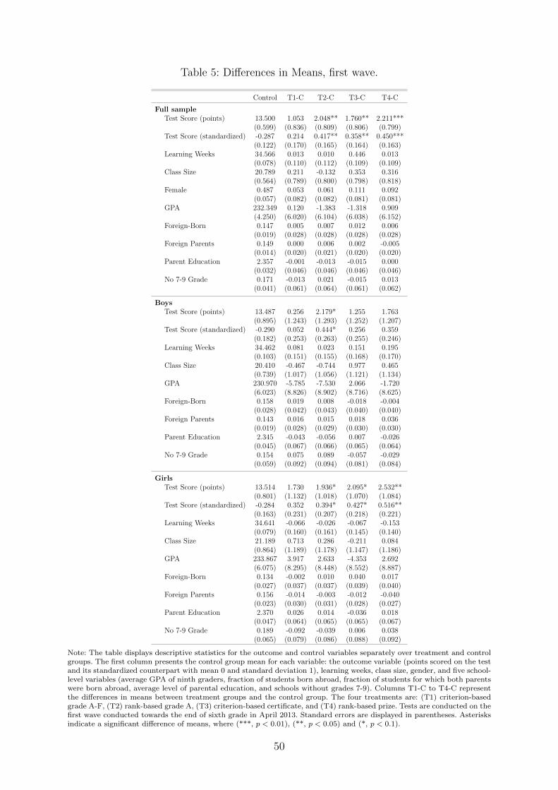
Table 5: Differences in Means, first wave.

Control T1-C T2-C T3-C T4-C

Full sampleTest Score (points) 13.500 1.053 2.048** 1.760** 2.211***

(0.599) (0.836) (0.809) (0.806) (0.799)Test Score (standardized) -0.287 0.214 0.417** 0.358** 0.450***

(0.122) (0.170) (0.165) (0.164) (0.163)Learning Weeks 34.566 0.013 0.010 0.446 0.013

(0.078) (0.110) (0.112) (0.109) (0.109)Class Size 20.789 0.211 -0.132 0.353 0.316

(0.564) (0.789) (0.800) (0.798) (0.818)Female 0.487 0.053 0.061 0.111 0.092

(0.057) (0.082) (0.082) (0.081) (0.081)GPA 232.349 0.120 -1.383 -1.318 0.909

(4.250) (6.020) (6.104) (6.038) (6.152)Foreign-Born 0.147 0.005 0.007 0.012 0.006

(0.019) (0.028) (0.028) (0.028) (0.028)Foreign Parents 0.149 0.000 0.006 0.002 -0.005

(0.014) (0.020) (0.021) (0.020) (0.020)Parent Education 2.357 -0.001 -0.013 -0.015 0.000

(0.032) (0.046) (0.046) (0.046) (0.046)No 7-9 Grade 0.171 -0.013 0.021 -0.015 0.013

(0.041) (0.061) (0.064) (0.061) (0.062)

BoysTest Score (points) 13.487 0.256 2.179* 1.255 1.763

(0.895) (1.243) (1.293) (1.252) (1.207)Test Score (standardized) -0.290 0.052 0.444* 0.256 0.359

(0.182) (0.253) (0.263) (0.255) (0.246)Learning Weeks 34.462 0.081 0.023 0.151 0.195

(0.103) (0.151) (0.155) (0.168) (0.170)Class Size 20.410 -0.467 -0.744 0.977 0.465

(0.739) (1.017) (1.056) (1.121) (1.134)GPA 230.970 -5.785 -7.530 2.066 -1.720

(6.023) (8.826) (8.902) (8.716) (8.625)Foreign-Born 0.158 0.019 0.008 -0.018 -0.004

(0.028) (0.042) (0.043) (0.040) (0.040)Foreign Parents 0.143 0.016 0.015 0.018 0.036

(0.019) (0.028) (0.029) (0.030) (0.030)Parent Education 2.345 -0.043 -0.056 0.007 -0.026

(0.045) (0.067) (0.066) (0.065) (0.064)No 7-9 Grade 0.154 0.075 0.089 -0.057 -0.029

(0.059) (0.092) (0.094) (0.081) (0.084)

GirlsTest Score (points) 13.514 1.730 1.936* 2.095* 2.532**

(0.801) (1.132) (1.018) (1.070) (1.084)Test Score (standardized) -0.284 0.352 0.394* 0.427* 0.516**

(0.163) (0.231) (0.207) (0.218) (0.221)Learning Weeks 34.641 -0.066 -0.026 -0.067 -0.153

(0.079) (0.160) (0.161) (0.145) (0.140)Class Size 21.189 0.713 0.286 -0.211 0.084

(0.864) (1.189) (1.178) (1.147) (1.186)GPA 233.867 3.917 2.633 -4.353 2.692

(6.075) (8.295) (8.448) (8.552) (8.887)Foreign-Born 0.134 -0.002 0.010 0.040 0.017

(0.027) (0.037) (0.037) (0.039) (0.040)Foreign Parents 0.156 -0.014 -0.003 -0.012 -0.040

(0.023) (0.030) (0.031) (0.028) (0.027)Parent Education 2.370 0.026 0.014 -0.036 0.018

(0.047) (0.064) (0.065) (0.065) (0.067)No 7-9 Grade 0.189 -0.092 -0.039 0.006 0.038

(0.065) (0.079) (0.086) (0.088) (0.092)

Note: The table displays descriptive statistics for the outcome and control variables separately over treatment and controlgroups. The first column presents the control group mean for each variable: the outcome variable (points scored on the testand its standardized counterpart with mean 0 and standard deviation 1), learning weeks, class size, gender, and five school-level variables (average GPA of ninth graders, fraction of students born abroad, fraction of students for which both parentswere born abroad, average level of parental education, and schools without grades 7-9). Columns T1-C to T4-C representthe differences in means between treatment groups and the control group. The four treatments are: (T1) criterion-basedgrade A-F, (T2) rank-based grade A, (T3) criterion-based certificate, and (T4) rank-based prize. Tests are conducted on thefirst wave conducted towards the end of sixth grade in April 2013. Standard errors are displayed in parentheses. Asterisksindicate a significant difference of means, where (***, p < 0.01), (**, p < 0.05) and (*, p < 0.1).

50

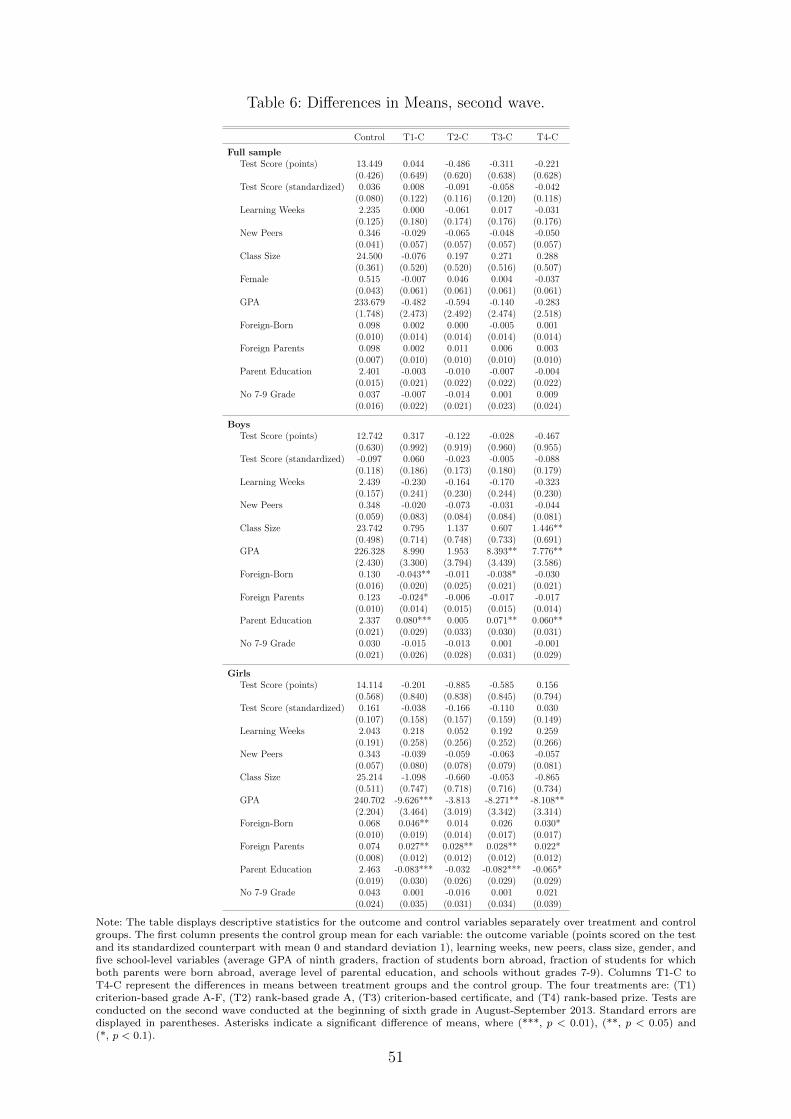
Table 6: Differences in Means, second wave.

Control T1-C T2-C T3-C T4-C

Full sampleTest Score (points) 13.449 0.044 -0.486 -0.311 -0.221

(0.426) (0.649) (0.620) (0.638) (0.628)Test Score (standardized) 0.036 0.008 -0.091 -0.058 -0.042

(0.080) (0.122) (0.116) (0.120) (0.118)Learning Weeks 2.235 0.000 -0.061 0.017 -0.031

(0.125) (0.180) (0.174) (0.176) (0.176)New Peers 0.346 -0.029 -0.065 -0.048 -0.050

(0.041) (0.057) (0.057) (0.057) (0.057)Class Size 24.500 -0.076 0.197 0.271 0.288

(0.361) (0.520) (0.520) (0.516) (0.507)Female 0.515 -0.007 0.046 0.004 -0.037

(0.043) (0.061) (0.061) (0.061) (0.061)GPA 233.679 -0.482 -0.594 -0.140 -0.283

(1.748) (2.473) (2.492) (2.474) (2.518)Foreign-Born 0.098 0.002 0.000 -0.005 0.001

(0.010) (0.014) (0.014) (0.014) (0.014)Foreign Parents 0.098 0.002 0.011 0.006 0.003

(0.007) (0.010) (0.010) (0.010) (0.010)Parent Education 2.401 -0.003 -0.010 -0.007 -0.004

(0.015) (0.021) (0.022) (0.022) (0.022)No 7-9 Grade 0.037 -0.007 -0.014 0.001 0.009

(0.016) (0.022) (0.021) (0.023) (0.024)

BoysTest Score (points) 12.742 0.317 -0.122 -0.028 -0.467

(0.630) (0.992) (0.919) (0.960) (0.955)Test Score (standardized) -0.097 0.060 -0.023 -0.005 -0.088

(0.118) (0.186) (0.173) (0.180) (0.179)Learning Weeks 2.439 -0.230 -0.164 -0.170 -0.323

(0.157) (0.241) (0.230) (0.244) (0.230)New Peers 0.348 -0.020 -0.073 -0.031 -0.044

(0.059) (0.083) (0.084) (0.084) (0.081)Class Size 23.742 0.795 1.137 0.607 1.446**

(0.498) (0.714) (0.748) (0.733) (0.691)GPA 226.328 8.990 1.953 8.393** 7.776**

(2.430) (3.300) (3.794) (3.439) (3.586)Foreign-Born 0.130 -0.043** -0.011 -0.038* -0.030

(0.016) (0.020) (0.025) (0.021) (0.021)Foreign Parents 0.123 -0.024* -0.006 -0.017 -0.017

(0.010) (0.014) (0.015) (0.015) (0.014)Parent Education 2.337 0.080*** 0.005 0.071** 0.060**

(0.021) (0.029) (0.033) (0.030) (0.031)No 7-9 Grade 0.030 -0.015 -0.013 0.001 -0.001

(0.021) (0.026) (0.028) (0.031) (0.029)

GirlsTest Score (points) 14.114 -0.201 -0.885 -0.585 0.156

(0.568) (0.840) (0.838) (0.845) (0.794)Test Score (standardized) 0.161 -0.038 -0.166 -0.110 0.030

(0.107) (0.158) (0.157) (0.159) (0.149)Learning Weeks 2.043 0.218 0.052 0.192 0.259

(0.191) (0.258) (0.256) (0.252) (0.266)New Peers 0.343 -0.039 -0.059 -0.063 -0.057

(0.057) (0.080) (0.078) (0.079) (0.081)Class Size 25.214 -1.098 -0.660 -0.053 -0.865

(0.511) (0.747) (0.718) (0.716) (0.734)GPA 240.702 -9.626*** -3.813 -8.271** -8.108**

(2.204) (3.464) (3.019) (3.342) (3.314)Foreign-Born 0.068 0.046** 0.014 0.026 0.030*

(0.010) (0.019) (0.014) (0.017) (0.017)Foreign Parents 0.074 0.027** 0.028** 0.028** 0.022*

(0.008) (0.012) (0.012) (0.012) (0.012)Parent Education 2.463 -0.083*** -0.032 -0.082*** -0.065*

(0.019) (0.030) (0.026) (0.029) (0.029)No 7-9 Grade 0.043 0.001 -0.016 0.001 0.021

(0.024) (0.035) (0.031) (0.034) (0.039)

Note: The table displays descriptive statistics for the outcome and control variables separately over treatment and controlgroups. The first column presents the control group mean for each variable: the outcome variable (points scored on the testand its standardized counterpart with mean 0 and standard deviation 1), learning weeks, new peers, class size, gender, andfive school-level variables (average GPA of ninth graders, fraction of students born abroad, fraction of students for whichboth parents were born abroad, average level of parental education, and schools without grades 7-9). Columns T1-C toT4-C represent the differences in means between treatment groups and the control group. The four treatments are: (T1)criterion-based grade A-F, (T2) rank-based grade A, (T3) criterion-based certificate, and (T4) rank-based prize. Tests areconducted on the second wave conducted at the beginning of sixth grade in August-September 2013. Standard errors aredisplayed in parentheses. Asterisks indicate a significant difference of means, where (***, p < 0.01), (**, p < 0.05) and(*, p < 0.1).

51

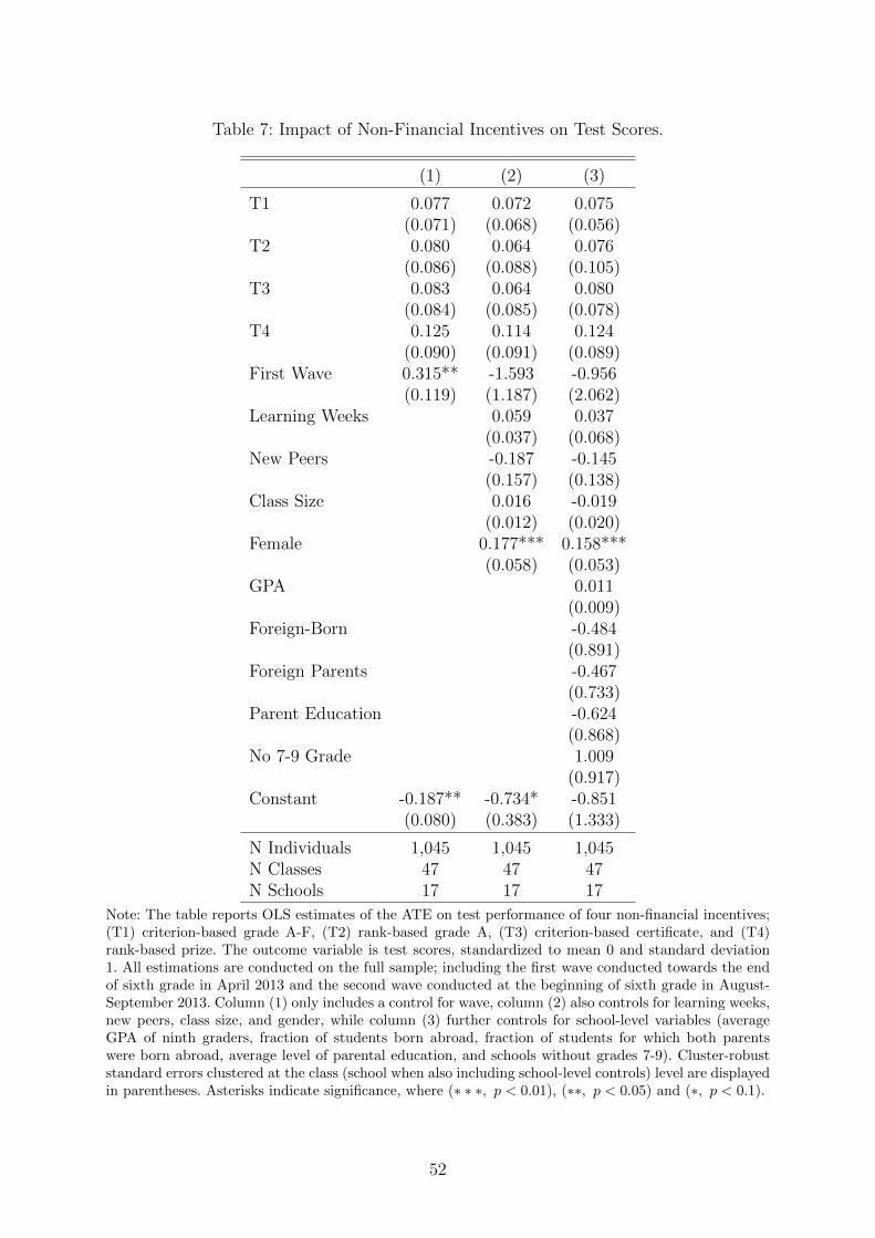
Table 7: Impact of Non-Financial Incentives on Test Scores.

(1) (2) (3)

T1 0.077 0.072 0.075(0.071) (0.068) (0.056)

T2 0.080 0.064 0.076(0.086) (0.088) (0.105)

T3 0.083 0.064 0.080(0.084) (0.085) (0.078)

T4 0.125 0.114 0.124(0.090) (0.091) (0.089)

First Wave 0.315** -1.593 -0.956(0.119) (1.187) (2.062)

Learning Weeks 0.059 0.037(0.037) (0.068)

New Peers -0.187 -0.145(0.157) (0.138)

Class Size 0.016 -0.019(0.012) (0.020)

Female 0.177*** 0.158***(0.058) (0.053)

GPA 0.011(0.009)

Foreign-Born -0.484(0.891)

Foreign Parents -0.467(0.733)

Parent Education -0.624(0.868)

No 7-9 Grade 1.009(0.917)

Constant -0.187** -0.734* -0.851(0.080) (0.383) (1.333)

N Individuals 1,045 1,045 1,045N Classes 47 47 47N Schools 17 17 17

Note: The table reports OLS estimates of the ATE on test performance of four non-financial incentives;(T1) criterion-based grade A-F, (T2) rank-based grade A, (T3) criterion-based certificate, and (T4)rank-based prize. The outcome variable is test scores, standardized to mean 0 and standard deviation1. All estimations are conducted on the full sample; including the first wave conducted towards the endof sixth grade in April 2013 and the second wave conducted at the beginning of sixth grade in August-September 2013. Column (1) only includes a control for wave, column (2) also controls for learning weeks,new peers, class size, and gender, while column (3) further controls for school-level variables (averageGPA of ninth graders, fraction of students born abroad, fraction of students for which both parentswere born abroad, average level of parental education, and schools without grades 7-9). Cluster-robuststandard errors clustered at the class (school when also including school-level controls) level are displayedin parentheses. Asterisks indicate significance, where (∗ ∗ ∗, p < 0.01), (∗∗, p < 0.05) and (∗, p < 0.1).

52

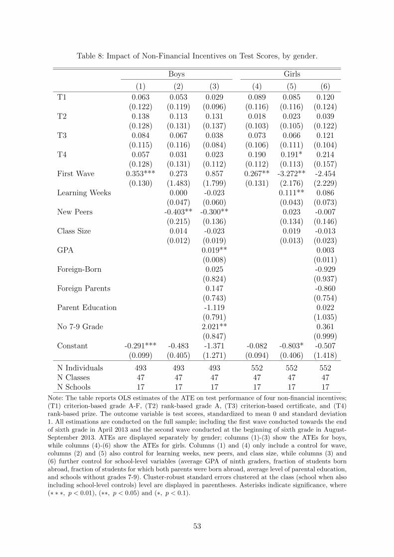
Table 8: Impact of Non-Financial Incentives on Test Scores, by gender.

Boys Girls

(1) (2) (3) (4) (5) (6)

T1 0.063 0.053 0.029 0.089 0.085 0.120(0.122) (0.119) (0.096) (0.116) (0.116) (0.124)

T2 0.138 0.113 0.131 0.018 0.023 0.039(0.128) (0.131) (0.137) (0.103) (0.105) (0.122)

T3 0.084 0.067 0.038 0.073 0.066 0.121(0.115) (0.116) (0.084) (0.106) (0.111) (0.104)

T4 0.057 0.031 0.023 0.190 0.191* 0.214(0.128) (0.131) (0.112) (0.112) (0.113) (0.157)

First Wave 0.353*** 0.273 0.857 0.267** -3.272** -2.454(0.130) (1.483) (1.799) (0.131) (2.176) (2.229)

Learning Weeks 0.000 -0.023 0.111** 0.086(0.047) (0.060) (0.043) (0.073)

New Peers -0.403** -0.300** 0.023 -0.007(0.215) (0.136) (0.134) (0.146)

Class Size 0.014 -0.023 0.019 -0.013(0.012) (0.019) (0.013) (0.023)

GPA 0.019** 0.003(0.008) (0.011)

Foreign-Born 0.025 -0.929(0.824) (0.937)

Foreign Parents 0.147 -0.860(0.743) (0.754)

Parent Education -1.119 0.022(0.791) (1.035)

No 7-9 Grade 2.021** 0.361(0.847) (0.999)

Constant -0.291*** -0.483 -1.371 -0.082 -0.803* -0.507(0.099) (0.405) (1.271) (0.094) (0.406) (1.418)

N Individuals 493 493 493 552 552 552N Classes 47 47 47 47 47 47N Schools 17 17 17 17 17 17

Note: The table reports OLS estimates of the ATE on test performance of four non-financial incentives;(T1) criterion-based grade A-F, (T2) rank-based grade A, (T3) criterion-based certificate, and (T4)rank-based prize. The outcome variable is test scores, standardized to mean 0 and standard deviation1. All estimations are conducted on the full sample; including the first wave conducted towards the endof sixth grade in April 2013 and the second wave conducted at the beginning of sixth grade in August-September 2013. ATEs are displayed separately by gender; columns (1)-(3) show the ATEs for boys,while columns (4)-(6) show the ATEs for girls. Columns (1) and (4) only include a control for wave,columns (2) and (5) also control for learning weeks, new peers, and class size, while columns (3) and(6) further control for school-level variables (average GPA of ninth graders, fraction of students bornabroad, fraction of students for which both parents were born abroad, average level of parental education,and schools without grades 7-9). Cluster-robust standard errors clustered at the class (school when alsoincluding school-level controls) level are displayed in parentheses. Asterisks indicate significance, where(∗ ∗ ∗, p < 0.01), (∗∗, p < 0.05) and (∗, p < 0.1).

53

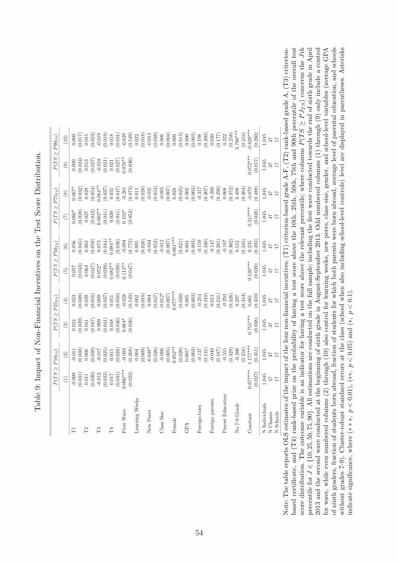
Tab

le9:

Impac

tof

Non

-Fin

anci

alIn

centi

ves

onth

eT

est

Sco

reD

istr

ibuti

on.

P(TS≥P

10TS)

P(TS≥P

25TS)

P(TS≥P

50TS)

P(TS≥P

75TS)

P(TS≥P

90TS)

(1)

(2)

(3)

(4)

(5)

(6)

(7)

(8)

(9)

(10)

T1

-0.0

09-0

.011

0.02

40.

023

0.05

70.

056

0.06

6*0.

067*

0.00

00.

000

(0.0

31)

(0.0

30)

(0.0

39)

(0.0

38)

(0.0

43)

(0.0

45)

(0.0

38)

(0.0

32)

(0.0

24)

(0.0

17)

T2

0.01

10.

006

0.04

10.

039

0.06

40.

063

0.02

70.

029

0.01

30.

015

(0.0

30)

(0.0

30)

(0.0

47)

(0.0

58)

(0.0

47)

(0.0

59)

(0.0

42)

(0.0

54)

(0.0

27)

(0.0

23)

T3

-0.0

12-0

.017

0.00

90.

009

0.07

2*0.

073

0.08

3**

0.08

4**

-0.0

18-0

.019

(0.0

32)

(0.0

25)

(0.0

41)

(0.0

37)

(0.0

39)

(0.0

44)

(0.0

41)

(0.0

37)

(0.0

21)

(0.0

19)

T4

0.01

70.

015

0.04

80.

051

0.08

2**

0.08

4**

0.03

00.

031

0.02

10.

018

(0.0

31)

(0.0

28)

(0.0

46)

(0.0

50)

(0.0

39)

(0.0

36)

(0.0

41)

(0.0

47)

(0.0

27)

(0.0

31)

Fir

stW

ave

0.06

6***

-0.0

930.

064*

-0.0

280.

113*

*-0

.094

0.10

2*-0

.261

0.07

6**

-0.6

29(0

.022

)(0

.268

)(0

.036

)(0

.549

)(0

.047

)(0

.772

)(0

.052

)(0

.873

)(0

.036

)(0

.549

)L

earn

ing

Wee

ks

0.00

40.

002

0.00

50.

011

0.02

2(0

.009

)(0

.018

)(0

.026

)(0

.028

)(0

.018

)N

ewP

eers

-0.0

48*

0.00

4-0

.034

-0.0

31-0

.013

(0.0

26)

(0.0

47)

(0.0

52)

(0.0

53)

(0.0

38)

Cla

ssS

ize

-0.0

06-0

.012

*-0

.012

-0.0

050.

006

(0.0

05)

(0.0

07)

(0.0

07)

(0.0

07)

(0.0

04)

Fem

ale

0.05

2**

0.07

7***

0.06

1***

0.02

80.

009

(0.0

20)

(0.0

20)

(0.0

21)

(0.0

25)

(0.0

15)

GP

A0.

005*

0.00

50.

004

0.00

20.

000

(0.0

03)

(0.0

03)

(0.0

03)

(0.0

03)

(0.0

03)

For

eign

-bor

n-0

.137

-0.2

54-0

.159

-0.3

170.

198

(0.1

31)

(0.3

10)

(0.3

40)

(0.3

07)

(0.2

00)

For

eign

par

ents

-0.0

480.

013

-0.1

47-0

.200

0.02

0(0

.187

)(0

.241

)(0

.281

)(0

.290

)(0

.177

)P

aren

tE

du

cati

on-0

.555

-0.2

93-0

.187

0.06

80.

322

(0.3

29)

(0.3

26)

(0.3

02)

(0.3

72)

(0.2

58)

No

7-9

Gra

de

-0.2

060.

297

0.51

20.

499

0.78

0***

(0.2

58)

(0.3

44)

(0.3

45)

(0.3

64)

(0.2

16)

Con

stan

t0.

877*

**1.

177*

**0.

755*

**0.

661

0.53

0***

0.23

50.

317*

**-0

.070

0.07

2***

-0.8

29**

*(0

.027

)(0

.351

)(0

.038

)(0

.459

)(0

.039

)(0

.493

)(0

.038

)(0

.488

)(0

.017

)(0

.260

)

NIn

div

idu

als

1,04

51,

045

1,04

51,

045

1,04

51,

045

1,04

51,

045

1,04

51,

045

NC

lass

es47

4747

4747

4747

4747

47N

Sch

ool

s17

1717

1717

1717

1717

17

Not

e:T

he

tab

lere

por

tsO

LS

esti

mat

esof

the

imp

act

ofth

efo

ur

non

-fin

an

cialin

centi

ves;

(T1)

crit

erio

n-b

ase

dgra

de

A-F

,(T

2)

ran

k-b

ase

dgra

de

A,(T

3)

crit

erio

n-

bas

edce

rtifi

cate

,and

(T4)

ran

k-b

ased

pri

zeon

the

pro

bab

ilit

yof

hav

ing

ate

stsc

ore

ab

ove

the

10th

,25th

,50th

,75th

an

d90th

per

centi

leof

the

over

all

test

scor

ed

istr

ibu

tion

.T

he

outc

ome

vari

able

isan

ind

icat

orfo

rh

avin

ga

test

score

ab

ove

the

rele

vant

per

centi

le;

wh

ere

colu

mn

sP

(TS≥

PJTS

)co

nce

rns

theJ

thp

erce

nti

lefo

rJ∈{1

0,2

5,50

,75,

90}.

All

esti

mat

ion

sar

eco

nd

uct

edon

the

full

sam

ple

;in

clu

din

gth

efi

rst

wav

eco

nd

uct

edto

ward

sth

een

dof

sixth

gra

de

inA

pri

l20

13an

dth

ese

con

dw

ave

con

du

cted

atth

eb

egin

nin

gof

sixth

gra

de

inA

ugu

st-S

epte

mb

er2013.

Od

dnu

mb

ered

colu

mn

s(1

)th

rou

gh

(9)

on

lyin

clu

de

aco

ntr

ol

for

wav

e,w

hil

eev

ennu

mb

ered

colu

mn

s(2

)th

rou

gh(1

0)als

oco

ntr

ol

for

learn

ing

wee

ks,

new

pee

rs,

class

size

,gen

der

,an

dsc

hool-

leve

lva

riab

les

(ave

rage

GP

Aof

nin

thgr

ader

s,fr

acti

onof

stu

den

tsb

orn

abro

ad,

frac

tion

of

stu

den

tsfo

rw

hic

hb

oth

pare

nts

wer

eb

orn

ab

road

,av

erage

leve

lof

pare

nta

led

uca

tion

,an

dsc

hools

wit

hou

tgr

ades

7-9)

.C

lust

er-r

obu

stst

and

ard

erro

rsat

the

class

(sch

ool

when

als

oin

clu

din

gsc

hool-

leve

lco

ntr

ols

)le

vel

are

dis

pla

yed

inp

are

nth

eses

.A

ster

isks

ind

icat

esi

gnifi

can

ce,

wh

ere

(∗∗∗,

p<

0.0

1),

(∗∗,

p<

0.05

)an

d(∗,p<

0.1).

54

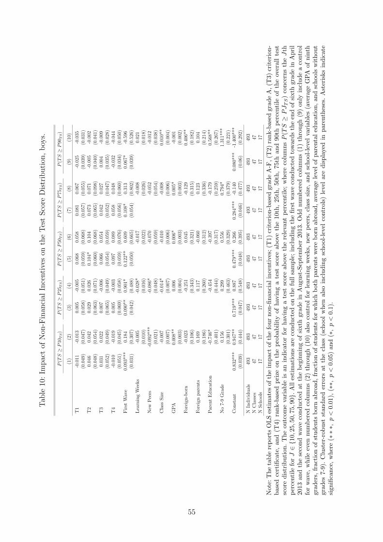
Tab

le10

:Im

pac

tof

Non

-Fin

anci

alIn

centi

ves

onth

eT

est

Sco

reD

istr

ibuti

on,

boy

s.

P(TS≥P

10TS)

P(TS≥P

25TS)

P(TS≥P

50TS)

P(TS≥P

75TS)

P(TS≥P

90TS)

(1)

(2)

(3)

(4)

(5)

(6)

(7)

(8)

(9)

(10)

T1

-0.0

11-0

.013

0.00

5-0

.005

0.06

80.

058

0.08

10.

067

-0.0

25-0

.035

(0.0

49)

(0.0

47)

(0.0

58)

(0.0

51)

(0.0

59)

(0.0

68)

(0.0

57)

(0.0

55)

(0.0

39)

(0.0

31)

T2

0.04

60.

042

0.02

90.

026

0.10

4*0.

104

0.07

30.

071

-0.0

05-0

.002

(0.0

48)

(0.0

54)

(0.0

63)

(0.0

71)

(0.0

60)

(0.0

68)

(0.0

65)

(0.0

98)

(0.0

40)

(0.0

41)

T3

0.03

10.

022

0.00

7-0

.006

0.06

60.

054

0.04

20.

027

0.00

4-0

.009

(0.0

52)

(0.0

49)

(0.0

65)

(0.0

49)

(0.0

54)

(0.0

59)

(0.0

52)

(0.0

47)

(0.0

35)

(0.0

28)

T4

-0.0

10-0

.019

0.00

5-0

.003

0.09

70.

089

0.05

80.

048

-0.0

32-0

.044

(0.0

51)

(0.0

45)

(0.0

69)

(0.0

58)

(0.0

59)

(0.0

76)

(0.0

56)

(0.0

60)

(0.0

34)

(0.0

50)

Fir

stW

ave

0.09

3***

0.18

40.

090*

*0.

901*

0.12

2**

0.60

90.

108*

0.31

30.

067*

-0.5

96(0

.031

)(0

.307

)(0

.042

)(0

.488

)(0

.050

)(0

.665

)(0

.054

)(0

.802

)(0

.039

)(0

.526

)L

earn

ing

Wee

ks

-0.0

05-0

.028

*-0

.017

-0.0

080.

021

(0.0

10)

(0.0

16)

(0.0

22)

(0.0

26)

(0.0

18)

New

Pee

rs-0

.092

***

-0.0

86*

-0.0

70-0

.052

-0.0

12(0

.021

)(0

.048

)(0

.059

)(0

.054

)(0

.038

)C

lass

Siz

e-0

.007

-0.0

14*

-0.0

10-0

.008

0.01

0**

(0.0

07)

(0.0

07)

(0.0

06)

(0.0

06)

(0.0

04)

GP

A0.

008*

*0.

006

0.00

6*0.

005*

-0.0

01(0

.003

)(0

.004

)(0

.003

)(0

.003

)(0

.002

)F

orei

gn-b

orn

-0.0

23-0

.251

0.04

5-0

.129

0.40

6**

(0.1

06)

(0.3

43)

(0.3

21)

(0.3

15)

(0.1

82)

For

eign

par

ents

0.16

90.

117

-0.0

600.

123

0.10

4(0

.186

)(0

.260

)(0

.312

)(0

.336

)(0

.214

)P

aren

tE

du

cati

on-0

.746

*-0

.454

-0.3

97-0

.179

0.56

8**

(0.4

01)

(0.4

44)

(0.3

17)

(0.2

59)

(0.2

67)

No

7-9

Gra

de

0.15

60.

299

0.55

60.

794*

1.31

1***

(0.3

01)

(0.4

63)

(0.3

29)

(0.3

79)

(0.2

21)

Con

stan

t0.

832*

**0.

947*

*0.

719*

**0.

887

0.47

9***

0.26

60.

284*

**-0

.140

0.08

0***

-1.4

00**

*(0

.039

)(0

.444

)(0

.047

)(0

.548

)(0

.048

)(0

.395

)(0

.046

)(0

.477

)(0

.06)

(0.2

92)

NIn

div

idu

als

493

493

493

493

493

493

493

493

493

493

NC

lass

es47

4747

4747

4747

4747

47N

Sch

ool

s17

1717

1717

1717

1717

17

Not

e:T

he

tab

lere

por

tsO

LS

esti

mat

esof

the

imp

act

ofth

efo

ur

non

-fin

an

cialin

centi

ves;

(T1)

crit

erio

n-b

ase

dgra

de

A-F

,(T

2)

ran

k-b

ase

dgra

de

A,(T

3)

crit

erio

n-

bas

edce

rtifi

cate

,and

(T4)

ran

k-b

ased

pri

zeon

the

pro

bab

ilit

yof

hav

ing

ate

stsc

ore

ab

ove

the

10th

,25th

,50th

,75th

an

d90th

per

centi

leof

the

over

all

test

scor

ed

istr

ibu

tion

.T

he

outc

ome

vari

able

isan

ind

icat

orfo

rh

avin

ga

test

score

ab

ove

the

rele

vant

per

centi

le;

wh

ere

colu

mn

sP

(TS≥

PJTS

)co

nce

rns

theJ

thp

erce

nti

lefo

rJ∈{1

0,2

5,50

,75,

90}.

All

esti

mat

ion

sar

eco

nd

uct

edon

the

full

sam

ple

;in

clu

din

gth

efi

rst

wav

eco

nd

uct

edto

ward

sth

een

dof

sixth

gra

de

inA

pri

l20

13an

dth

ese

con

dw

ave

con

du

cted

atth

eb

egin

nin

gof

sixth

gra

de

inA

ugu

st-S

epte

mb

er2013.

Od

dnu

mb

ered

colu

mn

s(1

)th

rou

gh

(9)

on

lyin

clu

de

aco

ntr

ol

for

wav

e,w

hil

eev

ennu

mb

ered

colu

mns

(2)

thro

ugh

(10)

also

contr

ol

for

learn

ing

wee

ks,

new

pee

rs,

class

size

,an

dsc

hool-

leve

lva

riab

les

(ave

rage

GP

Aof

nin

thgr

ader

s,fr

acti

onof

stu

den

tsb

orn

abro

ad,

frac

tion

ofst

ud

ents

for

wh

ich

both

pare

nts

wer

eb

orn

ab

road

,av

erage

leve

lof

pare

nta

led

uca

tion

,an

dsc

hools

wit

hou

tgr

ades

7-9)

.C

lust

er-r

obu

stst

and

ard

erro

rsat

the

clas

s(s

chool

wh

enals

oin

clu

din

gsc

hool-

leve

lco

ntr

ols

)le

vel

are

dis

pla

yed

inp

are

nth

eses

.A

ster

isks

ind

icate

sign

ifica

nce

,w

her

e(∗∗∗,

p<

0.01

),(∗∗,

p<

0.0

5)an

d(∗,p<

0.1).

55

Tab

le11

:Im

pac

tof

Non

-Fin

anci

alIn

centi

ves

onth

eT

est

Sco

reD

istr

ibuti

on,

girl

s.

P(TS≥P

10TS)

P(TS≥P

25TS)

P(TS≥P

50TS)

P(TS≥P

75TS)

P(TS≥P

90TS)

(1)

(2)

(3)

(4)

(5)

(6)

(7)

(8)

(9)

(10)

T1

-0.0

08-0

.011

0.04

10.

050

0.04

40.

059

0.05

10.

074

0.02

30.

029

(0.0

30)

(0.0

41)

(0.0

53)

(0.0

49)

(0.0

63)

(0.0

62)

(0.0

62)

(0.0

65)

(0.0

36)

(0.0

37)

T2

-0.0

22-0

.023

0.04

70.

051

0.02

30.

028

-0.0

15-0

.001

0.02

90.

032

(0.0

35)

(0.0

42)

(0.0

52)

(0.0

65)

(0.0

66)

(0.0

74)

(0.0

56)

(0.0

56)

(0.0

35)

(0.0

28)

T3

-0.0

51-0

.052

**0.

010

0.03

10.

070

0.09

80.

111*

0.14

1**

-0.0

37-0

.031

(0.0

30)

(0.0

19)

(0.0

45)

(0.0

48)

(0.0

57)

(0.0

62)

(0.0

58)

(0.0

60)

(0.0

31)

(0.0

33)

T4

0.04

40.

045

0.09

1*0.

104

0.06

80.

081

0.00

30.

018

0.06

90.

071

(0.0

29)

(0.0

35)

(0.0

54)

(0.0

61)

(0.0

55)

(0.0

72)

(0.0

63)

(0.0

88)

(0.0

43)

(0.0

48)

Fir

stW

ave

0.03

9-0

.361

0.03

5-0

.859

0.10

1*-0

.656

0.09

2-0

.681

0.08

2**

-0.5

76(0

.025

)(0

.289

)(0

.041

)(0

.601

)(0

.056

)(0

.921

)(0

.064

)(0

.917

)(0

.040

)(0

.620

)L

earn

ing

Wee

ks

0.01

30.

028

0.02

30.

025

0.02

0((

0.00

9)(0

.020

)(0

.030

)(0

.030

)(0

.020

)N

ewP

eers

-0.0

090.

092*

-0.0

08-0

.016

-0.0

21(0

.027

)(0

.046

)(0

.064

)(0

.062

)(0

.042

)C

lass

Siz

e-0

.003

-0.0

08-0

.014

-0.0

030.

004

(0.0

05)

(0.0

07)

(0.0

09)

(0.0

10)

(0.0

06)

GP

A0.

002

0.00

30.

003

-0.0

02-0

.001

(0.0

03)

(0.0

03)

(0.0

04)

(0.0

05)

(0.0

04)

For

eign

-bor

n-0

.204

-0.2

26-0

.373

-0.5

390.

000

(0.1

61)

(0.2

83)

(0.3

85)

(0.3

45)

(0.2

60)

For

eign

par

ents

-0.2

10-0

.009

-0.1

96-0

.476

0.00

2(0

.230

)(0

.268

)(0

.291

)(0

.316

)(0

.191

)P

aren

tE

du

cati

on-0

.356

-0.0

940.

025

0.34

40.

189

(0.2

95)

(0.3

09)

(0.3

92)

(0.5

71)

(0.3

10)

No

7-9

Gra

de

-0.4

82*

0.39

00.

528

0.28

70.

382

(0.2

66)

(0.3

03)

(0.4

27)

(0.4

67)

(0.2

93)

Con

stan

t0.

921*

**1.

364*

**0.

792*

**0.

431

0.58

2***

0.23

80.

351*

**0.

008

0.06

5**

-0.4

07(0

.027

)(0

.322

)(0

.045

)(0

.418

)(0

.051

)(0

.600

)(0

.047

)(0

.596

)(0

.028

)(0

.334

)

NIn

div

idu

als

552

552

552

552

552

552

552

552

552

552

NC

lass

es47

4747

4747

4747

4747

47N

Sch

ool

s17

1717

1717

1717

1717

17

Not

e:T

he

tab

lere

por

tsO

LS

esti

mat

esof

the

imp

act

ofth

efo

ur

non

-fin

an

cialin

centi

ves;

(T1)

crit

erio

n-b

ase

dgra

de

A-F

,(T

2)

ran

k-b

ase

dgra

de

A,(T

3)

crit

erio

n-

bas

edce

rtifi

cate

,and

(T4)

ran

k-b

ased

pri

zeon

the

pro

bab

ilit

yof

hav

ing

ate

stsc

ore

ab

ove

the

10th

,25th

,50th

,75th

an

d90th

per

centi

leof

the

over

all

test

scor

ed

istr

ibu

tion

.T

he

outc

ome

vari

able

isan

ind

icat

orfo

rh

avin

ga

test

score

ab

ove

the

rele

vant

per

centi

le;

wh

ere

colu

mn

sP

(TS≥

PJTS

)co

nce

rns

theJ

thp

erce

nti

lefo

rJ∈{1

0,2

5,50

,75,

90}.

All

esti

mat

ion

sar

eco

nd

uct

edon

the

full

sam

ple

;in

clu

din

gth

efi

rst

wav

eco

nd

uct

edto

ward

sth

een

dof

sixth

gra

de

inA

pri

l20

13an

dth

ese

con

dw

ave

con

du

cted

atth

eb

egin

nin

gof

sixth

gra

de

inA

ugu

st-S

epte

mb

er2013.

Od

dnu

mb

ered

colu

mn

s(1

)th

rou

gh

(9)

on

lyin

clu

de

aco

ntr

ol

for

wav

e,w

hil

eev

ennu

mb

ered

colu

mns

(2)

thro

ugh

(10)

also

contr

ol

for

learn

ing

wee

ks,

new

pee

rs,

class

size

,an

dsc

hool-

leve

lva

riab

les

(ave

rage

GP

Aof

nin

thgr

ader

s,fr

acti

onof

stu

den

tsb

orn

abro

ad,

frac

tion

ofst

ud

ents

for

wh

ich

both

pare

nts

wer

eb

orn

ab

road

,av

erage

leve

lof

pare

nta

led

uca

tion

,an

dsc

hools

wit

hou

tgr

ades

7-9)

.C

lust

er-r

obu

stst

and

ard

erro

rsat

the

clas

s(s

chool

wh

enals

oin

clu

din

gsc

hool-

leve

lco

ntr

ols

)le

vel

are

dis

pla

yed

inp

are

nth

eses

.A

ster

isks

ind

icate

sign

ifica

nce

,w

her

e(∗∗∗,

p<

0.01

),(∗∗,

p<

0.0

5)an

d(∗,p<

0.1).

56

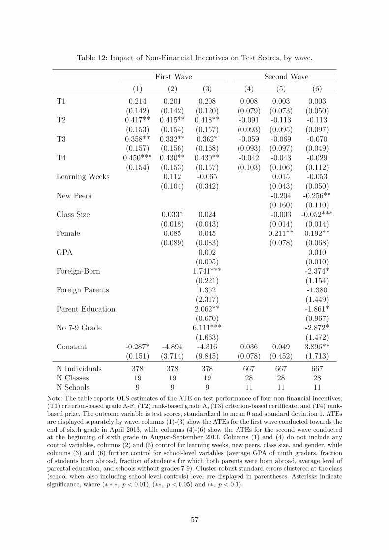
Table 12: Impact of Non-Financial Incentives on Test Scores, by wave.

First Wave Second Wave

(1) (2) (3) (4) (5) (6)

T1 0.214 0.201 0.208 0.008 0.003 0.003(0.142) (0.142) (0.120) (0.079) (0.073) (0.050)

T2 0.417** 0.415** 0.418** -0.091 -0.113 -0.113(0.153) (0.154) (0.157) (0.093) (0.095) (0.097)

T3 0.358** 0.332** 0.362* -0.059 -0.069 -0.070(0.157) (0.156) (0.168) (0.093) (0.097) (0.049)

T4 0.450*** 0.430** 0.430** -0.042 -0.043 -0.029(0.154) (0.153) (0.157) (0.103) (0.106) (0.112)

Learning Weeks 0.112 -0.065 0.015 -0.053(0.104) (0.342) (0.043) (0.050)

New Peers -0.204 -0.256**(0.160) (0.110)

Class Size 0.033* 0.024 -0.003 -0.052***(0.018) (0.043) (0.014) (0.014)

Female 0.085 0.045 0.211** 0.192**(0.089) (0.083) (0.078) (0.068)

GPA 0.002 0.010(0.005) (0.010)

Foreign-Born 1.741*** -2.374*(0.221) (1.154)

Foreign Parents 1.352 -1.380(2.317) (1.449)

Parent Education 2.062** -1.861*(0.670) (0.967)

No 7-9 Grade 6.111*** -2.872*(1.663) (1.472)

Constant -0.287* -4.894 -4.316 0.036 0.049 3.896**(0.151) (3.714) (9.845) (0.078) (0.452) (1.713)

N Individuals 378 378 378 667 667 667N Classes 19 19 19 28 28 28N Schools 9 9 9 11 11 11

Note: The table reports OLS estimates of the ATE on test performance of four non-financial incentives;(T1) criterion-based grade A-F, (T2) rank-based grade A, (T3) criterion-based certificate, and (T4) rank-based prize. The outcome variable is test scores, standardized to mean 0 and standard deviation 1. ATEsare displayed separately by wave; columns (1)-(3) show the ATEs for the first wave conducted towards theend of sixth grade in April 2013, while columns (4)-(6) show the ATEs for the second wave conductedat the beginning of sixth grade in August-September 2013. Columns (1) and (4) do not include anycontrol variables, columns (2) and (5) control for learning weeks, new peers, class size, and gender, whilecolumns (3) and (6) further control for school-level variables (average GPA of ninth graders, fractionof students born abroad, fraction of students for which both parents were born abroad, average level ofparental education, and schools without grades 7-9). Cluster-robust standard errors clustered at the class(school when also including school-level controls) level are displayed in parentheses. Asterisks indicatesignificance, where (∗ ∗ ∗, p < 0.01), (∗∗, p < 0.05) and (∗, p < 0.1).

57

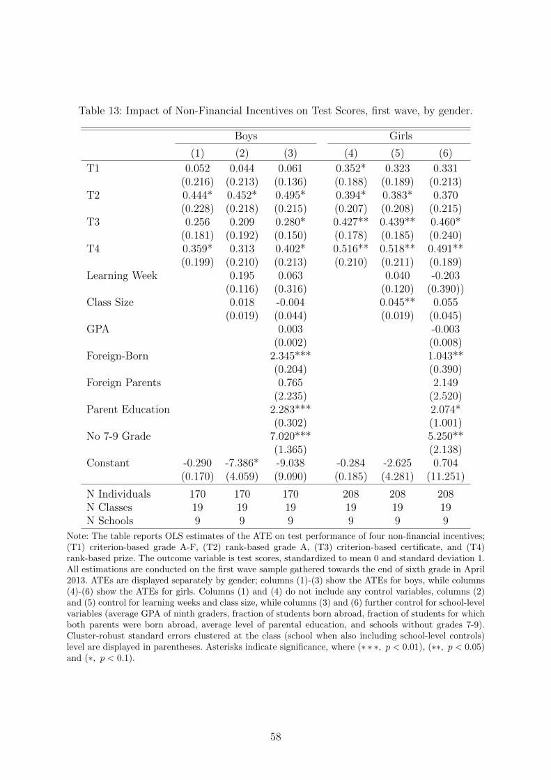
Table 13: Impact of Non-Financial Incentives on Test Scores, first wave, by gender.

Boys Girls

(1) (2) (3) (4) (5) (6)

T1 0.052 0.044 0.061 0.352* 0.323 0.331(0.216) (0.213) (0.136) (0.188) (0.189) (0.213)

T2 0.444* 0.452* 0.495* 0.394* 0.383* 0.370(0.228) (0.218) (0.215) (0.207) (0.208) (0.215)

T3 0.256 0.209 0.280* 0.427** 0.439** 0.460*(0.181) (0.192) (0.150) (0.178) (0.185) (0.240)

T4 0.359* 0.313 0.402* 0.516** 0.518** 0.491**(0.199) (0.210) (0.213) (0.210) (0.211) (0.189)

Learning Week 0.195 0.063 0.040 -0.203(0.116) (0.316) (0.120) (0.390))

Class Size 0.018 -0.004 0.045** 0.055(0.019) (0.044) (0.019) (0.045)

GPA 0.003 -0.003(0.002) (0.008)

Foreign-Born 2.345*** 1.043**(0.204) (0.390)

Foreign Parents 0.765 2.149(2.235) (2.520)

Parent Education 2.283*** 2.074*(0.302) (1.001)

No 7-9 Grade 7.020*** 5.250**(1.365) (2.138)

Constant -0.290 -7.386* -9.038 -0.284 -2.625 0.704(0.170) (4.059) (9.090) (0.185) (4.281) (11.251)

N Individuals 170 170 170 208 208 208N Classes 19 19 19 19 19 19N Schools 9 9 9 9 9 9

Note: The table reports OLS estimates of the ATE on test performance of four non-financial incentives;(T1) criterion-based grade A-F, (T2) rank-based grade A, (T3) criterion-based certificate, and (T4)rank-based prize. The outcome variable is test scores, standardized to mean 0 and standard deviation 1.All estimations are conducted on the first wave sample gathered towards the end of sixth grade in April2013. ATEs are displayed separately by gender; columns (1)-(3) show the ATEs for boys, while columns(4)-(6) show the ATEs for girls. Columns (1) and (4) do not include any control variables, columns (2)and (5) control for learning weeks and class size, while columns (3) and (6) further control for school-levelvariables (average GPA of ninth graders, fraction of students born abroad, fraction of students for whichboth parents were born abroad, average level of parental education, and schools without grades 7-9).Cluster-robust standard errors clustered at the class (school when also including school-level controls)level are displayed in parentheses. Asterisks indicate significance, where (∗ ∗ ∗, p < 0.01), (∗∗, p < 0.05)and (∗, p < 0.1).

58

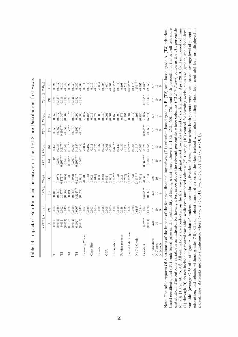
Tab

le14

:Im

pac

tof

Non

-Fin

anci

alIn

centi

ves

onth

eT

est

Sco

reD

istr

ibuti

on,

firs

tw

ave.

P(TS≥P

10TS)

P(TS≥P

25TS)

P(TS≥P

50TS)

P(TS≥P

75TS)

P(TS≥P

90TS)

(1)

(2)

(3)

(4)

(5)

(6)

(7)

(8)

(9)

(10)

T1

0.06

60.

065

0.10

50.

101

0.15

8*0.

155

0.05

30.

052

0.02

60.

024

(0.0

49)

(0.0

36)

(0.0

80)

(0.0

87)

(0.0

81)

(0.0

86)

(0.0

67)

(0.0

72)

(0.0

35)

(0.0

17)

T2

0.06

40.

062

0.17

7**

0.17

7**

0.20

7***

0.20

7**

0.19

3***

0.19

4**

0.01

80.

019

(0.0

54)

(0.0

43)

(0.0

62)

(0.0

75)

(0.0

54)

(0.0

66)

(0.0

57)

(0.0

62)

(0.0

39)

(0.0

42)

T3

0.07

9*0.

078

0.12

10.

120

0.19

0**

0.19

1**

0.17

7**

0.18

1**

0.02

50.

022

(0.0

44)

(0.0

50)

(0.0

86)

(0.0

82)

(0.0

67)

(0.0

63)

(0.0

70)

(0.0

70)

(0.0

41)

(0.0

39)

T4

0.09

2*0.

090*

0.22

4***

0.21

3**

0.19

7***

0.18

8**

0.10

50.

099

0.09

20.

085

(0.0

47)

(0.0

42)

(0.0

77)

(0.0

81)

(0.0

67)

(0.0

56)

(0.0

72)

(0.0

83)

(0.0

56)

(0.0

62)

Lea

rnin

gW

eeks

0.00

7-0

.031

-0.0

56-0

.035

0.01

1(0

.039

)(0

.108

)(0

.197

)(0

.188

)(0

.074

)C

lass

Siz

e0.

003

0.00

20.

011

0.01

30.

015

(0.0

04)

(0.0

14)

(0.0

25)

(0.0

22)

(0.0

10)

Fem

ale

0.01

20.

038

0.03

70.

000

-0.0

04(0

.026

)(0

.038

)(0

.052

)(0

.049

)(0

.028

)G

PA

0.00

00.

002*

0.00

10.

001

-0.0

01(0

.002

)(0

.001

)(0

.002

)(0

.001

)(0

.001

)F

orei

gn-b

orn

0.11

30.

970*

**0.

471*

*0.

150

0.51

1***

(0.1

10)

(0.1

03)

(0.1

42)

(0.0

90)

(0.0

74)

For

eign

par

ents

0.33

80.

242

0.48

00.

377

0.19

8(0

.237

)(0

.742

)(1

.354

)(1

.297

)(0

.512

)P

aren

tE

du

cati

on0.

185

0.67

1***

0.72

7**

0.38

40.

610*

**(0

.220

)(0

.153

)(0

.266

)(0

.217

)(0

.178

)N

o7-

9G

rad

e0.

614*

2.41

3***

2.16

1**

1.49

31.

430*

**(0

.284

)(0

.521

)(0

.909

)(0

.886

)(0

.397

)C

onst

ant

0.88

2***

0.01

40.

645*

**-0

.660

0.36

8***

0.02

60.

355*

**-0

.035

0.10

5**

-1.8

77(0

.044

)(1

.170

)(0

.069

)(3

.154

)(0

.061

)(5

.658

)(0

.060

)(5

.371

)(0

.042

)(2

.053

)

NIn

div

idu

als

378

378

378

378

378

378

378

378

378

378

NC

lass

es19

1919

1919

1919

1919

19N

Sch

ool

s9

99

99

99

99

9

Not

e:T

he

tab

lere

por

tsO

LS

esti

mat

esof

the

imp

act

ofth

efo

ur

non

-fin

an

cialin

centi

ves;

(T1)

crit

erio

n-b

ase

dgra

de

A-F

,(T

2)

ran

k-b

ase

dgra

de

A,(T

3)

crit

erio

n-

bas

edce

rtifi

cate

,an

d(T

4)ra

nk-b

ased

pri

zeon

the

pro

bab

ilit

yof

hav

ing

ate

stsc

ore

ab

ove

the

10th

,25th

,50th

,75th

an

d90th

per

centi

leof

the

over

all

test

score

dis

trib

uti

on.

Th

eou

tcom

eva

riab

leis

anin

dic

ator

for

hav

ing

ate

stsc

ore

ab

ove

the

rele

vant

per

centi

le;

wh

ere

colu

mn

sP

(TS≥

PJTS

)co

nce

rns

theJ

thp

erce

nti

lefo

rJ∈{1

0,2

5,50

,75,

90}.

All

esti

mat

ion

sar

eco

ndu

cted

onth

efi

rst

wav

esa

mp

legath

ered

tow

ard

sth

een

dof

sixth

gra

de

inA

pri

l2013.

Od

dnu

mb

ered

colu

mn

s(1

)th

rou

gh(9

)d

on

otin

clu

de

any

contr

olva

riab

les,

wh

ile

even

nu

mb

ered

colu

mn

s(2

)th

rou

gh

(10)

contr

ol

for

learn

ing

wee

ks,

class

size

,gen

der

,an

dsc

hool-

leve

lva

riab

les

(ave

rage

GP

Aof

nin

thgr

ader

s,fr

acti

onof

stu

den

tsb

orn

ab

road

,fr

act

ion

of

stud

ents

for

wh

ich

both

pare

nts

wer

eb

orn

ab

road

,av

erage

leve

lof

pare

nta

led

uca

tion

,an

dsc

hool

sw

ith

out

grad

es7-

9).

Clu

ster

-rob

ust

stan

dard

erro

rsat

the

class

(sch

ool

wh

enals

oin

clu

din

gsc

hool-

leve

lco

ntr

ols

)le

vel

are

dis

pla

yed

inp

aren

thes

es.

Ast

eris

ks

ind

icat

esi

gnifi

can

ce,

wh

ere

(∗∗∗,

p<

0.01),

(∗∗,

p<

0.0

5)

an

d(∗,p<

0.1).

59

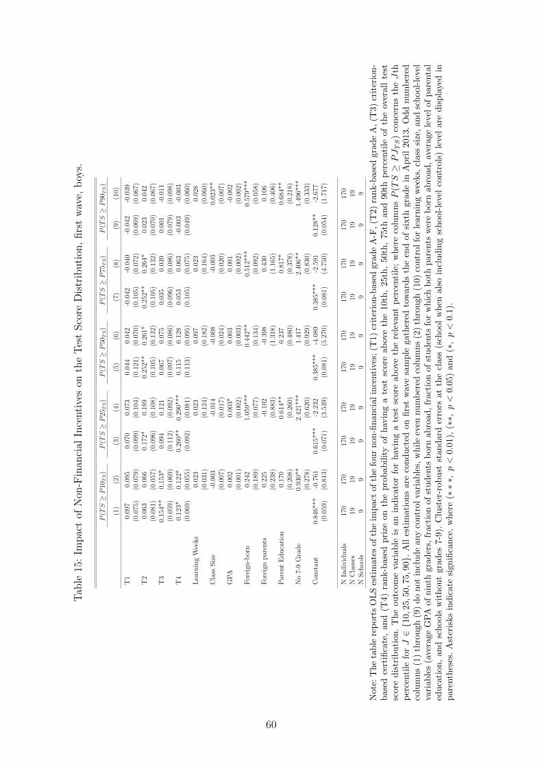
Tab

le15

:Im

pac

tof

Non

-Fin

anci

alIn

centi

ves

onth

eT

est

Sco

reD

istr

ibuti

on,

firs

tw

ave,

boy

s.

P(TS≥P

10TS)

P(TS≥P

25TS)

P(TS≥P

50TS)

P(TS≥P

75TS)

P(TS≥P

90TS)

(1)

(2)

(3)

(4)

(5)

(6)

(7)

(8)

(9)

(10)

T1

0.09

70.

095

0.07

00.

073

0.04

40.

042

-0.0

42-0

.040

-0.0

42-0

.039

(0.0

75)

(0.0

79)

(0.0

99)

(0.1

04)

(0.1

21)

(0.0

70)

(0.1

05)

(0.0

72)

(0.0

69)

(0.0

67)

T2

0.06

30.

066

0.17

2*0.

189

0.25

2**

0.26

1*0.

252*

*0.

264*

0.02

30.

042

(0.0

81)

(0.0

57)

(0.0

96)

(0.1

08)

(0.1

05)

(0.1

32)

(0.1

05)

(0.1

32)

(0.0

70)

(0.0

67)

T3

0.15

4**

0.15

3*0.

094

0.12

10.

067

0.07

50.

035

0.03

90.

001

-0.0

11(0

.059

)(0

.069

)(0

.112

)(0

.092

)(0

.097

)(0

.086

)(0

.096

)(0

.086

)(0

.079

)(0

.098

)T

40.

123*

0.12

2*0.

260*

*0.

290*

**0.

115

0.12

80.

053

0.06

3-0

.003

-0.0

03(0

.069

)(0

.055

)(0

.092

)(0

.081

)(0

.113

)(0

.095

)(0

.105

)(0

.075

)(0

.049

)(0

.060

)L

earn

ing

Wee

ks

0.02

30.

023

0.09

70.

023

0.02

8(0

.031

)(0

.124

)(0

.182

)(0

.164

)(0

.060

)C

lass

Siz

e-0

.003

-0.0

14-0

.008

-0.0

030.

023*

*(0

.007

)(0

.017

)(0

.024

)(0

.020

)(0

.007

)G

PA

0.00

20.

003*

0.00

30.

001

-0.0

02(0

.001

)(0

.002

)(0

.003

)(0

.002

)(0

.002

)F

orei

gn-b

orn

0.24

21.

059*

**0.

442*

*0.

512*

**0.

579*

**(0

.189

)(0

.077

)(0

.134

)(0

.092

)(0

.058

)F

orei

gnp

aren

ts0.

225

-0.1

02-0

.398

0.43

00.

106

(0.2

38)

(0.8

83)

(1.3

18)

(1.1

65)

(0.4

06)

Par

ent

Ed

uca

tion

0.17

00.

614*

*0.

237

0.81

7*0.

684*

*(0

.208

)(0

.260

)(0

.480

)(0

.378

)(0

.218

)N

o7-

9G

rad

e0.

930*

*2.

421*

**1.

417

2.40

6**

1.49

6***

(0.2

78)

(0.6

20)

(0.9

29)

(0.8

30)

(0.3

33)

Con

stan

t0.

846*

**-0

.761

0.61

5***

-2.2

320.

385*

**-4

.089

0.38

5***

-2.5

910.

128*

*-2

.677

(0.0

59)

(0.8

13)

(0.0

71)

(3.5

39)

(0.0

81)

(5.2

70)

(0.0

81)

(4.7

50)

(0.0

54)

(1.7

17)

NIn

div

idu

als

170

170

170

170

170

170

170

170

170

170

NC

lass

es19

1919

1919

1919

1919

19N

Sch

ool

s9

99

99

99

99

9

Not

e:T

he

tab

lere

por

tsO

LS

esti

mat

esof

the

imp

act

ofth

efo

ur

non

-fin

an

cialin

centi

ves;

(T1)

crit

erio

n-b

ase

dgra

de

A-F

,(T

2)

ran

k-b

ase

dgra

de

A,(T

3)

crit

erio

n-

bas

edce

rtifi

cate

,and

(T4)

ran

k-b

ased

pri

zeon

the

pro

bab

ilit

yof

hav

ing

ate

stsc

ore

ab

ove

the

10th

,25th

,50th

,75th

an

d90th

per

centi

leof

the

over

all

test

scor

ed

istr

ibu

tion

.T

he

outc

ome

vari

able

isan

ind

icat

orfo

rh

avin

ga

test

score

ab

ove

the

rele

vant

per

centi

le;

wh

ere

colu

mn

sP

(TS≥

PJTS

)co

nce

rns

theJ

thp

erce

nti

lefo

rJ∈{1

0,2

5,50

,75,

90}.

All

esti

mat

ion

sar

eco

nd

uct

edon

firs

tw

ave

sam

ple

gath

ered

tow

ard

sth

een

dof

sixth

gra

de

inA

pri

l2013.

Od

dnu

mb

ered

colu

mn

s(1

)th

rou

gh(9

)d

on

otin

clu

de

any

contr

olva

riab

les,

wh

ile

even

nu

mb

ered

colu

mn

s(2

)th

rou

gh

(10)

contr

ol

for

learn

ing

wee

ks,

class

size

,an

dsc

hool-

leve

lva

riab

les

(ave

rage

GP

Aof

nin

thgr

ader

s,fr

acti

onof

stu

den

tsb

orn

ab

road

,fr

act

ion

of

stud

ents

for

wh

ich

both

pare

nts

wer

eb

orn

ab

road

,av

erage

leve

lof

pare

nta

led

uca

tion

,an

dsc

hool

sw

ith

out

grad

es7-

9).

Clu

ster

-rob

ust

stan

dard

erro

rsat

the

class

(sch

ool

wh

enals

oin

clu

din

gsc

hool-

leve

lco

ntr

ols

)le

vel

are

dis

pla

yed

inp

aren

thes

es.

Ast

eris

ks

ind

icat

esi

gnifi

can

ce,

wh

ere

(∗∗∗,

p<

0.01),

(∗∗,

p<

0.0

5)

an

d(∗,p<

0.1).

60

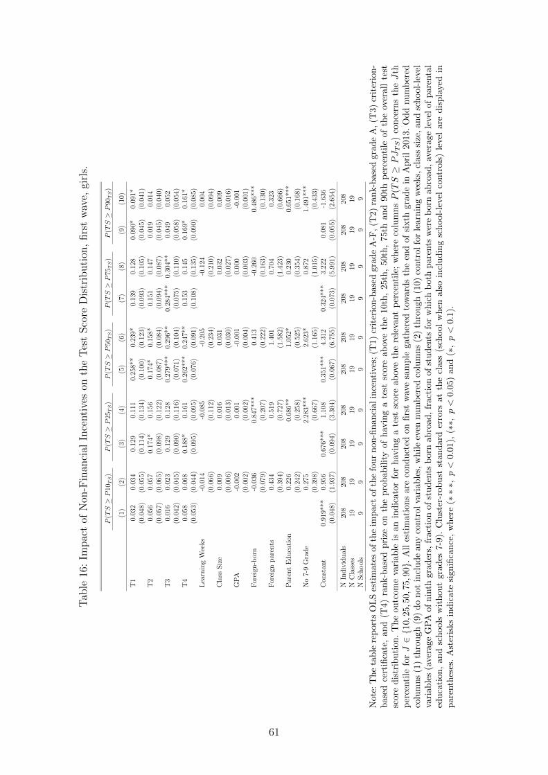
Tab

le16

:Im

pac

tof

Non

-Fin

anci

alIn

centi

ves

onth

eT

est

Sco

reD

istr

ibuti

on,

firs

tw

ave,

girl

s.

P(TS≥P

10TS)

P(TS≥P

25TS)

P(TS≥P

50TS)

P(TS≥P

75TS)

P(TS≥P

90TS)

(1)

(2)

(3)

(4)

(5)

(6)

(7)

(8)

(9)

(10)

T1

0.03

20.

034

0.12

90.

111

0.25

8**

0.23

9*0.

139

0.12

80.

090*

0.09

1*(0

.048

)(0

.055

)(0

.114

)(0

.134

)(0

.100

)(0

.123

)(0

.093

)(0

.105

)(0

.045

)(0

.041

)T

20.

056

0.05

70.

174*

0.15

60.

174*

0.15

8*0.

151

0.14

70.

019

0.01

4(0

.057

)(0

.065

)(0

.098

)(0

.122

)(0

.087

)(0

.084

)(0

.094

)(0

.087

)(0

.045

)(0

.040

)T

30.

016

0.02

30.

129

0.12

80.

279*

**0.

296*

*0.

284*

**0.

304*

*0.

049

0.05

2(0

.042

)(0

.045

)(0

.090

)(0

.116

)(0

.071

)(0

.104

)(0

.075

)(0

.110

)(0

.058

)(0

.054

)T

40.

058

0.06

80.

188*

0.16

10.

262*

**0.

247*

*0.

153

0.14

50.

169*

0.16

1*(0

.053

)(0

.044

)(0

.095

)(0

.095

)(0

.076

)(0

.091

)(0

.108

)(0

.135

)(0

.090

)(0

.085

)L

earn

ing

Wee

ks

-0.0

14-0

.085

-0.2

05-0

.124

0.00

4(0

.066

)(0

.112

)(0

.234

)(0

.210

)(0

.094

)C

lass

Siz

e0.

009

0.01

60.

031

0.03

20.

009

(0.0

06)

(0.0

13)

(0.0

30)

(0.0

27)

(0.0

16)

GP

A-0

.002

0.00

1-0

.001

0.00

0-0

.001

(0.0

02)

(0.0

02)

(0.0

04)

(0.0

03)

(0.0

01)

For

eign

-bor

n-0

.036

0.84

7***

0.41

3-0

.260

0.48

6***

(0.0

79)

(0.2

07)

(0.2

22)

(0.1

63)

(0.1

30)

For

eign

par

ents

0.43

40.

519

1.40

10.

704

0.32

3(0

.394

)(0

.727

)(1

.582

)(1

.423

)(0

.666

)P

aren

tE

du

cati

on0.

226

0.68

6**

1.05

2*0.

230

0.65

1***

(0.2

42)

(0.2

58)

(0.5

25)

(0.3

54)

(0.1

68)

No

7-9

Gra

de

0.27

52.

283*

**2.

623*

0.87

21.

491*

**(0

.398

)(0

.667

)(1

.165

)(1

.015

)(0

.433

)C

onst

ant

0.91

9***

0.95

60.

676*

**1.

108

0.35

1***

4.31

20.

324*

**3.

222

0.08

1-1

.636

(0.0

48)

(1.9

37)

(0.0

94)

(3.3

04)

(0.0

67)

(6.7

55)

(0.0

73)

(5.9

91)

(0.0

55)

(2.6

54)

NIn

div

idu

als

208

208

208

208

208

208

208

208

208

208

NC

lass

es19

1919

1919

1919

1919

19N

Sch

ool

s9

99

99

99

99

9

Not

e:T

he

tab

lere

por

tsO

LS

esti

mat

esof

the

imp

act

ofth

efo

ur

non

-fin

an

cialin

centi

ves;

(T1)

crit

erio

n-b

ase

dgra

de

A-F

,(T

2)

ran

k-b

ase

dgra

de

A,(T

3)

crit

erio

n-

bas

edce

rtifi

cate

,and

(T4)

ran

k-b

ased

pri

zeon

the

pro

bab

ilit

yof

hav

ing

ate

stsc

ore

ab

ove

the

10th

,25th

,50th

,75th

an

d90th

per

centi

leof

the

over

all

test

scor

ed

istr

ibu

tion

.T

he

outc

ome

vari

able

isan

ind

icat

orfo

rh

avin

ga

test

score

ab

ove

the

rele

vant

per

centi

le;

wh

ere

colu

mn

sP

(TS≥

PJTS

)co

nce

rns

theJ

thp

erce

nti

lefo

rJ∈{1

0,2

5,50

,75,

90}.

All

esti

mat

ion

sar

eco

nd

uct

edon

firs

tw

ave

sam

ple

gath

ered

tow

ard

sth

een

dof

sixth

gra

de

inA

pri

l2013.

Od

dnu

mb

ered

colu

mn

s(1

)th

rou

gh(9

)d

on

otin

clu

de

any

contr

olva

riab

les,

wh

ile

even

nu

mb

ered

colu

mn

s(2

)th

rou

gh

(10)

contr

ol

for

learn

ing

wee

ks,

class

size

,an

dsc

hool-

leve

lva

riab

les

(ave

rage

GP

Aof

nin

thgr

ader

s,fr

acti

onof

stu

den

tsb

orn

ab

road

,fr

act

ion

of

stud

ents

for

wh

ich

both

pare

nts

wer

eb

orn

ab

road

,av

erage

leve

lof

pare

nta

led

uca

tion

,an

dsc

hool

sw

ith

out

grad

es7-

9).

Clu

ster

-rob

ust

stan

dard

erro

rsat

the

class

(sch

ool

wh

enals

oin

clu

din

gsc

hool-

leve

lco

ntr

ols

)le

vel

are

dis

pla

yed

inp

aren

thes

es.

Ast

eris

ks

ind

icat

esi

gnifi

can

ce,

wh

ere

(∗∗∗,

p<

0.01),

(∗∗,

p<

0.0

5)

an

d(∗,p<

0.1).

61

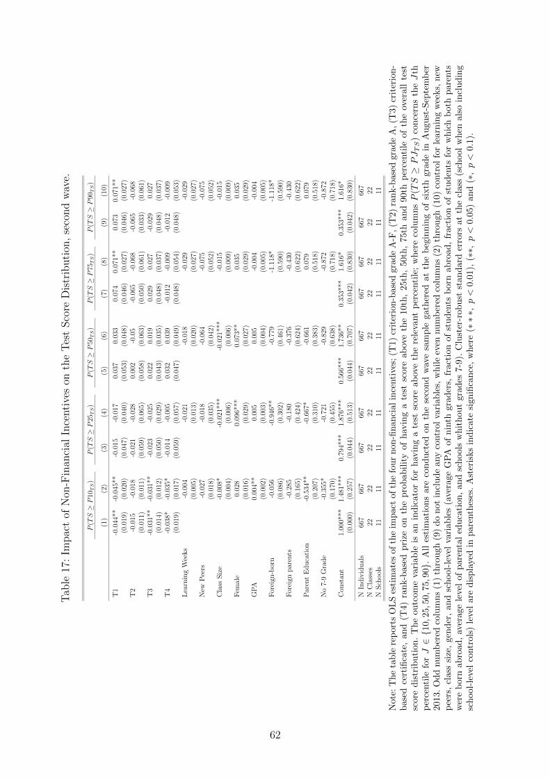
Tab

le17

:Im

pac

tof

Non

-Fin

anci

alIn

centi

ves

onth

eT

est

Sco

reD

istr

ibuti

on,

seco

nd

wav

e.

P(TS≥P

10TS)

P(TS≥P

25TS)

P(TS≥P

50TS)

P(TS≥P

75TS)

P(TS≥P

90TS)

(1)

(2)

(3)

(4)

(5)

(6)

(7)

(8)

(9)

(10)

T1

-0.0

44**

-0.0

45**

-0.0

15-0

.017

0.03

70.

033

0.07

40.

071*

*0.

073

0.07

1**

(0.0

19)

(0.0

20)

(0.0

47)

(0.0

40)

(0.0

53)

(0.0

48)

(0.0

46)

(0.0

27)

(0.0

46)

(0.0

27)

T2

-0.0

15-0

.018

-0.0

21-0

.028

0.00

2-0

.05

-0.0

65-0

.068

-0.0

65-0

.068

(0.0

11)

(0.0

11)

(0.0

59)

(0.0

65)

(0.0

58)

(0.0

63)

(0.0

50)

(0.0

61)

(0.0

33)

(0.0

61)

T3

-0.0

31**

-0.0

31**

-0.0

23-0

.025

0.02

20.

019

0.02

90.

027

-0.0

290.

027

(0.0

14)

(0.0

12)

(0.0

50)

(0.0

29)

(0.0

43)

(0.0

35)

(0.0

48)

(0.0

37)

(0.0

48)

(0.0

37)

T4

-0.0

38*

-0.0

35*

-0.0

14-0

.005

0.03

20.

039

-0.0

12-0

.009

-0.0

12-0

.009

(0.0

19)

(0.0

17)

(0.0

59)

(0.0

57)

(0.0

47)

(0.0

49)

(0.0

48)

(0.0

54)

(0.0

48)

(0.0

53)

Lea

rnin

gW

eeks

-0.0

04-0

.021

-0.0

18-0

.029

-0.0

29(0

.005

)(0

.013

)(0

.020

)(0

.027

)(0

.027

)N

ewP

eers

-0.0

27-0

.018

-0.0

64-0

.075

-0.0

75(0

.018

)(0

.035

)(0

.042

)(0

.052

)(0

.052

)C

lass

Siz

e-0

.008

*-0

.021

***

-0.0

21**

*-0

.015

-0.0

15(0

.004

)(0

.006

)(0

.006

)(0

.009

)(0

.009

)F

emal

e0.

028

0.09

6***

0.07

3**

0.03

50.

035

(0.0

16)

(0.0

29)

(0.0

27)

(0.0

29)

(0.0

29)

GP

A0.

004*

*0.

005

0.00

5-0

.004

-0.0

04(0

.002

)(0

.003

)(0

.004

)(0

.005

)(0

.005

)F

orei

gn-b

orn

-0.0

56-0

.946

**-0

.779

-1.1

18*

-1.1

18*

(0.0

86)

(0.3

02)

(0.4

61)

(0.5

90)

(0.5

90)

For

eign

par

ents

-0.2

85-0

.180

-0.3

76-0

.430

-0.4

30(0

.165

)(0

.424

)(0

.624

)(0

.622

)(0

.622

)P

aren

tE

du

cati

on-0

.534

**-0

.667

*-0

.661

0.07

90.

079

(0.2

07)

(0.3

10)

(0.3

83)

(0.5

18)

(0.5

18)

No

7-9

Gra

de

-0.3

55*

-0.7

21-0

.829

-0.8

72-0

.872

(0.1

70)

(0.4

55)

(0.6

38)

(0.7

18)

(0.7

18)

Con

stan

t1.

000*

**1.

481*

**0.

794*

**1.

876*

**0.

566*

**1.

736*

*0.

353*

**1.

616*

0.35

3***

1.61

6*(0

.000

)(0

.257

)(0

.044

)(0

.513

)(0

.044

)(0

.707

)(0

.042

)(0

.830

)(0

.042

)(0

.830

)

NIn

div

idu

als

667

667

667

667

667

667

667

667

667

667

NC

lass

es22

2222

2222

2222

2222

22N

Sch

ool

s11

1111

1111

1111

1111

11

Not

e:T

he

tab

lere

por

tsO

LS

esti

mat

esof

the

imp

act

ofth

efo

ur

non

-fin

an

cialin

centi

ves;

(T1)

crit

erio

n-b

ase

dgra

de

A-F

,(T

2)

ran

k-b

ase

dgra

de

A,(T

3)

crit

erio

n-

bas

edce

rtifi

cate

,and

(T4)

ran

k-b

ased

pri

zeon

the

pro

bab

ilit

yof

hav

ing

ate

stsc

ore

ab

ove

the

10th

,25th

,50th

,75th

an

d90th

per

centi

leof

the

over

all

test

scor

ed

istr

ibu

tion

.T

he

outc

ome

vari

able

isan

ind

icat

orfo

rh

avin

ga

test

score

ab

ove

the

rele

vant

per

centi

le;

wh

ere

colu

mn

sP

(TS≥

PJTS

)co

nce

rns

theJ

thp

erce

nti

lefo

rJ∈{1

0,2

5,5

0,7

5,9

0}.

All

esti

mat

ion

sar

eco

nd

uct

edon

the

seco

nd

wav

esa

mp

legath

ered

at

the

beg

inn

ing

of

sixth

gra

de

inA

ugu

st-S

epte

mb

er20

13.

Od

dnu

mb

ered

colu

mn

s(1

)th

rou

gh(9

)d

on

otin

clu

de

any

contr

ol

vari

ab

les,

wh

ile

even

nu

mb

ered

colu

mn

s(2

)th

rou

gh

(10)

contr

ol

for

learn

ing

wee

ks,

new

pee

rs,

clas

ssi

ze,

gen

der

,an

dsc

hool

-lev

elva

riab

les

(aver

age

GP

Aof

nin

thgra

der

s,fr

act

ion

of

stu

den

tsb

orn

ab

road

,fr

act

ion

of

stu

den

tsfo

rw

hic

hb

oth

pare

nts

wer

eb

orn

abro

ad,

aver

age

leve

lof

par

enta

led

uca

tion

,an

dsc

hools

wh

ith

ou

tgra

des

7-9

).C

lust

er-r

ob

ust

stan

dard

erro

rsat

the

class

(sch

ool

wh

enals

oin

clu

din

gsc

hool

-lev

elco

ntr

ols)

leve

lar

ed

isp

laye

din

par

enth

eses

.A

ster

isks

ind

icate

sign

ifica

nce

,w

her

e(∗∗∗,

p<

0.01),

(∗∗,

p<

0.0

5)

an

d(∗,p<

0.1).

62

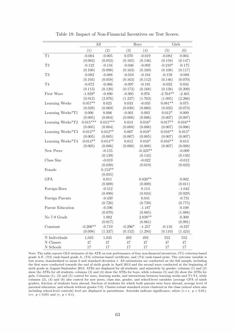
Table 18: Impact of Non-Financial Incentives on Test Scores.

All Boys Girls

(1) (2) (3) (4) (5) (6)

T1 -0.004 -0.005 0.070 -0.019 -0.082 0.004(0.083) (0.052) (0.165) (0.146) (0.158) (0.147)

T2 -0.122 -0.134 -0.046 -0.092 -0.210* -0.175(0.100) (0.098) (0.163) (0.169) (0.108) (0.117)

T3 -0.082 -0.088 -0.010 -0.104 -0.159 -0.088(0.103) (0.058) (0.163) (0.112) (0.146) (0.070)

T4 -0.072 -0.066 -0.097 -0.191 -0.032 0.034(0.113) (0.120) (0.173) (0.168) (0.138) (0.209)

First Wave -1.829* -0.890 -0.905 0.976 -2.764** -2.465(0.912) (2.076) (1.227) (1.763) (1.095) (2.266)

Learning Weeks 0.057** 0.025 0.033 -0.035 0.081** 0.075(0.028) (0.069) (0.038) (0.060) (0.033) (0.073)

Learning Weeks*T1 0.006 0.006 -0.001 0.003 0.012* 0.009(0.005) (0.004) (0.008) (0.006) (0.007) (0.007)

Learning Weeks*T2 0.015*** 0.015*** 0.013 0.016* 0.017** 0.016**(0.005) (0.004) (0.008) (0.008) (0.007) (0.006)

Learning Weeks*T3 0.012** 0.012** 0.007 0.010* 0.016** 0.015*(0.005) (0.005) (0.007) (0.005) (0.007) (0.007)

Learning Weeks*T4 0.014** 0.014** 0.012 0.016* 0.016** 0.013(0.005) (0.006) (0.008) (0.008) (0.007) (0.008)

New Peers -0.155 -0.323** -0.009(0.139) (0.142) (0.150)

Class Size -0.019 -0.022 -0.012(0.020) (0.019) (0.023)

Female 0.153**(0.055)

GPA 0.011 0.020** 0.002(0.009) (0.009) (0.011)

Foreign-Born -0.512 0.114 -1.042(0.890) (0.824) (0.929)

Foreign Parents -0.439 0.041 -0.731(0.726) (0.739) (0.775)

Parent Education -0.596 -1.187 0.109(0.870) (0.865) (1.088)

No 7-9 Grade 1.002 2.038** 0.309(0.917) (0.861) (0.991)

Constant -0.206** -0.719 -0.296* -1.257 -0.116 -0.337(0.098) (1.337) (0.152) (1.294) (0.110) (1.424)

N Individuals 1,045 1,045 493 493 552 552N Classes 47 47 47 47 47 47N Schools 17 17 17 17 17 17

Note: The table reports OLS estimates of the ATE on test performance of four non-financial incentives; (T1) criterion-basedgrade A-F, (T2) rank-based grade A, (T3) criterion-based certificate, and (T4) rank-based prize. The outcome variable istest scores, standardized to mean 0 and standard deviation 1. All estimations are conducted on the full sample; includingthe first wave conducted towards the end of sixth grade in April 2013 and the second wave conducted at the beginning ofsixth grade in August-September 2013. ATEs are displayed for all students, and separately by gender; columns (1) and (2)show the ATEs for all students, columns (3) and (4) show the ATEs for boys, while columns (5) and (6) show the ATEs forgirls. Columns (1), (3) and (5) control for wave, learning weeks, and interactions between learning weeks and T1-T4, whilecolumns (2), (4) and (6) also control for new peers, class size, gender, and school-level variables (average GPA of ninthgraders, fraction of students born abroad, fraction of students for which both parents were born abroad, average level ofparental education, and schools without grades 7-9). Cluster-robust standard errors clustered at the class (school when alsoincluding school-level controls) level are displayed in parentheses. Asterisks indicate significance, where (∗ ∗ ∗, p < 0.01),(∗∗, p < 0.05) and (∗, p < 0.1).

63

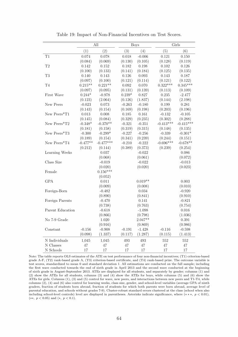
Table 19: Impact of Non-Financial Incentives on Test Scores.

All Boys Girls

(1) (2) (3) (4) (5) (6)

T1 0.074 0.078 0.018 -0.006 0.121 0.150(0.084) (0.069) (0.130) (0.105) (0.128) (0.119)

T2 0.142 0.152 0.182 0.198 0.102 0.126(0.100) (0.133) (0.141) (0.184) (0.125) (0.135)

T3 0.140 0.143 0.126 0.093 0.143 0.187(0.097) (0.100) (0.121) (0.114) (0.121) (0.122)

T4 0.215** 0.221** 0.092 0.070 0.322*** 0.345***(0.097) (0.095) (0.131) (0.139) (0.113) (0.109)

First Wave 0.244* -0.978 0.239* 0.827 0.235 -2.477(0.123) (2.064) (0.126) (1.837) (0.144) (2.198)

New Peers -0.023 0.073 -0.263 -0.180 0.199 0.281(0.143) (0.154) (0.169) (0.198) (0.203) (0.196)

New Peers*T1 0.013 0.008 0.185 0.161 -0.132 -0.105(0.145) (0.084) (0.329) (0.235) (0.302) (0.288)

New Peers*T2 -0.348* -0.370** -0.321 -0.351 -0.413*** -0.415***(0.181) (0.158) (0.319) (0.315) (0.148) (0.135)

New Peers*T3 -0.300 -0.299* -0.227 -0.256 -0.339 -0.301*(0.189) (0.154) (0.341) (0.239) (0.244) (0.151)

New Peers*T4 -0.477** -0.477*** -0.210 -0.222 -0.696*** -0.678**(0.212) (0.144) (0.389) (0.373) (0.239) (0.254)

Learning Weeks 0.037 -0.022 0.086(0.068) (0.061) (0.072)

Class Size -0.019 -0.022 -0.013(0.020) (0.020) (0.023)

Female 0.156***(0.052)

GPA 0.011 0.019** 0.003(0.009) (0.008) (0.010)

Foreign-Born -0.482 0.034 -0.920(0.890) (0.841) (0.910)

Foreign Parents -0.470 0.141 -0.821(0.738) (0.763) (0.754)

Parent Education -0.618 -1.098 0.016(0.866) (0.798) (1.036)

No 7-9 Grade 1.020 2.047** 0.391(0.916) (0.869) (0.986)

Constant -0.156 -0.908 -0.191 -1.428 -0.116 -0.598(0.098) (1.337) (0.117) (1.287) (0.115) (1.413)

N Individuals 1,045 1,045 493 493 552 552N Classes 47 47 47 47 47 47N Schools 17 17 17 17 17 17

Note: The table reports OLS estimates of the ATE on test performance of four non-financial incentives; (T1) criterion-basedgrade A-F, (T2) rank-based grade A, (T3) criterion-based certificate, and (T4) rank-based prize. The outcome variable istest scores, standardized to mean 0 and standard deviation 1. All estimations are conducted on the full sample; includingthe first wave conducted towards the end of sixth grade in April 2013 and the second wave conducted at the beginningof sixth grade in August-September 2013. ATEs are displayed for all students, and separately by gender; columns (1) and(2) show the ATEs for all students, columns (3) and (4) show the ATEs for boys, while columns (5) and (6) show theATEs for girls. Columns (1), (3) and (5) control for wave, new peers, and interactions between new peers and T1-T4, whilecolumns (2), (4) and (6) also control for learning weeks, class size, gender, and school-level variables (average GPA of ninthgraders, fraction of students born abroad, fraction of students for which both parents were born abroad, average level ofparental education, and schools without grades 7-9). Cluster-robust standard errors clustered at the class (school when alsoincluding school-level controls) level are displayed in parentheses. Asterisks indicate significance, where (∗ ∗ ∗, p < 0.01),(∗∗, p < 0.05) and (∗, p < 0.1).

64

Tab

le20

:Im

pac

tof

Non

-Fin

anci

alIn

centi

ves

onth

eT

est

Sco

reD

istr

ibuti

on,

sam

ep

eers

.

P(TS≥P

10TS)

P(TS≥P

25TS)

P(TS≥P

50TS)

P(TS≥P

75TS)

P(TS≥P

90TS)

(1)

(2)

(3)

(4)

(5)

(6)

(7)

(8)

(9)

(10)

T1

0.01

50.

014

0.03

60.

036

0.02

80.

029

0.05

70.

061

0.01

60.

018

(0.0

35)

(0.0

33)

(0.0

42)

(0.0

40)

(0.0

51)

(0.0

50)

(0.0

41)

(0.0

41)

(0.0

27)

(0.0

16)

T2

0.05

10.

049

0.08

9*0.

090

0.07

50.

079

0.03

10.

038

0.01

80.

022

(0.0

32)

(0.0

32)

(0.0

49)

(0.0

52)

(0.0

57)

(0.0

77)

(0.0

47)

(0.0

69)

(0.0

28)

(0.0

27)

T3

0.02

60.

024

0.02

90.

031

0.08

1*0.

085

0.10

4**

0.10

9**

-0.0

14-0

.013

(0.0

34)

(0.0

25)

(0.0

47)

(0.0

45)

(0.0

48)

(0.0

58)

(0.0

44)

(0.0

47)

(0.0

24)

(0.0

24)

T4

0.05

00.

051*

0.07

10.

075

0.08

8*0.

092*

0.06

30.

067

0.04

60.

045

(0.0

32)

(0.0

26)

(0.0

48)

(0.0

43)

(0.0

44)

(0.0

48)

(0.0

46)

(0.0

55)

(0.0

31)

(0.0

34)

Fir

stW

ave

0.04

7**

-0.2

330.

055

-0.2

010.

093*

-0.1

750.

084

-0.3

100.

065*

-0.6

01(0

.023

)(0

.255

)(0

.038

)(0

.555

)(0

.049

)(0

.809

)(0

.056

)(0

.915

)(0

.037

)(0

.603

)L

earn

ing

Wee

ks

0.00

80.

007

0.00

80.

012

0.02

1(0

.008

)(0

.018

)(0

.027

)(0

.030

)(0

.020

)C

lass

Siz

e-0

.004

-0.0

10-0

.013

-0.0

050.

006

(0.0

05)

(0.0

07)

(0.0

08)

(0.0

09)

(0.0

05)

Fem

ale

0.03

00.

052*

*0.

060*

*0.

020

0.01

2(0

.020

)(0

.022

)(0

.027

)(0

.030

)(0

.019

)G

PA

0.00

40.

003

0.00

40.

002

0.00

0(0

.002

)(0

.003

)(0

.003

)(0

.004

)(0

.003

)F

orei

gn-b

orn

-0.0

51-0

.130

-0.0

86-0

.282

0.17

7(0

.119

)(0

.313

)(0

.340

)(0

.313

)(0

.216

)F

orei

gnp

aren

ts0.

051

0.14

4-0

.079

-0.1

830.

014

(0.1

81)

(0.2

60)

(0.2

92)

(0.2

95)

(0.1

79)

Par

ent

Ed

uca

tion

-0.4

16-0

.123

-0.1

280.

049

0.32

9(0

.302

)(0

.325

)(0

.315

)(0

.391

)(0

.276

)N

o7-

9G

rad

e-0

.077

0.48

20.

613

0.52

10.

771*

**(0

.279

)(0

.367

)(0

.362

)(0

.355

)(0

.230

)C

onst

ant

0.86

9***

0.97

9**

0.74

4***

0.43

00.

551*

**0.

145

0.32

5***

-0.0

960.

073*

**-0

.828

**(0

.032

)(0

.350

)(0

.044

)(0

.498

)(0

.049

)(0

.550

)(0

.046

)(0

.518

)(0

.022

)(0

.285

)

NIn

div

idu

als

840

840

840

840

840

840

840

840

840

840

NC

lass

es39

3939

3939

3939

3939

39N

Sch

ool

s16

1616

1616

1616

1616

16

Not

e:T

he

tab

lere

por

tsO

LS

esti

mat

esof

the

imp

act

ofth

efo

ur

non

-fin

an

cialin

centi

ves;

(T1)

crit

erio

n-b

ase

dgra

de

A-F

,(T

2)

ran

k-b

ase

dgra

de

A,(T

3)

crit

erio

n-

bas

edce

rtifi

cate

,and

(T4)

ran

k-b

ased

pri

zeon

the

pro

bab

ilit

yof

hav

ing

ate

stsc

ore

ab

ove

the

10th

,25th

,50th

,75th

an

d90th

per

centi

leof

the

over

all

test

scor

ed

istr

ibu

tion

.T

he

outc

ome

vari

able

isan

ind

icat

orfo

rh

avin

ga

test

score

ab

ove

the

rele

vant

per

centi

le;

wh

ere

colu

mn

sP

(TS≥

PJTS

)co

nce

rns

theJ

thp

erce

nti

lefo

rJ∈{1

0,2

5,50

,75,

90}.

All

esti

mat

ion

sar

eco

nd

uct

edon

the

full

sam

ple

;in

clu

din

gth

efi

rst

wav

eco

nd

uct

edto

ward

sth

een

dof

sixth

gra

de

inA

pri

l20

13an

dth

ese

con

dw

ave

con

du

cted

atth

eb

egin

nin

gof

sixth

gra

de

inA

ugu

st-S

epte

mb

er2013.

Od

dnu

mb

ered

colu

mn

s(1

)th

rou

gh

(9)

on

lyin

clu

de

aco

ntr

ol

for

wav

e,w

hil

eev

ennu

mb

ered

colu

mn

s(2

)th

rou

gh(1

0)als

oco

ntr

ol

for

learn

ing

wee

ks,

class

size

,gen

der

,an

dsc

hool-

leve

lva

riab

les

(aver

age

GP

Aof

nin

thgr

ader

s,fr

acti

onof

stu

den

tsb

orn

abro

ad,

frac

tion

ofst

ud

ents

for

wh

ich

both

pare

nts

wer

eb

orn

ab

road

,av

erage

leve

lof

pare

nta

led

uca

tion

,an

dsc

hools

wit

hou

tgr

ades

7-9)

.C

lust

er-r

obu

stst

and

ard

erro

rsat

the

clas

s(s

chool

wh

enals

oin

clu

din

gsc

hool-

leve

lco

ntr

ols

)le

vel

are

dis

pla

yed

inp

are

nth

eses

.A

ster

isks

ind

icate

sign

ifica

nce

,w

her

e(∗∗∗,

p<

0.01

),(∗∗,

p<

0.0

5)an

d(∗,p<

0.1).

65

Tab

le21

:Im

pac

tof

Non

-Fin

anci

alIn

centi

ves

onth

eT

est

Sco

reD

istr

ibuti

on,

sam

ep

eers

,b

oys.

P(TS≥P

10TS)

P(TS≥P

25TS)

P(TS≥P

50TS)

P(TS≥P

75TS)

P(TS≥P

90TS)

(1)

(2)

(3)

(4)

(5)

(6)

(7)

(8)

(9)

(10)

T1

0.02

40.

022

0.02

10.

016

0.00

60.

001

0.03

70.

027

-0.0

20-0

.030

(0.0

54)

(0.0

50)

(0.0

56)

(0.0

61)

(0.0

63)

(0.0

59)

(0.0

64)

(0.0

59)

(0.0

45)

(0.0

38)

T2

0.10

8**

0.10

9***

0.08

60.

092

0.09

70.

105

0.05

00.

056

-0.0

010.

006

(0.0

47)

(0.0

37)

(0.0

62)

(0.0

56)

(0.0

71)

(0.0

87)

(0.0

75)

(0.1

22)

(0.0

44)

(0.0

51)

T3

0.09

6*0.

088*

0.03

10.

022

0.05

40.

046

0.03

10.

020

0.01

50.

005

(0.0

54)

(0.0

44)

(0.0

66)

(0.0

54)

(0.0

64)

(0.0

70)

(0.0

58)

(0.0

56)

(0.0

39)

(0.0

34)

T4

0.03

80.

031

0.02

30.

021

0.05

90.

057

0.05

30.

047

-0.0

18-0

.028

(0.0

52)

(0.0

39)

(0.0

66)

(0.0

61)

(0.0

63)

(0.0

72)

(0.0

67)

(0.0

72)

(0.0

41)

(0.0

63)

Fir

stW

ave

0.05

9*0.

064

0.05

80.

659

0.09

7*0.

469

0.08

10.

197

0.05

8-0

.523

(0.0

30)

(0.2

61)

(0.0

43)

(0.4

53)

(0.0

52)

(0.6

39)

(0.0

58)

(0.8

41)

(0.0

41)

(0.5

82)

Lea

rnin

gW

eeks

-0.0

01-0

.020

-0.0

13-0

.005

0.01

9(0

.008

)(0

.015

)(0

.021

)(0

.027

)(0

.019

)C

lass

Siz

e-0

.005

-0.0

13*

-0.0

12-0

.007

0.00

9(0

.005

)(0

.007

)(0

.008

)(0

.007

)(0

.005

)G

PA

0.00

6**

0.00

50.

007*

*0.

004

-0.0

01(0

.002

)(0

.004

)(0

.003

)(0

.003

)(0

.003

)F

orei

gn-b

orn

0.04

5-0

.085

0.16

5-0

.059

0.36

1*(0

.123

)(0

.346

)(0

.274

)(0

.316

)(0

.192

)F

orei

gnp

aren

ts0.

275

0.31

70.

049

0.20

90.

049

(0.1

74)

(0.2

62)

(0.3

21)

(0.3

45)

(0.2

11)

Par

ent

Ed

uca

tion

-0.5

37-0

.243

-0.3

74-0

.084

0.52

6*(0

.315

)(0

.428

)(0

.324

)(0

.291

)(0

.283

)N

o7-

9G

rad

e0.

297

0.53

90.

681*

*0.

880*

*1.

261*

**(0

.260

)(0

.526

)(0

.285

)(0

.388

)(0

.247

)C

onst

ant

0.82

5***

0.70

3*0.

728*

**0.

583

0.52

7***

0.19

20.

327*

**-0

.244

0.08

2**

-1.3

37**

*(0

.046

)(0

.365

)(0

.049

)(0

.617

)(0

.055

)(0

.429

)(0

.058

)(0

.540

)(0

.031

)(0

.316

)

NIn

div

idu

als

391

391

391

391

391

391

391

391

391

391

NC

lass

es39

3939

3939

3939

3939

39N

Sch

ool

s16

1616

1616

1616

1616

16

Not

e:T

he

tab

lere

por

tsO

LS

esti

mat

esof

the

imp

act

ofth

efo

ur

non

-fin

an

cialin

centi

ves;

(T1)

crit

erio

n-b

ase

dgra

de

A-F

,(T

2)

ran

k-b

ase

dgra

de

A,(T

3)

crit

erio

n-

bas

edce

rtifi

cate

,and

(T4)

ran

k-b

ased

pri

zeon

the

pro

bab

ilit

yof

hav

ing

ate

stsc

ore

ab

ove

the

10th

,25th

,50th

,75th

an

d90th

per

centi

leof

the

over

all

test

scor

ed

istr

ibu

tion

.T

he

outc

ome

vari

able

isan

ind

icat

orfo

rh

avin

ga

test

score

ab

ove

the

rele

vant

per

centi

le;

wh

ere

colu

mn

sP

(TS≥

PJTS

)co

nce

rns

theJ

thp

erce

nti

lefo

rJ∈{1

0,2

5,50

,75,

90}.

All

esti

mat

ion

sar

eco

nd

uct

edon

the

full

sam

ple

;in

clu

din

gth

efi

rst

wav

eco

nd

uct

edto

ward

sth

een

dof

sixth

gra

de

inA

pri

l20

13an

dth

ese

con

dw

ave

con

du

cted

atth

eb

egin

nin

gof

sixth

gra

de

inA

ugu

st-S

epte

mb

er2013.

Od

dnu

mb

ered

colu

mn

s(1

)th

rou

gh

(9)

on

lyin

clu

de

aco

ntr

ol

for

wav

e,w

hil

eev

ennu

mb

ered

colu

mn

s(2

)th

rou

gh(1

0)al

soco

ntr

ol

for

learn

ing

wee

ks,

class

size

,an

dsc

hool-

leve

lva

riab

les

(ave

rage

GP

Aof

nin

thgra

der

s,fr

act

ion

ofst

ud

ents

bor

nab

road

,fr

acti

onof

stu

den

tsfo

rw

hic

hb

oth

pare

nts

wer

eb

orn

ab

road

,av

erage

leve

lof

pare

nta

led

uca

tion

,and

sch

ools

wit

hout

gra

des

7-9

).C

lust

er-r

obu

stst

and

ard

erro

rsat

the

clas

s(s

chool

wh

enal

soin

clu

din

gsc

hool-

leve

lco

ntr

ols

)le

vel

are

dis

pla

yed

inp

are

nth

eses

.A

ster

isks

ind

icate

sign

ifica

nce

,w

her

e(∗∗∗,

p<

0.01

),(∗∗,

p<

0.05

)an

d(∗,p<

0.1)

.

66

Tab

le22

:Im

pac

tof

Non

-Fin

anci

alIn

centi

ves

onth

eT

est

Sco

reD

istr

ibuti

on,

sam

ep

eers

,gi

rls.

P(TS≥P

10TS)

P(TS≥P

25TS)

P(TS≥P

50TS)

P(TS≥P

75TS)

P(TS≥P

90TS)

(1)

(2)

(3)

(4)

(5)

(6)

(7)

(8)

(9)

(10)

T1

0.00

40.

000

0.04

80.

054

0.04

70.

060

0.07

60.

096

0.04

90.

057

(0.0

32)

(0.0

39)

(0.0

64)

(0.0

51)

(0.0

72)

(0.0

71)

(0.0

64)

(0.0

62)

(0.0

42)

(0.0

36)

T2

-0.0

02-0

.003

0.08

90.

090

0.05

40.

058

0.01

60.

030

0.03

40.

039

(0.0

37)

(0.0

42)

(0.0

60)

(0.0

74)

(0.0

81)

(0.0

92)

(0.0

62)

(0.0

60)

(0.0

38)

(0.0

35)

T3

-0.0

34-0

.036

0.02

60.

045

0.09

80.

127*

0.16

2***

0.18

7***

-0.0

36-0

.029

(0.0

34)

(0.0

24)

(0.0

55)

(0.0

61)

(0.0

63)

(0.0

72)

(0.0

56)

(0.0

58)

(0.0

37)

(0.0

40)

T4

0.05

9*0.

061*

0.11

3*0.

125*

*0.

112*

0.12

7*0.

073

0.08

50.

103*

*0.

106*

(0.0

32)

(0.0

34)

(0.0

62)

(0.0

58)

(0.0

57)

(0.0

67)

(0.0

65)

(0.0

74)

(0.0

49)

(0.0

50)

Fir

stW

ave

0.03

4-0

.441

0.04

7-0

.893

0.08

4-0

.676

0.08

2-0

.668

0.06

7-0

.582

(0.0

29)

(0.3

14)

(0.0

45)

(0.6

38)

(0.0

62)

(0.9

70)

(0.0

70)

(0.9

50)

(0.0

42)

(0.6

49)

Lea

rnin

gW

eeks

0.01

50.

029

0.02

40.

025

0.02

1(0

.009

)(0

.021

)(0

.032

)(0

.031

)(0

.021

)C

lass

Siz

e-0

.003

-0.0

08-0

.014

-0.0

050.

005

(0.0

05)

(0.0

07)

(0.0

10)

(0.0

12)

(0.0

06)

GP

A0.

002

0.00

20.

002

-0.0

01-0

.001

(0.0

02)

(0.0

03)

(0.0

04)

(0.0

05)

(0.0

04)

For

eign

-bor

n-0

.146

-0.1

94-0

.346

-0.5

28-0

.002

(0.1

49)

(0.2

96)

(0.4

07)

(0.3

41)

(0.2

77)

For

eign

par

ents

-0.1

400.

046

-0.1

17-0

.470

0.04

2(0

.232

)(0

.284

)(0

.302

)(0

.326

)(0

.200

)P

aren

tE

du

cati

on-0

.279

0.02

80.

163

0.26

40.

242

(0.2

95)

(0.3

40)

(0.4

04)

(0.5

95)

(0.3

17)

No

7-9

Gra

de

-0.3

930.

477

0.64

10.

303

0.41

1(0

.310

)(0

.302

)(0

.453

)(0

.453

)(0

.310

)C

onst

ant

0.91

3***

1.24

7***

0.76

2***

0.32

20.

577*

**0.

099

0.32

5***

0.00

20.

066*

-0.4

66(0

.033

)(0

.357

)(0

.054

)(0

.436

)(0

.062

)(0

.643

)(0

.052

)(0

.602

)(0

.034

)(0

.359

)

NIn

div

idu

als

449

449

449

449

449

449

449

449

449

449

NC

lass

es39

3939

3939

3939

3939

39N

Sch

ool

s16

1616

1616

1616

1616

16

Not

e:T

he

tab

lere

por

tsO

LS

esti

mat

esof

the

imp

act

ofth

efo

ur

non

-fin

an

cialin

centi

ves;

(T1)

crit

erio

n-b

ase

dgra

de

A-F

,(T

2)

ran

k-b

ase

dgra

de

A,(T

3)

crit

erio

n-

bas

edce

rtifi

cate

,and

(T4)

ran

k-b

ased

pri

zeon

the

pro

bab

ilit

yof

hav

ing

ate

stsc

ore

ab

ove

the

10th

,25th

,50th

,75th

an

d90th

per

centi

leof

the

over

all

test

scor

ed

istr

ibu

tion

.T

he

outc

ome

vari

able

isan

ind

icat

orfo

rh

avin

ga

test

score

ab

ove

the

rele

vant

per

centi

le;

wh

ere

colu

mn

sP

(TS≥

PJTS

)co

nce

rns

theJ

thp

erce

nti

lefo

rJ∈{1

0,2

5,50

,75,

90}.

All

esti

mat

ion

sar

eco

nd

uct

edon

the

full

sam

ple

;in

clu

din

gth

efi

rst

wav

eco

nd

uct

edto

ward

sth

een

dof

sixth

gra

de

inA

pri

l20

13an

dth

ese

con

dw

ave

con

du

cted

atth

eb

egin

nin

gof

sixth

gra

de

inA

ugu

st-S

epte

mb

er2013.

Od

dnu

mb

ered

colu

mn

s(1

)th

rou

gh

(9)

on

lyin

clu

de

aco

ntr

ol

for

wav

e,w

hil

eev

ennu

mb

ered

colu

mn

s(2

)th

rou

gh(1

0)al

soco

ntr

ol

for

learn

ing

wee

ks,

class

size

,an

dsc

hool-

leve

lva

riab

les

(ave

rage

GP

Aof

nin

thgra

der

s,fr

act

ion

ofst

ud

ents

bor

nab

road

,fr

acti

onof

stu

den

tsfo

rw

hic

hb

oth

pare

nts

wer

eb

orn

ab

road

,av

erage

leve

lof

pare

nta

led

uca

tion

,and

sch

ools

wit

hout

gra

des

7-9

).C

lust

er-r

obu

stst

and

ard

erro

rsat

the

clas

s(s

chool

wh

enal

soin

clu

din

gsc

hool-

leve

lco

ntr

ols

)le

vel

are

dis

pla

yed

inp

are

nth

eses

.A

ster

isks

ind

icate

sign

ifica

nce

,w

her

e(∗∗∗,

p<

0.01

),(∗∗,

p<

0.05

)an

d(∗,p<

0.1)

.

67