KI i mamodel le

Experten-und Laienmodelle

Hans von Storch GKSS Forschungszentrum

Zürich

12.Juni 1997

Zurich 1

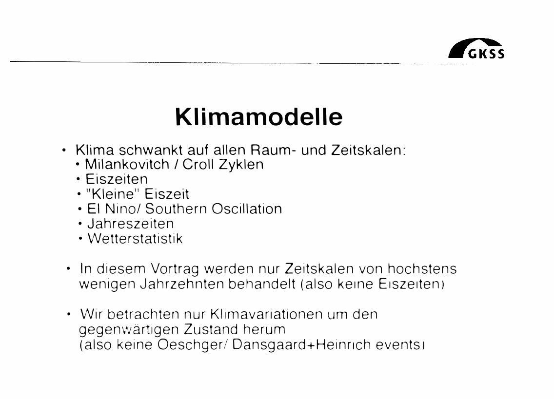
Klimamodelle • Klima schwankt auf allen Raum- und Zeitskalen:

• Mi\ankovitch I Croll Zyklen • Eiszeiten • "Kleine11 Eiszeit • EI Nino/ Southern Oscillation • Jahreszeiten • Wetterstatistik

• In diesem Vortrag werden nur Zeitskalen von hoct1stens wenigen Jahrzehnten behandelt (also keine Eiszeiten)

• Wir betrachten nur Klin1avariationen urn den gegenv;ärtigen Zustand herum (also keine Oeschger/ Dansgaard+Heinr1ch events)

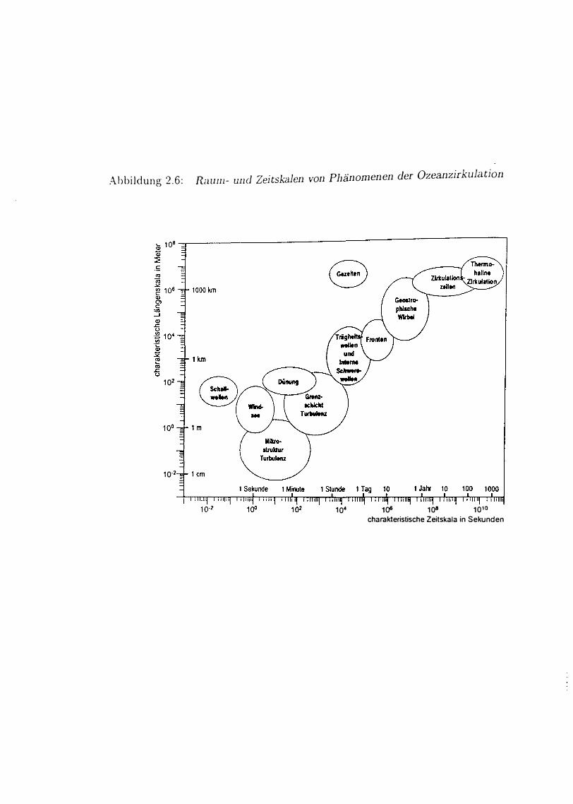
Abbildung 2.6: Raum- und Zeitskalen von Phänomenen der Ozeanzirkulation

102

10·2

104 106 108 1010 charakteristische Zeitskala in Sekunden

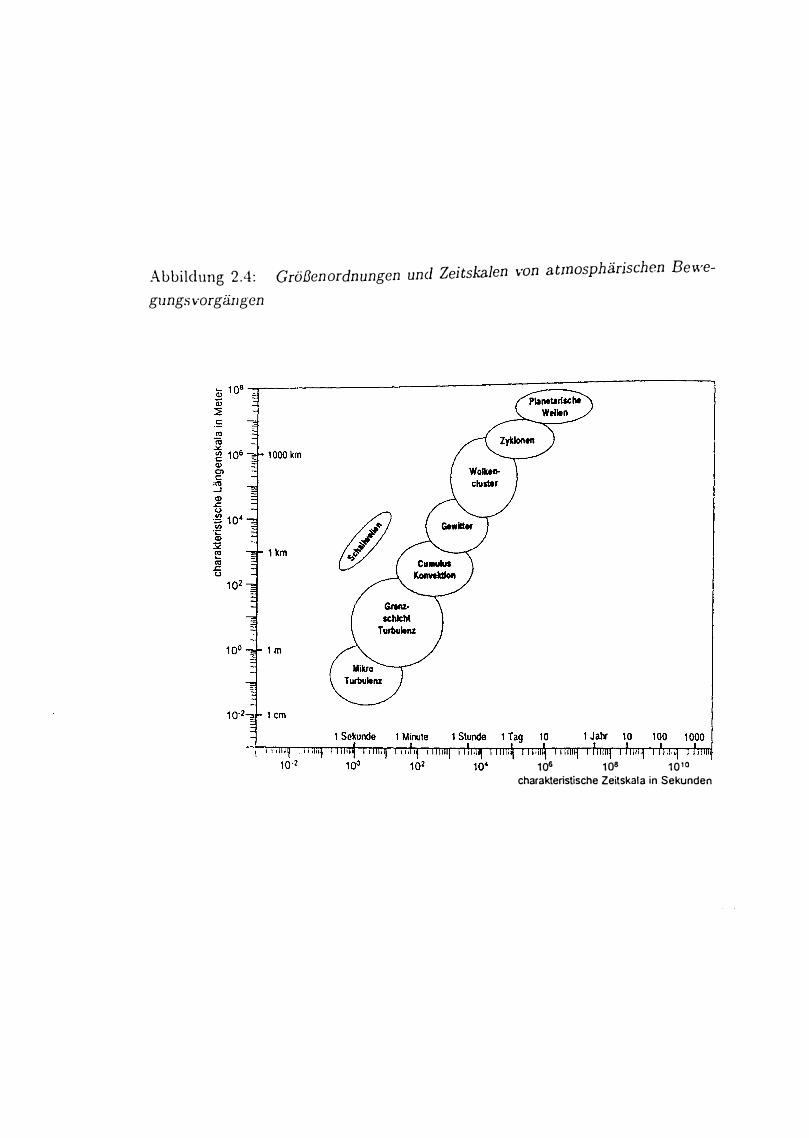
Abbildung 2.4: gungsvorgfingen

Größenordnungen und Zeitskalen von atmosphärischen Bewe-

106 1os 1010 charakteristische Zeitskala in Sekunden

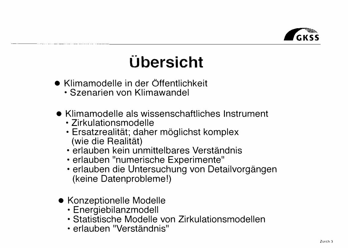
übersieht • Klimamodelle in der Öffentlichkeit

• Szenarien von Klimawandel

• Klimamodelle als wissensch aftlich es Instrument • Zirkulationsmodelle • Ersatzrealität; dah er möglich st komplex

(wie die Realität) • erlauben kein unmittelbares Verständnis • erlauben "numerisch e Experimente" • erlauben die Untersuch ung von Detailvorgängen

(keine Datenprobleme!)

• Konzeptionelle Modelle • Energiebilanzmodell • Statistisch e Modelle von Zirkulationsmodellen • erlauben "Verständnis"

Zurich 3

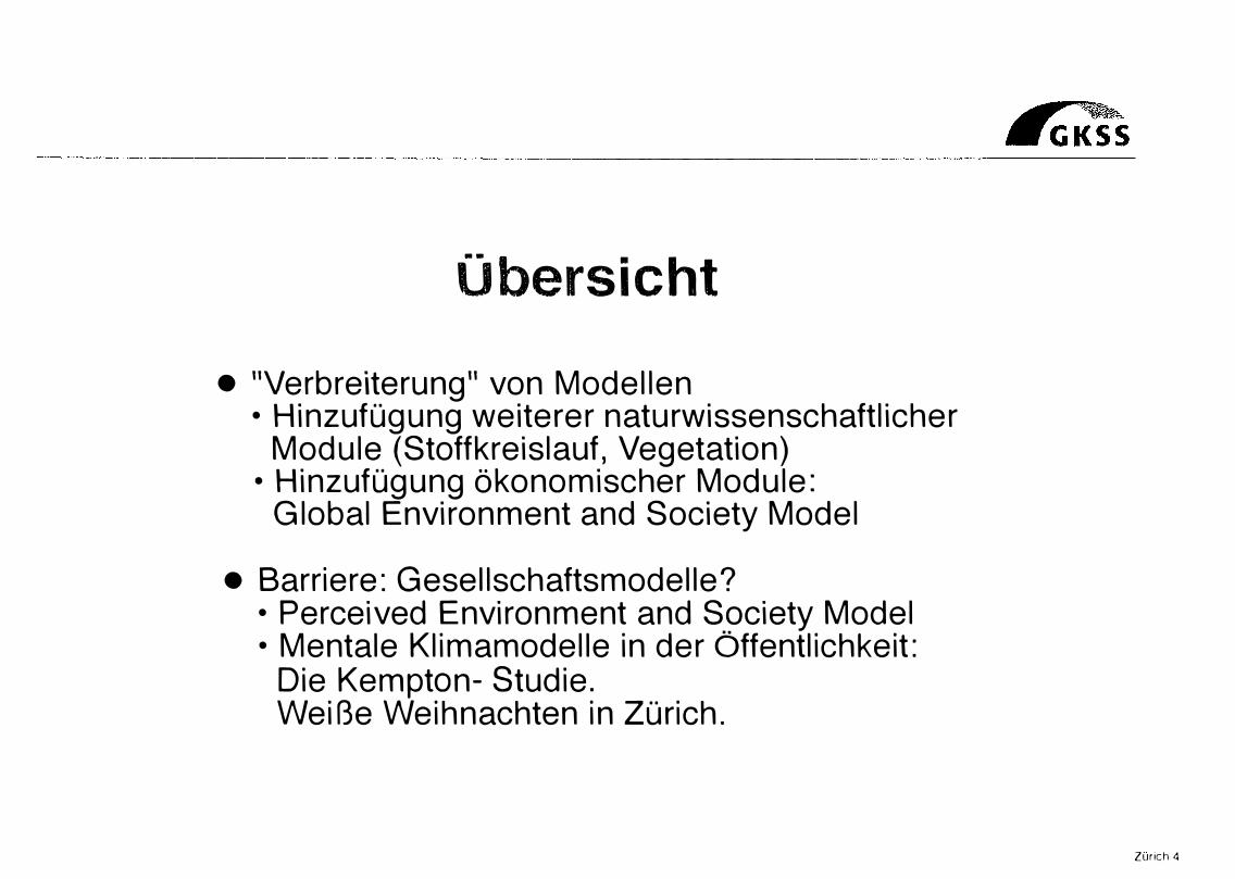
übersieht

• 11Verbreiterung11 von Modellen • Hinzufügung weiterer naturwissenschaftlich er

Module (Stoffkreislauf, Vegetation) • Hinzufügung ökonomisch er Module:

Global Environment and Society Model

• Barriere: Gesellsch aftsmodelle? • Perceived Environment and Society Model • Mentale Klimamodelle in der Öffentlichkeit:

Die Kempten- Studie. Weiße Weih nach ten in Zürich .

Zurich 4

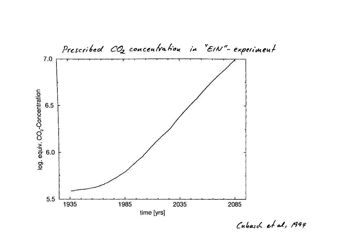
c 0 1u -E 6.5 Q) 0 c 0

() 1

N 0 ()

. > � 6.0 Q)

.

O> 0

5.5 1935 1985 2035 2085 time [yrs]

2

1935

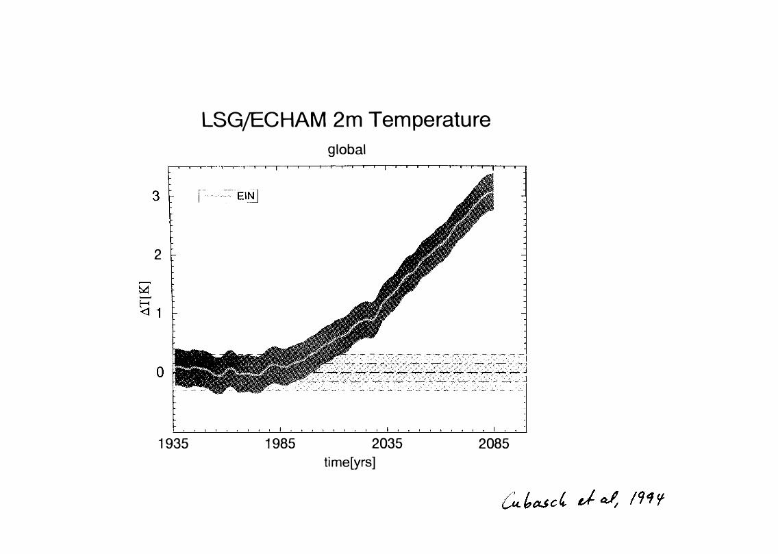
LSGjECHAM 2m Temperature global

1985

-------- -----------

" � c-: ;' ,."_?-'':'-..:._,-� .:_�-� _: _ =:j

2035 time[yrs]

2085

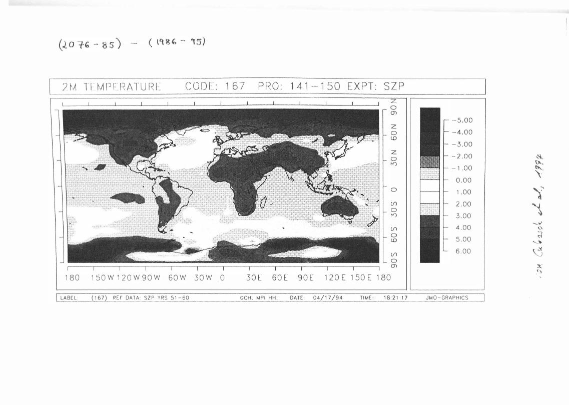
7. M T FJ-11 r F_ R AT U R [ CODE: 167 PRO: 141 -1 50 EXPT: SZP

)\l .... .. . . ;:;\:: ;}}} .;:: .' ::: \t ; .l.\.;.,.•\.\.1 .•. ' .\.:.\. 1.•.•.:.\,l .,\.\ .• •.'.•.l .. •.'.'.l.•.• .. 1•.• .l.� .• ;.·.·.· �\\\l��l\\\l\ .;:: '

''

'

··\�: �\·:,•· ······••i•'·•··•\\• :·-\···:···:·,,

180 150W120W90W 60W 30W 0

1 LABEL (167) REF DATA SZP YRS 51-60

30 t: 60 E 90 E 1 20 E 1 50 E 1 80

z 0 (J)

z 0 t.O

z 0 rr)

0

(/) 0 rr)

(/) 0 t.O

U1 0 (J)

GCH. MPI HH. DATE 04/17/94 TIME 1821:17

-5.00 -4.00 -3.00 -2.00 �

�� -1.00 �-

0.00 \· 1 .00 '{ 2.00 '\ 3.00

....._.,, 4.00 :'\ ....... 5.00 �

� 6.00 .:(

)

::oit: .„)

JMO-GRAPHICS

•JI)

N 60

JO

i)

30

.60 s

.90

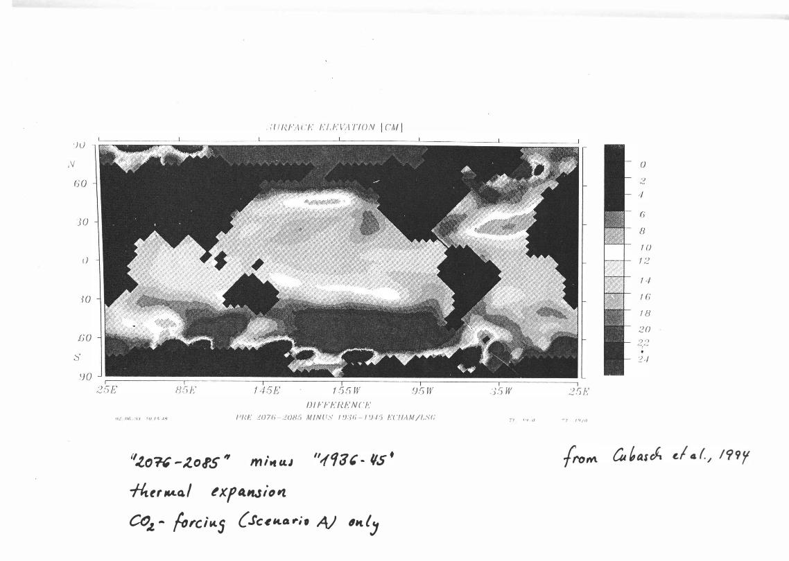
. U I /� /"1\ < .'/'.' /•.' U.'1'1\ '/'I 0 N 1 CM 1

15SW .9S W 1J / /,'/•'/•,'H. /1,'N r.·11:

11..! or. �1.1 111 J "i .JR /'/{/<,' lJJ7f>-:.!OH5 M 1 N US / .9.')1)- / 94') /':Cl /!IM //„\'!;

11-l(')� -J..o<fS " m ltt uJ

-ftttr tcA.4/ � Xf 4.11.Sio �

CO.: - forci11..5 {.Sc�l4.o „;, AJ 61t(J

.J.') w

T1 ,., t)

2 .'1 /�'

.,..".! 1'1;•1

0

2

6

8

1 ()

14

1 (i

18

20

1 Vortrag Freiberg, 10. Jull 1996, Seite 5, Version: 0&-07·96

Realitätsnahe Klimamodelle ...

• ... beschreiben mit komplexen nichtlinearen

Differentialgleichungen die Hydro- und Thermodynamik der

Atmosphäre, und des Ozeans und stellen die Wirkungen von

anderen klimarelevanten Komponenten, wie Meereis, Vegetation

etc. in parameterisierter Form dar.

• ... haben sehr viele Freiheitsgrade (> 106), und erzeugen aufgrund

der internen Prozesse Variabilität auf allen Raum- und Zeitskalen.

• ... sind numerische Approximationen und beschreiben daher nur

die Variabilität auf aufgelösten Skalen. Vorgänge auf

nichtaufgelösten Skalen werden in parameterisierter Form

dargestellt. Dazu gehören Prozesse wie Strahlungsabsorption,

Wolken etc.

1

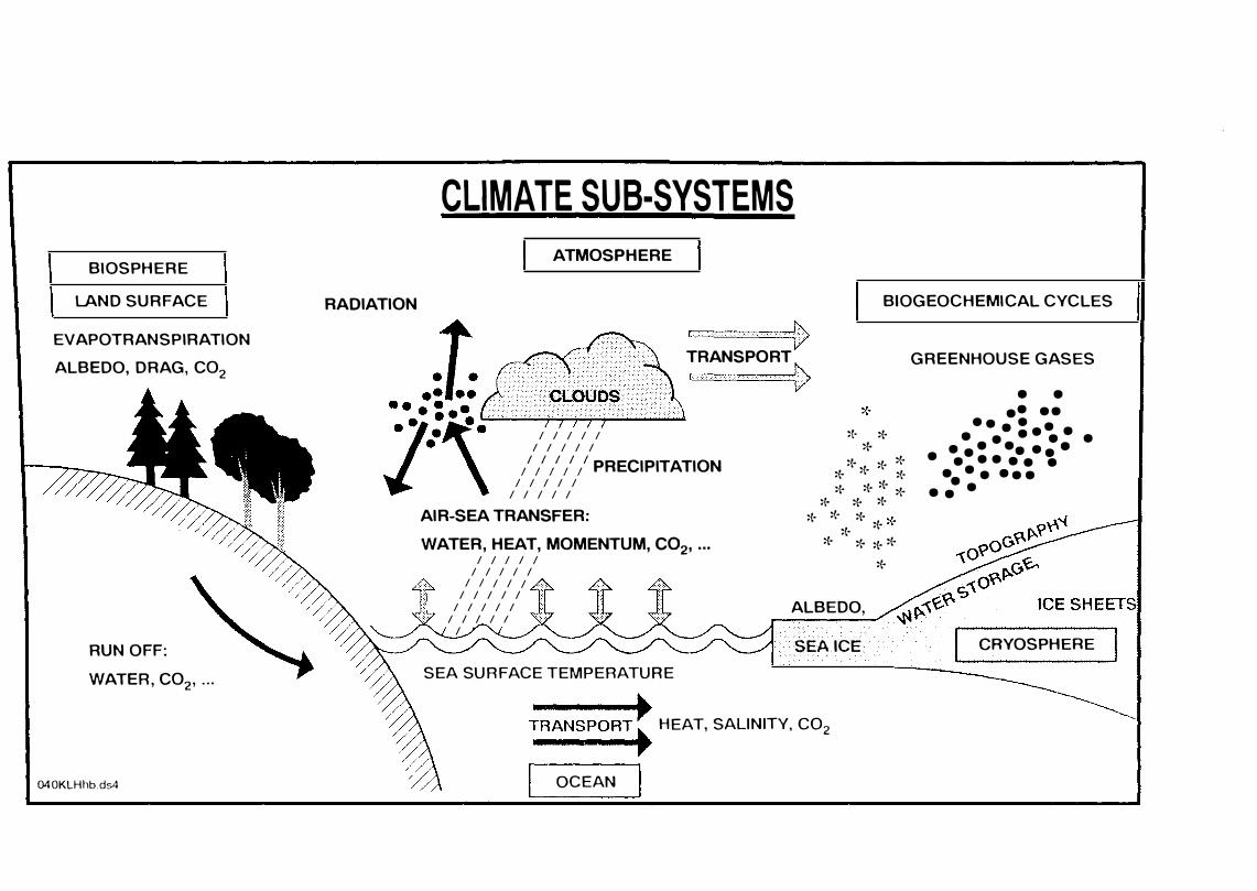
BIOSPHERE

LAND SURFACE

EVAPOTRANSPI RATION

ALBEDO,DRAG,C02

RUN OFF:

WATEA, C02, ...

040KLHhb.ds4

RADIATION

CLIMATE SUB-SYSTEMS ATMOSPHERE

BIOGEOCHEMICAL CYCLES

/ / / / / / / / / /

' .. ·.· . . . . . . . . . · .·.. t> TRANSPORT 1 t>

:(- * :(-///// PRECIPITATION :{-� �· �·

* . . �· / / / / /

/ / / / / AIR-SEA TRANSFER: WATER, HEAT, MOMENTUM, C02, •.•

/ / / / / / / / / /

/ / / / / / / / / /

/ / / / / / / / / !

/

SEA SURFACE TEMPERATUAE

:(- * * �·

:(- * �·

* �

· * .., :(- * .,.

* :t· * * *

ALBEDO,

SEAICE

TRANSPORT: HEAT, SALINITY, eo,

L OCEAN

GREENHOUSE GASES

• • •• • •

•• • • • • • •• • • •

• •• •• •• • • • •• •• •

•••• •••

• • •

CRYOSPHEAE

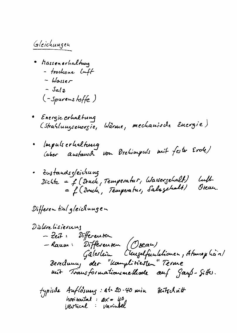
• ha.si�1it. 6-r�d� - frock.e"'"" l�f-

- Sa.f � ( -.Sfu.Y-e&A-/j fö{{e )

• E" e rs lc. �r� /.-IA � ( Slro.lc.{ uuj.r�u.ers i e, t.Ja��t 1 JU. td..a1A.ic1 Jt. ltlf.�r-a / t.. )

•

• t:v...J /.a,�.r5( e/r..,�U tAj J);·,(fc =- / (!Jr"-Ck 1 tetM./el'e:..kr1 fJas.fYJd..afi)

� /(�, �,er.f14.,} d��J

1

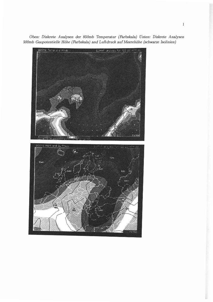
Oben: Diskrete Analysen der 850mb Temperatur (Farbskala) Unten: Diskrete Analysen

500mb Geopotentielle Höhe (Farbskala} and Luftdruck auf Meerehöhe (schwarze Isolinien)

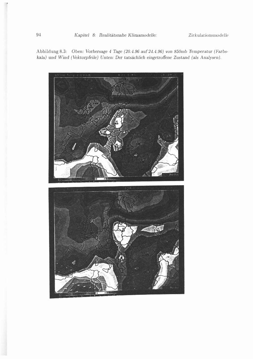
94 Kapitel 8: Realitätsnahe Klimamodelle: Zirkulationsmodellc

Abbildung 8.3: Oben: Vorhersage 4 Tage (20.4.96 auf 24.4.96) von 850mb Temperatur (Farbs­

kala) und Wind (Vektorpfeile) Unten: Der tatsächlich eingetroffene Zustand (als Analysen).

50 ..... 100 150 200 250 300

400

:soo

700

1000 . : : 1 1 1 1 1 1 1 : 1 l SOS 30S

044HVSb.drw

0

1 i

obs. ) --1 -,�-�, �1-1 -

JON 60N

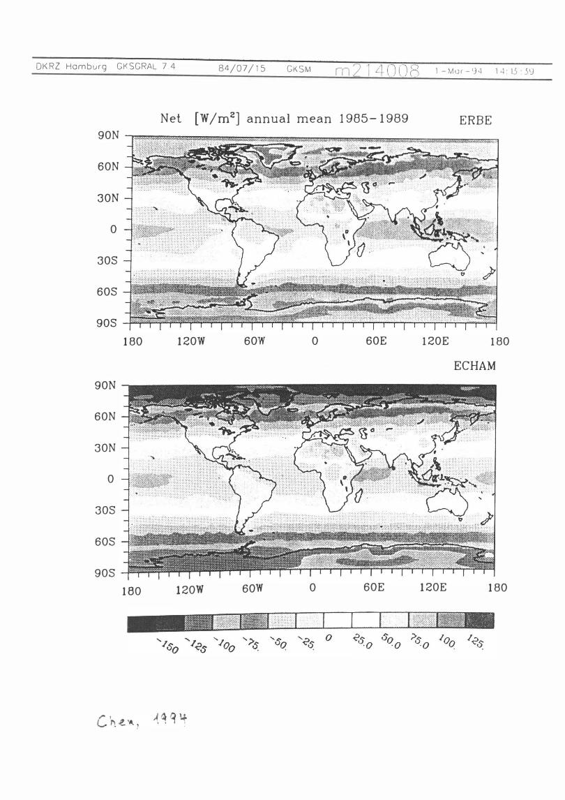
DKRZ Homburg Gl<SGRAL 7.4 84/07/15 GKSM rn2 14008

Nel [W /m2] annual mean 1985-1989 90N

60N

30N

0

30S

60S

90S 180 120W 60W 0 60E

90N

60N

30N

0

30S

60S

90S 180 120W 60W 0 60E

l-Mor-94 14:1-S : 9

ERBE

120E 180

ECHAM

120E 180

t­o_ w 0

1000

... 2 Y'.

'--'

I 1-(L w 0

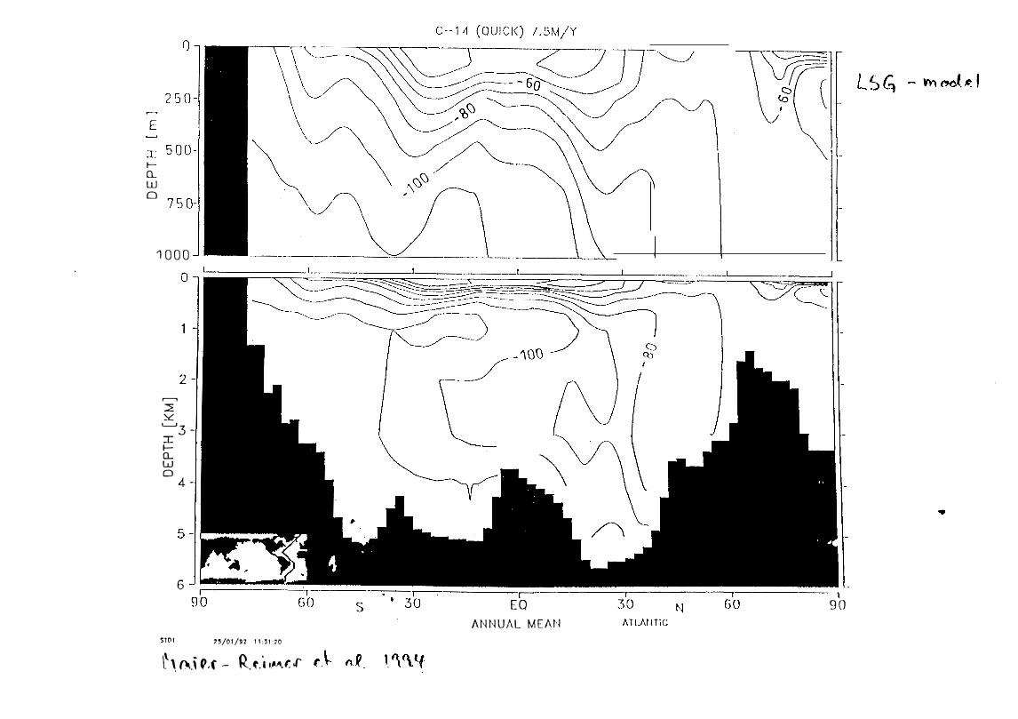
STOI

3 -

4-

6

\ '5/01/92 IUUO

\.\l\.\Qc R · . . ' - _('.l 1M.l.f „ I n „ . � {\..lf

EQ ANNU/\L ME/\N

\_

1 90

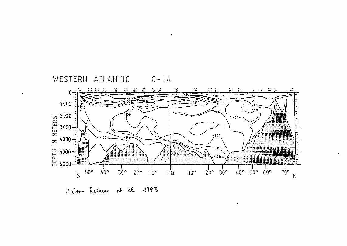
WESTERN

V1 � LtJ 1-LtJ ::L: z

:i: .__ 0.. w D

s 50°

0 •() <0 '\Q ...... , '" 1n 1n

EQ 30° '�o

o

rn '"

50° 60° 70° N

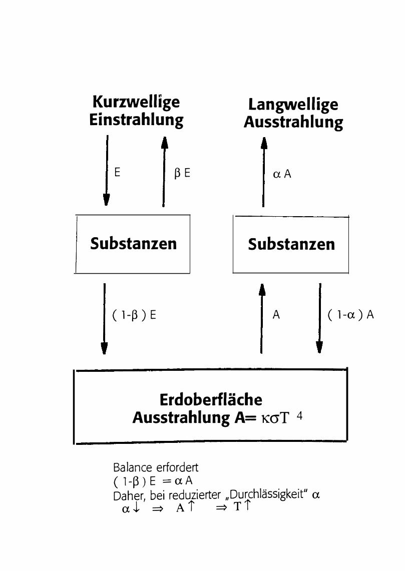
Kurzwellige Einstrahlung

langwellige Ausstrahlung

E ßE aA

Substanzen Substanzen

( 1-ß) E A

Erdoberfläche Ausstrahlung A= KcrT 4

Balance erfordert ( 1-ß ) E = a A . . . . . " Daher, bei reduzierter „Durchlass1gke1t a a� => Ai =>Tl

( 1-a) A

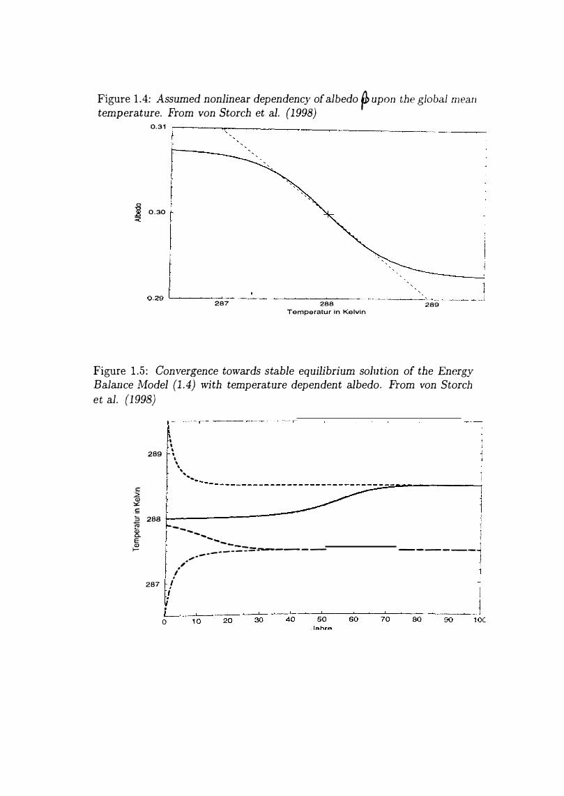
Figure 1.4: Assumed nonlinear dependency of albedo � upon the global rnean temperature. From von Storch et al. (1998)

0.31

� 0.30 <

' 1 0.29 .....__ ___ _,__��---�-��--��--�"-��----�- -�----1 287 288

Temperatur in Kelvin 289

Figure 1.5: Convergence towards stable equilibrium solution of the Energy Balance Model (1.4) with temperature dependent albedo. From von Storch

et al. (1998)

289 ' ' ' '

• \ ' ' „

... „

--------------------------------· �-�-;-�---�����_, c: :2 � _s;; ::; 28a L---------­<ti � E Q) 1-

287

----...... ... _ ---... --·--- -=�-- -

-.,,,.

,· / .

I i .

1 1

--- ---� 1

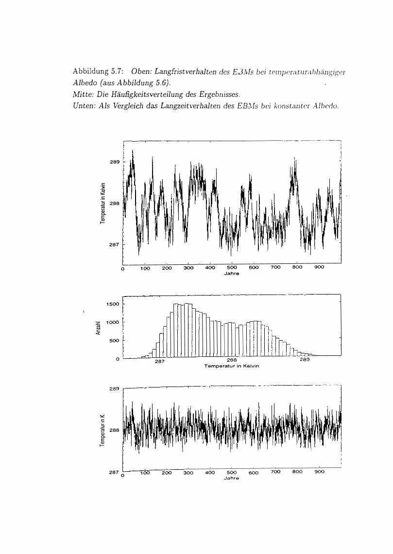
Abbildung 5.7: Oben: Langfristverhalten des E31\ls bei temperaturahhcinf)�er Albedo (aus Abbildung 5.6).

·Mitte: Die Häufigkeitsverteilung des Ergebnisses.

Unten: Als Vergleich das Langzeitverhalten des EB1\Js bei konstanter Albedo.

--�--r---------: J 1 1

289 1 1\ c: ·:;: ä> � .f;

� 288 ::> Cii 8. E Q) 1-

287

1500

� 1000 N c

<( 500

0

� ��· 100 200 300 400 500 600 700 800 900

Jahre

0 l__�...c::L.D_UJ..Jj_l.J....UJ.J...L.LLLU_Ll_L2�8�8;-u...l...L.LLLLI--LL..LLLLl�2�8�9"-'-��-' 287

� .s 5 "§ 288 a.> 0.. E <1> 1-

287 0

Temperatur in Kelvin

100 200 300 400 500 600 Jahre

-----�--

700 800 900

1�!1 "·! ,.

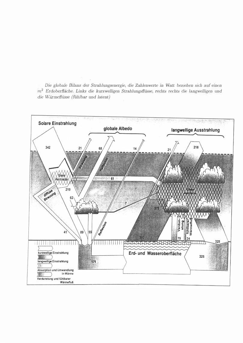
Die globale Bilanz der Strahlungsenergie, die Zahlenwerte in Watt beziehen sich auf einen

m2 Erdoberfläche. Links die kurzwelligen Strahlungsflüsse, rechts rechts die langwelligen und

die Wännefliisse (fühlbar und latent)

Solare Einstrahlung

kurzwellige Einstrahlung

langwellige Einstrahlung

) . ) Absorption und Umwandlung

).'.f ) in Wärme

Verdunstung und fühlbarer Wärmenu&

globale Albedo langwellige Ausstrahlung

a)

d)

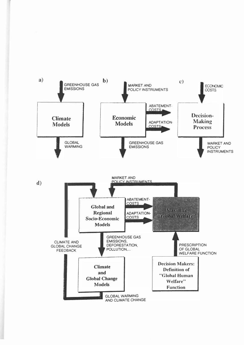
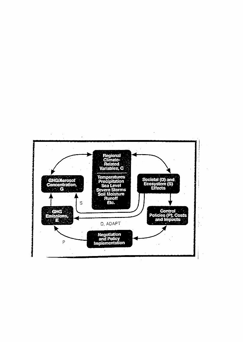
b) c) 'GREENHOUSE GAS 'IAARKET ANO ,� EMISSIONS POLICY INSTRUMENTS COSTS

Climate �lodels

GLOBAL WARMING

CLIMATE AND GLOBAL CHANGE

FEEDBACK

ABATEMENT· COSTS

Econornic Decision-Making Models ADAPTATION·

COSTS Process

GREENHOUSE GAS EMISSIONS

MARKET AND POLICY INSTRUMENTS

MARKET AND POUCY INSTRUMENTS

Global and Regional

Socio-Economic Models

GREENHOUSE GAS EMISSIONS, DEFORESTATION, POLLUTION, ...

Climate and

Global Change Models

PRESCRIPTION OF GLOBAL WELFARE FUNCTION

Decision Makers: Definition of

"Global Human Welfare" Function

GLOBAL WARMING ·------ AND CLIMATE CHANGE

" " " "

:.J

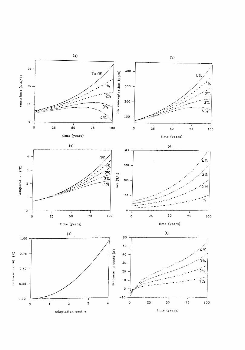
(a)

:JO

0

.,,,. ... „ ... ---

1'= 0%

„ ...... „ ... „ --------- 2% „ 'J! c "

10 „,„,,„,,,-,§•0::'�'�{.�:?;.�.::::::::=::::::-3%-·· �'�""",

...... u '

�

„ ...

--" ... " c.

"

a

4

:J

2

0

1 0

1 0

1.00

J 0,75

Q,50

0.25

0.00

0

1 25

1 25

50

time (years)

(c)

50

time (years)

(e)

1 2

1 75

75

3

adaptation cost 7

100

0%

100

4

::: c. c.

--

c:

400

0 :JOO --„ ...

--c: „ u c: 0 <J

ö u

200

100

0

:JOO -

...... --

...... ...

(b)

/ / -­

" -·

,,,. „„ ·····

„ ...• : .. ://:'::':::-:::. 25 50

tir:i.e (years)

00/ ,0

75 100

l%

„ „/3% „ .. ·· .·· „„ 200 -�

>< .

.

„

...

„

.. ··· " --

......

� "'

--"' 0 u c: „ "' „ "' ... u „

-:;

100 -.. ·· ...

.-··

. ---�:::::: ::

. . . . -- · · · · · � �- � - � - � - � · � ' � , � - �

- � ' . „„„„ - --

---

.... -······

--

... ----

0 -1-,����������-,���������--I

0 25 50

60

50 -

40 -

30 -

20 -

10 -

0 -

-10

0 25

time (years)

(f)

1 50

tir:i.e (years)

75 100

1%

75 100

Zürich 6

Lauenburg_ Dienstag, 3. Juni 1997

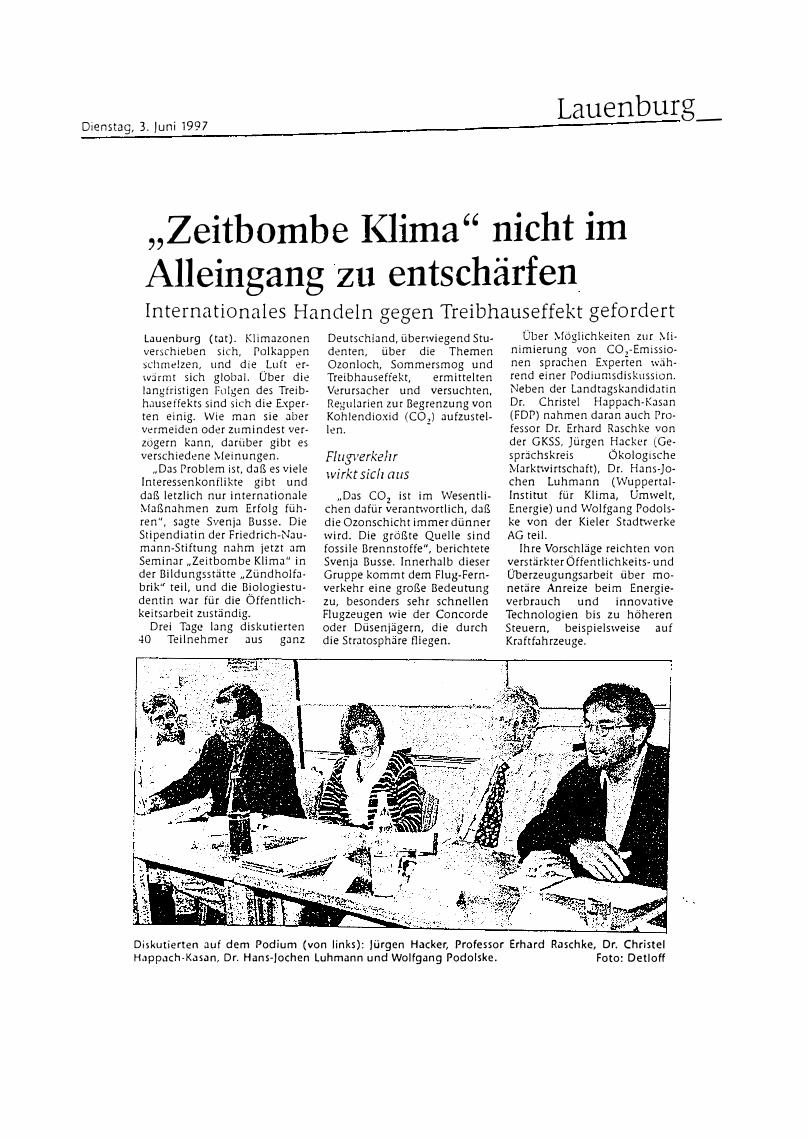
„Zeitbombe l(lima '' nicht im Alleingang zu entschärfen Internationales Handeln gegen Treibhauseffekt gefordert Lauenburg (tat). Klimazonen verschieben sich, Polkappen schmelzen, und die Luft er­wirmt sich global. Über die langfristigen Folgen des Treib­hauseffekts sind sich die Exper­ten einig. Wie man sie aber vermeiden oder zumindest ver­zögern kann, darüber gibt es verschiedene :V!einungen.

„Das Problem ist, daß es viele Interessenkonflikte gibt und daß letzlich nur internationale Maßnahmen zum Erfolg füh­ren", sagte Svenja Busse. Die Stipendiatin der Friedrich-Nau­mann-Stiftung nahm jetzt am Seminar „Zeitbombe Klima" in der Bildungsstätte „Zündholfa­brik" teil, und die Biologiestu­dentin war für die Öffentlich­keitsarbeit zuständig.

Drei Tage lang diskutierten 40 Teilnehmer aus ganz

Deutschland, überwiegend Stu· denten, über die T hemen Ozonloch, Sommersmog und Treibhauseffekt, ermittelten Verursacher und versuchten, Regularien zur Begrenzung von Kohlendioxid (C02) aufzustel­len.

Flugverke!z r wirkt siclz aus

„Das C02 ist im Wesentli­chen dafür verantwortlich, daß die Ozonschicht immer dünner wird. Die größte Quelle sind fossile Brennstoffe", berichtete Svenja Busse. Innerhalb dieser Gruppe kommt dem Flug-Fern­verkehr eine große Bedeutung zu, besonders sehr schnellen Flugzeugen wie der Concorde oder Düsenjägern, die durch die Stratosphäre fliegen.

Über :V!öglichkeiten zur :V!i­nimierung von C02-Emissio­nen sprachen Experten wäh­rend einer Podiumsdiskussion. Neben der LandtagskandidJtin Dr. Christel Happach-Kasan (FDP) nahmen daran auch Pro­fessor Dr. Erhard Raschke von der GKSS, Jürgen Hacker (Ge­sprkhskreis Ökologische Marktwirtschaft), Dr. Hans-Jo­chen Luhmann (Wuppertal­Institut für Klima, Umwelt, Energie) und Wolfgang Podols­ke von der Kieler Stadtvverke AG teil.

Ihre Vorschläge reichten von verstärkter Öffentlichkeits- und Überzeugungsarbeit über mo­netäre Anreize beim Energie­verbrauch und innovative Technologien bis zu höheren Steuern, beispielsweise auf Kraftfahrzeuge.

Diskutierten auf dem Podium (von links): Jürgen Hacker, Professor Erhard RJschke, Dr. Christei H,1ppJch-KasJn, Dr. Hans-Jochen Luhmann und Wolfgang Podolske. Foto: Detloff

1. :1 1 1 :c'. �.'f

1

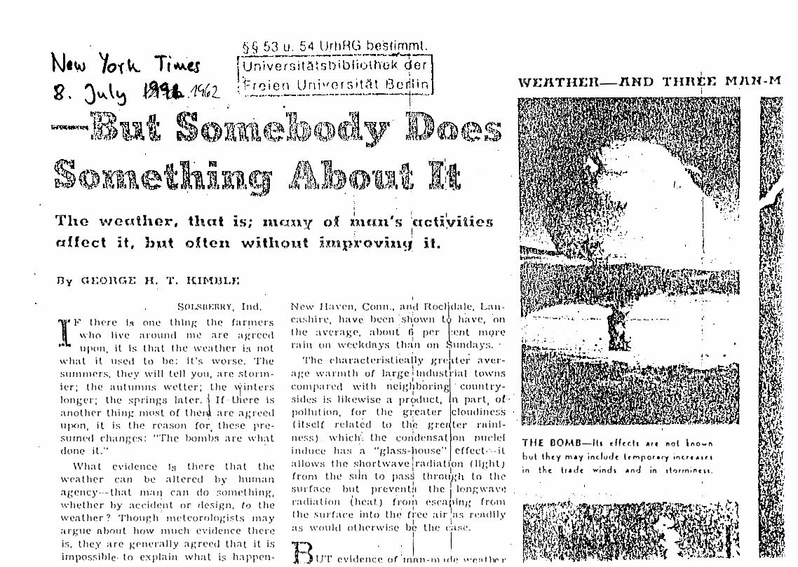
The \-'renihex-, r..tffect it, hut

thut is; n1Q:o.y of ten without

of xun:n's \etctiviiies 1 ' i :Ul p x,• 0 Vill �J i f •

Dy Gl�OHGE H. 1'. RI1''lHLJ:

sourn�:1rnY, Incl.

I F lll C're !� 0ne lh lng the farmers

wlw live around 1111� ;ue agrce<\ •" 11 pPn, il ls l ha l 1 he Wl':I thcr i'.1 not

whal il 11�cd lo hc: lt's \Vorsc. The s11m11wrs. lhcy \Vill teil yo11, are -"lonn-icr; the a11t11mns \Vt'llcr; lhc \)'inters longcr; lhe springs Inter. i If · Lherc is

anothcr thing nwst of thc1� arc agrccd upon, it is the rrason for, thc'.;c prc­

surnC'd rhangcs: "Thc bomb� arc what

<lone il." \Vha t cvidcnce ls tlwrc tha t thc

weathcr can be altcrcd by h11rnan agency---that m:1r� r;1n clo :>nmt'lhing·,

whelhcr by accicle,nl or dcsign, to thc

wcalher? Though mclcorologisls may

arguc nhout how m uch evidencc lhcrc

is, thcy arc genl'l'ally :lgrccd that it is

irnpossihlc· to cxpl:lin what i.s lnpprn-

1 N1:w 1 I:t \'Cll, Conn., ,ar.t,d Hoclj cla � c, Lan-

ca.shi rc, have becn shown tl· havc, on . 1 the :ivcragf', about fi per :cnt mqrc ra in oll wcd«lays th:i n on S1111days. ·

Th e <" ha ra cl P l'is li��a p y Y, n�ll te1: i1 ver·­a ge \v arm th of ]arge i lnd llstria l to\vns

1 • l cornpa n'<l wit h rH�iglllJOring · country-. sides i.s lil<ewisc a pr�>ducl, n parl, of·

poll11t ion, for lhc g1:cater cloudincss (it�clf rclatcd to th� grcc t1�r rninl­

nt•ss). which„·. thc cur�d<'nsal Oll nuclel

induce has a "glass-j10usc" cffcct-·-- il

allo\V� thc shorl\vave lrndiation (1!1•hlJ 1 1 '

from llH� s1ln lo pass throtwh lo thc 1 {' 0urface but prcvr.nU1 lhc 1 1c1nr�wa\'•!

radialinn ( hcat.) fro1;1 escapi1111 (rein\ 1 l ' the surface into llw frce air as r1•1Hlllv 1 : •

as \\'nllld otherwi�;e bc the c;1.se.

1 1 13 UT evldcnc �' of mn11-n1 1d1� 11·r.:i t 111' 1'

1

\VEllTllEH-11.ND TlIJlEE MllM-M

THE DOMB-lh rffcr.11 iirt not ino-.n bul thty may includt lrr•,poru'f in<."""' 1n the lradt windi 11nd in il•"Hrn;1101.

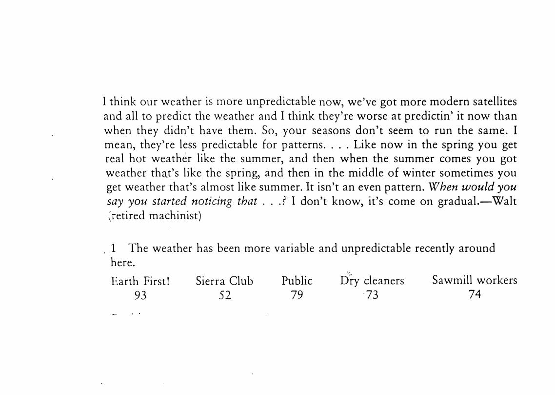
I think our weather is more unpredictable now, we've got more modern satellites and all to predict the weather and I think they're worse at predictin' it now than when they didn't have them. So, your seasons don't seem to run the same. I mean, they're less predictable for patterns . . . . Like now in the spring you get real hot weather like the summer, and then when the summer comes you got weather that's like the spring, and then in the middle of winter sometimes you get weather that's almost like summer. lt isn't an even pattern. When would you say you started noticing that . . . ? I don't know, it's come on gradual.-Walt �retired machinist)

1 The weather has been more variable and unpredictable recently around here.

Earth First! 93

Sierra Club 52

Public 79

,.

Dry cleaners ·73

Sawmill workers 74

,--

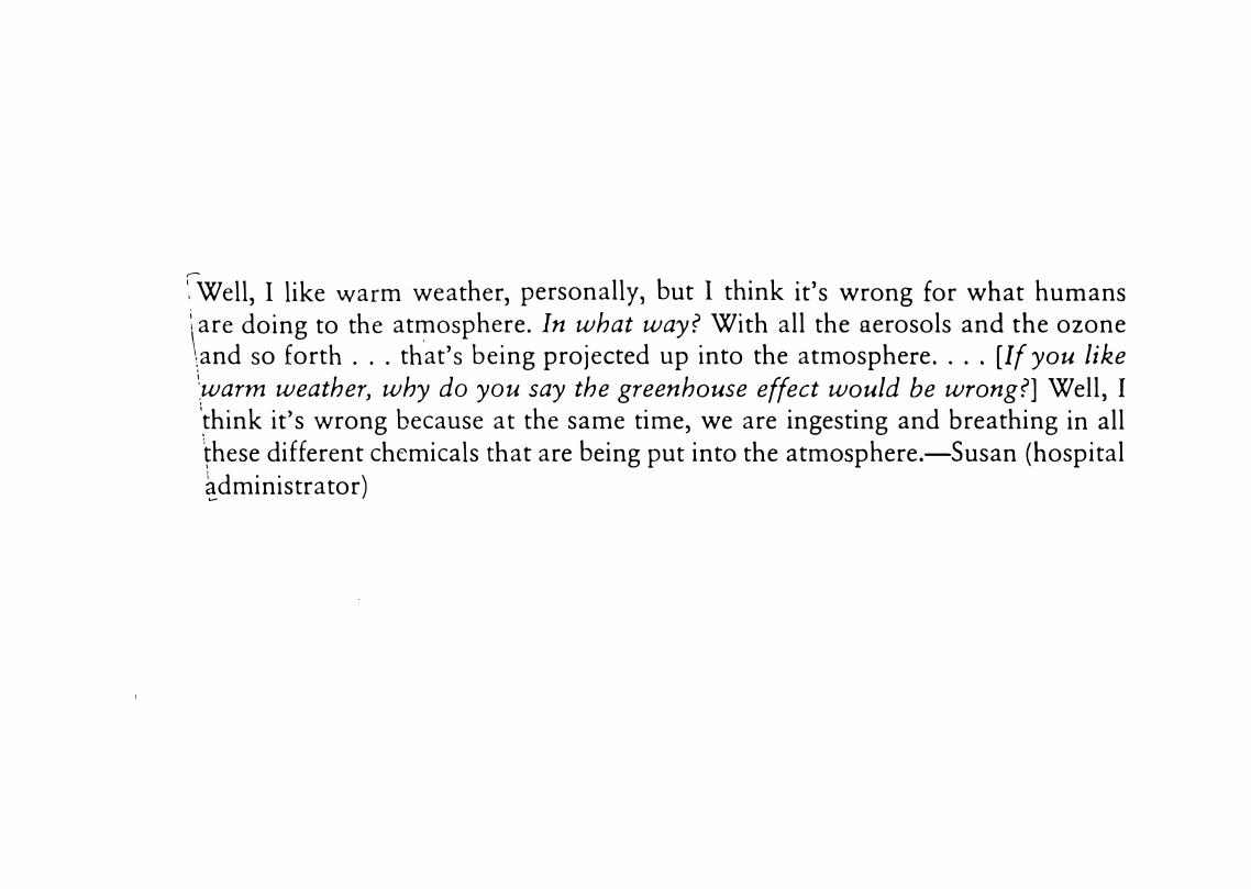
1i Well, I like warm weather, personally, but I think it's wrong for what humans \ are doing to the atmosphere. In what way? With all the aerosols and the ozone \and so forth .. . th.at's being projected up into the atmosphere . . . . [If you like \.warm weather, why do you say the greenhouse effect would be wrang?] Weil, 1 1think it's wrong because at the same time, we are ingesting and breathing in all �hese different chemicals that are being put into the atmosphere.-Susan (hospital �dministrator)

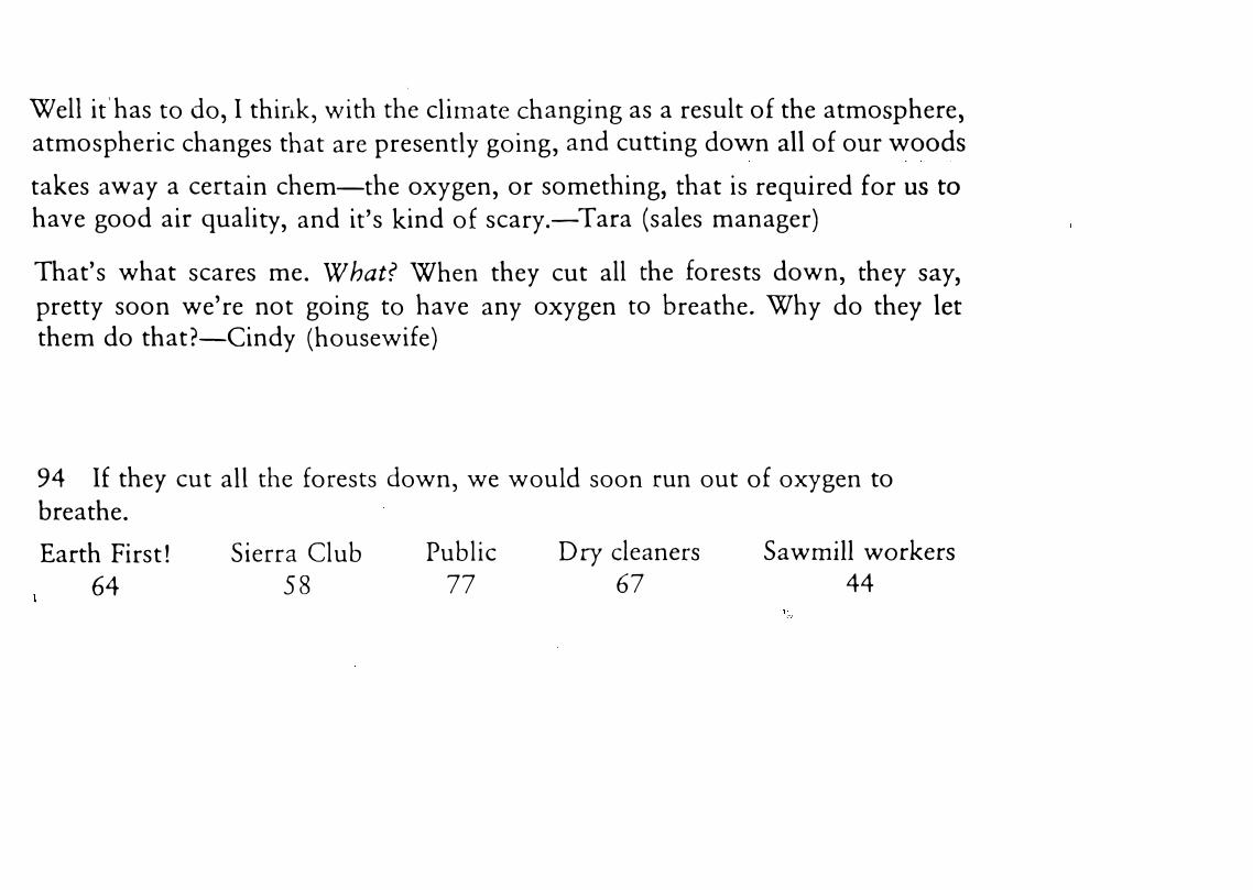
Well it'has to do, I think, with the clirnate changing as a result of the atmosphere, atmospheric changes that are presently going, and cutting down all of our woods takes away a certain chem-the oxygen, or something, that is required for us to have good air quality, and it's kind of scary.-Tara (sales manager)

That's what scares me. What? When they cut all the forests down, they say, pretty soon we're not going to have any oxygen to breathe. Why do they let them do that?-Cindy (housewife)

94 If they cut all the forests down, we would soon run out of oxygen to breathe.

Earth First! 64

Sierra Club 58

Public 77

Dry cleaners

67 Sawmill workers

44

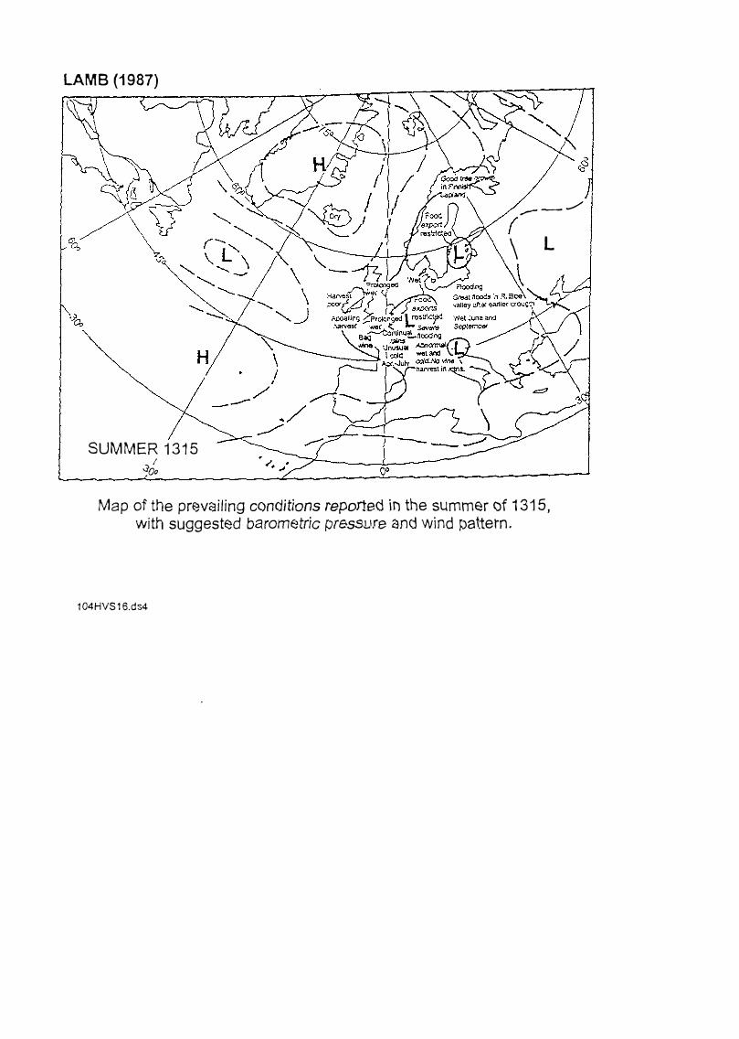
LAMB (1987)

SUMMER 1315 I �Oo

H

____ _ ./ ( \ L \

Map of the prE3VC3iling conc:titions reported in the summer öf 1315, with suggest�d barometric pressvre '3nd wind pattern.

104HVS 16.dS4

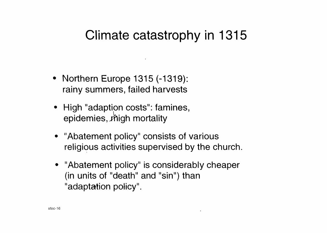
Climate catastrophy in 1315

• Northern Europe 1315 (-1319): rainy summers, failed harvests

• High "adaption costs": famines, epidemies, ifiigh mortality

• 11Abatement policy" consists of various religi�us activities supervised by the church.

• "Abatement policy" is considerably cheaper (in units of "death" and "sin") than "adaptation policy".

stoc-16

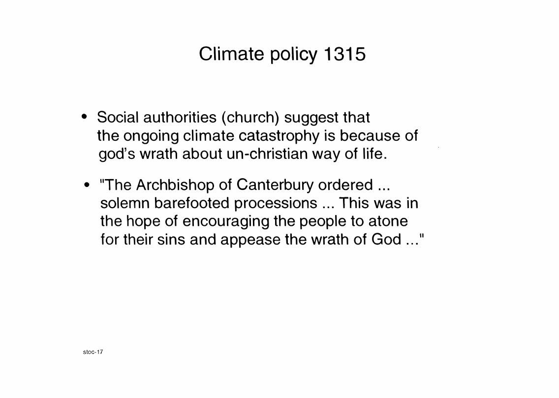
Climate policy 1315

• Social authorities (church) suggest that the ongoing climate catastrophy is because of god's wrath about un-christian way of life.

• "The Archbishop of Canterbury ordered ... solemn barefooted processions ... This was in the hope of encouraging the people to atone for their sins and appease the wrath of God ... "

stoc-17

G> m c •

.c u G>

..., • E

·­-

u

05JHVSa

... .,....

1

...... �

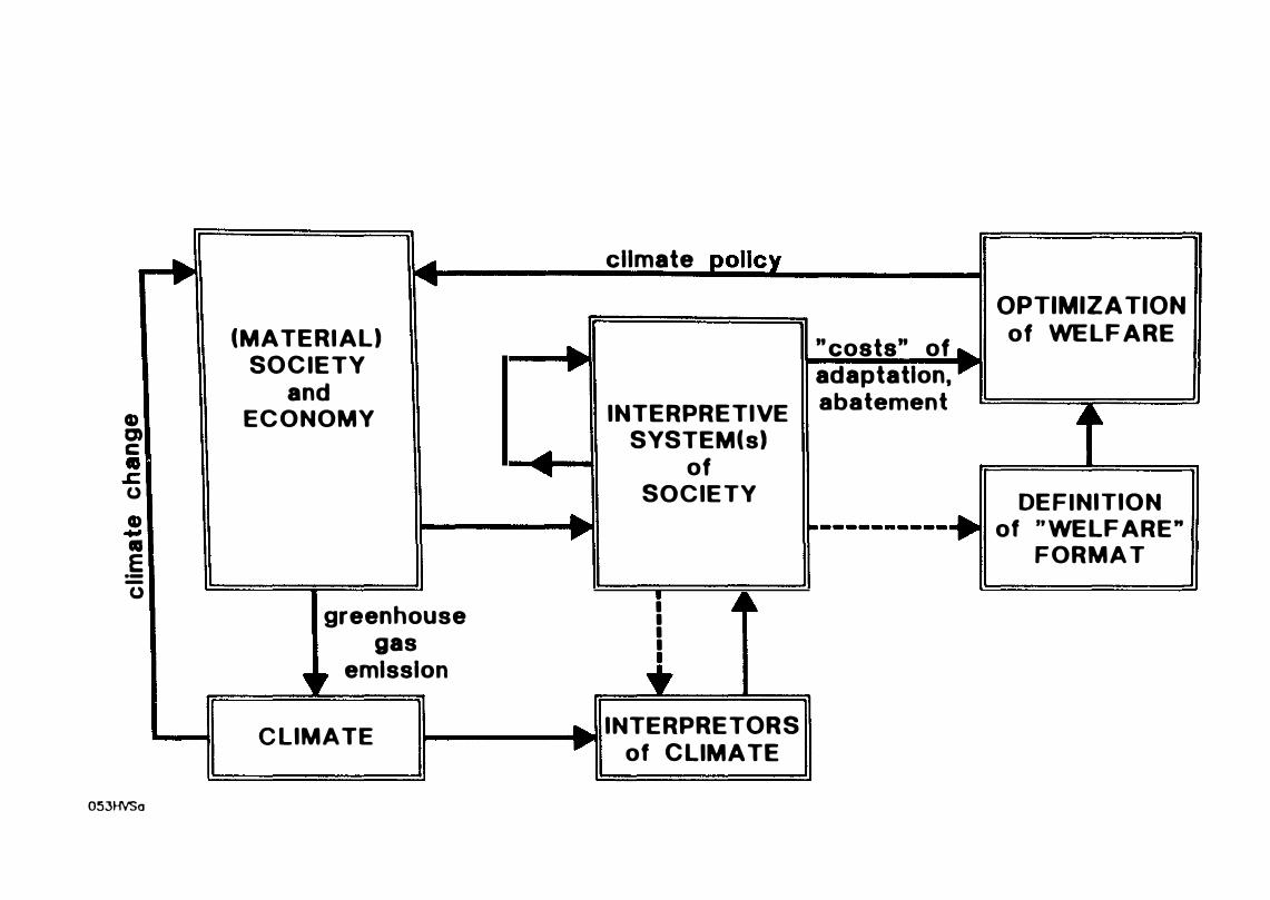
(MATERIAL) SOCIETY

and ECONOMY

... �

greenhouse gas

� , emlsslon

CLIMATE 1

cllmate pollcy

OPTIMIZA TION ... "costs" of .....

of WELFARE

.,.... adaptatlon, .,....

INTERPRETIVE abatement .4 �

SYSTEM(s) of

SOCIETY DEFINITION .....

.,.... ·----------+ of "WELF ARE" FORMAT

1 � 1 � 1 1 1

• ... INTERPRETORS .,.... of CLIMATE

Folgerungen • Gesellsch aftlich e Vorgänge spielen eine Rolle

für die Entwicklung des Klimas.

• Gesellsch aftlich e Vorgänge lassen sich nur seh r bedingt in math ematisch e Modelle fassen: Mensch en lassen sich nich t in der Art der Th ermodynamik wie gleich artige von unveränderlich en Prinzipien geleitete Moleküle besch reiben.

• Naturwissensch aftler glauben bisweilen, die gesellsch aftlich en Vorgänge mechanistisch in Klimamodelle einfügen zukönnen. Rückkeh r des Klimadeterminismus?

Zurich fl

Folgerungen

• Klimamodelle sind weitgehend ausgereift für die realitätsnahe Beschreibung von Klimavorgängen auf der Zeitskala von Tagen bis zuwenigen Jahren im Bereich des h eutigen Klimas.

• Klimamodelle können verkomplettiert werden durch Hinzufügung anderer naturwissenschaftlich er Komponenten.

Zurich 7

/80 !GQ 11-0 IZO 100 /j(J o. ,_O 40 ii.:J l!O

-teryH;g� !Z2Zl K;g>, �Med;urn 6ol__i=lt;2_�lo��::__��--,-�--,-�������������-""���-:...�--'-���--:-�� 0. Veorvl..ow

„„ ............. _ .. _ .. ___ _ _ _ _ _ - - „ - ... „ - „ -- -- - _..,. ______ .... - ---- - -- ----- -- - - - --- --- -- - - --..- - ----- - -- - --- - - -- -- - - -- -- - „ -- -- -

!·50 16"0 HO

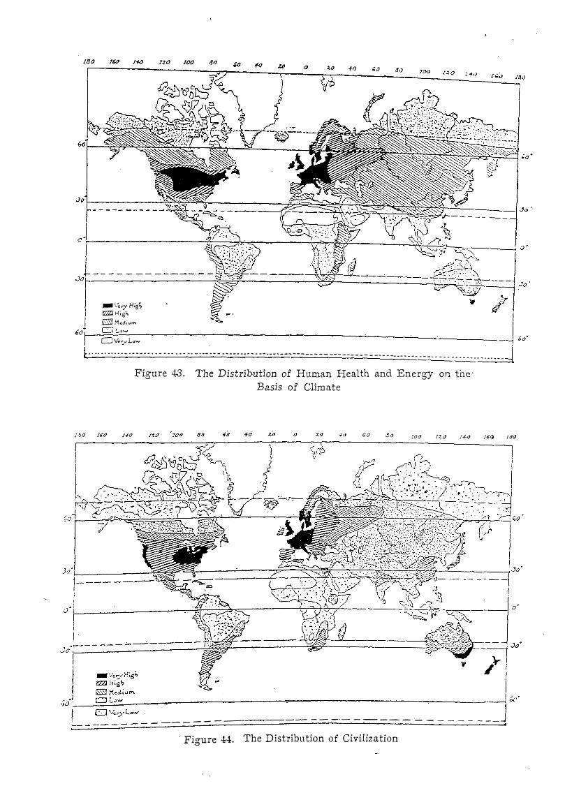
Figure 43. The Distribution of Human Health and Energy o:ri foe· Ba.sis of Climate

60 80 :oo rzo 14<7 t6Q 1ao

c= --------- - ---·--- - - -·- - - -- - - - - - - - - -- .

The Distribution of Civilization Figure 44.

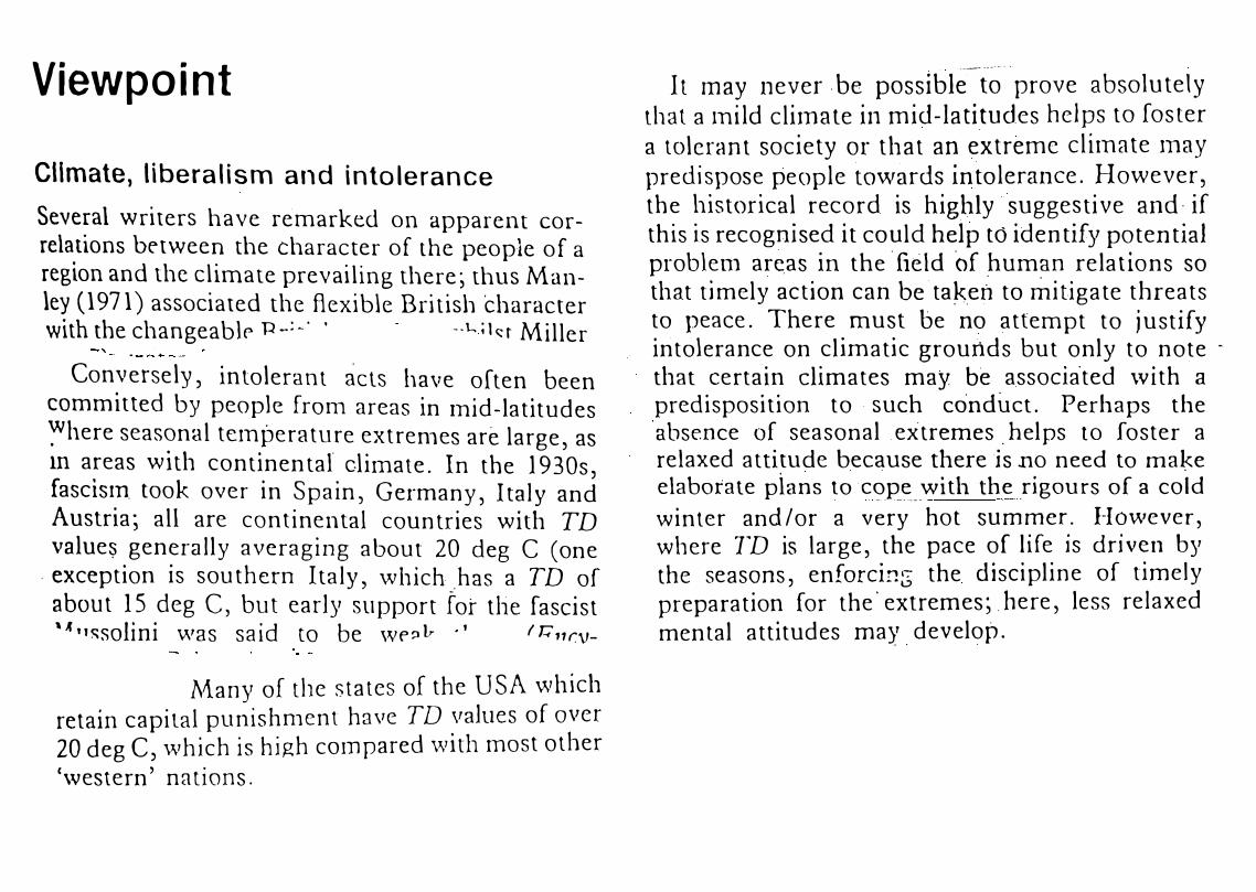
Viewpoint

Cllmate, liberalism and intolerance Several writers have remarked on apparent cor­relations between the character of the people of a region and the climate prevailing there; thus Man­

ley ( 1971) associated the ftexi ble Bri tish character with the changeablP p_:_· · -.i..;1,t Miller

Conversely, intolerant acts have often been committed by people fron1 areas in 1nid-latitudes �here seas?nal tetnperature extren1es are large , as 1n areas wi th continen tal cli1nate . In the l 930s, fascis1n. took over in S pain , Germany, Italy and Austria; all are continental coun tr ies with TD value� generally averaging abou t 20 deg C (one

· exception is southern ltaly , which has a TD of about 15 deg C, but ear ly support fot the fascist ' .( 11SSO{ini \V2S Sa id tO be \Vf'� lr . ' / r:; nr.v-

.A1.any of the s tates of the USA \vhich

retain capital punishn1ent have TD values of over 20 deg C, \vhich is high co1n pared \Vith most other

'\vestern' na tions.

��- ----- .

lt may never be possible to prove absolutely

that a inild clitnate in mid-lati.tudes helps to f oster

a tolera nt society or that an extreme clitnate tnay predispose people towards intolerance. However, the historical record is highly suggestive and - if this is recognised it could help tö identify potential problen1 are.as in the "field of _human relat ions so that ti mely action can be tak.en to mitigate threats to peace. There must be no attempt to justify intolerance on climatic grounds but only to note ··

that certain climates may be associa.ted \Vith a predisposition to such conduct. Perhaps the absence of seasonal extremes _ helps to f oster a relaxed atti tude because there is no need to make elaborate pians to cgp_� ___ with the _ _ rigours of a coid

winter and /or a very hot summer. I-Iowever, where TD is large , the pace of life is driven by the seasons, enforcin G the d iscipline of timely

p reparation for the ·extremes;. here, less relaxed mental attitudes may. develop .

If the weather gets a Lot warmer, do you think it would be good, bad, or neutral? I think it would be bad; I think it would be terrible. Why? Well, 1 think people react differently in warm weather than when it's cooler. I think it has an effect on attitudes-behavior ... . l mean in the prison system especially, where the people are just, you know, stuck in there, and they've got to let off steam. So, sure. So you think in prison it makes people more violent? Sure, but outside the prisons, too, 'cause I even see it at work; you know, when the weather is extremely warm, people tend to be, you know, a little hot tempered. 1 think, you know, their blood boils. And when the blood boils in the body, it goes to the head, and next thing you know, there's, you know, an explosion . .. . , l've seen them react that way.-Paige (manufacturing worker)

Methoden zur Beschreibung

dominanter Muster in geophysikalischen Vektorzeitreihen

Hans von Storch GKSS Forschungszentrum

Basierend auf Kapitel 13, "Spatial patterns: EOFs and CCA" in: von Storch, H., and A. Navarra (Eds. ), 1995: Analysis of Climate Variability: Applications of Statistical Techniques, Springer Verlag, (ISBN 3-540�58918-X)

1

S ignal and Noise Subspace,

Guess Patterns

The separation of the full phase space into a "signal" su bspace �

spanned by a few patterns pk and a "noise" subspace may be for­mally written as

_. K k Xt = I: ak(t)p + nt k=l

with t representing time. The K "guess patterns" pk and time co­effi.cients ak(t) are supposed to describe the dynamics in the signal subspace, and the vector nt represents the "noise subspace" . The truncated vector of state "

_.5 K k Xt = I: ak(t)p k=l

is the projection of the full vector of state on the signal subspace. The

residual vector - - s nt = Xt - xt

represents the contribution from the noise subspace.

Expansion Coeffi.cients

• The "expansion coefficients" ä = ( a1, a2 ... a K) T are determined as those numbers which minimize

..... with the "dot product' (ä, b) = L.1 a1b1. The optimal vector of expansion coefficients is obtained as a zero of the first derivative of E: K T · T ..... � -k -i -k X � p p Üi = p i=l A.fter introduction of the notation A = ( äl b · · ·) for a matrix A with the first column given by the vector ä and the second column

.....

by a vector b, P..... (-1 1 , ..... K)TX-. a = p . . . p

with the symmetric Kx K-matrix P = (PkT pi). In all but patho­logical cases the matrix P will be invertible such that a unique solution exists:

..... p-1 (-1 1 1-K)TX ..... a = p ... p Finally, if we define K vectors ß1 ... p!f so that

(ß11 · . · lßf) = (ß1I · . · lßK) p-l

Then the k-th expansion coefficient ak is given as the dot product of the vector of state X and the "adjoint pattern" p�: -k ..... Ük = (pA, X)

• In some cases, and in particular in case of EO Fs, the patterns p k

are orthogonal such that P is the identity matrix and pk = fi.�. In this case -k ..... ak = (p , X)

3

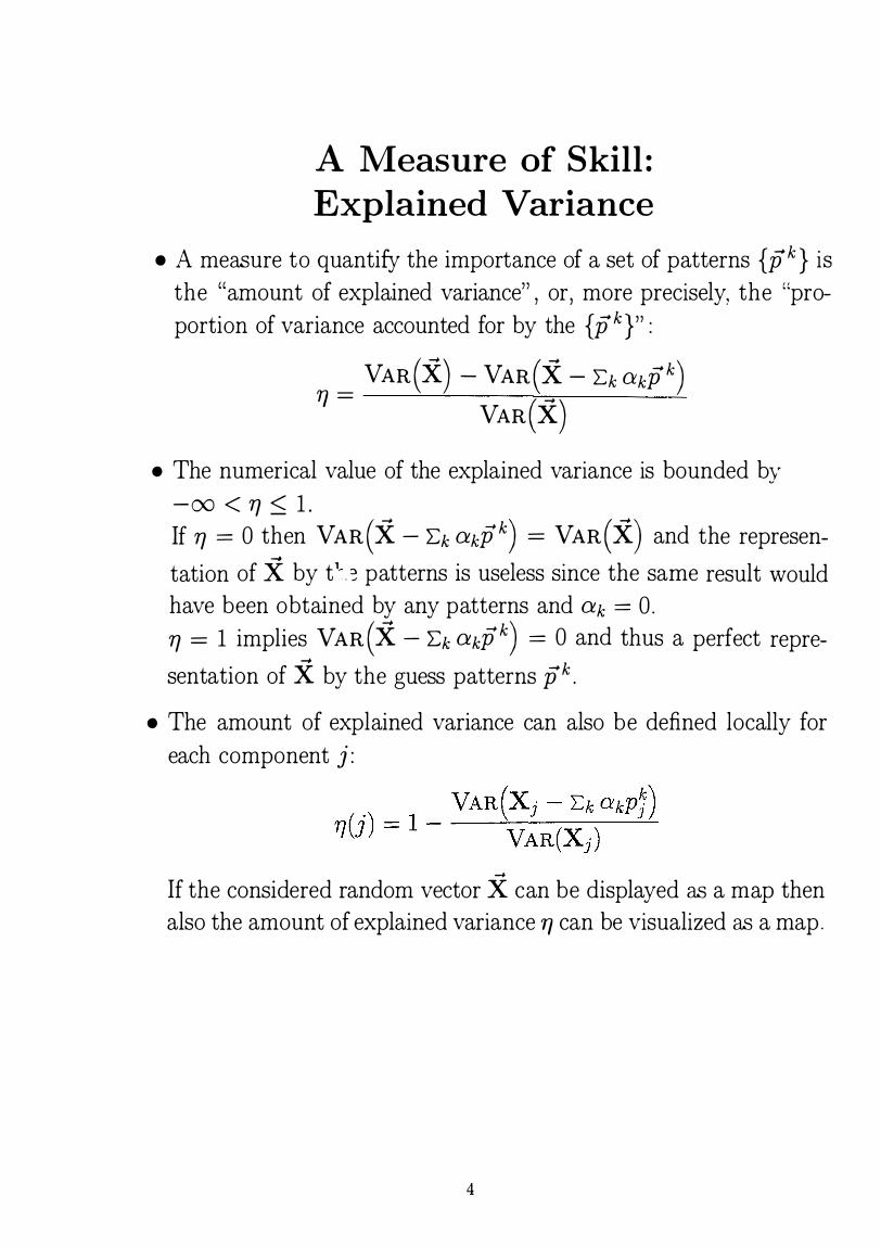
A Measure of Skill :

Explained Variance

• A measure to quantify the importance of a set of patterns {pk} is the "amount of explained variance" , or, more precisely, the "pro­portion of variance accounted f or by the {p k}" :

T/ _ VAR(X) - VAR(X - 'Lk akpk) - VAR(X) • The numerical value of the explained variance is bounded by

- 00 < 'T/ < 1. If 'T/ == 0 then VAR(X - 'L.k O'.kPk) == VAR(X) and the represen-

-

tation of X by t1�. � patterns is useless since the same result would have been obtained by any patterns and O'.k == 0. 'T/ == 1 implies VAR(X - 'L.k O'.kPk) == 0 and thus a perfect repre-

sentation of X by the guess patterns p k.

• The amount of explained variance can also be defined locally f or each component j:

-

If the considered random vector X can be displayed as a map then also the amount of explained variance 'T/ can be visualized as a map .

4

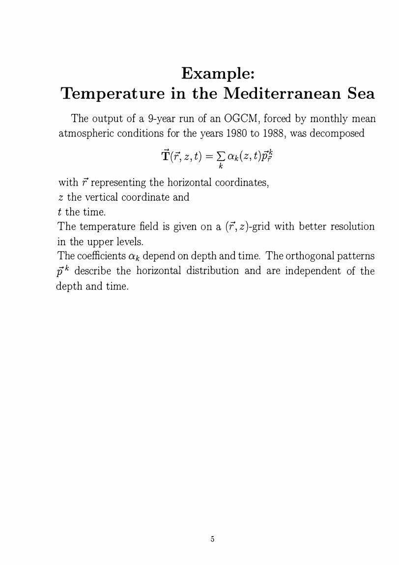
Example:

Temperat ure in the Mediterranean Sea

The output of a 9-year run of an OGCM, forced by monthly mean atmospheric conditions for the years 1980 to 1988, was decomposed

T(r, z, t) = L, ak (z, t)ft k

with r representing the horizontal coordinates , z the vertical coordinate and t the time. The temperature field is given Oll a ( r, z )-grid with better resolution in the upper levels. The coefficients ak depend on depth and time. The orthogonal patterns p k describe the horizontal distribution and are independent of the depth and time.

5

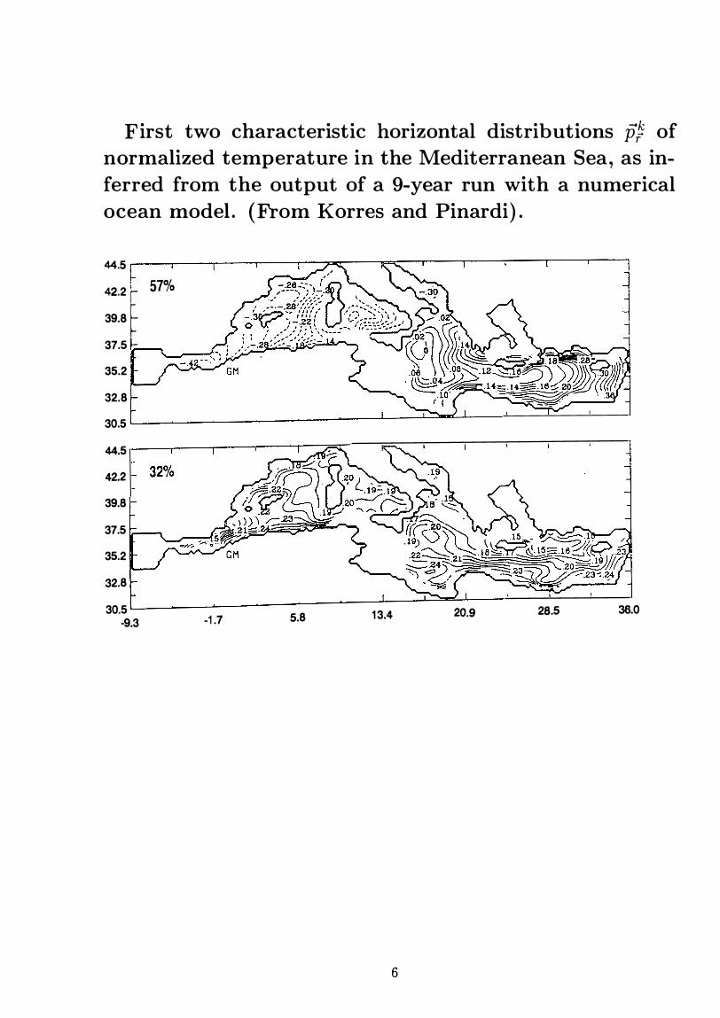
First two characteristic horizontal distributions pfr of normalized temperature in the Mediterranean Sea, as in­ferred from the output of a 9-year run with a numerical ocean model. (From Korres and Pinardi).

44.5,

� r- 57% �.2 t 39.8

37.5

35.2

32.8

30.5

44.5

42.2

39.8

37.5

35.2

32.8

30.5 5.8 13.4 20.9 28.5 36.0 -9.3 -1.7

6

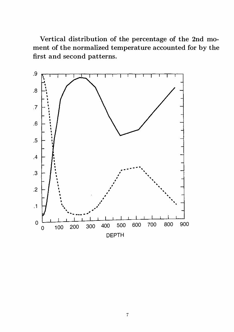
Vertical distribution of the percentage of the 2nd mo­ment of the normalized temperature accounted for by the first and second patterns.

.3

.2

. 1

0 0

1 1 1 •

„ - „ „" 1 # „ „ ' ' ' ' ' ' '

' ' ' ' ' ' ' ' ' ' '

' ' ' ' ' ' �

' ' . ' ' ' ' � 1 ' �

' � ' ' .

�, „� � #

.„„ -·- - _,

100 200 300 400 500 600 700 800 900

DEPTH

7

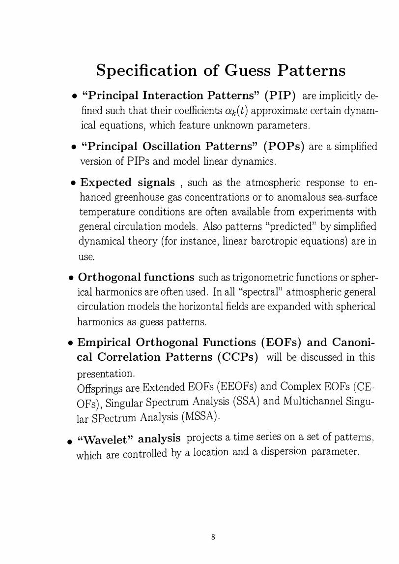
Specification of Guess Patterns

• "Principal Interaction Patterns" (PIP) are implicitly de­fined such that their coefficients ak ( t) approximate certain dynam­ical equations , which feature unknown parameters .

• "Principal Oscillation Patterns" {POPs) are a simplified version of PIPs and model linear dynamics.

• Expected signals , such as the atmospheric response to en­hanced greenhouse gas concentrations or to anomalous sea-surf ace temperature conditions are often available from experiments with general circulation models. Also patterns "predicted" by simplified dynamical theory ( for instance, linear barotropic equations) are in use.

• Orthogonal functions such as trigonometric functions or spher­ical harmonics are often used. In all "spectral" atmospheric general circulation models the horizontal fields are expanded with spherical harmonics as guess patterns.

• Empirical Orthogonal Functions {EOFs) and Canoni­cal Correlation Patterns { CCPs) will be discussed in this

presentation. Offsprings are Extended EOFs (EEOFs) and Complex EOFs (CE-

OFs) , Singular Spectrum Analysis (SSA) and Multichannel Singu-

lar SPectrum Analysis (MSSA) .

• "Wavelet" analysis projects a time series on a set of patterns,

which are controlled by a location and a dispersion parameter .

8

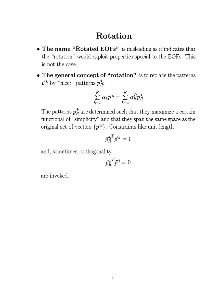
Rotation

• The name "Rotated EOFs" is misleading as it indicates that the "rotation" would exploit properties special to the EOFs. This is not the case.

• The general concept of "rotation" is to replace the patterns pk by "nicer" patterns fA:

K -k K R -k L Ü.kP = L <Y.k PR k=l k=l The patterns f A are determined such that they maximize a certain functional of "simplicity" and that they span the same space as the original set of vectors {pk}. Constraints like unit length

-kT -k 1 PR P =

and, sometimes, orthogonality

are invoked.

-kT -i Ü PR P =

9

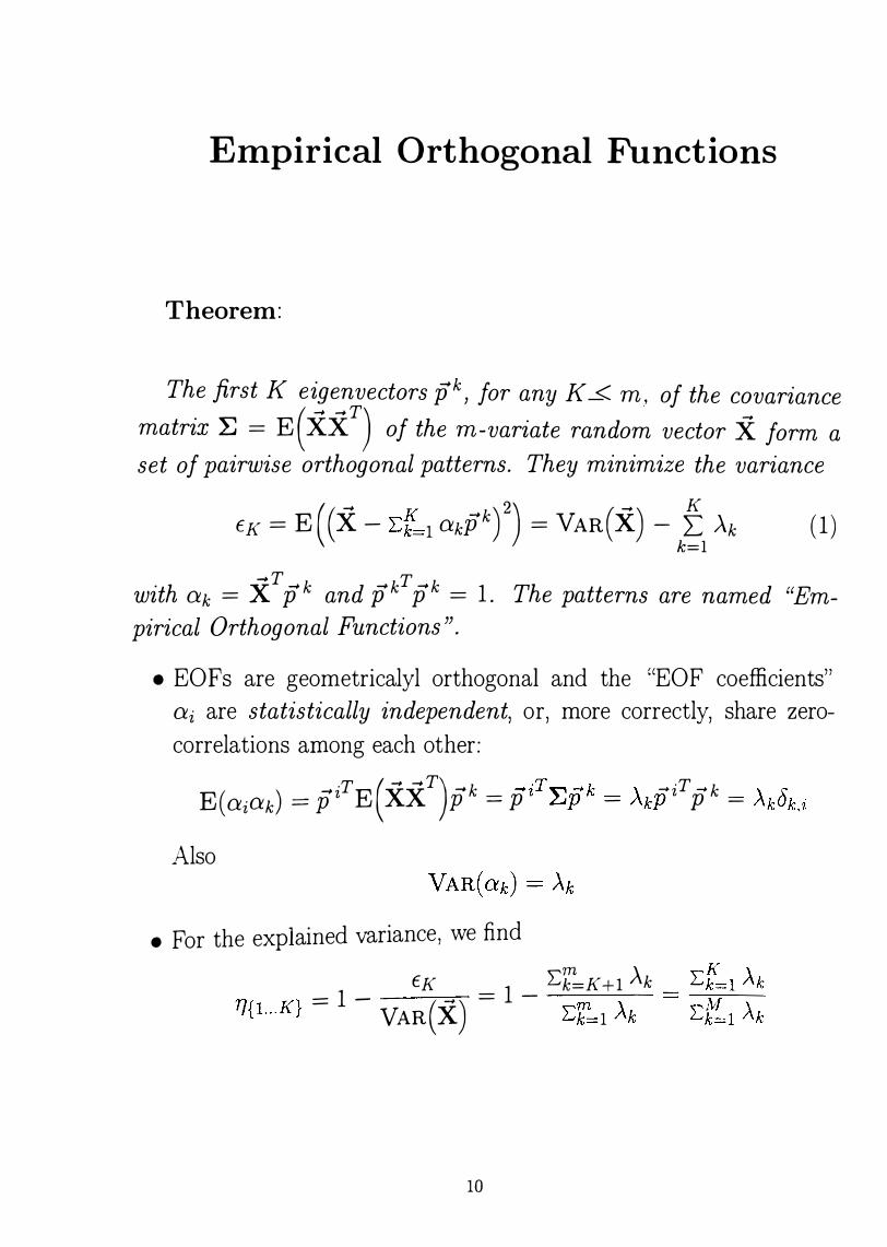
Empirical Orthogonal Functions

Theorem:

The first K eigenvectors pk, for any K < m., of the covariance ( - -T) -matrix :E = E XX of the m-variate random vector X form a set of pairwise orthogonal patterns. They minimize the variance

EK = E( (X - Lf 1 ak'ffkn = VAR(X) - l-1 >..k (1)

with ak = XT pk and pkT pk = 1. The patterns are named "Em­pirical Orthogonal Functions ".

• EOFs are geometricalyl orthogonal and the "EOF coefficients" ai are statistically independent, or, more correctly, share zero­correlations among each other:

-iT ( - -T) -k _ -iT�-k _ ' -iT-k _' � E( aiak) == p E XX p - P �P - AkP P - Akuk,i

�A.lso

• For the explained variance, we find

f.K L:k=K+l Ak '11 - 1 - ( -+ ) = 1 - \ ·i{l...K} - VAR X L:k 1 /\k

10

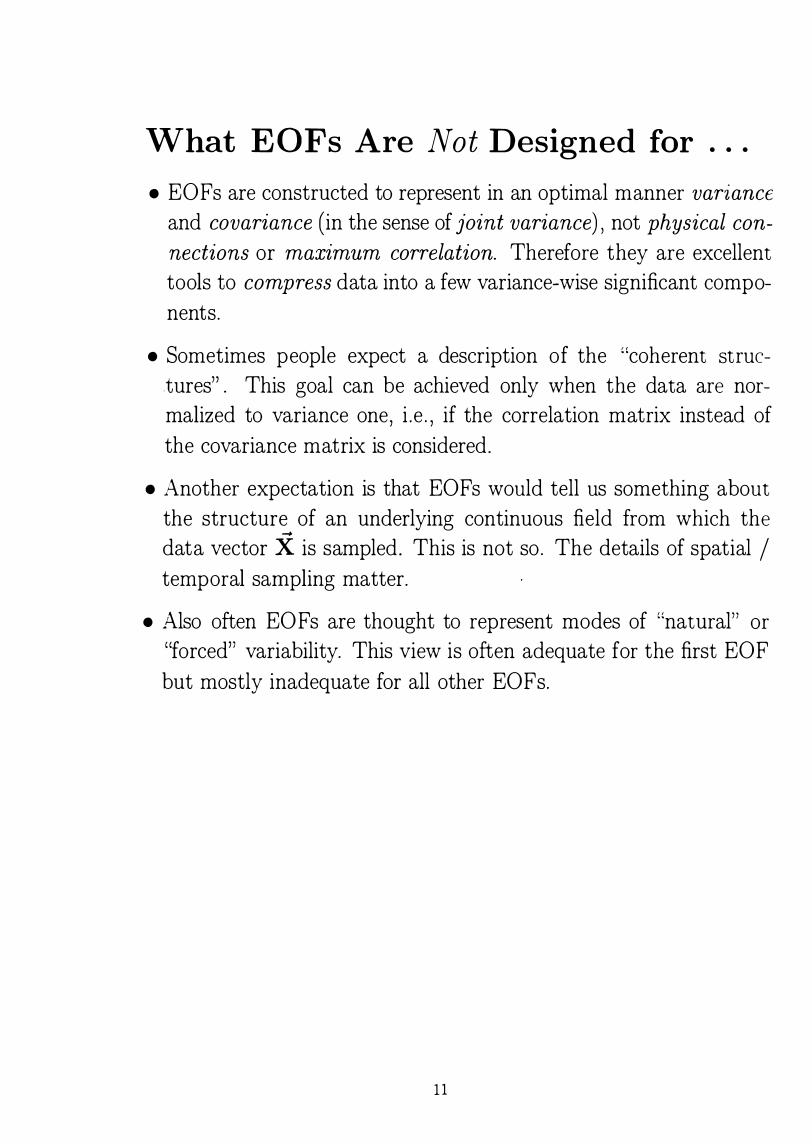
What EOFs Are Not Designed for ...

• EOFs are constructed to represent in an optimal manner variance and covariance (in the sense of joint variance), not physical con­nections or maximum correlation. Therefore they are excellent tools to compress data into a few variance-wise significant compo­nents.

• Sometimes people expect a description of the "coherent struc­tures" . This goal can be achieved only when the data are nor­malized to variance one, i.e . , if the correlation matrix instead of the covariance matrix is considered.

• Another expectation is that EOFs would tell us something about the structure of an underlying continuous field from which the data vector X is sampled. This is not so . The details of spatial / temporal sampling matter.

• A.lso often EO Fs are thought to represent modes of "natural" or "forced" variability. This view is often adequate for the first EOF but mostly inadequate for all other EOFs.

11

Estimation of EOFs

• U sually clone by centering data, and replacing expectation opera­tors by sums.

• Low-index EO Fs and eigenvalues are usually better estimated than high-indexed EOFs and eigenvalues.

• "Significance tests" are designed for detecting degeneracy of eigenvalues, not for assessing the quality of the estimation of the eigenvectors.

12

Example:

Central European Temperat ure

in Winter

• Werner, P.C. and H . von Storch , 1993: lnterannual variability of Central European mean temperature in J anuary /February and its relation to the large-scale circulation . - Clim Res. 3, 195-207

• Winter mean temperature anomalies (i .e . , deviations from the over­all winter mean) at eleven Central European stations.

• Homogeneous time series were available for eighty winters from 1901 to 1980.

• For a better display of the results sometimes a different normaliza­tion is convenient, namely akpk = ( ak / yf}:k) x (pkyf}:k) = a�p 'k. In this normalization the coefficient time series has variance one for all indices k and the relative strength of the signal is in the patterns p'. A typical coefficient is a' = 1 so that the typical

I reconstructed signal is p .

• EOFs were calculated for 1901-40 and 1941-80 separately.

13

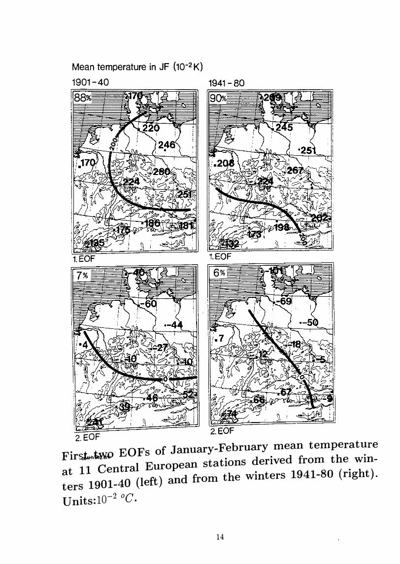
Mean temperature in JF (10-2 K) 1901-40 188%

2.EOF

Fir�WrO EOFs of January-February mean temperature

at 11 Central European stations derived from the win­

ters 1901-40 (left) and from the winters 1941-80 ( right).

U nits: 10-2 °C.

14

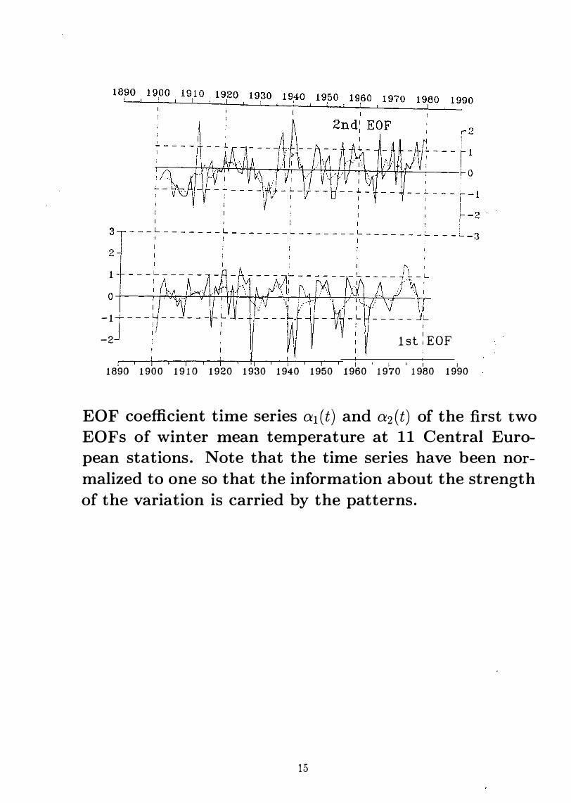
1

-1

-2 1 lst 1 EOF

1890 1900 1910 1920 1930 1940 1950 1960 1970 1980 1990

EO F coefficient time series a1 ( t) and a2 ( t) of the first two EOFs of winter mean temperature at 11 Central Euro­pean stations. Note that the time series have been nor­malized to one so that the information about the strength of the variation is carried by the patterns.

15

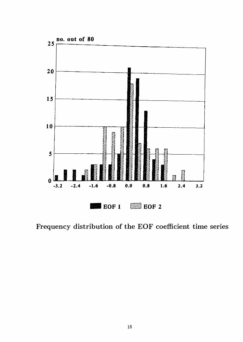
no. out of 80 25r-���������������

0 1.8-----------��� -3.2 -2.4 -1.6 -0.8 0.0 0.8 1.6 2.4 3.2

-EOF 1 -EOF 2

Frequency distribution of the EOF coefficient time series

16

Canonical Correlation Analysis

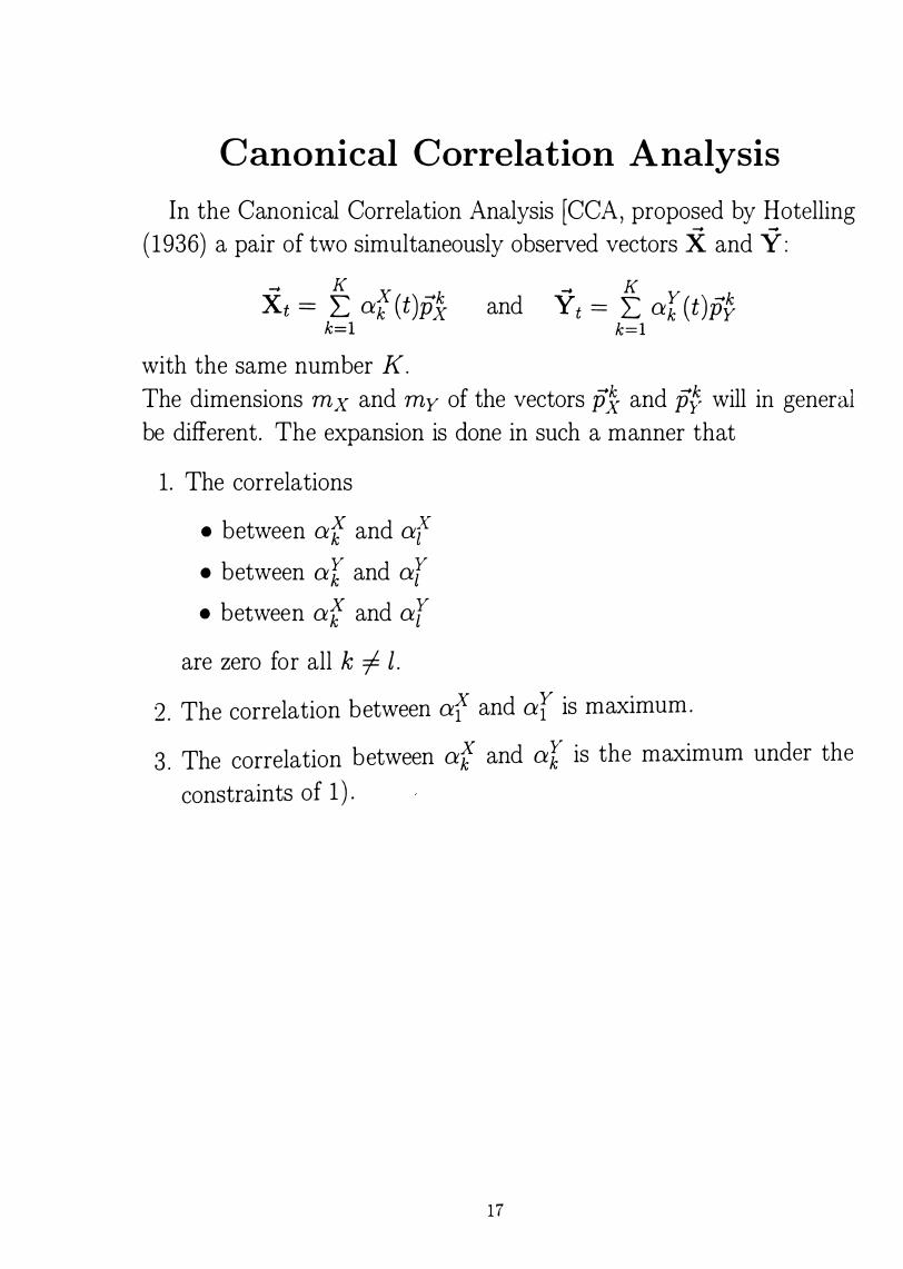
In the Canonical Correlation Analysis [CCA, proposed by Hotelling (1936) a pair of two simultaneously observed vectors X and Y:

_, K X -k Xt == 2: ak (t)Px k=l

with the same number K.

and - K y -k Yt = L: ak (t)py k=l

The dimensions m x and m y of the vectors ff 'X and p� will in general be different. The expansion is clone in such a manner that

1. The correlations

• between af and af • between ar and ar • between af and ar

are zero f or all k -j; l. X d y . .

2. The correlation between a1 an a1 is maximum.

3 . The correlation between af and ar is the maximum under the

constraints of 1) .

17

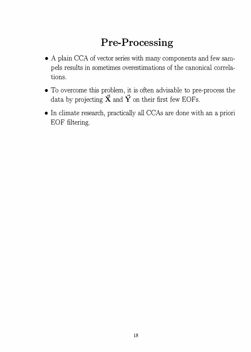
Pre-Processing

• A plain CCA of vector series with many components and few san1-pels results in sometimes overestimations of the canonical correla­tions .

• To overcome this problem, it is often advisable to pre-process the -+ -+

data by projecting X and Y on their first few EOFs.

• In climate research, practically all CCAs are clone with an a priori EOF filtering.

18

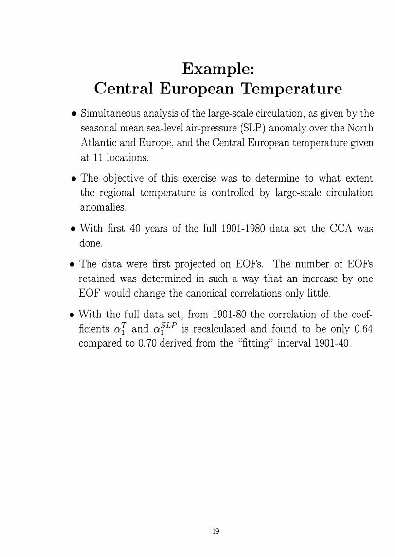
Example:

Central European Temperature

• Simultaneous analysis of the large-scale circulation, as given by the seasonal mean sea-level air-pressure (SLP) anomaly over the North A.tlantic and Europe, and the Central European temperature given at 11 locations.

• The objective of this exercise was to determine to what extent the regional temperature is controlled by large-scale circulation anomalies .

• With first 40 years of the full 1901-1980 data set the CCA was clone.

• The data were first projected on EOFs. The number of EOFs retained was determined in such a way that an increase by one EOF would change the canonical correlations only little.

• With the full data set, from 1901-80 the correlation of the coef­ficients af and af_LP is recalculated and found to be only 0 .64 compared to 0.70 derived from the "fitting" interval 1901-40 .

19

h Pa

JF

10-2 K

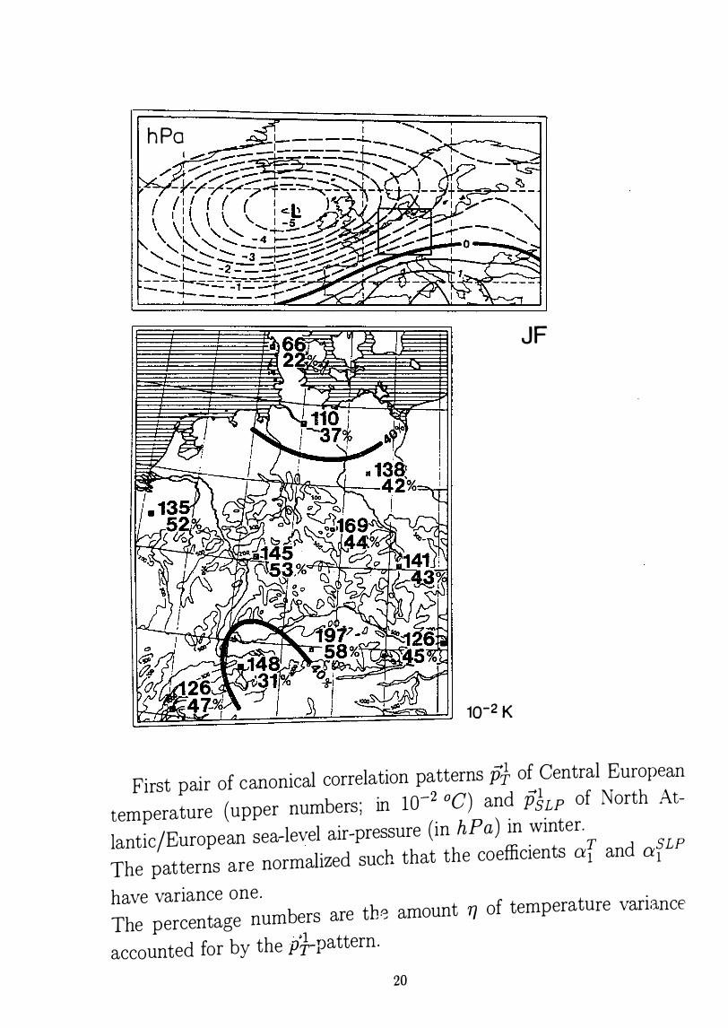
First pair of canonical correlation patterns ff of Central European

temperature (upper numbers ; in 10-2 °C) and P§LP of North At­

lantic/European sea-level air-pressure (in h Pa ) in winter.

The patterns are normalized such that the coefficients o{ and afLP

have variance one.

The percentage numbers are th� amount ry of temperature variance

accounted for by the pj,-pattern.

20

7

5

3

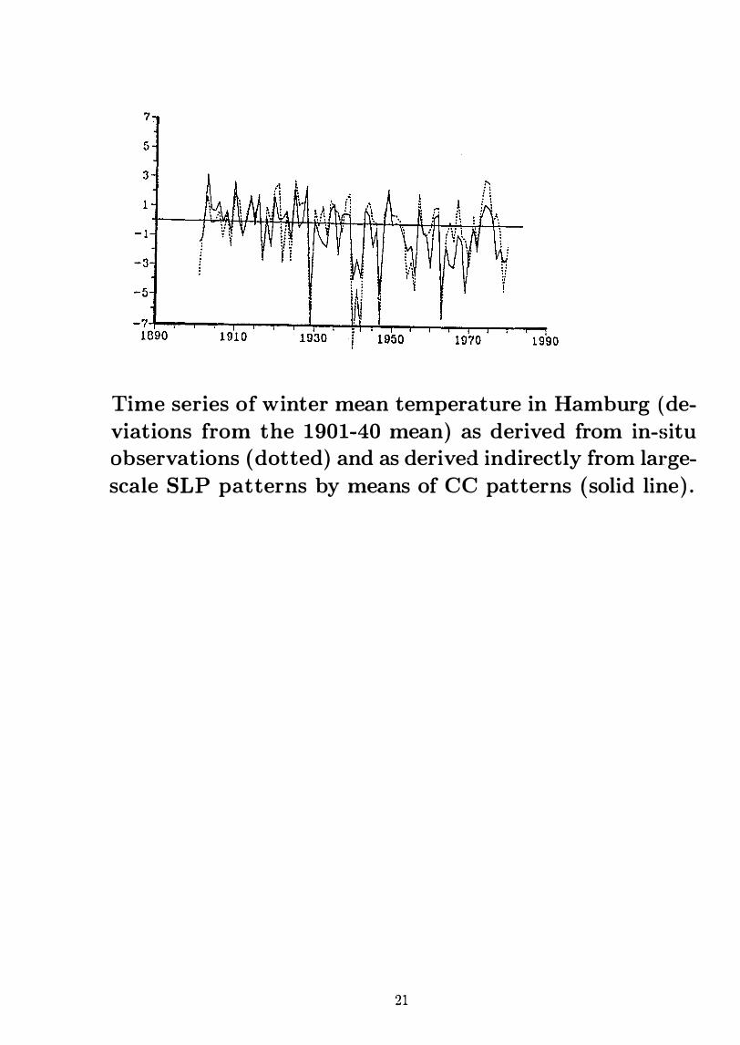
Time series of winter mean temperature in Hamburg (de­viations from the 1901-40 mean) as derived from in-situ observations ( dotted) and as derived indirectly from large­scale SLP patterns by means of CC patterns (solid line) .

21

Application:

Verification of GCM

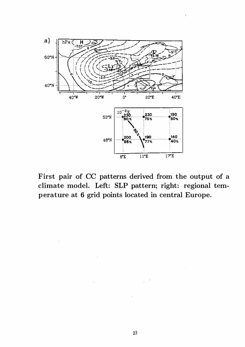
• The output of a climate GCM has been analysed whether it repro­duces the connection represented by the CCA-pairs. The regional temperature from a GCM output is given at grid points. Therefore the 11 Central European stations are replaced by 6 grid points.

• The first pair of CC patterns, derived from 100 years of simulated data, is similar to the pair of patterns derived from observed data� with an anomalous southwesterly fiow being associated with an overall warming of the order of one to two degrees .

• The details, however, do not fit . First, the correlation is only 0 . 53 compared to 0.64 in the real world. Second, the structure within Central Europe is not reproduced: Maximum temperature anoma­lies are at the westernmost grid points and minimum values at the easternmost. The local explained variances 1] are much higher for the GCM output ( with a maximum of 96% and a minimum of 50o/c compared to 58% and 22% in the real world) .

22

53°N

l 1°E

First pair of CC patterns derived from the output of a

climate model. Left: SLP pattern; right: regional tem­perature at 6 grid points located in central Europe.

23

A Downcaling Example :

Flowering of Snowdrops

• Maak, K. and H . von Storch, 1997: Statistical downscaling of monthly mean air temperature to the beginning of the fl.ovvering of Galanthus nivalis L. in Northern Germany. - Intern . J . Biometeor . (in press)

-+

• X is the date of first fiowering of snowdrops at many locations in Schleswig Holstein.

• Y is the European temperature in January, February and March .

• A robust and plausible CCA pair is found.

• A. regression model is built , specifying the fiowering date as a linear

function of the temperature pattern.

• A rearession model was used to reconstruct past flowering dates , b

and to interpret climate change scenario�

24

Conclusion

• Pattern-related techniques are powerful for reducing the degrees of freedom in high-dimensional problems. Various different types of patterns are available .

• EOFs or Principal Component Analysis is a powerful technique to decompose the variance of vector time series , so that a minimum of patterns represents a ma,'<imum of variance .

• C CA is a ··powerful technique for the identification of linear links between two vector time series. A related technique is "redundancy analysis" .

• CCA may be used for the design of regression models , which may

be used for, for instance, downscaling purposes or for the recon-

struction of unobserved states.

25

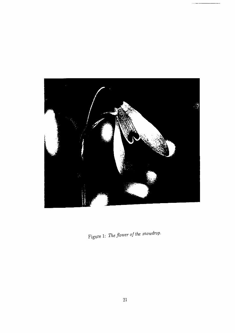
Figure 1: The fiower of the snowdrop.

21

z 0 LO LO

. ..- . C"l I{) N C"l

0 • I{) •

z 0 ..q-LO

0) CD •

;

z 0 ('t') l()

w 0 .....­.....-

w 0 0 .....-

w 0 cn

w 0 CO

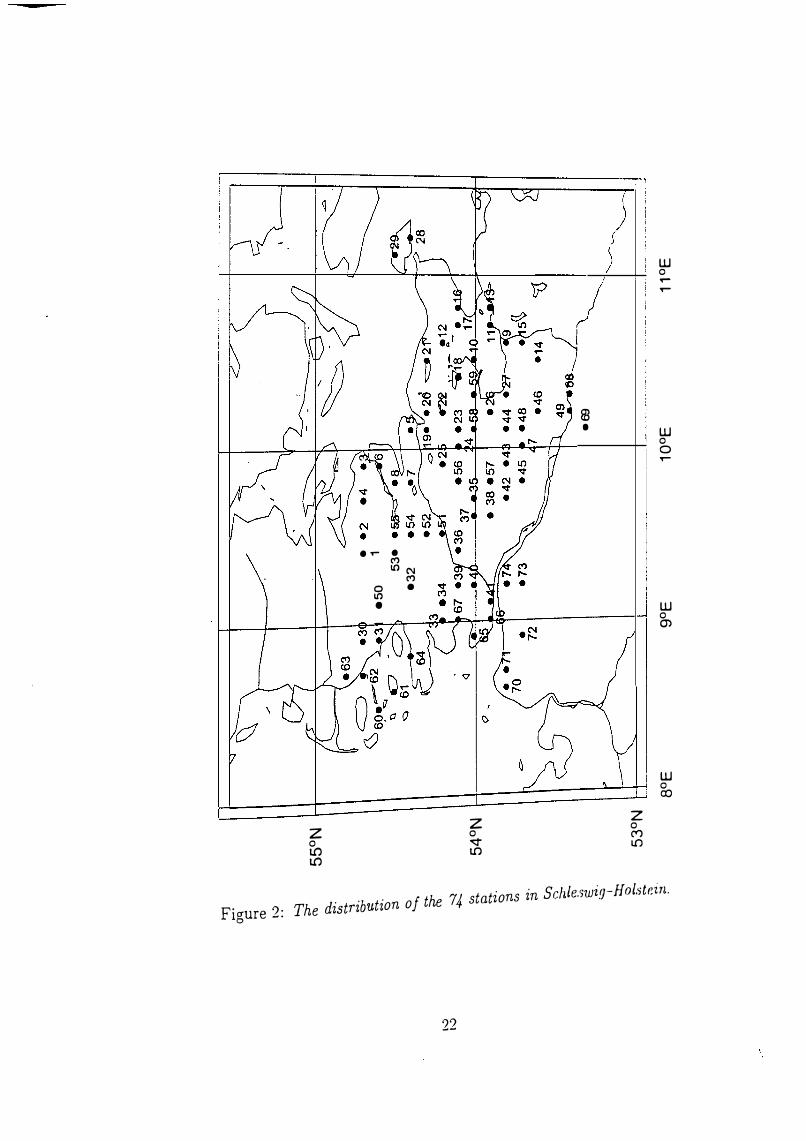
Figure 2 : The distribution of the 74 stations in Schle.5wig-H ol:;tcin.

22

--- 0 -----J

rr-�-t-..:0.....-.1---�'-f---+---+-����-'-__u � � �

"? • n-�-?---V:+--:����..;;+--�'-a!.!'.--f-+��----LI � 0

�

w 0 CO z z z 0 0 0 L() '1" (") L() L() L()

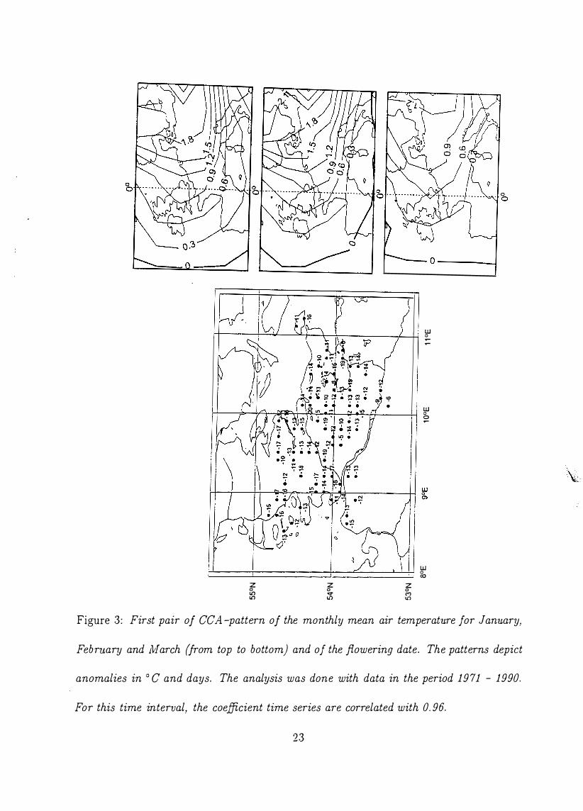
Figure 3 : First pair of CCA -pattern of the monthly mean air temperature for January,

February and Jvfarch (from top to bottom) and of the fiowering date . The patterns depict

anomalies in ° C and days. The analysis was done with data in the period 1971 - 1990.

For this time interval, the coefficient time series are correlated with 0. 96.

23

0 0)

„ ...... „ • 0) . �

0 CX) 0) � 0 !"-0) � 0 c.o

t � 0) � 0 -.:::t" 0) � 0 ('!') 0) � 0 C\J

ti t�

0 0) CX) � 0 CX) CX) � 0 !"-CX)

0 0 0 0 0 0 0 0 o � -.:::t" ('!') C\J � � C\J ('!') -.:::t"

1 1 1 1

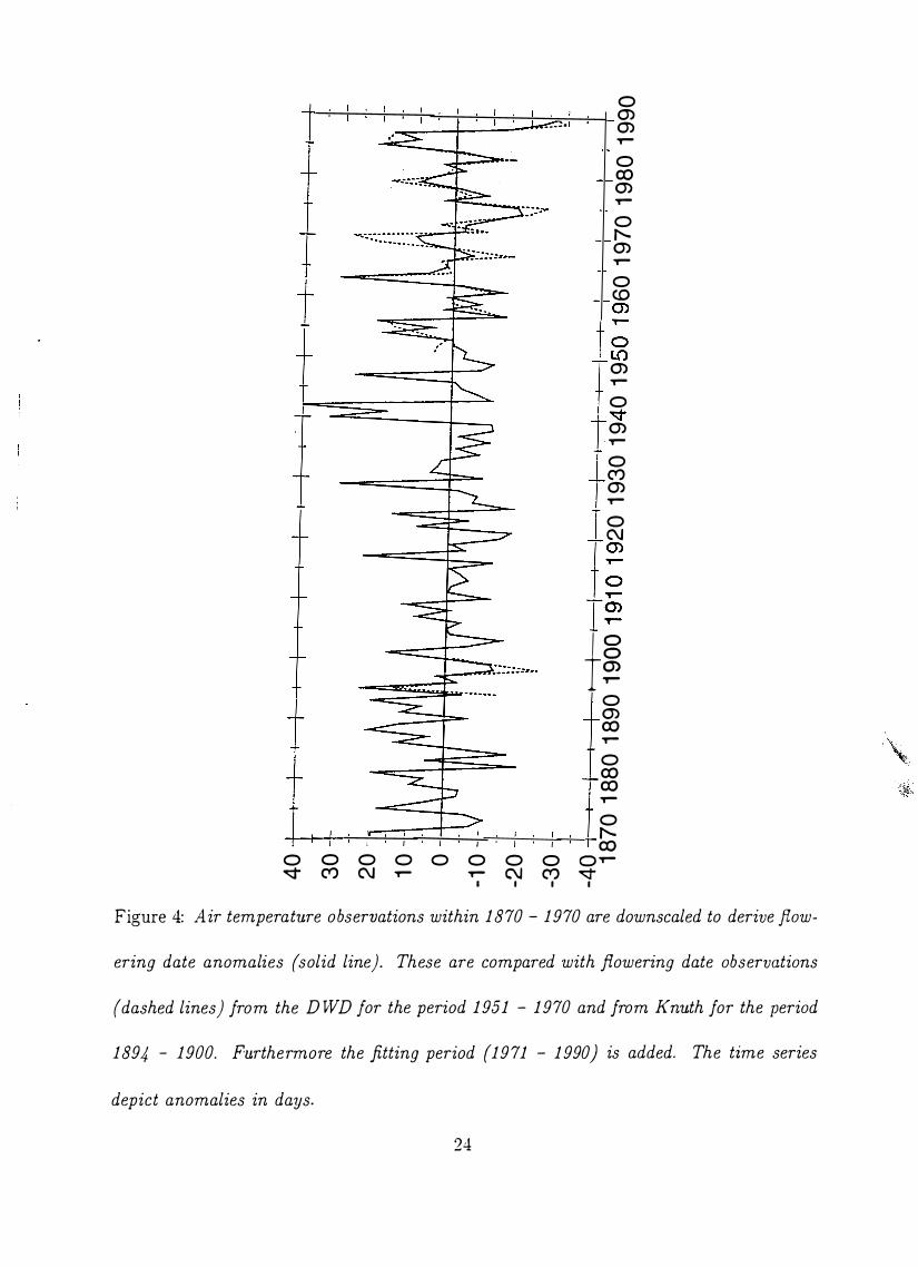
Figure 4: Air temperature observations within 1 810 - 1 910 are downscaled to derive fiow-

ering date anomalies (solid line). These are compared with fiowering date observations

(dashed lines) from the D }VD Jor the period 1 951 - 1 910 and from Knuth for the period

1894 - 1900. Furthermore the fitting period (1911 - 1 990) is added. The time series

depict anomalies in days.

24

VI >. CO � >. -ro E 0 c: CO

-20

-30 · Fahrenkrug correlation: 0.86

-40 1 1 1 1

1 950

40

30

20

1 0

0

-1 0

-20

1 1 1 1 1 1 ! 1 1 1 r

1 960 1 970 time (years)

-30 Niedermarschaft correlation: 0.5

1 1 1 1 1 1 1 1 •-40 1 1

1 950 1 960 1 970 time (years)

' 1 1 1 f

1 980 1 990

� : : . ' •

1 'i

1 980 1 990

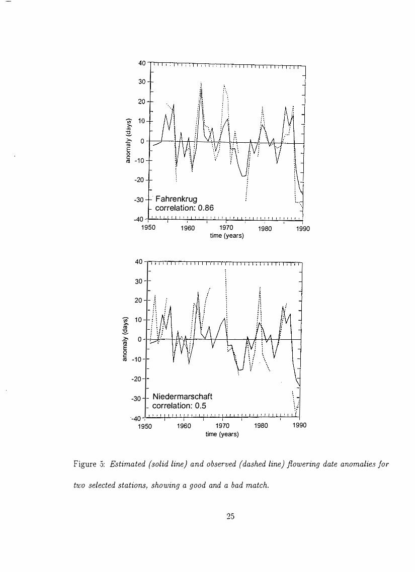
Figure 5: Estimated (solid line) and observed ( dashed line) fiowering date anomalie.5 for

two selected stations, showing a good and a bad match.

25

0 CD (j) �

0

t: t: _ Cf)

�-- 1 � 0 C\J (j) �

0

1 1 • 1 · 1 • , 1 1 • eo o o o o o o o o o o o � CD I.{) � Cf) C\J � � C\J Cf) �

1 1 1 1

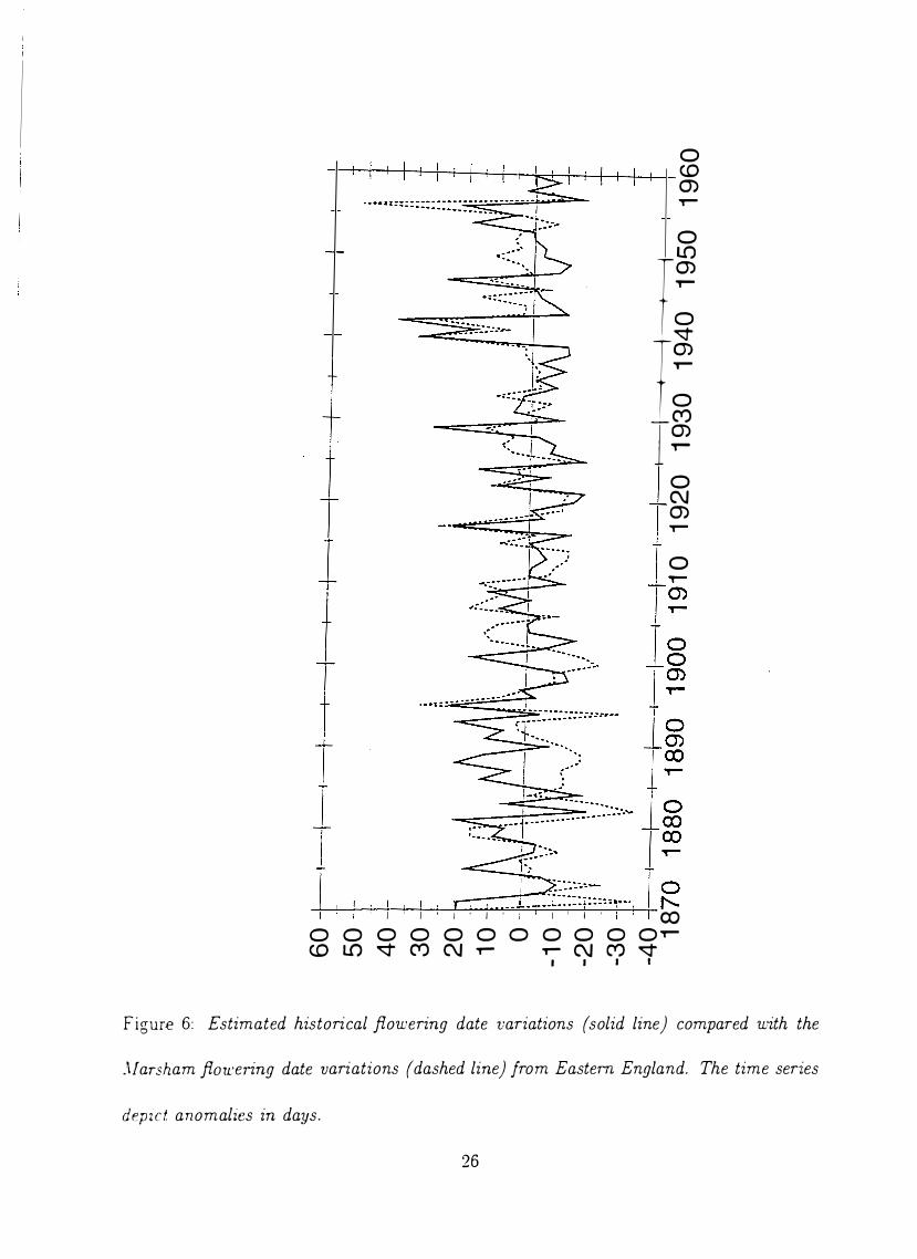
f igure 6: Estimated historical fiowering date variations (solid line) compared with the

;\/arsham fimrering date variations ( dashed line) Jrom Eastern England. The time series

dep z c t anomalies in days.

26

1

0 . 5

0 1

0

,- -

- J 1 1 1

1 1

1 1

1 _ , 1

1

!

1 1 1

1

1 1 1

1 1 1

' 1

1

-1

' 1 1

1 1 1

, �

1 J

1 1

1 - - 1

1 - '

20 40 60 t i m e (days)

80

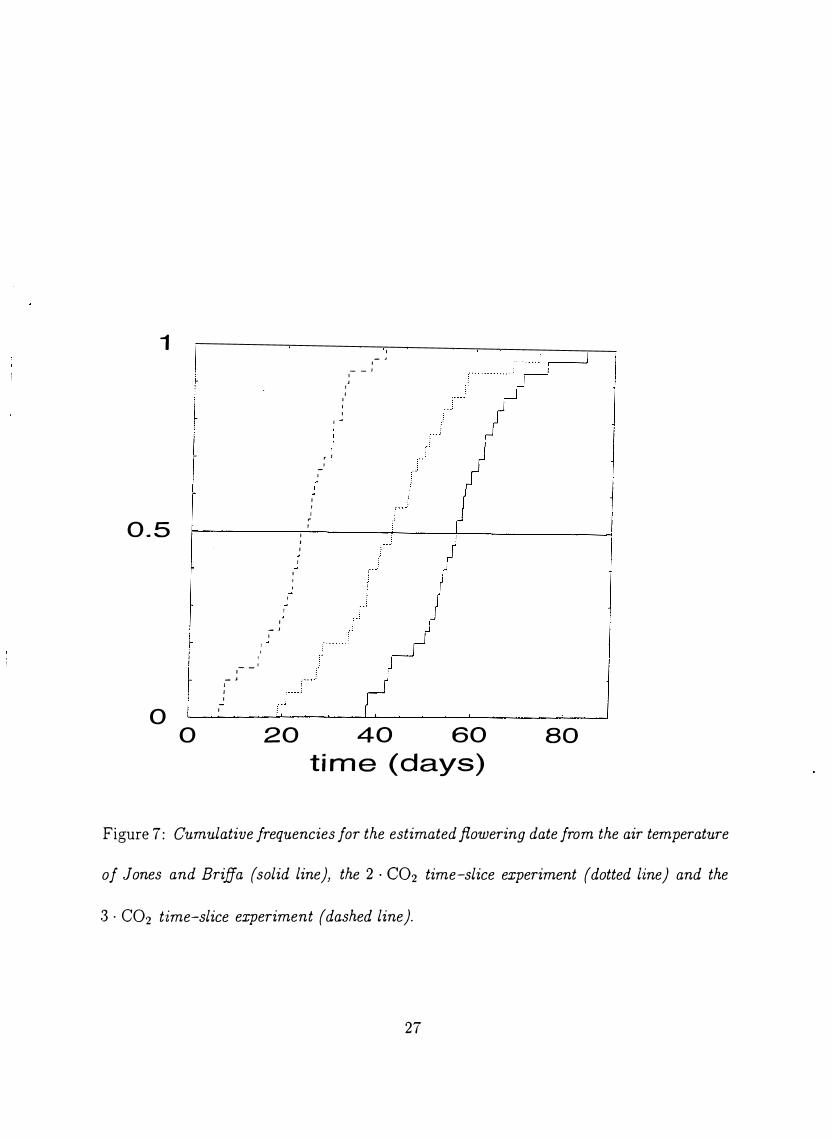
Figure 7 : Cumulative frequencies for the estimated fiowering date from the air temperature

of Jones and Briffa (solid line), the 2 · C02 time-slice experiment (dotted line) and the

3 · C02 time-slice experiment ( dashed line).

27