Freie Universität Berlin

Faculty of Mathematics and Computer Science

Department of Arti�cial Intelligence

Bachelor Thesis Computer Science

Learning Footstep Prediction ForHumanoid Robots

Mihai S, uteu

Supevisor:

Prof. Dr. Raúl Rojas

Advisor:Dr. Hamid Reza Moballegh

January 4, 2012

Eidesstattliche Erklärung

Ich erkläre an Eides statt, dass ich die vorliegende Bachelorarbeit selbständigund ohne fremde Hilfe verfasst habe. Ich habe dazu keine weiteren als dieangegebenen Hilfsmittel benutzt und die aus anderen Quellen entnommenenStellen als solche gekennzeichnet.

Berlin, den 4. Januar 2012

1

Abstract

This Bachelor Thesis presents an attempt to learn a prediction model of footsteplocations for a humanoid robot. Reliable footstep planning plays a key role inthe RoboCup Humanoid Soccer League. Being able to predict the e�ect ofdi�erent commands on the robot's pose receives therefore great importance.

In order to obtain reliable footstep prediction with minimal resources, an ap-proach through machine learning was chosen. This thesis presents the resultsof applying regression models to approximate the new footstep locations in arelative Cartesian coordinate system. For this purpose a library of machinelearning algorithms has been developed.

The data to be approximated has been extracted through forward kinematicsand learned by various regression models. Basic methods used in the learningprocess like dimension reduction and ways of preventing over�tting, are alsodescribed.

Contents

1 Introduction and Motivation 3

1.1 RoboCup . . . . . . . . . . . . . . . . . . . . . . . . . . . . . . . 3

1.2 FUmanoids . . . . . . . . . . . . . . . . . . . . . . . . . . . . . . 4

1.3 Aim and Structure of Thesis . . . . . . . . . . . . . . . . . . . . . 5

2 Theory and Related Work 7

2.1 Motion Model . . . . . . . . . . . . . . . . . . . . . . . . . . . . . 7

2.1.1 Robotics and Kinematics . . . . . . . . . . . . . . . . . . 8

2.1.2 Forward Kinematics . . . . . . . . . . . . . . . . . . . . . 10

2.2 Machine Learning . . . . . . . . . . . . . . . . . . . . . . . . . . . 12

2.3 Regression Models . . . . . . . . . . . . . . . . . . . . . . . . . . 13

2.3.1 Linear Regression . . . . . . . . . . . . . . . . . . . . . . . 13

2.3.2 Least Squares . . . . . . . . . . . . . . . . . . . . . . . . . 14

2.3.3 Polynomial Regression . . . . . . . . . . . . . . . . . . . . 15

2.3.4 Regression with History . . . . . . . . . . . . . . . . . . . 16

2.4 Dimension Reduction . . . . . . . . . . . . . . . . . . . . . . . . . 16

2.4.1 Feature Selection . . . . . . . . . . . . . . . . . . . . . . . 17

2.4.2 Feature Extraction . . . . . . . . . . . . . . . . . . . . . . 18

2.5 Over�tting . . . . . . . . . . . . . . . . . . . . . . . . . . . . . . 19

2.5.1 K-Fold Cross-Validation . . . . . . . . . . . . . . . . . . . 19

2.5.2 Ridge Regression . . . . . . . . . . . . . . . . . . . . . . . 20

3 The FUmanoid 2009 Platform 21

3.1 Hardware . . . . . . . . . . . . . . . . . . . . . . . . . . . . . . . 21

3.2 Sensors . . . . . . . . . . . . . . . . . . . . . . . . . . . . . . . . 21

1

4 Acquiring Ground Truth Data 23

4.1 Kinematic Model . . . . . . . . . . . . . . . . . . . . . . . . . . . 24

4.2 Implementation . . . . . . . . . . . . . . . . . . . . . . . . . . . . 26

5 Learning Ground Truth Data 28

5.1 K-Fold Cross-Validation . . . . . . . . . . . . . . . . . . . . . . . 29

5.2 Regression Models . . . . . . . . . . . . . . . . . . . . . . . . . . 30

5.2.1 Linear and Polynomial Regression . . . . . . . . . . . . . 30

5.2.2 Regression with History . . . . . . . . . . . . . . . . . . . 32

5.2.3 Ridge Regression . . . . . . . . . . . . . . . . . . . . . . . 33

5.3 Dimension Reduction . . . . . . . . . . . . . . . . . . . . . . . . . 34

5.3.1 Forward- and Backward-Stepwise Selection . . . . . . . . 34

5.3.2 Principal Component Regression . . . . . . . . . . . . . . 36

5.4 Time Complexity . . . . . . . . . . . . . . . . . . . . . . . . . . . 38

5.5 Additional Features . . . . . . . . . . . . . . . . . . . . . . . . . . 38

6 Results and Discussion 40

7 Conclusion and Future Work 43

Bibliography 45

2

Chapter 1

Introduction and Motivation

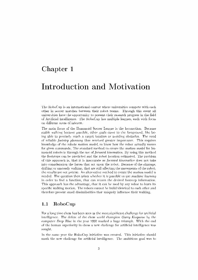
The RoboCup is an international contest where universities compete with eachother in soccer matches between their robot teams. Through this event alluniversities have the opportunity to present their research progress in the �eldof Arti�cial Intelligence. The RoboCup has multiple leagues, each with focuson di�erent areas of interest.

The main focus of the Humanoid Soccer League is the locomotion. Becausestable walking became possible, other goals came to the foreground, like be-ing able to precisely reach a target location or avoiding obstacles. The needof reliable footstep planning thus received greater importance. This requiresknowledge of the robots motion model, to know how the robot actually movesfor given commands. The standard method to create the motion model for hu-manoid robots is through the use of forward kinematics. By using this methodthe footsteps can be predicted and the robot location estimated. The problemof this approach is, that it is inaccurate as forward kinematics does not takeinto consideration the forces that act upon the robot. Because of the slippage,drifting or unsteady walking, that are still a�ecting the movements of the robot,the results are not precise. An alternative method to create the motion model isneeded. The question then arises whether it is possible to use machine learningin order to �nd a function, that can return the desired footstep information.This approach has the advantage, that it can be used by any robot to learn itsspeci�c walking motion. The robots cannot be build identical to each other andtherefore present small dissimilarities that uniquely in�uence their walking.

1.1 RoboCup

For a long time chess has been seen as the most signi�cant challenge for arti�cialintelligence. The defeat of the chess world champion Garry Kasparov by thecomputer Deep Blue in the year 1997 marked a huge triumph. With the endof the human superiority in chess a new challenge for arti�cial intelligence wassought.

In the same year the RoboCup initiative was created. This initiative shouldmark the new challenge for arti�cial intelligence. The ambitious goal was to

3

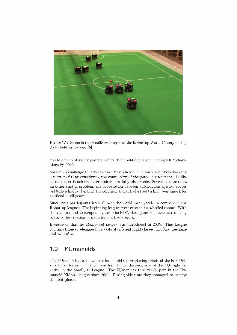
Figure 1.1: Game in the SmallSize League of the RoboCup World Championship2004, held in Lisbon. [5]

create a team of soccer playing robots that could defeat the leading FIFA cham-pions by 2050.

Soccer is a challenge that was not arbitrary chosen. The success in chess was onlya matter of time considering the complexity of the game environment. Unlikechess, soccer is neither deterministic nor fully observable. Soccer also presentsan other kind of problem: the cooperation between autonomous agents. Soccerpresents a highly dynamic environment and therefore sets a high benchmark forarti�cial intelligence.

Since 1997 participants from all over the world meet yearly to compete in theRoboCup leagues. The beginning leagues were created for wheeled robots. Withthe goal in mind to compete against the FIFA champions the focus was movingtowards the creation of more human like leagues.

Because of this the Humanoid League was introduced in 2005. This Leaguecontains three sub-leagues for robots of di�erent hight classes: KidSize, TeenSizeand AdultSize.

1.2 FUmanoids

The FUmanoids are the team of humanoid soccer playing robots of the Free Uni-versity of Berlin. The team was founded as the successor of the FU-Fighters,active in the SmallSize League. The FUmanoids take yearly part in the Hu-manoid KidSize league since 2007. During this time they managed to occupythe �rst places.

4

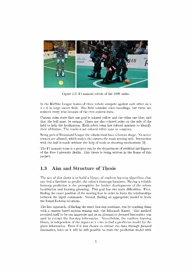
Figure 1.2: FUmanoid robots of the 2009 series.

In the KidSize League teams of three robots compete against each other on a4 × 6 m large soccer �eld. The �eld contains color-encodings, but these arereduced every year because of the ever stricter rules.

Current rules state that one goal is colored yellow and the other one blue, andthat the ball must be orange. There are also colored poles on the side of the�eld to help the localization. Each robot team has colored markers to identifytheir a�liation. The markers are colored either cyan or magenta.

Being part of Humanoid League the robots must have a human shape. No activesensors are allowed, which makes the camera the main sensing unit. Interactionwith the ball is made without the help of tools or shooting mechanisms [2].

The FUmanoid team is a project run by the department of arti�cial intelligenceof the Free University Berlin. This thesis is being written in the frame of thisproject.

1.3 Aim and Structure of Thesis

The aim of this thesis is to build a library of machine learning algorithms thatcan �nd a function to predict the robot's footsteps locations. Having a reliablefootstep prediction is the prerequisite for further developments of the robotslocalization and footstep planning. This goal has two main di�culties. First,�nding the exact position of the moving foot in order to learn the relationshipsbetween the input commands. Second, �nding an appropriate model to learnthe found footstep locations.

The �rst approach, of �nding the exact footstep positions, was by tracking themwith a camera based motion sensing unit, the Microsoft Kinect. This methodrevealed itself to be too imprecise and as an alternative forward kinematics wasused to extract the footstep information. Nevertheless, the machine learninglibrary is independent of the inputs as it tries to �nd a prediction model for thegiven information. Even if it was chosen to extract the data through forwardkinematics, later on it will be still possible to train the prediction model with

5

more accurate data, perhaps collected in a di�erent way. The machine learningalgorithms �nd the best prediction model for the given data, regardless of theirprovenance.

Chapter 2 will cover the basic theoretical aspect of the methods used in thethesis. The general problem of calculating the odometry for humanoid robotswill be presented as well as the way through forward kinematics. Further on,basic techniques of supervised learning will be explained as well as ways to avoidover�tting and approaches to reduce high dimensionality.

Chapter 3 will present the hardware for which the motion model was created. Itwill be a short description of the 2009 model of soccer playing humanoid robotsof the Free University of Berlin's team, the FUmanoids.

In Chapter 4 the way of �nding accurate footstep information for the presentedrobot is described. The kinematic model of the robot will also be shown.

Chapter 5 presents the process of learning the function that can approximatethe collected footstep data. The methods explained in Chapter 2 will be appliedand their results shown.

Chapter 6 shows the overall results of the methods and a detailed comparisonof these.

In the �nal chapter the conclusion of the thesis is discussed.

6

Chapter 2

Theory and Related Work

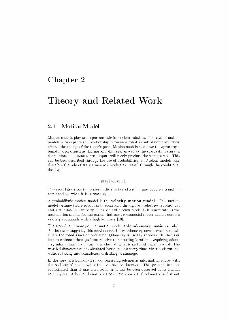
2.1 Motion Model

Motion models play an important role in modern robotics. The goal of motionmodels is to capture the relationship between a robot's control input and theire�ects, the change of the robot's pose. Motion models also have to capture sys-tematic errors, such as drifting and slippage, as well as the stochastic nature ofthe motion. The same control inputs will rarely produce the same results. Thiscan be best described through the use of probabilities [3]. Motion models playtherefore the role of state transition models expressed through the conditionaldensity

p(xt | ut, xt−1).

This model describes the posterior distribution of a robot pose xt, given a motioncommand ut, when it is in state xt−1.

A probabilistic motion model is the velocity motion model. This motionmodel assumes that a robot can be controlled through two velocities, a rotationaland a translational velocity. This kind of motion model is less accurate as thenext motion model, for the reason that most commercial robots cannot executevelocity commands with a high accuracy [19].

The second, and more popular motion model is the odometry motion model.As the name suggests, this motion model uses odometry measurements to cal-culate the robot's motion over time. Odometry is used by robots with wheels orlegs to estimate their position relative to a starting location. Acquiring odom-etry information in the case of a wheeled agent is rather straight forward. Thetraveled distance can be calculated based on how many times the wheels turned,without taking into consideration drifting or slippage.

In the case of a humanoid robot, retrieving odometric information comes withthe problem of not knowing the step size or direction. This problem is morecomplicated than it may �rst seem, as it can be even observed at its humancounterpart. A human being relies completely on visual odometry and is not

7

capable of orientation when blindfolded. This fact puzzled scientists for quitesome time and experiments revealed that even walking in a straight line seemsnearly impossible, as people tend to walk in circles [17].

In order to create a motion model not only the input commands are required, butalso their e�ects. In this case the result of a command is the actual displacementof the robot's foot. To retrieve correct footstep information two approacheswere found. One solution is to visually observe the robot walking and extractthe correct foot positions. This method was approached by an other Germanhumanoid robot soccer team from the University of Bonn, NimbRo in whichthey tracked the legs of the robot using motion capture [13]. The methodproved to be successful, but requires dedicated equipment. The alternativeapproach is to compute the required information through the robots odometryinformation. This is done using forward kinematics, which make it possible todescribe the motion of a series of rigid joints. With this method the position ofthe swinging leg can be computed by a chain of transformations and expressedin the coordinate system of the standing foot. This method will be presentedfurther on.

2.1.1 Robotics and Kinematics

A robot is an intelligent agent who perceives its surrounding environment throughsensors and is capable of a�ecting it with his actuators. In order to a�ect theenvironment the robot has to be able to move its actuator, be it an arm or leg,into the right position to ful�ll its goal. This is a trivial process for humans butrather complicated for a robot.

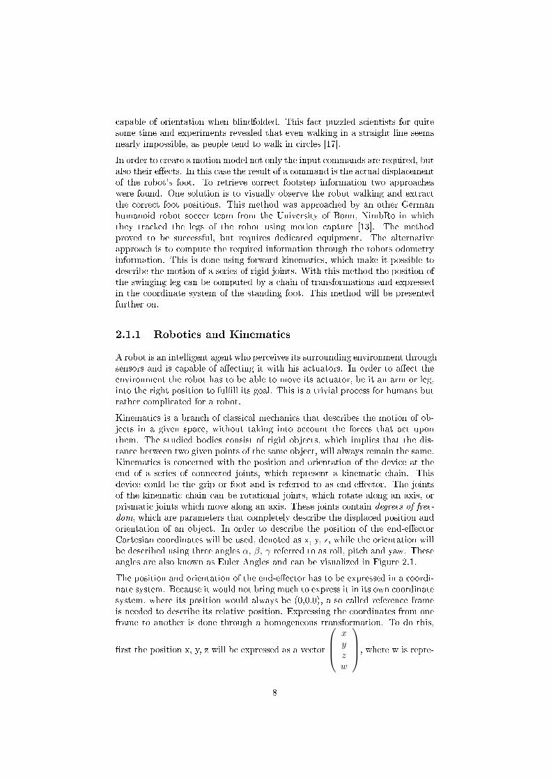
Kinematics is a branch of classical mechanics that describes the motion of ob-jects in a given space, without taking into account the forces that act uponthem. The studied bodies consist of rigid objects, which implies that the dis-tance between two given points of the same object, will always remain the same.Kinematics is concerned with the position and orientation of the device at theend of a series of connected joints, which represent a kinematic chain. Thisdevice could be the grip or foot and is referred to as end-e�ector. The jointsof the kinematic chain can be rotational joints, which rotate along an axis, orprismatic joints which move along an axis. These joints contain degrees of free-dom, which are parameters that completely describe the displaced position andorientation of an object. In order to describe the position of the end-e�ectorCartesian coordinates will be used, denoted as x, y, z, while the orientation willbe described using three angles α, β, γ referred to as roll, pitch and yaw. Theseangles are also known as Euler Angles and can be visualized in Figure 2.1.

The position and orientation of the end-e�ector has to be expressed in a coordi-nate system. Because it would not bring much to express it in its own coordinatesystem, where its position would always be (0,0,0), a so called reference frameis needed to describe its relative position. Expressing the coordinates from oneframe to another is done through a homogeneous transformation. To do this,

�rst the position x, y, z will be expressed as a vector

xyzw

, where w is repre-

8

Yaw AxisRoll Axis

Pitch Axis

Figure 2.1: Roll-Pitch-Yaw Plane. [22]

senting a weighting factor, set usually to 1. By expressing the point this way, itcan be multiplied with the frame coordinates, to obtain its relative coordinates.This conversion can be done by four matrix multiplications which represent thepossible changes of the pose [11].

A rotation along the x-axis of an angle α is calculated through the matrix

Rx(α) =

1 0 0 00 cosα − sinα 00 sinα cosα 00 0 0 1

Similar, a rotation along the y-axis of an angle β is done through the matrix

Ry(β) =

cosβ 0 sinβ 00 1 0 0

− sinβ 0 cosβ 00 0 0 1

and a rotation along the z-axis of an angle γ by the matrix

Rz(γ) =

cos γ − sin γ 0 0sin γ cos γ 0 00 0 1 00 0 0 1

By multiplying the rotation matrices together a rotation along all axes of anglesα, β and γ is obtained.

Rxyz(α, β, γ) = Rx(α)×Ry(β)×Rz(γ)

A translation, a simple movement along the axes of distance dx, dy and dz, isexpressed through the following Matrix:

9

Translation(dx, dy, dz) =

1 0 0 dx0 1 0 dy0 0 1 dz0 0 0 1

Through these matrix multiplications the position and orientation of the end-e�ector can be transformed into an other coordinate frame.

2.1.2 Forward Kinematics

Forward kinematics is concerned with the relationship of individual joints of theactuator, as well as with the position and orientation of its end-e�ector. Statedmore formally, the forward kinematics problem is to determine the position andorientation of the end-e�ector, given the joint angles of the robot. In contrastto forward kinematics, inverse kinematics is concerned with �nding the jointangles that achieve the desired position of the robot's end-e�ector [18]. Onlyforward kinematics will be discussed, as the goal is to �nd the position of therobot foot and not how to move in order to get there.

In the previous section it was explained how to create a matrix that will com-pute the coordinates of a point in one coordinate system, given the position ofthat point in another coordinate system. This was possible under the conditionthat the two frames must only di�er by a translation or a rotation. In order tocompute more di�cult conversions like translation, rotation, translation, thesehave to be split up into the basic transformations after which all transforma-tion matrices can be multiplied together. The resulting matrix represents theconversion between two coordinate frames.

The objective of forward kinematics is to determine the cumulative e�ect of alljoint variables of a manipulator and therefore to �nd a transformation matrixthat is a function of the joint angles of the robot. This is done by a seriesof transformations through all the coordinate frames of the actuator. Thus, amanipulator with n joints will have n + 1 links, since each joint connects twolinks. The location of joint i is �xed with respect to link i− 1 and when joint iis actuated, link i will move. The �rst link is therefore �xed and does not movewhen other joints are actuated. To obtain the transformation matrix for the�rst link, it is needed to iterate through all coordinate frames and successivelymultiply the transformation matrices of joint i− 1 and i. Formally:

0Tn =

n∏i=1

i−1Ti(δi)

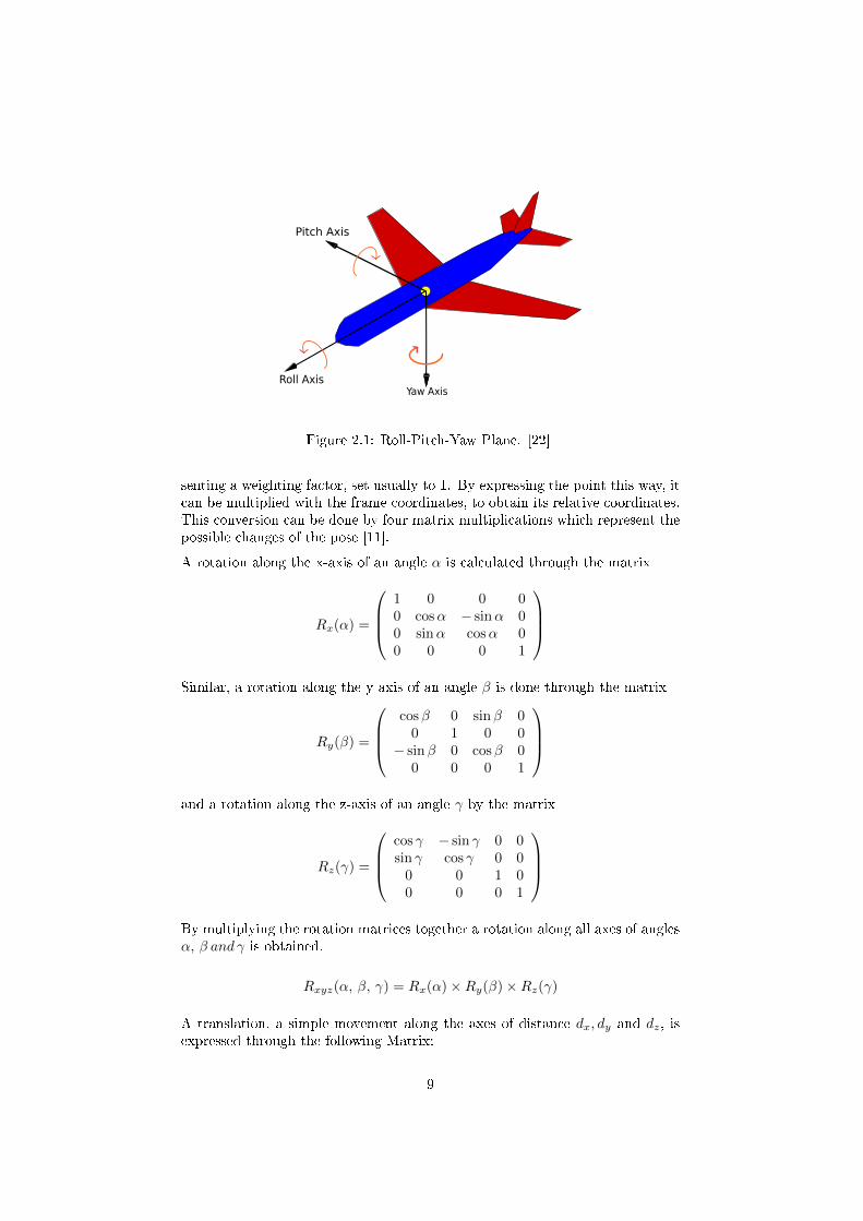
Where i−1Tnis the transformation of joint i's frame into the coordinate systemof joint i − 1. δi are the parameters of the transformation matrix which canbe either translations or rotations. Figure 2.2 shows the di�erent coordinatesystems which can be observed in a manipulator.

While it is possible to carry out all basic transformations to get from one co-ordinate to another, for more complex transformations these easily end up in a

10

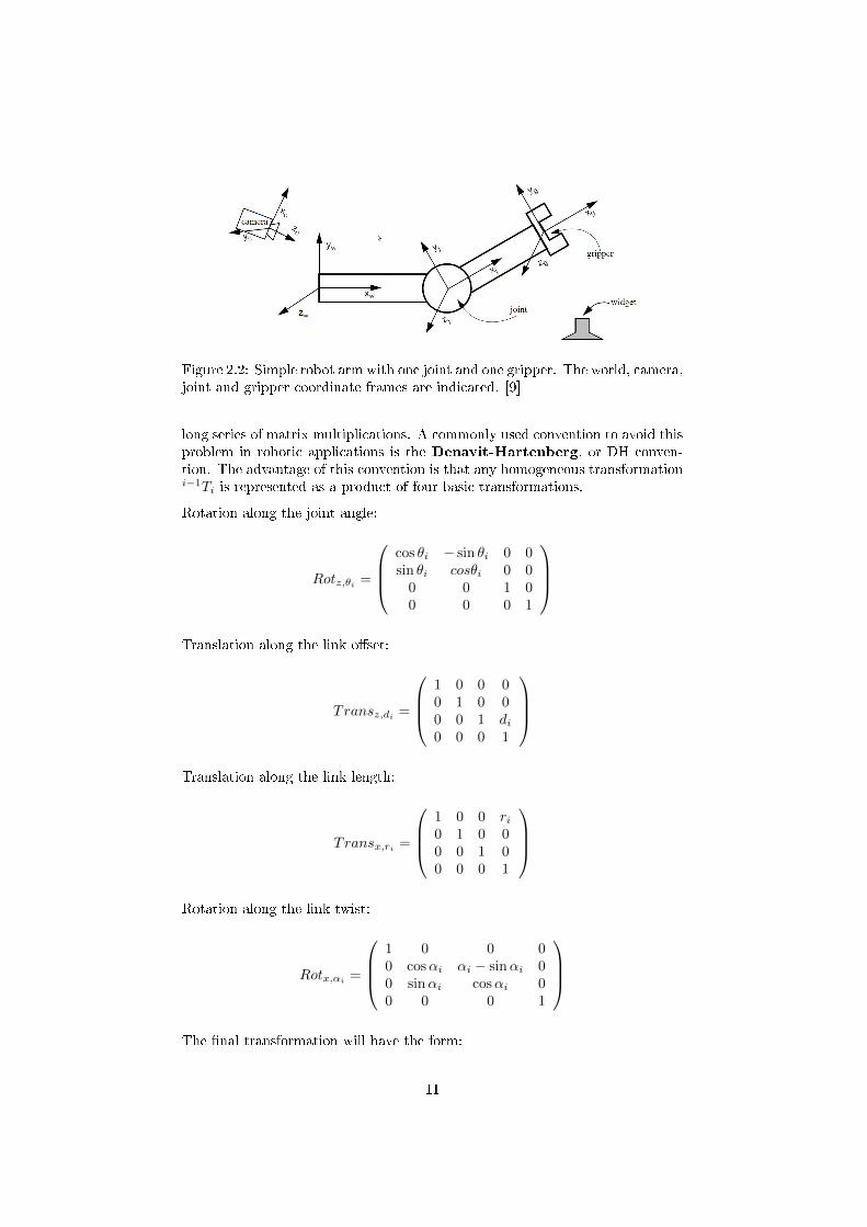
Figure 2.2: Simple robot arm with one joint and one gripper. The world, camera,joint and gripper coordinate frames are indicated. [9]

long series of matrix multiplications. A commonly used convention to avoid thisproblem in robotic applications is the Denavit-Hartenberg, or DH conven-tion. The advantage of this convention is that any homogeneous transformationi−1Ti is represented as a product of four basic transformations.

Rotation along the joint angle:

Rotz,θi =

cos θi − sin θi 0 0sin θi cosθi 0 00 0 1 00 0 0 1

Translation along the link o�set:

Transz,di =

1 0 0 00 1 0 00 0 1 di0 0 0 1

Translation along the link length:

Transx,ri =

1 0 0 ri0 1 0 00 0 1 00 0 0 1

Rotation along the link twist:

Rotx,αi=

1 0 0 00 cosαi αi − sinαi 00 sinαi cosαi 00 0 0 1

The �nal transformation will have the form:

11

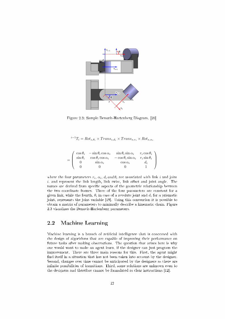
Figure 2.3: Sample Denavit-Hartenberg Diagram. [20]

i−1Ti = Rotz,θi × Transz,di × Transx,ri ×Rotx,αi

=

cos θi − sin θi cosαi sin θi sinαi ri cos θisin θi cos θi cosαi − cos θi sinαi ri sin θi0 sinαi cosαi di0 0 0 1

where the four parameters ri, αi, di and θi are associated with link i and jointi, and represent the link length, link twist, link o�set and joint angle. Thenames are derived from speci�c aspects of the geometric relationship betweenthe two coordinate frames. Three of the four parameters are constant for agiven link, while the fourth, θi in case of a revolute joint and di for a prismaticjoint, represents the joint variable [18]. Using this convention it is possible toobtain a matrix of parameters to minimally describe a kinematic chain. Figure2.3 visualizes the Denavit-Hartenberg parameters.

2.2 Machine Learning

Machine learning is a branch of arti�cial intelligence that is concerned withthe design of algorithms that are capable of improving their performance onfuture tasks after making observations. The question that arises here is whyone would want to make an agent learn, if the designer can just program theimprovement. There are three main reasons for this. First, the agent might�nd itself in a situation that has not been taken into account by the designer.Second, changes over time cannot be anticipated by the designers as there arein�nite possibilities of transitions. Third, some solutions are unknown even tothe designers and therefore cannot be formulated as clear instructions [12].

12

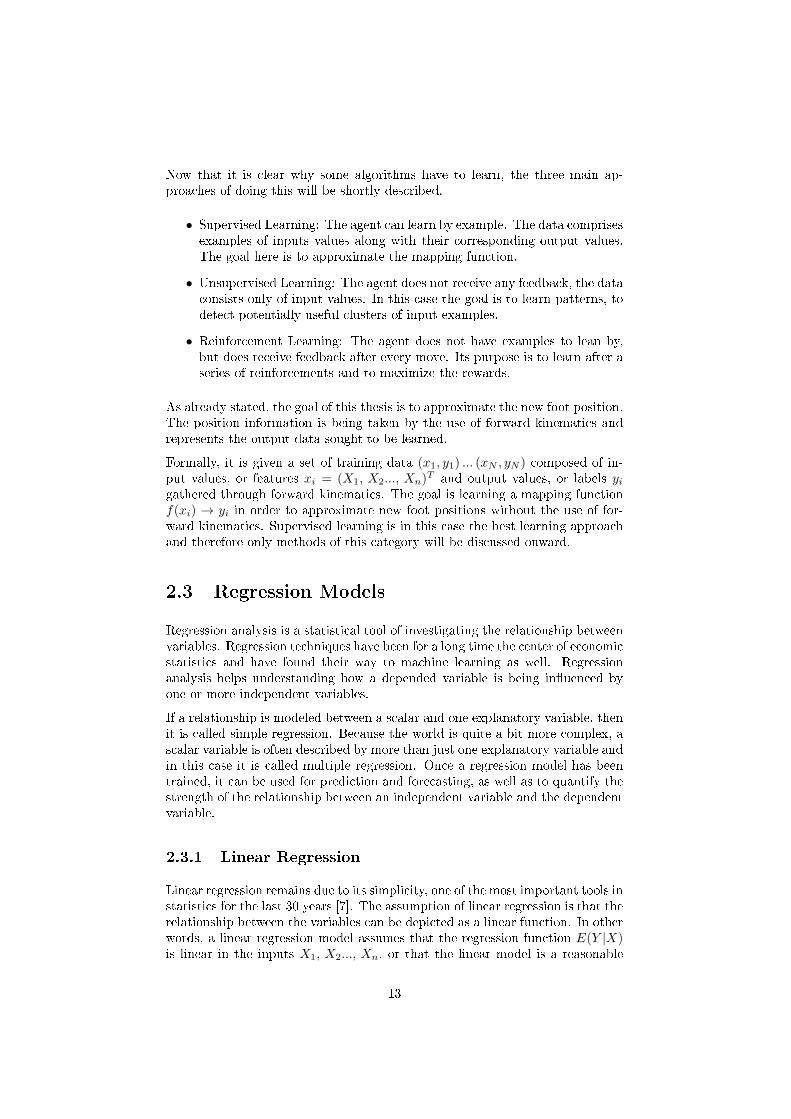
Now that it is clear why some algorithms have to learn, the three main ap-proaches of doing this will be shortly described.

• Supervised Learning: The agent can learn by example. The data comprisesexamples of inputs values along with their corresponding output values.The goal here is to approximate the mapping function.

• Unsupervised Learning: The agent does not receive any feedback, the dataconsists only of input values. In this case the goal is to learn patterns, todetect potentially useful clusters of input examples.

• Reinforcement Learning: The agent does not have examples to lean by,but does receive feedback after every move. Its purpose is to learn after aseries of reinforcements and to maximize the rewards.

As already stated, the goal of this thesis is to approximate the new foot position.The position information is being taken by the use of forward kinematics andrepresents the output data sought to be learned.

Formally, it is given a set of training data (x1, y1) ... (xN , yN ) composed of in-put values, or features xi = (X1, X2..., Xn)

T and output values, or labels yigathered through forward kinematics. The goal is learning a mapping functionf(xi) → yi in order to approximate new foot positions without the use of for-ward kinematics. Supervised learning is in this case the best learning approachand therefore only methods of this category will be discussed onward.

2.3 Regression Models

Regression analysis is a statistical tool of investigating the relationship betweenvariables. Regression techniques have been for a long time the center of economicstatistics and have found their way to machine learning as well. Regressionanalysis helps understanding how a depended variable is being in�uenced byone or more independent variables.

If a relationship is modeled between a scalar and one explanatory variable, thenit is called simple regression. Because the world is quite a bit more complex, ascalar variable is often described by more than just one explanatory variable andin this case it is called multiple regression. Once a regression model has beentrained, it can be used for prediction and forecasting, as well as to quantify thestrength of the relationship between an independent variable and the dependentvariable.

2.3.1 Linear Regression

Linear regression remains due to its simplicity, one of the most important tools instatistics for the last 30 years [7]. The assumption of linear regression is that therelationship between the variables can be depicted as a linear function. In otherwords, a linear regression model assumes that the regression function E(Y |X)is linear in the inputs X1, X2..., Xn, or that the linear model is a reasonable

13

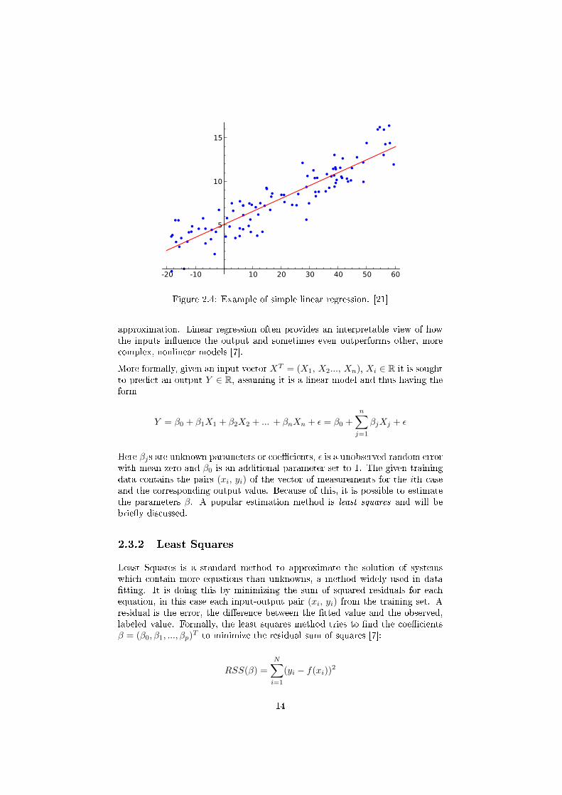
Figure 2.4: Example of simple linear regression. [21]

approximation. Linear regression often provides an interpretable view of howthe inputs in�uence the output and sometimes even outperforms other, morecomplex, nonlinear models [7].

More formally, given an input vector XT = (X1, X2..., Xn), Xi ∈ R it is soughtto predict an output Y ∈ R, assuming it is a linear model and thus having theform

Y = β0 + β1X1 + β2X2 + ... + βnXn + ε = β0 +

n∑j=1

βjXj + ε

Here βjs are unknown parameters or coe�cients, ε is a unobserved random errorwith mean zero and β0 is an additional parameter set to 1. The given trainingdata contains the pairs (xi, yi) of the vector of measurements for the ith caseand the corresponding output value. Because of this, it is possible to estimatethe parameters β. A popular estimation method is least squares and will bebrie�y discussed.

2.3.2 Least Squares

Least Squares is a standard method to approximate the solution of systemswhich contain more equations than unknowns, a method widely used in data�tting. It is doing this by minimizing the sum of squared residuals for eachequation, in this case each input-output pair (xi, yi) from the training set. Aresidual is the error, the di�erence between the �tted value and the observed,labeled value. Formally, the least squares method tries to �nd the coe�cientsβ = (β0, β1, ..., βp)

T to minimize the residual sum of squares [7]:

RSS(β) =

N∑i=1

(yi − f(xi))2

14

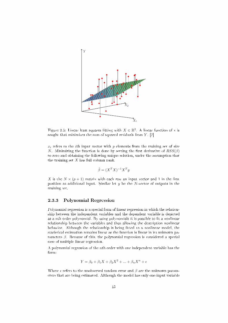
Figure 2.5: Linear least squares �tting with X ∈ R2. A linear function of x issought that minimizes the sum of squared residuals from Y . [7]

xi refers to the ith input vector with p elements from the training set of sizeN . Minimizing the function is done by setting the �rst derivative of RSS(β)to zero and obtaining the following unique solution, under the assumption thatthe training set X has full column rank.

β̂ = (XTX)−1XT y

X is the N × (p + 1) matrix with each row an input vector and 1 in the �rstposition as additional input. Similar let y be the N -vector of outputs in thetraining set.

2.3.3 Polynomial Regression

Polynomial regression is a special form of linear regression in which the relation-ship between the independent variables and the dependent variable is depictedas a nth order polynomial. By using polynomials it is possible to �t a nonlinearrelationship between the variables and thus allowing the description nonlinearbehavior. Although the relationship is being �tted to a nonlinear model, thestatistical estimation remains linear as the function is linear in its unknown pa-rameters β. Because of this, the polynomial regression is considered a specialcase of multiple linear regression.

A polynomial regression of the nth order with one independent variable has theform:

Y = β0 + β1X + β2X2 + ...+ βnX

n + ε

Where ε refers to the unobserved random error and β are the unknown param-eters that are being estimated. Although the model has only one input variable

15

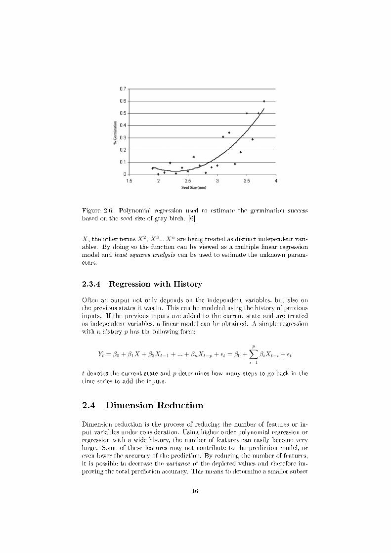
Figure 2.6: Polynomial regression used to estimate the germination successbased on the seed size of gray birch. [6]

X, the other terms X2, X3... Xn are being treated as distinct independent vari-ables. By doing so the function can be viewed as a multiple linear regressionmodel and least squares analysis can be used to estimate the unknown param-eters.

2.3.4 Regression with History

Often an output not only depends on the independent variables, but also onthe previous states it was in. This can be modeled using the history of previousinputs. If the previous inputs are added to the current state and are treatedas independent variables, a linear model can be obtained. A simple regressionwith a history p has the following form:

Yt = β0 + β1X + β2Xt−1 + ...+ βnXt−p + εt = β0 +

p∑i=1

βiXt−i + εt

t denotes the current state and p determines how many steps to go back in thetime series to add the inputs.

2.4 Dimension Reduction

Dimension reduction is the process of reducing the number of features or in-put variables under consideration. Using higher order polynomial regression orregression with a wide history, the number of features can easily become verylarge. Some of these features may not contribute to the prediction model, oreven lower the accuracy of the prediction. By reducing the number of features,it is possible to decrease the variance of the depicted values and therefore im-proving the total prediction accuracy. This means to determine a smaller subset

16

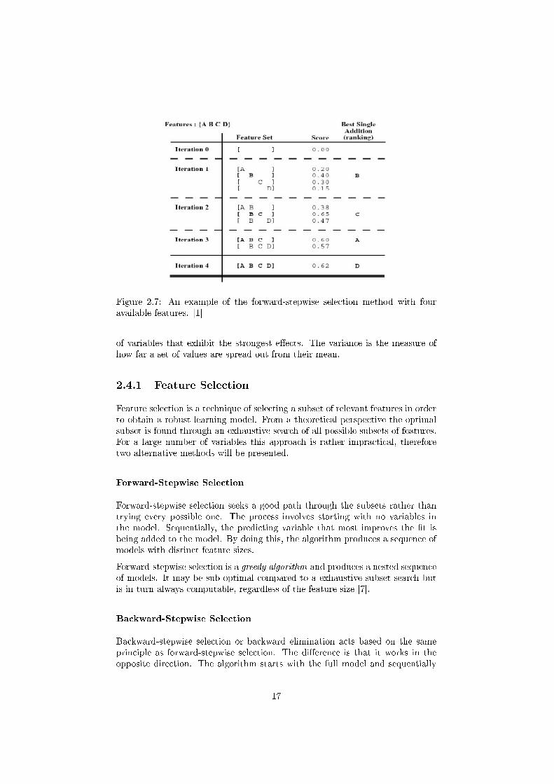
Figure 2.7: An example of the forward-stepwise selection method with fouravailable features. [1]

of variables that exhibit the strongest e�ects. The variance is the measure ofhow far a set of values are spread out from their mean.

2.4.1 Feature Selection

Feature selection is a technique of selecting a subset of relevant features in orderto obtain a robust learning model. From a theoretical perspective the optimalsubset is found through an exhaustive search of all possible subsets of features.For a large number of variables this approach is rather impractical, thereforetwo alternative methods will be presented.

Forward-Stepwise Selection

Forward-stepwise selection seeks a good path through the subsets rather thantrying every possible one. The process involves starting with no variables inthe model. Sequentially, the predicting variable that most improves the �t isbeing added to the model. By doing this, the algorithm produces a sequence ofmodels with distinct feature sizes.

Forward-stepwise selection is a greedy algorithm and produces a nested sequenceof models. It may be sub-optimal compared to a exhaustive subset search butis in turn always computable, regardless of the feature size [7].

Backward-Stepwise Selection

Backward-stepwise selection or backward elimination acts based on the sameprinciple as forward-stepwise selection. The di�erence is that it works in theopposite direction. The algorithm starts with the full model and sequentially

17

removes the predicting variable that has the least impact on the �t. This isalso a greedy algorithm and chooses at each step, as a dropping candidate, thevariable with which the model has the highest mean squared error.

Both algorithms use the mean squared error to measure the �t of the estimatedcoe�cient β̂, which was trained by the use of the regression models presentedin the previous section.

2.4.2 Feature Extraction

Rather than just selecting a subset of input variables, feature selection alsotransforms the input data into a reduced representation set of features. Thisimplies simplifying the amount of resources required to describe the data setaccurately.

Principal Components Analysis

Principal Components Analysis, further on referred to as PCA, is a way ofidentifying patterns in data and expressing the data in such a way to highlighttheir similarities and di�erences. The main advantage of PCA is that once thepatterns in the data have been found, the data can be compressed by reducingthe number of dimensions without much loss of information [16].

PCA works by transforming the original data into a new coordinate system,through orthogonal linear transformations. In the new representation the great-est variances of the data are projected on the �rst dimensions, called the prin-cipal components.

This is done by �rst subtracting the mean from each of the data dimensions toproduce a data set whose mean is zero. For this new data set the covariancematrix will be calculated to see how the dimensions behave towards each other,that is which two dimensions increase or decrease together. After �nding thecovariance matrix its eigenvectors and eigenvalues will be calculated. These pro-vide useful information about the pattern of the data. The eigenvectors withthe highest eigenvalues provide the best �t of the data. They show how thepoints are related along these lines. By taking the eigenvectors of the covari-ance matrix, it is possible to extract the lines that characterize the data. Asmentioned before, the eigenvector with the highest eigenvalues is the principalcomponent of the data set.

The next step is to order all eigenvectors by their eigenvalue, thus having thecomponents in order of signi�cance. At this point is is possible to take the �rstp eigenvectors and represent the data with these lines that characterize it themost. By choosing the best dimensions for the new data set, the dimensionalityhas been reduced without too much loss of information. The �nal step is torepresent the data set through the chosen components, by multiplying the rowfeature vector with the mean-adjusted data, transposed. The row feature vectoris simply a vector of the chosen eigenvectors as rows, with the most signi�canteigenvector at the top. Through this transformation the original data can beexpressed solely in terms of the chosen vectors [16]. A property of eigenvectors is

18

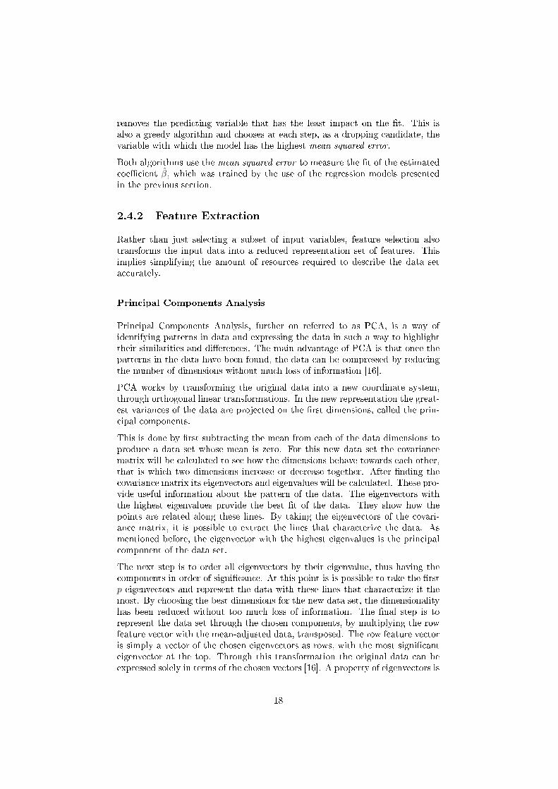
Figure 2.8: An example of PCA used to �nd the principal components for thetwo correlated variables X and Y. X1 accounts for a larger amount of variancein the data and is therefore the �rst principal component. [14]

that they are orthogonal to each other which means that the prediction vectorswill be orthogonal as well.

Principal Components Regression

A regression model that uses the principal components analysis is the prin-cipal components regression. Here the idea is to retrieve the most important pcomponents of the data set and regress the dependent variable on those, ratherthan on the independent variables.

2.5 Over�tting

Occam's Razor, or the principle of parsimony calls for models to use only thenecessary information for the model and nothing more. Over�tting is the useof models that violate this parsimony. By including more terms than necessarycomplexity is added to the model, which has a poorer performance than thesimpler model [8]. Adding predictors, that perform no useful function, resultsin �tting the model exactly on the training data. Although the model operateswell on the training data, it is performing poorly on data it has not seen before.This happens because it specializes itself only on the training data. Two methodsof preventing over�tting will be presented further on.

2.5.1 K-Fold Cross-Validation

Cross-Validation is a method to observe possible over�tting by splitting theoriginal sample into a training set and a validation set. By doing this the per-formance of the model is sought based on its performance on the validation set

19

rather than the one it was trained on. K-fold cross-validation is a generalizationof leave-one-out cross-validation and works as follows: the sample set is splitinto K partitions. For each partition the model will be trained on all the datanot contained in the selected partition. The trained model will then be validatedon the selected partition and the mean of the squared errors will be returned.This process is repeated for each of the K partitions and the �nal result is theaverage of the squared errors of each validation partition. This way the actualperformance of a model will be evaluated and represented as a mean squarederror [10]. By using this measure, algorithms can be safely compared on howwell they perform on the data.

2.5.2 Ridge Regression

Ridge regression is a shrinking method, that means it shrinks the regressioncoe�cients by imposing a penalty on their size. When a linear regression modelcontains many correlated variables, the coe�cients can be poorly determinedand exhibit high variance.

ˆβridge =argminβ

N∑i=1

(yi − f(xi))2 + λ

p∑j=1

β2j

The penalty λ on the p parameters is added to the squared error of the predictionfunction f . Just like with the least squares, the function of β is being derivedto the �rst order and equaled to zero in order to �nd the local minimum. Thismethod reduces the variance and minimizes the residual sum of squares byadding small positive quantities to the diagonal of the XTX matrix.

β̂ridge = (XTX + λI)−1XT y ,

where I is the Identity matrix. λ is the complexity parameter that controls theamount of shrinkage. The ridge regression solution is still a linear function ofy. The inputs have to be normally scaled before the regularization [7].

20

Chapter 3

The FUmanoid 2009 Platform

This chapter describes the 2009 model of the FUmanoid robot team for whichthe footstep prediction model was trained. The 2009 robot model was success-fully deployed in the 2009 and 2010 robot soccer world cup, the RoboCup, inthe KidSize-League.

3.1 Hardware

The robots have a height of 59 cm, weight approx. 4.3 kg and contain as actu-ators 21 servos from Robotis Inc. Two types of servos are used, the DynamixelRX-28 for the upper body and the more powerful Dynamixel RX-64 for the legs.These Dynamixel servos can be controlled through an 8-bit microcontroller overa serial Half-Duplex-Bus (RS-485) using protocols provided by Robotis. Sup-ported commands are, among other, setting and querying the motor position aswell as calling up the temperature and load of the servo.

A special feature of the 2009 robot model is the double knee joint. Because theknee joint is being activated in any of the robots movements it has to act as amediator between the pitch motors of the foot and the hip, therefore twice asmuch e�ort is needed. All of the servos found in the leg are of the same modeland in order for the knee to move twice as fast, two servos were used [11]. Thelegs of this robot model are, because of its seven servos, 33 cm long and relativebig compared to other robot models.

The processing unit of the robot is a 80×20 mm large verdex pro from GumstixInc. This unit contains a ARM processor of the PXA270 family with 600 MHzand 128 MB RAM. Being the only processing unit it is used for all calculationslike vision, localization, world modeling, movements as well as for network andmotor communication.

3.2 Sensors

The RoboCup rules state that only passive, human-like sensors are allowedand has the consequence that sensors like laser scanners cannot be used. The

21

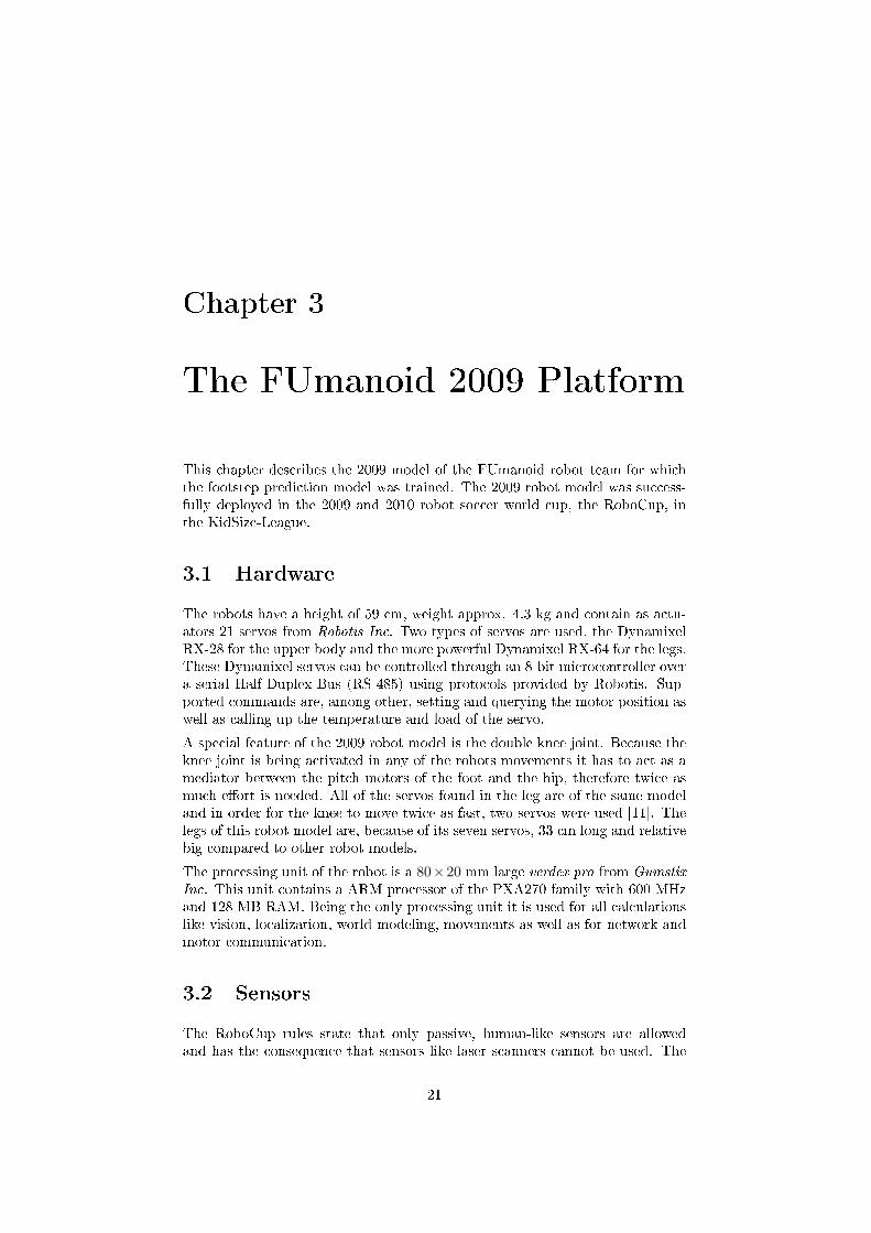
Figure 3.1: The kinematic model of the 2009 robot with motor names and IDs.[11]

main sensor of the robot is therefore a HV7131RP camera with a resolution of640× 480 pixels. In order to receive and process the images quickly, the camerais connected directly to the CPU through the Quick-Capture-Interface. Thisdirect connection forces the verdex pro to be placed in the head of the robot.The camera is equipped with a �sheye lens which has an opening angle of 175◦.This allows the robot to see the whole �eld and its own feet at the same time.

Other sensors are switches placed under the feet. Each foot has four of thoseswitches which can measure if the foot is on the ground or not. This informationis crucial for the robot in order to walk.

The servos are also used as sensors to measure the angle of the joint and itsload or temperature. Being able to receive this kind of feedback is useful for therobot's stabilization.

An other useful sensor for stabilization is the Inertial Measurement Unit. TheIMU uses accelerometers and gyroscopes in order to measure velocity, orienta-tion and gravitational forces. With this data the robot can balance itself whenwalking and �gure out on which side it is in the case it fell down.

22

Chapter 4

Acquiring Ground Truth Data

This chapter describes the process of �nding the footstep information of therobot. The needed information is the actual e�ect of the input commands onthe robots pose. This information is needed in order to apply the learningalgorithms for �nding a correlation between the input commands and theire�ect. This reference data will be called ground truth data further on and is theinformation that is wished to be estimated. In order to successfully calculate therobots location after a series of steps the gathered data has to contain enoughinformation. Thus, the ground truth data has to include the position of themoved foot, relative to the standing foot, as well as its orientation. The desiredmodel is therefore

F (−→x ) = (px, py, pθ)

where −→x represents the vector of input commands. Which these input values arewill be explained in the next chapter as the current concern is to �nd px, py, pθ.

The initial idea of �nding the ground truth data was by externally observing therobot's walk and recording its steps. This approach of tracking the robot's feethas the advantage of obtaining objective data which also includes the slippageand drifting of its walk. The tracking was attempted through the use of theMicrosoft Kinect, a motion sensing input device by Microsoft for the Xbox 360video game console. The features of a kinect are along the RGB camera, a depthsensor which makes it suitable for motion capture.

After several attempts to track the robot the approach revealed itself to be tooimprecise. In order to observe the whole �eld, the sensor has to be placed at arelatively large distance to the robot. At an average distance of 4 meters andwith interfering noise, or random error, the tracking of only the robot's headresulted in an o�set error of approx. 5-10 cm. This error is relatively smallif the goal would be tracking the robot's absolute position on the �eld. Forthe purpose of measuring the footstep length it is too inaccurate, as an averagefootstep has a length of 10 cm. An obstacle is also the fact the the feet are

23

covering each other in some situations, which makes it impossible to extractuseful information.

As an alternative method of retrieving the footstep information, forward kine-matics was chosen. Although this approach does not take into considerationslippage and drifting it still o�ers useful information and is more precise thantracking with the Kinect. Even with small inaccuracy the collected informationis suitable as ground truth data for the creation of the learning models, as itcaptures the robot's gait. The information gathered this way ful�lls its purpose,helping to create the learning model and can be changed later on with moreaccurate data. The approach of collecting the footstep information throughforward kinematics will be presented onwards.

The usage of forward kinematics to gather the ground truth data is only atemporary solution. This is done in order to be able to create and test theprediction model. The temporary models are created with the goal in mid toacquire more precise ground truth data and to recreate the models. With moreprecise ground truth data, more accurate prediction models can be obtained.The collection of machine learning algorithms will automatically compute thebetter prediction model when new data is available.

4.1 Kinematic Model

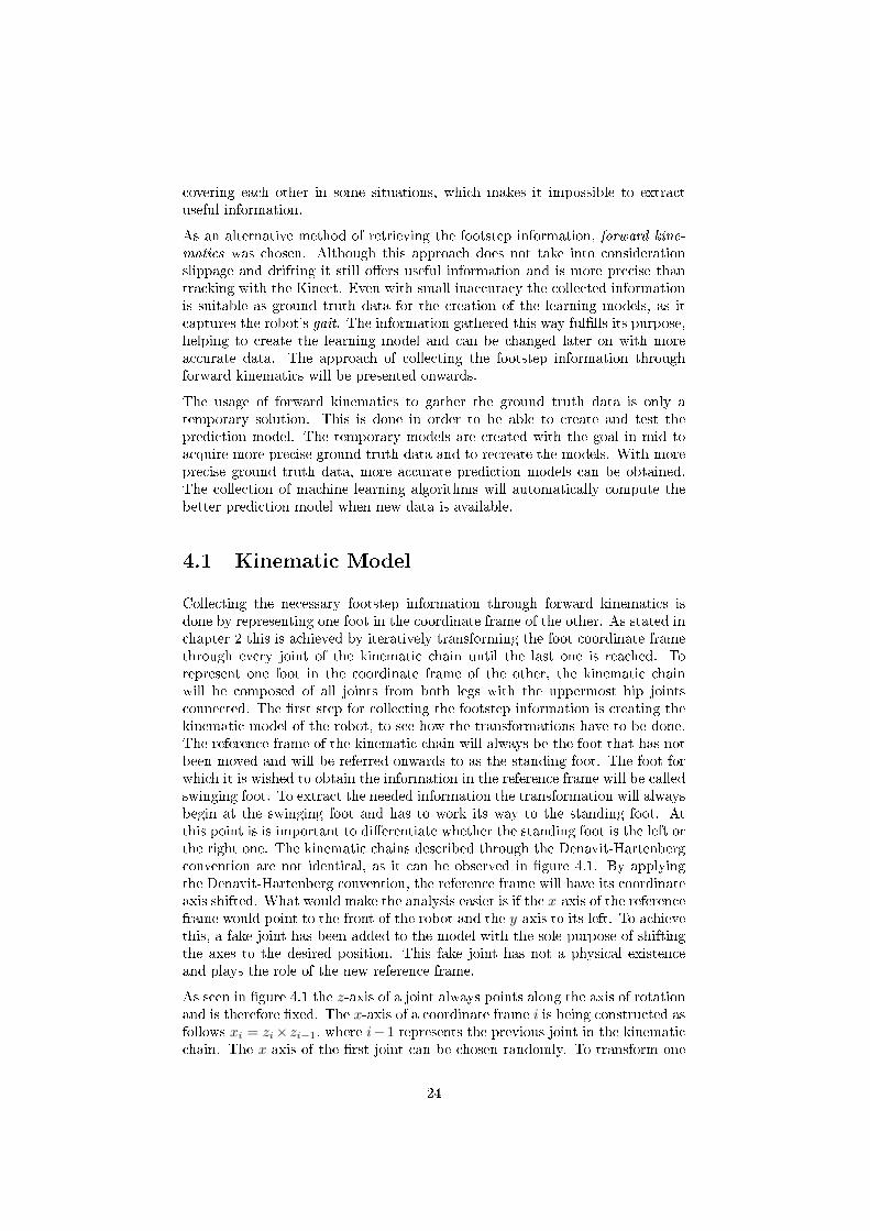
Collecting the necessary footstep information through forward kinematics isdone by representing one foot in the coordinate frame of the other. As stated inchapter 2 this is achieved by iteratively transforming the foot coordinate framethrough every joint of the kinematic chain until the last one is reached. Torepresent one foot in the coordinate frame of the other, the kinematic chainwill be composed of all joints from both legs with the uppermost hip jointsconnected. The �rst step for collecting the footstep information is creating thekinematic model of the robot, to see how the transformations have to be done.The reference frame of the kinematic chain will always be the foot that has notbeen moved and will be referred onwards to as the standing foot. The foot forwhich it is wished to obtain the information in the reference frame will be calledswinging foot. To extract the needed information the transformation will alwaysbegin at the swinging foot and has to work its way to the standing foot. Atthis point is is important to di�erentiate whether the standing foot is the left orthe right one. The kinematic chains described through the Denavit-Hartenbergconvention are not identical, as it can be observed in �gure 4.1. By applyingthe Denavit-Hartenberg convention, the reference frame will have its coordinateaxis shifted. What would make the analysis easier is if the x-axis of the referenceframe would point to the front of the robot and the y-axis to its left. To achievethis, a fake joint has been added to the model with the sole purpose of shiftingthe axes to the desired position. This fake joint has not a physical existenceand plays the role of the new reference frame.

As seen in �gure 4.1 the z-axis of a joint always points along the axis of rotationand is therefore �xed. The x-axis of a coordinate frame i is being constructed asfollows xi = zi× zi−1, where i−1 represents the previous joint in the kinematicchain. The x-axis of the �rst joint can be chosen randomly. To transform one

24

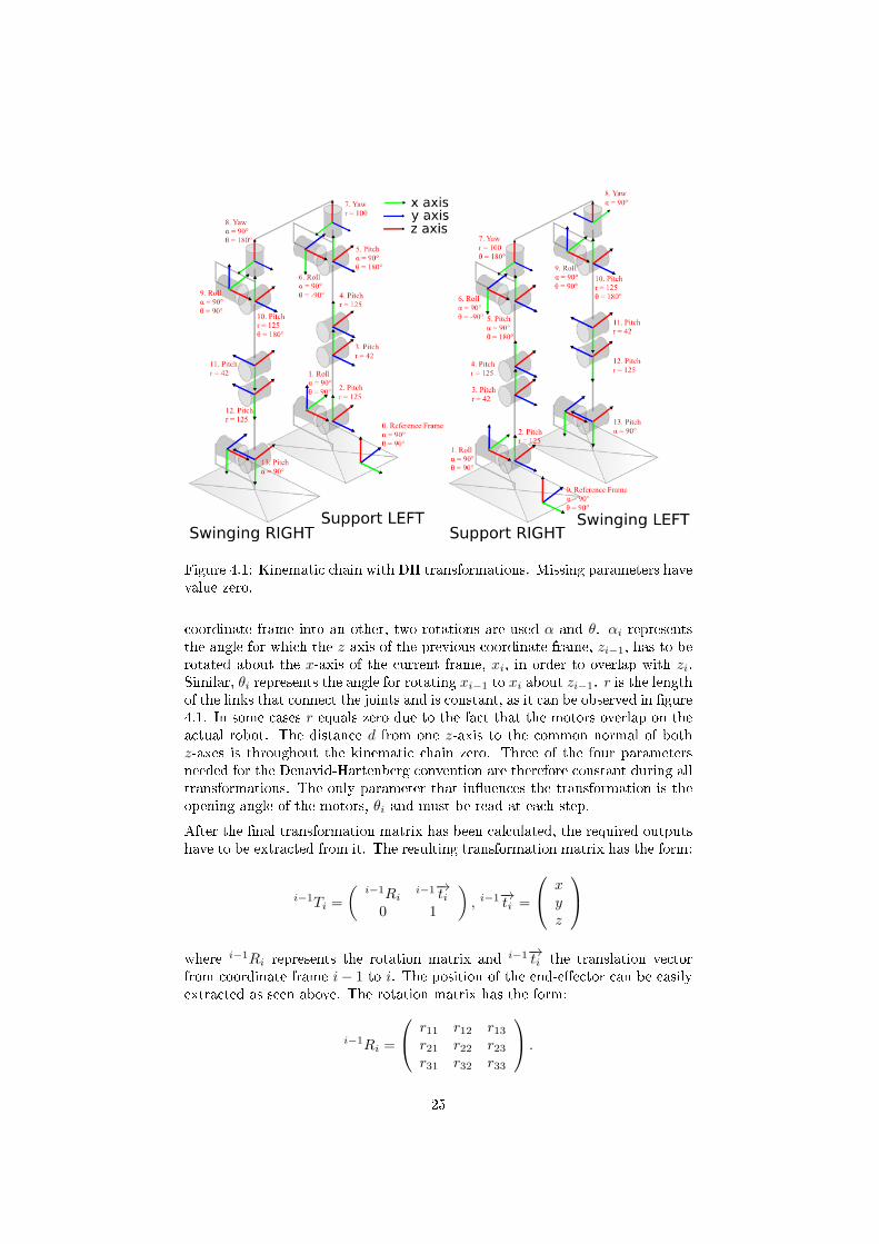
Figure 4.1: Kinematic chain with DH transformations. Missing parameters havevalue zero.

coordinate frame into an other, two rotations are used α and θ. αi representsthe angle for which the z-axis of the previous coordinate frame, zi−1, has to berotated about the x-axis of the current frame, xi, in order to overlap with zi.Similar, θi represents the angle for rotating xi−1 to xi about zi−1. r is the lengthof the links that connect the joints and is constant, as it can be observed in �gure4.1. In some cases r equals zero due to the fact that the motors overlap on theactual robot. The distance d from one z-axis to the common normal of bothz-axes is throughout the kinematic chain zero. Three of the four parametersneeded for the Denavid-Hartenberg convention are therefore constant during alltransformations. The only parameter that in�uences the transformation is theopening angle of the motors, θi and must be read at each step.

After the �nal transformation matrix has been calculated, the required outputshave to be extracted from it. The resulting transformation matrix has the form:

i−1Ti =

(i−1Ri

i−1−→ti0 1

), i−1−→ti =

xyz

where i−1Ri represents the rotation matrix and i−1−→ti the translation vectorfrom coordinate frame i− 1 to i. The position of the end-e�ector can be easilyextracted as seen above. The rotation matrix has the form:

i−1Ri =

r11 r12 r13r21 r22 r23r31 r32 r33

.

25

Figure 4.2: Readings of the motor values for each leg with respect to time.Reading errors are represented as spikes.

The angle that determines the desired foot orientation is the yaw angle pθ.Because the pitch angle of the foot is always in the interval (−π/2, π/2) , theyaw angle can be calculated as follows [15][4]:

pθ = atan2(r32, r33)

By using these methods the needed outputs can be extracted from the �naltransformation matrix without di�culty.

4.2 Implementation

The implementation of the footstep information extraction algorithm throughforward kinematics has been done in C++ on the FUmanoid platform. Asmentioned in the previous section once the kinematic model has been builtmost of the information needed for the Denavid-Hartenberg transformation isavailable and remains constant throughout the process. The only parameterthat is changing its value is θ, the opening angle of the servos, and can be foundout by querying the motors.

The needed information is required for each of the robot's steps and the algo-rithm is therefore called up during the walking routine. The existing walkingalgorithm is able to know when a footstep ended, through the use of the switchesunder the foot and timers. The walking algorithm runs the footstep informationextraction algorithm with an error rate of one every 100 steps. Every time theextraction algorithm is called it appends its outputs, the x , y coordinates aswell as the foot orientation pθ, to a �le stored on the robot.

The algorithm calculates the outputs through the kinematic transformations asdescribed in chapter 2, which resumes itself to a matrix multiplication for each

26

joint. Because the kinematic chain is composed of 15 joints, the �nal result willbe obtained by the 14 matrix multiplications. Before the transformations canbe calculated the motor values have to be read for each servo. The queryingof the motors should be rather straight forward but after several attempts itturned out that reading errors often appear. These reading errors, marked asa returned value of -1, lead to a wrong calculation and erroneous results withhigh variances. To avoid this outcome, the algorithm queries a motor again ifit previously encountered a reading error.

Figure 4.2 shows the readings of the motors with respect to time. The normalmotor values of the robot's legs are around 500 during a walk. It is easy toobserve that the reading errors disturb the continuity and can therefore heavilyin�uence the outcome of the calculations.

The recording of the footstep information has been done in two di�erent ways.In one case the input commands were introduced manually, in order to obtaininformation about basic paths, like going forward 4 m. This way it is easier toobserve and compare the results of the learning algorithms. The other recordingswere done while the robot was running its standard behavior, the one used inreal soccer matches. The data obtained this way is authentic and contains thepatterns that are wished to be learned.

27

Chapter 5

Learning Ground Truth Data

This chapter describes how the machine learning methods, presented in chapter2, are used to learn the footstep prediction model and what results each of themhas. Once the ground truth data has been gathered, the next step is to �nd howthese correlate to the given input commands. The goal is to �nd a function thatmaps the input commands to the correct x, y and yaw values of the foot forthe given data. After doing this it is wished to be able to predict these valuesin new situations without further use of forward kinematics.

The input commands for a robot movement consist of three values forward speed,sidewards speed and rotation. These values specify the internal velocity of therobot and are being calculated based on the distance to the desired location.The values are being set by the walking program and represent the desired speedof the robot and not the actual actions taken. Because the footstep lengthand orientation are not only in�uenced by the input commands, but also bythe current stance and oscillation of the robot, these commands do not containsu�cient information for the prediction model. In order to add more dimensionsto the model, the motor values for each of the legs servo have been includedin the input data set of the learning models. By doing this, more informationabout the robot's pose is added to the model. This increases the probabilityfor the algorithms to �nd correlations between di�erent values. The mappingfunction will thus have the following form

f(fw, sw, rot,−→mv)→ (px, py, pθ)

where fw, sw and rot are the commands and −→mv the vector of motor values.This function is a multivariate regression, mapping the output values px, pyand pθ from the same input values. In this thesis the standard approach will betaken of regarding this regression as three independent univariate regressions.

fx(fw, sw, rot,−→mv)→ px

fy(fw, sw, rot,−→mv)→ py

28

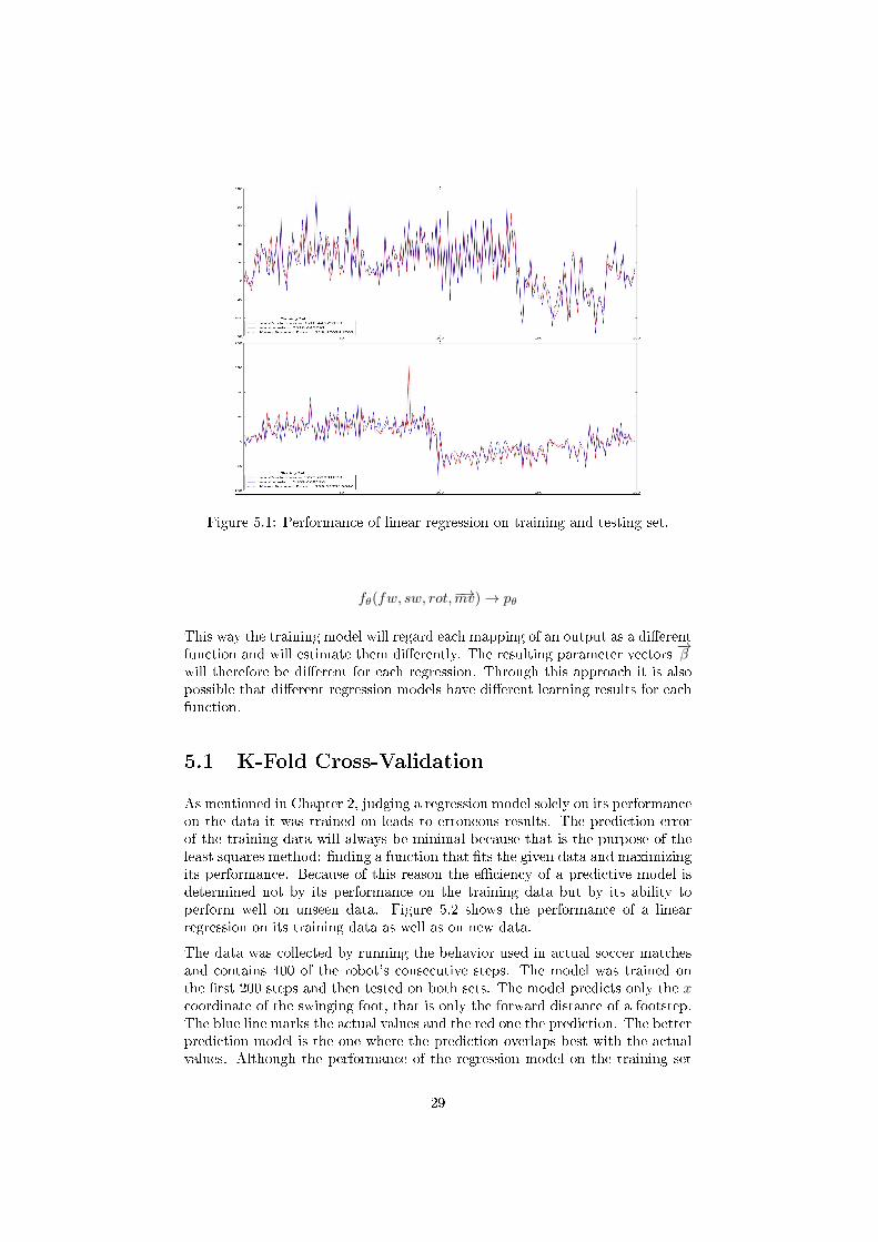
Figure 5.1: Performance of linear regression on training and testing set.

fθ(fw, sw, rot,−→mv)→ pθ

This way the training model will regard each mapping of an output as a di�erentfunction and will estimate them di�erently. The resulting parameter vectors

−→β

will therefore be di�erent for each regression. Through this approach it is alsopossible that di�erent regression models have di�erent learning results for eachfunction.

5.1 K-Fold Cross-Validation

As mentioned in Chapter 2, judging a regression model solely on its performanceon the data it was trained on leads to erroneous results. The prediction errorof the training data will always be minimal because that is the purpose of theleast squares method: �nding a function that �ts the given data and maximizingits performance. Because of this reason the e�ciency of a predictive model isdetermined not by its performance on the training data but by its ability toperform well on unseen data. Figure 5.2 shows the performance of a linearregression on its training data as well as on new data.

The data was collected by running the behavior used in actual soccer matchesand contains 400 of the robot's consecutive steps. The model was trained onthe �rst 200 steps and then tested on both sets. The model predicts only the xcoordinate of the swinging foot, that is only the forward distance of a footstep.The blue line marks the actual values and the red one the prediction. The betterprediction model is the one where the prediction overlaps best with the actualvalues. Although the performance of the regression model on the training set

29

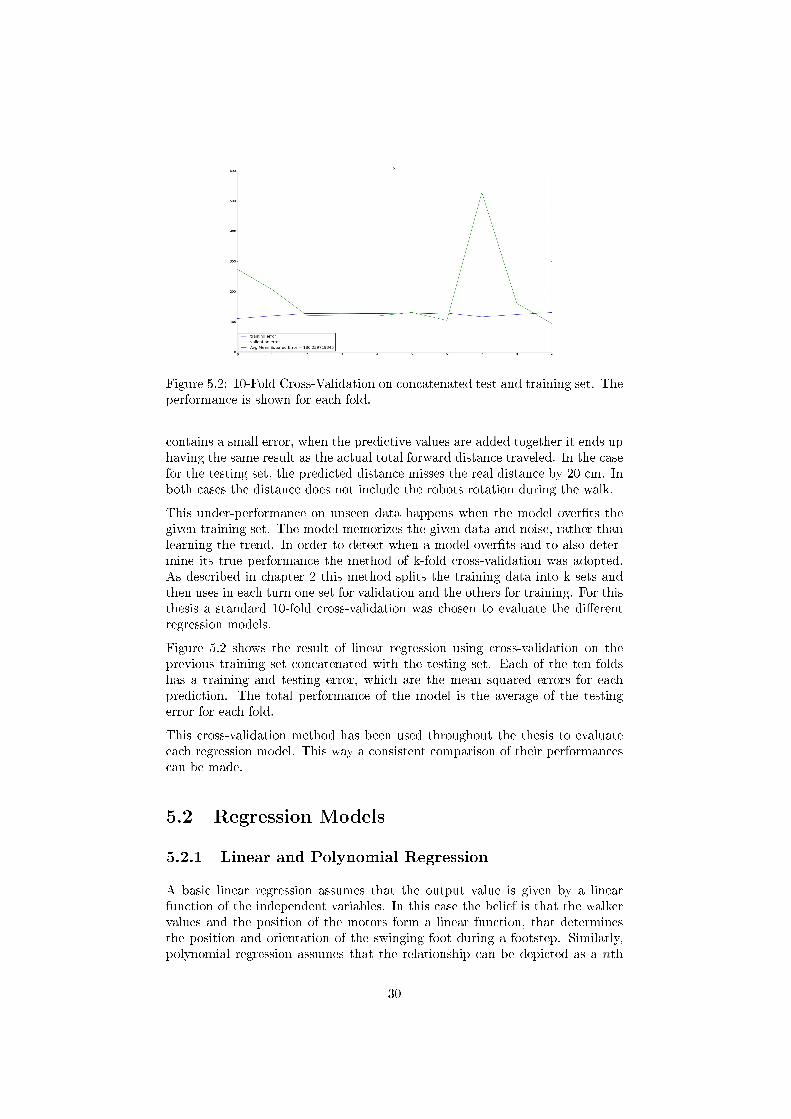
Figure 5.2: 10-Fold Cross-Validation on concatenated test and training set. Theperformance is shown for each fold.

contains a small error, when the predictive values are added together it ends uphaving the same result as the actual total forward distance traveled. In the casefor the testing set, the predicted distance misses the real distance by 20 cm. Inboth cases the distance does not include the robots rotation during the walk.

This under-performance on unseen data happens when the model over�ts thegiven training set. The model memorizes the given data and noise, rather thanlearning the trend. In order to detect when a model over�ts and to also deter-mine its true performance the method of k-fold cross-validation was adopted.As described in chapter 2 this method splits the training data into k sets andthen uses in each turn one set for validation and the others for training. For thisthesis a standard 10-fold cross-validation was chosen to evaluate the di�erentregression models.

Figure 5.2 shows the result of linear regression using cross-validation on theprevious training set concatenated with the testing set. Each of the ten foldshas a training and testing error, which are the mean squared errors for eachprediction. The total performance of the model is the average of the testingerror for each fold.

This cross-validation method has been used throughout the thesis to evaluateeach regression model. This way a consistent comparison of their performancescan be made.

5.2 Regression Models

5.2.1 Linear and Polynomial Regression

A basic linear regression assumes that the output value is given by a linearfunction of the independent variables. In this case the belief is that the walkervalues and the position of the motors form a linear function, that determinesthe position and orientation of the swinging foot during a footstep. Similarly,polynomial regression assumes that the relationship can be depicted as a nth

30

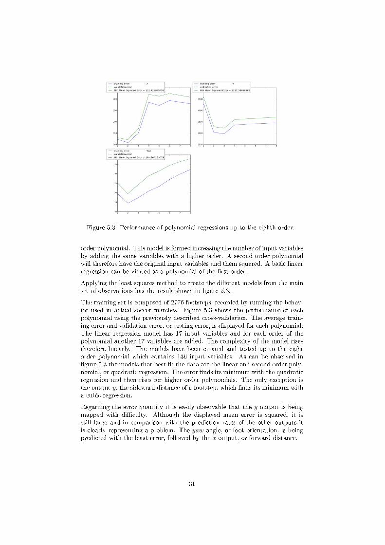
Figure 5.3: Performance of polynomial regressions up to the eighth order.

order polynomial. This model is formed increasing the number of input variablesby adding the same variables with a higher order. A second order polynomialwill therefore have the original input variables and them squared. A basic linearregression can be viewed as a polynomial of the �rst order.

Applying the least squares method to create the di�erent models from the mainset of observations has the result shown in �gure 5.3.

The training set is composed of 2776 footsteps, recorded by running the behav-ior used in actual soccer matches. Figure 5.3 shows the performance of eachpolynomial using the previously described cross-validation. The average train-ing error and validation error, or testing error, is displayed for each polynomial.The linear regression model has 17 input variables and for each order of thepolynomial another 17 variables are added. The complexity of the model risestherefore linearly. The models have been created and tested up to the eightorder polynomial which contains 136 input variables. As can be observed in�gure 5.3 the models that best �t the data are the linear and second order poly-nomial, or quadratic regression. The error �nds its minimum with the quadraticregression and then rises for higher order polynomials. The only exception isthe output y, the sideward distance of a footstep, which �nds its minimum witha cubic regression.

Regarding the error quantity it is easily observable that the y output is beingmapped with di�culty. Although the displayed mean error is squared, it isstill large and in comparison with the prediction rates of the other outputs itis clearly representing a problem. The yaw angle, or foot orientation, is beingpredicted with the least error, followed by the x output, or forward distance.

31

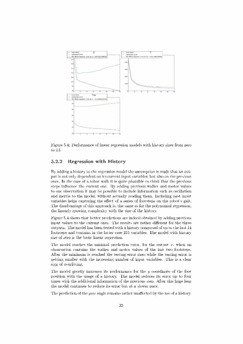
Figure 5.4: Performance of linear regression models with history sizes from zeroto 14.

5.2.2 Regression with History

By adding a history to the regression model the assumption is made that an out-put is not only dependent on its current input variables, but also on the previousones. In the case of a robot walk it is quite plausible to think that the previoussteps in�uence the current one. By adding previous walker and motor valuesto one observation it may be possible to include information such as oscillationand inertia to the model, without actually reading them. Including past inputvariables helps capturing the e�ect of a series of footsteps on the robot's gait.The disadvantage of this approach is, the same as for the polynomial regression,the linearly growing complexity with the size of the history.

Figure 5.4 shows that better predictions are indeed obtained by adding previousinput values to the current ones. The results are rather di�erent for the threeoutputs. The model has been tested with a history composed of up to the last 14footsteps and contains in the latter case 255 variables. The model with historysize of zero is the basic linear regression.

The model reaches the minimal prediction error, for the output x, when anobservation contains the walker and motor values of the last two footsteps.After the minimum is reached the testing error rises while the testing error isgetting smaller with the increasing number of input variables. This is a clearsign of over�tting.

The model greatly increases its performance for the y coordinate of the footposition with the usage of a history. The model reduces its error up to fourtimes with the additional information of the previous step. After this huge leapthe model continues to reduce its error but at a slower pace.

The prediction of the yaw angle remains rather una�ected by the use of a history.

32

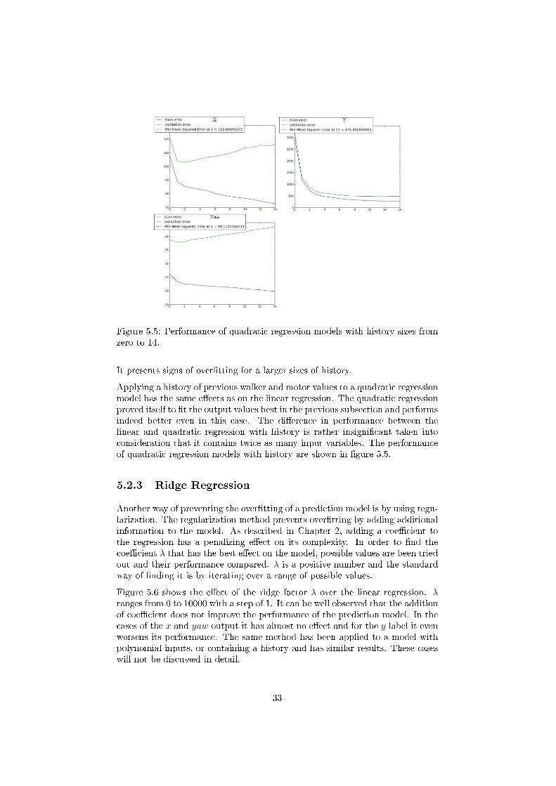
Figure 5.5: Performance of quadratic regression models with history sizes fromzero to 14.

It presents signs of over�tting for a larger sizes of history.

Applying a history of previous walker and motor values to a quadratic regressionmodel has the same e�ects as on the linear regression. The quadratic regressionproved itself to �t the output values best in the previous subsection and performsindeed better even in this case. The di�erence in performance between thelinear and quadratic regression with history is rather insigni�cant taken intoconsideration that it contains twice as many input variables. The performanceof quadratic regression models with history are shown in �gure 5.5.

5.2.3 Ridge Regression

Another way of preventing the over�tting of a prediction model is by using regu-larization. The regularization method prevents over�tting by adding additionalinformation to the model. As described in Chapter 2, adding a coe�cient tothe regression has a penalizing e�ect on its complexity. In order to �nd thecoe�cient λ that has the best e�ect on the model, possible values are been triedout and their performance compared. λ is a positive number and the standardway of �nding it is by iterating over a range of possible values.

Figure 5.6 shows the e�ect of the ridge factor λ over the linear regression. λranges from 0 to 10000 with a step of 1. It can be well observed that the additionof coe�cient does not improve the performance of the prediction model. In thecases of the x and yaw output it has almost no e�ect and for the y label it evenworsens its performance. The same method has been applied to a model withpolynomial inputs, or containing a history and has similar results. These caseswill not be discussed in detail.

33

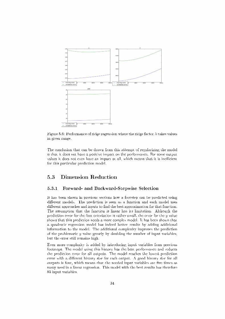
Figure 5.6: Performance of ridge regression where the ridge factor λ takes valuesin given range.

The conclusion that can be drawn from this attempt of regularizing the modelis that it does not have a positive impact on the performance. For some outputvalues it does not even have an impact at all, which means that it is ine�cientfor this particular prediction model.

5.3 Dimension Reduction

5.3.1 Forward- and Backward-Stepwise Selection

It has been shown in previous sections how a footstep can be predicted usingdi�erent models. The prediction is seen as a function and each model usesdi�erent approaches and inputs to �nd the best approximation for that function.The assumption that the function is linear has its limitation. Although theprediction error for the foot orientation is rather small, the error for the y valueshows that this prediction needs a more complex model. It has been shown thata quadratic regression model has indeed better results by adding additionalinformation to the model. The additional complexity improves the predictionof the problematic y value greatly by doubling the number of input variables,but the error still remains high.

Even more complexity is added by introducing input variables from previousfootsteps. The model using this history has the best performance and reducesthe prediction error for all outputs. The model reaches the lowest predictionerror with a di�erent history size for each output. A good history size for alloutputs is four, which means that the needed input variables are �ve times asmany used in a linear regression. This model with the best results has therefore85 input variables.

34

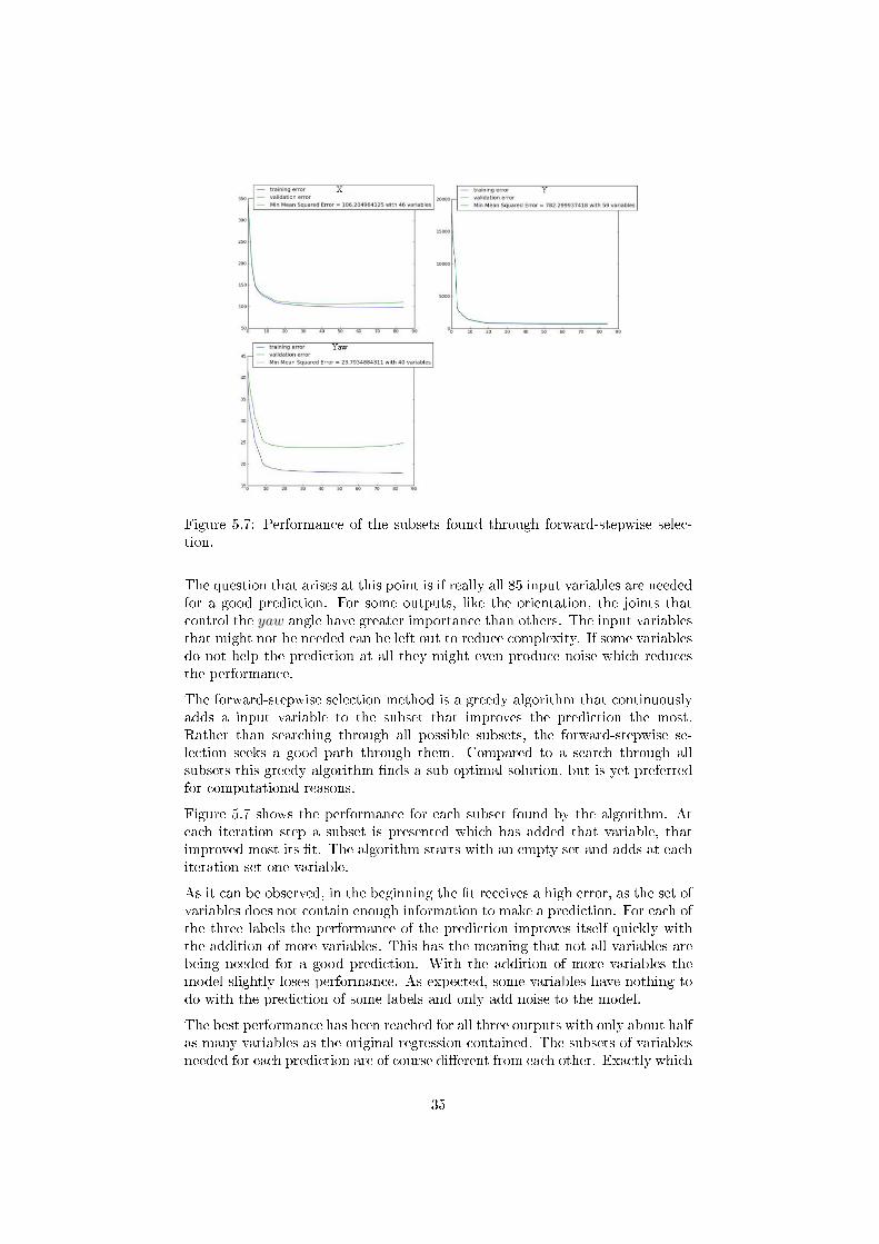
Figure 5.7: Performance of the subsets found through forward-stepwise selec-tion.

The question that arises at this point is if really all 85 input variables are neededfor a good prediction. For some outputs, like the orientation, the joints thatcontrol the yaw angle have greater importance than others. The input variablesthat might not be needed can be left out to reduce complexity. If some variablesdo not help the prediction at all they might even produce noise which reducesthe performance.

The forward-stepwise selection method is a greedy algorithm that continuouslyadds a input variable to the subset that improves the prediction the most.Rather than searching through all possible subsets, the forward-stepwise se-lection seeks a good path through them. Compared to a search through allsubsets this greedy algorithm �nds a sub-optimal solution, but is yet preferredfor computational reasons.

Figure 5.7 shows the performance for each subset found by the algorithm. Ateach iteration step a subset is presented which has added that variable, thatimproved most its �t. The algorithm starts with an empty set and adds at eachiteration set one variable.

As it can be observed, in the beginning the �t receives a high error, as the set ofvariables does not contain enough information to make a prediction. For each ofthe three labels the performance of the prediction improves itself quickly withthe addition of more variables. This has the meaning that not all variables arebeing needed for a good prediction. With the addition of more variables themodel slightly loses performance. As expected, some variables have nothing todo with the prediction of some labels and only add noise to the model.

The best performance has been reached for all three outputs with only about halfas many variables as the original regression contained. The subsets of variablesneeded for each prediction are of course di�erent from each other. Exactly which

35

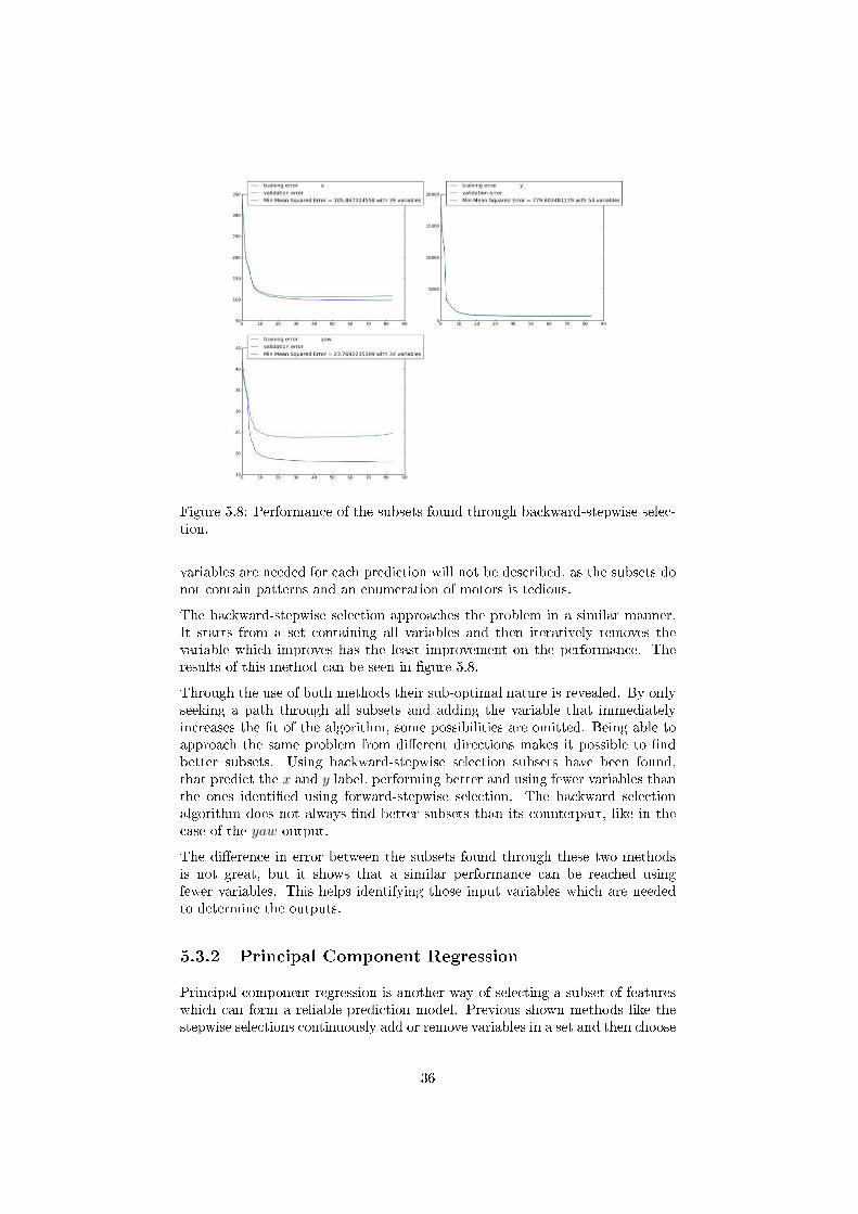
Figure 5.8: Performance of the subsets found through backward-stepwise selec-tion.

variables are needed for each prediction will not be described, as the subsets donot contain patterns and an enumeration of motors is tedious.

The backward-stepwise selection approaches the problem in a similar manner.It starts from a set containing all variables and then iteratively removes thevariable which improves has the least improvement on the performance. Theresults of this method can be seen in �gure 5.8.

Through the use of both methods their sub-optimal nature is revealed. By onlyseeking a path through all subsets and adding the variable that immediatelyincreases the �t of the algorithm, some possibilities are omitted. Being able toapproach the same problem from di�erent directions makes it possible to �ndbetter subsets. Using backward-stepwise selection subsets have been found,that predict the x and y label, performing better and using fewer variables thanthe ones identi�ed using forward-stepwise selection. The backward selectionalgorithm does not always �nd better subsets than its counterpart, like in thecase of the yaw output.

The di�erence in error between the subsets found through these two methodsis not great, but it shows that a similar performance can be reached usingfewer variables. This helps identifying those input variables which are neededto determine the outputs.

5.3.2 Principal Component Regression

Principal component regression is another way of selecting a subset of featureswhich can form a reliable prediction model. Previous shown methods like thestepwise selections continuously add or remove variables in a set and then choose

36

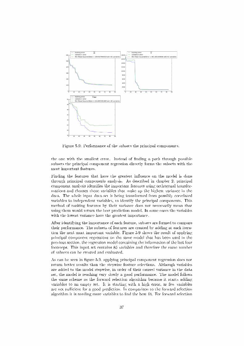
Figure 5.9: Performance of the subsets the principal components.

the one with the smallest error. Instead of �nding a path through possiblesubsets the principal component regression directly forms the subsets with themost important features.

Finding the features that have the greatest in�uence on the model is donethrough principal components analysis. As described in chapter 2, principalcomponent analysis identi�es the important features using orthogonal transfor-mations and chooses those variables that make up the highest variance in thedata. The whole input data set is being transformed from possibly correlatedvariables to independent variables, to identify the principal components. Thismethod of ranking features by their variance does not necessarily mean thatusing them would return the best prediction model. In some cases the variableswith the lowest variance have the greatest importance.

After identifying the importance of each feature, subsets are formed to comparetheir performance. The subsets of features are created by adding at each itera-tion the next most important variable. Figure 5.9 shows the result of applyingprincipal component regressions on the same model that has been used in theprevious section, the regression model containing the information of the last fourfootsteps. This input set contains 85 variables and therefore the same numberof subsets can be created and evaluated.

As can be seen in �gure 5.9, applying principal component regression does notreturn better results than the stepwise feature selections. Although variablesare added to the model stepwise, in order of their caused variance in the dataset, the model is reaching very slowly a good performance. The model followsthe same scheme as the forward selection algorithm because it starts addingvariables to an empty set. It is starting with a high error, as few variablesare not su�cient for a good prediction. In comparison to the forward selectionalgorithm it is needing more variables to �nd the best �t. For forward selection

37

the increase in performance tends to stall when the subset contains around 10variables. That point is only reached with PCR when using between 30 and 40variables. The best subset found using principal component regression is alsonot as good as the ones found through the stepwise selections.

Reducing the dimensions of the regression model using principal componentregression is therefore not as powerful as the greedy algorithms.

5.4 Time Complexity

An advantage of using a regression model over forward kinematics, to predictthe footstep of a humanoid robot, is the e�ciency in time. As presented inchapter 4, the calculation of the relative foot position using forward kinematicsimplies 14 transformations, one for every joint. The transformations are madethrough multiplications of 4 × 4 matrices. Because the matrices have a smallsize, their multiplication is done naive in a running time of O(n3). n representsthe row length of a quadratic matrix. This means that a transformation will bemade using 64 multiplications. The total cost of the prediction using forwardkinematics is therefore 14 ∗ 43 = 896 multiplications.

In comparison to this the best found regression model, that includes the infor-mation of the last four footsteps, returns a function that is able to predict thefootstep using only 85 multiplications. If this model has its dimensions reducedusing the feature selection algorithms, the number of multiplications drops to44, 30 and 40 for the three di�erent outputs.

5.5 Additional Features

All the previous learning methods have included as their input the commandvalues from the walking algorithm, as well as the read motor values from thelegs. With these dimensions, functions have been learned that can predict theposition x and the yaw angle with small squared errors of 105.8 and 23.7 mm2.A more di�cult output to predict is the y label, the sideward position of thefoot. The prediction of this output has a squared error of 779.6 mm2 which ishigh in comparison with the performance for the other outputs. This footstepinformation obviously presents di�culties to be predicted. A reason why thiscould be is because of the robot's oscillation during the walk.

A way of increasing the prediction performance for the y value is by includingmore information to the input data, that is relevant for this output. This meansadding more dimensions to the model. An attempt of doing so is by includingthe data read from the robot's gyroscope. Two values have been included to theinput data set, the forward and sideward acceleration measured when both feetare on the ground.

For this new data set the library of regression algorithms has been reused in orderto evaluate the performance of the new regression models. For all regressionmethods the performance graphs keeps the same scheme as the one observed

38

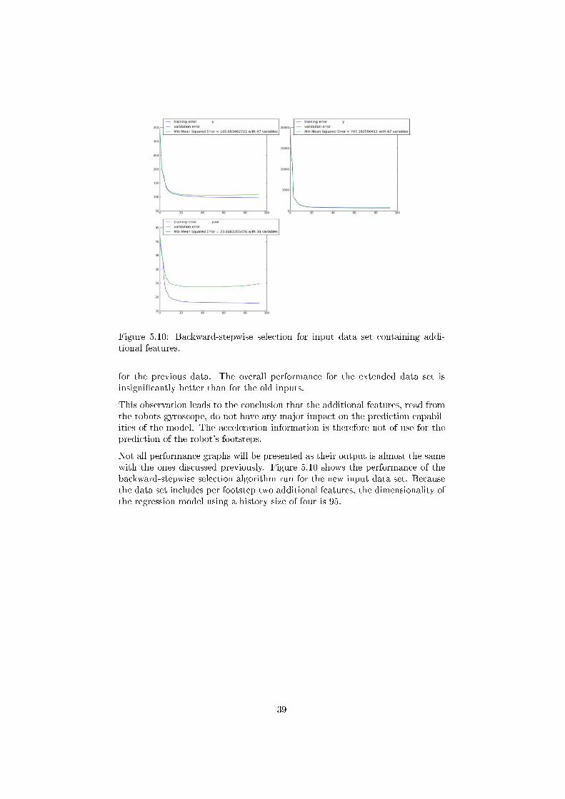
Figure 5.10: Backward-stepwise selection for input data set containing addi-tional features.

for the previous data. The overall performance for the extended data set isinsigni�cantly better than for the old inputs.

This observation leads to the conclusion that the additional features, read fromthe robots gyroscope, do not have any major impact on the prediction capabil-ities of the model. The acceleration information is therefore not of use for theprediction of the robot's footsteps.

Not all performance graphs will be presented as their output is almost the samewith the ones discussed previously. Figure 5.10 shows the performance of thebackward-stepwise selection algorithm run for the new input data set. Becausethe data set includes per footstep two additional features, the dimensionality ofthe regression model using a history size of four is 95.

39

Chapter 6

Results and Discussion

The aim of this thesis was to create a library of machine learning algorithmsin order to train a prediction model for the walk of humanoid robots. Variousregression models have been included to approximate the three needed outputs:the forward and sideward distance and the orientation of the swinging foot.These three functions have been approximated using 17 input variables. Threeof the input variables are the control commands sent by the walking algorithmand the other 14 are the motor values of the leg servos, read at the end ofa footstep. All regression models have been trained using the ordinary leastsquares method. The performance of each model has then been evaluated usinga 10-fold cross-validation.

The �rst belief that had to be tested is if the desired outputs can be obtainedthrough a linear function of the input variables. The performance of this modelhas been compared with the result of testing if the functions could rather be de-picted as polynomials. This �rst test compared the performance of polynomialsup to the eighth order.

The result of this test was that the prediction model can be best seen as aquadratic function. The performances of the models drop and reach a minimumfor the quadratic function and then rise for higher order polynomials. This isbecause for each higher order another 17 variables are added to the model. Inthe beginning additional information helps improving the prediction rate. Forhigher orders the additional information hinders the prediction. This happensbecause too much additional information increases the complexity of the modeland does not help better de�ne the function.

The results of these models is expressed in the mean squared error of the tenfolds used in the cross-validation. This error is further on abbreviated as MSE.The forward distance x and the foot orentation yaw, are being predicted bestusing these models. The drop in the MSE is not of great magnitude whencomparing the linear to the quadratic regression. These two labels, x and yawhave been predicted with a MSE of 121.4 and 19.4. The y label, the sidewarddistance of a footstep, is the hardest to predict and has its di�culties will allmethods. This label sees a big drop in MSE, from 4500 which is obtained usinglinear regression, to 3200 for a cubic regression. The increased performance isgood but contains still a high error.

40

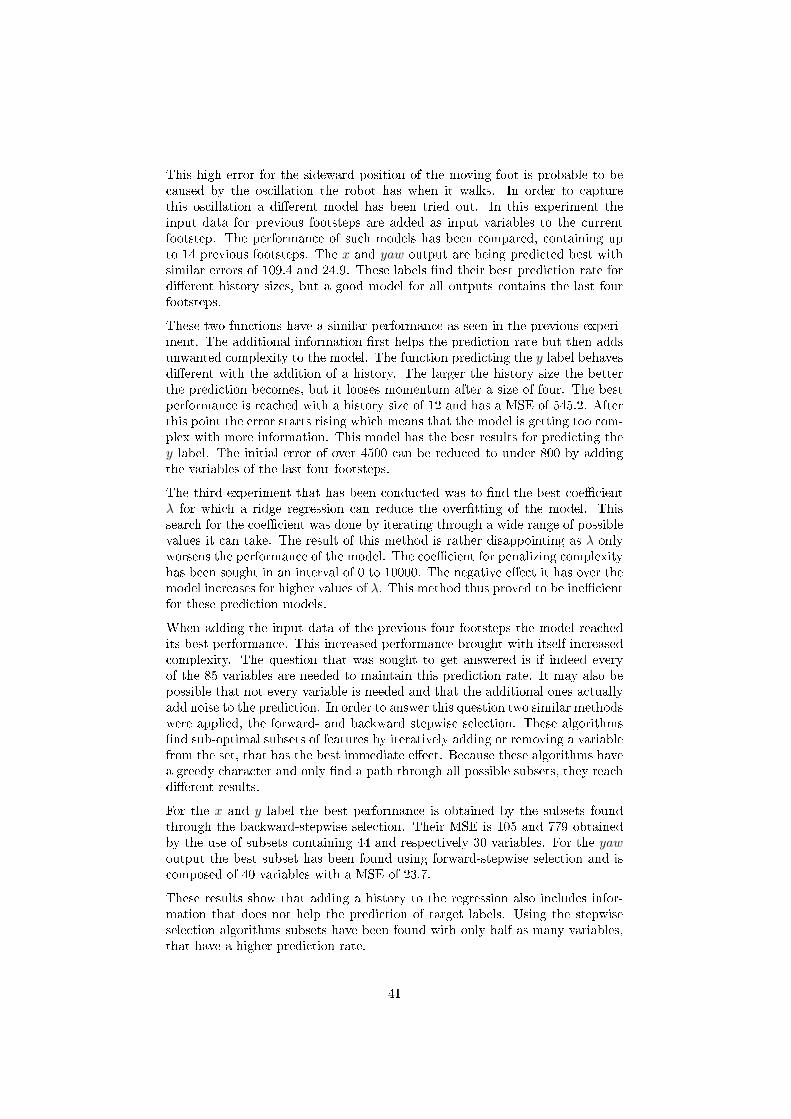
This high error for the sideward position of the moving foot is probable to becaused by the oscillation the robot has when it walks. In order to capturethis oscillation a di�erent model has been tried out. In this experiment theinput data for previous footsteps are added as input variables to the currentfootstep. The performance of such models has been compared, containing upto 14 previous footsteps. The x and yaw output are being predicted best withsimilar errors of 109.4 and 24.9. These labels �nd their best prediction rate fordi�erent history sizes, but a good model for all outputs contains the last fourfootsteps.

These two functions have a similar performance as seen in the previous experi-ment. The additional information �rst helps the prediction rate but then addsunwanted complexity to the model. The function predicting the y label behavesdi�erent with the addition of a history. The larger the history size the betterthe prediction becomes, but it looses momentum after a size of four. The bestperformance is reached with a history size of 12 and has a MSE of 545.2. Afterthis point the error starts rising which means that the model is getting too com-plex with more information. This model has the best results for predicting they label. The initial error of over 4500 can be reduced to under 800 by addingthe variables of the last four footsteps.

The third experiment that has been conducted was to �nd the best coe�cientλ for which a ridge regression can reduce the over�tting of the model. Thissearch for the coe�cient was done by iterating through a wide range of possiblevalues it can take. The result of this method is rather disappointing as λ onlyworsens the performance of the model. The coe�cient for penalizing complexityhas been sought in an interval of 0 to 10000. The negative e�ect it has over themodel increases for higher values of λ. This method thus proved to be ine�cientfor these prediction models.

When adding the input data of the previous four footsteps the model reachedits best performance. This increased performance brought with itself increasedcomplexity. The question that was sought to get answered is if indeed everyof the 85 variables are needed to maintain this prediction rate. It may also bepossible that not every variable is needed and that the additional ones actuallyadd noise to the prediction. In order to answer this question two similar methodswere applied, the forward- and backward stepwise selection. These algorithms�nd sub-optimal subsets of features by iteratively adding or removing a variablefrom the set, that has the best immediate e�ect. Because these algorithms havea greedy character and only �nd a path through all possible subsets, they reachdi�erent results.

For the x and y label the best performance is obtained by the subsets foundthrough the backward-stepwise selection. Their MSE is 105 and 779 obtainedby the use of subsets containing 44 and respectively 30 variables. For the yawoutput the best subset has been found using forward-stepwise selection and iscomposed of 40 variables with a MSE of 23.7.

These results show that adding a history to the regression also includes infor-mation that does not help the prediction of target labels. Using the stepwiseselection algorithms subsets have been found with only half as many variables,that have a higher prediction rate.

41

Analyzing the selected input variables show that they are not the same for thewhole history. Some motor values are relevant for one footstep but when addedto a history other motors become more important. Although half of the inputvariables have been excluded from the model, still all 14 motor values have tobe read in order to make a prediction.

An alternative method of �nding a reduced set of variables has been also used,the principal components regression. This method �nds the relevant features byranking them according to the variance they have on the data. This approachmakes the assumption that variables that cause a high variance are also the mostimportant features of the model. This belief can be misleading as sometimesfeatures with a low variance have a greater importance.

The results of this method show that the greedy algorithms are able to �ndsubsets with fewer variables that can perform better than the ones found throughprincipal component regression. This means that the assumption, that variableswith the highest variance are also the most important features, does not holdin the case of the robot walk.

A �nal attempt of increasing the prediction rate of the y label has been madeby adding new dimensions to the model. The hope was that this new acquireddata contains information about the robot's oscillation when walking. The datahas been recorded using the robot's gyroscope and measures the forward andsideward acceleration.

All the algorithms described above have been run again for the new data setcontaining the additional two dimensions. Sadly the performance of every modelwas either unchanged or insigni�cantly better. This leads to the conclusion thatthe information extracted from the gyroscope is either not useful or alreadyincluded in the existing data.

42

Chapter 7

Conclusion and Future Work

The purpose of this thesis was to create a library of machine learning algorithmsthat can learn a prediction model for the footsteps of humanoid robots. Thislibrary creates linear and polynomial regressions models and also models thatcontain the information of previous footsteps. By having a range of functionsto �t to the data, these can be compared to �nally choose the one with the bestperformance. In order to objectively compare the models, their performance isevaluated using a 10-fold cross-validation. This method is used to observe if theregression model over�ts the data.

Over�tting of the model can be also prevented using ridge regression. Thismethod seeks the coe�cient with the best impact on the model.

After testing regression methods that add complexity to the model, the libraryprovides algorithms to reduce their dimensions. Two of these methods are theforward and backward-stepwise selection. They are greedy algorithms and �nda sub-optimal set of features that can predict the footsteps. An other methodof dimension reduction found in the library, is using the principal componentregression. This algorithm selects the features according to their caused varianceon the data.

The input data for learning the robot's footsteps was chosen to contain the com-mands sent by the walking algorithm and the motor values, that are measuredfrom the robot's legs. The data was recorded by running the behavior used insoccer matches. It contains information read from 2776 footsteps and includestheir corresponding e�ect on the robot.

The collection of machine learning algorithms is independent from the used data.Obviously better results are achieved when the acquired ground truth data, theactual e�ect of the input data on the robot, is expressing accurate observations.

The �rst attempt of retrieving the ground truth data for this thesis was bythe use of a Microsoft Kinect. This approach proved itself to return inaccurateinformation, that could not be used to learn the relationship between the inputvariables and their e�ect. As an alternative this information was extractedusing forward kinematics. Although the information does not include the robotsoscillation and slippage during a walk, it still captures its gait.

43

The machine learning algorithms have been run on the collected data and ob-tained di�erent results.

Linear and polynomial regression models have been �tted on the data, as wellas models containing a history of last entries. The most e�ective regressionmodel proved itself to be the one containing the input variables of the last fourfootsteps. A regression that showed to have no improving e�ect on the modelsis the ridge regression.

After increasing the number of input variables using these regressions, algo-rithms for dimension reduction were applied. The backward-stepwise selectionfound the best performing subset of features. This method reduced the numberof needed variables to predict the footsteps from 85 to almost the half.

A method that revealed itself to be ine�cient for this data was the principalcomponent regression.

As mentioned before, the library of learning algorithms is a tool of approximat-ing and comparing prediction functions. In an attempt to measure the robot'soscillation, the input data set was modi�ed to include two additional dimen-sions. The measurements of the robot's gyroscope were added to the input dataset in order to improve the prediction rate. The addition of the forward andsideward acceleration turned out to not have any signi�cant e�ect on the model.

The future use of the library will be to predict the footsteps of newer modelsof humanoid soccer playing robots of the FUmanoid team. Better ground truthdata is also hoped to get acquired with the appearance of the Microsoft Kinect2. The newer model of the Kinect will hopefully have enough accuracy to trackthe movement of the robot's legs. With more accurate data the relationship,between input variables and their e�ect on the robot's walk, can be learnedmore precisely using the created library.

44

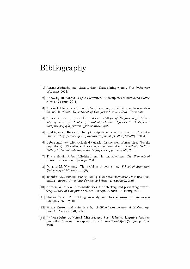
Bibliography

[1] Arthur Andrzejak and Heike Eckart. Data mining course. Free Universityof Berlin, 2011.

[2] RoboCup Humanoid League Commitee. Robocup soccer humanoid leaguerules and setup. 2011.

[3] Austin I. Eliazar and Ronald Parr. Learning probabilistic motion modelsfor mobile robots. Department of Computer Science, Duke University.

[4] Nicola Ferrier. Inverse kinematics. College of Engineering, Univer-sity of Wisconsin-Madison, Available Online: "gicl.cs.drexel.edu/wiki-data/images/e/e4/Ferrier_kinematics4.ppt".

[5] FU-Fighters. Robocup championship lisbon smallsize league. AvailableOnline: "http://robocup.mi.fu-berlin.de/pmwiki/Gallery/WM04", 2004.

[6] Urban habitats. Morphological variation in the seed of gray birch (betulapopulifolia): The e�ects of soil-metal contamination. Available Online:"http://urbanhabitats.org/v06n01/graybirch_�gure5.html", 2011.

[7] Trevor Hastie, Robert Tibshirani, and Jerome Friedman. The Elements ofStatistical Learning. Springer, 2001.

[8] Douglas M. Hawkins. The problem of over�tting. School of Statistics,University of Minnesota, 2003.

[9] Jennifer Kay. Introduction to homogeneous transformations & robot kine-matics. Rowan University Computer Science Department, 2005.

[10] Andrew W. Moore. Cross-validation for detecting and preventing over�t-ting. School of Computer Science Carnegie Mellon University, 2001.

[11] Ste�an Otte. Entwicklung eines dynamischen schusses für humanoidefuÿballroboter. 2010.

[12] Stuart Russell and Peter Norvig. Arti�cial Intelligence: A Modern Ap-proach. Prentice Hall, 2009.

[13] Andreas Schmitz, Marcell Missura, and Sven Behnke. Learning footstepprediction from motion capture. 14th International RoboCup Symposium,2010.

45

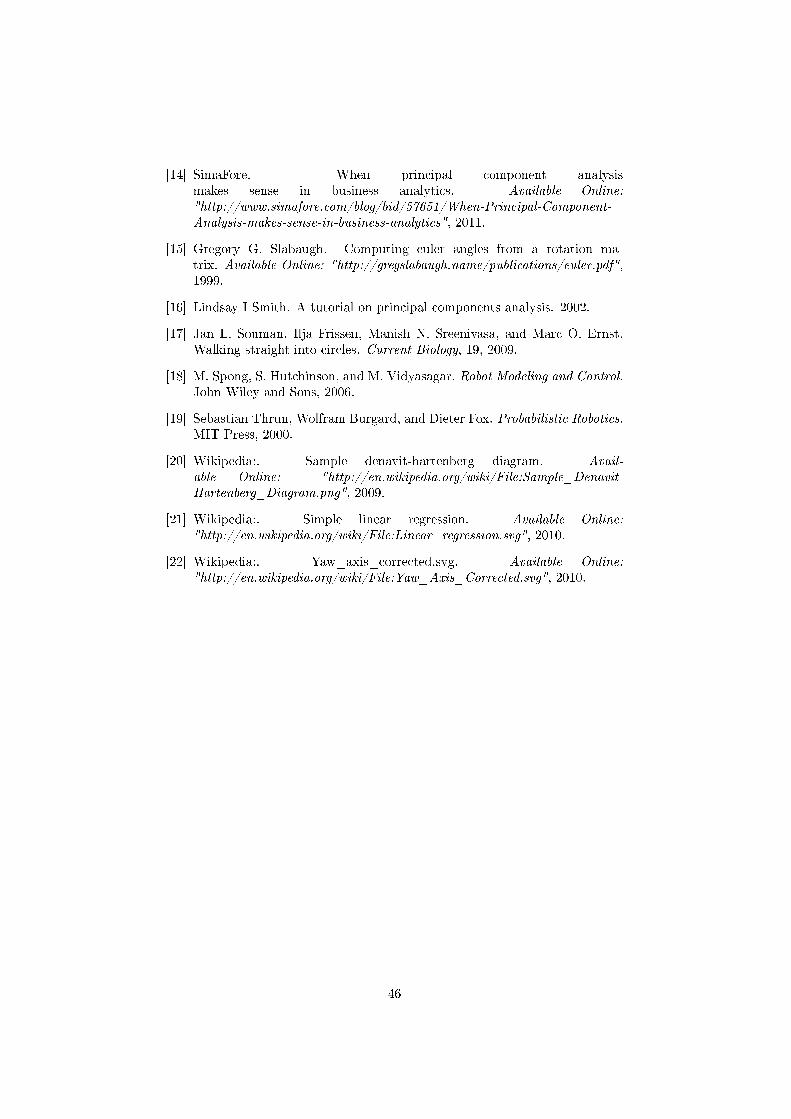
[14] SimaFore. When principal component analysismakes sense in business analytics. Available Online:"http://www.simafore.com/blog/bid/57651/When-Principal-Component-Analysis-makes-sense-in-business-analytics", 2011.

[15] Gregory G. Slabaugh. Computing euler angles from a rotation ma-trix. Available Online: "http://gregslabaugh.name/publications/euler.pdf",1999.

[16] Lindsay I Smith. A tutorial on principal components analysis. 2002.

[17] Jan L. Souman, Ilja Frissen, Manish N. Sreenivasa, and Marc O. Ernst.Walking straight into circles. Current Biology, 19, 2009.

[18] M. Spong, S. Hutchinson, and M. Vidyasagar. Robot Modeling and Control.John Wiley and Sons, 2006.

[19] Sebastian Thrun, Wolfram Burgard, and Dieter Fox. Probabilistic Robotics.MIT Press, 2000.

[20] Wikipedia:. Sample denavit-hartenberg diagram. Avail-able Online: "http://en.wikipedia.org/wiki/File:Sample_Denavit-Hartenberg_Diagram.png", 2009.

[21] Wikipedia:. Simple linear regression. Available Online:"http://en.wikipedia.org/wiki/File:Linear_regression.svg", 2010.

[22] Wikipedia:. Yaw_axis_corrected.svg. Available Online:"http://en.wikipedia.org/wiki/File:Yaw_Axis_Corrected.svg", 2010.

46