Linear and nonlinear spin dynamicsin Co2Mn0.6Fe0.4Si

Heusler microstructures

Dissertation

Thomas Sebastian

Vom Fachbereich Physik der Technischen Universität Kaiserslautern zur Verleihung desakademischen Grades „Doktor der Naturwissenschaften“ genehmigte Dissertation

Betreuer: Prof. Dr. Burkard Hillebrands

Zweitgutachter: Prof. Dr. Yasuo Ando

Datum der wissenschaftlichen Aussprache: 09. Oktober 2013

D 386

Kurzfassung

In der vorliegenden Arbeit wurde die Propagation von Spinwellen in mikrostrukturierten Wellen-

leitern aus dem Heusler-Material Co2Mn0.6Fe0.4Si (CMFS) im Rahmen des japanisch-deutschen

JST-DFG Projektes Advanced Spintronics Materials and Transport Phenomena untersucht. Der

wichtigste Projektpartner auf japanischer Seite, die Gruppe von Prof. Dr. Y. Ando an der Tohoku

University in Sendai, war als eine der weltweit führenden Gruppen in diesem Feld verantwortlich

für die Herstellung von CMFS-Schichten. Die Fragestellung nach der Eignung von CMFS als

Träger für Spinwellen bezieht ihre Relevanz zum einen aus zahlreichen Entwicklungen im Bereich

der Magnonspintronik sowie aus den vielversprechenden Eigenschaften des Materials selbst.

Das Ziel der Magnonspintronik ist die technisch relevante Nutzung des Elektronenspins zum

Transport und zur Verarbeitung von Daten, ohne auf Ladungsströme angewiesen zu sein. Informa-

tionsträger sind also Spinwellen, die fundamentalen Anregungen magnetischer Festkörper. Damit

stellt dieses Konzept eine Erweiterung und Alternative zu bisher genutzter Elektronik und Spin-

tronik dar. Der Vorteil des Konzepts liegt in der Natur der Spinwelle als kollektiver Anregung

des Spinsystems. Dadurch ist unter anderem eine energieeffizientere Datenverarbeitung möglich,

als durch den Transport von Elektronen, welcher immer mit Stoßprozessen und daher Verlusten

behaftet ist.

Während die prinzipiellen Möglichkeiten der Magnonspintronik durch die Erforschung neuartiger

Methoden zur Anregung, Manipulation und Detektion von Spinwellen in den letzten Jahren deut-

lich zunahmen, stellt der Transfer dieser Konzepte auf die Mikro- oder Nanometer-Skala nach

wie vor eine große Herausforderung dar. Diese Herausforderung besteht hauptsächlich in der Ent-

wicklung geeigneter Materialien, die einen geeigneten Herstellungsprozess und die Möglichkeit

zur Mikrostrukturierung mit einer geringen magnetischen Gilbert-Dämpfung verbinden. Die vor-

liegende Arbeit liefert einen Beitrag zur Bewältigung dieser Herausforderung durch die Nutzung

des Heusler Materials CMFS.

Die Wahl von CMFS erklärt sich durch die geringe Dämpfung für Spinwellen, sowie die Verein-

barkeit des Herstellungsprozesses mit industriellen Standards und insbesondere mit Complemen-

tary Metal Oxide Semiconductor-Elektronik.

Die Präparation von CMFS-Mikrostrukturen sowie geeigneter Strukturen zur Spinwellenanregung

i

mittels Mikrowellen-Technik wurde am Nanostructuring Center der TU Kaiserslautern durchge-

führt. Die hauptsächlich genutzte Messtechnik war Brillouin-Lichtstreuung, die inelastische Streu-

ung von Photonen an Spinwellen.

Im Rahmen dieser Arbeit wurden die ersten direkten Messungen zur Spinwellen-Propagation in

einem mikrostrukturierten CMFS-Wellenleiter überhaupt durchgeführt. Die quantitative Analyse

unterschiedlicher Spinwellen-Moden im linearen Bereich der Spindynamik ergab Abklinglängen,

die deutlich über bisher beobachteten Werten in konventionellen metallischen 3d-Ferromagneten

oder Verbindungen liegen. Zusätzlich zur Abklinglänge wurde auch die Kohärenz der extern an-

geregten Spinwellen untersucht. Die Spinwellen zeigten dabei eine kohärente Ausbreitung über die

gesamte Propagationslänge, die im Rahmen der Messgenauigkeit zugänglich war. Damit ist eine

mögliche Ausnutzung der Welleneigenschaften der Spinwellen zur Datenverarbeitung gewährleis-

tet. Dieses erste Ergebnis ist zum einen ein wichtiger Schritt hin zur Realisierung möglicher tech-

nischer Anwendungen auf Spinwellen-Basis. Zum anderen erlaubt die große Abklinglänge aber

auch die Realisierung komplexerer Experimente zum grundlegenden Verständnis der Spindynamik

in Mikrostrukturen.

Durch das Erhöhen der externen Mikrowellen-Leistung zur Anregung der Spindynamik konnte die

nichtlineare Emission der ersten und zweiten Harmonischen von einer direkt angeregten, lokalisier-

ten Spinwellen-Mode beobachtet werden. Die Lokalisierung dieser Mode konnte durch eine lokale

Absenkung des effektiven magnetischen Feldes erklärt werden, die einen Potentialtopf für Spin-

wellen darstellt. Die Erzeugung der höheren Harmonischen wurde anhand der intrinsisch nicht-

linearen Landau-Lifschitz-Gleichung, der Grundgleichung der Spindynamik, erläutert. Die Emis-

sion dieser Moden bei der zweifachen und dreifachen Anregungsfrequenz erfolgte in Form von

Strahlen mit definierter Propagationsrichtung. Diese stark gerichtete Emission ist vor allem von

technischem Interesse, ihr Zustandekommen ist aber auch eine physikalisch interessante Fragestel-

lung. Ähnliche Beobachtungen sind aus anderen Gebieten der Wellenphysik, beispielsweise der

Optik, bekannt und werden oft unter dem Begriff der Kaustik zusammengefasst. Die Besonder-

heiten dieser Wellenausbreitung im vorliegenden Experiment konnten durch die Eigenschaften der

anisotropen Spinwellen-Dispersion in dünnen Schichten mit guter quantitativer Übereinstimmung

beschrieben werden.

Die Emission nichtlinear erzeugter höherer Harmonischer von einer lokalisierten Mode wurde

vor dieser Arbeit und insbesondere in anderen Materialien noch nicht beobachtet. Ebenso wie

die große Abklinglänge, die im Rahmen dieser Arbeit beobachtet werden konnte, unterstreicht

dieses Ergebnis die Eignung und das Potential des Heusler-Materials CMFS. Die Resultate zeigen

insbesondere die Wichtigkeit der Nutzung fortschrittlicher Materialien sowohl in technischer als

auch in grundlagen-physikalischer Hinsicht.

ii

Abstract

In the present work, the propagation of spin waves in microstructured waveguides made of the

Heusler compound Co2Mn0.6Fe0.4Si (CMFS) was investigated in the framework of the joint Japa-

nese-German JST-DFG research unit Advanced Spintronics Materials and Transport Phenomena.

The major Japanese collaborator, the group of Prof. Dr. Y. Ando at the Tohoku University in Sendai,

was, as one of the leading groups in this field worldwide, responsible for the fabrication of CMFS

thin films. The relevance of the question if CMFS can be successfully used as a carrier material

for spin waves is based on numerous developments in the field of magnon spintronics as well as

the promising properties of the material itself.

The goal of magnon spintronics is the technically relevant utilization of the electron spin for the

transport and the processing of information without the need of charge currents. Therefore, the car-

riers of information are magnons, the fundamental excitations of a magnetic material. This concept

is an alternative as well as a further development of the currently used concepts of electronics and

spintronics. The advantages of magnon spintronics can be explained by the nature of spin waves as

collective excitations of the spin system. Therefore, spin waves allow for a more energy efficient

data processing than charge currents, which are always bound to scattering processes and, thus,

rather large losses.

The development of new methods for the excitation, manipulation, and detection of spin waves

offers a variety of tools for a spin-wave based data processing. However, the transfer of these

concepts to the micro- or nanoscale is a big challenge. This challenge can be overcome by the

development of materials that combine a suitable growth process as well as the possibility for pat-

terning by maintaining a low magnetic Gilbert damping. The present work addresses this challenge

by the utilization of the Heusler compound CMFS.

The choice of CMFS can be explained by the low damping for spin waves as well the as compa-

tibility of the fabrication process with industrial standards and, in particular, with complementary

metal oxide semiconductor-electronics.

Patterning of CMFS microstructures as well as the fabrication of structures for the excitation of

spin waves was performed at the Nanostructuring Center of the TU Kaiserslautern. The major

measurement technique was Brillouin light scattering, the inelastic scattering of photons on spin

iii

waves.

In the frame of the present work, the first direct observations of spin-wave propagation in a CMFS

microstructure have been performed. The quantitative analysis for different spin-wave modes in

the linear regime of spin dynamics resulted in magnitudes of the decay length, that are much larger

than the values observed before in conventional metallic 3d-ferromagnets or related compounds.

In addition to the decay length, the coherence of the externally excited spin waves was investi-

gated. The spin waves exhibited a coherent propagation for the entire propagation distance that

was accessible by the experimental instrumentation. This allows for the utilization of the wave

nature for data processing. These first results are important steps towards the realization of poten-

tial spin-wave based technical applications. In addition, the increased decay length allows for the

realization of more complex experiments regarding the basic understanding of spin dynamics in

microstructures.

By increasing the external microwave power for the excitation of spin dynamics, it was possible to

observe the nonlinear emission of the second and third harmonic by a directly excited and localized

spin-wave mode. The localization of this mode was explained by a local reduction of the effective

magnetic field that acts as a potential well for spin waves. The generation of higher harmonics can

be understood on the basis of the intrinsically nonlinear Landau-Lifshitz equation, that governs

spin dynamics. The emission of the modes at twice and three times the excitation frequency re-

sulted in strongly directed beams. While the occurrence of this well-defined propagation direction

is of particular interest regarding technical applications, the reason for the observed propagation

characteristics is a scientifically interesting question. Similar observations are known from other

fields of wave physics, for example optics, and are usually referred to as caustics. The propaga-

tion characteristics in the present experiment are described in terms of the anisotropic spin-wave

dispersion for thin films with very good quantitative agreement.

The nonlinear emission of higher harmonics from a localized mode was the first observation of

this kind and was, in particular, not observed in other magnetic materials before. In addition

to the increased decay length, that could be observed in the present work, this result underlines

the suitability and the potential of the Heusler material CMFS. In particular, the overall results

highlight the importance of the utilization of advanced materials regarding technical applications

as well as basic physical understanding.

iv

Contents

1 Introduction . . . . . . . . . . . . . . . . . . . . . . . . . . . . . . . . . . . . . . . . . . . . . . . . . . . . . . . . . . . . . . . . . . . . . . . . . . . 12 Physical background . . . . . . . . . . . . . . . . . . . . . . . . . . . . . . . . . . . . . . . . . . . . . . . . . . . . . . . . . . . . . . . . . . 7

2.1 Magnetic interactions and anisotropies . . . . . . . . . . . . . . . . . . . . . . . . . . . . . . . . . . . . . . . . . . . . 8

2.1.1 Dipolar interaction. . . . . . . . . . . . . . . . . . . . . . . . . . . . . . . . . . . . . . . . . . . . . . . . . . . . . . . . . 8

2.1.2 Exchange interaction and ferromagnetism. . . . . . . . . . . . . . . . . . . . . . . . . . . . . . . . . . 10

2.1.3 Crystalline anisotropy . . . . . . . . . . . . . . . . . . . . . . . . . . . . . . . . . . . . . . . . . . . . . . . . . . . . . 12

2.2 Spin dynamics . . . . . . . . . . . . . . . . . . . . . . . . . . . . . . . . . . . . . . . . . . . . . . . . . . . . . . . . . . . . . . . . . . . . 12

2.2.1 Landau-Lifschitz equation and Polder susceptibility. . . . . . . . . . . . . . . . . . . . . . . . 14

2.2.2 Walker equation and dispersion relation for magnetic films. . . . . . . . . . . . . . . . . 17

2.2.3 Analytical model for the spin-wave dispersion in magnetic thin films . . . . . . . 22

2.2.4 Quantization in finite systems. . . . . . . . . . . . . . . . . . . . . . . . . . . . . . . . . . . . . . . . . . . . . . 25

2.2.5 Gilbert damping . . . . . . . . . . . . . . . . . . . . . . . . . . . . . . . . . . . . . . . . . . . . . . . . . . . . . . . . . . . 26

2.2.6 Nonlinear spin dynamics. . . . . . . . . . . . . . . . . . . . . . . . . . . . . . . . . . . . . . . . . . . . . . . . . . . 29

2.2.7 Parallel parametric amplification . . . . . . . . . . . . . . . . . . . . . . . . . . . . . . . . . . . . . . . . . . . 31

2.3 Cobalt-based Heusler compounds . . . . . . . . . . . . . . . . . . . . . . . . . . . . . . . . . . . . . . . . . . . . . . . . . 34

2.3.1 Composition and crystal structure. . . . . . . . . . . . . . . . . . . . . . . . . . . . . . . . . . . . . . . . . . 35

2.3.2 Band structure and spin polarization . . . . . . . . . . . . . . . . . . . . . . . . . . . . . . . . . . . . . . . 37

2.3.3 Gilbert damping . . . . . . . . . . . . . . . . . . . . . . . . . . . . . . . . . . . . . . . . . . . . . . . . . . . . . . . . . . . 38

3 Experimental methods . . . . . . . . . . . . . . . . . . . . . . . . . . . . . . . . . . . . . . . . . . . . . . . . . . . . . . . . . . . . . . . . 403.1 Brillouin light scattering - physical background . . . . . . . . . . . . . . . . . . . . . . . . . . . . . . . . . . . 41

3.2 Brillouin light scattering - experimental realization . . . . . . . . . . . . . . . . . . . . . . . . . . . . . . . . 43

3.3 Brillouin light scattering microscopy . . . . . . . . . . . . . . . . . . . . . . . . . . . . . . . . . . . . . . . . . . . . . . 47

3.4 Phase-resolved Brillouin light scattering microscopy . . . . . . . . . . . . . . . . . . . . . . . . . . . . . . 48

3.5 Time-resolved Brillouin light scattering microscopy . . . . . . . . . . . . . . . . . . . . . . . . . . . . . . . 50

4 Experimental results . . . . . . . . . . . . . . . . . . . . . . . . . . . . . . . . . . . . . . . . . . . . . . . . . . . . . . . . . . . . . . . . . . 524.1 Sample preparation and material parameters. . . . . . . . . . . . . . . . . . . . . . . . . . . . . . . . . . . . . . . 55

4.1.1 Fabrication and characterization of CMFS thin films . . . . . . . . . . . . . . . . . . . . . . . 55

4.1.2 Patterning of CMFS microstructures and preparation of antennas. . . . . . . . . . . 59

v

CONTENTS

4.2 Spin-wave propagation in the linear regime of spin dynamics . . . . . . . . . . . . . . . . . . . . . . 64

4.2.1 Sample layout . . . . . . . . . . . . . . . . . . . . . . . . . . . . . . . . . . . . . . . . . . . . . . . . . . . . . . . . . . . . . 64

4.2.2 Decay length . . . . . . . . . . . . . . . . . . . . . . . . . . . . . . . . . . . . . . . . . . . . . . . . . . . . . . . . . . . . . . 66

4.2.3 Coherence length . . . . . . . . . . . . . . . . . . . . . . . . . . . . . . . . . . . . . . . . . . . . . . . . . . . . . . . . . . 73

4.3 Gilbert damping in a CMFS microstructure. . . . . . . . . . . . . . . . . . . . . . . . . . . . . . . . . . . . . . . . 75

4.4 Nonlinear emission of spin-wave caustics . . . . . . . . . . . . . . . . . . . . . . . . . . . . . . . . . . . . . . . . . 82

4.4.1 Sample layout . . . . . . . . . . . . . . . . . . . . . . . . . . . . . . . . . . . . . . . . . . . . . . . . . . . . . . . . . . . . . 83

4.4.2 First observation and power dependence of the involved spin-wave modes. . 84

4.4.3 Phenomenological description of the propagation characteristics . . . . . . . . . . . 87

4.4.4 Quantitative description of the propagation characteristics. . . . . . . . . . . . . . . . . . 91

5 Summary and outlook . . . . . . . . . . . . . . . . . . . . . . . . . . . . . . . . . . . . . . . . . . . . . . . . . . . . . . . . . . . . . . . . 98Own Publications . . . . . . . . . . . . . . . . . . . . . . . . . . . . . . . . . . . . . . . . . . . . . . . . . . . . . . . . . . . . . . . . . . . . . . . . . .102Bibliography . . . . . . . . . . . . . . . . . . . . . . . . . . . . . . . . . . . . . . . . . . . . . . . . . . . . . . . . . . . . . . . . . . . . . . . . . . . . . . .103Curriculum Vitae . . . . . . . . . . . . . . . . . . . . . . . . . . . . . . . . . . . . . . . . . . . . . . . . . . . . . . . . . . . . . . . . . . . . . . . . . .119Acknowledgments . . . . . . . . . . . . . . . . . . . . . . . . . . . . . . . . . . . . . . . . . . . . . . . . . . . . . . . . . . . . . . . . . . . . . . . . . .122

vi

CHAPTER 1

Introduction

The present work Linear and nonlinear spin dynamics in Co2Mn0.6Fe0.4Si Heusler microstructures

describes the first steps towards the utilization of novel, low-damping Heusler compounds in the

field of magnon spintronics [1–4]. The utilization of Co2Mn0.6Fe0.4Si (CMFS) illustrates possible

ways to overcome material-related challenges in this research field and resulted in the observation

of novel phenomena in linear and nonlinear spin dynamics.

The work was performed in the frame of the joint Japanese-German research unit Advanced Spin-

tronic Materials and Transport Phenomena (ASPIMATT).1 This research unit brings together

specialists from theoretical and experimental physics as well as for material fabrication and ad-

vanced characterization. The goal of the project is the fabrication, characterization, and utilization

of novel materials from the class of Heusler materials in the fields of spintronics and magnon spin-

tronics. The working package addressed in Kaiserslautern in the group of Prof. B. Hillebrands was

Nonlinear spin-wave dynamics and radiation properties of small Heusler devices. It was worked

on in close collaboration with the group of Prof. Y. Ando in Sendai, Japan.

In the following paragraphs, the research field of magnon spintronics will be introduced and re-

viewed to explain the major motivation behind this topic in general as well as behind the present

thesis in particular. Finally, an outline of the content of this thesis will be presented.

Contemporary information transport and processing is mainly based on conventional complemen-

tary metal oxide semiconductor electronics (CMOS). Limitations for the further development of

the currently used CMOS technologies have been specified in Moore’s law, which, therefore, indi-

cates the necessity of novel approaches for data processing to overcome these limitations. A pos-

sible way to extend conventional technologies has been illustrated by the introduction of magneto-

resistive elements in technical applications for data storage as well as sensing. This extension of

conventional electronics by the additional utilization of the electron spin is usually referred to as

spintronics [5–8].

The first observations of magneto-resistive effects in ferromagnetic/metallic layer systems were

1http://www.aspimatt.de/

1

reported independently from each other by Fert and Grünberg [9–12]. The impact of their investi-

gations is highlighted by the award of the Nobel prize in 2007 as well as by the following research

efforts and the technical progress related to the field of spintronics. The most important result of

the utilization of magneto-resistive devices is the tremendous increase in the storage density of

hard-disc drives in the last decade. A second high-potential application already available at the

market and based on spintronics is the magnetic random access memory (MRAM) [13].

However, even though spintronics led to a very successful extension of electronics, both fields

are facing the same issue. Both fields are based on charge currents and the accompanying Joule

heating. Due to the intrinsic nature of the electronic transport with its rather small mean free patch,

the related losses and waste heat are unavoidable.

One possible way to reduce the losses in information transport might be an alternative and en-

hanced utilization of the electron spin as the carrier of information. The goal of magnon spintron-

ics is information transport and processing that is purely based on spin waves. Spin waves are the

fundamental excitations of the magnetic system and their quasi particles are magnons. Magnons or

spin waves are collective excitations and eigenstates of the spin system and, therefore, less subject

to scattering processes than charge currents.

The major loss channels for spin waves is coupling to the electron or phonon system. By a min-

imization of possible coupling mechanisms of the spin system to the electronic and phononic

systems, an energy efficient data processing can be realized. In fact, there are already numer-

ous proposals and first demonstrations for the utilization of magnons in a purely spin-wave based

logic [1, 2, 4, 14–19]. However, the above-mentioned reduction of losses is still a major material-

related challenge, that hinders the further progress regarding both, basic research in the field of

spin dynamics as well as potential technical applications. Thus, the identification and incorpora-

tion of novel, low-damping materials is key to the development of the full potential in magnon

spintronics. The present work represents an important contribution to this development.

The field of magnon spintronics, or spin dynamics in general, exhibits a variety of mechanisms for

the generation, amplification, and detection of spin dynamics. In addition, the intrinsic nonlinearity

of the spin system as well as the anisotropic dispersion relation of spin waves make spin dynamics

an excellent system for the investigation of wave physics in general. Thus, the engagement with

magnon spintronics combines the aspects of basic research and potential technical applications. In

the following, basic properties of spin dynamics as well as major developments in this research

field will be reviewed.

In the last years, several new schemes for the excitation and amplification of spin dynamics based

on spin-polarized direct currents have been presented. In contrast to conventional mechanisms

based on dynamic Oersted fields, these new schemes allow for a localized excitation of spin dy-

2

namics. In addition, direct currents can be used for the amplification of arbitrary spin-wave modes,

while the amplification via Oersted fields would require complicated schemes for frequency as well

as phase matching. The underlying physical mechanism is the spin-transfer torque (STT) exerted

on a magnet layer by a spin-polarized current [20, 21]. A widely-used method for the genera-

tion of spin-polarized currents is the partial polarization of electrons flowing through a magnetic

layer [22–24]. An alternative approach is the utilization of the spin Hall effect in a nonmag-

netic metal that generates spin-polarized currents in transverse direction of the original current

flow [25, 26].

Of equal importance are the reverse effects, that can be used to convert spin dynamics to direct-

current signals and, thus, for the detection of spin dynamics. This new method for the detection of

spin dynamics complements the possible detection via antennas. A major advantage of this method

is the coverage of the entire spin-wave spectrum regarding large wave vectors, that is not accessible

via alternative techniques [25, 27–29]. The coupling of spin dynamics in a magnetic material to

the electron system of an adjacent metal is given by the spin pumping effect [30]. Spin pumping

injects a spin-polarized current into the metal, that can be converted to a detectable voltage signal

via the inverse spin Hall effect. Thus, a complete conversion scheme is given from electrical to

spin signals and vice versa including a possible amplification of spin dynamics.

A second promising field in spin dynamics is the interaction with heat currents. Spin Seebeck

effects in various geometries are another alternative for the generation or amplification of spin dy-

namics [31–33]. Of particular interest is a possible energy harvesting via the conversion and trans-

fer of waste heat to the spin system, that was already demonstrated in [34]. In addition, temperature

gradients can be used to manipulate the characteristics of propagating spin-wave modes [35].

While the discovery and further investigation of the above-mentioned effects broaden the funda-

mental possibilities given in magnon spintronics, new concepts for the fabrication and the lay-

out of magnetic microstructures aim at their technical realization. Relevant issues are the two-

dimensional spin-wave propagation [36, 37], novel approaches for a non-geometric confinement

of spin waves [38, 39], magnonic crystals [39, 40], and the above-mentioned excitation based on

spin-polarized currents on the microscale [22–24, 26].

Regarding the variety of phenomena and technical possibilities mentioned above, the major chal-

lenge in magnon spintronics is the identification and utilization of materials that allow for a feasible

realization of advanced sample structures. In particular, the most important pre-conditions are the

compatibility with the standardized industrial growth- and patterning techniques of CMOS elec-

tronics as well as a small magnetic Gilbert damping. In the scientific environment, the materials,

that are typically used in related studies, are yttrium iron garnet (YIG) and Ni81Fe19.

YIG has the lowest magnetic damping among all practicable materials [41, 42]. It is the material

3

of choice for all experiments on the macroscale. This fact already illustrates the most important

drawback concerning YIG. Its complicated crystal structure hinders the fabrication of thin films

and a subsequent patterning of microstructures. Typically, high-quality YIG films have a thickness

of a few micrometers which defines the overall size of possible YIG sample structures. While

macroscopic YIG components are widely-used in microwave-technique devices, these dimensions

exclude YIG as a possible candidate for information processing on the microscale. In addition,

the standard growth processes of YIG are not compatible with industrial standards. Common

techniques for the fabrication of YIG are liquid-phase epitaxy (LPE) or pulsed-laser deposition

(PLD) [43, 44]. These methods do not allow for mass production on the industrial level. Just re-

cently, serious efforts are made to fabricate thin YIG films also by sputtering technique. However,

up to now, the damping values of sputtered YIG is more than one order of magnitude larger than in

YIG fabricated by LPE or PED [45]. Therefore, YIG is an excellent material to gain insight in the

fundamental physics of the spin system as well as for the proof of principle of several schemes re-

lated to data processing or spin-wave logic. However, its value for potential technical applications

is limited.

The issues of growth and patterning of micro- or even nanostructures can be easily overcome by the

utilization of metallic ferromagnets. High-quality thin films even for thicknesses in the nanometer

range are available via sputtering technique, which is the industrial standard. The capability for

the patterning of nanostructures has already been demonstrated in the field of data storage and in

particular for MRAM cells [46–48]. However, the losses in the conventional 3d-ferromagnets and

compounds like Ni81Fe19 are two orders of magnitude larger than in the YIG [49]. This increased

Gilbert damping still allows for the observation of the major phenomena on the microscale but, of

course, hinders the development in the field of magnon spintronics.

In summary, both standard materials YIG and Ni81Fe19 can fulfill only one of the two major

requirements in magnon spintronics. In the class of cobalt-based Heusler compounds [49], there

are candidates to overcome both material-related issues: the increased Gilbert damping in most

metallic ferromagnets as well as the limitations in the fabrication process of YIG. Fabrication as

well as patterning of Heusler thin films is fully compatible with industrial demands. This fact

is also illustrated by the utilization of Heusler materials in the research related to data storage

[46–48]. In addition and according to first-principle calculations, there are compounds with a

magnetic Gilbert damping, that is more than one order of magnitude smaller than in Ni81Fe19 [50].

Even though the experimentally observed values are still well above these predictions, the actual

Gilbert damping in CMFS is substantially smaller than in Ni81Fe19 [51, 52]. Thus, cobalt-based

Heusler compounds are promising candidates for magnon spintronics.

In addition to the low Gilbert damping, the high spin polarization, that can be found in this class

of materials, is stimulating the research related to cobalt-based Heusler compounds. The high spin

4

polarization is a result of the half-metallic character of the materials. Therefore, many reports on

the utilization of Heusler compounds for magneto-resistive devices or the realization of a direct-

current based excitation of spin dynamics can be found [46–48]. Their high potential is also

illustrated by experiments on the interaction with heat currents as well as new detection schemes

via spin pumping and inverse Spin Hall effect [53, 54].

However, a direct observation and analysis of the propagation characteristics of spin waves in

Heusler-based microstructures has been lacking so far. The present work addresses this issue via

the experimental technique of Brillouin light scattering (BLS) spectroscopy. BLS can be used

for frequency-, space-, phase-, and time-resolved investigations of spin dynamics [55, 56]. By

an external excitation of spin-wave modes, the first direct observations of linear and nonlinear

phenomena in CMFS microstructures were realized. The results presented in this thesis confirm

the advantages of utilizing the low-damping CMFS as the carrier material of spin waves. They are,

therefore, an important contribution to overcome the material-related issues in magnon spintronics.

Among the major achievements is the observation of a decay length for propagating spin-wave

modes in a microstructured CMFS waveguide, that is almost three times larger than in commonly

used Ni81Fe19 [A4]. In addition to the quantitative analysis of the decay length, general properties

of the spin-wave propagation in microstructures were observed and discussed on the basis of pre-

vious experiments. Phase-resolved BLS measurements indicate the coherence of spin dynamics

in CMFS, that is crucial for the realization of advanced schemes for logic building blocks based

on the interference. Therefore, it was shown that CMFS fulfills important criteria regarding its

utilization in potential technical applications as well as in basic research on spin dynamics.

In addition, time-resolved BLS measurements were used to estimate the Gilbert damping of an

individual CMFS microstructure. The Gilbert damping is typically evaluated on homogeneous thin

films where this material parameter is easily accessible via standard experimental techniques like

ferromagnetic resonance measurements. However, the damping in Heusler compounds depends

on the crystallographic L21 order. Thus, it is important to verify that crystal order and, therefore,

the low damping, are preserved in the process of patterning. In fact, the present result suggests that

the damping is indeed preserved on the microscale.

In the nonlinear regime of spin dynamics, the decreased Gilbert damping in CMFS led to the

observation of a novel phenomenon: the nonlinear emission of spin-wave caustics from a localized

edge mode [A6]. The overall process of this phenomenon combines many aspects of linear and

nonlinear spin dynamics. Three major effects can be listed: namely the formation of localized edge

modes in a field gradient, the nonlinear emission of the second and third higher harmonic, and the

formation of spin-wave caustics beams. Each of these effects has stimulated intense research in the

field of spin dynamics on its own. Therefore, the complex interplay of the constituent phenomena

highlights the possibilities given by the introduction of CMFS to magnon spintronics and opens

5

the perspective for advanced sample structures and experiments.

The above-mentioned experimental results are presented in chapter 4 of this work.

An introduction to the physical background related to this work is provided in chapter 2. Subse-

quently, this chapter addresses the fundamental magnetic interaction and anisotropies, the basics

of linear and nonlinear spin dynamics, and a brief review of the class of cobalt-based Heusler

compounds.

The experimental realization and the underlying physical mechanisms of BLS will be discussed in

chapter 3.

The thesis is completed by chapter 5 with a summary of the experimental results, the major conclu-

sion, that can be drawn on their basis, and an outlook regarding the future of Heusler compounds

in magnon spintronics.

6

CHAPTER 2

Physical background

This chapter is devoted to the theoretical background of magnetic interactions and spin dynamics as

well as to the introduction of the class of cobalt-based Heusler materials. The derivations presented

in the following are the basis for the understanding of all experimental results. The introduction of

Heusler compounds provides the reader with the most important facts about this class of materials,

that was used as the carrier material for spin waves throughout this work.

Since a detailed discussion of these topics would by far exceed the scope of the present thesis, this

chapter is restricted to a selection of the most relevant issues. More elaborate descriptions about

magnetism in general and in particular spin dynamics can be found in several textbooks. The

following discussion is mainly based on textbooks by Gurevich and Stancil [57, 58]. Additional

reviews on Heusler materials in general and Co-based Heusler compounds in particular can be

found in [49, 59] and in several references about experimental as well as theoretical studies of

these materials, that are given in the last section of this chapter.

The following section 2.1 is devoted to the fundamental magnetic interactions, namely the dipolar

and the exchange interaction, as well as to magnetic anisotropies. Based on the introduction of

these two interactions, the shape and crystalline anisotropies will be discussed. In a magnetic solid

state, the spin-orbit interaction defines the preferential magnetization direction via the magneto-

crystalline anisotropy. The crystal anisotropy will be introduced in the last part of section 2.1.

Section 2.2 addresses the issue of spin dynamics and spin waves. In several subsections, the

underlying physical mechanisms that govern spin dynamics will be discussed. Based on the well-

known Landau-Lifshitz equation, a general approach for the derivation of a linearized spin-wave

dispersion in magnetic films will be presented. For this purpose the Polder susceptibility and

the Walker equation are introduced. Following a brief discussion of the general properties of the

spin-wave dispersion, the specific case of magnetic thin films is illustrated based on the analytical

model by Kalinikos and Slavin. The following subsection addresses the possible extension of the

Kalinikos-Slavin model regarding the quantization due to lateral confinement. The origin and the

impact of the Gilbert damping in spin dynamics is reviewed in an additional subsection on its

7

2.1 Magnetic interactions and anisotropies

own on the basis of the Landau-Lifshitz and Gilbert equation. The section about spin dynamics

is concluded by a discussion of nonlinear phenomena as well as the process of the parametric

amplification of spin dynamics.

In the final section 2.3 of this chapter an overview over the most important properties of Co-based

and magnetic Heusler compounds is presented. The section is subdivided into three parts that

deal with composition and crystal order, the electronic band structure, and the Gilbert damping,

respectively.

2.1. Magnetic interactions and anisotropies

The magnetic interactions are the basis for the understanding of the following derivations. Two

different major interactions can be distinguished and will be discussed in the subsections 2.1.1

and 2.1.2. These subsections are devoted to the dipolar interaction and the exchange interaction,

respectively. Finally, the magneto-crystalline anisotropy will be introduced. This anisotropy is

based on the spin-orbit interaction in a magnetic medium.

2.1.1 Dipolar interaction

The following subsection is devoted to the dipolar interaction. Based on this interaction, demag-

netizing effects will be discussed.

The energy given by the interaction of two magnetic dipoles µ1 and µ2 can be written as [60–62]:

ED(µ1,µ2,r) = µ0

[µ1 ·µ2|r|3 −3

(µ1 · r)(µ2 · r)|r|5

], (2.1)

where r is the relative position of these magnetic dipoles. Of course, Eq. (2.1) can be easily

extended to more than two magnetic moments by summing up the individual interactions of all

dipoles.

To get a feeling for the magnitude of the dipolar interaction on the atomic scale, we will now

consider the interaction of two magnetic moments with |µ|= µB in a distance of 0.1 nm - a typical

next-neighbor distance. The calculation yields an energy ED ≈ 9.6×10−26 J which corresponds to

a temperature of T = ED/kB ≈ 7 mK. This estimation shows that the dipolar interaction cannot be

the origin of ferromagnetic order in a solid state at room temperature. As we will see in the next

subsection, it is the exchange interaction that causes magnetism.

However, the dipolar interaction is very important for the description of magnetic systems. The

reason for this is the rather long range of the interaction proportional to ∝ 1/|r|3. In contrast to

this, the range of the exchange interaction is on the atomic scale. In fact, approximate descriptions

8

2.1 Magnetic interactions and anisotropies

of the exchange interaction are often restricted to the interaction of neighboring atoms. Therefore,

the exchange interaction can be assumed as the microscopic origin of ferromagnetic order, while

the dipolar interaction describes the interaction of larger magnetic volumes.

In the following, the stray fields of a magnetic volume will be considered. The starting point of

this discussion are the Maxwell equations in the limiting case of magnetostatics [60]

∇×Hs = 0 (2.2)

∇ ·B = µ0∇ · (Hs +M) = 0 . (2.3)

The magneto-static limit describes a system in the absence of charges and currents. This approach

is valid in systems, where changes can be regarded as quasi-static, that is slow compared to the

speed of light. This pre-condition is fulfilled in all systems investigated in the present work.

Since ∇× (∇Φ) = 0 for any scalar function Φ, Eq. (2.2) allows for the introduction of a scalar

potential Φ with Hs =−∇Φ. The combination of this potential with Eq. (2.3) yields:

∆Φ =−∇ ·Hs = ∇ ·M =−ρM . (2.4)

Equation (2.4) is the magneto-static analog to the well-known Poisson equation in electrostatics.

Thus, in analog to electric charges, ρM can be regarded as the source for magnetic stray fields. Any

ρM 6= 0 is a result of inhomogeneous magnetization configurations. There are two different cases

of inhomogeneous magnetization configurations, that give rise to stray fields. These cases will be

discussed in the following. For this purpose, we will now consider the solution to Eq. (2.4) for a

finite magnetic volume, that can be found in many textbooks [60–62]:

Φ(r) =− 14π

∫V

∇′ ·M(r′)|r− r′| d3r′+

14π

∮∂V

n(r′) ·M(r′)|r− r′| dF ′ , (2.5)

where n(r′) is the normal to the boundary of the magnetic volume. Thus, Φ is the sum of two

integrals: one describes stray fields generated in the magnetic volume and the latter describes the

impact of magnetic moments at the surface, that are not compensated by neighboring moments.

The first term in Eq. (2.5) vanishes for homogeneous magnetization configurations in the magnetic

volume. Thus, it describes the influence of magnetic domains or the stray fields generated by spin

waves with finite wave length. The latter case will be discussed later in subsection 2.2.2.

The second term must be taken into account whenever there are magnetization components normal

to the surface of the investigated magnetic volume. Such components give rise to the so called

demagnetizing field Hdemag, that is strongly influenced by the shape of the magnetic volume. In

9

2.1 Magnetic interactions and anisotropies

geometry Nxx Nyy Nzz

sphere 1/3 1/3 1/3

cylinder along z 1/2 1/2 0

film in (x,y)-plane 0 0 1

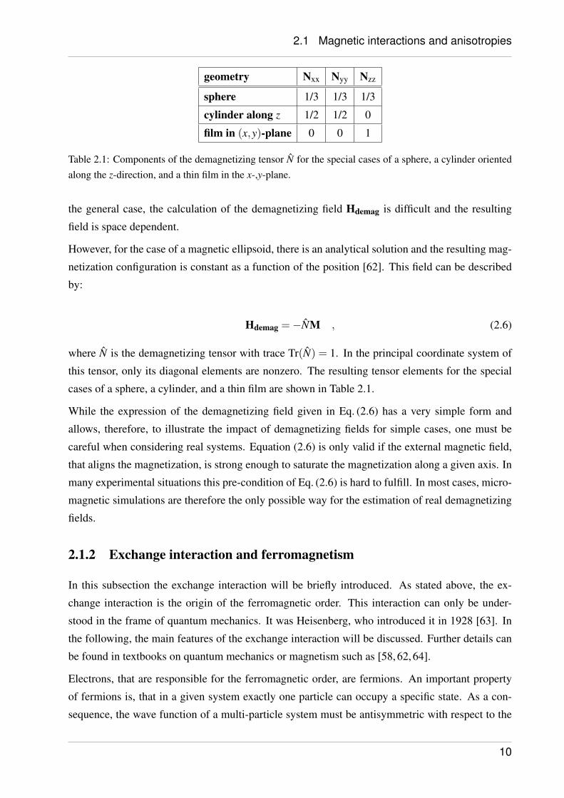
Table 2.1: Components of the demagnetizing tensor N for the special cases of a sphere, a cylinder orientedalong the z-direction, and a thin film in the x-,y-plane.

the general case, the calculation of the demagnetizing field Hdemag is difficult and the resulting

field is space dependent.

However, for the case of a magnetic ellipsoid, there is an analytical solution and the resulting mag-

netization configuration is constant as a function of the position [62]. This field can be described

by:

Hdemag =−NM , (2.6)

where N is the demagnetizing tensor with trace Tr(N) = 1. In the principal coordinate system of

this tensor, only its diagonal elements are nonzero. The resulting tensor elements for the special

cases of a sphere, a cylinder, and a thin film are shown in Table 2.1.

While the expression of the demagnetizing field given in Eq. (2.6) has a very simple form and

allows, therefore, to illustrate the impact of demagnetizing fields for simple cases, one must be

careful when considering real systems. Equation (2.6) is only valid if the external magnetic field,

that aligns the magnetization, is strong enough to saturate the magnetization along a given axis. In

many experimental situations this pre-condition of Eq. (2.6) is hard to fulfill. In most cases, micro-

magnetic simulations are therefore the only possible way for the estimation of real demagnetizing

fields.

2.1.2 Exchange interaction and ferromagnetism

In this subsection the exchange interaction will be briefly introduced. As stated above, the ex-

change interaction is the origin of the ferromagnetic order. This interaction can only be under-

stood in the frame of quantum mechanics. It was Heisenberg, who introduced it in 1928 [63]. In

the following, the main features of the exchange interaction will be discussed. Further details can

be found in textbooks on quantum mechanics or magnetism such as [58, 62, 64].

Electrons, that are responsible for the ferromagnetic order, are fermions. An important property

of fermions is, that in a given system exactly one particle can occupy a specific state. As a con-

sequence, the wave function of a multi-particle system must be antisymmetric with respect to the

10

2.1 Magnetic interactions and anisotropies

exchange of one particle with another. This is the statement of the well-known Pauli principle from

1925 [65].

In a two-electron system like the hydrogen molecule, the total electronic wave function is com-

posed of a spin-dependent part and a space-dependent part. To end up with an antisymmetric total

wave function, there are two possible combinations of these parts: a symmetric spin-dependent

wave function (spins aligned parallel) with an antisymmetric spatial wave function or vice versa.

Therefore, the Pauli principle can be regarded as the connection of these two different parts, that

describe the spin state and the local position.

Symmetric and antisymmetric spatial wave functions lead to different relative averaged positions

of the electrons with respect to each other as well as with respect to the hydrogen cores. As a result,

the symmetric and antisymmetric spatial wave functions lead to different Coulomb energies. These

difference of the Coulomb energies is called the exchange energy. Of course, the lower energy state

is more probable. Thus, a system exhibits a preferred symmetry of the spatial wave function. As

a consequence, the spin-dependent part of the wave function will adapt its symmetry. Therefore,

the preferential occurrence of a parallel or antiparallel alignment of the electron spins and, thus,

magnetic order is caused by the Coulomb interaction.

Quantum mechanical derivations show, that the exchange energy for a two-electron system with

atoms n and m can be expressed via the exchange integral:

Jn,mex = 2

∫ϕ∗n (r1)ϕ

∗m(r2)

e2

|r1− r2|ϕn(r2)ϕm(r1) (2.7)

with the one-electron wave functions ϕn,m. The exchange integral (2.7) allows for a description of

the exchange energy of a spin Si in terms of the orientation of the neighboring spins S j:

E iex =−

2Jex

h2 Si ·n.n.∑

j

S j =2Jex

gµBh2 µi ·n.n.∑

j

S j , (2.8)

where the sum is taken over the next neighbors (n.n.) of the spin Si and the exchange integral is

assumed to be the same for all neighbors. In the last step, the relation µi =−gµBSi was used.

As can be understood on the basis of the exchange integral, it is a reasonable simplification to

take only neighboring spins into account for the calculation of the exchange energy. The exchange

integral is based on the overlap of the one-electron wave functions of different atoms. This overlap

decreases drastically if going from neighboring atoms to atoms that are in larger distance to each

other. This justifies an approximate approach restricted to nearest neighbors.

By using Eq. (2.8) it is possible to define the exchange field

11

2.2 Spin dynamics

Hex =−2Jex

gµBh2

n.n.∑j

S j . (2.9)

Further consideration do also allow to express this exchange field in the following useful form:

Hex =D

µ0Ms∆M , (2.10)

where D = 2AMs

is the exchange stiffness that can be calculated with the exchange constant A and

the saturation magnetization MS.

2.1.3 Crystalline anisotropy

In this subsection the crystalline anisotropy will be introduced. The crystalline anisotropy is caused

by the spin-orbit interaction. It describes the anisotropy of the magnetization direction with respect

to the crystallographic axes of a solid state body [58, 62].

To minimize the energy in a solid state, the individual atoms are arranged in a specific orientation

and distance to each other to achieve an optimal overlap of the atomic orbitals [66]. This orientation

defines the orbital momentum L of the solid state. Due to the spin-orbit interaction ∝ ξSOL ·S, the

orientation of the atomic orbitals also leads to a preferential direction for the spin S. In materials

with ferromagnetic order, this leads to a magnetic easy axis which is the magnetization direction

corresponding to the energy minimum of the spin-orbit interaction.

In the absence of external magnetic fields, the magnetization will mostly be oriented along an easy

axis. If an external field forces the magnetization in another direction, the energy of the system is

increased with respect to this ground state.

The crystalline anisotropy is usually described phenomenologically by the anisotropy constants for

the investigated material and the angle between the actual magnetization direction and the easy axis

direction. It is possible to express the anisotropy field in the following way via the free anisotropy

energy density Eani and the magnetization [58, 62]

Hani =−1µ0

∂Eani

∂M. (2.11)

2.2. Spin dynamics

In this section, the issue of spin dynamics will be discussed. The term spin dynamics usually

refers to the precessional motion of the magnetic moments in a solid state about an effective field

12

2.2 Spin dynamics

direction. In this motion, the individual magnetic moments can have a relative phase to each other.

Due to the coupling of the magnetic moments via dipolar and exchange interaction, this relative

phase cannot have arbitrary values, but forms a periodic pattern in space. Thus, the frequency of

the precession and the periodicity of the relative phase can be used to define the frequency and

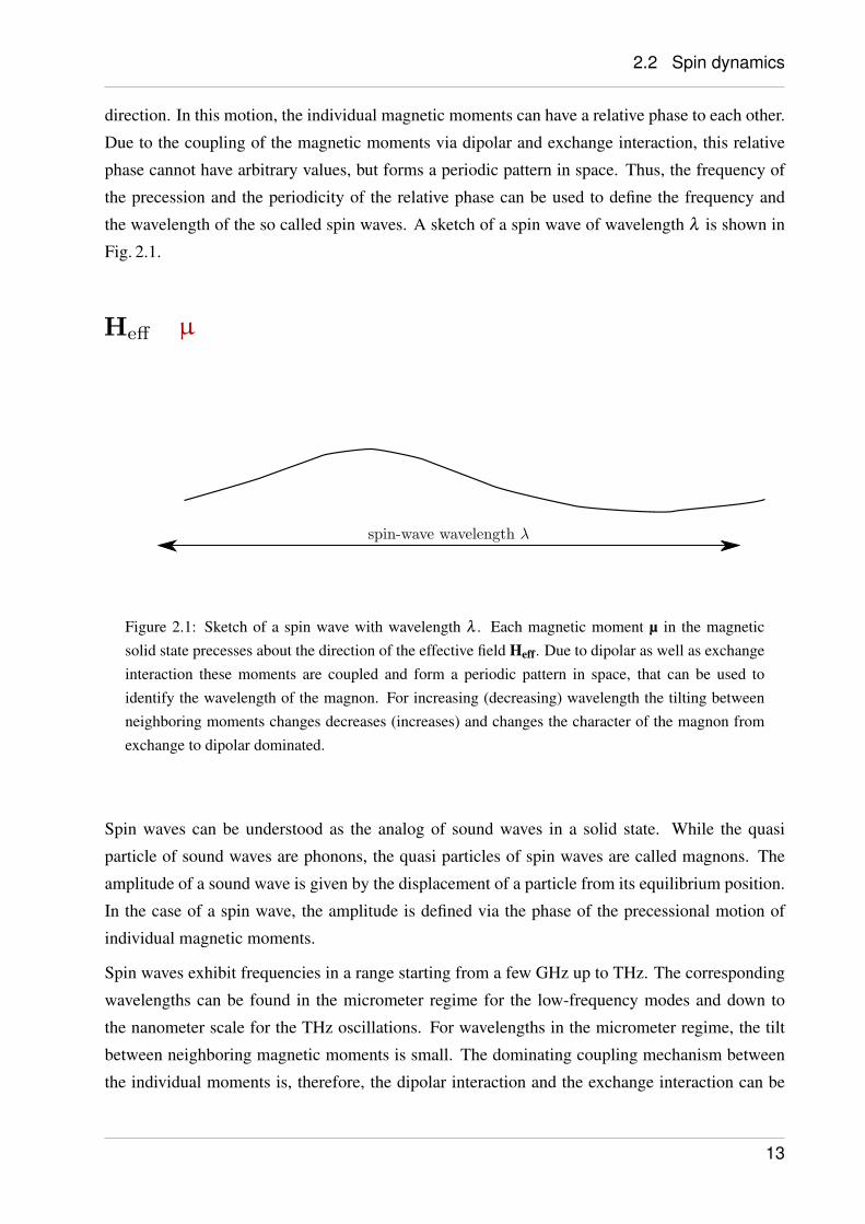
the wavelength of the so called spin waves. A sketch of a spin wave of wavelength λ is shown in

Fig. 2.1.

Figure 2.1: Sketch of a spin wave with wavelength λ . Each magnetic moment µ in the magneticsolid state precesses about the direction of the effective field Heff. Due to dipolar as well as exchangeinteraction these moments are coupled and form a periodic pattern in space, that can be used toidentify the wavelength of the magnon. For increasing (decreasing) wavelength the tilting betweenneighboring moments changes decreases (increases) and changes the character of the magnon fromexchange to dipolar dominated.

Spin waves can be understood as the analog of sound waves in a solid state. While the quasi

particle of sound waves are phonons, the quasi particles of spin waves are called magnons. The

amplitude of a sound wave is given by the displacement of a particle from its equilibrium position.

In the case of a spin wave, the amplitude is defined via the phase of the precessional motion of

individual magnetic moments.

Spin waves exhibit frequencies in a range starting from a few GHz up to THz. The corresponding

wavelengths can be found in the micrometer regime for the low-frequency modes and down to

the nanometer scale for the THz oscillations. For wavelengths in the micrometer regime, the tilt

between neighboring magnetic moments is small. The dominating coupling mechanism between

the individual moments is, therefore, the dipolar interaction and the exchange interaction can be

13

2.2 Spin dynamics

almost neglected. Spin waves in this limit of long wavelength are usually referred to as dipolar-

dominated or magneto-static spin waves. The spin-wave modes investigated in the present work

can be assumed to be dipolar-dominated waves. Following an intermediate regime of dipolar-

exchange waves, we find the exchange-dominated spin-waves for small wavelengths. In this case

of small wavelength the dispersion takes the simple form of f ∝ Dk2.

In the following, the basic concepts for the description of magneto-static spin dynamics or spin

waves will be introduced. The discussion starts with the derivation of the well-known Landau-

Lifshitz equation that governs all spin dynamics. Based on this equation, a general approach

for the derivation of a linearized spin-wave dispersion in magnetic films will be presented. For

this purpose, the Polder susceptibility and the Walker equation will be introduced subsequently

in the subsections 2.2.1 and 2.2.2. This derivation is purely based on the dipolar interaction and,

therefore, only valid in the limit of long wavelength.

Finally, an analytical solution for spin dynamics in magnetic thin films derived by Kalinikos and

Slavin will be presented. This analytical solution will be used throughout the entire work to model

the experimental findings. For this purpose, the Kalinikos and Slavin model will be extended to

systems with finite lateral dimensions in an additional subsection.

In the last three subsections the origin and the impact of the Gilbert damping, the intrinsic nonlin-

earity of the Landau-Lifshitz and Gilbert equation, and the parametric amplification of spin waves

will be discussed.

2.2.1 Landau-Lifschitz equation and Polder susceptibility

The starting point for the following discussion of spin dynamics is the torque D, that acts on a

magnetic moment µm in an effective magnetic field Heff [57, 58]:

D = µ0µm×Heff , (2.12)

where µ0 is the vacuum permeability. This magnetic moment µm is connected to a corresponding

angular momentum J via µm = γJ, where the gyromagnetic ratio γ =−28 GHz/T serves a propor-

tionality constant. Since a torque is the derivation of an angular momentum with respect to time,

it can be also expressed via the equation

D = dJ/dt = γµ0J×Heff . (2.13)

Together with the relation M = γNJ between N magnetic moments γJ and the magnetization

M, it is possible to formulate the fundamental equation of spin dynamics, the Landau-Lifshitz

equation [67]:

14

2.2 Spin dynamics

dMdt

=−µ0 |γ|(M×Heff) . (2.14)

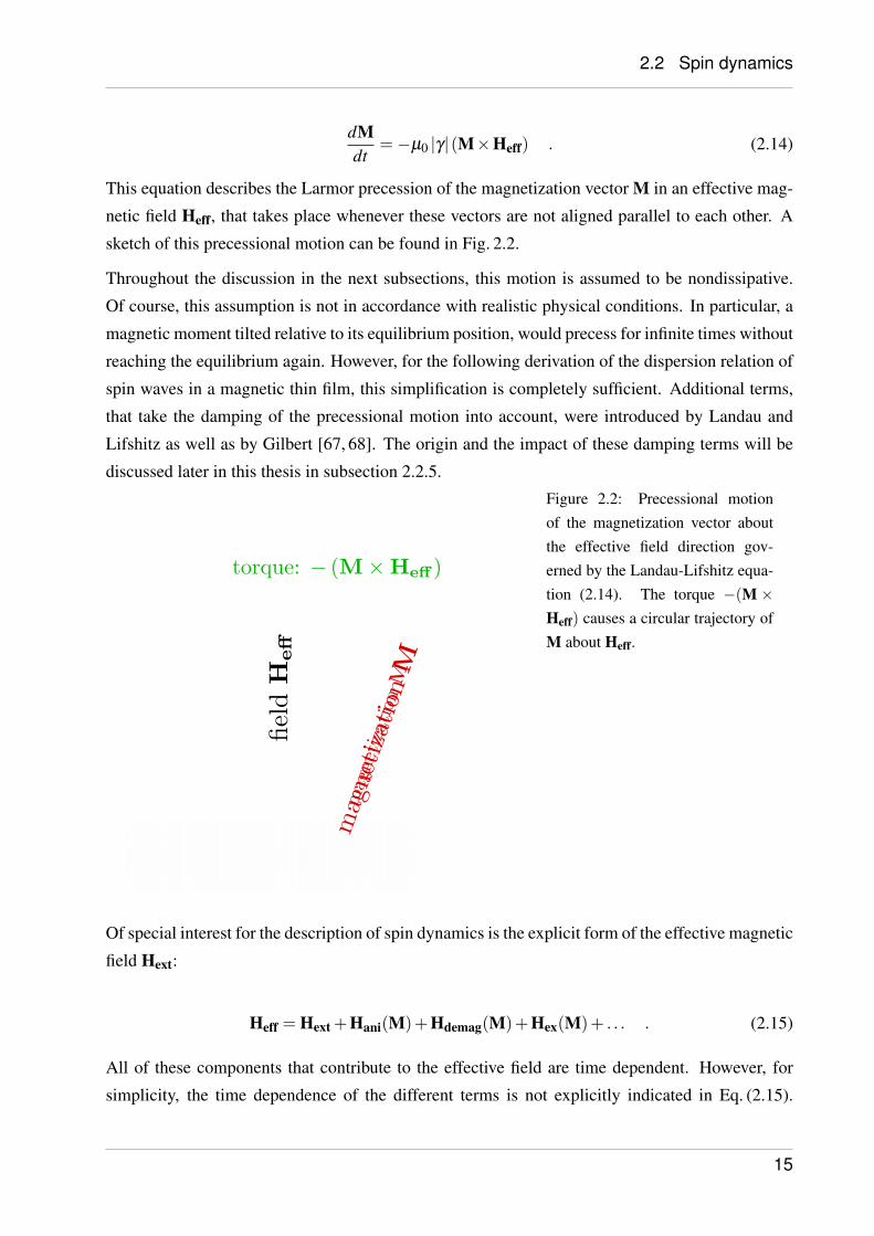
This equation describes the Larmor precession of the magnetization vector M in an effective mag-

netic field Heff, that takes place whenever these vectors are not aligned parallel to each other. A

sketch of this precessional motion can be found in Fig. 2.2.

Throughout the discussion in the next subsections, this motion is assumed to be nondissipative.

Of course, this assumption is not in accordance with realistic physical conditions. In particular, a

magnetic moment tilted relative to its equilibrium position, would precess for infinite times without

reaching the equilibrium again. However, for the following derivation of the dispersion relation of

spin waves in a magnetic thin film, this simplification is completely sufficient. Additional terms,

that take the damping of the precessional motion into account, were introduced by Landau and

Lifshitz as well as by Gilbert [67, 68]. The origin and the impact of these damping terms will be

discussed later in this thesis in subsection 2.2.5.

Figure 2.2: Precessional motionof the magnetization vector aboutthe effective field direction gov-erned by the Landau-Lifshitz equa-tion (2.14). The torque −(M ×Heff) causes a circular trajectory ofM about Heff.

Of special interest for the description of spin dynamics is the explicit form of the effective magnetic

field Hext:

Heff = Hext +Hani(M)+Hdemag(M)+Hex(M)+ . . . . (2.15)

All of these components that contribute to the effective field are time dependent. However, for

simplicity, the time dependence of the different terms is not explicitly indicated in Eq. (2.15).

15

2.2 Spin dynamics

The major components of the effective field Heff are the external field Hext, the anisotropy field

Hani(M), the demagnetizing field Hdemag(M), and the exchange field Hex(M). The dependence

of the three latter fields on the magnetization gives rise to their time dependence as well as the

nonlinearity of the Landau-Lifshitz equation. In fact, nonlinear phenomena are well-known to

appear in the spin system. Experimental results on nonlinear spin dynamics are presented in section

4.4. However, the following discussion is restricted to the limiting case of linear spin dynamics.

This limiting case is a good approximation as long as the cone angle of the spin precession is small.

Since nonlinear spin dynamics are essential for the understanding of the following experimental

results, section 2.2.6 is devoted to the basic concepts for their description.

In addition to the linearization of the Landau-Lifshitz equation and for further simplification, we

assume the case of insignificant anisotropy (Hani = 0) as well as exchange field (Hex = 0). The

general approach for solving the Landau-Lifshitz equation is not changed by these simplifications.

The approach presented in the following can be also found in the work of Hurben and co-workers

[69]. The more general case of finite anisotropy Hani 6= 0 was also discussed by Hurben in [70].

The modification of these approaches due to the exchange field (Hex 6= 0) is illustrated in [57, 58].

The present case of linear spin dynamics is associated with small time-dependent components of

the effective field Heff as well as of the magnetization M. Thus, it is possible to express these

quantities as the sum of static and dynamic parts:

Heff = H0 +h(t) and M = M0 +m(t) , (2.16)

where h(t)H0 and m(t)M0. Substituting Eq. (2.16) into the Landau-Lifshitz equation (2.14)

yields:

dmdt

= γµ0 (H0×M0 +M0×h+m×H0 +m×h) . (2.17)

In the following we assume an infinite and single-domain magnetic medium with the static mag-

netization M0 as well as the static field H0 pointing in z-direction. In the limit of small time-

dependent components, this restricts the dynamic components to the x-, y- plane:

h(t) =

hx(t)

hy(t)

0

and m(t) =

mx(t)

my(t)

0

. (2.18)

The disregard of terms of second order in the small quantities h(t) and m(t) as well as the assump-

tion of a harmonic time dependence ∝ exp(−iωt) finally leads to

16

2.2 Spin dynamics

−iωm = z× (−ωMh+ω0m) . (2.19)

To allow for a compact notation the following abbreviations have been used in Eq. (2.19):

ω0 =−γµ0Heff and ωM =−γµ0Ms . (2.20)

On the basis of Eq. (2.19), it is possible to derive the linear response χ of the dynamic magnetiza-

tion m to a dynamic magnetic field h:

m = χ ·h , (2.21)

where

χ =

(χ −iκ

iκ χ

)(2.22)

and

χ =ω0ωM

ω20 −ω2 and κ =

ωωM

ω20 −ω2 . (2.23)

The matrix in Eq. (2.22) is called the Polder susceptibility. As already pointed out, it describes

the linear response of the magnetization to a dynamic magnetic field in a nondissipative, infinite

magnetic medium in the absence of anisotropy and exchange fields.

The Polder susceptibility exhibits a resonance for frequencies ω close to ω0, that is ω→ω0. Since

the derivation presented above does not contain any space-dependent terms, this resonance is asso-

ciated with the in-phase precessional motion of all magnetic moments in the medium. The special

case of an in-phase precession, and thus infinite wavelength, is usually referred to as ferromagnetic

resonance (FMR).

For the more interesting and general case of finite wavelengths and magnetic thin films (instead of

an infinite medium), the Maxwell equations must be taken into account. The further development

of the above derivation will be described in the next subsection.

2.2.2 Walker equation and dispersion relation for magnetic films

In the following, the discussion of spin dynamics will be extended to the case of magnetic films and

finite wavelength on the basis of the Polder susceptibility in Eq. (2.22). Therefore, the restrictions

17

2.2 Spin dynamics

(Hani = 0 and Hex = 0) and the definitions (Heff = H0+h(t) and M = M0+m(t) with H0 and M0

in z-direction) from the previous subsection are still valid in the present one.

The major difference between the two cases of an infinite magnetic medium with infinite wave-

length on the one hand, and a finite magnetic volume with a finite wavelength on the other hand,

are the stray fields that arise in the latter case. Therefore, the Maxwell equations, that describe

stray fields, must be combined with the Polder susceptibility to derive the dispersion relation for

spin waves in magnetic films. Equations (2.24) show the Maxwell equations in the magneto-static

limit:

∇×Heff = 0 and ∇ ·B = 0 , (2.24)

where

B = µ0 (Heff +M) . (2.25)

Using the presentation of Heff and M in terms of static and dynamics parts as given in Eq. (2.16),

the above equations can be rewritten as follows to describe the dynamic stray fields in the system:

∇×h = 0 and ∇ · (h+m) = 0 . (2.26)

The dynamic magnetization m in Eq. (2.26) can be expressed via the Polder susceptibility in

Eq. (2.22) in terms of the dynamic field component h. Substituting this expression in Eqs. (2.26),

we end up with a system of differential equations exclusively depending on h:

∇×h = 0 (2.27)

∇ · (1+χ)h = 0 . (2.28)

Equation (2.27) allows for the definition of a scalar potential ψ with h =−∇ψ . The corresponding

differential equation for this potential can be derived from Eq. (2.28) and is given by:

(1+ χ)

[∂ 2ψ

∂x2 +∂ 2ψ

∂y2

]+

∂ 2ψ

∂ z2 = 0 , (2.29)

where χ is a matrix element of the Polder susceptibility and can be found in Eq. (2.23). Equation

(2.29) is called the Walker equation. Via the contribution of the Polder susceptibility it describes

the time dependence of the corresponding spin dynamics. The space dependence given by the

dipolar interaction was introduced by the Maxwell equations. Thus, the equation describes spin

waves with finite wavelength.

18

2.2 Spin dynamics

The Walker equation can be used as the fundamental equation for the derivation of the spin-wave

dispersion in different geometries. Since all experiments presented in this thesis were performed

with magnetic thin films, the following paragraphs are devoted to a sketch of the general approach

towards a dispersion relation for films. A more general approach even valid for the case of multi-

layered structures can be also found in [71].

In this derivation, the static magnetization M0 and the static effective field H0 are aligned parallel

to each other and along the z-axis as before. The magnetic film with a thickness d is positioned in

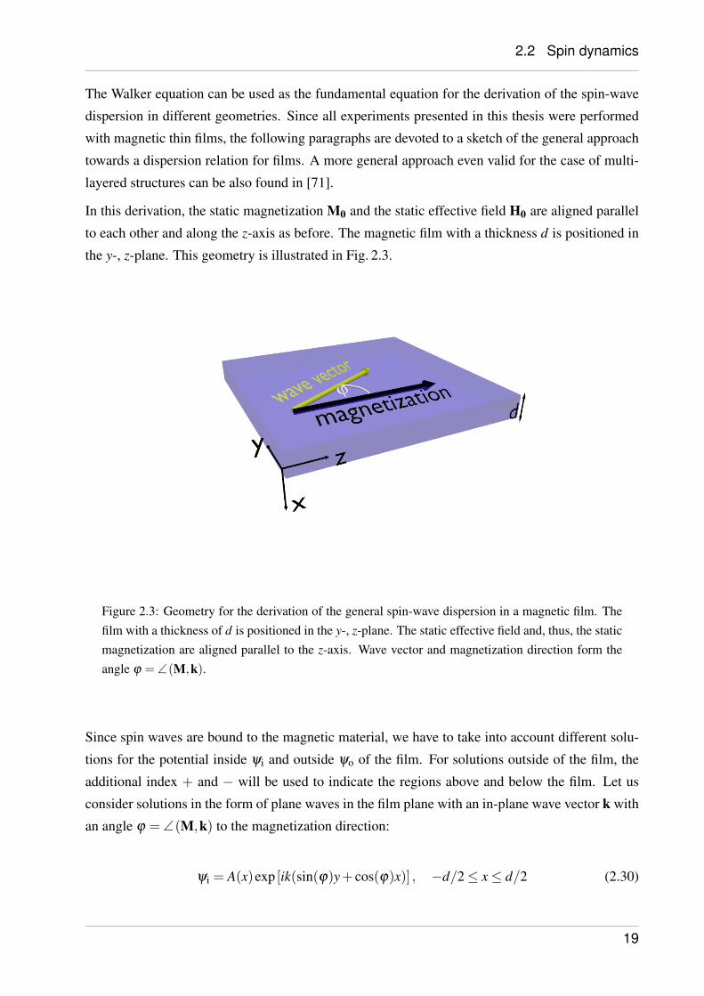
the y-, z-plane. This geometry is illustrated in Fig. 2.3.

Figure 2.3: Geometry for the derivation of the general spin-wave dispersion in a magnetic film. Thefilm with a thickness of d is positioned in the y-, z-plane. The static effective field and, thus, the staticmagnetization are aligned parallel to the z-axis. Wave vector and magnetization direction form theangle ϕ = ∠(M,k).

Since spin waves are bound to the magnetic material, we have to take into account different solu-

tions for the potential inside ψi and outside ψo of the film. For solutions outside of the film, the

additional index + and − will be used to indicate the regions above and below the film. Let us

consider solutions in the form of plane waves in the film plane with an in-plane wave vector k with

an angle ϕ = ∠(M,k) to the magnetization direction:

ψi = A(x)exp [ik(sin(ϕ)y+ cos(ϕ)x)] , −d/2≤ x≤ d/2 (2.30)

19

2.2 Spin dynamics

ψ±o = B±(x)exp [ik(sin(ϕ)y+ cos(ϕ)x)] , x≤−d/2 and x≥ d/2 . (2.31)

For the evaluation of the parameters A(x) and B±(x), the following relations must be used: The

potential inside the film ψi has to fulfill the Walker equation (2.29), that was derived above. Outside

of the film, where m = 0, the potentials ψ±o have to fulfill the Laplace equation ∆ψo = 0.

In addition, continuity conditions must be taken into account: the tangential component of the

magnetic field h and the normal component of the magnetic induction b = µ0(h+m) must be

continuous at the surface of the film. These conditions can be written as:

hiy,z = ho

y,z at x =±d/2 (2.32)

bix = bo

x at x =±d/2 . (2.33)

The details of the corresponding calculations are not presented in the following. Instead the results

will be discussed shortly in the next paragraphs. Detailed calculations taking into account the

above relations to specify the remaining parameters can be found in [58, 69, 70].

The resulting functions A(x) and B±(x) have the following form:

A(x) = acos(qx)+bsin(qx) with q = k

√(−1+ χ sin2(ϕ)

1+ χ

), (2.34)

B±(x) = c±e±kx . (2.35)

The values for the amplitudes a, b, and c± are derived in [58,69,70]. However, even without these

values, it is possible to understand the general form of the solutions in Eqs. (2.34) and (2.35).

Let us first turn to the solutions outside the magnetic material ψ±o . The potentials ψ±o describe

plane waves along the film plane, that decay in the ±x-direction which is normal to the film. It

is also interesting to note, that the decay length is given by the in-plane wave vector k. This is

reasonable, because this decay is defined by the dipolar stray fields created by the magnetization

precession. For large wavelengths, these stray fields are also large.

For the potential ψ±i inside the film, we also found plane waves in the film plane but a more

complicated form of the out-of-plane wave vector q as defined in Eq. (2.34). Without going into

detail, it should be mentioned that q can have real or imaginary values. For the latter case, the spin

wave is located at the surface of the film and its amplitude is decaying along the film thickness.

This class of surface waves also includes the well-known Damon-Eshbach spin waves [72, 73].

This class of waves is usually referred to as magneto-static surface waves (MSSW).

20

2.2 Spin dynamics

For wave vectors q with real values, the spin-wave amplitude has a harmonic distribution over the

film thickness. This class of waves is therefore referred to as magneto-static backward volume

waves (MSBVW). The word backward indicates an interesting feature of MSBVW: for this kind

of waves, the group velocity is oriented antiparallel to the wave vector and, thus, antiparallel to the

phase velocity.

The general dispersion that can be derived following the approach sketched above is:

k2− (1+ χ)2q2− κ2k2 sin2(ϕ)+2(1+ χ)qk cot(qd) = 0 , (2.36)

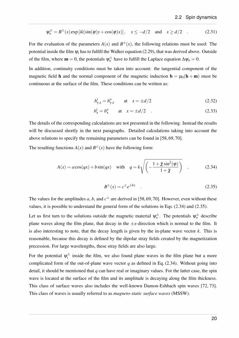
where κ is part of the Polder susceptibility and defined in Eq. (2.23). The result of corresponding

numerical calculations by Damon and Eshbach taken from [73] is shown in Fig. 2.4. It is impor-

tant to note, that the solutions ψ±i strongly depend on the angle ϕ = ∠(M,k). In particular, we

have to distinguish values of ϕ , which allow for the observation of both kinds of waves, MSSW

and MSBVW, or exclusively MSBVW. This anisotropy of the spin-wave dispersion for in-plane

magnetized films will be discussed in more detail in the following subsection.

Unfortunately, there are no analytical solutions to this implicit equation of the frequency ω without

further restrictions to the system. However, there is an approximate analytical solution if the film

thickness is restricted to values, that are small compared to the spin-wave wavelength d λ . This

is the case in all sample layouts used in the experiments of the present work. Therefore, instead

of discussing this general spin-wave dispersion in more detail, the analytical solution for very thin

films by Kalinikos and Slavin [74] will be introduced in the next subsection.

Before turning to this analytical model, the present subsection will be closed with some final re-

marks regarding the general dispersion. For the numerical calculation of the solutions to Eq. (2.36)

it is more practical to use the following representation where q was substituted by Eq. (2.34):

1− (1+ χ)2(−1+ χ sin2

ϕ

1+ χ

)− κ

2 sin2ϕ

+2(1+ χ)

√−1+ χ sin2

ϕ

1+ χcot

kd

√−1+ χ sin2

ϕ

1+ χ

= 0 .

(2.37)

In addition, it has to be emphasized that the approach sketched above does not take into account

a possible orientation of the magnetization perpendicular to the film plane. Calculations for an

out-of-plane magnetization yield the so called magneto-static forward volume waves (MSFVW).

As the MSBVW, this class of spin wave is formed by volume waves. In contrast to the MSBVW,

the group velocity and the wave vector point into the same direction for MSFVW. One interesting

feature for out-of-plane magnetization is the isotropy of the dispersion with respect to the in-plane

21

2.2 Spin dynamics

surface mode (MSSW)

volume waves (MSBVW)

frequency

kz

ky

Figure 2.4: Spin-wave dispersion according to Eq. (2.37) taken from a publication by Damon andEshbach [73]. For some angles ϕ the dispersion exhibits both, surface and volume waves. Both kindsof waves are anisotropic with respect to the angle ϕ . The volume-wave dispersion comprises severaldifferent thickness modes, which can be distinguished by their out-of-plane wave vector in Eq. (2.34).

wave vector. This isotropy is a result of the symmetry of the system. In contrast to the case of

an in-plane magnetization, the angle between magnetization and wave vector is fixed and cannot

change the propagation characteristics.

2.2.3 Analytical model for the spin-wave dispersion in magnetic thin films

This subsection is devoted to the introduction of an analytical dispersion relation for spin waves

in magnetic thins films derived by Kalinikos and Slavin in 1986 [74]. As already discussed above,

there are no analytical solutions to the general spin-wave dispersion in magnetic films presented in

Eq. (2.37). However, as shown by Kalinikos and Slavin, it is possible to find an approximate ana-

lytical solution by restricting the film thickness to values, that are small compared to the spin-wave

wavelength d λ . As this restriction is valid in all experiments presented below, this analyti-

cal equation will be used for all calculations throughout the present work. As an indication of

the reliability of this solution, several publications can be found that show a good accordance of

experimental findings and calculated values (see for example [36–40, 75]).

The dispersion relation has the following form:

22

2.2 Spin dynamics

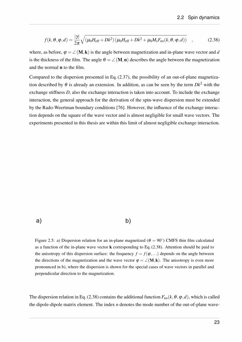
f (k,θ ,ϕ,d) =|γ|2π

√(µ0Heff +Dk2)(µ0Heff +Dk2 +µ0MsFnn(k,θ ,ϕ,d)) , (2.38)

where, as before, ϕ =∠(M,k) is the angle between magnetization and in-plane wave vector and d

is the thickness of the film. The angle θ =∠(M,n) describes the angle between the magnetization

and the normal n to the film.

Compared to the dispersion presented in Eq. (2.37), the possibility of an out-of-plane magnetiza-

tion described by θ is already an extension. In addition, as can be seen by the term Dk2 with the

exchange stiffness D, also the exchange interaction is taken into account. To include the exchange

interaction, the general approach for the derivation of the spin-wave dispersion must be extended

by the Rado-Weertman boundary conditions [76]. However, the influence of the exchange interac-

tion depends on the square of the wave vector and is almost negligible for small wave vectors. The

experiments presented in this thesis are within this limit of almost negligible exchange interaction.

a) b)

Figure 2.5: a) Dispersion relation for an in-plane magnetized (θ = 90) CMFS thin film calculatedas a function of the in-plane wave vector k corresponding to Eq. (2.38). Attention should be paid tothe anisotropy of this dispersion surface: the frequency f = f (ϕ, . . .) depends on the angle betweenthe directions of the magnetization and the wave vector ϕ = ∠(M,k). The anisotropy is even morepronounced in b), where the dispersion is shown for the special cases of wave vectors in parallel andperpendicular direction to the magnetization.

The dispersion relation in Eq. (2.38) contains the additional function Fnn(k,θ ,ϕ,d), which is called

the dipole-dipole matrix element. The index n denotes the mode number of the out-of-plane wave-

23

2.2 Spin dynamics

vector component of the corresponding spin-wave mode. Since the film thickness was assumed to

be very small, this out-of-plane component is quantized and can have only discrete values defined

by the film thickness and the mode number n. In the following, only the lowest order mode with

n = 0 will be considered. In this case, the dipole-dipole matrix element has the following form:

F00(k,θ ,ϕ,d) = P00 + sin2θ

(1−P00(1+ cos2

ϕ)+µ0MsP00(1−P00)sin2

ϕ

µ0Heff +Dk2

), (2.39)

where

P00(k,d) = 1− 1− exp(−kd)kd

. (2.40)

The calculated dispersion surface according to Eq. (2.38) is shown in Fig. 2.5a) for a 30 nm thick

Co2Mn0.6Fe0.4Si film and an in-plane external magnetic field of µ0Hext = 48.5 mT. As can be seen,

only one solution exists for all k and ϕ . This is in contrast to the general dispersion for magnetic

films as shown in Fig. 2.4, where surface and volume modes can exist simultaneously for specific

values of ϕ .

The absence of multiple co-existing modes is a result of the small thickness assumed for the cal-

culations of Kalinikos and Slavin. For very thin films the decay of the surface waves across the

thickness of the film is large compared to the thickness. Therefore, the mode profiles can be as-

sumed to be constant over the entire film thickness like in the case of MSBVW.

For ϕ = 90 the spin waves in the Kalinikos model have similar dispersion characteristics as the

Damon-Eshbach surface waves in the previous section. If the angle ϕ is gradually decreased to

zero, the group velocity decreases and becomes negative as in the previous case of MSBVW.

However, in the case of thin films, the mode profile across the film thickness is almost preserved.

The changing dispersion characteristics depending on ϕ are the result of the anisotropy of the spin-

wave dispersion relation, that was already mentioned above and will be discussed in the following.

Because of the ambiguities related to the terms surface and volume waves in thin films, individual

modes will rather be characterized by their angle ϕ in the rest of this thesis. In contrast to this, the

term Damon-Eshbach wave will still be used for waves with ϕ = 90.

The changing dispersion characteristics and the anisotropy is very pronounced in Fig. 2.5b). In

this graph, the dispersion curves for the in-plane wave vector k parallel (k ‖M) and perpendicular

(k ⊥M) to the magnetization M are shown. As can be seen, the slope of the dispersion curve

for k ‖M is negative. This is reminiscent of the discussion about the MSBVW in the previous

subsection and leads to a group velocity vG = 2π∂ f∂k pointing in the opposite direction than the

wave vector.

24

2.2 Spin dynamics

In the case of k⊥M the slope of the dispersion curve, and therefore the resulting group velocity,

is much higher than in the case of k ‖M. In addition to the higher excitation efficiency, that will be

discussed in the corresponding section of chapter 4, the high group velocity is an important reason

for the common choice of Damon-Eshbach waves in most experiments on the microscale.

2.2.4 Quantization in finite systems

In the present subsection, the quantization of spin waves due to lateral confinement will be dis-

cussed. As known from classical wave physics and in particular from quantum mechanics, the

confinement of waves leads to a discretization of the possible wave vectors and, thus, of the ener-

gies in a system. The model for the spin-wave dispersion in magnetic thin films by Kalinikos and

Slavin, that was discussed in the previous paragraphs, already incorporates the confinement due

to the film thickness. As mentioned above, the dispersion in thin films therefore exhibits different

standing spin-wave modes across the film thickness. Since the energy separation of these modes is

in the range of ~10 GHz for the samples used in the present work, only the lowest thickness mode

must be considered in the following.

However, the experimental results presented below have been obtained not for a magnetic film but

for microstructures. Thus, in addition to the above-mentioned quantization across the film thick-

ness, the lateral confinement must be taken into account. Many experimental findings indicate,

that not only a geometric confinement due to the patterning of microstructures is relevant. The

quantization of spin waves was also observed for inhomogeneous configurations of the effective

field. Since the energy of a spin-wave strongly depends on the effective field, inhomogeneous con-

figurations can lead to potential wells for low-frequency modes. Exemplary results can be found

in [77–80]. The two cases of a purely geometric confinement as well as confinement due to field

inhomogeneities will be addresses in the following.

Even though the model by Kalinikos and Slavin was developed for a system without lateral con-

finement, its application to finite systems by the introduction of additional quantization conditions

turned out to be very successful in many cases [77, 79, 81–83]. An important issue regarding the

quantization condition for the spin-wave wave vector

kn =nπ

weff, n ∈ N (2.41)

is the evaluation of the effective width weff, that leads to the quantization. This effective width can

strongly differ from the geometrical one. If we consider the important case of a spin-wave waveg-

uide, there are two cases of particular interest: the magnetization direction along the waveguide

and the magnetization direction along the width of the waveguide.

25

2.2 Spin dynamics

In the first case, static demagnetizing fields can be neglected and the resulting effective field is

constant across the waveguide. However, in this case the dynamic demagnetizing fields result

in an effective width that is larger than the actual width of the waveguide. The corresponding

derivation can be found in [81].

In the second case of a waveguide that is magnetized along its width, the static demagnetizing

fields must be taken into account. Since this corresponds to the experimental situation in the

present work, details will be also discussed together with the experimental findings in sections 4.2

and 4.4. Therefore, the following remarks will only briefly comment on this issue.

In general, the static demagnetizing fields lead to an inhomogeneous effective field across the

width of the waveguide. In the center of the waveguide, the field can be assumed to be constant

in a certain range. The estimation of this area of almost constant effective field defines the effec-

tive width weff of the waveguide, which is smaller than the geometrical one. While this argument

describes the center area of the waveguide, the situation at the edges must be considered on its

own. The strongly decreased effective field at the edges of the waveguide forms a potential well

for low-frequency modes. The frequencies of these modes can be far below the dispersion relation

for modes that propagate in the center of the waveguide. Thus, a quantization due to the inho-

mogeneous effective field can be observed. These modes are usually referred to as edge modes.

Experimental evidence can be found in [82, 84].

Even though there is also an additional model for the spin-wave dispersion, that was developed

especially for waveguide structures [85], the description of waveguides magnetized across their

width turns out to be complicated. The reason is the demagnetizing field. Experimentally, it is very

difficult to fully saturate the magnetization close to the edges. Thus, there is no analytical model

that can describe the trend of the effective field or the inhomogeneous magnetization configuration.

Therefore, quantitative agreement of calculations and experimental findings cannot be achieved in

this case, even though all physical mechanisms are known. This argument will be illustrated for

the actual situations in the description of the experimental results below.

2.2.5 Gilbert damping

In this section, the impact and the origin of dissipation in spin dynamics will be discussed. As

already mentioned above, all derivations presented so far are based on the Landau-Lifshitz equation

(2.14) for nondissipative systems. While the assumption of nondissipative systems is an important

simplification for the theoretical description of spin dynamics, it does, of course, not correspond

to real systems.

Landau and Lifshitz were the first to propose an additional damping term for the extension of

the Landau-Lifshitz equation [67]. However, their approach was contradictory since it led to an

26

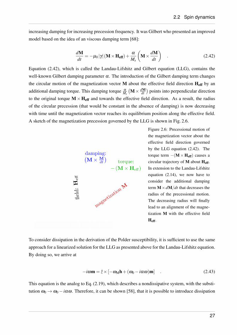
2.2 Spin dynamics

increasing damping for increasing precession frequency. It was Gilbert who presented an improved

model based on the idea of an viscous damping term [68]:

dMdt

=−µ0 |γ|(M×Heff)+α

Ms

(M× dM

dt

). (2.42)

Equation (2.42), which is called the Landau-Lifshitz and Gilbert equation (LLG), contains the

well-known Gilbert damping parameter α . The introduction of the Gilbert damping term changes

the circular motion of the magnetization vector M about the effective field direction Heff by an

additional damping torque. This damping torque α

Ms

(M× dM

dt

)points into perpendicular direction

to the original torque M×Heff and towards the effective field direction. As a result, the radius

of the circular precession (that would be constant in the absence of damping) is now decreasing

with time until the magnetization vector reaches its equilibrium position along the effective field.

A sketch of the magnetization precession governed by the LLG is shown in Fig. 2.6.

Figure 2.6: Precessional motion ofthe magnetization vector about theeffective field direction governedby the LLG equation (2.42). Thetorque term −(M×Heff) causes acircular trajectory of M about Heff.In extension to the Landau-Lifshitzequation (2.14), we now have toconsider the additional dampingterm M×dM/dt that decreases theradius of the precessional motion.The decreasing radius will finallylead to an alignment of the magne-tization M with the effective fieldHeff.

To consider dissipation in the derivation of the Polder susceptibility, it is sufficient to use the same

approach for a linearized solution for the LLG as presented above for the Landau-Lifshitz equation.

By doing so, we arrive at

−iωm = z× [−ωMh+(ω0− iαω)m] . (2.43)

This equation is the analog to Eq. (2.19), which describes a nondissipative system, with the substi-

tution ω0→ ω0− iαω . Therefore, it can be shown [58], that it is possible to introduce dissipation

27

2.2 Spin dynamics

in the system by making the same substitution ω0→ ω0− iαω in the Polder susceptibility tensor.

The Polder susceptibility for dissipative system can then be used for all further derivations.

The Gilbert damping parameter can be connected to the decay time τ of the investigated spin-wave

modes. This is shown here exemplary for the case of Damon-Eshbach spin waves [86]:

τ =1

αγµ0 (Heff +Ms/2). (2.44)

A finite decay time is always connected to a certain linewidth in the spectrum of a system. By the

introduction of dissipation in the spin system, the Polder susceptibility can be used to describe this

linewidth in the frequency space. Excitation spectra of the spin system show a Lorentzian behavior

[58]. These spectra are experimentally accessible via ferromagnetic resonance experiments and can

be used to evaluate the Gilbert damping in magnetic thin films (see for example [87] and [A8]).

The introduction of the Gilbert damping parameter, that leads to the LLG, is a phenomenological

approach that does not allow for any conclusion about the magnitude of the damping. Even though

serious research efforts combined basic theory with ab-initio calculations over the last decades [50,

88–93], there is still no self-contained theory for the description of all phenomenological findings

related to the Gilbert damping. An example for these difficulties is the temperature dependence of

α , that is not understood thoroughly.

However, in most theories the following general dependence can be found:

α ∝ ξ2SOD(EF) , (2.45)

where ξ 2SO and D(EF) are the square of the spin-orbit interaction and the densitiy of states at the

Fermi level EF, respectively.

In fact, there is strong experimental evidence for these dependencies of the Gilbert damping pa-

rameter on the spin-orbit inter interaction [94–96] as well as on the density of states [51, 52]. This

can be understood even by basic considerations about the possible loss channels in a magnetic

medium. In a magnetic solid state we can identify three subsystems, namely the phonon system,

the electron system, and the spin system. The coupling of these systems with regard to the Gilbert

damping will be discussed in the next paragraphs.

Spin-spin interactions are driven by nonlinearities in the spin system or scattering on defects and

impurities. These interactions can indeed lead to an energy redistribution in the spin system and,

thus, an enhanced relaxation rate for a particular spin-wave mode [97–100]. However, this loss

channel is usually excluded from the discussion about the intrinsic Gilbert damping. The reason for

this is the dependence of the related effects to extrinsic parameters. In the case of nonlinear effects,

this can be the power of an external excitation of the spin system in an individual measurement.

28

2.2 Spin dynamics

Magnon-magnon scattering mechanisms depend on the actual quality of an individual sample and

therefore not only on general properties of the investigated material.

Therefore, the major constituents of the intrinsic Gilbert damping are the interactions of the spin

system with the phonon system [101] as well as with the electron system. The coupling to the

phonon system is given by the spin-orbit interaction. By this coupling, the energy of the spin

system is transferred to the lattice and, thus, to heat. Additional loss channels are the scattering

on electrons [90] as well as possible eddy currents in metallic systems [92]. The possibility of the

latter effects is connected to the density of states at the Fermi level.

2.2.6 Nonlinear spin dynamics

Spin dynamics is known to exhibit a large variety of nonlinear effects. As already discussed above,

the reason can be found in the intrinsically nonlinear LLG equation. We have to keep in mind,

that all derivations considered so far have been made in the limit of small dynamic magnetization

components. While this linearized approach of the description of spin dynamics is very valuable

and sufficient and many cases, it does not describe the general case of arbitrary amplitudes of the

spin precession.

The list of experimental observations of nonlinear spin dynamics is remarkable. Among the related

phenomena are various cases of nonlinear coupling of different spin-wave modes. This coupling

comprises the nonlinear higher harmonic generation as wells as the splitting of initial magnons to

secondary magnons with lower energies [22, 102–110]. Nonlinearities in the magnetic system can

also lead to a modulation of the propagation characteristics as observed in the linear regime and

in particular to the observation of solitons [111–113]. While already observed on the macroscale,

recent results on the localized and direct-current based excitation of the spin system confirmed the

existence of self-localized spin-wave bullet modes on the microscale [26, 114–117]. In addition,

a nonlinear modification of the spin-wave spectrum due to nonlinear frequency shifts or nonlinear

damping was observed [97, 99, 100, 118].

Rigorous solutions of the full LLG can be found only for limited cases with special geometries

and excitation fields. Thus, general approaches towards a model that covers all nonlinear spin

dynamics are hard to find. Typically, most approaches use expansions of the Landau-Lifshitz

equation in terms of the magnetization to determine an approximate solution. In the following the

classical approach presented in [57] will be sketched.

Basis of this derivation is the conservation of the modulus of the magnetization vector M during the

precessional motion. Based on this conservation, it is possible to express the total magnetization

as

29

2.2 Spin dynamics

M = M0 +M(1)+M(2)+ . . . , (2.46)

where |M0| |M(1)| |M(2)| . . .. Thus, in this series, M0 and M(1) can be identified with the

representation of the magnetization in terms of a static and a dynamic part as defined above for

the calculations in the linear regime (see Eq. (2.16)). Substituting the first order of the expan-

sion in Eq. (2.46) into the Landau-Lifshitz equation under the assumption of an effective field

Heff = H0 +h(t) with external dynamic field h(t) will, therefore, yield the ame results as pre-

sented in the previous subsections and, thus, M(1) is already known.

Using the expansion of M up to the second order will mix terms, that contain the already calculated

M(1), with the higher order quantity M(2). Therefore, this approach yields a linearized equation of

motion for M(2). In general, the equation of motion for order M(n) can be derived by successively

calculating the solution for all lower orders M(m) with m < n. In the simplified case of an isotropic

and nondissipative magnetic medium, the general equation of motion for M(n) can be written as

dM(n)

dt+µ0|γ|

(M(n)×H0

)=−µ0|γ|

(M(n−1)×h

). (2.47)

However, as we have seen, even the solution for a spin-wave dispersion for a nondissipative mag-

netic film in the linear case is a complicated implicit function of the frequency. Thus, even though

the derivation sketched above yields an approximate solution for nonlinear spin dynamics up to an

arbitrary order in M, the actual calculations for specific problems are complex and time consuming.

An alternative and widely used approach for a description of (nonlinear) spin dynamics is the

Hamilton formalism [119]. The general approach as well as its applications to particular cases

is also presented in [57, 58, 98, 120]. In this description, the energy of the magnetic system is ex-

pressed via the Hamilton function H . Once this function has been derived for a certain system, the

magnetization precession is expressed in terms of quantum mechanical operators for the generation

a∗k or annihilation ak of certain spin-wave modes k via a Holstein-Primakoff transformation [121].

The energy of the system is given by the Hamilton functional, that is typically expanded in a power

series in terms of the operators a∗k :

H (a∗k , ak) = H (0)+H (1)+H (2)+H (3)+ . . . . (2.48)

The dynamics of the system can be described by the terms of second and higher order. As an

explicit example, the second-order Hamiltonian can be expressed as follows:

H (2)(a∗k , ak) =∑

k

(Aka∗k ak +

12[Bka∗k a∗−k +B∗k aka−k

]), (2.49)

30

2.2 Spin dynamics

where the sum must be taken over all possible spin-wave modes k in the system. The prefactors

Ak and Bk contain the information about the investigated system such as effective field, material

parameters, and the geometry. From Eq. (2.49) the linear dispersion can be calculated via a Bogoli-

ubov transformation bk = ukak + vka∗−k. In terms of these new variables, the Hamilton operator of

second order is diagonal and the corresponding eigenvalues define the linear spin-wave dispersion:

ω2k = A2

k−|Bk|2 . (2.50)

The higher order terms of the total Hamilton in Eq. (2.48) can be treated by perturbation theory

based on the solution of Eq. (2.49). These higher orders are not diagonal in the operators bk any-

more and therefore couple different spin-wave modes k. This coupling of different spin-wave

modes can be understood as the nonlinear interaction of the single spin-wave modes. As an exam-

ple

H (3) =∑

k1,k2,k3

(Vk1,k2,k3 a∗k1

a∗k2ak3 + . . .

)(2.51)

can be understood as a three-magnon splitting. For k1 = k2, the spin-wave mode k3 splits to two

secondary magnons with half the energy than the initial one. The prefactors Vk1,k2,k3 reduce the

possible coupling of magnon modes by energy and wave-vector conservation. As illustrated by

this example, the Hamilton approach is very suited to reveal the direct coupling of different spin-

wave modes. In contrast to this, the above treatment of nonlinear spin dynamics in terms of the

magnetization allows in some cases for a more intuitive understanding.

2.2.7 Parallel parametric amplification

The following subsection is devoted to a brief introduction of the process of parallel parametric

amplification of spin-wave modes that was used in the experiments presented in subsection 4.3.

The discussion is mainly focused on a sketch of the mathematical approach for the description of

the parametric amplification. It is based on the textbooks [57,122] and the theses [27,123,124]. A

more intuitive approach for the understanding of this process will be presented together with the

corresponding experimental results in subsection 4.3.

Parallel parametric amplification denotes the amplification of spin dynamics by an external dy-

namic Oersted field h2f = h2fez that is parallel to the static external field H0 = H0ez as well as to

the static magnetization M0 = M0ez. The aim of the following sketch is a solution of the LLG

equation in the presence of this field h2f. Of major importance is an additional dynamic contribu-

tion to the effective field, namely the dynamic stray fields hS as already discussed in subsection

2.2.2.

31

2.2 Spin dynamics

By assuming solutions for the dynamic magnetization in the form of plane waves with a harmonic

time dependence

m(r, t) =∑

k

mkexp(−iωt)exp(−ikr) (2.52)

and by substituting these quantities in the nondissipative LLG, it is possible to describe the system.

A typical way for the analysis of this system is the introduction of new variables

ak =1

M0

(mkx + imky

)(2.53)

a∗−k =1

M0

(m∗−kx

+ im∗−ky

)=

1M0

(mkx + imky

). (2.54)

The equation of motion for these variables can be written as follows:

−idakdt

= (Ak + γh2f) ak +Bka∗k +Ωnk , (2.55)

with the gyromagnetic ratio γ . The quantity Ωnk summarizes nonlinear terms of higher order. Of

particular interest are the quantities Ak and Bk, that describe the ellipticity of the precessional

motion of the dynamic magnetization. The ellipticity can be expressed in terms of these variables

as follows:

ε =2|Bk|

Ak +Bk. (2.56)

As we will see in the following, the ellipticity is an essential pre-condition for the application of

parallel parametric amplification. The reason for the ellipticity is given by the dynamic stray fields

hS already mentioned some paragraphs above. This issue will be illustrated in subsection 4.3.

A Bogoliubov transformation (as already demonstrated in subsection 2.2.6) of Eq. (2.55) to the

new variables bk allows for a direct illustration of the necessity of an elliptical precession. In the

linear case, this procedure yields:

dbkdt

= iωkbk + iγh2fBkωk

b∗−k (2.57)

db∗−kdt

=−iωkb∗−k− iγh2fB∗kωk

bk . (2.58)

Thus, for |Bk| = 0, which results in an ellipticity ε = 2|Bk|Ak+Bk

= 0, the terms that contain the exter-

nal dynamic field h2f vanish and a parallel parametric amplification cannot be achieved. In this

32

2.2 Spin dynamics

case, the above Eqs. (2.57) and (2.58) describe the common spin-wave dispersion as derived in

subsection 2.2.2.

In addition, it is possible to show that the maximal amplification is obtained if the dynamic field h2f

oscillates with twice the frequency ω2f of the amplified spin-wave mode. In the particle picture, this

can be understood as follows. The dynamic Oersted field h2f can be associated with a microwave

photon. In the process of the parametric amplification, this photon splits into two magnons with

opposed wave vectors and half the frequency of the photon. The simultaneous generation of two

magnons with opposed wave vectors is caused by the coupling of these modes in Eqs. (2.57) and

(2.58). Thus, the total momentum after the splitting of the photon is zero. However, since the

wave vector of the initial photon is negligibly small compared to the spin-wave wave vectors, the

process conserves the total momentum.

It has to be mentioned, that the above derivations describe a nondissipative system. If damping is

included in the considerations, it turns out, that the parallel parametric amplification is a threshold

process. The amplification and the damping are competing processes in the magnetic system.

Only if the number of magnons generated by the splitting of microwave photons is large enough

to compensate the number of magnons that are annihilated, an amplification can be obtained.

Mathematically, this can be described by the introduction of nonlinear terms as well as a damping

term Γk in Eqs. (2.57) and (2.58). This leads to

[ddt

+Γk− i(

ωk−ω2f

2

)]bk− iPkb∗−k = 0 (2.59)

and an analog equation for the complex conjugate. In the above equation

ωk = ωk +2∑

k′Tkk′|bk′|2 (2.60)

describes a nonlinear frequency shift in the magnon system. This frequency shift can be neglected

in many cases and, therefore, ωk ≈ ωk will be assumed in the following [125]. Of particular

interest is the remaining effective pumping field

Pk =Vkh2f +∑

k′Skk′ bk′ b−k′ (2.61)

with the coupling parameter Vk between the dynamic Oersted field and the amplified magnon

mode as well as with a sum that describes the nonlinear interaction of the generated magnon pairs.

Via the parameter Skk′ , a dependence of this effective pumping field on the number of magnons

is introduced. As a consequence, the efficiency of the amplification decreases with increasing

33

2.3 Cobalt-based Heusler compounds

number of magnons in the system. Therefore, after an amplification of magnons from the thermal

level, a threshold level will be reached.

On the basis of the above considerations it is possible to derive the following equation for the

intensity of an amplified spin-wave mode

Ik(t) = I0,k exp(Vkh2f sin(Ψ)−Γk) . (2.62)

In this equation, I0,k is the initial intensity. Thus, it is obvious, that the process of parallel paramet-

ric amplification cannot be used to excite spin-wave modes from zero intensity. The coupling Vk

depends on several parameters of the system like the saturation magnetization or the ellipticity of

the precession. It can differ significantly for different spin-wave modes and the estimation of this

parameter for microstructures is difficult.

The quantity Ψ describes the phase of the amplification process. This parameter depends on the

intensity Ik and, therefore, governs the temporal evolution of Eq. (2.62). For small intensities,

Ψ = 90 = const. Thus, in this case, the intensity of the observed spin-wave mode increases if

Vkh2f > Γk . (2.63)

This condition defines the threshold for the parametric amplification and can in principle be used

for the estimation of the damping in the system. However, the estimation of the damping based

on the threshold involves the parameters Vk and h2f. The exact estimation of this parameters for

microscopic samples turns out to be difficult. The estimation of the Gilbert damping presented

in subsection 4.3 is, therefore, not based on the threshold of the parametric amplification but on

the power- and the time-dependence of the spin-wave intensity. Thus, it is possible to obtain the

damping without the exact knowledge of the above-mentioned parameters.

For increasing intensity, Ψ deviates from 90 and the amplification decreases until an equilibrium

is reached with Vkh2f sin(Ψ) = Γk.

2.3. Cobalt-based Heusler compounds

The class of Heusler materials is called after Friedrich Heusler, a German scientist who discovered

the first Heusler compound Cu2MnAl in 1903 [126]. In fact, Heusler discovered the material by

accident. Since the constituent materials of the compound are nonmagnetic, the property, that draw

his attention, was its ferromagnetism.

Even though, the history of Heusler compounds started long ago, this class of materials gains a lot

of interest in contemporary science. One of the main reasons for this interest is the wide tunabil-

34

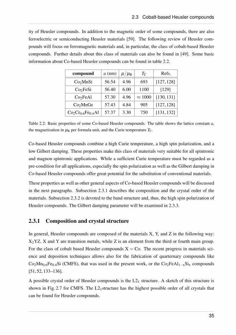
2.3 Cobalt-based Heusler compounds

ity of Heusler compounds. In addition to the magnetic order of some compounds, there are also

ferroelectric or semiconducting Heusler materials [59]. The following review of Heusler com-

pounds will focus on ferromagnetic materials and, in particular, the class of cobalt-based Heusler

compounds. Further details about this class of materials can also be found in [49]. Some basic

information about Co-based Heusler compounds can be found in table 2.2.

compound a (nm) µ/µB TC Refs.

Co2MnSi 56.54 4.96 693 [127, 128]

Co2FeSi 56.40 6.00 1100 [129]

Co2FeAl 57.30 4.96 ≈ 1000 [130, 131]

Co2MnGe 57.43 4.84 905 [127, 128]

Co2Cr0.6Fe0.4Al 57.37 3.30 750 [131, 132]

Table 2.2: Basic properties of some Co-based Heusler compounds. The table shows the lattice constant a,the magnetization in µB per formula unit, and the Curie temperature TC.

Co-based Heusler compounds combine a high Curie temperature, a high spin polarization, and a

low Gilbert damping. These properties make this class of materials very suitable for all spintronic

and magnon spintronic applications. While a sufficient Curie temperature must be regarded as a

pre-condition for all applications, especially the spin polarization as well as the Gilbert damping in

Co-based Heusler compounds offer great potential for the substitution of conventional materials.

These properties as well as other general aspects of Co-based Heusler compounds will be discussed

in the next paragraphs. Subsection 2.3.1 describes the composition and the crystal order of the

materials. Subsection 2.3.2 is devoted to the band structure and, thus, the high spin polarization of

Heusler compounds. The Gilbert damping parameter will be examined in 2.3.3.

2.3.1 Composition and crystal structure

In general, Heusler compounds are composed of the materials X, Y, and Z in the following way:

X2YZ. X and Y are transition metals, while Z is an element from the third or fourth main group.

For the class of cobalt based Heusler compounds X = Co. The recent progress in materials sci-

ence and deposition techniques allows also for the fabrication of quarternary compounds like

Co2Mn0.6Fe0.4Si (CMFS), that was used in the present work, or the Co2FeAl1−xSix compounds

[51, 52, 133–136].

A possible crystal order of Heusler compounds is the L21 structure. A sketch of this structure is

shown in Fig. 2.7 for CMFS. The L21structure has the highest possible order of all crystals that

can be found for Heusler compounds.

35

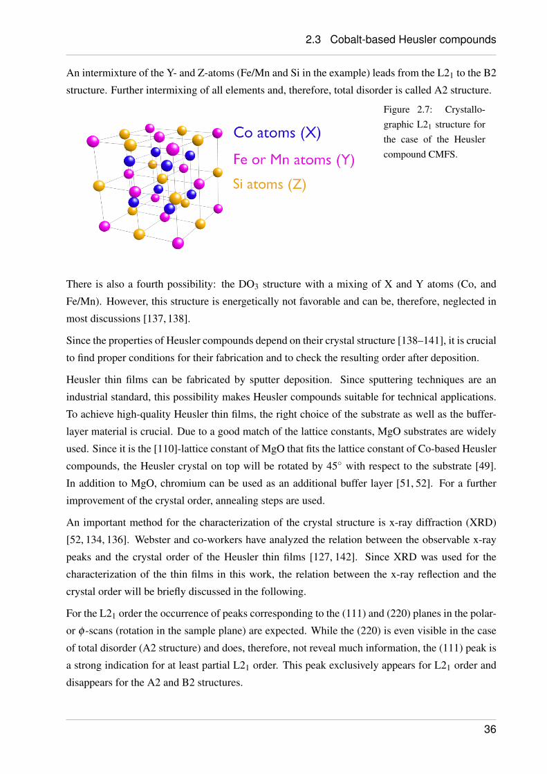
2.3 Cobalt-based Heusler compounds

An intermixture of the Y- and Z-atoms (Fe/Mn and Si in the example) leads from the L21 to the B2

structure. Further intermixing of all elements and, therefore, total disorder is called A2 structure.

Figure 2.7: Crystallo-graphic L21 structure forthe case of the Heuslercompound CMFS.

There is also a fourth possibility: the DO3 structure with a mixing of X and Y atoms (Co, and

Fe/Mn). However, this structure is energetically not favorable and can be, therefore, neglected in

most discussions [137, 138].

Since the properties of Heusler compounds depend on their crystal structure [138–141], it is crucial

to find proper conditions for their fabrication and to check the resulting order after deposition.

Heusler thin films can be fabricated by sputter deposition. Since sputtering techniques are an

industrial standard, this possibility makes Heusler compounds suitable for technical applications.

To achieve high-quality Heusler thin films, the right choice of the substrate as well as the buffer-

layer material is crucial. Due to a good match of the lattice constants, MgO substrates are widely

used. Since it is the [110]-lattice constant of MgO that fits the lattice constant of Co-based Heusler

compounds, the Heusler crystal on top will be rotated by 45 with respect to the substrate [49].

In addition to MgO, chromium can be used as an additional buffer layer [51, 52]. For a further

improvement of the crystal order, annealing steps are used.

An important method for the characterization of the crystal structure is x-ray diffraction (XRD)

[52, 134, 136]. Webster and co-workers have analyzed the relation between the observable x-ray

peaks and the crystal order of the Heusler thin films [127, 142]. Since XRD was used for the

characterization of the thin films in this work, the relation between the x-ray reflection and the

crystal order will be briefly discussed in the following.

For the L21 order the occurrence of peaks corresponding to the (111) and (220) planes in the polar-

or φ -scans (rotation in the sample plane) are expected. While the (220) is even visible in the case

of total disorder (A2 structure) and does, therefore, not reveal much information, the (111) peak is

a strong indication for at least partial L21 order. This peak exclusively appears for L21 order and

disappears for the A2 and B2 structures.

36

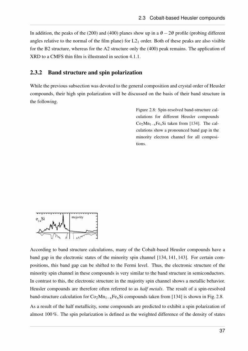
2.3 Cobalt-based Heusler compounds

In addition, the peaks of the (200) and (400) planes show up in a θ −2θ profile (probing different

angles relative to the normal of the film plane) for L21 order. Both of these peaks are also visible

for the B2 structure, whereas for the A2 structure only the (400) peak remains. The application of

XRD to a CMFS thin film is illustrated in section 4.1.1.

2.3.2 Band structure and spin polarization

While the previous subsection was devoted to the general composition and crystal order of Heusler

compounds, their high spin polarization will be discussed on the basis of their band structure in

the following.

Figure 2.8: Spin-resolved band-structure cal-culations for different Heusler compoundsCo2Mn1−xFexSi taken from [134]. The cal-culations show a pronounced band gap in theminority electron channel for all composi-tions.

According to band structure calculations, many of the Cobalt-based Heusler compounds have a

band gap in the electronic states of the minority spin channel [134, 141, 143]. For certain com-

positions, this band gap can be shifted to the Fermi level. Thus, the electronic structure of the

minority spin channel in these compounds is very similar to the band structure in semiconductors.

In contrast to this, the electronic structure in the majority spin channel shows a metallic behavior.

Heusler compounds are therefore often referred to as half metals. The result of a spin-resolved

band-structure calculation for Co2Mn1−xFexSi compounds taken from [134] is shown in Fig. 2.8.

As a result of the half metallicity, some compounds are predicted to exhibit a spin polarization of

almost 100 %. The spin polarization is defined as the weighted difference of the density of states

37

2.3 Cobalt-based Heusler compounds

compound SP at given temperature Refs.

Co2MnSi 61% at 10 K and 83% at 3 K [144, 145]

Co2FeSi 67% at 5 K and 43% at RT [146]

Co2Cr0.6Fe0.4Al 79% at 4.2 K and 50% at RT [147]

Co2FeAl0.5Si0.5Al 90% at RT [148]

NiFe 37% [149]

CoFe 49% [150]

Table 2.3: Spin polarization of selected Heusler compounds. For comparison the table also includes thevalues for NiFe and CoFe. Results of measurements at different temperatures but for the same compoundillustrate the strong temperature dependence of the spin polarization, that is mentioned in the text.

for up-spin and down-spin electrons at the Fermi level:

SP =D↑(EF)−D↓(EF)

D↑(EF)+D↓(EF). (2.64)

The spin polarization is one of the crucial material parameters for the design of magneto-resistive

devices for data storage and sensing. Therefore, in the research fields related to the development

of such devices, the fabrication and utilization of Heusler compounds and the evaluation of their

properties is a central topic. However, even though the observed spin polarizations are higher than

those of most conventional 3d ferromagnets for some compounds, a spin polarization of 100 %

has not been observed by now. In particular, the strong dependence of the spin polarization on the

temperature is widely discussed at the moment. Table 2.3 shows the spin polarization of selected

Co-based Heusler compounds.

2.3.3 Gilbert damping

The most important property of the class of Co-based Heusler compounds regarding the present

work is the magnetic Gilbert damping. Even though not all compounds show values below the

damping in conventional 3d ferromagnets, there are several low-damping materials that are promis-

ing candidates for the field of magnon spintronics. The most interesting materials among these

candidates are Co2FeAl and the Co2Mn1−xFexSi compounds. For the experiments presented be-

low Co2Mn0.6Fe0.4Si (CMFS) with a Gilbert damping of α = 3×10−3 was used. The decision to

use CMFS was taken together with the Japanese project partners in the group Prof. Dr. Y. Ando at

the Tohoku University for the following reason. The fabrication process of this material was estab-

lished already a few years ago and can be assumed to be a standard process with a high reliability

regarding quality of the thin films. An overview and a comparison to the some conventional 3d

ferromagnets is presented in table 2.4.

38

2.3 Cobalt-based Heusler compounds

compound α (×10−3) Refs.

Co2MnSi 3 [151]

Co2FeSi 8 [152]

Co2Mn0.6Fe0.4Si 3 [51]

Co2FeAl 1 [153]

NiFe 8 [154]

CoFeB 4 [A8]

Table 2.4: Gilbert damping parameter of selected Heusler compounds. As indicated by the comparison withNiFe and CoFeB, Co2FeAl and the Co2Mn1−xFexSi compounds are of particular interest.

The origin of the Gilbert damping was discussed in section 2.2.5. It turned out that crucial param-

eters for the estimation of the damping constant are the density of states at the Fermi level and the

spin-orbit interaction α ∝ ξ 2SOD(EF).

It is obvious from the above discussion of the band structure, that the density of states at the

Fermi level is rather small for the Heusler compounds. The vanishing contribution of the minority

electrons in the half-metallic materials is the reason for the decreased magnetic damping compared

to conventional 3d ferromagnets.

Even though the experimentally observed values are promising, a large discrepancy to the predic-

tions of ab-initio calculations can be found. Liu and co-workers calculated the damping constant

for the materials Co2MnSi and Co2MnGe and presented their work in [50]. The results of their cal-

culations are one order of magnitude smaller than experimental findings. The reason for this large

discrepancy is still unknown. However, these results highlight the further potential of Co-based

Heusler compounds.

The utilization of the low-damping CMFS for magnon spintronics was the major motivation of the

present thesis. As can be seen from Table 2.4, the Gilbert damping in CMFS is almost three times

smaller than in Ni81Fe19, which is the material of choice for almost all studies of spin dynamics on

the microscale. Therefore, advantages as an increased decay length or the pronounced occurrence

of nonlinear effects have been anticipated for the spin-wave propagation in CMFS microstructures.

The present work indicates, that these advantages can indeed be observed in CMFS and utilized

for the field of magnon spintronics.

39

CHAPTER 3

Experimental methods

The following chapter provides an overview over the experimental techniques that have been used

for the observation presented in the present thesis. The most important technique was Brillouin

light scattering (BLS) microscopy. BLS spectroscopy in general offers a wide variety of tools for

the observation of spin dynamics with frequency-, space-, phase-, and time resolution [55, 56].

Therefore, this chapter is devoted to the description of the underlying physical mechanisms of

BLS and the experimental realization. The chapter is subdivided to briefly introduce the different

techniques for frequency-, space-, phase-, and time-resolved measurements, respectively.

Before turning to the discussion of BLS, alternative experimental techniques with their drawbacks

and advantages will be briefly commented on. The major alternatives for the investigation of

spin dynamics are other optical techniques based on the Faraday- or magneto-optical Kerr effect

[155–157] as well as electrical microwave characterization [158].

Common microwave devices offer an excellent frequency resolution down to the megahertz regime

which cannot be achieved by methods based on magneto optics. Electrical characterization of the

ferromagnetic resonance in magnetic thin films is the standard technique for the evaluation of ma-

terial parameters like the Gilbert damping and the saturation magnetization. However, concerning

the present work, electrical methods are limited. Electrical detection is mostly used on macro-

scopic sample structures because it does not allow for a space resolution on the microscale. In

any case, antenna structures are required for the observation of spin dynamics. These antenna

structures restrict the space information in the measurement to fixed probing positions and hinder

a flexible detection scheme. In addition, antenna structures affect the observed spin dynamics by

the absorption of energy from the spin system.

In contrast to this, optical microscopy offers a spacial resolution that allows for the observation of

spin dynamics even on the microscale via magneto-optical effects. Except from possible heating

effects induced by the probing laser beam, optical detection does not affect the sample structure

and, thus, does not affect the observed spin dynamics. The probing position can be easily adapted

to the experimental requirements. Magnetooptics is, therefore, an ideal and flexible technique for

40

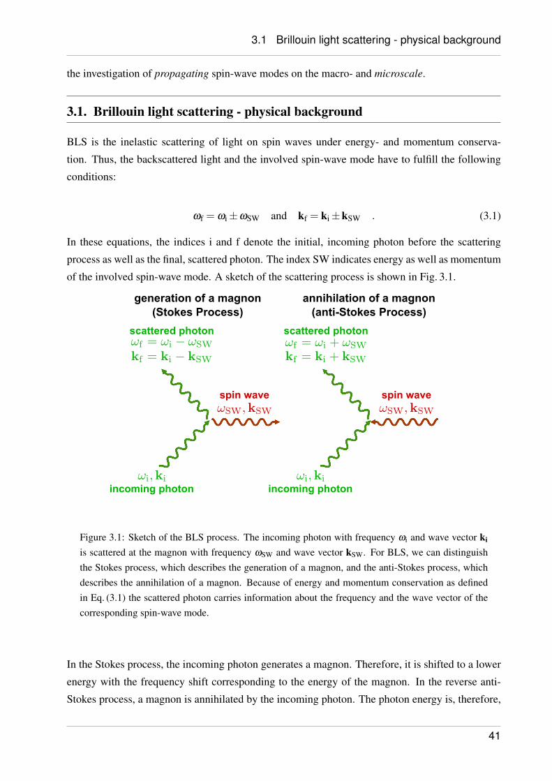
3.1 Brillouin light scattering - physical background

the investigation of propagating spin-wave modes on the macro- and microscale.

3.1. Brillouin light scattering - physical background

BLS is the inelastic scattering of light on spin waves under energy- and momentum conserva-

tion. Thus, the backscattered light and the involved spin-wave mode have to fulfill the following

conditions:

ωf = ωi±ωSW and kf = ki±kSW . (3.1)

In these equations, the indices i and f denote the initial, incoming photon before the scattering

process as well as the final, scattered photon. The index SW indicates energy as well as momentum

of the involved spin-wave mode. A sketch of the scattering process is shown in Fig. 3.1.

Figure 3.1: Sketch of the BLS process. The incoming photon with frequency ωi and wave vector ki

is scattered at the magnon with frequency ωSW and wave vector kSW. For BLS, we can distinguishthe Stokes process, which describes the generation of a magnon, and the anti-Stokes process, whichdescribes the annihilation of a magnon. Because of energy and momentum conservation as definedin Eq. (3.1) the scattered photon carries information about the frequency and the wave vector of thecorresponding spin-wave mode.

In the Stokes process, the incoming photon generates a magnon. Therefore, it is shifted to a lower

energy with the frequency shift corresponding to the energy of the magnon. In the reverse anti-

Stokes process, a magnon is annihilated by the incoming photon. The photon energy is, therefore,

41

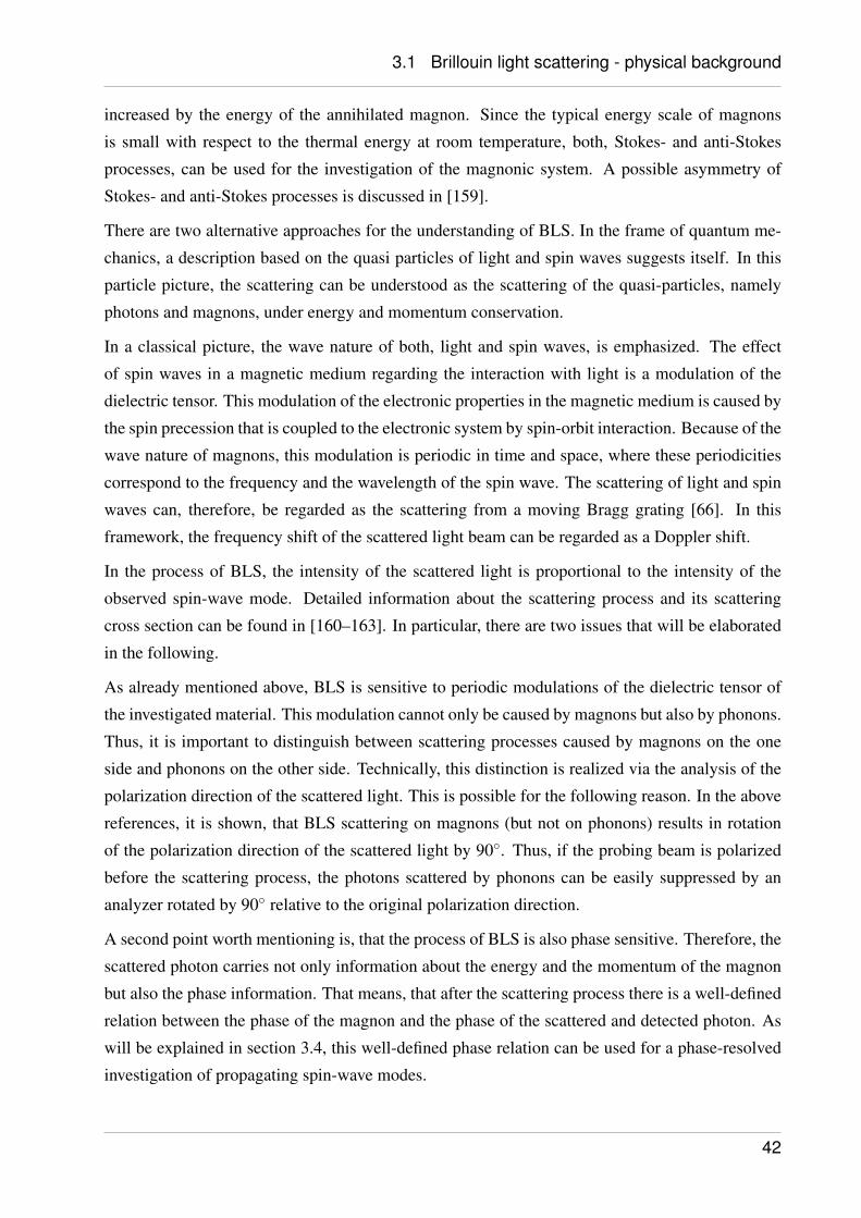
3.1 Brillouin light scattering - physical background

increased by the energy of the annihilated magnon. Since the typical energy scale of magnons

is small with respect to the thermal energy at room temperature, both, Stokes- and anti-Stokes

processes, can be used for the investigation of the magnonic system. A possible asymmetry of

Stokes- and anti-Stokes processes is discussed in [159].

There are two alternative approaches for the understanding of BLS. In the frame of quantum me-

chanics, a description based on the quasi particles of light and spin waves suggests itself. In this

particle picture, the scattering can be understood as the scattering of the quasi-particles, namely

photons and magnons, under energy and momentum conservation.

In a classical picture, the wave nature of both, light and spin waves, is emphasized. The effect

of spin waves in a magnetic medium regarding the interaction with light is a modulation of the

dielectric tensor. This modulation of the electronic properties in the magnetic medium is caused by

the spin precession that is coupled to the electronic system by spin-orbit interaction. Because of the

wave nature of magnons, this modulation is periodic in time and space, where these periodicities

correspond to the frequency and the wavelength of the spin wave. The scattering of light and spin

waves can, therefore, be regarded as the scattering from a moving Bragg grating [66]. In this

framework, the frequency shift of the scattered light beam can be regarded as a Doppler shift.

In the process of BLS, the intensity of the scattered light is proportional to the intensity of the

observed spin-wave mode. Detailed information about the scattering process and its scattering

cross section can be found in [160–163]. In particular, there are two issues that will be elaborated

in the following.

As already mentioned above, BLS is sensitive to periodic modulations of the dielectric tensor of

the investigated material. This modulation cannot only be caused by magnons but also by phonons.

Thus, it is important to distinguish between scattering processes caused by magnons on the one

side and phonons on the other side. Technically, this distinction is realized via the analysis of the

polarization direction of the scattered light. This is possible for the following reason. In the above

references, it is shown, that BLS scattering on magnons (but not on phonons) results in rotation

of the polarization direction of the scattered light by 90. Thus, if the probing beam is polarized

before the scattering process, the photons scattered by phonons can be easily suppressed by an

analyzer rotated by 90 relative to the original polarization direction.

A second point worth mentioning is, that the process of BLS is also phase sensitive. Therefore, the

scattered photon carries not only information about the energy and the momentum of the magnon

but also the phase information. That means, that after the scattering process there is a well-defined

relation between the phase of the magnon and the phase of the scattered and detected photon. As

will be explained in section 3.4, this well-defined phase relation can be used for a phase-resolved

investigation of propagating spin-wave modes.

42

3.2 Brillouin light scattering - experimental realization

3.2. Brillouin light scattering - experimental realization

As mentioned in the previous section, photons, that were scattered inelastically on magnons, carry

information about the frequency, the wave vector, and the phase of the involved spin-wave mode.

In this section, it will be explained how the first two quantities are accessible experimentally.

As a result of the inelastic scattering on a magnon, the scattered photon is subject to a frequency

shift corresponding to the magnon energy. In the experimental setup, that was used for all investiga-

tions presented in this thesis, this frequency shift is analyzed by multi-path a tandem Fabry-Pérot

interferometer (TFPI) [164, 165]. A sketch of the light path in a TFPI taken from [166, 167] is

shown in Fig. 3.2. The operating principle of a TFPI will be explained in the following.

Figure 3.2: Sketch of a TFPI taken from [166, 167]. The TFPI is used to analyze the frequency shiftof the inelastically scattered light. It consists of two single FPIs with a tilt of angle α to suppressdifferent transmission orders. The working principles of the TFPI and its components is discussed inthe text below.

A TFPI consists of two individual Fabry-Pérot interferometers (FPI). A FPI is based on the inter-

ference of light beams that are reflected many times between two plane-parallel mirroring plates.

The multiple reflection of a light beam between these plates causes a path difference relative to a

directly transmitted beam. This path difference ∆s can be described via the number of reflections

n and the distance d between the plates:

∆s = 2nd . (3.2)

43

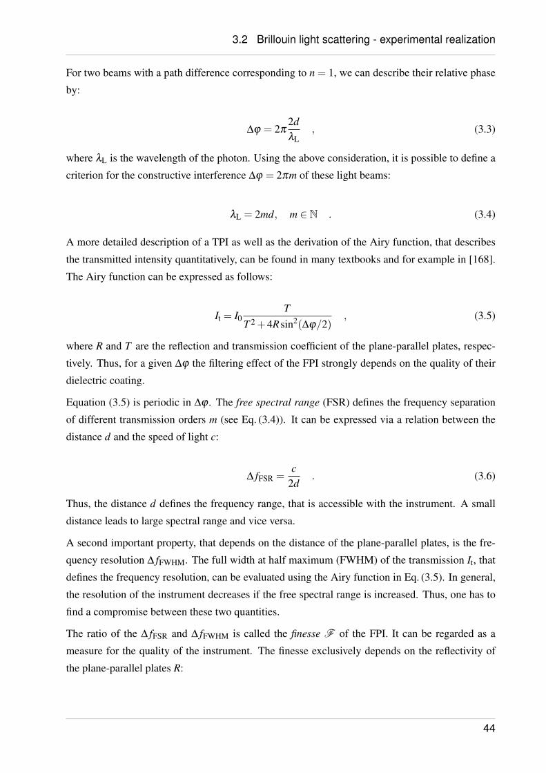
3.2 Brillouin light scattering - experimental realization

For two beams with a path difference corresponding to n = 1, we can describe their relative phase

by:

∆ϕ = 2π2dλL

, (3.3)

where λL is the wavelength of the photon. Using the above consideration, it is possible to define a

criterion for the constructive interference ∆ϕ = 2πm of these light beams:

λL = 2md, m ∈ N . (3.4)

A more detailed description of a TPI as well as the derivation of the Airy function, that describes

the transmitted intensity quantitatively, can be found in many textbooks and for example in [168].

The Airy function can be expressed as follows:

It = I0T

T 2 +4Rsin2(∆ϕ/2), (3.5)

where R and T are the reflection and transmission coefficient of the plane-parallel plates, respec-

tively. Thus, for a given ∆ϕ the filtering effect of the FPI strongly depends on the quality of their

dielectric coating.

Equation (3.5) is periodic in ∆ϕ . The free spectral range (FSR) defines the frequency separation

of different transmission orders m (see Eq. (3.4)). It can be expressed via a relation between the

distance d and the speed of light c:

∆ fFSR =c

2d. (3.6)

Thus, the distance d defines the frequency range, that is accessible with the instrument. A small

distance leads to large spectral range and vice versa.

A second important property, that depends on the distance of the plane-parallel plates, is the fre-

quency resolution ∆ fFWHM. The full width at half maximum (FWHM) of the transmission It, that

defines the frequency resolution, can be evaluated using the Airy function in Eq. (3.5). In general,

the resolution of the instrument decreases if the free spectral range is increased. Thus, one has to

find a compromise between these two quantities.

The ratio of the ∆ fFSR and ∆ fFWHM is called the finesse F of the FPI. It can be regarded as a

measure for the quality of the instrument. The finesse exclusively depends on the reflectivity of

the plane-parallel plates R:

44

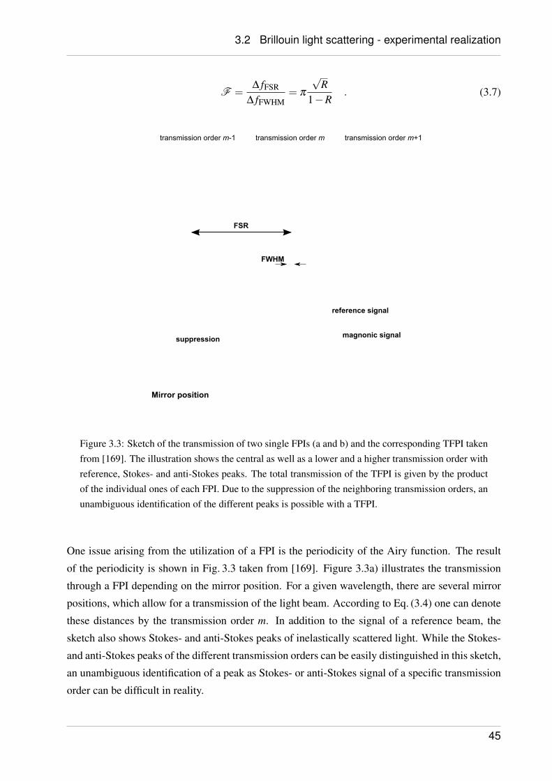
3.2 Brillouin light scattering - experimental realization

F =∆ fFSR

∆ fFWHM= π

√R

1−R. (3.7)

Mirror position

reference signal

magnonic signal

FSR

FWHM

suppression

transmission order m transmission order m+1transmission order m-1

Figure 3.3: Sketch of the transmission of two single FPIs (a and b) and the corresponding TFPI takenfrom [169]. The illustration shows the central as well as a lower and a higher transmission order withreference, Stokes- and anti-Stokes peaks. The total transmission of the TFPI is given by the productof the individual ones of each FPI. Due to the suppression of the neighboring transmission orders, anunambiguous identification of the different peaks is possible with a TFPI.

One issue arising from the utilization of a FPI is the periodicity of the Airy function. The result

of the periodicity is shown in Fig. 3.3 taken from [169]. Figure 3.3a) illustrates the transmission

through a FPI depending on the mirror position. For a given wavelength, there are several mirror

positions, which allow for a transmission of the light beam. According to Eq. (3.4) one can denote

these distances by the transmission order m. In addition to the signal of a reference beam, the

sketch also shows Stokes- and anti-Stokes peaks of inelastically scattered light. While the Stokes-

and anti-Stokes peaks of the different transmission orders can be easily distinguished in this sketch,

an unambiguous identification of a peak as Stokes- or anti-Stokes signal of a specific transmission

order can be difficult in reality.

45

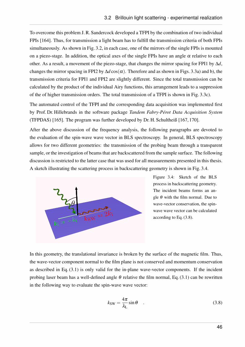
3.2 Brillouin light scattering - experimental realization

To overcome this problem J. R. Sandercock developed a TFPI by the combination of two individual

FPIs [164]. Thus, for transmission a light beam has to fulfill the transmission criteria of both FPIs

simultaneously. As shown in Fig. 3.2, in each case, one of the mirrors of the single FPIs is mounted

on a piezo-stage. In addition, the optical axes of the single FPIs have an angle α relative to each

other. As a result, a movement of the piezo-stage, that changes the mirror spacing for FPI1 by ∆d,

changes the mirror spacing in FPI2 by ∆d cos(α). Therefore and as shown in Figs. 3.3a) and b), the

transmission criteria for FPI1 and FPI2 are slightly different. Since the total transmission can be

calculated by the product of the individual Airy functions, this arrangement leads to a suppression

of the of higher transmission orders. The total transmission of a TFPI is shown in Fig. 3.3c).

The automated control of the TFPI and the corresponding data acquisition was implemented first

by Prof. Dr. Hillebrands in the software package Tandem Fabry-Pérot Data Acquisition System

(TFPDAS) [165]. The program was further developed by Dr. H. Schultheiß [167, 170].

After the above discussion of the frequency analysis, the following paragraphs are devoted to

the evaluation of the spin-wave wave vector in BLS spectroscopy. In general, BLS spectroscopy

allows for two different geometries: the transmission of the probing beam through a transparent

sample, or the investigation of beams that are backscattered from the sample surface. The following

discussion is restricted to the latter case that was used for all measurements presented in this thesis.

A sketch illustrating the scattering process in backscattering geometry is shown in Fig. 3.4.

Figure 3.4: Sketch of the BLSprocess in backscattering geometry.The incident beams forms an an-gle θ with the film normal. Due towave-vector conservation, the spin-wave wave vector can be calculatedaccording to Eq. (3.8).

In this geometry, the translational invariance is broken by the surface of the magnetic film. Thus,

the wave-vector component normal to the film plane is not conserved and momentum conservation

as described in Eq. (3.1) is only valid for the in-plane wave-vector components. If the incident

probing laser beam has a well-defined angle θ relative the film normal, Eq. (3.1) can be rewritten

in the following way to evaluate the spin-wave wave vector:

kSW =4π

λLsinθ . (3.8)

46

3.3 Brillouin light scattering microscopy

By changing the angle θ as well as the polar angle φ in the sample plane, it is therefore possible to

probe the entire spin-wave spectrum with wave-vector resolution. A realization of this approach is

described in [171, 172].

3.3. Brillouin light scattering microscopy

The following section is devoted to the description of the BLS microscope that was used for the

present work. Since BLS spectroscopy is an optical technique, the limit for the spacial resolu-

tion is given by the fundamental diffraction limit. The spacial resolution of the actual instrument

with a laser wavelength of λL = 532 nm and a microscope objective with a numerical aperture of

NA = 0.75 is 300 nm. It has to be mentioned, that this resolution refers to distinctness of purely

geometric objects at the sample. In the case of purely geometric objects, it is exclusively the in-

tensity of the reflected light that defines the spacial resolution. However, as stated above, BLS

is a phase-sensitive process. In analogy to phase-contrast microscopy, this might even enhance

the spacial resolution of the instrument for the detection of photons scattered from magnons by a

factor of√

2.

The instrument was developed in the last decade in the group of Prof. B. Hillebrands. A description

of this development over the years as well as technical details can be found in various publications

[167, 170, 173, 174].

A sketch of the light path for the probing beam as well as for the illumination can be found in

Fig. 3.5. These illustrations are taken from [166,167]. In addition to the basic components required

for BLS spectroscopy, like the laser, an electromagnet, and the TFPI, the setup comprises the

microscope objective as well as a CCD camera. The latter is used for monitoring the sample

position throughout the measurement. For the positioning of the sample, the setup is equipped

with a piezo stage with an accuracy of about ~10 nm.

An important issue concerning measurements on the microscale is the long-term stability of the

sample position. To ensure this stability, the setup is equipped with an automated picture-recognition

software routine. Via this routine, the sample position is monitored and corrected throughout the

entire measurement process. This routine and many important parts for the control of the BLS

microscope have been developed by Dr. H. Schultheiß.1

While the evaluation of the spin-wave frequency with the BLS microscope follows the same ap-

proach as discussed in the previous section, it is important to consider the following facts con-

cerning the wave-vector sensitivity. Due to Heisenberg’s uncertainty principle [175], the spacial

resolution of the microscope results in the loss of the wave-vector selectivity. This can be easily

1For details see http://www.tfpdas-micro.de/

47

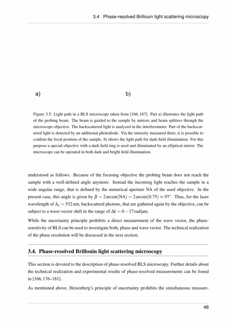
3.4 Phase-resolved Brillouin light scattering microscopy

a) b)

Figure 3.5: Light path in a BLS microscope taken from [166, 167]. Part a) illustrates the light pathof the probing beam. The beam is guided to the sample by mirrors and beam splitters through themicroscope objective. The backscattered light is analyzed in the interferometer. Part of the backscat-tered light is detected by an additional photodiode. Via the intensity measured there, it is possible toconfirm the focal position of the sample. b) shows the light path for dark-field illumination. For thispurpose a special objective with a dark field ring is used and illuminated by an elliptical mirror. Themicroscope can be operated in both dark and bright field illumination.

understood as follows. Because of the focusing objective the probing beam does not reach the

sample with a well-defined angle anymore. Instead the incoming light reaches the sample in a

wide angular range, that is defined by the numerical aperture NA of the used objective. In the

present case, this angle is given by β = 2arcsin(NA) = 2arcsin(0.75) ≈ 97. Thus, for the laser

wavelength of λL = 532 nm, backscatterd photons, that are gathered again by the objective, can be

subject to a wave-vector shift in the range of ∆k = 0−17 rad/µm.

While the uncertainty principle prohibits a direct measurement of the wave vector, the phase-

sensitivity of BLS can be used to investigate both, phase and wave vector. The technical realization

of the phase resolution will be discussed in the next section.

3.4. Phase-resolved Brillouin light scattering microscopy

This section is devoted to the description of phase-resolved BLS microscopy. Further details about

the technical realization and experimental results of phase-resolved measurements can be found

in [166, 176–181].

As mentioned above, Heisenberg’s principle of uncertainty prohibits the simultaneous measure-

48

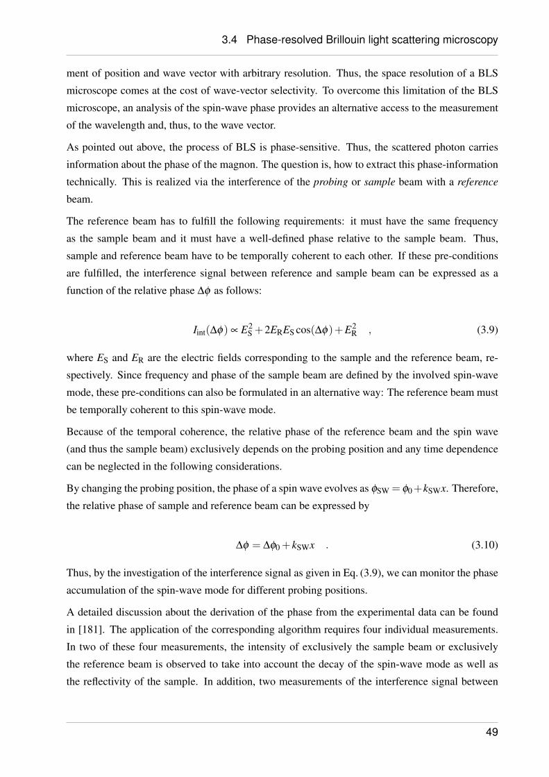
3.4 Phase-resolved Brillouin light scattering microscopy

ment of position and wave vector with arbitrary resolution. Thus, the space resolution of a BLS

microscope comes at the cost of wave-vector selectivity. To overcome this limitation of the BLS

microscope, an analysis of the spin-wave phase provides an alternative access to the measurement

of the wavelength and, thus, to the wave vector.

As pointed out above, the process of BLS is phase-sensitive. Thus, the scattered photon carries

information about the phase of the magnon. The question is, how to extract this phase-information

technically. This is realized via the interference of the probing or sample beam with a reference

beam.

The reference beam has to fulfill the following requirements: it must have the same frequency

as the sample beam and it must have a well-defined phase relative to the sample beam. Thus,

sample and reference beam have to be temporally coherent to each other. If these pre-conditions

are fulfilled, the interference signal between reference and sample beam can be expressed as a

function of the relative phase ∆φ as follows:

Iint(∆φ) ∝ E2S +2ERES cos(∆φ)+E2

R , (3.9)

where ES and ER are the electric fields corresponding to the sample and the reference beam, re-

spectively. Since frequency and phase of the sample beam are defined by the involved spin-wave

mode, these pre-conditions can also be formulated in an alternative way: The reference beam must

be temporally coherent to this spin-wave mode.

Because of the temporal coherence, the relative phase of the reference beam and the spin wave

(and thus the sample beam) exclusively depends on the probing position and any time dependence

can be neglected in the following considerations.

By changing the probing position, the phase of a spin wave evolves as φSW = φ0+kSWx. Therefore,

the relative phase of sample and reference beam can be expressed by

∆φ = ∆φ0 + kSWx . (3.10)

Thus, by the investigation of the interference signal as given in Eq. (3.9), we can monitor the phase

accumulation of the spin-wave mode for different probing positions.

A detailed discussion about the derivation of the phase from the experimental data can be found

in [181]. The application of the corresponding algorithm requires four individual measurements.

In two of these four measurements, the intensity of exclusively the sample beam or exclusively

the reference beam is observed to take into account the decay of the spin-wave mode as well as

the reflectivity of the sample. In addition, two measurements of the interference signal between

49

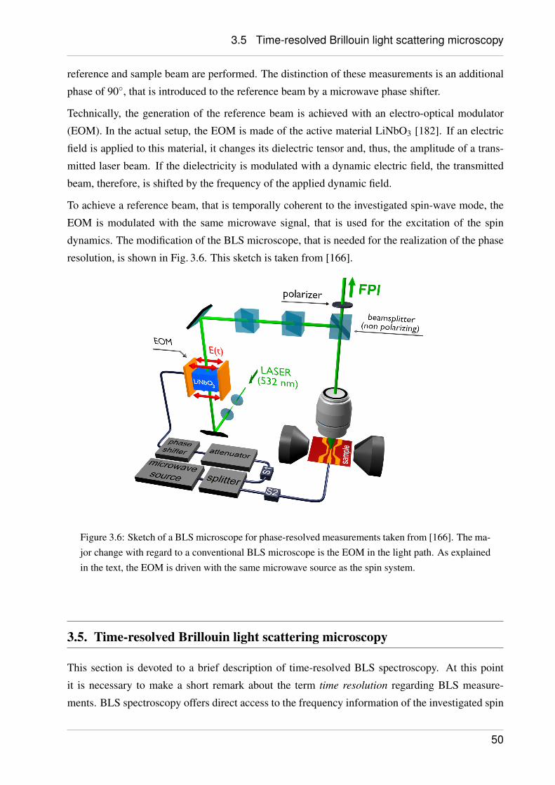
3.5 Time-resolved Brillouin light scattering microscopy

reference and sample beam are performed. The distinction of these measurements is an additional

phase of 90, that is introduced to the reference beam by a microwave phase shifter.

Technically, the generation of the reference beam is achieved with an electro-optical modulator

(EOM). In the actual setup, the EOM is made of the active material LiNbO3 [182]. If an electric

field is applied to this material, it changes its dielectric tensor and, thus, the amplitude of a trans-

mitted laser beam. If the dielectricity is modulated with a dynamic electric field, the transmitted

beam, therefore, is shifted by the frequency of the applied dynamic field.

To achieve a reference beam, that is temporally coherent to the investigated spin-wave mode, the

EOM is modulated with the same microwave signal, that is used for the excitation of the spin

dynamics. The modification of the BLS microscope, that is needed for the realization of the phase

resolution, is shown in Fig. 3.6. This sketch is taken from [166].

Figure 3.6: Sketch of a BLS microscope for phase-resolved measurements taken from [166]. The ma-jor change with regard to a conventional BLS microscope is the EOM in the light path. As explainedin the text, the EOM is driven with the same microwave source as the spin system.

3.5. Time-resolved Brillouin light scattering microscopy

This section is devoted to a brief description of time-resolved BLS spectroscopy. At this point

it is necessary to make a short remark about the term time resolution regarding BLS measure-

ments. BLS spectroscopy offers direct access to the frequency information of the investigated spin

50

3.5 Time-resolved Brillouin light scattering microscopy

dynamics. Therefore, the purpose of time resolution in BLS spectroscopy is not to directly im-

age the precessional motion in the spin system in the time domain. This is typically done with

time-resolved Kerr effect measurements on the picosecond scale. In contrast, the purpose of time-

resolved BLS techniques is a time-resolved measurement of the spin-wave intensity. Typically, the

technique is used to determine the rise time or the decay time of a certain spin-wave mode after

switching on or off the external excitation, respectively. This also allows for the evaluation of the

time a spin wave needs to propagate from one probing point to another.

Since the intensity of the observed spin-wave modes is governed by the external excitation, of

particular interest is the estimation of the actual point of time t, relative to either the time t0 of

switching on the excitation or the time t1 of switching off the excitation. Between t0 and t1 a

continuous wave signal is applied for the excitation of spin dynamics. The temporal control of the

external excitation is realized via an externally triggered switch. Only if a voltage signal is applied

to this switch, spin waves are excited. This voltage signal is provided by a pulse generator.

In addition to the voltage pulse, the pulse generator outputs a trigger signal that can be shifted by an

arbitrary time relative to the voltage pulse. This second signal triggers the start of the measurement

via a time-of-flight measuring board. For a certain time span ∆t any photon detected by the interfer-

ometer causes a stop signal at the measuring board. Whenever a stop signal occurs, the frequency

of the scattered photon is registered by the measuring board together with the corresponding time

information. The measuring board has a restricted time resolution of 250 ps.

First experimental results of time-resolved BLS spectroscopy as well as microscopy can be found

in [104, 112, 114, 183]. A detailed discussion of the technical realization is given in [167].

51

CHAPTER 4

Experimental results

In the present work, the issue of spin-wave propagation in the Heusler compound Co2Mn0.6Fe0.4Si

(CMFS) is the central topic. The major motivation behind this work is the lack of suitable materials

for the realization of spin-wave based transport and processing of information on the microscale.

As described in this chapter, major challenges caused by material aspects can be overcome by the

utilization of CMFS as the carrier material for spin waves. In the following paragraphs, the current

possibilities as well as the major challenges in the research field of magnon spintronics will be

sketched. In addition, it will be shown how CMFS can help to overcome some of the difficulties

in this field and how it opens new perspectives regarding the realization of potential technical

applications.

Recent reports about new schemes for the excitation, manipulation, and detection of spin dynamics

as well as the progress in sample design and fabrication on the microscale reveal possible routes

for a technically relevant information transport and processing that is purely based on spin waves.

The research field magnon spintronics picks up this idea and has the goal to realize the numerous

proposals towards a spin-wave based logic [1, 3, 14–19, 184, 185].

Among the most prominent phenomena, that are interesting regarding potential future applications,

are the direct-current based excitation of spin dynamics via spin Hall effect and spin-transfer torque

[20, 21, 26, 186, 187], as well as the reverse process that converts spin dynamics into detectable

direct-current signals by spin pumping and the inverse spin Hall effect [29, 30, 53, 188–190]. A

second rather new field of huge interest is given by the interactions of spin currents and heat

currents, like for example the spin Seebeck effect [31–35, 54]. Since a detailed discussion of all

these effects would by far exceed the scope of this thesis, I will concentrate on the major material

aspects behind them.

Most of the experimental results related to the above-mentioned phenomena have been obtained

in macroscopic sample structures comprising the ferrimagnetic insulator yttrium iron garnet (YIG)

[42]. Macroscopic structures of YIG are also used in many devices in the field of microwave

technique such as signal generators. The reason for this choice is the extremely small magnetic

52

Gilbert damping of YIG. However, there are several reasons that prohibit the utilization of YIG

regarding technical applications in the field of data processing. First of all, the growth process of

YIG is incompatible with industrial demands. Even though serious efforts are made to improve

the process, up to now, the industrially used sputtering technique results in a lower quality of YIG

films than alternative methods [45]. Standard methods for the growth of YIG films are liquid-phase

epitaxy or pulsed laser deposition - methods that are rather slow and therefore expensive [43, 44].

In addition, high quality YIG films typically have a minimum thickness of several micrometers.

This hinders the patterning of nano- or even microstructures, that is needed for the production of

end-consumer devices such as cell phones. In addition to these technical aspects, some interest-

ing physical mechanisms for the excitation of spin waves are not accessible on the macroscale or

with magnetic insulators at all. These mechanisms will be addressed in the next paragraph. Fur-

thermore, yttrium is a rare-earth metal. Rare-earth metals are a class of materials that are rather

expensive compared to the alternative materials, that will be introduced later in this section. In

summary, YIG is an excellent material for basic research and demonstrator systems but its value

concerning potential industrial applications on the microscale is small.

On the microscale, several steps towards the realization of two-dimensional spin-wave transport

have been taken [36, 37] and new concepts for advanced waveguide structures have been real-

ized [38–40]. The progress in thin film fabrication as well as patterning techniques also allowed

for the realization of excitation schemes exclusively available on the microscale by spin-torque

nano oscillators [22–24]. The compound Ni81Fe19, that is used in most related studies, is com-

patible with industrial demands and patterning techniques, that allow for the utilization of sam-

ple layouts even on the nanoscale. However, the rather large Gilbert damping in Ni81Fe19 and

other conventional 3d-ferromagnets and compounds causes huge losses in the magnetic systems.

The dissipation limits the further progress and hinders the utilization of many of the phenomena

discussed in the previous paragraphs. Therefore, material aspects are the major reason that the

potential given in the field of magnon spintronics cannot be fully developed.

These issues at hand, the class of Heusler materials contains several promising candidates with a

decreased magnetic damping to overcome the challenges sketched above. Heusler materials can be

grown using sputtering techniques and patterned by standardized industrial processes, that are also

used for complementary-metal-oxide-semiconductor electronics. This ensures an easy integration

into existing circuitry and fabrication facilities.

The identification and incorporation of advanced Heusler materials, that are suitable for the trans-

port of spin waves and that are compatible with industrial growth- and patterning standards, is a

key aspect of the joint Japanese-German research unit Advanced Spintronics Materials and Trans-

port Phenomena (ASPIMATT). The present work was performed in the framework of the ASPI-

MATT collaboration. The working package addressed at the TU Kaiserslautern in the group of

53

Prof. Dr. B. Hillebrands and in close collaboration with the research group of Prof. Dr. Y. Ando at

the Tohoku University in Sendai, Japan, was Nonlinear spin-wave dynamics and radiation proper-

ties of small Heusler devices.

Of particular interest for the present work is the class of cobalt-based Heusler compounds. Many

of these compounds combine a high Curie temperature, a high spin polarization, and a low mag-

netic Gilbert damping. A sufficiently high Curie temperature is pre-condition for any technical

application based on magnetism. The high spin polarization is advantageous for magneto-resistive

devices for sensing and data storage applications as well as for the excitation of spin dynamics

in spin-torque oscillators. Since the rather large Gilbert damping in most conventional materi-

als is one of the major challenges in magnon spintronics, the decreased damping in some of the

cobalt-based compounds is the most important materials aspect regarding the present work.

The material class of Co-based Heusler compounds has been introduced in section 2.3 of this the-

sis. An overview over the properties of many cobalt-based Heusler compounds and a comparison to

conventional 3d-ferromagnets can also be found in [49]. Due to their promising properties, cobalt-

based Heusler compounds have already been extensively used in the field of magneto-resistive

devices for data storage as well as for the excitation of spin dynamics [46–48, 191]. The materials

also proved their applicability for the realization of advanced detection schemes using spin pump-

ing and the inverse spin Hall effect [53] as well as for experiments based on the interaction of spin

and heat currents [54].

Despite this intensive research related to cobalt-based Heusler compounds, the direct and space-

resolved observations of spin-wave propagation in Heusler microstructures, that are discussed in

the present work, are the first observations of their kind. The particular material, that was used, is

the Heusler compound Co2Mn0.6Fe0.4Si (CMFS) with a Gilbert damping of α(CMFS) = 3×10−3

which is almost three times smaller than in Ni81Fe19 with α(Ni81Fe19) = 8×10−3. Ni81Fe19 will

serve as a reference throughout this chapter due to its utilization in most related experiments on

spin-wave propagation. Detailed information about CMFS can be found in Refs. [48, 49, 51, 52,

134, 191]. The observations presented below are an important first step towards the introduction

of CMFS in the field of magnon spintronics. The results that were achieved in this work show that

the major advantages expected for the utilization of CMFS can indeed be observed and utilized for

the realization of future applications.

In this chapter the major results of my work will be presented and discussed. The experimental

observations comprise spin dynamics in the linear as well as in the nonlinear regime. For the

observation of the spin dynamics Brillouin light scattering (BLS) microscopy was used. Chapter 3

provides a description of this experimental technique.

The present chapter is subdivided into four major sections. Section 4.1 is devoted to the preparation

54

4.1 Sample preparation and material parameters

and the material parameters of the samples used for the following measurements. Section 4.2

describes the utilization of CMFS as a carrier of spin dynamics in the linear regime. Central aspects

like the decay length and the coherence of the spin-wave propagation in a microstructured spin-

wave waveguide will be discussed. The Gilbert damping in an individual CMFS microstructure

will be evaluated in section 4.3 via the parametric amplification of a spin-wave mode. Section 4.4

describes a novel phenomenon in the field of magnon spintronics. This nonlinear emission of spin-

wave caustics at higher harmonic frequencies opens the perspective for new excitations schemes

of propagating spin waves. The observation combines many aspects of spin-wave physics, that

already gained huge interest on their own. This fact indicates the complex interplay of physical

phenomena that finally led to the observation presented below.

4.1. Sample preparation and material parameters

In this section the growth of CMFS thin films at the Tohoku University in Sendai and the subse-

quent patterning of microstructures at both, the Tohoku University and the TU Kaiserslautern, will

be discussed. A characterization of the CMFS thin films by standard experimental techniques like

x-ray diffraction (XRD), atomic-force microscopy (AFM), ferromagnetic resonance (FMR), and

magneto-optical Kerr effect (MOKE) will be briefly illustrated with exemplary data.

4.1.1 Fabrication and characterization of CMFS thin films

All CMFS thin films used for the experiments presented in this thesis were prepared by the group

of Prof. Y. Ando at the Tohoku University in Sendai in the framework of the ASPIMATT project.1

During my secondment to the group of Prof. Y. Ando in April and May 2012, I was personally

involved in the sample preparation.

The following sample characterization was necessary to ensure a high quality of the used samples

as well as to obtain the material parameters necessary for the quantitative analysis of the experi-

mental findings. However, since it involved only standard techniques and is not a key aspect of the

present work, the following paragraphs should only serve as a brief overview rather than a detailed

discussion of thin film preparation and characterization.

For the realization of the final sample layouts, two different layer stacks A and B were grown on

epitaxial MgO substrates. The common utilization of MgO substrates has already been discussed

in section 2.3. The stacking sequences including the thicknesses of the individual layers are shown

in Fig. 4.1.

1The preparation of thin films was performed by Dr. Takahide Kubota, Yusuke Ohdaira and Ikhtiar.

55

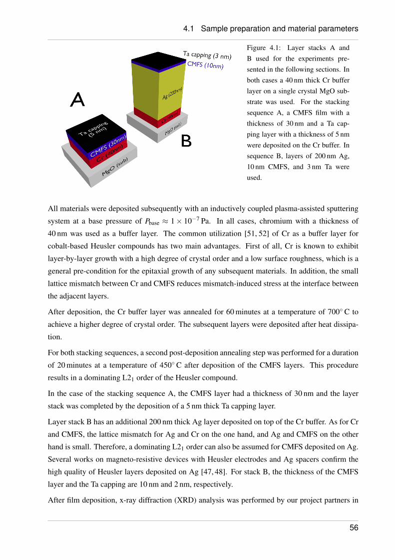
4.1 Sample preparation and material parameters

Figure 4.1: Layer stacks A andB used for the experiments pre-sented in the following sections. Inboth cases a 40 nm thick Cr bufferlayer on a single crystal MgO sub-strate was used. For the stackingsequence A, a CMFS film with athickness of 30 nm and a Ta cap-ping layer with a thickness of 5 nmwere deposited on the Cr buffer. Insequence B, layers of 200 nm Ag,10 nm CMFS, and 3 nm Ta wereused.

All materials were deposited subsequently with an inductively coupled plasma-assisted sputtering

system at a base pressure of Pbase ≈ 1× 10−7 Pa. In all cases, chromium with a thickness of

40 nm was used as a buffer layer. The common utilization [51, 52] of Cr as a buffer layer for

cobalt-based Heusler compounds has two main advantages. First of all, Cr is known to exhibit

layer-by-layer growth with a high degree of crystal order and a low surface roughness, which is a

general pre-condition for the epitaxial growth of any subsequent materials. In addition, the small

lattice mismatch between Cr and CMFS reduces mismatch-induced stress at the interface between

the adjacent layers.

After deposition, the Cr buffer layer was annealed for 60 minutes at a temperature of 700 C to

achieve a higher degree of crystal order. The subsequent layers were deposited after heat dissipa-

tion.

For both stacking sequences, a second post-deposition annealing step was performed for a duration

of 20 minutes at a temperature of 450 C after deposition of the CMFS layers. This procedure

results in a dominating L21 order of the Heusler compound.

In the case of the stacking sequence A, the CMFS layer had a thickness of 30 nm and the layer

stack was completed by the deposition of a 5 nm thick Ta capping layer.

Layer stack B has an additional 200 nm thick Ag layer deposited on top of the Cr buffer. As for Cr

and CMFS, the lattice mismatch for Ag and Cr on the one hand, and Ag and CMFS on the other

hand is small. Therefore, a dominating L21 order can also be assumed for CMFS deposited on Ag.

Several works on magneto-resistive devices with Heusler electrodes and Ag spacers confirm the

high quality of Heusler layers deposited on Ag [47, 48]. For stack B, the thickness of the CMFS

layer and the Ta capping are 10 nm and 2 nm, respectively.

After film deposition, x-ray diffraction (XRD) analysis was performed by our project partners in

56

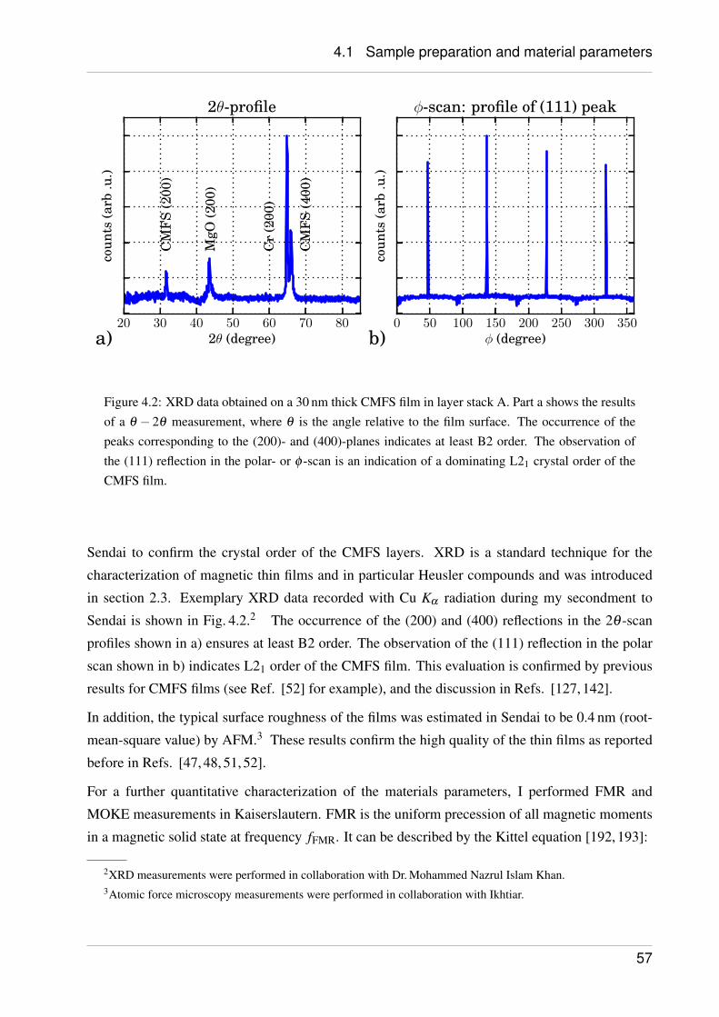
4.1 Sample preparation and material parameters

20 30 40 50 60 70 802θ (degree)

coun

ts(a

rb.u

.)

CM

FS

(200

)

CM

FS

(400

)

Cr

(200

)

MgO

(200

)

2θ-profile

0 50 100 150 200 250 300 350φ (degree)

coun

ts(a

rb.u

.)

φ-scan: profile of (111) peak

a) b)

Figure 4.2: XRD data obtained on a 30 nm thick CMFS film in layer stack A. Part a shows the resultsof a θ − 2θ measurement, where θ is the angle relative to the film surface. The occurrence of thepeaks corresponding to the (200)- and (400)-planes indicates at least B2 order. The observation ofthe (111) reflection in the polar- or φ -scan is an indication of a dominating L21 crystal order of theCMFS film.

Sendai to confirm the crystal order of the CMFS layers. XRD is a standard technique for the

characterization of magnetic thin films and in particular Heusler compounds and was introduced

in section 2.3. Exemplary XRD data recorded with Cu Kα radiation during my secondment to

Sendai is shown in Fig. 4.2.2 The occurrence of the (200) and (400) reflections in the 2θ -scan

profiles shown in a) ensures at least B2 order. The observation of the (111) reflection in the polar

scan shown in b) indicates L21 order of the CMFS film. This evaluation is confirmed by previous

results for CMFS films (see Ref. [52] for example), and the discussion in Refs. [127, 142].

In addition, the typical surface roughness of the films was estimated in Sendai to be 0.4 nm (root-

mean-square value) by AFM.3 These results confirm the high quality of the thin films as reported

before in Refs. [47, 48, 51, 52].

For a further quantitative characterization of the materials parameters, I performed FMR and

MOKE measurements in Kaiserslautern. FMR is the uniform precession of all magnetic moments

in a magnetic solid state at frequency fFMR. It can be described by the Kittel equation [192, 193]:

2XRD measurements were performed in collaboration with Dr. Mohammed Nazrul Islam Khan.3Atomic force microscopy measurements were performed in collaboration with Ikhtiar.

57

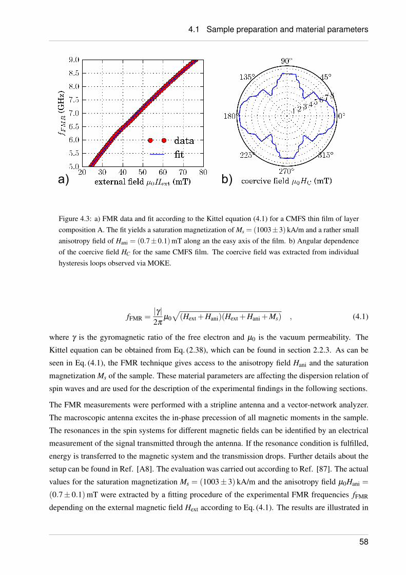
4.1 Sample preparation and material parameters

Figure 4.3: a) FMR data and fit according to the Kittel equation (4.1) for a CMFS thin film of layercomposition A. The fit yields a saturation magnetization of Ms = (1003±3) kA/m and a rather smallanisotropy field of Hani = (0.7± 0.1)mT along an the easy axis of the film. b) Angular dependenceof the coercive field HC for the same CMFS film. The coercive field was extracted from individualhysteresis loops observed via MOKE.

fFMR =|γ|2π

µ0√(Hext +Hani)(Hext +Hani +Ms) , (4.1)

where γ is the gyromagnetic ratio of the free electron and µ0 is the vacuum permeability. The

Kittel equation can be obtained from Eq. (2.38), which can be found in section 2.2.3. As can be

seen in Eq. (4.1), the FMR technique gives access to the anisotropy field Hani and the saturation

magnetization Ms of the sample. These material parameters are affecting the dispersion relation of

spin waves and are used for the description of the experimental findings in the following sections.

The FMR measurements were performed with a stripline antenna and a vector-network analyzer.

The macroscopic antenna excites the in-phase precession of all magnetic moments in the sample.

The resonances in the spin systems for different magnetic fields can be identified by an electrical

measurement of the signal transmitted through the antenna. If the resonance condition is fulfilled,

energy is transferred to the magnetic system and the transmission drops. Further details about the

setup can be found in Ref. [A8]. The evaluation was carried out according to Ref. [87]. The actual

values for the saturation magnetization Ms = (1003± 3) kA/m and the anisotropy field µ0Hani =

(0.7± 0.1)mT were extracted by a fitting procedure of the experimental FMR frequencies fFMR

depending on the external magnetic field Hext according to Eq. (4.1). The results are illustrated in

58

4.1 Sample preparation and material parameters

Fig. 4.3a).

The MOKE causes a rotation of the polarization direction of light reflected at a magnetic material

[194]. Since this rotation is proportional to the magnetization, MOKE is a common tool for the

characterization of magnetic switching and magnetic anisotropies [A1, A2] and is widely used for

the characterization of Heusler compounds [49, 195–197].

Fig. 4.3b) shows the in-plane angular dependence of the coercive field HC measured on a CMFS

thin film in layer stack A. This polar plot summarizes the results of several individual hystere-

sis loops for different orientations. Since a high coercive field is an indication for an easy axis,

the fourfold symmetry of the coercivity reflects the cubic crystallographic structure of CMFS. In

accordance with the small value for the anisotropy field estimated via FMR, the variation of the

coercive field µ0HC = 4−8 mT is also rather small. These results indicate a crystalline anisotropy

that is almost negligible in comparison with the shape anisotropy in the microstructures that were

used for the following measurements.

In summary, the characterization confirmed the high quality of the CMFS thin films and the quan-

titative analysis yielded the material parameters for the following analysis of the experimental

findings. All analytical calculations as well as the micromagnetic simulations presented below are

based on the material parameters estimated above.

4.1.2 Patterning of CMFS microstructures and preparation of antennas

In this section, the patterning of the CMFS microstructures from the thin films as well as the

preparation of antenna structures for the external excitation of spin dynamics will be discussed.

This presentation is mainly focused on the technical details of the sample preparation. Detailed

descriptions of the final sample layouts with all relevant dimensions will be presented together

with the experimental results in the corresponding sections.

While the realization of the final sample layout for the layer stack A was performed in the Nano

Structuring Center of the TU Kaiserslautern,4 the final structures prepared from layer stack B

were fabricated in Sendai during my secondment.5 The different approaches for the two different

systems will be explained in the following. Further information including technical details can be

found in [124, 198].

The samples structures fabricated from stack A and B, respectively, are used for different experi-

mental purposes. The sample layouts patterned from layer stack A comprise spin-wave waveguides

4The sample preparation of layer stack A was supported by Thomas Brächer and Philipp Pirro. Electron-beamlithography was performed by Bert Lägel.

5The patterning of the magnetic microstructures as well as the antenna structures for layer stack B was performedby Yuki Kawada.

59

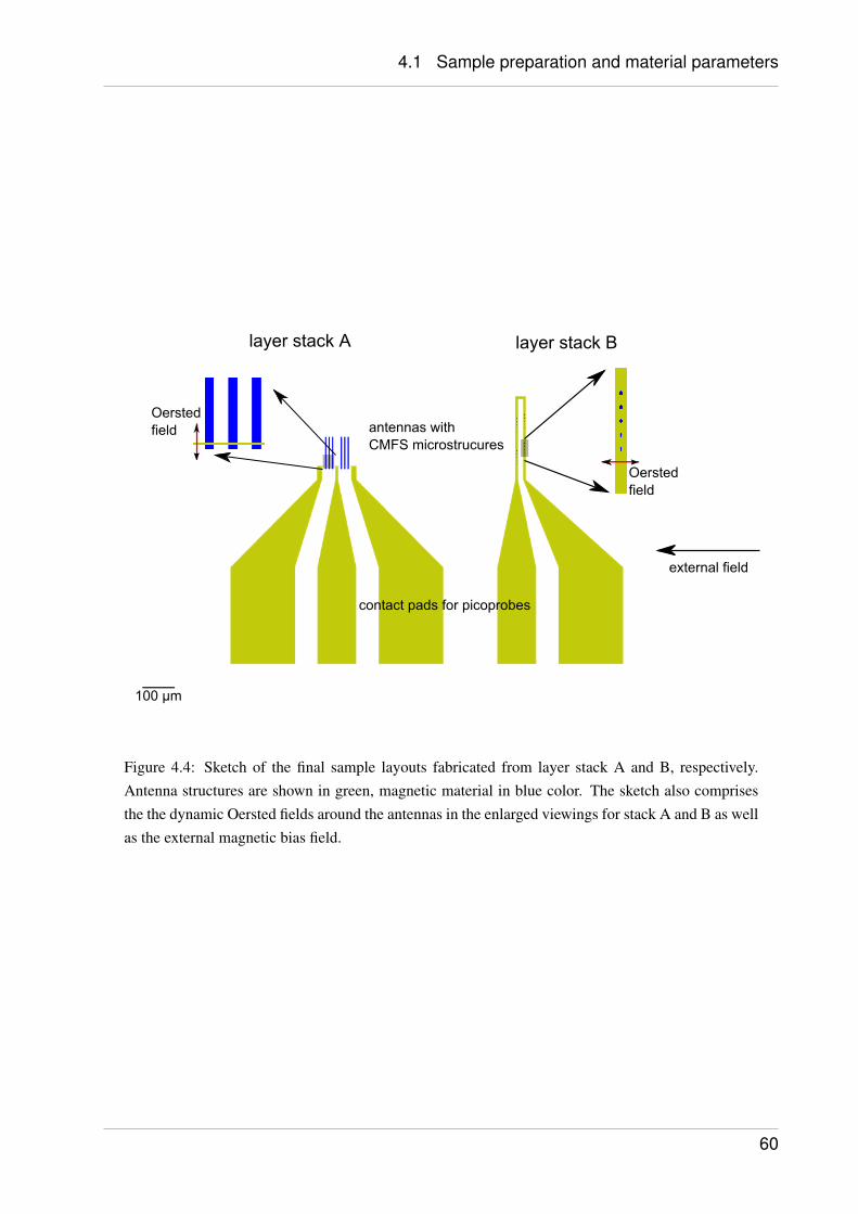
4.1 Sample preparation and material parameters

Figure 4.4: Sketch of the final sample layouts fabricated from layer stack A and B, respectively.Antenna structures are shown in green, magnetic material in blue color. The sketch also comprisesthe the dynamic Oersted fields around the antennas in the enlarged viewings for stack A and B as wellas the external magnetic bias field.

60

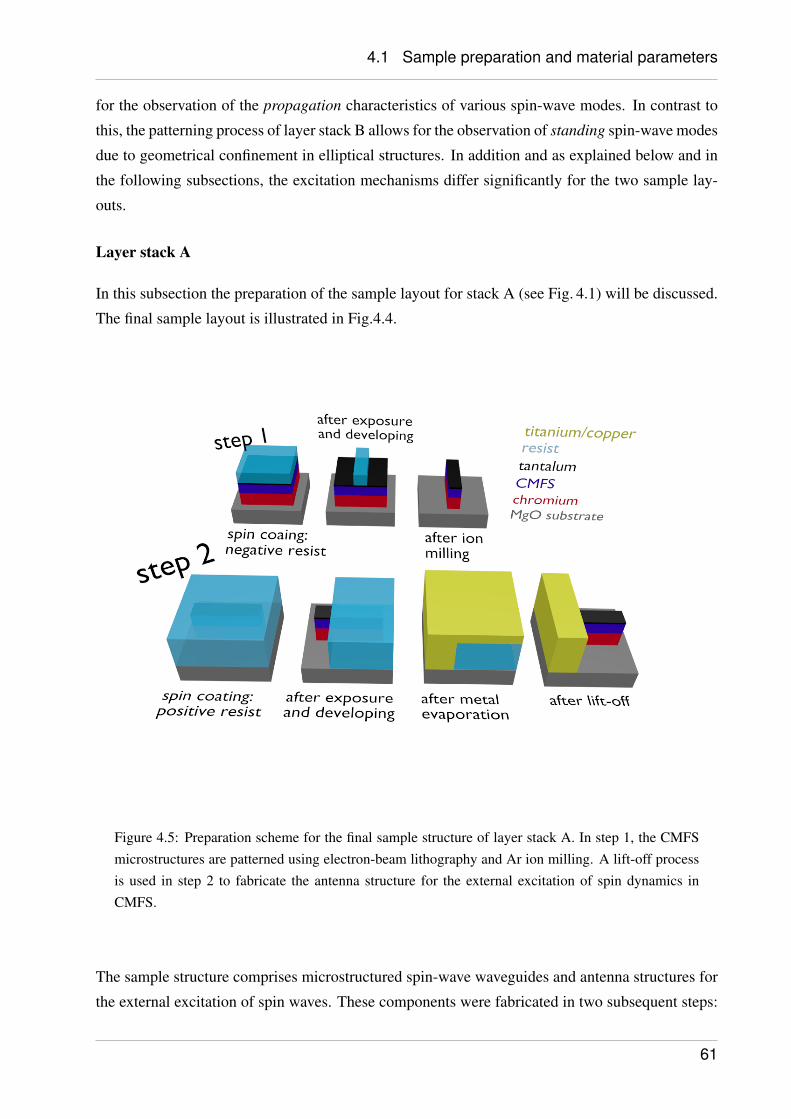
4.1 Sample preparation and material parameters

for the observation of the propagation characteristics of various spin-wave modes. In contrast to

this, the patterning process of layer stack B allows for the observation of standing spin-wave modes

due to geometrical confinement in elliptical structures. In addition and as explained below and in

the following subsections, the excitation mechanisms differ significantly for the two sample lay-

outs.

Layer stack A

In this subsection the preparation of the sample layout for stack A (see Fig. 4.1) will be discussed.

The final sample layout is illustrated in Fig.4.4.

Figure 4.5: Preparation scheme for the final sample structure of layer stack A. In step 1, the CMFSmicrostructures are patterned using electron-beam lithography and Ar ion milling. A lift-off processis used in step 2 to fabricate the antenna structure for the external excitation of spin dynamics inCMFS.

The sample structure comprises microstructured spin-wave waveguides and antenna structures for

the external excitation of spin waves. These components were fabricated in two subsequent steps:

61

4.1 Sample preparation and material parameters

the patterning of the CMFS microstructures and the deposition of the antenna structure. A sketch

of these processes, that will be discussed below, can be found in Fig. 4.5

The microstructures were patterned from the CMFS thin films via a combination of electron-beam

lithography and subsequent argon-ion milling. For this purpose, the samples were spin-coated

with a negative resist. After electron-beam irradiation and developing of the resist, this procedure

resulted in a mask covering the areas corresponding to the microstructures. This mask protected

the entire layer stack below, while the unprotected material was removed in the following Ar-ion

milling. This process leaves exclusively the isolated CMFS microstructures on the MgO substrate.

For the external excitation of spin waves in these CMFS microstructures, a structure of titanium

and copper serves as the antenna. This structure consists of two different parts: large contact pads

with dimensions of several 100 µm and the actual micron sized antennas close to the CMFS mi-

crostructures. These dimensions were chosen to achieve two different requirements. First of all,

the almost macroscopic dimensions of the contact pads allow for the connection of the antenna

structure to external microwave circuitry via picoprobes.6 Secondly, the microscopic dimensions

of the actual antennas are required for the efficient excitation of spin-wave wavelengths on the

microscale. Excitation or amplification of spin dynamics is realized via the Oersted fields that ac-

company currents flowing through a conductor. By the application of alternating currents, dynamic

Oersted fields, that act on the magnetization, can be achieved. The particular choice of microwave

currents can be explained by their frequencies in the gigahertz regime where spin dynamics can be

excited resonantly. The actual mechanisms of excitation and amplification will be discussed in the

corresponding sections in more detail.

For the fabrication of the antenna structures, electron-beam lithography and the lift-off technique

were used. For this purpose, the samples were spin-coated with a positive resist. After electron-

beam irradiation and developing of the resist, the resist covered the entire sample, but for the areas

of the final antenna structures. In a next step, two layers of 20 nm titanium and 400 nm copper

were deposited on the sample via electron-beam evaporation. Finally, the remaining resist - and

thus the undesired part of the Ti/Cu bilayer on top - was removed in a lift-off process to form the

final antenna structure.

Layer stack B

The major difference between the layer stacks A and B is the need of an additional metallic layer

in the case of stack A. The deposition of this additional layer was required for the fabrication of the

antenna structure. Layer stack B already contains an Ag layer with a thickness 200 nm, that will be

used for this purpose. Thus, the Ag will be used to form the contact pads to the external microwave

6For details see: http://ggb.com/

62

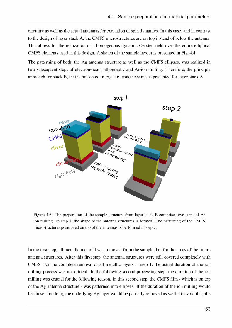
4.1 Sample preparation and material parameters

circuitry as well as the actual antennas for excitation of spin dynamics. In this case, and in contrast

to the design of layer stack A, the CMFS microstructures are on top instead of below the antenna.

This allows for the realization of a homogenous dynamic Oersted field over the entire elliptical

CMFS elements used in this design. A sketch of the sample layout is presented in Fig. 4.4.

The patterning of both, the Ag antenna structure as well as the CMFS ellipses, was realized in

two subsequent steps of electron-beam lithography and Ar-ion milling. Therefore, the principle

approach for stack B, that is presented in Fig. 4.6, was the same as presented for layer stack A.

Figure 4.6: The preparation of the sample structure from layer stack B comprises two steps of Arion milling. In step 1, the shape of the antenna structures is formed. The patterning of the CMFSmicrostructures positioned on top of the antennas is performed in step 2.

In the first step, all metallic material was removed from the sample, but for the areas of the future

antenna structures. After this first step, the antenna structures were still covered completely with

CMFS. For the complete removal of all metallic layers in step 1, the actual duration of the ion

milling process was not critical. In the following second processing step, the duration of the ion

milling was crucial for the following reason. In this second step, the CMFS film - which is on top

of the Ag antenna structure - was patterned into ellipses. If the duration of the ion milling would

be chosen too long, the underlying Ag layer would be partially removed as well. To avoid this, the

63

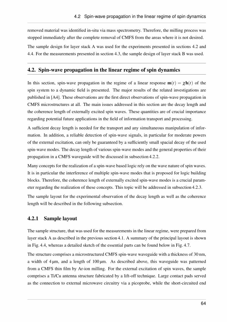
4.2 Spin-wave propagation in the linear regime of spin dynamics

removed material was identified in-situ via mass spectrometry. Therefore, the milling process was

stopped immediately after the complete removal of CMFS from the areas where it is not desired.

The sample design for layer stack A was used for the experiments presented in sections 4.2 and

4.4. For the measurements presented in section 4.3, the sample design of layer stack B was used.

4.2. Spin-wave propagation in the linear regime of spin dynamics

In this section, spin-wave propagation in the regime of a linear response m(t) = χh(t) of the

spin system to a dynamic field is presented. The major results of the related investigations are

published in [A4]. These observations are the first direct observations of spin-wave propagation in

CMFS microstructures at all. The main issues addressed in this section are the decay length and

the coherence length of externally excited spin waves. These quantities are of crucial importance

regarding potential future applications in the field of information transport and processing.

A sufficient decay length is needed for the transport and any simultaneous manipulation of infor-

mation. In addition, a reliable detection of spin-wave signals, in particular for moderate powers

of the external excitation, can only be guaranteed by a sufficiently small spacial decay of the used

spin-wave modes. The decay length of various spin-wave modes and the general properties of their

propagation in a CMFS waveguide will be discussed in subsection 4.2.2.

Many concepts for the realization of a spin-wave based logic rely on the wave nature of spin waves.

It is in particular the interference of multiple spin-wave modes that is proposed for logic building

blocks. Therefore, the coherence length of externally excited spin-wave modes is a crucial param-

eter regarding the realization of these concepts. This topic will be addressed in subsection 4.2.3.

The sample layout for the experimental observation of the decay length as well as the coherence

length will be described in the following subsection.

4.2.1 Sample layout

The sample structure, that was used for the measurements in the linear regime, were prepared from

layer stack A as described in the previous section 4.1. A summary of the principal layout is shown

in Fig. 4.4, whereas a detailed sketch of the essential parts can be found below in Fig. 4.7.

The structure comprises a microstructured CMFS spin-wave waveguide with a thickness of 30 nm,

a width of 4 µm, and a length of 100 µm. As described above, this waveguide was patterned

from a CMFS thin film by Ar-ion milling. For the external excitation of spin waves, the sample

comprises a Ti/Cu antenna structure fabricated by a lift-off technique. Large contact pads served

as the connection to external microwave circuitry via a picoprobe, while the short-circuited end

64

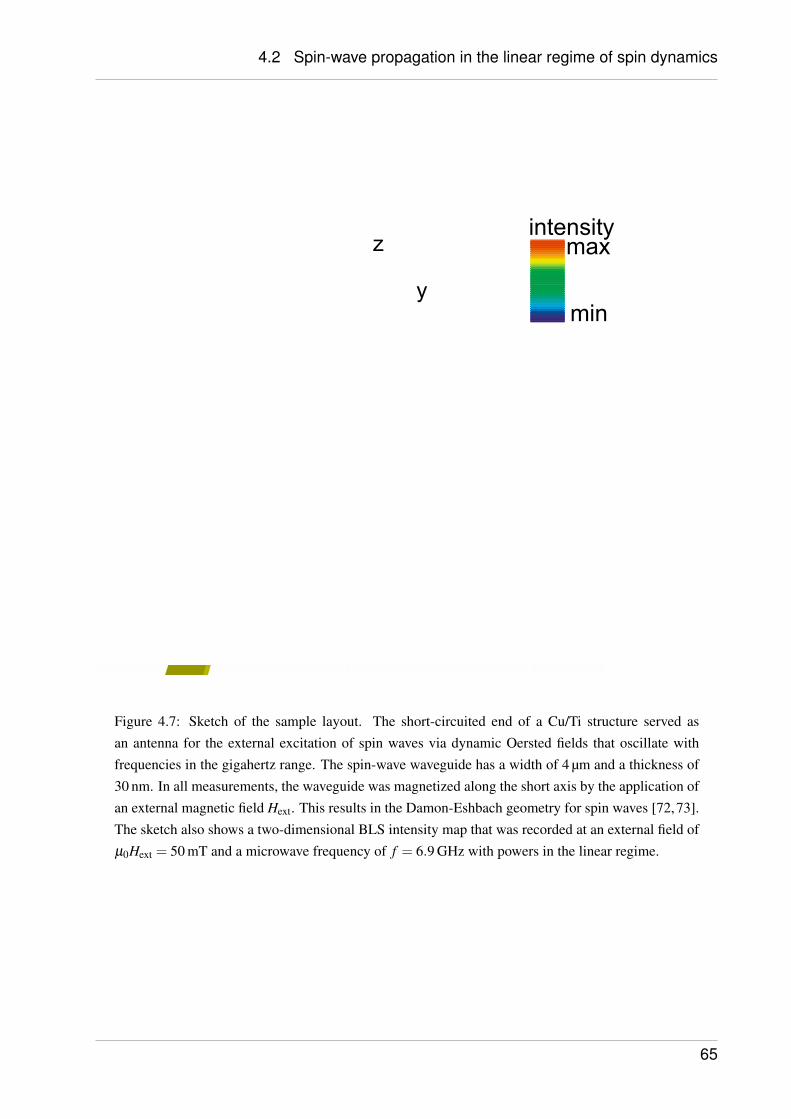
4.2 Spin-wave propagation in the linear regime of spin dynamics

intensitymax

min

z

y

Figure 4.7: Sketch of the sample layout. The short-circuited end of a Cu/Ti structure served asan antenna for the external excitation of spin waves via dynamic Oersted fields that oscillate withfrequencies in the gigahertz range. The spin-wave waveguide has a width of 4 µm and a thickness of30 nm. In all measurements, the waveguide was magnetized along the short axis by the application ofan external magnetic field Hext. This results in the Damon-Eshbach geometry for spin waves [72,73].The sketch also shows a two-dimensional BLS intensity map that was recorded at an external field ofµ0Hext = 50 mT and a microwave frequency of f = 6.9 GHz with powers in the linear regime.

65

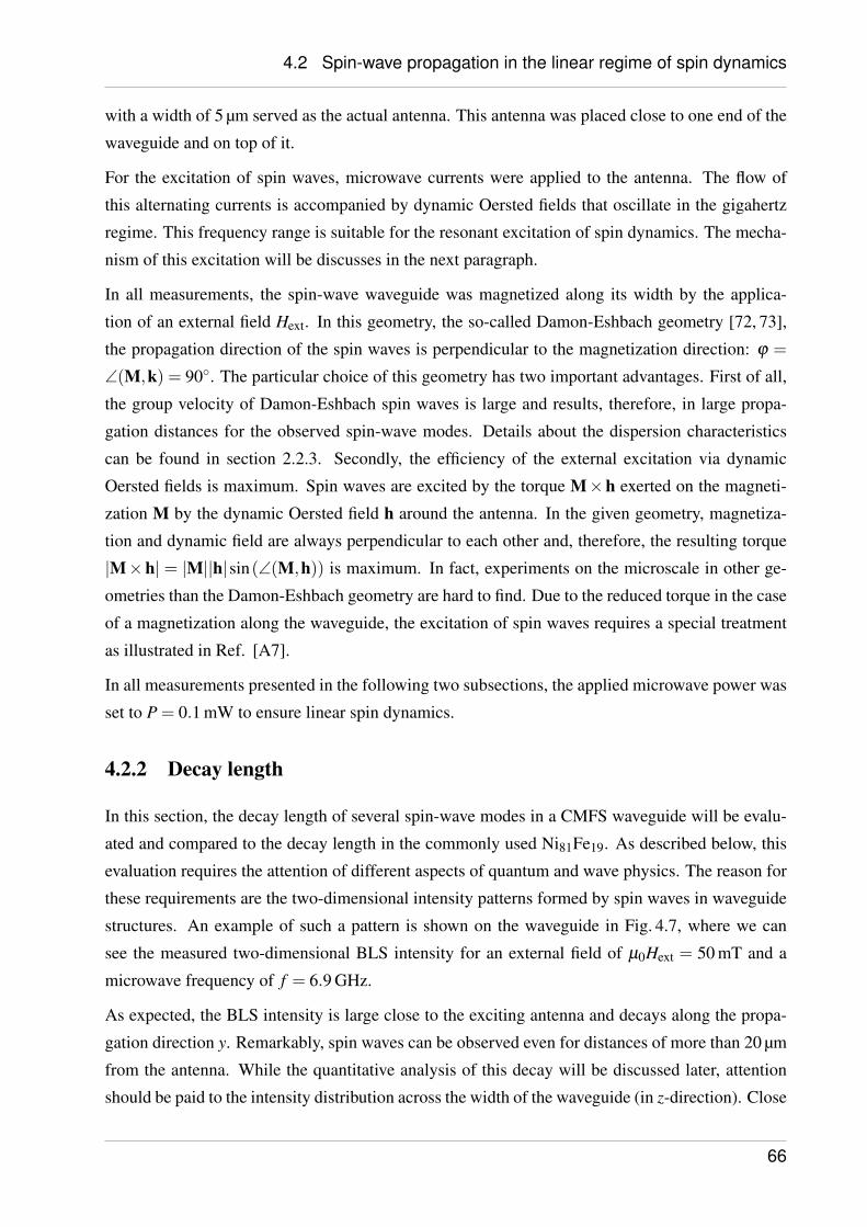
4.2 Spin-wave propagation in the linear regime of spin dynamics

with a width of 5 µm served as the actual antenna. This antenna was placed close to one end of the

waveguide and on top of it.

For the excitation of spin waves, microwave currents were applied to the antenna. The flow of

this alternating currents is accompanied by dynamic Oersted fields that oscillate in the gigahertz

regime. This frequency range is suitable for the resonant excitation of spin dynamics. The mecha-

nism of this excitation will be discusses in the next paragraph.

In all measurements, the spin-wave waveguide was magnetized along its width by the applica-

tion of an external field Hext. In this geometry, the so-called Damon-Eshbach geometry [72, 73],

the propagation direction of the spin waves is perpendicular to the magnetization direction: ϕ =

∠(M,k) = 90. The particular choice of this geometry has two important advantages. First of all,

the group velocity of Damon-Eshbach spin waves is large and results, therefore, in large propa-

gation distances for the observed spin-wave modes. Details about the dispersion characteristics

can be found in section 2.2.3. Secondly, the efficiency of the external excitation via dynamic

Oersted fields is maximum. Spin waves are excited by the torque M×h exerted on the magneti-

zation M by the dynamic Oersted field h around the antenna. In the given geometry, magnetiza-

tion and dynamic field are always perpendicular to each other and, therefore, the resulting torque

|M×h| = |M||h|sin(∠(M,h)) is maximum. In fact, experiments on the microscale in other ge-

ometries than the Damon-Eshbach geometry are hard to find. Due to the reduced torque in the case

of a magnetization along the waveguide, the excitation of spin waves requires a special treatment

as illustrated in Ref. [A7].

In all measurements presented in the following two subsections, the applied microwave power was

set to P = 0.1 mW to ensure linear spin dynamics.

4.2.2 Decay length

In this section, the decay length of several spin-wave modes in a CMFS waveguide will be evalu-

ated and compared to the decay length in the commonly used Ni81Fe19. As described below, this

evaluation requires the attention of different aspects of quantum and wave physics. The reason for

these requirements are the two-dimensional intensity patterns formed by spin waves in waveguide

structures. An example of such a pattern is shown on the waveguide in Fig. 4.7, where we can

see the measured two-dimensional BLS intensity for an external field of µ0Hext = 50 mT and a

microwave frequency of f = 6.9 GHz.

As expected, the BLS intensity is large close to the exciting antenna and decays along the propa-

gation direction y. Remarkably, spin waves can be observed even for distances of more than 20 µm

from the antenna. While the quantitative analysis of this decay will be discussed later, attention

should be paid to the intensity distribution across the width of the waveguide (in z-direction). Close

66

4.2 Spin-wave propagation in the linear regime of spin dynamics

← waveguide →

spin

-wav

eam

plit

ude

n=1

n=2

n=3

waveguide modes

← waveguide →

spin

-wav

eam

plit

ude

∆ϕ=0

∆ϕ=π

mode 1 and 3

a) b)

Figure 4.8: a) Spin-wave amplitudealong the width of the waveguidefor the mode numbers n = 1− 3.The number n is defined by thequantization condition kz =

nπ

w andcounts the number of antinodes. b)Interference pattern of the first andthird waveguide mode for relativephases of ∆φ = 0 and ∆φ = π .

to the antenna two distinct maxima can be observed. In contrast to this observation, at a distance of

about 7 µm from the antenna only one maximum in the center of the waveguide is visible. Similar

patterns have been observed in spin-wave waveguides of other materials before and their origin

will be described supported by former publications like Refs. [75, 199, 200] and [A7].

The reason for the formation of these patterns is a quantization of spin-wave modes due to the finite

width of the waveguide as already discussed in section 2.2.4. While the wave-vector component

ky along the propagation direction can have arbitrary values, the wave-vector component kz across

the width of the waveguide must fulfill the following quantization condition:

kz =nπ

weff. (4.2)

In this equation, weff is the effective width of the waveguide and n is a natural number as described

in section 2.2.4. Following the usual convention used in literature about spin dynamics, the number

n is equal to the number of antinodes in the intensity pattern formed by the corresponding spin-

wave mode (see for example [200] and [A7]). Therefore, the z-component of the total in-plane

wave vector k=(ky,kz) can have only discrete values ky = ky,n defined by the waveguide geometry.

The mode profiles along the width of the waveguide are shown in Fig. 4.8a) for the spin-wave

modes n = 1−3.

A result of this quantization effect is the excitation of multiple modes that propagate simultane-

ously in the waveguide. In the case of an external excitation via an antenna across the entire

waveguide, symmetry arguments reduce the possible mode numbers n to odd numbers. This can

be understood as follows. For typical frequencies used in the present experiment, the microwave

wavelength is in the centimeter range. Therefore, the space dependence of the dynamic Oersted

field across the spin-wave waveguide with a width of only 4 µm can be neglected. In contrast to

this, waveguide modes with even mode numbers n, like the second mode shown in Fig. 4.8a), have

magnetization patterns composed of equal parts with a relative phase shift of π . As a consequence,

67

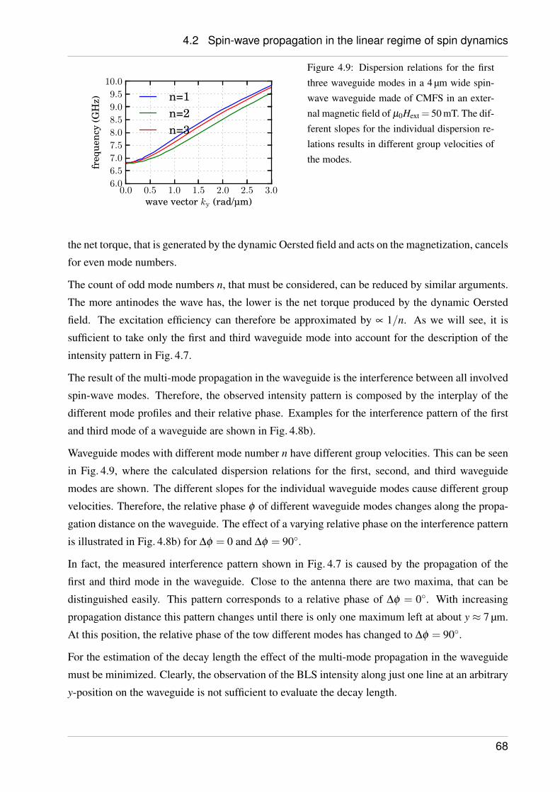
4.2 Spin-wave propagation in the linear regime of spin dynamics

0.0 0.5 1.0 1.5 2.0 2.5 3.0wave vector ky (rad/µm)

6.0

6.5

7.0

7.5

8.0

8.5

9.0

9.5

10.0

freq

uenc

y(G

Hz) n=1

n=2n=3

Figure 4.9: Dispersion relations for the firstthree waveguide modes in a 4 µm wide spin-wave waveguide made of CMFS in an exter-nal magnetic field of µ0Hext = 50 mT. The dif-ferent slopes for the individual dispersion re-lations results in different group velocities ofthe modes.

the net torque, that is generated by the dynamic Oersted field and acts on the magnetization, cancels

for even mode numbers.

The count of odd mode numbers n, that must be considered, can be reduced by similar arguments.

The more antinodes the wave has, the lower is the net torque produced by the dynamic Oersted

field. The excitation efficiency can therefore be approximated by ∝ 1/n. As we will see, it is

sufficient to take only the first and third waveguide mode into account for the description of the

intensity pattern in Fig. 4.7.

The result of the multi-mode propagation in the waveguide is the interference between all involved

spin-wave modes. Therefore, the observed intensity pattern is composed by the interplay of the

different mode profiles and their relative phase. Examples for the interference pattern of the first

and third mode of a waveguide are shown in Fig. 4.8b).

Waveguide modes with different mode number n have different group velocities. This can be seen

in Fig. 4.9, where the calculated dispersion relations for the first, second, and third waveguide

modes are shown. The different slopes for the individual waveguide modes cause different group

velocities. Therefore, the relative phase φ of different waveguide modes changes along the propa-

gation distance on the waveguide. The effect of a varying relative phase on the interference pattern

is illustrated in Fig. 4.8b) for ∆φ = 0 and ∆φ = 90.

In fact, the measured interference pattern shown in Fig. 4.7 is caused by the propagation of the

first and third mode in the waveguide. Close to the antenna there are two maxima, that can be

distinguished easily. This pattern corresponds to a relative phase of ∆φ = 0. With increasing

propagation distance this pattern changes until there is only one maximum left at about y≈ 7 µm.

At this position, the relative phase of the tow different modes has changed to ∆φ = 90.

For the estimation of the decay length the effect of the multi-mode propagation in the waveguide

must be minimized. Clearly, the observation of the BLS intensity along just one line at an arbitrary

y-position on the waveguide is not sufficient to evaluate the decay length.

68

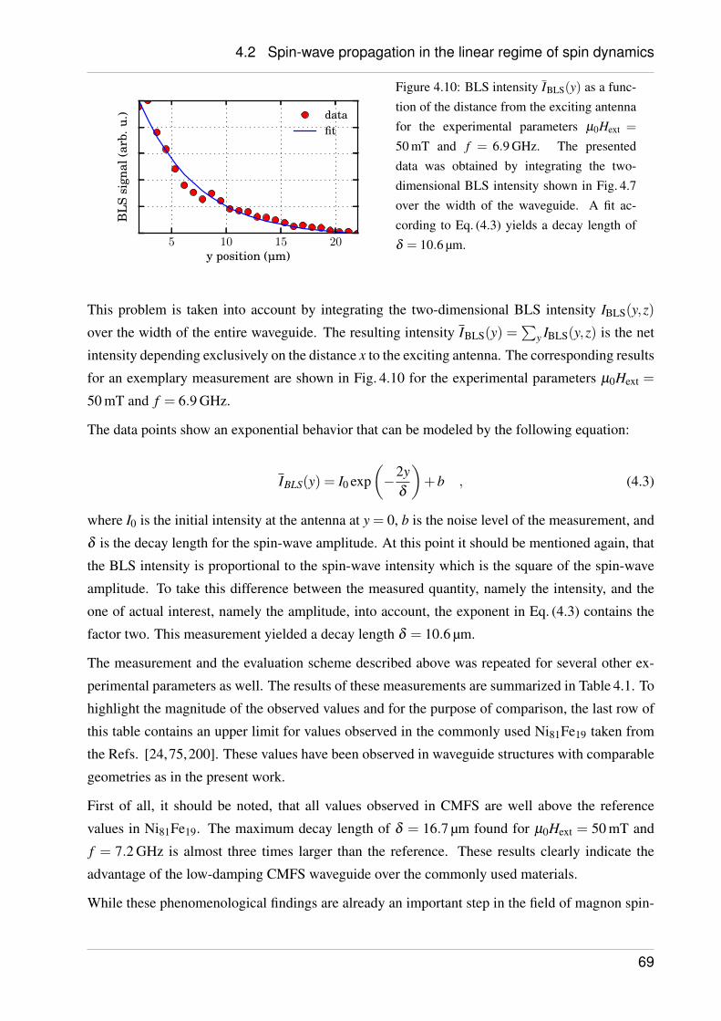
4.2 Spin-wave propagation in the linear regime of spin dynamics

5 10 15 20y position (µm)

BL

Ssi

gnal

(arb

.u.) data

fit

Figure 4.10: BLS intensity IBLS(y) as a func-tion of the distance from the exciting antennafor the experimental parameters µ0Hext =

50 mT and f = 6.9 GHz. The presenteddata was obtained by integrating the two-dimensional BLS intensity shown in Fig. 4.7over the width of the waveguide. A fit ac-cording to Eq. (4.3) yields a decay length ofδ = 10.6 µm.

This problem is taken into account by integrating the two-dimensional BLS intensity IBLS(y,z)

over the width of the entire waveguide. The resulting intensity IBLS(y) =∑

y IBLS(y,z) is the net

intensity depending exclusively on the distance x to the exciting antenna. The corresponding results

for an exemplary measurement are shown in Fig. 4.10 for the experimental parameters µ0Hext =

50 mT and f = 6.9 GHz.

The data points show an exponential behavior that can be modeled by the following equation:

IBLS(y) = I0 exp(−2y

δ

)+b , (4.3)

where I0 is the initial intensity at the antenna at y = 0, b is the noise level of the measurement, and

δ is the decay length for the spin-wave amplitude. At this point it should be mentioned again, that

the BLS intensity is proportional to the spin-wave intensity which is the square of the spin-wave

amplitude. To take this difference between the measured quantity, namely the intensity, and the

one of actual interest, namely the amplitude, into account, the exponent in Eq. (4.3) contains the

factor two. This measurement yielded a decay length δ = 10.6 µm.

The measurement and the evaluation scheme described above was repeated for several other ex-

perimental parameters as well. The results of these measurements are summarized in Table 4.1. To

highlight the magnitude of the observed values and for the purpose of comparison, the last row of

this table contains an upper limit for values observed in the commonly used Ni81Fe19 taken from

the Refs. [24,75,200]. These values have been observed in waveguide structures with comparable

geometries as in the present work.

First of all, it should be noted, that all values observed in CMFS are well above the reference

values in Ni81Fe19. The maximum decay length of δ = 16.7 µm found for µ0Hext = 50 mT and

f = 7.2 GHz is almost three times larger than the reference. These results clearly indicate the

advantage of the low-damping CMFS waveguide over the commonly used materials.

While these phenomenological findings are already an important step in the field of magnon spin-

69

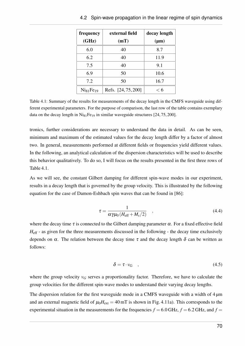
4.2 Spin-wave propagation in the linear regime of spin dynamics

frequency external field decay length(GHz) (mT) (µm)

6.0 40 8.7

6.2 40 11.9

7.5 40 9.1

6.9 50 10.6

7.2 50 16.7

Ni81Fe19 Refs. [24, 75, 200] < 6

Table 4.1: Summary of the results for measurements of the decay length in the CMFS waveguide using dif-ferent experimental parameters. For the purpose of comparison, the last row of the table contains exemplarydata on the decay length in Ni81Fe19 in similar waveguide structures [24, 75, 200].

tronics, further considerations are necessary to understand the data in detail. As can be seen,

minimum and maximum of the estimated values for the decay length differ by a factor of almost

two. In general, measurements performed at different fields or frequencies yield different values.

In the following, an analytical calculation of the dispersion characteristics will be used to describe

this behavior qualitatively. To do so, I will focus on the results presented in the first three rows of

Table 4.1.

As we will see, the constant Gilbert damping for different spin-wave modes in our experiment,

results in a decay length that is governed by the group velocity. This is illustrated by the following

equation for the case of Damon-Eshbach spin waves that can be found in [86]:

τ =1

αγµ0 (Heff +Ms/2), (4.4)

where the decay time τ is connected to the Gilbert damping parameter α . For a fixed effective field

Heff - as given for the three measurements discussed in the following - the decay time exclusively

depends on α . The relation between the decay time τ and the decay length δ can be written as

follows:

δ = τ · vG , (4.5)

where the group velocity vG serves a proportionality factor. Therefore, we have to calculate the

group velocities for the different spin-wave modes to understand their varying decay lengths.

The dispersion relation for the first waveguide mode in a CMFS waveguide with a width of 4 µm

and an external magnetic field of µ0Hext = 40 mT is shown in Fig. 4.11a). This corresponds to the

experimental situation in the measurements for the frequencies f = 6.0 GHz, f = 6.2 GHz, and f =

70

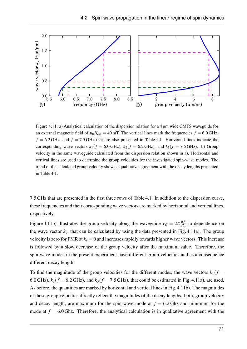
4.2 Spin-wave propagation in the linear regime of spin dynamics

5.5 6.0 6.5 7.0 7.5 8.0 8.5frequency (GHz)

0.0

0.5

1.0

1.5

2.0w

ave

vect

ork

y(r

ad/µ

m)

2 4 6 8group velocity (µm/ns)a) b)

Figure 4.11: a) Analytical calculation of the dispersion relation for a 4 µm wide CMFS waveguide foran external magnetic field of µ0Hext = 40 mT. The vertical lines mark the frequencies f = 6.0 GHz,f = 6.2 GHz, and f = 7.5 GHz that are also presented in Table 4.1. Horizontal lines indicate thecorresponding wave vectors k1( f = 6.0 GHz), k2( f = 6.2 GHz), and k3( f = 7.5 GHz). b) Groupvelocity in the same waveguide calculated from the dispersion relation shown in a). Horizontal andvertical lines are used to determine the group velocities for the investigated spin-wave modes. Thetrend of the calculated group velocity shows a qualitative agreement with the decay lengths presentedin Table 4.1.

7.5 GHz that are presented in the first three rows of Table 4.1. In addition to the dispersion curve,

these frequencies and their corresponding wave vectors are marked by horizontal and vertical lines,

respectively.

Figure 4.11b) illustrates the group velocity along the waveguide vG = 2πd fdky

in dependence on

the wave vector ky, that can be calculated by using the data presented in Fig. 4.11a). The group

velocity is zero for FMR at ky = 0 and increases rapidly towards higher wave vectors. This increase

is followed by a slow decrease of the group velocity after the maximum value. Therefore, the

spin-wave modes in the present experiment have different group velocities and as a consequence

different decay length.

To find the magnitude of the group velocities for the different modes, the wave vectors k1( f =

6.0 GHz), k2( f = 6.2 GHz), and k3( f = 7.5 GHz), that could be estimated in Fig. 4.11a), are used.

As before, the quantities are marked by horizontal and vertical lines in Fig. 4.11b). The magnitudes

of these group velocities directly reflect the magnitudes of the decay lengths: both, group velocity

and decay length, are maximum for the spin-wave mode at f = 6.2 Ghz and minimum for the

mode at f = 6.0 Ghz. Therefore, the analytical calculation is in qualitative agreement with the

71

4.2 Spin-wave propagation in the linear regime of spin dynamics

experimental finding and can serve as an explanation for the observation of a varying decay length.

In principle, Eqs. (4.4) and (4.5) cannot only be used to understand the experimental findings, but

also to estimate the Gilbert damping by using the measured decay length and the calculated group

velocities.

However, despite the qualitative agreement of the calculations and the measured values, a quan-

titative agreement of calculation and experiment could not be found. The major reason for this

is related to the calculation of the group velocity. This can be understood by taking into account

two facts: a strong dependence of the calculated group velocity on many parameters and the used

model itself.

To calculate the group velocity in a spin-wave waveguide many parameters are needed: material

parameters - like the saturation magnetization, the exchange constant, and the anisotropy constants

- as well as geometrical parameters - like the film thickness and the width of the waveguide. For

a waveguide magnetized along its width, the demagnetizing field and, therefore the effective field,

depends on all of these parameters and cannot be calculated analytically. Due to the specific fea-

tures of the group velocity in a waveguide, in particular the rapid increase for small wave vectors,

small changes of one or many of these parameters can cause large deviations of the calculated

group velocities.

In addition to these difficulties, it must be emphasized again that the analytical calculations pre-

sented above are based on a model for the spin-wave dispersion in thin films and not for wave-

guides. The application of this model to a system with a finite dimension by the additional in-

troduction of quantization conditions must be assumed as an approximation rather than an exact

solution. Calculations of the Gilbert damping parameter based on the data presented above yield

values ranging from α = 4×10−3 to α = 8×10−3. Even though these values are close to the value

of α = 3×10−3 (see [51]), their estimation is not very reliable. Therefore, an alternative approach

to estimate the Gilbert damping in a CMFS microstructure will be presented in Section 4.3.

In summary, the first direct observations of spin-wave propagation in a CMFS microstructure at

all were reported in this chapter. Features like the multi-mode propagation in waveguides were

observed and understood supported by previous results in other materials. The general trends for

the observed spin-wave decay lengths was reproduced qualitatively by an analytical calculation.

The quantitative evaluation of the decay lengths in CMFS yielded remarkable values. In compar-

ison with reports about the spin-wave propagation in Ni81Fe19 waveguides, the maximum decay

lengths increased by a factor of almost three to δ = 16.7 µm. This increase can be attributed to the

decreased Gilbert damping in CMFS.

This result confirms the expected advantage of the low-damping CMFS over the typically used

materials and is an important step in magnon spintronics. On the one hand, the increased decay

72

4.2 Spin-wave propagation in the linear regime of spin dynamics

length is a pre-condition for the realization of any concepts regarding potential technical applica-

tions. On the other hand, the successful utilization of CMFS opens the perspective for advanced

experiments on spin dynamics in the microscale.

4.2.3 Coherence length

In addition to a large decay length described in the former section, the coherence of spin waves

[201] is of particular interest for data processing. A long propagation distance is crucial for the

transport and for the detection of information. However, the utilization of spin waves as the carrier

of information also allows for the utilization of an additional degree of freedom: the phase. Indeed,

in the field of magnonic spintronics there are many schemes for information processing that are

based on the interference of spin waves [14,16,17,75,202,203], and do therefore rely on a coherent

propagation. For this reason, the following section is devoted to the investigation of the phase of

externally excited spin-wave modes in CMFS.

The process of BLS itself is phase sensitive. Photons, that were inelastically scattered from

spin waves, therefore carry information about the phase of the involved spin-wave mode. Phase-

resolved BLS microscopy as described in detail in section 3.4 and in Refs. [166, 176, 179–181] is

a powerful tool for the investigation of propagating spin waves and was used for the measurements

presented below. To extract the phase information from the scattered photons, the interference

between the sample beam and a reference beam is observed. This reference beam is shifted by the

same frequency as the sample beam via an electro-optical modulator (EOM). To achieve the same

frequency shift, the EOM is driven by the microwave generator, that is also used for the spin-wave

excitation. Therefore, sample beam and reference beam have the same frequency and are tempo-

rally coherent. Their relative phase is completely determined by the phase accumulation of the

involved spin-wave mode during its propagation. Fig. 4.12 shows the directly observed results of

an phase-resolved BLS measurement as well as the evaluated data for the experimental parameters

µ0Hext = 40 mT and f = 8.5 GHz.

In Fig. 4.12a) the interference signal of the inelastically scattered light with the reference beam is

illustrated for probing positions in different distances to the antenna. The graph contains two data

sets representing individual measurements with a relative phase shift of ∆φ = 90. This artificial

phase shift ∆φ was introduced to the reference beam by shifting the driving microwave signal

with an external phase shifter. The measurements with relative phase shifts as well as intensity

measurements of only the reference beam and only the sample beam (the latter two not shown

here) are needed for the further evaluation as described in [181].

For both interference measurements, the signals are proportional to the square of a sinus with an

exponentially decreasing amplitude. This decreasing amplitude is caused by the decreasing inten-

73

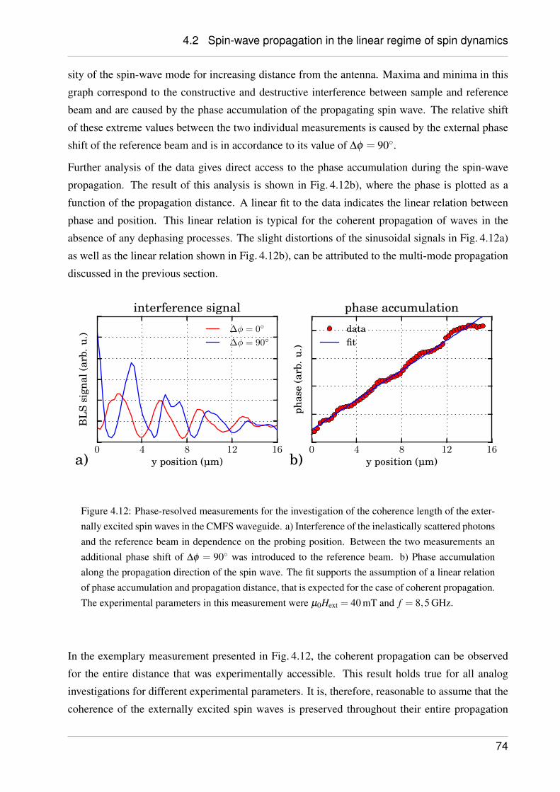
4.2 Spin-wave propagation in the linear regime of spin dynamics

sity of the spin-wave mode for increasing distance from the antenna. Maxima and minima in this

graph correspond to the constructive and destructive interference between sample and reference

beam and are caused by the phase accumulation of the propagating spin wave. The relative shift

of these extreme values between the two individual measurements is caused by the external phase

shift of the reference beam and is in accordance to its value of ∆φ = 90.

Further analysis of the data gives direct access to the phase accumulation during the spin-wave

propagation. The result of this analysis is shown in Fig. 4.12b), where the phase is plotted as a

function of the propagation distance. A linear fit to the data indicates the linear relation between

phase and position. This linear relation is typical for the coherent propagation of waves in the

absence of any dephasing processes. The slight distortions of the sinusoidal signals in Fig. 4.12a)

as well as the linear relation shown in Fig. 4.12b), can be attributed to the multi-mode propagation

discussed in the previous section.

0 4 8 12 16y position (µm)

BL

Ssi

gnal

(arb

.u.)

interference signal

∆φ = 0

∆φ = 90

0 4 8 12 16y position (µm)

phas

e(a

rb.u

.)phase accumulation

datafit

a) b)

Figure 4.12: Phase-resolved measurements for the investigation of the coherence length of the exter-nally excited spin waves in the CMFS waveguide. a) Interference of the inelastically scattered photonsand the reference beam in dependence on the probing position. Between the two measurements anadditional phase shift of ∆φ = 90 was introduced to the reference beam. b) Phase accumulationalong the propagation direction of the spin wave. The fit supports the assumption of a linear relationof phase accumulation and propagation distance, that is expected for the case of coherent propagation.The experimental parameters in this measurement were µ0Hext = 40 mT and f = 8,5 GHz.

In the exemplary measurement presented in Fig. 4.12, the coherent propagation can be observed

for the entire distance that was experimentally accessible. This result holds true for all analog

investigations for different experimental parameters. It is, therefore, reasonable to assume that the

coherence of the externally excited spin waves is preserved throughout their entire propagation

74

4.3 Gilbert damping in a CMFS microstructure

distance in the CMFS waveguide.

In summary, it was shown that spin waves propagating in CMFS waveguides fulfill a crucial pre-

condition for the realization of any schemes of data processing based on interference or other

phase-dependent processes. This pre-condition is their coherent propagation. Together with the

increased propagation distance, the coherence makes CMFS an interesting candidate for any ex-

periments in magnon spintronics. Since the observations described above are the first direct obser-

vations of spin-wave propagation in CMFS microstructures at all, they open the perspective for an

increasing utilization of the CMFS.

In particular, the field of advanced waveguide structures for two-dimensional spin-wave transport

and the field of magnonic crystals could benefit from the low-damping material [36–40]. While

there are numerous interesting concepts in these fields, that have been proven in Ni81Fe19-based

structures, the actual benefit of these concepts is still limited due to the rather small propagation

distances in conventional materials. Thus, the combination of these advanced concepts with the

utilization of low-damping Heusler compounds is a promising way for the further development of

magnon spintronics towards potential technical applications. Therefore, one of the most important

results of the present work is the experimental confirmation of the expected advantages of CMFS

regarding spin-wave propagation that was presented above.

4.3. Gilbert damping in a CMFS microstructure

The following section is devoted to the evaluation of the Gilbert damping parameter in an individ-

ual CMFS microstructure. The Gilbert damping in Heusler materials - among all other material

parameters - strongly depends on the crystallographic order of the thin film [137,138]. The lowest

Gilbert damping is usually reported for the highest order, the L21 state. While the analysis of the

crystallographic order and the Gilbert damping by XRD and FMR are standard techniques for thin

films (see also in section 4.1.1), the analysis turns out to be more complicated on the microscale.

At the same time, it is not self-evident that the crystallographic order and therefore the low Gilbert

damping are preserved in the patterning process. The results on the increased propagation dis-

tances in a CMFS waveguide presented in Section 4.2.2 indicate a low Gilbert damping. However,

a quantitative analysis has not been presented so far.

The issue of the Gilbert damping in patterned microstructures is not only relevant for experiments

on spin-wave propagation but also for the utilization of Heusler materials in devices based on

magneto-resistive effects, namely giant magneto resistance or tunneling magneto resistance de-

vices. In particular, the critical currents for the spin-torque switching in storage devices depend

on the Gilbert damping, which is, therefore, a crucial parameter for all related devices. While the

direct-current based switching of magnetic layer is already utilized in technical applications, the

75

4.3 Gilbert damping in a CMFS microstructure

excitation of spin dynamics by spin-transfer torque is an interesting research field, that can also

profit from a decreased Gilbert damping [23, 24, 47, 48].

In this section, an approach for the measurement of the Gilbert damping in individual microstruc-

tures will be introduced and applied to an elliptical CMFS microstructure [204]. The underlying

physical principle of this method is the parallel parametric amplification of spin dynamics from the

thermal level. Parallel parametric amplification is a widely used technique in the field of spin-wave

physics and was introduced in subsection 2.2.7 [28, 57, 122, 205–208]. Since the previous discus-

sion in subsection 2.2.7 was mainly focused on the mathematical formalism for the description of

the process, a more intuitive approach will be presented in the following.

A big advantage of this method for the evaluation of the damping parameter over the approach

based on the calculation of the group velocity (as discussed in section 4.2.2) is, that its results ex-

clusively depend on measurement parameters and directly accessible data. No additional material

parameters or complicated models are involved in the evaluation.

However, parametric amplification is a phenomenon known not only from the field of spin dy-

namics but for oscillations in general. A prominent example from every day’s life is a child on a

swing. In this case, the amplitude of an oscillating system - child and swing - can be increased

by shifting the center of mass periodically with twice the oscillation frequency of the swing. This

example also illustrates an important fact related to this process: it can be only applied to an al-

ready oscillating system to amplify this oscillation. It is not possible to excite an oscillation from

its equilibrium position. In the following, an illustrative presentation of the process will be given.

A mathematical approach for its description was presented in subsection 2.2.7.

For the analogy to the child on the swing in the magnetic system, we have to consider a precessing

magnetic moment as the oscillating system. A dynamic external magnetic field h2f is the parameter

responsible for the amplification of the precessional motion. This field h2f is usually referred to as

the pumping field. The details will be discussed in the following.

To start this discussion, the precessional motion of a magnetic moment in a thin film must be

considered. In an infinite magnetic medium without any kind of magnetic anisotropy, the tip of a

magnetic moment, that precesses about an effective field, will follow a perfectly circular trajectory.

If we now change the given scenario by reducing one of the dimensions of this magnetic medium,

we can consider it as a magnetic thin film. The sketch in Fig. 4.13 illustrates this scenario.

The finite film thickness gives rise to demagnetizing fields caused by magnetization components

normal to the surface of this film. Therefore, the precession of a magnetic moment will immedi-

ately cause dynamic demagnetizing fields whenever the magnetic moment points out of the thin

film during its precessional motion. Due to these demagnetizing fields, and to minimize the en-

ergy of the system, the circular trajectory of the tip will change to an elliptical one. Since the film

76

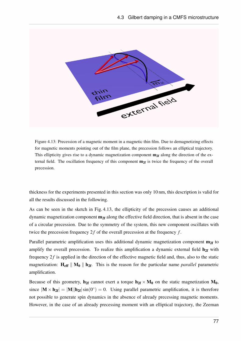
4.3 Gilbert damping in a CMFS microstructure

Figure 4.13: Precession of a magnetic moment in a magnetic thin film. Due to demagnetizing effectsfor magnetic moments pointing out of the film plane, the precession follows an elliptical trajectory.This ellipticity gives rise to a dynamic magnetization component m2f along the direction of the ex-ternal field. The oscillation frequency of this component m2f is twice the frequency of the overallprecession.

thickness for the experiments presented in this section was only 10 nm, this description is valid for

all the results discussed in the following.

As can be seen in the sketch in Fig. 4.13, the ellipticity of the precession causes an additional

dynamic magnetization component m2f along the effective field direction, that is absent in the case

of a circular precession. Due to the symmetry of the system, this new component oscillates with

twice the precession frequency 2 f of the overall precession at the frequency f .

Parallel parametric amplification uses this additional dynamic magnetization component m2f to

amplify the overall precession. To realize this amplification a dynamic external field h2f with

frequency 2 f is applied in the direction of the effective magnetic field and, thus, also to the static

magnetization: Heff ‖ M0 ‖ h2f. This is the reason for the particular name parallel parametric

amplification.

Because of this geometry, h2f cannot exert a torque h2f×M0 on the static magnetization M0,

since |M× h2f| = |M||h2f|sin(0) = 0. Using parallel parametric amplification, it is therefore

not possible to generate spin dynamics in the absence of already precessing magnetic moments.

However, in the case of an already precessing moment with an elliptical trajectory, the Zeeman

77

4.3 Gilbert damping in a CMFS microstructure

energy ∝ h2f ·m2f causes the amplification of the precession amplitude.

The typical energy scale for spin waves ESW = h f ≈ 10−24 J corresponds to temperatures T =

ESW/kB ≈ 1 K far below room temperature. Therefore, the intensity of thermally activated spin

waves is sufficiently large to apply parametric amplification for all experiments performed at room

temperature as presented in this work.

Parallel parametric amplification can be regarded as an opposed process to the damping in the

magnetic system. While the damping reduces the precession amplitude until the magnetic moment

is aligned with the effective field in its equilibrium position, parametric amplification increases the

amplitude. Therefore, parallel parametric amplification is a threshold process: Only if the pumping

field is strong enough to overcome the damping, the intensity of the involved spin-wave modes will

rise above the thermal level. The threshold condition was already discussed in subsection 2.2.7 and

can be found in Eq. (2.63). The relation of this threshold and the Gilbert damping parameter for the

actual sample layout will be discussed below and is presented in Eq. 4.7. Because of this relation

between the pumping field and the damping, parametric amplification can be used to evaluate the

Gilbert damping.

In the following, the application of this technique to a sample structure fabricated from layer stack

B by ion milling in a two-step process will be discussed. The fabrication process as well as a

summary of the principal sample layout can be found in section 4.1.2 and Fig. 4.4.

A detailed sketch of the most important components of the sample structure is shown in Fig. 4.14.

A 10 nm thick elliptical CMFS microstructure with a major axis of 3 µm and a minor axis of 2 µm

was placed on top of an Ag antenna with a width of 8 µm. Microwave currents were applied to the

antenna structure via external microwave circuitry. As described in section 4.1.2, the connection

of the antenna structure to the external circuitry was realized via a picoprobe.

The resulting pumping field h2f as well as the external magnetic Hext with an amplitude of µ0Hext =

48.5 mT were applied parallel to each other along the minor axis of the ellipse in all cases. The

frequency of the pumping field was fixed at 2 f = 15 GHz. Therefore, as discussed above, the fre-

quency of the overall precession of the amplified and detected spin-wave mode was f = 7.5 GHz.

The amplitude of the pumping field was controlled via the applied microwave power. The pumping

field and the square root of the microwave power scale linearly according to |h2f| ∝√

P. In the

measurements presented below, different microwave powers were used.

Fig. 4.15 shows the time-resolved BLS intensity obtained at a probing position in the center of the

element for different microwave power of P = 12.6 mW and P = 16.4 mW. A detailed description

about the technical realization of time-resolved BLS measurements can be found in section 3.5.

For both measurements, the procedure and the overall trend are the same: the detected BLS inten-

sity starts at the thermal level b. At time t0 the pumping field is switched on and the BLS amplitude

78

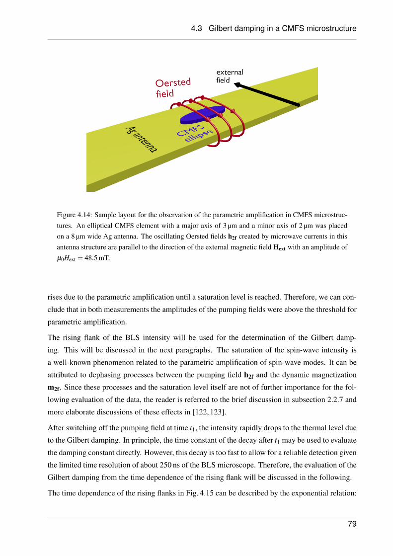
4.3 Gilbert damping in a CMFS microstructure

Figure 4.14: Sample layout for the observation of the parametric amplification in CMFS microstruc-tures. An elliptical CMFS element with a major axis of 3 µm and a minor axis of 2 µm was placedon a 8 µm wide Ag antenna. The oscillating Oersted fields h2f created by microwave currents in thisantenna structure are parallel to the direction of the external magnetic field Hext with an amplitude ofµ0Hext = 48.5 mT.

rises due to the parametric amplification until a saturation level is reached. Therefore, we can con-

clude that in both measurements the amplitudes of the pumping fields were above the threshold for

parametric amplification.

The rising flank of the BLS intensity will be used for the determination of the Gilbert damp-

ing. This will be discussed in the next paragraphs. The saturation of the spin-wave intensity is

a well-known phenomenon related to the parametric amplification of spin-wave modes. It can be

attributed to dephasing processes between the pumping field h2f and the dynamic magnetization

m2f. Since these processes and the saturation level itself are not of further importance for the fol-

lowing evaluation of the data, the reader is referred to the brief discussion in subsection 2.2.7 and

more elaborate discussions of these effects in [122, 123].

After switching off the pumping field at time t1, the intensity rapidly drops to the thermal level due

to the Gilbert damping. In principle, the time constant of the decay after t1 may be used to evaluate

the damping constant directly. However, this decay is too fast to allow for a reliable detection given

the limited time resolution of about 250 ns of the BLS microscope. Therefore, the evaluation of the

Gilbert damping from the time dependence of the rising flank will be discussed in the following.

The time dependence of the rising flanks in Fig. 4.15 can be described by the exponential relation:

79

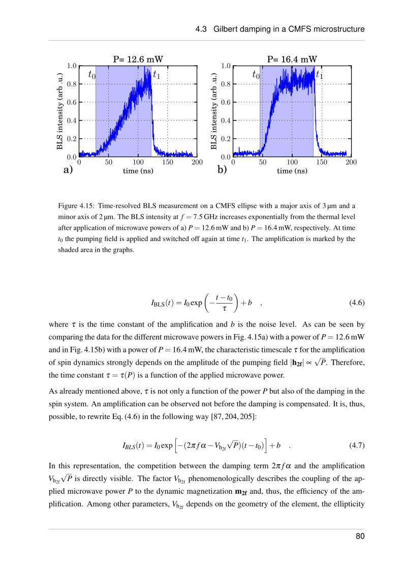
4.3 Gilbert damping in a CMFS microstructure

0 50 100 150 200time (ns)

0.0

0.2

0.4

0.6

0.8

1.0B

LS

inte

nsit

y(a

rb.u

.) t0 t1

P= 12.6 mW

0 50 100 150 200time (ns)

0.0

0.2

0.4

0.6

0.8

1.0

BL

Sin

tens

ity

(arb

.u.) t0 t1

P= 16.4 mW

a) b)

Figure 4.15: Time-resolved BLS measurement on a CMFS ellipse with a major axis of 3 µm and aminor axis of 2 µm. The BLS intensity at f = 7.5 GHz increases exponentially from the thermal levelafter application of microwave powers of a) P = 12.6 mW and b) P = 16.4 mW, respectively. At timet0 the pumping field is applied and switched off again at time t1. The amplification is marked by theshaded area in the graphs.

IBLS(t) = I0 exp(−t− t0

τ

)+b , (4.6)

where τ is the time constant of the amplification and b is the noise level. As can be seen by

comparing the data for the different microwave powers in Fig. 4.15a) with a power of P= 12.6 mW

and in Fig. 4.15b) with a power of P= 16.4 mW, the characteristic timescale τ for the amplification

of spin dynamics strongly depends on the amplitude of the pumping field |h2f| ∝√

P. Therefore,

the time constant τ = τ(P) is a function of the applied microwave power.

As already mentioned above, τ is not only a function of the power P but also of the damping in the

spin system. An amplification can be observed not before the damping is compensated. It is, thus,

possible, to rewrite Eq. (4.6) in the following way [87, 204, 205]:

IBLS(t) = I0 exp[−(2π f α−Vh2f

√P)(t− t0)

]+b . (4.7)

In this representation, the competition between the damping term 2π f α and the amplification

Vh2f

√P is directly visible. The factor Vh2f phenomenologically describes the coupling of the ap-

plied microwave power P to the dynamic magnetization m2f and, thus, the efficiency of the am-

plification. Among other parameters, Vh2f depends on the geometry of the element, the ellipticity

80

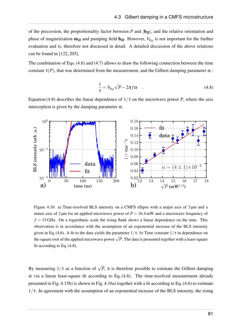
4.3 Gilbert damping in a CMFS microstructure

of the precession, the proportionality factor between P and |h2f|, and the relative orientation and

phase of magnetization m2f and pumping field h2f. However, Vh2f is not important for the further

evaluation and is, therefore not discussed in detail. A detailed discussion of the above relations

can be found in [122, 205].

The combination of Eqs. (4.6) and (4.7) allows to draw the following connection between the time

constant τ(P), that was determined from the measurement, and the Gilbert damping parameter α :

1τ=Vh2f

√P−2π f α . (4.8)

Equation (4.8) describes the linear dependence of 1/τ on the microwave power P, where the axis

interception is given by the damping parameter α .

0 50 100 150 200time (ns)

10−2

10−1

100

BL

Sin

tens

ity

(arb

.u.)

datafit

12 13 14 15 16 17 18√P (mW1/2)

0.02

0.04

0.06

0.08

0.10

0.12

0.14

0.16

0.181/τ

(ns−

1)

α = (4± 1)×10−3

fitdata

a) b)

Figure 4.16: a) Time-resolved BLS intensity on a CMFS ellipse with a major axis of 3 µm and aminor axis of 2 µm for an applied microwave power of P = 16.4 mW and a microwave frequency off = 15 GHz. On a logarithmic scale the rising flank shows a linear dependence on the time. Thisobservation is in accordance with the assumption of an exponential increase of the BLS intensitygiven in Eq. (4.6). A fit to the data yields the parameter 1/τ . b) Time constant 1/τ in dependence onthe square root of the applied microwave power

√P. The data is presented together with a least-square

fit according to Eq. (4.8).

By measuring 1/τ as a function of√

P, it is therefore possible to estimate the Gilbert damping

α via a linear least-square fit according to Eq. (4.8). The time-resolved measurement already

presented in Fig. 4.15b) is shown in Fig. 4.16a) together with a fit according to Eq. (4.6) to estimate

1/τ . In agreement with the assumption of an exponential increase of the BLS intensity, the rising

81

4.4 Nonlinear emission of spin-wave caustics

flank of the BLS intensity shows a linear dependence on the time in a logarithmic presentation of

the data.

Fig. 4.16b) summarizes the results of several measurements for different microwave powers. A

least-square fit according to Eq. (4.8) yields a Gilbert damping parameter of α = (4± 1)× 10−3.

This value is in agreement with the Gilbert damping reported for homogeneous CMFS thin films

with L21 order (α = 3×10−3 in [51]).

As already indicated by the increased propagation distance observed in a CMFS waveguide, the

quantitative evaluation confirms the low values of the Gilbert damping in the investigated CMFS

microstructure. While the effect of this low damping was already illustrated for the spin-wave

propagation in CMFS waveguides, it also reveals a big potential for other fields of spin dynamics.

In particular, all direct-current based schemes for the excitation of spin dynamics or the switching

of magnetic layers directly depend on a low Gilbert damping [22–24, 26, 47, 48]. Therefore, the

results above strongly suggest the utilization of CMFS in all related experiments. In addition, the

decreased Gilbert damping also leads to a pronounced occurrence of nonlinear effects. The field

of nonlinear spin dynamics in CMFS will be discussed in the next chapter.

4.4. Nonlinear emission of spin-wave caustics

This section is devoted to the novel phenomena of the nonlinear emission of spin-wave caustics,

that was observed for the first time at all in a microstructured CMFS waveguide.

The spin system is known to exhibit a large variety of nonlinear phenomena such as nonlinear

confluence and splitting processes [22, 104–108, 110], the formation of spin-wave bullet modes

[26, 114–117] or solitons [111], the spatial self-modulation of propagating spin waves [112, 113],

and many others. All of these phenomena are driven by the intrinsic nonlinearity of the Landau-

Lifshitz equation that governs the spin dynamics. Some of them are even easier accessible in the

spin system than in other fields of wave physics. The spin system is therefore a unique system to

gather basic knowledge in nonlinear wave physics. On the other hand, nonlinearities can be used

for novel schemes for the excitation or manipulation of spin-wave propagation regarding technical

applications.

Because of these reasons, it is crucial to investigate and to understand nonlinear phenomena in the

spin system in general and, in particular, in novel material systems like the low-damping Heusler

compounds.

One of the crucial parameters for the appearance of nonlinear phenomena is the Gilbert damping.

While there are numerous reports about nonlinearities in the spin system of magnetic microstruc-

tures, most of these phenomena have been observed in the same material, namely Ni81Fe19. The

82

4.4 Nonlinear emission of spin-wave caustics

substantially smaller Gilbert damping in CMFS - that already led to a remarkable increase of the

observed decay length - should also allow for the pronounced occurrence of nonlinear effects and

even for the observation of novel phenomena. In fact, the complex interplay of different aspects of

spin dynamics, that will be presented in the following, is unique and has not been reported before.

This nonlinear emission of spin-wave caustics from a localized spin-wave mode was published

first in Ref. [A6]. Thus, this experimental result illustrates again the advantages of CMFS over the

commonly used materials as well as the possibilities given by the utilization of the low-damping

material.

In addition to these material aspects, the underlying physical mechanisms comprise many interest-

ing aspects of spin dynamics. The overall process of our observation can be subdivided into the

following phenomena:

1. formation of localized edge modes [84, 209]

2. higher harmonic generation [107, 108]

3. formation of caustic spin-wave beams [210, 211].

As indicated by the exemplary references given in this list, each of these phenomena on its own

gained huge interest and stimulated serious research efforts in the field of magnon spintronics.

Since the present results combine all of these phenomena, these references also highlight the com-

plexity of the physical mechanisms that finally lead to the observed results.

For simplicity, the present section is subdivided into three subsections. Instead of describing the

phenomena consecutively as listed above, the content of these subsections is ordered according

to the experimental approach. Subsection 4.4.2 introduces the first observation of the nonlinear

effects and the questions arising from this observation. Subsection 4.4.3 gives a phenomenological

description of the involved spin-wave modes. Finally, section 4.4.4 describes these findings quan-

titatively supported by an analytical calculation. The discussion starts with a brief description of

the sample structure in the next subsection.

4.4.1 Sample layout

The principle sample layout and geometry in this experiment was the same as discussed in subsec-

tion 4.2.1 about the spin-wave propagation in the linear regime. For a details about the fabrication

process, please turn to section 4.1.2. A sketch of the structure can be found in Fig. 4.17. This

structure was fabricated from layer stack A. It comprises a 30 nm thick spin-wave waveguide of

CMFS with a width of 5 µm. The short-circuited end of a Cu/Ti structure with a width of 1 µm

served as an antenna for the excitation of spin waves. This excitation was based on the torque

83

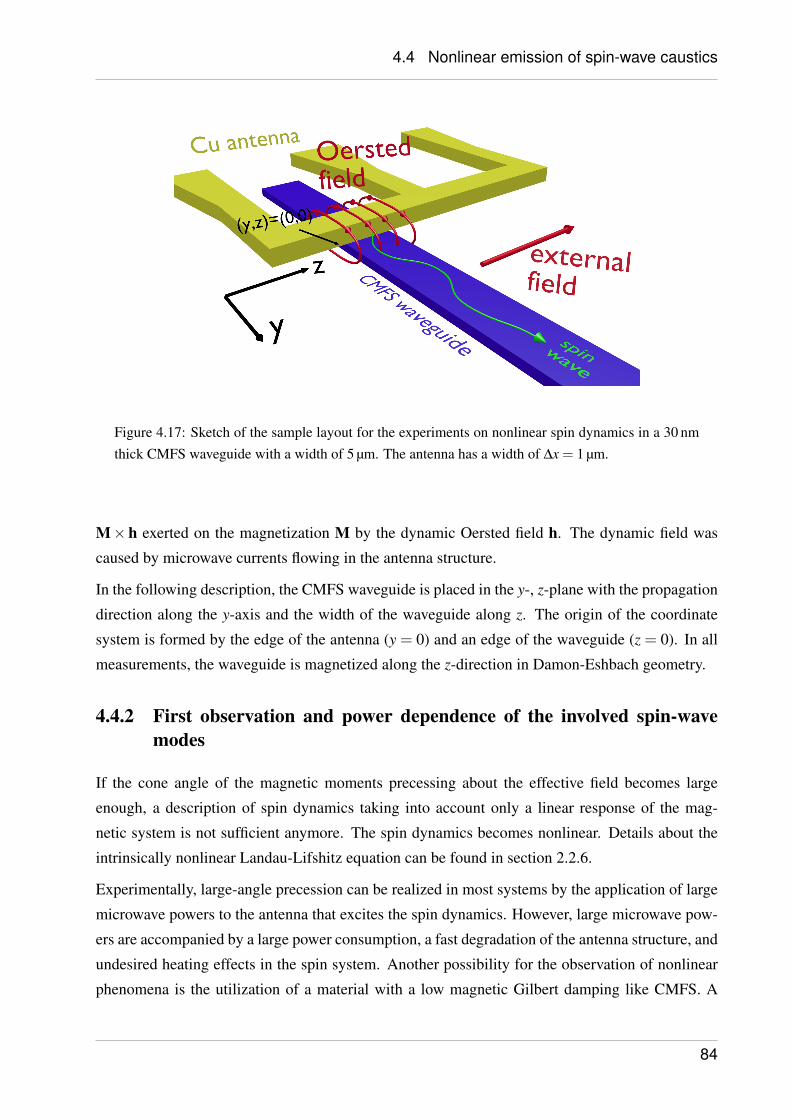
4.4 Nonlinear emission of spin-wave caustics

Figure 4.17: Sketch of the sample layout for the experiments on nonlinear spin dynamics in a 30 nmthick CMFS waveguide with a width of 5 µm. The antenna has a width of ∆x = 1 µm.

M×h exerted on the magnetization M by the dynamic Oersted field h. The dynamic field was

caused by microwave currents flowing in the antenna structure.

In the following description, the CMFS waveguide is placed in the y-, z-plane with the propagation

direction along the y-axis and the width of the waveguide along z. The origin of the coordinate

system is formed by the edge of the antenna (y = 0) and an edge of the waveguide (z = 0). In all

measurements, the waveguide is magnetized along the z-direction in Damon-Eshbach geometry.

4.4.2 First observation and power dependence of the involved spin-wavemodes

If the cone angle of the magnetic moments precessing about the effective field becomes large

enough, a description of spin dynamics taking into account only a linear response of the mag-

netic system is not sufficient anymore. The spin dynamics becomes nonlinear. Details about the

intrinsically nonlinear Landau-Lifshitz equation can be found in section 2.2.6.

Experimentally, large-angle precession can be realized in most systems by the application of large

microwave powers to the antenna that excites the spin dynamics. However, large microwave pow-

ers are accompanied by a large power consumption, a fast degradation of the antenna structure, and

undesired heating effects in the spin system. Another possibility for the observation of nonlinear

phenomena is the utilization of a material with a low magnetic Gilbert damping like CMFS. A

84

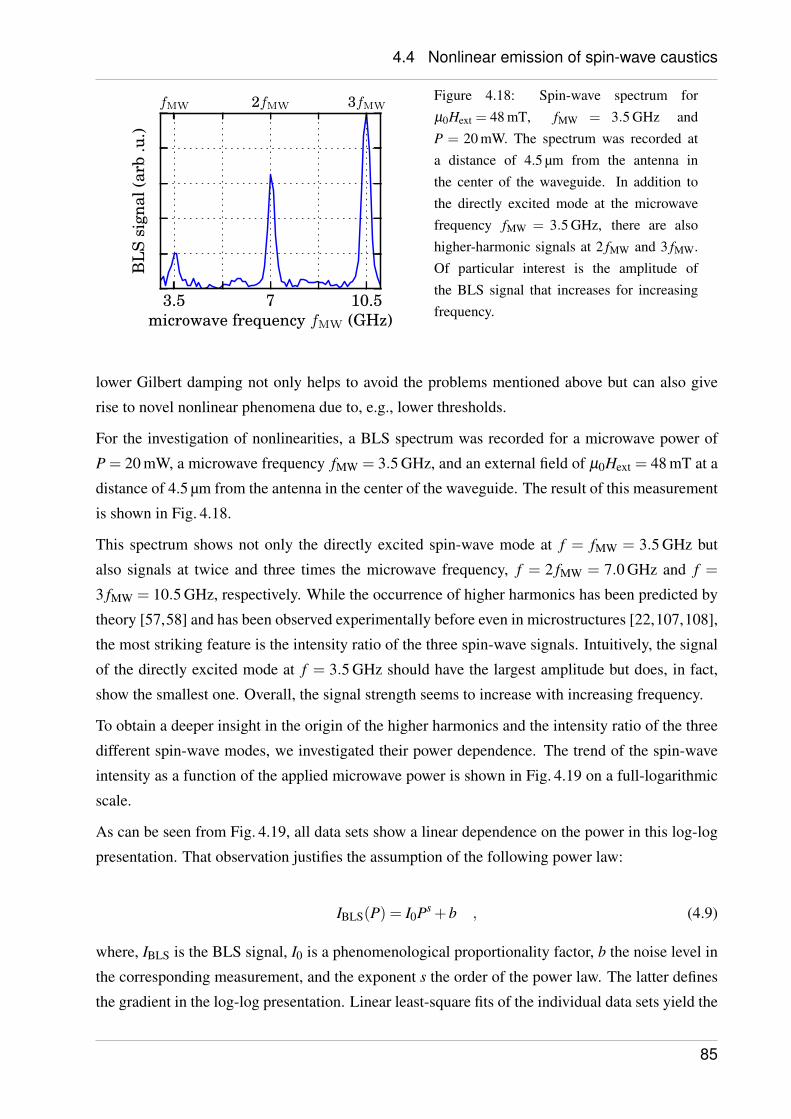
4.4 Nonlinear emission of spin-wave caustics

3.5 7 10.5microwave frequency fMW (GHz)

BL

Ssi

gnal

(arb

.u.)

fMW 2fMW 3fMWFigure 4.18: Spin-wave spectrum forµ0Hext = 48 mT, fMW = 3.5 GHz andP = 20 mW. The spectrum was recorded ata distance of 4.5 µm from the antenna inthe center of the waveguide. In addition tothe directly excited mode at the microwavefrequency fMW = 3.5 GHz, there are alsohigher-harmonic signals at 2 fMW and 3 fMW.Of particular interest is the amplitude ofthe BLS signal that increases for increasingfrequency.

lower Gilbert damping not only helps to avoid the problems mentioned above but can also give

rise to novel nonlinear phenomena due to, e.g., lower thresholds.

For the investigation of nonlinearities, a BLS spectrum was recorded for a microwave power of

P = 20 mW, a microwave frequency fMW = 3.5 GHz, and an external field of µ0Hext = 48 mT at a

distance of 4.5 µm from the antenna in the center of the waveguide. The result of this measurement

is shown in Fig. 4.18.

This spectrum shows not only the directly excited spin-wave mode at f = fMW = 3.5 GHz but

also signals at twice and three times the microwave frequency, f = 2 fMW = 7.0 GHz and f =

3 fMW = 10.5 GHz, respectively. While the occurrence of higher harmonics has been predicted by

theory [57,58] and has been observed experimentally before even in microstructures [22,107,108],

the most striking feature is the intensity ratio of the three spin-wave signals. Intuitively, the signal

of the directly excited mode at f = 3.5 GHz should have the largest amplitude but does, in fact,

show the smallest one. Overall, the signal strength seems to increase with increasing frequency.

To obtain a deeper insight in the origin of the higher harmonics and the intensity ratio of the three

different spin-wave modes, we investigated their power dependence. The trend of the spin-wave

intensity as a function of the applied microwave power is shown in Fig. 4.19 on a full-logarithmic

scale.

As can be seen from Fig. 4.19, all data sets show a linear dependence on the power in this log-log

presentation. That observation justifies the assumption of the following power law:

IBLS(P) = I0Ps +b , (4.9)

where, IBLS is the BLS signal, I0 is a phenomenological proportionality factor, b the noise level in

the corresponding measurement, and the exponent s the order of the power law. The latter defines

the gradient in the log-log presentation. Linear least-square fits of the individual data sets yield the

85

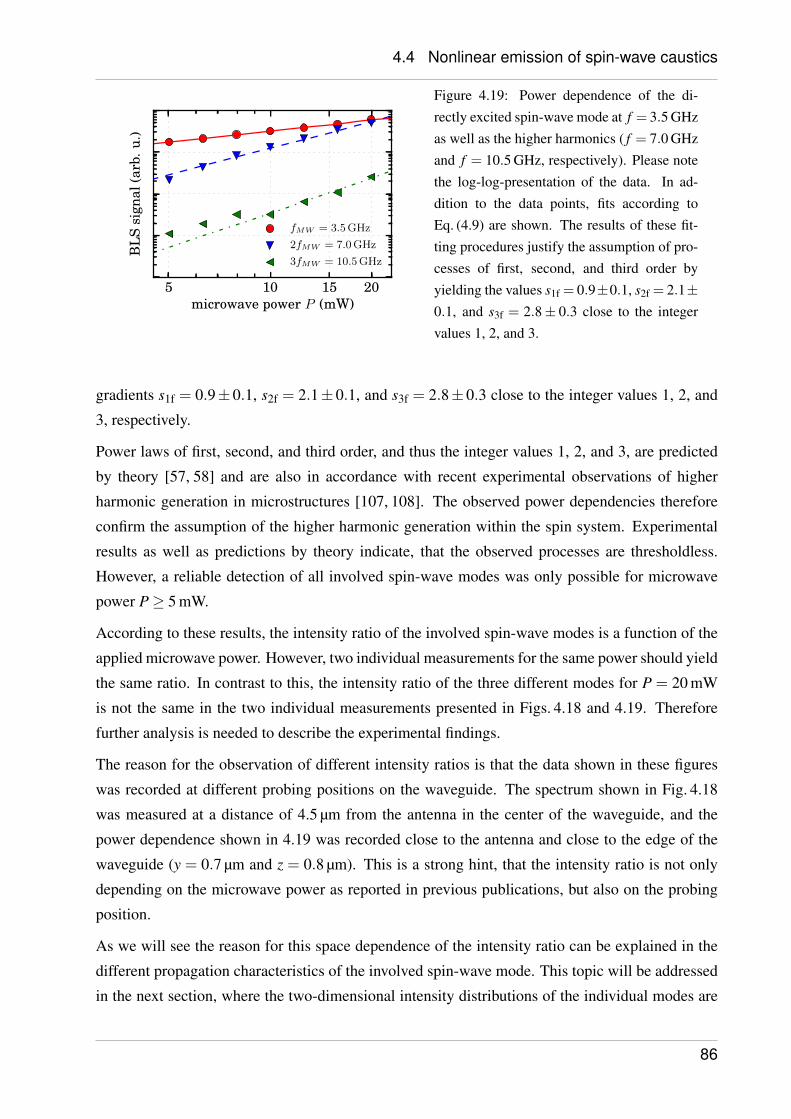
4.4 Nonlinear emission of spin-wave caustics

5 10 15 20microwave power P (mW)

BL

Ssi

gnal

(arb

.u.)

fMW = 3.5 GHz

2fMW = 7.0 GHz

3fMW = 10.5 GHz

Figure 4.19: Power dependence of the di-rectly excited spin-wave mode at f = 3.5 GHzas well as the higher harmonics ( f = 7.0 GHzand f = 10.5 GHz, respectively). Please notethe log-log-presentation of the data. In ad-dition to the data points, fits according toEq. (4.9) are shown. The results of these fit-ting procedures justify the assumption of pro-cesses of first, second, and third order byyielding the values s1f = 0.9±0.1, s2f = 2.1±0.1, and s3f = 2.8± 0.3 close to the integervalues 1, 2, and 3.

gradients s1f = 0.9±0.1, s2f = 2.1±0.1, and s3f = 2.8±0.3 close to the integer values 1, 2, and

3, respectively.

Power laws of first, second, and third order, and thus the integer values 1, 2, and 3, are predicted

by theory [57, 58] and are also in accordance with recent experimental observations of higher

harmonic generation in microstructures [107, 108]. The observed power dependencies therefore

confirm the assumption of the higher harmonic generation within the spin system. Experimental

results as well as predictions by theory indicate, that the observed processes are thresholdless.

However, a reliable detection of all involved spin-wave modes was only possible for microwave

power P≥ 5 mW.

According to these results, the intensity ratio of the involved spin-wave modes is a function of the

applied microwave power. However, two individual measurements for the same power should yield

the same ratio. In contrast to this, the intensity ratio of the three different modes for P = 20 mW

is not the same in the two individual measurements presented in Figs. 4.18 and 4.19. Therefore

further analysis is needed to describe the experimental findings.

The reason for the observation of different intensity ratios is that the data shown in these figures

was recorded at different probing positions on the waveguide. The spectrum shown in Fig. 4.18

was measured at a distance of 4.5 µm from the antenna in the center of the waveguide, and the

power dependence shown in 4.19 was recorded close to the antenna and close to the edge of the

waveguide (y = 0.7 µm and z = 0.8 µm). This is a strong hint, that the intensity ratio is not only

depending on the microwave power as reported in previous publications, but also on the probing

position.

As we will see the reason for this space dependence of the intensity ratio can be explained in the

different propagation characteristics of the involved spin-wave mode. This topic will be addressed

in the next section, where the two-dimensional intensity distributions of the individual modes are

86

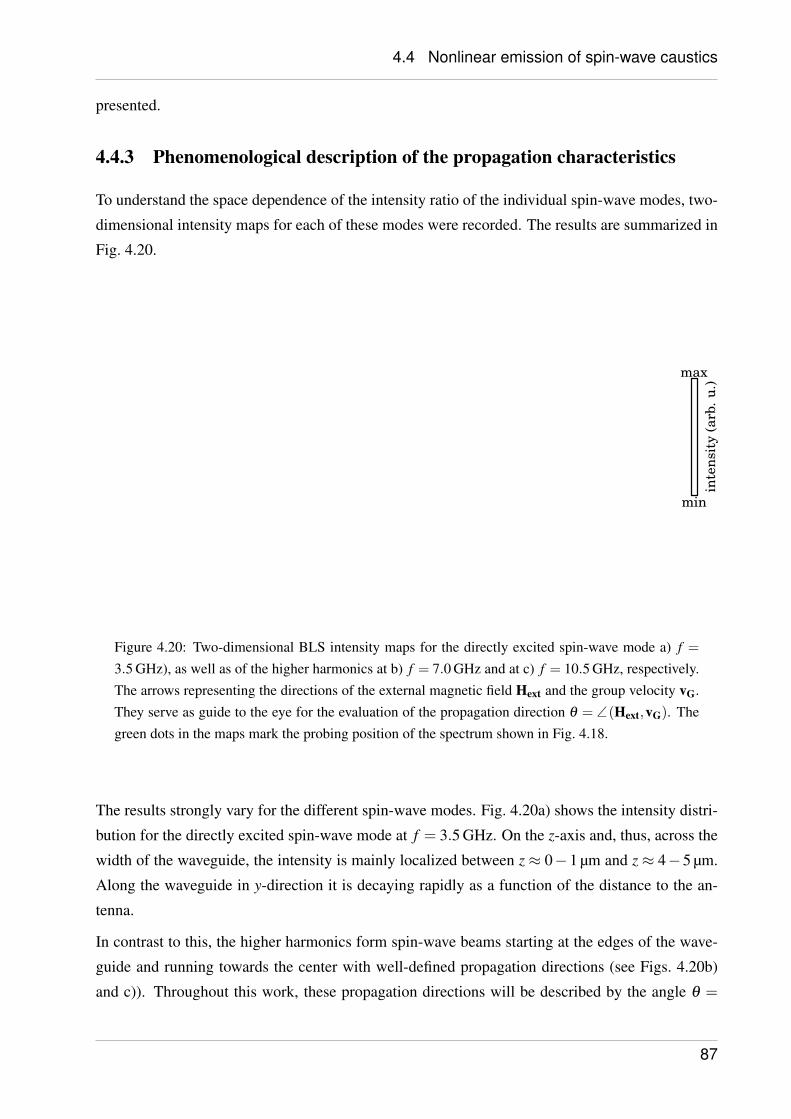
4.4 Nonlinear emission of spin-wave caustics

presented.

4.4.3 Phenomenological description of the propagation characteristics

To understand the space dependence of the intensity ratio of the individual spin-wave modes, two-

dimensional intensity maps for each of these modes were recorded. The results are summarized in

Fig. 4.20.

Figure 4.20: Two-dimensional BLS intensity maps for the directly excited spin-wave mode a) f =3.5 GHz), as well as of the higher harmonics at b) f = 7.0 GHz and at c) f = 10.5 GHz, respectively.The arrows representing the directions of the external magnetic field Hext and the group velocity vG.They serve as guide to the eye for the evaluation of the propagation direction θ = ∠(Hext,vG). Thegreen dots in the maps mark the probing position of the spectrum shown in Fig. 4.18.

The results strongly vary for the different spin-wave modes. Fig. 4.20a) shows the intensity distri-

bution for the directly excited spin-wave mode at f = 3.5 GHz. On the z-axis and, thus, across the

width of the waveguide, the intensity is mainly localized between z≈ 0−1 µm and z≈ 4−5 µm.

Along the waveguide in y-direction it is decaying rapidly as a function of the distance to the an-

tenna.

In contrast to this, the higher harmonics form spin-wave beams starting at the edges of the wave-

guide and running towards the center with well-defined propagation directions (see Figs. 4.20b)

and c)). Throughout this work, these propagation directions will be described by the angle θ =

87

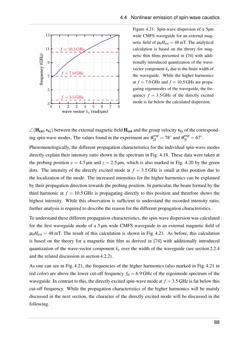
4.4 Nonlinear emission of spin-wave caustics

0 1 2 3 4 5 6 7 8wave vector ky (rad/µm)

3

5

7

9

11

13

freq

uenc

y(G

Hz)

f = 3.5 GHz

f = 7.0 GHz

f = 10.5 GHz

Figure 4.21: Spin-wave dispersion of a 5µmwide CMFS waveguide for an external mag-netic field of µ0Hext = 48 mT. The analyticalcalculation is based on the theory for mag-netic thin films presented in [74] with addi-tionally introduced quantization of the wave-vector component kz due to the finite width ofthe waveguide. While the higher harmonicsat f = 7.0 GHz and f = 10.5 GHz are propa-gating eigenmodes of the waveguide, the fre-quency f = 3.5 GHz of the directly excitedmode is far below the calculated dispersion.

∠(Hext,vG) between the external magnetic field Hext and the group velocity vG of the correspond-

ing spin-wave modes. The values found in the experiment are θexp2f = 78 and θ

exp3f = 67.

Phenomenologically, the different propagation characteristics for the individual spin-wave modes

directly explain their intensity ratio shown in the spectrum in Fig. 4.18. These data were taken at

the probing position y = 4.5 µm and z = 2.5 µm, which is also marked in Fig. 4.20 by the green

dots. The intensity of the directly excited mode at f = 3.5 GHz is small at this position due to

the localization of the mode. The increased intensities for the higher harmonics can be explained

by their propagation direction towards the probing position. In particular, the beam formed by the

third harmonic at f = 10.5 GHz is propagating directly to this position and therefore shows the

highest intensity. While this observation is sufficient to understand the recorded intensity ratio,

further analysis is required to describe the reason for the different propagation characteristics.

To understand these different propagation characteristics, the spin-wave dispersion was calculated

for the first waveguide mode of a 5 µm wide CMFS waveguide in an external magnetic field of

µ0Hext = 48 mT. The result of this calculation is shown in Fig. 4.21. As before, this calculation

is based on the theory for a magnetic thin film as derived in [74] with additionally introduced

quantization of the wave-vector component kz over the width of the waveguide (see section 2.2.4

and the related discussion in section 4.2.2).

As one can see in Fig. 4.21, the frequencies of the higher harmonics (also marked in Fig. 4.21 in

red color) are above the lower cut-off frequency f0 = 6.9 GHz of the eigenmode spectrum of the

waveguide. In contrast to this, the directly excited spin-wave mode at f = 3.5 GHz is far below this

cut-off frequency. While the propagation characteristics of the higher harmonics will be mainly

discussed in the next section, the character of the directly excited mode will be discussed in the

following.

88

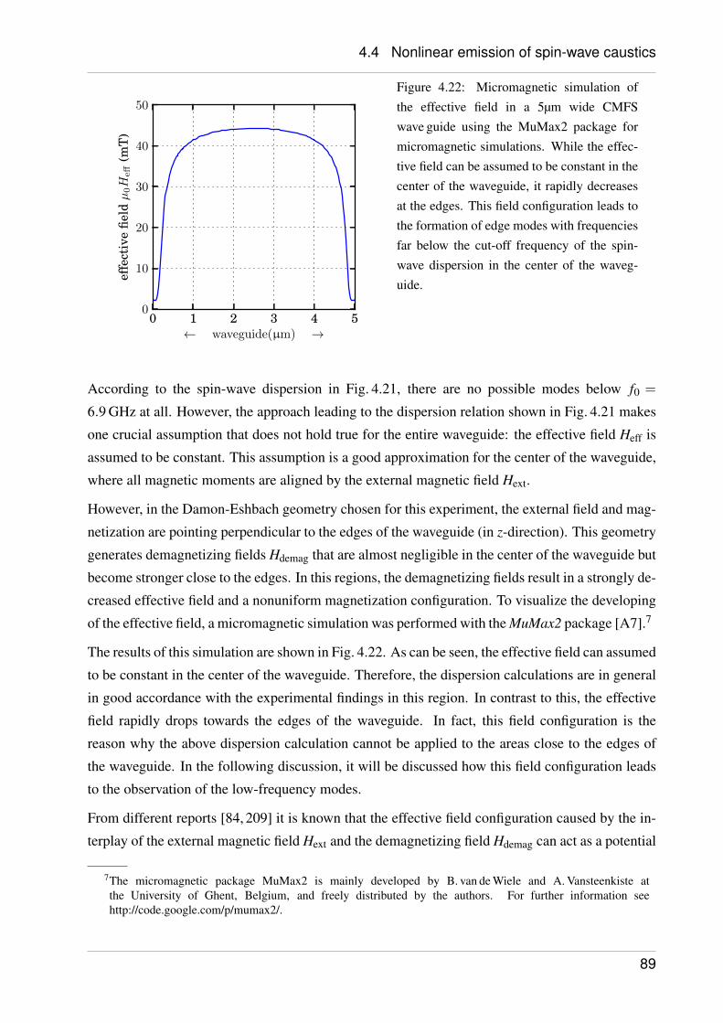
4.4 Nonlinear emission of spin-wave caustics

0 1 2 3 4 5← waveguide(µm) →

0

10

20

30

40

50

effe

ctiv

efie

ldµ

0H

eff

(mT

)

Figure 4.22: Micromagnetic simulation ofthe effective field in a 5µm wide CMFSwave guide using the MuMax2 package formicromagnetic simulations. While the effec-tive field can be assumed to be constant in thecenter of the waveguide, it rapidly decreasesat the edges. This field configuration leads tothe formation of edge modes with frequenciesfar below the cut-off frequency of the spin-wave dispersion in the center of the waveg-uide.

According to the spin-wave dispersion in Fig. 4.21, there are no possible modes below f0 =

6.9 GHz at all. However, the approach leading to the dispersion relation shown in Fig. 4.21 makes

one crucial assumption that does not hold true for the entire waveguide: the effective field Heff is

assumed to be constant. This assumption is a good approximation for the center of the waveguide,

where all magnetic moments are aligned by the external magnetic field Hext.

However, in the Damon-Eshbach geometry chosen for this experiment, the external field and mag-

netization are pointing perpendicular to the edges of the waveguide (in z-direction). This geometry

generates demagnetizing fields Hdemag that are almost negligible in the center of the waveguide but

become stronger close to the edges. In this regions, the demagnetizing fields result in a strongly de-

creased effective field and a nonuniform magnetization configuration. To visualize the developing

of the effective field, a micromagnetic simulation was performed with the MuMax2 package [A7].7

The results of this simulation are shown in Fig. 4.22. As can be seen, the effective field can assumed

to be constant in the center of the waveguide. Therefore, the dispersion calculations are in general

in good accordance with the experimental findings in this region. In contrast to this, the effective

field rapidly drops towards the edges of the waveguide. In fact, this field configuration is the

reason why the above dispersion calculation cannot be applied to the areas close to the edges of

the waveguide. In the following discussion, it will be discussed how this field configuration leads

to the observation of the low-frequency modes.

From different reports [84, 209] it is known that the effective field configuration caused by the in-

terplay of the external magnetic field Hext and the demagnetizing field Hdemag can act as a potential

7The micromagnetic package MuMax2 is mainly developed by B. van de Wiele and A. Vansteenkiste atthe University of Ghent, Belgium, and freely distributed by the authors. For further information seehttp://code.google.com/p/mumax2/.

89

4.4 Nonlinear emission of spin-wave caustics

well for localized spin-wave edge modes. Because of the lower magnitude of the effective field at

the edges compared to the center of the waveguide, these modes can have frequencies far below the

cut-off frequency for waveguide eigenmodes. On the other hand, because of energy conservation,

these edge modes are trapped in the area of the decreased effective field. It is therefore reasonable

to conclude that the observed spin-wave mode a f = 3.5 GHz is an edge mode localized between

z ≈ 0−1 µm and z ≈ 4−5 µm. In the regions close to the edges of the waveguide, the mode can

be excited resonantly by the microwave field. In contrast to this, the rather small intensity between

these maxima at z≈ 1−4 µm can be attributed to forced excitation.

While the above descriptive argument is supported by previous experimental results and closely

matches the experimental findings qualitatively, it does not allow for quantitative conclusions.

Therefore, a more sophisticated theory on spin-wave dispersion in waveguides that also confirms

the conclusions about the character of the directly excited mode must be mentioned. This model

was introduced by Kostylev et al. [85]. In contrast to the approach of a thin film dispersion with

added quantization conditions, Kostylev takes the finite dimensions of the waveguide into account

right from the start of his calculations. In fact, his model predicts spin-wave modes localized

at the edges of the waveguide with lower frequencies than in the center. Therefore, his theory

qualitatively supports our conclusions.

Quantitatively, however, it is almost impossible to model the experimental situation at the edges.

While Kostylev takes into account the demagnetizing fields, he still assumes a uniform magneti-

zation configuration over the entire waveguide. At the edges this assumption is not valid in most

experimental situations. To saturate the magnetization in perpendicular direction to an edge re-

quires large external magnetic fields to overcome the demagnetizing fields. The micromagnetic

simulation discussed above, shows that the magnetization was not saturated along the external

field in the present experiment. In addition, the actual magnetization configuration in a real sample

always depends on the individual conditions at each probing position. Therefore, it is not possible

to model it even with micromagnetic simulations. These facts always cause a discrepancy between

experimental findings and theoretical description as also stated by Kostylev himself [85]:

"There is considerable discrepancy between measured and calculated frequencies because of our

assumption of uniform static magnetization and local internal fields in the stripes. The exact

distribution of magnetization and local fields will be strongly affected by edge morphology, defects,

and history of magnetization."

For this reason, no further quantitative conclusions about the character of the edge mode will

be drawn in the following. However, the accordance of the experimental findings with previous

experimental observations as well as with the predictions by the Kostylev model strongly supports

the phenomenological description of the edge modes by our own considerations.

90

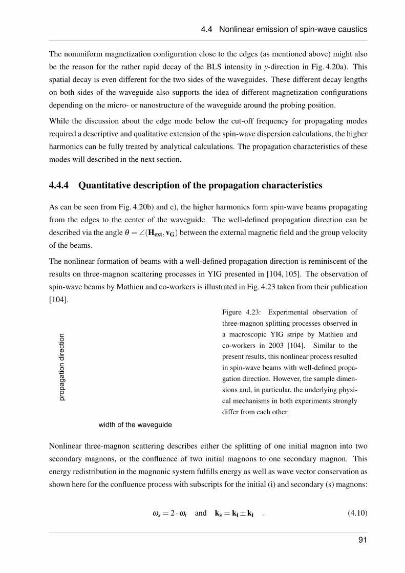
4.4 Nonlinear emission of spin-wave caustics

The nonuniform magnetization configuration close to the edges (as mentioned above) might also

be the reason for the rather rapid decay of the BLS intensity in y-direction in Fig. 4.20a). This

spatial decay is even different for the two sides of the waveguides. These different decay lengths

on both sides of the waveguide also supports the idea of different magnetization configurations

depending on the micro- or nanostructure of the waveguide around the probing position.

While the discussion about the edge mode below the cut-off frequency for propagating modes

required a descriptive and qualitative extension of the spin-wave dispersion calculations, the higher

harmonics can be fully treated by analytical calculations. The propagation characteristics of these

modes will described in the next section.

4.4.4 Quantitative description of the propagation characteristics

As can be seen from Fig. 4.20b) and c), the higher harmonics form spin-wave beams propagating

from the edges to the center of the waveguide. The well-defined propagation direction can be

described via the angle θ =∠(Hext,vG) between the external magnetic field and the group velocity

of the beams.

The nonlinear formation of beams with a well-defined propagation direction is reminiscent of the

results on three-magnon scattering processes in YIG presented in [104, 105]. The observation of

spin-wave beams by Mathieu and co-workers is illustrated in Fig. 4.23 taken from their publication

[104].

width of the waveguide

prop

agat

ion

dire

ctio

n

Figure 4.23: Experimental observation ofthree-magnon splitting processes observed ina macroscopic YIG stripe by Mathieu andco-workers in 2003 [104]. Similar to thepresent results, this nonlinear process resultedin spin-wave beams with well-defined propa-gation direction. However, the sample dimen-sions and, in particular, the underlying physi-cal mechanisms in both experiments stronglydiffer from each other.

Nonlinear three-magnon scattering describes either the splitting of one initial magnon into two

secondary magnons, or the confluence of two initial magnons to one secondary magnon. This

energy redistribution in the magnonic system fulfills energy as well as wave vector conservation as

shown here for the confluence process with subscripts for the initial (i) and secondary (s) magnons:

ωs = 2 ·ωi and ks = ki±ki . (4.10)

91

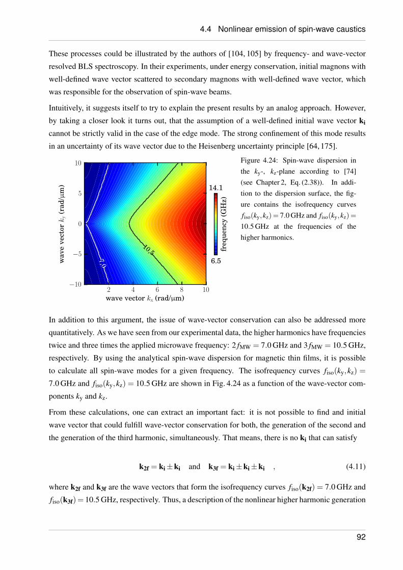
4.4 Nonlinear emission of spin-wave caustics

These processes could be illustrated by the authors of [104, 105] by frequency- and wave-vector

resolved BLS spectroscopy. In their experiments, under energy conservation, initial magnons with

well-defined wave vector scattered to secondary magnons with well-defined wave vector, which

was responsible for the observation of spin-wave beams.

Intuitively, it suggests itself to try to explain the present results by an analog approach. However,

by taking a closer look it turns out, that the assumption of a well-defined initial wave vector ki

cannot be strictly valid in the case of the edge mode. The strong confinement of this mode results

in an uncertainty of its wave vector due to the Heisenberg uncertainty principle [64, 175].

Figure 4.24: Spin-wave dispersion inthe ky-, kz-plane according to [74](see Chapter 2, Eq. (2.38)). In addi-tion to the dispersion surface, the fig-ure contains the isofrequency curvesfiso(ky,kz) = 7.0 GHz and fiso(ky,kz) =

10.5 GHz at the frequencies of thehigher harmonics.

In addition to this argument, the issue of wave-vector conservation can also be addressed more

quantitatively. As we have seen from our experimental data, the higher harmonics have frequencies

twice and three times the applied microwave frequency: 2 fMW = 7.0 GHz and 3 fMW = 10.5 GHz,

respectively. By using the analytical spin-wave dispersion for magnetic thin films, it is possible

to calculate all spin-wave modes for a given frequency. The isofrequency curves fiso(ky,kz) =

7.0 GHz and fiso(ky,kz) = 10.5 GHz are shown in Fig. 4.24 as a function of the wave-vector com-

ponents ky and kz.

From these calculations, one can extract an important fact: it is not possible to find and initial

wave vector that could fulfill wave-vector conservation for both, the generation of the second and

the generation of the third harmonic, simultaneously. That means, there is no ki that can satisfy

k2f = ki±ki and k3f = ki±ki±ki , (4.11)

where k2f and k3f are the wave vectors that form the isofrequency curves fiso(k2f) = 7.0 GHz and

fiso(k3f)= 10.5 GHz, respectively. Thus, a description of the nonlinear higher harmonic generation

92

4.4 Nonlinear emission of spin-wave caustics

based on a well-defined intial wave vector of the edge mode is not valid and cannot reveal the nature

of the higher harmonics in the present experiment.

An alternative way to explain the existence of the higher harmonics and the nature of the observed

spin-wave beams, is to consider the dynamic Oersted fields that accompany the precessional mo-

tion of magnetic moments. This approach describes the experimental findings in terms of the

oscillating magnetic moments of the edge mode.

In the following, the occurrence of frequency doubling in terms of higher frequency components

in the magnetization precession will be explained. A more detailed explanation of this sketch can

be found in [57]. After this discussion about the generation of the higher harmonics and based on

this process, the formation and the nature of the observed spin-wave beams will be explained.

The following discussion of the spin precession in a magnetic thin films is similar to the discussion

about the parallel parametric amplification of spin dynamics presented in section 4.3. In an infinite

magnetic medium without any kind of magnetic anisotropy, the tip of a magnetic moment precess-

ing about an effective field will follow a perfectly circular trajectory. Let us assume, without loss

of generality, that this effective field and, thus, the magnetization, points in z-direction. If we now

change the given scenario by reducing the x-dimension of the magnetic medium, we can consider

it as an infinite magnetic film in the y-, z-plane as in the actual experiment. The finite x-dimension

will immediately cause dynamic demagnetizing fields whenever the magnetic moments point out

of this film during their precessional motion. Due to this demagnetizing fields, and to minimize

the energy of the system, the circular trajectory of the tip will change to an elliptical one. A sketch

of this elliptical precession can be found in Fig. 4.13.

While for the description of a circular precession around the z-axis, the x- and y-component are

sufficient, ellipticity gives rise to a dynamic z-component. This z-component is oscillating with

twice the frequency of the original precession. The resulting 2 f magnetic field can be regarded

as the source for the excitation of the second higher harmonic. We can therefore understand the

occurrence of the second harmonic in our experiment. A longer derivation of the above sketch

based on the approach introduced in section 2.2.6 can be found in [57].

While the occurrence of higher harmonic frequencies was illustrated in the paragraphs above, the

next paragraphs are devoted to the discussion of the resulting wave vectors and the propagation

characteristics of the higher harmonic modes.

From the two-dimensional intensity profiles of the higher harmonics in Fig. 4.20b) and c), we

can identify the edge mode as the source of the higher harmonics. According to the discussion

about the dynamic stray fields that accompany the high amplitude precession, the localized edge

mode can be regarded as an antenna that is driven at twice and three time the original microwave

frequency.

93

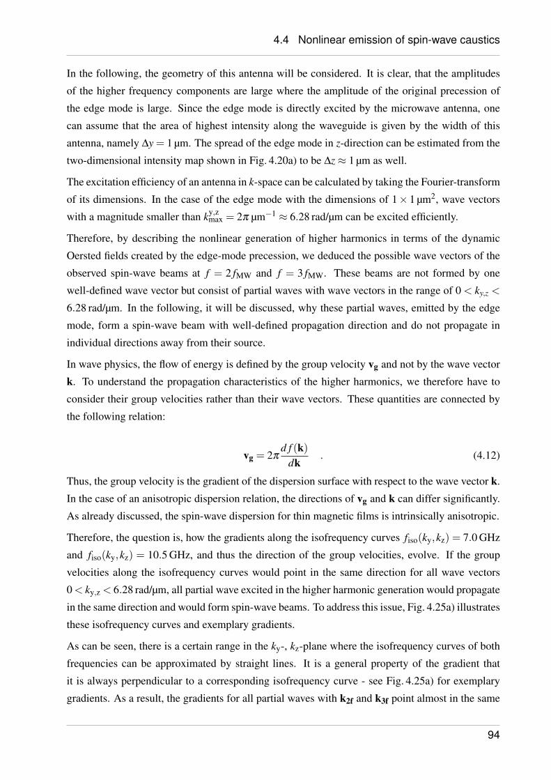
4.4 Nonlinear emission of spin-wave caustics

In the following, the geometry of this antenna will be considered. It is clear, that the amplitudes

of the higher frequency components are large where the amplitude of the original precession of

the edge mode is large. Since the edge mode is directly excited by the microwave antenna, one

can assume that the area of highest intensity along the waveguide is given by the width of this

antenna, namely ∆y = 1 µm. The spread of the edge mode in z-direction can be estimated from the

two-dimensional intensity map shown in Fig. 4.20a) to be ∆z≈ 1 µm as well.

The excitation efficiency of an antenna in k-space can be calculated by taking the Fourier-transform

of its dimensions. In the case of the edge mode with the dimensions of 1× 1 µm2, wave vectors

with a magnitude smaller than ky,zmax = 2π µm−1 ≈ 6.28 rad/µm can be excited efficiently.

Therefore, by describing the nonlinear generation of higher harmonics in terms of the dynamic

Oersted fields created by the edge-mode precession, we deduced the possible wave vectors of the

observed spin-wave beams at f = 2 fMW and f = 3 fMW. These beams are not formed by one

well-defined wave vector but consist of partial waves with wave vectors in the range of 0 < ky,z <

6.28 rad/µm. In the following, it will be discussed, why these partial waves, emitted by the edge

mode, form a spin-wave beam with well-defined propagation direction and do not propagate in

individual directions away from their source.

In wave physics, the flow of energy is defined by the group velocity vg and not by the wave vector

k. To understand the propagation characteristics of the higher harmonics, we therefore have to

consider their group velocities rather than their wave vectors. These quantities are connected by

the following relation:

vg = 2πd f (k)

dk. (4.12)

Thus, the group velocity is the gradient of the dispersion surface with respect to the wave vector k.

In the case of an anisotropic dispersion relation, the directions of vg and k can differ significantly.

As already discussed, the spin-wave dispersion for thin magnetic films is intrinsically anisotropic.

Therefore, the question is, how the gradients along the isofrequency curves fiso(ky,kz) = 7.0 GHz

and fiso(ky,kz) = 10.5 GHz, and thus the direction of the group velocities, evolve. If the group

velocities along the isofrequency curves would point in the same direction for all wave vectors

0 < ky,z < 6.28 rad/µm, all partial wave excited in the higher harmonic generation would propagate

in the same direction and would form spin-wave beams. To address this issue, Fig. 4.25a) illustrates

these isofrequency curves and exemplary gradients.

As can be seen, there is a certain range in the ky-, kz-plane where the isofrequency curves of both

frequencies can be approximated by straight lines. It is a general property of the gradient that

it is always perpendicular to a corresponding isofrequency curve - see Fig. 4.25a) for exemplary

gradients. As a result, the gradients for all partial waves with k2f and k3f point almost in the same

94

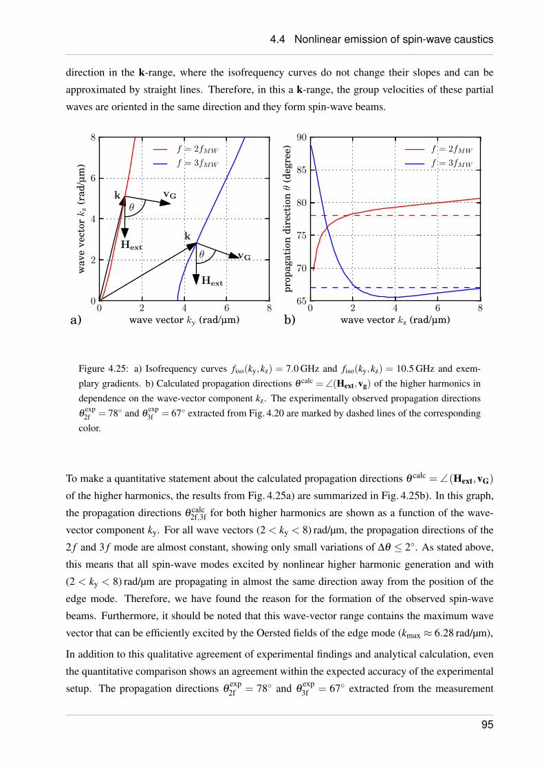
4.4 Nonlinear emission of spin-wave caustics

direction in the k-range, where the isofrequency curves do not change their slopes and can be

approximated by straight lines. Therefore, in this a k-range, the group velocities of these partial

waves are oriented in the same direction and they form spin-wave beams.

0 2 4 6 8wave vector ky (rad/µm)

0

2

4

6

8

wav

eve

ctork

z(r

ad/µ

m)

k vG

Hext

θ

k

vG

Hext

θ

f = 2fMW

f = 3fMW

0 2 4 6 8wave vector kz (rad/µm)

65

70

75

80

85

90

prop

agat

ion

dire

ctio

nθ

(deg

ree) f = 2fMW

f = 3fMW

a) b)

Figure 4.25: a) Isofrequency curves fiso(ky,kz) = 7.0 GHz and fiso(ky,kz) = 10.5 GHz and exem-plary gradients. b) Calculated propagation directions θ calc = ∠(Hext,vg) of the higher harmonics independence on the wave-vector component kz. The experimentally observed propagation directionsθ

exp2f = 78 and θ

exp3f = 67 extracted from Fig. 4.20 are marked by dashed lines of the corresponding

color.

To make a quantitative statement about the calculated propagation directions θ calc = ∠(Hext,vG)

of the higher harmonics, the results from Fig. 4.25a) are summarized in Fig. 4.25b). In this graph,

the propagation directions θ calc2f,3f for both higher harmonics are shown as a function of the wave-

vector component ky. For all wave vectors (2 < ky < 8) rad/µm, the propagation directions of the

2 f and 3 f mode are almost constant, showing only small variations of ∆θ ≤ 2. As stated above,

this means that all spin-wave modes excited by nonlinear higher harmonic generation and with

(2 < ky < 8) rad/µm are propagating in almost the same direction away from the position of the

edge mode. Therefore, we have found the reason for the formation of the observed spin-wave

beams. Furthermore, it should be noted that this wave-vector range contains the maximum wave

vector that can be efficiently excited by the Oersted fields of the edge mode (kmax ≈ 6.28 rad/µm),

In addition to this qualitative agreement of experimental findings and analytical calculation, even

the quantitative comparison shows an agreement within the expected accuracy of the experimental

setup. The propagation directions θexp2f = 78 and θ

exp3f = 67 extracted from the measurement

95

4.4 Nonlinear emission of spin-wave caustics

shown in Fig. 4.20 are marked in Fig. 4.25 by dashed lines. The average values of the calculated

propagation directions in the range (2 < ky < 8) rad/µm yield θcalc2f = 79 and θ

calc3f = 66 with an

discrepancy of only ∆θ =±1 from the experimental observation.

In contrast to the partial waves contributing to the beam formation, the spin-wave modes with (kz <

2) rad/µm show stronger variations of the propagation direction and do, therefore, not contribute to

the formation of the beams. The intensity of these modes is distributed in a larger area around the

position of the edge mode and forms a background in the overall BLS intensity.

In close analogy to optics, the observed spin-wave beams are called spin-wave caustics. In optics

a caustic usually describes a focal point in the light path. A caustic in optics can occur if reflection

or refraction at curved boundaries takes place. An example from every day’s life is the observation

of bright spots on the table below a drinking glass. Incoming partial waves out of the visible

spectrum, that are propagating through the glass, are gathered at a specific spot: the caustic point.

In the present experiment, partial spin waves from a well-defined area in k-space are bound to

propagate in almost the same direction to form a spin-wave caustic. In a first approximation, a

strongly localized source like the edge mode can be assumed to cause an isotropic radiation. In

the present experiment, it is the anisotropic dispersion of spin waves, that oppresses an isotropic

propagation around this source. In contrast to an isotropic propagation and in analog to optical

caustics, the partial waves are gathered along a certain direction to form spin-wave beams. While

in optics, caustics can only be realized by additional media, the formation of spin-wave caustics is

caused by the intrinsic properties of their dispersion in any magnetic material.

In the next paragraphs, the previous discussion about the nonlinear emission of spin-wave caustics

from localized edge modes will be summarized. Since this observation is based on the interplay of

three major phenomena in spin dynamics, this summary is subdivided into three section:

1. For the observation of spin-wave caustics, a source emitting partial waves at a fixed fre-

quency is required. In general, this requirement can be fulfilled by any point-like source. In

the present experiment, the localization of spin-wave edge modes could be used for the re-

alization of an approximately point-like source. This low-frequency spin-wave edge modes

were confined by the potential well formed by the strongly decreased effective field at the

edges of the CMFS waveguide. The formation of the edge modes was explained on the basis

of previous experimental results as well as an advanced model for spin-wave propagation in

spin-wave waveguides.

2. To overcome the confinement in the region of the decreased effective field, spin waves with

higher frequencies must be generated. Only spin waves with frequencies above the lower

cut-off of the spin-wave dispersion can escape out of this potential well. In the present

96

4.4 Nonlinear emission of spin-wave caustics

experiment, this could be achieved by the nonlinear generation of higher harmonics. While

the generation of higher harmonics in general is not a novel phenomenon in spin dynamics,

the nonlinear emission of higher harmonics from a localized source has not been reported

before. The generation of the higher harmonics in the present experiment was described in

terms of the dynamic stray fields that accompany spin precession in magnetic thin films.

3. Finally, the formation of spin-wave beams with a well-defined propagation direction was ob-

served at the higher harmonics frequencies. This formation of spin-wave caustic beams was

understood by an analytical calculation based on the anisotropic dispersion for spin waves

in a magnetic thin film. In addition to the qualitative agreement between the experimental

findings and the calculation, even a quantitative agreement was observed.

Due to their well-defined propagation direction, that is not defined by geometric confinement but

due to the dispersion relation, spin-wave caustics are very interesting regarding technical appli-

cations. On the macro scale it has already been shown, that the propagation direction of caustic

beams can be controlled by changing the direction of the external magnetic bias field [211]. There-

fore, spin-wave caustics can be used for data processing in two dimensions. The magnetic-field

control of the propagation direction even allows for a dynamically adjustable system for informa-

tion transport. Even though it is more difficult to achieve this control on the micrometer scale for

technical reasons, from the scientific point of view there is no reason that could avoid the same

mechanisms.

In summary, the present work, which reports the first observation of a nonlinear emission of spin-

wave caustics realized by the utilization of CMFS, opens the perspective towards a directed and

steerable radiation of spin waves. At the same time, it underlines the importance to develop and

optimize novel materials like CMFS and to incorporate them into existing or novel and advanced

sample layouts. These results are, therefore, not only interesting from the scientific point of view

but might also show a way towards the realization of potential future application based on magnons.

97

CHAPTER 5

Summary and outlook

The present thesis Linear and nonlinear spin dynamics in Co2Mn0.6Fe0.4Si Heusler microstruc-

tures was devoted to the introduction of the Heusler compound Co2Mn0.6Fe0.4Si (CMFS) to the

field of magnon spintronics. The experimental results comprise the first direct observations of

propagating spin-wave modes in CMFS microstructures at all, and illustrate the advantage of the

material over the commonly used Ni81Fe19. Thus, the introduction and utilization of CMFS as a

carrier material for spin waves can be regarded as an important step towards the development of

the full potential given by magnon spintronics.

The major motivation of this work was to open perspectives to overcome material-related issues in

magnon spintronics. By a comparison with conventional materials in the linear regime as well as by

the observation of a novel and complex phenomenon in nonlinear spin dynamics, it was illustrated,

that the utilization of CMFS can indeed contribute to the solution of these challenges. Thus, the

present results combine interesting new insights in the fundamental physics of spin dynamics with

the potential for future technical applications and advanced sample structures. In the following,

the major results will be briefly summarized and commented on regarding the future of Heusler

compounds in magnon spintronics.

In the linear regime of wave propagation, the decay length in a microstructured CMFS spin-wave waveguide was evaluated [A4]. The maximum value, that was found, is almost three times

larger than in Ni81Fe19 waveguides of comparable geometries. This increased decay length can be

attributed to the low damping in the CMFS waveguide. In addition, phase-resolved measurements

confirmed a coherent propagation of spin waves in CMFS for the entire range, that was experi-

mentally accessible. Thus, CMFS not only fulfills important pre-conditions for its utilization in

basic research as well as for potential applications, but by far exceeds the possibilities offered by

most conventional 3d-ferromagnets. This remarkable result can open new perspectives for spin-

wave transport on the microscale. New concepts and sample layouts for spin-wave propagation in

two dimensions, magnonic crystals, and the confinement of spin waves haven been demonstrated

recently based on Ni81Fe19 [36–39, 39, 40]. These interesting concepts on their own illustrate the

progress in magnonic transport, but in particular, they would profit a lot from the possible com-

98

bination with the present material-related results and the increased decay length in CMFS. A way

from the Ni81Fe19-based proof of principle towards potential technical applications can, therefore,

be realized by an increasing utilization of CMFS.

In addition to the increased decay length, the Gilbert damping in individual CMFS microstruc-tures was evaluated by parallel parametric amplification of spin dynamics in a micron sized ellipti-

cal element. The common way for the estimation of the damping in the spin system is an electrical

characterization of the ferromagnetic resonance (FMR) in magnetic thin films. However, for tech-

nical reasons it is difficult to obtain this material parameter for individual microstructures. The

damping in microstructures of CMFS, or Heusler compounds in general, is of particular interest.

That is because the damping depends on the crystal structure. It is therefore not self-evident that

the low values reported for films are preserved in patterned microstructures.

The space resolution offered by Brillouin light scattering (BLS) microscopy helps to overcome

problems related to the investigation of microstructures. In addition, the time resolution allows for

the observation of the interplay of amplification and damping of spin dynamics, and, thus, for the

evaluation of the damping parameter in microstructures. The present results indicate, that the low

damping can indeed be preserved during the patterning process. Within the estimated error this

result of α = (4±1)×10−3 confirms the literature value for thin films (αLit = 3×10−3) [51].

While the above-mentioned phenomenological finding of an increased decay length is favorable

for all experiments on spin-wave propagation, the low Gilbert damping in patterned structures is

of particular interest for excitation schemes based on spin-polarized direct currents [22–24, 26,

212]. The excitation of spin dynamics or the switching of a magnetic layer via direct currents

are threshold processes. The corresponding threshold currents are directly proportional to the

Gilbert damping constant. Thus, the actual results suggest the utilization of low damping Heusler

materials like CMFS for the excitation of propagating spin waves by recently discovered spin-Hall

nano oscillators or conventional spin-torque nano oscillators. In the latter case, one can also profit

from the rather large spin polarization of many Heusler materials.

In addition, low-damping materials like CMFS stimulate the pronounced occurrence of nonlinear

effects. The present work illustrates this by the observation of the nonlinear emission of spin-wave caustics from a localized edge mode [A6]. This novel phenomenon is reported for the first

time at all and has not been observed in other materials before. The overall process combines

three major phenomena known from spin dynamics: the formation of spin-wave edge modes, the

nonlinear generation of higher harmonics, and the formation of spin-wave caustic beams.

Each of the constituent phenomena was explained for the actual experiments at least qualitatively

on a phenomenological basis and by reference to additional literature about spin dynamics. The

propagation characteristics of the spin-wave caustics beams were even described quantitatively

99

by an analytical calculation using the model for the spin-wave dispersion in magnetic thin films

derived by Kalinikos and Slavin.

The most remarkable feature of this novel observation is the complex interplay of the three con-

stituent steps, that finally led to the overall process. Since the individual phenomena have been

reported for sample structures of Ni81Fe19 before, the observed combination of all effects in one

single experiment can be attributed to the advantages offered by the utilization of CMFS.

While the nonlinear emission of spin-wave caustics is an interesting physical phenomenon on its

own, it also offers interesting new possibilities for the design of sample structures for magnon

transport. There is a huge potential regarding two-dimensional structures given by spin-wave

beams with a well-defined propagation direction like the observed caustics. Since it was already

shown, that the propagation direction of spin-wave caustics can even be controlled via the direction

of external magnetic fields [211], it is possible to pass information from one individual sender to

exclusively one receiver chosen from many possible ones. Thus, this sender-receiver connection

can be dynamically programmed via external fields and, thus offers a large flexibility for informa-

tion processing.

In addition to the general observation of caustic beams in CMFS, there is one interesting difference

between the present experiment and previous reports on spin-wave caustics. In these previous

experiments [210,211], the generation and formation of caustics required a special arrangement in

the sample design to achieve a confinement of the source for the caustic beams. This confinement

is a general pre-condition for the excitation of caustic beams, which requires partial waves from a

certain wave-vector range at a single frequency. As indicated by the Fourier-transform with respect

to space, a localized source can emit in a wide wave-vector range for a single frequency.

Even in the present work, the localization of the edge mode, which was the source for the caustic

beams, was a results of the sample geometry. However, this edge mode was not confined by the

sample geometry but trapped in a potential well given by the gradient of the effective field config-

uration. This is the important difference between the previous and the present experiments. The

present experiment indicates, that caustic beams can be generated by higher harmonic generation

from any localized spin-wave mode.

This is of particular interest for the above-mentioned direct-current based excitation schemes

for spin waves. It was predicted by theory and observed experimentally as well as by micro-

magnetic simulations that the generation of spin waves by spin-polarized direct-currents leads

to the nonlinear formation of a self-localized spin-wave bullet mode for in-plane magnetized

films [23, 24, 26, 116, 117, 212]. Due to this self-localization of the generated mode, information

transport based on spin-Hall or spin-torque nano oscillators is difficult. However, this localiza-

tion can be combined with the present observation of the nonlinear radiation spin-wave caustics at

100

higher harmonic frequencies to form a new approach of a spin-wave based logic based on CMFS

or other low-damping Heusler compounds.

In summary, the anticipated advantages of CMFS regarding the field of magnon spintronics were

confirmed by several experiments presented in this thesis. By the incorporation of CMFS as the

carrier material for spin waves in different sample structures remarkable results in the linear as well

as nonlinear regime of spin dynamics were observed. The relevance of each of these results was

briefly discussed above to illustrate the possible impact of the present work in magnon spintronics.

Thus, these results revealed not only new insight in spin dynamics on the microscale but also

showed a way towards the development of the full potential in magnon spintronics.

101

Own publications

[A1] T. Sebastian, Magnetooptische Untersuchungen zum Schaltverhalten kleiner magnetischer

Strukturen, Diplomarbeit, Technische Universität Kaiserslautern (2009).

[A2] T. Sebastian, A. Conca, G. Wolf, H. Schultheiss, B. Leven, B. Hillebrands, Magneto-optical

Investigation of the Shape Anisotropy of Individual Micron-Sized Magnetic Elements, J.

Appl. Phys. 110, 083909 (2011).

[A3] K. Vogt, O. Sukhostavets, H. Schultheiss, B. Obry, P. Pirro, A. Serga, T. Sebastian, J. Gon-

zalez, K. Guslienko, B. Hillebrands, Optical Detection of Vortex Spin-Wave Eigenmodes in

Microstructured Ferromagnetic Disks, Phys. Ref. B 84, 174401 (2011).

[A4] T. Sebastian, Y. Ohdaira, T. Kubota, P. Pirro, T. Brächer, K. Vogt, A. Serga, H. Naganuma,

M. Oogane, Y. Ando, B. Hillebrands, Low-damping Spin-Wave Propagation in a Microstruc-

tured Co2Mn0.6Fe0.4Si Heusler Waveguide, Appl. Phys. Lett. 100, 112402 (2012).

[A5] R. Neb, T. Sebastian, P. Pirro, B. Hillebrands, S. Pofahl, R. Schäfer, B. Reuscher, Fabricating

High-Density Magnetic Storage Elements by Low-Dose Ion Beam Irradiation, Appl. Phys.

Lett. 101, 112406 (2012).

[A6] T. Sebastian, T. Brächer, P. Pirro, A. Serga, B. Hillebrands, T. Kubota, H. Naganuma,

M. Oogane, Y. Ando, Nonlinear Emission of Spin-Wave Caustics from an Edge Mode of

a Microstructured Co2Mn0.6Fe0.4Si Waveguide, Phys. Rev. Lett. 110, 067201 (2013).

[A7] T. Brächer, P. Pirro, J. Westermann, T. Sebastian, B. Lägel, B. Van de Wiele,

A. Vansteenkiste, B. Hillebrands, Generation of Propagating Backward Volume Spin Waves

by phase-sensitive Mode Conversion in two-dimensional Microstructures, Appl. Phys. Lett.

102, 132411 (2013).

[A8] A. Conca, J. Greser, T. Sebastian, S. Klingner, B. Obry, B. Leven, B. Hillebrands, Low Spin-

Wave Damping in amorphous Co40Fe40B20 Thin Films, J. Appl. Phys. 113, 213909 (2013).

102

Bibliography

[1] V. Kruglyak, R. Hicken, Magnonics: Experiment to Prove the Concept, J. Magn. Magn. Mater.

306, 191 (2006).

[2] S. Neusser, D. Grundler, Magnonics: Spin Waves on the Nanoscale, Adv. Mater. 21, 2927

(2009).

[3] V. Kruglyak, S. Demokritov, D. Grundler, Magnonics, J. Phys. D: Appl. Phys. 43, 264001

(2010).

[4] B. Lenk, H. Ulrichs, F. Garbs, M. Münzenberg, The Building Blocks of Magnonics, Phys. Rep.

507, 107 (2011).

[5] S. Wolf, D. Awschalom, R. Buhrman, J. Daughton, S. Von Molnar, M. Roukes, A. Y.

Chtchelkanova, D. Treger, Spintronics: A spin-based Electronics Vision for the Future, Sci-

ence 294, 1488 (2001).

[6] I. Žutic, S. Das Sarma, Spintronics: Fundamentals and Applications, Rev. Mod. Phys. 76, 323

(2004).

[7] H. Ohno, A Window on the Future of Spintronics, Nat. Mater. 9, 952 (2010).

[8] S. Bader, S. Parkin, Spintronics, Annu. Rev. Condens. Matter Phys. 1, 71 (2010).

[9] M. N. Baibich, J. M. Broto, A. Fert, F. N. Van Dau, F. Petroff, P. Etienne, G. Creuzet,

A. Friederich, J. Chazelas, Giant Magnetoresistance of (001)Fe/(001)Cr Magnetic Superlat-

tices, Phys. Rev. Lett. 61, 2472 (1988).

[10] G. Binasch, P. Grünberg, F. Saurenbach, W. Zinn, Enhanced Magnetoresistance in Lay-

ered Magnetic Structures with Antiferromagnetic Interlayer Exchange, Phys. Rev. B 39, 4828

(1989).

[11] S. M. Thompson, The Discovery, Development and Future of GMR: The Nobel Prize 2007,

J. Phys. D: Appl. Phys. 41, 093001 (2008).

103

BIBLIOGRAPHY

[12] A. Fert, Nobel Lecture: Origin, Development, and Future of Spintronics, Rev. Mod. Phys.

80, 1517 (2008).

[13] J. M. Slaughter, R. W. Dave, M. DeHerrera, M. Durlam, B. N. Engel, J. Janesky, N. D. Rizzo,

S. Tehrani, Fundamentals of MRAM Technology, J. Supercond. Novel Magn. 15, 19 (2002).

[14] M. P. Kostylev, A. A. Serga, T. Schneider, B. Leven, B. Hillebrands, Spin-Wave Logical

Gates, Appl. Phys. Lett. 87, 153501 (2005).

[15] A. Khitun, M. Bao, K. L. Wang, Spin Wave Magnetic Nanofabric: A new Approach to Spin-

Based Logic Circuitry, IEEE T. Magn. 44, 2141 (2008).

[16] T. Schneider, A. A. Serga, B. Leven, R. L. Stamps, M. P. Kostylev, B. Hillebrands, Realization

of Spin-Wave Logic Gates, Appl. Phys. Lett. 92, 022505 (2008).

[17] A. Khitun, M. Bao, K. L. Wang, Magnonic Logic Circuits, J. Phys. D: Appl. Phys. 43, 264005

(2010).

[18] A. Khitun, K. L. Wang, Non-Volatile Magnonic Logic Circuits Engineering, J. Appl. Phys.

110, 034306 (2011).

[19] A. Khitun, Multi-Frequency Magnonic Logic Circuits for Parallel Data Processing, J. Appl.

Phys. 111, 054307 (2012).

[20] L. Berger, Emission of Spin Waves by a Magnetic Multilayer Traversed by a Current, Phys.

Ref. B 54, 9353 (1996).

[21] J. C. Slonczewski, Current-Driven Excitation of Magnetic Multilayers, J. Magn. Magn.

Mater. 159, L1 (1996).

[22] H. Schultheiss, X. Janssens, M. van Kampen, F. Ciubotaru, S. J. Hermsdoerfer, B. Obry,

A. Laraoui, A. A. Serga, L. Lagae, A. N. Slavin, B. Leven, B. Hillebrands, Direct Current

Control of Three Magnon Scattering Processes in Spin-Valve Nanocontacts, Phys. Rev. Lett.

103, 157202 (2009).

[23] V. E. Demidov, S. Urazhdin, S. O. Demokritov, Direct Observation and Mapping of Spin

Waves Emitted by Spin-Torque Nano-Oscillators, Nat. Mater. 9, 984 (2010).

[24] M. Madami, S. Bonetti, G. Consolo, S. Tacchi, G. Carlotti, G. Gubbiotti, F. B. Mancoff, M. a.

Yar, J. Akerman, Direct Observation of a Propagating Spin Wave Induced by Spin-Transfer

Torque, Nat. Nanotechnol. 6, 635 (2011).

104

BIBLIOGRAPHY

[25] Y. Kajiwara, K. Harii, S. Takahashi, J. Ohe, K. Uchida, M. Mizuguchi, H. Umezawa,

H. Kawai, K. Ando, K. Takanashi, S. Maekawa, E. Saitoh, Transmission of Electrical Sig-

nals by Spin-Wave Interconversion in a Magnetic Insulator, Nature 464, 262 (2010).

[26] V. E. Demidov, S. Urazhdin, H. Ulrichs, V. Tiberkevich, A. N. Slavin, D. Baither, G. Schmitz,

S. O. Demokritov, Magnetic Nano-Oscillator Driven by Pure Spin Current, Nat. Mater. 11, 1

(2012).

[27] C. W. Sandweg, Untersuchung parametrisch gepumpter Magnonengase, Dissertation, Tech-

nische Universität Kaiserslautern (2011).

[28] C. W. Sandweg, Y. Kajiwara, A. V. Chumak, A. A. Serga, V. I. Vasyuchka, M. B. Jungfleisch,

E. Saitoh, B. Hillebrands, Spin Pumping by Parametrically Excited Exchange Magnons, Phys.

Rev. Lett. 106 (2011).

[29] M. B. Jungfleisch, A. V. Chumak, V. I. Vasyuchka, A. A. Serga, B. Obry, H. Schultheiss,

P. A. Beck, A. D. Karenowska, E. Saitoh, B. Hillebrands, Temporal Evolution of Inverse Spin

Hall Effect Voltage in a Magnetic Insulator-Nonmagnetic Metal Structure, Appl. Phys. Lett.

99, 182512 (2011).

[30] Y. Tserkovnyak, A. Brataas, G. E. Bauer, Spin pumping and magnetization dynamics in

metallic multilayers, Phys. Ref. B 66, 224403 (2002).

[31] K. Uchida, S. Takahashi, K. Harii, J. Ieda, W. Koshibae, K. Ando, S. Maekawa, E. Saitoh,

Observation of the spin Seebeck effect, Nature 455, 778 (2008).

[32] K. Uchida, T. Ota, K. Harii, S. Takahashi, S. Maekawa, Y. Fujikawa, E. Saitoh, Spin-Seebeck

Effects in Ni81Fe19/Pt Films, Solid State Commun. 150, 524 (2010).

[33] M. B. Jungfleisch, T. An, K. Ando, Y. Kajiwara, K. Uchida, V. I. Vasyuchka, A. V. Chumak,

A. A. Serga, E. Saitoh, B. Hillebrands, Heat-Induced Damping Modification in Yttrium Iron

Garnet/Platinum Hetero-Structures, Appl. Phys. Lett. 102, 062417 (2013).

[34] A. Kirihara, K. Uchida, Y. Kajiwara, M. Ishida, Y. Nakamura, T. Manako, E. Saitoh,

S. Yorozu, Spin-Current-Driven Thermoelectric Coating, Nat. Mater. 11, 686 (2012).

[35] B. Obry, V. I. Vasyuchka, A. V. Chumak, A. A. Serga, B. Hillebrands, Spin-Wave Propagation

and Transformation in a Thermal Gradient, Appl. Phys. Lett. 101, 192406 (2012).

[36] P. Clausen, K. Vogt, H. Schultheiss, S. Schäfer, B. Obry, G. Wolf, P. Pirro, B. Leven, B. Hille-

brands, Mode Conversion by Symmetry Breaking of Propagating Spin Waves, Appl. Phys. Lett.

99, 162505 (2011).

105

BIBLIOGRAPHY

[37] K. Vogt, H. Schultheiss, S. Jain, J. Pearson, A. Hoffmann, S. Bader, B. Hillebrands, Spin

Waves Turning a Corner, Appl. Phys. Lett. 101, 042410 (2012).

[38] B. Obry, T. Meyer, P. Pirro, T. Brächer, B. Lägel, J. Osten, T. Strache, J. Fassbender, B. Hille-

brands, Microscopic Magnetic Structuring of a Spin-Wave Waveguide by Ion Implantation in

a Ni81Fe19 Layer, Appl. Phys. Lett. 102, 022409 (2013).

[39] B. Obry, P. Pirro, T. Brächer, A. V. Chumak, J. Osten, F. Ciubotaru, A. A. Serga, J. Fass-

bender, B. Hillebrands, A Microstructured Ion-Implanted Magnonic Crystal, Appl. Phys. Lett.

102, 202403 (2013).

[40] A. V. Chumak, P. Pirro, A. A. Serga, M. P. Kostylev, R. L. Stamps, H. Schultheiss, K. Vogt,

S. J. Hermsdoerfer, B. Lägel, P. A. Beck, B. Hillebrands, Spin-Wave Propagation in a Mi-

crostructured Magnonic Crystal, Appl. Phys. Lett. 95, 262508 (2009).

[41] V. B. Cherepanov, I. Kolokolov, V. L’vov, The Saga of YIG: Spectra, Thermodynamics, Inter-

action, and Relaxation of Magnons in a Complex Magnet, Phys. Rep. 229, 81 (1993).

[42] A. A. Serga, A. V. Chumak, B. Hillebrands, YIG Magnonics, J. Phys. D: Appl. Phys. 43,

264002 (2010).

[43] H. Glass, M. Elliott, Accommodation of Pb in Yttrium Iron Garnet Films Grown by Liquid

Phase Epitaxy, J. Cryst. Growth 27, 253 (1974).

[44] P. C. Dorsey, S. E. Bushnell, R. G. Seed, C. Vittoria, Epitaxial Yttrium Iron Garnet Films

Grown by Pulsed Laser Deposition, J. Appl. Phys. 74, 1242 (1993).

[45] M. Wu, Growth, Damping, and Spin Pumping of Nanometer-Thick Yttrium Iron Garnet Thin

Films, Contribution at the Magnonics 2013 Conference in Varberg .

[46] S. Tsunegi, Y. Sakuraba, M. Oogane, K. Takanashi, Y. Ando, Large Tunnel Magnetoresis-

tance in Magnetic Tunnel Junctions using a Co2MnSi Heusler Alloy Electrode and a MgO

Barrier, Appl. Phys. Lett. 93, 112506 (2008).

[47] Y. Sakuraba, K. Izumi, T. Iwase, S. Bosu, K. Saito, K. Takanashi, Y. Miura, K. Futatsukawa,

K. Abe, M. Shirai, Mechanism of Large Magnetoresistance in Co2MnSi/Ag/Co2MnSi Devices

with Current Perpendicular to the Plane, Phys. Ref. B 82, 094444 (2010).

[48] Y. Sakuraba, M. Ueda, Y. Miura, K. Sato, S. Bosu, K. Saito, M. Shirai, T. Konno,

K. Takanashi, Extensive study of giant magnetoresistance properties in half-metallic Co2(Fe,

Mn)Si-based devices, Appl. Phys. Lett. 101, 252408 (2012).

106

BIBLIOGRAPHY

[49] S. Trudel, O. Gaier, J. Hamrle, B. Hillebrands, Magnetic Anisotropy, Exchange and Damping

in Cobalt-Based Full-Heusler Compounds: an Experimental Review, J. Phys. D: Appl. Phys.

43, 193001 (2010).

[50] C. Liu, C. K. A. Mewes, M. Chshiev, T. Mewes, W. H. Butler, Origin of Low Gilbert Damping

in Half Metals, Appl. Phys. Lett. 95, 022509 (2009).

[51] T. Kubota, S. Tsunegi, M. Oogane, S. Mizukami, T. Miyazaki, H. Naganuma, Y. Ando, Half-

Metallicity and Gilbert Damping Constant in Co2FexMn1−xSi Heusler Alloys Depending on

the Film Composition, Appl. Phys. Lett. 94, 122504 (2009).

[52] M. Oogane, T. Kubota, Y. Kota, S. Mizukami, H. Naganuma, A. Sakuma, Y. Ando, Gilbert

Magnetic Damping Constant of Epitaxially Grown Co-Based Heusler Alloy Thin Films, Appl.

Phys. Lett. 96, 252501 (2010).

[53] H. Chudo, K. Ando, K. Saito, S. Okayasu, R. Haruki, Y. Sakuraba, H. Yasuoka, K. Takanashi,

E. Saitoh, Spin Pumping Efficiency from Half-Metallic Co2MnSi, J. Appl. Phys. 109, 073915

(2011).

[54] S. Bosu, Y. Sakuraba, K. Uchida, K. Saito, T. Ota, E. Saitoh, K. Takanashi, Spin Seebeck

Effect in Thin Films of the Heusler Compound Co2MnSi, Phys. Ref. B 83, 1 (2011).

[55] B. Hillebrands, Brillouin Light Scattering Spectroscopy, in: Modern Techniques for Charac-

terizing Magnetic Materials, Y. Zhu (Ed.), Springer (2005).

[56] B. Hillebrands, Y. Harmle, Investigation of Spin Waves and Spin Dynamics by Optical Tech-

niques, in Handbook of Magnetism and Advanced Magnetic Materials, Vol. 3, H. Kronmüller,

S.P. Parkin (Eds.), Wiley–Interscience (2007).

[57] A. G. Gurevich, G. A. Melkov, Magnetization Oscillations and Waves, CRC Press (1996).

[58] D. D. Stancil, A. Prahbhkar, Spin Waves: Theory and Applications, Springer Sci-

ence+Business Media, LLC, New York (2009).

[59] C. Felser, B. Hillebrands, Cluster Issue on Heusler Compounds and Devices, J. Phys. D:

Appl. Phys. 42, 080301 (2009).

[60] J. D. Jackson, Classical Electrodynamics, Wiley, dritte Auflage (1998).

[61] A. Aharoni, Introduction to the Theory of Ferromagnetism, Clarendon Press, Oxford, zweite

Auflage (2001).

107

BIBLIOGRAPHY

[62] B. Hillebrands, S. Blügel, Magnetismus, in Bergmann, Schäfer: Festkörper, de Gruyter,

Berlin, zweite Auflage (2005).

[63] W. Heisenberg, Zur Theorie des Ferromagnetismus, Zeitschrift für Physik 49, 619 (1928).

[64] C. Cohen-Tannoudji, B. Diu, F. Laloë, Quantenmechanik, Band 2, Walter de Gruyter, Berlin,

New York (1999).

[65] W. Pauli, Über den Zusammenhang des Abschlusses der Elektronengruppen im Atom mit der

Komplexstruktur der Spektren, Z. Phys. A 31, 765 (1925).

[66] H. Ibach, H. Lüth, Festkörperphysik, Springer, Berlin, Heidelberg, New York, 7. Auflage

(2009).

[67] L. D. Landau, E. Lifshitz, On the Theory of the Dispersion of Magnetic Permeability in

Ferromagnetic Bodies, Phys. Z. Sowjetunion 8, 153 (1935).

[68] T. Gilbert, A Phenomenological Theory of Damping in Ferromagnetic Materials, IEEE T.

Magn. 40, 3443 (2004).

[69] M. J. Hurben, C. E. Patton, Theory of Magnetostatic Waves for in-plane Magnetized Isotropic

Films, J. Magn. Magn. Mater. 139, 263 (1995).

[70] M. J. Hurben, C. E. Patton, Theory of Magnetostatic Waves for in-plane Magnetized

Anisotropic Films, J. Magn. Magn. Mater. 163, 39 (1996).

[71] B. Hillebrands, Spin-wave Calculations for Multilayered Structures, Phys. Ref. B 41, 530

(1990).

[72] R. Damon, J. Eshbach, Magnetostatic Modes of a Ferromagnetic Slab, J. Appl. Phys. 31, 104

(1960).

[73] R. Damon, J. Eshbach, Magnetostatic Modes of a Ferromagnetic Slab, J. Phys. Chem. Solids

19, 308 (1961).

[74] B. Kalinikos, A. N. Slavin, Theory of Dipole-Exchange Spin Wave Spectrum for Ferromag-

netic Films with Mixed Exchange Boundary Conditions, J. Phys. C Solid State. 19, 7013

(1986).

[75] P. Pirro, T. Brächer, K. Vogt, B. Obry, H. Schultheiss, B. Leven, B. Hillebrands, Interference

of Coherent Spin Waves in Micron-Sized Ferromagnetic Waveguides, Phys. Status Solidi B

248, 2404 (2011).

108

BIBLIOGRAPHY

[76] G. Rado, J. Weertman, Spin-Wave Resonance in a Ferromagnetic Metal, J. Phys. Chem.

Solids 11, 315 (1959).

[77] J. Jorzick, C. Krämer, S. Demokritov, B. Hillebrands, B. Bartenlian, C. Chappert, D. De-

canini, F. Rousseaux, E. Cambril, E. Søndergard, M. Bailleul, C. Fermon, A. N. Slavin, Spin

Wave Quantization in Laterally Confined Magnetic Structures, J. Appl. Phys. 89, 7091 (2001).

[78] Y. Roussigné, S. Chérif, C. Dugautier, P. Moch, Experimental and Theoretical Study of Quan-

tized Spin-Wave Modes in Micrometer-Size Permalloy Wires, Phys. Rev. B 63, 134429 (2001).

[79] J. Jorzick, S. Demokritov, B. Hillebrands, M. Bailleul, C. Fermon, K. Guslienko, A. Slavin,

D. Berkov, N. Gorn, Spin Wave Wells in Nonellipsoidal Micrometer Size Magnetic Elements,

Phys. Rev. Lett 88, 13 (2002).

[80] J. Park, P. Eames, D. Engebretson, J. Berezovsky, P. Crowell, Spatially Resolved Dynamics

of Localized Spin-Wave Modes in Ferromagnetic Wires, Phys. Rev. Lett. 89, 277201 (2002).

[81] K. Y. Guslienko, S. Demokritov, B. Hillebrands, A. Slavin, Effective Dipolar Boundary Con-

ditions for Dynamic Magnetization in Thin Magnetic Stripes, Phys. Rev. B 66, 132402 (2002).

[82] C. Bayer, J. Jorzick, B. Hillebrands, R. Kouba, R. Bozinoski, a. N. Slavin, K. Y. Guslienko,

D. V. Berkov, N. L. Gorn, M. P. Kostylev, Spin-Wave Excitations in Finite Rectangular Ele-

ments of Ni80Fe20, Phys. Ref. B 72, 1 (2005).

[83] M. Kostylev, P. Schrader, R. Stamps, G. Gubbiotti, G. Carlotti, A. Adeyeye, S. Goolaup,

N. Singh, Partial Frequency Band Gap in One-Dimensional Magnonic Crystals, Appl. Phys.

Lett. 92, 132504 (2008).

[84] G. Gubbiotti, M. Conti, G. Carlotti, P. Candeloro, E. D. Fabrizio, K. Y. Guslienko, A. Andre,

C. Bayer, A. N. Slavin, Magnetic Field Dependence of Quantized and Localized Spin Wave

Modes in Thin Rectangular Magnetic Dots, J. Phys.: Condens. Matter 16, 7709 (2004).

[85] M. P. Kostylev, G. Gubbiotti, J.-G. Hu, G. Carlotti, T. Ono, R. Stamps, Dipole-Exchange

Propagating Spin-Wave Modes in Metallic Ferromagnetic Stripes, Phys. Ref. B 76, 054422

(2007).

[86] D. D. Stancil, Phenomenological Propagation Loss Theory for Magnetostatic Waves in Thin

Ferrite Films, J. Appl. Phys. 59, 218 (1986).

[87] S. S. Kalarickal, P. Krivosik, M. Wu, C. E. Patton, M. L. Schneider, P. Kabos, T. J. Silva,

J. P. Nibarger, Ferromagnetic Resonance Linewidth in Metallic Thin Films: Comparison of

Measurement Methods, J. Appl. Phys. 99, 093909 (2006).

109

BIBLIOGRAPHY

[88] B. Heinrich, D. Fraitová, V. Kambersky, The Influence of s-d Exchange on Relaxation of

Magnons in Metals, Phys. Status Solidi B 23, 501 (1967).

[89] V. Kambersky, On the Landau-Lifshitz Relaxation in Ferromagnetic Metals, Can. J. Phys. 48,

2906 (1970).

[90] V. Kambersky, C. Patton, Spin-Wave Relaxation and Phenomenological Damping in Ferro-

magnetic Resonance, Phys. Rev. B 11, 2668 (1975).

[91] V. Kambersky, On Ferromagnetic Resonance Damping in Metals, Czech. J. Phys. 26, 1366

(1976).

[92] B. Heinrich, R. Urban, G. Woltersdorf, Magnetic Relaxation in Metallic Films: Single and

Multilayer Structures, J. Appl. Phys. 91, 7523 (2002).

[93] V. Kamberský, Spin-orbital Gilbert Damping in Common Magnetic Metals, Phys. Rev. B 76,

134416 (2007).

[94] F. Schreiber, J. Pflaum, Z. Frait, T. Mühge, J. Pelzl, Gilbert Damping and g-Gactor in

FexCo1−x Alloy Films, Solid State Commun. 93, 965 (1995).

[95] J. O. Rantschler, R. D. McMichael, A. Castillo, A. J. Shapiro, W. F. Egelhoff, B. B.

Maranville, D. Pulugurtha, A. P. Chen, L. M. Connors, Effect of 3d, 4d, and 5d Transition

Metal Doping on Damping in Permalloy Thin Films, J. Appl. Phys. 101, 033911 (2007).

[96] S. Ingvarsson, G. Xiao, S. S. P. Parkin, R. H. Koch, Tunable Magnetization Damping in

Transition Metal Ternary Alloys, Appl. Phys. Lett. 85, 4995 (2004).

[97] M. M. Scott, C. E. Patton, M. P. Kostylev, B. A. Kalinikos, Nonlinear Damping of High-

Power Magnetostatic Waves in Yttrium-Iron-Garnet Films, J. Appl. Phys. 95, 6294 (2004).

[98] P. Krivosik, N. Mo, S. Kalarickal, C. E. Patton, Hamiltonian Formalism for Two-Magnon

Scattering Microwave Relaxation: Theory and applications, J. Appl. Phys. 101, 083901

(2007).

[99] D. V. Berkov, N. L. Gorn, Magnetization Oscillations Induced by a Spin-Polarized Current

in a Point-Contact Geometry: Mode Hopping and Nonlinear Damping Effects, Phys. Rev. B

76, 144414 (2007).

[100] C. T. Boone, J. A. Katine, J. R. Childress, V. Tiberkevich, A. Slavin, J. Zhu, X. Cheng,

I. N. Krivorotov, Resonant Nonlinear Damping of Quantized Spin Waves in Ferromagnetic

Nanowires: A Spin Torque Ferromagnetic Resonance Study, Phys. Rev. Lett. 103, 167601

(2009).

110

BIBLIOGRAPHY

[101] H. Suhl, Theory of the Magnetic Damping Constant, IEEE Trans. Magn. 34, 1834 (1998).

[102] P. Anderson, H. Suhl, Instability in the Motion of Ferromagnets at High Microwave Power

Levels, Phys. Rev. 100, 1788 (1955).

[103] H. Suhl, The Theory of Ferromagnetic Resonance at High Signal Powers, J. Phys. Chem.

Solids 1, 209 (1957).

[104] C. Mathieu, V. Synogatch, C. E. Patton, Brillouin Light Scattering Analysis of Three-

Magnon Splitting Processes in Yttrium Iron Garnet Films, Phys. Ref. B 67, 104402 (2003).

[105] C. Ordóñez Romero, B. Kalinikos, P. Krivosik, W. Tong, P. Kabos, C. E. Patton, Three-

Magnon Splitting and Confluence Processes for Spin-Wave Excitations in Yttrium Iron Garnet

Films: Wave Vector Selective Brillouin Light Scattering Measurements and Analysis, Phys.

Ref. B 79, 144428 (2009).

[106] H. Nembach, K. Livesey, M. P. Kostylev, P. Martin-Pimentel, S. J. Hermsdoerfer, B. Leven,

J. Fassbender, B. Hillebrands, Magneto-Optical Observation of Four-Wave Scattering in a 15-

nm Ni81Fe19 Film during Large-Angle Magnetization Precession, Phys. Ref. B 84, 1 (2011).

[107] V. E. Demidov, M. P. Kostylev, K. Rott, P. Krzysteczko, G. Reiss, S. O. Demokritov, Gener-

ation of the Second Harmonic by Spin Waves Propagating in Microscopic Stripes, Phys. Ref.

B 83, 054408 (2011).

[108] V. E. Demidov, H. Ulrichs, S. Urazhdin, S. O. Demokritov, V. Bessonov, R. Gieniusz,

A. Maziewski, Resonant Frequency Multiplication in Microscopic Magnetic Dots, Appl. Phys.

Lett. 99, 012505 (2011).

[109] F. Ciubotaru, A. A. Serga, B. Leven, B. Hillebrands, L. Lopez-Diaz, Mechanisms of Nonlin-

ear Spin-Wave Emission from a Microwave-Driven Nanocontact, Phys. Ref. B 84, 1 (2011).

[110] H. Schultheiss, K. Vogt, B. Hillebrands, Direct Observation of Nonlinear Four-Magnon

Scattering in Spin-Wave Microconduits, Phys. Ref. B 86, 054414 (2012).

[111] S. O. Demokritov, A. A. Serga, V. E. Demidov, M. P. Kostylev, B. A. Kalinikos, B. Hille-

brands, Experimental Observation of Symmetry-Breaking Nonlinear Modes in an Active Ring,

Nature 426, 159 (2003).

[112] M. Bauer, O. Büttner, S. O. Demokritov, B. Hillebrands, A. N. Slavin, Observation of Spa-

tiotemporal Self-Focusing of Spin Waves in Magnetic Films, Phys. Rev. Lett. 81, 3769 (1998).

[113] V. E. Demidov, J. Jersch, K. Rott, P. Krzysteczko, G. Reiss, S. O. Demokritov, Nonlinear

Propagation of Spin Waves in Microscopic Magnetic Stripes, Phys. Rev. Lett. 102, 1 (2009).

111

BIBLIOGRAPHY

[114] A. Serga, S. Demokritov, B. Hillebrands, A. Slavin, Self-Generation of Two-Dimensional

Spin-Wave Bullets, Phys. Ref. Lett. 92, 117203 (2004).

[115] A. A. Serga, S. O. Demokritov, V. Vasyuchka, O. Dzyapko, A. V. Chumak, A. N. Slavin,

P. Wierzbicki, B. Hillebrands, Parametric Generation of Forward and Phase-Conjugated Spin-

Wave Bullets in Magnetic Films, Phys. Rev. Lett. 94, 1 (2005).

[116] A. N. Slavin, V. Tiberkevich, Spin Wave Mode Excited by Spin-Polarized Current in a Mag-

netic Nanocontact is a Standing Self-Localized Wave Bullet, Phys. Rev. Lett. 95, 2 (2005).

[117] G. Consolo, B. Azzerboni, G. Gerhart, G. Melkov, V. Tiberkevich, A. N. Slavin, Excita-

tion of Self-Localized Spin-Wave Bullets by Spin-Polarized Current in in-plane Magnetized

Magnetic Nanocontacts: A Micromagnetic Study, Phys. Ref. B 76, 1 (2007).

[118] J.-V. Kim, V. Tiberkevich, A. N. Slavin, Generation Linewidth of an Auto-Oscillator with

a Nonlinear Frequency Shift: Spin-Torque Nano-Oscillator, Phys. Rev. Lett. 100, 017207

(2008).

[119] F. Scheck, Theoretische Physik 1: Mechanik, 7. Auflage, Springer (2002).

[120] P. Krivosik, C. E. Patton, Hamiltonian Formulation of Nonlinear Spin-Wave Dynamics: The-

ory and Applications, Phys. Rev. B. 82, 184428 (2010).

[121] T. Holstein, H. Primakoff, Field Dependence of the Intrinsic Domain Magnetization of a

Ferromagnet, Phys. Rev. 58, 1098 (1940).

[122] V. S. L’vov, Wave Turbulence Under Parametric Excitation, Band 2, Springer, Berlin (1994).

[123] S. Schäfer, Parametrisch angeregte kohärente Wechselwirkungen in räumlich eingeschränk-

ten Magnonengasen, Dissertation, Technische Universität Kaiserslautern (2010).

[124] T. Brächer, Interferenz und parallele parametrische Verstärkung von Spinwellen in In-

haltsverzeichnis, Diplomarbeit, Technische Universität Kaiserslautern (2010).

[125] A. V. Chumak, A. a. Serga, B. Hillebrands, V. Tiberkevich, A. N. Slavin, Parametrically

stimulated recovery of a microwave signal using standing spin-Wave modes of a magnetic

film, Phys. Ref. B 79, 1 (2009).

[126] F. Heusler, Über die Synthese ferromagnetischer Manganlegierungen, Verhandlungen der

Deutschen Physikalischen Gesellschaft 12, 219 (1903).

[127] P. Webster, Magnetic and Chemical Order in Heusler Alloys Containing Cobalt and Man-

ganese, J. Phys. Chem. Solids 32, 1221 (1971).

112

BIBLIOGRAPHY

[128] P. J. Brown, K. U. Neumann, P. J. Webster, K. R. A. Ziebeck, The Magnetization Distri-

butions in some Heusler Alloys Proposed as Half-Metallic Ferromagnets, J. Phys.: Condens.

Matter 12, 1827 (2000).

[129] S. Wurmehl, G. H. Fecher, H. C. Kandpal, V. Ksenofontov, C. Felser, H.-J. Lin, J. Morais,

Geometric, Electronic, and Magnetic Structure of Co2FeSi: Curie temperature and Magnetic

Moment Measurements and Calculations, Phys. Rev. B 72, 184434 (2005).

[130] K. H. J. Buschow, P. G. Van Engen, R. Jongebreur, Magneto-optical properties of metallic

ferromagnetic materials, J. Magn. Magn. Mater. 38, 1 (1983).

[131] H. Elmers, S. Wurmehl, G. Fecher, G. Jakob, C. Felser, G. Schönhense, Field Dependence

of Orbital Magnetic Moments in the Heusler Compounds Co2FeAl and Co2Cr0.6Fe0.4Al, Appl.

Phys. A 79, 557 (2004).

[132] T. Block, C. Felser, G. Jakob, J. Ensling, B. Mühling, P. Gütlich, R. Cava, Large Negative

Magnetoresistance Effects in Co2Cr0.6Fe0.4Al, J. Solid State Chem. 176, 646 (2003).

[133] R. Kelekar, B. Clemens, Properties of Heusler Alloy Co2Cr1−xFexAl Epitaxial Thin Films,

B. Am. Phys. Soc. (2005).

[134] B. Balke, G. H. Fecher, H. C. Kandpal, C. Felser, K. Kobayashi, E. Ikenaga, J.-J. Kim,

S. Ueda, Properties of the Quaternary Half-Metal-Type Heusler Alloy Co2Mn1−xFexSi, Phys.

Rev. B 74, 104405 (2006).

[135] M. Kallmayer, H. Elmers, B. Balke, S. Wurmehl, F. Emmerling, G. Fecher, C. Felser, Mag-

netic Properties of Co2Mn1−xFexSi Heusler Alloys, J. Phys. D: Appl. Phys. 39, 786 (2006).

[136] D. Ebke, A. Thomas, A. Hütten, B. Balke, C. Felser, J. Schmalhorst, G. Reiss, Preparation

of Heusler Thin Films: The Quaternary Alloy Co2Fe0.5Mn0.5Si, Phys. Status Solidi A 205,

2298 (2008).

[137] S. Picozzi, A. Continenza, A. Freeman, Role of Structural Defects on the Half-Metallic

Character of Co2MnGe and Co2MnSi Heusler Alloys, Phys. Rev. B 69, 094423 (2004).

[138] Y. Miura, K. Nagao, M. Shirai, Atomic Disorder Effects on Half-Metallicity of the Full-

Heusler Alloys Co2Cr1−xFexAl: A first-principles Study, Phys. Rev. B 69, 144413 (2004).

[139] M. P. Raphael, B. Ravel, Q. Huang, M. A. Willard, S. F. Cheng, B. N. Das, R. M. Stroud,

K. M. Bussmann, J. H. Claassen, V. G. Harris, Presence of antisite disorder and its character-

ization in the predicted half-metal Co2MnSi, Phys. Rev. B 66, 104429 (2002).

113

BIBLIOGRAPHY

[140] O. Gaier, J. Hamrle, S. J. Hermsdoerfer, H. Schultheiß, B. Hillebrands, Y. Sakuraba,

M. Oogane, Y. Ando, Influence of the L21 ordering degree on the magnetic properties of

Co2MnSi Heusler films, J. Appl. Phys. 103, 103910 (2008).

[141] V. Jung, G. H. Fecher, B. Balke, V. Ksenofontov, C. Felser, Electronic Structure, Magnetic

properties and Order-Disorder Phenomena in Co2Mn1−xFexAl, J. Phys. D: Appl. Phys. 42,

084007 (2009).

[142] P. J. Webster, Heusler Alloys, Contem. Phys. 10, 559 (1969).

[143] S. Picozzi, a. Continenza, A. J. Freeman, Co2MnX (X=Si, Ge, Sn) Heusler Compounds: An

ab-initio Study of their Structural, Electronic, and Magnetic Properties at zero and elevated

Pressure, Phys. Ref. B 66, 1 (2002).

[144] S. Kämmerer, A. Thomas, A. Hütten, G. Reiss, Co2MnSi Heusler Alloy as Magnetic Elec-

trodes in Magnetic Tunnel Junctions, Appl. Phys. Lett. 85, 79 (2004).

[145] Y. Sakuraba, M. Hattori, M. Oogane, Y. Ando, H. Kato, a. Sakuma, T. Miyazaki, H. Kubota,

Giant Tunneling Magnetoresistance in Co2MnSi/AlO/Co2MnSi Magnetic Tunnel Junctions,

Appl. Phys. Lett. 88, 192508 (2006).

[146] Z. Gercsi, A. Rajanikanth, Y. K. Takahashi, K. Hono, M. Kikuchi, N. Tezuka, K. Inomata,

Spin Polarization of Co2FeSi full-Heusler Alloy and Tunneling Magnetoresistance of its Mag-

netic Tunneling Junctions, Appl. Phys. Lett. 89, 082512 (2006).

[147] T. Marukame, T. Ishikawa, K.-I. Matsuda, T. Uemura, M. Yamamoto, High Tunnel

Magnetoresistance in Fully Epitaxial Magnetic Tunnel Junctions with a Full-Heusler Alloy

Co2C0.6Fe0.4Al Thin Film, Appl. Phys. Lett. 88, 262503 (2006).

[148] R. Shan, H. Sukegawa, W. Wang, M. Kodzuka, T. Furubayashi, T. Ohkubo, S. Mitani,

K. Inomata, K. Hono, Demonstration of Half-Metallicity in Fermi-Level-Tuned Heusler Al-

loy C2FeA0.5Si0.5 at Room Temperature, Phys. Rev. Lett. 102, 246601 (2009).

[149] R. J. Soulen Jr., Measuring the Spin Polarization of a Metal with a Superconducting Point

Contact, Science 282, 85 (2008).

[150] J. S. Moodera, G. Mathon, Spin Polarized Tunneling in Ferromagnetic Junctions, J. Magn.

Magn. Mater. 200, 248 (1999).

[151] R. Yilgin, M. Oogane, Y. Ando, T. Miyazaki, Gilbert Damping Constant in Polycrystalline

CO2MnSi Heusler Alloy Films, J. Magn. Magn. Mater. 310, 2322 (2007).

114

BIBLIOGRAPHY

[152] M. Oogane, R. Yilgin, M. Shinano, S. Yakata, Y. Sakuraba, Y. Ando, T. Miyazaki, Magnetic

Damping Constant of Co2FeSi Heusler Alloy Thin Film, J. Appl. Phys. 101, 09J501 (2007).

[153] S. Mizukami, D. Watanabe, M. Oogane, Y. Ando, Y. Miura, M. Shirai, T. Miyazaki, Low

Damping Constant for Co2FeAl Heusler Alloy Films and its Correlation with Density of States,

J. Appl. Phys. 105, 07D306 (2009).

[154] M. Oogane, T. Wakitani, S. Yakata, R. Yilgin, Y. Ando, A. Sakuma, T. Miyazaki, Magnetic

Damping in Ferromagnetic Thin Films, Jpn. J. Appl. Phys 45, 3889 (2006).

[155] Y. Acremann, C. H. Back, M. Buess, O. Portmann, A. Vaterlaus, D. Pescia, H. Melchior,

Imaging Precessional Motion of the Magnetization Vector, Science 290, 492 (2000).

[156] M. Bauer, R. Lopusnik, H. Dötsch, B. Kalinikos, C. Patton, J. Fassbender, B. Hillebrands,

Time Domain MOKE Detection of Spin Wave Modes and Precession Control for Magnetization

Switching in Ferrite Films, J. Magn. Magn. Mater. 226, 507 (2001).

[157] M. Van Kampen, C. Jozsa, J. T. Kohlhepp, P. LeClair, L. Lagae, W. J. M. de Jonge, B. Koop-

mans, All-Optical Probe of Coherent Spin Waves, Phys. Rev. Lett. 88, 227201 (2002).

[158] M. Farle, Ferromagnetic Resonance of Ultrathin Metallic Layers, Rep. Prog. Phys. 61, 755

(1998).

[159] R. E. Camley, P. Grünberg, C. M. Mayer, Stokes- anti-Stokes Asymmetry in Brillouin Scat-

tering from Magnons in Thin Ferromagnetic Films, Phys. Ref. B 26, 2609 (1982).

[160] J. Cochran, J. Dutcher, Calculation of the Intensity of Light Scattered from Magnons in Thin

Films, J. Magn. Magn. Mater. 73, 299 (1988).

[161] J. Dutcher, J. Cochran, I. Jacob, W. Egelhoff, Brillouin Light-Scattering Intensities for Thin

Magnetic Films with Large Perpendicular Anisotropies, Phys. Ref. B 39, 10430 (1989).

[162] J. Cochran, Light Scattering from Ultrathin Magnetic Layers and Bilayers, in: Ultrathin

Magnetic Structures II, B. Heinrich, J.A.C. Bland (Eds.) Springer Verlag (1994).

[163] J. Cochran, Brillouin Light Scattering Intensities for Patterned Magnetic Thin Films, J.

Magn. Magn. Mater. 212, 40 (2000).

[164] J. Sandercock, Brillouin Scattering Study of SbSI using a Double-passed, Stabilised Scan-

ning Interferometer, Opt. Commun. 2, 73 (1970).

[165] B. Hillebrands, Progress in Multipass Tandem Fabry-Perot Interferometry: A Fully Auto-

mated, Easy to Use, Self-Aligning Spectrometer with Increased Stability and Flexibility, Rev.

Sci. Instrum. 70, 1589 (1999).

115

BIBLIOGRAPHY

[166] K. Vogt, Zeit- und phasenaufgelöste Brillouin-Lichtstreumikroskopie an propagierenden

Spinwellen, Diplomarbeit, Technische Universität Kaiserslautern (2010).

[167] H. Schultheiss, Kohärenz und Dämpfungsverhalten von Spinwellen in magnetischen

Mikrostrukturen, Dissertation, Technische Universität Kaiserslautern (2010).

[168] W. Demtröder, Experimentalphysik 2, Springer, Berlin, Heidelberg, New York, 4. Auflage

(2006).

[169] B. Obry, Untersuchung der Modenkopplung in magnetischen Ringen anhand zeitaufgelöster

Brillouin-Lichtstreumikroskopie, Diplomarbeit, Technische Universität Kaiserslautern (2009).

[170] H. Schultheiß, Brillouin-Lichtstreu-Mikroskopie an magnetischen Mikrostrukturen, Diplo-

marbeit, Technische Universität Kaiserslautern (2005).

[171] M. Jungfleisch, Wellenvektoraufgelöste Brillouin-Lichtstreuspektroskopie an nichtlinearen

Spinwellen, Diplomarbeit, Technische Universität Kaiserslautern (2009).

[172] C. W. Sandweg, M. B. Jungfleisch, V. I. Vasyuchka, A. A. Serga, P. Clausen, H. Schultheiss,

B. Hillebrands, A. Kreisel, P. Kopietz, Wide-Range Wavevector Selectivity of Magnon Gases

in Brillouin Light Scattering Spectroscopy, Rev. Sci. Instrum. 81, 073902 (2010).

[173] V. E. Demidov, S. O. Demokritov, B. Hillebrands, M. Laufenberg, P. P. Freitas, Radiation

of Spin Waves by a Single Micrometer-Sized Magnetic Element, Appl. Phys. Lett. 85, 2866

(2004).

[174] K. Perzlmaier, M. Buess, C. H. Back, V. E. Demidov, B. Hillebrands, S. O. Demokritov,

Spin-Wave Eigenmodes of Permalloy Squares with a Closure Domain Structure, Phys. Rev.

Lett. 94, 057202 (2005).

[175] W. Heisenberg, Über den anschaulichen Inhalt der quantentheoretischen Kinematik und

Mechanik, Z. Phys. 43, 172 (1927).

[176] A. A. Serga, T. Schneider, B. Hillebrands, S. O. Demokritov, M. P. Kostylev, Phase-

Sensitive Brillouin Light Scattering Spectroscopy from Spin-Wave Packets, Appl. Phys. Lett.

89, 063506 (2006).

[177] T. Schneider, A. A. Serga, B. Hillebrands, M. P. Kostylev, Linear and nonlinear phase

accumulation of backward volume magnetostatic spin waves in yttrium-iron-garnet spin-wave

waveguides, Europhys. Lett. 77, 57002 (2007).

[178] T. Schneider, A. A. Serga, T. Neumann, B. Hillebrands, M. P. Kostylev, Phase Reciprocity

of Spin-Wave Excitation by a Microstrip Antenna, Phys. Ref. B 77, 1 (2008).

116

BIBLIOGRAPHY

[179] K. Vogt, H. Schultheiss, S. J. Hermsdoerfer, P. Pirro, A. A. Serga, B. Hillebrands, All-

Optical Detection of Phase Fronts of Propagating Spin Waves in a Ni81Fe19 Microstripe, Appl.

Phys. Lett. 95, 182508 (2009).

[180] F. Fohr, A. A. Serga, T. Schneider, J. Hamrle, B. Hillebrands, Phase-Sensitive Brillouin

Scattering Measurements with a Novel Magneto-Optic Modulator, Rev. Sci. Instrum. 80,

043903 (2009).

[181] T. Schneider, Phasenaufgelöste Untersuchengen der Propagation und der Entstehung von

Spinwellen-Kaustiken, Dissertation, Technische Universität Kaiserslautern (2009).

[182] A. Yariv, Optical Electronics in Modern Communications, Oxford University Press, New

York, 5. Auflage 125–128 (1997).

[183] H. Schultheiss, C. W. Sandweg, B. Obry, S. J. Hermsdoerfer, S. Schäfer, B. Leven, B. Hille-

brands, Dissipation Characteristics of Quantized Spin Waves in Nano-Scaled Magnetic Ring

Structures, J. Phys. D: Appl. Phys. 41, 164017 (2008).

[184] T. Schneider, A. A. Serga, B. Hillebrands, M. Kostylev, Spin-Wave Ferromagnetic Film

Combiner as a NOT Logic Gate, J. Nanoelectron. Optoe. 3, 69 (2008).

[185] T. Chiba, G. E. W. Bauer, S. Takahashi, Spin Torque Transistor Revisited, Appl. Phys. Lett.

102, 192412 (2013).

[186] J. Hirsch, Spin Hall Effect, Phys. Rev. Lett. 83, 1834 (1999).

[187] K. Ando, S. Takahashi, K. Harii, K. Sasage, J. Ieda, S. Maekawa, E. Saitoh, Electric Ma-

nipulation of Spin Relaxation Using the Spin Hall Effect, Phys. Rev. Lett. 101, 036601 (2008).

[188] Y. Tserkovnyak, A. Brataas, G. E. Bauer, Enhanced Gilbert Damping in Thin Ferromagnetic

Films, Phys. Rev. Lett. 88, 117601 (2002).

[189] E. Saitoh, M. Ueda, H. Miyajima, G. Tatara, Conversion of Spin Current into Charge Cur-

rent at Room Temperature: Inverse Spin-Hall Effect, Appl. Phys. Lett. 88, 182509 (2006).

[190] K. Ando, T. Yoshino, E. Saitoh, Optimum Condition for Spin-Current Generation from Mag-

netization Precession in Thin Film Systems, Appl. Phys. Lett. 94, 152509 (2009).

[191] J. Sato, M. Oogane, H. Naganuma, Y. Ando, Large Magnetoresistance Effect in Epitaxial

Co2Fe0.4Mn0.6Si/Ag/Co2Fe0.4Mn0.6Si Devices, Appl. Phys. Express 4, 113005 (2011).

[192] C. Kittel, Interpretation of Anomalous Larmor Frequencies in Ferromagnetic Resonance

Experiment, Phys. Rev. 71, 270 (1947).

117

BIBLIOGRAPHY

[193] C. Kittel, On the Theory of Ferromagnetic Resonance Absorption, Phys. Rev. 73, 155

(1948).

[194] J. Kerr, On Rotation of the Plane of Polarization by Reflection from the Pole of a Magnet,

The London, Edinburgh, and Dublin Philosophical Magazine and Journal of Science 3, 321

(1877).

[195] J. Hamrle, S. Blomeier, O. Gaier, B. Hillebrands, R. Schäfer, M. Jourdan, Magnetic

Anisotropies and Magnetization Reversal of the Co2Cr0.6Fe0.4Al Heusler Compound, J. Appl.

Phys. 100, 103904 (2006).

[196] T. Kubota, J. Hamrle, Y. Sakuraba, O. Gaier, M. Oogane, A. Sakuma, B. Hille-

brands, K. Takanashi, Y. Ando, Structure, Exchange Stiffness, and Magnetic Anisotropy of

Co2MnAlxSi1−x Heusler Compounds, J. Appl. Phys. 106, 113907 (2009).

[197] G. Wolf, J. Hamrle, S. Trudel, T. Kubota, Y. Ando, B. Hillebrands, Quadratic Magneto-

Optical Kerr Effect in Co2MnSi, J. Appl. Phys. 110, 043904 (2011).

[198] P. Pirro, Domänenwandkonfiguration in dünnen magnetischen Schichten und Einfluss von

Domänenwänden auf das Spinwellenspektrum, Diplomarbeit, Technische Universität Kaiser-

slautern (2009).

[199] O. Büttner, M. Bauer, C. Mathieu, S. O. Demokritov, B. Hillebrands, P. Kolodin, M. P.

Kostylev, S. Sure, H. Dotsch, V. Grimalsky, Y. Rapoport, A. N. Slavin, Mode Beating of Spin

Wave Beams in Ferrimagnetic Lu2.04Bi0.96Fe5O12 Films, IEEE Trans. Magn. 34, 1381 (1998).

[200] V. E. Demidov, S. O. Demokritov, K. Rott, P. Krzysteczko, G. Reiss, Linear and Nonlinear

Spin-Wave Dynamics in Macro- and Microscopic Magnetic Confined Structures, J. Phys. D:

Appl. Phys. 41, 164012 (2008).

[201] H. Schultheiss, S. Schäfer, P. Candeloro, B. Leven, B. Hillebrands, A. N. Slavin, Observa-

tion of Coherence and Partial Decoherence of Quantized Spin Waves in Nanoscaled Magnetic

Ring Structures, Phys. Rev. Lett. 100, 2 (2008).

[202] K.-S. Lee, S.-K. Kim, Conceptual Design of Spin Wave Logic Gates based on a Mach-

Zehnder-Type Spin Wave Interferometer for Universal Logic Functions, J. Appl. Phys. 104,

053909 (2008).

[203] K. Perzlmaier, G. Woltersdorf, C. H. Back, Observation of the Propagation and Interference

of Spin Waves in Ferromagnetic Thin Films, Phys. Ref. B 77, 054425 (2008).

118

BIBLIOGRAPHY

[204] H. Ulrichs, V. E. Demidov, S. O. Demokritov, S. Urazhdin, Parametric Excitation of Eigen-

modes in Microscopic Magnetic Dots, Phys. Ref. B 84, 094401 (2011).

[205] D. Chartoryzhskii, B. Kalinikos, O. Vendik, Parallel Pump Spin Wave Instability in Thin

Ferromagnetic Films, Solid State Commun. 20, 985 (1976).

[206] S. Schäfer, V. Kegel, A. A. Serga, M. P. Kostylev, B. Hillebrands, Variable Damping and

Coherence in a High-Density Magnon Gas, Phys. Rev. B 83, 184407 (2011).

[207] T. Brächer, P. Pirro, B. Obry, B. Leven, A. A. Serga, B. Hillebrands, Mode Selective Para-

metric Excitation of Spin Waves in a Ni81Fe19 Microstripe, Appl. Phys. Lett. 99, 162501

(2011).

[208] A. A. Serga, C. W. Sandweg, V. I. Vasyuchka, M. B. Jungfleisch, B. Hillebrands, A. Kreisel,

P. Kopietz, M. P. Kostylev, Brillouin Light Scattering Spectroscopy of Parametrically Excited

Dipole-Exchange Magnons, Phys. Rev. B 86, 134403 (2012).

[209] C. Bayer, J. Park, H. Wang, M. Yan, C. Campbell, P. Crowell, Spin Waves in an Inhomoge-

neously Magnetized Stripe, Phys. Ref. B 69, 134401 (2004).

[210] V. E. Demidov, S. O. Demokritov, D. R. Birt, B. O’Gorman, M. Tsoi, X. Li, Radiation of

Spin Waves from the Open End of a Microscopic Magnetic-Film Waveguide, Phys. Ref. B 80,

1 (2009).

[211] T. Schneider, A. A. Serga, A. V. Chumak, C. W. Sandweg, S. Trudel, S. Wolff, M. P.

Kostylev, V. S. Tiberkevich, A. N. Slavin, B. Hillebrands, Nondiffractive Subwavelength Wave

Beams in a Medium with Externally Controlled Anisotropy, Phys. Rev. Lett. 104, 197203

(2010).

[212] S. Bonetti, V. Puliafito, G. Consolo, V. Tiberkevich, A. N. Slavin, J. Åkerman, Power and

linewidth of propagating and localized modes in nanocontact spin-torque oscillators, Phys.

Ref. B 85, 174427 (2012).

119

Curriculum Vitae

Personal Data

Name: Thomas Sebastian

Date of Birth: September 28, 1982

Place of Birht: Neustadt an der Weinstraße

Nationality: German

Family Status: unwed

School Education

1989-1993 Eichendorff Grundschule, Neustadt an der Weinstraße

1993-2002 Käthe-Kollwitz Gymnasium, Neustadt an der Weinstraße

March 2002 Allgemeine Hochschulreife (Abitur)

general qualification for university entrance

Studies

2003-2009 Study of Physics, Technische Universität Kaiserslautern

March 2005 Intermediate Diploma in Physics with

Secondary Subject Informatics

December 2009 Diploma in Physics with Secondary Subject Mathematics

Diploma Thesis: Magnetooptische Untersuchungen zum

Schaltverhalten kleiner magnetischer Elemente

Magneto-optical investigations of the switching behavior of

micron-sized magnetic elements

120

Curriculum Vitae

PhD Studies

since January 2010 PhD Studies in the group of Prof. Dr. B. Hillebrands

at the Technische Universität Kaiserslautern

September 2013 Submission of the Dissertation

Linear and nonlinear spin dynamics in Co2Mn0.6Fe0.4Si

Heusler microstructures

121

Acknowledgments

I would like to thank all colleagues, friends and family members who contributed to this thesis by

some means or other.

In particular, I thank Prof. Dr. Burkard Hillebrands for giving me the opportunity to perform my

studies in his group and in a very interesting research field. I really appreciated the trust that was

shown in me in any regard. This trust was very helpful not only for my scientific education but also

for my personal development during the years as a diploma as well as PhD student in his group.

I also thank Prof. Dr. Yasuo Ando from the Tohoku University in Sendai, Japan, for accepting the

role of the second referee of this thesis. In addition, I want to express my gratitude for hosting me

during my research stay in his group in 2012. I profited a lot from the experience I could gather by

working in his group and getting to know the Japanese culture.

I thank Dr. Mikihiko Oogane, Dr. Hiroshi Naganuma, and Dr. Oleksandr Serha, for the valuable

discussions and the general assistance within the ASPIMATT project.

My gratitude goes to all colleagues who directly supported my work in the laboratory as well as in

the clean room. In particular, I want to thank Dr. Takahide Kubota, Yuki Kawada, Yusuke Ohdaira,

Dr. Mohammed Nazrul Islam Khan, and Ikhtiar from the Tohoku University in Sendai for their

assistance in the fabrication and characterization of Heusler samples.

I owe special thanks to Philipp Pirro and Thomas Brächer who contributed a lot to the success of

this work by their support in the sample fabrication and the measurements as well as for valuable

discussions and advice.

I would like to thank Katrin Vogt, Björn Obry, and Dr. Andrés Conca for assisting me in the

laboratory.

I thank Dr. Sandra Wolff, Dr. Bert Lägel, and Christian Dautermann for their help in the Nano

Structuring Center.

Furthermore, my gratitude goes to Thomas Meyer for proofreading my thesis as well as to Dr. Isabel

Sattler and Dieter Weller for their assistance in organizational and technical matters.

I gratefully acknowledge financial support by the DFG Research Unit 1464 and the Strategic

Japanese-German Joint Research Program from JST: ASPIMATT. I gratefully acknowledge the

122

support by the Graduate School of Excellence: Materials Science in Mainz.

I would like to express my gratitude to Dr. Takahide Kubota, Yuki Kawada, and Dr. Hiroshi Na-

ganuma for the kind reception during my stay in Sendai and our amicably personal relationship.

Ich danke allen ehemaligen und aktuellen Mitgliedern der AG Magnetismus, mit denen ich während

meiner Zeit in Kaiserslautern zusammenarbeiten durfte, für das angenehme und menschliche Mit-

einander, das mir immer in positiver Erinnerung bleiben wird.

Insbesondere danke ich Katrin Vogt/Schultheiß für die freundschaftliche Atmosphäre im gemein-

samen Büro wie auch bei gemeinsamen Unternehmungen in und um Kaiserslautern.

Ich danke Thomas Meyer für sein undermüdliches Bemühen, mich durch lebhafte und heraus-

fordernde Disskusionskultur trotz fortschreitenden Alters jung zu halten.

Ganz besonderer Dank gilt dem ewigen Benjamin Jungfleisch, der mich nicht nur während meiner

Zeit in der AG Magnetismus, sondern während des gesamten Studiums als Freund begleitete und

mir in allen wissenschaftlichen und privaten Angelegenheiten mit Rat und Tat zur Seite stand.

Ich danke meiner Freundin Katharina dafür, dass sie da ist.

Abschließend gilt mein Dank meinen Eltern, die mir durch ihre Unterstützung den Weg zur Pro-

motion ermöglicht haben.

123