Solving Partial Differential Equations with Machine Learning
Long time integration of stochastic differential
equations: the interplay of geometric
integration and stochastic integration
Gilles Vilmart
based on joint works withAssyr Abdulle (Lausanne), Ibrahim Almuslimani (Geneva),
Charles-Édouard Bréhier (Lyon), David Cohen (Univ. Umea),Adrien Laurent (Geneva), Konstantinos C. Zygalakis (Edinburgh)
Université de Genève
ETHZ, 09/2018
Gilles Vilmart (Univ. Geneva) High-order integrators ETHZ, 09/2018 1 / 47
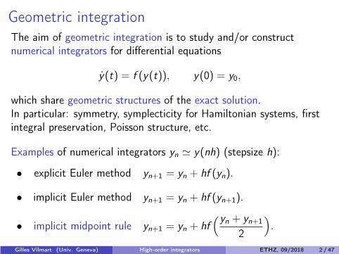
Geometric integrationThe aim of geometric integration is to study and/or constructnumerical integrators for differential equations
y(t) = f (y(t)), y(0) = y0,
which share geometric structures of the exact solution.In particular: symmetry, symplecticity for Hamiltonian systems, firstintegral preservation, Poisson structure, etc.
Examples of numerical integrators yn ≃ y(nh) (stepsize h):
• explicit Euler method yn+1 = yn + hf (yn).
• implicit Euler method yn+1 = yn + hf (yn+1).
• implicit midpoint rule yn+1 = yn + hf(yn + yn+1
2
).
Gilles Vilmart (Univ. Geneva) High-order integrators ETHZ, 09/2018 2 / 47
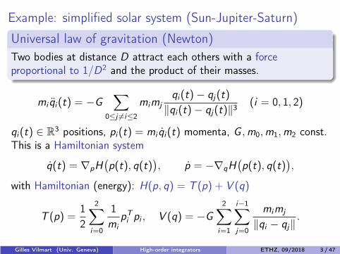
Example: simplified solar system (Sun-Jupiter-Saturn)
Universal law of gravitation (Newton)
Two bodies at distance D attract each others with a forceproportional to 1/D2 and the product of their masses.
mi qi(t) = −G∑
0≤j 6=i≤2
mimj
qi(t)− qj(t)
‖qi(t)− qj(t)‖3(i = 0, 1, 2)
qi(t) ∈ R3 positions, pi(t) = mi qi(t) momenta, G ,m0,m1,m2 const.
This is a Hamiltonian system
q(t) = ∇pH(p(t), q(t)
), p = −∇qH
(p(t), q(t)
),
with Hamiltonian (energy): H(p, q) = T (p) + V (q)
T (p) =12
2∑
i=0
1mi
pTi pi , V (q) = −G
2∑
i=1
i−1∑
j=0
mimj
‖qi − qj‖.
Gilles Vilmart (Univ. Geneva) High-order integrators ETHZ, 09/2018 3 / 47
Conservation of first integrals
Energy conservation for Hamiltonian systems
For a Hamiltonian system
q(t) = ∇pH(p(t), q(t)
), p(t) = −∇qH
(p(t), q(t)
),
the Hamiltonian H(p, q) is a first integral: H(p(t), q(t)) = const.
More generally, a quantity C (y) is a first integral (C (y(t)) = const)of a general system y = f (y) if and only if
∇C (y) · f (y) = 0, for all y .
Comparison of numerical methods: →anim.
Gilles Vilmart (Univ. Geneva) High-order integrators ETHZ, 09/2018 4 / 47
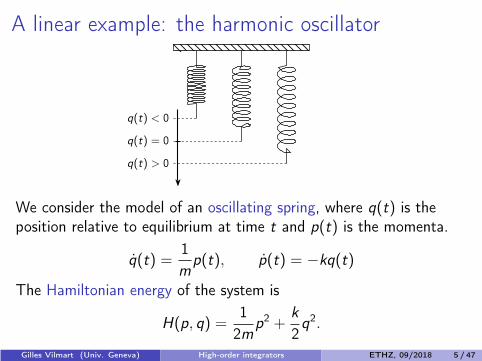
A linear example: the harmonic oscillator
q(t) < 0
q(t) = 0
q(t) > 0
We consider the model of an oscillating spring, where q(t) is theposition relative to equilibrium at time t and p(t) is the momenta.
q(t) =1mp(t), p(t) = −kq(t)
The Hamiltonian energy of the system is
H(p, q) =1
2mp2 +
k
2q2.
Gilles Vilmart (Univ. Geneva) High-order integrators ETHZ, 09/2018 5 / 47
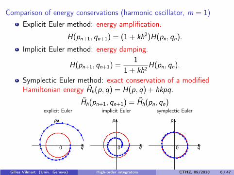
Comparison of energy conservations (harmonic oscillator, m = 1)
Explicit Euler method: energy amplification.
H(pn+1, qn+1) = (1 + kh2)H(pn, qn).
Implicit Euler method: energy damping.
H(pn+1, qn+1) =1
1 + kh2H(pn, qn).
Symplectic Euler method: exact conservation of a modifiedHamiltonian energy Hh(p, q) = H(p, q) + hkpq.
Hh(pn+1, qn+1) = Hh(pn, qn)
0 q
p
explicit Euler
0 q
p
implicit Euler
0 q
p
symplectic Euler
Gilles Vilmart (Univ. Geneva) High-order integrators ETHZ, 09/2018 6 / 47
What happened? Theory of backward error analysis
Given a differential equation
y = f (y), y(0) = y0
and a one-step numerical integrator
yn+1 = Φf ,h(yn)
we search for a modified differential equation
z = fh(z) = f (z) + hf2(z) + h2f3(z) + h3f4(z) + . . . , z(0) = y0
such that (formally) yn = z(nh)
Ruth (1983), Griffiths, Sanz-Serna (86), Gladman, Duncan, Candy (91),Feng (91), Sanz-Serna (92), Yoshida (93), Eirola (93), Hairer (94), Fiedler,Scheurle (96), . . .
Gilles Vilmart (Univ. Geneva) High-order integrators ETHZ, 09/2018 7 / 47
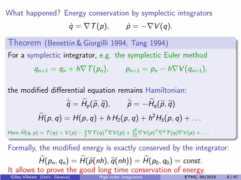
What happened? Energy conservation by symplectic integrators
q = ∇T (p), p = −∇V (q).
Theorem (Benettin & Giorgilli 1994, Tang 1994)
For a symplectic integrator, e.g. the symplectic Euler method
qn+1 = qn + h∇T (pn), pn+1 = pn − h∇V (qn+1),
the modified differential equation remains Hamiltonian:
˙q = Hp(p, q), ˙p = −Hq(p, q)
H(p, q) = H(p, q) + h H2(p, q) + h2H3(p, q) + . . .
Here H(q, p) = T (q) + V (p)− h2∇T (q)T∇V (p) + h2
12∇V (p)T∇2T (q)∇V (p) + . . ..
Formally, the modified energy is exactly conserved by the integrator:
H(pn, qn) = H(p(nh), q(nh)) = H(p0, q0) = const.It allows to prove the good long time conservation of energy.Gilles Vilmart (Univ. Geneva) High-order integrators ETHZ, 09/2018 8 / 47

Example of a stochastic model: Langevin dynamics
It models particle motions subject to a potential V , linear friction andmolecular diffusion:
q(t) = p(t), p(t) = −∇V (q(t))− γp(t) +√
2γβ−1W (t).
W (t): standard Brownian motion in Rd ,continuous, independent
increments, W (t + h)−W (t) ∼ N (0, h), a.s. nowhere differentiable.
Itô integral: for f (t) a (continuous and adapted) stochastic process,∫ t=tN
0
f (s)dW (s) = limh→0
N−1∑
n=0
f (tn)(W (tn+1)−W (tn)), tn = nh.
Example in 2DA quartic potential V (see level curves):V (x) = (1 − x2
1 )2 + (1 − x2
2 )2 + x1x2
2+ x2
5.
−2 −1 0 1 2−2
−1
0
1
2
x1
x2
Gilles Vilmart (Univ. Geneva) High-order integrators ETHZ, 09/2018 9 / 47
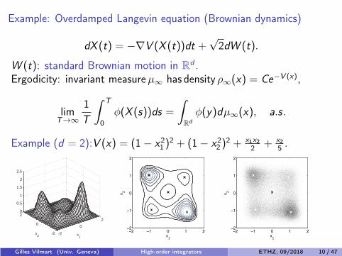
Example: Overdamped Langevin equation (Brownian dynamics)
dX (t) = −∇V (X (t))dt +√
2dW (t).
W (t): standard Brownian motion in Rd .
Ergodicity: invariant measureµ∞ has density ρ∞(x) = Ce−V (x),
limT→∞
1T
∫ T
0
φ(X (s))ds =
∫
Rd
φ(y)dµ∞(x), a.s.
Example (d = 2):V (x) = (1 − x21 )
2 + (1 − x22 )
2 + x1x22
+ x25.
-2
0
2
-2
0
20
0.5
1
1.5
2
2.5
x1
x2
−2 −1 0 1 2−2
−1
0
1
2
x1
x 2
−2 −1 0 1 2−2
−1
0
1
2
x1
x 2
Gilles Vilmart (Univ. Geneva) High-order integrators ETHZ, 09/2018 10 / 47
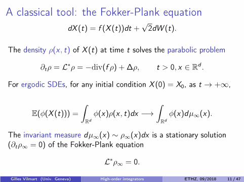
A classical tool: the Fokker-Plank equation
dX (t) = f (X (t))dt +√
2dW (t).
The density ρ(x , t) of X (t) at time t solves the parabolic problem
∂tρ = L∗ρ = −div(f ρ) + ∆ρ, t > 0, x ∈ Rd .
For ergodic SDEs, for any initial condition X (0) = X0, as t → +∞,
E(φ(X (t))) =
∫
Rd
φ(x)ρ(x , t)dx −→∫
Rd
φ(x)dµ∞(x).
The invariant measure dµ∞(x) ∼ ρ∞(x)dx is a stationary solution(∂tρ∞ = 0) of the Fokker-Plank equation
L∗ρ∞ = 0.
Gilles Vilmart (Univ. Geneva) High-order integrators ETHZ, 09/2018 11 / 47
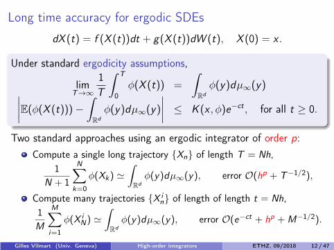
Long time accuracy for ergodic SDEs
dX (t) = f (X (t))dt + g(X (t))dW (t), X (0) = x .
Under standard ergodicity assumptions,
limT→∞
1T
∫ T
0
φ(X (t)) =
∫
Rd
φ(y)dµ∞(y)∣∣∣∣E(φ(X (t)))−
∫
Rd
φ(y)dµ∞(y)
∣∣∣∣ ≤ K (x , φ)e−ct , for all t ≥ 0.
Two standard approaches using an ergodic integrator of order p:
Compute a single long trajectory Xn of length T = Nh,
1
N + 1
N∑
k=0
φ(Xk) ≃∫
Rd
φ(y)dµ∞(y), error O(hp + T−1/2),
Compute many trajectories X in of length of length t = Nh,
1
M
M∑
i=1
φ(X iN) ≃
∫
Rd
φ(y)dµ∞(y), error O(e−ct + hp +M−1/2).
Gilles Vilmart (Univ. Geneva) High-order integrators ETHZ, 09/2018 12 / 47

Example: stiff and nonstiff Brownian dynamics.Gibbs density ρ∞(x) = Ze−
2σ2 V (x).
−2 −1.5 −1 −0.5 0 0.5 1 1.5 2−2
−1.5
−1
−0.5
0
0.5
1
x1
x 2
Nonstiff case V (x) = (1 − x21 )
2 + x42 − x + x1 cos(x2) + (x2 + x2
1 )2
−2 −1.5 −1 −0.5 0 0.5 1 1.5 2−2
−1.5
−1
−0.5
0
0.5
1
x1
x 2
Stiff case V (x) = (1 − x21 )
2 + x42 − x + x3 cos(x2) + 100(x2 + x2
1 )2 + 106
2(x1 − x3)2.
Gilles Vilmart (Univ. Geneva) High-order integrators ETHZ, 09/2018 13 / 47
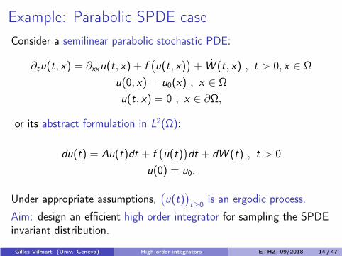
Example: Parabolic SPDE case
Consider a semilinear parabolic stochastic PDE:
∂tu(t, x) = ∂xxu(t, x) + f(u(t, x)
)+ W (t, x) , t > 0, x ∈ Ω
u(0, x) = u0(x) , x ∈ Ω
u(t, x) = 0 , x ∈ ∂Ω,
or its abstract formulation in L2(Ω):
du(t) = Au(t)dt + f(u(t)
)dt + dW (t) , t > 0
u(0) = u0.
Under appropriate assumptions,(u(t)
)t≥0
is an ergodic process.
Aim: design an efficient high order integrator for sampling the SPDEinvariant distribution.
Gilles Vilmart (Univ. Geneva) High-order integrators ETHZ, 09/2018 14 / 47
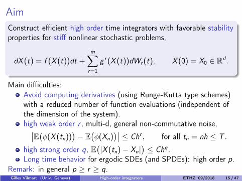
Aim
Construct efficient high order time integrators with favorable stabilityproperties for stiff nonlinear stochastic problems,
dX (t) = f (X (t))dt +m∑
r=1
g r (X (t))dWr (t), X (0) = X0 ∈ Rd .
Main difficulties:Avoid computing derivatives (using Runge-Kutta type schemes)with a reduced number of function evaluations (independent ofthe dimension of the system).high weak order r , multi-d, general non-commutative noise,∣∣E(φ(X (tn))
)− E
(φ(Xn)
)∣∣ ≤ Chr , for all tn = nh ≤ T .
high strong order q, E(|X (tn)− Xn|
)≤ Chq.
Long time behavior for ergodic SDEs (and SPDEs): high order p.Remark: in general p ≥ r ≥ q.Gilles Vilmart (Univ. Geneva) High-order integrators ETHZ, 09/2018 15 / 47
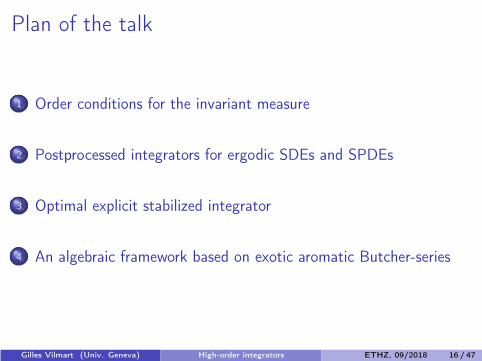
Plan of the talk
1 Order conditions for the invariant measure
2 Postprocessed integrators for ergodic SDEs and SPDEs
3 Optimal explicit stabilized integrator
4 An algebraic framework based on exotic aromatic Butcher-series
Gilles Vilmart (Univ. Geneva) High-order integrators ETHZ, 09/2018 16 / 47
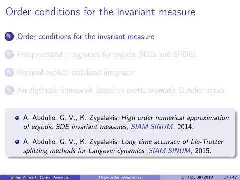
Order conditions for the invariant measure
1 Order conditions for the invariant measure
2 Postprocessed integrators for ergodic SDEs and SPDEs
3 Optimal explicit stabilized integrator
4 An algebraic framework based on exotic aromatic Butcher-series
A. Abdulle, G. V., K. Zygalakis, High order numerical approximationof ergodic SDE invariant measures, SIAM SINUM, 2014.
A. Abdulle, G. V., K. Zygalakis, Long time accuracy of Lie-Trottersplitting methods for Langevin dynamics, SIAM SINUM, 2015.
Gilles Vilmart (Univ. Geneva) High-order integrators ETHZ, 09/2018 17 / 47
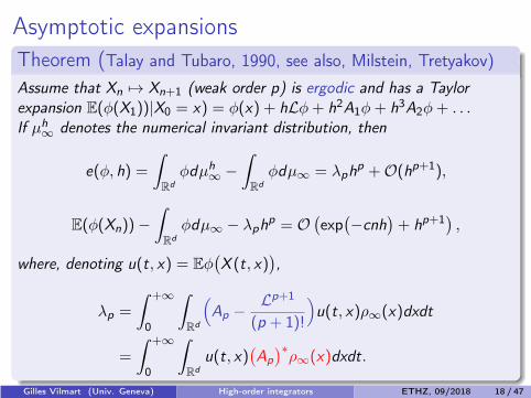
Asymptotic expansions
Theorem (Talay and Tubaro, 1990, see also, Milstein, Tretyakov)
Assume that Xn 7→ Xn+1 (weak order p) is ergodic and has a Taylorexpansion E(φ(X1))|X0 = x) = φ(x) + hLφ+ h2A1φ+ h3A2φ+ . . .If µh
∞ denotes the numerical invariant distribution, then
e(φ, h) =
∫
Rd
φdµh∞ −
∫
Rd
φdµ∞ = λphp +O(hp+1),
E(φ(Xn))−∫
Rd
φdµ∞ − λphp = O
(exp
(−cnh
)+ hp+1
),
where, denoting u(t, x) = Eφ(X (t, x)
),
λp =
∫ +∞
0
∫
Rd
(Ap −
Lp+1
(p + 1)!
)u(t, x)ρ∞(x)dxdt
=
∫ +∞
0
∫
Rd
u(t, x)(Ap
)∗ρ∞(x)dxdt.
Gilles Vilmart (Univ. Geneva) High-order integrators ETHZ, 09/2018 18 / 47
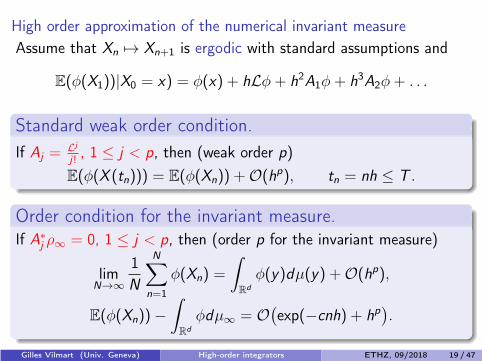
High order approximation of the numerical invariant measure
Assume that Xn 7→ Xn+1 is ergodic with standard assumptions and
E(φ(X1))|X0 = x) = φ(x) + hLφ+ h2A1φ+ h3A2φ+ . . .
Standard weak order condition.
If Aj =Lj
j!, 1 ≤ j < p, then (weak order p)
E(φ(X (tn))) = E(φ(Xn)) +O(hp), tn = nh ≤ T .
Order condition for the invariant measure.If A∗
j ρ∞ = 0, 1 ≤ j < p, then (order p for the invariant measure)
limN→∞
1N
N∑
n=1
φ(Xn) =
∫
Rd
φ(y)dµ(y) +O(hp),
E(φ(Xn))−∫
Rd
φdµ∞ = O(exp(−cnh) + hp
).
Gilles Vilmart (Univ. Geneva) High-order integrators ETHZ, 09/2018 19 / 47
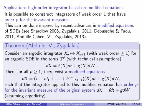
Application: high order integrator based on modified equations
It is possible to construct integrators of weak order 1 that haveorder p for the invariant measure.This can be done inspired by recent advances in modified equationsof SDEs (see Shardlow 2006, Zygalakis, 2011, Debussche & Faou,2011, Abdulle Cohen, V., Zygalakis, 2013).
Theorem (Abdulle, V., Zygalakis)
Consider an ergodic integrator Xn 7→ Xn+1 (with weak order ≥ 1) foran ergodic SDE in the torus Td (with technical assumptions),
dX = f (X )dt + g(X )dW .
Then, for all p ≥ 1, there exist a modified equations
dX = (f + hf1 + . . .+ hp−1fp−1)(X )dt + g(X )dW ,
such that the integrator applied to this modified equation has order pfor the invariant measure of the original system dX = fdt + gdW
(assuming ergodicity).
Gilles Vilmart (Univ. Geneva) High-order integrators ETHZ, 09/2018 20 / 47
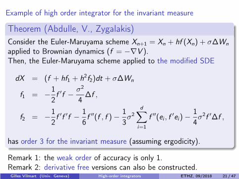
Example of high order integrator for the invariant measure
Theorem (Abdulle, V., Zygalakis)
Consider the Euler-Maruyama scheme Xn+1 = Xn + hf (Xn) + σ∆Wn
applied to Brownian dynamics (f = −∇V ).Then, the Euler-Maruyama scheme applied to the modified SDE
dX = (f + hf1 + h2f2)dt + σ∆Wn
f1 = −12f ′f − σ2
4∆f ,
f2 = −12f ′f ′f − 1
6f ′′(f , f )− 1
3σ2
d∑
i=1
f ′′(ei , f′ei)−
14σ2f ′∆f ,
has order 3 for the invariant measure (assuming ergodicity).
Remark 1: the weak order of accuracy is only 1.Remark 2: derivative free versions can also be constructed.Gilles Vilmart (Univ. Geneva) High-order integrators ETHZ, 09/2018 21 / 47
Postprocessed integrators for ergodic SDEs and
SPDEs
1 Order conditions for the invariant measure
2 Postprocessed integrators for ergodic SDEs and SPDEs
3 Optimal explicit stabilized integrator
4 An algebraic framework based on exotic aromatic Butcher-series
G. V., Postprocessed integrators for the high order integration of
ergodic SDEs, SIAM SISC , 2015.
C.-E. Bréhier and G. V., High-order integrator for sampling the
invariant distribution of a class of parabolic SPDEs with additive
space-time noise, SIAM SISC , 2016.
Gilles Vilmart (Univ. Geneva) High-order integrators ETHZ, 09/2018 22 / 47
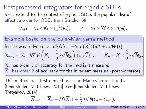
Postprocessed integrators for ergodic SDEsIdea: extend to the context of ergodic SDEs the popular idea ofeffective order for ODEs from Butcher 69’,
yn+1 = χh Kh χ−1
h (yn), yn = χh K nh χ−1
h (y0).
Example based on the Euler-Maruyama method
for Brownian dynamics: dX (t) = −∇V (X (t))dt + σdW (t).
Xn+1 = Xn−h∇V
(Xn +
12σ√hξn
)+σ
√hξn, X n = Xn+
12σ√hξn.
Xn has order 1 of accuracy for the invariant measure.X n has order 2 of accuracy for the invariant measure (postprocessor).
This method was first derived as a non-Markovian method by[Leimkhuler, Matthews, 2013], see [Leimkhuler, Matthews,Tretyakov, 2014],
X n+1 = X n + hf (X n) +12σ√h(ξn + ξn+1).
Gilles Vilmart (Univ. Geneva) High-order integrators ETHZ, 09/2018 23 / 47
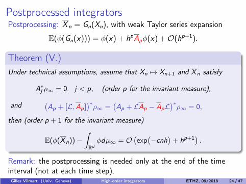
Postprocessed integratorsPostprocessing: X n = Gn(Xn), with weak Taylor series expansion
E(φ(Gn(x))) = φ(x) + hpApφ(x) +O(hp+1).
Theorem (V.)
Under technical assumptions, assume that Xn 7→ Xn+1 and X n satisfy
A∗j ρ∞ = 0 j < p, (order p for the invariant measure),
and(Ap + [L,Ap]
)∗ρ∞ =
(Ap + LAp − ApL
)∗ρ∞ = 0,
then (order p + 1 for the invariant measure)
E(φ(X n))−∫
Rd
φdµ∞ = O(exp
(−cnh
)+ hp+1
).
Remark: the postprocessing is needed only at the end of the timeinterval (not at each time step).Gilles Vilmart (Univ. Geneva) High-order integrators ETHZ, 09/2018 24 / 47
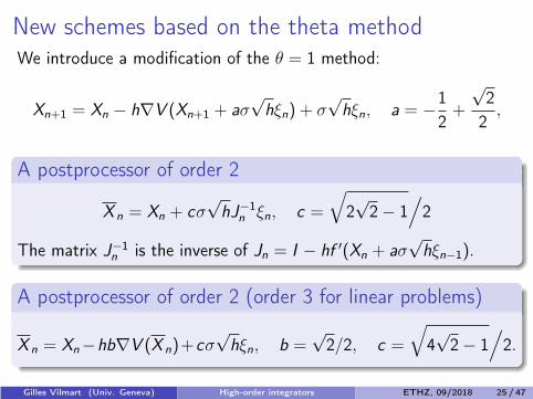
New schemes based on the theta methodWe introduce a modification of the θ = 1 method:
Xn+1 = Xn − h∇V (Xn+1 + aσ√hξn) + σ
√hξn, a = −1
2+
√2
2,
A postprocessor of order 2
X n = Xn + cσ√hJ−1
n ξn, c =
√2√
2 − 1/
2
The matrix J−1n is the inverse of Jn = I − hf ′(Xn + aσ
√hξn−1).
A postprocessor of order 2 (order 3 for linear problems)
X n = Xn−hb∇V (X n)+cσ√hξn, b =
√2/2, c =
√4√
2 − 1/
2.
Gilles Vilmart (Univ. Geneva) High-order integrators ETHZ, 09/2018 25 / 47
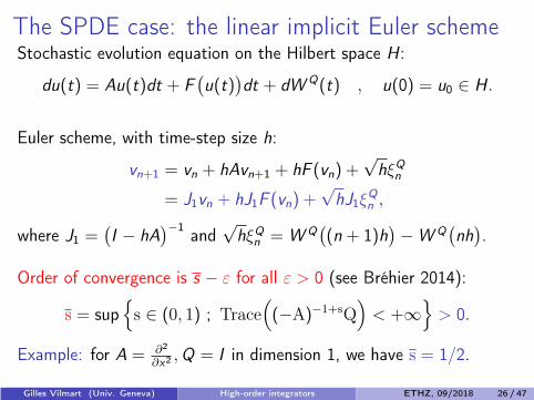
The SPDE case: the linear implicit Euler schemeStochastic evolution equation on the Hilbert space H :
du(t) = Au(t)dt + F(u(t)
)dt + dW Q(t) , u(0) = u0 ∈ H .
Euler scheme, with time-step size h:
vn+1 = vn + hAvn+1 + hF (vn) +√hξQn
= J1vn + hJ1F (vn) +√hJ1ξ
Qn ,
where J1 =(I − hA
)−1and
√hξQn = W Q
((n + 1)h
)−W Q
(nh
).
Order of convergence is s − ε for all ε > 0 (see Bréhier 2014):
s = sup
s ∈ (0, 1) ; Trace((−A)−1+sQ
)< +∞
> 0.
Example: for A = ∂2
∂x2 ,Q = I in dimension 1, we have s = 1/2.
Gilles Vilmart (Univ. Geneva) High-order integrators ETHZ, 09/2018 26 / 47
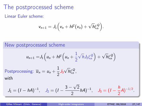
The postprocessed scheme
Linear Euler scheme:
vn+1 = J1
(vn + hF (vn) +
√hξQn
).
New postprocessed scheme
un+1 =J1
(un + hF
(un +
12
√hJ2ξ
Qn
)+√hξQn
)
Postprocessing: un = un +12J3
√hξQn ,
with
J1 = (I − hA)−1, J2 = (I − 3 −√
22
hA)−1, J3 = (I − h
2A)−1/2.
Gilles Vilmart (Univ. Geneva) High-order integrators ETHZ, 09/2018 27 / 47
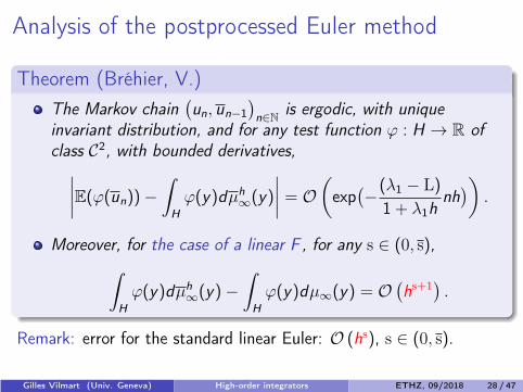
Analysis of the postprocessed Euler method
Theorem (Bréhier, V.)
The Markov chain(un, un−1
)n∈N
is ergodic, with unique
invariant distribution, and for any test function ϕ : H → R of
class C2, with bounded derivatives,
∣∣∣∣E(ϕ(un))−∫
H
ϕ(y)dµh∞(y)
∣∣∣∣ = O(exp
(−(λ1 − L)
1 + λ1hnh
)).
Moreover, for the case of a linear F , for any s ∈ (0, s),
∫
H
ϕ(y)dµh∞(y)−
∫
H
ϕ(y)dµ∞(y) = O(hs+1
).
Remark: error for the standard linear Euler: O (hs), s ∈ (0, s).
Gilles Vilmart (Univ. Geneva) High-order integrators ETHZ, 09/2018 28 / 47
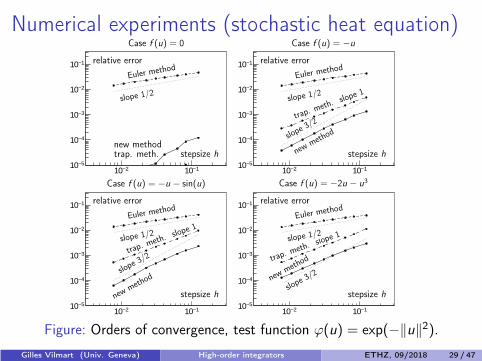
Numerical experiments (stochastic heat equation)
10−2 10−110−5
10−4
10−3
10−2
10−1
10−2 10−110−5
10−4
10−3
10−2
10−1
10−2 10−110−5
10−4
10−3
10−2
10−1
10−2 10−110−5
10−4
10−3
10−2
10−1
relative error
Case f (u) = 0
stepsize h
Euler method
slope 1/2
new methodtrap. meth.
relative error
Case f (u) = −u
stepsize h
Euler method
trap. meth.
slope 1
newmeth
od
slope 1/2
slope
3/2
relative error
Case f (u) = −u − sin(u)
stepsize h
Euler method
trap. meth.
slope 1
newmeth
od
slope 1/2
slope
3/2
relative error
Case f (u) = −2u − u3
stepsize h
Euler method
trap. meth.
slope 1
newmeth
od
slope 1/2
slope
3/2
Figure: Orders of convergence, test function ϕ(u) = exp(−‖u‖2).
Gilles Vilmart (Univ. Geneva) High-order integrators ETHZ, 09/2018 29 / 47

Qualitative behaviorData: f (u) = −u − sin(u), Q = I , h = 0.01.
1
x0.5
00
0.5t
1
-1
0
1
u
1
x0.5
00
0.5t
-1
0
1
1
u
standard Euler method postprocessed method
Remark: the process(un
)n∈N
has the same spatial regularity as thecontinuous-time process
(u(t)
)t≥0
, while the Euler scheme(vn)n∈N
ismore regular.
Related work: Chong and Walsh, 2012 (regularity study of theθ = 1/2 stochastic method).Gilles Vilmart (Univ. Geneva) High-order integrators ETHZ, 09/2018 30 / 47
Qualitative behaviorData: f (u) = −u − sin(u), Q = I , h = 0.01, T = 1.
x0 0.2 0.4 0.6 0.8 1
u(x,
1)
-0.6
-0.4
-0.2
0
0.2
0.4
0.6
x0 0.2 0.4 0.6 0.8 1
u(x,
1)
-0.6
-0.4
-0.2
0
0.2
0.4
0.6
standard Euler method postprocessed method
Remark: the process(un
)n∈N
has the same spatial regularity as thecontinuous-time process
(u(t)
)t≥0
, while the Euler scheme(vn)n∈N
ismore regular.
Related work: Chong and Walsh, 2012 (regularity study of theθ = 1/2 stochastic method).Gilles Vilmart (Univ. Geneva) High-order integrators ETHZ, 09/2018 30 / 47

Optimal explicit stabilized integrator for stiff and
ergodic SDEs
1 Order conditions for the invariant measure
2 Postprocessed integrators for ergodic SDEs and SPDEs
3 Optimal explicit stabilized integrator
4 An algebraic framework based on exotic aromatic Butcher-series
A. Abdulle, I. Almuslimani, G. V., Optimal explicit stabilized
integrator of weak order one for stiff and ergodic stochastic
differential equations, SIAM JUQ, 2018.
Gilles Vilmart (Univ. Geneva) High-order integrators ETHZ, 09/2018 31 / 47
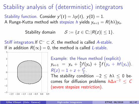
Stability analysis of (deterministic) integrators
Stability function. Consider y ′(t) = λy(t), y(0) = 1.A Runge-Kutta method with stepsize h yields yn+1 = R(hλ)yn.
Stability domain S := z ∈ C; |R(z)| ≤ 1.
Stiff integrators.If C− ⊂ S, the method is called A-stable.If in addition R(∞) = 0, the method is called L-stable.
-2.5 -2.0 -1.5 -1.0 -0.5 0.0 0.5-3
-2
-1
0
1
2
3
Example: the Heun method (explicit)yn+1 = yn + h
2f (yn) + h
2f(yn + hf (yn)
).
R(z) = 1 + z + z2
2.
The stability condition −2 ≤ hλ ≤ 0 be-comes for diffusion problems h∆x−2 ≤ C
(severe stepsize restriction).
Gilles Vilmart (Univ. Geneva) High-order integrators ETHZ, 09/2018 32 / 47

Example: the θ-method for the heat equation
∂tu = ∂xxu, t > 0, x ∈ (0, 1)
with Dirichlet boundary conditions: u(0, t) = u(1, t) = 0.
Discretization.Spatial discretization with finite differences, with ∆x = 1/100.Time discretization: θ-method with ∆t = 0.01.
Un+1 = Un + (1 − θ)∆tAUn + θ∆tAUn+1.
Comparison of θ = 1/2 (A-stable, not L-stable) or θ = 1 (L-stable),with initial condition u(x , 0) = sin(2πx) or u(x , 0) = sin(2πx) + 1.
Remark.If θ = 0 (Forward Euler), severe timestep restriction ∆t ≤ 0.0002.Gilles Vilmart (Univ. Geneva) High-order integrators ETHZ, 09/2018 33 / 47
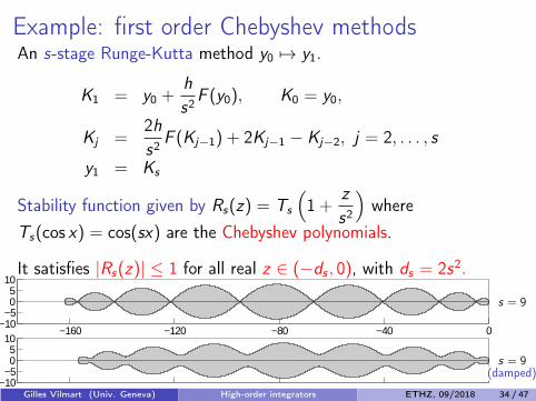
Example: first order Chebyshev methodsAn s-stage Runge-Kutta method y0 7→ y1.
K1 = y0 +h
s2F (y0), K0 = y0,
Kj =2hs2
F (Kj−1) + 2Kj−1 − Kj−2, j = 2, . . . , s
y1 = Ks
Stability function given by Rs(z) = Ts
(1 +
z
s2
)where
Ts(cos x) = cos(sx) are the Chebyshev polynomials.
It satisfies |Rs(z)| ≤ 1 for all real z ∈ (−ds , 0), with ds = 2s2.
−160 −120 −80 −40 0−10−505
10
−10−505
10
s = 9
s = 9(damped)
Gilles Vilmart (Univ. Geneva) High-order integrators ETHZ, 09/2018 34 / 47
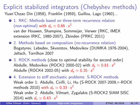
Explicit stabilized integrators (Chebyshev methods)Yuan’Chzao Din (1958), Franklin (1959), Guillou, Lago (1960)...
1. RKC: Methods based on three-term recurrence relation(non-optimal) with ds ≃ 0.66 · s2
van der Houwen, Shampine, Sommeijer, Verwer (RKC, IMEXextension IRKC, 1980-2007), Zbinden (PRKC 2011)
2. Methods based on composition (no-recurrence relation)Bogatyrev, Lebedev, Skvorstov, Medovikov (DUMKA 1976-2004),Jeltsch, Torrilhon 2007
3. ROCK methods (close to optimal stability for second order)Abdulle, Medovikov (ROCK2 2000-02) with ds ≃ 0.81 · s2
Abdulle (ROCK4 2002-05) with ds ≃ 0.35 · s2
4. Extension to stiff stochastic problems: S-ROCK methodsWeak order 1: Abdulle, Cirilli, Li, Hu (S-ROCK 2007-2009,τ -ROCKmethods 2010) with ds ≃ 0.33 · s2
Weak order 2: Abdulle, Vilmart, Zygalakis (S-ROCK2 SIAM SISC2014) with ds ≃ 0.43 · s2
...Gilles Vilmart (Univ. Geneva) High-order integrators ETHZ, 09/2018 35 / 47
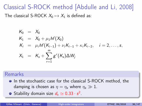
Classical S-ROCK method [Abdulle and Li, 2008]The classical S-ROCK X0 7→ X1 is defined as:
K0 = X0
K1 = X0 + µ1hf (X0)
Ki = µihf (Ki−1) + νiKi−1 + κiKi−2, i = 2, . . . , s,
X1 = Ks +m∑
r=1
g r (Ks)∆Wj
RemarksIn the stochastic case for the classical S-ROCK method, thedamping is chosen as η = ηs where ηs ≫ 1.
Stability domain size ds ≃ 0.33 · s2.
Gilles Vilmart (Univ. Geneva) High-order integrators ETHZ, 09/2018 36 / 47
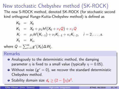
New stochastic Chebyshev method (SK-ROCK)The new S-ROCK method, denoted SK-ROCK (for stochastic secondkind orthogonal Runge-Kutta-Chebyshev method) is defined as
K0 = X0
K1 = X0 + µ1hf (X0 + ν1Q) + κ1Q
Ki = µihf (Ki−1) + νiKi−1 + κiKi−2, i = 2, . . . , s.
X1 = Ks ,
where Q =∑m
r=1g r (X0)∆Wj .
RemarksAnalogously to the deterministic method, the dampingparameter η is fixed to a small value (typically η = 0.05).
Without noise (g r = 0), we recover the standard deterministicChebyshev method.
Stability domain size ds ≥ (2 − 4
3η)s2.
Gilles Vilmart (Univ. Geneva) High-order integrators ETHZ, 09/2018 37 / 47
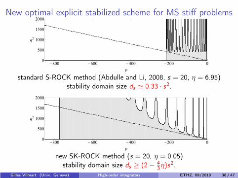
New optimal explicit stabilized scheme for MS stiff problems
-800 -600 -400 -200 00
500
1000
1500
2000
p
q2
standard S-ROCK method (Abdulle and Li, 2008, s = 20, η = 6.95)stability domain size ds ≃ 0.33 · s2.
-800 -600 -400 -200 00
500
1000
1500
2000
p
q2
new SK-ROCK method (s = 20, η = 0.05)stability domain size ds ≥ (2 − 4
3η)s2.
Gilles Vilmart (Univ. Geneva) High-order integrators ETHZ, 09/2018 38 / 47
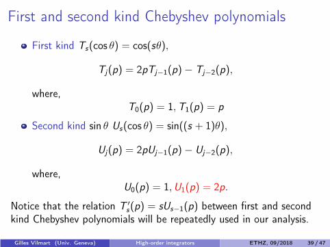
First and second kind Chebyshev polynomials
First kind Ts(cos θ) = cos(sθ),
Tj(p) = 2pTj−1(p)− Tj−2(p),
where,T0(p) = 1,T1(p) = p
Second kind sin θ Us(cos θ) = sin((s + 1)θ),
Uj(p) = 2pUj−1(p)− Uj−2(p),
where,U0(p) = 1,U1(p) = 2p.
Notice that the relation T ′s(p) = sUs−1(p) between first and second
kind Chebyshev polynomials will be repeatedly used in our analysis.
Gilles Vilmart (Univ. Geneva) High-order integrators ETHZ, 09/2018 39 / 47
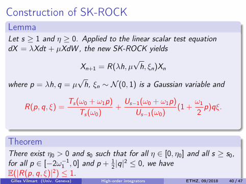
Construction of SK-ROCKLemmaLet s ≥ 1 and η ≥ 0. Applied to the linear scalar test equation
dX = λXdt + µXdW , the new SK-ROCK yields
Xn+1 = R(λh, µ√h, ξn)Xn
where p = λh, q = µ√h, ξn ∼ N (0, 1) is a Gaussian variable and
R(p, q, ξ) =Ts(ω0 + ω1p)
Ts(ω0)+
Us−1(ω0 + ω1p)
Us−1(ω0)(1 +
ω1
2p)qξ.
TheoremThere exist η0 > 0 and s0 such that for all η ∈ [0, η0] and all s ≥ s0,
for all p ∈ [−2ω−1
1, 0] and p + 1
2|q|2 ≤ 0, we have
E(|R(p, q, ξ)|2) ≤ 1.Gilles Vilmart (Univ. Geneva) High-order integrators ETHZ, 09/2018 40 / 47
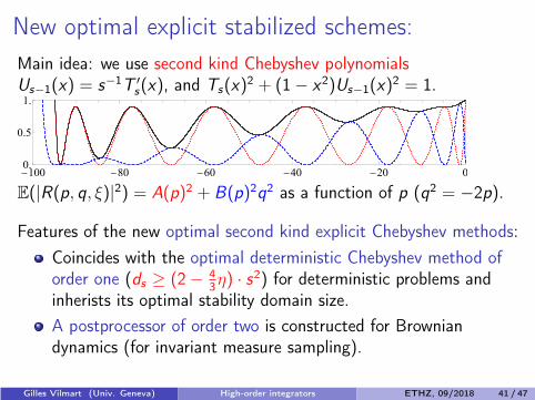
New optimal explicit stabilized schemes:
Main idea: we use second kind Chebyshev polynomialsUs−1(x) = s−1T ′
s(x), and Ts(x)2 + (1 − x2)Us−1(x)
2 = 1.
-100 -80 -60 -40 -20 00.
0.5
1.
E(|R(p, q, ξ)|2) = A(p)2 + B(p)2q2 as a function of p (q2 = −2p).
Features of the new optimal second kind explicit Chebyshev methods:
Coincides with the optimal deterministic Chebyshev method oforder one (ds ≥ (2 − 4
3η) · s2) for deterministic problems and
inherists its optimal stability domain size.
A postprocessor of order two is constructed for Browniandynamics (for invariant measure sampling).
Gilles Vilmart (Univ. Geneva) High-order integrators ETHZ, 09/2018 41 / 47
An algebraic framework based on exotic aromatic
Butcher-series
1 Order conditions for the invariant measure
2 Postprocessed integrators for ergodic SDEs and SPDEs
3 Optimal explicit stabilized integrator
4 An algebraic framework based on exotic aromatic Butcher-series
A. Laurent, G. V., Exotic aromatic B-series for the study of long time
integrators for a class of ergodic SDEs, ArXiv, submitted , 2017.
Gilles Vilmart (Univ. Geneva) High-order integrators ETHZ, 09/2018 42 / 47
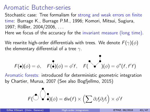
Aromatic Butcher-seriesStochastic case: Tree formalism for strong and weak errors on finitetime: Burrage K., Burrage P.M., 1996; Komori, Mitsui, Sugiura,1997; Rößler, 2004/2006, . . .Here we focus of the accuracy for the invariant measure (long time).
We rewrite high-order differentials with trees. We denote F (γ)(φ)the elementary differential of a tree γ.
F ( )(φ) = φ, F ( )(φ) = φ′f , F ( )(φ) = φ′′(f , f ′f )
Aromatic forests: introduced for deterministic geometric integrationby Chartier, Murua, 2007 (See also Bogfjellmo, 2015)
F ( )(φ) = div(f )×(∑
∂i fj∂j fi
)× φ′f
Gilles Vilmart (Univ. Geneva) High-order integrators ETHZ, 09/2018 43 / 47
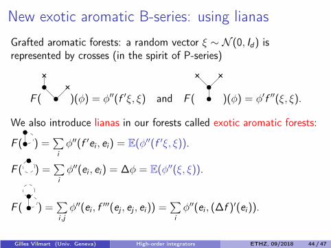
New exotic aromatic B-series: using lianas
Grafted aromatic forests: a random vector ξ ∼ N (0, Id) isrepresented by crosses (in the spirit of P-series)
F ( )(φ) = φ′′(f ′ξ, ξ) and F ( )(φ) = φ′f ′′(ξ, ξ).
We also introduce lianas in our forests called exotic aromatic forests:
F ( ) =∑i
φ′′(f ′ei , ei) = E(φ′′(f ′ξ, ξ)).
F ( ) =∑i
φ′′(ei , ei) = ∆φ = E(φ′′(ξ, ξ)).
F ( ) =∑i ,j
φ′′(ei , f′′′(ej , ej , ei)) =
∑i
φ′′(ei , (∆f )′(ei)).
Gilles Vilmart (Univ. Geneva) High-order integrators ETHZ, 09/2018 44 / 47
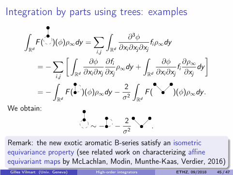
Integration by parts using trees: examples
∫
Rd
F ( )(φ)ρ∞dy =∑
i ,j
∫
Rd
∂3φ
∂xi∂xj∂xjfiρ∞dy
= −∑
i ,j
[ ∫
Rd
∂φ
∂xi∂xj
∂fi∂xj
ρ∞dy +
∫
Rd
∂φ
∂xi∂xjfi∂ρ∞∂xj
dy
]
= −∫
Rd
F ( )(φ)ρ∞dy − 2σ2
∫
Rd
F ( )(φ)ρ∞dy .
We obtain:
∼ − − 2σ2
.
Remark: the new exotic aromatic B-series satisfy an isometricequivariance property (see related work on characterizing affineequivariant maps by McLachlan, Modin, Munthe-Kaas, Verdier, 2016)Gilles Vilmart (Univ. Geneva) High-order integrators ETHZ, 09/2018 45 / 47
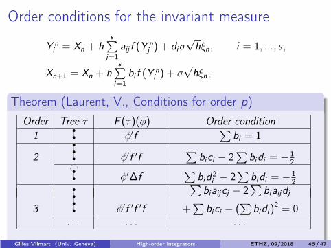
Order conditions for the invariant measure
Y ni = Xn + h
s∑j=1
aij f (Ynj ) + diσ
√hξn, i = 1, ..., s,
Xn+1 = Xn + hs∑
i=1
bi f (Yni ) + σ
√hξn,
Theorem (Laurent, V., Conditions for order p)
Order Tree τ F (τ)(φ) Order condition
1 φ′f∑
bi = 1
2 φ′f ′f∑
bici − 2∑
bidi = −1
2
φ′∆f∑
bid2i − 2
∑bidi = −1
2∑biaijcj − 2
∑biaijdj
3 φ′f ′f ′f +∑
bici − (∑
bidi)2 = 0
. . . . . . . . .
Gilles Vilmart (Univ. Geneva) High-order integrators ETHZ, 09/2018 46 / 47
SummaryUsing tools from geometric integration, we presented new orderconditions for the accuracy of ergodic integrators, with emphasison postprocessed integrators.In particular, high order in the deterministic or weak sense is notnecessary to achieve high order for the invariant measure.A new high-order method (s + 1 instead of s for linearized Euler)for sampling the invariant distribution of parabolic SPDEs
du(t) = Au(t)dt + F(u(t)
)dt + dW Q(t),
(proof in a simplified linear case).study of algebraic structures with exotic aromatic Butcher trees.
Current works:analysis of the order of convergence in the general semilinearSPDE case.combination with Multilevel Monte-Carlo strategies.
Gilles Vilmart (Univ. Geneva) High-order integrators ETHZ, 09/2018 47 / 47