
LS-SVMlab Toolbox User’s Guide
113
LS-SVMlab Toolbox User’s Guide version 1.7 K. De Brabanter, P. Karsmakers, F. Ojeda, C. Alzate, J. De Brabanter, K. Pelckmans, B. De Moor, J. Vandewalle, J.A.K. Suykens Katholieke Universiteit Leuven Department of Electrical Engineering, ESAT-SCD-SISTA Kasteelpark Arenberg 10, B-3001 Leuven-Heverlee, Belgium {kris.debrabanter,johan.suykens}@esat.kuleuven.be http://www.esat.kuleuven.be/sista/lssvmlab/ ESAT-SISTA Technical Report 10-146 September 2010
Transcript of LS-SVMlab Toolbox User’s Guide
LS-SVMlab Toolbox User’s Guideversion 1.7
K. De Brabanter, P. Karsmakers, F. Ojeda, C. Alzate,J. De Brabanter, K. Pelckmans, B. De Moor,
J. Vandewalle, J.A.K. Suykens
Katholieke Universiteit Leuven
Department of Electrical Engineering, ESAT-SCD-SISTA
Kasteelpark Arenberg 10, B-3001 Leuven-Heverlee, Belgium
{kris.debrabanter,johan.suykens}@esat.kuleuven.be
http://www.esat.kuleuven.be/sista/lssvmlab/
ESAT-SISTA Technical Report 10-146
September 2010

2
Acknowledgements
Research supported by Research Council KUL: GOA AMBioRICS, GOA MaNet,CoE EF/05/006 Optimization in Engineering(OPTEC), IOF-SCORES4CHEM, sev-eral PhD/post-doc & fellow grants; Flemish Government: FWO: PhD/postdoc grants,projects G.0452.04 (new quantum algorithms), G.0499.04 (Statistics), G.0211.05 (Non-linear), G.0226.06 (cooperative systems and optimization), G.0321.06 (Tensors), G.0302.07 (SVM/Kernel), G.0320.08 (convex MPC), G.0558.08 (Robust MHE), G.0557.08(Glycemia2), G.0588.09 (Brain-machine) research communities (ICCoS, ANMMM,MLDM); G.0377.09 (Mechatronics MPC), IWT: PhD Grants, McKnow-E, Eureka-Flite+, SBO LeCoPro, SBO Climaqs, POM, Belgian Federal Science Policy Office:IUAP P6/04 (DYSCO, Dynamical systems, control and optimization, 2007-2011); EU:ERNSI; FP7-HD-MPC (INFSO-ICT-223854), COST intelliCIS, EMBOCOM, Con-tract Research: AMINAL, Other: Helmholtz, viCERP, ACCM, Bauknecht, Hoerbiger.JS is a professor at K.U.Leuven Belgium. BDM and JWDW are full professors atK.U.Leuven Belgium.

Preface to LS-SVMLab v1.7
We have added new functions to the toolbox and updated some of the existing commands withrespect to the previous version v1.6. Because many readers are familiar with the layout of version1.5 and version 1.6, we have tried to change it as little as possible. Here is a summary of the mainchanges:
• The major difference with the previous version is the optimization routine used to findthe minimum of the cross-validation score function. The tuning procedure consists out oftwo steps: 1) Coupled Simulated Annealing determines suitable tuning parameters and 2)a simplex method uses these previous values as starting values in order to perform a fine-tuning of the parameters. The major advantage is speed. The number of function evaluationsneeded to find optimal parameters reduces from ±200 in v1.6 to 50 in this version.
• The construction of bias-corrected approximate 100(1− α)% pointwise/simulataneous con-fidence and prediction intervals have been added to this version.
• Some bug-fixes are performed in the function roc. The class do not need to be +1 or −1,but can also be 0 and 1. The conversion is automatically done.
The LS-SVMLab TeamHeverlee, BelgiumSeptember 2010
3

4

Preface to LS-SVMLab v1.6
We have added new functions to the toolbox and updated some of the existing commands withrespect to the previous version v1.5. Because many readers are familiar with the layout of version1.5, we have tried to change it as little as possible. The major difference is the speed-up of severalmethods. Here is a summary of the main changes:
Chapter/solver/function What’s new1. A birds eye on LS-SVMLab
2. LS-SVMLab toolbox examples Roadmap to LS-SVM; Addition of more regres-sion and classification examples; Easier interface formulti-class classification; Changed implementationfor robust LS-SVM.
3. Matlab functions Possibility of regression or classification using onlyone command!; The function validate has beendeleted; Faster (robust) training and (robust) modelselection criteria are provided; In case of robust re-gression different weight functions are provided tobe used with iteratively reweighted LS-SVM.
4. LS-SVM solver All CMEX and/or C files have been removed. Thelinear system is solved by using the Matlab com-mand “backslash” (\).
The LS-SVMLab TeamHeverlee, BelgiumJune 2010
5

6
Contents
1 Introduction 9
2 A birds eye view on LS-SVMlab 112.1 Classification and regression . . . . . . . . . . . . . . . . . . . . . . . . . . . . . . . 11
2.1.1 Classification extensions . . . . . . . . . . . . . . . . . . . . . . . . . . . . . 122.1.2 Tuning and robustness . . . . . . . . . . . . . . . . . . . . . . . . . . . . . . 122.1.3 Bayesian framework . . . . . . . . . . . . . . . . . . . . . . . . . . . . . . . 12
2.2 NARX models and prediction . . . . . . . . . . . . . . . . . . . . . . . . . . . . . . 132.3 Unsupervised learning . . . . . . . . . . . . . . . . . . . . . . . . . . . . . . . . . . 132.4 Solving large scale problems with fixed size LS-SVM . . . . . . . . . . . . . . . . . 13
3 LS-SVMlab toolbox examples 153.1 Roadmap to LS-SVM . . . . . . . . . . . . . . . . . . . . . . . . . . . . . . . . . . 153.2 Classification . . . . . . . . . . . . . . . . . . . . . . . . . . . . . . . . . . . . . . . 15
3.2.1 Hello world . . . . . . . . . . . . . . . . . . . . . . . . . . . . . . . . . . . . 153.2.2 Example . . . . . . . . . . . . . . . . . . . . . . . . . . . . . . . . . . . . . . 173.2.3 Using the object oriented interface: initlssvm . . . . . . . . . . . . . . . . 193.2.4 LS-SVM classification: only one command line away! . . . . . . . . . . . . . 193.2.5 Bayesian inference for classification . . . . . . . . . . . . . . . . . . . . . . . 203.2.6 Multi-class coding . . . . . . . . . . . . . . . . . . . . . . . . . . . . . . . . 22
3.3 Regression . . . . . . . . . . . . . . . . . . . . . . . . . . . . . . . . . . . . . . . . . 233.3.1 A simple example . . . . . . . . . . . . . . . . . . . . . . . . . . . . . . . . 233.3.2 LS-SVM regression: only one command line away! . . . . . . . . . . . . . . 253.3.3 Bayesian Inference for Regression . . . . . . . . . . . . . . . . . . . . . . . . 263.3.4 Using the object oriented model interface . . . . . . . . . . . . . . . . . . . 273.3.5 Confidence/Predition Intervals for Regression . . . . . . . . . . . . . . . . . 283.3.6 Robust regression . . . . . . . . . . . . . . . . . . . . . . . . . . . . . . . . . 313.3.7 Multiple output regression . . . . . . . . . . . . . . . . . . . . . . . . . . . . 333.3.8 A time-series example: Santa Fe laser data prediction . . . . . . . . . . . . 343.3.9 Fixed size LS-SVM . . . . . . . . . . . . . . . . . . . . . . . . . . . . . . . . 35
3.4 Unsupervised learning using kernel principal component analysis . . . . . . . . . . 38
A MATLAB functions 39A.1 General notation . . . . . . . . . . . . . . . . . . . . . . . . . . . . . . . . . . . . . 39A.2 Index of function calls . . . . . . . . . . . . . . . . . . . . . . . . . . . . . . . . . . 40
A.2.1 Training and simulation . . . . . . . . . . . . . . . . . . . . . . . . . . . . . 40A.2.2 Object oriented interface . . . . . . . . . . . . . . . . . . . . . . . . . . . . 41A.2.3 Training and simulating functions . . . . . . . . . . . . . . . . . . . . . . . 42A.2.4 Kernel functions . . . . . . . . . . . . . . . . . . . . . . . . . . . . . . . . . 43A.2.5 Tuning, sparseness and robustness . . . . . . . . . . . . . . . . . . . . . . . 44A.2.6 Classification extensions . . . . . . . . . . . . . . . . . . . . . . . . . . . . . 45A.2.7 Bayesian framework . . . . . . . . . . . . . . . . . . . . . . . . . . . . . . . 46
7

8 CONTENTS
A.2.8 NARX models and prediction . . . . . . . . . . . . . . . . . . . . . . . . . . 47A.2.9 Unsupervised learning . . . . . . . . . . . . . . . . . . . . . . . . . . . . . . 48A.2.10 Fixed size LS-SVM . . . . . . . . . . . . . . . . . . . . . . . . . . . . . . . . 49A.2.11 Demos . . . . . . . . . . . . . . . . . . . . . . . . . . . . . . . . . . . . . . . 50
A.3 Alphabetical list of function calls . . . . . . . . . . . . . . . . . . . . . . . . . . . . 51A.3.1 AFEm . . . . . . . . . . . . . . . . . . . . . . . . . . . . . . . . . . . . . . . . 51A.3.2 bay errorbar . . . . . . . . . . . . . . . . . . . . . . . . . . . . . . . . . . . 52A.3.3 bay initlssvm . . . . . . . . . . . . . . . . . . . . . . . . . . . . . . . . . . 54A.3.4 bay lssvm . . . . . . . . . . . . . . . . . . . . . . . . . . . . . . . . . . . . . 55A.3.5 bay lssvmARD . . . . . . . . . . . . . . . . . . . . . . . . . . . . . . . . . . . 57A.3.6 bay modoutClass . . . . . . . . . . . . . . . . . . . . . . . . . . . . . . . . . 59A.3.7 bay optimize . . . . . . . . . . . . . . . . . . . . . . . . . . . . . . . . . . . 61A.3.8 bay rr . . . . . . . . . . . . . . . . . . . . . . . . . . . . . . . . . . . . . . . 63A.3.9 cilssvm . . . . . . . . . . . . . . . . . . . . . . . . . . . . . . . . . . . . . . 65A.3.10 code, codelssvm . . . . . . . . . . . . . . . . . . . . . . . . . . . . . . . . 66A.3.11 crossvalidate . . . . . . . . . . . . . . . . . . . . . . . . . . . . . . . . . . 69A.3.12 deltablssvm . . . . . . . . . . . . . . . . . . . . . . . . . . . . . . . . . . . 71A.3.13 denoise kpca . . . . . . . . . . . . . . . . . . . . . . . . . . . . . . . . . . . 72A.3.14 eign . . . . . . . . . . . . . . . . . . . . . . . . . . . . . . . . . . . . . . . . 73A.3.15 gcrossvalidate . . . . . . . . . . . . . . . . . . . . . . . . . . . . . . . . . 74A.3.16 initlssvm, changelssvm . . . . . . . . . . . . . . . . . . . . . . . . . . . . 76A.3.17 kentropy . . . . . . . . . . . . . . . . . . . . . . . . . . . . . . . . . . . . . 78A.3.18 kernel matrix . . . . . . . . . . . . . . . . . . . . . . . . . . . . . . . . . . 79A.3.19 kpca . . . . . . . . . . . . . . . . . . . . . . . . . . . . . . . . . . . . . . . . 80A.3.20 latentlssvm . . . . . . . . . . . . . . . . . . . . . . . . . . . . . . . . . . . 82A.3.21 leaveoneout . . . . . . . . . . . . . . . . . . . . . . . . . . . . . . . . . . . 83A.3.22 lin kernel, MLP kernel, poly kernel, RBF kernel . . . . . . . . . . . . 85A.3.23 linf, mae, medae, misclass, mse . . . . . . . . . . . . . . . . . . . . . . 86A.3.24 lssvm . . . . . . . . . . . . . . . . . . . . . . . . . . . . . . . . . . . . . . . 87A.3.25 plotlssvm . . . . . . . . . . . . . . . . . . . . . . . . . . . . . . . . . . . . 88A.3.26 predict . . . . . . . . . . . . . . . . . . . . . . . . . . . . . . . . . . . . . . 89A.3.27 predlssvm . . . . . . . . . . . . . . . . . . . . . . . . . . . . . . . . . . . . 91A.3.28 preimage rbf . . . . . . . . . . . . . . . . . . . . . . . . . . . . . . . . . . . 92A.3.29 prelssvm, postlssvm . . . . . . . . . . . . . . . . . . . . . . . . . . . . . . 93A.3.30 rcrossvalidate . . . . . . . . . . . . . . . . . . . . . . . . . . . . . . . . . 94A.3.31 ridgeregress . . . . . . . . . . . . . . . . . . . . . . . . . . . . . . . . . . 96A.3.32 robustlssvm . . . . . . . . . . . . . . . . . . . . . . . . . . . . . . . . . . . 97A.3.33 roc . . . . . . . . . . . . . . . . . . . . . . . . . . . . . . . . . . . . . . . . 98A.3.34 simlssvm . . . . . . . . . . . . . . . . . . . . . . . . . . . . . . . . . . . . . 100A.3.35 trainlssvm . . . . . . . . . . . . . . . . . . . . . . . . . . . . . . . . . . . . 101A.3.36 tunelssvm, linesearch & gridsearch . . . . . . . . . . . . . . . . . . . . 103A.3.37 windowize & windowizeNARX . . . . . . . . . . . . . . . . . . . . . . . . . . 108

Chapter 1
Introduction
Support Vector Machines (SVM) is a powerful methodology for solving problems in nonlinearclassification, function estimation and density estimation which has also led to many other recentdevelopments in kernel based learning methods in general [14, 5, 27, 28, 48, 47]. SVMs havebeen introduced within the context of statistical learning theory and structural risk minimization.In the methods one solves convex optimization problems, typically quadratic programs. LeastSquares Support Vector Machines (LS-SVM) are reformulations to standard SVMs [32, 43] whichlead to solving linear KKT systems. LS-SVMs are closely related to regularization networks [10]and Gaussian processes [51] but additionally emphasize and exploit primal-dual interpretations.Links between kernel versions of classical pattern recognition algorithms such as kernel Fisherdiscriminant analysis and extensions to unsupervised learning, recurrent networks and control [33]are available. Robustness, sparseness and weightings [7, 34] can be imposed to LS-SVMs whereneeded and a Bayesian framework with three levels of inference has been developed [44]. LS-SVMalike primal-dual formulations are given to kernel PCA [37, 1], kernel CCA and kernel PLS [38].For very large scale problems and on-line learning a method of Fixed Size LS-SVM is proposed[8], based on the Nystrom approximation [12, 49] with active selection of support vectors andestimation in the primal space. The methods with primal-dual representations have also beendeveloped for kernel spectral clustering [2], data visualization [39], dimensionality reduction andsurvival analysis [40]
The present LS-SVMlab toolbox User’s Guide contains Matlab implementations for a numberof LS-SVM algorithms related to classification, regression, time-series prediction and unsupervisedlearning. All functions are tested with Matlab R2008a, R2008b, R2009a, R2009b and R2010a. Ref-erences to commands in the toolbox are written in typewriter font.
A main reference and overview on least squares support vector machines is
J.A.K. Suykens, T. Van Gestel, J. De Brabanter, B. De Moor, J. Vandewalle,Least Squares Support Vector Machines,World Scientific, Singapore, 2002 (ISBN 981-238-151-1).
The LS-SVMlab homepage is
http://www.esat.kuleuven.be/sista/lssvmlab/
The LS-SVMlab toolbox is made available under the GNU general license policy:
Copyright (C) 2010 KULeuven-ESAT-SCD
This program is free software; you can redistribute it and/or modify it under the termsof the GNU General Public License as published by the Free Software Foundation;either version 2 of the License, or (at your option) any later version.
9

10 CHAPTER 1. INTRODUCTION
This program is distributed in the hope that it will be useful, but WITHOUT ANYWARRANTY; without even the implied warranty of MERCHANTABILITY or FIT-NESS FOR A PARTICULAR PURPOSE. See the website of LS-SVMlab or the GNUGeneral Public License for a copy of the GNU General Public License specifications.
Chapter 2
A birds eye view on LS-SVMlab
The toolbox is mainly intended for use with the commercial Matlab package. The Matlab toolboxis compiled and tested for different computer architectures including Linux and Windows. Mostfunctions can handle datasets up to 20.000 data points or more. LS-SVMlab’s interface for Matlabconsists of a basic version for beginners as well as a more advanced version with programs for multi-class encoding techniques and a Bayesian framework. Future versions will gradually incorporatenew results and additional functionalities.
A number of functions are restricted to LS-SVMs (these include the extension “lssvm” in thefunction name), the others are generally usable. A number of demos illustrate how to use thedifferent features of the toolbox. The Matlab function interfaces are organized in two principalways: the functions can be called either in a functional way or using an object oriented structure(referred to as the model) as e.g. in Netlab [22], depending on the user’s choice1.
2.1 Classification and regression
Function calls: trainlssvm, simlssvm, plotlssvm, prelssvm, postlssvm, cilssvm,
predlssvm;Demos: Subsections 3.2, 3.3, demofun, democlass, democonfint.
The Matlab toolbox is built around a fast LS-SVM training and simulation algorithm. Thecorresponding function calls can be used for classification as well as for function estimation. Thefunction plotlssvm displays the simulation results of the model in the region of the trainingpoints.
The linear system is solved via the flexible and straightforward code implemented in Matlab(lssvmMATLAB.m), which is based on the Matlab matrix division (backslash command \).
Functions for single and multiple output regression and classification are available. Trainingand simulation can be done for each output separately by passing different kernel functions, kerneland/or regularization parameters as a column vector. It is straightforward to implement otherkernel functions in the toolbox.
The performance of a model depends on the scaling of the input and output data. An appro-priate algorithm detects and appropriately rescales continuous, categorical and binary variables(prelssvm, postlssvm).
An important tool accompanying the LS-SVM for function estimation is the construction ofinterval estimates such as confidence intervals. In the area of kernel based regression, a populartool to construct interval estimates is the bootstrap (see e.g. [15] and reference therein). Thefunctions cilssvm and predlssvm result in confidence and prediction intervals respectively for
1See http://www.kernel-machines.org/software.html for other software in kernel based learning techniques.
11
12 CHAPTER 2. A BIRDS EYE VIEW ON LS-SVMLAB
LS-SVM [9]. This method is not based on bootstrap and thus obtains in a fast way intervalestimates.
2.1.1 Classification extensions
Function calls: codelssvm, code, deltablssvm, roc, latentlssvm;Demos: Subsection 3.2, democlass.
A number of additional function files are available for the classification task. The latent vari-able of simulating a model for classification (latentlssvm) is the continuous result obtained bysimulation which is discretised for making the final decisions. The Receiver Operating Characteris-tic curve [16] (roc) can be used to measure the performance of a classifier. Multiclass classificationproblems are decomposed into multiple binary classification tasks [45]. Several coding schemes canbe used at this point: minimum output, one-versus-one, one-versus-all and error correcting codingschemes. To decode a given result, the Hamming distance, loss function distance and Bayesiandecoding can be applied. A correction of the bias term can be done, which is especially interestingfor small data sets.
2.1.2 Tuning and robustness
Function calls: tunelssvm, crossvalidatelssvm, leaveoneoutlssvm, robustlssvm;Demos: Subsections 3.2.2, 3.2.6, 3.3.6, 3.3.8, demofun, democlass, demomodel.
A number of methods to estimate the generalization performance of the trained model areincluded. For classification, the rate of misclassifications (misclass) can be used. Estimates basedon repeated training and validation are given by crossvalidatelssvm and leaveoneoutlssvm. Arobust crossvalidation (based on iteratively reweighted LS-SVM) score function [7, 6] is called byrcrossvalidatelssvm. In the case of outliers in the data, corrections to the support values willimprove the model (robustlssvm) [34]. These performance measures can be used to determine thetuning parameters (e.g. the regularization and kernel parameters) of the LS-SVM (tunelssvm). Inthis version, the tuning of the parameters is conducted in two steps. First, a state-of-the-art globaloptimization technique, Coupled Simulated Annealing (CSA) [52], determines suitable parametersaccording to some criterion. Second, these parameters are then given to a second optimizationprocedure (simplex or gridsearch) to perform a fine-tuning step. CSA have already proven tobe more effective than multi-start gradient descent optimization [35]. Another advantage of CSAis that it uses the acceptance temperature to control the variance of the acceptance probabilitieswith a control scheme. This leads to an improved optimization efficiency because it reduces thesensitivity of the algorithm to the initialization parameters while guiding the optimization processto quasi-optimal runs. By default, CSA uses five multiple starters.
2.1.3 Bayesian framework
Function calls: bay lssvm, bay optimize, bay lssvmARD, bay errorbar, bay modoutClass,
kpca, eign;Demos: Subsections 3.2.5, 3.3.3.
Functions for calculating the posterior probability of the model and hyper-parameters atdifferent levels of inference are available (bay_lssvm) [41]. Errors bars are obtained by tak-ing into account model- and hyper-parameter uncertainties (bay_errorbar). For classification[44], one can estimate the posterior class probabilities (this is also called the moderated output)(bay_modoutClass). The Bayesian framework makes use of the eigenvalue decomposition of thekernel matrix. The size of the matrix grows with the number of data points. Hence, one needs
2.2. NARX MODELS AND PREDICTION 13
approximation techniques to handle large datasets. It is known that mainly the principal eigenval-ues and corresponding eigenvectors are relevant. Therefore, iterative approximation methods suchas the Nystrom method [46, 49] are included, which is also frequently used in Gaussian processes.Input selection can be done by Automatic Relevance Determination (bay_lssvmARD) [42]. In abackward variable selection, the third level of inference of the Bayesian framework is used to inferthe most relevant inputs of the problem.
2.2 NARX models and prediction
Function calls: predict, windowize;Demo: Subsection 3.3.8.
Extensions towards nonlinear NARX systems for time-series applications are available [38].A NARX model can be built based on a nonlinear regressor by estimating in each iterationthe next output value given the past output (and input) measurements. A dataset is convertedinto a new input (the past measurements) and output set (the future output) by windowize andwindowizeNARX for respectively the time-series case and in general the NARX case with exogenousinput. Iteratively predicting (in recurrent mode) the next output based on the previous predictionsand starting values is done by predict.
2.3 Unsupervised learning
Function calls: kpca, denoise kpca, preimage rbf;Demo: Subsection 3.4.
Unsupervised learning can be done by kernel based PCA (kpca) as described by [30], for whicha primal-dual interpretation with least squares support vector machine formulation has been givenin [37], which has also be further extended to kernel canonical correlation analysis [38] and kernelPLS.
2.4 Solving large scale problems with fixed size LS-SVM
Function calls: demo fixedsize, AFEm, kentropy;Demos: Subsection 3.3.9, demo fixedsize, demo fixedclass.
Classical kernel based algorithms like e.g. LS-SVM [32] typically have memory and computa-tional requirements of O(N2). Work on large scale methods proposes solutions to circumvent thisbottleneck [38, 30].
For large datasets it would be advantageous to solve the least squares problem in the primalweight space because then the size of the vector of unknowns is proportional to the feature vectordimension and not to the number of datapoints. However, the feature space mapping inducedby the kernel is needed in order to obtain non-linearity. For this purpose, a method of fixed sizeLS-SVM is proposed [38]. Firstly the Nystrom method [44, 49] can be used to estimate the featurespace mapping. The link between Nystrom approximation, kernel PCA and density estimation hasbeen discussed in [12]. In fixed size LS-SVM these links are employed together with the explicitprimal-dual LS-SVM interpretations. The support vectors are selected according to a quadraticRenyi entropy criterion (kentropy). In a last step a regression is done in the primal space whichmakes the method suitable for solving large scale nonlinear function estimation and classificationproblems. The method of fixed size LS-SVM is suitable for handling very large data sets.
An alternative criterion for subset selection was presented by [3, 4], which is closely related to[49] and [30]. It measures the quality of approximation of the feature space and the space induced

14 CHAPTER 2. A BIRDS EYE VIEW ON LS-SVMLAB
by the subset (see Automatic Feature Extraction or AFEm). In [49] the subset was taken as arandom subsample from the data (subsample).

Chapter 3
LS-SVMlab toolbox examples
3.1 Roadmap to LS-SVM
In this Section we briefly sketch how to obtain an LS-SVM model (valid for classification andregression), see Figure 3.1.
1. Choose between the functional or objected oriented interface (initlssvm), see A.3.16
2. Search for suitable tuning parameters (tunelssvm), see A.3.36
3. Train the model given the previously determined tuning parameters (trainlssvm), see A.3.35
4a. Simulate the model on e.g. test data (simlssvm), see A.3.34
4b. Visualize the results when possible (plotlssvm), see A.3.25
Figure 3.1: List of commands for obtaining an LS-SVM model
3.2 Classification
At first, the possibilities of the toolbox for classification tasks are illustrated.
3.2.1 Hello world
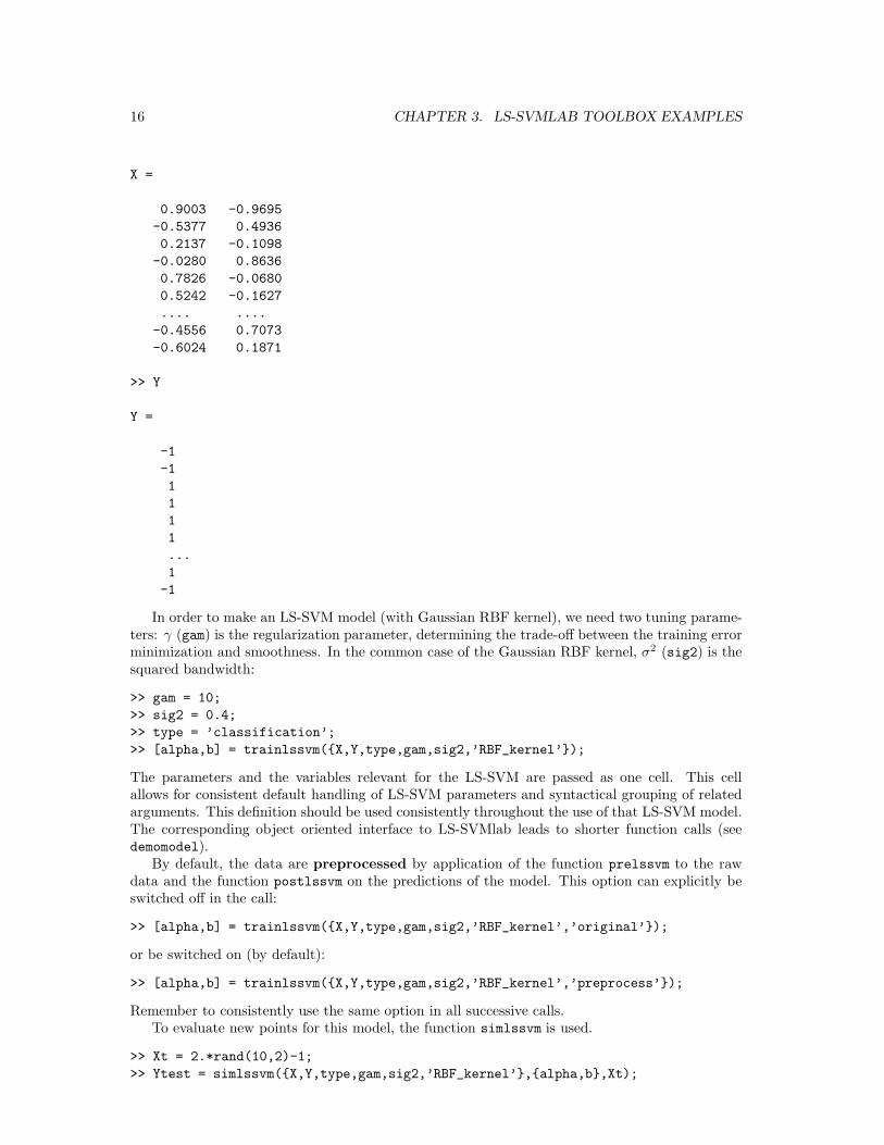
A simple example shows how to start using the toolbox for a classification task. We start withconstructing a simple example dataset according to the correct formatting. Data are representedas matrices where each row of the matrix contains one datapoint:
>> X = 2.*rand(100,2)-1;
>> Y = sign(sin(X(:,1))+X(:,2));
>> X
15
16 CHAPTER 3. LS-SVMLAB TOOLBOX EXAMPLES
X =
0.9003 -0.9695
-0.5377 0.4936
0.2137 -0.1098
-0.0280 0.8636
0.7826 -0.0680
0.5242 -0.1627
.... ....
-0.4556 0.7073
-0.6024 0.1871
>> Y
Y =
-1
-1
1
1
1
1
...
1
-1
In order to make an LS-SVM model (with Gaussian RBF kernel), we need two tuning parame-ters: γ (gam) is the regularization parameter, determining the trade-off between the training errorminimization and smoothness. In the common case of the Gaussian RBF kernel, σ2 (sig2) is thesquared bandwidth:
>> gam = 10;
>> sig2 = 0.4;
>> type = ’classification’;
>> [alpha,b] = trainlssvm({X,Y,type,gam,sig2,’RBF_kernel’});
The parameters and the variables relevant for the LS-SVM are passed as one cell. This cellallows for consistent default handling of LS-SVM parameters and syntactical grouping of relatedarguments. This definition should be used consistently throughout the use of that LS-SVM model.The corresponding object oriented interface to LS-SVMlab leads to shorter function calls (seedemomodel).
By default, the data are preprocessed by application of the function prelssvm to the rawdata and the function postlssvm on the predictions of the model. This option can explicitly beswitched off in the call:
>> [alpha,b] = trainlssvm({X,Y,type,gam,sig2,’RBF_kernel’,’original’});
or be switched on (by default):
>> [alpha,b] = trainlssvm({X,Y,type,gam,sig2,’RBF_kernel’,’preprocess’});
Remember to consistently use the same option in all successive calls.To evaluate new points for this model, the function simlssvm is used.
>> Xt = 2.*rand(10,2)-1;
>> Ytest = simlssvm({X,Y,type,gam,sig2,’RBF_kernel’},{alpha,b},Xt);

3.2. CLASSIFICATION 17
1
1
1
1
X1
X2
LS−SVMγ=10,σ2=0.4
RBF , with 2 different classes
−1 −0.5 0 0.5 1
−0.8
−0.6
−0.4
−0.2
0
0.2
0.4
0.6
0.8
1Classifierclass 1class 2
Figure 3.2: Figure generated by plotlssvm in the simple classification task.
The LS-SVM result can be displayed if the dimension of the input data is two.
>> plotlssvm({X,Y,type,gam,sig2,’RBF_kernel’},{alpha,b});
All plotting is done with this simple command. It looks for the best way of displaying the result(Figure 3.2).
3.2.2 Example
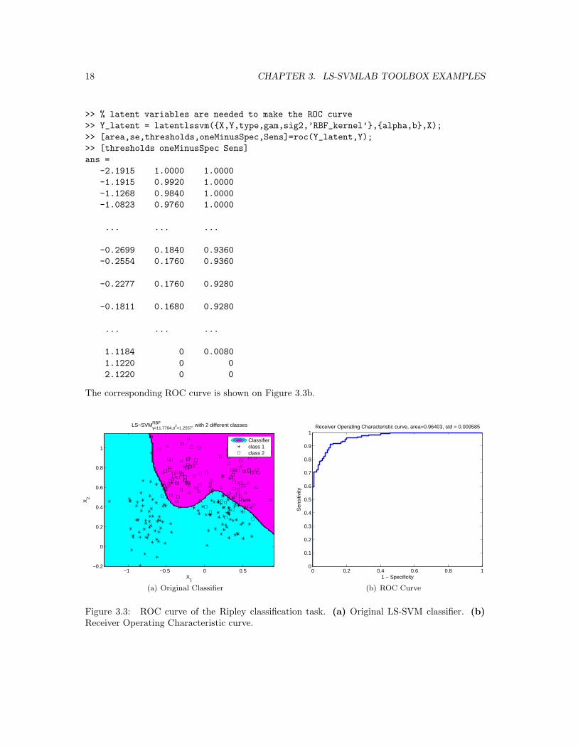
The well-known Ripley dataset problem consists of two classes where the data for each class havebeen generated by a mixture of two normal distributions (Figure 3.3a).
First, let us build an LS-SVM on the dataset and determine suitable tuning parameters. Thesetuning parameters are found by using a combination of Coupled Simulated Annealing (CSA) anda standard simplex method. First, CSA finds good starting values and these are passed to thesimplex method in order to fine tune the result.
>> % load dataset ...
>> type = ’classification’;
>> L_fold = 10; % L-fold crossvalidation
>> [gam,sig2] = tunelssvm({X,Y,type,[],[],’RBF_kernel’},’simplex’,...
’crossvalidatelssvm’,{L_fold,’misclass’});
>> [alpha,b] = trainlssvm({X,Y,type,gam,sig2,’RBF_kernel’});
>> plotlssvm({X,Y,type,gam,sig2,’RBF_kernel’},{alpha,b});
It is still possible to use a gridsearch in the second run i.e. as a replacement for the simplexmethod
>> [gam,sig2] = tunelssvm({X,Y,type,[],[],’RBF_kernel’},’gridsearch’,...
’crossvalidatelssvm’,{L_fold,’misclass’});
The Receiver Operating Characteristic (ROC) curve gives information about the quality of theclassifier:
>> [alpha,b] = trainlssvm({X,Y,type,gam,sig2,’RBF_kernel’});
18 CHAPTER 3. LS-SVMLAB TOOLBOX EXAMPLES
>> % latent variables are needed to make the ROC curve
>> Y_latent = latentlssvm({X,Y,type,gam,sig2,’RBF_kernel’},{alpha,b},X);
>> [area,se,thresholds,oneMinusSpec,Sens]=roc(Y_latent,Y);
>> [thresholds oneMinusSpec Sens]
ans =
-2.1915 1.0000 1.0000
-1.1915 0.9920 1.0000
-1.1268 0.9840 1.0000
-1.0823 0.9760 1.0000
... ... ...
-0.2699 0.1840 0.9360
-0.2554 0.1760 0.9360
-0.2277 0.1760 0.9280
-0.1811 0.1680 0.9280
... ... ...
1.1184 0 0.0080
1.1220 0 0
2.1220 0 0
The corresponding ROC curve is shown on Figure 3.3b.
11
1
1
X1
X2
LS−SVMγ=11.7704,σ2=1.2557
RBF , with 2 different classes
−1 −0.5 0 0.5−0.2
0
0.2
0.4
0.6
0.8
1
Classifierclass 1class 2
(a) Original Classifier
0 0.2 0.4 0.6 0.8 10
0.1
0.2
0.3
0.4
0.5
0.6
0.7
0.8
0.9
1Receiver Operating Characteristic curve, area=0.96403, std = 0.009585
1 − Specificity
Sen
sitiv
ity
(b) ROC Curve
Figure 3.3: ROC curve of the Ripley classification task. (a) Original LS-SVM classifier. (b)Receiver Operating Characteristic curve.
3.2. CLASSIFICATION 19
3.2.3 Using the object oriented interface: initlssvm
Another possibility to obtain the same results is by using the object oriented interface. This goesas follows:
>> % load dataset ...
>> % gateway to the object oriented interface
>> model = initlssvm(X,Y,type,[],[],’RBF_kernel’);
>> model = tunelssvm(model,’simplex’,’crossvalidatelssvm’,{L_fold,’misclass’});
>> model = trainlssvm(model);
>> plotlssvm(model);
>> % latent variables are needed to make the ROC curve
>> Y_latent = latentlssvm(model,X);
>> [area,se,thresholds,oneMinusSpec,Sens]=roc(Y_latent,Y);
3.2.4 LS-SVM classification: only one command line away!
The simplest way to obtain an LS-SVM model goes as follows (binary classification problems andone versus one encoding for multiclass)
>> % load dataset ...
>> type = ’classification’;
>> Yp = lssvm(X,Y,type);
The lssvm command automatically tunes the tuning parameters via 10-fold cross-validation (CV)or leave-one-out CV depending on the sample size. This function will automatically plot (whenpossible) the solution. By default, the Gaussian RBF kernel is taken. Further information can befound in A.3.24.
20 CHAPTER 3. LS-SVMLAB TOOLBOX EXAMPLES
3.2.5 Bayesian inference for classification
This Subsection further proceeds on the results of Subsection 3.2.2. A Bayesian framework is usedto optimize the tuning parameters and to obtain the moderated output. The optimal regularizationparameter gam and kernel parameter sig2 can be found by optimizing the cost on the second andthe third level of inference, respectively. It is recommended to initiate the model with appropriatestarting values:
>> [gam, sig2] = bay_initlssvm({X,Y,type,gam,sig2,’RBF_kernel’});
Optimization on the second level leads to an optimal regularization parameter:
>> [model, gam_opt] = bay_optimize({X,Y,type,gam,sig2,’RBF_kernel’},2);
Optimization on the third level leads to an optimal kernel parameter:
>> [cost_L3,sig2_opt] = bay_optimize({X,Y,type,gam_opt,sig2,’RBF_kernel’},3);
The posterior class probabilies are found by incorporating the uncertainty of the model parameters:
>> gam = 10;
>> sig2 = 1;
>> Ymodout = bay_modoutClass({X,Y,type,10,1,’RBF_kernel’},’figure’);
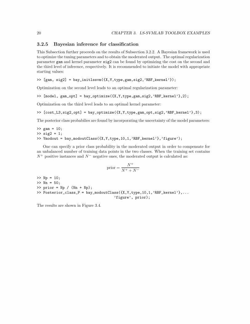
One can specify a prior class probability in the moderated output in order to compensate foran unbalanced number of training data points in the two classes. When the training set containsN+ positive instances and N− negative ones, the moderated output is calculated as:
prior =N+
N+ +N−
>> Np = 10;
>> Nn = 50;
>> prior = Np / (Nn + Np);
>> Posterior_class_P = bay_modoutClass({X,Y,type,10,1,’RBF_kernel’},...
’figure’, prior);
The results are shown in Figure 3.4.

3.2. CLASSIFICATION 21
−1.2 −1 −0.8 −0.6 −0.4 −0.2 0 0.2 0.4 0.6 0.8−0.2
0
0.2
0.4
0.6
0.8
1
Probability of occurence of class 1
X1
X2
class 1class 2
(a) Moderated Output
−1.2 −1 −0.8 −0.6 −0.4 −0.2 0 0.2 0.4 0.6 0.8−0.2
0
0.2
0.4
0.6
0.8
1
Probability of occurence of class 1
X1
X2
class 1class 2
(b) Unbalanced subset
−1.2 −1 −0.8 −0.6 −0.4 −0.2 0 0.2 0.4 0.6 0.8−0.2
0
0.2
0.4
0.6
0.8
1
Probability of occurence of class 1
X1
X2
class 1class 2
(c) With correction for unbalancing
Figure 3.4: (a) Moderated output of the LS-SVM classifier on the Ripley data set. The colorsindicate the probability to belong to a certain class; (b) This example shows the moderated outputof an unbalanced subset of the Ripley data; (c) One can compensate for unbalanced data in thecalculation of the moderated output. Notice that the area of the blue zone with the positivesamples increases by the compensation. The red zone shrinks accordingly.
22 CHAPTER 3. LS-SVMLAB TOOLBOX EXAMPLES
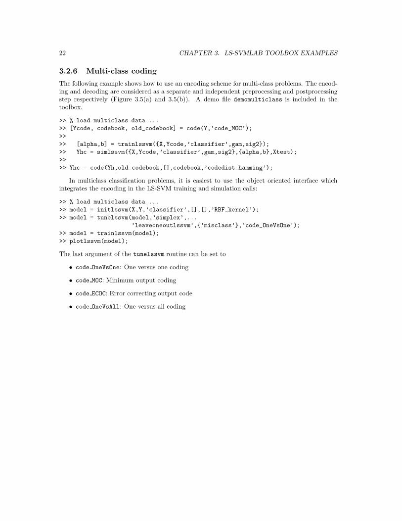
3.2.6 Multi-class coding
The following example shows how to use an encoding scheme for multi-class problems. The encod-ing and decoding are considered as a separate and independent preprocessing and postprocessingstep respectively (Figure 3.5(a) and 3.5(b)). A demo file demomulticlass is included in thetoolbox.
>> % load multiclass data ...
>> [Ycode, codebook, old_codebook] = code(Y,’code_MOC’);
>>
>> [alpha,b] = trainlssvm({X,Ycode,’classifier’,gam,sig2});
>> Yhc = simlssvm({X,Ycode,’classifier’,gam,sig2},{alpha,b},Xtest);
>>
>> Yhc = code(Yh,old_codebook,[],codebook,’codedist_hamming’);
In multiclass classification problems, it is easiest to use the object oriented interface whichintegrates the encoding in the LS-SVM training and simulation calls:
>> % load multiclass data ...
>> model = initlssvm(X,Y,’classifier’,[],[],’RBF_kernel’);
>> model = tunelssvm(model,’simplex’,...
’leaveoneoutlssvm’,{’misclass’},’code_OneVsOne’);
>> model = trainlssvm(model);
>> plotlssvm(model);
The last argument of the tunelssvm routine can be set to
• code OneVsOne: One versus one coding
• code MOC: Minimum output coding
• code ECOC: Error correcting output code
• code OneVsAll: One versus all coding
3.3. REGRESSION 23
12
222
2
3
3
3
3
3
1
X1
X2
−2 0 2 4 6
0
1
2
3
4
5
6
7
8 classifierclass 1class 2class 3
(a)
1
11
2
2
2
2
3
33
1
1
1 12 2
111
1111
12
1
12
11
12
1
X1
X2
−2 0 2 4 6
0
1
2
3
4
5
6
7
8Classifierclass 1class 2class 3
(b)
2
2
2
22
2
33
32
2
X1
X2
−2 0 2 4 6
0
1
2
3
4
5
6
7
8Classifierclass 1class 2class 3
(c)
1
1
1
1
1
2
2
2
2
2
2
3
3
3 3
1
1
1 11
1
121212
X1
X2
−2 0 2 4 6
0
1
2
3
4
5
6
7
8Classifierclass 1class 2class 3
(d)
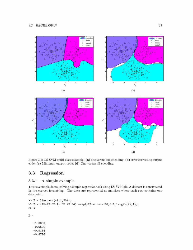
Figure 3.5: LS-SVM multi-class example: (a) one versus one encoding; (b) error correcting outputcode; (c) Minimum output code; (d) One versus all encoding.
3.3 Regression
3.3.1 A simple example
This is a simple demo, solving a simple regression task using LS-SVMlab. A dataset is constructedin the correct formatting. The data are represented as matrices where each row contains onedatapoint:
>> X = linspace(-1,1,50)’;
>> Y = (15*(X.^2-1).^2.*X.^4).*exp(-X)+normrnd(0,0.1,length(X),1);
>> X
X =
-1.0000
-0.9592
-0.9184
-0.8776
24 CHAPTER 3. LS-SVMLAB TOOLBOX EXAMPLES
-0.8367
-0.7959
...
0.9592
1.0000
>> Y =
Y =
0.0138
0.2953
0.6847
1.1572
1.5844
1.9935
...
-0.0613
-0.0298
In order to obtain an LS-SVM model (with the RBF kernel), we need two extra tuning pa-rameters: γ (gam) is the regularization parameter, determining the trade-off between the trainingerror minimization and smoothness of the estimated function. σ2 (sig2) is the kernel functionparameter. In this case we use leave-one-out CV to determine the tuning parameters.
>> type = ’function estimation’;
>> [gam,sig2] = tunelssvm({X,Y,type,[],[],’RBF_kernel’},’simplex’,...
’leaveoneoutlssvm’,{’mse’});
>> [alpha,b] = trainlssvm({X,Y,type,gam,sig2,’RBF_kernel’});
>> plotlssvm({X,Y,type,gam,sig2,’RBF_kernel’},{alpha,b});
The parameters and the variables relevant for the LS-SVM are passed as one cell. This cellallows for consistent default handling of LS-SVM parameters and syntactical grouping of relatedarguments. This definition should be used consistently throughout the use of that LS-SVM model.The object oriented interface to LS-SVMlab leads to shorter function calls (see demomodel).
By default, the data are preprocessed by application of the function prelssvm to the rawdata and the function postlssvm on the predictions of the model. This option can be explicitlyswitched off in the call:
>> [alpha,b] = trainlssvm({X,Y,type,gam,sig2,’RBF_kernel’,’original’});
or can be switched on (by default):
>> [alpha,b] = trainlssvm({X,Y,type,gam,sig2,’RBF_kernel’,’preprocess’});
Remember to consistently use the same option in all successive calls.To evaluate new points for this model, the function simlssvm is used. At first, test data is
generated:
>> Xt = rand(10,1).*sign(randn(10,1));
Then, the obtained model is simulated on the test data:
3.3. REGRESSION 25
>> Yt = simlssvm({X,Y,type,gam,sig2,’RBF_kernel’,’preprocess’},{alpha,b},Xt);
ans =
0.0847
0.0378
1.9862
0.4688
0.3773
1.9832
0.2658
0.2515
1.5571
0.3130
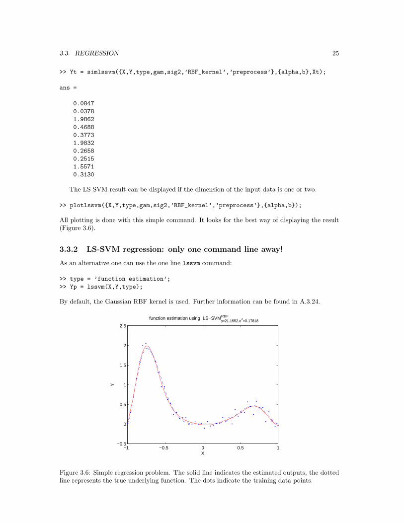
The LS-SVM result can be displayed if the dimension of the input data is one or two.
>> plotlssvm({X,Y,type,gam,sig2,’RBF_kernel’,’preprocess’},{alpha,b});
All plotting is done with this simple command. It looks for the best way of displaying the result(Figure 3.6).
3.3.2 LS-SVM regression: only one command line away!
As an alternative one can use the one line lssvm command:
>> type = ’function estimation’;
>> Yp = lssvm(X,Y,type);
By default, the Gaussian RBF kernel is used. Further information can be found in A.3.24.
−1 −0.5 0 0.5 1−0.5
0
0.5
1
1.5
2
2.5
X
Y
function estimation using LS−SVMγ=21.1552,σ2=0.17818
RBF
Figure 3.6: Simple regression problem. The solid line indicates the estimated outputs, the dottedline represents the true underlying function. The dots indicate the training data points.
26 CHAPTER 3. LS-SVMLAB TOOLBOX EXAMPLES
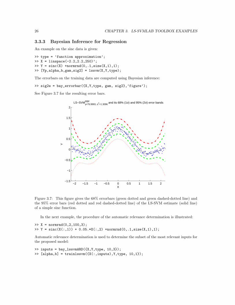
3.3.3 Bayesian Inference for Regression
An example on the sinc data is given:
>> type = ’function approximation’;
>> X = linspace(-2.2,2.2,250)’;
>> Y = sinc(X) +normrnd(0,.1,size(X,1),1);
>> [Yp,alpha,b,gam,sig2] = lssvm(X,Y,type);
The errorbars on the training data are computed using Bayesian inference:
>> sig2e = bay_errorbar({X,Y,type, gam, sig2},’figure’);
See Figure 3.7 for the resulting error bars.
−2 −1.5 −1 −0.5 0 0.5 1 1.5 2−1.5
−1
−0.5
0
0.5
1
1.5
2
LS−SVMγ=79.9993, σ2=1.3096
RBF and its 68% (1σ) and 95% (2σ) error bands
X
Y
Figure 3.7: This figure gives the 68% errorbars (green dotted and green dashed-dotted line) andthe 95% error bars (red dotted and red dashed-dotted line) of the LS-SVM estimate (solid line)of a simple sinc function.
In the next example, the procedure of the automatic relevance determination is illustrated:
>> X = normrnd(0,2,100,3);
>> Y = sinc(X(:,1)) + 0.05.*X(:,2) +normrnd(0,.1,size(X,1),1);
Automatic relevance determination is used to determine the subset of the most relevant inputs forthe proposed model:
>> inputs = bay_lssvmARD({X,Y,type, 10,3});
>> [alpha,b] = trainlssvm({X(:,inputs),Y,type, 10,1});

3.3. REGRESSION 27
3.3.4 Using the object oriented model interface
This case illustrates how one can use the model interface. Here, regression is considered, but theextension towards classification is analogous.
>> type = ’function approximation’;
>> X = normrnd(0,2,100,1);
>> Y = sinc(X) +normrnd(0,.1,size(X,1),1);
>> kernel = ’RBF_kernel’;
>> gam = 10;
>> sig2 = 0.2;
A model is defined
>> model = initlssvm(X,Y,type,gam,sig2,kernel);
>> model
model =
type: ’f’
x_dim: 1
y_dim: 1
nb_data: 100
kernel_type: ’RBF_kernel’
preprocess: ’preprocess’
prestatus: ’ok’
xtrain: [100x1 double]
ytrain: [100x1 double]
selector: [1x100 double]
gam: 10
kernel_pars: 0.2000
x_delays: 0
y_delays: 0
steps: 1
latent: ’no’
code: ’original’
codetype: ’none’
pre_xscheme: ’c’
pre_yscheme: ’c’
pre_xmean: -0.0690
pre_xstd: 1.8282
pre_ymean: 0.2259
pre_ystd: 0.3977
status: ’changed’
weights: []
Training, simulation and making a plot is executed by the following calls:
>> model = trainlssvm(model);
>> Xt = normrnd(0,2,150,1);
>> Yt = simlssvm(model,Xt);
>> plotlssvm(model);
The second level of inference of the Bayesian framework can be used to optimize the regular-ization parameter gam. For this case, a Nystrom approximation of the 20 principal eigenvectors isused:
28 CHAPTER 3. LS-SVMLAB TOOLBOX EXAMPLES
>> model = bay_optimize(model,2,’eign’, 50);
Optimization of the cost associated with the third level of inference gives an optimal kernelparameter. For this procedure, it is recommended to initiate the starting points of the kernelparameter. This optimization is based on Matlab’s optimization toolbox. It can take a while.
>> model = bay_initlssvm(model);
>> model = bay_optimize(model,3,’eign’,50);
3.3.5 Confidence/Predition Intervals for Regression
Consider the following example: Fossil data set
>> % Load data set X and Y
Initializing and tuning the parameters
>> model = initlssvm(X,Y,’f’,[],[], ’RBF_kernel’);
>> model = tunelssvm(model,’simplex’,’crossvalidatelssvm’,{10,’mse’});
Bias corrected approximate 100(1−α)% pointwise confidence intervals on the estimated LS-SVMmodel can then be obtained by using the command cilssvm:
>> ci = cilssvm(model,alpha,’pointwise’);
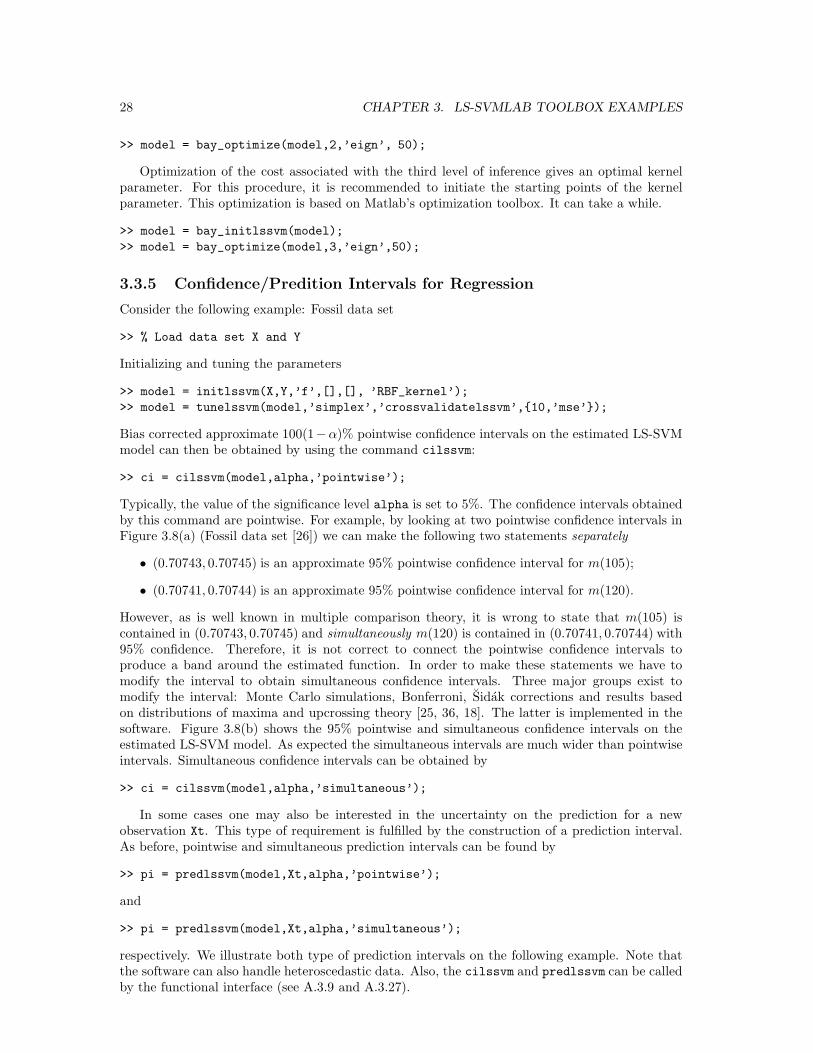
Typically, the value of the significance level alpha is set to 5%. The confidence intervals obtainedby this command are pointwise. For example, by looking at two pointwise confidence intervals inFigure 3.8(a) (Fossil data set [26]) we can make the following two statements separately
• (0.70743, 0.70745) is an approximate 95% pointwise confidence interval for m(105);
• (0.70741, 0.70744) is an approximate 95% pointwise confidence interval for m(120).
However, as is well known in multiple comparison theory, it is wrong to state that m(105) iscontained in (0.70743, 0.70745) and simultaneously m(120) is contained in (0.70741, 0.70744) with95% confidence. Therefore, it is not correct to connect the pointwise confidence intervals toproduce a band around the estimated function. In order to make these statements we have tomodify the interval to obtain simultaneous confidence intervals. Three major groups exist tomodify the interval: Monte Carlo simulations, Bonferroni, Sidak corrections and results basedon distributions of maxima and upcrossing theory [25, 36, 18]. The latter is implemented in thesoftware. Figure 3.8(b) shows the 95% pointwise and simultaneous confidence intervals on theestimated LS-SVM model. As expected the simultaneous intervals are much wider than pointwiseintervals. Simultaneous confidence intervals can be obtained by
>> ci = cilssvm(model,alpha,’simultaneous’);
In some cases one may also be interested in the uncertainty on the prediction for a newobservation Xt. This type of requirement is fulfilled by the construction of a prediction interval.As before, pointwise and simultaneous prediction intervals can be found by
>> pi = predlssvm(model,Xt,alpha,’pointwise’);
and
>> pi = predlssvm(model,Xt,alpha,’simultaneous’);
respectively. We illustrate both type of prediction intervals on the following example. Note thatthe software can also handle heteroscedastic data. Also, the cilssvm and predlssvm can be calledby the functional interface (see A.3.9 and A.3.27).
3.3. REGRESSION 29
90 95 100 105 110 115 120 1250.7071
0.7072
0.7072
0.7073
0.7073
0.7074
0.7074
0.7075
X
m(X
)
(a)
90 95 100 105 110 115 120 1250.7072
0.7072
0.7073
0.7073
0.7074
0.7074
0.7075
X
m(X
)
(b)
Figure 3.8: (a) Fossil data with two pointwise 95% confidence intervals.; (b) Simultaneous andpointwise 95% confidence intervals. The outer (inner) region corresponds to simultaneous (point-wise) confidence intervals. The full line (in the middle) is the estimated LS-SVM model. Forillustration purposes the 95% pointwise confidence intervals are connected.
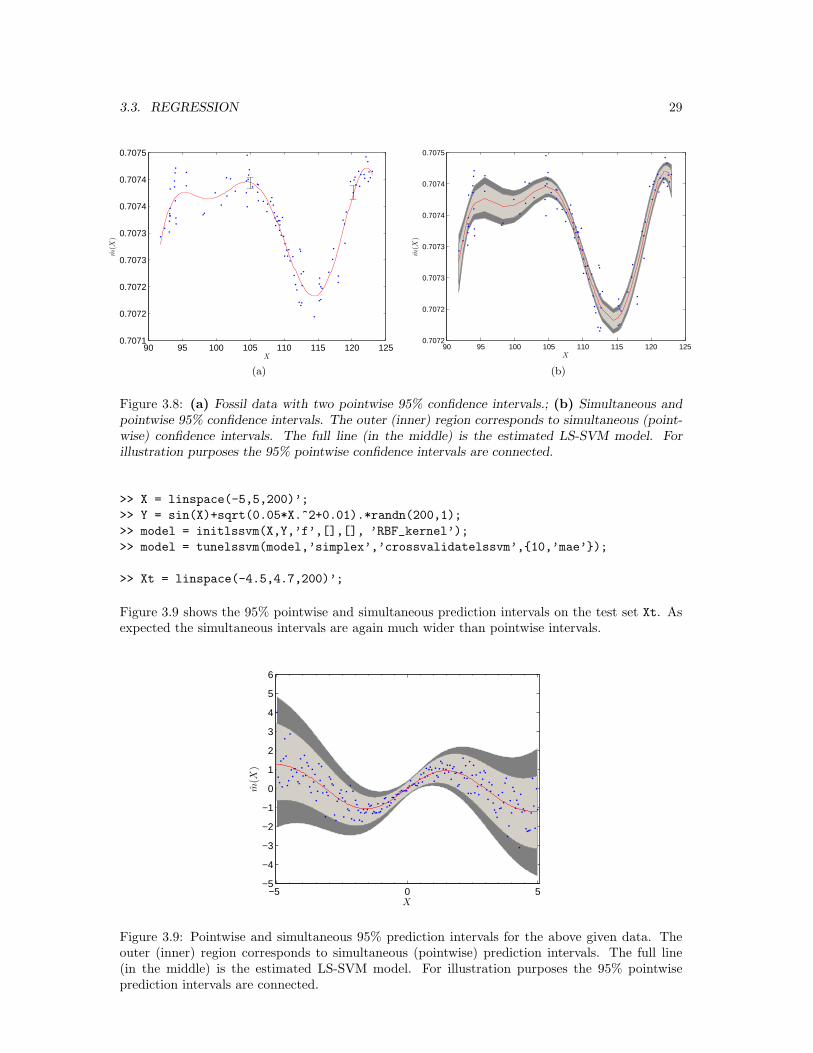
>> X = linspace(-5,5,200)’;
>> Y = sin(X)+sqrt(0.05*X.^2+0.01).*randn(200,1);
>> model = initlssvm(X,Y,’f’,[],[], ’RBF_kernel’);
>> model = tunelssvm(model,’simplex’,’crossvalidatelssvm’,{10,’mae’});
>> Xt = linspace(-4.5,4.7,200)’;
Figure 3.9 shows the 95% pointwise and simultaneous prediction intervals on the test set Xt. Asexpected the simultaneous intervals are again much wider than pointwise intervals.
−5 0 5−5
−4
−3
−2
−1
0
1
2
3
4
5
6
X
m(X
)
Figure 3.9: Pointwise and simultaneous 95% prediction intervals for the above given data. Theouter (inner) region corresponds to simultaneous (pointwise) prediction intervals. The full line(in the middle) is the estimated LS-SVM model. For illustration purposes the 95% pointwiseprediction intervals are connected.

30 CHAPTER 3. LS-SVMLAB TOOLBOX EXAMPLES
As a final example, consider the Boston Housing data set (multivariate example). We selectedrandomly 338 training data points and 168 test data points. The corresponding simultaneousconfidence and prediction intervals are shown in Figure 3.10(a) and Figure 3.10(b) respectively.The outputs on training as well as on test data are sorted and plotted against their correspond-ing index. Also, the respective intervals are sorted accordingly. For illustration purposes thesimultaneous confidence/prediction intervals are not connected.
>> % load full data set X and Y
>> sel = randperm(506);
>>
>> % Construct test data
>> Xt = X(sel(1:168),:);
>> Yt = Y(sel(1:168));
>>
>> % training data
>> X = X(sel(169:end),:);
>> Y = Y(sel(169:end));
>>
>> model = initlssvm(X,Y,’f’,[],[],’RBF_kernel’);
>> model = tunelssvm(model,’simplex’,’crossvalidatelssvm’,{10,’mse’});
>> model = trainlssvm(model);
>> Yhci = simlssvm(model,X);
>> Yhpi = simlssvm(model,Xt);
>> [Yhci,indci] = sort(Yhci,’descend’);
>> [Yhpi,indpi] = sort(Yhpi,’descend’);
>>
>> % Simultaneous confidence intervals
>> ci = cilssvm(model,0.05,’simultaneous’); ci = ci(indci,:);
>> plot(Yhci); hold all, plot(ci(:,1),’g.’); plot(ci(:,2),’g.’);
>>
>> % Simultaneous prediction intervals
>> pi = predlssvm(model,Xt,0.05,’simultaneous’); pi = pi(indpi,:);
>> plot(Yhpi); hold all, plot(pi(:,1),’g.’); plot(pi(:,2),’g.’);
0 50 100 150 200 250 300 350−3
−2
−1
0
1
2
3
4
Index
sorted
m(X
)(T
rainingdata)
(a)
0 20 40 60 80 100 120 140 160 180−4
−3
−2
−1
0
1
2
3
4
5
Index
sorted
m(Xt)
(Testdata)
(b)
Figure 3.10: (a) Simultaneous 95% confidence intervals for the Boston Housing data set (dots).Sorted outputs are plotted against their index; (b) Simultaneous 95% prediction intervals for theBoston Housing data set (dots). Sorted outputs are plotted against their index.

3.3. REGRESSION 31
3.3.6 Robust regression
First, a dataset containing 15% outliers is constructed:
>> X = (-5:.07:5)’;
>> epsilon = 0.15;
>> sel = rand(length(X),1)>epsilon;
>> Y = sinc(X)+sel.*normrnd(0,.1,length(X),1)+(1-sel).*normrnd(0,2,length(X),1);
Robust tuning of the tuning parameters is performed by rcrossvalildatelssvm. Also noticethat the preferred loss function is the L1 (mae). The weighting function in the cost function ischosen to be the Huber weights. Other possibilities, included in the toolbox, are logistic weights,myriad weights and Hampel weights.
>> model = initlssvm(X,Y,’f’,[],[],’RBF_kernel’);
>> L_fold = 10; %10 fold CV
>> model = tunelssvm(model,’simplex’,...
’rcrossvalidatelssvm’,{L_fold,’mae’},’whuber’);
Robust training is performed by robustlssvm:
>> model = robustlssvm(model);
>> plotlssvm(model);
−5 0 5−4
−3
−2
−1
0
1
2
3
4
X
Y
function estimation using LS−SVMγ=0.14185,σ2=0.047615
RBF
LS−SVMdataReal function
(a)
−5 0 5−4
−3
−2
−1
0
1
2
3
4
X
Y
function estimation using LS−SVMγ=95025.4538,σ2=0.66686
RBF
LS−SVMdataReal function
(b)
Figure 3.11: Experiments on a noisy sinc dataset with 15% outliers: (a) Application of thestandard training and hyperparameter selection techniques; (b) Application of an iterativelyreweighted LS-SVM training together with a robust crossvalidation score function, which enhancesthe test set performance.

32 CHAPTER 3. LS-SVMLAB TOOLBOX EXAMPLES
In a second, more extreme, example, we have taken the contamination distribution to be acubic standard Cauchy distribution and ǫ = 0.3.
>> X = (-5:.07:5)’;
>> epsilon = 0.3;
>> sel = rand(length(X),1)>epsilon;
>> Y = sinc(X)+sel.*normrnd(0,.1,length(X),1)+(1-sel).*trnd(1,length(X),1).^3;
As before, we use the robust version of cross-validation. The weight function in the cost function is
chosen to be the myriad weights. All weight functions W : R → [0, 1], with W (r) = ψ(r)r
satisfyingW (0) = 1, are shown in Table 3.1 with corresponding loss function L(r) and score function
ψ(r) = dL(r)dr
. This type of weighting function is especially designed to handle extreme outliers.The results are shown in Figure 3.12. Three of the four weight functions contain parameters whichhave to be tuned (see Table 3.1). The software automatically tunes the parameters of the huberand myriad weight function according to the best performance for these two weight functions. Thetwo parameters of the Hampel weight function are set to b1 = 2.5 and b2 = 3.
>> model = initlssvm(X,Y,’f’,[],[],’RBF_kernel’);
>> L_fold = 10; %10 fold CV
>> model = tunelssvm(model,’simplex’,...
’rcrossvalidatelssvm’,{L_fold,’mae’},’wmyriad’);
>> model = robustlssvm(model);
>> plotlssvm(model);
−5 0 5
−40
−20
0
20
40
60
80
X
Y
function estimation using LS−SVMγ=0.018012,σ2=0.93345
RBF
LS−SVMdataReal function
(a)
−5 0 5−4
−3
−2
−1
0
1
2
3
4
X
Y
function estimation using LS−SVMγ=35.1583,σ2=0.090211
RBF
LS−SVMdataReal function
(b)
Figure 3.12: Experiments on a noisy sinc dataset with extreme outliers. (a) Application of thestandard training and tuning parameter selection techniques; (b) Application of an iterativelyreweighted LS-SVM training (myriad weights) together with a robust cross-validation score func-tion, which enhances the test set performance;
3.3. REGRESSION 33
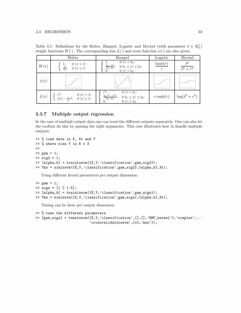
Table 3.1: Definitions for the Huber, Hampel, Logistic and Myriad (with parameter δ ∈ R+0 )
weight functions W (·). The corresponding loss L(·) and score function ψ(·) are also given.
Huber Hampel Logistic Myriad
W (r)
{
1, if |r| < β;β
|r|, if |r| ≥ β.
1, if |r| < b1;b2−|r|b2−b1
, if b1 ≤ |r| ≤ b2;
0, if |r| > b2.
tanh(r)
r
δ2
δ2 + r2
ψ(r)
L(r){
r2, if |r| < β;β|r| − 1
2c2, if |r| ≥ β.
r2, if |r| < b1;b2r
2−|r3|b2−b1
, if b1 ≤ |r| ≤ b2;
0, if |r| > b2.
r tanh(r) log(δ2 + r2)
3.3.7 Multiple output regression
In the case of multiple output data one can treat the different outputs separately. One can also letthe toolbox do this by passing the right arguments. This case illustrates how to handle multipleoutputs:
>> % load data in X, Xt and Y
>> % where size Y is N x 3
>>
>> gam = 1;
>> sig2 = 1;
>> [alpha,b] = trainlssvm({X,Y,’classification’,gam,sig2});
>> Yhs = simlssvm({X,Y,’classification’,gam,sig2},{alpha,b},Xt);
Using different kernel parameters per output dimension:
>> gam = 1;
>> sigs = [1 2 1.5];
>> [alpha,b] = trainlssvm({X,Y,’classification’,gam,sigs});
>> Yhs = simlssvm({X,Y,’classification’,gam,sigs},{alpha,b},Xt);
Tuning can be done per output dimension:
>> % tune the different parameters
>> [gam,sigs] = tunelssvm({X,Y,’classification’,[],[],’RBF_kernel’},’simplex’,...
’crossvalidatelssvm’,{10,’mse’});
34 CHAPTER 3. LS-SVMLAB TOOLBOX EXAMPLES
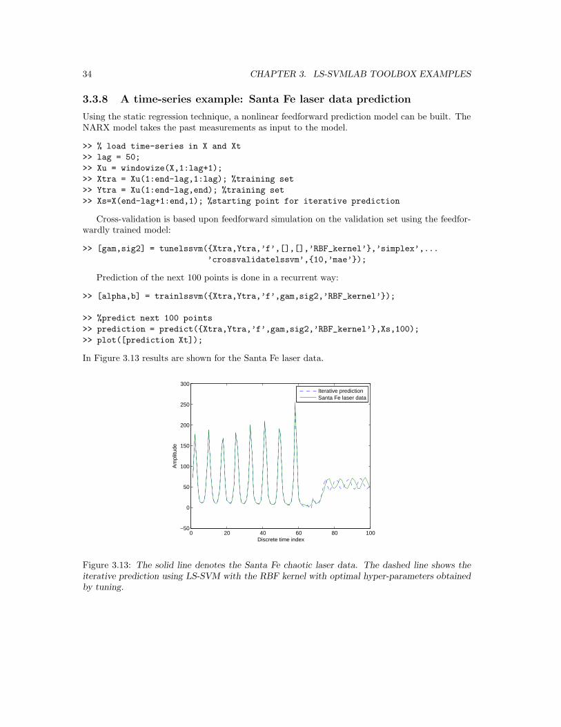
3.3.8 A time-series example: Santa Fe laser data prediction
Using the static regression technique, a nonlinear feedforward prediction model can be built. TheNARX model takes the past measurements as input to the model.
>> % load time-series in X and Xt
>> lag = 50;
>> Xu = windowize(X,1:lag+1);
>> Xtra = Xu(1:end-lag,1:lag); %training set
>> Ytra = Xu(1:end-lag,end); %training set
>> Xs=X(end-lag+1:end,1); %starting point for iterative prediction
Cross-validation is based upon feedforward simulation on the validation set using the feedfor-wardly trained model:
>> [gam,sig2] = tunelssvm({Xtra,Ytra,’f’,[],[],’RBF_kernel’},’simplex’,...
’crossvalidatelssvm’,{10,’mae’});
Prediction of the next 100 points is done in a recurrent way:
>> [alpha,b] = trainlssvm({Xtra,Ytra,’f’,gam,sig2,’RBF_kernel’});
>> %predict next 100 points
>> prediction = predict({Xtra,Ytra,’f’,gam,sig2,’RBF_kernel’},Xs,100);
>> plot([prediction Xt]);
In Figure 3.13 results are shown for the Santa Fe laser data.
0 20 40 60 80 100−50
0
50
100
150
200
250
300
Discrete time index
Am
plitu
de
Iterative predictionSanta Fe laser data
Figure 3.13: The solid line denotes the Santa Fe chaotic laser data. The dashed line shows theiterative prediction using LS-SVM with the RBF kernel with optimal hyper-parameters obtainedby tuning.
3.3. REGRESSION 35
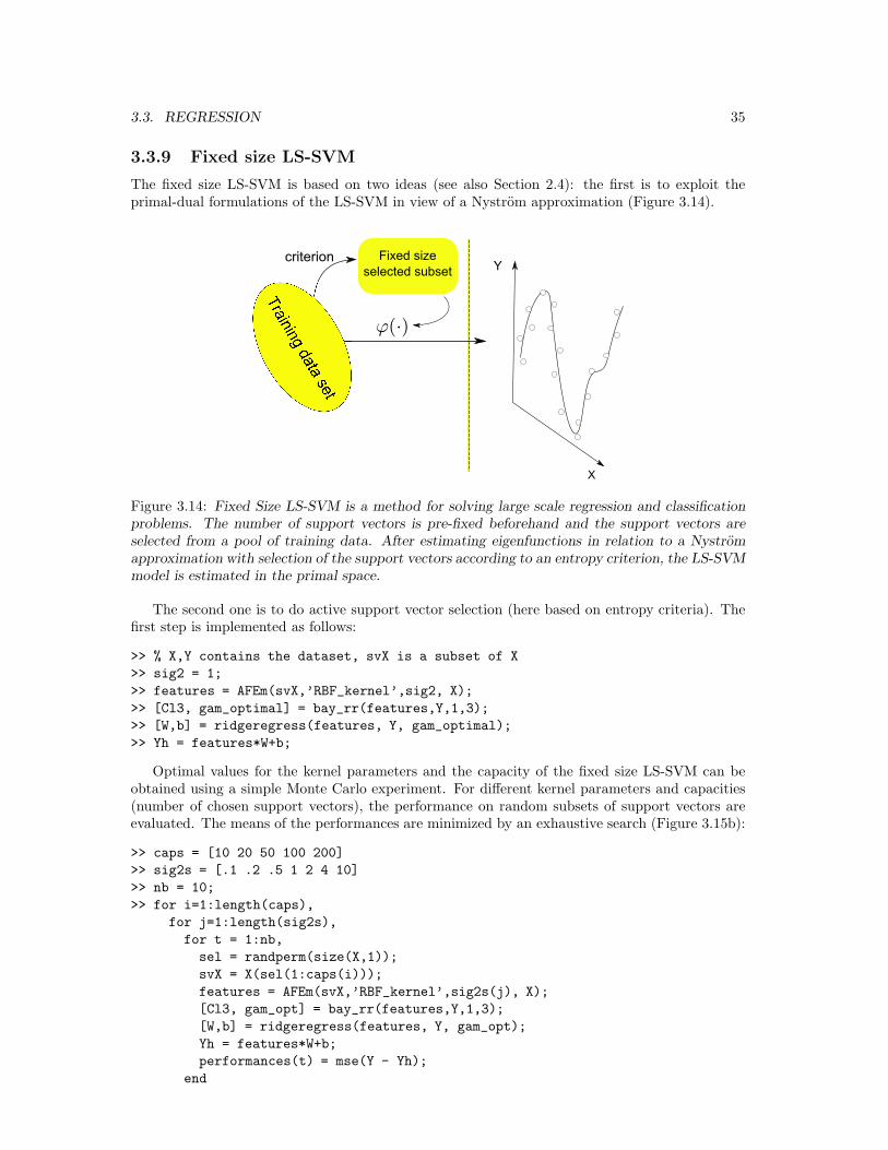
3.3.9 Fixed size LS-SVM
The fixed size LS-SVM is based on two ideas (see also Section 2.4): the first is to exploit theprimal-dual formulations of the LS-SVM in view of a Nystrom approximation (Figure 3.14).
Figure 3.14: Fixed Size LS-SVM is a method for solving large scale regression and classificationproblems. The number of support vectors is pre-fixed beforehand and the support vectors areselected from a pool of training data. After estimating eigenfunctions in relation to a Nystromapproximation with selection of the support vectors according to an entropy criterion, the LS-SVMmodel is estimated in the primal space.
The second one is to do active support vector selection (here based on entropy criteria). Thefirst step is implemented as follows:
>> % X,Y contains the dataset, svX is a subset of X
>> sig2 = 1;
>> features = AFEm(svX,’RBF_kernel’,sig2, X);
>> [Cl3, gam_optimal] = bay_rr(features,Y,1,3);
>> [W,b] = ridgeregress(features, Y, gam_optimal);
>> Yh = features*W+b;
Optimal values for the kernel parameters and the capacity of the fixed size LS-SVM can beobtained using a simple Monte Carlo experiment. For different kernel parameters and capacities(number of chosen support vectors), the performance on random subsets of support vectors areevaluated. The means of the performances are minimized by an exhaustive search (Figure 3.15b):
>> caps = [10 20 50 100 200]
>> sig2s = [.1 .2 .5 1 2 4 10]
>> nb = 10;
>> for i=1:length(caps),
for j=1:length(sig2s),
for t = 1:nb,
sel = randperm(size(X,1));
svX = X(sel(1:caps(i)));
features = AFEm(svX,’RBF_kernel’,sig2s(j), X);
[Cl3, gam_opt] = bay_rr(features,Y,1,3);
[W,b] = ridgeregress(features, Y, gam_opt);
Yh = features*W+b;
performances(t) = mse(Y - Yh);
end

36 CHAPTER 3. LS-SVMLAB TOOLBOX EXAMPLES
minimal_performances(i,j) = mean(performances);
end
end
The kernel parameter and capacity corresponding to a good performance are searched:
>> [minp,ic] = min(minimal_performances,[],1);
>> [minminp,is] = min(minp);
>> capacity = caps(ic);
>> sig2 = sig2s(is);
The following approach optimizes the selection of support vectors according to the quadraticRenyi entropy:
>> % load data X and Y, ’capacity’ and the kernel parameter ’sig2’
>> sv = 1:capacity;
>> max_c = -inf;
>> for i=1:size(X,1),
replace = ceil(rand.*capacity);
subset = [sv([1:replace-1 replace+1:end]) i];
crit = kentropy(X(subset,:),’RBF_kernel’,sig2);
if max_c <= crit, max_c = crit; sv = subset; end
end
This selected subset of support vectors is used to construct the final model (Figure 3.15a):
>> features = AFEm(svX,’RBF_kernel’,sig2, X);
>> [Cl3, gam_optimal] = bay_rr(features,Y,1,3);
>> [W,b, Yh] = ridgeregress(features, Y, gam_opt);
−5 0 5−0.6
−0.4
−0.2
0
0.2
0.4
0.6
0.8
1
1.2
1.4
X
Y
Fixed−Size LS−SVM on 20.000 noisy sinc data points
training datasupport vectorsreal functionestimated function
(a)
0
20
40
60
80
100 0200
400600
8001000
1200
0.04
0.06
0.08
0.1
σ2
Estimated cost surface of fixed−size LS−SVM on repeated i.i.d. subsampling
capacity subset
(b)
Figure 3.15: Illustration of fixed size LS-SVM on a noisy sinc function with 20.000 data points: (a)fixed size LS-SVM selects a subset of the data after Nystrom approximation. The regularizationparameter for the regression in the primal space is optimized here using the Bayesian framework;(b) Estimated cost surface of the fixed size LS-SVM based on random subsamples of the data, ofdifferent subset capacities and kernel parameters.
3.3. REGRESSION 37
The same idea can be used for learning a classifier from a huge data set.
>> % load the input and output of the trasining data in X and Y
>> cap = 25;
The first step is the same: the selection of the support vectors by optimizing the entropy cri-terion. Here, the pseudo code is showed. For the working code, one can study the code ofdemo_fixedclass.m.
% initialise a subset of cap points: Xs
>> for i = 1:1000,
Xs_old = Xs;
% substitute a point of Xs by a new one
crit = kentropy(Xs, kernel, kernel_par);
% if crit is not larger then in the previous loop,
% substitute Xs by the old Xs_old
end
By taking the values -1 and +1 as targets in a linear regression, the Fisher discriminant is obtained:
>> features = AFEm(Xs,kernel, sigma2,X);
>> [w,b] = ridgeregress(features,Y,gamma);
New data points can be simulated as follows:
>> features_t = AFEm(Xs,kernel, sigma2,Xt);
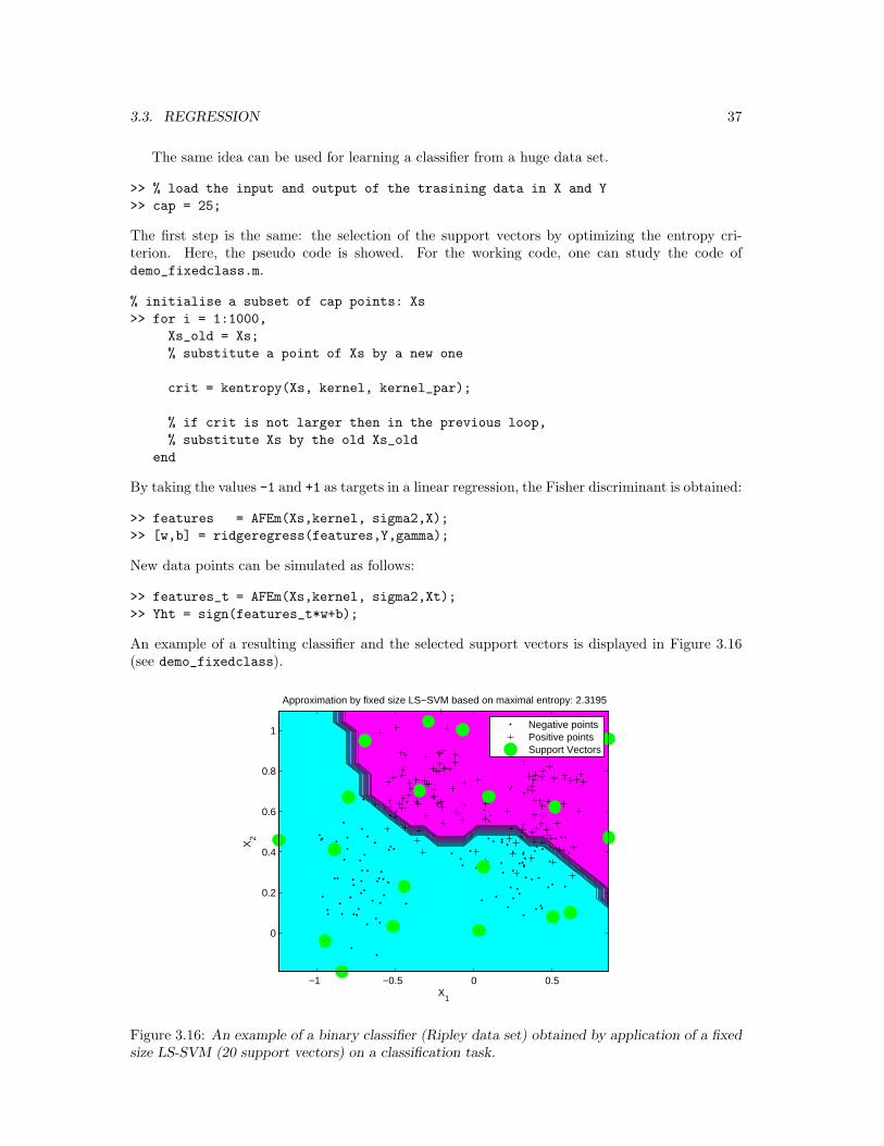
>> Yht = sign(features_t*w+b);
An example of a resulting classifier and the selected support vectors is displayed in Figure 3.16(see demo_fixedclass).
X1
X2
Approximation by fixed size LS−SVM based on maximal entropy: 2.3195
−1 −0.5 0 0.5
0
0.2
0.4
0.6
0.8
1Negative pointsPositive pointsSupport Vectors
Figure 3.16: An example of a binary classifier (Ripley data set) obtained by application of a fixedsize LS-SVM (20 support vectors) on a classification task.
38 CHAPTER 3. LS-SVMLAB TOOLBOX EXAMPLES
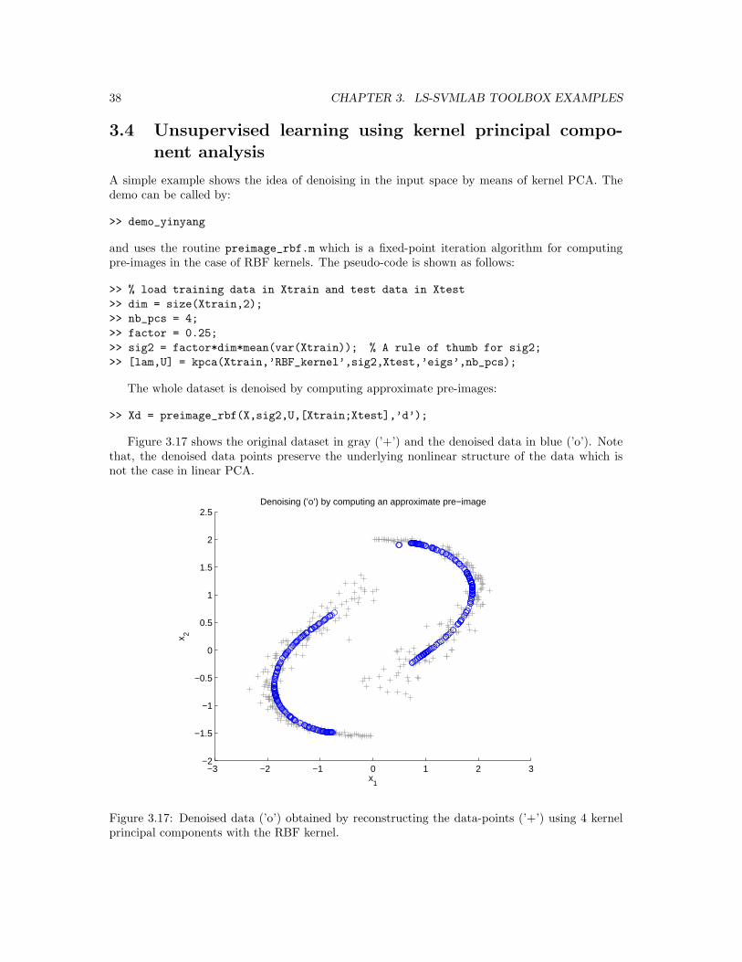
3.4 Unsupervised learning using kernel principal compo-nent analysis
A simple example shows the idea of denoising in the input space by means of kernel PCA. Thedemo can be called by:
>> demo_yinyang
and uses the routine preimage_rbf.m which is a fixed-point iteration algorithm for computingpre-images in the case of RBF kernels. The pseudo-code is shown as follows:
>> % load training data in Xtrain and test data in Xtest
>> dim = size(Xtrain,2);
>> nb_pcs = 4;
>> factor = 0.25;
>> sig2 = factor*dim*mean(var(Xtrain)); % A rule of thumb for sig2;
>> [lam,U] = kpca(Xtrain,’RBF_kernel’,sig2,Xtest,’eigs’,nb_pcs);
The whole dataset is denoised by computing approximate pre-images:
>> Xd = preimage_rbf(X,sig2,U,[Xtrain;Xtest],’d’);
Figure 3.17 shows the original dataset in gray (’+’) and the denoised data in blue (’o’). Notethat, the denoised data points preserve the underlying nonlinear structure of the data which isnot the case in linear PCA.
−3 −2 −1 0 1 2 3−2
−1.5
−1
−0.5
0
0.5
1
1.5
2
2.5
x1
x 2
Denoising (’o’) by computing an approximate pre−image
Figure 3.17: Denoised data (’o’) obtained by reconstructing the data-points (’+’) using 4 kernelprincipal components with the RBF kernel.
Appendix A
MATLAB functions
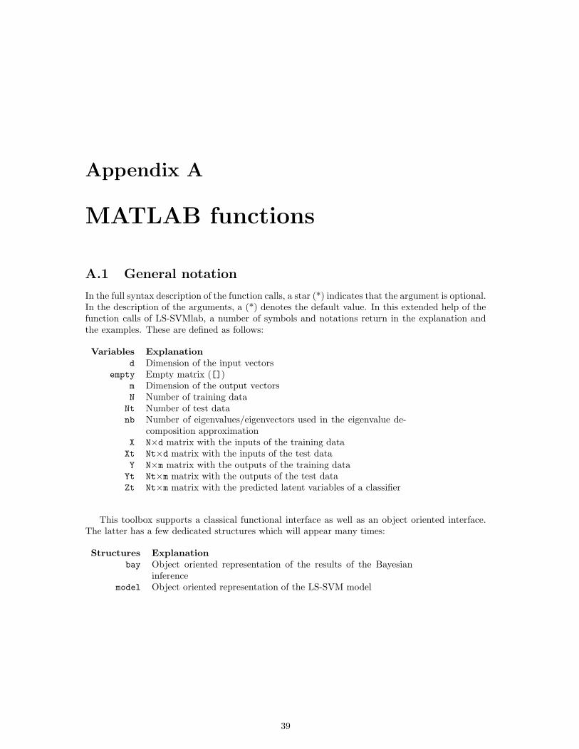
A.1 General notation
In the full syntax description of the function calls, a star (*) indicates that the argument is optional.In the description of the arguments, a (*) denotes the default value. In this extended help of thefunction calls of LS-SVMlab, a number of symbols and notations return in the explanation andthe examples. These are defined as follows:
Variables Explanationd Dimension of the input vectors
empty Empty matrix ([])m Dimension of the output vectorsN Number of training dataNt Number of test datanb Number of eigenvalues/eigenvectors used in the eigenvalue de-
composition approximationX N×d matrix with the inputs of the training dataXt Nt×d matrix with the inputs of the test dataY N×m matrix with the outputs of the training dataYt Nt×m matrix with the outputs of the test dataZt Nt×m matrix with the predicted latent variables of a classifier
This toolbox supports a classical functional interface as well as an object oriented interface.The latter has a few dedicated structures which will appear many times:
Structures Explanationbay Object oriented representation of the results of the Bayesian
inferencemodel Object oriented representation of the LS-SVM model
39
40 APPENDIX A. MATLAB FUNCTIONS
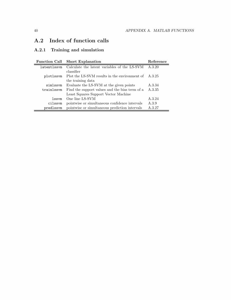
A.2 Index of function calls
A.2.1 Training and simulation
Function Call Short Explanation Reference
latentlssvm Calculate the latent variables of the LS-SVMclassifier
A.3.20
plotlssvm Plot the LS-SVM results in the environment ofthe training data
A.3.25
simlssvm Evaluate the LS-SVM at the given points A.3.34trainlssvm Find the support values and the bias term of a
Least Squares Support Vector MachineA.3.35
lssvm One line LS-SVM A.3.24cilssvm pointwise or simultaneous confidence intervals A.3.9
predlssvm pointwise or simultaneous prediction intervals A.3.27

A.2. INDEX OF FUNCTION CALLS 41
A.2.2 Object oriented interface
This toolbox supports a classical functional interface as well as an object oriented interface. Thelatter has a few dedicated functions. This interface is recommended for the more experienced user.
Function Call Short Explanation Reference
changelssvm Change properties of an LS-SVM object A.3.16demomodel Demo introducing the use of the compact calls
based on the model structureinitlssvm Initiate the LS-SVM object before training A.3.16

42 APPENDIX A. MATLAB FUNCTIONS
A.2.3 Training and simulating functions
Function Call Short Explanation Reference
lssvmMATLAB.m MATLAB implementation of training -prelssvm Internally called preprocessor A.3.29
postlssvm Internally called postprocessor A.3.29
A.2. INDEX OF FUNCTION CALLS 43
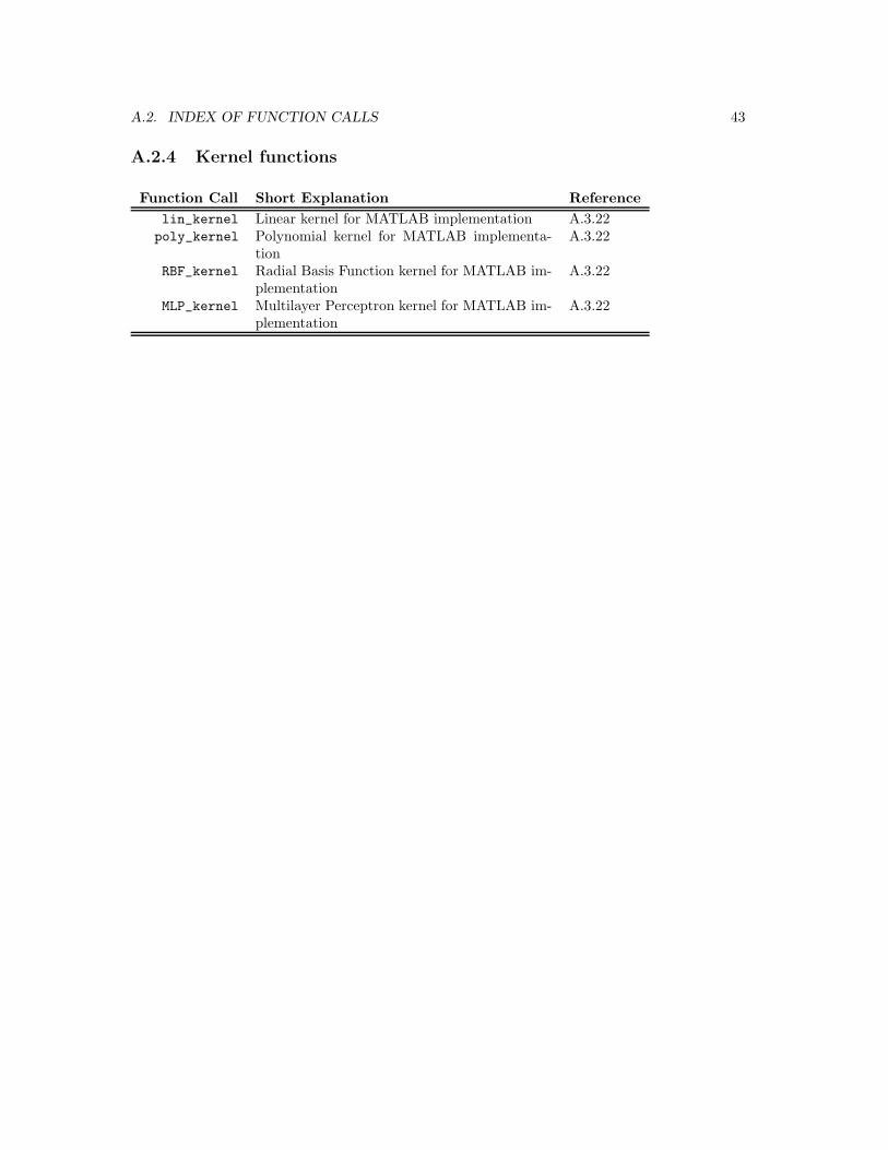
A.2.4 Kernel functions
Function Call Short Explanation Reference
lin_kernel Linear kernel for MATLAB implementation A.3.22poly_kernel Polynomial kernel for MATLAB implementa-
tionA.3.22
RBF_kernel Radial Basis Function kernel for MATLAB im-plementation
A.3.22
MLP_kernel Multilayer Perceptron kernel for MATLAB im-plementation
A.3.22
44 APPENDIX A. MATLAB FUNCTIONS
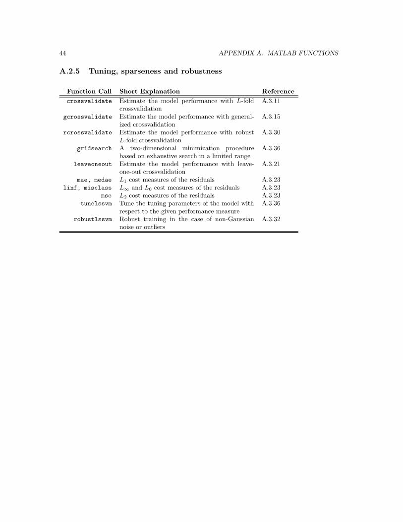
A.2.5 Tuning, sparseness and robustness
Function Call Short Explanation Reference
crossvalidate Estimate the model performance with L-foldcrossvalidation
A.3.11
gcrossvalidate Estimate the model performance with general-ized crossvalidation
A.3.15
rcrossvalidate Estimate the model performance with robustL-fold crossvalidation
A.3.30
gridsearch A two-dimensional minimization procedurebased on exhaustive search in a limited range
A.3.36
leaveoneout Estimate the model performance with leave-one-out crossvalidation
A.3.21
mae, medae L1 cost measures of the residuals A.3.23linf, misclass L∞ and L0 cost measures of the residuals A.3.23
mse L2 cost measures of the residuals A.3.23tunelssvm Tune the tuning parameters of the model with
respect to the given performance measureA.3.36
robustlssvm Robust training in the case of non-Gaussiannoise or outliers
A.3.32
A.2. INDEX OF FUNCTION CALLS 45
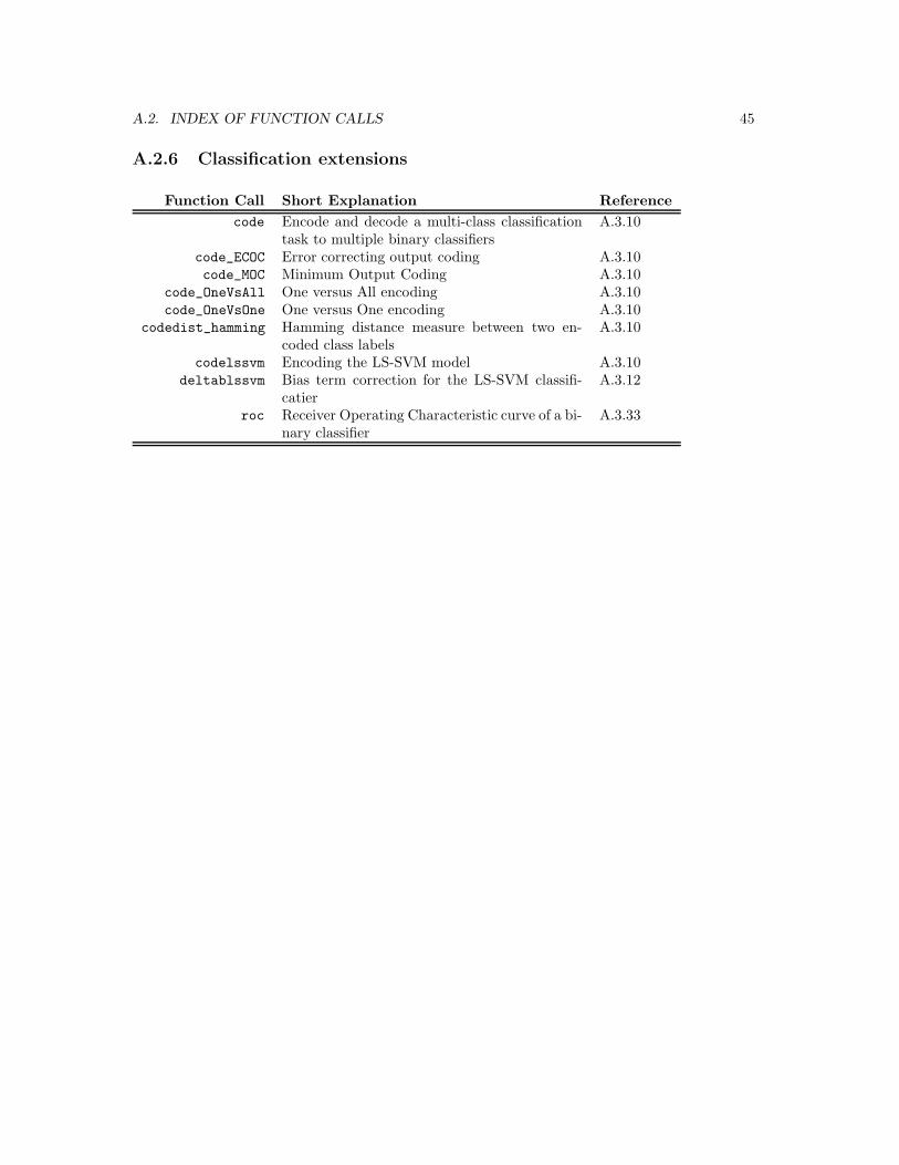
A.2.6 Classification extensions
Function Call Short Explanation Reference
code Encode and decode a multi-class classificationtask to multiple binary classifiers
A.3.10
code_ECOC Error correcting output coding A.3.10code_MOC Minimum Output Coding A.3.10
code_OneVsAll One versus All encoding A.3.10code_OneVsOne One versus One encoding A.3.10
codedist_hamming Hamming distance measure between two en-coded class labels
A.3.10
codelssvm Encoding the LS-SVM model A.3.10deltablssvm Bias term correction for the LS-SVM classifi-
catierA.3.12
roc Receiver Operating Characteristic curve of a bi-nary classifier
A.3.33

46 APPENDIX A. MATLAB FUNCTIONS
A.2.7 Bayesian framework
Function Call Short Explanation Reference
bay_errorbar Compute the error bars for a one dimensionalregression problem
A.3.2
bay_initlssvm Initialize the tuning parameters for Bayesian in-ference
A.3.3
bay_lssvm Compute the posterior cost for the different lev-els in Bayesian inference
A.3.4
bay_lssvmARD Automatic Relevance Determination of the in-puts of the LS-SVM
A.3.5
bay_modoutClass Estimate the posterior class probabilities of abinary classifier using Bayesian inference
A.3.6
bay_optimize Optimize model- or tuning parameters with re-spect to the different inference levels
A.3.7
bay_rr Bayesian inference for linear ridge regression A.3.8eign Find the principal eigenvalues and eigenvectors
of a matrix with Nystrom’s low rank approxi-mation method
A.3.14
kernel_matrix Construct the positive (semi-) definite kernelmatrix
A.3.18
kpca Kernel Principal Component Analysis A.3.19ridgeregress Linear ridge regression A.3.31
A.2. INDEX OF FUNCTION CALLS 47
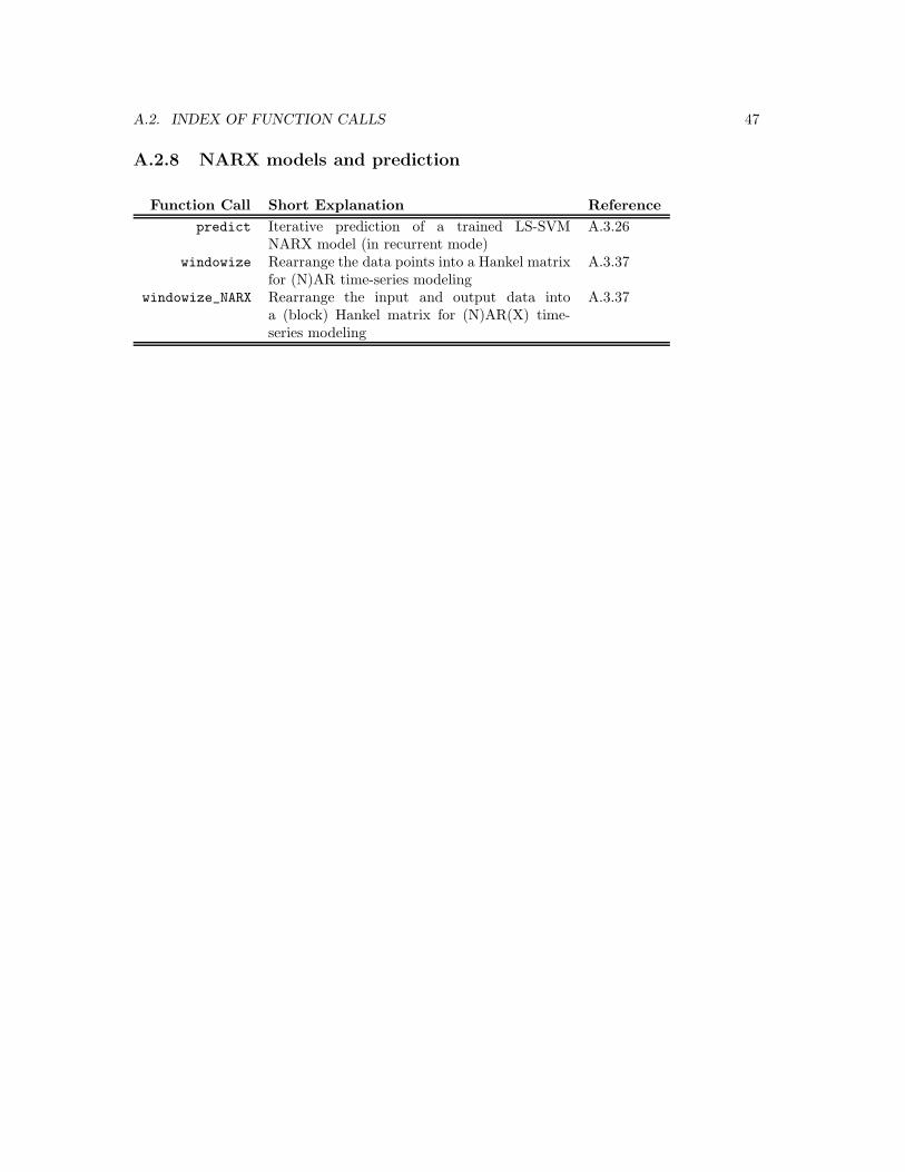
A.2.8 NARX models and prediction
Function Call Short Explanation Reference
predict Iterative prediction of a trained LS-SVMNARX model (in recurrent mode)
A.3.26
windowize Rearrange the data points into a Hankel matrixfor (N)AR time-series modeling
A.3.37
windowize_NARX Rearrange the input and output data intoa (block) Hankel matrix for (N)AR(X) time-series modeling
A.3.37
48 APPENDIX A. MATLAB FUNCTIONS
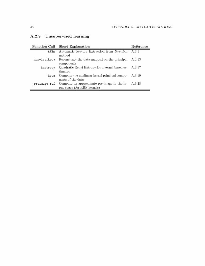
A.2.9 Unsupervised learning
Function Call Short Explanation Reference
AFEm Automatic Feature Extraction from Nystrommethod
A.3.1
denoise_kpca Reconstruct the data mapped on the principalcomponents
A.3.13
kentropy Quadratic Renyi Entropy for a kernel based es-timator
A.3.17
kpca Compute the nonlinear kernel principal compo-nents of the data
A.3.19
preimage_rbf Compute an approximate pre-image in the in-put space (for RBF kernels)
A.3.28

A.2. INDEX OF FUNCTION CALLS 49
A.2.10 Fixed size LS-SVM
The idea of fixed size LS-SVM is still under development. However, in order to enable the userto explore this technique a number of related functions are included in the toolbox. A demoillustrates how to combine these in order to build a fixed size LS-SVM.
Function Call Short Explanation Reference
AFEm Automatic Feature Extraction from Nystrommethod
A.3.1
bay_rr Bayesian inference of the cost on the 3 levels oflinear ridge regression
A.3.8
demo_fixedsize Demo illustrating the use of fixed size LS-SVMsfor regression
-
demo_fixedclass Demo illustrating the use of fixed size LS-SVMsfor classification
-
kentropy Quadratic Renyi Entropy for a kernel based es-timator
A.3.17
ridgeregress Linear ridge regression A.3.31

50 APPENDIX A. MATLAB FUNCTIONS
A.2.11 Demos
name of the demo Short Explanation
demofun Simple demo illustrating the use of LS-SVMlabfor regression
demo_fixedsize Demo illustrating the use of fixed size LS-SVMsfor regression
democlass Simple demo illustrating the use of LS-SVMlabfor classification
demo_fixedclass Demo illustrating the use of fixed size LS-SVMsfor classification
demomodel Simple demo illustrating the use of the objectoriented interface of LS-SVMlab
demo_yinyang Demo illustrating the possibilities of unsuper-vised learning by kernel PCA
democonfint Demo illustrating the construction of confi-dence intervals for LS-SVMs (regression)

A.3. ALPHABETICAL LIST OF FUNCTION CALLS 51
A.3 Alphabetical list of function calls
A.3.1 AFEm
Purpose
Automatic Feature Extraction by Nystrom method
Basic syntax
>> features = AFEm(X, kernel, sig2, Xt)
Description
Using the Nystrom approximation method, the mapping of data to the feature space can be evalu-ated explicitly. This gives features that one can use for a parametric regression or classification inthe primal space. The decomposition of the mapping to the feature space relies on the eigenvaluedecomposition of the kernel matrix. The Matlab (’eigs’) or Nystrom’s (’eign’) approximationusing the nb most important eigenvectors/eigenvalues can be used. The eigenvalue decompositionis not re-calculated if it is passed as an extra argument.
Full syntax
>> [features, U, lam] = AFEm(X, kernel, sig2, Xt)
>> [features, U, lam] = AFEm(X, kernel, sig2, Xt, etype)
>> [features, U, lam] = AFEm(X, kernel, sig2, Xt, etype, nb)
>> features = AFEm(X, kernel, sig2, Xt, [],[], U, lam)
Outputsfeatures Nt×nb matrix with extracted featuresU(*) N×nb matrix with eigenvectorslam(*) nb×1 vector with eigenvalues
InputsX N×d matrix with input datakernel Name of the used kernel (e.g. ’RBF_kernel’)sig2 Kernel parameter(s) (for linear kernel, use [])Xt Nt×d data from which the features are extractedetype(*) ’eig’(*), ’eigs’ or ’eign’nb(*) Number of eigenvalues/eigenvectors used in the eigenvalue de-
composition approximationU(*) N×nb matrix with eigenvectorslam(*) nb×1 vector with eigenvalues
See also:
kernel_matrix, RBF_kernel, demo_fixedsize
52 APPENDIX A. MATLAB FUNCTIONS
A.3.2 bay errorbar
Purpose
Compute the error bars for a one dimensional regression problem
Basic syntax
>> sig_e = bay_errorbar({X,Y,’function’,gam,sig2}, Xt)
>> sig_e = bay_errorbar(model, Xt)
Description
The computation takes into account the estimated noise variance and the uncertainty of the modelparameters, estimated by Bayesian inference. sig_e is the estimated standard deviation of theerror bars of the points Xt. A plot is obtained by replacing Xt by the string ’figure’.
Full syntax
• Using the functional interface:
>> sig_e = bay_errorbar({X,Y,’function’,gam,sig2,kernel,preprocess}, Xt)
>> sig_e = bay_errorbar({X,Y,’function’,gam,sig2,kernel,preprocess}, Xt, etype)
>> sig_e = bay_errorbar({X,Y,’function’,gam,sig2,kernel,preprocess}, Xt, etype, nb)
>> sig_e = bay_errorbar({X,Y,’function’,gam,sig2,kernel,preprocess}, ’figure’)
>> sig_e = bay_errorbar({X,Y,’function’,gam,sig2,kernel,preprocess}, ’figure’, etype, nb)
Outputssig_e Nt×1 vector with the σ2 error bars of the test data
InputsX N×d matrix with the inputs of the training dataY N×1 vector with the inputs of the training datatype ’function estimation’ (’f’)gam Regularization parametersig2 Kernel parameterkernel(*) Kernel type (by default ’RBF_kernel’)preprocess(*) ’preprocess’(*) or ’original’Xt Nt×d matrix with the inputs of the test dataetype(*) ’svd’(*), ’eig’, ’eigs’ or ’eign’nb(*) Number of eigenvalues/eigenvectors used in the eigenvalue de-
composition approximation
• Using the object oriented interface:
>> [sig_e, bay, model] = bay_errorbar(model, Xt)
>> [sig_e, bay, model] = bay_errorbar(model, Xt, etype)
>> [sig_e, bay, model] = bay_errorbar(model, Xt, etype, nb)
>> [sig_e, bay, model] = bay_errorbar(model, ’figure’)
>> [sig_e, bay, model] = bay_errorbar(model, ’figure’, etype)
>> [sig_e, bay, model] = bay_errorbar(model, ’figure’, etype, nb)

A.3. ALPHABETICAL LIST OF FUNCTION CALLS 53
Outputssig_e Nt×1 vector with the σ2 error bars of the test datamodel(*) Object oriented representation of the LS-SVM modelbay(*) Object oriented representation of the results of the Bayesian
inferenceInputs
model Object oriented representation of the LS-SVM modelXt Nt×d matrix with the inputs of the test dataetype(*) ’svd’(*), ’eig’, ’eigs’ or ’eign’nb(*) Number of eigenvalues/eigenvectors used in the eigenvalue de-
composition approximation
See also:
bay_lssvm, bay_optimize, bay_modoutClass, plotlssvm
54 APPENDIX A. MATLAB FUNCTIONS
A.3.3 bay initlssvm
Purpose
Initialize the tuning parameters γ and σ2 before optimization with bay_optimize
Basic syntax
>> [gam, sig2] = bay_initlssvm({X,Y,type,[],[]})
>> model = bay_initlssvm(model)
Description
A starting value for σ2 is only given if the model has kernel type ’RBF_kernel’.
Full syntax
• Using the functional interface:
>> [gam, sig2] = bay_initlssvm({X,Y,type,[],[],kernel})
Outputsgam Proposed initial regularization parametersig2 Proposed initial ’RBF_kernel’ parameter
InputsX N×d matrix with the inputs of the training dataY N×1 vector with the outputs of the training datatype ’function estimation’ (’f’) or ’classifier’ (’c’)kernel(*) Kernel type (by default ’RBF_kernel’)
• Using the object oriented interface:
>> model = bay_initlssvm(model)
Outputsmodel Object oriented representation of the LS-SVMmodel with initial
tuning parametersInputs
model Object oriented representation of the LS-SVM model
See also:
bay_lssvm, bay_optimize

A.3. ALPHABETICAL LIST OF FUNCTION CALLS 55
A.3.4 bay lssvm
Purpose
Compute the posterior cost for the 3 levels in Bayesian inference
Basic syntax
>> cost = bay_lssvm({X,Y,type,gam,sig2}, level, etype)
>> cost = bay_lssvm(model , level, etype)
Description
Estimate the posterior probabilities of model tuning parameters on the different inference levels.By taking the negative logarithm of the posterior and neglecting all constants, one obtains thecorresponding cost.
Computation is only feasible for one dimensional output regression and binary classificationproblems. Each level has its different input and output syntax:
• First level: The cost associated with the posterior of the model parameters (support valuesand bias term) is determined. The type can be:
– ’train’: do a training of the support values using trainlssvm. The total cost, thecost of the residuals (Ed) and the regularization parameter (Ew) are determined by thesolution of the support values
– ’retrain’: do a retraining of the support values using trainlssvm
– the cost terms can also be calculated from an (approximate) eigenvalue decompositionof the kernel matrix: ’svd’, ’eig’, ’eigs’ or Nystrom’s ’eign’
• Second level: The cost associated with the posterior of the regularization parameter iscomputed. The etype can be ’svd’, ’eig’, ’eigs’ or Nystrom’s ’eign’.
• Third level: The cost associated with the posterior of the chosen kernel and kernel param-eters is computed. The etype can be: ’svd’, ’eig’, ’eigs’ or Nystrom’s ’eign’.
Full syntax
• Outputs on the first level
>> [costL1,Ed,Ew,bay] = bay_lssvm({X,Y,type,gam,sig2,kernel,preprocess}, 1)
>> [costL1,Ed,Ew,bay] = bay_lssvm({X,Y,type,gam,sig2,kernel,preprocess}, 1, etype)
>> [costL1,Ed,Ew,bay] = bay_lssvm({X,Y,type,gam,sig2,kernel,preprocess}, 1, etype, nb)
>> [costL1,Ed,Ew,bay] = bay_lssvm(model, 1)
>> [costL1,Ed,Ew,bay] = bay_lssvm(model, 1, etype)
>> [costL1,Ed,Ew,bay] = bay_lssvm(model, 1, etype, nb)
With
costL1 Cost proportional to the posteriorEd(*) Cost of the training error termEw(*) Cost of the regularization parameterbay(*) Object oriented representation of the results of the Bayesian
inference
• Outputs on the second level
56 APPENDIX A. MATLAB FUNCTIONS
>> [costL2,DcostL2, optimal_cost, bay] = ...
bay_lssvm({X,Y,type,gam,sig2,kernel,preprocess}, 2, etype, nb)
>> [costL2,DcostL2, optimal_cost, bay] = bay_lssvm(model, 2, etype, nb)
With
costL2 Cost proportional to the posterior on the second levelDcostL2(*) Derivative of the costoptimal_cost(*) Optimality of the regularization parameter (optimal = 0)bay(*) Object oriented representation of the results of the Bayesian
inference
• Outputs on the third level
>> [costL3,bay] = bay_lssvm({X,Y,type,gam,sig2,kernel,preprocess}, 3, etype, nb)
>> [costL3,bay] = bay_lssvm(model, 3, etype, nb)
With
costL3 Cost proportional to the posterior on the third levelbay(*) Object oriented representation of the results of the Bayesian
inference
• Inputs using the functional interface
>> bay_lssvm({X,Y,type,gam,sig2,kernel,preprocess}, level, etype, nb)
X N×d matrix with the inputs of the training dataY N×1 vector with the outputs of the training datatype ’function estimation’ (’f’) or ’classifier’ (’c’)gam Regularization parametersig2 Kernel parameter(s) (for linear kernel, use [])kernel(*) Kernel type (by default ’RBF_kernel’)preprocess(*) ’preprocess’(*) or ’original’level 1, 2, 3etype(*) ’svd’(*), ’eig’, ’eigs’, ’eign’nb(*) Number of eigenvalues/eigenvectors used in the eigenvalue de-
composition approximation
• Inputs using the object oriented interface
>> bay_lssvm(model, level, etype, nb)
model Object oriented representation of the LS-SVM modellevel 1, 2, 3etype(*) ’svd’(*), ’eig’, ’eigs’, ’eign’nb(*) Number of eigenvalues/eigenvectors used in the eigenvalue de-
composition approximation
See also:
bay_lssvmARD, bay_optimize, bay_modoutClass, bay_errorbar
A.3. ALPHABETICAL LIST OF FUNCTION CALLS 57
A.3.5 bay lssvmARD
Purpose
Bayesian Automatic Relevance Determination of the inputs of an LS-SVM
Basic syntax
>> dimensions = bay_lssvmARD({X,Y,type,gam,sig2})
>> dimensions = bay_lssvmARD(model)
Description
For a given problem, one can determine the most relevant inputs for the LS-SVM within theBayesian evidence framework. To do so, one assigns a different weighting parameter to eachdimension in the kernel and optimizes this using the third level of inference. According to theused kernel, one can remove inputs based on the larger or smaller kernel parameters. This routineonly works with the ’RBF_kernel’ with a sig2 per input. In each step, the input with the largestoptimal sig2 is removed (backward selection). For every step, the generalization performance isapproximated by the cost associated with the third level of Bayesian inference.
The ARD is based on backward selection of the inputs based on the sig2s corresponding ineach step with a minimal cost criterion. Minimizing this criterion can be done by ’continuous’ orby ’discrete’. The former uses in each step continuous varying kernel parameter optimization,the latter decides which one to remove in each step by binary variables for each component (thiscan only be applied for rather low dimensional inputs as the number of possible combinationsgrows exponentially with the number of inputs). If working with the ’RBF_kernel’, the kernelparameter is rescaled appropriately after removing an input variable.
The computation of the Bayesian cost criterion can be based on the singular value decompo-sition ’svd’ of the full kernel matrix or by an approximation of these eigenvalues and vectors bythe ’eigs’ or ’eign’ approximation based on ’nb’ data points.
Full syntax
• Using the functional interface:
>> [dimensions, ordered, costs, sig2s] = ...
bay_lssvmARD({X,Y,type,gam,sig2,kernel,preprocess}, method, etype, nb)
Outputsdimensions r×1 vector of the relevant inputsordered(*) d×1 vector with inputs in decreasing order of relevancecosts(*) Costs associated with third level of inference in every selection
stepsig2s(*) Optimal kernel parameters in each selection step
InputsX N×d matrix with the inputs of the training dataY N×1 vector with the outputs of the training datatype ’function estimation’ (’f’) or ’classifier’ (’c’)gam Regularization parametersig2 Kernel parameter(s) (for linear kernel, use [])kernel(*) Kernel type (by default ’RBF_kernel’)preprocess(*) ’preprocess’(*) or ’original’method(*) ’discrete’(*) or ’continuous’etype(*) ’svd’(*), ’eig’, ’eigs’, ’eign’nb(*) Number of eigenvalues/eigenvectors used in the eigenvalue de-
composition approximation
58 APPENDIX A. MATLAB FUNCTIONS
• Using the object oriented interface:
>> [dimensions, ordered, costs, sig2s, model] = bay_lssvmARD(model, method, etype, nb)
Outputsdimensions r×1 vector of the relevant inputsordered(*) d×1 vector with inputs in decreasing order of relevancecosts(*) Costs associated with third level of inference in every selection
stepsig2s(*) Optimal kernel parameters in each selection stepmodel(*) Object oriented representation of the LS-SVM model trained
only on the relevant inputsInputs
model Object oriented representation of the LS-SVM modelmethod(*) ’discrete’(*) or ’continuous’etype(*) ’svd’(*), ’eig’, ’eigs’, ’eign’nb(*) Number of eigenvalues/eigenvectors used in the eigenvalue de-
composition approximation
See also:
bay_lssvm, bay_optimize, bay_modoutClass, bay_errorbar
A.3. ALPHABETICAL LIST OF FUNCTION CALLS 59
A.3.6 bay modoutClass
Purpose
Estimate the posterior class probabilities of a binary classifier using Bayesian inference
Basic syntax
>> [Ppos, Pneg] = bay_modoutClass({X,Y,’classifier’,gam,sig2}, Xt)
>> [Ppos, Pneg] = bay_modoutClass(model, Xt)
Description
Calculate the probability that a point will belong to the positive or negative classes taking intoaccount the uncertainty of the parameters. Optionally, one can express prior knowledge as aprobability between 0 and 1, where prior equal to 2/3 means that the prior positive class probabilityis 2/3 (more likely to occur than the negative class).
For binary classification tasks with a two dimensional input space, one can make a surface plotby replacing Xt by the string ’figure’.
Full syntax
• Using the functional interface:
>> [Ppos, Pneg] = bay_modoutClass({X,Y,’classifier’,...
gam,sig2, kernel, preprocess}, Xt)
>> [Ppos, Pneg] = bay_modoutClass({X,Y,’classifier’,...
gam,sig2, kernel, preprocess}, Xt, prior)
>> [Ppos, Pneg] = bay_modoutClass({X,Y,’classifier’,...
gam,sig2, kernel, preprocess}, Xt, prior, etype)
>> [Ppos, Pneg] = bay_modoutClass({X,Y,’classifier’,...
gam,sig2, kernel, preprocess}, Xt, prior, etype, nb)
>> bay_modoutClass({X,Y,’classifier’,...
gam,sig2, kernel, preprocess}, ’figure’)
>> bay_modoutClass({X,Y,’classifier’,...
gam,sig2, kernel, preprocess}, ’figure’, prior)
>> bay_modoutClass({X,Y,’classifier’,...
gam,sig2, kernel, preprocess}, ’figure’, prior, etype)
>> bay_modoutClass({X,Y,’classifier’,...
gam,sig2, kernel, preprocess}, ’figure’, prior, etype, nb)
60 APPENDIX A. MATLAB FUNCTIONS
OutputsPpos Nt×1 vector with probabilities that testdata Xt belong to the
positive classPneg Nt×1 vector with probabilities that testdata Xt belong to the
negative(zero) classInputs
X N×d matrix with the inputs of the training dataY N×1 vector with the outputs of the training datatype ’function estimation’ (’f’) or ’classifier’ (’c’)gam Regularization parametersig2 Kernel parameter(s) (for linear kernel, use [])kernel(*) Kernel type (by default ’RBF_kernel’)preprocess(*) ’preprocess’(*) or ’original’Xt(*) Nt×d matrix with the inputs of the test dataprior(*) Prior knowledge of the balancing of the training data (or [])etype(*) ’svd’(*), ’eig’, ’eigs’ or ’eign’nb(*) Number of eigenvalues/eigenvectors used in the eigenvalue de-
composition approximation
• Using the object oriented interface:
>> [Ppos, Pneg, bay, model] = bay_modoutClass(model, Xt)
>> [Ppos, Pneg, bay, model] = bay_modoutClass(model, Xt, prior)
>> [Ppos, Pneg, bay, model] = bay_modoutClass(model, Xt, prior, etype)
>> [Ppos, Pneg, bay, model] = bay_modoutClass(model, Xt, prior, etype, nb)
>> bay_modoutClass(model, ’figure’)
>> bay_modoutClass(model, ’figure’, prior)
>> bay_modoutClass(model, ’figure’, prior, etype)
>> bay_modoutClass(model, ’figure’, prior, etype, nb)
OutputsPpos Nt×1 vector with probabilities that testdata Xt belong to the positive
classPneg Nt×1 vector with probabilities that testdata Xt belong to the nega-
tive(zero) classbay(*) Object oriented representation of the results of the Bayesian inferencemodel(*) Object oriented representation of the LS-SVM model
Inputsmodel Object oriented representation of the LS-SVM modelXt(*) Nt×d matrix with the inputs of the test dataprior(*) Prior knowledge of the balancing of the training data (or [])etype(*) ’svd’(*), ’eig’, ’eigs’ or ’eign’nb(*) Number of eigenvalues/eigenvectors used in the eigenvalue decomposi-
tion approximation
See also:
bay_lssvm, bay_optimize, bay_errorbar, ROC

A.3. ALPHABETICAL LIST OF FUNCTION CALLS 61
A.3.7 bay optimize
Purpose
Optimize the posterior probabilities of model (hyper-) parameters with respect to the different levelsin Bayesian inference
Basic syntax
One can optimize on the three different inference levels as described in section 2.1.3.
• First level: In the first level one optimizes the support values α’s and the bias b.
• Second level: In the second level one optimizes the regularization parameter gam.
• Third level: In the third level one optimizes the kernel parameter. In the case of thecommon ’RBF_kernel’ the kernel parameter is the bandwidth sig2.
This routine is only tested with Matlab R2008a, R2008b, R2009a, R2009b and R2010a using thecorresponding optimization toolbox.
Full syntax
• Outputs on the first level:
>> [model, alpha, b] = bay_optimize({X,Y,type,gam,sig2,kernel,preprocess}, 1)
>> [model, alpha, b] = bay_optimize(model, 1)
With
model Object oriented representation of the LS-SVM model optimized on thefirst level of inference
alpha(*) Support values optimized on the first level of inferenceb(*) Bias term optimized on the first level of inference
• Outputs on the second level:
>> [model,gam] = bay_optimize({X,Y,type,gam,sig2,kernel,preprocess}, 2)
>> [model,gam] = bay_optimize(model, 2)
With
model Object oriented representation of the LS-SVM model optimized on thesecond level of inference
gam(*) Regularization parameter optimized on the second level of inference
• Outputs on the third level:
>> [model, sig2] = bay_optimize({X,Y,type,gam,sig2,kernel,preprocess}, 3)
>> [model, sig2] = bay_optimize(model, 3)
With
model Object oriented representation of the LS-SVM model optimized on thethird level of inference
sig2(*) Kernel parameter optimized on the third level of inference
• Inputs using the functional interface
62 APPENDIX A. MATLAB FUNCTIONS
>> model = bay_optimize({X,Y,type,gam,sig2,kernel,preprocess}, level)
>> model = bay_optimize({X,Y,type,gam,sig2,kernel,preprocess}, level, etype)
>> model = bay_optimize({X,Y,type,gam,sig2,kernel,preprocess}, level, etype, nb)
X N×d matrix with the inputs of the training dataY N×1 vector with the outputs of the training datatype ’function estimation’ (’f’) or ’classifier’ (’c’)gam Regularization parametersig2 Kernel parameter(s) (for linear kernel, use [])kernel(*) Kernel type (by default ’RBF_kernel’)preprocess(*) ’preprocess’(*) or ’original’level 1, 2, 3etype(*) ’eig’, ’svd’(*), ’eigs’, ’eign’nb(*) Number of eigenvalues/eigenvectors used in the eigenvalue decomposi-
tion approximation
• Inputs using the object oriented interface
>> model = bay_optimize(model, level)
>> model = bay_optimize(model, level, etype)
>> model = bay_optimize(model, level, etype, nb)
model Object oriented representation of the LS-SVM modellevel 1, 2, 3etype(*) ’eig’, ’svd’(*), ’eigs’, ’eign’nb(*) Number of eigenvalues/eigenvectors used in the eigenvalue decomposi-
tion approximation
See also:
bay_lssvm, bay_lssvmARD, bay_modoutClass, bay_errorbar

A.3. ALPHABETICAL LIST OF FUNCTION CALLS 63
A.3.8 bay rr
Purpose
Bayesian inference of the cost on the three levels of linear ridge regression
Basic syntax
>> cost = bay_rr(X, Y, gam, level)
Description
This function implements the cost functions related to the Bayesian framework of linear ridgeRegression [44]. Optimizing these criteria results in optimal model parameters W,b and tuningparameters. The criterion can also be used for model comparison. The obtained model parametersw and b are optimal on the first level for J = 0.5*w’*w+gam*0.5*sum(Y-X*w-b).^2.
Full syntax
• Outputs on the first level: Cost proportional to the posterior of the model parameters.
>> [costL1, Ed, Ew] = bay_rr(X, Y, gam, 1)
With
costL1 Cost proportional to the posteriorEd(*) Cost of the training error termEw(*) Cost of the regularization parameter
• Outputs on the second level: Cost proportional to the posterior of gam.
>> [costL2, DcostL2, Deff, mu, ksi, eigval, eigvec] = bay_rr(X, Y, gam, 2)
With
costL2 Cost proportional to the posterior on the second levelDcostL2(*) Derivative of the cost proportional to the posteriorDeff(*) Effective number of parametersmu(*) Relative importance of the fitting error termksi(*) Relative importance of the regularization parametereigval(*) Eigenvalues of the covariance matrixeigvec(*) Eigenvectors of the covariance matrix
• Outputs on the third level: The following commands can be used to compute the level3 cost function for different models (e.g. models with different selected sets of inputs). Thebest model can then be chosen as the model with best level 3 cost (CostL3).
>> [costL3, gam_optimal] = bay_rr(X, Y, gam, 3)
With
costL3 Cost proportional to the posterior on the third inference levelgam_optimal(*) Optimal regularization parameter obtained from optimizing the second
level

64 APPENDIX A. MATLAB FUNCTIONS
• Inputs:
>> cost = bay_rr(X, Y, gam, level)
X N×d matrix with the inputs of the training dataY N×1 vector with the outputs of the training datagam Regularization parameterlevel 1, 2, 3
See also:
ridgeregress,bay_lssvm
A.3. ALPHABETICAL LIST OF FUNCTION CALLS 65
A.3.9 cilssvm
Purpose
Construction of bias corrected 100(1− α)% pointwise or simultaneous confidence intervals
Basic syntax
>> ci = cilssvm({X,Y,type,gam,kernel_par,kernel,preprocess},alpha,conftype)
>> ci = cilssvm(model,alpha,conftype)
Description
This function calculates bias corrected 100(1−α)% pointwise or simultaneous confidence intervals.The procedure support homoscedastic data sets as well heteroscedastic data sets. The constructionof the confidence intervals are based on the central limit theorem for linear smoothers combinedwith bias correction and variance estimation.
Full syntax
• Using the functional interface:
>> ci = cilssvm({X,Y,type,gam,kernel_par,kernel,preprocess})
>> ci = cilssvm({X,Y,type,gam,kernel_par,kernel,preprocess}, alpha)
>> ci = cilssvm({X,Y,type,gam,kernel_par,kernel,preprocess}, alpha, conftype)
Outputsci N × 2 matrix containing the lower and upper confidence intervals
InputsX Training input data used for defining the LS-SVM and the preprocessingY Training output data used for defining the LS-SVM and the preprocess-
ingtype ’function estimation’ (’f’) or ’classifier’ (’c’)gam Regularization parametersig2 Kernel parameter(s) (for linear kernel, use [])kernel(*) Kernel type (by default ’RBF_kernel’)preprocess(*) ’preprocess’(*) or ’original’alpha(*) Significance level (by default 5%)conftype(*) Type of confidence interval ’pointwise’ or ’simultaneous’ (by default ’si-
multaneous’)
• Using the object oriented interface:
>> ci = cilssvm(model)
>> ci = cilssvm(model, alpha)
>> ci = cilssvm(model, alpha, conftype)
Outputsci N × 2 matrix containing the lower and upper confidence intervals
Inputsmodel Object oriented representation of the LS-SVM modelalpha(*) Significance level (by default 5%)conftype(*) Type of confidence interval ’pointwise’ or ’simultaneous’ (by default
simultaneous)
See also:
trainlssvm, simlssvm, predlssvm

66 APPENDIX A. MATLAB FUNCTIONS
A.3.10 code, codelssvm
Purpose
Encode and decode a multi-class classification task into multiple binary classifiers
Basic syntax
>> Yc = code(Y, codebook)
Description
The coding is defined by the codebook. The codebook is represented by a matrix where thecolumns represent all different classes and the rows indicate the result of the binary classifiers.An example is given: the 3 classes with original labels [1 2 3] can be encoded in the followingcodebook (using Minimum Output Coding):
>> codebook
= [-1 -1 1;
1 -1 1]
For this codebook, a member of the first class is found if the first binary classifier is negativeand the second classifier is positive. A don’t care is represented by NaN. By default it is assumedthat the original classes are represented as different numerical labels. One can overrule this bypassing the old_codebook which contains information about the old representation.
A codebook can be created by one of the functions (codefct) code_MOC, code_OneVsOne,code_OneVsAll, code_ECOC. Additional arguments to this function can be passed as a cell incodefct_args.
>> Yc = code(Y,codefct,codefct_args)
>> Yc = code(Y,codefct,codefct_args, old_codebook)
>> [Yc, codebook, oldcodebook] = code(Y,codefct,codefct_args)
To detect the classes of a disturbed encoded signal given the corresponding codebook, oneneeds a distance function (fctdist) with optional arguments given as a cell (fctdist_args). Bydefault, the Hamming distance (of function codedist_hamming) is used.
>> Yc = code(Y, codefct, codefct_args, old_codebook, fctdist, fctdist_args)
A simple example is given here, a more elaborated example is given in section 3.2.6. Here, ashort categorical signal Y is encoded in Yec using Minimum Output Coding and decoded again toits original form:
>> Y = [1; 2; 3; 2; 1]
>> [Yc,codebook,old_codebook] = code(Y,’code_MOC’) % encode
>> Yc
= [-1 -1
-1 1
1 -1
-1 1
-1 -1]
>> codebook
= [ -1 -1 1
-1 1 -1]
>> old_codebook
= [1 2 3]

A.3. ALPHABETICAL LIST OF FUNCTION CALLS 67
>> code(Yc, old_codebook, [], codebook, ’codedist_hamming’) % decode
ans
= [1; 2; 3; 2; 1]
Different encoding schemes are available:
• Minimum Output Coding (code_MOC)Here the minimal number of bits nb is used to encode the nc classes:
nb = ⌈log2 nc⌉.
• Error Correcting Output Code (code_ECOC)This coding scheme uses redundant bits. Typically, one bounds the number of binary clas-sifiers nb by
nb ≤ 15⌈log2 nc⌉.
However, it is not guaranteed to have a valid nb-representation of nc classes for all combi-nations. This routine based on backtracking can take some memory and time.
• One versus All Coding (code_OneVsAll)Each binary classifier k = 1, ..., nc is trained to discriminate between class k and the unionof the others.
• One Versus One Coding (code_OneVsOns)Each of the nb binary classifiers is used to discriminate between a specific pair of nc classes
nb =nc(nc − 1)
2.
Different decoding schemes are implemented:
• Hamming Distance (codedist_hamming)This measure equals the number of corresponding bits in the binary result and the codeword.Typically, it is used for the Error Correcting Code.
• Bayesian Distance Measure (codedist_bay)The Bayesian moderated output of the binary classifiers is used to estimate the posteriorprobability.
Encoding using the previous algorithms of the LS-SVM multi-class classifier can easily be doneby codelssvm. It will be invoked by trainlssvm if an appropriate encoding scheme is defined ina model. An example shows how to use the Bayesian distance measure to extract the estimatedclass from the simulated encoded signal. Assumed are input and output data X and Y (size isrespectively Ntrain×Din and Ntrain×1), a kernel parameter sig2 and a regularization parametergam. Yt corresponding to a set of data points Xt (size is Ntest ×Din) is to be estimated:
% encode for training
>> model = initlssvm(X, Y, ’classifier’, gam, sig2)
>> model = changelssvm(model, ’codetype’, ’code_MOC’)
>> model = changelssvm(model, ’codedist_fct’, ’codedist_hamming’)
>> model = codelssvm(model) % implicitly called by next command
>> model = trainlssvm(model)
>> plotlssvm(model);
% decode for simulating
>> model = changelssvm(model, ’codedist_fct’, ’codedist_bay’)
>> model = changelssvm(model, ’codedist_args’,...
{bay_modoutClass(model,Xt)})
>> Yt = simlssvm(model, Xt)

68 APPENDIX A. MATLAB FUNCTIONS
Full syntax
We denote the number of used binary classifiers by nbits and the number of different representedclasses by nc.
• For encoding:
>> [Yc, codebook, old_codebook] = code(Y, codefct)
>> [Yc, codebook, old_codebook] = code(Y, codefct, codefct_args)
>> Yc = code(Y, given_codebook)
OutputsYc N×nbits encoded output classifiercodebook(*) nbits*nc matrix representing the used encodingold_codebook(*) d*nc matrix representing the original encoding
InputsY N×d matrix representing the original classifiercodefct(*) Function to generate a new codebook (e.g. code_MOC)codefct_args(*) Extra arguments for codefctgiven_codebook(*) nbits*nc matrix representing the encoding to use
• For decoding:
>> Yd = code(Yc, codebook,[], old_codebook)
>> Yd = code(Yc, codebook,[], old_codebook, codedist_fct)
>> Yd = code(Yc, codebook,[], old_codebook, codedist_fct, codedist_args)
OutputsYd N×nc decoded output classifier
InputsY N×d matrix representing the original classifiercodebook d*nc matrix representing the original encodingold_codebook bits*nc matrix representing the encoding of the given classifiercodedist_fct Function to calculate the distance between to encoded classifiers (e.g.
codedist_hamming)codedist_args(*) Extra arguments of codedist_fct
See also:
code_ECOC, code_MOC, code_OneVsAll, code_OneVsOne, codedist_hamming
A.3. ALPHABETICAL LIST OF FUNCTION CALLS 69
A.3.11 crossvalidate
Purpose
Estimate the model performance of a model with l-fold crossvalidation.
CAUTION!! Use this function only to obtain the value of the crossvalidation score function giventhe tuning parameters. Do not use this function together with tunelssvm, but use crossvalidatelssvminstead. The latter is a faster implementation which uses previously computed results.
Basic syntax
>> cost = crossvalidate({Xtrain,Ytrain,type,gam,sig2})
>> cost = crossvalidate(model)
Description
The data is once permutated randomly, then it is divided into L (by default 10) disjoint sets.In the i-th (i = 1, ..., l) iteration, the i-th set is used to estimate the performance (’validationset’) of the model trained on the other l − 1 sets (’training set’). Finally, the l (denoted by L)different estimates of the performance are combined (by default by the ’mean’). The assumptionis made that the input data are distributed independent and identically over the input space. Asadditional output, the costs in the different folds (’costs’) of the data are returned:
>> [cost, costs] = crossvalidate(model)
Some commonly used criteria are:
>> cost = crossvalidate(model, 10, ’misclass’, ’mean’)
>> cost = crossvalidate(model, 10, ’mse’, ’mean’)
>> cost = crossvalidate(model, 10, ’mae’, ’median’)
Full syntax
• Using LS-SVMlab with the functional interface:
>> [cost, costs] = crossvalidate({X,Y,type,gam,sig2,kernel,preprocess})
>> [cost, costs] = crossvalidate({X,Y,type,gam,sig2,kernel,preprocess}, L)
>> [cost, costs] = crossvalidate({X,Y,type,gam,sig2,kernel,preprocess},...
L, estfct, combinefct)
Outputscost Cost estimation of the L-fold cross-validationcosts(*) L×1 vector with costs estimated on the L different folds
InputsX Training input data used for defining the LS-SVM and the preprocessingY Training output data used for defining the LS-SVM and the preprocess-
ingtype ’function estimation’ (’f’) or ’classifier’ (’c’)gam Regularization parametersig2 Kernel parameter(s) (for linear kernel, use [])kernel(*) Kernel type (by default ’RBF_kernel’)preprocess(*) ’preprocess’(*) or ’original’L(*) Number of folds (by default 10)estfct(*) Function estimating the cost based on the residuals (by default mse)combinefct(*) Function combining the estimated costs on the different folds (by default
mean)

70 APPENDIX A. MATLAB FUNCTIONS
• Using the object oriented interface:
>> [cost, costs] = crossvalidate(model)
>> [cost, costs] = crossvalidate(model, L)
>> [cost, costs] = crossvalidate(model, L, estfct)
>> [cost, costs] = crossvalidate(model, L, estfct, combinefct)
Outputscost Cost estimation of the L-fold cross-validationcosts(*) L×1 vector with costs estimated on the L different folds
Inputsmodel Object oriented representation of the LS-SVM modelL(*) Number of folds (by default 10)estfct(*) Function estimating the cost based on the residuals (by default mse)combinefct(*) Function combining the estimated costs on the different folds (by default
mean)
See also:
leaveoneout, gcrossvalidate, trainlssvm, simlssvm

A.3. ALPHABETICAL LIST OF FUNCTION CALLS 71
A.3.12 deltablssvm
Purpose
Bias term correction for the LS-SVM classifier
Basic syntax
>> model = deltablssvm(model, b_new)
Description
This function is only useful in the object oriented function interface. Set explicitly the bias termb_new of the LS-SVM model.
Full syntax
>> model = deltablssvm(model, b_new)
Outputsmodel Object oriented representation of the LS-SVM model with initial tuning
parametersInputs
model Object oriented representation of the LS-SVM modelb_new m×1 vector with new bias term(s) for the model
See also:
roc, trainlssvm, simlssvm, changelssvm
72 APPENDIX A. MATLAB FUNCTIONS
A.3.13 denoise kpca
Purpose
Reconstruct the data mapped on the most important principal components.
Basic syntax
>> Xd = denoise_kpca(X, kernel, kernel_par);
Description
Denoising can be done by moving the point in input space so that its corresponding map to thefeature space is optimized. This means that the data point in feature space is as close as possiblewith its corresponding reconstructed points by using the principal components. If the principalcomponents are to be calculated on the same data ’X’ as one wants to denoise, use the command:
>> Xd = denoise_kpca(X, kernel, kernel_par);
>> [Xd,lam,U] = denoise_kpca(X, kernel, kernel_par, [], etype, nb);
When one wants to denoise data ’Xt’ other than the data used to obtain the principal components:
>> Xd = denoise_kpca(X, kernel, kernel_par, Xt);
>> [Xd, lam, U] = denoise_kpca(X, kernel, kernel_par, Xt, etype, nb);
Full syntax
• >> [Xd, lam, U] = denoise_kpca(X, kernel, kernel_par, Xt);
>> [Xd, lam, U] = denoise_kpca(X, kernel, kernel_par, Xt, etype);
>> [Xd, lam, U] = denoise_kpca(X, kernel, kernel_par, Xt, etype, nb);
OutputsXd N×d (Nt×d) matrix with denoised data X (Xt)lam(*) nb×1 vector with eigenvalues of principal componentsU(*) N×nb (Nt×d) matrix with principal eigenvectors
InputsX N×d matrix with data points used for finding the principal componentskernel Kernel type (e.g. ’RBF_kernel’)kernel_par Kernel parameter(s) (for linear kernel, use [])Xt(*) Nt×d matrix with noisy points (if not specified, X is denoised instead)etype(*) ’eig’(*), ’svd’, ’eigs’, ’eign’nb(*) Number of principal components used in approximation
• >> Xd = denoise_kpca(X, U, lam, kernel, kernel_par, Xt);
OutputsXd N×d (Nt×d) matrix with denoised data X (Xt)
InputsX N×d matrix with data points used for finding the principal componentsU N×nb (Nt×d) matrix with principal eigenvectorslam nb×1 vector with eigenvalues of principal componentskernel Kernel type (e.g. ’RBF_kernel’)kernel_par Kernel parameter(s) (for linear kernel, use [])Xt(*) Nt×d matrix with noisy points (if not specified, X is denoised instead)
See also:
kpca, kernel_matrix, RBF_kernel
A.3. ALPHABETICAL LIST OF FUNCTION CALLS 73
A.3.14 eign
Purpose
Find the principal eigenvalues and eigenvectors of a matrix with Nystrom’s low rank approximationmethod
Basic syntax
>> D = eign(A, nb)
>> [V, D] = eign(A, nb)
Description
In the case of using this method for low rank approximation and decomposing the kernel matrix,one can call the function without explicit construction of the matrix A.
>> D = eign(X, kernel, kernel_par, nb)
>> [V, D] = eign(X, kernel, kernel_par, nb)
Full syntax
We denote the size of positive definite matrix A with a*a.
• Given the full matrix:
>> D = eign(A,nb)
>> [V,D] = eign(A,nb)
OutputsV(*) a×nb matrix with estimated principal eigenvectors of AD nb×1 vector with principal estimated eigenvalues of A
InputsA a*a positive definite symmetric matrixnb(*) Number of approximated principal eigenvalues/eigenvectors
• Given the function to calculate the matrix elements:
>> D = eign(X, kernel, kernel_par, n)
>> [V,D] = eign(X, kernel, kernel_par, n)
OutputsV(*) a×nb matrix with estimated principal eigenvectors of AD nb×1 vector with estimated principal eigenvalues of A
InputsX N×d matrix with the training datakernel Kernel type (e.g. ’RBF_kernel’)kernel_par Kernel parameter(s) (for linear kernel, use [])nb(*) Number of eigenvalues/eigenvectors used in the eigenvalue decomposi-
tion approximation
See also:
eig, eigs, kpca, bay_lssvm
74 APPENDIX A. MATLAB FUNCTIONS
A.3.15 gcrossvalidate
Purpose
Estimate the model performance of a model with generalized crossvalidation.
CAUTION!! Use this function only to obtain the value of the generalized crossvalidation scorefunction given the tuning parameters. Do not use this function together with tunelssvm, butuse gcrossvalidatelssvm instead. The latter is a faster implementation which uses previouslycomputed results.
Basic syntax
>> cost = gcrossvalidate({Xtrain,Ytrain,type,gam,sig2})
>> cost = gcrossvalidate(model)
Description
Instead of dividing the data into L disjoint sets, one takes the complete data and the effectivedegrees of freedom (effective number of parameters) into account. The assumption is made thatthe input data are distributed independent and identically over the input space.
>> cost = gcrossvalidate(model)
Some commonly used criteria are:
>> cost = gcrossvalidate(model, ’misclass’)
>> cost = gcrossvalidate(model, ’mse’)
>> cost = gcrossvalidate(model, ’mae’)
Full syntax
• Using LS-SVMlab with the functional interface:
>> cost = gcrossvalidate({X,Y,type,gam,sig2,kernel,preprocess})
>> cost = gcrossvalidate({X,Y,type,gam,sig2,kernel,preprocess}, estfct)
Outputscost Cost estimation of the generalized cross-validation
InputsX Training input data used for defining the LS-SVM and the preprocessingY Training output data used for defining the LS-SVM and the preprocess-
ingtype ’function estimation’ (’f’) or ’classifier’ (’c’)gam Regularization parametersig2 Kernel parameter(s) (for linear kernel, use [])kernel(*) Kernel type (by default ’RBF_kernel’)preprocess(*) ’preprocess’(*) or ’original’estfct(*) Function estimating the cost based on the residuals (by default mse)
• Using the object oriented interface:
>> cost = gcrossvalidate(model)
>> cost = gcrossvalidate(model, estfct)

A.3. ALPHABETICAL LIST OF FUNCTION CALLS 75
Outputscost Cost estimation of the generalized cross-validation
Inputsmodel Object oriented representation of the LS-SVM modelestfct(*) Function estimating the cost based on the residuals (by default mse)
See also:
leaveoneout, crossvalidatelssvm, trainlssvm, simlssvm

76 APPENDIX A. MATLAB FUNCTIONS
A.3.16 initlssvm, changelssvm
Purpose
Only for use with the object oriented model interface
Description
The Matlab toolbox interface is organized in two equivalent ways. In the functional way, func-tion calls need explicit input and output arguments. An advantage is their similarity with themathematical equations.
An alternative syntax is based on the concept of a model, gathering all the relevant signals,parameters and algorithm choices. The model is initialized by model=initlssvm(...), or will beinitiated implicitly by passing the arguments of initlssvm(...) in one cell as the argument ofthe LS-SVM specific functions, e.g. for training:
>> model = trainlssvm({X,Y,type,gam,sig2})
...
>> model = changelssvm(model,’field’,’value’)
After training, the model contains the solution of the training including the used default values. Allcontents of the model can be requested (model.<contenttype>) or changed (changelssvm) eachmoment. The user is advised not to change the fields of the model by model.<field>=<value>
as the toolbox cannot guarantee consistency anymore in this way.The different options are given in following table:
• General options representing the kind of model:
type: ’classifier’ ,’function estimation’
status: Status of this model (’trained’ or ’changed’ )
alpha: Support values of the trained LS-SVM model
b: Bias term of the trained LS-SVM model
duration: Number of seconds the training lasts
latent: Returning latent variables (’no’ ,’yes’ )
x_delays: Number of delays of eXogeneous variables (by default 0 )
y_delays: Number of delays of responses (by default 0 )
steps: Number of steps to predict (by default 1 )
gam: Regularisation parameter
kernel_type: Kernel function
kernel_pars: Extra parameters of the kernel function
weights: Weighting function for robust regression
• Fields used to specify the used training data:
x_dim: Dimension of input space
y_dim: Dimension of responses
nb_data: Number of training data
xtrain: (preprocessed) inputs of training data
ytrain: (preprocessed,coded) outputs of training data
selector: Indexes of training data effectively used during training
costCV: Cost of the cross-validation score function when model is tuned

A.3. ALPHABETICAL LIST OF FUNCTION CALLS 77
• Fields with the information for pre- and post-processing (only given if appropriate):
preprocess: ’preprocess’ or ’original’
schemed: Status of the preprocessing
(’coded’ ,’original’ or ’schemed’ )
pre_xscheme: Scheme used for preprocessing the input data
pre_yscheme: Scheme used for preprocessing the output data
pre_xmean: Mean of the input data
pre_xstd: Standard deviation of the input data
pre_ymean: Mean of the responses
pre_ystd: Standard deviation of the reponses
• The specifications of the used encoding (only given if appropriate):
code: Status of the coding
(’original’ ,’changed’ or ’encoded’)
codetype: Used function for constructing the encoding
for multiclass classification (by default ’none’)
codetype_args: Arguments of the codetype function
codedist_fct: Function used to calculate to which class a
coded result belongs
codedist_args: Arguments of the codedist function
codebook2: Codebook of the new coding
codebook1: Codebook of the original coding
Full syntax
• >> model = initlssvm(X, Y, type, gam, sig2, kernel, preprocess)
Outputsmodel Object oriented representation of the LS-SVM model
InputsX N×d matrix with the inputs of the training dataY N×1 vector with the outputs of the training datatype ’function estimation’ (’f’) or ’classifier’ (’c’)gam Regularization parametersig2 Kernel parameter(s) (for linear kernel, use [])kernel(*) Kernel type (by default ’RBF_kernel’)preprocess(*) ’preprocess’(*) or ’original’
• >> model = changelssvm(model, field, value)
Outputsmodel(*) Obtained object oriented representation of the LS-SVM model
Inputsmodel Original object oriented representation of the LS-SVM modelfield Field of the model that one wants to change (e.g. ’preprocess’)value New value of the field of the model that one wants to change
See also:
trainlssvm, initlssvm, simlssvm, plotlssvm.
78 APPENDIX A. MATLAB FUNCTIONS
A.3.17 kentropy
Purpose
Quadratic Renyi Entropy for a kernel based estimator
Basic syntax
Given the eigenvectors and the eigenvalues of the kernel matrix, the entropy is computed by
>> H = kentropy(X, U, lam)
The eigenvalue decomposition can also be computed (or approximated) implicitly:
>> H = kentropy(X, kernel, sig2)
Full syntax
• >> H = kentropy(X, kernel, kernel_par)
>> H = kentropy(X, kernel, kernel_par, etype)
>> H = kentropy(X, kernel, kernel_par, etype, nb)
OutputsH Quadratic Renyi entropy of the kernel matrix
InputsX N×d matrix with the training datakernel Kernel type (e.g. ’RBF_kernel’)kernel_par Kernel parameter(s) (for linear kernel, use [])etype(*) ’eig’(*), ’eigs’, ’eign’nb(*) Number of eigenvalues/eigenvectors used in the eigenvalue decomposi-
tion approximation
• >> H = kentropy(X, U, lam)
OutputsH Quadratic Renyi entropy of the kernel matrix
InputsX N×d matrix with the training dataU N×nb matrix with principal eigenvectorslam nb×1 vector with eigenvalues of principal components
See also:
kernel_matrix, demo_fixedsize, RBF_kernel

A.3. ALPHABETICAL LIST OF FUNCTION CALLS 79
A.3.18 kernel matrix
Purpose
Construct the positive (semi-) definite and symmetric kernel matrix
Basic Syntax
>> Omega = kernel_matrix(X, kernel_fct, sig2)
Description
This matrix should be positive definite if the kernel function satisfies the Mercer condition. Con-struct the kernel values for all test data points in the rows of Xt, relative to the points of X.
>> Omega_Xt = kernel_matrix(X, kernel_fct, sig2, Xt)
Full syntax
>> Omega = kernel_matrix(X, kernel_fct, sig2)
>> Omega = kernel_matrix(X, kernel_fct, sig2, Xt)
OutputsOmega N×N (N×Nt) kernel matrix
InputsX N×d matrix with the inputs of the training datakernel Kernel type (by default ’RBF_kernel’)sig2 Kernel parameter(s) (for linear kernel, use [])Xt(*) Nt×d matrix with the inputs of the test data
See also:
RBF_kernel, lin_kernel, kpca, trainlssvm

80 APPENDIX A. MATLAB FUNCTIONS
A.3.19 kpca
Purpose
Kernel Principal Component Analysis (KPCA)
Basic syntax
>> [eigval, eigvec] = kpca(X, kernel_fct, sig2)
>> [eigval, eigvec, scores] = kpca(X, kernel_fct, sig2, Xt)
Description
Compute the nb largest eigenvalues and the corresponding rescaled eigenvectors correspondingwith the principal components in the feature space of the centered kernel matrix. To calculatethe eigenvalue decomposition of this N × N matrix, Matlab’s eig is called by default. Thedecomposition can also be approximated by Matlab (’eigs’) or by Nystrom’s method (’eign’)using nb components. In some cases one wants to disable (’original’) the rescaling of theprincipal components in feature space to unit length.
The scores of a test set Xt on the principal components is computed by the call:
>> [eigval, eigvec, scores] = kpca(X, kernel_fct, sig2, Xt)
Full syntax
>> [eigval, eigvec, empty, omega] = kpca(X, kernel_fct, sig2)
>> [eigval, eigvec, empty, omega] = kpca(X, kernel_fct, sig2, [], etype)
>> [eigval, eigvec, empty, omega] = kpca(X, kernel_fct, sig2, [],etype, nb)
>> [eigval, eigvec, empty, omega] = kpca(X, kernel_fct, sig2, [],etype, nb, rescaling)
>> [eigval, eigvec, scores, omega] = kpca(X, kernel_fct, sig2, Xt)
>> [eigval, eigvec, scores, omega] = kpca(X, kernel_fct, sig2, Xt, etype)
>> [eigval, eigvec, scores, omega] = kpca(X, kernel_fct, sig2, Xt,etype, nb)
>> [eigval, eigvec, scores, omega] = kpca(X, kernel_fct, sig2, Xt,etype, nb, rescaling)
>> [eigval, eigvec, scores, omega, recErrors] = kpca(X, kernel_fct, sig2, Xt, etype)
>> [eigval, eigvec, scores, omega, recErrors] = kpca(X, kernel_fct, sig2, Xt, ...
etype, nb)
>> [eigval, eigvec, scores, omega, recErrors] = kpca(X, kernel_fct, sig2, Xt, ...
etype, nb, rescaling)
>> [eigval, eigvec, scores, omega, recErrors, optOut] = kpca(X, kernel_fct, ...
sig2, Xt, etype)
>> [eigval, eigvec, scores, omega, recErrors, optOut] = kpca(X, kernel_fct, sig2, Xt, ...
etype, nb)
>> [eigval, eigvec, scores, omega, recErrors, optOut] = kpca(X, kernel_fct, sig2, Xt, ...
etype, nb, rescaling)

A.3. ALPHABETICAL LIST OF FUNCTION CALLS 81
Outputseigval N (nb)×1 vector with eigenvalues valueseigvec N×N (N×nb) matrix with the principal directionsscores(*) Nt×nb matrix of the scores of test data (or [])omega(*) N×N centered kernel matrixrecErrors(*) Nt×1 vector with the reconstruction errors of test dataoptOut(*) 1×2 cell array with the centered test kernel matrix in optOut{1} and
the squared norms of the test points in the feature space in optOut{2}Inputs
X N×d matrix with the inputs of the training datakernel Kernel type (e.g. ’RBF_kernel’)sig2 Kernel parameter(s) (for linear kernel, use [])Xt(*) Nt×d matrix with the inputs of the test data (or [])etype(*) ’svd’, ’eig’(*),’eigs’,’eign’nb(*) Number of eigenvalues/eigenvectors used in the eigenvalue decomposi-
tion approximationrescaling(*) ’original size’ (’o’) or ’rescaling’(*) (’r’)
See also:
bay_lssvm, bay_optimize, eign
82 APPENDIX A. MATLAB FUNCTIONS
A.3.20 latentlssvm
Purpose
Calculate the latent variables of the LS-SVM classifier at the given test data
Basic syntax
>> Zt = latentlssvm({X,Y,’classifier’,gam,sig2,kernel}, {alpha,b}, Xt)
>> Zt = latentlssvm({X,Y,’classifier’,gam,sig2,kernel}, Xt)
>> [Zt, model] = latentlssvm(model, Xt)
Description
The latent variables of a binary classifier are the continuous simulated values of the test or trainingdata which are used to make the final classifications. The classification of a test point depends onwhether the latent value exceeds the model’s threshold (b). If appropriate, the model is trainedby the standard procedure (trainlssvm) first.
Full syntax
• Using the functional interface:
>> Zt = latentlssvm({X,Y,’classifier’,gam,sig2,kernel}, {alpha,b}, Xt)
>> Zt = latentlssvm({X,Y,type,gam,sig2,kernel,preprocess}, Xt)
OutputsZt Nt×m matrix with predicted latent simulated outputs
InputsX N×d matrix with the inputs of the training dataY N×m vector with the outputs of the training datatype ’classifier’ (’c’)gam Regularization parametersig2 Kernel parameter(s) (for linear kernel, use [])kernel(*) Kernel type (by default ’RBF_kernel’)preprocess(*) ’preprocess’(*) or ’original’alpha(*) N×1 matrix with the support valuesb(*) the bias termsXt Nt×d matrix with the inputs of the test data
• Using the object oriented interface:
>> [Zt, model] = latentlssvm(model, Xt)
OutputsZt Nt×m matrix with continuous latent simulated outputsmodel(*) Trained object oriented representation of the LS-SVM model
Inputsmodel Object oriented representation of the LS-SVM modelXt Nt×d matrix with the inputs of the test data
See also:
trainlssvm, simlssvm
A.3. ALPHABETICAL LIST OF FUNCTION CALLS 83
A.3.21 leaveoneout
Purpose
Estimate the performance of a trained model with leave-one-out crossvalidation.
CAUTION!! Use this function only to obtain the value of the leave-one-out crossvalidation scorefunction given the tuning parameters. Do not use this function together with tunelssvm, but useleaveoneoutlssvm instead. The latter is a faster implementation based on one full matrix inverse.
Basic syntax
>> leaveoneout({X,Y,type,gam,sig2})
>> leaveoneout(model)
Description
In each iteration, one leaves out one point, and fits a model on the other data points. Theperformance of the model is estimated based on the point left out. This procedure is repeated foreach data point. Finally, all the different estimates of the performance are combined (default bycomputing the mean). The assumption is made that the input data is distributed independentand identically over the input space.
Full syntax
• Using the functional interface for the LS-SVMs:
>> cost = leaveoneout({X,Y,type,gam,sig2,kernel,preprocess})
>> cost = leaveoneout({X,Y,type,gam,sig2,kernel,preprocess}, estfct, combinefct)
Outputscost Cost estimated by leave-one-out crossvalidation
InputsX Training input data used for defining the LS-SVM and the preprocessingY Training output data used for defining the LS-SVM and the preprocess-
ingtype ’function estimation’ (’f’) or ’classifier’ (’c’)gam Regularization parametersig2 Kernel parameter(s) (for linear kernel, use [])kernel(*) Kernel type (by default ’RBF_kernel’)preprocess(*) ’preprocess’(*) or ’original’estfct(*) Function estimating the cost based on the residuals (by default mse)combinefct(*) Function combining the estimated costs on the different folds (by default
mean)
• Using the object oriented interface for the LS-SVMs:
>> cost = leaveoneout(model)
>> cost = leaveoneout(model, estfct)
>> cost = leaveoneout(model, estfct, combinefct)

84 APPENDIX A. MATLAB FUNCTIONS
Outputscost Cost estimated by leave-one-out crossvalidation
Inputsmodel Object oriented representation of the modelestfct(*) Function estimating the cost based on the residuals (by default mse)combinefct(*) Function combining the estimated costs on the different folds (by default
mean)
See also:
crossvalidate, trainlssvm, simlssvm

A.3. ALPHABETICAL LIST OF FUNCTION CALLS 85
A.3.22 lin kernel, MLP kernel, poly kernel, RBF kernel
Purpose
Kernel implementations used with the Matlab training and simulation procedure
Description
lin kernel
Linear kernel:K(xi, xj) = xTi xj
poly kernel
Polynomial kernel:K(xi, xj) = (xTi xj + t)d, t ≥ 0
with t the intercept and d the degree of the polynomial.
RBF kernel
Radial Basis Function kernel:
K(xi, xj) = e−||xi−xj ||
2
σ2
with σ2 the variance of the Gaussian kernel.
MLP kernel
Multilayer perceptron kernel:K(xi, xj) = tanh(sxTi xj + θ)
with θ and s tuning parameters.
Full syntax
>> v = RBF_kernel(x1, X2, sig2)
Outputsv N×1 vector with kernel values
CallsRBF_kernel or lin_kernel, MLP_kernel, poly_kernel,...
Inputsx1 1×d matrix with a data pointX2 N×d matrix with data pointssig2 Kernel parameters
See also:
kernel_matrix, kpca, trainlssvm

86 APPENDIX A. MATLAB FUNCTIONS
A.3.23 linf, mae, medae, misclass, mse
Purpose
Cost measures of residuals
Description
A variety of global distance measures can be defined:
• mae: L1 CL1(e) =
∑Ni=1
|ei|
N
• medae: L1 CmedianL1(e) = medianNi=1|ei|
• linf: L∞ CL∞(e) = supi |ei|
• misclass: L0 CL0(e) =
∑Ni=1
|yi 6=yi|
N
• mse: L2 CL2(e) =
∑Ni=1
e2iN
Full syntax
• >> C = mse(e)
OutputsC Estimated cost of the residuals
Callsmse mae, medae, linf or mse
Inputse N×d matrix with residuals
• >> [C, which] = trimmedmse(e, beta, norm)
OutputsC Estimated cost of the residualswhich(*) N×d matrix with indexes of the used residuals
Inputse N×d matrix with residualsbeta(*) Trimming factor (by default 0.15)norm(*) Function implementing norm (by default squared norm)
• >> [rate, n, which] = misclass(Y, Yh)
Outputsrate Rate of misclassification (between 0 (none
misclassified) and 1 (all misclassified))n(*) Number of misclassified data pointswhich(*) Indexes of misclassified points
InputsY N×d matrix with true class labelsYh N×d matrix with estimated class labels
See also:
crossvalidate, leaveoneout, rcrossvalidate

A.3. ALPHABETICAL LIST OF FUNCTION CALLS 87
A.3.24 lssvm
Purpose
Construct an LS-SVM model with one command line and visualize results if possible
Basic syntax
>> yp = lssvm(X,Y,type)
>> yp = lssvm(X,Y,type,kernel)
Description
type can be ’classifier’ or ’function estimation’ (these strings can be abbreviated into’c’ or ’f’, respectively). X and Y are matrices holding the training input and training output.The i-th data point is represented by the i-th row X(i,:) and Y(i,:). The tuning parametersare automatically tuned via leave-one-out cross-validation or 10-fold cross-validation dependingon the size of the data set. Leave-one-out cross-validation is used when the size is less or equalthan 300 points. The loss functions for cross-validation are mse for regression and misclass forclassification. If possible, the results will be visualized using plotlssvm. By default the GaussianRBF kernel is used. Other kernels can be used, for example
>> Yp = lssvm(X,Y,type,’lin_kernel’)
>> Yp = lssvm(X,Y,type,’poly_kernel’)
When using the polynomial kernel there is no need to specify the degree of the polynomial, thesoftware will automatically tune it to obtain best performance on the cross-validation or leave-one-out score functions.
>> Yp = lssvm(X,Y,type,’RBF_kernel’)
>> Yp = lssvm(X,Y,type,’lin_kernel’)
>> Yp = lssvm(X,Y,type,’poly_kernel’)
Full syntax
>> [Yp,alpha,b,gam,sig2,model] = lssvm(X,Y,type)
>> [Yp,alpha,b,gam,sig2,model] = lssvm(X,Y,type,kernel)
InputsX N×d matrix with the inputs of the training dataY N×1 vector with the outputs of the training datatype ’function estimation’ (’f’) or ’classifier’ (’c’)kernel(*) Kernel type (by default ’RBF_kernel’)
OutputsYp N ×m matrix with output of the training dataalpha(*) N ×m matrix with support values of the LS-SVMb(*) 1×m vector with bias term(s) of the LS-SVMgam(*) Regularization parameter (determined by cross-validation)sig2(*) Squared bandwidth (determined by cross-validation), for linear kernel sig2=0model(*) Trained object oriented representation of the LS-SVM model
See also:
trainlssvm, simlssvm, crossvalidate, leaveoneout, plotlssvm.
88 APPENDIX A. MATLAB FUNCTIONS
A.3.25 plotlssvm
Purpose
Plot the LS-SVM results in the environment of the training data
Basic syntax
>> plotlssvm({X,Y,type,gam, sig2, kernel})
>> plotlssvm({X,Y,type,gam, sig2, kernel}, {alpha,b})
>> model = plotlssvm(model)
Description
The first argument specifies the LS-SVM. The latter specifies the results of the training if alreadyknown. Otherwise, the training algorithm is first called. One can specify the precision of the plotby specifying the grain of the grid. By default this value is 50. The dimensions (seldims) of theinput data to display can be selected as an optional argument in case of higher dimensional inputs(> 2). A grid will be taken over this dimension, while the other inputs remain constant (0).
Full syntax
• Using the functional interface:
>> plotlssvm({X,Y,type,gam,sig2,kernel,preprocess}, {alpha,b})
>> plotlssvm({X,Y,type,gam,sig2,kernel,preprocess}, {alpha,b}, grain)
>> plotlssvm({X,Y,type,gam,sig2,kernel,preprocess}, {alpha,b}, grain, seldims)
>> plotlssvm({X,Y,type,gam,sig2,kernel,preprocess})
>> plotlssvm({X,Y,type,gam,sig2,kernel,preprocess}, [], grain)
>> plotlssvm({X,Y,type,gam,sig2,kernel,preprocess}, [], grain, seldims)
InputsX N×d matrix with the inputs of the training dataY N×1 vector with the outputs of the training datatype ’function estimation’ (’f’) or ’classifier’ (’c’)gam Regularization parametersig2 Kernel parameter(s) (for linear kernel, use [])kernel(*) Kernel type (by default ’RBF_kernel’)preprocess(*) ’preprocess’(*) or ’original’alpha(*) Support values obtained from trainingb(*) Bias term obtained from traininggrain(*) The grain of the grid evaluated to compose the surface (by default 50)seldims(*) The principal inputs one wants to span a grid (by default [1 2])
• Using the object oriented interface:
>> model = plotlssvm(model)
>> model = plotlssvm(model, [], grain)
>> model = plotlssvm(model, [], grain, seldims)
Outputsmodel(*) Trained object oriented representation of the LS-SVM model
Inputsmodel Object oriented representation of the LS-SVM modelgrain(*) The grain of the grid evaluated to compose the surface (by default 50)seldims(*) The principal inputs one wants to span a grid (by default [1 2])
See also:
trainlssvm, simlssvm.
A.3. ALPHABETICAL LIST OF FUNCTION CALLS 89
A.3.26 predict
Purpose
Iterative prediction of a trained LS-SVM NARX model (in recurrent mode)
Description
>> Yp = predict({Xw,Yw,type,gam,sig2}, Xt, nb)
>> Yp = predict(model, Xt, nb)
Description
The model needs to be trained using Xw, Yw which is the result of windowize or windowizeNARX.The number of time lags for the model is determined by the dimension of the input, or if notappropriate, by the number of given starting values.
By default, the model is evaluated on the past points using simlssvm. However, if one wantsto use this procedure for other models, this default can be overwritten by your favorite trainingfunction. This function (denoted by simfct) has to follow the following syntax:
>> simfct(model,inputs,arguments)
thus:
>> Yp = predict(model, Xt, nb, simfct)
>> Yp = predict(model, Xt, nb, simfct, arguments)
Full syntax
• Using the functional interface for the LS-SVMs:
>> Yp = predict({Xw,Yw,type,gam,sig2,kernel,preprocess}, Xt)
>> Yp = predict({Xw,Yw,type,gam,sig2,kernel,preprocess}, Xt, nb)
OutputsYp nb×1 matrix with the predictions
InputsXw N×d matrix with the inputs of the training dataYw N×1 matrix with the outputs of the training datatype ’function estimation’ (’f’) or ’classifier’ (’c’)gam Regularization parametersig2 Kernel parameter(s) (for linear kernel, use [])kernel(*) Kernel type (by default ’RBF_kernel’)preprocess(*) ’preprocess’ or ’original’ (by default)Xt nb×1 matrix of the starting points for the predictionnb(*) Number of outputs to predict
• Using the object oriented interface with LS-SVMs:
>> Yp = predict(model, Xt)
>> Yp = predict(model, Xt, nb)
OutputsYp nb×1 matrix with the predictions
Inputsmodel Object oriented representation of the LS-SVM modelXt nb×1 matrix of the starting points for the predictionnb(*) Number of outputs to predict

90 APPENDIX A. MATLAB FUNCTIONS
• Using another model:
>> Yp = predict(model, Xt, nb, simfct, arguments)
OutputsYp nb×1 matrix with the predictions
Inputsmodel Object oriented representation of the LS-SVM modelXt nb×1 matrix of the starting points for the predictionnb Number of outputs to predictsimfct Function used to evaluate a test pointarguments(*) Cell with the extra arguments passed to simfct
See also:
windowize, trainlssvm, simlssvm.
A.3. ALPHABETICAL LIST OF FUNCTION CALLS 91
A.3.27 predlssvm
Purpose
Construction of bias corrected 100(1− α)% pointwise or simultaneous prediction intervals
Description
>> pi = predlssvm({X,Y,type,gam,sig2,kernel,preprocess}, Xt, alpha, conftype)
>> pi = predlssvm(model,Xt, alpha, conftype)
Description
This function calculates bias corrected 100(1−α)% pointwise or simultaneous prediction intervals.The procedure support homoscedastic data sets as well heteroscedastic data sets. The constructionof the prediction intervals are based on the central limit theorem for linear smoothers combinedwith bias correction and variance estimation.
Full syntax
• Using the functional interface:
>> pi = predlssvm({X,Y,type,gam,kernel_par,kernel,preprocess}, Xt)
>> pi = predlssvm({X,Y,type,gam,kernel_par,kernel,preprocess}, Xt, alpha)
>> pi = predlssvm({X,Y,type,gam,kernel_par,kernel,preprocess}, Xt, alpha, conftype)
Outputspi N × 2 matrix containing the lower and upper prediction intervals
InputsX Training input data used for defining the LS-SVM and preprocessingY Training output data used for defining the LS-SVM and preprocessingtype ’function estimation’ (’f’) or ’classifier’ (’c’)gam Regularization parametersig2 Kernel parameter(s) (for linear kernel, use [])kernel(*) Kernel type (by default ’RBF_kernel’)preprocess(*) ’preprocess’(*) or ’original’Xt Test points where prediction intervals are calculatedalpha(*) Significance level (by default 5%)conftype(*) Type of prediction interval ’pointwise’ or ’simultaneous’ (by default ’si-
multaneous’)
• Using the object oriented interface:
>> pi = predlssvm(model)
>> pi = predlssvm(model, Xt, alpha)
>> pi = predlssvm(model, Xt, alpha, conftype)
Outputspi N × 2 matrix containing the lower and upper prediction intervals
Inputsmodel Object oriented representation of the LS-SVM modelalpha(*) Significance level (by default 5%)conftype(*) Type of prediction interval ’pointwise’ or ’simultaneous’ (by default ’si-
multaneous’)
See also:
trainlssvm, simlssvm, cilssvm

92 APPENDIX A. MATLAB FUNCTIONS
A.3.28 preimage rbf
Purpose
Reconstruction or denoising after kernel PCA with RBF kernels, i.e. to find the approximatepre-image (in the input space) of the corresponding feature space expansions.
Basic syntax
>> Xdtr = preimage_rbf(Xtr,sig2,U) % denoising on training data;
Description
This method uses a fixed-point iteration scheme to obtain approximate pre-images for RBF kernelsonly. Denoising a test set Xnoisy can be done using:
>> Xd = preimage_rbf(Xtr,sig2,U,Xnoisy,’d’);
and for reconstructing feature space expansions:
>> Xr = preimage_rbf(Xtr,sig2,U,projections,’r’);
Full syntax
• >> Ximg = preimage_rbf(Xtr,sig2,U,B,type);
>> Ximg = preimage_rbf(Xtr,sig2,U,B,type,npcs);
>> Ximg = preimage_rbf(Xtr,sig2,U,B,type,npcs,maxIts);
OutputsXimg N×d (Nt×d) matrix with reconstructed or denoised data
InputsXtr N×d matrix with training data points used for finding the principal com-
ponentssig2 parameter of the RBF kernelU N×npcs matrix of principal eigenvectorsB for reconstruction B are the projections, for denoising B is the Nt×d
matrix of noisy data. If B is not specified, then Xtr is denoised insteadtype ’reconstruct’ or ’denoise’npcs number of PCs used for approximationmaxIts maximum iterations allowed, 1000 by default.
See also:
denoise_kpca, kpca, kernel_matrix, RBF_kernel
A.3. ALPHABETICAL LIST OF FUNCTION CALLS 93
A.3.29 prelssvm, postlssvm
Purpose
Pre- and postprocessing of the LS-SVM
Description
These functions should only be called by trainlssvm or by simlssvm. At first the preprocessingassigns a label to each input and output component (a for categorical, b for binary variables or cfor continuous). According to this label each dimension is rescaled:
• continuous: zero mean and unit variance
• categorical: no preprocessing
• binary: labels −1 and +1
Full syntax
Using the object oriented interface:
• Preprocessing:
>> model = prelssvm(model)
>> Xp = prelssvm(model, Xt)
>> [empty, Yp] = prelssvm(model, [], Yt)
>> [Xp, Yp] = prelssvm(model, Xt, Yt)
Outputsmodel Preprocessed object oriented representation of the LS-SVM modelXp Nt×d matrix with the preprocessed inputs of the test dataYp Nt×d matrix with the preprocessed outputs of the test data
Inputsmodel Object oriented representation of the LS-SVM modelXt Nt×d matrix with the inputs of the test data to preprocessYt Nt×d matrix with the outputs of the test data to preprocess
• Postprocessing:
>> model = postlssvm(model)
>> Xt = postlssvm(model, Xp)
>> [empty, Yt] = postlssvm(model, [], Yp)
>> [Xt, Yt] = postlssvm(model, Xp, Yp)
Outputsmodel Postprocessed object oriented representation of the LS-SVM modelXt Nt×d matrix with the postprocessed inputs of the test dataYt Nt×d matrix with the postprocessed outputs of the test data
Inputsmodel Object oriented representation of the LS-SVM modelXp Nt×d matrix with the inputs of the test data to postprocessYp Nt×d matrix with the outputs of the test data to postprocess
94 APPENDIX A. MATLAB FUNCTIONS
A.3.30 rcrossvalidate
Purpose
Estimate the model performance with robust L-fold crossvalidation (only regression).
CAUTION!! Use this function only to obtain the value of the robust L-fold crossvalidation scorefunction given the tuning parameters. Do not use this function together with tunelssvm, but usercrossvalidatelssvm instead.
Basic syntax
>> cost = rcrossvalidate(model)
>> cost = rcrossvalidate({X,Y,’function’,gam,sig2})
Description
Robustness in the l-fold crossvalidation score function is obtained by iteratively reweightingschemes. This routine is ONLY valid for regression!!
Full syntax
• Using LS-SVMlab with the functional interface:
>> [cost, costs] = rcrossvalidate({X,Y,type,gam,sig2,kernel,preprocess})
>> [cost, costs] = rcrossvalidate({X,Y,type,gam,sig2,kernel,preprocess}, L)
>> [cost, costs] = rcrossvalidate({X,Y,type,gam,sig2,kernel,preprocess}, L,...
wfun, estfct)
>> [cost, costs] = rcrossvalidate({X,Y,type,gam,sig2,kernel,preprocess}, L,...
wfun, estfct, combinefct)
Outputscost Cost estimation of the robust L-fold cross-validationcosts(*) L×1 vector with costs estimated on the L different folds
InputsX Training input data used for defining the LS-SVM and the preprocessingY Training output data used for defining the LS-SVM and the preprocess-
ingtype ’function estimation’ (’f’) or ’classifier’ (’c’)gam Regularization parametersig2 Kernel parameter(s) (for linear kernel, use [])kernel(*) Kernel type (by default ’RBF_kernel’)preprocess(*) ’preprocess’(*) or ’original’L(*) Number of folds (by default 10)wfun(*) weighting scheme (by default: whuber)estfct(*) Function estimating the cost based on the residuals (by default mse)combinefct(*) Function combining the estimated costs on the different folds (by default
mean)
• Using the object oriented interface:
>> [cost, costs] = rcrossvalidate(model)
>> [cost, costs] = rcrossvalidate(model, L)
>> [cost, costs] = rcrossvalidate(model, L, wfun)
>> [cost, costs] = rcrossvalidate(model, L, wfun, estfct)

A.3. ALPHABETICAL LIST OF FUNCTION CALLS 95
>> [cost, costs] = rcrossvalidate(model, L, wfun, ...
estfct, combinefct)
Outputscost Cost estimation of the robust L-fold cross-validationcosts(*) L×1 vector with costs estimated on the L different foldsec(*) N×1 vector with residuals of all data
Inputsmodel Object oriented representation of the LS-SVM modelL(*) Number of folds (by default 10)wfun(*) weighting scheme (by default: whuber)estfct(*) Function estimating the cost based on the residuals (by default mse)combinefct(*) Function combining the estimated costs on the different folds (by default
mean)
See also:
mae,weightingscheme, crossvalidate, trainlssvm, robustlssvm
96 APPENDIX A. MATLAB FUNCTIONS
A.3.31 ridgeregress
Purpose
Linear ridge regression
Basic syntax
>> [w, b] = ridgeregress(X, Y, gam)
>> [w, b, Yt] = ridgeregress(X, Y, gam, Xt)
Description
Ordinary least squares on training errors together with minimization of a regularization parameter(gam).
Full syntax
>> [w, b] = ridgeregress(X, Y, gam)
>> [w, b, Yt] = ridgeregress(X, Y, gam, Xt)
Outputsw d×1 vector with the regression coefficientsb bias termYt(*) Nt×1 vector with predicted outputs of test data
InputsX N×d matrix with the inputs of the training dataY N×1 vector with the outputs of the training datagam Regularization parameterXt(*) Nt×d matrix with the inputs of the test data
See also:
bay_rr,bay_lssvm

A.3. ALPHABETICAL LIST OF FUNCTION CALLS 97
A.3.32 robustlssvm
Purpose
Robust training in the case of non-Gaussian noise or outliers
Basic syntax
>> [alpha, b] = robustlssvm({X,Y,type,gam,sig2,kernel})
>> model = robustlssvm(model)
Robustness towards outliers can be achieved by reducing the influence of support values cor-responding to large errors. One should first use the function tunelssvm so all the necessaryparameters are optimally tuned before calling this routine.
Full syntax
• Using the functional interface:
>> [alpha, b] = robustlssvm({X,Y,type,gam,sig2})
>> [alpha, b] = robustlssvm({X,Y,type,gam,sig2,kernel})
>> [alpha, b] = robustlssvm({X,Y,type,gam,sig2,kernel, preprocess})
>> [alpha, b] = robustlssvm({X,Y,type,gam,sig2,kernel, preprocess}, {alpha,b})
Outputsalpha N×1 matrix with support values of the robust LS-SVMb 1×1 vector with bias term(s) of the robust LS-SVM
InputsX N×d matrix with the inputs of the training dataY N×1 vector with the outputs of the training datatype ’function estimation’ (’f’) or ’classifier’ (’c’)gam Regularization parametersig2 Kernel parameter(s) (for linear kernel, use [])kernel(*) Kernel type (by default ’RBF_kernel’)preprocess(*) ’preprocess’(*) or ’original’alpha(*) Support values obtained from trainingb(*) Bias term obtained from training
• Using the object oriented interface:
>> model = robustlssvm(model)
Outputsmodel Robustly trained object oriented representation of the LS-SVM model
Inputsmodel Object oriented representation of the LS-SVM model
See also:
trainlssvm, tunelssvm, rcrossvalidate

98 APPENDIX A. MATLAB FUNCTIONS
A.3.33 roc
Purpose
Receiver Operating Characteristic (ROC) curve of a binary classifier
Basic syntax
>> [area, se, thresholds, oneMinusSpec, sens, TN, TP, FN, FP] = roc(Zt, Y)
Description
The ROC curve [11] shows the separation abilities of a binary classifier: by setting different possibleclassifier thresholds, the data set is tested on misclassifications [16]. As a result, a plot is shownwhere the various outcomes are described. If the plot has an area under the curve of 1 on testdata, a perfectly separating classifier is found (on that particular dataset), if the area equals 0.5,the classifier has no discriminative power at all. In general, this function can be called with thelatent variables Zt and the corresponding class labels Yclass
>> Zt = [-.7 Yclass = [-1
.3 -1
1.5 1
... ..
-.2] 1]
>> roc(Zt, Yclass)
For use in LS-SVMlab, a shorthand notation allows making the ROC curve on the trainingdata. Implicit training and simulation of the latent values simplifies the call.
>> roc({X,Y,’classifier’,gam,sig2,kernel})
>> roc(model)
Full syntax
• Standard call (LS-SVMlab independent):
>> [area, se, thresholds, oneMinusSpec, sens, TN, TP, FN, FP] = roc(Zt, Y)
>> [area, se, thresholds, oneMinusSpec, sens, TN, TP, FN, FP] = roc(Zt, Y, figure)
Outputsarea(*) Area under the ROC curvese(*) Standard deviation of the residualsthresholds(*) N×1 different thresholds valueoneMinusSpec(*) 1-Specificity of each threshold valuesens(*) Sensitivity for each threshold valueTN(*) Number of true negative predictionsTP(*) Number of true positive predictionsFN(*) Number of false negative predictionsFP(*) Number of false positive predictions
InputsZt N×1 latent values of the predicted outputsY N×1 of true class labelsfigure(*) ’figure’(*) or ’nofigure’

A.3. ALPHABETICAL LIST OF FUNCTION CALLS 99
• Using the functional interface for the LS-SVMs:
>> [area, se, thresholds, oneMinusSpec, sens, TN, TP, FN, FP] = ...
roc({X,Y,’classifier’,gam,sig2,kernel})
>> [area, se, thresholds, oneMinusSpec, sens, TN, TP, FN, FP] = ...
roc({X,Y,’classifier’,gam,sig2,kernel}, figure)
Outputsarea(*) Area under the ROC curvese(*) Standard deviation of the residualsthresholds(*) Different thresholdsoneMinusSpec(*) 1-Specificity of each threshold valuesens(*) Sensitivity for each threshold valueTN(*) Number of true negative predictionsTP(*) Number of true positive predictionsFN(*) Number of false negative predictionsFP(*) Number of false positive predictions
InputsX N×d matrix with the inputs of the training dataY N×1 vector with the outputs of the training datatype ’classifier’ (’c’)gam Regularization parametersig2 Kernel parameter(s) (for linear kernel, use [])kernel(*) Kernel type (by default ’RBF_kernel’)preprocess(*) ’preprocess’(*) or ’original’figure(*) ’figure’(*) or ’nofigure’
• Using the object oriented interface for the LS-SVMs:
>> [area, se, thresholds, oneMinusSpec, sens, TN, TP, FN, FP] = roc(model)
>> [area, se, thresholds, oneMinusSpec, sens, TN, TP, FN, FP] = roc(model, figure)
Outputsarea(*) Area under the ROC curvese(*) Standard deviation of the residualsthresholds(*) N×1 vector with different thresholdsoneMinusSpec(*) 1-Specificity of each threshold valuesens(*) Sensitivity for each threshold valueTN(*) Number of true negative predictionsTP(*) Number of true positive predictionsFN(*) Number of false negative predictionsFP(*) Number of false positive predictions
Inputsmodel Object oriented representation of the LS-SVM modelfigure(*) ’figure’(*) or ’nofigure’
See also:
deltablssvm, trainlssvm

100 APPENDIX A. MATLAB FUNCTIONS
A.3.34 simlssvm
Purpose
Evaluate the LS-SVM at given points
Basic syntax
>> Yt = simlssvm({X,Y,type,gam,sig2,kernel}, {alpha,b}, Xt)
>> Yt = simlssvm({X,Y,type,gam,sig2,kernel}, Xt)
>> Yt = simlssvm(model, Xt)
Description
The matrix Xt represents the points one wants to predict. The first cell contains all argumentsneeded for defining the LS-SVM (see also trainlssvm, initlssvm). The second cell contains theresults of training this LS-SVM model. The cell syntax allows for flexible and consistent defaulthandling.
Full syntax
• Using the functional interface:
>> [Yt, Zt] = simlssvm({X,Y,type,gam,sig2}, Xt)
>> [Yt, Zt] = simlssvm({X,Y,type,gam,sig2,kernel}, Xt)
>> [Yt, Zt] = simlssvm({X,Y,type,gam,sig2,kernel,preprocess}, Xt)
>> [Yt, Zt] = simlssvm({X,Y,type,gam,sig2,kernel}, {alpha,b}, Xt)
OutputsYt Nt×m matrix with predicted output of test dataZt(*) Nt×m matrix with predicted latent variables of a classifier
InputsX N×d matrix with the inputs of the training dataY N×m vector with the outputs of the training datatype ’function estimation’ (’f’) or ’classifier’ (’c’)gam Regularization parametersig2 Kernel parameter(s) (for linear kernel, use [])kernel(*) Kernel type (by default ’RBF_kernel’)preprocess(*) ’preprocess’(*) or ’original’alpha(*) Support values obtained from trainingb(*) Bias term obtained from trainingXt Nt×d inputs of the test data
• Using the object oriented interface:
>> [Yt, Zt, model] = simlssvm(model, Xt)
OutputsYt Nt×m matrix with predicted output of test dataZt(*) Nt×m matrix with predicted latent variables of a classifiermodel(*) Object oriented representation of the LS-SVM model
Inputsmodel Object oriented representation of the LS-SVM modelXt Nt×d matrix with the inputs of the test data
See also:
trainlssvm, initlssvm, plotlssvm, code, changelssvm
A.3. ALPHABETICAL LIST OF FUNCTION CALLS 101
A.3.35 trainlssvm
Purpose
Train the support values and the bias term of an LS-SVM for classification or function approxi-mation
Basic syntax
>> [alpha, b] = trainlssvm({X,Y,type,gam,kernel_par,kernel,preprocess})
>> model = trainlssvm(model)
Description
type can be ’classifier’ or ’function estimation’ (these strings can be abbreviated into’c’ or ’f’, respectively). X and Y are matrices holding the training input and training output.The i-th data point is represented by the i-th row X(i,:) and Y(i,:). gam is the regularizationparameter: for gam low minimizing of the complexity of the model is emphasized, for gam high,fitting of the training data points is stressed. kernel par is the parameter of the kernel; in thecommon case of an RBF kernel, a large sig2 indicates a stronger smoothing. The kernel type
indicates the function that is called to compute the kernel value (by default RBF kernel). Otherkernels can be used for example:
>> [alpha, b] = trainlssvm({X,Y,type,gam,[d; p],’poly_kernel’})
>> [alpha, b] = trainlssvm({X,Y,type,gam,[] ,’lin_kernel’})
The kernel parameter(s) are passed as a column vector, in the case no kernel parameter is needed,pass the empty vector!
The training can either be proceeded by the preprocessing function (’preprocess’) (by de-fault) or not (’original’). The training calls the preprocessing (prelssvm, postlssvm) and theencoder (codelssvm) if appropriate.
In the remainder of the text, the content of the cell determining the LS-SVM is given by{X,Y, type, gam, sig2}. However, the additional arguments in this cell can always be addedin the calls.
If one uses the object oriented interface (see also A.3.16), the training is done by
>> model = trainlssvm(model)
>> model = trainlssvm(model, X, Y)
The status of the model checks whether a retraining is needed. The extra arguments X, Y allowto re-initialize the model with this new training data as long as its dimensions are the same as theold initiation.
One implementation is included:
• The Matlab implementation: a straightforward implementation based on the matrixdivision ’\’ (lssvmMATLAB.m).
This implementation allows to train a multidimensional output problem. If each output usesthe same kernel type, kernel parameters and regularization parameter, this is straightforward. Ifnot so, one can specify the different types and/or parameters as a row vector in the appropriateargument. Each dimension will be trained with the corresponding column in this vector.
>> [alpha, b] = trainlssvm({X, [Y_1 ... Y_d],type,...
[ gam_1 ... gam_d], ...
[sig2_1 ... sig2_d],...
{kernel_1,...,kernel_d}})

102 APPENDIX A. MATLAB FUNCTIONS
Full syntax
• Using the functional interface:
>> [alpha, b] = trainlssvm({X,Y,type,gam,sig2})
>> [alpha, b] = trainlssvm({X,Y,type,gam,sig2,kernel})
>> [alpha, b] = trainlssvm({X,Y,type,gam,sig2,kernel,preprocess})
Outputsalpha N×m matrix with support values of the LS-SVMb 1×m vector with bias term(s) of the LS-SVM
InputsX N×d matrix with the inputs of the training dataY N×m vector with the outputs of the training datatype ’function estimation’ (’f’) or ’classifier’ (’c’)gam Regularization parametersig2 Kernel parameter(s) (for linear kernel, use [])kernel(*) Kernel type (by default ’RBF_kernel’)preprocess(*) ’preprocess’(*) or ’original’
• Using the object oriented interface:
>> model = trainlssvm(model)
>> model = trainlssvm({X,Y,type,gam,sig2})
>> model = trainlssvm({X,Y,type,gam,sig2,kernel})
>> model = trainlssvm({X,Y,type,gam,sig2,kernel,preprocess})
Outputsmodel(*) Trained object oriented representation of the LS-SVM model
Inputsmodel Object oriented representation of the LS-SVM modelX(*) N×d matrix with the inputs of the training dataY(*) N×m vector with the outputs of the training datatype(*) ’function estimation’ (’f’) or ’classifier’ (’c’)gam(*) Regularization parametersig2(*) Kernel parameter(s) (for linear kernel, use [])kernel(*) Kernel type (by default ’RBF_kernel’)preprocess(*) ’preprocess’(*) or ’original’
See also:
simlssvm, initlssvm, changelssvm, plotlssvm, prelssvm, codelssvm
A.3. ALPHABETICAL LIST OF FUNCTION CALLS 103
A.3.36 tunelssvm, linesearch & gridsearch
Purpose
Tune the tuning parameters of the model with respect to the given performance measure
Basic syntax
[gam, sig2, cost] = tunelssvm({X,Y,type,[],[]}, optfun, costfun, costargs)
where the values for tuning parameters (fourth and fifth argument) are set to the status of empty.Using the object oriented interface this becomes:
model = tunelssvm(model, optfun, costfun, costargs)
where model is the object oriented interface of the LS-SVM. This is created by the commandinitlssvm.
model = initlssvm(X,Y,type,[],[]);
Description
There are three optimization algorithms: simplex which works for all kernels, gridsearch isused (this one is restricted to 2-dimensional tuning parameter optimization); and the third oneis linesearch (used with the linear kernel). The complete tuning process goes as follows: First,for every kernel, first Coupled Simulated Annealing (CSA) determines suitable starting points forevery method. The search limits of the CSA method are set to [exp(−10), exp(10)]. Second, thesestarting points are then given to on of the three optimization routines above. These routines haveto be explicitly specified by the user. CSA have already proven to be more effective than multi-start gradient descent optimization. Another advantage of CSA is that it uses the acceptancetemperature to control the variance of the acceptance probabilities with a control scheme. Thisleads to an improved optimization efficiency because it reduces the sensitivity of the algorithmto the initialization parameters while guiding the optimization process to quasi-optimal runs. Bydefault, CSA uses five multiple starters.
The tuning parameters are the regularization parameter gam and the squared kernel parame-ter (or sig2 in the case of the ’RBF_kernel’). costfun gives an estimate of the performanceof the model. Possible functions for costfun are crossvalidatelssvm, leaveoneoutlssvm,rcrossvalidatelssvm and gcrossvalidatelssvm. Possible combinations are
>> model = tunelssvm(model, ’simplex’, ’crossvalidatelssvm’, {10,’mse’})
>> model = tunelssvm(model, ’gridsearch’, ’crossvalidatelssvm’, {10,’mse’})
>> model = tunelssvm(model, ’linesearch’, ’crossvalidatelssvm’, {10,’mse’})
In the robust cross-validation case, other possibilities for the weights are whampel, wlogistic andwmyriad.
In case of function approximation for a linear kernel:
>> gam = tunelssvm({X,Y,’f’,[],[],’lin_kernel’},’simplex’,...
’leaveoneoutlssvm’, {’mse’});
>> gam = tunelssvm({X,Y,’f’,[],[],’RBF_kernel’}, ’linesearch’,...
’leaveoneoutlssvm’, {’mse’})
In the case of the RBF kernel:
>> [gam, sig2] = tunelssvm({X,Y,’f’,[],[],’RBF_kernel’}, ’simplex’,...
’leaveoneoutlssvm’, {’mse’});
>> [gam, sig2] = tunelssvm({X,Y,’f’,[],[],’RBF_kernel’}, ’gridsearch’,...
’leaveoneoutlssvm’, {’mse’});

104 APPENDIX A. MATLAB FUNCTIONS
In case of the polynomial (degree is automatically tuned) and robust 10-fold cross-validation(combined with logistic weights):
>> [gam, sig2] = tunelssvm({X,Y,’f’,[],[],’poly_kernel’}, ’simplex’,...
’rcrossvalidatelssvm’, {10,’mae’},’wlogistic’)
In the case of classification (notice the use of the function misclass)
>> gam = tunelssvm({X,Y,’c’,[],[],’lin_kernel’},’simplex’,...
’leaveoneoutlssvm’, {’misclass’});
>> gam = tunelssvm({X,Y,’c’,[],[],’lin_kernel’},’linesearch’,...
’leaveoneoutlssvm’, {’misclass’});
In the case of the RBF kernel where the 10-fold cross-validation cost function is the numberof misclassifications (misclass):
>> [gam,sig2] = tunelssvm({X,Y,’c’,[],[],’RBF_kernel’}, ’simplex’,...
’crossvalidatelssvm’,{10,’misclass’});
>> [gam,sig2] = tunelssvm({X,Y,’c’,[],[],’RBF_kernel’}, ’gridsearch’,...
’crossvalidatelssvm’,{10,’misclass’})
The most simple algorithm to determine the minimum of a cost function with possibly multipleoptima is to evaluate a grid over the parameter space and to pick the minimum. This procedureiteratively zooms to the candidate optimum. The StartingValues determine the limits of the gridover parameter space.
>> Xopt = gridsearch(fun, StartingValues)
This optimization function can be customized by passing extra options and the correspondingvalue. These options cannot be changed in the tunelssvm command. The default valuesof gridsearch, linesearch or simplex are used when invoking tunelssvm.
>> [Xopt, Yopt, Evaluations, fig] = gridsearch(fun, startvalues, funargs,...
option1,value1,...)
the possible options and their default values are:
’nofigure’ =’figure’;
’maxFunEvals’= 190;
’TolFun’ = .0001;
’TolX’ = .0001;
’grain’ = 10;
’zoomfactor’ = 5;
An example is given:
>> fun = inline(’1-exp(-norm([X(1) X(2)]))’,’X’);
>> gridsearch(fun,[-4 3; 2 -3])
the corresponding grid which is evaluated is shown in Figure A.1.
>> gridsearch(fun,[-3 3; 3 -3],{},’nofigure’,’nofigure’,’MaxFunEvals’,1000)
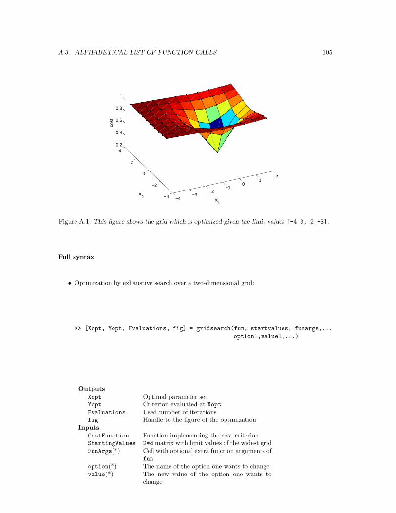
A.3. ALPHABETICAL LIST OF FUNCTION CALLS 105
−4−3
−2−1
01
2
−4
−2
0
2
40.2
0.4
0.6
0.8
1
X1
X2
cost
Figure A.1: This figure shows the grid which is optimized given the limit values [-4 3; 2 -3].
Full syntax
• Optimization by exhaustive search over a two-dimensional grid:
>> [Xopt, Yopt, Evaluations, fig] = gridsearch(fun, startvalues, funargs,...
option1,value1,...)
OutputsXopt Optimal parameter setYopt Criterion evaluated at XoptEvaluations Used number of iterationsfig Handle to the figure of the optimization
InputsCostFunction Function implementing the cost criterionStartingValues 2*d matrix with limit values of the widest gridFunArgs(*) Cell with optional extra function arguments of
fun
option(*) The name of the option one wants to changevalue(*) The new value of the option one wants to
change
106 APPENDIX A. MATLAB FUNCTIONS
The different options:
’Nofigure’ ’figure’(*) or ’nofigure’’MaxFunEvals’ Maximum number of function evaluations (de-
fault: 100)’GridReduction’ grid reduction parameter (e.g. ’2’: small re-
duction; ‘10’: heavy reduction; default ’5’)’TolFun’ Minimal toleration of improvement on func-
tion value (default: 0.0001)’TolX’ Minimal toleration of improvement on X value
(default: 0.0001)’Grain’ Square root number of function evaluations in
one grid (default: 10)
• Optimization by exhaustive search of linesearch:
>> [Xopt, Yopt, Evaluations, fig] = linesearch(fun, startvalues, funargs,...
option1,value1,...)
OutputsXopt Optimal parameter setYopt Criterion evaluated at Xoptiterations Used number of iterationsfig Handle to the figure of the optimization
InputsCostFun Function implementing the cost criterionStartingValues 2*d matrix with limit values of the widest gridFunArgs(*) Cell with optional extra function arguments of
fun
option(*) The name of the option one wants to changevalue(*) The new value of the option one wants to
change
The different options:
’Nofigure’ ’figure’(*) or ’nofigure’’MaxFunEvals’ Maximum number of function evaluations (de-
fault: 20)’GridReduction’ grid reduction parameter (e.g. ’1.5’: small re-
duction; ‘10’: heavy reduction; default ’2’)’TolFun’ Minimal toleration of improvement on func-
tion value (default: 0.01)’TolX’ Minimal toleration of improvement on X value
(default: 0.01)’Grain’ Number of evaluations per iteration (default:
10)
Full syntax
• SIMPLEX - multidimensional unconstrained non-linear optimization. Simplex finds a localminimum of a function, via a function handle fun, starting from an initial point X. The localminimum is located via the Nelder-Mead simplex algorithm [23], which does not require anygradient information. opt contains the user specified options via a structure. The differentoptions are set via a structure with members denoted by opt.*
>> Xopt = simplex(fun,X,opt)

A.3. ALPHABETICAL LIST OF FUNCTION CALLS 107
• The different options:
opts.Chi Parameter governing expansion steps (default:2)
opts.Delta Parameter governing size of initial simplex(default: 1.2)
opts.Gamma Parameter governing contraction steps (de-fault: 0.5)
opts.Rho Parameter governing reflection steps (default:1)
opts.Sigma Parameter governing shrinkage steps (default:0.5)
opts.MaxIter Maximum number of optimization steps (de-fault: 15)
opts.MaxFunEvals Maximum number of function evaluations (de-fault: 25)
opts.TolFun Stopping criterion based on the relativechange in value of the function in each step(default: 1e-6)
opts.TolX Stopping criterion based on the change in theminimizer in each step (default: 1e-6)
See also:
trainlssvm, crossvalidate
108 APPENDIX A. MATLAB FUNCTIONS
A.3.37 windowize & windowizeNARX
Purpose
Re-arrange the data points into a (block) Hankel matrix for (N)AR(X) time-series modeling
Basic Syntax
>> w = windowize(A, window)
>> [Xw,Yw] = windowizeNARX(X,Y,xdelays, ydelays, steps)
Description
Use windowize function to make a nonlinear AR predictor with a nonlinear regressor. The lastelements of the resulting matrix will contain the future values of the time-series, the others willcontain the past inputs. window is the relative index of data points in matrix A, that are selectedto make a window. Each window is put in a row of matrix W. The matrix W contains as many rowsas there are different windows selected in A.
Schematically, this becomes
>> A = [a1 a2 a3;
b1 b2 b3;
c1 c2 c3;
d1 d2 d3;
e1 e2 e3;
f1 f2 f3;
g1 g2 g3];
>> W = windowize(A, [1 2 3])
W =
a1 a2 a3 b1 b2 b3 c1 c2 c3
b1 b2 b3 c1 c2 c3 d1 d2 d3
c1 c2 c3 d1 d2 d3 e1 e2 e3
d1 d2 d3 e1 e2 e3 f1 f2 f3
e1 e2 e3 f1 f2 f3 g1 g2 g3
The function windowizeNARX converts the time-series and its exogeneous variables into a blockHankel format useful for training a nonlinear function approximation as a nonlinear ARX model.
Full syntax
• >> Xw = windowize(X, window)
The length of window is denoted by w.
OutputsXw (N-w+1)×—w— matrix of the sequences of windows over X
InputsX N×1 vector with data pointsw w×1 vector with the relative indices of one window
• >> [Xw, Yw, xdim, ydim, n] = windowizeNARX(X, Y, xdelays, ydelays)
>> [Xw, Yw, xdim, ydim, n] = windowizeNARX(X, Y, xdelays, ydelays, steps)
A.3. ALPHABETICAL LIST OF FUNCTION CALLS 109
OutputsXw Matrix of the data used for input including the delaysYw Matrix of the data used for output including the next stepsxdim(*) Number of dimensions in new inputydim(*) Number of dimensions in new outputn(*) Number of new data points
InputsX N×m vector with input data pointsY N×d vector with output data pointsxdelays Number of lags of X in new inputydelays Number of lags of Y in new inputsteps(*) Number of future steps of Y in new output (by default 1)
See also:
windowizeNARX, predict, trainlssvm, simlssvm

110 APPENDIX A. MATLAB FUNCTIONS
Bibliography
[1] Alzate C. and Suykens J.A.K. (2008), “Kernel Component Analysis using an Epsilon Insen-sitive Robust Loss Function”, IEEE Transactions on Neural Networks, 19(9), 1583–1598.
[2] Alzate C. and Suykens J.A.K. (2010), “Multiway Spectral Clustering with Out-of-SampleExtensions through Weighted Kernel PCA”, IEEE Transactions on Pattern Analysis andMachine Intelligence, 32(2), 335–347.
[3] Baudat G., Anouar F. (2001), “Kernel-based methods and function approximation”, in Inter-national Joint Conference on Neural Networks (IJCNN 2001), Washington DC USA, 1244–1249.
[4] Cawley G.C., Talbot N.L.C. (2002), “Efficient formation of a basis in a kernel induced featurespace”, in Proc. European Symposium on Artificial Neural Networks (ESANN 2002), BruggeBelgium, 1–6.
[5] Cristianini N., Shawe-Taylor J. (2000), An Introduction to Support Vector Machines, Cam-bridge University Press.
[6] De Brabanter J., Pelckmans K., Suykens J.A.K., Vandewalle J. (2002), “Robust cross-validation score function for LS-SVM non-linear function estimation”, International Con-ference on Artificial Neural Networks (ICANN 2002), Madrid Spain, Madrid, Spain, Aug.2002, 713–719.
[7] De Brabanter K., Pelckmans K., De Brabanter J., Debruyne M., Suykens J.A.K., HubertM., De Moor B. (2009), “Robustness of Kernel Based Regression: a Comparison of IterativeWeighting Schemes”, Proc. of the 19th International Conference on Artificial Neural Networks(ICANN), Limassol, Cyprus, September, 100–110.
[8] De Brabanter K., De Brabanter J., Suykens J.A.K., De Moor B. (2010), “Optimized Fixed-Size Kernel Models for Large Data Sets”, Computational Statistics & Data Analysis, 54(6),1484–1504.
[9] De Brabanter K., De Brabanter J., Suykens J.A.K., De Moor B. (2010), “Approximate Con-fidence and Prediction Intervals for Least Squares Support Vector Regression”, TechnicalReport, 10-156.
[10] Evgeniou T., Pontil M., Poggio T. (2000), “Regularization networks and support vectormachines,” Advances in Computational Mathematics, 13(1), 1–50.
[11] Fawcett T. (2006) “An Introduction to ROC analysis”, Pattern Recogniction Letters, 27,861–874.
[12] Girolami M. (2002), “Orthogonal series density estimation and the kernel eigenvalue prob-lem”, Neural Computation, 14(3), 669–688.
[13] Golub G.H. and Van Loan C.F. (1989), Matrix Computations, Johns Hopkins UniversityPress, Baltimore, MD.
111
112 BIBLIOGRAPHY
[14] Gyorfi L., Kohler M., Krzyzak A., Walk H. (2002), A Distribution-Free Theory of Nonpara-metric Regression, Springer
[15] Hall, P. (1992), “On Bootstrap Confidence Intervals in Nonparametric Regression,” Annalsof Statistics, 20(2), 695–711.
[16] Hanley J.A., McNeil B.J. (1982), “The meaning and use of the area under a receiver operatingcharacteristic (ROC) curve” Radiology 1982; 143, 29-36.
[17] Huber P.J. (1964), “Robust estimation of a location parameter”, Ann. Math. Statist., 35,73–101.
[18] Loader C. (1999), Local Regression and Likelihood, Springer-Verlag.
[19] MacKay D.J.C. (1992), “Bayesian interpolation”, Neural Computation, 4(3), 415–447.
[20] Mika S., Scholkopf B., Smola A., Muller K.-R., Scholz M., Ratsch G. (1999), “Kernel PCAand de-noising in feature spaces”, Advances in Neural Information Processing Systems 11,536–542, MIT Press.
[21] Mika S., Ratsch G., Weston J., Scholkopf B., Muller K.-R. (1999), “Fisher discriminantanalysis with kernels”, In Neural Networks for Signal Processing IX, 41–48, IEEE.
[22] Nabney I.T. (2002), Netlab: Algorithms for Pattern Recognition, Springer.
[23] Nelder J. A. and Mead R., (1965) “A simplex method for function minimization”, ComputerJournal, 7, 308-313.
[24] Poggio T., Girosi F. (1990), “Networks for approximation and learning”, Proc. of the IEEE,78, 1481–1497.
[25] Rice S.O. (1939), “The distribution of the maxima of a random curve,” American Journal ofMathematics, 61(2), 409-416.
[26] Ruppert D., Wand M.P. and Carroll R.J. (2003), Semiparametric Regression, CambridgeUniversity Press.
[27] Scholkopf B., Burges C., Smola A. (Eds.) (1998), Advances in Kernel Methods - SupportVector Learning, MIT Press.
[28] Scholkopf B., Smola A. J., Muller K.-R. (1998), “Nonlinear component analysis as a kerneleigenvalue problem”, Neural Computation, 10, 1299–1319.
[29] Scholkopf B., Smola A. (2002), Learning with Kernels, MIT Press.
[30] Smola A.J., Scholkopf B. (2000), “Sparse greedy matrix approximation for machine learning”,Proc. 17th International Conference on Machine Learning, 911–918, San Francisco, MorganKaufman.
[31] Stone M. (1974), “Cross-validatory choice and assessment of statistical predictions”, J. RoyalStatist. Soc. Ser. B, 36, 111–147.
[32] Suykens J.A.K., Vandewalle J. (1999), “Least squares support vector machine classifiers”,Neural Processing Letters, 9(3), 293–300.
[33] Suykens J.A.K., Vandewalle J. (2000), “Recurrent least squares support vector machines”,IEEE Transactions on Circuits and Systems-I, 47(7), 1109–1114.
[34] Suykens J.A.K., De Brabanter J., Lukas L., Vandewalle J. (2002), “Weighted least squaressupport vector machines : robustness and sparse approximation”, Neurocomputing, Specialissue on fundamental and information processing aspects of neurocomputing, 48(1-4), 85–105.
BIBLIOGRAPHY 113
[35] Suykens, J. A. K., Vandewalle, J., & De Moor, B. (2001), “Intelligence and cooperativesearch by coupled local minimizers”, International Journal of Bifurcation and Chaos, 11(8),21332144.
[36] Sun J. and Loader C.R. (1994), “Simultaneous confidence bands for linear regression andsmoothing,” Annals of Statistics, 22(3), 1328-1345.
[37] Suykens J.A.K., Van Gestel T., Vandewalle J., De Moor B. (2002), “A support vector machineformulation to PCA analysis and its Kernel version”, IEEE Transactions on Neural Networks,14(2), 447–450.
[38] Suykens J.A.K., Van Gestel T., De Brabanter J., De Moor B., Vandewalle J. (2002), LeastSquares Support Vector Machines, World Scientific, Singapore.
[39] Suykens J.A.K. (2008), “Data Visualization and Dimensionality Reduction using Kernel Mapswith a Reference Point”, IEEE Transactions on Neural Networks, 19(9), 1501–1517.
[40] Van Belle V., Pelckmans K., Suykens J.A.K., Van Huffel S. (2010), “Additive survival leastsquares support vector machines”, Statistics in Medicine, 29(2), 296–308.
[41] Van Gestel T., Suykens J.A.K., Baestaens D., Lambrechts A., Lanckriet G., Vandaele B., DeMoor B., Vandewalle J. (2001) “Financial time series prediction using least squares supportvector machines within the evidence framework”, IEEE Transactions on Neural Networks(special issue on Neural Networks in Financial Engineering), 12(4), 809–821.
[42] Van Gestel T., Suykens J.A.K., De Moor B., Vandewalle J. (2001), “Automatic relevancedetermination for least squares support vector machine classifiers”, Proc. of the EuropeanSymposium on Artificial Neural Networks (ESANN 2001), Bruges, Belgium, 13–18.
[43] Van Gestel T., Suykens J.A.K., Baesens B., Viaene S., Vanthienen J., Dedene G., De MoorB., Vandewalle J. (2001), “Benchmarking least squares support vector machine classifiers ”,Machine Learning, 54(1), 5–32.
[44] Van Gestel T., Suykens J.A.K., Lanckriet G., Lambrechts A., De Moor B., Vandewalle J.(2002), “Bayesian framework for least squares support vector machine classifiers, gaussianprocesses and kernel fisher discriminant analysis”, Neural Computation, 15(5), 1115–1148.
[45] Van Gestel T., Suykens J.A.K., Lanckriet G., Lambrechts A., De Moor B., Vandewalle J.(2002), “Multiclass LS-SVMs : moderated outputs and coding-decoding schemes”, NeuralProcessing Letters, 15(1), 45–58.
[46] Van Gestel T., Suykens J.A.K., De Moor B., Vandewalle J. (2002), “Bayesian inference forLS-SVMs on large data sets using the Nystrom method”, International Joint Conference onNeural Networks (WCCI-IJCNN 2002), Honolulu, USA, May 2002, 2779–2784.
[47] Vapnik V. (1995), The Nature of Statistical Learning Theory, Springer-Verlag, New York.
[48] Vapnik V. (1998), Statistical Learning Theory, John Wiley, New-York.
[49] Williams C.K.I., Seeger M. (2001), “Using the Nystrom method to speed up kernel machines”,Advances in neural information processing systems, 13, 682–688, MIT Press.
[50] Wahba G.,Wold S. (1975), “A completely automatic french curve: fitting spline functions bycross-validation”, Comm. Statist., 4, 1-17.
[51] Wahba G. (1990), Spline Models for observational data, SIAM, 39.
[52] Xavier de Souza, S., Suykens, J. A. K., Vandewalle, J., & Bolle, D. (2010), “Coupled SimulatedAnnealing”, IEEE Transactions on Systems, Man and Cybernetics - Part B, 40(2), 320–335.