Lyapunov Exponents for Random Dynamical Systems Thai Son_Dissertation.pdf · Lyapunov Exponents for...
181
Lyapunov Exponents for Random Dynamical Systems DISSERTATION zur Erlangung des akademischen Grades Doctor rerum naturalium (Dr.rer.nat.) vorgelegt der Fakult¨at Mathematik und Naturwissenschaften der Technischen Universit¨at Dresden von Bachel.-Math. Doan Thai Son geboren am 05.10.1984 in Namdinh Gutachter: Prof. Stefan Siegmund Technische Universit¨ at Dresden Prof. Nguyen Dinh Cong Hanoi Institute of Mathematics, Vietnam Eingereicht am: 15.1.2009 Tag der Disputation: 27.11.2009
Transcript of Lyapunov Exponents for Random Dynamical Systems Thai Son_Dissertation.pdf · Lyapunov Exponents for...
Lyapunov Exponents forRandom Dynamical Systems
DISSERTATION
zur Erlangung des akademischen Grades
Doctor rerum naturalium
(Dr.rer.nat.)
vorgelegt
der Fakultat Mathematik und Naturwissenschaften
der Technischen Universitat Dresden
von
Bachel.-Math. Doan Thai Son
geboren am 05.10.1984 in Namdinh
Gutachter: Prof. Stefan Siegmund
Technische Universitat Dresden
Prof. Nguyen Dinh Cong
Hanoi Institute of Mathematics, Vietnam
Eingereicht am: 15.1.2009
Tag der Disputation: 27.11.2009


Contents
Introduction 1
1 Background on Random Dynamical Systems 9
1.1 Definition of Random Dynamical System . . . . . . . . . . . . . . . . . . 9
1.2 Generation . . . . . . . . . . . . . . . . . . . . . . . . . . . . . . . . . . 16
1.2.1 Discrete Time: Products of Random Mappings . . . . . . . . . . 16
1.2.2 Continuous Time 1: Random Differential Equations . . . . . . . 17
1.2.3 Continuous Time 2: Stochastic Differential Equations . . . . . . 19
1.3 Multiplicative Ergodic Theorem in Rd . . . . . . . . . . . . . . . . . . . 20
1.3.1 Singular Values . . . . . . . . . . . . . . . . . . . . . . . . . . . . 20
1.3.2 Exterior Powers . . . . . . . . . . . . . . . . . . . . . . . . . . . . 21
1.3.3 The Furstenberg-Kesten Theorem . . . . . . . . . . . . . . . . . 22
1.3.4 Multiplicative Ergodic Theorem . . . . . . . . . . . . . . . . . . 24
1.4 Multiplicative Ergodic Theorem in Banach Spaces . . . . . . . . . . . . 25
2 Generic Properties of Lyapunov Exponents of Discrete Random Dy-namical Systems 29
2.1 The Space of Linear Cocycles . . . . . . . . . . . . . . . . . . . . . . . . 29
2.2 Uniformly Hyperbolic Linear Cocycles . . . . . . . . . . . . . . . . . . . 31
2.2.1 Exponential Dichotomy . . . . . . . . . . . . . . . . . . . . . . . 31
2.2.2 Exponential Separation of Bounded Cocycles . . . . . . . . . . . 39
2.2.3 Exponential Dichotomy is Strictly Stronger than Exponential Sep-aration . . . . . . . . . . . . . . . . . . . . . . . . . . . . . . . . 41
2.2.4 Exponential Separation of Unbounded Cocycles . . . . . . . . . . 44
2.3 An Open Set of Cocycles with Simple Lyapunov Spectrum but no Expo-nentially Separated Splitting . . . . . . . . . . . . . . . . . . . . . . . . 50
3 Generic Properties of Lyapunov Exponents of Linear Random Differ-ential Equations 58
3.1 Spaces of Linear Random Differential Equations . . . . . . . . . . . . . 59
3.2 Generic Properties of Lyapunov Exponents of Linear Random DifferentialEquations . . . . . . . . . . . . . . . . . . . . . . . . . . . . . . . . . . . 60
i

4 Difference Equations with Random Delay 644.1 A Setting for Difference Equations with Random Delay . . . . . . . . . 664.2 MET for Difference Equations with Random Delay . . . . . . . . . . . . 704.3 Some Examples . . . . . . . . . . . . . . . . . . . . . . . . . . . . . . . . 78
4.3.1 Bounded Random Delay . . . . . . . . . . . . . . . . . . . . . . . 794.3.2 Deterministic Delay . . . . . . . . . . . . . . . . . . . . . . . . . 82
5 Differential Equations with Random Delay 855.1 Differential Equations with Random Delay . . . . . . . . . . . . . . . . . 855.2 MET for differential equations with random delay . . . . . . . . . . . . 93
5.2.1 Integrability . . . . . . . . . . . . . . . . . . . . . . . . . . . . . . 935.2.2 Kuratowski Measure . . . . . . . . . . . . . . . . . . . . . . . . . 955.2.3 Multiplicative Ergodic Theorem . . . . . . . . . . . . . . . . . . 99
5.3 Differential equations with bounded delay . . . . . . . . . . . . . . . . . 104
6 Computational Ergodic Theorem 1076.1 Iterated Function Systems . . . . . . . . . . . . . . . . . . . . . . . . . . 109
6.1.1 Finite Iterated Function Systems . . . . . . . . . . . . . . . . . . 1096.1.2 Finite Iterated Function Systems with Place-dependent Probabilities1136.1.3 Infinite Iterated Function Systems . . . . . . . . . . . . . . . . . 115
6.2 Computational Ergodic Theorem for Place-dependent IFS . . . . . . . . 1226.3 Computational Ergodic Theorem for IIFS . . . . . . . . . . . . . . . . . 125
6.3.1 Approximating IIFS through a Sequence of IFS . . . . . . . . . . 1256.3.2 An Approximation and Convergence Result . . . . . . . . . . . . 128
6.4 Products of Random Matrices . . . . . . . . . . . . . . . . . . . . . . . . 1326.4.1 Products of Random Matrices . . . . . . . . . . . . . . . . . . . . 1326.4.2 An Approximation and Convergence Result . . . . . . . . . . . . 136
6.5 Examples . . . . . . . . . . . . . . . . . . . . . . . . . . . . . . . . . . . 139
7 Outlook 1467.1 One-Sided RDS on Banach Space . . . . . . . . . . . . . . . . . . . . . . 1467.2 Lyapunov norm for RDS on Banach Space . . . . . . . . . . . . . . . . . 153
Appendices 155
A Birkhoff Ergodic Theorem 156
B Kingman Subadditive Ergodic Theorem 161
C Baire Category and Baire Class of Functions 165
Bibliography 167
Index 177
Introduction
A dynamical system is a concept in mathematics where a specified rule describes thetime dependence of a point in a state space. The mathematical models used to describethe motion of planets, the swinging of a clock pendulum in Newton’s mechanics, the flowof water in a pipe, chemical reactions, or even the number of fish each spring in a lakeare examples of dynamical systems. A dynamical system is determined by a state spaceand a fixed evolution rule which describes how future states follow from the currentstate.
The history of dynamical system began with the foundational work of Poincare [117]and Lyapunov [90] on the qualitative behavior of ordinary differential equations. Theconcept of dynamical systems was then introduced by Birkhoff [18], followed by impor-tant contributions by Markov [94], Nemytskii and Stefanov [107], Bhatia and Szegoe[16], Smale [127], among others. The main goal of this theory is to study the qualitativebehavior of systems from geometrical and topological view points.
The concept of random dynamical systems is a comparatively recent developmentcombining ideas and methods from the well developed areas of probability theory anddynamical systems. Due to our inaccurate knowledge of the particular model or dueto computational or theoretical limitations (lack of sufficient computational power, in-efficient algorithms or insufficiently developed mathematical and physical theory, forexample), the mathematical models never correspond exactly to the phenomenon theyare meant to model. Moreover, when considering practical systems we cannot avoid ei-ther external noise or inaccuracy errors in measurements, so every realistic mathematicalmodel should allow for small errors along orbits. To be able to cope with unavoidableuncertainty about the ”correct” parameter values, observed initial states and even thespecific mathematical formulation involved, we let randomness be embedded within themodel. Therefore, random dynamical systems arise naturally in the modeling of manyphenomena in physics, biology, economics, climatology, etc.
The concept of random dynamical systems was mainly developed by Arnold [3] andhis ”Bremen group”, based on the research of Baxendale [13], Bismut [19], Elworthy [52],Gihman and Skorohod [65], Ikeda and Watanabe [72] and Kunita [83] on two-parameterstochastic flows generated by stochastic differential equations. Three main classes ofrandom dynamical systems are:
• Products of random maps: Let (Ω,F ,P) be a probability space and θ : Ω → Ωan ergodic transformation preserving the probability P. Let (X,B) be a measur-
1

2
able space. For a given measurable function ψ : Ω × X → X we can define thecorresponding random dynamical system ϕ : N × Ω ×X → X by
ϕ(n, ω) =
ψ(θn−1ω) · · · ψ(ω), if n ≥ 1,
idX , otherwise.(1)
The random dynamical system ϕ is said to be generated by the random mappingψ. Conversely, every one-sided discrete time random dynamical system has theform (1), i.e. is a product of random mappings, or an iterated function system, ora system in a random environment (see Arnold [3, pp. 50]).
• Random differential equations: Let (Ω,F ,P) be a probability space and (θt)t∈R :Ω → Ω an ergodic flow preserving the probability P. Let f : Ω × Rd → Rd be ameasurable function satisfying that for a fixed ω ∈ Ω the function (t, x) 7→ f(θtω, x)is locally Lipschitz in x, integrable in t and
‖f(ω, x)‖ ≤ α(ω)‖x‖ + β(ω),
where t 7→ α(θtω) and t 7→ β(θtω) are locally integrable. Then the random differ-ential equation
x = f(θtω, x)
uniquely generates a continuous random dynamical system ϕ : R+ ×Ω×Rd → Rd
satisfying
ϕ(t, ω)x = x+
∫ t
0f(θsω,ϕ(s, ω)x) ds,
(we refer to Arnold [3, pp. 57–63] for more details).
• Stochastic differential equations: The classical Stratonovic stochastic differentialequation
dxt = f0(xt)dt +
m∑
j=1
fj(xt) dW jt , t ∈ R,
where f0, . . . , fm are smooth vector fields, and W is standard Brownian motionof Rm generates a unique (up to indistinguishability) smooth random dynamicalsystem ϕ over the filtered dynamical system describing Brownian motion (we referto Arnold [3, pp. 68-107] for more details).
For the gap between random dynamical systems and continuous skew products werefer to the paper by Berger and Siegmund [15].
Lyapunov exponent or Lyapunov characteristic exponent of a dynamical system isa quantity that characterizes the rate of separation of infinitesimally close trajectories.The concept was introduced by Lyapunov when studying the stability of non-stationarysolutions of ordinary differential equations, and has been widely employed in studyingdynamical systems since then.
3
The fundamental results on Lyapunov exponents for random dynamical systems onfinite dimensional systems were first obtained by Oseledets [109] in 1968, which is nowcalled the Oseledets Multiplicative Ergodic Theorem. Originally formulated for productsof random matrices, it has been reformulated and reproved several times during the pastthirty years. Basically, there are two classes of proofs. One makes use of the Kingman’sSubadditive Ergodic Theorem together with the polar decomposition of square matrices(see Arnold [3] and the references therein). The other one relies on the triangularizationof a linear cocycle and the classical ergodic theorem for the triangular cocycles. Thistechnique was also used in the contemporaneous paper of Millionscikov [97] who inde-pendently derived a portion of the multiplicative ergodic theorem, and then taken upagain by Johnson, Palmer and Sell [74] (assuming a topological setting for the metricdynamical system).
Thanks to the multiplicative ergodic theorem of Oseledets [109], the Lyapunov spec-trum of products of random matrices is well defined (under some integrability conditions)and it is a generalization of the Lyapunov spectrum in the deterministic case and theOseledets subspaces are generalizations of the eigenspaces.
The study of the Lyapunov spectrum of linear cocycles is one of the central tasks ofthe theory of random dynamical systems (see Arnold [3]). In various situations it is oftheoretical and practical importance to know when the Lyapunov spectrum is simpleand the Oseledets splitting is exponentially separated. Recently, Arbieto and Bochi [2],Bochi [21], Bochi and Viana [22, 23], Bonatti and Viana [24] and Cong [36] have derivedsome new results on genericity of hyperbolicity of several classes of dynamical systemsincluding smooth dynamical systems and linear cocycles. Let us mention here a resultof Cong [36] stating that the set of cocycles with integral separation is open and densein the space of all bounded Gl(d,R)-cocycles equipped with the uniform topology. Asa consequence, a generic bounded linear cocycle has simple Lyapunov spectrum andexponentially separated Oseledets splitting. In Chapter 2, we show that this resultcannot be extended to the case of unbounded cocycles. In particular, we construct anopen set of cocycles with simple Lyapunov spectrum but no exponentially separatedsplitting.
Generic properties of Lyapunov exponents have recently been extended to continuoustime. Basse [14] has shown that for a C0-generic subset of all the 2-dimensional conser-vative nonautonomous linear differential equations, either Lyapunov exponents are zeroor there is a dominated splitting. Dai [42] investigated the generic properties of contin-uous linear skew-product systems. His results ensured that based on a uniquely ergodicequi-continuous endomorphism the set of linear hyperbolic skew-product systems is openand dense in the set of all skew product systems. In Chapter 3, using the approach inArnold and Cong [4] we obtain several generic properties of Lyapunov exponents oflinear random differential equations. Precisely, we are able to show that the Lyapunovexponents are of the second Baire class. As a consequence, there exists a residual set onwhich the Lyapunov exponents are continuous. In other words, generically the Lyapunovexponents of linear random differential equations depend continuously on the coefficient.
Multiplicative ergodic theory becomes much more difficult when considering infi-nite dimensional random dynamical systems, i.e. random dynamical systems on infinite
4
dimensional Banach spaces. Recall that for a finite dimensional linear deterministicsystem the Lyapunov exponents are precisely the real parts of the eigenvalues of A (forcontinuous time, x = Ax) or the logarithms of the eigenvalues of A (for discrete time,xn+1 = Axn), respectively. Thus, the Lyapunov exponents are determined by the spec-trum. Since the spectra of infinite dimensional operators in general have a considerablymore complicated structure than finite dimensional ones, it is clear that much less canbe expected for infinite dimensional random dynamical systems.
In his remarkable paper [122], Ruelle extended the classical multiplicative ergodictheorem to compact linear random operators in a separable Hilbert space with a basemeasurable metric dynamical system in a probability space. A typical example of thesemaps is the time-one map of the solution operator of a stochastic or random parabolicpartial differential equation. In this case, one has to face the difficulties arising fromthe fact that the phase space is not locally compact and the dynamical system maynot be invertible over the phase space. Ruelle’s results have been applied to studycertain stochastic partial differential equations and delay differential equations (see,e.g., Mohammed and Scheutzow [102]).
Later, Mane [93] extended the multiplicative ergodic theorem to compact operatorsin a Banach space, where the base metric dynamical system is a homeomorphism over acompact topological space. A drawback of Mane’s results is that they can not be appliedto random dynamical systems generated by stochastic partial differential equations.Besides the obstacles Ruelle encountered in a Hilbert space, one also needs to overcomethe problem that there is no inner product.
Thieullen [136] further extended Mane’s results on Lyapunov exponents to boundedlinear operators in a Banach space, where the base metric dynamical system is a home-omorphism over a topological space which is homeomorphic to a Borel subset of aseparable metric space.
In [54], Flandoli and Schaumloffel obtained a multiplicative ergodic theorem forrandom isomorphisms on a separable Hilbert space with a measurable metric dynamicalsystem over a probability space. This result is used to study hyperbolic stochastic partialdifferential equations. Schaumloffel [124] extended the multiplicative ergodic theoremto a class of bounded random linear operators which map a closed linear subspace ontoa closed linear subspace in a Banach space with certain convexity.
Recently, Lian and Lu [89] extended the multiplicative ergodic theorem to a generalsetting, products of random bounded operators on a Banach space with a measurablemetric dynamical system over a probability space. Crauel, Doan and Siegmund [41]used this result to study scalar difference equations with random delay. After that,based on the multiplicative ergodic theorem results by Lian and Lu [89], differentialequations with random delay are investigated by Doan and Siegmund [45]. The work ofCrauel, Doan and Siegmund [41] and Doan and Siegmund [45] can be considered as thefirst step towards a general theory of difference and differential equations incorporatingunbounded random delays. In Chapter 4 we extend the results in Crauel, Doan andSiegmund [41] on Lyapunovs exponents of difference equations with random delay toarbitrary dimension. Moreover, the coefficients are also random. In particular, we showthat the number of Lyapunov exponents of difference equations is always finite. Using
5
the materials in Doan and Siegmund [45], differential equations with random delay areinvestigated in Chapter 5.
Computational methods are a basic tool in investigation of dynamical systems, bothto explore what may happen and to approximate specific dynamical features such aslimit cycles and attractors and, more generally, invariant measures, see e.g., Stuart andHumphries [134].
Invariant measures is a central concept in the theory of dynamical system, bothdeterministic and random, and their investigation has been closely related to develop-ments in ergodic theory, see e.g., Katok and Hasselblatt [76]. A variety of methods havebeen proposed and implemented for computing invariant measures, see e.g., Dellnitz,Froyland and Junge [43], Dellnitz and Junge [44], Diamond, Kloeden and Pokrovskii[46] and Guder, Dellnitz and Kreuzer [68].
By discretizing the state space and replacing the action of generator by the transitionmechanism of a Markov chain, Imkeller and Kloeden [73] provided a method for com-puting invariant measures of dynamical system generated by difference equations. Foriterated functions systems, which are important examples of random dynamical system,Perrugia [114] introduced a general method of discretisation as a way of approximatingthe attracting set and invariant measure. Using an extension of this construction, Froy-land [56] and Froyland and Aihara [57] present a computational method for rigorouslyapproximating the unique invariant measure of an iterated function system which iscontractive on average. The advantage of this method is that it provides quantitativebounds on the accuracy of the approximation. Using the same idea, Cong, Doan andSiegmund [38] extended this method to infinite iterated systems which are contractiveon average. In Chapter 6, we go one further step to provide a computational method forcomputing the invariant measure of a contractive on average iterated functions systemwith place-dependent probabilities and an infinite iterated functions system which isl-contractive on average - a notion which is more general than contractive on average.With a rigorous method for computing invariant measures at hand, we also provide amethod for computing the Lyapunov exponents of products of random matrices whichserve as a main generator of random dynamical systems.
Invariant manifold theory for RDS based on the MET is an important part ofsmooth ergodic theory. It was started in 1976 with the pioneering work of Pesin [115,116]. He constructed the classical stable and unstable manifolds of a deterministicdiffeomorphism on a compact Riemannian manifolds preserving a measure which isabsolutely continuous with respect to the Riemannian volume. His technique is to copewith the non-uniformity of the MET (random norms, ε-slowly varying functions). Thistechnique is also used in Wanner [139] and Arnold [3] to construct invariant manifoldsfor RDS on finite dimensional space. In chapter 7, we provide the Lyapunov normcorresponding to a linear equation with random delay. This can be considered as thefirst technical step toward the nonlinear theory of equations with random delay.
To conclude the introduction let us outline the structure of the thesis. Chapter 1 isdevoted to provide some fundamental aspects of random dynamical systems. We firststart with the notion of metric dynamical system. Based on a metric dynamical systemthe notion of random dynamical systems is defined. Three important classes of linear
6
random dynamical systems, namely products of random matrices, random differentialequations and stochastic differential equations, are discussed. In the remaining part ofthis chapter, one of the most important theorems for random dynamical systems, themultiplicative ergodic theorem, is presented.
In Chapter 2, we deal with the generic properties of random dynamical systemshaving dominated splitting. The notion of dominated splitting is discussed carefullyin the first part of this chapter. More precisely, we point out that in the definition ofdominated splitting the condition that the angle between the invariant subspaces areuniformly bounded from zero plays an important role in deciding the robustness of thisnotion. In the remaining part of this chapter, we construct an explicit open set of linearrandom dynamical systems with simple Lyapunov spectrum but no dominated splitting.Consequently, the set of all random dynamical systems having dominated splitting isnot generic. Moreover, unlike the case of bounded linear random dynamical systemsthe continuity of Lyapunov exponents is not equivalent to the existence of a dominatedsplitting.
The generic properties of Lyapunov exponents for random differential equationsis the main topic in Chapter 3. In this chapter, we first introduce the space of allrandom differential equations satisfying the integrability condition of the multiplicativeergodic theorem. On this space, we show that the top Lyapunov exponent is uppersemi-continuous. Consequently, the repeated Lyapunov exponents are of the first Baireclass. However, the Lyapunov exponents are only of the second Baire class.
Difference equations with random delay is the topic of Chapter 4. By introducing anappropriate initial value space, we obtain random dynamical systems corresponding todifference equations with random delay in infinite dimension. Under natural assumptionson the random delay and coefficients we show that the generated random dynamicalsystem satisfies the integrability condition of the multiplicative ergodic theorem by Lianand Lu [89]. The Kuratowski measures of the generated random dynamical systems areexplicitly computed. Consequently, the Lyapunov exponents for difference equationswith random delay are provided. It is also worth emphasizing that the number ofLyapunov exponents for difference equations with random delay is finite. Differenceequations with constant delay and bounded random delay are also investigated in orderto see the link between classical results and our new results about infinite dimensionalrandom dynamical systems.
In Chapter 5, we extend the results of Chapter 4 to differential equations with ran-dom delay. We first introduce the space of initial values. Second, we prove the existenceand uniqueness of solutions of differential equations with random delay. Based on theseresults, the corresponding random dynamical system is defined. Checking the integrabil-ity condition and computing the Kuratowski mueasure of the random dynamical systemleads to a multiplicative ergodic theorem for random differential equations with randomdelay.
In Chapter 6, we provide a method to compute invariant measures for iterated func-tion systems with place-dependent probabilities and infinite iterated function systems.We start this chapter by introducing the notion of iterated function systems, iteratedfunction systems with place-dependent probabilities, and infinite iterated function sys-

7
tems. A short proof of an ergodic theorem for infinite iterated function systems whichare l-contractive on average is given. We then construct an approximating sequence offinite iterated function systems. Using the method for computing the invariant mea-sure of a finite iterated function system we obtain a numerical method to compute theinvariant measures of iterated function systems with place-dependent probabilities andinfinite iterated function systems. In the last section of the chapter, we apply the aboveprocedure to compute numerically the Lyapunov exponents for a special class of ran-dom dynamical systems, products of random matrices. Several examples are providedto illustrate the method.
Finally, in the first part of Chapter 7 we state and prove the MET for one-sidedRDS on Banach space. In the last part of Chapter 7, we construct the Lyapunov normcorresponding to a linear equation with random delay. This work is the first attempt toestablish the nonlinear theory of equations with random delay.
This thesis contains new results, some are published with multiple authors in Congand Doan [37], Cong, Doan and Siegmund [38], Crauel, Doan and Siegmund [41] andDoan and Siegmund [45]. Not all of the results of these papers are repeated here, butonly those to which I actively and critically made contributions.

Acknowledgement
This work would not have been possible without the help of many people, to whom Iwould like to express my gratitude at this place.
First of all, I am very grateful to my advisor, Prof. Dr. Stefan Siegmund. Prof. Siegmundproposed me this interesting subject. He taught me how to ask questions and explainmathematical issues in a very intuitive way. I greatly benefited from his broad knowledgeand I thank him for discussing with me lots of problems during the time I wrote thisthesis, as well as helping me read carefully the manuscript, correcting the mistakes andsuggesting the better presentation. His help really improved the quality of my thesis.
I also want to thank Prof. Dr. Gerhard Keller for pointing out several formulations andstatements in an earlier version which needed clarification.
I also take this chance to greatly thank my co-advisor in Vietnam, Prof. Dr. NguyenDinh Cong, who always encouraged me to become a mathematician, recommended meto study abroad and gave me a lot of advice not only in the scientific life but also beyond.
My special thanks go also to the Institute for Analysis, Technical University of Dresden,for offering an active PhD program and for a friendly working environment.
My friendly thanks to my colleagues in the group, Dr. Anke Kalauch and Mr. NguyenTien Yet for the time we spent discussing together.
And last but not least, on a more personal note, I thank my parents, Mr. Doan TheLien and Mrs. Lam Thi Huyen, my brother, Mr. Doan Huy Hien and specially my grandmother for their love and supports during all these years. My thesis is dedicated to themas an expression of my respect.
8
Chapter 1
Background on Random
Dynamical Systems
This foundation chapter is devoted to recall some basic definitions and facts about ran-dom dynamical systems. For a more detailed discussion of the theory and applicationsof random dynamical systems we refer to the monograph Arnold [3]. We pay particularattention to the notion of the generator and Lyapunov exponent for random dynamicalsystems.Throughout the thesis we will be concerned with a probability space by which we meana triple (Ω,F ,P), where Ω is a set, F is a σ-algebra of sets in Ω, and P is a nonnegativeσ-additive measure on F with P(Ω) = 1. The time T always stands for the followingsemigroups or groups :
- T = R : Two-sided continuous time.
- T = Z := 0,±1,±2, . . . : Two-sided discrete time.
1.1 Definition of Random Dynamical System
A random dynamical system is an object consisting of a metric dynamical system and acocycle over this system. We need a metric dynamical system for modeling of randomperturbations. We begin with a definition of a metric dynamical system.
Definition 1.1.1 (Metric Dynamical System ). A metric dynamical system1 with timeT, θ ≡ (Ω,F ,P, (θt)t∈T), is a probability space (Ω,F ,P) with a family of transformationsθt : Ω → Ω, t ∈ T such that
(i) it is an one-parameter group, i.e.
θ0 = idΩ, θt θs = θt+s for all t, s ∈ T,
where idΩ is the identical map on Ω,
1”Metric Dynamical System(s)” is henceforth often abbreviated as ”MDS”.
9

Chapter 1: Background on Random Dynamical Systems 10
(ii) The mapping (t, ω) 7→ θtω is B(T) ⊗F ,F measurable,
(iii) θtP = P for all t ∈ T, i.e. P(θtB) = P(B) for all B ∈ F and all t ∈ T.
A set B ∈ F is called θ-invariant (for short invariant) if θtB = B for all t ∈ T. A metricdynamical system θ is said to be ergodic under P if for any invariant set B ∈ F we haveeither P(B) = 0 or P(B) = 1.
In the case that T is discrete, i.e. T = Z we use the notation (Ω,F ,P, (θn)n∈Z) instead ofthe notation (Ω,F ,P, (θt)t∈T) which is usually used in the continuous time case T = R
to denote an MDS with time T. We refer to Cornfeld, Fomin and Sinai [39], Walters[138] for the references and presentation of MDS and ergodic theorem. Now we giveseveral important examples of MDS.
Example 1.1.2 (Periodic Case). Consider the probability space (Ω,F ,P), where Ω isa circle of unit circumference, F is the σ-algebra of Borel sets and P is the Lebesguemeasure on Ω. Let (θt)t∈R be the group of rotations of the circle. It is easy to see thatwe obtain an ergodic MDS (Ω,F ,P, (θt)t∈R) with continuous time.
Example 1.1.3 (Quasi-Periodic Case). Let Ω be a d-dimensional torus, Ω = Tord. As-sume that its points are written as x = (x1, x2, . . . , xd) with xi ∈ [0, 1). Let F bethe σ-algebra of Borel sets of Tord and P the Lebesgue measure on Tord. We definetransformations (θt)t∈T by
θtx =(x1 + ta1(mod 1), x2 + ta2(mod 1), . . . , xd + tad(mod 1)
), t ∈ T,
for a given a = (a1, a2, . . . , ad). Thus we obtain an MDS. If the numbers a1, a2, . . . , ad
are rationally independent, then this MDS is ergodic (see, e.g., Rudolph [119]).
Example 1.1.4 (Almost Periodic Case). Let f(x) be a Bohr almost periodic function onR. We define the hull H(f) of the function f as the closure of the set f(x+ t), t ∈ Rin the norm ‖f‖ = supx∈R |f(x)|. The hull H(f) is a compact metric space and it has anatural commutative group structure. Therefore, it processes a Haar measure which, ifnormalized to unity, makes H(f) into a probability space. If we define transformations(θt)t∈R as shifts
θtg(x) = g(x+ t) for all g ∈ H(f),
then we obtain an ergodic MDS with continuous time. For details we refer to Ellis [49]and Leviton and Zhikov [88].
Example 1.1.5 (Ordinary Differential Equations). Let us consider a system of ordinarydifferential equation in Rd:
dxi
dt= fi(x1, x2, . . . , xd), i = 1, 2, . . . , d. (1.1)
Assume that the Cauchy problem for this system is well-posed. We define transforma-tions (θt)t∈R : Rd → Rd by θtx = x(t), where x(t) is the solution of (1.1) with x(0) = x.
11 1.1 Definition of Random Dynamical System
Assume that a nonnegative smooth function ρ(x1, x2, . . . , xd) satisfies the stationaryLiouville equation
d∑
i=1
∂
∂xi
(ρ(x1, x2, . . . , xd)fi(x1, x2, . . . , xd)
)= 0 (1.2)
and possesses the property∫
Rd ρ(x) dx = 1. Then ρ(x) is a density of a probabilitymeasure on Rd. By Liouville’s theorem we have
∫
Rd
f(θtx)ρ(x) dx =
∫
Rd
f(x)ρ(x) dx
for all bounded continuous functions f(x) on Rd. Therefore in this situation an MDSis generated with Ω = Rd, F = B(Rd) the Borel σ-algebra of sets in Rd and P(dx) =ρ(x) dx. Sometimes it is also possible to construct an MDS connected with (1.1), whenthe solution ρ of (1.2) possesses a first integral (e.g., if (1.1) is a Hamiltonian system)with appropriate properties (see, e.g., Sinai [126] for more details).
Example 1.1.6 (Bernoulli Shifts). Let (Ω0,F0,P0) be a probability space and (Ω,F ,P)the probability space of infinite sequences ω = (ωi)i∈Z, where ωi ∈ Ω0, i ∈ Z. Here F isthe σ-algebra generated by finite dimensional cylinders
Ci1,i2,...,im = ω |ωik ∈ Ck, k = 1, 2, . . . ,m,
where Ck ∈ F0 and i1, i2, . . . , im ∈ Z. The probability measure P is defined such thatP(Ci1,i2,...,im) = P0(C1)P0(C2) . . .P0(Cm). We define transformations (θt)t∈Z by (θtω)i =ωt+i for all i ∈ Z, ω ∈ Ω. Since
θtCi1,i2,...,im = ω |ωik−t ∈ Ck, k = 1, 2, . . . ,m,
the probability measure P is invariant under θt. Thus we obtain an MDS. In the particularcase when Ω0 = 0, 1 is a two-point set and P0(0) = P0(1) = 1/2, we have thestandard Bernoulli shift. In the general case we can interpret this MDS as one generatedby an infinite sequence of independent identically distributed random variables. Werefer the reader to Walter [138] for more details.
Example 1.1.7 (Stationary Random Process). Let ξ = (ξ(t))t∈T be a stationary randomprocess on a probability space (Ω,F ,P), where F is the σ-algebra generated by ξ. As-sume that in the continuous time case (T = R) the process ξ possesses the followingproperty: all trajectories are right-continuous and have limits from the left. Then theshift ξ(t) 7→ (θτξ)(t) = ξ(t + τ) generate an MDS. See Arnold [3] and the referencestherein for details.
In the framework of stochastic equations the following example of an MDS is of impor-tance.
Example 1.1.8 (Wiener Process). Let Wt = (W 1t ,W
2t , . . . ,W
dt ) be a Wiener process with
values in Rd and two-sided time R. Let (Ω,F ,P) be the corresponding canonical Wiener

Chapter 1: Background on Random Dynamical Systems 12
space. More precisely, let C0(R,Rd) be the space of continuous functions ω from R intoRd such that ω(0) = 0, endowed with the compact-open topology, i.e. with the topologygenerated by the metric
ρ(ω, ω∗) :=
∞∑
n=1
1
2n
ρn(ω, ω∗)
1 + ρn(ω, ω∗), ρn(ω, ω∗) = max
t∈[−n,n]|ω(t) − ω∗(t)|.
Let F be the corresponding Borel σ-algebra of C0(R,Rd), and let P be the Wienermeasure on F . We suppose that Ω is the subset in C0(R,Rd) consisting of the functionsthat have a growth rate less than linear when t→ ±∞ and F is the restriction of F toΩ. In this realization Wt(ω) = ω(t), where ω ∈ Ω, i.e. the elements of Ω are identifiedwith the paths of the Wiener process. We define an MDS θ by
θtω(·) := ω(t+ ·) − ω(t) for all ω ∈ Ω.
These transformations preserve the Wiener measure and are ergodic. Thus we have anergodic MDS. The flow (θt)t∈R is called the Wiener shift (for more details we refer toArnold [3, pp. 544-548]).
With the notion of MDS at hand, we are in a position to state the notion of randomdynamical system.
Definition 1.1.9 (Random Dynamical System [3]). A measurable random dynamicalsystem2 on the measurable space (X,B) over an MDS (Ω,F ,P, (θt)t∈T) with time T isa mapping
ϕ : T × Ω ×X → X, (t, ω, x) 7→ ϕ(t, ω, x)
with the following properties:
(i) Measurablity : ϕ is B(T) ⊗F ⊗ B,B-measurable.
(ii) Cocycle property : The mappings ϕ(t, ω) := ϕ(t, ω, ·) : X → X form a cocycle over(θt)t∈T, i.e. they satisfy
ϕ(0, ω) = idX for all ω ∈ Ω (if 0 ∈ T),
ϕ(t+ s, ω) = ϕ(t, θsω) ϕ(s, ω) for all s, t ∈ T, ω ∈ Ω,
where idX is the identical map on X.
Here ” ” means composition, which canonically defines an action on the left of thesemigroup of self-mappings of X on the space X, i.e. (f g)(x) = f(g(x)).
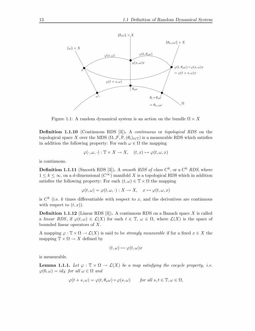
It is very useful to imagine an RDS as fiber maps on the bundle Ω × X. Figure 1.1can be explained as follows: While ω is shifted by the dynamical system θ in time s tothe point θsω on the base space Ω, the cocycle ϕ(s, ω) moves the point x in the fiberω × X over ω to the point ϕ(s, ω)x in the fiber θsω × X over θsω. The cocycleproperty can be clearly visualized on this bundle.
2”Random Dynamical System(s)” is henceforth often abbreviated as ”RDS”.
13 1.1 Definition of Random Dynamical System
ω ×X
x
ω
ϕ(s, ω)
ϕ(t + s, ω)
θsω ×X
ϕ(s, ω)x
θsω
ϕ(t, θsω)
θt+sω ×X
ϕ(t, θsω) ϕ(s, ω)x
= ϕ(t + s, ω)x
θt θsω
Ω= θt+sω
Figure 1.1: A random dynamical system is an action on the bundle Ω ×X
Definition 1.1.10 (Continuous RDS [3]). A continuous or topological RDS on thetopological space X over the MDS (Ω,F ,P, (θt)t∈T) is a measurable RDS which satisfiesin addition the following property: For each ω ∈ Ω the mapping
ϕ(·, ω, ·) : T ×X → X, (t, x) 7→ ϕ(t, ω, x)
is continuous.
Definition 1.1.11 (Smooth RDS [3]). A smooth RDS of class Ck, or a Ck RDS, where1 ≤ k ≤ ∞, on a d-dimensional (C∞) manifold X is a topological RDS which in additionsatisfies the following property: For each (t, ω) ∈ T × Ω the mapping
ϕ(t, ω) = ϕ(t, ω, ·) : X → X, x 7→ ϕ(t, ω, x)
is Ck (i.e. k times differentiable with respect to x, and the derivatives are continuouswith respect to (t, x)).
Definition 1.1.12 (Linear RDS [3]). A continuous RDS on a Banach space X is calleda linear RDS , if ϕ(t, ω) ∈ L(X) for each t ∈ T, ω ∈ Ω, where L(X) is the space ofbounded linear operators of X.
A mapping ϕ : T × Ω → L(X) is said to be strongly measurable if for a fixed x ∈ X themapping T × Ω → X defined by
(t, ω) 7→ ϕ(t, ω)x
is measurable.
Lemma 1.1.1. Let ϕ : T × Ω → L(X) be a map satisfying the cocycle property, i.e.ϕ(0, ω) = idX for all ω ∈ Ω and
ϕ(t + s, ω) = ϕ(t, θsω) ϕ(s, ω) for all s, t ∈ T, ω ∈ Ω,
Chapter 1: Background on Random Dynamical Systems 14
where X is a separable Banach space. Assume that ϕ is strongly measurable. Then ϕ isB(T) ⊗F ,B(L(X))-measurable. In particular, if X = Rd then the mapping defined by
T × Ω ×X ∋ (t, ω, x) 7→ ϕ(t, ω)x ∈ X
is also B(T) ⊗F ⊗ B(X),B(X)-measurable and is therefore a linear RDS.
Proof. Since X is a separable Banach space it follows that there exists a countable setxi∞i=1 which is dense in X. For a fixed T ∈ L(X) and ε > 0, we define
ΩT := (t, ω) ∈ T × Ω : ‖ϕ(t, ω) − T‖ ≤ ε.
This implies together with the fact that xi∞i=1 is dense in X that
ΩT =∞⋂
i=1
(t, ω) : ‖ϕ(t, ω)xi − Txi‖ ≤ ε‖xi‖.
Using strong measurability of ϕ, the set
(t, ω) : ‖ϕ(t, ω)xi − Txi‖ ≤ ε‖xi‖ is measurable for all i = 1, 2, . . . ,
which proves that ΩT is a measurable set. Hence, ϕ is B(T) ⊗F ,B(L(X))-measurable.For the remaining part of the proof, we deal with the case that X = Rd. Choose andfix x ∈ Rd and ε > 0. Define
Ωx := (t, ω, y) ∈ T × Ω × Rd : ‖ϕ(t, ω)y − x‖ < ε.
Our aim is to show that Ωx is measurable. Since ϕ is B(T) ⊗ F ,B(L(Rd))-measurable,there exists a sequence of mappings ϕn : T × Ω → L(Rd) of the form
ϕn =n∑
i=1
χΩiTi, (1.3)
where Ωi ⊂ T × Ω are disjoint measurable sets and Ti ∈ L(Rd) for i = 1, . . . , n, suchthat
limn→∞
‖ϕn(t, ω) − ϕ(t, ω)‖L(Rd) = 0 for all (t, ω) ∈ T × Ω. (1.4)
For each k ≥ 1, we define
Ωkn,x :=
(t, ω, y) ∈ T × Ω ×X : ‖ϕn(t, ω)y − x‖ ≤ ε− 1
k
.
Clearly, we have Ω1n,x ⊆ Ω2
n,x ⊆ . . . . We show that
Ωx =∞⋃
k=1
∞⋂
i=1
∞⋃
n=i
Ωkn,x. (1.5)

15 1.1 Definition of Random Dynamical System
By the definition of Ωx, for each (t, ω, y) ∈ Ωx we have ‖ϕ(t, ω)y − x‖ < ε− 1k for some
k ∈ N. Due to (1.4) there exists N ∈ N such that
‖ϕn(t, ω)y − x‖ < ε− 1
kfor all n ≥ N,
which implies that (t, ω, y) ∈ ⋂∞i=1
⋃∞n=i Ωk
n,x and hence Ωx ⊂ ⋃∞k=1
⋂∞i=1
⋃∞n=i Ωk
n,x. For
(t, ω, y) ∈ ⋃∞k=1
⋂∞i=1
⋃∞n=i Ωk
n,x, by the definition of the set Ωkn,x there exist k ∈ N and a
sequence kn∞n=1 with limn→∞ kn = ∞ such that ‖ϕkn(t, ω)y−x‖ ≤ ε− 1
k . This impliestogether with (1.4) that (t, ω, y) ∈ Ωx and therefore (1.5) is proved. As a consequence,to prove the measurability of Ωx, it is therefore sufficient to show the measurability ofΩk
n,x for all n, k ∈ N. From expression (1.3), we derive
Ωkn,x = (t, ω, y) ∈ T × Ω ×X : ‖
n∑
i=1
χΩi(t, ω)Ti(y) − x‖ ≤ ε− 1
k
=n⋃
i=1
Ωi × T−1i (Bε− 1
k(x)),
where Bε− 1k(x) := y ∈ Rd : ‖x− y‖ ≤ ε− 1
k, which leads to the measurability of Ωkn,x
and the proof is completed.
Remark 1.1.2. According to Lemma 1.1.1, throughout this thesis a strongly measur-able mapping ϕ : T×Ω → L(X) satisfying the cocycle property as in Definition 1.1.9 isalso called a linear RDS.
In the following lemma, some fundamental properties of RDS with two-sided time areprovided. The proof can be found in Arnold [3, pp. 7].
Theorem 1.1.3 (Basic Properties of RDS with Two-Sided Time, [3]). Suppose that T
is two-sided (i.e. T = R or Z). Let ϕ be a measurable RDS on a measurable space (X,B)over an MDS (Ω,F ,P, θ). Then for all (t, ω) ∈ T×Ω, ϕ(t, ω) is a bimeasurable bijectionof (X,B) and
ϕ(t, ω)−1 = ϕ(−t, θtω) for all (t, ω) ∈ T × Ω,
or, equivalently,
ϕ(−t, ω) = ϕ(t, θ−tω)−1 for all (t, ω) ∈ T × Ω.
Moreover, the mapping
(t, ω, x) → ϕ(t, ω)−1x
is measurable.
Remark 1.1.4 (RDS as a skew product). Given an RDS ϕ. Then the mapping
(ω, x) 7→ (θtω,ϕ(t, ω)x) := Θ(t)(ω, x), t ∈ T,

Chapter 1: Background on Random Dynamical Systems 16
is a measurable dynamical system on (Ω ×X,F ⊗ B), which is called the skew productof the MDS (Ω,F ,P, (θt)t∈T) and the cocycle ϕ(t, ω) on X. Conversely, every suchmeasurable skew product dynamical system Θ of the MDS (Ω,F ,P, (θt)t∈T) and thecocycle ϕ(t, ω) on X defines a cocycle ϕ on its x component, thus a measurable RDS.We can consequently use ”RDS ϕ”, ”cocycle ϕ” and ”skew product Θ”, synonymously.
1.2 Generation
1.2.1 Discrete Time: Products of Random Mappings
Let ϕ be an RDS on X over θ with time T = Z. Introduce the time-one mapping
ψ(ω) := ϕ(1, ω) : X → X.
By the cocycle property, the mapping ψ(ω) and the time-minus-one mapping ϕ(−1, ω)are related by
ϕ(−1, ω) = ϕ(1, θ−1ω)−1 = ψ(θ−1ω)−1,
so the mapping ψ(ω) : X → X is invertible for all ω. The repeated application of thecocycle property forwards and backwards in time gives
ϕ(n, ω) =
ψ(θn−1ω) · · · ψ(ω), n ≥ 1,
idX , n = 0,
ψ(θnω)−1 · · · ψ(θ−1ω)−1, n ≤ −1.
(1.6)
This defines an RDS ϕ if and only if the mappings
(ω, x) 7→ ψ(ω)x and (ω, x) 7→ ψ(ω)−1x, (1.7)
are measurable. Moreover, the RDS ϕ is continuous or Ck if and only if ψ(ω) ∈Homeo(X) or Diffk(X), respectively.
Conversely, let for each ω an invertible mapping ψ(ω) : X → X be given such that thetwo mappings in (1.7) are measurable. Then ϕ defines via (1.6) an RDS. We say that ϕis generated by ψ.
Hence every two-sided discrete RDS has the form (1.6), i.e. is a product of (a stationarysequence of) random mappings, or an iterated function system, or a system in a randomenvironment.
To emphasize the dynamical perspective, we can write the discrete time cocycle ϕ(n, ω)as the ”solution” of an initial value problem for a random difference equation
xn+1 = ψ(θnω)xn, n ∈ Z, x0 ∈ X.
The sequence of random points (ϕ(n, ω)x)n∈Z in the state space X is the orbit of thepoint x under the RDS ϕ.

17 1.2 Generation
Example 1.2.1. The cases X = Rd, ψ(ω) an invertible matrix, or ψ(ω) an invertibleaffine mapping, are of particular importance.
(i) Linear RDS, products of random matrices: Let Gl(d) be the group of all nonsingularmatrices in Rd×d, with matrix multiplication as composition. A linear RDS has thus theform
Φ(n, ω) :=
A(θn−1ω) · · · A(ω), n > 0,
Id, n = 0,
A(θnω)−1 · · · A(θ−1ω)−1, n < 0,
where Id is the identical matrix of dimension d and A : Ω → Gl(d) is measurable. Thetheory of products of random matrices together with the multiplicative ergodic theorem(see Section 1.3) is the core of the theory of RDS, with many fundamental papers suchas Furstenberg and Kesten [60], Furstenberg [61], Oseledets [109], Ruelle [120].
(iii) Affine RDS : Let ψ(ω) = A(ω)x+b(ω) be the time-one mapping of the affine cocycleϕ. We have
ϕ(1, ω)x = A(ω)x+ b(ω), ϕ(−1, ω) = A(θ−1ω)−1(x− b(θ−1ω)
),
where A : Ω → Gl(d) and b : Ω → Rd are measurable. By induction,
ϕ(n, ω)x =
Φ(n, ω)(x+
∑n−1i=0 Φ(i+ 1, ω)−1b(θiω)
), n > 0,
x, n = 0,
Φ(n, ω)(x−∑−1
i=n Φ(i+ 1, ω)−1b(θiω)), n < 0,
where Φ is the linear cocycle generated by A. Affine RDS are iterated function systemsin the classical sense. They are important for encoding and visualizing fractals (seeChapter 6 for more details).
1.2.2 Continuous Time 1: Random Differential Equations
Let T = R,X = Rd, and θ be an MDS. We establish a one-to-one correspondencebetween RDS over θ which are absolutely continuous with respect to t and randomdifferential equations3 driven by θ
xt = f(θtω, xt). (1.8)
The integral form of (1.8) is given by
ϕ(t, ω)x = x+
∫ t
0f(θsω,ϕ(s, ω)x) ds, (1.9)
which is valid in global, i.e. for all t ∈ R. If (1.9) holds, we say that t 7→ ϕ(t, ω)xis a solution of the RDE (1.8), or that the RDS generates ϕ. The following theorem
3Random Differential Equations is henceforth often abbreviated as ”RDE”.
Chapter 1: Background on Random Dynamical Systems 18
provides a sufficient condition for the generation of RDS by RDE. The proof can befound in Arnold [3, Remark 2.2.3]. We first recall the following notions: Let C0,1 denotethe Frechet space of locally Lipschitz continuous functions f : Rd → Rd with seminorms
‖f‖0,1;K := supx∈K
|f(x)| + supx,y∈K,x 6=y
|f(x)| − f(y)
|x− y| ,
where K is a compact convex subset of Rd. Let Lloc(R, C0,1) be the set of measurablefunctions f : R × Rd → Rd for which
• f(t, ·) ∈ C0,1 for Lebesgue-almost all t ∈ R,
• for every compact set K ⊂ Rd and every bounded interval [a, b] ⊂ R
∫ b
a‖f(t, ·)‖0,1;K dt <∞.
Theorem 1.2.1 (RDS from RDE, [3]). Let f : Ω × Rd → Rd be measurable, considerthe pathwise RDE
xt = f(θtω, xt), (1.10)
and for fixed ω let fω(t, x) := f(θtω, x). Assume that fω ∈ Lloc(R, C0,1) and
‖f(ω, x)‖ ≤ α(ω)‖x‖ + β(ω),
where t 7→ α(θtω) and t 7→ β(θtω) are locally integrable. Then (1.10) generates uniquelya continuous RDS ϕ over θ.
Example 1.2.2 (Linear and Affine RDE). (i) Linear RDE : Let the measurable functionA : Ω → Rd×d satisfy A ∈ L1(P). Then fω(t, x) := A(θtω)x satisfies the conditions inTheorem 1.2.1. Hence the linear RDE
xt = A(θtω)xt,
generates a unique RDS Φ satisfying
Φ(t, ω) = Id +
∫ t
0A(θsω)Φ(s, ω) ds
and
det Φ(t, ω) = exp
∫ t
0traceA(θsω) ds.
Moreover, differentiating Φ(t, ω)Φ(t, ω)−1 = Id yields
Φ(t, ω)−1 = Id −∫ t
0Φ(s, ω)−1A(θsω) ds.

19 1.2 Generation
(ii) Affine RDE : Similarly, the equation
xt = A(θtω)xt + b(θtω), A, b ∈ L1(P),
generates a unique RDS. The variation of constants formula yields
ϕ(t, ω)x = Φ(t, ω)x+
∫ t
0Φ(t, ω)Φ(u, ω)−1b(θuω) du
= Φ(t, ω)x+
∫ t
0Φ(t− u, θuω)b(θuω) du,
where Φ is the matrix cocycle generated by xt = A(θtω)xt. Consequently, the RDS ϕconsists of affine mappings.
In the next example, we compute explicitly the RDS generated from a nonlinear RDE.
Example 1.2.3. Consider a scalar RDE of the following form
xt = (1 + ξ(θtω))xt − x3t , (1.11)
where ξ : Ω → R is a random variable with ξ ∈ L1(Ω,F ,P) and Eξ = 0. Equation(1.11) can be solved explicitly and the generated RDS is
ϕ(t, ω)x :=xt+St(ω)
(1 + 2x2
∫ t0 e
2(s+Ss(ω)) ds) 1
2
,
where St(ω) :=∫ t0 ξ(θsω) ds.
We now deal with the inverse problem of when for a given RDS ϕ on Rd over θ withtime T = R there exists an RDE xt = f(θtω, xt) which generates ϕ.
Theorem 1.2.2 (RDE from RDS). Let ϕ be a continuous RDS for which t 7→ ϕ(t, ω)xis absolutely continuous for all t ∈ R and (ω, x). Then there exists a measurable functionf : Ω × Rd → Rd for which for all (ω, x)
ϕ(t, ω)x = x+
∫ t
0f(θsω,ϕ(s, ω)) ds,
i.e. ϕ is a solution of xt = f(θtω, xt). The function f is unique in the sense that if f isanother generator then for all (ω, x), f(θtω, x) = f(θtω, x) for Lebesgue-almost t ∈ R.
Proof. See Arnold [3, Theorem 2.2.13].
1.2.3 Continuous Time 2: Stochastic Differential Equations
An RDS can be also generated by a stochastic differential equation. We emphasizehere that in this situation, to obtain the cocycle we have to construct the probabilityspace, the dynamical system θ (which is usually the shift operator). Because of the

Chapter 1: Background on Random Dynamical Systems 20
complexity of the stochastic case, we aim in this section only to discuss how a preciseaffine stochastic differential equation generates an RDS and for more details we refer toArnold [3]. Let (Ω,F0,P, (θt)t∈R) be the canonical MDS describing Rm-valued Brownianmotion Wt(ω) = ω(t). Then the following equation
dxt =
m∑
j=0
(Ajxt + bj) dW jt , Aj ∈ Rd×d, bj ∈ Rd
uniquely generates a global C∞ RDS, which consists of affine mappings given by thevariation of constants formula
ϕ(t)x = Φ(t)
x+
m∑
j=0
∫ t
0Φ(s)−1bj dW j
s
,
where Φ is the fundamental matrix of the corresponding linear stochastic dynamicalsystem
dxt =
m∑
j=0
Ajxt dW jt ,
which is a linear RDS over θ.
1.3 Multiplicative Ergodic Theorem in Rd
It is well-known that the dynamics of the autonomous linear system x = Ax, x ∈ Rd,is completely described by linear algebra, more precisely, by the spectral theory of A.It might be surprise that an important class of nonautonomous linear systems, namelythose driven by an MDS has a spectral theory, with probability one. This is the contentof the celebrated multiplicative ergodic theorem4 of Oseledets [109]. Our aim in thisSection is to state the MET for RDS on finite dimensional spaces. The version of theMET for RDS on an arbitrary Banach space will be provided in the next section. Inorder to obtain MET, we first start with some preparatory tools, singular values andexterior powers.
1.3.1 Singular Values
Let Rd be endowed with the standard scalar product and (ei)di=1 be the standard basis.
Define
O(d,R) := U ∈ Gl(d,R) : U∗U = Id,
where U∗ denotes the transpose of U , the orthogonal group. We say for A ∈ Rd×d that
A = V DU
4”Multiplicative ergodic theorem” is henceforth abbreviated as ”MET”
21 1.3 Multiplicative Ergodic Theorem in Rd
is a singular value decomposition of A if U, V ∈ O(d,R) and D = diag(δ1, . . . , δd) with0 ≤ δd ≤ · · · ≤ δ1. Then δi, i = 1, . . . , d, are called the singular values of A. Thefollowing lemma gives some fundamental properties of the singular values for a matrix.Its proof can be seen easily in standard books about linear algebra (see e.g. Gantmacher[64]).
Lemma 1.3.1 (Singular Value Decomposition). Any d × d matrix A has a singularvalue decomposition. Moreover, 0 ≤ δd ≤ · · · ≤ δ1 are necessarily the eigenvalues of√A∗A, and the columns of U∗ are corresponding eigenvectors of
√A∗A. In particularly,
‖A‖ = δ1, where ‖ · ‖ is the operator norm associated with the standard Euclidean normin Rd, and |detA| = δ1 . . . δd.
1.3.2 Exterior Powers
Let E be a real vector space of dimension d and for 1 ≤ k ≤ d, let ∧kE, the k-foldexterior power of E, be the vector space of alternating k-linear forms on the dual spaceE∗ (see e.g. Temam [135, Chap.V]). The space ∧kE can be identified with the set offormal expressions
m∑
i=1
ci(u(i)1 ∧ · · · ∧ u(i)
k ) with m ∈ N, c1, . . . , cm ∈ R, and u(i)1 , . . . , u
(i)k ∈ E
if we compute with the following conventions:1. u1 ∧ · · · ∧ (uj + u
′
j) ∧ · · · ∧ uk = (u1 ∧ · · · ∧ uj ∧ · · · ∧ uk)+
+(u1 ∧ · · · ∧ u′
j ∧ · · · ∧ uk),2. u1 ∧ · · · ∧ cuj ∧ · · · ∧ uk = c (u1 ∧ · · · ∧ uj ∧ · · · ∧ uk),3. for any permutation π of 1, . . . , k
uπ(1) ∧ · · · ∧ uπ(k) = sign(π) u1 ∧ · · · ∧ uk.
The elements in ∧kE of the form u1 ∧ · · · ∧uk are called decomposable k-vectors and theset of decomposable k-vectors is denoted by ∧k
0E. Clearly, ∧kE = span(∧k0E). The next
proposition provides the fundamental properties of singular values of exterior power.
Proposition 1.3.2 (Singular Values of Exterior Power). Let A be a d × d matrix, letA = V DU be a singular value decomposition and let 0 ≤ δd ≤ · · · ≤ δ1 be the singularvalues of A. Then
(i) ∧kA = (∧kV )(∧kD)(∧kU) is a singular value decomposition of ∧kA.
(ii) ∧kD = diag(δi1 . . . δik : 1 ≤ i1 < · · · < ik ≤ d). In particular, the top singularvalue of ∧kA is δ1 . . . δk, and the smallest is δd−k+1 . . . δd.
(iii) ‖∧kA‖ = δ1 . . . δk and ‖∧k+mA‖ ≤ ‖∧kA‖‖∧mA‖, 1 ≤ k,m ≤ d with k+m ≤ d.Here ‖·‖ is the corresponding operator norm associated with the standard Euclideannorm in Rd.
Proof. See Arnold [3, Proposition 3.2.7].
Chapter 1: Background on Random Dynamical Systems 22
1.3.3 The Furstenberg-Kesten Theorem
We now present a theorem of Furstenberg and Kesten [60] which now bears their names.Based on this theorem, the MET is a direct consequence. However, we first introducesome new notations. For a probability space (Ω,F ,P) we denote by L1(Ω,F ,P) thespace of all integral measurable functions. For each f ∈ L1(Ω,F ,P) the number
Ef :=
∫
Ωf(ω) dP(ω)
is called the expectation of the random variable f . For a real-valued function f : X → R,where X is an arbitrary space, we define the function f+ : X → R by
f+(x) = max
0, f(x)
for all x ∈ X.
Theorem 1.3.3 (Furstenberg-Kesten Theorem). Let Φ be a linear cocycle with two-sided time over the MDS (Ω,F ,P, (θt)t∈T).
(A) Discrete time case T = Z: Assume that the generator A : Ω → Gl(d,R) of Φ satisfies
log+ ‖A‖ ∈ L1(Ω,F ,P) and log+ ‖A−1‖ ∈ L1(Ω,F ,P).
Then the following statements hold:
(i) For each k = 1, . . . , d the sequence
f (k)n (ω) := log ‖ ∧k Φ(n, ω)‖, n ∈ N,
is subadditive and f(k)+1 ∈ L1(Ω,F ,P).
(ii) There is an invariant set Ω of full measure and measurable functions γ(k) : Ω → R
with γ(k)+ ∈ L1(Ω,F ,P) such that on Ω
limn→∞
log ‖ ∧k Φ(n, ω)‖ = γ(k)(ω),
andγ(k)(θω) = γ(k)(ω), γ(k+m)(ω) ≤ γ(k)(ω) + γ(m)(ω),
γ(k)(ω) = Eγk in the ergodic case. Further,
limn→∞
1
nE log ‖ ∧k Φ(n, ·)‖ = Eγ(k) = inf
n∈N
1
nE log ‖ ∧k Φ(n, ·)‖.
(iii) The measurable functions Λk successively defined by
Λ1(ω) + · · · + Λk(ω) := γk(ω), k = 1, . . . , d,
have the following properties on Ω:
Λk(ω) = limn→∞
1
nlog δk(Φ(n, ω),
23 1.3 Multiplicative Ergodic Theorem in Rd
where δk(Φ(n, ω)) are the singular values of Φ(n, ω), and
Λk(θω) = Λk(ω), Λd(ω) ≤ · · · ≤ Λ1(ω),
Λk(ω) = EΛk in the ergodic case. Further,
limn→∞
1
nE log δk(Φ(n, ·)) = EΛk.
(iv) Define Ψ(n, ω) := Φ(−n, ω). Then Ψ is a cocycle over θ−1 generated by A−1 θ−1,and on Ω we have for k = 1, . . . , d
γ(k)−(ω) := limn→∞
1
nlog ‖ ∧k Φ(−n, ω)‖ = γ(d−k)(ω) − γ(d)(ω)
and
Λ−k (ω) := lim
n→∞1
nlog δk(Φ(−n, ω)) = −Λd+1−k(ω).
(B) Continuous time case T = R: Assume that α± ∈ L1(Ω,F ,P), where
α±(ω) := sup0≤t≤1
log+ ‖Φ(t, ω)±1‖ for all ω ∈ Ω.
Then all statements of part (A) hold with n and N replaced by t and R+, respectively.
Using the Furstenberg-Kesten theorem, the spectrum of a linear cocycle can be well-defined. It can be considered as an extension of the notion of spectrum of a constantmatrix.
Definition 1.3.1 (Lyapunov Spectrum). Suppose that Φ is a linear cocycle over anergodic MDS θ for which Theorem 1.3.3 holds. Then the functions Λi(·), i = 1, 2, . . . , d,are constant on the invariant set Ω of full measure. Denote on Ω by
λp < λp−1 < · · · < λ1,
the different numbers in the sequence Λd ≤ Λd−1 ≤ · · · ≤ Λ1. Denote by di the multi-plicities of appearance of λi in this sequence. The numbers λi are called the Lyapunovexponents of Φ, and di their multiplicities. The set
S(θ,Φ) := (λi, di) : i = 1, . . . , p
is called the Lyapunov spectrum of Φ.
Remark 1.3.4. Assume that Φ is a linear cocycle with two-sided time over an ergodicMDS (Ω,F ,P, (θt)t∈T). Then Φ(t, ω) := Φ(−t, ω) is a coycle over θ−1 and
S(θ−1,Φ(−·)) = −S(θ,Φ) := (−λi, di) : i = 1, . . . , p.
We now give some explicit formulas of Lyapunov exponents of the products of triangularmatrices.

Chapter 1: Background on Random Dynamical Systems 24
Example 1.3.2 (Products of 2 × 2 Triangular Matrices). Let A : Ω → Gl(2,R), where
A(ω) =
(a(ω) c(ω)
0 b(ω)
), a(ω) 6= 0, b(ω) 6= 0.
These matrices form a subgroup of Gl(2,R) and the cocycle on T = N over θ generatedby A is
Φ(n, ·) = An−1 . . . A0 =
an−1 . . . a0∑n−1
k=0 an−1 . . . ak+1ckbk−1 . . . b0
0 bn−1 . . . b0
,
where ak := a(θkω), bk := b(θkω) and ck := c(θkω). The following facts are easily verified
(i) log+ ‖A±1‖ ∈ L1(Ω,F ,P) if and only if log |a|, log |b| and log+ |c| ∈ L1(Ω,F ,P),which we assume from now on in this example.
(ii) By the above assumptions and using the Birkhoff Theorem (see Appendix A), weobtain
limn→∞
1
n
n−1∑
k=0
log |ak| = E log |a| =: α,
limn→∞
1
n
n−1∑
k=0
log |bk| = E log |b| =: β,
hence
limn→∞
log |det Φ(n, ·)| = γ(2) = Λ1 + Λ2 =: 2λΣ = α+ β.
(iii) The Lyapunov exponent of Φ(n, ω)11 is α, that of Φ(n, ω)22 is β, and that ofΦ(n, ω)12 is less than or equal to max(α, β). Therefore, by using Euclidean normwe obtain
limn→∞
log ‖Φ(n, ω)‖ = γ(1) = Λ1 = maxα, β,
hence for α 6= β
λ1 = maxα, β > λΣ =1
2(α+ β) > λ2 = minα, β.
For α = β, λ1 = λΣ = α = β with multiplicity d1 = 2.
1.3.4 Multiplicative Ergodic Theorem
Theorem 1.3.5 (Multiplicative Ergodic Theorem). Let Φ be a linear cocycle with two-sided time over an ergodic MDS (Ω,F ,P, (θt)t∈T).

25 1.4 Multiplicative Ergodic Theorem in Banach Spaces
(A) Discrete time T = Z : Let
Φ(n, ω) =
A(θn−1ω) · · · A(ω), n > 0,
Id, n = 0,
A(θnω)−1 · · · A(θ−1ω)−1, n < 0,
be generated by A : Ω → Gl(d,R) and assume
log+ ‖A(·)‖ ∈ L1(Ω,F ,P) and log+ ‖A−1(·)‖ ∈ L1(Ω,F ,P). (1.12)
Then there exists an invariant set Ω of full measure such that for each ω ∈ Ω thefollowing assertions hold:
(i) The limit limn→∞(Φ(n, ω)∗Φ(n, ω))1/2n =: Ψ(ω) exists. Furthermore, the differenteigenvalues of Ψ(ω), denoted by eλp < · · · < eλ1 , are almost surely constant.
(ii) There exists a splitting
Rd = E1(ω) ⊕ · · · ⊕ Ep(ω)
of Rd into random subspaces Ei(ω) depending measurably on ω with constant dimensiondimEi(ω) = di with the following properties: For i ∈ 1, . . . , p
• if Pi(ω) : Rd → Ei(ω) denotes the projection onto Ei(ω) along Fi(ω) := ⊕j 6=iEj(ω),then
A(ω)Pi(ω) = Pi(θω)A(ω),
equivalently
A(ω)Ei(ω) = Ei(θω).
•lim
n→±∞1
nlog ‖Φ(n, ω)x‖ = λi ⇔ x ∈ Ei(ω) \ 0.
(B) Continuous time T = R : Assume that α± ∈ L1(Ω,F ,P), where
α±(ω) := sup0≤t≤1
log+ ‖Φ(t, ω)±1‖.
Then all statements of part (A) hold with n, θ and A(ω) replaced by t, θt and Φ(t, ω),respectively.
1.4 Multiplicative Ergodic Theorem in Banach Spaces
In order to state the MET in Banach spaces we recall a measure of noncompactnessof an operator and its properties. Let (X, ‖ · ‖) be a Banach space and B a subset of
Chapter 1: Background on Random Dynamical Systems 26
X. Assume that A : Ω → L(X) is strongly measurable and define the correspondingone-sided linear RDS Φ : N0 × Ω → L(X) by
Φ(n, ω) =
idX, if n = 0,
A(θn−1ω) · · · A(ω), otherwise.(1.13)
The Kuratowski measure α of noncompactness is defined by
α(B) := infd : B has a finite cover by sets of diameter d. (1.14)
For each L ∈ L(X) we define
‖L‖α = α(L(B1(0))),
where B1(0) is the unit ball of X with center at 0. Furthermore, ‖·‖α is a multiplicativesemi-norm, i.e. for all L1, L2 ∈ L(X) we have
‖L1 + L2‖α ≤ ‖L1‖α + ‖L2‖α, ‖L1 L2‖α ≤ ‖L1‖α‖L2‖α.
We introduce the following quantities
lα(Φ) := limn→∞
1
nlog ‖Φ(n, ω)‖α
and
κ(Φ) := limn→∞
1
nlog ‖Φ(n, ω)‖
and note that they are constant P-a.s. due to the ergodicity of θ and the Kingmansubadditive ergodic theorem (see Appendix B).
Remark 1.4.1. (i) If Φ(ω) : X → X is a compact operator for P-a.e. ω ∈ Ω thenlα = −∞.
(ii) Since ‖L‖α ≤ ‖L‖ for all linear operators L ∈ L(X) it follows that lα(Φ) ≤ κ(Φ).
Now, we cite a short version of the MET for RDS on a separable Banach space from Lianand Lu [89] in the ergodic case.
Theorem 1.4.2 (MET in Banach Spaces, [89]). Let (Ω,F ,P, θ) be an ergodic MDSand X a separable Banach space. Assume that A : Ω → L(X) is strongly measurable,injective almost everywhere, and the integrability condition
log+ ‖A(·)‖ ∈ L1(Ω,F ,P)
holds. Let Φ : N0 × X → X denote the one-sided RDS generated by A as in (1.13).Then there exists a θ-invariant subset Ω ⊂ Ω of full measure such that exactly one ofthe following alternatives holds:
(I) κ(Φ) = lα(Φ).
27 1.4 Multiplicative Ergodic Theorem in Banach Spaces
(II) There exists k ∈ N, Lyapunov exponents λ1 > · · · > λk > lα(Φ) and a splittinginto measurable Oseledets spaces
X = E1(ω) ⊕ · · · ⊕ Ek(ω) ⊕ F (ω)
with finite dimensional linear subspaces Ej(ω) and an infinite dimensional linearsubspace F (ω) such that the following properties hold:
(i) Invariance: Φ(ω)Ej(ω) = Ej(θω) and Φ(ω)F (ω) ⊂ F (θω).
(ii) Lyapunov exponents:
limn→±∞
1
nlog ‖Φ(n, ω)v‖ = λj for all v ∈ Ej(ω) \ 0 and j = 1, . . . , k .
(iii) Exponential Decay Rate on F (ω):
lim supn→+∞
1
nlog ‖Φ(n, ω)|F (ω)‖ ≤ lα(Φ)
and if v ∈ F (ω) \ 0 and (Φ(n, θ−nω))−1v exists for all n ≥ 0, which isdenoted by Φ(−n, ω)v, then
lim infn→+∞
1
nlog ‖Φ(−n, ω)v‖ ≥ −lα(Φ) .
(III) There exist infinitely many finite dimensional measurable subspaces Ej(ω), in-finitely many infinite dimensional measurable subspaces Fj(ω) and infinitely manyLyapunov exponents
λ1 > λ2 > · · · > lα(Φ) with limj→+∞
λj = lα(Φ)
such that the following properties hold:
(i) Invariance: Φ(ω)Ej(ω) = Ej(θω) and Φ(ω)Fj(ω) ⊂ Fj(θω).
(ii) Invariant Splitting:
X = E1(ω) ⊕ · · · ⊕ Ej(ω) ⊕ Fj(ω) and Fj(ω) = Ej+1(ω) ⊕ Fj+1(ω) .
(iii) Lyapunov exponents:
limn→±∞
1
nlog ‖Φ(n, ω)v‖ = λj for all v ∈ Ej(ω) \ 0 .
(iv) Exponential Decay Rate on Fj(ω):
limn→+∞
1
nlog ‖Φ(n, ω)|Fj(ω)‖ = λj+1
and if v ∈ Fj(ω) \ 0 such that Φ(−n, ω)v exists for all n ∈ N then
lim infn→+∞
1
nlog ‖Φ(−n, ω)v‖ ≥ −λj+1 .

Chapter 1: Background on Random Dynamical Systems 28
The next theorem is the MET for continuous-time RDS in Banach spaces.
Theorem 1.4.3 (MET for Continuous Time Linear RDS in Banach Spaces, [89]). LetΦ : R+ × Ω → L(X) be a continuous-time linear RDS and X be a separable Banachspace. Assume that Φ(1, ·) : Ω → L(X) is strongly measurable and Φ(1, ω) is injectivealmost everywhere, and
sup0≤s≤1
log+ ‖Φ(s, ·)‖, sup0≤s≤1
log+ ‖Φ(1 − s, θs·)‖ ∈ L1(Ω,F ,P). (1.15)
Define
lα(Φ) := lims→∞
1
slog ‖Φ(s, ω)‖α
and
κ(Φ) := lims→∞
1
slog ‖Φ(s, ω)‖.
Then there exists a θt-invariant subset Ω ⊂ Ω of full measure such that all statementsof Theorem 1.4.2 hold with n ∈ N replaced by t ∈ R+.

Chapter 2
Generic Properties of Lyapunov
Exponents of Discrete Random
Dynamical Systems
2.1 The Space of Linear Cocycles
Let (Ω,F ,P, θ) be an ergodic MDS. Throughout this chapter, we assume additionallythat the probability space (Ω,F ,P) is a non-atomic Lebesgue space, i.e. any measur-able set of positive probability in Ω includes a measurable subset of a less but nonzeroprobability. A measurable mapping A from the probability space (Ω,F ,P) to the topo-logical space Gl(d,R) equipped with its Borel σ-algebra is called a random linear map.A generates a linear cocycle (see also Section 1.2.1) over the dynamical system θ via
ΦA(n, ω) :=
A(θn−1ω) · · · A(ω), n > 0,
Id, n = 0,
A(θnω)−1 · · · A(θ−1ω)−1, n < 0.
Conversely, if we are given a linear cocycle over θ, then its time-one map is a linearrandom map. Therefore, we usually speak of a linear cocycle A, meaning the cocycleΦA generated by A. The above construction applies to any topological group G in placeof Gl(d,R) (in particular, G can be a Lie subgroup of Gl(d,R), for instance Sl(d,R)).For simplicity of notation we denote by ‖·‖ both the standard Euclidean norm of Rd andthe operator norm of linear operators of Rd. We shall look at linear cocycles as linearoperators of Rd and identify them with their matrix representations in the standardEuclidean basis of Rd.The MET of Oseledets [109] (see also Theorem 1.3.5) states that if A(·) satisfies theintegrability conditions
log+ ‖A(·)±1‖ ∈ L1(Ω,F ,P), (2.1)
then the cocycle ΦA has Lyapunov exponents λp < · · · < λ1 with multiplicities dp, . . . , d1,which are independent of ω due to the ergodicity of θ, and the phase space Rd is de-
29
Chapter 2: Generic Properties of Lyapunov Exponents of Discrete RDS 30
composed into the direct sum of subspaces Ei(ω) of dimensions di corresponding to theLyapunov exponents λi, i = 1, . . . , p, i.e.
limn→±∞
n−1 log ‖ΦA(n, ω)x‖ = λi ⇐⇒ x ∈ Ei(ω)\0.
The above splitting is called Oseledets splitting of ΦA, and the subspaces Ei(ω) arecalled Oseledets subspaces of ΦA, they are measurable and invariant with respect to A,i.e., A(ω)Ei(ω) = Ei(θω). The Lyapunov spectrum of A, (λi, di), i = 1, . . . , p, issaid to be simple if p = d . The cocycle A is called hyperbolic if none of its Lyapunovexponents vanishes. We note that the statements of the MET hold on an invariant setof full P-measure. Since we deal with discrete-time cocycles we can always neglect setsof null measure, and we shall identify the random mappings which coincide P-almostsurely, and when needed we assume w.l.o.g. that the assertions of the Oseledets theoremhold on the whole of Ω.
Denote by G(d) the set of all Gl(d,R)-valued random maps. Let GIC(d) ⊂ G(d) denotethe subset of those random maps which satisfy the integrability conditions (2.1) andG∞(d) ⊂ G(d) the subset of those random maps which are essentially bounded togetherwith their inverses. Clearly, G∞(d) ⊂ GIC(d). We define a metric ρp, 1 ≤ p ≤ ∞, onG(d) such that (G(d), ρp) can be considered as a version of the Lp-norm on Lp(Ω,F ,P).For A,B ∈ G(d) set
δp(A,B) :=
(∫Ω ‖A(ω) −B(ω)‖p dP(ω) +
∫Ω ‖A(ω)−1 −B(ω)−1‖p dP(ω)
) 1p ,
∞, in case at least one of the above integrals does not exist,
for 1 ≤ p <∞, and for p = ∞ put
δ∞(A,B) := ess supω∈Ω
‖A(ω) −B(ω)‖ + ess supω∈Ω
‖A(ω)−1 −B(ω)−1‖.
Set
ρp(A,B) :=
δp(A,B)(1 + δp(A,B))−1 if δp(A,B) <∞,
1 if δp(A,B) = ∞.
The following lemma ensures that (G(d), ρp) is a metric and provides some fundamentalproperties of this metric.
Lemma 2.1.1 (Arnold and Cong [4, 5]). Let 1 ≤ p ≤ ∞ and ρp : G(d) × G(d) → R bethe function defined as in above. Then the following statements hold:
(i) ρp is a metric on G(d), hence on GIC(d) and G∞(d).
(ii) If A ∈ GIC(d) and B ∈ G(d) with ρp(A,B) < 1, then B ∈ GIC(d). In particular,GIC(d) are both ρp-closed and ρp-open in G(d).
(iii) (G(d), ρp), hence (GIC(d), ρp) is complete.
31 2.2 Uniformly Hyperbolic Linear Cocycles
Remark 2.1.2. (i) We note that for A,B ∈ G(d) and 1 ≤ p ≤ p′ ≤ ∞ we haveδp(A,B) ≤ δp′(A,B), hence ρp(A,B) ≤ ρp′(A,B). Therefore, the topology generated byρp′ is finer than the topology generated by ρp.(ii) Being complete spaces,
(G(d), ρp
),(GIC(d), ρp
)and
(G∞(d), ρp
)are Baire spaces (see
Theorem C.0.9).
The angle between two non-vanishing vectors x, y ∈ Rd is defined by
∡(x, y) := arccos〈x, y〉‖x‖‖y‖ ∈ [0, π]. (2.2)
The (minimal) angle between two subspaces E1, E2 ⊂ Rd is defined by
∡(E1, E2) := inf∡(x, y) | 0 6= x ∈ E1, 0 6= y ∈ E2 ∈ [0,π
2]. (2.3)
Throughout this chapter, we are only interested in ρ∞ norm and for a better presentationwe use the notation ρ to indicate ρ∞.
2.2 Uniformly Hyperbolic Linear Cocycles
2.2.1 Exponential Dichotomy
Definition 2.2.1 (Exponential Dichotomy). A linear cocycle A ∈ G(d) is said to admitan exponential dichotomy if there exist positive numbers K > 0, α > 0 and a family ofprojections Pω of Rd depending measurably on ω ∈ Ω such that for P-a.e. ω ∈ Ω thefollowing inequalities hold:
‖ΦA(n, ω)PωΦA(m,ω)−1‖ ≤ K e−α(n−m) for all n ≥ m,
‖ΦA(n, ω)(Id − Pω)ΦA(m,ω)−1‖ ≤ K eα(n−m) for all n ≤ m.
Remark 2.2.1. (i) If A ∈ G(d) has an exponential dichotomy with positive constantsK,α and a family of projections Pω of Rd, then the angle between the subspaces PωRd
and (Id −Pω)Rd is bounded away from zero by a positive constant which is independentof ω ∈ Ω.
(ii) The random subspaces E1(ω) := PωRd and E2(ω) := (Id −Pω)Rd are invariant withrespect to A, i.e., ΦA(n, ω)Ei(ω) = Ei(θ
nω) for all n ∈ Z, ω ∈ Ω and i = 1, 2.
(iii) Exponential dichotomy is also called uniform hyperbolicity.
Now we turn to the notion of cohomology of linear cocycles which is the notion of randombasis change for the linear cocycles.
Definition 2.2.2. Two linear cocycles A,B ∈ G(d) are called cohomologous if thereexists a measurable map L ∈ G(d) such that for almost all ω ∈ Ω
A(ω) = L(θω)−1 B(ω) L(ω).
Chapter 2: Generic Properties of Lyapunov Exponents of Discrete RDS 32
In the following lemmas, we study the relation between cohomology and exponentialdichotomy of linear cocycles.
Lemma 2.2.2. Suppose that A ∈ G(d) admits an exponential dichotomy with positiveconstants K,α and a family of projections Pω of Rd, and A is cohomologous to B ∈ G(d)by a bounded cohomology L which has bounded inverse, i.e. A(ω) = L(θω)−1B(ω)L(ω)for P-a.e. ω ∈ Ω. Then B also admits an exponential dichotomy. Furthermore, we have
‖ΦB(n, ω)QωΦB(m,ω)−1‖ ≤ KM1M2 e−α(n−m) for all n ≥ m,
‖ΦB(n, ω)(Id −Qω)ΦB(m,ω)−1‖ ≤ KM1M2 eα(n−m) for all n ≤ m,
where
Qω = L(ω)PωL(ω)−1, M1 := ess supω∈Ω
‖L(ω)‖, M2 := ess supω∈Ω
‖L(ω)−1‖.
Proof. A direct computation yields that
ΦB(n, ω)QωΦB(m,ω)−1 = L(θnω)ΦA(n, ω)PωΦA(m,ω)−1L(θmω)−1.
Therefore,
‖ΦB(n, ω)QωΦB(m,ω)−1‖ ≤ KM1M2e−α(n−m) for all n ≥ m.
Similarly, we also have
‖ΦB(n, ω)(Id −Qω)ΦB(m,ω)−1‖ ≤ KM1M2 eα(n−m) for all n ≤ m,
which completes the proof.
Lemma 2.2.3. Suppose that A ∈ G(d) admits an exponential dichotomy with positiveconstants K,α and a family of projections Pω of Rd. Then A is cohomologous to ablock-diagonal cocycle
A(ω) =
(A1(ω) 0
0 A2(ω)
), Ai ∈ G(di), i = 1, 2,
by a cohomology L ∈ G(d) satisfying that
ess supω∈Ω
‖L(ω)‖ ≤ K√
2, ess supω∈Ω
‖L(ω)−1‖ ≤√
2.
Moreover,
‖ΦA1
(n−m, θmω)‖ ≤ 2K2e−α(n−m) for all n ≥ m,
‖ΦA2
(m− n, θnω)−1‖ ≤ 2K2eα(n−m) for all n ≤ m.
33 2.2 Uniformly Hyperbolic Linear Cocycles
Proof. Choose orthonormal bases in the random subspaces imPω and kerPω, and com-pose from them a random basis f1(ω), . . . , fd(ω) of Rd. Define a random linear map-ping L : Ω → Gl(d) by the formula
L(ω)fi(ω) = ei, i = 1, 2, . . . , d,
where e1, . . . , ed is the standard Euclidean basis of Rd. Put
A(ω) := L(θω)A(ω)L(ω)−1.
Clearly, A has the block-diagonal form as stated in the lemma, where d1 = dim(imPω)and d2 = dim(kerPω). We now estimate ‖L(ω)‖ and ‖L(ω)−1‖. By the definition ofL(ω) we have
‖L(ω)x‖2 = ‖Pωx‖2 + ‖(Id − Pω)x‖2 for all x ∈ Rd, (2.4)
which together with the fact that ‖Pω‖, ‖Id − Pω‖ ≤ K implies that
ess supω∈Ω
‖L(ω)‖ ≤ K√
2.
From equality (2.4) we derive
‖L(ω)−1x‖2
‖x‖2=
‖L(ω)−1x‖2
‖PωL(ω)−1x‖2 + ‖(Id − Pω)L(ω)−1x‖2≤ 2,
which proves that ‖L(ω)−1‖ ≤√
2 almost surely. By the construction of L(ω) we obtainthat
P := L(ω)PωL(ω)−1 =
(Id1 00 0
).
Note that the matrix A(ω) commutes to P and we thus obtain
‖ΦA
(n, ω)PΦA
(m,ω)−1‖ = ‖ΦA1
(n−m, θmω)‖ for all n ≥ m,
‖ΦA
(n, ω)(Id − P )ΦA
(m,ω)−1‖ = ‖ΦA2
(m− n, θnω)−1‖ for all n ≤ m.
Hence, the remaining part of the proof is a direct consequence of Lemma 2.2.2.
The property of exponential dichotomy is robust under small perturbations. The proofof this statement for deterministic dynamical system can be found e.g. in Coppel [33],Ju and Wiggins [75]. Although the statement for RDS is used by many authors, as far aswe know there is so far no proof in the literature. For sake of completeness, we providea proof of the theorem on the robustness of exponential dichotomy for RDS. We followthe proof in Coppel [33, Chapter 5].
Theorem 2.2.4 (Robustness of Exponential Dichotomy). Let A ∈ G(d) be a linearcocycle exhibiting an exponential dichotomy with positive constants K,α and a family ofprojections Pω of Rd. Set
δ∗ := min
e2α − 1
72K5eα,
α
6√
2K3eα,
α
6√
2K3e−αα+ 24√
2K7e−α
. (2.5)

Chapter 2: Generic Properties of Lyapunov Exponents of Discrete RDS 34
Then any cocycle B ∈ G(d) satisfying that δ := esssupω∈Ω‖B(ω) − A(ω)‖ < δ∗ alsoexhibits an exponential dichotomy with the exponential rate β determined by
β := min
α− 6
√2K3eαδ, α− 24
√2K7e−αδ
1 − 6√
2K3e−αδ
.
Furthermore, the projections Qω of the exponential dichotomy of B satisfy
ess supω∈Ω
‖Qω − Pω‖ ≤ 72K6eαδ
e2α − 1 − 36K5eαδ.
Proof. Let B ∈ G(d) satisfy that δ = esssupω∈Ω‖B(ω) − A(ω)‖ < δ∗. To simplify theformulas throughout the proof let us introduce the following constants
η := K5δeα
e2α − 1, γ :=
12√
2K5e−2αδ
1 − 6√
2K3e−αδ.
For convenience, we divide the proof into several steps.Step 1: Transfer the linear cocycle A to a block-triangular form: According to Lemma2.2.3, A is cohomologeous to a block-diagonal cocycle
A(ω) :=
(A1(ω) 0
0 A2(ω)
), Ai ∈ G(di), i = 1, 2,
by a cohomology L ∈ G(d), i.e. A(ω) = L(θω)A(ω)L(ω)−1, satisfying that
ess supω∈Ω
‖L(ω)‖ ≤√
2K, ess supω∈Ω
‖L(ω)−1‖ ≤√
2, (2.6)
and for P-a.e. ω ∈ Ω the following inequalities hold
‖ΦA1
(n−m, θmω)‖ ≤ 2K2 e−α(n−m) for all n ≥ m, (2.7)
‖ΦA2(m− n, θnω)−1‖ ≤ 2K2 eα(n−m) for all n ≤ m. (2.8)
In other words, the linear cocycle A admits an exponential dichotomy with the expo-
nential rate α and the projection P :=
(Id1 00 0
). We define
B(ω) = L(θω)B(ω)L(ω)−1, ∆(ω) = B(ω) − A(ω).
From inequality (2.6), we derive
ess supω∈Ω
‖∆(ω)‖ ≤ 2Kess supω∈Ω
‖B(ω) −A(ω)‖ = 2Kδ. (2.9)
Step 2: Transfer the perturbed linear cocycle B: For any matrix E ∈ Rd×d, we put
E1 := PEP + (Id − P )E(Id − P ),
E2 := PE(Id − P ) + (Id − P )EP,

35 2.2 Uniformly Hyperbolic Linear Cocycles
so that E1 +E2 = E. Obviously, the matrix E1 commutes with P , i.e. E1 P =P E1, and ‖ E1 ‖ ≤
√2‖E‖. We look for a bounded cohomology S ∈ G(d) which
has bounded inverse such that
S(θω)B(ω)S(ω)−1 = A(ω) +
∆(ω)S(ω)−1
1:= B(ω). (2.10)
In other words, we show that B and B are cohomologeous by a cohomology which isbounded together with its inverse. For this purpose, let B denote the Banach space ofmatrix-valued functions f : Z → Rd×d with the sup norm
‖f‖B := supn∈Z
‖f(n)‖.
Let B 12(0) denote the closed ball with radius 1
2 centered at 0. For each ω ∈ Ω we define
a mapping Tω : B 12(0) → B 1
2(0) by
Tωf(n) =
n∑
k=−∞ΦA(n, ω)PΦA(k, ω)−1(Id − f(k))∆(θk−1ω)(Id + f(k − 1)) ·
·ΦA(k − 1, ω)(Id − P )ΦA(n, ω)−1 −
−∞∑
k=n+1
ΦA(n, ω)(Id − P )ΦA(k, ω)−1(Id − f(k))∆(θk−1ω)(Id + f(k − 1)) ·
·ΦA(k − 1, ω)PΦA(n, ω)−1.
From the definition of η, inequalities (2.7), (2.8) and (2.9), we get
‖Tωf‖ ≤ 16η(1 + ‖f‖)2 ≤ 1
2for all f ∈ B 1
2(0),
which implies that the mapping Tω is well-defined. We now show that Tω is a contraction.Consider f, g ∈ B 1
2(0). It is easy to prove that the following identity
(Id−F )M(Id+F )−(Id−G)M(Id+G) = (G−F )M+M(F−G)+(G−F )MG+FM(G−F )
holds for all M,G,F ∈ Rd×d. As a consequence, the following estimate
‖(Id−f(k))∆(θk−1ω)(Id +f(k−1))− (Id−g(k))∆(θk−1ω)(Id +g(k−1))‖ ≤ 6Kδ‖f −g‖
holds for all f, g ∈ B 12(0). Therefore, a direct estimate yields that
‖Tωf − Tωg‖ ≤ 48η‖f − g‖ for all f, g ∈ B 12(0).
Hence, Tω is a contraction on the closed subset B 12(0) of a Banach space. Consequently,
by the contraction principle, the equation Tωf = f has a unique solution denoted byfω. Obviously, the function fω depends measurably on ω and satisfies
ess supω∈Ω
‖fω‖ ≤ 36η. (2.11)
Chapter 2: Generic Properties of Lyapunov Exponents of Discrete RDS 36
Note that for all f ∈ B 12(0) we have
Tθkωf(n) = Tωg(n + k) for all n, k ∈ Z,
where g : Z → Rd×d is defined by g(n) = f(n− k). As a consequence, we get
fθkω(n) = fω(n+ k) for all n, k ∈ Z (2.12)
We define a random linear mapping S : Ω → Gl(d) by
S(ω) = (Id + fω(0))−1 for all ω ∈ Ω. (2.13)
From the fact that ‖fω(0)‖ ≤ 12 , we derive that
ess supω∈Ω
‖S(ω)‖ ≤ 2, ess supω∈Ω
‖S(ω)−1‖ ≤ 3
2, (2.14)
which together with inequality (2.9) and relation (2.10) implies that
ess supω∈Ω
‖B(ω) − A(ω)‖ = ess supω∈Ω
‖∆(ω)S(ω)−11‖ ≤ 3√
2Kδ. (2.15)
Since fω is the fixed point of Tω it follows that
fω(n+ 1)A(θnω) − A(θnω)fω(n) =
(Id − fω(n+ 1))∆(θnω)(Id + fω(n))
2. (2.16)
Moreover, fω satisfies
Pfω(n)P = 0, (Id − P )fω(n)(Id − P ) = 0.
Hence, fω = Pfω + fωP . Therefore, we get
(Id − fω(n+ 1))∆(θnω)(Id + fω(n))
2
=
∆(θnω)(Id + fω(n))
2−
−fω(n+ 1)
∆(θnω)(Id + fω(n))
1.
Together with (2.16) this implies that
A(θnω)fω(n) +
∆(θnω)(Id + fω(n))
2= fω(n+ 1)A(θnω) +
+fω(n+ 1)
∆(θnω)(Id + fω(n))
1,
which leads that
(Id + fω(n + 1))(A(θnω) +
∆(θnω)(Id + fω(n))
1
)= B(θnω)(Id + fω(n)).
This together with (2.12) and (2.13) proves that the cohomology S(ω) satisfies relation(2.10). By combining Step 1 and Step 2, we obtain that two linear coycles B and B are

37 2.2 Uniformly Hyperbolic Linear Cocycles
cohomologeous by the cohomology S L. Furthermore, by using (2.6) and (2.14), weget
‖S(ω) L(ω)‖ ≤ 2√
2K, ‖L(ω)−1 S(ω)−1‖ ≤ 3√
2
2. (2.17)
Step 3: Show that B admits an exponential dichotomy: Since the matrix B(ω) commutewith P it follows that B(ω) is of the form
B(ω) =
(B1(ω) 0
0 B2(ω)
).
Hence, we get
‖ΦB
(n, ω)PΦB
(m,ω)−1‖ = ‖ΦB1
(n−m, θmω)‖ for all n ≥ m,
‖ΦB
(n, ω)(Id − P )ΦB
(m,ω)−1‖ = ‖ΦB2
(m− n, θnω)−1‖ for all n ≤ m.
We now estimate ‖ΦB1
(n − m, θmω)‖. W.o.l.g. we assume that m = 0 and considern ≥ 0. Since
ΦB1(n, ω) = ΦA1
(n, ω) +
n−1∑
k=0
ΦA1(n− k − 1, θk+1ω)(B1(θkω) − A1(θkω))ΦB1
(k, ω)
it follows together with(2.7) and (2.15) that
sn ≤ 2K2e−αn + 6√
2K3δ
n−1∑
k=0
e−α(n−k−1)sk,
where sk := ‖ΦB1(k, ω)‖. Using the discrete Gronwall lemma (see e.g. Popenda [118]),
we obtain
eαnsn ≤ (2K2 + 6√
2K3eαδ)(1 + 6√
2K3eαδ)n−1,
which implies together with the inequality ex ≥ 1 + x for all x ≥ 0 that the followingrelations
‖ΦB1(n−m, θmω)‖ ≤ 2K2e(−α+6
√2K3eαδ)(n−m)
≤ 2K2e−β(n−m)
hold for all n ≥ m. To prove the fact that B admits an exponential dichotomy weneed to estimate additionally the term ‖Φ
B2(m − n, θnω)−1‖ for all m ≥ n. W.l.o.g.
we assume that n = 0 and consider m ≥ 0. From inequality (2.8), we derive that‖A2(ω)−1‖ ≤ 2K2e−α. This together with (2.15) implies that
‖B2(ω)−1 − A2(ω)−1‖ ≤ 12√
2K5e−2αδ
1 − 6√
2K3e−αδ= γ.
Chapter 2: Generic Properties of Lyapunov Exponents of Discrete RDS 38
Since
ΦB2(m,ω)−1 = ΦA2
(m,ω)−1 +
m−1∑
k=0
ΦB2(k, ω)−1(B2(θkω)−1 − A2(θkω)−1) ·
·ΦA2
(m− k − 1, θk+1ω)−1
it follows together with (2.8) that
tm ≤ 2K2e−αm + 2K2γ
m−1∑
k=0
e−α(m−k−1)tk,
where tk := ‖ΦB2
(k, ω)−1‖. Using the discrete Gronwall lemma (see e.g. Popenda [118]),we obtain
eαmtm ≤ (2K2 + 2K2eαγ)(1 + 2K2eαγ)m−1,
which implies together with the inequality ex ≥ 1 + x for all x ≥ 0 that the followingrelations
‖ΦB2(m− n, θmω)−1‖ ≤ 2K2e(−α+2K2eαγ)(m−n)
≤ 2K2e−β(m−n)
hold for all n ≤ m. So far we have proved that the linear cocycle B admits an exponentialdichotomy with positive constants 2K2, β and the projection P .Step 4: Note that B and B are cohomologous. By virtue of Lemma 2.2.2, the lin-ear cocycle B admits an exponential dichotomy with the exponential rate β and thecorresponding projections Qω are determined by
Qω = S(ω)L(ω)PL(ω)−1S(ω)−1 = S(ω)PωS(ω)−1.
Therefore, by (2.13) and the fact that ‖Pω‖ ≤ K we have
‖Qω − Pω‖ ≤ 2K(‖fω(0)‖ + ‖fω(0)‖2 + . . . )
≤ 72Kη
1 − 36η,
where we use (2.11) to obtain the last estimate and the proof is complete.
Remark 2.2.5. (i) Let A ∈ G(d) be a linear cocycle exhibiting an exponential dichotomywith the exponential rate α and the projections Pω. Since
limδ→0
α− 6√
2K3eαδ = limδ→0
α− 24√
2K7e−αδ
1 − 6√
2K3e−αδ= α, lim
δ→0
72K6eαδ
e2α − 1 − 36K5eαδ= 0
it follows together with Theorem 2.2.4 that for any ε > 0 there exists δ > 0 such that ifB ∈ G(d) and esssupω∈Ω‖A(ω) − B(ω)‖ < δ then B admits an exponential dichotomywith the exponential rate β and the projections Qω satisfying
|α− β| ≤ ε, ess supω∈Ω
‖Qω − Pω‖ ≤ ε.
39 2.2 Uniformly Hyperbolic Linear Cocycles
(ii) Let A ∈ G(d) be a linear cocycle exhibiting an exponential dichotomy. Since
ess supω∈Ω
‖A(ω) −B(ω)‖ ≤ ρ(A,B)
it follows together with Theorem 2.2.4 that there exists δ > 0 such that any cocycleB ∈ G(d) satisfying ρ(A,B) < δ also exhibits an exponential dichotomy.
(iii) Let A ∈ G(d) be a linear cocycle exhibiting an exponential dichotomy. We want toinvestigate and compute the following quantity
rdich(A) := inf ‖∆‖ : A+ ∆ does not admit an exponential dichotomy .
Theorem 2.2.4 ensures not only that rdich(A) > 0 but also provides an explicit lowerestimate on rdich(A).
2.2.2 Exponential Separation of Bounded Cocycles
Definition 2.2.3. Let A ∈ G∞(d) and
Rd = E1(ω) ⊕ · · · ⊕ Ek(ω), k ≥ 2, (2.18)
be an invariant splitting of A, i.e. for almost all ω ∈ Ω and any i = 1, . . . , k we haveA(ω)Ei(ω) = Ei(θω). Splitting (2.18) is called exponentially separated if there existpositive numbers α,K > 0 such that for any n ∈ N, ω ∈ Ω, and any i = 1, . . . , k− 1 theinequality
‖ΦA(n, ω)x‖‖x‖ ≤ Ke−nα · ‖ΦA(n, ω)y‖
‖y‖holds for all 0 6= x ∈ E1(ω) ⊕ · · · ⊕ Ei(ω) and 0 6= y ∈ Ei+1(ω) ⊕ · · · ⊕ Ek(ω).
The notion of exponential separation given in Definition 2.2.3 (for discrete-time boundedcocycles) is equivalent to the notion of domination introduced by Viana and his co-workers [22, 23, 24] for classical dynamical systems on compact manifolds and cocyclesover them. It is also a random version of the notion of exponential separation of ordinarydifferential equations which originated from the works of Bylov, Coppel, Sacker and Sell,Palmer and Siegmund (see [27, 33, 123, 111, 113]). For linear cocycles there is also anotion of integral separateness introduced by Cong [36] which is a random version of thenotion of integral separateness of linear systems of differential equations and is equivalentto the notion of exponential separation (see Bylov, Vinograd, Grobman and Nemytskii[27] for the case of ordinary differential equations). Although these terms are equivalentin a sense, for linear cocycles we prefer the term exponential separation which has alonger history and emphasizes the ”separation” of invariant subspaces.
Note that, like exponential dichotomy, in case of bounded cocycle, exponential separationimplies boundedness away zero of the angle between invariant subspaces of the splitting(see also Bochi and Viana [22]).
Chapter 2: Generic Properties of Lyapunov Exponents of Discrete RDS 40
Proposition 2.2.6. If A ∈ G∞(d) has an exponentially separated splitting
Rd = E1(ω) ⊕ · · · ⊕ Ek(ω),
then for any i = 1, . . . , k − 1 the angle between Ei(ω) and E1(ω) ⊕ · · · ⊕ Ei−1(ω) ⊕Ei+1(ω)⊕· · ·⊕Ek(ω) is bounded away zero by a positive constant independent of ω ∈ Ω.
Proof. Put
Fi(ω) := E1(ω) ⊕ · · · ⊕Ei(ω) and Gi+1(ω) := Ei+1(ω) ⊕ · · · ⊕ Ek(ω).
Further,M := ess sup
ω∈Ω‖A(ω)‖ + ess sup
ω∈Ω‖A−1(ω)‖ <∞. (2.19)
Letm be a positive integer such that 2Ke−mα < 1, whereK,α are the constants providedby the definition of exponential separation of A. Let x ∈ Fi(ω) and y ∈ Gi+1(ω) bearbitrary unit vectors. Since
‖ΦA(m,ω)x‖ 6 Ke−αm‖ΦA(m,ω)y‖
it follows that2‖ΦA(m,ω)x‖ 6 ‖ΦA(m,ω)y‖.
Hence,2‖ΦA(m,ω)x‖ 6 ‖ΦA(m,ω)x‖ + ‖ΦA(m,ω)(y − x)‖,
which implies that
‖ΦA(m,ω)x‖ 6 ‖ΦA(m,ω)‖‖y − x‖.
Consequently, together with (2.19) we obtain
‖y − x‖ ≥ ‖ΦA(m,ω)‖−1‖ΦA(m,ω)−1‖−1
≥ M−2m,
which implies ∡(x, y) ≥M−2m. In other words, we have
∡(Fi−1(ω), Gi(ω)) ≥M−2m. (2.20)
Now, let z ∈ Ei(ω) and h ∈ Fi−1(ω) ⊕ Gi+1(ω) be arbitrary unit vectors. Then thereexist u ∈ Fi−1(ω) and v ∈ Gi+1(ω) with ‖u‖ = ‖v‖ = 1 such that
h = a1u+ a2v for some a1, a2 ∈ R.
Clearly, max|a1|, |a2|
≥ 1/2. W.l.o.g. we can assume that |a1| ≥ 1/2. A direct com-
putation yields that
‖h− z‖ = |a1|‖u+a2
a1v − 1
a1z‖
= |a1|‖u+ r‖, (2.21)

41 2.2 Uniformly Hyperbolic Linear Cocycles
where r :=(
a2a1v − 1
a1z)∈ Gi(ω). Since u ∈ Fi−1(ω), ‖u‖ = 1 and (2.20), we have
|〈u, r〉| ≤ cos(M−2m
)‖r‖.
Therefore, we get
‖u+ r‖2 = 1 + 2〈u, r〉 + ‖r‖2
≥ 1 − 2 cos(M−2m
)‖r‖ + ‖r‖2
≥ sin(M−2m
)2,
which together with (2.21) and the inequality sinx ≥ x2 for small x implies that ‖h−z‖ ≥
M−2m/4. Thus, ∡(Ei(ω), Fi−1(ω)⊕Gi+1(ω)) ≥M−2m/4 and it completes the proof.
The property of having an exponentially separated splitting is also robust.
Proposition 2.2.7 (Robustness of Exponential Separation of Bounded Linear RDS).If A ∈ G∞(d) has an exponentially separated splitting then there exists ε > 0 such thatany cocycle B ∈ G(d) satisfying ess sup
ω∈Ω‖A(ω) − B(ω)‖ < ε also has an exponentially
separated splitting. Moreover, for a small ε > 0 the exponentially separated rate and thesplitting of the exponential separation B are close to those of A.
The proof of this proposition is analogous to that of robustness of exponential dichotomyin Theorem 2.2.4 above (see also Bochi and Viana [22]).
Corollary 2.2.8. If A ∈ G∞(d) has an exponentially separated splitting then there existsε > 0 such that any cocycle B ∈ G(d) satisfying ρ(A,B) < ε also has an exponentiallyseparated splitting.
Remark 2.2.9. Corollary 2.2.8 is in fact equivalent to Proposition 2.2.7 because inG∞(d) the distance defined by ess sup
ω∈Ω‖A(ω)−B(ω)‖ is equivalent to ρ. To see this, use
the formula B(ω)−1 −A(ω)−1 = B(ω)−1(A(ω) −B(ω)
)A(ω)−1.
2.2.3 Exponential Dichotomy is Strictly Stronger than Exponential
Separation
Theorem 2.2.10 (Exponential Dichotomy Implies Exponential Separation). Supposethat A ∈ G(d) admits an exponential dichotomy with constants K > 0, α > 0 and afamily of projections Pω of Rd. Then the invariant splitting
Rd = E1(ω) ⊕ E2(ω),
where E1(ω) := PωRd and E2(ω) := (Id − Pω)Rd, is exponentially separated.
Chapter 2: Generic Properties of Lyapunov Exponents of Discrete RDS 42
Proof. As noted in Remark 2.2.1, the spaces E1(ω) and E2(ω) are invariant with respectto A. For any nonvanishing vectors x ∈ E1(ω) and y ∈ E2(ω) and n ∈ N we have
‖ΦA(n, ω)x‖‖x‖ ≤ ‖ΦA(n, ω)Pω‖
≤ Ke−αn
and
‖ΦA(n, ω)y‖‖y‖ ≥ 1
‖(Id − Pω)ΦA(n, ω)−1‖
≥ eαn
K.
Therefore, the splitting Rd = E1(ω) ⊕ E2(ω) is exponentially separated.
The following proposition (based on a one-dimensional example by Cong [35, Proposition3.2]) provides a bounded linear two-dimensional cocycle which has an exponentiallyseparated splitting but does not exhibit an exponential dichotomy. First we recall from[35] a technical lemma which will be needed later.
Lemma 2.2.11 ([35]). Let (Ω,F ,P, θ) be an ergodic MDS. Suppose that the probabilityspace (Ω,F ,P) is a non-atomic Lebesgue space. Then there exists a measurable setU ⊂ Ω which can be represented in the form
U =∞⋃
k=1
3k−1⋃
j=0
θjUk, (2.22)
where the sets θjUk, k = 1, . . ., j = 0, . . . , 3k − 1, are pairwise disjoint and are all ofpositive P-measure.
To better understand the above Lemma, let us describe its geometrical meaning in Fig2.1. The figure points out that in order to construct a desired cocycle for some purposeson the whole space Ω one needs to construct it on two disjoint sets U and Ω \ U . Anadvantage of the structure of the set U is that it is the union of infinitely many sets⋃3k−1
j=0 θjUk for k ∈ N consisting of 3k disjoint sets Uk, θUk, . . . , θ3k−1Uk.
Proposition 2.2.12. There exists A ∈ G∞(2) and ε ∈ (0, 1) such that any cocycleB ∈ G∞(2) satisfying ρ(B,A) < ε is hyperbolic and the Oseledets splitting of B isexponentially separated but B exhibits no exponential dichotomy.
Proof. Let U ⊂ Ω be a set with representation (2.22) provided by Lemma 2.2.11. It iseasily seen that we may assume P(U) < 1
4 . We construct a cocycle
A(ω) :=
(a1(ω) 0
0 a2(ω)
)∈ G∞(2)

43 2.2 Uniformly Hyperbolic Linear Cocycles
Ω
U
U1θU1
θ2U1U2
θU2
θ2U2
θ3U2 θ4U2θ5U2
.........
......
...
Uk
θUk
· · · θ3k−1Uk
Figure 2.1: Structure of the sets Ω and U
by setting
a1(ω) =
14 for ω ∈ U,1 for ω ∈ Ω \ U,
a2(ω) =
12 for ω ∈ U,2 for ω ∈ Ω \ U.
Clearly,R2 = Re1 ⊕ Re2 (2.23)
is an invariant and exponentially separated splitting of A. The Lyapunov exponents ofA are easily computed and since P(U) < 1/4 we have
λ1(A) =
∫
Ω
log |a1(ω)| dP(ω) < 0,
λ2(A) =
∫
Ω
log |a2(ω)| dP(ω) > 0,
hence A is hyperbolic. By Proposition 2.2.7, there is ε > 0 such that any B ∈ G∞(2)satisfying ρ(B,A) < ε has an exponentially separated splitting which is close to the

Chapter 2: Generic Properties of Lyapunov Exponents of Discrete RDS 44
splitting (2.23). By making ε > 0 smaller if necessary we can show that B is alsohyperbolic. Note that along the orbit segments on U the norm of A(ω) equals 1/2,hence, for ε < 1/4, we have ‖B(ω)‖ < 3/4 < 1. The set U contains arbitrarily longorbit segments and on these segments there are no expanding directions for B. HenceB has no uniformly expanding directions, and thus it cannot exhibit an exponentialdichotomy.
Remark 2.2.13. A higher dimensional example is easily constructed in a similar way.Thus the converse of Theorem 2.2.10 is false, hence exponential dichotomy is strictlystronger than exponential separation.
2.2.4 Exponential Separation of Unbounded Cocycles
For the general case of unbounded cocycles the definition of exponentially separatedsplitting is more subtle. Subsection 2.2.2 contains the definition of an exponentiallyseparated splitting for bounded cocycles and some important properties concerning withrobustness and boundedness away zero of the angles between subspaces. These twoproperties are no longer automatically satisfied in the unbounded case as will be shown inProposition 2.2.14. Besides, it is not difficult to construct an unbounded cocycle whichhas an invariant splitting satisfying the properties stated in Definition 2.2.3 but theangles between subspaces are not bounded away from zero. Therefore, it is reasonableto require additionally an angle condition in the definition of exponential separation forunbounded cocycles. Thus we arrive at the following definition.
Definition 2.2.4 (Exponential Separation). Let A ∈ G(d) and
Rd = E1(ω) ⊕ · · · ⊕ Ek(ω), k ≥ 2, (2.24)
be an invariant splitting of A, i.e. for almost all ω ∈ Ω and any i = 1, . . . , k we haveA(ω)Ei(ω) = Ei(θω). The splitting (2.24) is called exponentially separated if the follow-ing two conditions are satisfied:
(i) there exist numbers K,α > 0 such that for each n ∈ N, ω ∈ Ω and each i =1, . . . , k − 1 the inequality
‖ΦA(n, ω)x‖‖x‖ ≤ Ke−nα · ‖ΦA(n, ω)y‖
‖y‖
holds for all 0 6= x ∈ E1(ω) ⊕ · · · ⊕ Ei(ω) and 0 6= y ∈ Ei+1(ω) ⊕ · · · ⊕ Ek(ω);
(ii) for each i = 1, . . . , k − 1, the angle between Ei(ω) and E1(ω) ⊕ · · · ⊕ Ei−1(ω) ⊕Ei+1(ω) ⊕ · · · ⊕Ek(ω) is bounded away zero by a positive constant which is inde-pendent of ω ∈ Ω.
Note that due to Proposition 2.2.6, Definition 2.2.4 is equivalent to Definition 2.2.3 ifA ∈ G∞(d). If A ∈ GIC(d) has an exponentially separated splitting then it has at least

45 2.2 Uniformly Hyperbolic Linear Cocycles
two different Lyapunov exponents and its Oseledets splitting is nontrivial. The followingproposition shows that the condition (ii) of Definition 2.2.4 is crucial for the robustnessof an exponentially separated splitting.
Proposition 2.2.14. If in Definition 2.2.4 we drop the angle condition (ii), then thereexists A ∈ GIC(2) such that A has an exponentially separated splitting but in any neigh-borhood of A there is a cocycle B which has no exponentially separated splitting.
Proof. By Lemma 2.2.11 we can find a measurable set U ⊂ Ω such that
U =
∞⋃
k=4
2k⋃
j=0
θjUk, (2.25)
where the sets θjUk, j = 0, 1, . . . , 2k, k ≥ 4, are measurable, disjoint, have positivemeasure and P(Uk) ≤ 1
4k for all k ≥ 4. Moreover, we can choose U such that for anyk ≥ 4 the sets Uk are not coboundaries, i.e. they cannot be represented in the formUk = Vk θVk with Vk ∈ F (see Knill [79, Corollary 3.5]). We construct a cocycle Asatisfying the assertion of the proposition together with the Oseledets splitting of A.Let e1, e2 denote the standard Euclidean basis of R2. We construct a random basisf1(ω), f2(ω) of R2 by setting f1(ω) ≡ e1, and for any k ≥ 4
f2(ω) =
cos( π2i+1 )e1 + sin( π
2i+1 )e2 if ω ∈ θiUk, i = 0, 1, . . . k − 1,
cos( π2k )e1 + sin( π
2k )e2 if ω ∈ θkUk,
cos( π22k−i )e1 + sin( π
22k−i )e2 if ω ∈ θiUk, i = k + 1, k + 2, . . . 2k − 1,
e2 if ω = θ2kω0, ω0 ∈ Uk,
and f2(ω) = e2 for ω ∈ Ω \ U . See also Fig 2.2 for the geometrical meaning of theconstruction of f1(ω), f2(ω) on the set
⋃2kj=0 θ
jUk for k ≥ 4.
For the definition of A ∈ G(2) we set A(ω) = I2 on⋃∞
k=4 θk−1Uk
⋃θ2k−1Uk and
A(ω)f1(ω) = f1(θω), A(ω)f2(ω) =1
2f2(θω)
on Ω \⋃∞k=4 θ
k−1Uk ∪ θ2k−1Uk. By construction, A ∈ GIC(2) and
R2 = E1(ω) ⊕ E2(ω), (2.26)
where E1(ω), E2(ω) are the subspaces spanned by vectors f1(ω), f2(ω) respectively, isan exponentially separated splitting of A. Now, let ε ∈ (0, 1) be arbitrary. We willshow that there exists B ∈ GIC(2) such that ρ(A,B) < ε and B has no exponentiallyseparated splitting. Choose and fix n ∈ N such that 2n−3ε > 1. We define B by setting
(i) B(ω) =
(cos( π
2n ) − sin( π2n )
sin( π2n ) cos( π
2n )
)A(ω) for ω ∈ θn−1Un,

Chapter 2: Generic Properties of Lyapunov Exponents of Discrete RDS 46
f2(ω)
f1(ω)
f2(θω)
f1(θω)
f2(θkω)
f1(θkω)
f2(θk+1ω)
f1(θk+1ω)
f2(θk+2ω)
f1(θk+2ω)
f2(θ2kω)
f1(θ2kω)
. . .
. . .
Figure 2.2: The construction of f1(ω), f2(ω) on⋃2k
j=0 θjUk
(ii) B(ω) =
(1 0b 1
)A(ω) for ω ∈ θ2n−1Un, where b =
cos π2n
2n−1 ,
(iii) B(ω) = A(ω) for ω ∈ Ω \(θn−1Un ∪ θ2n−1Un
).
By construction, ρ(A,B) < ε and for any ω ∈ Un we have
ΦB(2n, ω)f1(ω) is collinear with e2,
ΦB(2n, ω)f2(ω) is collinear with e1.
The set Un is not a coboundary, P(Un) > 0, and the sets Un, θUn, . . . , θ2nUn are disjoint.
Furthermore, for all ω ∈ Un we have
ΦB(2n, ω)E1(ω) = E2(θ2nω),
ΦB(2n, ω)E2(ω) = E1(θ2nω).
and on Ω \(⋃2n
i=0 θiUn
)we have B(ω) = A(ω). Therefore, by a version of Lemma 4.4
of Knill [79] B has one Lyapunov exponent with multiplicity 2 (see also Bochi [20]),hence the Oseledets splitting of B is trivial and so B has no exponentially separatedsplitting.
The following theorem shows that for unbounded cocycles the exponential separationproperty is also robust, thus gives another justification for the angle condition in theDefinition 2.2.4.
Theorem 2.2.15 (Robustness of Exponentially Separated Splitting). If A ∈ G(d) hasan exponentially separated splitting then there exists ε > 0 such that any cocycle B ∈G(d) satisfying ρ(A,B) < ε also has an exponentially separated splitting.
47 2.2 Uniformly Hyperbolic Linear Cocycles
Proof. By Lemma 2.11 of Cong [36], if A has an exponentially separated splitting then itis cohomologous to a block-diagonal cocycle by a cohomology which is bounded togetherwith its inverse. Therefore, we may assume that A has a block diagonal form. First,we give a proof for the two-dimensional case. Suppose that we have a two-dimensionalcocycle
A(ω) =
(a1(ω) 0
0 a2(ω)
)
with the exponentially separated splitting R2 = Re1 ⊕ Re2. Then there are positiveconstants K,α such that
n−1∏
k=0
‖a2(θkω)‖ ≥ Keαnn−1∏
k=0
‖a1(θkω)‖ for all ω ∈ Ω, n ∈ N. (2.27)
We can assume w.l.o.g. that K < 1. Put β := α2 . We construct a diagonal cocycle
A(ω) =
(a1(ω) 0
0 a2(ω)
)by setting A(ω) = A(ω) in case |a2(ω)| ≥ 1
K eβ and |a1(ω)| ≤
Ke−β, and A(ω) = eβ
|a2(ω)|A(ω), i.e.
a1(ω) =eβa1(ω)
|a2(ω)| , a2(ω) =eβa2(ω)
|a2(ω)| , (2.28)
otherwise. We show that A exhibits an exponential dichotomy. Let n ∈ N and ω ∈ Ωbe arbitrary. We estimate the product
‖ΦA(n, ω)e1‖ =
n−1∏
k=0
‖a1(θkω)‖ (2.29)
in three cases:Case 1 : a1(ω) = a1(ω) and a1(θiω) = eβa1(θiω)
|a2(θiω)| for all i = 1, . . . , n− 1: In this case, by
(2.27) and (2.28) we have a1(ω) = a1(ω) ≤ Ke−β and
‖ΦA
(n, ω)e1‖ =n−1∏
k=0
‖a1(θkω)‖
≤ Ke−β 1
Ke(n−1)β
≤ e−nβ;
Case 2 : a1(θiω) = a1(θiω) for all i = 0, . . . , n − 1: In this case, by (2.28) we havea1(θiω) ≤ Ke−β for all i = 0, . . . , n− 1, hence
‖ΦA(n, ω)e1‖ =
n−1∏
k=0
‖a1(θkω)‖
≤ Kne−nβ
≤ e−nβ;
Chapter 2: Generic Properties of Lyapunov Exponents of Discrete RDS 48
Case 3 : a1(θiω) = eβa1(θiω)|a2(θiω)| for all i = 0, . . . , n− 1: In this case, by (2.27) and (2.28) we
have
‖ΦA(n, ω)e1‖ =
n−1∏
k=0
‖a1(θkω)‖
≤ 1
Ke−nβ.
Note that for arbitrary n ∈ N and ω ∈ Ω the product (2.29) can be decomposed intoproduct of terms of the three basic types above. Furthermore, Case 3 can occurs possiblyonly once. Thus, we always have
‖ΦA(n, ω)e1‖ =
n−1∏
k=0
‖a1(θkω)‖
≤ 1
Ke−nβ.
By construction and by (2.28) we always have |a2(ω)| ≥ eβ , hence
n−1∏
k=0
‖ΦA(n, ω)e2‖ ≥ eβn for all ω ∈ Ω, n ∈ N.
Therefore, A exhibits an exponential dichotomy. Consequently, by Theorem 2.2.4 thereexists δ1 > 0 such that any cocycle A′ satisfying ess sup
ω∈Ω‖A′(ω)−A(ω)‖ < δ1 also exhibits
an exponential dichotomy. Choose and fix a number δ > 0 which satisfies the followinginequalities
δ < δ1, δ <K2
eβ, and δ <
K3δ1e2β +Kδ1eβ
. (2.30)
We show that any cocycle B satisfying ρ(A,B) < δ has an exponentially separatedsplitting. Thereto let us construct a cocycle B by setting B(ω) = B(ω) in case |a2(ω)| ≥1K e
β and |a1(ω)| ≤ Ke−β, and B(ω) = eβB(ω)|a2(ω)| , i.e.
b1(ω) =eβb1(ω)
|a2(ω)| , b2(ω) =eβb2(ω)
|a2(ω)| ,
otherwise. We will estimate ‖B(ω) − A(ω)‖. There are two cases:
Case 1 : |a2(ω)| ≥ 1K e
β: If |a1(ω)| ≤ Ke−β we have
‖B(ω) − A(ω)‖ = ‖B(ω) −A(ω)‖ ≤ δ < δ1.
If |a1(ω)| ≥ Ke−β then from the definition of A and B we have
‖B(ω) − A(ω)‖ =eβ
|a2(ω)| ‖B(ω) −A(ω)‖ ≤ Kδ < δ1.
49 2.2 Uniformly Hyperbolic Linear Cocycles
Case 2 : |a2(ω)| < 1K e
β: From (2.27) we get |a1(ω)| ≤ 1K |a2(ω)|, hence ‖A(ω)‖ ≤
1K |a2(ω)| < eβ
K2 . From the definition of B and A we have
‖B(ω) − A(ω)‖ =eβ
|a2(ω)|‖B(ω) −A(ω)‖. (2.31)
Setting C(ω) = A−1(ω) −B−1(ω), we see that ‖C(ω)‖ ≤ ρ(A,B) ≤ δ, and
B−1(ω) = A−1(ω)(Id −A(ω)C(ω)
).
Since ‖A(ω)C(ω)‖ < eβ
K2 · δ := δ2 < 1, the matrix Id − A(ω)C(ω) is invertible and
B(ω) =(Id −A(ω)C(ω)
)−1A(ω). Put D(ω) := A(ω)C(ω). We have
B(ω) =(Id +D(ω) +D(ω)2 · · ·
)A(ω),
which implies that
B(ω) −A(ω) =(D(ω) +D(ω)2 + · · ·
)A(ω).
Therefore, we get
‖B(ω) −A(ω)‖ ≤ (δ2 + δ22 + · · · )‖A(ω)‖
≤ δ21 − δ2
· 1
K|a2(ω)|,
which together with (2.31) implies that
‖B(ω) − A(ω)‖ ≤ eβ
K· δ2
1 − δ2≤ δ1,
where we use (2.30) to obtain the last inequality. Thus, in any case, by the choice of δ1,the cocycle B exhibits an exponential dichotomy, hence has an exponentially separatedsplitting. SinceB differs from B only by a scalar multiplier it follows that B has the sameexponentially separated splitting as B. The theorem is proved in this two-dimensionalcase.The general d-dimensional case is similar to the two-dimensional case treated above.We list here the changes necessary for transition from the two-dimensional to the d-dimensional case with the splitting consisting of two subspaces: instead of scalars(one-dimensional matrices) a1(ω), a2(ω) we have to deal with matrices a1(ω), a2(ω)(of higher order, in general); the absolute values |a1(ω)| should be changed to the ma-trix norm ‖a1(ω)‖ and the absolute value |a2(ω)| should be changed to the matrix co-norm m(a2(ω)) := ‖a2(ω)−1‖−1 (cf. Bochi and Viana [23]); the product
∏n−1j=0 |a1(θjω)|
should be changed to the norm ‖∏n−1j=0 a1(θjω)‖ and the product
∏n−1j=0 |a2(θjω)| should
be changed to the co-norm m(∏n−1
j=0 a2(θjω)). The case of the splitting consisting ofmore than two subspaces can be easily deduced from the case of two subspaces.
Chapter 2: Generic Properties of Lyapunov Exponents of Discrete RDS 50
From the proof of Theorem 2.2.15 above we can see that for small ε > 0 the exponentiallyseparated splitting of B is close to that of A (exponentially separated splitting variescontinuously in (G(d), ρ)). Although in G∞(d) the exponential separation is robust in thesup-norm as stated in Proposition 2.2.7, in the unbounded case this is no longer true (thisis already indicated by the essential use of the smallness of ess sup
ω∈Ω‖A(ω)−1 − B(ω)−1‖
in the proof of Theorem 2.2.15).
Proposition 2.2.16. There exists A ∈ GIC(2) with exponentially separated splittingsuch that for any ε > 0 one can find a cocycle B ∈ G(2) which has no exponentiallyseparated splitting and satisfies ess sup
ω∈Ω‖A(ω) −B(ω)‖ < ε.
Proof. By Lemma 2.2.11 we can find a measurable set F which can be represented inthe form
F =
∞⋃
k=4
k−1⋃
j=0
θjUk,
where the sets θjUk, k ≥ 4, 0 6 j 6 k − 1, are pairwise disjoint and are all of positivemeasure. We can assume additionally that the sets Uk satisfy the inequality
∞∑
k=4
k2P(Uk) 6 1. (2.32)
Define a cocycle A ∈ G(2) by
A(ω) =
(1 00 1
2
)for ω ∈ Ω \ F,
(1k 00 1
2k
)for ω ∈ ⋃k−1
j=0 θjUk, k ≥ 4.
It is easily seen that A ∈ GIC(2). For arbitrary ε > 0 we choose and fix n ∈ N such thatn ≥ 4ε−1. Define B ∈ GIC(2) by setting
B(ω) =
(12k 00 1
2k
)
for ω ∈ ∪k−1j=0θ
jUk, k ≥ n, and B(ω) = A(ω) for other ω ∈ Ω. It is easily seen that Bfurnishes the assertions of the proposition.
2.3 An Open Set of Cocycles with Simple Lyapunov Spec-
trum but no Exponentially Separated Splitting
In this section we will construct an open set of cocycles such that each cocycle inthis set has simple Lyapunov spectrum but has no exponentially separated splitting.
51 2.3. An Open Set of Cocycles
Moreover, the Lyapunov exponents considered as function of cocycles are continuous inthis set. This is a distinguished feature of unbounded cocycles since in the bounded casecontinuity of all Lyapunov exponents implies exponential separation of the Oseledetssplitting (see Bochi [21] and Bochi and Viana [22, 23]). We will construct a cocycleA0 ∈ GIC(2) such that a neighborhood of it will have the properties claimed in the titleof the section. First, by Lemma 2.2.11 we can find a measurable set U =
⋃∞k=4
⋃3k−1j=0 θjUk
such that the sets θjUk, 0 ≤ j ≤ 3k − 1, k ≥ 4, are pairwise disjoint, measurable andof positive measure. Denote the probability of Uk by xk for all k ≥ 4. We can assumeadditionally that the sets Uk satisfy also the condition
∞∑
k=4
k2xk ≤ 1
4. (2.33)
Set F :=⋃∞
k=4
⋃2k−1j=k θjUk, we get P(F ) =
∑∞k=4 kxk ≤ 1
16 . Now, the cocycle A0 ∈ G(2)is constructed as follows:
A0(ω) =
(2 00 1
2
)for ω ∈ Ω \ F,
(k + 1 0
0 k
)for ω ∈ ⋃2k−1
j=k θjUk, k ≥ 4.
From (2.33) it follows that A0 ∈ GIC(2). Clearly, A0 6∈ G∞(2). Denote by e1, e2 thestandard Euclidean basis of R2. It is easy to see that
R2 = Re1 ⊕ Re2 (2.34)
is the Oseledets splitting of the cocycle A0. Using the Birkhoff theorem (see AppendixA) we can compute and estimate the Lyapunov exponents of A0 as follows
λ1(A0) =
∫
Ω
log ‖A0(ω)e1‖ dP(ω)
=
∞∑
k=4
kxk log(k + 1) + (1 − P(F )) log 2
> 0,
and
λ2(A0) =
∫
Ω
log ‖A0(ω)e2‖ dP(ω)
=
∞∑
k=4
kxk log k − (1 − P(F )) log 2
<1
4− 3 log 2
4< 0.
Chapter 2: Generic Properties of Lyapunov Exponents of Discrete RDS 52
Hence the cocycle A0 is hyperbolic and has simple Lyapunov spectrum. However, A0
has no exponentially separated splitting because otherwise the exponentially separatedsplitting must be the Oseledets splitting (2.34) but for fixed positive numbers α,K wecan find n > 4 such that (n+ 1)n < Keαnnn. We also define a cocycle A by setting
A(ω) :=
(2 00 1
2
)for ω ∈ Ω \ F,
(1 + 1
k 00 1
)for ω ∈ ⋃2k−1
j=k θjUk, k ≥ 4.
Proposition 2.3.1. There exists a positive number δ such that any cocycle B ∈ GIC(2)satisfying ρ(A0, B) < δ has simple Lyapunov spectrum. Moreover, the functions λi(·) :GIC(2) → R, B 7→ λi(B), i = 1, 2, are continuous on the ball centered at A0 with radiusδ in (GIC(2), ρ).
Proof. We choose and fix a positive number δ satisfying
δ <1
40, δ <
1
3
∞∑
k=4
kxk log(1 +1
k).
Let B ∈ GIC(2) be an arbitrary cocycle satisfying ρ(A0, B) < δ/2. Setting
B(ω) :=
B(ω) for ω ∈ Ω \ F,1kB(ω) for ω ∈ ⋃2k−1
j=k θjUk, k ≥ 4,
and C(ω) := B(ω) − A(ω), we have
‖C(ω)‖ ≤ δ if ω ∈ Ω \ F,
‖C(ω)‖ ≤ 1
kδ if ω ∈
2k−1⋃
j=k
θjUk, k ≥ 4.
Define a random projector Pω of R2 by setting Pω =
(0 00 1
)for all ω ∈ Ω. We state
the following claim.
Claim. For any ω ∈ Ω and any n ∈ N the following inequalities hold
n−1∑
k=0
‖ΦA
(n− k − 1, θk+1ω)Pθk+1ωC(θkω)‖ ≤ (7 +√
2)δ, (2.35)
∞∑
k=n
‖Φ−1
A(k + 1 − n, θnω)(Id − Pθk+1ω)C(θkω)‖ ≤ (7 +
√2)δ. (2.36)
53 2.3. An Open Set of Cocycles
To prove the claim we set
Em := Um ∪ θUm · · · ∪ θ3m−2Um, E :=∞⋃
m=4
Em.
Note that ‖ΦA(n − k − 1, θk+1ω)Pθk+1ω‖ =∏n−1
j=k+1 |a2(θjω)|, where
a2(ω) :=
12 for ω ∈ Ω \ F,1 for ω ∈ ⋃2k−1
j=k θjUk, k ≥ 4.
Therefore, by the construction of U and E it follows that if θn−1ω 6∈ E then
‖ΦA(n− k − 1, θk+1ω)Pθk+1ω‖ ≤(
1√2
)n−k−1
(2.37)
for all integers 0 ≤ k ≤ n − 1. Now, back to (2.35) we see that there are two cases:either θn−1ω ∈ E or not. If θn−1ω 6∈ E, then by (2.37) we have
n−1∑
k=0
‖ΦA
(n− k − 1, θk+1ω)Pθk+1ωC(θkω)‖ ≤ δ ·n−1∑
k=0
(1√2
)n−k−1
≤ (2 +√
2)δ, (2.38)
which proves (2.35). If θn−1ω ∈ E then θn−1ω ∈ θhUm for some m ≥ 4 and 0 ≤ h < 3m−1. In this case θn−1−h−1ω 6∈ E, hence using (2.38) and the fact that ‖ΦA(r, ω)Pω‖ ≤ 1for all r ≥ 0 and all ω ∈ Ω, we have
n−h−2∑
k=0
‖ΦA(n − k − 1, θk+1ω)Pθk+1ωC(θkω)‖ ≤n−h−2∑
k=0
‖ΦA(n− h− k − 2, θk+1ω) ·
Pθk+1ωC(θkω)‖≤ (2 +
√2)δ. (2.39)
To estimate the term∑n−1
k=n−h−1 ‖ΦA(n− k − 1, θk+1ω)Pθk+1ωC(θkω)‖ we notice that
n−1∑
k=n−h−1
‖ΦA(n− k − 1, θk+1ω)Pθk+1ωC(θkω)‖ ≤n−1∑
k=n−h−1
‖C(θkω)‖n−1∏
j=k+1
|a2(θjω)|.
By considering three possible cases 0 ≤ h ≤ m−1, m ≤ h ≤ 2m−1 and 2m ≤ h < 3m−1,and using the definition of A and C (remember that on θhUm with m ≤ h ≤ 2m− 1 wehave ‖C(ω)‖ ≤ δ/m), one can show that
n−1∑
k=n−h−1
‖ΦA
(n− k − 1, θk+1ω)Pθk+1ωC(θkω)‖ ≤ 5δ, (2.40)
Chapter 2: Generic Properties of Lyapunov Exponents of Discrete RDS 54
which together with (2.39) implies inequality (2.35). Inequality (2.36) can be proved ina similar way. Thus, the claim is proved.
Now, let B denote the Banach space of all bounded matrix-valued functions f : N −→R2×2, where R2×2 is the space of all two-by-two matrices with matrix norm, with thenorm
‖f‖B = supn∈N
‖f(n)‖.
For every ω ∈ Ω we define a mapping Tω : B → B by
(Tωf)(n) = ΦA(n, ω)Pω +
n−1∑
k=0
ΦA(n, ω)PωΦA(k + 1, ω)−1C(θkω)f(k)
−∞∑
k=n
ΦA
(n, ω)(Id − Pω)ΦA
(k + 1, ω)−1C(θkω)f(k).
By the definition of A and Pω we have ‖ΦA
(n, ω)Pω‖ ≤ 1 for all n ∈ N, ω ∈ Ω. Therefore,due to (2.35)–(2.36) the mapping Tω is well-defined and depends measurably on ω ∈ Ω.Moreover, for every f1, f2 ∈ B we have
‖Tωf1 − Tωf2‖B ≤ (14 + 2√
2)δ‖f1 − f2‖B<
1
2‖f1 − f2‖B,
hence Tω is a contraction mapping for all ω ∈ Ω. By the contraction principle, themapping Tω has a unique fixed point which depends measurably on ω ∈ Ω, too. Denotingthis point by Yω, we have
Yω(n) = ΦA
(n, ω)Pω +n−1∑
k=0
ΦA
(n, ω)PωΦA
(k + 1, ω)−1C(θkω)Yω(k) −
−∞∑
k=n
ΦA
(n, ω)(Id − Pω)ΦA
(k + 1, ω)−1C(θkω)Yω(k). (2.41)
From this formula we derive Yω(n + 1) = B(θnω)Yω(n). Since Yω(n)Pω is also a fixedpoint of Tω we get Yω(n)Pω = Yω(n). Put Qω := Yω(0) then QωPω = Qω. Letting n = 0in equality (2.41), we obtain
Qω = Yω(0) = Pω −∞∑
k=0
(Id − Pω)ΦA(k + 1, ω)−1C(θkω)Yω(k), (2.42)
which gives that PωQω = Pω. Thus, YωQω satisfies (2.41), hence it is also a fixed pointof Tω. Consequently, YωQω = Yω, so Q2
ω = Qω and Qω is a random projector. Set
Mω := ‖Yω‖B = supn∈N
‖Yω(n)‖ = supn∈N
‖ΦB(n, ω)Qω‖.

55 2.3. An Open Set of Cocycles
Using (2.41), for any n ∈ N we have
‖Yω(n)‖ ≤ ‖ΦA(n, ω)Pω‖ +
n−1∑
k=0
‖ΦA(n, ω)PωΦA(k + 1, ω)−1C(θkω)Yω(k)‖ +
+
∞∑
k=n
‖ΦA(n, ω)(Id − Pω)ΦA(k + 1, ω)−1C(θkω)Yω(k)‖
≤ 1 + (14 + 2√
2)δMω,
which leads that Mω ≤ 1 + (14 + 2√
2)δMω . Equivalently, we have
Mω ≤ (1 − (14 + 2√
2)δ)−1 < 2. (2.43)
Now we will show that the cocycle B has simple Lyapunov spectrum. For this purpose,let f be a unit vector in the space ImQω (it exists because Qω 6= 0), then for all n ∈ N
we get
1
nlog ‖ΦB(n, ω)f‖ =
1
nlog ‖ΦB(n, ω)Qωf‖ =
1
nlog ‖Yω(n)f‖ ≤ logMω
n≤ log 2
n,
where we use (2.43) to obtain the last inequality. As a consequence, the linear cocycleB has a negative Lyapunov exponent. On the other hand, by the construction of thecocycle A we have
det A(ω) =
1 if ω ∈ Ω \ F,1 + 1
k if ω ∈ ⋃2k−1j=k θjUk, k ≥ 4.
Since ‖B(ω) − A(ω)‖ ≤ δ it follows that
| log det B(ω) − log det A(ω)| ≤ 3δ.
Hence, an elementary computation yields that
∫
Ω
log det B(ω) Pdω ≥∞∑
k=4
kxk log(1 +1
k) − 3δ
> 0,
which together with an application of Theorem 1.3.3 implies that the linear cocycle Bhas a positive Lyapunov exponent. Thus, the linear cocycle B has simple Lyapunovspectrum and imQω is the Oseledets subspace corresponding to the negative Lyapunovexponent of B. Next we estimate the difference ‖Qω − Pω‖. Combining (2.36) and(2.42), we obtain
‖Qω − Pω‖ ≤ Mω
∞∑
k=0
‖(I − Pω)ΦA(k + 1, ω)C(θkω)‖
≤ Mω(7 +√
2)δ
< 17δ.

Chapter 2: Generic Properties of Lyapunov Exponents of Discrete RDS 56
Since B differs from B only by a scalar multiplier (scalar function), the linear cocycle Balso has simple Lyapunov spectrum and has the same Oseledets splitting as B. Denoteby λ1(B) > λ2(B) the Lyapunov exponents and by R2 = E1(ω) ⊕ E2(ω) the Oseledetssplitting of B. As is proved above, we get E2(ω) = imQω. Choose measurably a unitvector f2(ω) in the space E2(ω) then
limn→∞
1
nlog ‖ΦB(n, ω)f2(ω)‖ = λ2(B).
The unit measurable vector f2(ω) can be given of the form f2(ω) = α(ω)e1 + β(ω)e2,where α, β : Ω → R are measurable and α(ω)2 + β(ω)2 = 1. Set x(ω) := ‖A0(ω)e2‖ andy(ω) := ‖B(ω)f2(ω)‖. Using the Birkhoff theorem (see Appendix A), we have
λ2(A0) =
∫
Ω
log x(ω) dP(ω), λ2(B) =
∫
Ω
log y(ω) dP(ω).
By the construction of A0 we have
x(ω) =
12 if ω ∈ Ω \ F,k if ω ∈ ⋃2k−1
j=k θjUk, k ≥ 4.
Therefore,
λ2(A0) =
∞∑
k=4
kxk log k − (1 − P(F )) log 2.
Note that Pω =
(0 00 1
). Since ‖Qω − Pω‖ ≤ 17δ it follows that
|α(ω)| ≤ ‖Pω −Qω‖ ≤ 17δ, β(ω) ≥√
1 − (17δ)2,
which implies together with δ < 140 that ‖f2(ω) − e2‖ < 30δ. Since |x(ω) − y(ω)| ≤
‖A0(ω)e2 −B(ω)f2(ω)‖, for every ω ∈ Ω we have
|x(ω) − y(ω)| ≤ ‖A0(ω)e2 −A0(ω)f2(ω)‖ + ‖A0(ω)f2(ω) −B(ω)f2(ω)‖
≤ ‖A0(ω)‖‖e2 − f2(ω)‖ + δ
≤ (30‖A0(ω)‖ + 1)δ.
Consequently,
1. For ω ∈ Ω \ F we have ‖A0(ω)‖ = 2, |x(ω)| = 12 , and
1
2− 60δ − δ ≤ y(ω) ≤ 1
2+ 60δ + δ.
2. For ω ∈ ⋃2k−1j=k θjUk, k ≥ 4, we have ‖A0(ω)‖ = k + 1, |x(ω)| = k, and
k − 30(k + 1)δ − δ ≤ y(ω) ≤ k + 30(k + 1)δ + δ.
57 2.3. An Open Set of Cocycles
Therefore, we obtain
λ2(B) ≥ (1 − P(F )) log(1
2− 61δ) +
∞∑
k=4
kxk log(k − (30k + 31)δ),
and
λ2(B) ≤ (1 − P(F )) log(1
2+ 61δ) +
∞∑
k=4
kxk log(k + (30k + 31)δ).
From these inequalities, using the fact that for any a > 0, 0 < x < a/4 the inequalitieslog(a+ x) < log a+ x/a and log(a− x) > log a− 2x/a hold, we get for any δ < 1/500
λ2(A0) − 2(122 + 3)δ ≤ λ2(B) ≤ λ2(A0) + (122 + 3)δ.
It implies that the Lyapunov exponent λ2(·) is continuous at A0. Now, note that if wehave another cocycle B′ which also satisfies ρ(A0, B
′) < δ, and B′ is close to B, thenB′ also has simple Lyapunov spectrum and the corresponding random projector Q′
ω ofB′ (onto its stable subspace) is close to the above random projector Qω of B. By thesame arguments as that for proving λ2(B) is close to λ2(A0) above, we can show thatλ2(B′) is close to λ2(B), hence λ2(·) is continuous at B. The continuity of λ2(·) impliesthe continuity of λ1(·) because they add up to the exponent of the determinant, but theexponent of the determinant is easily seen to be continuous in (GIC(2), ρ).
Theorem 2.3.2. There exist A ∈ GIC(2) and ε > 0 such that every cocycle B ∈GIC(2) satisfying ρ(A,B) < ε has simple Lyapunov spectrum but has no exponentiallyseparated splitting. Moreover, the functions λi(·) : GIC(2) → R, B 7→ λi(B), i = 1, 2,are continuous on the ball centered at A with radius ε in (GIC(2), ρ).
Proof. Take A = A0 and ε = δ with A0 and δ provided by Proposition 2.3.1. Due toProposition 2.3.1, it remains only to prove that any B ∈ GIC(2) satisfying ρ(A,B) < εhas no exponentially separated splitting. Indeed, for any fixed positive numbers α,K wecan find n > 4 such that (n+ 2)n < Keαn(n− 1)n and, as in the proof of no exponentialseparation of A0 above, we see that B has no exponentially separated splitting.
Note that Theorem 2.3.2 can be easily generalized to the d-dimensional case.
Chapter 3
Generic Properties of Lyapunov
Exponents of Linear Random
Differential Equations
In the early eighties, Millionshchikov has investigated some generic properties of theLyapunov exponents of linear deterministic systems. He has proved that Lyapunovexponents in such a set-up are Baire functions of the second class (see Millionshchikov[99], [100] and [101]).
Mane [92] has studied the deterministic multiplicative ergodic theorem from a genericviewpoint, i.e. for a generic C1 diffeomorphism on a compact Riemannian manifold, anda generic invariant measure.
In the paper [4] by Arnold and Cong, the generic properties of Lyapunov exponentsof linear cocycles generated by products of random matrices are investigated. Moreprecisely, the authors show that the top Lyapunov exponent is upper semi-continuousand the smallest Lyapunov exponent is lower semi-continuous. Furthermore, on the onehand all the repeated Lyapunov exponents are Baire functions of the first class and onthe other hand all Lyapunov exponents are of the second Baire class.
This chapter is devoted to the study of the Baire class functions of Lyapunov exponentsof linear RDE which is an important generator of RDS on R (see Subsection 1.2.2).Note that in the conclusion of Arnold and Cong [4] the authors also mentioned thattheir results about the generic properties of Lyapuonv exponents can be extended tocontinuous time. However, our situation here is different. Instead of investigating thedependence of Lyapunov exponents of RDS with T = R on some perturbations of theRDS (see Arnold and Cong [4]), we start from a linear RDE and thus deal with thedependence of Lyapunov exponents on some perturbations of the ”vector field”. Thestructure of this chapter is as follows: In Section 3.1, we introduce the space of linearRDE and the generic properties of Lyapunov exponents of linear RDS are discussed inSection 3.2.
58

59 3.2 Generic Properties of Lyapunov Exponents of Linear RDS
3.1 Spaces of Linear Random Differential Equations
Let (Ω,F ,P) be a non-atomic Lebesgue probability space, and (θt)t∈R an ergodic flowof (Ω,F ,P) preserving the probability measure P. We consider a linear pathwise RDE
xt = A(θtω)xt, (3.1)
where A ∈ L1(P). By virtue of Theorem 1.2.1, equation (3.1) generates a linear RDSΦA satisfying
ΦA(t, ω) = Id +
∫ t
0A(θsω)ΦA(s, ω) ds. (3.2)
Also, differentiating Φ(t, ω)Φ(t, ω)−1 = Id yields that
ΦA(t, ω)−1 = Id −∫ t
0ΦA(s, ω)−1A(θsω) ds. (3.3)
The following lemma ensures that the integrability of A implies the integrability condi-tion for the linear RDS ΦA. A proof can be found in Arnold [3, pp. 159]. However, forsake of completeness we present a short proof of the result.
Lemma 3.1.1. If A ∈ L1(P) then the corresponding linear RDS ΦA satisfies the inte-grability condition in Theorem 1.3.5, i.e. α+ ∈ L1(P) and α− ∈ L1(P), where
α±(ω) := sup0≤t≤1
log+ ‖ΦA(t, ω)±1‖.
Proof. Since the linear RDS ΦA satisfies (3.2) and (3.3) it follows that
‖ΦA(t, ω)±1‖ ≤ 1 +
∫ t
0‖A(θsω)‖‖ΦA(s, ω)±1‖ ds for all t ≥ 0.
Using the Gronwall inequality (see Aulbach and Wanner [8]), we obtain
‖ΦA(t, ω)±1‖ ≤ exp
∫ t
0‖A(θsω)‖ ds.
Consequently,
α±(ω) ≤∫ 1
0‖A(θsω)‖ ds. (3.4)
On the other hand, by the Fubini theorem, noting that E‖A(θt·)‖ = m <∞, we get
∫ 1
0E‖A(θt·)‖ dt = m = E
∫ 1
0‖A(θt·)‖ dt <∞.
Together with (3.4) this concludes the proof.
Chapter 3: Generic Properties of Lyapunov Exponents of Linear RDS 60
3.2 Generic Properties of Lyapunov Exponents of Linear
Random Differential Equations
In this section, we consider the space of all linear pathwise RDE
xt = A(θtω)xt, (3.5)
where A ∈ L∞(P), i.e. ess supω∈Ω ‖A(ω)‖ < ∞. For each A ∈ L∞(P), Lemma 3.1.1 im-plies that the RDS ΦA generated by (3.1) satisfies the integrability condition of Theorem1.3.5. Let (λi(A), di(A)) : i = 1, . . . , p(A) denote the Lyapunov spectrum and
Rd = E1(ω) ⊕ E2(ω) ⊕ · · · ⊕Ep(ω),
the Oseledet splitting of ΦA. We rewrite the Lyapunov exponents of ΦA in the followingsequence counting also their multiplicities
χd(A) ≤ χd−1(A) ≤ · · · ≤ χ1(A),
where the Lyapunov exponent λi(A) appears di(A) times, i = 1, 2, . . . , p(A). We callχ1(A), χ2(A), . . . , χd(A) the repeated Lyapunov exponents of ΦA. For each A ∈ GIC(d),there exists a one-to-one maping between the Lyapunov spectrum of ΦA, (λi(A), di(A)) :i = 1, . . . , p(A), and the repeated Lyapunov exponents of ΦA, χ1(A), . . . , χd(A), butthe dependence of Lyapunov exponents λ1(A), . . . , λp(A)(A) and repeated Lyapunov ex-ponents χ1(A), χ2(A), . . . , χd(A) on A can be quite different as the results of this chaptershow. Notice that χ1(A) = λ1(A) and χd(A) = λp(A)(A).We define
δ(A,B) = ess supω∈Ω
‖A(ω) −B(ω)‖
and endow the space L∞(P) with the following metric
ρ(A,B) :=
1, if δ(A,B) = ∞,
δ(A,B)1+δ(A,B) , otherwise.
It is easy to see that (L∞(P), ρ) is a complete metric space. In what follows, we willinvestigate the properties of the top Lyapunov exponent function λ1 : L∞(P) → R,A 7→ λ1(A).
Theorem 3.2.1. The top Lyapunov exponent function λ1(·) : (L∞(P), ρ) → R is upper-semi continuous.
Proof. By virtue of the Furstenberg-Kesten theorem (see Theorem 1.3.3), we get
λ1(A) = limt→∞
1
t
∫
Ωlog ‖ΦA(t, ω)‖ dP(ω).
Fix ε > 0. Then there exists T = T (ε) > 0 such that
1
T
∫
Ωlog ‖ΦA(T, ω)‖ dP(ω) ≤ λ1(A) +
ε
2. (3.6)
61 3.2 Generic Properties of Lyapunov Exponents of Linear RDS
Define M(ω) := exp∫ T0 ‖A(θsω)‖ ds. Since A is essentially bounded it follows that
M(·) ∈ L∞(Ω,F ,P). Hence, there exists δ > 0 such that
∫
Ωlog(
1 + δTM(ω)2eδTM(ω))dP(ω) <
ε
2. (3.7)
We now show that
λ1(B) < λ1(A) + ε for all B ∈ L∞(d) with ρ(A,B) <δ
1 + δ. (3.8)
By the variation of constants formula we obtain
ΦB(t, ω) = ΦA(t, ω) +
∫ t
0ΦA(t− s, θsω)C(θsω)ΦB(s, ω) ds,
for all t ≥ 0, where C(ω) := B(ω) −A(ω). Together with
‖ΦA(t− s, θsω)‖ ≤ exp
∫ t
0‖A(θuω)‖ du for all s ≤ t,
we thus get
‖ΦB(t, ω)‖ ≤ ‖ΦA(t, ω)‖ + δM(ω)
∫ t
0‖ΦB(s, ω)‖ ds for all 0 ≤ t ≤ T.
Applying the Gronwall inequality (see Aulbach and Wanner [8]), we obtain
‖ΦB(T, ω)‖ ≤ ‖ΦA(T, ω)‖ + δM(ω)
∫ T
0‖ΦA(s, ω)‖eδM(ω)(T−s) ds. (3.9)
On the other hand, we have
ΦA(s, ω) = (ΦA(T − s, θsω))−1 ΦA(T, ω) for all 0 < s < T.
This implies with the inequality ‖ (ΦA(T − s, θsω))−1 ‖ ≤ exp∫ T0 ‖A(θuω)‖ du that
‖ΦA(s, ω)‖ ≤M(ω)‖ΦA(T, ω)‖ for all 0 < s < T. (3.10)
Combining (3.9) and (3.10), we obtain
‖ΦB(T, ω)‖ ≤ ‖ΦA(T, ω)‖(
1 + δTM(ω)2eδTM(ω)).
Therefore,∫
Ωlog ‖ΦB(T, ω)‖ dP(ω) ≤
∫
Ωlog ‖ΦA(T, ω)‖ dP(ω)
+
∫
Ωlog(
1 + δTM(ω)2eδTM(ω))dP(ω),

Chapter 3: Generic Properties of Lyapunov Exponents of Linear RDS 62
which implies with (3.6), (3.7) that
1
T
∫
Ωlog ‖ΦB(T, ω)‖ dP(ω) < λ1(A) + ε.
Consequently, to prove (3.8) it suffices to show that
λ1(B) ≤ 1
T
∫
Ωlog ‖ΦB(T, ω)‖ dP(ω). (3.11)
Since
ΦB(nT, ω) = ΦB(T, θ(n−1)Tω) ΦB(T, θ(n−2)Tω) · · · ΦB(T, ω) for all n ∈ N,
it follows that
log ‖ΦB(nT, ω)‖ ≤ log ‖ΦB(T, θ(n−1)Tω)‖+log ‖ΦB(T, θ(n−2)Tω)‖+ · · ·+log ‖ΦB(T, ω)‖.
Integrating both sides of this inequality implies together with the ergodicity of θ that
1
nT
∫
Ωlog ‖ΦB(nT, ω)‖ dP(ω) ≤ 1
T
∫
Ωlog ‖ΦB(T, ω)‖ dP(ω) for all n ∈ N.
Letting n tend to infinity, we get (3.11). As a consequence, λ1(·) is upper semi-continuous.
Remark 3.2.2. Analogously, by considering the inverse direction of time the smallestLyapunov exponent λp(A)(A) = χd(A) depends lower-semicontinously on A.
In the next theorem, we deal with the Baire class of the repeated Lyapunov exponentsfunctions χi(·), i = 1, . . . , d.
Theorem 3.2.3. The functions χi(·) : (L∞(P), ρ) → R, i = 1, . . . , d, are of the firstBaire class.
Proof. Let ΛkΦA denote the RDS on the k-fold exterior power Λk(Rd), k = 1, . . . , d,induced by ΦA. In view of the Furstenberg and Kesten theorem (see Theorem 1.3.3),we have
Λk(A) = limt→∞
1
t
∫
Ωlog ‖ΛkΦA(t, ω)‖ dP(ω).
Let ε > 0 be arbitrary but fixed. Then there exists T > 0 such that
Λk(A) ≤ ε
2+
1
T
∫
Ωlog ‖ΛkΦA(T, ω)‖ dP(ω).
By the same argument as in Theorem 3.2.1, there exists δ > 0 such that the followinginequality
1
T
∫
Ωlog ‖ΛkΦB(T, ω)‖ dP(ω) ≤ ε
2+
1
T
∫
Ωlog ‖ΛkΦA(T, ω)‖ dP(ω)
63 3.2 Generic Properties of Lyapunov Exponents of Linear RDS
holds for all B ∈ L∞(P) with ρ(A,B) < δ. This together with the inequality
Λk(B) ≤ 1
T
∫
Ωlog ‖ΛkΦB(T, ω)‖ dP(ω)
implies the upper-semi continuity of Λk(·). Hence, the function Λk(·) is of the first Baireclass (see e.g. Stromberg [133]). On the other hand, we have χi = Λi − Λi−1 for alli = 1, . . . , d. Therefore, the functions χi, i = 1, . . . , d, are of the first Baire class and theproof is completed.
Using the definition of Lyapunov exponents and repeated Lyapunov exponents for anRDS, we obtain the following corollary (we refer to Arnold and Cong [4] for a proof).
Corollary 3.2.4. The functions λi(·) : (L∞(P), ρ) → R are of the second Baire class.
For completeness, let us quote a brief discussion about some generic properties of Bairefunctions from Arnold and Cong [4, Remark 2.8].
Remark 3.2.5. (i) Because all Baire functions are measurable with respect to the Borelσ-algebra of L∞(P) (see Goffman [67, Theorem 1]), the Lusin theorem (see Goffman [67,Theorem 5]) is applicable: Let µ be any probability measure on the measurable spaceL∞(P) with the Borel σ-algebra. For any ε > 0 there exists a set S1, whose complementhas µ-measure less than ε, such that the restrictions of λ1(·), . . . , λp(·)(·) to S1 are con-tinuous on S1.
(ii) Due to the properties of the Baire functions (see Goffman [67, Theorem 2]), thereexists a residual set S2 such that the restrictions of λ1(·), . . . , λp(·)(·) to S2 are continuouson S2.
(iii) By virtue of Theorem C.0.10, the functions χ1(·), . . . , χd(·) are generically continu-ous on the whole space L∞(P).
Chapter 4
Difference Equations with
Random Delay
The work presented here is a first step towards a general theory of differential and differ-ence equations incorporating random delays which are not assumed to be bounded. Themain technical tool relies on recent work of Lian and Lu [89], which gives a generalizationof the MET, going back to V. I. Oseledets [109], to Banach spaces.
We present a linear delay random difference equation with a random delay, which is notassumed to be bounded. Whereas the case of a bounded delay may be modeled using afinite dimensional state space, resulting in a product of random matrices, this does notwork in the case of a delay for which the probability that it exceeds a value M is positivefor every M . The first step is therefore the introduction of a suitable state space. Herewe use a subspace of the linear space of all real valued sequences. With a suitable choiceof a norm this gives a Banach space. Already here considerably more attention than inthe finite dimensional case, where any two norms are equivalent, is needed.
For bounded delay, resulting in the finite dimensional case, the standard one-sided METapplies. The integrability condition is satisfied provided that the coefficients are in-tegrable. On the other hand, one necessarily has a non-invertible and therefore onlyone-sided system as soon as the delay is not deterministic.
Using the model proposed here for the case of unbounded random delays, the inte-grability condition of the MET is satisfied provided the delay and the coefficients areintegrable. Furthermore, the system is invertible.
We then show that modeling a bounded delay using the infinite dimensional setup,and then applying the MET in a Banach space, yields the same result as the finite-dimensional model with the standard MET, provided the norm on the infinite-dimensionalspace is chosen appropriately.
Delays in difference and in differential equations are used for mathematical modeling inmany applications for the description of evolutions which incorporate influence of eventsfrom the past.
In particular, there is a vast literature on delays in biological systems. We briefly dis-cuss some aspects here, but it should be emphasized that we do not claim to give an
64
65
exhaustive presentation, and we refer to Kot [80], Kuang [82], and MacDonald [91] aswell as to recent work by Forde [58], also for further references.Delays in biological applications may be caused by quite different sources. In populationdynamics there are gestation and incubation times, which often can be assumed to bedeterministic (see e. g. Finerty [53] and Flowerdew [55]) in first approximation. For amore detailed investigation it may also then become necessary to model these as random.For a discussion of human pregnancy see e. g. Forde [58, pp. 89]. However, there arepopulations with structurally non-deterministic maturation times. These may be causedby changes of external influences and living conditions due to weather or to climatechanges, or also due to human influences such as fertilisation or forestial clearing. Forinsect populations where the end of the larval stage is governed by external conditions,for instance given by climatic or nutrimental parameters, the incorporation of a randomdelay with large and possibly even unbounded variance is justified, if not necessary.Models for immune response are another situation where the incorporation of delays isreasonable (see e. g. Cooke et al. [40]). The incorporation of a random delay into modelsfor immune response seems particularly appropriate, since the time of the outbreak of adisease caused by an infection is influenced by complicated biological and environmentalprocesses. This is another case where the assumption of an a priori bound for the(random) delay, thereby discarding events which may occur with a small, albeit positiveprobability, may yield an erroneous model.Recent investigations of discrete epidemiological models allow the period of infectivityto be of arbitrary length, see Lara-Sagahon, Kharchenko, and Jose [86]. This is anothersituation where the inclusion of randomness into the delay forbids the assumption ofboundedness of the delay.Also genetic changes which have taken place under circumstances which are long gonemay get virulent, activating information which had long been hidden.Another field of application of random delays is the stock market. The usual Black-Scholes-Merton-Samuelson (1965, 1973) model is based on the explicit assumption thatinformation is uniformly held by everyone and that it does not play a role in stockprices. More recent models incorporate the evident nonuniformity of information in themarket and the evident time delay until new information becomes generally known, seeShepp [125]. Clearly it would not be appropriate to model this information delay asdeterministic, and also it seems questionable whether the assumption of a bounded ran-dom delay would yield a realistic model. In the economy also events such like corruptionor other proceedings taking place in concealment come into operational conscience onlyafter discovery. Often this is caused by ‘lucky’ circumstances, and may therefore wellbe modelled by a random time, acting as a delay.In economic order quantity models it is often assumed that payments are made onthe receipt of items. This is usually not fulfilled in practice. It is, on the contrary,quite common in the market that suppliers offer a credit period to retailers in order tostimulate demand, see Chang and Dye [31]. This is another situation where randomdelays may be used in order to obtain an appropriate model. Here the random delay,used to model the credit return time, should be assumed to be not bounded in orderalso to cover the credit loss risk.
Chapter 4: Difference Equations with Random Delay 66
Also mathematical modelling of other situations where an unexpected discovery or anevent going back to a possibly far remote past are well modelled taking unboundedrandom delays into account. While in several situations it may be appropriate to considerthese events as non-delayed random events, occuring actually and without delay, thiswill not be appropriate if the effects of a past event become virulent for several parts ofvegetation or animal population which are otherwise independent.For the investigation of a model incorporating fixed delays in a Black-Scholes-Merton-Samuelson model see Arriojas et al. [7] and Kazmerchuk et al. [77].A major property of the model we are going to consider here is the fact that we allowfor an unbounded distribution for the random delay time. As already mentioned, thismakes it necessary to use an infinite dimensional state space. One may argue that theassumption of an unbounded distribution is not realistic for certain applications suchas animal populations with backbreed evolution, and that there the standard finite-dimensional models would suffice. This being true in certain situations, it may notbe appropriate to assume a bounded distribution founding on the argument that anunbounded delay time has never been observed yet. The probability of very large delaysmust be small anyway. Often the assumption of a bound for the possible delay timesmay be justified, as soon as only finite evolution times are of interest. However, forassertions about asymptotic properties it is relevant if the delay can be arbitrarily largewith positive, albeit very small, probability. The Poincare recurrence theorem as wellas the ergodic theorem imply probability one for exceeding every value. Thereforethe assumption of a bounded delay may be appropriate for investigations with a finitetime horizon, but it may yield wrong conclusions for questions concerning asymptoticproperties.Further recent contributions on the theory of stochastic differential equations with de-lay, which may also be allowed to be random itself, are Caraballo et al. [28, 29], forunbounded delay see Caraballo et al. [30].
4.1 A Setting for Difference Equations with Random De-
lay
Let (Ω,F ,P) be a probability space, θ : Ω → Ω an invertible ergodic map which preservesthe probability measure P and let r : Ω → N be a measurable map which we call randomdelay map. Let A,B : Ω → Rd×d be measurable functions. We consider a lineardifference equation with random delay of the form
xn+1 = A(θnω)xn +B(θnω)xn−r(θnω). (4.1)
In order to introduce an RDS generated by (4.1) we first need to construct an appropriatestate space. Since the delay map r is in general unbounded, an initial value for (4.1)is an infinite sequence (. . . , x−2, x−1, x0) and for an arbitrary norm ‖ · ‖ we denote thenormed linear space of all those sequences by
X = x = (. . . , x−2, x−1, x0) : ‖x‖ <∞ .
67 4.1 A Setting for Difference Equations with Random Delay
The time-1-map Φ(1, ω) = Φ(ω) : X → X generated by (4.1) is defined to be the map
Φ : Ω×X → X, (ω,x) 7→ Φ(ω)x =(. . . , x−2, x−1, x0, A(ω)x0 +B(ω)x−r(ω)
), (4.2)
which gives rise to a linear cocycle Φ : N0 × Ω → L(X) defined by
Φ(n, ω) =
idX, if n = 0,
Φ(1, θn−1ω) · · · Φ(1, ω), otherwise.(4.3)
Remark 4.1.1. Note that Φ(ω), and hence Φ(n, ω) for every n ∈ N, are injective, sinceker Φ(ω) = 0. For ω ∈ Ω, n ∈ N and x ∈ im Φ(n, θ−nω) due to the injectivity ofΦ(n, θ−nω) there is a unique y ∈ X, which is also denoted by Φ(−n, ω)x, such that
Φ(n, θ−nω)y = x.
In order to complete the definition of Φ we need to fix a norm on X. Since in theunbounded delay case, the initial data is always a part of the solution. Hence, somekind of regularity must be imposed from the beginning, see e.g. [30, 63]. From now onwe deal with a special class of norms on X which is appropriate for (4.1). For γ > 0fixed we define
Xγ :=x = (· · · , x−1, x0) : lim
n→∞e−γnx−n exists
,
‖x‖γ := supn∈N0
e−γn|x−n| = supn∈N−
0
eγn|xn| for all x ∈ Xγ ,
where | · | is an arbitrary norm on Rd. It is easy to see that (Xγ , ‖ · ‖γ) is a Banachspace. The following lemma provides the separability of the space (Xγ , ‖ · ‖γ).
Lemma 4.1.2. For γ > 0 the space (Xγ , ‖ · ‖γ) is separable.
Proof. Let Qd denote the set of all vectors in Rd whose components are rational. Clearly,Qd is countable dense set in Rd. For each N ∈ N, we define
XN :=f : −N, . . . ,−1, 0 → Rd
.
We endow the space XN with the sup norm ‖ · ‖∞, i.e.
‖f‖∞ = supk∈−N,...,−1,0
|f(k)| for all f ∈ XN .
Obviously, (XN , ‖ · ‖∞) is a separable Banach space. As a consequence, there exists acountable set
AN := f (N)1 , f
(N)2 , . . . , where f
(N)1 , f
(N)2 , · · · ∈ XN ,
which is dense in XN . For each function f(N)k ∈ AN and v ∈ Qd, we define the extended
function f(N)k,v : N−
0 → Rd by
f(N)k,v (n) :=
f(N)k (n), for all n ∈ −N, . . . ,−1, 0,e−γnv, otherwise.
(4.4)
Chapter 4: Difference Equations with Random Delay 68
Since limn→∞ e−γnf(N)k,v (−n) = v it follows that f
(N)k,v ∈ Xγ . Define
AN :=⋃
v∈Qd
f
(N)1,v , f
(N)2,v , . . .
for all N ∈ N.
To prove the separability of the Banach space (Xγ , ‖ · ‖γ) we will show that
A :=⋃
N∈N
AN is dense in Xγ .
For a given x = (. . . , x−1, x0) ∈ Xγ , set u := limn→∞ e−γnx−n ∈ Rd. Hence, for anarbitrary ε > 0 there exists N ∈ N such that
|e−γnx−n − u| ≤ ε
3for all n ≥ N. (4.5)
Since Qd is dense in Rd it follows that there exists v ∈ Qd such that |v−u| ≤ ε3 . On the
other hand, due to the denseness of AN in XN there exists k ∈ N such that
supn∈−N,...,−1,0
∣∣f (N)k (n) − xn
∣∣ < ε. (4.6)
We now estimate ‖f (N)k,v − x‖γ . By (4.4) and (4.6), the relation
eγn∣∣f (N)
k,v (n) − xn
∣∣ = eγn∣∣f (N)
k (n) − xn
∣∣
≤∣∣f (N)
k (n) − xn
∣∣≤ ε
holds for all n ∈ −N, . . . ,−1, 0. On the other hand, for all n ∈ −N −1,−N −2, . . . by (4.4) we have
eγn∣∣∣f (N)
k,v (n) − xn
∣∣∣ = eγn|e−γnv − xn|≤ |u− v| + |u− eγnxn|
≤ 2
3ε,
where we use (4.5) to obtain the last inequality. Therefore, we have
‖f (N)k,v − x‖γ = sup
n∈N−
0
eγn∣∣f (N)
k,v (n) − xn
∣∣ ≤ ε,
which proves that A is dense in Xγ and this completes the proof.
Throughout this chapter we assume that γ > 0 and consider equation (4.1) on the statespace (Xγ , ‖·‖γ). In the following lemma, we provide a sufficient and necessary conditionfor which the solution of (4.1) tends to 0 when the time tends to infinity.

69 4.1 A Setting for Difference Equations with Random Delay
Lemma 4.1.3. Let x ∈ Xγ. The following two statements are equivalent:
(i) limn→∞ ‖Φ(n, ω)x‖γ = 0.
(ii) limn→∞∣∣(Φ(n, ω)x
)0
∣∣ = 0, where(Φ(n, ω)x
)0
denotes the 0-th entry of Φ(n, ω)x.
Proof. (⇒) Suppose that limn→∞ ‖Φ(n, ω)x‖γ = 0. Since ‖Φ(n, ω)x‖γ ≥∣∣(Φ(n, ω)x
)0
∣∣it follows that limn→∞
∣∣(Φ(n, ω)x)0
∣∣ = 0.
(⇐) Conversely, we assume that limn→∞∣∣(Φ(n, ω)x
)0
∣∣ = 0. Thus for any ε > 0 there
exists N ∈ N such that∣∣(Φ(n, ω)x
)0
∣∣ ≤ ε for all n ≥ N . Choose k ∈ N large enough
such that e−γk‖Φ(N,ω)x‖γ ≤ ε. Now we show that
‖Φ(n, ω)x‖γ ≤ ε for all n ≥ N + k. (4.7)
From (4.2) and (4.3) we have for all n ≥ N + k
(Φ(n, ω)x
)−j
=
(Φ(n− j, ω)x
)0, if 0 ≤ j ≤ n−N ,
(Φ(N,ω)x
)n−N−j
, if n−N + 1 ≤ j .
Hence, for all n ≥ N + k we get
‖Φ(n, ω)x‖γ = supj∈N0
e−γj∣∣(Φ(n, ω)x
)−j
∣∣
= max
sup
0≤j≤n−Ne−γj
∣∣(Φ(n− j, ω)x)0
∣∣, supn−N+1≤j
e−γj∣∣(Φ(N,ω)x
)n−N−j
∣∣
≤ maxε, e−γk‖Φ(N,ω)x‖γ
,
proving (4.7) and this completes the proof.
Example 4.1.1. We now discuss the case that B = 0 and A is a scalar number
xn+1 = Axn for A 6= 0.
It generates the deterministic cocycle
Φ(n, ω)x = (. . . , x−1, x0, Ax0, A2x0, . . . , A
nx0) .
Since
Φ(ω)
(. . . ,
1
A2,
1
A, 1
)= A
(. . . ,
1
A2,
1
A, 1
)
it follows that A is an eigenvalue of Φ(ω) with the corresponding eigenvector x =(. . . , 1
A2 ,1A , 1
). The eigenvector x is an element of Xγ , i.e. limn→∞ e−γnA−n exists,
if and only if A ∈ (−∞,−e−γ) ∪ [e−γ ,∞) . In this case we have
Φ(n, ω)x = Anx for all n ∈ N,
Chapter 4: Difference Equations with Random Delay 70
which implies that
limn→∞
1
nlog ‖Φ(n, ω)x‖γ = log |A| (4.8)
is a Lyapunov exponent of Φ. Let E1 denote the subspace which realizes this exponent,i.e.
E1 :=
x ∈ Xγ : lim
n→±∞1
nlog ‖Φ(n, ω)x‖γ = log |A|
and define
E :=x ∈ Xγ : Φ(−n, ω)x exists for all n ∈ N
.
It is easy to obtain that E = spanx, where x =(. . . , 1
A2 ,1A , 1
). This implies together
with (4.8) that E1 = E = span(. . . , 1
A2 ,1A , 1
)and log |A| is the unique Lyapunov
exponent of Φ. Define
F :=
(. . . , x−1, x0) = x ∈ Xγ : x0 = 0.
It is clear to see that F is a complementary subspace of E1 and invariant under Φ(ω),i.e. Φ(ω)F ⊂ F . Moreover, we have
‖Φ(n+ 1, ω)x‖γ = e−γ‖Φ(n, ω)x‖γ for all n ∈ N,x ∈ F.
As a consequence,
limn→∞
1
nlog ‖Φ(n, ω)|F ‖γ = −γ
and we conclude that Xγ = E1 ⊕ F is the Oseledets splitting of Φ.
4.2 MET for Difference Equations with Random Delay
In this section we consider a difference equation with random delay of the form
xn+1 = A(θnω)xn +B(θnω)xn−r(θnω).
In the following lemma, we provide a sufficient condition for which the generated RDSsatisfies the integrability condition of the MET.
Lemma 4.2.1 (Sufficient Integrability Condition). If r ∈ L1(Ω,F ,P) and A,B : Ω →Rd×d are measurable functions satisfying that
log+ |A(·)|, log+ |B(·)| ∈ L1(Ω,F ,P),
then the linear cocycle Φ, defined as in (4.2), satisfies the integrability condition of theMET (see Theorem 1.4.2), i.e.
log+ ‖Φ(·)‖γ ∈ L1(Ω,F ,P).
71 4.2 MET for Difference Equations with Random Delay
Proof. For each x = (. . . , x−1, x0) ∈ Xγ , by using (4.2), we obtain
‖Φ(ω)x‖γ = max
supn∈N0
e−γ(n+1)|x−n|, |A(ω)x0 +B(ω)x−r(ω)|
= maxe−γ‖x‖γ , |A(ω)x0 +B(ω)x−r(ω)|
≤ maxe−γ‖x‖γ ,
(|A(ω)| + eγr(ω)|B(ω)|
)‖x‖γ
.
Consequently, for all ω ∈ Ω we have
log+ ‖Φ(ω)‖γ = max 0, log ‖Φ(ω)‖γ≤ max
0, log e−γ , log
(|A(ω)| + eγr(ω)|B(ω)|
)
≤ log+(|A(ω)| + eγr(ω)|B(ω)|
).
This implies together with the inequality log+(x + y) ≤ log+ x + log+ y + log 2 for allx, y ∈ R+ that
log+ ‖Φ(ω)‖γ ≤ log+ |A(ω)| + log+(eγr(ω)|B(ω)|
)+ log 2.
Since log+ ‖A(·)‖ ∈ L1(Ω,F ,P) it is thus sufficient to show that
log+(eγr(·)|B(·)|
)∈ L1(Ω,F ,P). (4.9)
Indeed, using the inequality log+(xy) ≤ log+ x+ log+ y, the following inequality
log+(eγr(ω)|B(ω)|
)≤ log+
(eγr(ω)
)+ log+ |B(ω)|
≤ γr(ω) + log+ |B(ω)|
holds for all ω ∈ Ω. This proves together with log+ |B(·)|, r(·) ∈ L1(Ω,F ,P) conclusion(4.9) and the proof is completed.
Recall that for a bounded linear map L : Xγ → Xγ we define
‖L‖α = α(L(B1(0))),
where α(L(B1(0))) is the Kuratowski measure of noncompactness of B1(0) which isdefined as in (1.14). Let Φ be the linear cocycle defined as in (4.3). We define
lα(Φ) := limn→∞
1
nlog ‖Φ(n, ω)‖α.
If Φ(n, ω) would be a compact operator then ‖Φ(n, ω)‖α = 0 and hence lα(Φ) = −∞.In the following lemma, we show that Φ(n, ω) is not compact for all ω ∈ Ω, n ∈ N andwe compute lα(Φ).
Lemma 4.2.2. For each ω ∈ Ω and n ∈ N the operator Φ(n, ω) : Xγ → Xγ is notcompact. Furthermore, we have lα(Φ) = −γ.
Chapter 4: Difference Equations with Random Delay 72
Proof. W.l.o.g. we assume that | · | is the max norm on Rd, i.e.
|x| = max1≤i≤d
|xi| for all x = (x1, . . . , xd) ∈ Rd.
We first show that the operator Φ(n, ω) is not compact for all ω ∈ Ω and n ∈ N. Chooseand fix n ∈ N. For each i ∈ N we define a function xi : N−
0 → Rd by
xi(−k) =
0, if k 6= i,
(eγi, . . . , eγi), if k = i.
Since limk→∞ e−γkxi(−k) = 0 it follows that xi ∈ Xγ . A direct computation yields that
‖xi‖γ = supk∈N0
e−γk|xi(−k)| = 1 for all i ∈ N.
For an arbitrary i, j ∈ N with i 6= j we now estimate ‖Φ(n, ω)xi − Φ(n, ω)xj‖γ . Since
(Φ(n, ω)(xi − xj)
)(−k) =
(eγi, . . . , eγi), if k = i+ n,
(−eγj , . . . ,−eγj), if k = j + n,
it follows that
‖Φ(n, ω)xi − Φ(n, ω)xj‖γ ≥ e−γn for all i, j ∈ N, i 6= j.
Consequently, there is no convergent subsequences of Φ(n, ω)xii∈N and hence Φ(n, ω)is not a compact operator. Moreover, one has
α(Φ(n, ω)B1(0)
)≥ e−γn for all n ∈ N, ω ∈ Ω.
Thus, ‖Φ(n, ω)‖α ≥ e−γn and as a consequence we get
lα(Φ) = limn→∞
1
nlog ‖Φ(n, ω)‖α ≥ −γ. (4.10)
Let ε be an arbitrary positive number. Choose and fix n ∈ N0 such that n ≥ log 2ε . We
show that lα(Φ) ≤ −γ + ε. Since ‖ · ‖α is multiplicative it follows that
1
knlog ‖Φ(kn, ω)‖α ≤ 1
kn
(log ‖Φ(n, θ(k−1)nω)‖α + · · · + log ‖Φ(n, ω)‖α
).
Hence, it is sufficient to show that log ‖Φ(n, ω)‖α ≤ n(−γ+ε) for all ω ∈ Ω. Equivalently,
α (Φ(n, ω)B1(0)) ≤ en(−γ+ε) for all ω ∈ Ω. (4.11)
Fix ω ∈ Ω and define D := Φ(n, ω)B1(0). By the definition of Φ(n, ω), see (4.3), weobtain that for any x ∈ D one has
|x(−k − n)| ≤ eγk for all k ∈ N0, (4.12)

73 4.2 MET for Difference Equations with Random Delay
and there exists M > 0 such that
|x(−k)| ≤M for all k = 0, 1, . . . , n− 1.
Since the set [−M,M ]n is compact in Rn it follows that there exist D1, . . . , DN ⊂ Rn
with
d(Di) ≤ en(−γ+ε) for all i = 1, . . . , N, and [−M,M ]n ⊂N⋃
i=1
Di. (4.13)
For each i ∈ 1, . . . , N we define the following set
Di :=x ∈ Xγ : |x(−k − n)| ≤ eγk for all k ∈ N0, and
(x(−n+ 1), . . . ,x(0)
)∈ Di
.
Combining (4.12) and (4.13), we get
Φ(n, ω)B1(0) ⊂N⋃
i=1
Di, and d(Di) ≤ maxen(−γ+ε), 2e−γn
for all i = 1, . . . , N,
which implies that
α(Φ(n, ω)B1(0)) ≤ maxen(−γ+ε), 2e−γn
.
This together with n ≥ log 2ε proves (4.11). Consequently, we obtain lα(Φ) ≤ −γ + ε.
Since ε can be chosen arbitrarily small it follows that lα(Φ) ≤ −γ and together with(4.10) completes the proof.
We are now in a position to state our main result as an application of the MET by Lianand Lu [89] (see also Theorem 1.4.2).
Theorem 4.2.3 (MET for Difference Equations with Random Delay). Consider thedifference equation (4.1) with a measurable random delay map r. Fix γ > 0 and letΦ denote the corresponding cocycle on the state space (Xγ , ‖ · ‖γ). Assume that theintegrability condition
log+ |A(·)|, log+ |B(·)|, r ∈ L1(Ω,F ,P) (4.14)
holds. Then there exists a θ-invariant subset Ω ⊂ Ω of full measure such that exactlyone of the following alternatives holds:
(I) κ(Φ) = −γ.
(II) There exists k ∈ N, Lyapunov exponents λ1 > · · · > λk > −γ and a splitting intomeasurable Oseledets spaces
Xγ = E1(ω) ⊕ · · · ⊕ Ek(ω) ⊕ F (ω)
with finite dimensional linear subspaces Ej(ω) and an infinite dimensional linearsubspace F (ω) such that the following properties hold:
Chapter 4: Difference Equations with Random Delay 74
(i) Invariance: Φ(ω)Ej(ω) = Ej(θω) and Φ(ω)F (ω) ⊂ F (θω).
(ii) Lyapunov exponents:
limn→±∞
1
nlog ‖Φ(n, ω)v‖γ = λj for all v ∈ Ej(ω) \ 0 and j = 1, . . . , k .
(iii) Exponential Decay Rate on F (ω):
lim supn→+∞
1
nlog ‖Φ(n, ω)|F (ω)‖γ ≤ −γ
and if v ∈ F (ω) \ 0 and (Φ(−n, ω))v exists for all n ≥ 0 then
lim infn→+∞
1
nlog ‖Φ(−n, ω)v‖γ ≥ γ .
Proof. We first show the strong measurability of Φ. Fix x ∈ Xγ and define
Ωn = ω ∈ Ω : r(ω) = n for each n ∈ N.
Since A,B : Ω → Rd are measurable, there exist sequences (Ak)k∈N and (Bk)k∈N, whereAk, Bk : Ω → Rd, k ∈ N, are simple functions with the properties
limk→∞
Ak(ω) = A(ω) and limk→∞
Bk(ω) = B(ω) for all ω ∈ Ω. (4.15)
Define fk : Ω → Xγ by
fk(ω)(n) =
x(n + 1) if n ≤ −1,
Ak(ω)x(0) +Bk(ω)x(−r(ω)) if n = 0.(4.16)
Due to (4.15), we thus obtain
limk→∞
fk(ω) = Φ(ω)x for P -a.e. ω ∈ Ω. (4.17)
Measurability of r implies that Ωn is a measurable set and from (4.16) we get for ω ∈ Ωn
fk(ω)(n) =
x(n + 1) if n ≤ −1,
Ak(ω)x(0) +Bk(ω)x(−n) if n = 0.
Together with the fact that Ak, Bk are simple functions, the map Ω → Xγ , ω 7→ fk(ω),is a simple function, i.e. it takes constant values on a measurable partition of Ω. This,together with (4.17), implies the strong measurability of Φ.By virtue of Lemma 4.2.1, the linear RDS Φ satisfies the integrability condition, i.e.log+ ‖Φ(·)‖ ∈ L1(Ω,F ,P). Therefore, the linear cocycle Φ fulfills all conditions of Theo-rem 1.4.2. It remains to show that Φ cannot have infinitely many Lyapunov exponents.To prove this, for each n ∈ N we define
Ωn :=n⋃
k=1
Ωk = ω ∈ Ω : r(ω) ≤ n.
75 4.2 MET for Difference Equations with Random Delay
Set pn = P(Ωn). A straightforward computation yields that
P(Ωn) = p1 + · · · + pn for all n ∈ N (4.18)
and ∞∑
n=1
npn = Er :=
∫
Ωr(ω) dP(ω) <∞.
As a consequence, there exists k ∈ N such that
∞∑
n=k
npn <1
2. (4.19)
Define
Ω :=
∞⋂
n=k
θk−nΩn.
Using the inequality P(A ∩B) ≥ P(A) + P(B) − 1 for all measurable sets A,B ∈ F , weeasily obtain together with (4.19) the following estimate
P(Ω) ≥ 1 −∞∑
n=k
(n− k)pn ≥ 1
2. (4.20)
Hence, Ω is a measurable set with positive probability. Define
Xk := x ∈ Xγ : x(−n) = 0 for all 0 ≤ n ≤ k.
Obviously, Xk is an infinite dimensional subspace of Xγ . Furthermore, for each ω ∈ Ωand x ∈ Xk we have
Φ(n, ω)x(−m) =
0 if m ≤ n+ k,
x(n−m) if m ≥ n+ k + 1.
Thus
limn→∞
1
nlog ‖Φ(n, ω)|Xk
‖γ = −γ. (4.21)
DefineXk := x ∈ Xγ : x(−n) = 0 for all n ≥ k + 1.
Obviously, we have dim Xk = k + 1 and
Xγ = Xk ⊕ Xk.
Let πk denote the projection of Xγ on Xk along Xk, i.e. im πk = Xk and ker πk =
Xk. Fix ω ∈ Ω and let λ > −γ be a Lyapunov exponent of Φ and x ∈ Xγ a vectorcorresponding to the Lyapunov exponent λ at the fiber ω, i.e.
limn→∞
1
nlog ‖Φ(n, ω)x‖γ = λ,

Chapter 4: Difference Equations with Random Delay 76
which yields that
limn→∞
1
nlog ‖Φ(n, ω)πkx + Φ(n, ω)(I − πk)x‖γ = λ.
Applying (4.21) with (I − πk)x ∈ Xk, we obtain
limn→∞
1
nlog ‖Φ(n, ω)(I − πk)x‖γ = −γ < λ.
Therefore,
limn→∞
1
nlog ‖Φ(n, ω)πkx‖γ = λ.
Together with the fact that dim Xk = k+1, we obtain that Φ has at most k+1 differentLyapunov exponents. This completes the proof.
Theorem 4.2.4 (Lyapunov Exponents are Independent of Exponential Weight Factor).Let γ > 0 and consider (4.1) on the state space (Xγ , ‖ · ‖γ). Assume that λ > −γ be aLyapunov exponent of (4.1), i.e. for P-a.e. ω ∈ Ω there exists x(ω) ∈ Xγ such that
limn→±∞
1
nlog ‖Φ(n, ω)x(ω)‖γ = λ.
Then for every ζ > γ we have x(ω) ∈ Xζ and the number λ is also a Lyapunov exponentof (4.1) on the state space (Xζ , ‖ · ‖ζ). In particular,
limn→±∞
1
nlog ‖Φ(n, ω)x(ω)‖ζ = λ for P-a.e. ω ∈ Ω. (4.22)
Proof. Let y ∈ Xγ . From the definition of Xγ we obtain that limn→∞ e−γny(−n) exists.For ζ > γ it is easy to see that
limn→∞
e−ζny(−n) = limn→∞
e(γ−ζ)ne−γny(−n)
= 0,
which implies that y ∈ Xζ . Furthermore, for any y ∈ Xγ we have
‖y‖ζ = supn∈N0
e−ζn|y(−n)|
≤ supn∈N0
e−γn|y(−n)|
≤ ‖y‖γ .
As a consequence, we get
lim supn→∞
1
nlog ‖Φ(n, ω)x(ω)‖ζ ≤ lim
n→∞1
nlog ‖Φ(n, ω)x(ω)‖γ , (4.23)
and
lim infn→−∞
1
nlog ‖Φ(n, ω)x(ω)‖ζ ≥ lim
n→−∞1
nlog ‖Φ(n, ω)x(ω)‖γ . (4.24)
77 4.2 MET for Difference Equations with Random Delay
Let −ζ < λk < λk−1 < · · · < λ1 be the Lyapunov exponents of the linear cocycle Φ onthe state space (Xζ , ‖ · ‖ζ) and
Xζ = E1(ω) ⊕ · · · ⊕ Ek(ω) ⊕ F (ω)
the corresponding Oseledets splitting of Φ. We write x(ω) in the following form
x(ω) = x1 + x2 + · · · + xk + xF ,
where xi ∈ Ei(ω) and xF ∈ F (ω). For convenience, we divide the proof into severalsteps.
Step 1 : We first show that xF = 0 by contradiction, i.e. we assume that xF 6= 0. Inview of Theorem 4.2.3, we have
lim supn→−∞
1
nlog ‖Φ(n, ω)xF ‖ζ ≤ −ζ,
and for all i ∈ 1, . . . , k with xi 6= 0
limn→−∞
1
nlog ‖Φ(n, ω)xi‖ζ = λi.
Therefore, for any ε ∈(
0, λk+ζ4
)there exists N(ε) ∈ N such that
1
nlog ‖Φ(n, ω)xF ‖ζ ≤ −ζ + ε for all n ≤ −N(ε),
and for all i ∈ 1, . . . , k with xi 6= 0
λi − ε ≤ 1
nlog ‖Φ(n, ω)xi‖ζ ≤ λi + ε for all n ≤ −N(ε).
Hence, for all n ≤ −N(ε) we have
‖Φ(n, ω)x(ω)‖ζ =∥∥∥Φ(n, ω)xF +
∑
i∈1,...,k,xi 6=0
Φ(n, ω)xi
∥∥∥ζ
≥ ‖Φ(n, ω)xF ‖ζ −∥∥∥
∑
i∈1,...,k,xi 6=0
Φ(n, ω)xi
∥∥∥ζ
≥ en(−ζ+ε) −k∑
i=1
en(λi−ε).
Consequently,
1
nlog ‖Φ(n, ω)x(ω)‖ζ ≤ 1
nlog
(en(−ζ+ε) −
k∑
i=1
en(λi−ε)
)for all n ≤ −N(ε),

Chapter 4: Difference Equations with Random Delay 78
which implies that
lim supn→−∞
1
nlog ‖Φ(n, ω)x(ω)‖ζ ≤ −ζ + ε,
where we use the fact that
limn→−∞
1
nlog(ena − enb
)= a provided that a < b,
to obtain the last inequality. Since ε can be chosen arbitrarily small it follows togetherwith (4.24) that
−ζ ≥ limn→−∞
1
nlog ‖Φ(n, ω)x(ω)‖γ ,
which contradicts to the fact that
−ζ < −γ < λ = limn→−∞
1
nlog ‖Φ(n, ω)x(ω)‖γ .
Step 2 : Define
imin := minxi 6=0
i, imax := maxxi 6=0
i.
By the same arguments as in Step 1, we obtain that
λimin= lim
n→∞1
nlog ‖Φ(n, ω)x(ω)‖ζ ,
λimax = limn→−∞
1
nlog ‖Φ(n, ω)x(ω)‖ζ ,
which implies together with (4.23), (4.24), and the fact that λimin≥ λimax that
limn→±∞
1
nlog ‖Φ(n, ω)x(ω)‖ζ = λ,
proving (4.22) and the proof is completed.
4.3 Some Examples
It is easy to see that alternative (I) of Theorem 4.2.3 occurs in the trivial case A(ω) =B(ω) = 0. We now present examples for alternative (II). For convenience, we prefer toconsider the scalar difference equation with random delay of the following form
xn+1 = A(θnω)xn +B(θnω)xn−r(θnω), (4.25)
where A,B, r : Ω → R are measurable functions. Suppose that log+ |A(·)|, log+ |B(·)| ∈L1(Ω,F ,P). For a fixed γ > 0, let Φ : Ω → L(Xγ) denote the RDS generated by (4.25).
79 4.3 Some Examples
4.3.1 Bounded Random Delay
Assume that the random delay map r is bounded, i.e. for a fixed r∗ ∈ N
r(ω) ∈ 1, . . . , r∗ for all ω ∈ Ω . (4.26)
We define a random map M : Ω → R(r∗+1)×(r∗+1) by M(ω) =(mi,j(ω)
)(r∗+1)×(r∗+1)
with
mi,j(ω) :=
A(ω), if i = j = r∗ + 1;
B(ω), if i = r∗ + 1, j = r∗ + 1 − r(ω);
1, if j = i+ 1;
0, otherwise;
i.e.
M(ω) =
0 1
. . .. . .
0 10 . . . B(ω) . . . 0 A(ω)
. (4.27)
↑(r∗ + 1 − r(ω))-th column
Let π : Xγ → Rr∗+1 be the projection defined by
πx = (x−r∗ , . . . , x−1, x0)⊤ for all x ∈ Xγ .
Using (4.2), a straightforward computation shows the identity
πΦ(ω)x = M(ω)πx for all ω ∈ Ω,x ∈ Xγ . (4.28)
On the other hand, the random map M also generates an RDS over the dynamicalsystems θ via
ΦM(n, ω) :=
M(θn−1ω) · · · M(ω), n > 0,
Ir∗+1, n = 0.
Note that on the linear space Rr∗+1 all norms are equivalent but for convenience let usfix the following norm
‖v‖ = max0≤n≤r∗
e−γn|v−n| for all v = (v−r∗ , . . . , v−1, v0)⊤ ∈ Rr∗+1,
and
‖Q‖ = sup06=v∈Rr∗+1
‖Qv‖‖v‖ for all Q ∈ R(r∗+1)×(r∗+1).
Chapter 4: Difference Equations with Random Delay 80
From the definition of M(·) it is clear that log+ ‖M(·)‖ ∈ L1(Ω,F ,P). Hence, theMultiplicative Ergodic Theorem (see Arnold [3, pp. 134]) ensures that the limit
limn→∞
1
nlog ‖ΦM (n, ω)v‖, where v ∈ Rr∗+1, (4.29)
exists on a subset Ω ⊂ Ω of full measure and takes on finitely many (non-random) values
−∞ ≤ βk < · · · < β1 for some k ≤ r∗ + 1
as v varied over Rr∗+1. Moreover, there exists a filtration of Rr∗+1
0 := Vk+1(ω) ⊂ Vk(ω) ⊂ · · · ⊂ V1(ω) = Rr∗+1
such that the limit (4.29) equals βi, for i = 1, . . . , k, if and only if v ∈ Vi(ω)\Vi+1(ω). Inthe following theorem, we provide a relation between Lyapunov exponents of the RDSΦM and Φ.
Theorem 4.3.1 (Lyapunov Exponents for Bounded Delay). Consider the differenceequation
xn+1 = A(θnω)xn +B(θnω)xn−r(θnω)
with bounded delay (4.26) on the state space Xγ . Define
k∗ := mini : βi > −γ.
Then there exist exactly k∗ Lyapunov exponents λk∗ < · · · < λ1 of Φ and
β1, . . . , βk∗ = λ1, . . . , λk∗ .
Proof. Firstly, we show that λi ∈ β1, β2, . . . , βk∗ for any i ∈ N. Fix i ∈ N and let0 6= x ∈ Xγ be a vector realizing the Lyapunov exponent λi, i.e.
limn→∞
1
nlog ‖Φ(n, ω)x‖γ = λi. (4.30)
Now we show that
β := limn→∞
1
nlog ‖ΦM (n, ω)πx‖ = λi. (4.31)
From (4.28), we derive
ΦM (n, ω)πx = πΦ(n, ω)x for all n ∈ N, ω ∈ Ω, (4.32)
which implies with ‖πΦ(n, ω)x‖ ≤ ‖Φ(n, ω)x‖γ that β ≤ λi. Let us assume that β < λi
and derive a contradiction. Since β < λi it follows that there exists ε > 0 such thatβ + 2ε < λi. From (4.30) and (4.31), N ∈ N can be chosen large enough such that
‖ΦM (n, ω)πx‖ ≤ e(β+ε)n ≤ ‖Φ(n, ω)x‖γ for all n ≥ N. (4.33)

81 4.3 Some Examples
This implies with the definition of π and (4.32) that
∣∣(Φ(n, ω)x)−j
∣∣ ≤ eγje(β+ε)n for all 0 ≤ j ≤ r∗, n ≥ N.
On the other hand, we have(Φ(n+ 1, ω)x
)−j
=(Φ(n, ω)x
)−j+1
for all j ≥ 1. Thus, weobtain
‖Φ(n+ 1, ω)x‖γ ≤ maxe−γ‖Φ(n, ω)x‖γ , |
(Φ(n+ 1, ω)x
)0|
≤ maxe−γ‖Φ(n, ω)x‖γ , e
(β+ε)(n+1).
Together with (4.33) we derive
‖Φ(n+ 1, ω)x‖γ ≤ e−γ‖Φ(n, ω)x‖γ for all n ≥ N.
Therefore,
λi = limn→∞
1
nlog ‖Φ(n, ω)x‖γ ≤ −γ
which contradicts to the fact that λi > −γ and proves (4.31). Consequently, we getλi ∈ β1, β2, . . . , βk∗ for all i ∈ N. For the remaining part of the proof, let βi > −γ bea Lyapunov exponent of ΦM and 0 6= v = (v−r∗ , . . . , v−1, v0) ∈ Rr∗+1 a vector realizingthis Lyapunov exponent, i.e.
limn→∞
1
nlog ‖ΦM (n, ω)v‖ = βi.
Define x = (. . . , x−1, x0) ∈ Xγ by
x−j =
v−j , if 0 ≤ j ≤ r∗,
0, otherwise.
Then πx = v and from (4.32), together with the fact that ‖πΦ(n, ω)x‖ ≤ ‖Φ(n, ω)x‖γ ,we get
limn→∞
1
nlog ‖Φ(n, ω)x‖γ ≥ βi > −γ.
This implies with (4.31) that
limn→∞
1
nlog ‖Φ(n, ω)x‖γ = βi,
which proves that βi ∈ λ1, . . . , λk∗. and the proof is complete.
Remark 4.3.2. Note that the random map M in (4.27) takes only finitely many valuesand thus the RDS ΦM can be considered as the iteration of finitely many matriceswith some specific chosen probability at each step. By approximating the invariantmeasure for such an iterated function system we can numerically compute the Lyapunovexponents of ΦM (see Cong, Doan and Siegmund [38] and also in Chapter 6).
Chapter 4: Difference Equations with Random Delay 82
4.3.2 Deterministic Delay
Now we deal with a special case of bounded delay, namely a fixed deterministic delay,see Elaydi [48] for a more comprehensive treatment. The technical advantage in thisspecial situation is that we can construct an invertible finite dimensional matrix, basedon which we can represent both Lyapunov exponents as well as the Oseledets splittingof Φ. Assume that the random delay map r : Ω → N takes a constant value r ∈ N. Weconsider the scalar difference equation with fixed delay time r
xn+1 = Axn +Bxn−r, where B 6= 0. (4.34)
It can be rewritten as a system
(xn−r−1, . . . , xn+1
)⊤= M
(xn−r, . . . , xn
)⊤
with the matrix
M =
0 1
. . .. . .
0 1B 0 . . . 0 A
of dimension r + 1. Its characteristic polynomial is
σr+1 −Aσr −B = 0 .
Every root σ gives rise to a Lyapunov exponent log |σ| of (4.34). Let σ1 denote the rootwith largest absolute value |σ1|. Then (4.34) is asymptotically stable if |σ1| < 1 andunstable if |σ1| > 1. E.g. for r = 2 these regions are shown in Figure 6.2. Obviously,the generated RDS Φ(ω) is independent of ω and we define
E :=x ∈ Xγ : Φ−nx exists for all n ∈ N
. (4.35)
It is easy to show that E is an invariant subspace of Φ in both backward and forwardtime, i.e. ΦE = E. Let π be the projection map from Xγ into Rr+1 defined by
πx = (x−r, . . . , x−1, x0) for all x ∈ Xγ .
A direct computation yields that
πΦnx = Mnπx for all x ∈ Xγ , n ∈ N .
Consequently, πE : E → Rr+1 is a linear bijective map, where πE is the restriction ofπ on the linear subspace E. Let βik
i=1 be the set of the logarithms of the moduli ofthe eigenvalues of M and Wik
i=1 the subspaces of Rr+1 realizing βiki=1, respectively.
Hence,Rr+1 = W1 ⊕ · · · ⊕Wk−1 ⊕Wk .
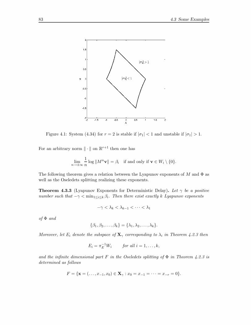
83 4.3 Some Examples
Figure 4.1: System (4.34) for r = 2 is stable if |σ1| < 1 and unstable if |σ1| > 1.
For an arbitrary norm ‖ · ‖ on Rr+1 then one has
limn→±∞
1
nlog ‖Mnv‖ = βi if and only if v ∈Wi \ 0.
The following theorem gives a relation between the Lyapunov exponents of M and Φ aswell as the Oseledets splitting realizing these exponents.
Theorem 4.3.3 (Lyapunov Exponents for Deterministic Delay). Let γ be a positivenumber such that −γ < min1≤i≤k βi. Then there exist exactly k Lyapunov exponents
−γ < λk < λk−1 < · · · < λ1
of Φ and
β1, β2, . . . , βk = λ1, λ2, . . . , λk.
Moreover, let Ei denote the subspace of Xγ corresponding to λi in Theorem 4.2.3 then
Ei = π−1E Wi for all i = 1, . . . , k,
and the infinite dimensional part F in the Oseledets splitting of Φ in Theorem 4.2.3 isdetermined as follows
F = x = (. . . , x−1, x0) ∈ Xγ : x0 = x−1 = · · · = x−r = 0.

Chapter 4: Difference Equations with Random Delay 84
Proof. By virtue of Theorem 4.3.1, we get λi = βi for all 1 ≤ i ≤ k. Note that inLian and Lu [89] (see also Theorem 1.4.2) the subspace Ei of Xγ realizing the Lyapunovexponent λi can be determined as follows
Ei :=x ∈ Xγ : Φ−nx exists for all n ∈ N and lim
n→±∞1
nlog ‖Φnx‖ = λi
.
From the definition of E, see (4.35), one has Ei ⊂ E. Hence, we get
Ei =x ∈ E : lim
n→±∞1
nlog ‖Φnx‖ = λi
.
Now we show that Ei = π−1E Wi for all i = 1, . . . , k. Equivalently, we show that
limn→±∞
1
nlog ‖Φnx‖γ = λi if and only if lim
n→±∞1
nlog ‖MnπEx‖ = λi. (4.36)
Using Theorem 4.3.1, we get
limn→∞
1
nlog ‖Φnx‖γ = lim
n→∞1
nlog ‖MnπEx‖ for all x ∈ E. (4.37)
Replacing Φ by Φ−1 and M by M−1, we obtain
limn→−∞
1
nlog ‖Φnx‖γ = lim
n→−∞1
nlog ‖MnπEx‖ for all x ∈ E,
this together with (4.37) implies statement (4.36). It thus remains to determine theinfinite dimensional part of the Oseledets splitting of Φ. Define
F :=x = (. . . , x−1, x0) ∈ Xγ : x0 = x−1 = · · · = x−r = 0
.
Obviously, F is invariant under Φ, i.e. ΦF ⊂ F , and
Xγ = E ⊕ F = E1 ⊕ E2 ⊕ · · · ⊕ Ek ⊕ F.
In order to prove that F is the infinite dimensional part as described in Theorem 4.2.3(ii) it is sufficient to show that
limn→∞
1
nlog ‖Φn|F‖γ ≤ −γ.
Indeed, from the definition of F it is easy to obtain that
‖Φnx‖γ = e−γn‖x‖γ for all x ∈ F, n ∈ N.
Therefore, ‖Φn|F ‖γ = e−γn and this completes the proof.

Chapter 5
Differential Equations with
Random Delay
Delays in difference and in differential equations are used for mathematical modelingin many applications for the description of evolutions which incorporate influences ofevents from the past. Delays appear quite often in biological models when traditionalpointwise modeling assumptions are replaced by more realistic distributed assumptions.
In contrast to ordinary differential equations the set of initial values of a differentialequation with delay is an infinite dimensional space. As a consequence, a lot of technicalproblems arise when we deal with delay equations. Based on the recent work of Lianand Lu [89] the first step towards a general theory of difference equations incorporatingrandom delays which are not assumed to be bounded is established in Chapter 4. Inthis chapter, we extend this work to differential equations with random delays.
5.1 Differential Equations with Random Delay
Let (Ω,F ,P) be a probability space, (θt)t∈R : Ω → Ω an ergodic flow which preservesthe probability measure P and which has measurable inverse, and let r : Ω → R+ be ameasurable map. We consider a random linear differential equation with random delay
x(t) = A(θtω)x(t) +B(θtω)x(t− r(θtω)) for t ≥ 0, (5.1)
where A,B ∈ L1(P). In order to introduce an RDS generated by (5.1) we first need toconstruct an appropriate state space. Since the delay map r is in general unbounded,an initial value for (5.1) is a continuous function x : (−∞, 0] → Rd. A correspondingform of (5.1) is given by
ϕ(t, ω)x = x(0) +
∫ t
0A(θsω)ϕ(s, ω)x +B(θsω)ϕ(s − r(θsω), ω)x ds, (5.2)
with the convention that ϕ(s, ω)x = x(s) for all s ≤ 0, which is valid for all t ≥ 0. If(5.2) holds, we say that t 7→ ϕ(t, ω)x =: ϕω(t,x) solves, or is a solution of, equation(5.1) starting at 0 in x.
85

Chapter 5: Differential Equations with Random Delay 86
Since in the unbounded delay case the initial data is always a part of the solution, somekind of regularity must be imposed from the beginning. The continuous time setting isdiscussed e.g. in Hale and Kato [63] and Hino, Murakami and Naito [69]. This leads usto work with a canonical phase space
Xγ :=
x ∈ C
((−∞, 0],Rd
): lim
t→−∞eγtx(t) exists
,
‖x‖γ := supt∈(−∞,0]
eγt|x(t)|.
Throughout this chapter we assume that γ > 0 and consider system (5.1) on the statespace (Xγ , ‖ · ‖γ). It is easy to see that (Xγ , ‖ · ‖γ) is a Banach space. The followinglemma ensures the separability of the space (Xγ , ‖ · ‖γ).
Lemma 5.1.1. For γ > 0 the space (Xγ , ‖ · ‖γ) is separable.
Proof. Let Qd denote the set of all vectors in Rd whose components are rational. Clearly,Qd is dense in Rd. For each N ∈ N we consider the Banach space C([−N, 0],Rd) togetherwith the sup norm ‖ · ‖∞, i.e.
‖f‖∞ = supt∈[−N,0]
|f(t)| for all f ∈ C([−N, 0],Rd).
It is well known that(C([−N, 0],Rd), ‖ · ‖∞
)is a separable Banach space (see e.g.
Willard [141]). Consequently, there exists a countable set
AN := f (N)1 , f
(N)2 , . . . , f
(N)1 , f
(N)2 , . . . ∈ C([−N, 0],Rd),
which is dense in(C([−N, 0],Rd), ‖ · ‖∞
). For each function f
(N)k , v ∈ Qd and p ∈ Q+
we defined the extended function f(N)k,v,p : (−∞, 0] → Rd by
f(N)k,v,p(t) :=
f(N)k (t), t ∈ [−N, 0],(
N+tp + 1
)f
(N)k (−N) − N+t
p e(N+p)γv, t ∈ [−N − p,−N),
e−γtv t ∈ (−∞,−N − p).
(5.3)
Obviously, for all k ∈ N, v ∈ Qd and p ∈ Q+ the function f(N)k,v,p is continuous and
limt→−∞
eγtf(N)k,v,p(t) = v,
which implies that f(N)k,v,p ∈ Xγ . Define
AN =⋃
v,p∈Qd×Q+
f
(N)1,v,p, f
(N)2,v,p, . . .
for all N ∈ N.
87 5.1 Differential Equations with Random Delay
To prove the separability of the Banach space (Xγ , ‖ · ‖γ), it is sufficient to show that
⋃
N∈N
AN is dense in (Xγ , ‖ · ‖γ). (5.4)
For a given x ∈ Xγ , set u := limt→−∞ eγtx(t). Hence, for an arbitrary ε > 0 there existsN ∈ N such that
|eγtx(t) − u| ≤ ε
8for all t ≤ −N. (5.5)
Since Qd is dense in Rd it follows that there exists v ∈ Qd such that |v−u| ≤ ε8 . On the
other hand, due to the denseness of AN in the space C([−N, 0],Rd) there exists k ∈ N
such thatsup
t∈[−N,0]|f (N)
k (t) − x(t)| < ε
8. (5.6)
Direct estimations yield that
limp→0
supt∈ [−N−p,−N ]
eγt∣∣∣f (N)
k (−N) − x(t)∣∣∣ = e−γN
∣∣∣f (N)k (−N) − x(−N)
∣∣∣
≤ e−γN ε
8
and
limp→0
supt∈ [−N−p,−N ]
eγt∣∣∣f (N)
k (−N) − e(N+p)γv∣∣∣ =
∣∣∣e−γNf(N)k (−N) − v
∣∣∣
≤ e−γN ε
8+∣∣e−γNx(−N) − u
∣∣+ |u− v|
≤ 3ε
8.
As a consequence, there exists p ∈ Q+ such that for all t ∈ [−N − p,−N ] we have
eγt∣∣∣f (N)
k (−N) − x(t)∣∣∣ ≤ ε
3, eγt
∣∣∣f (N)k (−N) − e(N+p)γv
∣∣∣ ≤ ε
2. (5.7)
We now estimate ‖f (N)k,v,p − x‖γ . By (5.3) and (5.6), the relation
eγt∣∣∣f (N)
k,v,p(t) − x(t)∣∣∣ = eγt|f (N)
k (t) − x(t)|
≤ |f (N)k (t) − x(t)|
≤ ε
8
holds for all t ∈ [−N, 0]. For all t ∈ (−∞,−N − p], by (5.3) we have
eγt∣∣∣f (N)
k,v,p(t) − x(t))∣∣∣ = eγt|e−γtv − x(t)|
≤ |u− v| + |u− eγtx(t)|≤ ε
4,
Chapter 5: Differential Equations with Random Delay 88
where we use (5.5) to obtain the last inequality. On the other hand, for all t ∈ [−N −p,−N ] by (5.3) we have
eγt∣∣∣f (N)
k,v,p(t) − x(t))∣∣∣ = eγt
∣∣∣∣(N + t
p+ 1
)f
(N)k (−N) − N + t
pe(N+p)γv − x(t)
∣∣∣∣
≤ eγt∣∣∣f (N)
k (−N) − x(t)∣∣∣+ eγt
∣∣∣f (N)k (−N) − e(N+p)γv
∣∣∣
≤ ε
3+ε
2,
where we use (5.7) to obtain the last inequality. Therefore, we have
‖f (N)k,v,p − x‖γ = sup
t∈(−∞,0]eγt|f (N)
k,v,p(t) − x(t)| ≤ ε,
which proves that A is dense in Xγ and the proof is completed.
In the following theorem, we give a sufficient condition for the existence and uniquenessof solution of (5.1) on the state space Xγ .
Theorem 5.1.2 (Existence of Solutions). Suppose that A(·), B(·)eγr(·) ∈ L1(P). Thenthere exists a measurable set Ω of full measure such that for every ω ∈ Ω the followingpathwise random delay differential equation
x(t) = A(θtω)x(t) +B(θtω)x(t− r(θtω)), (5.8)
with the initial condition, x(t) = x(t) for all t ∈ (−∞, 0] for some x ∈ Xγ , has a uniquesolution on R, denoted by ϕω(·,x). Furthermore, for a fixed x ∈ Xγ and T > 0 the map
Ω → Rd, defined byω 7→ ϕω(T,x),
is measurable.
Proof. For convenience, we divide the proof into the several steps.
Step 1 : We define
Ω := ω ∈ Ω : t 7→ ‖A(θtω)‖ + ‖B(θtω)‖eγr(θtω) is locally integrable. (5.9)
It is easy to see that Ω is a θ-invariant measurable set and P(Ω) = 1 (see e.g. [3, Lemma2.2.5]). We finish this step by showing that for all 0 < a < b and measurable functionsf : Ω → Rd the following function
ω 7→∫ b
aA(θsω)f(ω) ds is measurable for all t ≥ 0. (5.10)
Since ∫ b
a|A(θsω)v| ds ≤ |v|
∫ b
a‖A(θsω)‖ ds <∞ for all v ∈ Rd,
89 5.1 Differential Equations with Random Delay
it follows that the map
ω 7→∫ b
aA(θsω)v ds is measurable for all v ∈ Rd.
By approximating f by a sequence of simple functions, (5.10) is proved.
Step 2 : For a fixed ω ∈ Ω and T ∈ R+ we show that equation (5.8) has a unique solutionon [0, T ] with the initial value x ∈ Xγ . Define
Cx([0, T ],Rd) := f ∈ C([0, T ],Rd) : f(0) = x(0).
Obviously, Cx([0, T ],Rd) is a closed subset of C([0, T ],Rd). Corresponding to each func-tion f ∈ Cx([0, T ],Rd), we define the function f : (−∞, T ] → Rd by
f(t) =
f(t), if t ≥ 0,
x(t), if t ≤ 0.
By the definition of Cx([0, T ],Rd), f is a continuous function from (−∞, T ] to Rd.Furthermore, by the definition of Xγ we have
∣∣∣f(s− r(θsω))∣∣∣ ≤ max
sup
0≤t≤T|f(t)|, ‖x‖γe
γr(θsω)
for all s ∈ [0, T ].
Hence, by (5.9) we obtain
∫ t
0|A(θsω)f(s)| ds,
∫ t
0|B(θsω)f(s− r(θsω))| ds <∞ for all t ∈ [0, T ].
Therefore, to solve equation (5.8) we define the following operator Tω : Cx([0, T ],Rd) →Cx([0, T ],Rd) by
Tωf(t) := f(0) +
∫ t
0A(θsω)f(s) ds+
∫ t
0B(θsω)f(s− r(θsω)) ds for all t ∈ [0, T ].
(5.11)Clearly, Tωf is a continuous function and Tωf(0) = f(0) = x(0). Hence, Tω is well-defined. Let f ,g ∈ Cx([0, T ],Rd) we show that
|Tnωf(t) − Tn
ωg(t)| ≤ 1
n!
∣∣∣∣∫ t
0‖A(θsω)‖ + ‖B(θsω)‖ ds
∣∣∣∣n
‖f − g‖ (5.12)
for all t ∈ [0, T ], n ∈ N. Indeed, due to (5.11) we obtain
|Tωf(t) − Tωg(t)| =
∫ t
0A(θsω)(f(s) − g(s)) ds+
∫ t
0B(θsω)
(f(s− r(θsω)) − g(s− r(θsω))
)ds.

Chapter 5: Differential Equations with Random Delay 90
Together with the fact that f(t) = g(t) for all t ≤ 0 we have
|Tωf(t) − Tωg(t)| ≤∫ t
0‖A(θsω)‖ + ‖B(θsω)‖ ds · ‖f − g‖,
which proves that inequality (5.12) holds for n = 1. Now assume that inequality (5.12)is proven for some n ∈ N. For n+ 1, using the proof for n = 1, we have
‖Tn+1ω f(t) −Tn+1
ω g(t)‖ ≤∫ t
0‖A(θsω)‖|Tn
ωf(s) − Tnωg(s)| ds+
∫ t
0‖B(θsω)‖|Tn
ωf(s) − Tnωg(s)| ds
≤∫ t
0l(s) · 1
n!
(∫ s
0l(u) du
)n
ds · ‖f − g‖,
where l(s) := ‖A(θsω)‖ + ‖B(θsω)‖. Together with the equality
∫ t
0l(s) · 1
n!
(∫ s
0l(u) du
)n
ds =1
(n+ 1)!
(∫ t
0l(s) ds
)n+1
this proves (5.12) for n+ 1. Due to Step 1 we know that
∫ T
0‖A(θsω)‖ + ‖B(θsω)‖ ds <∞.
Therefore, there exists N ∈ N such that
KN :=1
N !
∣∣∣∣∫ T
0‖A(θsω)‖ + ‖B(θsω)‖ ds
∣∣∣∣N
< 1,
which together with (5.12) implies that TNω is a contractive map from Cx([0, T ],Rd)
into itself. As an application of the Banach fixed point theorem, there exists a uniquefixed point in Cx([0, T ],Rd) for Tω denoted by fω. Since T can be chosen arbitrarily wethus can extend fω to achieve the unique continuous function fω : [0,∞) → Rd such thatfω(0) = x(0) and
fω(t) := fω(0) +
∫ t
0A(θsω)fω(s) ds+
∫ t
0B(θsω)fω(s − r(θsω)) ds for all t ∈ R+.
In other words, equation (5.8) has a unique solution for each ω ∈ Ω.
Step 3 : It remains to show the measurability of the map Ω → Rd defined by
ω 7→ ϕω(T,x),
where x ∈ Xγ and T > 0 are fixed and ϕω(·,x) is the solution of (5.8) with theinitial value x. Choose and fix f ∈ Cx([0, T ],Rd). Define a sequence of functionsgn : [0, T ] × Ω → Rd by
gn(t, ω) = Tnωf(t) for all (t, ω) ∈ [0, T ] × Ω.
91 5.1 Differential Equations with Random Delay
By (5.11), we have
gn+1(t, ω) = f(0) +
∫ t
0A(θsω)gn(s, ω) ds+
∫ t
0B(θsω)gn(s− r(θsω), ω) ds. (5.13)
On the other hand, as is proved in Step 2 we have
ϕω(T,x) = limn→∞
Tnωf(T ) = lim
n→∞gn(T, ω) for all ω ∈ Ω.
Therefore, it is sufficient to show the measurability of the mappings gn(t, ·) : Ω → Rd forall t ∈ [0, T ], n ∈ N. We will prove this fact by induction. Clearly, the statement holdswith n = 0. Suppose that for some n ∈ N the function gn(t, ·) : Ω → Rd is measurablefor all t ∈ [0, T ]. Choose and fix t ∈ [0, T ]. For each k ∈ N, define gk
n : [0, t) × Ω → Rd
by
gkn(s, ω) =
k−1∑
i=0
χ[ it
k, (i+1)t
k)(s)gn
(it
k, ω
)for all (s, ω) ∈ [0, t) × Ω.
Together with the fact that gn(·, ω) : [0, t] → Rd is a continuous function we derive that
limk→∞
∫ t
0A(θsω)gk
n(s, ω) ds =
∫ t
0A(θsω)gn(s, ω) ds for all ω ∈ Ω.
As a consequence, by using Step 1 the mapping
ω 7→∫ t
0A(θsω)gn(s, ω) ds
is F ,B(Rd)-measurable for all t ∈ [0, T ]. On the other hand, due to the measurabilityof the mapping (s, ω) 7→ r(θsω) there is a sequence of simple functions from [0, t] × Ωto R converging pointwise to r. Using similar arguments as above, we also obtain themeasurability of the map
ω 7→∫ t
0B(θsω)gn(s − r(θsω), ω) ds.
Hence, the mapping gn(t, ·) is measurable for all t ∈ [0, T ] and n ∈ N. This completesthe proof.
Remark 5.1.3. Since we can choose a θ-invariant set Ω with full measure, we canassume w.l.o.g. from now on that the statements in Theorem 5.1.2 hold on Ω.
Now we are at a position to define the random dynamical system on Xγ generated by(5.1) as follows.
Definition 5.1.1. Let A,B ∈ L1(P) and r : Ω → R+ be a random delay satisfying thatB(·)eγr(·) ∈ L1(P). Consider a random differential equation with random delay
x(t) = A(θtω)x(t) +B(θtω)x(t− r(θtω)) for t ≥ 0. (5.14)

Chapter 5: Differential Equations with Random Delay 92
The random dynamical system Φ : R+ × Ω → L(Xγ) defined by
Φ(t, ω)x(s) :=
x(t+ s), if t+ s ≤ 0,
ϕω(t + s,x), if t+ s ≥ 0,
for all s ∈ R−, where ϕω(·,x) is the unique solution of (5.14) with the initial value x, iscalled the random dynamical system generated by (5.14).
Remark 5.1.4. From the unique existence of solution of (5.14) we derive that Φ(t, ω)is injective for all t ∈ R+. For ω ∈ Ω, t ∈ R+ and x ∈ im
(Φ(t, θ−tω)Xγ
)due to the
injectivity of Φ(t, θ−tω) there is a unique y ∈ Xγ , which is also denoted by Φ(−t, ω)x,such that
Φ(t, θ−tω)y = x.
Lemma 5.1.5 (Strong Measurability of Φ). Let Φ be the random dynamical systemgenerated by (5.14). Then the mapping Φ(1, ·) : Ω → L(Xγ) is strongly measurable, i.e.,Φ(1, ·)x : Ω → Xγ is measurable for each x ∈ Xγ .
Proof. It is sufficient to show that the set
A := ω ∈ Ω : ‖Φ(1, ω)x − y‖γ ≤ ε
is measurable for all y ∈ Xγ and ε > 0. By Definition 5.1.1 we can rewrite the set A asfollows
A :=ω ∈ Ω : eγs|ϕω(s + 1,x) − y(s)| ≤ ε for all s ∈ [−1, 0],
eγs|x(s + 1) − y(s)| ≤ ε for all s ∈ (−∞,−1).
Clearly, if the estimate
eγs|x(s+ 1) − y(s)| ≤ ε for all s ∈ (−∞,−1) (5.15)
does not hold then A = ∅ and hence A is measurable. Therefore, it remains to deal withthe case that inequality (5.15) holds. Using continuity of y and ϕω(·,x), we obtain
A =⋂
s∈Q∩[−1,0]
ω ∈ Ω : eγs|ϕω(s + 1,x) − y(s)| ≤ ε.
According to Theorem 5.1.2, the set
ω ∈ Ω : eγs|ϕω(s+ 1,x) − y(s)| ≤ ε
is measurable for each s ∈ [−1, 0]. Consequently, A is measurable and the proof iscompleted.
93 5.2 MET for differential equations with random delay
5.2 MET for differential equations with random delay
So far we have proved the existence of the random dynamical system Φ generated by arandom differential equation with random delay
x = A(θtω)x(t) +B(θtω)x(t− r(θtω)), (5.16)
where A(·), B(·)eγr(·) ∈ L1(P). Recall that Φ is said to satisfy the integrability conditionprovided that
sup0≤t≤1
log+ ‖Φ(t, ·)‖γ and sup0≤t≤1
log+ ‖Φ(1 − t, θt·)‖γ ∈ L1(Ω,F ,P),
(see Lian and Lu [89] and also Theorem 1.4.3).
5.2.1 Integrability
The aim of this subsection is to show the integrability of the random dynamical systemΦ generated by equation (5.16).
Lemma 5.2.1 (Sufficient Integrability Condition). Let A ∈ L1(P) and r : Ω → R+ bea random map such that B(·)eγr(·) ∈ L1(P). Denote by Φ : R × Ω → L(Xγ) the randomdynamical system generated (5.16). Then Φ satisfies the integrability condition, i.e.
sup0≤t≤1
log+ ‖Φ(t, ·)‖γ and sup0≤t≤1
log+ ‖Φ(1 − t, θt·)‖γ ∈ L1(Ω,F ,P).
Proof. For each ω ∈ Ω, let ϕω(·,x) be the solution of (5.16) starting at t = 0 with theinitial value x ∈ Xγ . By Definition 5.1.1, we obtain
‖Φ(t, ω)x‖γ = max
sups∈(−∞,−t]
eγs|x(t + s)|, sups∈(−t,0]
eγs|ϕω(t + s,x)|
= maxe−γt‖x‖γ , sup
s∈(0,t]eγ(s−t)|ϕω(s,x)|
.
Therefore, the following inequalities
sup0≤t≤1
log+ ‖Φ(t, ω)‖γ ≤ sup0≤t≤1
log+ ‖ϕω(t, ·)‖ (5.17)
and
sup0≤t≤1
log+ ‖Φ(1 − t, θtω)‖γ ≤ sup0≤t≤1,0≤s≤1−t
log+ ‖ϕθtω(s, ·)‖ (5.18)
hold for all ω ∈ Ω. In what follows, we estimate |ϕω(t,x)| for all 0 ≤ t ≤ 1. To simplifythe notation, we define a set
Mω :=s ∈ R+ : s ≥ r(θsω)
.

Chapter 5: Differential Equations with Random Delay 94
and an operator Tω : Cx([0, 1],Rd) → Cx([0, 1],Rd) by
Tωf(t) = x(0) +
∫ t
0A(θsω)f(s) ds+
∫
[0,t]∩Mω
B(θsω)f(s− r(θsω)) ds+
+
∫
[0,t]∩Mcω
B(θsω)x(s− r(θsω)) ds.
By (5.2), the function ϕω(·,x) is the unique fixed point of Tω. Moreover, due to thecontractiveness of TN
ω for some N ∈ N we have
ϕω(t,x) = limn→∞
Tnωf(t) for all f ∈ Cx([0, 1],Rd), t ∈ [0, 1]. (5.19)
From the definition of Tω, we derive that
|Tωf(t)| ≤ |x(0)| +
∫ t
0‖A(θsω)‖|f(s)| ds+
∫
[0,t]∩Mω
‖B(θsω)‖|f(s − r(θsω))| ds+
+
∫
[0,t]∩Mcω
eγ(r(θsω)−s)‖B(θsω)‖‖x‖γ ds.
which implies that for all 0 ≤ t ≤ 1
|Tωf(t)| ≤ k(ω)‖x‖γ +
∫
[0,t]∩Mω
‖B(θsω)‖|f(s − r(θsω))| ds+
+
∫ t
0‖A(θsω)‖|f(s)| ds,
where k(ω) := 1 +∫ 10 ‖B(θsω)‖eγ(r(θsω)−s) ds. A direct computation yields that the
non-empty closed set
Bω := f ∈ Cx([0, 1],Rd) : f(t) ≤ k(ω)‖x‖γ e∫ t
0‖A(θsω)‖+‖B(θsω)‖ ds for all 0 ≤ t ≤ 1
is invariant under Tω. Therefore, together with (5.19) we get
‖ϕω(t, ·)‖ ≤ k(ω)e∫ t
0‖A(θsω)‖+‖B(θsω)‖ ds for all 0 ≤ t ≤ 1,
which gives
sup0≤t≤1
log+ ‖ϕω(t, ·)‖ ≤ log k(ω) +
∫ 1
0‖A(θsω)‖ + ‖B(θsω)‖ ds (5.20)
and
sup0≤t≤1,0≤s≤1−t
log+ ‖ϕθtω(s, ·)‖ ≤ sup0≤t≤1
log k(θtω) +
∫ 1
0‖A(θsω)‖ + ‖B(θsω)‖ ds. (5.21)
Using the inequality log(1 + x) ≤ 1 + log+ x for x ∈ R+, we have
sup0≤t≤1
log k(θtω) ≤ 1 + log+
∫ 2
0‖B(θsω)‖eγr(θsω) ds. (5.22)

95 5.2 MET for differential equations with random delay
By the Fubini theorem, we get∫
Ω
∫ 2
0‖B(θsω)‖eγr(θsω) ds dP =
∫ 2
0
∫
Ω‖B(θsω)‖eγr(θsω) dP ds.
On the other hand, for all s ∈ [0, 2]∫
Ω‖B(θsω)‖eγr(θsω) dP(ω) =
∫
Ω‖B(ω)‖eγr(ω) dP(ω)
< ∞.
Hence, ∫ 2
0‖B(θs·)‖eγr(θs ·) ds ∈ L1(Ω,F ,P),
which together with (5.22) proves that sup0≤t≤1 log k(θt·) ∈ L1(Ω,F ,P). Therefore, by(5.17), (5.18) and (5.20), (5.21) we obtain
sup0≤t≤1
log+ ‖Φ(t, ·)‖γ , sup0≤t≤1
log+ ‖Φ(1 − t, θt·)‖γ ∈ L1(Ω,F ,P).
This completes the proof.
5.2.2 Kuratowski Measure
Recall that for a subset A ⊂ Xγ , the Kuratowski measure of noncompactness of A isdefined by
α(A) := infd : A has a finite cover by sets of diameter d.For a bounded linear map L : Xγ → Xγ we define
‖L‖α = α(L(B1(0))).
Let Φ be the linear cocycle defined as in Definition 5.1.1. We recall the following quantity(see Subsection 1.4)
lα(Φ) := limt→∞
1
tlog ‖Φ(t, ω)‖α,
and note that it is constant P-a.s. due to the ergodicity of θ and the Kingman subadditiveergodic theorem (see e.g. Arnold [3, pp. 122], Ruelle [120, Appendix A]). To computethe quantity lα(Φ), we first prove the following preparatory lemma.
Lemma 5.2.2. (i) Let T > 0 and a : [0, T ] → R be an integrable function. Then forany ε > 0 there exists a partition 0 = t0 < t1 < · · · < tK = T such that
∫ ti+1
ti
|a(s)| ds ≤ ε for all i = 0, . . . ,K − 1.
(ii) Let T ∈ R+ and ω ∈ Ω satisfy that the function t 7→ ‖A(θtω)‖ + ‖B(θtω)‖eγ(θtω) islocally integrable. Define
A := ϕω(·,x) : [0, T ] → Rd : x ∈ B1(0).Then lα(A) = 0, where A is considered as a subset of C([0, T ],Rd).

Chapter 5: Differential Equations with Random Delay 96
Proof. (i) The proof is straightforward by using the fact that the function from R+ intoitself defined by
t 7→∫ t
0|a(s)| ds
is continuous.
(ii) By the same arguments in the proof of Lemma 5.2.1, the following inequality
|ϕω(t,x)| ≤(
1 +
∫ T
0‖B(θsω)‖eγr(θsω) ds
)e∫ T0 ‖A(θsω)‖+‖B(θsω)‖ ds
holds for all x ∈ B1(0) and t ∈ [0, T ]. Then there exists a positive number M whichdepends only on ω and T such that
|ϕω(t,x)| ≤M for all t ∈ [0, T ],x ∈ B1(0). (5.23)
Using equation (5.2), we obtain that for any t, s ∈ [0, T ] with t > s and x ∈ B1(0)
ϕω(t,x) − ϕω(s,x) =
∫ t
sA(θuω)ϕω(u,x) +B(θuω)ϕω(u− r(θuω),x) du
=
∫ t
sA(θuω)ϕω(u,x) du+
∫
[s,t]∩Mω
B(θuω)ϕω(u− r(θuω),x) du+
+
∫
[s,t]∩Mcω
B(θuω)x(u− r(θuω)) du,
where Mω := s ∈ R+, s ≥ r(θsω). Together with estimate (5.23) this implies that
|ϕω(t,x) − ϕω(s,x)| ≤M
∫ t
s‖A(θuω)‖ + ‖B(θuω)‖ du+
∫ t
s‖B(θuω)‖eγr(θuω) du
holds for all ϕω(·,x) ∈ A. Applying part (i) to the right hand side of the estimate, weget for an arbitrary ε > 0 a partition 0 = t0 < t1 < · · · < tK = T such that
|f(t) − f(s)| ≤ ε
3for all f ∈ A, tk ≤ t, s ≤ tk+1, k = 0, . . . ,K − 1. (5.24)
In the following, we first give a proof in the scalar case, i.e. d = 1. Choose and fixN ∈ N such that M
N ≤ ε3 . For each index (i1, . . . , iK) ∈ −N,−N + 1, . . . , N − 1, NK ,
by writing each t ∈ [0, T ] uniquely as t = αtk + βtk+1 for k ∈ 0, . . . ,K − 1 andα, β ∈ [0, 1] with α+ β = 1, we define a continuous function fi1,...,iK ∈ C([0, T ],R) by
fi1,...,iK (αtk + βtk+1) = αikM
N+ β
ik+1M
N.
Now we show that
A ⊂⋃
−N≤i1,...,iK≤N
Bε(fi1,...,iK ). (5.25)
97 5.2 MET for differential equations with random delay
By the definition of A and inequality (5.23) we have
−M ≤ f(tk) ≤M for all f ∈ A, k = 0, . . . ,K − 1.
which implies together with the inequality MN ≤ ε
3 that for any f ∈ A there exists anindex (i1, . . . , iK) ∈ −N,−N + 1, . . . , N − 1, NK such that
∣∣∣∣f(tk) − ikM
N
∣∣∣∣ ≤M
N≤ ε
3for all k = 0, . . . ,K − 1.
Equivalently,
|f(tk) − fi1,...,iK (tk)| ≤ ε
3for all k = 0, . . . ,K − 1. (5.26)
For any α, β ∈ [0, 1] with α+ β = 1 we get
|f(αtk + βtk+1) − αf(tk) − βf(tk+1)| ≤ α|f(αtk + βtk+1) − f(tk)|+β|f(tk+1) − f(αtk + βtk+1)|
≤ ε
3,
where we use (5.24) to obtain the last estimate. This implies with (5.26) that
|f(αtk + βtk+1) − fi1,...,iK (αtk + βtk+1)| ≤ ε
3+ α|f(tk) − fi1,...,iK (tk)|
+β|f(tk+1) − fi1,...,iK (tk+1)|
≤ 2ε
3
for all k = 0, . . . ,K − 1 and α, β ∈ [0, 1] with α + β = 1. This proves (5.25) and sinceε can be chosen arbitrarily small it follows that lα(A) = 0 in the case that d = 1. Sinceeach continuous function f ∈ C([0, T ],Rd) can be written of the form f = (f1, . . . , fd),where f1, . . . , fd are scalar continuous functions, the high dimension case can be reducedto the scalar case and therefore we also obtain the desired conclusion in the general case.This completes the proof.
Proposition 5.2.3. Let Φ : R×Ω×Xγ → Xγ be the random dynamical system generatedby (5.16). Then
lα = limt→∞
1
tlog ‖Φ(t, ω)‖α = −γ.
Proof. For convenience, throughout the proof we only deal with the max norm on Rd,i.e. |x| = max1≤i≤d |xi| for all x = (x1, . . . , xd)T ∈ Rd. We first obtain the inequalitylα ≥ −γ by sufficiently showing that
α(Φ(T, ω)B1(0)) ≥ e−γ(T+1) for all T > 0. (5.27)
Chapter 5: Differential Equations with Random Delay 98
For this purpose, we define a sequence of functions xnn∈N by
xn(t) =
0, if t ∈ (−n+ 1, 0],
eγ(n−1)(−n+ 1 − t)(1, . . . , 1)T, if t ∈ (−n,−n+ 1],
eγ(n−1)(1, . . . , 1)T, if t ∈ (−∞,−n].
Obviously, the function xn : (−∞, 0] → Rd is continuous, and the relations
limt→−∞
eγtxn(t) = 0, supt∈(−∞,0]
eγt|xn(t)| ≤ 1
lead that xn ∈ B1(0) for all n ∈ N. A straightforward computation yields that for allm > n the following equality holds
Φ(T, ω)xm(−n− T ) − Φ(T, ω)xn(−n− T ) = xm(−n) − xn(−n)
= −eγ(n−1)(1, . . . , 1)T.
Thus,‖Φ(T, ω)xm − Φ(T, ω)xn‖γ ≥ e−γ(T+1),
which proves (5.27). Hence,
lα(Φ) = limt→∞
1
tlog ‖Φ(t, ω)‖α ≥ −γ.
Therefore, it remains to show that
lα(Φ) ≤ −γ + ε for all 0 < ε < γ. (5.28)
Choose and fix T ≥ log 3ε . By definition of Φ(T, ω) (see Definition 5.1.1), we have
Φ(T, ω)x(t) =
x(t + T ), for all t ∈ (−∞,−T ),
ϕω(t+ T,x), for all t ∈ [−T, 0],
for all x ∈ B1(0). Therefore, we get
Φ(T, ω)x(·) ≡ ϕω(· + T,x) on [−T, 0]. (5.29)
According to Lemma 5.2.2 (ii), there exist f1, . . . , fn ∈ C([−T, 0],Rd) such that
ϕω(·,x) : [0, T ] → Rd,x ∈ B1(0) ⊂n⋃
k=1
Be(−γ+ε)T (fk),
which implies with (5.29) that
Φ(T, ω)x|[−T,0],x ∈ B1(0)
⊂
n⋃
k=1
Be(−γ+ε)T (fk), (5.30)
99 5.2 MET for differential equations with random delay
where fk : [−T, 0] → Rd is defined by fk(t) = fk(t+ T ). Define fk : (−∞, 0] → Rd by
fk(t) :=
fk(t), if t ∈ [−T, 0],
fk(−T ), if t ∈ (−∞,−T ).
We show that
Φ(T, ω)B1(0) ⊂n⋃
k=1
Be(−γ+ε)T (fk). (5.31)
To prove this statement let x ∈ B1(0). Using (5.30), there exists k ∈ 1, . . . , n suchthat
|Φ(T, ω)x(t) − fk(t)| ≤ e(−γ+ε)T for all t ∈ [−T, 0].
In particular, fk(−T ) ≤ 1 + e(−γ+ε)T . On the other hand, for all t ∈ (−∞,−T ] we get
eγt|Φ(T, ω)x(t) − fk(t)| = eγt|x(t + T ) − fk(−T )|≤ eγt
(e−γ(t+T ) + 1 + e(−γ+ε)T
)
≤ 3e−γT ,
which together with T ≥ log 3ε proves (5.31). Consequently, we have
‖Φ(T, ω)‖α ≤ e(−γ+ε)T for all T ≥ log 3
ε,
which implies that
lα(Φ) = limt→∞
1
tlog ‖Φ(t, ω)‖α ≤ −γ + ε,
proving (5.28) and the proof is completed.
5.2.3 Multiplicative Ergodic Theorem
We have just proved in the above sections that the random dynamical system generatedby a differential equation with random delay fulfills all assumptions of the multiplicativeergodic theorem on Banach space (see Lian and Lu [89]). Therefore, we are now ata position to state the multiplicative ergodic theorem for differential equations withrandom delay.
Theorem 5.2.4 (Multiplicative Ergodic Theorem for Differential Equations with Ran-dom Delay). Let (Ω,F ,P, (θt)t∈R) be an ergodic MDS and A,B : Ω → Rd×d andr : Ω → R+ be measurable functions satisfying that
A(·), B(·)eγr(·) ∈ L1(P).
Denote by Φ : R+×Xγ → Xγ the random dynamical system generated by the differentialequation with random delay
x = A(θtω)x(t) +B(θtω)x(t− r(θtω)).
Then, there exists a θ-invariant subset Ω ⊂ Ω of full measure such that for each ω ∈ Ωexactly one of the following statements holds

Chapter 5: Differential Equations with Random Delay 100
(I) κ(Φ) = −γ
(II) There exists k ∈ N, Lyapunov exponents λ1 > · · · > λk > −γ and a splitting intomeasurable Oseledets spaces
Xγ = E1(ω) ⊕ · · · ⊕Ek(ω) ⊕ F (ω)
with finite dimensional linear subspaces Ej(ω) and an infinite dimensional linearsubspace F (ω) such that the following properties hold:
(i) Invariance: Φ(t, ω)Ej(ω) = Ej(θtω) and Φ(t, ω)F (ω) ⊂ F (θtω).
(ii) Lyapunov exponents:
limt→±∞
1
tlog ‖Φ(t, ω)x‖γ = λj for all x ∈ Ej(ω) \ 0 and j = 1, . . . , k.
(iii) Exponential Decay Rate on F (ω):
lim supt→+∞
1
tlog ‖Φ(t, ω)|F (ω)‖γ ≤ −γ.
Moreover, for x ∈ F (ω) \ 0 such that Φ(t, θ−tω)−1x := Φ(−t, ω)x exists forall t ∈ R+ we get
lim inft→+∞
1
tlog ‖Φ(−t, ω)x‖γ ≥ γ.
(III) There exist infinitely many finite dimensional measurable subspaces Ej(ω), in-finitely many infinite dimensional subspaces Fj(ω) and infinitely many Lyapunovexponents
λ1 > λ2 > · · · > −γ with limj→+∞
λj = −γ
such that the following properties hold:
(i) Invariance: Φ(t, ω)Ej(ω) = Ej(θtω) and Φ(t, ω)Fj(ω) ⊂ Fj(θtω).
(ii) Invariant Splitting
Xγ = E1(ω) ⊕ · · · ⊕ Ej(ω) ⊕ Fj(ω) and Fj(ω) = Ej+1(ω) ⊕ Fj+1(ω).
(iii) Lyapunov exponents:
limt→±∞
1
tlog ‖Φ(t, ω)x‖γ = λj for all x ∈ Ej(ω) \ 0 and j = 1, . . . , k.
(iv) Exponential Decay Rate on Fj(ω):
lim supt→+∞
1
tlog ‖Φ(t, ω)|Fj(ω)‖γ = λj+1.
Moreover, for x ∈ Fj(ω) \ 0 such that Φ(t, θ−tω)−1x := Φ(−t, ω)x exists forall t ∈ R+ we get
lim inft→+∞
1
tlog ‖Φ(−t, ω)x‖γ ≥ −λj+1.

101 5.2 MET for differential equations with random delay
Theorem 5.2.5 (Lyapunov Exponents are Independent of Exponential Weight Factor).Let γ > 0 and consider (5.14) on the state space (Xγ , ‖ · ‖γ). Assume that λ > −γ is aLyapunov exponent of (5.14), i.e. for P-a.e. ω ∈ Ω there exists x(ω) ∈ Xγ such that
limt→±∞
1
tlog ‖Φ(t, ω)x(ω)‖γ = λ .
Then for every ζ > γ satisfying that eζr(·)B(·) ∈ L1(P) we have x(ω) ∈ Xζ and thenumber λ is also a Lyapunov exponent of (5.14) on the state space (Xζ , ‖ · ‖ζ). Inparticular,
limt→±∞
1
tlog ‖Φ(t, ω)x(ω)‖ζ = λ . (5.32)
Proof. Let y ∈ Xγ . From the definition of Xγ we obtain that limt→∞ e−γty(−t) exists.For ζ > γ it is easy to see that
limt→∞
e−ζty(−t) = limt→∞
e(γ−ζ)te−γty(−t)= 0,
which implies that y ∈ Xζ . Furthermore, for any y ∈ Xγ we have
‖y‖ζ = supt∈[0, ∞)
e−ζt|y(−t)|
≤ supt∈[0, ∞)
e−γt|y(−t)|
≤ ‖y‖γ .
As a consequence, we get
lim supt→∞
1
tlog ‖Φ(t, ω)x(ω)‖ζ ≤ lim
t→∞1
tlog ‖Φ(t, ω)x(ω)‖γ , (5.33)
and
lim inft→−∞
1
tlog ‖Φ(t, ω)x(ω)‖ζ ≥ lim
t→−∞1
tlog ‖Φ(t, ω)x(ω)‖γ . (5.34)
In view of Theorem 5.2.4 we divide the proof into several cases.
Case 1: The linear cocycle Φ on the state space (Xζ , ‖ · ‖ζ) has finitely many Lyapunovexponents. Let −ζ < λk < λk−1 < · · · < λ1 be the Lyapunov exponents of the linearcocycle Φ on the state space (Xζ , ‖ · ‖ζ) and
Xζ = E1(ω) ⊕ · · · ⊕ Ek(ω) ⊕ F (ω)
the corresponding Oseledets splitting of Φ. We write x(ω) in the following form
x(ω) = x1 + x2 + · · · + xk + xF ,
where xi ∈ Ei(ω) and xF ∈ F (ω). For convenience, we divide the proof into severalsteps.
Chapter 5: Differential Equations with Random Delay 102
Step 1: We first show that xF = 0 by contradiction, i.e. we assume that xF 6= 0. Inview of Theorem 5.2.4, we have
lim supt→−∞
1
tlog ‖Φ(t, ω)xF ‖ζ ≤ −ζ,
and for all i ∈ 1, . . . , k with xi 6= 0
limt→−∞
1
tlog ‖Φ(t, ω)xi‖ζ = λi.
Therefore, for any ε ∈(
0, λk+ζ4
)there exists T (ε) ∈ R+ such that
1
tlog ‖Φ(t, ω)xF ‖ζ ≤ −ζ + ε for all t ≤ −T (ε),
and for all i ∈ 1, . . . , k with xi 6= 0
λi −ε
2≤ 1
tlog ‖Φ(t, ω)xi‖ζ ≤ λi +
ε
2for all t ≤ −T (ε).
Hence, for all t ≤ −T (ε) we have
‖Φ(t, ω)x(ω)‖ζ =∥∥∥Φ(t, ω)xF +
∑
i∈1,...,k,xi 6=0
Φ(t, ω)xi
∥∥∥ζ
≥ ‖Φ(t, ω)xF ‖ζ −∥∥∥
∑
i∈1,...,k,xi 6=0
Φ(t, ω)xi
∥∥∥ζ
≥ et(−ζ+ε) −k∑
i=1
et(λi−ε).
Consequently,
1
tlog ‖Φ(t, ω)x(ω)‖ζ ≤ 1
tlog
(et(−ζ+ε) −
k∑
i=1
et(λi−ε)
)for all t ≤ −T (ε),
which implies that
lim supt→−∞
1
tlog ‖Φ(t, ω)x(ω)‖ζ ≤ −ζ + ε,
where we use the fact that
limt→−∞
1
tlog(eta − etb
)= a provided that a < b,
to obtain the last inequality. Since ε can be chosen arbitrarily small it follows togetherwith (5.34) that
limt→−∞
1
tlog ‖Φ(t, ω)x(ω)‖γ ≤ −ζ,
103 5.2 MET for differential equations with random delay
which contradicts to the fact that
−ζ < −γ < λ = limt→−∞
1
tlog ‖Φ(t, ω)x(ω)‖γ .
Step 2: Define
imin := minxi 6=0
i, imax := maxxi 6=0
i.
By the same argument as in Step 1, we obtain that
limt→∞
1
tlog ‖Φ(t, ω)x(ω)‖ζ ≥ λimin
,
limt→−∞
1
tlog ‖Φ(t, ω)x(ω)‖ζ ≤ λimax ,
which implies together with (5.33), (5.34), and the fact that λimin≥ λimax that
limt→±∞
1
tlog ‖Φ(t, ω)x(ω)‖ζ = λ,
proving (5.32) and the proof in this case is completed.
Case 2: The linear cocycle Φ on the state space (Xζ , ‖·‖ζ) has infinitely many Lyapunovexponents. Let −ζ < · · · < λ2 < λ1 with limk→∞ λk = −ζ be the Lyapunov exponentsof the linear cocycle Φ on the state space (Xζ , ‖ · ‖ζ) and
Xζ = E1(ω) ⊕ · · · ⊕ Ek(ω) ⊕ Fk(ω)
the corresponding invariant splittings. We prove the fact that λ ∈ λ1, λ2, . . . bycontradiction, i.e. we assume that λk 6= λ for all k ∈ N. Since limk→∞ λk = −ζ itfollows that there exists k ∈ N such that λk < λ. Set k∗ := mink : λk < λ. By using(5.34) and in view of Theorem 5.2.4, we obtain that k∗ > 1. Hence, λk∗ < λ < λk∗−1.We write x(ω) in the following form
x(ω) = x1 + x2 + · · · + xk∗−1 + xF ,
where xi ∈ Ei(ω), i = 1, . . . , k∗ − 1 and xF ∈ Fk∗−1(ω). Using a similar proof as in Step1 of Case 1, we also have xF = 0 and
lim inft→∞
1
tlog ‖Φ(t, ω)x(ω)‖ζ ≥ λk∗−1,
which together with (5.33) contradicts to the fact that λ < λk∗−1 and the proof iscompleted.
Chapter 5: Differential Equations with Random Delay 104
5.3 Differential equations with bounded delay
The aim of this section is to investigate differential equations with bounded delay. Wecan easily observe that if the delay is bounded we do not need all information fort ∈ (−∞, 0] in order to know the value of solutions in the future. As a consequence,there are several options to define a dynamical system generated by such an equation.Naturally, we can ask the question whether there are any relations between the Lyapunovexponents of these dynamical systems. Throughout this section we consider the followingsystem
x = A(θtω)x(t) +B(θtω)x(t− r(θtω)). (5.35)
Assume that the random delay map r is bounded, i.e. there exists M > 0 such that
r(ω) ≤M for all ω ∈ Ω
and A,B ∈ L1(P). Due to the boundedness of the delay the initial values of (5.35)can be either in Xγ or in C([−M, 0],Rd). Using the same procedure to introduce andinvestigate the RDS in Xγ generated by (5.35) we also obtain an RDS in C([−M, 0],Rd)generated by (5.35) as follows:
Random Dynamical System on C([−M, 0],Rd): For each ω ∈ Ω and an initial valuex ∈ C([−M, 0],Rd), equation (5.35) has a unique solution denoted by ψω(·, x), i.e. theequality
ψω(t, x) =
∫ t
0A(θsω)ψω(s, x) +
∫ t
0B(θsω)ψω(s− r(θsω), x) ds
holds for all t ∈ R+, where
ψω(s− r(θsω), x) =
x(s − r(θsω)), if s ≤ r(θsω),
ψω(s− r(θsω), x), otherwise.
Based on the existence and uniqueness solution of (5.35) we can define an RDS Ψ :R+ × Ω → L(C([−T, 0],Rd)), where L(C([−T, 0],Rd)) denotes the space of all boundedlinear operators from C([−T, 0],Rd) into itself, by
Ψ(t, ω)x(s) =
ψω(t + s, x), if t+ s ≥ 0,
x(t+ s), otherwise,
for all s ∈ [−M, 0].
Properties of Ψ: Along the lines of the proof of Theorem 5.1.2, Lemma 5.2.1 and Propo-sition 5.2.3 we have:
• Ψ is strongly measurable.

105 5.3 Differential equations with bounded delay
• Ψ satisfies the integrability condition, i.e.
sup0≤t≤1
log+ ‖Ψ(t, ·)‖ and sup0≤t≤1
log+ ‖Ψ(1 − t, θt·)‖ ∈ L1(Ω,F ,P).
• lα(Ψ) = −∞.
Theorem 5.3.1. Let α1 > α2 > . . . be the Lyapunov exponents of Φ and β1 > β2 > . . .be the Lyapunov exponent of Ψ. Then
αi = βi : βi > −γ.
Proof. (⇒) Suppose that λ is a Lyapunov exponent of Φ. Fix ω ∈ Ω and let x ∈ Xγ bea vector corresponding to this Lyapunov exponent, i.e.
limt→∞
1
tlog ‖Φ(t, ω)x‖γ = λ.
Define x ∈ C([−M, 0],Rd) by
x(s) = x(s) for all s ∈ [−M, 0].
A direct computation yields that
ϕω(t,x) = ψω(t, x) for all t ≥ 0,
which leads
Φ(t, ω)x(s) = Ψ(t, ω)x(s) for all s ∈ [−M, 0], t ≥M.
Consequently, for all t ≥M we have
1
tlog ‖Φ(t, ω)x‖γ ≥ 1
tlog(e−γM‖Ψ(t, ω)x‖),
proving that
lim supt→∞
1
tlog ‖Ψ(t, ω)x‖ ≤ λ.
To prove λ is a Lyapunov exponent of Ψ, by virtue of Theorem 5.2.4 it is sufficient toshow that
lim supt→∞
1
tlog ‖Ψ(t, ω)x‖ = λ.
Thereto, we assume a contradiction, i.e. there exists ε ∈ (0, λ+ γ) and T > 0 such that
‖Ψ(t, ω)x‖ ≤ e(λ−ε)t for all t ≥ T.
Therefore,
|ϕω(t,x)| = |ψω(t, x)| ≤ e(λ−ε)t for all t ≥ T.
Chapter 5: Differential Equations with Random Delay 106
As a consequence, for all t ≥ T we have
‖Φ(t, ω)x‖γ = max
sup
−∞<s≤−teγs|Φ(t, ω)x(s)|, sup
−t≤s≤0eγs|Φ(t, ω)x(s)|
≤ max
e−γt‖x‖γ , sup
−t≤s≤0eγs|ϕω(t+ s,x)|
≤ max
e−γt‖x‖γ , e
−γt sup0≤s≤T
eγs|ϕω(s,x)|, e(λ−ε)t
.
This implies together with −γ ≤ λ− ε that
lim supt→∞
1
tlog ‖Φ(t, ω)x‖γ ≤ λ− ε.
This is a contradiction and we get the desired conclusion.(⇐) Assume that β > −γ is a Lyapunov exponent of Ψ and let x ∈ C([−M, 0],Rd) bea vector corresponding to β, i.e.
limt→∞
1
tlog ‖Ψ(t, ω)x‖ = β.
Define x : (−∞, 0] → Rd by
x(s) =
x(s), if s ∈ [−M, 0],
x(−M), otherwise.
Using similar arguments as in the first part of the proof, we also have
limt→∞
1
tlog ‖Φ(t, ω)x‖γ = β.
Therefore, β is a Lyapunov exponent of Φ and the proof is completed.

Chapter 6
Computational Ergodic Theorem
Iterated function systems (IFS) consisting of finitely many affine transformations becamepopular as a method for constructing fractals like, e.g. the Sierpinski Gasket or theBarnsley Fern in the plane, Barnsley [10]. A common algorithm consists of picking arandom point in the plane, then iteratively applying one of the functions chosen atrandom from the function system and drawing the point. Iterated function systems areexamples of RDS. For IFS which are uniformly contractive Peruggia [114] introduces ageneral method of discretisation as a way of approximating the attracting sets and theinvariant measure. Using an extension of this construction, Froyland [56] and Froylandand Aihara [57] present a computational method for rigorously approximating the uniqueinvariant measure of an IFS which is contractive on average – a notion which is moregeneral than uniformly contractive. An advantage of this method is that it providesquantitative bounds on the accuracy of the approximation. For the same class of IFSElton [50] proved an ergodic theorem which states that the time average along almostevery random iterate of any starting point converges to a constant number, the spaceaverage. This theorem is extended in a number of directions, e.g. to recurrent IFSby Barnsley, Elton and Hardin [12], to systems with time dependent probabilities byStenflo [130], to systems with place-dependent probabilities by Barnsley, Demko, Eltonand Geronimo [11], to contractive Markov systems by Werner [140]. Using the Banachlimit technique, Forte and Mendivil [59] give a simple proof of the ergodic theorem foran IFS which is uniformly contractive. Based on the same method, Hyong-chol et al.[71] extend the ergodic theorem to infinite iterated function systems (IIFS) which areuniformly contractive. Combining the Kingman subadditive ergodic theorem and theBirkhoff ergodic theorem, Cong, Doan and Siegmund [38] provide a simple proof of theergodic theorem for IIFS which are contractive on average.
In this chapter, we extend the result in Cong, Doan and Siegmund [38] to IIFS which arel-contractive on average, a notion which is weaker than contraction on average. We alsoconstruct an approximating sequence of finite IFS such that the corresponding sequenceof invariant measures converges to the unique invariant measure of the approximatedIIFS. One of our main results is a computational version of the ergodic theorem whichallows to approximate the time average of an IIFS together with explicit error bounds.
107
Chapter 6: Computational Ergodic Theorem 108
At the same time, we also use the method in Froyland and Aihara [57] to establish analgorithm to compute the time average of a contractive on average place-dependent IFS.Having a rigorous method to compute the invariant measure, we apply this method tocompute Lyapunov exponents of products of random matrices. Several examples arealso provided to illustrate the theoretical results.
Given an RDS ϕ as in Definition 1.1.9 or its corresponding skew product Θ as in Remark1.1.4 we define its time-one map τ : Ω ×X → Ω ×X by
τ(ω, x) = Θ(1)(ω, x).
Then it is easy to see that Θ(n) = τn. Conversely, let τ : Ω ×X → Ω ×X be a mapsatisfying τ(ω, x) = (θω, ϕ(1, ω)x) for an RDS ϕ. Then Θ(n) := τn is the skew productcorresponding to the RDS ϕ. Hence we can identify a skew product with its time-onemap. Next we will recall the notion of invariant measure which is a central concept forRDS.
Definition 6.0.1 (Invariant Measure). Let τ : Ω × X → Ω ×X be the skew productcorresponding to an RDS ϕ over an MDS (Ω,F ,P, θ). A probability measure µ on (X,B)is said to be invariant under τ if the probability measure P × µ on Ω ×X is invariantwith respect to the skew product τ , i.e. satisfies
P × µ(B) = P × µ(τ−1B) for all B ∈ F ⊗ B.
We recall some elementary properties of Lipschitz functions which will be used in thenext sections. Let (X1, d1) and (X2, d2) be metric spaces and f : X1 → X2 a Lipschitzfunction. Denote by Lip(f) the Lipschitz constant of f , i.e.,
Lip(f) = supx,y∈X1
d2(f(x), f(y))
d1(x, y)< +∞.
For a compact metric space (X, d), we define
Lip1(X) := h : X → R | Lip(h) ≤ 1.
Remark 6.0.2. (i) Let (Xi, di), with i = 1, 2, 3, be metric spaces and suppose thatf : X1 → X2 and g : X2 → X3 are Lipschitz functions. Then the composition functiong f : X1 → X3 is also a Lipschitz function and Lip(g f) ≤ Lip(f)Lip(g).
(ii) Let (X, d) be a metric space and f : X → R a Lipschitz function. Then for anyα ∈ R the function αf is Lipschitz and Lip(αf) = |α|Lip(f).
From now on, suppose that (X, d) is a compact metric space. Denote by C(X), M(X)the space of real-valued continuous maps on X and probability measures on (X,B(X)),respectively. In order to estimate the distance between two probability measures we in-troduce a metric dH on M(X) which is known as the Hutchinson metric (see Hutchinson[70]) as follows
dH(ν1, ν2) := suph∈Lip1(X)
∣∣∣∣∫
Xh dν1 −
∫
Xh dν2
∣∣∣∣ for all ν1, ν2 ∈ M(X). (6.1)
109 6.1 Iterated Function Systems
In the following remark, we collect some well-known properties of this metric spacewhich are used later.
Remark 6.0.3. (i) (M(X), dH ) is a complete metric space.
(ii) Let x0 ∈ X be fixed. Then the Hutchinson metric satisfies
dH(ν1, ν2) = suph∈Lip1(X),h(x0)=0
∣∣∣∣∫
Xh dν1 −
∫
Xh dν2
∣∣∣∣ for all ν1, ν2 ∈ M(X) .
(iii) If ν1, ν2 ∈ M(X) satisfy dH(ν1, ν2) = 0 then∫X G(z) dν1(z) =
∫X G(z) dν2(z) for
all continuous functions G ∈ C(X).
(iv) If limn→∞ νn = ν then
limn→∞
∫
Xf dνn =
∫
Xf dν for all f ∈ C(X).
(v) (M(X), dH ) is a compact metric space.
6.1 Iterated Function Systems
6.1.1 Finite Iterated Function Systems
Let (X, d) be a compact metric space, k ∈ N and f = fnkn=1 a sequence of k Lipschitz
maps from X into itself. Let p = pnkn=1 be a collection of k positive probabilities
pn > 0,∑k
n=1 pn = 1. The pair (f ,p) is called (finite) iterated function system (IFS),see [9]. In order to explain how the IFS (f ,p) generates an RDS on X we introduce thespace of addresses containing k symbols
Ω(k) =
∞∏
n=0
1, . . . , k = 1, . . . , k∞
together with the σ-algebra F (k) generated by the cylinders in Ω(k) and define a productprobability measure P(k) on (Ω(k),F (k)) by
P(k) =
∞∏
n=0
ρ(k) with ρ(k)(n) = pn .
Let θ : Ω(k) → Ω(k) denote the left shift, i.e., (θω)j = ωj+1 for all ω ∈ Ω(k) and j ∈ N0.It is well known that θ is an ergodic transformation preserving the probability P(k) (seee.g. Walter [138]).
Remark 6.1.1 (RDS generated by IFS). An IFS (f ,p) generates a random dynamicalsystem ϕ(k) over the MDS (Ω(k),F (k),P(k), θ) by setting
ϕ(k)(n, ω)x = fωn−1 fωn−2 · · · fω0(x) for n ∈ Z+ .
The corresponding skew product τ (k) : Ω(k) ×X → Ω(k) ×X is given by
τ (k)(ω, x) = (θω, fω0x) .
Chapter 6: Computational Ergodic Theorem 110
Definition 6.1.1 (l-Average Expansion Rate and Contraction). Let (f ,p) be an IFS.The number
Lipl(f) :=k∑
n1,n2,...,nl=1
pn1pn2 . . . pnlLip(fn1 fn2 · · · fnl
)
is called the l-average expansion rate of (f ,p). The IFS (f ,p) is said to be l-contractive onaverage if Lipl(f) < 1. The IFS (f ,p) is said to be contractive on average if Lip1(f) < 1.
Remark 6.1.2. For an IFS (f ,p) and l ∈ N, we define an IFS (f , p) by
fn1,...,nl= fn1 fn2 · · · fnl
, pn1,...,nl= pn1pn2 . . . pnl
,
where n1, . . . , nl = 1, . . . , k. Then
Lipl(f) = Lip1(f).
The following lemma ensures that contraction on average implies l-contraction on aver-age for all l ∈ N.
Lemma 6.1.3. Let (f ,p) be an iterated function system. Then
Lipl(f) ≤ (Lip1(f))l for all l ∈ N.
Consequently, contraction on average implies l-contraction on average for all l ∈ N.However, the converse implication does not in general hold.
Proof. Using Remark 6.0.2 (i), we obtain
Lipl(f) =
k∑
n1,n2,...,nl=1
pn1pn2 . . . pnlLip(fn1 fn2 · · · fnl
)
≤k∑
n1,n2,...,nl=1
pn1pn2 . . . pnlLip(fn1)Lip(fn2) . . .Lip(fnl
)
=
k∑
n1=1
pn1 Lip(fn1)
k∑
n2=1
pn2 Lip(fn2) · · ·k∑
nl=1
pnlLip(fnl
)
= (Lip1(f))l ,
proving that contraction on average implies l-contraction on average. For the remainingpart of the proof, we need to construct an IFS (f ,p) which is l-contractive on averagebut not contractive on average. Set X = [0, 1], k = 2, p1 = p2 = 1/2 and we define twofunctions f1, f2 : X → X by
f1(x) :=x2
2, f2(x) := 1 − x2
2.
111 6.1 Iterated Function Systems
Note that the Lipschitz constant of a C1 map f : [0, 1] → [0, 1] can be determined by
Lip(f) = maxx∈[0,1]
|f ′
(x)|. (6.2)
Hence,
Lip(f1) = Lip(f2) = 1,
which implies that the IFS (f ,p) is not contractive on average. On the other hand, adirect computation yields that
f21 (x) =
x4
8, f2
2 (x) =1
2+x2
2− x4
8, f1 f2(x) =
1
2− x2
2+x4
8, f2 f1 = 1 − x4
8.
Therefore, by using statement (6.2), we have
Lip(f21 ) = Lip(f2 f1) =
1
2, Lip(f2
2 ) = Lip(f1 f2) =2√
2
3√
3,
which implies that
Lip2(f) =1
4+
√2
3√
3< 1.
As a consequence, (f ,p) is 2-contractive on average. This completes the proof.
Remark 6.1.4 (Uniform Contraction is Stronger than Contraction on Average). AnIFS (f ,p) is said to be uniformly contractive if Lip(fn) < 1 for all 1 ≤ n ≤ k. Auniformly contractive IFS is also contractive on average, since Lip(fn) < 1 togetherwith
∑kn=1 pn = 1 implies that
∑kn=1 pn Lip(fn) < 1.
For an IFS (f ,p), we call the operator P(k) : M(X) → M(X) defined by
P(k)ν =
k∑
n=1
pnν f−1n for all ν ∈ M(X) (6.3)
the associated Markov operator . By the definition of P(k) we have
∫
Xh dP l
(k)ν =
k∑
n1,...,nl=1
pn1 . . . pnl
∫
Xh fn1 · · · fnl
dν for all ν ∈ M(X). (6.4)
The following lemma from Foryland [56] characterizes invariant measures of IFS as fixedpoints of an associated Markov operator.
Lemma 6.1.5 (Froyland [56]). Let (f ,p) be an IFS on a compact metric space (X, d).Then a probability measure µ ∈ M(X) is invariant under the IFS (f ,p), i.e. µ×P(k) isinvariant under the skew product τ (k) associated with (f ,p), if and only if µ is a fixedpoint of the associated Markov operator P(k) defined as in (6.3).

Chapter 6: Computational Ergodic Theorem 112
Moreover, in Froyland [56] it is shown that if the IFS (f ,p) is contractive on average thenthe operator P(k) is contractive with respect to the Hutchinson metric. More precisely,we have
Lip(P(k)) ≤k∑
n=1
pnLip(fn).
As a consequence, the contractive on average IFS (f ,p) has a unique invariant probabilitymeasure. In the following lemma, we investigate a contractivity property of the Markovoperator for an l-contractive IFS.
Lemma 6.1.6. Let (f ,p) be an IFS on a compact metric space (X, d). Then
Lip(P l(k)) ≤ Lipl(f) for all l ∈ N.
As a consequence, if the IFS (f ,p) is l-contractive on average then P l(k) is a contractive
operator and therefore the system (f ,p) has a unique invariant probability measure.
Proof. It is equivalent to show that
dH(P l(k)ν1,P l
(k)ν2) ≤ Lipl(f)dH(ν1, ν2) for all ν1, ν2 ∈ M(X).
By the definition of Hutchinson metric, see (6.1), we have
dH(P l(k)ν1,P l
(k)ν2) = suph∈Lip1(X)
∣∣∣∣∫
Xh dP l
(k)ν1 −∫
Xh dP l
(k)ν2
∣∣∣∣ ,
which together with (6.4) implies that
dH(P l(k)ν1,P l
(k)ν2) ≤ suph∈Lip1(X)
k∑
n1,...,nl=1
pn1 . . . pnl·
·∣∣∣∣∫
Xh fn1 · · · fnl
dν1 −∫
Xh fn1 · · · fnl
dν2
∣∣∣∣ .(6.5)
On the other hand, by using Remark 6.0.2 (ii), we get
Lip(h fn1 · · · fnl) ≤ Lip(fn1 · · · fnl
) for all h ∈ Lip1(X),
which gives together with estimate (6.5) that
dH(P l(k)ν1,P l
(k)ν2) ≤k∑
n1,...,nl=1
pn1 . . . pnlLip(fn1 · · · fnl
) dH(ν1, ν2)
= Lipl(f) dH(ν1, ν2).
This completes the proof.
113 6.1 Iterated Function Systems
Barnsley, Elton and Hardin [12] proved the following ergodic theorem for IFS which arel-contractive on average. For a simple proof in the more restrictive case of uniformlycontractive IFS we refer to Forte and Mendivil [59].
Theorem 6.1.7 (Ergodic Theorem for l-Contractive on Average IFS, [12]). Let (f ,p) bean IFS which is l-contractive on average. Then for any continuous function G : X → R
and any x ∈ X we have
limN→∞
1
N + 1
N∑
n=0
G(ϕ(k)(n, ω)x) =
∫
XG(z) dµ(z) for P(k)-a.e. ω ∈ Ω(k),
where µ is the invariant probability measure of the IFS (f ,p).
6.1.2 Finite Iterated Function Systems with Place-dependent Proba-
bilities
Let fnkn=1 be Lipschitz continuous maps from a compact metric space (X, d) into
itself. Associated to each map are given continuous probability weights pn : X → (0, 1),n = 1, . . . , k, and
k∑
n=1
pn(x) = 1 for all x ∈ X.
To simplify the notation and to emphasize the fact that pn depends on the state space,we define f = fnk
n=1 and p(·) = pn(·)kn=1. We call the set (f ,p(·)) an iterated func-
tion system with place-dependent probabilities (place-dependent IFS), see e.g. Barnsley,Demko, Elton and Geronimo [11]. The operator T : M(X) → M(X) defined by
T ν(B) =k∑
n=1
∫
f−1n (B)
pn(x) dν(x) for all ν ∈ M(X)
is called the Markov operator associated to the place-dependent IFS (f ,p(·)). A proba-bility measure µ ∈ M(X) is said to be invariant or stationary if T µ = µ. It is said tobe attractive if for all ν ∈ M(X),
limn→∞
∫
Xh dT nν =
∫
Xh dµ for all h ∈ C(X).
Remark 6.1.8. Suppose that (f ,p) is an IFS which is l-contractive on average. Thenaccording to Lemma 6.1.6, the system (f ,p) has a unique attractive invariant measure.
We call a place-dependent IFS (f ,p(·)) contractive on average if there exists r ∈ (0, 1)such that
k∑
n=1
pn(x)d(fn(x), fn(y)) ≤ rd(x, y) for all x, y ∈ X,

Chapter 6: Computational Ergodic Theorem 114
(see e.g. Werner [140]). Before giving a sufficient condition for the existence of anattractive invariant measure we recall the following notion. A real-valued continuousfunction h : X → R is called Dini-continuous if for some c > 0
∫ c
0
ϕh(t)
tdt <∞,
where ϕh is the modulus of uniform continuity of h, i.e.
ϕh(t) := sup|h(x) − h(y)| : d(x, y) ≤ t, x, y ∈ X for all t ≥ 0.
The following theorem is a consequence of a theorem proved in Barnsley, Demko, Eltonand Geronimo [11]. However, we first note that since p1, . . . , pk are continuous functionsand the metric space (X, d) is compact, the functions p1, . . . , pk are bounded away from0, i.e. there exists δ > 0 such that
pn(x) ≥ δ for all x ∈ X,n = 1, . . . , k.
Theorem 6.1.9 (Existence of Attractive Invariant Measure for Contractive on AveragePlace-dependent IFS, [11]). Let (f ,p(·)) be a contractive on average place-dependentIFS with all f1, . . . , fk being Lipschitz-continuous and all p1, . . . , pk are Dini-continuous.Then the place-dependent IFS (f ,p(·)) has an attractive (and thus necessarily unique)invariant measure.
In Stenflo [132], an example is constructed to show that the content of the above theoremis no longer true under the weaker assumption that all p1, . . . , pk are continuous. Othersufficient conditions for the existence of an invariant measure and an attractive measurecan be found among others in Elton and Piccioni [51], Burton and Keller [26], Lasotaand Yorke [87], etc. We refer to Stenflo [131] for a survey of results on the question ofuniqueness of invariant measures for place-dependent IFS.Now we follow the construction in Kwiecinska and S lomczynski [84] to define the RDSgenerated by a contractive on average place-dependent IFS. We consider a place-dependentIFS (f ,p(·)) which fulfills all assumptions of Theorem 6.1.9 and let µ denote the uniqueinvariant measure of (f ,p(·)). To obtain an RDS generated by (f ,p(·)), we define thecorresponding probability measure on the space of addresses (Ω(k),F (k)) by first setting
P((i0, . . . , in)0,...,n) =
∫
Xpi0(x)pi1(fi0(x)) . . . pin(fin−1 · · · fi0(x)) dµ(x), (6.6)
for all n ∈ N, i0, . . . , in ∈ 1, . . . , k, and then extend P to the whole F (k). Havingconstructed the probability space, we consider the left shift on it, i.e. the mappingθ : Ω(k) → Ω(k) defined by (θω)j = ωj+1. Since µ is an attractive invariant measure of(f ,p(·)), the mapping θ is an ergodic transformation preserving the probability P (seee.g. Kwiecinska and S lomczynski [84, Proposition 1], Werner [140, Proposition 2.1]).
Remark 6.1.10 (RDS generated by place-dependent IFS). Suppose that (f ,p(·)) is acontractive on average place-dependent IFS and p1, . . . , pk are Dini-continuous. Then

115 6.1 Iterated Function Systems
(f ,p(·)) generates a random dynamical system ϕ over the MDS (Ω(k),F (k),P, θ) bysetting
ϕ(n, ω)x = fωn−1 fωn−2 · · · fω0(x).
The corresponding skew product τ : Ω(k) ×X → Ω(k) ×X is given by
τ(ω, x) = (θω, fω0(x)).
So far we have discussed and explained why an RDS can be generated by a contractiveon average place-dependent IFS. In the following theorem, an ergodic theorem for place-dependent IFS is stated and we refer to Barnsley, Demko, Elton and Geronimo [11] andWerner [140] for a proof.
Theorem 6.1.11 (Ergodic Theorem for Place-dependent IFS, [11]). Let (f ,p(·)) be acontractive on average place-dependent IFS satisfying that p1, . . . , pk are Dini-continuous.Let µ denote the unique measure of (f ,p(·)). Denote by P the generated measure on theaddress space (Ω(k),F (k)) which is defined as in (6.6). Then for any continuous functionG : X → R and any x ∈ X the following limit exists and equality holds
limN→∞
1
N + 1
N∑
n=0
G(ϕ(n, ω)x) =
∫
XG(z) dµ(z) for P-a.e. ω ∈ Ω.
6.1.3 Infinite Iterated Function Systems
In this subsection, we introduce a generalization of finite iterated function systems to sys-tems of infinitely many functions. Let (X, d) be a compact metric space and f = fn∞n=1
a sequence of Lipschitz maps on X. Let p = pn∞n=1 be a sequence of probabilitiespn > 0 with
∑∞n=1 pn = 1. Then the pair (f ,p) is called an infinite iterated function
system (IIFS), see [95]. Similarly as in the case of finite iterated function systems wherewe had k symbols 1, . . . , k we now define the space of addresses but with infinitelymany symbols N
Ω =
∞∏
n=0
N = N∞
together with the σ-algebra F generated by the cylinders in Ω. For convenience, wedefine
(i0, i1, . . . , ik)p0,p1...,pk:=ω ∈ Ω : ωpj
= ij for all j = 0, 1, . . . , k.
A probability measure on (Ω,F) is defined by
P =∞∏
n=0
ρ with ρ(n) = pn .
The left shift θ : Ω → Ω with (θω)j = ωj+1 for all ω ∈ Ω and j ∈ N0 is ergodic andpreserves the probability P, see [138]. Moreover, using the same arguments as in theproof of Walter [138, Theorem 1.12], we also obtain that θl is an ergodic transformationfor all l ∈ N.

Chapter 6: Computational Ergodic Theorem 116
Remark 6.1.12 (RDS generated by IIFS). An IIFS (f ,p) generates a random dynam-ical system ϕ over the MDS (Ω,F ,P, θ) by setting
ϕ(n, ω)x = fωn−1 fωn−2 · · · fω0(x) .
The corresponding skew product τ : Ω ×X → Ω ×X is given by
τ(ω, x) = (θω, fω0x) .
Similarly as for IFS we define the l-average rate of expansion for IIFS as follows.
Definition 6.1.2 (l-Average Expansion Rate and Contraction for IIFS). Let (f ,p) bean IIFS. The number
Lipl(f) :=
∞∑
n1,...,nl=1
pn1 . . . pnlLip(fn1 · · · fnl
)
is called the l-average expansion rate of (f ,p). The IIFS (f ,p) is said to be l-contractiveon average if Lipl(f) < 1.
For the remainder of this chapter we mainly deal with IIFS which are l-contractiveon average. Next we extend Lemmas 6.1.5 and 6.1.6 to IIFS. However, we first recalla criteria to check whether a transformation is measure-preserving. In [138, Theorem1.1], it is proved that a transformation T from a probability (Ω,F ,P) into itself ismeasure-preserving if and only if P(T−1A) = P(A) for all A ∈ S, where S is a semi-algebra generating the σ-algebra F . Recall that a collection S of subsets of Ω is calleda sigma-algebra if the following three conditions hold:
(i) ∅ ∈ S,
(ii) if A,B ∈ S then A ∩B ∈ S,
(iii) if A ∈ S then Ac =⋃n
i=1Ei, where each Ei ∈ S and E1, . . . , En are pairwisedisjoint subsets of Ω.
Lemma 6.1.13. Let (f ,p) be an IIFS on a compact metric space (X, d). Then a prob-ability measure µ ∈ M(X) is invariant under the IIFS (f ,p), i.e. P × µ is invariantunder the skew product τ associated with (f ,p), if and only if µ is a fixed point of theMarkov operator P : M(X) → M(X) defined by
Pν =
∞∑
n=1
pnν f−1n for ν ∈ M(X) . (6.7)
Moreover, if the IIFS (f ,p) is l-contractive on average then the operator P l is contrac-tive with respect to the Hutchinson metric. More precisely, Lip(P l) ≤ Lipl(f) and as aconsequence, the IIFS (f ,p) has a unique invariant probability measure.

117 6.1 Iterated Function Systems
Proof. Let τ denote the skew product associated to the IIFS (f ,p) as in Remark 6.1.12.We first prove that the invariance of µ ∈ M(X) is equivalent to Pµ = µ.
(⇒) Suppose that µ ∈ M(X) is an invariant probability measure of the system (f ,p).For any measurable set B ∈ B(X), we have
P × µ(τ−1(Ω ×B)
)= P × µ ((ω, x) ∈ Ω ×X : θω ∈ Ω, fω0(x) ∈ B)
=
∞∑
n=1
P × µ(
(ω, x) ∈ Ω ×X : ω0 = n, x ∈ f−1n (B)
)
=∞∑
n=1
pnµ(f−1
n (B))
= Pµ(B),
which together with P × µ(Ω ×B) = µ(B) proves that Pµ = µ.
(⇐) Let µ be a probability measure on X satisfying that µ =∑∞
n=1 pnµ f−1n . To show
that P × µ is invariant under the skew product τ we first prove the following claim:Claim: The collection of sets
S := N × · · · × N ×Bp × · · · ×Bp+k × N × · · · ⊂ Ω| p, k ∈ N0, Bp, . . . , Bp+k ⊂ N
is a semi-algebra on Ω generating the sigma-algebra F . Indeed, it is easy to see that Fis the sigma-algebra generated by S. For A1, A2 ∈ S with the form
A1 = N × · · · × N ×Bp × · · · ×Bp+k × N × . . . ,
A2 = N × · · · × N × Cp′ × · · · × Cp′+k′ × N × . . . ,
a direct computation yields that A1 ∩A2 ∈ S. Finally, for A ∈ S with the form
A = N × · · · × N ×Bp × · · · ×Bp+k × N × . . . ,
we have Ac =⋃k
i=0Ei, where
Ei = N × · · · × N ×Bp × · · · ×Bp+i−1 ×Bcp+i × N × . . .
Obviously, E0, . . . , Ek are pairwise disjoint and E0, . . . , Ek ∈ S. This proves the claim.Returning to the proof, by using the above claim, we obtain that the collection of sets
S := A×B|A ∈ S, B ∈ B(X)
is a semi-algebra on Ω×X generating the sigma-algebra F ⊗B(X). On the other hand,each set in S can be represented as a countably disjoint union of sets which have theform (i0, . . . , ik)p,...,p+k ×B. Therefore, it is sufficient to prove that
P × µ ((i0, . . . , ik)p,...,p+k ×B) = P × µ(τ−1 ((i0, . . . , ik)p,...,p+k ×B)
)(6.8)
holds for all B ∈ B(X), p, k ∈ N0, and i0, . . . , ik ∈ N. The set τ−1 ((i0, . . . , ik)p,...,p+k ×B)can be represented as the following disjoint union
τ−1 ((i0, . . . , ik)p,...,p+k ×B) =
∞⋃
n=1
(n, i0, . . . , ik)0,p+1,...,p+k+1 × f−1n (B).
Chapter 6: Computational Ergodic Theorem 118
Together with the fact that µ(B) =∑∞
n=1 pnµ(f−1
n (B))
this implies
P × µ(τ−1 ((i0, . . . , ik)p,...,p+k ×B)
)= pi0 . . . pik
∞∑
n=1
pnµ(f−1
n (B))
= pi0 . . . pikµ(B),
proving (6.8). For the remaining part of the proof, we suppose that the system (f ,p) isl-contractive on average and we need to show that the following inequality
∣∣∣∣∫
XhdP lν1 −
∫
XhdP lν2
∣∣∣∣ ≤ Lipl(f) dH(ν1, ν2) (6.9)
holds for all ν1, ν2 ∈ M(X) and h ∈ Lip1(X). A direct computation yields that
∫
XhdP lν =
∞∑
n1,...,nl=1
pn1 . . . pnl
∫
Xh fn1 · · · fnl
dν for all l ∈ N, ν ∈ M(X).
Hence, we get
∣∣∣∣∫
XhdP lν1 −
∫
XhdP lν2
∣∣∣∣ ≤∞∑
n1,...,nl=1
pn1 . . . pnl
∣∣∣∣∫
Xh fn1 · · · fnl
dν1
−∫
Xh fn1 · · · fnl
dν2
∣∣∣∣.
Using Remark 6.0.2, we have Lip(hfn1 · · · fnl) ≤ Lip(fn1 · · · fnl
) and this togetherwith the above inequality equality proves (6.9) and the proof is complete.
The Barnsley ergodic theorem 6.1.7 for IFS was extended in many ways, e.g. to generalIIFS with time-dependent probabilities by Stenflo [130], for an extension to uniformlycontractive IIFS see Hyong-chol et al. [71]. Cong, Doan and Siegmund [38] extend thisresult to IIFS which are contractive on average. In the following, we present a short proofof an extension of Theorem 6.1.7 to IIFS which are l-contractive on average. Firstly, weextend a result from Furstenberg and Kesten [60] (see also Krengel [81, p.40]).
Lemma 6.1.14. Let (f ,p) be an IIFS which is l-contractive on average. Then thereexists α < 0 such that
limn→∞
1
nlog Lip (ϕ(n, ω)) = α for P-a.e. ω ∈ Ω . (6.10)
Proof. For each n ∈ N we define a measurable function gn : Ω → R by
gn(ω) = log Lip (ϕ(n, ω)) for all ω ∈ Ω.
Since ϕ(n +m,ω) = ϕ(m, θnω) ϕ(n, ω) and using Remark 6.0.2 (i), we get
gn+m(ω) ≤ gm(θnω) + gn(ω) for all n,m ∈ N. (6.11)
119 6.1 Iterated Function Systems
Therefore, gn∞n=1 is a subadditive sequence of random variables over the ergodic MDS(Ω,F ,P, θ). Now we show that g+
l ∈ L1(Ω,F ,P). By the definition of gl, we get∫
Ωg+l (ω) dP(ω) =
∑
(n1,...,nl)∈A
pn1 . . . pnllog Lip(fn1 · · · fnl
),
where A := (n1, . . . , nl) ∈ Nl : Lip(fn1 · · ·fnl) > 1. Since log(·) is a concave function
it follows with Lipl(f) < 1 that
∑
(n1,...,nl)∈A
pn1 . . . pnllog Lip(fn1 · · · fnl
) ≤
∑
(n1,...,nl)∈A
pn1 . . . pnl
·
· log1∑
(n1,...,nl)∈A pn1 . . . pnl
.
This implies with the inequality x log 1x ≤ 1 for all 0 < x ≤ 1 that g+
l ∈ L1(Ω,F , P).Thus the subsequence gnl∞n=1 fulfills all assumptions of the Kingman subadditive er-godic theorem B.0.8 over the ergodic MDS (Ω,F ,P, θl). Consequently, there existsΩ ⊂ Ω which is θl forward invariant with P(Ω) = 1 and
limn→∞
1
ngnl(ω) = β := lim
n→∞1
n
∫
Ωgnl(ω) dP(ω) for all ω ∈ Ω. (6.12)
We now show that β < 0. Integrating both sides of the inequality gnl+ml(ω) ≤gml(θ
nlω) + gnl(ω) and using the fact that θ is an ergodic transformation preservingthe probability P, we obtain
∫
Ωgnl+ml(ω) dP(ω) ≤
∫
Ωgnl(ω) dP(ω) +
∫
Ωgml(ω) dP(ω).
In particular,
β = limn→∞
1
n
∫
Ωgnl(ω) dP(ω) ≤
∫
Ωgl(ω) dP(ω). (6.13)
From the definition of gl, we derive that
∫
Ωgl(ω) dP(ω) =
∞∑
n1,...,nl=1
pn1 . . . pnllog Lip(fn1 · · · fnl
).
Using the fact that log(·) is a concave function together with Lipl(f) < 1 implies
∫
Ωgl(ω) dP(ω) ≤ log
∞∑
n1,...,nl=1
pn1 . . . pnlLip(fn1 · · · fnl
)
< 0,
which together with (6.13) shows that β < 0. Define α := βl and to complete the proof
we show that
limn→∞
1
ngn(ω) = α for all ω ∈
l−1⋂
i=0
θiΩ.
Chapter 6: Computational Ergodic Theorem 120
Using (6.11), for all i = 0, 1, . . . , l − 1 and ω ∈ ⋂l−1i=0 θ
iΩ, we obtain the followinginequality
gnl+l(θi−lω)
nl + i− gl−i(θ
i−lω)
nl+ i≤ gnl+i(ω)
nl + i≤ gnl(θ
iω)
nl + i+gi(ω)
nl + i,
where we use the fact that ω ∈ θl−iΩ to ensure the existence of θi−lω ∈ Ω. Note thatsince ω ∈ θl−iΩ, we have θiω ∈ θlΩ ⊂ Ω. Taking n→ ∞ and using (6.12), we have
limn→∞
1
nl+ ignl+i(ω) = α for i = 0, 1, . . . , l − 1 and P-a.e. ω ∈ Ω.
This completes the proof.
Remark 6.1.15. If the IIFS (f ,p) is uniformly contractive, i.e., there exists β < 1 suchthat Lip(fn) ≤ β for all n ∈ N then the following inequality holds
1
nlog Lip (ϕ(n, ω)) ≤ log β < 0 for all n ∈ N, and P-a.e. ω ∈ Ω.
The following theorem extends the Barnsley ergodic theorem 6.1.7 to IIFS which arel-contractive on average.
Theorem 6.1.16 (Ergodic Theorem for l-Contractive on Average IIFS). Suppose thatthe IIFS (f ,p) is l-contractive on average. Then for any continuous function G : X → R
and any x ∈ X the following limit exists and equality holds
limN→∞
1
N + 1
N∑
n=0
G(ϕ(n, ω)x) =
∫
XG(z) dµ(z) for P-a.e. ω ∈ Ω,
where µ is the invariant probability measure of (f ,p).
Proof. By using Lemma 6.1.14 together with the fact that θ is an ergodic transformationpreserving the probability P, there exists α < 0 such that the following limits
limn→∞
1
nlog Lip (ϕ(n, ω)) = α and lim
n→∞1
nlog Lip (ϕ(n, θω)) = α (6.14)
hold for P a.e. ω ∈ Ω. We define a real valued function G : Ω×X → R by G(ω, x) = G(x).By Remark 6.1.12, we have G(ϕ(n, ω)x) = G(τn(ω, x)) and hence
1
N + 1
N∑
n=0
G(ϕ(n, ω)x) =1
N + 1
N∑
n=0
G(τn(ω, x)) for all (ω, x) ∈ Ω ×X.
By virtue of Lemma 6.1.13, the measure P×µ is invariant under τ and since G ∈ C(X)it follows that G is a bounded measurable function from Ω × X to R. By applying

121 6.1 Iterated Function Systems
the Birkhoff ergodic theorem (see Appendix A), there exists a measurable functionG∗ : Ω ×X → R such that
limN→∞
1
N + 1
N∑
n=0
G(τn(ω, x)) = G∗(ω, x) (6.15)
holds for P × µ -a.e. (ω, x) ∈ Ω ×X and∫
Ω×XG∗(ω, x) d(P × µ)(ω, x) =
∫
Ω×XG(ω, x) d(P × µ)(ω, x). (6.16)
Define
Ω = ω ∈ Ω : (6.14) holds and there exists x ∈ X such that (6.15) holds .
It is easy to obtain that P(Ω) = 1. We will show that the function G∗ is constant onthe set Ω×X. For this purpose, choose and fix ω ∈ Ω. According to (6.14), there existsN1 ∈ N such that
Lip (ϕ(n, ω)) ≤ eαn2 for all n ≥ N1,
which gives that
d (ϕ(n, ω)x, ϕ(n, ω)y) ≤ eαn2 diam(X) for all x, y ∈ X and n ≥ N1.
On the other hand, we have
G(τn(ω, x)) − G(τn(ω, y)) = G(ϕ(n, ω)x) −G(ϕ(n, ω)y).
Together with (6.15) and the fact that G is a uniformly continuous function from Xto R we conclude that the function G∗ is independent of x on the set Ω ×X. Now wechoose and fix x ∈ X,ω ∈ Ω. According to (6.14) there exists N2 ∈ N such that
Lip (ϕ(n, θω)) ≤ eαn2 for all n ≥ N2.
Therefore,
d(ϕ(n, θω)x, ϕ(n + 1, ω)x) ≤ eαn2 diam(X) for all n ≥ N2.
On the other hand,
G(τn(θω, x)) − G(τn+1(ω, x)) = G(ϕ(n, θω)x) −G(ϕ(n + 1, ω)x).
This implies with (6.15) that G∗(θω, x) = G(ω, x). Since θ is ergodic it follows thatG∗(ω, x) is independent of ω on Ω×X and the claim is proved. By using (6.16) and thefact that
∫Ω×X G(ω, x) d(P × µ)(ω, x) =
∫X G(x) dµ(x), we get
G∗(ω, x) =
∫
XG(x) dµ(x) for all (ω, x) ∈ Ω ×X.
This completes the proof.

Chapter 6: Computational Ergodic Theorem 122
6.2 Computational Ergodic Theorem for Place-dependent
IFS
In this section, we consider a place-dependent IFS (f ,p(·)) defined on a compact subsetX ⊂ Rd, where f = fnk
n=1,p = pnkn=1, which is contractive on average, i.e. there
exists r ∈ (0, 1) such that
k∑
n=1
pn(x)d(fn(x), fn(y)
)≤ rd(x, y) for all x, y ∈ X.
We assume additionally that the functions p1, . . . , pk : X → (0, 1) are Dini-continuous.According to Lemma 6.1.9, the associated Markov operator T : M(X) → M(X) definedby
T ν(B) =
k∑
n=1
∫
f−1n (B)
pn(x) dν(x) for all ν ∈ M(X), B ∈ B(X), (6.17)
has a unique attractive invariant measure denoted by µ. Let P be the probability onthe space of addresses (Ω(k),F (k)) which is defined as in (6.6). For a given continuousmap G : X → R, we define the time average of (f ,p(·)) with respect to G by
λ := limN→∞
1
N + 1
N∑
n=0
G(ϕ(n, ω)x) =
∫
XG(z) dµ(z).
Theorem 6.1.11 implies that the limit almost surely equals the space average and there-fore λ is well-defined. Our aim is to establish an algorithm to approximate λ.
An Approximation and Convergence Result
Construct a partition of X into K connected sets X1,X2, . . . ,XK. From each set,choose a single point xn, n = 1, . . . ,K, and for each mapping fn, where n = 1, . . . , k,define a K ×K stochastic matrix Sn = (Sn,ij)i,j=1,...,K by setting
Sn, ij =
1, if fn(xi) ∈ Xj ,
0, otherwise .(6.18)
We use the matrices Sn to define a family of Markov operators that will approximatethe Markov operator T . Precisely, we define the operator TK : M(X) → M(X) by
TKν =K∑
j=1
(k∑
n=1
K∑
i=1
∫
Xi
pn(x)Sn,ij dν(x)
)δxj
for all ν ∈ M(X), (6.19)
where δxjis the Dirac measure centered at the point xj. The following lemma provides
an estimate between the operator TK and the operator T .

123 6.2 Computational Ergodic Theorem for Place-dependent IFS
Lemma 6.2.1. Define εK := max1≤n≤K diam(Xn). Then
supν∈M(X)
dH(TKν,T ν) ≤ 2εK .
Proof. By the definition of the Hutchison metric as in (6.1), it is equivalent to show that∣∣∣∣∫
Xh dT ν −
∫
Xh dTKν
∣∣∣∣ ≤ 2εK for all h ∈ Lip1(X). (6.20)
A direct computation yields that
∣∣∣∣∫
Xh dT ν −
∫
Xh dTKν
∣∣∣∣ =
∣∣∣∣k∑
n=1
K∑
i=1
∫
Xi
pn(x)h fn(x) dν(x) −
−K∑
j=1
(k∑
n=1
K∑
i=1
∫
Xi
pn(x)Sn,ij dν(x)
)h(xj)
∣∣∣∣
≤ S1 + S2,
where
S1 :=
∣∣∣∣∣∣
k∑
n=1
K∑
i=1
h fn(xi)
∫
Xi
pn(x) dν(x) −K∑
j=1
(k∑
n=1
K∑
i=1
∫
Xi
pn(x)Sn,ij dν(x)
)h(xj)
∣∣∣∣∣∣,
S2 :=
∣∣∣∣∣
k∑
n=1
K∑
i=1
∫
Xi
pn(x)(h fn(x) − h fn(xi)
)dν(x)
∣∣∣∣∣ .
Since h ∈ Lip1(X) and the system (f ,p(·)) is contractive on average, we have
S2 ≤k∑
n=1
K∑
i=1
∫
Xi
pn(x)d(fn(x), fn(xi)
)dν(x)
=
K∑
i=1
∫
Xi
k∑
n=1
pn(x)d(fn(x), fn(xi)
)dν(x)
≤ εK . (6.21)
On the other hand, using the equality hfn(xi) =∑K
j=1 hfn(xi)Sn,ij for all i = 1, . . . ,Kand n = 1, . . . , k, we obtain
S1 =
∣∣∣∣∣∣
k∑
n=1
K∑
i,j=1
∫
Xi
Sn,ij
(h fn(xi) − h(xj)
)pn(x) dν(x)
∣∣∣∣∣∣
≤k∑
n=1
K∑
i,j=1
∫
Xi
εKSn,ijpn(x) dν(x)
= εK ,
which together with estimate (6.21) proves (6.20) and the proof is complete.
Chapter 6: Computational Ergodic Theorem 124
To construct an invariant measure of TK , we use the following K ×K stochastic matrix
S(K) = (S(K)ij )i,j=1,...,K defined by
S(K)ij =
k∑
n=1
pn(xi)Sn,ij, (6.22)
where the stochastic matrices S1, . . . , Sk are defined as in (6.18).
Lemma 6.2.2. Let s(K) = (s1, . . . , sK) be an arbitrary fixed left eigenvector of S(K).Then the probability measure
νK :=
K∑
j=1
sjδxj(6.23)
is an invariant measure of TK
Proof. From (6.19), we derive that
TKδxm =
K∑
j=1
(k∑
n=1
pn(xm)Sn,mj
)δxj,
which implies that
TK
K∑
m=1
smδxm =
K∑
m=1
sm
K∑
j=1
S(K)mj δxj
=
k∑
j=1
sjδxj,
where we use the assumption that (s1, . . . , sK) is a fixed left eigenvector of S(K) toobtain the last equality. This completes the proof.
Theorem 6.2.3 (Computational Ergodic Theorem for Place-dependent IFS). Let (f ,p(·))be a contractive on average place-dependent IFS on a compact subset X ⊂ Rd satisfyingthat p1, . . . , pk are Dini-continuous. For a given continuous function G : X → R, wehave
limK→∞
K∑
j=1
sjG(xj) = λ =
∫
XG(z) dµ(z), provided that lim
K→∞εK = 0,
where s(K) = (s1, . . . , sK) is a fixed left eigenvector of the stochastic matrix S(K) definedas in (6.22) and µ is the invariant measure of (f ,p(·)).
Proof. According to Lemma 6.2.1 and Lemma 6.2.2, we have
dH(TKνK ,T νK) = dH(νK ,T νK) ≤ 2εK . (6.24)
125 6.3 Computational Ergodic Theorem for IIFS
Let ν be an arbitrary limit point of the sequence νKK∈N. Then there exists a subse-quence nKK∈N with limK→∞ nK = ∞ such that ν = limK→∞ νnK
. By the definitionof T and using the fact that p1, . . . , pk and f1, . . . , fk are continuous function, we obtainthat limK→∞ T νnK
= T ν. Together with (6.24) this implies that T ν = ν. Hence, ν = µand therefore µ is the unique limit point of the sequence νKK∈N. On the other hand,since the metric space (M(X), dH ) is compact (see e.g. Barnsley [10, pp. 355]) it followsthat limK→∞ νK = µ. As a consequence, we have
limK→∞
∫
XG dνK = lim
K→∞
K∑
j=1
sjG(xj) =
∫
XG(z) dµ(z) = λ,
which completes the proof.
6.3 Computational Ergodic Theorem for IIFS
Throughout this section we consider an IIFS (f ,p) which is l-contractive on average andis defined on a compact subset X ⊂ Rd. Let G : X → R be a given Lipschitz function.Define the time average of (f ,p) with respect to G by
λ = limN→∞
1
N + 1
N∑
n=0
G(ϕ(n, ω)x) . (6.25)
Theorem 6.1.16 implies that the limit almost surely equals the space average and there-fore λ is well-defined. Our aim is to establish an algorithm to approximate λ. Thealgorithm contains two steps: In the first step, we approximate the IIFS by a sequenceof IFS. In the last step, we follows the idea in Froyland [56] to compute the invari-ant measure of the approximating IFS. Combining these steps, we obtain a method tocompute the time-average of an l-contractive IIFS with respect to a Lipschitz function.
6.3.1 Approximating IIFS through a Sequence of IFS
We introduce a sequence of “approximating IFS” (f (k),p(k)) consisting of k functions.More precisely, for each k ∈ N we consider the IFS (f (k),p(k)) defined by f (k) =
f1, f2, . . . , fk and p(k) = p(k)1 , p
(k)2 , . . . , p
(k)k with
p(k)n =
pn
p1 + p2 + · · · + pkfor all 1 ≤ n ≤ k. (6.26)
Denote by ϕ(k) the RDS generated by the IFS (f (k),p(k)) as in Remark 6.1.1. A directcomputation yields that
Lipl(f(k)) =
1
(p1 + · · · + pk)l
k∑
n1,...,nl=1
pn1 . . . pnlLip(fn1 · · · fnl
).

Chapter 6: Computational Ergodic Theorem 126
Consequently,
limk→∞
Lipl(f(k)) = Lipl(f),
which implies that there exists K ∈ N such that system (f (k),p(k)) is l-contractive onaverage for all k ≥ K. Because we are only interested in the difference between (f ,p)and (f (k),p(k)) when k tends to infinity we can therefore assume w.l.o.g. that (f (k),p(k))is l-contractive on average for all k ∈ N. Hence, Theorem 6.1.7 enables us to define thetime average of (f (k),p(k)) with respect to the function G as follows:
λ(k) = limN→∞
1
N + 1
N∑
n=0
G(ϕ(k)(n, ω)x) . (6.27)
The Markov operators associated with these systems are determined as follows:
P(k)ν(B) =k∑
n=1
p(k)n ν(f−1
n (B)) for all B ∈ B(X). (6.28)
The relation between the sequence of Markov operators P(k)∞k=1 for (f (k),p(k)) andthe Markov operator P for (f ,p) is the content of the following lemma.
Lemma 6.3.1. Let P(k) denote the Markov operator defined in (6.28). Then the fol-lowing inequality holds
supν∈M(X)
dH(P l(k)ν,P lν) ≤ 2 diam(X)
[1 − (p1 + · · · + pk)l
].
Proof. Choose and fix x0 ∈ X. Using Remark 6.0.3 (ii), it is sufficient to show that thefollowing inequality
∣∣∣∣∫
XhdP l
(k)ν −∫
XhdP lν
∣∣∣∣ ≤ 2 diam(X)
[1 − (p1 + · · · + pk)l
]
holds for all ν ∈ M(X) and h ∈ Lip1(X) with h(x0) = 0. For this purpose, we proceed
∣∣∣∣∫
XhdP lν −
∫
XhdP l
(k)ν
∣∣∣∣ =
∣∣∣∣∞∑
n1,...,nl=1
pn1 . . . pnl
∫
Xh fn1 · · · fnl
dν −
−k∑
n1,...,nl=1
p(k)n1. . . p(k)
nl
∫
Xh fn1 · · · fnl
dν
∣∣∣∣
≤∑
n1,...,nl∈Ak
pn1 . . . pnl
∣∣∣∣∫
Xh fn1 · · · fnl
dν
∣∣∣∣+
+
k∑
n1,...,nl=1
(p(k)
n1. . . p(k)
nl− pn1 . . . pnl
) ∣∣∣∣∫
Xh fn1 · · · fnl
dν
∣∣∣∣ ,
127 6.3 Computational Ergodic Theorem for IIFS
where Ak := Nl \ 1, . . . , kl. Since h ∈ Lip1(X) and h(x0) = 0 it follows that |h(x)| ≤diam(X) for all x ∈ X and we conclude that
∣∣∫X h fn1 · · · fnl
dν∣∣ ≤ diam(X) for all
n1, . . . , nl ∈ N. Therefore, for all ν ∈ M(X) and h ∈ Lip1(X) we have
∣∣∣∣∫
XhdP lν −
∫
XhdP l
(k)ν
∣∣∣∣ ≤ diam(X)
[ k∑
n1,...,nl=1
pn1 . . . pnl
(1
(p1 + . . . pk)l− 1
)+
+∑
n1,...,nl∈Ak
pn1 . . . pnl
]
= 2 diam(X)
[1 − (p1 + · · · + pk)l
],
which completes the proof.
Now we are in a position to state the main result in this subsection on the approximationof the invariant measure of a l-contractive on average IIFS by a sequence of invariantmeasures of approximating IFS.
Theorem 6.3.2 (Approximation of Invariant Measure for IIFS). Let (f ,p) be an IIFSwhich is l-contractive on average and (f (k),p(k)) the corresponding sequence of approxi-mating IFS. Let µ(k) be the fixed point of P(k) and µ the fixed point of P. Then
dH(µ, µ(k)) ≤ 2 diam(X)1 − (p1 + · · · + pk)l
1 − Lipl(f).
Moreover, for k ∈ N let λ(k) denote the time average of (f (k),p(k)) with respect to theLipschitz function G as in (6.27) then
|λ(k) − λ| ≤ 2 diam(X)1 − (p1 + · · · + pk)l
1 − Lipl(f)Lip(G).
Proof. Choose and fix k ∈ N. Since µ is the fixed point of P and by using Lemma 6.1.13,we have
dH(µ,P lµ(k)) = dH(P lµ,P lµ(k)) ≤ Lipl(f)dH(µ, µ(k)). (6.29)
On the other hand, by using the triangle inequality, we have
dH(µ, µ(k)) = dH(P lµ,P l(k)µ
(k))
≤ dH(P lµ,P lµ(k)) + dH(P lµ(k),P l(k)µ
(k)),
which implies with Lemma 6.3.1 and (6.29) that
dH(µ, µ(k)) ≤ Lipl(f)dH(µ, µ(k)) + 2diam(X)
[1 − (p1 + · · · + pk)l
].
Therefore,
dH(µ, µ(k)) ≤ 2 diam(X)1 − (p1 + · · · + pk)l
1 − Lipl(f). (6.30)
Chapter 6: Computational Ergodic Theorem 128
Now we will prove the relation between λ(k) and λ. Using the ergodic theory for IFS(see Theorem 6.1.7) and for IIFS (see Theorem 6.1.16), we have
λ =
∫
XG(z) dµ(z) and λ(k) =
∫
XG(z) dµ(k)(z) .
Hence
|λ(k) − λ| =
∣∣∣∣∫
XG(z) dµ(z) −
∫
XG(z) dµ(k)(z)
∣∣∣∣ .
By Remark 6.0.2 (ii) we get GLip(G) ∈ Lip1(X) and together with (6.30) this completes
the proof.
6.3.2 An Approximation and Convergence Result
As in Section 6.3.1, we approximate the system (f ,p) by the sequence of “approximating
IFS” (f (k),p(k)), where f (k) = f1, f2, . . . , fk and p(k) = p(k)1 , p
(k)2 , . . . , p
(k)k defined as
in (6.26). Now we compute the invariant measure of the IFS (f (k),p(k)). To do it,we first construct a partition of X into k connected sets X1,X2, . . . ,Xk. From eachset, choose a single point xn, n = 1, . . . , k, and for each mapping fn1 · · · fnl
, where
n1, . . . , nl ∈ 1, . . . , k, define a k × k stochastic matrix S(k)n1,...,nl
=(S
(k)n1,...,nl,ij
)
i,j=1,...,k
by setting
S(k)n1,...,nl, ij
=
1, if fn1 · · · fnl
(xi) ∈ Xj ,
0, otherwise .(6.31)
We use the matrices S(k)n1,...,nl
to define a family of Markov operators that will approximatethe Markov operator P. Let ν ∈ M(X) and define the operator S(k) : M(X) → M(X)by
S(k)ν =
k∑
j=1
k∑
n1,...,nl=1
p(k)n1. . . p(k)
nl
k∑
i=1
ν(Xi)S(k)n1,...,nl, ij
δxj
, (6.32)
where δxjis the Dirac measure centered at the point xj. Recall that Lemma 3.11 in
Froyland [56] provides an estimate between S(k) and P(k) in the case that (f (k),p(k)) iscontractive on average. We now go one step further to extend this result to the casethat (f (k),p(k)) is l-contractive on average.
Lemma 6.3.3. Define εk = max1≤n≤k diam(Xn). Then
supν∈M(X)
dH(S(k)ν,P l(k)ν) ≤
(1 + Lipl(f
(k)))εk.
Proof. Choose and fix h ∈ Lip1(X), ν ∈ M(X). By the definition of the Hutchinsonmetric as in (6.1), we therefore need to show that
∣∣∣∣∫
Xh(x) dP l
(k)ν(x) −∫
Xh(x) dS(k)ν(x)
∣∣∣∣ ≤(1 + Lipl(f
(k)))εk. (6.33)
129 6.3 Computational Ergodic Theorem for IIFS
By (6.32) and (6.4), we obtain∣∣∣∣∫
Xh(x) dP l
(k)ν(x) −∫
Xh(x) dS(k)ν(x)
∣∣∣∣
=
∣∣∣∣k∑
n1,...,nl=1
p(k)n1. . . p(k)
nl
∫
Xh fn1 · · · fnl
(x) dν(x) −
−k∑
j=1
k∑
n1,...,nl=1
p(k)n1. . . p(k)
nl
k∑
i=1
ν(Xi)S(k)n1,...,nl,ij
h(xj)
∣∣∣∣
≤k∑
n1,...,nl=1
p(k)n1. . . p(k)
nl(S1 + S2), (6.34)
where for each n1, . . . , nl ∈ 1, . . . , k
S1 :=
∣∣∣∣∣
∫
Xh fn1 · · · fnl
(x) dν(x) −k∑
i=1
ν(Xi)h fn1 · · · fnl(xi)
∣∣∣∣∣ , (6.35)
S2 :=
∣∣∣∣∣∣
k∑
i=1
ν(Xi)h fn1 · · · fnl(xi) −
k∑
i,j=1
ν(Xi)S(k)n1,...,nl,ij
h(xj)
∣∣∣∣∣∣. (6.36)
By (6.35), we obtain
S1 ≤k∑
i=1
ν(Xi)
(supx∈Xi
h fn1 · · · fnl(x) − inf
x∈Xi
h fn1 · · · fnl(x)
)
≤ εk Lip(fn1 · · · fnl),
which gives thatk∑
n1,...,nl=1
p(k)n1. . . p(k)
nlS1 ≤ εkLipl(f
(k)). (6.37)
By (6.36), we have
S2 ≤k∑
i=1
ν(Xi)
∣∣∣∣∣∣h fn1 · · · fnl
(xi) −k∑
j=1
S(k)n1,...,nl,ij
h(xj)
∣∣∣∣∣∣,
which implies that
S2 ≤k∑
i=1
ν(Xi)∣∣h fn1 · · · fnl
(xi) − h(xj(i))∣∣ ,
where j(i) denotes the unique number in 1, . . . , k such that
fn1,...,nl(xi) ∈ Xj(i) for all i ∈ 1, . . . , k.
Chapter 6: Computational Ergodic Theorem 130
Hence,
S2 ≤k∑
i=1
ν(Xi)εk = εk,
which together with (6.37) and (6.34) gives
∣∣∣∣∫
Xh(x) dP l
(k)ν(x) −∫
Xh(x) dS(k)ν(x)
∣∣∣∣ ≤ εk(1 + Lipl(f
(k))),
proving (6.33). This completes the proof.
The following proposition provides an estimate of the distance between the operatorsS(k) and P l.
Proposition 6.3.4. Define εk = max1≤n≤k diam(Xn). Then
supν∈M(X)
dH(S(k)ν,P lν) ≤ 2 diam(X)
[1 − (p1 + · · · + pk)l
]+ εk
(1 + Lipl(f
(k))).
Proof. Let P(k) denote the Markov operator associated with the system (f (k),p(k)).Choose and fix ν ∈ M(X). In view of Lemma 6.3.3, we have
dH(P l(k)ν,S(k)ν) ≤ εk
(1 + Lipl(f
(k))).
This implies with Lemma 6.3.1 that
dH(S(k)ν,P lν) ≤ dH(P l(k)ν,S(k)ν) + dH(P l
(k)ν,P lν)
≤ εk(1 + Lipl(f
(k)))
+ 2 diam(X)
[1 − (p1 + · · · + pk)l
].
This completes the proof.
For the operator S(k), we can easily construct its fixed point. The following lemmaprovides a simple way to construct a fixed point of the operator S(k).
Lemma 6.3.5. Define the k × k matrix S(k) as
S(k) :=
k∑
n1,...,nl=1
p(k)n1. . . p(k)
nlS(k)
n1,...,nl, (6.38)
and denote by s(k) = (s(k)1 , . . . , s
(k)k ) an arbitrary fixed left eigenvector of S(k), i.e.
s(k)S(k) = s(k). Then the measure
ν(k) :=
k∑
n=1
s(k)n δxn (6.39)
is a fixed point of the operator S(k).
131 6.3 Computational Ergodic Theorem for IIFS
Proof. By (6.32), we obtain
S(k)δxn =
k∑
j=1
k∑
n1,...,nl=1
p(k)n1. . . p(k)
nlS
(k)n1,...,nl,nj
δxj
,
which implies that
S(k)ν(k) =
k∑
n=1
s(k)n · S(k)δxn
=
k∑
n=1
s(k)n
k∑
j=1
k∑
n1,...,nl=1
p(k)n1. . . p(k)
nlS
(k)n1,...,nl,nj
δxj
=
k∑
j=1
k∑
n=1
s(k)n
k∑
n1,...,nl=1
p(k)n1. . . p(k)
nlS
(k)n1,...,nl,nj
δxj
=
k∑
j=1
s(k)j δxj
,
where we use the assumption that (s(k)1 , . . . , s
(k)k ) is a fixed left eigenvector of S(k) to get
the last equality. This completes the proof.
The following theorem is our main result on the approximation of the time average λ ofthe IIFS through a computable quantity, together with an explicit error estimate.
Theorem 6.3.6 (Computational Ergodic Theorem for IIFS). Let (f ,p) be an l-contractiveon average IIFS on a compact subset X ⊂ Rd and G : X → R a Lipschitz function.
Then∑k
n=1 s(k)n G(xn) converges to the time average (6.25) of (f ,p) w.r.t. G for k → ∞,
more precisely, the following estimate holds
∣∣∣∣∣
k∑
n=1
s(k)n G(xn) − λ
∣∣∣∣∣ ≤ Lip(G)
1 − Lipl(f)
[2 diam(X)(1 − (p1 + · · · + pk)l) +
+(1 + Lipl(f
(k)))εk)
]. (6.40)
Proof. Since µ and ν(k) are the fixed points of P and S(k), respectively, it follows withLemma 6.1.13 that
dH(µ, ν(k)) = dH(P lµ,S(k)ν(k))
≤ dH(P lµ,P lν(k)) + dH(P lν(k),S(k)ν(k))
≤ Lipl(f)dH(µ, ν(k)) + dH(P lν(k),S(k)ν(k)).
Chapter 6: Computational Ergodic Theorem 132
This implies with Proposition 6.3.4 that
dH(µ, ν(k)) ≤ 1
1 − Lipl(f)
[2 diam(X)(1 − (p1 + · · · + pk)l) +
(1 + Lipl(f
(k)))εk
],
which gives
∣∣∣∣∫
XG dµ −
∫
XG dν(k)
∣∣∣∣ ≤ Lip(G)
1 − Lipl(f)
[2 diam(X)(1 − (p1 + · · · + pk)l) +
+(1 + Lipl(f
(k)))εk
].
On the other hand, Lemma 6.3.5 implies∫X G(z) dν(k)(z) =
∑kn=1 s
(k)n G(xn) and by
Theorem 6.1.16 we have∫X G(z) dµ(z) = λ. Hence,
∣∣∣∣∫
XG(z) dν(k)(z) −
∫
XG(z) dµ(z)
∣∣∣∣ =
∣∣∣∣∣
k∑
n=1
s(k)n G(xn) − λ
∣∣∣∣∣ ,
which completes the proof.
6.4 Products of Random Matrices
Now we have a rigorous method to compute the invariant measure for place-dependentIFS and IIFS. In this section, we will apply this method to compute Lyapunov exponentsof products of random matrices satisfying some additional assumptions. For clarity wedeal with the top Lyapunov exponent, but using the Furtensberg-Kersten Theorem (seeTheorem 1.3.3) and exterior power (see Section 1.3.2), one can also compute otherLyapunov exponents. For simplicity, throughout this section we always endow Rd withthe standard Euclidean norm.
6.4.1 Products of Random Matrices
Assume that we have a collection of nonsingular matrices A = An∞n=1 associated witha collection of probabilities p = pn∞n=1, i.e.,
∑∞n=1 pn = 1 and pn > 0 for n = 1, 2, . . . .
Definition 6.4.1. A pair (A,p) defines an RDS on the ergodic MDS (Ω,F ,P, θ) definedas in Subsection 6.1.3 in the following way. Define a random map A : Ω → Gl(d) byA(ω) = Aω0 , then the random map A generates the following linear cocycle over thedynamical system θ via
ΦA(n, ω) :=
A(θn−1ω) · · · A(ω), n > 0,
Id, n = 0.
133 6.4 Products of Random Matrices
We are interested in the limits
limn→∞
1
nlog ‖ΦA(n, ω)v‖, where 0 6= v ∈ Rd. (6.41)
The following result of Oseledets for one-sided RDS (see, e.g. [3, Theorem 3.4.1]) guar-antees that these limits exist and are independent of the random sequence ω ∈ Ω.
Theorem 6.4.1 ([3]). Suppose that the pair (A,p) satisfies the integrability condition,i.e.,
∞∑
n=1
pn log+ ‖An‖,∞∑
n=1
pn log+ ‖A−1n ‖ <∞. (6.42)
Then for P-a.e. ω ∈ Ω the following statements hold:
(i) Limit (6.41) exists and takes on finitely many (non-random) values
−∞ < λp < · · · < λ1 <∞,
as v is varied over Rd \ 0.
(ii) There exists a pointwise filtration of random subspaces
0 ⊂ Vp(ω) ⊂ · · · ⊂ Vi(ω) ⊂ · · · ⊂ V1(ω) = Rd,
such that the limit in (6.41) equals λi if v ∈ Vi(ω) \ Vi+1(ω).
(iii) The subspaces Vi(ω) satisfy
A(ω)Vi(ω) = Vi(θ ω).
(iv) Denote by di, the non-random value dimVi(ω)−dimVi+1(ω), the multiplicity of theexponent λi. If Φ∧k
A (n, ω) denotes the kth exterior power of ΦA(n, ω) for 1 ≤ k ≤ dthen
limn→∞
1
nlog ‖Φ∧k
A (n, ω)‖
exists and equals the sum of the k largest values λi, counted with multiplicity.
We establish direct estimates for the top Lyapunov exponent λ1, and recover the re-maining exponents by working with exterior powers. By using the auxiliary measuresin the projective space and the study of product of induced matrices on the projectivespace, Furstenberg and Kifer [62] obtained the following result.
Lemma 6.4.2 ([62]). Suppose that the only subspace of Rd which is invariant under allof the An is the trivial subspace, i.e., if V is a subspace of Rd satisfying that AnV = Vfor all n = 1, 2, . . . , then V = 0. Then for every v ∈ Rd \ 0 we have
limn→∞
1
nlog ‖ΦA(n, ω)v‖ = λ1 P-a.e. ω ∈ Ω.

Chapter 6: Computational Ergodic Theorem 134
Remark 6.4.3. In Froyland [56] it is shown that it is very rare for all the An to sharea common nontrivial invariant subspace. Hence the assumptions in Lemma 6.4.2 holdfor almost all pairs (A,p).
Instead of working with the original dynamical system (A,p) we will work with aninduced dynamical system on Sd−1, the unit sphere of (Rd, 〈·, ·〉). The reason is thatSd−1 together with the natural Riemannian metric from Rd is a compact metric spaceand we can apply the method which was developed in the previous sections to estimatethe invariant measure. Now we explain how to compute the top Lyapunov exponent byusing the induced RDS on Sd−1.
Denote by An, for n = 1, 2, . . . , the nonlinear operator on Sd−1 which is induced by An,i.e.,
An(v) :=Anv
‖Anv‖for all unit vectors v ∈ Sd−1. (6.43)
Let Lip(An) denote the Lipschitz constant of the function Lip(An) for each n = 1, 2, . . . .We require that the Lipschitz constant on average satisfies
Lip(A) :=∞∑
n=1
pn Lip(An) <∞. (6.44)
If the pair (A,p) satisfies (6.44) then we say that this system is Lipschitz on average.We define the skew product τ : Ω × Sd−1 → Ω × Sd−1 by
τ(ω, v) = (θω, Aω0v) for all (ω, v) ∈ Ω × Sd−1, (6.45)
and the scalar measurable function G : Ω × Sd−1 → R by
G(ω, v) = log ‖Aω0v‖ for all (ω, v) ∈ Ω × Sd−1. (6.46)
An elementary computation yields that for all (ω, v) ∈ Ω × Sd−1
1
nlog ‖ΦA(n, ω)v‖ =
1
nlog ‖Aωn−1 . . . Aω0v‖
=1
n
n−1∑
k=0
log‖Aωk
. . . Aω0v‖‖Aωk−1
. . . Aω0v‖
=1
n
n−1∑
k=0
G(τk(ω, v)).
This implies with Lemma 6.4.2 that for every v ∈ Sd−1
limn→∞
1
n
n−1∑
k=0
G(τk(ω, v)) = λ1 P-a.e. ω ∈ Ω. (6.47)

135 6.4 Products of Random Matrices
Definition 6.4.2. Let M(Sd−1) be the space of all probability measures on Sd−1. Aprobability measure µ on M(Sd−1) is said to be an invariant measure of the pair (A,p)if µ is a fixed point of P, where P : M(Sd−1) → M(Sd−1) is defined by
Pν =
∞∑
n=1
pnν A−1n for all ν ∈ M(Sd−1). (6.48)
Some properties of the operator P as well as the invariant measures of the pair (A,p)are collected in the following remark. Its proof is analog to the proof in Lemma 6.1.13.
Remark 6.4.4. (i) A probability measure µ is invariant if and only if the productmeasure P × µ on Ω × Sd−1 is invariant with respect to the skew product τ .(ii) Let dH be the Hutchinson metric on M(Sd−1). Then we have
dH(Pν1,Pν2) ≤ Lip(A)dH(ν1, ν2) for all ν1, ν2 ∈ M(Sd−1).
Now we prove that the top Lyapunov exponent can be represented by an arbitraryinvariant probability measure on M(Sd−1).
Lemma 6.4.5. Let µ be an invariant probability measure in M(Sd−1). Suppose thatthe pair (A,p) satisfies the assumptions of Theorem 6.4.1 and Lemma 6.4.2. Then wehave
λ1 = λ(µ) :=
∞∑
n=1
pn
∫
Sd−1
log ‖Anv‖ dµ(v).
Proof. Let G : Ω × Sd−1 → R be the function which is defined as in (6.46). Theintegrability condition of Theorem 6.4.1 ensures that
∫
Ω×Sd−1
G+(ω, v) d(P × µ)(ω, v) =
∞∑
n=1
pn
∫
Sd−1
log+ ‖Anv‖ dµ(v)
≤∞∑
n=1
pn log+ ‖An‖
< ∞
and∫
Ω×Sd−1
G−(ω, v) d(P × µ)(ω, v) =
∞∑
n=1
pn
∫
Sd−1
log− ‖Anv‖ dµ(v)
≤∞∑
n=1
pn log+ ‖A−1n ‖
< ∞.
Consequently, the function G ∈ L1(Ω × Sd−1,F ⊗ B(Sd−1),P × µ) and from (6.46) weget ∫
Ω×Sd−1
G(ω, v) d(P × µ)(ω, v) =
∞∑
n=1
pn
∫
Sd−1
log ‖Anv‖ dµ(v). (6.49)

Chapter 6: Computational Ergodic Theorem 136
By Remark 6.4.4 and since µ is an invariant measure, the probability measure P × µis invariant under the skew product τ which is defined as in (6.45). Using the Birkhoffergodic theorem (see Appendix A), there exists an L1 function G∗ : Ω×Sd−1 → R suchthat
limn→∞
1
n
n−1∑
k=0
G(τk(ω, v)) = G∗(ω, v) P × µ-a.e. (ω, v) ∈ Ω × Sd−1
and∫
Ω×Sd−1
G(ω, v) d(P × µ)(ω, v) =
∫
Ω×Sd−1
G∗(ω, v) d(P × µ)(ω, v). (6.50)
Using (6.47) and the Fubini theorem, we get
∫
Ω×S1
G∗(ω, v) d(P × µ)(ω, v) =
∫
Sd−1
(∫
ΩG∗(ω, v) dP(ω)
)dµ(v) = λ1,
which together with (6.49) and (6.50) implies that
λ1 =∞∑
n=1
pn
∫
Sd−1
log ‖Anv‖ dµ(v),
which completes the proof.
6.4.2 An Approximation and Convergence Result
In this subsection, we develop a method to approximate the top Lyapunov exponent ofthe pair (A,p).
Lemma 6.4.6. For each k = 1, 2, . . . , we define the operator P(k) : M(Sd−1) →M(Sd−1) by
P(k)ν =
k∑
n=1
p(k)n ν A−1
n for all ν ∈ P(Sd−1),
where p(k)n = pn
p1+p2+···+pk. Then we have
supν∈M(Sd−1)
dH(P(k)ν,Pν) ≤ 4
[1 − (p1 + · · · + pk)
].
Proof. As in the proof of Lemma 6.3.1.
Proposition 6.4.7. Partition Sd−1 into k connected measurable subsets B1, B2, . . . , Bk.Choose and fix a single point bi ∈ Bi, i = 1, 2, . . . , k, and construct the k × k transition
matrices S(k)n,ij by
S(k)n,ij =
1, if An(bi) ∈ Bj,
0, otherwise.
137 6.4 Products of Random Matrices
Define an operator S(k) : M(Sd−1) → M(Sd−1) by
S(k)ν =k∑
j=1
(k∑
n=1
p(k)n
k∑
i=1
ν(Bi)S(k)n,ij
)δbj
for all ν ∈ M(S(d−1)).
Then the following estimate holds
supν∈M(Sd−1)
dH(S(k)ν,Pν) ≤ 4
[1 − (p1 + · · · + pk)
]+ εk
(1 + Lip(A(k))
),
where
εk := max1≤i≤k
diam(Bi), Lip(A(k)) :=
k∑
n=1
p(k)n Lip(An).
Proof. Analog to the proof of Proposition 6.3.4.
We now provide a natural way to construct an invariant measure of the operator S(k).
Lemma 6.4.8. Define the k × k matrix S(k) as
S(k) :=k∑
n=1
p(k)n S(k)
n , (6.51)
where S(k)1 , . . . , S
(k)k are the matrices defined as in Proposition 6.4.7. Denote by s(k) =
(s(k)1 , . . . , s
(k)k ) a fixed left eigenvector of S(k). Then the measure
ν(k) :=
k∑
n=1
s(k)n δbn
(6.52)
is a fixed point of the Markov operator S(k).
Proof. Similar to the proof of Lemma 6.3.5.
Based on the above results, the following theorem provides an algorithm to compute theLyapunov exponents of products of random matrices.
Theorem 6.4.9. Suppose that the system (A,p) satisfies the assumptions of Theorem6.4.1, Lemma 6.4.5 and is Lipschitz on average. Then
k∑
n=1
p(k)n
k∑
i=1
s(k)i log ‖An(bi)‖ := λ(k) → λ1 as k → ∞, (6.53)
provided that limk→∞ εk = 0.
Chapter 6: Computational Ergodic Theorem 138
Proof. We first remark that the integrability condition, see (6.42), of Theorem 6.4.1implies that
∞∑
n=1
pn
∣∣∣∣∫
Sd−1
log ‖Anv‖ dζ∣∣∣∣ ≤
∞∑
n=1
pn(log+ ‖An‖ + log+ ‖A−1n ‖) <∞ (6.54)
for all ζ ∈ M(Sd−1). As a consequence, we can define the function λ : M(Sd−1) → R
by
λ(ζ) =∞∑
n=1
pn
∫
Sd−1
log ‖Anv‖ dζ for all ζ ∈ M(Sd−1). (6.55)
We show that λ is a continuous function. For an arbitrary but fixed ε > 0 by using(6.54), there exists N > 0 such that
∞∑
n=N+1
pn
(log+ ‖An‖ + log+ ‖A−1
n ‖)≤ ε
4. (6.56)
Now for each ζ ∈ M(Sd−1), in view of Remark 6.0.3 (iv) there exists δ > 0 such that
N∑
n=1
pn
∣∣∣∣∫
Sd−1
log ‖Anv‖ dζ −∫
Sd−1
log ‖Anv‖ dν∣∣∣∣ ≤
ε
2for all ν ∈ Bδ(ζ),
which together with (6.56) implies that the statements
∞∑
n=1
pn
∣∣∣∣∫
Sd−1
log ‖Anv‖ dζ −∫
Sd−1
log ‖Anv‖ dν∣∣∣∣ ≤ ε
2+ 2
∞∑
n=N+1
pn log+ ‖An‖ +
+2
∞∑
n=N+1
pn log+ ‖A−1n ‖
≤ ε
hold for all ν ∈ Bδ(ζ). As a consequence, λ is a continuous function. By (6.55) and(6.52), we have
λ(ν(k)) =
∞∑
n=1
pn
∫
Sd−1
log ‖Anv‖ dν(k)
=
∞∑
n=1
pn
k∑
i=1
s(k)i log ‖Anbi‖,
which implies thatlim
k→∞
∣∣λ(ν(k)) − λ(k)∣∣ = 0.
Hence, it remains to show that limk→∞ λ(ν(k)
)= λ1. We prove this statement by
contradiction, i.e. there exist ε > 0 and a subsequence ν(nk) such that∣∣λ(ν(nk)) − λ1
∣∣ ≥ ε for all k ∈ N. (6.57)

139 6.5 Examples
Taking a subsequence of ν(nk)k∈N if necessary, one can find a probability measureξ ∈ M(Sd−1) such that
limk→∞
dH
(ν(nk), ξ
)= 0,
which together with the continuity of λ gives that
limk→∞
λ(ν(nk)
)= λ(ξ). (6.58)
On the other hand, using Proposition 6.4.7, we obtain
limk→∞
supν∈M(Sd−1)
dH(S(k)ν,Pν) = 0,
which together with Remark 6.4.4 (ii) and Lemma 6.4.8 implies that
dH(Pξ, ξ) ≤ dH
(Pξ,Pν(nk)
)+ dH
(Pν(nk),S(nk)ν
(nk))
+ dH
(ν(nk), ξ
)
≤ (1 + Lip(A))dH (ξ, ν(nk)) + dH
(Pν(nk),S(nk)ν
(nk)).
Letting k → ∞, we have Pξ = ξ. Hence, according to Lemma 6.4.5 and (6.58), we get
limk→∞
λ(ν(nk)
)= λ(ξ) = λ1,
which contradicts to inequality (6.57) and the proof is completed.
6.5 Examples
Example 6.5.1 (Contractive on Average Place-dependent IFS). We consider a place-dependent IFS (f ,p(·)) on X = [0, 1] defined as follows:
f1(x) = x, f2(x) =1
2x+
1
2, p1(x) =
3 − 2x
4, p2(x) =
1 + 2x
4.
The following inequality
p1(x)|f1(x) − f1(y)| + p2(x)|f2(x) − f2(y)| ≤ 7
8|x− y| for all x, y ∈ X
implies that the system (f ,p(·)) is contractive on average. Since f1(1) = f2(1) = 1 andby virtue of Theorem 6.1.9, δ1 is the unique invariant measure of (f ,p(·)). Let G be acontinuous function from X to R. Denote by λ the time average of the place-dependentIFS (f ,p(·)) with respect to the function G. Then
λ =
∫
XG(z) dδ1(z) = G(1). (6.59)
To apply the algorithm described in Section 6.2 we fix K ∈ N and partition X intoX1,X2, ...,XK , where Xn = [n−1
K , nK ) for all 1 ≤ n ≤ K − 1 and XK = [K−1
K , 1]. Foreach interval Xn we define the middle point xn = 2n−1
2K ∈ Xn.

Chapter 6: Computational Ergodic Theorem 140
For an explicit computation we set G ≡ id. From (6.59) we get λ = 1. For each K ∈ N
we numerically compute the matrix S(K) as in (6.22) and a fixed left eigenvector s(K),see [56, Remark 3.10]. Our main result Theorem 6.2.3 implies that
λapprox(K) :=
K∑
n=1
s(K)n G(xn)
converges to λ = 1 as K → ∞. Figure 6.1 shows how λapprox(K) converges to λ = 1.
0 100 200 300 400 500 600 700 800 900 10000.994
0.995
0.996
0.997
0.998
0.999
1
1.001
λ
λapprox
Figure 6.1: Numerical approximation λapprox tends to λ for G ≡ id.
Example 6.5.2 (Contractive on average IIFS). We consider a parameter-dependent fam-ily of IIFS
(fα,p) on X = [0, 1] with α ∈ R, α ≥ 1
where the family of Lipschitz maps fα = fα,n∞n=1 with associated probabilities p =pn∞n=1 is defined as follows:
fα,n(x) =1
nx+
n− 1
αnand pn =
1
n− 1
n+ 1for all n ∈ N.
It is easy to see that Lip(fα,n) = 1n and consequently the average expansion rate of the
pair (fα,p) is independent of α and satisfies
∞∑
n=1
pnLip(fα,n) =
∞∑
n=1
(1
n− 1
n+ 1
)1
n=π2
6− 1 < 1.
141 6.5 Examples
Hence the IIFS (fα,p) is contractive on average. Since 1α is the fixed point of fα,n for
all n ∈ N, it follows that δ 1α
is the invariant measure of the IIFS (fα,p). Let G be a
continuous function from X to R. Denote by λα the time average of the IIFS (fα,p)with respect to the function G. Then
λα =
∫
XG(z) dδ 1
α(z) = G
( 1
α
). (6.60)
To apply the algorithm described in Section 6.3 we fix k ∈ N and partition X intoX1,X2, ...,Xk, where Xn = [n−1
k , nk ) for all 1 ≤ n ≤ k − 1 and Xk = [k−1
k , 1]. For eachinterval Xn we define the middle point xn = 2n−1
2k ∈ Xn.
For an explicit computation we set G ≡ id and α = 3. From (6.60) we get λ3 = 13 . For
each k ∈ N we numerically compute the matrix S(k) as in (6.38) for l = 1 and a fixedleft eigenvector s(k), see [56, Remark 3.10]. Our main result Theorem 6.3.6 implies that
λapprox(k) :=k∑
n=1
s(k)n G(xn)
converges to λ3 as k → ∞. Table 6.1 shows the error λapprox − λ3 of the numericalapproximation and the upper bound err(k) of λapprox − λ3 provided by the right handside of (6.40), see also Figure 6.2.
k Numerical approximation error: λapprox − λ3 Upper bound as in (6.40): err(k)
50 3.3 × 10⁻³ 2 × 10⁻¹
100 1.7 × 10⁻³ 1 × 10⁻¹
500 3.3 × 10⁻⁴ 2 × 10⁻²
1000 1.7 × 10⁻⁴ 1 × 10⁻²
Table 6.1: Error of numerical approximation and upper bound as in (6.40) for G ≡ idand α = 3.
Example 6.5.3 (l-Contractive on average IIFS). We consider an IIFS (f ,p) on X =[−1, 1] defined as follows fn(x) = anx
2 + bn, where
an :=
1 if n = 1;
12(n−1) if n ≥ 2,
and bn :=1
2− an,
and pn := 1n − 1
n+1 for all n ∈ N. A direct computation yields that
Lip(fn) = 2an for all n ∈ N.
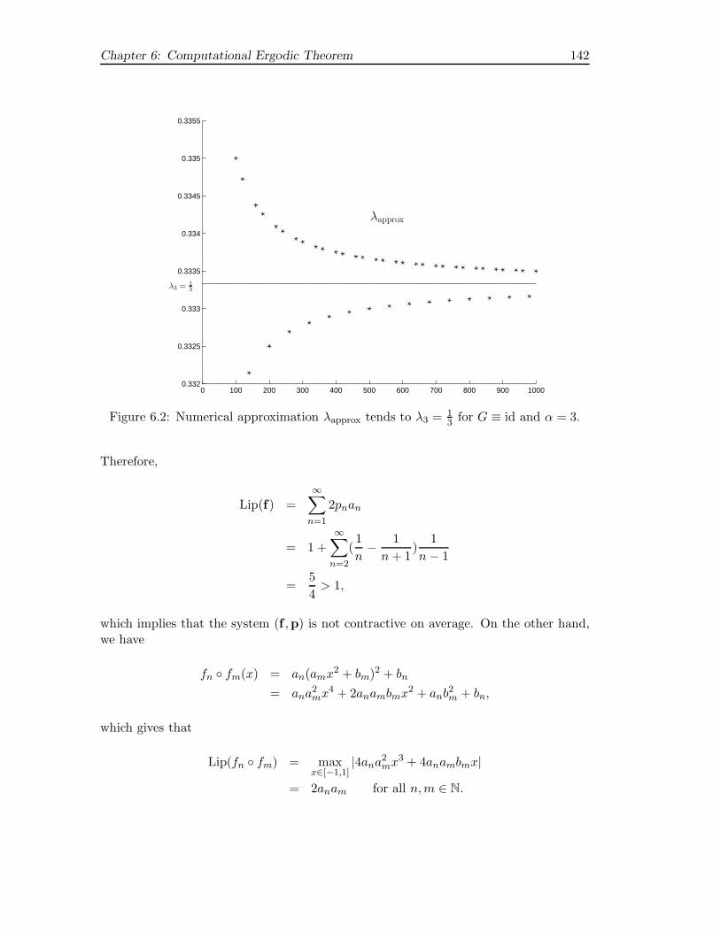
Chapter 6: Computational Ergodic Theorem 142
0 100 200 300 400 500 600 700 800 900 10000.332
0.3325
0.333
0.3335
0.334
0.3345
0.335
0.3355
λ3 = 13
λapprox
Figure 6.2: Numerical approximation λapprox tends to λ3 = 13 for G ≡ id and α = 3.
Therefore,
Lip(f) =∞∑
n=1
2pnan
= 1 +
∞∑
n=2
(1
n− 1
n+ 1)
1
n− 1
=5
4> 1,
which implies that the system (f ,p) is not contractive on average. On the other hand,we have
fn fm(x) = an(amx2 + bm)2 + bn
= ana2mx
4 + 2anambmx2 + anb
2m + bn,
which gives that
Lip(fn fm) = maxx∈[−1,1]
|4ana2mx
3 + 4anambmx|
= 2anam for all n,m ∈ N.

143 6.5 Examples
Consequently,
Lip2(f) =
∞∑
n,m=1
pnpmLip(fn fm)
=1
2
∞∑
n,m=1
4pnpmanam
=25
32< 1,
which ensures that the system (f ,p) is 2-contractive on average. To apply the algorithmdescribed in Section 6.3 we fix k ∈ N and partition X into X1,X2, ...,Xk, where for all
1 ≤ n ≤ k− 1, Xn =[−1 + 2(n−1)
k ,−1 + 2nk
)and Xk =
[1 − 2
k , 1]. For each interval Xn
we define the middle point xn = −1 + 2n−1k ∈ Xn. For an explicit computation we set
G ≡ id. For each k ∈ N we numerically compute the matrix S(k) as in (6.38) for l = 2and a fixed left eigenvector s(k), see [56, Remark 3.10]. Our main result Theorem 6.3.6implies that
λapprox(k) :=k∑
n=1
s(k)n G(xn)
converges to λ as k → ∞. Table 6.2 shows the approximation λapprox(k) and the upperbound err(k) of λapprox(k) − λ provided by the right hand side of (6.40).
k Approximation λapprox(k) Upper bound as in (6.40): err(k)
50 −0.0562 1
100 −0.0511 5 × 10⁻¹
500 −0.0479 1 × 10⁻¹
1000 −0.0466 5 × 10⁻²
Table 6.2: Approximated number and upper bound as in (6.40) for G ≡ id.
Example 6.5.4 (Products of random matrices). Define the pair (A,P) by
A1 =
(0 11 0
), p1 =
1
2; An =
(2n− 2 0
0 n− 1
), pn =
1
2n − 2− 1
2n, n = 2, 3, . . . .
(6.61)We first point out that the pair (A,P) fulfills all assumptions of Theorem 6.4.9. It iseasy to see that the only subspace of R2 which is invariant under all of Ak is the trivialsubspace. Since
∑∞n=1
log nn2 <∞ it follows that
∞∑
n=1
pn
(log+ ‖An‖ + log+ ‖A−1
n ‖)
=1
2
∞∑
n=1
log n+ log 2
n(n+ 1)<∞,
which implies the integrability of (A,P). Concerning the Lipschitz constant on averageof (A,P), we use the observation that Lip(An) = Lip(A2) for all n = 2, 3, . . . , where An
Chapter 6: Computational Ergodic Theorem 144
is the induced map of An on Sd−1, i.e.
An(v) =An(v)
‖An(v)‖ for all v ∈ Sd−1.
Therefore, by (6.44) we have
Lip(A) =∞∑
n=1
pn Lip(An) =1
2Lip(A1) +
1
2Lip(A2) <∞.
Now we compute explicitly an invariant measure of (A,p). By (6.61), we have
A1
(cosϕsinϕ
)=
(sinϕcosϕ
)for all ϕ ∈ [0, 2π]
and
An
(cosϕsinϕ
)=
1√4 cos2 ϕ+ sin2 ϕ
(2 cosϕsinϕ
)for all n = 2, 3, . . . and ϕ ∈ [0, 2π].
Hence, a direct computation yields that µ := 12 (δ(1,0)T +δ(0,1)T ) ∈ M(S1) is an invariant
probability measure under the operator P : M(S1) → M(S1) which is defined as in(6.48), i.e.
Pν =∞∑
n=1
pnν A−1n for all ν ∈ M(S1).
Therefore, in view of Lemma 6.4.5 the top Lyapunov exponent λ1 of (A,p) can becomputed by
λ1 =
∞∑
n=1
pn
∫
S1
log ‖An(v)‖ dµ(v)
=1
2
( ∞∑
n=1
pn
∫
S1
log ‖An(v)‖ dδ(0,1)T (v) +
∞∑
n=1
pn
∫
S1
log ‖An(v)‖ dδ(1,0)T (v)
)
=1
2
( ∞∑
n=2
pn log(n− 1)
)+
1
2
( ∞∑
n=2
pn log(2n− 2)
)
=1
2
∞∑
n=1
log n
n(n+ 1)+
log 2
4. (6.62)
To apply the algorithm described in Subsection 6.4.2 we fix k ∈ N and partition S1 intok disjoint sets B1, B2, . . . , Bk by
Bn :=
(cosϕsinϕ
): ϕ ∈
[2π(n − 1)
k,
2πn
k
), n = 1, 2, . . . , k.

145 6.5 Examples
For each set Bn we define the middle point bn =
(cos π(2n−1)
k
sin π(2n−1)k
). In the first step of
the algorithm we compute the matrix S(k) as in (6.51) and a fixed left eigenvector s(k).By virtue of Theorem 6.4.9 we obtain that
λapprox(k) :=k∑
n=1
p(k)n
k∑
i=1
s(k)i log ‖An(bi)‖
converges to λ1. Figure 6.3 shows how λapprox(k) converges to λ1 which is determinedexplicitly by (6.62).
0 100 200 300 400 500 600 700 800 900 10000.46
0.48
0.5
0.52
0.54
0.56
0.58
λ1
λapprox
Figure 6.3: Numerical approximation λapprox tends to λ1.
Chapter 7
Outlook
7.1 One-Sided RDS on Banach Space
As in finite dimensional case, if the RDS is not invertible one can only hope for a flagdecomposition of the state space. We use here a similar approach as in Thieullen [136], itmeans that we enlarge the state space to make the RDS invertible. Then the flag spacesof the original system are obtained as images of the projections of Oseledet spaces of theenlarged system. A technical problem arising here is that the separability of the statespace is an important property for which the MET in Banach space in Lian and Lu [89](see also Theorem 1.4.2) can be applied. The enlarged state space provided in Thieullen[136] is in general not separable. In this section, using positive weight factors, we firstenlarge the state space to become a separable Banach space and the corresponding RDSon this space is injective. After that applying the MET in Banach space in Lian and Lu[89] gives the MET for one-sided RDS on Banach space.Let X be a separable Banach space and Φ : Ω → L(X) a strongly measurable mapsatisfying that
log+ ‖Φ(·)‖ ∈ L1(Ω,F ,P). (7.1)
Recall that the Kuratowski measure of the RDS Φ is determined by
lα(Φ) := limn→∞
1
nlog ‖Φ(n, ω)‖α P-a.e. ω ∈ Ω.
For a fixed positive number γ > 0, the state space X is enlarged by
Xγ =x := (xn)n∈N0 : lim
n→∞e−γnxn exists
.
We endow the space Xγ with the following norm
‖x‖γ := supn∈N0
e−γn‖xn‖ for all x ∈ Xγ .
Lemma 7.1.1. The Banach space (Xγ , ‖ · ‖γ) is separable.
Proof. The proof is analog to Lemma 4.1.2.
146
147 7.1 One-Sided RDS on Banach Space
We choose and fix a sequence (αn)n∈N0 satisfying the following conditions:
1. αn > αn+1 > 0 for all n ∈ N0.
2. Set
γ0 := 0, γn :=
n−1∑
k=0
log αk for all n ≥ 1 (7.2)
and for each µ < 0
Pµ(n) := sup p ∈ N0 : γp ≥ (n + p)µ . (7.3)
Then we have
limn→∞
γn
n= −∞, and lim
n→∞Pµ(n)
n= 0, for all µ < 0. (7.4)
An explicit example of sequence satisfying the above conditions is
αn = e−(2n+1) for all n ∈ N0.
Associated to the sequence (αn)n∈N0 we define a mapping Φ : Ω → L(Xγ) by
Φ(ω)(x0, x1, . . . ) = (Φ(ω)x0, α0x0, α1x1, . . . ). (7.5)
An explicit form of Φ(n, ω) is given by
Φ(n, ω)x = (Φ(n, ω)x0, α0Φ(n− 1, ω)x0, . . . , αn−1 . . . α0x0, αn . . . α1x1, . . . ) , (7.6)
where x = (x0, x1, . . . ) ∈ Xγ .
Lemma 7.1.2. The mapping Φ is strongly measurable and satisfies
log+ ‖Φ(·)‖γ ∈ L1(Ω,F ,P).
Moreover, for each ω ∈ Ω the linear operator Φ(ω) : Xγ → Xγ is injective.
Proof. Since the sequence (αn)n∈N0 is positive and decreasing it follows that the limitlimn→∞ αn exists. Hence, for each x = (xn)n∈N0 the limit limn→∞ e−γ(n+1)αnxn existsand thus Φ(ω)x ∈ Xγ . Furthermore, a direct computation yields that
‖Φ(ω)x‖γ ≤ max‖Φ(ω)‖, α0e
−γ
for all ‖x‖γ = 1.
As a consequence, the function Φ is well-defined and satisfies the integrability condition,i.e. it satisfies
log+ ‖Φ(·)‖γ ∈ L1(Ω,F ,P).
To prove the strong measurability of Φ, we choose and fix x ∈ Xγ . For any ε > 0 andy = (y0, y1, . . . ) ∈ Xγ we consider the following cases.
Chapter 7: Outlook 148
Case 1 : If |αnxn − yn+1| ≤ εeγ(n+1) for all n ∈ N0 thenω ∈ Ω : Φ(ω)x ∈ Bε(y)
=ω ∈ Ω : Φ(ω)x0 ∈ Bε(y0)
.
Case 2 : If there exists n ∈ N0 such that |αnxn − yn+1| > εeγ(n+1) thenω ∈ Ω : Φ(ω)x ∈ Bε(y)
= ∅.
Hence, the function Φ is strongly measurable. The injectivity of the linear operatorΦ(ω) can be easily seen from (7.5) and the proof is complete.
So far we have enlarged the state space and introduced the corresponding RDS Φ onthe enlarged state space. We now investigate the relation between the linear cocycles Φand Φ. Firstly, we state and prove the following technical lemma.
Lemma 7.1.3. Let (γn)n∈N0 and (an)n∈N0 be sequences such that
limn→∞
γn
n= −∞, lim
n→∞an
n= a.
Then
limn→∞
bnn
= a, where bn := max0≤j≤n−1
(γj + an−j).
Proof. By the definition of the sequence (bn)n∈N0 we have
lim infn→∞
bnn
≥ limn→∞
an
n.
Hence, it remains to show that
lim supn→∞
bnn
≤ limn→∞
an
n+ ε for all ε > 0.
Choose N ∈ N such that
an ≤ n(a+ ε), γn ≤ na for all n ≥ N,
which implies that for all n ≥ 2N
bnn
= max
sup
0≤j≤N−1
γj + an−j
n, supN≤j≤n−N−1
γj + an−j
n, supn−N≤j≤n−1
γj + an−j
n
≤ max
sup
0≤j≤N−1
γj + (n− j)(a + ε)
n, a+ ε, sup
n−N≤j≤n−1
ja+ an−j
n
.
Letting n→ ∞ gives that
lim supn→∞
bnn
≤ max a+ ε, a+ ε, a ,
which completes the proof.

149 7.1 One-Sided RDS on Banach Space
Lemma 7.1.4. Suppose that (αn)n∈N0 be a strictly decreasing and positive sequencesatisfying condition (7.4). Then lα(Φ) = lα(Φ).
Proof. Let B1(0) and B1(0) denote the unit ball in (Xγ , ‖ · ‖γ) and X, respectively. Set
βn := ‖Φ(n, ω)‖α = α (Φ(n, ω)B1(0)) .
From the definition of Kuratowski measure (see (1.14)), there exist finitely many setsAn
1 , . . . , Ankn
such that
Φ(n, ω)B1(0) ⊂kn⋃
i=1
Ani , diam(An
i ) ≤ βn for all i = 1, . . . , kn.
For each n ∈ N and ij = 1, . . . , kn−j for j = 0, . . . , n− 1, we define
Bni0,...,in−1
:=
(x0, x1, . . . ) ∈ Xγ : xj ∈ αj−1 . . . αj−ne(j−n)γB1(0) for j ≥ n,
x0 ∈ Ani0 , xj ∈ αj−1 . . . α0A
n−jij
for 1 ≤ j ≤ n− 1.
By (7.6), a direct computation yields that
Φ(n, ω)B1(0) ⊂kn⋃
i0=1
kn−1⋃
i1=1
· · ·k1⋃
in−1=1
Bni0,...,in−1
for all n ∈ N,
and
diam(Bni0,...,in−1
) ≤ sup
βn, α0βn−1, . . . , αn−2 . . . α0β1, e
−γn supj≥n
αj−1 . . . αj−n
.
As a consequence, we get
‖Φ(n, ω)‖α ≤ maxβn, α0βn−1, . . . , αn−2 . . . α0β1, e
−γnαn−1 . . . α0
.
Therefore,
log ‖Φ(n, ω)‖α ≤ max
max
0≤j≤n−1(γj + log βn−j), γn − γn
, (7.7)
where (γn)n∈N0 is defined as in (7.2). In light of Lemma 7.1.3 we have
limn→∞
max0≤j≤n−1(γj + log βn−j)
n= lim
n→∞log βn
n= lα(Φ),
which together with (7.7) implies that
lα(Φ) = limn→∞
1
nlog ‖Φ(n, ω)‖α ≤ lα(Φ).
On the other hand, it is easy to verify that
‖Φ(n, ω)‖α ≤ ‖Φ(n, ω)‖α for all ω ∈ Ω, n ∈ N,
which gives that lα(Φ) ≤ lα(Φ) and the proof is complete.
Chapter 7: Outlook 150
Lemma 7.1.5. Let Φ be the linear cocycle defined as in (7.5). Then
limn→∞
1
nlog ‖Φ(n, ω)‖ = lim
n→∞1
nlog ‖Φ(n, ω)‖γ .
Proof. An elementary computation from (7.6) yields that
‖Φ(n, ω)‖γ ≥ ‖Φ(n, ω)‖ for all n ∈ N, ω ∈ Ω.
On the other hand, from (7.6) we derive
log ‖Φ(n, ω)‖γ ≤ max
sup
0≤j≤n−1
(log γj + log ‖Φ(n− j, ω)‖
),−γn+ γn
,
where (γn)n∈N0 is defined as in (7.2). According to Lemma 7.1.3, we obtain
limn→∞
1
nlog ‖Φ(n, ω)‖γ ≤ lim
n→∞1
nlog ‖Φ(n, ω)‖,
which completes the proof.
Lemma 7.1.6. Let x = (x0, x1, . . . ) ∈ Xγ such that limn→∞1n log ‖Φ(n, ω)x‖γ exists.
Then
limn→∞
1
nlog ‖Φ(n, ω)x0‖ = lim
n→∞1
nlog ‖Φ(n, ω)x‖γ .
Proof. By (7.6), we get
λ := limn→∞
1
nlog ‖Φ(n, ω)x‖γ ≥ lim sup
n→∞
1
nlog ‖Φ(n, ω)x0‖.
Hence, it remains to show that
a := lim infn→∞
1
nlog ‖Φ(n, ω)x0‖ ≥ λ. (7.8)
For any ε > 0 there exists a sequence (nk)k∈N0 such that nk < nk+1 and
1
nklog ‖Φ(nk, ω)x0‖ ≤ a+ ε for all k ∈ N0. (7.9)
Choose and fix µ < 0 such that µ ≤ a. Define
mk := nk + Pµ(nk) for all k ∈ N0,
where Pµ(nk) is defined as in (7.3). By considering a new cocycle Φ(ω) := Φ(ω)max1,‖Φ(ω)‖
if necessary, we assume w.l.o.g. that ‖Φ(ω)‖ ≤ 1 for all ω ∈ Ω. Therefore, we have
‖Φ(n, ω)x0‖ ≤ ‖Φ(m,ω)x0‖ for all n ≥ m,

151 7.1 One-Sided RDS on Banach Space
which implies together with (7.9) that for 0 ≤ j ≤ Pµ(nk) we get
γj + log ‖Φ(mk − j, ω)x0‖ ≤ supj≥0
γj + ‖Φ(nk, ω)x0‖
≤ supj≥0
γj + (a+ ε)nk. (7.10)
On the other hand, for any mk − 1 ≥ j > Pµ(nk) we get
γj + log ‖Φ(mk − j, ω)x0‖ ≤ (nk + Pµ(nk))µ + ‖x0‖,
which together with (7.10) and (7.6) implies that
log ‖Φ(mk, ω)x‖γ ≤ max
max
0≤j≤mk−1(γj + log ‖Φ(mk − j, ω)x0‖) ,
, γmk+ log ‖x‖γ − γmk
≤ max
(a+ ε)nk + sup
j≥0γj,mkµ+ ‖x0‖, γmk
+ log ‖x‖γ − γmk
,
where (γn)n∈N0 is defined as in (7.2). As a consequence, we obtain
lim infk→∞
1
mklog ‖Φ(mk, ω)x‖γ ≤ a+ ε,
where we use the assumption limk→∞nk
mk= limk→∞
nk
nk+Pµ(nk) = 1 to obtain the above
estimate. Hence, statement (7.8) is proved and the proof is complete.
Now we are at a position to state and prove the MET for one-sided random dynamicalsystems on Banach spaces.
Theorem 7.1.7 (MET for One-sided RDS on Banach Space). Let (Ω,F ,P, θ) be anergodic MDS and X a separable Banach space. Assume that Φ : Ω → L(X) is a stronglymeasurable mapping satisfying that
log+ ‖Φ(·)‖ ∈ L1(Ω,F ,P).
Suppose additionally that κ(Φ) > lα(Φ). Then there exists a θ-invariant subset Ω ⊂ Ωof full measure such that there exist Lyapunov exponents λ1 > · · · > λp > lα(Φ) and afiltration
X = V1(ω) ⊃ V2(ω) ⊃ · · · ⊃ Vp+1(ω)
with the following properties hold:
(i) Invariance: Vj is of finite codimension and Φ(ω)Vj(ω) ⊂ Vj(θω).
Chapter 7: Outlook 152
(ii) Lyapunov exponents: for all j = 1, . . . , p
limn→∞
1
nlog ‖Φ(n, ω)v‖ = λj for all v ∈ Vj(ω) \ Vj+1(ω)
and if p is infinite then limp→∞ λp = lα(Φ).
Proof. Let (αn)n∈N0 be a strictly decreasing and positive sequence satisfying condition(7.4). We define the enlarged RDS Φ : Ω → L(Xγ) as in (7.5). By virtue of Lemma
7.1.4 and Lemma 7.1.5, we get κ(Φ) > lα(Φ). Furthermore, in view of Lemma 7.1.2, thelinear cocycle Φ fulfills all assumptions of Theorem 1.4.2. We divide the proof into thefollowing cases:
Case 1 : The linear cocycle Φ has finitely many Lyapunov exponents denoted by λ1 >λ2 > · · · > λp > lα(Φ). The corresponding Oseledet’s splitting is given by
Xγ = E1(ω) ⊕ E2(ω) ⊕ · · · ⊕ Ep(ω) ⊕ F(ω),
where
limn→∞
1
nlog ‖Φ(n, ω)x‖γ = λj for all 0 6= x ∈ Ej(ω) (7.11)
and
limn→∞
1
nlog ‖Φ(n, ω)|F(ω)‖γ ≤ lα(Φ). (7.12)
Let π : Xγ → X denote the projection onto the first component, i.e.
πx = x0 for all x = (x0, x1, . . . ) ∈ Xγ .
Define
Vj(ω) := π
F(ω) ⊕
⊕
j≤i≤p
Ei(ω)
for all 1 ≤ j ≤ p+ 1.
Using the fact that
Φ(ω)πx = πΦ(ω)x for all x ∈ Xγ ,
we obtain that the subspace Vj(ω) is invariant under Φ. Using (7.11) and (7.12) and inview of Lemma 7.1.6, we get
limn→∞
1
nlog ‖Φ(n, ω)x‖ = λj for all x ∈ Vj(ω) \ Vj+1(ω),
which completes the proof in this case.
Case 2: The linear cocycle Φ has infinitely many Lyapunov exponents λ1 > λ2 > . . . ,where limp→∞ λp = lα(Φ). The proof in this case is analog to Case 1 and we obtain thedesired conclusion.
153 7.2 Lyapunov norm for RDS on Banach Space
7.2 Lyapunov norm for RDS on Banach Space
Invariant manifold theory for RDS based on the MET is an important part of smoothergodic theory. It was started in 1976 with the pioneering work of Pesin [115, 116].He constructed the classical stable and unstable manifolds of a deterministic diffeomor-phism on a compact Riemannian manifold preserving a measure which is absolutelycontinuous with respect to the Riemannian volume. His technique is to cope with thenon-uniformity of the MET (random norms, ε-slowly varying functions). This techniqueis also used in Wanner [139] and Arnold [3] to construct invariant manifolds for RDS onfinite dimensional space. In this chapter, based on the non-uniformity of the MET forRDS on Banach space we construct the Lyapunov norms corresponding to a linear dif-ference equation with random delay which is the investigated object in Chapter 4. Thework in this subsetion can be considered as the first technical step toward the nonlineartheory of difference equations with random delay.
We start this chapter by introducing the notion of tempered and ε-slowly varying randomvariable.
Definition 7.2.1 (Tempered, Slowly Varying Random Variables). Let (Ω,F ,P, θ) bean MDS.
(i) A random variable R : Ω → (0,∞) is called tempered with respect to θ if
limn→±∞
1
nR(θnω) = 0 for P-a.e. ω ∈ Ω.
(ii) For a given ε ≥ 0, a random variable R : Ω → (0,∞) is called ε-slowly varying withrespect to θ if P-a.s.
e−ε|n|R(ω) ≤ R(θnω) ≤ eε|n|R(ω) for all n ∈ Z.
A relation between tempered and slowly varying random variables is the content of thefollowing lemma.
Lemma 7.2.1 (Tempered Versus Slowly Varying). (i) If Rε is ε-slowly varying for someε ≥ 0 then it is tempered.
(ii) Conversely, if f : Ω → (0,∞) is tempered then for any ε > 0 there is an ε-slowlyvarying random variable Rε for which
1
Rε(ω)≤ f(ω) ≤ Rε(ω).
Proof. A proof can be found in Arnold [3, Proposition 4.3.3].
Now we discuss about the Lyapunov norm associated with a linear difference equationwith random delay. We consider a linear difference equation of the form
xn+1 = A(θnω)xn +B(θnω)xn−r(θnω), (7.13)
Chapter 7: Outlook 154
where A,B : Ω → Rd×d are measurable functions and r : Ω → N is measurable, onthe state space Xγ . Let Φ denote the linear cocycle generated (7.13). Throughout thischapter, we assume that Φ satisfies the integrability condition of the MET, i.e.
log+ ‖Φ(·)‖ ∈ L1(Ω,F ,P).
By virtue of Theorem 4.2.3, let −γ < λp < · · · < λ1 be the Lyapunov exponents of Φand
Xγ = E1(ω) ⊕ E2(ω) ⊕ · · · ⊕Ep(ω) ⊕ F (ω)
denote the corresponding Oseledet splitting. Choose any j with 1 ≤ j < p, let
Λ+j := λ1 > · · · > λj, E+
j (ω) :=⊕
1≤i≤j
Ei(ω), Fj(ω) :=⊕
j+1≤i≤p
Ei(ω) ⊕ F (ω).
Let πj(ω) denote the projection onto Fj(ω) along E+j (ω). By virtue of MET, we obtain
that the random variable ‖πj(·)‖ is tempered. The following theorem is a direct conse-quence of the non-uniformity of the MET for RDS on Banach space which is proved inLian and Lu [89].
Theorem 7.2.2 (Non-Uniformity of MET is Slowly Varying, [89]). Suppose that system(7.13) fulfills all assumptions in Theorem 4.2.3. Then there exists an ε-slowly varyingrandom variable Rε : Ω → [1,∞) such that on the invariant set Ω of the MET thecocycle Φ has the following properties:
1
Rε(ω)eλjn−ε|n|‖x‖ ≤ ‖Φ(n, ω)x‖ ≤ Rε(ω)eλjn+ε|n|‖x‖, x ∈ E+
j (ω),
and
‖Φ(n, ω)x‖ ≤ Rε(ω)eλj+1n+ε|n|‖x‖, x ∈ Fj(ω).
We choose and fix a positive constant κ such that λj − κ > λj+1 + κ and construct thefollowing norms
‖xu‖ω :=
∞∑
n=0
e(λj−κ)n‖Φ(−n, ω)xu‖ for all xu ∈ E+j (ω),
‖xs‖ω :=
∞∑
n=0
e−(λj+1+κ)n‖Φ(n, ω)xs‖ for all xs ∈ Fj+1(ω).
For any x ∈ Xγ and ω ∈ Ω with x = xs + xu, where xs ∈ E+j (ω) and xu ∈ Fj+1(ω), we
set
‖x‖ω = max‖xu‖ω, ‖xs‖ω.The norm ‖ · ‖ω is usually called the Lyapunov norm. In the following theorem, weprovide some fundamental properties of the above norm.

155 7.2 Lyapunov norm for RDS on Banach Space
Theorem 7.2.3. The norm ‖ · ‖ω is strongly measurable, i.e. for each fixed x ∈ Xγ
the scalar valued function Ω → R+, ω 7→ ‖x‖ω is measurable, and satisfies that for eachε > 0 there exists an ε-slowly varying random variable Dε : Ω → [1,∞) such that
1
Dε(ω)‖ · ‖ ≤ ‖ · ‖ω ≤ Dε(ω)‖ · ‖. (7.14)
Furthermore, we obtain that for all n ≥ 0
‖Φ(n, ω)xs‖θnω ≤ e(λj+1+κ)n‖xs‖ω for all xs ∈ Fj+1(ω),
‖Φ(−n, ω)xu‖θ−nω ≤ e−(λj−κ)n‖xu‖ω for all xu ∈ E+i (ω).
Proof. The fact that ‖ · ‖ω is strongly measurable is a direct consequence of the strongmeasurability of the projection πj(·). W.l.o.g. we assume that ε < κ
2 . We first verifythe estimate of ‖ · ‖ω from above. In view of Theorem 7.2.2, there exists an ε
2 -slowlyvarying random variable R ε
2: Ω → [1,∞) such that for all n ≥ 0
‖Φ(−n, ω)xu‖ ≤ R ε2(ω)e−(λj−ε)n‖xu‖ for all xu ∈ E+
j (ω),
‖Φ(n, ω)xs‖ ≤ R ε2(ω)e(λj+1+ε)n‖xs‖ for all xs ∈ Fj(ω).
As a consequence, a direct computation yields that
‖xu‖ω ≤ eε
eε − 1R ε
2(ω)‖xu‖, ‖xs‖ω ≤ eε
eε − 1R ε
2(ω)‖xs‖,
which implies that
‖x‖ω ≤ eε
eε − 1R ε
2(ω)(1 + 2‖πj(ω)‖)‖x‖.
On the other hand, from the definition of ‖ · ‖ω we derive
‖x‖ω ≥ 1
2(‖xu‖ω + ‖xs‖ω) ≥ 1
2‖x‖.
Define Dε(ω) := eε
eε−1R ε2(ω)(1+ 2‖πj(ω)‖). Note that ‖πj(·)‖ is tempered and by virtue
of Lemma 7.2.1, the random variable Dε is thus ε-slowly varying. Obviously, Dε satisfiesinequality (7.14). For the remainder of the proof, we need to estimate
‖Φ(n, ω)xs‖θnω, ‖Φ(−n, ω)xu‖θ−nω for all n ≥ 0.
Using the fact that Φ(n, ω)Fj(ω) ⊂ Fj(θnω), we obtain
‖Φ(n, ω)xs‖θnω =
∞∑
k=0
e−(λj+1+κ)k‖Φ(k, θnω)Φ(n, ω)xs‖
= e(λj+1+κ)n∞∑
k=0
e−(λj+1+κ)(k+n)‖Φ(k + n, ω)xs‖
≤ e(λj+1+κ)n‖xs‖ω.
Similarly, we also have
‖Φ(−n, ω)xu‖θ−nω ≤ e−(λj−κ)n‖xu‖ω,
which completes the proof.
Appendix A
Birkhoff Ergodic Theorem
A central aspect of ergodic theory is the long-term behavior of a dynamical system andthe relation to the spacial behavior. This is expressed through the Birkhoff ergodictheorem which asserts that, under certain conditions, the time average of a functionalong the trajectories exists almost everywhere and is related to the space average. Tomake the thesis self-contained we state and prove the Birkhoff ergodic theorem in thisAppendix. Here we follow the presentation to prove the Birkhoff ergodic theorem inWalter [138].
Theorem A.0.4 (Birkhoff Ergodic Theorem). Let θ be a measure preserving transfor-mation of a probability space (Ω,F ,P) and f ∈ L1(Ω,F ,P). Then there exists a functionf∗ ∈ L1(Ω,F ,P) such that
limn→∞
n−1∑
k=0
f(θkω) = f∗(ω) for P-a.e. ω ∈ Ω.
Moreover, f∗ is invariant under θ, i.e. f∗ θ = f∗, and∫Ω f
∗ dP =∫Ω f dP. In
particular, if θ is an ergodic transformation then
limn→∞
n−1∑
k=0
f(θkω) =
∫
Ωf(ω) dP(ω) for P-a.e. ω ∈ Ω.
Before we prove the Birkhoff ergodic theorem we show a preparatory theorem which iswell known under the name maximal ergodic theorem.
Theorem A.0.5 (Maximal Ergodic Theorem). Let (Ω,F ,P) be a probability space andL1(Ω,F ,P) denote the space of all real-valued integrable functions on (Ω,F ,P). Supposethat U : L1(Ω,F ,P) → L1(Ω,F ,P) is a positive linear operator, i.e. Uf ≥ 0 for allf ∈ L1(Ω,F ,P) with f ≥ 0, and ‖U‖ ≤ 1. Let N ≥ 0 be an integer and f ∈ L1(Ω,F ,P).Define the sequence of functions (fn)n∈N0 by
f0 := 0, fn := f + Uf + · · · + Un−1f for all n ≥ 1,
156
157
and define FN = max0≤n≤N fn. Then the following statement holds∫
ω:FN (ω)>0f dP ≥ 0. (A.1)
Proof. Clearly FN ∈ L1(Ω,F ,P). For any 0 ≤ n ≤ N , we have FN ≥ fn so UFN ≥ Ufn
by the positivity of U . Hence, we obtain
UFN + f ≥ Ufn + f = fn+1 for all 0 ≤ n ≤ N.
Therefore,UFN (ω) + f(ω) ≥ max
1≤n≤Nfn(ω).
In particular, if FN (ω) > 0 then
UFN (ω) + f(ω) = max0≤n≤N
fn(ω) = FN (ω),
which implies that f(ω) ≥ FN (ω) − UFN (ω) on the set ω : FN (ω) > 0. As a conse-quence, we get
∫
ω:FN (ω)>0f dP ≥
∫
ω:FN (ω)>0FN dP −
∫
ω:FN (ω)>0UFN dP
≥∫
ΩFN dP −
∫
ω:FN (ω)>0UFN dP,
On the other hand, since FN ≥ 0 it follows that UFN ≥ 0 by positivity of U and wetherefore obtain the following estimate
∫
ω:FN (ω)>0f dP ≥
∫
ΩFN dP −
∫
ΩUFN dP.
This implies with ‖U‖ ≤ 1 inequality (A.1) and completes the proof.
Remark A.0.6. For any probability space (Ω,F ,P) and a transformation θ : Ω → Ωpreserving the probability P, we can define an operator U : L1(P) → L1(Ω,F ,P) by
Uf(ω) = f(θω) for all f ∈ L1(Ω,F ,P), ω ∈ Ω.
Then it is easy to see that U is a positive linear operator and ‖U‖ = 1.
Corollary A.0.7. Let (Ω,F ,P) be a probability space and θ : Ω → Ω a transformationpreserving the probability P. Let g ∈ L1(Ω,F ,P) and define
Bα := ω ∈ Ω : supn≥1
1
n
n−1∑
i=0
g(θiω) > α
Then ∫
Bα∩Ag(ω) dP(ω) ≥ α P(Bα ∩A)
if A is a measurable set which is invariant under θ, i.e. θ−1A = A.
Chapter A: Birkhoff Ergodic Theorem 158
Proof. We first prove this result under the assumption A = X. Define f := g − α, thesequence of functions (fn)n≥0 from Ω to R by
f0 := 0, fn := f + f θ + · · · + f θn−1 for n ≥ 1,
and FN = max0≤n≤N fn. Hence,
Bα =∞⋃
N=0
ω : FN (ω) > 0.
By virtue of Theorem A.0.5 and Remark A.0.6, we get∫
Bα
f(ω) dP(ω) ≥ 0.
Consequently, ∫
Bα
g(ω) dP(ω) ≥ αP(Bα).
In the general case, we apply the above result to θ|A to get
∫
A∩Bα
g(ω) dP(ω) ≥ αP(A ∩Bα),
and this completes the proof.
Proof of Theorem A.0.4. Define
f∗(ω) = lim supn→∞
1
n
n−1∑
i=0
f(θiω) for ω ∈ Ω,
and
f∗(ω) = lim infn→∞
1
n
n−1∑
i=0
f(θiω) for ω ∈ Ω.
It is easy to see that f∗θ = f∗ and f∗θ = f∗. Now, we show that f∗ = f∗ P-a.e. andthat they belong to L1(Ω,F ,P). For real numbers α, β with α < β, define
Eα,β := ω ∈ Ω : f∗(ω) < β and α < f∗(ω).
Note thatω : f∗(ω) < f∗(ω) =
⋃
α,β∈Q,β<α
Eα,β.
Hence, to prove f∗ = f∗ P-a.e. it is sufficient to show that P(Eα,β) = 0. Clearly, the setEα,β is invariant under θ, i.e. θ−1Eα,β = Eα,β, and if we put
Bα := ω ∈ Ω : supn≥1
1
n
n−1∑
i=0
f(θiω) > α
159
then Eα,β ∩Bα = Eα,β. By Corollary (A.0.7) we obtain
∫
Eα,β
f(ω) dP(ω) =
∫
Eα,β∩Bα
f(ω) dP(ω) ≥ αP(Eα,β ∩Bα) = αP(Eα,β).
Consequently, ∫
Eα,β
f(ω) dP(ω) ≥ αP(Eα,β). (A.2)
On the other hand, if we replace f, α, β by −f,−β,−α, respectively, then since (−f)∗ =−f∗ and (−f)∗ = −f∗, we get
∫
Eα,β
f(ω) dP(ω) ≤ βP(Eα,β). (A.3)
Combining (A.2) and (A.3), we get αP(Eα,β) ≤ βP(Eα,β). This implies that P(Eα,β) =0. Hence, f∗ = f∗ P-a.e., and then
limn→∞
1
n
n−1∑
i=0
f(θiω) = f∗(ω) = f∗(ω) for P-a.e. ω ∈ Ω.
To show f∗ ∈ L1(Ω,F ,P) we use the Fatou lemma (see Lang [85, pp. 141]) that assertslimn→∞ gn ∈ L1(Ω,F ,P) if (gn)n∈N is a pointwise convergent sequence of nonnegativeintegrable functions with lim inf
∫Ω gn dP(ω) <∞. Define
gn(ω) =1
n
n−1∑
i=0
f(θiω) for ω ∈ Ω.
It is easily seen that
∫
Ωgn(ω) dP(ω) ≤
∫
Ω|f(ω)| dP(ω) for all n ∈ N.
Therefore, we can apply the Fatou lemma together with the fact that limn→∞ gn(ω) =|f∗(ω)| to conclude that f∗ ∈ L1(Ω,F ,P). It remains to show that
∫Ω f(ω) dP(ω) =∫
Ω f∗(ω) dP(ω). For this purpose, we define
Dnk :=
ω ∈ Ω :
k
n≤ f∗(ω) <
k + 1
n
,
where k ∈ Z, n = 1, 2, . . . . For each small ε > 0, we have Dnk ∩ B k
n−ε = Dn
k and by
Corollary A.0.7 we get
∫
Dnk
f(ω) dP(ω) ≥(k
n− ε
)P(Dn
k ).
Chapter A: Birkhoff Ergodic Theorem 160
This implies that
∫
Dnk
f∗(ω) dP(ω) ≤ k + 1
nP(Dn
k ) ≤ 1
nP(Dn
k ) +
∫
Dnk
f(ω) dP(ω).
Summing this inequality over k gives∫Ω f
∗(ω) dP(ω) ≤ 1n +
∫Ω f(ω) dP(ω). Since this
holds for all n ≥ 1, we have
∫
Ωf∗(ω) dP(ω) ≤
∫
Ωf(ω) dP(ω). (A.4)
Applying (A.4) to −f instead of f gives
∫
Ω(−f)∗(ω) dP(ω) ≤ −
∫
Ωf(ω) dP(ω).
Hence, ∫
Ωf∗(ω) dP(ω) ≥
∫
Ωf(ω) dP(ω). (A.5)
Combining (A.4) and (A.5) and the fact that f∗ = f∗ P-a.e., we get∫Ω f
∗(ω) dP(ω) =∫Ω f(ω) dP(ω). For the remaining part of the proof, we consider the case that θ is an
ergodic transformation. Since f∗θ = θ it follows that the function f∗ is almost surelyconstant. Consequently, the limit
limn→∞
n−1∑
k=0
f(θkω) = f∗(ω) =
∫
Ωf∗(ω) dP(ω) =
∫
Ωf(ω)
holds for P-a.e. ω ∈ Ω and this completes the proof.
Appendix B
Kingman Subadditive Ergodic
Theorem
A substantial generalization of Birkhoff ergodic theorem was obtained by Kingman,who proved an ergodic theorem for subadditive stationary processes in [78]. This resulthas also been reproved with elegant proofs in Burkholder [25], Steele [129]. Here wefollow the materials in Steele [129] to state and prove the Kingman subadditive ergodictheorem.
Theorem B.0.8 (Kingman subadditive ergodic theorem). Let θ be a measure preservingtransformation of a probability space (Ω,F ,P) and gn∞n=1 a subadditive sequence ofrandom variables over the MDS (Ω,F ,P, θ), i.e.,
gn+m(ω) ≤ gn(ω) + gm(θnω) for P-a.e. ω ∈ Ω. (B.1)
Suppose that g+1 ∈ L1(Ω,F ,P), where a+ := max(0, a). Then, with probability one, we
have
limn→∞
gn(ω)
n= g(ω) ≥ −∞,
and g(ω) is an invariant measurable function, i.e. g(θω) = g(ω) for P-a.e. ω ∈ Ω. Inparticular, if θ is an ergodic transformation then
limn→∞
1
ngn(ω) = lim
n→∞1
n
∫
Ωgn(ω) dP(ω).
Proof. We first deal with the case that gn∞n=1 is a subadditive sequence of integrablerandom variables. For n ∈ N we define a new process g
′
n(·) : Ω → R by
g′
n(ω) = gn(ω) −n−1∑
k=1
g1(θkω) for all ω ∈ Ω.
Due to (B.1) one has that g′
n(ω) ≤ 0 for all n ∈ N and P-a.e. ω ∈ Ω. Moreover, thesequence g′
n∞n=1 again satisfies inequality (B.1). Since the Birkhoff ergodic theorem
161

Chapter B: Kingman Subadditive Ergodic Theorem 162
(see Theorem A.0.4) can be applied to the second term of g′
n it follows that the almostsure convergence of g
′
n/n implies the almost sure convergence of gn/n. Thus, we canassume w.l.o.g. that gn(ω) ≤ 0. Now we define a function g : Ω → R by
g(ω) := lim infn→∞
gn(ω)
nfor all ω ∈ Ω.
The function g is clearly measurable and we show that g is furthermore invariant underθ, i.e. g(θω) = g(ω) for P-a.e. ω ∈ Ω. By (B.1) we have
gn+1(ω)
n≤ g1(ω)
n+gn(θω)
nfor all ω ∈ Ω, n ∈ N.
By taking the limit inferior we get g(ω) ≤ g(θω). Assume that there exists α ∈ R suchthat P(Eα) > 0, where Eα = ω ∈ Ω : g(θω) − g(ω) > α. Since
Eα ⊂⋃
p/q∈Q
ω ∈ Ω : g(ω) <
p
qand g(θω) >
p
q+α
2
,
it follows that there exists p/q ∈ Q with
P
(ω ∈ Ω : g(ω) <
p
qand g(θω) >
p
q+α
2
)> 0. (B.2)
Since g(θω) ≥ g(ω) it follows that
ω ∈ Ω : g(ω) >
p
q
⊂ω ∈ Ω : g(θω) ≥ p
q
= θ−1
ω ∈ Ω : g(ω) ≥ p
q
.
On the other hand, due to θ is a preserving measure we have
P
(ω ∈ Ω : g(ω) ≥ p
q
)= P
(ω ∈ Ω : g(θω) ≥ p
q
)
Hence,
0 = P
(ω ∈ Ω : g(θω) ≥ p
q
\ω ∈ Ω : g(ω) ≥ p
q
)
= P
(ω ∈ Ω : g(θω) ≥ p
qand g(ω) <
p
q
),
which contradicts to (B.2). Therefore, we can assume w.l.o.g. that g(θkω) = g(ω) forall k ∈ N and for all ω ∈ Ω. Now we show that
lim supn→∞
gn(ω)
n≤ lim inf
n→∞gn(ω)
n= g(ω) for P-a.e. ω ∈ Ω. (B.3)
For any ε > 0, 1 < N <∞ and M > 0 we define
GM (ω) = max−M,g(ω) for all ω ∈ Ω,

163
and consider the set
B(N,M) =
ω ∈ Ω :
gk(ω)
k> GM (ω) + ε for all 1 ≤ k ≤ N
, (B.4)
and its complement A(N,M) = B(N,M)c. For any ω ∈ Ω and n ≥ N we decompose theinteger set 1, 2, . . . , n− 1 into the union of three disjoint sets U, V,W by the followingalgorithm:Begin with l = 1. If l is the smallest integer in 1, 2, . . . , n − 1 which is not in a setalready constructed, then consider θl. There are two cases:
Case 1 : If θlω ∈ A(N,M): Let k be the smallest integer number in 1, . . . , N suchthat gk(θlω)/k ≤ GM (θlω) + ε = GM (ω) + ε. We have two subcases here:
• Case 1a If l + k ≤ n: Then we put the points l, l + 1, . . . , l + k − 1 in the set U .
• Case 1b If l + k > n: Then we just put the point l in the set W .
Case 2 : If θlω ∈ B(N,M): Then we put the point l in the set V .
Thus, for any ω we have a decomposition of the set 1, 2, . . . , n − 1 into the set Ucontaining li, li + 1, . . . , li + ki − 1, where gki
(θliω)/ki ≤ GM (ω) + ε with 1 ≤ ki ≤ N ,the set V containing singletons li for which χB(N,M)(θ
liω) = 1 and the second set ofsingletons W contained in the set n − N + 1, n − N + 2, . . . , n − 1. By subadditiveinequality (B.1), our decomposition of thet set 1, 2, . . . , n − 1, one has the followingestimate:
gn(ω) ≤ g1(ω) +∑
li,...,li+ki−1⊂U
gki(θliω) +
∑
li∈V
g1(θliω) +∑
li∈W
g1(θliω).
This implies together with g1(ω) ≤ 0 for all ω ∈ Ω that
gn(ω) ≤∑
li,...,li+ki−1⊂U
gki(θliω).
Using the definition of the set U , we have
gn(ω) ≤ (GM (ω) + ε)∑
li,...,li+ki−1⊂U
ki ≤ nε+GM (ω)∑
li,...,li+ki−1⊂U
ki. (B.5)
Also, by the construction of the sets U, V,W we have
∑
li,...,li+ki−1⊂U
ki ≤ n−n∑
l=1
χB(N,M)(θlω).
Hence, by Birkhoff ergodic theorem (see Theorem A.0.4) we get
lim supn→∞
∑li,...,li+ki−1⊂U ki
n≤ 1 − hN,M (ω) for P-a.e. ω ∈ Ω,

Chapter B: Kingman Subadditive Ergodic Theorem 164
where the nonnegative integrable function hN,M : Ω → R is defined by
hN,M (ω) := limn→∞
1
n
n∑
l=1
χB(N,M)(θlω).
By (B.5) we then conclude that
lim supn→∞
gn(ω)
n≤ GM (ω)(1 − hN,M (ω)) + ε for P-a.e. ω ∈ Ω.
Letting N → ∞, with the observation that the definition of B(N,M) as in (B.4) guar-antees that χB(N,M) → 0 for P-a.e. ω ∈ Ω, we obtain
lim supn→∞
gn(ω)
n≤ GM (ω) + ε for P-a.e. ω ∈ Ω. (B.6)
Since estimate (B.6) holds for arbitrary M > 0 and ε > 0 estimate (B.3) follows andthus we have limn→∞ g(θnω)/n = g(ω) for P-a.e. ω ∈ Ω. Hence, we get the desiredconclusions in the case that gn ∈ L1(Ω,F ,P) for all n ∈ N. We refer to Ruelle [120,Appendix A] for how the theorem can be reduced to the case g+
1 ∈ L1(Ω,F ,P).

Appendix C
Baire Category and Baire Class
of Functions
The following material is taken from Oxtoby [110] and Munkres [106].
Baire Category:
Let X be a topological space. A set A ⊂ X is called nowhere dense if the interior of itsclosure is empty. A set B ⊂ X is said to be of first category if B can be representedas a countable union of the nowhere dense sets. A set C ⊂ X is of second category ifit is not of first category. A subset A of X is called residual if it is a complement of aset of first category in X, i.e. A contains a countable intersection of open dense subsetsof X. The topological space X is said to be a Baire space if every non-empty open setU ⊂ X is of second category. A Baire space has the following characteristic properties(see Munkres [106]):
(i) Every intersection of countably many dense open sets is dense.
(ii) The countable union of any collection of closed sets with empty interior has emptyinterior.
As a consequence, in a Baire space a set is residual if and only if it is of second categoryand dense in X. A property of a function f defined on X is called generic if it holds ona residual subset of X. In the following theorem, we state the Baire category theoremand refer to Munkres [106, Theorem 48.2] for a proof of the theorem.
Theorem C.0.9 (Baire category theorem). Let X be either a complete semimetric spaceor a locally compact Hausdorff space. Then X is a Baire space.
Baire Class of Functions:
An effective tool for investigating analytic properties of real-valued functions on topolog-ical spaces is the notion of Baire classes of functions. Let X be a topological space andf : X → R a real-valued function. The function f is said to be of the first Baire class iff can be represented as a pointwise limit of continuous functions. The function f is saidto be of the second Baire class if f can be represented as a pointwise limit of functions
165
Chapter C: Baire Category and Baire Class of Functions 166
of the first Baire class. Inductively, one defines all other Baire classes of functions. Werefer to Goffman [67] for more details on Baire functions. Note that the Baire classes offunctions are closed with respect to the operations of taking sums, differences, productsand quotients (if the denominator is nowhere vanishing) of their elements.
A function of the first Baire class does not need to be continuous, as simple examplesshow. For instance, the functions fn(x) = max(0, 1 − n|x|) are continuous and thesequence converges pointwise to the discontinuous function f(x) = 1 or 0 according towhether x = 0 or x 6= 0. However, the following theorem shows that a function ofthe first Baire class cannot be everywhere discontinuous and we refer to Oxtoby [110,Theorem 7.3] for a proof of the theorem.
Theorem C.0.10 (Baire theorem on functions of the first Baire class ). Let f : X → R
be a real-valued function of the first Baire class. Then f is continuous except on a setof first category.

Bibliography
[1] L. Ya. Adrianova, Introduction to Linear Systems of Differential Equations. Trans-lated from Russian by P. Zhevandrov. Translations of Mathematical Monographs,146. American Mathematical Society, Providence, 1995.
[2] A. Arbieto and J. Bochi, Lp-generic cocycles have one-point Lyapunov spectrum.Stochastics and Dynamics 3 (2003), no. 1, 73–81; Corrigendum: Stochastics andDynamics 3 (2003), no. 3, 419–420.
[3] L. Arnold, Random Dynamical Systems. Springer-Verlag, Berlin, 1998.
[4] L. Arnold and N.D. Cong, Generic properties of Lyapunov exponents. Random &Computational Dynamics 2 (1994), no. 3-4, 335–345.
[5] L. Arnold and N.D. Cong, On the simplicity of the Lyapunov spectrum of productsof random matrices. Ergodic Theory and Dynamical Systems 17 (1997), no. 5,1005–1025.
[6] L. Arnold and N.D. Cong, Linear cocycles with simple Lyapunov spectrum aredense in L∞. Ergodic Theory and Dynamical Systems 19 (1999), no. 6, 1389–1404.
[7] M. Arriojas, Y. Hu, S.-E. Mohammed and G. Pap, A delayed Black and Scholesformula. Stochastic Analysis and Applications 25 (2007), no. 2, 471–492.
[8] B. Aulbach, T. Wanner, Integral manifolds for Carathodory type differential equa-tions in Banach spaces. Six Lectures on Dynamical Systems (Augsburg, 1994),45-119, World Sci. Publishing, River Edge, NJ, 1996.
[9] M.F. Barnsley and S. Demko, Iterated function systems and the global constructionof fractals. Proc. Roy. Soc. London Ser.A 399 (1985), no. 1817, 243–275.
[10] M.F. Barnsley, Fractals Everywhere, Academic Press, Inc., Boston, MA, 1988.
[11] M.F. Barnsley, S.G. Demko, J.H. Elton and J.S. Geronimo, Invariant measuresfor Markov processes arsing from iterated function systems with place-dependentprobabilities. Ann. Inst. H. Poincare Probab. Statist. 24 (1988), no. 3, 367–394;Erratum: Ann. Inst. H. Poincare Probab. Statist. 25 (1989), no. 4, 589–590.
167
BIBLIOGRAPHY 168
[12] M.F. Barnsley, J.H. Elton and D.P. Hardin, Recurrent iterated function systems.Fractal approximation. Constr. Approx. 5 (1989), no. 1, 3–31.
[13] P. Baxendale, Wiener processes on manifolds of maps. Proc. Roy. Soc. EdinburgSect. A 87 (1980/1981), no. 1-2, 127–152.
[14] M. Bessa, Dynamics of generic 2-dimensional linear differential equations. Journalof Differential Equations 228 (2006), no. 2, 685–706.
[15] A. Berger and S. Siegmund, On the gap between random dynamical systems andcontinuous skew products. Journal of Dynamics and Differential Equations 15(2003), no. 2-3, 237–263.
[16] N. P. Bhatia and G. P. Szego, Stability Theory of Dynamical Systems. Springer-Berlin, 1970.
[17] G. D. Birkhoff, Proof of the ergodic theorem. Proc. Natl. Acad. Sci. 17 (1931),656–660.
[18] G. D. Birkhoff, Dynamical Systems. American Mathematical Society, Providence,R.I. Reprinted 1966.
[19] J. M. Bismut, A generalized formula of Ito and some other properties of stochasticflows. Z. Warsch. Verw. Gebiete 55 (1981), no.3, 331–350.
[20] J. Bochi, Discontinuity of the Lyapunov exponent for non-hyperbolic cocycles.Unpublished. http://w3.impa.br/˜bochi/discont.ps (1999)
[21] J. Bochi, Genericity of zero Lyapunov exponents. Ergodic Theory and DynamicalSystems 22 (2002), no. 6, 1667–1696.
[22] J. Bochi and M. Viana, Uniform (projective) hyperbolicity or no hyperbolicity:A dichotomy for generic conservative maps. Ann. Inst. H. Poincare Anal. NonLineaire 19 (2002), no.1, 113–123.
[23] J. Bochi and M. Viana, The Lyapunov exponents of generic volume preserving andsymplectic systems. Annals of Mathematics (2) 161 (2005), no. 3, 1423–1485.
[24] C. Bonatti and M. Viana, Lyapunov exponents with multiplicity 1 for deterministicproducts of matrices. Ergodic Theory and Dynamical Systems 24 (2004), no. 5,1295–1330.
[25] D. L. Burkholder, Discussion of Prof. Kingman’s paper. Ann. Probab., 1(1973),900–902.
[26] R.M. Burton and G. Keller, Stationary measures for randomly chosen maps. J.Theoret. Probab. 6 (1993), no. 1, 1–16.
[27] B. F. Bylov, R. E. Vinograd, D. M. Grobman and V. V. Nemytskii, Theory ofLyapunov Exponents. Nauka, Moscow, 1966. In Russian.
169 BIBLIOGRAPHY
[28] T. Caraballo, M. J. Garrido-Atienza, B. Schmalfußand J. Valero, Non-autonomousand random attractors for delay random semilinear equations without uniqueness.Disrete Contin. Dyn. Syst. 21 (2008), no. 2, 415–443.
[29] T. Caraballo, P. E. Kloeden and J. Real, Discretization of asymptotically stablestationary solutions of delay differential equations with a random stationary delay.Journal of Dynamics and Differential Equations 18 (2006), no. 4, 863–880.
[30] T. Caraballo, P. Marın-Rubio and J. Valero, Attractors for differential equationswith unbounded delays. Journal of Differential Equations 239 (2007), no. 2, 311–342.
[31] H.-J. Chang and C.-Y. Dye, An inventory model with stock-dependent demandunder conditions of permissible delay in payments. J. Stat. Manag. Syst. 2 (1999),117–126.
[32] I. Chueshov, Monotone Random Systems Theory and Applications. Springer-Verlag,Berlin, 2002.
[33] W. A. Coppel, Dichotomies in Stability Theory. Lecture Notes in MathematicsVolume 629. Springer-Verlag, Berlin, 1978.
[34] N.D. Cong, Structural stability of linear random dynamical systems. Ergodic Theoryand Dynamical Systems 16 (1996), no. 6, 1207–1220.
[35] N.D. Cong, A remark on non-uniform property of linear cocycles. Vietnam Journalof Mathematics 28 (2000), no. 1, 81–85.
[36] N.D. Cong, A generic bounded linear cocycle has simple Lyapunov spectrum.Ergodic Theory and Dynamical Systems 25 (2005), no. 6, 1775–1797.
[37] N.D. Cong and T.S. Doan, An open set of unbounded linear cocycle with simpleLyapunov sepectrum and no exponential separation. Stochastics and Dynamics 7(2007), no. 3, 335-355.
[38] N.D. Cong, T. S. Doan and S. Siegmund, A computational ergodic theorem forinfinite iterated functions systems. Stochastics and Dynamics 8 (2008), no. 3, 365–381.
[39] I. P. Cornfeld, S. V. Fomin and Y. G. Sinai, Ergodic Theory. Springer-Verlag, BerlinHeidelberg New York, 1982.
[40] K.L. Cooke, Y. Kuang and B. Li, Analyses of an antiviral immune response modelwith time delays. Canad. Appl. Math. Quart. 6 (1998), no. 4, 321–354.
[41] H. Crauel, T.S. Doan and S. Siegmund, Difference equations with random delay.J. Difference Equ. Appl. 15 (2009), no. 7, 627–647.
BIBLIOGRAPHY 170
[42] X. Dai, Hyperbolicity and integral expression of the Lyapunov exponents for linearcocycles. Journal of Differential Equations 242 (2007), no. 1, 121–170.
[43] M. Dellnitz, G. Froyland and O. Junge, The algorithms behind GAIO–set orientednumerical methods for dynamical system. Ergodic Theory; Analysis and EfficientSimulation of Dynamical Systems. Editor: B. Friedler, Springer-Verlag, pp. 144-174, 2001.
[44] M. Dellnitz and O. Junge, On the approximation of complicated dynamical behav-ior. SIAM J. Numer. Anal. 36 (1999), no .2, 491–515.
[45] T.S. Doan and S. Siegmund, Differential equations with random delay. In prepa-ration.
[46] P. Diamond, P. Kloeden and A. Pokrovskii, An invariant measure arising in com-puter simulation of a chaotic dynamical system. J. Nonlinear Sci. 4 (1994), no. 1,59–68.
[47] P. Diamond, P. Kloeden and A. Pokrovskii, Interval stochastic matrices: a combi-natorial lemma and the computation of invariant measures of dynamical systems.Journal of Dynamics and Differential Equations 7 (1995), no. 2, 341–364.
[48] S. Elaydi, An Introduction to Difference Equations. Springer-Verlag, New York,1999.
[49] R. Ellis, Lectures on Topological Dynamics. W.A. Benjamin, Inc., New York, 1969.
[50] J.H. Elton, An ergodic theorem for iterated maps. Ergodic Theory and DynamicalSystems 7 (1987), no. 4, 481–488.
[51] J.H. Elton and M. Piccioni, Iterated function systems arising from recursive esti-mation problems. Probab. Theory Relat. Fields 91 (1992), 103–114.
[52] K. D. Elworthy, Stochastic dynamical systems and their flows. Stoch. Anal., Aca-demic Press, New York (1978), 79–95.
[53] J. P. Finerty, The Population Ecology of Cycles in Small Mammals. Yale UniversityPress, New Haven, 1980.
[54] F. Flandoli and K.-U. Schaumloffel, A multiplicative ergodic theorem with ap-plications to a first order stochastic hyperbolic equation in a bounded domain.Stochastics Stochastics Rep. 34 (1991), no. 3-4, 241–255.
[55] J. R. Flowerdew, Mammals: Their Reproductive Biology and Population Ecology.Edward Arnold, London 1987.
[56] G. Froyland, On the estimation of invariant measures and Lyapunov exponentsarising from iid compositions of maps. Technical report, 1998.
171 BIBLIOGRAPHY
[57] G. Froyland and K. Aihara, Rigorous numerical estimation of Lyapunov exponentsand invariant measures of iterated function systems and random matrix products.Internat. J. Bifur. Chaos Appl. Sci. Engrg. 10 (2000), no. 1, 103–122.
[58] J.E. Forde, Delay Differential Equation Models in Mathematical Biology. PhD the-sis, University of Michigan 2005.
[59] B. Forte and F. Mendivil, A classical ergodic property for IFS: A simple proof.Ergodic Theory and Dynamical Systems 18 (1998), no. 3, 609–611.
[60] H. Furstenberg and H. Kesten, Products of random matrices. Ann. Math. Statist31 (1960), 457–469.
[61] H. Furstenberg, Noncommuting random products. Trans. Amer. Math. Soc. 108(1963), 377–428.
[62] H. Furstenberg and Y. Kifer, Random matrix products and measures on projectivespaces. Israel Journal of Mathematics 46 (1983), no. 1-2, 12–32.
[63] J.K. Hale and J. Kato, Phase space for retarded equations with infinite delay.Funkcial. Ekvac. 21 (1978), no. 1, 11-41.
[64] F.R. Gantmacher, The Theory of Matrices. Chelsea, New York, 1960.
[65] I. Gihman and A. Skorohod, Stochastic Differential Equations. Springer-Verlag,Berlin Heidelberg New York, 1972.
[66] I. Gihman and A. Skorohod, The theory of stochastic processes I, II, III. Springer-Verlag, Berlin Heidelberg New York, 1974–1979.
[67] C. Goffman, Real Functions. Prindle, Weber and Schmidt: Boston, 1967.
[68] R. Guder, M. Dellnitz and E. Kreuzer, An adaptive method for the approximationof the generalized cell mapping. Chaos Fractals Solitons 8 (1997), no. 4, 525–534.
[69] Y. Hino, S. Murakami and T. Naito, Functional differential equations with infinitedelay. Lecture note in Mathematics, 1473. Springer-Verlag, Berlin, 1991.
[70] J.E. Hutchinson, Fractals and Self-similarity, Indiana Univ. Math. J. 30 (1981),no. 5, 713–747.
[71] O. Hyong-chol, Ro. Yong-hwa and Kil. Won-gun, Ergodic theorem for infiniteiterated function systems. Appl. Math. Mech. (English Ed.) 26 (2005), no. 4, 426–430.
[72] N. Ikeda and S. Watanabe, Stochastic Differential Equations and Diffusion Pro-cesses. North Holland-Kodansha, Tokyo, 1981.
[73] P. Imkeller and P. Kloeden, On the computation of invariant measures in randomdynamical systems. Stochastics and Dynamics 3 (2003), no. 2, 247–265.

BIBLIOGRAPHY 172
[74] R. Johnson, K. Palmer and G. Sell, Ergodic properties of linear dynamical systems.SIAM J. Math. Anal. 18 (1987), 1–33.
[75] N. Ju and S. Wiggins, On roughness of exponential dichotomy. J. Math. Anal.Appl. 262 (2001), no. 1, 39–49.
[76] A. Katok and B. Hasselblatt, Introduction to the Modern Theory of DynamicalSystems. Cambridge University Press, Cambridge, 1995.
[77] Y. Kazmerchuk, A. Swishchuk and J. Wu, The pricing of options for securitiesmarkets with delayed response. Math. Comput. Simulation 75 (2007), no. 3-4,69–79.
[78] J.F.C. Kingman, The ergodic theory of subadditive processes. J. Roy. Statist. Soc.Ser. B 30 (1968), 499–510.
[79] O. Knill, The upper Lyapunov exponent of Sl(2,R) cocycles: Discontinuity and theproblem of positivity. Lyapunov Exponents (Oberwolfach, 1990), 86–97. LectureNotes in Math., 1486, Springer, Berlin, 1991.
[80] M. Kot, Elements of Mathematical Ecology. Cambridge University Press, Cam-bridge 2001.
[81] U. Krengel, Ergodic Theorems. New York, de Gruyter, 1985.
[82] Y. Kuang, Delay Differential Equations with Applications to Population Biology.Academic Press, New York 1993.
[83] H. Kunita, On the decomposition of solutions of stochastic differential equa-tions. Stochastic Integral (Durham, 1980), 213–255. Lecture Notes in Math., 851,Springer, Berlin-New York, 1981.
[84] A.A. Kwiecinska and W. S lomczynski, Random dynamical systems arsing fromiterated function systems with place-dependent probabilities. Statist. Probab. Lett.50 (2000), no. 4, 401–407.
[85] S. Lang, Real and Functional Analysis. Graduate Texts in Mathematics, 142.Springer-Verlag, New York, 1993.
[86] A.V. Lara-Sagahon, V. Kharchenko and M.V. Jose, Stability analysis of a delay-difference SIS epidemiological model. Appl. Math. Sci. (Ruse) 1 (2007), no. 25-28,1277–1298.
[87] A. Lasota and J.A. Yorke, Lower bound technique for Markov operators and iter-ated function systems. Random Comput. Dynam. 2 (1994), no. 1, 41–77.
[88] B.M. Levitan and V.V. Zhikov, Almost Periodic Functions and Differential Equa-tions. Translated from the Russian by L. W. Longdon. Cambridge University Press,Cambridge-New York, 1982.
173 BIBLIOGRAPHY
[89] Z. Lian and K. Lu, Lyapunov exponents and invariant manifolds for random dy-namical systems in a Banach space. To appear in Mem. Amer. Math. Soc. .
[90] A. Lyapunov, General problems on the stability of motions. Ann. Math. Stud. 17(1949). Princeton University Press, Princeton, New York.
[91] N. MacDonald, Biological Delay Systems: Linear Stability Theory. CambridgeUniversity Press, Cambridge, 1989.
[92] R. Mane, Oseledec’s theorem from the generic viewpoint. Proceedings of the Inter-national Congress of Mathematicians, Vol.1,2 (Warsaw, 1983), 1269–1276.
[93] R. Mane, Lyapunov exponents and stable manifolds for compact transformations.Geometric Dynamics (Rio de Janeiro, 1981), 522-577. Lecture Notes in Math.,1007, Springer, Berlin, 1983.
[94] A. A. Markov, Sur une propreiete generale des ensembles minimaux de M. Birkhorff.C. R. Math. Acad. Sci. Paris 193 (1931), 823–825.
[95] R.D. Mauldin and M. Urbanski, Dimensions and measures in infinite iteratedfunction systems. Proc. London Math. Soc. (3) 73 (1996), no. 1, 105–154.
[96] F. Mendivil, A generalization of ifs probability to infinitely many maps. RockyMountain J. Math. 28 (1998), no. 3, 1043–1051.
[97] V. M. Millionscikov, Metric theory of linear systems of differential equations. Math.USSR Sbornik 6 (1968), 149–158.
[98] V. M. Millionscikov, Systems with integral division which are everywhere dense inthe set of all linear systems of differential equations. Differentsial’nye Uravneniya5 (1969), 1167–1170.
[99] V. M. Millionscikov, Baire classes of functions and Lyapunov exponents. I. Dif-ferentsial’nye Uravneniya 16 (1980), no. 9, 1408–1416.
[100] V. M. Millionscikov, Baire classes of functions and Lyapunov exponents. XII.Differentsial’nye Uravneniya 19 (1983), no. 2, 215–220.
[101] V. M. Millionscikov, Lyapunov exponents as functions of a parameter. Mat. Sb.(N.S.) 137(179) (1988), no. 3, 364–380. English translation in Math. USSR-Sb.65 (1990), no. 2, 369–384.
[102] S-E. A. Mohammed and M. Scheutzow, The stable manifold theorem for stochasticdifferential equations. Ann. Probab. 27 (1999), no. 2, 615–652.
[103] S-E. A. Mohammed and M. Scheutzow, The stable manifold theorem for non-linearstochastic systems with memory. I. Existence of the semiflow. J. Funct. Anal. 205(2003), no. 2, 271–305.

BIBLIOGRAPHY 174
[104] S-E. A. Mohammed and M. Scheutzow, The stable manifold theorem for non-linear stochastic systems with memory. II. The local stbale manifold theorem. J.Funct. Anal. 206 (2004), no. 2, 253–306.
[105] J. T. Morrison, Functional Analysis. An Introduction to Banach Space Theory.Wiley-Interscience, New York, 2001.
[106] J.R. Munkres, Topology. Prentice-Hall, 2000.
[107] V. V. Nemytskii and V. V. Stepanov, Qualitative Theory of Differential Equations.Princeton Mathematical Series, No. 22. Princeton University Press, 1960.
[108] T. Ohno, Asymptotic behaviors of dynamical systems with random parameters.Publ. Res. Inst. Math. Sci. 19 (1983), no. 1, 83–98.
[109] V. I. Oseledets, A multiplicative ergodic theorem. Lyapunov characteristic num-bers for dynamical systems. Trans. Moscow Math. Soc. 19 (1968), 197–231.
[110] J.C. Oxtoby, Measure and Category. A Servey of the Analogies between Topologicaland Measure Spaces. Graduate Texts in Mathematics, 2. Springer-Verlag, NewYork-Berlin, 1980.
[111] K. J. Palmer, Exponential separation, exponential dichotomy and spectral the-ory for linear systems of ordinary differential equations. Journal of DifferentialEquations 46 (1982), no. 3, 324–345.
[112] K. J. Palmer, Exponential dichotomies, the shadowing lemma and transversal ho-moclinic points. Dynamics reported, Vol 1, 265–306. Dynam. Report. Ser. Dynam.Systems Appl., 1, Wiley, Chichester, 1988.
[113] K. J. Palmer and S. Siegmund, Generalized attractor-repeller pairs, diagonaliz-ability and integral separation. Adv. Nonlinear Stud. 4 (2004), no. 2, 189–207.
[114] M. Peruggia, Discrete Iterated Function Systems. A K Peters, Ltd., Wellesley,MA, 1993.
[115] Y.B. Pesin, Families of invariant manifolds corresponding to nonzero characteristicexponents. Math. USSR Izvestija 10 (1976), 1261–1305.
[116] Y.B. Pesin, Characteristic Lyapunov exponents and smooth ergodic theory. Rus-sian Mathematical Surveys 32 (1977), 55–114.
[117] H. Poincare, Memoire sur les courbes definies par une equation differentielle. J.de Math. 7 (1881), 375–422; 8 (1882), 251–296; 11 (1885), 187–244; 12 (1886),151–217.
[118] J. Popenda, Remark on Gronwall’s inequality. Proc. Indian Acad. Sci. Math. Sci.102 (1992), no. 1, 73–81.
175 BIBLIOGRAPHY
[119] D. J. Rudolph, Fundamentals of Measurable Dynamics. Oxford University Ex-press, New York, 1990.
[120] D. Ruelle, Ergodic theory of differentiable dynamical systems. Inst. Hautes EtudesSci. Publ. Math. No.50 (1979), 27–58.
[121] D. Ruelle, Analyticity properties of the characteristic exponents of random matrixproducts. Adv. in Math. 32 (1979), no. 1, 68–80.
[122] D. Ruelle, Characteristic exponents and invariant manifolds in Hilbert space.Annals of Mathematics (2) 115 (1982), no. 2, 243–290.
[123] R. J. Sacker and G. R. Sell, A spectral theory for linear differential systems.Journal of Differential Equations 27 (1978), no. 3, 320–358.
[124] K.-U. Schaumloffel, Multiplicative ergodic theorems in infinite dimension. Lya-punov exponents (Oberwolfach, 1990), 187–195. Lecture Notes in Math., 1486,Springer Berlin, 1991.
[125] L. Shepp, A model for stock price fluctuations based on information. IEEE Trans.Inform. Theory 48 (2002), no. 6, 1372–1378.
[126] Y.G. Sinai, Topics in Ergodic Theory. Princeton Mathematical Series, 44. Prince-ton University Press, Princeton, 1994.
[127] S. Smale, Differentiable dynamical systems. Bull. Amer. Math. Soc. 73 (1967),747–817.
[128] L.L. Stacho and L.I. Szabo, A note on invariant sets of iterated function systems.Acta Math. Hungar. 119 (2008), no. 1-2, 159–164.
[129] J.M. Steele, Kingman’s subadditive ergodic theorem. Ann. Inst. H. PoincareProbab. Statist. 25 (1989), no. 1, 93–98.
[130] O. Stenflo, Ergodic theorems for time-dependent random iteration of fucntions.Fractal and beyond (Valletta, 1998), 129–136, Word Sci. Publ. River Edge, NJ,1998.
[131] O. Stenflo, Uniqueness of invariant measures for place-dependent random itera-tions of functions. Fractals in multimedia (Minneapolis, MN, 2001), 13–32, IMAVol. Math. Appl. 132, Springer, New York, 2002.
[132] O. Stenflo, A note on a theorem of Karlin. Statist. Probab. Lett. 54 (2001), no. 2,183–187.
[133] K.R. Stromberg, Introduction to Classical Real Analysis. Wadsworth InternationalMathematics Series. Wadsworth International, Belmont, Calif., 1981.
[134] A.M. Stuart and A.R. Humphries, Numerical Analysis and Dynamical Systems.Cambridge University Press, Cambridge, 1996.
BIBLIOGRAPHY 176
[135] R. Temam, Infinite-dimensional Dynamical Systems in Mechanics and Physis.Springer-Verlag, Berlin Heidelberg New York, 1988.
[136] P. Thieullen, Fibres dynamiques asymptotiquement compacts. Exposants de Lya-punov. Entropie. Dimension. Ann. Inst. H. Poincare Anal. Non Lineaire 4 (1987),no. 1, 49–97.
[137] L.-S. Young, Some open sets of nonuniformly hyperbolic cocycles. Ergodic Theoryand Dynamical Systems 13 (1993), no. 2, 409–415.
[138] P. Walters, Introduction to Ergodic Theory. Springer-Verlag, New York, 2000.
[139] T. Wanner, Linearisierung zufalliger dynamischer Systeme. Dissertation, Univer-sitat Augsburg, Augsburg, 1993.
[140] I. Werner, Ergodic theorem for contractive Markov systems. Nonlinearity 17(2004), no. 6, 2303–2313.
[141] S. Willard, General topology. Addison-Wesley Publishing Co., Reading, Mass.-London-Don Mills, Ont, 1970.
Affirmation
Hereby I affirm that I wrote the present thesis without any inadmissible help by a thirdparty and without using any other means than indicated. Thoughts that were takendirectly or indirectly from other sources are indicated as such. This thesis has not beenpresented to any other examination board in this or a similar form, neither in this norany other country.
The present thesis was started at the Institute for Mathematic of Johann WolfgangGoethe University at Frankfurt am Main and finished at the Institute for Analysis ofTechnical University of Dresden under the supervision of Prof. Dr. Stefan Siegmund.
I accept the rules for obtaining a PhD (Promotionsordnung) of the Faculty of Scienceat Dresden University of Technology, issued March 20, 2000.
Versicherung
Hiermit versichere ich, dass ich die vorliegende Arbeit ohne unzulassige Hilfe Dritterund ohne Benutzung anderer als der angegebenen Hilfsmittel angefertigt habe; die ausfremden Quellen direkt oder indirekt ubernommenen Gedanken sind als solche kenntlichgemacht. Die Arbeit wurde bisher weder im Inland noch im Ausland in gleicher oderahnlicher Form einer anderen Prufungsbehorde vorgelegt.
Die vorliegende Dissertation wurde am Mathematischen Institut der Johann WolfgangGoethe Universitat in Frankfurt am Main unter der Betreuung von Herrn Prof. Dr.Stefan Siegmund begonnen und am Institut fur Analysis der Technischen UniversitatDresden, ebenfalls unter der Betreuung von Herrn Prof. Dr. Stefan Siegmund, fertiggestellt.
Ich erkenne die Promotionsordnung der Fakultat Mathematik und Naturwissenschaftender TU Dresden vom 20. Marz 2000 an.
Dresden, denDoan Thai Son