Machine Learning Models for Lipophilicity and theirDomain of Applicability

The original publication is available at pubs.acs.orghttp://dx.doi.org/10.1021/mp0700413

Timon Schroeter‡†, Anton Schwaighofer†, Sebastian Mika¶,Antonius Ter Laak‖, Detlev Suelzle‖, Ursula Ganzer‖, Nikolaus Heinrich‖,

Klaus-Robert Muller‡†

† Fraunhofer FIRST, Kekulestraße 7, 12489 Berlin, Germany‡ Technische Universitat Berlin, Department of Computer Science, Franklinstraße

28/29, 10587 Berlin, Germany¶ idalab GmbH, Sophienstraße 24, 10178 Berlin, Germany

‖ Research Laboratories of Bayer Schering Pharma AG, Mullerstraße 178, 13342Berlin, Germany

July 21, 2007

Abstract

Unfavorable lipophilicity and water solubility cause many drug fail-ures, therefore these properties have to be taken into account early on inlead discovery. Commercial tools for predicting lipophilicity usually havebeen trained on small and neutral molecules, and are thus often unableto accurately predict in-house data.

Using a modern Bayesian machine learning algorithm—a GaussianProcess model—this study constructs a log D7 model based on 14556 drugdiscovery compounds of Bayer Schering Pharma. Performance is com-pared with support vector machines, decision trees, ridge regression andfour commercial tools. In a blind test on 7013 new measurements fromthe last months (including compounds from new projects) 81 % were pre-dicted correctly within one log unit, compared to only 44 % achieved bycommercial software. Additional evaluations using public data are pre-sented.

We consider error bars for each method (model based error bars, en-semble based, and distance based approaches), and investigate how wellthey quantify the domain of applicability of each model.

1 Introduction

Lipophilicity of drugs is a major factor in both pharmacokinetics and phar-macodynamics. Since a large fraction of drug failures (∼ 50%)1 results froman unfavorable PC-ADME/T profile (absorption, distribution, metabolism, ex-cretion, toxicity), the octanol water partition coefficients log P and log D arenowadays considered early on in lead discovery.

1

Due to the confidentiality of in-house data, makers of predictive tools areusually not able to incorporate such data from pharmaceutical companies. Com-mercial predictive tools are therefore typically constructed using publicly avail-able measurements of relatively small and mostly neutral molecules. Often, theiraccuracy on the in-house compounds of pharmaceutical companies is relativelylow2.

In our work, we follow a different route to derive models for lipophilicitythat are tailored to in-house data. We use a modern machine learning tool, aso-called Gaussian Process model3 (short: GP), to obtain a nonlinear mappingfrom descriptors to lipophilicity. A specific advantage of the tool is its Bayesianframework for model selection, that provides theoretically well founded criteriato automatically choose the “right amount of nonlinearity” for modeling. Wecan avoid extensive grid search in cross-validation or expert intervention tochoose optimal parameter settings. Thus, the process can be fully automated.For the first data analysis phase, structures do not need to be disclosed, sinceall modeling is descriptor based.

Apart from the high performance, the chosen modeling approach shows an-other virtue that makes it an excellent tool for applications in chemistry: GPmodels have their roots in Bayesian statistics, and thus can supply the user withan error bar for each individual prediction. This quantification of the predictionuncertainty allows to reduce the error rate, by discarding predictions with largeerror bars, or by re-confirming the prediction with a laboratory experiment. Inour work, we also compare these error bars with error bar heuristics that canbe applied to other commonly used modeling approaches.

Performance is compared with models constructed using three establishedmachine learning algorithms: Support Vector Machines, Random Forests andlinear Ridge Regression. We show that the different log P and log D7 modelsexhibit convincing prediction performance, both on benchmark data and in-house data of drug molecules. We compare our results with several commercialtools, and show a large improvement of performance, in particular on the in-house classes of compounds.

Using machine learning algorithms, one can construct models of biologicaland chemical properties of molecules from a limited set of measurements4;5;6;7;8.This so called training set is used to infer the underlying statistical propertiesand select a prediction model. Tuning of (hyper-)parameters is usually per-formed using cross-validation or re-sampling methods. To evaluate the perfor-mance of the model, one should use a set of data that was not used in modelbuilding in any form. In the best case, the model is evaluated in a blind test,where the modelers do not have access to the held out data. Instead, the finalmodel is applied to the blind test data by an independent evaluating team. Innormal benchmark evaluations, re-tuning models on held-out data is possibleand typically results in too optimistic results. In contrast, the blind-test strat-egy is nearly unbiased, because “cheating”, i.e., using results on the held-outdata for re-tuning the model, becomes infeasible. Note however that the blindtest set of data needs to be of somewhat reasonable size, and should representthe typical application scenario of the model that is to be evaluated.

2

GP models have been previously1 applied in computational chemistry, butrather small data sets were used, and typically no blind test was conducted:

• Burden9 learned the toxicity of compounds and their activity on mus-carinic and benzodiazepine receptors using up to 277 compounds.

• Enot et al.10 predicted log P using 44 compounds from a 1,2-dithiole-3-oneseries.

• Tino et al.11 built GP models for log P from a public data set of 6912compounds. Here, a blind test was conducted, but the validation set(provided by Pfizer) contained only 266 compounds.

This study goes beyond the prior work: Our models were trained on largesets of public and in-house data (up to 14556 compounds). A blind test wasperformed by an independent evaluating team at Bayer Schering Pharma usinga set of 7013 drug discovery molecules from recent projects, that have not beenavailable to the modeling team Fraunhofer FIRST and idalab. To facilitatereproduction of our results by other researchers, the complete list of compoundsin the public data set is included in the supporting information to our initialcommunication4.

2 Estimating the Domain of Applicability

of Models

A typical challenge for statistical models in the chemical space is to adequatelydetermine the domain of applicability, i.e. the part of the chemical space wherethe model’s predictions are reliable. To this end several “classical” approachesexists: Range based methods are based on checking whether descriptors of testset compounds exceed the range of the respective descriptor covered in train-ing12;13. A warning message is raised when this occurs. Also, geometric methodsthat estimate the convex hull of the training data can be used to further detailsuch estimates14. Mind that both these methods are not able to detect “holes”in the training data, that is, regions that are only scarcely populated with data.2

If experimental data for some new compounds are available, error estimatesbased on the library approach 15 can be used. By considering the closest neigh-bors in the library of new compounds with known measurements, it is possibleto get a rough estimate of the bias for the respective test compound.

Probability density distribution based methods could, theoretically, be usedto estimate the model reliability14. Still, high dimensional density estimationis recognized as an extremely difficult task, in particular since the behavior ofdensities in high dimensions may be completely counterintuitive16.

1Our own recent results of modeling aqueous solubility are presented in5;6.2Holes in the training data can, in principle, be detected using geometric methods in a

suitable feature space. To the best of our knowledge, there exists no published study aboutthis kind of approach.

3

Distance based methods and extrapolation measures 17;14;18;2;12 consider oneof a number of distance measures (Mahalanobis, Euclidean etc.) to calculate thedistance of a test compound to its closest neighbor(s) or the whole training set,respectively. Another way of using distance measures is to define a threshold andcount the number of training compounds closer than the threshold. Hotellingstest or the leverage rely on the assumption that the data follows a Gaussiandistribution in descriptor space and compute the Mahalanobis distance to thewhole training set. Tetko correctly states in18 that descriptors have differentrelevance for predicting a specific property and concludes, that property specificdistances (resp. similarities) should be used 3.

When estimating the domain of applicability with ensemble methods, a num-ber of models is trained on different sets of data. Typically the sets are generatedby (re)sampling from a larger set of available training data. Therefore the mod-els will tend to agree in regions of the descriptor space where a lot of trainingcompounds are available and will disagree in sparsely populated regions. Alter-natively, the training sets for the individual models may be generated by addingnoise to the descriptors, such that each model operates on a slightly modifiedversion of the whole set of descriptors. In this case the models will agree inregions where the predictions are not very sensitive to small changes in the de-scriptors and they will disagree in descriptor space regions where the sensitivitywith respect to small descriptor changes is large. This methodology can be usedwith any type of models, but ensembles of ANNs18;2;19;20;17 and ensembles ofdecision trees13;17 (“random forests”, Breiman21) are most commonly used.

The idea behind Bayesian methods is to treat all quantities involved in mod-eling as random variables. By means of Bayesian inference, the a priori assump-tions about parameters are combined with the experimental data, to obtain thea posteriori knowledge. Hence, such models naturally output a probability dis-tribution, instead of the “point prediction” in conventional learning methods.Regions of high predictive variance not only indicate compounds outside the do-main of applicability, but also regions of contradictory or scarce measurements.The most simple and also most widely used method is the naive Bayes classi-fier22;23. Gaussian Process regression and classification are more sophisticatedBayesian methods, see Sec. 3.5.4.

In the present study, we use the Bayesian Gaussian Process models, ensem-bles and distance based methods. All of these can handle empty regions indescriptor-space and quantify their confidence, rather than just marking somepredictions as possibly unreliable. Confidence estimates will be presented in aform that is intuitively understandable to chemists and other scientists.

4

−10 −8 −6 −4 −2 0 2 4 6 8 10−1.5

−1

−0.5

0

0.5

1

1.5

(a) Random forest(ensemble)

−10 −8 −6 −4 −2 0 2 4 6 8 10−1.5

−1

−0.5

0

0.5

1

1.5

(b) Ridge Regression(distance based)

−10 −8 −6 −4 −2 0 2 4 6 8 10−1.5

−1

−0.5

0

0.5

1

1.5

(c) S.V. Machine (dis-tance based)

−10 −8 −6 −4 −2 0 2 4 6 8 10−1.5

−1

−0.5

0

0.5

1

1.5

(d) Gaussian Process(Bayesian)

Figure 1: The four different regression models employed in this study are trainedon a small number of noisy measurements (black crosses) of the sine function(blue line). Predictions from each model are drawn as solid red lines, whiledashed red lines indicate errors estimated by the respective model (in case ofthe Gaussian Process and random forest) or a distance based approach (in caseof the Support Vector Machine and Ridge Regression model).

2.1 One Dimensional Examples

Figure 1 shows a simple one-dimensional example of the four different methodsof error estimation we use in this study. The sine function (shown as a blueline in each subplot) is to be learned. The available training data are ten pointsmarked by black crosses. These are generated by randomly choosing x-valuesand evaluating the sine function at these points. We simulate measurementnoise by adding Gaussian distributed random numbers with standard deviation0.2 to the y-values.

The random forest, Figure 1 (a), does provide a reasonable fit to the trainingpoints (yet the prediction is not smooth, due to the space dividing propertyof the decision trees). Predicted errors are acceptable in the vicinity of thetraining points, but overconfident when predictions far from the training pointsare sought. It should be noted that the behavior of error bars in regions outsideof the training data depends solely on the ensemble members on the boundary ofthe training data. If the ensemble members, by chance, agree in their prediction,an error bar of zero would be the result.

The linear model, Figure 1 (b), clearly cannot fit the points from the non-linear function. Therefore, the distance based error estimations are misleading:Low errors are predicted in regions close to the training points, but the actualerror is quite large due to the poorly fitting model. This shows that the processof error estimation should not be decoupled from the actual model fitting: Theerror estimate should also indicate regions of poor fit.

The Support Vector Machine, Figure 1 (c), adapts to the non-linearity in theinput data and extrapolates well. The error estimation (the same distance basedprocedure as described for the real data, Sec. 4.4) produces slightly conservative

3There is an interesting parrallel to Gaussian Process models: When allowing GP modelsto assign weights to each descriptor that enters the model as input, they implicitly construct aproperty specific distance measure and use it both for making predictions and for estimatingprediction errors.

5

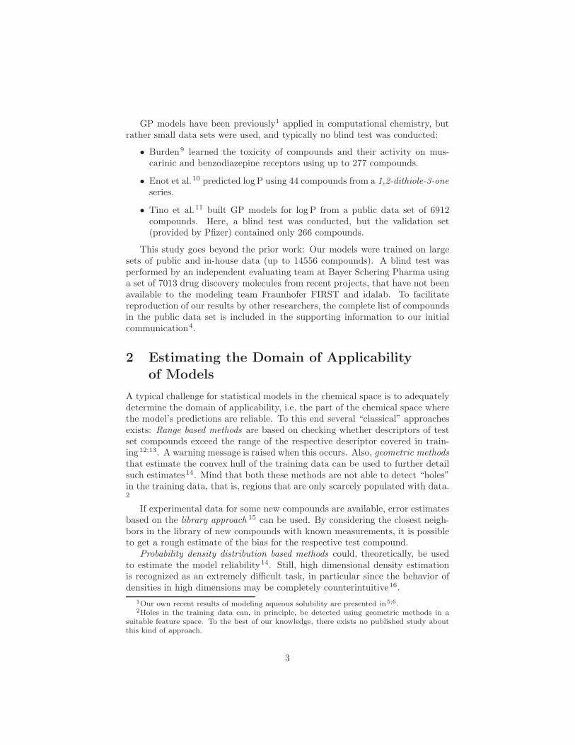
Figure 2: The process of model building.

(large) error bars in the region close the training points, and too small errorswhen extrapolating.

The Gaussian Process, Figure 1 (d) also captures the non-linearity in theinput data and is able to extrapolate. Predicted errors are small in the regionclose to the training points and increase strong enough in the extrapolationregion.

3 Methods and Data

3.1 Methodology Overview

The training procedure is outlined in Figure 2. We use Corina24 to generate a3D structure for each molecule. Molecular descriptors are calculated using theDragon25 software. Finally, a number of machine learning algorithms is usedto “train” models, i.e., to infer the relationship between the descriptors and theexperimental values for log P and log D7.

To make predictions for new compounds, structures are again converted to3D and descriptors are calculated. From the descriptors of each molecule, themodel generates a prediction of log P and/or log D7, and in case of the GaussianProcess and random forest also a confidence estimate (error bar).

3.2 Data Preparation

3.2.1 Multiple Measurements

If multiple measurements exist for the same compound, we merge them as de-scribed in the following to obtain a consensus value for model building. Foreach compound we generate the histogram of experimental values. Characteris-tic properties of histograms are the spread of values (y-spread) and the spreadof the bin heights (z-spread). If all measured values are similar (small y-spread)the median value is taken as consensus value. If a group of similar measure-ments and smaller number of far apart measurements exists, both y-spread andz-spread are large. In this case we treat the far apart measurements as outliers,i.e., we remove them and then use the median of the agreeing measurements asconsensus value. If an equal number of measurements supports on of two (or

6

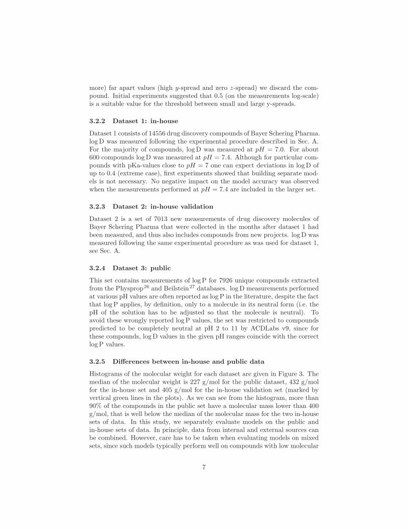
more) far apart values (high y-spread and zero z-spread) we discard the com-pound. Initial experiments suggested that 0.5 (on the measurements log-scale)is a suitable value for the threshold between small and large y-spreads.

3.2.2 Dataset 1: in-house

Dataset 1 consists of 14556 drug discovery compounds of Bayer Schering Pharma.log D was measured following the experimental procedure described in Sec. A.For the majority of compounds, log D was measured at pH = 7.0. For about600 compounds log D was measured at pH = 7.4. Although for particular com-pounds with pKa-values close to pH = 7 one can expect deviations in log D ofup to 0.4 (extreme case), first experiments showed that building separate mod-els is not necessary. No negative impact on the model accuracy was observedwhen the measurements performed at pH = 7.4 are included in the larger set.

3.2.3 Dataset 2: in-house validation

Dataset 2 is a set of 7013 new measurements of drug discovery molecules ofBayer Schering Pharma that were collected in the months after dataset 1 hadbeen measured, and thus also includes compounds from new projects. log D wasmeasured following the same experimental procedure as was used for dataset 1,see Sec. A.

3.2.4 Dataset 3: public

This set contains measurements of log P for 7926 unique compounds extractedfrom the Physprop26 and Beilstein27 databases. log D measurements performedat various pH values are often reported as log P in the literature, despite the factthat log P applies, by definition, only to a molecule in its neutral form (i.e. thepH of the solution has to be adjusted so that the molecule is neutral). Toavoid these wrongly reported log P values, the set was restricted to compoundspredicted to be completely neutral at pH 2 to 11 by ACDLabs v9, since forthese compounds, log D values in the given pH ranges coincide with the correctlog P values.

3.2.5 Differences between in-house and public data

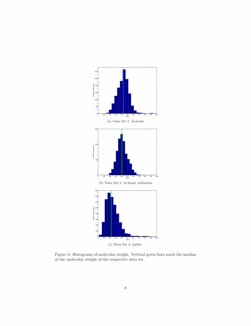
Histograms of the molecular weight for each dataset are given in Figure 3. Themedian of the molecular weight is 227 g/mol for the public dataset, 432 g/molfor the in-house set and 405 g/mol for the in-house validation set (marked byvertical green lines in the plots). As we can see from the histogram, more than90% of the compounds in the public set have a molecular mass lower than 400g/mol, that is well below the median of the molecular mass for the two in-housesets of data. In this study, we separately evaluate models on the public andin-house sets of data. In principle, data from internal and external sources canbe combined. However, care has to be taken when evaluating models on mixedsets, since such models typically perform well on compounds with low molecular

7

0 100 200 300 400 500 600 700 800 900 10000

500

1000

1500

2000

2500

3000

num

ber

of c

ompo

unds

mass

(a) Data Set 1: in-house

0 100 200 300 400 500 600 700 800 900 10000

500

1000

1500

num

ber

of c

ompo

unds

mass

(b) Data Set 2: in-house validation

0 100 200 300 400 500 600 700 800 900 10000

200

400

600

800

1000

1200

1400

1600

num

ber

of c

ompo

unds

mass

(c) Data Set 3: public

Figure 3: Histograms of molecular weight. Vertical green lines mark the medianof the molecular weight of the respective data set.

8

Setup Prediction Data

In-house log D Training Validation

in−house (14556)

In-house validation log D Training Validation

in−house (14556) in−house validation (7013)

Public log P ValidationTraining

Physprop/Beilstein (7926)

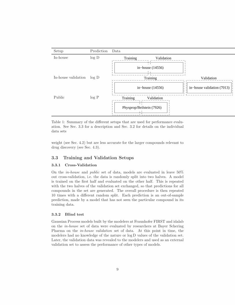
Table 1: Summary of the different setups that are used for performance evalu-ation. See Sec. 3.3 for a description and Sec. 3.2 for details on the individualdata sets

weight (see Sec. 4.2) but are less accurate for the larger compounds relevant todrug discovery (see Sec. 4.3).

3.3 Training and Validation Setups

3.3.1 Cross-Validation

On the in-house and public set of data, models are evaluated in leave 50%out cross-validation, i.e. the data is randomly split into two halves. A modelis trained on the first half and evaluated on the other half. This is repeatedwith the two halves of the validation set exchanged, so that predictions for allcompounds in the set are generated. The overall procedure is then repeated10 times with a different random split. Each prediction is an out-of-sampleprediction, made by a model that has not seen the particular compound in itstraining data.

3.3.2 Blind test

Gaussian Process models built by the modelers at Fraunhofer FIRST and idalabon the in-house set of data were evaluated by researchers at Bayer ScheringPharma on the in-house validation set of data. At this point in time, themodelers had no knowledge of the nature or log D values of the validation set.Later, the validation data was revealed to the modelers and used as an externalvalidation set to assess the performance of other types of models.

9

3.4 Molecular Descriptors

We use the Dragon descriptors by Todeschini et al.28. They are organizedin 20 blocks and include, among others, constitutional descriptors, topologicaldescriptors, walk and path counts, eigenvalue-based indices, functional groupcounts and atom-centered fragments. A full list including references can befound online29.

As one of their most pronounced features, Gaussian Process models allow toassign weights to each descriptor that enters the model as input. The similarityfor two compounds as computed by the GP model takes into account that theith descriptor contributes to the similarity with weight wi (see 3.5.4). Theseweights are chosen automatically during model fitting and can then be inspectedin order to get an impression of the relevance of individual descriptors.

We found that using a small (< 50) set of descriptors results in only slightlydecreased accuracy when comparing to models built on the full set of 1,664descriptors. The error predictions, however, turn out to be too optimistic inthis case. Including whole blocks containing important descriptors leads toboth accurate predictions and accurate error estimations (see Sec. 4.1). In thisstudy, we used the full Dragon blocks 1, 2, 6, 9, 12, 15, 16, 17, 18, and 20. Adiscussion of the importance of individual descriptors can be found in Sec. 4.1.

3.5 Machine Learning Methods

3.5.1 Introductory remarks

Since the application of Gaussian Process regression is still relatively new inthe field of chemoinformatics we chose to explain and illustrate the modelingidea. Support vector machines are seen as established, but still deserve somediscussion due to interesting parallels and differences with the Bayesian GPapproach.

Linear ridge regression, decision trees and ensembles of trees (random forests)are considered established methods - here we mainly note how the employed im-plementation differs from the original algorithm, for which the reader is referredto the literature.

3.5.2 Linear Ridge Regression

Ridge regression combines a linear model with a regularization term that ef-fectively shrinks coefficients of the model towards zero. This is particularlyimportant for our application since a standard linear model runs into problemswhen descriptors are correlated. We choose the complexity parameter λ thatcontrols the amount of shrinkage by grid search in nested cross-validation.

3.5.3 Random Forest

A modified version the random forests method of Breiman21 is employed. Treesare constructed without bagging or bootstrapping and pruning of individual

10

−5 0 5−3

−2

−1

0

1

2

3

Descriptor

log

D

0 5

0

1

2

3

Descriptor

log

D

−5 0 5−3

−2

−1

0

1

2

3

Descriptor

log

D

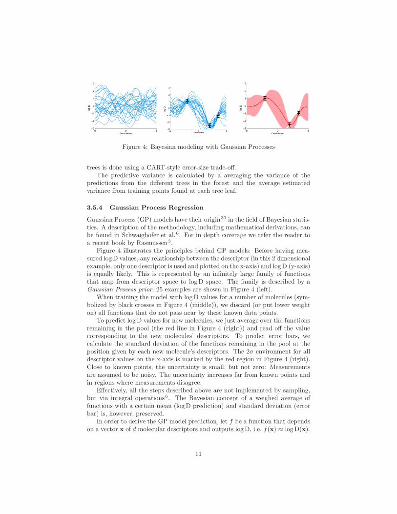
Figure 4: Bayesian modeling with Gaussian Processes

trees is done using a CART-style error-size trade-off.The predictive variance is calculated by a averaging the variance of the

predictions from the different trees in the forest and the average estimatedvariance from training points found at each tree leaf.

3.5.4 Gaussian Process Regression

Gaussian Process (GP) models have their origin30 in the field of Bayesian statis-tics. A description of the methodology, including mathematical derivations, canbe found in Schwaighofer et al.6. For in depth coverage we refer the reader toa recent book by Rasmussen3.

Figure 4 illustrates the principles behind GP models: Before having mea-sured log D values, any relationship between the descriptor (in this 2 dimensionalexample, only one descriptor is used and plotted on the x-axis) and log D (y-axis)is equally likely. This is represented by an infinitely large family of functionsthat map from descriptor space to log D space. The family is described by aGaussian Process prior, 25 examples are shown in Figure 4 (left).

When training the model with log D values for a number of molecules (sym-bolized by black crosses in Figure 4 (middle)), we discard (or put lower weighton) all functions that do not pass near by these known data points.

To predict log D values for new molecules, we just average over the functionsremaining in the pool (the red line in Figure 4 (right)) and read off the valuecorresponding to the new molecules’ descriptors. To predict error bars, wecalculate the standard deviation of the functions remaining in the pool at theposition given by each new molecule’s descriptors. The 2σ environment for alldescriptor values on the x-axis is marked by the red region in Figure 4 (right).Close to known points, the uncertainty is small, but not zero: Measurementsare assumed to be noisy. The uncertainty increases far from known points andin regions where measurements disagree.

Effectively, all the steps described above are not implemented by sampling,but via integral operations6. The Bayesian concept of a weighed average offunctions with a certain mean (log D prediction) and standard deviation (errorbar) is, however, preserved.

In order to derive the GP model prediction, let f be a function that dependson a vector x of d molecular descriptors and outputs log D, i.e. f(x) ≈ log D(x).

11

We assume that each possible function f is a realization of a Gaussian stochasticprocess, and thus can be fully described by considering pairs of compounds x andx′. By the properties of the Gaussian process, functional values f(x1), . . . , f(xn)for any finite set of n points form a Gaussian distribution. The covariance foreach pair is then given by the covariance function,

cov(f(x), f(x′)) = k(x,x′), (1)

which has a role similar to the kernel function in Support Vector Machines31;8

and other kernel based learning methods. Any previous knowledge of the phe-nomenon to be predicted is expressed in the covariance function k.

For n compounds the actual data consist of n log D measurements, y1, . . . yn

and n descriptor vectors, x1 . . .xn, (each of length d).Assuming that measurements are noisy, we relate the n measured values to

the true log D byyi = f(xi) + ǫ, (2)

where ǫ is Gaussian noise with standard deviation σ4

Applying a number of transformations and steps of statistical inference6

we find that the predicted log D for a new compound x∗ follows a Gaussiandistribution with mean f(x∗) and standard deviation std f(x∗), with

f(x∗) =∑n

i=1 αik(x∗,xi) (3)

std f(x∗) =√

k(x∗,x∗) −∑n

i=1

∑n

j=1 k(x∗,xi)k(x∗,xj)Lij . (4)

Coefficients αi are found by solving a system of linear equations, (K + σ2I)α,with Kij = k(xi,xj). For the standard deviation, Lij are the elements of thematrix L = (K + σ2I)−1.

Details on inferring the parameters of the covariance function k and themeasurement noise σ can be found in Schwaighofer et al.6 .

Recent developments of approximation and sampling techniques32 allow totrain Gaussian process models on thousands of data points. However, memorydemand and computing time still increase with the third power of the numberof data points (compounds). For the larger datasets treated in this study, wetherefore precede the actual GP training with a k-means clustering, such thateach cluster contains up to 5000 compounds and train one GP per cluster. Whenapplying the model, predictions from the individual GP models are generatedand the prediction with the highest confidence (smallest error bar) is chosen.

4σ can be a scalar, meaning that all measurements are equally noisy. σ can also be a vector,

allowing, in principle, to use a different noise level for each individual compound. In practicewe found it useful to assume equal measurement noise for groups of compounds that e.g. havebeen measured in the same laboratory. In this way, model performance can be improved andwe can learn the noise level resulting from different (or uniform) experimental proceduresdirectly from the data6.

12

3.5.5 Support Vector Regression

Support Vector Machines for regression and classification are based on the prin-ciple of structural risk minimization. Out of a certain class of functions we wantto find the function that minimizes some notion of error, measured by the so-called loss function. Using a very large class of functions (i.e., a very complexmodel) one can perfectly fit to the training data, but the resulting function willnot generalize to new, unseen data (over-fitting). On the contrary, using a smallclass of functions (simple, e.g. linear models) one may not be able to fit thedata reasonably, again resulting in inaccurate predictions.

Choosing a function class with functions of the right complexity can beachieved by regularization: We combine the empirical loss on the training datawith a penalty term for the complexity and then minimize the sum (objectivefunction). Under certain assumptions (for example, that the training and testdata are sampled from the same distribution), it can be proven that this way ofchoosing the function class leads to an optimal model33;34;35.

In the following we will first describe the idea behind linear SVR and thengeneralize to the non-linear case.

Given a vector x of descriptors for a compound, the quantity of interest y

(in our case log D) will be predicted as y = f(x). Linear SVM finds a predictorf(x) = w⊤x+ b, such that the empirical error as well as the norm of the weightvector w are minimal. We employ an ǫ-insensitive loss function which does notpenalize deviations from the measured value that are smaller than ǫ. Modeltraining is done by solving the convex quadratic optimization problem:

minw,b,ξ

1

2‖w‖2 + C

n∑

i=1

ξi,

subject to |f(xi) − yi| ≤ ǫ + ξi,

ξi ≥ 0, i = 1, . . . , n.

The threshold ǫ from the loss function manifests in the constraints. “Slackvariables” ξ are introduced and penalized in the objective function such thatdeviation by more than ǫ increases the objective function only linearly. Thisreduces the influence of outliers in the data. The constants ǫ and C are chosenby cross-validation5.

Employing the so-called kernel trick8;35 one can generalize to non-linearmodels. Functions f of the form f(x) =

∑n

i=1 αik(xi,x) + b can be gener-ated by rewriting the liner SVM equations such that the descriptors x onlyappear inside scalar products (x⊤

i xj). These scalar products can then be re-placed by a kernel function k(xi,xj), that implicitly maps the descriptors into ahigh-dimensional feature-space and computes the scalar product there. An in-teresting connection with Gaussian Processes exists: Valid kernel functions forsupport vector algorithms are also valid covariance functions for a GP model

5In principle, it is also possible to use more sophisticated approaches36 that compute SVRsolutions for multiple parameter values in a efficient manner.

13

and vice versa. In this study, we do regression using Support Vector Machineswith the RBF kernel.

4 Results & Discussion

4.1 Choice of Descriptors

Gaussian Process models can assign weights to each descriptor that enters themodel as input (see Sec. 3.4 for details). The importance of individual descrip-tors was evaluated using subsets of the training data. The 30 interpretabledescriptors with highest weight are clearly connected with log P and log D7.They include the sum of geometrical distances between pairs of oxygen atoms,counts of the following functional groups,

• donor atoms for H-bonds (N and O)

• H attached to hetero atom

• hydroxyl groups

• hydroxyl groups in phenol, enol, carboxyl

• ether groups

• oxygen atoms

• benzene-like rings

• carbon atoms

• quaternary nitrogen

• tertiary amines

• secondary amines

and a number of continuous quantities:

• topological polar surface area using N, O polar contributions

• topological polar surface area using N, O, S, P polar contributions

• mean atomic van der Waals volume (scaled on Carbon atom)

• harmonic oscillator model of aromaticity index total

• molar refractivity

• hydrophilic factor?

• molecular weight and 11 other measures of size, e.g. sum of conventionalbond orders, sum of atomic van der Waals volumes and size indices

14

Public data Physprop/Beilstein MAE RMSE % ± 1Gaussian Process 0.38 0.66 92.6Linear Ridge Regression 0.59 0.89 84.4Support Vector Machine 0.40 0.71 91.8Random Forest 0.52 0.82 87.6ACDLabs v9 0.43 0.90 89.2Wskowwin v1.41 0.25 0.90 91.6AdmetPredictor v1.2.3 0.65 1.32 86.9QikProp v2.2 0.76 1.23 79.6baseline: predict mean log P 1.68 2.24 40.7

Table 2: Accuracy achieved on the public data sets Physprop/Beilstein usingdifferent machine learning methods compared with the performance of commer-cial tools. MAE, RMSE and % ± 1 denote the mean absolute error, the rootmean squared error, and the percentage of compounds predicted with less thanone log unit error.

We found that using a small set of descriptors results in only slightly decreasedaccuracy when comparing to models built on the full set of 1,664 descriptors.The error predictions, however, turn out to be too optimistic. In other words:The log D7 is predicted accurately for most compounds, but the model cannot correctly detect whether the test compound has, for example, additionalfunctional groups. These functional groups might not have occurred in thetraining data, and were thus not included by the feature selection step. In thetest case, the information about these additional functional groups is importantsince it helps to detect, that these compounds are different from those themodel has been trained on, i.e. the error bar should increase. Including wholeblocks containing important descriptors leads to both accurate predictions andaccurate error estimations. For, e.g. , a GP model these surplus descriptors willget only a small weight during training – but the weight will not be zero. Inconsequence the model has more information than it needs for predicting log D7

and will respond to new properties (functional groups etc.) of molecules byestimating a larger prediction error.

In this study, we used the full Dragon blocks 1, 2, 6, 9, 12, 15, 16, 17, 18and 20, thereby including constitutional descriptors, topological descriptors, 2Dautocorrelations, topological charge indices geometrical descriptors, WHIM de-scriptors, GETAWAY descriptors, functional group counts, atom-centered frag-ments and molecular properties. With this set of 904 descriptors, the modelsaccuracy is only slightly smaller the accuracy of models built on all 1,664 de-scriptors, but the computational cost and memory requirements are significantlyreduced, and predicted error bars display close to ideal statistical properties (seeSec. 4.4 and Sec. 4.5).

15

−10 −5 0 5 10 15−10

−5

0

5

10

15

Measured log p

Pre

dict

ed lo

g p

(a) GP

−10 −5 0 5 10 15−25

−20

−15

−10

−5

0

5

10

15

20

25

Measured log p

Pre

dict

ed lo

g p

(b) Ridge regression

−10 −5 0 5 10 15−10

−5

0

5

10

15

Measured log p

Pre

dict

ed lo

g p

(c) SVM

−10 −5 0 5 10 15−10

−5

0

5

10

15

Measured log p

Pre

dict

ed lo

g p

(d) Random forests

−10 −5 0 5 10 15−10

−5

0

5

10

15

Measured logP

AC

DLa

bs p

redi

cted

logP

(e) ACDLabs v9

−10 −5 0 5 10 15−10

−5

0

5

10

15

Measured logP

Wsk

oww

in p

redi

cted

logP

(f) Wskowwin v1.41

−10 −5 0 5 10 15−10

−5

0

5

10

15

Measured logP

Adm

etP

redi

ctor

pre

dict

ed lo

gP

(g) AdmetPredictor v1.2.3

−10 −5 0 5 10 15−10

−5

0

5

10

15

Measured logP

Qik

Pro

p pr

edic

ted

logP

(h) QikProp v2.2

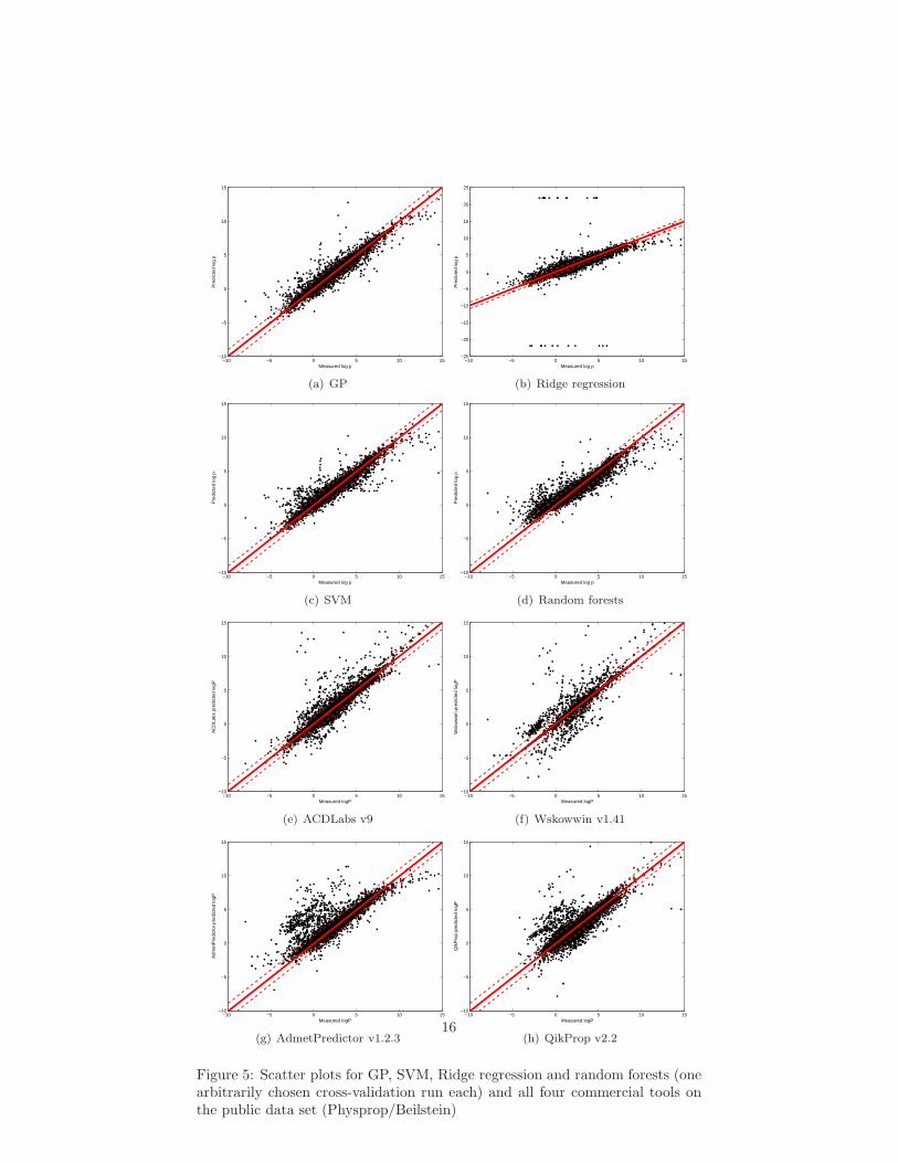
Figure 5: Scatter plots for GP, SVM, Ridge regression and random forests (onearbitrarily chosen cross-validation run each) and all four commercial tools onthe public data set (Physprop/Beilstein)

16

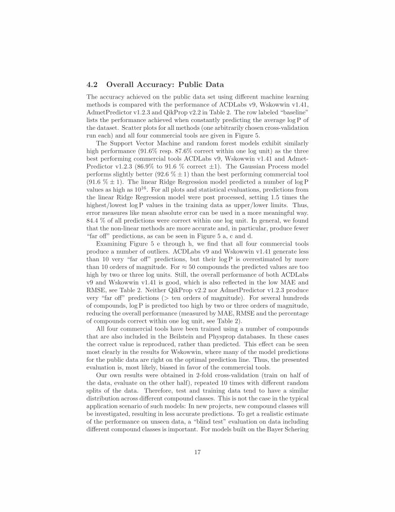
4.2 Overall Accuracy: Public Data

The accuracy achieved on the public data set using different machine learningmethods is compared with the performance of ACDLabs v9, Wskowwin v1.41,AdmetPredictor v1.2.3 and QikProp v2.2 in Table 2. The row labeled “baseline”lists the performance achieved when constantly predicting the average log P ofthe dataset. Scatter plots for all methods (one arbitrarily chosen cross-validationrun each) and all four commercial tools are given in Figure 5.

The Support Vector Machine and random forest models exhibit similarlyhigh performance (91.6% resp. 87.6% correct within one log unit) as the threebest performing commercial tools ACDLabs v9, Wskowwin v1.41 and Admet-Predictor v1.2.3 (86.9% to 91.6 % correct ±1). The Gaussian Process modelperforms slightly better (92.6 %± 1) than the best performing commercial tool(91.6 % ± 1). The linear Ridge Regression model predicted a number of log Pvalues as high as 1016. For all plots and statistical evaluations, predictions fromthe linear Ridge Regression model were post processed, setting 1.5 times thehighest/lowest log P values in the training data as upper/lower limits. Thus,error measures like mean absolute error can be used in a more meaningful way.84.4 % of all predictions were correct within one log unit. In general, we foundthat the non-linear methods are more accurate and, in particular, produce fewer“far off” predictions, as can be seen in Figure 5 a, c and d.

Examining Figure 5 e through h, we find that all four commercial toolsproduce a number of outliers. ACDLabs v9 and Wskowwin v1.41 generate lessthan 10 very “far off” predictions, but their log P is overestimated by morethan 10 orders of magnitude. For ≈ 50 compounds the predicted values are toohigh by two or three log units. Still, the overall performance of both ACDLabsv9 and Wskowwin v1.41 is good, which is also reflected in the low MAE andRMSE, see Table 2. Neither QikProp v2.2 nor AdmetPredictor v1.2.3 producevery “far off” predictions (> ten orders of magnitude). For several hundredsof compounds, log P is predicted too high by two or three orders of magnitude,reducing the overall performance (measured by MAE, RMSE and the percentageof compounds correct within one log unit, see Table 2).

All four commercial tools have been trained using a number of compoundsthat are also included in the Beilstein and Physprop databases. In these casesthe correct value is reproduced, rather than predicted. This effect can be seenmost clearly in the results for Wskowwin, where many of the model predictionsfor the public data are right on the optimal prediction line. Thus, the presentedevaluation is, most likely, biased in favor of the commercial tools.

Our own results were obtained in 2-fold cross-validation (train on half ofthe data, evaluate on the other half), repeated 10 times with different randomsplits of the data. Therefore, test and training data tend to have a similardistribution across different compound classes. This is not the case in the typicalapplication scenario of such models: In new projects, new compound classes willbe investigated, resulting in less accurate predictions. To get a realistic estimateof the performance on unseen data, a “blind test” evaluation on data includingdifferent compound classes is important. For models built on the Bayer Schering

17

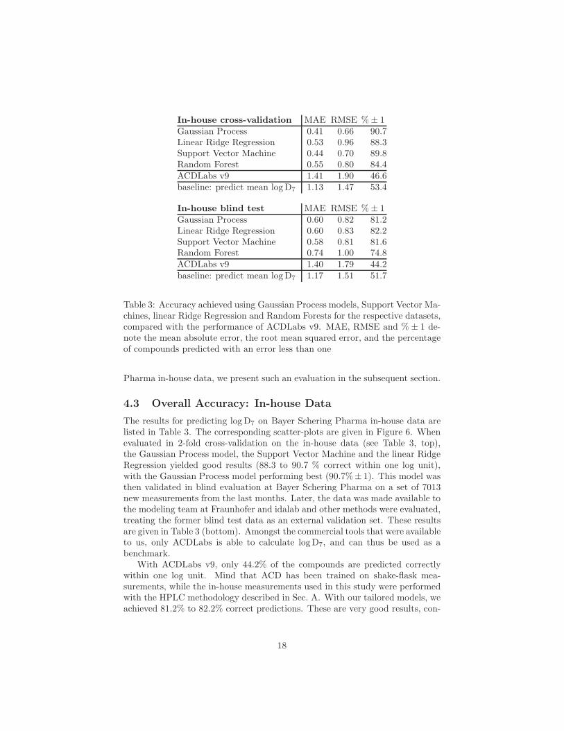
In-house cross-validation MAE RMSE % ± 1Gaussian Process 0.41 0.66 90.7Linear Ridge Regression 0.53 0.96 88.3Support Vector Machine 0.44 0.70 89.8Random Forest 0.55 0.80 84.4ACDLabs v9 1.41 1.90 46.6baseline: predict mean log D7 1.13 1.47 53.4

In-house blind test MAE RMSE % ± 1Gaussian Process 0.60 0.82 81.2Linear Ridge Regression 0.60 0.83 82.2Support Vector Machine 0.58 0.81 81.6Random Forest 0.74 1.00 74.8ACDLabs v9 1.40 1.79 44.2baseline: predict mean log D7 1.17 1.51 51.7

Table 3: Accuracy achieved using Gaussian Process models, Support Vector Ma-chines, linear Ridge Regression and Random Forests for the respective datasets,compared with the performance of ACDLabs v9. MAE, RMSE and % ± 1 de-note the mean absolute error, the root mean squared error, and the percentageof compounds predicted with an error less than one

Pharma in-house data, we present such an evaluation in the subsequent section.

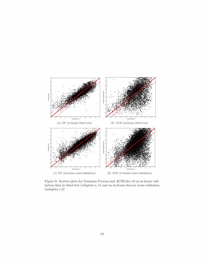
4.3 Overall Accuracy: In-house Data

The results for predicting log D7 on Bayer Schering Pharma in-house data arelisted in Table 3. The corresponding scatter-plots are given in Figure 6. Whenevaluated in 2-fold cross-validation on the in-house data (see Table 3, top),the Gaussian Process model, the Support Vector Machine and the linear RidgeRegression yielded good results (88.3 to 90.7 % correct within one log unit),with the Gaussian Process model performing best (90.7%± 1). This model wasthen validated in blind evaluation at Bayer Schering Pharma on a set of 7013new measurements from the last months. Later, the data was made available tothe modeling team at Fraunhofer and idalab and other methods were evaluated,treating the former blind test data as an external validation set. These resultsare given in Table 3 (bottom). Amongst the commercial tools that were availableto us, only ACDLabs is able to calculate log D7, and can thus be used as abenchmark.

With ACDLabs v9, only 44.2% of the compounds are predicted correctlywithin one log unit. Mind that ACD has been trained on shake-flask mea-surements, while the in-house measurements used in this study were performedwith the HPLC methodology described in Sec. A. With our tailored models, weachieved 81.2% to 82.2% correct predictions. These are very good results, con-

18

−3 −2 −1 0 1 2 3 4 5 6 7−3

−2

−1

0

1

2

3

4

5

6

7

Measured log d

Pre

dict

ed lo

g d

(a) GP (in-house blind test)

−3 −2 −1 0 1 2 3 4 5 6 7−3

−2

−1

0

1

2

3

4

5

6

7

Measured log D

AC

DLa

bs p

redi

cted

log

D

(b) ACD (in-house blind test)

−3 −2 −1 0 1 2 3 4 5 6 7−3

−2

−1

0

1

2

3

4

5

6

7

Measured log p

Pre

dict

ed lo

g p

(c) GP (in-house cross-validation)

−3 −2 −1 0 1 2 3 4 5 6 7−3

−2

−1

0

1

2

3

4

5

6

7

Measured log D

AC

DLa

bs p

redi

cted

log

D

(d) ACD (in-house cross-validation)

Figure 6: Scatter-plots for Gaussian Process and ACDLabs v9 on in-house vali-dation data in blind test (subplots a, b) and on in-house data in cross-validation(subplots c,d)

19

0 1000 2000 3000 4000 5000 6000 70000

500

1000

1500

2000

2500

3000pr

edic

tions

distance

(a) In-house cross-validation

0 1000 2000 3000 4000 5000 6000 70000

100

200

300

400

500

600

700

800

900

pred

ictio

ns

distance

(b) In-house blind test

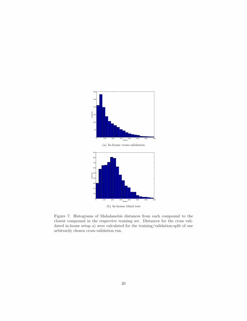
Figure 7: Histograms of Mahalanobis distances from each compound to theclosest compound in the respective training set. Distances for the cross vali-dated in-house setup a) were calculated for the training/validation-split of onearbitrarily chosen cross-validation run.

20

environment pred ± σ pred ± 2σ

optimal % 68.7 95.0GP 67.5 90.4RR 62.6 88.0SVM 63.7 87.9forest 62.5 90.2

Table 4: Predicted error bars can be evaluated by counting how many pre-dictions are actually within a σ, 2σ etc. environment and comparing with theoptimal percentage. A graphical presentation of these results including fractionsof σ can be found in Figure 8.

sidering that the structures were at no point in time available to the modelingteam at FIRST/idalab. Furthermore, the blind test data stems from new drugdiscovery projects, and thus represents different structural classes than thosepresent in the training data.

The fact that performance decreases when comparing the results achievedin cross-validation with the blind test could be taken as a hint that the non-linear models did overfit to their training data. However, typical symptoms ofoverfitting, like a too large number of support vectors in SVM models, were notpresent. A large fraction of all compounds in the validation set is, however,very dissimilar to the training data. Histograms of Mahalanobis distances fromeach compound in the validation to the closest training compound are presentedin Figure 7. We used the same set of descriptors for both model building anddistance calculation.

In a typical cross-validation run on the in-house data set, 50 % of the com-pounds have a nearest neighbor closer than 1100 units, see Figure 7, top. Inthe blind test set, less than 25 % of the compounds have neighbors closer that1100 units, see Figure 7 bottom.

This supports our hypothesis that the difference in performance betweenthe cross-validation results and the blind test is caused by a large number ofcompounds being dissimilar to the training set compounds. Therefore it shouldbe possible to achieve higher performance by focusing on compounds that areclearly inside the domain of applicability of the respective model. We investigatethis question in Sec. 4.5.

4.4 Individual Error Estimation for Interactive Use

Researchers establishing error estimations based on the distance of compoundsto the training data typically present plots or tables where prediction errors arebinned by distance, i.e., averaging over a large number of predictions, becausethe correlation between distances and errors is typically not too strong whenconsidering individual compounds. When binning by the distance, one canclearly see how the error increases as the distance increases17;14. One can fit

21

50 60 70 80 90 95 98 9950

55

60

65

70

75

80

85

90

95

100

Confidence interval [%]

Em

piric

al c

onfid

ence

[%]

PredictionOptimal

(a) GP (in-house blind test)

50 60 70 80 90 95 98 9940

50

60

70

80

90

100

Confidence interval [%]

Em

piric

al c

onfid

ence

[%]

PredictionOptimal

(b) RR (in-house external validation)

50 60 70 80 90 95 98 9940

50

60

70

80

90

100

Confidence interval [%]

Em

piric

al c

onfid

ence

[%]

PredictionOptimal

(c) SVM (in-house external validation)

50 60 70 80 90 95 98 9940

50

60

70

80

90

100

Confidence interval [%]

Em

piric

al c

onfid

ence

[%]

PredictionOptimal

(d) forest (in-house external validation)

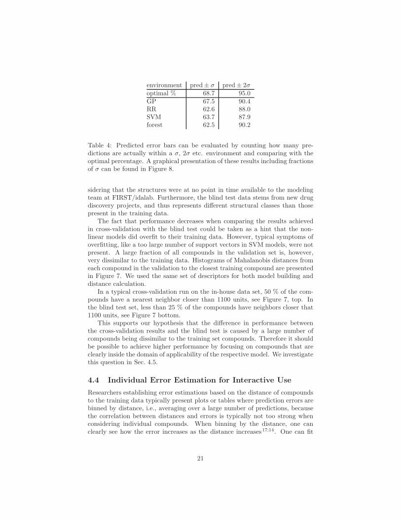
Figure 8: Predicted error bars can be evaluated by counting how many predic-tions are actually within a σ, 2σ etc. environment (red line) and comparingwith the optimal percentage (black line). The vertical green lines indicate theσ and 2σ environments, the corresponding numbers can be found in Table 4.

22

a function to this relationship and use it to generate an error prediction foreach prediction the model makes. But how does the user know, what an errorprediction of e.g. 0.6 log units really means? In how many cases does the userexpect the error to be larger than the predicted error? How much larger canerrors turn out?

The most commonly used description of uncertainty (such as measurementerrors, prediction errors, etc.) in chemistry, physics and other fields is the errorbar. Its definition is based on the assumption that errors follow a Gaussiandistribution. When using a probabilistic model that predicts a Gaussian (i.e.,a mean f and a standard deviation σ), it follows that the true value has to bein the interval f ± σ with 68% confidence, and in the interval f ± 2σ with 95%confidence, etc. To evaluate the quality of the predicted error bars, one cantherefore compare with the true experimental values, and count how many ofthem are actually within the σ, 2σ etc. intervals.6

Gaussian Process model can directly predict error bars. In the implementa-tion of random forests used in this study, the predictive variance is calculatedby averaging the variance of the predictions from the different trees in the forestand the average estimated variance from training points found at each tree leaf.

For the and linear Ridge Regression models and the Support Vector Ma-chines, error bars were estimated by fitting exponential and linear functions tothe errors observed when evaluating the models in cross-validation and the ma-halanobis distances to the closest neighbours in the training set of the respectivesplit. Since both linear and exponential functions worked equally well, we chosethe simple linear functions to estimate to error bars from the distances.

Plots of the empirical confidence versus the confidence interval are presentedin Figure 8 (red line). The optimal curve is marked by the black line. The σ and2σ environments are marked by green lines, with the corresponding percentagesof predictions within each environment being listed in Table 4. Predicted er-ror bars of all four models exhibit the correct statistical properties, with theGPlogD error predictions being closest to the ideal distribution. The resultspresented for the GP model stem from a “blind test” of the final model deliv-ered to Bayer Schering Pharma4;5;6;7;8. The remaining algorithms have beenevaluated a posteriori, after the experimental values for the validation set hadbeen revealed.

In conclusion, using Bayesian models, ensemble models or distance basedapproaches one can not only identify compounds outside of the models domainof applicability, but also quantify the reliability of a prediction in a way that isintuitively understandable for the user.

23

0.1 0.2 0.29 0.4 0.55 0.72 1.260

0.1

0.2

0.3

0.4

0.5

0.6

0.7

0.8

0.9

Mea

n A

bsol

ute

Err

or

Model based error bar

(a) GPlogD on Flask (external validation)

448 1021 1534 1986 2428 3057 52560

0.1

0.2

0.3

0.4

0.5

0.6

0.7

0.8

0.9

Mea

n A

bsol

ute

Err

or

Mahalanobis distance

(b) RR on Flask (external validation)

448 1021 1534 1986 2428 3057 52560

0.1

0.2

0.3

0.4

0.5

0.6

0.7

0.8

0.9

Mea

n A

bsol

ute

Err

or

Mahalanobis distance

(c) SVM on Flask (external validation)

0.22 0.37 0.47 0.57 0.68 0.85 1.190

0.1

0.2

0.3

0.4

0.5

0.6

0.7

0.8

0.9

Mea

n A

bsol

ute

Err

or

Model based error bar

(d) Forest on Flask (external validation)

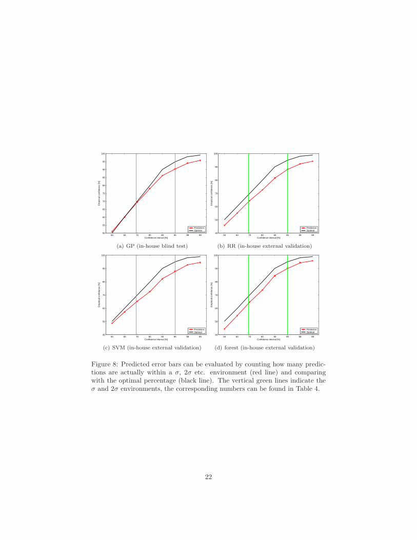
Figure 9: Mean absolute error achieved when binning by the model based errorbar (in the case of the GP and the random forest) resp. the Mahalanobis distanceto the closest point in the training set (linear Ridge Regression and SupportVector Machines do not provide error bars). Each bin contains one seventh(1000 compounds) of the in-house validation set. Corresponding numbers canbe found in Table 5.

24

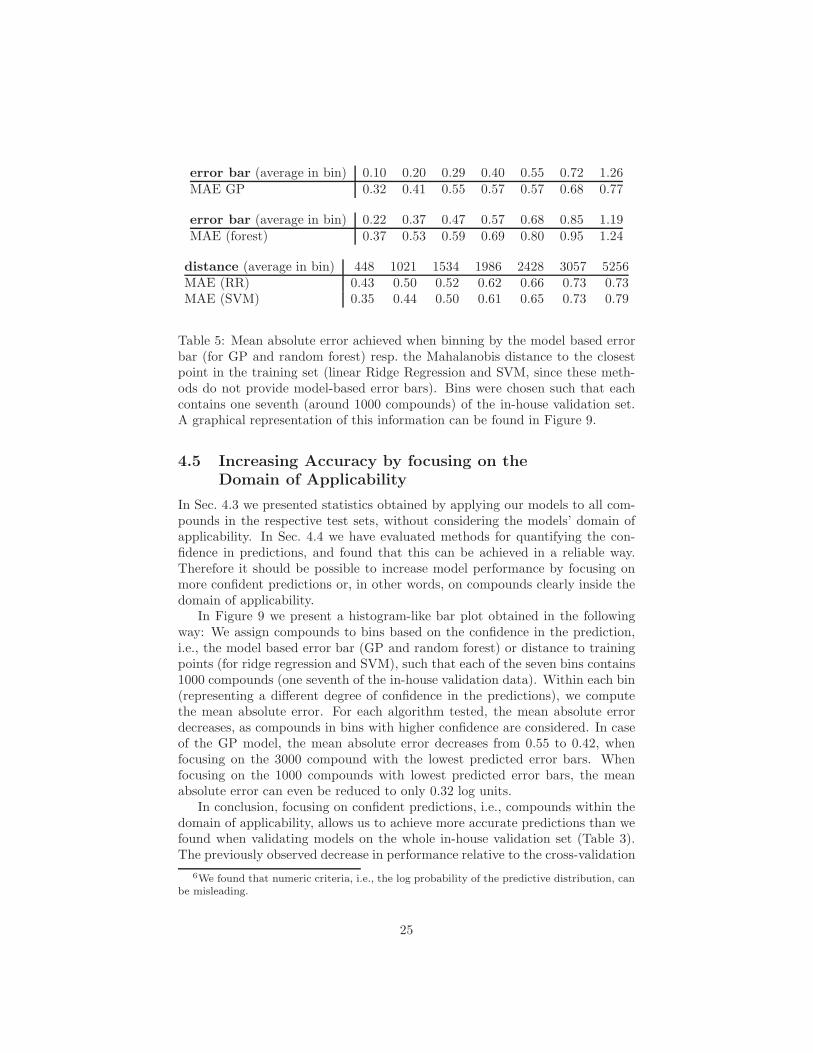
error bar (average in bin) 0.10 0.20 0.29 0.40 0.55 0.72 1.26MAE GP 0.32 0.41 0.55 0.57 0.57 0.68 0.77

error bar (average in bin) 0.22 0.37 0.47 0.57 0.68 0.85 1.19MAE (forest) 0.37 0.53 0.59 0.69 0.80 0.95 1.24

distance (average in bin) 448 1021 1534 1986 2428 3057 5256MAE (RR) 0.43 0.50 0.52 0.62 0.66 0.73 0.73MAE (SVM) 0.35 0.44 0.50 0.61 0.65 0.73 0.79

Table 5: Mean absolute error achieved when binning by the model based errorbar (for GP and random forest) resp. the Mahalanobis distance to the closestpoint in the training set (linear Ridge Regression and SVM, since these meth-ods do not provide model-based error bars). Bins were chosen such that eachcontains one seventh (around 1000 compounds) of the in-house validation set.A graphical representation of this information can be found in Figure 9.

4.5 Increasing Accuracy by focusing on the

Domain of Applicability

In Sec. 4.3 we presented statistics obtained by applying our models to all com-pounds in the respective test sets, without considering the models’ domain ofapplicability. In Sec. 4.4 we have evaluated methods for quantifying the con-fidence in predictions, and found that this can be achieved in a reliable way.Therefore it should be possible to increase model performance by focusing onmore confident predictions or, in other words, on compounds clearly inside thedomain of applicability.

In Figure 9 we present a histogram-like bar plot obtained in the followingway: We assign compounds to bins based on the confidence in the prediction,i.e., the model based error bar (GP and random forest) or distance to trainingpoints (for ridge regression and SVM), such that each of the seven bins contains1000 compounds (one seventh of the in-house validation data). Within each bin(representing a different degree of confidence in the predictions), we computethe mean absolute error. For each algorithm tested, the mean absolute errordecreases, as compounds in bins with higher confidence are considered. In caseof the GP model, the mean absolute error decreases from 0.55 to 0.42, whenfocusing on the 3000 compound with the lowest predicted error bars. Whenfocusing on the 1000 compounds with lowest predicted error bars, the meanabsolute error can even be reduced to only 0.32 log units.

In conclusion, focusing on confident predictions, i.e., compounds within thedomain of applicability, allows us to achieve more accurate predictions than wefound when validating models on the whole in-house validation set (Table 3).The previously observed decrease in performance relative to the cross-validation

6We found that numeric criteria, i.e., the log probability of the predictive distribution, canbe misleading.

25

on the training data can therefore be avoided.

5 Summary

We presented results of modeling lipophilicity using the Gaussian Process method-ology on public and in-house data. The statistical evaluations show that theprediction quality of our GP models compares favorably with four commercialtools and three other machine learning algorithms that were applied to thesame sets of data. The positive results achieved with the model on in-housedrug discovery compounds are re-confirmed by a blind evaluation on a large setof measurements from new drug discovery projects at Bayer Schering Pharma.

It should be noted that GP models are not only capable of making accu-rate predictions, but can also provide fully automatic adaptable tools: Using aBayesian model selection criteria allows for re-training without user interventionwhenever new data becomes available. As a further advantage for every day usein drug discovery applications, GP models quantify their domain of applicabil-ity in a statistically well founded manner. The confidence of each prediction isquantified by error bars, an intuitively understood quantity. This allows both,increasing the average accuracy of predictions by focusing on predictions thatare inside the domain of applicability of the model, and judging the reliabilityof individual predictions in interactive use.

Acknowledgments

The authors gratefully acknowledge DFG grant MU 987/4-1 and partial supportfrom the PASCAL Network of Excellence (EU #506778). We thank VincentSchutz and Carsten Jahn for maintaining the PCADMET database and GillesBlanchard for implementing the random forest method as part of our machinelearning toolbox.

A Appendix: Measuring log D7 using HPLC

High Performance Liquid Chromatography (HPLC) is performed on analyticalcolumns packed with a commercially available solid phase containing long hy-drocarbon chains chemically bound onto silica. Chemicals injected onto sucha column move along it by partitioning between the mobile solvent phase andthe hydrocarbon stationary phase. The chemicals are retained in proportionto their hydrocarbon-water partition coefficient, with water-soluble chemicalseluted first and oil-soluble chemicals last. This enables the relationship betweenthe retention time on a reverse-phase column and the n-octanol/water partitioncoefficient to be established. The partition coefficient is deduced from the ca-pacity factor k = tr−t0

t0, where tr is the retention time of the test substance and

t0 is the dead time, i.e., the average time a solvent molecule needs to pass thecolumn. In order to correlate the measured capacity factor k of a compoundwith its log D7, a calibration graph is established. The partition coefficients

26

of the test compounds are obtained by interpolation of the calculated capac-ity factors on the calibration graph using a proprietary software tool “POWDetermination”.

A.1 Apparatus and Materials

Experiments are carried out following the OECD Guideline for Testing of Chem-icals No. 117. A set of 9 reference compounds with known log D7values selectedfrom this guideline is used.

• HPLC: Waters Alliance HT 2790 with DAD- and MS-detection

• Column: Spherisorb ODS 3 µm, 4.6 × 60 mm

• Mobile phase: Methanol/0.01 m Ammoniumacetate buffer (pH 7) 75:25

• Dead time compound: Formamide, Stock solution in MeOH

• Test compounds: 10 mmolar DMSO stock

• Reference compounds (Stock solutions in MeOH): Acetanilide, 4-Methyl-benzyl alcohol, Methyl benzoate, Ethyl benzoate, Naphthalene, 1,2,4-Trichlorobenzene, 2,6-Diphenylpyridine, Triphenylamine, DDT.

References

[1] T.J. Hou and X.J. Xu. Adme evaluation in drug discovery. 3. model-ing blood-brain barrier partitioning using simple molecular descriptors.J. Chem. Inf. Comput. Sci., 43(6):2137–2152, 2003.

[2] Pierre Bruneau and Nathan R. McElroy. Generalized fragment-substructure based property prediction method. J. Chem. Inf. Model., 46:1379–1387, 2006.

[3] Carl Edward Rasmussen and Christopher K.I. Williams. Gaussian Pro-cesses for Machine Learning. MIT Press, 2005.

[4] Timon Schroeter, Anton Schwaighofer, Sebastian Mika, Antonius TerLaak, Detlev Suelzle, Ursula Ganzer, Nikolaus Heinrich, and Klaus-RobertMuller. Predicting lipophilicity of drug discovery molecules using gaussianprocess models. ChemMedChem, 2007. submitted.

[5] Timon Schroeter, Anton Schwaighofer, Sebastian Mika, Antonius TerLaak, Detlev Suelzle, Ursula Ganzer, Nikolaus Heinrich, and Klaus-RobertMuller. Estimating the domain of applicability for machine learningqsar rmodels: A study on aqueous solubility of drug discovery molecules.J. Comput.-Aided Mol. Des., 2007. submitted.

27

[6] Anton Schwaighofer, Timon Schroeter, Sebastian Mika, Julian Laub, Anto-nius ter Laak, Detlev Sulzle, Ursula Ganzer, Nikolaus Heinrich, and Klaus-Robert Muller. Accurate solubility prediction with error bars for elec-trolytes: A machine learning approach. Journal of Chemical Informationand Modelling, 47(2):407–424, 2007. URL http://dx.doi.org/10.1021/

ci600205g.

[7] Klaus-Robert Muller, Gunnar Ratsch, Soren Sonnenburg, Sebastian Mika,Michael Grimm, and Nikolaus Heinrich. Classifying ’drug-likeness’ withkernel-based learning methods. J. Chem. Inf. Model, 45:249–253, 2005.

[8] K.-R. Muller, S. Mika, G. Ratsch, K. Tsuda, and B. Scholkopf. An intro-duction to kernel-based learning algorithms. IEEE Transactions on NeuralNetworks, 12(2):181–201, 2001.

[9] Frank R. Burden. Quantitative structure-activity relationship studies usingGaussian processes. J. Chem. Inf. Comput. Sci., 41(3):830–835, 2000.

[10] D.P. Enot, R. Gautier, and J.Y. Le Marouille. Gaussian process: an efficienttechnique to solve quantitative structure-property relationship problems.SAR QSAR Environ. Res., 12(5):461–469, 2001.

[11] Peter Tino, Ian Nabney, Bruce S. Williams, Jens Losel, and Yi Sun. Non-linear prediction of quantitative structure-activity relationships. J. Chem.Inf. Comput. Sci., 44(5):1647–1653, 2004.

[12] Alexander Tropsha. Variable selection qsar modeling, model validation,and virtual screening. In David C. Spellmeyer, editor, Annual Reports inComputational Chemistry, volume 2, chapter 7, pages 113–126. Elsevier,2006.

[13] Weida Tong, Qian Xie, uixiao Hong, Leming Shi, Hong Fang, and RogerPerkins. Assessment of prediction confidence and domain extrapolation oftwo structure-activity relationship models for predicting estrogen receptorbinding activity. Environmental Health Perspectives, 112(12):1249–1254,2004.

[14] Tatiana I. Netzeva, Andrew P. Worth, Tom Aldenberg, Romualdo Be-nigni, Mark T.D. Cronin, Paola Gramatica, Joanna S. Jaworska, ScottKahn, Gilles Klopman, Carol A. Marchant, Glenn Myatt, Nina Nikolova-Jeliazkova, Grace Y. Patlewicz, Roger Perkins, David W. Roberts, Terry W.Schultz, David T. Stanton, Johannes J.M. van de Sandt, Weida Tong,Gilman Veith, and Chihae Yang. Current status of methods for definingthe applicability domain of (quantitative) structure-activity relationships.Alternatives to Laboratory Animals, 33(2):1–19, 2005.

[15] Ralph Kuhne, Ralf-Uwe Ebert, and Gerrit Schuurmann. Model selectionbased on structural similarity-method description and application to watersolubility prediction. J. Chem. Inf. Model., 46:636–641, 2006.

28

[16] Bernard W. Silverman. Density Estimation for Statistics and Data Anal-ysis. Number 26 in Monographs on Statistics and Applied Probability.Chapman & Hall, 1986.

[17] Pierre Bruneau and Nathan R. McElroy. Generalized fragment-substructure based property prediction method. J. Chem. Inf. Model., 44:1912–1928, 2004.

[18] Igor V. Tetko, Pierre Bruneau, Hans-Werner Mewes, Douglas C. Rohrer,and Gennadiy I. Poda. Can we estimate the accuracy of ADME-tox pre-dictions? Drug Discovery Today, 11(15/16):700–707, August 2006.

[19] Andreas H. Goller, Matthias Hennemann, Jorg Keldenich, and TimothyClark. In silico prediction of buffer solubility based on quantum-mechanicaland hqsar- and topology-based descriptors. J. Chem. Inf. Model., 46(2):648–658, 2006.

[20] David T. Manallack, Benjamin G. Tehan, Emanuela Gancia, Brian D. Hud-son, Martyn G. Ford, David J. Livingstone, David C. Whitley, , and Will R.Pitt. A consensus neural network-based technique for discriminating sol-uble and poorly soluble compounds. J. Chem. Inf. Model., 43:674–679,2003.

[21] Leo Breiman. Random forests. Machine Learning, 45:5–32, 2001. URLhttp://dx.doi.org/10.1023/A:1010933404324.

[22] Andreas Bender, Hamse Y. Mussa, and Robert C. Glen. Screening fordihydrofolate reductase inhibitors using molprint 2d, a fast fragment-based method employing the nave bayesian classifier: Limitations ofthe descriptor and the importance of balanced chemistry in trainingand test sets. Journal of Biomolecular Screening, 10(7):658–666, 2005.http://jbx.sagepub.com/cgi/content/abstract/10/7/658.

[23] Hongmao Sun. An accurate and interpretable bayesian classification modelfor prediction of herg liability. ChemMedChem, 1(3):315–322, 2006.

[24] J. Sadowski, C. Schwab, and J. Gasteiger. Corina v3.1. Erlangen, Germany.

[25] R. Todeschini, V. Consonni, A. Mauri, and M. Pavan. DRAGON v1.2.Milano, Italy, .

[26] Physical/Chemical Property Database (PHYSPROP). Syracuse, NY, USA.

[27] Beilstein CrossFire Database. San Ramon, CA, USA.

[28] Roberto Todeschini and Viviana Consonni. Handbook of Molecular De-scriptors. John Wiley & Sons, Ltd., 2000.

[29] R. Todeschini, V. Consonni, A. Mauri, and M. Pavan. Dragon for windowsand linux 2006. http://www.talete.mi.it/help/dragon help/ (accessed14 May 2006), .

29

[30] Anthony O’Hagan. Curve fitting and optimal design for prediction. Journalof the Royal Statistical Society, Series B: Methodological, 40(1):1–42, 1978.

[31] Bernhard Scholkopf and Alex J. Smola. Learning with Kernels. MIT Press,2002.

[32] Joaquin Quionero-Candela and Carl Edward Rasmussen. A unifying view ofsparse approximate Gaussian process regression. Journal of Machine Learn-ing Research, 6:1939–1959, December 2005. URL http://www.jmlr.org/

papers/volume6/quinonero-candela05a/quinonero-candela05a.pdf.

[33] V.N. Vapnik. Statistical Learning Theory. Wiley, New York, 1998.

[34] N. Cristianini and J. Shawe-Taylor. An Introduction to Support VectorMachines. Cambridge University Press, Cambridge, UK, 2000.

[35] B. Scholkopf and A.J. Smola. Learning with Kernels. MIT Press, Cam-bridge, MA, 2002.

[36] Gang Wang, Dit-Yan Yeung, and Frederick H. Lochovsky. Two-dimensionalsolution path for support vector regression. In Luc De Raedt and Ste-fan Wrobel, editors, Proceedings of ICML06, pages 993–1000. ACM Press,2006. URL http://www.icml2006.org/icml documents/camera-ready/

125 Two Dimensional Solu.pdf.

30