MACS: Rapid aqueous clearing system for three-dimensional ...intact organs 3 4 Jingtan Zhu 1,2†...

of 42

MACS: Rapid aqueous clearing system for three-dimensional mapping of 1 intact organs 2

3 Jingtan Zhu1,2† , Tingting Yu1,2† , Yusha Li1,2, Jianyi Xu1,2, Yisong Qi1,2, Yingtao Yao1,2, Yilin 4 Ma1,2, Peng Wan1,2, Zhilong Chen1,2, Xiangning Li1,2, Hui Gong1,2 , Qingming Luo1,2, Dan Zhu1,2* 5 6

1Britton Chance Center for Biomedical Photonics, Wuhan National Laboratory for 7 Optoelectronics, Huazhong University of Science and Technology, Wuhan, Hubei, China 8 2MoE Key Laboratory for Biomedical Photonics, Huazhong University of Science and 9 Technology, Wuhan, Hubei, China 10

†These authors contributed equally to this work. 11 *Author for correspondence ([email protected]) 12 13 Abstract 14 Tissue optical clearing techniques have provided important tools for large-volume imaging. 15 Aqueous-based clearing methods are known for good fluorescence preservation and scalable size 16 maintenance, but are limited by either long incubation time, or insufficient clearing performance, 17 or requirements for specialized devices. Additionally, due to the use of high concentration organic 18 solvents or detergents, few clearing methods are compatible with lipophilic dyes while maintaining 19 high clearing performance. To address these issues, we developed a rapid, highly efficient aqueous 20 clearing method with robust compatibility, termed m-xylylenediamine (MXDA)-based Aqueous 21 Clearing System (MACS). MACS can render intact organs highly transparent in a fairly short time 22 and possesses ideal compatibility with multiple probes, especially for lipophilic dyes. Using MACS, 23 we cleared the adult mouse brains within only 2.5 days for three-dimensional (3D) imaging of the 24 neural structures labelled by various techniques. Combining MACS with DiI labelling, we 25 visualized the vascular structures of various organs. MACS provides a useful tool for 3D mapping 26 of intact tissues and is expected to facilitate morphological, physiological and pathological studies 27 of various organs. 28 29

All rights reserved. No reuse allowed without permission. The copyright holder for this preprint (which was not peer-reviewed) is the author/funder.. https://doi.org/10.1101/832733doi: bioRxiv preprint

mailto:[email protected]

https://doi.org/10.1101/832733

of 42

Introduction 30

Three-dimensional (3D) imaging of tissue structures at high resolution plays an 31

indispensable role in life science. The development of diverse fluorescent labelling methods 32

and optical imaging techniques provides essential tools for 3D imaging of large-volume 33

tissues1-4. However, the imaging depth is rather limited due to the opaqueness of tissue5. 34

Automated serial-sectioning and imaging techniques have been developed to address this 35

issue, allowing the acquisition of high-resolution images throughout the brain6-9. 36

As a distinct solution, tissue optical clearing technique has been proposed for 37

imaging deeper without cutting10-13. In the past decade, a variety of optical clearing methods 38

have been developed and are principally divided into solvent-based methods, such as 39

3DISCO14, 15, iDISCO16, uDISCO17, PEGASOS18, Ethanol-ECi19, FDISCO20, vDISCO21, 40

sDISCO22, boneclear23 and aqueous-based methods, such as SeeDB/SeeDB224, 25, ClearT26, 41

ScaleS27, CUBIC-series28-31, CLARITY32, 33, PACT-PARS34, SWITCH35, OPTIClear36 and 42

Ce3D37. These methods provide powerful tools for visualizing tissue structures and greatly 43

promote the development of life science. 44

Aqueous-based clearing methods are known for good fluorescence preservation and 45

scalable maintenance of tissue size11, but are also faced with poor clearing performance or 46

slow clearing speed. For example, SeeDB and ClearT performed well on embryos and 47

neonatal mouse tissues, while showed modest transparency in whole-mount adult tissues38, 48

39. CUBIC and CLARITY can achieve high tissue transparency but require long incubation 49

time for clarification (e.g., approximately 2-3 weeks for the whole brain). Moreover, due to 50

the usage of organic solvents or high concentration detergents, most clearing methods with 51

high clearing capability are incompatible with lipophilic dyes, such as DiI, which has been 52


https://doi.org/10.1101/832733

of 42

widely used to trace neuronal structures and vasculatures26, 40-42. These drawbacks have 53

limited their applications in researches. 54

In this work, we developed an aqueous clearing method based on m-xylylenediamine 55

(MXDA), termed MXDA-based Aqueous Clearing System (MACS). MACS achieved high 56

transparency of intact organs and rodent bodies in a fairly short time and showed ideal 57

compatibility with multiple probes, especially with lipophilic dyes. MACS is applicable for 58

imaging the neural structures of transgenic whole adult brains and immunostained mouse 59

embryos, as well as the neural projections throughout the whole brain labelled by viruses. 60

MACS also allows imaging of DiI-labelled vascular structures of various organs. MACS is 61

expected to promote comprehensive morphological and pathological studies of intact organs. 62

Results 63

MACS enables rapid clearing of multiscale tissues 64

We successfully cleared the intact brain with a high level of transparency within only 65

2.5 d using our MACS protocol (Fig. 1a). Compared with other available clearing methods, 66

MACS renders brain samples highly transparent much faster (Fig. 1a-c, Fig. S1a, c) and 67

nearly maintains the sample size after transient expansion (Fig. 1d, Fig. S1b). The computed 68

tomography (CT) reconstruction images revealed no significant changes of brain volume 69

before and after MACS clearing (Fig. S2a, b). The outlines and internal regions of the brain 70

slices overlapped well before and after MACS treatment (Fig. S2c-h). Furthermore, to 71

investigate the influence of MACS on the preservation of fine structures, we imaged a 72

typical pyramidal neuron and single microglia before and after clearing. The results showed 73

that MACS could maintain the cell morphology and fine structures well (Fig. S2i, j). 74

MACS could also efficiently clarify other mouse tissues, including both soft internal 75

organs and hard bones (Fig. 1e), and was also applicable for the adult mouse body (Fig. 1f). 76


https://doi.org/10.1101/832733

of 42

Additionally, MACS was effective for intact adult rat organs (Fig. S3a). Notably, MACS 77

demonstrated superior ability in clearing mouse embryos and pups (Fig. S3b). 78

We also found that MXDA solution could efficiently decolourize heme-rich tissues, 79

such as embryos (Fig. 1g). The absorbance of the decolourizing medium indicated that 80

MXDA decolourized the samples in a manner similar to that of NaOH solution (release Fe) 81

but quite different from that of Quadrol solution (release heme) used in CUBIC29 (Fig. 1h). 82

Additionally, MXDA showed high pH stability over NaOH solution during clearing (Table 83

S1). The decolourizing capability of MXDA enables MACS to decolourize samples during 84

clarification (Fig. S3c). 85

MACS preserves signals of multiple fluorescent probes, especially lipophilic dyes 86

Furthermore, we investigated the fluorescence preservation of MACS for both endogenous 87

fluorescent proteins and chemical fluorescent tracers. The results demonstrated that MACS 88

could preserve the endogenous EGFP, EYFP and tdTomato very well after clearing (Fig. 2a, 89

b, Fig. S4a). We also imaged MACS-cleared brain slices during long-term storage, and the 90

fluorescence intensity remained relatively high after one month (Fig. 2c, Fig. S4b). 91

DiI is a commonly used lipophilic fluorescent dye for neural tracing and vascular 92

labelling. Due to the high concentration of membrane-removing detergents or organic 93

solvents, CUBIC-L, PACT and uDISCO are not compatible with DiI labelling. By contrast, 94

MACS can preserve the fluorescence of DiI fairly well, similar to ScaleS and SeeDB2 (Fig. 95

2d). Indeed, MACS used neither detergents nor organic solvents, thus samples treated by 96

MACS maintained membrane integrity well, which was crucial for DiI signalling (Fig. 2e). 97

The superior compatibility enables visualization of neuronal projections in the DiI-labelled 98

hippocampus region in mouse brain tissue (Fig. 2f). We also tested MACS with other types 99

of chemical tracers, including propidium iodide (PI) for nuclear staining, 100


https://doi.org/10.1101/832733

of 42

Tetramethylrhodamine-conjugated dextran for vessel labelling, virus-delivered proteins 101

(DsRed and mCherry) and fluorophore-conjugated antibodies in immunostaining 102

(AlexaFluor 594 (AF 594) and AlexaFluor 633 (AF 633)) (Fig. 2f, Fig. S4c, d). The results 103

showed that MACS maintained the fluorescence signals of all tested tracers well. 104

Additionally, previous studies demonstrated that CM-DiI could be used as an 105

alternative in CLARITY-based methods. CM-DiI is an aldehyde-fixably modified version 106

of DiI which adheres not only to the cellular membranes but also protein structures after 107

fixation, such that it would remain in the tissue after lipid extraction43. However, we found 108

that the signals from CM-DiI was only partial remained after treatment by CUBIC-L, PACT 109

and uDISCO, the signal loss was obvious as previously reported44. Due to the good 110

membrane integrity after MACS treatment, both the DiI and CM-DiI signals were well 111

maintained without any obvious loss (Fig. S4e). 112

MACS achieves 3D reconstruction of neural structures in intact tissues 113

Using the rapid MACS clearing protocol, we cleared transgenic whole mouse brains and 114

performed fluorescence imaging by light sheet fluorescence microscopy (LSFM). We 115

obtained the neurons in Thy1-GFP-M mouse brain at different depths and performed 3D 116

reconstruction (Fig. 3a-d). The fine neural structures were well observed in different brain 117

regions, including the midbrain, hippocampus, cerebellum, striatum, cortex, and cerebellar 118

nuclei (Fig. 3e-j). We also cleared and imaged the Sst-IRES-Cre::Ai14 transgenic mouse 119

brain, and MACS allowed fine imaging of tdTomato fluorescence labelled neurons 120

throughout the whole brain at single-cell resolution (Fig. S5a-e). 121

Virus labelling is widely used to reveal neural circuits across the whole brain45, 46. 122

Here, we applied MACS protocol to visualize neuronal projections labelled by different 123

types of virus, including retrograde rabies virus (RV) and anterograde adeno-associated 124


https://doi.org/10.1101/832733

of 42

virus (AAV). We imaged the input and output of the nucleus reuniens (RE), which 125

reportedly receives afferent projections across the brain and is an important temporal 126

constraint in hippocampus-RE-mPFC circuits47, 48. We injected RV-DsRed and AAV-127

mCherry into the RE region for retrograde and anterograde tracing of the projections, 128

respectively (Fig. S5f). The 3D rendering of acquired images showed a diverse and widely 129

distributed set of afferents to RE (Fig. 3k), which heavily projected from the dorsal/ventral 130

agranular insular cortex (AID/AIV), medial prefrontal cortex (mPFC), ventral CA1 of the 131

hippocampus, ectorhinal cortex (ECT), medial amygdaloid nucleus (MEA) (Fig. 3l-q), etc. 132

Moreover, the 3D rendering showed a relatively limited output from RE, which was mainly 133

directed to the hippocampal formation (e.g., CA1), ventral subiculum (S) and mPFC (Fig. 134

S5g-k), as previously reported49. 135

In addition to transgenic labelling and virus labelling, immunostaining is a powerful 136

method to label tissues. Due to the hyperhydration of MXDA used in MACS, we explored 137

whether MXDA pretreatment would enhance the permeability of antibodies in 138

immunostaining. The results revealed that MXDA pretreated samples could achieve deeper 139

staining than those without MXDA pretreatment (Fig. S6a-c). After MXDA pretreatment, 140

whole embryos were stained with neurofilament antibody and followed by MACS clearing 141

and imaging with LSFM (Fig. S6d). We obtained the 3D nerve distributions of embryos at 142

different ages (Fig. 3r, Fig. S6e, j). The fine neural branches in the limbs, spinal cord, tail, 143

and whisker pad could be clearly visualized (Fig. 3s-v, Fig. S6f-i). 144

MACS enables 3D mapping of the DiI-labelled vascular system 145

High-resolution reconstruction of the vasculature of various organs facilitates studies of 146

many vascular-associated diseases50, 51. A previous study provided an excellent labelling 147

protocol for vasculatures with high signal intensities by perfusion of DiI solution52, which 148


https://doi.org/10.1101/832733

of 42

has been demonstrated experimentally to be more effective on specific mouse organs (e.g. 149

mouse spleen and kidney) than some common-used labelling methods (Fig. S7). However, 150

few clearing methods could be applied to this labelling because of incompatibility. Here, 151

due to the superior compatibility with DiI and high clearing capability, we applied MACS 152

to acquire the vasculatures of DiI-labelled organs, including the whole mouse brain, spinal 153

cord and other internal organs. 154

After MACS clearing, the DiI-labelled vasculature of the whole brain could be 155

observed directly (Fig. 4a). Combined with LSFM imaging, we visualized the brain 156

vasculature in 3D (Fig. 4b). The detailed vascular structures in the cortex, middle of the 157

brain, cerebellum and hippocampus could be clearly identified (Fig. 4c-f). The sagittal view 158

showed the vascular distribution along the z-axis (Fig. 4g). The spinal cord was also finely 159

imaged with both the central blood vessels and the surrounding capillaries distinguished 160

(Fig. 4h, i). The vascular network throughout the entire spleen was constructed with fine 161

vessels clearly visualized (Fig. 4j, k) 162


https://doi.org/10.1101/832733

of 42

Discussion 163

For current aqueous-based clearing methods, the main urgent issue is that methods with 164

good clearing capability usually need rather long incubation time or complex equipment for 165

clearing, and methods with reduced clearing time always show insufficient transparency on 166

adult organs. In this article, we solved this problem by presenting MACS, a rapid and 167

effective aqueous-based optical clearing method scalable for various tissues. MACS can 168

make samples highly transparent in a fairly short time. For instance, MACS requires only 169

2.5 d to clear a whole adult brain, saving almost 80% of the time needed for CUBIC. MACS 170

also shows ideal compatibility with multiple probes, especially with lipophilic dyes. 171

Combined with LSFM, MACS performed well in 3D reconstruction of neuronal structures 172

in various intact tissues. Due to its superior compatibility with DiI, MACS is applicable to 173

3D visualization of DiI-labelled vascular structures of various tissues. 174

Notably, MXDA was first introduced to tissue clearing and used as the central 175

reagent in MACS. Similar to urea, MXDA has two NH2 groups, which indicates a strong 176

hydration ability to release dense fibres. Moreover, MXDA has a rather high RI up to 1.57. 177

Combined with its superior liquidity and water solubility, MXDA can efficiently decrease 178

the RI mismatch in tissue and contribute to the rapid clearing capability of MACS, 179

addressing the problem of long clearing time (weeks to months) of the available aqueous 180

methods. The addition of sorbitol further enhances transparency and fluorescence 181

preservation. By controlling the concentration of MXDA and sorbitol, the MACS protocol 182

was designed for three steps by passive immersion, which is rather rapid, highly efficient 183

and simply executed. 184

Recently, several groups have introduced novel physical principles and devices to 185

accelerate the CLARITY clearing procedure, such as stochastic electrotransport53 and ACT-186


https://doi.org/10.1101/832733

of 42

PRESTO54. The acceleration is very successful that whole brains could be clarified within 187

several days, but requires highly specialized devices. For MACS, a tri-step incubation with 188

no need of extra equipment makes it rather simple and convenient for researchers to achieve 189

rapid and high-performance clearing using this method. Additionally, the solvent-based 190

clearing methods can also achieve high transparency in a relatively short time but often 191

exhibit fluorescence quenching and tissue shrinkage. Recently, the problem of fluorescence 192

quenching has been partially resolved by many groups17, 18, 20. However, the tissue shrinkage 193

caused by thorough dehydration is inevitable. MACS could not only nearly maintain the 194

original sample size with tissue fine structures preserved but also achieve high transparency 195

in a fairly short time, it may become beneficial for such studies. 196

For some heme-rich tissues, such as the spleen, kidney and embryo, residual blood 197

in these tissues will cause severe light absorbance in the visible region (400-600 nm)55, thus 198

affecting tissue transparency and imaging quality. To overcome this limitation, several 199

effective chemicals showing good decolourizing capability have been used for 200

decolourization in the latest clearing methods18, 21, 29, 31. In this study, we found that MXDA 201

also had excellent decolourizing characteristic. The decolourization principle of MXDA is 202

different from that of Quadrol (releasing hemin) used in CUBIC but similar to that of NaOH 203

(releasing Fe)29. However, during immersion, the pH of NaOH solution showed an obvious 204

decrease, while MXDA showed high pH stability (Table S1). The decolourization effect of 205

MXDA enables MACS to directly extract residual chromophores in tissues, thus leading to 206

efficient clearing without any additional decolourization steps. Furthermore, MACS is 207

expected to be combined with solvent-based methods, which are often blood-sensitive, to 208

provide decolourization prior to clearing. 209


https://doi.org/10.1101/832733

of 42

Compatibility with diverse fluorescent labels is also essential for a successful 210

clearing method. MACS shows great compatibility with both endogenous fluorescence 211

proteins and many chemical fluorescent tracers, and is also compatible with virus labelling 212

and immunostaining. We also find that pretreatment with MXDA solution could enhance 213

the permeability of tissues and promote antibody penetration. Moreover, the immunostained 214

samples nearly maintained their original sizes after MACS clearing and could be finely 215

imaged by LSFM. This method will provide valuable tool in studies that require whole-216

mount immunostaining and imaging for large tissues with minimal size changes. 217

Lipophilic carbocyanine dyes, such as DiI, have been widely used to label cell 218

membranes and trace neuronal projections in live and fixed tissues26, 40-42. These dyes can 219

also be used to attain fine labelling of the vasculature52. However, existing methods with 220

high clearing capability are always incompatible with lipophilic dyes due to the use of high 221

concentrations of detergents or organic solvents. MACS uses neither solvents nor detergents 222

during clearing, so it preserves the membrane architectures that are critical for DiI labelling 223

thus demonstrates ideal compatibility with lipophilic dyes (Fig. 2d, e), along with its high 224

clearing performance, MACS enables 3D visualization of DiI-labelled vascular structures 225

in various intact organs (Fig. 4). Notably, the DiI labelling method could offer more detailed 226

vascular information than other commonly used methods in specific organs. This approach 227

is expected to facilitate the analysis of vasculature networks in specific disease models. 228

Recently, CM-DiI has been reported to be used as an alternative of DiI in CLARITY 229

method43. However, CM-DiI was experimentally only partial compatible with methods 230

using high concentration of detergents or organic solvents, such as CUBIC-L, PACT and 231

uDISCO. The signal loss was obvious, which was consistent with previously reported44. For 232

MACS, both the DiI and CM-DiI signals were well maintained without obvious loss. 233

Additionally, the CM-DiI dye is nearly 100 times more expensive than the common DiI dye 234


https://doi.org/10.1101/832733

of 42

(price from Thermo Fisher). It seems not cost-effective to label the vasculature by perfusing 235

large amount CM-DiI dyes. So we believe the excellent DiI compatibility along with the 236

high clearing performance is a big advantage for MACS over existing methods. 237

For aqueous-based methods, high RI aqueous solutions are often used for final 238

matching with scatters such as lipid or protein11. High concentration sugars and polyalcohols 239

are often employed in matching solution. However, most of these solutions have limited RI 240

and high viscosity. Contrast reagents, such as iohexol solution, can achieve high RI, but too 241

costly for common use. In MACS, due to the high RI of MXDA (up to 1.57), the MACS-242

R2 has a high RI of 1.51 with low viscosity, which was sufficient for rapid RI matching and 243

LSFM imaging. Additionally, the fluorescence signals are well maintained over time in 244

MACS-R2 (Fig. 2c). In fact, the RI of MACS-R2 could be easily increased by adding extra 245

sorbitol, which could be used for other experimental purpose, such as imaging with oil-246

immersion objectives (RI≈1.52). Notably, the price of MACS ingredient is rather cheap 247

(about 1.3 US dollars per 10 ml, Tokyo Chemical Industry) for researchers to afford. These 248

findings implies that the MACS-R2 is hopeful to be used widely as RI matching solution or 249

mounting media in different studies. 250

As a newly developed clearing protocol, MACS not only maintains the common 251

advantages of aqueous-based methods, including good fluorescence preservation and fine 252

size maintenance, but also overcomes the limitations of slow clearing speed and insufficient 253

transparency. MACS is also compatible with lipophilic fluorescent dyes. In summary, 254

MACS is a rapid, highly efficient clearing method with robust compatibility. We believe 255

that MACS could provide a valuable alternative for the clearing, labelling and imaging of 256

large-volume tissues. Moreover, MACS has a great potential for 3D pathology of human 257

clinical samples. 258


https://doi.org/10.1101/832733

of 42

Materials and Methods 259

Animals 260

Animals were housed in a specific-pathogen-free (SPF) animal house under a 12/12 h 261

light/dark cycle with unrestricted access to food and water. Wild-type (C57BL/6J, 8-12 262

weeks old), Thy1-GFP-M (8-10 weeks old), Thy1-YFP-H (8-10 weeks old), Sst-IRES-263

Cre::Ai14 (8-9 weeks old), Cx3cr1-GFP (8-12 weeks old) mice and Sprague-Dawley rats 264

(8 weeks old) were used in this study. Animals were selected for each experiment based on 265

their genetic background (wild-type or fluorescence transgenes). All animal experiments 266

protocols were performed under the Experimental Animal Management Ordinance of Hubei 267

Province, P. R. China, and the guidelines from the Huazhong University of Science and 268

Technology. These protocols were approved by the Institutional Animal Ethics Committee 269

of Huazhong University of Science and Technology. 270

271


https://doi.org/10.1101/832733

of 42

Sample preparation 272

Adult mice and rats were deeply anaesthetized with a mixture of 2% α-chloralose and 10% 273

urethane (8 ml/kg) and were transcardially perfused with 0.01 M phosphate buffered saline 274

(PBS, Sigma, P3813) followed by 4% paraformaldehyde (PFA, Sigma-Aldrich, 158127) in 275

PBS for fixation. The intact brains, bones, and desired organs were excised from the 276

perfused animal body. Mouse embryos were collected from anaesthetized pregnant mice. 277

The day on which a plug was found was defined as embryonic day 0.5 (E0.5). All harvested 278

samples were post-fixed overnight in 4% PFA at 4°C. Coronal brain sections (1 mm and 2 279

mm) were sliced using a commercial vibratome (Leica VT 1200 s, Germany). 280

Preparation of MACS solutions 281

The MACS protocol involves three solutions, which were consisted of gradient MXDA 282

and sorbitol dissolved in distilled water or PBS, termed MACS-R0, MACS-R1 and MACS-283

R2, respectively. Proper heating with a water bath could promote the dissolution of sorbitol. 284

When preparing MACS solutions, latex gloves should be wore to avoid direct contact with 285

chemicals. 286

MACS clearing procedure 287

For passive clearing, fixed samples were serially incubated in 20-30 ml MACS-R0, MACS-288

R1 and MACS-R2 solutions in 50 ml conical tubes with gentle shaking. The time needed 289

for clearing in each solution depends on the tissue type and thickness. Hard bones and whole 290

body should be incubated first in 0.2 M ethylene diamine tetraacetic acid (EDTA) 291

(Sinopharm Chemical Reagent Co., Ltd, China) for decalcification and then treated with 292

MACS-R0, MACS-R1 and MACS-R2 in succession. The incubation time in final buffer 293

was adjustable by visual inspection for desired transparency. All other clearing protocols 294


https://doi.org/10.1101/832733

of 42

mentioned in this paper, including SeeDB2, ScaleS, CUBIC-L/R/RA, PACT and uDISCO, 295

were performed following the original publications17, 24, 27, 31, 34. 296

Imaging 297

Fluorescence images of cleared samples (embryos from E12.5 to E16.5, whole adult brains 298

and entire organs) were acquired with a light sheet microscope (Ultramicroscope I, LaVision 299

BioTec, Germany), which was equipped with a sCMOS camera (Andor Neo 5.5) and a 300

macrozoom body (Olympus MVX-ZB10, magnification from 0.63× to 6.3×) with a 2× 301

objective lens (Olympus MVPLAPO2X, NA = 0.5, working distance (WD) = 20 mm). Thin 302

light sheets were illuminated from both the right and left sides of the sample, and a merged 303

image was saved. We acquired light-sheet microscope stacks using ImSpector (Version 304

4.0.360, LaVision BioTec) as 16-bit grayscale TIFF images for each channel separately. 305

An inverted laser-scanning confocal fluorescence microscope (LSM710, Zeiss, 306

Germany) was used to perform fluorescence imaging of regions of brain sections and intact 307

bones. Samples were placed on a slide with MACS-R2 and covered with a coverslip to keep 308

tissue submerged in solutions. A 5× objective lens (FLUAR, NA=0.25, WD=12.5 mm), 10× 309

objective lens (FLUAR, NA=0.5, WD=2 mm), and a 20× objective lens (PLAN-310

APOCHROMAT, NA=0.8, WD=550 μm) were used for imaging. Zen 2011 SP2 (Version 311

8.0.0.273, Carl Zeiss GmbH) software was used to collect data. 312

Specimens including brain slices were immersed in PBS or MACS-R2 and imaged 313

before or after clearing with a fluorescence stereomicroscope (Axio Zoom. V16, Zeiss, 314

Germany) using a 1× long working distance air objective lens (PLAN Z 1×, NA=0.25, WD 315

= 56 mm). ZEN 2012 (Version 1.1.2.0, Carl Zeiss GmbH) was used to collect data. 316

317


https://doi.org/10.1101/832733

of 42

Transmission Electron Microscopy 318

Fixed brain slices were sequentially treated in MACS solution for 6-8 h each step, or stored 319

in PBS at 4°C. The treated samples were then restored by washing in 1× PBS at room 320

temperature for 12 h. The samples were post-fixed with 2.5% glutaraldehyde for several 321

hours, then washed by 0.1 M PBS three times. The samples were then fixed with 1% Osmic 322

acid in 0.1 M PBS buffer for 2 hours at room temperature, and washed three times in 0.1 M 323

PBS buffer. The fixed samples were then dehydrated with a series of 30%, 50%, 70%, 90%, 324

100% ethanol. A 1:2 and 1:1 mixtures of epoxy resin and acetone were then sequentially 325

added to infiltrate the blocks for 8-12 h at 37°C. The blocks were then incubated in pure 326

epoxy resin at 37°C overnight, and allowed to polymerize at 65°C for 2 d. Thin sections 327

were obtained using a Leica EM UC7 Ultramicrotomy. Sections were stained with uranyl 328

acetate and lead acetate, and visualized using a Transmission Electron Microscope (FEI 329

Tecnai G2 20 TWIN, USA). 330

331

Measurement of light transmittance 332

We measured the light transmittance of 2 mm thick mouse brain sections with a 333

commercially available spectrophotometer (Lambda 950, PerkinElmer, USA). Cleared 334

samples were placed on two glass slides covered with black tape, and a customized 3 mm× 335

3 mm slit was opened to obtain the collimated transmitted beam. We measured transmittance 336

spectra from 400 nm to 800 nm. 337

Measurement of tissue volume 338

To measure the volume of the whole mouse brain, a customized microcomputed 339

Tomography (micro-CT) was used56. The whole mouse brains were imaged by micro-CT 340


https://doi.org/10.1101/832733

of 42

before and after MACS clearing, and reconstructed in 3D. The volume was calculated by 341

Imaris software. 342

Vasculature labelling 343

DiI stock solution was prepared by dissolving 30 mg DiI powder (Aladdin, D131225) in 10 344

ml 100% ethanol and stored in the dark at room temperature. DiI working solution was 345

prepared by adding 200 ml DiI stock solution into 10 ml diluent (0.01 M PBS and 5% (wt/vol) 346

glucose at a ratio of 1:4). DiI working solution should be freshly made under room lighting. 347

CM-DiI (Thermo Fisher Scientifc, USA) solution was prepared as 0.01% (wt/vol). 348

Anaesthetized mice were first perfused with 0.01 M PBS at a rate of 1-2 ml/min (total 3-4 349

min) and perfused with 10-15 ml DiI working solution (CM-DiI solution) at a rate of 1-2 350

ml/min (total 10-15 min). During perfusion with DiI solution, the ears, nose and palms will 351

turn slightly purple. Finally, the mice were perfused with 4% PFA for fixation. Tissues of 352

interest could be harvested and post-fixed in 4% PFA overnight. 353

Tetramethylrhodamine dextran was used to label the vasculature. Dextran (70,000 354

MW, Lysine Fixable, Invitrogen) was diluted in saline at a concentration of 15 mg/ml and 355

injected into the tail vein (0.1 ml per animal). After injection, the animals were placed in a 356

warm cage for 15-20 min before standard perfusion steps. Notably, heparin should not be 357

added to PBS used in the prewashing step of the perfusion (use 0.1 M PBS instead), which 358

will result in better labelling of the vasculature. 359

DyLight 649 conjugated L. esculentum (Tomato) lectin (LEL-Dylight649, DL-1178, 360

Vector Laboratories) and Alexa Fluor 647 conjugated anti-mouse CD31 antibody (CD31-361

A647, 102416, BioLegend) were also used to label the vasculature. Lectin were diluted in 362

saline to a concentration of 0.5 mg/ml and injected into the tail vein (0.1 ml per mouse). The 363

Alexa Fluor 647 anti-mouse CD31 antibody (10 to 15 mg) was diluted in saline and injected 364


https://doi.org/10.1101/832733

of 42

into the tail vein (total volume of 200 ml). After injection, the animals were placed in a 365

warm cage for 30 min prior to perfusion. 366

Immunostaining 367

The following primary antibodies were used in this study: anti-GFP (Abcam, Ab290, 368

dilution 1:500), anti-neurofilament (NF-M) (DSHB, 2H3, dilution 1:100), anti-beta-tubulin 369

(Servicebio, GB13017-2, dilution 1:500), and anti-tyrosine hydroxylase (Servicebio, 370

GB11181, dilution 1:500). Secondary antibodies including Alexa Fluor 594 goat anti-rabbit 371

IgG (H+L) (1:500 dilution; A-11037, Life Technologies) and Alexa Fluor 633 goat anti-372

rabbit IgG (H+L) (1:500 dilution; A-21070, Life Technologies) were used. 373

For immunostaining without pretreatment, fixed brain slices were directly subjected 374

to immunostaining with the primary antibodies in 1-2 ml 0.1% PBST (0.1 vol% Triton X-375

100 in PBS) containing 0.5% (w/v) donkey serum albumin and 0.01% (w/v) sodium azide 376

for 2-3 d at room temperature with rotation. The stained samples were then washed with 10 377

ml 0.1% PBST several times with rotation and immersed in secondary antibodies in 1-2 ml 378

0.1% PBST containing 0.1% (w/v) donkey serum albumin and 0.01% (w/v) sodium azide 379

for 2-3 d at room temperature with rotation. The samples were then washed with 10 ml 0.1% 380

PBST several times and stored in PBS at 4°C prior to clearing. 381

For pretreatment, thick samples, such as brain slices, were stained using the 382

following protocol: fixed samples were serially treated with MXDA solutions for 1-2 d 383

and then washed with PBS several times. The recovered samples were subjected to 384

immunostaining with primary antibodies in 1-2 ml 0.1% PBST (0.1 vol% Triton X-100 in 385

PBS) containing 0.5% (w/v) donkey serum albumin and 0.01% (w/v) sodium azide for 2-3 386

d at room temperature with rotation. The stained samples were then washed with 10 ml 0.1% 387

PBST several times with rotation and immersed in secondary antibodies in 1-2 ml 0.1% 388


https://doi.org/10.1101/832733

of 42

PBST containing 0.1% (w/v) donkey serum albumin and 0.01% (w/v) sodium azide for 2-3 389

d at room temperature with rotation. The samples were then washed with 10 ml 0.1% PBST 390

several times and stored in PBS at 4°C prior to clearing. 391

For samples with large volumes, such as whole embryos, we used the following 392

iDISCO immuno protocols. Fixed samples were serially treated with MXDA solutions for 393

1-2 d and then washed with PBS several times. The recovered samples were subsequently 394

transferred to 50% methanol in PBS for 1 h, 80% methanol for 1 h, and 100% methanol for 395

1 h twice. Samples were then bleached with 5% H2O2 in 20% DMSO/methanol (vol%) at 396

4°C overnight. After bleaching, samples were washed with 100% methanol for 1 h twice, 397

80% and 50% methanol for 1 h, PBS for 1 h twice, and finally 0.2% PBST (0.2 vol% Triton 398

X-100 in PBS) for 1 h twice. For the immunostaining step, pretreated samples were 399

incubated in 0.2% PBST containing 20% DMSO and 0.3 M glycine at 37°C overnight, 400

blocked in 0.2% PBST containing 10% DMSO and 6% goat serum at 37°C for 1 d, washed 401

in PTwH (PBS–0.2% Tween-20 with 10 mg/ml heparin) overnight and then incubated with 402

primary antibody dilutions in PTwH containing 5% DMSO and 3% goat serum at 37°C with 403

gentle shaking on a shaker for 5-7 d. Samples were then washed for 2 d with PTwH and 404

then incubated with secondary antibodies diluted in PTwH containing 3% goat serum at 405

37°C with gentle shaking for 5-7 d. Sections were finally washed in PTwH for 2 d and stored 406

in PBS at 4°C prior to clearing. 407

Neuronal tracing by RV and AAV 408

In this study, we used RV-N2C (G)-ΔG-DsRed (RV-DsRed, BrainVTA, R03002), rAAV-409

hSyn-mCherry-WPRE-pA (AAV-mCherry, BrainVTA, PT-0100) for tracing neuronal 410

projections. For the RV and AAV injection to RE, 2-month-old C57BL/6J mice were used. 411

The injection site of RV-DsRed (400 nl) and AAV-mCherry (400 nl) was targeted to the RE 412


https://doi.org/10.1101/832733

of 42

in different mice with the following coordinates: bregma, -0.82 mm; lateral, -0.27 mm; and 413

ventral, 1.75 mm. 414

For injection, a cranial window was created on the skull to expose the brain area 415

targeted for tracing neurons. The virus was injected into the brain using a custom-established 416

injector fixed with a pulled glass pipette. The animal was placed in a warm cage after 417

injection for waking up and then transferred into a regular animal room. The animals were 418

kept for 7 d after RV and 28 d after AAV injection before perfusion. 419

Image data processing 420

All raw image data were collected in a lossless TIFF format (8-bit images for confocal 421

microscopy and 16-bit images for light sheet microscopy). Processing and 3D rendering 422

were executed by a Dell workstation with 8 core Xeon processor, 256 GB RAM, and Nvidia 423

Quadro P2000 graphics card. We used Imaris (Version 7.6, Bitplane AG) and Fiji (Version 424

1.51n) for 3D and 2D image visualization, respectively. Stitching of tile scans from light 425

sheet microscopy was performed via Matlab (Version 2014a, Mathworks). The 16-bit 426

images were transformed to 8-bit images with Fiji to enable fast processing using different 427

software. 428

Quantifications 429

Measurement of linear size changes. For the measurement of sample expansion and 430

shrinkage, 2 mm brain slices and whole brains were used, and bright field images were taken 431

before and after clearing. Based on top view photos, the area of samples was determined 432

using the ‘polygon-selections’ function of Fiji. The linear expansion value was determined 433

by the square root of the area size changes. 434


https://doi.org/10.1101/832733

of 42

Relative fluorescence quantification. For evaluation of relative fluorescence intensity, the 435

cell body of a neuron was encircled by the ‘freehand-selection’ tool in Fiji, and the mean 436

fluorescence intensity and area were measured. The multiplication values of the two 437

parameters were identified as the total fluorescence intensity of the neurons. The total 438

fluorescence intensity was normalized to intensity in PBS (100%) for the same neuron, 439

which was defined as relative fluorescence. 440

Statistical analysis 441

Data are presented as the mean ± s.d. and were analysed using SPSS software (Version 22, 442

IBM, USA) with 95% confidence interval. Sample sizes are indicated in the figure legends. 443

For analysis of statistical significance, the normality of the data distribution in each 444

experiment was checked using the Shapiro-Wilk test. The variance homogeneity for each 445

group was evaluated by Levene’s test. P values were calculated using an independent-446

sample t test (two-sided) to compare data between two groups in Supplementary Information, 447

Fig. S4b. P values were calculated using one-way ANOVA followed by the Bonferroni post 448

hoc test to compare data in Fig. 2b, Supplementary Information and Fig. S1g. In this study, 449

P < 0.05 was considered significant (*, P < 0.05; **, P < 0.01; ***, P < 0.001). 450

451


https://doi.org/10.1101/832733

of 42

References 452

1. Tomer, R. et al. SPED Light Sheet Microscopy: Fast Mapping of Biological System Structure and Function. 453

Cell 163, 1796-1806 (2015). 454

2. Dodt, H. U. et al. Ultramicroscopy: three-dimensional visualization of neuronal networks in the whole mouse 455

brain. Nat. Methods 4, 331 (2007). 456

3. Huisken, J. & Stainier, D.Y.R. Even fluorescence excitation by multidirectional selective plane illumination 457

microscopy (mSPIM). Opt. Lett. 32, 2608-2610 (2007). 458

4. Livet, J. et al. Transgenic strategies for combinatorial expression of fluorescent proteins in the nervous 459

system. Nature 450, 56-62 (2007). 460

5. Tuchin, V. V. et al. Light propagation in tissues with controlled optical properties. J. Biomed. Opt. 2, 401-461

417 (1997). 462

6. Economo, M.N. et al. A platform for brain-wide imaging and reconstruction of individual neurons. eLife 5, 463

e10566 (2016). 464

7. Gong, H. et al. Continuously tracing brain-wide long-distance axonal projections in mice at a one-micron 465

voxel resolution. NeuroImage 74, 87-98 (2013). 466

8. Li, A. et al. Micro-Optical Sectioning Tomography to Obtain a High-Resolution Atlas of the Mouse Brain. 467

Science 330, 1404 (2010). 468

9. Seiriki, K. et al. High-Speed and Scalable Whole-Brain Imaging in Rodents and Primates. Neuron 94, 1085-469

1100 e1086 (2017). 470

10. Susaki, E.A. & Ueda, H.R. Whole-body and Whole-Organ Clearing and Imaging Techniques with Single 471

Cell Resolution: Toward Organism-Level Systems Biology in Mammals. Cell Chem. Biol. 23, 137-157 472

(2016). 473

11. Tainaka, K., Kuno, A., Kubota, S.I., Murakami, T. & Ueda, H.R. Chemical Principles in Tissue Clearing 474

and Staining Protocols for Whole-Body Cell Profiling. Annu. Rev. Cell Dev. Biol. 32, 713-741 (2016). 475

12. Zhu, D., Larin, K.V., Luo, Q. & Tuchin, V.V. Recent progress in tissue optical clearing. Laser Photon. Rev. 476

7, 732-757 (2013). 477

13. Yu, T., Qi, Y., Gong, H., Luo, Q. & Zhu, D. Optical clearing for multiscale biological tissues. J. Biophotonics 478

11 (2018). 479

14. Erturk, A. et al. Three-dimensional imaging of solvent-cleared organs using 3DISCO. Nat. Protoc. 7, 1983-480


https://doi.org/10.1101/832733

of 42

1995 (2012). 481

15. Erturk, A. et al. Three-dimensional imaging of the unsectioned adult spinal cord to assess axon regeneration 482

and glial responses after injury. Nat. Med. 18, 166-171 (2011). 483

16. Renier, N. et al. iDISCO: a simple, rapid method to immunolabel large tissue samples for volume imaging. 484

Cell 159, 896-910 (2014). 485

17. Pan, C. et al. Shrinkage-mediated imaging of entire organs and organisms using uDISCO. Nat. Methods 13, 486

859-867 (2016). 487

18. Jing, D. et al. Tissue clearing of both hard and soft tissue organs with the PEGASOS method. Cell Res. 28, 488

803-818 (2018). 489

19. Klingberg, A. et al. Fully Automated Evaluation of Total Glomerular Number and Capillary Tuft Size in 490

Nephritic Kidneys Using Lightsheet Microscopy. J. Am. Soc. Nephrol. 28, 452-459 (2017). 491

20. Qi, Y. et al. FDISCO: Advanced solvent-based clearing method for imaging whole organs. Sci. Adv. 5, 492

eaau8355 (2019). 493

21. Cai, R. et al. Panoptic imaging of transparent mice reveals whole-body neuronal projections and skull-494

meninges connections. Nat. Neurosci. 22, 317-327 (2019). 495

22. Hahn, C. et al. High-resolution imaging of fluorescent whole mouse brains using stabilised organic media 496

(sDISCO). J.Biophotonics, e201800368 (2019). 497

23. Wang, Q., Liu, K., Yang, L., Wang, H. & Yang, J. BoneClear: whole-tissue immunolabeling of the intact 498

mouse bones for 3D imaging of neural anatomy and pathology. Cell Res. (2019). 499

24. Ke, M.T. et al. Super-Resolution Mapping of Neuronal Circuitry With an Index-Optimized Clearing Agent. 500

Cell Rep. 14, 2718-2732 (2016). 501

25. Ke, M.T., Fujimoto, S. & Imai, T. SeeDB: a simple and morphology-preserving optical clearing agent for 502

neuronal circuit reconstruction. Nat. Neurosci. 16, 1154-1161 (2013). 503

26. Kuwajima, T. et al. ClearT: a detergent- and solvent-free clearing method for neuronal and non-neuronal 504

tissue. Development 140, 1364-1368 (2013). 505

27. Hama, H. et al. ScaleS: an optical clearing palette for biological imaging. Nat. Neurosci. 18, 1518-1529 506

(2015). 507

28. Susaki, Etsuo A. et al. Whole-Brain Imaging with Single-Cell Resolution Using Chemical Cocktails and 508

Computational Analysis. Cell 157, 726-739 (2014). 509


https://doi.org/10.1101/832733

of 42

29. Tainaka, K. et al. Whole-body imaging with single-cell resolution by tissue decolorization. Cell 159, 911-510

924 (2014). 511

30. Kubota, S.I. et al. Whole-Body Profiling of Cancer Metastasis with Single-Cell Resolution. Cell Rep. 20, 512

236-250 (2017). 513

31. Tainaka, K. et al. Chemical Landscape for Tissue Clearing Based on Hydrophilic Reagents. Cell Rep. 24, 514

2196-2210 e2199 (2018). 21, 625-637 (2018). 515

32. Chung, K. et al. Structural and molecular interrogation of intact biological systems. Nature 497, 332-337 516

(2013). 517

33. Tomer, R., Ye, L., Hsueh, B. & Deisseroth, K. Advanced CLARITY for rapid and high-resolution imaging 518

of intact tissues. Nat. Protoc. 9, 1682-1697 (2014). 519

34. Yang, B. et al. Single-Cell Phenotyping within Transparent Intact Tissue through Whole-Body Clearing. 520

Cell 158, 945-958 (2014). 521

35. Murray, E. et al. Simple, Scalable Proteomic Imaging for High-Dimensional Profiling of Intact Systems. 522

Cell 163, 1500-1514 (2015). 523

36. Lai, H.M. et al. Next generation histology methods for three-dimensional imaging of fresh and archival 524

human brain tissues. Nat. Commun. 9, 1066 (2018). 525

37. Li, W., Germain, R.N. & Gerner, M.Y. Multiplex, quantitative cellular analysis in large tissue volumes with 526

clearing-enhanced 3D microscopy (Ce3D). Proc. Natl. Acad. Sci. U.S.A. 114, E7321-E7330 (2017). 527

38. Yu, T. et al. RTF: a rapid and versatile tissue optical clearing method. Sci. Rep. 8, 1964 (2018). 528

39. Wan, P. et al. Evaluation of seven optical clearing methods in mouse brain. Neurophotonics 5, 035007 (2018). 529

40. Collazo, A., Bronner-Fraser, M. & Fraser, S.E. Vital dye labelling of Xenopus laevis trunk neural crest 530

reveals multipotency and novel pathways of migration. Development 118, 363 (1993). 531

41. Stark, M.R., Sechrist, J., Bronner-Fraser, M. & Marcelle, C. Neural tube-ectoderm interactions are required 532

for trigeminal placode formation. Development 124, 4287 (1997). 533

42. Molnár, Z. & Blakemore, C. Lack of regional specificity for connections formed between thalamus and 534

cortex in coculture. Nature 351, 475 (1991). 535

43. Jensen, K.H. & Berg, R.W. CLARITY-compatible lipophilic dyes for electrode marking and neuronal 536

tracing. Sci. Rep. 6, 32674 (2016). 537

44. Kim, J.H. et al. Optimizing tissue-clearing conditions based on analysis of the critical factors affecting tissue-538


https://doi.org/10.1101/832733

of 42

clearing procedures. Sci. Rep. 8, 12815 (2018). 539

45. Wickersham, I.R., Finke, S., Conzelmann, K.K. & Callaway, E.M. Retrograde neuronal tracing with a 540

deletion-mutant rabies virus. Nat. Methods 4, 47-49 (2007). 541

46. Nassi, J.J., Cepko, C.L., Born, R.T. & Beier, K.T. Neuroanatomy goes viral! Front. Neuroanat. 9, 80 (2015). 542

47. Griffin, A.L. Role of the thalamic nucleus reuniens in mediating interactions between the hippocampus and 543

medial prefrontal cortex during spatial working memory. Front. Syst. Neurosci. 9, 29 (2015). 544

48. McKenna, J.T. & Vertes, R.P. Afferent projections to nucleus reuniens of the thalamus. J. Comp. Neurol. 545

480, 115-142 (2004). 546

49. Mj, D.V.D.W. & Witter, M.P. Projections from the nucleus reuniens thalami to the entorhinal cortex, 547

hippocampal field CA1, and the subiculum in the rat arise from different populations of neurons. J Comp 548

Neurol. 364, 637-650 (2015). 549

50. Xiong, B. et al. Precise Cerebral Vascular Atlas in Stereotaxic Coordinates of Whole Mouse Brain, Front. 550

Neuroanat. 11, 128 (2017). 551

51. Zhang, L.Y. et al. CLARITY for High-resolution Imaging and Quantification of Vasculature in the Whole 552

Mouse Brain. Aging and disease 9, 262-272 (2018). 553

52. Li, Y. et al. Direct labeling and visualization of blood vessels with lipophilic carbocyanine dye DiI. Nat. 554

Protoc. 3, 1703-1708 (2008). 555

53. Kim, S. Y. et al. Stochastic electrotransport selectively enhances the transport of highly electromobile 556

molecules. Proc. Natl. Acad. Sci. U.S.A. 112, E6274 (2015). 557

54. Lee, E. et al. ACT-PRESTO: Rapid and consistent tissue clearing and labeling method for 3-dimensional 558

(3D) imaging. Sci. Rep. 6, 18631 (2016). 559

55. Faber, D.J., Mik, E.G., Aalders, M.C.G. & Leeuwen, T.G., Van Light absorption of (oxy-)hemoglobin 560

assessed by spectroscopic optical coherence tomography. Opt. Lett. 28, 1436-1438 (2003). 561

56. Yang, X. et.al, Combined system of fluorescence diffuse optical tomography and microcomputed 562

tomography for small animal imaging. Rev. Sci. Instrum. 81, 054304 (2010). 563

564

565


https://doi.org/10.1101/832733

of 42

Figures 566

567

568


https://doi.org/10.1101/832733

of 42

Fig. 1. MACS enables rapid clearing for multiscale tissues with decolourization. (a) Bright field images of 569

whole adult mouse brains cleared by different clearing protocols. (b) Comparison of clearing time needed for each 570

method. (c) Transmission curves of cleared whole brains treated by different methods. Light transmittance was 571

measured from 400 to 800 nm (n=3). (d) Quantification of linear expansion of whole brains after clearing by each 572

method (n=3 brains each). (e) Clearing performance of both hard and soft organs cleared by MACS. (f) Clearing 573

performance of MACS for P60 whole mouse body. (g) The decolourization effect of different solutions, including 574

50 vol% MXDA, 50 vol% Quadrol and 0.01 M NaOH. The reflection images of fixed embryos and immersions 575

are shown before and after decolourization. Note that each immersion is colourless before decolourization. (h) 576

The absorbance curves of each solution were measured after decolourization. Inset: magnification of the boxed 577

region. All values are presented as the mean ± s.d. 578


https://doi.org/10.1101/832733

of 42

579


https://doi.org/10.1101/832733

of 42

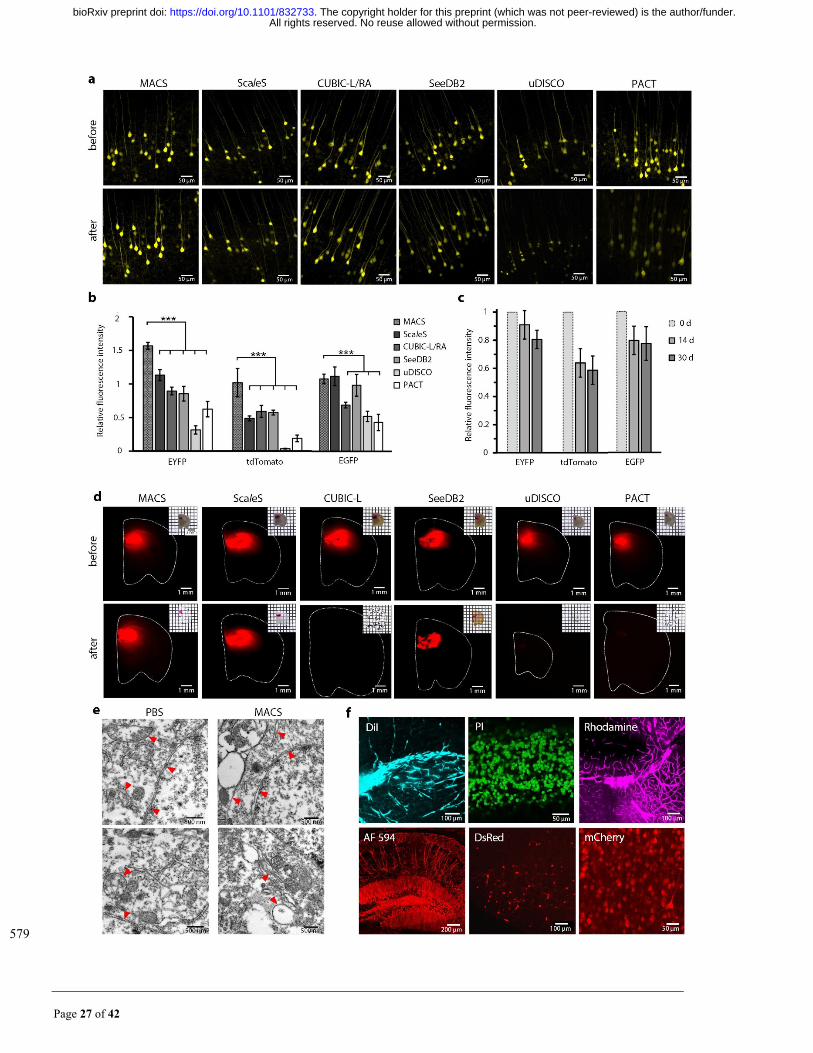
Fig. 2. MACS maintains the signals of multiple fluorescent probes. (a) Fluorescence images of endogenous 580

EYFP signals (1 mm Thy1-YFP-H brain slices) before and after MACS clearing compared with other clearing 581

protocols. (b) Quantification of fluorescence preservation of EYFP, tdTomato and EGFP after MACS clearing 582

compared with different methods (n=3). (c) Quantitative analysis of long-term fluorescence preservation of EYFP, 583

tdTomato and EGFP after MACS clearing (n=3). (d) Bright field and fluorescence images of DiI-labelled brain 584

slices before and after clearing by each method. (e) Ultramicroscopic imaging of mouse brain samples restored 585

from MACS or PBS by transmission electron microscopy. Red arrow heads indicate typical membrane structures. 586

(f) Fluorescence signals labelled by various chemical fluorescent tracers are finely imaged after MACS clearing, 587

including DiI, PI, Tetramethylrhodamine (Rhodamine), AlexaFluor 594 (AF 594)-conjugated antibody, DsRed 588

and mCherry. All values are presented as the mean ± s.d.; Statistical significance in b (***, P < 0.001) was assessed 589

by one-way ANOVA followed by the Bonferroni post hoc test. 590


https://doi.org/10.1101/832733

of 42

591


https://doi.org/10.1101/832733

of 42

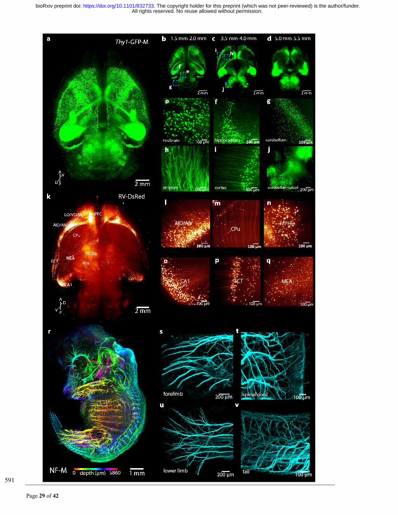
Fig. 3. MACS is applicable for 3D imaging and reconstruction of neural structures in intact tissues. (a) 592

3D reconstruction of LSFM images of whole brain (Thy1-GFP-M) cleared by MACS. (b-d) Maximum 593

projection of acquired images between 1.5 mm-2.0 mm (b), 3.5 mm-4.0 mm (c) and 5.0 mm-5.5 mm (d). (e-594

j) The high-magnification images of cleared brains reveal fine structures at different positions of the brain, 595

including the midbrain (e), hippocampus (f), cerebellum (g), striatum (h), cortex (i), and cerebellar nuclei (j). 596

(k) 3D reconstruction of RV-labelled afferent projections to nucleus reuniens (RE) throughout the whole 597

brain. (l-q) Several regions of specific projections to RE, including the dorsal/ventral agranular insular cortex 598

(AID/AIV) (l), caudate putamen (CPu) (m), medial prefrontal cortex (mPFC) (n), ventral CA1 of the 599

hippocampus region (o), ectorhinal cortex (ECT) (p) and medial amygdaloid nucleus (MEA) (q). (r) 3D 600

reconstruction of whole embryo (E14.5) labelled for neurofilament (NF-M). The images along the z stack 601

are coloured by spectrum. (s-v) Details of the nerve innervation in the forelimb (s), spinal cord (t), lower 602

limb (u), and tail (v). Thin nerve fibres are finely labelled and detected. 603


https://doi.org/10.1101/832733

of 42

604


https://doi.org/10.1101/832733

of 42

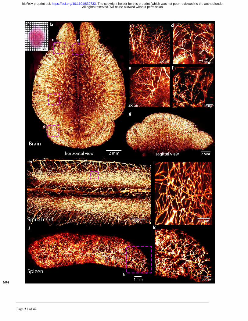
Fig. 4. MACS enables 3D visualization of the vascular network of DiI-labelled mouse organs. (a) Direct 605

view of DiI-labelled vasculatures in the cleared brain. (b) 3D rendering of the vascular network throughout 606

an entire adult brain imaged by LSFM. (c-f) Detailed vasculature in the cortex (c), middle of the brain (d), 607

cerebellum (e) and hippocampus (f). (g) Sagittal view of the reconstructed brain shown in a. (h) 3D rendering 608

of vasculatures in the spinal cord. (i) Magnification of boxed regions in h, the surrounded capillaries are 609

finely labelled and clearly visualized. (j) Reconstructed vascular network of adult mouse spleen. (k) 610

Magnification of boxed regions in j, the small branches are well detected. 611

612


https://doi.org/10.1101/832733

of 42

Supplementary Figures 613

614

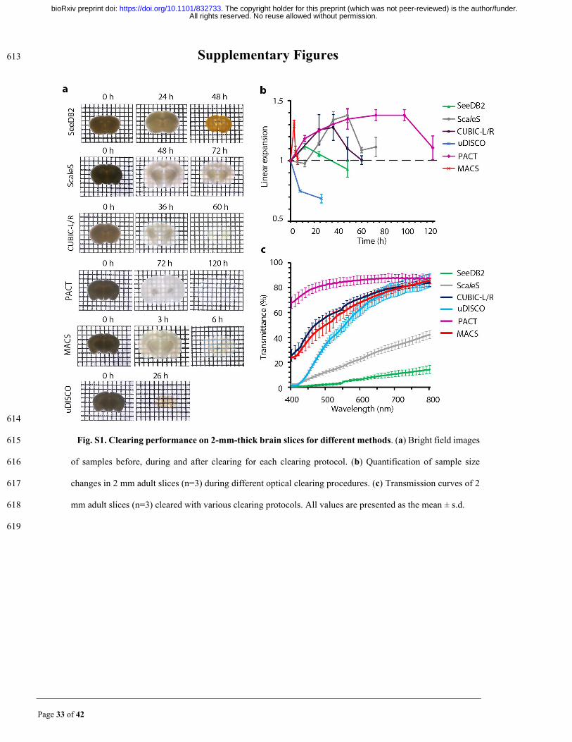
Fig. S1. Clearing performance on 2-mm-thick brain slices for different methods. (a) Bright field images 615

of samples before, during and after clearing for each clearing protocol. (b) Quantification of sample size 616

changes in 2 mm adult slices (n=3) during different optical clearing procedures. (c) Transmission curves of 2 617

mm adult slices (n=3) cleared with various clearing protocols. All values are presented as the mean ± s.d. 618

619


https://doi.org/10.1101/832733

of 42

620

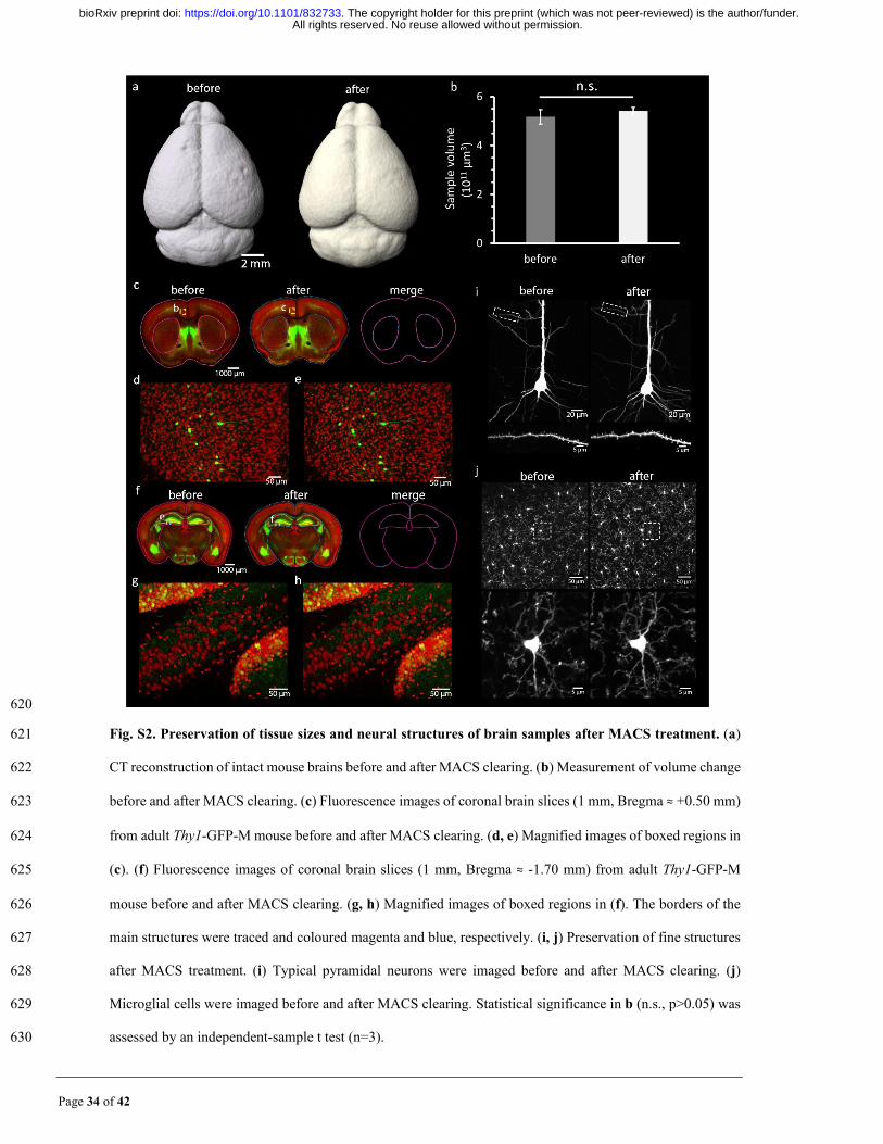
Fig. S2. Preservation of tissue sizes and neural structures of brain samples after MACS treatment. (a) 621

CT reconstruction of intact mouse brains before and after MACS clearing. (b) Measurement of volume change 622

before and after MACS clearing. (c) Fluorescence images of coronal brain slices (1 mm, Bregma ≈ +0.50 mm) 623

from adult Thy1-GFP-M mouse before and after MACS clearing. (d, e) Magnified images of boxed regions in 624

(c). (f) Fluorescence images of coronal brain slices (1 mm, Bregma ≈ -1.70 mm) from adult Thy1-GFP-M 625

mouse before and after MACS clearing. (g, h) Magnified images of boxed regions in (f). The borders of the 626

main structures were traced and coloured magenta and blue, respectively. (i, j) Preservation of fine structures 627

after MACS treatment. (i) Typical pyramidal neurons were imaged before and after MACS clearing. (j) 628

Microglial cells were imaged before and after MACS clearing. Statistical significance in b (n.s., p>0.05) was 629

assessed by an independent-sample t test (n=3). 630


https://doi.org/10.1101/832733

of 42

631


https://doi.org/10.1101/832733

of 42

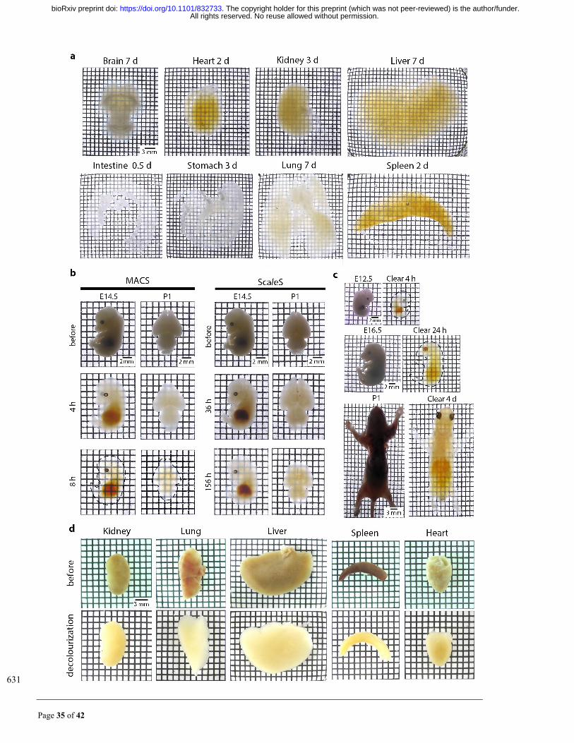
Fig. S3. Efficient clearing and decolourization of different tissues by MACS. (a) Intact rat organs were 632

cleared with MACS, and bright field images show that the brain, heart, kidney, liver, intestine, stomach, lung 633

and spleen were rendered optically transparent at the indicated time. (b) Rapid clearing for mouse embryos 634

and pups by MACS. Comparison of clearing performance for embryos and young mice by ScaleS and MACS. 635

E14.5 mouse embryos and whole neonatal mouse brain (P1) were used. Samples were cleared according to 636

the original protocols for ScaleS. At the time points indicated, bright field images were taken to examine the 637

clarification of the samples. (c) Efficient clearing for embryos (E12.5 and E16.5) and P1 pups by MACS. (d) 638

Decolourization of different mouse organs by MACS-R0. Hemi-rich mouse organs such as kidney, lung, liver, 639

spleen and heart were incubated in MACS-R0 for 24 h and then washed with PBS. Reflection images were 640

taken before and after treatment. 641

642


https://doi.org/10.1101/832733

of 42

643

644


https://doi.org/10.1101/832733

of 42

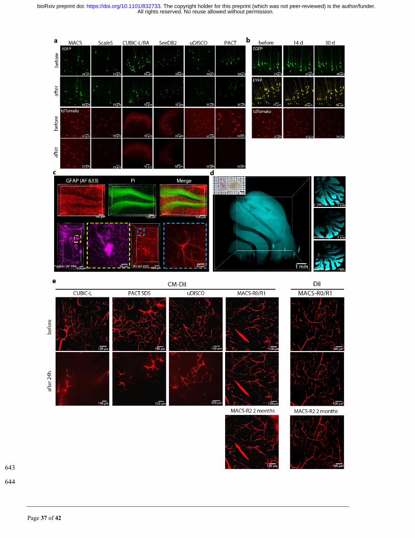
Fig. S4. MACS performs good compatibility with transgenic labelling, immunolabelling, nucleus 645

staining and DiI labelling, related to Fig. 2. (a) Fluorescence images of endogenous EGFP and tdTomato in 646

1 mm brain slices before and after clarification by each method. (b) Fluorescence images of endogenous EGFP, 647

EYFP and tdTomato of MACS-cleared 1 mm brain slices over time. Bright field image of a rat hemisphere 648

cleared by MACS. (c) (top) GFAP immunostaining and PI labelling of 1 mm coronal brain sections. Images 649

show labelling of astrocytes and cell nuclei in hippocampus region. (lower left) 3D rendering of 1 mm mouse 650

kidney slices stained by anti-beta tubulin, Magnification of boxed regions reveal fine labelling of microtubules. 651

(lower right) 3D rendering of 1 mm brain blocks stained by anti-tyrosine hydrogenase (TH). Magnification 652

of boxed regions reveals the structure of an individual TH-positive neuron. (d) LSFM imaging and 653

reconstruction of the cerebellum of a PI-stained rat hemisphere cleared by MACS, the imaging depth is over 654

6800 μm. Optical sections are shown at different depths. The structure of the cerebellum is clearly visible 655

throughout the entire imaging depth. (e) Comfocal images of CM-DiI labelled brain slices before and after 24 656

h clearing by each method. MACS could not only preserve the DiI signal, but also preserve the signals from 657

CM-DiI. 658

659


https://doi.org/10.1101/832733

of 42

660

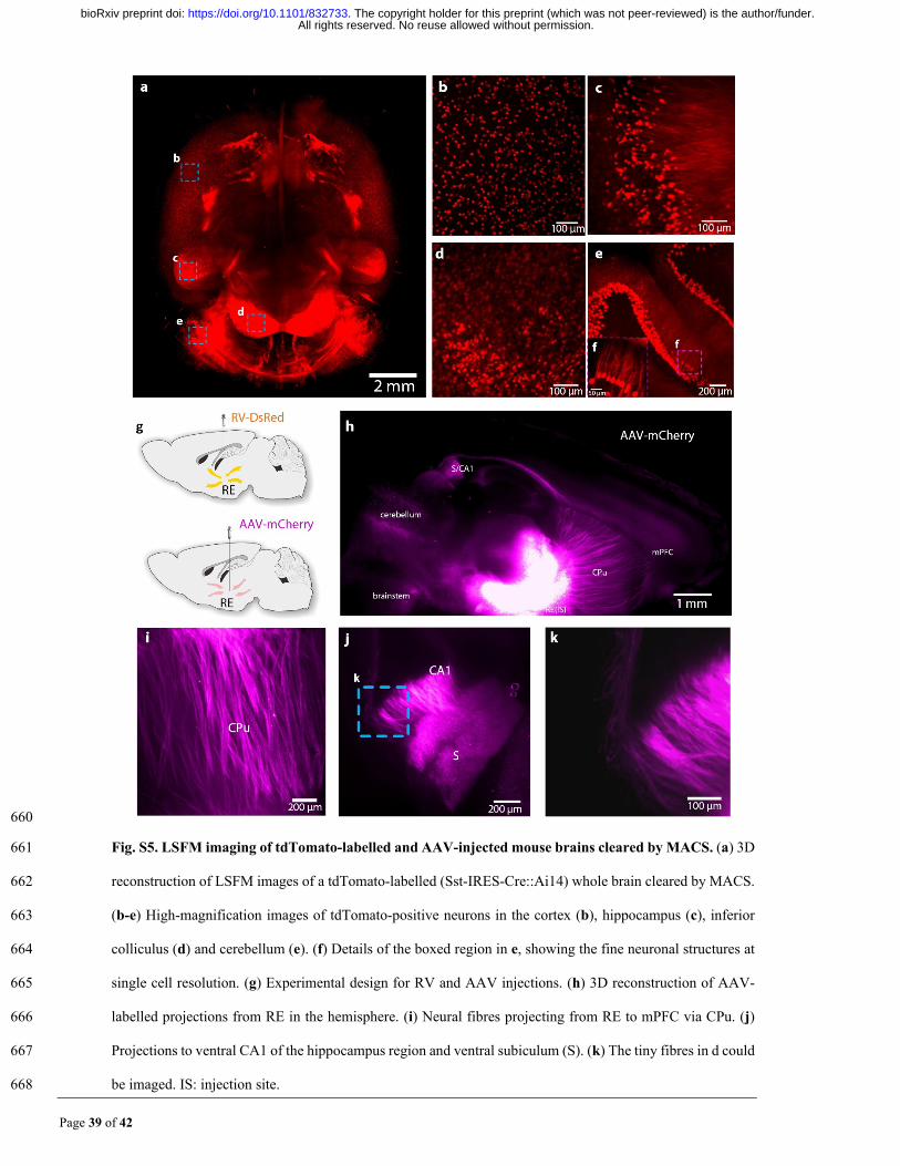
Fig. S5. LSFM imaging of tdTomato-labelled and AAV-injected mouse brains cleared by MACS. (a) 3D 661

reconstruction of LSFM images of a tdTomato-labelled (Sst-IRES-Cre::Ai14) whole brain cleared by MACS. 662

(b-e) High-magnification images of tdTomato-positive neurons in the cortex (b), hippocampus (c), inferior 663

colliculus (d) and cerebellum (e). (f) Details of the boxed region in e, showing the fine neuronal structures at 664

single cell resolution. (g) Experimental design for RV and AAV injections. (h) 3D reconstruction of AAV-665

labelled projections from RE in the hemisphere. (i) Neural fibres projecting from RE to mPFC via CPu. (j) 666

Projections to ventral CA1 of the hippocampus region and ventral subiculum (S). (k) The tiny fibres in d could 667

be imaged. IS: injection site. 668


https://doi.org/10.1101/832733

of 42

669

670

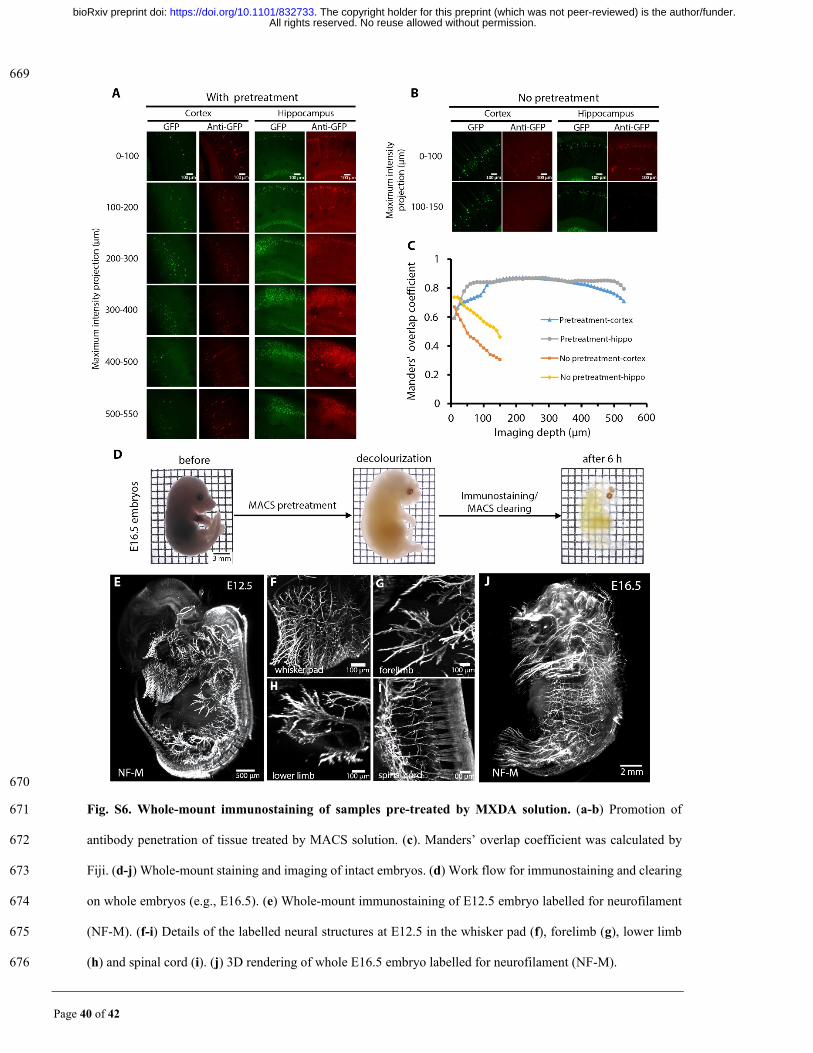
Fig. S6. Whole-mount immunostaining of samples pre-treated by MXDA solution. (a-b) Promotion of 671

antibody penetration of tissue treated by MACS solution. (c). Manders’ overlap coefficient was calculated by 672

Fiji. (d-j) Whole-mount staining and imaging of intact embryos. (d) Work flow for immunostaining and clearing 673

on whole embryos (e.g., E16.5). (e) Whole-mount immunostaining of E12.5 embryo labelled for neurofilament 674

(NF-M). (f-i) Details of the labelled neural structures at E12.5 in the whisker pad (f), forelimb (g), lower limb 675

(h) and spinal cord (i). (j) 3D rendering of whole E16.5 embryo labelled for neurofilament (NF-M). 676


https://doi.org/10.1101/832733

of 42

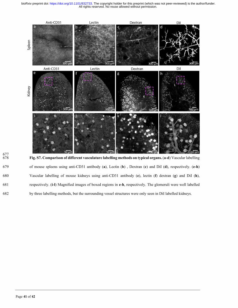
677 Fig. S7. Comparison of different vasculature labelling methods on typical organs. (a-d) Vascular labelling 678

of mouse spleens using anti-CD31 antibody (a), Lectin (b) , Dextran (c) and DiI (d), respectively. (e-h) 679

Vascular labelling of mouse kidneys using anti-CD31 antibody (e), lectin (f) dextran (g) and DiI (h), 680

respectively. (i-l) Magnified images of boxed regions in e-h, respectively. The glomeruli were well labelled 681

by three labelling methods, but the surrounding vessel structures were only seen in DiI labelled kidneys. 682


https://doi.org/10.1101/832733

of 42

Table S1. Changes in the pH of different agents after decolourization 683

Agents 50 vol% Quadrol 0.01 M NaOH 50 vol% MXDA

pH (before) 10.5 12.0 11.5

pH (after) 9.8 10.6 11.4

The pH values of the three solutions were measured before and after decolourization of embryos containing 684

blood. The pH values of Quadrol and NaOH solution revealed an obvious decline, while MXDA solution 685

remained stable. 686

687


https://doi.org/10.1101/832733

MACS: Rapid aqueous clearing system for three-dimensional ...intact organs 3 4 Jingtan Zhu 1,2†...

Documents

Transcript of MACS: Rapid aqueous clearing system for three-dimensional ...intact organs 3 4 Jingtan Zhu 1,2†...