
Magnetic guidance for linear drives -...
165
Magnetic Guidance for Linear Drives Vom Fachbereich Elektrotechnik und Informationstechnik der Technischen Universität Darmstadt zur Erlangung des akademischen Grades eines Doktor-Ingenieurs (Dr.-Ing.) genehmigte Dissertation von Phong C. Khong, M.Sc. Geboren am 10. April 1978 in Hanoi, Vietnam Referent: Prof. Dr.-Ing. Peter Mutschler Korreferent: Prof. Dr.-Ing. Mario Pacas Tag der Einreichung: 11. 04. 2011 Tag der mündlichen Prüfung: 29. 08. 2011 D17 Darmstadt 2011
Transcript of Magnetic guidance for linear drives -...
Magnetic Guidance for Linear Drives
Vom Fachbereich Elektrotechnik und Informationstechnik
der Technischen Universität Darmstadt
zur Erlangung des akademischen Grades eines
Doktor-Ingenieurs (Dr.-Ing.)
genehmigte Dissertation
von
Phong C. Khong, M.Sc.
Geboren am 10. April 1978 in Hanoi, Vietnam
Referent: Prof. Dr.-Ing. Peter Mutschler
Korreferent: Prof. Dr.-Ing. Mario Pacas
Tag der Einreichung: 11. 04. 2011
Tag der mündlichen Prüfung: 29. 08. 2011
D17
Darmstadt 2011


Erklärung laut §9 PromO
I
Erklärung laut §9 PromO
Ich versichere hiermit, dass ich die vorliegende Dissertation allein und nur unter
Verwendung der angegebenen Literatur verfasst habe. Die Arbeit hat bisher noch
nicht zu Prüfungszwecken gedient.
______________
Darmstadt, den 08. April 2011. Phong C. Khong


Preface
III
Preface This dissertation is the results of my 4-years study and research in the Department of
Power Electronics and Control of Drives - Darmstadt University of Technology. Besides
the personal works, the results are achieved by the contributed help directly or indirectly
from many people to the dissertation. Therefore, I would like to give here my thanks to
them.
Firstly, I would like to give my thanks to Prof. Dr.-Ing. Peter Mutschler, the
supervisor and director of the Department. I would thank for his greatest support
throughout my thesis with his supervision, inspiration and wonderful working plan
during the 4-years. I would thank for his support in formalities and finance for my study
in Germany.
To Prof. Dr.-Ing. Mario Pacas, I thank for his interest and for acting as the co-advisor.
I thank the DFG Deutsche Forschungsgemeinschaft for financially supporting my
projects MU 1109.
I thank the 322 project of the Vietnamese Ministry of Education and Training
(MOET) and Deutscher Akademischer Austausch Dienst (DAAD) for the financially
supporting my basic living cost, formalities and the language course at the beginning.
I would like to thank all my colleagues in the institute for their supports and
comments, a good working atmosphere, and many useful discussions. Especially, I
would like to thank to Dr.-Ing Roberto Leidhold for his support since the beginning of
my works in the Department.
Many non-scientific issues are important for an experimental project. I appreciate the
work and advice of the institute’s technical staff, and administrative staff.
I am very grateful to my parents and my wife for their support, encouragement and
especially take care of my daughter during my study.
After all the help, I had been given, it was really wonderful in my preface to be able to
express my thanks one more time, especially to my great supervisor who had shared his
immense knowledge and precious time with me, and to my long-suffering family who
had supported me through all the stress every step of the way!
Darmstadt, 08 April 2011.

Abstract
V
Abstract Linear drives provide many new attractive solutions for the material transportation
and processing in the manufacturing industry. With no mechanical transmission
elements, they enable high dynamics and rigidity as well as low installation- and low
maintenance-costs. That performance can give the linear motor system a better
precision, a higher acceleration and a higher speed of the moving part. Therefore, the
material transportation and processing using linear motors is studied and applied
increasingly in manufacturing industry.
For these applications, the linear motor is typically with stationary long primary
and a short moving secondary. As the secondary part is passive, no energy
transmission is required between the moving and stationary part, avoiding the use of
brushes or inductive transmission. The motor type best suited for the mentioned
applications is the synchronous one with permanent magnets, because of its higher
efficiency, compactness, but most important because it allows a higher air-gap.
In the usual approach, the linear motor is only used for thrust force production. The
guidance is usually implemented by a mechanical assembly. The guidance constrains
the movement to the longitudinal displacement, fixing the lateral and vertical
displacement: yaw, roll and pitch. To achieve the necessary precision of the
movement, accurate mechanical guidance is required. Such the mechanical assembly
can be complex and source of high friction.
In this dissertation, a research of an active guiding system is presented. The
purpose of this research is finding out a solution for the material transportation and
processing applications. The target is a linear drive system, which can reduce the
complicated mechanical structure. In additions, the passive vehicle is also necessary.
The result of the research is PM-synchronous linear motors with long and double-
sided primaries. In the system, the lateral displacement and the yaw angle are
controlled while a simple wheel-rail system fixes the vertical displacement. This
combination of the magnetic and mechanical guidance offers a good trade-off among
the complexity of the control, actuators and mechanics, when considering industrial
applications. To allow multiple vehicles traveling simultaneously and independently
on the guide-way (each vehicle is controlled by an individual part of the guide-way),
the double side primary is separated into segments. With that structure, flexible-
operating methods can be implemented. That is very useful in process-integrated
material handling where different speeds of material carriers in each processing
Abstract
VI
station are necessary. Another advantage of segmented structure is the energy saving.
The power is supplied only to the segment or the two consecutive segments in which
the vehicle runs over. In one segment, each side of the primary is supplied by its own
inverter, allowing the necessary degree of freedom to control the lateral position and
the yaw angle in addition to the thrust control.
In order to make the vehicle completely passive, a capacitive sensor is proposed
and implemented to measure the lateral position and the yaw angle. The sensor has
active parts installed on the guide-way and passive parts on the vehicle.
The mathematical analysis and the finite element method (FEM) are used to
analysis the proposed system. With the analysed results, the control for the system is
investigated in detail. Hardware and software for the experimental system is
developed and implemented.
The analysed results and the experimental results validate the proposed system.
That gives a new solution for the material transportation and processing application
using linear synchronous motors.
Kurzfassung
VII
Kurzfassung Zum Transport und zur Bearbeitung von Gegenständen in der
Verarbeitungsindustrie bieten die Linear- Direktantriebe zunehmend interessante
Lösungen. Unter Wegfall mechanischer Übertragungselemente ermöglichen sie hohe
Dynamik und Steifigkeit sowie Verschleiß- und Wartungsarmut. Diese Eigenschaften
ermöglichen den Linearmotor-Systemen eine höhere Genauigkeit, höhere
Beschleunigung und eine höhere Geschwindigkeit der beweglichen Teile. Daher wird
der Transport und die Bearbeitung mit Linearmotoren in der Verarbeitungsindustrie
zunehmend erforscht und eingesetzt.
Für diese Anwendungen werden normalerweise Linearmotoren mit langem
stationären Primärteil und kurzem bewegenden Sekundärteil eingesetzt. Da der
Sekundärteil passiv ist, wird keine Energieübertragung zwischen den beweglichen
und stationären Teilen benötigt, und somit werden Bürsten oder induktive
Übertragungssysteme vermieden. Der permanenterregte Synchronmotor ist der am
besten passende Motortyp für die genannten Anwendungen, aufgrund seines höheren
Wirkungsgrades und Leistungsdichte, aber vor allem weil er einen höheren Luftspalt
ermöglicht.
Üblicherweise wird der Linearmotor nur für Erzeugung der Schubkraft eingesetzt.
Die Spurführung ist in der Regel durch eine mechanische Konstruktion realisiert. Die
Spurführung beschränkt die Bewegung auf die Längsachse. Bewegung auf der
Transversal- und Vertikalachse (Gieren, Rollen und Nicken) ist durch die
Spurführung nicht möglich. Um die notwendige Präzision der Bewegung zu
erreichen, werden hochgenaue mechanische Führungen eingesetzt. Solche
mechanische Führungen sind aufwendig und verursachen höhere Reibung.
Die Forschung eines aktiven Spurführungssystems wird in dieser Dissertation
behandelt. Die Absicht dieser Forschung ist, Lösungen für Anwendungen des
Materialtransports und Bearbeitung herauszufinden. Das Ziel ist ein Linearantrieb,
der aufwendige mechanischer Strukturen vermeidet und dessen Fahrzeug passiv ist.
Das Ergebnis der Studie ist ein PM-Synchron-Linearmotor mit langen und
doppelseitigen Primärteilen. Die seitliche Bewegung und der Gierwinkel werden
geregelt, während die vertikale Bewegung von einem einfachen Rad-Schiene-System
fixiert wird. Diese Kombination von magnetischer und mechanischer Führung bietet
einen guten Kompromiss zwischen der Komplexität der Regelung, des Aktuators und

Kurzfassung
VIII
der Mechanik in dem Fall der industriellen Anwendungen. Um mehrere Fahrzeuge
gleichzeitig und unabhängig auf dem Fahrweg führen zu können (jedes Fahrzeug
wird durch einen individuellen Teil der Führung kontrolliert), ist der doppelseitige
Primärteil in Segmente getrennt. Mit dieser Struktur können flexible
Betriebsverfahren umgesetzt werden. Das ist sehr nützlich im integrierten Material-
Handling, wo unterschiedliche Geschwindigkeiten des Materialträgers in jeder
Bearbeitungsstation notwendig sind. Ein weiterer Vorteil der segmentierten Struktur
ist die Energieeinsparung. Nur das Segment oder die zwei aufeinander folgenden
Segmente die das Fahrzeug überfährt, werden gespeist. In einem Segment wird jede
Seite des Primärteils von einem eigenen Wechselrichter versorgt, so dass der
erforderliche Freiheitsgrad besteht, um die laterale Position, Gierwinkel und
Schubkraft zu steuern.
Um das Fahrzeug vollständig passiv zu machen wird ein kapazitiver Sensor zur
Messung der lateralen Position und des Gierwinkels vorgeschlagen und umgesetzt.
Der aktive Teil des Sensors wird am Führungsweg und der passive Teil am Fahrzeug
installiert.
Die mathematische Analyse und die Finite-Elemente-Methode (FEM) wurden
verwendet um das vorgeschlagene System zu analysieren. Mit den analytischen
Ergebnissen wurde die Regelung für das System im Detail untersucht. Hardware und
Software für das experimentelle System wurde entwickelt und umgesetzt.
Die analytischen und experimentellen Ergebnisse bestätigen das vorgeschlagene
System. Das gibt neue Lösungen für die Anwendungen in Materialtransport und
Verarbeitung bei Nutzung von Linear-Synchronmotoren.

Table of Contents
IX
Table of Contents
Erklärung laut §9 PromO .............................................................................................................. I
Preface ........................................................................................................................................ III
Abstract ........................................................................................................................................ V
Kurzfassung .............................................................................................................................. VII
Table of Contents ....................................................................................................................... IX
List of Symbols ........................................................................................................................ XIII
Abbreviation .......................................................................................................................... XVII
1. INTRODUCTION ................................................................................................................ 1
1.1. Linear motor concept and applications ........................................................................ 1
1.2. Linear drives for industrial material handling and processing ..................................... 3
1.3. Aim of the study ........................................................................................................... 5
1.4. Organization of the dissertation ................................................................................... 6
2. PROPOSED SYSTEM ......................................................................................................... 7
2.1. Topology of linear motors applied in industrial material handling and processing ..... 7
2.2. State of the art .............................................................................................................. 9
2.2.1. Research from other institutes ............................................................................ 10
2.2.2. Research in our department ................................................................................ 14
2.3. Proposed system ......................................................................................................... 15
2.3.1. Target of research ............................................................................................... 15
2.3.2. Proposed structure .............................................................................................. 15
2.4. Program of the work ................................................................................................... 16
2.4.1. Control duty. ....................................................................................................... 16
2.4.2. Lateral position sensor and yaw angle sensor. ................................................... 17
2.4.3. Work steps .......................................................................................................... 18
3. EXPERIMENTAL SETUP ................................................................................................ 19
3.1. Mechanical structure .................................................................................................. 19
3.1.1. The motors .......................................................................................................... 19
3.1.2. Construction ....................................................................................................... 21
3.2. Electrical structure ...................................................................................................... 23
3.2.1. Power supply ...................................................................................................... 23
3.2.2. Inverter modules ................................................................................................. 24
3.2.3. Inverter interface ................................................................................................ 24
3.2.4. Sensor system ..................................................................................................... 26
3.2.5. Controller ........................................................................................................... 27
3.3. Software ..................................................................................................................... 29
3.3.1. Operating System ............................................................................................... 29
3.3.2. Real time control software ................................................................................. 30
4. MATHEMATICAL MODEL ............................................................................................ 32
4.1. The magnetic guidance LSM model .......................................................................... 32
4.1.1. The experimental system in the horizontal plane ............................................... 32
4.1.2. Forces and torque on the vehicle ........................................................................ 33
4.2. Forces and torque calculation ..................................................................................... 34

Table of Contents
X
4.2.1. Current density and flux distribution ................................................................. 35
4.2.2. Magneto motive force and flux in the air-gap ................................................... 39
4.2.3. Magnetic energy and force calculation .............................................................. 42
4.2.4. Linearization of the force and torque equations ................................................ 44
4.3. Equations of motion ................................................................................................... 46
4.4. FEM simulation ......................................................................................................... 47
4.4.1. Finite element method ....................................................................................... 47
4.4.2. FEM model of the experimental setup ............................................................... 48
4.4.3. FEM results ........................................................................................................ 49
4.5. Practical measurement ............................................................................................... 53
5. CONTROLLER DESIGN ................................................................................................. 57
5.1. Control block diagram ............................................................................................... 57
5.1.1. Proposed control method ................................................................................... 57
5.1.2. Block diagrams of the control system ............................................................... 59
5.2. Controller design ....................................................................................................... 65
5.2.1. Current control loops ......................................................................................... 65
5.2.2. Speed control loops ............................................................................................ 67
5.2.3. Position control loops ........................................................................................ 68
5.3. Control system simulation ......................................................................................... 69
5.3.1. Simulation model ............................................................................................... 69
5.3.2. Simulation results .............................................................................................. 71
6. MAGNETIC GUIDANCE EXPERIMENTS .................................................................... 79
6.1. Implementation of control method ............................................................................ 79
6.2. Lateral position control .............................................................................................. 81
6.3. Yaw angle control ...................................................................................................... 83
6.4. Three DOFs control ................................................................................................... 86
6.5. Perturbation in longitudinal traveling ........................................................................ 89
7. CAPACITIVE SENSOR ................................................................................................... 94
7.1. Capacitive sensor structure ........................................................................................ 94
7.1.1. Mechanical structure .......................................................................................... 94
7.1.2. Electric circuit .................................................................................................... 96
7.2. Mathematic model ..................................................................................................... 98
7.2.1. Ideal case analysis .............................................................................................. 98
7.2.2. Calculation of the optimal value of d. ............................................................. 101
7.3. FEM simulation ....................................................................................................... 104
7.3.1. Parasitic capacitances ...................................................................................... 104
7.3.2. Capacitive sensor performances ...................................................................... 106
7.4. Experimental setup and results ................................................................................ 108
7.4.1. Experimental setup .......................................................................................... 108
7.4.2. Capacitive sensor calibration ........................................................................... 109
7.4.3. Control with capacitive sensor ......................................................................... 110
7.4.4. Quality of control with capacitive sensor. ....................................................... 111
8. CONCLUSIONS ............................................................................................................. 114
8.1. Summary .................................................................................................................. 114
8.2. Future work .............................................................................................................. 115
Bibliography ............................................................................................................................. 117
APPENDIX A .......................................................................................................................... 123

Table of Contents
XI
A1. Inverter interface board - IIB ......................................................................................... 123
A1.1 IIB structure .......................................................................................................... 123
A1. 2 Modulation in IIB ............................................................................................. 125
A2. Vehicle control interface - VCI ..................................................................................... 126
A3. The experimental communication bus ........................................................................... 127
APPENDIX B ........................................................................................................................... 129
B1. The d-q projection .......................................................................................................... 129
B2. Transformation of three phase currents ......................................................................... 132
B3 Anti-windup current control ............................................................................................ 133
B4 Basics of designing controller for drives ........................................................................ 135
B4.1 Amplitude optimum ..................................................................................................... 136
a. Apply for current control loop with PI controller ......................................................... 137
b. Apply for position control loop with P controller ........................................................ 138
B4.2 Symmetrical optimum .................................................................................................. 138
APPENDIX C ........................................................................................................................... 141
C1. Review of electromagnetic field theory ......................................................................... 141
C2. Permanent Magnet in PMLSM ...................................................................................... 142
Curriculum Vitae ...................................................................................................................... 145


List of Symbols
XIII
List of Symbols
SYMBOLS MEANING
a , 2a Complex unit vectors of the b-axis and c -axis unit vector in abc frame
sb Slot width of linear motor primary.
FNxC Normal force constant values ( 1..5x )
FTxC Thrust force constant values ( 1..2x )
MC Leakage capacitance
xxC Capacitances of the capacitive bridge ( 11;12;21;...;42xx )
d Coupling electrode horizontal gap
Ld Distance between the permanent magnets and the armature
LLd , LRd Ld of the left- and right-side of the vehicle
Md Thickness of the permanent magnets
E Electric field, Electric field intensity
F Mechanical force
F Force on the vehicle in y -direction
pF Perturbation force in y -direction
NaF , NPMF Normal force caused by the armature currents and the permanent magnet
NLF , NRF The left- and right- normal force on the vehicle
TLF , TRF The left- and right-side thrust on the vehicle
maxTF Maximum thrust of the linear motor
TnF Nominal thrust of the linear motor
( )wF s Transfer function of a closed loop
xF Electromagnetic thrust force along x -axis,
g Gap between primary and secondary back iron; Electrode stripes gap
eg Gap between sending- and receiving-electrode of the capacitive sensor
g Notation of space vector
H Height of the coupling electrode
h Height of electrode stripes
BH Height of the system basement
List of Symbols
XIV
eh Height of the sending and receiving electrode
VH Height of the vehicle
zh Height of permanent magnets
ai Amplitude of the armature current
di , qi Current components in dq -projection
i Current for actuating F
i Current for actuating T
maxI Max RMS current for 10s of the linear motor primary
NI Rate current (RMS) of the linear motor primary
1
si Primary current vector in static frame
1mi Primary current vector in moving frame
xi Current for actuating xF
cK Converter gain
eK Electrical gain
pK Constant value of the perturbation torque on the vehicle
pK Gain constant of a controller
k Winding factor at harmonic frequency v
xK Forces constant values ( 1..4x )
xpK Constant value of the perturbation force in x -direction
l Length of the capacitive sensor stripes
L1, L2,
L3, N Three phases four wires voltage system
amL Armature inductance
BL Length of the system basement
VL Length of the vehicle
M Mechanical torque
m Vehicle weight
Vm Weight of the vehicle
1N Number of series winding turns per one primary slot
ap Number of primary poles
List of Symbols
XV
ip The internal power of the air-gap without stator losses
mp Number of secondary poles
s Coupling electrode length
DT Converter delay
T Torque on the vehicle
iT Integral time value of a PI controller
sT Sampling time
u Relative velocity between the magnet and the armature
0u Excitation voltage of the capacitive sensor
1u , 2u Output voltages of the capacitive sensor
u , u , output voltages from the capacitive sensor
NU Nominal voltage of the linear motor primary
dv qv Phase voltages presented in dq -projection
1
sv is the primary voltage vector in static frame
BW Width of the system basement
magW Magnetic energy in the air-gap
VW Width of the vehicle
x Longitudinal position of the vehicle (in x axis)
0x Displacement between origins of the static- and moving-frame
mx Position presented in moving frame
sx Position presented in static frame
0y Air-gap of the vehicle when the vehicle in the middle of the guide-way
1a Fundamental component of the armature current density
1PM The equivalent current distribution of permanent magnet
Magnetic field, Magnetic flux density
L Magnetic flux density of the air-gap
R Magnetic flux density of the permanent magnet
RN Remanent flux density of the permanent magnet
Electric flux density
or Magneto motive force (MMF)
1PM Fundamental component of the permanent magnet MMF

List of Symbols
XVI
Magnetic field intensity
c Coercive force
Surface current density
PM Equivalent MMF of permanent magnet
Inertial moment of vehicle
m Angle between dq -frame and -frame
Lateral position of the vehicle (in y axis)
Relative dielectric constant
0 Dielectric constant of air
Yaw angle of the vehicle
Permeability
0 Permeability of free space or vacuum permeability
d Relative differential permeability
M Permeability of the permanent magnet
Mr Relative permeability of the permanent magnet
r Relative permeability
Magnetic flux
L Magnetic flux in the air-gap
R Magnetic flux in the permanent magnet
m Phase angle of the armature currents presented in moving frame
s Phase angle of the armature currents presented in static frame
Pole pitch.
p The magnet width.
s Slot pitch of linear motor primary.
Angular frequency of the three phase voltage
Abbreviation
XVII
Abbreviation
ABBREVIATION EXPLANATION
AD Analog to Digital
ADC Analog to Digital Converter
AMR Anisotropic magneto-resistive
CNC Computer Numerical Control
CPLD Complex Programmable Logic Device
CSS Capacitive sensor
DOF Degree of Freedom
EMF Electromotive Force
FEM Finite Element Method
FOC Field Oriented Control
FOCC Field Oriented Control Converter
FPGA Field-programmable Gate Array
IGBT Insulated-gate Bipolar Transistor
IIB Inverter Interface Board
ISR Interrupt Subroutine Request
ISS Inductive sensor
LIM Linear Induction Motor
LSM Linear Synchronous Motor
LUT Look Up Table
MMF Magneto Motive Force
PC Personal Computer
PCI Peripheral Component Interconnect
PDE Partial Differential Equations
PI controller Proportional–Integral controller
PM Permanent Magnet
PM LSM Permanent Magnet Linear Synchronous Motor
PWM Pulse width modulation
RTAI Real-Time Application Interface
SV-PWM Space Vector Pulse Width Modulation
TF Transfer function
VCI Vehicle Control Interface

INTRODUCTION
1
1. INTRODUCTION
1.1. Linear motor concept and applications
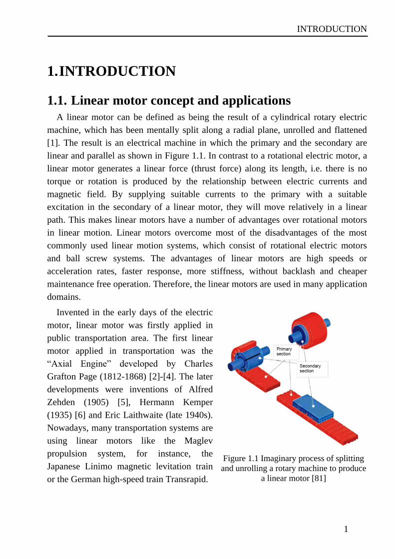
A linear motor can be defined as being the result of a cylindrical rotary electric
machine, which has been mentally split along a radial plane, unrolled and flattened
[1]. The result is an electrical machine in which the primary and the secondary are
linear and parallel as shown in Figure 1.1. In contrast to a rotational electric motor, a
linear motor generates a linear force (thrust force) along its length, i.e. there is no
torque or rotation is produced by the relationship between electric currents and
magnetic field. By supplying suitable currents to the primary with a suitable
excitation in the secondary of a linear motor, they will move relatively in a linear
path. This makes linear motors have a number of advantages over rotational motors
in linear motion. Linear motors overcome most of the disadvantages of the most
commonly used linear motion systems, which consist of rotational electric motors
and ball screw systems. The advantages of linear motors are high speeds or
acceleration rates, faster response, more stiffness, without backlash and cheaper
maintenance free operation. Therefore, the linear motors are used in many application
domains.
Invented in the early days of the electric
motor, linear motor was firstly applied in
public transportation area. The first linear
motor applied in transportation was the
“Axial Engine” developed by Charles
Grafton Page (1812-1868) [2]-[4]. The later
developments were inventions of Alfred
Zehden (1905) [5], Hermann Kemper
(1935) [6] and Eric Laithwaite (late 1940s).
Nowadays, many transportation systems are
using linear motors like the Maglev
propulsion system, for instance, the
Japanese Linimo magnetic levitation train
or the German high-speed train Transrapid.
Figure 1.1 Imaginary process of splitting
and unrolling a rotary machine to produce
a linear motor [81]
Linear motor concept and applications
2
Other transportation systems without magnetic levitation are Bombardier´s Advanced
Rapid Transit systems and number of modern Japanese subways. One more
technology using linear motor is in the roller coasters [7].
Besides the public transportation applications, the linear motors are also applied in
lifting mechanisms and many motion control applications. With small limitations of
space and the required height, the vertical linear motors are suitable for skyscraper or
deep mining elevators. Linear motors are also used in industrial or military lifting
systems. In addition, they are offered to use on sliding doors of trams, buildings or
elevators [8]-[12]. Dual axis linear motors also produced and applied to the
applications that require X-Y motion, such as in precision laser cutting machines,
automated drafting machines and others kind of CNC machine tools.
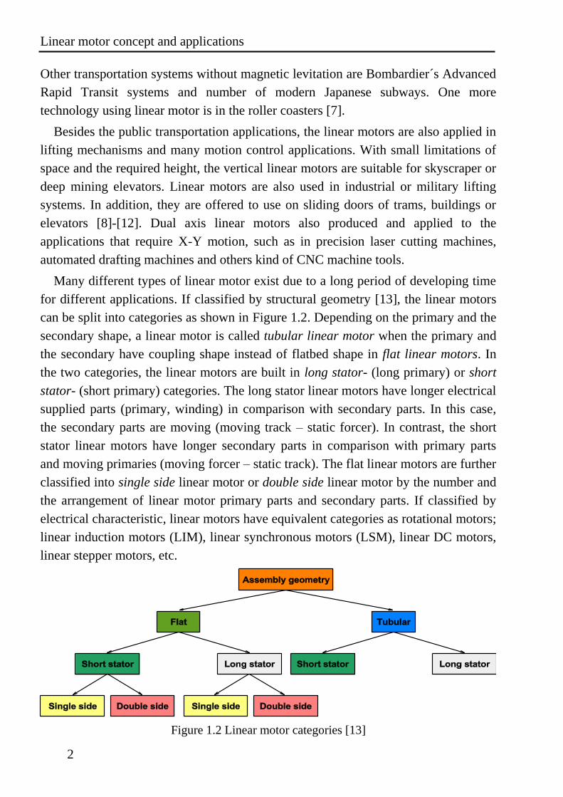
Many different types of linear motor exist due to a long period of developing time
for different applications. If classified by structural geometry [13], the linear motors
can be split into categories as shown in Figure 1.2. Depending on the primary and the
secondary shape, a linear motor is called tubular linear motor when the primary and
the secondary have coupling shape instead of flatbed shape in flat linear motors. In
the two categories, the linear motors are built in long stator- (long primary) or short
stator- (short primary) categories. The long stator linear motors have longer electrical
supplied parts (primary, winding) in comparison with secondary parts. In this case,
the secondary parts are moving (moving track – static forcer). In contrast, the short
stator linear motors have longer secondary parts in comparison with primary parts
and moving primaries (moving forcer – static track). The flat linear motors are further
classified into single side linear motor or double side linear motor by the number and
the arrangement of linear motor primary parts and secondary parts. If classified by
electrical characteristic, linear motors have equivalent categories as rotational motors;
linear induction motors (LIM), linear synchronous motors (LSM), linear DC motors,
linear stepper motors, etc.
Figure 1.2 Linear motor categories [13]
INTRODUCTION
3
Altogether, many types of linear motor have been developed for any applications
until now. The researches to use the advantages of linear motors in practical
applications are continuing. In this dissertation, a research to apply linear motor in the
process integrated material handling will be presented.
1.2. Linear drives for industrial material handling and
processing
As mentioned above, the linear motors are used today more and more in industrial
applications because of their advanced features. With their advanced mechanical
structure over the rotational motors in linear motions, the linear motors have attracted
many interests in the industrial material handling and processing applications.
In industrial production lines, materials must be processed and transported between
processing stations. The raw materials are processed sequentially to transform from a
raw state into finished parts or products. Each operation is done in one processing
station. Within the processing stations, for high precise operation, materials need to
be fastened when they are moving in and released when they are moving out. The
final parts or products are completed at least after passing several stations. In between
the stations, the raw materials are transported by conveyor belts, mobile vehicles or
robots.
In traditional processing method, the materials are tightened and released in each
operating station. That takes time of the process. In order to eliminate the significant
time-consuming for tightening and releasing, material handling systems nowadays
have a newly developing trend. That is using the high precise mobile mechanism,
which can stop or move precisely within the processing stations. With that, the
process can be operated on the mobile mechanism in each processing station.
Therefore, the raw materials just need to be fastened to the mobile mechanism at the
beginning of the processing chain and released at the end.
As the requirements mentioned above, the linear drive is a good option for the new
trend of the industrial transportation and processing system. By using the linear drive
[14] directly for processing and transportation without releasing and re-adjusting the
work pieces, with a linear drive system will result in many benefits as follows:
High productivity
High dynamic and high precision (few m)
No mechanical transmission reduced wear, assembling and maintenance
costs
Linear drives for industrial material handling and processing
4
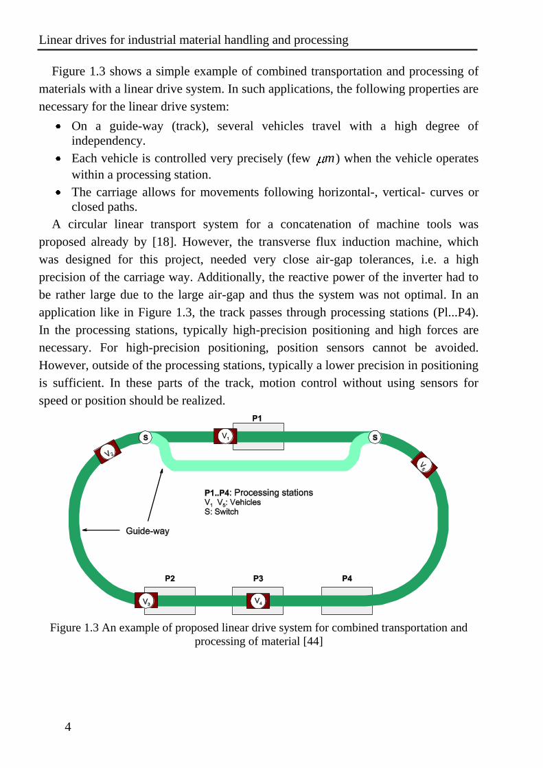
Figure 1.3 shows a simple example of combined transportation and processing of
materials with a linear drive system. In such applications, the following properties are
necessary for the linear drive system:
On a guide-way (track), several vehicles travel with a high degree of
independency.
Each vehicle is controlled very precisely (few m) when the vehicle operates
within a processing station.
The carriage allows for movements following horizontal-, vertical- curves or
closed paths.
A circular linear transport system for a concatenation of machine tools was
proposed already by [18]. However, the transverse flux induction machine, which
was designed for this project, needed very close air-gap tolerances, i.e. a high
precision of the carriage way. Additionally, the reactive power of the inverter had to
be rather large due to the large air-gap and thus the system was not optimal. In an
application like in Figure 1.3, the track passes through processing stations (Pl...P4).
In the processing stations, typically high-precision positioning and high forces are
necessary. For high-precision positioning, position sensors cannot be avoided.
However, outside of the processing stations, typically a lower precision in positioning
is sufficient. In these parts of the track, motion control without using sensors for
speed or position should be realized.
Figure 1.3 An example of proposed linear drive system for combined transportation and
processing of material [44]
INTRODUCTION
5
1.3. Aim of the study
With the advantages mentioned above, the linear drives provide many new
solutions for material transportation and processing in the manufacturing industry.
Instances of application can be found for stretching of plastic films [15] or in material
handling [14][16][17]. For these applications, the linear motor is typically with
stationary long primary part and a short moving secondary part [14]. As the
secondary part is passive, no energy transmission is required between the moving and
stationary part, avoiding the use of brushes or inductive transmission. The motor type
best suited for the mentioned applications is the synchronous one with permanent
magnets, because of its higher efficiency, compactness, but most important because it
allows a higher air-gap.
In the usual approach, the linear motor is only used for thrust force production. The
guidance is usually implemented by a mechanical assembly. The mechanical
guidance constrains the movement to the longitudinal displacement, fixing the lateral
and vertical displacement, yaw, roll and pitch. Such a mechanical assembly can be
complex and source of high friction.
In this thesis, a study of an active guiding system is presented. The proposed
guiding system is used for permanent magnet synchronous linear motors (PM SLM)
with long and double-sided primary. The lateral displacement and the yaw angle are
controlled while a simple wheel-rail system fixes the vertical displacement. This
combination of magnetic and mechanical guidance offers a good trade-off among the
complexity of the control, actuators and mechanics, when industrial applications are
considered. To allow multiple vehicles traveling simultaneously and independently
on the guide-way (each vehicle is controlled by an individual part of the guide-way),
the double side primary is separated into segments. With that structure, flexible-
operating methods can be implemented. That is very useful in process integrated
material handling where different speeds of material carriers in each processing
station are required. Another advantage of segmented structure is the energy saving.
The power is supplied only to the segment or the two consecutive segments in which
the vehicle runs over. In one segment, each side of the primary is supplied by its own
inverter, allowing the necessary degrees of freedom to control the lateral position and
the yaw angle in addition to the longitudinal position. With this arrangement, the
mover can be kept passive avoiding any energy transmission system to it (besides for
the sensors).
Together with the guiding system, the sensor system is also studied in order to
make a complete passive vehicle. As the requirement of the guiding system, sensor
Organization of the dissertation
6
system must be able to supply three feedback parameters, namely: lateral position,
yaw angle and longitudinal position. To eliminate either the supplying energy or the
data transmission, the sensor system must have the active part on the guide-way,
while the passive part is mounted on the moving vehicle.
1.4. Organization of the dissertation
According to the aim of the study, the thesis will be introduced in the main
chapters as follows:
In chapter 2, the topologies of the linear motors will be presented in order to find a
suitable topology for the material transportation and handling applications. Based on
the current state of art, a new system is proposed. Finally, a list of studying matters,
which have to be solved in order to implement the proposed system, is established.
Chapter 3 is the descriptions of the experimental system. A prototype of the
proposed system is realized with the combination of commercial products and
institute-developed products.
The system is analyzed by mathematic calculations and finite element method
(FEM) simulations in Chapter 4. The results are verified with the practical
measurement in the experimental setup.
In chapter 5, the control method is proposed. Parameters of regulator units are
calculated based on the proposed control method. The control system and regulator’s
parameter are then verified with a Matlab simulation model.
In chapter 6, the control method is implemented in the experimental setup.
Verifying experiments are executed to test the proposed control method on a
prototype system.
Finally, a new sensor system, which can make the vehicle passive, is studied and
presented. The complete structure, mathematical analysis and practical experiment of
the sensor system are introduced in chapter 7.
The conclusions are given in chapter 8. In the chapter, the summary of the works in
the dissertation is presented, and suggestions for the future works are quoted.
PROPOSED SYSTEM
7
2. PROPOSED SYSTEM
2.1. Topology of linear motors applied in industrial
material handling and processing
After a long period of development, linear drives are manufactured in many
different kinds, suitable for different applications. For industrial material handling
and processing, the properties of linear drives need to be analyzed to make suitable
choices. In this section, the two main distinguished categories of linear motor (short
primary and long primary) are firstly analyzed. Then the suitable linear drive is
chosen for the study in this dissertation.
In short-primary linear motors, the winding is mounted on the moving part. Hence,
the short-primary linear drive requires active vehicles i.e. energy and information
must be transmitted to the vehicle. The solutions for energy transmission can be
running cables, sliding contacts or contact-less (inductive energy transmission). The
running cable solution is not applicable in industrial material handling and
processing, as the vehicle has to travel long distances and closed paths. In many
industrial production environments, sliding contacts should be avoided because of the
safety for workers, maintenance or exploding protection. In the short-primary
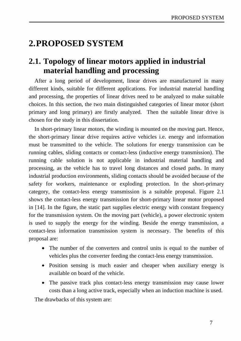
category, the contact-less energy transmission is a suitable proposal. Figure 2.1
shows the contact-less energy transmission for short-primary linear motor proposed
in [14]. In the figure, the static part supplies electric energy with constant frequency
for the transmission system. On the moving part (vehicle), a power electronic system
is used to supply the energy for the winding. Beside the energy transmission, a
contact-less information transmission system is necessary. The benefits of this
proposal are:
The number of the converters and control units is equal to the number of
vehicles plus the converter feeding the contact-less energy transmission.
Position sensing is much easier and cheaper when auxiliary energy is
available on board of the vehicle.
The passive track plus contact-less energy transmission may cause lower
costs than a long active track, especially when an induction machine is used.
The drawbacks of this system are:
Topology of linear motors applied in industrial material handling and processing
8
Because of the energy transmission system and the on board inverter, the
vehicles have high weight and big volume.
The power limitation of contact-less transmission system and the vehicle
weight reduce the dynamic of the vehicle.
Figure 2.1 A short primary system with contact-less energy transmission [14]
With the above characteristics, the short-primary linear drive can be a good
solution for applications with a long track, low number of vehicles and low
acceleration.
In order to overcome the drawbacks of the short-primary linear drive, the long-
primary one can give solutions for high acceleration, passive, lightweight vehicles by
using an active track. The system does not need energy or information transfer to the
vehicles. Because of its higher efficiency, compactness, but most important because it
allows a higher air-gap, permanent magnet excitations are usually used in the system.
For use in industrial material handling and processing applications, the primary of the
system is separated in to segments. This ensures that:
Each vehicle can be controlled and moved independently by one or two
contiguous primary segments.
The reactive power can be reduced (save energy) by switching off the stator
segments not carrying any vehicle.
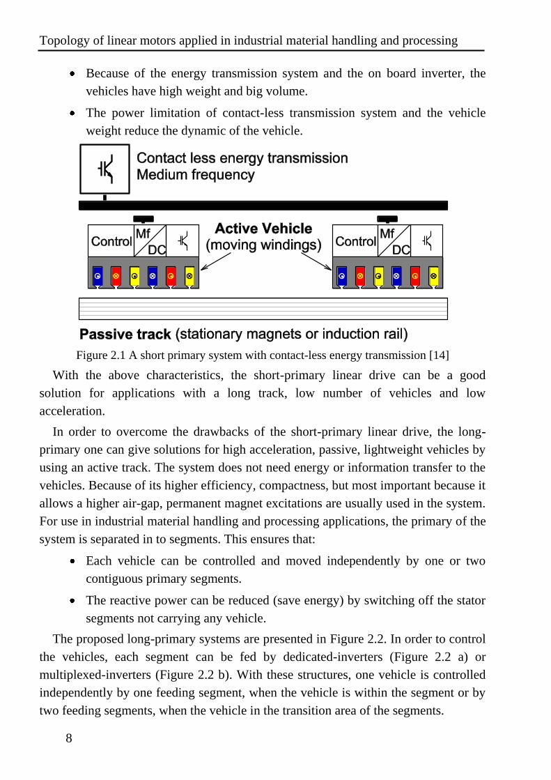
The proposed long-primary systems are presented in Figure 2.2. In order to control
the vehicles, each segment can be fed by dedicated-inverters (Figure 2.2 a) or
multiplexed-inverters (Figure 2.2 b). With these structures, one vehicle is controlled
independently by one feeding segment, when the vehicle is within the segment or by
two feeding segments, when the vehicle in the transition area of the segments.

PROPOSED SYSTEM
9
a) Dedicated inverters
b) Multiplex inverters
Figure 2.2 Proposed long primary topology [14]
As mentioned above, several suitable topologies are applicable for industrial
material handling and processing. In this dissertation “Magnetic guidance for linear
motor”, the research on long primary motors with dedicated inverters applicable to
industrial material handling and processing is presented. The research is done with
double side long-primary linear motor for high thrust force applications. Magnetic
guidance is studied to avoid precise mechanical guidance.
2.2. State of the art
Regarding to the introduction in chapter 1, the research of this dissertation relates
to the control of the magnetic thrust and lateral air-gap in a synchronous motor with
long stator and “passive mover”. With no transmission between the environment and
the vehicle (neither electric energy nor information), the “passive mover”, for
example, can be used in material processing.
This topic is one part of the wide area of magnetic driving, levitation and guidance.
We have to distinguish between rotating and linear drives. There are many interesting
documents in literature of rotating drives, concerning magnetic bearing and bearing
State of the art
10
less motors. They are also related to the research topic, but in this subsection, they are
not discussed in detail.
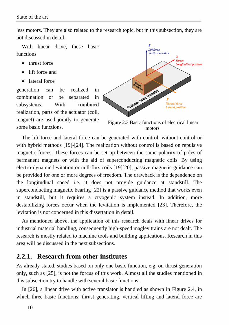
With linear drive, these basic
functions
thrust force
lift force and
lateral force
generation can be realized in
combination or be separated in
subsystems. With combined
realization, parts of the actuator (coil,
magnet) are used jointly to generate
some basic functions.
Figure 2.3 Basic functions of electrical linear
motors
The lift force and lateral force can be generated with control, without control or
with hybrid methods [19]-[24]. The realization without control is based on repulsive
magnetic forces. These forces can be set up between the same polarity of poles of
permanent magnets or with the aid of superconducting magnetic coils. By using
electro-dynamic levitation or null-flux coils [19][20], passive magnetic guidance can
be provided for one or more degrees of freedom. The drawback is the dependence on
the longitudinal speed i.e. it does not provide guidance at standstill. The
superconducting magnetic bearing [22] is a passive guidance method that works even
in standstill, but it requires a cryogenic system instead. In addition, more
destabilizing forces occur when the levitation is implemented [23]. Therefore, the
levitation is not concerned in this dissertation in detail.
As mentioned above, the application of this research deals with linear drives for
industrial material handling, consequently high-speed maglev trains are not dealt. The
research is mostly related to machine tools and building applications. Research in this
area will be discussed in the next subsections.
2.2.1. Research from other institutes
As already stated, studies based on only one basic function, e.g. on thrust generation
only, such as [25], is not the forcus of this work. Almost all the studies mentioned in
this subsection try to handle with several basic functions.
In [26], a linear drive with active translator is handled as shown in Figure 2.4, in
which three basic functions: thrust generating, vertical lifting and lateral force are
PROPOSED SYSTEM
11
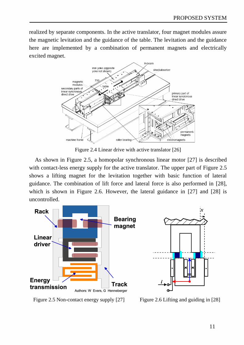
realized by separate components. In the active translator, four magnet modules assure
the magnetic levitation and the guidance of the table. The levitation and the guidance
here are implemented by a combination of permanent magnets and electrically
excited magnet.
Figure 2.4 Linear drive with active translator [26]
As shown in Figure 2.5, a homopolar synchronous linear motor [27] is described
with contact-less energy supply for the active translator. The upper part of Figure 2.5
shows a lifting magnet for the levitation together with basic function of lateral
guidance. The combination of lift force and lateral force is also performed in [28],
which is shown in Figure 2.6. However, the lateral guidance in [27] and [28] is
uncontrolled.
Figure 2.5 Non-contact energy supply [27] Figure 2.6 Lifting and guiding in [28]
State of the art
12
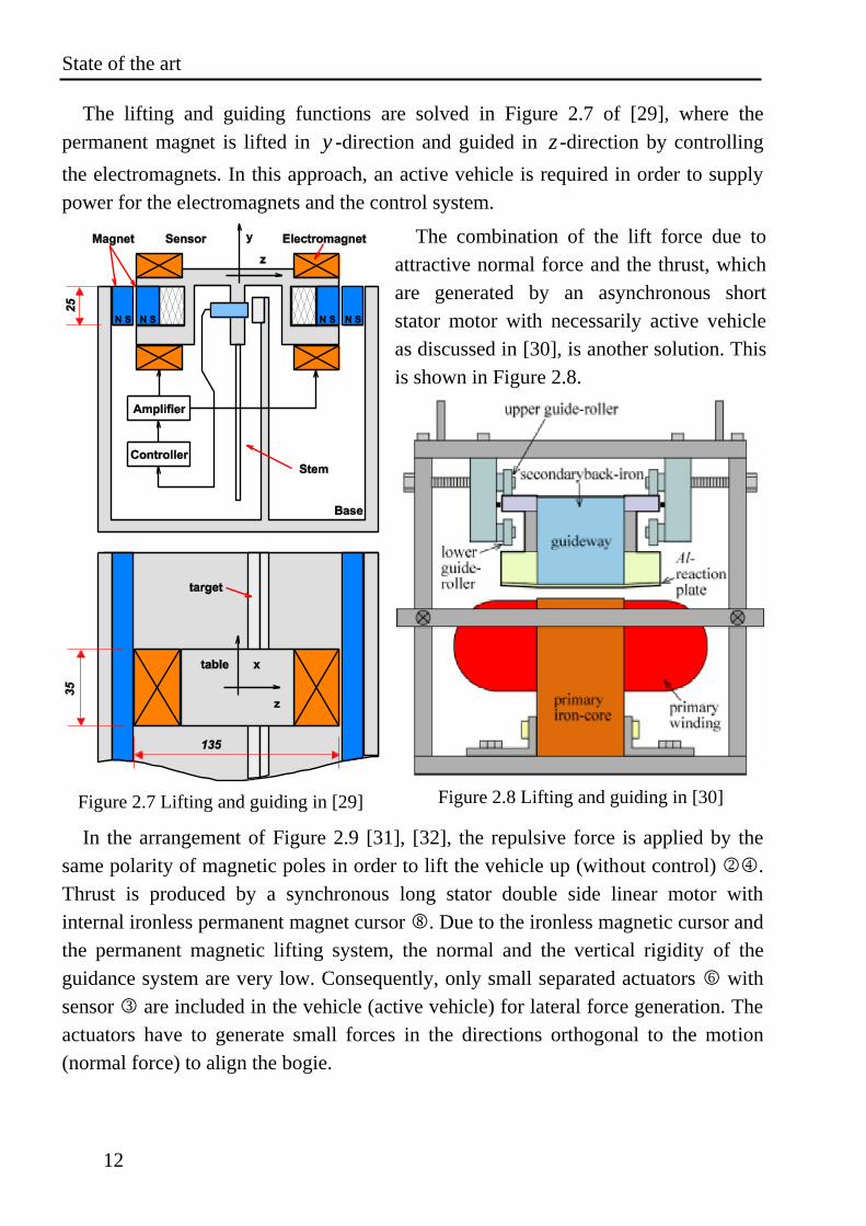
The lifting and guiding functions are solved in Figure 2.7 of [29], where the
permanent magnet is lifted in y -direction and guided in z -direction by controlling
the electromagnets. In this approach, an active vehicle is required in order to supply
power for the electromagnets and the control system.
Figure 2.7 Lifting and guiding in [29]
The combination of the lift force due to
attractive normal force and the thrust, which
are generated by an asynchronous short
stator motor with necessarily active vehicle
as discussed in [30], is another solution. This
is shown in Figure 2.8.
Figure 2.8 Lifting and guiding in [30]
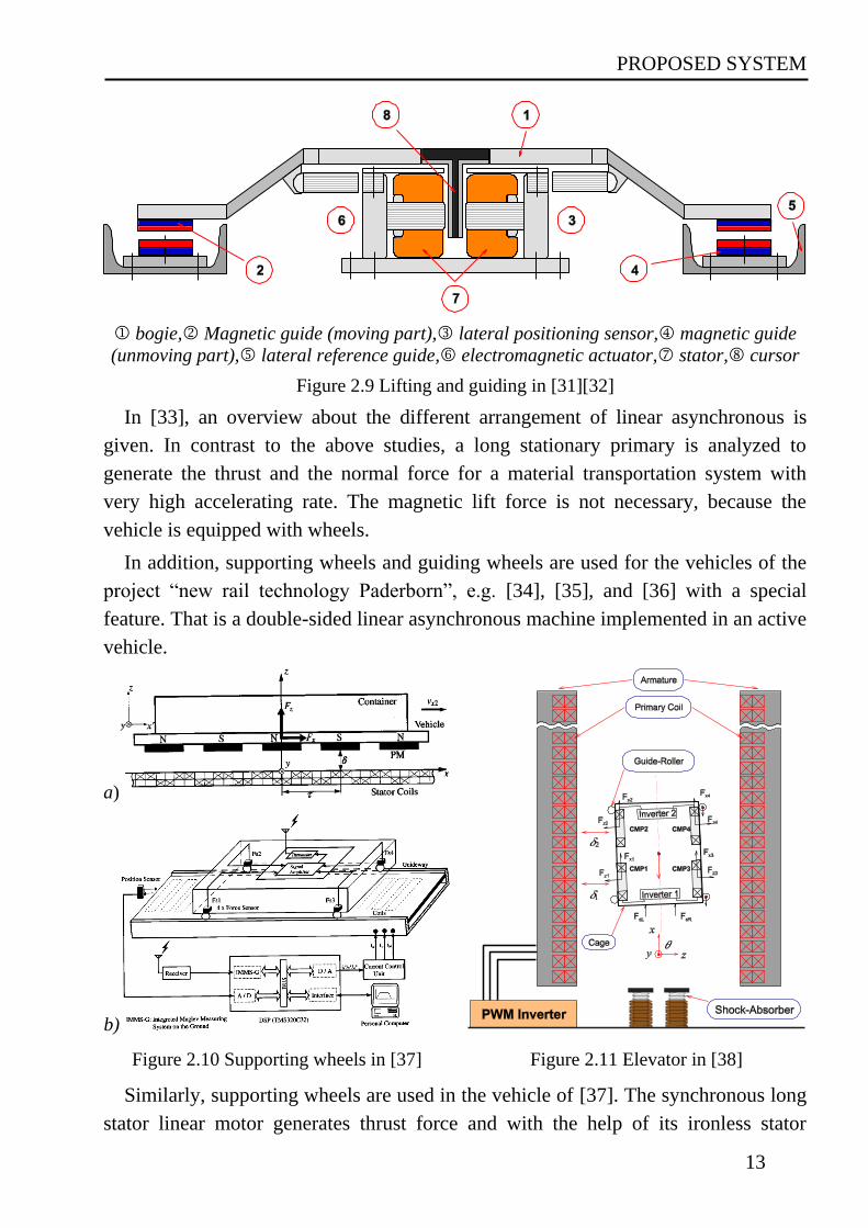
In the arrangement of Figure 2.9 [31], [32], the repulsive force is applied by the
same polarity of magnetic poles in order to lift the vehicle up (without control) .
Thrust is produced by a synchronous long stator double side linear motor with
internal ironless permanent magnet cursor . Due to the ironless magnetic cursor and
the permanent magnetic lifting system, the normal and the vertical rigidity of the
guidance system are very low. Consequently, only small separated actuators with
sensor are included in the vehicle (active vehicle) for lateral force generation. The
actuators have to generate small forces in the directions orthogonal to the motion
(normal force) to align the bogie.
PROPOSED SYSTEM
13
bogie, Magnetic guide (moving part), lateral positioning sensor, magnetic guide
(unmoving part), lateral reference guide, electromagnetic actuator, stator, cursor
Figure 2.9 Lifting and guiding in [31][32]
In [33], an overview about the different arrangement of linear asynchronous is
given. In contrast to the above studies, a long stationary primary is analyzed to
generate the thrust and the normal force for a material transportation system with
very high accelerating rate. The magnetic lift force is not necessary, because the
vehicle is equipped with wheels.
In addition, supporting wheels and guiding wheels are used for the vehicles of the
project “new rail technology Paderborn”, e.g. [34], [35], and [36] with a special
feature. That is a double-sided linear asynchronous machine implemented in an active
vehicle.
a)
b)
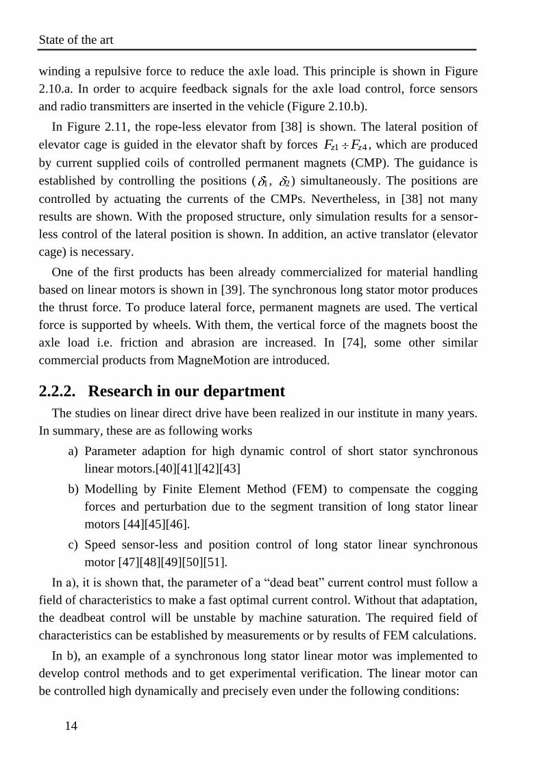
Figure 2.10 Supporting wheels in [37] Figure 2.11 Elevator in [38]
Similarly, supporting wheels are used in the vehicle of [37]. The synchronous long
stator linear motor generates thrust force and with the help of its ironless stator
State of the art
14
winding a repulsive force to reduce the axle load. This principle is shown in Figure
2.10.a. In order to acquire feedback signals for the axle load control, force sensors
and radio transmitters are inserted in the vehicle (Figure 2.10.b).
In Figure 2.11, the rope-less elevator from [38] is shown. The lateral position of
elevator cage is guided in the elevator shaft by forces 1 4z zF F , which are produced
by current supplied coils of controlled permanent magnets (CMP). The guidance is
established by controlling the positions ( 1 , 2) simultaneously. The positions are
controlled by actuating the currents of the CMPs. Nevertheless, in [38] not many
results are shown. With the proposed structure, only simulation results for a sensor-
less control of the lateral position is shown. In addition, an active translator (elevator
cage) is necessary.
One of the first products has been already commercialized for material handling
based on linear motors is shown in [39]. The synchronous long stator motor produces
the thrust force. To produce lateral force, permanent magnets are used. The vertical
force is supported by wheels. With them, the vertical force of the magnets boost the
axle load i.e. friction and abrasion are increased. In [74], some other similar
commercial products from MagneMotion are introduced.
2.2.2. Research in our department
The studies on linear direct drive have been realized in our institute in many years.
In summary, these are as following works
a) Parameter adaption for high dynamic control of short stator synchronous
linear motors.[40][41][42][43]
b) Modelling by Finite Element Method (FEM) to compensate the cogging
forces and perturbation due to the segment transition of long stator linear
motors [44][45][46].
c) Speed sensor-less and position control of long stator linear synchronous
motor [47][48][49][50][51].
In a), it is shown that, the parameter of a “dead beat” current control must follow a
field of characteristics to make a fast optimal current control. Without that adaptation,
the deadbeat control will be unstable by machine saturation. The required field of
characteristics can be established by measurements or by results of FEM calculations.
In b), an example of a synchronous long stator linear motor was implemented to
develop control methods and to get experimental verification. The linear motor can
be controlled high dynamically and precisely even under the following conditions:
PROPOSED SYSTEM
15
strong and quick varying asymmetric phase windings,
strong dependency of parameters and produced force on position.
saturation.
The important thing is the compensation of varying forces, when the moving part
passes between segments. Therefore, lookup tables, which are generated by field
calculations, are used for calculating the reference values to compensate the influence
of thrust forces. A control algorithm based on field oriented control technology is
implemented in the experimental set-up in order to verify the method. Besides this a
composed system of controller, interface bus, inverters etc. was developed.
In c), a highly important subject for linear drives - especially for long stator drives,
is solved. It is well known that large research and development attempts to eliminate
the sensors in rotating motors have been performed. Nevertheless, the position sensor
of rotating motor is a relatively compact device. In contrary, the position sensor of a
linear machine extends along the guide-way through a typically harsh environment.
The cost for the linear position sensor (encoder), especially for passive vehicles, is
disproportionately high. This is a strong motivation for sensor-less control. In
addition, the difficulties of sensor less methods are solved in PM rotating machine
with surface mounted magnets. Thus in c), the main study is finding solutions to
solve problems caused by end effect, low coverage of the stator magnetic carrier and
the transition between the stator segments.
2.3. Proposed system
2.3.1. Target of research
This study deals with production and control of the thrust force and the lateral
guiding of synchronous long stator linear drives with passive and wheel-supported
vehicles, which can be used in material handling and processing. The lateral guiding
of the vehicle is controlled by electromagnetic forces. That will simplify the
mechanical structure of the long roadway, as no lateral precision guidance is required
anymore. By the double-sided stator, no vertical force is created.
2.3.2. Proposed structure
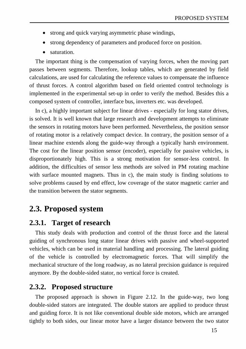
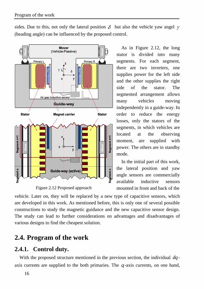
The proposed approach is shown in Figure 2.12. In the guide-way, two long
double-sided stators are integrated. The double stators are applied to produce thrust
and guiding force. It is not like conventional double side motors, which are arranged
tightly to both sides, our linear motor have a larger distance between the two stator
Program of the work
16
sides. Due to this, not only the lateral position but also the vehicle yaw angel
(heading angle) can be influenced by the proposed control.
Figure 2.12 Proposed approach
As in Figure 2.12, the long
stator is divided into many
segments. For each segment,
there are two inverters, one
supplies power for the left side
and the other supplies the right
side of the stator. The
segmented arrangement allows
many vehicles moving
independently in a guide-way. In
order to reduce the energy
losses, only the stators of the
segments, in which vehicles are
located at the observing
moment, are supplied with
power. The others are in standby
mode.
In the initial part of this work,
the lateral position and yaw
angle sensors are commercially
available inductive sensors
mounted in front and back of the
vehicle. Later on, they will be replaced by a new type of capacitive sensors, which
are developed in this work. As mentioned before, this is only one of several possible
constructions to study the magnetic guidance and the new capacitive sensor design.
The study can lead to further considerations on advantages and disadvantages of
various designs to find the cheapest solution.
2.4. Program of the work
2.4.1. Control duty.
With the proposed structure mentioned in the previous section, the individual dq -
axis currents are supplied to the both primaries. The q -axis currents, on one hand,
PROPOSED SYSTEM
17
produce the thrust following the guide-way direction ( x -direction). On the other
hand, they control the yaw angel of the vehicle by controlling the difference of both
feeding thrusts around zero. That control can keep the vehicle parallel to the guide-
way axis. With d -axis currents, the normal forces are produced to keep the center of
vehicle coincide with guide-way center (middle of the stators - e.g. lateral position
0).
Altogether, there are three coupled control duties to realize
x -position,
lateral control 0 and
yaw control 0 .
During the movement of the vehicle from one feeding segment to the next, it
covers two-stator segments simultaneously, where the coverage of the vehicle’s
magnets at the old segment decreases and the coverage at the new segment increases.
At that time both segments are supplied, that means controls for both segments (i.e.
four stators, eight current components) must be coordinated together, such that the
three control duties are produced co-ordinately 1. x -position, 2. Lateral control
( 0), 3. Yaw control ( 0). These three control duties have to be fulfilled not
only in one stator segment but also during the transition between two stator segments.
2.4.2. Lateral position sensor and yaw angle sensor.
In the above outline, to implement control duties, beside the available actuators
(inverters + stators) the actual value of controlled qualities i.e. x , , are required.
In this thesis, a basic sensor system was developed and investigated.
One difficult condition of the sensor is the demand that neither information nor
auxiliary power is transferred between vehicle and stationary environment (passive
vehicle). To fulfil the duty, only sensors for lateral- and yaw- control are tested and
examined. For the x -position sensor, one of the methods studied in [52][53] can be
applied.
To get the lateral position and yaw angle , we can use many different sensor
principles, particularly inductive or capacitive. In this thesis, a new capacitive sensor
will be introduced later on. Furthermore, other principles (not in this thesis) are
possible i.e. inductive sensor method, sensor-less method. The best solution may be
found when the advantages and disadvantages of different sensors are compared
together.

Program of the work
18
2.4.3. Work steps
With the duties mentioned above, the study program was arranged in following
steps:
Linear motor prototype assembly: Stator selection, Inverter components,
Position sensor for x -direction, Mechanical design and construction.
Control parameters calculation.
Development of the control method: Implementation and test.
Design of the new capacitive sensor for lateral position and yaw angle
control.
Documentation.
EXPERIMENTAL SETUP
19
3. EXPERIMENTAL SETUP To implement the experimental setup as proposed in chapter 2, a combination of
the available equipment in the market and self-developed products of the institute
was implemented. In this chapter, the experimental setup system is introduced in
three main parts: Mechanical structure, Electrical system and Control system.
3.1. Mechanical structure
3.1.1. The motors
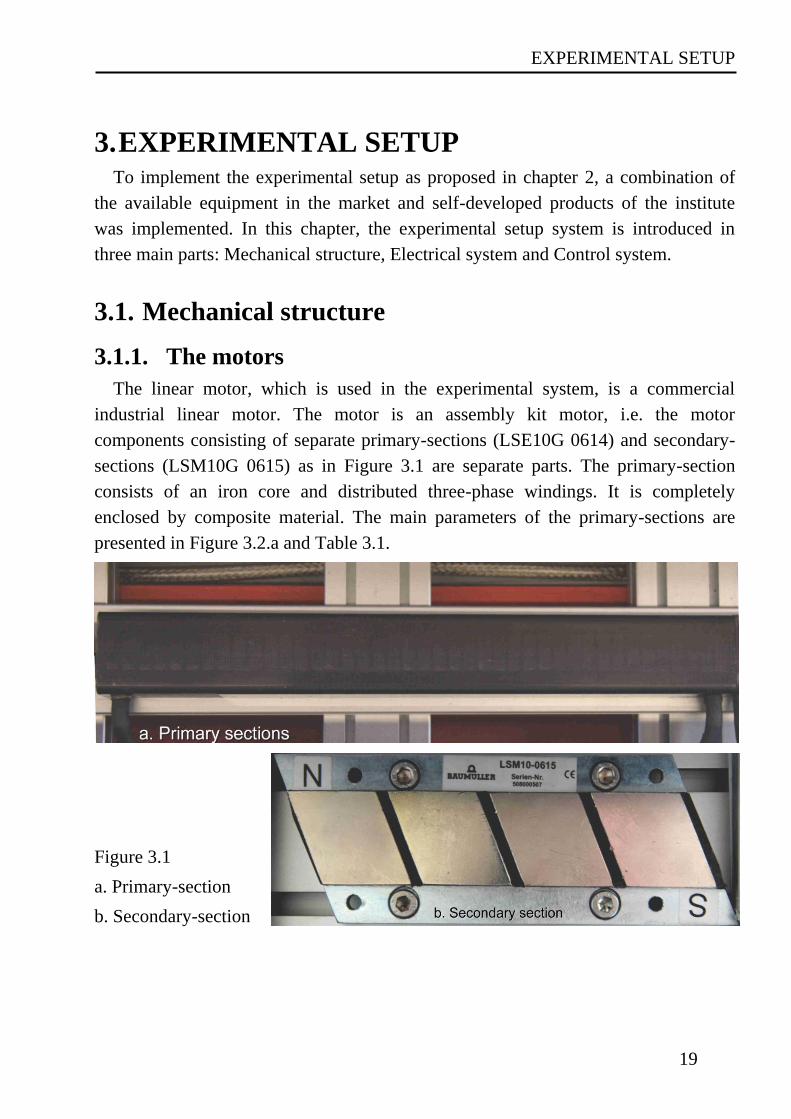
The linear motor, which is used in the experimental system, is a commercial
industrial linear motor. The motor is an assembly kit motor, i.e. the motor
components consisting of separate primary-sections (LSE10G 0614) and secondary-
sections (LSM10G 0615) as in Figure 3.1 are separate parts. The primary-section
consists of an iron core and distributed three-phase windings. It is completely
enclosed by composite material. The main parameters of the primary-sections are
presented in Figure 3.2.a and Table 3.1.
Figure 3.1
a. Primary-section
b. Secondary-section
Mechanical structure
20
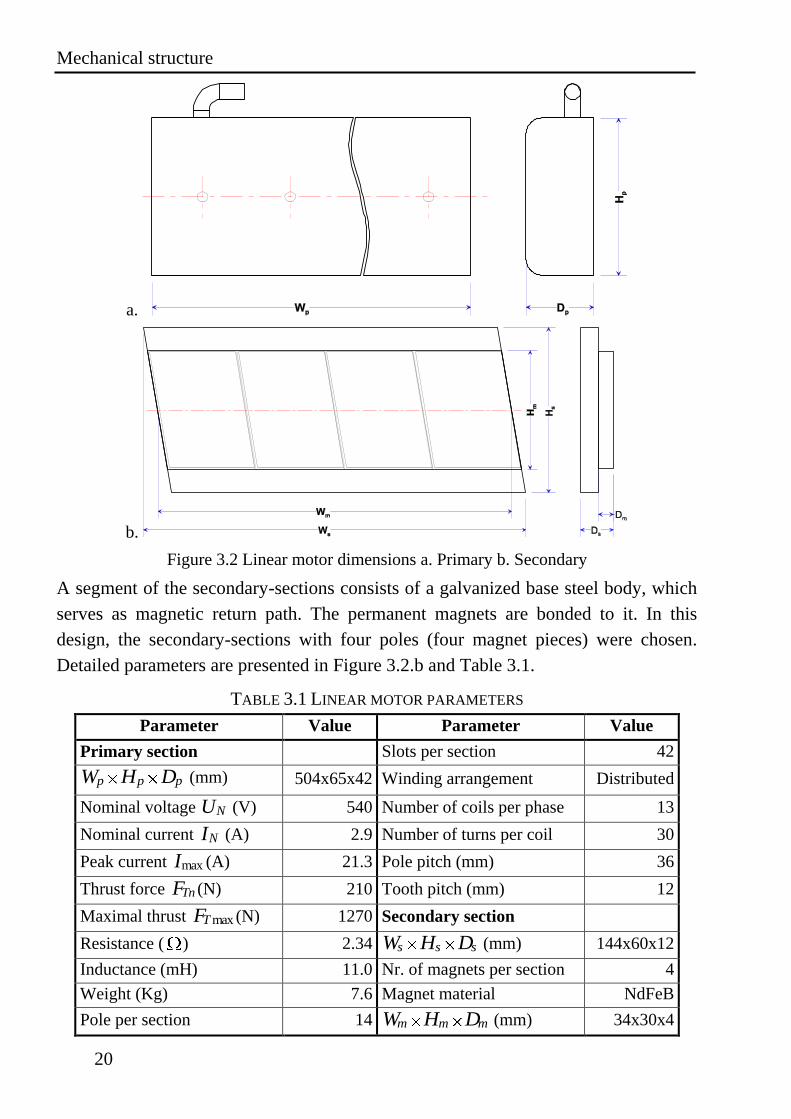
Figure 3.2 Linear motor dimensions a. Primary b. Secondary
A segment of the secondary-sections consists of a galvanized base steel body, which
serves as magnetic return path. The permanent magnets are bonded to it. In this
design, the secondary-sections with four poles (four magnet pieces) were chosen.
Detailed parameters are presented in Figure 3.2.b and Table 3.1.
TABLE 3.1 LINEAR MOTOR PARAMETERS
Parameter Value Parameter Value
Primary section Slots per section 42
p p pW H D (mm) 504x65x42 Winding arrangement Distributed
Nominal voltage NU (V) 540 Number of coils per phase 13
Nominal current NI (A) 2.9 Number of turns per coil 30
Peak current maxI (A) 21.3 Pole pitch (mm) 36
Thrust force TnF (N) 210 Tooth pitch (mm) 12
Maximal thrust maxTF (N) 1270 Secondary section
Resistance ( ) 2.34 s s sW H D (mm) 144x60x12
Inductance (mH) 11.0 Nr. of magnets per section 4
Weight (Kg) 7.6 Magnet material NdFeB
Pole per section 14 m m mW H D (mm) 34x30x4
a.
b.
EXPERIMENTAL SETUP
21
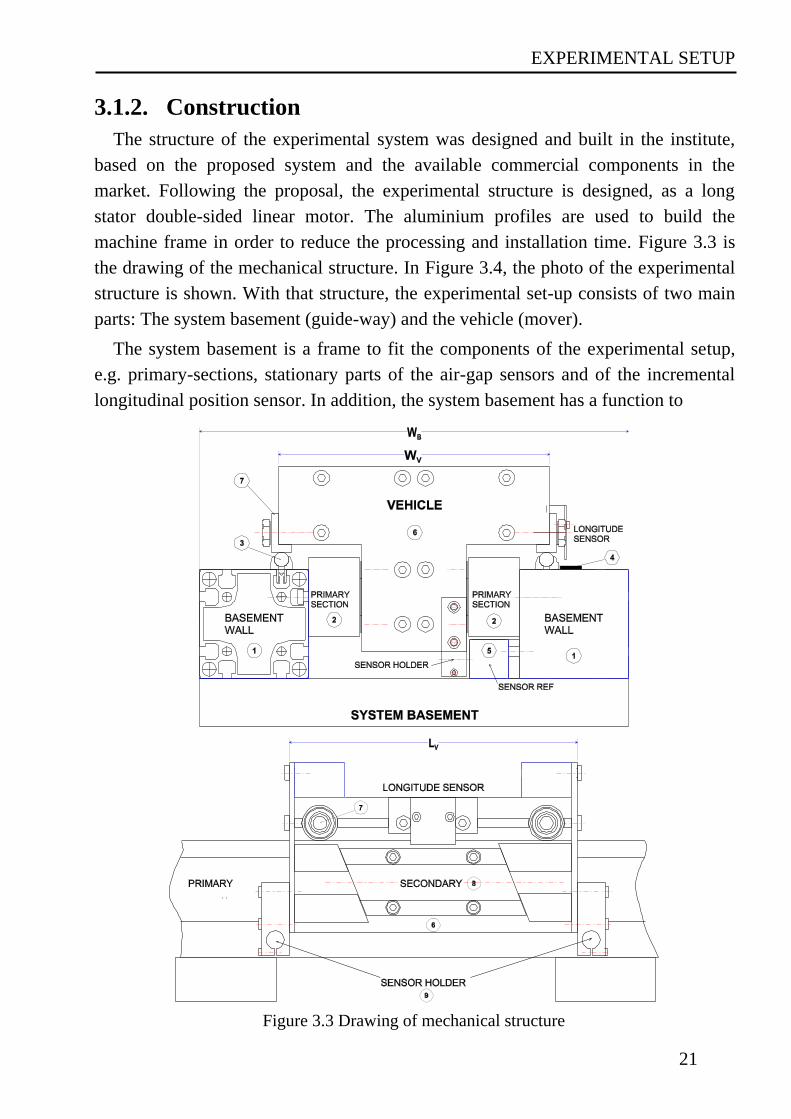
3.1.2. Construction
The structure of the experimental system was designed and built in the institute,
based on the proposed system and the available commercial components in the
market. Following the proposal, the experimental structure is designed, as a long
stator double-sided linear motor. The aluminium profiles are used to build the
machine frame in order to reduce the processing and installation time. Figure 3.3 is
the drawing of the mechanical structure. In Figure 3.4, the photo of the experimental
structure is shown. With that structure, the experimental set-up consists of two main
parts: The system basement (guide-way) and the vehicle (mover).
The system basement is a frame to fit the components of the experimental setup,
e.g. primary-sections, stationary parts of the air-gap sensors and of the incremental
longitudinal position sensor. In addition, the system basement has a function to
Figure 3.3 Drawing of mechanical structure
Mechanical structure
22
constrain the vehicle in the vertical movement. The system basement was built with
two parallel aluminium walls along the guide-way of the vehicle. On each wall
side, the primary sections were fastened consecutively to make a line. Each pair of
primary sections, in opposite, composes a primary segment. The experimental setup
here was constructed with two primary segments. On the top of the aluminium walls,
two round iron rods were attached to make a running way for the vehicle. A
magnetic incremental tape was pasted on the top of the left wall to give the
measuring reference for the longitudinal position sensor. Under the left primary
sections, a small aluminium wall was installed in order to give a reference for
inductive air-gap sensors.
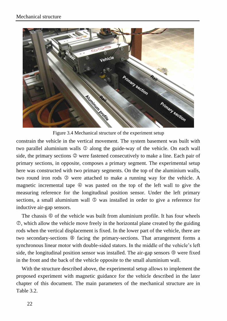
The chassis of the vehicle was built from aluminium profile. It has four wheels
, which allow the vehicle move freely in the horizontal plane created by the guiding
rods when the vertical displacement is fixed. In the lower part of the vehicle, there are
two secondary-sections facing the primary-sections. That arrangement forms a
synchronous linear motor with double-sided stators. In the middle of the vehicle’s left
side, the longitudinal position sensor was installed. The air-gap sensors were fixed
in the front and the back of the vehicle opposite to the small aluminium wall.
With the structure described above, the experimental setup allows to implement the
proposed experiment with magnetic guidance for the vehicle described in the later
chapter of this document. The main parameters of the mechanical structure are in
Table 3.2.
Figure 3.4 Mechanical structure of the experiment setup
EXPERIMENTAL SETUP
23
TABLE 3.2 MAIN PARAMETERS OF MECHANICAL STRUCTURE.
Parameters Value Parameters Value
System basement Length VL (mm) 238
Width BW (mm) 354 Weight Vm (kg) 6.5
Length BL (mm) 1764 Wheels distances (mm) 183x219
Height BH (mm) 194.5 Lateral sensor distance (mm) 263
Nr. of primaries per side 2 Nominal air-gap (mm) 1.5
Vehicle Max air-gap (mm) 2.4
Width VW (mm) 224 Max longitudinal position (mm) 1008
Height VH (mm) 152.5
3.2. Electrical structure
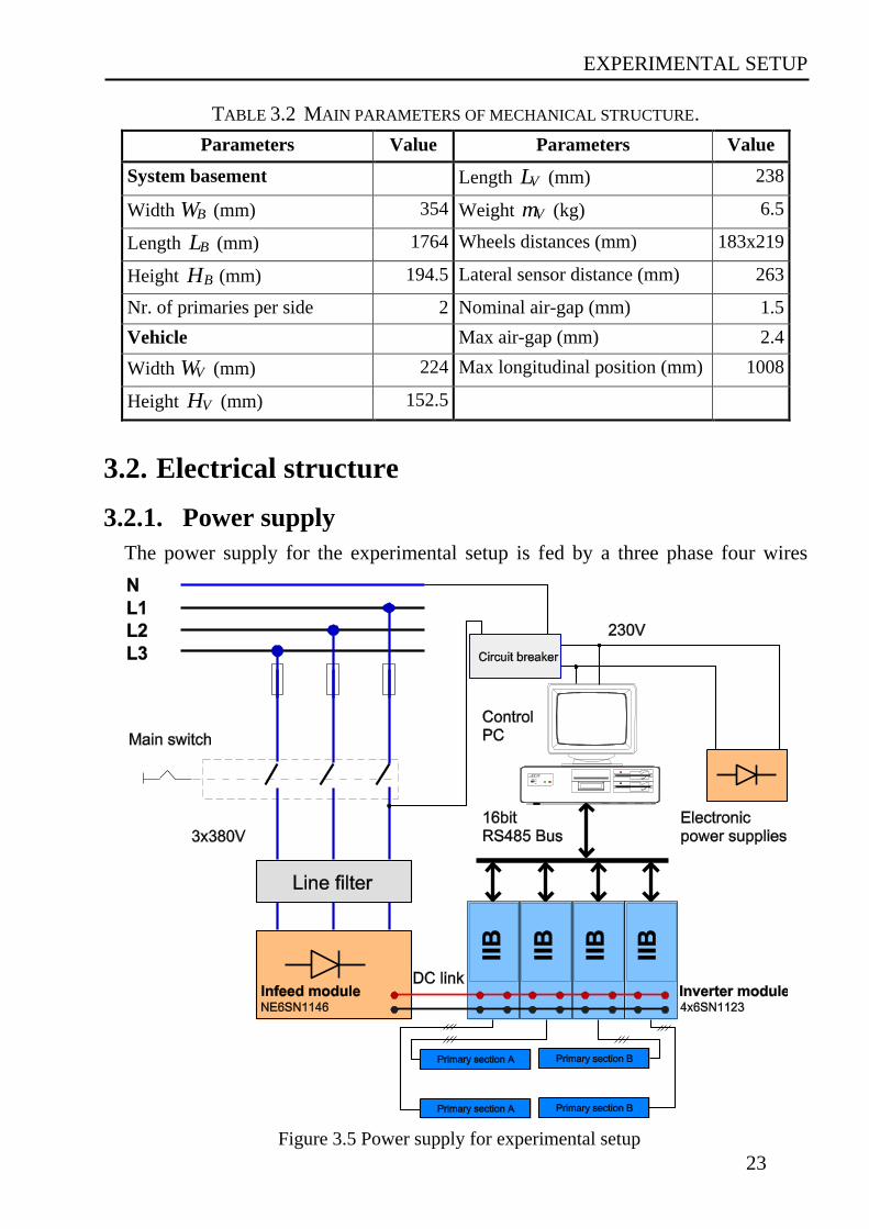
3.2.1. Power supply
The power supply for the experimental setup is fed by a three phase four wires
Figure 3.5 Power supply for experimental setup
Electrical structure
24
(with neutral) power in the laboratory. It has the duty to supply power to the inverter
system, controller system and electronic system as show in Figure 3.5.
First, the three-phase voltages are supplied through three fuses, which are used to
protect the completely experimental setup from over current. The three-phase
voltages are then fed to a three-phase main switch. After the main switch, the three-
phase voltages are connected to a three-phase line filter and then supplied to the
inverter system. Another part of the power supply, after the main switch, is to feed
the control system and electronic power suppliers (DC adapters). The voltage
between phase L1 and the neutral is supplied to one phase line filter. Output voltage
of the filter is used by the controller system and the electronic power suppliers.
3.2.2. Inverter modules
Most of the power for the experimental setup is supplied to the inverter system.
The inverter system then generates suitable output voltages to feed the linear motor.
Normally, it supplies two primary-sections. When the vehicle crosses the junction
point of two segments, it feeds four primary-sections simultaneously.
As described in subsection 3.2.1, the inverter system has a main function to feed
the four primary-sections of the LSM. Further, the inverter system must have the
ability to communicate with the controller in order to form a closed control loop for
the proposed experiment.
In order to supply the four primary-sections, the inverter system has one rectifier
module (in-feed module) NE6SN1146 and four inverter-modules (power module)
6SN1123 from Siemens. The details of the modules are presented in [75].
The communication of the inverter module is executed by an electronic board. The
board is a self-developed interface board mounted in the inverter module. The
interface board also replace of the original commercial control unit in each inverter
module. Functions of the interface board are presented clearly in the next subsection.
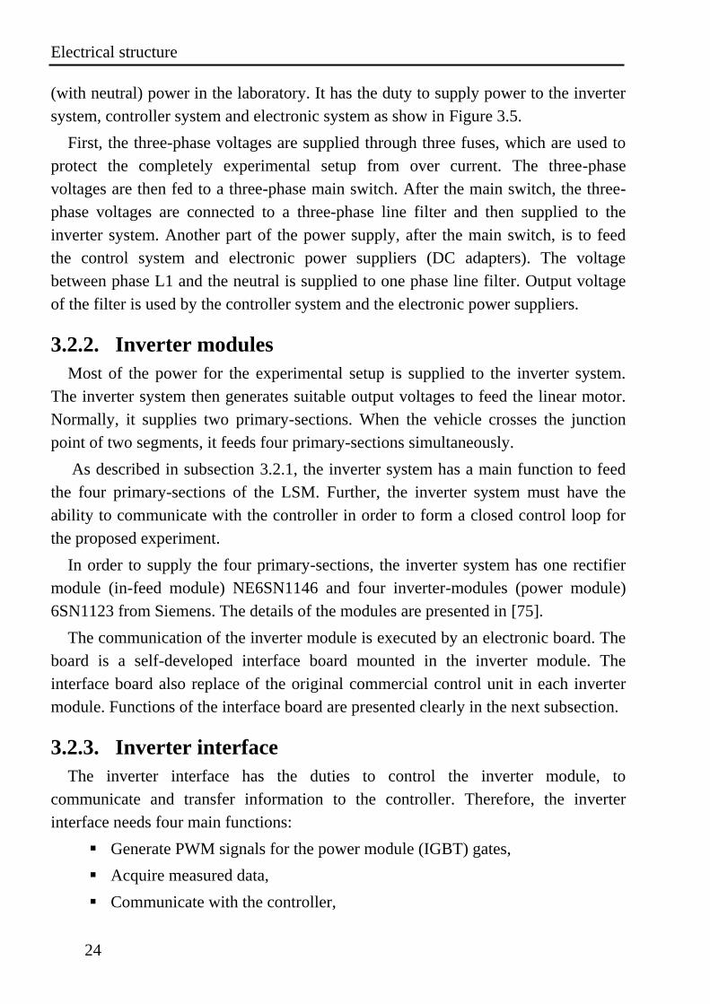
3.2.3. Inverter interface
The inverter interface has the duties to control the inverter module, to
communicate and transfer information to the controller. Therefore, the inverter
interface needs four main functions:
Generate PWM signals for the power module (IGBT) gates,
Acquire measured data,
Communicate with the controller,
EXPERIMENTAL SETUP
25
Protect the inverter (over current, over temperature etc.).
Because of experimental requirements, all the calculations and the regulation tasks
are done by a central controller (a PC) instead of microprocessors for each inverter
module. That requirement could not be satisfied by any commercial inverter control
unit. Therefore, in the experimental setup, each inverter module has one inverter
interface board (IIB), which was developed by colleges in our institute [13][54].
Replacing the control unit in the inverter module, the IIB has a function to generate
PWM signals. The PWM signals are generated by using the time values received
from the controller. The signals are used to drive six IGBTs of the inverter module.
In the IIB, there are three AD channels in order to acquire the measured data. The
data include two phase-current values and a position value. They are acquired and
sent to the controller via the communication bus.
As mentioned in the two previous functions, the IIB has to receive the timing
values from the controller and send the acquired data to the controller. That requires
the IIB needs to be able to communicate with the controller. Therefore, a
communication module is implemented in the IIB. The module communicates with
the controller by a 16-bit parallel bus. Each bit of the bus is transferred by one pair of
wires using RS485 transceivers.
The main protected functions of the IIB are the over current and the over
temperature. They protect the system from serious damages. In addition, the IIB gives
also some other protections i.e. the communication is broken; one of requirement
signals from the rectifier module is missed.
The photo of the IIB is shown in Figure 3.6, and the details are described in
appendix A1.
Figure 3.6 Photo of an Inverter interface board (IIB)
Electrical structure
26
3.2.4. Sensor system
The information required for the system to execute the control is
Information about vehicle’s position,
Information about electric currents.
To control the vehicle’s motion (guidance) in the plane, which is generated by the
guide-way, the information about vehicle positions needs to be evaluated. In the
proposed system, they are the positions in x direction (longitudinal position), in y
direction (lateral position) and the yaw angle.
In the first part of the experiments, the lateral position and the yaw angle are
measured by two inductive air-gap sensors. These air-gap sensors are eddy current
displacement sensors from LION precision with ECA100 amplifier and U18 probe,
shown in Figure 3.8a. The sensors have 0-10V nonlinear outputs and 100 kHz
bandwidth. The U18 probe can measure in a range from 0.75 mm to 5.0mm with a
resolution 0.02% i.e. precision 0.85 m .
The two air-gap sensors are arranged in front and rear of the vehicle. They measure
the distances to the aluminium reference wall mentioned in subsection 3.1.2 and
generate output voltages which are nonlinea function of the distances. The voltages
result in nonlinear values in the control programme by AD converters. The nonlinear
values are then linearized by a lookup table, which is generated by calibrating the
sensors with practical measurements. The calibration is performed with precision
feeler gauges. Blades of the gauges are inserted in between the vehicle and the
primary. That gives high-precision references for the air-gap between the vehicle and
the primary. At each reference position, output values of the air-gap sensors are
captured. The position references values and the captured values are the calibration
data of the sensors. The calibration data are then interpolated in Matlab in order to
generate the lookup table. The two air-gap sensors with the look-up table can give the
linearized values of the vehicle front and rear air-gaps. The mean values of the front
and rear air-gaps are used as the reference for calculating the vehicle lateral positions.
The different values of the front and rear air-gaps are used as the reference for
calculating vehicle yaw angles. In chapter 7, these sensors will be replaced by a
capacitive sensor in order to implement a total passive vehicle.
The longitudinal position is measured with a magnet incremental sensor ELS29-
200I-SST03-01 from Sensitec, shown in Figure 3.8.b. The sensor contains an
anisotropic magneto-resistive (AMR) length sensor and a 13-bit interpolation-IC. In
use with a magnetic linear measurement scale with 1 mm pitch, the electronic

EXPERIMENTAL SETUP
27
delivers two 90-degree phase shifted rectangular signals A and B. The resolution can
be configured up to 8192 increments per pole through the configuration interface of
the processing unit. In a typical application like the experimental setup, the resolution
is set to 200 increments per pole i.e. the sensor´s resolution is 5 m . The sensor
provides the longitudinal position for the vehicle position control and reference
information for the field oriented control (FOC) method. In addition, the time
derivative of the vehicle position is used as the feedback value for the speed control
loop.
The three phase supply currents in the output of one inverter module are measured
by current sensors. The current sensors used in the experimental setup are current
transducers LAH 25-NP from LEM, shown in Figure 3.8.c. The sensor has 25A
primary nominal current and 25mA secondary nominal current with the accuracy
0.3% of the full scale. In the experiment, only two of three phase currents of each
inverter module are measured. The two output signals from current sensors are fed to
two analogue channels of the IIB. They are amplified, converted to digital values and
are sent to the controller of the system. In the controller, the third current of the three
phase currents is calculated from the two other current values.
Figure 3.7 Sensors used in the set-up
3.2.5. Controller
The controller of the experimental system has the duty to acquire feedback signals
from the plant and send the control signals according to control algorithms to the
inverter interface board. To simplify the system configuration, the system parameter
setting, the control algorithm, the data acquisition etc., a personal computer (PC) is
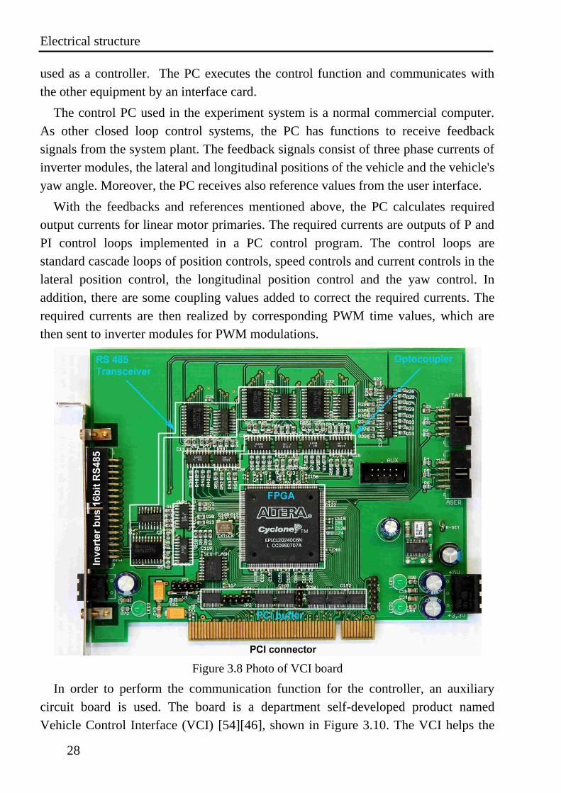
Electrical structure
28
used as a controller. The PC executes the control function and communicates with
the other equipment by an interface card.
The control PC used in the experiment system is a normal commercial computer.
As other closed loop control systems, the PC has functions to receive feedback
signals from the system plant. The feedback signals consist of three phase currents of
inverter modules, the lateral and longitudinal positions of the vehicle and the vehicle's
yaw angle. Moreover, the PC receives also reference values from the user interface.
With the feedbacks and references mentioned above, the PC calculates required
output currents for linear motor primaries. The required currents are outputs of P and
PI control loops implemented in a PC control program. The control loops are
standard cascade loops of position controls, speed controls and current controls in the
lateral position control, the longitudinal position control and the yaw control. In
addition, there are some coupling values added to correct the required currents. The
required currents are then realized by corresponding PWM time values, which are
then sent to inverter modules for PWM modulations.
Figure 3.8 Photo of VCI board
In order to perform the communication function for the controller, an auxiliary
circuit board is used. The board is a department self-developed product named
Vehicle Control Interface (VCI) [54][46], shown in Figure 3.10. The VCI helps the
EXPERIMENTAL SETUP
29
control PC to transmit and receive information from the IIBs. In addition, it acquires
longitudinal position directly from the position sensors. In a control process, the VCI
transfers data to each IIB in every 100 s . The transfer protocol has a time slot of
10 s , so in 100 s the VCI can transfer data to maximum 10 IIBs.
3.3. Software
3.3.1. Operating System
Based on the basic requirements of the experimental setup, Linux operating system
has many advantages in comparison with the others. Therefore, Linux was chosen as
the operating system for the experimental control PC. The Linux operating system,
which is used in the system, is a Vector-Linux Soho distribution using the Kernel
2.6.18.
First, the experimental operating system in this setup must have the ability to
support basic software functions. For this requirement, Linux can support:
Documentary read-write software with Open office, KDE (PDF file
reading),
Analysis Software (Matlab, Scilab),
Programming Software (C, C++ with GNU compiler, Interface with GTK+,
GTKmm, CLX…)
These are all the basic requirements of a control PC for the experimental-
execution, documentation and analysis.
Another important characteristic of the control system is the stability and the real-
time control. In this aspect, Linux has many advantages in comparison with other
operating systems. Because Linux is open-source software, Linux has fewer system
crash problems as the others do. On the other hand, Linux has less attack from virus
and malware because of its character and number of Linux user. Therefore, Linux is
stable operating software. To be open-source software, Linux allows the users
interfere with its kernel. Hence, it is easy to implement the real time control
applications in Linux by adding a real time extension module to Linux kernel. There
are some different approaches to transform Linux into a real-time operating system.
In this thesis, the Real-Time Application Interface (RTAI) was used as the solution
for the Linux real-time operating system.
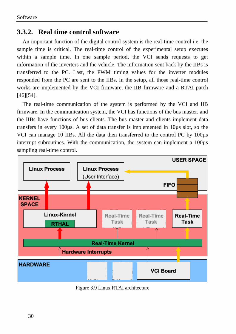
Software
30
3.3.2. Real time control software
An important function of the digital control system is the real-time control i.e. the
sample time is critical. The real-time control of the experimental setup executes
within a sample time. In one sample period, the VCI sends requests to get
information of the inverters and the vehicle. The information sent back by the IIBs is
transferred to the PC. Last, the PWM timing values for the inverter modules
responded from the PC are sent to the IIBs. In the setup, all those real-time control
works are implemented by the VCI firmware, the IIB firmware and a RTAI patch
[46][54].
The real-time communication of the system is performed by the VCI and IIB
firmware. In the communication system, the VCI has functions of the bus master, and
the IIBs have functions of bus clients. The bus master and clients implement data
transfers in every 100µs. A set of data transfer is implemented in 10µs slot, so the
VCI can manage 10 IIBs. All the data then transferred to the control PC by 100µs
interrupt subroutines. With the communication, the system can implement a 100µs
sampling real-time control.
Figure 3.9 Linux RTAI architecture
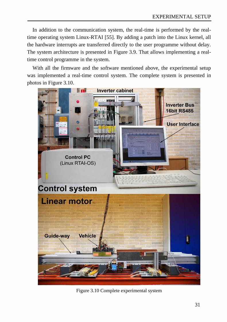
EXPERIMENTAL SETUP
31
In addition to the communication system, the real-time is performed by the real-
time operating system Linux-RTAI [55]. By adding a patch into the Linux kernel, all
the hardware interrupts are transferred directly to the user programme without delay.
The system architecture is presented in Figure 3.9. That allows implementing a real-
time control programme in the system.
With all the firmware and the software mentioned above, the experimental setup
was implemented a real-time control system. The complete system is presented in
photos in Figure 3.10.
Figure 3.10 Complete experimental system
The magnetic guidance LSM model
32
4. MATHEMATICAL MODEL The mathematical model is the basic requirement for the analysis of the
experimental system, the simulation and the controller designs. In this chapter, the
geometrical and physical-characteristics of the experimental system are analyzed and
presented in equations. The results are then compared with the Finite Element
Method (FEM) simulation results and experimental measurements.
4.1. The magnetic guidance LSM model
4.1.1. The experimental system in the horizontal plane
As in the experimental structure presented in chapter 3, the vehicle can freely
move on the horizontal plane formed by the guiding rails while the vertical
movement is constrained. With that structure, the setup can be simply presented in
the horizontal plane by a geometrical figure as presented in Figure 4.1. In that figure,
the main parameters of the experimental setup and also forces and torques acting on
the vehicle are presented.
The figure describes the vehicle simply as a light blue rectangle. The sections of
the secondary (magnet) are depicted by black lines on both sides. The two parallel red
lines represent the primary sections. All geometrical parameters of the experimental
system required for the model analysis and calculation are presented in corresponding
symbols. The orange rectangle shows the desired position of the vehicle in the control
process. At that position, the vehicle is in the middle and parallel with the guide-way
i.e. the left-side air-gap ( LLd ) and the right-side air-gap ( LRd ) are equal, or the
vehicle’s centerline coincides with the guide-way centerline.
In order to determine the vehicle’s position, a coordinate system 0x y is used, as
shown in the Figure 4.1. The origin of the coordinate system is placed on the
centerline of the guide-way. The vertical axis (0x ) is parallel to the guide-way, and
the horizontal axis (0y ) is perpendicular to the guide-way. The vehicle’s center
position is referred to this coordinate system. The center position of the vehicle
referred to 0y axis is called lateral position ( ). The center position referred to 0x
axis is called longitudinal position ( x ). The angle between the vehicle’s centerline
and the guide-way’s centerline is called yaw angle ( ). The aim of the control
process is to control the lateral position and the yaw angle to zero ( 0, 0) and
to change the longitudinal position x according to control requirements.
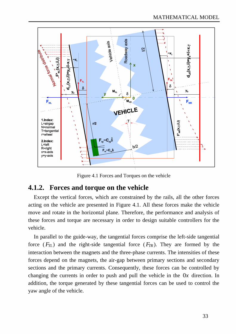
MATHEMATICAL MODEL
33
Figure 4.1 Forces and Torques on the vehicle
4.1.2. Forces and torque on the vehicle
Except the vertical forces, which are constrained by the rails, all the other forces
acting on the vehicle are presented in Figure 4.1. All these forces make the vehicle
move and rotate in the horizontal plane. Therefore, the performance and analysis of
these forces and torque are necessary in order to design suitable controllers for the
vehicle.
In parallel to the guide-way, the tangential forces comprise the left-side tangential
force ( TLF ) and the right-side tangential force ( TRF ). They are formed by the
interaction between the magnets and the three-phase currents. The intensities of these
forces depend on the magnets, the air-gap between primary sections and secondary
sections and the primary currents. Consequently, these forces can be controlled by
changing the currents in order to push and pull the vehicle in the 0x direction. In
addition, the torque generated by these tangential forces can be used to control the
yaw angle of the vehicle.
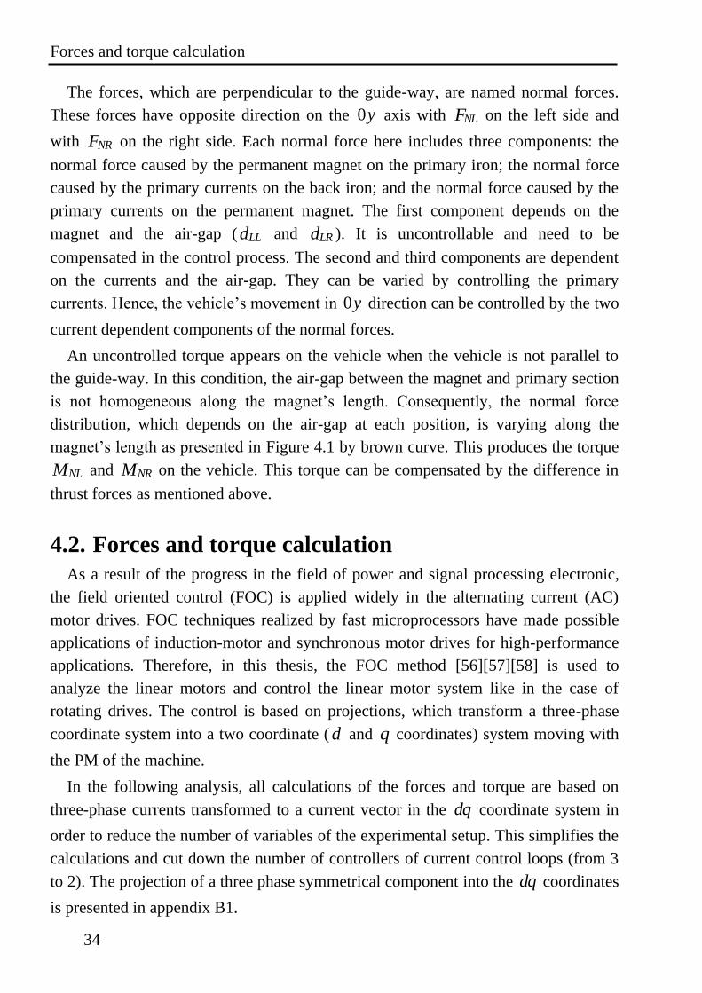
Forces and torque calculation
34
The forces, which are perpendicular to the guide-way, are named normal forces.
These forces have opposite direction on the 0y axis with NLF on the left side and
with NRF on the right side. Each normal force here includes three components: the
normal force caused by the permanent magnet on the primary iron; the normal force
caused by the primary currents on the back iron; and the normal force caused by the
primary currents on the permanent magnet. The first component depends on the
magnet and the air-gap ( LLd and LRd ). It is uncontrollable and need to be
compensated in the control process. The second and third components are dependent
on the currents and the air-gap. They can be varied by controlling the primary
currents. Hence, the vehicle’s movement in 0y direction can be controlled by the two
current dependent components of the normal forces.
An uncontrolled torque appears on the vehicle when the vehicle is not parallel to
the guide-way. In this condition, the air-gap between the magnet and primary section
is not homogeneous along the magnet’s length. Consequently, the normal force
distribution, which depends on the air-gap at each position, is varying along the
magnet’s length as presented in Figure 4.1 by brown curve. This produces the torque
NLM and NRM on the vehicle. This torque can be compensated by the difference in
thrust forces as mentioned above.
4.2. Forces and torque calculation
As a result of the progress in the field of power and signal processing electronic,
the field oriented control (FOC) is applied widely in the alternating current (AC)
motor drives. FOC techniques realized by fast microprocessors have made possible
applications of induction-motor and synchronous motor drives for high-performance
applications. Therefore, in this thesis, the FOC method [56][57][58] is used to
analyze the linear motors and control the linear motor system like in the case of
rotating drives. The control is based on projections, which transform a three-phase
coordinate system into a two coordinate ( d and q coordinates) system moving with
the PM of the machine.
In the following analysis, all calculations of the forces and torque are based on
three-phase currents transformed to a current vector in the dq coordinate system in
order to reduce the number of variables of the experimental setup. This simplifies the
calculations and cut down the number of controllers of current control loops (from 3
to 2). The projection of a three phase symmetrical component into the dq coordinates
is presented in appendix B1.
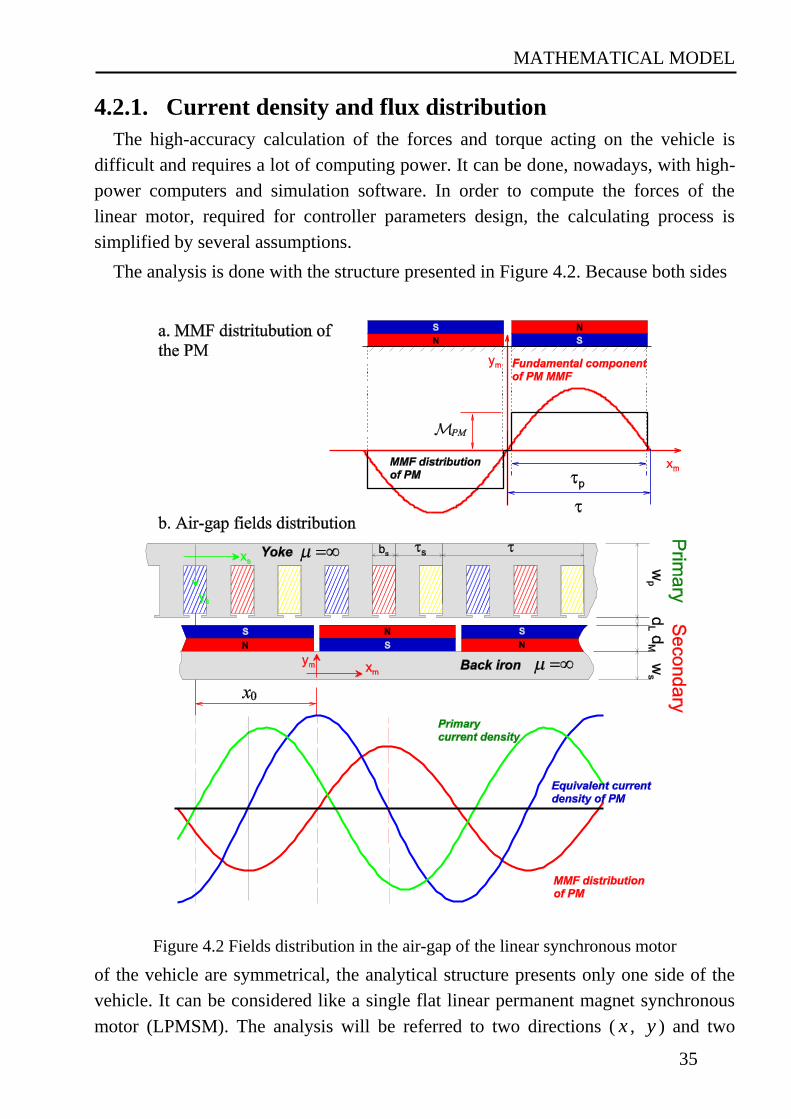
MATHEMATICAL MODEL
35
4.2.1. Current density and flux distribution
The high-accuracy calculation of the forces and torque acting on the vehicle is
difficult and requires a lot of computing power. It can be done, nowadays, with high-
power computers and simulation software. In order to compute the forces of the
linear motor, required for controller parameters design, the calculating process is
simplified by several assumptions.
The analysis is done with the structure presented in Figure 4.2. Because both sides
Figure 4.2 Fields distribution in the air-gap of the linear synchronous motor
of the vehicle are symmetrical, the analytical structure presents only one side of the
vehicle. It can be considered like a single flat linear permanent magnet synchronous
motor (LPMSM). The analysis will be referred to two directions ( x , y ) and two
Forces and torque calculation
36
coordinate axes ( 0m mx y , 0s sx y ). The coordinate 0s sx y is the static frame fixed to
the linear motor primary and the coordinate 0m mx y is the moving frame, fixed to the
permanent magnet of the linear motor.
First, the slotted structure of the LPMSM is simplified by assuming smooth
structure, i.e. the primary of the linear motor has isotropic magnetic properties.
Moreover, in order to simplify the magnetic circuit calculations, the primary iron and
the secondary back iron are assumed to have an infinite permeability ( r ).
Therefore, the primary permeability is infinite ( a ), i.e. the primary reluctance is
zero. The magnetic circuit is simplified in the area defined by L Md d , from the
primary surface to the secondary back iron surface as shown in Figure 4.2. In
addition, the regions containing magnets are considered isotropic, with
0 0PM M with 1M (4.1)
Second, the field distributions of the linear motor are assumed sinusoidal.
Therefore, in the analysis, only the fundamental components of current distributions
and magneto motive force (MMF) are considered. With the assumption that the
permanent magnet is a constant MMF source as presented in Figure 4.2.a and
appendix C2, the fundamental component of MMF distribution 1PM caused by the
PM is given by
14
( ) sin sin2
pPM m PM mx x (4.2)
where is the pole pitch,
p is the magnet width,
PM c Md is the equivalent MMF of the PM per pole,
c is coercive force.
The corresponding equivalent current distribution along the longitudinal permanent
magnet, x -axis, is given by
1
1
4( ) sin( )cos( )
2
pPMPM m PM m
m
dx x
dx (4.3)
Consequently, the remanent flux density of the magnet is also assumed to have
sinusoidal distribution. It is defined as follows.
4
( ) sinR m RN mx x (4.4)
where: RN is the actual remanent flux density of the magnets.
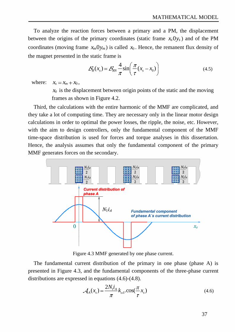
MATHEMATICAL MODEL
37
To analyze the reaction forces between a primary and a PM, the displacement
between the origins of the primary coordinates (static frame 0s sx y ) and of the PM
coordinates (moving frame 0m mx y ) is called 0x . Hence, the remanent flux density of
the magnet presented in the static frame is
0
4( ) sin ( )R s RN sx x x (4.5)
where: 0s mx x x ,
0x is the displacement between origin points of the static and the moving
frames as shown in Figure 4.2.
Third, the calculations with the entire harmonic of the MMF are complicated, and
they take a lot of computing time. They are necessary only in the linear motor design
calculations in order to optimal the power losses, the ripple, the noise, etc. However,
with the aim to design controllers, only the fundamental component of the MMF
time-space distribution is used for forces and torque analyses in this dissertation.
Hence, the analysis assumes that only the fundamental component of the primary
MMF generates forces on the secondary.
Figure 4.3 MMF generated by one phase current.
The fundamental current distribution of the primary in one phase (phase A) is
presented in Figure 4.3, and the fundamental components of the three-phase current
distributions are expressed in equations (4.6)-(4.8).
11 1
2( ) .cos( )A
A s s
N ix k x (4.6)
Forces and torque calculation
38
11 1
2 2( ) .cos( )
3B
B s s
N ix k x (4.7)
11 1
2 4( ) .cos( )
3C
C s s
N ix k x (4.8)
where Ai , Bi , Ci : are instantaneous values of the primary currents,
1N : is the number of series turns per primary slot,
1k : is the winding factor at fundamental wave,
: is the pole pitch.
In general, the three-phase currents are arbitrary. However, in this thesis, the three
phase currents are modulated by the field oriented control (FOC) method i.e. the three
phase currents are transformed from a dq current vector without zero component by
inverse Park´s transformation as it is presented in appendix B2. The fundamental
component of the primary current distribution is the algebraic sum of the three-phase
current distributions, as presented in (4.9).
1 1 1 1
11
11
11
( ) ( ) ( ) ( )
2.cos( ). .cos( )
2 2 2.cos( ). .cos( )
3 3
2 4 4.cos( ). .cos( )
3 3
a s A s B s C s
as s
as s
as s
x x x x
N ik x
N ik x
N ik x
(4.9)
where ai is the instantaneous value of the primary current vector,
s is the instantaneous phase of the primary currents in the static frame.
Reducing the right expression of the equation (4.9), a simple current distribution
equation is presented in (4.10).
1 11
1 1
2 1( ) . cos( ) cos( )
2
4cos( ) cos( )
3
8cos( ) cos( )
3
3cos( )
aa s s s s
s s s
s s s
as s
N i kx x x
x x
x x
N i kx
(4.10)
The fundamental component of primary current distribution can be rewritten in the
moving frame 0m mx y by
MATHEMATICAL MODEL
39
1 11
3( ) cos( )a
a m m m
N i kx x (4.11)
where: 0m s x is phase of the current distribution in the moving frame.
In order to calculate the fundamental component of the MMF, the primary core is
assumed non-saturating. Therefore, the MMFs generated by the fundamental current
density are sinusoidal, and the primary MMF has a relationship with the current
density as in equation (4.12).
11
( )( ) a s
a s
s
d xx
dx (4.12)
Consequently
1 11 1
3( ) sin( )a
a s a s s s
N i kx dx x C (4.13)
The integration constant C is determined the condition of Gauss’s law for
magnetism; the integral of the flux along the air-gap is zero. In the next subsection,
the MMF 1 ( )a sx will be used to calculate flux along the air-gap. Solving the
Gauss’s equation for the magnetism in the air-gap will give the value of C .
4.2.2. Magneto motive force and flux in the air-gap
In Figure 4.4 the simplified model of one side of the linear motor, based on the
current distribution (current coverage), is presented. In this figure, the current
coverage wave and the MMF wave along the x-axis are represented in red and
green color respectively. The secondary flux density wave R is represented in blue
color.
In this model, the two axes as mentioned above are used: the sx -axis in the primary
and the mx -axis in the secondary. The secondary displacement ( 0x ) defines the
distance between the origin of both axes:
0m sx x x (4.14)
(for the sx to mx axis transformation the angle of the secondary will be neglected)
Using the simplified model, the MMF and flux in the air-gap are defined and
calculated as following.
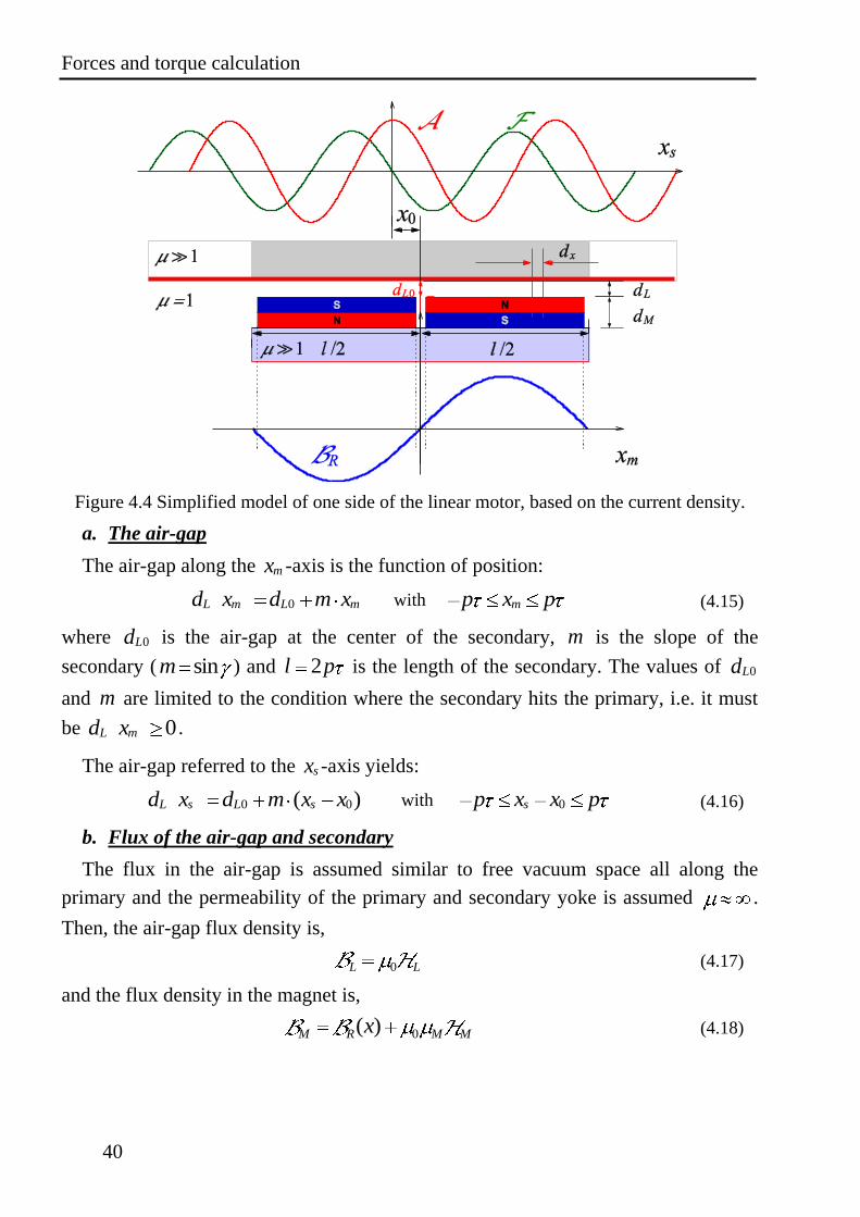
Forces and torque calculation
40
Figure 4.4 Simplified model of one side of the linear motor, based on the current density.
a. The air-gap
The air-gap along the mx -axis is the function of position:
0L m L md x d m x with mp x p (4.15)
where 0Ld is the air-gap at the center of the secondary, m is the slope of the
secondary ( sinm ) and 2l p is the length of the secondary. The values of 0Ld
and m are limited to the condition where the secondary hits the primary, i.e. it must
be 0L md x .
The air-gap referred to the sx -axis yields:
0 0( )L s L sd x d m x x with 0sp x x p (4.16)
b. Flux of the air-gap and secondary
The flux in the air-gap is assumed similar to free vacuum space all along the
primary and the permeability of the primary and secondary yoke is assumed .
Then, the air-gap flux density is,
0L L (4.17)
and the flux density in the magnet is,
0( )M R M Mx (4.18)
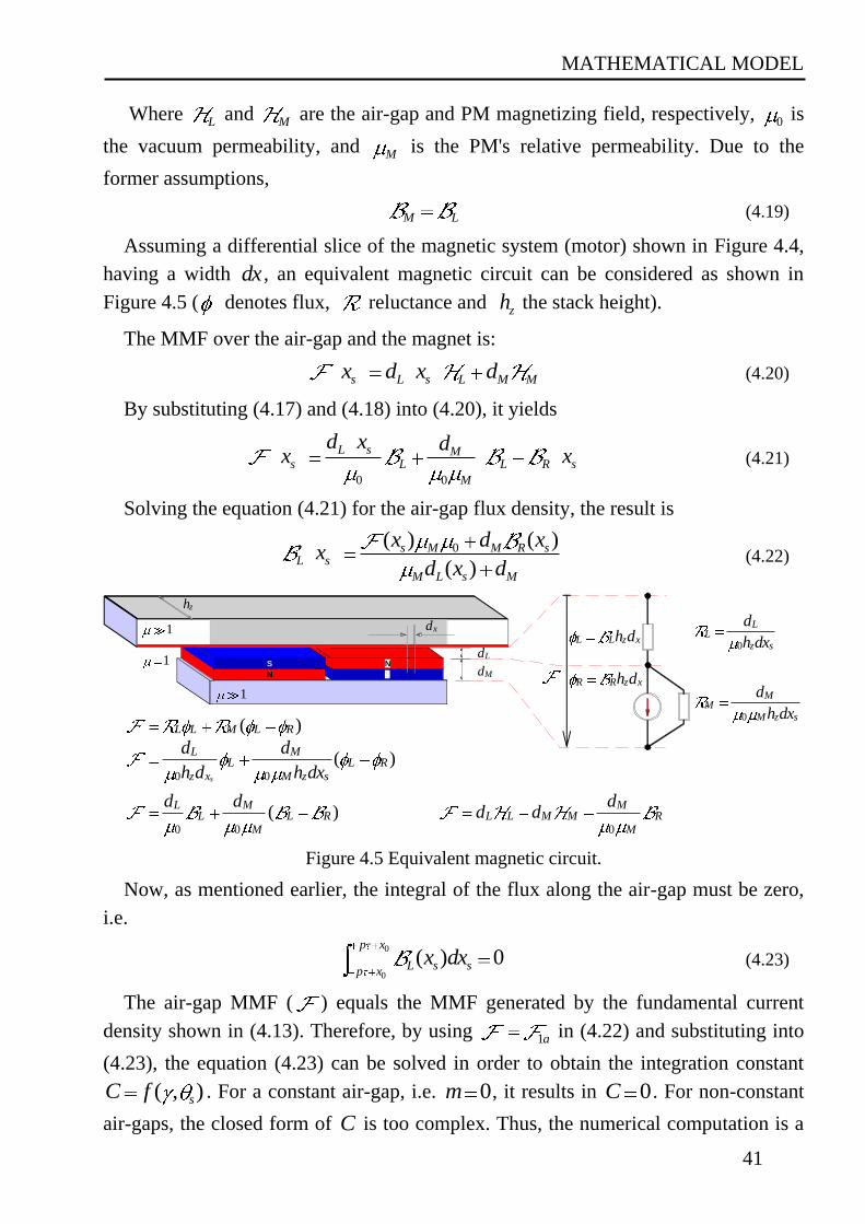
MATHEMATICAL MODEL
41
Where L and M are the air-gap and PM magnetizing field, respectively, 0 is
the vacuum permeability, and M is the PM's relative permeability. Due to the
former assumptions,
M L (4.19)
Assuming a differential slice of the magnetic system (motor) shown in Figure 4.4,
having a width dx , an equivalent magnetic circuit can be considered as shown in
Figure 4.5 ( denotes flux, reluctance and zh the stack height).
The MMF over the air-gap and the magnet is:
s L s L M Mx d x d (4.20)
By substituting (4.17) and (4.18) into (4.20), it yields
0 0
L s Ms L L R s
M
d x dx x (4.21)
Solving the equation (4.21) for the air-gap flux density, the result is
0( ) ( )
( )s M M R s
L s
M L s M
x d xx
d x d (4.22)
N
SLd
Md
1
1
1
N
S
xd
zh
0
LL
z s
d
h dx
0
MM
M z s
d
h dx
L L z xh d
R R z xh d
( )L L M L R
0 0
( )s
L ML L R
z x M z s
d d
h d h dx
0 0
( )L M
L L RM
d d
0
ML L M M R
M
dd d
Figure 4.5 Equivalent magnetic circuit.
Now, as mentioned earlier, the integral of the flux along the air-gap must be zero,
i.e.
0
0
( ) 0p x
L s sp x
x dx (4.23)
The air-gap MMF ( ) equals the MMF generated by the fundamental current
density shown in (4.13). Therefore, by using 1a in (4.22) and substituting into
(4.23), the equation (4.23) can be solved in order to obtain the integration constant
( , )sC f . For a constant air-gap, i.e. 0m , it results in 0C . For non-constant
air-gaps, the closed form of C is too complex. Thus, the numerical computation is a
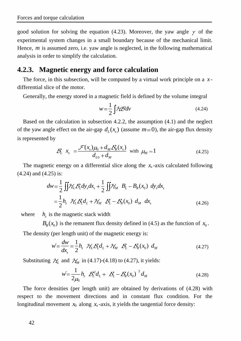
Forces and torque calculation
42
good solution for solving the equation (4.23). Moreover, the yaw angle of the
experimental system changes in a small boundary because of the mechanical limit.
Hence, m is assumed zero, i.e. yaw angle is neglected, in the following mathematical
analysis in order to simplify the calculation.
4.2.3. Magnetic energy and force calculation
The force, in this subsection, will be computed by a virtual work principle on a x -
differential slice of the motor.
Generally, the energy stored in a magnetic field is defined by the volume integral
1
2w dv (4.24)
Based on the calculation in subsection 4.2.2, the assumption (4.1) and the neglect
of the yaw angle effect on the air-gap ( )L sd x (assume 0m ), the air-gap flux density
is represented by
0
0
( ) ( )s M R sL s
L M
x d xx
d d with 1M (4.25)
The magnetic energy on a differential slice along the sx -axis calculated following
(4.24) and (4.25) is:
0
0
1 1( )
2 2
1( )
2
L L s s M L R s s
z L L L M L R M s
dw dy dx B B x dy dx
h d x d dx
(4.26)
where zh is the magnetic stack width
0( )RB x is the remanent flux density defined in (4.5) as the function of 0x .
The density (per length unit) of the magnetic energy is:
0
1´ ( )
2z L L L M L R M
s
dww h d x d
dx (4.27)
Substituting L and M in (4.17)-(4.18) to (4.27), it yields:
22
0
0
1´ ( )
2z L L L R Mw h d x d (4.28)
The force densities (per length unit) are obtained by derivations of (4.28) with
respect to the movement directions and in constant flux condition. For the
longitudinal movement 0x along sx -axis, it yields the tangential force density:
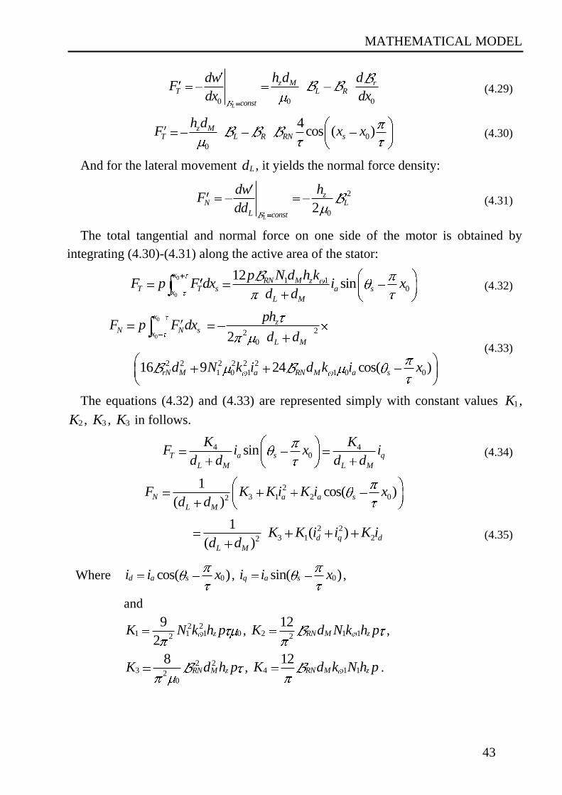
MATHEMATICAL MODEL
43
0 0 0L
z M rT L R
const
dw h d dF
dx dx (4.29)
0
0
4cos ( )z M
T L R RN s
h dF x x (4.30)
And for the lateral movement Ld , it yields the normal force density:
2
02L
zN L
L const
dw hF
dd (4.31)
The total tangential and normal force on one side of the motor is obtained by
integrating (4.30)-(4.31) along the active area of the stator:
0
0
1 10
12sin
xRN M z
T T s a sx
L M
p N d h kF p F dx i x
d d (4.32)
0
022
0
2 2 2 2 2 2
1 0 1 1 0 0
2
16 9 24 cos( )
xz
N N sx
L M
rN M a RN M a s
phF p F dx
d d
d N k i d k i x
(4.33)
The equations (4.32) and (4.33) are represented simply with constant values 1K ,
2K , 3K , 3K in follows.
4 40sinT a s q
L M L M
K KF i x i
d d d d (4.34)
2
3 1 2 02
1cos( )
( )N a a s
L M
F K K i K i xd d
2 2
3 1 22
1( )
( )d q d
L M
K K i i K id d
(4.35)
Where 0cos( )d a si i x , 0sin( )q a si i x ,
and
2 21 1 1 02
9
2zK N k h p , 2 1 12
12RN M zK d N k h p ,
2 23 2
0
8RN M zK d h p , 4 1 1
12RN M zK d k N h p .
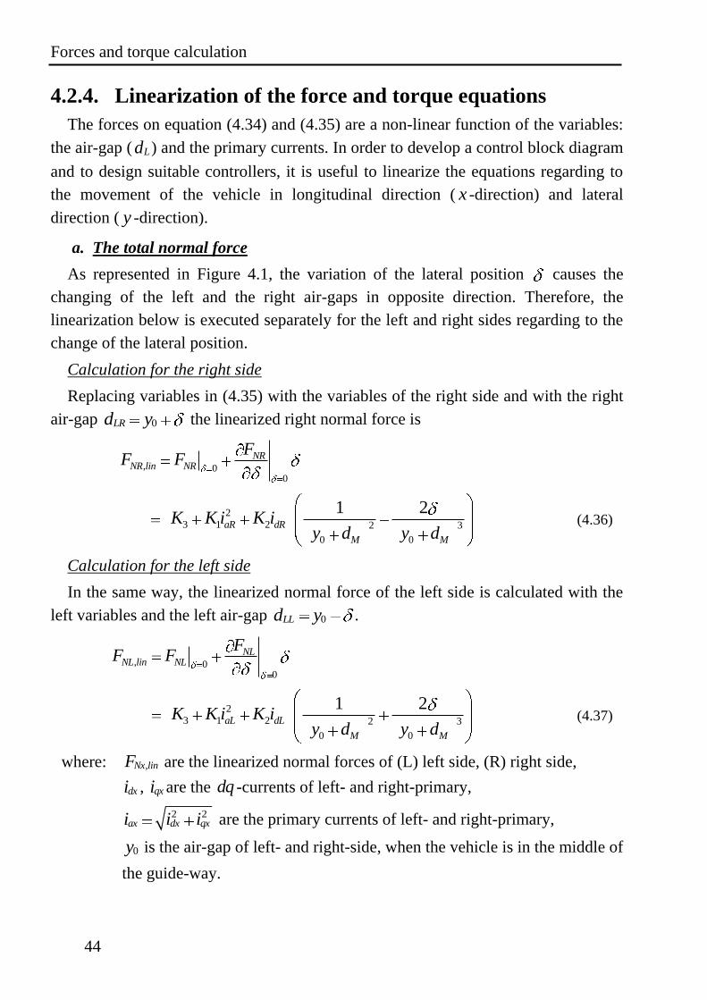
Forces and torque calculation
44
4.2.4. Linearization of the force and torque equations
The forces on equation (4.34) and (4.35) are a non-linear function of the variables:
the air-gap ( Ld ) and the primary currents. In order to develop a control block diagram
and to design suitable controllers, it is useful to linearize the equations regarding to
the movement of the vehicle in longitudinal direction ( x -direction) and lateral
direction ( y -direction).
a. The total normal force
As represented in Figure 4.1, the variation of the lateral position causes the
changing of the left and the right air-gaps in opposite direction. Therefore, the
linearization below is executed separately for the left and right sides regarding to the
change of the lateral position.
Calculation for the right side
Replacing variables in (4.35) with the variables of the right side and with the right
air-gap 0LRd y the linearized right normal force is
, 00
NRNR lin NR
FF F
2
3 1 2 2 3
0 0
1 2aR dR
M M
K K i K iy d y d
(4.36)
Calculation for the left side
In the same way, the linearized normal force of the left side is calculated with the
left variables and the left air-gap 0LLd y .
, 00
NLNL lin NL
FF F
2
3 1 2 2 3
0 0
1 2aL dL
M M
K K i K iy d y d
(4.37)
where: ,Nx linF are the linearized normal forces of (L) left side, (R) right side,
dxi , qxi are the dq -currents of left- and right-primary,
2 2ax dx qxi i i are the primary currents of left- and right-primary,
0y is the air-gap of left- and right-side, when the vehicle is in the middle of
the guide-way.
MATHEMATICAL MODEL
45
The total normal force acting on the vehicle is the difference of normal forces on
the left- and right-side in opposite directions. From equation (4.36) and equation
(4.37), the total normal force acting upon the vehicle is
2 23 1 2, , 3 2 2
0 0 0
2 21 23 3
0 0
4
2 2
NL lin NR lin aL aR dL dR
M M M
aL aR dL dR
M M
K K KF F i i i i
d y d y d y
K Ki i i i
d y d y
And presented in a simple way
2 2
, , 1 2 3
2 2
4 5
NL lin NR lin FN FN aL aR FN dL dR
FN aL aR FN dL dR
F F C C i i C i i
C i i C i i
(4.38)
where: 31 3
0
4FN
M
KC
d y; 1
2 2
0
FN
M
KC
d y; 2
3 2
0
FN
M
KC
d y;
14 3
0
2FN
M
KC
d y; 2
5 3
0
2FN
M
KC
d y.
b. The total thrust and torque
Besides the normal forces, which are perpendicular to the PM, the tangential forces
lie on the surface of the PM and along the guide-way. On the vehicle, the two
tangential forces of both sides produce the motion and the rotation of the vehicle on
the 0x y plane. Therefore, the sum of two tangential forces produces a thrust force
and the difference of them produces a torque.
As assumed in the previous subsection, the influence of a small yaw angle can
be neglected. With the yaw angle 0 , the air-gap is constant along the longitudinal
x -position, so the tangential forces can be calculated as it is presented in (4.34).
Therefore, the thrust forces on both sides are presented simply as
4
0
qL
TL
M
iF K
d y (4.39)
4
0
qR
TR
M
iF K
d y
(4.40)
where: TxF are the thrust forces of left- and right-side.
Equations of motion
46
Using the same linearized process as for normal forces, the linearized tangential
forces of left and right sides are
4 4, 2
0 0
TL lin qL qL
M M
K KF i i
d y d y (4.41)
4 4, 2
0 0
TR lin qR qR
M M
K KF i i
d y d y (4.42)
The equations (4.41) and (4.42) are simplified by means of the constant
coefficients:
41
0
FT
M
KC
d y; 4
2 2
0
FT
M
KC
d y
The thrust force and the torque impact on the vehicle are the functions of
difference and sum of linearized tangential forces presented by
, , 1 2TL lin TR lin FT qL qR FT qL qRF F C i i C i i (4.43)
, , 1 2TL lin TR lin FT qL qR FT qL qRF F C i i C i i (4.44)
All the linearized equations in this subsection are used in the next chapter in order
to design controllers for the experimental system.
4.3. Equations of motion
In following, equations of motion are the basic dynamic equations of the vehicle
presented in the Figure 4.1. With all the forces acting on the vehicle, which are
defined in section 4.2, the dynamic equations of vehicle’s motion can be presented in
three degrees of freedom like below:
Yaw rotating motion: 42 2
TL TR rr
b rF F F (4.45)
Lateral motion: 4NL NR rym F F F (4.46)
Longitudinal motion: 4TL TR rxmx F F F (4.47)
where: : is the moment of inertia of the vehicle,
m : is the mass of the vehicle,
b : is the width of the vehicle,
r : is the distance from the centre of the vehicle to the wheels,
rrF , rxF , ryF : Friction forces in rotation, x - and y -axis.
MATHEMATICAL MODEL
47
4.4. FEM simulation
4.4.1. Finite element method
The finite element method (FEM) [60] is a numerical technique for finding
approximate solutions of partial differential equations (PDE) as well as of integral
equations. The solution approach is based either on eliminating the differential
equation completely (steady state problems), or discretizing the PDE into an
approximating system of ordinary differential equations, which are then numerically
integrated using standard techniques such as Euler's method, Runge-Kutta, etc. With
that characteristic, the method is useful to solve many technical problems, including
electromagnetic problems. In this section, the electromagnetic forces on the vehicle
are simulated by Maxwell 2D program.
In solving PDE, the main challenge is to produce an equation that approximates the
equation needs to be studied. However, the solution of the equation has to be
numerically stable, i.e. errors in the input and intermediate calculations do not
accumulate and do not cause the resulting output to be meaningless. The FEM is a
good selection for solving partial differential equations over complicated domains
like the electromagnetic one. Therefore, the FEM together with real experimental
measurement was used in this research in order to verify the reliability of the
theoretical calculations above.
Maxwell® is the premier electromagnetic field simulation software from Ansoft
for engineers tasked with designing and analyzing 3-D and 2-D electromagnetic and
electromechanical devices such as motors, actuators, transformers, sensors and coils
[59]. Maxwell uses the accurate finite element method to solve static, frequency-
domain and time varying electromagnetic and electric fields. A key benefit of
Maxwell is its automated solution process where users are only required to specify
geometry, material properties and the desired output. From this point, Maxwell will
automatically generate an appropriate, efficient and accurate mesh for solving the
problem. This proven automatic adaptive meshing process removes complexity from
the analysis process and allows engineers to benefit from a highly efficient, easy-to-
use design flow. For these reasons, the simulation used Maxwell 2D for analyzing the
electromagnetic forces influencing the vehicle of the designed experimental setup.
The analytical work is simplified by supplying the software with the geometries and
the material properties of the experimental machine, which are presented in chapter 3.
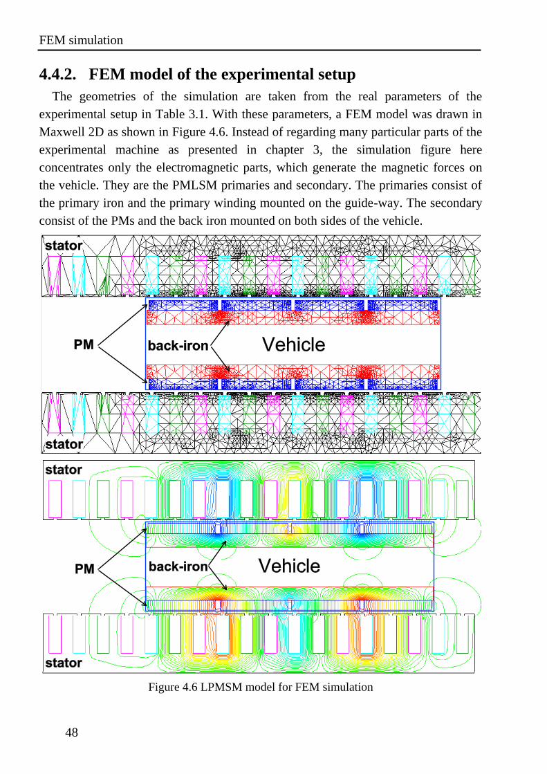
FEM simulation
48
4.4.2. FEM model of the experimental setup
The geometries of the simulation are taken from the real parameters of the
experimental setup in Table 3.1. With these parameters, a FEM model was drawn in
Maxwell 2D as shown in Figure 4.6. Instead of regarding many particular parts of the
experimental machine as presented in chapter 3, the simulation figure here
concentrates only the electromagnetic parts, which generate the magnetic forces on
the vehicle. They are the PMLSM primaries and secondary. The primaries consist of
the primary iron and the primary winding mounted on the guide-way. The secondary
consist of the PMs and the back iron mounted on both sides of the vehicle.
Figure 4.6 LPMSM model for FEM simulation
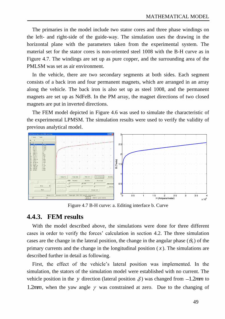
MATHEMATICAL MODEL
49
The primaries in the model include two stator cores and three phase windings on
the left- and right-side of the guide-way. The simulation uses the drawing in the
horizontal plane with the parameters taken from the experimental system. The
material set for the stator cores is non-oriented steel 1008 with the B-H curve as in
Figure 4.7. The windings are set up as pure copper, and the surrounding area of the
PMLSM was set as air environment.
In the vehicle, there are two secondary segments at both sides. Each segment
consists of a back iron and four permanent magnets, which are arranged in an array
along the vehicle. The back iron is also set up as steel 1008, and the permanent
magnets are set up as NdFeB. In the PM array, the magnet directions of two closed
magnets are put in inverted directions.
The FEM model depicted in Figure 4.6 was used to simulate the characteristic of
the experimental LPMSM. The simulation results were used to verify the validity of
previous analytical model.
Figure 4.7 B-H curve: a. Editing interface b. Curve
4.4.3. FEM results
With the model described above, the simulations were done for three different
cases in order to verify the forces’ calculation in section 4.2. The three simulation
cases are the change in the lateral position, the change in the angular phase ( s ) of the
primary currents and the change in the longitudinal position ( x ). The simulations are
described further in detail as following.
First, the effect of the vehicle’s lateral position was implemented. In the
simulation, the stators of the simulation model were established with no current. The
vehicle position in the y direction (lateral position ) was changed from 1.2mm to
1.2mm, when the yaw angle was constrained at zero. Due to the changing of

FEM simulation
50
lateral position, the normal forces generated by the PMs of the left- and right-side are
not balanced. Therefore, the normal force influencing the vehicle is nonzero and
depends on the lateral position. The result is presented in Figure 4.8 with normal
force as the function of . The normal force changing line generated by the
simulation is shown in green colour. The simulation result is linear as expected in the
theoretical calculation presented in the blue colour line. The difference between the
two lines is caused by the simplifying assumptions in the analytical calculation and
simulation material.
Figure 4.8 Normal force generated by the PM, as the function of lateral position
Second, the simulations were implemented to verify the validity of the normal
force and the thrust calculations in the moving reference frame.
At the beginning, the vehicle’s right stator was supplied with symmetrical three
phase currents:
sin( )A a si i ,
0sin( 120 )B a si i ,
0sin( 240 )C a si i ,
while the left stator currents were set to zero.
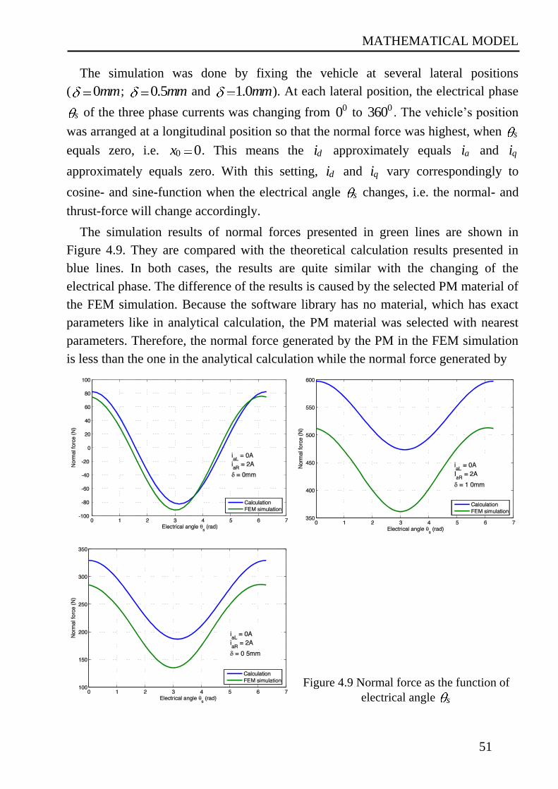
MATHEMATICAL MODEL
51
The simulation was done by fixing the vehicle at several lateral positions
( 0mm; 0.5mm and 1.0mm). At each lateral position, the electrical phase
s of the three phase currents was changing from 00 to 0360 . The vehicle’s position
was arranged at a longitudinal position so that the normal force was highest, when s
equals zero, i.e. 0 0x . This means the di approximately equals ai and qi
approximately equals zero. With this setting, di and qi vary correspondingly to
cosine- and sine-function when the electrical angle s changes, i.e. the normal- and
thrust-force will change accordingly.
The simulation results of normal forces presented in green lines are shown in
Figure 4.9. They are compared with the theoretical calculation results presented in
blue lines. In both cases, the results are quite similar with the changing of the
electrical phase. The difference of the results is caused by the selected PM material of
the FEM simulation. Because the software library has no material, which has exact
parameters like in analytical calculation, the PM material was selected with nearest
parameters. Therefore, the normal force generated by the PM in the FEM simulation
is less than the one in the analytical calculation while the normal force generated by
Figure 4.9 Normal force as the function of
electrical angle s
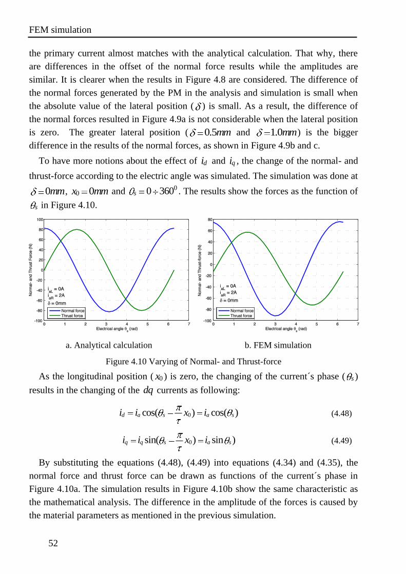
FEM simulation
52
the primary current almost matches with the analytical calculation. That why, there
are differences in the offset of the normal force results while the amplitudes are
similar. It is clearer when the results in Figure 4.8 are considered. The difference of
the normal forces generated by the PM in the analysis and simulation is small when
the absolute value of the lateral position ( ) is small. As a result, the difference of
the normal forces resulted in Figure 4.9a is not considerable when the lateral position
is zero. The greater lateral position ( 0.5mm and 1.0mm) is the bigger
difference in the results of the normal forces, as shown in Figure 4.9b and c.
To have more notions about the effect of di and qi , the change of the normal- and
thrust-force according to the electric angle was simulated. The simulation was done at
0mm, 0 0x mm and 00 360s . The results show the forces as the function of
s in Figure 4.10.
a. Analytical calculation b. FEM simulation
Figure 4.10 Varying of Normal- and Thrust-force
As the longitudinal position ( 0x ) is zero, the changing of the current´s phase ( s )
results in the changing of the dq currents as following:
0cos( ) cos( )d a s a si i x i (4.48)
0sin( ) sin )q q s a si i x i (4.49)
By substituting the equations (4.48), (4.49) into equations (4.34) and (4.35), the
normal force and thrust force can be drawn as functions of the current´s phase in
Figure 4.10a. The simulation results in Figure 4.10b show the same characteristic as
the mathematical analysis. The difference in the amplitude of the forces is caused by
the material parameters as mentioned in the previous simulation.
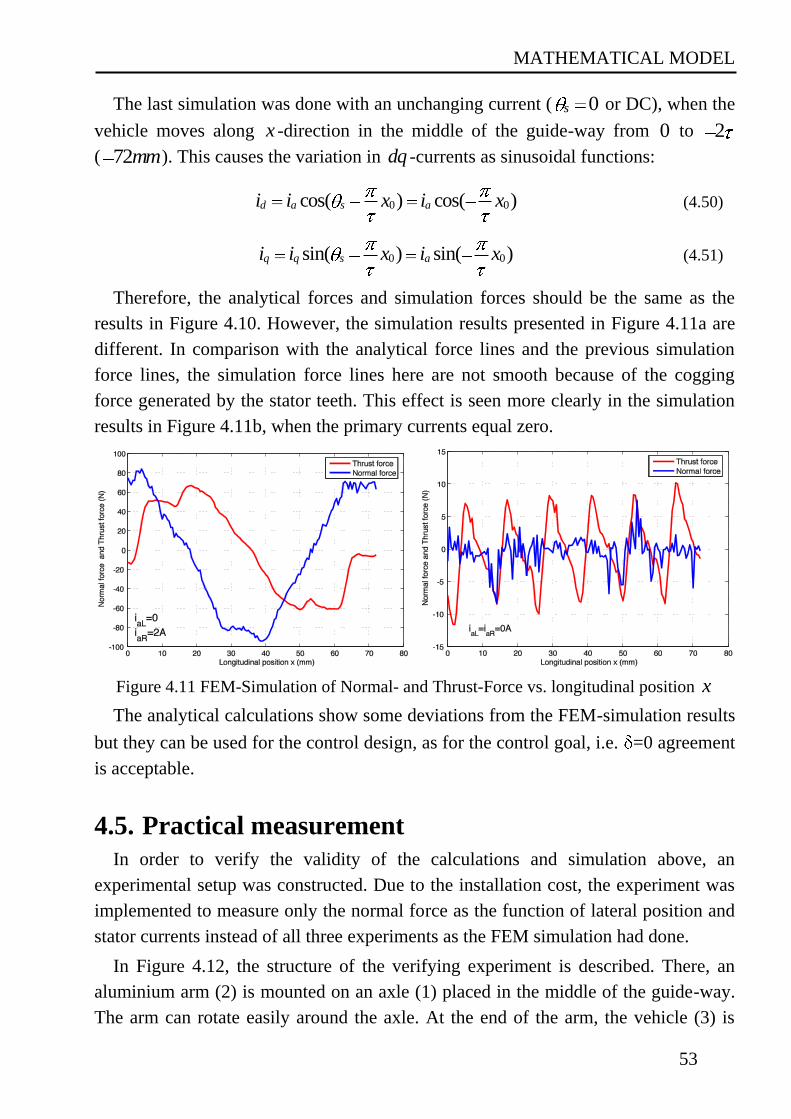
MATHEMATICAL MODEL
53
The last simulation was done with an unchanging current ( 0s or DC), when the
vehicle moves along x -direction in the middle of the guide-way from 0 to 2
( 72mm). This causes the variation in dq -currents as sinusoidal functions:
0 0cos( ) cos( )d a s ai i x i x (4.50)
0 0sin( ) sin( )q q s ai i x i x (4.51)
Therefore, the analytical forces and simulation forces should be the same as the
results in Figure 4.10. However, the simulation results presented in Figure 4.11a are
different. In comparison with the analytical force lines and the previous simulation
force lines, the simulation force lines here are not smooth because of the cogging
force generated by the stator teeth. This effect is seen more clearly in the simulation
results in Figure 4.11b, when the primary currents equal zero.
Figure 4.11 FEM-Simulation of Normal- and Thrust-Force vs. longitudinal position x
The analytical calculations show some deviations from the FEM-simulation results
but they can be used for the control design, as for the control goal, i.e. =0 agreement
is acceptable.
4.5. Practical measurement
In order to verify the validity of the calculations and simulation above, an
experimental setup was constructed. Due to the installation cost, the experiment was
implemented to measure only the normal force as the function of lateral position and
stator currents instead of all three experiments as the FEM simulation had done.
In Figure 4.12, the structure of the verifying experiment is described. There, an
aluminium arm (2) is mounted on an axle (1) placed in the middle of the guide-way.
The arm can rotate easily around the axle. At the end of the arm, the vehicle (3) is
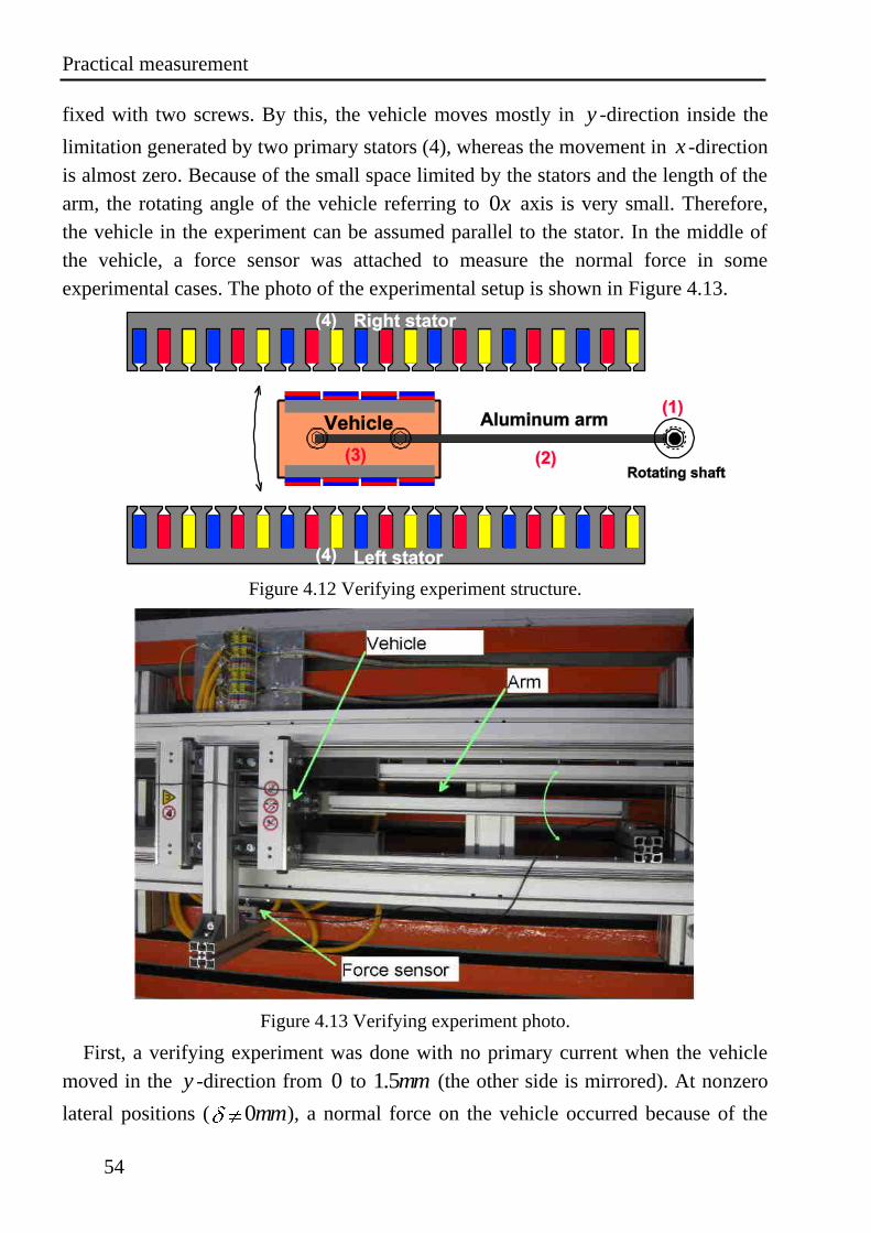
Practical measurement
54
fixed with two screws. By this, the vehicle moves mostly in y -direction inside the
limitation generated by two primary stators (4), whereas the movement in x -direction
is almost zero. Because of the small space limited by the stators and the length of the
arm, the rotating angle of the vehicle referring to 0x axis is very small. Therefore,
the vehicle in the experiment can be assumed parallel to the stator. In the middle of
the vehicle, a force sensor was attached to measure the normal force in some
experimental cases. The photo of the experimental setup is shown in Figure 4.13.
Figure 4.12 Verifying experiment structure.
Figure 4.13 Verifying experiment photo.
First, a verifying experiment was done with no primary current when the vehicle
moved in the y -direction from 0 to 1.5mm (the other side is mirrored). At nonzero
lateral positions ( 0mm), a normal force on the vehicle occurred because of the
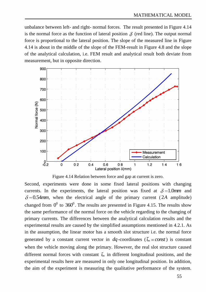
MATHEMATICAL MODEL
55
unbalance between left- and right- normal forces. The result presented in Figure 4.14
is the normal force as the function of lateral position (red line). The output normal
force is proportional to the lateral position. The slope of the measured line in Figure
4.14 is about in the middle of the slope of the FEM-result in Figure 4.8 and the slope
of the analytical calculation, i.e. FEM result and analytical result both deviate from
measurement, but in opposite direction.
Figure 4.14 Relation between force and gap at current is zero.
Second, experiments were done in some fixed lateral positions with changing
currents. In the experiments, the lateral position was fixed at 1.0mm and
0.54mm, when the electrical angle of the primary current ( 2A amplitude)
changed from 00 to 0360 . The results are presented in Figure 4.15. The results show
the same performance of the normal force on the vehicle regarding to the changing of
primary currents. The differences between the analytical calculation results and the
experimental results are caused by the simplified assumptions mentioned in 4.2.1. As
in the assumption, the linear motor has a smooth slot structure i.e. the normal force
generated by a constant current vector in dq -coordinates ( mi const ) is constant
when the vehicle moving along the primary. However, the real slot structure caused
different normal forces with constant mi in different longitudinal positions, and the
experimental results here are measured in only one longitudinal position. In addition,
the aim of the experiment is measuring the qualitative performance of the system.
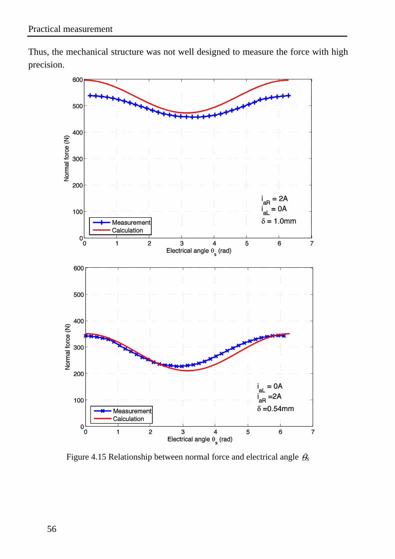
Practical measurement
56
Thus, the mechanical structure was not well designed to measure the force with high
precision.
Figure 4.15 Relationship between normal force and electrical angle s
CONTROLLER DESIGN
57
5. CONTROLLER DESIGN The main target of the controller in this dissertation is the ability to guide the
vehicle in the horizontal plane by a magnetic guiding system without any extra
mechanical or magnetic structure. With reference to the mathematical model
analyzed and examined in chapter 4, a control method will be proposed in this
chapter. The block diagram and calculation will be presented in the following
sections.
5.1. Control block diagram
5.1.1. Proposed control method
The proposed control method of each plant must be based on the plant’s
characteristic. Thus, the PM LSM force and torque equations in the previous chapter
will be analysed and rearranged in this subsection in order to derive a proposed
control method.
In chapter 4, the system was analysed, calculated and presented by mathematical
equations. The equations were then verified by the FEM simulations and
experimental measurements. The simulation and experimental results agree with the
calculated results; therewith the validity of the mathematical equations is confirmed.
With the limitations of the real experimental setup, the linear equations (4.38), (4.43),
(4.44) give the approximate behaviour of the system. In the description of the
experimental system, the vehicle has three degrees of freedom (DOF) to move on the
horizontal plane created by the two guiding rails. They are the longitudinal movement
in the x -axis, the lateral movement in the y -axis and the yaw rotation around
the z -axis. In order to propose a control method for the system, the three equations
(4.38), (4.43), (4.44) were rearranged to present the three-motion axes as the
functions of the currents xi , i , i .
The thrust force is derived from the equation (4.44), and the results is
x TL TR x x xpF F F K i K i (5.1)
where xF is the force impacting the vehicle in x -axis (thrust force),
and 1x FTK C , 2xp FTF C .
The lateral force is the difference of the normal forces presented in (4.38)
, , ,NL NR pF F F K i F i i (5.2)
Control block diagram
58
where 3FNK C and
2 2 2 2
1 2 4 5( , , , )p FN FN aL aR FN aL aR FN dL dRF i i C C i i C i i C i i
Derived from the equation (4.43), it attains the torque (T ) impacting the vehicle
from the tangential forces
2
TL TR pb
T F F K i K i (5.3)
where b is the gap in between the two PMs of the vehicle,
2
2
FTbCK ,
1
2
FTp
bCK .
In these equations, the forces and torque impacting the vehicle in x -axis ( xF ), y -
axis ( F ) and yaw (T ) are presented by proportional relations with the current
variables xi , i , i and the nonlinear functions xpK i , , , ,pF i i ,
pK i . The current variables ( xi , i , i ) have relations with the dq -currents of
the LM primaries presented in (5.4) and (5.5). The dq -currents of the primaries are
distinguished by subscript L for the left primary and subscript R for the right
primary.
; ;2 2
x xqL qR
i i i ii i (5.4)
; ;2 2
dL dRi i
i i (5.5)
Therefore,
;; ;dL dR qL qR x qL qRi i i i i i i i i (5.6)
In addition, with the linear dynamic equations of the vehicle’s motions (4.45)-
(4.47), the controllers for the three DOFs suggest the use of standard cascaded PI
control method. Assume that the inverters are used to generate the required currents
in a very short time in comparison with the dynamic motions. The cascaded PI
controllers of the vehicle motions are presented in equations from (5.7) to (5.12).
0
( ) ( )tpv
x pvi
ki k v v v v dt
T (5.7)
0
( ) ( )tp
pi
ki k dt
T (5.8)
0
( ) ( )tp
pi
ki k dt
T (5.9)
CONTROLLER DESIGN
59
( )pxv k x x (5.10)
( )pk (5.11)
( )pk (5.12)
where: *xi , *i , *i are reference values of current for three DOF motion,
*v , * , * are the reference values of three DOF motion velocity,
*x , * , * are the reference values of three DOF motion position,
...pk , iT are the constant parameters of the PI controllers.
In the proposed control method above, the nonlinear parts of equation (5.1), (5.2)
and (5.3) are considered as perturbations. This consideration can cause a reduction in
the control quality of the system, especially when the values of and are
significant. In order to improve the control quality, compensation of the perturbations
needs to be implemented by decoupling and feed forward calculations in the
controllers. Detail of the methods is clearly represented in the next subsection by
block diagrams.
5.1.2. Block diagrams of the control system
In this subsection, the control system is described by block diagrams. In the block
diagram, the LSM characteristics presented by the equations in chapter 4 are
represented as a set of elementary blocks. The proposed control methods and the
limitations for the system are also presented in three different block diagrams.
Using the dynamic equations of the vehicle’s motions and the linearized equations
of forces and torque with regard to and in chapter 4, the LSM block diagram is
produced and presented in the right part (yellow area) of Figure 5.1. The small
friction forces on the wheels have been greatly simplified to be proportional with
vehicle velocities in the horizontal plane. The instability of the open loop caused by
lateral offset distance and yaw angle is not difficult to recognize by the positive
feedback through the coefficients 1FNC , 3FNC , 4FNC , 5FNC , 1FTC and 2FTC .
Consequently, the closed cascaded control loops as mentioned above need to be
employed.
The basic structure of the control system for each of the three DOF motion ( x , ,
) presented in the Figure 5.1 is a cascaded control system. The internal loops of the
system are the current control loops using field oriented control (FOC) method ( d -
and q-currents). The superposed control loops of the current control are the speed
Control block diagram
60
( /dx dt , /d dt and /d dt ) control loops. It is assumed here that the sensor signals
of the positions x , and are available. The lateral position ( ) and yaw angle ( )
signals are supplied by industrial inductive sensors and afterwards supplied by a self-
developed capacitive sensor. Beside and , the longitudinal position ( x ) is
supplied by the incremental magnet position sensor. The time derivatives of the
positions, which provide feedback speed information ( x , and ), are obtained by
either approximate differentiate or by an observer structure, that is described in the
right-hand side of the block diagram in Figure 5.1.
The output signal of the controller for the longitudinal velocity ( /dx dt ) is the
reference value for the sum of current values in the q -axis of the left- and right-
primary ( *xi ). The combination of real q -currents caused by *
xi leads the vehicle with
0 moving by the total forces in x -direction TL TRF F .
The controller for yaw angle velocity /d dt sends out the reference value for the
difference between the current values in the q -axis of the left- and right-primary ( *i ).
The accompanying real q -currents caused by *i in the primaries control the
difference between the left and the right tangential forces to generate a rotational
moment on the vehicle around a z-axis in the middle of the vehicle.
The reference values of the q-currents ( *qLi , *
qRi ) are determined from the
relationship in equation (5.4) and presented in the block diagram.
The controller of the lateral velocity ( /d dt ) returns the reference value for the
difference of d -currents in the primaries to control the lateral position. From the
output of /d dt controller, the d -current references are extracted to generate the
corresponding normal forces on the left- and right-side of the vehicle against the
lateral motion. In this approach, the two d -axis currents ( *dLi , *
dRi ) are simply mapped
to half of the difference value with inverted signs as in (5.5).
The external control loops are the position control loops ( -, -, x - controller).
The position controllers receive position reference values ( * , *, *x ) from the user
interface and feedback values ( , , x ) from system sensors to calculate the speed
references. The references are then supplied to the corresponding speed controllers.
Because of the strong coupling and positive feedback with regard to the lateral
offset distance and the yaw angle , the proposed control system discussed till
now can work only at poor dynamics. Hence, extra signals are added to the reference
signals of the current controllers in Figure 5.2. The signal are the estimated values of
CONTROLLER DESIGN
61
the perturbations xpK i , , , ,pF i i and pK i mentioned in (5.1)-(5.3).
They are used to counteract the positive feedback in the control system and decouple
the effect of , , x on the control qualities of the others. In the decoupling blocks,
1FNC 2FNC … 1FTC … are the estimated constants of the system. The currents
dRi , qRi , dLi , qRi are estimated from the feedback currents of two phases, instead of
three phases as usual.
In the block diagram Figure 5.2 described above, the control system of the vehicle
is assumed a linear circuit according to the linearized coefficients. The current
controllers are assumed to have a very small delay time. It is also useful to consider
that the current controllers can generate the combination of dq -currents linearly
proportional to the reference value. With these assumptions, the control signals of the
velocity controllers ( /d dt , /d dt and /dx dt ) can be implemented to guide the
vehicle as presented in the block diagram Figure 5.2.
With the limited current supplies of the inverters, the limitations of current values
are also added as in Figure 5.3. Here, the d -currents are given higher priorities
versus the q -currents, i.e. in operating under the current limitation, most current is
used in the d -axis to produce enough normal force against the magnetic attraction
between the permanent magnets and the primaries.
maxdxi I (5.13)
2 2maxqx dxi I i (5.14)
where dxi , qxi are the dq -currents of the left and right primary,
maxI is the limited current of the inverter.
However, the normal forces must be high only at the beginning when the vehicle
leaves the rest position, from one side of the guide-way to the middle of the guide-
way. When the vehicle is in the middle of the guide-way, the required d -currents are
small; most current can be used in the q -axis to guide the vehicle moving in the
longitudinal direction.
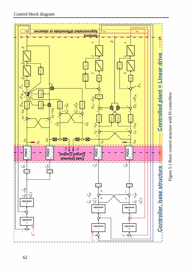
Control block diagram
62
Fig
ure
5.1
Bas
ic c
on
tro
l st
ruct
ure
wit
h P
I co
ntr
oll
ers
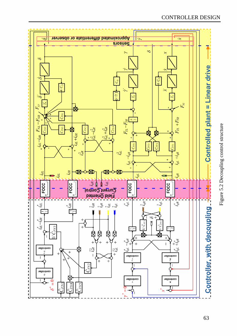
CONTROLLER DESIGN
63
Fig
ure
5.2
Dec
ou
pli
ng
co
ntr
ol
stru
ctu
re
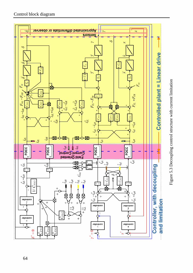
Control block diagram
64
Fig
ure
5.3
Dec
ou
pli
ng
co
ntr
ol
stru
ctu
re w
ith
curr
ent
lim
itat
ion
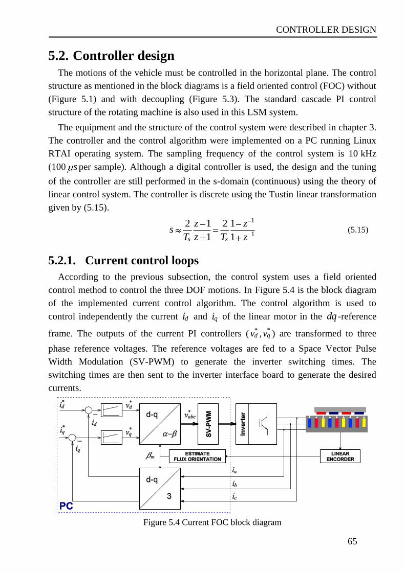
CONTROLLER DESIGN
65
5.2. Controller design
The motions of the vehicle must be controlled in the horizontal plane. The control
structure as mentioned in the block diagrams is a field oriented control (FOC) without
(Figure 5.1) and with decoupling (Figure 5.3). The standard cascade PI control
structure of the rotating machine is also used in this LSM system.
The equipment and the structure of the control system were described in chapter 3.
The controller and the control algorithm were implemented on a PC running Linux
RTAI operating system. The sampling frequency of the control system is 10 kHz
(100 s per sample). Although a digital controller is used, the design and the tuning
of the controller are still performed in the s-domain (continuous) using the theory of
linear control system. The controller is discrete using the Tustin linear transformation
given by (5.15).
1
1
2 1 2 1
1 1s s
z zs
T z T z (5.15)
5.2.1. Current control loops
According to the previous subsection, the control system uses a field oriented
control method to control the three DOF motions. In Figure 5.4 is the block diagram
of the implemented current control algorithm. The control algorithm is used to
control independently the current di and qi of the linear motor in the dq -reference
frame. The outputs of the current PI controllers ( *dv , *
qv ) are transformed to three
phase reference voltages. The reference voltages are fed to a Space Vector Pulse
Width Modulation (SV-PWM) to generate the inverter switching times. The
switching times are then sent to the inverter interface board to generate the desired
currents.
Figure 5.4 Current FOC block diagram
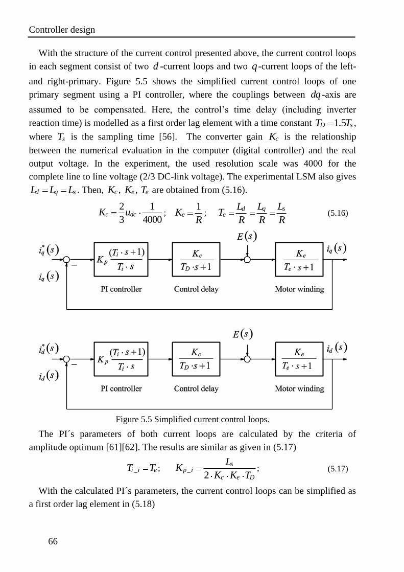
Controller design
66
With the structure of the current control presented above, the current control loops
in each segment consist of two d -current loops and two q -current loops of the left-
and right-primary. Figure 5.5 shows the simplified current control loops of one
primary segment using a PI controller, where the couplings between dq -axis are
assumed to be compensated. Here, the control’s time delay (including inverter
reaction time) is modelled as a first order lag element with a time constant 1.5D sT T ,
where sT is the sampling time [56]. The converter gain cK is the relationship
between the numerical evaluation in the computer (digital controller) and the real
output voltage. In the experiment, the used resolution scale was 4000 for the
complete line to line voltage (2/3 DC-link voltage). The experimental LSM also gives
d q sL L L . Then, cK , eK , eT are obtained from (5.16).
2 1
3 4000c dcK u ;
1eK
R;
d q se
L L LT
R R R (5.16)
Figure 5.5 Simplified current control loops.
The PI´s parameters of both current loops are calculated by the criteria of
amplitude optimum [61][62]. The results are similar as given in (5.17)
_i i eT T ; _2
sp i
c e D
LK
K K T; (5.17)
With the calculated PI´s parameters, the current control loops can be simplified as
a first order lag element in (5.18)
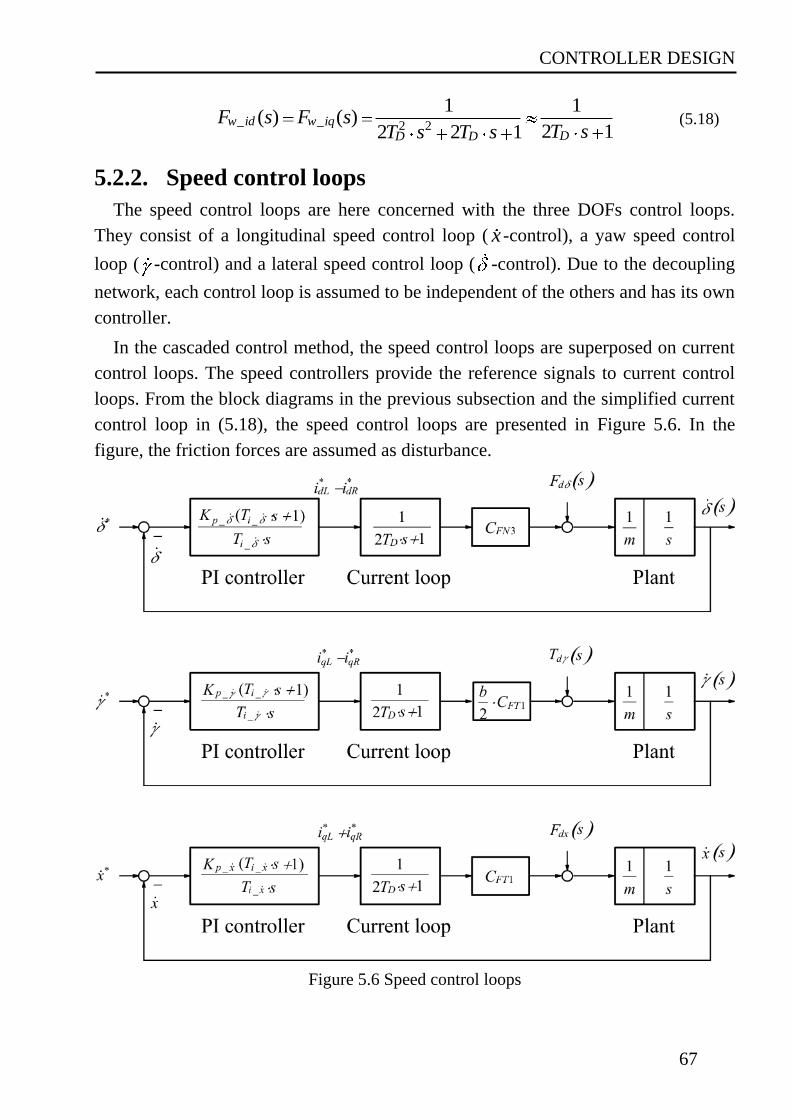
CONTROLLER DESIGN
67
_ _ 2 2
1 1( ) ( )
2 12 2 1w id w iq
DD D
F s F sT sT s T s
(5.18)
5.2.2. Speed control loops
The speed control loops are here concerned with the three DOFs control loops.
They consist of a longitudinal speed control loop ( x -control), a yaw speed control
loop ( -control) and a lateral speed control loop ( -control). Due to the decoupling
network, each control loop is assumed to be independent of the others and has its own
controller.
In the cascaded control method, the speed control loops are superposed on current
control loops. The speed controllers provide the reference signals to current control
loops. From the block diagrams in the previous subsection and the simplified current
control loop in (5.18), the speed control loops are presented in Figure 5.6. In the
figure, the friction forces are assumed as disturbance.
Figure 5.6 Speed control loops
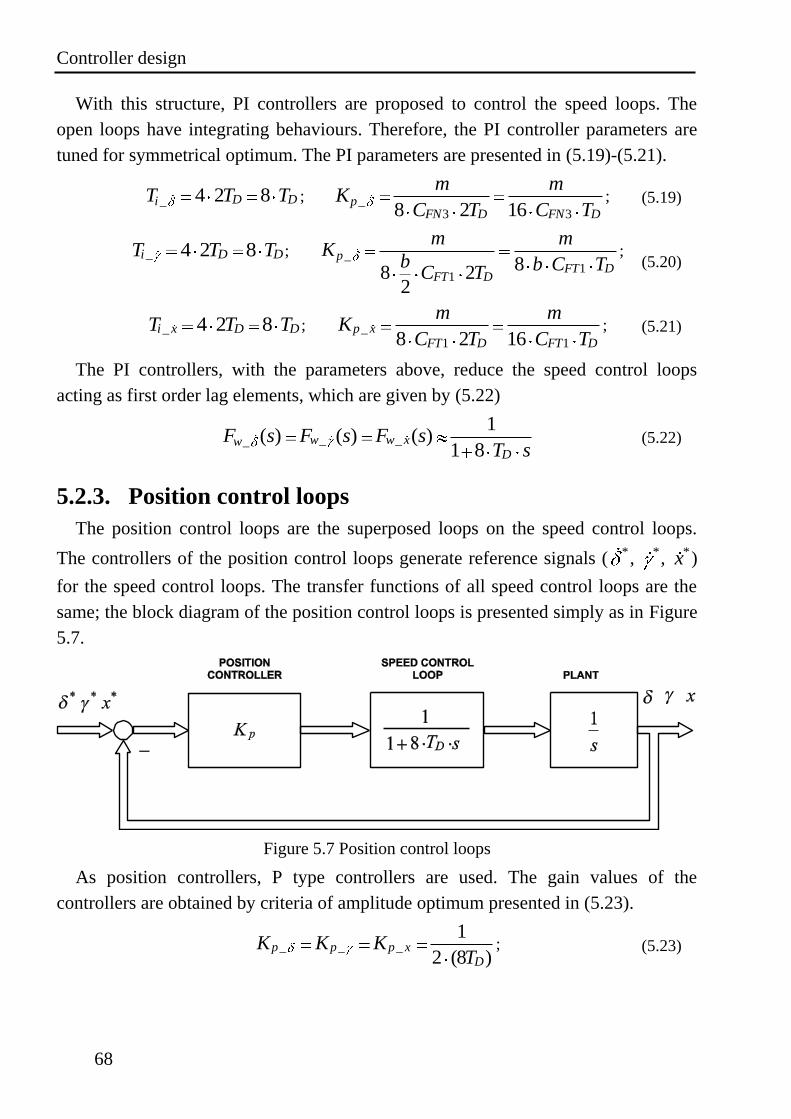
Controller design
68
With this structure, PI controllers are proposed to control the speed loops. The
open loops have integrating behaviours. Therefore, the PI controller parameters are
tuned for symmetrical optimum. The PI parameters are presented in (5.19)-(5.21).
_ 4 2 8D DiT T T ; _3 38 2 16
pFN D FN D
m mK
C T C T; (5.19)
_ 4 2 8i D DT T T ; _
11
88 22
pFT D
FT D
m mK
b b C TC T
; (5.20)
_ 4 2 8i x D DT T T ; _1 18 2 16
p xFT D FT D
m mK
C T C T; (5.21)
The PI controllers, with the parameters above, reduce the speed control loops
acting as first order lag elements, which are given by (5.22)
_ __
1( ) ( ) ( )
1 8w w xw
D
F s F s F sT s
(5.22)
5.2.3. Position control loops
The position control loops are the superposed loops on the speed control loops.
The controllers of the position control loops generate reference signals ( * , *, *x )
for the speed control loops. The transfer functions of all speed control loops are the
same; the block diagram of the position control loops is presented simply as in Figure
5.7.
Figure 5.7 Position control loops
As position controllers, P type controllers are used. The gain values of the
controllers are obtained by criteria of amplitude optimum presented in (5.23).
_ _ _1
2 (8 )p p p x
D
K K KT
; (5.23)
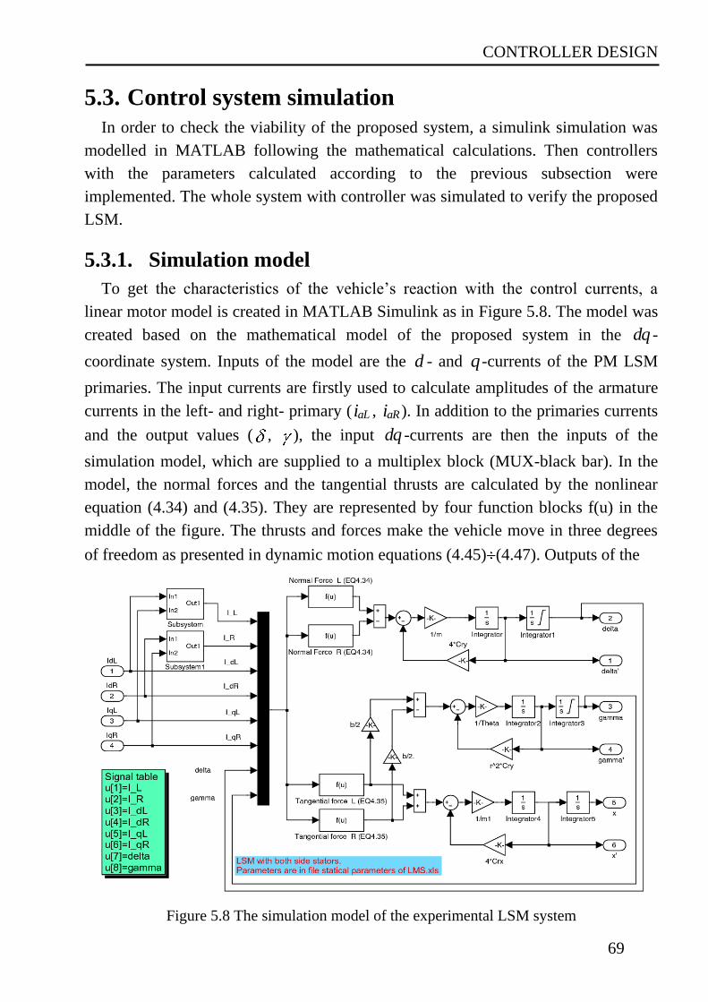
CONTROLLER DESIGN
69
5.3. Control system simulation
In order to check the viability of the proposed system, a simulink simulation was
modelled in MATLAB following the mathematical calculations. Then controllers
with the parameters calculated according to the previous subsection were
implemented. The whole system with controller was simulated to verify the proposed
LSM.
5.3.1. Simulation model
To get the characteristics of the vehicle’s reaction with the control currents, a
linear motor model is created in MATLAB Simulink as in Figure 5.8. The model was
created based on the mathematical model of the proposed system in the dq -
coordinate system. Inputs of the model are the d - and q -currents of the PM LSM
primaries. The input currents are firstly used to calculate amplitudes of the armature
currents in the left- and right- primary ( aLi , aRi ). In addition to the primaries currents
and the output values ( , ), the input dq -currents are then the inputs of the
simulation model, which are supplied to a multiplex block (MUX-black bar). In the
model, the normal forces and the tangential thrusts are calculated by the nonlinear
equation (4.34) and (4.35). They are represented by four function blocks f(u) in the
middle of the figure. The thrusts and forces make the vehicle move in three degrees
of freedom as presented in dynamic motion equations (4.45) (4.47). Outputs of the
Figure 5.8 The simulation model of the experimental LSM system
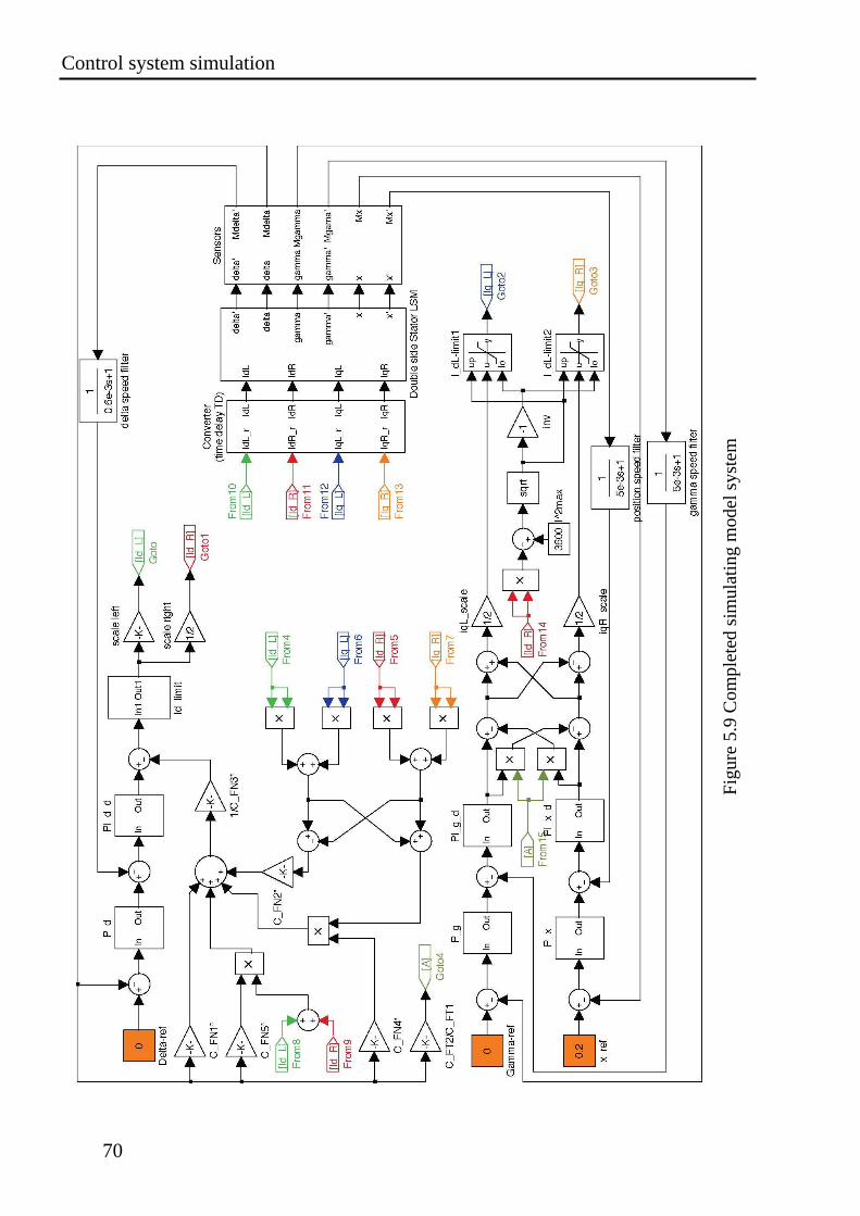
Control system simulation
70
Fig
ure
5.9
Co
mp
lete
d s
imu
lati
ng
mo
del
sy
stem
CONTROLLER DESIGN
71
model are lateral position ( ), yaw angle ( ), longitudinal position ( x ) and their
corresponding speeds.
The whole-system model is developed to study some characteristics of the
PM SLM and the ability of the designed controller. In the completed model in Figure
5.9, the PM SLM model in Figure 5.8 is packed as a block with four current input
signals ( dLi , dRi , qLi , qRi ) and six motor state variable outputs ( , , , , x , x ).
The PM SLM is connected with the converter block (input) and the measurement
block (output). Here, they are simplified as first order lag elements. The measurement
system has a duty to supply feedback signals for the control system, and the converter
receives desired current values from the control system.
The model of the control system is built according to the left part of the block
diagram Figure 5.3. The control model is separated into three control loops to control
three DOFs independently with feed forward control to compensate the coupling
between the control values. The feed forward block diagram is based on the estimated
parameters of linearized equation (4.38, (4.43) and (4.44). Each DOF is controlled by
three cascaded control loops: current control loop, speed control loop and position
control loop.
5.3.2. Simulation results
With the simulation model mentioned above, simulations were done to verify the
proposed control method on the mathematical model of the PM LSM. The
simulations consist of separated controls and simultaneous control as follows.
At first, the simulation was done with separated controls. Each DOF of the vehicle
was controlled from starting value (rest position) to desired control values while the
two other controls were constrained, i.e. only one position ( or or x ) is
controlled, the other two positions were modelled to be constant. At the beginning,
the system was started with one position at rest value ( 1.2mm or 8.0mrad
or 0x mm), and the two others were constrained at zero ( 0mm, 0mrad ,
0x ). At 0.1t s , the control position was set for desired value ( * 0mm or
* 0mrad or * 200x mm). The simulation results are presented in turn in Figure
5.10-Figure 5.12. In the figures, the lateral position ( ), yaw angle ( ) and
longitudinal ( x ) are shown as functions of time.
In Figure 5.10, the lateral position was controlled from the rest position
1.2mm to the reference position * 0 . In this control, only the d -currents are
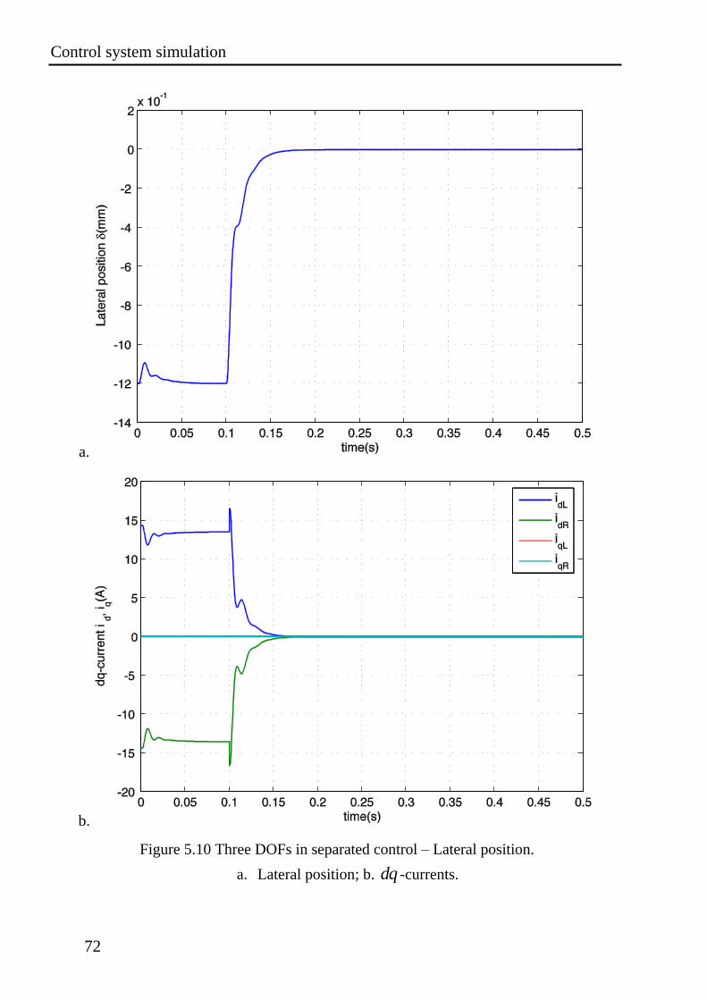
Control system simulation
72
a.
b.
Figure 5.10 Three DOFs in separated control – Lateral position.
a. Lateral position; b. dq -currents.
CONTROLLER DESIGN
73
required to control the lateral position, while the q -currents are zero, as shown in
Figure 5.10b. The simulation results show a good control quality in lateral position
control (Figure 5.10a). There was a disturbance at the beginning of the simulation
when the vehicle was in the rest position. The phenomenon is caused by the
compensation currents from the decoupling structure. The currents make the vehicle
move toward the centre of the guide-way, i.e. the lateral position ( ) trends toward
zero. However, this reduces the compensation currents. Therefore, the vehicle moves
back to the rest position, and the system here establishes a balance between the
normal forces generated by the compensation currents and the other forces.
The simulation results of yaw angle ( ) control are presented in Figure 5.11. The
yaw angle was controlled from 8.0mrad to 0mrad with a high-
performance, as shown in Figure 5.11a. In the simulation, only the difference of the
q-currents is used in order to control the yaw angle as the q -currents ( qLi , qRi ) are
symmetrical with respect to the horizontal axis, i.e. the sum of the q -currents is zero.
The d -currents are also not necessary in this case. These are shown in Figure 5.11b.
The longitudinal position ( x ) control ability was consider in the third simulation.
The results are shown in Figure 5.12. The controller leads precisely the vehicle to the
desired position * 200x mm (Figure 5.12a). The slow dynamic of this control in
comparison with the two other controls is the aim of the design. In order to limit the
acceleration of the vehicle, the absolute value of maximum q -current is restricted
under 12A . This causes a reduction in the control dynamic. Moreover, a low-pass
filter used in the speed loop is another cause. The filter is used to eliminate noises of
speed feedback signal, which is the derivative of an incremental sensor signal.
Therefore, a high time-constant filter is required. Finally, the dynamic of the
longitudinal position control must be lower than the two other in order to improve the
qualities of the motion control. Figure 5.12b shows the dq -currents of the simulation.
The d -currents are not necessary for longitudinal position control ( 0dL dRi i ). The
q-currents are the same in order to generate thrust force by the sum of the tangential
forces and not generate torque on the vehicle. In the figure, the limit of q -current can
also be recognized.
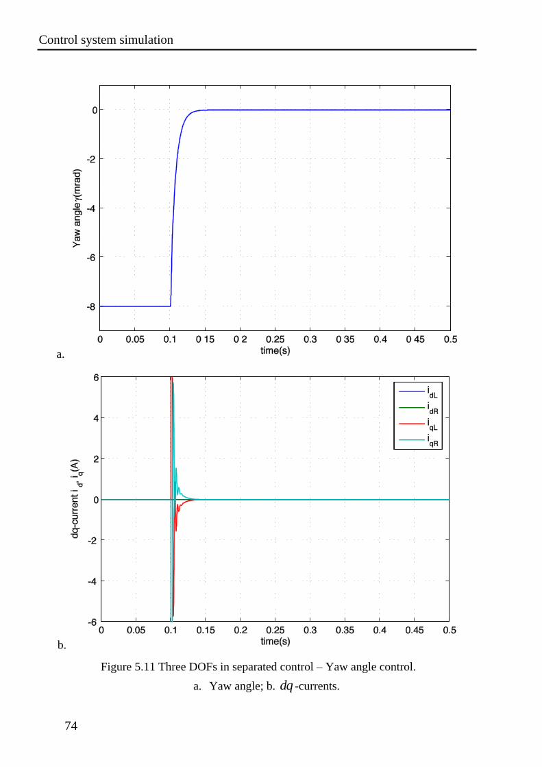
Control system simulation
74
a.
b.
Figure 5.11 Three DOFs in separated control – Yaw angle control.
a. Yaw angle; b. dq -currents.
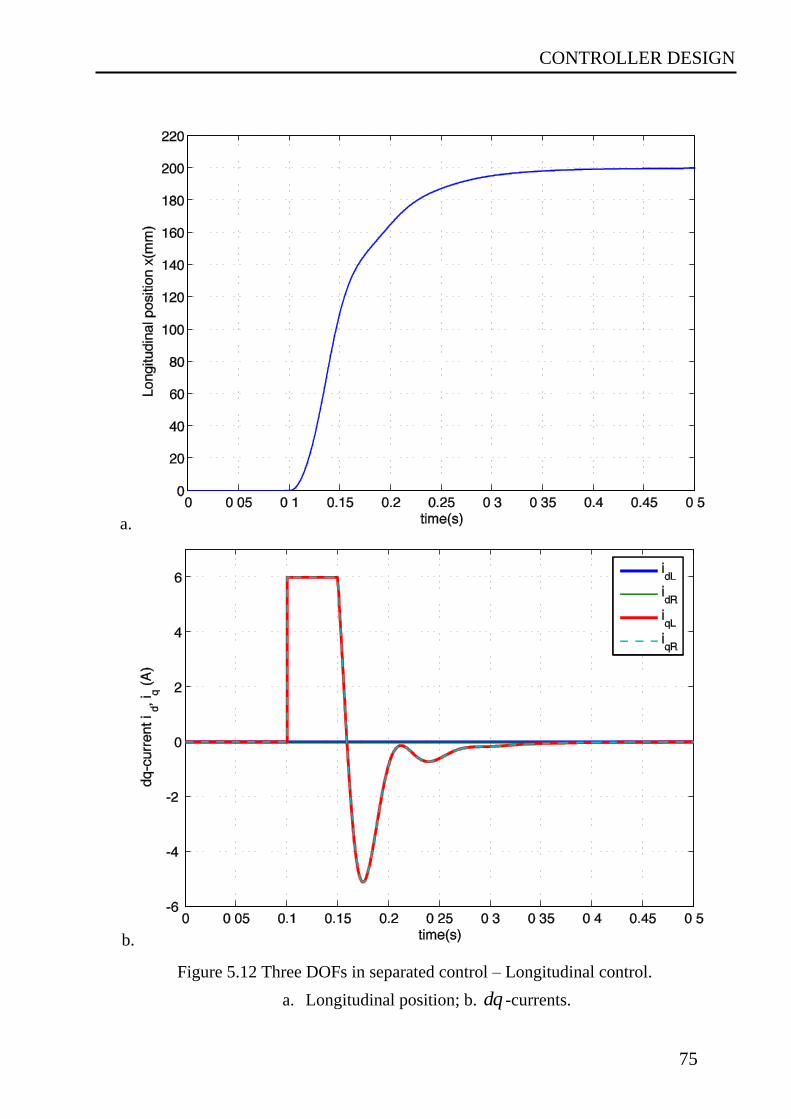
CONTROLLER DESIGN
75
a.
b.
Figure 5.12 Three DOFs in separated control – Longitudinal control.
a. Longitudinal position; b. dq -currents.
Control system simulation
76
Second, the simulation results in the case of simultaneous control were performed.
In this simulation, all DOFs are controlled simultaneously from the rest positions to
desired positions. The parameters here were set for the same parameters like in the
case of the separated controls. At the beginning, the vehicle was at the rest positions
( 1.2mm, 8.0mrad and 0x mm). At 0.1t s , all the control positions
were set for desired values ( * 0mm, * 0mrad and * 200x mm). The vehicle
was controlled to move centrally and parallel to the middle of the guide-way. The
results display the response of the vehicle position in three DOFs as functions of time
in Figure 5.13-Figure 5.15.
In Figure 5.13, all the three controlled variables are presented. They show the same
performance as the results of separated controls do. That means the proposed control
method can eliminate the coupling of the three DOFs of the simulation model. Each
control variable ( or or x ) can be controlled independently.
In Figure 5.14 and Figure 5.15, the response currents of the primaries in the d - and
q-axis with regards to the simultaneously control simulation are presented. Here, all
the dq -currents are required instead of using the currents of only one axis (the d - or
q-axis). As in the figures, the d -currents are required when the vehicle is controlled
to move from the rest position to the middle of the guide-way. The d -currents are
zero when the vehicle is in the middle of the guide-way ( 0). The difference of q -
currents is necessary when the controller is steering the vehicle parallel to the guide-
way ( 0), and the sum of q-currents is used to push the vehicle along the guide-
way.
As the results of the simulation presented here and many other simulations, the
proposed control method could be suitable for the mathematical model of the PM
LSM system. The linearized decoupling parameters in (4.38), (4.43) and (4.44) can
compensate well for the nonlinear equations (4.34) and (4.35) used in the vehicle
model. This leads to the well-controlled results of three DOFs control. Altogether, the
simulation results are the foundation to implement the control method of the real
experimental system in the next chapter.
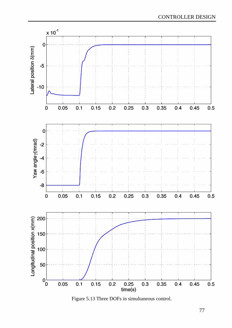
CONTROLLER DESIGN
77
Figure 5.13 Three DOFs in simultaneous control.
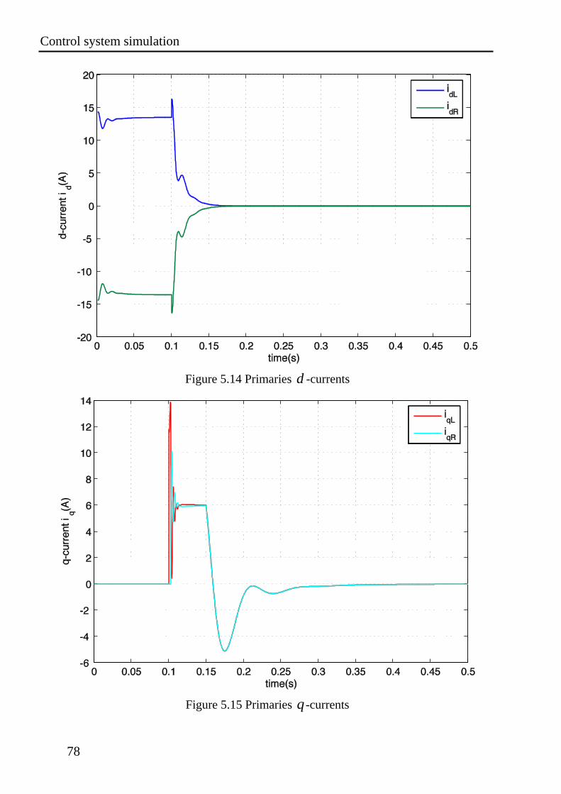
Control system simulation
78
Figure 5.14 Primaries d -currents
Figure 5.15 Primaries q -currents
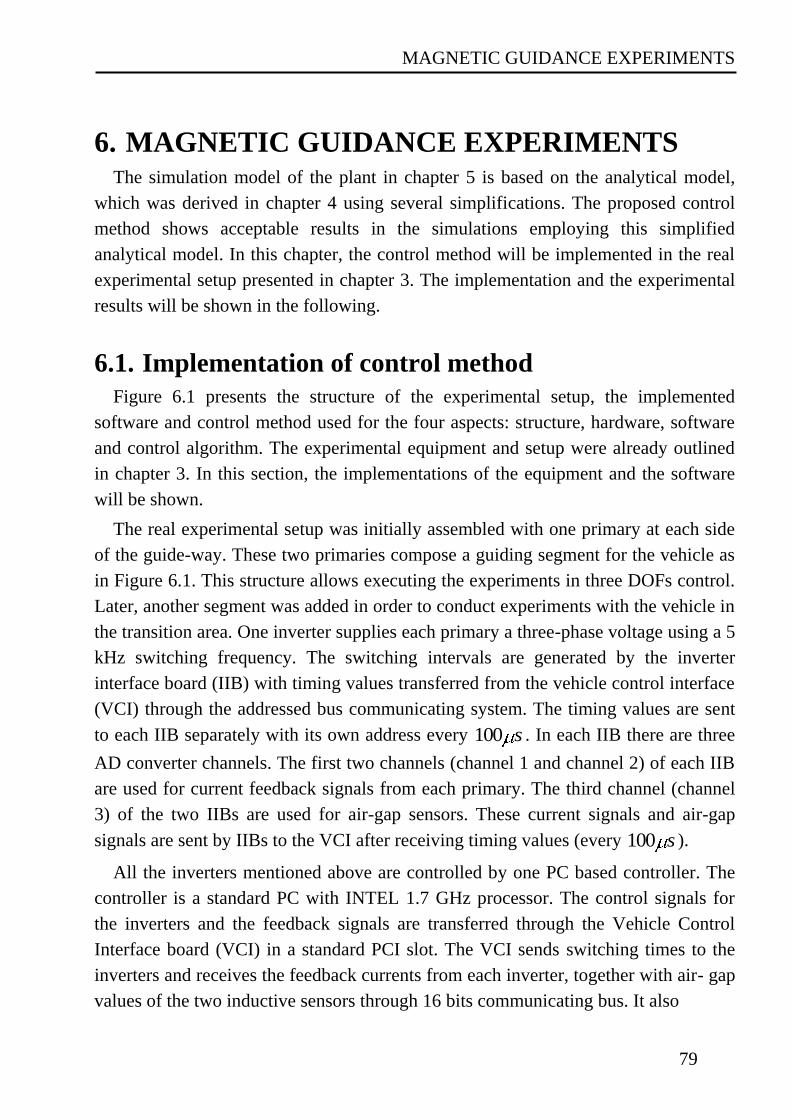
MAGNETIC GUIDANCE EXPERIMENTS
79
6. MAGNETIC GUIDANCE EXPERIMENTS The simulation model of the plant in chapter 5 is based on the analytical model,
which was derived in chapter 4 using several simplifications. The proposed control
method shows acceptable results in the simulations employing this simplified
analytical model. In this chapter, the control method will be implemented in the real
experimental setup presented in chapter 3. The implementation and the experimental
results will be shown in the following.
6.1. Implementation of control method
Figure 6.1 presents the structure of the experimental setup, the implemented
software and control method used for the four aspects: structure, hardware, software
and control algorithm. The experimental equipment and setup were already outlined
in chapter 3. In this section, the implementations of the equipment and the software
will be shown.
The real experimental setup was initially assembled with one primary at each side
of the guide-way. These two primaries compose a guiding segment for the vehicle as
in Figure 6.1. This structure allows executing the experiments in three DOFs control.
Later, another segment was added in order to conduct experiments with the vehicle in
the transition area. One inverter supplies each primary a three-phase voltage using a 5
kHz switching frequency. The switching intervals are generated by the inverter
interface board (IIB) with timing values transferred from the vehicle control interface
(VCI) through the addressed bus communicating system. The timing values are sent
to each IIB separately with its own address every 100 s . In each IIB there are three
AD converter channels. The first two channels (channel 1 and channel 2) of each IIB
are used for current feedback signals from each primary. The third channel (channel
3) of the two IIBs are used for air-gap sensors. These current signals and air-gap
signals are sent by IIBs to the VCI after receiving timing values (every 100 s ).
All the inverters mentioned above are controlled by one PC based controller. The
controller is a standard PC with INTEL 1.7 GHz processor. The control signals for
the inverters and the feedback signals are transferred through the Vehicle Control
Interface board (VCI) in a standard PCI slot. The VCI sends switching times to the
inverters and receives the feedback currents from each inverter, together with air- gap
values of the two inductive sensors through 16 bits communicating bus. It also
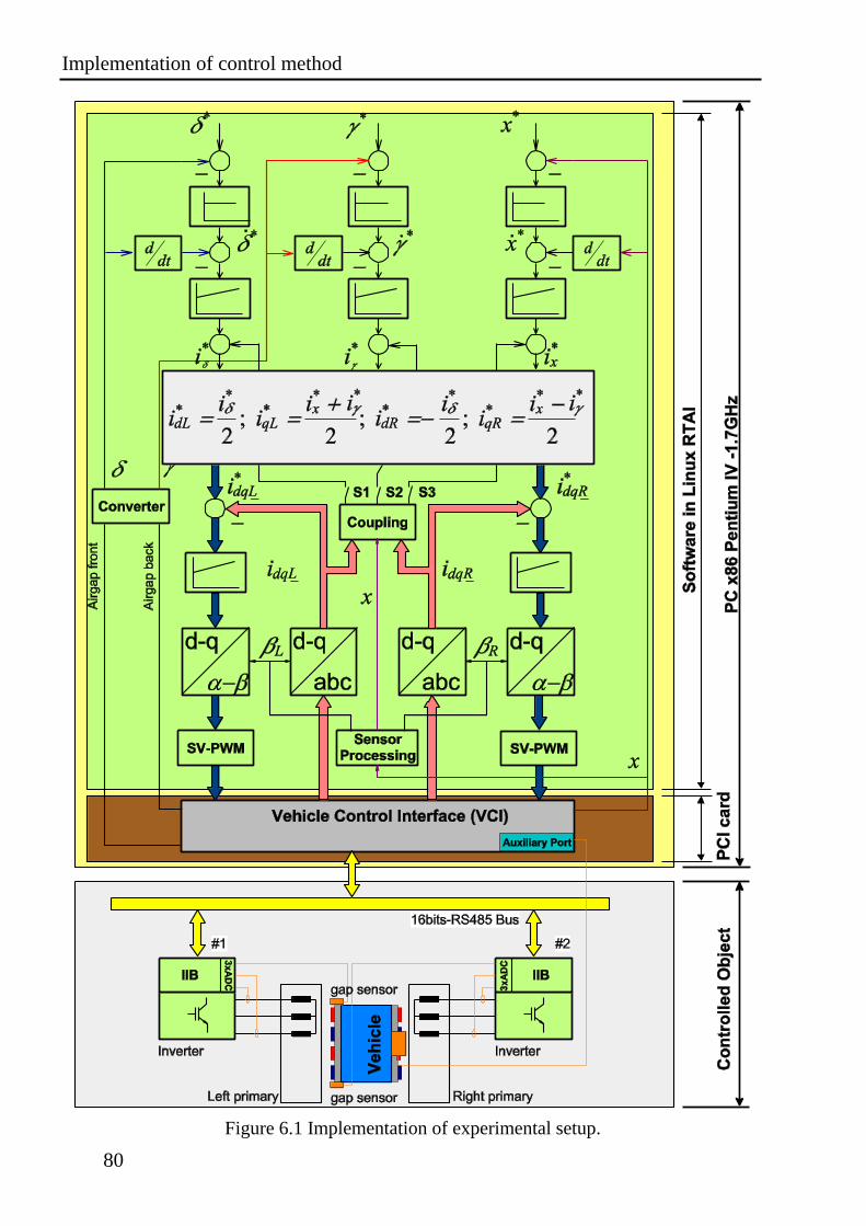
Implementation of control method
80
Figure 6.1 Implementation of experimental setup.
MAGNETIC GUIDANCE EXPERIMENTS
81
receives incremental signals from the position encoder through an auxiliary port. This
exchange of data with inverters of one segment and the control software takes place
every 100 s under control of an interrupt service routine (ISR). The VCI generates
one interrupt request (IRQ) to communicate with inverters of each segment every
100 s . Therefore, the sampling time of each inverter control loop is 100 s .
The control PC works under Linux Soho kernel 2.6.18 operating system with
RTAI patch. The control program was written in C language. The user interface was
programmed by Glade program for GTK+ toolkit. Regarding the control software, the
algorithm was implemented as shown by the light green area in Figure 6.1. As
mentioned in the previous chapter, the current controls were implemented by using
the field oriented control algorithm with anti-windup PI controllers. The details are
depicted in appendix B3. The other superposed control loops were also implemented
with PI controller for speed loops and P controller for position loops as shown in the
figure. Decoupling control can be applied by enabling switches S1, S2 and S3.
6.2. Lateral position control
With the implemented prototype above, the proposed control method was
implemented and tested step by step. At first, the controller for each DOF was
implemented in the control program. In this section, the experiment with the
controllers in lateral position control loops will be presented.
In this experiment, the vehicle was kept parallel with the guide-way in a
longitudinal position by the same mechanical structure used for the normal force
measuring experiment (Figure 4.12, Figure 4.13). Only the lateral position ( ) of the
structure could move freely in the y -direction under the limitation of two stators. The
two other DOFs ( and x ) were constrained in fixed positions. This arrangement
enables the lateral position controller to be tested independently in the experimental
system.
The control method was implemented only in lateral position loops with P
controller for lateral position and PI controller for lateral speed as presented in
chapter 5. The reference values for current control loops were implemented by the
left- and right- dq currents:
*
2dL dR
ii i (6.1)
0qL qRi i (6.2)
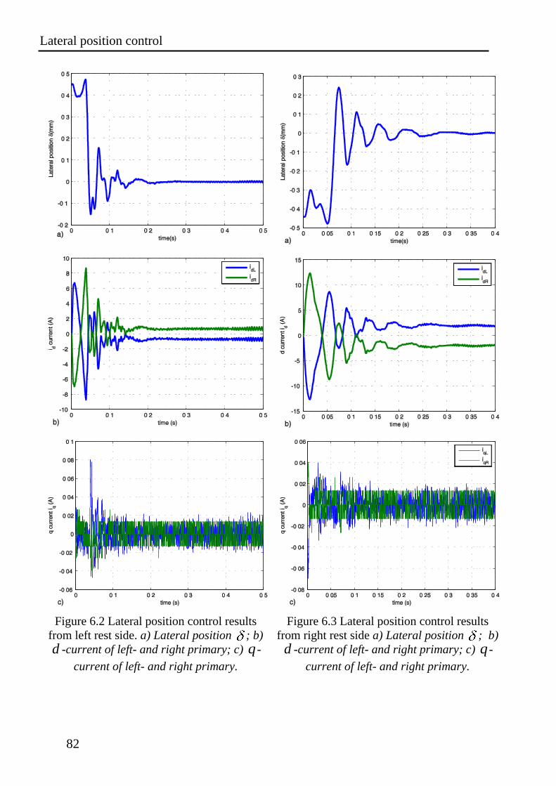
Lateral position control
82
Figure 6.2 Lateral position control results
from left rest side. a) Lateral position ; b)
d -current of left- and right primary; c) q -
current of left- and right primary.
Figure 6.3 Lateral position control results
from right rest side a) Lateral position ; b)
d -current of left- and right primary; c) q -
current of left- and right primary.
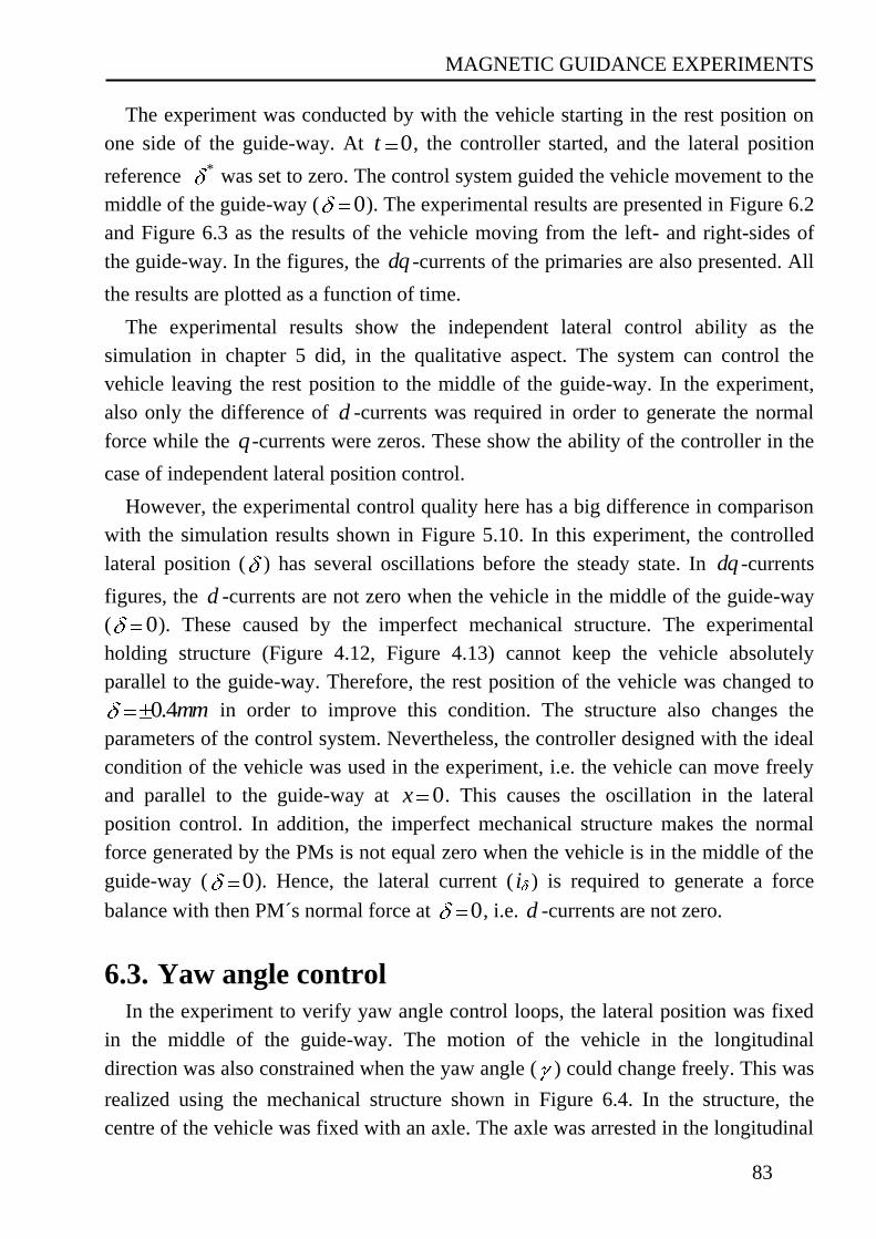
MAGNETIC GUIDANCE EXPERIMENTS
83
The experiment was conducted by with the vehicle starting in the rest position on
one side of the guide-way. At 0t , the controller started, and the lateral position
reference * was set to zero. The control system guided the vehicle movement to the
middle of the guide-way ( 0). The experimental results are presented in Figure 6.2
and Figure 6.3 as the results of the vehicle moving from the left- and right-sides of
the guide-way. In the figures, the dq -currents of the primaries are also presented. All
the results are plotted as a function of time.
The experimental results show the independent lateral control ability as the
simulation in chapter 5 did, in the qualitative aspect. The system can control the
vehicle leaving the rest position to the middle of the guide-way. In the experiment,
also only the difference of d -currents was required in order to generate the normal
force while the q -currents were zeros. These show the ability of the controller in the
case of independent lateral position control.
However, the experimental control quality here has a big difference in comparison
with the simulation results shown in Figure 5.10. In this experiment, the controlled
lateral position ( ) has several oscillations before the steady state. In dq -currents
figures, the d -currents are not zero when the vehicle in the middle of the guide-way
( 0). These caused by the imperfect mechanical structure. The experimental
holding structure (Figure 4.12, Figure 4.13) cannot keep the vehicle absolutely
parallel to the guide-way. Therefore, the rest position of the vehicle was changed to
0.4mm in order to improve this condition. The structure also changes the
parameters of the control system. Nevertheless, the controller designed with the ideal
condition of the vehicle was used in the experiment, i.e. the vehicle can move freely
and parallel to the guide-way at 0x . This causes the oscillation in the lateral
position control. In addition, the imperfect mechanical structure makes the normal
force generated by the PMs is not equal zero when the vehicle is in the middle of the
guide-way ( 0). Hence, the lateral current ( i ) is required to generate a force
balance with then PM´s normal force at 0, i.e. d -currents are not zero.
6.3. Yaw angle control
In the experiment to verify yaw angle control loops, the lateral position was fixed
in the middle of the guide-way. The motion of the vehicle in the longitudinal
direction was also constrained when the yaw angle ( ) could change freely. This was
realized using the mechanical structure shown in Figure 6.4. In the structure, the
centre of the vehicle was fixed with an axle. The axle was arrested in the longitudinal
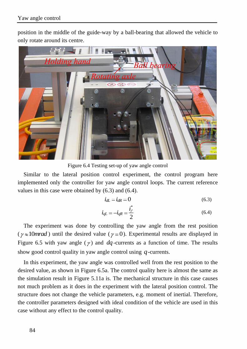
Yaw angle control
84
position in the middle of the guide-way by a ball-bearing that allowed the vehicle to
only rotate around its centre.
Figure 6.4 Testing set-up of yaw angle control
Similar to the lateral position control experiment, the control program here
implemented only the controller for yaw angle control loops. The current reference
values in this case were obtained by (6.3) and (6.4).
0dL dRi i (6.3)
*
2qL qR
ii i (6.4)
The experiment was done by controlling the yaw angle from the rest position
( 10mrad ) until the desired value ( 0). Experimental results are displayed in
Figure 6.5 with yaw angle ( ) and dq -currents as a function of time. The results
show good control quality in yaw angle control using q -currents.
In this experiment, the yaw angle was controlled well from the rest position to the
desired value, as shown in Figure 6.5a. The control quality here is almost the same as
the simulation result in Figure 5.11a is. The mechanical structure in this case causes
not much problem as it does in the experiment with the lateral position control. The
structure does not change the vehicle parameters, e.g. moment of inertial. Therefore,
the controller parameters designed with ideal condition of the vehicle are used in this
case without any effect to the control quality.
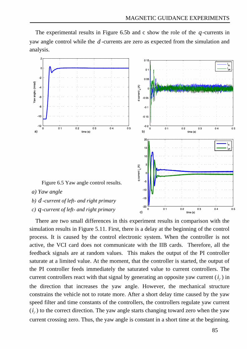
MAGNETIC GUIDANCE EXPERIMENTS
85
The experimental results in Figure 6.5b and c show the role of the q -currents in
yaw angle control while the d -currents are zero as expected from the simulation and
analysis.
Figure 6.5 Yaw angle control results.
a) Yaw angle
b) d -current of left- and right primary
c) q -current of left- and right primary
There are two small differences in this experiment results in comparison with the
simulation results in Figure 5.11. First, there is a delay at the beginning of the control
process. It is caused by the control electronic system. When the controller is not
active, the VCI card does not communicate with the IIB cards. Therefore, all the
feedback signals are at random values. This makes the output of the PI controller
saturate at a limited value. At the moment, that the controller is started, the output of
the PI controller feeds immediately the saturated value to current controllers. The
current controllers react with that signal by generating an opposite yaw current ( i ) in
the direction that increases the yaw angle. However, the mechanical structure
constrains the vehicle not to rotate more. After a short delay time caused by the yaw
speed filter and time constants of the controllers, the controllers regulate yaw current
( i ) to the correct direction. The yaw angle starts changing toward zero when the yaw
current crossing zero. Thus, the yaw angle is constant in a short time at the beginning.
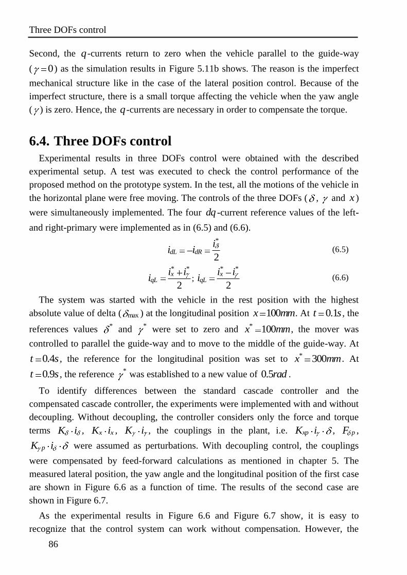
Three DOFs control
86
Second, the q-currents return to zero when the vehicle parallel to the guide-way
( 0) as the simulation results in Figure 5.11b shows. The reason is the imperfect
mechanical structure like in the case of the lateral position control. Because of the
imperfect structure, there is a small torque affecting the vehicle when the yaw angle
( ) is zero. Hence, the q -currents are necessary in order to compensate the torque.
6.4. Three DOFs control
Experimental results in three DOFs control were obtained with the described
experimental setup. A test was executed to check the control performance of the
proposed method on the prototype system. In the test, all the motions of the vehicle in
the horizontal plane were free moving. The controls of the three DOFs ( , and x )
were simultaneously implemented. The four dq -current reference values of the left-
and right-primary were implemented as in (6.5) and (6.6).
*
2dL dR
ii i (6.5)
* *
2
xqL
i ii ;
* *
2
xqL
i ii (6.6)
The system was started with the vehicle in the rest position with the highest
absolute value of delta ( max ) at the longitudinal position 100x mm. At 0.1t s , the
references values * and * were set to zero and * 100x mm, the mover was
controlled to parallel the guide-way and to move to the middle of the guide-way. At
0.4t s , the reference for the longitudinal position was set to * 300x mm. At
0.9t s , the reference * was established to a new value of 0.5rad .
To identify differences between the standard cascade controller and the
compensated cascade controller, the experiments were implemented with and without
decoupling. Without decoupling, the controller considers only the force and torque
terms K i , x xK i , K i , the couplings in the plant, i.e. xpK i , pF ,
pK i were assumed as perturbations. With decoupling control, the couplings
were compensated by feed-forward calculations as mentioned in chapter 5. The
measured lateral position, the yaw angle and the longitudinal position of the first case
are shown in Figure 6.6 as a function of time. The results of the second case are
shown in Figure 6.7.
As the experimental results in Figure 6.6 and Figure 6.7 show, it is easy to
recognize that the control system can work without compensation. However, the
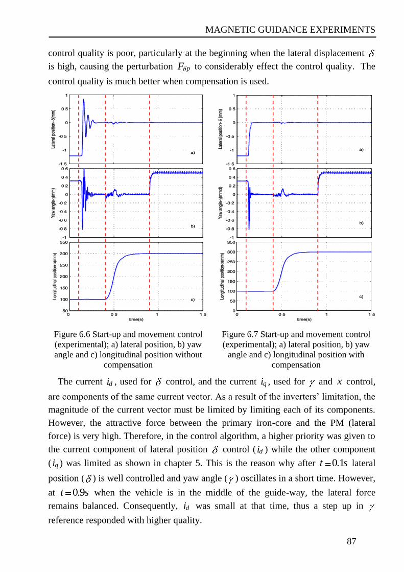
MAGNETIC GUIDANCE EXPERIMENTS
87
control quality is poor, particularly at the beginning when the lateral displacement
is high, causing the perturbation pF to considerably effect the control quality. The
control quality is much better when compensation is used.
Figure 6.6 Start-up and movement control
(experimental); a) lateral position, b) yaw
angle and c) longitudinal position without
compensation
Figure 6.7 Start-up and movement control
(experimental); a) lateral position, b) yaw
angle and c) longitudinal position with
compensation
The current di , used for control, and the current qi , used for and x control,
are components of the same current vector. As a result of the inverters’ limitation, the
magnitude of the current vector must be limited by limiting each of its components.
However, the attractive force between the primary iron-core and the PM (lateral
force) is very high. Therefore, in the control algorithm, a higher priority was given to
the current component of lateral position control ( di ) while the other component
( qi ) was limited as shown in chapter 5. This is the reason why after 0.1t s lateral
position ( ) is well controlled and yaw angle ( ) oscillates in a short time. However,
at 0.9t s when the vehicle is in the middle of the guide-way, the lateral force
remains balanced. Consequently, di was small at that time, thus a step up in
reference responded with higher quality.
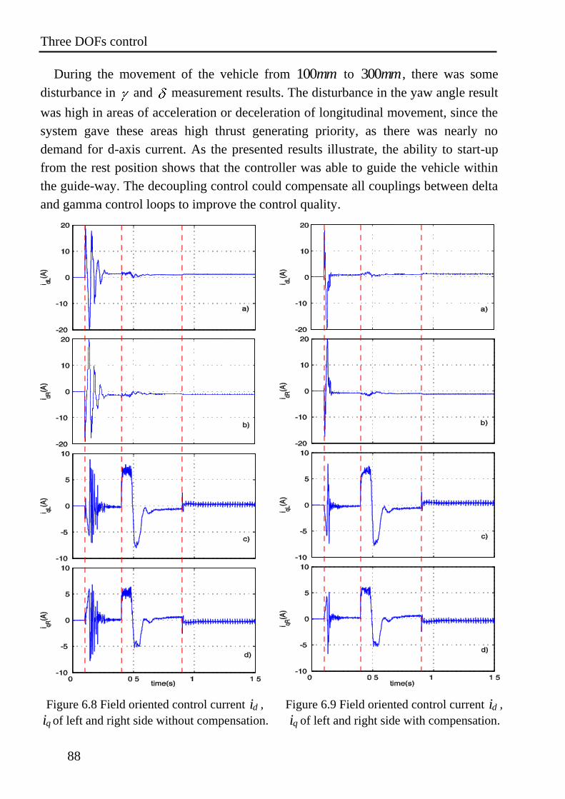
Three DOFs control
88
During the movement of the vehicle from 100mm to 300mm, there was some
disturbance in and measurement results. The disturbance in the yaw angle result
was high in areas of acceleration or deceleration of longitudinal movement, since the
system gave these areas high thrust generating priority, as there was nearly no
demand for d-axis current. As the presented results illustrate, the ability to start-up
from the rest position shows that the controller was able to guide the vehicle within
the guide-way. The decoupling control could compensate all couplings between delta
and gamma control loops to improve the control quality.
Figure 6.8 Field oriented control current di ,
qi of left and right side without compensation.
Figure 6.9 Field oriented control current di ,
qi of left and right side with compensation.
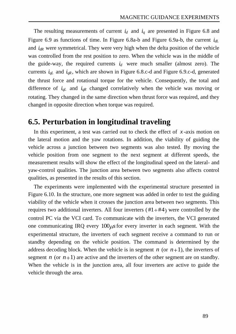
MAGNETIC GUIDANCE EXPERIMENTS
89
The resulting measurements of current di and qi are presented in Figure 6.8 and
Figure 6.9 as functions of time. In Figure 6.8a-b and Figure 6.9a-b, the current dLi
and dRi were symmetrical. They were very high when the delta position of the vehicle
was controlled from the rest position to zero. When the vehicle was in the middle of
the guide-way, the required currents di were much smaller (almost zero). The
currents qLi and qRi , which are shown in Figure 6.8.c-d and Figure 6.9.c-d, generated
the thrust force and rotational torque for the vehicle. Consequently, the total and
difference of qLi and qRi changed correlatively when the vehicle was moving or
rotating. They changed in the same direction when thrust force was required, and they
changed in opposite direction when torque was required.
6.5. Perturbation in longitudinal traveling
In this experiment, a test was carried out to check the effect of x -axis motion on
the lateral motion and the yaw rotations. In addition, the viability of guiding the
vehicle across a junction between two segments was also tested. By moving the
vehicle position from one segment to the next segment at different speeds, the
measurement results will show the effect of the longitudinal speed on the lateral- and
yaw-control qualities. The junction area between two segments also affects control
qualities, as presented in the results of this section.
The experiments were implemented with the experimental structure presented in
Figure 6.10. In the structure, one more segment was added in order to test the guiding
viability of the vehicle when it crosses the junction area between two segments. This
requires two additional inverters. All four inverters ( #1 #4) were controlled by the
control PC via the VCI card. To communicate with the inverters, the VCI generated
one communicating IRQ every 100 s for every inverter in each segment. With the
experimental structure, the inverters of each segment receive a command to run or
standby depending on the vehicle position. The command is determined by the
address decoding block. When the vehicle is in segment n (or 1n ), the inverters of
segment n (or 1n ) are active and the inverters of the other segment are on standby.
When the vehicle is in the junction area, all four inverters are active to guide the
vehicle through the area.
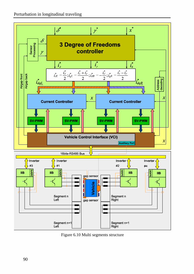
Perturbation in longitudinal traveling
90
Figure 6.10 Multi segments structure
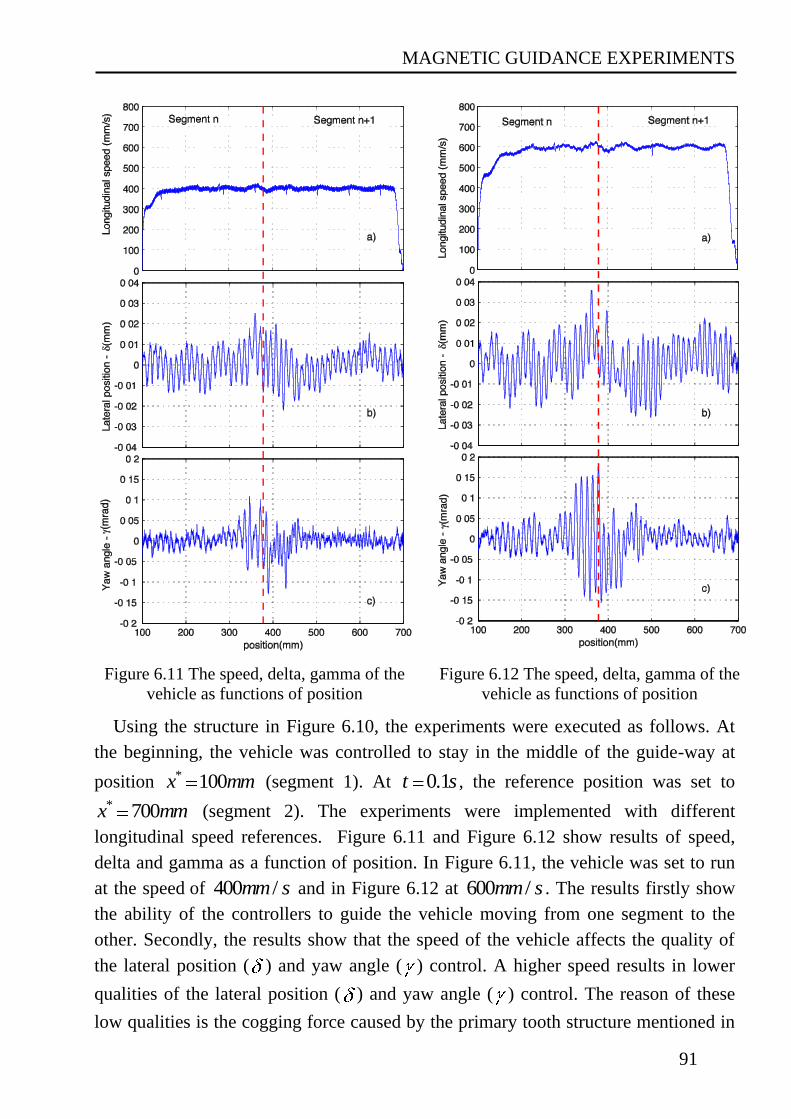
MAGNETIC GUIDANCE EXPERIMENTS
91
Figure 6.11 The speed, delta, gamma of the
vehicle as functions of position
Figure 6.12 The speed, delta, gamma of the
vehicle as functions of position
Using the structure in Figure 6.10, the experiments were executed as follows. At
the beginning, the vehicle was controlled to stay in the middle of the guide-way at
position * 100x mm (segment 1). At 0.1t s , the reference position was set to
* 700x mm (segment 2). The experiments were implemented with different
longitudinal speed references. Figure 6.11 and Figure 6.12 show results of speed,
delta and gamma as a function of position. In Figure 6.11, the vehicle was set to run
at the speed of 400 /mm s and in Figure 6.12 at 600 /mm s . The results firstly show
the ability of the controllers to guide the vehicle moving from one segment to the
other. Secondly, the results show that the speed of the vehicle affects the quality of
the lateral position ( ) and yaw angle ( ) control. A higher speed results in lower
qualities of the lateral position ( ) and yaw angle ( ) control. The reason of these
low qualities is the cogging force caused by the primary tooth structure mentioned in
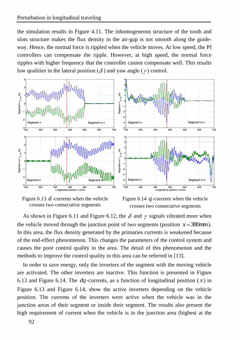
Perturbation in longitudinal traveling
92
the simulation results in Figure 4.11. The inhomogeneous structure of the tooth and
slots structure makes the flux density in the air-gap is not smooth along the guide-
way. Hence, the normal force is rippled when the vehicle moves. At low speed, the PI
controllers can compensate the ripple. However, at high speed, the normal force
ripples with higher frequency that the controller cannot compensate well. This results
low qualities in the lateral position ( ) and yaw angle ( ) control.
Figure 6.13 d -currents when the vehicle
crosses two consecutive segments
Figure 6.14 q -currents when the vehicle
crosses two consecutive segments
As shown in Figure 6.11 and Figure 6.12, the and signals vibrated more when
the vehicle moved through the junction point of two segments (position 380x mm).
In this area, the flux density generated by the primaries currents is weakened because
of the end-effect phenomenon. This changes the parameters of the control system and
causes the poor control quality in the area. The detail of this phenomenon and the
methods to improve the control quality in this area can be referred in [13].
In order to save energy, only the inverters of the segment with the moving vehicle
are activated. The other inverters are inactive. This function is presented in Figure
6.13 and Figure 6.14. The dq -currents, as a function of longitudinal position ( x ) in
Figure 6.13 and Figure 6.14, show the active inverters depending on the vehicle
position. The currents of the inverters were active when the vehicle was in the
junction areas of their segment or inside their segment. The results also present the
high requirement of current when the vehicle is in the junction area (highest at the

MAGNETIC GUIDANCE EXPERIMENTS
93
junction point presented by red dash line). This is the result of the reduced magneto
motive force (MMF) in the first and last pole of each primary, due to a lack of
windings [45]. The ripple in control currents is caused by the primaries’ tooth ripple
force.
Capacitive sensor structure
94
7. CAPACITIVE SENSOR In the magnetic guidance of the mover in a long-primary linear motor, the vehicle,
which was proposed as the short secondary of the linear motor, is controlled to run in
the middle of the guide-way by the primary magnet. The feedback signals required
for the control system are the lateral position , the yaw angle and the vehicle’s
longitudinal position x . The signals are provided by the sensors mounted in the linear
motor system.
With the desire to have a passive vehicle for industrial processing and material
handling applications, the active parts of the sensors must be mounted on the guide-
way: the static part of the system. That means neither information nor auxiliary
power between the surrounding environment and the vehicle must be exchanged. But
the inductive, eddy current based sensors which were used in the previous chapters
need both: energy and information transfer between the stationary and the moving
parts of the system. For this reason, a new sensor prototype for measuring lateral and
yaw values was designed and implemented in the magnetic guiding system. The new
sensor prototype does not need energy and information transfer between the
stationary and the moving parts of the system and was developed in order to replace
the industrial inductive sensors, which are used in the previous discussed
experiments. For longitudinal measurement, the sensor proposed in [52] and [53] can
be used.
To determine the lateral position and the yaw angle , we can use many
different sensor principles, particularly with the inductive principle or the capacitive
principle. In theory, several possible sensor prototypes can be used. In this
dissertation, we further develop the capacitive sensor concept to obtain a new
solution.
7.1. Capacitive sensor structure
7.1.1. Mechanical structure
In order to simultaneously measure the lateral position and the yaw angle as
the vehicle moves along the guide-way, the designed capacitive sensor is proposed to
consist of two symmetrical parts: the static part and the moving part. As mentioned,
the static part of the sensor was designed to be active with a connecting cable to
supply energy and to receive measuring signals. The moving part is simply a couple
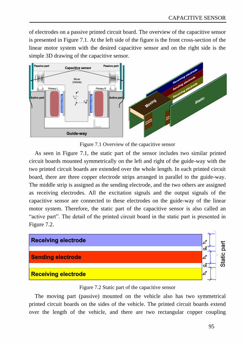
CAPACITIVE SENSOR
95
of electrodes on a passive printed circuit board. The overview of the capacitive sensor
is presented in Figure 7.1. At the left side of the figure is the front cross-section of the
linear motor system with the desired capacitive sensor and on the right side is the
simple 3D drawing of the capacitive sensor.
Figure 7.1 Overview of the capacitive sensor
As seen in Figure 7.1, the static part of the sensor includes two similar printed
circuit boards mounted symmetrically on the left and right of the guide-way with the
two printed circuit boards are extended over the whole length. In each printed circuit
board, there are three copper electrode strips arranged in parallel to the guide-way.
The middle strip is assigned as the sending electrode, and the two others are assigned
as receiving electrodes. All the excitation signals and the output signals of the
capacitive sensor are connected to these electrodes on the guide-way of the linear
motor system. Therefore, the static part of the capacitive sensor is also called an
“active part”. The detail of the printed circuit board in the static part is presented in
Figure 7.2.
Figure 7.2 Static part of the capacitive sensor
The moving part (passive) mounted on the vehicle also has two symmetrical
printed circuit boards on the sides of the vehicle. The printed circuit boards extend
over the length of the vehicle, and there are two rectangular copper coupling
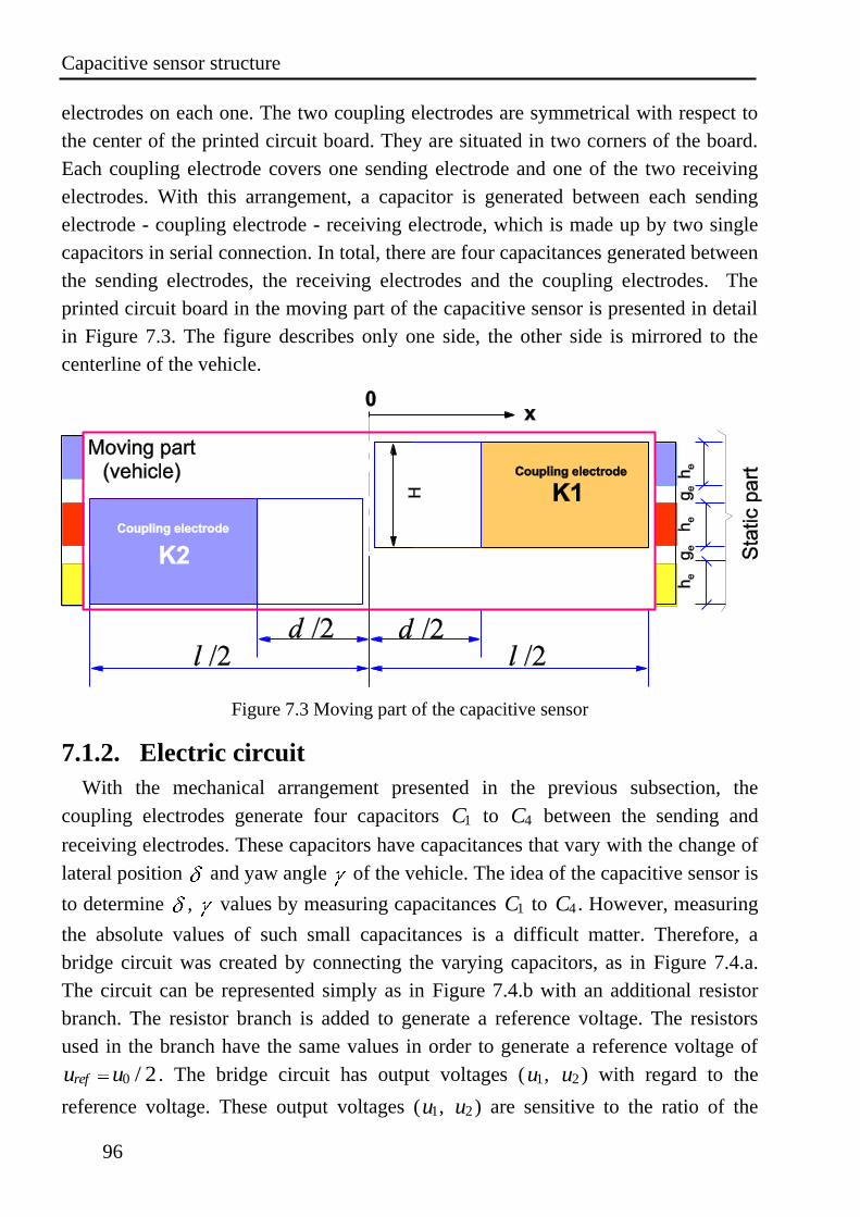
Capacitive sensor structure
96
electrodes on each one. The two coupling electrodes are symmetrical with respect to
the center of the printed circuit board. They are situated in two corners of the board.
Each coupling electrode covers one sending electrode and one of the two receiving
electrodes. With this arrangement, a capacitor is generated between each sending
electrode - coupling electrode - receiving electrode, which is made up by two single
capacitors in serial connection. In total, there are four capacitances generated between
the sending electrodes, the receiving electrodes and the coupling electrodes. The
printed circuit board in the moving part of the capacitive sensor is presented in detail
in Figure 7.3. The figure describes only one side, the other side is mirrored to the
centerline of the vehicle.
Figure 7.3 Moving part of the capacitive sensor
7.1.2. Electric circuit
With the mechanical arrangement presented in the previous subsection, the
coupling electrodes generate four capacitors 1C to 4C between the sending and
receiving electrodes. These capacitors have capacitances that vary with the change of
lateral position and yaw angle of the vehicle. The idea of the capacitive sensor is
to determine , values by measuring capacitances 1C to 4C . However, measuring
the absolute values of such small capacitances is a difficult matter. Therefore, a
bridge circuit was created by connecting the varying capacitors, as in Figure 7.4.a.
The circuit can be represented simply as in Figure 7.4.b with an additional resistor
branch. The resistor branch is added to generate a reference voltage. The resistors
used in the branch have the same values in order to generate a reference voltage of
0 / 2refu u . The bridge circuit has output voltages ( 1u , 2u ) with regard to the
reference voltage. These output voltages ( 1u , 2u ) are sensitive to the ratio of the
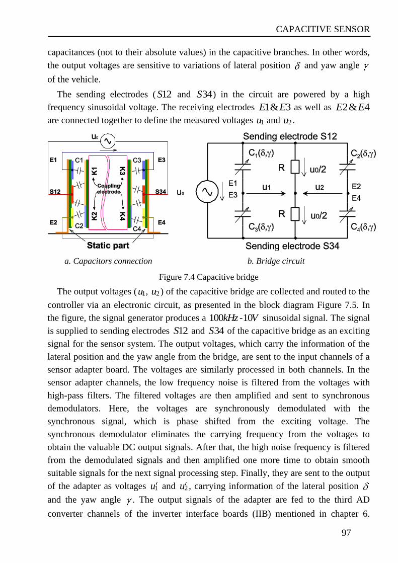
CAPACITIVE SENSOR
97
capacitances (not to their absolute values) in the capacitive branches. In other words,
the output voltages are sensitive to variations of lateral position and yaw angle
of the vehicle.
The sending electrodes ( 12S and 34S ) in the circuit are powered by a high
frequency sinusoidal voltage. The receiving electrodes 1& 3E E as well as 2& 4E E
are connected together to define the measured voltages 1u and 2u .
a. Capacitors connection b. Bridge circuit
Figure 7.4 Capacitive bridge
The output voltages ( 1u , 2u ) of the capacitive bridge are collected and routed to the
controller via an electronic circuit, as presented in the block diagram Figure 7.5. In
the figure, the signal generator produces a 100kHz -10V sinusoidal signal. The signal
is supplied to sending electrodes 12S and 34S of the capacitive bridge as an exciting
signal for the sensor system. The output voltages, which carry the information of the
lateral position and the yaw angle from the bridge, are sent to the input channels of a
sensor adapter board. The voltages are similarly processed in both channels. In the
sensor adapter channels, the low frequency noise is filtered from the voltages with
high-pass filters. The filtered voltages are then amplified and sent to synchronous
demodulators. Here, the voltages are synchronously demodulated with the
synchronous signal, which is phase shifted from the exciting voltage. The
synchronous demodulator eliminates the carrying frequency from the voltages to
obtain the valuable DC output signals. After that, the high noise frequency is filtered
from the demodulated signals and then amplified one more time to obtain smooth
suitable signals for the next signal processing step. Finally, they are sent to the output
of the adapter as voltages 1u and 2u , carrying information of the lateral position
and the yaw angle . The output signals of the adapter are fed to the third AD
converter channels of the inverter interface boards (IIB) mentioned in chapter 6.
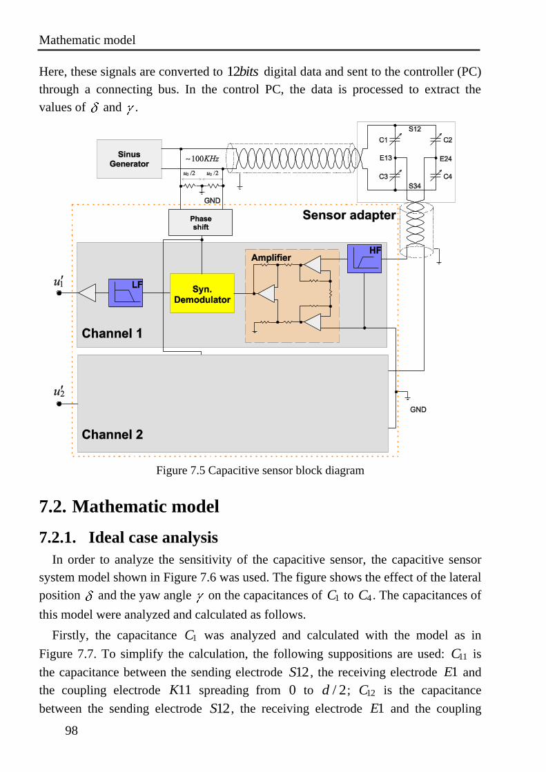
Mathematic model
98
Here, these signals are converted to 12bits digital data and sent to the controller (PC)
through a connecting bus. In the control PC, the data is processed to extract the
values of and .
Figure 7.5 Capacitive sensor block diagram
7.2. Mathematic model
7.2.1. Ideal case analysis
In order to analyze the sensitivity of the capacitive sensor, the capacitive sensor
system model shown in Figure 7.6 was used. The figure shows the effect of the lateral
position and the yaw angle on the capacitances of 1C to 4C . The capacitances of
this model were analyzed and calculated as follows.
Firstly, the capacitance 1C was analyzed and calculated with the model as in
Figure 7.7. To simplify the calculation, the following suppositions are used: 11C is
the capacitance between the sending electrode 12S , the receiving electrode 1E and
the coupling electrode 11K spreading from 0 to / 2d ; 12C is the capacitance
between the sending electrode 12S , the receiving electrode 1E and the coupling
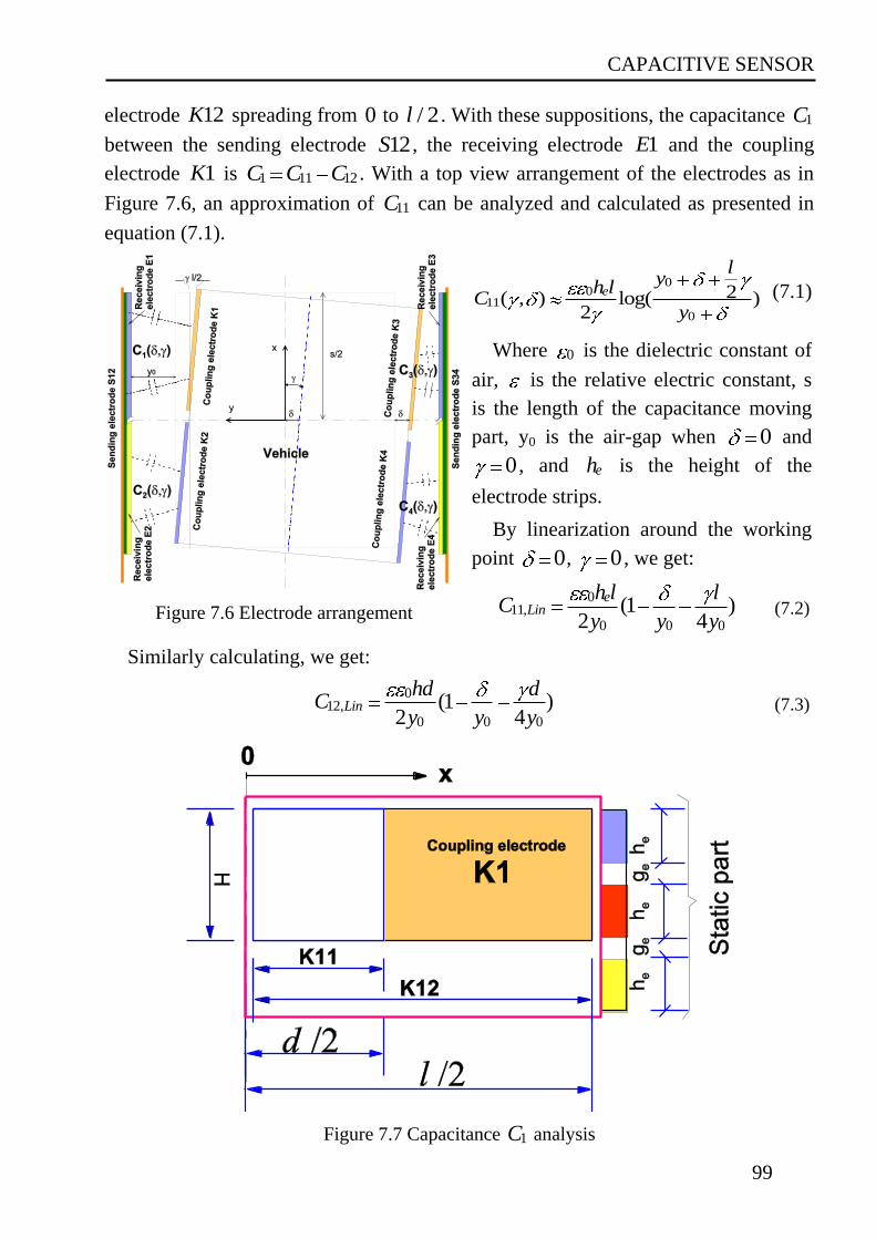
CAPACITIVE SENSOR
99
electrode 12K spreading from 0 to / 2l . With these suppositions, the capacitance 1C
between the sending electrode 12S , the receiving electrode 1E and the coupling
electrode 1K is 1 11 12C C C . With a top view arrangement of the electrodes as in
Figure 7.6, an approximation of 11C can be analyzed and calculated as presented in
equation (7.1).
Figure 7.6 Electrode arrangement
00
110
2( , ) log( )2
e
ly
h lC
y (7.1)
Where 0 is the dielectric constant of
air, is the relative electric constant, s
is the length of the capacitance moving
part, y0 is the air-gap when 0 and
0 , and eh is the height of the
electrode strips.
By linearization around the working
point 0, 0 , we get:
011,
0 0 0
(1 )2 4
eLin
h l lC
y y y (7.2)
Similarly calculating, we get:
012,
0 0 0
(1 )2 4
Linhd d
Cy y y
(7.3)
Figure 7.7 Capacitance 1C analysis
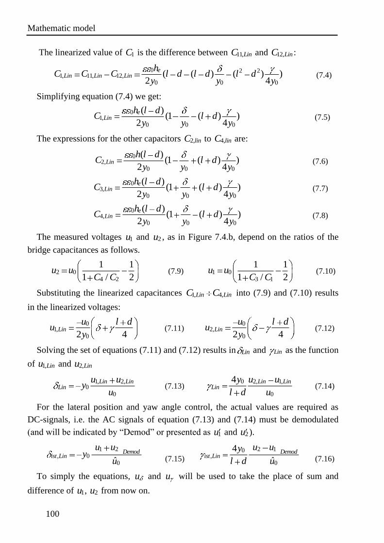
Mathematic model
100
The linearized value of 1C is the difference between 11,LinC and 12,LinC :
0 2 21, 11, 12,
0 0 0
( ( ) ( ) )2 4
eLin Lin Lin
hC C C l d l d l d
y y y (7.4)
Simplifying equation (7.4) we get:
01,
0 0 0
( )(1 ( ) )
2 4
eLin
h l dC l d
y y y (7.5)
The expressions for the other capacitors 2,linC to 4,linC are:
02,
0 0 0
( )(1 ( ) )
2 4Lin
h l dC l d
y y y (7.6)
03,
0 0 0
( )(1 ( ) )
2 4
eLin
h l dC l d
y y y (7.7)
04,
0 0 0
( )(1 ( ) )
2 4
eLin
h l dC l d
y y y (7.8)
The measured voltages 1u and 2u , as in Figure 7.4.b, depend on the ratios of the
bridge capacitances as follows.
2 04 2
1 1
1 / 2u u
C C (7.9) 1 0
3 1
1 1
1 / 2u u
C C (7.10)
Substituting the linearized capacitances 1, 4,Lin LinC C into (7.9) and (7.10) results
in the linearized voltages:
01,
02 4Lin
u l du
y (7.11)
02,
02 4Lin
u l du
y (7.12)
Solving the set of equations (7.11) and (7.12) results in Lin and Lin as the function
of 1,Linu and 2,Linu
1, 2,0
0
Lin LinLin
u uy
u (7.13)
0 2, 1,
0
4 Lin LinLin
y u u
l d u (7.14)
For the lateral position and yaw angle control, the actual values are required as
DC-signals, i.e. the AC signals of equation (7.13) and (7.14) must be demodulated
(and will be indicated by “Demod” or presented as 1u and 2u ).
1 2, 0
0ˆDemod
ist Lin
u uy
u
(7.15)
2 10,
0
4
ˆDemod
ist Lin
u uy
l d u
(7.16)
To simply the equations, u and u will be used to take the place of sum and
difference of 1u , 2u from now on.
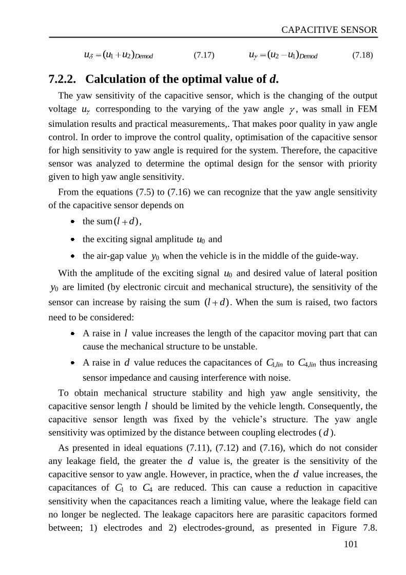
CAPACITIVE SENSOR
101
1 2( )Demodu u u (7.17) 2 1( )Demodu u u (7.18)
7.2.2. Calculation of the optimal value of d.
The yaw sensitivity of the capacitive sensor, which is the changing of the output
voltage u corresponding to the varying of the yaw angle , was small in FEM
simulation results and practical measurements,. That makes poor quality in yaw angle
control. In order to improve the control quality, optimisation of the capacitive sensor
for high sensitivity to yaw angle is required for the system. Therefore, the capacitive
sensor was analyzed to determine the optimal design for the sensor with priority
given to high yaw angle sensitivity.
From the equations (7.5) to (7.16) we can recognize that the yaw angle sensitivity
of the capacitive sensor depends on
the sum ( )l d ,
the exciting signal amplitude 0u and
the air-gap value 0y when the vehicle is in the middle of the guide-way.
With the amplitude of the exciting signal 0u and desired value of lateral position
0y are limited (by electronic circuit and mechanical structure), the sensitivity of the
sensor can increase by raising the sum ( )l d . When the sum is raised, two factors
need to be considered:
A raise in l value increases the length of the capacitor moving part that can
cause the mechanical structure to be unstable.
A raise in d value reduces the capacitances of 1,linC to 4,linC thus increasing
sensor impedance and causing interference with noise.
To obtain mechanical structure stability and high yaw angle sensitivity, the
capacitive sensor length l should be limited by the vehicle length. Consequently, the
capacitive sensor length was fixed by the vehicle’s structure. The yaw angle
sensitivity was optimized by the distance between coupling electrodes ( d ).
As presented in ideal equations (7.11), (7.12) and (7.16), which do not consider
any leakage field, the greater the d value is, the greater is the sensitivity of the
capacitive sensor to yaw angle. However, in practice, when the d value increases, the
capacitances of 1C to 4C are reduced. This can cause a reduction in capacitive
sensitivity when the capacitances reach a limiting value, where the leakage field can
no longer be neglected. The leakage capacitors here are parasitic capacitors formed
between; 1) electrodes and 2) electrodes-ground, as presented in Figure 7.8.
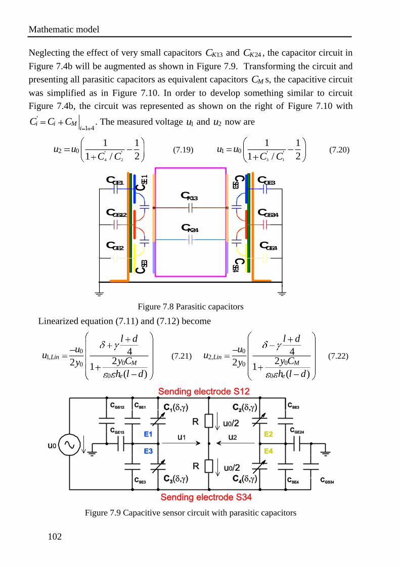
Mathematic model
102
Neglecting the effect of very small capacitors 13KC and 24KC , the capacitor circuit in
Figure 7.4b will be augmented as shown in Figure 7.9. Transforming the circuit and
presenting all parasitic capacitors as equivalent capacitors MC s, the capacitive circuit
was simplified as in Figure 7.10. In order to develop something similar to circuit
Figure 7.4b, the circuit was represented as shown on the right of Figure 7.10 with
'
1 4i i M
iC C C . The measured voltage 1u and 2u now are
4 2
2 0 ' '
1 1
21 /u u
C C (7.19)
3 1
1 0 ' '
1 1
21 /u u
C C (7.20)
CGE3
CGE4
CGS34
CGE1
CGS12
CGE2
C SE
1C S
E3
CSE3
CSE4
CK13
CK24
Figure 7.8 Parasitic capacitors
Linearized equation (7.11) and (7.12) become
01,
00
0
422 1
( )
LinM
e
l du
uy Cy
h l d
(7.21) 0
2,00
0
422 1
( )
LinM
e
l du
uy Cy
h l d
(7.22)
Figure 7.9 Capacitive sensor circuit with parasitic capacitors
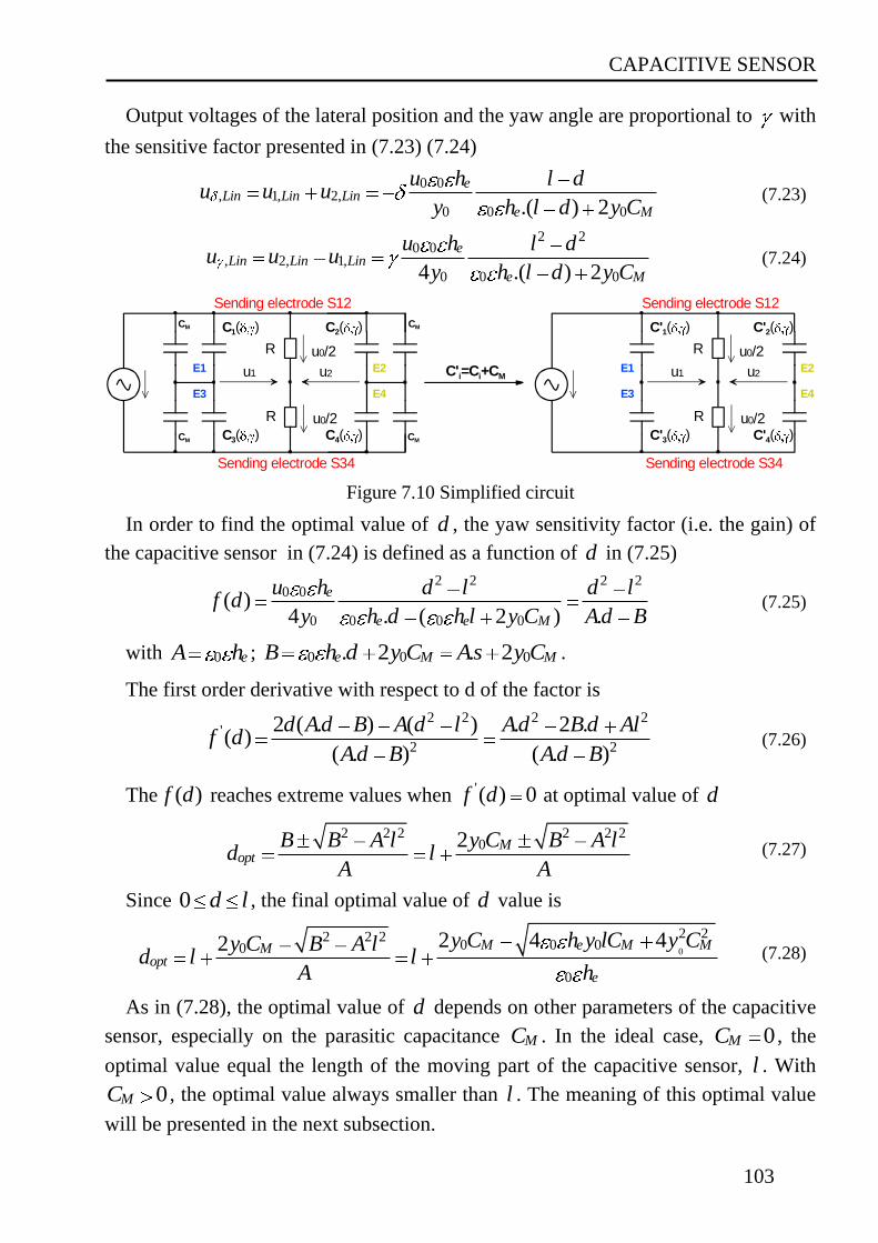
CAPACITIVE SENSOR
103
Output voltages of the lateral position and the yaw angle are proportional to with
the sensitive factor presented in (7.23) (7.24)
0 0, 1, 2,
0 0 0.( ) 2
eLin Lin Lin
e M
u h l du u u
y h l d y C (7.23)
2 20 0
, 2, 1,0 0 04 .( ) 2
eLin Lin Lin
e M
u h l du u u
y h l d y C (7.24)
R
R
u1 u2
u0/2
u0/2
Sending electrode S12
Sending electrode S34
E1
E3
E2
E4
C1( ) C2( )
C3( ) C4( )
CM
CM
CM
CM
R
R
u1 u2
u0/2
u0/2
Sending electrode S12
Sending electrode S34
E1
E3
E2
E4
C'1( ) C'2( )
C'3( ) C'4( )
C'i=Ci+CM
Figure 7.10 Simplified circuit
In order to find the optimal value of d , the yaw sensitivity factor (i.e. the gain) of
the capacitive sensor in (7.24) is defined as a function of d in (7.25)
2 2 2 20 0
0 0 0 0
( )4 . ( 2 ) .
e
e e M
u h d l d lf d
y h d h l y C Ad B (7.25)
with 0 eA h ; 0 0 0. 2 . 2e M MB h d y C As y C .
The first order derivative with respect to d of the factor is
2 2 2 2'
2 2
2 ( . ) ( ) . 2 .( )
( . ) ( . )
d Ad B A d l Ad B d Alf d
Ad B Ad B (7.26)
The ( )f d reaches extreme values when '( ) 0f d at optimal value of d
2 2 2 2 2 202 M
optB B A l y C B A l
d lA A
(7.27)
Since 0 d l , the final optimal value of d value is
0
2 22 2 20 0 00
0
2 4 42 M e M MMopt
e
y C h y lC y Cy C B A ld l l
A h (7.28)
As in (7.28), the optimal value of d depends on other parameters of the capacitive
sensor, especially on the parasitic capacitance MC . In the ideal case, 0MC , the
optimal value equal the length of the moving part of the capacitive sensor, l . With
0MC , the optimal value always smaller than l . The meaning of this optimal value
will be presented in the next subsection.
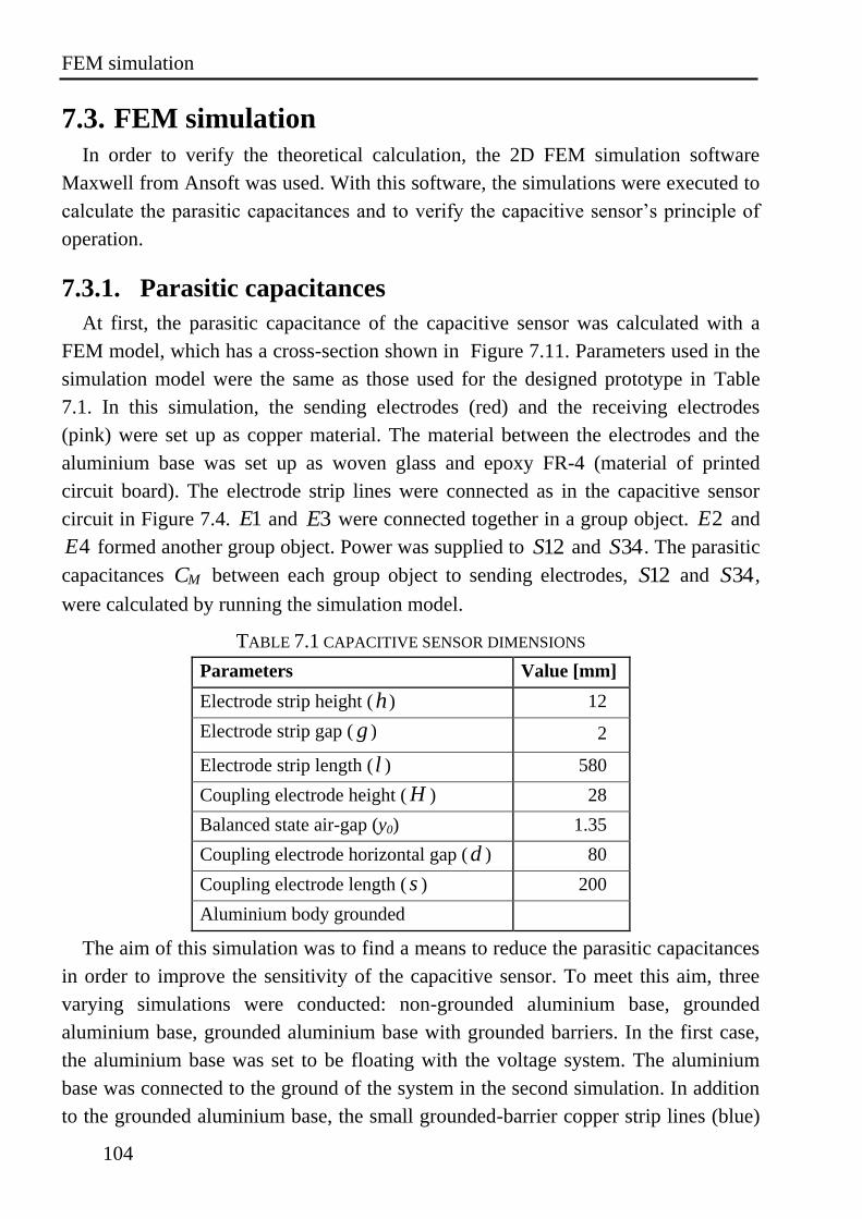
FEM simulation
104
7.3. FEM simulation
In order to verify the theoretical calculation, the 2D FEM simulation software
Maxwell from Ansoft was used. With this software, the simulations were executed to
calculate the parasitic capacitances and to verify the capacitive sensor’s principle of
operation.
7.3.1. Parasitic capacitances
At first, the parasitic capacitance of the capacitive sensor was calculated with a
FEM model, which has a cross-section shown in Figure 7.11. Parameters used in the
simulation model were the same as those used for the designed prototype in Table
7.1. In this simulation, the sending electrodes (red) and the receiving electrodes
(pink) were set up as copper material. The material between the electrodes and the
aluminium base was set up as woven glass and epoxy FR-4 (material of printed
circuit board). The electrode strip lines were connected as in the capacitive sensor
circuit in Figure 7.4. 1E and 3E were connected together in a group object. 2E and
4E formed another group object. Power was supplied to 12S and 34S . The parasitic
capacitances MC between each group object to sending electrodes, 12S and 34S ,
were calculated by running the simulation model.
TABLE 7.1 CAPACITIVE SENSOR DIMENSIONS
Parameters Value [mm]
Electrode strip height (h ) 12
Electrode strip gap ( g ) 2
Electrode strip length (l ) 580
Coupling electrode height ( H )
28
Balanced state air-gap (y0) 1.35
Coupling electrode horizontal gap ( d ) 80
Coupling electrode length ( s ) 200
Aluminium body grounded
The aim of this simulation was to find a means to reduce the parasitic capacitances
in order to improve the sensitivity of the capacitive sensor. To meet this aim, three
varying simulations were conducted: non-grounded aluminium base, grounded
aluminium base, grounded aluminium base with grounded barriers. In the first case,
the aluminium base was set to be floating with the voltage system. The aluminium
base was connected to the ground of the system in the second simulation. In addition
to the grounded aluminium base, the small grounded-barrier copper strip lines (blue)
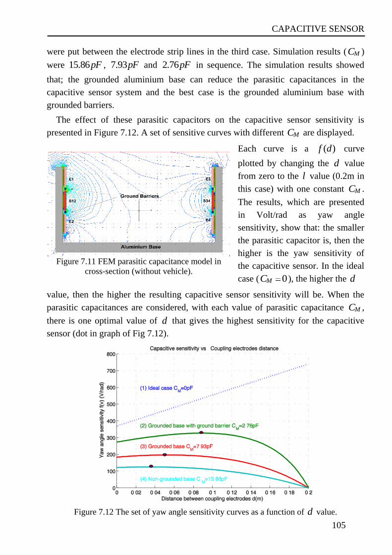
CAPACITIVE SENSOR
105
were put between the electrode strip lines in the third case. Simulation results ( MC )
were 15.86pF , 7.93pF and 2.76pF in sequence. The simulation results showed
that; the grounded aluminium base can reduce the parasitic capacitances in the
capacitive sensor system and the best case is the grounded aluminium base with
grounded barriers.
The effect of these parasitic capacitors on the capacitive sensor sensitivity is
presented in Figure 7.12. A set of sensitive curves with different MC are displayed.
Figure 7.11 FEM parasitic capacitance model in
cross-section (without vehicle).
Each curve is a ( )f d curve
plotted by changing the d value
from zero to the l value (0.2m in
this case) with one constant MC .
The results, which are presented
in Volt/rad as yaw angle
sensitivity, show that: the smaller
the parasitic capacitor is, then the
higher is the yaw sensitivity of
the capacitive sensor. In the ideal
case ( 0MC ), the higher the d
value, then the higher the resulting capacitive sensor sensitivity will be. When the
parasitic capacitances are considered, with each value of parasitic capacitance MC ,
there is one optimal value of d that gives the highest sensitivity for the capacitive
sensor (dot in graph of Fig 7.12).
Figure 7.12 The set of yaw angle sensitivity curves as a function of d value.
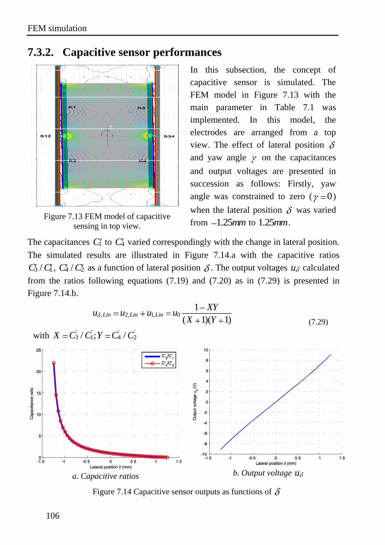
FEM simulation
106
7.3.2. Capacitive sensor performances
Figure 7.13 FEM model of capacitive
sensing in top view.
In this subsection, the concept of
capacitive sensor is simulated. The
FEM model in Figure 7.13 with the
main parameter in Table 7.1 was
implemented. In this model, the
electrodes are arranged from a top
view. The effect of lateral position
and yaw angle on the capacitances
and output voltages are presented in
succession as follows: Firstly, yaw
angle was constrained to zero ( 0)
when the lateral position was varied
from 1.25mm to 1.25mm.
The capacitances 1C to 4C varied correspondingly with the change in lateral position.
The simulated results are illustrated in Figure 7.14.a with the capacitive ratios
3 1/C C , 4 2/C C as a function of lateral position . The output voltages u calculated
from the ratios following equations (7.19) and (7.20) as in (7.29) is presented in
Figure 7.14.b.
, 2, 1, 01
( 1)( 1)Lin Lin Lin
XYu u u u
X Y
with ' '3 1/X C C ; ' '
4 2/Y C C
(7.29)
a. Capacitive ratios
b. Output voltage u
Figure 7.14 Capacitive sensor outputs as functions of
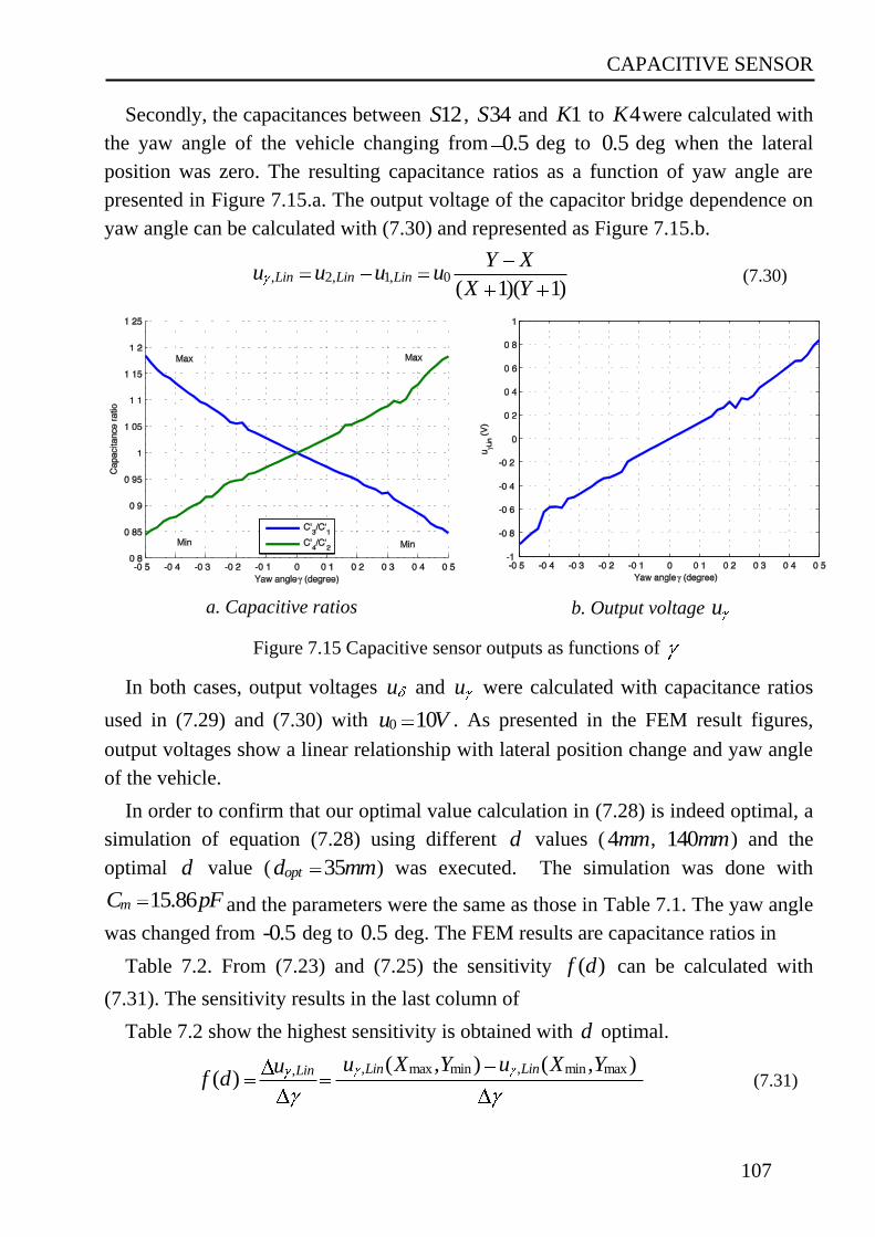
CAPACITIVE SENSOR
107
Secondly, the capacitances between 12S , 34S and 1K to 4K were calculated with
the yaw angle of the vehicle changing from 0.5 deg to 0.5 deg when the lateral
position was zero. The resulting capacitance ratios as a function of yaw angle are
presented in Figure 7.15.a. The output voltage of the capacitor bridge dependence on
yaw angle can be calculated with (7.30) and represented as Figure 7.15.b.
, 2, 1, 0( 1)( 1)
Lin Lin LinY X
u u u uX Y
(7.30)
a. Capacitive ratios
b. Output voltage u
Figure 7.15 Capacitive sensor outputs as functions of
In both cases, output voltages u and u were calculated with capacitance ratios
used in (7.29) and (7.30) with 0 10u V . As presented in the FEM result figures,
output voltages show a linear relationship with lateral position change and yaw angle
of the vehicle.
In order to confirm that our optimal value calculation in (7.28) is indeed optimal, a
simulation of equation (7.28) using different d values (4mm, 140mm) and the
optimal d value ( 35optd mm) was executed. The simulation was done with
15.86mC pF and the parameters were the same as those in Table 7.1. The yaw angle
was changed from -0.5 deg to 0.5 deg. The FEM results are capacitance ratios in
Table 7.2. From (7.23) and (7.25) the sensitivity ( )f d can be calculated with
(7.31). The sensitivity results in the last column of
Table 7.2 show the highest sensitivity is obtained with d optimal.
, max min , min max, ( , ) ( , )( )
Lin LinLin u X Y u X Yuf d (7.31)
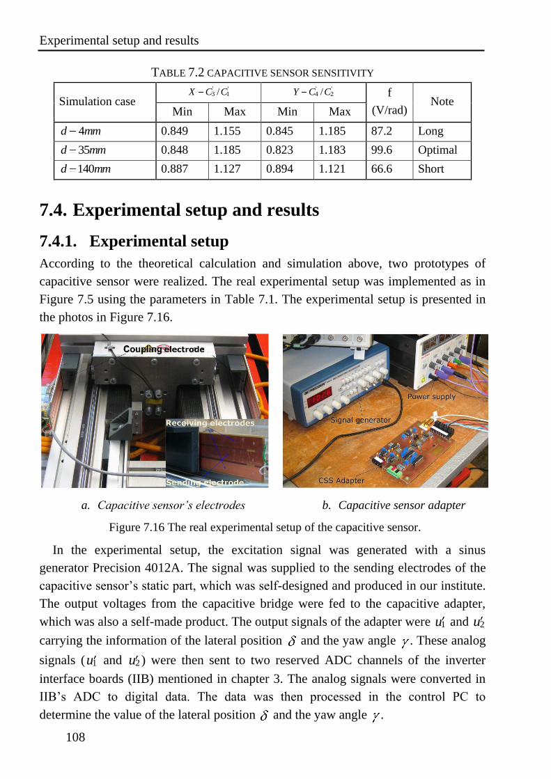
Experimental setup and results
108
TABLE 7.2 CAPACITIVE SENSOR SENSITIVITY
Simulation case
' '3 1/X C C ' '
4 2/Y C C f
(V/rad) Note
Min Max Min Max
4d mm 0.849 1.155 0.845 1.185 87.2 Long
35d mm 0.848 1.185 0.823 1.183 99.6 Optimal
140d mm 0.887 1.127 0.894 1.121 66.6 Short
7.4. Experimental setup and results
7.4.1. Experimental setup
According to the theoretical calculation and simulation above, two prototypes of
capacitive sensor were realized. The real experimental setup was implemented as in
Figure 7.5 using the parameters in Table 7.1. The experimental setup is presented in
the photos in Figure 7.16.
In the experimental setup, the excitation signal was generated with a sinus
generator Precision 4012A. The signal was supplied to the sending electrodes of the
capacitive sensor’s static part, which was self-designed and produced in our institute.
The output voltages from the capacitive bridge were fed to the capacitive adapter,
which was also a self-made product. The output signals of the adapter were 1u and 2u
carrying the information of the lateral position and the yaw angle . These analog
signals ( 1u and 2u ) were then sent to two reserved ADC channels of the inverter
interface boards (IIB) mentioned in chapter 3. The analog signals were converted in
IIB’s ADC to digital data. The data was then processed in the control PC to
determine the value of the lateral position and the yaw angle .
a. Capacitive sensor’s electrodes b. Capacitive sensor adapter
Figure 7.16 The real experimental setup of the capacitive sensor.
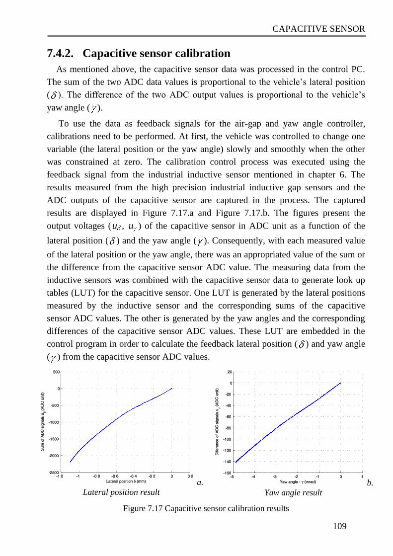
CAPACITIVE SENSOR
109
7.4.2. Capacitive sensor calibration
As mentioned above, the capacitive sensor data was processed in the control PC.
The sum of the two ADC data values is proportional to the vehicle’s lateral position
( ). The difference of the two ADC output values is proportional to the vehicle’s
yaw angle ( ).
To use the data as feedback signals for the air-gap and yaw angle controller,
calibrations need to be performed. At first, the vehicle was controlled to change one
variable (the lateral position or the yaw angle) slowly and smoothly when the other
was constrained at zero. The calibration control process was executed using the
feedback signal from the industrial inductive sensor mentioned in chapter 6. The
results measured from the high precision industrial inductive gap sensors and the
ADC outputs of the capacitive sensor are captured in the process. The captured
results are displayed in Figure 7.17.a and Figure 7.17.b. The figures present the
output voltages (u , u ) of the capacitive sensor in ADC unit as a function of the
lateral position ( ) and the yaw angle ( ). Consequently, with each measured value
of the lateral position or the yaw angle, there was an appropriated value of the sum or
the difference from the capacitive sensor ADC value. The measuring data from the
inductive sensors was combined with the capacitive sensor data to generate look up
tables (LUT) for the capacitive sensor. One LUT is generated by the lateral positions
measured by the inductive sensor and the corresponding sums of the capacitive
sensor ADC values. The other is generated by the yaw angles and the corresponding
differences of the capacitive sensor ADC values. These LUT are embedded in the
control program in order to calculate the feedback lateral position ( ) and yaw angle
( ) from the capacitive sensor ADC values.
a.
Lateral position result b.
Yaw angle result
Figure 7.17 Capacitive sensor calibration results
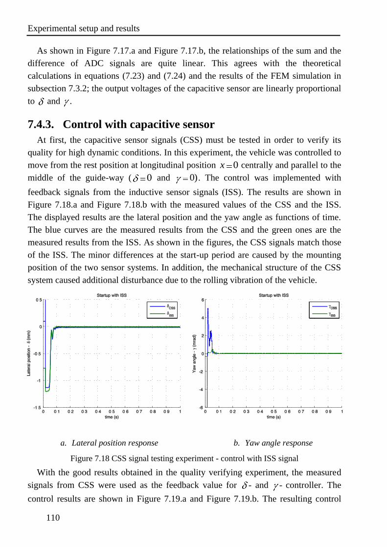
Experimental setup and results
110
As shown in Figure 7.17.a and Figure 7.17.b, the relationships of the sum and the
difference of ADC signals are quite linear. This agrees with the theoretical
calculations in equations (7.23) and (7.24) and the results of the FEM simulation in
subsection 7.3.2; the output voltages of the capacitive sensor are linearly proportional
to and .
7.4.3. Control with capacitive sensor
At first, the capacitive sensor signals (CSS) must be tested in order to verify its
quality for high dynamic conditions. In this experiment, the vehicle was controlled to
move from the rest position at longitudinal position 0x centrally and parallel to the
middle of the guide-way ( 0 and 0). The control was implemented with
feedback signals from the inductive sensor signals (ISS). The results are shown in
Figure 7.18.a and Figure 7.18.b with the measured values of the CSS and the ISS.
The displayed results are the lateral position and the yaw angle as functions of time.
The blue curves are the measured results from the CSS and the green ones are the
measured results from the ISS. As shown in the figures, the CSS signals match those
of the ISS. The minor differences at the start-up period are caused by the mounting
position of the two sensor systems. In addition, the mechanical structure of the CSS
system caused additional disturbance due to the rolling vibration of the vehicle.
a. Lateral position response b. Yaw angle response
Figure 7.18 CSS signal testing experiment - control with ISS signal
With the good results obtained in the quality verifying experiment, the measured
signals from CSS were used as the feedback value for - and - controller. The
control results are shown in Figure 7.19.a and Figure 7.19.b. The resulting control
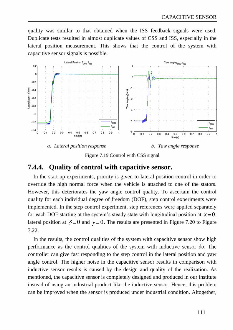
CAPACITIVE SENSOR
111
quality was similar to that obtained when the ISS feedback signals were used.
Duplicate tests resulted in almost duplicate values of CSS and ISS, especially in the
lateral position measurement. This shows that the control of the system with
capacitive sensor signals is possible.
a. Lateral position response b. Yaw angle response
Figure 7.19 Control with CSS signal
7.4.4. Quality of control with capacitive sensor.
In the start-up experiments, priority is given to lateral position control in order to
override the high normal force when the vehicle is attached to one of the stators.
However, this deteriorates the yaw angle control quality. To ascertain the control
quality for each individual degree of freedom (DOF), step control experiments were
implemented. In the step control experiment, step references were applied separately
for each DOF starting at the system’s steady state with longitudinal position at 0x ,
lateral position at 0 and 0 . The results are presented in Figure 7.20 to Figure
7.22.
In the results, the control qualities of the system with capacitive sensor show high
performance as the control qualities of the system with inductive sensor do. The
controller can give fast responding to the step control in the lateral position and yaw
angle control. The higher noise in the capacitive sensor results in comparison with
inductive sensor results is caused by the design and quality of the realization. As
mentioned, the capacitive sensor is completely designed and produced in our institute
instead of using an industrial product like the inductive sensor. Hence, this problem
can be improved when the sensor is produced under industrial condition. Altogether,
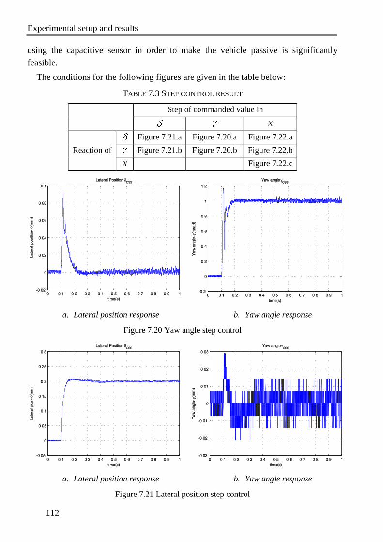
Experimental setup and results
112
using the capacitive sensor in order to make the vehicle passive is significantly
feasible.
The conditions for the following figures are given in the table below:
TABLE 7.3 STEP CONTROL RESULT
a. Lateral position response b. Yaw angle response
Figure 7.20 Yaw angle step control
a. Lateral position response b. Yaw angle response
Figure 7.21 Lateral position step control
Step of commanded value in
x
Reaction of
Figure 7.21.a Figure 7.20.a Figure 7.22.a
Figure 7.21.b Figure 7.20.b Figure 7.22.b
x Figure 7.22.c
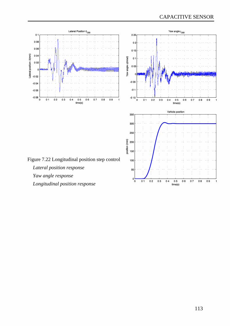
CAPACITIVE SENSOR
113
Figure 7.22 Longitudinal position step control
Lateral position response
Yaw angle response
Longitudinal position response
Summary
114
8. CONCLUSIONS To summarize the results of the “magnetic guidance for linear drives” research
presented in this thesis, as well as to mention the remaining research problems, the
summary and the future work are presented in this chapter.
8.1. Summary
In this thesis, an active magnetic guidance for the permanent magnet synchronous
linear motors (PMSLM) with long primary was researched. Applications like
transport and handling systems in industrial plant would specially profit from this
research. The thesis’s idea was the use of an active magnetic guidance for the lateral
displacement and the yaw angle, while keeping a mechanical guidance for the vertical
displacement. This gives an opportunity to simplify the complicated mechanical
assembly significantly without any higher complexity in electromagnetic actuators or
control. The active magnetic guidance was proposed with double side long-primary
PM SLM. In order to apply the proposed system in multi-mover plant transport and
handling systems, the long primaries should be divided into segments. Each segment
was driven by a dedicated inverter, which is controlled by a PC based controller.
The prototype based on the proposed idea was constructed and presented in
chapter 3. The prototype was realized using commercial PM SLMs from the company
Baumüller and commercial inverters from Siemens. The system control method was
implemented in a 1.7GHz PC running on Linux Soho operating system. The
communication between the PC based controller and the inverters was established
using the products developed at our institute.
Based on the proposed structure, the mathematical model of the magnetic guidance
system was analyzed. The calculations were based on the assumption of the
sinusoidal magnetic model and the synchronous dq -frame projection. The results
were the normal forces and the thrust on the vehicle as the functions of the lateral
position , the yaw angle and the primaries’ dq -currents. In order to verify the
mathematical calculation, 2D FEM simulations were carried out using Maxwell 2D
software from Ansoft company. The system was simulated for different operating
points of the vehicle such as in lateral position, longitudinal position and different
sinusoidal currents. Finally, the system was validated in a real prototype setup. The
results in three cases are quite close together. This confirms that the theoretical
CONCLUSIONS
115
calculations are correct. Consequently, the mathematical model can be used in design
calculations of the system’s controllers.
The verified mathematical calculations were used in order to design the controllers
for the system as presented in chapter 5. The control system used three standard
cascade control loops to control the lateral position , the yaw angle and the
longitudinal position x of the vehicle. In addition to the cascade control loops, the
decoupling control was suggested to give the improvement in control quality. The
control method was then successfully verified in the Matlab Simulink model.
The practical experiments were performed in chapter 6 by implementing the
control method on the proposed system. The experiments’ results show the successful
controls in each independent degree of freedom (DOF) of the vehicle as well as in the
three DOFs simultaneously. The control quality was also improved with the
implementation of the decoupling control. The successful transmission of the vehicle
from one segment to the other segment was presented at the end of the chapter. That
confirms the ability to use segmented structure in order to realize a multi-vehicle
system as aimed in the target of the study.
In chapter 7, a capacitive sensor for magnetic guidance PM SLMs with long
primary was presented. The capacitive sensor is a combination of the lateral position
sensor and the yaw angle sensor. The sensor was designed to have the active part
mounted on the static area of the system. With the design, the vehicle required no
connecting cable for the lateral position and yaw angle measurement. The
mathematical calculation and the FEM simulation prove the capacitive sensor’s
working ability. Consequently, prototypes of the capacitive sensor were incorporated
in the experimental setup. The capacitive sensor was installed to the system to supply
the feedback signals for the controller. The experimental results show the similar
control quality with the capacitive sensor in comparison to the inductive sensor.
Therefore, the capacitive sensor can replace the inductive sensor in order to make the
vehicle completely passive.
8.2. Future work
In order to apply the system to a plant transport and handling systems in industrial
manufacturing, some further research has to be done.
Firstly, a new method for the longitudinal position measurement needs to be
applied to get a completely passive vehicle. The position measurement can be done
by using either optical sensor or incremental sensor, with the encoding header on the
Future work
116
static part of the system. It has been studied and successful implemented at our
institute [52]. One other study of our institute can also be utilized for this case is the
use of capacitive sensor [53]. If these suggested methods are applied successfully to
the system, the vehicle will totally be passive with no connecting cable.
Secondly, the vehicle control quality, when the vehicle passing the junction
between two consecutive segments, has some small perturbation due to the end-effect
of the linear motor. That can be reduced with correct compensating currents. Hence,
mathematical calculation, FEM simulation and real experimental measurement of that
junction area must be studied in order to calculate the correct compensating current
for the linear motor.
Finally, the implementation of a multi-vehicle system requires not only the
segmented primary of the linear motor but also the segmented measuring sensor. In a
multi-vehicle system, each vehicle is controlled to move independently in one
segment. That means, each segment needs its own measuring system with three
sensing parameters: lateral position, yaw angle, longitudinal position.
Bibliography
117
Bibliography [1] E. R. Laithwaite. “Linear Electric Machines- A Personal View”, proceedings of
the IEEE, vol. 63, no. 2, February 1975
[2] R. C. Post. “The Page Locomotive: Federal Sponsorship of Invention in Mid-
19th-Century America.” Technology and Culture, vol. 13, pp. 140–169, 1972
[3] R. C. Post. Physics, Patents, and Politics: A Biography of Charles Grafton Page.
Science History Publications: New York, 1976.
[4] R. C. Post. “Stray Sparks from the Induction Coil: The Volta Prize and the Page
Patent.” Proceedings of the IEEE, pp. 1279–1286, 1976.
[5] U.S. Patent 782312
[6] G. Hugenberg. “Hermann Kemper Pionier der Magnetbahntechnik.” Standort -
Zeitschrift für angewandte Geographie, vol. 25, no. 1, pp. 52–53, 2001
[7] Linear Induktions Motoren - Mit Volldampf auf der Magnetwelle
http://www.coastersandmore.de/rides/lim/lim_lsm.shtml
[8] J. Pasanen, P. Jahkonen and S.J. Ovaska. “An integrated digital motion control
unit.”, IEEE Transactions on Instrumentation and Measurement, vol. 40, no 3,
pp. 654-657, Jun. 1991.
[9] T. Masuda, M. Yoshikawa, M. Tawada. “Formulation of elevator door equation
of motion.” JSME International Journal Series Dynamics Control Robotics
Design and Manufacturing, vol. 39, no. 2, pp. 279–285, 1996.
[10] R. Krishnan. “Propulsion with and without wheels.” in IEEE International
Conference on Industrial Technology (ICIT), vol. 1, no. 2, 2005, pp. 11–19.
[11] X. Liu, Y.Y. Ye, Z. Zheng. “A novel tubular permanent magnet linear
synchronous motor used for elevator door,” in Electrical Machines and Systems,
2007. ICEMS, Oct. 2007 pp. 801.
[12] M. Dursun, F. Koc and H. Ozbay. “Determination of Geometric Dimensions of a
Double Sided Linear Switched Reluctance Motor.” World Academy of Science,
Engineering and Technology, vol. 70, pp. 282–288, 2010.
[13] R. Benavides. “Investigation of Control Methods for Segmented Long Stator
Linear Drives”, PhD. Dissertation, TU Darmstadt, Germany, 2008.
[14] P. Mutschler. “Comparison of topologies for linear drives in industrial material
handling and processing applications,” in 7th International Conference on Power
Electronics ICPE '07, 2007, pp. 1027–1032.
[15] B. Sieber, J. Breil. “New developments for a linear motor system with multiple
carriers,” in Int. LDIA2003 Symp., 2003, pp. 21–24.
Future work
118
[16] C. Bosshard. “MagneTrak(c) Paradigmenwechsel im Materialhandling,” in 13.
Deutscher Materialfluss-Kongress Innovative Techniken für die Logistik. vol.
1815 Garching, Germany, 2004, pp. 189–200.
[17] G. Stöppler. “Segmentierte Langstator-Linearmotoren für die
Schnellpositionierung von Werkstückträgern in längsverketteten Montagelinien,”
in SPS/IPC/DRIVES/Electric Automation Systems and Components, Nürnberg,
Gemany, 2008.
[18] N.A. Duffi, R.D. Lorenz, L. Sanders. “High performance LIM based material
transfer,” in Proc. NSF Design and Manufacturing Systems Conference, Atlanta,
GA, Jan. 1992, pp.1027–1030.
[19] J. Boeij, M. Steinbuch and H. Gutiérrez. “Modelling the Electromechanical
Interactions in a Null-Flux EDS Maglev System.” Electromagnetic Launch
Technology, 12th Symposium, 2004.
[20] J. Boeij, M. Steinbuch and H. Gutiérrez. “Modeling the Electromechanical
Interactions in a Null-Flux Electrodynamic Maglev System.” IEEE transactions
on magnetics, vol. 41, no. 1, January 2005.
[21] D. Li and H. Gutiérrez. “Precise motion control of a hybrid magnetic suspension
actuator with large travel,” in Industrial Electronics, 2008. IECON 2008. 34th
Annual Conference of IEEE, Nov. 2008, pp. 2661–2666.
[22] S.O. Siems and W.-R. Canders. “Experimental investigation of linear and
rotatory HTSC bearings for industrial applications.” Int. Journal of Applied
Electromagnetics and Mechanics, vol. 19, pp. 199–202, 2004.
[23] C. Navau, A. Sanchez and E. Pardo. “Lateral Force in Permanent Magnet-
Superconductor Levitation Systems With High Critical Current.” IEEE
transactions on applied superconductivity, vol. 13, no. 2, June 2003.
[24] I.-Y.A Wang and I. Busch-Vishniac. “A new repulsive magnetic levitation
approach using permanent magnets and air-core electromagnets.” Magnetics,
IEEE Transactions, vol. 30 , no. 4 , Part: 2, 1994.
[25] K. Yoshida, Z. Dai and M. Sato. “Sensor-less Propulsion Control of PM LSM
Vehicle with DTC Method,” in Proceedings. IPEMC, 2000, pp. 191–196, vol.1
[26] K. Ben-Yahia and G. Henneberger. “Linear magnetic bearing for high speed
machine tools,” in PCIM 99, Nürnberg, 1999.
[27] W. Evers and G. Henneberger. “A New Linear Drive for a Magnetic Levitation
Transport System,” in EPE 99 Lausanne, 1999.
[28] D’Arrigo and A. Rufer. “Design of an integrated electromagnetic levitation and
guidance system for SwissMetro,” in EPE 99 Lausanne, 1999.
Bibliography
119
[29] D. Silva and O. Horikawa. “Experimental development of a one degree-of-
freedom controlled magnetic linear bearing.” IEEE transactions On Magnetics,
vol. 41, pp. 4257–4260, 2005.
[30] K. Yoshida, T. Yoshida and K. Noda. “Combined-Levitation-and-Propulsion
Control of SLIM Maglev Vehicle on Flexible Guideway,” in EPE2003 Toulouse,
2003.
[31] F. Profumo, A. Tenconi, G. Gianolio and K. Gigliotti. “Design and performance
evaluation of a PM linear synchronous motor with magnetic guides for industrial
applications,” in IEEE-IAS Annual Meeting, 1999, pp.110–116.
[32] F. Profumo, A. Tenconi, G. Gianolio and K. Gigliotti. “Parameters and forces of
a PM linear synchronous motor with magnetic guides for industrial applications:
computed and experimental results,” in IEEE-IAS Annual Meeting, Rome, 2000,
pp.15–20 vol.1.
[33] P.L. Jansen, L. J. Li and R.D. Lorenz. “Analysis of Competing Topologies of
Linear Induction Machines for High Speed Material Transport Systems,” in
IEEE-IAS Annual Meeting, Toronto, 1993, pp. 274–281.
[34] B. Yang, M. Henke and H. Grotstollen. “Pitch Analysis and Control Design for
the Linear Motor of a Railway Carriage,” in Industry Applications Conference,
Chicago, 2001, pp. 2360–2365 vol.4.
[35] B. Yang, M. Henke and H. Grotstollen. “Control Strategy for a Novel Combined
Operation of Long Stator and Short Stator Linear Drive System,” in European
Conference on Power Electronis and Applications, Toulouse, France, 2003.
[36] A. Pottharst, M. Henke and H. Grotstollen. “Power Supply Concept of the
Longstator Linear Motor of the NBP-Test Track,” in EPE-PEMC 2002
Dubrovnik & Cavtat, 2002, pp. P1-P5
[37] K. Yoshida, H. Takami, X. Kong and A. Sonoda. “Mass Reduction and
Propulsion Control for a Permanetn-Magnet Linear Synchronous Motor
Vehicle.” IEEE Transactions on Industry Applications, vol. 37, no. 1, Jan. 2001.
[38] K. Yoshida and X. Zhang. “Sensorless Guidance Congrol With Constant Airgap
In Ropeless Linear Elevator,” in Power Electronics and Motion Control
Conference, 2004, pp. 772 – 776, vol. 2.
[39] “MagneTrak®. Paradigmenwechsel im Material-handling. Elektromagnetische
Technologie für komplexe Materialflusssysteme,” http://www.translift.ch/.
[40] J. Weigel and P. Mutschler. “Acquisition Of A Permanent Magnet Synchronous
Linear Motor's Electrical Parameters And Dead Beat Current Control
Considering Saturation,” in IEMDC 2003, Madison Wisconsin, USA, 2003, pp.
791–798.
Future work
120
[41] J. Weigel and P. Mutschler. “Modelling and control of a permanent magnet linear
synchronous motor featuring unbalance and saturation including cross-
saturation,” in IEEE 35th Annual PESC, Jun. 2004, pp. 2204 –2210, vol.3
[42] J. Weigel and P. Mutschler. “Modellbildung und parameteradaptive
hochdynamische Regelung eines permanenterregten Synchronlinearmotors.”
PhD. dissertation, TU Darmstadt, Germany, 2004.
[43] J. Weigel and P. Mutschler. “Enhanced disturbance force rejection due to highly
dynamic parameter-adaptive control of saturated PM linear motor,” in IEEE-IAS
2005, Hong Kong, Oct. 2005, pp. 723–730 vol. 1.
[44] R. Benavides and P. Mutschler. “Controlling a System of Linear Drives,” in
IEEE-PESC 2005, Brazil, Jun. 2005, pp. 1587 – 1593.
[45] R. Benavides and P. Mutschler. “Compensation of Disturbances in Segmented
Long Stator Linear Drives using Finite Element Models,” in IEEE International
Symposium on Industrial Electronics ISIE, Jul. 2006, pp. 2445–2449.
[46] R. Benavides and P. Mutschler. “Improved application of resonant controllers for
compensation of cogging force ripple in long-stator Permanent-Magnet Linear
machines,” in Optimization of Electrical and Electronic Equipment, OPTIM,
May 2008, pp. 125–131.
[47] R. Leidhold and P. Mutschler. “Speed Sensorless Control of a Long-Stator
Linear Synchronous-Motor arranged by Multiple Sections,” in IEEE-IECON,
Raleigh, North Carolina USA, Nov. 2005, pp. 1395 – 1400.
[48] R. Leidhold, R. Benavides and P. Mutschler. “Comparison of control oriented
models for the Long Stator Synchronous Motor and their experimental
validation,” in SPEEDAM, Taormina, May 2006, pp. S22-18 – S22-23.
[49] R. Leidhold and P. Mutschler. “A Linear Synchronous Motor Model for
Evaluation of Sensorless Methods,” in IEEE - ISIE, Montreal Canada, Jul. 2006,
pp. 2467 – 2472.
[50] R. Leidhold and P. Mutschler. “Sensorless position-control method based on
magnetic saliencies for a Long-Stator Linear Synchronous-Motor,” in IEEE-
IECON 32nd
, Paris, Nov. 2006, pp. 781–786.
[51] R. Leidhold and P. Mutschler. “Implementation of Sensorless Methods in
Segmented Long Stator Synchronous Linear Motors,” in LDIA, Lille, France,
Sept. 2007, pp. 167–168.
[52] M. Mihalachi and P.Mutschler. “Evaluation of two position acquisition systems
for permanent magnet linear motors with passive movers,” in OPTIM, May 2008,
pp. 37–44.
Bibliography
121
[53] M. Mihalachi and P.Mutschler. “Position Acquisition for Long Primary Linear
Drives with Passive Vehicles, ” in IAS '08, Oct. 2008. pp. 1–8.
[54] R. Benavides. “Entwurf eines Kommunikationssystem, Parallel Bussystems auf
485-Basis. ” Diplomarbeit, TU Darmstadt, 2003.
[55] https://rtai.org
[56] P. Mutschler. Class lecture, Topic: “Control of Drives.” Institute of Power
Electronics and Control of Drives, TU Darmstadt, Sep. 2004.
[57] I.Boldea and S. A. Nasar. Linear electric actuators and generators. Cambridge
University Press, 1997, ISBN 0-521-48017-5.
[58] Texas Instrument Europe. “Field Orientated Control of 3-Phase AC-Motors”,
http://www.focus.ti.com/lit/an/bpra073/bpra073.pdf [Feb. 1998].
[59] Ansys. “Maxwell Electromagnetic Field Simulation for High-Performance
Electromechanical Design,” http://www.ansoft.com/products/em/maxwell/
[60] Wikipedia. “Finite element method,”
http://en.wikipedia.org/wiki/Finite_element_method
[61] D. Schröder. Elektrische Antriebe 2. Springer-Verlag Berlin – Heidelberg – New
York, 1995, ISBN 3-540-57610-X
[62] P. Mutschler. Practical training, Topic: “S2 - AC drive with voltage source
inverter (VSI).” Institute of Power Electronics and Control of Drives, TU
Darmstadt, Sep. 2003.
[63] I. Müller. Practical training, Topic: “S3 - Field oriented control.” Institute of
Power Electronics and Control of Drives, TU Darmstadt, 2003-2004.
[64] O. Föllinger. Regelungstechnik – Einführung in die Methoden und Ihre
Anwendung. Hüthig Verlag, Heidelberg, 1994.
[65] R.Benavides and P.Mutschler. “Control Techniques to Compensate Detent
Forces in Segmented Long Stator Linear Motors,” in LDIA, Lille, France, Sep.
2007, pp. 160-161.
[66] R. Benavides and P. Mutschler. “Detent force compensation in Segmented Long
Stator Permanent Magnet Linear Drives using Finite Element Models,” in 12th
European Conference on Power Electronics and Applications, EPE 2007,
Aalborg, Denmark, Sep. 2007, pp. DS3.5, topic 10
[67] R. Benavides and P. Mutschler. “Comparison of field oriented control and
indirect flux control applied to segmented long stator linear machine,” in PCIM
2007, Nürnberg, May 2007, pp. S3d (p.8).
[68] J. F. Gieras and Z. J. Piech. Linear synchronous motor: Transportation and
Automation Systems. CRC Press 2000, ISBN: 0-8493-1859-7
Future work
122
[69] D. Schröder. Intelligent Observer and Control Design for Nonlinear Systems.
Springer, Berlin – Heidelberg – New York, 2000, ISBN-10: 3-540-63639-0.
[70] P. Vas. Vector control of AC machines. Clarendon Press - Oxford University,
New York, 1990, ISBN 10: 0-198-59370-8
[71] R. Isermann, K. H. Lachmann and D. Matko. Adaptive Control Systems.
Prentice-Hall, 1993, ISBN-10: 0-131-37456-7.
[72] U. Tietze, C. Schenk, E. Gamm. Electronic Circuits: Handbook for Design and
Application. Springer Verlag, 2007, ISBN: 978-3-540-00429-5
[73] L. K. Baxter. Capacitive Sensors: Design and Applications. IEEE Press -1996,
ISBN-10: 0-780-31130-2.
[74] http://www.magnemotion.com
[75] Siemens. SIMODRIVE 611 digital Drive Converters Configuration Manual. Feb.
2007.
[76] M. Mihalachi. “Software Implementation for FVA 445 Project,” Institute für
Stromrichtertechnik und Antriebsregelung, TU Darmstadt, Feb. 2008
[77] P. Khong, R. Leidhold and P. Mutschler. “Magnetic guidance of the mover in a
long-primary linear motor” Accepted for publication in Industry Applications,
IEEE Transactions - electronic publishing, DOI: 10.1109/TIA.2011.2125934,
Mar. 2011.
[78] P. Khong, R. Leidhold and P. Mutschler. “Magnetic guidance of the mover in a
long-primary linear motor,” in IEEE-ECCE 2009, San Jose, CA Sept. 2009, pp.
2354-2361
[79] P. Khong, R. Leidhold and P. Mutschler. “Magnetic guiding and capacitive
sensing for a passive vehicle of a long-primary linear motor,” in EPE/PEMC
2010, Ohrid - Macedonia, Sept. 2010, pp. S3-1 – S3-8.
[80] P. Khong, R. Leidhold and P. Mutschler. “Capacitive gap and yaw angle sensor
for linear drives,” in IECON 2010, Glendale – AZ, Nov. 2010, pp. 1240 – 1245.
[81] Baumüller. LSE Synchronous Linear Motors Documentation. Jul. 2002
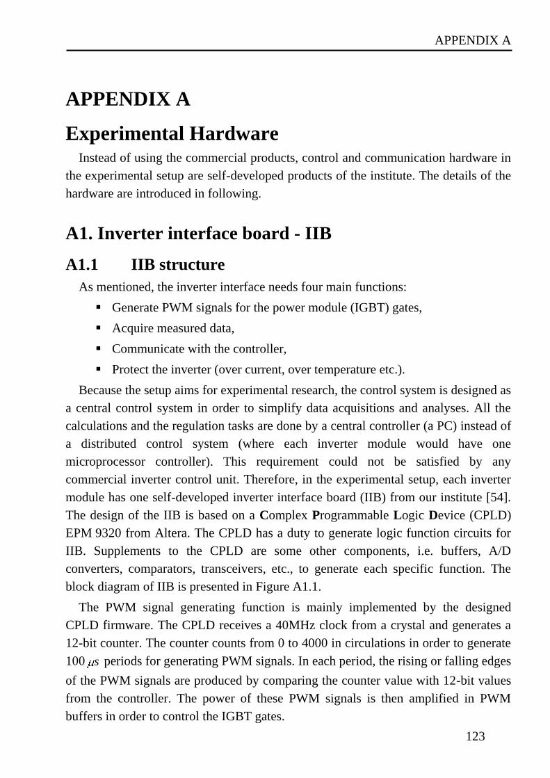
APPENDIX A
123
APPENDIX A
Experimental Hardware Instead of using the commercial products, control and communication hardware in
the experimental setup are self-developed products of the institute. The details of the
hardware are introduced in following.
A1. Inverter interface board - IIB
A1.1 IIB structure
As mentioned, the inverter interface needs four main functions:
Generate PWM signals for the power module (IGBT) gates,
Acquire measured data,
Communicate with the controller,
Protect the inverter (over current, over temperature etc.).
Because the setup aims for experimental research, the control system is designed as
a central control system in order to simplify data acquisitions and analyses. All the
calculations and the regulation tasks are done by a central controller (a PC) instead of
a distributed control system (where each inverter module would have one
microprocessor controller). This requirement could not be satisfied by any
commercial inverter control unit. Therefore, in the experimental setup, each inverter
module has one self-developed inverter interface board (IIB) from our institute [54].
The design of the IIB is based on a Complex Programmable Logic Device (CPLD)
EPM 9320 from Altera. The CPLD has a duty to generate logic function circuits for
IIB. Supplements to the CPLD are some other components, i.e. buffers, A/D
converters, comparators, transceivers, etc., to generate each specific function. The
block diagram of IIB is presented in Figure A1.1.
The PWM signal generating function is mainly implemented by the designed
CPLD firmware. The CPLD receives a 40MHz clock from a crystal and generates a
12-bit counter. The counter counts from 0 to 4000 in circulations in order to generate
100 s periods for generating PWM signals. In each period, the rising or falling edges
of the PWM signals are produced by comparing the counter value with 12-bit values
from the controller. The power of these PWM signals is then amplified in PWM
buffers in order to control the IGBT gates.
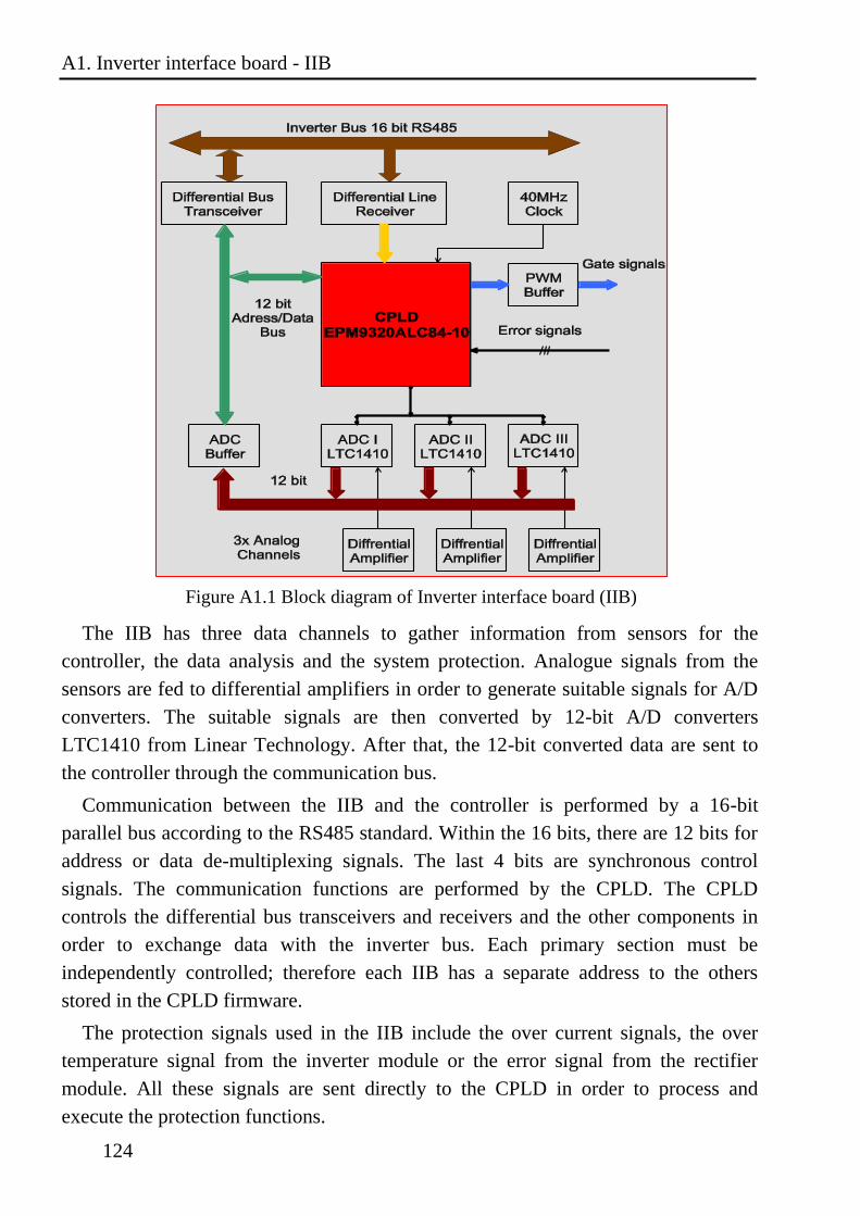
A1. Inverter interface board - IIB
124
The IIB has three data channels to gather information from sensors for the
controller, the data analysis and the system protection. Analogue signals from the
sensors are fed to differential amplifiers in order to generate suitable signals for A/D
converters. The suitable signals are then converted by 12-bit A/D converters
LTC1410 from Linear Technology. After that, the 12-bit converted data are sent to
the controller through the communication bus.
Communication between the IIB and the controller is performed by a 16-bit
parallel bus according to the RS485 standard. Within the 16 bits, there are 12 bits for
address or data de-multiplexing signals. The last 4 bits are synchronous control
signals. The communication functions are performed by the CPLD. The CPLD
controls the differential bus transceivers and receivers and the other components in
order to exchange data with the inverter bus. Each primary section must be
independently controlled; therefore each IIB has a separate address to the others
stored in the CPLD firmware.
The protection signals used in the IIB include the over current signals, the over
temperature signal from the inverter module or the error signal from the rectifier
module. All these signals are sent directly to the CPLD in order to process and
execute the protection functions.
Figure A1.1 Block diagram of Inverter interface board (IIB)
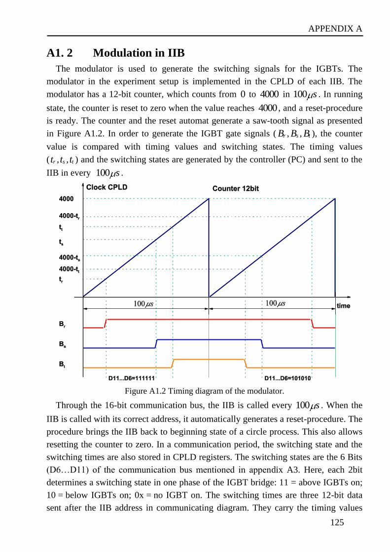
APPENDIX A
125
A1. 2 Modulation in IIB
The modulator is used to generate the switching signals for the IGBTs. The
modulator in the experiment setup is implemented in the CPLD of each IIB. The
modulator has a 12-bit counter, which counts from 0 to 4000 in 100 s . In running
state, the counter is reset to zero when the value reaches 4000 , and a reset-procedure
is ready. The counter and the reset automat generate a saw-tooth signal as presented
in Figure A1.2. In order to generate the IGBT gate signals ( rB , sB , tB ), the counter
value is compared with timing values and switching states. The timing values
( rt , st , tt ) and the switching states are generated by the controller (PC) and sent to the
IIB in every 100 s .
Figure A1.2 Timing diagram of the modulator.
Through the 16-bit communication bus, the IIB is called every 100 s . When the
IIB is called with its correct address, it automatically generates a reset-procedure. The
procedure brings the IIB back to beginning state of a circle process. This also allows
resetting the counter to zero. In a communication period, the switching state and the
switching times are also stored in CPLD registers. The switching states are the 6 Bits
(D6…D11) of the communication bus mentioned in appendix A3. Here, each 2bit
determines a switching state in one phase of the IGBT bridge: 11 = above IGBTs on;
10 = below IGBTs on; 0x = no IGBT on. The switching times are three 12-bit data
sent after the IIB address in communicating diagram. They carry the timing values
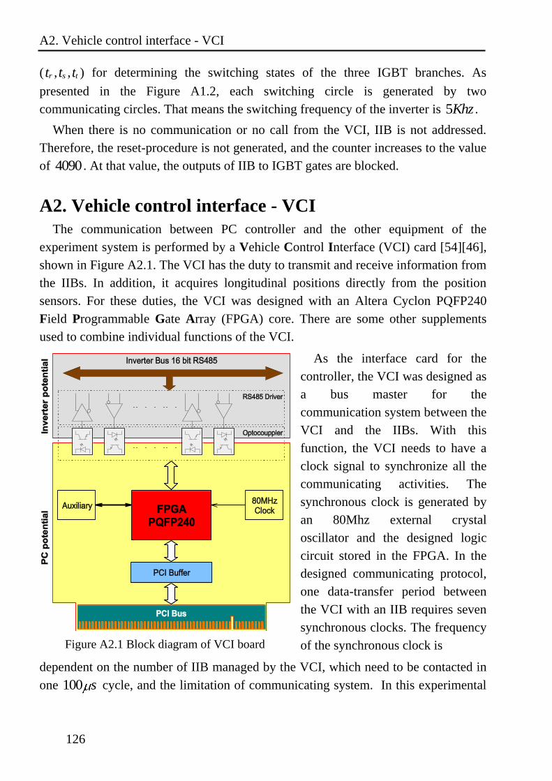
A2. Vehicle control interface - VCI
126
( rt , st , tt ) for determining the switching states of the three IGBT branches. As
presented in the Figure A1.2, each switching circle is generated by two
communicating circles. That means the switching frequency of the inverter is 5Khz .
When there is no communication or no call from the VCI, IIB is not addressed.
Therefore, the reset-procedure is not generated, and the counter increases to the value
of 4090 . At that value, the outputs of IIB to IGBT gates are blocked.
A2. Vehicle control interface - VCI
The communication between PC controller and the other equipment of the
experiment system is performed by a Vehicle Control Interface (VCI) card [54][46],
shown in Figure A2.1. The VCI has the duty to transmit and receive information from
the IIBs. In addition, it acquires longitudinal positions directly from the position
sensors. For these duties, the VCI was designed with an Altera Cyclon PQFP240
Field Programmable Gate Array (FPGA) core. There are some other supplements
used to combine individual functions of the VCI.
Figure A2.1 Block diagram of VCI board
As the interface card for the
controller, the VCI was designed as
a bus master for the
communication system between the
VCI and the IIBs. With this
function, the VCI needs to have a
clock signal to synchronize all the
communicating activities. The
synchronous clock is generated by
an 80Mhz external crystal
oscillator and the designed logic
circuit stored in the FPGA. In the
designed communicating protocol,
one data-transfer period between
the VCI with an IIB requires seven
synchronous clocks. The frequency
of the synchronous clock is
dependent on the number of IIB managed by the VCI, which need to be contacted in
one 100 s cycle, and the limitation of communicating system. In this experimental
APPENDIX A
127
setup, the synchronous clock was 1.44Mhz to generate 20 communicating time slots,
for maximum 20 IIBs, per 100 s .
The communication between the VCI and the IIBs is implemented by a 16-bit bus
using the RS485 standard. Because the signals in the transmitters and the receivers
have the same ground potential as the IIBs, the opto-couplers are used to isolate the
PC potential and the inverter potential in the VCI board. All the 16-bit signals from
the FPGA, including A/D multiplexing signals, the synchronous clock and control
signals, are exchanged with the opto-couplers. The output signals from opto-couplers
are converted to the RS485 standard.
Information exchanged between the VCI and the PC is transferred through a PCI
slot of the PC. The PCI protocol is embedded in the FPGA inside the circuit using a
PCI software module supplied by Altera. Input and output signals using the PCI
standard are led from the FPGA to buffers. The signals are then connected to the PCI
bus of the PC through a PCI standard connector.
With the FPGA, the longitudinal position decoding circuit was also embedded in
the VCI board. The 90deg-shifted signals from the incremental position sensor are
sent to the VCI through transmitting and receiving auxiliary boards. These signals are
decoded to give the longitudinal position of the vehicle.
A3. The experimental communication bus
The communication between a vehicle control interface (VCI) board and inverter
interface boards (IIBs) is fulfilled by a 16-bits parallel bus. The bus is implemented
following the RS485-Standard (twisted pairs). In the 16-bit signals, there are four
signals used as driven Bus-Master signals. The four signals are named CLK, Addr,
WR and RD. The other 12 signals are used for addresses or data (timing, switching
state, current values) transferring. They are called AD0...AD5 and D6...D11. The
Figure A3.1 shows the 16-bit bus signals and their timing diagram.
In transferring processes, each VCI waits for the state (clk=1)&(Addr=1)
&(WR=0)&(RD=0) i.e. the beginning of the first clock cycle (CLK). When the state
occurs, the Bus master sends out the signals AD0…AD5. The 6 signals carry an
address of a VCI, which the Bus master wants to communicate with it. The state takes
¾ of a clock cycle.
When the control signal WR=1 (at the beginning of the second cycle), the VCI
sends the 12 signals AD0…AD5 and D6…D11 to the bus. The WR signal is kept in
“1” in four CLK (from 2nd
cycle to end of 5th
cycle). In the 2nd
cycle, the VCI
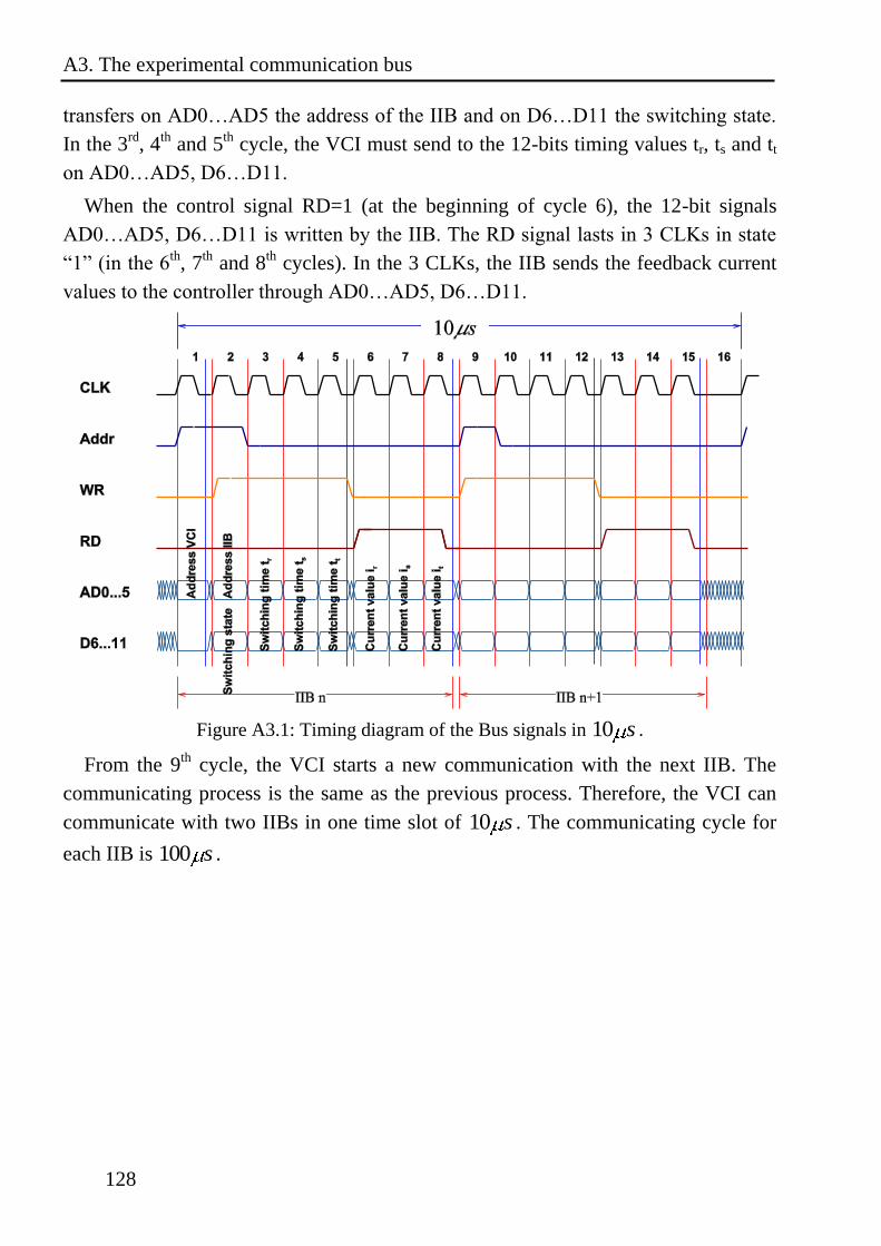
A3. The experimental communication bus
128
transfers on AD0…AD5 the address of the IIB and on D6…D11 the switching state.
In the 3rd
, 4th
and 5th
cycle, the VCI must send to the 12-bits timing values tr, ts and tt
on AD0…AD5, D6…D11.
When the control signal RD=1 (at the beginning of cycle 6), the 12-bit signals
AD0…AD5, D6…D11 is written by the IIB. The RD signal lasts in 3 CLKs in state
“1” (in the 6th
, 7th
and 8th cycles). In the 3 CLKs, the IIB sends the feedback current
values to the controller through AD0…AD5, D6…D11.
Figure A3.1: Timing diagram of the Bus signals in 10 s .
From the 9th
cycle, the VCI starts a new communication with the next IIB. The
communicating process is the same as the previous process. Therefore, the VCI can
communicate with two IIBs in one time slot of 10 s . The communicating cycle for
each IIB is 100 s .
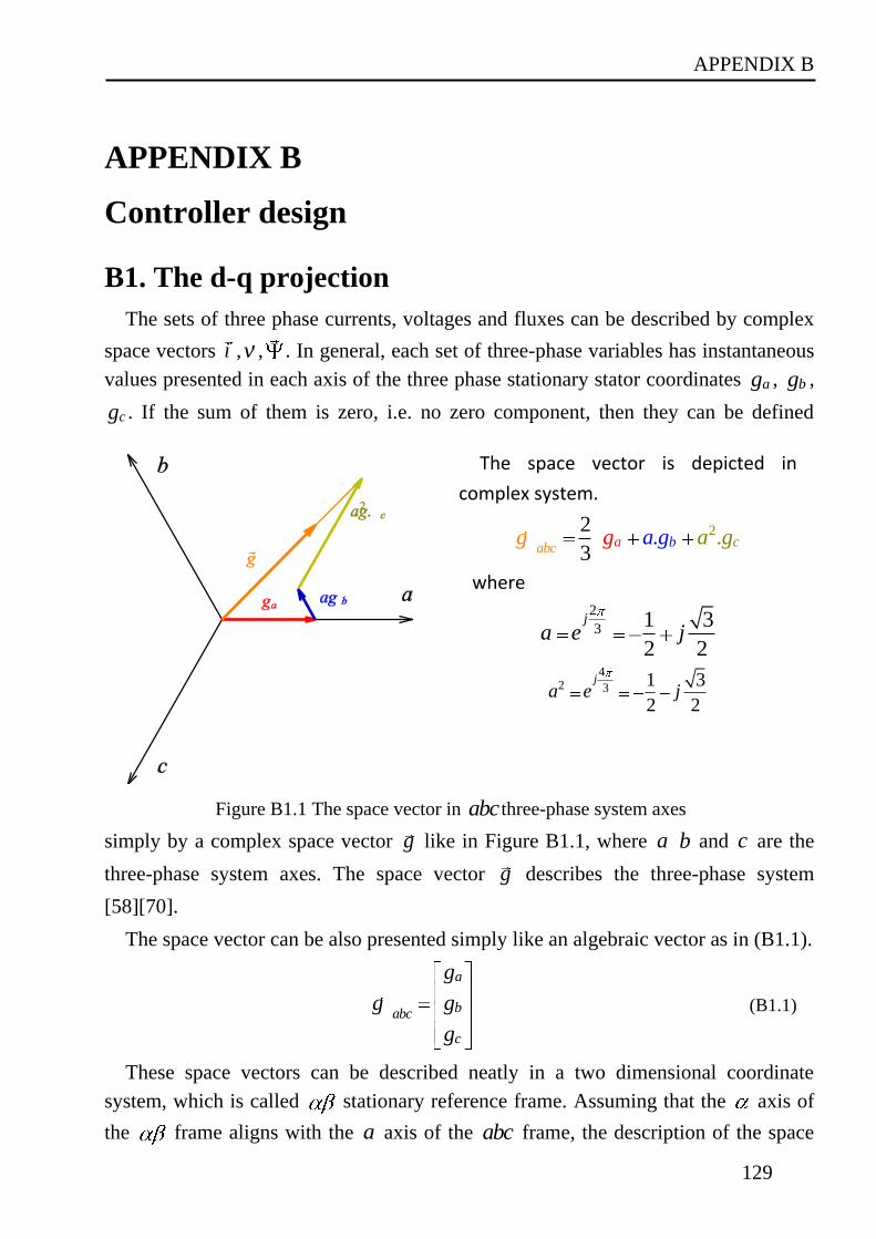
APPENDIX B
129
APPENDIX B
Controller design
B1. The d-q projection
The sets of three phase currents, voltages and fluxes can be described by complex
space vectors i ,v , . In general, each set of three-phase variables has instantaneous
values presented in each axis of the three phase stationary stator coordinates ag , bg ,
cg . If the sum of them is zero, i.e. no zero component, then they can be defined
simply by a complex space vector g like in Figure B1.1, where a b and c are the
three-phase system axes. The space vector g describes the three-phase system
[58][70].
The space vector can be also presented simply like an algebraic vector as in (B1.1).
a
babc
c
g
g g
g
(B1.1)
These space vectors can be described neatly in a two dimensional coordinate
system, which is called stationary reference frame. Assuming that the axis of
the frame aligns with the a axis of the abc frame, the description of the space
The space vector is depicted in
complex system.
22. .
3aabc b cg ag g a g
where
2
31 3
2 2
j
a e j
42 3
1 3
2 2
j
a e j
Figure B1.1 The space vector in abc three-phase system axes
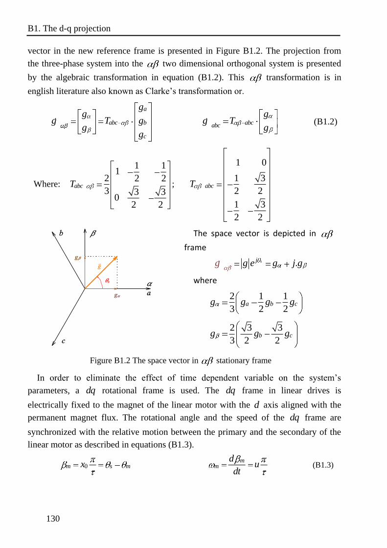
B1. The d-q projection
130
vector in the new reference frame is presented in Figure B1.2. The projection from
the three-phase system into the two dimensional orthogonal system is presented
by the algebraic transformation in equation (B1.2). This transformation is in
english literature also known as Clarke’s transformation or.
a
abc b
c
gg
g T gg
g
abcabc
gg T
g (B1.2)
Where:
1 11
2 2 2
3 3 30
2 2
abcT ;
1 0
1 3
2 2
1 3
2 2
abcT
The space vector is depicted in
frame
.sjg e g j gg
where
2 1 1
3 2 2a b cg g g g
2 3 3
3 2 2b cg g g
Figure B1.2 The space vector in stationary frame
In order to eliminate the effect of time dependent variable on the system’s
parameters, a dq rotational frame is used. The dq frame in linear drives is
electrically fixed to the magnet of the linear motor with the d axis aligned with the
permanent magnet flux. The rotational angle and the speed of the dq frame are
synchronized with the relative motion between the primary and the secondary of the
linear motor as described in equations (B1.3).
0m s mx m
md
udt
(B1.3)
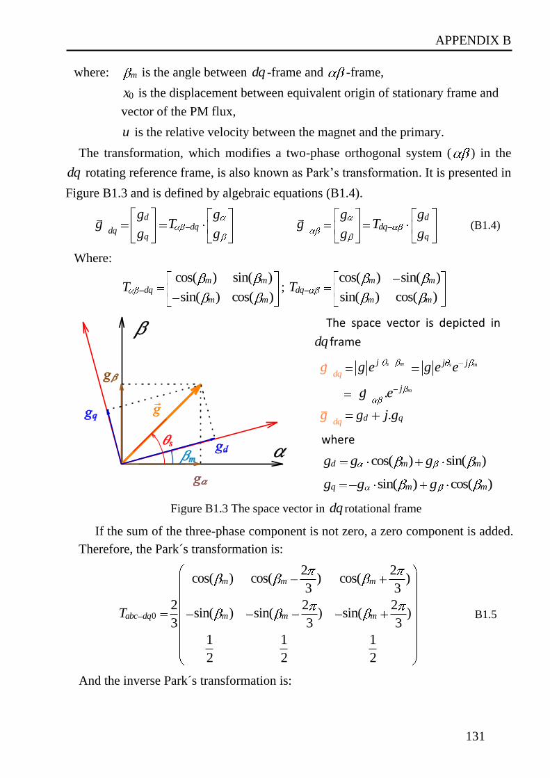
APPENDIX B
131
where: m is the angle between dq -frame and -frame,
0x is the displacement between equivalent origin of stationary frame and
vector of the PM flux,
u is the relative velocity between the magnet and the primary.
The transformation, which modifies a two-phase orthogonal system ( ) in the
dq rotating reference frame, is also known as Park’s transformation. It is presented in
Figure B1.3 and is defined by algebraic equations (B1.4).
ddqdq
q
g gg T
g g
ddq
q
ggg T
gg (B1.4)
Where:
cos( ) sin( )
sin( ) cos( )
m mdq
m m
T ; cos( ) sin( )
sin( ) cos( )
m mdq
m m
T
The space vector is depicted in
dq frame
.
s m s m
m
j j j
j
dqg e g e
g e
g e
.ddq qgg g j
where
cos( ) sin( )d m mg g g
sin( ) cos( )q m mg g g
Figure B1.3 The space vector in dq rotational frame
If the sum of the three-phase component is not zero, a zero component is added.
Therefore, the Park´s transformation is:
0
2 2cos( ) cos( ) cos( )
3 3
2 2 2sin( ) sin( ) sin( )
3 3 3
1 1 1
2 2 2
m m m
abc dq m m mT B1.5
And the inverse Park´s transformation is:
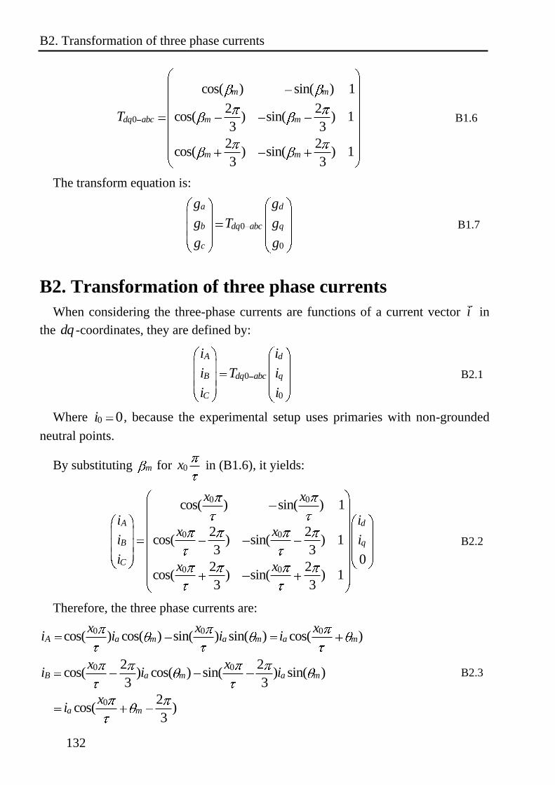
B2. Transformation of three phase currents
132
0
cos( ) sin( ) 1
2 2cos( ) sin( ) 1
3 3
2 2cos( ) sin( ) 1
3 3
m m
dq abc m m
m m
T B1.6
The transform equation is:
0
0
a d
b dq abc q
c
g g
g T g
g g
B1.7
B2. Transformation of three phase currents
When considering the three-phase currents are functions of a current vector i in
the dq -coordinates, they are defined by:
0
0
A d
B dq abc q
C
i i
i T i
i i
B2.1
Where 0 0i , because the experimental setup uses primaries with non-grounded
neutral points.
By substituting m for 0x in (B1.6), it yields:
0 0
0 0
0 0
cos( ) sin( ) 1
2 2cos( ) sin( ) 1
3 30
2 2cos( ) sin( ) 1
3 3
A d
B q
C
x x
i ix x
i i
ix x
B2.2
Therefore, the three phase currents are:
0 0 0cos( ) cos( ) sin( ) sin( ) cos( )A a m a m a m
x x xi i i i
0 0
0
2 2cos( ) cos( ) sin( ) sin( )
3 3
2cos( )
3
B a m a m
a m
x xi i i
xi
B2.3

APPENDIX B
133
0 0
0
2 2cos( ) cos( ) sin( ) sin( )
3 3
2cos( )
3
C a m a m
a m
x xi i i
xi
Derive from (B1.3), it yields
0s m
x B2.4
Substituting (B2.4) into (B2.3), the three-phase currents are simplified as:
cos( )A a si i
2cos( )
3B a si i
2cos( )
3C a si i
B2.5
B3 Anti-windup current control
Figure B3.1 shows the block diagram of the implemented current control
algorithm, which uses two PI controllers in a dq reference frame and a Space Vector
Pulse Width Modulation (SV-PWM block) to generate the inverters’ switching times,
in the control system of the linear motor experiment setup [76].
In the control system, the reference input values consist of:
A current reference vector mi with
o Magnitude of the current vector 2 2
* * *
m d qi i i
o Angle of the current vector * * *arctan( , )m d qi i i
Maximal voltage maxu
The current control will be realized in a dq two-phased reference frame, with the
angle m between the phase d of the control reference frame and the phase a of the
three-phased abc system.
Because of the inverters ability, the output voltage vectors of the inverter are
bounded by maxu . This causes the windup effect in the PI current control loops when
the voltage boundary (presented by a circle with maxu radius in dq -reference frame)
is exceeded. Therefore, general implementation of the PI regulators with anti-windup
was used in current control loops of the experimental setup. In the implementation,
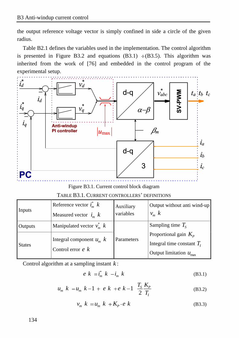
B3 Anti-windup current control
134
the output reference voltage vector is simply confined in side a circle of the given
radius.
Table B2.1 defines the variables used in the implementation. The control algorithm
is presented in Figure B3.2 and equations (B3.1) (B3.5). This algorithm was
inherited from the work of [76] and embedded in the control program of the
experimental setup.
Figure B3.1. Current control block diagram
TABLE B3.1. CURRENT CONTROLLERS’ DEFINITIONS
Inputs Reference vector
*
mi k
Measured vector mi k
Auxiliary
variables
Output without anti wind-up
mv k
Outputs Manipulated vector *
mv k
Parameters
Sampling time ST
Proportional gain PK
Integral time constant IT
Output limitation maxu
States Integral component mu k
Control error e k
Control algorithm at a sampling instant k :
*
m me k i k i k (B3.1)
1 12S P
m m
I
T Ku k u k e k e k
T (B3.2)
m m Pv k u k K e k (B3.3)
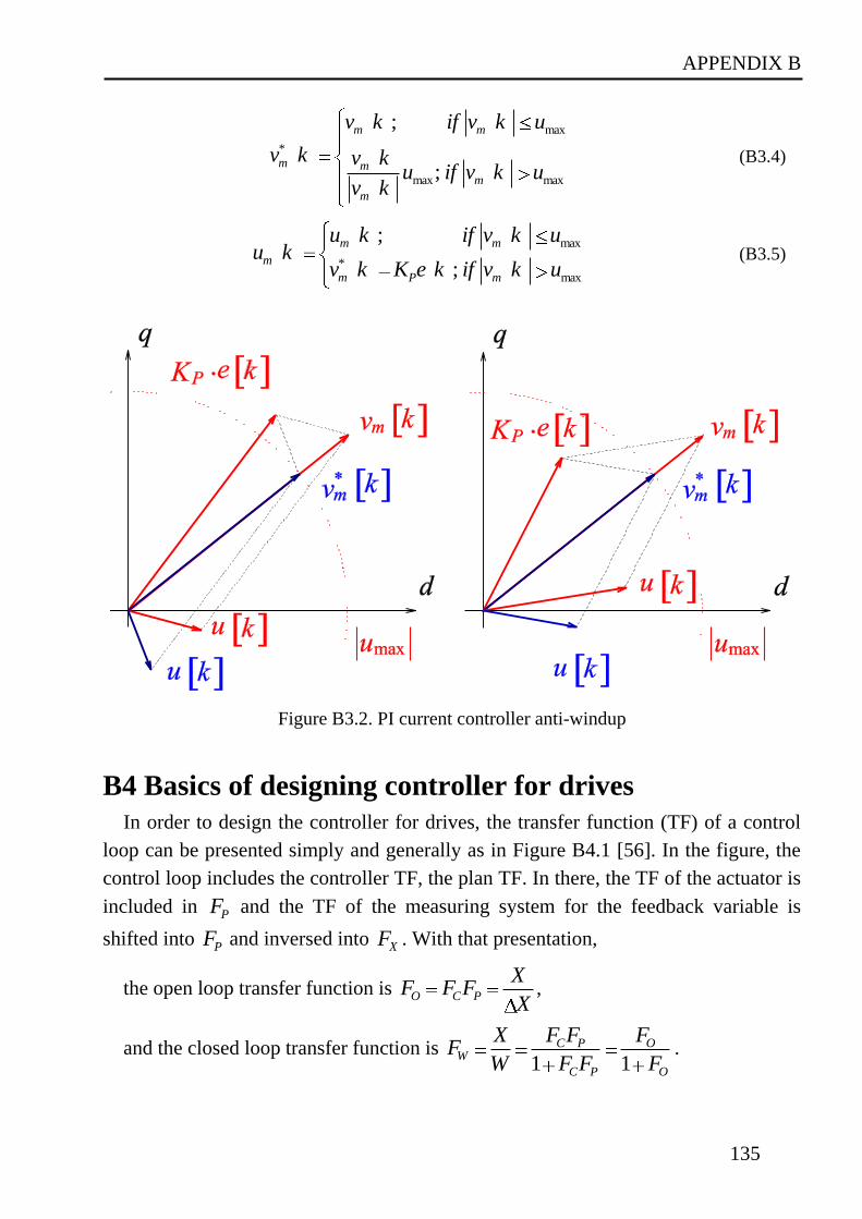
APPENDIX B
135
max
*
max max
;
;
m m
m m
m
m
v k if v k u
v k v ku if v k u
v k
(B3.4)
max
*
max
;
;
m m
m
m P m
u k if v k uu k
v k K e k if v k u (B3.5)
Figure B3.2. PI current controller anti-windup
B4 Basics of designing controller for drives
In order to design the controller for drives, the transfer function (TF) of a control
loop can be presented simply and generally as in Figure B4.1 [56]. In the figure, the
control loop includes the controller TF, the plan TF. In there, the TF of the actuator is
included in PF and the TF of the measuring system for the feedback variable is
shifted into PF and inversed into XF . With that presentation,
the open loop transfer function is O C P
XF F F
X,
and the closed loop transfer function is 1 1
C P OW
C P O
X F F FF
W F F F.
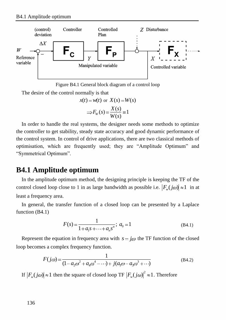
B4.1 Amplitude optimum
136
Figure B4.1 General block diagram of a control loop
The desire of the control normally is that
( ) ( )x t w t or ( ) ( )X s W s
( )( ) 1
( )W
X sF s
W s
In order to handle the real systems, the designer needs some methods to optimize
the controller to get stability, steady state accuracy and good dynamic performance of
the control system. In control of drive applications, there are two classical methods of
optimisation, which are frequently used; they are “Amplitude Optimum” and
“Symmetrical Optimum”.
B4.1 Amplitude optimum
In the amplitude optimum method, the designing principle is keeping the TF of the
control closed loop close to 1 in as large bandwidth as possible i.e. ( ) 1wF j in at
least a frequency area.
In general, the transfer function of a closed loop can be presented by a Laplace
function (B4.1)
0
1
1( ) ; 1
1 n
n
F s aa s a s
(B4.1)
Represent the equation in frequency area with s j the TF function of the closed
loop becomes a complex frequency function.
2 4 3
2 4 1 3
1( )
(1 ) ( )F j
a a j a a (B4.2)
If ( ) 1wF j then the square of closed loop TF 2
( ) 1wF j . Therefore
APPENDIX B
137
2
2 4 2 3 2
2 4 1 3
1( )
(1 ) ( )F j
a a a a (B4.3)
In order to have ( ) 1wF j in a large bandwidth, the closed loop TF should be
designed with
2
2 2 4 2 2
1 2 2 4 1 3
0 0
1( )
1 ( 2 ) ( 2 2 )w n
n
F ja a a a a a a
(B4.4)
2
1 2
2
2 4 1 3
2 0
2 2 0
a a
a a a a (B4.5)
After optimization, we get: 2
2
1( )
1w n
n
F ja 2
1( )
1w n
n
F ja
Apply the method for control of drive in current control loop and position control
loop; the results are presented in follows.
a. Apply for current control loop with PI controller
The current control loop in control of drive can be simplified and present as a
second order lag element (PT2 element) in (B4.5).
1 2
( )(1 )(1 )
PP
KF s
sT sT (B4.6)
And the TF of PI controller is presented in (A3.6)
1( ) 1 1p
C p i
i i
KF s K sT
sT sT (B4.7)
Compensate the higher time constant 1T of the controlled plan by choosing value
of controller iT with
1iT T (B4.8)
The open loop TF of the system is simplified to
2
2 1 2
1( ) ( ) ( )
(1 )
p P
O C P
i
K KF s F s F s
sT sT sa s a (B4.9)
With 1i
p P
Ta
K K; 2
2i
p P
TTa
K K
B4.2 Symmetrical optimum
138
The closed loop TF of the system will be
2
1 2
1( )
1 1O
W
O
FF s
F sa s a (B4.10)
Optimize the TF as in (A3.), we got
2
2
1 22 i
p P
Ta a
K K2
T 2i
p P
T
K K (B4.11)
1
2 22 2i
p
P P
T TK
K T K T (B4.12)
b. Apply for position control loop with P controller
With the position control loop the plan TF is presented as a PT1 element in series
with an integral element as in (B4.13)
1
1( )
(1 )PF s
s sT (B4.13)
And the TF of PI controller is presented in (B3.4)
( )C pF s K (B4.14)
The open loop TF of the system is simplified to
2
1 1 2
1( ) ( ) ( )
(1 )
p
O C P
i
KF s F s F s
s sT sa s a (B4.15)
With 1
1
p
aK
; 2
p
Ta
K
Optimize TF, we got
1
1
2pK
T (B4.16)
B4.2 Symmetrical optimum
The design principle of the symmetrical optimum is finding the maximum
damping of the control loop system. The optimal damping is the highest phase
margin of the open loop OF at the position that the gain crossover 1 with the
crossing frequency CR i.e. the design method will find the controller parameter that
makes max( )CR .
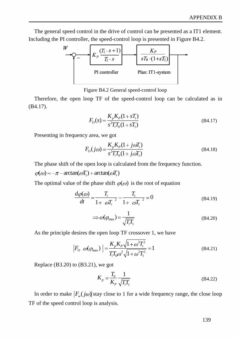
APPENDIX B
139
The general speed control in the drive of control can be presented as a IT1 element.
Including the PI controller, the speed-control loop is presented in Figure B4.2.
Figure B4.2 General speed-control loop
Therefore, the open loop TF of the speed-control loop can be calculated as in
(B4.17).
2
0 1
(1 )( )
(1 )
p P i
O
i
K K sTF s
s TT sT (B4.17)
Presenting in frequency area, we got
2
0 1
(1 )( )
(1 )
p P i
O
i
K K j TF j
s TT j T (B4.18)
The phase shift of the open loop is calculated from the frequency function.
1( ) arctan( ) arctan( )iT T
The optimal value of the phase shift ( ) is the root of equation
12 2
1
( )0
11
i
i
d T T
dt TT (B4.19)
max
1
1( )
iTT (B4.20)
As the principle desires the open loop TF crossover 1, we have
2 2
max 2 2 2
0 1
1( ) 1
1
p P i
O
i
K K TF
TT T (B4.21)
Replace (B3.20) to (B3.21), we got
0
1
1p
P i
TK
K TT (B4.22)
In order to make ( )wF j stay close to 1 for a wide frequency range, the close loop
TF of the speed control loop is analysis.
B4.2 Symmetrical optimum
140
2
0 1
2 3
0 0 1
(1 )( )
1 (1 ) (1 )
1
1 11
p P iOw
O i p P i
i
i i i
p P p P
K K sTFF s
F s TT sT K K sT
sT
sT s TT s TT TK K K K
(B4.23)
Presenting in frequency area
2 3
0 0 1
1( )
1 11
iw
i i i
p P p P
j TF j
j T TT j TT TK K K K
(B4.24)
To make ( ) 1wF j we have to make the denominator ( ( )D j ) of ( )wF j
close to 1. In another words, we have to make 2
( ) 1D j .
! !
2
2 2 3
0 0 1
22 !
2 2 2 4 60 0 0 1 0 1
0 0
1 1( ) 1 1
( ) 1 2 2 1
i i i
p P p P
i i i ii
p P p P p P p P
D j TT T TT TK K K K
TT TT T T T TT TD j T
K K K K K K K K
Solve the set of two equations, the result is
14iT T (B4.25)
APPENDIX C
141
APPENDIX C
Fundamental of electromagnetic field in
synchronous linear motors
C1. Review of electromagnetic field theory
In order to review the knowledge of the electromagnetic field theory, the basic
laws of electricity are repeated in this appendix by a set of equations called
Maxwell´s equations and some other derived equations from them [57].
The force F acting on a charge q moving with a velocity u in an electric field E
and in magnetic field is given by the Lorentz force equation.
EF q E u F F (C1.1)
The electric field intensity E and the magnetic field can be defined from
(C1.1) by the following equations:
.EF q E (C1.2)
.F q u (C1.3)
The potential difference dV between two points separated by a distance dl is
defined as
.dV E dl or E V (C1.4)
The total magnetic flux can be expressed from the magnetic flux density as
sds (C1.5)
where the integral is over a surface s .
The electromotive force ( EMF ) is induced in a closed circuit following the
Faraday´s law when the magnetic flux linking the circuit changes. With a N -turn
coil closed circuit, the induced EMF is given by
dEMF N
dt (C1.6)
From equation (C1.4), the EMF can be defined as
C2. Permanent Magnet in PMLSM
142
EMF Edl (C1.7)
If consider 1N , then from (C1.5) to (C1.7) it follows that
sEdl ds
t (C1.8)
The relationship between given currents and resulting magnetic field is expressed
by Ampere´s circuital law. The law gives the relationship between the magnetic field
intensity and the current I as following
dl I (C1.9)
If J is the surface current density, then (C1.9) can be rewritten as
sdl J ds (C1.10)
In order to obtain complete information reading the various field quantities, in
addition to the equations in this appendix certain auxiliary relations are also useful.
These relations are as following.
Ohm’s law: For a conductor of conductivity ,
.J E (C1.11)
where J is surface current density, and E is electric field intensity.
Permittivity: The electric field intensity and the electric flux density in a medium
are related to each other by
.D E (C1.12)
where is called the permittivity of the material.
Permeability: The magnetic field intensity and the magnetic flux density in a
material are related to each other by
. (C1.13)
where is called the permeability of the medium.
C2. Permanent Magnet in PMLSM
As presented in the previous appendix, the magnetic flux density and the
magnetic field intensity in free space are related by the constant 0 known as the
permeability of free space [57]:
0. (C2.1)
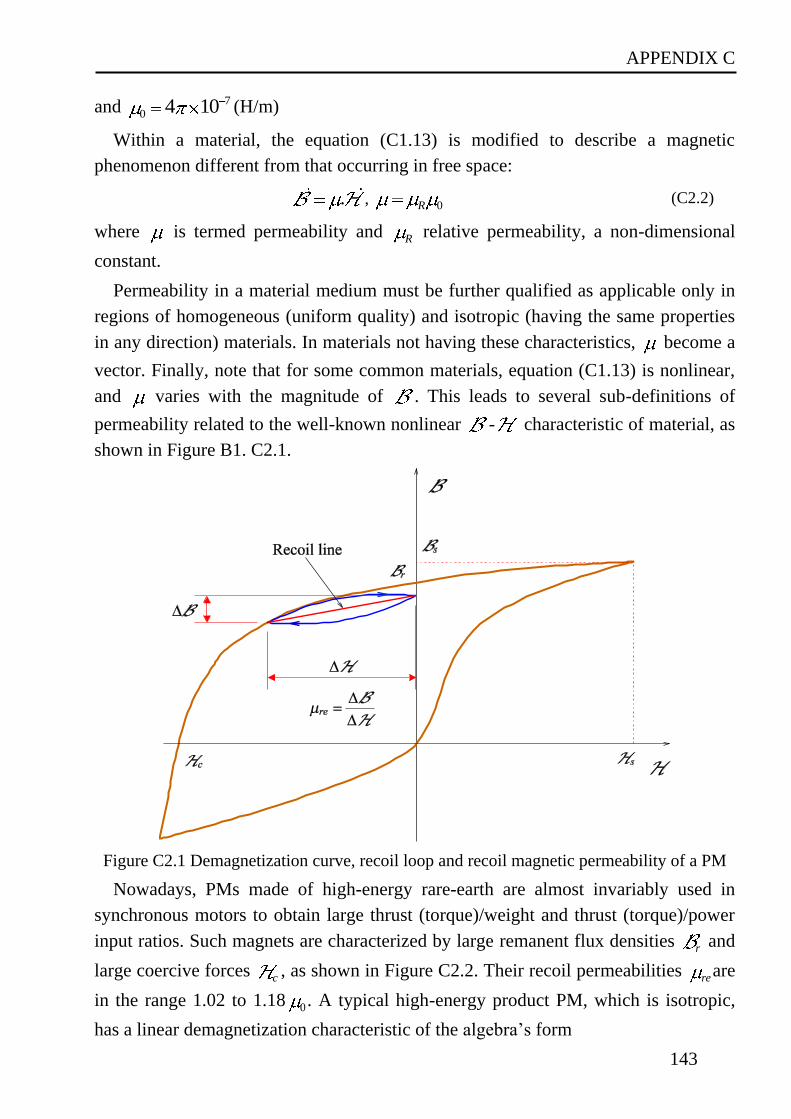
APPENDIX C
143
and 7
0 4 10 (H/m)
Within a material, the equation (C1.13) is modified to describe a magnetic
phenomenon different from that occurring in free space:
. , 0R (C2.2)
where is termed permeability and R relative permeability, a non-dimensional
constant.
Permeability in a material medium must be further qualified as applicable only in
regions of homogeneous (uniform quality) and isotropic (having the same properties
in any direction) materials. In materials not having these characteristics, become a
vector. Finally, note that for some common materials, equation (C1.13) is nonlinear,
and varies with the magnitude of . This leads to several sub-definitions of
permeability related to the well-known nonlinear - characteristic of material, as
shown in Figure B1. C2.1.
Figure C2.1 Demagnetization curve, recoil loop and recoil magnetic permeability of a PM
Nowadays, PMs made of high-energy rare-earth are almost invariably used in
synchronous motors to obtain large thrust (torque)/weight and thrust (torque)/power
input ratios. Such magnets are characterized by large remanent flux densities r and
large coercive forces c , as shown in Figure C2.2. Their recoil permeabilities reare
in the range 1.02 to 1.18 0 . A typical high-energy product PM, which is isotropic,
has a linear demagnetization characteristic of the algebra’s form
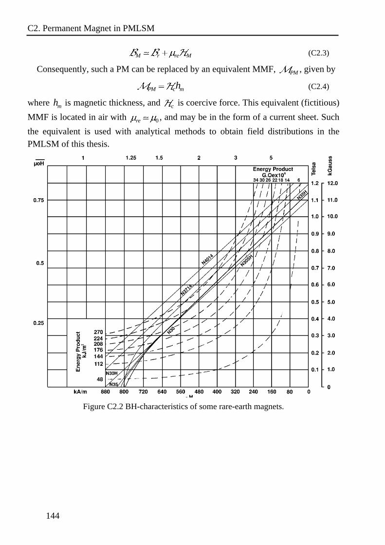
C2. Permanent Magnet in PMLSM
144
M r re M (C2.3)
Consequently, such a PM can be replaced by an equivalent MMF, PM , given by
PM c mh (C2.4)
where mh is magnetic thickness, and c is coercive force. This equivalent (fictitious)
MMF is located in air with 0re , and may be in the form of a current sheet. Such
the equivalent is used with analytical methods to obtain field distributions in the
PMLSM of this thesis.
Figure C2.2 BH-characteristics of some rare-earth magnets.
Curriculum Vitae
145
Curriculum Vitae
Personal data
Name: Phong C. Khong
Date of birth / place: 10.04.1978 / Hanoi – Vietnam
Family status: Married, One child
Education and Career
1984-1989: Primary school Duc Giang
1989-1993: Junior high school Duc Giang
1993-1996: Senior high school Nguyen Gia Thieu
1996-2001: Study for diploma´s degree of Electrical engineering at Hanoi
University of technology
2001-2003: Study for master´s degree of Electrical engineering at Hanoi
University of technology.
2001-2007: Assistant at the Department of Automation for Mining and
Petroleum Factory, Hanoi University of Mining and Geology.
Since 2007: Studying for PhD degree at the Department of Power electronic and
control of drives, Technical university of Darmstadt.
Publication
[1] P. Khong, R. Leidhold and P. Mutschler. “Magnetic guidance of the mover in a long-
primary linear motor,” Industry Applications, IEEE Transactions – electronic
publishing, DOI: 10.1109/TIA.2011.2125934, March 2011.
[2] P. Khong, R. Leidhold and P. Mutschler. “Magnetic guidance of the mover in a long-
primary linear motor,” in ECCE 2009. IEEE, San Jose, CA Sept. 2009, pp. 2354–2361.
[3] P. Khong, R. Leidhold and P. Mutschler. “Magnetic guiding and capacitive sensing for a
passive vehicle of a long-primary linear motor,” in EPE/PEMC 2010, Ohrid-Macedonia,
Sept. 2010, pp. S3-1 – S3-8.
[4] P. Khong and P. Mutschler.: “Capacitive gap and yaw angle sensor for linear drives,” in
IECON 2010, Glendale, AZ Nov. 2010, pp. 1240–1245.
[5] P. Khong, R. Leidhold and P. Mutschler. “Active magnetic guidance for material
handling systems based on linear motors,” in LDIA 2009, Incheon-Korea, Sep. 2009.