Maschinenbau von Makro bis Nano / Mechanical Engineering ... · 50. Internationales...

50. Internationales Wissenschaftliches Kolloquium September, 19-23, 2005 Maschinenbau von Makro bis Nano /

Mechanical Engineering from Macro to Nano Proceedings Fakultät für Maschinenbau / Faculty of Mechanical Engineering

Startseite / Index: http://www.db-thueringen.de/servlets/DocumentServlet?id=15745

Impressum Herausgeber: Der Rektor der Technischen Universität llmenau Univ.-Prof. Dr. rer. nat. habil. Peter Scharff Redaktion: Referat Marketing und Studentische Angelegenheiten Andrea Schneider Fakultät für Maschinenbau

Univ.-Prof. Dr.-Ing. habil. Peter Kurtz, Univ.-Prof. Dipl.-Ing. Dr. med. (habil.) Hartmut Witte, Univ.-Prof. Dr.-Ing. habil. Gerhard Linß, Dr.-Ing. Beate Schlütter, Dipl.-Biol. Danja Voges, Dipl.-Ing. Jörg Mämpel, Dipl.-Ing. Susanne Töpfer, Dipl.-Ing. Silke Stauche

Redaktionsschluss: 31. August 2005 (CD-Rom-Ausgabe) Technische Realisierung: Institut für Medientechnik an der TU Ilmenau (CD-Rom-Ausgabe) Dipl.-Ing. Christian Weigel

Dipl.-Ing. Helge Drumm Dipl.-Ing. Marco Albrecht

Technische Realisierung: Universitätsbibliothek Ilmenau (Online-Ausgabe) Postfach 10 05 65 98684 Ilmenau

Verlag: Verlag ISLE, Betriebsstätte des ISLE e.V. Werner-von-Siemens-Str. 16 98693 llmenau © Technische Universität llmenau (Thür.) 2005 Diese Publikationen und alle in ihr enthaltenen Beiträge und Abbildungen sind urheberrechtlich geschützt. ISBN (Druckausgabe): 3-932633-98-9 (978-3-932633-98-0) ISBN (CD-Rom-Ausgabe): 3-932633-99-7 (978-3-932633-99-7) Startseite / Index: http://www.db-thueringen.de/servlets/DocumentServlet?id=15745

50. Internationales Wissenschaftliches KolloquiumTechnische Universität Ilmenau

19.-23. September 2005

Model Building, Control Design and practicalImplementation of a MEMS Acceleration Sensor

Heiko Wolfram, Ralf Schmiedel, Torsten Aurich, Jan Mehner, Thomas Geßner andWolfram Dötzel

ABSTRACTThis paper presents some new results on MEMS acceleration sensors. An approximate method is de-scribed to analytically analyze deep airstream channels on the mass surface. The channels enormouslydecrease the squeeze-film damping force for ambient pressure inside the sensor. The ambient pressuresimplifies the fabrication process and guarantees approximate equal dynamics for all sensor samples.The sensor fabrication and design is shortly covered. A theoretical model is built from the physicalprinciples of the complete sensor system, consisting of the MEMS sensor, the charge amplifier and thePWM driver for the sensor element. A reduced-order model of the entire system is used to design arobust control with the H∞-Approach. The weighting takes the plant-input disturbance into accountand prevents a slow disturbance rejection, which is the case for the S/KS-design. Remarks are givenon the identification of the mechanical system. Practical tests and the system identification prove thenewly found results.

Keywords: Acceleration Sensor, Model Building, H∞-Control, Mixed-Sensitivity Approach, Identi-fication

1. INTRODUCTION

MICRO-ELECTRO-MECHANICAL systems (MEMS) play an important role in the realization of

sensor/actuator systems. They are small, very compact, have a simple and robust layout. An-

other advantage is the technology, which can directly be applied from the micro electronics and hence,

makes the integration of the electronics and the production of large quantities possible. There are,

however, some limitations such as packaging, cross-talk related problems, the MEMS mechanical

limitation. A major problem for the control design and stability is the strong nonlinearity of the elec-

trostatic field component and the nonlinearity of fluid damping. Therefore, an intensive analysis of the

open and closed-loop system may be necessary.

Digital

PWM−Unit

Control

DSP

Output

A/D−Converter

AccelerationSensor

AmplifierCharge

Acceleration

filterOutput−

ω

t

u

dB

y

y

Cf+

−

−u

+u

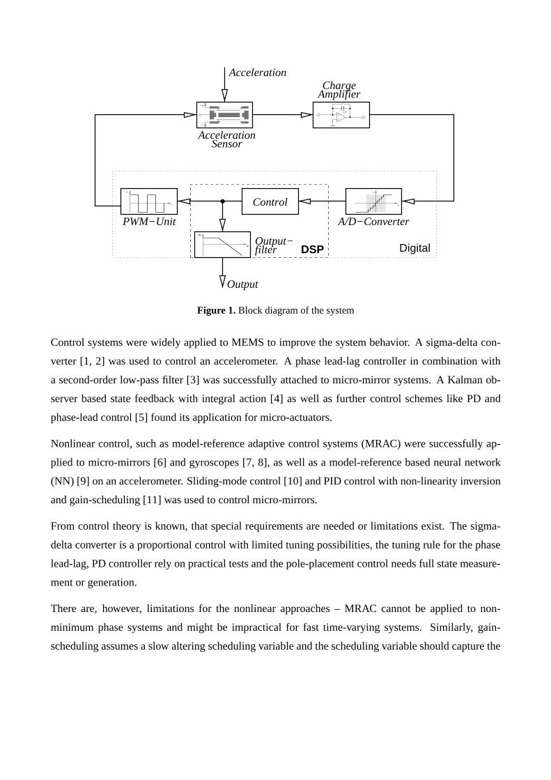
Figure 1. Block diagram of the system

Control systems were widely applied to MEMS to improve the system behavior. A sigma-delta con-

verter [1, 2] was used to control an accelerometer. A phase lead-lag controller in combination with

a second-order low-pass filter [3] was successfully attached to micro-mirror systems. A Kalman ob-

server based state feedback with integral action [4] as well as further control schemes like PD and

phase-lead control [5] found its application for micro-actuators.

Nonlinear control, such as model-reference adaptive control systems (MRAC) were successfully ap-

plied to micro-mirrors [6] and gyroscopes [7, 8], as well as a model-reference based neural network

(NN) [9] on an accelerometer. Sliding-mode control [10] and PID control with non-linearity inversion

and gain-scheduling [11] was used to control micro-mirrors.

From control theory is known, that special requirements are needed or limitations exist. The sigma-

delta converter is a proportional control with limited tuning possibilities, the tuning rule for the phase

lead-lag, PD controller rely on practical tests and the pole-placement control needs full state measure-

ment or generation.

There are, however, limitations for the nonlinear approaches – MRAC cannot be applied to non-

minimum phase systems and might be impractical for fast time-varying systems. Similarly, gain-

scheduling assumes a slow altering scheduling variable and the scheduling variable should capture the

plant nonlinearities. The non-linearity inversion assumes a perfect cancellation and the sliding-mode

control produces high-frequency switching in the control-loop. Further, the NN approach just gives

a black-box model with no knowledge of the inside dynamical system and needs a large amount of

training data sets.

All applied control schemes are developed in time domain and except of the MARC, sliding-mode

control and gain-scheduling do not consider robustness explicitly. Therefore, the H∞ control design

is introduced to control the system, depicted in Fig. 1. Since there is no guaranteed stability for the

developed linear time-invariant (LTI) control on the nonlinear system, stability analysis has to be given

explicitly. This will be a task for the future.

2. DESIGN

A capacitance acceleration sensor has been developed in bulk micro machining technology. It con-

sists of a silicon wafer with the mechanical structure (Fig. 2(a)) and glass wafers with the electrodes,

which are anodic bonded to both sides of the silicon wafer. Fig. 2(b) shows the sensor’s schematic

configuration.

spacer

air channels

torsion springseismic mass

(a) SEM micrography of the seismic mass

��

��

��

� � � ��

� � ��

��

��

��

��

��

��

� � � � � � � � � � � � � � � � � � � � � � � � � � � � � � � � � � � � � � � � � � � � � � � � � �

��

��

��

� ��

� ��

��

��

��

��

��

��

��

��

!�!"#�#$

%�%&

'�'�'�'�'�'�'�'�'�'�'�'�'�'�'�'�'�'�'�'�''�'�'�'�'�'�'�'�'�'�'�'�'�'�'�'�'�'�'�'�''�'�'�'�'�'�'�'�'�'�'�'�'�'�'�'�'�'�'�'�''�'�'�'�'�'�'�'�'�'�'�'�'�'�'�'�'�'�'�'�''�'�'�'�'�'�'�'�'�'�'�'�'�'�'�'�'�'�'�'�''�'�'�'�'�'�'�'�'�'�'�'�'�'�'�'�'�'�'�'�''�'�'�'�'�'�'�'�'�'�'�'�'�'�'�'�'�'�'�'�''�'�'�'�'�'�'�'�'�'�'�'�'�'�'�'�'�'�'�'�''�'�'�'�'�'�'�'�'�'�'�'�'�'�'�'�'�'�'�'�'

(�(�(�(�(�(�(�(�(�(�(�(�(�(�(�(�(�(�(�((�(�(�(�(�(�(�(�(�(�(�(�(�(�(�(�(�(�(�((�(�(�(�(�(�(�(�(�(�(�(�(�(�(�(�(�(�(�((�(�(�(�(�(�(�(�(�(�(�(�(�(�(�(�(�(�(�((�(�(�(�(�(�(�(�(�(�(�(�(�(�(�(�(�(�(�((�(�(�(�(�(�(�(�(�(�(�(�(�(�(�(�(�(�(�((�(�(�(�(�(�(�(�(�(�(�(�(�(�(�(�(�(�(�((�(�(�(�(�(�(�(�(�(�(�(�(�(�(�(�(�(�(�((�(�(�(�(�(�(�(�(�(�(�(�(�(�(�(�(�(�(�(

)�)�)�)�)�)�)�)�)�)�)�)�)�)�)�)�)�)�)�)�)�)�)�)�)�)�)�)�)�)�)�)�)�)�)�)*�*�*�*�*�*�*�*�*�*�*�*�*�*�*�*�*�*�*�*�*�*�*�*�*�*�*�*�*�*�*�*�*�*�*

+�+�+�+�+�+�+�+�+�+�+�+�+�+�+�+�+�+�+�+�+�+�+�+�+�+�+�+�+�+�+�+�+�+�+�+,�,�,�,�,�,�,�,�,�,�,�,�,�,�,�,�,�,�,�,�,�,�,�,�,�,�,�,�,�,�,�,�,�,�,

seismic mass

holevia

-�-�-�--�-�-�--�-�-�-.�.�.�..�.�.�..�.�.�.

/ / / / / / // / / / / / // / / / / / /0 0 0 0 0 0 00 0 0 0 0 0 00 0 0 0 0 0 0

1�1�1�11�1�1�11�1�1�12�2�2�22�2�2�22�2�2�2

3�3�33�3�33�3�34�44�44�45�55�5

5�56�66�66�6

silicon oxide

glasssilicon

aluminumtitaniumgold

ventilationhole

conn

ecti

on c

onta

cts

glass covertorsion spring electrode

spacer channels

(b) Schematic configuration

Figure 2. The sensor chip

By using silicon-nitride and silicon-oxide as mask layers, eight different masks (four for each side)

are used to etch the spring-mass components into the silicon wafer (Fig. 3). Caps of about 3 µm are

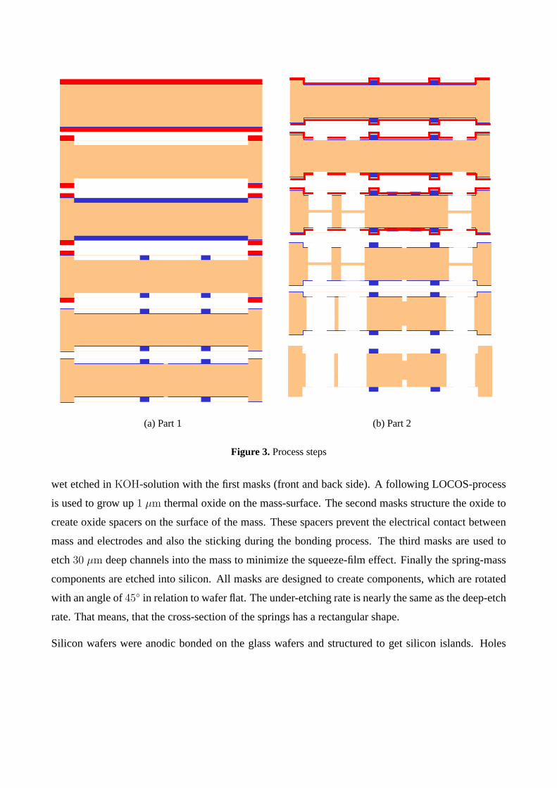
(a) Part 1 (b) Part 2

Figure 3. Process steps

wet etched in KOH-solution with the first masks (front and back side). A following LOCOS-process

is used to grow up 1 µm thermal oxide on the mass-surface. The second masks structure the oxide to

create oxide spacers on the surface of the mass. These spacers prevent the electrical contact between

mass and electrodes and also the sticking during the bonding process. The third masks are used to

etch 30 µm deep channels into the mass to minimize the squeeze-film effect. Finally the spring-mass

components are etched into silicon. All masks are designed to create components, which are rotated

with an angle of 45◦ in relation to wafer flat. The under-etching rate is nearly the same as the deep-etch

rate. That means, that the cross-section of the springs has a rectangular shape.

Silicon wafers were anodic bonded on the glass wafers and structured to get silicon islands. Holes

are ultrasonic drilled into the glass wafers to get the electrical contact from outside to inside of the

glass wafers and the equalization to ambient pressure. The holes have a diameter of 500 µm and a

deepness of about 600 µm. Silicon hard-masks are used to sputter aluminum electrodes and to realize

the connection between electrodes and outer silicon islands.

One silicon wafer is anodic bonded together with two glass wafers to get the final sensor. The process

parameters are a temperature of 400 ◦C, ambient pressure and a voltage of 300 V. The ambient pressure

guarantees equal heating of silicon and glass wafers during bonding process, and thus minimizes the

deformation of the components after cooling down. An electric charge on top of the SiO2-spacers

can emerge from the anodic bonding process, which can create an additional unknown electrostatic

moment. The outer islands are connected with the middle wafer during the bonding process to prevent

this effect. A bonding grid at the outside of the glass wafers applies the bonding voltage exactly to the

position of the silicon frame on the silicon wafer.

The sensors are separated and a final sputter process supplies the side wall contacts. Therefore, some

sensors are put together in a sputter feature and covered by a hard-mask to separate the connection

contacts. Bonding wires finally connect the sensor to the electronics.

3. MODEL BUILDING

The acceleration sensor can generally be described as a spring-mass system

[

−ω2M + jω{D + Ds(ω,v(ω))} + K + Ks(ω,v(ω))]

v(ω) = pext(ω) + pel(v(ω), u(ω)) (1)

with the inertial matrix M, the damping matrix D and stiffness matrix K, consisting of constant me-

chanical and frequency dependent squeeze-film parts, the displacement vector v and the load vectors,

the electrostatic load pel and the disturbance, the mechanical load pext .

The mechanical system has in general several degrees of freedom, where only the first mode

f0 =1

2π

√

K

J(2)

with the moment of inertia J and mechanical spring constant K is considered. The higher degrees of

freedom usually appear in higher frequency areas (Fig. 4), which are uncontrollable and undetectable

from the electronics.

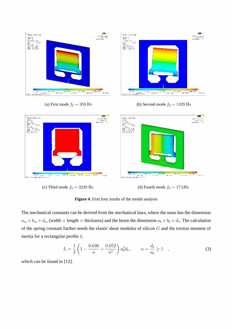
(a) First mode f0 = 359 Hz (b) Second mode f0 = 1329 Hz

(c) Third mode f0 = 3229 Hz (d) Fourth mode f0 = 17 kHz

Figure 4. First four results of the modal analysis

The mechanical constants can be derived from the mechanical laws, where the mass has the dimension

am × bm × dm (width × length × thickness) and the beam the dimension ab × bb × db. The calculation

of the spring constant further needs the elastic shear modulus of silicon G and the torsion moment of

inertia for a rectangular profile It

It =1

3

(

1 −0.630

n+

0.052

n5

)

a3bdb , n =

db

ab

≥ 1 , (3)

which can be found in [12].

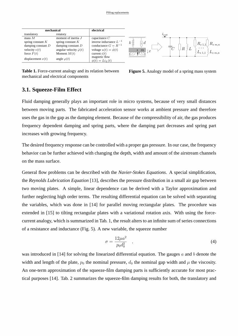
mechanical electricaltranslatory rotatorymass M moment of inertia J capacitance C

spring constant K spring constant K inverse inductance L−1

damping constant D damping constant D conductance G = R−1

velocity v(t) angular velocity ϕ(t) voltage u(t) = φ(t)force F (t) Moment M(t) current i(t)

displacement x(t) angle ϕ(t)magnetic flowφ(t) = LiL(t)

Table 1. Force-current analogy and its relation betweenmechanical and electrical components

PSfrag replacements

iext

RC L

Rs 1,1

Ls 1,1

Rs m,n

Ls m,n

k d

m xF

Figure 5. Analogy model of a spring mass system

3.1. Squeeze-Film Effect

Fluid damping generally plays an important role in micro systems, because of very small distances

between moving parts. The fabricated acceleration sensor works at ambient pressure and therefore

uses the gas in the gap as the damping element. Because of the compressibility of air, the gas produces

frequency dependent damping and spring parts, where the damping part decreases and spring part

increases with growing frequency.

The desired frequency response can be controlled with a proper gas pressure. In our case, the frequency

behavior can be further achieved with changing the depth, width and amount of the airstream channels

on the mass surface.

General flow problems can be described with the Navier-Stokes Equations. A special simplification,

the Reynolds Lubrication Equation [13], describes the pressure distribution in a small air gap between

two moving plates. A simple, linear dependence can be derived with a Taylor approximation and

further neglecting high order terms. The resulting differential equation can be solved with separating

the variables, which was done in [14] for parallel moving rectangular plates. The procedure was

extended in [15] to tilting rectangular plates with a variational rotation axis. With using the force-

current analogy, which is summarized in Tab. 1, the result alters to an infinite sum of series connections

of a resistance and inductance (Fig. 5). A new variable, the squeeze number

σ =12µa2

p0d20

, (4)

was introduced in [14] for solving the linearized differential equation. The gauges a and b denote the

width and length of the plate, p0 the nominal pressure, d0 the nominal gap width and µ the viscosity.

An one-term approximation of the squeeze-film damping parts is sufficiently accurate for most prac-

tical purposes [14]. Tab. 2 summarizes the squeeze-film damping results for both, the translatory and

rotatory motion.

REMARK 1. An analytical solution of the plate with airstream channels is not a trivial task. The

channels are deep enough to set the pressure inside of them to nominal pressure. This approximation

would split of the plate area into (nx + 1)(ny + 1) small planes with the new dimension

a =a − nxwg

nx + 1and b =

b − nywg

ny + 1, (5)

where wg is the width of the channels, nx the number in x-direction and ny in y-direction. The summa-

tion of all spring and damping forces gives the resulting load

Rtrans m,n =

1

(nx + 1)(ny + 1)Rtran

s m,n and Ltrans m,n =

1

(nx + 1)(ny + 1)Ltran

s m,n , (6)

which is valid for the translatory movement.

The rotatory motion needs some more calculation, since the rotation axis varies from plane to plane.

One gets the solution of the squeeze-film parts for a variational rotation axis [15]

Rrots 1,1 =

d0π6

64a3bζ2p0σ

(

1 +a2

b2

)

and Lrots 1,1 =

d0π4

64a3bζ2p0

. (7)

A one-term approximation is in this case correct, since the distance ζ = c/a will be a factor of 1/2.

The length c defines the distance of the rotation axis to the barycentric axis of each plane. A summation

of all moments gives

Rrots 1,1 =

ζ2

(ny + 1)ζ2Rrot

s 1,1 and Lrots 1,1 =

ζ2

(ny + 1)ζ2Lrot

s 1,1 (8)

where

ζ2 =

nx∑

n=0

(2n + 1)2

4=

(1 + nx)(1 + 2nx)(3 + 2nx)

12. (9)

The gap between each plate can be neglected for the moment calculation, as long as a � wg. For the

approximation is further supposed, that the channel depth is greater than the mean free path dg � d0

and the plate area a × b not too small.

A detailed analysis of airstream channels can be found in [16], which considers the actual pressure

distribution and the viscous friction on the sidewalls.

The transfer function of the acceleration sensor can be easily get from the state-space description,

found from the Kirchhoff Equations. An one-term approximation for the squeeze-film parts at the top

and bottom side is sufficiently accurate, since the seismic mass is controlled in zero position. The

model for the control design reduces further to

Gmech =

[

A B

C D

]

=

− 1CR

− 1C

− 1C

1C

L−1 0 0 0L−1

s 0 −Rs

Ls0

0 L 0 0

with the valuesRs =

1

2Rs 1,1

Ls =1

2Ls 1,1 .

(10)

This approximation will be also used for the control design, since the order of the model directly

determines the order of the controller.

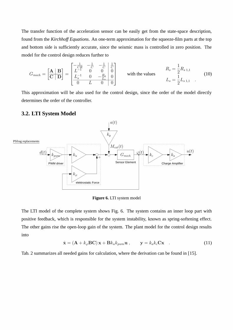
3.2. LTI System Model

Sensor Element Charge Amplifier

elektrostatic Force

PWM driver

PSfrag replacements

d(t)

Mext(t)

a(t)

kpwm

kϕ

ku Gmech

kg

kakcϕ(t) u(t)

Figure 6. LTI system model

The LTI model of the complete system shows Fig. 6. The system contains an inner loop part with

positive feedback, which is responsible for the system instability, known as spring-softening effect.

The other gains rise the open-loop gain of the system. The plant model for the control design results

into

x = (A + kϕBC)x + Bkukpwmu , y = kakcCx . (11)

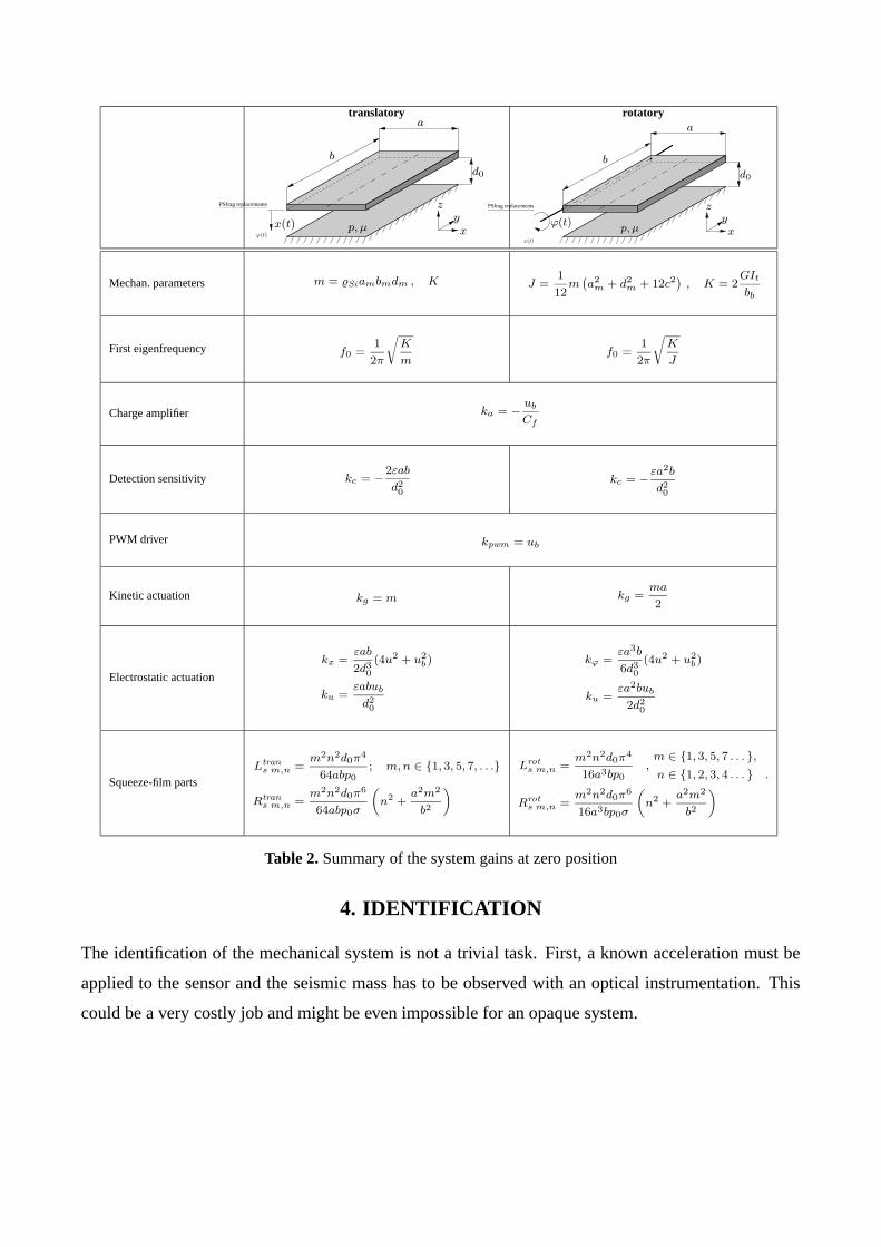
Tab. 2 summarizes all needed gains for calculation, where the derivation can be found in [15].

translatory rotatory

PSfrag replacements z

x

y

b

a

d0

p, µϕ(t)

x(t)

PSfrag replacements z

x

y

b

a

d0

p, µϕ(t)

x(t)

Mechan. parameters m = %Siambmdm , K J =1

12m

(

a2

m + d2

m + 12c2)

, K = 2GIt

bb

First eigenfrequency f0 =1

2π

√

K

mf0 =

1

2π

√

K

J

Charge amplifier ka = −ub

Cf

Detection sensitivity kc = −2εab

d2

0

kc = −εa2b

d2

0

PWM driver kpwm = ub

Kinetic actuation kg = m kg =ma

2

Electrostatic actuation

kx =εab

2d3

0

(4u2 + u2

b)

ku =εabub

d2

0

kϕ =εa3b

6d3

0

(4u2 + u2

b)

ku =εa2bub

2d2

0

Squeeze-film partsLtran

s m,n =m2n2d0π4

64abp0

; m, n ∈ {1, 3, 5, 7, . . .}

Rtrans m,n =

m2n2d0π6

64abp0σ

(

n2 +a2m2

b2

)

Lrots m,n =

m2n2d0π4

16a3bp0

,m ∈ {1, 3, 5, 7 . . . },

n ∈ {1, 2, 3, 4 . . . } .

Rrots m,n =

m2n2d0π6

16a3bp0σ

(

n2 +a2m2

b2

)

Table 2. Summary of the system gains at zero position

4. IDENTIFICATION

The identification of the mechanical system is not a trivial task. First, a known acceleration must be

applied to the sensor and the seismic mass has to be observed with an optical instrumentation. This

could be a very costly job and might be even impossible for an opaque system.

An alternative to circumvent this problem is to use the electrostatic system and to calculate back the

underlying mechanical system. This can be done with a two-stage identification [17], which identifies

the system at an operating voltage near zero. The dynamics of the electrostatic system is in that stage

close to the mechanical system behavior. The mechanical system DC gain is got from the measured

resonance frequency of the spring-mass system in the unmounted stage. The second stage fine-tunes

the system at nominal operating voltage.

A better alternative to identify the mechanical system, including the system gains, can be found in

[15]. The identification uses the voltage dependences of the linearized gains and interpolates them

with a polynomial. This means, that only two identifications at different operating voltages are needed

to completely calculate back the mechanical system. The algorithm was stated as following:

ALGORITHM 1. The pole movement under variating operating voltage can be approximately de-

scribed with a parabola of second order around the zero operating voltage

pjel (ub) ≈(

ϕj0r+ ϕj2r

u2b

)

+ j(

ϕj0i+ ϕj2i

u2b

)

, (12)

where the vertex of the parabola defines the approximate pole location of the mechanical poles ϕj0r+

jϕj0i.

The value of the mechanical plant gain kp can be approximately calculated from the dominant real

pole to

kp ≈=ϕ12r

u2b

kϕ(ub). (13)

The system forward gain kpk is the static gain of the electromechanical System Gemech divided by the

quotient of the products of the pole and zero locations

kpk = Gemech(s = 0, ub)

∏n

j=1 −pjel (ub)∏m

i=1 −zi

, (14)

where Gemech(s) is a strictly proper system (n > m).

The dependence of the gain kpk, where k = ku(ub)ka(ub)kckpwm(ub) is described with a cubic

parabola in ub

kpk = ϕ3u3b . (15)

REMARK 2. A similar estimation of the plant gain as in Eq. (13) could be also get for the two dominant

imaginary poles

kp ≈ϕ2

20i− (ϕ22i

u2b)

2

kϕ(ub)(16)

of an undamped system.

The Identification algorithm relies on the exactly known order m and n. Subspace Identification [18]

directly determines the system order n from the input-output data. The transformation rule z = esTs

can be easily applied to the poles and a mean value of the zeros zi can be used to calculate back the

system gain in Eq. (14).

It is clear, that the identification routines just only consider the small-signal model at the equilibrium

point. Therfore, a very low excitation signal is only appropriate.

NOTE 1. Finding the system zeros in S-domain is not a trivial task. Identification routines generally

find a discrete-time system model. The Z-Transformation might increase the numerator order and the

location of the zeros vary with the location of the poles. A simple example

G(s) =1

(s + p1)(s + p2)

Z

d t G(z) =p1(1 − e−Tsp2)(z − e−Tsp1) − p2(1 − e−Tsp1)(z − e−Tsp2)

p1p2(p1 − p2)(z − e−Tsp1)(z − e−Tsp2)(17)

shows the problem of the transformation. A sign of order discrepancy in the identification are very fast

poles and zeros, which should be canceled.

5. CONTROL DESIGN

The S/KS/GS/T-Standard-Design Problem is used for the control design. In this design, the transfer

function matrix N will be minimized with the ∞-Norm.

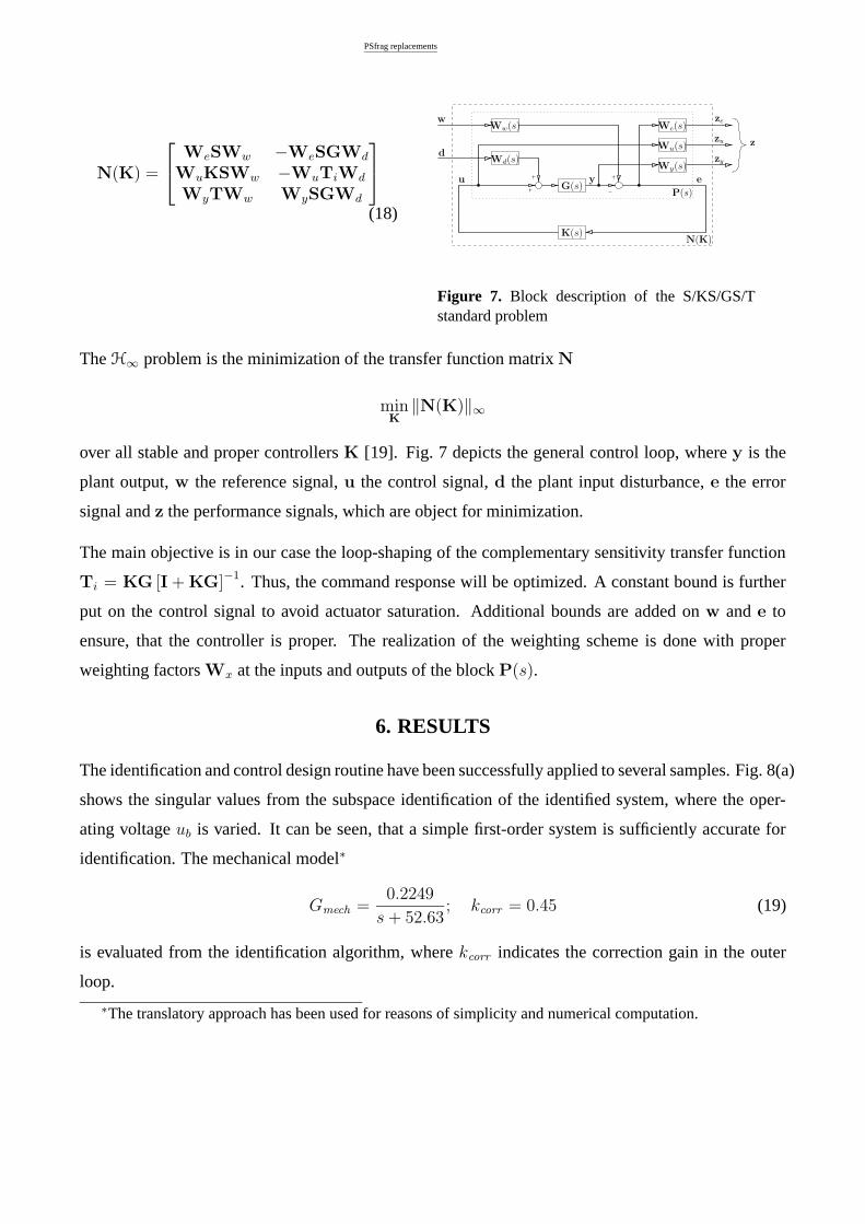
N(K) =

WeSWw −WeSGWd

WuKSWw −WuTiWd

WyTWw WySGWd

(18)

PSfrag replacements

We(s)

Wu(s)

Wy(s)Wd(s)

Ww(s)

G(s)

K(s)

z

u

w

ey

dzy

zu

ze

P(s)

N(K)

Figure 7. Block description of the S/KS/GS/Tstandard problem

The H∞ problem is the minimization of the transfer function matrix N

minK

‖N(K)‖∞

over all stable and proper controllers K [19]. Fig. 7 depicts the general control loop, where y is the

plant output, w the reference signal, u the control signal, d the plant input disturbance, e the error

signal and z the performance signals, which are object for minimization.

The main objective is in our case the loop-shaping of the complementary sensitivity transfer function

Ti = KG [I + KG]−1. Thus, the command response will be optimized. A constant bound is further

put on the control signal to avoid actuator saturation. Additional bounds are added on w and e to

ensure, that the controller is proper. The realization of the weighting scheme is done with proper

weighting factors Wx at the inputs and outputs of the block P(s).

6. RESULTS

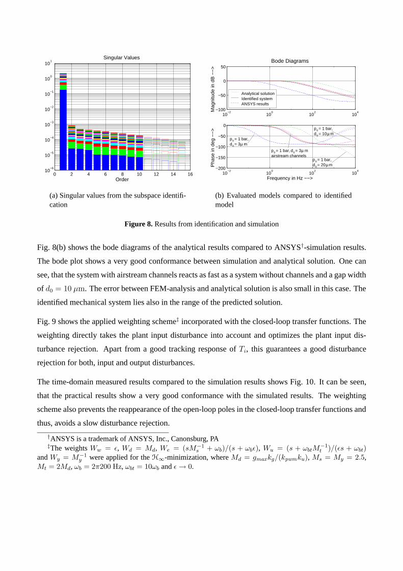
The identification and control design routine have been successfully applied to several samples. Fig. 8(a)

shows the singular values from the subspace identification of the identified system, where the oper-

ating voltage ub is varied. It can be seen, that a simple first-order system is sufficiently accurate for

identification. The mechanical model∗

Gmech =0.2249

s + 52.63; kcorr = 0.45 (19)

is evaluated from the identification algorithm, where kcorr indicates the correction gain in the outer

loop.

∗The translatory approach has been used for reasons of simplicity and numerical computation.

0 2 4 6 8 10 12 14 1610

−6

10−5

10−4

10−3

10−2

10−1

100

101

Order

Singular Values

(a) Singular values from the subspace identifi-cation

10−2

100

102

104

−100

−50

0

50

Mag

nitu

de in

dB

−−

>

Bode Diagrams

10−2

100

102

104

−200

−150

−100

−50

0

Frequency in Hz −−>

Pha

se in

deg

−−

>

Analytical solutionIdentified systemANSYS results

p = 1 bar,0

0d = 3 mµ

0

0d = 20 mp = 1 bar,

µ

0

0d = 10 mp = 1 bar,

µ

p = 1 bar,0 0d = 3 mµairstream channels

(b) Evaluated models compared to identifiedmodel

Figure 8. Results from identification and simulation

Fig. 8(b) shows the bode diagrams of the analytical results compared to ANSYS†-simulation results.

The bode plot shows a very good conformance between simulation and analytical solution. One can

see, that the system with airstream channels reacts as fast as a system without channels and a gap width

of d0 = 10 µm. The error between FEM-analysis and analytical solution is also small in this case. The

identified mechanical system lies also in the range of the predicted solution.

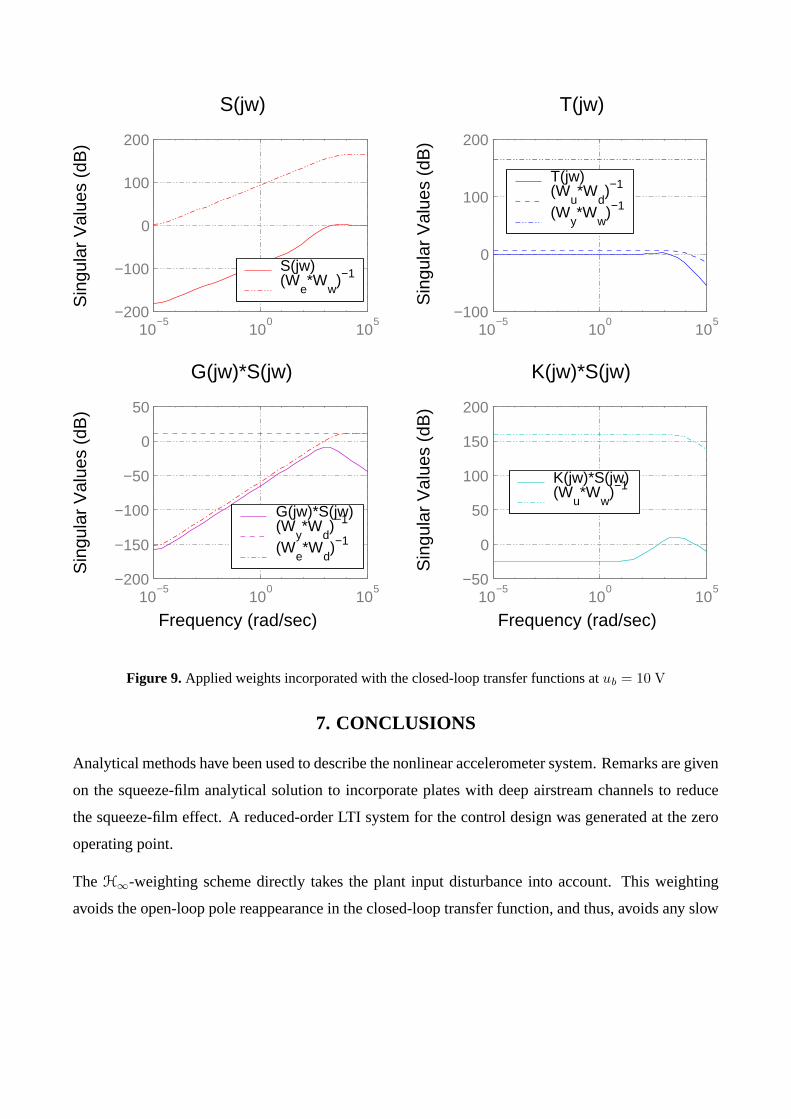
Fig. 9 shows the applied weighting scheme‡ incorporated with the closed-loop transfer functions. The

weighting directly takes the plant input disturbance into account and optimizes the plant input dis-

turbance rejection. Apart from a good tracking response of Ti, this guarantees a good disturbance

rejection for both, input and output disturbances.

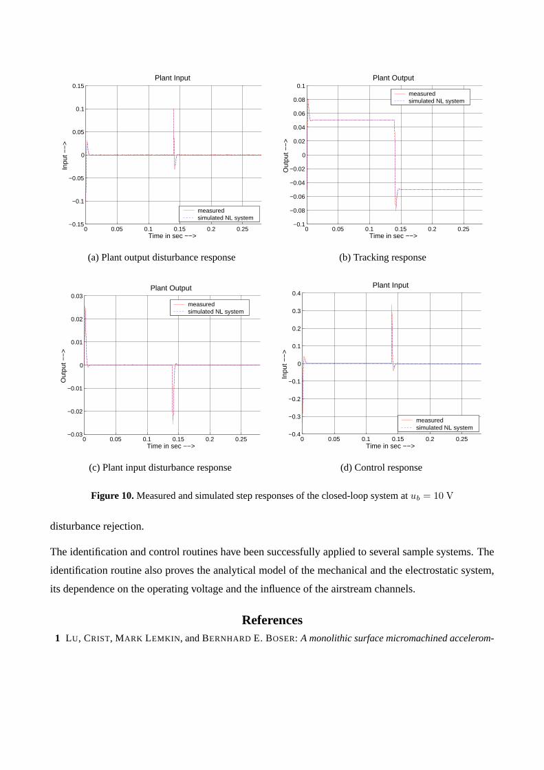
The time-domain measured results compared to the simulation results shows Fig. 10. It can be seen,

that the practical results show a very good conformance with the simulated results. The weighting

scheme also prevents the reappearance of the open-loop poles in the closed-loop transfer functions and

thus, avoids a slow disturbance rejection.

†ANSYS is a trademark of ANSYS, Inc., Canonsburg, PA‡The weights Ww = ε, Wd = Md, We = (sM−1

s + ωb)/(s + ωbε), Wu = (s + ωbtM−1t )/(εs + ωbt)

and Wy = M−1y were applied for the H∞-minimization, where Md = gmaxkg/(kpwmku), Ms = My = 2.5,

Mt = 2Md, ωb = 2π200 Hz, ωbt = 10ωb and ε → 0.

Sin

gula

r V

alue

s (d

B)

S(jw)

10−5

100

105

−200

−100

0

100

200

S(jw) (W

e*W

w)−1

Sin

gula

r V

alue

s (d

B)

T(jw)

10−5

100

105

−100

0

100

200

T(jw) (W

u*W

d)−1

(Wy*W

w)−1

Frequency (rad/sec)

Sin

gula

r V

alue

s (d

B)

G(jw)*S(jw)

10−5

100

105

−200

−150

−100

−50

0

50

G(jw)*S(jw) (W

y*W

d)−1

(We*W

d)−1

Frequency (rad/sec)

Sin

gula

r V

alue

s (d

B)

K(jw)*S(jw)

10−5

100

105

−50

0

50

100

150

200

K(jw)*S(jw) (W

u*W

w)−1

Figure 9. Applied weights incorporated with the closed-loop transfer functions at ub = 10 V

7. CONCLUSIONS

Analytical methods have been used to describe the nonlinear accelerometer system. Remarks are given

on the squeeze-film analytical solution to incorporate plates with deep airstream channels to reduce

the squeeze-film effect. A reduced-order LTI system for the control design was generated at the zero

operating point.

The H∞-weighting scheme directly takes the plant input disturbance into account. This weighting

avoids the open-loop pole reappearance in the closed-loop transfer function, and thus, avoids any slow

0 0.05 0.1 0.15 0.2 0.25−0.15

−0.1

−0.05

0

0.05

0.1

0.15

Time in sec −−>

Inpu

t −−

>

Plant Input

measured simulated NL system

(a) Plant output disturbance response

0 0.05 0.1 0.15 0.2 0.25−0.1

−0.08

−0.06

−0.04

−0.02

0

0.02

0.04

0.06

0.08

0.1

Time in sec −−>

Out

put −

−>

Plant Output


(b) Tracking response

0 0.05 0.1 0.15 0.2 0.25−0.03

−0.02

−0.01

0

0.01

0.02

0.03

Time in sec −−>

Out

put −

−>

Plant Output


(c) Plant input disturbance response

0 0.05 0.1 0.15 0.2 0.25−0.4

−0.3

−0.2

−0.1

0

0.1

0.2

0.3

0.4

Time in sec −−>

Inpu

t −−

>Plant Input


(d) Control response

Figure 10. Measured and simulated step responses of the closed-loop system at ub = 10 V

disturbance rejection.

The identification and control routines have been successfully applied to several sample systems. The

identification routine also proves the analytical model of the mechanical and the electrostatic system,

its dependence on the operating voltage and the influence of the airstream channels.

References1 LU, CRIST, MARK LEMKIN, and BERNHARD E. BOSER: A monolithic surface micromachined accelerom-

eter with digital output. IEEE Journal of Solid-State Circuits, 30(12):1367–1373, December 1995.

2 HANDTMANN, MARTIN: Dynamische Regelung mikroelektromechanischer Systeme (MEMS) mit Hilfe ka-pazitiver Signalwandlung und Kraftrückkoppelung. Doktorarbeit, Technische Universität München, Mün-chen, Juli 2004.

3 WINE, DAVID W., MARK P. HELSEL, LORNE JENKINS, HAKAN UREY, and THOR D. OSBORN: Perfor-mance of a biaxial mems-based scanner for microdisplay applications. In MOTAMEDI, M. EDWARD andROLF GOERING (editors): MOEMS and Miniaturized Systems, volume 4178 of Proceedings of SPIE, pages186–196, Santa Clara, CA, September 2000. SPIE.

4 CHEUNG, PATRICK, ROBERTO HOROWITZ, and ROGER T. HOWE: Design, fabrication, position sens-ing, and control of an electrostatically-driven polysilicon microactuator. IEEE Transactions on Magnetics,32(1):122–128, January 1996.

5 HORSLEY, DAVID A., NAIYAVUDHI WONGKOMET, ROBERTO HOROWITZ, and ALBERT P. PISANO:Precision positioning using a microfabricated electrostatic actuator. IEEE Transactions on Magnetics,35(2):993–999, March 1999.

6 LIAO, KE-MIN, YI-CHIH WANG, CHIH-HSIEN YEH, and RONGSHUN CHEN: Closed-loop adaptive con-trol for torsional micromirrors. In EL-FATATRY, AYMAN (editor): MOEMS and Miniaturized Systems IV,volume 5346 of Proceedings of SPIE, pages 184–192, Bellingham, WA, 2004. SPIE.

7 PARK, SUNGSU, ROBERTO HOROWITZ, and CHIN-WOO TAN: Adaptive controller design of mems gyro-scopes. In Proceedings of the 2001 IEEE Intelligent Transportation Systems, pages 496–501, Oakland, CA,August 25–29, 2001. IEEE.

8 PARK, SUNGSU and ROBERTO HOROWITZ: Adaptive control for the conventional mode of operation ofmems gyroscopes. Journal of Microelectromechanical Systems, 12(1):101–108, February 2003.

9 GAURA, E. I., N. FERREIRA, R. J. RIDER, and N. STEELE: Closed-loop, neural network controlled ac-celerometer design. In LAUDON, MATTHEW and BART ROMANOWICZ (editors): Proceedings of the ThirdInternational Conference on Modeling and Simulation of Microsystems, pages 513–516, San Diego, CA,March 27–29, 2000.

10 SANE, HARSHAD S., NAVID YAZDI, and CARLOS MASTRANGELO: Robust control of electrostatic tor-sional micromirrors using adaptive sliding-mode control. In Proceedings of SPIE – Photonics West 2005,volume 5719, pages 115–126, San Jose, CA, January 22–27, 2005.

11 JUNEAU, THOR, KLAUS UNTERKOFLER, TONY SELIVERSTOV, SAM ZHANG, and MICHAEL JUDY: Dual-axis optical mirror positioning using a nonlinear closed-loop controller. In Transducers: InternationalConference on Solid State Sensors, Actuators and Microsystems, volume 1 & 2, pages 560–563, Boston,MA, June 2003. IEEE.

12 WINKLER, JOHANNES und HORST AURICH: Technische Mechanik. Nachschlagebücher für Grundlagen-fächer. VEB Fachbuchverlag Leipzig, 1985.

13 LANGLOIS, W. E.: Isothermal squeeze films. Quarterly of Applied Mathematics, 20(2):131–150, 1962.

14 GRIFFIN, W. S., H. H. RICHARDSON, and S. YAMANAMI: A study of fluid squeeze-film damping. Journalof Basic Engineering, Transactions of the ASME, 88:451–456, 1966.

15 WOLFRAM, HEIKO, RALF SCHMIEDEL, KARLA HILLER, TORSTEN AURICH, WOLFGANG GÜNTHER,STEFFEN KURTH, JAN MEHNER, WOLFRAM DÖTZEL, and THOMAS GESSNER: Model building, controldesign and practical implementation of a high precision, high dynamical mems acceleration sensor. InProc. of SPIE, Sevilla, Spain, May 09–11, 2005. SPIE.

16 UCHIDA, NORIO, KIYOTAKA UCHIMARU, MINORU YONEZAWA, and MASAYUKI SEKIMURA: Dampingof micro electrostatic torsion mirror caused by air-film viscosity. In International Conference on MicroElectro Mechanical Systems, pages 449–454, Miyazaki, Japan, January 23–27, 2000. IEEE.

17 WOLFRAM, HEIKO, RALF SCHMIEDEL, KARLA HILLER, THORSTEN AURICH, WOLFGANG GÜNTHER,WOLFRAM DÖTZEL und THOMAS GESSNER: Modellierung, Reglerentwurf und Praxistest eines hochdyna-mischen MEMS-Präzisionsbeschleunigungssensors. In: 5. GMM/ITG/GI-Workshop Multi-Nature Systems,Seiten 33–40, Dresden, 18. Februar 2005. Fraunhofer-Institut für Integrierte Schaltungen.

18 VAN OVERSCHEE, PETER and BART DE MOOR: Subspace Identification for Linear Systems – Theory -Implementation - Applications. Kluwer Academic Publishers, Boston, London, Dordrecht, 1996.

19 ZHOU, KEMIN and JOHN C. DOYLE: Essentials of Robust Control. Prentice Hall, Upper Saddle River, NJ,1998.

Authors:Heiko WolframChemnitz University of Technology,Faculty of Electrical Engineering and Information TechnologyReichenhainer Str. 7009126 Chemnitz, GermanyTelephone: +49 (0)371/531-3274Fax: +49 (0)371/531-3259E-mail: <[email protected]>

Ralf SchmiedelChemnitz University of Technology,Faculty of Electrical Engineering and Information TechnologyReichenhainer Str. 7009126 Chemnitz, GermanyTelephone: +49 (0)371/531-3253Fax: +49 (0)371/531-3131E-mail: <[email protected]>

Torsten AurichGEMAC – Gesellschaft für Mikroelektronikanwendungen Chemnitz m.b.H.Zwickauer Str. 22709116 Chemnitz, GermanyTelephone: +49 (0)371/3377-305Fax: +49 (0)371/3377-272E-mail: <[email protected]>

Jan MehnerFraunhofer Institute for Reliability and MicrointegrationReichenhainer Str. 8809126 Chemnitz, GermanyTelephone: +49 (0)371/5397-924Fax: +49 (0)371/5397-310E-mail: <[email protected]>

Thomas GeßnerChemnitz University of Technology,Faculty of Electrical Engineering and Information TechnologyReichenhainer Str. 7009126 Chemnitz, GermanyTelephone: +49 (0)371/531-3130Fax: +49 (0)371/531-3131E-mail: <[email protected]>

Wolfram DötzelChemnitz University of Technology,Faculty of Electrical Engineering and Information TechnologyReichenhainer Str. 7009126 Chemnitz, GermanyTelephone: +49 (0)371/531-3264Fax: +49 (0)371/531-3259E-mail: <[email protected]>

http://www.tu-chemnitz.de

http://www.tu-chemnitz.de/etit/microsys

mailto:[email protected]


http://www.zfm.tu-chemnitz.de


http://www.gemac-chemnitz.de


http://www.pb.izm.fhg.de/mdae



http://www.tu-chemnitz.de/etit/microtec



http://www.tu-chemnitz.de/etit/microsys


Maschinenbau von Makro bis Nano / Mechanical Engineering ... · 50. Internationales...

Documents

Transcript of Maschinenbau von Makro bis Nano / Mechanical Engineering ... · 50. Internationales...