
Masterarbeit - RWTH Aachen Universityexmi.rwth-aachen.de/wp-content/uploads/thesis_grahe.pdf ·...
84
Masterarbeit vorgelegt der Fakultät für Mathematik, Informatik und Naturwissenschaften angefertigt im Institut Experimentelle Molekulare Bildgebung in der Arbeitsgruppe Physik der Molekularen Bildgebungssysteme an der RWTH Aachen Titel: Optical Simulation of Differently Shaped Monolithic Scintillators for PET-MRI Detectors Autor: Jan Gerrit Grahe MatNr. 309810 Abgabedatum: 29. August 2017 1. Gutachter: Univ.-Prof. Dr.-Ing. Volkmar Schulz 2. Gutachter: Univ.-Prof. Dr. rer. nat. Achim Stahl
Transcript of Masterarbeit - RWTH Aachen Universityexmi.rwth-aachen.de/wp-content/uploads/thesis_grahe.pdf ·...

Masterarbeit
vorgelegt der
Fakultät für Mathematik, Informatik
und Naturwissenschaften
angefertigt im Institut
Experimentelle Molekulare Bildgebung
in der Arbeitsgruppe
Physik der Molekularen Bildgebungssysteme
an der
RWTH Aachen
Titel: Optical Simulation of Differently Shaped Monolithic Scintillators forPET-MRI Detectors
Autor: Jan Gerrit GraheMatNr. 309810
Abgabedatum: 29. August 2017
1. Gutachter: Univ.-Prof. Dr.-Ing. Volkmar Schulz2. Gutachter: Univ.-Prof. Dr. rer. nat. Achim Stahl

Zentrales Prüfungsamt/Central Examination Office
Eidesstattliche Versicherung Statutory Declaration in Lieu of an Oath
___________________________ ___________________________
Name, Vorname/Last Name, First Name Matrikelnummer (freiwillige Angabe) Matriculation No. (optional)
Ich versichere hiermit an Eides Statt, dass ich die vorliegende Arbeit/Bachelorarbeit/
Masterarbeit* mit dem Titel I hereby declare in lieu of an oath that I have completed the present paper/Bachelor’s thesis/Master’s thesis* entitled
__________________________________________________________________________
__________________________________________________________________________
__________________________________________________________________________
selbstständig und ohne unzulässige fremde Hilfe erbracht habe. Ich habe keine anderen als
die angegebenen Quellen und Hilfsmittel benutzt. Für den Fall, dass die Arbeit zusätzlich auf
einem Datenträger eingereicht wird, erkläre ich, dass die schriftliche und die elektronische
Form vollständig übereinstimmen. Die Arbeit hat in gleicher oder ähnlicher Form noch keiner
Prüfungsbehörde vorgelegen. independently and without illegitimate assistance from third parties. I have use no other than the specified sources and aids. In
case that the thesis is additionally submitted in an electronic format, I declare that the written and electronic versions are fully
identical. The thesis has not been submitted to any examination body in this, or similar, form.
___________________________ ___________________________
Ort, Datum/City, Date Unterschrift/Signature
*Nichtzutreffendes bitte streichen
*Please delete as appropriate
Belehrung: Official Notification:
§ 156 StGB: Falsche Versicherung an Eides Statt
Wer vor einer zur Abnahme einer Versicherung an Eides Statt zuständigen Behörde eine solche Versicherung
falsch abgibt oder unter Berufung auf eine solche Versicherung falsch aussagt, wird mit Freiheitsstrafe bis zu drei
Jahren oder mit Geldstrafe bestraft.
Para. 156 StGB (German Criminal Code): False Statutory Declarations
Whosoever before a public authority competent to administer statutory declarations falsely makes such a declaration or falsely
testifies while referring to such a declaration shall be liable to imprisonment not exceeding three years or a fine. § 161 StGB: Fahrlässiger Falscheid; fahrlässige falsche Versicherung an Eides Statt
(1) Wenn eine der in den §§ 154 bis 156 bezeichneten Handlungen aus Fahrlässigkeit begangen worden ist, so
tritt Freiheitsstrafe bis zu einem Jahr oder Geldstrafe ein.
(2) Straflosigkeit tritt ein, wenn der Täter die falsche Angabe rechtzeitig berichtigt. Die Vorschriften des § 158
Abs. 2 und 3 gelten entsprechend.
Para. 161 StGB (German Criminal Code): False Statutory Declarations Due to Negligence
(1) If a person commits one of the offences listed in sections 154 to 156 negligently the penalty shall be imprisonment not exceeding one year or a fine. (2) The offender shall be exempt from liability if he or she corrects their false testimony in time. The provisions of section 158 (2) and (3) shall apply accordingly.
Die vorstehende Belehrung habe ich zur Kenntnis genommen: I have read and understood the above official notification:
___________________________ ___________________________
Ort, Datum/City, Date Unterschrift/Signature


Acknowledgements 4
Acknowledgements
At the beginning I would like to express my gratitude for the opportunity to write my master’s thesisin the group of Prof. Volkmar Schulz. I would like to thank the whole group for the nice atmosphere,the provided feedback and the fertile discussions.
Especially I would like to thank Dr. David Schug for his supervision and the consistent help providedduring my thesis. Furthermore, I thank Patrick Hallen and Florian Müller for the frequent discussions,the provided knowledge and the close collaboration.

Abstract 6
Abstract
In this work, a Monte Carlo simulation of monolithic detectors used in positron emission therapy(PET) is developed. The performance of the detector module depends on the light generation anddistribution in the scintillator, as well as the properties of the attached photodetector. The detectormodule is modeled using Geant4 to estimate and understand the influence of the detector moduleparameters on the performance. The simulation is used to investigate possible improvements of thedetector module.
The simulation is matched to experimental data of a monolithic detector module, which allows todetermine the optical properties and validate the obtained results. The best match for the scintillator’slight yield and bulk attenuation length are 35 000 photons/MeV and 25 cm, respectively. The simulatedcalibration of a 12 mm thick LYSO crystal wrapped in reflective Teflon obtains a similar performanceas the experimental calibration with a spatial resolution of Ssim = 1.72 mm to Sexp = 1.68 mm. Theapplication of a machine-learning positioning algorithm trained on simulated data to the experimentaldetector module results in an overall good performance. The proof of concept is successful.
The geometrical investigations using the simulation of the PET detector module for 10 mm thickscintillators yields the best spatial resolutions of 1.00 mm if the crystal is wrapped in retroreflectortape. The performance of the detector module does not change when using Meltmount 1.704 insteadof SYLGARD 527 as an optical adhesive between crystal and photodetector.

Contents
Abstract 5
1 Introduction 9
2 Physical Processes 122.1 Radioactive Decay . . . . . . . . . . . . . . . . . . . . . . . . . . . . . . . . . . . . . . 122.2 Interaction of Positrons with Matter . . . . . . . . . . . . . . . . . . . . . . . . . . . . 132.3 Interaction of Gamma Particles with Matter . . . . . . . . . . . . . . . . . . . . . . . . 142.4 Scintillation . . . . . . . . . . . . . . . . . . . . . . . . . . . . . . . . . . . . . . . . . . 172.5 Interactions of Optical Photons . . . . . . . . . . . . . . . . . . . . . . . . . . . . . . . 17
3 PET Detector Modules 203.1 PET Detector Properties and Applications . . . . . . . . . . . . . . . . . . . . . . . . 203.2 Scintillator Materials . . . . . . . . . . . . . . . . . . . . . . . . . . . . . . . . . . . . . 213.3 Photodetectors . . . . . . . . . . . . . . . . . . . . . . . . . . . . . . . . . . . . . . . . 223.4 Combination of Scintillator and Detector . . . . . . . . . . . . . . . . . . . . . . . . . . 233.5 Monolithic Detector Modules . . . . . . . . . . . . . . . . . . . . . . . . . . . . . . . . 23
4 Monte Carlo Simulation 284.1 Motivation . . . . . . . . . . . . . . . . . . . . . . . . . . . . . . . . . . . . . . . . . . 284.2 Working Principle . . . . . . . . . . . . . . . . . . . . . . . . . . . . . . . . . . . . . . 28
5 Optimization of the Radioactive Source 315.1 Experimental Collimator Setup . . . . . . . . . . . . . . . . . . . . . . . . . . . . . . . 315.2 Source Geometry . . . . . . . . . . . . . . . . . . . . . . . . . . . . . . . . . . . . . . . 315.3 Simulation . . . . . . . . . . . . . . . . . . . . . . . . . . . . . . . . . . . . . . . . . . . 325.4 Efficiency of Different Sources . . . . . . . . . . . . . . . . . . . . . . . . . . . . . . . . 335.5 Analysis of Particle Composition . . . . . . . . . . . . . . . . . . . . . . . . . . . . . . 33
6 Optical Simulation 356.1 Gamma Absorption . . . . . . . . . . . . . . . . . . . . . . . . . . . . . . . . . . . . . 356.2 Light Generation in the Scintillator . . . . . . . . . . . . . . . . . . . . . . . . . . . . . 366.3 Propagation of Optical Photons . . . . . . . . . . . . . . . . . . . . . . . . . . . . . . . 386.4 The Photodetector . . . . . . . . . . . . . . . . . . . . . . . . . . . . . . . . . . . . . . 416.5 Matching the Simulation to the Experiment . . . . . . . . . . . . . . . . . . . . . . . . 466.6 Conclusion . . . . . . . . . . . . . . . . . . . . . . . . . . . . . . . . . . . . . . . . . . 51
7 Monolithic Calibration Algorithms 537.1 Positioning Algorithm . . . . . . . . . . . . . . . . . . . . . . . . . . . . . . . . . . . . 537.2 Energy Calibration . . . . . . . . . . . . . . . . . . . . . . . . . . . . . . . . . . . . . . 56
8 Calibration in Experiment and Simulation 588.1 Comparison of Experimental and Simulated Calibration . . . . . . . . . . . . . . . . . 598.2 Cross Positioning . . . . . . . . . . . . . . . . . . . . . . . . . . . . . . . . . . . . . . . 618.3 General Discussion . . . . . . . . . . . . . . . . . . . . . . . . . . . . . . . . . . . . . . 65
9 Evaluation of Promising Geometries 669.1 Variation of Sensor Placement . . . . . . . . . . . . . . . . . . . . . . . . . . . . . . . . 669.2 Variation of Wrapping . . . . . . . . . . . . . . . . . . . . . . . . . . . . . . . . . . . . 689.3 Variation of Thickness . . . . . . . . . . . . . . . . . . . . . . . . . . . . . . . . . . . . 729.4 Variation of Scintillator Shape . . . . . . . . . . . . . . . . . . . . . . . . . . . . . . . 739.5 Variation of the Optical Adhesive . . . . . . . . . . . . . . . . . . . . . . . . . . . . . . 749.6 Conclusion . . . . . . . . . . . . . . . . . . . . . . . . . . . . . . . . . . . . . . . . . . 76
10 Summary 79
11 Appendix 8011.1 Initial Matching of Optical Parameters . . . . . . . . . . . . . . . . . . . . . . . . . . . 80

Abstract 8
Literature 81
1 Introduction 9
1 Introduction
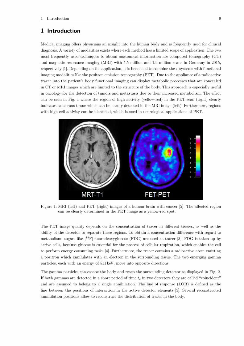
Medical imaging offers physicians an insight into the human body and is frequently used for clinicaldiagnosis. A variety of modalities exists where each method has a limited scope of application. The twomost frequently used techniques to obtain anatomical information are computed tomography (CT)and magnetic resonance imaging (MRI) with 5.5 million and 1.9 million scans in Germany in 2015,respectively [1]. Depending on the application, it is beneficial to combine these systems with functionalimaging modalities like the positron emission tomography (PET). Due to the appliance of a radioactivetracer into the patient’s body functional imaging can display metabolic processes that are concealedin CT or MRI images which are limited to the structure of the body. This approach is especially usefulin oncology for the detection of tumors and metastasis due to their increased metabolism. The effectcan be seen in Fig. 1 where the region of high activity (yellow-red) in the PET scan (right) clearlyindicates cancerous tissue which can be hardly detected in the MRI image (left). Furthermore, regionswith high cell activity can be identified, which is used in neurological applications of PET.
Figure 1: MRI (left) and PET (right) images of a human brain with cancer [2]. The affected regioncan be clearly determined in the PET image as a yellow-red spot.
The PET image quality depends on the concentration of tracer in different tissues, as well as theability of the detector to separate these regions. To obtain a concentration difference with regard tometabolism, sugars like [18F]-fluorodeoxyglucose (FDG) are used as tracer [3]. FDG is taken up byactive cells, because glucose is essential for the process of cellular respiration, which enables the cellto perform energy consuming tasks [4]. Furthermore, the tracer contains a radioactive atom emittinga positron which annihilates with an electron in the surrounding tissue. The two emerging gammaparticles, each with an energy of 511 keV, move into opposite directions.
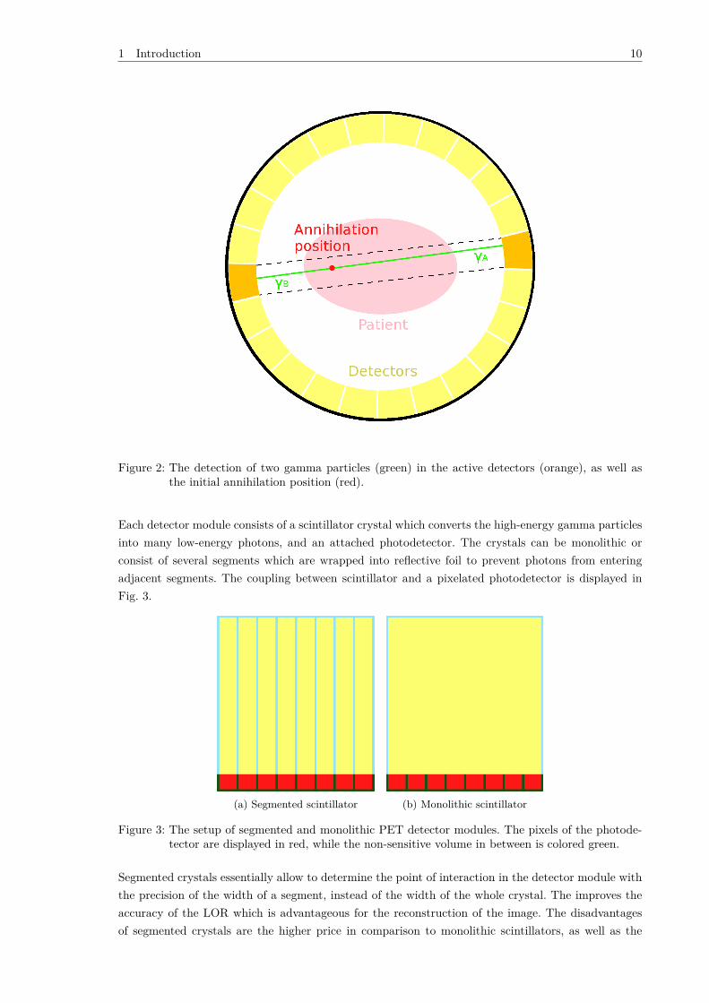
The gamma particles can escape the body and reach the surrounding detector as displayed in Fig. 2.If both gammas are detected in a short period of time tc in two detectors they are called “coincident”and are assumed to belong to a single annihilation. The line of response (LOR) is defined as theline between the positions of interaction in the active detector elements [5]. Several reconstructedannihilation positions allow to reconstruct the distribution of tracer in the body.
1 Introduction 10
Figure 2: The detection of two gamma particles (green) in the active detectors (orange), as well asthe initial annihilation position (red).
Each detector module consists of a scintillator crystal which converts the high-energy gamma particlesinto many low-energy photons, and an attached photodetector. The crystals can be monolithic orconsist of several segments which are wrapped into reflective foil to prevent photons from enteringadjacent segments. The coupling between scintillator and a pixelated photodetector is displayed inFig. 3.
(a) Segmented scintillator (b) Monolithic scintillator
Figure 3: The setup of segmented and monolithic PET detector modules. The pixels of the photode-tector are displayed in red, while the non-sensitive volume in between is colored green.
Segmented crystals essentially allow to determine the point of interaction in the detector module withthe precision of the width of a segment, instead of the width of the whole crystal. The improves theaccuracy of the LOR which is advantageous for the reconstruction of the image. The disadvantagesof segmented crystals are the higher price in comparison to monolithic scintillators, as well as the
1 Introduction 11
reduction of the sensitive volume due to the addition of reflective foil [6]. Monolithic detector modulescan improve their resolution by determining the point of interaction based on the spatial distributionof photons among the pixels of the detector. Furthermore, it is possible to determine the depth ofinteraction (DOI), which can improve the reconstruction of the annihilation position along the LOR[7]. The determination of the interaction position requires a calibration step, where an algorithm isdeveloped using detector responses for events with known interaction points. The positioning algorithmis then tested by using further events with known interaction points.If the algorithm predicts theinteraction point reasonably well, the calibration step is concluded. Crystals with different dimensions,shapes and wrappings are calibrated and tested by several research groups to increase the performanceof the crystal. The variation of several crystal parameters, as well as different calibration setups andalgorithm, make it hard to estimate the influence of the individual changes on the performance of thedetector concept.
This Master’s thesis aims to support experiments using monolithic PET detectors with regards tothe calibration setup and monolithic PET detector geometries. The experimental calibration setup isrecreated virtually to test whether monolithic scintillators can be calibrated using machine learningalgorithms based on simulated data. This could spare the calibration of several detector modules.Therefore, an optical simulation of the scintillator block, as well as the modeling of the electronicreadout properties, are required to reproduce the experimental characteristics. Once the simulationof the detector module matches to the experiment and is reliable, it allows to change certain param-eters of the module. Therefore the performance of different monolithic scintillator geometries can bedetermined to give guidance for new experiments.
2 Physical Processes 12
2 Physical Processes
In this chapter, the relevant physical processes for PET are explained. The description is basedon [8].
2.1 Radioactive Decay
Unstable atomic nuclei decay spontaneously after a finite “lifetime” by emitting particles or splittinginto smaller nuclei. Depending on the nucleus, α, β± or γ particles can be emitted. Due to their verysmall mean free path, α and β− particles are not important for PET imaging, because they cannotleave the body or generate particles that could do so. Consequently, this paragraph focuses on theβ+ and γ decay which both lead to detectable particles in PET imaging. In general, a decay is onlypossible if the energy E in the initial state X is higher or equal than the combined energy of the finalstate of the nucleus Y and the energy of the emitted particle Ep. This relation is described by theformula
E(AZX) ≥ E(A′
Z′Y ) + Ep , (1)
where Z and A denote the atomic and mass number, respectively. For E(AZX) > E(A′
Z′Y ) + Ep theexcess energy is distributed among the product particles as kinetic energy. Furthermore, the decayhas to conserve other symmetries like the total numbers of leptons and baryons, which restricts thenumber of possible decays.
2.1.1 Beta+ Decay
The β+ decay is characterized by the emission of a positron and a neutrino from the nucleus. It canbe described by
AZX →A
Z−1 Y + e+ + νe , (2)
where e+ denotes a positron and ν a neutrino. Due to the three particles involved, the distribution ofkinetic energy varies for each decay. This leads to a continuous energy spectrum of the resulting β+
particle.
2.1.2 Gamma Decay
The spontaneous emission of γ particles, also denoted as gammas or gamma particles, only occurs incombination of either α or β radiation [8]. Furthermore, it can be artificially induced by excitationwith another γ particle. Experiments confirmed that γ particles originate from the de-excitation of anucleus from state k → i with
Eγ = ~ · ω = Ek − Ei for Ek > Ei , (3)
where E denotes the energy of a state or particle, ω the angular frequency and ~ the reduced Planckconstant.
2 Physical Processes 13
2.1.3 Electron Capture
The probability density |Ψ(r)|2 for electrons of the K-shell is non-zero in the nucleus (at r = 0).Therefore an electron can be captured by a proton which transforms into a neutron following
e− + p→ n+ νe . (4)
The transformation of nucleus X into nucleus Y can be described by
AZX + e− →A
Z−1 Y + νe . (5)
2.1.4 Relevant Decays
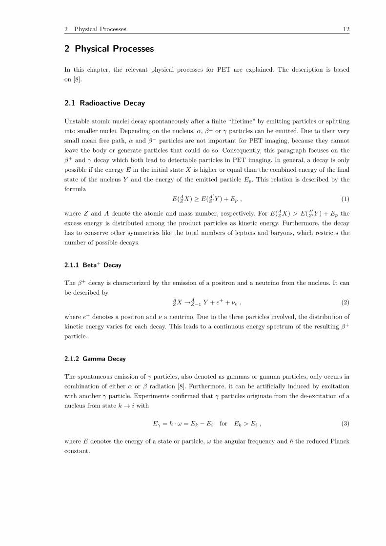
For the calibration of the detector module β+ emitting isotopes are used as a source. In principle FDGcould be used, but the half-life of approximately 110 minutes is impractical for long-term researchprojects. Therefore other β+ emitting isotopes like 22Na with a half-life of 2.6 years are used. Itgenerates a positron with an energy of up to 546 keV (average of 215 keV) in 90.3 % of its decays [9].The decaying isotope is bound in the chemical composition of sodium chloride. The decay scheme isdisplayed in Fig. 4a. The initial decay produces two gamma particles in an annihilation (see chapter2.2) e−+ e+ → 2γ1 with E(γ1) = 511 keV. It is important to denote that the emission of a γ2 particlewith energy E(γ2) = 1.280 MeV takes part only 3.60 ps [10] after the emission of the positron. Thereforethe three gamma particles are emitted at the same time, but there is no directional correlation betweenone of the two back-to-back oriented 511 keV gamma particles and the 1.275 MeV gamma particle. Theinfluence of 1.275 MeV gamma particles is reduced by the measurement of coincident gamma particles.An alternative source material is the isotope 68Ge which is contained in the chemical compositiongermanium disulfide [11]. It decays to 68Ga, which creates the desired positron as displayed in its decayscheme in Fig. 4b. The energy of the mainly occurring positron which is created in approximately88 % of all decays, can reach 1899 keV (on average 836 keV) which is higher than the energy of thepositrons created by 22Na.
(a) The decay scheme for 22Na. (b) The decay scheme for 68Ge [12].
Figure 4: The decay schemes for 22Na and 68Ge.
2.2 Interaction of Positrons with Matter
Positrons emitted in a β+ decay can travel a certain distance in tissue. They lose most of their energyby interactions with atomic electrons along the way. The distance traveled increases with positronenergy and decreases with tissue density [14]. Due to the multiple interactions and the corresponding
2 Physical Processes 14
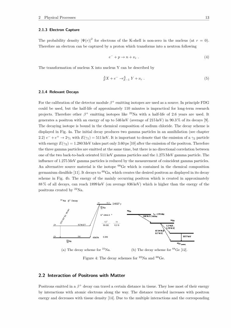
(a) The annihilation of the emitted positron e+
with an electron e−, following the β+ decay ofan atom, results in two γ-particles with oppos-ing direction. A neutrino ν is emitted whichmostly leaves the system undetected.
(b) The positron range in water equivalent forpositrons generated by 18F [13].
Figure 5: The annihilation process and the positron range of positrons.
directional changes, the total traveled distance is longer than the distance between start and end point.The latter value is displayed in Fig. 5b for positrons generated by 18F in water equivalent.
At the end of its trajectory the positron annihilates with an electron as displayed in Fig. 5a. Thecreated gamma particles are emitted into opposing directions in their center-of-momentum frame.When observing the interaction in the laboratory frame, the kinetic energies of positron and electronlead to a slight deviation from 180, which is called acollinearity. The measured standard deviation ofthe distribution of the angle is astimated as 0.23 [15][16]. The generation process is displayed in Fig.5a.
2.3 Interaction of Gamma Particles with Matter
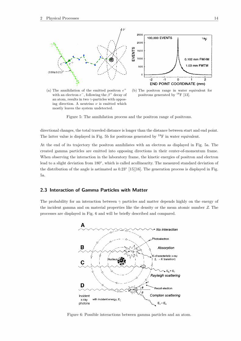
The probability for an interaction between γ particles and matter depends highly on the energy ofthe incident gamma and on material properties like the density or the mean atomic number Z. Theprocesses are displayed in Fig. 6 and will be briefly described and compared.
Figure 6: Possible interactions between gamma particles and an atom.
2 Physical Processes 15
2.3.1 Compton Scattering
Compton scattering denotes the inelastic interaction between a γ particle and a loosely bound electron.The gamma transfers energy to the electron and therefore loses energy itself, elongates its wavelengthand changes its direction. The differential cross section dσ
dΩ can be calculated analytically using theKlein-Nishina formula
dσ
dΩ ∝ P (Eγ , θ)2[P (Eγ , θ) + P (Eγ , θ)−1 − sin2 θ]/2 (6)
withP (Eγ , θ) = 1
1 + (Eγ/mec2)(1− cos θ) , (7)
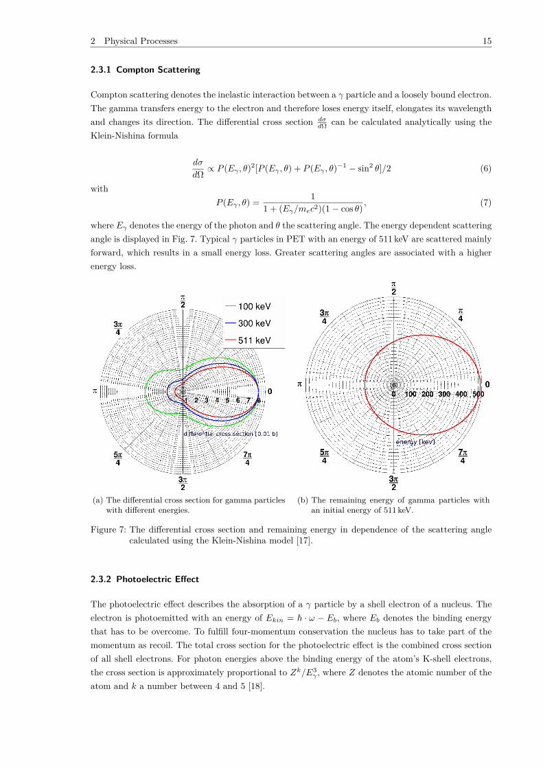
where Eγ denotes the energy of the photon and θ the scattering angle. The energy dependent scatteringangle is displayed in Fig. 7. Typical γ particles in PET with an energy of 511 keV are scattered mainlyforward, which results in a small energy loss. Greater scattering angles are associated with a higherenergy loss.
(a) The differential cross section for gamma particleswith different energies.
(b) The remaining energy of gamma particles withan initial energy of 511 keV.
Figure 7: The differential cross section and remaining energy in dependence of the scattering anglecalculated using the Klein-Nishina model [17].
2.3.2 Photoelectric Effect
The photoelectric effect describes the absorption of a γ particle by a shell electron of a nucleus. Theelectron is photoemitted with an energy of Ekin = ~ · ω − Eb, where Eb denotes the binding energythat has to be overcome. To fulfill four-momentum conservation the nucleus has to take part of themomentum as recoil. The total cross section for the photoelectric effect is the combined cross sectionof all shell electrons. For photon energies above the binding energy of the atom’s K-shell electrons,the cross section is approximately proportional to Zk/E3
γ , where Z denotes the atomic number of theatom and k a number between 4 and 5 [18].
2 Physical Processes 16
2.3.3 Rayleigh Scattering
Rayleigh scattering denotes the effect of elastic scattering. The γ particle’s direction is changed slightly,but no energy is deposited. The Rayleigh cross-section is approximately proportional to the sixth powerof the effective diameter of the atom d and inverse proportional to the fourth power of the wavelengthλ as displayed in Eq. 8. The variable n denotes the refractive index of the medium [19].
σs ∝d6
λ4
(n2 − 1n2 + 2
)2
(8)
2.3.4 Beer-Lambert law
The total transmittance of a material can be defined by Lambert’s law by
T = e−∫ l
0µ(z)dz
, (9)
where l denotes the length of the path z in the material and µ its attenuation coefficient at eachposition along the path. From Beer’s Law the latter is defined as
µ(z) =N∑i=1
µi(z) =N∑i=1
σini(z) (10)
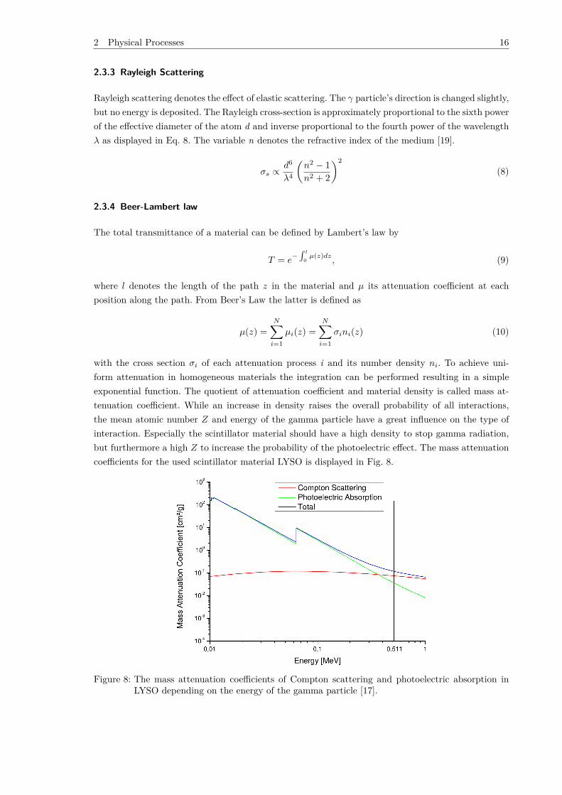
with the cross section σi of each attenuation process i and its number density ni. To achieve uni-form attenuation in homogeneous materials the integration can be performed resulting in a simpleexponential function. The quotient of attenuation coefficient and material density is called mass at-tenuation coefficient. While an increase in density raises the overall probability of all interactions,the mean atomic number Z and energy of the gamma particle have a great influence on the type ofinteraction. Especially the scintillator material should have a high density to stop gamma radiation,but furthermore a high Z to increase the probability of the photoelectric effect. The mass attenuationcoefficients for the used scintillator material LYSO is displayed in Fig. 8.
Figure 8: The mass attenuation coefficients of Compton scattering and photoelectric absorption inLYSO depending on the energy of the gamma particle [17].
2 Physical Processes 17
2.4 Scintillation
Scintillation is the process of generating optical photons in a crystal after an excitation of its atoms ormolecules by radiation. Optical photons are defined by an energy of below 100 eV. This luminescencecan be used to convert a high-energy gamma particle into many low-energy photons that can bedetected in photomultipliers attached to the scintillator. The energy spectrum of the emitted opticalphotons is characteristic for each material and might also depend on the kind of radiation that isdetected [20]. For most materials and energy ranges the mean number of optical photons produced isproportional to the deposited energy and is called light yield, abbreviated LY. The number of photonsgenerated in a single interaction fluctuates around the mean number of generated photons. However,the distribution of photon counts can deviate from the expected distribution of a pure Poisson process,depending on the crystal properties. The number, position and non-uniformity of inhomogeneities inthe crystal can broaden the distribution, while a high regularity of the crystal could tighten it. Thefactor is called Fano factor.
2.5 Interactions of Optical Photons
Optical photons can interact by [21]:
1. Elastic (Rayleigh) scattering
2. Absorption
3. Medium boundary interactions
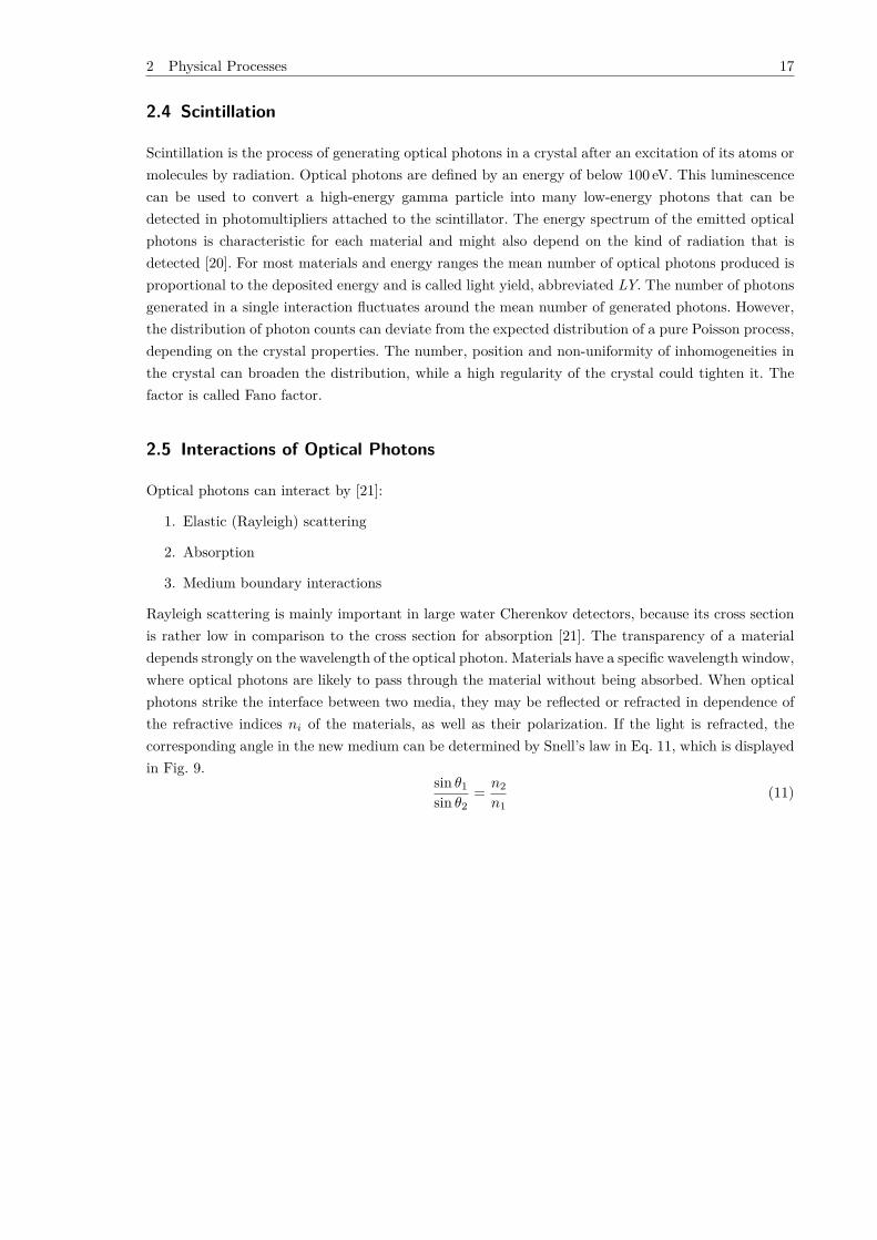
Rayleigh scattering is mainly important in large water Cherenkov detectors, because its cross sectionis rather low in comparison to the cross section for absorption [21]. The transparency of a materialdepends strongly on the wavelength of the optical photon. Materials have a specific wavelength window,where optical photons are likely to pass through the material without being absorbed. When opticalphotons strike the interface between two media, they may be reflected or refracted in dependence ofthe refractive indices ni of the materials, as well as their polarization. If the light is refracted, thecorresponding angle in the new medium can be determined by Snell’s law in Eq. 11, which is displayedin Fig. 9.
sin θ1
sin θ2= n2
n1(11)
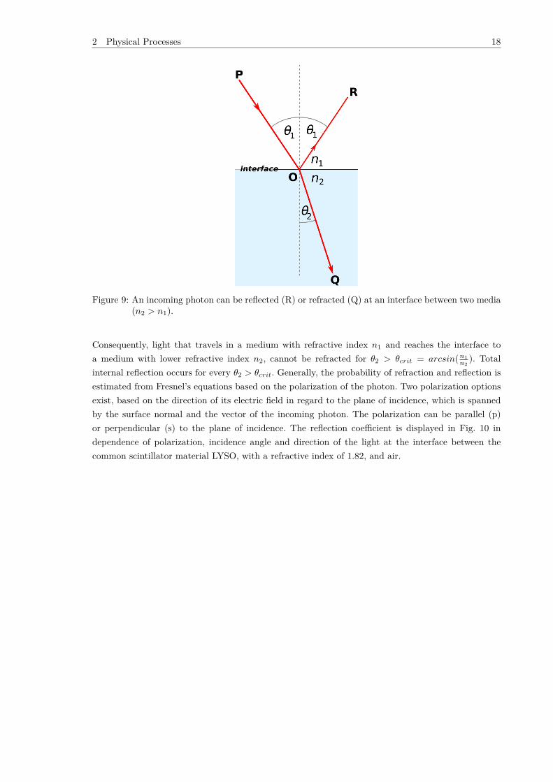
2 Physical Processes 18
Figure 9: An incoming photon can be reflected (R) or refracted (Q) at an interface between two media(n2 > n1).
Consequently, light that travels in a medium with refractive index n1 and reaches the interface toa medium with lower refractive index n2, cannot be refracted for θ2 > θcrit = arcsin(n1
n2). Total
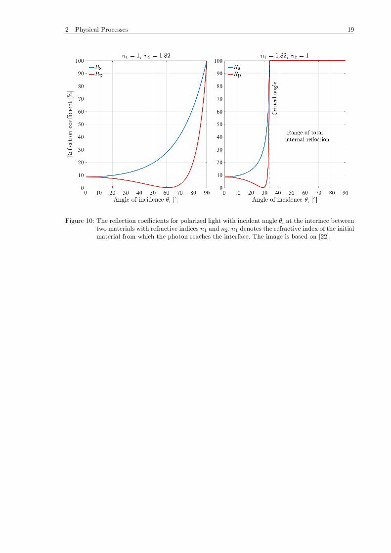
internal reflection occurs for every θ2 > θcrit. Generally, the probability of refraction and reflection isestimated from Fresnel’s equations based on the polarization of the photon. Two polarization optionsexist, based on the direction of its electric field in regard to the plane of incidence, which is spannedby the surface normal and the vector of the incoming photon. The polarization can be parallel (p)or perpendicular (s) to the plane of incidence. The reflection coefficient is displayed in Fig. 10 independence of polarization, incidence angle and direction of the light at the interface between thecommon scintillator material LYSO, with a refractive index of 1.82, and air.
2 Physical Processes 19
Figure 10: The reflection coefficients for polarized light with incident angle θi at the interface betweentwo materials with refractive indices n1 and n2. n1 denotes the refractive index of the initialmaterial from which the photon reaches the interface. The image is based on [22].
3 PET Detector Modules 20
3 PET Detector Modules
The requirements for PET detector modules depend on the application. Generally, they consist of ascintillator, converting high-energy gamma particles into optical photons, and a detector to measurethe optical photons and turn them into an electronic signal.
3.1 PET Detector Properties and Applications
PET scanners can be divided in two categories based on the diameter of the system:
1. Preclinical PET: Imaging of small animals
2. Clinical PET: Imaging of patients (whole-body, brain, . . . )
In the first approach the distribution of tracer is displayed in small animals, e.g. to obtain informationon the absorption of tracer in tissues or the efficiency of tumor treatments [23]. Clinical imaging ismainly used to locate tumors/metastasis in oncology or to display the activity of the brain [1].
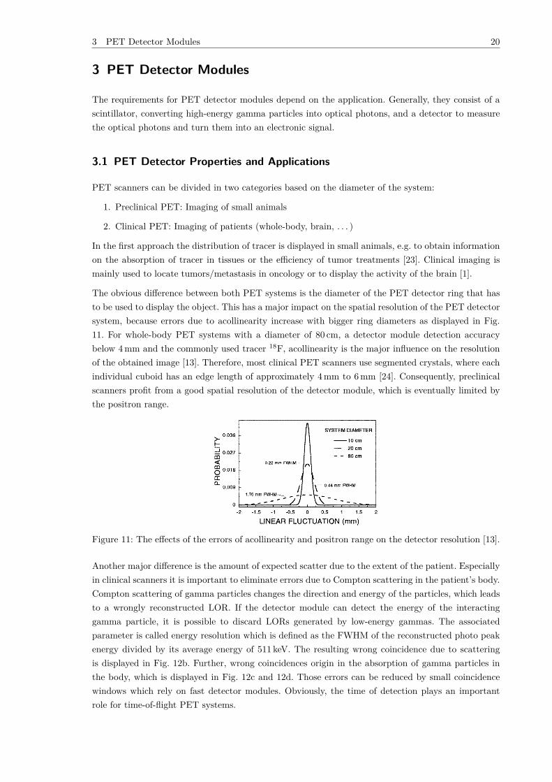
The obvious difference between both PET systems is the diameter of the PET detector ring that hasto be used to display the object. This has a major impact on the spatial resolution of the PET detectorsystem, because errors due to acollinearity increase with bigger ring diameters as displayed in Fig.11. For whole-body PET systems with a diameter of 80 cm, a detector module detection accuracybelow 4 mm and the commonly used tracer 18F, acollinearity is the major influence on the resolutionof the obtained image [13]. Therefore, most clinical PET scanners use segmented crystals, where eachindividual cuboid has an edge length of approximately 4 mm to 6 mm [24]. Consequently, preclinicalscanners profit from a good spatial resolution of the detector module, which is eventually limited bythe positron range.
Figure 11: The effects of the errors of acollinearity and positron range on the detector resolution [13].
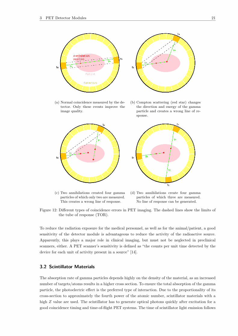
Another major difference is the amount of expected scatter due to the extent of the patient. Especiallyin clinical scanners it is important to eliminate errors due to Compton scattering in the patient’s body.Compton scattering of gamma particles changes the direction and energy of the particles, which leadsto a wrongly reconstructed LOR. If the detector module can detect the energy of the interactinggamma particle, it is possible to discard LORs generated by low-energy gammas. The associatedparameter is called energy resolution which is defined as the FWHM of the reconstructed photo peakenergy divided by its average energy of 511 keV. The resulting wrong coincidence due to scatteringis displayed in Fig. 12b. Further, wrong coincidences origin in the absorption of gamma particles inthe body, which is displayed in Fig. 12c and 12d. Those errors can be reduced by small coincidencewindows which rely on fast detector modules. Obviously, the time of detection plays an importantrole for time-of-flight PET systems.
3 PET Detector Modules 21
(a) Normal coincidence measured by the de-tector. Only these events improve theimage quality.
(b) Compton scattering (red star) changesthe direction and energy of the gammaparticle and creates a wrong line of re-sponse.
(c) Two annihilations created four gammaparticles of which only two are measured.This creates a wrong line of response.
(d) Two annihilations create four gammaparticles of which three are measured.No line of response can be generated.
Figure 12: Different types of coincidence errors in PET imaging. The dashed lines show the limits ofthe tube of response (TOR).
To reduce the radiation exposure for the medical personnel, as well as for the animal/patient, a goodsensitivity of the detector module is advantageous to reduce the activity of the radioactive source.Apparently, this plays a major role in clinical imaging, but must not be neglected in preclinicalscanners, either. A PET scanner’s sensitivity is defined as “the counts per unit time detected by thedevice for each unit of activity present in a source” [14].
3.2 Scintillator Materials
The absorption rate of gamma particles depends highly on the density of the material, as an increasednumber of targets/atoms results in a higher cross section. To ensure the total absorption of the gammaparticle, the photoelectric effect is the preferred type of interaction. Due to the proportionality of itscross-section to approximately the fourth power of the atomic number, scintillator materials with ahigh Z value are used. The scintillator has to generate optical photons quickly after excitation for agood coincidence timing and time-of-flight PET systems. The time of scintillator light emission follows
3 PET Detector Modules 22
a combination of one or more exponential decays, where the decay times are characteristic for eachmaterial. Additionally, some scintillators suffer from afterglow, the phenomenon of photon creationlong after the initial excitation. The number of generated photons should depend on the depositedenergy to determine the initial energy of the gamma particle. Furthermore, the number of generatedphotons for a deposited energy is called light yield. It should be high to account for good statisticsand stable to determine the energy of the gamma particle precisely. The stability of the light outputis referred to as the photon resolution of the scintillator. It can be written as R2
scinti = R2intr +R2
stat
with the intrinsic term Rintr and the statistical term Rstat [25]. While the latter originates from thein principle underlying Poisson process, the intrinsic resolution is based on the positional dependencyof the light yield in the crystal. Impurities from doping or crystal defects decrease the mean free pathof the generated optical photons [26] and create a dependence of the light yield on the position in thecrystal, which widens the total photon resolution [27]. The wavelength of the emitted photons has tomatch the material dependent window of transparency of the scintillator. Furthermore, the attachedphoton detector has to have a high detection efficiency for photons of this wavelength.
The best combination of these properties can by obtained using cerium-doped lutetium oxyorthosilicatecrystals (LSO) [28][29]. Mixing LSO with yttrium can reduce the afterglow of the crystal [30], butalso worsens the photon resolution slightly [31]. This effect can be explained by inhomogeneities in thecrystal, due to the addition of yttrium. The material is called LYSO. The average light yield does notchange significantly for yttrium fractions between 4 % to 10 % [31] and the most important advantagesof LSO are maintained, while the price for raw materials is reduced [25][31]. The properties of themost promising scintillator crystals for PET are summarized in Tab. 1.
Table 1: Physical properties of common scintillator crystals [29][32]. The relative light yield is normedto LYSO. The variable n denotes the refractive index of the scintillator material, while t1and t2 are the characteristic decay times.
Material Density [g cm−3] Effective Z rel. LY n t1 [ns] t2 [ns]
CdWO4 7.90 64 27 2.20 5000 20000
Lu2SiO5:Ce (LSO) 7.40 65 100 1.82 40 -
Bi4Ge3O12 (BGO) 7.12 75 20 2.15 300 -
Lu1.8Y0.2SiO5:Ce (LYSO) 7.11 65 100 1.82 40 -
BaF2 4.88 53 16 1.49 0.8 600
CsI:Tl 4.51 54 60 1.80 1000 -
NaI:Tl 3.67 51 133 1.85 230 10000
3.3 Photodetectors
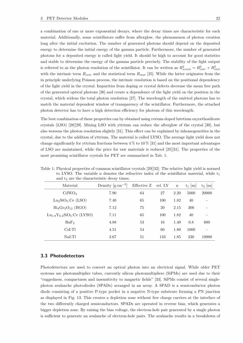
Photodetectors are used to convert an optical photon into an electrical signal. While older PETsystems use photomultiplier tubes, currently silicon photomultipliers (SiPMs) are used due to their“ruggedness, compactness and insensitivity to magnetic fields” [33]. SiPMs consist of several single-photon avalanche photodiodes (SPADs) arranged in an array. A SPAD is a semiconductor photondiode consisting of a positive P-type pocket in a negative N-type substrate forming a PN junctionas displayed in Fig. 13. This creates a depletion zone without free charge carriers at the interface ofthe two differently charged semiconductors. SPADs are operated in reverse bias, which generates abigger depletion zone. By raising the bias voltage, the electron-hole pair generated by a single photonis sufficient to generate an avalanche of electron-hole pairs. The avalanche results in a breakdown of
3 PET Detector Modules 23
the SPAD, which results in a digital signal. The number of SPADs that break down correspond tothe number of optical photons detected. The used digital SiPM not only calculates the total sum ofSPAD breakdowns, but provides additional timing information and allows to interact with specificSPADs. A SPAD can be recharged after the generation of an avalanche, which allows the detection ofthe next photon. Due to the high voltage required for the detection of photons, small influences dueto thermal noise can activate a SPAD. Furthermore, SPADs themselves generate new optical photonswhen triggering, which can cause triggers in adjacent SPADs. This effect is reduced by separatingSPADs from each other using absorbing materials. The SiPM returns the photon count in pixelsconsisting of several adjacent SPADs.
Figure 13: The layout of a SPAD with the P-type pocket in the overall negative N-type substrate.The optical photon can enter the SPAD through an opening window.
3.4 Combination of Scintillator and Detector
Different combinations of coupling between scintillator and photon detector exist, based on the scin-tillator structure. Segmented crystal arrays are commonly used in current PET scanners and consistof an array of smaller crystals, each wrapped in reflective foil. In a one-to-one coupling scheme eachof the smaller cuboids is attached to exactly one pixel of the photon detectors. Neglecting multipleinteractions of the high-energy gamma particle, one expects only a single pixel of the detector to beactive. This limits the resolution of the crystal to the resolution of the photon detector. The resolutioncan be improved to the size of the pitch of a single crystal cuboid by determining the hit cuboid basedon the light distribution among several pixels of the photodetector. Therefore, a light guide is usedto distribute the light generated in a cuboid over several pixels. The scintillator cuboid that detectedthe gamma particle can be extracted from the distribution of activated pixels using algorithms, e.g.the center of gravity [17].
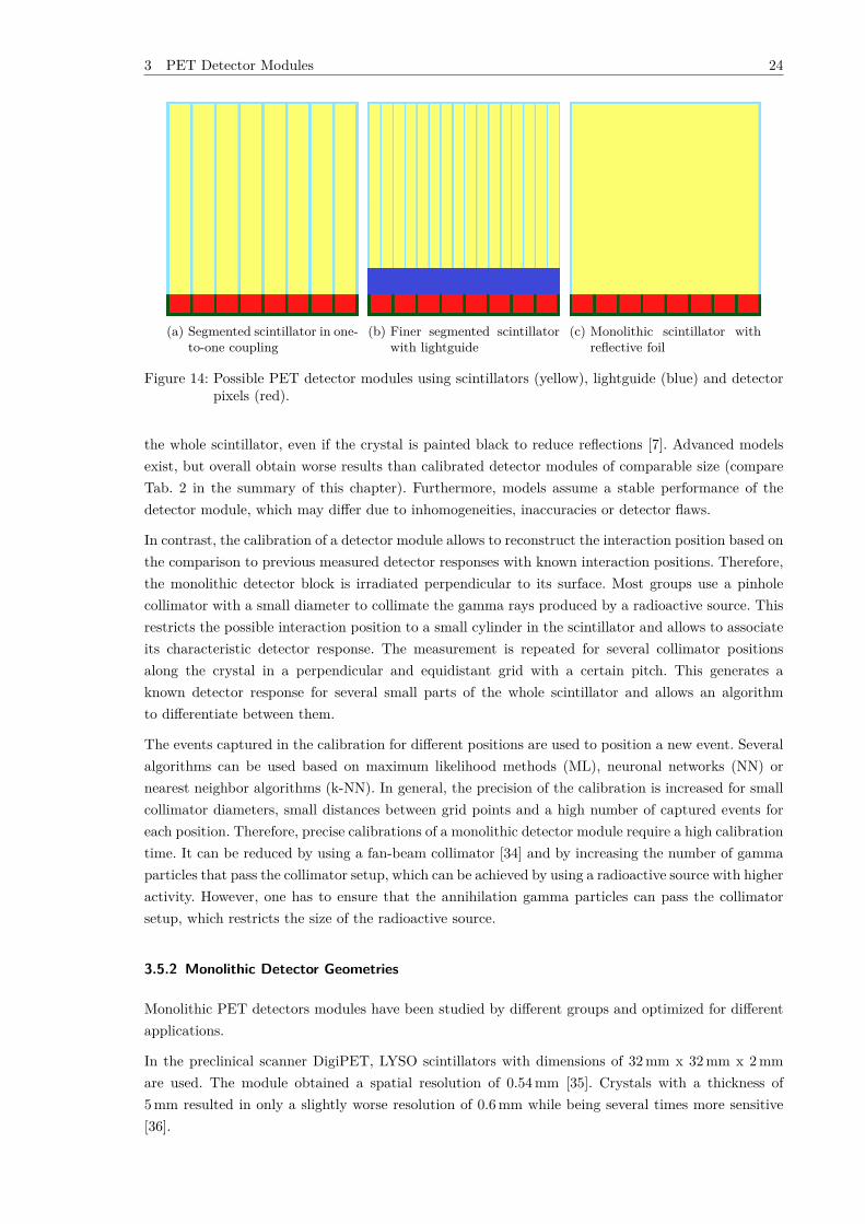
This work concentrates on the usage of monolithic scintillators which consist of a single crystal asdisplayed in Fig. 14.
3.5 Monolithic Detector Modules
3.5.1 Calibration Process
To determine the interaction position of a gamma particle in the crystal, a calibration step or aparametric model is required.
Models are theoretically motivated and mostly do not include the reflection of optical photons at theborders of the crystal. This reduces the scintillator area where the model is applicable to only 64 % of
3 PET Detector Modules 24
(a) Segmented scintillator in one-to-one coupling
(b) Finer segmented scintillatorwith lightguide
(c) Monolithic scintillator withreflective foil
Figure 14: Possible PET detector modules using scintillators (yellow), lightguide (blue) and detectorpixels (red).
the whole scintillator, even if the crystal is painted black to reduce reflections [7]. Advanced modelsexist, but overall obtain worse results than calibrated detector modules of comparable size (compareTab. 2 in the summary of this chapter). Furthermore, models assume a stable performance of thedetector module, which may differ due to inhomogeneities, inaccuracies or detector flaws.
In contrast, the calibration of a detector module allows to reconstruct the interaction position based onthe comparison to previous measured detector responses with known interaction positions. Therefore,the monolithic detector block is irradiated perpendicular to its surface. Most groups use a pinholecollimator with a small diameter to collimate the gamma rays produced by a radioactive source. Thisrestricts the possible interaction position to a small cylinder in the scintillator and allows to associateits characteristic detector response. The measurement is repeated for several collimator positionsalong the crystal in a perpendicular and equidistant grid with a certain pitch. This generates aknown detector response for several small parts of the whole scintillator and allows an algorithmto differentiate between them.
The events captured in the calibration for different positions are used to position a new event. Severalalgorithms can be used based on maximum likelihood methods (ML), neuronal networks (NN) ornearest neighbor algorithms (k-NN). In general, the precision of the calibration is increased for smallcollimator diameters, small distances between grid points and a high number of captured events foreach position. Therefore, precise calibrations of a monolithic detector module require a high calibrationtime. It can be reduced by using a fan-beam collimator [34] and by increasing the number of gammaparticles that pass the collimator setup, which can be achieved by using a radioactive source with higheractivity. However, one has to ensure that the annihilation gamma particles can pass the collimatorsetup, which restricts the size of the radioactive source.
3.5.2 Monolithic Detector Geometries
Monolithic PET detectors modules have been studied by different groups and optimized for differentapplications.
In the preclinical scanner DigiPET, LYSO scintillators with dimensions of 32 mm x 32 mm x 2 mmare used. The module obtained a spatial resolution of 0.54 mm [35]. Crystals with a thickness of5 mm resulted in only a slightly worse resolution of 0.6 mm while being several times more sensitive[36].
3 PET Detector Modules 25
In clinical applications, the crystal thickness has to be increased further to improve the system’ssensitivity. This results in a widening of the photon distribution in the scintillator and a less precisespatial resolution, which, as mentioned above, is less critical than in preclinical scanners. Severalparameters can be adjusted and will be presented briefly.
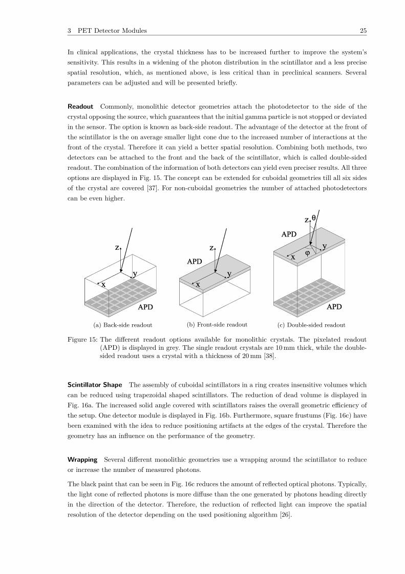
Readout Commonly, monolithic detector geometries attach the photodetector to the side of thecrystal opposing the source, which guarantees that the initial gamma particle is not stopped or deviatedin the sensor. The option is known as back-side readout. The advantage of the detector at the front ofthe scintillator is the on average smaller light cone due to the increased number of interactions at thefront of the crystal. Therefore it can yield a better spatial resolution. Combining both methods, twodetectors can be attached to the front and the back of the scintillator, which is called double-sidedreadout. The combination of the information of both detectors can yield even preciser results. All threeoptions are displayed in Fig. 15. The concept can be extended for cuboidal geometries till all six sidesof the crystal are covered [37]. For non-cuboidal geometries the number of attached photodetectorscan be even higher.
(a) Back-side readout (b) Front-side readout (c) Double-sided readout
Figure 15: The different readout options available for monolithic crystals. The pixelated readout(APD) is displayed in grey. The single readout crystals are 10 mm thick, while the double-sided readout uses a crystal with a thickness of 20 mm [38].
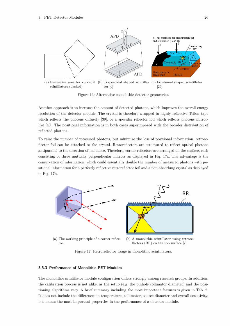
Scintillator Shape The assembly of cuboidal scintillators in a ring creates insensitive volumes whichcan be reduced using trapezoidal shaped scintillators. The reduction of dead volume is displayed inFig. 16a. The increased solid angle covered with scintillators raises the overall geometric efficiency ofthe setup. One detector module is displayed in Fig. 16b. Furthermore, square frustums (Fig. 16c) havebeen examined with the idea to reduce positioning artifacts at the edges of the crystal. Therefore thegeometry has an influence on the performance of the geometry.
Wrapping Several different monolithic geometries use a wrapping around the scintillator to reduceor increase the number of measured photons.
The black paint that can be seen in Fig. 16c reduces the amount of reflected optical photons. Typically,the light cone of reflected photons is more diffuse than the one generated by photons heading directlyin the direction of the detector. Therefore, the reduction of reflected light can improve the spatialresolution of the detector depending on the used positioning algorithm [26].
3 PET Detector Modules 26
(a) Insensitive area for cuboidalscintillators (dashed)
(b) Trapezoidal shaped scintilla-tor [6]
(c) Frustumal shaped scintillator[26]
Figure 16: Alternative monolithic detector geometries.
Another approach is to increase the amount of detected photons, which improves the overall energyresolution of the detector module. The crystal is therefore wrapped in highly reflective Teflon tapewhich reflects the photons diffusely [39], or a specular reflector foil which reflects photons mirror-like [40]. The positional information is in both cases superimposed with the broader distribution ofreflected photons.
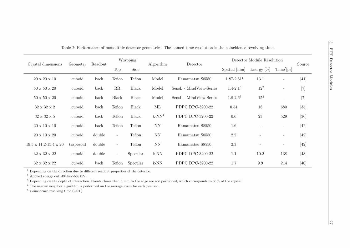
To raise the number of measured photons, but minimize the loss of positional information, retrore-flector foil can be attached to the crystal. Retroreflectors are structured to reflect optical photonsantiparallel to the direction of incidence. Therefore, corner reflectors are arranged on the surface, eachconsisting of three mutually perpendicular mirrors as displayed in Fig. 17a. The advantage is theconservation of information, which could essentially double the number of measured photons with po-sitional information for a perfectly reflective retroreflector foil and a non-absorbing crystal as displayedin Fig. 17b.
(a) The working principle of a corner reflec-tor.
(b) A monolithic scintillator using retrore-flectors (RR) on the top surface [7].
Figure 17: Retroreflector usage in monolithic scintillators.
3.5.3 Performance of Monolithic PET Modules
The monolithic scintillator module configuration differs strongly among research groups. In addition,the calibration process is not alike, as the setup (e.g. the pinhole collimator diameter) and the posi-tioning algorithms vary. A brief summary including the most important features is given in Tab. 2.It does not include the differences in temperature, collimator, source diameter and overall sensitivity,but names the most important properties in the performance of a detector module.
3PET
Detector
Modules
27
Table 2: Performance of monolithic detector geometries. The named time resolution is the coincidence revolving time.
Crystal dimensions Geometry ReadoutWrapping
Algorithm DetectorDetector Module Resolution
SourceTop Side Spatial [mm] Energy [%] Time5[ps]
20 x 20 x 10 cuboid back Teflon Teflon Model Hamamatsu S8550 1.87-2.511 13.1 - [41]
50 x 50 x 20 cuboid back RR Black Model SensL - MindView-Series 1.4-2.13 122 - [7]
50 x 50 x 20 cuboid back Black Black Model SensL - MindView-Series 1.8-2.63 152 - [7]
32 x 32 x 2 cuboid back Teflon Black ML PDPC DPC-3200-22 0.54 18 680 [35]
32 x 32 x 5 cuboid back Teflon Black k-NN4 PDPC DPC-3200-22 0.6 23 529 [36]
20 x 10 x 10 cuboid back Teflon Teflon NN Hamamatsu S8550 1.6 - - [42]
20 x 10 x 20 cuboid double - Teflon NN Hamamatsu S8550 2.2 - - [42]
19.5 x 11.2-15.4 x 20 trapezoid double - Teflon NN Hamamatsu S8550 2.3 - - [42]
32 x 32 x 22 cuboid double - Specular k-NN PDPC DPC-3200-22 1.1 10.2 138 [43]
32 x 32 x 22 cuboid back Teflon Specular k-NN PDPC DPC-3200-22 1.7 9.9 214 [40]1 Depending on the direction due to different readout properties of the detector.2 Applied energy cut: 434 keV-588 keV.3 Depending on the depth of interaction. Events closer than 5 mm to the edge are not positioned, which corresponds to 36 % of the crystal.4 The nearest neighbor algorithm is performed on the average event for each position.5 Coincidence resolving time (CRT)
4 Monte Carlo Simulation 28
4 Monte Carlo Simulation
4.1 Motivation
Monte Carlo simulations can be used in many applications regarding the tracking of particles. There-fore, they offer several applications to the calibration and optimization of monolithic scintillators.
In this work, the first application is the optimization of the source activity and distribution in regardto the used collimator. This reduces the experimental calibration time, without needlessly increasingthe activity of the source. Furthermore, only the best performing source has to be purchased. Theoptimization is described in chapter 5.
Other applications are based on the simulation of the interaction of gamma particles and the trackingof optical photons in the detector module. The implementation of the optical simulation is describedin chapter 6.
A further application is the simulation of the whole calibration process, which could allow the cali-bration of the detector module solely on simulated data. This would allow to reduce the measurementtime on the one hand, while increasing the computational effort on the other hand. However, due tothe nature of the simulation algorithm, the time for the calibration can be reduced by dividing theprocess into several, parallel running jobs. An important question is, whether the obtained calibrationcould be universally applied to different detector modules in a PET detector ring. This would sparethe calibration of several detector modules. Furthermore, the gain of additional information in thesimulation could improve the overall performance, e.g. due to the known interaction position in thedetector. The used algorithms are described in chapter 7, while the calibration is performed in chapter8.
Another application of the optical simulation is the study of the performance of different detectormodules. Changes in the detector module geometry can be easily implemented in the simulation,which is not possible in the experiment. Therefore, the simulation can guide new experiments. Ad-ditional information, e.g. the light distribution before and after the optical adhesive, could improvethe understanding of the performance of the detector module. The variation of the detector modulegeometry is described in chapter 9.
4.2 Working Principle
Monte Carlo simulations are commonly used to describe complex systems that proceed in a stochasti-cal manner. This applies to the passage of particles through matter, where each interaction can changethe particles’ properties like direction and energy. For a given geometry and defined interaction prob-abilities, the resulting trajectories of particles will differ and cannot be calculated analytically. Theconvolution of possible multiple interactions based on the geometry makes the system too complicated.The use of Monte Carlo methods gives an alternative solution, which requires the simulation of manyparticles to obtain a statistically reliable solution. In this work, the C++ toolkit Geant4 (“GEometryANd Tracking”) is used as a fast, reliable and well verified open source software [21][44].
4 Monte Carlo Simulation 29
A simulation consist of several phases:
1. Setup of materials and geometry
2. Setup of physics list
3. Simulation of particles
4. Analysis of data
5. Storage of data
First the implementation of the experimental setup has to be performed. Therefore, the materials(atomic number, density) are specified and volumes are created. A volume can be declared as “sensi-tive”, which allows to access and store every interaction that occurs in it.
Several physics lists contain models that can simulate the creation of particles and their interactionswith matter. These models can be chosen individually in dependence of the application, which makesGeant4 versatile on the one hand, but prone to user errors on the other hand. As it is of the essenceto replicate reality as close as possible to generate a simulation that models all the relevant physicalprocesses, the physics list “emstandard_opt4” is used. It uses the “most accurate standard and low-energy models” available [45][46], which can accurately describe the propagation of particles down to250 eV. However, every model is an approximation and the results will be slightly distorted due toerrors in the models, which can accumulate over many model applications.
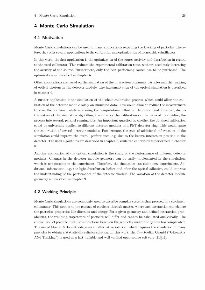
The actual simulation starts when a “run”, consisting of several “events” is started. The flowchartto the following description of the algorithm is displayed in Fig. 18. A particle is generated by the“primary generator action”, which is specified by the user. The particle’s properties, e.g. the startingenergy or momentum vector, can be based on a defined model, sampled from a data file or enteredmanually. The event manager organizes the processing of all particles that originate from the originallycreated particle using the tracking manager. Hereby, every particle is forwarded separately to thetracking manager, which determines its path based on the geometry and the allowed physical processesspecified in the physics list. This implies that Geant4 cannot simulate interactions between particles.Therefore, the simulation lacks the possibility to simulate interferences. Corresponding effects have tobe accounted for manually.
The tracking process consists of the generation of consecutive steps. From the current position of aparticle it is calculated how far the particle travels in the current medium. This “step” is limited by thefirst interaction in this volume. If the distance to the first interaction is further away than the borderof the current volume, no interaction occurs in this step. The step length is calculated using the cross-sections of all possible interactions defined for the particle using the physics list. After calculating theproperties of the particle after the interaction, the information is updated in the tracking manager.Additional information regarding the interaction can be stored if the volume is sensitive. Subsequently,the next step is calculated. This process repeats until the particle is absorbed, its energy drops belowthe tracking threshold or it reaches the end of the observed volume. If new particles have been createdin any of the interactions, the event manager starts the tracking progress for the next particle untilall remaining particles have been simulated. The information of the event can be analyzed and storedbefore the run manager starts the next event. After the processing of a specified number of events, therun manager stops the simulation. The user is responsible for analyzing and storing the data obtainedin the run, which will be described in the associated chapter for each simulation.
4 Monte Carlo Simulation 30
Figure 18: The Geant4 run explained in a flowchart [47].

5 Optimization of the Radioactive Source 31
5 Optimization of the Radioactive Source
The used collimator setup in the experimental calibration is explained and simulated in this sec-tion.
5.1 Experimental Collimator Setup
Figure 19: The calibration setup consists of pinhole collimator, two radioactive sources and the twodetectors [48].
The radioactive sources are arranged in a block of lead, as displayed in Fig. 19. The top half of the leadhousing is removed in the picture. On the right of the housing, the target detector under calibrationis positioned, while another detector on the left is used to measure the second gamma particle createdin the annihilation. The coincident detection supresses noise events. The detector under study isseparated from the sources by a removable pinhole collimator with a length of 51 mm and an innerdiameter of 0.5 mm. The detector behind the collimator is replaced by an ideal detector right behindthe collimator in this chapter, because the focus is set to the efficiency of the collimator setup inregard to the distribution of radioactive sources. The detector size corresponds to the size of the realdetector. On the opposing side a circular hole with a diameter of 4.1 mm allows gamma particles toreach the reference detector with a length and width of 2 mm x 2 mm, respectively [48].
5.2 Source Geometry
Two types of source geometries have been investigated as they were available from vendors:
• A point source with a variable diameter of the active element of 0.25 mm, 0.5 mm or 1 mmcovered in a cast acrylic plate with a diameter of 25.4 mm and a thickness of 6.35 mm.
• A line source with an active element of diameter 1.1 mm and length 54 mm incorporated bya stainless steel tube as displayed in Fig. 20. The used radioactive salt is incorporated into aceramic matrix.
Figure 20: A sketch of the simulated line source. The active element (red) is fully enclosed in a stainlesssteel tube (grey).
The activity of the source scales approximately with its size. While the smallest point source reachesup to 1.85 MBq [49], the source with a diameter of 0.5 mm can reach up to 15 MBq [50]. The increase
5 Optimization of the Radioactive Source 32
in activity is based on the increased size of the active element by a factor 8. Applying this theoreticallimit onto the point source with a diameter of 1 mm, the source would yield an activity of above100 MBq. The activity of the line source was not directly specified, only its dimensions and sourcecomposition.
5.3 Simulation
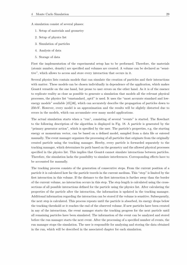
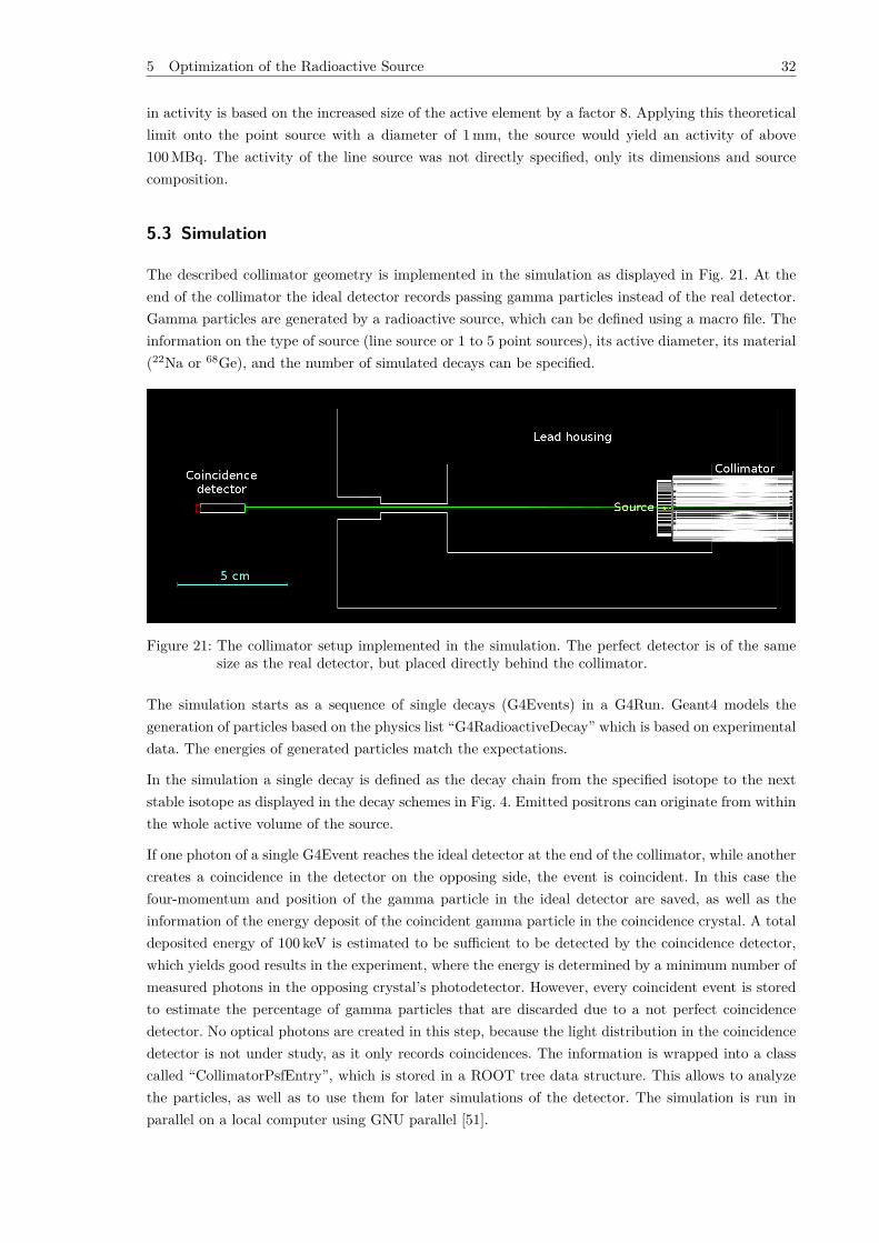
The described collimator geometry is implemented in the simulation as displayed in Fig. 21. At theend of the collimator the ideal detector records passing gamma particles instead of the real detector.Gamma particles are generated by a radioactive source, which can be defined using a macro file. Theinformation on the type of source (line source or 1 to 5 point sources), its active diameter, its material(22Na or 68Ge), and the number of simulated decays can be specified.
Figure 21: The collimator setup implemented in the simulation. The perfect detector is of the samesize as the real detector, but placed directly behind the collimator.
The simulation starts as a sequence of single decays (G4Events) in a G4Run. Geant4 models thegeneration of particles based on the physics list “G4RadioactiveDecay” which is based on experimentaldata. The energies of generated particles match the expectations.
In the simulation a single decay is defined as the decay chain from the specified isotope to the nextstable isotope as displayed in the decay schemes in Fig. 4. Emitted positrons can originate from withinthe whole active volume of the source.
If one photon of a single G4Event reaches the ideal detector at the end of the collimator, while anothercreates a coincidence in the detector on the opposing side, the event is coincident. In this case thefour-momentum and position of the gamma particle in the ideal detector are saved, as well as theinformation of the energy deposit of the coincident gamma particle in the coincidence crystal. A totaldeposited energy of 100 keV is estimated to be sufficient to be detected by the coincidence detector,which yields good results in the experiment, where the energy is determined by a minimum number ofmeasured photons in the opposing crystal’s photodetector. However, every coincident event is storedto estimate the percentage of gamma particles that are discarded due to a not perfect coincidencedetector. No optical photons are created in this step, because the light distribution in the coincidencedetector is not under study, as it only records coincidences. The information is wrapped into a classcalled “CollimatorPsfEntry”, which is stored in a ROOT tree data structure. This allows to analyzethe particles, as well as to use them for later simulations of the detector. The simulation is run inparallel on a local computer using GNU parallel [51].

5 Optimization of the Radioactive Source 33
5.4 Efficiency of Different Sources
The efficiency of a source is defined independent from its activity as the probability of coincidentgamma particles passing the collimator.
Material The comparison between 22Na and 68Ge was performed for the smallest point source of0.25 mm diameter. The efficiency using the 22Na sources is (5.75± 0.07) · 10−6, while the 68Ge sourceobtained an efficiency of (1.32 ± 0.03) · 10−6. The difference in efficiency can be attributed to thepositron energy, which directly influences the range of the positrons. Therefore, a 68Ge source has tobe four times stronger than a 22Na point source to create the same number of events.
Line Source The estimated efficiency for a 22Na line source is determined as (0.43 ± 0.02) · 10−6.Therefore, the activity of the line source has to be 13 times higher than a single point source to obtainthe same resulting number of events.
Point Sources The efficiency of the point sources is summarized in Tab. 3.
Table 3: The efficiency of the source in 10−6 depending on the number of perfectly aligned pointsources with diameter d.
d[mm] 1 3 5
0.25 5.75± 0.07 4.18± 0.06 3.16± 0.05
0.5 5.73± 0.07 4.21± 0.06 2.98± 0.05
1 3.49± 0.05 2.82± 0.05 2.22± 0.04
The change in source size from 0.25 mm to 0.5 mm diameter does not influence the efficiency sig-nificantly. When using a point source with an active diameter of 1 mm, the efficiency is reduced byapproximately 40 %.
Summary The experimental calibration time can be effectively reduced when 22Na point sources of0.5 mm diameter with an activity of up to 15 MBq are used instead of the eight times weaker 0.25 mmdiameter sources with the almost same efficiency.
Based on the obtained results, two 22Na point sources with an active diameter of 0.5 mm and anactivity of 9.787 MBq and 10.530 MBq are used in the system. This is more advantageous than theuse of a line source with an activity of 200 MBq, even if it could be manufactured.
5.5 Analysis of Particle Composition
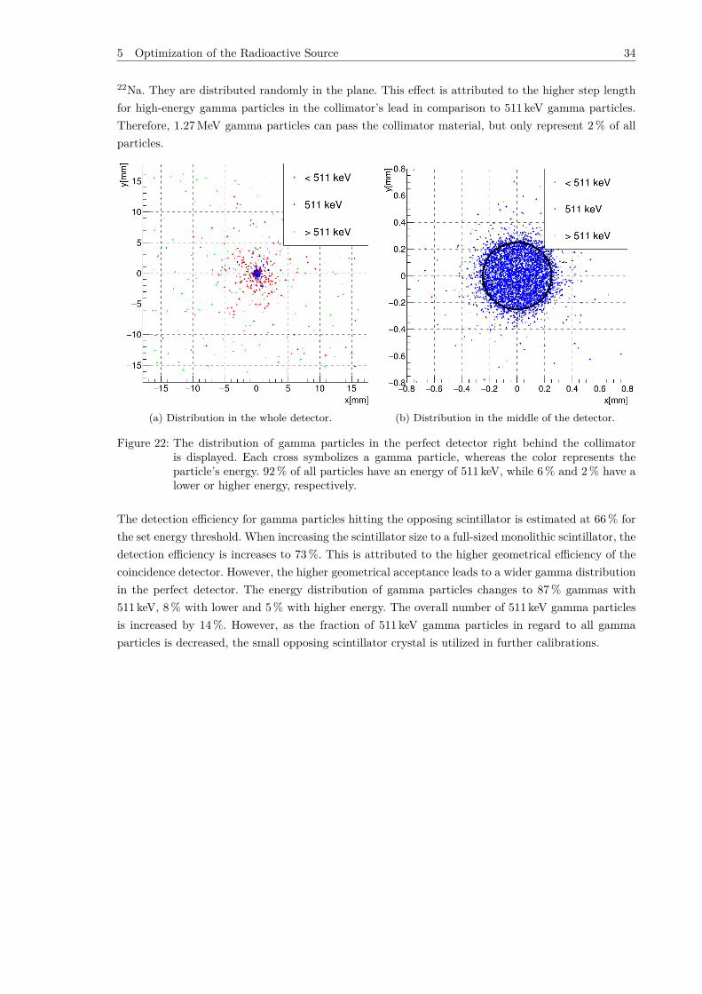
The simulation offers the possibility to analyze the properties of the particles passing the collimator.The distribution of gamma particles in the perfect detector is displayed in Fig. 22. The left imageshows the distribution over the whole detector, while the right image displays the middle regionenlarged including a black circle, which represents the collimator pinhole diameter. Noticeably, gammaparticles that passed through the pinhole collimator mainly have an energy of 511 keV, while gammaparticles with lower energies are deviated to the outward sides of the detector. This corresponds toscattered photons that pass part of the collimator’s material. Therefore, the beam is widened which isdisadvantageous for the calibration. Higher energy gamma particles belong to the 1.275 MeV decay of
5 Optimization of the Radioactive Source 34
22Na. They are distributed randomly in the plane. This effect is attributed to the higher step lengthfor high-energy gamma particles in the collimator’s lead in comparison to 511 keV gamma particles.Therefore, 1.27 MeV gamma particles can pass the collimator material, but only represent 2 % of allparticles.
(a) Distribution in the whole detector. (b) Distribution in the middle of the detector.
Figure 22: The distribution of gamma particles in the perfect detector right behind the collimatoris displayed. Each cross symbolizes a gamma particle, whereas the color represents theparticle’s energy. 92 % of all particles have an energy of 511 keV, while 6 % and 2 % have alower or higher energy, respectively.
The detection efficiency for gamma particles hitting the opposing scintillator is estimated at 66 % forthe set energy threshold. When increasing the scintillator size to a full-sized monolithic scintillator, thedetection efficiency is increases to 73 %. This is attributed to the higher geometrical efficiency of thecoincidence detector. However, the higher geometrical acceptance leads to a wider gamma distributionin the perfect detector. The energy distribution of gamma particles changes to 87 % gammas with511 keV, 8 % with lower and 5 % with higher energy. The overall number of 511 keV gamma particlesis increased by 14 %. However, as the fraction of 511 keV gamma particles in regard to all gammaparticles is decreased, the small opposing scintillator crystal is utilized in further calibrations.
6 Optical Simulation 35
6 Optical Simulation
It is crucial for the simulation to obtain all the needed input parameters to model an interaction. Whilethe parameters influencing the interactions of high-energy gamma particles are few and tangible, e.g.the density or atomic number of the material, optical photon interactions are harder to describe as theyfurther depend on properties like the refractive index of the material. While the change of refractiveindex for an even boundary among materials is described well by models (see chapter 2.5), any realsurface cannot be assumed to be perfectly even. Furthermore, local changes of the refractive indexin the crystal can occur due to inhomogeneities. These changes can be visible to the naked eye forlow-quality scintillators, but not in the used crystal. Reportedly, the variation of parameters in thecrystal growth process has a great influence on the performance of the crystal [52].
The main processes that are important for the simulation of optical processes in the detector moduleare:
• The absorption of gamma particles in the scintillator.
• The generation of optical photons in the scintillator.
• The passage of optical photons through the detector module.
• The detection and readout properties of the detector.
The gamma particles that were recorded and stored using the simulation of the collimator setup areused as the input particles for the simulation of the interaction of the gamma beam with the detectormodule. This reduces the computational effort for investigations of parameters that only influence theoptical part of the simulation.
6.1 Gamma Absorption
The scintillator consists of lutetium-yttrium oxyorthosilicate (LYSO) doped with cerium. The yttriumfraction of the crystal is 5 %, which leads to the formula is Lu1.9Y0.1SiO5:Ce [20]. The crystal ismanufactured by EPIC Crystal, China. The material is implemented accordingly in the simulation.As stated in chapter 3.2, LYSO is a common scintillator material due to its high density of 7.11 g/cm3
and high effective atomic number of 65 [32]. Despite the high atomic number of LYSO, the Comptonscattering cross section for 511 keV γ particles is approximately twice as high as the cross sectionfor the photoelectric effect. The cross sections and the corresponding mean free path are displayedin Tab. 4. Therefore, 67 % of all gamma interactions are Compton scattered gamma particles. Aneffective atomic number above 75 would be required to make the photoelectric effect more likely thanCompton scattering.
In the simulation the first interaction position of a gamma particle in the crystal is stored, as well asits initial energy, the energy deposit and the corresponding interaction. The Monte Carlo truth canbe used in the calibration process.
Table 4: Cross section σ and mean free path lγ for gamma particles with 511 keV in LYSO determinedusing Geant4.
photoeffect compton
σ [mm2/g] 3.57 7.32
lγ [cm] 3.92 1.92
6 Optical Simulation 36
6.2 Light Generation in the Scintillator
Light Yield As discussed before, the light yield for LYSO is high in comparison to other materials[29]. To model the expected number of optical photons generated by an energy deposit in the crystal,the simplified relation n = LY · Edep is used. Due to the underlying Poisson process, the statisticalerror can be estimated as
√n for a perfectly homogeneous crystal. The non-Poisson characteristics due
to inhomogeneities in the crystal are taken into account by introducing a resolution scaling factor rto broaden the distribution of generated photons. Therefore, the number of generated optical photonsn for an interaction with energy deposit Edep is determined by Eq. 12.
n = Edep · LY ± r ·√Edep · LY (12)
In principle the factor r can be determined using the energy resolution ∆EE of the crystal by
r =√n
2.35∆EE
, (13)
where ∆E denotes the FWHM of the energy distribution, which induces the factor of 2.35 [53].This assumes that the detector module does not have an influence on the resolution and is a lowerborder.
Literature values for the average light yield, the determined energy resolution and the resulting scalingfactor vary strongly between groups. The results for several crystals are summarized in Tab. 5. As aconsequence, the light yield and the scaling factor are determined by comparison to the experiment.The manufacturer determined the light yield as 29 000 /MeV.
Table 5: Light yield LY, energy resolution Eres and scaling factor for LYSO:Ce crystals with yttriumfraction Y determined by different groups.
LY [ph/MeV] Eres r Y [%] source
35 000 – 50 000† - - - [54]
39 900 ± 4000 8.2± 0.3 5.0 10 [27]
36 600 ± 3000 8.2± 0.4 4.8 10 [32]
33 800 ± 2200 7.5 – 9.5 4.2 – 5.3 10 [55]
32 000 8 4.3 10 [52]
32 000± 650∗ 10.2 5.6 10 [30]
29 000 10.9 5.6 5 [56]
27 000 - - - [57]
26 000 9.0 4.4 - [53]
20 200 – 22 800 10.5 – 11 4.5 – 4.8 - [6]† depending on the purity of the crystal* systematic error of 1300 ph/MeV
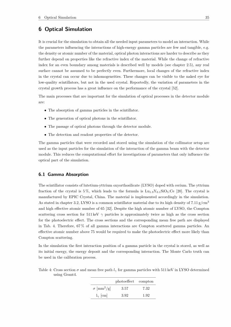
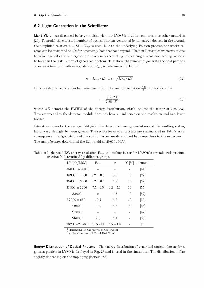
Energy Distribution of Optical Photons The energy distribution of generated optical photons by agamma particle in LYSO is displayed in Fig. 23 and is used in the simulation. The distribution differsslightly depending on the impinging particle [20].
6 Optical Simulation 37
Figure 23: The distribution of optical photon energy when irradiating LYSO with gamma particlesbased on [20].
Timing of Optical Photon Generation Optical photons generation can be described by a singleexponential decay with a time constant of 40 ns [20][30][58], which is implemented in the simula-tion.
Angular Distribution and Polarization of Optical Photons The used model generates optical pho-tons isotropically with a random linear polarization.
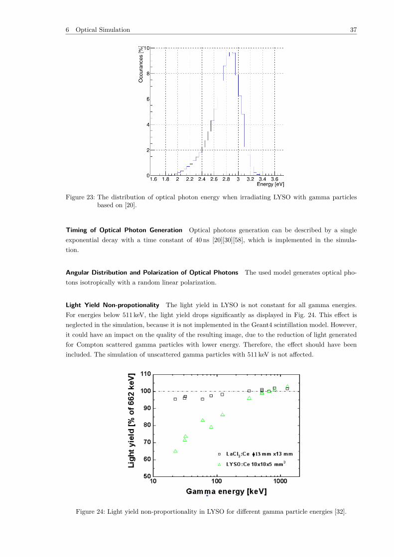
Light Yield Non-propotionality The light yield in LYSO is not constant for all gamma energies.For energies below 511 keV, the light yield drops significantly as displayed in Fig. 24. This effect isneglected in the simulation, because it is not implemented in the Geant4 scintillation model. However,it could have an impact on the quality of the resulting image, due to the reduction of light generatedfor Compton scattered gamma particles with lower energy. Therefore, the effect should have beenincluded. The simulation of unscattered gamma particles with 511 keV is not affected.
Figure 24: Light yield non-proportionality in LYSO for different gamma particle energies [32].
6 Optical Simulation 38
6.3 Propagation of Optical Photons
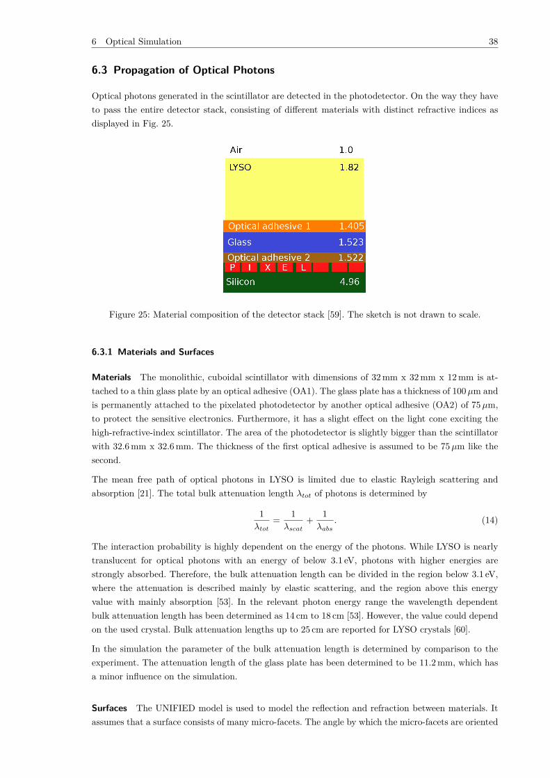
Optical photons generated in the scintillator are detected in the photodetector. On the way they haveto pass the entire detector stack, consisting of different materials with distinct refractive indices asdisplayed in Fig. 25.
Figure 25: Material composition of the detector stack [59]. The sketch is not drawn to scale.
6.3.1 Materials and Surfaces
Materials The monolithic, cuboidal scintillator with dimensions of 32 mm x 32 mm x 12 mm is at-tached to a thin glass plate by an optical adhesive (OA1). The glass plate has a thickness of 100µm andis permanently attached to the pixelated photodetector by another optical adhesive (OA2) of 75µm,to protect the sensitive electronics. Furthermore, it has a slight effect on the light cone exciting thehigh-refractive-index scintillator. The area of the photodetector is slightly bigger than the scintillatorwith 32.6 mm x 32.6 mm. The thickness of the first optical adhesive is assumed to be 75µm like thesecond.
The mean free path of optical photons in LYSO is limited due to elastic Rayleigh scattering andabsorption [21]. The total bulk attenuation length λtot of photons is determined by
1λtot
= 1λscat
+ 1λabs
. (14)
The interaction probability is highly dependent on the energy of the photons. While LYSO is nearlytranslucent for optical photons with an energy of below 3.1 eV, photons with higher energies arestrongly absorbed. Therefore, the bulk attenuation length can be divided in the region below 3.1 eV,where the attenuation is described mainly by elastic scattering, and the region above this energyvalue with mainly absorption [53]. In the relevant photon energy range the wavelength dependentbulk attenuation length has been determined as 14 cm to 18 cm [53]. However, the value could dependon the used crystal. Bulk attenuation lengths up to 25 cm are reported for LYSO crystals [60].
In the simulation the parameter of the bulk attenuation length is determined by comparison to theexperiment. The attenuation length of the glass plate has been determined to be 11.2 mm, which hasa minor influence on the simulation.
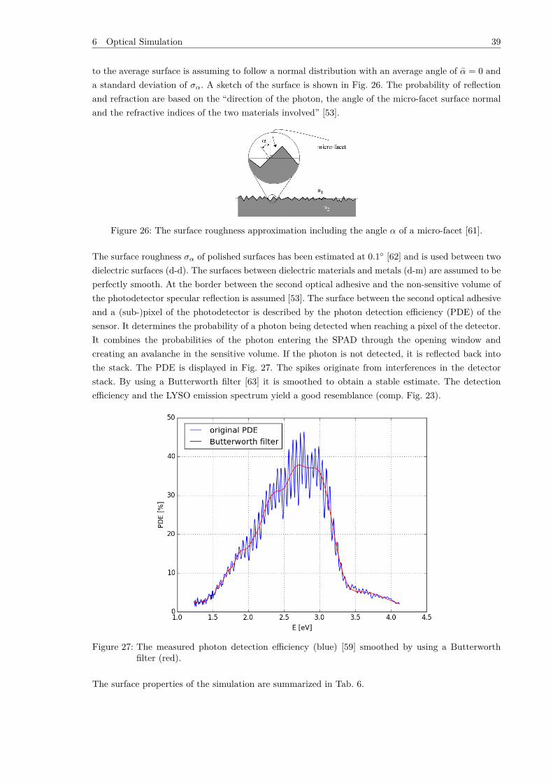
Surfaces The UNIFIED model is used to model the reflection and refraction between materials. Itassumes that a surface consists of many micro-facets. The angle by which the micro-facets are oriented
6 Optical Simulation 39
to the average surface is assuming to follow a normal distribution with an average angle of α = 0 anda standard deviation of σα. A sketch of the surface is shown in Fig. 26. The probability of reflectionand refraction are based on the “direction of the photon, the angle of the micro-facet surface normaland the refractive indices of the two materials involved” [53].
Figure 26: The surface roughness approximation including the angle α of a micro-facet [61].
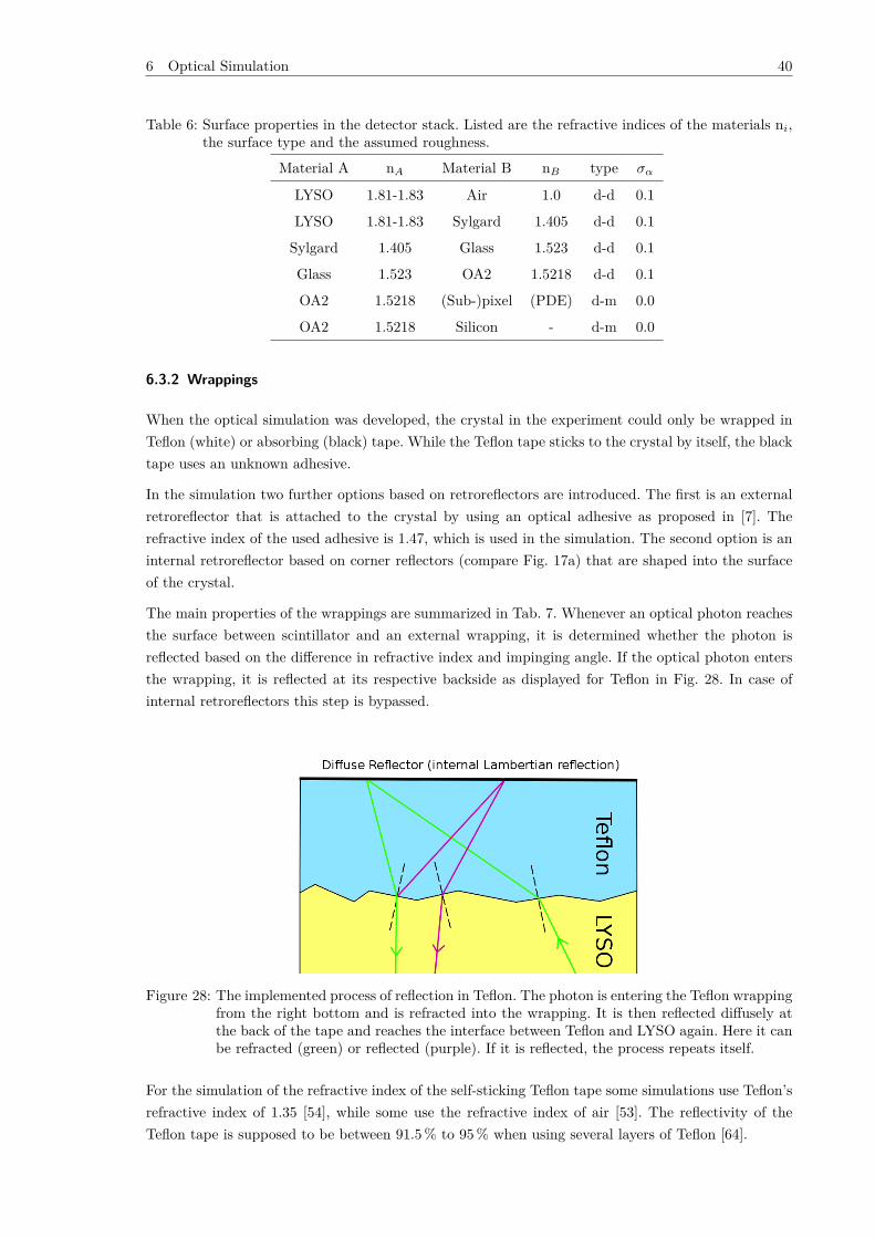
The surface roughness σα of polished surfaces has been estimated at 0.1 [62] and is used between twodielectric surfaces (d-d). The surfaces between dielectric materials and metals (d-m) are assumed to beperfectly smooth. At the border between the second optical adhesive and the non-sensitive volume ofthe photodetector specular reflection is assumed [53]. The surface between the second optical adhesiveand a (sub-)pixel of the photodetector is described by the photon detection efficiency (PDE) of thesensor. It determines the probability of a photon being detected when reaching a pixel of the detector.It combines the probabilities of the photon entering the SPAD through the opening window andcreating an avalanche in the sensitive volume. If the photon is not detected, it is reflected back intothe stack. The PDE is displayed in Fig. 27. The spikes originate from interferences in the detectorstack. By using a Butterworth filter [63] it is smoothed to obtain a stable estimate. The detectionefficiency and the LYSO emission spectrum yield a good resemblance (comp. Fig. 23).
Figure 27: The measured photon detection efficiency (blue) [59] smoothed by using a Butterworthfilter (red).
The surface properties of the simulation are summarized in Tab. 6.
6 Optical Simulation 40
Table 6: Surface properties in the detector stack. Listed are the refractive indices of the materials ni,the surface type and the assumed roughness.
Material A nA Material B nB type σα
LYSO 1.81-1.83 Air 1.0 d-d 0.1
LYSO 1.81-1.83 Sylgard 1.405 d-d 0.1
Sylgard 1.405 Glass 1.523 d-d 0.1
Glass 1.523 OA2 1.5218 d-d 0.1
OA2 1.5218 (Sub-)pixel (PDE) d-m 0.0
OA2 1.5218 Silicon - d-m 0.0
6.3.2 Wrappings
When the optical simulation was developed, the crystal in the experiment could only be wrapped inTeflon (white) or absorbing (black) tape. While the Teflon tape sticks to the crystal by itself, the blacktape uses an unknown adhesive.
In the simulation two further options based on retroreflectors are introduced. The first is an externalretroreflector that is attached to the crystal by using an optical adhesive as proposed in [7]. Therefractive index of the used adhesive is 1.47, which is used in the simulation. The second option is aninternal retroreflector based on corner reflectors (compare Fig. 17a) that are shaped into the surfaceof the crystal.
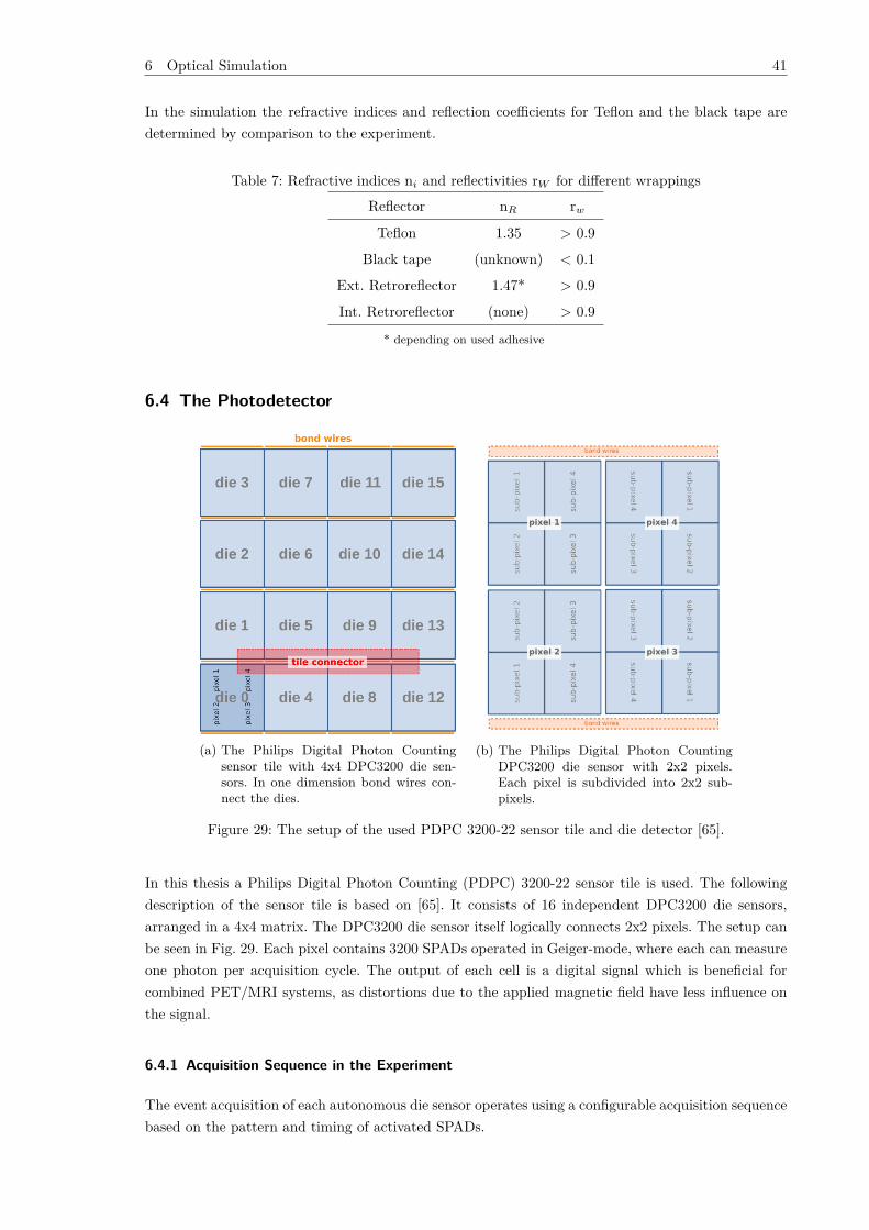
The main properties of the wrappings are summarized in Tab. 7. Whenever an optical photon reachesthe surface between scintillator and an external wrapping, it is determined whether the photon isreflected based on the difference in refractive index and impinging angle. If the optical photon entersthe wrapping, it is reflected at its respective backside as displayed for Teflon in Fig. 28. In case ofinternal retroreflectors this step is bypassed.
Figure 28: The implemented process of reflection in Teflon. The photon is entering the Teflon wrappingfrom the right bottom and is refracted into the wrapping. It is then reflected diffusely atthe back of the tape and reaches the interface between Teflon and LYSO again. Here it canbe refracted (green) or reflected (purple). If it is reflected, the process repeats itself.
For the simulation of the refractive index of the self-sticking Teflon tape some simulations use Teflon’srefractive index of 1.35 [54], while some use the refractive index of air [53]. The reflectivity of theTeflon tape is supposed to be between 91.5 % to 95 % when using several layers of Teflon [64].
6 Optical Simulation 41
In the simulation the refractive indices and reflection coefficients for Teflon and the black tape aredetermined by comparison to the experiment.
Table 7: Refractive indices ni and reflectivities rW for different wrappings
Reflector nR rwTeflon 1.35 > 0.9
Black tape (unknown) < 0.1
Ext. Retroreflector 1.47* > 0.9
Int. Retroreflector (none) > 0.9
* depending on used adhesive
6.4 The Photodetector
(a) The Philips Digital Photon Countingsensor tile with 4x4 DPC3200 die sen-sors. In one dimension bond wires con-nect the dies.
(b) The Philips Digital Photon CountingDPC3200 die sensor with 2x2 pixels.Each pixel is subdivided into 2x2 sub-pixels.
Figure 29: The setup of the used PDPC 3200-22 sensor tile and die detector [65].
In this thesis a Philips Digital Photon Counting (PDPC) 3200-22 sensor tile is used. The followingdescription of the sensor tile is based on [65]. It consists of 16 independent DPC3200 die sensors,arranged in a 4x4 matrix. The DPC3200 die sensor itself logically connects 2x2 pixels. The setup canbe seen in Fig. 29. Each pixel contains 3200 SPADs operated in Geiger-mode, where each can measureone photon per acquisition cycle. The output of each cell is a digital signal which is beneficial forcombined PET/MRI systems, as distortions due to the applied magnetic field have less influence onthe signal.
6.4.1 Acquisition Sequence in the Experiment
The event acquisition of each autonomous die sensor operates using a configurable acquisition sequencebased on the pattern and timing of activated SPADs.
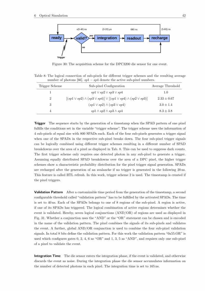
6 Optical Simulation 42
Figure 30: The acquisition scheme for the DPC3200 die sensor for one event.
Table 8: The logical connection of sub-pixels for different trigger schemes and the resulting averagenumber of photons [66]. sp1− sp4 denote the active sub-pixel numbers.
Trigger Scheme Sub-pixel Configuration Average Threshold
1 sp1 ∨ sp2 ∨ sp3 ∨ sp4 1.0
2 [(sp1 ∨ sp2) ∧ (sp3 ∨ sp4)] ∨ [(sp1 ∨ sp4) ∧ (sp2 ∨ sp3)] 2.33± 0.67
3 (sp1 ∨ sp2) ∧ (sp3 ∨ sp4) 3.0± 1.4
4 sp1 ∧ sp2 ∧ sp3 ∧ sp4 8.3± 3.8
Trigger The sequence starts by the generation of a timestamp when the SPAD pattern of one pixelfulfills the conditions set in the variable “trigger scheme”. The trigger scheme uses the information of4 sub-pixels of equal size with 800 SPADs each. Each of the four sub-pixels generates a trigger signalwhen one of the SPADs in the respective sub-pixel breaks down. The four sub-pixel trigger signalscan be logically combined using different trigger schemes resulting in a different number of SPADbreakdowns over the area of a pixel as displayed in Tab. 8. This can be used to suppress dark counts.The first trigger scheme only requires one detected photon in any sub-pixel to generate a trigger.Assuming equally distributed SPAD breakdowns over the area of a DPC pixel, the higher triggerschemes show a characteristic probability distribution for the pixel trigger signal generation. SPADsare recharged after the generation of an avalanche if no trigger is generated in the following 20 ns.This feature is called RTL refresh. In this work, trigger scheme 2 is used. The timestamp is created ifthe pixel triggers.
Validation Pattern After a customizable time period from the generation of the timestamp, a secondconfigurable threshold called “validation pattern” has to be fulfilled by the activated SPADs. The timeis set to 40 ns. Each of the SPADs belongs to one of 8 regions of the sub-pixel. A region is active,if one of its SPADs has triggered. The logical combination of active regions determines whether theevent is validated. Hereby, seven logical conjunctions (AND/OR) of regions are used as displayed inFig. 31. Whether a conjunction uses the “AND” or the “OR” statement can be chosen and is encodedin the name of the validation pattern. The pixel combines the signals of its sub-pixels and validatesthe event. A further, global AND/OR conjunction is used to combine the four sub-pixel validationsignals. In total 8 bits define the validation pattern. For this work the validation pattern “0x55:OR” isused which configures gates 0, 2, 4, 6 as “OR” and 1, 3, 5 as “AND”, and requires only one sub-pixelof a pixel to validate the event.
Integration Time The die sensor enters the integration phase, if the event is validated, and otherwisediscards the event as noise. During the integration phase the die sensor accumulates information onthe number of detected photons in each pixel. The integration time is set to 165 ns.
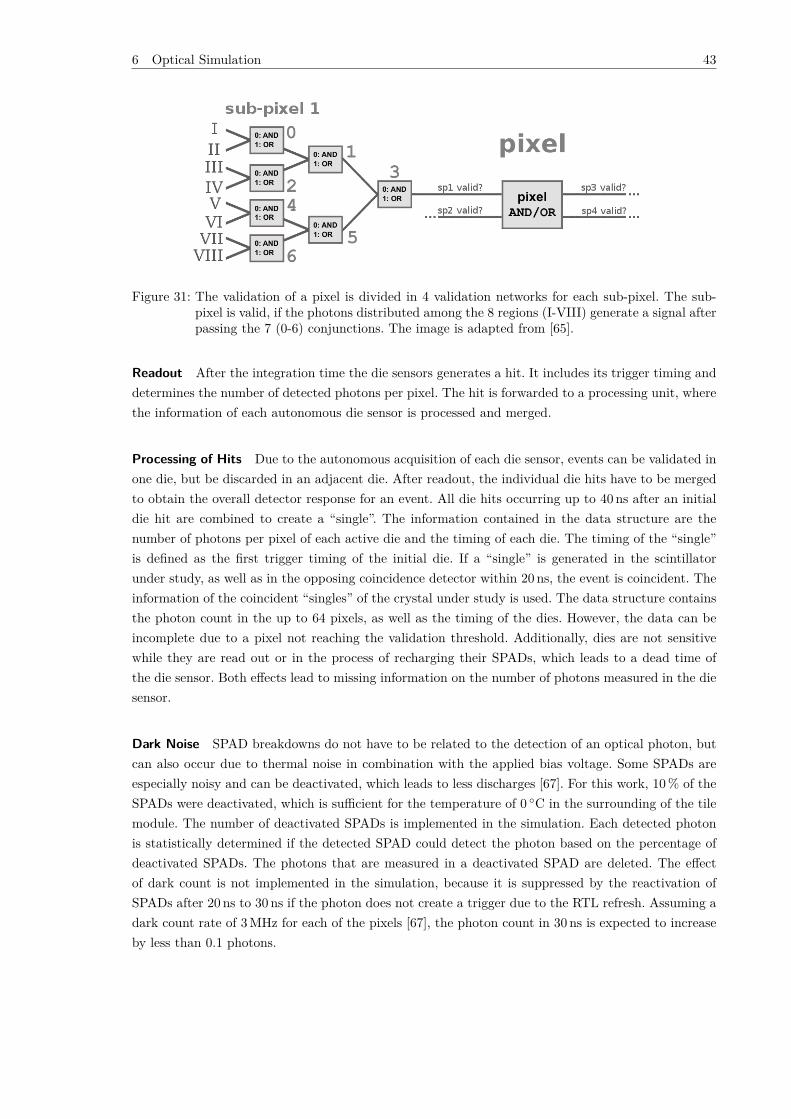
6 Optical Simulation 43
Figure 31: The validation of a pixel is divided in 4 validation networks for each sub-pixel. The sub-pixel is valid, if the photons distributed among the 8 regions (I-VIII) generate a signal afterpassing the 7 (0-6) conjunctions. The image is adapted from [65].
Readout After the integration time the die sensors generates a hit. It includes its trigger timing anddetermines the number of detected photons per pixel. The hit is forwarded to a processing unit, wherethe information of each autonomous die sensor is processed and merged.
Processing of Hits Due to the autonomous acquisition of each die sensor, events can be validated inone die, but be discarded in an adjacent die. After readout, the individual die hits have to be mergedto obtain the overall detector response for an event. All die hits occurring up to 40 ns after an initialdie hit are combined to create a “single”. The information contained in the data structure are thenumber of photons per pixel of each active die and the timing of each die. The timing of the “single”is defined as the first trigger timing of the initial die. If a “single” is generated in the scintillatorunder study, as well as in the opposing coincidence detector within 20 ns, the event is coincident. Theinformation of the coincident “singles” of the crystal under study is used. The data structure containsthe photon count in the up to 64 pixels, as well as the timing of the dies. However, the data can beincomplete due to a pixel not reaching the validation threshold. Additionally, dies are not sensitivewhile they are read out or in the process of recharging their SPADs, which leads to a dead time ofthe die sensor. Both effects lead to missing information on the number of photons measured in the diesensor.
Dark Noise SPAD breakdowns do not have to be related to the detection of an optical photon, butcan also occur due to thermal noise in combination with the applied bias voltage. Some SPADs areespecially noisy and can be deactivated, which leads to less discharges [67]. For this work, 10 % of theSPADs were deactivated, which is sufficient for the temperature of 0 C in the surrounding of the tilemodule. The number of deactivated SPADs is implemented in the simulation. Each detected photonis statistically determined if the detected SPAD could detect the photon based on the percentage ofdeactivated SPADs. The photons that are measured in a deactivated SPAD are deleted. The effectof dark count is not implemented in the simulation, because it is suppressed by the reactivation ofSPADs after 20 ns to 30 ns if the photon does not create a trigger due to the RTL refresh. Assuming adark count rate of 3 MHz for each of the pixels [67], the photon count in 30 ns is expected to increaseby less than 0.1 photons.
6 Optical Simulation 44
6.4.2 Implementation of the Acquisition Sequence
In the simulation the process of trigger generation, validation, integration and storage has to bemodeled. The detector geometry is implemented according to [65]. The finest structure available inthe simulation is a sub-pixel, as the dimensions and distribution of the SPADs cannot be reconstructed.The reduced sensitive area in the photodetector due to the insensitive area between SPADs is accountedfor in the PDE. For the evaluation of trigger and validation scheme, the timing and sub-pixel numberof each detection is required. To reduce the data size for storage it is advantageous to perform theanalysis of the trigger generation in the optical simulation. If the trigger generation did not applydirectly, the simulation would have to save each detected photon including sub-pixel and timing. Thedisadvantage of this method is the dependence of the optical simulation on the used trigger schme. Toevaluate the consequences of another trigger scheme the time-consuming part of the simulation hasto be repeated.
Simulation of the Trigger Scheme and Storage The trigger scheme is evaluated for each gammaparticle, if at least one sub-pixel has been hit by an optical photon. The initial interactions in thesub-pixels are sorted by the die the subpixel belongs to. For each die the evaluation is done separatelyand starts by sorting the photon interactions by time. An interaction may be statistically discardedin dependence on the number of deactivated cells in a pixel. This value consists of the number ofphotons already measured in a pixel and the number of deactivated, noisy cells. In the following, itis determined whether the remaining hits can trigger a die. A hit in the measurement is discardedwhen no trigger is activated in 20 ns after detection. The check for a discharged SPAD is done every10 ns [65] and therefore SPADs with up to 30 ns time difference could create a trigger. The additionaltime “bonus” is approximated as evenly distributed between 0 ns to 10 ns. The RTL refresh not onlyreactivates the one discharged SPAD but a whole “line” of logically connected SPADs. Therefore, itmay happen that an additional hit along the line is discarded because the first did not create a trigger.This “overwriting” of a valid interaction is not implemented in the simulation because the smallestsimulated structure is the sub-pixel, but not its substructure. The algorithm for the trigger detectionof each die runs like depicted in listing 1. The fourth is implemented accordingly.
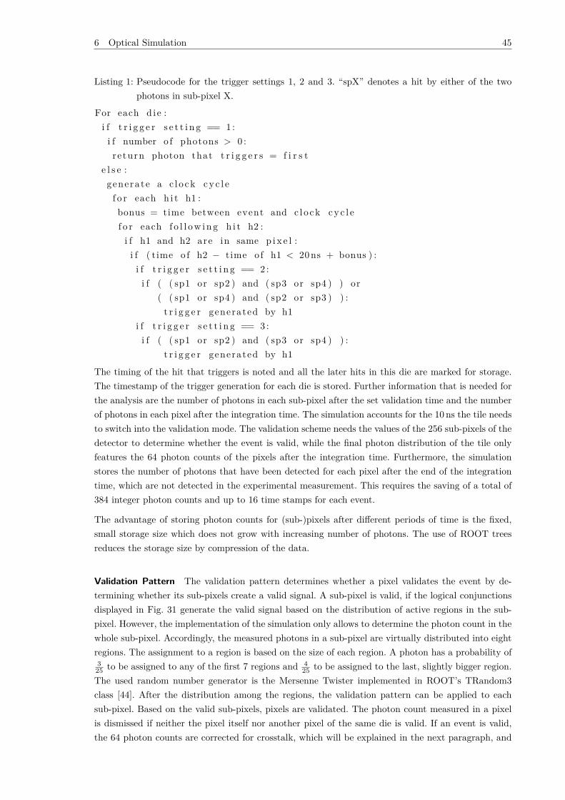
6 Optical Simulation 45
Listing 1: Pseudocode for the trigger settings 1, 2 and 3. “spX” denotes a hit by either of the twophotons in sub-pixel X.
For each d i e :i f t r i g g e r s e t t i n g == 1 :i f number o f photons > 0 :re turn photon that t r i g g e r s = f i r s t
e l s e :generate a c l o ck cy c l ef o r each h i t h1 :bonus = time between event and c l o ck cy c l ef o r each f o l l ow i ng h i t h2 :i f h1 and h2 are in same p i x e l :i f ( time o f h2 − time o f h1 < 20ns + bonus ) :i f t r i g g e r s e t t i n g == 2 :i f ( ( sp1 or sp2 ) and ( sp3 or sp4 ) ) or
( ( sp1 or sp4 ) and ( sp2 or sp3 ) ) :t r i g g e r generated by h1
i f t r i g g e r s e t t i n g == 3 :i f ( ( sp1 or sp2 ) and ( sp3 or sp4 ) ) :
t r i g g e r generated by h1
The timing of the hit that triggers is noted and all the later hits in this die are marked for storage.The timestamp of the trigger generation for each die is stored. Further information that is needed forthe analysis are the number of photons in each sub-pixel after the set validation time and the numberof photons in each pixel after the integration time. The simulation accounts for the 10 ns the tile needsto switch into the validation mode. The validation scheme needs the values of the 256 sub-pixels of thedetector to determine whether the event is valid, while the final photon distribution of the tile onlyfeatures the 64 photon counts of the pixels after the integration time. Furthermore, the simulationstores the number of photons that have been detected for each pixel after the end of the integrationtime, which are not detected in the experimental measurement. This requires the saving of a total of384 integer photon counts and up to 16 time stamps for each event.
The advantage of storing photon counts for (sub-)pixels after different periods of time is the fixed,small storage size which does not grow with increasing number of photons. The use of ROOT treesreduces the storage size by compression of the data.
Validation Pattern The validation pattern determines whether a pixel validates the event by de-termining whether its sub-pixels create a valid signal. A sub-pixel is valid, if the logical conjunctionsdisplayed in Fig. 31 generate the valid signal based on the distribution of active regions in the sub-pixel. However, the implementation of the simulation only allows to determine the photon count in thewhole sub-pixel. Accordingly, the measured photons in a sub-pixel are virtually distributed into eightregions. The assignment to a region is based on the size of each region. A photon has a probability of325 to be assigned to any of the first 7 regions and 4
25 to be assigned to the last, slightly bigger region.The used random number generator is the Mersenne Twister implemented in ROOT’s TRandom3class [44]. After the distribution among the regions, the validation pattern can be applied to eachsub-pixel. Based on the valid sub-pixels, pixels are validated. The photon count measured in a pixelis dismissed if neither the pixel itself nor another pixel of the same die is valid. If an event is valid,the 64 photon counts are corrected for crosstalk, which will be explained in the next paragraph, and
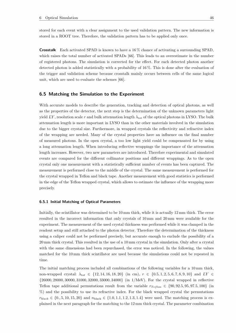
6 Optical Simulation 46
stored for each event with a clear assignment to the used validation pattern. The new information isstored in a ROOT tree. Therefore, the validation pattern has to be applied only once.
Crosstalk Each activated SPAD is known to have a 16 % chance of activating a surrounding SPAD,which raises the total number of activated SPADs [66]. This leads to an overestimate in the numberof registered photons. The simulation is corrected for the effect. For each detected photon anotherdetected photon is added statistically with a probability of 16 %. This is done after the evaluation ofthe trigger and validation scheme because crosstalk mainly occurs between cells of the same logicalunit, which are used to evaluate the schemes [66].
6.5 Matching the Simulation to the Experiment
With accurate models to describe the generation, tracking and detection of optical photons, as wellas the properties of the detector, the next step is the determination of the unknown parameters lightyield LY , resolution scale r and bulk attenuation length λtot of the optical photons in LYSO. The bulkattenuation length is more important in LYSO than in the other materials involved in the simulationdue to the bigger crystal size. Furthermore, in wrapped crystals the reflectivity and refractive indexof the wrapping are needed. Many of the crystal properties have an influence on the final numberof measured photons. In the open crystal, a too low light yield could be compensated for by usinga long attenuation length. When introducing reflective wrappings the importance of the attenuationlength increases. However, two new parameters are introduced. Therefore experimental and simulatedevents are compared for the different collimator positions and different wrappings. As to the opencrystal only one measurement with a statistically sufficient number of events has been captured. Themeasurement is performed close to the middle of the crystal. The same measurement is performed forthe crystal wrapped in Teflon and black tape. Another measurement with good statistics is performedin the edge of the Teflon wrapped crystal, which allows to estimate the influence of the wrapping moreprecisely.
6.5.1 Initial Matching of Optical Parameters
Initially, the scintillator was determined to be 10 mm thick, while it is actually 12 mm thick. The errorresulted in the incorrect information that only crystals of 10 mm and 20 mm were available for theexperiment. The measurement of the used crystal thickness was performed while it was clamped in thereadout setup and still attached to the photon detector. Therefore the determination of the thicknessusing a caliper could not be performed precisely, but accurate enough to exclude the possibility of a20 mm thick crystal. This resulted in the use of a 10 mm crystal in the simulation. Only after a crystalwith the same dimensions had been repurchased, the error was noticed. In the following, the valuesmatched for the 10 mm thick scintillator are used because the simulations could not be repeated intime.
The initial matching process included all combinations of the following variables for a 10 mm thick,non-wrapped crystal: λtot ∈ 12, 14, 16, 18, 20 (in cm), r ∈ 0.5, 1, 2, 5, 6, 7, 8, 9, 10 and LY ∈26000, 28000, 30000, 31000, 32000, 33000, 34000 (in 1/MeV). For the crystal wrapped in reflectiveTeflon tape additional permutations result from the variable rTeflon ∈ 90, 92.5, 95, 97.5, 100 (in%) and the possibility to use its refractive index. For the black wrapped crystal the permutationsrblack ∈ 0., 5, 10, 15, 20 and nblack ∈ 1.0, 1.1, 1.2, 1.3, 1.4 were used. The matching process is ex-plained in the next paragraph for the matching to the 12 mm thick crystal. The parameter combination
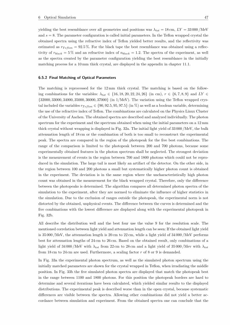
6 Optical Simulation 47
yielding the best resemblance over all geometries and positions was λtot = 18 cm, LY = 33 000 /MeVand s = 8. The parameter configuration is called initial parameters. In the Teflon wrapped crystal theobtained spectra using the refractive index of Teflon yielded better results, and the reflectivity wasestimated as rTeflon = 92.5 %. For the black tape the best resemblance was obtained using a reflec-tivity of rblack = 5 % and an refractive index of nblack = 1.2. The spectra of the experiment, as wellas the spectra created by the parameter configuration yielding the best resemblance in the initiallymatching process for a 10 mm thick crystal, are displayed in the appendix in chapter 11.1.
6.5.2 Final Matching of Optical Parameters
The matching is reprocessed for the 12 mm thick crystal. The matching is based on the follow-ing combinations for the variables: λtot ∈ 16, 18, 20, 22, 24, 26 (in cm), r ∈ 6, 7, 8, 9 and LY ∈32000, 33000, 34000, 35000, 36000, 37000 (in 1/MeV). The variation using the Teflon wrapped crys-tal included the variables rTeflon ∈ 90, 92.5, 95, 97.5 (in %) as well as a boolean variable, determiningthe use of the refractive index of Teflon. The combinations are calculated on the Physics Linux Clusterof the University of Aachen. The obtained spectra are described and analyzed individually. The photonspectrum for the experiment and the spectrum obtained when using the initial parameters on a 12 mmthick crystal without wrapping is displayed in Fig. 32a. The initial light yield of 33 000 /MeV, the bulkattenuation length of 18 cm or the combination of both is too small to reconstruct the experimentalpeak. The spectra are compared in the region of the photopeak for the five best combinations. Therange of the comparison is limited to the photopeak between 200 and 700 photons, because someexperimentally obtained features in the photon spectrum shall be neglected. The strongest deviationis the measurement of events in the region between 700 and 1800 photons which could not be repro-duced in the simulation. The large tail is most likely an artifact of the detector. On the other side, inthe region between 100 and 200 photons a small but systematically higher photon count is obtainedin the experiment. The deviation is in the same region where the uncharacteristically high photoncount was obtained in the measurement for the black wrapped crystal. Therefore, only the differencebetween the photopeaks is determined. The algorithm compares all determined photon spectra of thesimulation to the experiment, after they are normed to eliminate the influence of higher statistics inthe simulation. Due to the exclusion of ranges outside the photopeak, the experimental norm is notdistorted by the obtained, unphysical events. The difference between the curves is determined and thefive combinations with the lowest difference are displayed along with the experimental photopeak inFig. 32b.
All describe the distribution well and the best four use the value 9 for the resolution scale. Thementioned correlation between light yield and attenuation length can be seen: If the obtained light yieldis 35 000 /MeV, the attenuation length is 20 cm to 22 cm, while a light yield of 34 000 /MeV performsbest for attenuation lengths of 24 cm to 26 cm. Based on the obtained result, only combinations of alight yield of 34 000 /MeV with λtot from 22 cm to 28 cm and a light yield of 35 000 /Mev with λtot
from 18 cm to 24 cm are used. Furthermore, a scaling factor r of 8 or 9 is demanded.
In Fig. 33a the experimental photon spectrum, as well as the simulated photon spectrum using theinitially matched parameters are shown for the crystal wrapped in Teflon, when irradiating the middleposition. In Fig. 33b the five simulated photon spectra are displayed that match the photopeak bestin the range between 1100 and 1800 photons. For this position the photopeak borders are hard todetermine and several iterations have been calculated, which yielded similar results to the displayeddistributions. The experimental peak is described worse than in the open crystal, because systematicdifferences are visible between the spectra. Allowing other combinations did not yield a better ac-cordance between simulation and experiment. From the obtained spectra one can conclude that the
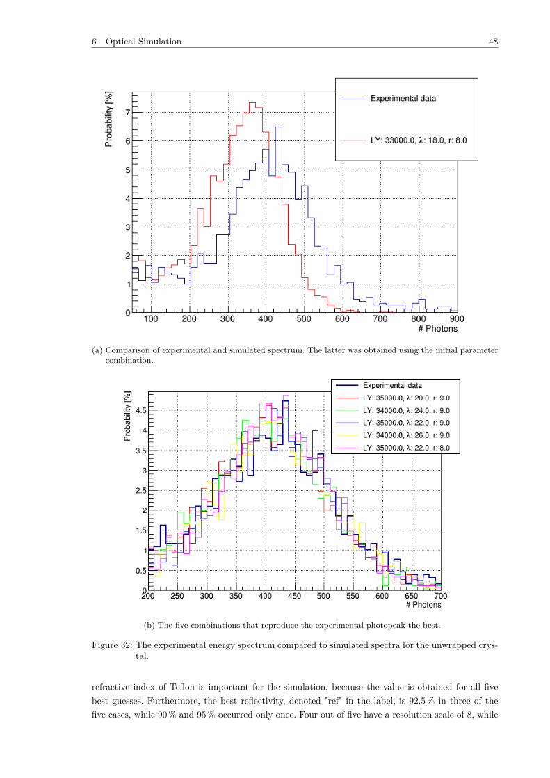
6 Optical Simulation 48
(a) Comparison of experimental and simulated spectrum. The latter was obtained using the initial parametercombination.
(b) The five combinations that reproduce the experimental photopeak the best.
Figure 32: The experimental energy spectrum compared to simulated spectra for the unwrapped crys-tal.
refractive index of Teflon is important for the simulation, because the value is obtained for all fivebest guesses. Furthermore, the best reflectivity, denoted "ref" in the label, is 92.5 % in three of thefive cases, while 90 % and 95 % occurred only once. Four out of five have a resolution scale of 8, while
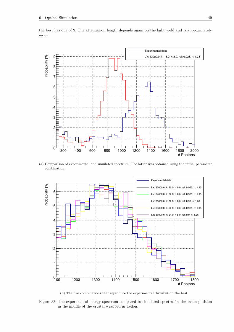
6 Optical Simulation 49
the best has one of 9. The attenuation length depends again on the light yield and is approximately22 cm.
(a) Comparison of experimental and simulated spectrum. The latter was obtained using the initial parametercombination.
(b) The five combinations that reproduce the experimental distribution the best.
Figure 33: The experimental energy spectrum compared to simulated spectra for the beam positionin the middle of the crystal wrapped in Teflon.

6 Optical Simulation 50
In Fig. 34a the same spectra concerning the crystal wrapped in Teflon are shown, but the crystal isirradiated at the corner. The same combinations are demanded as in the middle of the crystal. InFig. 34b the five simulated photon spectra are displayed that match the photopeak best in the rangebetween 800 and 1800 photons. The peak is very clearly distinct in the spectrum. The best light yieldto describe it is 35 000 /MeV. The attenuation length ranges from 20 cm to 24 cm. A resolution scaleof 8 is preferred, which corresponds to the value for the best match in the previously positions. Thereflectivity ranges from 90 % to 95 %. Furthermore, at the edge the refractive index of Teflon obtainedbetter results than the refractive index of air.
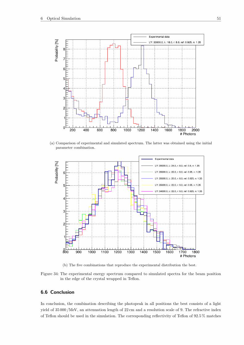
6 Optical Simulation 51
(a) Comparison of experimental and simulated spectrum. The latter was obtained using the initialparameter combination.
(b) The five combinations that reproduce the experimental distribution the best.
Figure 34: The experimental energy spectrum compared to simulated spectra for the beam positionin the edge of the crystal wrapped in Teflon.
6.6 Conclusion
In conclusion, the combination describing the photopeak in all positions the best consists of a lightyield of 35 000 /MeV, an attenuation length of 22 cm and a resolution scale of 9. The refractive indexof Teflon should be used in the simulation. The corresponding reflectivity of Teflon of 92.5 % matches
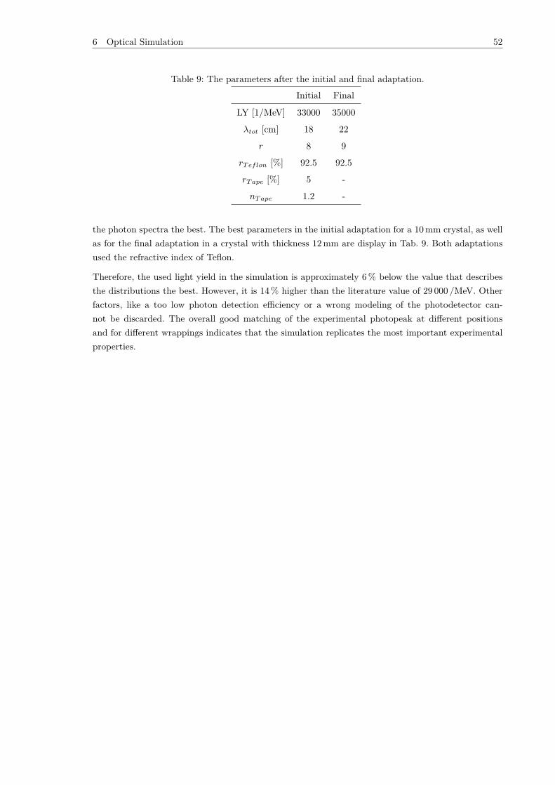
6 Optical Simulation 52
Table 9: The parameters after the initial and final adaptation.
Initial Final
LY [1/MeV] 33000 35000
λtot [cm] 18 22
r 8 9
rTeflon [%] 92.5 92.5
rTape [%] 5 -
nTape 1.2 -
the photon spectra the best. The best parameters in the initial adaptation for a 10 mm crystal, as wellas for the final adaptation in a crystal with thickness 12 mm are display in Tab. 9. Both adaptationsused the refractive index of Teflon.
Therefore, the used light yield in the simulation is approximately 6 % below the value that describesthe distributions the best. However, it is 14 % higher than the literature value of 29 000 /MeV. Otherfactors, like a too low photon detection efficiency or a wrong modeling of the photodetector can-not be discarded. The overall good matching of the experimental photopeak at different positionsand for different wrappings indicates that the simulation replicates the most important experimentalproperties.

7 Monolithic Calibration Algorithms 53
7 Monolithic Calibration Algorithms
7.1 Positioning Algorithm
Before the comparison of experimental and simulated calibration is performed, the algorithms for thepositioning are defined. Several algorithms exist which determine the initial interaction position of the64 photon counts that define the detector response.
7.1.1 Preparation: Preprocessing
Additional features are used to guide the positioning algorithm:
• Number of the die with the highest photon count.
• Number of the pixel with the highest photon count.
• Calculated center of gravity position.
• Number of photons in a row/column of pixels.
Pixels with unknown photon counts due to missing die data are treated as minus one, while pixelsthat did not measure photons are stored as zero. The latter can occur due to another pixel of the diereaching the validation threshold.
7.1.2 Preparation: Principal Component Analysis
The goal of the principal component analysis (PCA) is to characterize a set of inter-correlated dataand extract the linearly uncorrelated variables that represent the set best. This allows to dwindlethe input parameters used by positioning algorithms from 64 numbers to 16. The description of thealgorithm is based on [68]. Basically, the principal components are a linear combination of the originalvariables. The first principal component (PC) is the variable with the largest possible variance whichtherefore extracts the largest part of information from the data set. Subsequently, the second PC iscomputed to have the largest possible variance under the constraint of being orthogonal to the firstPC. Any following PC has to be orthogonal to all other previously determined PCs. Therefore, thePCs create a vector space of the same size as the original variables did, but most of the informationis contained along the axes of the first few PCs. However, the resulting vectors are artificial and donot reflect descriptive observables. The transformation of detector output into the PCA coordinates isachieved by multiplying the data with a matrix which has to be determined only once in the calibrationphase. Therefore it can be applied quickly onto measured data in the system.
7.1.3 Machine Learning Positioning Algorithms
In this work, machine learning algorithms are used to position events that have been simulated.These algorithms behave especially well for positioning incomplete data [69] originating in missing dieinformation. Different approaches have already been taken to determine the position of interaction inPET including nearest-neighbor methods [70], neural networks [39] and algorithms based on decisiontrees [71]. The first method compares a new event to all events measured in the calibration of thedetector module. Therefore, the calculation time scales with the number of calibration points, whichresults in a high calculation effort for each event [69]. Furthermore, nearest-neighbor calibrationsuse only events where all dies were read out, which is the minority for most PET geometries and
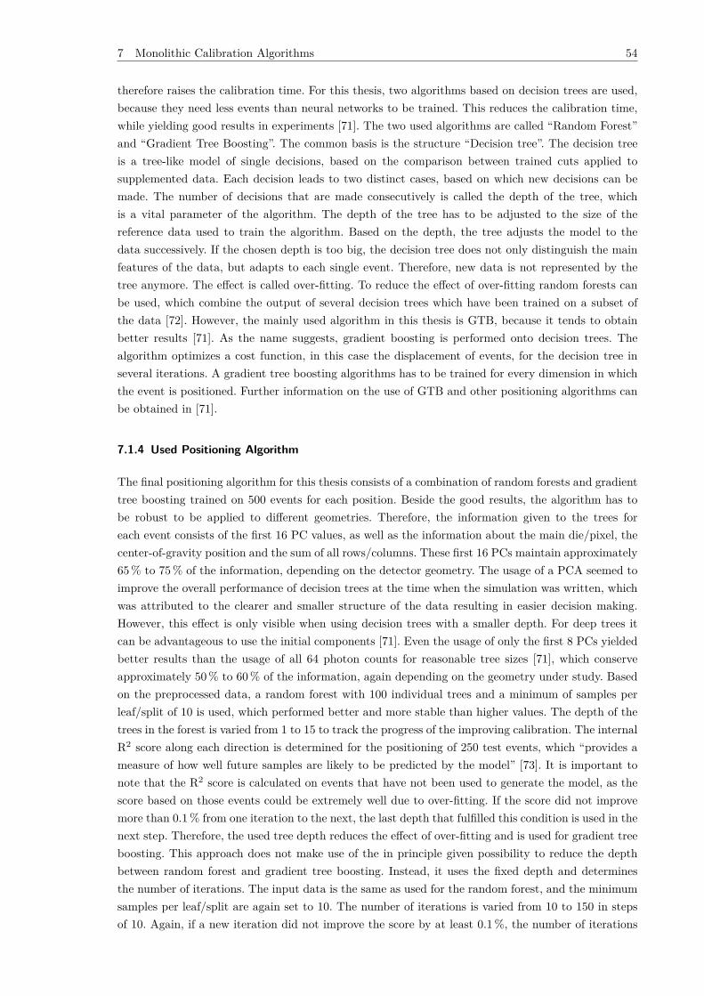
7 Monolithic Calibration Algorithms 54
therefore raises the calibration time. For this thesis, two algorithms based on decision trees are used,because they need less events than neural networks to be trained. This reduces the calibration time,while yielding good results in experiments [71]. The two used algorithms are called “Random Forest”and “Gradient Tree Boosting”. The common basis is the structure “Decision tree”. The decision treeis a tree-like model of single decisions, based on the comparison between trained cuts applied tosupplemented data. Each decision leads to two distinct cases, based on which new decisions can bemade. The number of decisions that are made consecutively is called the depth of the tree, whichis a vital parameter of the algorithm. The depth of the tree has to be adjusted to the size of thereference data used to train the algorithm. Based on the depth, the tree adjusts the model to thedata successively. If the chosen depth is too big, the decision tree does not only distinguish the mainfeatures of the data, but adapts to each single event. Therefore, new data is not represented by thetree anymore. The effect is called over-fitting. To reduce the effect of over-fitting random forests canbe used, which combine the output of several decision trees which have been trained on a subset ofthe data [72]. However, the mainly used algorithm in this thesis is GTB, because it tends to obtainbetter results [71]. As the name suggests, gradient boosting is performed onto decision trees. Thealgorithm optimizes a cost function, in this case the displacement of events, for the decision tree inseveral iterations. A gradient tree boosting algorithms has to be trained for every dimension in whichthe event is positioned. Further information on the use of GTB and other positioning algorithms canbe obtained in [71].
7.1.4 Used Positioning Algorithm
The final positioning algorithm for this thesis consists of a combination of random forests and gradienttree boosting trained on 500 events for each position. Beside the good results, the algorithm has tobe robust to be applied to different geometries. Therefore, the information given to the trees foreach event consists of the first 16 PC values, as well as the information about the main die/pixel, thecenter-of-gravity position and the sum of all rows/columns. These first 16 PCs maintain approximately65 % to 75 % of the information, depending on the detector geometry. The usage of a PCA seemed toimprove the overall performance of decision trees at the time when the simulation was written, whichwas attributed to the clearer and smaller structure of the data resulting in easier decision making.However, this effect is only visible when using decision trees with a smaller depth. For deep trees itcan be advantageous to use the initial components [71]. Even the usage of only the first 8 PCs yieldedbetter results than the usage of all 64 photon counts for reasonable tree sizes [71], which conserveapproximately 50 % to 60 % of the information, again depending on the geometry under study. Basedon the preprocessed data, a random forest with 100 individual trees and a minimum of samples perleaf/split of 10 is used, which performed better and more stable than higher values. The depth of thetrees in the forest is varied from 1 to 15 to track the progress of the improving calibration. The internalR2 score along each direction is determined for the positioning of 250 test events, which “provides ameasure of how well future samples are likely to be predicted by the model” [73]. It is important tonote that the R2 score is calculated on events that have not been used to generate the model, as thescore based on those events could be extremely well due to over-fitting. If the score did not improvemore than 0.1 % from one iteration to the next, the last depth that fulfilled this condition is used in thenext step. Therefore, the used tree depth reduces the effect of over-fitting and is used for gradient treeboosting. This approach does not make use of the in principle given possibility to reduce the depthbetween random forest and gradient tree boosting. Instead, it uses the fixed depth and determinesthe number of iterations. The input data is the same as used for the random forest, and the minimumsamples per leaf/split are again set to 10. The number of iterations is varied from 10 to 150 in stepsof 10. Again, if a new iteration did not improve the score by at least 0.1 %, the number of iterations

7 Monolithic Calibration Algorithms 55
before was used. This approach was pursued to have a fixed exit condition for every tested geometry.Furthermore, it reduces the used storage space of the algorithm, which is useful if it would be usedin a real system using a field-programmable gate array with limited memory of approximately 900 kBreserved memory for the algorithms. A detailed analysis of the storage space needed for random forestand GTB in monolithic PET detectors is conducted in [71].
7.1.5 Evaluation of Positioning Algorithms
The displacement of events from the initial interaction position by the algorithm can be characterizedusing several parameters. All parameters are calculated for each collimator position.
The first parameter is the bias vector which displays the average displacement of the events of onecalibration position. It originates in the position of the collimator and ends in the mean reconstructedposition. The bias vector is especially strong at the borders of the crystal, because the algorithmcan displace an event into the middle of the crystal, but not outside of it. Therefore, the averagedisplacement of events at a single collimator positions increases to the outer sides of the crystal. Whendisplaying the bias vector length for different positions of a crystal in a histogram, the peak that isgenerated by the middle of the crystal creates a nearly Gaussian peak, while the outer regions add along tail. The mean of the bias vector length does not characterize the distribution well. Therefore,the median and the 90th percentile of the bias vector length are used.
The next two parameters are the spatial resolution in each dimension. This value determines thesystem’s ability to distinguish two objects. It is usually defined as the full width at half maximum(FWHM) of the projected point spread function (PSF) for each position. However, due to the mostlynon-Gaussian shape of the function, the NEMA standard defines the spatial resolution differently. Thereconstructed positions are projected onto each axis and the highest bin of the created histogram isdetermined. Afterwards, the bins next to it are used to describe a parabola which is used to determinethe FWHM instead of the original histogram. The spatial resolution is abbreviated Si, where i denotesthe x- or y-direction.
Furthermore, percentiles are used to describe the displacement. Hereby, the x-th percentile describesthe distance from the collimator position in which x percent of the events are placed by the algorithm.In this thesis, the 90th percentile is used to evaluate the behavior of the positioning algorithm whichignores the influence of the 10 % worst-placed events. This creates a stable performance that is lessinfluenced by large tails and describes the performance of the positioning algorithm for the majority ofpositioned data. The two dimensional 90th percentile of the displacement is denoted as 2D percentileor r90, where r denotes the radius of the displacement circle. It is not to be confused with the 90thpercentile of the bias vector length distribution. All characteristic parameters are displayed in Fig.35.
Another interesting parameter is the error rate. It estimates the fraction of events that are not placedwithin a radius of 1.5 mm. The approach is contrary to the 2D percentile, because the radius aroundthe collimator position is fixed and the fraction of events within is estimated.
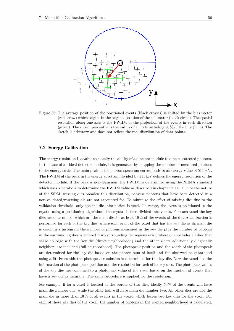
7 Monolithic Calibration Algorithms 56
Figure 35: The average position of the positioned events (black crosses) is shifted by the bias vector(red arrow) which origins in the original position of the collimator (black circle). The spatialresolution along one axis is the FWHM of the projection of the events in each direction(green). The shown percentile is the radius of a circle including 90 % of the hits (blue). Thesketch is arbitrary and does not reflect the real distribution of data points.
7.2 Energy Calibration
The energy resolution is a value to classify the ability of a detector module to detect scattered photons.In the case of an ideal detector module, it is generated by mapping the number of measured photonsto the energy scale. The main peak in the photon spectrum corresponds to an energy value of 511 keV.The FWHM of the peak in the energy spectrum divided by 511 keV defines the energy resolution of thedetector module. If the peak is non-Gaussian, the FWHM is determined using the NEMA standardwhich uses a parabola to determine the FWHM value as described in chapter 7.1.5. Due to the natureof the SiPM, missing dies broaden this distribution, because photons that have been detected in anon-validated/resetting die are not accounted for. To minimize the effect of missing dies due to thevalidation threshold, only specific die information is used. Therefore, the event is positioned in thecrystal using a positioning algorithm. The crystal is then divided into voxels. For each voxel the keydies are determined, which are the main die for at least 10 % of the events of the die. A calibration isperformed for each of the key dies, where each event of the voxel that has the key die as its main dieis used. In a histogram the number of photons measured in the key die plus the number of photonsin the surrounding dies is entered. Two surrounding die regions exist, where one includes all dies thatshare an edge with the key die (direct neighborhood) and the other where additionally diagonallyneighbors are included (full neighborhood). The photopeak position and the width of the photopeakare determined for the key die based on the photon sum of itself and the observed neighborhoodusing a fit. From this the photopeak resolution is determined for the key die. Now the voxel has theinformation of the photopeak position and the resolution for each of its key dies. The photopeak valuesof the key dies are combined to a photopeak value of the voxel based on the fraction of events thathave a key die as main die. The same procedure is applied for the resolution.
For example, if for a voxel is located at the border of two dies, ideally 50 % of the events will havemain die number one, while the other half will have main die number two. All other dies are not themain die in more than 10 % of all events in the voxel, which leaves two key dies for the voxel. Foreach of those key dies of the voxel, the number of photons in the wanted neighborhood is calculated,

7 Monolithic Calibration Algorithms 57
based on the corresponding events. Assuming that the neighborhood of die one yields an average of700 photons and the neighborhood of die two yields 800 photons on average, the photopeak of thevoxel is determined to 750 photons.
If an event belonging to a voxel with a key die which is missing in the event, the missing informationis attributed to a dead-time of the die. The count is interpolated using the importance of the missingdie photon count in the average event of the voxel, based on the measured, residual photon sum of theevent. If the main die of the event is not one of the key dies of its voxel, the most probable key die forthe voxel is used. This generates a stable criteria for the determination of the final energy resolution.The process is precisely described in [71].
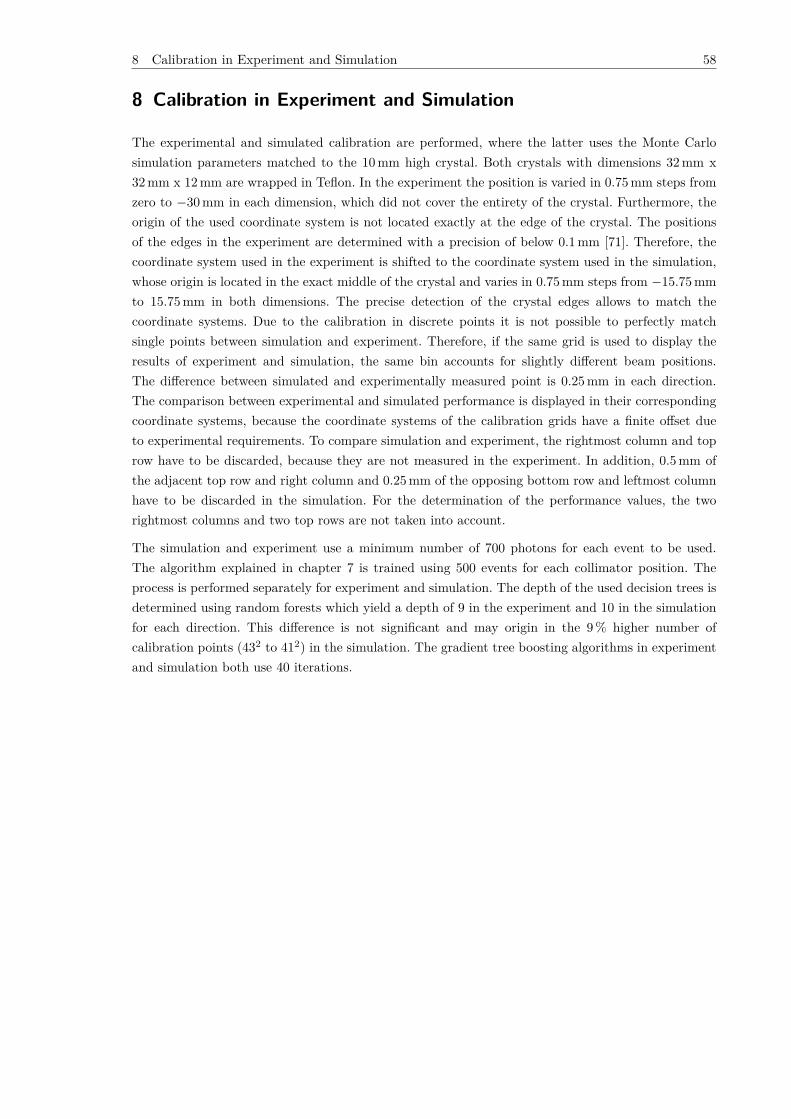
8 Calibration in Experiment and Simulation 58
8 Calibration in Experiment and Simulation
The experimental and simulated calibration are performed, where the latter uses the Monte Carlosimulation parameters matched to the 10 mm high crystal. Both crystals with dimensions 32 mm x32 mm x 12 mm are wrapped in Teflon. In the experiment the position is varied in 0.75 mm steps fromzero to −30 mm in each dimension, which did not cover the entirety of the crystal. Furthermore, theorigin of the used coordinate system is not located exactly at the edge of the crystal. The positionsof the edges in the experiment are determined with a precision of below 0.1 mm [71]. Therefore, thecoordinate system used in the experiment is shifted to the coordinate system used in the simulation,whose origin is located in the exact middle of the crystal and varies in 0.75 mm steps from −15.75 mmto 15.75 mm in both dimensions. The precise detection of the crystal edges allows to match thecoordinate systems. Due to the calibration in discrete points it is not possible to perfectly matchsingle points between simulation and experiment. Therefore, if the same grid is used to display theresults of experiment and simulation, the same bin accounts for slightly different beam positions.The difference between simulated and experimentally measured point is 0.25 mm in each direction.The comparison between experimental and simulated performance is displayed in their correspondingcoordinate systems, because the coordinate systems of the calibration grids have a finite offset dueto experimental requirements. To compare simulation and experiment, the rightmost column and toprow have to be discarded, because they are not measured in the experiment. In addition, 0.5 mm ofthe adjacent top row and right column and 0.25 mm of the opposing bottom row and leftmost columnhave to be discarded in the simulation. For the determination of the performance values, the tworightmost columns and two top rows are not taken into account.
The simulation and experiment use a minimum number of 700 photons for each event to be used.The algorithm explained in chapter 7 is trained using 500 events for each collimator position. Theprocess is performed separately for experiment and simulation. The depth of the used decision trees isdetermined using random forests which yield a depth of 9 in the experiment and 10 in the simulationfor each direction. This difference is not significant and may origin in the 9 % higher number ofcalibration points (432 to 412) in the simulation. The gradient tree boosting algorithms in experimentand simulation both use 40 iterations.
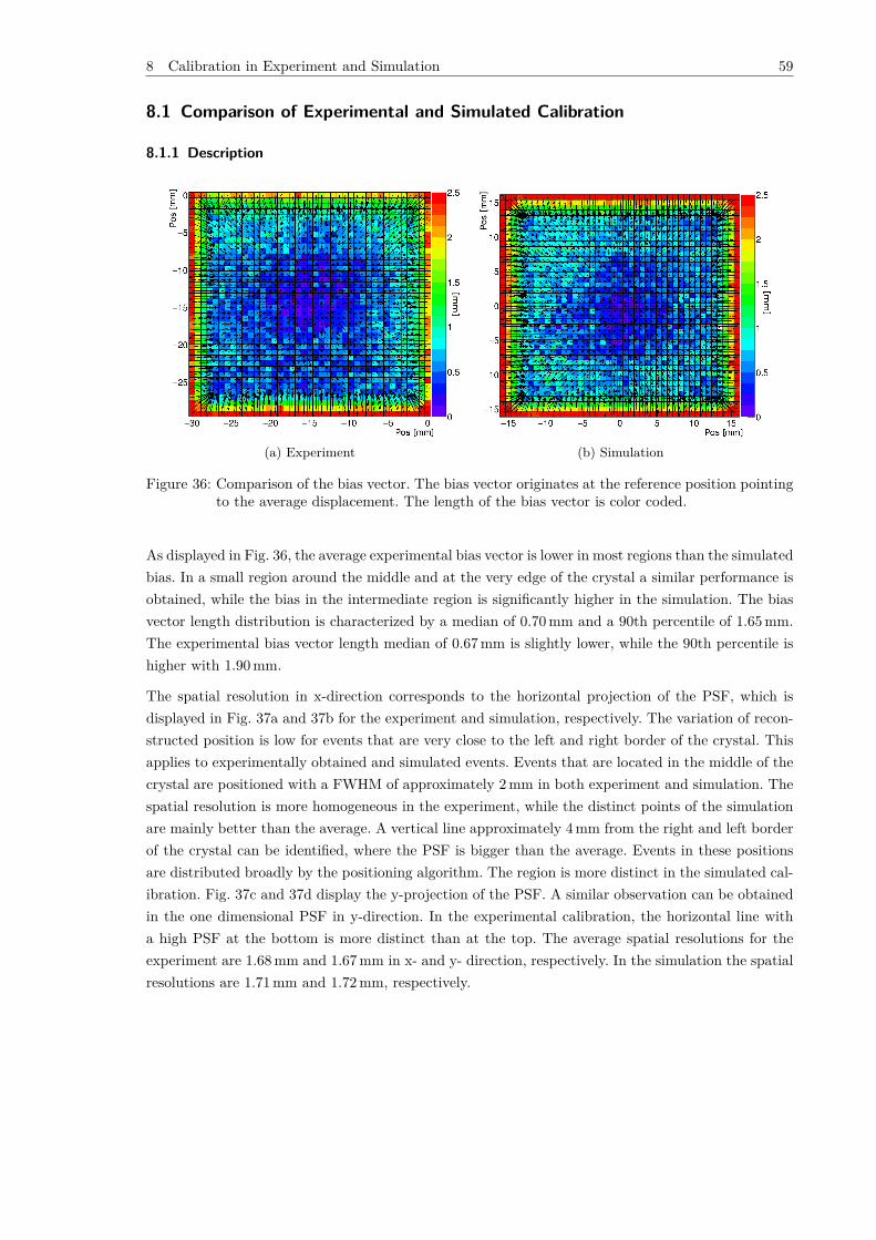
8 Calibration in Experiment and Simulation 59
8.1 Comparison of Experimental and Simulated Calibration
8.1.1 Description
(a) Experiment (b) Simulation
Figure 36: Comparison of the bias vector. The bias vector originates at the reference position pointingto the average displacement. The length of the bias vector is color coded.
As displayed in Fig. 36, the average experimental bias vector is lower in most regions than the simulatedbias. In a small region around the middle and at the very edge of the crystal a similar performance isobtained, while the bias in the intermediate region is significantly higher in the simulation. The biasvector length distribution is characterized by a median of 0.70 mm and a 90th percentile of 1.65 mm.The experimental bias vector length median of 0.67 mm is slightly lower, while the 90th percentile ishigher with 1.90 mm.
The spatial resolution in x-direction corresponds to the horizontal projection of the PSF, which isdisplayed in Fig. 37a and 37b for the experiment and simulation, respectively. The variation of recon-structed position is low for events that are very close to the left and right border of the crystal. Thisapplies to experimentally obtained and simulated events. Events that are located in the middle of thecrystal are positioned with a FWHM of approximately 2 mm in both experiment and simulation. Thespatial resolution is more homogeneous in the experiment, while the distinct points of the simulationare mainly better than the average. A vertical line approximately 4 mm from the right and left borderof the crystal can be identified, where the PSF is bigger than the average. Events in these positionsare distributed broadly by the positioning algorithm. The region is more distinct in the simulated cal-ibration. Fig. 37c and 37d display the y-projection of the PSF. A similar observation can be obtainedin the one dimensional PSF in y-direction. In the experimental calibration, the horizontal line witha high PSF at the bottom is more distinct than at the top. The average spatial resolutions for theexperiment are 1.68 mm and 1.67 mm in x- and y- direction, respectively. In the simulation the spatialresolutions are 1.71 mm and 1.72 mm, respectively.
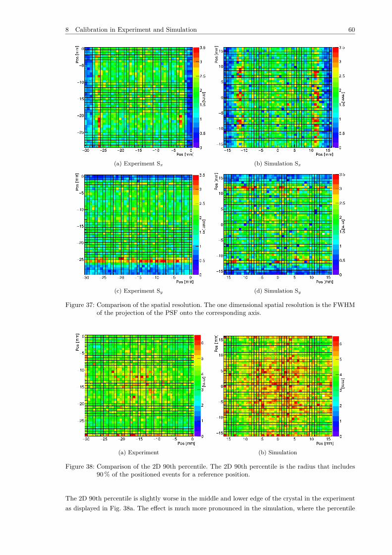
8 Calibration in Experiment and Simulation 60
(a) Experiment Sx (b) Simulation Sx
(c) Experiment Sy (d) Simulation Sy
Figure 37: Comparison of the spatial resolution. The one dimensional spatial resolution is the FWHMof the projection of the PSF onto the corresponding axis.
(a) Experiment (b) Simulation
Figure 38: Comparison of the 2D 90th percentile. The 2D 90th percentile is the radius that includes90 % of the positioned events for a reference position.
The 2D 90th percentile is slightly worse in the middle and lower edge of the crystal in the experimentas displayed in Fig. 38a. The effect is much more pronounced in the simulation, where the percentile
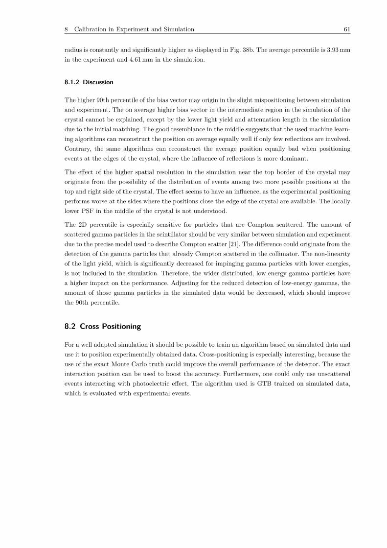
8 Calibration in Experiment and Simulation 61
radius is constantly and significantly higher as displayed in Fig. 38b. The average percentile is 3.93 mmin the experiment and 4.61 mm in the simulation.
8.1.2 Discussion
The higher 90th percentile of the bias vector may origin in the slight mispositioning between simulationand experiment. The on average higher bias vector in the intermediate region in the simulation of thecrystal cannot be explained, except by the lower light yield and attenuation length in the simulationdue to the initial matching. The good resemblance in the middle suggests that the used machine learn-ing algorithms can reconstruct the position on average equally well if only few reflections are involved.Contrary, the same algorithms can reconstruct the average position equally bad when positioningevents at the edges of the crystal, where the influence of reflections is more dominant.
The effect of the higher spatial resolution in the simulation near the top border of the crystal mayoriginate from the possibility of the distribution of events among two more possible positions at thetop and right side of the crystal. The effect seems to have an influence, as the experimental positioningperforms worse at the sides where the positions close the edge of the crystal are available. The locallylower PSF in the middle of the crystal is not understood.
The 2D percentile is especially sensitive for particles that are Compton scattered. The amount ofscattered gamma particles in the scintillator should be very similar between simulation and experimentdue to the precise model used to describe Compton scatter [21]. The difference could originate from thedetection of the gamma particles that already Compton scattered in the collimator. The non-linearityof the light yield, which is significantly decreased for impinging gamma particles with lower energies,is not included in the simulation. Therefore, the wider distributed, low-energy gamma particles havea higher impact on the performance. Adjusting for the reduced detection of low-energy gammas, theamount of those gamma particles in the simulated data would be decreased, which should improvethe 90th percentile.
8.2 Cross Positioning
For a well adapted simulation it should be possible to train an algorithm based on simulated data anduse it to position experimentally obtained data. Cross-positioning is especially interesting, because theuse of the exact Monte Carlo truth could improve the overall performance of the detector. The exactinteraction position can be used to boost the accuracy. Furthermore, one could only use unscatteredevents interacting with photoelectric effect. The algorithm used is GTB trained on simulated data,which is evaluated with experimental events.
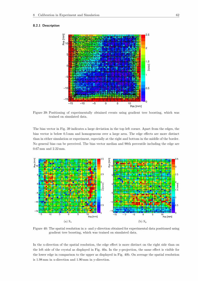
8 Calibration in Experiment and Simulation 62
8.2.1 Description
Figure 39: Positioning of experimentally obtained events using gradient tree boosting, which wastrained on simulated data.
The bias vector in Fig. 39 indicates a large deviation in the top left corner. Apart from the edges, thebias vector is below 0.5 mm and homogeneous over a large area. The edge effects are more distinctthan in either simulation or experiment, especially at the right and bottom in the middle of the border.No general bias can be perceived. The bias vector median and 90th percentile including the edge are0.67 mm and 2.22 mm.
(a) Sx (b) Sy
Figure 40: The spatial resolution in x- and y-direction obtained for experimental data positioned usinggradient tree boosting, which was trained on simulated data.
In the x-direction of the spatial resolution, the edge effect is more distinct on the right side than onthe left side of the crystal as displayed in Fig. 40a. In the y-projection, the same effect is visible forthe lower edge in comparison to the upper as displayed in Fig. 40b. On average the spatial resolutionis 1.98 mm in x-direction and 1.90 mm in y-direction.
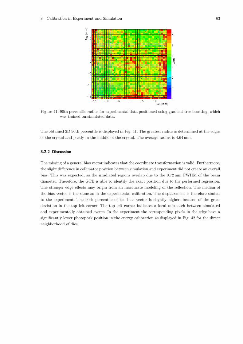
8 Calibration in Experiment and Simulation 63
Figure 41: 90th percentile radius for experimental data positioned using gradient tree boosting, whichwas trained on simulated data.
The obtained 2D 90th percentile is displayed in Fig. 41. The greatest radius is determined at the edgesof the crystal and partly in the middle of the crystal. The average radius is 4.64 mm.
8.2.2 Discussion
The missing of a general bias vector indicates that the coordinate transformation is valid. Furthermore,the slight difference in collimator position between simulation and experiment did not create an overallbias. This was expected, as the irradiated regions overlap due to the 0.72 mm FWHM of the beamdiameter. Therefore, the GTB is able to identify the exact position due to the performed regression.The stronger edge effects may origin from an inaccurate modeling of the reflection. The median ofthe bias vector is the same as in the experimental calibration. The displacement is therefore similarto the experiment. The 90th percentile of the bias vector is slightly higher, because of the greatdeviation in the top left corner. The top left corner indicates a local mismatch between simulatedand experimentally obtained events. In the experiment the corresponding pixels in the edge have asignificantly lower photopeak position in the energy calibration as displayed in Fig. 42 for the directneighborhood of dies.
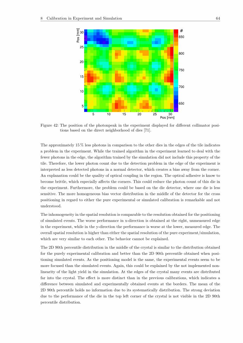
8 Calibration in Experiment and Simulation 64
Figure 42: The position of the photonpeak in the experiment displayed for different collimator posi-tions based on the direct neighborhood of dies [71].
The approximately 15 % less photons in comparison to the other dies in the edges of the tile indicatesa problem in the experiment. While the trained algorithm in the experiment learned to deal with thefewer photons in the edge, the algorithm trained by the simulation did not include this property of thetile. Therefore, the lower photon count due to the detection problem in the edge of the experiment isinterpreted as less detected photons in a normal detector, which creates a bias away from the corner.An explanation could be the quality of optical coupling in the region. The optical adhesive is know tobecome brittle, which especially affects the corners. This could reduce the photon count of this die inthe experiment. Furthermore, the problem could be based on the die detector, where one die is lesssensitive. The more homogeneous bias vector distribution in the middle of the detector for the crosspositioning in regard to either the pure experimental or simulated calibration is remarkable and notunderstood.
The inhomogeneity in the spatial resolution is comparable to the resolution obtained for the positioningof simulated events. The worse performance in x-direction is obtained at the right, unmeasured edgein the experiment, while in the y-direction the performance is worse at the lower, measured edge. Theoverall spatial resolution is higher than either the spatial resolution of the pure experiment/simulation,which are very similar to each other. The behavior cannot be explained.
The 2D 90th percentile distribution in the middle of the crystal is similar to the distribution obtainedfor the purely experimental calibration and better than the 2D 90th percentile obtained when posi-tioning simulated events. As the positioning model is the same, the experimental events seem to bemore focused than the simulated events. Again, this could be explained by the not implemented non-linearity of the light yield in the simulation. At the edges of the crystal many events are distributedfar into the crystal. The effect is more distinct than in the previous calibrations, which indicates adifference between simulated and experimentally obtained events at the borders. The mean of the2D 90th percentile holds no information due to its systematically distribution. The strong deviationdue to the performance of the die in the top left corner of the crystal is not visible in the 2D 90thpercentile distribution.
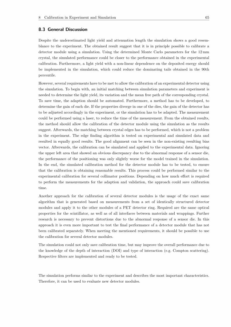
8 Calibration in Experiment and Simulation 65
8.3 General Discussion
Despite the underestimated light yield and attenuation length the simulation shows a good resem-blance to the experiment. The obtained result suggest that it is in principle possible to calibrate adetector module using a simulation. Using the determined Monte Carlo parameters for the 12 mmcrystal, the simulated performance could be closer to the performance obtained in the experimentalcalibration. Furthermore, a light yield with a non-linear dependence on the deposited energy shouldbe implemented in the simulation, which could reduce the dominating tails obtained in the 90thpercentile.
However, several requirements have to be met to allow the calibration of an experimental detector usingthe simulation. To begin with, an initial matching between simulation parameters and experiment isneeded to determine the light yield, its variation and the mean free path of the corresponding crystal.To save time, the adaption should be automated. Furthermore, a method has to be developed, todetermine the gain of each die. If the properties diverge in one of the dies, the gain of the detector hasto be adjusted accordingly in the experiment, or the simulation has to be adapted. The measurementcould be performed using a laser, to reduce the time of the measurement. From the obtained results,the method should allow the calibration of the detector module using the simulation as the resultssuggest. Afterwards, the matching between crystal edges has to be performed, which is not a problemin the experiment. The edge finding algorithm is tested on experimental and simulated data andresulted in equally good results. The good alignment can be seen in the non-existing resulting biasvector. Afterwards, the calibration can be simulated and applied to the experimental data. Ignoringthe upper left area that showed an obvious discrepancy due to the abnormal response of a sensor die,the performance of the positioning was only slightly worse for the model trained in the simulation.In the end, the simulated calibration method for the detector module has to be tested, to ensurethat the calibration is obtaining reasonable results. This process could be performed similar to theexperimental calibration for several collimator positions. Depending on how much effort is requiredto perform the measurements for the adaption and validation, the approach could save calibrationtime.
Another approach for the calibration of several detector modules is the usage of the exact samealgorithm that is generated based on measurements from a set of identically structured detectormodules and apply it to the other modules of a PET detector ring. Required are the same opticalproperties for the scintillator, as well as of all interfaces between materials and wrappings. Furtherresearch is necessary to prevent distortions due to the abnormal response of a sensor die. In thisapproach it is even more important to test the final performance of a detector module that has notbeen calibrated separately. When meeting the mentioned requirements, it should be possible to usethe calibration for several detector modules.
The simulation could not only save calibration time, but may improve the overall performance due tothe knowledge of the depth of interaction (DOI) and type of interaction (e.g. Compton scattering).Respective filters are implemented and ready to be tested.
The simulation performs similar to the experiment and describes the most important characteristics.Therefore, it can be used to evaluate new detector modules.
9 Evaluation of Promising Geometries 66
9 Evaluation of Promising Geometries
The simulation is used in this chapter to determine the performance of different detector geometries.The creation of events is based on the gamma particles stored in the simulation of the collimatorsetup. The whole crystal is irradiated perpendicular in an equidistant grid with a pitch of 0.5 mm. Forthe used crystal with dimensions 30 mm x 30 mm x 10 mm (30 · 2 + 1)2 collimator positions, with 500events each, are simulated. The performance of the detector modules shall be evaluated independentlyfrom the used collimator setup. Therefore, the real interaction position in the crystal is taken intoaccount, instead of the position of the collimator. Otherwise, the collimator position is folded withthe beam profile and the interaction position is blurred. The obtained results would only apply tothe simulated collimator configuration. The simulation uses only gamma particles that interact byphotoelectic effect and have an energy of 511 keV, which eliminates problems due to the reduces lightyield for lower energy gamma particles. This yields approximately the same result as the photon cutat 700 photons used in chapter 8 for the Teflon wrapped crystal. Therefore, the simulation determinesthe performance of geometries in a best-case scenario for the positioning algorithm that is describedin chapter 7. For all geometries the GTB adapted to 40 iterations.
The simulation is controlled using macros to adjust the geometry and properties of the detector setup,before the simulation of particles begins. This allows to adjust the following properties:
• The type of scintillator (cuboid, trapezoid).
• The thickness of the scintillator.
• The width of the scintillator.
• The wrapping of the scintillator.
• The type of optical adhesive.
• The x-y position of the detector module.
• The rotation of the detector module.
The use of a wider crystal was not studied, because of the fixed size of the photodetector. In principle,the simulation could be performed with an arbitrary detector or several photodetectors attached todifferent sides of the crystal. However, priority was given to the other parameters.
If not further specified, the standard geometry, consisting of a 30 mm x 30 mm x 10 mm open crystalwith a photodetector attached at its backside, is used. Open indicates that no wrapping is attachedto the crystal. The optical adhesive used is SYLGARD 527 with a refractive index of 1.405. Thevariations evaluated in this thesis concern the side of readout, wrapping and thickness of the crystal,as well as the used optical adhesive.
9.1 Variation of Sensor Placement
9.1.1 Motivation
The performance of front- and back-readout is tested using the standard geometry. Double-sidedreadout has not been implemented, because it did not improve the resolution of the detector moduleaccordingly [42]. The positioning algorithms would be based on the combined information of bothtiles, which might lead to a different approach in preprocessing and training of GTB. For example,additional features could be implemented to guide the GTB. Furthermore, the double-sided readout
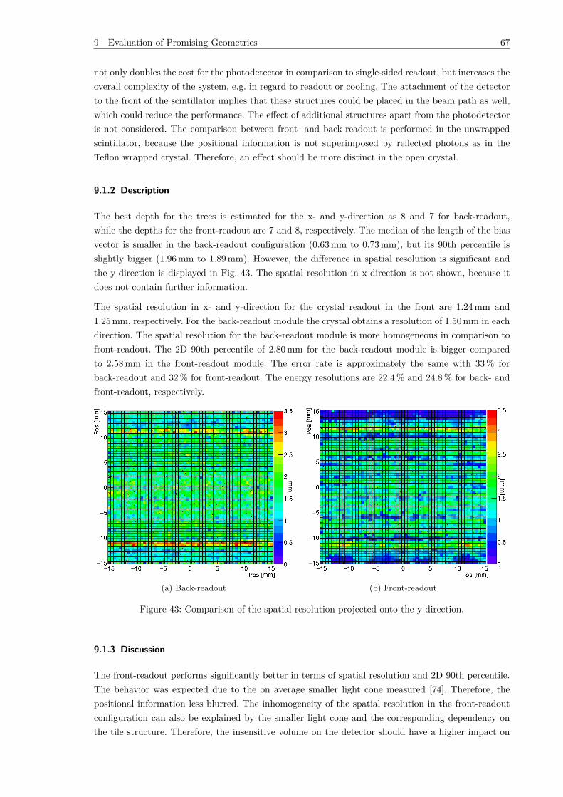
9 Evaluation of Promising Geometries 67
not only doubles the cost for the photodetector in comparison to single-sided readout, but increases theoverall complexity of the system, e.g. in regard to readout or cooling. The attachment of the detectorto the front of the scintillator implies that these structures could be placed in the beam path as well,which could reduce the performance. The effect of additional structures apart from the photodetectoris not considered. The comparison between front- and back-readout is performed in the unwrappedscintillator, because the positional information is not superimposed by reflected photons as in theTeflon wrapped crystal. Therefore, an effect should be more distinct in the open crystal.
9.1.2 Description
The best depth for the trees is estimated for the x- and y-direction as 8 and 7 for back-readout,while the depths for the front-readout are 7 and 8, respectively. The median of the length of the biasvector is smaller in the back-readout configuration (0.63 mm to 0.73 mm), but its 90th percentile isslightly bigger (1.96 mm to 1.89 mm). However, the difference in spatial resolution is significant andthe y-direction is displayed in Fig. 43. The spatial resolution in x-direction is not shown, because itdoes not contain further information.
The spatial resolution in x- and y-direction for the crystal readout in the front are 1.24 mm and1.25 mm, respectively. For the back-readout module the crystal obtains a resolution of 1.50 mm in eachdirection. The spatial resolution for the back-readout module is more homogeneous in comparison tofront-readout. The 2D 90th percentile of 2.80 mm for the back-readout module is bigger comparedto 2.58 mm in the front-readout module. The error rate is approximately the same with 33 % forback-readout and 32 % for front-readout. The energy resolutions are 22.4 % and 24.8 % for back- andfront-readout, respectively.
(a) Back-readout (b) Front-readout
Figure 43: Comparison of the spatial resolution projected onto the y-direction.
9.1.3 Discussion
The front-readout performs significantly better in terms of spatial resolution and 2D 90th percentile.The behavior was expected due to the on average smaller light cone measured [74]. Therefore, thepositional information less blurred. The inhomogeneity of the spatial resolution in the front-readoutconfiguration can also be explained by the smaller light cone and the corresponding dependency onthe tile structure. Therefore, the insensitive volume on the detector should have a higher impact on
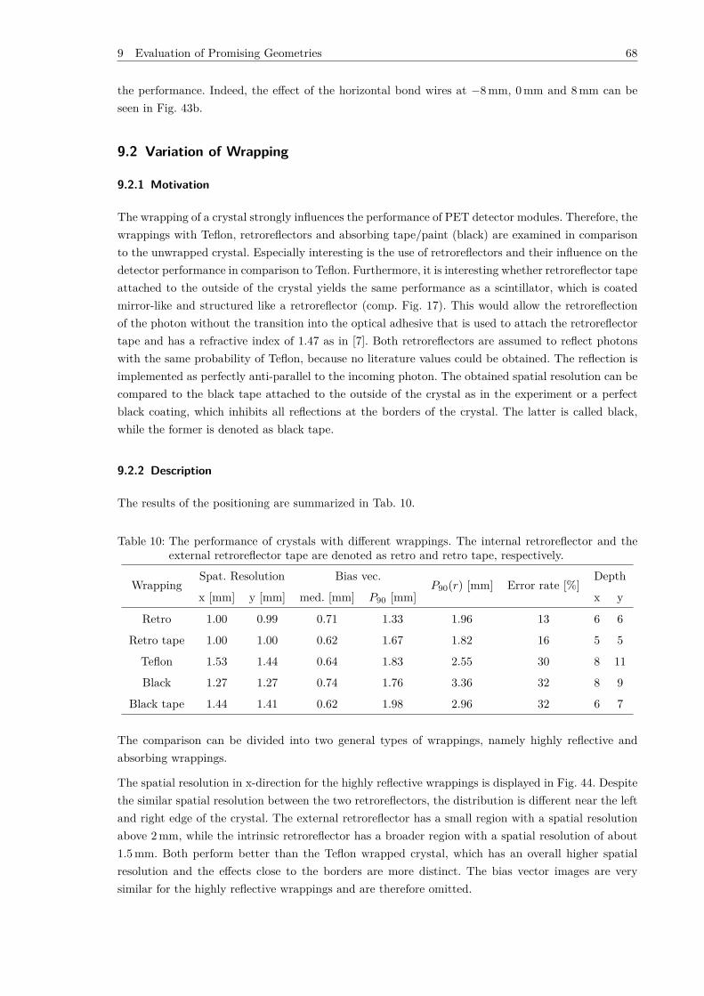
9 Evaluation of Promising Geometries 68
the performance. Indeed, the effect of the horizontal bond wires at −8 mm, 0 mm and 8 mm can beseen in Fig. 43b.
9.2 Variation of Wrapping
9.2.1 Motivation
The wrapping of a crystal strongly influences the performance of PET detector modules. Therefore, thewrappings with Teflon, retroreflectors and absorbing tape/paint (black) are examined in comparisonto the unwrapped crystal. Especially interesting is the use of retroreflectors and their influence on thedetector performance in comparison to Teflon. Furthermore, it is interesting whether retroreflector tapeattached to the outside of the crystal yields the same performance as a scintillator, which is coatedmirror-like and structured like a retroreflector (comp. Fig. 17). This would allow the retroreflectionof the photon without the transition into the optical adhesive that is used to attach the retroreflectortape and has a refractive index of 1.47 as in [7]. Both retroreflectors are assumed to reflect photonswith the same probability of Teflon, because no literature values could be obtained. The reflection isimplemented as perfectly anti-parallel to the incoming photon. The obtained spatial resolution can becompared to the black tape attached to the outside of the crystal as in the experiment or a perfectblack coating, which inhibits all reflections at the borders of the crystal. The latter is called black,while the former is denoted as black tape.
9.2.2 Description
The results of the positioning are summarized in Tab. 10.
Table 10: The performance of crystals with different wrappings. The internal retroreflector and theexternal retroreflector tape are denoted as retro and retro tape, respectively.
WrappingSpat. Resolution Bias vec.
P90(r) [mm] Error rate [%]Depth
x [mm] y [mm] med. [mm] P90 [mm] x y
Retro 1.00 0.99 0.71 1.33 1.96 13 6 6
Retro tape 1.00 1.00 0.62 1.67 1.82 16 5 5
Teflon 1.53 1.44 0.64 1.83 2.55 30 8 11
Black 1.27 1.27 0.74 1.76 3.36 32 8 9
Black tape 1.44 1.41 0.62 1.98 2.96 32 6 7
The comparison can be divided into two general types of wrappings, namely highly reflective andabsorbing wrappings.
The spatial resolution in x-direction for the highly reflective wrappings is displayed in Fig. 44. Despitethe similar spatial resolution between the two retroreflectors, the distribution is different near the leftand right edge of the crystal. The external retroreflector has a small region with a spatial resolutionabove 2 mm, while the intrinsic retroreflector has a broader region with a spatial resolution of about1.5 mm. Both perform better than the Teflon wrapped crystal, which has an overall higher spatialresolution and the effects close to the borders are more distinct. The bias vector images are verysimilar for the highly reflective wrappings and are therefore omitted.
9 Evaluation of Promising Geometries 69
(a) Retroreflector (b) Retroreflector tape
(c) Teflon
Figure 44: The spatial resolution in x-direction for the highly reflective wrappings.
The 2D 90th percentile between the two retroreflector types are very similar, while Teflon obtains ahomogeneously worse 2D 90th percentile in the middle and a strong degradation at the edges.
The energy resolution of the highly reflective geometries is best for the crystal wrapped in Teflonwith 16.5 %. The currently implemented method of the full or direct neighborhood of dies yields aresolution of 26.3 % for the retroreflector tape. The algorithm estimates the energy resolution of theintrinsic retroreflector as 42.3 %.
The x-direction of the spatial resolution is displayed in Fig. 46 for the absorbing wrappings. Thespatial resolution of the totally absorbing black wrapping is 1.27 mm in x- and y-direction, while theblack tape obtained 1.44 mm and 1.41 mm in x- and y-direction, respectively. Stronger edge effects arevisible for the black tape.
The 2D 90th percentile is better for the black tape as displayed in Fig. 47.
The energy resolution for the crystal with black tape is 35.1 %. The energy resolution for the to-tally black wrapping could not be determined, because the photopeak is not distinct from the back-ground.
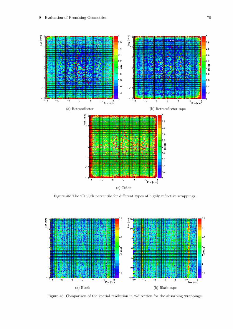
9 Evaluation of Promising Geometries 70
(a) Retroreflector (b) Retroreflector tape
(c) Teflon
Figure 45: The 2D 90th percentile for different types of highly reflective wrappings.
(a) Black (b) Black tape
Figure 46: Comparison of the spatial resolution in x-direction for the absorbing wrappings.
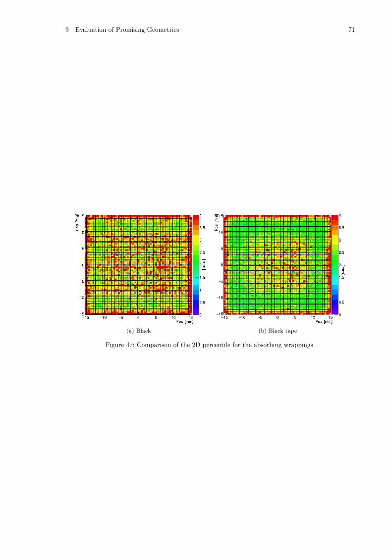
9 Evaluation of Promising Geometries 71
(a) Black (b) Black tape
Figure 47: Comparison of the 2D percentile for the absorbing wrappings.
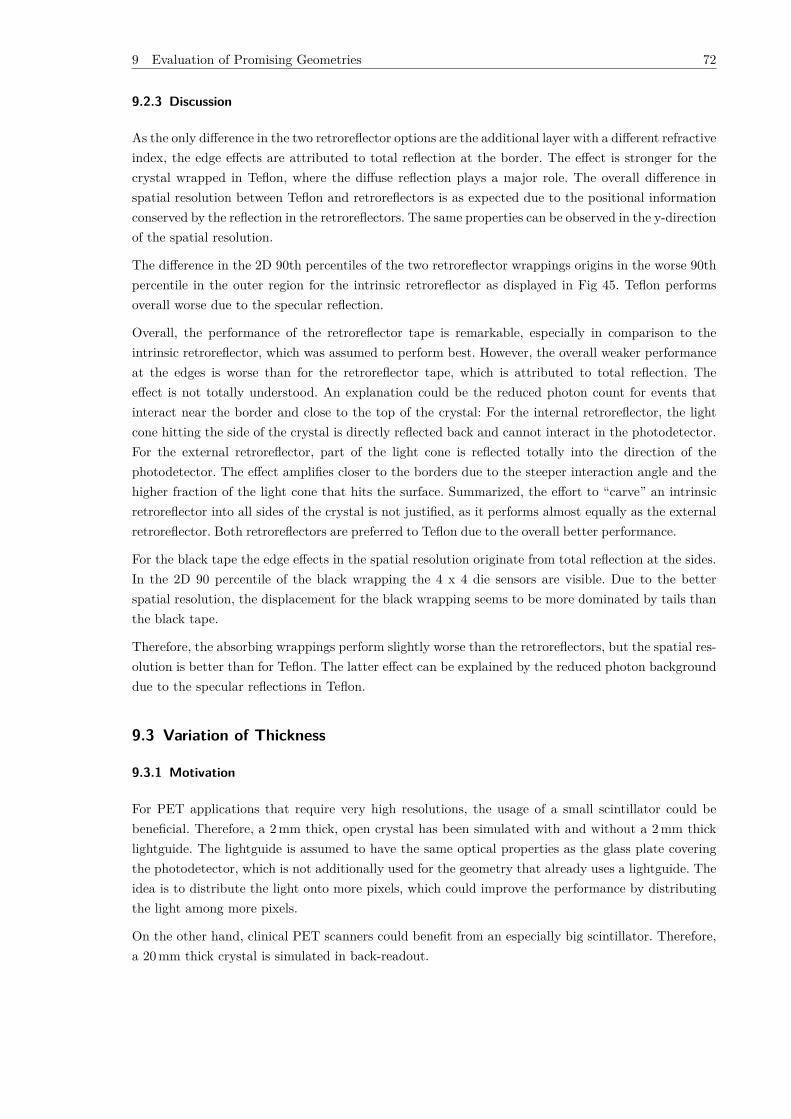
9 Evaluation of Promising Geometries 72
9.2.3 Discussion
As the only difference in the two retroreflector options are the additional layer with a different refractiveindex, the edge effects are attributed to total reflection at the border. The effect is stronger for thecrystal wrapped in Teflon, where the diffuse reflection plays a major role. The overall difference inspatial resolution between Teflon and retroreflectors is as expected due to the positional informationconserved by the reflection in the retroreflectors. The same properties can be observed in the y-directionof the spatial resolution.
The difference in the 2D 90th percentiles of the two retroreflector wrappings origins in the worse 90thpercentile in the outer region for the intrinsic retroreflector as displayed in Fig 45. Teflon performsoverall worse due to the specular reflection.
Overall, the performance of the retroreflector tape is remarkable, especially in comparison to theintrinsic retroreflector, which was assumed to perform best. However, the overall weaker performanceat the edges is worse than for the retroreflector tape, which is attributed to total reflection. Theeffect is not totally understood. An explanation could be the reduced photon count for events thatinteract near the border and close to the top of the crystal: For the internal retroreflector, the lightcone hitting the side of the crystal is directly reflected back and cannot interact in the photodetector.For the external retroreflector, part of the light cone is reflected totally into the direction of thephotodetector. The effect amplifies closer to the borders due to the steeper interaction angle and thehigher fraction of the light cone that hits the surface. Summarized, the effort to “carve” an intrinsicretroreflector into all sides of the crystal is not justified, as it performs almost equally as the externalretroreflector. Both retroreflectors are preferred to Teflon due to the overall better performance.
For the black tape the edge effects in the spatial resolution originate from total reflection at the sides.In the 2D 90 percentile of the black wrapping the 4 x 4 die sensors are visible. Due to the betterspatial resolution, the displacement for the black wrapping seems to be more dominated by tails thanthe black tape.
Therefore, the absorbing wrappings perform slightly worse than the retroreflectors, but the spatial res-olution is better than for Teflon. The latter effect can be explained by the reduced photon backgrounddue to the specular reflections in Teflon.
9.3 Variation of Thickness
9.3.1 Motivation
For PET applications that require very high resolutions, the usage of a small scintillator could bebeneficial. Therefore, a 2 mm thick, open crystal has been simulated with and without a 2 mm thicklightguide. The lightguide is assumed to have the same optical properties as the glass plate coveringthe photodetector, which is not additionally used for the geometry that already uses a lightguide. Theidea is to distribute the light onto more pixels, which could improve the performance by distributingthe light among more pixels.
On the other hand, clinical PET scanners could benefit from an especially big scintillator. Therefore,a 20 mm thick crystal is simulated in back-readout.
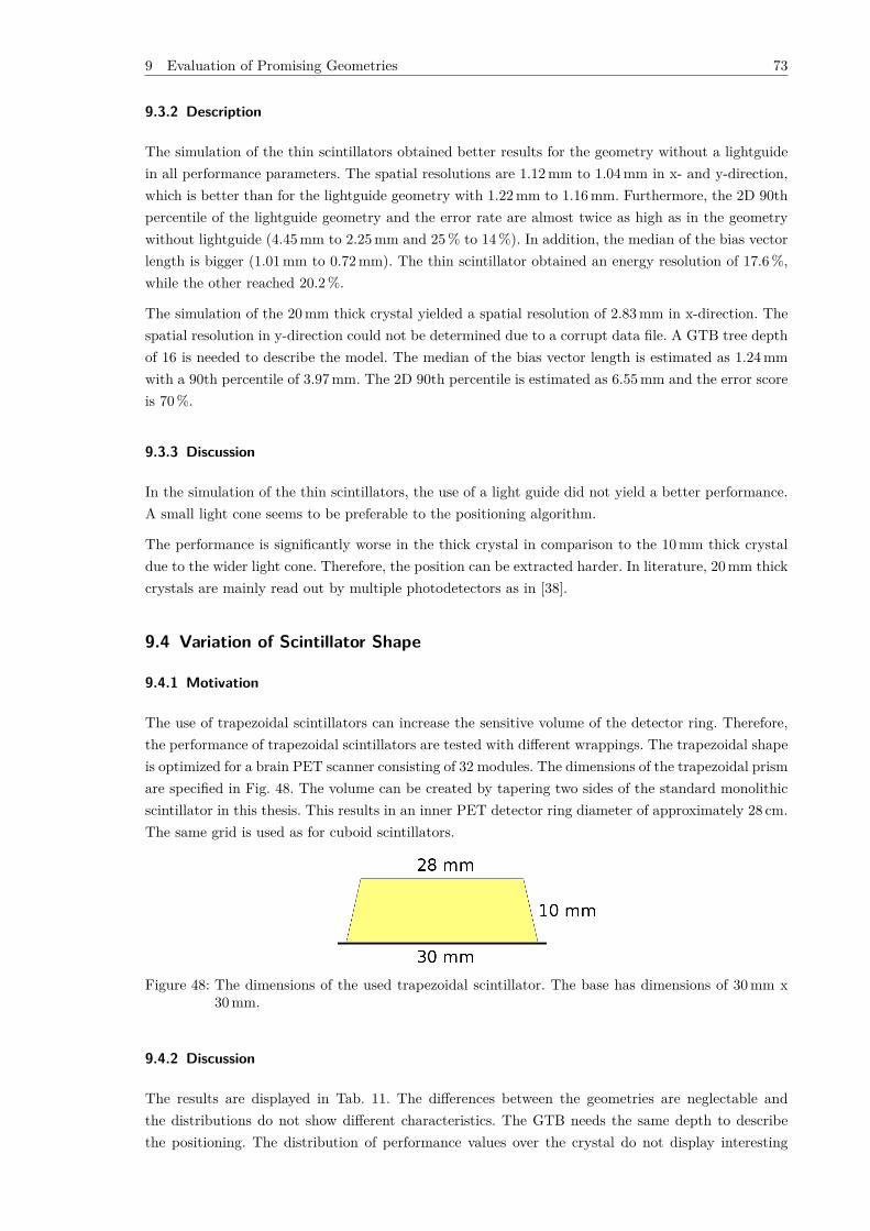
9 Evaluation of Promising Geometries 73
9.3.2 Description
The simulation of the thin scintillators obtained better results for the geometry without a lightguidein all performance parameters. The spatial resolutions are 1.12 mm to 1.04 mm in x- and y-direction,which is better than for the lightguide geometry with 1.22 mm to 1.16 mm. Furthermore, the 2D 90thpercentile of the lightguide geometry and the error rate are almost twice as high as in the geometrywithout lightguide (4.45 mm to 2.25 mm and 25 % to 14 %). In addition, the median of the bias vectorlength is bigger (1.01 mm to 0.72 mm). The thin scintillator obtained an energy resolution of 17.6 %,while the other reached 20.2 %.
The simulation of the 20 mm thick crystal yielded a spatial resolution of 2.83 mm in x-direction. Thespatial resolution in y-direction could not be determined due to a corrupt data file. A GTB tree depthof 16 is needed to describe the model. The median of the bias vector length is estimated as 1.24 mmwith a 90th percentile of 3.97 mm. The 2D 90th percentile is estimated as 6.55 mm and the error scoreis 70 %.
9.3.3 Discussion
In the simulation of the thin scintillators, the use of a light guide did not yield a better performance.A small light cone seems to be preferable to the positioning algorithm.
The performance is significantly worse in the thick crystal in comparison to the 10 mm thick crystaldue to the wider light cone. Therefore, the position can be extracted harder. In literature, 20 mm thickcrystals are mainly read out by multiple photodetectors as in [38].
9.4 Variation of Scintillator Shape
9.4.1 Motivation
The use of trapezoidal scintillators can increase the sensitive volume of the detector ring. Therefore,the performance of trapezoidal scintillators are tested with different wrappings. The trapezoidal shapeis optimized for a brain PET scanner consisting of 32 modules. The dimensions of the trapezoidal prismare specified in Fig. 48. The volume can be created by tapering two sides of the standard monolithicscintillator in this thesis. This results in an inner PET detector ring diameter of approximately 28 cm.The same grid is used as for cuboid scintillators.
Figure 48: The dimensions of the used trapezoidal scintillator. The base has dimensions of 30 mm x30 mm.
9.4.2 Discussion
The results are displayed in Tab. 11. The differences between the geometries are neglectable andthe distributions do not show different characteristics. The GTB needs the same depth to describethe positioning. The distribution of performance values over the crystal do not display interesting
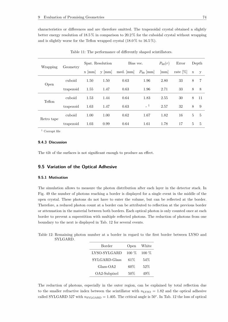
9 Evaluation of Promising Geometries 74
characteristics or differences and are therefore omitted. The trapezoidal crystal obtained a slightlybetter energy resolution of 18.5 % in comparison to 20.2 % for the cuboidal crystal without wrappingand is slightly worse for the Teflon wrapped crystal (18.0 % to 16.5 %).
Table 11: The performance of differently shaped scintillators.
Wrapping GeometrySpat. Resolution Bias vec. P90(r) Error Depth
x [mm] y [mm] med. [mm] P90 [mm] [mm] rate [%] x y
Opencuboid 1.50 1.50 0.63 1.96 2.80 33 8 7
trapezoid 1.55 1.47 0.63 1.96 2.71 33 8 8
Tefloncuboid 1.53 1.44 0.64 1.83 2.55 30 8 11
trapezoid 1.63 1.47 0.63 - 1 2.57 32 8 9
Retro tapecuboid 1.00 1.00 0.62 1.67 1.82 16 5 5
trapezoid 1.03 0.99 0.64 1.61 1.78 17 5 51 Corrupt file
9.4.3 Discussion
The tilt of the surfaces is not significant enough to produce an effect.
9.5 Variation of the Optical Adhesive
9.5.1 Motivation
The simulation allows to measure the photon distribution after each layer in the detector stack. InFig. 49 the number of photons reaching a border is displayed for a single event in the middle of theopen crystal. These photons do not have to enter the volume, but can be reflected at the border.Therefore, a reduced photon count at a border can be attributed to reflection at the previous borderor attenuation in the material between both borders. Each optical photon is only counted once at eachborder to prevent a superstition with multiple reflected photons. The reduction of photons from oneboundary to the next is displayed in Tab. 12 for several events.
Table 12: Remaining photon number at a border in regard to the first border between LYSO andSYLGARD.
Border Open White
LYSO-SYLGARD 100 % 100 %
SYLGARD-Glass 61% 54%
Glass-OA2 60% 52%
OA2-Subpixel 50% 49%
The reduction of photons, especially in the outer region, can be explained by total reflection dueto the smaller refractive index between the scintillator with nLYSO = 1.82 and the optical adhesivecalled SYLGARD 527 with nSYLGARD = 1.405. The critical angle is 50. In Tab. 12 the loss of optical
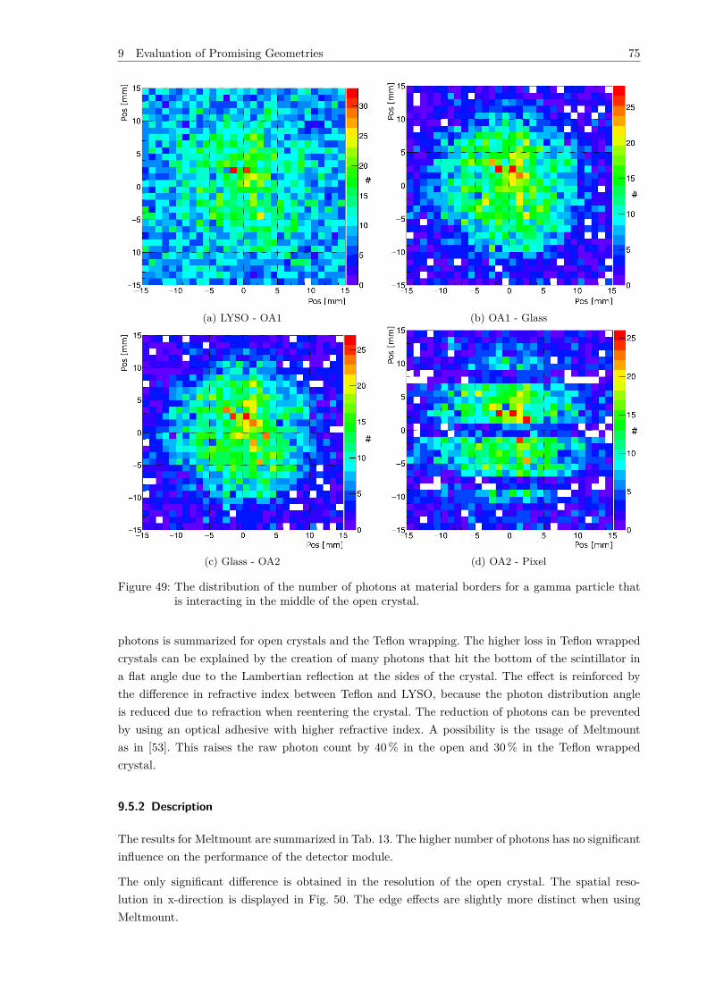
9 Evaluation of Promising Geometries 75
(a) LYSO - OA1 (b) OA1 - Glass
(c) Glass - OA2 (d) OA2 - Pixel
Figure 49: The distribution of the number of photons at material borders for a gamma particle thatis interacting in the middle of the open crystal.
photons is summarized for open crystals and the Teflon wrapping. The higher loss in Teflon wrappedcrystals can be explained by the creation of many photons that hit the bottom of the scintillator ina flat angle due to the Lambertian reflection at the sides of the crystal. The effect is reinforced bythe difference in refractive index between Teflon and LYSO, because the photon distribution angleis reduced due to refraction when reentering the crystal. The reduction of photons can be preventedby using an optical adhesive with higher refractive index. A possibility is the usage of Meltmountas in [53]. This raises the raw photon count by 40 % in the open and 30 % in the Teflon wrappedcrystal.
9.5.2 Description
The results for Meltmount are summarized in Tab. 13. The higher number of photons has no significantinfluence on the performance of the detector module.
The only significant difference is obtained in the resolution of the open crystal. The spatial reso-lution in x-direction is displayed in Fig. 50. The edge effects are slightly more distinct when usingMeltmount.
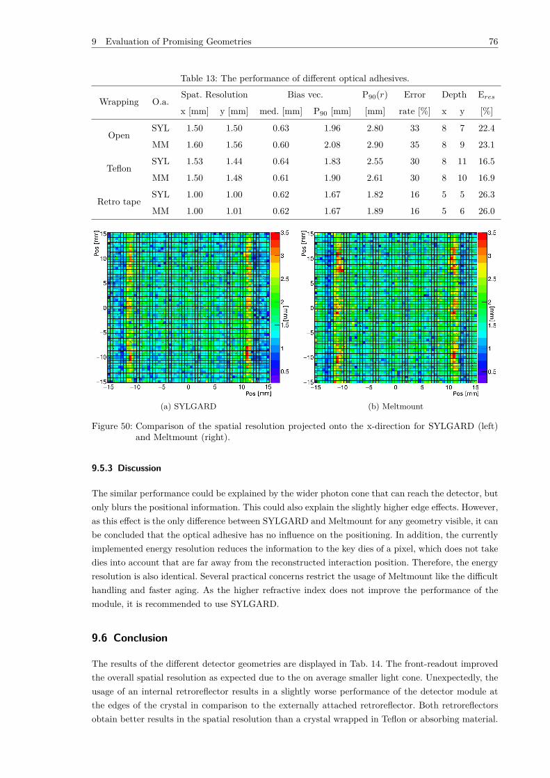
9 Evaluation of Promising Geometries 76
Table 13: The performance of different optical adhesives.
Wrapping O.a.Spat. Resolution Bias vec. P90(r) Error Depth Eresx [mm] y [mm] med. [mm] P90 [mm] [mm] rate [%] x y [%]
OpenSYL 1.50 1.50 0.63 1.96 2.80 33 8 7 22.4
MM 1.60 1.56 0.60 2.08 2.90 35 8 9 23.1
TeflonSYL 1.53 1.44 0.64 1.83 2.55 30 8 11 16.5
MM 1.50 1.48 0.61 1.90 2.61 30 8 10 16.9
Retro tapeSYL 1.00 1.00 0.62 1.67 1.82 16 5 5 26.3
MM 1.00 1.01 0.62 1.67 1.89 16 5 6 26.0
(a) SYLGARD (b) Meltmount
Figure 50: Comparison of the spatial resolution projected onto the x-direction for SYLGARD (left)and Meltmount (right).
9.5.3 Discussion
The similar performance could be explained by the wider photon cone that can reach the detector, butonly blurs the positional information. This could also explain the slightly higher edge effects. However,as this effect is the only difference between SYLGARD and Meltmount for any geometry visible, it canbe concluded that the optical adhesive has no influence on the positioning. In addition, the currentlyimplemented energy resolution reduces the information to the key dies of a pixel, which does not takedies into account that are far away from the reconstructed interaction position. Therefore, the energyresolution is also identical. Several practical concerns restrict the usage of Meltmount like the difficulthandling and faster aging. As the higher refractive index does not improve the performance of themodule, it is recommended to use SYLGARD.
9.6 Conclusion
The results of the different detector geometries are displayed in Tab. 14. The front-readout improvedthe overall spatial resolution as expected due to the on average smaller light cone. Unexpectedly, theusage of an internal retroreflector results in a slightly worse performance of the detector module atthe edges of the crystal in comparison to the externally attached retroreflector. Both retroreflectorsobtain better results in the spatial resolution than a crystal wrapped in Teflon or absorbing material.

9 Evaluation of Promising Geometries 77
The best energy resolution can be obtained with Teflon tape. The performance of the 20 mm thickmonolithic scintillator is considerably worse than a 10 mm thick crystal. The performance does notchange for the studied trapezoidal scintillator or the used optical adhesive.
In further research, several other interesting geometries can be simulated. Especially the double-sidedreadout could yield good results using the GTB algorithm. Even the attachment of four additionaldetectors to the sides of the crystal has been tested before [37]. Another idea would be the attachmentof two detectors to the bottom side of the crystal as displayed in Fig. 51. Furthermore, the simulationallows the placement of different wrappings on the sides and top of the crystal, which has not beenused in this thesis.
Figure 51: A detector geometry based on a pentagon with two photodetectors attached to the twobottom sides.
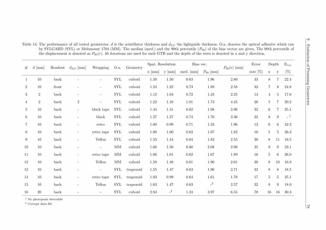
9Evaluation
ofPromising
Geom
etries78
Table 14: The performance of all tested geometries. d is the scintillator thickness and dLG the lightguide thickness. O.a. denotes the optical adhesive which canby SYLGARD (SYL) or Meltmount 1704 (MM). The median (med.) and the 90th percentile (P90) of the bias vector are given. The 90th percentile ofthe displacement is denoted as P90(r). 40 iterations are used for each GTB and the depth of the trees is denoted in x and y direction.
# d [mm] Readout dLG [mm] Wrapping O.a. GeometrySpat. Resolution Bias vec.
P90(r) [mm]Error Depth Eres
x [mm] y [mm] med. [mm] P90 [mm] rate [%] x y [%]
1 10 back - - SYL cuboid 1.50 1.50 0.63 1.96 2.80 33 8 7 22.4
2 10 front - - SYL cuboid 1.24 1.25 0.73 1.89 2.58 32 7 8 24.8
3 2 back - - SYL cuboid 1.12 1.04 0.72 1.43 2.25 14 4 5 17.6
4 2 back 2 - SYL cuboid 1.22 1.16 1.01 1.73 4.45 26 5 7 20.2
5 10 back - black tape SYL cuboid 1.44 1.41 0.62 1.98 2.96 32 6 7 35.1
6 10 back - black SYL cuboid 1.27 1.27 0.74 1.76 3.36 32 8 9 - 1
7 10 back - retro SYL cuboid 1.00 0.99 0.71 1.33 1.96 13 6 6 42.3
8 10 back - retro tape SYL cuboid 1.00 1.00 0.62 1.67 1.82 16 5 5 26.3
9 10 back - Teflon SYL cuboid 1.53 1.44 0.64 1.83 2.55 30 8 11 16.5
10 10 back - - MM cuboid 1.60 1.56 0.60 2.08 2.90 35 8 9 23.1
11 10 back - retro tape MM cuboid 1.00 1.01 0.62 1.67 1.89 16 5 6 26.0
12 10 back - Teflon MM cuboid 1.50 1.48 0.61 1.90 2.61 30 8 10 16.9
13 10 back - - SYL trapezoid 1.55 1.47 0.63 1.96 2.71 33 8 8 18.5
14 10 back - retro tape SYL trapezoid 1.03 0.99 0.64 1.61 1.78 17 5 5 25.1
15 10 back - Teflon SYL trapezoid 1.63 1.47 0.63 -2 2.57 32 8 9 18.0
16 20 back - - SYL cuboid 2.83 -2 1.24 3.97 6.55 70 16 16 30.31 No photopeak obervable2 Corrupt data file
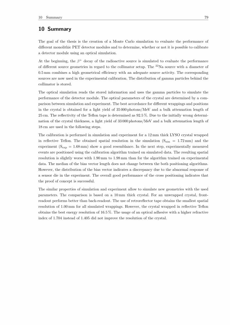
10 Summary 79
10 Summary
The goal of the thesis is the creation of a Monte Carlo simulation to evaluate the performance ofdifferent monolithic PET detector modules and to determine, whether or not it is possible to calibratea detector module using an optical simulation.
At the beginning, the β+ decay of the radioactive source is simulated to evaluate the performanceof different source geometries in regard to the collimator setup. The 22Na source with a diameter of0.5 mm combines a high geometrical efficiency with an adequate source activity. The correspondingsources are now used in the experimental calibration. The distribution of gamma particles behind thecollimator is stored.
The optical simulation reads the stored information and uses the gamma particles to simulate theperformance of the detector module. The optical parameters of the crystal are determined by a com-parison between simulation and experiment. The best accordance for different wrappings and positionsin the crystal is obtained for a light yield of 35 000 photons/MeV and a bulk attenuation length of25 cm. The reflectivity of the Teflon tape is determined as 92.5 %. Due to the initially wrong determi-nation of the crystal thickness, a light yield of 33 000 photons/MeV and a bulk attenuation length of18 cm are used in the following steps.
The calibration is performed in simulation and experiment for a 12 mm thick LYSO crystal wrappedin reflective Teflon. The obtained spatial resolution in the simulation (Ssim = 1.72 mm) and theexperiment (Sexp = 1.68 mm) show a good resemblance. In the next step, experimentally measuredevents are positioned using the calibration algorithm trained on simulated data. The resulting spatialresolution is slightly worse with 1.90 mm to 1.98 mm than for the algorithm trained on experimentaldata. The median of the bias vector length does not change between the both positioning algorithms.However, the distribution of the bias vector indicates a discrepancy due to the abnormal response ofa sensor die in the experiment. The overall good performance of the cross positioning indicates thatthe proof of concept is successful.
The similar properties of simulation and experiment allow to simulate new geometries with the usedparameters. The comparison is based on a 10 mm thick crystal. For an unwrapped crystal, front-readout performs better than back-readout. The use of retroreflector tape obtains the smallest spatialresolution of 1.00 mm for all simulated wrappings. However, the crystal wrapped in reflective Teflonobtains the best energy resolution of 16.5 %. The usage of an optical adhesive with a higher refractiveindex of 1.704 instead of 1.405 did not improve the resolution of the crystal.
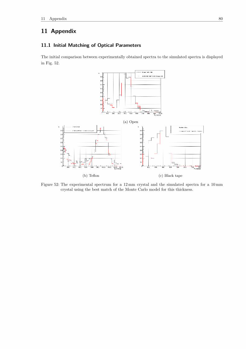
11 Appendix 80
11 Appendix
11.1 Initial Matching of Optical Parameters
The initial comparison between experimentally obtained spectra to the simulated spectra is displayedin Fig. 52.
(a) Open
(b) Teflon (c) Black tape
Figure 52: The experimental spectrum for a 12 mm crystal and the simulated spectra for a 10 mmcrystal using the best match of the Monte Carlo model for this thickness.

Literature 81
Literature
[1] Statistisches Bundesamt, “Fallpauschalenbezogene Krankenhausstatistik 2015 (DRG- Statis-tik),” 2016.
[2] Jülich Forschungszentrum, No Title, 2015.[3] D. L. Bailey et al., Positron Emission Tomography, 3. 2005, vol. 27. doi: 10.1088/0031-
9155/51/13/R08.[4] H. Lodish et al., Molecular cell biology, vol. 3.[5] T. G. Turkington, “PET Imaging Basics,” in Clinical PET-CT in Radiology, Springer, 2011,
pp. 21–28.[6] M. C. Maas et al., “Monolithic scintillator PET detectors with intrinsic depth-of-interaction
correction,” Phys. Med. Biol, vol. 54, pp. 1893–1908, 2009. doi: 10.1088/0031-9155/54/7/003.[7] A. Aguilar et al., “Performance S tudy of a Large Monolithic LYSO PET Detector with Accurate
Photon DOI Using Retroreflector L ayers,” vol. 7311, no. c, 2017. doi: 10.1109/TRPMS.2017.
2692819.[8] W. Demtroeder, Experimentalphysik 4, 5. Auflage. Springer. doi: 10.1007/978-3-662-52884-
6 ISBN.[9] M. Galan, “Table de Radionucléides,” Ciemat, pp. 1–6, 2009.[10] National Nuclear Data Center, ENSDF dataset for 22Ne, Brookhaven.[11] Eckert & Ziegler Isotope Products GmbH, No Title, private communication, 2017.[12] A. Dash et al., “Industrial radionuclide generators: A potential step towards accelerating radio-
tracer investigations in industry,” RSC Adv., vol. 3, 2013.[13] C. S. Levin et al., “Calculation of positron range and its effect on the fundamental limit of
positron emission tomography system spatial resolution.,” Physics in medicine and biology, vol.44, no. 3, pp. 781–799, 1999. doi: 10.1088/0031-9155/45/2/501.
[14] G. B. Saha, “Basics of PET Imaging Basics of PET Imaging,” Imaging, vol. 202, no. 6, p. 199,2005. doi: 10.1007/978-1-4419-0805-6.
[15] K. Shibuya et al., “Annihilation photon acollinearity in PET: volunteer and phantom FDGstudies,” Physics in Medicine and Biology, vol. 52, no. 17, p. 5249, 2007. doi: 10.1088/0031-
9155/52/17/010.[16] K. Shibuya et al., “A Healthy Volunteer FDG-PET Study on Annihilation Radiation Non-
collinearity,” in 2006 IEEE Nuclear Science Symposium Conference Record, vol. 3, 2006, pp. 1889–1892. doi: 10.1109/NSSMIC.2006.354262.
[17] N. Groß-Weege, “Development of an algorithm for detecting multiple interactions in high reso-lution PET scanners,” 2014.
[18] C. Davisson, “Interaction of γ Radiation with Matter,” in Alpha-, Beta- and Gamma-ray Spec-troscopy, K. Siegbahn, Ed., 1965, p. 37.
[19] J. R. Howell et al., Thermal radiation heat transfer. CRC press, 2010.[20] L. Zhang, “Emission Spectra of LSO and LYSO Crystals,” Science And Technology, vol. 55,
pp. 1759–1766, 2008. doi: 10.1109/NSSMIC.2007.4437128.[21] Cern, “Physics reference manual - geant4,” vol. 1, no. December, 2013.[22] Ulflund, Matlab code to plot the reflection coefficient based on Fresnel equations, 2011.[23] M. S. Judenhofer et al., “Applications for preclinical PET/MRI,” in Seminars in nuclear medicine,
Elsevier, vol. 43, 2013, pp. 19–29. doi: 10.1053/j.semnuclmed.2012.08.004.[24] J. Humm et al., “From PET detectors to PET scanners,” European Journal of Nuclear Medicine
and Molecular Imaging, vol. 30, no. 11, pp. 1574–1597, 2003. doi: 10.1007/s00259-003-1266-2.
Literature 82
[25] C. M. Pepin et al., “Properties of LYSO and recent LSO scintillators for phoswich PET de-tectors,” IEEE Transactions on Nuclear Science, vol. 51, no. 3 II, pp. 789–795, 2004. doi:10.1109/TNS.2004.829781.
[26] C. W. Lerche et al., “Dependency of Energy-, Position- and Depth of Interaction Resolution onScintillation Crystal Coating and Geometry,” vol. 55, no. 3, pp. 1344–1351, 2008.
[27] T. District et al., “Luminescence and Scintillation Properties of Ce-Doped LYSO and YSOCrystals Chalerm Wanarak 1,,” pp. 1796–1803, 2011. doi: 10.4028/www.scientific.net/
AMR.199-200.1796.[28] C. L. Melcher et al., “Scintillation properties of LSO:Ce boules,” in 1998 IEEE Nuclear Science
Symposium Conference Record. 1998 IEEE Nuclear Science Symposium and Medical ImagingConference (Cat. No.98CH36255), vol. 1, 1998, 154–157 vol.1. doi: 10.1109/NSSMIC.1998.
774827.[29] C. L. Melcher, “Scintillation Crystals for PET*,” pp. 1051–1055, 2000.[30] R. Mao et al., “Crystal growth and scintillation properties of LSO and LYSO crystals,” Journal
of Crystal Growth, vol. 368, pp. 97–100, 2013. doi: 10.1016/j.jcrysgro.2013.01.038.[31] L. Qin et al., “Growth and characteristics of LYSO (Lu2(1-x-y)Y2xSiO5:Cey) scintillation crys-
tals,” Journal of Crystal Growth, vol. 281, no. 2–4, pp. 518–524, 2005. doi: 10 . 1016 / j .
jcrysgro.2005.04.057.[32] C. Wanarak et al., “Light Yield Non-Proportionality and Energy Resolution of Lu1.8Y0.2SiO5:Ce
and LaCl3:Ce Scintillation Crystals,” Advanced Materials Research, vol. 284-286, pp. 2002–2007,2011. doi: 10.4028/www.scientific.net/AMR.284-286.2002.
[33] T. Frach et al., “The digital silicon photomultiplier - Principle of operation and intrinsic detectorperformance,” IEEE Nuclear Science Symposium Conference Record, pp. 1959–1965, 2009. doi:10.1109/NSSMIC.2009.5402143.
[34] G. Borghi et al., “Experimental validation of an efficient fan-beam calibration procedure fork-nearest neighbor position estimation in monolithic scintillator detectors,” IEEE Transactionson Nuclear Science, vol. 62, no. 1, pp. 57–67, 2015. doi: 10.1109/TNS.2014.2375557.
[35] S. España et al., “DigiPET: sub-millimeter spatial resolution small-animal PET imaging usingthin monolithic scintillators,” Physics in Medicine and Biology, vol. 59, no. 13, p. 3405, 2014.doi: 10.1088/0031-9155/59/13/3405.
[36] R. Marcinkowski et al., “Sub-millimetre DOI detector based on monolithic LYSO and digitalSiPM for a dedicated small-animal PET system,” Physics in medicine and biology, vol. 61, no.5, p. 2196, 2016. doi: 10.1088/0031-9155/61/5/2196.
[37] D. J. Van Der Laan et al., “Using cramér-rao theory combined with monte carlo simulationsfor the optimization of monolithic scintillator PET detectors,” IEEE Transactions on NuclearScience, 2006. doi: 10.1109/TNS.2006.873710.
[38] M. C. Maas et al., “Experimental characterization of monolithic-crystal small animal PET detec-tors read out by APD arrays,” IEEE Transactions on Nuclear Science, vol. 53, no. 3, pp. 1071–1077, 2006. doi: 10.1109/TNS.2006.873711.
[39] P. Bruyndonckx et al., “Neural network-based position estimators for PET detectors using mono-lithic LSO blocks,” IEEE Transactions on Nuclear Science, 2004. doi: 10.1109/TNS.2004.
835782.[40] G. Borghi et al., “Towards monolithic scintillator based TOF-PET systems: practical methods
for detector calibration and operation,” Physics in Medicine and Biology, 2016. doi: 10.1088/
0031-9155/61/13/4904.[41] Z. Li et al., “Nonlinear least-squares modeling of 3D interaction position in a monolithic scin-
tillator block,” Phys. Med. Biol. Phys. Med. Biol, vol. 55, no. 55, pp. 6515–6515, 2010. doi:10.1088/0031-9155/55/21/012.
Literature 83
[42] P. Bruyndonckx et al., “Evaluation of machine learning algorithms for localization of photonsin undivided scintillator blocks for PET detectors,” in IEEE Transactions on Nuclear Science,2008. doi: 10.1109/TNS.2008.922811.
[43] G. Borghi et al., “A 32 mm x 32 mm x 22 mm monolithic LYSO:Ce detector with dual-sided digi-tal photon counter readout for ultrahigh-performance TOF-PET and TOF-PET/MRI,” Physicsin Medicine and Biology, 2016. doi: 10.1088/0031-9155/61/13/4929.
[44] S. Agostinelli et al., “Geant4 - a simulation toolkit,” Nuclear Instruments and Methods in PhysicsResearch Section A: Accelerators, Spectrometers, Detectors and Associated Equipment, vol. 506,no. 3, pp. 250–303, 2003. doi: 10.1016/S0168-9002(03)01368-8. arXiv: 1005.0727v1.
[45] Geant4, Physics Lists EM constructors in Geant4 10.3.[46] ——, Low Energy Physics Lists.[47] H. Gast, “GEANT 4 Introductory Course,” 2009.[48] C. Ritzer, “Development and Operation of a Testing Bench for the Characterisation of PET
Detectors,” no. August, 2015.[49] E. &. Ziegler, “Medical imaging Source Catalogue,” Biomedical Engineering, pp. 1–20, 2006.[50] IDB Holland bv, No Title, private communication, 2016.[51] O. Tange, “GNU Parallel - The Command-Line Power Tool,” ;login: The USENIX Magazine,
vol. 36, no. 1, pp. 42–47, Feb. 2011.[52] S. Blahuta et al., “Next Generation LYSO:Ce,Ca Single Crystals,” vol. 3141, no. 2013, p. 3141,
2014.[53] D. J. J. van der Laan et al., “Optical simulation of monolithic scintillator detectors using
GATE/GEANT4.,” Phys Med Biol, vol. 55, no. 6, pp. 1659–1675, 2010. doi: 10.1088/0031-
9155/55/6/009.[54] M. Kronberger et al., “Determination of the Absolute Light Yields of LuYAP and LYSO,”
pp. 1153–1157, 2008.[55] L. Pidol et al., “High efficiency of lutetium silicate scintillators, Ce-doped LPS, and LYSO
crystals,” IEEE Transactions on Nuclear Science, vol. 51, no. 3 III, pp. 1084–1087, 2004. doi:10.1109/TNS.2004.829542.
[56] Epic Crystal, LYSO(Ce) Crystal.[57] A. I. N. Press, “Optimization of the effective light attenuation length of YAP:Ce and LYSO:Ce
crystals for a novel geometrical PET concept,” vol. 564, pp. 506–514, 2006. doi: 10.1016/j.
nima.2006.04.079.[58] I. G. Valais et al., “Evaluation of the light emission efficiency of LYSO:Ce scintillator under X-ray
excitation for possible applications in medical imaging,” Nuclear Instruments and Methods inPhysics Research, Section A: Accelerators, Spectrometers, Detectors and Associated Equipment,vol. 569, no. 2 SPEC. ISS. Pp. 201–204, 2006. doi: 10.1016/j.nima.2006.08.018.
[59] T. Frach, No Title, private communication, 2017.[60] A. I. N. Press, “Scintillator studies for the HPD-PET concept,” vol. 571, pp. 419–424, 2007.
doi: 10.1016/j.nima.2006.10.124.[61] J. Martin, “Simulating scintillation light collection using measured optical reflectance,” IEEE T
Nucl Sci, no. TNS-00249-2009.R1, pp. 1–8, 2010. doi: doi: 10.1109/TNS.2010.2042731.[62] C. Moisan et al., “Testing Scintillation Transport Models with Photoelectron Yields Measured
under Different Surface Finishes,” pp. 824–828,[63] S. Butterworth, “On the theory of filter amplifiers,” 1930.[64] B. J. Pichler et al., “Production of a diffuse very high reflectivity material for light collection
in nuclear detectors,” Nuclear Instruments and Methods in Physics Research, Section A: Accel-erators, Spectrometers, Detectors and Associated Equipment, vol. 442, no. 1, pp. 333–336, 2000.doi: 10.1016/S0168-9002(99)01245-0.
Literature 84
[65] R. Schulze, PDPC-TEK user manual, 1.03. Philips Digital Photon Counting, 2016.[66] V. Tabacchini et al., “Probabilities of triggering and validation in a digital silicon photomulti-
plier,” doi: 10.1088/1748-0221/9/06/P06016.[67] R. Marcinkowski et al., “Effects of dark counts on Digital Silicon Photomultipliers performance,”
IEEE Nuclear Science Symposium Conference Record, no. 1, 2013. doi: 10.1109/NSSMIC.2013.
6829323.[68] H. Abdi et al., “Principal component analysis,” Wiley Interdisciplinary Reviews: Computational
Statistics, vol. 2, no. 4, pp. 433–459, 2010. doi: 10.1002/wics.101. arXiv: arXiv:1011.1669v3.[69] P. J. García-Laencina et al., “Pattern classification with missing data: a review,” Neural Com-
puting and Applications, vol. 19, no. 2, pp. 263–282, 2010. doi: 10.1007/s00521-009-0295-6.arXiv: arXiv:1011.1669v3.
[70] H. T. Van Dam et al., “Improved nearest neighbor methods for gamma photon interactionposition determination in monolithic scintillator PET detectors,” IEEE Transactions on NuclearScience, vol. 58, no. 5 PART 1, pp. 2139–2147, 2011. doi: 10.1109/TNS.2011.2150762.
[71] F. Müller, “Evaluation and Calibration of Monolithic Scintillator Crystals for Positron EmissionTomography,” PhD thesis, University of Aachen, 2017.
[72] T. Hastie et al., The elements of statistical learning: data mining, inference and prediction, 2.2005, vol. 27, pp. 83–85. doi: 10.1007/BF02985802.
[73] F. Pedregosa et al., “Scikit-learn: Machine Learning in Python,” Journal of Machine LearningResearch, vol. 12, pp. 2825–2830, 2011.
[74] D. R. Schaart et al., “A novel, SiPM-array-based, monolithic scintillator detector for PET.,”Physics in medicine and biology, vol. 54, no. 11, pp. 3501–3512, 2009. doi: 10.1088/0031-
9155/54/11/015.