Mechatronik und elektrische Antriebe - ei.uni-paderborn.de · 8 Elektronisch kommutierte Motoren...
180
Dieses Skript ist vornehmlich für die Studenten der Universität Paderborn als vorlesungsbegleitende Unterlage gedacht. Über das Internet steht es auch anderen Interessierten zur Verfügung. In jedem Fall ist nur die private, individuelle, nicht-kommerzielle Nutzung gestattet. Insbesondere ist nicht gestattet, das Skript oder dessen Bestandteile weiter zu verbreiten, zu vervielfältigen oder für andere Zwecke zu nutzen. Ausnahmen bedürfen der Genehmigung des Verfassers. Der Verfasser ist für Hinweise auf Fehler oder Unzulänglichkeiten dankbar. These lecture notes are primarily dedicated to the students of the University of Paderborn. It is also available to other persons on the internet. In any case, only private, individual, non-commercial use is allowed. In particular, it is not allowed to distribute, to copy the lecture notes or parts of it or to use it for other means. Exceptions have to be agreed by the author. The author would appreciate any comment on errors or incompleteness. Mechatronik und elektrische Antriebe Mechatronics and Electrical Drives Prof. Dr.-Ing. Joachim Böcker Skript zur Vorlesung / Lecture Notes Stand/Edition: 2018-05-18 Universität Paderborn Leistungselektronik und Elektrische Antriebstechnik Power Electronics and Electrical Drives
Transcript of Mechatronik und elektrische Antriebe - ei.uni-paderborn.de · 8 Elektronisch kommutierte Motoren...
Dieses Skript ist vornehmlich für die Studenten der Universität Paderborn als vorlesungsbegleitende Unterlage gedacht. Über das Internet
steht es auch anderen Interessierten zur Verfügung. In jedem Fall ist nur die private, individuelle, nicht-kommerzielle Nutzung gestattet.
Insbesondere ist nicht gestattet, das Skript oder dessen Bestandteile weiter zu verbreiten, zu vervielfältigen oder für andere Zwecke zu nutzen. Ausnahmen bedürfen der Genehmigung des Verfassers. Der Verfasser ist für Hinweise auf Fehler oder Unzulänglichkeiten dankbar.
These lecture notes are primarily dedicated to the students of the University of Paderborn. It is also available to other persons on the internet. In any case, only private, individual, non-commercial use is allowed. In particular, it is not allowed to distribute, to copy the lecture notes or
parts of it or to use it for other means. Exceptions have to be agreed by the author. The author would appreciate any comment on errors or
incompleteness.
Mechatronik und elektrische Antriebe
Mechatronics and Electrical Drives
Prof. Dr.-Ing. Joachim Böcker
Skript zur Vorlesung / Lecture Notes
Stand/Edition: 2018-05-18
Universität Paderborn
Leistungselektronik und Elektrische Antriebstechnik Power Electronics and Electrical Drives
Mechatronik und elektrische Antriebe S. 2
Inhalt 1 Mechatronische Systeme Mechatronic Systems ............................................................ 6 2 Energiebilanz Energy Balance ...................................................................................... 10
2.1 Energiebilanz Elektromechanischer Wandler Energy Balance of Electromechanical
Converters..................................................................................................................... 10 2.2 Energiebilanz bei Elektromagnetische Aktoren Energy Balance with Electromagnetic
Actuators....................................................................................................................... 12
2.3 Die Ko- oder Ergänzungsenergie The Co-Energy ........................................................ 16 2.4 Die zweiten Ableitungen der Energie The Second-Order Derivatives of the Energy . 21
3 Magnetische Kreise Magnetic Circuits ......................................................................... 23 3.1 Electromagnetische Energiedichte Electromagnetic Energy Density ......................... 23 3.2 Magnetische Netzwerke Magnetic Networks .............................................................. 24 3.3 Magnetische Werkstoffe Magnetic Materials ............................................................. 30 3.4 Permanentmagnete Permanent Magnets...................................................................... 39
4 Magnetlager Magnetic Bearing .................................................................................... 55 4.1 Magnetisches Joch Magnetic Yoke ............................................................................. 55 4.2 Anordnung mit zwei Jochen Construction with two Yokes ........................................ 57 4.3 Regelung eines Magnetlagers mit Vorspannung durch separate Wicklung Control of a
Magnetic Bearing with Bias Excitation by a Separate Winding .................................. 58 4.4 Magnetlager mit Permanentmagneten Magnetic Bearing with Permanent Magnets .. 68
4.5 Sensorik
Sensors .......................................................................................................................... 71
4.6 Stromrichter Converters .............................................................................................. 71 4.7 Pulsweitenmodulation Pulse Width Modulation ......................................................... 73 4.8 Magnetlager mit Lagerung in zwei Freiheitsgraden Magnetic Bearing with Two
Degrees of Freedom ..................................................................................................... 79
5 Geschalteter Reluktanz-Motor Switched Reluctance Motor ..................................... 81 5.1 Konstruktiver Aufbau Construction ............................................................................ 81 5.2 Funktionsprinzip Functional principle ........................................................................ 83 5.3 Dynamisches Verhalten Dynamic Behavior ............................................................... 90 5.4 Stromrichter .................................................................................................................. 98
6 Schrittmotoren Stepping Motors ................................................................................ 102 7 Gleichstrommotor DC-Motor ..................................................................................... 104
7.1 Wirkprinzip Operating Principle ............................................................................... 104 7.2 Aufbau ........................................................................................................................ 106 7.3 Kommutator und Ankerwicklungsschemata .............................................................. 108 7.4 Kommutierung und Wendepolwicklung .................................................................... 110 7.5 Ankerrückwirkung, Kompensations- und Kompoundwicklung................................. 112
7.6 Mathematische Modellierung ..................................................................................... 113 7.7 Elektrische und mechanische Leistung, Wirkungsgrad.............................................. 116 7.8 Schaltungsarten, Klemmenbezeichnungen und Schaltzeichen ................................... 117 7.9 Fremderregter und permanent erregter Motor ............................................................ 118 7.10 Nebenschlussmotor..................................................................................................... 123
7.11 Reihenschlussmotor .................................................................................................... 124
7.12 Geregelter Betrieb Controlled Operation .................................................................. 128
7.13 Betrieb an Strom- und Spannungsgrenzen Operation at the Limits of Current and
Voltages ...................................................................................................................... 136
8 Elektronisch kommutierte Motoren Electronically Commutated Motors ............. 140 8.1 Funktionsprinzip Functional Principle ...................................................................... 140

Mechatronik und elektrische Antriebe S. 3
8.2 Induzierte Spannungen Induced Voltages ................................................................. 143 8.3 Ersatzschaltbild und Drehmoment Equivalent Circuit Diagram and Torque ............ 147 8.4 Stromrichter Converter .............................................................................................. 149
8.5 Kommutierung Commutation .................................................................................... 151 8.6 Regelung Control....................................................................................................... 155
9 Entwurf von Strom- und Drehzahlregelung Design of Current and Speed Control
158 9.1 Reglerentwurf durch Pol-Nullstellen-Kürzung Controller Design with Pole-Zero-
Cancellation ................................................................................................................ 159 9.2 Symmetrisches Optimum Symmetrical Optimum ..................................................... 169

Mechatronik und elektrische Antriebe S. 4
Literatur References
R. Isermann
Mechatronische Systeme
Springer Verlag, 1999
J. Pyrhönen, T. Jokinen and V. Hrabovcová
Design of Rotating Electrical Machines
Wiley & Sons, 2008
D. Schröder
Elektrische Antriebe – Grundlagen
Springer Verlag, 2. Aufl., 2000
Germar Müller, Bernd Ponick
Grundlagen elektrischer Maschinen
Wiley-VHC, 9. Auflage, 2006
Germar Müller, Bernd Ponick
Theorie elektrischer Maschinen
Wiley-VHC, 4. Auflage
H. Goldstein
Klassische Mechanik
Akademische Verlagsgesellschaft, 1981
D. Hanselman
Brushless Permanent Magnet Motor Design
The Writer’s Collective, 2003
T. J. E. Miller
Brushless Permanent-Magnet and Reluctance Motor Drives
Oxford Science Publications, 1989
D. Schröder
Elektrische Antriebe – Grundlagen
Springer Verlag, 2. Aufl., 2000
Hans-Dieter Stölting, Eberhard Kallenbach
Handbuch Elektrische Kleinantriebe
Hanser Verlag, 3. Auflage, 2006
R. Krishnan
Electric Motor Drives
Prentice Hall, 2001
D. K. Miu
Mechatronics – Electromechanics and Contromechanics
Springer-Verlag, 1993
G. Schweitzer, A. Traxler, H. Bleuler
Magnetlager
Springer-Verlag, 1993
G. Schweitzer, E. H. Maslen (eds.)
Magnetic Bearings
Springer-Verlag 2009

Mechatronik und elektrische Antriebe S. 5
H. Lutz, W. Wendt
Taschenbuch der Regelungstechnik
Verlag Harri Deutsch, 7. Auflage, 2007
W. Bolton
Bausteine mechatronischer Systeme
Pearson, 3. Auflage 2003
Entwicklungsmethodik für mechatronische Systeme
VDI-Richtlinie VDI 2206 (Entwurf), März 2003
Griechische Buchstaben Greek Letters
Majuskel Minuskel Name
Α1 α Alpha
Β1 β Beta
Γ γ Gamma
Δ δ Delta
Ε1 ε Epsilon
Ζ1 ζ Zeta
Η1 η Eta
Θ θ, 2 Theta
Ι1 ι Iota
Κ1 κ Kappa
Λ λ Lambda
Μ1 μ My
Ν1 ν Ny
Ξ ξ Xi
Ο1 ο
1 Omikron
Π π Pi
Ρ1 ρ Rho
Σ σ, ς1 Sigma
Τ1 τ Tau
Υ1 υ Ypsilon
Φ , φ2 Phi
Χ1 χ Chi
Ψ ψ Psi
Ω ω Omega
1 Wegen Übereinstimmung mit lateinischen
Typen werden diese griechischen Buchstaben nicht als mathematische Symbole verwendet. Das Schluss-Sigma ς wird auch nicht benutzt.
1 Since these letters are equal to Latin letters,
they are not used as mathematical symbols. The end-sigma ς is also not used.
2 Die typografische Darstellung dieser
Minuskeln variiert je nach Schriftsatz.
2 The typographic shape of these letters may
vary depending on the fonts.
Mechatronik und elektrische Antriebe S. 6
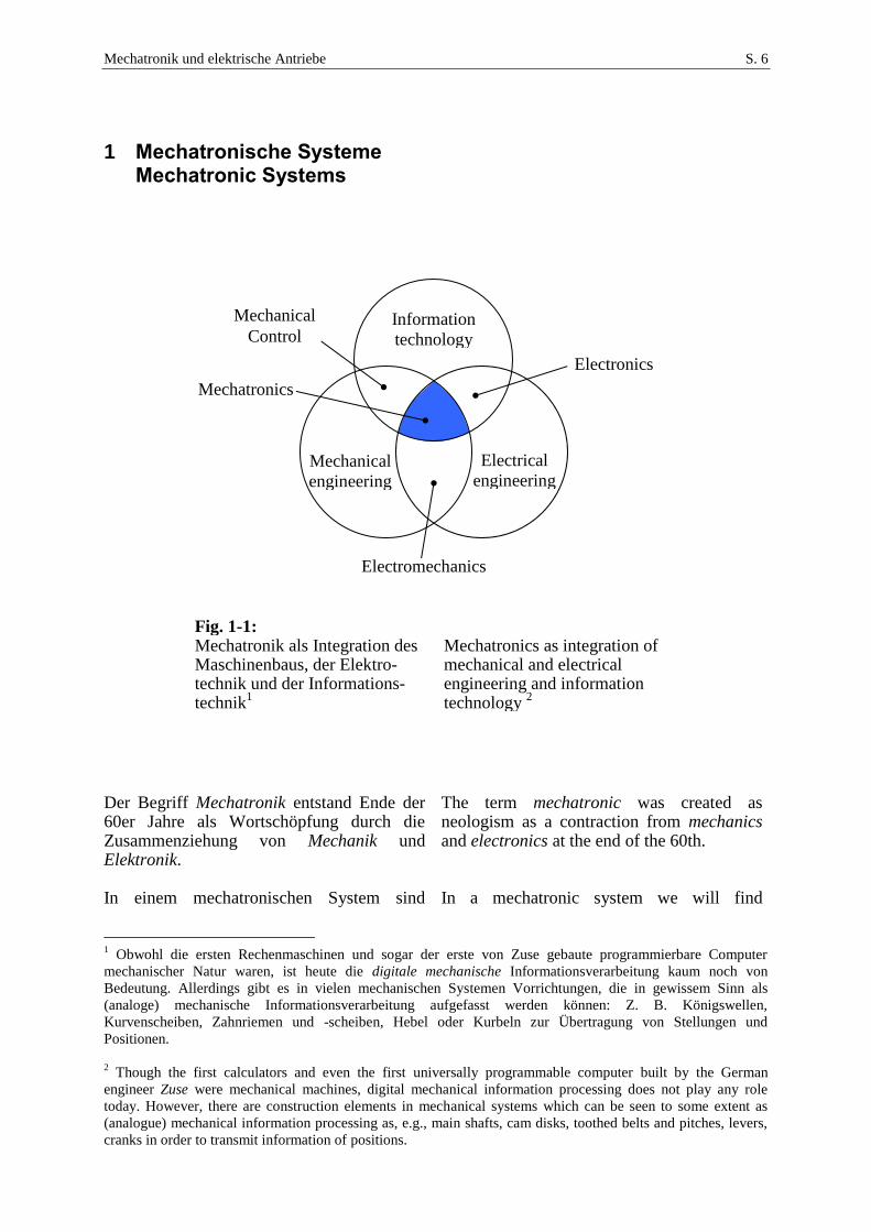
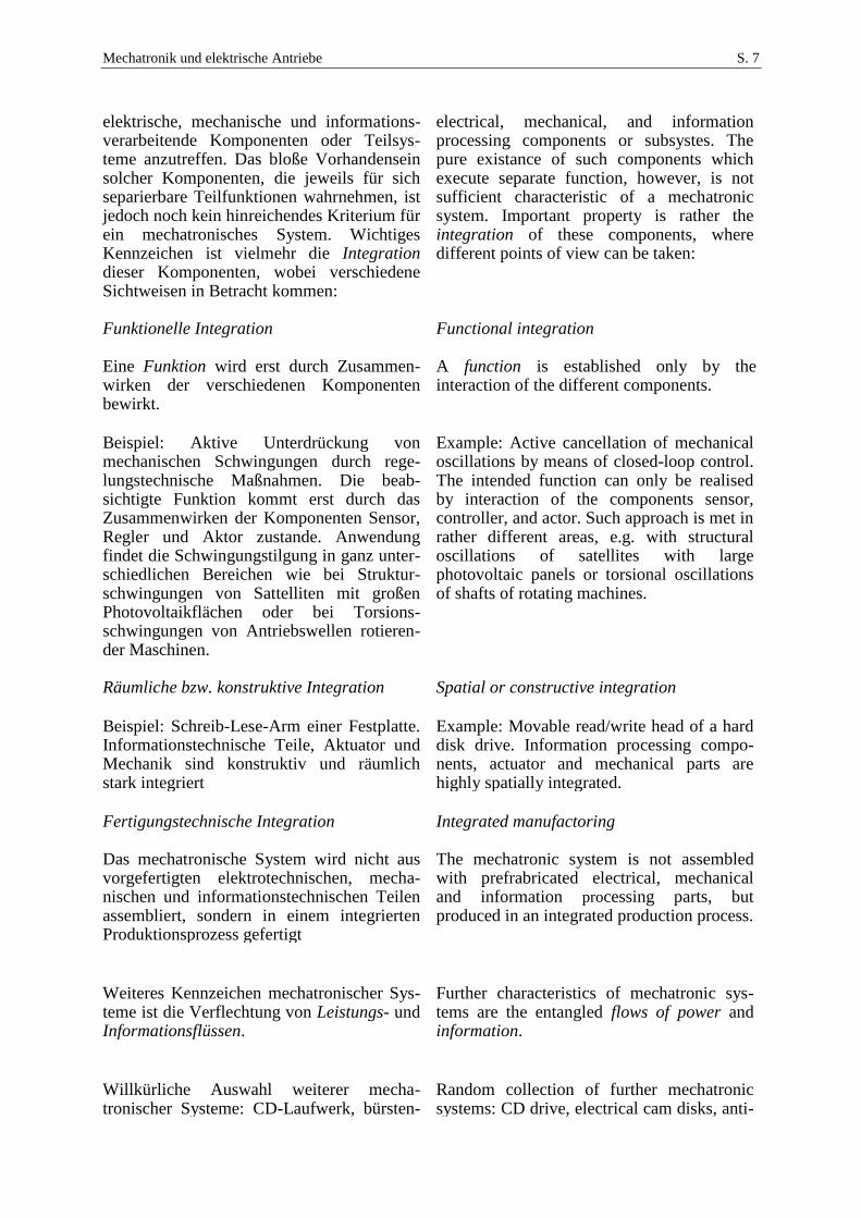
1 Mechatronische Systeme Mechatronic Systems
Fig. 1-1: Mechatronik als Integration des Maschinenbaus, der Elektro-technik und der Informations-technik
1
Mechatronics as integration of mechanical and electrical engineering and information technology
2
Der Begriff Mechatronik entstand Ende der 60er Jahre als Wortschöpfung durch die Zusammenziehung von Mechanik und Elektronik. In einem mechatronischen System sind
The term mechatronic was created as neologism as a contraction from mechanics and electronics at the end of the 60th. In a mechatronic system we will find
1 Obwohl die ersten Rechenmaschinen und sogar der erste von Zuse gebaute programmierbare Computer
mechanischer Natur waren, ist heute die digitale mechanische Informationsverarbeitung kaum noch von
Bedeutung. Allerdings gibt es in vielen mechanischen Systemen Vorrichtungen, die in gewissem Sinn als
(analoge) mechanische Informationsverarbeitung aufgefasst werden können: Z. B. Königswellen,
Kurvenscheiben, Zahnriemen und -scheiben, Hebel oder Kurbeln zur Übertragung von Stellungen und
Positionen.
2 Though the first calculators and even the first universally programmable computer built by the German
engineer Zuse were mechanical machines, digital mechanical information processing does not play any role
today. However, there are construction elements in mechanical systems which can be seen to some extent as
(analogue) mechanical information processing as, e.g., main shafts, cam disks, toothed belts and pitches, levers,
cranks in order to transmit information of positions.
Information
technology
Mechanical
engineering
Electrical
engineering
Mechatronics
Electronics
Mechanical
Control
Electromechanics
Mechatronik und elektrische Antriebe S. 7
elektrische, mechanische und informations-verarbeitende Komponenten oder Teilsys-teme anzutreffen. Das bloße Vorhandensein solcher Komponenten, die jeweils für sich separierbare Teilfunktionen wahrnehmen, ist jedoch noch kein hinreichendes Kriterium für ein mechatronisches System. Wichtiges Kennzeichen ist vielmehr die Integration dieser Komponenten, wobei verschiedene Sichtweisen in Betracht kommen:
electrical, mechanical, and information processing components or subsystes. The pure existance of such components which execute separate function, however, is not sufficient characteristic of a mechatronic system. Important property is rather the integration of these components, where different points of view can be taken:
Funktionelle Integration Eine Funktion wird erst durch Zusammen-wirken der verschiedenen Komponenten bewirkt.
Functional integration A function is established only by the interaction of the different components.
Beispiel: Aktive Unterdrückung von mechanischen Schwingungen durch rege-lungstechnische Maßnahmen. Die beab-sichtigte Funktion kommt erst durch das Zusammenwirken der Komponenten Sensor, Regler und Aktor zustande. Anwendung findet die Schwingungstilgung in ganz unter-schiedlichen Bereichen wie bei Struktur-schwingungen von Sattelliten mit großen Photovoltaikflächen oder bei Torsions-schwingungen von Antriebswellen rotieren-der Maschinen.
Example: Active cancellation of mechanical oscillations by means of closed-loop control. The intended function can only be realised by interaction of the components sensor, controller, and actor. Such approach is met in rather different areas, e.g. with structural oscillations of satellites with large photovoltaic panels or torsional oscillations of shafts of rotating machines.
Räumliche bzw. konstruktive Integration Spatial or constructive integration Beispiel: Schreib-Lese-Arm einer Festplatte. Informationstechnische Teile, Aktuator und Mechanik sind konstruktiv und räumlich stark integriert
Example: Movable read/write head of a hard disk drive. Information processing compo-nents, actuator and mechanical parts are highly spatially integrated.
Fertigungstechnische Integration Das mechatronische System wird nicht aus vorgefertigten elektrotechnischen, mecha-nischen und informationstechnischen Teilen assembliert, sondern in einem integrierten Produktionsprozess gefertigt
Integrated manufactoring The mechatronic system is not assembled with prefrabricated electrical, mechanical and information processing parts, but produced in an integrated production process.
Weiteres Kennzeichen mechatronischer Sys-teme ist die Verflechtung von Leistungs- und Informationsflüssen.
Further characteristics of mechatronic sys-tems are the entangled flows of power and information.
Willkürliche Auswahl weiterer mecha-tronischer Systeme: CD-Laufwerk, bürsten-
Random collection of further mechatronic systems: CD drive, electrical cam disks, anti-
Mechatronik und elektrische Antriebe S. 8
loser Gleichstrommotor, elektrische Kurven-scheiben, Anti-Blockier-System, Magnet-lager, Beschleunigungssensor, Servolenkung usw.
blocking system, magnetic bearing, acceleration sensor, servo-assisted steering etc.
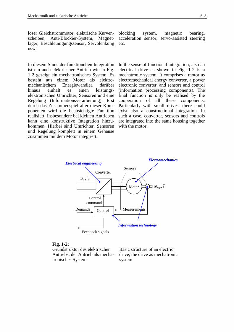
In diesem Sinne der funktionellen Integration ist ein auch elektrischer Antrieb wie in Fig. 1-2 gezeigt ein mechatronisches System. Es besteht aus einem Motor als elektro-mechanischem Energiewandler, darüber hinaus einhält es einen leistungs-elektronischen Umrichter, Sensoren und eine Regelung (Informationsverarbeitung). Erst durch das Zusammenspiel aller dieser Kom-ponenten wird die beabsichtigte Funktion realisiert. Insbesondere bei kleinen Antrieben kann eine konstruktive Integration hinzu-kommen. Hierbei sind Umrichter, Sensoren und Regelung komplett in einem Gehäuse zusammen mit dem Motor integriert.
In the sense of functional integration, also an electrical drive as shown in Fig. 1-2 is a mechatronic system. It comprises a motor as electromechanical energy converter, a power electronic converter, and sensors and control (information processing components). The final function is only be realised by the cooperation of all these components. Particularly with small drives, there could exist also a constructional integration. In such a case, converter, sensors and controls are integrated into the same housing together with the motor.
Fig. 1-2: Grundstruktur des elektrischen Antriebs, der Antrieb als mecha-tronisches System
Basic structure of an electric drive, the drive as mechatronic system
Motor
Converter
Control Demands
Control
commands
Sensors
Measurements
nn iu ,
Tme ,
Feedback signals
Electrical engineering
Information technology
Electromechanics
Mechatronik und elektrische Antriebe S. 9
Fig. 1-3:
Energie- und Informationsflüsse Flows of power and information
Motor
Steuerung
Regelung
Power flow
high-level
controls Information flow
mechanical
load
electric
energy supply
Mechatronik und elektrische Antriebe S. 10
2 Energiebilanz Energy Balance
2.1 Energiebilanz Elektromechanischer Wandler Energy Balance of Electromechanical Converters
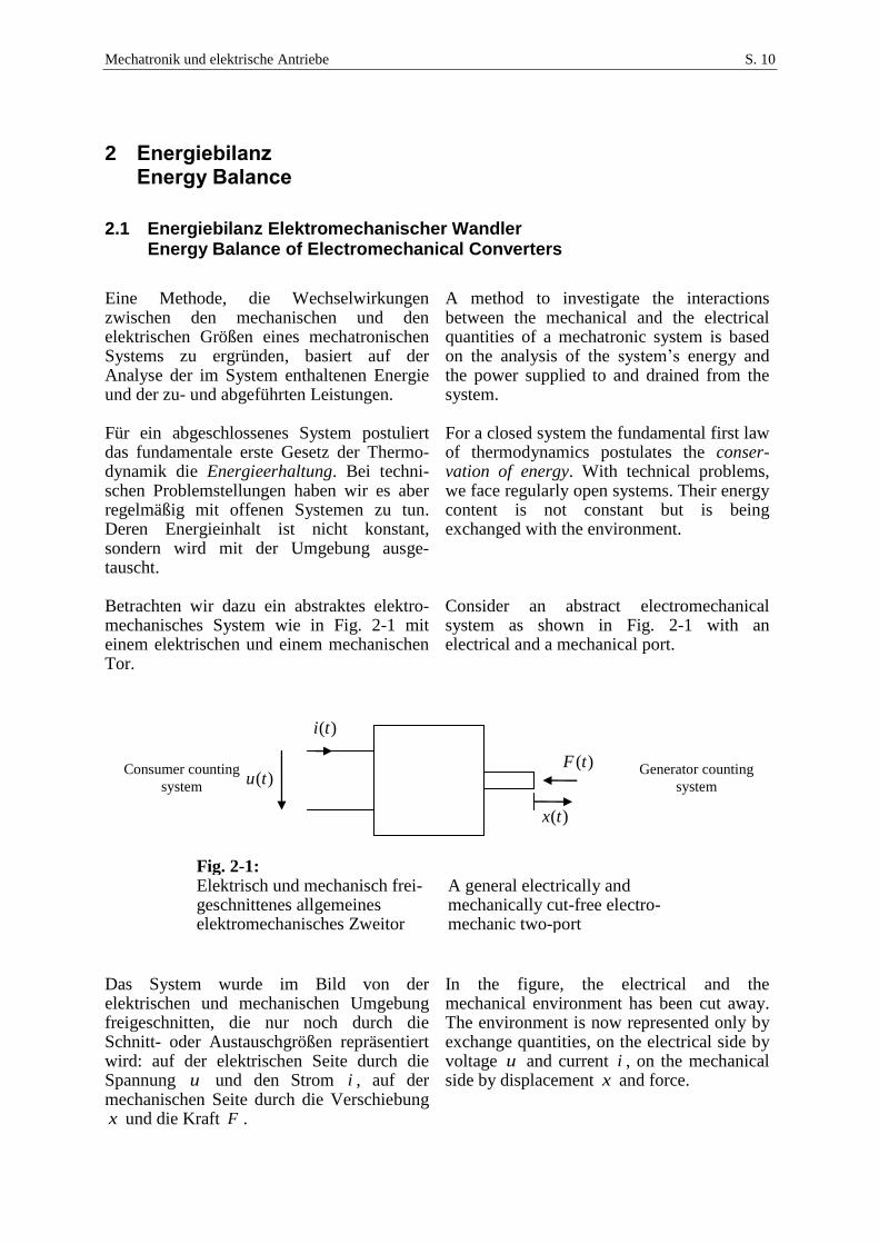
Eine Methode, die Wechselwirkungen zwischen den mechanischen und den elektrischen Größen eines mechatronischen Systems zu ergründen, basiert auf der Analyse der im System enthaltenen Energie und der zu- und abgeführten Leistungen. Für ein abgeschlossenes System postuliert das fundamentale erste Gesetz der Thermo-dynamik die Energieerhaltung. Bei techni-schen Problemstellungen haben wir es aber regelmäßig mit offenen Systemen zu tun. Deren Energieinhalt ist nicht konstant, sondern wird mit der Umgebung ausge-tauscht. Betrachten wir dazu ein abstraktes elektro-mechanisches System wie in Fig. 2-1 mit einem elektrischen und einem mechanischen Tor.
A method to investigate the interactions between the mechanical and the electrical quantities of a mechatronic system is based on the analysis of the system’s energy and the power supplied to and drained from the system. For a closed system the fundamental first law of thermodynamics postulates the conser-vation of energy. With technical problems, we face regularly open systems. Their energy content is not constant but is being exchanged with the environment. Consider an abstract electromechanical system as shown in Fig. 2-1 with an electrical and a mechanical port.
Fig. 2-1: Elektrisch und mechanisch frei-geschnittenes allgemeines elektromechanisches Zweitor
A general electrically and mechanically cut-free electro-mechanic two-port
Das System wurde im Bild von der elektrischen und mechanischen Umgebung freigeschnitten, die nur noch durch die Schnitt- oder Austauschgrößen repräsentiert wird: auf der elektrischen Seite durch die Spannung u und den Strom i , auf der mechanischen Seite durch die Verschiebung x und die Kraft F .
In the figure, the electrical and the mechanical environment has been cut away. The environment is now represented only by exchange quantities, on the electrical side by voltage u and current i , on the mechanical side by displacement x and force.
)(tu
)(ti
)(tF
)(tx
Generator counting
system
Consumer counting
system
Mechatronik und elektrische Antriebe S. 11
Wann immer solche Schnittgrößen eingeführt werden, muss die Zählrichtung festgelegt werden, was in Fig. 2-1 durch die Zählpfeile zum Ausdruck gebracht wird. Diese Pfeile zeigen nur an, was als positiv zu verstehen ist, nicht etwa, dass die betreffende Größe tatsächlich positiv sei. Die Wahl der Zählrichtungen ist lediglich eine Sache der Definition, sie können will-kürlich festgelegt werden. Auf der elek-trischen Seite wurden hier aber die Zählpfeile von Spannung und Strom gleichsinnig, d.h. beide von einem zum anderen Anschluss zeigend, eingeführt. Diese Art bezeichnet man als Verbraucher-Zählpfeilsystem. Als Folge ist die elektrische Leistung
Whenever introducing such exchange quantities, their counting directions have to be defined what is indicated in Fig. 2-1 by the counting arrows. The arrow indicates only what is to be understood positive, it does not imply that the quantity were actually positive. The choice of the counting arrow directions is only a question of definition, they could be chosen freely. However, on the electrical side both voltage and current arrows have the same direction, both pointing from one terminal to the other. This kind is called consumer counting system. As a result, the electrical power
uip el (2.1)
die Leistung, die von der Umgebung an das System abgegeben wird. Auch hier legt dies nur fest, was als positiv zu verstehen ist, nicht etwa, dass die Leistung wirklich positiv sei. Auf der mechanischen Seite wurden die Zählpfeile entgegengesetzt ausgerichtet, was man als Erzeuger-Zählpfeilsystem bezeich-net. In diesem Fall ist die mechanische Leistung
is to be understood as power supplied from the environment to the system. Again, this defines only what is to be understood as positiv, it does not mean that the power really flows from the environment to the system. On the mechanical side, the counting arrows are chosen in different directions, which is called generator counting system. As a result, the mechanical power calculated from
FxvFp me (2.2)
die Leistung, die vom System an die Umgebung geliefert wird. Diese Definitionen sind keinesfalls obligatorisch, jeder mag die Zählpfeile nach seinem Ermessen wählen, muss dann aber in sich konsistent bleiben.
is the power provided from the system to the environment. However, these definitions are not binding. Anybody may choose his own way, but must keep consistency sub-sequently.
Beide Leistungsterme fassen wir zur äußeren (externen) Leistung zusammen:
Both power terms are taken together as external power:
e el mep p p ui vF (2.3)
Verstehen wir unter dem System nur die elektromechanische Vorgänge, muss immer-hin der Leistungsaustausch mit der thermi-schen Domäne berücksichtigt werden, nämlich die Dissipationsleistung dp , die als
If we understand the system only as electromechanical processes, we have to consider at least a power exchange with the thermal domain, i.e. the dissipation power
dp which appears as another drain of the
Mechatronik und elektrische Antriebe S. 12
weiterer Abflussterm des elektromecha-nischen Systems auftritt.
electromechanical system.
Postulieren wir nun, dass das System die innere Energie iE enthalte, muss diese gemäß des ersten Hauptsatzes der Thermodynamik der Bilanzgleichung
The system is now postulated to contain an internal energy iE . According to the first law of thermodynmamics, the energy must obey the balance equation
i e d el me dE p p p p p (2.4)
gehorchen. Ganz allgemein muss die innere Energie eine Zustandsfunktion sein. Das bedeutet: Für das System gibt es einen Satz von Zustandsgrößen )(txi , die den aktuellen Zustand des Systems vollständig beschrei-ben. Eine Zustandsfunktion ist eine Funktion dieser Zustandsgrößen, womit ihr Wert eindeutig über die Zustandsgrößen bestimmt wird:
Generally, the internal energy has to be a state function. This means: For the system there exist a set of state variables )(txi which completely describe the current state of the system. A state function is now a function of these state variables. Thus, its value of the state function is uniquely defined by the state variables.
))(),...,(),(()( 21ii txtxtxEtE n . (2.5)
Für die Zeitableitung ergibt sich also nach den Ableitungsregeln
Due to derivation rules, the time derivative results as
nn
x
Ex
x
Ex
x
ExtE
i
2
i2
1
i1i ...)( (2.6)
Es stellt sich nun die Frage, wie die Zustandsgrößen )(txi gefunden werden können. Bei dem System in Fig. 2-1 ist offensichtlich eine dieser Zustandsgrößen die Verschiebung, z. B. xx 1 . Die Identifika-tion weiterer Zustandsgrößen ist jedoch ohne näheren Einblick in das System nicht möglich. Deshalb beschränken wir uns in Folge auf elektromagnetische Aktoren.
Now, the question rises how the state variables )(txi can be found. With the system of Fig. 2-1 the displacement is obviously one of theses state variables, e. g.
xx 1 . The identification of further state variables, however, is not possible without more insight into the system. That is why we focus hereafter on electromagnetic actuators.
2.2 Energiebilanz bei Elektromagnetische Aktoren Energy Balance with Electromagnetic Actuators
Nehmen wir an, der Aktor basiere auf einem magnetischen Prinzip wie in Fig. 2-2 gezeigt. Man kann sich leicht vorstellen, dass diese Anordnung abhängig von Stromstärke und Position eine Kraft auf den Stößel ausübt, wobei dieser aus einem magnetischen Material bestehen möge. Diese Kraft werden wir später erörtern. An dieser Stelle sei zunächst angenommen, dass der eigentlich
Let us assume the actuator is based on a magnetic principle as shown in Fig. 2-2. One can easily imagine that this construction generates a magnetic force on the pusher, which is assumed to consist of magnetic material. However, the force is to be debated later. At this point we temporarily assume the pusher to be locked at a certain mechanical displacement x . In this case the actuator
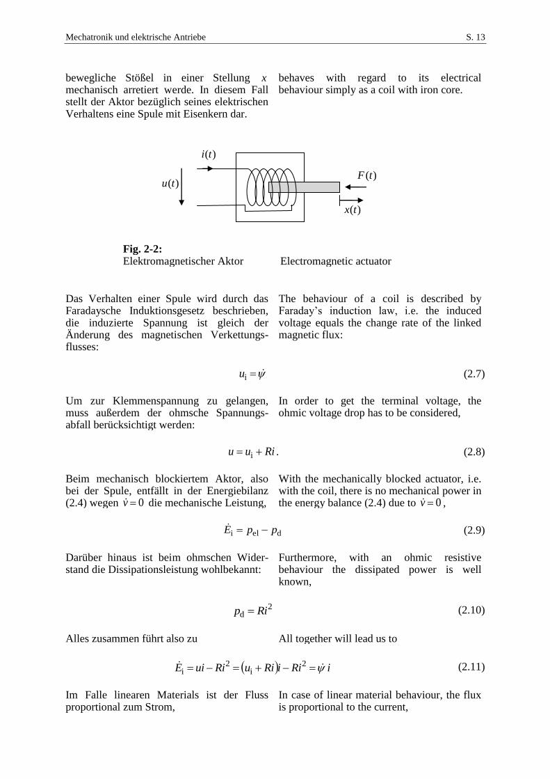
Mechatronik und elektrische Antriebe S. 13
bewegliche Stößel in einer Stellung x mechanisch arretiert werde. In diesem Fall stellt der Aktor bezüglich seines elektrischen Verhaltens eine Spule mit Eisenkern dar.
behaves with regard to its electrical behaviour simply as a coil with iron core.
Fig. 2-2: Elektromagnetischer Aktor Electromagnetic actuator
Das Verhalten einer Spule wird durch das Faradaysche Induktionsgesetz beschrieben, die induzierte Spannung ist gleich der Änderung des magnetischen Verkettungs-flusses:
The behaviour of a coil is described by Faraday’s induction law, i.e. the induced voltage equals the change rate of the linked magnetic flux:
iu (2.7)
Um zur Klemmenspannung zu gelangen, muss außerdem der ohmsche Spannungs-abfall berücksichtigt werden:
In order to get the terminal voltage, the ohmic voltage drop has to be considered,
Riuu i . (2.8)
Beim mechanisch blockiertem Aktor, also bei der Spule, entfällt in der Energiebilanz (2.4) wegen 0v die mechanische Leistung,
With the mechanically blocked actuator, i.e. with the coil, there is no mechanical power in the energy balance (2.4) due to 0v ,
deli ppE (2.9)
Darüber hinaus ist beim ohmschen Wider-stand die Dissipationsleistung wohlbekannt:
Furthermore, with an ohmic resistive behaviour the dissipated power is well known,
2
d Rip (2.10)
Alles zusammen führt also zu All together will lead us to
iRiiRiuRiuiE 2i
2i (2.11)
Im Falle linearen Materials ist der Fluss proportional zum Strom,
In case of linear material behaviour, the flux is proportional to the current,
)(tu
)(ti
)(tF
)(tx
Mechatronik und elektrische Antriebe S. 14
Li (2.12)
Die Proportionalitätskonstante L heißt Induktivität. Damit wird (2.11) zu:
The proportionality constant L is called inductance. Then, (2.11) becomes:
2
i2
1
d
dLi
tiiLE ,
2i
2
1LiE (2.13)
Das bedeutet, wir können die Zeitableitung der inneren Energie integrieren und die Energie direkt angeben. Das Ergebnis ist wohlbekannt. Wir müssen aber berück-sichtigen, dass für jede feste Position x eine anderer Induktivitätswert resultiert. Die Energie scheint demnach eine Funktion des Stroms und der Verschiebung zu sein, sie kann aber auch mithilfe von (2.12) als Funktion des Flusses und der Verschiebung ausgedrückt werden:
This means, we can integrate the time derivative of the internal energy and determine directly the internal energy. The result is well known. However, we have to consider that for any fixed position x a different value of the inductance results. Thus, the energy seems to be a function of the current and the displace, however, it is possible to express the energy with help of (2.12) as function of the flux and the displacement:
ixL
ixLE
2
1
)(2)(
2
1 22
i (2.14)
Das kann man derart interpretieren, dass entweder Verschiebung und Strom ),( ix oder aber die Verschiebung und der magne-tische Fluss ),( x die gesuchten Zustands-variablen sind. Die Erörterung dieser Frage soll aber noch etwas aufgeschoben werden. Da magnetische Materialien mehr oder minder stark sättigen, ist die Vorstellung einer linearen Beziehung zwischen Fluss und Strom allenfalls für einen kleinen Arbeits-bereich haltbar. Allgemein müssen wir von einem deutlich nichtlinearen Zusammenhang ausgehen. Die Funktion des magnetischen Flusses in Abhängigkeit des Stroms heißt Magnetisierungskennlinie:
This fact can be interpreted in the sense that either displacement and current or displacement and magnetic flux are the state variables we are searching for. The debate of this question, however, should be postponed for a short while. Since magnetic materials saturate more or less, the idea of linear relation between flux and current is valid at best only for a small operation range. In general, we have to take into account a distinct nonlinear relation. The function of the magnetic flux versus current is called magnetisation curve:
),( ix (2.15)
Diese hängt hier zusätzlich von der Verschie-bung ab, wobei auch dieser Zusammenhang im Allgemeinen nichtlinear ist. Trotz dieser Nichtlinearität gelingt es weiterhin, die Inte-gration zu bewältigen. Dazu multiplizieren wir formell die Gleichung (2.11) mit dem Zeitdifferenzial td und bilden Integrale auf beiden Seiten der Gleichung:
Here, the function depends also on the displacement. Also this relation is nonlinear in general. Despite the nonlinearity, we can accomplish the integration anyway. To do so, we multiply formally equation (2.11) with the time differential td and build integrals on both sides of the equations:
Mechatronik und elektrische Antriebe S. 15
dd ii iEE (2.16)
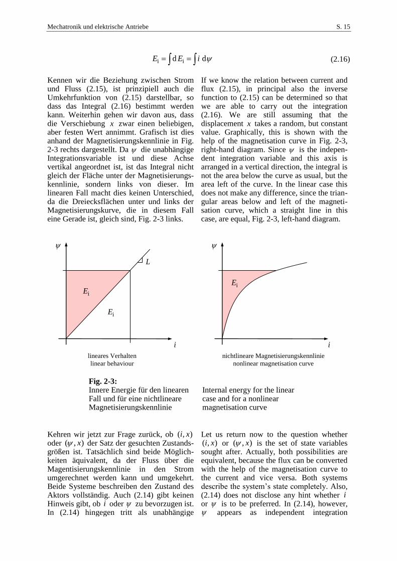
Kennen wir die Beziehung zwischen Strom und Fluss (2.15), ist prinzipiell auch die Umkehrfunktion von (2.15) darstellbar, so dass das Integral (2.16) bestimmt werden kann. Weiterhin gehen wir davon aus, dass die Verschiebung x zwar einen beliebigen, aber festen Wert annimmt. Grafisch ist dies anhand der Magnetisierungskennlinie in Fig. 2-3 rechts dargestellt. Da die unabhängige Integrationsvariable ist und diese Achse vertikal angeordnet ist, ist das Integral nicht gleich der Fläche unter der Magnetisierungs-kennlinie, sondern links von dieser. Im linearen Fall macht dies keinen Unterschied, da die Dreiecksflächen unter und links der Magnetisierungskurve, die in diesem Fall eine Gerade ist, gleich sind, Fig. 2-3 links.
If we know the relation between current and flux (2.15), in principal also the inverse function to (2.15) can be determined so that we are able to carry out the integration (2.16). We are still assuming that the displacement x takes a random, but constant value. Graphically, this is shown with the help of the magnetisation curve in Fig. 2-3, right-hand diagram. Since is the indepen-dent integration variable and this axis is arranged in a vertical direction, the integral is not the area below the curve as usual, but the area left of the curve. In the linear case this does not make any difference, since the trian-gular areas below and left of the magneti-sation curve, which a straight line in this case, are equal, Fig. 2-3, left-hand diagram.
Fig. 2-3: Innere Energie für den linearen Fall und für eine nichtlineare Magnetisierungskennlinie
Internal energy for the linear case and for a nonlinear magnetisation curve
Kehren wir jetzt zur Frage zurück, ob ),( xi oder ),( x der Satz der gesuchten Zustands-größen ist. Tatsächlich sind beide Möglich-keiten äquivalent, da der Fluss über die Magentisierungskennlinie in den Strom umgerechnet werden kann und umgekehrt. Beide Systeme beschreiben den Zustand des Aktors vollständig. Auch (2.14) gibt keinen Hinweis gibt, ob i oder zu bevorzugen ist. In (2.14) hingegen tritt als unabhängige
Let us return now to the question whether ),( xi or ),( x is the set of state variables
sought after. Actually, both possibilities are equivalent, because the flux can be converted with the help of the magnetisation curve to the current and vice versa. Both systems describe the system’s state completely. Also, (2.14) does not disclose any hint whether i or is to be preferred. In (2.14), however, appears as independent integration
i
iE
i
iE
L
iE
nichtlineare Magnetisierungskennlinie
nonlinear magnetisation curve
lineares Verhalten
linear behaviour
Mechatronik und elektrische Antriebe S. 16
Integrationsvariable auf. Das kann darauf hindeuten, dass Vorteile mit sich bringen könnte, weshalb wir vom Zustands-größensatz ),( x ausgehen und auch die innere Energie als Funktion von diesen beiden Variablen verstehen wollen. Geben wir nun die Vorstellung einer fixierten Verschiebung wieder auf und erlauben nun eine beliebige Bewegung. Für Zeitableitung der Energie folgt nun allgemein
variable. This can be taken as hint that could bring some advantages so that we choose the state variable set ),( x and understand also the internal energy as function of these variables. At this point we quit the imagination of a fixed displacement and allow any random movement. The time derivative of the energy follows as
iFxpppx
Ex
ExE
dmeel
iii ),( (2.17)
Da diese Beziehung für beliebige x und gelten muss, müssen die Terme vor diesen Zeitableitungen auf beiden Seiten gleich sein. Es muss folglich gelten:
As this relation has to hold for any random x and , the terms before these time derivatives must be equal. Thus, it follows:
.const
i
x
Ei
und
.const
i
x
EF (2.18)
Hätte man die innere Energie als Funktion von ),( xi angesetzt, würde bei der Zeit-ableitung ),(i xiE ein Term i auftreten. Dies wäre zwar nicht falsch ist, doch könnte keine einfache Beziehung mit dem rechts in (2.18) auftretenden Leistungsterm mit hergestellt werden. Daher sind die Zustandsgrößen
),( x zu bevorzugen, die deshalb auch als natürliche Zustandsgrößen bezeichnet werden. Man beachte, dass wir mit (2.18) ein Ergebnis für die Kraft erreicht haben, ohne dass wir an irgendeiner Stelle die Kraftgesetze von Lorentz oder Maxwell verwendet hätten. Dies sollte deutlich machen, wie leistungsfähig die Methode der Energiebilanz ist.
If we had taken the internal energy as a function of ),( xi , then a term with i would arise from the time derivative ),(i xiE . This would not be false, but we would not be able to identify a simple relation with power termin on the right-hand side of (2.18) with . Thus, the state variables ),( x are to be preferred. They are called natural state variables. Please note that we accomplished with (2.18) a result for the force although we had not used at any point the force formulae of Lorentz or Maxwell. This should make clear how powerful the tool of energy balance is.
2.3 Die Ko- oder Ergänzungsenergie The Co-Energy
Bei der inneren Energie hat sich der Fluss als Zustandsgröße gegenüber dem Strom als vorteilhaft herausgestellt. Für verschiedene praktische Problemstellung wäre es aber doch wünschenswert, den Systemzustand
With the internal energy, the flux has turned out as favorite state variable rather than the current. For a number of practical problems, however, it would be desirable to characterise the system state directly with the
Mechatronik und elektrische Antriebe S. 17
statt durch den Flusses direkt mit dem Strom zu beschreiben. Formal lässt sich dies durch die Legendre-Transformation bewerkstel-ligen, die einen Variablentausch bewirkt. Diese Transformation definiert eine neue Größe, die Ko- oder Ergänzungsenergie, die wir nun als Funktion von Strom und Verschiebung verstehen, wie folgt:
current instead of the flux. Formally, this can be done with the the Legendre transform, which results in a change of the variables. This transform defines a new quantity, the co-energy, which is to be understood as function of current and displacement as follows:
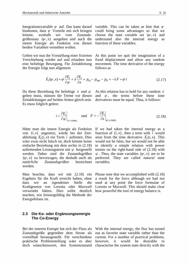
),(),( ic xEixiE (2.19)
Eine graphische Veranschaulichung zeigt Fig. 2-4.
A graphical visualisation is shown in Fig. 2-4.
Fig. 2-4: Innere Energie und Koenergie Internal energy and co-energy
Untersuchen wir die Zeitableitung der Ergänzungsenergie unter Zuhilfenahme von (2.17):
Let us investigate the time derivative of the co-energy with the help of (2.17):
FxiiFxiixEit
xiE ),(d
d),( ic (2.20)
Dies kann als Bilanzgleichung der Ergän-zungsenergie verstanden werden. Auch hier können wir durch Vergleich der Zeitablei-tungen die folgenden Beziehungen gewinnen:
This can be understood as balance equation of the co-energy. Also here, the comparison of the time derivatives delivers the following relations:
.const
i
c
x
EF und
.const
x
c
i
E (2.21)
Bei linearem Verhalten zwischen Strom und Fluss sind die innere Energie und die Ergänzungsenergie wertemäßig gleich, vgl.
With linear behaviour between current and flux, internal energy and co-energy are of the same values, compare (2.14) and the left-
cE
i
iE
Mechatronik und elektrische Antriebe S. 18
(2.14) und das linke Diagramm in Fig. 2-3. Im Fall eines nichtlinearen Materialgesetzes führt die Differenziation i /
iE x jedoch im
Allgemeinen zum falschen Ergebnis für die Kraft!
hand diagram of Fig. 2-3. However, in case of nonlinear behavior, the derivative
i /i
E x generally would yield the wrong result for the force!
Für die weitere Diskussion gehen wir von den Zeitableitungen auf Differenziale über, indem wir formell die Bilanzgleichungen (2.17) und (2.20) mit dem Zeitdifferenzial
td multiplizieren. Es folgt
For the further discussion we change from time derivatives to differentials by multiplying formally the balance equations (2.17) and (2.20) with the time differential
td . It follows
meeli ddddd WWxFψiE (2.22)
meecc ddddd WWxFiψE (2.23)
Die Terme auf den rechten Seiten der Gleichungen sind die Differenziale der mechanischen und der elektrischen Arbeit. Bei der Ergänzungsenergie tritt allerdings ein neuartiges abstraktes elektrisches Arbeits-differenzial iψW dd ec auf. Anders als die totalen Differenziale der inneren Energie und der Koenergie sind die Arbeitsdifferenziale eldW , medW , ecdW nicht total oder unvollständig, was mathe-matisch bedeutet, dass nur die Energien iE und cE Zustandsfunktionen sind. Die Arbeitsdifferenziale hingegegen können zwar auch zu elektrischer Arbeit elW bzw. mechanischer Arbeit meW aufintegriert werden, diese Ergebnisse sind aber keine Zustandsfunktionen, sondern hängen vom speziellen Integrationspfad ab. Dies ist auch der Grund, zwischen den Begriffen Arbeit und Energie zu unterscheiden.
The terms on the right-hand side of the equation are the differentials of the mechanical and electrical work. With the co-energy, however, there appears a new abstract electrical work differential
iψW dd ec . Unlike the total differentials of the internal energy and of the co-energy the work differentials eldW , medW , ecdW are not total or uncomplete. In a mathematical sense this means that only the energies iE und cE are functions of the state variables. The work differentials can be integrated to the elec-trical work elW or mechanical work meW , respectively. These results, however, are not states functions, but depend on the particular integration path. This is the reason to distinguish between the terms work and energy.
Ein Vorteil der Koenergie zeigt sich in Situationen, in denen der Strom konstant gehalten wird, also 0d i . Für diesen Fall ist die Koenergieänderung direkt gleich der mechanischen Arbeit:
In case of constant current, 0d i , the differential of the mechanic work can be expressed by the change of the co-energy,
xFWEi
ddd me.constc
(2.24)
Diese Situation ist in Fig. 2-5 dargestellt. This situation ist depicted in Fig. 2-5.
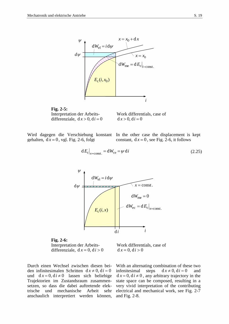
Mechatronik und elektrische Antriebe S. 19
Fig. 2-5: Interpretation der Arbeits-differenziale, 0d,0d ix
Work differentials, case of 0d,0d ix
Wird dagegen die Verschiebung konstant gehalten, 0d x , vgl. Fig. 2-6, folgt
In the other case the displacement is kept constant, 0d x , see Fig. 2-6, it follows
iWEx
ddd ce.constc
(2.25)
Fig. 2-6: Interpretation der Arbeits-differenziale, 0d,0d ix
Work differentials, case of 0d,0d ix
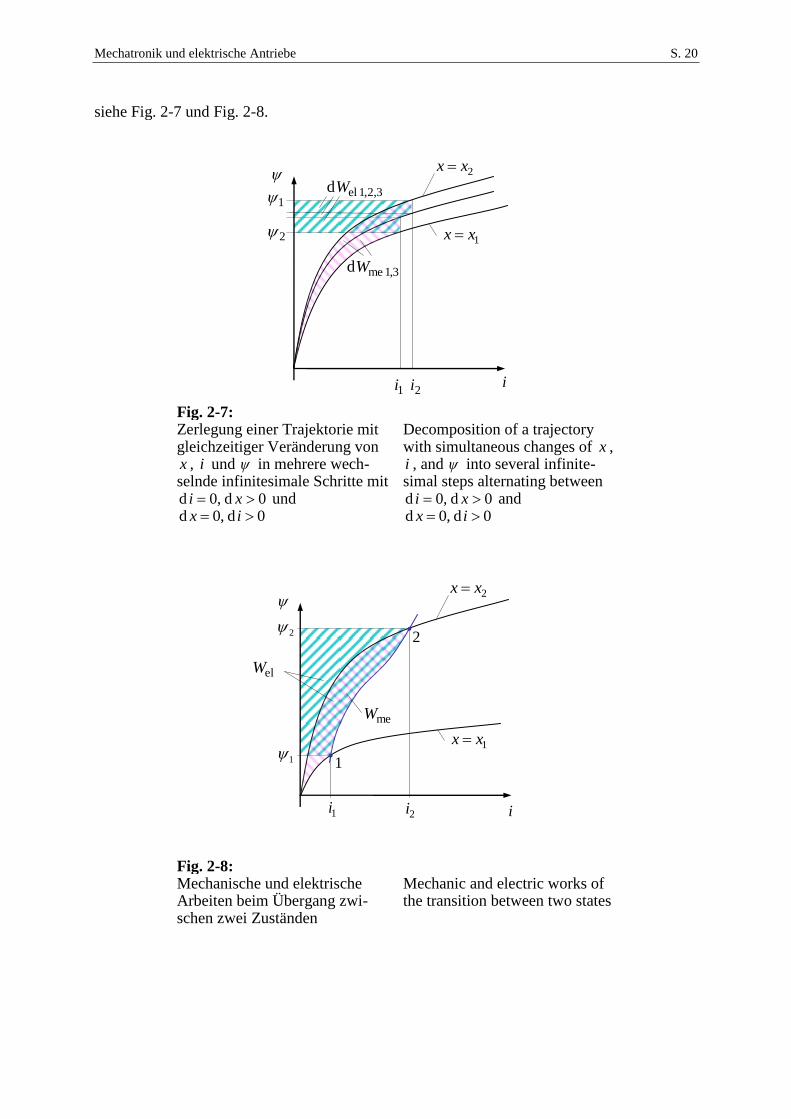
Durch einen Wechsel zwischen diesen bei-den infinitesimalen Schritten 0d,0d ix und 0d,0d ix lassen sich beliebige Trajektorien im Zustandsraum zusammen-setzen, so dass die dabei auftretende elek-trische und mechanische Arbeit sehr anschaulich interpretiert werden können,
With an alternating combination of these two infenitesimal steps 0d,0d ix and
0d,0d ix , any arbitrary trajectory in the state space can be composed, resulting in a very vivid interpretation of the contributing electrical and mechanical work, see Fig. 2-7 and Fig. 2-8.
const .x d
dd el iW
),(c xiE
0d me W
iid
.constcec dd
x
EW
0xx
xxx d0
d
dd el iW
),( 0c xiE
.constcme dd
i
EW
i
Mechatronik und elektrische Antriebe S. 20
siehe Fig. 2-7 und Fig. 2-8.
Fig. 2-7: Zerlegung einer Trajektorie mit gleichzeitiger Veränderung von x , i und in mehrere wech-selnde infinitesimale Schritte mit
0d,0d xi und 0d,0d ix
Decomposition of a trajectory with simultaneous changes of x , i , and into several infinite-simal steps alternating between
0d,0d xi and 0d,0d ix
Fig. 2-8: Mechanische und elektrische Arbeiten beim Übergang zwi-schen zwei Zuständen
Mechanic and electric works of the transition between two states
1xx
2xx
i
1
2
1i 2i
1
2
meW
elW
el 1,2,3dW
me 1,3dW
i1i 2i
1
2
2xx
1xx
Mechatronik und elektrische Antriebe S. 21
2.4 Die zweiten Ableitungen der Energie The Second-Order Derivatives of the Energy
Sind die Energiefunktionale zweifach stetig differenzierbar — was bei technischen Sys-temen in der Regel der Fall ist — darf die Reihenfolge der Differentialtion vertauscht werden. Aus den gemischten 2. Ableitungen der Energie,
The energy functionals should be assumed to be two times continuouly differentiable — which is usually the case with common tech-nical system. Then, the sequence of derivations can be exchanged. Thus, the mixed 2nd-order derivatives of the energy
x
E
x
E
i
2i
2
(2.26)
folgt somit die Reziprozitätsbeziehung yield the reciprocity law
),(),( xF
x
xi (2.27)
Aus dieser Gleichung ergibt sich eine wichtige Schlussfolgerung: Sollten die Ableitungen in (2.26) bzw. (2.27) Null sein, hieße das, die Kraft F hinge gar nicht von der elektromagnetischen Größe und umgekehrt der Strom i nicht von der Verschiebung x ab. Es gäbe es also gar keine Wechselwirkung zwischen den elektro-magnetischen und den mechanischen Größen. Das System wäre als Energie-wandler bzw. als Aktor unbrauchbar. Ein echter elektromechanischer Wandler zeichnet sich demnach durch diese Bedingung aus:
There is an important conclusion arising from this equation: If the derivatives in in (2.26) or (2.27), resp., were equal zero that then the force F would not depend on the electromagnetic quantity and, vice versa, the current i would not depend on the displacement x . Thus, there would not exist any interaction between the electromagnetic and the mechanical quantities so that the system would be unfeasible as electro-mechanic converter or actuator. A true electromagnetic converter is thus to be characterised by the condition
2 2
i i 0E E
x x
(2.28)
Die zweiten gemischten Ableitungen der Koenergie liefern eine weitere Beziehung:
The 2nd-order mixed derivatives of the co-energy yield another relation:
xi
E
ix
E
c2
c2
(2.29)
Es folgt It follows
i
xiF
x
xi
),(),( (2.30)
Ähnlich zu (2.28) kann auch anhand der gemischten Ableitungen der Koenergie ent-schieden werden, ob es sich um einen echten
Similar to (2.28), also the mixed derivatives of the co-energy can be used in order to decide whether the system is a true
Mechatronik und elektrische Antriebe S. 22
elektromechanischen Wandler handelt. electromechanical converter.
Die (differenzielle) Steifigkeit ist die Ableitung der Kraft nach der Verschiebung. Wegen des gewählten Erzeugerzählpfeil-systems auf der Seite der mechanischen Größen wird diese als negative Ableitung definiert. Dann resultiert die Steifigkeit z. B. einer konventionellen Feder wie gewohnt als positive Größe.
The (differential) stiffness is the derivative of the force with respect to the displacement. Due to the chosen generator counting system of the mechanical port, the stiffness is to be defined as negative derivative. This definition corresponds to the common definition of the stiffness of a convential spring as a positive quantity.
Bei konstantem Strom ergibt sich die Steifig-keit des Magnetlagers zu
With constant current, the magnetic stiffness results as
.const
2c
2
.const
iii
x
E
x
FS (2.31)
. Die Steifigkeit bei konstantem Fluss ist hin-gegen
However, the stiffness with constant magnetic flux is
.const
2i
2
.const
x
E
x
FS (2.32)
Die Steifigkeiten iS und S haben im All-gemeinen unterschiedliche Werte.
Both stiffnesses iS und S will have generally different values.
Die differenzielle Induktivität ergibt sich entsprechend aus
Accordingly, the differential inductance is being determined from the co-energy by
.const
2c
2
.const
xx i
E
iL
(2.33)
aber auch aus der inneren Energie über Alternatively, that can be done with the
internal energy
.const
2i
2
.const
1
xx
Ei
L (2.34)
Mechatronik und elektrische Antriebe S. 23
3 Magnetische Kreise Magnetic Circuits
3.1 Electromagnetische Energiedichte Electromagnetic Energy Density
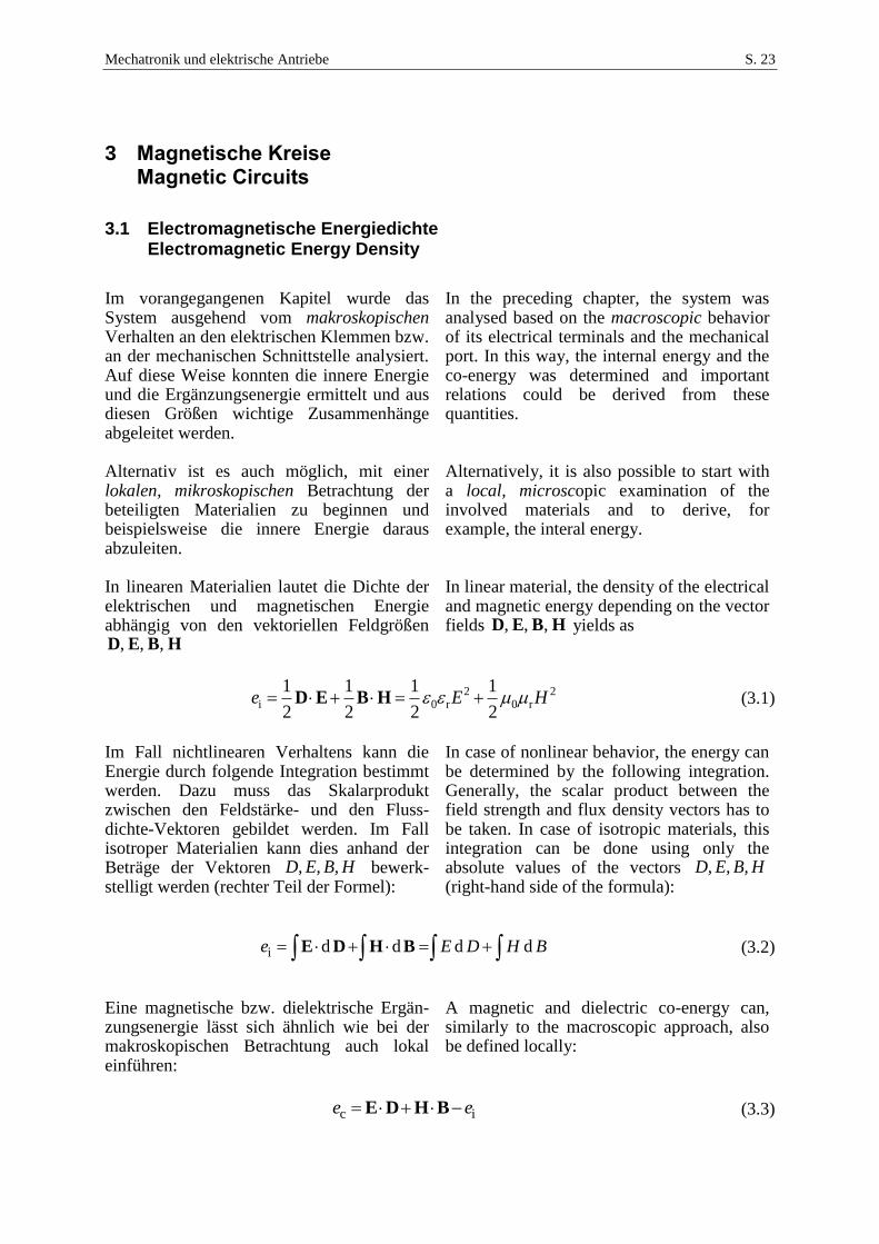
Im vorangegangenen Kapitel wurde das System ausgehend vom makroskopischen Verhalten an den elektrischen Klemmen bzw. an der mechanischen Schnittstelle analysiert. Auf diese Weise konnten die innere Energie und die Ergänzungsenergie ermittelt und aus diesen Größen wichtige Zusammenhänge abgeleitet werden. Alternativ ist es auch möglich, mit einer lokalen, mikroskopischen Betrachtung der beteiligten Materialien zu beginnen und beispielsweise die innere Energie daraus abzuleiten. In linearen Materialien lautet die Dichte der elektrischen und magnetischen Energie abhängig von den vektoriellen Feldgrößen
, , ,D E B H
In the preceding chapter, the system was analysed based on the macroscopic behavior of its electrical terminals and the mechanical port. In this way, the internal energy and the co-energy was determined and important relations could be derived from these quantities. Alternatively, it is also possible to start with a local, microscopic examination of the involved materials and to derive, for example, the interal energy. In linear material, the density of the electrical and magnetic energy depending on the vector fields , , ,D E B H yields as
2 2i 0 r 0 r
1 1 1 1
2 2 2 2e E HD E B H (3.1)
Im Fall nichtlinearen Verhaltens kann die Energie durch folgende Integration bestimmt werden. Dazu muss das Skalarprodukt zwischen den Feldstärke- und den Fluss-dichte-Vektoren gebildet werden. Im Fall isotroper Materialien kann dies anhand der Beträge der Vektoren D, E, B, H bewerk-stelligt werden (rechter Teil der Formel):
In case of nonlinear behavior, the energy can be determined by the following integration. Generally, the scalar product between the field strength and flux density vectors has to be taken. In case of isotropic materials, this integration can be done using only the absolute values of the vectors D, E, B, H (right-hand side of the formula):
i d d d de E D H B E D H B (3.2)
Eine magnetische bzw. dielektrische Ergän-zungsenergie lässt sich ähnlich wie bei der makroskopischen Betrachtung auch lokal einführen:
A magnetic and dielectric co-energy can, similarly to the macroscopic approach, also be defined locally:
c ie e E D H B (3.3)
Mechatronik und elektrische Antriebe S. 24
Die gesamte innere bzw. die Ko-Energie erhält man dann durch Volumenintegration:
The entire internal energy and the co-energy is then determined by a volume integral:
i i d
V
E e V , c c d
V
E e V (3.4)
3.2 Magnetische Netzwerke Magnetic Networks
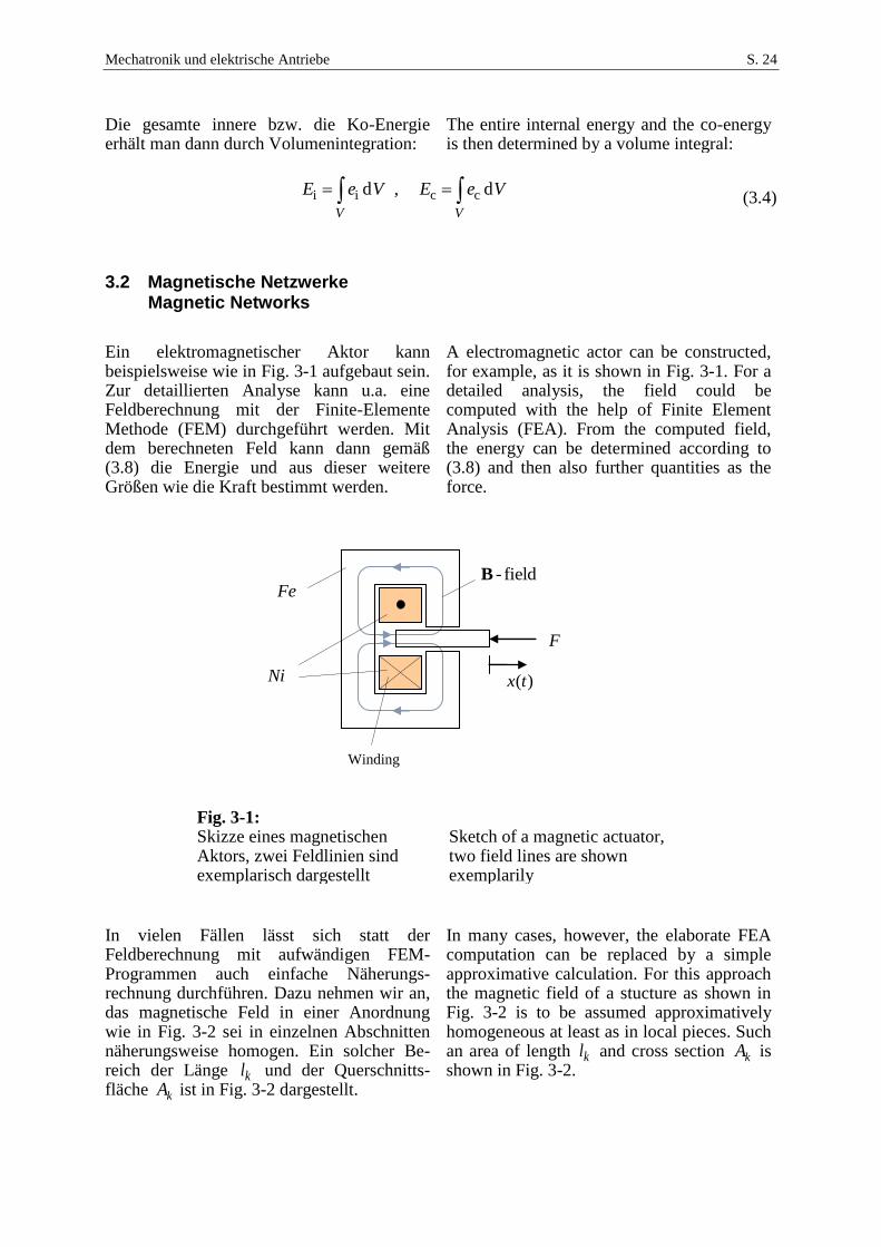
Ein elektromagnetischer Aktor kann beispielsweise wie in Fig. 3-1 aufgebaut sein. Zur detaillierten Analyse kann u.a. eine Feldberechnung mit der Finite-Elemente Methode (FEM) durchgeführt werden. Mit dem berechneten Feld kann dann gemäß (3.8) die Energie und aus dieser weitere Größen wie die Kraft bestimmt werden.
A electromagnetic actor can be constructed, for example, as it is shown in Fig. 3-1. For a detailed analysis, the field could be computed with the help of Finite Element Analysis (FEA). From the computed field, the energy can be determined according to (3.8) and then also further quantities as the force.
Fig. 3-1: Skizze eines magnetischen Aktors, zwei Feldlinien sind exemplarisch dargestellt
Sketch of a magnetic actuator, two field lines are shown exemplarily
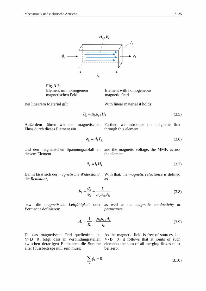
In vielen Fällen lässt sich statt der Feldberechnung mit aufwändigen FEM-Programmen auch einfache Näherungs-rechnung durchführen. Dazu nehmen wir an, das magnetische Feld in einer Anordnung wie in Fig. 3-2 sei in einzelnen Abschnitten näherungsweise homogen. Ein solcher Be-reich der Länge kl und der Querschnitts-fläche kA ist in Fig. 3-2 dargestellt.
In many cases, however, the elaborate FEA computation can be replaced by a simple approximative calculation. For this approach the magnetic field of a stucture as shown in Fig. 3-2 is to be assumed approximatively homogeneous at least as in local pieces. Such an area of length kl and cross section kA is shown in Fig. 3-2.
Fe
F
Winding
Ni )(tx
- fieldB
Mechatronik und elektrische Antriebe S. 25
Fig. 3-2: Element mit homogenem magnetischen Feld
Element with homogeneous magnetic field
Bei linearem Material gilt With linear material it holds:
0 rk k kB H (3.5)
Außerdem führen wir den magnetischen Fluss durch dieses Element ein
Further, we introduce the magnetic flux through this element
k k kA B (3.6)
und den magnetischen Spannungsabfall an diesem Element
and the magnetic voltage, the MMF, across the element
k k kl H (3.7)
Damit lässt sich der magnetische Widerstand, die Reluktanz,
With that, the magnetic reluctance is defined as
0 r
k kk
k k k
lR
A
(3.8)
bzw. die magnetische Leitfähigkeit oder Permeanz definieren:
as well as the magnetic conductivity or permeance
0 r1 k kk
k k
A
R l
(3.9)
Da das magnetische Feld quellenfrei ist,
0 B , folgt, dass an Verbindungsstellen zwischen derartigen Elementen die Summe aller Flussbeiträge null sein muss:
As the magnetic field is free of sources, i.e. 0 B , it follows that at joints of such
elements the sum of all merging fluxes must bei zero:
0k
k
(3.10)
,k kH B
kk
kl
kA
Mechatronik und elektrische Antriebe S. 26
In Anlehnung an ein elektrisches Netzwerk bezeichen wir diese Verbindungsstellen als Knoten. Die Gleichung (3.10) entspricht der Knotenregel bzw. dem ersten Kirchhoffschen Gesetz. Statt des elektrischen Stroms tritt hier der magnetische Fluss als Durchgangs- oder Flussgröße auf. Der Ørsted-Ampèresche Durchflutungssatz lautet in lokaler bzw. integraler Form ( A bezeichnet die Kontur der Fläche A )
In the style of electric networks, we call these joints nodes. Equation (3.10) corresponds to the node rule or the first Kirchhoff’s law. Instead of the electric current, the magnetic flux appears as the flow or through variable. Ampere’s law reads in local and integral form as follows ( A denotes the contour of the area A )
t
DH J
d d d
A A At
H s J A D A
(3.11)
In der Magnetostatik bzw. bei Vorgängen, bei denen die Wellenausbreitung und Diffusionsvorgänge (Skineffekt) keine Rolle spielen, darf die Verschiebungsstromdichte vernachlässigt werden. Dann ergibt das Feld-stärkeumlaufintegral in einer Masche mit Elementen der Art Fig. 3-2
In magnetostatics and in situations where wave propagation and diffusion processes (skin effect) do not play a role, the displacement current can be neglected. Thus, the circulation integral of the field strength yields with elements of the kind of Fig. 3-2
d k k k
k kA
H l Ni
H s (3.12)
Die Gleichung hat also zunächst nicht die Struktur des zweiten Kirchhoffschen Geset-zes, da die Maschensumme der magnetischen Spannungen, die across-Variablen, nicht null, sondern gleich der Summe der eingeschlossenen Ströme ist. Wir können die gewünschte Form aber erzwingen, indem wir den Term des elektrischen Stroms der linken Gleichungsseite zuschlägen:
So far, the equation has not the structure of the second Kirchhoff’s law as the sum of the magnetic voltages, the across-variables, is not zero but equals the sum of the encircled electric currents. However, we can force this desired format by placing the term with the electric currents on the left-hand side of the equation:
0 0k
k
, 0 Ni (3.13)
Dann muss allerdings in der Masche eine zusätzliche magnetische Spannungsquelle 0 eingefügt werden. Mit dieser Hilfsmaßnahme kann die Anordnung aus Fig. 3-2 durch ein mag-netisches Netzwerk beschrieben werden, wobei jetzt die gleichen Regeln wie in einem elektrischen Netzwerk gelten, siehe Fig. 3-3.
Then, in the mesh an additional MMF 0 source has to be introduced. With this auxiliary measure, the structure of Fig. 3-2 can be described by a magnetic network, where the same rules apply as in an electric network, see Fig. 3-3.
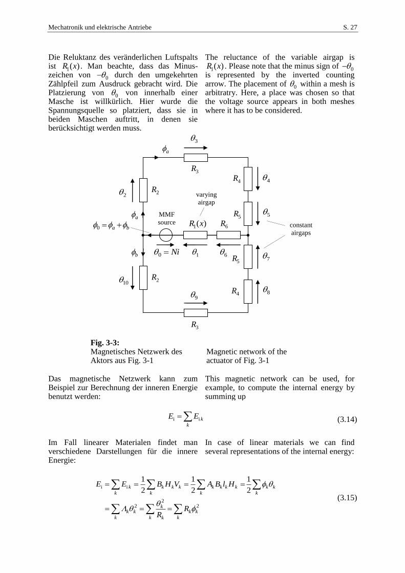
Mechatronik und elektrische Antriebe S. 27
Die Reluktanz des veränderlichen Luftspalts ist 1( )R x . Man beachte, dass das Minus-zeichen von 0 durch den umgekehrten Zählpfeil zum Ausdruck gebracht wird. Die Platzierung von 0 von innerhalb einer Masche ist willkürlich. Hier wurde die Spannungsquelle so platziert, dass sie in beiden Maschen auftritt, in denen sie berücksichtigt werden muss.
The reluctance of the variable airgap is
1( )R x . Please note that the minus sign of 0 is represented by the inverted counting arrow. The placement of 0 within a mesh is arbitratry. Here, a place was chosen so that the voltage source appears in both meshes where it has to be considered.
Fig. 3-3: Magnetisches Netzwerk des Aktors aus Fig. 3-1
Magnetic network of the actuator of Fig. 3-1
Das magnetische Netzwerk kann zum Beispiel zur Berechnung der inneren Energie benutzt werden:
This magnetic network can be used, for example, to compute the internal energy by summing up
i i k
k
E E (3.14)
Im Fall linearer Materialen findet man verschiedene Darstellungen für die innere Energie:
In case of linear materials we can find several representations of the internal energy:
i i
22 2
1 1 1
2 2 2k k k k k k k k k k
k k k k
kk k k k
k k kk
E E B H V A B l H
RR
(3.15)
a
Ni0
varying
airgap
1( )R x
1
2R
3R
4R
2
5
6
5R
6R0 a b
3
4
3R
9
2R10
8
5R 7
a
b
4R
constant
airgaps
MMF
source
Mechatronik und elektrische Antriebe S. 28
Eine wichtige Schlussfolgerung bezüglich der räumlichen Verteilung ergibt sich aus der letzten Darstellungsart der Energie: In den Elementen mit kleiner Reluktanz, typischer-weise also solchen aus ferromagnetischem Material, wird fast gar keine Energie gespeichert, sondern dort, wo die Reluktanz groß ist, also z. B. im Luftspalt. Auch lässt sich die Induktivität der Wicklung mit Hilfe des Netzwerks rasch berechnen:
An important conclusion with respect to the spatial distribution results from the last representation of the energy. In elements with small reluctance, typically those made of ferromagnetic material, only litte energy is stored. The energy is mainly stored where the reluctance is large, e. g. within the airgap. Also the inductance of the winding can be quickly computed using the network:
2
20 0
0 0
( )( )
N NL x N
i i R x
(3.16)
Hierbei ist 0R die wirksame Reluktanz des gesamten magnetischen Netzwerks ge-genüber der magnetischen Spannungsquelle:
Here, 0R is the effective reluctance of the whole magnetic network against the magnetic MMF source:
0 1 6 2 3 4 5 2 3 4 5
1 6 2 3 4 5
( ) ( ) ( ) || ( )
1( ) ( )
2
R x R x R R R R R R R R R
R x R R R R R
(3.17)
Dies kann auch wieder zur Darstellung der Energie genutzt werden:
This can again be used to represent the energy:
2i 2
1 1
2 2E Li
L (3.18)
Mechatronik und elektrische Antriebe S. 29
Übersicht über die verwendeten Größen List of used quantities
Größe Quantity
Symbol
Maßeinheit
Unit
Elektrische Spannung Electric Voltage
u V1
Magnetische Flussdichte Magnetic flux density
B 2Vs/m1T1
Magnetischer Fluss Magnetic flux
Vs1
Magnetischer Verkettungsfluss Magnetic flux linkage
Vs1
Elektrischer Strom Electric current
i A1
Magnetische Feldstärke Magnetic field strength
H A/m1
Magnetische Spannung, mag-netische Durchflutung Magnetic voltage, MMF
1)
A1
Induktivität Inductance
L Vs/A1H1
Magnetischer Leitwert, Permeanz Magnetic conductivity, permeance
Vs/A1H1
Reluktanz Reluctance
R A/Vs1
Energiedichte Energy density
2)
e 3 21J/ m 1N/ m
Energie Energy
E 1J
1)
In der Literatur findet man für die magnetische
Spannung sehr häufig die Einheit „Ampere-
Windungen“, was trotz vielfältiger Wiederholungen
falsch ist: Auch wenn die magnetische Spannung
durch mehrere Windungen aufgebaut wird, beibt ihre
Maßeinheit einfach nur das Ampere, denn die Zahl der
Windungen ist dimensions- und einheitenlos.
1) In literature, one finds often the unit “Ampere-
turns“, which is, though often repeated, wrong. Even
if the magnetomomotive force (MMF) is generated by
several turns, the unit of the MMF is still only
Ampere, because the number of turns is a pure number
without physical dimension and unit.
2)
Die Dimension der Energiedichte enspricht
tatsächlich der eines Drucks.
2) The dimension of the energy density is in fact the
same as of a pressure.
Mechatronik und elektrische Antriebe S. 30
3.3 Magnetische Werkstoffe Magnetic Materials
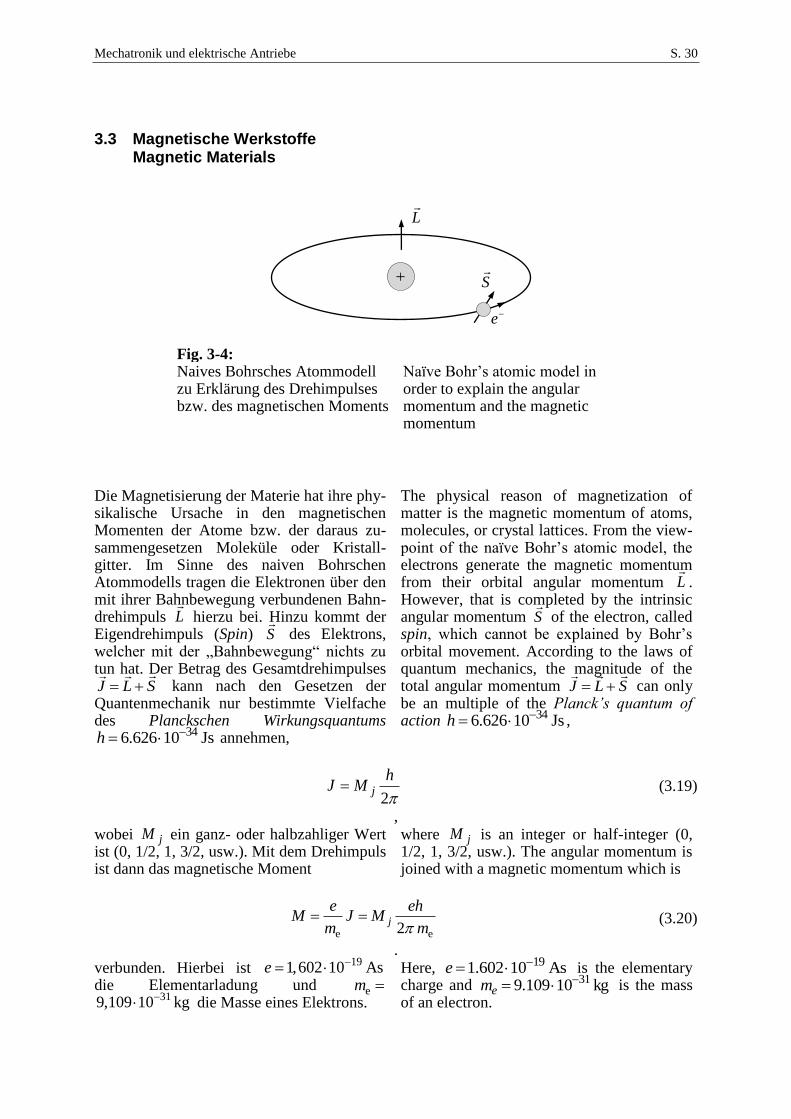
Fig. 3-4: Naives Bohrsches Atommodell zu Erklärung des Drehimpulses bzw. des magnetischen Moments
Naïve Bohr’s atomic model in order to explain the angular momentum and the magnetic momentum
Die Magnetisierung der Materie hat ihre phy-sikalische Ursache in den magnetischen Momenten der Atome bzw. der daraus zu-sammengesetzen Moleküle oder Kristall-gitter. Im Sinne des naiven Bohrschen Atommodells tragen die Elektronen über den mit ihrer Bahnbewegung verbundenen Bahn-drehimpuls L
hierzu bei. Hinzu kommt der
Eigendrehimpuls (Spin) S
des Elektrons, welcher mit der „Bahnbewegung“ nichts zu tun hat. Der Betrag des Gesamtdrehimpulses
SLJ
kann nach den Gesetzen der Quantenmechanik nur bestimmte Vielfache des Planckschen Wirkungsquantums
Js10626.6 34h annehmen,
The physical reason of magnetization of matter is the magnetic momentum of atoms, molecules, or crystal lattices. From the view-point of the naïve Bohr’s atomic model, the electrons generate the magnetic momentum from their orbital angular momentum L
.
However, that is completed by the intrinsic angular momentum S
of the electron, called
spin, which cannot be explained by Bohr’s orbital movement. According to the laws of quantum mechanics, the magnitude of the total angular momentum SLJ
can only
be an multiple of the Planck’s quantum of action Js10626.6 34h ,
2
hMJ j (3.19)
, wobei jM ein ganz- oder halbzahliger Wert ist (0, 1/2, 1, 3/2, usw.). Mit dem Drehimpuls ist dann das magnetische Moment
where jM is an integer or half-integer (0, 1/2, 1, 3/2, usw.). The angular momentum is joined with a magnetic momentum which is
e e2j
e ehM J M
m m (3.20)
. verbunden. Hierbei ist
191,602 10 Ase die Elementarladung und em
319,109 10 kg die Masse eines Elektrons.
Here, As10602.1 19e is the elementary charge and kg10109.9 31em is the mass of an electron.
e
S
L
Mechatronik und elektrische Antriebe S. 31
Zu einem gewissen Teil sind am magne-tischen Moment eines Atoms auch die Spins der Atomkerne beteiligt, was bei der Magnetresonanztomographie (MRT) ausge-nutzt wird. Die Materialeigenschaften mag-netischer Werkstoffe resultieren aber im Wesentlichen aus den Eigenschaften der Elektronenhüllen. Je nach Art der beteiligten Atome und der sich daraus bildenden Kristallgitter orientieren sich die resultie-renden magnetischen Gesamtmomente unter-einander parallel oder antiparallel bzw. richten sich an einem äußeren Feld aus. Die unterschiedlichen Ausprägungen nennt man wie folgt:
To some extent, also the spins of the atomic nuclei contribute to the total magnetic momentum of an atom. That effect is being exploited by magnetic resonance imaging (MRI). The common magnetic behavior of matter, however, is determined mainly by the atom’s electron shell only. Depending on the type of participating atoms or crystal lattices, the magnetic momenta of neighbouring atoms are interacting so that they may align in parallel or anti-parallel to each other or to an external field. The different types of magnetism are distinguished as follows:
Diamagnetismus: Auch wenn das magne-tische Moment im Grundzustand Null ist, werden durch quantenmechanische Wechsel-wirkung mit dem äußeren Feld Dipole induziert, die dem äußeren Feld ent-gegenwirken und es abschwächen. Aus makroskopischer Sicht resultiert 1r . Beispiele: Wasser, Kohlenstoff, Kupfer, Wismut.
Diamagnetism: Even if the magnetic momentum of atoms in the basic state is zero, an external field will excite magnetic dipoles by quantum mechanical interference. The direction of the dipoles is opposite to that of the external field which is then attenuated. From a macroscopic view, it results 1r . Examples: Water, carbon, copper, bismuth.
Paramagnetismus: Atome und Moleküle mit einem von Null verschiedenen magnetischen Moment richten sich parallel zum äußeren Feld aus und verstärken dieses: 1r . Akalimetalle und Seltene Erden zeigen paramagnetisches Verhalten.
Paramagnetism: Atoms and molecules with a non-zero magnetic momentum will align in parallel to an external field so that the field is enhanced: 1r . Alkali metals and rare earths show such paramagnetic behavior.
Ferromagnetismus: Die magnetischen Momente der Atome in einem Kristallgitter sind in den sogenannten Weissschen Bezirken bereits ohne äußeres Feld untereinander parallel ausgerichtet. Typischerweise wechselt die magnetische Ausrichtung benachbarter Weissscher Bezirke, so dass sich die Magnetisierungen in einer makro-skopischen Betrachtung aufheben. Durch ein äußeres Feld verschieben sich die Grenzen benachbarter Weissscher Bezirke, die Bloch-Wände. Bezirke mit einer Magnetisierung in Richtung des erregenden äußeren Feldes wachsen rasch an, während die anderen kleiner werden. Mit weiter zunehmendem äußerem Feld ändern die Weissschen Bezirke auch sprungförmig die Richtung ihrer Magnetisierung (Barkhausen-Sprung). Im Gegensatz zum Paramagnetismus reagiert das Material sehr stark auf äußere Felder:
1r . Dadurch entsteht auch der Effekt
Ferromagnetism: The magnetic momenta of the atoms in a lattice are parallely aligned within the Weiss domains already without any external field. Typically, the magnetic orientation of neighbouring Weiss domains varys so that, in total, the magnetization is cancelled out from a macroscopic viewpoint. With an external field, however, the borders of the Weiss domains, called Bloch walls, will move. Domains with a magnetization in parallel to the external field will grow rapidly while others are getting smaller. With further increasing external field, a Weiss domain may also abruptly change the direction of its magnetization (Barkhausen jump). Unlike paramagnetism, the material reacts extremely strongly to external fields which results in
1r . Another effect in ferromagnetic materials is the residual magnetism (remanence), i.e. a magnetization is retained even after the external field is switched off.
Mechatronik und elektrische Antriebe S. 32
der Remanenz, dass also eine magnetische Vorzugsrichtung auch nach Wegfall des äußeren Feldes zurückbleibt. Die bekanntesten Vertreter ferromagnetischer Materialien sind Eisen, Kobalt und Nickel.
Best known representatives of ferromagnetic materials are iron, cobalt, and nickel.
Ferrimagnetismus: Bei Ferriten sind die Magnetisierungen benachbarter Atome im Kristallgitter jeweils antiparallel ausgerichtet. Sie haben sich daher teilweise auf.
Ferrimagnetism: Within ferrites, the magnetizations of neighboured atoms are aligned anti-parallel so that the magnetisms is partly compensated.
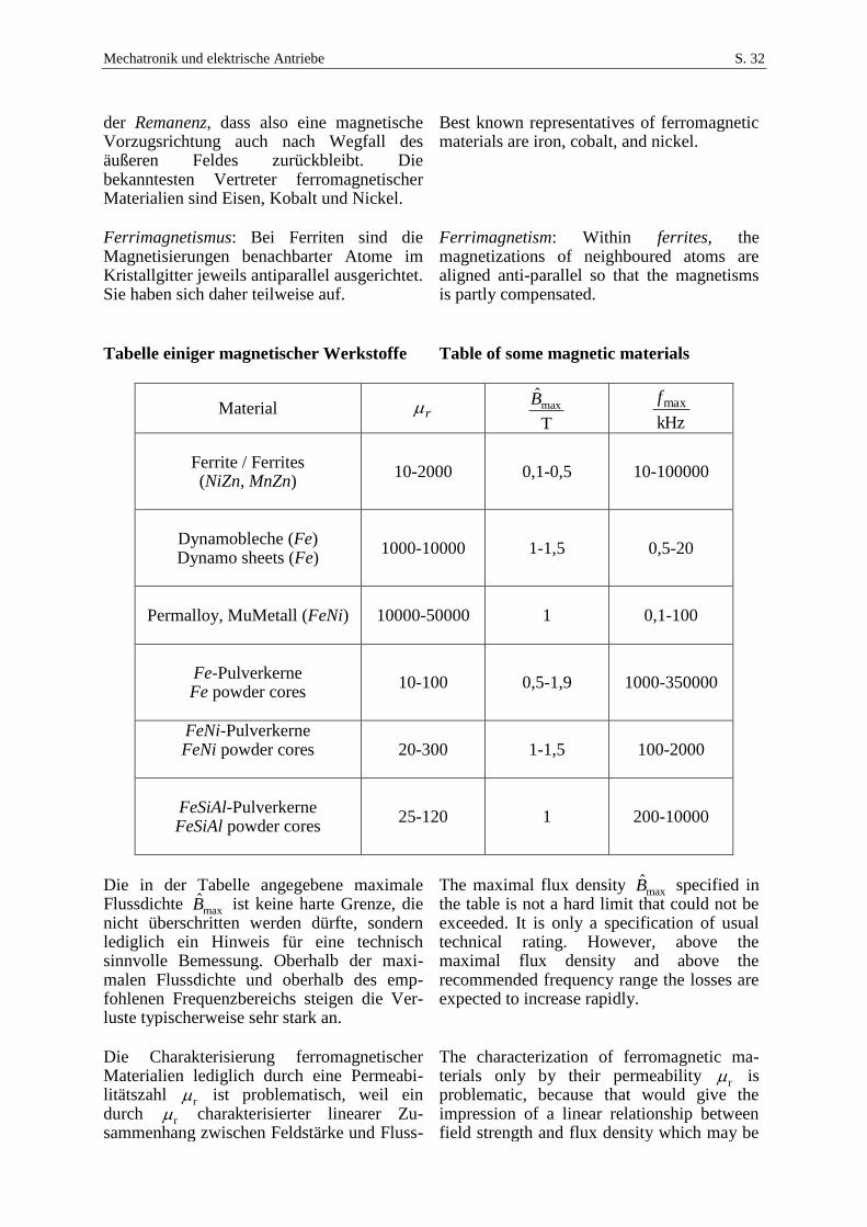
Tabelle einiger magnetischer Werkstoffe Table of some magnetic materials
Material r maxˆ
T
B
kHz
maxf
Ferrite / Ferrites (NiZn, MnZn)
10-2000 0,1-0,5 10-100000
Dynamobleche (Fe) Dynamo sheets (Fe)
1000-10000 1-1,5 0,5-20
Permalloy, MuMetall (FeNi)
10000-50000 1 0,1-100
Fe-Pulverkerne Fe powder cores
10-100 0,5-1,9 1000-350000
FeNi-Pulverkerne FeNi powder cores
20-300 1-1,5 100-2000
FeSiAl-Pulverkerne FeSiAl powder cores
25-120 1 200-10000
Die in der Tabelle angegebene maximale Flussdichte maxB̂ ist keine harte Grenze, die nicht überschritten werden dürfte, sondern lediglich ein Hinweis für eine technisch sinnvolle Bemessung. Oberhalb der maxi-malen Flussdichte und oberhalb des emp-fohlenen Frequenzbereichs steigen die Ver-luste typischerweise sehr stark an.
The maximal flux density maxB̂ specified in the table is not a hard limit that could not be exceeded. It is only a specification of usual technical rating. However, above the maximal flux density and above the recommended frequency range the losses are expected to increase rapidly.
Die Charakterisierung ferromagnetischer Materialien lediglich durch eine Permeabi-litätszahl r ist problematisch, weil ein durch r charakterisierter linearer Zu-sammenhang zwischen Feldstärke und Fluss-
The characterization of ferromagnetic ma-terials only by their permeability r is problematic, because that would give the impression of a linear relationship between field strength and flux density which may be
Mechatronik und elektrische Antriebe S. 33
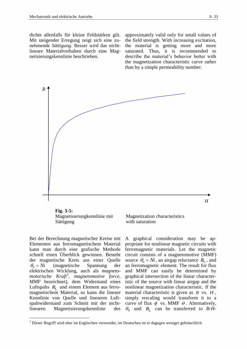
dichte allenfalls für kleine Feldstärken gilt. Mit steigender Erregung zeigt sich eine zu-nehmende Sättigung. Besser wird das nicht-lineare Materialverhalten durch eine Mag-netisierungskennlinie beschrieben.
approximately valid only for small values of the field strength. With increasing excitation, the material is getting more and more saturated. Thus, it is recommended to describe the material’s behavior better with the magnetization characteristic curve rather than by a simple permeability number.
Fig. 3-5: Magnetisierungkennlinie mit Sättigung
Magnetization characteristics with saturation
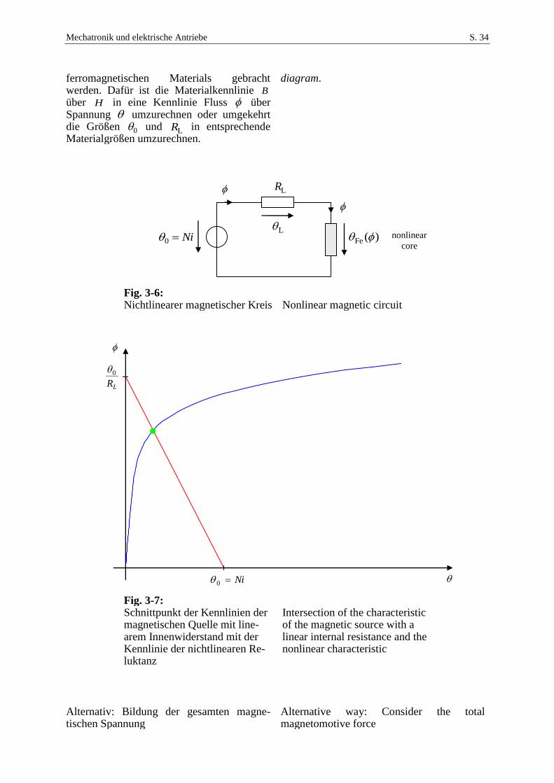
Bei der Berechnung magnetischer Kreise mit Elementen aus ferromagnetischem Material kann man durch eine grafische Methode schnell einen Überblick gewinnen. Besteht der magnetische Kreis aus einer Quelle
Ni0 (magnetische Spannung der elektrischen Wicklung, auch als magneto-motorische Kraft
3, magnetomotive force,
MMF bezeichnet), dem Widerstand eines Luftspalts LR und einem Element aus ferro-magnetischem Material, so kann die lineare Kennlinie von Quelle und linearem Luft-spaltwiderstand zum Schnitt mit der nicht-linearen Magnetisierungskennlinie des
A graphical consideration may be ap-propriate for nonlinear magnetic circuits with ferromagnetic materials. Let the magnetic circuit consists of a magnetomotive (MMF) source Ni0 , an airgap reluctance LR , and an ferromagnetic element. The result for flux and MMF can easily be determined by graphical intersection of the linear character-istic of the source with linear airgap and the nonlinear magnetization characteristic. If the material characteristic is given as B vs. H , simply rescaling would transform it to a curve of flux vs. MMF . Alternatively,
0 und LR can be transferred to B-H-
3 Dieser Begriff wird eher im Englischen verwendet, im Deutschen ist er dagegen weniger gebräuchlich.
B
H
Mechatronik und elektrische Antriebe S. 34
ferromagnetischen Materials gebracht werden. Dafür ist die Materialkennlinie B über H in eine Kennlinie Fluss über Spannung umzurechnen oder umgekehrt die Größen 0 und LR in entsprechende Materialgrößen umzurechnen.
diagram.
Fig. 3-6: Nichtlinearer magnetischer Kreis Nonlinear magnetic circuit
Fig. 3-7: Schnittpunkt der Kennlinien der magnetischen Quelle mit line-arem Innenwiderstand mit der Kennlinie der nichtlinearen Re-luktanz
Intersection of the characteristic of the magnetic source with a linear internal resistance and the nonlinear characteristic
Alternativ: Bildung der gesamten magne-tischen Spannung
Alternative way: Consider the total magnetomotive force
Ni0
LR
0
Fe( ) Ni0 nonlinear
core
LR
L
Mechatronik und elektrische Antriebe S. 35
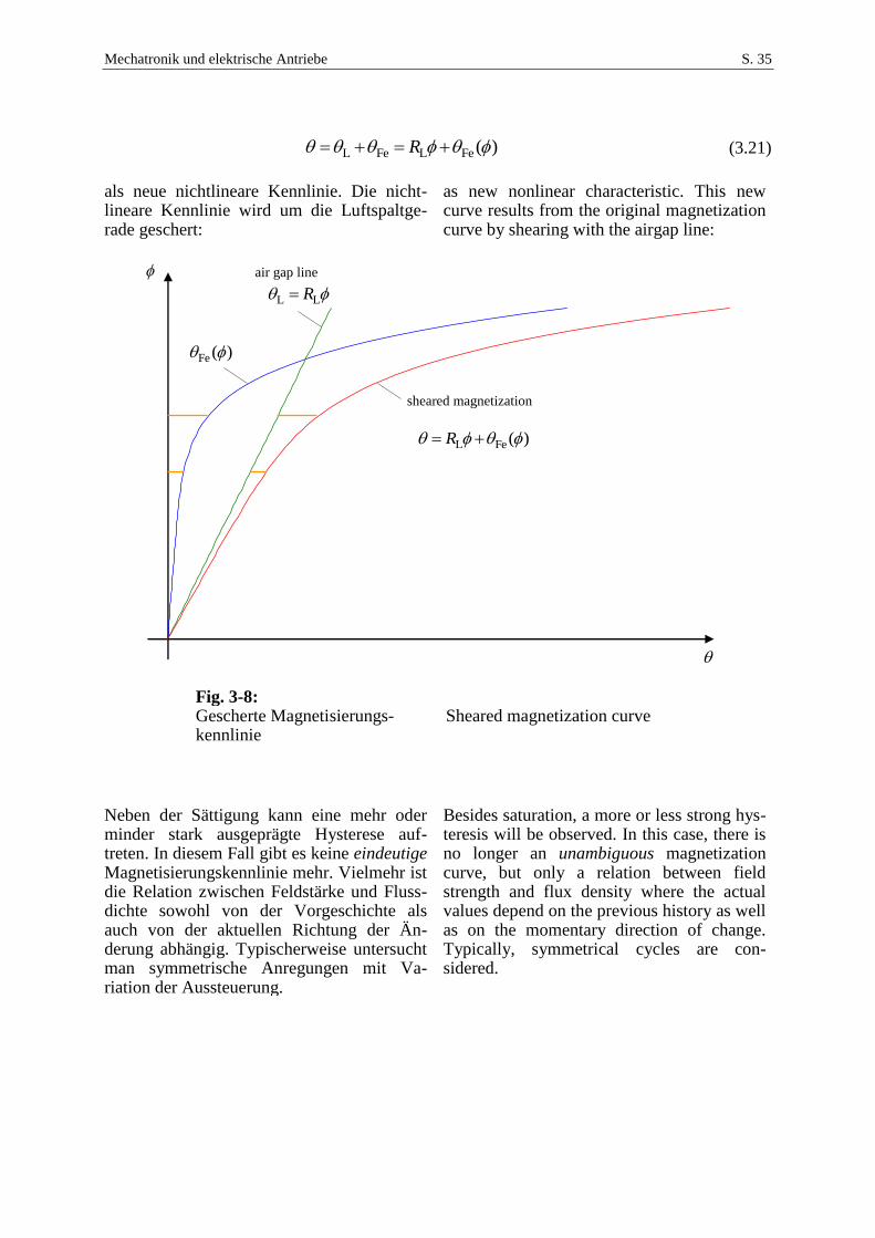
L Fe L Fe( )R (3.21)
als neue nichtlineare Kennlinie. Die nicht-lineare Kennlinie wird um die Luftspaltge-rade geschert:
as new nonlinear characteristic. This new curve results from the original magnetization curve by shearing with the airgap line:
Fig. 3-8: Gescherte Magnetisierungs-kennlinie
Sheared magnetization curve
Neben der Sättigung kann eine mehr oder minder stark ausgeprägte Hysterese auf-treten. In diesem Fall gibt es keine eindeutige Magnetisierungskennlinie mehr. Vielmehr ist die Relation zwischen Feldstärke und Fluss-dichte sowohl von der Vorgeschichte als auch von der aktuellen Richtung der Än-derung abhängig. Typischerweise untersucht man symmetrische Anregungen mit Va-riation der Aussteuerung.
Besides saturation, a more or less strong hys-teresis will be observed. In this case, there is no longer an unambiguous magnetization curve, but only a relation between field strength and flux density where the actual values depend on the previous history as well as on the momentary direction of change. Typically, symmetrical cycles are con-sidered.
Fe( )
L LR
air gap line
sheared magnetization
L Fe( )R
Mechatronik und elektrische Antriebe S. 36
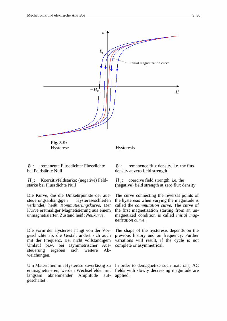
Fig. 3-9: Hysterese Hysteresis
rB : remanente Flussdichte: Flussdichte bei Feldstärke Null
rB : remanence flux density, i.e. the flux density at zero field strength
cH : Koerzitivfeldstärke: (negative) Feld-stärke bei Flussdichte Null
cH : coercive field strength, i.e. the (negative) field strength at zero flux density
Die Kurve, die die Umkehrpunkte der aus-steuerungsabhängigen Hystereseschleifen verbindet, heißt Kommutierungskurve. Der Kurve erstmaliger Magnetisierung aus einem unmagnetisierten Zustand heißt Neukurve.
The curve connecting the reversal points of the hysteresis when varying the magnitude is called the commutation curve. The curve of the first magnetization starting from an un-magnetized condition is called initial mag-netization curve.
Die Form der Hysterese hängt von der Vor-geschichte ab, die Gestalt ändert sich auch mit der Frequenz. Bei nicht vollständigem Umlauf bzw. bei asymmetrischer Aus-steuerung ergeben sich weitere Ab-weichungen.
The shape of the hysteresis depends on the previous history and on frequency. Further variations will result, if the cycle is not complete or asymmetrical.
Um Materialien mit Hysterese zuverlässig zu entmagnetisieren, werden Wechselfelder mit langsam abnehmender Amplitude auf-geschaltet.
In order to demagnetize such materials, AC fields with slowly decreasing magnitude are applied.
B
HcH
rB
initial magnetization curve
Mechatronik und elektrische Antriebe S. 37
Fig. 3-10:
Magnetische Hysterese Magnetic hysteresis
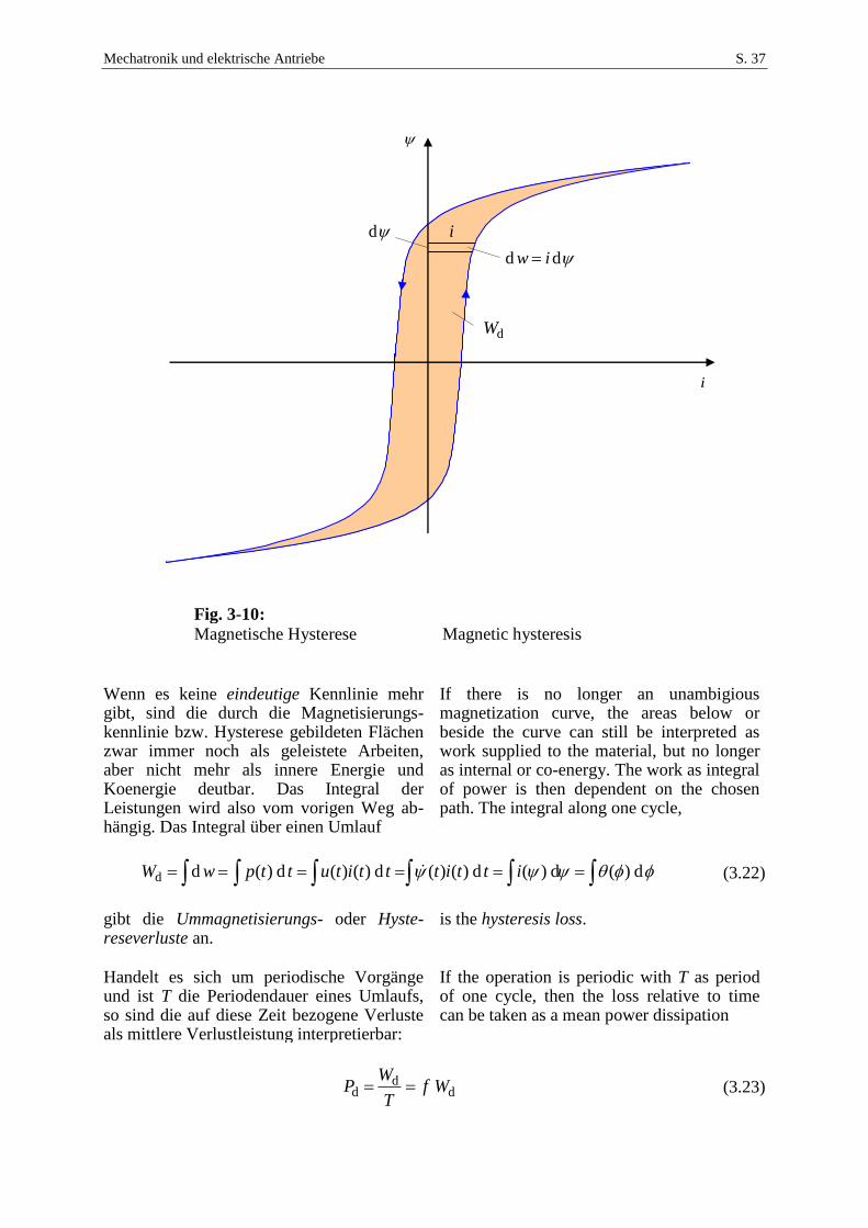
Wenn es keine eindeutige Kennlinie mehr gibt, sind die durch die Magnetisierungs-kennlinie bzw. Hysterese gebildeten Flächen zwar immer noch als geleistete Arbeiten, aber nicht mehr als innere Energie und Koenergie deutbar. Das Integral der Leistungen wird also vom vorigen Weg ab-hängig. Das Integral über einen Umlauf
If there is no longer an unambigious magnetization curve, the areas below or beside the curve can still be interpreted as work supplied to the material, but no longer as internal or co-energy. The work as integral of power is then dependent on the chosen path. The integral along one cycle,
d)(d)(d)()(d)()(d)(dd ittitttituttpwW (3.22)
gibt die Ummagnetisierungs- oder Hyste-reseverluste an.
is the hysteresis loss.
Handelt es sich um periodische Vorgänge und ist T die Periodendauer eines Umlaufs, so sind die auf diese Zeit bezogene Verluste als mittlere Verlustleistung interpretierbar:
If the operation is periodic with T as period of one cycle, then the loss relative to time can be taken as a mean power dissipation
dd
d WfT
WP (3.23)
i
dd iw
d i
dW
Mechatronik und elektrische Antriebe S. 38
In erster Näherung sind die Verluste also der Frequenz proportional.
Thus, as a first-order approximization, the power dissipation is proportional to the frequency,
fP ~d (3.24)
Für höhere Frequenzen gilt dies nicht mehr, da sich zusätzlich auch die Gestalt der Hyste-rese frequenzabhängig ändert. Die Verluste können dann überproportional steigen:
For higher frequencies, however, this relation will not describe the behavior well, because the shape of the hysteresis will also change. Typically, the losses rise more than linearly:
2...1,~d fe
efP f (3.25)
Für die Abhängigkeit von der Amplitude kann als grobe Näherung angesetzt werden:
An approximative empiric law describing the dependency on the magnitude is
3...2;ˆ~d be
ebP b (3.26)
Die Zusammenfassung dieser beiden empi-rischen Gesetze führt zu der sogenannten Steinmetz-Gleichung
Both relations are brought together as the so-called Steinmetz equation
bf eebfKP ˆ
d (3.27)
Die Steinmetz-Gleichung kann beispiels-weise dafür benutzt werden, um Verluste, die in einem Materialdatenblatt beispielsweise nur für eine bestimmte Aussteuerung und Frequenz zu finden sind (typischerweise finden sich solche Angaben in der Maßheit W/kg), auf einen anderen Arbeitspunkt um-zurechnen.
The Steinmetz equation can be used to calcu-late losses, based on the above coefficients which are given in a datasheet for all other operations points (magnitude of flux density and frequency). Material loss data are usually provided in units of W/kg.
Mechatronik und elektrische Antriebe S. 39
3.4 Permanentmagnete Permanent Magnets
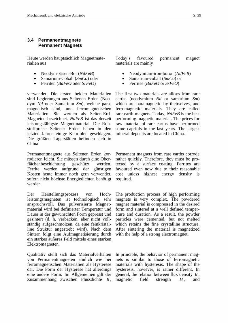
Heute werden hauptsächlich Magnetmate-rialien aus
Today’s favoured permanent magnet materials are mainly
Neodym-Eisen-Bor (NdFeB) Samarium-Cobalt (SmCo) oder Ferriten (BaFeO oder SrFeO)
Neodymium-iron-boron (NdFeB) Samarium-cobalt (SmCo) or Ferrites (BaFeO or SrFeO)
verwendet. Die ersten beiden Materialien sind Legierungen aus Seltenen Erden (Neo-dym Nd oder Samarium Sm), welche para-magnetisch sind, und ferromagnetischen Materialien. Sie werden als Selten-Erd-Magneten bezeichnet. NdFeB ist das derzeit leistungsfähigste Magnetmaterial. Die Roh-stoffpreise Seltener Erden haben in den letzten Jahren einige Kapriolen geschlagen. Die größten Lagerstätten befinden sich in China.
The first two materials are alloys from rare earths (neodymium Nd or samarium Sm) which are paramagnetic by theirselves, and ferromagnetic materials. They are called rare-earth-magnets. Today, NdFeB is the best performing magnetic material. The prices for raw material of rare earths have performed some capriols in the last years. The largest mineral deposits are located in China.
Permanentmagnete aus Seltenen Erden kor-rodieren leicht. Sie müssen durch eine Ober-flächenbeschichtung geschützt werden. Ferrite werden aufgrund der günstigen Kosten heute immer noch gern verwendet, sofern nicht höchste Energiedichten benötigt werden.
Permanent magnets from rare earths corrode rather quickly. Therefore, they must be pro-tected by a surface coating. Ferrites are favoured even now due to their reasonable cost unless highest energy density is required.
Der Herstellungsprozess von Hoch-leistungsmagneten ist technologisch sehr anspruchsvoll. Das pulverisierte Magnet-material wird bei definierter Temperatur und Dauer in der gewünschten Form gepresst und gesintert (d. h. verbacken, aber nicht voll-ständig aufgeschmolzen, da eine feinkristal-line Struktur angestrebt wird). Nach dem Sintern folgt eine Aufmagnetisierung durch ein starkes äußeres Feld mittels eines starken Elektromagneten.
The production process of high performing magnets is very complex. The powdered magnet material is compressed in the desired form and sintered at a well defined temper-ature and duration. As a result, the powder particles were cemented, but not melted which retains the fine crystalline structure. After sintering the material is magnetized with the help of a strong electromagnet.
Qualitativ stellt sich das Materialverhalten von Permanentmagneten ähnlich wie bei ferromagnetischen Materialien als Hysterese dar. Die Form der Hysterese hat allerdings eine andere Form. Im Allgemeinen gilt der Zusammenhang zwischen Flussdichte B ,
In principle, the behavior of permanent mag-nets is similar to those of ferromagnetic materials with hysteresis. The shape of the hysteresis, however, is rather different. In general, the relation between flux density B , magnetic field strength H , and
Mechatronik und elektrische Antriebe S. 40
Feldstärke H und Magnetisierung4 M magnetization
5 M is
MHB 0 (3.28)
Die Magnetisierung M ist bei Permanent-magneten im üblichen Betriebsbereich völlig gesättigt und dort nahezu konstant,
With permanent magnets, the magnetization M is during common operation nearly completely saturated and constant,
.constsat MM (3.29)
Das heißt, in diesem Bereich ist die differenzielle relative Permeabilität
Then, in such operation area, the differential permeability follows as
1d
d1
0r
H
B
(3.30)
der Permanentmagnet verhält sich also be-züglich seines magnetischen Widerstands weitgehend wie Luft oder Vakuum.
i.e., the permanent magnet behaves with respect to its magnetic reluctance like air or vacuum.
Typische Werte der Sättigungs-magnetisierung sind
Typical values of the saturated magnetization are:
ferritesmitT4,0
mitT9,0
mitT4,12,1
sat SmCo
NdFeB
M
Dann resultiert für die remanente Flussdichte unmittelbar
From this, the remanence flux density results directly as
satr MB (3.31)
und für die Koerzitivfeldstärke and the coercive field strength as
satc
0
MH
(3.32)
sofern dieser Punkt noch im reversiblen Be-reich liegt.
where this point is assumed to lie within the reversible area.
4 Man beachte, dass in der Literatur der Begriff der Magnetisierung nicht einheitlich verwendet wird: Für die
hier verwendeten Magnetisierung HBM 0 wird gern auch das Symbol J benutzt und dies als
magnetische Polarisation bezeichnet. Als Magnetisierung M findet man dann häufig die alternative Definition
HBM 0/ .
5 Please note that in literature the term magnetization is not used uniformly. For the magnetization as used here,
HBM 0 , you will find also the symbol J and the term magnetic polarization. As magnetization, the
definition HBM 0/ is also common.
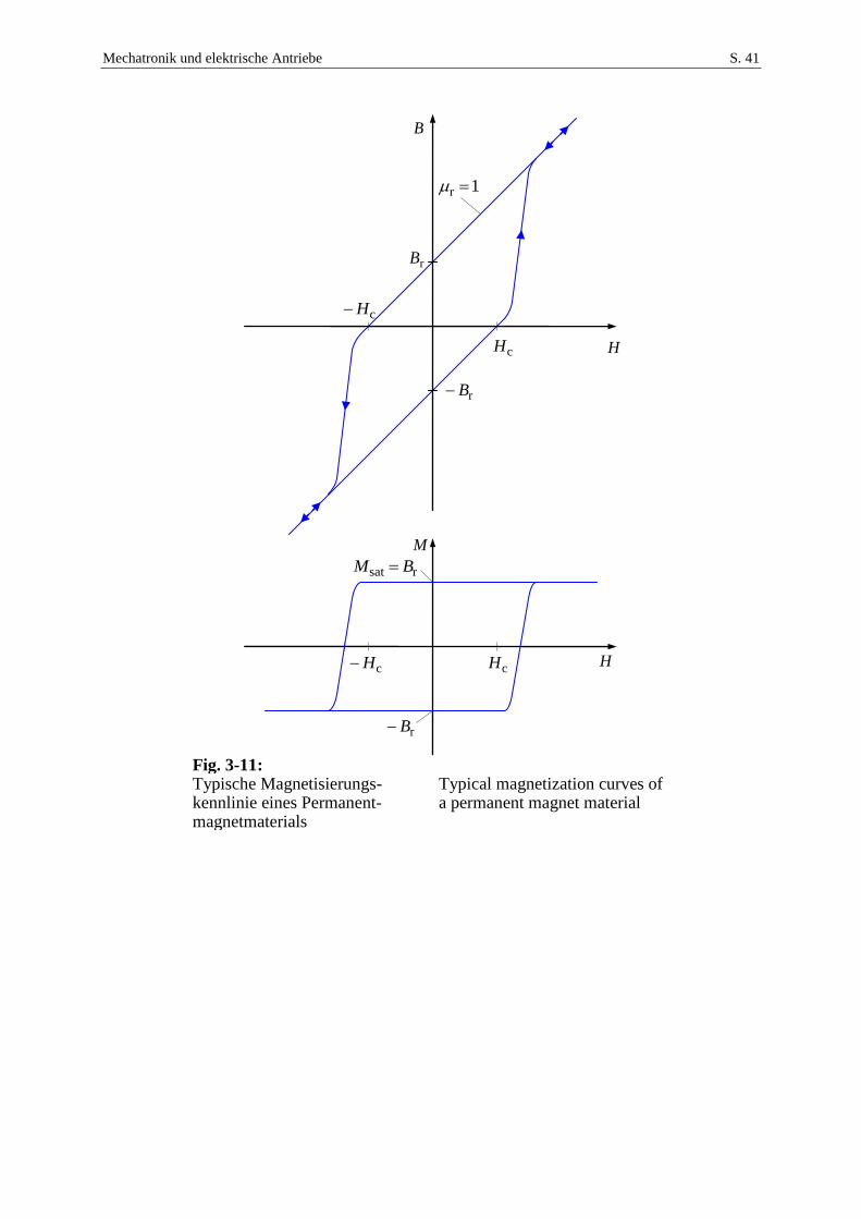
Mechatronik und elektrische Antriebe S. 41
Fig. 3-11: Typische Magnetisierungs-kennlinie eines Permanent-magnetmaterials
Typical magnetization curves of a permanent magnet material
B
cH
rB
rB
rB
rsat BM
M
H
r 1
cH
cH cH H
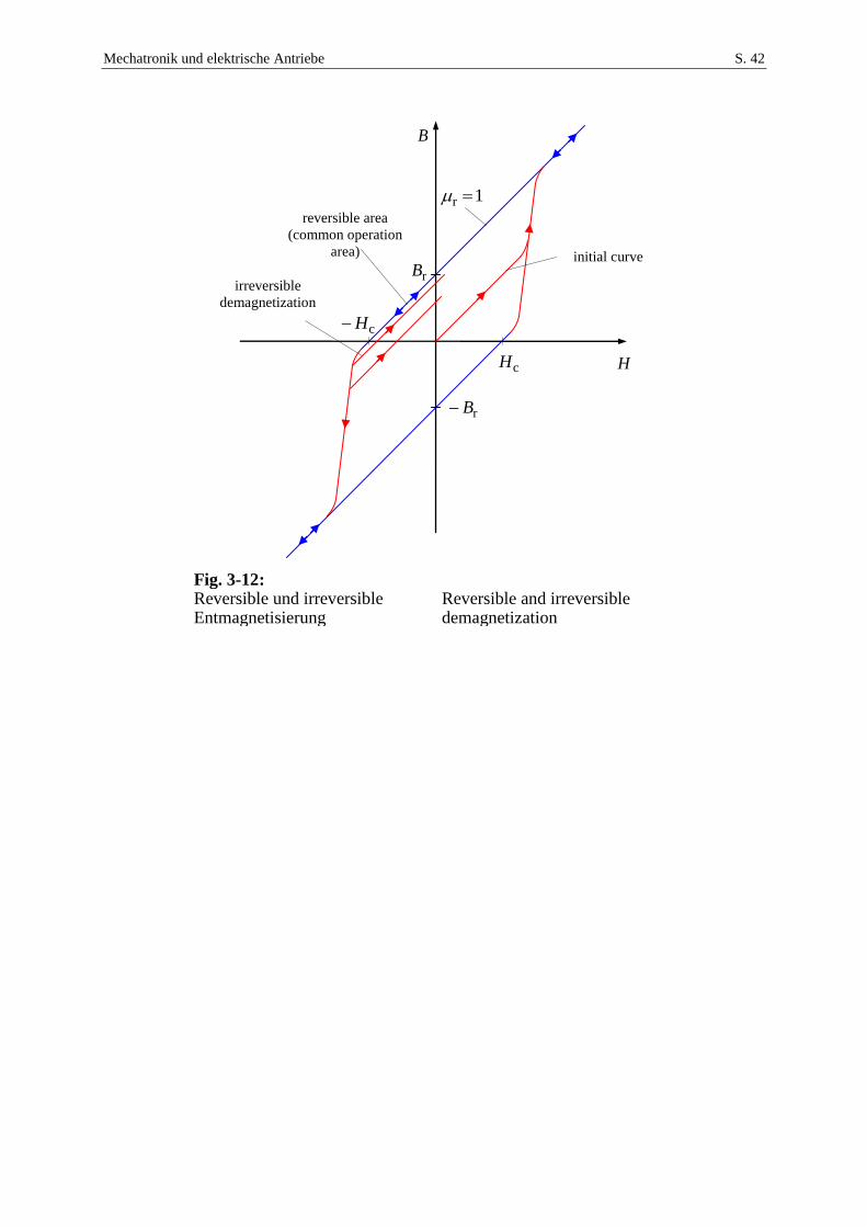
Mechatronik und elektrische Antriebe S. 42
Fig. 3-12: Reversible und irreversible Entmagnetisierung
Reversible and irreversible demagnetization
B
cH
cH
rB
rB
H
r 1
irreversible
demagnetization
reversible area
(common operation
area)
initial curve
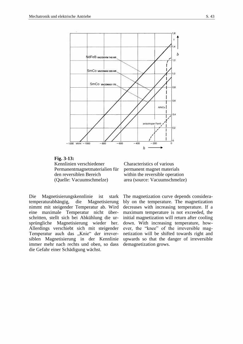
Mechatronik und elektrische Antriebe S. 43
Fig. 3-13: Kennlinien verschiedener Permanentmagnetmaterialien für den reversiblen Bereich (Quelle: Vacuumschmelze)
Characteristics of various permanent magnet materials within the reversible operation area (source: Vacuumschmelze)
Die Magnetisierungskennlinie ist stark temperaturabhängig, die Magnetisierung nimmt mit steigender Temperatur ab. Wird eine maximale Temperatur nicht über-schritten, stellt sich bei Abkühlung die ur-sprüngliche Magnetisierung wieder her. Allerdings verschiebt sich mit steigender Temperatur auch das „Knie“ der irrever-siblen Magnetisierung in der Kennlinie immer mehr nach rechts und oben, so dass die Gefahr einer Schädigung wächst.
The magnetization curve depends considera-bly on the temperature. The magnetization decreases with increasing temperature. If a maximum temperature is not exceeded, the initial magnetization will return after cooling down. With increasing temperature, how-ever, the “knee” of the irreversible mag-netization will be shifted towards right and upwards so that the danger of irreversible demagnetization grows.
NdFeB
SmCo
b
h
SmCo
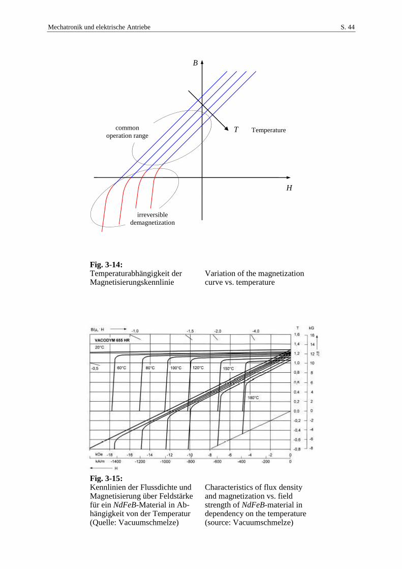
Mechatronik und elektrische Antriebe S. 44
Fig. 3-14: Temperaturabhängigkeit der Magnetisierungskennlinie
Variation of the magnetization curve vs. temperature
Fig. 3-15: Kennlinien der Flussdichte und Magnetisierung über Feldstärke für ein NdFeB-Material in Ab-hängigkeit von der Temperatur (Quelle: Vacuumschmelze)
Characteristics of flux density and magnetization vs. field strength of NdFeB-material in dependency on the temperature (source: Vacuumschmelze)
B
H
T
irreversible
demagnetization
common
operation range
Temperature
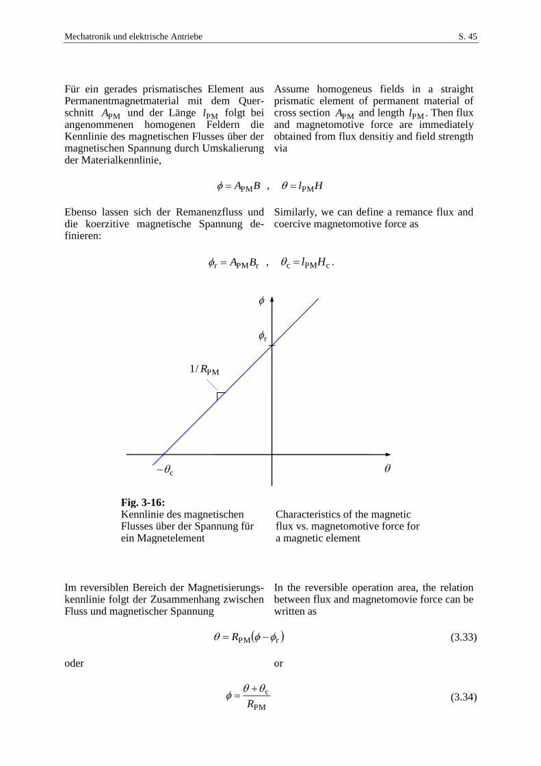
Mechatronik und elektrische Antriebe S. 45
Für ein gerades prismatisches Element aus Permanentmagnetmaterial mit dem Quer-schnitt PMA und der Länge PMl folgt bei angenommenen homogenen Feldern die Kennlinie des magnetischen Flusses über der magnetischen Spannung durch Umskalierung der Materialkennlinie,
Assume homogeneus fields in a straight prismatic element of permanent material of cross section PMA and length PMl . Then flux and magnetomotive force are immediately obtained from flux densitiy and field strength via
BAPM , HlPM
Ebenso lassen sich der Remanenzfluss und die koerzitive magnetische Spannung de-finieren:
Similarly, we can define a remance flux and coercive magnetomotive force as
rPMr BA , cPMc Hl .
Fig. 3-16: Kennlinie des magnetischen Flusses über der Spannung für ein Magnetelement
Characteristics of the magnetic flux vs. magnetomotive force for a magnetic element
Im reversiblen Bereich der Magnetisierungs-kennlinie folgt der Zusammenhang zwischen Fluss und magnetischer Spannung
In the reversible operation area, the relation between flux and magnetomovie force can be written as
rPM R (3.33)
oder or
PM
c
R
(3.34)
c
r
PM/1 R
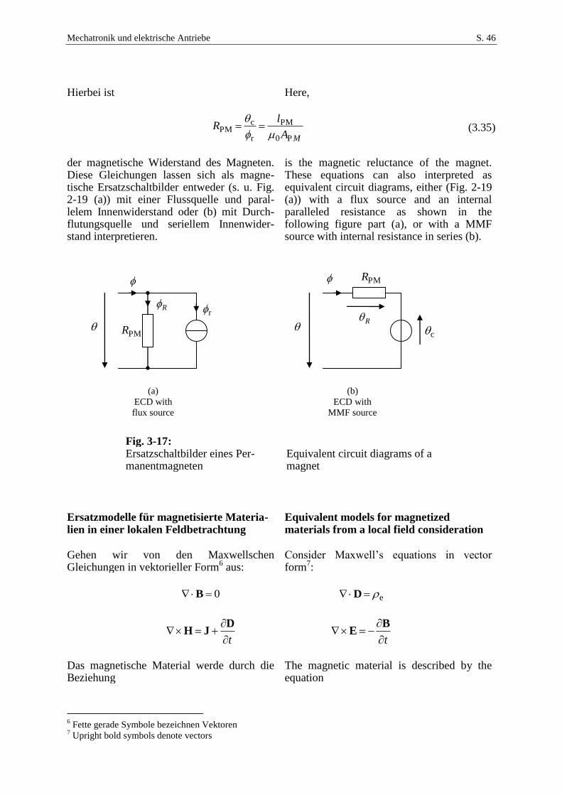
Mechatronik und elektrische Antriebe S. 46
Hierbei ist Here,
MA
lR
P0
PM
r
cPM
(3.35)
der magnetische Widerstand des Magneten. Diese Gleichungen lassen sich als magne-tische Ersatzschaltbilder entweder (s. u. Fig. 2-19 (a)) mit einer Flussquelle und paral-lelem Innenwiderstand oder (b) mit Durch-flutungsquelle und seriellem Innenwider-stand interpretieren.
is the magnetic reluctance of the magnet. These equations can also interpreted as equivalent circuit diagrams, either (Fig. 2-19 (a)) with a flux source and an internal paralleled resistance as shown in the following figure part (a), or with a MMF source with internal resistance in series (b).
Fig. 3-17: Ersatzschaltbilder eines Per-manentmagneten
Equivalent circuit diagrams of a magnet
Ersatzmodelle für magnetisierte Materia-lien in einer lokalen Feldbetrachtung
Equivalent models for magnetized materials from a local field consideration
Gehen wir von den Maxwellschen Gleichungen in vektorieller Form
6 aus:
Consider Maxwell’s equations in vector form
7:
0 B e D
t
DJH
t
BE
Das magnetische Material werde durch die Beziehung
The magnetic material is described by the equation
6 Fette gerade Symbole bezeichnen Vektoren
7 Upright bold symbols denote vectors
PMR
r
c
PMR
(a)
ECD with
flux source
(b)
ECD with
MMF source
R
R
Mechatronik und elektrische Antriebe S. 47
MHB 0 (3.36)
mit der Magnetisierung M berücksichtigt. Schreiben wir
with magnetization M . Let us write
00
00
MH
MBH (3.37)
Die so eingeführte Größe 0H ist als die mag-netische Feldstärke zu verstehen, die sich bei Vorgabe der Flussdichte B statt im magne-tisierten Material im Vakuum einstellen würde. Wir setzen dies in das Oerstedsche Gesetz ein:
The new introduced quantity 0H can be un-derstood as magnetic field strength that re-sults from a given flux density B if vacuum is assumed instead of magnetized material. Let us insert this representation into Oersted’s law:
t
D
00 J
MHH
(3.38)
Mit With
0m
MJ (3.39)
folgt it follows
t
DJJH m0 (3.40)
Das lässt sich so interpretieren, dass das ur-sprüngliche magnetisierte Material durch Vakuum und einer gedachten zusätzlichen Stromdichte mJ ersetzt wird, die aus den Wirbeln der ursprünglichen Magnetisierung berechnet wird. Dies lässt sich sehr anschau-lich interpretieren: Nimmt man ein homogen magnetisiertes Material .constM an, ist
mJ im Innern als auch außerhalb des Mate-rials Null. Auf Oberfläche gibt es aber eine sprungförmige Änderung der Magneti-sierung, die über die Differentiation zu einer Ersatz-Flächenstromdichte der Größe 0/M führt. Die Richtung dieser Stromdichte ist senkrecht zur Flächennormalen und zur ur-sprünglichen Magnetisierung. Dass es sich wirklich um einen zumindest gedanklich physikalisch korrekt interpretierbaren elektri-schen Strom handelt, der im stationären Fall quellfrei sein muss, wird durch Überprürfung von der Diverenz
This representation can be understood in such a way that the original magnetized material is being substituted by vacuum and an additional electrical current of density mJ that is calculated from the curls of the original magnetization. That is rather demonstrative: If homogeneously magnetised material is considered, .constM , then mJ is equal zero within the material as well as outside. On the surface, however, there is a step-like change between constant and zero magnetization. Thus, via differentiation, we will get an equivalent surface current density of 0/M . The direction of this current density is orthogonal to the surface normal and also orthogonal to the original magnetization. To verify that this equivalent current is really a physically correct electrical current, the divergence must be zero as it is acknowledged by
Mechatronik und elektrische Antriebe S. 48
0M
J 0
m (3.41)
bestätigt. Dieser Strom zirkuliert also in der Oberfläche. Man spricht von einem Mantel-strom. Die Stärke dieses Mantelstroms kann direkt aus den Materialkennlinien abgelesen werden. Sie ist gleich der koerzitiven Feldstärke. Bei Seltenerdmagneten liegen die Werte in der Größenordnung
So, the current will circulate within the surface and is called surface current. The value of this surface current is the same as the coercive field strength and can be directly obtained from the material characteristics. With rare earth materials it is in the range of
A/mm1000kA/m1000c0
HM
(3.42)
Wollte man also einen Seltenerdmagneten durch eine elektrische Spule ersetzen, kann man natürlich keinen idealen Flächenstrom realisieren, sondern muss eine gewisse Spulendicke in Kauf nehmen. Geht man von einer technisch in Kupfer erreichbaren Stromdichte von 2A/mm10 aus (was bereits gute Kühlung erfordert), führt das also zu einer Spulendicke von mm100 , um einen derartigen Mantelstrom zu realisieren. Dabei ist der Füllfaktor der Wicklung noch nicht berücksichtigt. Dieser Vergleich zeigt die enorme Stärke moderner Magnetmaterialien. Praktisch können Permanentmagnete mit Abmaßen von nur einigen Millimetern auf-grund der eben abgeschätzen Dicke der Spulen kaum durch solche ersetzt werden.
In reality, a surface current can be realized with an electric coil only approximatively, because a coil would require non-zero thick-ness for its wires. Assuming a technical current density in copper of 2A/mm10 (that requires already a good cooling), a thickness of the coil of mm100 would result in order to allow the above mentioned current. The filling factor is even not considered in that calculation. This comparison shows the enormous strength of modern magnet materials. In practice, it is nearly impossible to replace magnets of size of some millimeters by realistic electric coils.
Statt der Substitution der Magnetisierung durch Ersatzströme ist auch eine andere Er-satzvorstellung möglich. Schreiben wir diesmal die Materialbeziehung als
Instead of subsitution by equivalent currents it is possible to derive an alternative equiva-lent representation. Let us write the material relation as
MBMHB 00 (3.43)
Hier ist 0B die sich zu einem gegebenen Feldstärkefeld H im Vakuum einstellende Flussdichte. Wird diese Gleichung nun in die Quellengleichung eingesetzt, folgt
Here, 0B is the flux density that would result from a field strength H in vacuum. This equation is inserted into the equation of vanishing magnetic sources:
MBB 00 (3.44)
bzw. or
m0 B , (3.45)
mit einer gedachten magnetischen Ladungs- where can be seen as an equivalent magnetic
Mechatronik und elektrische Antriebe S. 49
dichte charge density.
Mm (3.46)
Bei einem Material mit konstanter Magneti-sierung ist im Innern 0 M . Es treten also nur Ersatz-Flächenladungen auf der Oberfläche auf. Die Größe der Flächen-ladung ergibt sich direkt aus der Magneti-sierung M . Da das Ersatz-Flussdichtefeld
0B nicht mehr quellenfrei ist, sind die Feld-linien eines stationären Magnetfeldes nun nicht mehr wie gewohnt geschlossen, son-dern laufen wie beim elektrostatischen Feld von einer positiven magnetischen Ladung zu einer negativen. Diese Vorstellung hat zwar keine technisch-physikalische Relevanz
8,
kann aber durchaus für die numerische Feldberechung nützlich sein. Die durch diese Vorstellungen eingeführten Ersatzfelder
With a material with constant magnetization, 0 M holds within the material. So,
equivalent magnetic sources will result only on the surface of the material. The magnitude of the charge density results directly from the original magnetization M . Since the equiva-lent flux density field 0B is no longer free of magnetic sources, the lines of the stationary field are no longer closed as it is common with the original magnetic field, but starting from a positive magnetic charge and ending in a negative charge. This equivalent model has no technical or physical relevance
9.
However, that method could be benefical for the purpose of numerical field computation. The fields introduced by this equivalent model
000
BMHH bzw. HMBB 00
unterscheiden sich von den ursprünglichen Feldern H bzw. B nur innerhalb des magne-tisierten Materials. Außerhalb des Materials sind sie diesen gleich, da dort 0M gilt.
differ from the original fields H and B , re-spectively, only within the magnetized material. Outside they equal the original fields, since 0M holds outside of the material.
8 Einige Theoretiker halten die Existenz magnetischer Einzelladungen für möglich. Bislang konnten diese aber
nicht nachgewiesen werden. 9 Some theorists consider magnetic single charges possibly existent. So far, such particles have not been
detected.
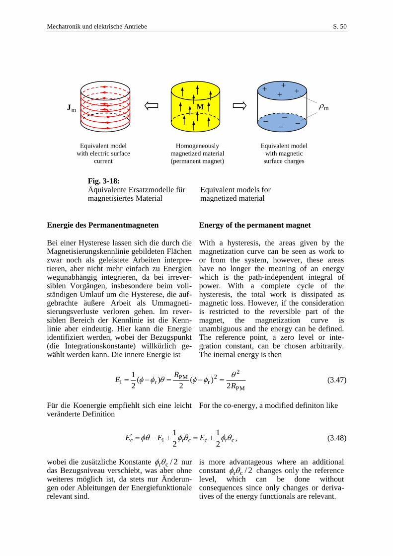
Mechatronik und elektrische Antriebe S. 50
Fig. 3-18: Äquivalente Ersatzmodelle für magnetisiertes Material
Equivalent models for magnetized material
Energie des Permanentmagneten Energy of the permanent magnet
Bei einer Hysterese lassen sich die durch die Magnetisierungskennlinie gebildeten Flächen zwar noch als geleistete Arbeiten interpre-tieren, aber nicht mehr einfach zu Energien wegunabhängig integrieren, da bei irrever-siblen Vorgängen, insbesondere beim voll-ständigen Umlauf um die Hysterese, die auf-gebrachte äußere Arbeit als Ummagneti-sierungsverluste verloren gehen. Im rever-siblen Bereich der Kennlinie ist die Kenn-linie aber eindeutig. Hier kann die Energie identifiziert werden, wobei der Bezugspunkt (die Integrationskonstante) willkürlich ge-wählt werden kann. Die innere Energie ist
With a hysteresis, the areas given by the magnetization curve can be seen as work to or from the system, however, these areas have no longer the meaning of an energy which is the path-independent integral of power. With a complete cycle of the hysteresis, the total work is dissipated as magnetic loss. However, if the consideration is restricted to the reversible part of the magnet, the magnetization curve is unambiguous and the energy can be defined. The reference point, a zero level or inte-gration constant, can be chosen arbitrarily. The inernal energy is then
PM
22
rPM
ri2
)(2
)(2
1
R
RE
(3.47)
Für die Koenergie empfiehlt sich eine leicht veränderte Definition
For the co-energy, a modified definiton like
crccric2
1
2
1 EEE , (3.48)
wobei die zusätzliche Konstante 2/cr nur das Bezugsniveau verschiebt, was aber ohne weiteres möglich ist, da stets nur Änderun-gen oder Ableitungen der Energiefunktionale relevant sind.
is more advantageous where an additional constant 2/cr changes only the reference level, which can be done without consequences since only changes or deriva-tives of the energy functionals are relevant.
Equivalent model
with electric surface
current
mit Flussquelle
M
mJ
Homogeneously
magnetized material
(permanent magnet)
Equivalent model
with magnetic
surface charges
mit Flussquelle
m
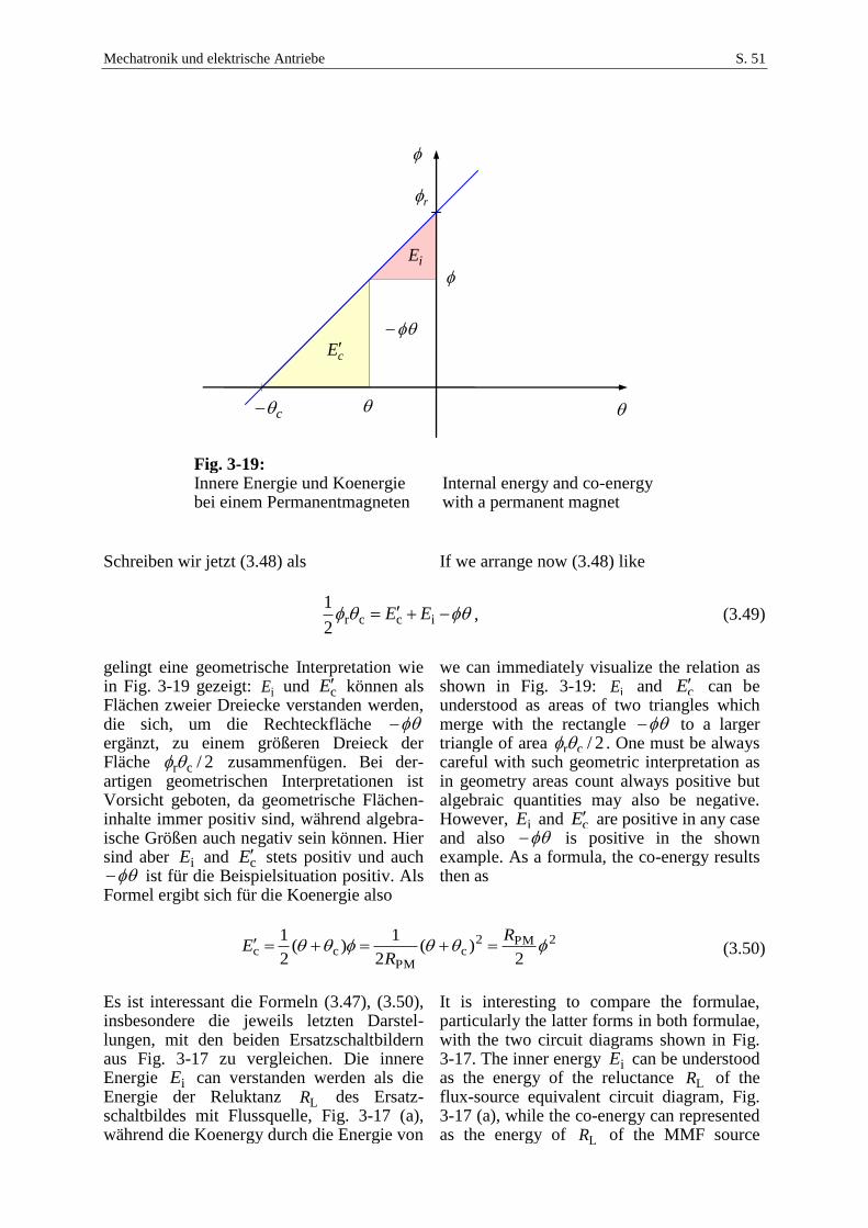
Mechatronik und elektrische Antriebe S. 51
Fig. 3-19: Innere Energie und Koenergie bei einem Permanentmagneten
Internal energy and co-energy with a permanent magnet
Schreiben wir jetzt (3.48) als If we arrange now (3.48) like
iccr2
1EE , (3.49)
gelingt eine geometrische Interpretation wie in Fig. 3-19 gezeigt: iE und cE können als Flächen zweier Dreiecke verstanden werden, die sich, um die Rechteckfläche ergänzt, zu einem größeren Dreieck der Fläche 2/cr zusammenfügen. Bei der-artigen geometrischen Interpretationen ist Vorsicht geboten, da geometrische Flächen-inhalte immer positiv sind, während algebra-ische Größen auch negativ sein können. Hier sind aber iE and cE stets positiv und auch ist für die Beispielsituation positiv. Als
Formel ergibt sich für die Koenergie also
we can immediately visualize the relation as shown in Fig. 3-19: iE and cE can be understood as areas of two triangles which merge with the rectangle to a larger triangle of area 2/cr . One must be always careful with such geometric interpretation as in geometry areas count always positive but algebraic quantities may also be negative. However, iE and cE are positive in any case and also is positive in the shown example. As a formula, the co-energy results then as
2PM2c
PMcc
2)(
2
1)(
2
1
R
RE (3.50)
Es ist interessant die Formeln (3.47), (3.50), insbesondere die jeweils letzten Darstel-lungen, mit den beiden Ersatzschaltbildern aus Fig. 3-17 zu vergleichen. Die innere Energie iE can verstanden werden als die Energie der Reluktanz LR des Ersatz-schaltbildes mit Flussquelle, Fig. 3-17 (a), während die Koenergy durch die Energie von
It is interesting to compare the formulae, particularly the latter forms in both formulae, with the two circuit diagrams shown in Fig. 3-17. The inner energy iE can be understood as the energy of the reluctance LR of the flux-source equivalent circuit diagram, Fig. 3-17 (a), while the co-energy can represented as the energy of LR of the MMF source
c
r
iE
cE
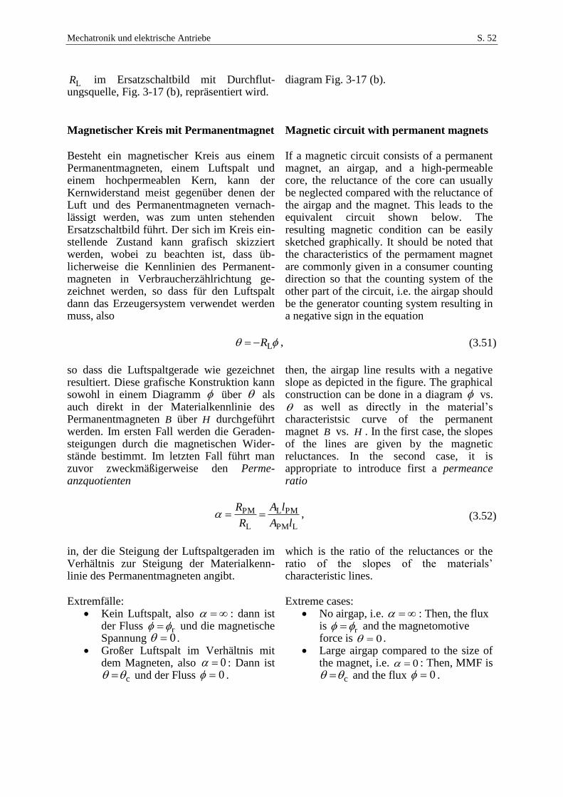
Mechatronik und elektrische Antriebe S. 52
LR im Ersatzschaltbild mit Durchflut-ungsquelle, Fig. 3-17 (b), repräsentiert wird.
diagram Fig. 3-17 (b).
Magnetischer Kreis mit Permanentmagnet Magnetic circuit with permanent magnets
Besteht ein magnetischer Kreis aus einem Permanentmagneten, einem Luftspalt und einem hochpermeablen Kern, kann der Kernwiderstand meist gegenüber denen der Luft und des Permanentmagneten vernach-lässigt werden, was zum unten stehenden Ersatzschaltbild führt. Der sich im Kreis ein-stellende Zustand kann grafisch skizziert werden, wobei zu beachten ist, dass üb-licherweise die Kennlinien des Permanent-magneten in Verbraucherzählrichtung ge-zeichnet werden, so dass für den Luftspalt dann das Erzeugersystem verwendet werden muss, also
If a magnetic circuit consists of a permanent magnet, an airgap, and a high-permeable core, the reluctance of the core can usually be neglected compared with the reluctance of the airgap and the magnet. This leads to the equivalent circuit shown below. The resulting magnetic condition can be easily sketched graphically. It should be noted that the characteristics of the permament magnet are commonly given in a consumer counting direction so that the counting system of the other part of the circuit, i.e. the airgap should be the generator counting system resulting in a negative sign in the equation
LR , (3.51)
so dass die Luftspaltgerade wie gezeichnet resultiert. Diese grafische Konstruktion kann sowohl in einem Diagramm über als auch direkt in der Materialkennlinie des Permanentmagneten B über H durchgeführt werden. Im ersten Fall werden die Geraden-steigungen durch die magnetischen Wider-stände bestimmt. Im letzten Fall führt man zuvor zweckmäßigerweise den Perme-anzquotienten
then, the airgap line results with a negative slope as depicted in the figure. The graphical construction can be done in a diagram vs. as well as directly in the material’s characteristsic curve of the permanent magnet B vs. H . In the first case, the slopes of the lines are given by the magnetic reluctances. In the second case, it is appropriate to introduce first a permeance ratio
LPM
PML
L
PM
lA
lA
R
R , (3.52)
in, der die Steigung der Luftspaltgeraden im Verhältnis zur Steigung der Materialkenn-linie des Permanentmagneten angibt.
which is the ratio of the reluctances or the ratio of the slopes of the materials’ characteristic lines.
Extremfälle:
Kein Luftspalt, also : dann ist der Fluss r und die magnetische Spannung 0 .
Großer Luftspalt im Verhältnis mit dem Magneten, also 0 : Dann ist
c und der Fluss 0 .
Extreme cases: No airgap, i.e. : Then, the flux
is r and the magnetomotive force is 0 .
Large airgap compared to the size of the magnet, i.e. 0 : Then, MMF is
c and the flux 0 .
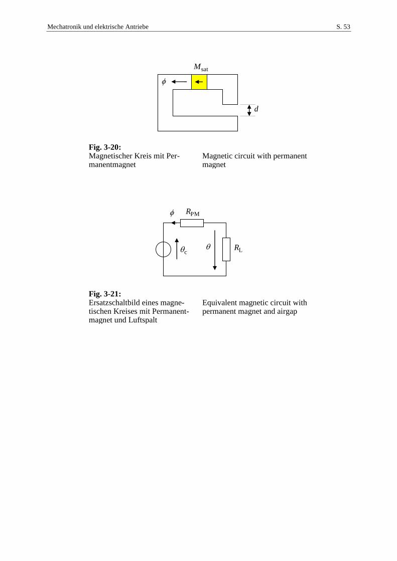
Mechatronik und elektrische Antriebe S. 53
Fig. 3-20: Magnetischer Kreis mit Per-manentmagnet
Magnetic circuit with permanent magnet
Fig. 3-21: Ersatzschaltbild eines magne-tischen Kreises mit Permanent-magnet und Luftspalt
Equivalent magnetic circuit with permanent magnet and airgap
c
PMR
LR
d
satM
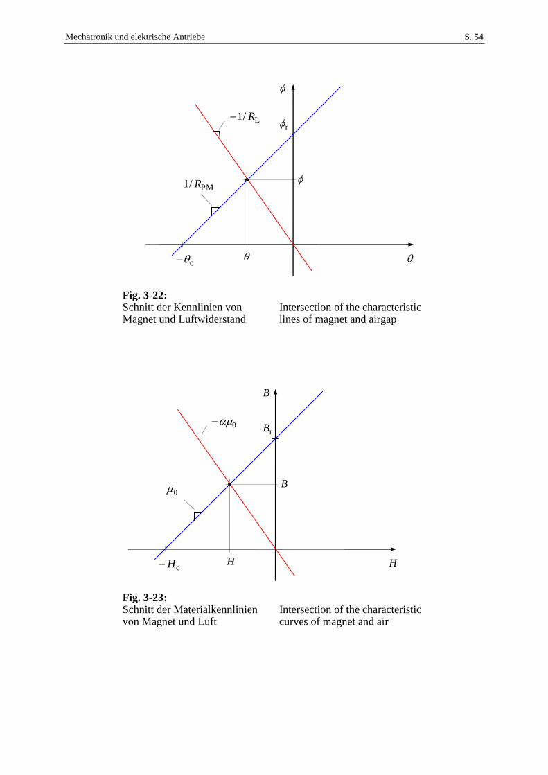
Mechatronik und elektrische Antriebe S. 54
Fig. 3-22: Schnitt der Kennlinien von Magnet und Luftwiderstand
Intersection of the characteristic lines of magnet and airgap
Fig. 3-23: Schnitt der Materialkennlinien von Magnet und Luft
Intersection of the characteristic curves of magnet and air
B
HcH
rB
0
0
H
B
c
r
PM/1 R
L/1 R
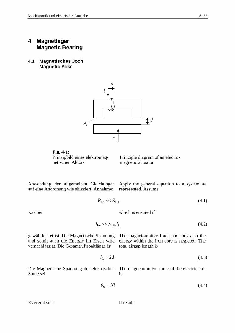
Mechatronik und elektrische Antriebe S. 55
4 Magnetlager Magnetic Bearing
4.1 Magnetisches Joch Magnetic Yoke
Fig. 4-1: Prinzipbild eines elektromag-netischen Aktors
Principle diagram of an electro-magnetic actuator
Anwendung der allgemeinen Gleichungen auf eine Anordnung wie skizziert. Annahme:
Apply the general equation to a system as represented. Assume
LFe RR , (4.1)
was bei which is ensured if
LrFeFe ll (4.2)
gewährleistet ist. Die Magnetische Spannung und somit auch die Energie im Eisen wird vernachlässigt. Die Gesamtluftspaltlänge ist
The magnetomotive force and thus also the energy within the iron core is negleted. The total airgap length is
dl 2L . (4.3)
Die Magnetische Spannung der elektrischen Spule sei
The magnetomotive force of the electric coil is
Ni0 (4.4)
Es ergibt sich It results
d
F
i
u
LA
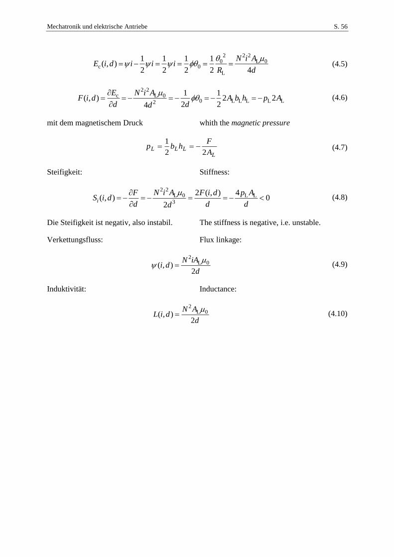
Mechatronik und elektrische Antriebe S. 56
2 2 20 L 0
c 0L
1 1 1 1( , )
2 2 2 2 4
N i AE i d i i i
R d
(4.5)
2 2
c L 00 L L L L L2
1 1( , ) 2 2
2 24
E N i AF i d A b h p A
d dd
(4.6)
mit dem magnetischem Druck whith the magnetic pressure
LLLL
A
Fhbp
22
1 (4.7)
Steifigkeit: Stiffness:
2 2L 0 L L3
42 ( , )( , ) 0
2i
N i A p AF F i dS i d
d d dd
(4.8)
Die Steifigkeit ist negativ, also instabil. The stiffness is negative, i.e. unstable. Verkettungsfluss: Flux linkage:
2L 0( , )
2
N iAi d
d
(4.9)
Induktivität: Inductance:
2L 0( , )
2
N AL i d
d
(4.10)
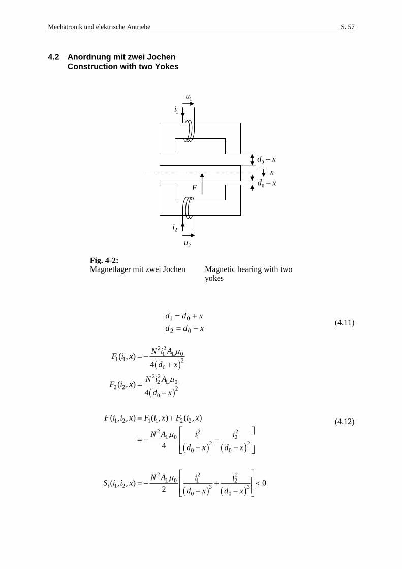
Mechatronik und elektrische Antriebe S. 57
4.2 Anordnung mit zwei Jochen Construction with two Yokes
Fig. 4-2: Magnetlager mit zwei Jochen Magnetic bearing with two
yokes
xdd
xdd
02
01 (4.11)
2 21 L 0
1 1 2
0
2 22 L 0
2 2 2
0
1 2 1 1 2 2
2 2 2L 0 1 2
2 2
0 0
2 2 2L 0 1 2
1 2 3 3
0 0
( , )4
( , )4
( , , ) ( , ) ( , )
4
( , , ) 02
i
N i AF i x
d x
N i AF i x
d x
F i i x F i x F i x
N A i i
d x d x
N A i iS i i x
d x d x
(4.12)
1i
1u
x
xd 0
xd 0F
2i
2u
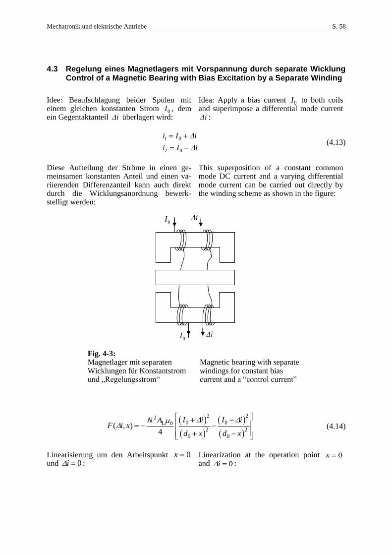
Mechatronik und elektrische Antriebe S. 58
4.3 Regelung eines Magnetlagers mit Vorspannung durch separate Wicklung Control of a Magnetic Bearing with Bias Excitation by a Separate Winding
Idee: Beaufschlagung beider Spulen mit einem gleichen konstanten Strom 0I , dem ein Gegentaktanteil i überlagert wird:
Idea: Apply a bias current 0I to both coils and superimpose a differential mode current
i :
iIi
iIi
02
01 (4.13)
Diese Aufteilung der Ströme in einen ge-meinsamen konstanten Anteil und einen va-riierenden Differenzanteil kann auch direkt durch die Wicklungsanordnung bewerk-stelligt werden:
This superposition of a constant common mode DC current and a varying differential mode current can be carried out directly by the winding scheme as shown in the figure:
Fig. 4-3: Magnetlager mit separaten Wicklungen für Konstantstrom und „Regelungsstrom“
Magnetic bearing with separate windings for constant bias current and a “control current”
2 220 0L 0
2 2
0 0
( , )4
I i I iN AF i x
d x d x
(4.14)
Linearisierung um den Arbeitspunkt 0x und 0i :
Linearization at the operation point 0x and 0i :
0I i
0I i
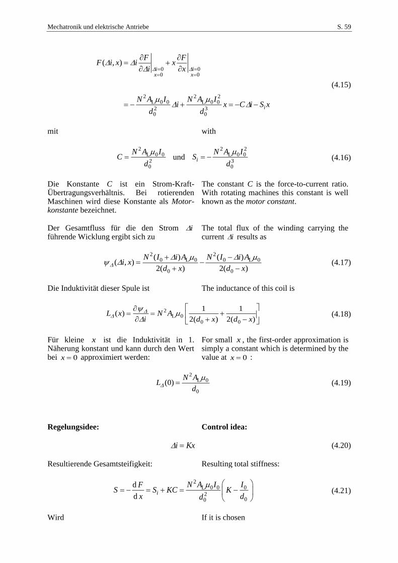
Mechatronik und elektrische Antriebe S. 59
0 00 0
2 2 2L 0 0 L 0 02 30 0
( , )i i
x x
i
F FF i x i x
i x
N A I N A Ii x C i S x
d d
(4.15)
mit with
2L 0 0
20
N A IC
d
und
2 2L 0 0
30
i
N A IS
d
(4.16)
Die Konstante C ist ein Strom-Kraft-Übertragungsverhältnis. Bei rotierenden Maschinen wird diese Konstante als Motor-konstante bezeichnet.
The constant C is the force-to-current ratio. With rotating machines this constant is well known as the motor constant.
Der Gesamtfluss für die den Strom i führende Wicklung ergibt sich zu
The total flux of the winding carrying the current i results as
2 2
0 L 0 0 L 0
0 0
( ) ( )( , )
2( ) 2( )
N I i A N I i Ai x
d x d x
(4.17)
Die Induktivität dieser Spule ist The inductance of this coil is
2L 0
0 0
1 1( )
2( ) 2( )L x N A
i d x d x
(4.18)
Für kleine x ist die Induktivität in 1. Näherung konstant und kann durch den Wert bei 0x approximiert werden:
For small x , the first-order approximation is simply a constant which is determined by the value at 0x :
2
L 0
0
(0)N A
Ld
(4.19)
Regelungsidee: Control idea:
Kxi (4.20)
Resultierende Gesamtsteifigkeit: Resulting total stiffness:
2L 0 0 0
200
d
di
N A I IFS S KC K
x dd
(4.21)
Wird If it is chosen
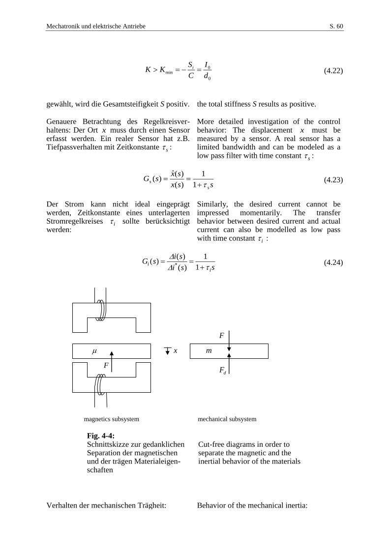
Mechatronik und elektrische Antriebe S. 60
0
0min
d
I
C
SKK i (4.22)
gewählt, wird die Gesamtsteifigkeit S positiv. the total stiffness S results as positive. Genauere Betrachtung des Regelkreisver-haltens: Der Ort x muss durch einen Sensor erfasst werden. Ein realer Sensor hat z.B. Tiefpassverhalten mit Zeitkonstante s :
More detailed investigation of the control behavior: The displacement x must be measured by a sensor. A real sensor has a limited bandwidth and can be modeled as a low pass filter with time constant s :
ssx
sxsG
s
s
1
1
)(
)(ˆ)( (4.23)
Der Strom kann nicht ideal eingeprägt werden, Zeitkonstante eines unterlagerten Stromregelkreises i sollte berücksichtigt werden:
Similarly, the desired current cannot be impressed momentarily. The transfer behavior between desired current and actual current can also be modelled as low pass with time constant i :
ssi
sisG
i
i
1
1
)(
)()(
* (4.24)
Fig. 4-4: Schnittskizze zur gedanklichen Separation der magnetischen und der trägen Materialeigen-schaften
Cut-free diagrams in order to separate the magnetic and the inertial behavior of the materials
Verhalten der mechanischen Trägheit: Behavior of the mechanical inertia:
x
F
magnetics subsystem
F
mechanical subsystem
m
dF
Mechatronik und elektrische Antriebe S. 61
2
1
)()(
)()(
mssFsF
sxsG
d
m
(4.25)
Im stationären Fall 0x gilt also In steady state, 0x , it follows
dFF (4.26)
. Die Übertragungsfunktion )(sGm wird mit Rückkopplung über iS zusammengefasst:
The transfer function )(sGm is to be merged with the feedback via iS :
2
1)(
msSsG
i
m
(4.27)
Weiterhin wird zusammengefasst: Let us introduce also:
CsGsG ii )()( (4.28)
Der Regler wird nach erster Idee als P-Regler angesetzt:
As a first approach, a P-type controller is used:
Ksx
sisGc
)(
)()(
*
(4.29)
bzw. das negative Vorzeichen vom Summenpunkt des mechanischen Teil-systems wird durchgeschoben und ein Regler
The negative sign is due to correct action of the controller. This sign can be compensated with the negative sign before the motor constant C so that the control law can be written as
Ksx
sisGsG cc
)(
)()()(
*
(4.30)
mit der üblichen positiven Verstärkung de-finiert.
with a common positive gain.
Regelfehler: Control error:
xxx * (4.31)
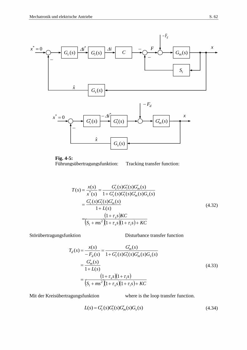
Mechatronik und elektrische Antriebe S. 62
Fig. 4-5: Führungsübertragungsfunktion: Tracking transfer function:
KCssmsS
KCs
sL
sGsGsG
sGsGsGsG
sGsGsG
sx
sxsT
isi
s
mic
smic
mic
11
1
)(1
)()()(
)()()()(1
)()()(
)(
)()(
2
*
(4.32)
Störübertragungsfunktion Disturbance transfer function
KCssmsS
ss
sL
sG
sGsGsGsG
sG
sF
sxsT
isi
is
m
smic
m
d
d
11
11
)(1
)(
)()()()(1
)(
)(
)()(
2
(4.33)
Mit der Kreisübertragungsfunktion where is the loop transfer function.
)()()()()( sGsGsGsGsL smic (4.34)
)(sGc
0* x)(sGi
C )(sGm
iS
x
dF
Fi*i
)(sGs
)(sGc
0* x)(sGi
)(sGm
x
dF
*i
)(sGs
x̂
x̂
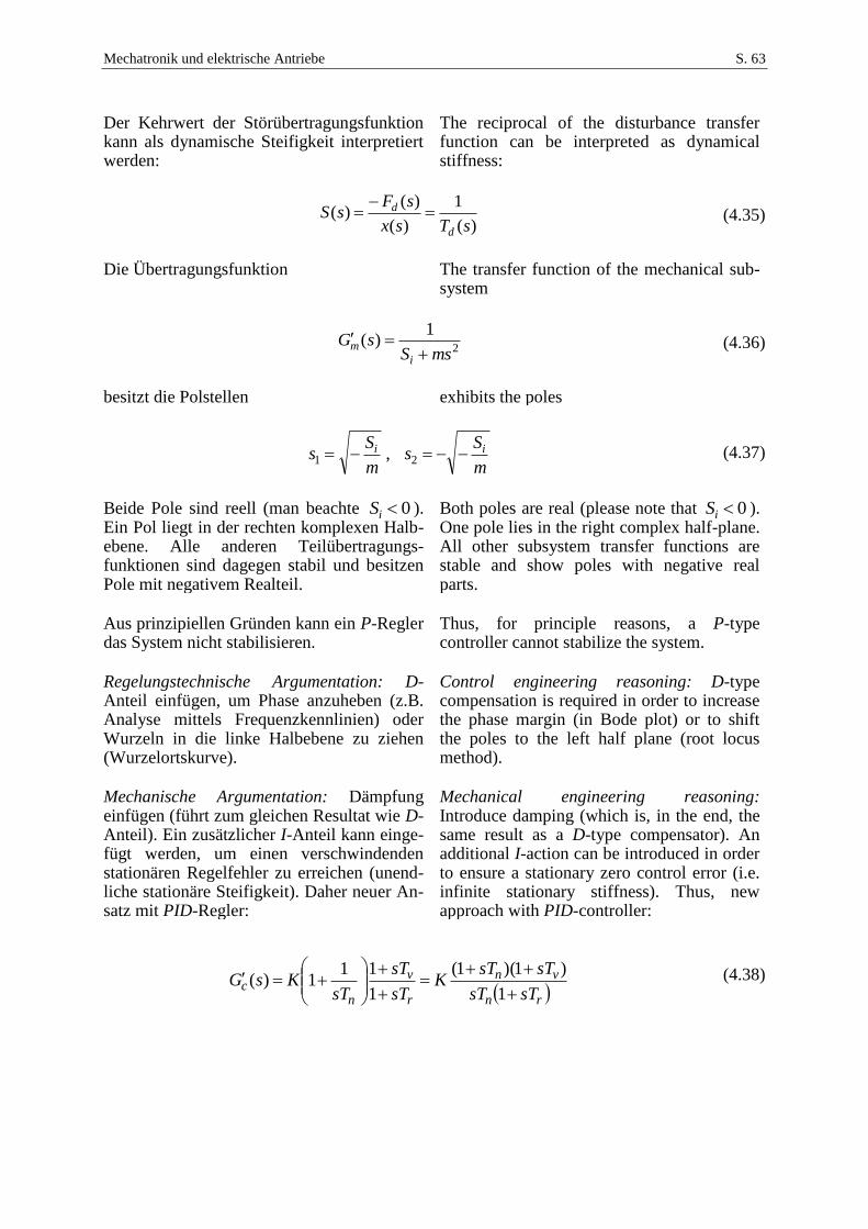
Mechatronik und elektrische Antriebe S. 63
Der Kehrwert der Störübertragungsfunktion kann als dynamische Steifigkeit interpretiert werden:
The reciprocal of the disturbance transfer function can be interpreted as dynamical stiffness:
)(
1
)(
)()(
sTsx
sFsS
d
d
(4.35)
Die Übertragungsfunktion The transfer function of the mechanical sub-
system
2
1)(
msSsG
i
m
(4.36)
besitzt die Polstellen exhibits the poles
m
Ss
m
Ss ii 21 , (4.37)
Beide Pole sind reell (man beachte 0iS ). Ein Pol liegt in der rechten komplexen Halb-ebene. Alle anderen Teilübertragungs-funktionen sind dagegen stabil und besitzen Pole mit negativem Realteil.
Both poles are real (please note that 0iS ). One pole lies in the right complex half-plane. All other subsystem transfer functions are stable and show poles with negative real parts.
Aus prinzipiellen Gründen kann ein P-Regler das System nicht stabilisieren.
Thus, for principle reasons, a P-type controller cannot stabilize the system.
Regelungstechnische Argumentation: D-Anteil einfügen, um Phase anzuheben (z.B. Analyse mittels Frequenzkennlinien) oder Wurzeln in die linke Halbebene zu ziehen (Wurzelortskurve).
Control engineering reasoning: D-type compensation is required in order to increase the phase margin (in Bode plot) or to shift the poles to the left half plane (root locus method).
Mechanische Argumentation: Dämpfung einfügen (führt zum gleichen Resultat wie D-Anteil). Ein zusätzlicher I-Anteil kann einge-fügt werden, um einen verschwindenden stationären Regelfehler zu erreichen (unend-liche stationäre Steifigkeit). Daher neuer An-satz mit PID-Regler:
Mechanical engineering reasoning: Introduce damping (which is, in the end, the same result as a D-type compensator). An additional I-action can be introduced in order to ensure a stationary zero control error (i.e. infinite stationary stiffness). Thus, new approach with PID-controller:
rn
vn
r
v
nc
sTsT
sTsTK
sT
sT
sTKsG
1
)1)(1(
1
111)( (4.38)
Mechatronik und elektrische Antriebe S. 64
Die Übertragungsfunktion des PI-Reglers wurde nun durch einen differenzieren Anteil
vsT1 mit Vorhaltzeit vT ergänzt. Außer-dem wurde berücksichtigt, dass ein realis-tischer Differenzierer nur eine beschränkte Bandbreite besitzt, die durch den zusätz-lichen Tiefpass )1/(1 rsT repräsentiert wird.
The transfer function of an PI controller is now augmented by an differential action
vsT1 with rate time vT . It was also considered that a realistic differentiator has only limited bandwith, represented by the additional low pass )1/(1 rsT .
Skizze des Regelungsentwurfs im Frequenz-bereich: Ein Pol der Kreisübertragungs-funktion )(sL hat positiven Realteil (Beitrag vom )(sGm
). Falls ein I-Anteil im Regler vorgesehen wird, liegt ein weiterer Pol auf der imaginären Achse. Die Nyquistortkurve
)(1 jL muss daher (für positive ) eine Umschlingung von 2/3 aufweisen, wenn der geschlossene Kreis stabil sein soll. Ohne integralen Anteil, also bei einem PD-Regler, muss die Umschlingung nur sein. Im Fall des PD-Reglers lässt sich sofort eine Mindestreglerverstärkung angeben, da die Umschlingung von nur zu Stande kommen kann, wenn der Anfangspunkt der Ortskurve die Bedingung
Outline of control design procedure in frequency domain: One pole of the loop gain transfer function )(sL has a positive real part (contribution of )(sGm
). In case of an I-action in the controller, an additional pole is located on the imaginary axis. The Nyquist locus curve )(1 jL must then show a wrapping of 2/3 (for positive ) in order to stabilize the closed-loop control. Without integral controller action, i.e. with a PD-controller, the wrapping must be only . In case of PD-control, the minimum
stabilizing controller gain can be directly deduced, because the wrapping of is only possible, if the starting point of the Nyquist locus satisfies the condition
1)0( L (4.39)
erfüllt. Daraus folgt From this follows
1iS
KC (4.40)
bzw. or
C
SKK i min (4.41)
Man beachte wieder 0iS . Dieses Ergebnis deckt sich mit der obigen Überlegung zu einer positiven Gesamtsteifigkeit.
Please note again 0iS . This result is consistent with the consideration of a positive total stiffnes.
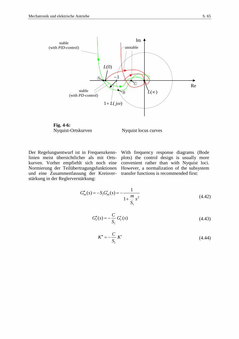
Mechatronik und elektrische Antriebe S. 65
Fig. 4-6: Nyquist-Ortskurven Nyquist locus curves
Der Regelungsentwurf ist in Frequenzkenn-linien meist übersichtlicher als mit Orts-kurven. Vorher empfiehlt sich noch eine Normierung der Teilübertragungsfunktionen und eine Zusammenfassung der Kreisver-stärkung in der Reglerverstärkung:
With frequency response diagrams (Bode plots) the control design is usually more convenient rather than with Nyquist loci. However, a normalization of the subsystem transfer functions is recommended first:
21
1)()(
sS
msGSsG
i
mim
(4.42)
)()( sGS
CsG c
i
c (4.43)
KS
CK
i
(4.44)
unstable
Re
Im
)(1 jL
stable
(with PD-control)
stable
(with PID-control)
)0(L
1A
C
B )(L
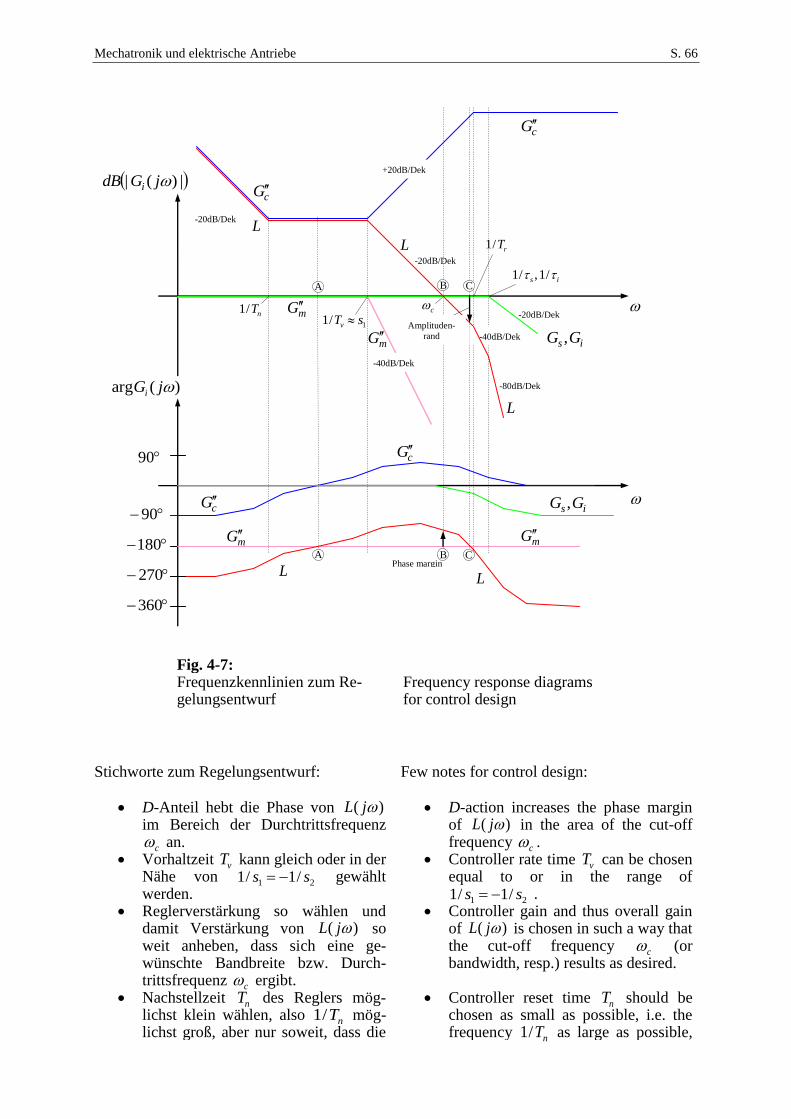
Mechatronik und elektrische Antriebe S. 66
Fig. 4-7: Frequenzkennlinien zum Re-gelungsentwurf
Frequency response diagrams for control design
Stichworte zum Regelungsentwurf: Few notes for control design:
D-Anteil hebt die Phase von )( jL im Bereich der Durchtrittsfrequenz
c an. Vorhaltzeit vT kann gleich oder in der
Nähe von 21 /1/1 ss gewählt werden.
Reglerverstärkung so wählen und damit Verstärkung von )( jL so weit anheben, dass sich eine ge-wünschte Bandbreite bzw. Durch-trittsfrequenz c ergibt.
Nachstellzeit nT des Reglers mög-lichst klein wählen, also nT/1 mög-lichst groß, aber nur soweit, dass die
D-action increases the phase margin of )( jL in the area of the cut-off frequency c .
Controller rate time vT can be chosen equal to or in the range of
21 /1/1 ss . Controller gain and thus overall gain
of )( jL is chosen in such a way that the cut-off frequency c (or bandwidth, resp.) results as desired.
Controller reset time nT should be chosen as small as possible, i.e. the frequency nT/1 as large as possible,
)(arg jGi
|)(| jGdB i
90
90
180
L
is GG ,
-40dB/Dek
-20dB/Dek
-80dB/Dek
+20dB/Dek
-20dB/Dek
270
360
L
nT/11/1 sTv
is /1,/1
rT/1
c
Phase margin
Amplituden-
rand
L
-20dB/Dek
mG
cG
L
L
cG
mG
is GG ,
mG mG
cG
cG
-40dB/Dek
C
B C
B A
A

Mechatronik und elektrische Antriebe S. 67
Phase in der Nähe der Durchtrittsfre-quenz c nicht zu sehr abgesenkt wird.
Knickfrequenzen der Sensorik und des Stromstellgliedes is /1,/1 sowie des realen Differenzierers
rT/1 müssen genügend weit oberhalb der angestrebten Durchtrittsfrequenz c liegen. Alle drei Zeitkonstanten zu-sammen verursachen erhebliche Phasenabsenkung, selbst wenn sie nicht sehr dicht an c liegen.
as far as the phase margin at c is not too much decreased.
Corner frequencies of the sensor and the current source is /1,/1 and the real differential action
rT/1 must be large enough above the desired cut-off frequency c . All three time constants together may cause a considerable decrease of the phase margin, even if they are not that close-by to c .
Genaue Reglerauslegung als Übungsaufgabe! Detailed control design as exercise!
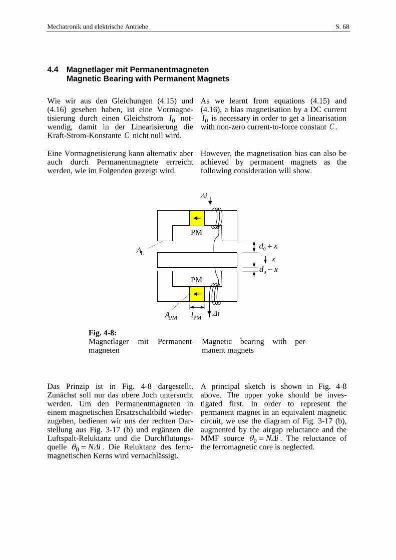
Mechatronik und elektrische Antriebe S. 68
4.4 Magnetlager mit Permanentmagneten Magnetic Bearing with Permanent Magnets
Wie wir aus den Gleichungen (4.15) und (4.16) gesehen haben, ist eine Vormagne-tisierung durch einen Gleichstrom 0I not-wendig, damit in der Linearisierung die Kraft-Strom-Konstante C nicht null wird.
As we learnt from equations (4.15) and (4.16), a bias magnetisation by a DC current
0I is necessary in order to get a linearisation with non-zero current-to-force constant C .
Eine Vormagnetisierung kann alternativ aber auch durch Permanentmagnete errreicht werden, wie im Folgenden gezeigt wird.
However, the magnetisation bias can also be achieved by permanent magnets as the following consideration will show.
Fig. 4-8: Magnetlager mit Permanent-magneten
Magnetic bearing with per-manent magnets
Das Prinzip ist in Fig. 4-8 dargestellt. Zunächst soll nur das obere Joch untersucht werden. Um den Permanentmagneten in einem magnetischen Ersatzschaltbild wieder-zugeben, bedienen wir uns der rechten Dar-stellung aus Fig. 3-17 (b) und ergänzen die Luftspalt-Reluktanz und die Durchflutungs-quelle iN 0 . Die Reluktanz des ferro-magnetischen Kerns wird vernachlässigt.
A principal sketch is shown in Fig. 4-8 above. The upper yoke should be inves-tigated first. In order to represent the permanent magnet in an equivalent magnetic circuit, we use the diagram of Fig. 3-17 (b), augmented by the airgap reluctance and the MMF source iN 0 . The reluctance of the ferromagnetic core is neglected.
PM
i
i
PM
x
xd 0
xd 0
PMlPMA
LA
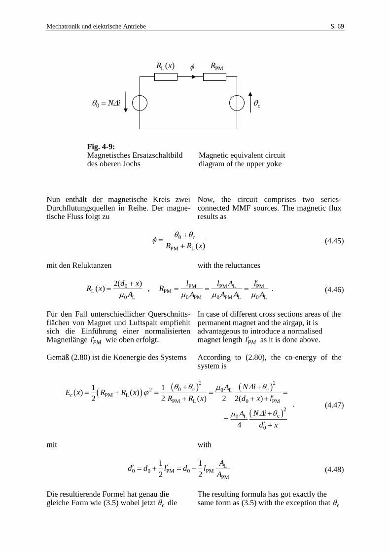
Mechatronik und elektrische Antriebe S. 69
Fig. 4-9: Magnetisches Ersatzschaltbild des oberen Jochs
Magnetic equivalent circuit diagram of the upper yoke
Nun enthält der magnetische Kreis zwei Durchflutungsquellen in Reihe. Der magne-tische Fluss folgt zu
Now, the circuit comprises two series-connected MMF sources. The magnetic flux results as
0 c
PM L ( )R R x
(4.45)
mit den Reluktanzen with the reluctances
0L
0 L
2( )( )
d xR x
A
, PM PM L PM
PM0 PM 0 PM L 0 L
l l A lR
A A A A
. (4.46)
Für den Fall unterschiedlicher Querschnitts-flächen von Magnet und Luftspalt empfiehlt sich die Einführung einer normalisierten Magnetlänge PMl wie oben erfolgt.
In case of different cross sections areas of the permanent magnet and the airgap, it is advantageous to introduce a normalised magnet length PMl as it is done above.
Gemäß (2.80) ist die Koenergie des Systems According to (2.80), the co-energy of the
system is
2 2
0 c c2 0c PM L
PM L 0 PM
2
c0 L
0
1 1( ) ( )
2 2 ( ) 2 2( )
4
LN iA
E x R R xR R x d x l
N iA
d x
. (4.47)
mit with
L0 0 PM 0 PM
PM
1 1
2 2
Ad d l d l
A (4.48)
Die resultierende Formel hat genau die gleiche Form wie (3.5) wobei jetzt c die
The resulting formula has got exactly the same form as (3.5) with the exception that c
c
PMR
iN 0
L( )R x
Mechatronik und elektrische Antriebe S. 70
Rolle der Vormagnetisierung übernimmt und die Magnetlänge bei der gesamten effektiven Luftspaltlänge zu berücksichtigen ist.
takes over the role of bias magnetisation and that the magnet length has to be considered in the total effective airgap length.
Für das System mit oberem und unterem Joch ergeben sich ähnliche Formeln zu denen des Abschnitts 4.3:
For the System with upper and lower yokes, similar formulae result to those of Section 4.3 as
2 2
c c0 L
0 0
( , )4
c
N i N iAE i x
d x d x
. (4.49)
2 2
c c0 L
2 2
0 0
( , )4
cN i N iE A
F i xx d x d x
(4.50)
2 2
c c0 L3 3
0 0
( , )2
i
N i N iAFS i x
x d x d x
(4.51)
Das gilt ebenso für die Linearisierung um den Arbeitspunkt 0i , 0x :
That applies also for the linearisation around the operating point 0i , 0x :
xSiCx
Fx
i
FixiF i
xi
xi
00
00
),( (4.52)
mit with
L 0 c2
0
AC
d
,
2L 0 c
30
i
AS
d
(4.53)
Die Vorteile einer Vormagnetisierung durch Permanentmagnete sind offensichtlich: Es wird keine elektrische Stromversorgung für die Vormagnetisierungs-Spule benötigt. Außerdem stellt sich heraus, dass mit einem Permanentmagneten eine viel stärkere Magnetisierung möglich ist als mit einer elektrischen Spule vergleichbarer geome-trischer Größe.
The advantages of a permanent bias magnetisation over a bias current are ob-vious: There is no need of an electrical sup-ply to feed the bias winding. Additionally, it turns out that a permanent magnet results in a much stronger magnetisation than it is possible with an electric winding of com-parable geometric size.
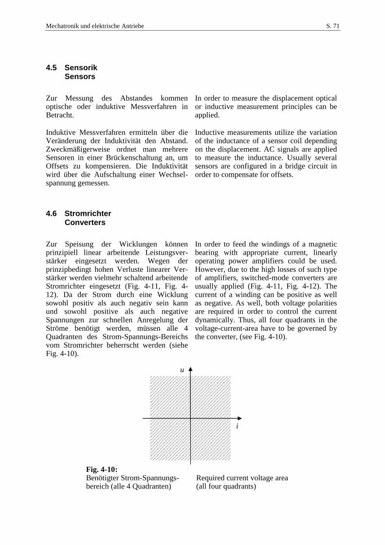
Mechatronik und elektrische Antriebe S. 71
4.5 Sensorik Sensors
Zur Messung des Abstandes kommen optische oder induktive Messverfahren in Betracht.
In order to measure the displacement optical or inductive measurement principles can be applied.
Induktive Messverfahren ermitteln über die Veränderung der Induktivität den Abstand. Zweckmäßigerweise ordnet man mehrere Sensoren in einer Brückenschaltung an, um Offsets zu kompensieren. Die Induktivität wird über die Aufschaltung einer Wechsel-spannung gemessen.
Inductive measurements utilize the variation of the inductance of a sensor coil depending on the displacement. AC signals are applied to measure the inductance. Usually several sensors are configured in a bridge circuit in order to compensate for offsets.
4.6 Stromrichter Converters
Zur Speisung der Wicklungen können prinzipiell linear arbeitende Leistungsver-stärker eingesetzt werden. Wegen der prinzipbedingt hohen Verluste linearer Ver-stärker werden vielmehr schaltend arbeitende Stromrichter eingesetzt (Fig. 4-11, Fig. 4-12). Da der Strom durch eine Wicklung sowohl positiv als auch negativ sein kann und sowohl positive als auch negative Spannungen zur schnellen Anregelung der Ströme benötigt werden, müssen alle 4 Quadranten des Strom-Spannungs-Bereichs vom Stromrichter beherrscht werden (siehe Fig. 4-10).
In order to feed the windings of a magnetic bearing with appropriate current, linearly operating power amplifiers could be used. However, due to the high losses of such type of amplifiers, switched-mode converters are usually applied (Fig. 4-11, Fig. 4-12). The current of a winding can be positive as well as negative. As well, both voltage polarities are required in order to control the current dynamically. Thus, all four quadrants in the voltage-current-area have to be governed by the converter, (see Fig. 4-10).
Fig. 4-10: Benötigter Strom-Spannungs-bereich (alle 4 Quadranten)
Required current voltage area (all four quadrants)
i
u
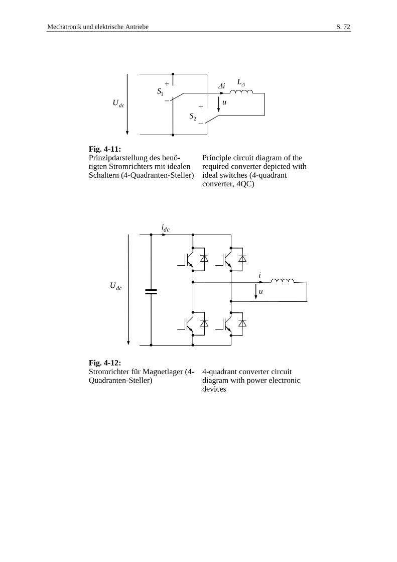
Mechatronik und elektrische Antriebe S. 72
Fig. 4-11: Prinzipdarstellung des benö-tigten Stromrichters mit idealen Schaltern (4-Quadranten-Steller)
Principle circuit diagram of the required converter depicted with ideal switches (4-quadrant converter, 4QC)
Fig. 4-12: Stromrichter für Magnetlager (4-Quadranten-Steller)
4-quadrant converter circuit diagram with power electronic devices
dcUu
i
dci
dcU
1S
2S
u
i
L
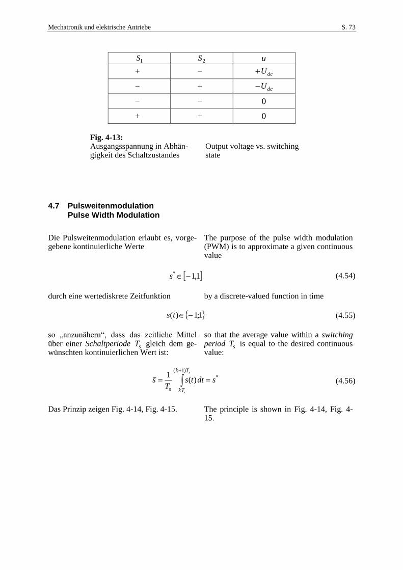
Mechatronik und elektrische Antriebe S. 73
1S 2S u
dcU
dcU
0
0
Fig. 4-13: Ausgangsspannung in Abhän-gigkeit des Schaltzustandes
Output voltage vs. switching state
4.7 Pulsweitenmodulation Pulse Width Modulation
Die Pulsweitenmodulation erlaubt es, vorge-gebene kontinuierliche Werte
The purpose of the pulse width modulation (PWM) is to approximate a given continuous value
1,1* s (4.54)
durch eine wertediskrete Zeitfunktion by a discrete-valued function in time
1;1)( ts (4.55)
so „anzunähern“, dass das zeitliche Mittel über einer Schaltperiode sT gleich dem ge-wünschten kontinuierlichen Wert ist:
so that the average value within a switching period sT is equal to the desired continuous value:
*
)1(
)(1
sdttsT
ss
s
Tk
kTs
(4.56)
Das Prinzip zeigen Fig. 4-14, Fig. 4-15. The principle is shown in Fig. 4-14, Fig. 4-
15.
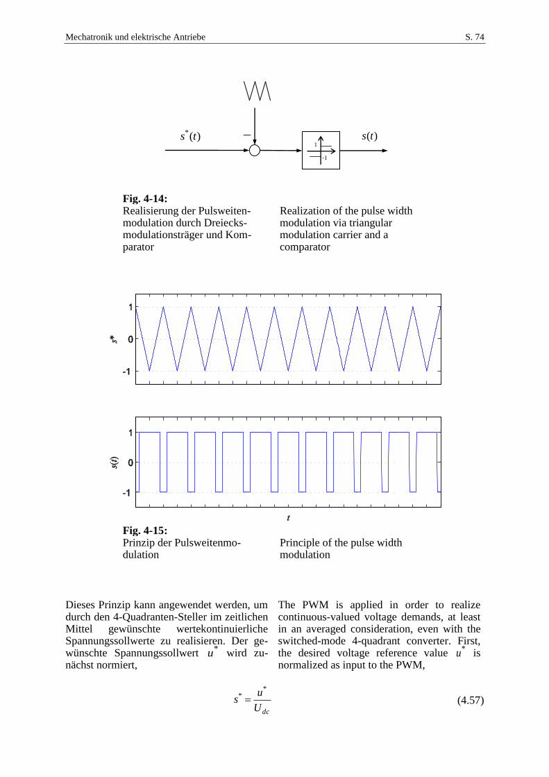
Mechatronik und elektrische Antriebe S. 74
Fig. 4-14: Realisierung der Pulsweiten-modulation durch Dreiecks-modulationsträger und Kom-parator
Realization of the pulse width modulation via triangular modulation carrier and a comparator
Fig. 4-15: Prinzip der Pulsweitenmo-dulation
Principle of the pulse width modulation
Dieses Prinzip kann angewendet werden, um durch den 4-Quadranten-Steller im zeitlichen Mittel gewünschte wertekontinuierliche Spannungssollwerte zu realisieren. Der ge-wünschte Spannungssollwert *u wird zu-nächst normiert,
The PWM is applied in order to realize continuous-valued voltage demands, at least in an averaged consideration, even with the switched-mode 4-quadrant converter. First, the desired voltage reference value *u is normalized as input to the PWM,
dcU
us
** (4.57)
1
-1
)(* ts )(ts
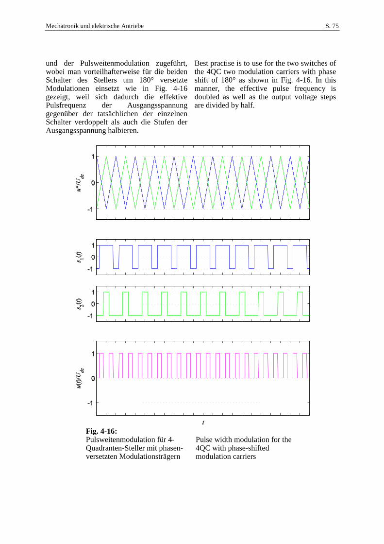
Mechatronik und elektrische Antriebe S. 75
und der Pulsweitenmodulation zugeführt, wobei man vorteilhafterweise für die beiden Schalter des Stellers um 180° versetzte Modulationen einsetzt wie in Fig. 4-16 gezeigt, weil sich dadurch die effektive Pulsfrequenz der Ausgangsspannung gegenüber der tatsächlichen der einzelnen Schalter verdoppelt als auch die Stufen der Ausgangsspannung halbieren.
Best practise is to use for the two switches of the 4QC two modulation carriers with phase shift of 180° as shown in Fig. 4-16. In this manner, the effective pulse frequency is doubled as well as the output voltage steps are divided by half.
Fig. 4-16: Pulsweitenmodulation für 4-Quadranten-Steller mit phasen-versetzten Modulationsträgern
Pulse width modulation for the 4QC with phase-shifted modulation carriers
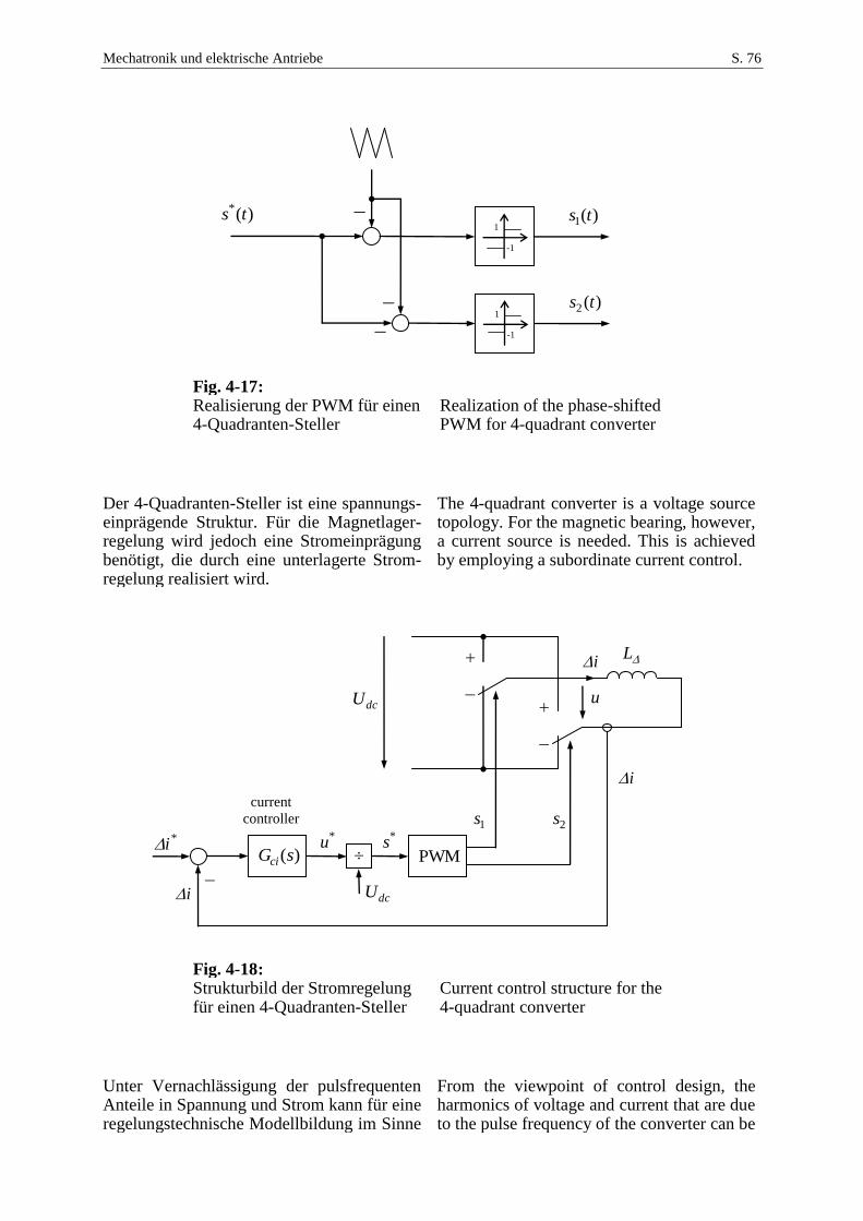
Mechatronik und elektrische Antriebe S. 76
Fig. 4-17: Realisierung der PWM für einen 4-Quadranten-Steller
Realization of the phase-shifted PWM for 4-quadrant converter
Der 4-Quadranten-Steller ist eine spannungs-einprägende Struktur. Für die Magnetlager-regelung wird jedoch eine Stromeinprägung benötigt, die durch eine unterlagerte Strom-regelung realisiert wird.
The 4-quadrant converter is a voltage source topology. For the magnetic bearing, however, a current source is needed. This is achieved by employing a subordinate current control.
Fig. 4-18: Strukturbild der Stromregelung für einen 4-Quadranten-Steller
Current control structure for the 4-quadrant converter
Unter Vernachlässigung der pulsfrequenten Anteile in Spannung und Strom kann für eine regelungstechnische Modellbildung im Sinne
From the viewpoint of control design, the harmonics of voltage and current that are due to the pulse frequency of the converter can be
dcU u
i
PWM
1s 2s
i
i
)(sGci
current
controller
dcU
*s*u
L
*i
1
-1
)(* ts )(1 ts
1
-1
)(2 ts
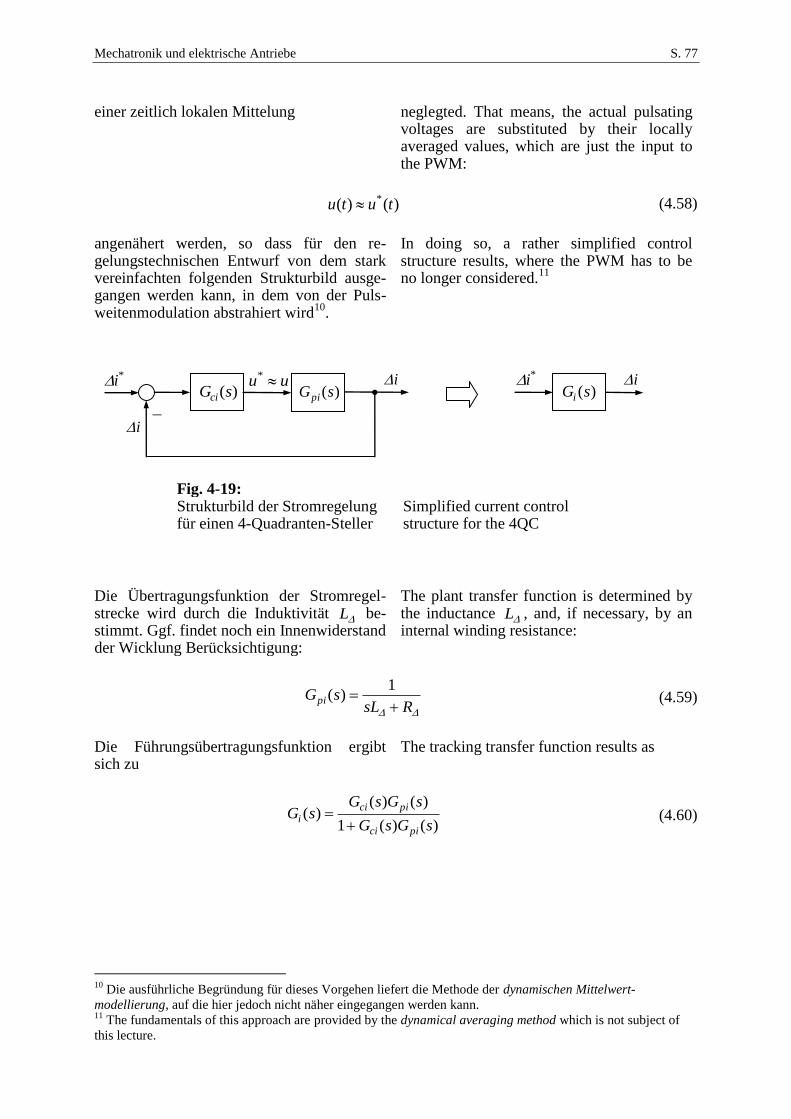
Mechatronik und elektrische Antriebe S. 77
einer zeitlich lokalen Mittelung neglegted. That means, the actual pulsating voltages are substituted by their locally averaged values, which are just the input to the PWM:
)()( * tutu (4.58)
angenähert werden, so dass für den re-gelungstechnischen Entwurf von dem stark vereinfachten folgenden Strukturbild ausge-gangen werden kann, in dem von der Puls-weitenmodulation abstrahiert wird
10.
In doing so, a rather simplified control structure results, where the PWM has to be no longer considered.
11
Fig. 4-19: Strukturbild der Stromregelung für einen 4-Quadranten-Steller
Simplified current control structure for the 4QC
Die Übertragungsfunktion der Stromregel-strecke wird durch die Induktivität L be-stimmt. Ggf. findet noch ein Innenwiderstand der Wicklung Berücksichtigung:
The plant transfer function is determined by the inductance L , and, if necessary, by an internal winding resistance:
RsLsGpi
1)( (4.59)
Die Führungsübertragungsfunktion ergibt sich zu
The tracking transfer function results as
)()(1
)()()(
sGsG
sGsGsG
pici
picii
(4.60)
10
Die ausführliche Begründung für dieses Vorgehen liefert die Methode der dynamischen Mittelwert-
modellierung, auf die hier jedoch nicht näher eingegangen werden kann. 11
The fundamentals of this approach are provided by the dynamical averaging method which is not subject of
this lecture.
*i
i
)(sGci )(sGpi
i)(sGi
i*iuu *
Mechatronik und elektrische Antriebe S. 78
Als Regler könnte ein PI- aber auch ein ein-facher P-Regler zum Einsatz kommen. Letz-terer kann zwar keinen Regelfehler von Null garantieren, doch wird ein stationärer Regel-fehler durch den integralen Anteil im über-lagerten Lageregler ausgeglichen. Mit
As controller, PI as well as P-types can be applied. The latter cannot guarantee a stationary zero control error. That can be accepted, however, because the integral action of an overlaid position control would compensate for this error. With
ici KsG )( (4.61)
folgt it follows
i
i
i
ii
s
V
sLRK
KsG
1)( (4.62)
mit where
i
iKR
V/1
1
,
RK
L
i
i
Für kleinen Innenwiderstand bzw. hohe Reglerverstärkung resultiert das weiter oben angenommene Verzögerungsverhalten des Stromstellglieds.
For small winding resistance or high controller gain iV is close to 1 and the above mentioned delay behavior of the controlled current source results.
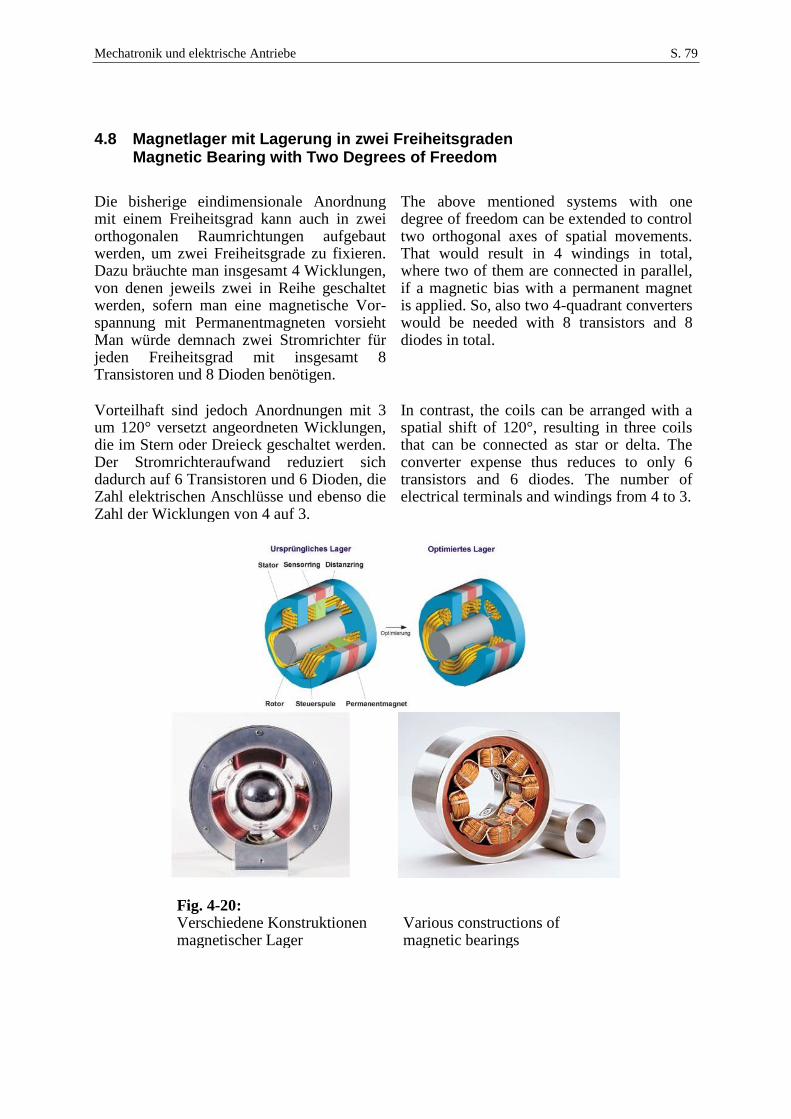
Mechatronik und elektrische Antriebe S. 79
4.8 Magnetlager mit Lagerung in zwei Freiheitsgraden Magnetic Bearing with Two Degrees of Freedom
Die bisherige eindimensionale Anordnung mit einem Freiheitsgrad kann auch in zwei orthogonalen Raumrichtungen aufgebaut werden, um zwei Freiheitsgrade zu fixieren. Dazu bräuchte man insgesamt 4 Wicklungen, von denen jeweils zwei in Reihe geschaltet werden, sofern man eine magnetische Vor-spannung mit Permanentmagneten vorsieht Man würde demnach zwei Stromrichter für jeden Freiheitsgrad mit insgesamt 8 Transistoren und 8 Dioden benötigen.
The above mentioned systems with one degree of freedom can be extended to control two orthogonal axes of spatial movements. That would result in 4 windings in total, where two of them are connected in parallel, if a magnetic bias with a permanent magnet is applied. So, also two 4-quadrant converters would be needed with 8 transistors and 8 diodes in total.
Vorteilhaft sind jedoch Anordnungen mit 3 um 120° versetzt angeordneten Wicklungen, die im Stern oder Dreieck geschaltet werden. Der Stromrichteraufwand reduziert sich dadurch auf 6 Transistoren und 6 Dioden, die Zahl elektrischen Anschlüsse und ebenso die Zahl der Wicklungen von 4 auf 3.
In contrast, the coils can be arranged with a spatial shift of 120°, resulting in three coils that can be connected as star or delta. The converter expense thus reduces to only 6 transistors and 6 diodes. The number of electrical terminals and windings from 4 to 3.
Fig. 4-20: Verschiedene Konstruktionen magnetischer Lager
Various constructions of magnetic bearings
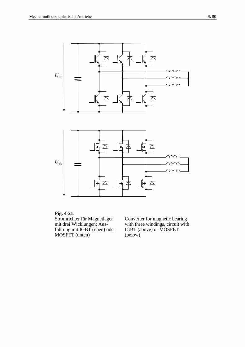
Mechatronik und elektrische Antriebe S. 80
Fig. 4-21: Stromrichter für Magnetlager mit drei Wicklungen; Aus-führung mit IGBT (oben) oder MOSFET (unten)
Converter for magnetic bearing with three windings, circuit with IGBT (above) or MOSFET (below)
dcU
dcU
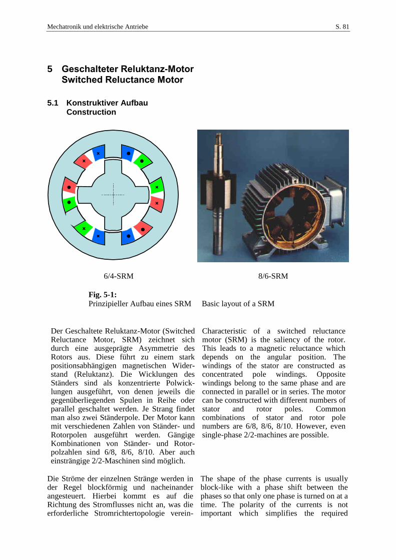
Mechatronik und elektrische Antriebe S. 81
5 Geschalteter Reluktanz-Motor Switched Reluctance Motor
5.1 Konstruktiver Aufbau Construction
6/4-SRM
8/6-SRM
Fig. 5-1:
Prinzipieller Aufbau eines SRM Basic layout of a SRM
Der Geschaltete Reluktanz-Motor (Switched Reluctance Motor, SRM) zeichnet sich durch eine ausgeprägte Asymmetrie des Rotors aus. Diese führt zu einem stark positionsabhängigen magnetischen Wider-stand (Reluktanz). Die Wicklungen des Ständers sind als konzentrierte Polwick-lungen ausgeführt, von denen jeweils die gegenüberliegenden Spulen in Reihe oder parallel geschaltet werden. Je Strang findet man also zwei Ständerpole. Der Motor kann mit verschiedenen Zahlen von Ständer- und Rotorpolen ausgeführt werden. Gängige Kombinationen von Ständer- und Rotor-polzahlen sind 6/8, 8/6, 8/10. Aber auch einsträngige 2/2-Maschinen sind möglich.
Characteristic of a switched reluctance motor (SRM) is the saliency of the rotor. This leads to a magnetic reluctance which depends on the angular position. The windings of the stator are constructed as concentrated pole windings. Opposite windings belong to the same phase and are connected in parallel or in series. The motor can be constructed with different numbers of stator and rotor poles. Common combinations of stator and rotor pole numbers are 6/8, 8/6, 8/10. However, even single-phase 2/2-machines are possible.
Die Ströme der einzelnen Stränge werden in der Regel blockförmig und nacheinander angesteuert. Hierbei kommt es auf die Richtung des Stromflusses nicht an, was die erforderliche Stromrichtertopologie verein-
The shape of the phase currents is usually block-like with a phase shift between the phases so that only one phase is turned on at a time. The polarity of the currents is not important which simplifies the required
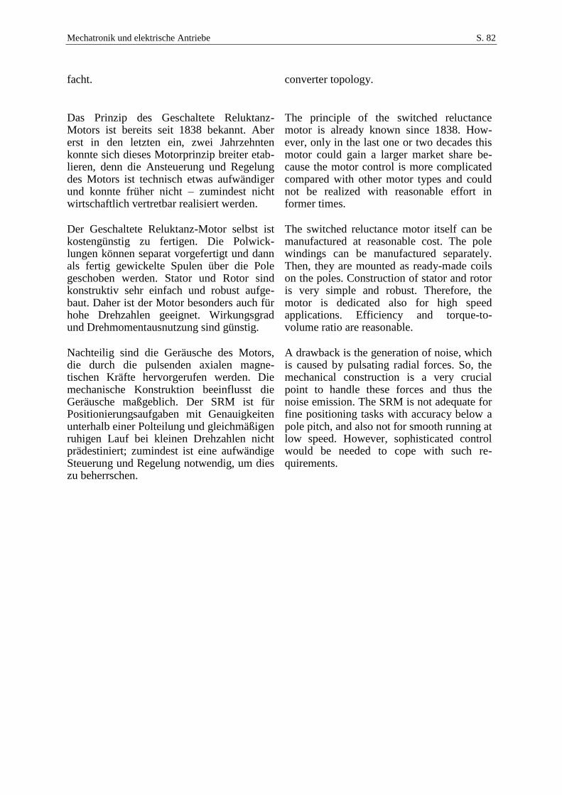
Mechatronik und elektrische Antriebe S. 82
facht. converter topology.
Das Prinzip des Geschaltete Reluktanz-Motors ist bereits seit 1838 bekannt. Aber erst in den letzten ein, zwei Jahrzehnten konnte sich dieses Motorprinzip breiter etab-lieren, denn die Ansteuerung und Regelung des Motors ist technisch etwas aufwändiger und konnte früher nicht – zumindest nicht wirtschaftlich vertretbar realisiert werden.
The principle of the switched reluctance motor is already known since 1838. How-ever, only in the last one or two decades this motor could gain a larger market share be-cause the motor control is more complicated compared with other motor types and could not be realized with reasonable effort in former times.
Der Geschaltete Reluktanz-Motor selbst ist kostengünstig zu fertigen. Die Polwick-lungen können separat vorgefertigt und dann als fertig gewickelte Spulen über die Pole geschoben werden. Stator und Rotor sind konstruktiv sehr einfach und robust aufge-baut. Daher ist der Motor besonders auch für hohe Drehzahlen geeignet. Wirkungsgrad und Drehmomentausnutzung sind günstig.
The switched reluctance motor itself can be manufactured at reasonable cost. The pole windings can be manufactured separately. Then, they are mounted as ready-made coils on the poles. Construction of stator and rotor is very simple and robust. Therefore, the motor is dedicated also for high speed applications. Efficiency and torque-to-volume ratio are reasonable.
Nachteilig sind die Geräusche des Motors, die durch die pulsenden axialen magne-tischen Kräfte hervorgerufen werden. Die mechanische Konstruktion beeinflusst die Geräusche maßgeblich. Der SRM ist für Positionierungsaufgaben mit Genauigkeiten unterhalb einer Polteilung und gleichmäßigen ruhigen Lauf bei kleinen Drehzahlen nicht prädestiniert; zumindest ist eine aufwändige Steuerung und Regelung notwendig, um dies zu beherrschen.
A drawback is the generation of noise, which is caused by pulsating radial forces. So, the mechanical construction is a very crucial point to handle these forces and thus the noise emission. The SRM is not adequate for fine positioning tasks with accuracy below a pole pitch, and also not for smooth running at low speed. However, sophisticated control would be needed to cope with such re-quirements.
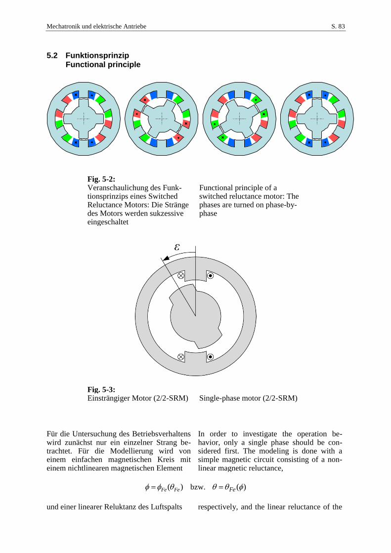
Mechatronik und elektrische Antriebe S. 83
5.2 Funktionsprinzip Functional principle
Fig. 5-2: Veranschaulichung des Funk-tionsprinzips eines Switched Reluctance Motors: Die Stränge des Motors werden sukzessive eingeschaltet
Functional principle of a switched reluctance motor: The phases are turned on phase-by-phase
Fig. 5-3: Einsträngiger Motor (2/2-SRM) Single-phase motor (2/2-SRM)
Für die Untersuchung des Betriebsverhaltens wird zunächst nur ein einzelner Strang be-trachtet. Für die Modellierung wird von einem einfachen magnetischen Kreis mit einem nichtlinearen magnetischen Element
In order to investigate the operation be-havior, only a single phase should be con-sidered first. The modeling is done with a simple magnetic circuit consisting of a non-linear magnetic reluctance,
)( FeFe bzw. )( Fe
und einer linearer Reluktanz des Luftspalts respectively, and the linear reluctance of the
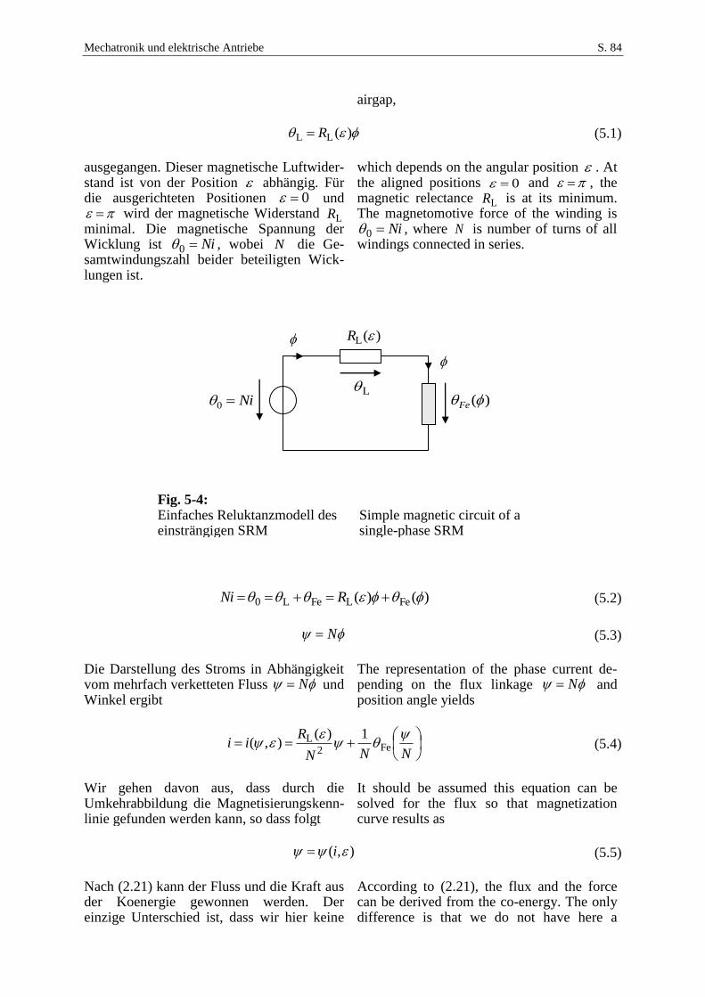
Mechatronik und elektrische Antriebe S. 84
airgap,
)(LL R (5.1)
ausgegangen. Dieser magnetische Luftwider-stand ist von der Position abhängig. Für die ausgerichteten Positionen 0 und
wird der magnetische Widerstand LR minimal. Die magnetische Spannung der Wicklung ist Ni0 , wobei N die Ge-samtwindungszahl beider beteiligten Wick-lungen ist.
which depends on the angular position . At the aligned positions 0 and , the magnetic relectance LR is at its minimum. The magnetomotive force of the winding is
Ni0 , where N is number of turns of all windings connected in series.
Fig. 5-4: Einfaches Reluktanzmodell des einsträngigen SRM
Simple magnetic circuit of a single-phase SRM
)()( FeLFeL0 RNi (5.2)
N (5.3)
Die Darstellung des Stroms in Abhängigkeit vom mehrfach verketteten Fluss N und Winkel ergibt
The representation of the phase current de-pending on the flux linkage N and position angle yields
NNN
Rii
Fe2
L 1)(),( (5.4)
Wir gehen davon aus, dass durch die Umkehrabbildung die Magnetisierungskenn-linie gefunden werden kann, so dass folgt
It should be assumed this equation can be solved for the flux so that magnetization curve results as
),( i (5.5)
Nach (2.21) kann der Fluss und die Kraft aus der Koenergie gewonnen werden. Der einzige Unterschied ist, dass wir hier keine
According to (2.21), the flux and the force can be derived from the co-energy. The only difference is that we do not have here a
)(FeNi0
)(L R
L
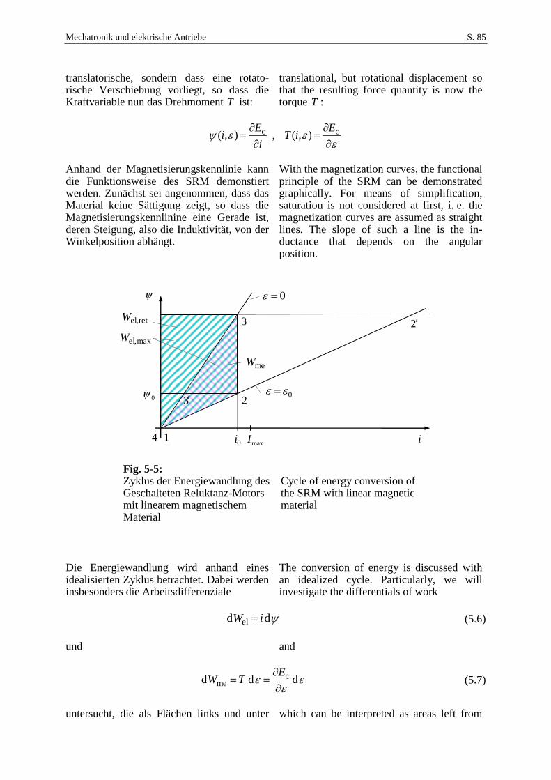
Mechatronik und elektrische Antriebe S. 85
translatorische, sondern dass eine rotato-rische Verschiebung vorliegt, so dass die Kraftvariable nun das Drehmoment T ist:
translational, but rotational displacement so that the resulting force quantity is now the torque T :
i
Ei
c),( ,
c),(
EiT
Anhand der Magnetisierungskennlinie kann die Funktionsweise des SRM demonstiert werden. Zunächst sei angenommen, dass das Material keine Sättigung zeigt, so dass die Magnetisierungskennlinine eine Gerade ist, deren Steigung, also die Induktivität, von der Winkelposition abhängt.
With the magnetization curves, the functional principle of the SRM can be demonstrated graphically. For means of simplification, saturation is not considered at first, i. e. the magnetization curves are assumed as straight lines. The slope of such a line is the in-ductance that depends on the angular position.
Fig. 5-5: Zyklus der Energiewandlung des Geschalteten Reluktanz-Motors mit linearem magnetischem Material
Cycle of energy conversion of the SRM with linear magnetic material
Die Energiewandlung wird anhand eines idealisierten Zyklus betrachtet. Dabei werden insbesonders die Arbeitsdifferenziale
The conversion of energy is discussed with an idealized cycle. Particularly, we will investigate the differentials of work
dd el iW (5.6)
und and
ddd cme
ETW (5.7)
untersucht, die als Flächen links und unter which can be interpreted as areas left from
0
1
3
0i
maxel,W
2
4
0
meW
30
2
imaxI
retel,W
Mechatronik und elektrische Antriebe S. 86
der Magnetisierungskurve interpretiert werden können (vgl. Fig. 2-4). Wir beginnen im
and below the magnetization curve (cf. Fig. 2-4). Let us begin in
Zustand 1: 0i , 0
Der Rotor befindet sich in einer nicht ausgerichteten Position 0 . Die Spule ist stromlos. Nun wird der Strom bis auf den Wert 0i i erhöht. Wir gehen im Gedankenexperiment davon aus, dass sich der Rotor während dieser Auf-magnetisierung nicht bewegt bzw. fest-gebremst ist. Wir gelangen dann in den
State 1: 0i , 0 The rotor is in an unaligned position
0 . The winding is turned off, the current is zero. Then, the current is increased from zero to the final value
0i i . During this time of magnetizing the rotor is assumed not to move or to be fixed by a brake. As a result, the next state is …
Zustand 2: 0i i , 0
Bis hierhin wurde die elektrische Arbeit
State 2: 0i i , 0 Until now, the electric work supplied to the motor is
2
1
2,1el diW (5.8)
verrichtet, die sich als Dreiecksfläche zwischen der Geraden 1-2 und der -Achse interpretieren lässt. Bei Übergang zwischen Zustand 1 und 2 wurde keinerlei mechanische Arbeit geleistet.
Nun wird der Rotor freigegeben, so dass sich dieser in die ausgerichtete Position drehen kann. Dabei werde der Strom konstant gehalten:
which is the triangular area between the line 1-2 and the -axis. During the transition between state 1 and state 2 no mechanical work is done. Now, the rotor is released so that it can move to the aligned position. During that movement, the current is kept constant, resulting in the new state
Zustand 3: 0i i , 0
Der Rotor hat sich unter den Statorpolen ausgerichtet. Bis hierhin wurde die elektrische Arbeit
State 3: 0i i , 0 The rotor has now aligned to the stator poles. Until now, the electrical work fed into the motor is
3
1
3,1elmaxel, diWW (5.9)
geleistet. Das ist die Fläche zwischen dem Kurvenzug 1-2-3 und der -Achse. Während des Übergangs von der Position 2 in die Position 3 wird die mechanische Arbeit
which is the area between the curve 1-2-3 and the -axis. During the transition from position 2 and 3, the motor provides the mechanical work
Mechatronik und elektrische Antriebe S. 87
3
1
me dcE
W (5.10)
geleistet. Das ist die vom Dreieck 1-2-3 gebildete Fläche, also die Änderung der Fläche unter der Magnetisierungskurve.
Im ausgerichteten Zustand wird der Rotor dann gedanklich wieder festgehalten und dann der Strom ausgeschaltet, so dass wir in den
This is the area of the triangle 1-2-3, i.e. the change of the area below the magnetization curve. In the aligned position, the rotor is assumed to be fixed again and then the current is turned off, resulting in …
Zustand 4: 0i , 0
gelangen. Während dieser Entmagne-tisierung wird die noch in der Spule befindliche innere Energie an die elektrische Einspeisung zurückgegeben:
State 4: 0i , 0
During this demagnetization, the stored magnetic energy of the winding is re-turned to the electrical energy supply:
4
3
retel, diW (5.11)
Das ist die Dreiecksfläche zwischen der Geraden 3-4 und der -Achse.
This is the area of the triangle between line 3-4 and the -axis.
Unter Vernachlässigung von ohmschen und Ummagnetisierungsverlusten gilt in der Ge-samtbilanz
Neglecting ohmic voltage drops and hysteresis losses, the total balance results as
retel,maxel,elme WWWW (5.12)
. Da aber von der elektrischen Einspeisung zunächst einmal der Spitzenwert maxel,W auf-gebracht werden muss, ist es gerechtfertigt, einen Leistungsfaktor ähnlich wie bei Wechsel- oder Drehstromsystemen zu de-finieren:
However, because the electrical supply must provide the full peak value maxel,W before a part of the work is returned, it is reasonable to introduce a power factor similar to that of common one-phase or three-phase AC systems like
maxel,
retel,
maxel,
me 1W
W
W
W (5.13)
Bei linearem Material kann dieser Leistungs-faktor prinzipiell nicht besser als 0,5 sein, wie aus der grafischen Darstellung sofort einsichtig wird:
Using linear materials, this power factor cannot be better as 0.5 by principle as it can be seen directly from the graphical representation:
5.0 (5.14)
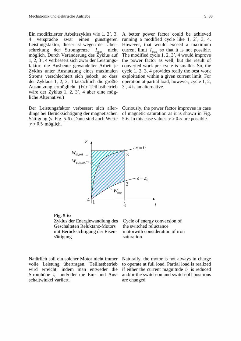
Mechatronik und elektrische Antriebe S. 88
Ein modifizierter Arbeitszyklus wie 1, 2´, 3, 4 verspräche zwar einen günstigeren Leistungsfaktor, dieser ist wegen der Über-schreitung der Stromgrenze maxI nicht möglich. Durch Veränderung des Zyklus auf 1, 2, 3´, 4 verbessert sich zwar der Leistungs-faktor, die Ausbeute gewandelter Arbeit je Zyklus unter Ausnutzung eines maximalen Stroms verschlechtert sich jedoch, so dass der Zyklaus 1, 2, 3, 4 tatsächlich die größte Ausnutzung ermöglicht. (Für Teillastbetrieb wäre der Zyklus 1, 2, 3´, 4 aber eine mög-liche Alternative.)
A better power factor could be achieved running a modified cycle like 1, 2´, 3, 4. However, that would exceed a maximum current limit maxI so that it is not possible. The modified cycle 1, 2, 3´, 4 would improve the power factor as well, but the result of converted work per cycle is smaller. So, the cycle 1, 2, 3, 4 provides really the best work exploitation within a given current limit. For operation at partial load, however, cycle 1, 2, 3´, 4 is an alternative.
Der Leistungsfaktor verbessert sich aller-dings bei Berücksichtigung der magnetischen Sättigung (s. Fig. 5-6). Dann sind auch Werte
5.0 möglich.
Curiously, the power factor improves in case of magnetic saturation as it is shown in Fig. 5-6. In this case values 5.0 are possible.
Fig. 5-6: Zyklus der Energiewandlung des Geschalteten Reluktanz-Motors mit Berücksichtigung der Eisen-sättigung
Cycle of energy conversion of the switched reluctance motorwith consideration of iron saturation
Natürlich soll ein solcher Motor nicht immer volle Leistung übertragen. Teillastbetrieb wird erreicht, indem man entweder die Stromhöhe 0i und/oder die Ein- und Aus-schaltwinkel variiert.
Naturally, the motor is not always in charge to operate at full load. Partial load is realized if either the current magnitude 0i is reduced and/or the switch-on and switch-off positions are changed.
0
i1
2
0i
meW
maxel,W
4
0
3retel,W
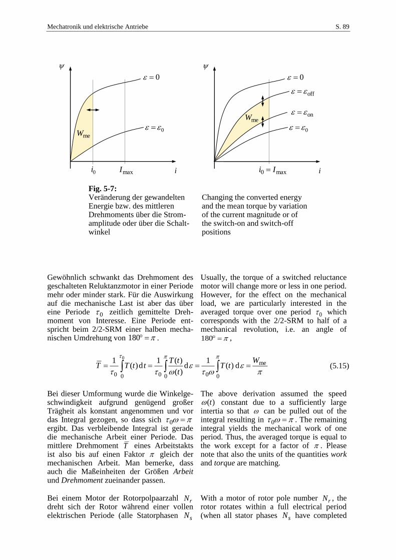
Mechatronik und elektrische Antriebe S. 89
Fig. 5-7: Veränderung der gewandelten Energie bzw. des mittleren Drehmoments über die Strom-amplitude oder über die Schalt-winkel
Changing the converted energy and the mean torque by variation of the current magnitude or of the switch-on and switch-off positions
Gewöhnlich schwankt das Drehmoment des geschalteten Reluktanzmotor in einer Periode mehr oder minder stark. Für die Auswirkung auf die mechanische Last ist aber das über eine Periode 0 zeitlich gemittelte Dreh-moment von Interesse. Eine Periode ent-spricht beim 2/2-SRM einer halben mecha-nischen Umdrehung von 180 .
Usually, the torque of a switched reluctance motor will change more or less in one period. However, for the effect on the mechanical load, we are particularly interested in the averaged torque over one period 0 which corresponds with the 2/2-SRM to half of a mechanical revolution, i.e. an angle of
180 ,
me
000000
d)(1
d)(
)(1d)(
1 0 WtT
t
tTttTT (5.15)
Bei dieser Umformung wurde die Winkelge-schwindigkeit aufgrund genügend großer Trägheit als konstant angenommen und vor das Integral gezogen, so dass sich 0 ergibt. Das verbleibende Integral ist gerade die mechanische Arbeit einer Periode. Das mittlere Drehmoment T eines Arbeitstakts ist also bis auf einen Faktor gleich der mechanischen Arbeit. Man bemerke, dass auch die Maßeinheiten der Größen Arbeit und Drehmoment zueinander passen.
The above derivation assumed the speed )(t constant due to a sufficiently large
intertia so that can be pulled out of the integral resulting in 0 . The remaining integral yields the mechanical work of one period. Thus, the averaged torque is equal to the work except for a factor of . Please note that also the units of the quantities work and torque are matching.
Bei einem Motor der Rotorpolpaarzahl rN dreht sich der Rotor während einer vollen elektrischen Periode (alle Statorphasen sN
With a motor of rotor pole number rN , the rotor rotates within a full electrical period (when all stator phases sN have completed
0
i0i
0
0
imax0 Ii
meW
0
maxI
on
off
meW
Mechatronik und elektrische Antriebe S. 90
durchlaufen genau einen Arbeitstakt) da-gegen nur um den Winkel r/ N . Außerdem leistet jeder der sN Statorstränge bzw. -Polpaare die gleiche Arbeit meW , also
one cycle) only by the angle r/ N . Additionally, each of the sN stator phases (or stator pole pairs) contribute with the same amount of work meW , resulting in the total work balance
mesWNT (5.16)
. Hieraus bestimmt sich das mittlere Dreh-moment eines rs 2/2 NN -Motors also zu
This yields the mean torque of a rs 2/2 NN -Motors as
me
rs
WNNT (5.17)
Drückt man die Drehfrequenz des Rotors durch die Kommutierungsfrequenz Kf (die Frequenz der Arbeitstakte) aus, erhält man für die mechanische Winkelgeschwindigkeit
Let the commutation frequency be Kf (the frequency of turning the current from one phase to the next). Then the resulting speed is
rs
K
Ks / NN
f
fN
(5.18)
bzw. für die mittlere Leistung and the averaged power is
meKWfTP (5.19)
5.3 Dynamisches Verhalten Dynamic Behavior
Bislang wurde die Energiewandlung des Ge-schalteten Reluktanz-Motors unter Ver-nachlässigung der Dynamik betrachtet. Tatsächlich benötigen die Übergänge zwischen den verschiedenen Zuständen Zeit, während der sich der Motor weiterdreht.
So far, the energy conversion was discussed without considering the dynamic behavior. In reality, the transistion between the idealized states require time, and during this time, the motor continues its rotation.
Ausgangspunkt ist das Induktionsgesetz Starting point is Faraday’s law:
Riu (5.20)
Mit With
),( i (5.21)
folgt für die Zeitableitung des Flusses The time derivative of the flux follows as
ii (5.22)
Mechatronik und elektrische Antriebe S. 91
sowie für die Spannung and then the voltage
iiRiu . (5.23)
Die Auflösung nach der Stromableitung liefert
Solving this equation for the derivative of the current yields
),(),(
c2
iL
i
TRiu
iL
i
ERiu
i
Riu
i
, (5.24)
mit with
(5.25)
und der differenziellen Induktivität and the differential inductance
2c
2
),(i
E
iiL
(5.26)
Bei konstantem Strom .constIi ist die erforderliche Spannung
In stationary case with constant current .constIi the required stationary voltage
results as
i
ERIRIU
c
2
0 (5.27)
Im Folgenden wird vereinfachend lineares magnetisches Material mit einer dann kon-stanten Reluktanz FeR betrachtet. Die Induk-tivität ist unter dieser Annahme nicht mehr vom Strom, sondern nur noch vom Winkel abhängig:
For means of simplicity, the magnetic material is assumed as linear with a constant reluctance FeR in the following section. With this assumption, the inductance no longer depends on the current, but on the rotation angle only:
2
Fe L
( )( )
NL
R R
(5.28)
Für den Fluss gilt The flux is then
iL )( (5.29)
. Die innere und die Ko-Energie resultieren zu The internal energy and the co-energy result
as
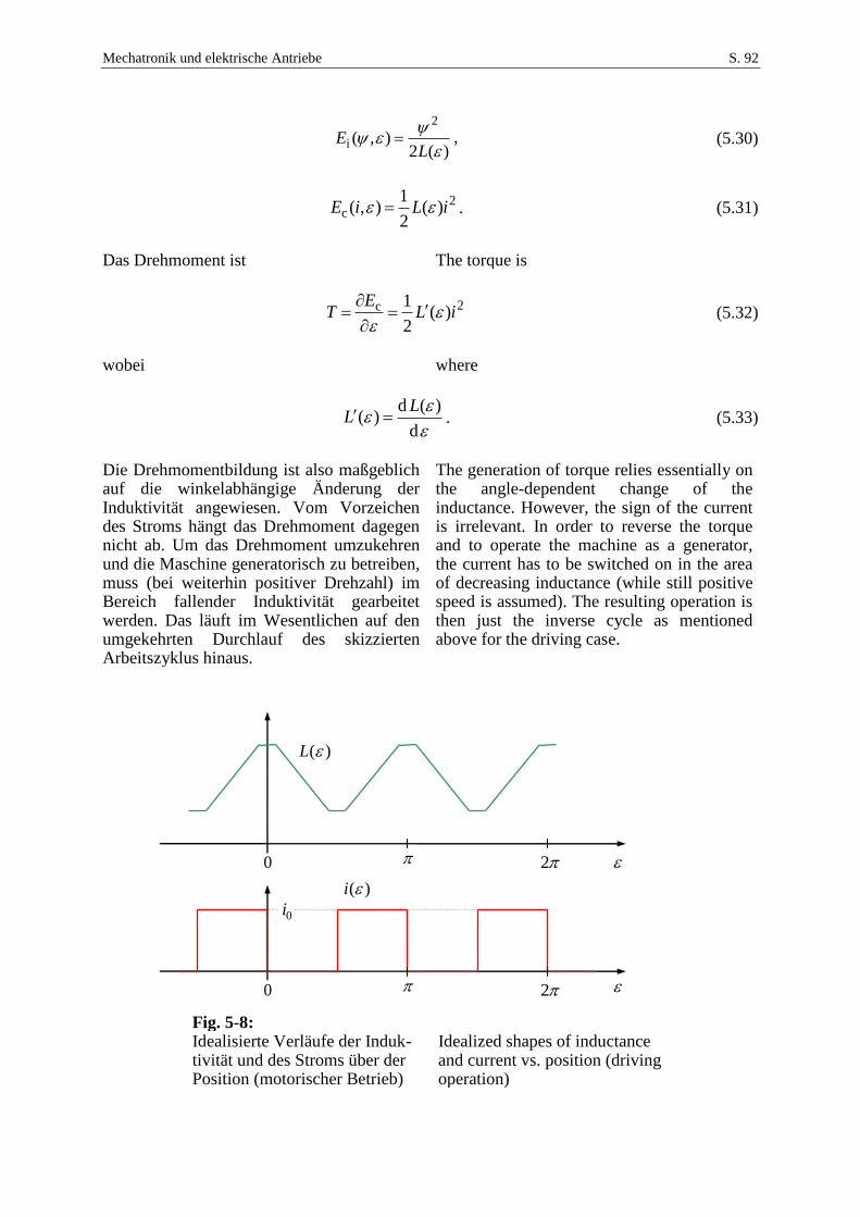
Mechatronik und elektrische Antriebe S. 92
)(2),(
2
i
LE , (5.30)
2c )(
2
1),( iLiE . (5.31)
Das Drehmoment ist The torque is
2c )(2
1iL
ET
(5.32)
wobei where
d
)(d)(
LL . (5.33)
Die Drehmomentbildung ist also maßgeblich auf die winkelabhängige Änderung der Induktivität angewiesen. Vom Vorzeichen des Stroms hängt das Drehmoment dagegen nicht ab. Um das Drehmoment umzukehren und die Maschine generatorisch zu betreiben, muss (bei weiterhin positiver Drehzahl) im Bereich fallender Induktivität gearbeitet werden. Das läuft im Wesentlichen auf den umgekehrten Durchlauf des skizzierten Arbeitszyklus hinaus.
The generation of torque relies essentially on the angle-dependent change of the inductance. However, the sign of the current is irrelevant. In order to reverse the torque and to operate the machine as a generator, the current has to be switched on in the area of decreasing inductance (while still positive speed is assumed). The resulting operation is then just the inverse cycle as mentioned above for the driving case.
Fig. 5-8: Idealisierte Verläufe der Induk-tivität und des Stroms über der Position (motorischer Betrieb)
Idealized shapes of inductance and current vs. position (driving operation)
0 2
)(L
0 2
0i
)(i
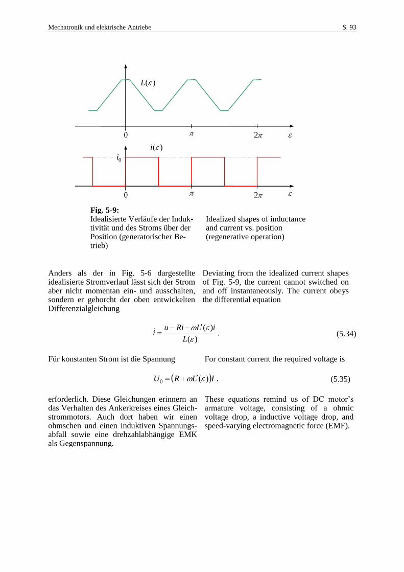
Mechatronik und elektrische Antriebe S. 93
Fig. 5-9: Idealisierte Verläufe der Induk-tivität und des Stroms über der Position (generatorischer Be-trieb)
Idealized shapes of inductance and current vs. position (regenerative operation)
Anders als der in Fig. 5-6 dargestellte idealisierte Stromverlauf lässt sich der Strom aber nicht momentan ein- und ausschalten, sondern er gehorcht der oben entwickelten Differenzialgleichung
Deviating from the idealized current shapes of Fig. 5-9, the current cannot switched on and off instantaneously. The current obeys the differential equation
)(
)(
L
iLRiui
. (5.34)
Für konstanten Strom ist die Spannung For constant current the required voltage is
ILRU )(0 . (5.35)
erforderlich. Diese Gleichungen erinnern an das Verhalten des Ankerkreises eines Gleich-strommotors. Auch dort haben wir einen ohmschen und einen induktiven Spannungs-abfall sowie eine drehzahlabhängige EMK als Gegenspannung.
These equations remind us of DC motor’s armature voltage, consisting of a ohmic voltage drop, a inductive voltage drop, and speed-varying electromagnetic force (EMF).
0 2
)(L
0 2
0i
)(i
Mechatronik und elektrische Antriebe S. 94
Abhängig von der Drehzahl sollen nun im Folgenden die zeitlichen Verläufe für den Arbeitszyklus qualitativ skizziert werden. Hierbei wird die speisende elektrische Energieversorgung als ideal steuerbare Quelle betrachtet, wobei allerdings eine Spannungsbegrenzung maxmax )( UtuU berücksichtigt werden soll.
The time behavior in a working cycle should now be discussed in detail for various cases of the speed. The feeding electrical supply is considered as a freely controllable voltage source within the limits
maxmax )( UtuU .
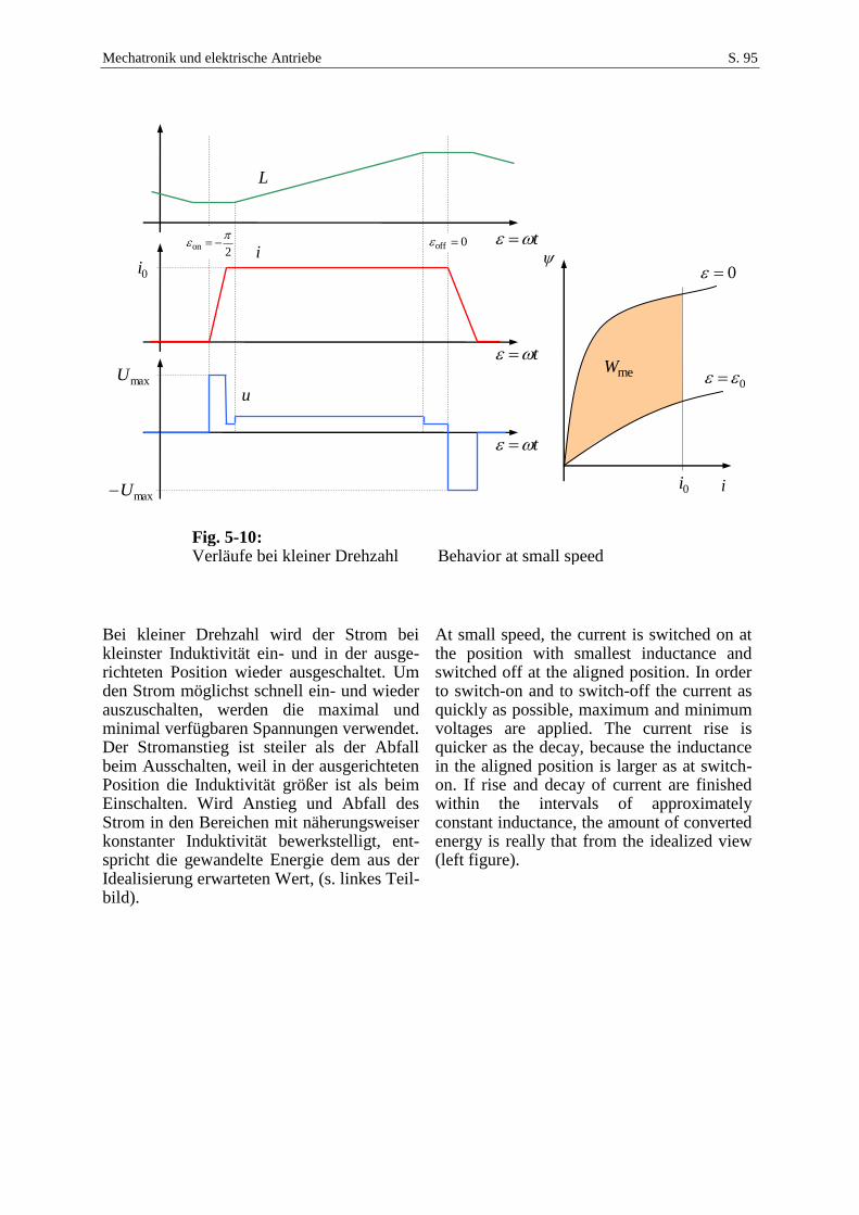
Mechatronik und elektrische Antriebe S. 95
Fig. 5-10: Verläufe bei kleiner Drehzahl Behavior at small speed
Bei kleiner Drehzahl wird der Strom bei kleinster Induktivität ein- und in der ausge-richteten Position wieder ausgeschaltet. Um den Strom möglichst schnell ein- und wieder auszuschalten, werden die maximal und minimal verfügbaren Spannungen verwendet. Der Stromanstieg ist steiler als der Abfall beim Ausschalten, weil in der ausgerichteten Position die Induktivität größer ist als beim Einschalten. Wird Anstieg und Abfall des Strom in den Bereichen mit näherungsweiser konstanter Induktivität bewerkstelligt, ent-spricht die gewandelte Energie dem aus der Idealisierung erwarteten Wert, (s. linkes Teil-bild).
At small speed, the current is switched on at the position with smallest inductance and switched off at the aligned position. In order to switch-on and to switch-off the current as quickly as possible, maximum and minimum voltages are applied. The current rise is quicker as the decay, because the inductance in the aligned position is larger as at switch-on. If rise and decay of current are finished within the intervals of approximately constant inductance, the amount of converted energy is really that from the idealized view (left figure).
0i
maxU
maxU
i
u
0
i0i
0 meW
2on
0off
L
t
t
t
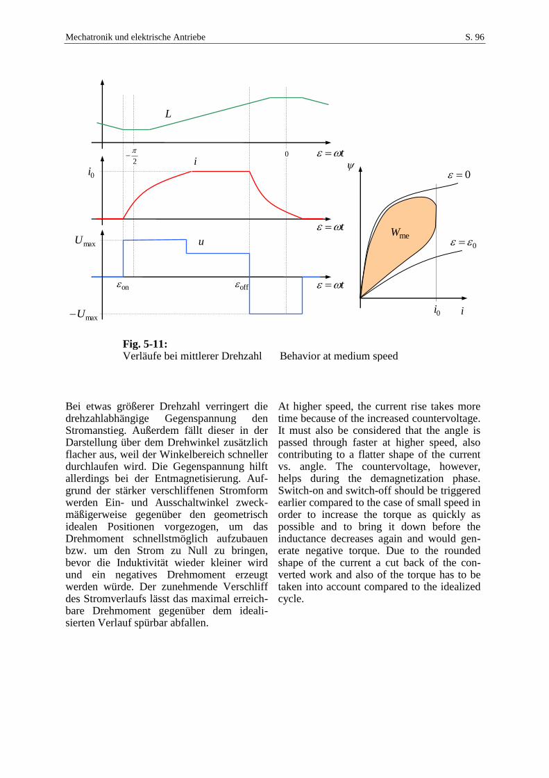
Mechatronik und elektrische Antriebe S. 96
Fig. 5-11: Verläufe bei mittlerer Drehzahl Behavior at medium speed
Bei etwas größerer Drehzahl verringert die drehzahlabhängige Gegenspannung den Stromanstieg. Außerdem fällt dieser in der Darstellung über dem Drehwinkel zusätzlich flacher aus, weil der Winkelbereich schneller durchlaufen wird. Die Gegenspannung hilft allerdings bei der Entmagnetisierung. Auf-grund der stärker verschliffenen Stromform werden Ein- und Ausschaltwinkel zweck-mäßigerweise gegenüber den geometrisch idealen Positionen vorgezogen, um das Drehmoment schnellstmöglich aufzubauen bzw. um den Strom zu Null zu bringen, bevor die Induktivität wieder kleiner wird und ein negatives Drehmoment erzeugt werden würde. Der zunehmende Verschliff des Stromverlaufs lässt das maximal erreich-bare Drehmoment gegenüber dem ideali-sierten Verlauf spürbar abfallen.
At higher speed, the current rise takes more time because of the increased countervoltage. It must also be considered that the angle is passed through faster at higher speed, also contributing to a flatter shape of the current vs. angle. The countervoltage, however, helps during the demagnetization phase. Switch-on and switch-off should be triggered earlier compared to the case of small speed in order to increase the torque as quickly as possible and to bring it down before the inductance decreases again and would gen-erate negative torque. Due to the rounded shape of the current a cut back of the con-verted work and also of the torque has to be taken into account compared to the idealized cycle.
0i
maxU
maxU
0
i0i
0
2
0
L
t
t
t
i
u
on
meW
off
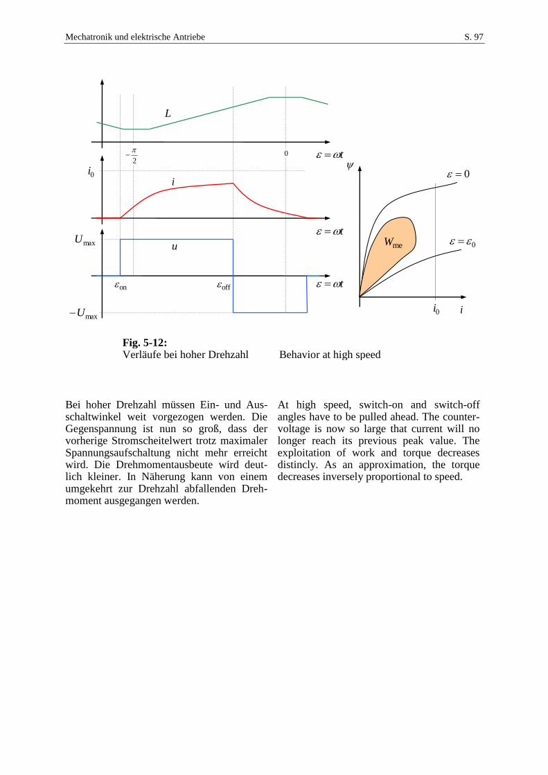
Mechatronik und elektrische Antriebe S. 97
Fig. 5-12: Verläufe bei hoher Drehzahl Behavior at high speed
Bei hoher Drehzahl müssen Ein- und Aus-schaltwinkel weit vorgezogen werden. Die Gegenspannung ist nun so groß, dass der vorherige Stromscheitelwert trotz maximaler Spannungsaufschaltung nicht mehr erreicht wird. Die Drehmomentausbeute wird deut-lich kleiner. In Näherung kann von einem umgekehrt zur Drehzahl abfallenden Dreh-moment ausgegangen werden.
At high speed, switch-on and switch-off angles have to be pulled ahead. The counter-voltage is now so large that current will no longer reach its previous peak value. The exploitation of work and torque decreases distincly. As an approximation, the torque decreases inversely proportional to speed.
0i
maxU
maxU
0
i0i
0
2
0
L
t
i
u
t
on
t meW
off
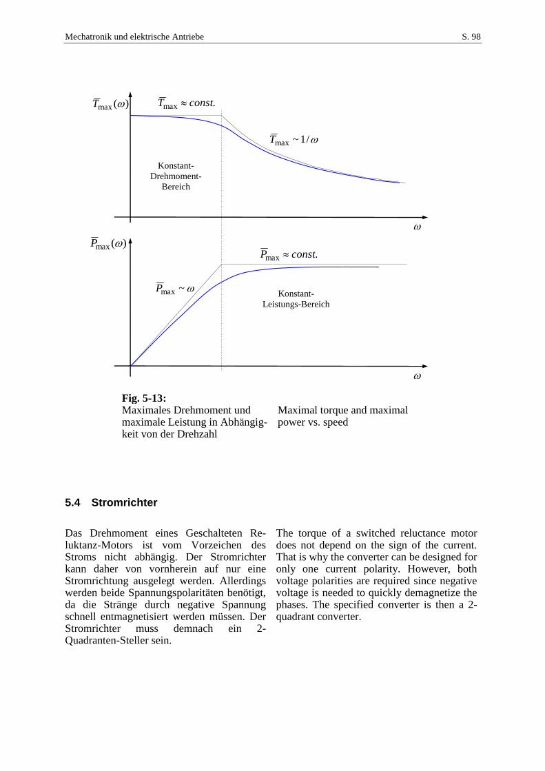
Mechatronik und elektrische Antriebe S. 98
Fig. 5-13: Maximales Drehmoment und maximale Leistung in Abhängig-keit von der Drehzahl
Maximal torque and maximal power vs. speed
5.4 Stromrichter
Das Drehmoment eines Geschalteten Re-luktanz-Motors ist vom Vorzeichen des Stroms nicht abhängig. Der Stromrichter kann daher von vornherein auf nur eine Stromrichtung ausgelegt werden. Allerdings werden beide Spannungspolaritäten benötigt, da die Stränge durch negative Spannung schnell entmagnetisiert werden müssen. Der Stromrichter muss demnach ein 2-Quadranten-Steller sein.
The torque of a switched reluctance motor does not depend on the sign of the current. That is why the converter can be designed for only one current polarity. However, both voltage polarities are required since negative voltage is needed to quickly demagnetize the phases. The specified converter is then a 2-quadrant converter.
)(max T
)(max P
.max constT
/1~maxT
~maxP
.max constP
Konstant-
Drehmoment-
Bereich
Konstant-
Leistungs-Bereich
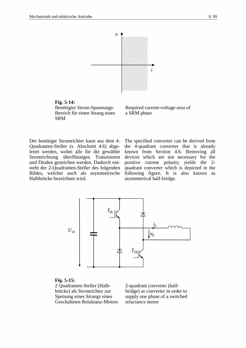
Mechatronik und elektrische Antriebe S. 99
Fig. 5-14: Benötigter Strom-Spannungs-Bereich für einen Strang eines SRM
Required current-voltage-area of a SRM phase
Der benötigte Stromrichter kann aus dem 4-Quadranten-Steller (s. Abschnitt 4.6) abge-leitet werden, wobei alle für die gewählte Stromrichtung überflüssigen Transistoren und Dioden gestrichen werden. Dadurch ent-steht der 2-Quadranten-Steller des folgenden Bildes, welcher auch als asymmetrische Halbbrücke bezeichnet wird.
The specified converter can be derived from the 4-quadrant converter that is already known from Section 4.6. Removing all devices which are not necessary for the positive current polarity yields the 2-quadrant converter which is depicted in the following figure. It is also known as asymmetrical half-bridge.
Fig. 5-15: 2 Quadranten-Steller (Halb-brücke) als Stromrichter zur Speisung eines Strangs eines Geschalteten Reluktanz-Motors
2-quadrant converter (half-bridge) as converter in order to supply one phase of a switched reluctance motor
i
u
dcU
kT1
kT2
ki
ku
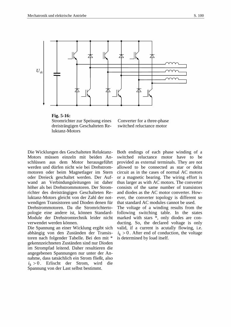
Mechatronik und elektrische Antriebe S. 100
Fig. 5-16: Stromrichter zur Speisung eines dreisträngigen Geschalteten Re-luktanz-Motors
Converter for a three-phase switched reluctance motor
Die Wicklungen des Geschalteten Reluktanz-Motors müssen einzeln mit beiden An-schlüssen aus dem Motor herausgeführt werden und dürfen nicht wie bei Drehstrom-motoren oder beim Magnetlager im Stern oder Dreieck geschaltet werden. Der Auf-wand an Verbindungsleitungen ist daher höher als bei Drehstrommotoren. Der Strom-richter des dreisträngigen Geschalteten Re-luktanz-Motors gleicht von der Zahl der not-wendigen Transistoren und Dioden denen für Drehstrommotoren. Da die Stromrichterto-pologie eine andere ist, können Standard-Module der Drehstromtechnik leider nicht verwendet werden können. Die Spannung an einer Wicklung ergibt sich abhängig von den Zuständen der Transis-toren nach folgender Tabelle. Bei den mit * gekennzeichneten Zuständen sind nur Dioden im Strompfad leitend. Daher resultieren die angegebenen Spannungen nur unter der An-nahme, dass tatsächlich ein Strom fließt, also
0ki . Erlischt der Strom, wird die Spannung von der Last selbst bestimmt.
Both endings of each phase winding of a switched reluctance motor have to be provided as external terminals. They are not allowed to be connected as star or delta circuit as in the cases of normal AC motors or a magnetic bearing. The wiring effort is thus larger as with AC motors. The converter consists of the same number of transistors and diodes as the AC motor converter. How-ever, the converter topology is different so that standard AC modules cannot be used. The voltage of a winding results from the following switching table. In the states marked with stars *, only diodes are con-ducting. So, the declared voltage is only valid, if a current is acutally flowing, i.e.
0ki . After end of conduction, the voltage is determined by load itself.
dcU

Mechatronik und elektrische Antriebe S. 101
kT1 kT2 ku
off off dcu *
off on 0 *
on off 0 *
on on dcu
Durch eine Pulsweitenmodulation oder durch direkte Strom-Schaltregelung werden die Transistoren geeignet getaktet. Die Puls-weitenmodulation kann direkt aus Abschnitt 3.8 übernommen werden.
The transistors are chopped with the help of a pulse width modulation or a suitable current hysteresis or peak mode control. The approach of Section 4.7 can be applied also here.
Mechatronik und elektrische Antriebe S. 102
6 Schrittmotoren Stepping Motors
Schrittmotoren zeichnen sich dadurch aus, dass sie in aller Regel ohne Positionsgeber betrieben werden. Vielmehr soll durch eine geeignete elektrische Ansteuerung (häufig durch blockförmige Ströme) sichergestellt werden, dass sich der Motor um einen genau definierten Winkel weiterdreht bzw. bei linearen Motoren um eine Strecke weiterbe-wegt, so dass sich durch Mitzählen der elektrischen Impulse die Position ergibt.
Stepping motors are characterized by the fact that they are operated usually without any position sensor. Rather, an adequate electrical command (often block-shaped currents) should ensure that the motor moved by a certain increment so that the actual position can be determined by counting the electrical cycles.
Als Schrittmotoren können Geschaltete Re-luktanz-Motoren oder bürstenlose, elektro-nisch kommutierte Permanent-Magnet-Moto-ren eingesetzt werden. Beide Arten von Motoren erzeugen im stromlosen Zustand jedoch kein oder nur ein geringes Haltedrehmoment bzw. eine Haltekraft. Nach dem Abschalten des Stroms kann sich daher der Motor bewegen. Seine Position ist beim nächsten Wiedereinschalten unbekannt. Für Anwenddungen, bei denen der Motor im ausgeschalteten Zustand seine Position nicht verändern soll, werden so genannte Hybrid-Motoren, die das Reluktanz-Prinzip mit Per-manentmagneten kombinieren, eingesetzt.
Switched reluctance motors or brushless electronically commutated DC motors could be operated, in principle, as stepping motors. Both motor types do not generate any hold-ing force or torque when the current is zero. The motor can move during the switched-off mode depending on the applied load so that the position may be unkown when starting next time. If the application requires to retain a definite position even in switched-off state, so-called hybrid motors are preferred, i.e. the varying reluctance is combined with per-manent magnets.
Das Bild Fig. 6-1 zeigt als Beispiel einen linearen zweiphasigen Schrittmotor. Die ein-fachste Betriebsart ist die Einprägung block-förmiger Ströme, womit der Motor mit einer der Polteilung oder eines Bruchteils der Pol-teilung des passiven Teils entsprechenden Genauigkeit positioniert werden kann. Durch Überlappung der Ströme bzw. durch sinus-förmige Speisung gelingt eine feinere oder sogar kontinuierliche Positionierung inner-halb einer Polteilung.
Fig. 6-1 shows the example of a linear two-
phase stepping motor. The simplest operation
mode is to apply block-shaped currents so
that the motor can be positioned with an
accuracy of one pole pitch of the passive
stator. Using current overlapping of both
phases or sinusoidally shaped currents, even
a finer positioning can be achieved.
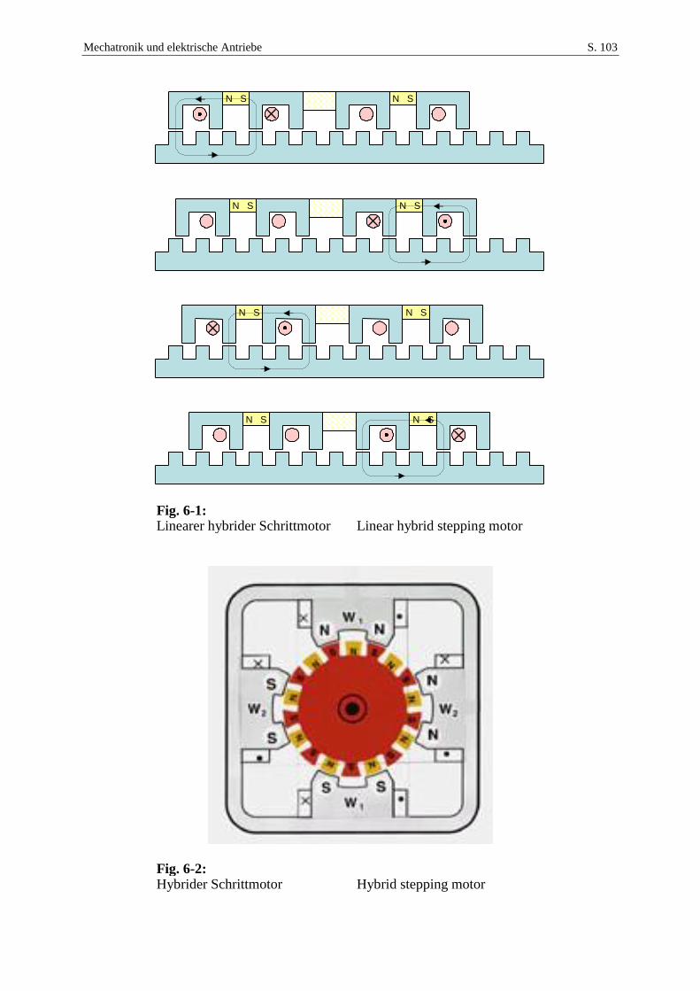
Mechatronik und elektrische Antriebe S. 103
Fig. 6-1: Linearer hybrider Schrittmotor Linear hybrid stepping motor
Fig. 6-2: Hybrider Schrittmotor Hybrid stepping motor
N S N S
N S N S
N S N S
N S N S
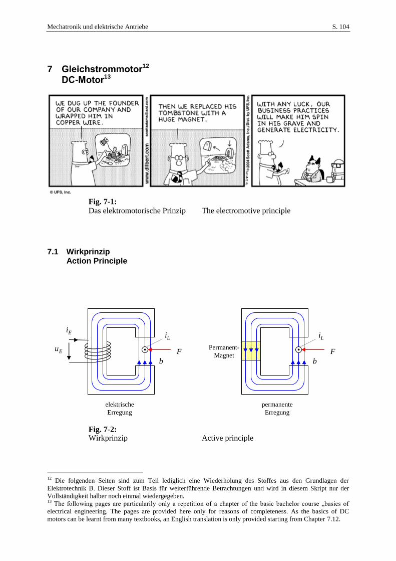
Mechatronik und elektrische Antriebe S. 104
7 Gleichstrommotor12 DC-Motor13
Fig. 7-1:
Das elektromotorische Prinzip The electromotive principle
7.1 Wirkprinzip Action Principle
Fig. 7-2: Wirkprinzip Active principle
12
Die folgenden Seiten sind zum Teil lediglich eine Wiederholung des Stoffes aus den Grundlagen der
Elektrotechnik B. Dieser Stoff ist Basis für weiterführende Betrachtungen und wird in diesem Skript nur der
Vollständigkeit halber noch einmal wiedergegeben. 13
The following pages are particularily only a repetition of a chapter of the basic bachelor course „basics of
electrical engineering. The pages are provided here only for reasons of completeness. As the basics of DC
motors can be learnt from many textbooks, an English translation is only provided starting from Chapter 7.12.
Ei
Eu
b
F
Li
b
F
Li
Permanent-
Magnet
elektrische
Erregung
permanente
Erregung
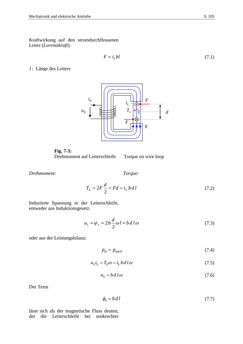
Mechatronik und elektrische Antriebe S. 105
Kraftwirkung auf den stromdurchflossenen Leiter (Lorentzkraft):
bliF L (7.1)
l : Länge des Leiters
Fig. 7-3:
Drehmoment auf Leiterschleife Torque on wire loop
Drehmoment: Torque:
ldbiFdd
FT LL 2
2 (7.2)
Induzierte Spannung in der Leiterschleife, entweder aus Induktionsgesetz:
ldbld
bu LL 2
2 (7.3)
oder aus der Leistungsbilanz:
mechel pp (7.4)
ldbiTiu LLLL (7.5)
ldbuL (7.6)
Der Term
ldb0 (7.7)
lässt sich als der magnetische Fluss deuten, der die Leiterschleife bei senkrechter
Ei
Eu d
Li
F
F
b
LT
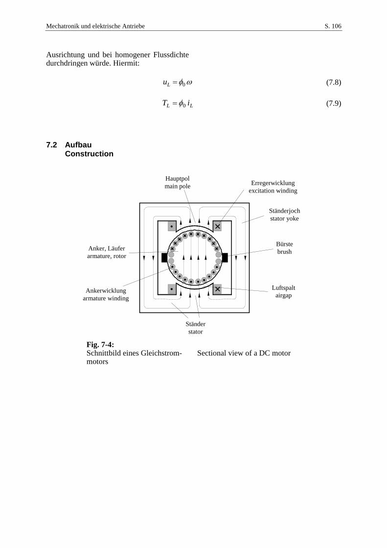
Mechatronik und elektrische Antriebe S. 106
Ausrichtung und bei homogener Flussdichte durchdringen würde. Hiermit:
0Lu (7.8)
LL iT 0 (7.9)
7.2 Aufbau Construction
Fig. 7-4: Schnittbild eines Gleichstrom-motors
Sectional view of a DC motor
Erregerwicklung
excitation winding
Ständer
stator
Anker, Läufer
armature, rotor
Bürste
brush
Ankerwicklung
armature winding
Luftspalt
airgap
Hauptpol
main pole
Ständerjoch
stator yoke
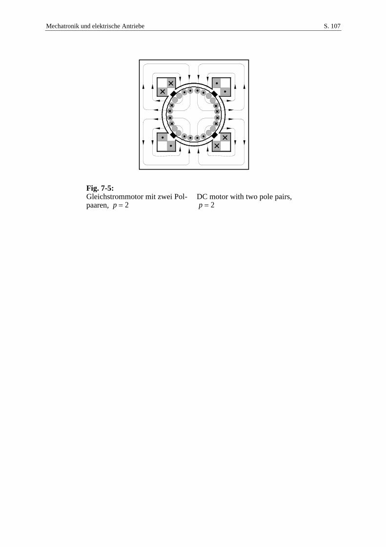
Mechatronik und elektrische Antriebe S. 107
Fig. 7-5: Gleichstrommotor mit zwei Pol-paaren, 2p
DC motor with two pole pairs, 2p
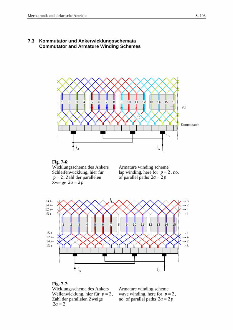
Mechatronik und elektrische Antriebe S. 108
7.3 Kommutator und Ankerwicklungsschemata Commutator and Armature Winding Schemes
Fig. 7-6: Wicklungsschema des Ankers Schleifenwicklung, hier für
2p , Zahl der parallelen Zweige pa 22
Armature winding scheme lap winding, here for 2p , no. of parallel paths pa 22
Fig. 7-7: Wicklungsschema des Ankers Wellenwicklung, hier für 2p , Zahl der parallelen Zweige
22 a
Armature winding scheme wave winding, here for 2p , no. of parallel paths pa 22
2 3 4 6 7 8 9 10 11 12 13 14 15 1 5
3 2 4 1
1 4 2 3
13 14 12 15
15 12 14 13
Ai Ai
Li
2 3 4 6 7 8 9 10 11 12 1 5
Ai Ai
Li
13 14 15 16
Kommutator
Pol

Mechatronik und elektrische Antriebe S. 109
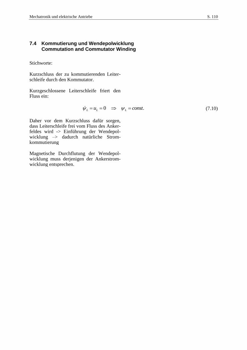
Mechatronik und elektrische Antriebe S. 110
7.4 Kommutierung und Wendepolwicklung Commutation and Commutator Winding
Stichworte: Kurzschluss der zu kommutierenden Leiter-schleife durch den Kommutator.
Kurzgeschlossene Leiterschleife friert den Fluss ein:
0 .L L Lu const (7.10)
Daher vor dem Kurzschluss dafür sorgen, dass Leiterschleife frei vom Fluss des Anker-feldes wird -> Einführung der Wendepol-wicklung –> dadurch natürliche Strom-kommutierung
Magnetische Durchflutung der Wendepol-wicklung muss derjenigen der Ankerstrom-wicklung entsprechen.
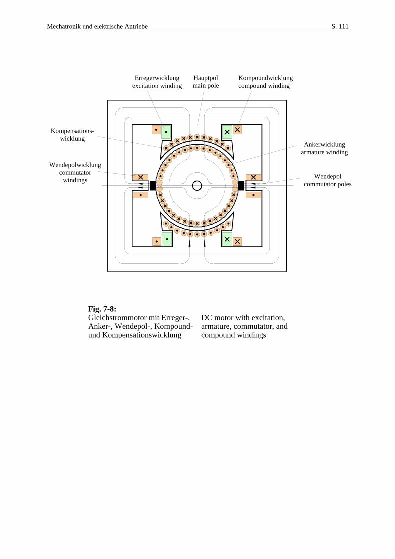
Mechatronik und elektrische Antriebe S. 111
Fig. 7-8: Gleichstrommotor mit Erreger-, Anker-, Wendepol-, Kompound- und Kompensationswicklung
DC motor with excitation, armature, commutator, and compound windings
Erregerwicklung
excitation winding
Wendepolwicklung
commutator
windings
Kompensations-
wicklung
Hauptpol
main pole
Wendepol
commutator poles
Ankerwicklung
armature winding
Kompoundwicklung
compound winding

Mechatronik und elektrische Antriebe S. 112
7.5 Ankerrückwirkung, Kompensations- und Kompoundwicklung Armature reaction, Compensation and Compound Windings
Stichworte: Ankerfeld verursacht Feldverzerrung in den Erregerpolen. Bei linearem Material wäre dies kein Nachteil. Die einseitige magne-tische Sättigung im Erregerpol führt jedoch zur Erhöhung des gesamten magnetischen Widerstands im Erregerkreis und somit zur Schwächung des Erregerflusses.
Gegenmaßnahmen
Erhöhung der magnetischen Spannung im magnetischen Erreger-kreis durch Kompoundwicklung, welche vom Ankerstrom durchflossen wird
Einführung der Kompensations-wicklung zur Kompensation der An-kerrückwirkung, ebenfalls vom An-kerstrom durchflossen.
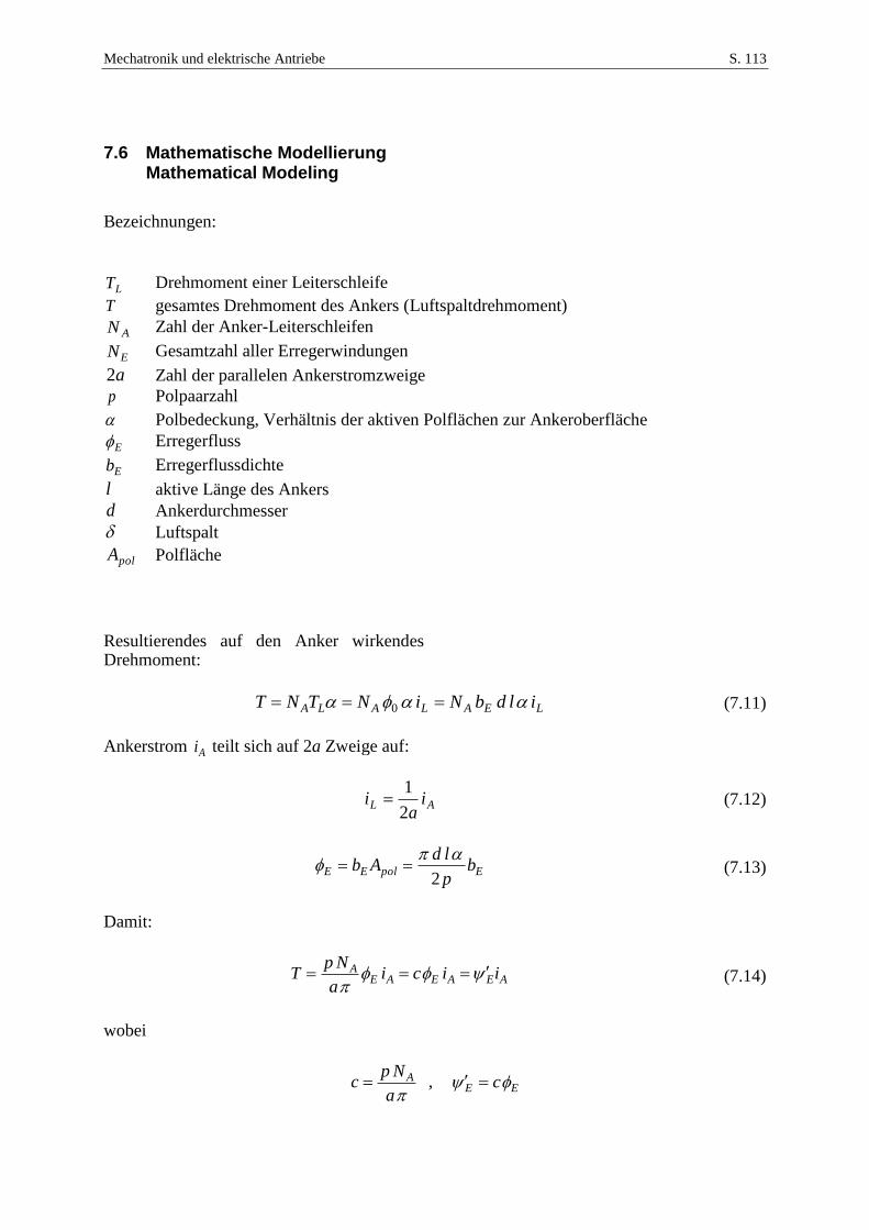
Mechatronik und elektrische Antriebe S. 113
7.6 Mathematische Modellierung Mathematical Modeling
Bezeichnungen:
LT Drehmoment einer Leiterschleife
T gesamtes Drehmoment des Ankers (Luftspaltdrehmoment)
AN Zahl der Anker-Leiterschleifen
EN Gesamtzahl aller Erregerwindungen
a2 Zahl der parallelen Ankerstromzweige
p Polpaarzahl
Polbedeckung, Verhältnis der aktiven Polflächen zur Ankeroberfläche
E Erregerfluss
Eb Erregerflussdichte
l aktive Länge des Ankers
d Ankerdurchmesser
Luftspalt
polA Polfläche
Resultierendes auf den Anker wirkendes Drehmoment:
LEALALA ildbNiNTNT 0 (7.11)
Ankerstrom Ai teilt sich auf 2a Zweige auf:
AL ia
i2
1 (7.12)
EpolEE bp
ldAb
2
(7.13)
Damit:
AEAEAEA iici
a
NpT
(7.14)
wobei
a
Npc A , EE c
Mechatronik und elektrische Antriebe S. 114
Die induzierte Spannung (elektromotorische Kraft, EMK) folgt wieder aus der Leistungs-bilanz,
EEi cu , (7.15)
oder alternativ durch Summation der indu-zierten Spannungen der in Reihe geschalteten Leiterschleifen.
Spannungsgleichung des Ankerkreises unter Berücksichtigung des Ankerwiderstands AR , der Ankerinduktivität AL und des Bürsten-spannungsabfalls Bu :
2A i A A A A Bu u L i R i u (7.16)
Mit guter Genauigkeit kann der Bürsten-spannungsabfall Bu also eine konstante, vom Ankerstrom unabhängige Spannung von etwa 1 V angesetzt werden.
Erregerstromkreis:
E E E E Eu L i R i (7.17)
Beachte: Im Allgemeinen sind zwischen zwei Wicklungen Gegeninduktivitäten zu berücksichtigen. Die Flüsse von Erreger- und Ankerwicklung sind aber durch die zuein-ander senkrechte Anordnung nicht mitei-nander verkettet, so dass die Gegeninduk-tivität zwischen diesen Wicklungen Null ist.
Magnetischer Kreis der Erregung: Magnetische Leitfähigkeit des Erregerkreises
p
ld
p
ldA
RPol
magE
E4222
1 000 (7.18)
Induktivität:
p
Np
p
NL E
EE
EE
2
2
2
(7.19)
Erregerfluss:
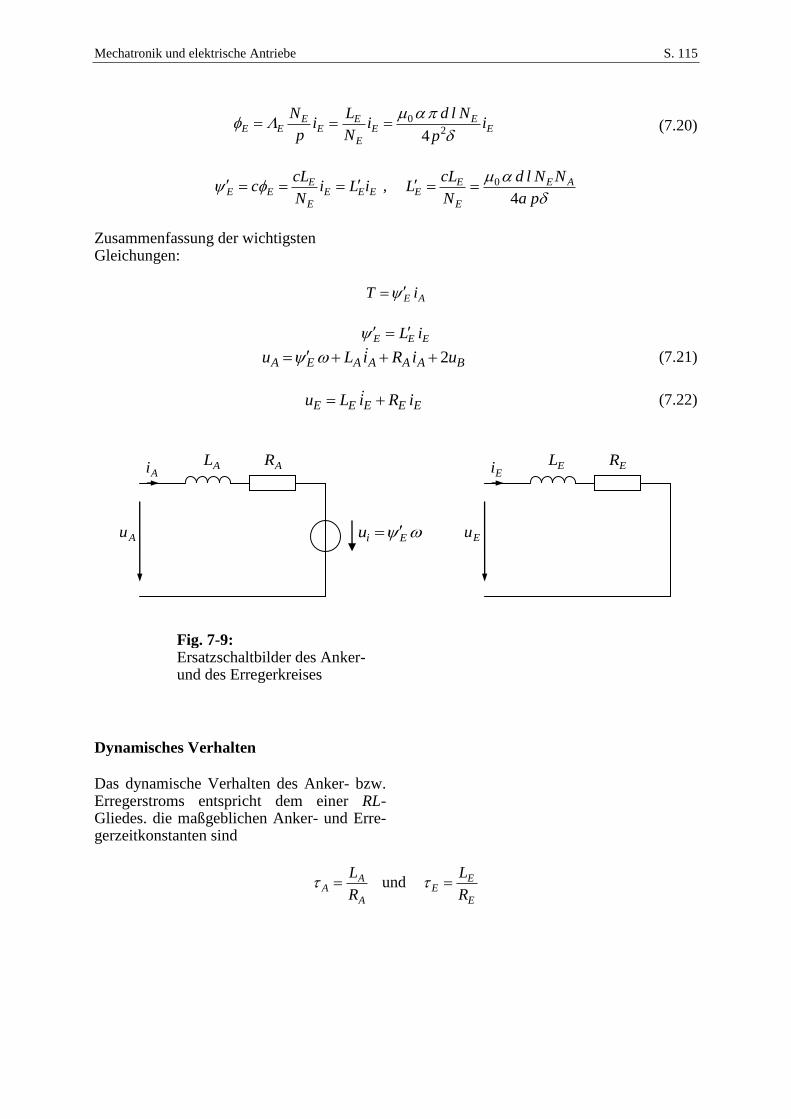
Mechatronik und elektrische Antriebe S. 115
EE
E
E
EE
EEE i
p
Nldi
N
Li
p
N
20
4 (7.20)
EEE
E
EEE iLi
N
cLc ,
pa
NNld
N
cLL AE
E
EE
4
0
Zusammenfassung der wichtigsten Gleichungen:
AE iT
EEE iL
BAAAAEA uiRiLu 2 (7.21)
EEEEE iRiLu (7.22)
Fig. 7-9: Ersatzschaltbilder des Anker- und des Erregerkreises
Dynamisches Verhalten
Das dynamische Verhalten des Anker- bzw. Erregerstroms entspricht dem einer RL-Gliedes. die maßgeblichen Anker- und Erre-gerzeitkonstanten sind
A
AA
R
L und
E
EE
R
L
Eiu
Ai
Au
AL AREi
Eu
EL ER
Mechatronik und elektrische Antriebe S. 116
7.7 Elektrische und mechanische Leistung, Wirkungsgrad Electrical and Mechanical Power, Efficiency
Elektrische Leistung (Verbraucherzählpfeil-system):
EEAAelEelAel iuiuppp (7.23)
Mechanische Leistung (Erzeugerzählpfeil-system):
Tpmech (7.24)
Energiebilanz:
mechVEAel ppwwp (7.25)
Verlustleistung:
22AAEEVEVAV iRiRPPP (7.26)
Innere Energien:
2
2
1AAA iLw ,
2
2
1EEE iLw
Wirkungsgrad des Ankerkreises (Vernach-lässigung der Erregerverluste) im stationären Zustand für den motorischen Betrieb:
TRT
RTTR
T
IIR
T
IU
T
P
P
E
A
E
A
E
E
E
AAEAAAAelA
mech
221
1
(7.27)
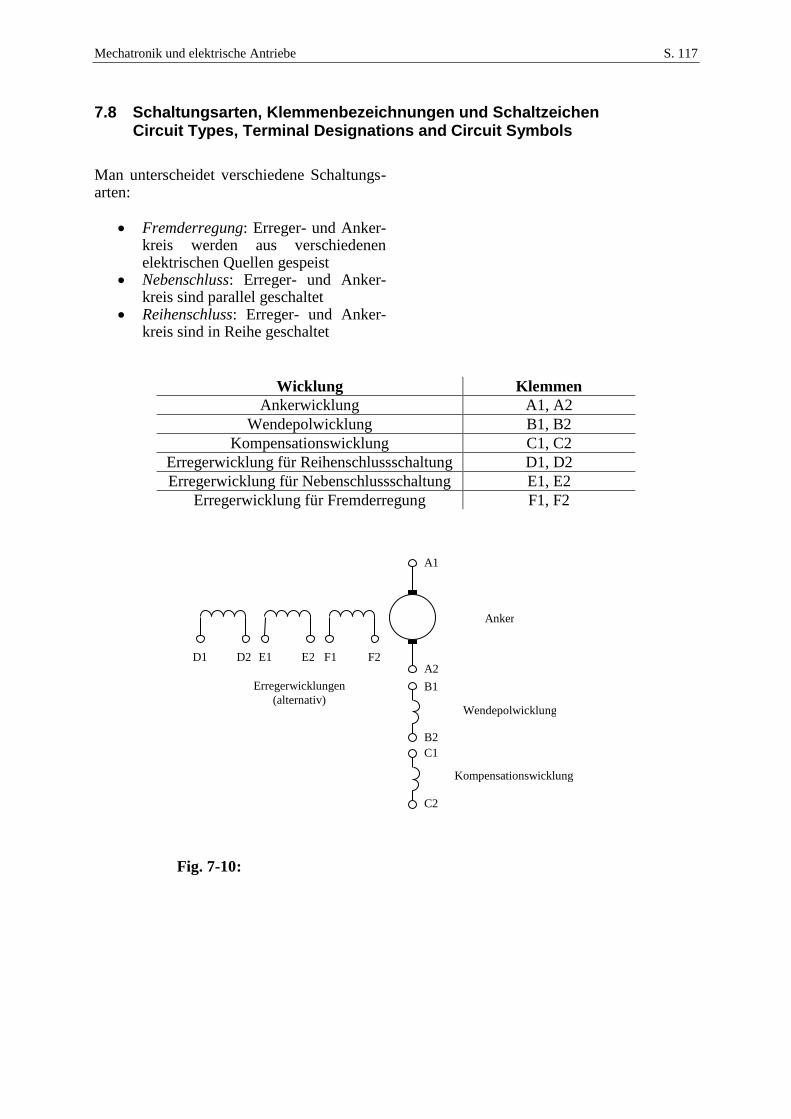
Mechatronik und elektrische Antriebe S. 117
7.8 Schaltungsarten, Klemmenbezeichnungen und Schaltzeichen Circuit Types, Terminal Designations and Circuit Symbols
Man unterscheidet verschiedene Schaltungs-arten:
Fremderregung: Erreger- und Anker-
kreis werden aus verschiedenen elektrischen Quellen gespeist
Nebenschluss: Erreger- und Anker-kreis sind parallel geschaltet
Reihenschluss: Erreger- und Anker-kreis sind in Reihe geschaltet
Wicklung Klemmen
Ankerwicklung A1, A2
Wendepolwicklung B1, B2
Kompensationswicklung C1, C2
Erregerwicklung für Reihenschlussschaltung D1, D2
Erregerwicklung für Nebenschlussschaltung E1, E2
Erregerwicklung für Fremderregung F1, F2
Fig. 7-10:
A1
A2 B1
B2 C1
C2
D1 D2 E1 E2 F1 F2
Wendepolwicklung
Kompensationswicklung
Erregerwicklungen
(alternativ)
Anker
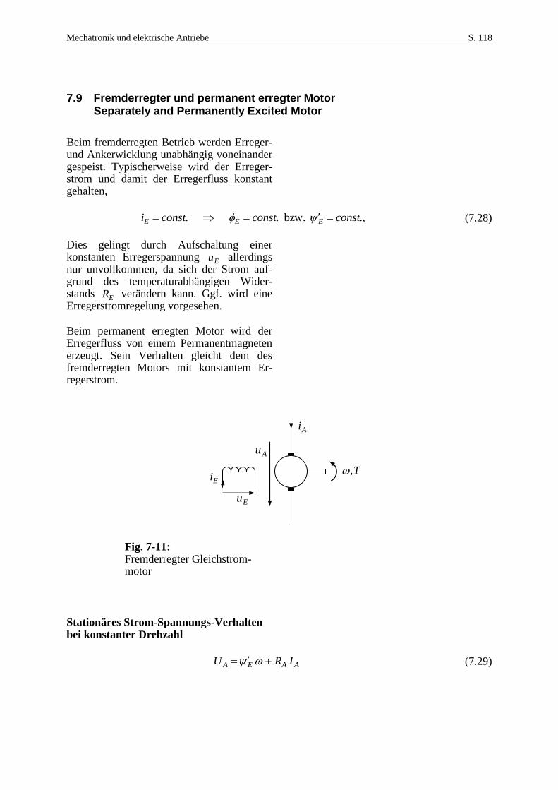
Mechatronik und elektrische Antriebe S. 118
7.9 Fremderregter und permanent erregter Motor Separately and Permanently Excited Motor
Beim fremderregten Betrieb werden Erreger- und Ankerwicklung unabhängig voneinander gespeist. Typischerweise wird der Erreger-strom und damit der Erregerfluss konstant gehalten,
.,bzw... constconstconsti EEE (7.28)
Dies gelingt durch Aufschaltung einer konstanten Erregerspannung Eu allerdings nur unvollkommen, da sich der Strom auf-grund des temperaturabhängigen Wider-stands ER verändern kann. Ggf. wird eine Erregerstromregelung vorgesehen.
Beim permanent erregten Motor wird der Erregerfluss von einem Permanentmagneten erzeugt. Sein Verhalten gleicht dem des fremderregten Motors mit konstantem Er-regerstrom.
Fig. 7-11: Fremderregter Gleichstrom-motor
Stationäres Strom-Spannungs-Verhalten bei konstanter Drehzahl
AAEA IRU (7.29)
T,Ei
Eu
Ai
Au
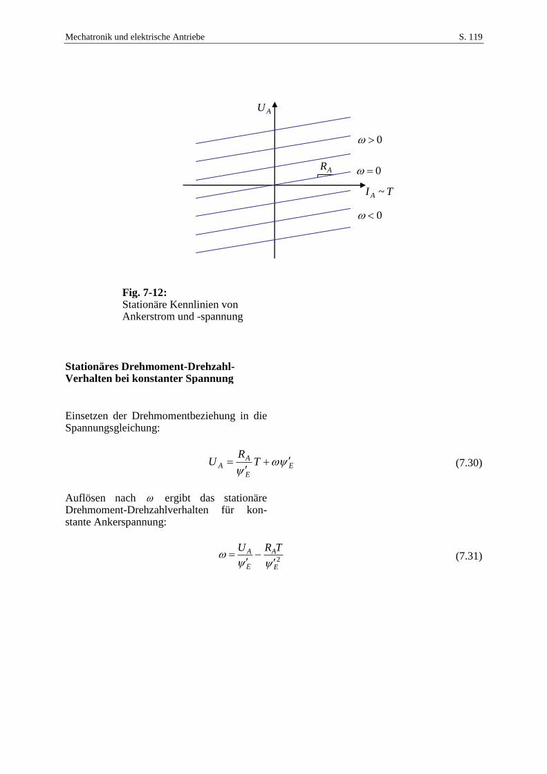
Mechatronik und elektrische Antriebe S. 119
Fig. 7-12: Stationäre Kennlinien von Ankerstrom und -spannung
Stationäres Drehmoment-Drehzahl-Verhalten bei konstanter Spannung
Einsetzen der Drehmomentbeziehung in die Spannungsgleichung:
E
E
AA T
RU
(7.30)
Auflösen nach ergibt das stationäre Drehmoment-Drehzahlverhalten für kon-stante Ankerspannung:
2E
A
E
A TRU
(7.31)
TI A ~
AU
AR 0
0
0
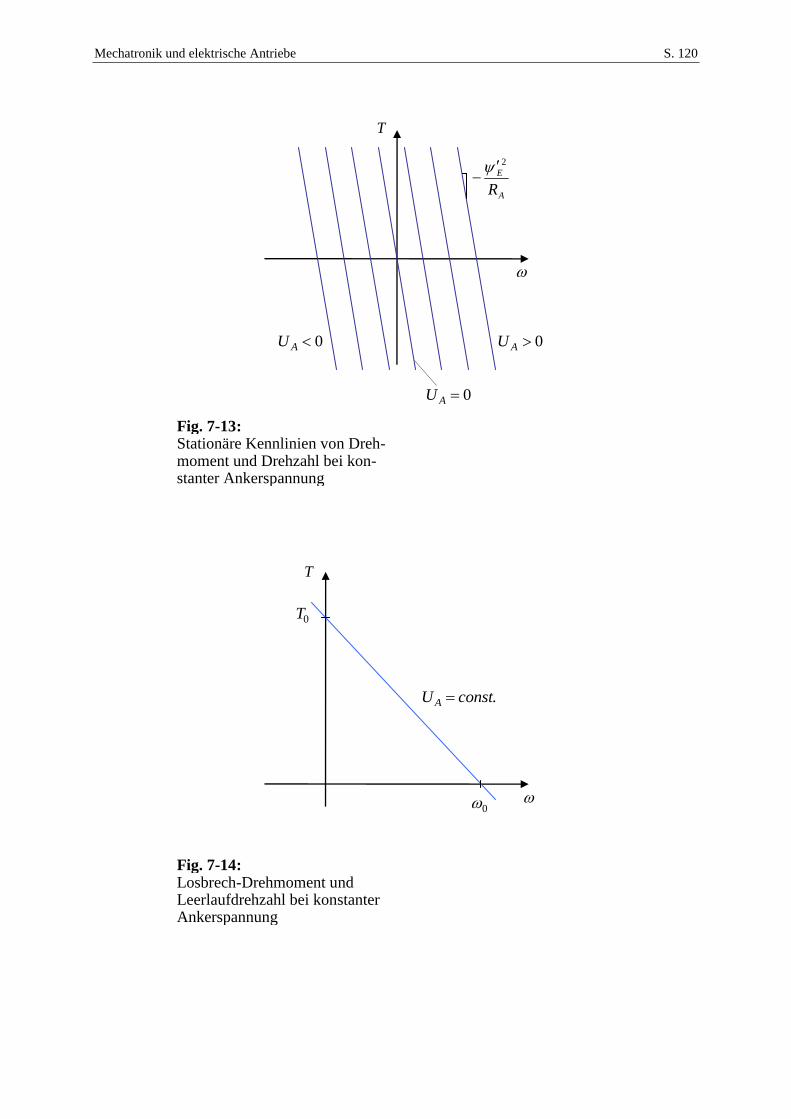
Mechatronik und elektrische Antriebe S. 120
Fig. 7-13: Stationäre Kennlinien von Dreh-moment und Drehzahl bei kon-stanter Ankerspannung
Fig. 7-14: Losbrech-Drehmoment und Leerlaufdrehzahl bei konstanter Ankerspannung
T
.constUA
0
0T
T
0AU
0AU0AU
A
E
R
2
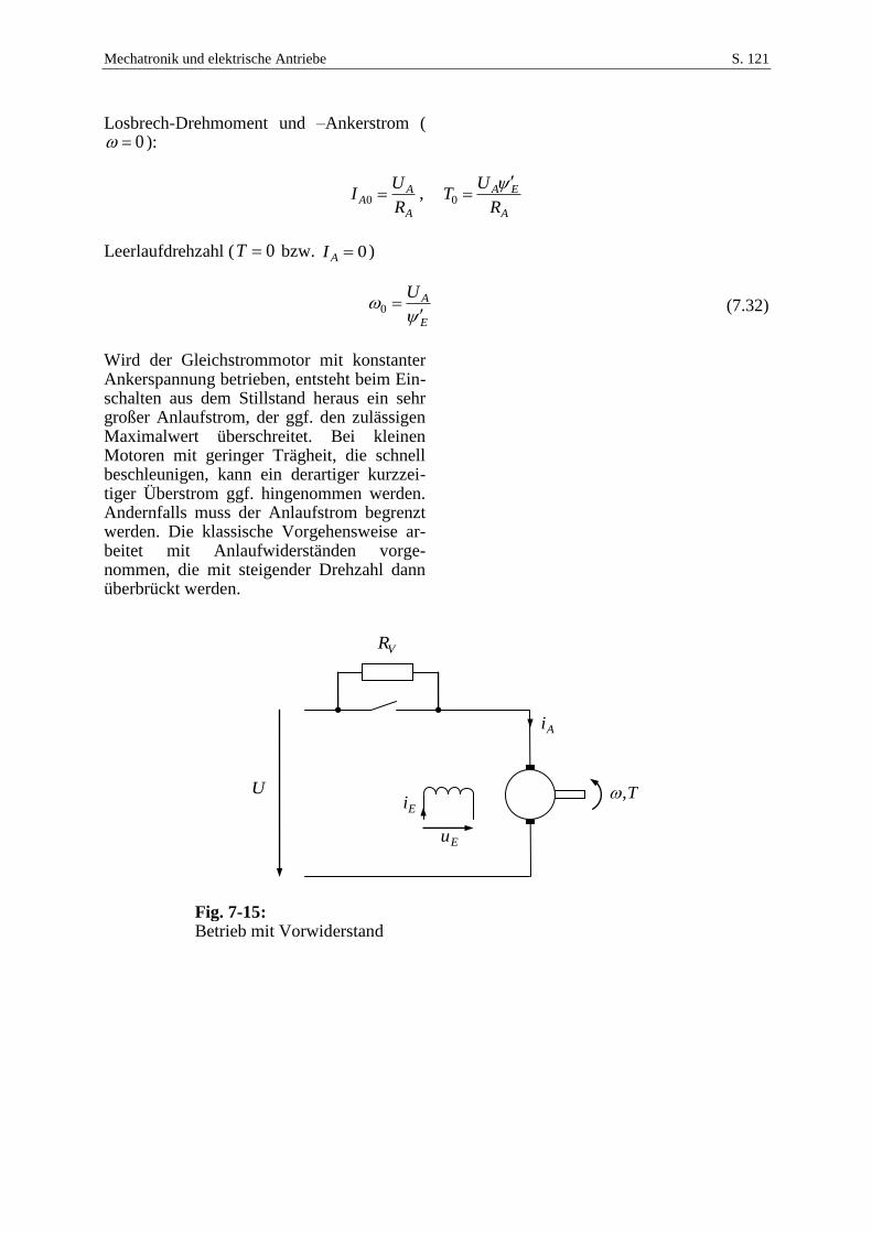
Mechatronik und elektrische Antriebe S. 121
Losbrech-Drehmoment und –Ankerstrom (0 ):
A
AA
R
UI 0 ,
A
EA
R
UT
0
Leerlaufdrehzahl ( 0T bzw. 0AI )
E
AU
0 (7.32)
Wird der Gleichstrommotor mit konstanter Ankerspannung betrieben, entsteht beim Ein-schalten aus dem Stillstand heraus ein sehr großer Anlaufstrom, der ggf. den zulässigen Maximalwert überschreitet. Bei kleinen Motoren mit geringer Trägheit, die schnell beschleunigen, kann ein derartiger kurzzei-tiger Überstrom ggf. hingenommen werden. Andernfalls muss der Anlaufstrom begrenzt werden. Die klassische Vorgehensweise ar-beitet mit Anlaufwiderständen vorge-nommen, die mit steigender Drehzahl dann überbrückt werden.
Fig. 7-15: Betrieb mit Vorwiderstand
T,Ei
Eu
Ai
VR
U
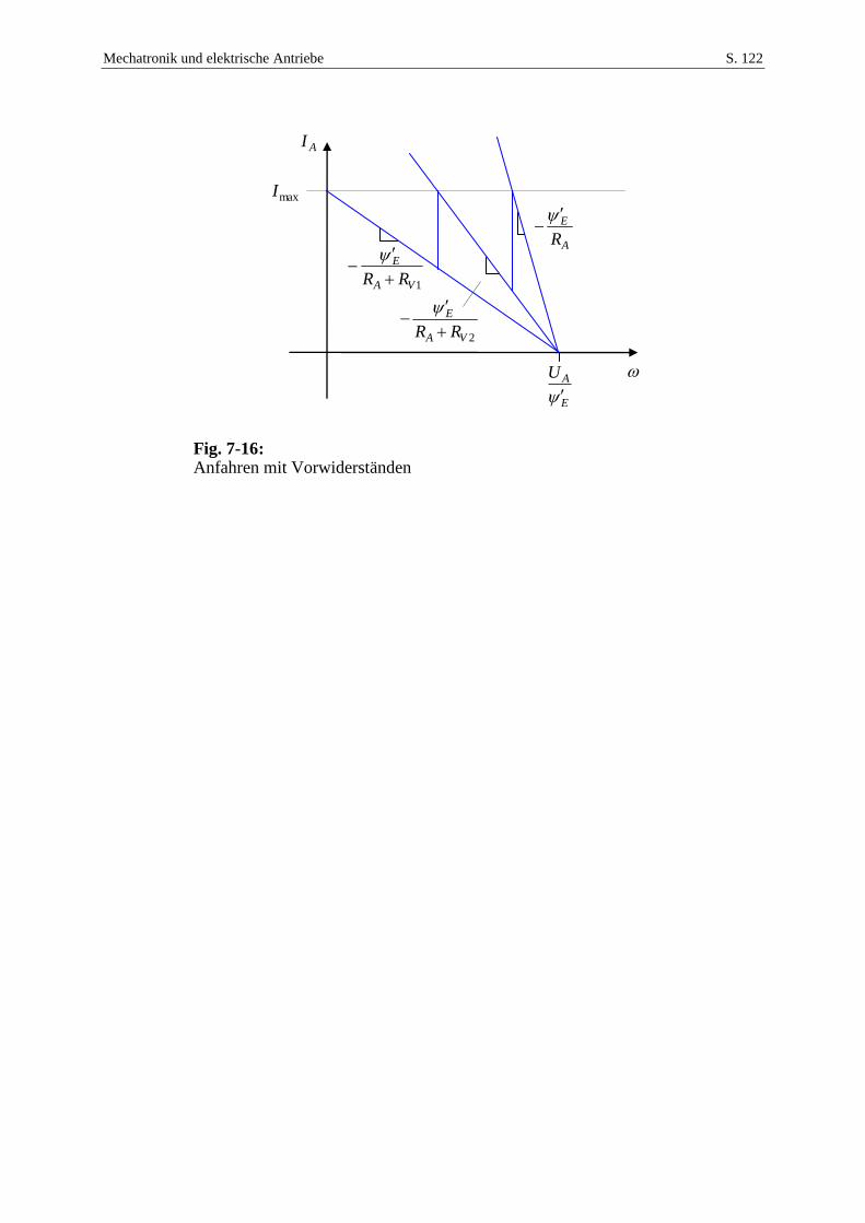
Mechatronik und elektrische Antriebe S. 122
Fig. 7-16: Anfahren mit Vorwiderständen
E
AU
AI
maxI
1VA
E
RR
2VA
E
RR
A
E
R
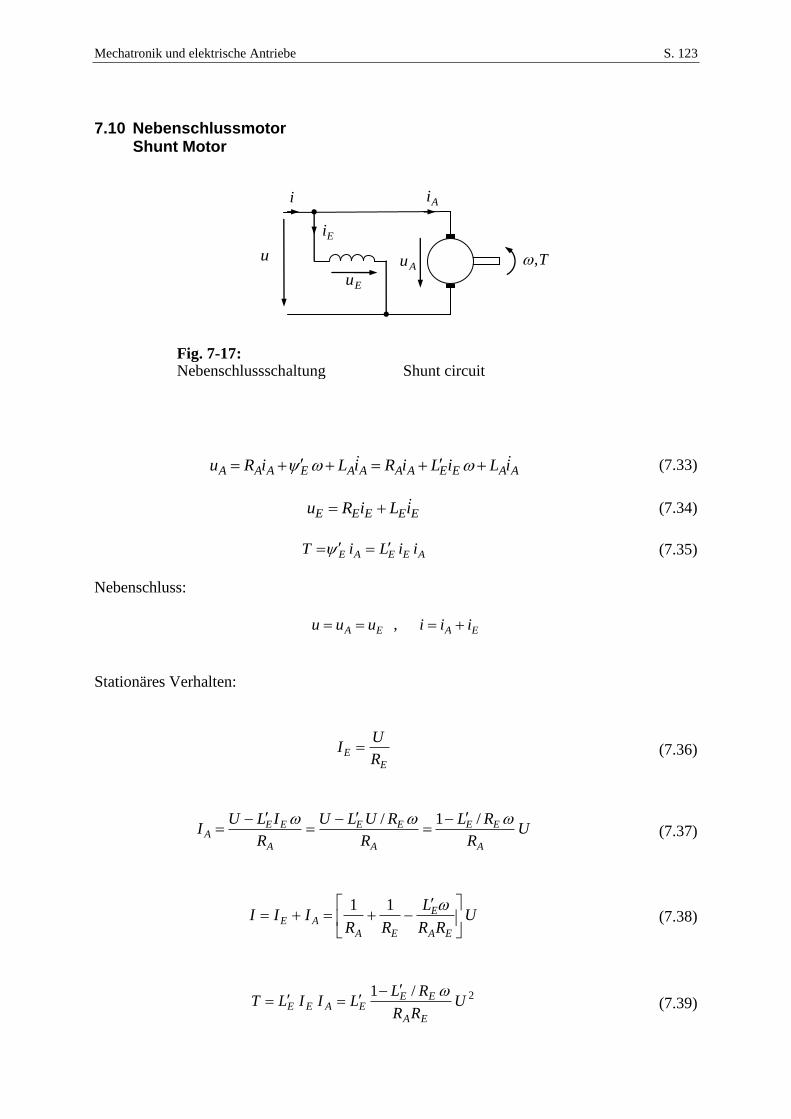
Mechatronik und elektrische Antriebe S. 123
7.10 Nebenschlussmotor Shunt Motor
Fig. 7-17: Nebenschlussschaltung Shunt circuit
AAEEAAAAEAAA iLiLiRiLiRu (7.33)
EEEEE iLiRu (7.34)
AEEAE iiLiT (7.35)
Nebenschluss:
EA uuu , EA iii
Stationäres Verhalten:
E
ER
UI (7.36)
UR
RL
R
RULU
R
ILUI
A
EE
A
EE
A
EEA
/1/
(7.37)
URR
L
RRIII
EA
E
EA
AE
11 (7.38)
2/1U
RR
RLLIILT
EA
EEEAEE
(7.39)
T,
i
Eu
uAu
Ai
Ei
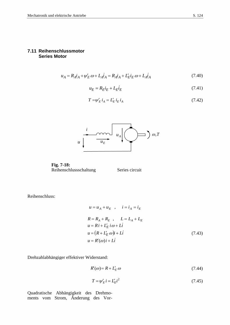
Mechatronik und elektrische Antriebe S. 124
7.11 Reihenschlussmotor Series Motor
AAEEAAAAEAAA iLiLiRiLiRu (7.40)
EEEEE iLiRu (7.41)
AEEAE iiLiT (7.42)
Fig. 7-18: Reihenschlussschaltung Series circuit
Reihenschluss:
EA uuu , EA iii
EA RRR , EA LLL
iLiRu
iLiLRu
iLiLiRu
E
E
)(
(7.43)
Drehzahlabhängiger effektiver Widerstand:
ELRR )( (7.44)
2iLiT EE
(7.45)
Quadratische Abhängigkeit des Drehmo-ments vom Strom, Änderung des Vor-
T,i
Euu
Au
Mechatronik und elektrische Antriebe S. 125
zeichens ist nur durch Wechsel der Ver-schaltung von Erreger- und Ankerwicklung möglich, EA iii Daher kann ein Reihenschlussmotor auch mit Wechselspannung gespeist werden. Sinus-förmige Speisung mit der Frequenz el , Schreibweise mit komplexen Effektiv-wertzeigern:
ILjIRU el )( (7.46)
LjR
UI
el
)( (7.47)
Das Drehmoment pulsiert mit el2 . Dreh-momentmittelwert:
222
222
)( LR
ULILiLT
el
EEE
(7.48)
Drehmoment-Drehzahl-Charakteristik:
2222 )( ULTLR Eel (7.49)
2222ULTLLR EelE (7.50)
Wird der Reihenschlussmotor mit konstanter Spannung betrieben und dabei mechanisch entlastet, 0T , wächst die Drehzahl über alle Grenzen, (s. Bild).
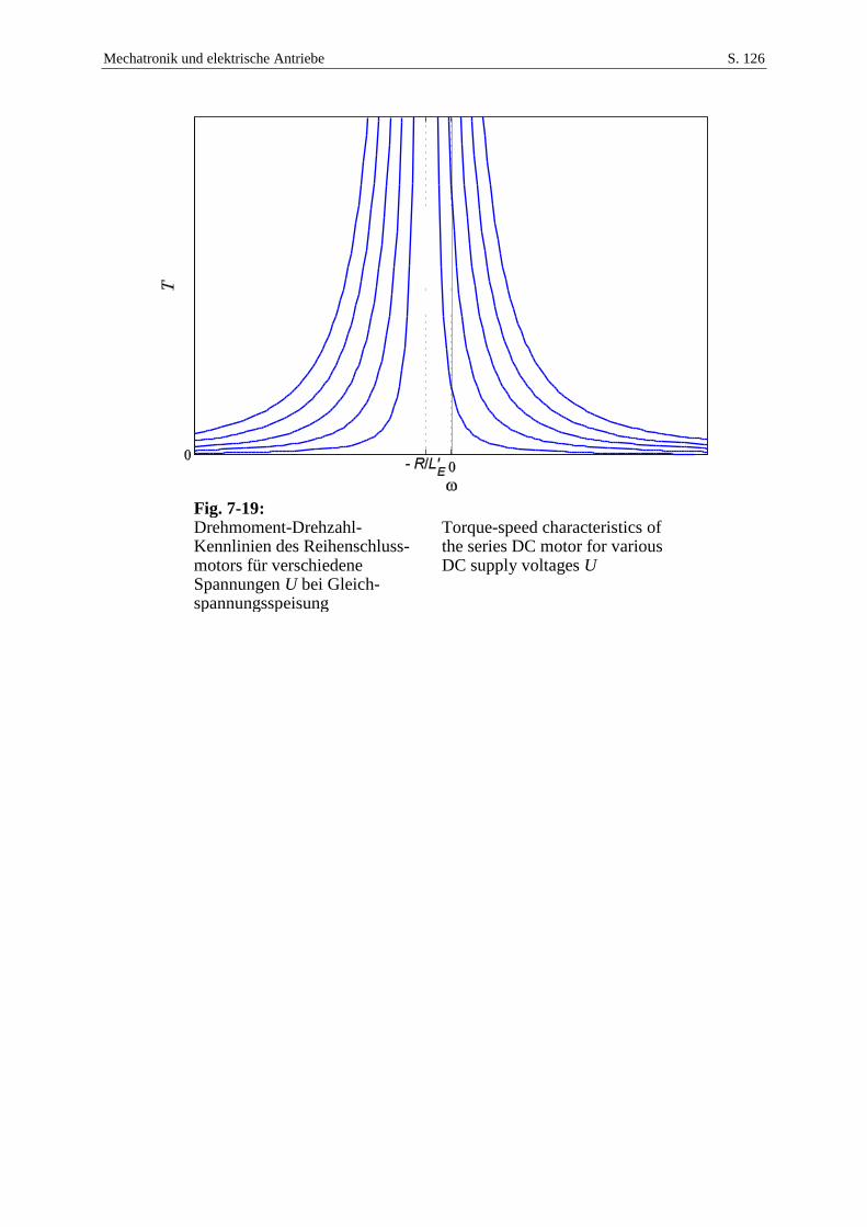
Mechatronik und elektrische Antriebe S. 126
Fig. 7-19: Drehmoment-Drehzahl-Kennlinien des Reihenschluss-motors für verschiedene Spannungen U bei Gleich-spannungsspeisung
Torque-speed characteristics of the series DC motor for various DC supply voltages U
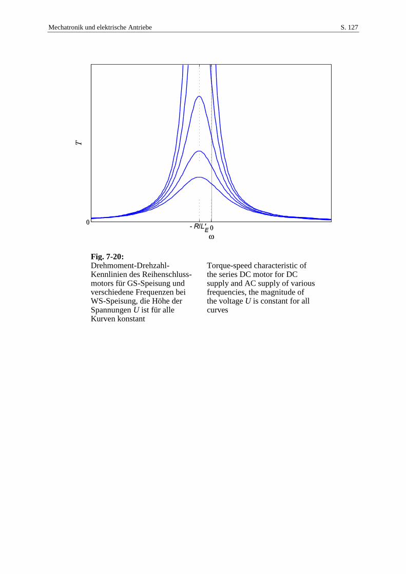
Mechatronik und elektrische Antriebe S. 127
Fig. 7-20: Drehmoment-Drehzahl-Kennlinien des Reihenschluss-motors für GS-Speisung und verschiedene Frequenzen bei WS-Speisung, die Höhe der Spannungen U ist für alle Kurven konstant
Torque-speed characteristic of the series DC motor for DC supply and AC supply of various frequencies, the magnitude of the voltage U is constant for all curves
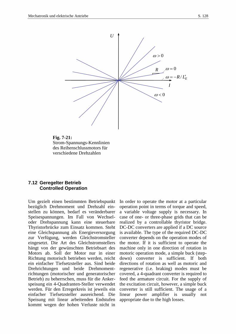
Mechatronik und elektrische Antriebe S. 128
Fig. 7-21: Strom-Spannungs-Kennlinien des Reihenschlussmotors für verschiedene Drehzahlen
7.12 Geregelter Betrieb Controlled Operation
Um gezielt einen bestimmten Betriebspunkt bezüglich Drehmoment und Drehzahl ein-stellen zu können, bedarf es veränderbarer Speisespannungen. Im Fall von Wechsel- oder Drehspannung kann eine steuerbare Thyristorbrücke zum Einsatz kommen. Steht eine Gleichspannung als Energieversorgung zur Verfügung, werden Gleichstromsteller eingesetzt. Die Art des Gleichstromstellers hängt von der gewünschten Betriebsart des Motors ab. Soll der Motor nur in einer Richtung motorisch betrieben werden, reicht ein einfacher Tiefsetzsteller aus. Sind beide Drehrichtungen und beide Drehmoment-richtungen (motorischer und generatorischer Betrieb) zu beherrschen, muss für die Anker-speisung ein 4-Quadranten-Steller verwendet werden. Für den Erregerkreis ist jeweils ein einfacher Tiefsetzsteller ausreichend. Die Speisung mit linear arbeitenden Endstufen kommt wegen der hohen Verluste nicht in
In order to operate the motor at a particular operation point in terms of torque and speed, a variable voltage supply is necessary. In case of one- or three-phase grids that can be realized by a controllable thyristor bridge. DC-DC converters are applied if a DC source is available. The type of the required DC-DC converter depends on the operation modes of the motor. If it is sufficient to operate the machine only in one direction of rotation in motoric operation mode, a simple buck (step-down) converter is sufficient. If both directions of rotation as well as motoric and regenerative (i.e. braking) modes must be covered, a 4-quadrant converter is required to feed the armature circuit. For the supply of the excitation circuit, however, a simple buck converter is still sufficient. The usage of a linear power amplifier is usually not appropriate due to the high losses.
I
U
R 0
0
0
ELR /
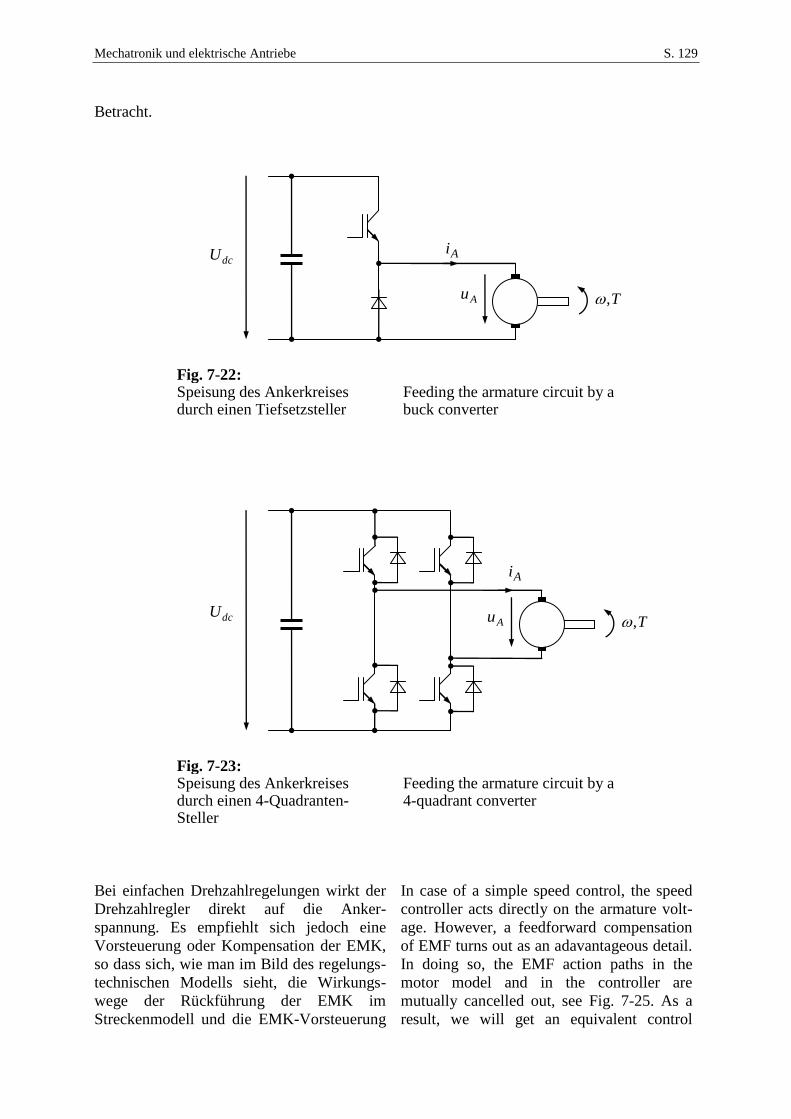
Mechatronik und elektrische Antriebe S. 129
Betracht.
Fig. 7-22: Speisung des Ankerkreises durch einen Tiefsetzsteller
Feeding the armature circuit by a buck converter
Fig. 7-23: Speisung des Ankerkreises durch einen 4-Quadranten-Steller
Feeding the armature circuit by a 4-quadrant converter
Bei einfachen Drehzahlregelungen wirkt der
Drehzahlregler direkt auf die Anker-
spannung. Es empfiehlt sich jedoch eine
Vorsteuerung oder Kompensation der EMK,
so dass sich, wie man im Bild des regelungs-
technischen Modells sieht, die Wirkungs-
wege der Rückführung der EMK im
Streckenmodell und die EMK-Vorsteuerung
In case of a simple speed control, the speed
controller acts directly on the armature volt-
age. However, a feedforward compensation
of EMF turns out as an adavantageous detail.
In doing so, the EMF action paths in the
motor model and in the controller are
mutually cancelled out, see Fig. 7-25. As a
result, we will get an equivalent control
dcUAu T,
Ai
dcU
Au T,
Ai
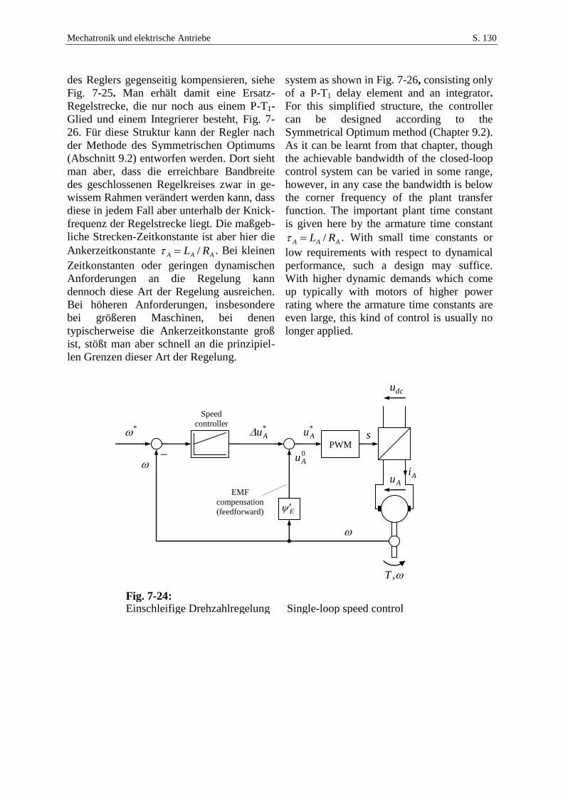
Mechatronik und elektrische Antriebe S. 130
des Reglers gegenseitig kompensieren, siehe
Fig. 7-25. Man erhält damit eine Ersatz-
Regelstrecke, die nur noch aus einem P-T1-
Glied und einem Integrierer besteht, Fig. 7-
26. Für diese Struktur kann der Regler nach
der Methode des Symmetrischen Optimums
(Abschnitt 9.2) entworfen werden. Dort sieht
man aber, dass die erreichbare Bandbreite
des geschlossenen Regelkreises zwar in ge-
wissem Rahmen verändert werden kann, dass
diese in jedem Fall aber unterhalb der Knick-
frequenz der Regelstrecke liegt. Die maßgeb-
liche Strecken-Zeitkonstante ist aber hier die
Ankerzeitkonstante AAA RL / . Bei kleinen
Zeitkonstanten oder geringen dynamischen
Anforderungen an die Regelung kann
dennoch diese Art der Regelung ausreichen.
Bei höheren Anforderungen, insbesondere
bei größeren Maschinen, bei denen
typischerweise die Ankerzeitkonstante groß
ist, stößt man aber schnell an die prinzipiel-
len Grenzen dieser Art der Regelung.
system as shown in Fig. 7-26, consisting only
of a P-T1 delay element and an integrator.
For this simplified structure, the controller
can be designed according to the
Symmetrical Optimum method (Chapter 9.2).
As it can be learnt from that chapter, though
the achievable bandwidth of the closed-loop
control system can be varied in some range,
however, in any case the bandwidth is below
the corner frequency of the plant transfer
function. The important plant time constant
is given here by the armature time constant
AAA RL / . With small time constants or
low requirements with respect to dynamical
performance, such a design may suffice.
With higher dynamic demands which come
up typically with motors of higher power
rating where the armature time constants are
even large, this kind of control is usually no
longer applied.
Fig. 7-24: Einschleifige Drehzahlregelung Single-loop speed control
*
,T
PWM s
*Au
Au
*Au
0Au
Ai
dcu
E
EMF
compensation
(feedforward)
Speed
controller
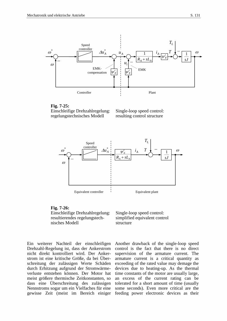
Mechatronik und elektrische Antriebe S. 131
Fig. 7-25: Einschleifige Drehzahlregelung: regelungstechnisches Modell
Single-loop speed control: resulting control structure
Fig. 7-26: Einschleifige Drehzahlregelung: resultierendes regelungstech-nisches Modell
Single-loop speed control: simplified equivalent control structure
Ein weiterer Nachteil der einschleifigen Drehzahl-Regelung ist, dass der Ankerstrom nicht direkt kontrolliert wird. Der Anker-strom ist eine kritische Größe, da bei Über-schreitung der zulässigen Werte Schäden durch Erhitzung aufgrund der Stromwärme-verluste entstehen können. Der Motor hat meist größere thermische Zeitkonstanten, so dass eine Überschreitung des zulässigen Nennstroms sogar um ein Vielfaches für eine gewisse Zeit (meist im Bereich einiger
Another drawback of the single-loop speed control is the fact that there is no direct supervision of the armature current. The armature current is a critical quantity as exceeding of the rated value may demage the devices due to heating-up. As the thermal time constants of the motor are usually large, an excess of the current rating can be tolerated for a short amount of time (usually some seconds). Even more critical are the feeding power electronic devices as their
* Ai
T
LT
AA
E
sLR
sJ
1
Speed
controller
*Au
Equivalent controller
Equivalent plant
* Ai
T
LT
E E
AA sLR
1
sJ
1
EMK EMK-
compensation
E
iu
Speed
controller
Controller Plant
*Au Au
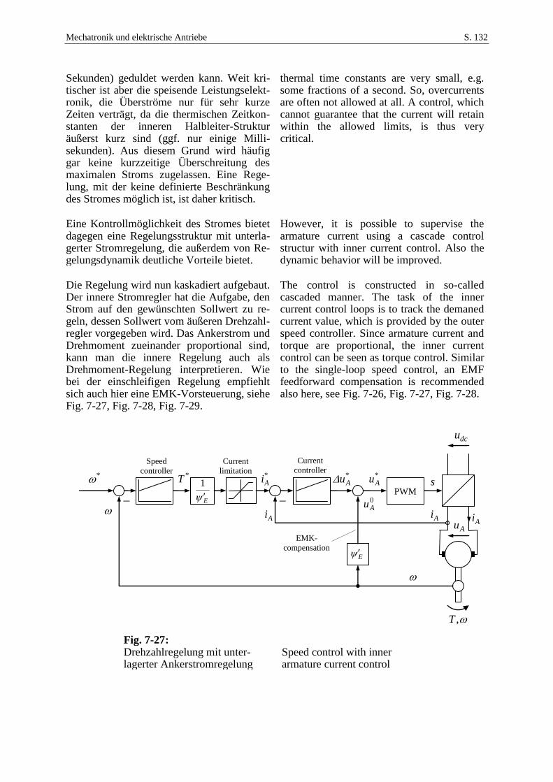
Mechatronik und elektrische Antriebe S. 132
Sekunden) geduldet werden kann. Weit kri-tischer ist aber die speisende Leistungselekt-ronik, die Überströme nur für sehr kurze Zeiten verträgt, da die thermischen Zeitkon-stanten der inneren Halbleiter-Struktur äußerst kurz sind (ggf. nur einige Milli-sekunden). Aus diesem Grund wird häufig gar keine kurzzeitige Überschreitung des maximalen Stroms zugelassen. Eine Rege-lung, mit der keine definierte Beschränkung des Stromes möglich ist, ist daher kritisch.
thermal time constants are very small, e.g. some fractions of a second. So, overcurrents are often not allowed at all. A control, which cannot guarantee that the current will retain within the allowed limits, is thus very critical.
Eine Kontrollmöglichkeit des Stromes bietet dagegen eine Regelungsstruktur mit unterla-gerter Stromregelung, die außerdem von Re-gelungsdynamik deutliche Vorteile bietet.
However, it is possible to supervise the armature current using a cascade control structur with inner current control. Also the dynamic behavior will be improved.
Die Regelung wird nun kaskadiert aufgebaut. Der innere Stromregler hat die Aufgabe, den Strom auf den gewünschten Sollwert zu re-geln, dessen Sollwert vom äußeren Drehzahl-regler vorgegeben wird. Das Ankerstrom und Drehmoment zueinander proportional sind, kann man die innere Regelung auch als Drehmoment-Regelung interpretieren. Wie bei der einschleifigen Regelung empfiehlt sich auch hier eine EMK-Vorsteuerung, siehe Fig. 7-27, Fig. 7-28, Fig. 7-29.
The control is constructed in so-called cascaded manner. The task of the inner current control loops is to track the demaned current value, which is provided by the outer speed controller. Since armature current and torque are proportional, the inner current control can be seen as torque control. Similar to the single-loop speed control, an EMF feedforward compensation is recommended also here, see Fig. 7-26, Fig. 7-27, Fig. 7-28.
Fig. 7-27: Drehzahlregelung mit unter-lagerter Ankerstromregelung
Speed control with inner armature current control
*
,T
PWM s
*Au
Au
*Au
0Au
AiAi
*T *Ai
dcu
E
1
E
EMK-
compensation
Current
controller
Speed
controller
Ai
Current
limitation
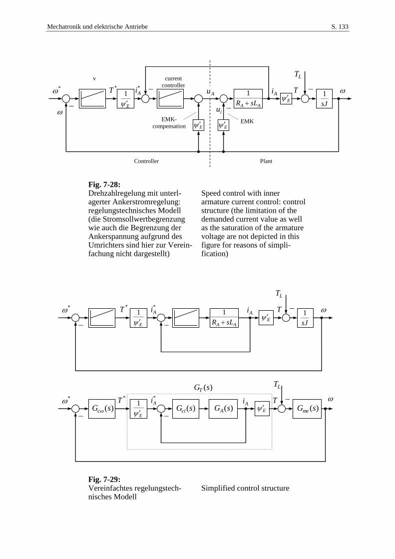
Mechatronik und elektrische Antriebe S. 133
Fig. 7-28: Drehzahlregelung mit unterl-agerter Ankerstromregelung: regelungstechnisches Modell (die Stromsollwertbegrenzung wie auch die Begrenzung der Ankerspannung aufgrund des Umrichters sind hier zur Verein-fachung nicht dargestellt)
Speed control with inner armature current control: control structure (the limitation of the demanded current value as well as the saturation of the armature voltage are not depicted in this figure for reasons of simpli-fication)
Fig. 7-29: Vereinfachtes regelungstech-nisches Modell
Simplified control structure
* Ai
*T *Ai
T
LT
AA sLR
1
E
1E
sJ
1
Ai
*T *Ai
T
LT
E
1E
*)(sGA)(sGci)(sGc )(sGme
)(sGT
* Ai*T *
Ai
T
LT
E
1
E E
AA sLR
1
sJ
1
EMK EMK-
compensation
E
iu
current
controller
v
Au
Controller Plant
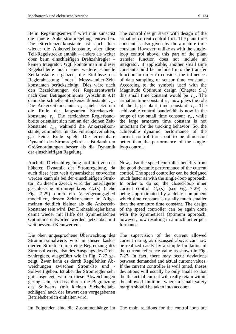
Mechatronik und elektrische Antriebe S. 134
Beim Regelungsentwurf wird nun zunächst die innere Ankerstromregelung entworfen. Die Streckenzeitkonstante ist auch hier wieder die Ankerzeitkonstante, aber diese Teil-Regelstrecke enthält – anders als weiter oben beim einschleifigen Drehzahlregler – keinen Integrator. Ggf. könnte man in dieser Regelschleife noch eine weitere schnelle Zeitkonstante ergänzen, die Einflüsse der Reglerabtastung oder Messwandler-Zeit-konstanten berücksichtigt. Dies wäre nach den Bezeichnungen des Regelerentwurfs nach dem Betragsoptimums (Abschnitt 9.1) dann die schnelle Streckenzeitkonstante . Die Ankerzeitkonstante
A spielt jetzt nur die Rolle der langsamen Streckenzeit-konstante s . Die erreichbare Reglerband-breite orientiert sich nun an der kleinen Zeit-konstante , während die Ankerzeitkon-stante, zumindest für das Führungsverhalten, gar keine Rolle spielt. Die erreichbare Dynamik des Stromregelkreises ist damit um Größenordnungen besser als die Dynamik der einschleifigen Regelung.
The control design starts with design of the armature current control first. The plant time constant is also given by the armature time constant. However, unlike as with the single-loop control above, this part of the plant transfer function does not include an integrator. If applicable, another small time constant could be included into the transfer function in order to consider the influences of data sampling or sensor time constants. According to the symbols used with the Magnitude Optimum design (Chapter 9.1) this small time constant would be . The armature time constant
A now plays the role of the large plant time constant s . The achievable control bandwidth is now in the range of the small time constant , while the large armature time constant is not important for the tracking behavior. So, the achievable dynamic performance of the current control turns out to be dimension better than the performance of the single-loop control.
Auch die Drehzahlregelung profitiert von der höheren Dynamik der Stromregelung, da auch diese jetzt weit dynamischer entworfen werden kann als bei der einschleifigen Struk-tur. Zu diesem Zweck wird der unterlagerte geschlossene Stromregelkreis ( )TG s (siehe Fig. 7-29) durch ein Verzögerungsglied modelliert, dessen Zeitkonstante im Allge-meinen deutlich kleiner als die Ankerzeit-konstante sein wird. Der Drehzahlregler kann damit wieder mit Hilfe des Symmetrischen Optimums entworfen werden, jetzt aber mit weit besseren Kennwerten.
Now, also the speed controller benefits from the good dynamic performance of the current control. The speed controller can be designed much faster as with the single-loop approach. In order to do so, the closed-loop inner current control ( )TG s (see Fig. 7-29) is being approximated by a delay component which time constant is usually much smaller than the armature time constant. The design of the speed controller can be again done with the Symmetrical Optimum approach, however, now resulting in a much better per-formance.
Die oben angesprochene Überwachung des Strommaximalwerts wird in dieser kaska-dierten Struktur durch eine Begrenzung des Stromsollwerts, also des Ausgangs des Dreh-zahlreglers, ausgeführt wie in Fig. 7-27 ge-zeigt. Zwar kann es durch Regelfehler Ab-weichungen zwischen Strom-Ist- und -Sollwert geben. Ist aber der Stromregler sehr gut ausgelegt, werden diese Abweichungen gering sein, so dass durch die Begrenzung des Sollwerts (mit kleinen Sicherheitab-schlägen) auch der Istwert den vorgegebenen Betriebsbereich einhalten wird.
The supervision of the current allowed current rating, as discussed above, can now be realized easily by a simple limitation of the current reference value as shown in Fig. 7-27. In fact, there may occur deviations between demanded and actual current values. If the current controller is well tuned, theses deviations will usually be only small so that the the actual current will really retain within the allowed limition, where a small safety margin should be taken into account.
Im Folgenden sind die Zusammenhänge im The main relations for the control loop are
Mechatronik und elektrische Antriebe S. 135
Regelkreis zusammengefasst: summarized as follows:
Differenzialgleichung für den Ankerstrom und Drehzahl:
Differential equation for armature current and speed:
EAAAiAAAAA iRuuiRuiL (7.51)
LTTJ (7.52)
Laplace-Transformierte: Laplace-Transformed
)()()( susiRsuisL iAAAAA (7.53)
)()()( sTsTssJ L (7.54)
Übertragungsfunktionen: Transfer functions: Übertragungsfunktion des elektrischen Teil-systems (Ankeradmittanz):
Transfer function of the electrical sub-system (armature admittance)
AAiA
AAA
sLRsusu
sisYsG
1
)()(
)()()( (7.55)
Drehmoment-Führungsübertragungsfunktion Torque transfer function
)()(1
)()(
)(
)()(
* sGsG
sGsG
sT
sTsG
Aci
AciT
(7.56)
Übertragungsfunktion des mechanischen Teilsystems:
Transfer function of the mechanical sub-system
sJsTsT
ssG
L
Ame
1
)()(
)()(
(7.57)
Drehzahl-Führungsübertragungsfunktion Speed tracking transfer function
)()()(1
)()()()(
sGsGsG
sGsGsGsG
meTc
meTc
(7.58)
Störübertragungsfunktion Disturbance transfer function
Mechatronik und elektrische Antriebe S. 136
)()()(1
)()(
sGsGsG
sGsG
meTc
meTL
(7.59)
7.13 Betrieb an Strom- und Spannungsgrenzen Operation at the Limits of Current and Voltages
Die stationären Gleichungen für den fremd-erregten Motor lauten
The steady-state equations of the separately excited DC motor are
EAAA siRu )( (7.60)
AEiT (7.61)
Das Drehmoment ist (bei konstantem Erre-gerfluss) durch die Stromgrenze des Motors bzw. des speisenden Umrichters
The maximum available torque results (at constant excitation flux) from the current limit of the motor or the feeding electric converter,
maxIiA ,
begrenzt, respectively:
maxmax IT E , maxmin IT E .
Auch die vom speisenden Umrichter ge-lieferte Spannung ist begrenzt:
Additionally, the voltage of the feeding converter is limited as well:
maxUuA . (7.62)
Wird der Erregerfluss konstant gehalten (was beim Permanentmagnet-Gleichstrommotor ohnehin der Fall ist), erreicht die Spannung bei der Drehzahl
If the exciting magnetic flux is considered constant (with permanent excitation this is the case anyhow), the voltage will reach its limit at the speed of
TR
TRUiRU
E
A
E
A
EE
AA202
maxmax1
(7.63)
ihre Begrenzung. Die Drehzahl kann darüber hinaus bei gleichbleibendem Fluss nicht weiter gesteigert werden. Die Drehzahl 0 ist die Leerlaufdrehzahl, die als ungefähre Abschätzung der Drehzahlgrenze dienen kann. Die exakte Grenzdrehzahl 1 hängt aber nicht nur vom Erregerfluss, sondern auch vom Ankerstrom bzw. vom Dreh-moment ab. Bei Betrieb mit maximalen Strom maxIiA resultieren für den motori-
The speed cannot be increased beyond that point with constant excitation flux. The speed 0 is the idling speed. This value can be taken as roughly approximated speed limit. The exact speed limit 1 , however, depends not only on the excitation flux, but also on the armature current or the torque, respectively. With operation at maximum current maxIiA , the exact motoric and regenerative speed limits result to
Mechatronik und elektrische Antriebe S. 137
schen und generatorischen Fall die Grenz-drehzahlen
E
Amot
IRU
maxmax
1 , E
Agen
IRU
maxmax
1
Höhere Drehzahlen sind jedoch möglich, wenn der Erregerfluss verringert (ge-schwächt) wird. Der Fluss muss umgekehrt proportional zur Drehzahl reduziert werden,
Higher speeds are possible, however, if the flux is reduced accordingly. The flux must be reduced inversely proportional to the speed,
maxmax UIRU AA
E
, (7.64)
um die Spannungsbegrenzung einzuhalten. Dazu bedarf es natürlich einer steuerbaren Erregerspeisung (bei permanent erregten Gleichstrommotoren ist das natürlich nicht möglich). Das verfügbare Drehmoment redu-ziert sich nun umkehrt proportional zur Drehzahl,
in order not to violate the voltage limit. To do so, a variable supply of the excitation circuit is required (which is not possible with permanently excited motors). Then, the provided torque will also be reduced inversely proportional to the speed,
maxmax
maxmaxmax
max
IUI
IRUT A
(7.65)
bzw. für generatorischen Betrieb in the motoric case, and for the regenerative
case
maxmax
maxmaxmax
min
IUI
IRUT A
(7.66)
Die verfügbare mechanische Leistung The maximum available mechanical power
yields as
maxmaxmaxmaxmaxmaxmax IUIIRUTP A (7.67)
konstant. Dieser Bereich wird Fluss-schwächbereich bzw. Konstant-Leistungs-Bereich genannt. Im unteren Drehzahlbereich
1 , wo die Ankerspannung nicht ihre Grenze erreicht, ist die verfügbare Leistung dagegen proportional zur Drehzahl
and results to be constant. This operation area is called flux weakening range or constant-power-range. In the lower speed area with 1 , where the armature voltage is not saturated, the maximium power results to be proportional to the speed
maxmaxmax ITP E (7.68)
bzw. or
maxminmin ITP E . (7.69)

Mechatronik und elektrische Antriebe S. 138
Dieser Bereich heißt Anker-Stellbereich oder Spannungs-Stellbereich bzw. Konstant-Drehmoment-Bereich. Der Flussschwäch-bereich wird häufig als dimensionsloses Ver-hältnis der Drehzahl 1 zur maximalen Drehzahl max , welche in der Regel aus mechanischen Grenzen resultiert, angegeben.
This area is called armature or voltage control range or constant-torque-range. The flux weakening range is often specified by the dimensionless ratio of the 1 and the maximum speed max , which usually results from mechanical restrictions.
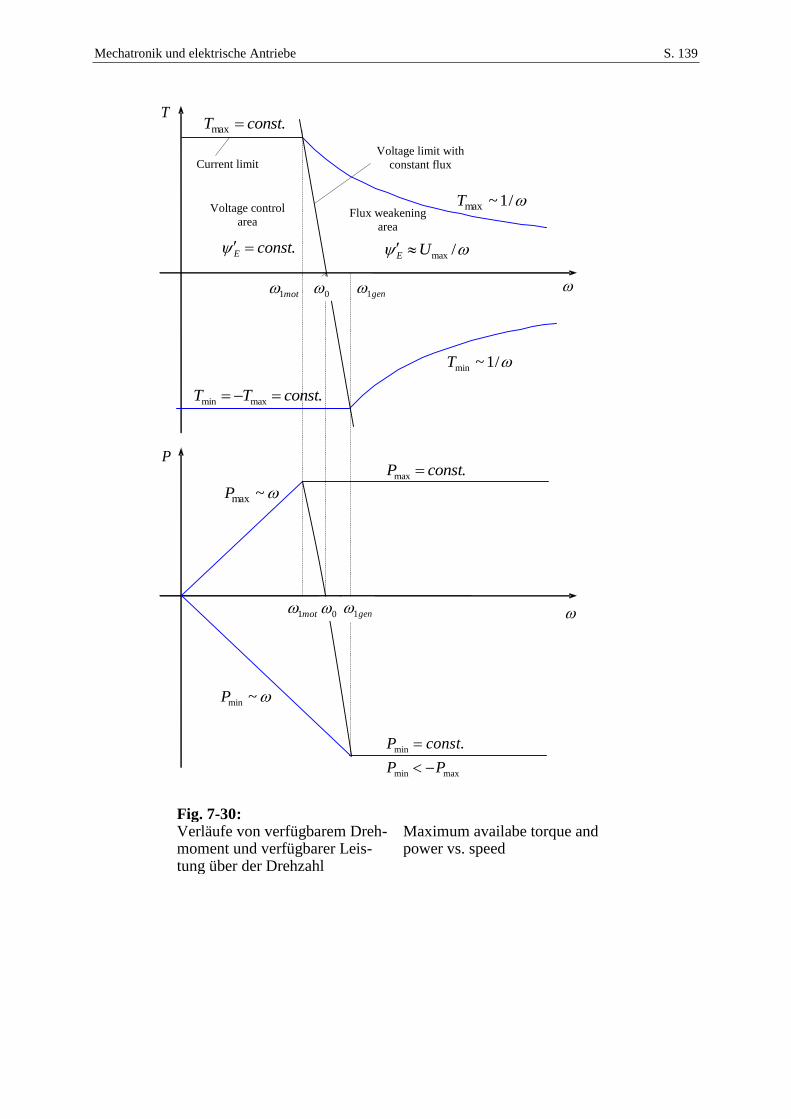
Mechatronik und elektrische Antriebe S. 139
Fig. 7-30: Verläufe von verfügbarem Dreh-moment und verfügbarer Leis-tung über der Drehzahl
Maximum availabe torque and power vs. speed
Voltage control
area Flux weakening
area
Current limit Voltage limit with
constant flux
/maxUE
/1~maxT
.max constT
.maxmin constTT
.max constP
maxmin
min .
PP
constP
~maxP
~minP
gen1mot1 0
gen1mot1 0
/1~minT
.constE
T
P
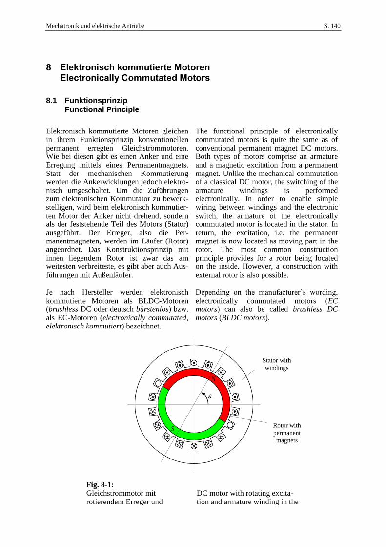
Mechatronik und elektrische Antriebe S. 140
8 Elektronisch kommutierte Motoren Electronically Commutated Motors
8.1 Funktionsprinzip Functional Principle
Elektronisch kommutierte Motoren gleichen in ihrem Funktionsprinzip konventionellen permanent erregten Gleichstrommotoren. Wie bei diesen gibt es einen Anker und eine Erregung mittels eines Permanentmagnets. Statt der mechanischen Kommutierung werden die Ankerwicklungen jedoch elektro-nisch umgeschaltet. Um die Zuführungen zum elektronischen Kommutator zu bewerk-stelligen, wird beim elektronisch kommutier-ten Motor der Anker nicht drehend, sondern als der feststehende Teil des Motors (Stator) ausgeführt. Der Erreger, also die Per-manentmagneten, werden im Läufer (Rotor) angeordnet. Das Konstruktionsprinzip mit innen liegendem Rotor ist zwar das am weitesten verbreiteste, es gibt aber auch Aus-führungen mit Außenläufer.
The functional principle of electronically commutated motors is quite the same as of conventional permanent magnet DC motors. Both types of motors comprise an armature and a magnetic excitation from a permanent magnet. Unlike the mechanical commutation of a classical DC motor, the switching of the armature windings is performed electronically. In order to enable simple wiring between windings and the electronic switch, the armature of the electronically commutated motor is located in the stator. In return, the excitation, i.e. the permanent magnet is now located as moving part in the rotor. The most common construction principle provides for a rotor being located on the inside. However, a construction with external rotor is also possible.
Je nach Hersteller werden elektronisch kommutierte Motoren als BLDC-Motoren (brushless DC oder deutsch bürstenlos) bzw. als EC-Motoren (electronically commutated, elektronisch kommutiert) bezeichnet.
Depending on the manufacturer’s wording, electronically commutated motors (EC motors) can also be called brushless DC motors (BLDC motors).
Fig. 8-1: Gleichstrommotor mit rotierendem Erreger und
DC motor with rotating excita-tion and armature winding in the
N
S
Stator with
windings
Rotor with
permanent
magnets
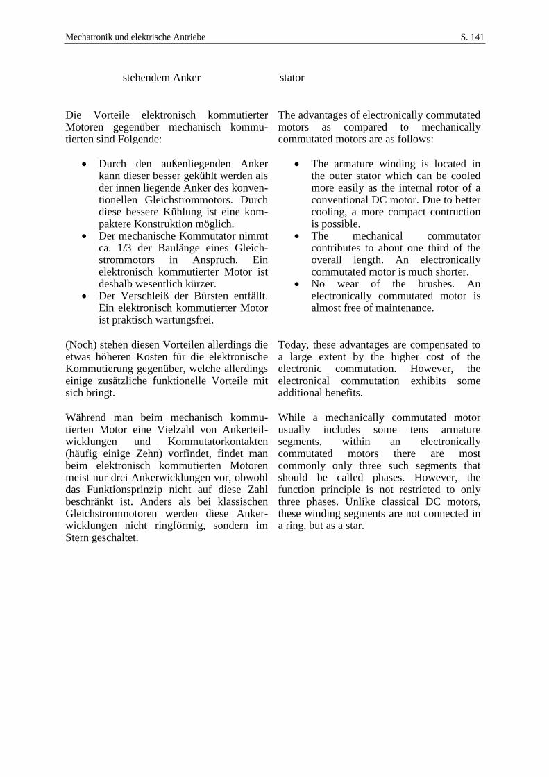
Mechatronik und elektrische Antriebe S. 141
stehendem Anker stator
Die Vorteile elektronisch kommutierter Motoren gegenüber mechanisch kommu-tierten sind Folgende:
The advantages of electronically commutated motors as compared to mechanically commutated motors are as follows:
Durch den außenliegenden Anker
kann dieser besser gekühlt werden als der innen liegende Anker des konven-tionellen Gleichstrommotors. Durch diese bessere Kühlung ist eine kom-paktere Konstruktion möglich.
Der mechanische Kommutator nimmt ca. 1/3 der Baulänge eines Gleich-strommotors in Anspruch. Ein elektronisch kommutierter Motor ist deshalb wesentlich kürzer.
Der Verschleiß der Bürsten entfällt. Ein elektronisch kommutierter Motor ist praktisch wartungsfrei.
The armature winding is located in the outer stator which can be cooled more easily as the internal rotor of a conventional DC motor. Due to better cooling, a more compact contruction is possible.
The mechanical commutator contributes to about one third of the overall length. An electronically commutated motor is much shorter.
No wear of the brushes. An electronically commutated motor is almost free of maintenance.
(Noch) stehen diesen Vorteilen allerdings die etwas höheren Kosten für die elektronische Kommutierung gegenüber, welche allerdings einige zusätzliche funktionelle Vorteile mit sich bringt.
Today, these advantages are compensated to a large extent by the higher cost of the electronic commutation. However, the electronical commutation exhibits some additional benefits.
Während man beim mechanisch kommu-tierten Motor eine Vielzahl von Ankerteil-wicklungen und Kommutatorkontakten (häufig einige Zehn) vorfindet, findet man beim elektronisch kommutierten Motoren meist nur drei Ankerwicklungen vor, obwohl das Funktionsprinzip nicht auf diese Zahl beschränkt ist. Anders als bei klassischen Gleichstrommotoren werden diese Anker-wicklungen nicht ringförmig, sondern im Stern geschaltet.
While a mechanically commutated motor usually includes some tens armature segments, within an electronically commutated motors there are most commonly only three such segments that should be called phases. However, the function principle is not restricted to only three phases. Unlike classical DC motors, these winding segments are not connected in a ring, but as a star.
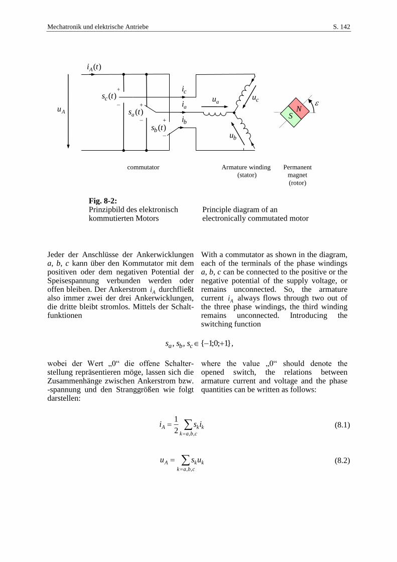
Mechatronik und elektrische Antriebe S. 142
Fig. 8-2: Prinzipbild des elektronisch kommutierten Motors
Principle diagram of an electronically commutated motor
Jeder der Anschlüsse der Ankerwicklungen a, b, c kann über den Kommutator mit dem positiven oder dem negativen Potential der Speisespannung verbunden werden oder offen bleiben. Der Ankerstrom Ai durchfließt also immer zwei der drei Ankerwicklungen, die dritte bleibt stromlos. Mittels der Schalt-funktionen
With a commutator as shown in the diagram, each of the terminals of the phase windings a, b, c can be connected to the positive or the negative potential of the supply voltage, or remains unconnected. So, the armature current Ai always flows through two out of the three phase windings, the third winding remains unconnected. Introducing the switching function
}1;0;1{,, cba sss ,
wobei der Wert „0“ die offene Schalter-stellung repräsentieren möge, lassen sich die Zusammenhänge zwischen Ankerstrom bzw. -spannung und den Stranggrößen wie folgt darstellen:
where the value „0“ should denote the opened switch, the relations between armature current and voltage and the phase quantities can be written as follows:
cbak
kkA isi,,2
1 (8.1)
cbak
kkA usu,,
(8.2)
N
S
)(tiA
)(tsc
Au
commutator Armature winding
(stator)
Permanent
magnet
(rotor)
+
− +
− +
−
au cu
bu
ci
ai
bi)(tsa
)(tsb
Mechatronik und elektrische Antriebe S. 143
8.2 Induzierte Spannungen Induced Voltages
Fig. 8-3: Zur induzierten Spannung in einer einzelnen Ankerwindung : Stellungswinkel des Rotors gegenüber dem Stator : Rotorfeste Koordinate zur Beschreibung des Rotorfeldes
On the induced voltage in a single armature winding turn : position angle of the rotor with respect to the stator : rotor-fixed coordinate to be used for the description of the rotor field
N
S
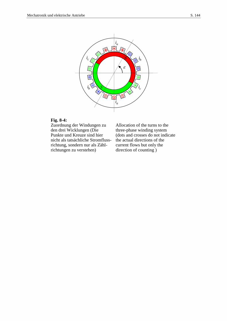
Mechatronik und elektrische Antriebe S. 144
Fig. 8-4: Zuordnung der Windungen zu den drei Wicklungen (Die Punkte und Kreuze sind hier nicht als tatsächliche Stromfluss-richtung, sondern nur als Zähl-richtungen zu verstehen)
Allocation of the turns to the three-phase winding system (dots and crosses do not indicate the actual directions of the current flows but only the direction of counting )
ai
ai
ci N
S
bi
bi ci
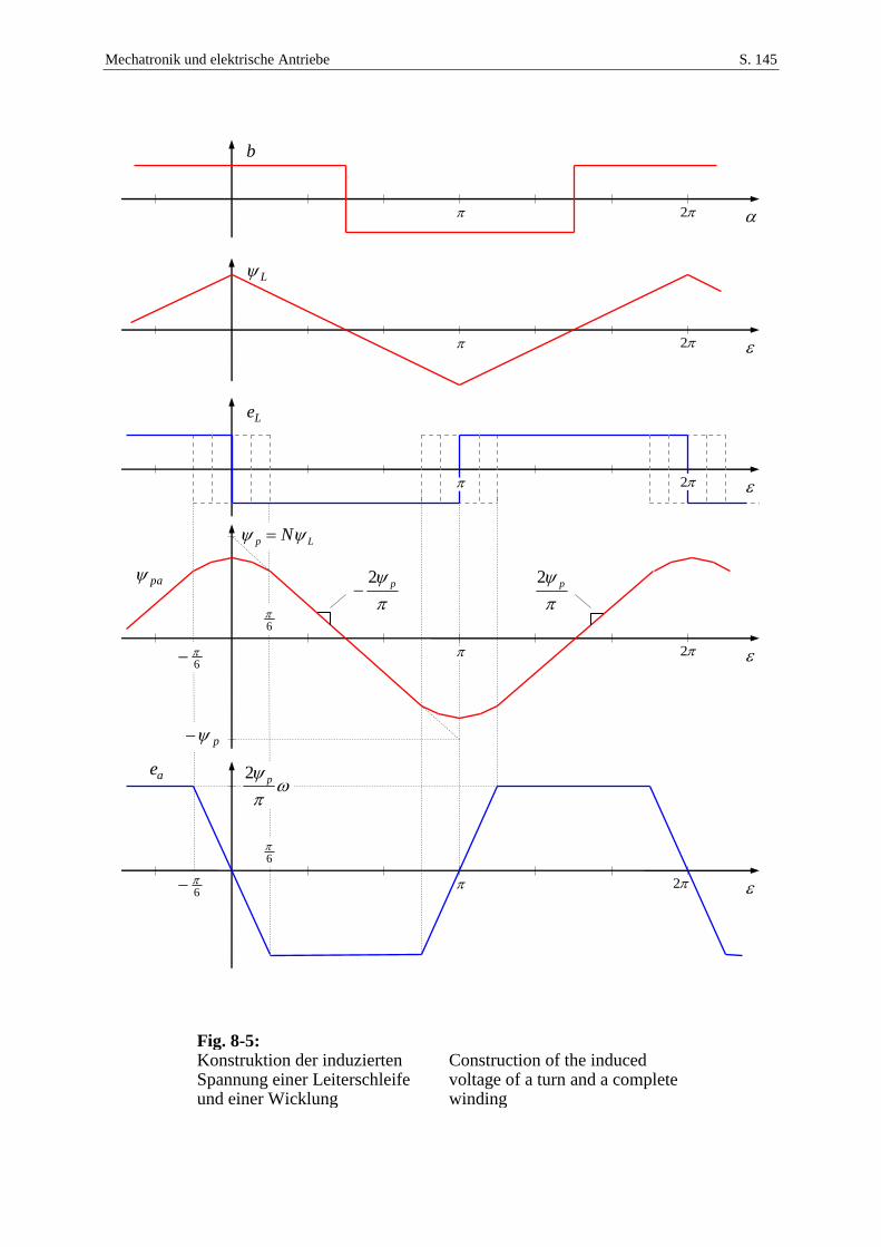
Mechatronik und elektrische Antriebe S. 145
Fig. 8-5: Konstruktion der induzierten Spannung einer Leiterschleife und einer Wicklung
Construction of the induced voltage of a turn and a complete winding
L
2
b
2
Le
2
pa
2
6
6
26
ae
6
Lp N
p
p2
p2
p2
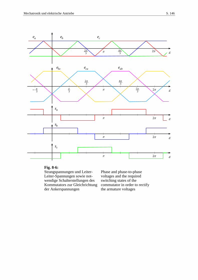
Mechatronik und elektrische Antriebe S. 146
Fig. 8-6: Strangspannungen und Leiter-Leiter-Spannungen sowie not-wendige Schalterstellungen des Kommutators zur Gleichrichtung der Ankerspannungen
Phase and phase-to-phase voltages and the required switching states of the commutator in order to rectify the armature voltages
ae
32
34
be ce
bce
32
34
cae abe
2
2
2
2
2
3
35
3
as
bs
cs
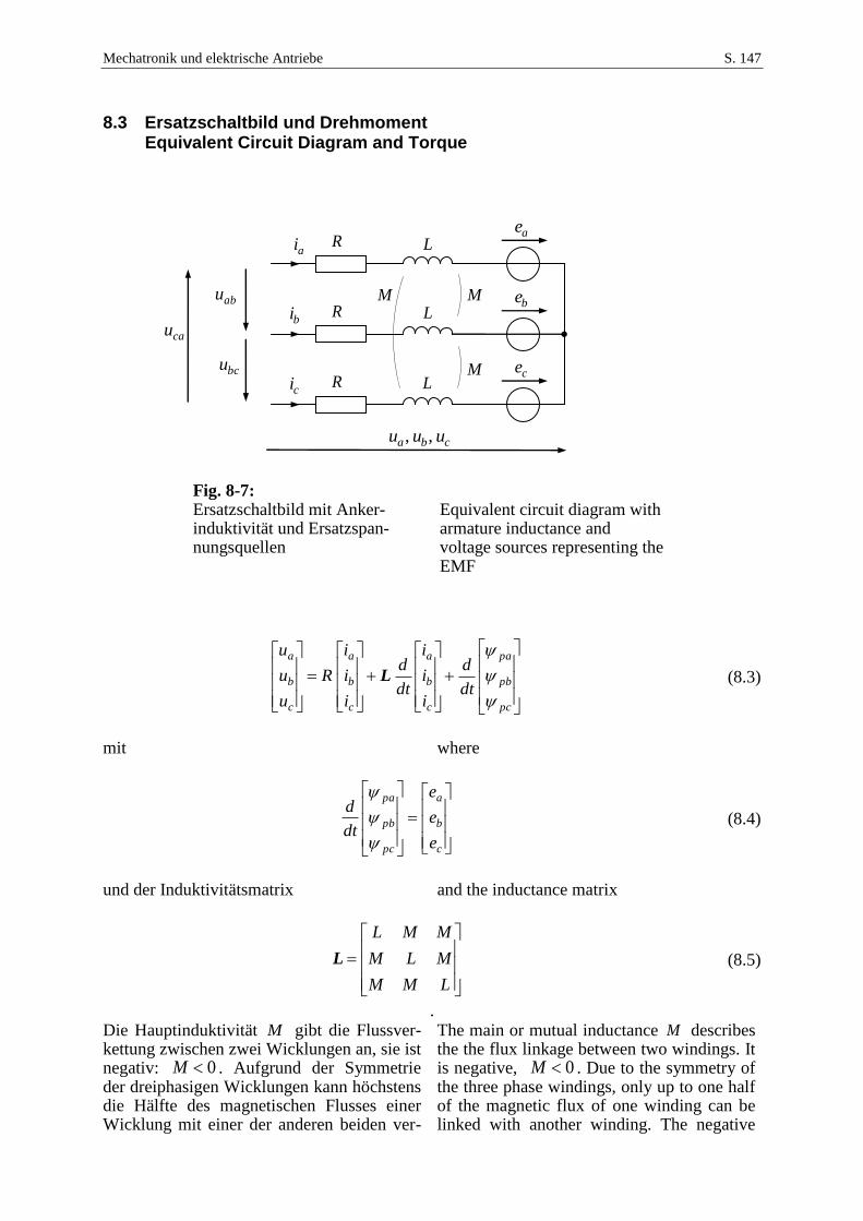
Mechatronik und elektrische Antriebe S. 147
8.3 Ersatzschaltbild und Drehmoment Equivalent Circuit Diagram and Torque
Fig. 8-7: Ersatzschaltbild mit Anker-induktivität und Ersatzspan-nungsquellen
Equivalent circuit diagram with armature inductance and voltage sources representing the EMF
pc
pb
pa
c
b
a
c
b
a
c
b
a
dt
d
i
i
i
dt
d
i
i
i
R
u
u
u
L (8.3)
mit where
c
b
a
pc
pb
pa
e
e
e
dt
d
(8.4)
und der Induktivitätsmatrix and the inductance matrix
LMM
MLM
MML
L (8.5)
. Die Hauptinduktivität M gibt die Flussver-kettung zwischen zwei Wicklungen an, sie ist negativ: 0M . Aufgrund der Symmetrie der dreiphasigen Wicklungen kann höchstens die Hälfte des magnetischen Flusses einer Wicklung mit einer der anderen beiden ver-
The main or mutual inductance M describes the the flux linkage between two windings. It is negative, 0M . Due to the symmetry of the three phase windings, only up to one half of the magnetic flux of one winding can be linked with another winding. The negative
abu
ae
be
cebcu
ai
bi
ci
L
L
L
R
R
R
M
M
M
cba uuu ,,
cau
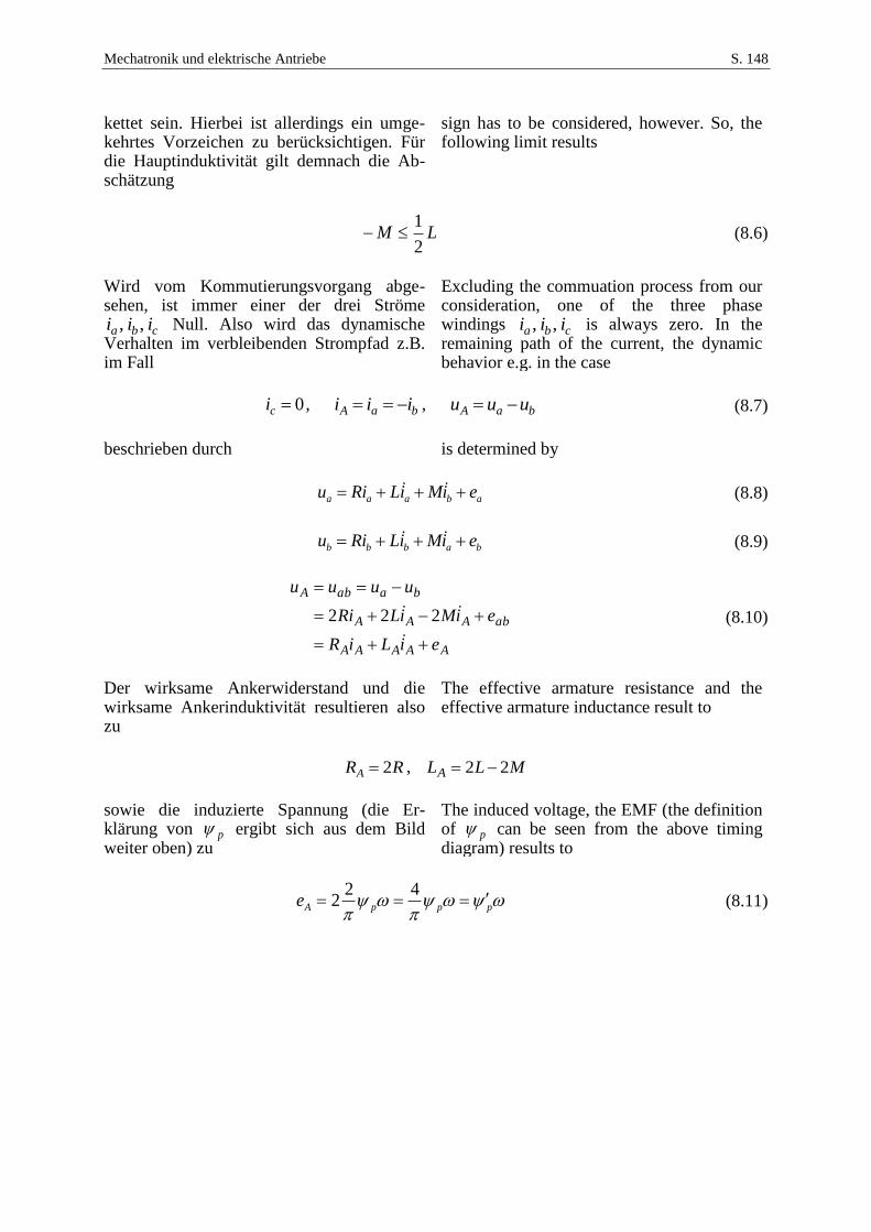
Mechatronik und elektrische Antriebe S. 148
kettet sein. Hierbei ist allerdings ein umge-kehrtes Vorzeichen zu berücksichtigen. Für die Hauptinduktivität gilt demnach die Ab-schätzung
sign has to be considered, however. So, the following limit results
LM2
1 (8.6)
Wird vom Kommutierungsvorgang abge-sehen, ist immer einer der drei Ströme
cba iii ,, Null. Also wird das dynamische Verhalten im verbleibenden Strompfad z.B. im Fall
Excluding the commuation process from our consideration, one of the three phase windings cba iii ,, is always zero. In the remaining path of the current, the dynamic behavior e.g. in the case
0ci , baA iii , baA uuu (8.7)
beschrieben durch is determined by
abaaa eiMiLRiu (8.8)
babbb eiMiLRiu (8.9)
AAAAA
abAAA
baabA
eiLiR
eiMiLRi
uuuu
222 (8.10)
Der wirksame Ankerwiderstand und die wirksame Ankerinduktivität resultieren also zu
The effective armature resistance and the effective armature inductance result to
RRA 2 , MLLA 22
sowie die induzierte Spannung (die Er-klärung von p ergibt sich aus dem Bild weiter oben) zu
The induced voltage, the EMF (the definition of p can be seen from the above timing diagram) results to
pppAe 42
2 (8.11)
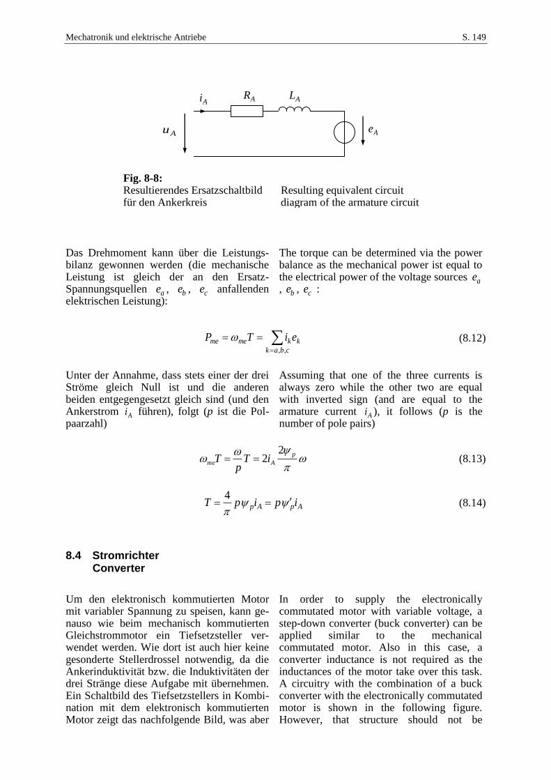
Mechatronik und elektrische Antriebe S. 149
Fig. 8-8: Resultierendes Ersatzschaltbild für den Ankerkreis
Resulting equivalent circuit diagram of the armature circuit
Das Drehmoment kann über die Leistungs-bilanz gewonnen werden (die mechanische Leistung ist gleich der an den Ersatz-Spannungsquellen ae , be , ce anfallenden elektrischen Leistung):
The torque can be determined via the power balance as the mechanical power ist equal to the electrical power of the voltage sources ae, be , ce :
cbak
kkmeme eiTP,,
(8.12)
Unter der Annahme, dass stets einer der drei Ströme gleich Null ist und die anderen beiden entgegengesetzt gleich sind (und den Ankerstrom Ai führen), folgt (p ist die Pol-paarzahl)
Assuming that one of the three currents is always zero while the other two are equal with inverted sign (and are equal to the armature current Ai ), it follows (p is the number of pole pairs)
p
Ame iTp
T2
2 (8.13)
ApAp ipipT
4
(8.14)
8.4 Stromrichter Converter
Um den elektronisch kommutierten Motor mit variabler Spannung zu speisen, kann ge-nauso wie beim mechanisch kommutierten Gleichstrommotor ein Tiefsetzsteller ver-wendet werden. Wie dort ist auch hier keine gesonderte Stellerdrossel notwendig, da die Ankerinduktivität bzw. die Induktivitäten der drei Stränge diese Aufgabe mit übernehmen. Ein Schaltbild des Tiefsetzstellers in Kombi-nation mit dem elektronisch kommutierten Motor zeigt das nachfolgende Bild, was aber
In order to supply the electronically commutated motor with variable voltage, a step-down converter (buck converter) can be applied similar to the mechanical commutated motor. Also in this case, a converter inductance is not required as the inductances of the motor take over this task. A circuitry with the combination of a buck converter with the electronically commutated motor is shown in the following figure. However, that structure should not be
Au Ae
Ai ALAR
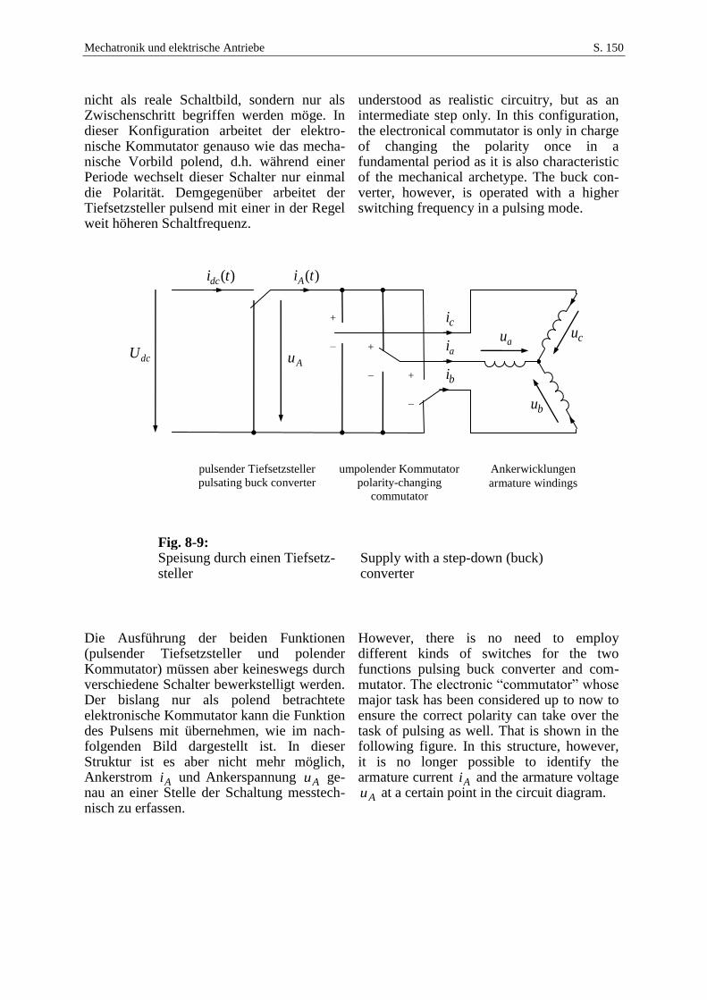
Mechatronik und elektrische Antriebe S. 150
nicht als reale Schaltbild, sondern nur als Zwischenschritt begriffen werden möge. In dieser Konfiguration arbeitet der elektro-nische Kommutator genauso wie das mecha-nische Vorbild polend, d.h. während einer Periode wechselt dieser Schalter nur einmal die Polarität. Demgegenüber arbeitet der Tiefsetzsteller pulsend mit einer in der Regel weit höheren Schaltfrequenz.
understood as realistic circuitry, but as an intermediate step only. In this configuration, the electronical commutator is only in charge of changing the polarity once in a fundamental period as it is also characteristic of the mechanical archetype. The buck con-verter, however, is operated with a higher switching frequency in a pulsing mode.
Fig. 8-9: Speisung durch einen Tiefsetz-steller
Supply with a step-down (buck) converter
Die Ausführung der beiden Funktionen (pulsender Tiefsetzsteller und polender Kommutator) müssen aber keineswegs durch verschiedene Schalter bewerkstelligt werden. Der bislang nur als polend betrachtete elektronische Kommutator kann die Funktion des Pulsens mit übernehmen, wie im nach-folgenden Bild dargestellt ist. In dieser Struktur ist es aber nicht mehr möglich, Ankerstrom Ai und Ankerspannung Au ge-nau an einer Stelle der Schaltung messtech-nisch zu erfassen.
However, there is no need to employ different kinds of switches for the two functions pulsing buck converter and com-mutator. The electronic “commutator” whose major task has been considered up to now to ensure the correct polarity can take over the task of pulsing as well. That is shown in the following figure. In this structure, however, it is no longer possible to identify the armature current Ai and the armature voltage
Au at a certain point in the circuit diagram.
dcUAu
)(tiA
+
− +
− +
−
au cu
bu
umpolender Kommutator
polarity-changing
commutator
Ankerwicklungen
armature windings
pulsender Tiefsetzsteller
pulsating buck converter
)(tidc
ci
ai
bi
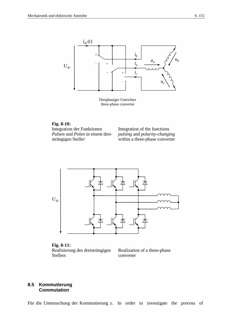
Mechatronik und elektrische Antriebe S. 151
Fig. 8-10: Integration der Funktionen Pulsen und Polen in einem drei-strängigen Steller
Integration of the functions pulsing and polarity-changing within a three-phase converter
Fig. 8-11: Realisierung des dreisträngigen Stellers
Realization of a three-phase converter
8.5 Kommutierung Commutation
Für die Untersuchung der Kommutierung z. In order to investigate the process of
dcU
dcU
)(tidc
bi
ai
ci
+
− +
− +
−
au bu
cu
Dreiphasiger Umrichter
three-phase converter
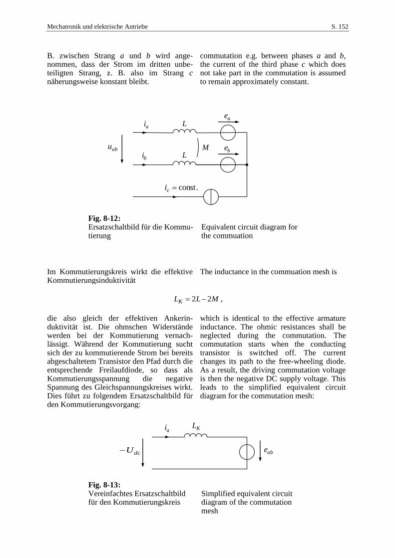
Mechatronik und elektrische Antriebe S. 152
B. zwischen Strang a und b wird ange-nommen, dass der Strom im dritten unbe-teiligten Strang, z. B. also im Strang c näherungsweise konstant bleibt.
commutation e.g. between phases a and b, the current of the third phase c which does not take part in the commutation is assumed to remain approximately constant.
Fig. 8-12: Ersatzschaltbild für die Kommu-tierung
Equivalent circuit diagram for the commuation
Im Kommutierungskreis wirkt die effektive Kommutierungsinduktivität
The inductance in the commuation mesh is
MLLK 22 ,
die also gleich der effektiven Ankerin-duktivität ist. Die ohmschen Widerstände werden bei der Kommutierung vernach-lässigt. Während der Kommutierung sucht sich der zu kommutierende Strom bei bereits abgeschaltetem Transistor den Pfad durch die entsprechende Freilaufdiode, so dass als Kommutierungsspannung die negative Spannung des Gleichspannungskreises wirkt. Dies führt zu folgendem Ersatzschaltbild für den Kommutierungsvorgang:
which is identical to the effective armature inductance. The ohmic resistances shall be neglected during the commutation. The commutation starts when the conducting transistor is switched off. The current changes its path to the free-wheeling diode. As a result, the driving commutation voltage is then the negative DC supply voltage. This leads to the simplified equivalent circuit diagram for the commutation mesh:
Fig. 8-13: Vereinfachtes Ersatzschaltbild für den Kommutierungskreis
Simplified equivalent circuit diagram of the commutation mesh
dcU abe
ai KL
abu
ae
be
ai
bi
.constci
L
LM
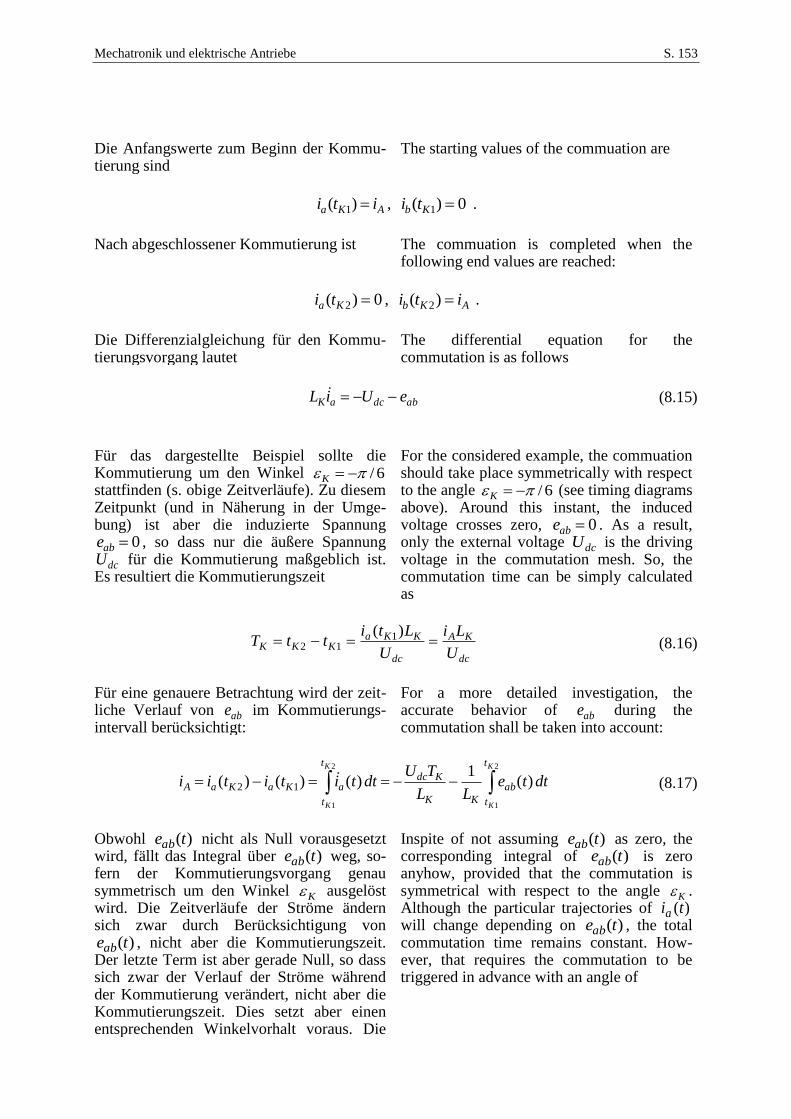
Mechatronik und elektrische Antriebe S. 153
Die Anfangswerte zum Beginn der Kommu-tierung sind
The starting values of the commuation are
AKa iti )( 1 , 0)( 1 Kb ti .
Nach abgeschlossener Kommutierung ist The commuation is completed when the
following end values are reached:
0)( 2 Ka ti , AKb iti )( 2 .
Die Differenzialgleichung für den Kommu-tierungsvorgang lautet
The differential equation for the commutation is as follows
abdcaK eUiL (8.15)
Für das dargestellte Beispiel sollte die Kommutierung um den Winkel 6/ K stattfinden (s. obige Zeitverläufe). Zu diesem Zeitpunkt (und in Näherung in der Umge-bung) ist aber die induzierte Spannung
0abe , so dass nur die äußere Spannung
dcU für die Kommutierung maßgeblich ist. Es resultiert die Kommutierungszeit
For the considered example, the commuation should take place symmetrically with respect to the angle 6/ K (see timing diagrams above). Around this instant, the induced voltage crosses zero, 0abe . As a result, only the external voltage dcU is the driving voltage in the commutation mesh. So, the commutation time can be simply calculated as
dc
KA
dc
KKaKKK
U
Li
U
LtittT
)( 112 (8.16)
Für eine genauere Betrachtung wird der zeit-liche Verlauf von abe im Kommutierungs-intervall berücksichtigt:
For a more detailed investigation, the accurate behavior of abe during the commutation shall be taken into account:
2
1
2
1
)(1
)()()( 12
K
K
K
K
t
t
ab
KK
Kdc
t
t
aKaKaA dtteLL
TUdttititii (8.17)
Obwohl )(teab nicht als Null vorausgesetzt wird, fällt das Integral über )(teab weg, so-fern der Kommutierungsvorgang genau symmetrisch um den Winkel K ausgelöst wird. Die Zeitverläufe der Ströme ändern sich zwar durch Berücksichtigung von
)(teab , nicht aber die Kommutierungszeit. Der letzte Term ist aber gerade Null, so dass sich zwar der Verlauf der Ströme während der Kommutierung verändert, nicht aber die Kommutierungszeit. Dies setzt aber einen entsprechenden Winkelvorhalt voraus. Die
Inspite of not assuming )(teab as zero, the corresponding integral of )(teab is zero anyhow, provided that the commutation is symmetrical with respect to the angle K . Although the particular trajectories of )(tia will change depending on )(teab , the total commutation time remains constant. How-ever, that requires the commutation to be triggered in advance with an angle of
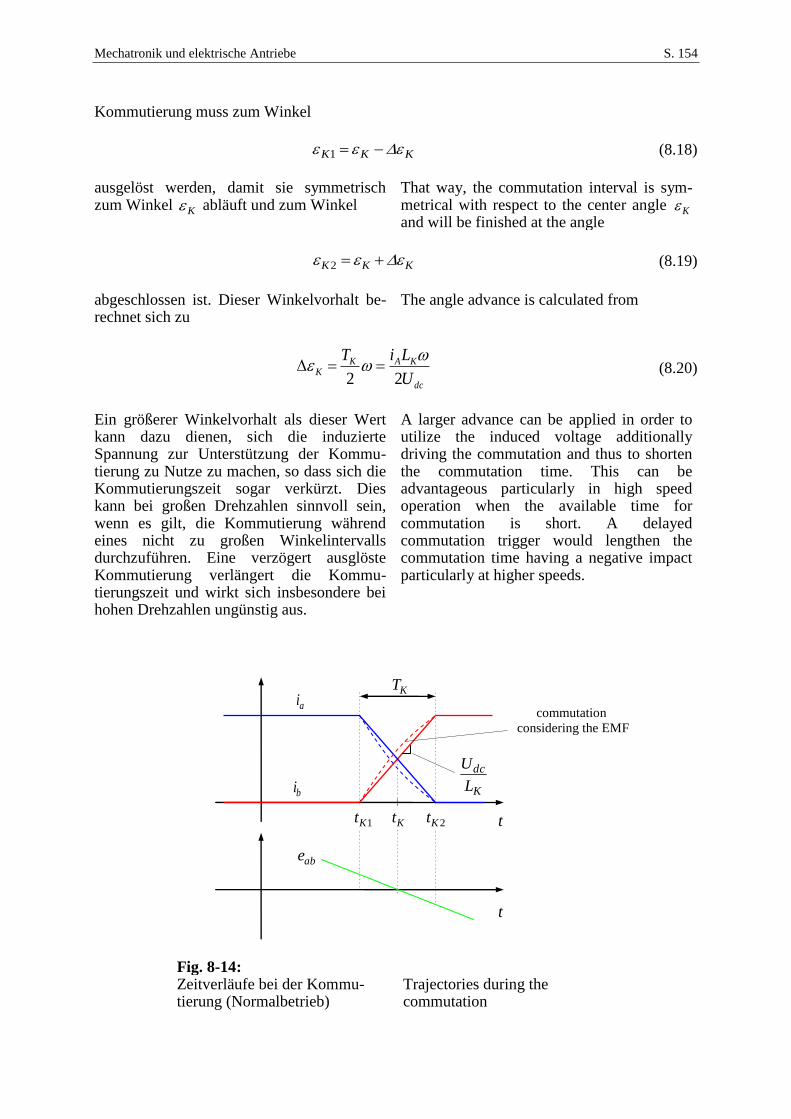
Mechatronik und elektrische Antriebe S. 154
Kommutierung muss zum Winkel
KKK 1 (8.18)
ausgelöst werden, damit sie symmetrisch zum Winkel K abläuft und zum Winkel
That way, the commutation interval is sym-metrical with respect to the center angle K and will be finished at the angle
2K K K (8.19)
abgeschlossen ist. Dieser Winkelvorhalt be-rechnet sich zu
The angle advance is calculated from
dc
KAKK
U
LiT
22
(8.20)
Ein größerer Winkelvorhalt als dieser Wert kann dazu dienen, sich die induzierte Spannung zur Unterstützung der Kommu-tierung zu Nutze zu machen, so dass sich die Kommutierungszeit sogar verkürzt. Dies kann bei großen Drehzahlen sinnvoll sein, wenn es gilt, die Kommutierung während eines nicht zu großen Winkelintervalls durchzuführen. Eine verzögert ausglöste Kommutierung verlängert die Kommu-tierungszeit und wirkt sich insbesondere bei hohen Drehzahlen ungünstig aus.
A larger advance can be applied in order to utilize the induced voltage additionally driving the commutation and thus to shorten the commutation time. This can be advantageous particularly in high speed operation when the available time for commutation is short. A delayed commutation trigger would lengthen the commutation time having a negative impact particularly at higher speeds.
Fig. 8-14: Zeitverläufe bei der Kommu-tierung (Normalbetrieb)
Trajectories during the commutation
ai
t
bi
1Kt 2Kt
KT
t
abe
commutation
considering the EMF
Kt
K
dc
L
U
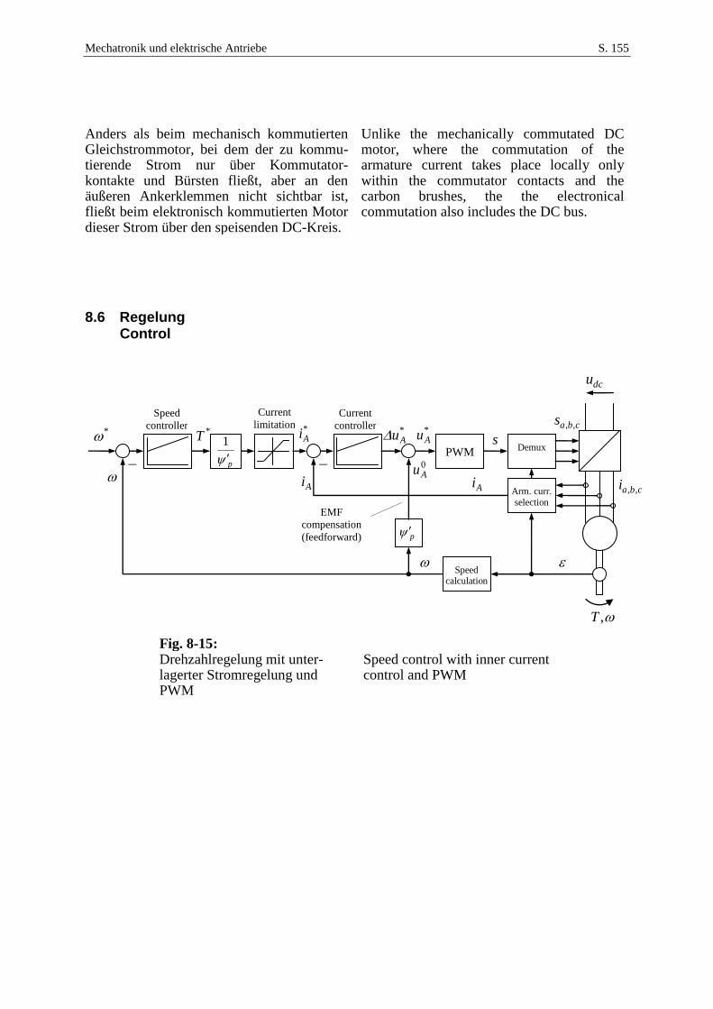
Mechatronik und elektrische Antriebe S. 155
Anders als beim mechanisch kommutierten Gleichstrommotor, bei dem der zu kommu-tierende Strom nur über Kommutator-kontakte und Bürsten fließt, aber an den äußeren Ankerklemmen nicht sichtbar ist, fließt beim elektronisch kommutierten Motor dieser Strom über den speisenden DC-Kreis.
Unlike the mechanically commutated DC motor, where the commutation of the armature current takes place locally only within the commutator contacts and the carbon brushes, the the electronical commutation also includes the DC bus.
8.6 Regelung Control
Fig. 8-15: Drehzahlregelung mit unter-lagerter Stromregelung und PWM
Speed control with inner current control and PWM
*
,T
PWM s
*Au*
Au
0Au
Ai
*T*Ai
dcu
p
1
p
EMF
compensation
(feedforward)
Current
controller Speed
controller
Ai
Demux
cbas ,,
Arm. curr.
selection
cbai ,,
Speed calculation
Current
limitation
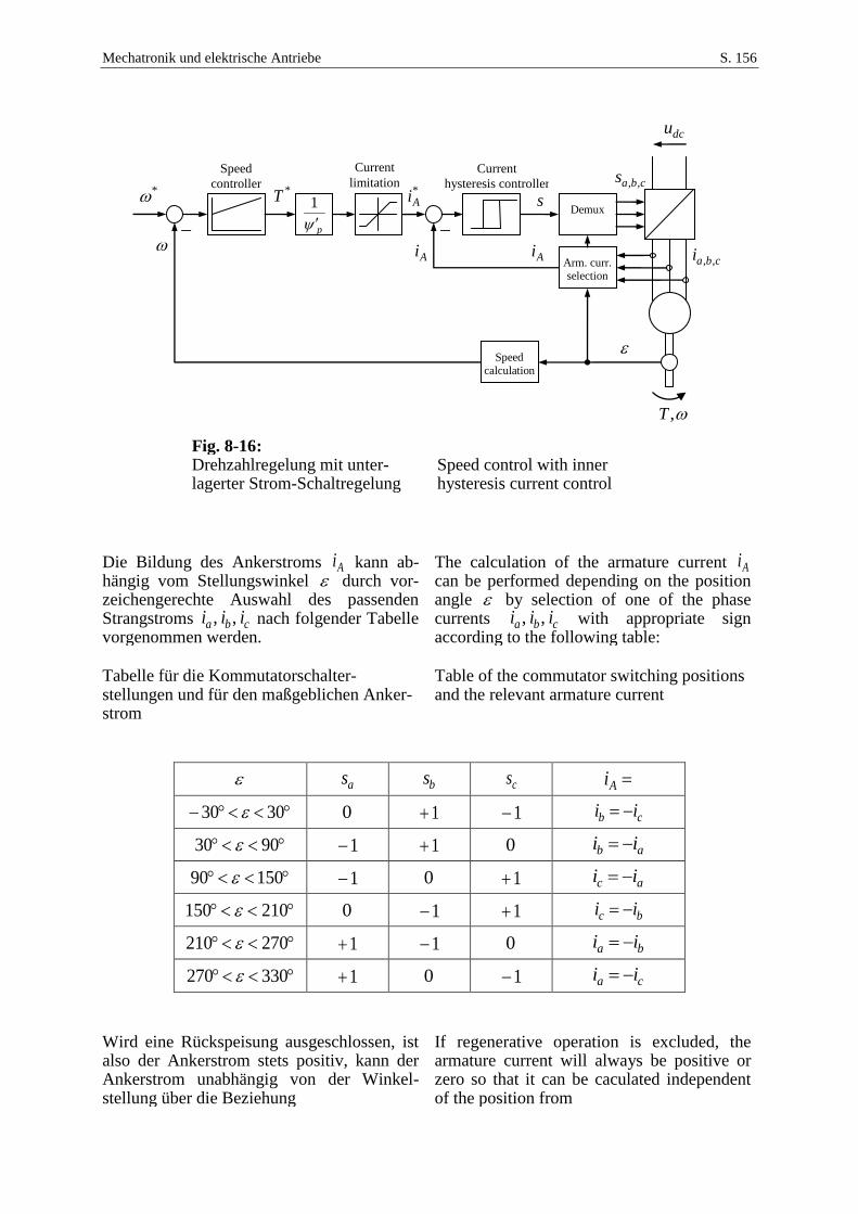
Mechatronik und elektrische Antriebe S. 156
Fig. 8-16: Drehzahlregelung mit unter-lagerter Strom-Schaltregelung
Speed control with inner hysteresis current control
Die Bildung des Ankerstroms Ai kann ab-hängig vom Stellungswinkel durch vor-zeichengerechte Auswahl des passenden Strangstroms cba iii ,, nach folgender Tabelle vorgenommen werden.
The calculation of the armature current Ai can be performed depending on the position angle by selection of one of the phase currents cba iii ,, with appropriate sign according to the following table:
Tabelle für die Kommutatorschalter-stellungen und für den maßgeblichen Anker-strom
Table of the commutator switching positions and the relevant armature current
as bs cs Ai
3030 0 1 1 cb ii
9030 1 1 0 ab ii
15090 1 0 1 ac ii
210150 0 1 1 bc ii
270210 1 1 0 ba ii
330270 1 0 1 ca ii
Wird eine Rückspeisung ausgeschlossen, ist also der Ankerstrom stets positiv, kann der Ankerstrom unabhängig von der Winkel-stellung über die Beziehung
If regenerative operation is excluded, the armature current will always be positive or zero so that it can be caculated independent of the position from
*
,T
s
Ai
*T *Ai
dcu
p
1
Current
hysteresis controller Speed
controller
Ai
Demux
cbas ,,
Arm. curr. selection
cbai ,,
Speed
calculation
Current
limitation
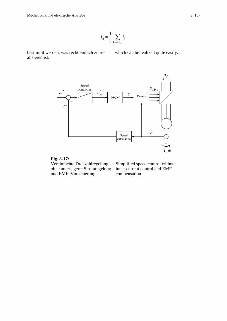
Mechatronik und elektrische Antriebe S. 157
cbak
kA ii,,2
1
bestimmt werden, was recht einfach zu re-alisieren ist.
which can be realized quite easily.
Fig. 8-17: Vereinfachte Drehzahlregelung ohne unterlagerte Stromregelung und EMK-Vorsteuerung
Simplified speed control without inner current control and EMF compensation
*
,T
PWM s
*Au
dcu
Speed
controller
Regler
Demux
cbas ,,
Speed
calculation
Mechatronik und elektrische Antriebe S. 158
9 Entwurf von Strom- und Drehzahlregelung Design of Current and Speed Control
In verschiedenen Zusammenhängen wie beim Magnetlager, beim Geschalteten Re-luktanzmotor, beim Gleichstrommotor, auch bei seiner elektronisch kommutierten Vari-ante, sind unterlagerte Stromregelungen zu entwerfen, die alle eine sehr ähnliche Struktur besitzen, und jeweils nach Standard-verfahren entworfen werden können. Ähnliches trifft auf die Drehzahlregelung zu.
In different contexts such as for the magnetic bearing, switched reluctance motor, DC motor – both variants with mechanical and electronic commutation – subordinate current controllers are to be employed. All of them have quite a similar structure and can be designed similarily using standard controller design methods. The same applies for the speed control.
Bei einer Stromregelung gehen wir bei-spielsweise von einer Streckenübertragungs-funktion (der Admittanz) eines RL-Gliedes aus:
For the current control, we should start with a plant transfer function (i. e. the admittance) of a RL-element:
p
s
( ) 1 1 1( ) ( )
( ) 1
I sY s G s
U s R sL R s
(9.1)
Fig. 9-1: Betrachteter Standardregelkreis mit Regelgröße y, Führungs-größe w und Störgröße d
Considered standard control loop with control variable y, set value w, and disturbance variable d
Von weiteren Einflüssen wie der EMK soll hier abgesehen werden. Wir nehmen an, dass diese z. B. zuvor durch eine entsprechende Vorsteuerung im Regler kompensiert wird (im regelungstechnischen Sinn handelt es sich um eine Störgrößenkompensation).
Other influences like the EMF shall not be considered here. It is assumed that the EMF has already been compensated by a feedforward action of the controller (in term of control engineering, we refer to distur-bance compensation).
Zusätzlich zum Verhalten des RL-Gliedes soll noch eine weitere Zeitkonstante be-rücksichtigt werden, die z. B. durch Sensoren oder durch eine Verzögerung des Spannungsstellgliedes verusacht wird. All-
Additionally to the behavior of the RL-element, another time constant shall be taken into account, which may be due to, e.g., the delays of sensors or the voltage actuator. Thus, we should start from the
w
p ( )G sc( )G s
d
ye
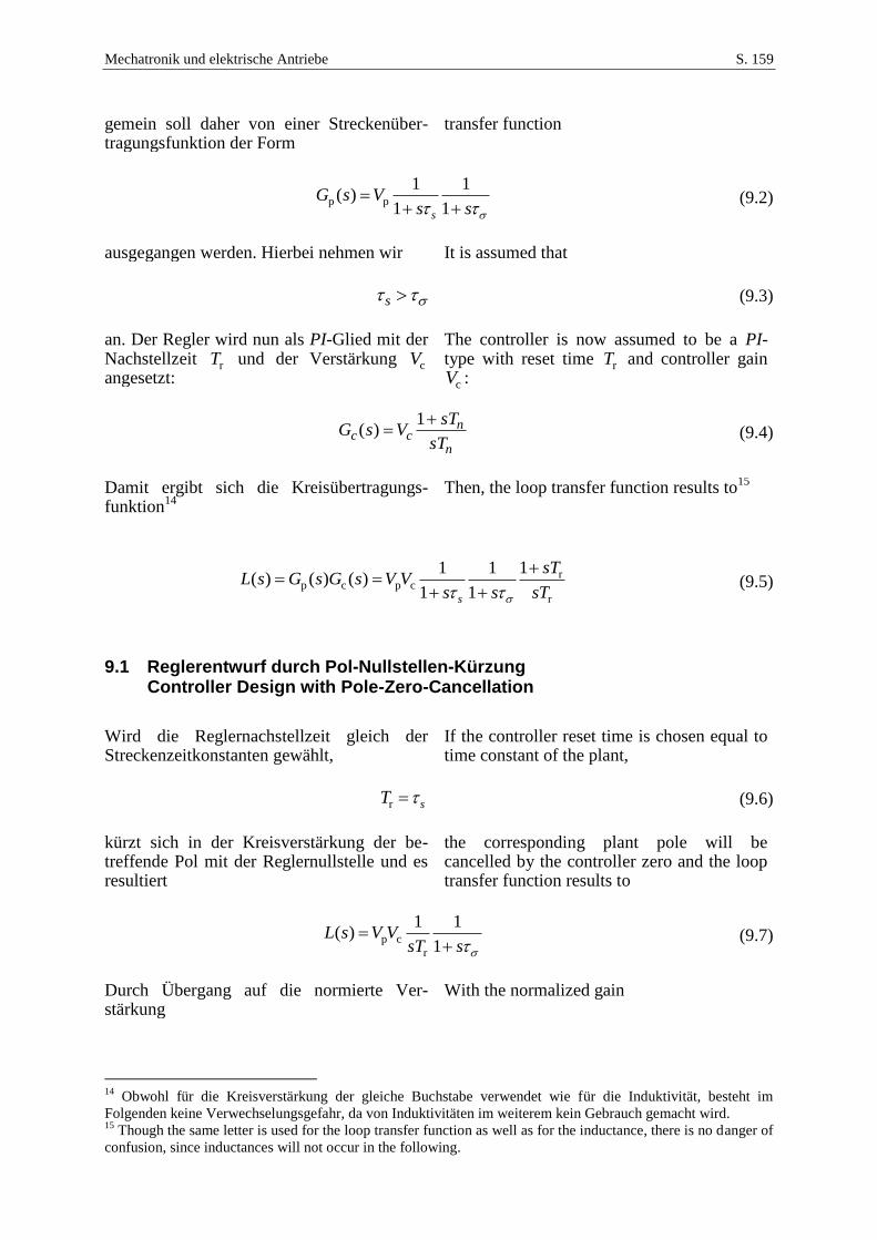
Mechatronik und elektrische Antriebe S. 159
gemein soll daher von einer Streckenüber-tragungsfunktion der Form
transfer function
p p
1 1( )
1 1s
G s Vs s
(9.2)
ausgegangen werden. Hierbei nehmen wir It is assumed that
s (9.3)
an. Der Regler wird nun als PI-Glied mit der Nachstellzeit rT und der Verstärkung cV angesetzt:
The controller is now assumed to be a PI-type with reset time rT and controller gain
cV :
n
ncc
sT
sTVsG
1)( (9.4)
Damit ergibt sich die Kreisübertragungs-funktion
14
Then, the loop transfer function results to15
rp c p c
r
11 1( ) ( ) ( )
1 1s
sTL s G s G s V V
s s sT
(9.5)
9.1 Reglerentwurf durch Pol-Nullstellen-Kürzung Controller Design with Pole-Zero-Cancellation
Wird die Reglernachstellzeit gleich der Streckenzeitkonstanten gewählt,
If the controller reset time is chosen equal to time constant of the plant,
r sT (9.6)
kürzt sich in der Kreisverstärkung der be-treffende Pol mit der Reglernullstelle und es resultiert
the corresponding plant pole will be cancelled by the controller zero and the loop transfer function results to
p c
r
1 1( )
1L s V V
sT s
(9.7)
Durch Übergang auf die normierte Ver-stärkung
With the normalized gain
14
Obwohl für die Kreisverstärkung der gleiche Buchstabe verwendet wie für die Induktivität, besteht im
Folgenden keine Verwechselungsgefahr, da von Induktivitäten im weiterem kein Gebrauch gemacht wird. 15
Though the same letter is used for the loop transfer function as well as for the inductance, there is no danger of
confusion, since inductances will not occur in the following.
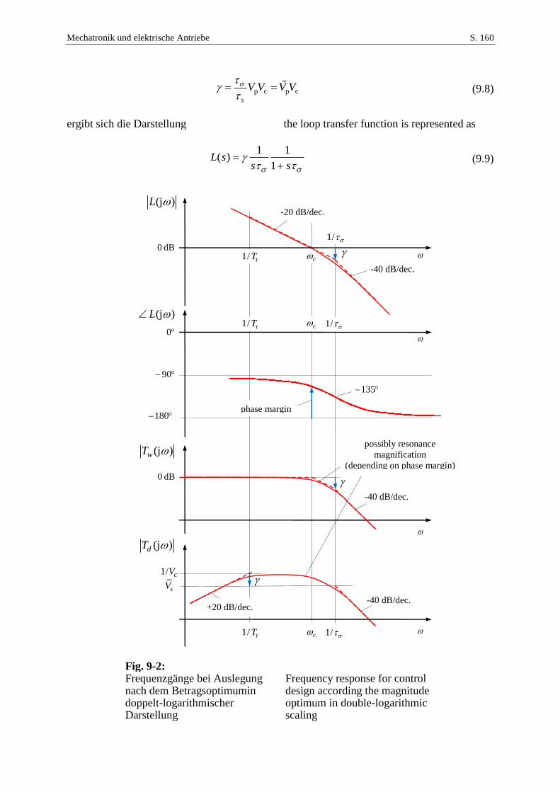
Mechatronik und elektrische Antriebe S. 160
p c p c
s
V V V V
(9.8)
ergibt sich die Darstellung the loop transfer function is represented as
sssL
1
11)( (9.9)
Fig. 9-2: Frequenzgänge bei Auslegung nach dem Betragsoptimumin doppelt-logarithmischer Darstellung
Frequency response for control design according the magnitude optimum in double-logarithmic scaling
(j )L
r1/T cdB0
(j )dT
-20 dB/dec.
-40 dB/dec.
dB0
0
90
180
(j )L
phase margin
possibly resonance
magnification
(depending on phase margin)
-40 dB/dec.
-40 dB/dec. +20 dB/dec.
(j )wT
/1
r1/T /1c
sV~
135
r1/T /1c
cV/1
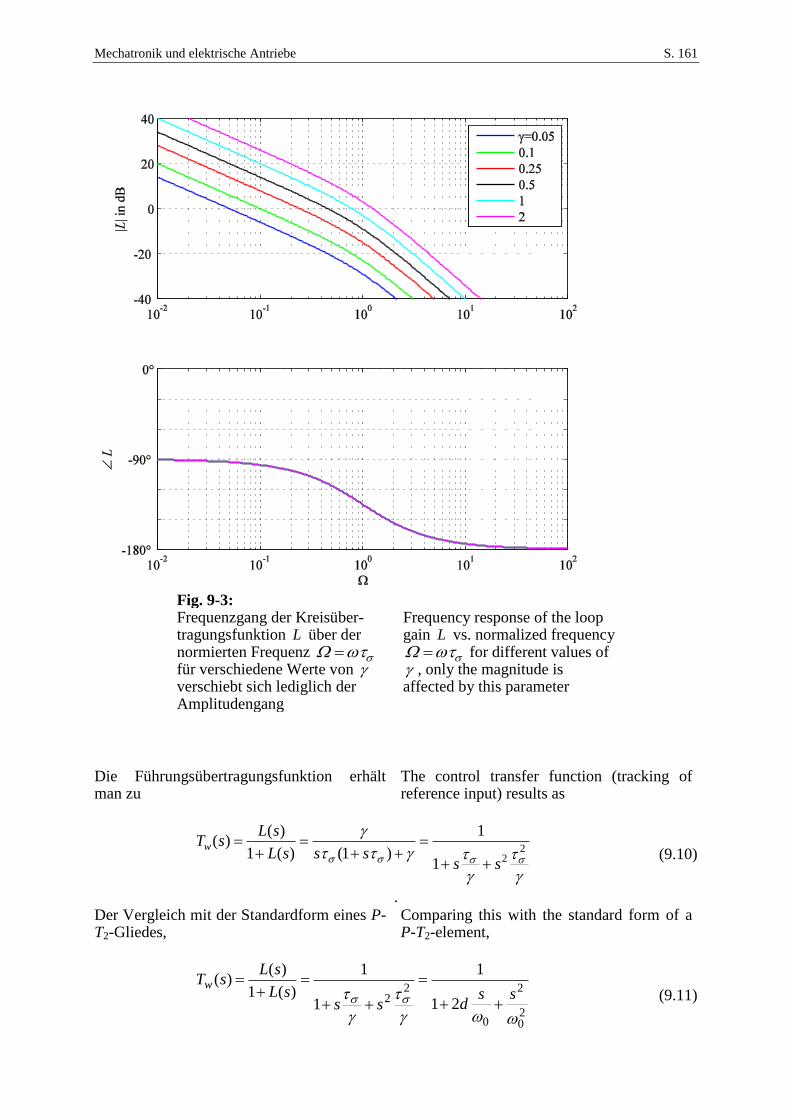
Mechatronik und elektrische Antriebe S. 161
Fig. 9-3: Frequenzgang der Kreisüber-tragungsfunktion L über der normierten Frequenz für verschiedene Werte von verschiebt sich lediglich der Amplitudengang
Frequency response of the loop gain L vs. normalized frequency
for different values of , only the magnitude is affected by this parameter
Die Führungsübertragungsfunktion erhält man zu
The control transfer function (tracking of reference input) results as
2
21
1
)1()(1
)()(
sssssL
sLsTw
(9.10)
. Der Vergleich mit der Standardform eines P-T2-Gliedes,
Comparing this with the standard form of a P-T2-element,
20
2
0
22 21
1
1
1
)(1
)()(
ssdss
sL
sLsTw
(9.11)
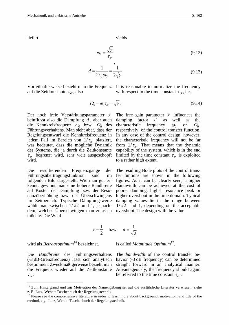
Mechatronik und elektrische Antriebe S. 162
liefert yields
0 (9.12)
,
2
1
2
1
0
d (9.13)
Vorteilhafterweise bezieht man die Frequenz auf die Zeitkonstante , also
It is reasonable to normalize the frequency with respect to the time constant , i.e.
00 . (9.14)
Der noch freie Verstärkungsparameter beinflusst also die Dämpfung d , aber auch die Kennkreisfrequenz 0 bzw. 0 des Führungsverhaltens. Man sieht aber, dass der Regelungsentwurf die Kennkreisfrequenz in jedem Fall im Bereich von /1 platziert, was bedeutet, dass die mögliche Dynamik des Systems, die ja durch die Zeitkonstante
begrenzt wird, sehr weit ausgeschöpft wird.
The free gain parameter influences the damping factor d as well as the characteristic frequency 0 or 0 , respectively, of the control transfer function. In any case of the control design, however, the characteristic frequency will not be far from /1 . That means that the dynamic capability of the system, which is in the end limited by the time constant is exploited to a rather high extent.
Die resultierenden Frequenzgänge der Führungsübertragungsfunktion sind im folgenden Bild dargestellt. Wie man gut er-kennt, gewinnt man eine höhere Bandbreite auf Kosten der Dämpfung bzw. der Reso-nanzüberhöhung bzw. des Überschwingens im Zeitbereich. Typische Dämpfungswerte wählt man zwischen 2/1 und 1, je nach-dem, welches Überschwingen man zulassen möchte. Die Wahl
The resulting Bode plots of the control trans-fer funtions are shown in the following figures. As it can be clearly seen, a higher Bandwidth can be achieved at the cost of poorer damping, higher resonance peak or higher overshoot in the time domain. Typical damping values lie in the range between
2/1 and 1, depending on the acceptable overshoot. The design with the value
2
1 bzw.
2
1d
wird als Betragsoptimum
16 bezeichnet. is called Magnitude Optimum
17.
Die Bandbreite des Führungsverhaltens (-3 dB-Grenzfrequenz) lässt sich analytisch bestimmen. Zweckmäßigerweise bezieht man die Frequenz wieder auf die Zeitkonstante
:
The bandwidth of the control transfer be-havior (-3 dB frequency) can be determined straight forward in an analytical manner. Advantageously, the frequency should again be referred to the time constant :
16
Zum Hintergrund und zur Motivation der Namengebung sei auf die ausführliche Literatur verwiesen, siehe
z. B. Lutz, Wendt: Taschenbuch der Regelungstechnik. 17
Please see the comprehensive literature in order to learn more about background, motivation, and title of the
method, e.g. Lutz, Wendt: Taschenbuch der Regelungstechnik.
Mechatronik und elektrische Antriebe S. 163
2(j )
jwT
(9.15)
2
b
1(j )
2wT (9.16)
22
2 2 2 2 2 2 4 2b b b b b b b2 j 2 (9.17)
2 4 2b b(1 2 ) 0 (9.18)
22 2b
1 1
2 2
(9.19)
22
b
1 1
2 2
(9.20)
Für die Standardauslegung 2/1 ergibt sich beispielsweise die Bandbreite
b 1/ 2 .
For the standard design 2/1 a bandwidth of b 1/ 2 results.
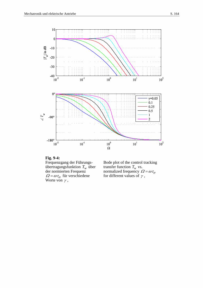
Mechatronik und elektrische Antriebe S. 164
Fig. 9-4: Frequenzgang der Führungs-übertragungsfunktion wT über der normierten Frequenz
für verschiedene Werte von ,
Bode plot of the control tracking transfer function wT vs. normalized frequency for different values of ,
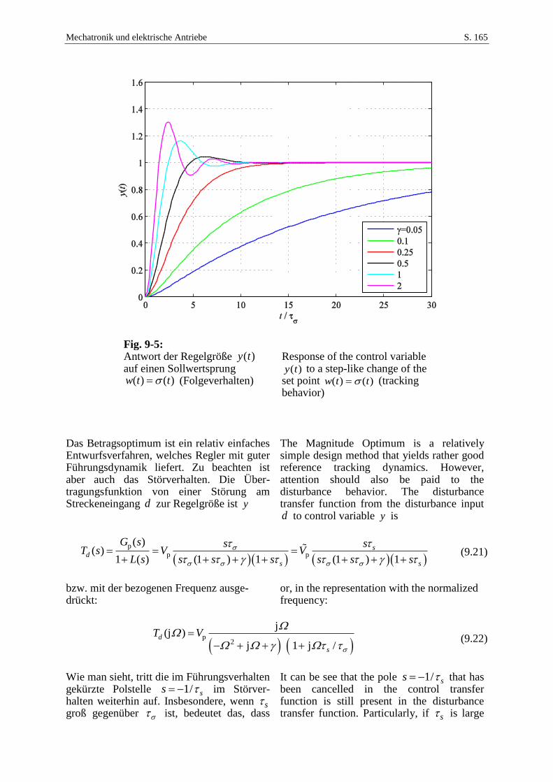
Mechatronik und elektrische Antriebe S. 165
Fig. 9-5: Antwort der Regelgröße )(ty auf einen Sollwertsprung
)()( ttw (Folgeverhalten)
Response of the control variable )(ty to a step-like change of the
set point )()( ttw (tracking behavior)
Das Betragsoptimum ist ein relativ einfaches Entwurfsverfahren, welches Regler mit guter Führungsdynamik liefert. Zu beachten ist aber auch das Störverhalten. Die Über-tragungsfunktion von einer Störung am Streckeneingang d zur Regelgröße ist y
The Magnitude Optimum is a relatively simple design method that yields rather good reference tracking dynamics. However, attention should also be paid to the disturbance behavior. The disturbance transfer function from the disturbance input d to control variable y is
p
p p
( )( )
1 ( ) (1 ) 1 (1 ) 1
sd
s s
G s s sT s V V
L s s s s s s s
(9.21)
bzw. mit der bezogenen Frequenz ausge-drückt:
or, in the representation with the normalized frequency:
p
2
j(j )
j 1 j /d
s
T V
(9.22)
Wie man sieht, tritt die im Führungsverhalten gekürzte Polstelle ss /1 im Störver-halten weiterhin auf. Insbesondere, wenn s groß gegenüber ist, bedeutet das, dass
It can be see that the pole ss /1 that has been cancelled in the control transfer function is still present in the disturbance transfer function. Particularly, if s is large
Mechatronik und elektrische Antriebe S. 166
ggf. vorhandene Störungen nur langsam aus-geregelt werden. Wie das Bild der Stör-größensprungantwort zeigt, wird selbst bei großer Reglerverstärkung der Regelfehler erst durch ein langsames kriechendes Ver-halten ausgeregelt. Im Stromregelkreis eines Gleichstrommotors kann beispielsweise eine solche Störung auftreten, wenn die EMK durch die Vorsteuerung nicht oder nicht exakt kompensiert wird (vgl. Abschnitt 7.12). Beim Betrieb mit konstanter oder langsam veränderlicher Drehzahl ist eine solche lang-same Störausregelung hinnehmbar. Werden aber sehr schnelle Drehzahländerungen aus-geführt, so dass sich auch die EMK als Stör-größe sehr schnell ändert, sollte eine schnelle Störausregelung angestrebt werden. Das ist mit dem im folgenden Abschnitt beschrie-benen Symmetrischen Optimum besser möglich.
compared to disturbances will take a relatively long time to be rejected. As the disturbance step response figure shows, even with high controller gain, the control error decreases only slowly with a creeping behavior. Such a disturbance can occur in the current control loop of a DC motor in the case the EMF is not or not precisely compensated for by the feedforward controller action (cp. Section 7.12). In case of operation with constant of slowly varying speed such a slow disturbance rejection would not cause any problems. However, if the speed and thus the EMF changes rapidly, a quick disturbance rejection is desired. In that case the design method described in the following section, the Symmetrical Op-timum, may be more suitable.
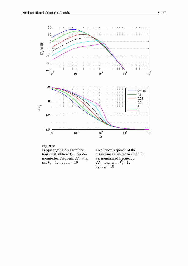
Mechatronik und elektrische Antriebe S. 167
Fig. 9-6: Frequenzgang der Störüber-tragungsfunktion dT über der normierten Frequenz mit p 1V , 10/ s
Frequency response of the disturbance transfer function dT vs. normalized frequency
with p 1V ,
10/ s
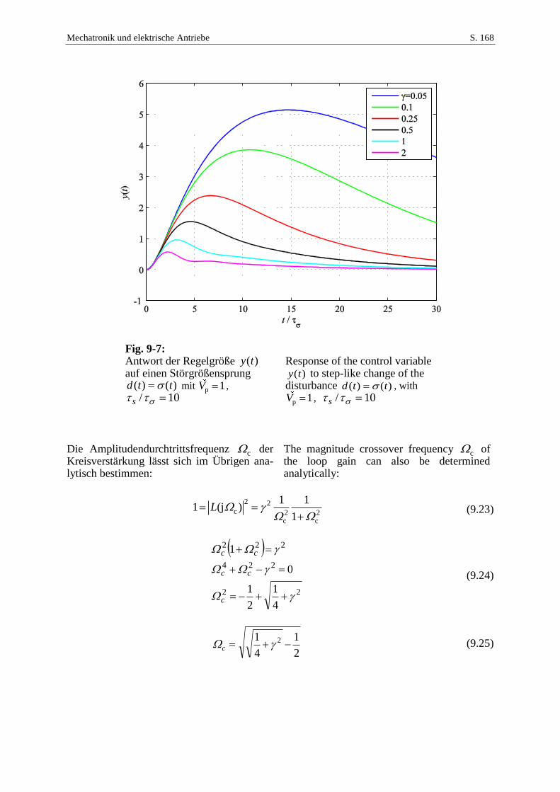
Mechatronik und elektrische Antriebe S. 168
Fig. 9-7: Antwort der Regelgröße )(ty auf einen Störgrößensprung
)()( ttd mit p 1V ,
10/ s
Response of the control variable )(ty to step-like change of the
disturbance )()( ttd , with
p 1V , 10/ s
Die Amplitudendurchtrittsfrequenz c der Kreisverstärkung lässt sich im Übrigen ana-lytisch bestimmen:
The magnitude crossover frequency c of the loop gain can also be determined analytically:
2 2c 2 2
c c
1 11 (j )
1L
(9.23)
22
224
222
4
1
2
1
0
1
c
cc
cc
(9.24)
2
1
4
1 2 c (9.25)
Mechatronik und elektrische Antriebe S. 169
9.2 Symmetrisches Optimum Symmetrical Optimum
Das vorangegangene Verfahren legt die Reglernachstellzeit so fest, dass eine Pol-Nullstellen-Kürzung auftritt, mit der ein günstiges Führungsverhalten resultiert. Das Störverhalten wird beim Entwurf nicht be-achtet. Soll ein besseres Störverhalten er-reicht werden, muss man – unter Beibe-haltung des PI-Reglertyps – die Reglernach-stellzeit anders festlegen. Von der Tendenz her muss diese verringert werden, damit der integrale Anteil schneller reagiert. Besonders einfach gestaltet sich der hier dargestellte Reglerentwurf, wenn man annimmt, dass die langsame Streckenzeitkonstante s der Strecke sehr viel größer als die schnelle Zeit-konstante und auch größer als die einzu-stellende Reglernachstellzeit rT ist:
r,s T . In diesem Fall lässt sich diese Zeitkonstante gänzlich vernachlässigen und das betreffende 1T -Glied durch einen Integrator approximieren:
The control design method introduced in the preceding section uses the controller reset time for a pole-zero-cancellation. With that design method, good reference tracking dynamics result while the disturbance behavior is not considered. Aiming for a better disturbance rejection while keeping the PI controller type, the controller reset time should be determined in a different way. As a tendency, the reset time should be reduced to enable a quicker reaction of the integral part of the controller. The situation becomes very simple if the plant time constant s is assumed to be much larger than the small time constant and also larger than the controller reset time rT : r,s T . In this case, the small time constant can bei approximated only by an integrative behavior:
p p p p p
1 1 1 1 1 1 1( )
1 1 1 1 (1 )s s s
G s V V V Vs s s s s s s s
(9.26)
. Bei der Drehzahlregelung enthält die Regel-strecke ohnehin von vornherein einen Integ-rierer. Die Kreisübertragungsfunktion lautet nun
In case of a speed control, the plant really includes such an integrator. The loop transfer function results to
rc p p c p c 2
r r
11 1 1 1( ) ( ) ( )
1 1
nsTsTL s G s G s V V V V
sT s s ss T
(9.27)
. Der Regelungsentwurf kann sehr gut mit genäherten Amplitudengängen skizziert werden. Für kleine Frequenzen fällt der Amplitudengang der Kreisverstärkung zu-nächst mit -40 dB/Dekade. Die Phasen-drehung ist dementsprechend etwa -180°. Durch die Knickfrequenz r1/T wird die Phase angehoben (Nullstelle), durch die folgende Knickfrequenz /1 (Polstelle) aber wieder abgesenkt. Der größte Phasen-winkel wird (bei logarithmischer Achsenska-lierung) daher genau zwischen den beiden Knickfrequenzen erreicht. Den größten Phasenrand erhält man also, wenn die Ver-
The idea of the control design can be outlined very well using approximated magnitude Bode plots. For small frequencies, the magnitude plot decreases first with -40 dB per decade. The phase delay is -180° accordingly. At the corner frequency
r1/T the phase is increased by the controller zero, but decreased again at the corner frequency /1 (plant pole). The maximum phase angle is achieved exactly between the two corner frequencies (in terms of the logarithmic scaling). The largest phase margin is obtained if the gain is chosen in that way so that the magnitude crossover
Mechatronik und elektrische Antriebe S. 170
stärkung so gewählt wird, dass die Amplitu-dendurchtrittsfrequenz genau an dieser Stelle
c platziert wird. Sei also
frequency c is exactly at this point. Let
2rTa
(9.28)
das Verhältnis von Nachstellzeit und schneller Streckenzeitkonstante, so soll die Amplitudendurchtrittsfrequenz bei
be the ratio between reset time and the small time constant. Then, the crossover frequency should be located at
cr
1 a
a T
(9.29)
zu liegen kommen. Das Verhältnis a lässt sich also durch zwei verschiedne Frequenz-verhältnisse interpretieren (vgl. Bild):
In doing so, the ratio a can be interpreted as two different frequency ratios as also shown in the figure:
c
r c
1/
1/a
T
(9.30)
. In Anlehnung an Begriffe der Geometrie wird a deshalb als Doppelverhältnis be-zeichnet. Bei einer logarithmischen Ska-lierung der Frequenzachse im Bodediagramm sind also die geometrischen Abstände der Knickfrequenzen /1 und r1/T von der Durchtrittsfrequenz c genau gleich.
With respect to terms of geometry, a is called double ratio. On a logarithmic frequency axis the geometric distances from the crossover frequency c is exactly the same to both corner frequencies /1 und
r1/T .
Bei der Durchtrittsfrequenz muss der Betrag der Kreisverstärkung 1 sein,
At the crossover frequency, the loop gain must be 1,
c(j ) 1L , (9.31)
was zur Festlegung der Reglerverstärkung führt:
that leads to the design of the controller gain:
c rp c p c p c p c2
cc r
1 j1 1 j 1 j1
1 j 1 j/ j
T a aV V V V V V a V V a
a aT
(9.32)
aVV cs
1~ bzw.
s
cVa
V ~1
Damit resultieren Kreis- und Führungsüber-tragungsfunktionen zu
With that, loop and reference transfer functions result to
Mechatronik und elektrische Antriebe S. 171
s
sa
sasL
1
11)(
2
223 (9.33)
2232232
2
2232
2
1
1
)1(1
1
)(1
)()(
sasasa
sa
ssasa
sa
sL
sLsTw
(9.34)
Die Reglerübertragungsfunktion lässt sich mit dem Doppelverhältnis a schreiben als
The controller transfer function can be expressed with the double ratio a as
2 2
c 2 3p
1 11 1( )
s
s a s aG s
aV ss a a V
(9.35)
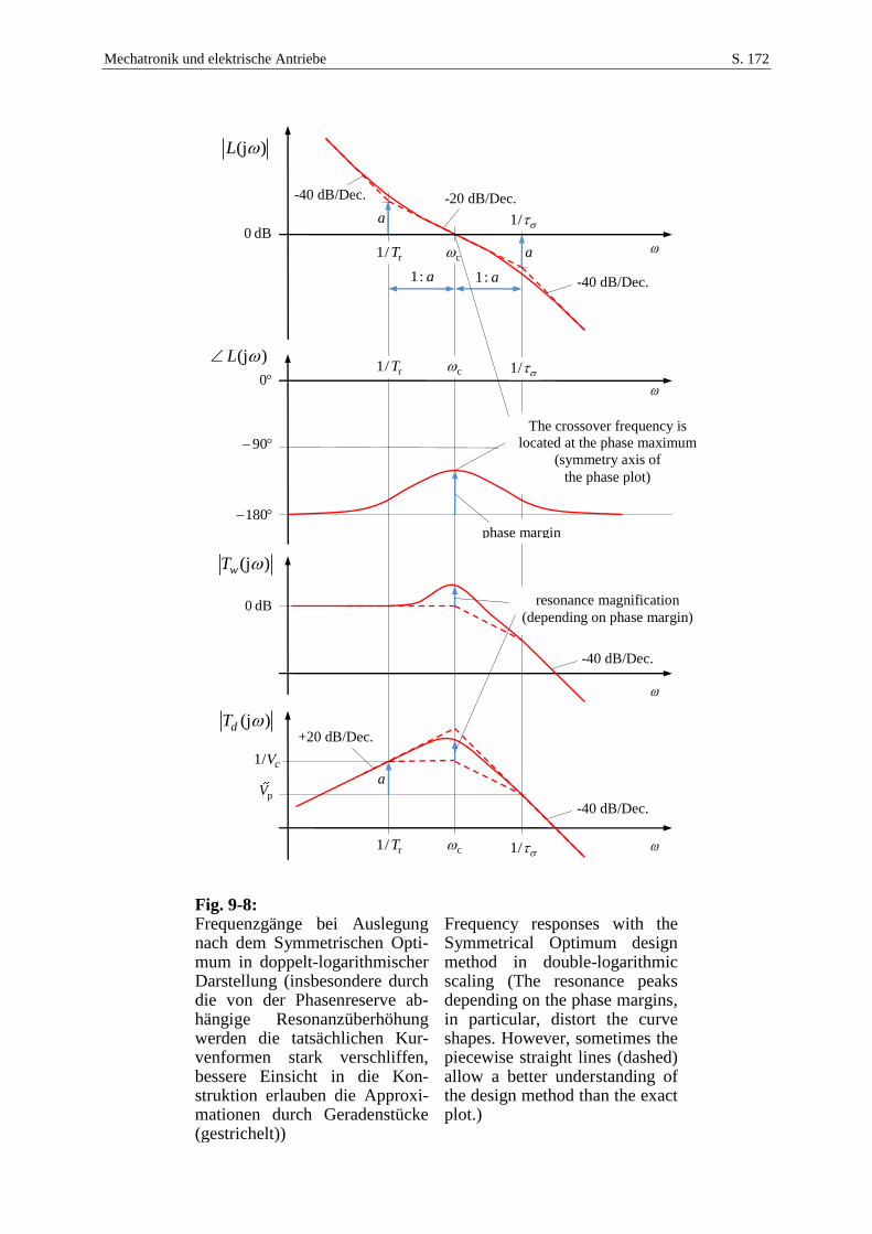
Mechatronik und elektrische Antriebe S. 172
Fig. 9-8: Frequenzgänge bei Auslegung nach dem Symmetrischen Opti-mum in doppelt-logarithmischer Darstellung (insbesondere durch die von der Phasenreserve ab-hängige Resonanzüberhöhung werden die tatsächlichen Kur-venformen stark verschliffen, bessere Einsicht in die Kon-struktion erlauben die Approxi-mationen durch Geradenstücke (gestrichelt))
Frequency responses with the Symmetrical Optimum design method in double-logarithmic scaling (The resonance peaks depending on the phase margins, in particular, distort the curve shapes. However, sometimes the piecewise straight lines (dashed) allow a better understanding of the design method than the exact plot.)
(j )L
r1/T
/1
a:1 a:1
c
dB0
(j )wT
(j )dT
-40 dB/Dec. -20 dB/Dec.
-40 dB/Dec.
dB0
0
90
180
(j )L
phase margin
resonance magnification
(depending on phase margin)
-40 dB/Dec.
-40 dB/Dec.
+20 dB/Dec.
The crossover frequency is
located at the phase maximum
(symmetry axis of
the phase plot)
a
a
pV
r1/T/1c
r1/T/1c
cV/1
a
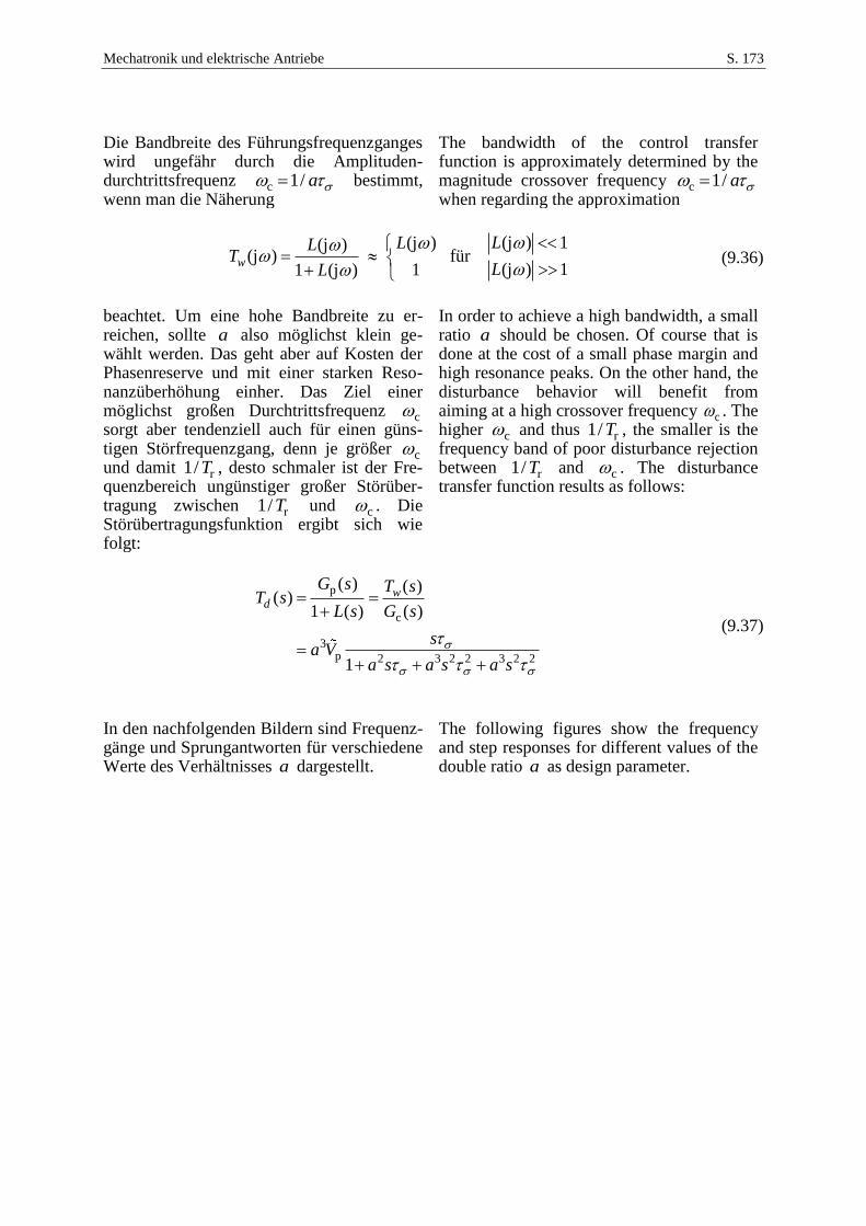
Mechatronik und elektrische Antriebe S. 173
Die Bandbreite des Führungsfrequenzganges wird ungefähr durch die Amplituden-durchtrittsfrequenz c 1/ a bestimmt, wenn man die Näherung
The bandwidth of the control transfer function is approximately determined by the magnitude crossover frequency c 1/ a when regarding the approximation
(j ) 1(j )(j )(j ) für
(j ) 111 (j )w
LLLT
LL
(9.36)
beachtet. Um eine hohe Bandbreite zu er-reichen, sollte a also möglichst klein ge-wählt werden. Das geht aber auf Kosten der Phasenreserve und mit einer starken Reso-nanzüberhöhung einher. Das Ziel einer möglichst großen Durchtrittsfrequenz c sorgt aber tendenziell auch für einen güns-tigen Störfrequenzgang, denn je größer c und damit r1/T , desto schmaler ist der Fre-quenzbereich ungünstiger großer Störüber-tragung zwischen r1/T und c . Die Störübertragungsfunktion ergibt sich wie folgt:
In order to achieve a high bandwidth, a small ratio a should be chosen. Of course that is done at the cost of a small phase margin and high resonance peaks. On the other hand, the disturbance behavior will benefit from aiming at a high crossover frequency c . The higher c and thus r1/T , the smaller is the frequency band of poor disturbance rejection between r1/T and c . The disturbance transfer function results as follows:
p
c
3p 2 3 2 2 3 2 2
( ) ( )( )
1 ( ) ( )
1
wd
G s T sT s
L s G s
sa V
a s a s a s
(9.37)
In den nachfolgenden Bildern sind Frequenz-gänge und Sprungantworten für verschiedene Werte des Verhältnisses a dargestellt.
The following figures show the frequency and step responses for different values of the double ratio a as design parameter.
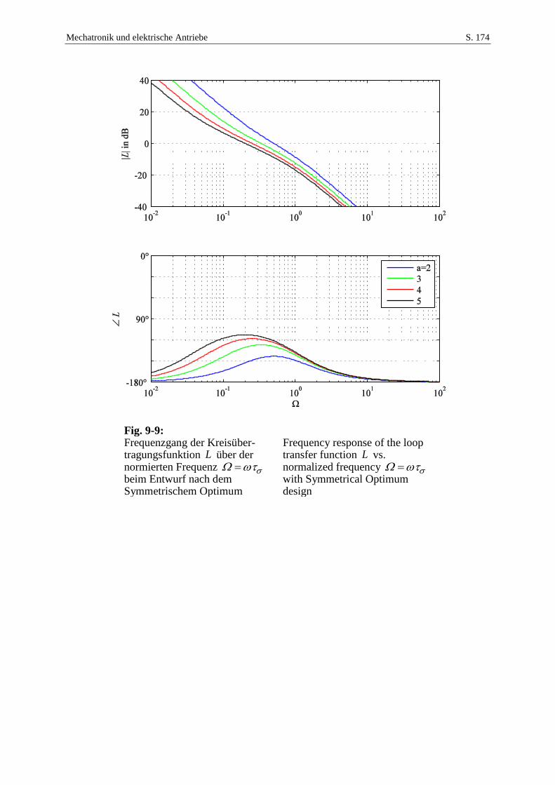
Mechatronik und elektrische Antriebe S. 174
Fig. 9-9: Frequenzgang der Kreisüber-tragungsfunktion L über der normierten Frequenz beim Entwurf nach dem Symmetrischem Optimum
Frequency response of the loop transfer function L vs. normalized frequency with Symmetrical Optimum design
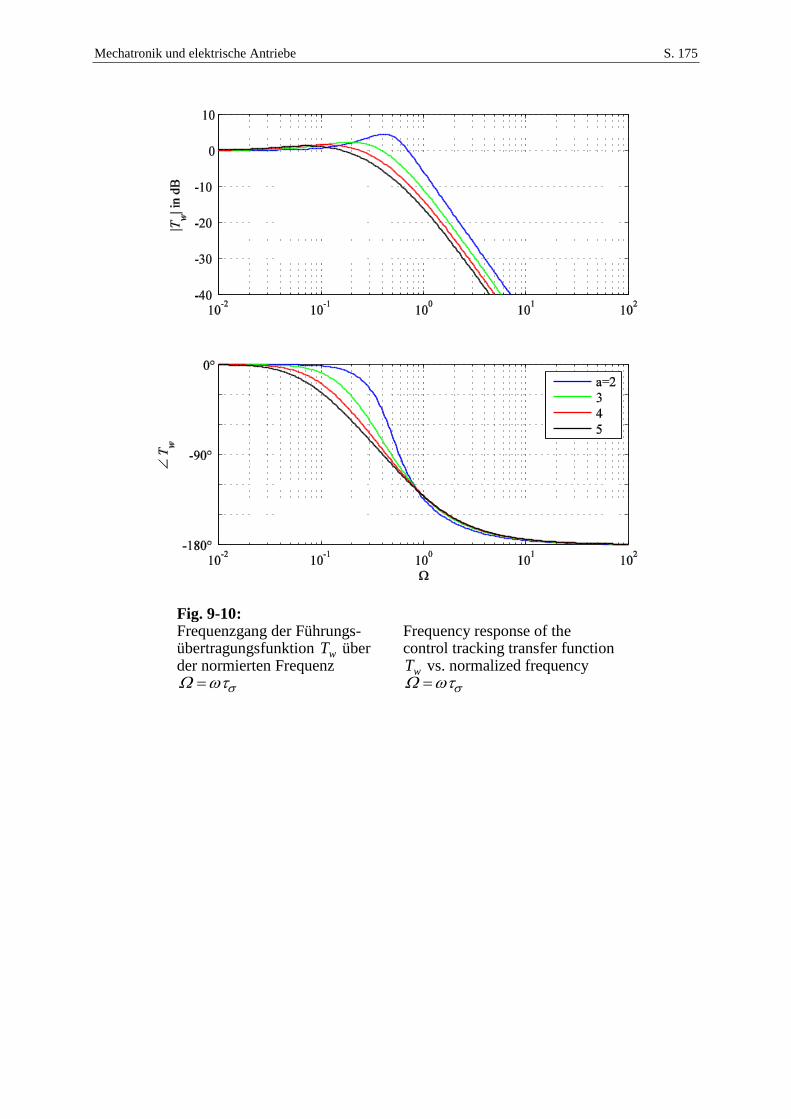
Mechatronik und elektrische Antriebe S. 175
Fig. 9-10: Frequenzgang der Führungs-übertragungsfunktion wT über der normierten Frequenz
Frequency response of the control tracking transfer function
wT vs. normalized frequency
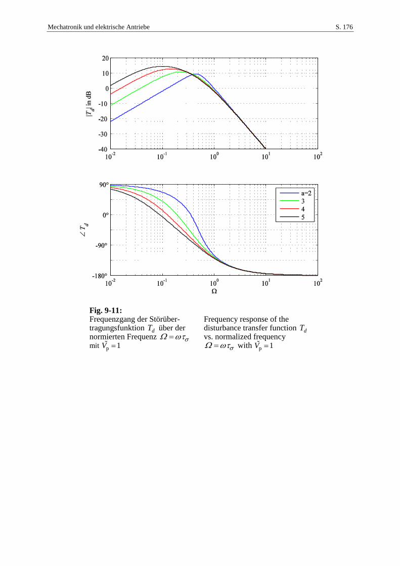
Mechatronik und elektrische Antriebe S. 176
Fig. 9-11: Frequenzgang der Störüber-tragungsfunktion dT über der normierten Frequenz mit p 1V
Frequency response of the disturbance transfer function dT vs. normalized frequency
with p 1V
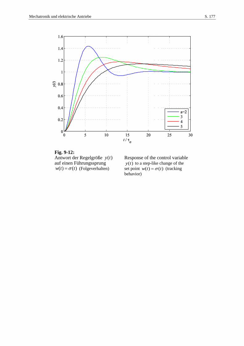
Mechatronik und elektrische Antriebe S. 177
Fig. 9-12: Antwort der Regelgröße )(ty auf einen Führungssprung
)()( ttw (Folgeverhalten)
Response of the control variable )(ty to a step-like change of the
set point )()( ttw (tracking
behavior)
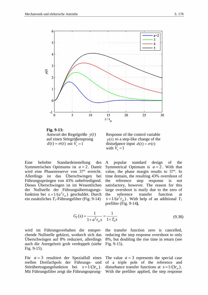
Mechatronik und elektrische Antriebe S. 178
Fig. 9-13: Antwort der Regelgröße )(ty auf einen Störgrößensprung
)()( ttd mit 1~sV
Response of the control variable )(ty to a step-like change of the
disturbance input )()( ttd with 1
~sV
Eine beliebte Standardeinstellung des Symmetrischen Optimums ist 2a . Damit wird eine Phasenreserve von 37° erreicht. Allerdings ist das Überschwingen bei Führungssprüngen von 43% unbefriedigend. Dieses Überschwingen ist im Wesentlichen der Nullstelle der Führungsübertragungs-funktion bei )/(1 2
as geschuldet. Durch ein zusätzliches T1-Führungsfilter (Fig. 9-14)
A popular standard design of the Symmetrical Optimum is 2a . With that value, the phase margin results to 37°. In time domain, the resulting 43% overshoot of the reference step response is not satisfactory, however. The reason for this large overshoot is maily due to the zero of the reference transfer function at
)/(1 2as . With help of an additional T1
prefilter (Fig. 9-14),
f 2
1 1( )
11 n
G sT sa s
(9.38)
wird im Führungsverhalten die entspre-chende Nullstelle gekürzt, wodurch sich das Überschwingen auf 8% reduziert, allerdings auch die Anregelzeit grob verdoppelt (siehe Fig. 9-15).
the transfer function zero is cancelled, reducing the step response overshoot to only 8%, but doubling the rise time in return (see Fig. 9-15).
Für 3a resultiert der Spezialfall eines reellen Dreifachpols der Führungs- und Störübertragungsfunktion bei )3/(1 s . Mit Führungsfilter zeigt die Führungssprung-
The value 3a represents the special case of a triple pole of the reference and disturbance transfer functions at )3/(1 s . With the prefilter applied, the step response
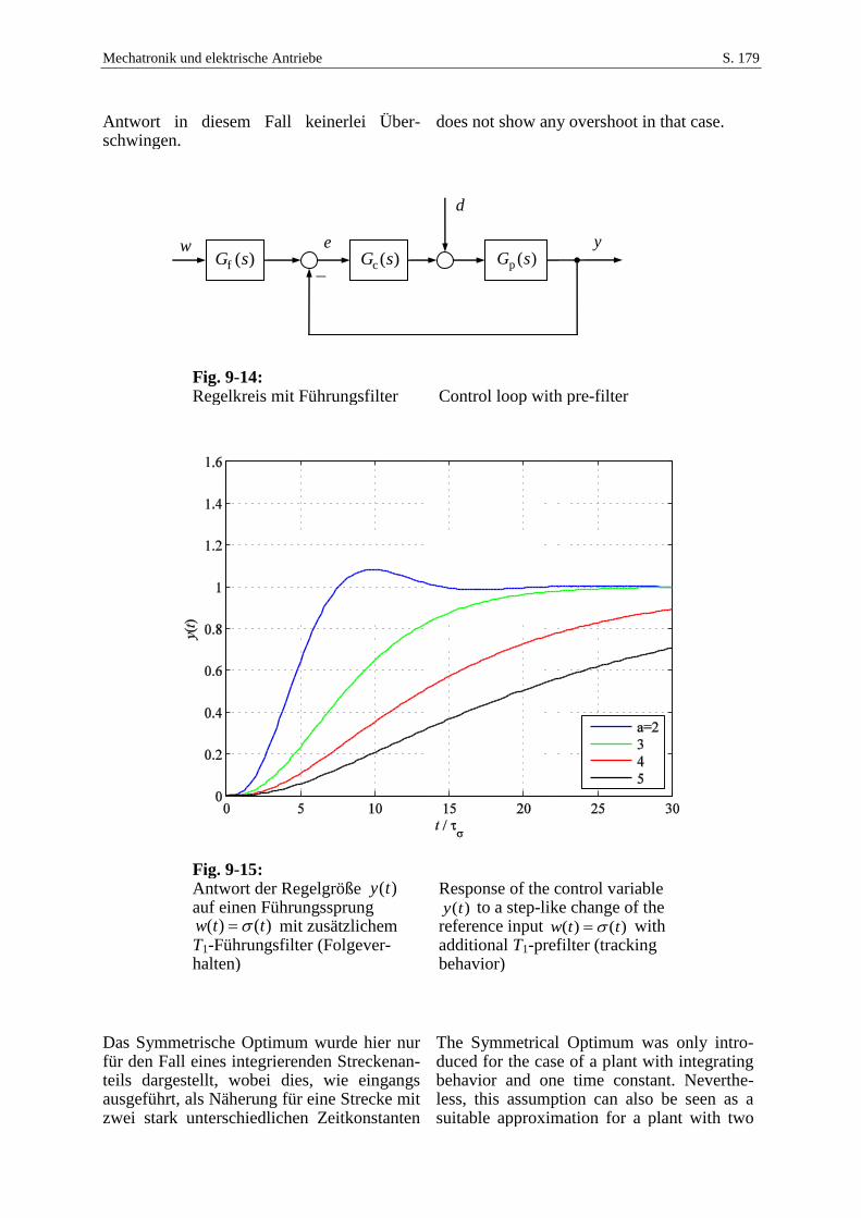
Mechatronik und elektrische Antriebe S. 179
Antwort in diesem Fall keinerlei Über-schwingen.
does not show any overshoot in that case.
Fig. 9-14: Regelkreis mit Führungsfilter Control loop with pre-filter
Fig. 9-15: Antwort der Regelgröße )(ty auf einen Führungssprung
)()( ttw mit zusätzlichem T1-Führungsfilter (Folgever-halten)
Response of the control variable )(ty to a step-like change of the
reference input )()( ttw with additional T1-prefilter (tracking behavior)
Das Symmetrische Optimum wurde hier nur für den Fall eines integrierenden Streckenan-teils dargestellt, wobei dies, wie eingangs ausgeführt, als Näherung für eine Strecke mit zwei stark unterschiedlichen Zeitkonstanten
The Symmetrical Optimum was only intro-duced for the case of a plant with integrating behavior and one time constant. Neverthe-less, this assumption can also be seen as a suitable approximation for a plant with two
wp ( )G sc( )G s
d
ye
f ( )G s
Mechatronik und elektrische Antriebe S. 180
s (wie beim Betragsoptimum voraus-gesetzt) dienen kann. In der Literatur wird aber auch der Fall ohne eine solche Näherung behandelt.
distant time constants s (as assumed with the Magnitude Optimum). In literature, however, also the exact case without such an approximation is covered.
Das Störverhalten des Symmetrischen Opti-mums ist für große Verhältnisse von Streckenzeitkonstanten /s günstiger als beim Betragsoptimum, da die langsame Streckenzeitkonstante nicht durch die Reglernachstellzeit kompensiert, sondern eine kürzere Nachstellzeit eingestellt wird. Bezüglich des Führungsverhaltens schneidet das Betragsoptimum besser ab.
The disturbance suppression characteristics of the Symmetrical Optimum are superior compared with Magnitude Optimum in case of large ratios of the time constants /s . This is due to the fact that the large time constant is not being cancelled by the controller reset time, but a much shorter controller reset time is chosen, instead. As far as only tracking control performance is concerned, the Magnitude Optimum outper-foms the Symmetrical Optimum.