
Model Selection and Uniqueness Analysis for Reservoir ...
114
Model Selection and Uniqueness Analysis for Reservoir History Matching Von der Fakultät für Geowissenschaften, Geotechnik und Bergbau der Technischen Universität Bergakademie Freiberg genehmigte Dissertation Zur Erlangung des akademischen Grades Doktor-Ingenieur (Dr.-Ing.) vorgelegt von: M.Mohsen Rafiee, M.Sc. geboren am 13.05.1982 in Shiraz, Iran Gutachter: Prof. Dr.-Ing. habil. Frieder Häfner, Freiberg Prof.Dr. -Ing. Leonhard Ganzer, Cluasthal Dr. Ralf Schulze-Riegert, Hamburg Tag der Verleihung: 28.01.2011
Transcript of Model Selection and Uniqueness Analysis for Reservoir ...
Model Selection and Uniqueness Analysis for
Reservoir History Matching
Von der Fakultät für Geowissenschaften, Geotechnik und Bergbau
der Technischen Universität Bergakademie Freiberg
genehmigte
Dissertation
Zur Erlangung des akademischen Grades
Doktor-Ingenieur
(Dr.-Ing.)
vorgelegt
von: M.Mohsen Rafiee, M.Sc.
geboren am 13.05.1982 in Shiraz, Iran
Gutachter: Prof. Dr.-Ing. habil. Frieder Häfner, Freiberg
Prof.Dr. -Ing. Leonhard Ganzer, Cluasthal
Dr. Ralf Schulze-Riegert, Hamburg
Tag der Verleihung: 28.01.2011
Model Selection and Uniqueness Analysis for
Reservoir History Matching
By the Faculty of Faculty of Geosciences, Geo-Engineering and Mining
of the Technische Universität Bergakademie Freiberg
approved this
THESIS
to attain the academic degree of
Doktor-Ingenieur
(Dr.-Ing.)
by: M.Mohsen Rafiee, M.Sc.
born on 13.05.1982 in Shiraz, Iran
Assessors: Prof. Dr.-Ing. habil. Frieder Häfner, Freiberg
Prof.Dr. -Ing. Leonhard Ganzer, Cluasthal
Dr. Ralf Schulze-Riegert, Hamburg
Date of the award: 28 January 2011

i
Acknowledgements
Foremost, I would like to thank my supervisor, Prof. Dr.Ing. habil. Frieder Häfner, for
his support, encouragement and his guidance during this work. He provided me brilliant
ideas and deep insights in research, the best environment to work in and many
opportunities to present my work.
I am greatly thankful to the professors of the Institute of Drilling Engineering and Fluid
Mining, Prof. Dr.Ing. Matthias Reich, head of Institute, Prof. Dr.Ing. Mohamed Amro,
head of Reservoir Engineering section and also Prof. Dr. Steffen Wagner for their helps
and supports during my work in the Institute.
I would also like to thank all my friends, PhD colleagues and other staff members of
the Institute of Drilling Engineering and Fluid Mining, especially Dr. Dieter Voigt, Dr.
Nils Hoth and Dr. Carstern Freese, for their encouragement and proper support during the
entire duration of my work. I take this opportunity to express my gratitude for all those
who helped me.
This work has been completed through DGMK (German Society for Petroleum and
Coal Science and Technology) research work 681. Here by I deeply appreciate the
financial support provided by DGMK that made this project possible. License of the
MEPO was provided by SPT-Group. I thank Dr. Ralf Schulze-Riegert for his ideas and
good instructions in building and developing some works I used in this study.
Last but not least, my warmest thanks go to my family and my wife Yasaman for their
effort, moral support and love during my work. This thesis is dedicated to them.

ii
Abstract
“History matching” (model calibration, parameter identification) is an established
method for determination of representative reservoir properties such as permeability,
porosity, relative permeability and fault transmissibility from a measured production
history; however the uniqueness of selected model is always a challenge in a successful
history matching.
Up to now, the uniqueness of history matching results in practice can be assessed only
after individual and technical experience and/or by repeating history matching with
different reservoir models (different sets of parameters as the starting guess).
The present study has been used the stochastical theory of Kullback & Leibler (K-L)
and its further development by Akaike (AIC) for the first time to solve the uniqueness
problem in reservoir engineering. In addition - based on the AIC principle and the principle
of parsimony - a penalty term for OF has been empirically formulated regarding
geoscientific and technical considerations. Finally a new formulation (Penalized Objective
Function, POF) has been developed for model selection in reservoir history matching and
has been tested successfully in a North German gas field.
Kurzfassung
„History Matching“ (Modell-Kalibrierung, Parameter Identifikation) ist eine bewährte
Methode zur Bestimmung repräsentativer Reservoireigenschaften, wie Permeabilität,
Porosität, relative Permeabilitätsfunktionen und Störungs-Transmissibilitäten aus einer
gemessenen Produktionsgeschichte (history).
Bis heute kann die Eindeutigkeit der identifizierten Parameter in der Praxis nicht
konstruktiv nachgewiesen werden. Die Resultate eines History-Match können nur nach
individueller Erfahrung und/oder durch vielmalige History-Match-Versuche mit
verschiedenen Reservoirmodellen (verschiedenen Parametersätzen als Startposition) auf
ihre Eindeutigkeit bewertet werden.
Die vorliegende Studie hat die im Reservoir Engineering erstmals eingesetzte
stochastische Theorie von Kullback & Leibler (K-L) und ihre Weiterentwicklung nach
Akaike (AIC) als Basis für die Bewertung des Eindeutigkeitsproblems genutzt. Schließlich
wurde das AIC-Prinzip als empirischer Strafterm aus geowissenschaftlichen und
technischen Überlegungen formuliert. Der neu formulierte Strafterm (Penalized Objective
Function, POF), wurde für das History Matching eines norddeutschen Erdgasfeldes
erfolgreich getestet.

iii
Table of Contents
Acknowledgements ................................................................................................................ i
Abstract .................................................................................................................................. ii
Kurzfassung ........................................................................................................................... ii
Table of Contents ................................................................................................................. iii
Table of Figures ..................................................................................................................... v
Table of Tables ..................................................................................................................... vi
Nomenclature....................................................................................................................... vii
Chapter 1. Introduction and Lterature Review ................................................................... 11
1.1. Background .............................................................................................................. 11
1.2. Statement of the Problem ......................................................................................... 11 1.2.1. Uniqueness Problem ................................................................................................................. 11 1.2.2. Consequences and Achievements ............................................................................................. 12
1.3. Literature review on History Matching and inverse problems ................................ 14 1.3.1. Forward modeling ..................................................................................................................... 15 1.3.2. Mathematical Model for inverse modeling ............................................................................... 16 1.3.3. Optimization – Minimization of an Objective Function ........................................................... 16 1.3.4. Effective model Calibration ...................................................................................................... 20
Chapter 2. Model Selection Criteria ................................................................................... 21
2.1. Model selection ........................................................................................................ 21
2.2. Model Parameterization ........................................................................................... 21
2.3. Simplicity and Parsimony ........................................................................................ 21
2.4. The Kullback-Leibler Distance (Information) ......................................................... 22 2.4.1. Information Criteria and Model Selection ................................................................................ 24 2.4.2. Akaike’s Information Criterion (AIC) ...................................................................................... 25
2.5. Using Optimization packages .................................................................................. 26 2.5.1. UCODE ..................................................................................................................................... 26 2.5.2. SIMOPT .................................................................................................................................... 29 2.5.3. MEPO ....................................................................................................................................... 31
Chapter 3. Test of Different Criteria on Synthetic and Experimental Cases ..................... 33
3.1. Synthetic 2D-Case ................................................................................................... 33 3.1.1. Model description ..................................................................................................................... 33 3.1.2. History matching and result ...................................................................................................... 35 3.1.3. AIC application ......................................................................................................................... 35
3.2. Laboratory Permeability Measurement ................................................................... 37 3.2.1. Model description ..................................................................................................................... 37 3.2.2. History matching and AIC application result ............................................................................ 37
3.3. Packer test system (Insitu permeability measurement)............................................ 39 3.3.1. Model Description .................................................................................................................... 39 3.3.2. History Matching and identification ......................................................................................... 40 3.3.3. Uninqueness Analysis ............................................................................................................... 41
3.4. New emperical correlation for packer test system (AICn) ....................................... 45
Chapter 4. Development of General Criteria for Model Selection .................................... 48
4.1. Model Selection Complexity ................................................................................... 48
4.2. Penalization (POF) ................................................................................................... 50 4.2.1. Development of POF ................................................................................................................ 50

iv
4.2.2. Verification of POF strategy in packer test system ................................................................... 52 Chapter 5. Field Case Model Study ................................................................................... 54
5.1. Model description .................................................................................................... 54 5.1.1. Static Data ................................................................................................................................. 54 5.1.2. Measurement Data .................................................................................................................... 55
5.2. Material Balance calculation ................................................................................... 57
5.3. Well test analysis ..................................................................................................... 59 5.3.1. Buildup analysis ........................................................................................................................ 59 5.3.2. Well test result .......................................................................................................................... 60
5.4. History Matching ..................................................................................................... 63 5.4.1. Methodology ............................................................................................................................. 63 5.4.2. Result of History Matching ....................................................................................................... 65 5.4.3. Application of POF strategy in field case ................................................................................. 65
Chapter 6. Development of a helpful software for automatic model selection .................. 70
6.1. Concept of helpful software for model selection ..................................................... 70
6.2. AKAIKI software .................................................................................................... 70 6.2.1. Input & Reading ........................................................................................................................ 71 6.2.2. Computation .............................................................................................................................. 72 6.2.3. Writing & Output ...................................................................................................................... 73
Summary and Conclusion .................................................................................................... 74
References ........................................................................................................................... 76
Appendices .......................................................................................................................... 80
A. AKAIKI software FORTRAN code........................................................................... 80
B. History matching result of the field case model with 22 permeability regions ....... 102
v
Table of Figures
Fig. 1: Forward and Inverse approach to modeling ............................................................. 15
Fig. 2: A comparison of steepest descent, Newton’s method and Levenberg-Marquardt
algorithm ...................................................................................................................... 18
Fig. 3: Relation between number of parameter and OF. (Description for principle of
parsimony) ................................................................................................................... 22
Fig. 4: Flowchart showing major steps in the UCODE_2005 parameter estimation mode
using perturbation sensitivities. ................................................................................... 28
Fig. 5: Example of the Evolution Strategy application ...................................................... 32
Fig. 6: Top view gridding of the synthetic model ............................................................... 33
Fig. 7: PVT and SCAL properties for synthetic model ....................................................... 34
Fig. 8: Example of region selection for matching case 2 of the synthetic model ................ 36
Fig. 9: Schematic of Laboratory Permeability Measurement apparatus ............................. 37
Fig. 10 Simulation model of laboratory permeability measurement ................................... 37
Fig. 11: Simulation result of the change in pressure in Laboratory Permeability
Measurement (Version 1 and 2 versus measurement data) ......................................... 38
Fig. 12: Schematic picture of packer test system (four packers installation system) ......... 39
Fig. 13: model and schematic of gridding of packer test system ........................................ 40
Fig. 14: Example of selected regions in a packer test (model 2 &14 regions) .................... 41
Fig. 15: The concept of global minima among different model sets ................................... 41
Fig. 16: Model with 3, 5, 6 and 7 regions parameter sets .................................................... 42
Fig. 17: comparison of different parameter set with different modifier starter ................... 43
Fig. 18: Graph of equivalent region modifier (sensitivity analysis) .................................... 44
Fig. 19: calculation of ( )AIC log OF K= + .............................................................................. 44
Fig. 20: Application of different weight factors for AIC equation ...................................... 45
Fig. 21: calculation of ( ) ( )AIC log OF log K= + ...................................................................... 46
Fig. 22: History matching of a packer test model with 2 parameters .................................. 47
Fig. 23: History matching of a packer test model with 5 parameters .................................. 47
Fig. 24: History matching of a packer test for model with 14 parameters .......................... 47
Fig. 25: Example of simple 2D Cartesian reservoir model ................................................. 48
Fig. 26: Penalization concept and region definition considering model complexity .......... 51
Fig. 27: Minimum Trust Region for packer test system ...................................................... 52
Fig. 28: Application of POF in packer test system .............................................................. 53
Fig. 29: Field Case model structure ..................................................................................... 54
Fig. 30 : Example of production rate and BHP measurement data with simulation response
in Well VIII ................................................................................................................. 55
Fig. 31: Uncertainty in draw down period data measurement ............................................. 56
Fig. 32 :Top view of field case model showing 5 different pore volume regions ............... 57
Fig. 33 : Material Balance and p/z analysis ......................................................................... 58
Fig. 34 : Buildup pressure test analysis for field case in each well ..................................... 62
Fig. 35: Example of model selection region in field case model (model with 5 and 60
regions) ........................................................................................................................ 63
Fig. 36: Identified permeability values for the model with 5 regions ................................. 66

vi
Fig. 37 :Identified permeability values for the model with 11 regions ............................... 66
Fig. 38: Identified permeability values for the model with 22 region ................................. 66
Fig. 39: Sensitivity analysis of field case with model of maximum 22 parameter regions . 67
Fig. 40: Comparison of OF and POF for the model with homogenous porosity ................ 67
Fig. 41: Comparison of OF and POF for the model with non-homogenous porosity ......... 68
Fig. 42: History Matching result of Well VIII for the model with 22-regions .................... 68
Fig. 43: Comparison between pressure buildup analysis and history matching for a model
with 22regions ............................................................................................................. 69
Fig. 44: part example of SIMOPT Logfile .......................................................................... 71
Fig. 45: sample example of akaiki.path file......................................................................... 71
Fig. 46: equivalent REGION file example .......................................................................... 72
Fig. 47: computation result of AKAIKI .............................................................................. 72
Fig . B.1: History matching result of Well I in a model with 22 permeability regions ..... 102
Fig . B.2: History matching result of Well II in a model with 22 permeability regions ... 103
Fig . B.3: History matching result of Well III in a model with 22 permeability regions .. 104
Fig . B.4: History matching result of Well V in a model with 22 permeability regions ... 105
Fig . B.5: History matching result of Well VI in a model with 22 permeability regions .. 106
Fig . B.6: History matching result of Well VII in a model with 22 permeability regions . 107
Fig . B.7: History matching result of Well VIII in a model with 22 permeability regions 108
Fig . B.8: History matching result of Well X in a model with 22 permeability regions ... 109
Fig . B.9: History matching result of Well XI in a model with 22 permeability regions .. 110
Fig . B.10: History matching result of Well IV in a model with 22 permeability regions 111
Fig . B.11: History matching result of Well IX in a model with 22 permeability regions 112
Table of Tables
Table 1:Guidelines for effective model calibration (after Hill and Tiedeman) .................. 20
Table 2: Comparison between SIMOPT and UCODE ........................................................ 31
Table 3: History matching with model selection calculation (Synthetic 2D case) .............. 36
Table 4: History matching with model selection calculation (Lab Measurement Test) ...... 38
Table 5: Initial and Identified permeability for packer test with 5 regions ......................... 47
Table 6: The concept of general development of model selection criteria .......................... 49
Table 7: Effect of pressure adjustment in field case ............................................................ 56
Table 8: Material balance calculation for different wells and regions ................................ 59
Table 9: Calculation of Permeability by pressure Buildup analysis in field case ............... 61
Table 10: History matching result of the model with homogeneous porosity .................... 64
Table 11: History matching result of the model with non-homogeneous porosity ............. 64
Table 12: Comparison of SIMOPT vs. MEPO for 3 different models ................................ 65

vii
Nomenclature
Symbols Unit
AIC Akaike’s Information Criterion
AICc Extended Akaike’s Information Criterion
AKAIKI New developed software for automatic history matching using SIMOPT
BHP Bottom Hole Pressure bar
BIC Bayesian Information Criterion
ct total compressibility 1/bar
d step change
dm Kashyap Index model selection criteria
Ef Expectation function
f full reality model
F(X) mathematical function in forward modeling
f(x) mathematical function of residual (objective function) in inverse modeling
fprior prior term of OF in SIMOPT
fresidual residual term of OF in SIMOPT
fsurvey survey term of OF in SIMOPT
g(x) approximating model being compared to measured value
GOR Gas Oil Ratio
Gp total cumulative gas production sm³
H Hessian matrix
h reservoir thickness m
I identity matrix
I(f, g) Kullback-Leibler Information
IGIP Initial Gas In Place sm³
K number of model parameters (regions or multiplier)
viii
k permeability mD
K-L Kullback-Leibler information
kr relative permeability
L(θ|x) maximum likelihood of a model with parameter vector θ and predictor variables x
LMA Levenberg-Marquardt Algorithm
Log natural logarithm function
m dip of straight line in pressure build-up analysis bars²/period
MES MEaSurement
n total number of observation points
N/G Net to Gross Ratio
OBS observation data
OF Objective Function
OFSIMOPT SIMOPT objective function
p pressure bar
Pi probability of the ith outcome
POF Penalized Objective Function
pw wellbore pressure bar
pw0 initial wellbore pressure bar
Q Gas production rate sm³/day
qcum cumulative gas production in drawdown period before shut-in sm³
RMS Root Mean Square
rweff effective wellbore radius m
SCAL Special Core Analysis
SIM SIMulation
T Temperature K
T transpose of the matrix or vector
t time days
Trfault Fault transmissibility
WBHP Well Bottom Hole Pressure bar

ix
WBHPH Well Bottom Hole Pressure History (pressure measurement data)
bar
WGOR Well Gas Oil Ratio
WWCT Well Water Cut
x predictor variables, measured data, distance
yobs ; ycal observation values and simulator computing values
z gas compressibility factor
Greek Symbols
Gradient operator
α,β,γ overall weights for the production, survey and prior terms in SIMOPT-OF
εi residual of n observation
θ parameter vector
µ Viscosity cp
µlm the step size in Levenberg-Marquardt Algorithm
ν vector of normalized parameter modifiers (multipliers)
νk parameter normalized modifier values
πi Approximating probability distribution of ith outcome
ρ fluid density kg/m³
σ standard deviation, measurement error
φ Porosity
ω weight factor
Indices
i stands for initial reservoir condition, iteration
i, j, k well number, time segment and data kind
n number of observation points
nw; nt; nk the maximum of i, j, k respectively
P production time before shut-in
R radial direction, number of sets of prior models
St standard or surface condition

x
Tr trust region
x x direction
xy Horizontal direction
y y direction
z vertical direction
Θ tangential direction
Chapter 1: Introduction and Lterature Review
11
Chapter 1. Introduction and Lterature Review
1.1. Background
In Reservoir Engineering a numerical reservoir model should be adjusted against
dynamic performance of the field so that it can be used as a prediction tool for future
forecasting. This process is so called “History Matching”. Although a number of different
methods have been proposed for integrating dynamic information in numerical model and
observation data [24],[2], the common conventional practice in the industry is to do multi
phase flow simulations [51],[29] with user selected reservoir parameters in trial and error
approach until agreeable history match is obtained.
History Matching in Reservoir Engineering is described as an automatic inverse model
calibration. This is formulated as an optimization problem, which has to be solved in the
presence of uncertainty because the available observed field data cannot be identical to the
system responses calculated with a reservoir model due to the measurement errors and the
simplified nature of the numerical model (model structure error). [30],[40],[65],[39]
Often it is advisable to simplify some representation of reality in order to achieve an
understanding of the dominant aspects of the system under study. The study of the inverse
problem in the stochastic framework provides capabilities using analytical statistics to
quantify a quality of calibration and the inferential statistics that quantify reliability of
parameter estimates and predictions [8],[31],[47]. The statistical criteria for model
selection may help the modelers to determine an appropriate level of complexity of
parameterization and one would like to have as good an approximation of the structure of
the system as the information permits[12].
1.2. Statement of the Problem
1.2.1. Uniqueness Problem
Because of the complexity of many real systems under study the number of reservoir
parameters is usually larger than the available data set allows to identify; therefore the
solution is non-unique [4],[32],[26]; In other words, more than one set of reservoir model
parameters fits the observation. While adding features to a model is often desirable to
minimize the misfit function or Objective Function (OF) between simulated and observed
values, the increased complexity comes with a cost and non-uniqueness. In general, the
more parameters that a model contains the smaller the minimum OF, but the more non-
unique the identified parameter set can be accrued[23],[22],[37],[8].
Since the same production history could be fit by different reservoir scenarios and
reservoir models; a history matched reservoir model cannot be unique. Consequently the
non-unique parameter set is more uncertain concerning the truth and the risk of wrong
forecast prediction may arise from such non-uniqueness [33],[41],[20],[62]. Yamada[67]
has shown these risks on three history matching scenarios over more than 20 years. These
models have shown that could not be appropriate model for the entire life of the reservoir.

Chapter 1: Introduction and Lterature Review
12
He has mentioned that different models should be investigated and evaluated in order of
successful history matching, although none of them is considered as unique solution.
The determination of the model parameters with history matching requires the
minimization of an objective function in a parameter space (wide ranges of different
parameters through reservoir); Indeed:
the necessary condition in any model selection is to have convergence in regression to
minimize the objective function (OF), using any minimization techniques,
but the sufficient condition would be the uniqueness of the model parameter set which
has been selected.
From mathematical point of view both conditions must be fulfilled in a successful
reservoir history match. In the today’s reservoir engineering practice only the necessary
condition can be fulfilled with modern optimization algorithms. However the open
question of parameter uniqueness leads to uncertainty in the prognosis of future reservoir
development and using the conventional history matching methods will not practically
guarantee to recover the true model.
Two of the major difficulties in history matching are, first, how to choose which
parameters to modify in order to obtain a match, and second, how to ensure that the
changes made to the model remain consistent with the geological concepts and other data
used to build the model in the first place [15]. In other words, if a minimum in the
objective function is found such that the differences between the calculated and measured
observable quantities are sufficiently small, and if the parameterization by which this
minimum has been found conforms to the geological model, then we have satisfactory
history match [12].
Tavassoli et al.[61] have described the non-uniqueness problem with multi-modal
objective function. They have defined three classes of non-uniqueness which may happen
in history matching. First type is where the model has a single optimum in the parameter
space; but because of the measurement errors, the ranges of error around the location of the
most likely model are quite large. This situation is expected to occur in almost all history
matching exercises. The next type is when the data cannot allow a unique optimum to be
determined. For example if two or more variables can be adjusted all together to keep the
overall misfit constant. The last type occurs where multiple high quality local optima exist,
but the unique solution is the model with global minimum. In this case rather good
minimum could be found with available data exist but these minimums involves lot of
different local minima. In other words, more than one set of reservoir model parameters
fits the observation history. Moreover, even a solution associated to a given minimum may
be unstable.
1.2.2. Consequences and Achievements
Conventionally, the parameters are chosen using combination of feeling and trial and
error manners, which can be time consuming and boring process. Researchers have been
building tools for automatic history matching of permeability and porosity distributions to
Chapter 1: Introduction and Lterature Review
13
match the production data for many years [40],[65],[39],[38]. However the problem of
uniqueness is still one of the main concerned issues in model selection.
Bissell [12] has described a method “gradzone analysis” for optimally parameterization
of a reservoir model in history matching. The method takes into account both the
mathematical structure of minimization of the Objective Function, which is the necessary
condition in successful history matching, and also the constraints imposed by geology
(This could be prior boundary information to condition the history matching parameters).
The method can be used to make a prediction about how far into the future can trust the
model.
Gavalas et al. [32] have applied Bayesian estimation theory to history matching as an
alternative to zonation. They expressed that it is a so called prior term can be added to the
objective function to constrain deviations from an initial model or from underlying
relationships between the parameters being varied. By using a priori statistical information
on the unknown parameters, the problem becomes statistically better determined.
Do Nascimento et al. [25] incorporated “smoothness constraint” method in the spatial
variation of physical properties as an example of a geological qualitative constraint that
can be mathematically incorporated in an objective function which could also honoring the
data. These constraints are applied by conditioning the permeability and/or porosity
difference between adjacent grid blocks to be small. The smoothness constraint reduces the
variance of the estimates by introducing bias in the solutions still preserving good match.
However this method cannot be applied to all reservoirs. For this reason they use the idea
that a “tool box” of history matching can be designed for each reservoir that can
incorporate a different constraint. Therefore, the interpreter can choose a specific tool from
this tool box according to the dependency and importance of its constraint to the particular
reservoir being studied.
In the previous work by Mtchedlishvili [46], the statistical model selection approach,
based on the Kullback-Leibler information, was used to choose the best parameter zonation
pattern for a reservoir model. This approach measures directly the model deviation from
the true system, taking into account the bias and variance between the predicted and
observed system responses. It balances the trade-off between increased information and
decreased reliability, which is fundamental to the principle of parsimony. Nevertheless in
the case where no single model is clearly superior to some of the others, it is reasonable to
use the concepts of model inference for translating the uncertainty associated with model
selection into the uncertainty to assess the model prediction performance.
In the work of Mtchedlishvili [46] the inverse modeling techniques was applied for
characterization of tight-gas reservoirs and in this situation the numerical investigation of
the production behavior of the hydraulically fractured wells was an essential part of the
investigations. He has also calculated the values for different model selection criteria. He
Chapter 1: Introduction and Lterature Review
14
has shown the calculation of objective function (OF) coupling with the three model
selection criteria (AICi, BIC [37],[32], dm[46]) with regard to the principle of parsimony
and the Kullback-Leibler (K-L) weights for each of the alternative models of PUNQii
project. The overall ranking of the models shows the different behaviors for each of the
applied approaches. Furthermore, based on the calculated K-L weights he made formal
inference from the entire set of models for model prediction purposes.
The need to limit the region of search space to physically meaningful ranges and
numbers of the parameters has been recognized and discussed by number of authors
[23],[15],[26],[12],[61]; nevertheless, the fact that wrong and not confident estimated
parameters can arise from history matching with much more problem. There is yet also no
clear guideline and rule that describes the number of parameters required for an accurate
simulation model and that indicates if these parameters are unique.
In the present work problem of uniqueness in Reservoir History Matching has been
explained. This has been discussed with the problem of under- and over-parameterization
in reservoir model. In the following chapters the History Matching and inverse problem in
Reservoir Engineering has been reviewed, different model selection criteria and also
minimization and optimization techniques have been explained. The basic model selection
criteria in our case have been implemented to three different cases; 2D synthetic model, lab
permeability experiment and packer test system.
Based on the result of these tests, a new model selection criterion for general case of
deterministic reservoir simulation model has been developed and explained in details.
Right after, the application of this new strategy in packer test system has been verified.
In the last part of this work, a complete history matching has been done for a gas field
reservoir in North of Germany. The results of history matching with minimum Objective
Function have been used to find most probable unique solution by implementing new
approach.
Beside of all, new software tool has been prepared to couple the results history
matching with different model selection approaches. This can be used to find optimum
solution in reservoir history matching.
1.3. Literature review on History Matching and inverse problems
It is not possible for geoscientist and reservoir engineers to know all static and dynamic
multi phase flow properties of the reservoir; therefore describing a full reliable
mathematical model for the reservoir is not achievable. Consequently “History Matching”
i AIC will be explained in more detail in section 2.4.2.
ii PUNQ which stands for Production forecasting with Uncertainty Quantification, is a typical reservoir history matching model, which has been used in a variety of different literatures to discussing the problem of optimization methods. The PUNQ case was qualified as a small size industrial reservoir engineering model[54].
Chapter 1: Introduction and Lterature Review
15
is certainly needed for a successful reservoir simulation, which is to find an appropriate set
of values for the simulator’s input parameters so that the simulator properly predicts the
fluid outputs and the pressures of the wells in the reservoir. It is an inverse problem of
partial differential equation theory and is not a well defined problem. History matching is
most often a multi objective optimization problem, which means that additional criteria
need to be met in order achieve an overall and acceptable match.
1.3.1. Forward modeling
In a mathematical model F if the model parameters X are known, then the relationship
of these parameters which describing the outcome or observable data, OBS, could be
expressed as:
( )F X OBS= EQ. 1
In our case F refers to a mathematical equation of fluid flow in porous media. A usual
forward modeling problem is described by differential equation with specified initial
boundary conditions. With above deterministic equation; OBS can be calculated typically
by running a numerical reservoir simulator that finds the solution of numerical
approximation of a set of partial differential equations. This procedure is so called forward
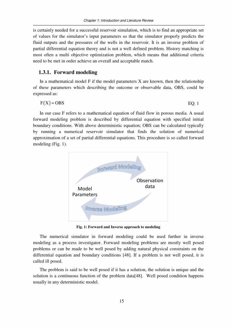
modeling (Fig. 1).
Model Parameters
Observation data
Fig. 1: Forward and Inverse approach to modeling
The numerical simulator in forward modeling could be used further in inverse
modeling as a process investigator. Forward modeling problems are mostly well posed
problems or can be made to be well posed by adding natural physical constraints on the
differential equation and boundary conditions [48]. If a problem is not well posed, it is
called ill posed.
The problem is said to be well posed if it has a solution, the solution is unique and the
solution is a continuous function of the problem data[48]. Well posed condition happens
usually in any deterministic model.
Chapter 1: Introduction and Lterature Review
16
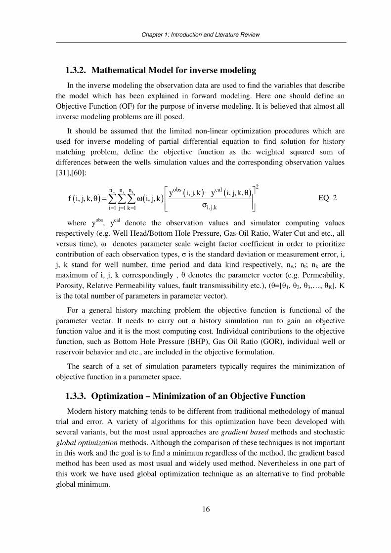
1.3.2. Mathematical Model for inverse modeling
In the inverse modeling the observation data are used to find the variables that describe
the model which has been explained in forward modeling. Here one should define an
Objective Function (OF) for the purpose of inverse modeling. It is believed that almost all
inverse modeling problems are ill posed.
It should be assumed that the limited non-linear optimization procedures which are
used for inverse modeling of partial differential equation to find solution for history
matching problem, define the objective function as the weighted squared sum of
differences between the wells simulation values and the corresponding observation values
[31],[60]:
( ) ( )( ) ( )w t k
2obs caln n n
i, j,ki 1 j 1 k 1
y i, j, k y i, j, k,f i, j, k, i, j, k
= = =
− θθ = ω
σ ∑∑∑ EQ. 2
where yobs, ycal denote the observation values and simulator computing values
respectively (e.g. Well Head/Bottom Hole Pressure, Gas-Oil Ratio, Water Cut and etc., all
versus time), ω denotes parameter scale weight factor coefficient in order to prioritize
contribution of each observation types, σ is the standard deviation or measurement error, i,
j, k stand for well number, time period and data kind respectively, nw; nt; nk are the
maximum of i, j, k correspondingly , θ denotes the parameter vector (e.g. Permeability,
Porosity, Relative Permeability values, fault transmissibility etc.), (θ=[θ1, θ2, θ3,…, θK], K
is the total number of parameters in parameter vector).
For a general history matching problem the objective function is functional of the
parameter vector. It needs to carry out a history simulation run to gain an objective
function value and it is the most computing cost. Individual contributions to the objective
function, such as Bottom Hole Pressure (BHP), Gas Oil Ratio (GOR), individual well or
reservoir behavior and etc., are included in the objective formulation.
The search of a set of simulation parameters typically requires the minimization of
objective function in a parameter space.
1.3.3. Optimization – Minimization of an Objective Function
Modern history matching tends to be different from traditional methodology of manual
trial and error. A variety of algorithms for this optimization have been developed with
several variants, but the most usual approaches are gradient based methods and stochastic
global optimization methods. Although the comparison of these techniques is not important
in this work and the goal is to find a minimum regardless of the method, the gradient based
method has been used as most usual and widely used method. Nevertheless in one part of
this work we have used global optimization technique as an alternative to find probable
global minimum.
Chapter 1: Introduction and Lterature Review
17
1.3.3.1. Gradient based methods
Gradient based optimization methods are increasingly used [50] and using by oil
industry for computer assisted history matching. This method allow a fast descend to the
closest minimum [41],[6].
One of the most efficient algorithms which based on gradient techniques is the
Levenberg-Marquardt Algorithm (LMA) as shown in EQ. 3 which is a combination of the
Newton’s methodi and a steepest descentii scheme. This Levenberg-Marquardt method
works very well in practice and has become the standard of nonlinear least-squares
routines [53].
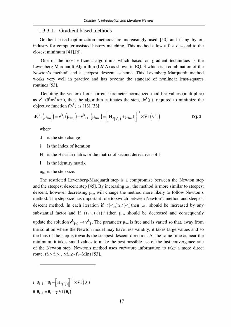
Denoting the vector of our current parameter normalized modifier values (multiplier)
as νk, (θk=νk×θ0), then the algorithm estimates the step, dνk(µ), required to minimize the
objective function f(νk) as [13],[33]:
( ) ( ) ( ) ( ) ( )ki i i ii
1k k k k
i lm i lm i 1 lm lm ifd H I f
−
+ ν ν µ = ν µ − ν µ = + µ ×∇ ν
EQ. 3
where
d is the step change
i is the index of iteration
H is the Hessian matrix or the matrix of second derivatives of f
I is the identity matrix
µlm is the step size.
The restricted Levenberg-Marquardt step is a compromise between the Newton step
and the steepest descent step [45]. By increasing µlm the method is more similar to steepest
descent; however decreasing µlm will change the method more likely to follow Newton’s
method. The step size has important role to switch between Newton’s method and steepest
descent method. In each iteration if ( ) ( )k ki 1 if f+ν ≥ ν then µlm should be increased by any
substantial factor and if ( ) ( )k ki 1 if f+ν < ν then µlm should be decreased and consequently
update the solution k ki 1 i+ν → ν . The parameter µlm is free and is varied so that, away from
the solution where the Newton model may have less validity, it takes large values and so
the bias of the step is towards the steepest descent direction. At the same time as near the
minimum, it takes small values to make the best possible use of the fast convergence rate
of the Newton step. Newton's method uses curvature information to take a more direct
route. (f1> f2>…>fn-1> fn=Min) [53].
i ( ) ( )i
1
i 1 i ifH f−
+ θ θ = θ − ×∇ θ
ii ( )i 1 i i if+θ = θ − γ ∇ θ
Chapter 1: Introduction and Lterature Review
18
The Levenberg-Marquardt algorithm is stronger than the Newton’s method, which
means that in many cases it finds a solution even if it starts very far from the final
minimum; however the Levenberg-Marquardt algorithm tends to be a bit slower than the
Newton’s method [53]. A comparison of steepest descent, Newton’s method and
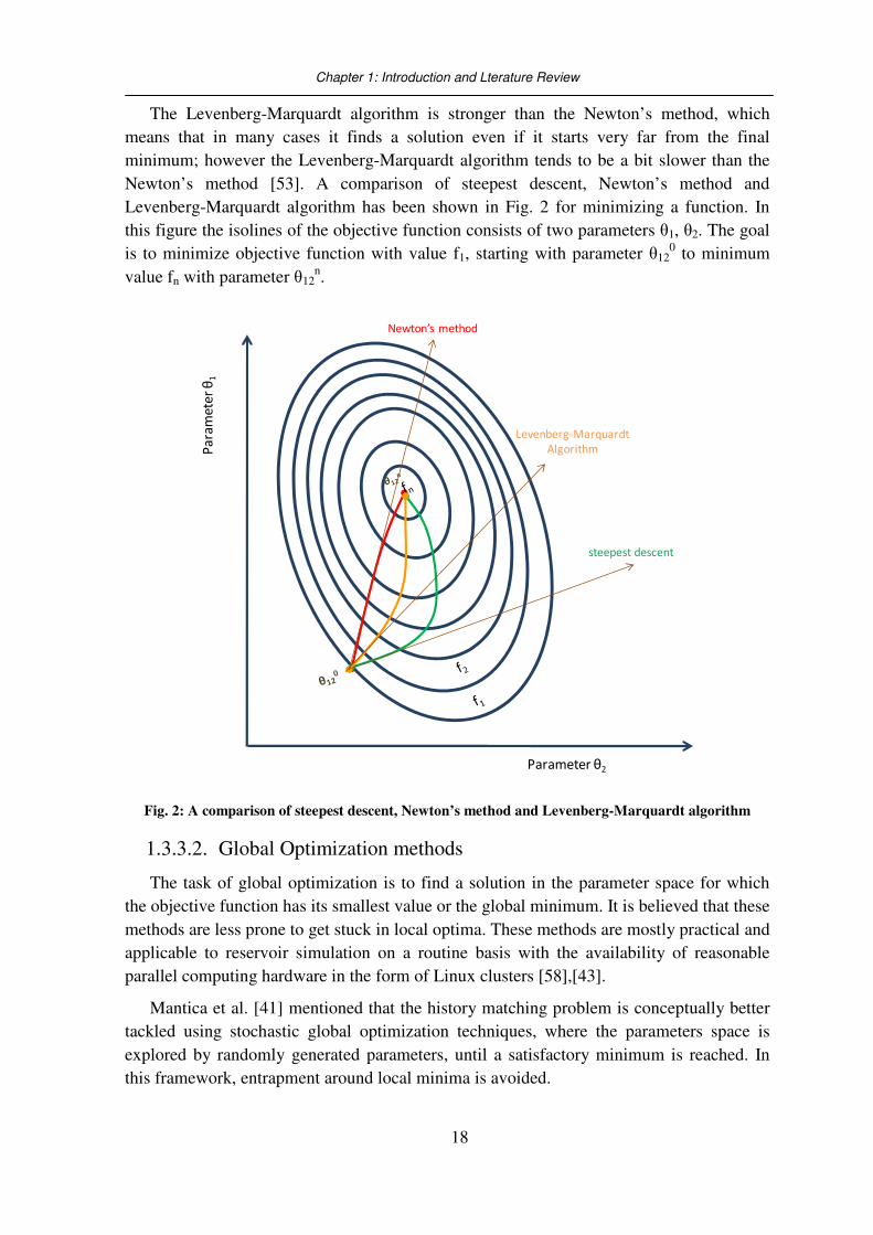
Levenberg-Marquardt algorithm has been shown in Fig. 2 for minimizing a function. In
this figure the isolines of the objective function consists of two parameters θ1, θ2. The goal
is to minimize objective function with value f1, starting with parameter θ120 to minimum
value fn with parameter θ12n.
Pa
ram
ete
r θ
1
Parameter θ2
Newton’s method
Levenberg-Marquardt
Algorithm
steepest descent
Fig. 2: A comparison of steepest descent, Newton’s method and Levenberg-Marquardt algorithm
1.3.3.2. Global Optimization methods
The task of global optimization is to find a solution in the parameter space for which
the objective function has its smallest value or the global minimum. It is believed that these
methods are less prone to get stuck in local optima. These methods are mostly practical and
applicable to reservoir simulation on a routine basis with the availability of reasonable
parallel computing hardware in the form of Linux clusters [58],[43].
Mantica et al. [41] mentioned that the history matching problem is conceptually better
tackled using stochastic global optimization techniques, where the parameters space is
explored by randomly generated parameters, until a satisfactory minimum is reached. In
this framework, entrapment around local minima is avoided.

Chapter 1: Introduction and Lterature Review
19
There are different global optimization methods available. Some of them such as
Simulated annealing[50] and Evolution Strategy [19],[56],[57]; have been tested in
reservoir history matching problems and found good applications in these context. Quenes
et al. [49] have shown general review of the application of global optimization methods to
reservoir history matching problems.
These methods are computationally so intensive and time consuming, because they
require the reservoir model to be run a large number of times (often several hundred) in
order to properly explore the sensitivity of the models to the reservoir parameters. Indeed
each simulation can take between a few minutes to several days, depending on the size and
complexity of the model [34]. However having available licenses and resources, it is
possible to make parallel computation.
1.3.3.3. Gadient versus Global Optimization methods
It is believed that the Global Optimization methods can find global minimum in a
parameters space populated by many local minima.
Some authors have used the combination of Gradient techniques and Global
Optimization method to be applied in reservoir history matching tasks [33][41]. In their
methods the combination of both techniques will cooperate to find better minimum than as
can be found individually with each technique.
Mantica et al. [54] have used the global optimization technique to identify several
points to be used as initial guesses for gradient based optimization. Their procedure
provides a series of alternative matched models, with different production forecasts, that
improve the understanding of the possible reservoir behaviors.
Gomez et al.[33] have tested the benefits of using global optimization method coupling
gradient information. In this case the process seeks to find a series of minima (with
gradient technique), each one with lower objective function that the previous one (with
global method). The last minimum in the series will be the global minimum.
Schulze-Riegert et al. [58] have described the application of global optimization
technique (Evolution Strategy) and gradient methods as complementary features. In their
method first they search in complete parameter space to find initial minimum. After that
the gradient method will be used to improve the convergence behavior.
In the following work these two methods have also been compared in a limited case
for a gas field reservoir (Section 5.4.1). However it is shown that in a typical deterministic
complex reservoir simulation, the hope to find global minimum is quite similar to that one
with local or gradient techniques.

Chapter 1: Introduction and Lterature Review
20
1.3.4. Effective model Calibration
There are many opinions about how nonlinear optimization can best be applied to the
calibration of complex models, and there is not a single set of ideas that is applicable to all
situations. It is useful, however, to consider one complete set of guidelines that
incorporates many of the methods and statistics available in nonlinear regression, such as
those suggested and explained by Hill and Tiedeman, [36], and listed in Table 1.
Table 1:Guidelines for effective model calibration (after Hill and Tiedeman,[36])
Model Development
• Apply the principle of parsimony (will be explained in section 2.3)
• Use a broad range of information to constrain the problem
• Maintain a well-posed, comprehensive regression problem
• Include many types of observations in the regression
• Use prior information carefully
• Assign weights that reflect errors
• Encourage convergence by improving the model and evaluating the
observations
• Consider alternative models
Test the Model
• Evaluate model fit
• Evaluate optimized parameters
Potential New Data
• Identify new data to improve model parameter estimates and distribution
• Identify new data to improve predictions
Prediction Accuracy and Uncertainty
• Evaluate prediction uncertainty and accuracy using deterministic methods
• Quantify prediction uncertainty using statistical methods

Chapter 2:Model Selection Criteria
21
Chapter 2. Model Selection Criteria
2.1. Model selection
Model selection is the task of selecting a simulation model from a set of potential
models, given data. In its most basic forms, this is one of the fundamental tasks of
scientific investigation. Determining the principle behind a series of observations is often
linked directly to a mathematical model predicting those observations.
Model selection techniques can be considered as estimators of some physical quantity,
such as the probability of the model producing the given data. A standard example of
model selection is that of curve fitting, where, given a set of points and other background
knowledge, we must select a function that describes the best curve.
2.2. Model Parameterization
A particular choice of model parameters is a parameterization of the system. For
quantitative considerations on the system, a particular parameterization has to be chosen.
To define a parameterization means to define a set of experimental procedures which allow
us to measure a set of physical quantities that characterize the system.
The selection of the model parameters to be used to describe a reservoir system is
generally not unique. The choice of discrete model parameters (in a reservoir grid) is called
the parameterization of the problem. Model calibration allows to identify (to calibrate) the
parameters and to reduce the parameter uncertainty (model selection) and, therefore,
uncertainty in reservoir forecast.
The special challenge in calibrating reservoir model is to describe different physical
processes and therefore includes a lot of different physical reservoir parameters (e.g.
permeability, porosity, functions of capillary pressure and relative permeability). These
parameters have to be discrete on a grid space. The higher the number of numerical
parameters to identify, the higher the possible level of over-parameterization and non-
uniqueness accrues.
In the present study, automatic model calibration and selection is demonstrated using
concepts of model selection such as Akaike’s Information Criterion (AIC) and principle of
parsimony which will be explained in section 2.4.2.
2.3. Simplicity and Parsimony
Parsimony enjoys a featured place in scientific thinking in general and in modeling
specifically for a strictly science philosophy. Model selection is a bias versus variance
trade-off and this is the statistical principle of parsimony, in other words the principle of
parsimony is to identify the least complex explanation model for a set of observed data.
The model has to be based on the basic physical process equations and the parameter set
has to be as simple as possible and as complex as necessary!
Chapter 2:Model Selection Criteria
22
Inference under models with too few parameters (variables) can be biased, while with
models having too many parameters (variables) there may be poor accuracy or
identification of effects that are false. These considerations refer to a balance between
under- and over-parameterized models [18].
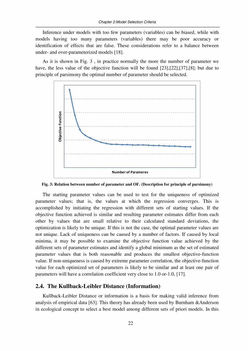
As it is shown in Fig. 3 , in practice normally the more the number of parameter we
have, the less value of the objective function will be found [23],[22],[37],[8]; but due to
principle of parsimony the optimal number of parameter should be selected.
Ob
ject
ive
Fu
nct
ion
Number of Parameres
Fig. 3: Relation between number of parameter and OF. (Description for principle of parsimony)
The starting parameter values can be used to test for the uniqueness of optimized
parameter values; that is, the values at which the regression converges. This is
accomplished by initiating the regression with different sets of starting values. If the
objective function achieved is similar and resulting parameter estimates differ from each
other by values that are small relative to their calculated standard deviations, the
optimization is likely to be unique. If this is not the case, the optimal parameter values are
not unique. Lack of uniqueness can be caused by a number of factors. If caused by local
minima, it may be possible to examine the objective function value achieved by the
different sets of parameter estimates and identify a global minimum as the set of estimated
parameter values that is both reasonable and produces the smallest objective-function
value. If non-uniqueness is caused by extreme parameter correlation, the objective-function
value for each optimized set of parameters is likely to be similar and at least one pair of
parameters will have a correlation coefficient very close to 1.0 or-1.0, [17].
2.4. The Kullback-Leibler Distance (Information)
Kullback-Leibler Distance or information is a basis for making valid inference from
analysis of empirical data [63]. This theory has already been used by Burnham &Anderson
in ecological concept to select a best model among different sets of priori models. In this
Chapter 2:Model Selection Criteria
23
work this theory will be introduced here as simple general method for the purpose of
model selection in History Matching problem.
The Kullback-Leibler (K-L) distance between the models f and g is defined for
continuous functions as the (usually multi-dimensional) integral [18]:
( ) ( )( )
( )f x
I f ,g f x log dxg x
=
θ ∫ EQ. 4
where log denotes the natural logarithm. Kullback and Leibler developed this quantity
from “information theory” thus they used the notation I(f,g). I(f,g) is the “information” lost
when g is used to approximate f.
It is useful to think of f as full reality and let it have an infinite number of parameters
which is typical for stochastic systems. This supports the infinite dimensionality at least
keeps the concept of reality even if it is in some unattainable perspective.
Let g be the approximating model being compared to (measured against) f. We use x to
denote the data being modeled and θ to denote the parameters in the approximating model
g.
g(x) is as an approximating model, whose parameter vector θ must be estimated from
these data (in fact, this will make explicit using the notation g(x׀θ), read as “the
approximating model g for data x given the parameters θ”), and ( ){ }ig x ,i 1,...,Rθ = is a
set of approximating models as candidates for the representation of the data.
It is good to think of an approximating model that loses as little information as
possible; this is equivalent to minimizing I(f,g), over g. f is considered to be given (fixed)
and only g varies over a parameter space by θ. An equivalent interpretation of minimizing
I(f,g) is finding an approximating model that has the “shortest distance” away from truth,
therefore using both interpretations are useful.
The expression for the K-L distance in the case of discrete distributionsi is:
( )K
ii
ii 1
PI f ,g P log
=
=
π ∑ EQ. 5
Here, there are K possible outcomes of the underlying random variable; the true
probability of the ith outcome is given by Pi, while the πi,…,πK compose the approximating
probability distribution (i.e., the approximating model). In the discrete case, we have
0<Pi<1, 0<πi <1, andK K
i ii 1 i 1
P 1= =
= π =∑ ∑ . Hence, here f and g correspond to the p and π,
respectively.
i This is our interest as we have discrete distribution of parameter.(observation and simulation time)
Chapter 2:Model Selection Criteria
24
The material above makes it obvious that both f and g (and their parameters) must be
known to compute the K-L distance between these two models. We see that this
requirement is diminished as I(f, g) can be written equivalently as
( ) ( ) ( )( ) ( ) ( )( )I f ,g f x log f x dx f x log g x dx= − θ∫ ∫ EQ. 6
Note, each of the two terms on the right of the above expression is a statistical
expectation with respect to f (truth). Thus, the K-L distance (above) can be expressed as a
difference between two expectations,
( ) ( )( ) ( )( )f fI f ,g E log f x E log g x = − θ EQ. 7
each with respect to the true distribution f. The important point is that the K-L distance
I(f,g) is a measure of the directed “distance” between the probability models f and g.
The above expression can be reduced to,
( ) ( )( )fI f ,g Const. E log g x − = − θ EQ. 8
The term ( ) ., ConstgfI − is a relative, directed distance between the two models f and
g, if one could compute or estimate ( )( )log θ fE g x .Thus, ( )( )logfE g x
θ becomes
the quantity of interest.
Consequently, one can determine a method to select the model gi that on average
minimizes, over the set of models g1,…, gR, a very relevant expected K-L distance.
2.4.1. Information Criteria and Model Selection
Let L(θ|x) be the maximum likelihoodi of a model with K parameters based on a sample
of size n, which has been defined by Burnham & Anderson [18] as:
( )1n
n21
L | x eˆ2
− θ =
πσ EQ. 9
where θ is the parameter vector, x is the predictor variable vector , 2σ̂ is an estimator
which is defined as n
2 2i
i 1
ˆ n=
σ = ε∑ ,n is the number of observation points and εi is the
residual of n observation
Then by taking logarithm of EQ. 9 we have log-likelihood:
i In statistics, the likelihood function (often simply the likelihood) is a function of the parameters of a
statistical model that plays a key role in statistical inference. In non-technical usage, “likelihood” is a
synonym for “probability”.
Chapter 2:Model Selection Criteria
25
( ) ( ) ( )2n n nˆlog L( x ) log log 2
2 2 2θ = − σ − π − EQ. 10
n2
ii 1=
ε∑ is the sum of residual differences and if we use weighted squares of residual
differences ( [ ]n
2i i
i 1=
ω ε∑ ) which is equal to OF. We can change above equation to:
( ) ( ) ( ) ( )n n n n
log L( x ) log OF log n log 22 2 2 2
θ = − + − π − EQ. 11
The additive constant can often be discarded from the log-likelihood because it is
constant that does not influence likelihood-based inference. Thus we can simply take:
( ) ( )n
log L( x ) log OF2
θ ≈ − EQ. 12
2.4.2. Akaike’s Information Criterion (AIC)
AIC developed by Hirotsugu Akaike under the name of “An Information Criterion”
(AIC) in 1971 and proposed by Akaike ,[3], is a measure of the goodness of fit of an
estimated statistical model. It is developed in effect offering a relative measure of the
information lost when a given model is used to describe reality. The AIC is an operational
way of trading off the complexity of an estimated model against how well the model fits
the data [11].
In the general case, if all the models in the set assume normally distributed errors with a
constant variance, then the AIC is:
( )AIC 2 log L( x ) 2K= − θ + EQ. 13
where K is the number of the parameters of vector θ.
The first term on the right-hand side tends to decrease as more parameter are added to
the approximating model (satisfies the necessary condition), while the second term (2K)
gets larger as more parameter are added to the approximating model (to fulfill the sufficient
condition). This is the tradeoff between under-parameterization (underfitting) and over-
parameterization (overfittingi) that is fundamental of the principle of parsimony.
Combining EQ. 12 and EQ. 13 gives:
( ) ( )AIC 2 log L( x ) 2K n log OF 2K= − θ + = + EQ. 14
and also
i In statistics, overfitting is fitting a statistical model that has too many parameters. A false model may fit
perfectly if the model has enough complexity by comparison to the amount of data available.
Chapter 2:Model Selection Criteria
26
( )( ) ( )
c
2K K 1 2K K 1AIC 2log L( x ) 2K AIC
n K 1 n K 1
+ += − θ + + = +
− − − − EQ. 15
called extended Akaike criteria, when K is large relative to sample size n [17].
The theory is based on linear models; hence the history matching problem is strongly
nonlinear. Therefore we have used EQ. 14 in an empirical form as:
( )1 2AIC log OF K= ω + ω EQ. 16
Increasing the number K of free parameters to be estimated improves the goodness of
fit, regardless of the number of free parameters in the data generating process. Hence AIC
not only rewards goodness of fit, but also includes a penalty that is an increasing the
number of estimated parameters. This penalty discourages overfitting and will be known as
over-parameterization in later stage of this project. The preferred model is the one with the
lowest AIC value among different sets of possible models.
2.5. Using Optimization packages
Generally the optimization software uses following steps in predicting parameter value
for all systems and models.
1. Work with process model input files and read values from process model output
files. (Designed to work with existing software packages).
2. Compare user provided observations with equivalent simulated values derived
from the process model output files using a number of summary statistics,
including a weighted objective function.
3. Use optimization methods to adjust the value of user-selected input parameters
in an iterative procedure to minimize the value of the weighted least-squares
objective function.
4. Report the estimated parameter values and if necessary prepare for the next
iteration.
5. Calculate and print statistics used to (a) diagnose inadequate data or identify
parameters that probably cannot be estimated, (b) evaluate estimated parameter
values, (c) evaluate model fit to observations, and (d) evaluate how accurately
the model represents the processes. (But this part is different in different
softwares and mostly is optional features.)
6. Find most probable unique solution and select the best model among different
sets of selected models. (This is our intention and final goal of this project.)
2.5.1. UCODE
UCODE is a Computer Code for Universal Sensitivity Analysis, Calibration, and
Uncertainty Evaluation, developed from U.S.Geological Survey, Ground Water branch.
Chapter 2:Model Selection Criteria
27
UCODE can compare observations and simulated equivalents. The simulated equivalents
can be any simulated value written in the process-model output files or can be calculated
from simulated values with user-defined equations. UCODE can be used effectively in
model calibration through its sensitivity analysis capabilities and its ability to estimate
parameter values that result in the best possible fit to the observations. Parameters are
estimated using nonlinear regression. A weighted least-squares objective function is
minimized with respect to the parameter values using a modified Gauss-Newton method or
a double-doglegi technique [63].
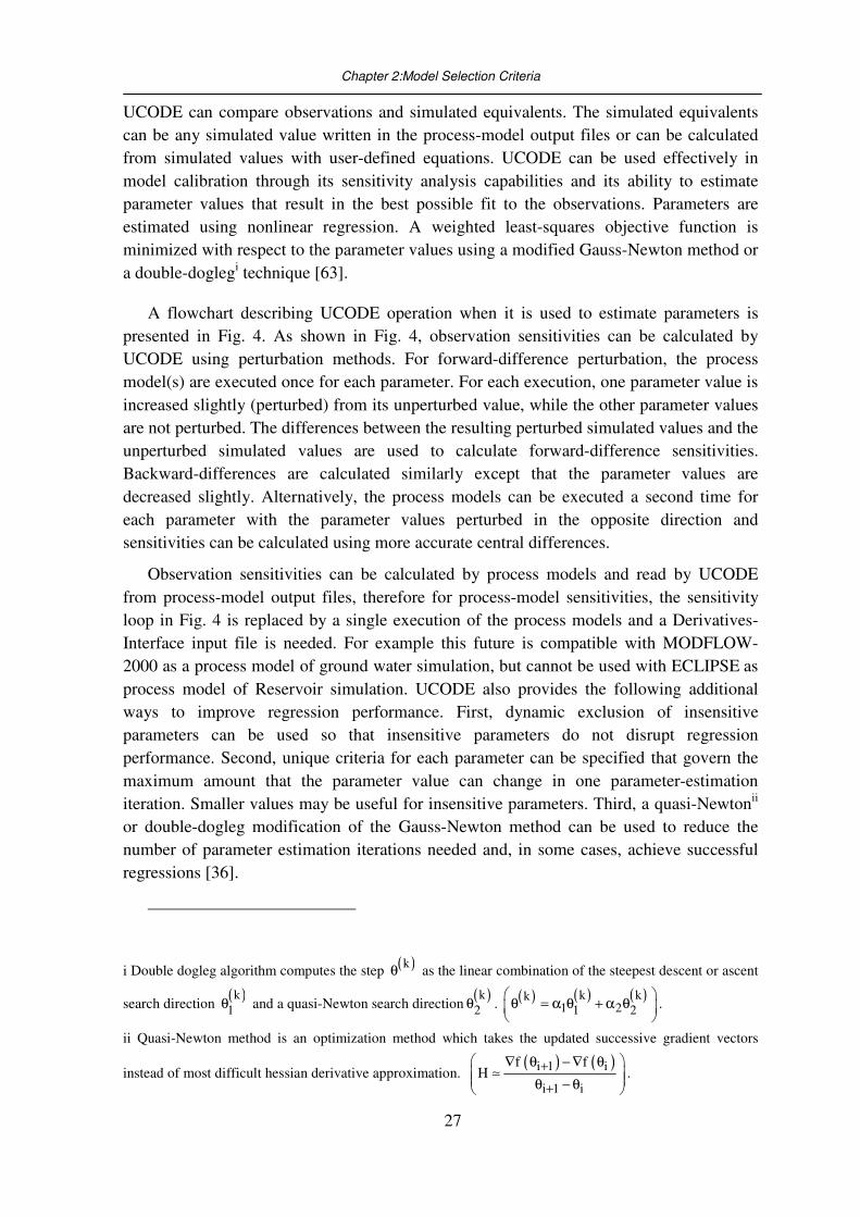
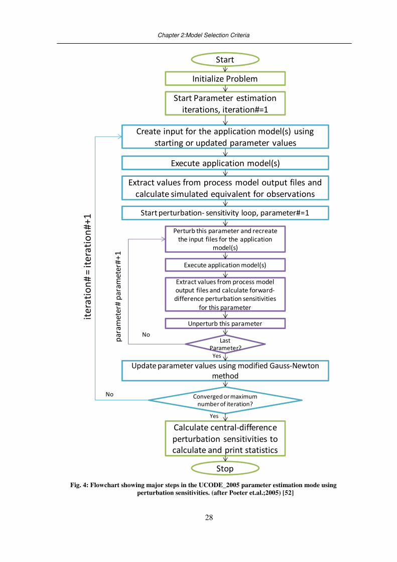
A flowchart describing UCODE operation when it is used to estimate parameters is
presented in Fig. 4. As shown in Fig. 4, observation sensitivities can be calculated by
UCODE using perturbation methods. For forward-difference perturbation, the process
model(s) are executed once for each parameter. For each execution, one parameter value is
increased slightly (perturbed) from its unperturbed value, while the other parameter values
are not perturbed. The differences between the resulting perturbed simulated values and the
unperturbed simulated values are used to calculate forward-difference sensitivities.
Backward-differences are calculated similarly except that the parameter values are
decreased slightly. Alternatively, the process models can be executed a second time for
each parameter with the parameter values perturbed in the opposite direction and
sensitivities can be calculated using more accurate central differences.
Observation sensitivities can be calculated by process models and read by UCODE
from process-model output files, therefore for process-model sensitivities, the sensitivity
loop in Fig. 4 is replaced by a single execution of the process models and a Derivatives-
Interface input file is needed. For example this future is compatible with MODFLOW-
2000 as a process model of ground water simulation, but cannot be used with ECLIPSE as
process model of Reservoir simulation. UCODE also provides the following additional
ways to improve regression performance. First, dynamic exclusion of insensitive
parameters can be used so that insensitive parameters do not disrupt regression
performance. Second, unique criteria for each parameter can be specified that govern the
maximum amount that the parameter value can change in one parameter-estimation
iteration. Smaller values may be useful for insensitive parameters. Third, a quasi-Newtonii
or double-dogleg modification of the Gauss-Newton method can be used to reduce the
number of parameter estimation iterations needed and, in some cases, achieve successful
regressions [36].
i Double dogleg algorithm computes the step ( )kθ as the linear combination of the steepest descent or ascent
search direction ( )k1θ and a quasi-Newton search direction
( )k2θ . ( ) ( ) ( )k kk
1 21 2
θ = α θ + α θ
.
ii Quasi-Newton method is an optimization method which takes the updated successive gradient vectors
instead of most difficult hessian derivative approximation. ( ) ( )i 1 i
i 1 i
f fH +
+
∇ θ − ∇ θ θ − θ ≃ .
Chapter 2:Model Selection Criteria
28
Initialize Problem
Start Parameter estimation
iterations, iteration#=1
Create input for the application model(s) using
starting or updated parameter values
Execute application model(s)
Extract values from process model output files and
calculate simulated equivalent for observations
Start perturbation- sensitivity loop, parameter#=1
Perturb this parameter and recreate
the input files for the application
model(s)
Execute application model(s)
Extract values from process model
output files and calculate forward-
difference perturbation sensitivities
for this parameter
Unperturb this parameter
Update parameter values using modified Gauss-Newton
method
Start
Last Parameter?
Converged or maximum number of iteration?
Calculate central-difference
perturbation sensitivities to
calculate and print statistics
Stop
ite
rati
on
# =
ite
rati
on
#+
1
pa
ram
ete
r# p
ara
me
ter#
+1
No
Yes
Yes
No
Fig. 4: Flowchart showing major steps in the UCODE_2005 parameter estimation mode using
perturbation sensitivities. (after Poeter et.al.;2005) [52]
[29]
2.5.2. SIMOPT
SIMOPT [60] is an optimization program from Schlumberger that assists in the steps
traditionally taken when trying to achieve a history match between an ECLIPSE 100/300
simulation model and the corresponding observed reservoir data. By applying
mathematical techniques, it provides additional information on which the reservoir
engineer can implement to improve the history match [28].
2.5.2.1. Objective function in SIMOPT
Objective function
The objective function, OFSIMOPT, which is minimized in SIMOPT regression, is a
modified form of the general used equation as shown previously in EQ. 2 with below
equation to be used in vector format:
SIMOPT residual prior surveyOF f f f= α + β + γ EQ. 17
OFSIMOPT is made from three parts: the production data or residual term, the prior
information term and the survey data term. Both prior and survey terms could be
considered as the extra penalty term for residual term. This idea of penalization will be
explained later in chapter Chapter 4 for developing general model selection criteria.
α,β and γ are overall weights for the production, prior and survey terms respectively
fresidual is the objective function residual term
fprior is the objective function prior term
fsurvey is the objective function survey term
Observed production data residuals
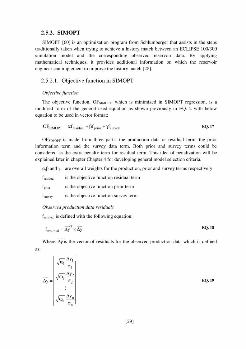
fresidual is defined with the following equation:
T
residualf y y= ∆ × ∆��� ���
EQ. 18
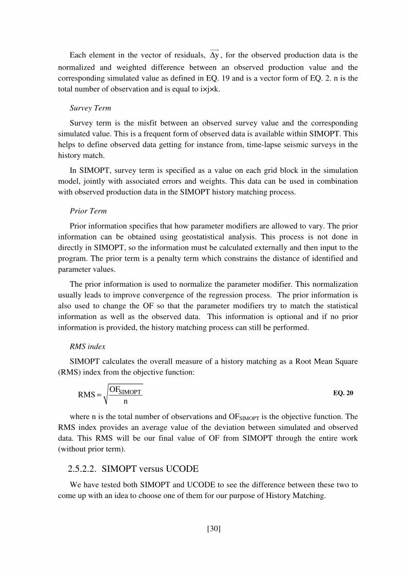
Where y∆���
is the vector of residuals for the observed production data which is defined
as:
11
1
22
2
nn
n
y
y
y
y
∆ ω σ
∆
ω σ∆ =
∆ ω σ
���
⋮
EQ. 19
[30]
Each element in the vector of residuals, y∆���
, for the observed production data is the
normalized and weighted difference between an observed production value and the
corresponding simulated value as defined in EQ. 19 and is a vector form of EQ. 2. n is the
total number of observation and is equal to i×j×k.
Survey Term
Survey term is the misfit between an observed survey value and the corresponding
simulated value. This is a frequent form of observed data is available within SIMOPT. This
helps to define observed data getting for instance from, time-lapse seismic surveys in the
history match.
In SIMOPT, survey term is specified as a value on each grid block in the simulation
model, jointly with associated errors and weights. This data can be used in combination
with observed production data in the SIMOPT history matching process.
Prior Term
Prior information specifies that how parameter modifiers are allowed to vary. The prior
information can be obtained using geostatistical analysis. This process is not done in
directly in SIMOPT, so the information must be calculated externally and then input to the
program. The prior term is a penalty term which constrains the distance of identified and
parameter values.
The prior information is used to normalize the parameter modifier. This normalization
usually leads to improve convergence of the regression process. The prior information is
also used to change the OF so that the parameter modifiers try to match the statistical
information as well as the observed data. This information is optional and if no prior
information is provided, the history matching process can still be performed.
RMS index
SIMOPT calculates the overall measure of a history matching as a Root Mean Square
(RMS) index from the objective function:
SIMOPTOFRMS
n= EQ. 20
where n is the total number of observations and OFSIMOPT is the objective function. The
RMS index provides an average value of the deviation between simulated and observed
data. This RMS will be our final value of OF from SIMOPT through the entire work
(without prior term).
2.5.2.2. SIMOPT versus UCODE
We have tested both SIMOPT and UCODE to see the difference between these two to
come up with an idea to choose one of them for our purpose of History Matching.

[31]
As can be seen in Table 2, UCODE is a universal code which could be used for every
model, but SIMOPT is specified only to be used with ECLIPSE Reservoir Simulation
models.
Although UCODE is good for matching every observation parameter (rather than
SIMOPT which could match only real measurement parameter, such as WBHP, WWCT,
WGOR, …), SIMOPT is faster, and more user friendly in petroleum engineering use. For
this reason we have used SIMOPT for our regression and history matching problems;
however in later stage of the projects MEPO has been used as an alternative to find
possible global minimum
Table 2: Comparison between SIMOPT and UCODE
SIMOPT UCODE
Specified only to be used with ECLIPSE Universal Code
User friendly and easy to use writing different codes are necessary
uses the Levenberg-Marquardt algorithm for minimization
Uses Modified Gauss Newton for minimization
Uses only the typical observation parameters for history matching
can be used for variety of different parameters for history matching
one simulation run in each perturbation step
one simulation run for each parameter in each perturbation step
2.5.3. MEPO
MEPO was originally developed in Germany under the name “Multipurpose
Environment for Parallel Optimization” through a research project at the Braunschweig
University of Technology.
MEPO is one of the global optimization tools for reservoir history matching which has
been further developed and commercialized by Scandpower Petroleum Technology.
MEPO uses global optimization methods such as Genetic Algorithms[19] and Evolution
Strategy [43].
Fig. 5 shows an example of Evolution Strategy and how this method applicable. In this
example, four simulation runs are made at the same time on separate CPUs, and at the end
of each set of runs the quality of the resulting matches is evaluated. The best are then be
used as the basis for the next set of runs (Parents and Children). Over successive
‘generations’, the resulting models show improving quality of history match.
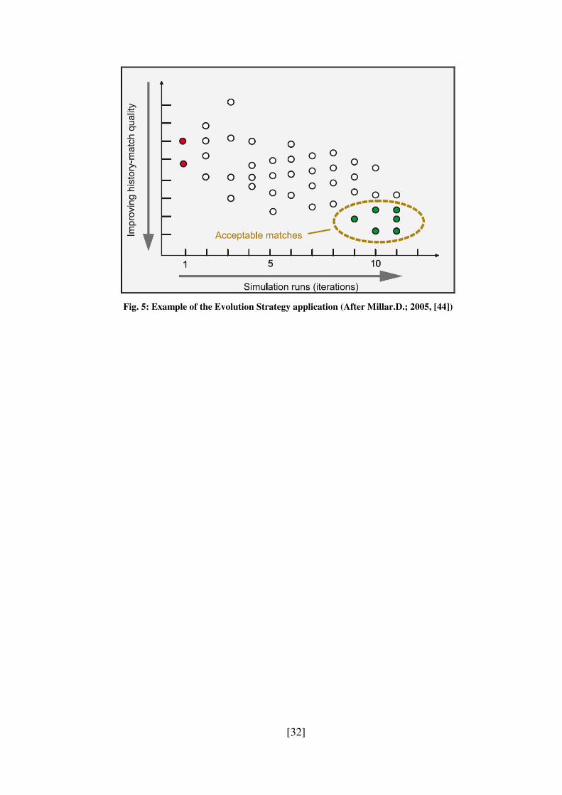
[32]
Fig. 5: Example of the Evolution Strategy application (After Millar.D.; 2005, [44])
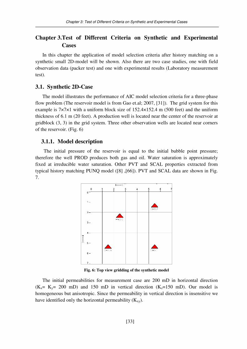
Chapter 3: Test of Different Criteria on Synthetic and Experimental Cases
[33]
Chapter 3. Test of Different Criteria on Synthetic and Experimental
Cases
In this chapter the application of model selection criteria after history matching on a
synthetic small 2D-model will be shown. Also there are two case studies, one with field
observation data (packer test) and one with experimental results (Laboratory measurement
test).
3.1. Synthetic 2D-Case
The model illustrates the performance of AIC model selection criteria for a three-phase
flow problem (The reservoir model is from Gao et.al; 2007, [31]). The grid system for this
example is 7×7×1 with a uniform block size of 152.4×152.4 m (500 feet) and the uniform
thickness of 6.1 m (20 feet). A production well is located near the center of the reservoir at
gridblock (3, 3) in the grid system. Three other observation wells are located near corners
of the reservoir. (Fig. 6)
3.1.1. Model description
The initial pressure of the reservoir is equal to the initial bubble point pressure;
therefore the well PROD produces both gas and oil. Water saturation is approximately
fixed at irreducible water saturation. Other PVT and SCAL properties extracted from
typical history matching PUNQ model ([8] ,[66]). PVT and SCAL data are shown in Fig.
7.
Fig. 6: Top view gridding of the synthetic model
The initial permeabilities for measurement case are 200 mD in horizontal direction
(Kx= Ky= 200 mD) and 150 mD in vertical direction (Kz=150 mD). Our model is
homogeneous but anisotropic. Since the permeability in vertical direction is insensitive we
have identified only the horizontal permeability (Kxy).
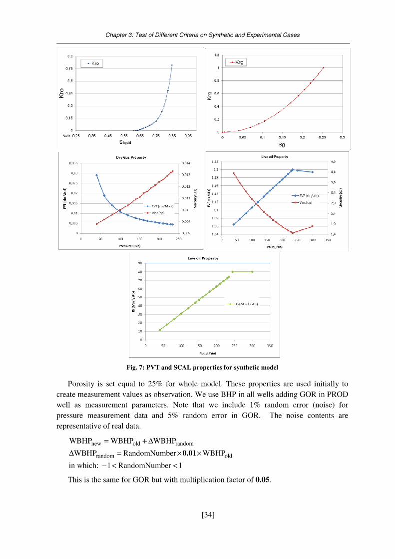
Chapter 3: Test of Different Criteria on Synthetic and Experimental Cases
[34]
Fig. 7: PVT and SCAL properties for synthetic model
Porosity is set equal to 25% for whole model. These properties are used initially to
create measurement values as observation. We use BHP in all wells adding GOR in PROD
well as measurement parameters. Note that we include 1% random error (noise) for
pressure measurement data and 5% random error in GOR. The noise contents are
representative of real data.
new old random
random old
WBHP WBHP WBHP
WBHP RandomNumber WBHP
in which: 1 RandomNumber 1
= + ∆
∆ = × ×
− < <
0.01
This is the same for GOR but with multiplication factor of 0.05.
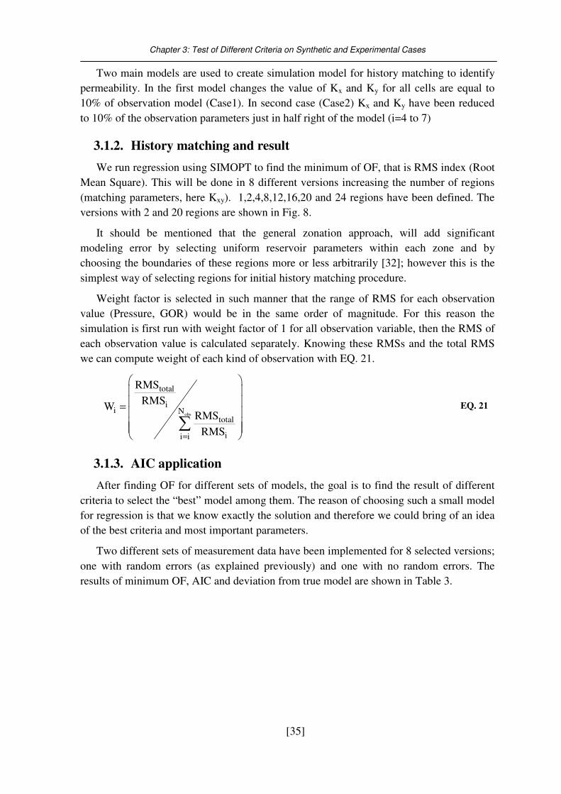
Chapter 3: Test of Different Criteria on Synthetic and Experimental Cases
[35]
Two main models are used to create simulation model for history matching to identify
permeability. In the first model changes the value of Kx and Ky for all cells are equal to
10% of observation model (Case1). In second case (Case2) Kx and Ky have been reduced
to 10% of the observation parameters just in half right of the model (i=4 to 7)
3.1.2. History matching and result
We run regression using SIMOPT to find the minimum of OF, that is RMS index (Root
Mean Square). This will be done in 8 different versions increasing the number of regions
(matching parameters, here Kxy). 1,2,4,8,12,16,20 and 24 regions have been defined. The
versions with 2 and 20 regions are shown in Fig. 8.
It should be mentioned that the general zonation approach, will add significant
modeling error by selecting uniform reservoir parameters within each zone and by
choosing the boundaries of these regions more or less arbitrarily [32]; however this is the
simplest way of selecting regions for initial history matching procedure.
Weight factor is selected in such manner that the range of RMS for each observation
value (Pressure, GOR) would be in the same order of magnitude. For this reason the
simulation is first run with weight factor of 1 for all observation variable, then the RMS of
each observation value is calculated separately. Knowing these RMSs and the total RMS
we can compute weight of each kind of observation with EQ. 21.
obs
total
ii N
total
ii i
RMS
RMSWRMS
RMS=
=
∑ EQ. 21
3.1.3. AIC application
After finding OF for different sets of models, the goal is to find the result of different
criteria to select the “best” model among them. The reason of choosing such a small model
for regression is that we know exactly the solution and therefore we could bring of an idea
of the best criteria and most important parameters.
Two different sets of measurement data have been implemented for 8 selected versions;
one with random errors (as explained previously) and one with no random errors. The
results of minimum OF, AIC and deviation from true model are shown in Table 3.
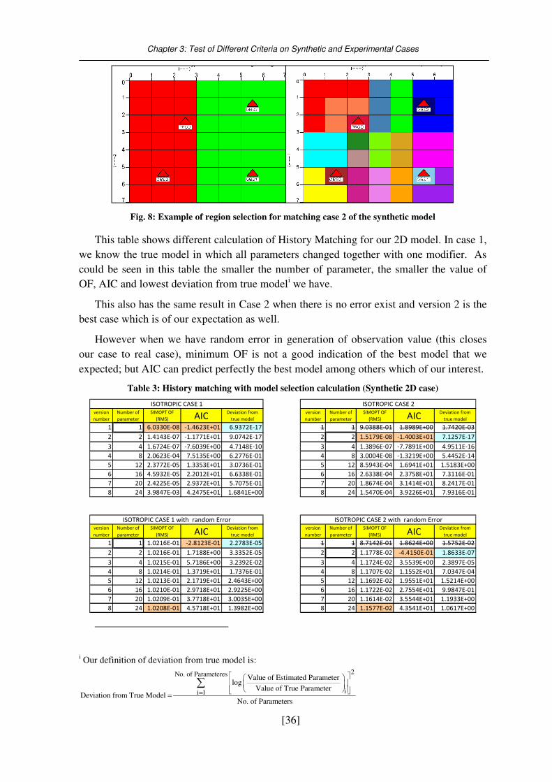
Chapter 3: Test of Different Criteria on Synthetic and Experimental Cases
[36]
Fig. 8: Example of region selection for matching case 2 of the synthetic model
This table shows different calculation of History Matching for our 2D model. In case 1,
we know the true model in which all parameters changed together with one modifier. As
could be seen in this table the smaller the number of parameter, the smaller the value of
OF, AIC and lowest deviation from true modeli we have.
This also has the same result in Case 2 when there is no error exist and version 2 is the
best case which is of our expectation as well.
However when we have random error in generation of observation value (this closes
our case to real case), minimum OF is not a good indication of the best model that we
expected; but AIC can predict perfectly the best model among others which of our interest.
Table 3: History matching with model selection calculation (Synthetic 2D case)
version
number
Number of
parameter
SIMOPT OF
(RMS) AICDeviation from
true model
version
number
Number of
parameter
SIMOPT OF
(RMS) AICDeviation from
true model
1 1 6.0330E-08 -1.4623E+01 6.9372E-17 1 1 9.0388E-01 1.8989E+00 1.7420E-03
2 2 1.4143E-07 -1.1771E+01 9.0742E-17 2 2 1.5179E-08 -1.4003E+01 7.1257E-17
3 4 1.6724E-07 -7.6039E+00 4.7148E-10 3 4 1.3896E-07 -7.7891E+00 4.9511E-16
4 8 2.0623E-04 7.5135E+00 6.2776E-01 4 8 3.0004E-08 -1.3219E+00 5.4452E-14
5 12 2.3772E-05 1.3353E+01 3.0736E-01 5 12 8.5943E-04 1.6941E+01 1.5183E+00
6 16 4.5932E-05 2.2012E+01 6.6338E-01 6 16 2.6338E-04 2.3758E+01 7.3116E-01
7 20 2.4225E-05 2.9372E+01 5.7075E-01 7 20 1.8674E-04 3.1414E+01 8.2417E-01
8 24 3.9847E-03 4.2475E+01 1.6841E+00 8 24 1.5470E-04 3.9226E+01 7.9316E-01
version
number
Number of
parameter
SIMOPT OF
(RMS) AICDeviation from
true model
version
number
Number of
parameter
SIMOPT OF
(RMS) AICDeviation from
true model
1 1 1.0216E-01 -2.8123E-01 2.2783E-05 1 1 8.7142E-01 1.8624E+00 1.5752E-02
2 2 1.0216E-01 1.7188E+00 3.3352E-05 2 2 1.1778E-02 -4.4150E-01 1.8633E-07
3 4 1.0215E-01 5.7186E+00 3.2392E-02 3 4 1.1724E-02 3.5539E+00 2.3897E-05
4 8 1.0214E-01 1.3719E+01 1.7376E-01 4 8 1.1707E-02 1.1552E+01 7.0347E-04
5 12 1.0213E-01 2.1719E+01 2.4643E+00 5 12 1.1692E-02 1.9551E+01 1.5214E+00
6 16 1.0210E-01 2.9718E+01 2.9225E+00 6 16 1.1722E-02 2.7554E+01 9.9847E-01
7 20 1.0209E-01 3.7718E+01 3.0035E+00 7 20 1.1614E-02 3.5544E+01 1.1933E+00
8 24 1.0208E-01 4.5718E+01 1.3982E+00 8 24 1.1577E-02 4.3541E+01 1.0617E+00
ISOTROPIC CASE 1 ISOTROPIC CASE 2
ISOTROPIC CASE 2 with random ErrorISOTROPIC CASE 1 with random Error
i Our definition of deviation from true model is:
2No. of Parameteres
ii 1
Value of Estimated Parameterlog
Value of True ParameterDeviation from True Model
No. of Parameters=
=
∑
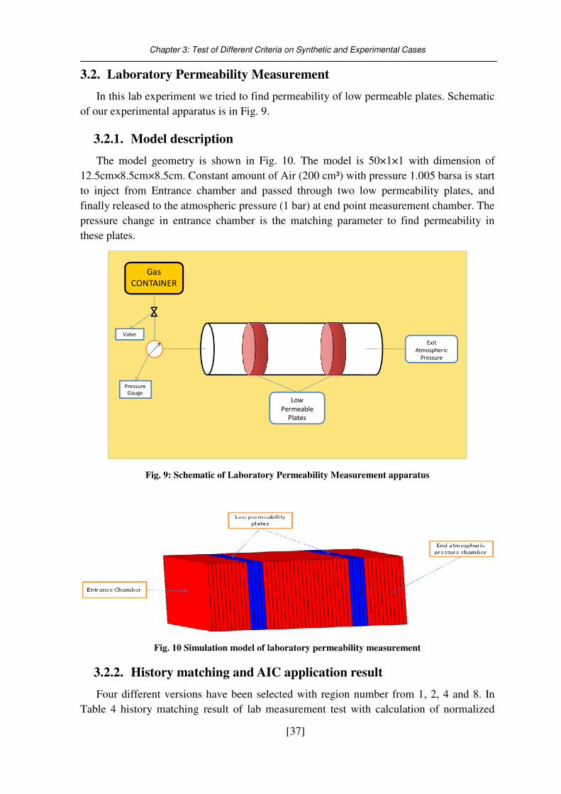
Chapter 3: Test of Different Criteria on Synthetic and Experimental Cases
[37]
3.2. Laboratory Permeability Measurement
In this lab experiment we tried to find permeability of low permeable plates. Schematic
of our experimental apparatus is in Fig. 9.
3.2.1. Model description
The model geometry is shown in Fig. 10. The model is 50×1×1 with dimension of
12.5cm×8.5cm×8.5cm. Constant amount of Air (200 cm³) with pressure 1.005 barsa is start
to inject from Entrance chamber and passed through two low permeability plates, and
finally released to the atmospheric pressure (1 bar) at end point measurement chamber. The
pressure change in entrance chamber is the matching parameter to find permeability in
these plates.
Gas
CONTAINER
Low
Permeable
Plates
Pressure Gauge
Valve
Exit
Atmospheric
Pressure
Fig. 9: Schematic of Laboratory Permeability Measurement apparatus
Fig. 10 Simulation model of laboratory permeability measurement
3.2.2. History matching and AIC application result
Four different versions have been selected with region number from 1, 2, 4 and 8. In
Table 4 history matching result of lab measurement test with calculation of normalized
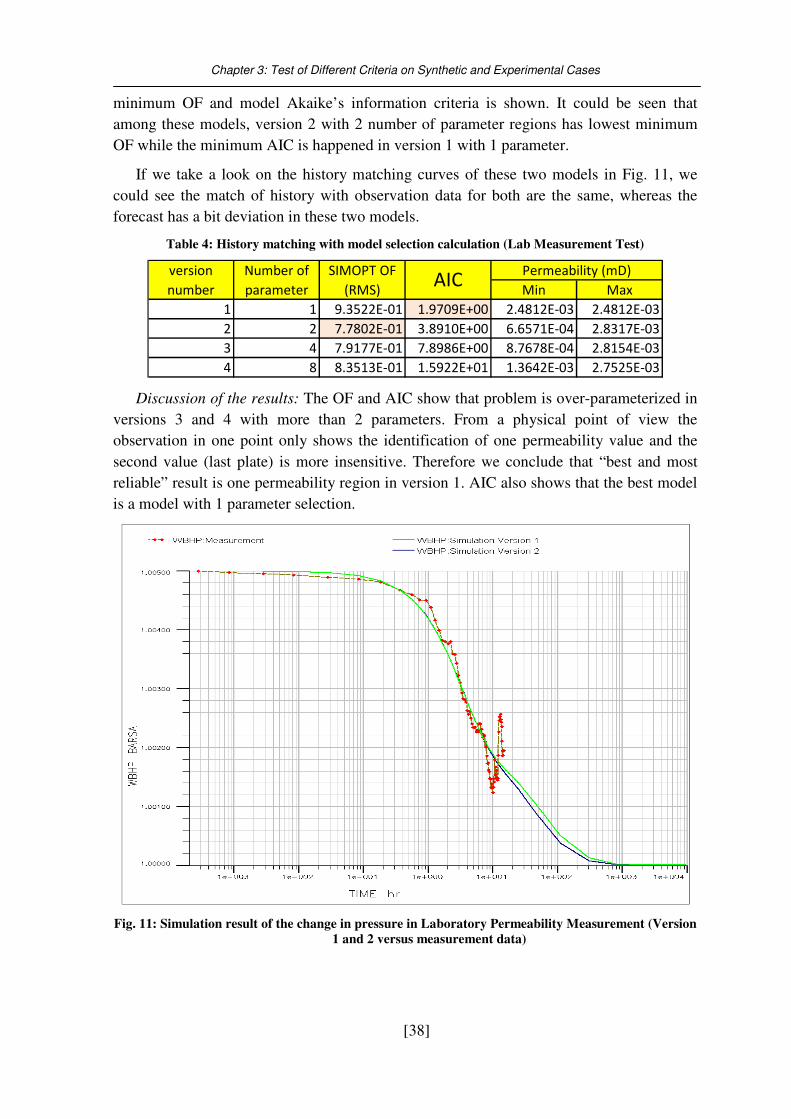
Chapter 3: Test of Different Criteria on Synthetic and Experimental Cases
[38]
minimum OF and model Akaike’s information criteria is shown. It could be seen that
among these models, version 2 with 2 number of parameter regions has lowest minimum
OF while the minimum AIC is happened in version 1 with 1 parameter.
If we take a look on the history matching curves of these two models in Fig. 11, we
could see the match of history with observation data for both are the same, whereas the
forecast has a bit deviation in these two models.
Table 4: History matching with model selection calculation (Lab Measurement Test)
Min Max
1 1 9.3522E-01 1.9709E+00 2.4812E-03 2.4812E-03
2 2 7.7802E-01 3.8910E+00 6.6571E-04 2.8317E-03
3 4 7.9177E-01 7.8986E+00 8.7678E-04 2.8154E-03
4 8 8.3513E-01 1.5922E+01 1.3642E-03 2.7525E-03
version
number
Number of
parameter
SIMOPT OF
(RMS)AIC
Permeability (mD)
Discussion of the results: The OF and AIC show that problem is over-parameterized in
versions 3 and 4 with more than 2 parameters. From a physical point of view the
observation in one point only shows the identification of one permeability value and the
second value (last plate) is more insensitive. Therefore we conclude that “best and most
reliable” result is one permeability region in version 1. AIC also shows that the best model
is a model with 1 parameter selection.
Fig. 11: Simulation result of the change in pressure in Laboratory Permeability Measurement (Version
1 and 2 versus measurement data)
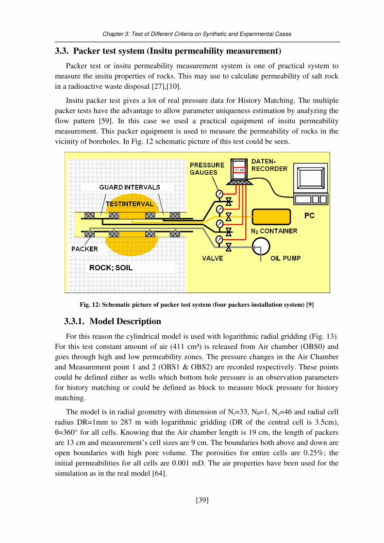
Chapter 3: Test of Different Criteria on Synthetic and Experimental Cases
[39]
3.3. Packer test system (Insitu permeability measurement)
Packer test or insitu permeability measurement system is one of practical system to
measure the insitu properties of rocks. This may use to calculate permeability of salt rock
in a radioactive waste disposal [27],[10].
Insitu packer test gives a lot of real pressure data for History Matching. The multiple
packer tests have the advantage to allow parameter uniqueness estimation by analyzing the
flow pattern [59]. In this case we used a practical equipment of insitu permeability
measurement. This packer equipment is used to measure the permeability of rocks in the
vicinity of boreholes. In Fig. 12 schematic picture of this test could be seen.
Fig. 12: Schematic picture of packer test system (four packers installation system) [9]
3.3.1. Model Description
For this reason the cylindrical model is used with logarithmic radial gridding (Fig. 13).
For this test constant amount of air (411 cm³) is released from Air chamber (OBS0) and
goes through high and low permeability zones. The pressure changes in the Air Chamber
and Measurement point 1 and 2 (OBS1 & OBS2) are recorded respectively. These points
could be defined either as wells which bottom hole pressure is an observation parameters
for history matching or could be defined as block to measure block pressure for history
matching.
The model is in radial geometry with dimension of Nr=33, Nθ=1, Nz=46 and radial cell
radius DR=1mm to 287 m with logarithmic gridding (DR of the central cell is 3.5cm),
θ=360° for all cells. Knowing that the Air chamber length is 19 cm, the length of packers
are 13 cm and measurement’s cell sizes are 9 cm. The boundaries both above and down are
open boundaries with high pore volume. The porosities for entire cells are 0.25%; the
initial permeabilities for all cells are 0.001 mD. The air properties have been used for the
simulation as in the real model [64].
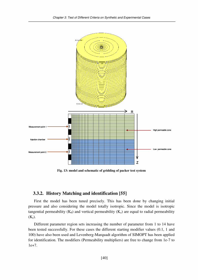
Chapter 3: Test of Different Criteria on Synthetic and Experimental Cases
[40]
Fig. 13: model and schematic of gridding of packer test system
3.3.2. History Matching and identification [55]
First the model has been tuned precisely. This has been done by changing initial
pressure and also considering the model totally isotropic. Since the model is isotropic
tangential permeability (Kθ) and vertical permeability (Kz) are equal to radial permeability
(Kr).
Different parameter region sets increasing the number of parameter from 1 to 14 have
been tested successfully. For these cases the different starting modifier values (0.1, 1 and
100) have also been used and Levenberg-Marquadt algorithm of SIMOPT has been applied
for identification. The modifiers (Permeability multipliers) are free to change from 1e-7 to
1e+7.
pack
er
OBS2
pack
er
pac
ker
OBS1
pack
er
OBS0
R
Z
Measurement point 1
Injection chamber
Measurement point 2
Low permeable zone
High permeable zone
pack
er
OBS2
pack
er
pac
ker
OBS1
pack
er
OBS0
R
Z
Measurement point 1
Injection chamber
Measurement point 2
Low permeable zone
High permeable zone
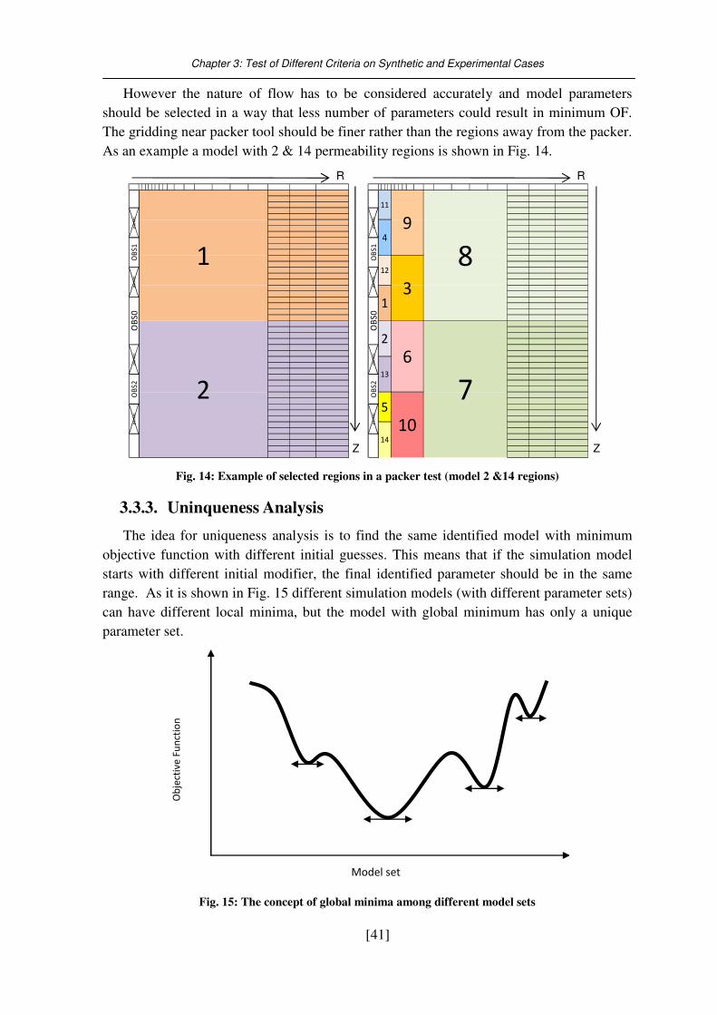
Chapter 3: Test of Different Criteria on Synthetic and Experimental Cases
[41]
However the nature of flow has to be considered accurately and model parameters
should be selected in a way that less number of parameters could result in minimum OF.
The gridding near packer tool should be finer rather than the regions away from the packer.
As an example a model with 2 & 14 permeability regions is shown in Fig. 14.
OB
S2
pa
cke
r
1
2
pa
cke
rO
BS
1p
ack
er
OB
S0
pa
cke
r
8
7
9
3
6
10
11
4
12
1
13
2
5
14
OB
S1
OB
S0
OB
S2
pa
cke
rp
ack
er
pa
cke
rp
ack
er
R
Z
R
Z
Fig. 14: Example of selected regions in a packer test (model 2 &14 regions)
3.3.3. Uninqueness Analysis
The idea for uniqueness analysis is to find the same identified model with minimum
objective function with different initial guesses. This means that if the simulation model
starts with different initial modifier, the final identified parameter should be in the same
range. As it is shown in Fig. 15 different simulation models (with different parameter sets)
can have different local minima, but the model with global minimum has only a unique
parameter set.
Ob
ject
ive
Fu
nct
ion
Model set
Fig. 15: The concept of global minima among different model sets
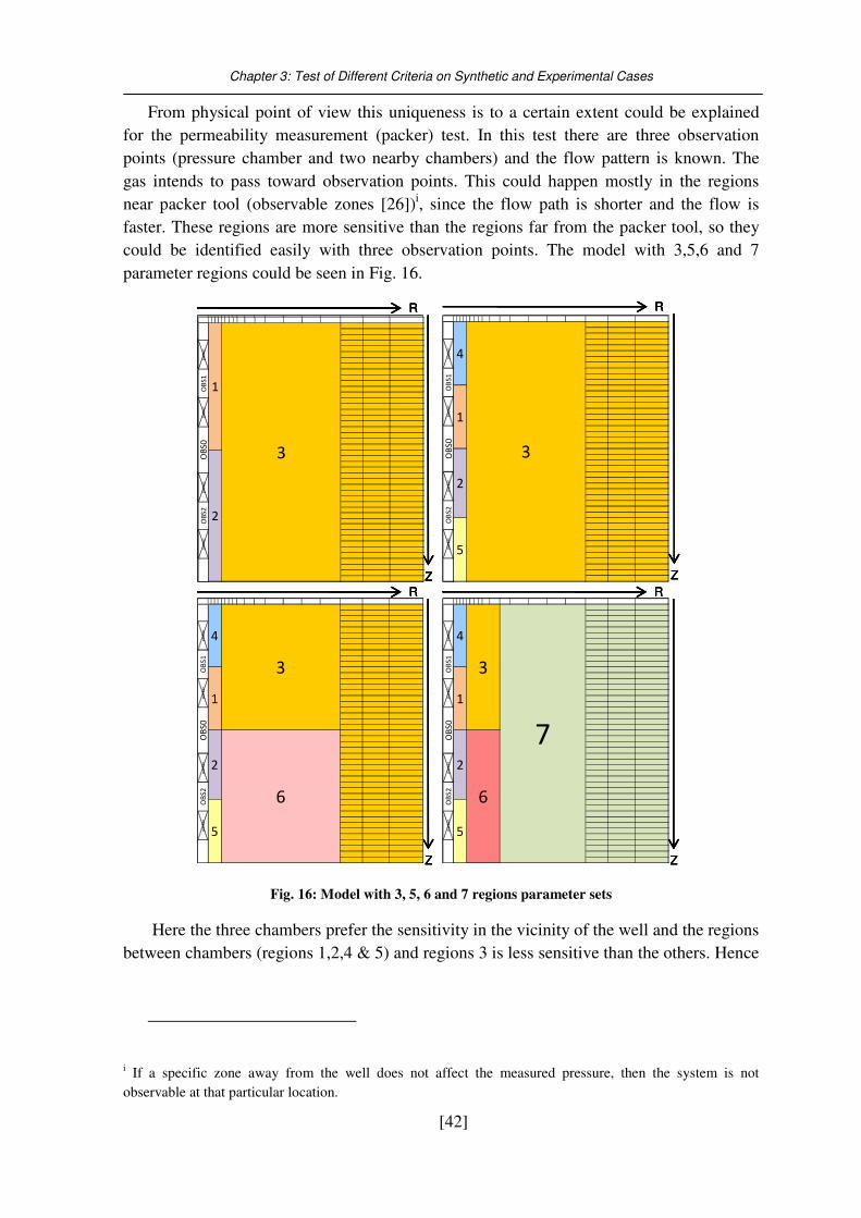
Chapter 3: Test of Different Criteria on Synthetic and Experimental Cases
[42]
From physical point of view this uniqueness is to a certain extent could be explained
for the permeability measurement (packer) test. In this test there are three observation
points (pressure chamber and two nearby chambers) and the flow pattern is known. The
gas intends to pass toward observation points. This could happen mostly in the regions
near packer tool (observable zones [26])i, since the flow path is shorter and the flow is
faster. These regions are more sensitive than the regions far from the packer tool, so they
could be identified easily with three observation points. The model with 3,5,6 and 7
parameter regions could be seen in Fig. 16.
R
Z
R
Z
R
Z
R
Z
6
pac
ker
OB
S2
5pa
cke
r
4
3
7
pa
cke
rO
BS
1
1pa
cke
rO
BS
0
22
6
pac
ker
OB
S2
5pa
cke
r
pa
cke
r
4
3
pa
cke
rO
BS
1
1pa
cke
rO
BS
0
3p
ack
er
OB
S1
1pa
cke
rO
BS
0
2
pac
ker
OB
S2
5
4
1
2
5
4
pa
cke
rO
BS
1p
ack
er
OB
S0
pa
cke
rO
BS
2p
ack
er
3
2
1
pac
ke
rO
BS0
pac
ke
rO
BS2
pac
ke
rp
acke
rO
BS1
R
Z
R
Z
R
Z
R
Z
R
Z
R
Z
R
Z
R
Z
R
Z
R
Z
R
Z
R
Z
6
pac
ke
rO
BS
2
5pa
cke
r
4
3
7
pa
cke
rO
BS
1
1pa
cke
rO
BS
0
22
6
pac
ke
rO
BS
2
5pa
cke
r
pa
cke
r
4
3
pa
cke
rO
BS
1
1pa
cke
rO
BS
0
3p
ack
er
OB
S1
1pa
cke
rO
BS
0
2
pac
ke
rO
BS
2
5
4
1
2
5
4
pa
cke
rO
BS
1p
ack
er
OB
S0
pa
cke
rO
BS
2p
ack
er
3
2
1
pac
ke
rO
BS0
pac
ke
rO
BS2
pac
ke
rp
acke
rO
BS1
6
pac
ke
rO
BS
2
5pa
cke
r
4
3
7
pa
cke
rO
BS
1
1pa
cke
rO
BS
0
22
6
pac
ke
rO
BS
2
5pa
cke
r
pa
cke
r
4
3
pa
cke
rO
BS
1
1pa
cke
rO
BS
0
3p
ack
er
OB
S1
1pa
cke
rO
BS
0
2
pac
ke
rO
BS
2
5
4
1
2
5
4
pa
cke
rO
BS
1p
ack
er
OB
S0
pa
cke
rO
BS
2p
ack
er
3
2
1
pac
ke
rO
BS0
pac
ke
rO
BS2
pac
ke
rp
acke
rO
BS1
Fig. 16: Model with 3, 5, 6 and 7 regions parameter sets
Here the three chambers prefer the sensitivity in the vicinity of the well and the regions
between chambers (regions 1,2,4 & 5) and regions 3 is less sensitive than the others. Hence
i If a specific zone away from the well does not affect the measured pressure, then the system is not
observable at that particular location.
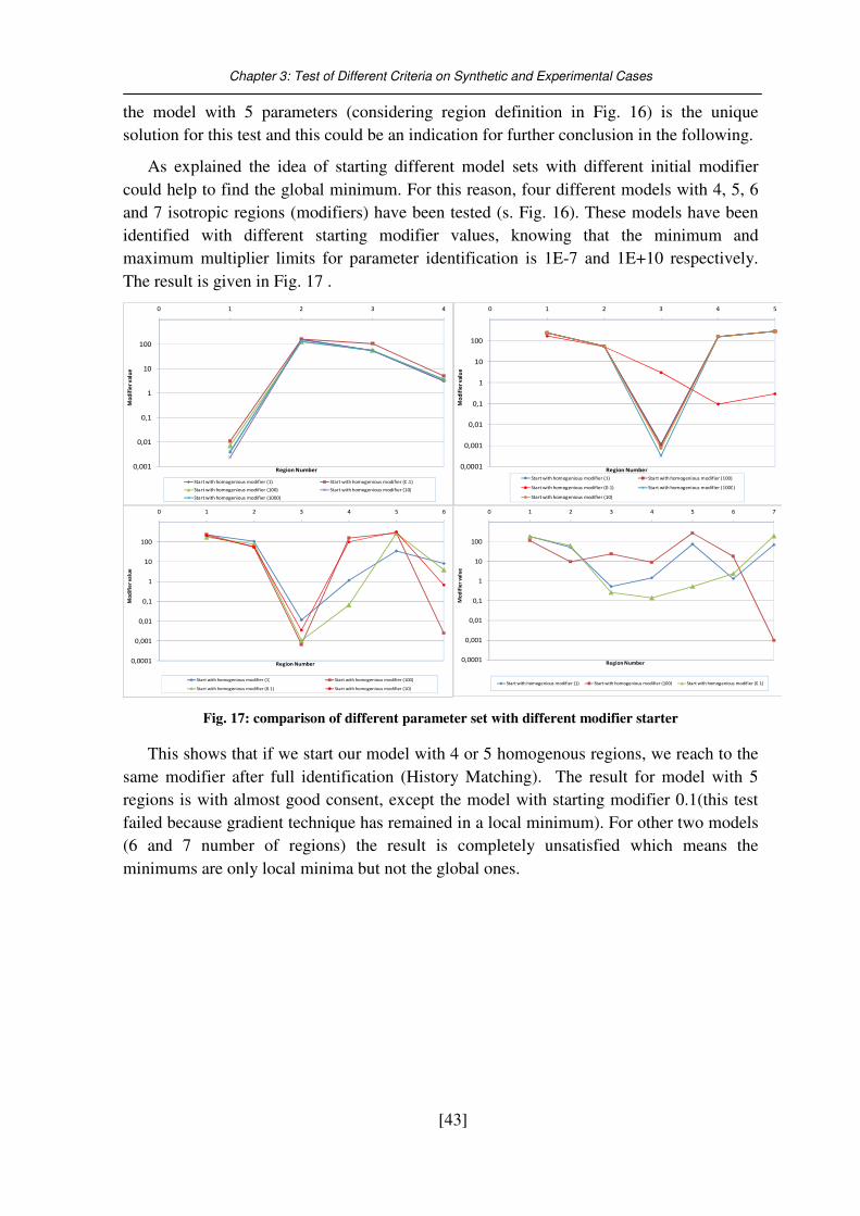
Chapter 3: Test of Different Criteria on Synthetic and Experimental Cases
[43]
the model with 5 parameters (considering region definition in Fig. 16) is the unique
solution for this test and this could be an indication for further conclusion in the following.
As explained the idea of starting different model sets with different initial modifier
could help to find the global minimum. For this reason, four different models with 4, 5, 6
and 7 isotropic regions (modifiers) have been tested (s. Fig. 16). These models have been
identified with different starting modifier values, knowing that the minimum and
maximum multiplier limits for parameter identification is 1E-7 and 1E+10 respectively.
The result is given in Fig. 17 .
0,001
0,01
0,1
1
10
100
0 1 2 3 4
Mo
dif
ier
val
ue
Region Number
Start with homogenious modifier (1) Start with homogenious modifier (0.1)
Start with homogenious modifier (100) Start with homogenious modifier (10)
Start with homogenious modifier (1000)
0,0001
0,001
0,01
0,1
1
10
100
0 1 2 3 4 5
Mo
dif
ier
val
ue
Region Number
Start with homogenious modifier (1) Start with homogenious modifier (100)
Start with homogenious modifier (0.1) Start with homogenious modifier (1000)
Start with homogenious modifier (10)
0,0001
0,001
0,01
0,1
1
10
100
0 1 2 3 4 5 6
Mo
dif
ier
valu
e
Region Number
Start with homogenious modifier (1) Start with homogenious modifier (100)
Start with homogenious modifier (0.1) Start with homogenious modifier (10)
0,0001
0,001
0,01
0,1
1
10
100
0 1 2 3 4 5 6 7
Mo
dif
ier
valu
e
Region Number
Start with homogenious modifier (1) Start with homogenious modifier (100) Start with homogenious modifier (0.1)
Fig. 17: comparison of different parameter set with different modifier starter
This shows that if we start our model with 4 or 5 homogenous regions, we reach to the
same modifier after full identification (History Matching). The result for model with 5
regions is with almost good consent, except the model with starting modifier 0.1(this test
failed because gradient technique has remained in a local minimum). For other two models
(6 and 7 number of regions) the result is completely unsatisfied which means the
minimums are only local minima but not the global ones.
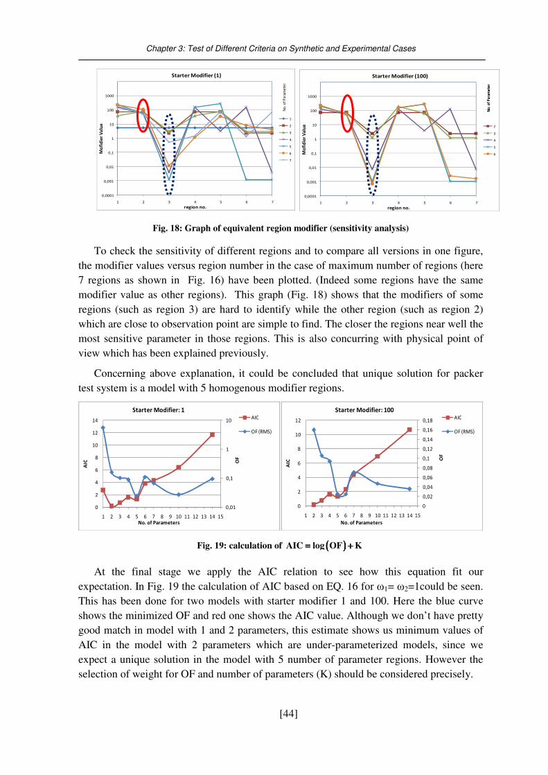
Chapter 3: Test of Different Criteria on Synthetic and Experimental Cases
[44]
0,0001
0,001
0,01
0,1
1
10
100
1000
1 2 3 4 5 6 7
Mo
fid
ier
Va
lue
region no.
Starter Modifier (1)
1
2
3
4
5
6
7
No
. of
Par
ame
ter
0,0001
0,001
0,01
0,1
1
10
100
1000
1 2 3 4 5 6 7
Mo
fid
ier
Va
lue
region no.
Starter Modifier (100)
2
3
4
5
6
No
. of
Par
ame
ter
No
. of
Par
ame
ter
Fig. 18: Graph of equivalent region modifier (sensitivity analysis)
To check the sensitivity of different regions and to compare all versions in one figure,
the modifier values versus region number in the case of maximum number of regions (here
7 regions as shown in Fig. 16) have been plotted. (Indeed some regions have the same
modifier value as other regions). This graph (Fig. 18) shows that the modifiers of some
regions (such as region 3) are hard to identify while the other region (such as region 2)
which are close to observation point are simple to find. The closer the regions near well the
most sensitive parameter in those regions. This is also concurring with physical point of
view which has been explained previously.
Concerning above explanation, it could be concluded that unique solution for packer
test system is a model with 5 homogenous modifier regions.
0,01
0,1
1
10
0
2
4
6
8
10
12
14
1 2 3 4 5 6 7 8 9 10 11 12 13 14 15
OF
AIC
No. of Parameters
Starter Modifier: 1AIC
OF (RMS)
0
0,02
0,04
0,06
0,08
0,1
0,12
0,14
0,16
0,18
0
2
4
6
8
10
12
1 2 3 4 5 6 7 8 9 10 11 12 13 14 15
OF
AIC
No. of Parameters
Starter Modifier: 100AIC
OF (RMS)
Fig. 19: calculation of (((( ))))AIC log OF K= += += += +
At the final stage we apply the AIC relation to see how this equation fit our
expectation. In Fig. 19 the calculation of AIC based on EQ. 16 for ω1= ω2=1could be seen.
This has been done for two models with starter modifier 1 and 100. Here the blue curve
shows the minimized OF and red one shows the AIC value. Although we don’t have pretty
good match in model with 1 and 2 parameters, this estimate shows us minimum values of
AIC in the model with 2 parameters which are under-parameterized models, since we
expect a unique solution in the model with 5 number of parameter regions. However the
selection of weight for OF and number of parameters (K) should be considered precisely.
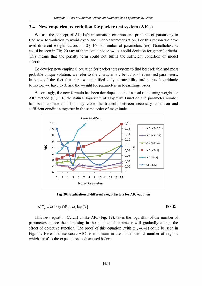
Chapter 3: Test of Different Criteria on Synthetic and Experimental Cases
[45]
3.4. New emperical correlation for packer test system (AICn)
We use the concept of Akaike’s information criterion and principle of parsimony to
find new formulation to avoid over- and under-parameterization. For this reason we have
used different weight factors in EQ. 16 for number of parameters (ω2). Nonetheless as
could be seen in Fig. 20 any of them could not show us a solid decision for general criteria.
This means that the penalty term could not fulfill the sufficient condition of model
selection.
To develop new empirical equation for packer test system to find best reliable and most
probable unique solution, we refer to the characteristic behavior of identified parameters.
In view of the fact that here we identified only permeability and it has logarithmic
behavior, we have to define the weight for parameters in logarithmic order.
Accordingly, the new formula has been developed so that instead of defining weight for
AIC method (EQ. 16) the natural logarithm of Objective Function and parameter number
has been considered. This may close the tradeoff between necessary condition and
sufficient condition together in the same order of magnitude.
0
0,02
0,04
0,06
0,08
0,1
0,12
0,14
0,16
0,18
-4
-2
0
2
4
6
8
10
12
2 3 4 5 6 7 8 9 10 11 12 13 14
OF
AIC
No. of Parameters
Starter Modifier 1
AIC (w2=0.01)
AIC (w2=0.1)
AIC (w2=0.5)
AIC (w2=1)
AIC (W=2)
OF (RMS)
Fig. 20: Application of different weight factors for AIC equation
( ) ( )n 1 2AIC log OF log k= ω + ω EQ. 22
This new equation (AICn) unlike AIC (Fig. 19), takes the logarithm of the number of
parameters, hence the increasing in the number of parameter will gradually change the
effect of objective function. The proof of this equation (with ω1, ω2=1) could be seen in
Fig. 11. Here in these cases AICn is minimum in the model with 5 number of regions
which satisfies the expectation as discussed before.
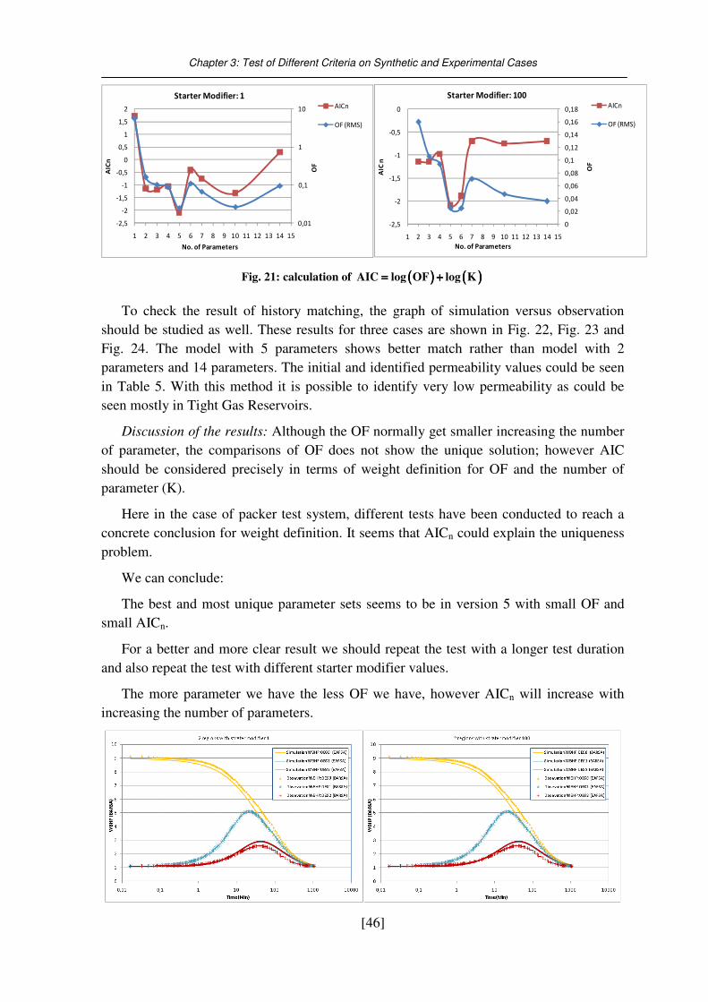
Chapter 3: Test of Different Criteria on Synthetic and Experimental Cases
[46]
0,01
0,1
1
10
-2,5
-2
-1,5
-1
-0,5
0
0,5
1
1,5
2
1 2 3 4 5 6 7 8 9 10 11 12 13 14 15
OF
AIC
n
No. of Parameters
Starter Modifier: 1AICn
OF (RMS)
0
0,02
0,04
0,06
0,08
0,1
0,12
0,14
0,16
0,18
-2,5
-2
-1,5
-1
-0,5
0
1 2 3 4 5 6 7 8 9 10 11 12 13 14 15
OF
AIC
n
No. of Parameters
Starter Modifier: 100AICn
OF (RMS)
Fig. 21: calculation of (((( )))) (((( ))))AIC log OF log K= += += += +
To check the result of history matching, the graph of simulation versus observation
should be studied as well. These results for three cases are shown in Fig. 22, Fig. 23 and
Fig. 24. The model with 5 parameters shows better match rather than model with 2
parameters and 14 parameters. The initial and identified permeability values could be seen
in Table 5. With this method it is possible to identify very low permeability as could be
seen mostly in Tight Gas Reservoirs.
Discussion of the results: Although the OF normally get smaller increasing the number
of parameter, the comparisons of OF does not show the unique solution; however AIC
should be considered precisely in terms of weight definition for OF and the number of
parameter (K).
Here in the case of packer test system, different tests have been conducted to reach a
concrete conclusion for weight definition. It seems that AICn could explain the uniqueness
problem.
We can conclude:
The best and most unique parameter sets seems to be in version 5 with small OF and
small AICn.
For a better and more clear result we should repeat the test with a longer test duration
and also repeat the test with different starter modifier values.
The more parameter we have the less OF we have, however AICn will increase with
increasing the number of parameters.
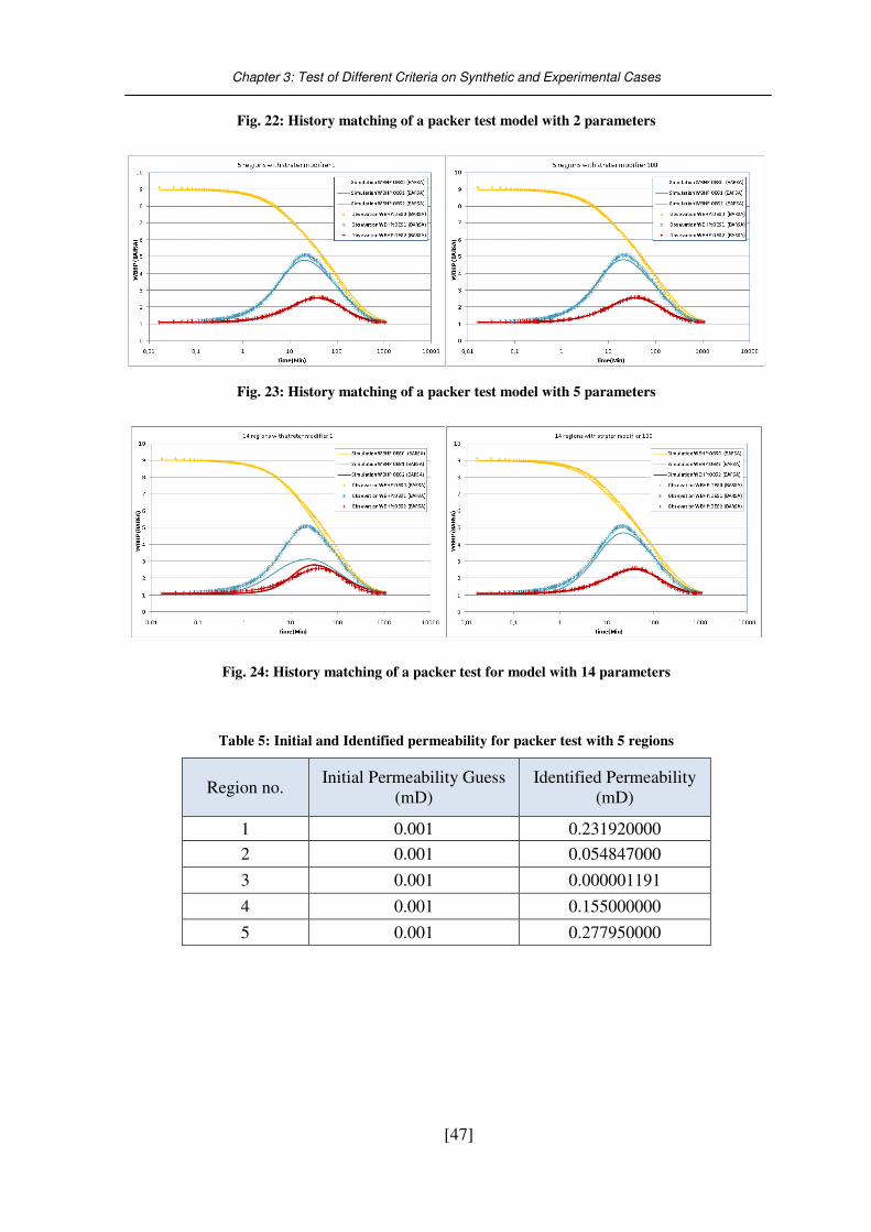
Chapter 3: Test of Different Criteria on Synthetic and Experimental Cases
[47]
Fig. 22: History matching of a packer test model with 2 parameters
Fig. 23: History matching of a packer test model with 5 parameters
Fig. 24: History matching of a packer test for model with 14 parameters
Table 5: Initial and Identified permeability for packer test with 5 regions
Region no. Initial Permeability Guess
(mD) Identified Permeability
(mD)
1 0.001 0.231920000
2 0.001 0.054847000
3 0.001 0.000001191
4 0.001 0.155000000
5 0.001 0.277950000
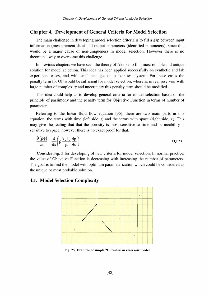
Chapter 4: Development of General Criteria for Model Selection
[48]
Chapter 4. Development of General Criteria for Model Selection
The main challenge in developing model selection criteria is to fill a gap between input
information (measurement data) and output parameters (identified parameters), since this
would be a major cause of non-uniqueness in model selection. However there is no
theoretical way to overcome this challenge.
In previous chapters we have seen the theory of Akaike to find most reliable and unique
solution for model selection. This idea has been applied successfully on synthetic and lab
experiment cases, and with small changes on packer test system. For these cases the
penalty term for OF would be sufficient for model selection; where as in real reservoir with
large number of complexity and uncertainty this penalty term should be modified.
This idea could help us to develop general criteria for model selection based on the
principle of parsimony and the penalty term for Objective Function in terms of number of
parameters.
Referring to the linear fluid flow equation [35], there are two main parts in this
equation, the terms with time (left side, t) and the terms with space (right side, x). This
may give the feeling that that the porosity is most sensitive to time and permeability is
sensitive to space, however there is no exact proof for that.
( ) x rk k p
t x x
∂ ρφ ∂ ∂= ρ
∂ ∂ µ ∂ EQ. 23
Consider Fig. 3 for developing of new criteria for model selection. In normal practice,
the value of Objective Function is decreasing with increasing the number of parameters.
The goal is to find the model with optimum parameterization which could be considered as
the unique or most probable solution.
4.1. Model Selection Complexity
O
O O
O
O
O O
Fig. 25: Example of simple 2D Cartesian reservoir model
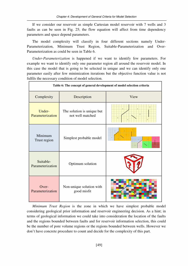
Chapter 4: Development of General Criteria for Model Selection
[49]
If we consider our reservoir as simple Cartesian model reservoir with 7 wells and 3
faults as can be seen in Fig. 25; the flow equation will affect from time dependency
parameters and space depend parameters.
The model complexity will classify in four different sections namely Under-
Parameterization, Minimum Trust Region, Suitable-Parameterization and Over-
Parameterization as could be seen in Table 6.
Under-Parameterization is happened if we want to identify few parameters. For
example we want to identify only one parameter region all around the reservoir model. In
this case the model that is going to be selected in unique and we can identify only one
parameter easily after few minimization iterations but the objective function value is not
fulfils the necessary condition of model selection.
Minimum Trust Region is the zone in which we have simplest probable model
considering geological prior information and reservoir engineering decision. As a hint; in
terms of geological information we could take into consideration the location of the faults
and the regions bounded between faults and for reservoir information selection, this could
be the number of pore volume regions or the regions bounded between wells. However we
don’t have concrete procedure to count and decide for the complexity of this part.
Table 6: The concept of general development of model selection criteria
Complexity Description View
Under- Parameterization
The solution is unique but not well matched
O
O O
O
O
O O
Minimum Trust region
Simplest probable model
O
O O
O
O
O OO
O O
O
O
O O
Suitable- Parameterization
Optimum solution
Over- Parameterization
Non-unique solution with good misfit
O
O O
O
O
O O

Chapter 4: Development of General Criteria for Model Selection
[50]
Suitable-Parameterization could be considered as our optimum solution which
satisfies the principle of parsimony and fulfils the necessary and sufficient condition of
model selection. This is the solution which we are looking for and solves our problem of
non-uniqueness.
In Over-Parameterization region, we have a model solution with good misfit but also
the solution is not unique. In this region we may have a lot of different models with the
same small misfit; however none of these models is the exact solution and could not be
used for further forecasting.
4.2. Penalization (POF)
From the principle of parsimony we know that the model which is going to be selected
should be as simple as possible and as complex as necessary. This means that we have to
avoid over-parameterization and under-parameterization. Hence the penalization of the
objective function is a way to stop over-parameterization; we have to think of the
penalization method.
Form theory of Akaike, we know that the penalization term is the number of parameter
(EQ. 16). This theory is applicable for stochastic model in which ranges of values for each
variable (in the form of probability distribution) are used for simulation. This is in different
from deterministic model in which outcomes are precisely determined through known
relationships among states and events, without any room for random variation. In such
models, a given input will always produce the same output, such as in a known reservoir
fluid flow model.
Since in real reservoir simulation, the models are deterministic, the theoretical method
of Akaike is not directly applicable; consequently the penalization method has been
developed to be applicable in general deterministic system. The application of this new
method of penalization will be shown later for packer test system and also for a field case
gas reservoir.
4.2.1. Development of POF
The penalization should be starting from the point that we have minimum trustable
information for the model (minimum trust region as it is shown in Fig. 26). Here is a
region where we have range of possible model with simplest complexity. This could be
defined from prior geological information (The boundary of the reservoir, the location of
the fault, transmissibility of the layers,…) and the reservoir engineering decision and
intuition (number of wells, number of measurement points, kinds of identifying
parameters, number of observable zones, …).
New formulation has been named POF which stands for Penalized Objective Function.
As described, this penalization or scaling should be starting in minimum trust region and
regulate the objective function value. For this reason the scaling factor has been defined
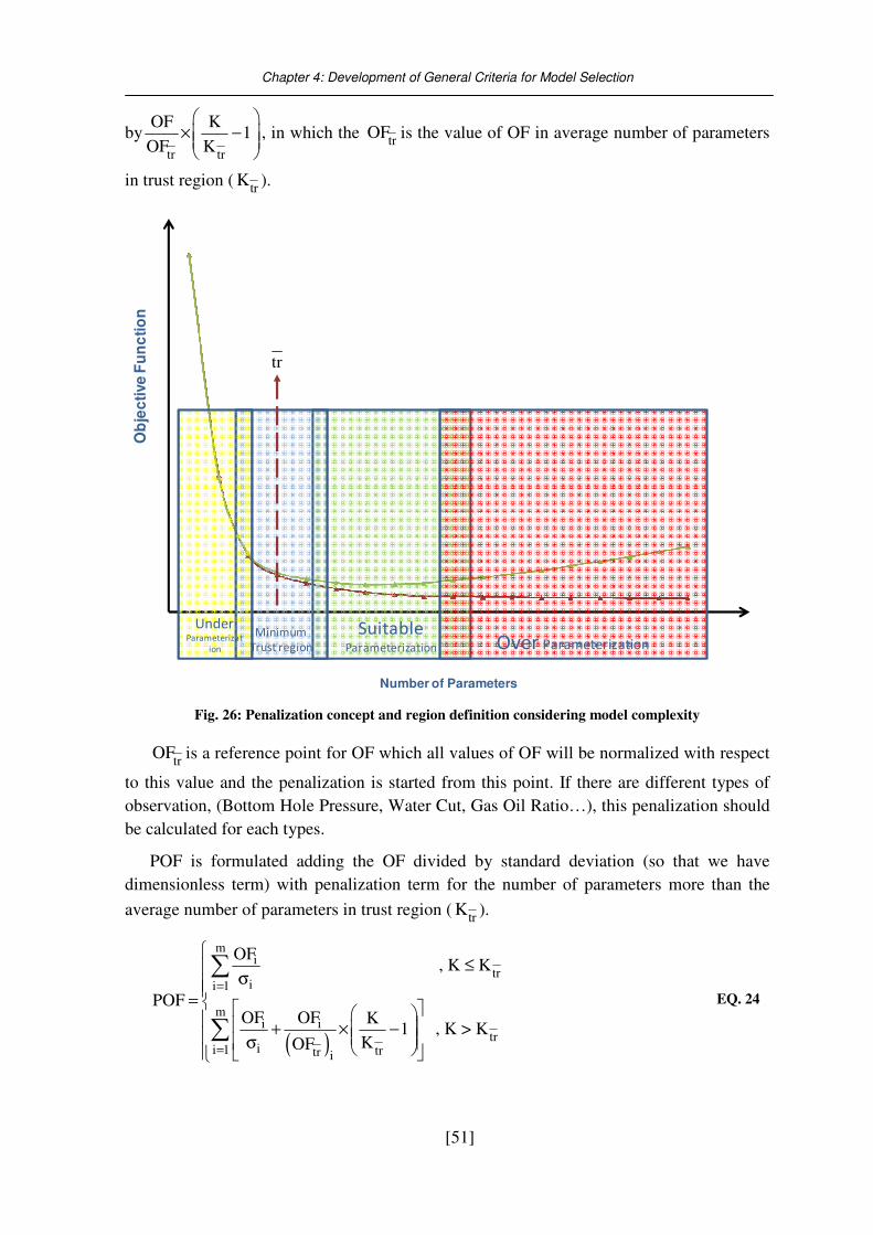
Chapter 4: Development of General Criteria for Model Selection
[51]
bytr tr
OF K1
OF K
× −
, in which the trOF is the value of OF in average number of parameters
in trust region ( trK ).
Fig. 26: Penalization concept and region definition considering model complexity
trOF is a reference point for OF which all values of OF will be normalized with respect
to this value and the penalization is started from this point. If there are different types of
observation, (Bottom Hole Pressure, Water Cut, Gas Oil Ratio…), this penalization should
be calculated for each types.
POF is formulated adding the OF divided by standard deviation (so that we have
dimensionless term) with penalization term for the number of parameters more than the
average number of parameters in trust region ( trK ).
( )
mi
trii 1
mi i
trii 1 trtr i
OF , K K
POFOF OF K
1 , K > KKOF
=
=
≤
σ= + × − σ
∑
∑ EQ. 24
tr
Ob
jec
tive
Fu
nc
tio
n
Number of Parameters
Suitable Parameterization Over Parameterization
Minimum
Trust region
Under Parameterizat
ion
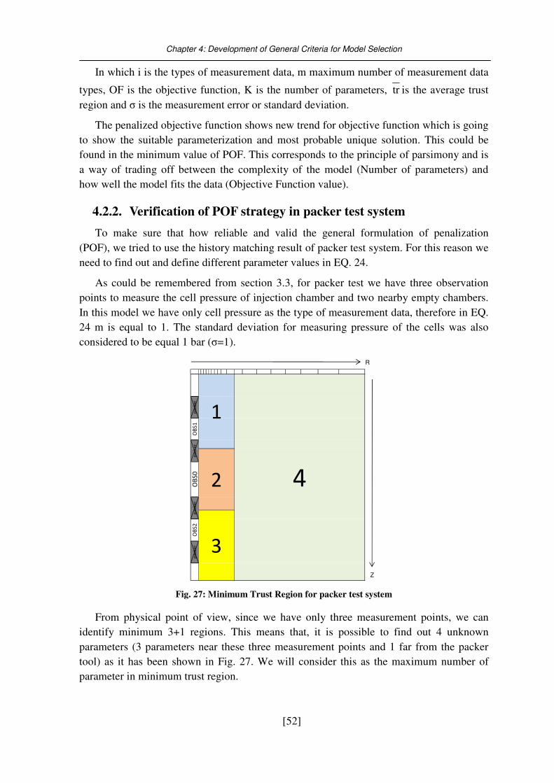
Chapter 4: Development of General Criteria for Model Selection
[52]
In which i is the types of measurement data, m maximum number of measurement data
types, OF is the objective function, K is the number of parameters, tr is the average trust
region and σ is the measurement error or standard deviation.
The penalized objective function shows new trend for objective function which is going
to show the suitable parameterization and most probable unique solution. This could be
found in the minimum value of POF. This corresponds to the principle of parsimony and is
a way of trading off between the complexity of the model (Number of parameters) and
how well the model fits the data (Objective Function value).
4.2.2. Verification of POF strategy in packer test system
To make sure that how reliable and valid the general formulation of penalization
(POF), we tried to use the history matching result of packer test system. For this reason we
need to find out and define different parameter values in EQ. 24.
As could be remembered from section 3.3, for packer test we have three observation
points to measure the cell pressure of injection chamber and two nearby empty chambers.
In this model we have only cell pressure as the type of measurement data, therefore in EQ.
24 m is equal to 1. The standard deviation for measuring pressure of the cells was also
considered to be equal 1 bar (σ=1).
R
Z
1
4
pa
cke
rO
BS
1p
ack
er
2OB
S0
pa
cke
r
3
OB
S2
pa
cke
r
Fig. 27: Minimum Trust Region for packer test system
From physical point of view, since we have only three measurement points, we can
identify minimum 3+1 regions. This means that, it is possible to find out 4 unknown
parameters (3 parameters near these three measurement points and 1 far from the packer
tool) as it has been shown in Fig. 27. We will consider this as the maximum number of
parameter in minimum trust region.
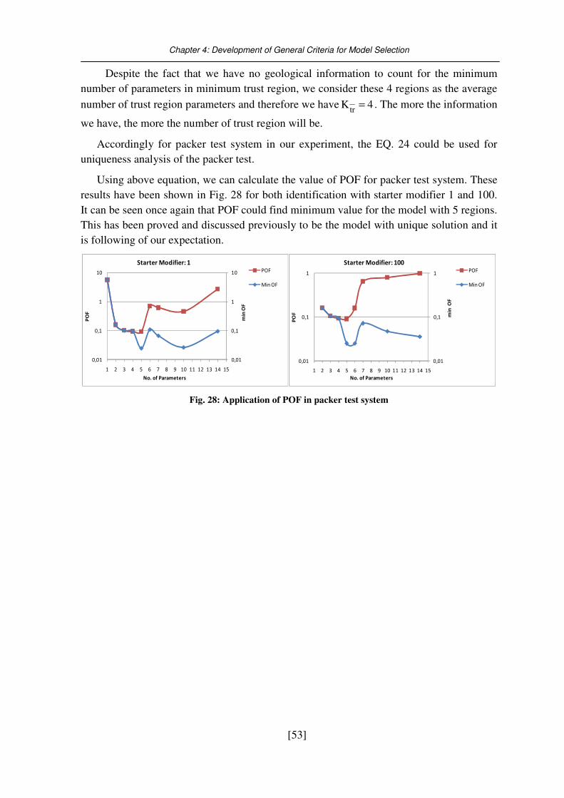
Chapter 4: Development of General Criteria for Model Selection
[53]
Despite the fact that we have no geological information to count for the minimum
number of parameters in minimum trust region, we consider these 4 regions as the average
number of trust region parameters and therefore we havetrK 4= . The more the information
we have, the more the number of trust region will be.
Accordingly for packer test system in our experiment, the EQ. 24 could be used for
uniqueness analysis of the packer test.
Using above equation, we can calculate the value of POF for packer test system. These
results have been shown in Fig. 28 for both identification with starter modifier 1 and 100.
It can be seen once again that POF could find minimum value for the model with 5 regions.
This has been proved and discussed previously to be the model with unique solution and it
is following of our expectation.
0,01
0,1
1
10
0,01
0,1
1
10
1 2 3 4 5 6 7 8 9 10 11 12 13 14 15
min
OF
PO
F
No. of Parameters
Starter Modifier: 1POF
Min OF
0,01
0,1
1
0,01
0,1
1
1 2 3 4 5 6 7 8 9 10 11 12 13 14 15
min
OF
PO
F
No. of Parameters
Starter Modifier: 100POF
Min OF
Fig. 28: Application of POF in packer test system

Chapter 5:Field Case Model Study
[54]
Chapter 5. Field Case Model Study
This section describes main results of the history matching and predictions for the gas
producing wells in the North Hannover area field. The initial static and dynamic input data
for the ECLIPSE simulation study are provided by DGMKi as a result of previous study on
this field (DGMK-research project 587). The main history matching was reviewed and
reconstructed taking into consideration the material balance calculation and well test
analysis using available buildup pressure for different wells in different measurement
periods.
5.1. Model description
For simulation of the model, ECLIPSE software package was used. The model is based
on 36×95 blocks horizontally with 14 layers vertically, with average grid block size of
250×250m.
5.1.1. Static Data
The porosity model is with constant and homogenous porosity of 6.57% for all cells.
This has been used to compare with material balance calculation and to fix pore volume
multiplier with respect to material balance calculation which will be explained later. In
other try the initial existing non-homogenous porosity distribution was used as initial static
data for porosity (average Porosity = 6.98%). For this case the pore volume multipliers
were changed with respect to material balance calculation.
Fig. 29: Field Case model structure
i German Society for Petroleum and Coal Science and Technology (Deutsche Wissenschaftliche
Gesellschaftfür Erdöl, Erdgas und Kohle e.V.)
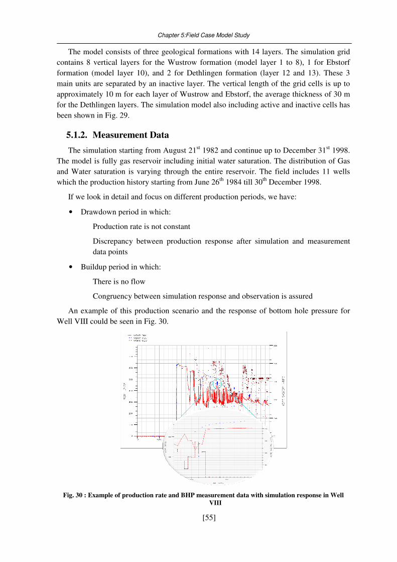
Chapter 5:Field Case Model Study
[55]
The model consists of three geological formations with 14 layers. The simulation grid
contains 8 vertical layers for the Wustrow formation (model layer 1 to 8), 1 for Ebstorf
formation (model layer 10), and 2 for Dethlingen formation (layer 12 and 13). These 3
main units are separated by an inactive layer. The vertical length of the grid cells is up to
approximately 10 m for each layer of Wustrow and Ebstorf, the average thickness of 30 m
for the Dethlingen layers. The simulation model also including active and inactive cells has
been shown in Fig. 29.
5.1.2. Measurement Data
The simulation starting from August 21st 1982 and continue up to December 31st 1998.
The model is fully gas reservoir including initial water saturation. The distribution of Gas
and Water saturation is varying through the entire reservoir. The field includes 11 wells
which the production history starting from June 26th 1984 till 30th December 1998.
If we look in detail and focus on different production periods, we have:
• Drawdown period in which:
Production rate is not constant
Discrepancy between production response after simulation and measurement
data points
• Buildup period in which:
There is no flow
Congruency between simulation response and observation is assured
An example of this production scenario and the response of bottom hole pressure for
Well VIII could be seen in Fig. 30.
Fig. 30 : Example of production rate and BHP measurement data with simulation response in Well
VIII
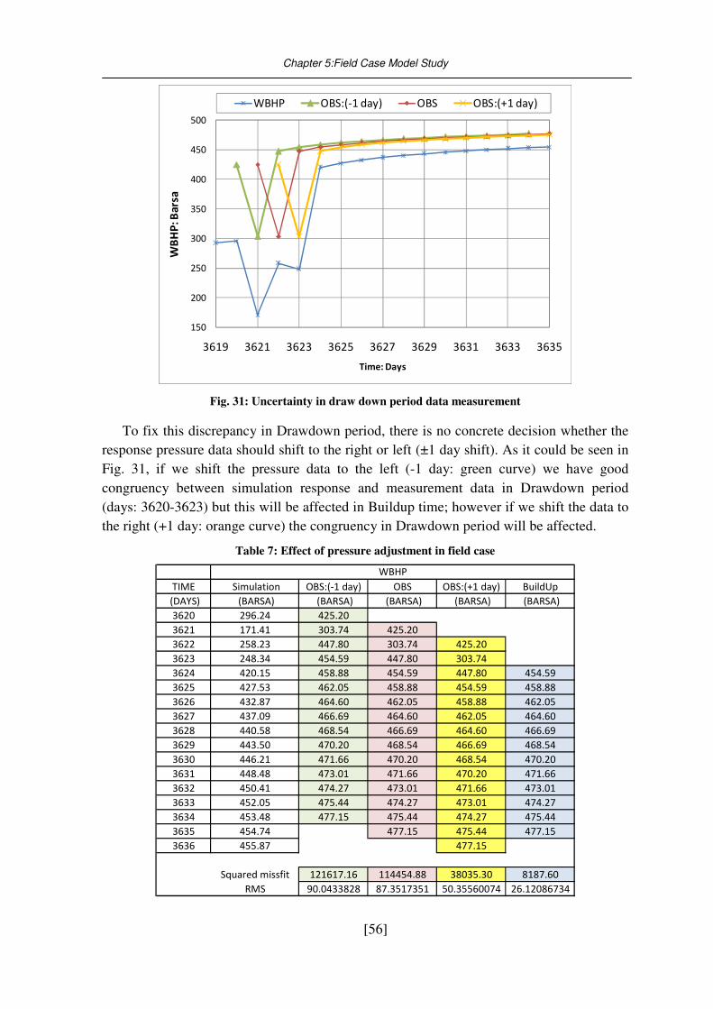
Chapter 5:Field Case Model Study
[56]
150
200
250
300
350
400
450
500
3619 3621 3623 3625 3627 3629 3631 3633 3635
WB
HP
: Ba
rsa
Time: Days
WBHP OBS:(-1 day) OBS OBS:(+1 day)
Fig. 31: Uncertainty in draw down period data measurement
To fix this discrepancy in Drawdown period, there is no concrete decision whether the
response pressure data should shift to the right or left (±1 day shift). As it could be seen in
Fig. 31, if we shift the pressure data to the left (-1 day: green curve) we have good
congruency between simulation response and measurement data in Drawdown period
(days: 3620-3623) but this will be affected in Buildup time; however if we shift the data to
the right (+1 day: orange curve) the congruency in Drawdown period will be affected.
Table 7: Effect of pressure adjustment in field case
TIME Simulation OBS:(-1 day) OBS OBS:(+1 day) BuildUp
(DAYS) (BARSA) (BARSA) (BARSA) (BARSA) (BARSA)
3620 296.24 425.20
3621 171.41 303.74 425.20
3622 258.23 447.80 303.74 425.20
3623 248.34 454.59 447.80 303.74
3624 420.15 458.88 454.59 447.80 454.59
3625 427.53 462.05 458.88 454.59 458.88
3626 432.87 464.60 462.05 458.88 462.05
3627 437.09 466.69 464.60 462.05 464.60
3628 440.58 468.54 466.69 464.60 466.69
3629 443.50 470.20 468.54 466.69 468.54
3630 446.21 471.66 470.20 468.54 470.20
3631 448.48 473.01 471.66 470.20 471.66
3632 450.41 474.27 473.01 471.66 473.01
3633 452.05 475.44 474.27 473.01 474.27
3634 453.48 477.15 475.44 474.27 475.44
3635 454.74 477.15 475.44 477.15
3636 455.87 477.15
Squared missfit 121617.16 114454.88 38035.30 8187.60
RMS 90.0433828 87.3517351 50.35560074 26.12086734
WBHP
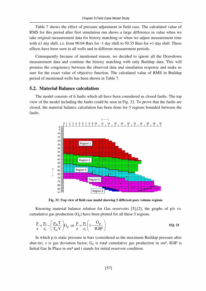
Chapter 5:Field Case Model Study
[57]
Table 7 shows the effect of pressure adjustment in field case. The calculated value of
RMS for this period after first simulation run shows a large difference in value when we
take original measurement data for history matching or when we adjust measurement time
with ±1 day shift. i.e. from 90.04 Bars for -1 day shift to 50.35 Bars for +1 day shift. These
effects have been seen in all wells and in different measurement periods.
Consequently because of mentioned reason, we decided to ignore all the Drawdown
measurement data and continue the history matching with only Buildup data. This will
promise the congruency between the observed data and simulation response and make us
sure for the exact value of objective function. The calculated value of RMS in Buildup
period of mentioned wells has been shown in Table 7.
5.2. Material Balance calculation
The model consists of 6 faults which all have been considered as closed faults. The top
view of the model including the faults could be seen in Fig. 32. To prove that the faults are
closed, the material balance calculation has been done for 5 regions bounded between the
faults.
Region 1
Region 2
Region 4
Region 5
Region 3
Fig. 32 :Top view of field case model showing 5 different pore volume regions
Knowing material balance relation for Gas reservoirs [5],[2]; the graphs of p/z vs.
cumulative gas production (Gp) have been plotted for all these 5 regions.
scip
i sc
p TppG
z z T V
= −
or
pi
i
Gpp1
z z IGIP
= −
EQ. 25
In which p is static pressure in bars (considered as the maximum Buildup pressure after
shut-in), z is gas deviation factor, Gp is total cumulative gas production in sm³, IGIP is
Initial Gas In Place in sm³ and i stands for initial reservoir condition.
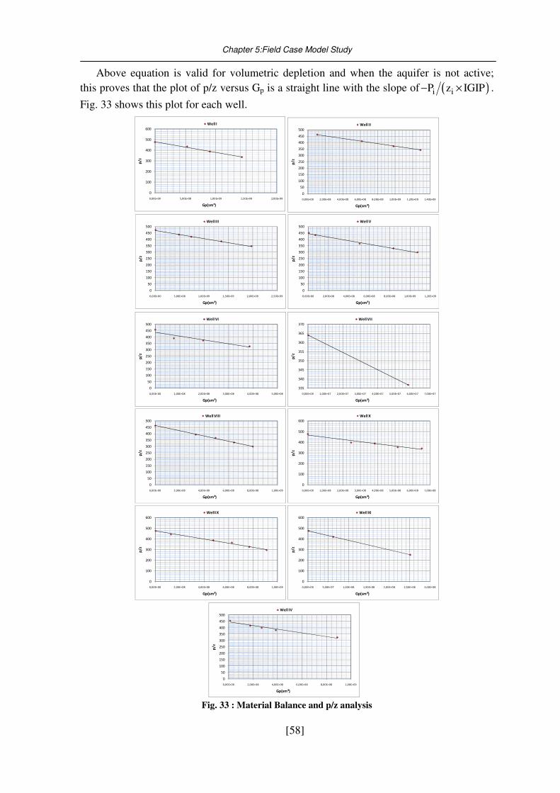
Chapter 5:Field Case Model Study
[58]
Above equation is valid for volumetric depletion and when the aquifer is not active;
this proves that the plot of p/z versus Gp is a straight line with the slope of ( )i iP z IGIP− × .
Fig. 33 shows this plot for each well.
0
100
200
300
400
500
600
0,00E+00 5,00E+08 1,00E+09 1,50E+09 2,00E+09
p/
z
Gp(sm³)
Well I
0
50
100
150
200
250
300
350
400
450
500
0,00E+00 2,00E+08 4,00E+08 6,00E+08 8,00E+08 1,00E+09 1,20E+09 1,40E+09
p/
z
Gp(sm³)
Well II
0
50
100
150
200
250
300
350
400
450
500
0,00E+00 5,00E+08 1,00E+09 1,50E+09 2,00E+09 2,50E+09
p/
z
Gp(sm³)
Well III
0
50
100
150
200
250
300
350
400
450
500
0,00E+00 2,00E+08 4,00E+08 6,00E+08 8,00E+08 1,00E+09 1,20E+09p
/z
Gp(sm³)
Well V
0
50
100
150
200
250
300
350
400
450
500
0,00E+00 1,00E+08 2,00E+08 3,00E+08 4,00E+08 5,00E+08
p/
z
Gp(sm³)
Well VI
335
340
345
350
355
360
365
370
0,00E+00 1,00E+07 2,00E+07 3,00E+07 4,00E+07 5,00E+07 6,00E+07 7,00E+07
p/
z
Gp(sm³)
Well VII
0
50
100
150
200
250
300
350
400
450
500
0,00E+00 2,00E+08 4,00E+08 6,00E+08 8,00E+08 1,00E+09
p/
z
Gp(sm³)
Well VIII
0
100
200
300
400
500
600
0,00E+00 1,00E+08 2,00E+08 3,00E+08 4,00E+08 5,00E+08 6,00E+08 7,00E+08
p/
z
Gp(sm³)
Well X
0
100
200
300
400
500
600
0,00E+00 2,00E+08 4,00E+08 6,00E+08 8,00E+08 1,00E+09
p/
z
Gp(sm³)
Well IX
0
100
200
300
400
500
600
0,00E+00 5,00E+07 1,00E+08 1,50E+08 2,00E+08 2,50E+08 3,00E+08
p/
z
Gp(sm³)
Well XI
0
50
100
150
200
250
300
350
400
450
500
0,00E+00 2,00E+08 4,00E+08 6,00E+08 8,00E+08 1,00E+09
p/
z
Gp(sm³)
Well IV
Fig. 33 : Material Balance and p/z analysis
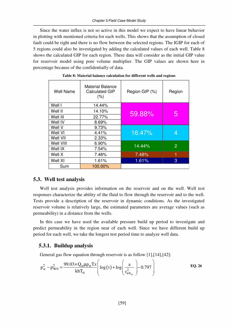
Chapter 5:Field Case Model Study
[59]
Since the water influx is not so active in this model we expect to have linear behavior
in plotting with mentioned criteria for each wells. This shows that the assumption of closed
fault could be right and there is no flow between the selected regions. The IGIP for each of
5 regions could also be investigated by adding the calculated values of each well. Table 8
shows the calculated GIP for each region. These data will consider as the initial GIP value
for reservoir model using pore volume multiplier. The GIP values are shown here in
percentage because of the confidentially of data.
Table 8: Material balance calculation for different wells and regions
Well Name Material Balance Calculated GIP
(%) Region GIP (%) Region
Well I 14.44%
59.88% 5 Well II 14.10%
Well III 22.77%
Well IV 8.69%
Well V 9.73%
16.47% 4 Well VI 4.41%
Well VII 2.33%
Well VIII 6.90% 14.44% 2
Well IX 7.54%
Well X 7.48% 7.48% 1
Well XI 1.61% 1.61% 3 Sum 100.00%
5.3. Well test analysis
Well test analysis provides information on the reservoir and on the well. Well test
responses characterize the ability of the fluid to flow through the reservoir and to the well.
Tests provide a description of the reservoir in dynamic conditions. As the investigated
reservoir volume is relatively large, the estimated parameters are average values (such as
permeability) in a distance from the wells.
In this case we have used the available pressure build up period to investigate and
predict permeability in the region near of each well. Since we have different build up
period for each well, we take the longest test period time to analyze well data.
5.3.1. Buildup analysis
General gas flow equation through reservoir is as follow [1],[14],[42]:
( )eff
2 2 st stw W0 2
st wb
99.03 Q p Tz ap p log t log 0.797
khT r
× µ − = + −
EQ. 26
Chapter 5:Field Case Model Study
[60]
Where t
ka
c=
φµ and pw is the well flow bottom hole pressure [barsa], pw0 is the initial
reservoir pressure [barsa], Qst is the gas flow rate at standard or surface condition
[sm³/day], {pst= 1 bara and Tst= 15°C}, µ is the viscosity [cp],k is the permeability [mD], T
is the temperature [K], z is the Gas compressibility factor, φ is the porosity [fraction], h is
the reservoir thickness [m], ct is the total compressibility [1/bar],t is the time [days] and
rwbeff
is the effective wellbore radius [m]
Considering well test concept for build up pressure, this equation shows that the plot of
well flow squared pressure (pw²) versus log(t) in late time should be a straight line with dip:
st st
st
99.03 Q p Tzm
khT
× µ= EQ. 27
This equation will be used to calculate flow capacity (kh) of the formation around the
well bore.
Thus for each well we have plotted (s. Fig. 34) the graph of (pw²) versus dt (time period
after shut-in) for the period of longest buildup time and tried to pass straight line for late
time and for each well. Since the flow rate is not constant before shut-in we take
cumst
p
t= , where qcum is the cumulative gas production in drawdown period before shut-
in an tp is the last draw down period time before shut-in [21].
5.3.2. Well test result
With this method we could estimate permeability through pressure buildup analysis for
the region around the wellbore. Knowing h as the effective reservoir thickness, in which
for our case is the layer thickness times Net to Gross ratio (N/G), we can calculate
permeability after kh. The calculation of permeability has been shown in Table 9.
The permeability value is varying from 0.1828 mD to 414.6610 mD with average
permeability of 60.5523 mD. These valued will be used later on to compare with the
identification through history matching and model selection.
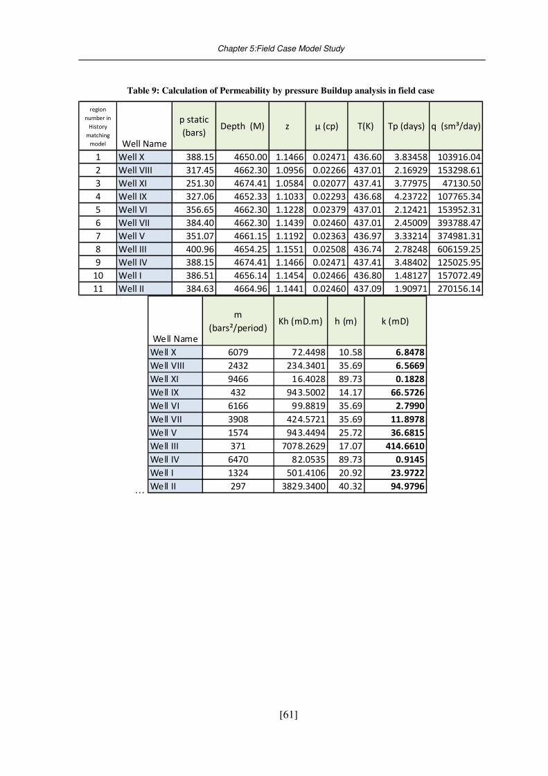
Chapter 5:Field Case Model Study
[61]
Table 9: Calculation of Permeability by pressure Buildup analysis in field case
region
number in
History
matching
model Well Name
p static
(bars)Depth (M) z μ (cp) T(K) Tp (days) q (sm³/day)
1 Well X 388.15 4650.00 1.1466 0.02471 436.60 3.83458 103916.04
2 Well VIII 317.45 4662.30 1.0956 0.02266 437.01 2.16929 153298.61
3 Well XI 251.30 4674.41 1.0584 0.02077 437.41 3.77975 47130.50
4 Well IX 327.06 4652.33 1.1033 0.02293 436.68 4.23722 107765.34
5 Well VI 356.65 4662.30 1.1228 0.02379 437.01 2.12421 153952.31
6 Well VII 384.40 4662.30 1.1439 0.02460 437.01 2.45009 393788.47
7 Well V 351.07 4661.15 1.1192 0.02363 436.97 3.33214 374981.31
8 Well III 400.96 4654.25 1.1551 0.02508 436.74 2.78248 606159.25
9 Well IV 388.15 4674.41 1.1466 0.02471 437.41 3.48402 125025.95
10 Well I 386.51 4656.14 1.1454 0.02466 436.80 1.48127 157072.49
11 Well II 384.63 4664.96 1.1441 0.02460 437.09 1.90971 270156.14
…
Well Name
m
(bars²/period)Kh (mD.m) h (m) k (mD)
Well X 6079 72.4498 10.58 6.8478
Well VIII 2432 234.3401 35.69 6.5669
Well XI 9466 16.4028 89.73 0.1828
Well IX 432 943.5002 14.17 66.5726
Well VI 6166 99.8819 35.69 2.7990
Well VII 3908 424.5721 35.69 11.8978
Well V 1574 943.4494 25.72 36.6815
Well III 371 7078.2629 17.07 414.6610
Well IV 6470 82.0535 89.73 0.9145
Well I 1324 501.4106 20.92 23.9722
Well II 297 3829.3400 40.32 94.9796
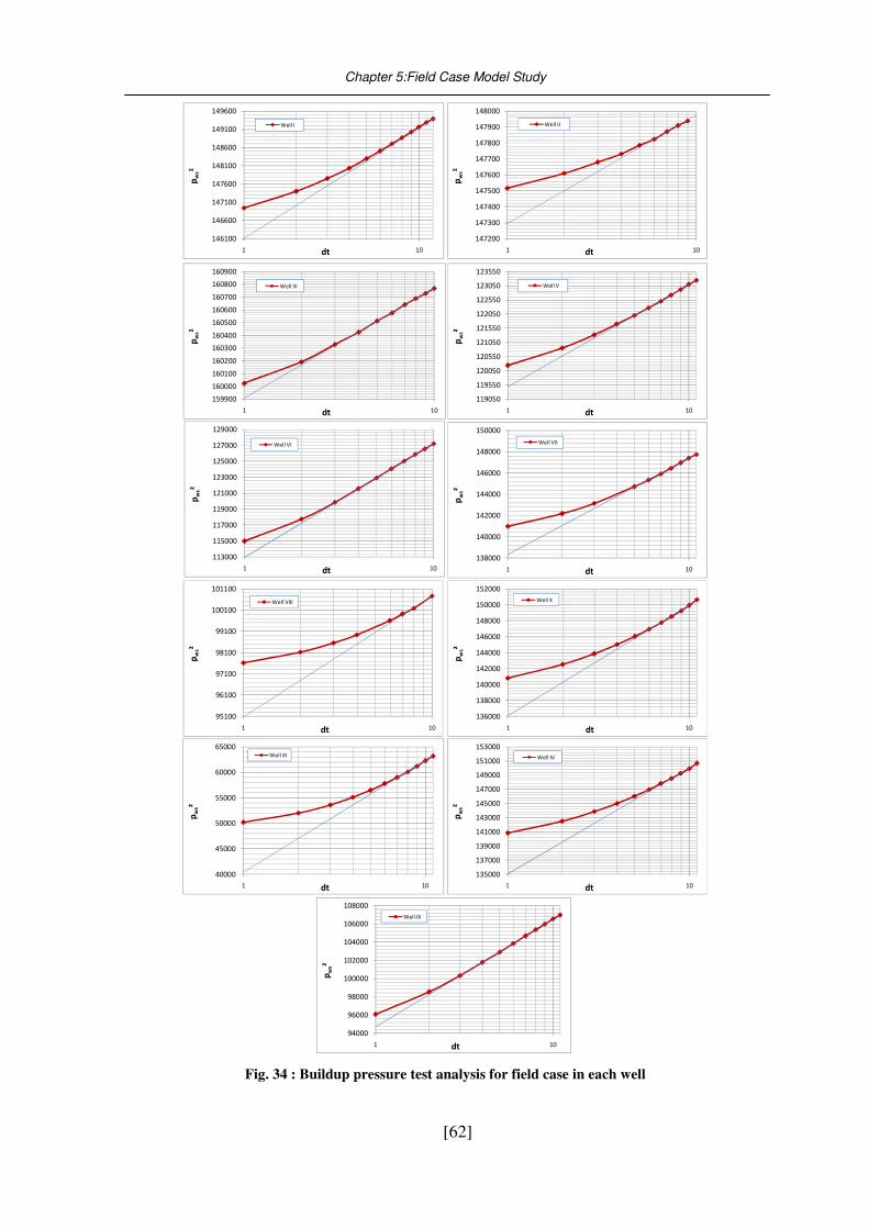
Chapter 5:Field Case Model Study
[62]
146100
146600
147100
147600
148100
148600
149100
149600
1 10
pw
s²
dt
Well I
147200
147300
147400
147500
147600
147700
147800
147900
148000
1 10
pw
s²
dt
Well II
159900
160000
160100
160200
160300
160400
160500
160600
160700
160800
160900
1 10
pw
s²
dt
Well III
119050
119550
120050
120550
121050
121550
122050
122550
123050
123550
1 10
pw
s²
dt
Well V
138000
140000
142000
144000
146000
148000
150000
1 10
pw
s²
dt
Well VII
95100
96100
97100
98100
99100
100100
101100
1 10
pw
s²
dt
Well VIII
136000
138000
140000
142000
144000
146000
148000
150000
152000
1 10
pw
s²
dt
Well X
40000
45000
50000
55000
60000
65000
1 10
pw
s²
dt
Well XI
135000
137000
139000
141000
143000
145000
147000
149000
151000
153000
1 10
pw
s²
dt
Well IV
94000
96000
98000
100000
102000
104000
106000
108000
1 10
pw
s²
dt
Well IX
113000
115000
117000
119000
121000
123000
125000
127000
129000
1 10
pw
s²
dt
Well VI
Fig. 34 : Buildup pressure test analysis for field case in each well
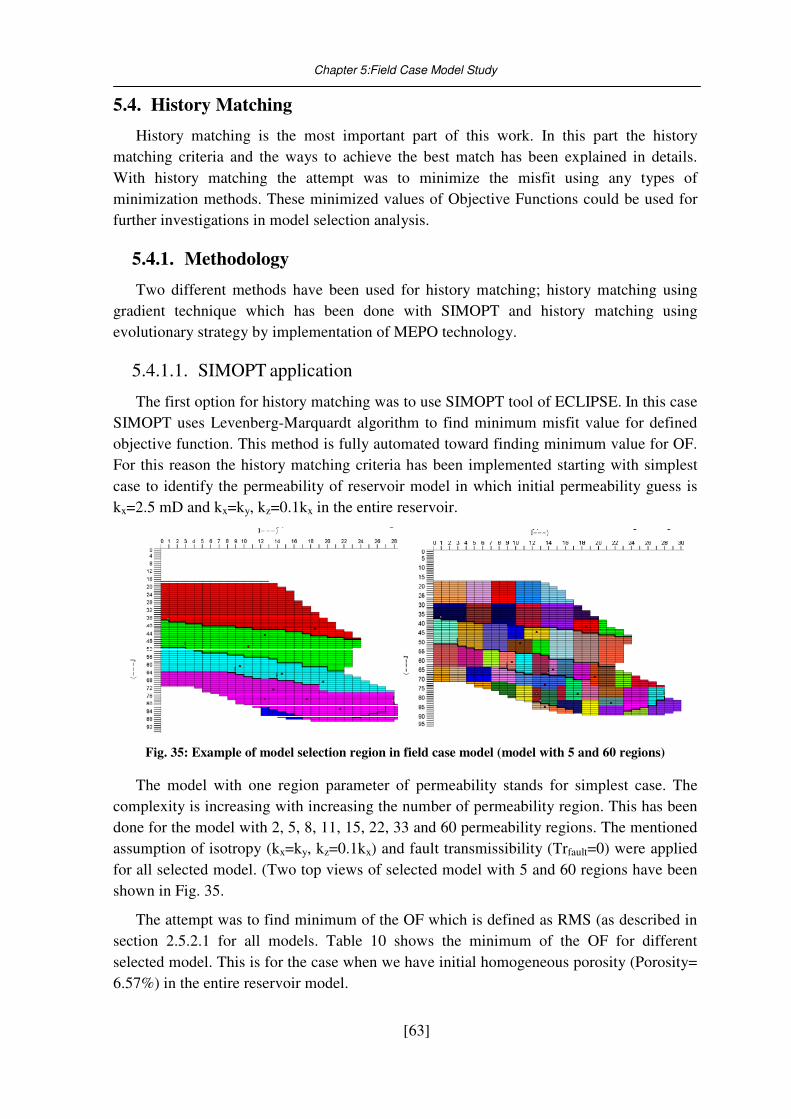
Chapter 5:Field Case Model Study
[63]
5.4. History Matching
History matching is the most important part of this work. In this part the history
matching criteria and the ways to achieve the best match has been explained in details.
With history matching the attempt was to minimize the misfit using any types of
minimization methods. These minimized values of Objective Functions could be used for
further investigations in model selection analysis.
5.4.1. Methodology
Two different methods have been used for history matching; history matching using
gradient technique which has been done with SIMOPT and history matching using
evolutionary strategy by implementation of MEPO technology.
5.4.1.1. SIMOPT application
The first option for history matching was to use SIMOPT tool of ECLIPSE. In this case
SIMOPT uses Levenberg-Marquardt algorithm to find minimum misfit value for defined
objective function. This method is fully automated toward finding minimum value for OF.
For this reason the history matching criteria has been implemented starting with simplest
case to identify the permeability of reservoir model in which initial permeability guess is
kx=2.5 mD and kx=ky, kz=0.1kx in the entire reservoir.
Fig. 35: Example of model selection region in field case model (model with 5 and 60 regions)
The model with one region parameter of permeability stands for simplest case. The
complexity is increasing with increasing the number of permeability region. This has been
done for the model with 2, 5, 8, 11, 15, 22, 33 and 60 permeability regions. The mentioned
assumption of isotropy (kx=ky, kz=0.1kx) and fault transmissibility (Trfault=0) were applied
for all selected model. (Two top views of selected model with 5 and 60 regions have been
shown in Fig. 35.
The attempt was to find minimum of the OF which is defined as RMS (as described in
section 2.5.2.1 for all models. Table 10 shows the minimum of the OF for different
selected model. This is for the case when we have initial homogeneous porosity (Porosity=
6.57%) in the entire reservoir model.

Chapter 5:Field Case Model Study
[64]
Table 10: History matching result of the model with homogeneous porosity
No. Of
PrametersOF
1 33.1490
5 22.6932
8 21.5211
11 20.8160
15 18.7736
22 18.0950
33 17.7756
60 17.9175
The OF is following the decline trend and is going to be on very low fix decreasing
development after increasing the number of regions. This trend is also similar when we
have non-homogenous porosity (average Porosity=6.98% as described in section 5.1.1) in
the reservoir model. This could be seen in Table 11.
Table 11: History matching result of the model with non-homogeneous porosity
No. Of
PrametersOF
1 26.9000
5 22.9690
8 21.2360
11 19.9789
15 18.7560
22 18.5670
33 18.0790
44 17.9530
60 17.796
5.4.1.2. MEPO application
In this case, a global history matching was carried out using MEPO for three selected
models with 1, 11 and 22 number of parameters. The objective function was composed by
bottom hole buildup pressure as before.
The models and region definition are exactly the same as for history matching using
SIMOPT. For history matching the Evolution Strategy (2+4) has been used and this
remained unchanged in all further processing. This has been done only for the case that we
have homogeneous porosity in the entire model. (Porosity= 6.57%)
The comparison between SIMOPT (with initial OF value of 56.1763) and MEPO (with
initial OF of 39914.4805) results for three different models with 1, 11 and 22 region has
been shown in Table 12. The quality of match for both softwares is quite the same. Since
the definitions of OF in SIMOPT and MEPO are not the same, in this table the equivalent
value of OF for both softwares has been given for the same identification.
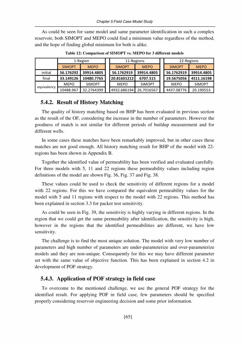
Chapter 5:Field Case Model Study
[65]
As could be seen for same model and same parameter identification in such a complex
reservoir, both SIMOPT and MEPO could find a minimum value regardless of the method,
and the hope of finding global minimum for both is alike.
Table 12: Comparison of SIMOPT vs. MEPO for 3 different models
SIMOPT MEPO SIMOPT MEPO SIMOPT MEPO
initial 56.176292 39914.4805 56.1762919 39914.4805 56.1762919 39914.4805
final 33.149126 10480.7765 20.81601212 6707.515 19.5675056 4511.16198
MEPO SIMOPT MEPO SIMOPT MEPO SIMOPT
10488.967 32.2764399 4932.686194 26.7016567 4437.08776 20.190553
1-Region 11-Regions 22-Regions
equivalency
5.4.2. Result of History Matching
The quality of history matching based on BHP has been evaluated in previous section
as the result of the OF, considering the increase in the number of parameters. However the
goodness of match is not similar for different periods of buildup measurement and for
different wells.
In some cases these matches have been remarkably improved, but in other cases these
matches are not good enough. All history matching result for BHP of the model with 22-
regions has been shown in Appendix B.
Together the identified value of permeability has been verified and evaluated carefully.
For three models with 5, 11 and 22 regions these permeability values including region
definitions of the model are shown Fig. 36, Fig. 37 and Fig. 38.
These values could be used to check the sensitivity of different regions for a model
with 22 regions. For this we have compared the equivalent permeability values for the
model with 5 and 11 regions with respect to the model with 22 regions. This method has
been explained in section 3.3 for packer test sensitivity.
As could be seen in Fig. 39, the sensitivity is highly varying in different regions. In the
region that we could get the same permeability after identification, the sensitivity is high,
however in the regions that the identified permeabilities are different, we have low
sensitivity.
The challenge is to find the most unique solution. The model with very low number of
parameters and high number of parameters are under-parameterize and over-parameterize
models and they are non-unique. Consequently for this we may have different parameter
set with the same value of objective function. This has been explained in section 4.2 in
development of POF strategy.
5.4.3. Application of POF strategy in field case
To overcome to the mentioned challenge, we use the general POF strategy for the
identified result. For applying POF in field case, few parameters should be specified
properly considering reservoir engineering decision and some prior information.
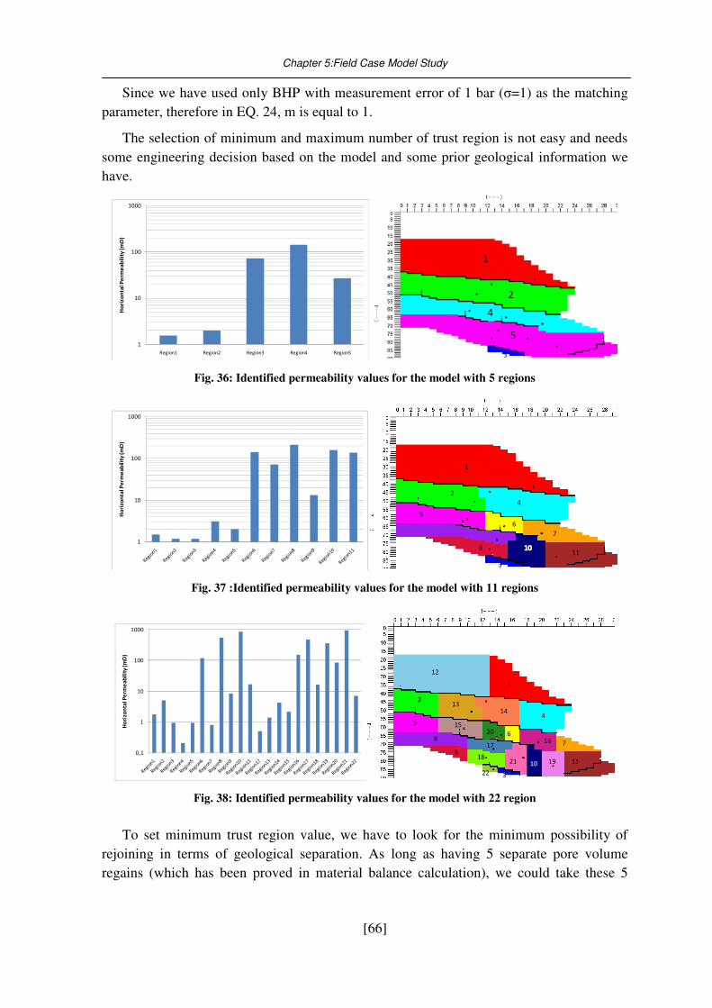
Chapter 5:Field Case Model Study
[66]
Since we have used only BHP with measurement error of 1 bar (σ=1) as the matching
parameter, therefore in EQ. 24, m is equal to 1.
The selection of minimum and maximum number of trust region is not easy and needs
some engineering decision based on the model and some prior geological information we
have.
1
10
100
1000
Region1 Region2 Region3 Region4 Region5
Ho
rizo
nta
l Pe
rme
ab
ilit
y (
mD
)
1
2
4
5
3
Fig. 36: Identified permeability values for the model with 5 regions
1
10
100
1000
Ho
rizo
nta
l Pe
rme
ab
ilit
y (
mD
)
1
2
4
5
6
7
811
3
Fig. 37 :Identified permeability values for the model with 11 regions
0,1
1
10
100
1000
Ho
rizo
nta
l Pe
rme
ab
ilit
y (
mD
)
12
1
213
144
5 1520 6
16 78
17
21 19 11
918
22 3
Fig. 38: Identified permeability values for the model with 22 region
To set minimum trust region value, we have to look for the minimum possibility of
rejoining in terms of geological separation. As long as having 5 separate pore volume
regains (which has been proved in material balance calculation), we could take these 5
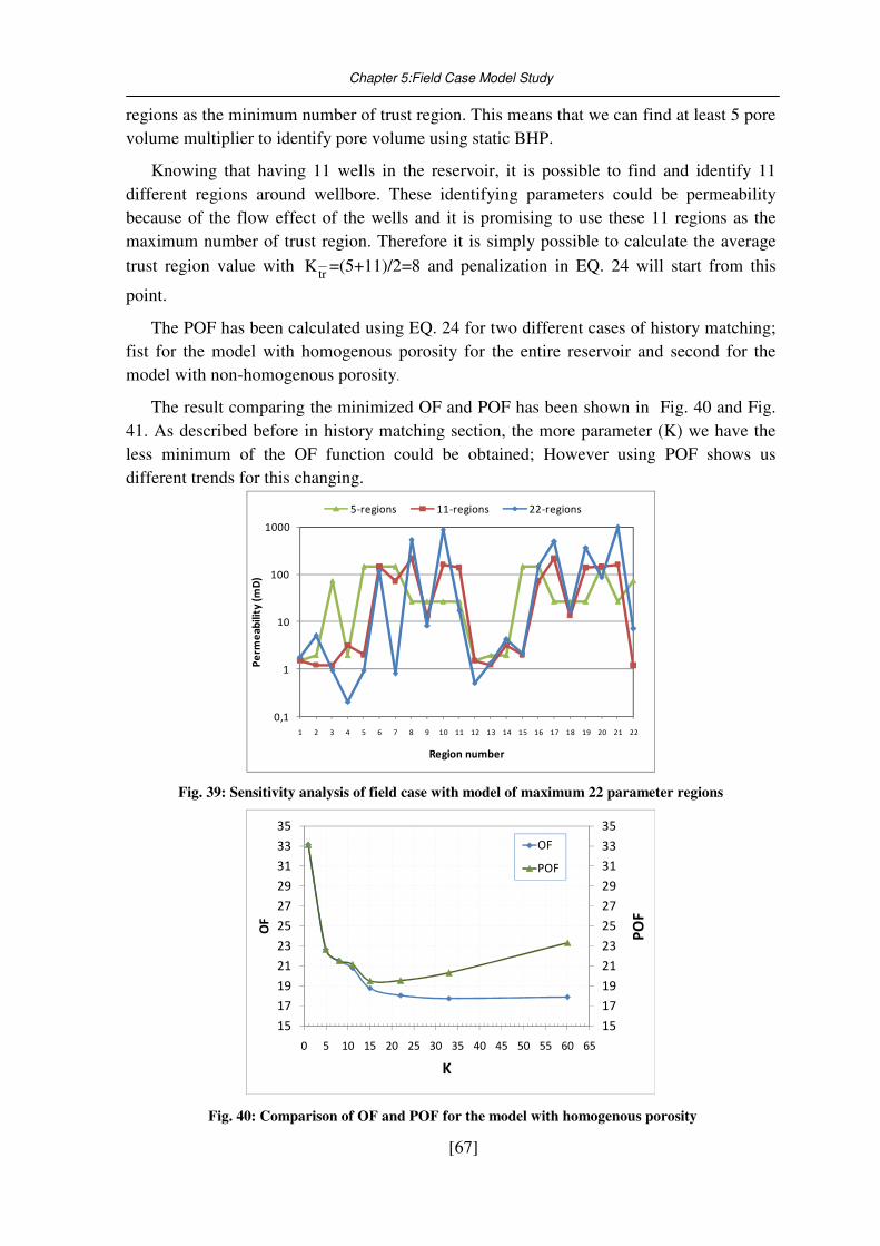
Chapter 5:Field Case Model Study
[67]
regions as the minimum number of trust region. This means that we can find at least 5 pore
volume multiplier to identify pore volume using static BHP.
Knowing that having 11 wells in the reservoir, it is possible to find and identify 11
different regions around wellbore. These identifying parameters could be permeability
because of the flow effect of the wells and it is promising to use these 11 regions as the
maximum number of trust region. Therefore it is simply possible to calculate the average
trust region value with trK =(5+11)/2=8 and penalization in EQ. 24 will start from this
point.
The POF has been calculated using EQ. 24 for two different cases of history matching;
fist for the model with homogenous porosity for the entire reservoir and second for the
model with non-homogenous porosity.
The result comparing the minimized OF and POF has been shown in Fig. 40 and Fig.
41. As described before in history matching section, the more parameter (K) we have the
less minimum of the OF function could be obtained; However using POF shows us
different trends for this changing.
0,1
1
10
100
1000
1 2 3 4 5 6 7 8 9 10 11 12 13 14 15 16 17 18 19 20 21 22
Pe
rme
ab
ility
(m
D)
Region number
5-regions 11-regions 22-regions
Fig. 39: Sensitivity analysis of field case with model of maximum 22 parameter regions
15
17
19
21
23
25
27
29
31
33
35
15
17
19
21
23
25
27
29
31
33
35
0 5 10 15 20 25 30 35 40 45 50 55 60 65
PO
F
OF
K
OF
POF
Fig. 40: Comparison of OF and POF for the model with homogenous porosity
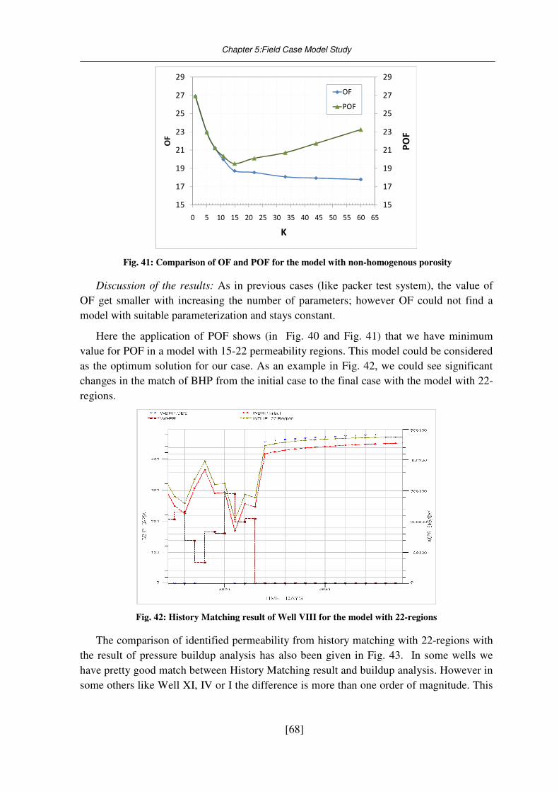
Chapter 5:Field Case Model Study
[68]
15
17
19
21
23
25
27
29
15
17
19
21
23
25
27
29
0 5 10 15 20 25 30 35 40 45 50 55 60 65
PO
F
OF
K
OF
POF
Fig. 41: Comparison of OF and POF for the model with non-homogenous porosity
Discussion of the results: As in previous cases (like packer test system), the value of
OF get smaller with increasing the number of parameters; however OF could not find a
model with suitable parameterization and stays constant.
Here the application of POF shows (in Fig. 40 and Fig. 41) that we have minimum
value for POF in a model with 15-22 permeability regions. This model could be considered
as the optimum solution for our case. As an example in Fig. 42, we could see significant
changes in the match of BHP from the initial case to the final case with the model with 22-
regions.
Fig. 42: History Matching result of Well VIII for the model with 22-regions
The comparison of identified permeability from history matching with 22-regions with
the result of pressure buildup analysis has also been given in Fig. 43. In some wells we
have pretty good match between History Matching result and buildup analysis. However in
some others like Well XI, IV or I the difference is more than one order of magnitude. This
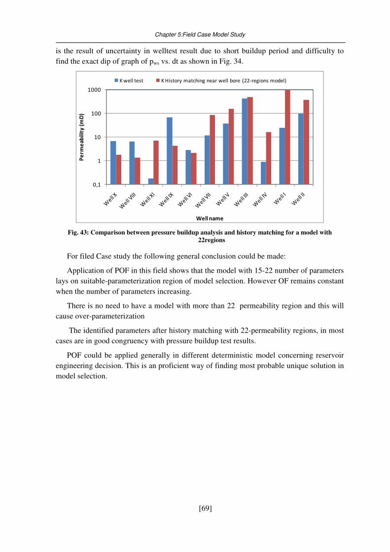
Chapter 5:Field Case Model Study
[69]
is the result of uncertainty in welltest result due to short buildup period and difficulty to
find the exact dip of graph of pws vs. dt as shown in Fig. 34.
0,1
1
10
100
1000
Pe
rme
ab
ilit
y (
mD
)
Well name
K well test K History matching near well bore (22-regions model)
Fig. 43: Comparison between pressure buildup analysis and history matching for a model with
22regions
For filed Case study the following general conclusion could be made:
Application of POF in this field shows that the model with 15-22 number of parameters
lays on suitable-parameterization region of model selection. However OF remains constant
when the number of parameters increasing.
There is no need to have a model with more than 22 permeability region and this will
cause over-parameterization
The identified parameters after history matching with 22-permeability regions, in most
cases are in good congruency with pressure buildup test results.
POF could be applied generally in different deterministic model concerning reservoir
engineering decision. This is an proficient way of finding most probable unique solution in
model selection.
Chapter 6:AKAIKI Software
[70]
Chapter 6. Development of a helpful software for automatic model
selection
In this section the development of software to use the available model selection criteria
has been explained. First there an introduction to the necessity of having such software has
been explained and then we have an overview of the package that we have developed.
6.1. Concept of helpful software for model selection
Reservoir history matching is a difficult inverse problem arising in the petroleum
industry. The aim of history matching is to find a model such that the difference between
the performance of the model and the history of a reservoir is minimized. Traditionally,
this is done by hand. But the task of varying the parameters of a reservoir description by
hand until a satisfactory match is obtained is extremely difficult and time-consuming.
Therefore, optimization techniques are increasingly adopted by the oil industry for
computer-aided history matching. (Such as Levenberg-Marquardt algorithm in SIMOPT).
This is because of the great time-saving benefits, they can offer over conventional trial-
and-error approaches. Starting with an initial reservoir description, these optimization
techniques automatically vary reservoir parameters until stopping criteria are achieved and
a history match of field performance is obtained. This mechanistic activity is referred to as
“automatic history matching.”
Researchers have been building tools for automatic history matching of permeability
and porosity distributions to honor production data for many years. In most of the studies,
independent of the method used for the history matching, there is usually an assumption
that there exists a simple unique solution at the “true” model. They therefore neglect the
non-uniqueness of the solution of this inverse problem. This, consequently, leads to the
assumption that a good history-matched model is a good representation of the reservoir and
therefore gives a good forecast, but this assumption is not proved and often misleading.
6.2. AKAIKI software
After regression and getting RMS as an OF from SIMOPT, the calculation of result of
different criteria is our goal. This should be done fully automatically by use of a software
which should read, calculate and process, select the best model between different sets of
models and finally export the best selected model data to be used for future forecasting.
Therefore it seems to be necessary the development of helpful software to do:
Automatic reading of all values, parameters and results of SIMOPT matches.
Sensitivity analysis of the results and AIC computation.
Select “best and most reliable” parameter set.
AKAIKI has been developed in FORTRAN programming language in Windows and
can be run as an executable program on any system.
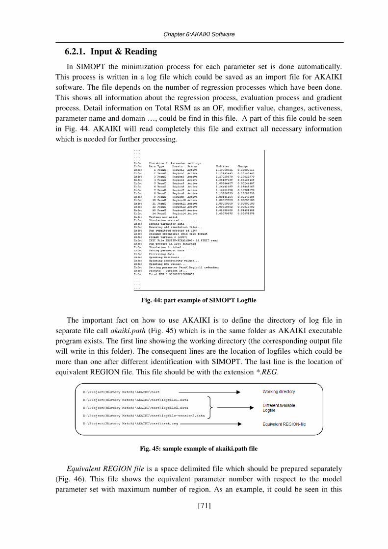
Chapter 6:AKAIKI Software
[71]
6.2.1. Input & Reading
In SIMOPT the minimization process for each parameter set is done automatically.
This process is written in a log file which could be saved as an import file for AKAIKI
software. The file depends on the number of regression processes which have been done.
This shows all information about the regression process, evaluation process and gradient
process. Detail information on Total RSM as an OF, modifier value, changes, activeness,
parameter name and domain …, could be find in this file. A part of this file could be seen
in Fig. 44. AKAIKI will read completely this file and extract all necessary information
which is needed for further processing.
Fig. 44: part example of SIMOPT Logfile
The important fact on how to use AKAIKI is to define the directory of log file in
separate file call akaiki.path (Fig. 45) which is in the same folder as AKAIKI executable
program exists. The first line showing the working directory (the corresponding output file
will write in this folder). The consequent lines are the location of logfiles which could be
more than one after different identification with SIMOPT. The last line is the location of
equivalent REGION file. This file should be with the extension *.REG.
Fig. 45: sample example of akaiki.path file
Equivalent REGION file is a space delimited file which should be prepared separately
(Fig. 46). This file shows the equivalent parameter number with respect to the model
parameter set with maximum number of region. As an example, it could be seen in this
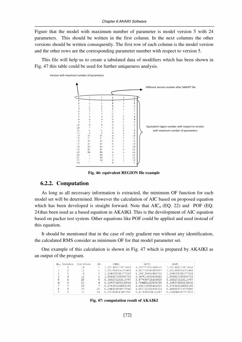
Chapter 6:AKAIKI Software
[72]
Figure that the model with maximum number of parameter is model version 5 with 24
parameters. This should be written in the first column. In the next columns the other
versions should be written consequently. The first row of each column is the model version
and the other rows are the corresponding parameter number with respect to version 5.
This file will help us to create a tabulated data of modifiers which has been shown in
Fig. 47 this table could be used for further uniqueness analysis.
Version with maximum number of parameters
Different version number after SIMOPT file
Equivalent region number with respect to version
with maximum number of parameters
Fig. 46: equivalent REGION file example
6.2.2. Computation
As long as all necessary information is extracted, the minimum OF function for each
model set will be determined. However the calculation of AIC based on proposed equation
which has been developed is straight forward. Note that AICn (EQ. 22) and POF (EQ.
24)has been used as a based equation in AKAIKI. This is the development of AIC equation
based on packer test system. Other equations like POF could be applied and used instead of
this equation.
It should be mentioned that in the case of only gradient run without any identification,
the calculated RMS consider as minimum OF for that model parameter set.
One example of this calculation is shown in Fig. 47 which is prepared by AKAIKI as
an output of the program.
Fig. 47: computation result of AKAIKI

Chapter 6:AKAIKI Software
[73]
6.2.3. Writing & Output
The extracted objective function, modifier value and calculated AIC and POF should be
prepared in tabulated format, so that it could be imported in any data processing packages
like Excel or Tecplot.
The main outputs of the AKAIKI are *.res file (the computation result of the AKAIKI)
and *.lst (tabulated equivalent REGION modifiers). The process will be shown on the
screen and will be written separately in *.out file. This includes all the messages and error
information as well.
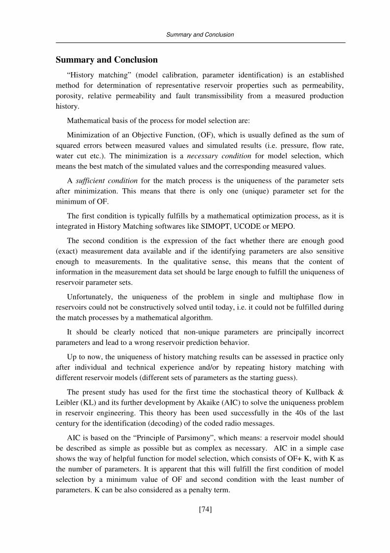
Summary and Conclusion
[74]
Summary and Conclusion
“History matching” (model calibration, parameter identification) is an established
method for determination of representative reservoir properties such as permeability,
porosity, relative permeability and fault transmissibility from a measured production
history.
Mathematical basis of the process for model selection are:
Minimization of an Objective Function, (OF), which is usually defined as the sum of
squared errors between measured values and simulated results (i.e. pressure, flow rate,
water cut etc.). The minimization is a necessary condition for model selection, which
means the best match of the simulated values and the corresponding measured values.
A sufficient condition for the match process is the uniqueness of the parameter sets
after minimization. This means that there is only one (unique) parameter set for the
minimum of OF.
The first condition is typically fulfills by a mathematical optimization process, as it is
integrated in History Matching softwares like SIMOPT, UCODE or MEPO.
The second condition is the expression of the fact whether there are enough good
(exact) measurement data available and if the identifying parameters are also sensitive
enough to measurements. In the qualitative sense, this means that the content of
information in the measurement data set should be large enough to fulfill the uniqueness of
reservoir parameter sets.
Unfortunately, the uniqueness of the problem in single and multiphase flow in
reservoirs could not be constructively solved until today, i.e. it could not be fulfilled during
the match processes by a mathematical algorithm.
It should be clearly noticed that non-unique parameters are principally incorrect
parameters and lead to a wrong reservoir prediction behavior.
Up to now, the uniqueness of history matching results can be assessed in practice only
after individual and technical experience and/or by repeating history matching with
different reservoir models (different sets of parameters as the starting guess).
The present study has used for the first time the stochastical theory of Kullback &
Leibler (KL) and its further development by Akaike (AIC) to solve the uniqueness problem
in reservoir engineering. This theory has been used successfully in the 40s of the last
century for the identification (decoding) of the coded radio messages.
AIC is based on the “Principle of Parsimony”, which means: a reservoir model should
be described as simple as possible but as complex as necessary. AIC in a simple case
shows the way of helpful function for model selection, which consists of OF+ K, with K as
the number of parameters. It is apparent that this will fulfill the first condition of model
selection by a minimum value of OF and second condition with the least number of
parameters. K can be also considered as a penalty term.
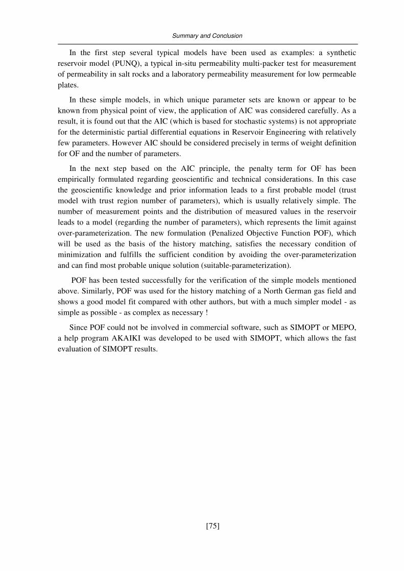
Summary and Conclusion
[75]
In the first step several typical models have been used as examples: a synthetic
reservoir model (PUNQ), a typical in-situ permeability multi-packer test for measurement
of permeability in salt rocks and a laboratory permeability measurement for low permeable
plates.
In these simple models, in which unique parameter sets are known or appear to be
known from physical point of view, the application of AIC was considered carefully. As a
result, it is found out that the AIC (which is based for stochastic systems) is not appropriate
for the deterministic partial differential equations in Reservoir Engineering with relatively
few parameters. However AIC should be considered precisely in terms of weight definition
for OF and the number of parameters.
In the next step based on the AIC principle, the penalty term for OF has been
empirically formulated regarding geoscientific and technical considerations. In this case
the geoscientific knowledge and prior information leads to a first probable model (trust
model with trust region number of parameters), which is usually relatively simple. The
number of measurement points and the distribution of measured values in the reservoir
leads to a model (regarding the number of parameters), which represents the limit against
over-parameterization. The new formulation (Penalized Objective Function POF), which
will be used as the basis of the history matching, satisfies the necessary condition of
minimization and fulfills the sufficient condition by avoiding the over-parameterization
and can find most probable unique solution (suitable-parameterization).
POF has been tested successfully for the verification of the simple models mentioned
above. Similarly, POF was used for the history matching of a North German gas field and
shows a good model fit compared with other authors, but with a much simpler model - as
simple as possible - as complex as necessary !
Since POF could not be involved in commercial software, such as SIMOPT or MEPO,
a help program AKAIKI was developed to be used with SIMOPT, which allows the fast
evaluation of SIMOPT results.
References
[76]
References
[1] Ahmed T, McKinney P.D., “Advanced Reservoir Engineering”, Gulf Professional
Publishing is an imprint of Elsevier, ISBN-13: 978-0-7506-7733-2, 2005.
[2] Ahmed T., “Reservoir Engineering Handbook”, Third Edition, Gulf Professional
Publishing is an imprint of Elsevier, ISBN 13: 978-0-7506-7972-5, 2006.
[3] Akaike H., “A new look at the statistical model identification”, IEEE Trans.
Automat. Contr., AC-19:716-23, 1974, Institute of Statistical Mathematics, Minato-
ku, Tokyo, Japan.
[4] Alkan H., Pusch G., Junker H. “A Global Search Supported CAHM Case Study
Improved By Geoscientific Expertise”, 65th EAGE Conference, Stavanger, June
2003.
[5] Amyx J.W., Bass, D.M, Whiting R.L., “Petroleum Reservoir Engineering Physical
properties”, McGraw-Hill Inc., ISBN 0-07-0016-3, 1988.
[6] Anterion F., Eymard R., Karcher B., “Use of Parameter Gradients for Reservoir
History Matching”, SPE Symposium on Reservoir Simulation, Houston, Texas, SPE
1843, 6-8 February 1989.
[7] Asghar B.M., “Practical Optimization Methods: With Mathematica Applications”,
Springer-Verlag New York Inc., 2000.
[8] Barker J.W, Cuypers M, Holden L., “Quantifying Uncertainty in Production
Forecasts: Another Look at the PUNQ-S3 Problem”, SPE Journal, 6(4):433–441,
2001.
[9] Behr A., Voigt, H.D., Haefner F., Belohlavek.K.U, “An advanced well test with
automatic model calibration for solids and rocks”, ModelCARE2002, Prague, June
2002.
[10] Belohlavek K,U., Förster S., Behr A., Häfner F., “In-situ determination of
permeability and porosity of natural salt rocks for gas in disturbed rock zones around
drifts”, Proc. SMRI spring meeting, p.212-215, Las Vegas, 11-14 April 1999.
[11] Bierens H.J, “Information Criteria and Model Selection”, Pennsylvania State
University, March 12, 2006.
[12] Bissell R., “Calculating Optimal Parameters for History Matching”, 4th European
Conference on the Mathematics of Oil Recovery, Roros, Norway, June 7-10, 1994.
[13] Bissell R., Sharma Y, Killough J. E., “History matching using the method of
gradients: Two case studies”, SPE 28590, 1994.
[14] Bourdarot, G., “Well Testing: Interpretation Methods”, Editions Technip and IFP,
Paris, ISBN 2-7108-0697-5, 1998.
[15] Brun B., Gosselin O., Barker J.W., “Use of Prior Information in Gradient-Based
History Matching”, SPE Journal, Vol.9, No.1, March 2004, Pages 67-78, DOI:
10.2118/87680-PA.
[16] Burnham K.P., Anderson D.R., “Kullback-Leibler information as a basis for strong
inference in ecological studies”, Wildlife Research Journal, 2001, No. 28. Pages 111-
119.
References
[77]
[17] Burnham P.K, Anderson R.D, “Multimodel Inference:Understanding AIC and BIC in
Model Selection” ,Colorado Cooperative Fish and Wildlife Research Unit (USGS-
BRD) summery report, May2004.
[18] Burnham P.K., Anderson R.D., “Model Selection and Multi-Model Inference”,
Springer, 2002.
[19] Carter J., Romero C., “Using genetic algorithm to invert numerical simulations”, 8th
European Conference on the Mathematics of Oil Recovery, 2002.
[20] Carter J.N., “Using Bayesian statistics to capture the effects of modelling errors in
inverse problems”, Mathematical Geology, Vol. 36, No.2, February 2004, Pages 187-
216.
[21] Chaudhry A.U., “Gas well testing handbook”, Gulf Professional Publishing is an
imprint of Elsevier Science, ISBN 0-7506-7705-8, 2003.
[22] Chavent G., “On the uniqueness of local minima for general abstract nonlinear least-
squares problems”, Inverse Problems Journal, UK, Vol. 4, 1988, Pages 417-433.
[23] Chavent, G., Dupuy, M., Lemonnier, P., “History Matching by Use of Optimal
Theory”, SPE Journal Vol. 15, No. 1 (SPE 4627), February 1975.
[24] Dake L.P., “Fundamentals of Reservoir Engineering”, Elsevier Science &
Technology, Amsterdam, ISBN 0-444-41830-X, Seventeenth edition 1998.
[25] Do Nascimento A.F., Medeiros W.E., Bielschowsky R.H. “Trade-off between
stability and bias in a history match problem using smoothness constraint”, Inverse
problem in Science and Engineering Journal, Vol.16, No. 5, July 2008, Pages: 567-
582, DOI: 10.1080/17415970701661446.
[26] Dogru A.H., Dixon T.N., Edgar T.F., “Confidence Limits on the Parameters and
Predictions of Slightly Compressible, Single-Phase Reservoirs”, SPE Journal
Vol. 17, No. 1 February 1977, DOI 10.2118/4983-PA, Pages 42-56.
[27] Dubost F.X., Zheng S.Y., Corbett P.W.M., “Analysis and numerical modelling of
wireline pressure tests in thin-bedded turbidites”, Journal of Petroleum Science and
Engineering 45 (2004), Page 247– 261.
[28] Eclipse technical description, Geoquest ; Schlumberger 2007.
[29] Ertekin T., Abou-Kassem J.H., King G.R., “Basic Applied Reservoir Simulation”,
Society of Petroleum Engineers, ISBN: 1555630898, 2001.
[30] Floris F. J. T., Bush M. D., Cuypers M., Roggero F., Syversveen A-R., “Methods for
quantifying the uncertainty of production forecasts: a comparative study”, Petroleum
Geoscience, Vol. 7 2001, pp. S87 S96.
[31] Gao.G, SPE, Chevron Corp, Li.G. , SPE, U. of Tulsa, Reynolds A.C. , SPE, U. of
Tulsa, “A Stochastic Optimization Algorithm for Automatic History Matching” ,
SPE 90065, June 2007, SPE Journal.
[32] Gavalas, G.R., Shah, P.C., and Seinfeld, J.H., “Reservoir History Matching by
Bayesian Estimation”, SPE Journal, Vol.16, No. 6, DOI:10.2118/5740-PA, February
1976, Pages 337-350.
[33] Gomez S., Gosselin O., Barker J.W., “Gradient-based history matching with a global
optimization method”, SPE Journal Vol. 6, No. 2, June 2001, Pages 200-208.
References
[78]
[34] Griess B., Diab A., Schulze-Riegert R.W., “Application of Global Optimization
Techniques for Model Validation and Prediction Scenarios for a North African Oil
Filed”, SPE 100193, June 2006.
[35] Häfner, F. & Sames, D. & Voigt, H.D., “Wärme- und Stofftransport - Mathematische
Methoden. - Springer Verlag, Berlin -Heidelberg - New York, ISBN 3-540-54665-0,
1992.
[36] Hill M.C ,Tiedeman C.R, “Effective Groundwater Model Calibration: With Analysis
of Data, Sensitivities, Predictions, and Uncertainty”, ISBN: 978-0-471-77636-9,
2007.
[37] Ibrahim Daoud A.M., “Automatic History Matching in Bayesian Framework For
Field-Scale Applications”, PhD Dissertation, Texas A&M University, December
2004.
[38] Junker H.J., Plas L, Dose T., Little A.J., “Modern Approach to Estimation of
Uncertainty of Predictions with Dynamic Reservoir Simulation - A Case Study of a
German Rotliegend”, SPE 103340, September 2006.
[39] Kent T.L., Hellums L.J., Reheis, G.M., “A Nonlinear Automatic History Matching
Technique for Reservoir Simulation Models”, SPE 3475, December 1972.
[40] Liu. N., “Automatic History Matching of Geologic Facies”, PhD Dissertation,
University of Oklahoma, January 2005.
[41] Mantica S., Cominelli A., Mantica G., “Combining global and local optimization
techniques for automatic history matching production and seismic data”, SPE
Journal, Vol. 7, No. 2, June 2002, Pages 123-130.
[42] Matthews C.S., Russell D.G., “Pressure Buildup and Flow Tests in Wells”, Society
of Petroleum Engineers of AIME, New York 1967.
[43] MEPO 3.2.4 Manual, SPT Group, 2009.
[44] Millar D., “Assisted History Matching gives better production forecasts”,
Scandpower Petroleum Technology, Oil Review Middle East, Nov 2005.
[45] Mizutani.E, “Powell’s dogleg trust-region steps with the quasi-Newton augmented
Hessian for neural nonlinear least-squares learning”, Dept. of Industrial Engineering
and Operations Research University of California at Berkeley, 1999.
[46] Mtchedlishvili.G, “Inverse Modeling of Tight Gas Reservoirs”, PhD Dissertation,
TU-Bergakademie Freiberg, 2007.
[47] Nocedal J., Wright S.J., “Numerical Optimization”, Second Edition, ISBN-13: 978-
0387-30303-1, Springer, New York, 2000.
[48] Oliver D.S., Reynolds A.C., Liu N., “Inverse Theory for Petroleum Reservoir
Characterization and History Matching”, ISBN-13 978-0-521-88151-7, Cambridge
University Press, 2008.
[49] Ouenes A., Bhagavan S., Travis B.J, “Application of Simulated Annealing and Other
Global Optimization Methods to Reservoir Description: Myths and Realities”, SPE
28415, September 1994.
[50] Ouenes A., Brefort B., Meunier G., Dupere S., “A New Algorithm for Automatic
History Matching: Application of Simulated Annealing Method (SAM) to Reservoir
Inverse Modeling”, SPE 26297, June 1993.
References
[79]
[51] Peaceman D.W., “Fundamentals of Numerical Reservoir Simulation”, Elsevier
Scientific Publishing Company, Amsterdam, ISBN: 0-444-41625-0, 1977.
[52] Poeter E.P., Hill. M.C., Banta E.R., Mehl. S, Christensen.S. “UCODE_2005 and Six
Other Computer Codes for Universal Sensitivity Analysis, Calibration, and
Uncertainty Evaluation”, U.S. Geological Survey, Reston, Virginia, 2005.
[53] Press W.H., Flannery B.P., Teukolsky S.A., Vetterling W.T., “Numerical Recipes in
FORTRAN 77: The Art of Scientific Computing”, Cambridge University Press,
1994.
[54] PUNQ reservoir, TNO web site [http://www.nitg.tno.nl/punq/]
[55] Rafiee M.M, Haefner F, Voigt H.D., “Akaike’s Information Criterion in Packer Test
Analysis”, SPE 125497, October 2009.
[56] Romero C.E., Carter J.N., Zimmerman R.W., Gringarten A.C., “Improved Reservoir
Characterization through Evolutionary Computation”, SPE 62942, October 2000.
[57] Schulze-Riegert R.W., Axmann J.K., Haase O., Rian D.T., You Y.-L., “Evolutionary
Algorithms Applied to History Matching of Complex Reservoirs”, SPE 77301,SPE
Reservoir Evaluation and Engineering, April 2002.
[58] Schulze-Riegert R.W., Haase O., Nekrassov A., “Combined Global and Local
Optimization Techniques Applied to History Matching”, SPE 79668, February 2003.
[59] Shu D.M., Lakshmanan C.C.,White N., “Estimation of In-Situ Coal Permeability
from Slug and Packer Tests”, SPE 28664, March 1994.
[60] SIMOPT user Guide 2007.1, service marks of Schlumberger, Optimization patent
works consistent with ECLIPSE Reservoir Simulation Software.
[61] Tavassoli Z., Carter J.N., King P.R., “An analysis of history matching errors”,
Journal of Computational Geosciences, January 2005, Vol 9 Page 99-123, DOI:
10.1007/s10596-005-9001-7.
[62] Tavassoli Z., Carter J.N., King P.R., Imperial College London, “Errors in History
Matching” , SPEJ 86883, September 2004.
[63] UCODE_2005 Manual, International Ground Water Modeling Center, Colorado
School of Mines, USA.
[64] VDI-Wärmeatlas, ISBN 3-18-401084-8, 1991.
[65] Wang. Sh, Zhao.G, Xu,L, Guo.D and Sun. S, “Optimization for Automatic History
Matching”, International Journal of Numerical Analysis And Modeling, Volume 2,
Supp , Pages 131-137, 2005.
[66] Web site: http://www3.imperial.ac.uk/earthscienceandengineering/research/perm/
punq-s3model
[67] Yamada T., “Non-Uniqueness of History Matching”, SPE 59434, April 2000.
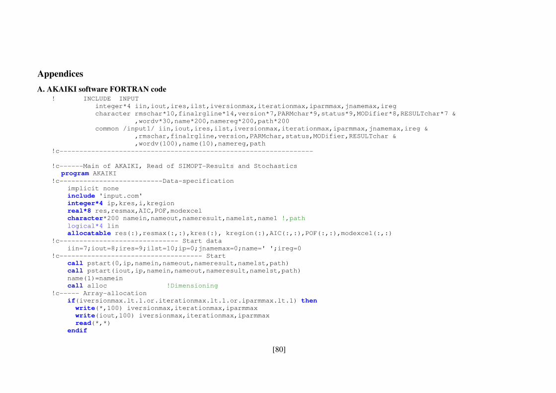
[80]
Appendices
A. AKAIKI software FORTRAN code ! INCLUDE INPUT
integer*4 iin,iout,ires,ilst,iversionmax,iterationmax,iparmmax,jnamemax,ireg
character rmschar*10,finalrgline*14,version*7,PARMchar*9,status*9,MODifier*8,RESULTchar*7 &
,wordv*30,name*200,namereg*200,path*200
common /input1/ iin,iout,ires,ilst,iversionmax,iterationmax,iparmmax,jnamemax,ireg &
,rmschar,finalrgline,version,PARMchar,status,MODifier,RESULTchar &
,wordv(100),name(10),namereg,path
!c----------------------------------------------------------------
!c------Main of AKAIKI, Read of SIMOPT-Results and Stochastics
program AKAIKI
!c--------------------------Data-specification
implicit none
include 'input.com'
integer*4 ip,kres,i,kregion
real*8 res,resmax,AIC,POF,modexcel
character*200 namein,nameout,nameresult,namelst,name1 !,path
logical*4 lin
allocatable res(:),resmax(:,:),kres(:), kregion(:),AIC(:,:),POF(:,:),modexcel(:,:)
!c------------------------------ Start data
iin=7;iout=8;ires=9;ilst=10;ip=0;jnamemax=0;name=' ';ireg=0
!c------------------------------------ Start
call pstart(0,ip,namein,nameout,nameresult,namelst,path)
call pstart(iout,ip,namein,nameout,nameresult,namelst,path)
name(1)=namein
call alloc !Dimensioning
!c----- Array-allocation
if(iversionmax.lt.1.or.iterationmax.lt.1.or.iparmmax.lt.1) then
write(*,100) iversionmax,iterationmax,iparmmax
write(iout,100) iversionmax,iterationmax,iparmmax
read(*,*)
endif
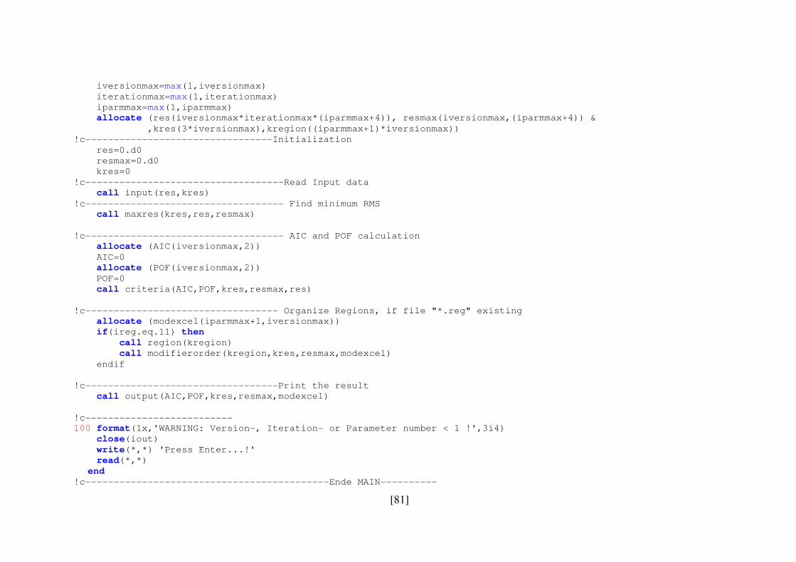
[81]
iversionmax=max(1,iversionmax)
iterationmax=max(1,iterationmax)
iparmmax=max(1,iparmmax)
allocate (res(iversionmax*iterationmax*(iparmmax+4)), resmax(iversionmax,(iparmmax+4)) &
,kres(3*iversionmax),kregion((iparmmax+1)*iversionmax))
!c---------------------------------Initialization
res=0.d0
resmax=0.d0
kres=0
!c-----------------------------------Read Input data
call input(res,kres)
!c----------------------------------- Find minimum RMS
call maxres(kres,res,resmax)
!c----------------------------------- AIC and POF calculation
allocate (AIC(iversionmax,2))
AIC=0
allocate (POF(iversionmax,2))
POF=0
call criteria(AIC,POF,kres,resmax,res)
!c---------------------------------- Organize Regions, if file "*.reg" existing
allocate (modexcel(iparmmax+1,iversionmax))
if(ireg.eq.11) then
call region(kregion)
call modifierorder(kregion,kres,resmax,modexcel)
endif
!c----------------------------------Print the result
call output(AIC,POF,kres,resmax,modexcel)
!c--------------------------
100 format(1x,'WARNING: Version-, Iteration- or Parameter number < 1 !',3i4)
close(iout)
write(*,*) 'Press Enter...!'
read(*,*)
end
!c-------------------------------------------Ende MAIN----------
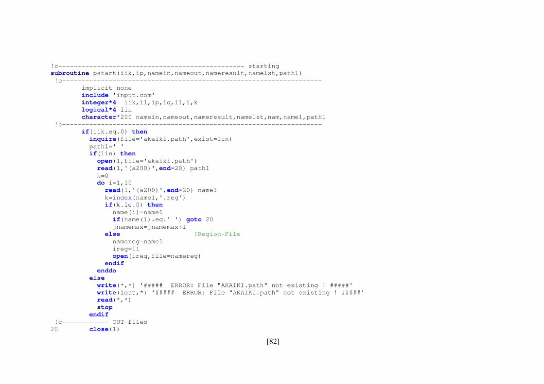
[82]
!c------------------------------------------------ starting
subroutine pstart(iik,ip,namein,nameout,nameresult,namelst,path1)
!c-------------------------------------------------------------------
implicit none
include 'input.com'
integer*4 iik,il,ip,iq,i1,i,k
logical*4 lin
character*200 namein,nameout,nameresult,namelst,nam,name1,path1
!c-------------------------------------------------------------------
if(iik.eq.0) then
inquire(file='akaiki.path',exist=lin)
path1=' '
if(lin) then
open(1,file='akaiki.path')
read(1,'(a200)',end=20) path1
k=0
do i=1,10
read(1,'(a200)',end=20) name1
k=index(name1,'.reg')
if(k.le.0) then
name(i)=name1
if(name(i).eq.' ') goto 20
jnamemax=jnamemax+1
else !Region-File
namereg=name1
ireg=11
open(ireg,file=namereg)
endif
enddo
else
write(*,*) '##### ERROR: File "AKAIKI.path" not existing ! #####'
write(iout,*) '##### ERROR: File "AKAIKI.path" not existing ! #####'
read(*,*)
stop
endif
!c------------ OUT-files
20 close(1)
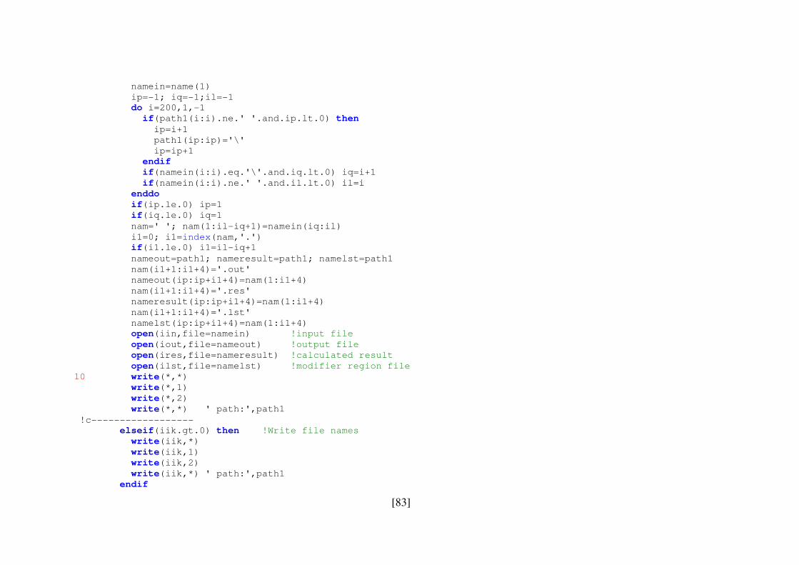
[83]
namein=name(1)
ip=-1; iq=-1;il=-1
do i=200,1,-1
if(path1(i:i).ne.' '.and.ip.lt.0) then
ip=i+1
path1(ip:ip)='\'
ip=ip+1
endif
if(namein(i:i).eq.'\'.and.iq.lt.0) iq=i+1
if(namein(i:i).ne.' '.and.il.lt.0) il=i
enddo
if(ip.le.0) ip=1
if(iq.le.0) iq=1
nam=' '; nam(1:il-iq+1)=namein(iq:il)
i1=0; i1=index(nam,'.')
if(i1.le.0) i1=il-iq+1
nameout=path1; nameresult=path1; namelst=path1
nam(i1+1:i1+4)='.out'
nameout(ip:ip+i1+4)=nam(1:i1+4)
nam(i1+1:i1+4)='.res'
nameresult(ip:ip+i1+4)=nam(1:i1+4)
nam(i1+1:i1+4)='.lst'
namelst(ip:ip+i1+4)=nam(1:i1+4)
open(iin,file=namein) !input file
open(iout,file=nameout) !output file
open(ires,file=nameresult) !calculated result
open(ilst,file=namelst) !modifier region file
10 write(*,*)
write(*,1)
write(*,2)
write(*,*) ' path:',path1
!c------------------
elseif(iik.gt.0) then !Write file names
write(iik,*)
write(iik,1)
write(iik,2)
write(iik,*) ' path:',path1
endif
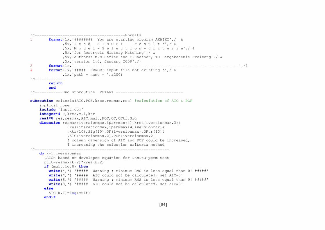
[84]
!c---------------------------------------Formats
1 format(1x,'######## You are starting program AKAIKI',/ &
,5x,'R e a d S I M O P T - r e s u l t s',/ &
,5x,'M o d e l - S e l e c t i o n - c r i t e r i a',/ &
,5x,'for Reservoir History Matching',/ &
,5x,'authors: M.M.Rafiee and F.Haefner, TU Bergakademie Freiberg',/ &
,5x,'version 1.0, January 2009',/)
2 format(1x,'-----------------------------------------------------------------------',/)
4 format(1x,'##### ERROR: input file not existing !',/ &
,1x,'path + name = ',a200)
!c------------
return
end
!c------------End subroutine PSTART -----------------------------
subroutine criteria(AIC,POF,kres,resmax,res) !calculation of AIC & POF
implicit none
include 'input.com'
integer*4 k,kres,m,l,ktr
real*8 res,resmax,AIC,mult,POF,OF,OFtr,Sig
dimension resmax(iversionmax,iparmmax+4),kres(iversionmax,3)&
,res(iterationmax,iparmmax+4,iversionmax)&
,ktr(10),Sig(10),OF(iversionmax),OFtr(10)&
,AIC(iversionmax,2),POF(iversionmax,2)
! column dimension of AIC and POF could be increased,
! increasing the selection criteria method
!c----------------------------------------------------------
do k=1,iversionmax
!AICn based on developed equation for insitu-perm test
mult=resmax(k,2)*kres(k,2)
if (mult.le.0) then
write(*,*) '##### Warning : minimum RMS is less equal than 0! #####'
write(*,*) '##### AIC could not be calculated, set AIC=0'
write(8,*) '##### Warning : minimum RMS is less equal than 0! #####'
write(8,*) '##### AIC could not be calculated, set AIC=0'
else
AIC(k,1)=log(mult)
endif
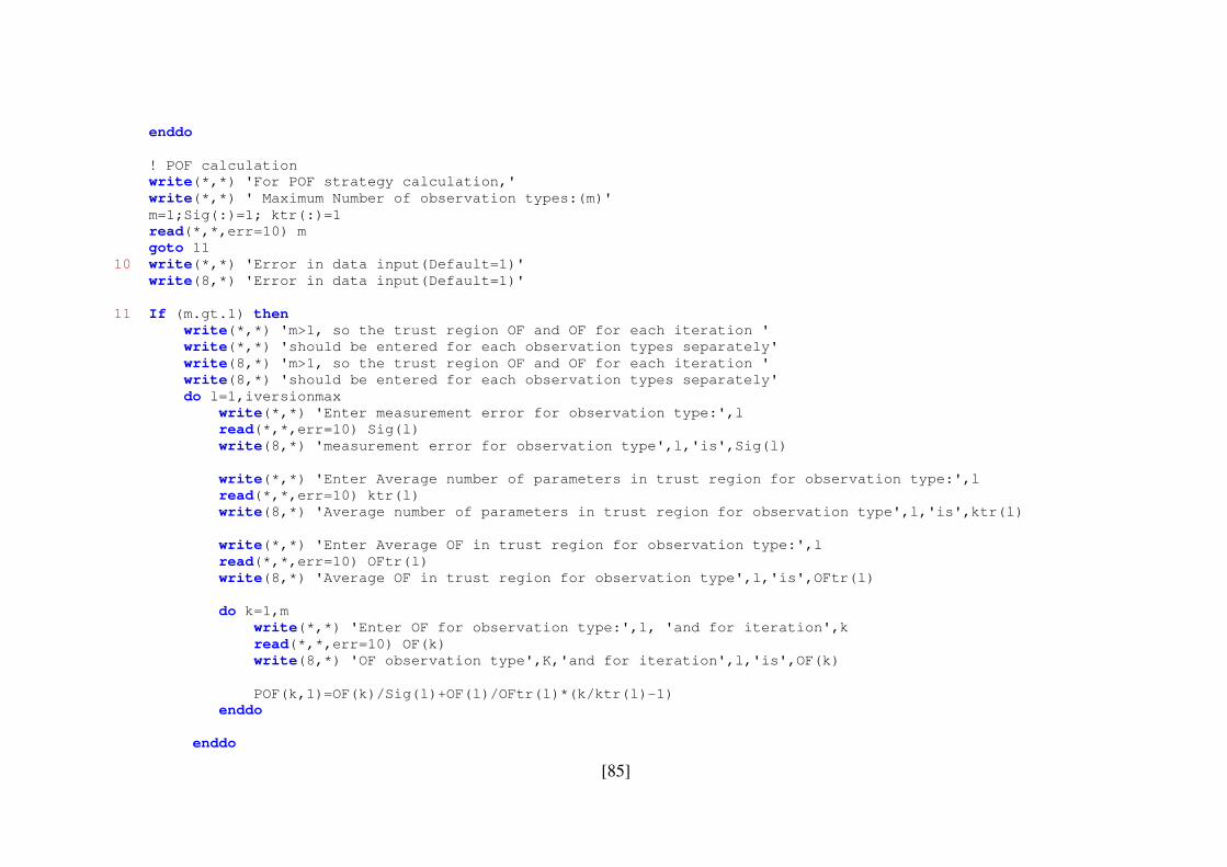
[85]
enddo
! POF calculation
write(*,*) 'For POF strategy calculation,'
write(*,*) ' Maximum Number of observation types:(m)'
m=1;Sig(:)=1; ktr(:)=1
read(*,*,err=10) m
goto 11
10 write(*,*) 'Error in data input(Default=1)'
write(8,*) 'Error in data input(Default=1)'
11 If (m.gt.1) then
write(*,*) 'm>1, so the trust region OF and OF for each iteration '
write(*,*) 'should be entered for each observation types separately'
write(8,*) 'm>1, so the trust region OF and OF for each iteration '
write(8,*) 'should be entered for each observation types separately'
do l=1,iversionmax
write(*,*) 'Enter measurement error for observation type:',l
read(*,*,err=10) Sig(l)
write(8,*) 'measurement error for observation type',l,'is',Sig(l)
write(*,*) 'Enter Average number of parameters in trust region for observation type:',l
read(*,*,err=10) ktr(l)
write(8,*) 'Average number of parameters in trust region for observation type',l,'is',ktr(l)
write(*,*) 'Enter Average OF in trust region for observation type:',l
read(*,*,err=10) OFtr(l)
write(8,*) 'Average OF in trust region for observation type',l,'is',OFtr(l)
do k=1,m
write(*,*) 'Enter OF for observation type:',l, 'and for iteration',k
read(*,*,err=10) OF(k)
write(8,*) 'OF observation type',K,'and for iteration',l,'is',OF(k)
POF(k,1)=OF(k)/Sig(l)+OF(l)/OFtr(l)*(k/ktr(l)-1)
enddo
enddo
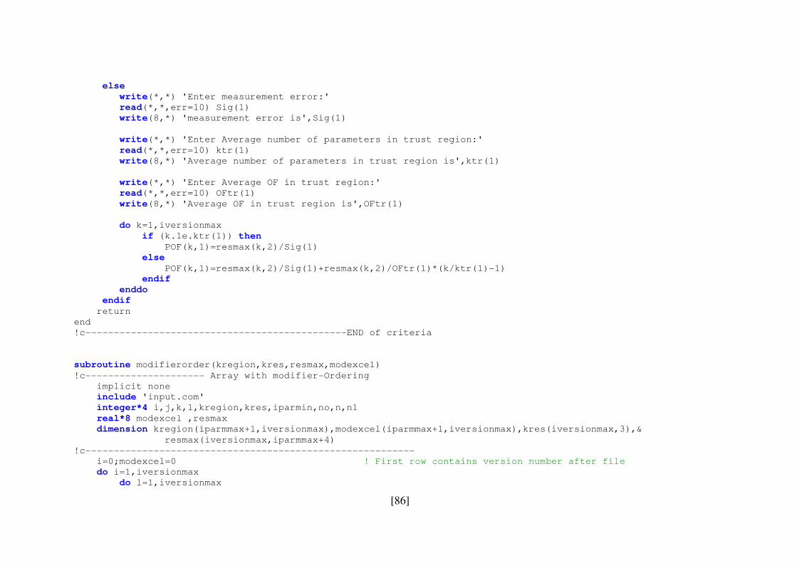
[86]
else
write(*,*) 'Enter measurement error:'
read(*,*,err=10) Sig(1)
write(8,*) 'measurement error is',Sig(1)
write(*,*) 'Enter Average number of parameters in trust region:'
read(*,*,err=10) ktr(1)
write(8,*) 'Average number of parameters in trust region is',ktr(1)
write(*,*) 'Enter Average OF in trust region:'
read(*,*,err=10) OFtr(1)
write(8,*) 'Average OF in trust region is',OFtr(1)
do k=1,iversionmax
if (k.le.ktr(1)) then
POF(k,1)=resmax(k,2)/Sig(1)
else
POF(k,1)=resmax(k,2)/Sig(1)+resmax(k,2)/OFtr(1)*(k/ktr(1)-1)
endif
enddo
endif
return
end
!c----------------------------------------------END of criteria
subroutine modifierorder(kregion,kres,resmax,modexcel)
!c--------------------- Array with modifier-Ordering
implicit none
include 'input.com'
integer*4 i,j,k,l,kregion,kres,iparmin,no,n,n1
real*8 modexcel ,resmax
dimension kregion(iparmmax+1,iversionmax),modexcel(iparmmax+1,iversionmax),kres(iversionmax,3),&
resmax(iversionmax,iparmmax+4)
!c----------------------------------------------------------
i=0;modexcel=0 ! First row contains version number after file
do i=1,iversionmax
do l=1,iversionmax
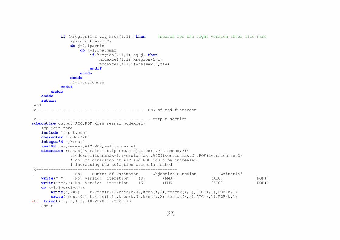
[87]
if (kregion(1,i).eq.kres(l,1)) then !search for the right version after file name
iparmin=kres(l,2)
do j=1,iparmin
do k=1,iparmmax
if(kregion(k+1,i).eq.j) then
modexcel(1,i)=kregion(1,i)
modexcel(k+1,i)=resmax(l,j+4)
endif
enddo
enddo
n1=iversionmax
endif
enddo
enddo
return
end
!c----------------------------------------------END of modifierorder
!c------------------------------------------------output section
subroutine output(AIC,POF,kres,resmax,modexcel)
implicit none
include 'input.com'
character header*200
integer*4 k,kres,i
real*8 res,resmax,AIC,POF,mult,modexcel
dimension resmax(iversionmax,iparmmax+4),kres(iversionmax,3)&
,modexcel(iparmmax+1,iversionmax),AIC(iversionmax,2),POF(iversionmax,2)
! column dimension of AIC and POF could be increased,
! increasing the selection criteria method
!c----------------------------------------------------------
! 'No. Number of Parameter Objective Function Criteria'
write(*,*) 'No. Version iteration (K) (RMS) (AIC) (POF)'
write(ires,*)'No. Version iteration (K) (RMS) (AIC) (POF)'
do k=1,iversionmax
write(*,400) k,kres(k,1),kres(k,3),kres(k,2),resmax(k,2),AIC(k,1),POF(k,1)
write(ires,400) k,kres(k,1),kres(k,3),kres(k,2),resmax(k,2),AIC(k,1),POF(k,1)
400 format(I3,I6,I10,I10,2F20.15,2F20.15)
enddo
[88]
close(ires)
! Write modifier regarding maximum number of parameters
header='Parm no. V1 V2 V3...... maximum Version no.'
write(ilst,'(a200)') header
write(ilst,121,err=123) (modexcel(1,k),k=1,iversionmax)
121 format(5x,100(1F10.0,1x))
do i=1,iparmmax
write(ilst,122,err=123) i,(modexcel(i+1,k),k=1,iversionmax)
122 format(4x,i4,1x,100(1pe10.3,1x))
123 continue
enddo
close(ilst)
return
end
!-------------------------------------------end of Output
subroutine alloc
!c--------- Dimensioning of arrays
implicit none
include 'input.com'
integer*4 i,jw,j,k,jres,jvers,jparm,jrms,k1,k2,k3,kend,kend1,ivers,jit,log &
,ifile,jname,kw,kww,kk,keof,ikend
real*8 rmsvalue
character word*200,wordn*30,name1*200,ant*1
logical*4 logres,logparm,logrms,lin
!c---------------------------------
jres=0;jvers=0;jparm=0;jrms=0;ivers=0;jw=0;jit=0;log=0;kend=0;kend1=0;jname=1
iversionmax=0;iterationmax=0;iparmmax=0;logres=.false.;logparm=.false.;logrms=.false.
RMSchar='total rms:'; keof=0;ikend=0
finalrgline='no improvement'
[89]
version='version'
PARMchar='parm type'
status='status'
MODifier='modifier'
RESULTchar='results'
ifile=iin
!c---------------------------------------------------
99 do 100 i=1,100000
call lesen(ifile,log,word,wordv,jw)
if(jw.eq.0.or.log.lt.0) goto 100 ! next row
if(log.eq.200) then
keof=1
goto 201 !End of file
endif
!c-----------------------------------------------------Analyzing
if(.not.logres.and..not.logparm.and..not.logrms) then !Find RESULT
if(index(word,'results : version').gt.0) then
kk=0
do k=2,jw
kk=k
kww=0
do kw=1,30
ant=wordv(k)(kw:kw)
if(ichar(ant).ge.48.and.ichar(ant).le.57) kww=kww+1
enddo
if(kww.gt.0) goto 133
enddo
134 write(*,*) 'ERROR in version number, set ivers=1 !'
write(8,*) 'ERROR in version number, set ivers=1 !'
read(*,*)
ivers=1
goto 11
!c----------
133 read(wordv(kk)(1:kww),*,err=134) ivers
!c-----------------------
11 logres=.true.
if(ivers.ne.jvers) then
iversionmax=iversionmax+1
[90]
jrms=0
endif
if(ivers.ne.jvers.and.ivers.gt.0) jvers=ivers
endif
elseif(.not.logparm.and..not.logrms.and.logres) then ! Find Total RMS
k1=index(word,'total rms')
if(k1.gt.0) then
jrms=jrms+1
iterationmax=max(jrms,iterationmax)
logrms=.true.
endif
!c-------------------------------------------------! READ PARM TYPE ---------
elseif(.not.logparm.and.logrms.and.logres) then
if(index(wordv(2),'parm').gt.0) logparm=.true.
jparm=0
elseif(logparm.and.logrms.and.logres) then ! READ number of parameters
kww=0
do kw=1,30
ant=wordv(2)(kw:kw)
if(ichar(ant).ge.48.and.ichar(ant).le.57) then
kww=kww+1
endif
enddo
if(kww.le.0) goto 13
read(wordv(2)(1:kww),*,err=13) k1
jparm=jparm+1
goto 12
!c--------------------------------------------- End of PARM numbers
13 logparm=.false.;logres=.false.;logrms=.false.
12 iparmmax=max(iparmmax,jparm)
!c--------------------------
endif
!c------------------------------------------Find End of Iteration or end of file
kend=index(word,'no improvement')
kend1=index(word,'no more iterations')
200 if(kend.gt.0.or.kend1.gt.0) then
ikend=ikend+1
write(*,*) 'filename: ', name(jname)(LEN_TRIM(path)+1:LEN_TRIM(name(jname)))
[91]
write(*,*) ' DIMENSIONING: End of Match, version: ',ivers
write(*,*)
write(8,*) 'filename: ', name(jname)(LEN_TRIM(path)+1:LEN_TRIM(name(jname)))
write(8,*) ' DIMENSIONING: End of Match, version: ',ivers
write(8,*)
endif
if(keof.gt.0.and.ikend.eq.0)then ! case of no identification
write(*,*) 'filename: ', name(jname)(LEN_TRIM(path)+1:LEN_TRIM(name(jname)))
write(*,*) ' DIMENSIONING: End of Match, version: ',ivers
write(*,*)
write(8,*) 'filename: ', name(jname)(LEN_TRIM(path)+1:LEN_TRIM(name(jname)))
write(8,*) ' DIMENSIONING: End of Match, version: ',ivers
write(8,*)
goto 201
endif
100 continue
!c-------------------------End of file
201 if(kend.le.0.or.kend1.le.0) then
if(iversionmax.le.0) iversionmax=iversionmax+1
endif
rewind(ifile)
!c----------------------- More than 1 input data file
if(jname.lt.jnamemax) then
jname=jname+1
inquire(file=name(jname),exist=lin)
ifile=jname+100
if(lin) open(unit=ifile,file=name(jname))
keof=0; ikend=0
goto 99
endif
write(*,*)
return
end
!c--------------------------- End subroutine alloc
subroutine input(res,kres)
!c--------- Read of Inputfile
implicit none
[92]
include 'input.com'
integer*4 i,jw,j,k,jres,jvers,jparm,jrms,k1,k2,k3,kend,kend1,ivers,jit,log,jinvers &
,kres,jname,ifile,kw,kww,kk,keof,ikend
real*8 rmsvalue,resmod,resgrad,res
character word*200,wordn*30,ant*1
logical*4 logres,logparm,logrms
dimension res(iterationmax,iparmmax+4,iversionmax),kres(iversionmax,3)
!c---------------------------------
! Structure /Itersave/
! Structure /IERATION/ ITER(10000) !maximum number of parameter
! integer*4 iparm(50)
! character*6 parmtype(50)
! character regname*8,parmstatus*10
! real*8 modifier,gradvalue
! end structure
! real*8 RMS(10000) !maximum number of iteration
! end structure
! record /Itersave/ VERSNO(iversionmax)
!c---------------------------------
jres=0;jvers=0;jparm=0;jrms=0;ivers=0;jw=0;jit=0;log=0;kend=0;kend1=0;jinvers=0
logres=.false.;logparm=.false.;logrms=.false.
RMSchar='total rms:';keof=0;ikend=0
finalrgline='no improvement'
version='version'
PARMchar='parm type'
status='status'
MODifier='modifier'
RESULTchar='results'
jname=1
ifile=iin
!c-----------------------------------
99 do 100 i=1,100000
call lesen(ifile,log,word,wordv,jw)
if(jw.eq.0.or.log.lt.0) goto 100 ! next row
if(log.eq.200) then
keof=1
goto 201 !End of file
[93]
endif
!c-----------------------------------------------------Analyzing
if(.not.logres.and..not.logparm.and..not.logrms) then !Find RESULT
if(index(word,'results : version').gt.0) then
kk=0
do k=2,jw
kk=k
kww=0
do kw=1,30
ant=wordv(k)(kw:kw)
if(ichar(ant).ge.48.and.ichar(ant).le.57) kww=kww+1
enddo
if(kww.gt.0) goto 133
enddo
134 write(*,*) 'ERROR in version number, set ivers=1 !'
write(8,*) 'ERROR in version number, set ivers=1 !'
read(*,*)
ivers=1
goto 11
!c----------
133 read(wordv(kk)(1:kww),*,err=134) ivers
!c-----------------------
11 logres=.true.
if(ivers.ne.jvers) then
jinvers=jinvers+1 ! Version number 1, 2 , 3 .......
jrms=0
endif
if(ivers.ne.jvers.and.ivers.gt.0) jvers=ivers !Version Number after file
endif
elseif(.not.logparm.and..not.logrms.and.logres) then ! Find Total RMS
k1=index(word,'total rms:')
if(k1.gt.0) then
jrms=jrms+1
logrms=.true.
k2=k1+10
if(k2.gt.0) then
kww=0
do kw=k2,k2+30
[94]
ant=word(kw:kw)
if(ichar(ant).ge.48.and.ichar(ant).le.57) then
kww=kww+1
endif
enddo
if(kww.le.0) then
write(*,*)'TOTAL RMS: value not readable, row=',i
write(8,*)'TOTAL RMS: value not readable, row=',i
read(*,*)
endif
read(word(k2:k2+kww),*) rmsvalue
res(jrms,1,jinvers)=jvers !Version-Number after file
res(jrms,2,jinvers)=rmsvalue !RMS
! VERSNO(jinvers).RMS(jrms)=rmsvalue !RMS in Structure
endif
endif
!c-------------------------------------------------! READ PARM TYPE ---------
elseif(.not.logparm.and.logrms.and.logres) then
if(index(wordv(2),'parm').gt.0) then
logparm=.true.
jparm=0
endif
elseif(logparm.and.logrms.and.logres) then ! READ number of parameters
kww=0
do kw=1,30
ant=wordv(2)(kw:kw)
if(ichar(ant).ge.48.and.ichar(ant).le.57) then
kww=kww+1
endif
enddo
if(kww.le.0) goto 13
read(wordv(2)(1:kww),*,err=13) k1
jparm=jparm+1
read(wordv(5),*) wordn
! VERSNO(jinvers).ITER(jrms).parmstatus=wordn !Status
if(wordn.eq.'active') res(jrms,3,jinvers)=1.
read(wordv(6),*) resmod
res(jrms,jparm+4,jinvers)=resmod !Modifier
[95]
! VERSNO(jinvers).ITER(jrms).modifier=resmod
if(jw.gt.6) then
read(wordv(7),*) resgrad !Gradient, if existing
res(jrms,4,jinvers)=resgrad
! VERSNO(jinvers).ITER(jrms).gradvalue=resgrad
endif
! read(wordv(2),*) VERSNO(jinvers).ITER(jrms).iparm(jparm)
! VERSNO(jinvers).ITER(jrms).parmtype=wordv(3)
! VERSNO(jinvers).ITER(jrms).regname=wordv(4)
kres(jinvers,1)=jvers ! Version-Number after file
kres(jinvers,2)=jparm ! Max. number of parameters in version jinvers
kres(jinvers,3)=jrms ! Max. number of iterations in version jinvers
goto 12
!c--------------------------------------------- End of PARM numbers
13 logparm=.false.;logres=.false.;logrms=.false.
12 continue
!c--------------------------
endif
!c------------------------------------------Find End of Iteration or end of file
kend=index(word,'no improvement')
kend1=index(word,'no more iterations')
200 if(kend.gt.0.or.kend1.gt.0) then
ikend=ikend+1
write(*,*) 'filename: ', name(jname)(LEN_TRIM(path)+1:LEN_TRIM(name(jname)))
write(*,*) ' READING/STORING: End of Match, version: ',ivers
write(*,*)
write(8,*) 'filename: ', name(jname)(LEN_TRIM(path)+1:LEN_TRIM(name(jname)))
write(8,*) ' READING/STORING: End of Match, version: ',ivers
write(8,*)
endif
if(keof.gt.0.and.ikend.eq.0)then ! case of no identification
write(*,*) 'filename: ', name(jname)(LEN_TRIM(path)+1:LEN_TRIM(name(jname)))
write(*,*) ' READING/STORING: End of Match, version: ',ivers
write(*,*)
write(8,*) 'filename: ', name(jname)(LEN_TRIM(path)+1:LEN_TRIM(name(jname)))
write(8,*) ' READING/STORING: End of Match, version: ',ivers
write(8,*)
goto 201
[96]
endif
100 continue
!c-------------------------End of file
!c----------------------- More than 1 input data file
201 close(ifile)
if(jname.lt.jnamemax) then
jname=jname+1
ifile=jname+100
keof=0; ikend=0
goto 99
endif
return
end
!c--------------------------- End subroutine input
subroutine lesen(ifile,log,word,wordv,jw)
!c------------READ and analyze a word
implicit none
integer*4 ifile,jw,log
character word*200,wordv*30
dimension wordv(100)
!c----------------------------------------------
log=0
read(ifile,'(a200)',err=100,end=200) word
call uncapslk(word)
if(index(word,'manual changes').gt.0) then
continue
endif
jw=0
call leszeile200(jw,word,wordv) !jw = number of sub-words in a row
return
!c---------------------ERROR
100 log=-100
return
!c---------------------END
200 log=200
[97]
return
end
!c-------------------------------End LESEN
subroutine leszeile200(j,wort,wort1)
!c----------------------------------------------------------
!c---- Routine for reading one character and saving
!c---- Text form part strings
!c---- attention: The patrameters must be separated by comma or space
!c----------------------------------------------------------
implicit none
integer*4 i,j,lw,iii,lww,jmax
character wort*200,wort1*30
dimension wort1(100)
!c-----------------------------------------------------------
if(wort.eq.' ') then
write(*,100)
write(8,100)
j=0
return
endif
100 format(' ERROR in LESZEILE200: Word is empty !')
lw=200
do i=1,100
wort1(i)=' '
enddo
lww=lw
do i=1,lw
if(wort(1:1).eq.' '.or.wort(1:1).eq.',') then
wort(1:lww-1)=wort(2:lww)
wort(lww:lww)=' '
lww=lww-1
else
exit
endif
enddo
!c--------------
jmax=200
[98]
j=0
i=1
do while(i.lt.lw.and.j.lt.jmax)
do while(wort(i:i).eq.' '.or.wort(i:i).eq.',')
i=i+1
if(i.eq.lw) return
enddo
iii=0
if(j.ge.100) exit
j=j+1
do while(wort(i:i).ne.' '.and.wort(i:i).ne.',')
iii=iii+1
if(iii.gt.28) then
! write(*,*) ' ERROR in LESZEILE100, Wordlength > 30, shorten it'!
! write(*,300) wort
! read(*,*)
300 format(' Full row: ',a200)
! return
goto 10
endif
wort1(j)(iii:iii)=wort(i:i)
i=i+1
enddo
10 wort1(j)(iii+1:iii+1)=' '
enddo
return
end
!c-----------------------------------Ende Leszeile200
subroutine uncapslk(text)
!* * * * * * * * * * * * * * * * * * * * * * * * * * * * * * * * * * * *
!* *
!* uncaps lock *
!* *
!* eingabe: text - text mit kleinen und grossen buchstaben *
!* ausgabe: text - text, indem grosse in kleinbuchstaben geaendert sind*
!* *
!* programmierer: dr.sames (ife) 16.10.89 *
!* *
[99]
!* * * * * * * * * * * * * * * * * * * * * * * * * * * * * * * * * * * *
character*(*) text
integer i, icode, j, lng, len
!*
!* code-festlegung: ascii (1) / dkoi (2)
!*
if (ichar('A') .eq. 65) then
icode = 1
else
icode = 2
endif
!* gross- durch kleinbuchstaben ersetzen
!*
lng = len(text)
goto (100,120), icode
100 do 110 i = 1, lng
j = ichar(text(i:i))
if (65 .le. j .and. j .le. 90) then
j = j + 32
text(i:i) = char(j)
endif
110 continue
goto 140
120 do 130 i = 1, lng
j = ichar(text(i:i))
if (193 .le. j .and. j .le. 233) then
j = j - 64
text(i:i) = char(j)
endif
130 continue
140 continue
return
end
!c----------------------End UNCAPSLK--------------------------------
subroutine maxres(kres,res,resmax)
!c------------------------- Array with minimum RMS
implicit none
[100]
include 'input.com'
integer*4 i,j,k,kres,iit,ipar,ixmax
real*8 res,resmax,xmax
dimension res(iterationmax,iparmmax+4,iversionmax),kres(iversionmax,3),resmax(iversionmax,iparmmax+4)
!c----------------------------------------------------------
do k=1,iversionmax
iit=kres(k,3)
ipar=kres(k,2)
xmax=1.d20
ixmax=0
do j=1,iit
if(res(j,2,k).lt.xmax) then
ixmax=j
xmax=res(j,2,k)
endif
enddo
do j=1,ipar+4
resmax(k,j)=res(ixmax,j,k)
enddo
enddo
return
end
!c-------------------------------End Resmax
subroutine region(kregion)
!c--------------------- Array with Region-Ordering
!c- the file should consist of an array which the first coulumn
!c- is the version of identification with maximum number of parameters
implicit none
include 'input.com'
integer*4 i,j,k,kregion
dimension kregion(iparmmax+1,iversionmax)
!c----------------------------------------------------------
i=0 ! First row contains version number after file
do k=1,iparmmax+1,1 ! READ rows (first column = max. region) of File "*.reg"
read(ireg,*,err=10,end=11) (kregion(k,j),j=1,iversionmax)
i=i+1
enddo
[101]
goto 11
!c-------------------ERROR
10 write(*,*) ' ERROR during READ file "*.reg" !'
write(8,*) ' ERROR during READ file "*.reg" !'
read(*,*)
!c----------------
11 if(i-1.ne.iparmmax) then
write(*,*) 'Maximum number of regions could not read !'
write(*,*) ' ERROR during READ file "*.reg" !'
write(8,*) 'Maximum number of regions could not read !'
write(8,*) ' ERROR during READ file "*.reg" !'
endif
return
end
!c-------------------------------End kregion
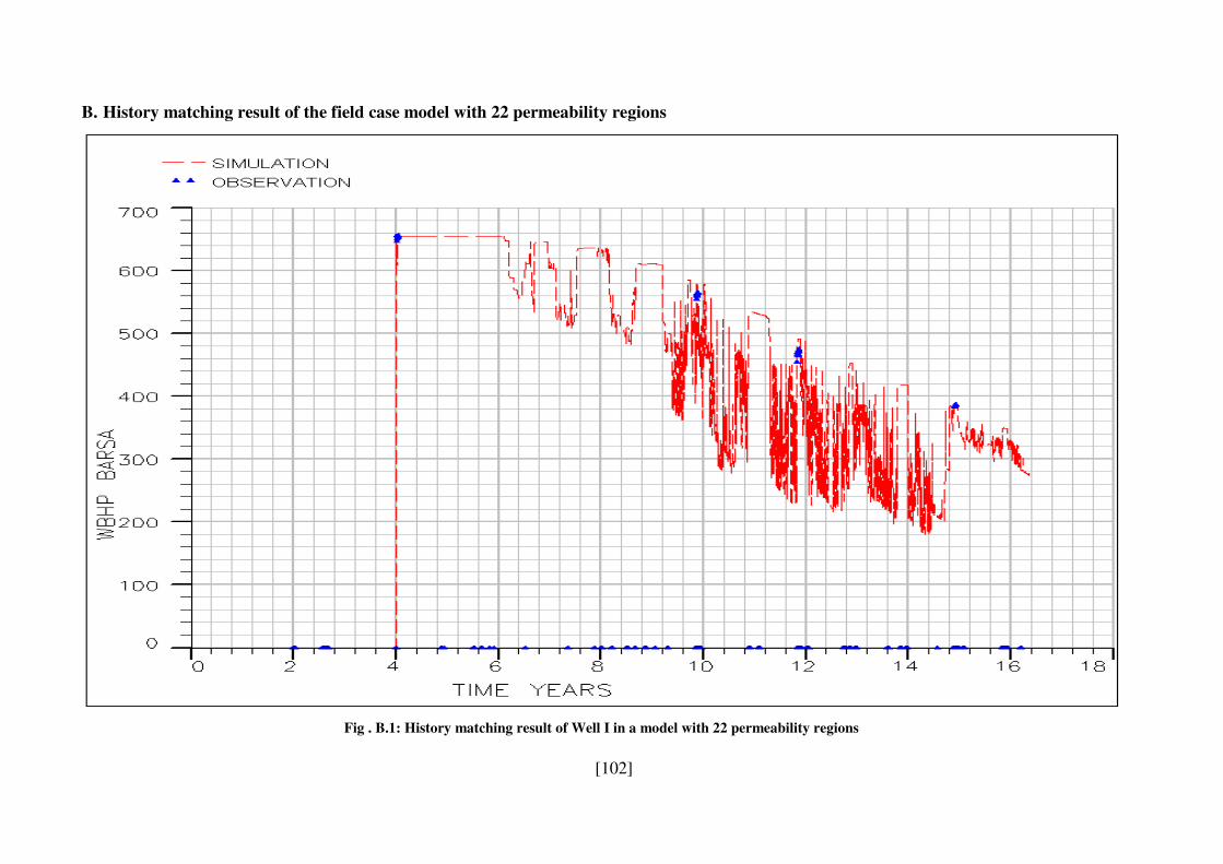
[102]
B. History matching result of the field case model with 22 permeability regions
Fig . B.1: History matching result of Well I in a model with 22 permeability regions

[103]
Fig . B.2: History matching result of Well II in a model with 22 permeability regions
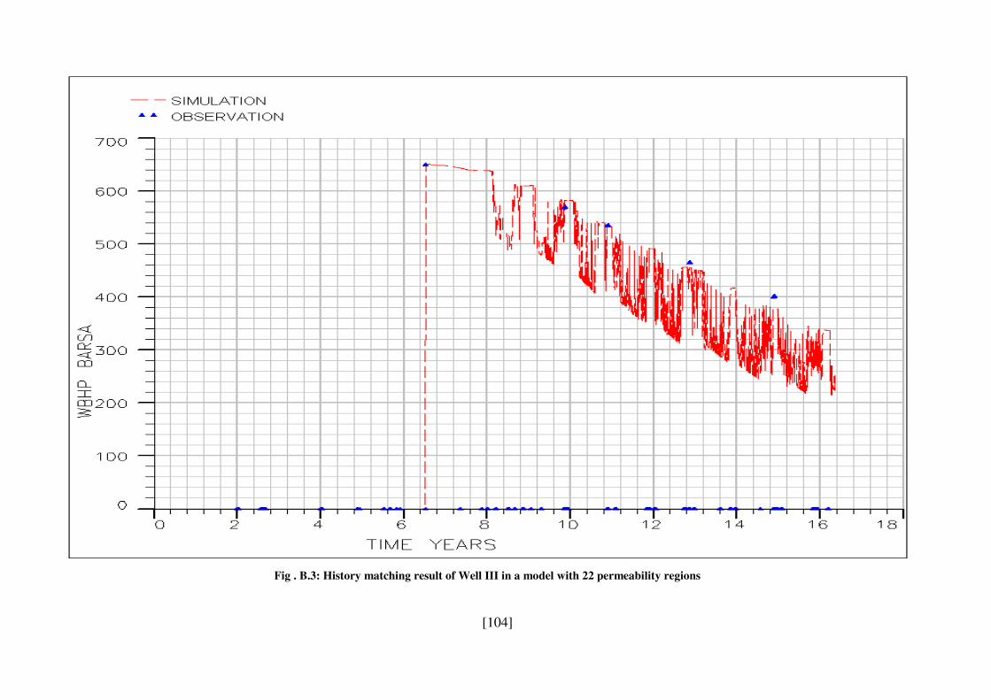
[104]
Fig . B.3: History matching result of Well III in a model with 22 permeability regions
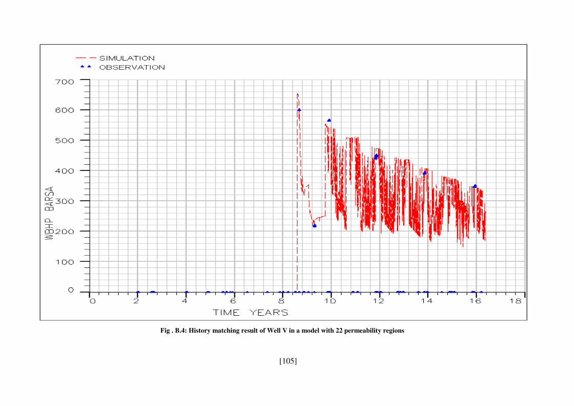
[105]
Fig . B.4: History matching result of Well V in a model with 22 permeability regions
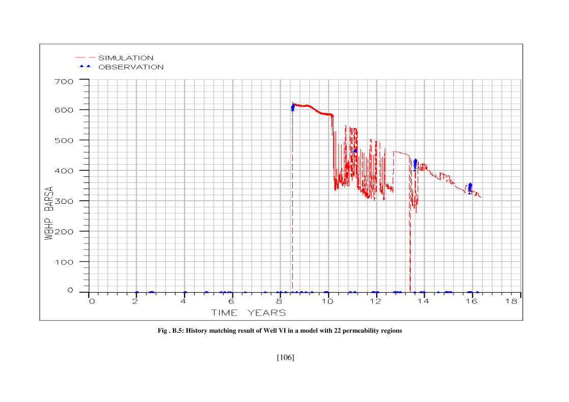
[106]
Fig . B.5: History matching result of Well VI in a model with 22 permeability regions
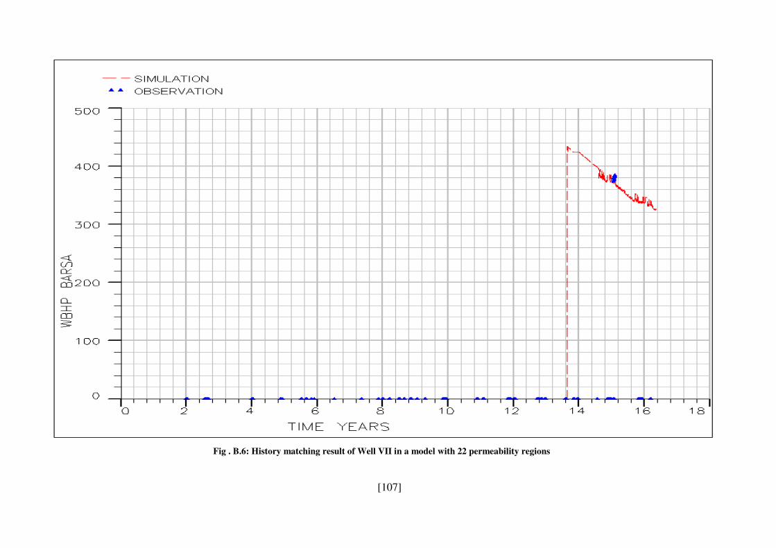
[107]
Fig . B.6: History matching result of Well VII in a model with 22 permeability regions
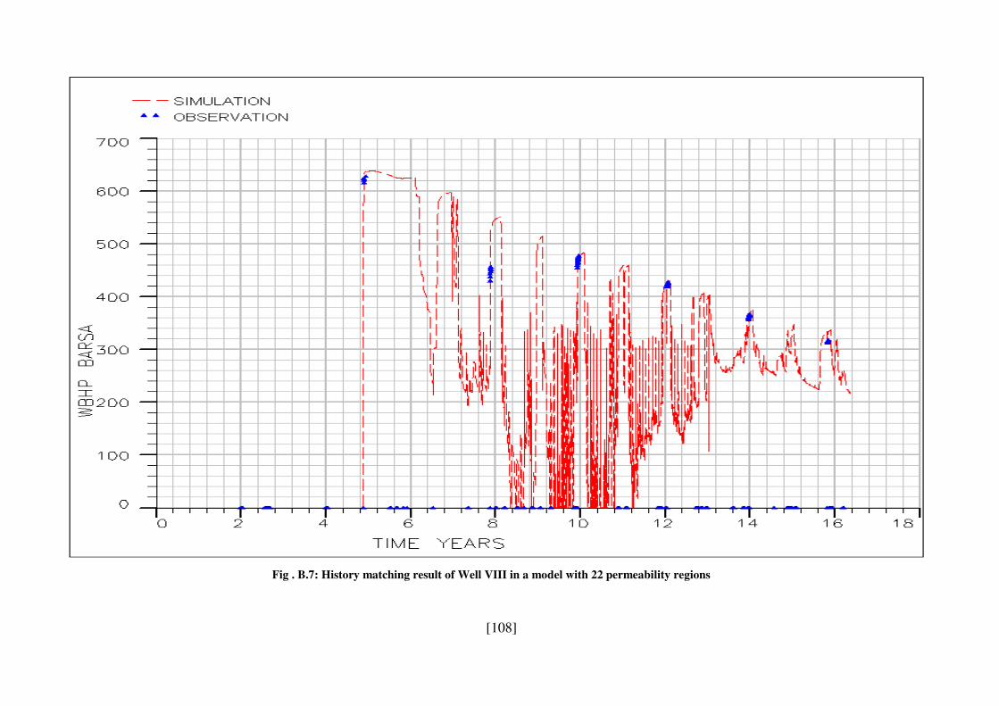
[108]
Fig . B.7: History matching result of Well VIII in a model with 22 permeability regions
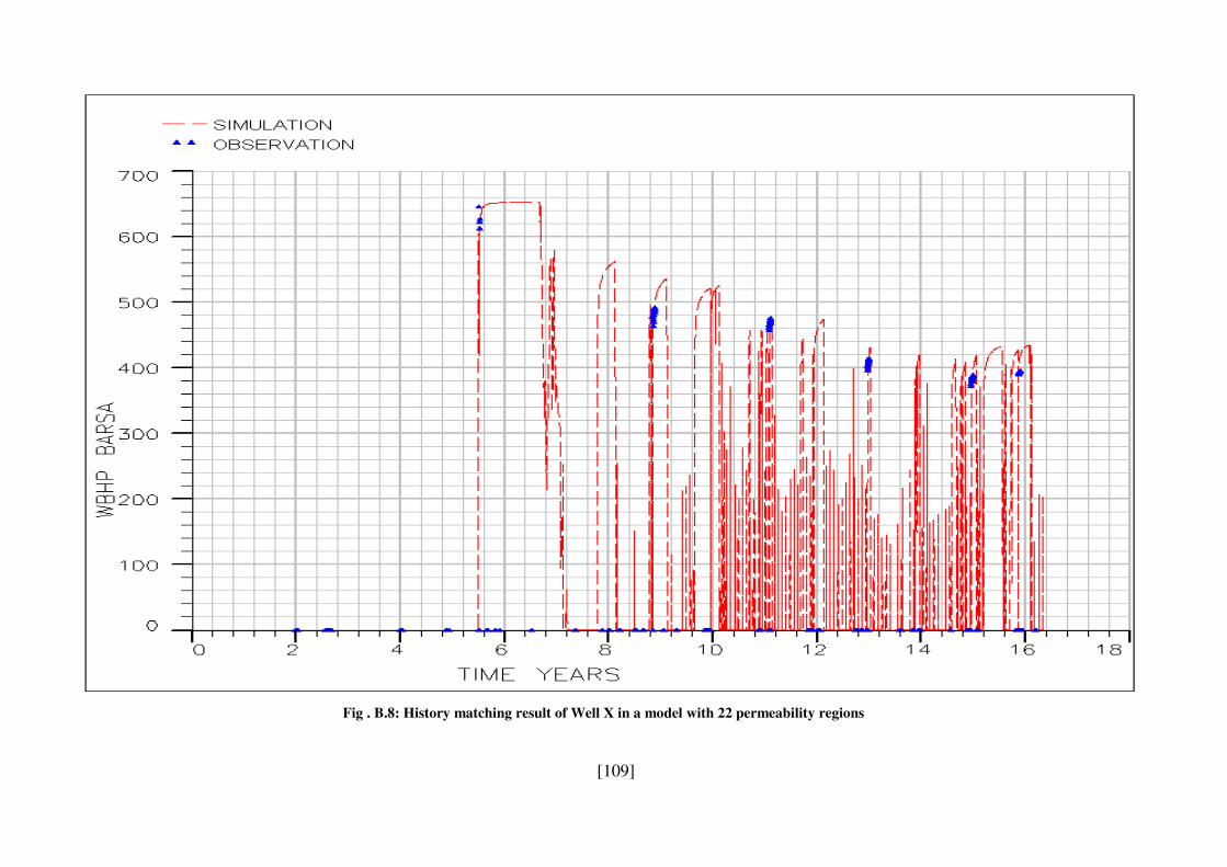
[109]
Fig . B.8: History matching result of Well X in a model with 22 permeability regions
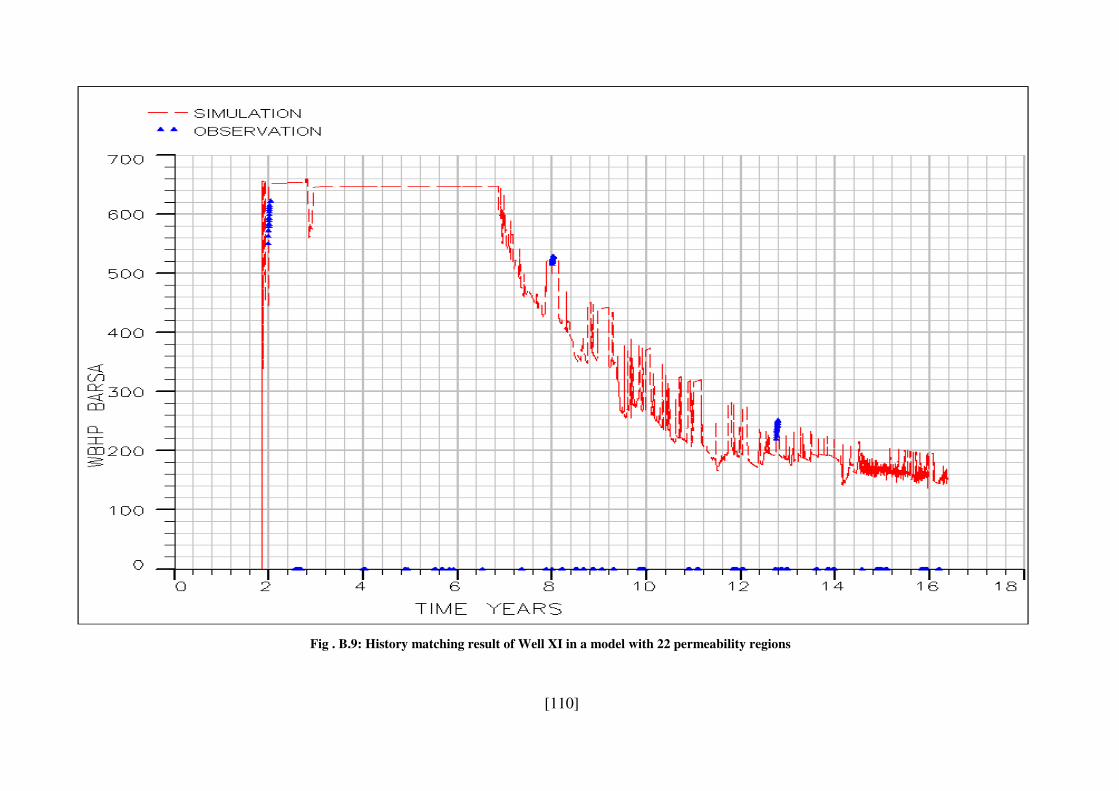
[110]
Fig . B.9: History matching result of Well XI in a model with 22 permeability regions
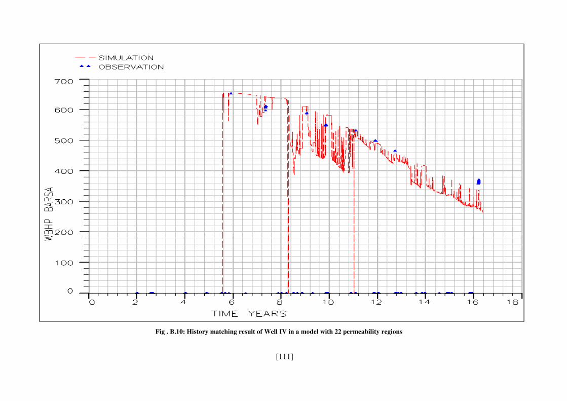
[111]
Fig . B.10: History matching result of Well IV in a model with 22 permeability regions
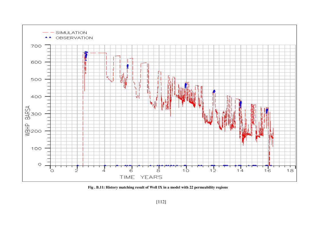
[112]
Fig . B.11: History matching result of Well IX in a model with 22 permeability regions