
Morphodynamic Equilibria Embayed Beach Systemselib.suub.uni-bremen.de/edocs/00103530-1.pdf ·...
104
Christopher Daly University of Bremen 8/30/2013 Morphodynamic Equilibria of Embayed Beach Systems
Transcript of Morphodynamic Equilibria Embayed Beach Systemselib.suub.uni-bremen.de/edocs/00103530-1.pdf ·...
Christopher Daly
University of Bremen
8/30/2013
Morphodynamic Equilibria of Embayed Beach Systems

Morphodynamic Equilibria of Embayed Beach Systems
– i –
Morphodynamic Equilibria of Embayed Beach Systems
Dissertation zur Erlangung des Doktorgrades
der Naturwissenschaften
– Dr. rer. nat. –
Im Fachbereich Geowissenschaften der Universität Bremen
vorgelegt von
Christopher John Daly
Bremen, 30 August 2013
Tag des Kolloquiums: 15 November 2013
Gutachter:
PD Dr. Christian Winter, Universität Bremen, Germany Prof. Dr. Karin R. Bryan, University of Waikato, New Zealand
Defense Committee:
PD Dr. Christian Winter, Universität Bremen, Germany Prof. Dr. Karin R. Bryan, University of Waikato, New Zealand
Prof. Dr. Michael Schultz, Universität Bremen, Germany Prof. Dr. Tobias Mörz, Universität Bremen, Germany
Dr. Bryna Flaim, Universität Bremen, Germany Mr. Markus Benninghoff, Universität Bremen, Germany

Morphodynamic Equilibria of Embayed Beach Systems
– ii –
Morphodynamic Equilibria of Embayed Beach Systems
– iii –
Declaration
Name / Name: Christopher John Daly Datum / Date: 30 August 2013 Anschrift / Address: Leobenerstrasse, 28359 Bremen Erklärung / Declaration Hiermit versichere ich, dass ich / Herewith I declare that
1. die Arbeit ohne unerlaubte fremde Hilfe angefertigt habe, / This document and the accompanying data have been composed by myself, and describes my own work.
2. keine anderen als die von mir angegebenen Quellen und Hilfsmittel benutzt habe und / Material
from the published or unpublished work of others, which is referred to in the dissertation, is credited to the author in the text.
3. die den benutzten Werken wörtlich oder inhaltlich entnommenen Stellen als solche kenntlich
gemacht habe / This work has not been submitted for any other degree.
Christopher Daly ____________________ Unterschrift / Signature Bremen, den 30.08.2013

Morphodynamic Equilibria of Embayed Beach Systems
– iv –
Morphodynamic Equilibria of Embayed Beach Systems
– v –
Abstract
Embayed beaches are well-known for the prominent curvature of their shorelines and are often observed in states of dynamic or static equilibrium. These equilibrium states are typically assumed to be influenced by headland geometry, cellular circulation patterns, wave obliquity at the shoreline and diffraction in and around the shadow zone. One of the main aims of this study is to gain a comprehensive understanding of the role of (i) wave forcing, (ii) environmental conditions and (iii) the geological setting in long-term embayed beach evolution. In doing so, a state-of-the-art morphodynamic model was used to simulate the evolution of a schematic embayment under idealized wave forcing conditions. Wave forcing is varied between a mixture of time-invariant and time-varying cases. Environmental conditions are varied by changing sediment size, tidal amplitude and mean wave height. The geological setting is varied by changing the angle of obliquity of the waves and the bay width.
Several wave climate variables influence the distribution of wave energy throughout the bay and in the shadow zone: wave direction, directional spreading and wave height. Diffraction is shown to be dominant only when the incoming wave conditions are both directionally narrow-banded and highly oblique. Nevertheless, time varying wave directions (as little as 6%) can account for shoreline curvature in the shadow zone. Changes in environmental conditions and geological setting generally affect the rate of development of the bay as well as the equilibrium size of the bay. For example: increased tidal amplitude enhances the size of the shadow zone due to modulation of the wave energy in this area, and wider bays require an exponentially larger period of time to attain equilibrium. Progressive weakening of the residual long-shore current and sediment transport as the bay develops is shown to be consistently related to long-term, non-uniform shoreline cutback (beach rotation). Hence, the curvature of the shoreline planform is primarily due to weakened shoreline erosion processes resulting from beach rotation.
The research aims are extended to investigate seasonal and event-driven changes based on real-world cases. In doing so, the model has been used to reconstruct the medium-term, quasi-equilibrium morphology of a bay by discretising the measured wave climate variability in terms of wave heights and directions into several representative wave conditions. The effect of extreme events appeared to be balanced by average forcing conditions occurring over a longer period of time. Additionally, the equilibrium bathymetry is largely determined by wave direction variability; therefore it is necessary to have a high level of directional resolution in order to obtain accurate results. A nine-month field campaign was conducted at embayed beaches of Tairua and Pauanui, Coromandel Peninsula, New Zealand. During this period the beaches exhibited highly dynamic behaviour in response to storm events characterised by non-uniform cross-shore sediment movement within the bay. The residual sediment transport pathways between the surf zone and the adjacent beach and shoaling zones will be determined in future.

Morphodynamic Equilibria of Embayed Beach Systems
– vi –
Morphodynamic Equilibria of Embayed Beach Systems
– vii –
Contents
Title Page ....................................................................................................................................................... i
Declaration .................................................................................................................................................... iii
Abstract ...................................................................................................................................................... v
Contents ....................................................................................................................................................vii
Acknowledgements ............................................................................................................................................. ix
Chapter 1 – General Introduction .............................................................................................................. 1
1.1 Motivation ............................................................................................................................... 1 1.2 Embayed Beaches ..................................................................................................................... 2 1.3 Research Hypotheses and Questions ......................................................................................... 3 1.4 Research Methods .................................................................................................................... 4 1.5 Thesis Outline .......................................................................................................................... 7
Chapter 2 – Long-Term, Constant Wave Forcing ................................................................................ 9
2.1 Abstract .................................................................................................................................... 9 2.2 Introduction ............................................................................................................................10 2.3 Model Setup ............................................................................................................................10 2.4 Results .....................................................................................................................................12 2.5 Discussion ...............................................................................................................................14 2.6 Conclusion ..............................................................................................................................15 2.7 Acknowledgements ..................................................................................................................16
Chapter 3 – Long-Term, Time-Varying Wave Forcing ...................................................................... 17
3.1 Abstract ...................................................................................................................................17 3.2 Introduction ............................................................................................................................18 3.3 Numerical Model Description and Setup ................................................................................20 3.4 Results .....................................................................................................................................26 3.5 Discussion ...............................................................................................................................34 3.6 Conclusion ..............................................................................................................................38 3.7 Acknowledgements ..................................................................................................................39
Morphodynamic Equilibria of Embayed Beach Systems
– viii –
Chapter 4 – Long-Term Morphological Evolution .............................................................................. 41
4.1 Abstract .................................................................................................................................. 41 4.2 Introduction ........................................................................................................................... 42 4.3 Methods ................................................................................................................................. 43 4.4 Results .................................................................................................................................... 46 4.5 Discussion .............................................................................................................................. 53 4.6 Conclusion ............................................................................................................................. 56 4.7 Acknowledgements ................................................................................................................. 57
Chapter 5 – Wave Climate & Equilibrium Bathymetry ................................................................... 59
5.1 Abstract .................................................................................................................................. 59 5.2 Introduction ........................................................................................................................... 60 5.3 Study Location and Available Data ......................................................................................... 61 5.4 Numerical Model Description and Setup ................................................................................ 62 5.5 Methods ................................................................................................................................. 63 5.6 Results .................................................................................................................................... 67 5.7 Discussion .............................................................................................................................. 68 5.8 Conclusion ............................................................................................................................. 70 5.9 Acknowledgements ................................................................................................................. 70
Chapter 6 – Short- to Medium-Term Dynamics .................................................................................. 71
6.1 Introduction ........................................................................................................................... 71 6.2 Study Location and Available Data ......................................................................................... 73 6.3 Methods ................................................................................................................................. 74 6.4 Initial Results .......................................................................................................................... 76 6.5 Discussion and Conclusion ..................................................................................................... 78 6.6 Acknowledgements ................................................................................................................. 78
Chapter 7 – Summary, Conclusions & Outlook ................................................................................. 79
7.1 Summary ................................................................................................................................ 79 7.2 Conclusions ............................................................................................................................ 80 7.3 Outlook .................................................................................................................................. 81
References ................................................................................................................................................... 83
Curriculum Vitae .................................................................................................................................................. 91
Morphodynamic Equilibria of Embayed Beach Systems
– ix –
Acknowledgements
Work on this thesis began in January 2010 as part of the Deutsche Forschungsgemeinschaft
(DFG) funded Integrated Coastal Zone and Shelf-Sea Research (INTERCOAST) International Research Training Group. INTERCOAST is based on a strong collaboration between the University of Bremen, Germany, and the University of Waikato, New Zealand. It focuses on the impacts of global, climate, and environmental change in coastal and shelf-sea areas within a framework that encompasses marine geosciences, marine biology, social sciences and law. The main scientific goal of INTERCOAST is “to develop a new scientific knowledge that contributes to the development of new and innovative strategies for a sustainable utilization of coastal and shelf-sea regions”. This thesis is the outcome of work done within the framework of the INTERCOAST project, IC1, which focuses on the “Morphodynamic Equilibria of Coastal Systems: Modelling the Role of Extreme Event and Average Forcing”.
It would not have been possible to complete this thesis without the help and support of many people whom I wish to acknowledge at this time. Firstly, many thanks to my supervisors, Dr. Christian Winter and Dr. Karin Bryan, for their continuous guidance, critique, and support during my studies. I would like to express my appreciation to Prof. Dr. Dierk Hebbeln, Prof. Dr. Dano Roelvink and Dr. Antonio Klein for their advice and support as part of my thesis committee. The Coastal Dynamics group at the MARUM Center for Marine Environmental Sciences, University of Bremen, has provided a good working environment in which I could conduct my research. Frequent group meetings and informal discussions allowed us to exchange feedback on our work and to learn about different aspects of the coastal morphodynamic system. Best of all, our many social gatherings, from short coffee breaks to long kohlfahrts, made us a very close-knit group. I have also spent a year as part of the Coastal Marine group at the Department of Earth and Ocean Science (DEOS), University of Waikato. There, I enjoyed organizing the fortnightly Coastal Marine Seminar Series (CMSS) for the M.Sc. and Ph.D. students. We also engaged in fruitful discussion regarding our diverse study areas. From time to time we would play touch rugby during the lunch break (one day we will win) and help each other on our many field trips.
I experienced both the joy and pain of planning and executing a nine-month field campaign at Tairua and Pauanui Beaches in New Zealand. This was no easy feat, and I definitely could not have done it on my own. I am, therefore, heavily indebted to many people who contributed to making the campaign a success. Firstly, thanks to my supervisors for supporting and contributing to my plans, and to INTERCOAST for funding this initiative. Considerable thanks to Dirk Immenga, whose technical knowledge, advanced planning, and many contacts with the local authorities and people of Tairua (Brenda Reid and Mike Harris), was instrumental in enabling us to efficiently carry out the hydrographic, sediment sampling and wave measurement surveys. Other DEOS staff members, Craig Hosking, Dean Sandwell, Christopher McKinnon, Annette Rodgers, Janine Ryburn and Sydney Wright variously provided instrumentation and logistical support. My trusty ‘First Officers’, Raimundo Labbe and Amir Emami braved cold and rough weather on many occasions to operate the total station, or be the one taking the plunge into the surf during the beach profile surveys. Many other volunteers joined the surveys once, twice, or even thrice: Josh Mawer, Wing Yan Man, Ruggero Capperucci, Raphael Guedes, Mike Desaever,

Morphodynamic Equilibria of Embayed Beach Systems
– x –
Gerhard Bartzke, Clarisse Niemand, Alicia Ferrer Costa, Alexander Port, Shawn Harrison, Cassandra Barker, Steven Hunt, Sarah Gardiner, Zhi (Cathy) Liu, Xiaohan (Daisy) Du, Sebastien Boulay, Renee Foster, Christopher Morcom, Sarah McSweeney, and backpacker Jan Hages. Thank you all! Lou MacWell (Thames-Coromandel Local Council) provided access to Pauanui beach, making our beach surveys much easier to conduct. Dr. Vernon Pickett and Keith Smith (Waikato Regional Council), Iain McDonald and George Payne (National Institute for Water and Atmosphere, NIWA), and Rob Donald and Shane Iremonger (Bay of Plenty Regional Council) are thanked for providing access to several data archives.
I am very happy to have been able to share my travels over the past three-and-half years with my fellow INTERCOAST PhD and Post-Doc colleagues. Not only did we learn to communicate our research across disciplines at the many INTERCOAST Workshops, Colloquia, and Retreats, but we have built lasting friendships. This was reinforced by all the wonderful lunches, get-togethers, and group trips in New Zealand, where we were all foreigners in a new, adventurous land. I truly appreciate our open discussions and camaraderie both in Hamilton and Bremen. Many to thanks to friends far and wide, who, despite being countless miles away, still stayed in touch with me as I moved about in a rather unpredictable fashion. I am even more grateful to those friends who have stuck with me through the entire experience, including my best mate, Mike. I sincerely apologise to my family for my prolonged absence from home. Thank you for keeping me in your thoughts, I have missed you all dearly. I would like to dedicate this thesis to my parents: my mother Jacqueline, and my late father, Edwin.
Morphodynamic Equilibria of Embayed Beach Systems
– 1 –
Chapter 1 – General Introduction
1.1 Motivation
Coastal regions are highly dynamic, densely populated, economically productive, and rich with natural resources. Many different types of natural systems have developed over varying time and spatial scales, and host diverse habitats and ecosystems, such as those located in estuaries, deltas, and coral reefs. The coastal zone is also an area that is suited to human development because of the presence of natural resources, such as fish and oil; flat coastal plains suited for urbanisation; and areas suited for ports and harbours necessary for trade. Currently, over 38% of the world’s population (more than 200 million in the EU) live within 100 km of the coast. The high human pressure on coastal areas often results in political conflict. Integrated Coastal Zone Management (ICZM) has been developed to provide an administrative framework for national and international coordination and cooperation in order to prevent and mitigate these conflicts while preserving the environment. Coastal erosion induced by anthropogenic impacts and climate change is also problematic for ensuring the safety of inhabitants of coastal areas and is still yet to be fully understood and accounted for in many coastal areas. It is, therefore, of significant interest that the coastal system is well understood for informed ICZM of protected coastal areas and resources.
A so-called ecosystem approach is taken in the implementation of ICZM policies where the protection and conservation of ecosystems is given the highest priority. In this regard, the interaction between natural processes and human activity should work positively to conserve biological diversity. This clearly connects the living with the non-living environment (FAO, 2006). Many governing bodies have recognised the need for more active monitoring of the environment, for example, via the Marine Strategy Framework Directive of the European Commission (ARGE BLMP, 2011). In this directive, one of the main objectives is to "protect and preserve the marine environment, prevent its deterioration or, where practicable, restore marine ecosystems in areas where they have been adversely affected". The state of the environment is characterised by assessing several qualitative descriptors, with the sea floor (Descriptor 6) and hydrography (Descriptor 7) particularly relevant to changes in coastal morphodynamics.
The morphological evolution of coastal systems, such as beaches or tidal inlets, is driven by the continuous interaction of natural hydrodynamic forcing (wind, waves, tides), sediment transport processes and direct or indirect human impact. Coastal sedimentary deposits, such as beaches, are often in a state of quasi-equilibrium, constantly reacting to varying forcing conditions at different temporal and spatial scales, e.g., beach erosion of the upper shoreface and dunes during storm events or the seasonal adaptation of beaches towards changing wave direction during the summer and winter. It is, therefore, important to know how such coastal systems currently react to forcing conditions and, additionally, perceived future environmental changes. The main motivation of this thesis is, therefore, driven by the need to both broaden and deepen our knowledge of coastal systems, in particular embayed beaches, in order to determine how they develop over the long-term, how they maintain equilibrium, and how to account for short-term, event driven and seasonal variability.
Morphodynamic Equilibria of Embayed Beach Systems
– 2 –
1.2 Embayed Beaches
1.2.1 Long-Term Equilibrium
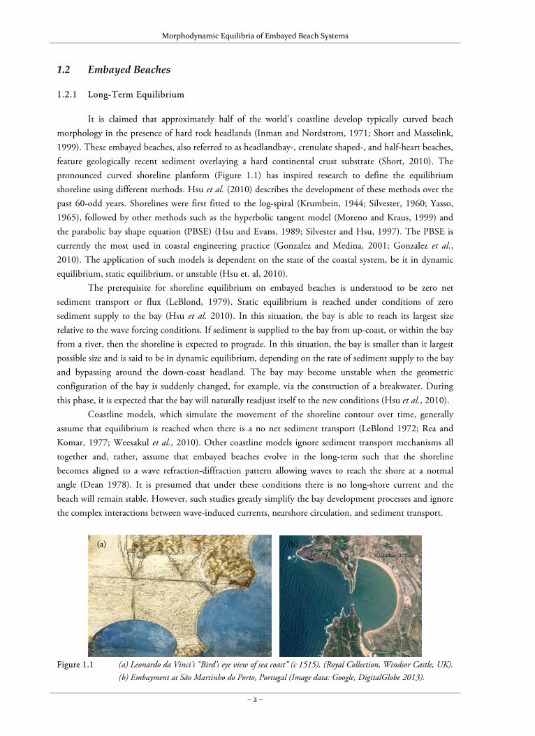
It is claimed that approximately half of the world's coastline develop typically curved beach morphology in the presence of hard rock headlands (Inman and Nordstrom, 1971; Short and Masselink, 1999). These embayed beaches, also referred to as headlandbay-, crenulate shaped-, and half-heart beaches, feature geologically recent sediment overlaying a hard continental crust substrate (Short, 2010). The pronounced curved shoreline planform (Figure 1.1) has inspired research to define the equilibrium shoreline using different methods. Hsu et al. (2010) describes the development of these methods over the past 60-odd years. Shorelines were first fitted to the log-spiral (Krumbein, 1944; Silvester, 1960; Yasso, 1965), followed by other methods such as the hyperbolic tangent model (Moreno and Kraus, 1999) and the parabolic bay shape equation (PBSE) (Hsu and Evans, 1989; Silvester and Hsu, 1997). The PBSE is currently the most used in coastal engineering practice (Gonzalez and Medina, 2001; Gonzalez et al., 2010). The application of such models is dependent on the state of the coastal system, be it in dynamic equilibrium, static equilibrium, or unstable (Hsu et. al, 2010).
The prerequisite for shoreline equilibrium on embayed beaches is understood to be zero net sediment transport or flux (LeBlond, 1979). Static equilibrium is reached under conditions of zero sediment supply to the bay (Hsu et al. 2010). In this situation, the bay is able to reach its largest size relative to the wave forcing conditions. If sediment is supplied to the bay from up-coast, or within the bay from a river, then the shoreline is expected to prograde. In this situation, the bay is smaller than it largest possible size and is said to be in dynamic equilibrium, depending on the rate of sediment supply to the bay and bypassing around the down-coast headland. The bay may become unstable when the geometric configuration of the bay is suddenly changed, for example, via the construction of a breakwater. During this phase, it is expected that the bay will naturally readjust itself to the new conditions (Hsu et al., 2010).
Coastline models, which simulate the movement of the shoreline contour over time, generally assume that equilibrium is reached when there is a no net sediment transport (LeBlond 1972; Rea and Komar, 1977; Weesakul et al., 2010). Other coastline models ignore sediment transport mechanisms all together and, rather, assume that embayed beaches evolve in the long-term such that the shoreline becomes aligned to a wave refraction-diffraction pattern allowing waves to reach the shore at a normal angle (Dean 1978). It is presumed that under these conditions there is no long-shore current and the beach will remain stable. However, such studies greatly simplify the bay development processes and ignore the complex interactions between wave-induced currents, nearshore circulation, and sediment transport.
Figure 1.1 (a) Leonardo da Vinci’s “Bird’s eye view of sea coast” (c 1515). (Royal Collection, Windsor Castle, UK).
(b) Embayment at São Martinho do Porto, Portugal (Image data: Google, DigitalGlobe 2013).
(b)(a)

Morphodynamic Equilibria of Embayed Beach Systems
– 3 –
1.2.2 Short-Term Dynamics
Sediment transport on beaches, and hence various morphodymanic features, are primarily driven by the action of waves and wave-induced currents. Nearshore circulation is, therefore, important in determining many shoreline and nearshore features, such as beach cusps, rip cells, and sandbars. Nearshore circulation patterns have been extensively studied on long, open coasts, with much attention paid to describing rip current circulation patterns within the surf zone from lagrangian field measurements (MacMahan et al., 2010) and also using numerical models (Castelle and Ruessink 2011). Circulation patterns within embayments are generally recognised to differ significantly from open coast circulation, with increased cellular circulation resulting from the presence of headland structures (Short, 1996; Loureiro et al., 2012b).
Field measurements of cellular circulation patterns within the shadow zone of embayments have been undertaken on a small scale (O~100 m), using lagrangian drifter methods (Pattiaratchi et al., 2009). In larger embayments (O~15 km), large-scale gyre structures have been observed (Valle-Levinson and Moraga-Opazo, 2006). Rip currents, ubiquitous on long, open coast beach systems, are also commonly observed within embayments, particularly using camera monitoring systems (Gallop et al., 2011; Loureiro et al., 2012a). These studies have all highlighted various flow patterns that tend to develop within embayments as well as studied their dynamics.
In addition to hydrodynamic processes, the observation of morphodynamic processes on embayed beaches has focused on shoreline evolution (Lavalle and Lakhan, 1997; Terpstra and Chrzastowski, 1992), beach cusp dynamics (Almar et al., 2008; Masselink and Pattiaratchi, 1998), beach rotation (Klein et al., 2003; Harley et al., 2011), bar migration (van Maanen et al., 2008), sediment bypassing around headland structures (Klein et al., 2010), and transitions of beach state (Price and Ruessink, 2011).
Numerical simulations of wave-driven circulation within embayments have reproduced the development of circulation cells around headland structures and within the embayment (Pattiaratchi et al., 2009; Silva et al., 2010). Improved accuracy in simulating nearshore hydrodynamics has led to sophisticated process-based morphodynamic modelling studies of embayed beaches (Reniers et al, 2004; Castelle and Coco, 2012). These studies have generally focused on nearshore rhythmicity induced by rip currents over relatively short time timescales, in the order of days to months.
1.3 Research Hypotheses and Questions
Following the aim of this thesis – to determine the processes governing how embayed beaches evolve over long-term timescales, and how they respond to short-term forcing – different types of wave forcing, environmental conditions, and geological settings are considered. In order to identify research questions, the existing assumptions commonly mentioned in the literature are first presented.
The equilibrium state of embayed beaches is often related to shore-normal wave incidence (e.g., Silvester and Hsu, 1997). According to this hypothesis, as waves approach the shoreline, they refract due to the local bathymetry. If the incident wave condition is in disequilibrium with the local bathymetry, the waves will reach the shore at an angle, break and generate long-shore currents that redistribute sediment in the direction of flow. Ultimately, the local bathymetry and wave refraction patterns will change so that an equilibrium state is reached when long-shore current velocities reach, theoretically, zero (LeBlond, 1979). It is further assumed that, once in this state, waves will break simultaneously around the beach, and that
Morphodynamic Equilibria of Embayed Beach Systems
– 4 –
diffraction plays an important role in this achieving this pattern as it is a process capable of redistributing energy in the shadow zone of emabyements (Dean, 1978; Silvester and Ho, 1972).
It is also commonly stated in the literature that the geological setting plays a significant role in determining the bay shape as it is capable of steering wave-driven currents causing cellular circulation patterns to develop in the bay (Short, 2010; Silva et al., 2010). The headlands also limit sediment bypassing, thus, restricting the movement of sediment within the bay. For example, Klein et al. (2000) describe the influence of the physical dimensions of the embayment (length and curvature) on the resulting morphodynamics.
Empirical shoreline formulae relate the curvature of the shoreline to the direction of wave approach and, in most cases, the mean or predominant (modal) wave direction is used for descriptive purposes (e.g., when applying the PBSE). Based on this assumption, the equilibrium state supposedly depends on a single wave direction.
The main hypothesis proposed in this thesis is that the variability of the wave climate has an important long-term effect on the orientation and shape of the beach planform. Variations in wave direction and directional spreading can alter the wave energy distribution around the embayment, therefore diffraction may not be important for determine the shoreline planform. Additionally, the equilibrium shape of an embayment cannot be determined solely from a single wave direction, but rather considering the directional variance of the wave climate. Moreover, the hypothesis can be extended to more general terms, so as to say that the magnitude of extreme events and their chronology are also important factors.
Based on the hypotheses presented above, several questions can be posed. What are the main processes affecting the morphological evolution of embayed beaches on a medium- to long-term timescale? What are the effects of extreme events versus average forcing on the equilibrium state? How do short- to medium-term dynamics affect long-term residuals? Can process-based models be used to simulate the morphological evolution of different boundary and initial conditions?
1.4 Research Methods
1.3.1 Numerical Modelling
In order to understand the long-term stability of embayed beaches, we need to be able to explain how such beaches form in the first place. In doing so, we can then predict how embayed beaches will respond to changes in forcing conditions. Most embayed beaches already exist in a stable state; hence it is rare to have real-world observations of embayed beach development. Down-scaled laboratory experiments have therefore been used to simulate such cases (Ho, 1971; Weesakul et al., 2012). However, laboratory experiments are prone to scale effects and it is impossible to separate interacting processes from each other, e.g., wave diffraction. Such processes have been identified as playing a key role in bay development but have not yet been quantified. Accordingly, process-based morphological models are therefore the best tools to use in order to conduct such investigations and fill this knowledge gap. For example, process-based models have been used in previous research by Yamashita and Tsuchiya (1992), who used a finite difference numerical model to determine the redistribution of sediment on an artificial sloping beach and an empirical parabolic-shaped beach; Reniers et al. (2004), who studied the morphological response of the nearshore area within an embayed beach caused by wave groups; and Silva et al. (2010), who examined the
Morphodynamic Equilibria of Embayed Beach Systems
– 5 –
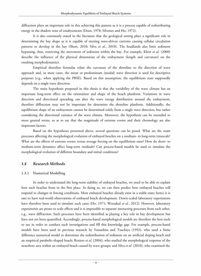
Figure 1.2 Schematization of the morphodynamic cycle. nearshore circulation patterns within embayed beaches. In this thesis, a state-of-the-art, morphodynamic, coastal area model was used in order to answer the previously identified research questions.
Coastal area models simulate hydrodynamic and morphodynamic processes over various temporal and spatial scales, typically between 1 day – 1000 years and 10 m – 100 km. The coastal morphodynamic processes are simulated by schematizing the morphodynamic cycle, as shown in Figure 1.2. Delft3D (Roelvink and van Banning, 1994; Lesser et al., 2004) is an open-source, process-based model that is structured into a number of modules that compute, for example, the propagation of waves, the direction and magnitude of currents, and the resulting sediment transport field. The model (version 5.00.11) uses a set of partial differential equations that are solved using finite difference methods. At the core of Delft3D are the Navier–Stokes (non-linear, shallow water) equations that describe water flow and are driven by the radiation stress gradients of the wave field and/or water level and velocity boundary conditions. The flow field can be defined in 1D, 2DH, 2DV and fully 3D modes using a rectangular or curvilinear grid structure. Wave forcing is computed using a spectral wave model, SWAN (Booij et al., 1999). The computation of bed level changes can be sped up with a morphological factor (Roelvink, 2006), enabling long-term simulations to be carried out within a reasonable amount of time.
A number of processes are parameterized within the model. For example, wave breaking is depth-induced and is controlled by a breaker parameter. Turbulence on a sub-grid scale is assumed to be contained within predefined constant eddy viscosity and eddy diffusivity terms. These parameters, therefore, require extensive calibration and validation. Most of these parameters are robust; however, a few are sensitive to specific cases and are often used to tune the model. These are generally parameters related to sediment transport and turbulence scaling. However, for schematic simulations where precise calibration is not required, the model can be verified based on how well the results fit an expected outcome. In this way, the models can be used for systematic study of forcing and initial conditions.
1.3.3 In-Situ Measurements
Embayed beaches are dynamic environments that vary over short- to medium timescales. Beach rotation and sediment redistribution within the bay occurs frequently and is dependent on the local wave
Morphodynamic Equilibria of Embayed Beach Systems
– 6 –
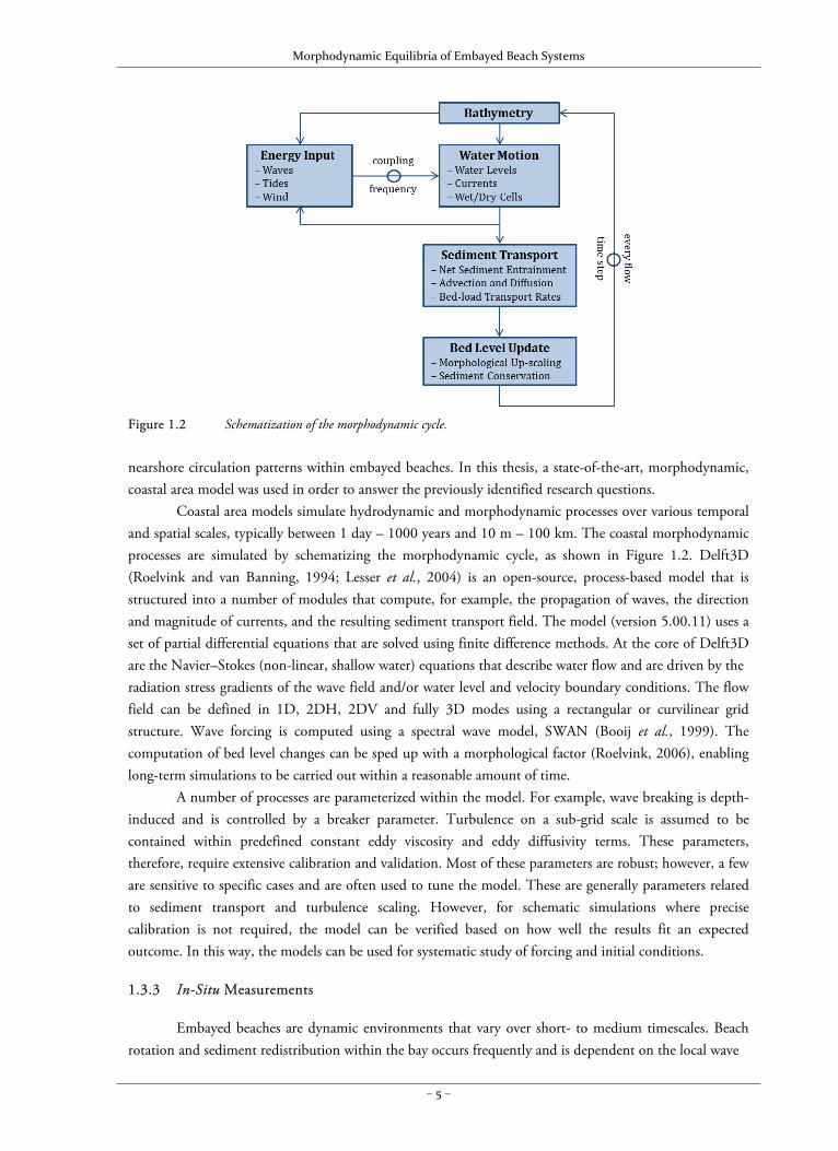
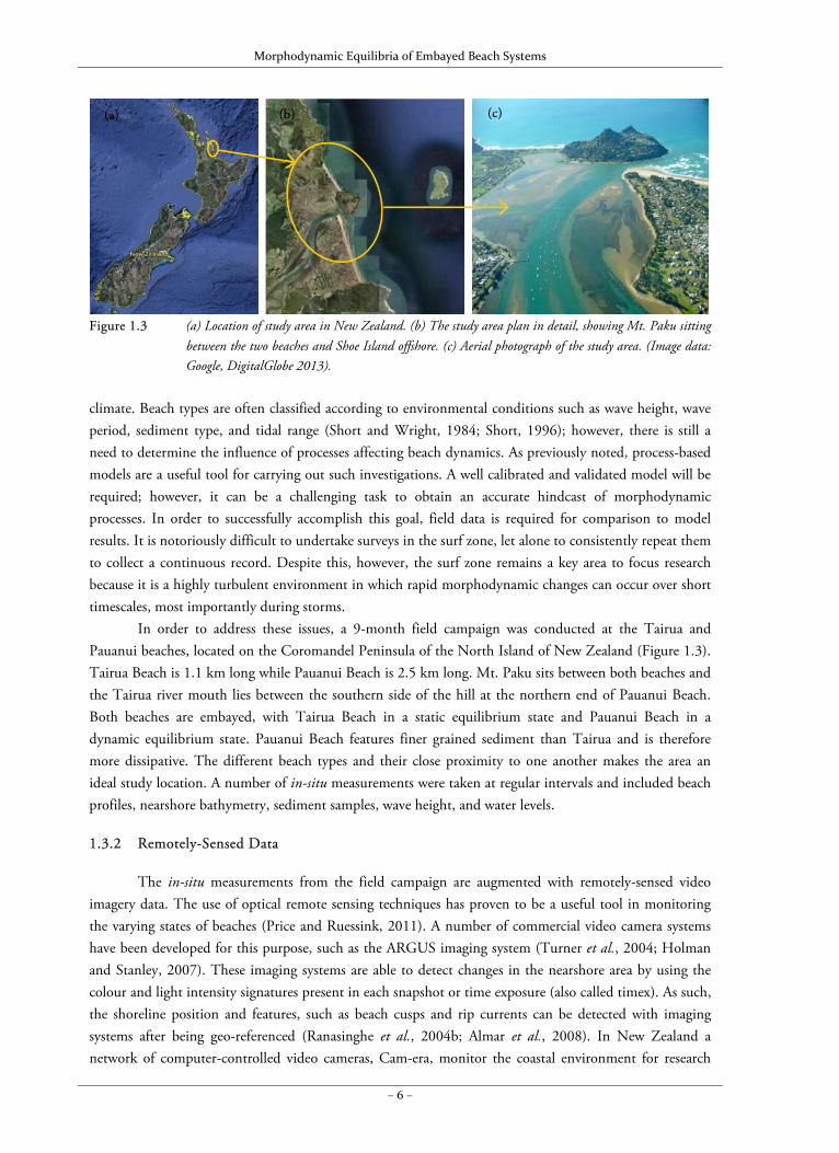
Figure 1.3 (a) Location of study area in New Zealand. (b) The study area plan in detail, showing Mt. Paku sitting
between the two beaches and Shoe Island offshore. (c) Aerial photograph of the study area. (Image data: Google, DigitalGlobe 2013).
climate. Beach types are often classified according to environmental conditions such as wave height, wave period, sediment type, and tidal range (Short and Wright, 1984; Short, 1996); however, there is still a need to determine the influence of processes affecting beach dynamics. As previously noted, process-based models are a useful tool for carrying out such investigations. A well calibrated and validated model will be required; however, it can be a challenging task to obtain an accurate hindcast of morphodynamic processes. In order to successfully accomplish this goal, field data is required for comparison to model results. It is notoriously difficult to undertake surveys in the surf zone, let alone to consistently repeat them to collect a continuous record. Despite this, however, the surf zone remains a key area to focus research because it is a highly turbulent environment in which rapid morphodynamic changes can occur over short timescales, most importantly during storms.
In order to address these issues, a 9-month field campaign was conducted at the Tairua and Pauanui beaches, located on the Coromandel Peninsula of the North Island of New Zealand (Figure 1.3). Tairua Beach is 1.1 km long while Pauanui Beach is 2.5 km long. Mt. Paku sits between both beaches and the Tairua river mouth lies between the southern side of the hill at the northern end of Pauanui Beach. Both beaches are embayed, with Tairua Beach in a static equilibrium state and Pauanui Beach in a dynamic equilibrium state. Pauanui Beach features finer grained sediment than Tairua and is therefore more dissipative. The different beach types and their close proximity to one another makes the area an ideal study location. A number of in-situ measurements were taken at regular intervals and included beach profiles, nearshore bathymetry, sediment samples, wave height, and water levels.
1.3.2 Remotely-Sensed Data
The in-situ measurements from the field campaign are augmented with remotely-sensed video imagery data. The use of optical remote sensing techniques has proven to be a useful tool in monitoring the varying states of beaches (Price and Ruessink, 2011). A number of commercial video camera systems have been developed for this purpose, such as the ARGUS imaging system (Turner et al., 2004; Holman and Stanley, 2007). These imaging systems are able to detect changes in the nearshore area by using the colour and light intensity signatures present in each snapshot or time exposure (also called timex). As such, the shoreline position and features, such as beach cusps and rip currents can be detected with imaging systems after being geo-referenced (Ranasinghe et al., 2004b; Almar et al., 2008). In New Zealand a network of computer-controlled video cameras, Cam-era, monitor the coastal environment for research
(a) (b) (c)
Morphodynamic Equilibria of Embayed Beach Systems
– 7 –
and resource management (http://www.niwa.co.nz/our-services/online-services/cam-era). There are Cam-era imaging systems at eight locations around New Zealand, including the embayed beaches of Tairua and Paunui. Using this technology, Van Maanen et al. (2008) detected onshore sandbar migration at Tairua, and Guedes et al. (2012) was able to discretize wave run-up on the beach slope. Images from the Cam-Era system were also be used to investigate nearshore and shoreline changes in response to changes in wave forcing conditions in the context of the research presented herein.
1.5 Thesis Outline
The work presented in this thesis consistently progresses from long-term timescales, over which the morphodynamic equilibrium of an embayed beach system can be determined, to short-term dynamics, characterised by high morphological variability. The initial investigations rely on process-based numerical modelling of schematized embayed beaches and subsequently move to real-world case studies. In Chapter 2, the applicability of morphodynamic models to simulate beach rotation is investigated. A schematic embayed beach, defined by combining equilibrium planform and profile formulae, is used and is exposed to constant wave forcing conditions. Results from these simulations show how sediment tends to be transported in the nearshore zone of the bay and gives an estimate for the amount of time required for the beach to stabilize. In Chapter 3, the effect of diffraction is investigated to determine its role in causing the curvature of embayed beach shorelines. More advanced schematic morphodynamic simulations are performed in which time-varying wave conditions are also taken into account. Additionally, the initial bathymetry for these simulations is a straight, plane-sloped beach rather than one that is already embayed. This approach is seen as a more rigorous test of the capability of the model to reproduce the expected curved shoreline shape. In Chapter 4, the effect of varying the environmental characteristics (sediment size, tidal range, wave energy) and geological setting (bay size and geometry) of an embayment is investigated. In these morphodynamic simulations, the development of the bay is analysed and the wide-ranging results synthesized to highlight similarities in patterns of bay development. A quantitative definition of site-specific spatial and temporal scales is reflected in the two coefficients of an exponential fit to the amount of time required for linear growth in bay area during its initial development. Chapter 5 shifts the study to the real world, with the aim of determining how the quasi-equilibrium bathymetry of an embayment is shaped by a highly variable directional wave climate. A method to determine the equilibrium bathymetry is tested by adapting morphodynamic input reduction methods to suit the limitations of embayed beach environments. Chapter 6 presents the outcome of the field campaign at Tairua and Pauanui beaches in New Zealand. This data will be used to reconstruct the measured short-term dynamics the embayed beaches using a conceptual, data-driven model. The results are to be used to determine how wave events and bay geometry force offshore sediment transport and beach rotation and will be inter-compared with morphodynamic simulations. Chapter 2 has been published in the Journal of Coastal Research, while Chapters 3 and 4 have been submitted to international peer-reviewed journals (Journal of Coastal Engineering and Journal of Geomorphology, respectively). Chapter 5 has been selected for publication in the Journal of Ocean Dynamics after initial review by the scientific committee of the 7th International Conference on Coastal Dynamics. The manuscript presented in Chapter 6 is currently in preparation.

Morphodynamic Equilibria of Embayed Beach Systems
– 8 –
Morphodynamic Equilibria of Embayed Beach Systems
– 9 –
Chapter 2 – Long‐Term, Constant Wave Forcing
This Chapter is based on a manuscript published in the Journal of Coastal Research (2011, Special Issue 64,
pages 1003–1007) titled:
“Morphodynamics of Embayed Beaches: The Effect of Wave Conditions”
Christopher J. Daly1,2, Karin R. Bryan2, Dano A. Roelvink3, Antonio H.F. Klein4, Dierk Hebbeln1 and Christian Winter1
1 MARUM – Center for Marine Environmental Research, University of Bremen, Bremen, Germany
2 Deptartment of Earth and Ocean Science, University of Waikato, Hamilton , New Zealand 3 UNESCO-IHE, Delft, the Netherlands
4 Department of Geosciences, Federal University of Santa Catarina, Florianópolis, Brazil
2.1 Abstract
Embayed beaches are abundant along many coastlines of the world, yet our understanding of the role of wave conditions on their morphodynamics still needs to be furthered in order to better predict their dynamics. In this paper, a numerical modeling approach was used to determine the response of embayed beaches to varied wave forcing. The process-based numerical model, Delft3D, was used to simulate 16 wave conditions. Results indicate that complex flow patterns develop within the bay which drive long-shore and cross-shore currents. These currents actively interact to promote the formation of a stable bay shape. The resulting bathymetry in the bay is highly dependent on the incident wave conditions. It is also shown that beach rotation can occur for the same mean wave direction due to changes in the directional spreading. The numerical modeling approach has given agreeable results, and can be further used to explore the importance of other factors affecting embayed beach morphology, such as nearshore processes and bay geometry.
Morphodynamic Equilibria of Embayed Beach Systems
– 10 –
2.2 Introduction
It is generally accepted that about half of the world's coastline features typical beach morphology in the presence of hard rock headlands (Short and Masselink, 1999). These embayed beaches, also referred to as headland-bay, crenulate-shaped, half-heart and pocket beaches, typically feature geologically recent sediment eroded from land and overlaying a hard continental crust substrate (Short, 2010). The shape of these beaches is typically curved in plan, which lead researchers to first define an equilibrium shoreline using different methods, as discussed in Hsu et al. (2010) (and references within).
The parabolic bay shape equation (PBSE) (Hsu and Evans, 1989) identifies the equilibrium planform of embayed beaches and is currently the most used in practice (Gonzalez and Medina, 2001). Its development has been stimulated by the general need for rapid evaluation of the effect of anthropogenic changes to coastal areas and shorelines (Silvester and Hsu, 1997). The PBSE can determine the approximate equilibrium shoreline shape, but it is purely empirical and does not offer an explanation for the effect of factors such as wave conditions, nearshore processes or bay geometry on the morphological response of the entire bay area.
In order to further understand embayed beach dynamics, researchers have in recent years sought answers from field observations of sediment transport (Dai et al., 2010), beach rotation (Klein et al., 2002), nearshore current structure (Dehouk et al., 2009) and storm impacts (Martins et al., 2010) over a short-term (monthly) basis. Long-term (yearly) observations obtained from camera images have been used to investigate small-scale morphological features such as beach cusps, bar patterns and rip currents (Almar et al., 2008, Gallop et al., 2010). Each field site features its own native geological structure and complex hydrodynamic forcing, which makes their assessment site specific.
In contrast to the number of reports on field observations, very few numerical studies have been done featuring embayed beaches (Yamashita and Tsuchiya, 1992; Reniers et al., 2004; Silva et al., 2010). Morphodynamic numerical models have been developed to such an advanced state that they are now used to investigate different types of coastal systems and complex morphological features (Reniers et al., 2004; Smit et al., 2008). As such, they can also be used to model embayed beach systems in order to measure how individual factors, such as wave conditions, bay geometry and physical process, affect their dynamics.
This research was therefore designed to gain insight into the main wave characteristics which influence the evolution of embayed beach systems. This is done by modeling various wave conditions (wave height, period, direction and spreading) and observing their effect on the morphodynamics of a schematized embayed beach. The different scenarios are investigated by using a time-dependent, process-based numerical model over moderate spatial and temporal scales. The commercial version of the numerical model Delft3D is used in the present work. The results point to the important mechanisms of sediment transport within the bay and give an estimate for the response time of the morphodynamic system to adjust to the forcing conditions.
2.3 Model Setup
2.3.1 Model Description
Delft3D (Lesser et al., 2004) is a time-dependent, process-based, morphological model which consists of wave and flow modules. In the wave module, wave propagation (refraction and diffraction) and dissipation (depth-induced breaking, bottom friction) are computed with the spectral wave model, SWAN
Morphodynamic Equilibria of Embayed Beach Systems
– 11 –
(Booij et al., 1999). The flow module solves the depth-averaged Navier-Stokes equations for an incompressible fluid (motion and continuity), driven by radiation stress gradients calculated in the wave module. The flow module is coupled with the wave module and can thus account for effect of currents on waves and vice versa (wave-current interaction). Additionally, a short-wave roller energy dissipation add-on is enabled which allows the modeling of surf-beat in the domain.
The flow module includes a sediment transport and morphology add-on. Non-cohesive suspended sediment transport (a function of inter alia the depth-averaged sediment concentration and horizontal diffusion coefficient) and bedload transport (a function of inter alia the bottom shear stress and median grain diameter) are computed according to Van Rijn (1993). The bed level continuity equation in combination with a sediment conservation scheme is used to determine bed level changes at each time step based on combined suspended sediment and bed load transport.
2.3.2 Initial Bathymetry
The initial bathymetry (Figure 2.1a) used for the morphological simulations feature headlands parallel to the coastline and interrupted in the center by an embayment. The gap width between the headlands is 1200 m and the depth of the bay is 450 m (determined by lines drawn from the headland tips at an angle of 37° to the coastline, which intersect in the centre of the bay). The length of each headland is 600 m.
The PBSE is used in conjunction with an equilibrium beach profile model (Dean, 1991) to generate an empirical internal bathymetry for the bay. These formulations are used to give a representative estimate of the volume of sediment in the system. In doing so, the down-drift control point used in the PBSE corresponds to the point of intersection of lines drawn from the tip of each headland at the angle specified above. The shoreline is defined by assuming waves arriving normal to the coast, thus the central beach profile of the bay is scaled around the rest of the bay area between the shoreline and the chord spanning from headland to headland, assuming that the depth between the headlands is constant.
The equilibrium beach profile is defined based on a median grain diameter of 0.3 mm. The profile extends to the seaward boundary of the model located at a depth of 18 m. The ‘open sea’ area of the domain (area seaward from headlands) is 900 m wide and 2400 m long.
2.3.3 Model Settings
The model is run on a variable rectangular grid, with lower resolution by the offshore boundary (40 m × 20 m grid cells) and a higher resolution within the bay (20 m × 20 m grid cells). A time step of 12 s is used in the flow computations. A morphological factor (Roelvink, 2006) of 10 is used to speed up the computation of bed level changes. Wave conditions are re-computed using an updated bathymetry every 72 minutes, which is equivalent to every 12 hours morphologically. The model is run for 150 days, which is equivalent to 4 years of morphological changes. The model setup allows a 12 hour period for the model to reach hydrodynamic equilibrium before beginning morphological computations.
Wave Conditions
The numerical simulations are set-up in a manner which will facilitate a broad sensitivity analysis for different combinations of wave conditions. A total of 16 simulations are designed based on combinations of 4 wave parameters given as:
Morphodynamic Equilibria of Embayed Beach Systems
– 12 –
- Significant Wave Height (Hs) = 1 m / 2 m
- Mean Wave Period (Tm01) = 6 s / 10 s
- Wave Direction (Dir) = 0° / 20°
- Directional Spreading (cosine) (Dspr) = 4 / 20 Wave forcing is kept constant for the entire simulation period. This allows the initial bathymetry to rework itself into a state that is relatively in equilibrium with the incoming wave conditions.
2.4 Results
2.4.1 Beach Rotation and Evolution by Wave Direction
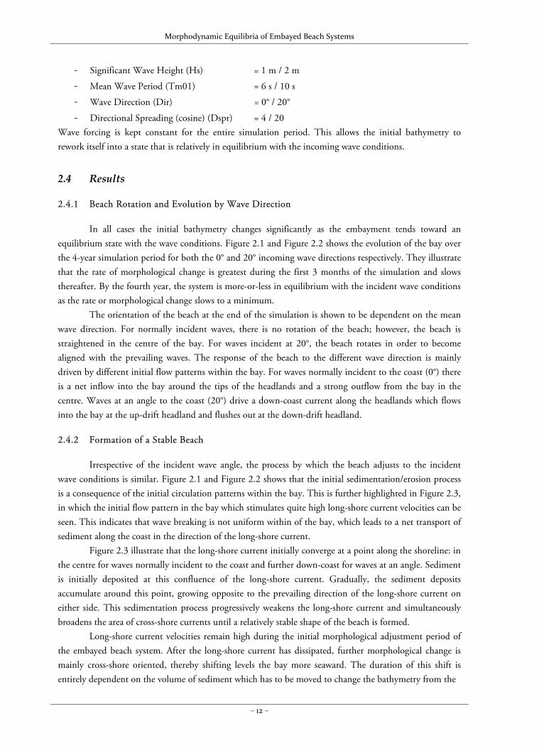
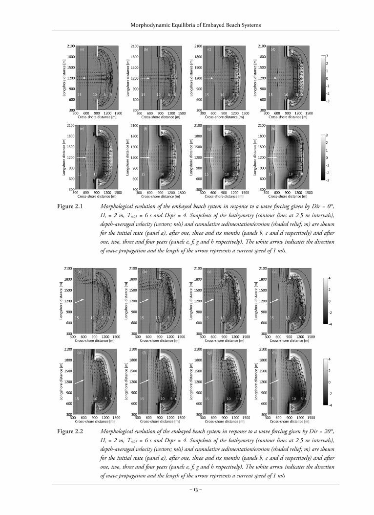
In all cases the initial bathymetry changes significantly as the embayment tends toward an equilibrium state with the wave conditions. Figure 2.1 and Figure 2.2 shows the evolution of the bay over the 4-year simulation period for both the 0° and 20° incoming wave directions respectively. They illustrate that the rate of morphological change is greatest during the first 3 months of the simulation and slows thereafter. By the fourth year, the system is more-or-less in equilibrium with the incident wave conditions as the rate or morphological change slows to a minimum.
The orientation of the beach at the end of the simulation is shown to be dependent on the mean wave direction. For normally incident waves, there is no rotation of the beach; however, the beach is straightened in the centre of the bay. For waves incident at 20°, the beach rotates in order to become aligned with the prevailing waves. The response of the beach to the different wave direction is mainly driven by different initial flow patterns within the bay. For waves normally incident to the coast (0°) there is a net inflow into the bay around the tips of the headlands and a strong outflow from the bay in the centre. Waves at an angle to the coast (20°) drive a down-coast current along the headlands which flows into the bay at the up-drift headland and flushes out at the down-drift headland.
2.4.2 Formation of a Stable Beach
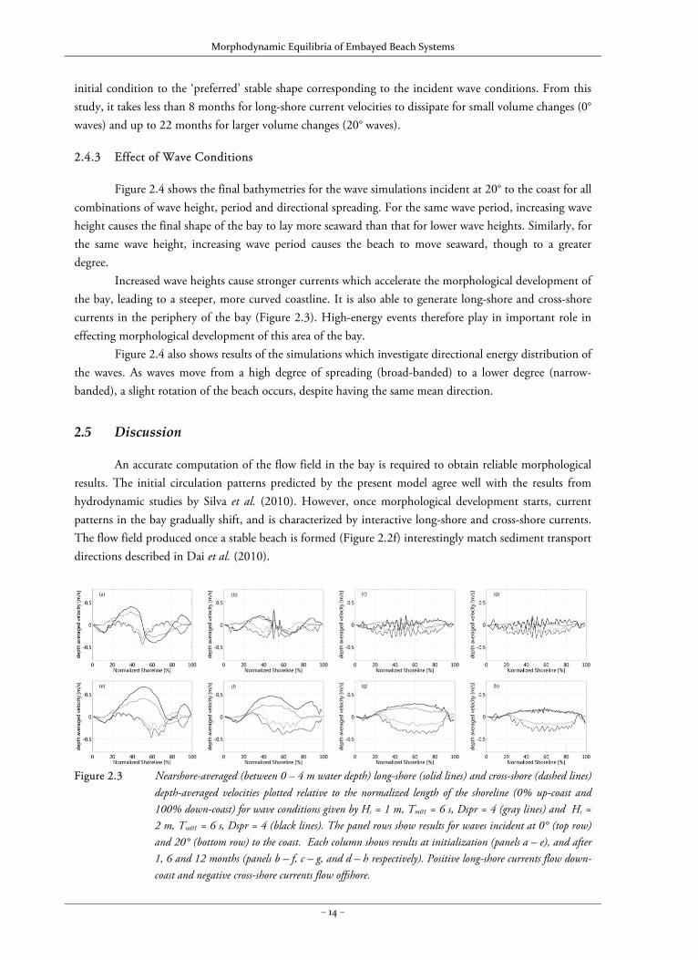
Irrespective of the incident wave angle, the process by which the beach adjusts to the incident wave conditions is similar. Figure 2.1 and Figure 2.2 shows that the initial sedimentation/erosion process is a consequence of the initial circulation patterns within the bay. This is further highlighted in Figure 2.3, in which the initial flow pattern in the bay which stimulates quite high long-shore current velocities can be seen. This indicates that wave breaking is not uniform within of the bay, which leads to a net transport of sediment along the coast in the direction of the long-shore current.
Figure 2.3 illustrate that the long-shore current initially converge at a point along the shoreline: in the centre for waves normally incident to the coast and further down-coast for waves at an angle. Sediment is initially deposited at this confluence of the long-shore current. Gradually, the sediment deposits accumulate around this point, growing opposite to the prevailing direction of the long-shore current on either side. This sedimentation process progressively weakens the long-shore current and simultaneously broadens the area of cross-shore currents until a relatively stable shape of the beach is formed.
Long-shore current velocities remain high during the initial morphological adjustment period of the embayed beach system. After the long-shore current has dissipated, further morphological change is mainly cross-shore oriented, thereby shifting levels the bay more seaward. The duration of this shift is entirely dependent on the volume of sediment which has to be moved to change the bathymetry from the
Morphodynamic Equilibria of Embayed Beach Systems
– 13 –
Figure 2.1 Morphological evolution of the embayed beach system in response to a wave forcing given by Dir = 0°,
Hs = 2 m, Tm01 = 6 s and Dspr = 4. Snapshots of the bathymetry (contour lines at 2.5 m intervals), depth-averaged velocity (vectors; m/s) and cumulative sedimentation/erosion (shaded relief; m) are shown for the initial state (panel a), after one, three and six months (panels b, c and d respectively) and after one, two, three and four years (panels e, f, g and h respectively). The white arrow indicates the direction of wave propagation and the length of the arrow represents a current speed of 1 m/s.
Figure 2.2 Morphological evolution of the embayed beach system in response to a wave forcing given by Dir = 20°,
Hs = 2 m, Tm01 = 6 s and Dspr = 4. Snapshots of the bathymetry (contour lines at 2.5 m intervals), depth-averaged velocity (vectors; m/s) and cumulative sedimentation/erosion (shaded relief; m) are shown for the initial state (panel a), after one, three and six months (panels b, c and d respectively) and after one, two, three and four years (panels e, f, g and h respectively). The white arrow indicates the direction of wave propagation and the length of the arrow represents a current speed of 1 m/s
Morphodynamic Equilibria of Embayed Beach Systems
– 14 –
initial condition to the ‘preferred’ stable shape corresponding to the incident wave conditions. From this study, it takes less than 8 months for long-shore current velocities to dissipate for small volume changes (0° waves) and up to 22 months for larger volume changes (20° waves).
2.4.3 Effect of Wave Conditions
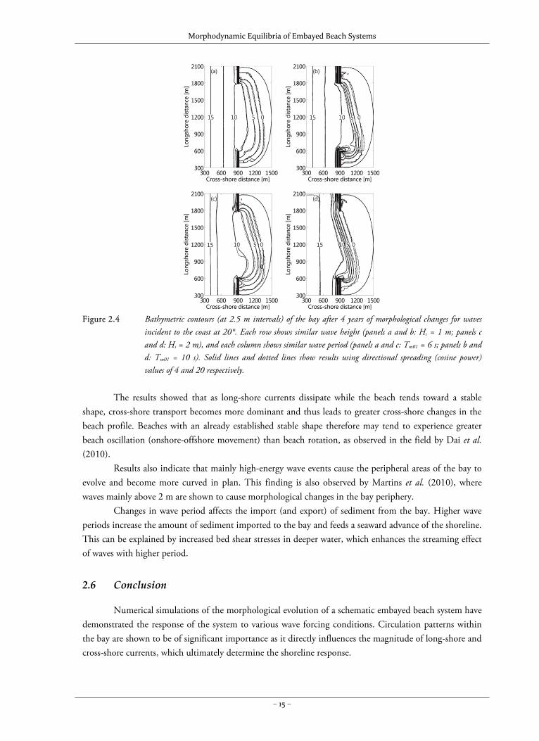
Figure 2.4 shows the final bathymetries for the wave simulations incident at 20° to the coast for all combinations of wave height, period and directional spreading. For the same wave period, increasing wave height causes the final shape of the bay to lay more seaward than that for lower wave heights. Similarly, for the same wave height, increasing wave period causes the beach to move seaward, though to a greater degree.
Increased wave heights cause stronger currents which accelerate the morphological development of the bay, leading to a steeper, more curved coastline. It is also able to generate long-shore and cross-shore currents in the periphery of the bay (Figure 2.3). High-energy events therefore play in important role in effecting morphological development of this area of the bay.
Figure 2.4 also shows results of the simulations which investigate directional energy distribution of the waves. As waves move from a high degree of spreading (broad-banded) to a lower degree (narrow-banded), a slight rotation of the beach occurs, despite having the same mean direction.
2.5 Discussion
An accurate computation of the flow field in the bay is required to obtain reliable morphological results. The initial circulation patterns predicted by the present model agree well with the results from hydrodynamic studies by Silva et al. (2010). However, once morphological development starts, current patterns in the bay gradually shift, and is characterized by interactive long-shore and cross-shore currents. The flow field produced once a stable beach is formed (Figure 2.2f) interestingly match sediment transport directions described in Dai et al. (2010).
Figure 2.3 Nearshore-averaged (between 0 – 4 m water depth) long-shore (solid lines) and cross-shore (dashed lines)
depth-averaged velocities plotted relative to the normalized length of the shoreline (0% up-coast and 100% down-coast) for wave conditions given by Hs = 1 m, Tm01 = 6 s, Dspr = 4 (gray lines) and Hs = 2 m, Tm01 = 6 s, Dspr = 4 (black lines). The panel rows show results for waves incident at 0° (top row) and 20° (bottom row) to the coast. Each column shows results at initialization (panels a – e), and after 1, 6 and 12 months (panels b – f, c – g, and d – h respectively). Positive long-shore currents flow down-coast and negative cross-shore currents flow offshore.
Morphodynamic Equilibria of Embayed Beach Systems
– 15 –
Figure 2.4 Bathymetric contours (at 2.5 m intervals) of the bay after 4 years of morphological changes for waves
incident to the coast at 20°. Each row shows similar wave height (panels a and b: Hs = 1 m; panels c and d: Hs = 2 m), and each column shows similar wave period (panels a and c: Tm01 = 6 s; panels b and d: Tm01 = 10 s). Solid lines and dotted lines show results using directional spreading (cosine power) values of 4 and 20 respectively.
The results showed that as long-shore currents dissipate while the beach tends toward a stable
shape, cross-shore transport becomes more dominant and thus leads to greater cross-shore changes in the beach profile. Beaches with an already established stable shape therefore may tend to experience greater beach oscillation (onshore-offshore movement) than beach rotation, as observed in the field by Dai et al. (2010).
Results also indicate that mainly high-energy wave events cause the peripheral areas of the bay to evolve and become more curved in plan. This finding is also observed by Martins et al. (2010), where waves mainly above 2 m are shown to cause morphological changes in the bay periphery.
Changes in wave period affects the import (and export) of sediment from the bay. Higher wave periods increase the amount of sediment imported to the bay and feeds a seaward advance of the shoreline. This can be explained by increased bed shear stresses in deeper water, which enhances the streaming effect of waves with higher period.
2.6 Conclusion
Numerical simulations of the morphological evolution of a schematic embayed beach system have demonstrated the response of the system to various wave forcing conditions. Circulation patterns within the bay are shown to be of significant importance as it directly influences the magnitude of long-shore and cross-shore currents, which ultimately determine the shoreline response.
Morphodynamic Equilibria of Embayed Beach Systems
– 16 –
Strong long-shore currents are initially induced which re-distribute sediment along the shoreline until a stable shape is formed (possibly causing rotation of the beach). Cross-shore transport subsequently becomes more significant once long-shore currents have dissipated.
The preferred stable shape that the bay tends towards is quite variable and is highly dependent on combinations of wave height and period. The rate of morphological change is dependent on wave height and the volume of sediment to be transported, with the time required for the beach adjustment to new wave conditions varying between 8 to 22 months. Directional spreading is of lesser importance to the overall evolution of the bay, but is shown to be capable of producing slight rotations of the beach.
Given the agreeable results from the model in the present study, its use can be further extended to investigate the importance of physical processes which influence nearshore hydrodynamics. The model can also be used to account for variations in physical parameters, such as sediment characteristics and bay geometry.
2.7 Acknowledgements
C.J. Daly acknowledges funding from the DFG (Deutsche Forschungs-gemeinschaft) International Research Training Group: INTERCOAST - Integrated Coastal Zone and Shelf-Sea Research. K.R. Bryan acknowledges the Hanse Wissenschaftskolleg for awarding a Research Fellowship in Delmenhorst, Germany.
Morphodynamic Equilibria of Embayed Beach Systems
– 17 –
Chapter 3 – Long‐Term, Time‐Varying Wave Forcing
This Chapter is based on a manuscript submitted to the Journal of Coastal Engineering titled:
“Wave Energy Distribution and Morphological Development in and around the Shadow Zone of an Embayed Beach”
Christopher J. Daly 1,2, Karin R. Bryan 2, and Christian Winter 1
1 MARUM – Center for Marine Environmental Sciences, Universität Bremen, Germany
2 Department of Earth and Ocean Sciences, University of Waikato, New Zealand
3.1 Abstract
The curved shoreline shape of embayed beaches is one of its most notable characteristics and can be described using the parabolic bay shape equation (PBSE). Wave diffraction in and around the shadow zone is often regarded as the primary forcing mechanism leading to the prominent curvature of the shoreline. However, wave climate variables (wave direction, directional spreading and wave height) are shown to be influential in redistributing wave energy throughout the bay and in the shadow zone. In this study, a process-based morphological model (Delft3D) is used for steady-state and morphodynamic simulations of a schematic embayed beach. Wave forcing conditions are systematically varied between a mixture of time-invariant and time-varying cases. The role of diffraction is shown to be dominant only when the wave conditions are both narrow-banded (< 20°) and when the PBSE angle β is high (> 30°). Otherwise, as little as 6% variation in wave direction within a 90° range can account for the shoreline curvature in and around the shadow zone. The degree to which wave direction and directional spreading vary through time therefore has a large effect on the equilibrium orientation and shoreline planform of the bay.
Morphodynamic Equilibria of Embayed Beach Systems
– 18 –
3.2 Introduction
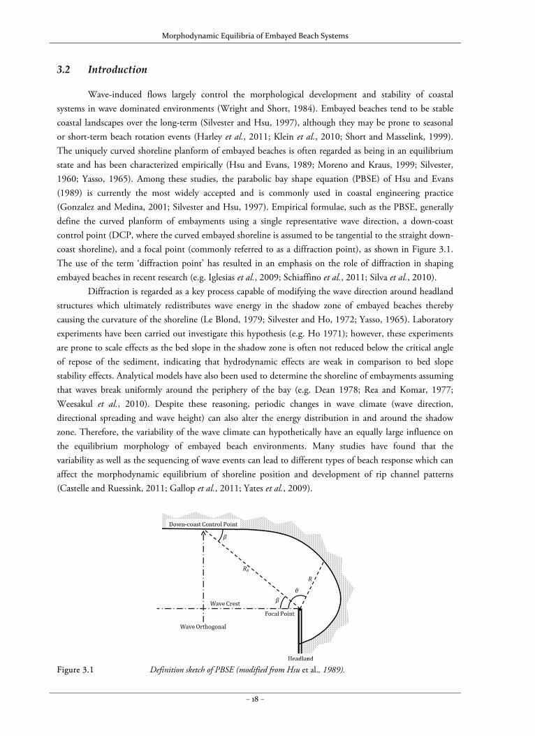
Wave-induced flows largely control the morphological development and stability of coastal systems in wave dominated environments (Wright and Short, 1984). Embayed beaches tend to be stable coastal landscapes over the long-term (Silvester and Hsu, 1997), although they may be prone to seasonal or short-term beach rotation events (Harley et al., 2011; Klein et al., 2010; Short and Masselink, 1999). The uniquely curved shoreline planform of embayed beaches is often regarded as being in an equilibrium state and has been characterized empirically (Hsu and Evans, 1989; Moreno and Kraus, 1999; Silvester, 1960; Yasso, 1965). Among these studies, the parabolic bay shape equation (PBSE) of Hsu and Evans (1989) is currently the most widely accepted and is commonly used in coastal engineering practice (Gonzalez and Medina, 2001; Silvester and Hsu, 1997). Empirical formulae, such as the PBSE, generally define the curved planform of embayments using a single representative wave direction, a down-coast control point (DCP, where the curved embayed shoreline is assumed to be tangential to the straight down-coast shoreline), and a focal point (commonly referred to as a diffraction point), as shown in Figure 3.1. The use of the term ‘diffraction point’ has resulted in an emphasis on the role of diffraction in shaping embayed beaches in recent research (e.g. Iglesias et al., 2009; Schiaffino et al., 2011; Silva et al., 2010).
Diffraction is regarded as a key process capable of modifying the wave direction around headland structures which ultimately redistributes wave energy in the shadow zone of embayed beaches thereby causing the curvature of the shoreline (Le Blond, 1979; Silvester and Ho, 1972; Yasso, 1965). Laboratory experiments have been carried out investigate this hypothesis (e.g. Ho 1971); however, these experiments are prone to scale effects as the bed slope in the shadow zone is often not reduced below the critical angle of repose of the sediment, indicating that hydrodynamic effects are weak in comparison to bed slope stability effects. Analytical models have also been used to determine the shoreline of embayments assuming that waves break uniformly around the periphery of the bay (e.g. Dean 1978; Rea and Komar, 1977; Weesakul et al., 2010). Despite these reasoning, periodic changes in wave climate (wave direction, directional spreading and wave height) can also alter the energy distribution in and around the shadow zone. Therefore, the variability of the wave climate can hypothetically have an equally large influence on the equilibrium morphology of embayed beach environments. Many studies have found that the variability as well as the sequencing of wave events can lead to different types of beach response which can affect the morphodynamic equilibrium of shoreline position and development of rip channel patterns (Castelle and Ruessink, 2011; Gallop et al., 2011; Yates et al., 2009).
Figure 3.1 Definition sketch of PBSE (modified from Hsu et al., 1989).
Morphodynamic Equilibria of Embayed Beach Systems
– 19 –
As the distribution of embayed beaches covers a wide range of geological settings and wave climates, it is difficult to separate the influence of the many interacting processes which affect local sediment transport dynamics, even based on well-structured field campaigns (Loureiro et al., 2012a; Short, 2010). Processed-based morphodynamic models are now sufficiently advanced that they can be used as a numerical laboratory to separate and study the interaction and effects of natural processes in relation to various wave forcing scenarios (Castelle and Ruessink, 2011; Roelvink and Reniers, 2012; Smit et al., 2008). These models have already been used to simulate embayed beaches with the goal of understanding their dynamics. For example, Yamashita and Tsuchiya (1992) simulated circulation patterns and sediment redistribution using a single wave condition. Reniers et al. (2004) studied the influence of wave groups and infragravity waves on the development of nearshore morphological rhythmicity induced by rip currents, and Castelle and Coco (2012) investigated how rip currents and circulation patterns are affected by changes in bay width. These studies are restricted to relatively short timescales (in the order of days to months) and feature embayments with limited curvature. Daly et al. (2011) showed how a schematic embayed beach responded to a number of constant wave forcing conditions over a four-year period, but did not investigate the effect of wave climate variability. Despite the many advances in this area of morphodynamic modelling, neither the influence of wave diffraction nor the variance of the wave climate have been together systematically investigated from a process-based perspective.
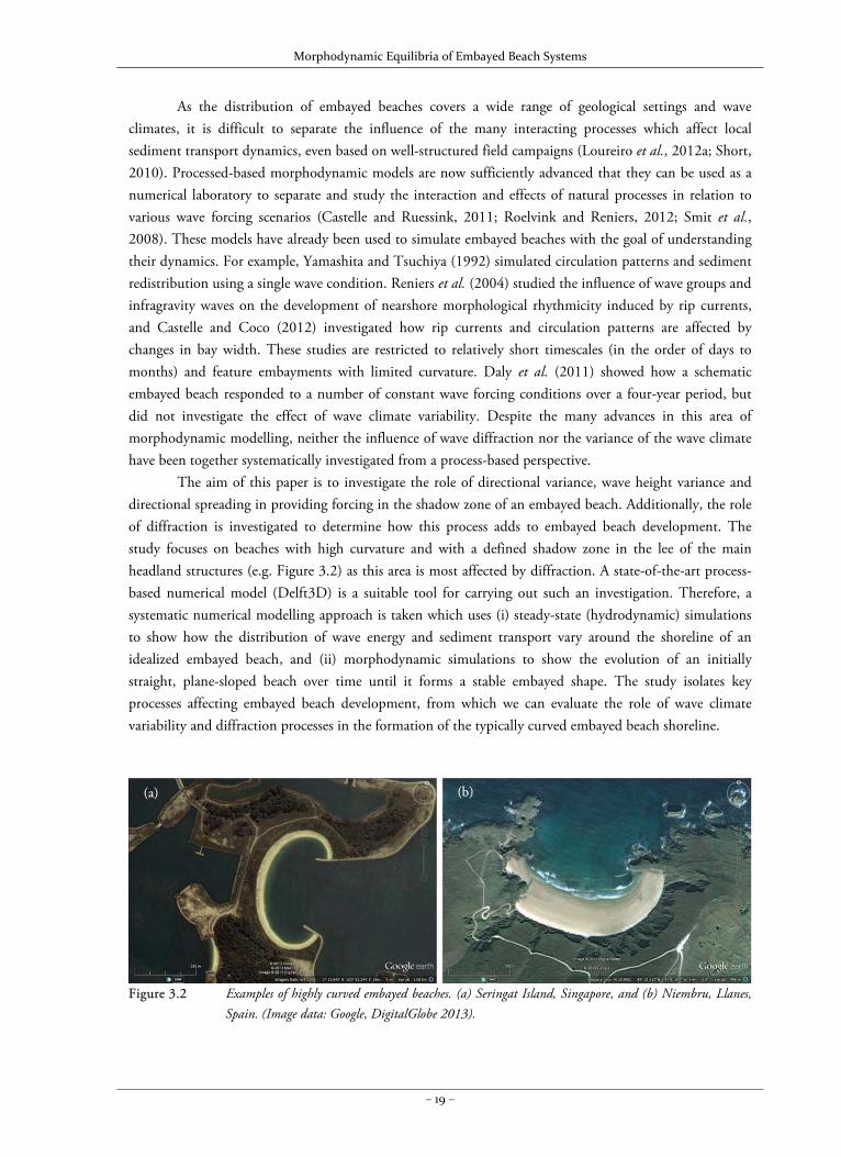
The aim of this paper is to investigate the role of directional variance, wave height variance and directional spreading in providing forcing in the shadow zone of an embayed beach. Additionally, the role of diffraction is investigated to determine how this process adds to embayed beach development. The study focuses on beaches with high curvature and with a defined shadow zone in the lee of the main headland structures (e.g. Figure 3.2) as this area is most affected by diffraction. A state-of-the-art process-based numerical model (Delft3D) is a suitable tool for carrying out such an investigation. Therefore, a systematic numerical modelling approach is taken which uses (i) steady-state (hydrodynamic) simulations to show how the distribution of wave energy and sediment transport vary around the shoreline of an idealized embayed beach, and (ii) morphodynamic simulations to show the evolution of an initially straight, plane-sloped beach over time until it forms a stable embayed shape. The study isolates key processes affecting embayed beach development, from which we can evaluate the role of wave climate variability and diffraction processes in the formation of the typically curved embayed beach shoreline.
Figure 3.2 Examples of highly curved embayed beaches. (a) Seringat Island, Singapore, and (b) Niembru, Llanes,
Spain. (Image data: Google, DigitalGlobe 2013).
(a) (b)
Morphodynamic Equilibria of Embayed Beach Systems
– 20 –
3.3 Numerical Model Description and Setup
3.3.1 Numerical Model Description
The open-source, process-based model, Delft3D (Lesser et al., 2004), was used to simulate hydrodynamic and morphodynamic processes on an idealized embayed beach (version 5.00.11). Delft3D combines several computational modules which interactively calculate wave transformation, wave-induced flows, sediment transport and the resulting morphological changes in a time-dependent cycle. Relevant aspects of the Delft3D model to the current work are described in the following section; however, detailed a description of the numerical structure and formulations of the model can be found in the Delft3D user manuals (http://oss.deltares.nl/web/delft3d/manuals). 3.3.1.1 Waves and Currents
The spectral, phase-averaged, third generation wave model, SWAN (Booij et al., 1999), is used as the Delft3D wave transformation module to solve the wave action balance equation, given as:
(3.1)
where A is the wave action density; t is time; x and y are horizontal Cartesian coordinates; ω and θ are the wave frequency and direction; cx, cy, cω, cθ are the phase velocity in x, y, ω and θ space, respectively; and S is a source and sink term related to wave generation, Sin, non-linear interactions (triads and quadruplets), Snl, and energy dissipation (bottom friction, breaking and whitecapping), Sdis. This equation transforms input spectral boundary wave conditions across the model domain while accounting for refraction. Additionally, the model includes a phase-decoupled approximation for wave diffraction based on the mild-slope equation (Holthuijsen et al., 2003). This is done by using a diffraction parameter, δa, to modify the wave number, k, which is the gradient of the phase function in the mild-slope equation. δa is expressed as:
(3.2)
where is the gradient operator ( ⁄ ⁄ ); cg is the group velocity; κ is a separation parameter; and a is the wave amplitude. δa therefore considers the spatial derivative of a caused by wave shadowing. The directional component of the phase velocity in Equation 3.1 is then modified by substituting it with:
1 12 1
(3.3)
where ⁄ is the directional turning rate in the direction of propagation, s; and m is the distance along the iso-phase line and Cg is the diffraction-corrected group velocity given as:
1 ⁄ (3.4)
The SWAN output gives the spatially varying direction of wave propagation and radiation stress gradients. Within the Delft3D flow module, the Navier–Stokes equations are solved under the shallow water and Boussinesq assumptions. The depth-averaged continuity equation is given as:
0 (3.5)
Morphodynamic Equilibria of Embayed Beach Systems
– 21 –
where η is the water level; h is the water depth (including η); and u and v are the depth-averaged velocities in the x and y direction, respectively. The momentum equations are given as:
0 (3.6)
0 (3.7)
where νt is the turbulent eddy viscosity; ρw is the water density; τ is the bed shear stress; and F is the wave-induced force computed in SWAN from the gradient of the radiation stresses. Vertical momentum and accelerations are neglected in these equations. The Generalized Lagrangian Mean (GLM) method (Groeneweg and Klopman, 1998; Walstra et al., 2000) is used to account for wave-induced mass flux, which includes the Stokes drift contribution from the waves, such that:
(3.8)
where the superscripts E and S represent the Eularian and Stokes contributions respectively. The flow and wave modules are coupled at regular intervals in order to update the wave field in response to changes in forcing conditions and bathymetry. During coupling, SWAN is able to include the effects of ambient currents (computed in the flow module) on wave propagation; therefore, the effect of wave-current interaction is accounted for. 3.3.1.2 Sediment Transport and Morphodynamics
In the sediment transport module of Delft3D, non-cohesive suspended sediment transport is computed using the depth-averaged advection-diffusion equation for sediment, given as:
(3.9)
where and eq are the depth-averaged and equilibrium suspended sediment concentrations; and are the depth-averaged GLM velocities; εh is the horizontal eddy diffusivity; and Ts is a timescale related to the ratio of shear velocity to fall velocity. Bed-load sediment transport (a function of inter alia the bed shear stress, bed slope and median grain diameter) is computed according to van Rijn (1993). Transverse and longitudinal slope effects on the bed-load sediment transport are determined according to Ikeda (1982). Bed-load sediment transport is enhanced by the effect of wave-induced currents, also following van Rijn (1993). Geomechanical failure of the sediment bed is characterized by an avalanching function whereby the volume of sediment above an established critical wet slope is added to the downslope bed-load sediment transport rate over a specified time period. The bed level continuity equation in combination with a sediment conservation scheme is used to determine bed level changes at each time step based on the combined suspended and bed-load sediment transport, given by:
1 , ,, , (3.10)
where εp is the bed porosity; zb is the bed level; Sb is the total bed-load sediment transport (due to waves and currents); and Sc,d and Sc,e are the deposition and erosion rates of suspended sediment transport. Morphodynamic updating is carried out at every time-step and can be accelerated using the ‘Morfac’ approach (Ranasinghe et al., 2011; Roelvink, 2006), whereby bed level changes computed over a single
Morphodynamic Equilibria of Embayed Beach Systems
– 22 –
time-step are up-scaled by a so-called morphological factor. The erosion of dry areas is determined by associating a percentage of the erosion computed in an adjacent wet grid cell to the dry cell. A dredging and dumping function is included which can be used as a sediment sink and also to maintain a fixed bed level within a predefined area of the computational domain.
3.3.2 Simulation Set-up
Two types of simulations are used in the current investigation: steady-state (hydrodynamic) (H) and morphodynamic (M). The steady-state simulations allow us to isolate the key wave forcing parameters that affect sediment transport rates throughout the surf zone of the bay, thus underpinning the understanding of how the beach will develop morphologically. The morphodynamic simulations model the development of an embayed beach under both constant and time-varying wave conditions, thereby adding perspective to the effect of variations in wave forcing. In the steady-state simulations the bathymetry is that of an idealized embayed beach (Figure 3.3b) and the boundary conditions are kept constant until a steady state flow pattern is achieved. In the morphodynamic simulations, the initial bathymetry is a straight plane-sloped beach (Figure 3.3c) which is allowed to evolve over time into an embayment in response to the wave forcing. 3.3.2.1 Steady-State Simulations
The bathymetry used in the steady-state simulations (Figure 3.3b) is based on the combination of the PBSE (Figure 3.1) and a simple equilibrium beach profile formula. The PBSE is given as:
(3.11)
where R0 is the length of the control line joining the DCP to the focal point; β is the angle formed between the incoming wave crests and the control line; R is the radius to the shoreline at an angle θ from the control line; and C0, C1 and C2 are polynomial coefficients variously defined by several authors (e.g. Hsu and Evans, 1989; Wang et al., 2008; Schiaffino et al., 2011), but typically a function of β. An equilibrium beach profile (Dean, 1991) is defined as:
(3.12)
where d is the water depth a distance y from the shoreline; and A is a scale parameter taken as 0.4275 between 0 and 5 m depth with a relatively plane 1:7 slope thereafter until 12.8 m depth (Figure 3.3a). Firstly, the shoreline of the bay was drawn based on the position of two headlands spaced 147 m apart in the cross-shore. Both headlands run north-south, parallel to the primary direction of wave approach. The planform was determined using β = 45° with the DCP attached to the northern headland. The northern headland extended 30 m seaward from the DCP in order to physically constrain the surf zone. The resulting shadow zone (i.e. the area east of the southern headland) is large, being 180° in width and featuring a high degree of curvature.
Several computed variables were spatially averaged and plotted in relation to the polar (angular and radial) coordinates of the shoreline relative to the tip of the southern headland. In doing so, the surf zone of the bay was divided into 20 sections between 0 and 3 m depth. An angular coordinate (α) of 0° is immediately north of the southern headland. Positive angular coordinates (0° < α < 45°) represent the open coast section of the beach while negative angular coordinates (-180° < α < 0°) represent the shadow zone of the beach.
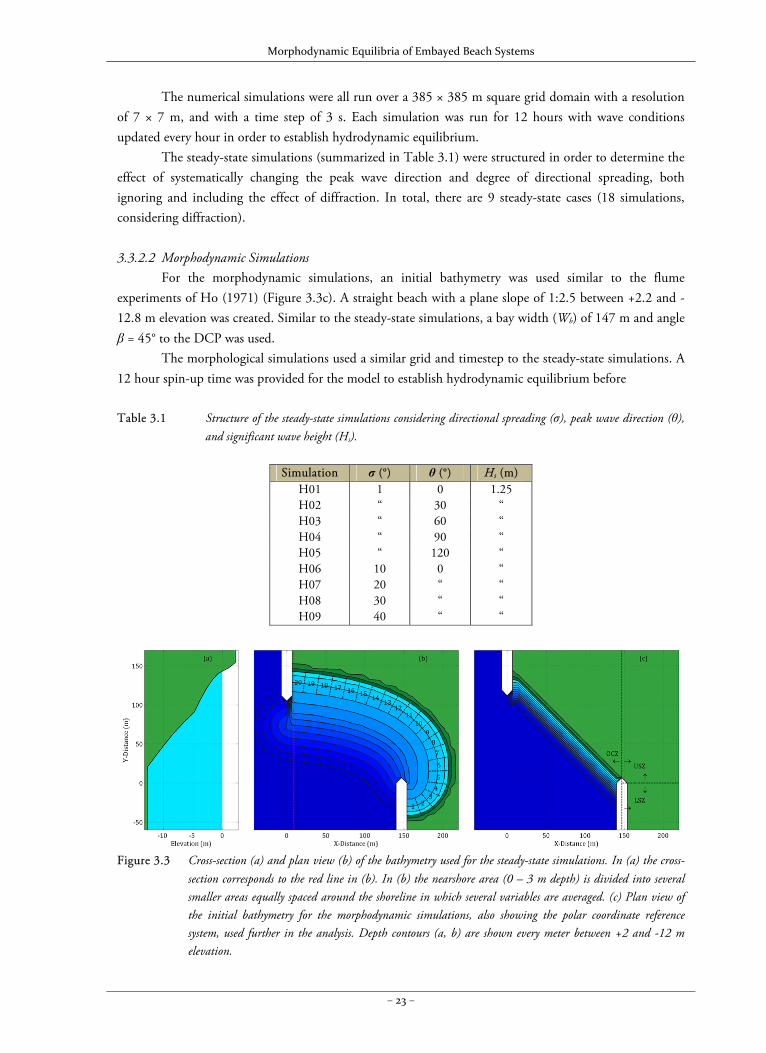
Morphodynamic Equilibria of Embayed Beach Systems
– 23 –
The numerical simulations were all run over a 385 × 385 m square grid domain with a resolution of 7 × 7 m, and with a time step of 3 s. Each simulation was run for 12 hours with wave conditions updated every hour in order to establish hydrodynamic equilibrium.
The steady-state simulations (summarized in Table 3.1) were structured in order to determine the effect of systematically changing the peak wave direction and degree of directional spreading, both ignoring and including the effect of diffraction. In total, there are 9 steady-state cases (18 simulations, considering diffraction).
3.3.2.2 Morphodynamic Simulations
For the morphodynamic simulations, an initial bathymetry was used similar to the flume experiments of Ho (1971) (Figure 3.3c). A straight beach with a plane slope of 1:2.5 between +2.2 and -12.8 m elevation was created. Similar to the steady-state simulations, a bay width (Wb) of 147 m and angle β = 45° to the DCP was used.
The morphological simulations used a similar grid and timestep to the steady-state simulations. A 12 hour spin-up time was provided for the model to establish hydrodynamic equilibrium before Table 3.1 Structure of the steady-state simulations considering directional spreading (σ), peak wave direction (θ),
and significant wave height (Hs).
Simulation σ (°) θ (°) Hs (m)H01 1 0 1.25H02 “ 30 “H03 “ 60 “H04 “ 90 “H05 “ 120 “H06 10 0 “H07 20 “ “H08 30 “ “H09 40 “ “
Figure 3.3 Cross-section (a) and plan view (b) of the bathymetry used for the steady-state simulations. In (a) the cross-
section corresponds to the red line in (b). In (b) the nearshore area (0 – 3 m depth) is divided into several smaller areas equally spaced around the shoreline in which several variables are averaged. (c) Plan view of the initial bathymetry for the morphodynamic simulations, also showing the polar coordinate reference system, used further in the analysis. Depth contours (a, b) are shown every meter between +2 and -12 m elevation.
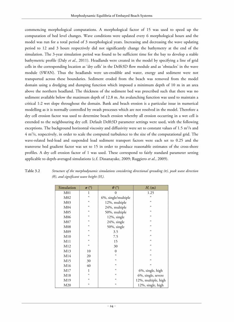
Morphodynamic Equilibria of Embayed Beach Systems
– 24 –
commencing morphological computations. A morphological factor of 15 was used to speed up the computation of bed level changes. Wave conditions were updated every 6 morphological hours and the model was run for a total period of 3 morphological years. Increasing and decreasing the wave updating period to 12 and 3 hours respectively did not significantly change the bathymetry at the end of the simulation. The 3-year simulation period was found to be sufficient time for the bay to develop a stable bathymetric profile (Daly et al., 2011). Headlands were created in the model by specifying a line of grid cells in the corresponding location as ‘dry cells’ in the Delft3D flow module and as ‘obstacles’ in the wave module (SWAN). Thus the headlands were un-erodible and water, energy and sediment were not transported across these boundaries. Sediment eroded from the beach was removed from the model domain using a dredging and dumping function which imposed a minimum depth of 10 m in an area above the northern headland. The thickness of the sediment bed was prescribed such that there was no sediment available below the maximum depth of 12.8 m. An avalanching function was used to maintain a critical 1:2 wet slope throughout the domain. Bank and beach erosion is a particular issue in numerical modelling as it is normally controlled by swash processes which are not resolved in the model. Therefore a dry cell erosion factor was used to determine beach erosion whereby all erosion occurring in a wet cell is extended to the neighbouring dry cell. Default Delft3D parameter settings were used, with the following exceptions. The background horizontal viscosity and diffusivity were set to constant values of 1.5 m2/s and 4 m2/s, respectively, in order to scale the computed turbulence to the size of the computational grid. The wave-related bed-load and suspended load sediment transport factors were each set to 0.25 and the transverse bed gradient factor was set to 15 in order to produce reasonable estimates of the cross-shore profiles. A dry cell erosion factor of 1 was used. These correspond to fairly standard parameter setting applicable to depth-averaged simulations (c.f. Dissanayake, 2009; Ruggiero et al., 2009). Table 3.2 Structure of the morphodynamic simulations considering directional spreading (σ), peak wave direction
(θ), and significant wave height (Hs).
Simulation σ (°) θ (°) Hs (m)M01 1 0 1.25M02 “ 6%, single/multiple “M03 “ 12%, multiple “M04 “ 24%, multiple “M05 “ 50%, multiple “M06 “ 12%, single “M07 “ 24%, single “M08 “ 50%, single “M09 “ 3.5 “M10 “ 7.5 “M11 “ 15 “M12 “ 30 “M13 10 0 “M14 20 “ “M15 30 “ “M16 40 “ “M17 1 “ 6%, single, highM18 “ “ 6%, single, severeM19 “ “ 12%, multiple, highM20 “ “ 12%, single, high
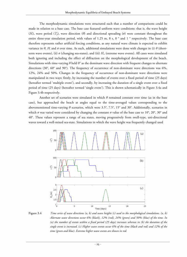
Morphodynamic Equilibria of Embayed Beach Systems
– 25 –
The morphodynamic simulations were structured such that a number of comparisons could be made in relation to a base case. The base case featured uniform wave conditions: that is, the wave height (Hs), wave period (Tp), wave direction (θ) and directional spreading (σ) were constant throughout the entire three-year simulation period, with values of 1.25 m, 8 s, 0 ° and 1 ° respectively. The base case therefore represents rather artificial forcing conditions, as any natural wave climate is expected to exhibit variance in θ, Hs and σ over time. As such, additional simulations were done with changes in (i) θ (short-term wave events), (ii) σ (changing sea-states), and (iii) Hs, (extreme wave events). All cases were simulated both ignoring and including the effect of diffraction on the morphological development of the beach. Simulations with time-varying θ held 0° as the dominant wave direction with frequent changes to alternate directions (30°, 60° and 90°). The frequency of occurrence of non-dominant wave directions was 6%, 12%, 24% and 50%. Changes in the frequency of occurrence of non-dominant wave directions were manipulated in two ways: firstly, by increasing the number of events over a fixed period of time (25 days) (hereafter termed ‘multiple event’), and secondly, by increasing the duration of a single event over a fixed period of time (25 days) (hereafter termed ‘single event’). This is shown schematically in Figure 3.4a and Figure 3.4b respectively.
Another set of scenarios were simulated in which θ remained constant over time (as in the base case), but approached the beach at angles equal to the time-averaged values corresponding to the abovementioned time-varying θ scenarios, which were 3.5°, 7.5°, 15° and 30°. Additionally, scenarios in which σ was varied were considered by changing the constant σ value of the base case to 10°, 20°, 30° and 40°. These values represent a range of sea states, moving progressively from swell-type, uni-directional waves toward a well-mixed sea-state. Simulations in which the wave height was frequently changed used
Figure 3.4 Time series of wave directions (a, b) and wave heights (c) used in the morphological simulations. (a, b)
Alternate wave directions occur 6% (black), 12% (red), 24% (green) and 50% (blue) of the time. In (a) the number of events within a fixed period (25 days) increases whereas in (b) the duration of the single event is increased. (c) Higher wave events occur 6% of the time (black and red) and 12% of the time (green and blue). Extreme higher wave events are shown in red.
(a)
(b)
(c)
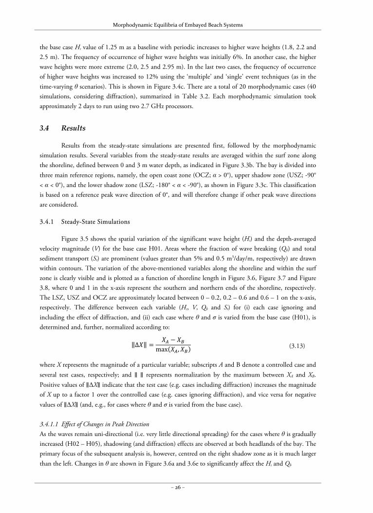
Morphodynamic Equilibria of Embayed Beach Systems
– 26 –
the base case Hs value of 1.25 m as a baseline with periodic increases to higher wave heights (1.8, 2.2 and 2.5 m). The frequency of occurrence of higher wave heights was initially 6%. In another case, the higher wave heights were more extreme (2.0, 2.5 and 2.95 m). In the last two cases, the frequency of occurrence of higher wave heights was increased to 12% using the ‘multiple’ and ‘single’ event techniques (as in the time-varying θ scenarios). This is shown in Figure 3.4c. There are a total of 20 morphodynamic cases (40 simulations, considering diffraction), summarized in Table 3.2. Each morphodynamic simulation took approximately 2 days to run using two 2.7 GHz processors.
3.4 Results
Results from the steady-state simulations are presented first, followed by the morphodynamic simulation results. Several variables from the steady-state results are averaged within the surf zone along the shoreline, defined between 0 and 3 m water depth, as indicated in Figure 3.3b. The bay is divided into three main reference regions, namely, the open coast zone (OCZ; α > 0°), upper shadow zone (USZ; -90° < α < 0°), and the lower shadow zone (LSZ; -180° < α < -90°), as shown in Figure 3.3c. This classification is based on a reference peak wave direction of 0°, and will therefore change if other peak wave directions are considered.
3.4.1 Steady-State Simulations
Figure 3.5 shows the spatial variation of the significant wave height (Hs) and the depth-averaged velocity magnitude (V) for the base case H01. Areas where the fraction of wave breaking (Qb) and total sediment transport (St) are prominent (values greater than 5% and 0.5 m3/day/m, respectively) are drawn within contours. The variation of the above-mentioned variables along the shoreline and within the surf zone is clearly visible and is plotted as a function of shoreline length in Figure 3.6, Figure 3.7 and Figure 3.8, where 0 and 1 in the x-axis represent the southern and northern ends of the shoreline, respectively. The LSZ, USZ and OCZ are approximately located between 0 – 0.2, 0.2 – 0.6 and 0.6 – 1 on the x-axis, respectively. The difference between each variable (Hs, V, Qb and St) for (i) each case ignoring and including the effect of diffraction, and (ii) each case where θ and σ is varied from the base case (H01), is determined and, further, normalized according to:
‖∆ ‖max ,
(3.13)
where X represents the magnitude of a particular variable; subscripts A and B denote a controlled case and several test cases, respectively; and ∥ ∥ represents normalization by the maximum between XA and XB. Positive values of ∥ΔX∥ indicate that the test case (e.g. cases including diffraction) increases the magnitude of X up to a factor 1 over the controlled case (e.g. cases ignoring diffraction), and vice versa for negative values of ∥ΔX∥ (and, e.g., for cases where θ and σ is varied from the base case). 3.4.1.1 Effect of Changes in Peak Direction As the waves remain uni-directional (i.e. very little directional spreading) for the cases where θ is gradually increased (H02 – H05), shadowing (and diffraction) effects are observed at both headlands of the bay. The primary focus of the subsequent analysis is, however, centred on the right shadow zone as it is much larger than the left. Changes in θ are shown in Figure 3.6a and 3.6e to significantly affect the Hs and Qb
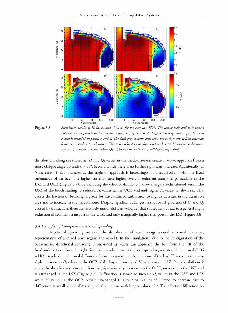
Morphodynamic Equilibria of Embayed Beach Systems
– 27 –
Figure 3.5 Simulation results of Hs (a, b) and V (c, d) for the base case H01. The colour scale and unit vectors
indicate the magnitude and direction, respectively, of Hs and V. Diffraction is ignored in panels a and c, and is included in panels b and d. The dark grey contour lines show the bathymetry at 2 m intervals between +2 and -12 m elevation. The area enclosed by the blue contour line (a, b) and the red contour line (c, d) indicates the area where Qb > 5% and where St > 0.5 m3/day/m, respectively.
distributions along the shoreline. Hs and Qb values in the shadow zone increase as waves approach from a more oblique angle up until θ = 90°, beyond which there is no further significant increase. Additionally, as θ increases, V also increases as the angle of approach is increasingly in disequilibrium with the fixed orientation of the bay. The higher currents force higher levels of sediment transport, particularly in the LSZ and OCZ (Figure 3.7). By including the effect of diffraction, wave energy is redistributed within the USZ of the beach leading to reduced Hs values at the OCZ end and higher Hs values in the LSZ. This causes the fraction of breaking, a proxy for wave-induced turbulence, to slightly decrease in the transition area and to increase in the shadow zone. Despite significant changes in the spatial gradients of Hs and Qb caused by diffraction, there are relatively minor shifts in velocities that subsequently lead to a general slight reduction of sediment transport in the USZ, and only marginally higher transport in the LSZ (Figure 3.8). 3.4.1.2 Effect of Changes in Directional Spreading
Directional spreading increases the distribution of wave energy around a central direction, representative of a mixed wave regime (non-swell). In the simulations, due to the configuration of the bathymetry, directional spreading is one-sided as waves can approach the bay from the left of the headlands but not from the right. Simulations where the directional spreading was steadily increased (H06 – H09) resulted in increased diffusion of wave energy in the shadow zone of the bay. This results in a very slight decrease in Hs values in the OCZ of the bay and increased Hs values in the LSZ. Periodic shifts in V along the shoreline are observed; however, St is generally decreased in the OCZ, increased in the USZ and is unchanged in the LSZ (Figure 3.7). Diffraction is shown to increase Hs values in the USZ and LSZ while Hs values in the OCZ remain unchanged (Figure 3.8). Values of V tend to decrease due to diffraction at small values of σ and gradually increase with higher values of σ. The effect of diffraction on
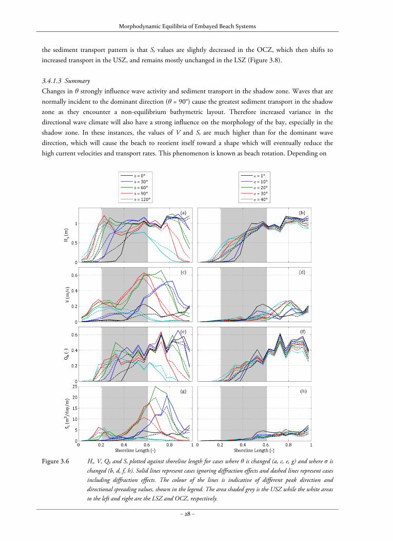
Morphodynamic Equilibria of Embayed Beach Systems
– 28 –
the sediment transport pattern is that St values are slightly decreased in the OCZ, which then shifts to increased transport in the USZ, and remains mostly unchanged in the LSZ (Figure 3.8).
3.4.1.3 Summary Changes in θ strongly influence wave activity and sediment transport in the shadow zone. Waves that are normally incident to the dominant direction (θ = 90°) cause the greatest sediment transport in the shadow zone as they encounter a non-equilibrium bathymetric layout. Therefore increased variance in the directional wave climate will also have a strong influence on the morphology of the bay, especially in the shadow zone. In these instances, the values of V and St are much higher than for the dominant wave direction, which will cause the beach to reorient itself toward a shape which will eventually reduce the high current velocities and transport rates. This phenomenon is known as beach rotation. Depending on
Figure 3.6 Hs, V, Qb and St plotted against shoreline length for cases where θ is changed (a, c, e, g) and where σ is
changed (b, d, f, h). Solid lines represent cases ignoring diffraction effects and dashed lines represent cases including diffraction effects. The colour of the lines is indicative of different peak direction and directional spreading values, shown in the legend. The area shaded grey is the USZ while the white areas to the left and right are the LSZ and OCZ, respectively.
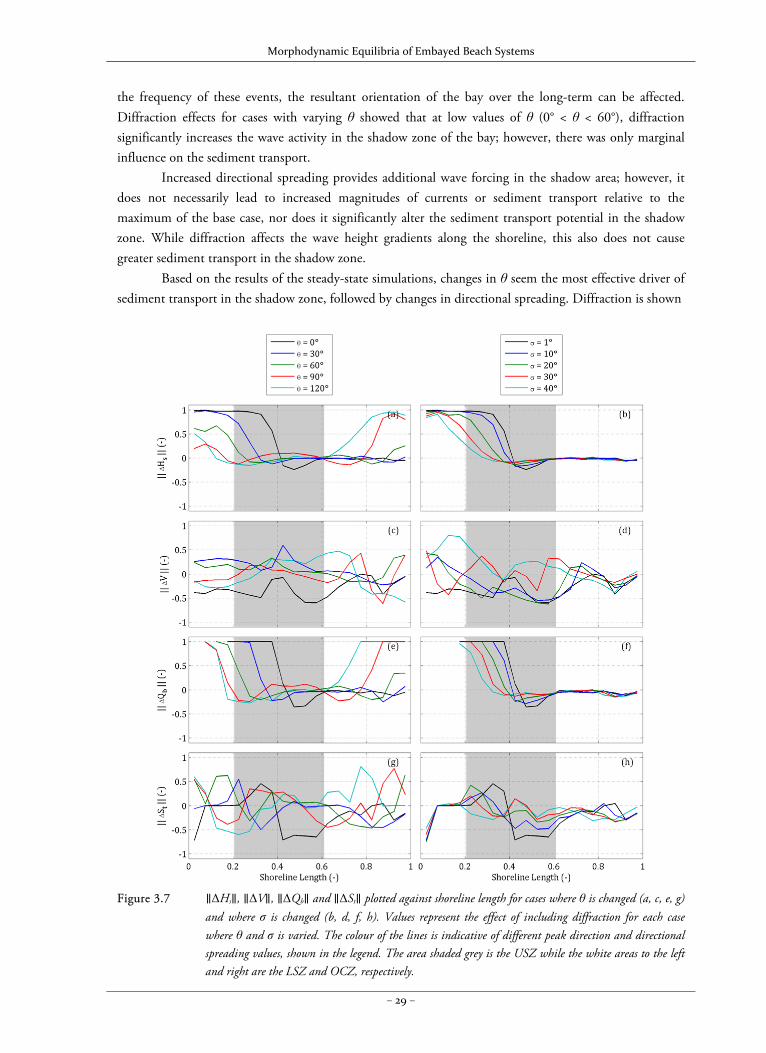
Morphodynamic Equilibria of Embayed Beach Systems
– 29 –
the frequency of these events, the resultant orientation of the bay over the long-term can be affected. Diffraction effects for cases with varying θ showed that at low values of θ (0° < θ < 60°), diffraction significantly increases the wave activity in the shadow zone of the bay; however, there was only marginal influence on the sediment transport.
Increased directional spreading provides additional wave forcing in the shadow area; however, it does not necessarily lead to increased magnitudes of currents or sediment transport relative to the maximum of the base case, nor does it significantly alter the sediment transport potential in the shadow zone. While diffraction affects the wave height gradients along the shoreline, this also does not cause greater sediment transport in the shadow zone.
Based on the results of the steady-state simulations, changes in θ seem the most effective driver of sediment transport in the shadow zone, followed by changes in directional spreading. Diffraction is shown
Figure 3.7 ∥ΔHs∥, ∥ΔV∥, ∥ΔQb∥ and ∥ΔSt∥ plotted against shoreline length for cases where θ is changed (a, c, e, g)
and where σ is changed (b, d, f, h). Values represent the effect of including diffraction for each case where θ and σ is varied. The colour of the lines is indicative of different peak direction and directional spreading values, shown in the legend. The area shaded grey is the USZ while the white areas to the left and right are the LSZ and OCZ, respectively.
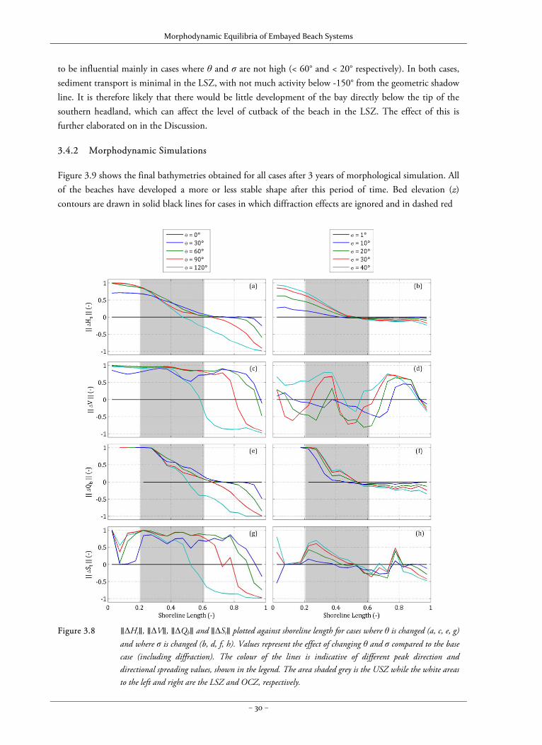
Morphodynamic Equilibria of Embayed Beach Systems
– 30 –
to be influential mainly in cases where θ and σ are not high (< 60° and < 20° respectively). In both cases, sediment transport is minimal in the LSZ, with not much activity below -150° from the geometric shadow line. It is therefore likely that there would be little development of the bay directly below the tip of the southern headland, which can affect the level of cutback of the beach in the LSZ. The effect of this is further elaborated on in the Discussion.
3.4.2 Morphodynamic Simulations
Figure 3.9 shows the final bathymetries obtained for all cases after 3 years of morphological simulation. All of the beaches have developed a more or less stable shape after this period of time. Bed elevation (z) contours are drawn in solid black lines for cases in which diffraction effects are ignored and in dashed red
Figure 3.8 ∥ΔHs∥, ∥ΔV∥, ∥ΔQb∥ and ∥ΔSt∥ plotted against shoreline length for cases where θ is changed (a, c, e, g)
and where σ is changed (b, d, f, h). Values represent the effect of changing θ and σ compared to the base case (including diffraction). The colour of the lines is indicative of different peak direction and directional spreading values, shown in the legend. The area shaded grey is the USZ while the white areas to the left and right are the LSZ and OCZ, respectively.
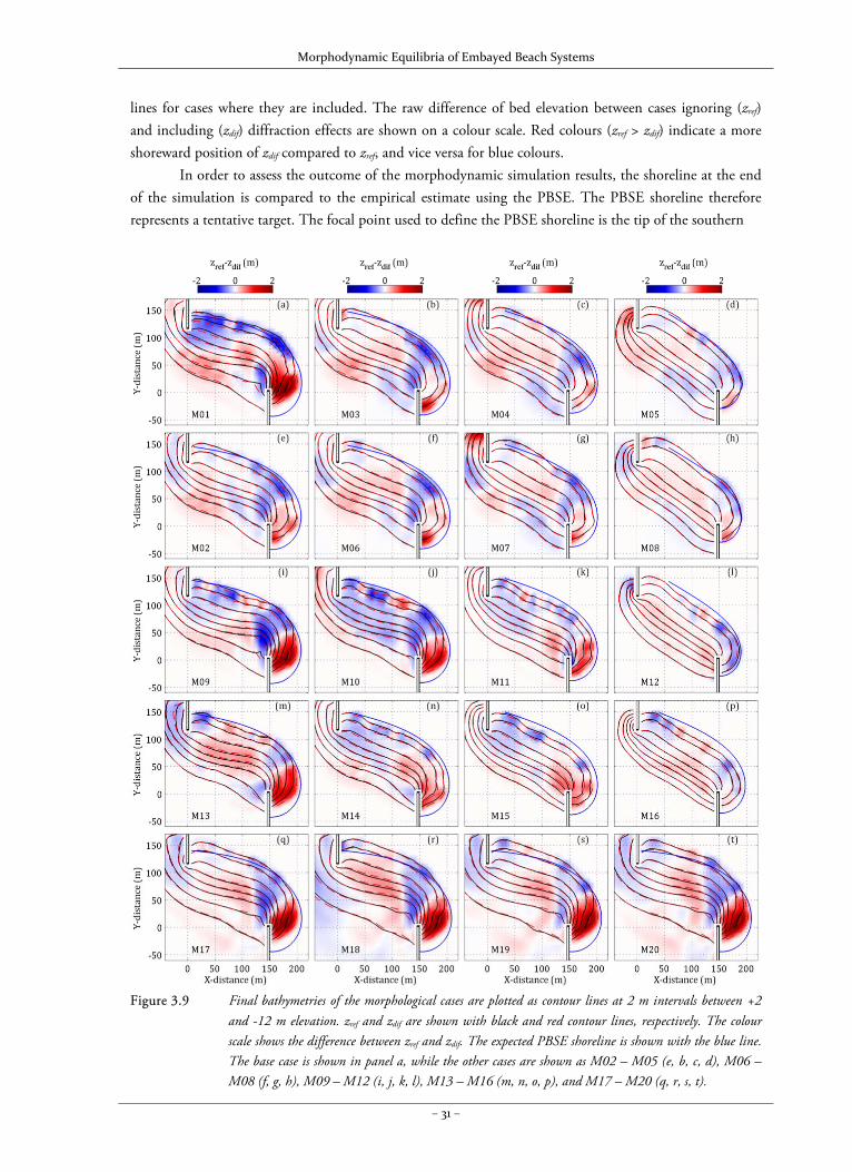
Morphodynamic Equilibria of Embayed Beach Systems
– 31 –
lines for cases where they are included. The raw difference of bed elevation between cases ignoring (zref) and including (zdif) diffraction effects are shown on a colour scale. Red colours (zref > zdif) indicate a more shoreward position of zdif compared to zref, and vice versa for blue colours.
In order to assess the outcome of the morphodynamic simulation results, the shoreline at the end of the simulation is compared to the empirical estimate using the PBSE. The PBSE shoreline therefore represents a tentative target. The focal point used to define the PBSE shoreline is the tip of the southern
Figure 3.9 Final bathymetries of the morphological cases are plotted as contour lines at 2 m intervals between +2
and -12 m elevation. zref and zdif are shown with black and red contour lines, respectively. The colour scale shows the difference between zref and zdif. The expected PBSE shoreline is shown with the blue line. The base case is shown in panel a, while the other cases are shown as M02 – M05 (e, b, c, d), M06 – M08 (f, g, h), M09 – M12 (i, j, k, l), M13 – M16 (m, n, o, p), and M17 – M20 (q, r, s, t).
Morphodynamic Equilibria of Embayed Beach Systems
– 32 –
headland. Generally, β is related to the mean wave direction ( ) such that β = 45° - . However, the DCP varies depending on . For cases with = 0° (e.g. the base case), the DCP is taken as the initial point of attachment of the shoreline to the northern headland (X, Y coordinates 0, 147 m). As increases, the DCP is assumed to move along an elliptical track between the above-mentioned DCP (reference point) and the tip of the southern headland. The radii of the ellipse are Wb and Wb/2 and it is inclined at the initial 45° shoreline angle. Thus, as increases, the DCP will move eastward toward to the southern headland and will initially move slightly north before moving south toward the southern headland. In cases in which the directional spreading is varied, is taken as σ/2. 3.4.2.1 Comparison to Natural and Empirical Bathymetry
The final shoreline shape obtained from the morphodynamic simulations, particularly from M02, M03 and M06, are quite comparable to what can be found in nature (Figure 3.2). Comparing the empirical estimate of the equilibrium morphology of the bay (Figure 3.3b) to the result of the base case simulation, M01, including diffraction effects (Figure 3.9a) differences in bed level gradients are easily seen throughout the bay. The empirical estimate used assumes that the cross-shore profile is constant around the entire bay; however, the base case simulation produces increasingly steeper bed level gradients moving from the OCZ into the LSZ. The steeper bed level gradients in the LSZ are, however, reduced when directional variability of the wave climate is considered (Figure 3.9b – h), and also when the directional spreading is high (Figure 3.9o – p). In these cases the cross-shore profile remains fairly constant around the bay, which is more comparable to the empirical estimate than the base case. 3.4.2.2 Effect of Fluctuations in Peak Direction
Figure 3.9e and 3.9b – d shows the results of cases M02 – M05 respectively, in which a timeseries of fluctuating wave directions is prescribed as multiple events of short duration. Similarly, Figure 3.9e – h shows results for cases M02 and M06 – M08 respectively, in which the frequency of occurrence of fluctuating wave directions is the same for cases M02 – M05, but prescribed as single events with longer duration. The results indicate that an increased frequency of occurrence of alternative wave directions causes the beach to develop an equilibrium shape that is rotated when compared to the base case, as waves approaching normal to the dominant wave direction induce a south-west sediment transport pattern which is counter to the dominant north-west transport pattern. The beach slope gets progressively milder around the southern headland as result, as the area of the shadow zone is decreased and sand is able to move more southward outside the southern headland because of the frequent changes in the direction of currents and sediment transport. The fluctuation of the wave directions, regardless of the number of events or their duration, produce quite similar bay shapes provided that the overall frequency of occurrence is kept constant. A minor difference is that for cases M02 – M05 the shoreline at the northern headland is slightly more landward, as the longer duration of the dominant wave direction allows time for more shoreline cutback in the OCZ. In all cases, the simulated shorelines generally compare well with the expected PBSE shoreline; however cases M02 – M05 appear to be slightly rotated relative to the PBSE shoreline because of the slightly greater cutback at the northern headland. 3.4.2.3 Effect of Changes in Peak Direction and Directional Spreading
Figure 3.9i – l shows the results of cases M09 – M12 in which θ was kept constant based on the average value of the fluctuations of θ for the ‘multiple’ and ‘single’ event cases. As expected, the final orientation of the beach is rotated compared to the base case as increases (β decreases), and it also
Morphodynamic Equilibria of Embayed Beach Systems
– 33 –
appears to be aligned to the corresponding ‘multiple’ and ‘single’ event cases. At the end of the simulation, however, the shorelines are not as fully developed as the corresponding ‘multiple’ and ‘single’ event cases when compared to the PBSE shoreline. The shoreline appears to be convex in the OCZ while the PBSE shoreline is concave. This is mainly due to the steady state of the long-shore current, and the circulation pattern in general, which causes the location of the maxima to remain unchanged over the simulation period. For cases where the wave direction is periodically changed, so is the location of the maxima of the long-shore current. Hence, at these locations in the OCZ, the shoreline is more likely to recede further landward to accommodate the higher flows, resulting in a more convex shoreline.
Figure 3.9m – p shows the results of cases M13 – M16 in which σ was varied. As σ is increased, so is the degree of rotation of the final orientation of the bay when compared to the base case. Bed level gradients in the shadow zone are less steep than the base case because of increased lateral sediment transport around the southern headland as a result of the directionally spread waves. As the spreading is one sided, the PBSE shoreline used to fit the model results assumes that the angle of incidence is σ/2. This results in a fair comparison between the model results and the PBSE shoreline. Similar to the cases above (M09 – M12), the fit between the model results and the PBSE shoreline indicates that the final bay shape is underdeveloped. Again, this is attributed to the steady nature of the current pattern in the bay. 3.4.2.4 Effect of Higher Wave Events As shown in the base case (Figure 3.9a), there is a substantial difference between the modelled and empirical shoreline planform in the lower section of the shadow zone, even when diffraction effects are included. This difference is obviously related to the lack of wave forcing in the shadow zone. Alternatively, wave forcing in the shadow zone can be increased during periodic high wave energy events. This is taken into account in cases M17 – M20 in which higher wave height events were considered. The results, shown in Figure 3.9q – t, indicate that higher wave events only slightly enhance the curvature of the shadow zone when compared to the base case, and therefore do not account for most of the difference between the modelled and empirical shorelines. In fact, the inclusion of high wave events forces the section of the bay in the OCZ to erode further shoreward than that prescribed by the PBSE. Expressing the frequency of occurrence as a ‘multiple’ or ‘single’ events does not significantly affect the final equilibrium shape of the bay. Increasing the intensity of the higher wave events is akin to increasing its frequency of occurrence. It is probable, by extrapolating from the present results, that the only way to increase the dimensions of the shadow zone is to also have extreme events approaching the beach from alternate wave directions. However, it is shown that this will only upscale the size of the bay, which would require the control points of the PBSE to be shifted to different locations for better comparison, thus restoring the original difference between the model results and the PBSE prediction. 3.4.2.5 Effect of Diffraction
The effect of diffraction can be readily seen by observing the colour scale of the plots in Figure 3.9. Dark red and blue colours indicate the largest differences between the simulations with and without diffraction. The effect of diffraction is most notable in cases where the wave direction is constant and, additionally, the peak direction is low (< 15°) and the directional spreading is low (< 20°). In these cases, diffraction effects smooth the bed levels in the shadow zone. Figure 3.10a shows the root mean square error (εrms) between the simulated and PBSE shorelines. εrms is computed for the cases ignoring (εrms,ref) and including (εrms,dif) the effect of diffraction as well as the difference between them (Δεrms), according to:
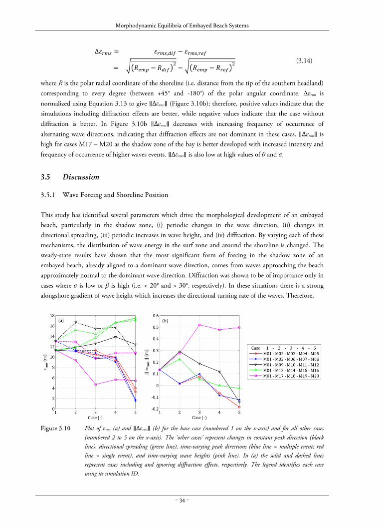
Morphodynamic Equilibria of Embayed Beach Systems
– 34 –
∆ , ,
(3.14)
where R is the polar radial coordinate of the shoreline (i.e. distance from the tip of the southern headland) corresponding to every degree (between +45° and -180°) of the polar angular coordinate. Δεrms is normalized using Equation 3.13 to give ∥Δεrms∥ (Figure 3.10b); therefore, positive values indicate that the simulations including diffraction effects are better, while negative values indicate that the case without diffraction is better. In Figure 3.10b ∥Δεrms∥ decreases with increasing frequency of occurrence of alternating wave directions, indicating that diffraction effects are not dominant in these cases. ∥Δεrms∥ is high for cases M17 – M20 as the shadow zone of the bay is better developed with increased intensity and frequency of occurrence of higher waves events. ∥Δεrms∥ is also low at high values of θ and σ.
3.5 Discussion
3.5.1 Wave Forcing and Shoreline Position This study has identified several parameters which drive the morphological development of an embayed beach, particularly in the shadow zone, (i) periodic changes in the wave direction, (ii) changes in directional spreading, (iii) periodic increases in wave height, and (iv) diffraction. By varying each of these mechanisms, the distribution of wave energy in the surf zone and around the shoreline is changed. The steady-state results have shown that the most significant form of forcing in the shadow zone of an embayed beach, already aligned to a dominant wave direction, comes from waves approaching the beach approximately normal to the dominant wave direction. Diffraction was shown to be of importance only in cases where σ is low or β is high (i.e. < 20° and > 30°, respectively). In these situations there is a strong alongshore gradient of wave height which increases the directional turning rate of the waves. Therefore,
Figure 3.10 Plot of εrms (a) and ∥Δεrms∥ (b) for the base case (numbered 1 on the x-axis) and for all other cases
(numbered 2 to 5 on the x-axis). The ‘other cases’ represent changes in constant peak direction (black line), directional spreading (green line), time-varying peak directions (blue line = multiple event; red line = single event), and time-varying wave heights (pink line). In (a) the solid and dashed lines represent cases including and ignoring diffraction effects, respectively. The legend identifies each case using its simulation ID.
Morphodynamic Equilibria of Embayed Beach Systems
– 35 –
the penetration of wave energy into the shadow zone of the beach is only achieved via diffraction processes. The morphodynamic simulations have shown that fluctuations in the directional wave climate tend to mask the effect of diffraction in the shadow zone and leads to the formation of a concave shoreline in the OCZ, an area typically unaffected by diffraction. A relatively small amount of directional variance of 6% (M02) significantly reduced the effect of diffraction compared to a similar case in which the peak wave direction was kept constant (M09). These results confirm the initial findings from the steady-state study. Periodic increases in the wave height tend to cause the shoreline to translate further shoreward OCZ, with relatively little effect on stimulating shoreline retreat in the shadow zone.
Previous research on the stability of embayed beaches clearly stated the importance of diffraction in forming the curved shoreline in and around the shadow zone (Hsu et al., 2010; Le Blond, 1979; Yasso, 1965). Gama et al. (2011) note that diffraction effects depend on the direction of wave approach, which effectively influences the shadowing produced by the headlands. It is often noted that diffraction alone is not the only cause for the curvature of the beach. Le Blond (1979), for example, state that variation in bed slope in the shadow zone is necessary to increase refraction effects which retard wave fronts as they move into shallow water, thereby allowing simultaneous breaking of the wave front around the bay periphery. However, these conclusions do not illustrate how embayments evolved in the first instance, nor do they take into account variability of the wave climate. The effect of short-term and seasonal beach rotation caused by wave climate variability has been well documented and adequately explained. Harley et al. (2011) and Short (2010) explain that rotation can be caused by shifts in long-shore sediment transport and long-shore gradients in cross-shore sediment transport. Klein et al. (2010) showed that the differences in the headland geometry of a bay can affect the degree of rotation experienced for beaches exposed to the same offshore wave climate. The results obtained from this study agree well with these findings, and also show that rotation events are important in steering the evolution of embayments not only in the short-term, but also in the long-term. 3.5.2 Equilibrium Shape and Orientation of the Beach
The simulated directional events cause sharp increases in current velocities and sediment transport over the entire bay as the hydrodynamic forcing is in disequilibrium with the bay bathymetry. During these events, the generally north-west long-shore current and sediment transport pattern is reversed as flow is driven to the south-east (Figure 3.11). While this causes some sediment to be temporarily redistributed into the USZ, most of the sediment is driven around the outside of the southern headland rather than causing infilling in the LSZ. There is also an increase in water levels in the LSZ that accelerates the erosion of the shoreline in this area. When normal (dominant) conditions are restored, the OCZ quickly recovers as sand is moved from the USZ back into the OCZ. As the LSZ has relatively weak currents and thus negligible sediment transport rates during normal conditions, the erosion caused during a rotation event remains permanent. The net effect of rotation events therefore causes the bay to shift sand back and forth in the OCZ and USZ while the LSZ develops independently.
The long-term residual sediment transport resulting from rotation events causes the beach to orient itself in a position which is in equilibrium with the frequency of change in forcing conditions. Thus, increases in the frequency of occurrence of rotation events gives greater influence to conditions that move sediment south-west therefore causing rotation of the beach as seen in the ‘multiple and single event’ cases. It is shown that neither the duration of wave events nor the number of times they occur are
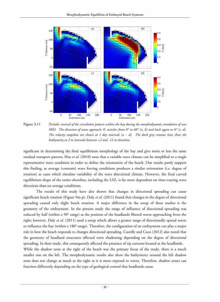
Morphodynamic Equilibria of Embayed Beach Systems
– 36 –
Figure 3.11 Periodic reversal of the circulation pattern within the bay during the morphodynamic simulation of case
M02. The direction of wave approach, θ, switches from 0° to 60° (a, b) and back again to 0° (c, d). The velocity snapshots are shown at 1 day intervals (a – d). The dark grey contour lines show the bathymetry at 2 m intervals between +2 and -12 m elevation.
significant in determining the final equilibrium morphology of the bay and give more or less the same residual transport pattern. Hsu et al. (2010) note that a variable wave climate can be simplified to a single representative wave condition in order to define the orientation of the beach. Our results partly support this finding, as average (constant) wave forcing conditions produces a similar orientation (i.e. degree of rotation) as cases which simulate variability of the wave directional climate. However, the final curved equilibrium shape of the entire shoreline, including the LSZ, is far more dependent on time-varying wave directions than on average conditions.
The results of this study have also shown that changes in directional spreading can cause significant beach rotation (Figure 9m-p). Daly et al. (2011) found that changes in the degree of directional spreading caused only slight beach rotation. A major difference in the setup of these studies is the geometry of the embayment. In the present study the range of influence of directional spreading was reduced by half (within a 90° range) as the position of the headlands filtered waves approaching from the right; however, Daly et al. (2011) used a setup which allows a greater range of directionally spread waves to influence the bay (within a 180° range). Therefore, the configuration of an embayment can play a major role in how the beach responds to changes directional spreading. Castelle and Coco (2012) also noted that the geometry of headland structures affected wave shadowing depending on the degree of directional spreading. In their study, this consequently affected the presence of rip currents located at the headlands. While the shadow zone at the right of the beach was the primary focus of the study, there is a much smaller one on the left. The morphodynamic results also show the bathymetry around the left shadow zone does not change as much as the right as it is more exposed to waves. Therefore, shadow zones can function differently depending on the type of geological control that headlands cause.
Morphodynamic Equilibria of Embayed Beach Systems
– 37 –
3.5.3 Differences to the Empirical Shoreline The PBSE was applied by rigidly defining the location of the focal point and the DCP. Better fits to the model results, assuming they are perfect, could have been obtained by carrying out a least-square error reduction procedure in which the input parameters to the PBSE are manipulated; however, it is not the aim of this study to improve the application of the PBSE. Nevertheless, the results show that at times the location of the input control points can be arbitrary. For example, for the cases in which higher wave heights are considered, it appears that by simply shifting the PBSE shoreline northward there would be an excellent fit to the model results. In that case, the focal point would not correspond to the location where diffraction is occurring, being the tip of the southern headland. Previous work have also noted that the location of the focal point and the DCP can be ambiguous (Gama et al, 2011; Lausman et al., 2010; Moreno and Kraus, 1997) and often relies on expert judgement or trial and error to determine the best fit to the observed shoreline. It is therefore easier to use the PBSE in hindsight rather than in foresight. It is recommended, however, that the use of the term ‘diffraction point’ be avoided as it may lead to misperception. A suggested alternative is ‘focal point’ (referring to the fact that it is the point of focus of the PBSE curve) or the commonly used ‘up-coast control point’.
The limited potential for morphological development in the LSZ is highlighted in the steady-state simulations due to limited wave-induced turbulence, and is also seen in the morphological results. Some cases produce a good fit between the PBSE shoreline and the model result in the OCZ of the beach, but with a correspondingly poor fit in the LSZ (e.g. M01 and M02) due to seemingly insufficient cutback of the beach, even under high wave conditions. Using the PBSE, the ratio between the polar radial coordinate corresponding to angular coordinates of -180° and -90° (R-180/R-90) is 0.74. Based on the model results, R-180/R-90 is 0.53, therefore less than what is predicted by the PBSE. However, from the observations of Lavalle and Lakhan (1997), R-180/R-90 is approximately 0.5, and for Seringat Island, Singapore (Figure 3.2) it is 0.62. Therefore the model results are within the range of what can be found in nature. Despite this, there is also a possibility that the model is limited in being able to produce enough erosion in the LSZ. This is further discussed in the following section.
3.5.4 Model Approach and Limitations
Most embayed beaches already exist in a dynamic equilibrium state; therefore, it is uncommon to observe how embayed beaches evolve toward this state and to identify the key processes that affect the final orientation of the beach. Flume experiments have been used in an effort to fill this gap (e.g. Ho, 1971); however, due to the small scale of the experiments, it is difficult to distinguish whether the curvature of the beach was actually due to hydrodynamic or geo-mechanical processes, as the resultant bed slope is often quite close to the critical wet slope of the sand, especially in the shadow zone. Process-based models are therefore a useful tool for helping to fill this knowledge gap by being able to separate and study individual processes.
The results have shown that these models can be applied systematically to study the role of variability in forcing conditions in determining the evolution of coastal landscapes. Further studies can be done to widen the scope of research in order to answer particular questions. However, the computational time required to simulate multiple scenarios in depth can be discouraging. Additionally, despite very convincing results, there are still a few limitations of the modelling system. Although Delft3D (SWAN) includes the effect of diffraction in wave computations, phase information is not accounted for in the approximation. This may be important in exceptional cases where complex nearshore bathymetry causes
Morphodynamic Equilibria of Embayed Beach Systems
– 38 –
wave trains intersect each other (such as around islands) or where wave reflection is significant. This is, however, not an issue for the schematic setup used for this study as there are no features which induce wave interference patterns. The simulation of wave-induced flows is done using a depth-averaged approach and the model does not account for wave asymmetry, skewness, or undertow. The simulations are therefore not able to precisely resolve cross-shore bar-rip formations in the surf zone. It is, however, assumed that these features do not contribute to the long-term (annual to decadal) residual transport pattern within the bay and that they are mainly transient features which depend on short-term changes in the wave conditions, in the order of 10 – 20 days (c.f. Castelle and Coco, 2012; Smit et al., 2008).
While Delft3D accurately describes wave transformation and wave-generated flows, the van Rijn (1993) sediment transport formulation is highly empirical. It is usually necessary to perform a rigorous calibration to obtain working values for the transport coefficients. In this study, such calibration was not done as the situation is schematized; however, commonly reported values are used (Dissanayake et al., 2009; Ruggiero et al., 2009). The method in which the erosion of dry cells is determined is behavioural. It was found that full erosion of dry cells (adjacent to wet cells) was necessary to produce observed levels of cutback in the LSZ. The simulations also initially tended to produce steep bed slopes around the headland tips and in the LSZ where there was low wave energy; therefore the process of producing reasonable bed slopes in these areas was not inherently controlled by wave-induced flows. In nature, geo-mechanical failure of the sediment bed controls the critical slope of sand under the influence of gravity. This process may be fast acting (avalanching) or slow (creep). It was necessary to include this process in the simulations in order to control bed slopes in the abovementioned areas. The avalanching process accelerated the initial cutback of the LSZ, allowing the wave-induced currents to effect further erosion in the LSZ. Therefore, the development of the LSZ was controlled by combined geo-mechanical and hydrodynamic processes.
3.6 Conclusion
The open-source, processed-based numerical model Delft3D was used to assess the significance of time-invariant and time-varying wave forcing conditions (directional variance, wave height variance and directional spreading) as drivers of embayed beach morphology and curvature. This is generally thought to be highly influenced by wave diffraction processes; however, it is shown that periodic changes in wave climate also has a high influence as it affects the wave energy distribution in the bay.
The results of morphological simulations, in which an initially straight beach develops into an embayment, have highlighted the main forcing mechanisms responsible to the formation of the typically curved shoreline planform. Directional spreading and diffraction are important in diffusing wave energy in the shadow zone of the bay and tend to smooth the cross-shore beach slope in the shadow zone. The influence of directional spreading is closely linked to the configuration of headland structures as they potentially limit the range of wave directions directly impacting the bay. Increased wave energy from high wave events causes the shoreline to recede shoreward in the direction of wave approach with relatively little effect in the shadow areas of the bay. Variance of the peak wave direction, rather than time-averaged conditions, influences the curvature of the shoreline and also provides the greatest means of wave forcing in the shadow zone of the bay.
The effect of diffraction is reduced (or is at least coincident) as the directional variance of the wave climate is increased. As little as 6% variation in wave directions within a 90° range is sufficient to mask the influence of diffraction, irrespective of the sequencing of events. However, it is clear that diffraction can be dominant in the lee side of the bay for monochromatic waves in which the directional spreading is low and
Morphodynamic Equilibria of Embayed Beach Systems
– 39 –
the angle β is high (i.e. < 20° and > 30°, respectively). As diffraction is a natural and on-going process, it should always be considered in cases where wave shadowing is expected. The results mainly show that short-term and seasonal beach rotation events steer the long-term evolution of embayments and directly influence residual sediment transport patterns. Therefore a good knowledge of the directional wave climate is critical to determine the orientation and planform of embayed beaches.
3.7 Acknowledgements
The authors acknowledge funding from the German Research Foundation (DFG) via the International Research Training Group: Integrated Coastal Zone and Shelf Sea Research (INTERCOAST). We gratefully acknowledge and appreciate advice from Dano Roelvink (UNESCO-IHE, Delft, the Netherlands). C.J. Daly is grateful to the German Academic Exchange Service (DAAD) Stibet Program for additional funding at the end of the doctoral promotion period.

Morphodynamic Equilibria of Embayed Beach Systems
– 40 –
Morphodynamic Equilibria of Embayed Beach Systems
– 41 –
Chapter 4 – Long‐Term Morphological Evolution
This Chapter is based on a manuscript submitted to the Journal of Geomorphology titled:
“On the Morphological Evolution of an Embayed Beach”
Christopher J. Daly 1,2, Karin R. Bryan 2, and Christian Winter 1
1 MARUM – Center for Marine Environmental Sciences, University of Bremen, Bremen, Germany
2 Department of Earth and Ocean Sciences, University of Waikato, Hamilton, New Zealand
4.1 Abstract
The typically curved planform shape of embayed beaches is often observed in the presence of rigid headlands and inclined wave forcing. The long-term alongshore equilibrium shape is variable and is controlled by headland geometry, cellular circulation patterns and wave obliquity at the shoreline. We use a state-of-the-art, process-based, morphological model to simulate the development of embayed beaches depending on different environmental conditions and geological settings (i.e., topography and geometry). The embayment is allowed to develop from an initially straight beach to one which is curved under idealized wave forcing conditions. Bay development can be approximated with an exponential function with coefficients representing rate of growth and bay size. Different stages of beach development (translation and rotation) are described and parameterized. Alongshore gradients in flow and transport patterns are related to long-term non-uniform shoreline cutback (beach rotation). Rotation of the beach ceases as the bay matures, leading to a curved shoreline planform, which is a remnant of decaying erosion processes.
Morphodynamic Equilibria of Embayed Beach Systems
– 42 –
4.2 Introduction
One of the defining features of an embayed beach is the curvature of its shoreline, which is typically spiral-shaped. Periodic rotation occurs, caused by event-driven or seasonal changes in wave direction that modify long-shore currents (Short and Masselink, 1999; Klein et al., 2010) or create long-shore gradients in cross-shore sediment transport (Harley et al., 2011). Nevertheless, over longer timescales, the position of the shoreline is often relatively stable (Yasso, 1965; Silvester and Hsu, 1997), evolving toward an ‘equilibrium’ configuration. Given that beaches are naturally dynamic environments, one of the main aims of coastal research is to improve our understanding and predictive capacity for informed coastal protection, especially in the face of climate change and increased anthropogenic impact on coastal areas (de Vriend et al., 1993). Such changes in boundary conditions will influence the trajectory a beach will take in reaching its equilibrium shape; therefore, thorough understanding of the processes that control the pathway toward equilibrium is fundamental to long-term impact assessments and coastal management.
Several concepts have been proposed in the literature to explain why embayed beaches develop a characteristically curved stable shape. Most agree that the geological settings (i.e., topography and geometry, e.g., headland position, orientation of the bay) plays a significant role in determining the bay shape as it is strongly coupled with the steering of wave-driven currents, causing cellular circulation patterns to develop in the bay (Klein and Menezes, 2001; Short, 2010; Silva et al., 2010). This is dependent on the length of the bay relative to width of the surf zone – short, compact embayments generally feature single circulation cells while larger emabyments allow room for more normal (open-coast) circulation (Short and Masselink, 1999) – and, additionally, the degree of curvature, which affects the indentation of the bay (Silvester and Hsu, 1997). Equilibrium on embayed beaches occurs as the beach responds in order to achieve zero sediment transport or flux along the shoreline (LeBlond, 1979). This often leads to the assumption that, as a bay develops over time, obliquely incident waves will ultimately become shore-normal once an equilibrium state is achieved (Dean 1978; Silvester and Hsu, 1997), causing simultaneous wave breaking occurs around its periphery. The latter two theories have been tested using coastline evolution models to simulate the evolution of the shoreline until an equilibrium condition is met (LeBlond 1972; Rea and Komar, 1977; Weesakul et al., 2010). However, such studies simplify, or ignore, the interaction between wave-induced currents, nearshore circulation and sediment transport – effects which dominate in surf zone environments.
Circulation patterns vary depending on the spatial dimensions of the bay. In large embayments (O~10 km), large-scale gyre structures have been observed and linked to surface winds and oceanic currents (Valle-Levinson and Moraga-Opazo, 2006). In small embayments (O~200 m) cellular circulation patterns and mega-rips are observed around headland structures with counter-rotating eddies in the open-coast section of the bay and in the shadow zone (Pattiaratchi et al., 2009; Loureiro et al., 2012). More specifically, within the surf zone, circulation of wave-induced currents is easily affected by the geometry of bay as well as by transient self-organized bar-rip nearshore morphology (Short and Masselink, 1999; Gallop et al, 2011; Castelle and Coco, 2012). These features may help to facilitate sediment bypassing if they migrate outside the surf zone, for example after a storm event; however they are expected to remain within the confines of the bay once it is in an equilibrium state. Until this state is achieved, we can therefore expect that as an embayment develops over time, flow patterns in the bay will change not only due to the fixed bay geometry, but also due to feedbacks as the underlying bathymetry changes over time (LeBlond, 1979).
Morphodynamic Equilibria of Embayed Beach Systems
– 43 –
Observations of natural embayed beach evolution are rare. Terpstra and Chrzastowski (1992) and Lavalle and Lakhan, (1997) documented the development of two different embayments of approximately 150 m length over a period of 10 years and 9 months respectively – the only known works to the knowledge of the authors. In an effort to garner more data, laboratory flume experiments have been conducted with the aim to include circulation effects on embayed beach development. For example, Ho (1971) performed experiments in which an initially straight shoreline is allowed to erode in order to create a curved embayment. Weesakul and Tasaduak (2012) also used flume experiments to investigate several cases of dynamic equilibrium by varying the degree of riverine sediment input. Flume experiments tend to suffer from scale effects, especially with regard to sediment sizing and reproducing prototype Reynolds numbers. Furthermore, the type of wave forcing is generally limited to monochromatic, uni-directional wave-trains. However, the results of these experiments nicely show the equilibrium shoreline shape of the bay and also indicate that the rate of development is non-linear over time (Silvester, 1985).
Today, medium- to long-term coastal behaviour can be investigated using process-based morphodynamic models (de Vriend et al., 1993; Roelvink and Reniers 2012; Winter, 2006). Such models simulate the non-linear interaction between currents, sediment transport and bed level changes at real-world scales and may therefore overcome limitations of coastline models and flume experiments. Recent advances in numerical morphodynamic models allow simulations over very large spatial and temporal scales, O ~ 100 km and O ~ 1000 years respectively, (Roelvink, 2006; Dissanayake et al., 2009; van der Wegen et al., 2010). Therefore, in the absence of sufficient observational data, systematic and schematic numerical simulations are assumed to be able to provide insight into medium- to long-term coastal evolution (Daly et al., 2011).
In this paper, we use a numerical modelling approach to examine the processes that cause an embayed beach to develop into a stable bathymetry starting from an initially straight beach over small to medium spatial scales and medium to long temporal scales (as defined in Stive et al, 2002). The effect of changes in environmental conditions (sediment size, mean wave energy and tidal range) and geological setting (inclination angle and bay width) is demonstrated by examining how the simulated circulation and transport patterns develop during the evolution of the bay.
4.3 Methods
4.3.1 Numerical Model Description
The open-source, process-based, morphological model, Delft3D (Version 5.04) (Lesser et al, 2004), was used in the present study to simulate the morphological development of embayed beaches. The most relevant aspects of the Delft3D model as it relates to the current work are briefly described below; however the Delft3D manuals (http://oss.deltares.nl/web/delft3d/manuals) offer a more detailed description of the numerical structure and formulations of the model.
The spectral, phase-averaged, third generation wave model, SWAN, (Booij et al., 1999) is used within the Delft3D wave module to solve the wave action balance equation, which accounts for refraction, dissipation (due to bottom friction, breaking and whitecapping) and non-linear interactions (triads and quadruplets) while transforming input boundary wave conditions across the model domain. SWAN uses an approximation for phase-decoupled wave diffraction (Holthuijsen et al., 2003). The Delft3D flow module solves the Navier–Stokes (non-linear, depth-averaged, shallow water) equations using finite difference methods. The depth-averaged (2DH) equations ignore vertical momentum and accelerations.
Morphodynamic Equilibria of Embayed Beach Systems
– 44 –
Hydrodynamics are driven by lateral and surficial boundary conditions; here predominantly by radiation stress gradients calculated in the wave module. Wave-induced mass flux, including the Stokes drift contribution from the waves, is accounted for using a Generalized Lagrangian Mean (GLM) method (Groeneweg and Klopman, 1998; Walstra et al., 2000). The flow and wave modules are coupled at regular intervals to update the wave field. The effect of wave-current interaction is accounted for as, during coupling, SWAN includes the effect of ambient currents (computed in the flow module) on wave propagation.
Non-cohesive suspended transport (a function of inter alia the depth-averaged sediment concentration, GLM velocity and horizontal eddy diffusivity) and bed-load transport (a function of inter alia the bed shear stress, median grain diameter, and bed slope) are computed according to van Rijn (1993). After each time step, bed level changes are determined based on the net suspended and bed-load transport by using a sediment conservation scheme together with a bed level continuity equation. Bed-load transport is enhanced by wave-induced currents, according to van Rijn, (1993), and also by avalanching, whereby sediment volumes above a defined critical wet slope is added to the downslope bed-load transport rate. Bed level changes can be up-scaled using the ‘morfac’ approach (Roelvink, 2006; Ranasinghe et al., 2011) in order to speed up computations. The modelling system includes a dredging and dumping function which can be used to maintain a fixed bed level. The erosion of dry land is simulated by assigning a percentage of the erosion computed in wet grid cells to neighbouring dry cells.
4.3.2 Simulation Set-up
4.3.2.1 Initial Bathymetry and Simulation Setup The initial bathymetry features a straight plane sloped (1:2.5) beach between +2.2 and -12.8 m
elevation created between two headland structures in a similar layout as the flume experiments of Ho (1971) (Figure 4.1). One headland is positioned to the north-west and the other to the south-east. The morphodynamic simulations are structured around a base case (M01) in which the lateral bay width between the headlands (Wb) is 140 m and wave obliquity (the angle β at the tip of the south-east headland between the (modal) wave crest and a down-coast control point (DCP)) is 45° (Figure 4.1). The significant wave height (Hs) and peak wave period (Tp) were kept constant at 1.25 m and 8 s, respectively, while the peak wave direction (θ) was varied between 0° and 90° 6% of the time. The median grain diameter (D50) was 300 μm and the tidal range (ζ) was zero, hence no variation in water level. Additional simulations were performed in which a characteristic of the base case was changed and are summarized in Table 4.1. M02 – M03, M04 – M05, M06 – M07, M08 – M09, and M10 – M11 feature cases in which D50, Hs, ζ, β, and Wb were varied, respectively. For cases M02 – M03, the overall D50 was changed by adding a second sediment fraction of 200 μm and 400 μm, respectively, to create a bimodal sediment distribution. For cases M06 – M07, the M2 tidal constituent was used to represent variations in water level.
4.3.2.2 Model Settings and Additional Features
The simulations were run on a spatially-uniform rectangular grid. The grid resolution, time step, morphological factor, frequency of wave updating, and total simulation period varied depending on the case. Cases M10 – M11 use a different model domain than the other cases as Wb is increased; therefore case specific settings are used in these simulations. All domain dependent model settings are specified in Table 4.2. For all simulations, a morphological spin-up time of 24 hours is provided for the model to
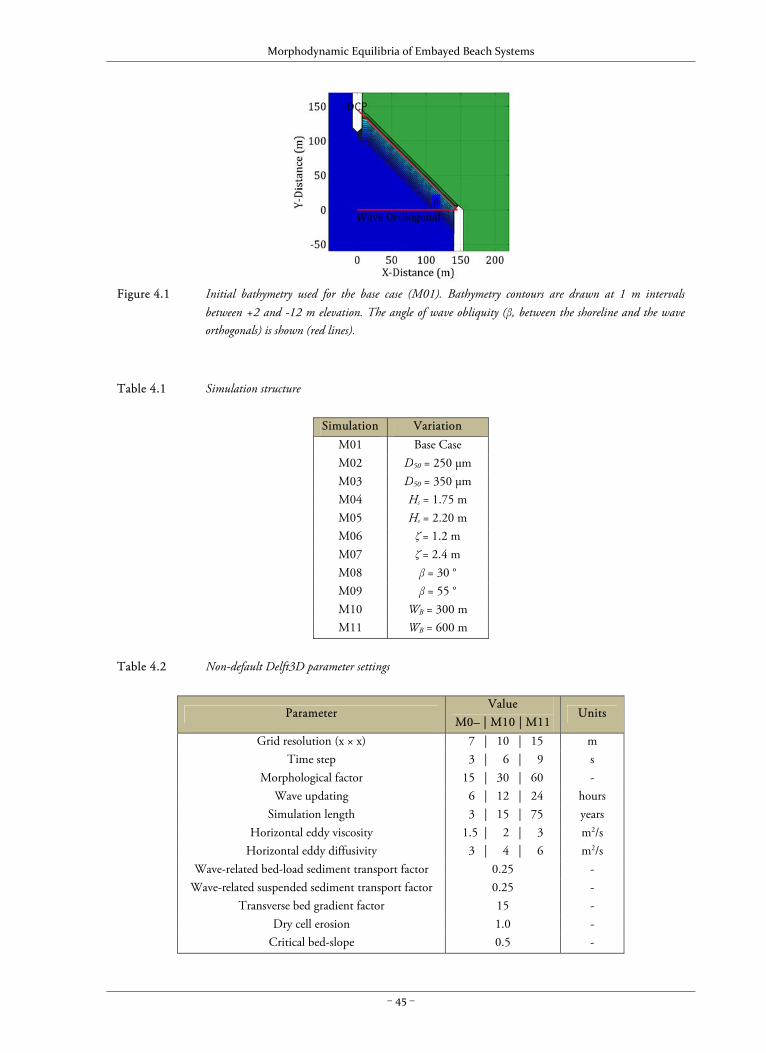
Morphodynamic Equilibria of Embayed Beach Systems
– 45 –
Figure 4.1 Initial bathymetry used for the base case (M01). Bathymetry contours are drawn at 1 m intervals
between +2 and -12 m elevation. The angle of wave obliquity (β, between the shoreline and the wave orthogonals) is shown (red lines).
Table 4.1 Simulation structure
Simulation VariationM01 Base CaseM02 D50 = 250 μmM03 D50 = 350 μmM04 Hs = 1.75 mM05 Hs = 2.20 mM06 ζ = 1.2 mM07 ζ = 2.4 mM08 β = 30 °M09 β = 55 °M10 WB = 300 mM11 WB = 600 m
Table 4.2 Non-default Delft3D parameter settings
Parameter Value
M0– | M10 | M11 Units
Grid resolution (x × x) 07 | 10 | 15 m Time step 03 | 06 | 09 s
Morphological factor 15 | 30 | 60 - Wave updating 06 | 12 | 24 hours
Simulation length 03 | 15 | 75 years Horizontal eddy viscosity 1.5 | 02 | 03 m2/s
Horizontal eddy diffusivity 03 | 04 | 06 m2/s Wave-related bed-load sediment transport factor 0.25 -
Wave-related suspended sediment transport factor 0.25 - Transverse bed gradient factor 15 -
Dry cell erosion 1.0 - Critical bed-slope 0.5 -
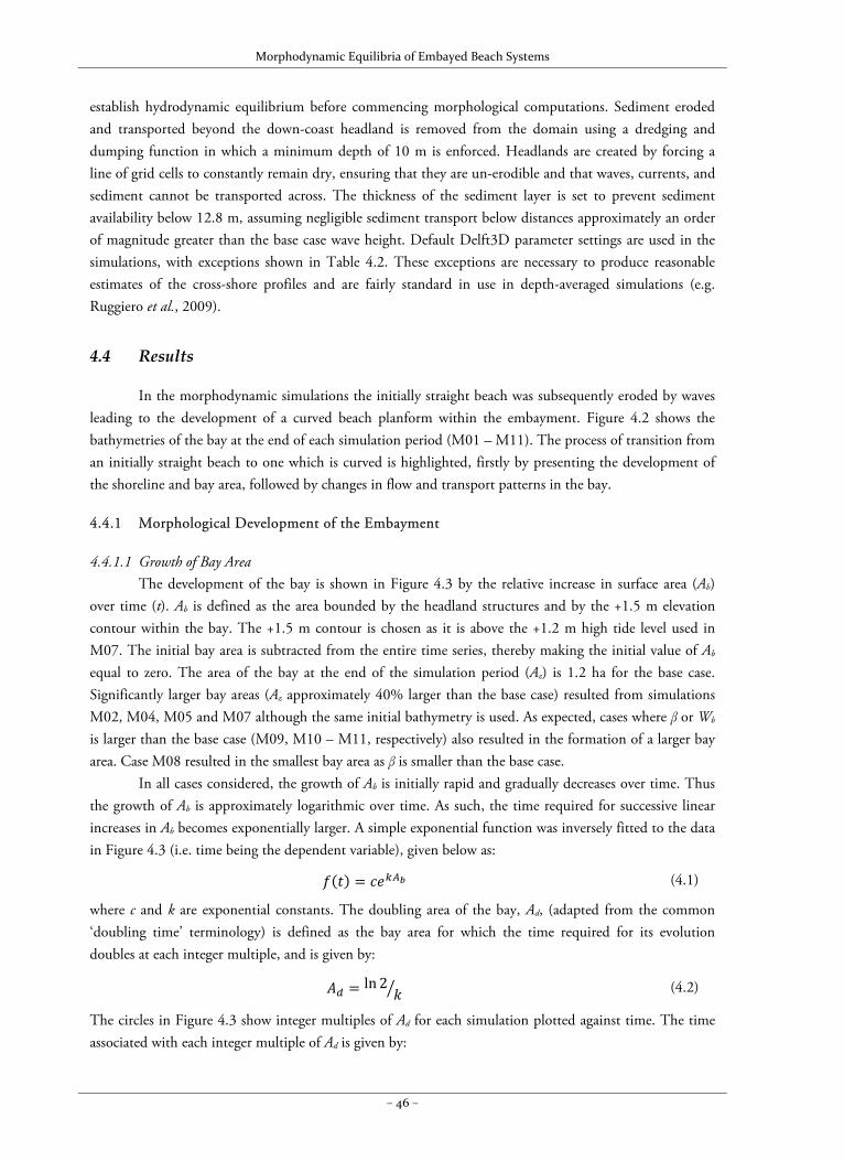
Morphodynamic Equilibria of Embayed Beach Systems
– 46 –
establish hydrodynamic equilibrium before commencing morphological computations. Sediment eroded and transported beyond the down-coast headland is removed from the domain using a dredging and dumping function in which a minimum depth of 10 m is enforced. Headlands are created by forcing a line of grid cells to constantly remain dry, ensuring that they are un-erodible and that waves, currents, and sediment cannot be transported across. The thickness of the sediment layer is set to prevent sediment availability below 12.8 m, assuming negligible sediment transport below distances approximately an order of magnitude greater than the base case wave height. Default Delft3D parameter settings are used in the simulations, with exceptions shown in Table 4.2. These exceptions are necessary to produce reasonable estimates of the cross-shore profiles and are fairly standard in use in depth-averaged simulations (e.g. Ruggiero et al., 2009).
4.4 Results
In the morphodynamic simulations the initially straight beach was subsequently eroded by waves leading to the development of a curved beach planform within the embayment. Figure 4.2 shows the bathymetries of the bay at the end of each simulation period (M01 – M11). The process of transition from an initially straight beach to one which is curved is highlighted, firstly by presenting the development of the shoreline and bay area, followed by changes in flow and transport patterns in the bay.
4.4.1 Morphological Development of the Embayment
4.4.1.1 Growth of Bay Area The development of the bay is shown in Figure 4.3 by the relative increase in surface area (Ab)
over time (t). Ab is defined as the area bounded by the headland structures and by the +1.5 m elevation contour within the bay. The +1.5 m contour is chosen as it is above the +1.2 m high tide level used in M07. The initial bay area is subtracted from the entire time series, thereby making the initial value of Ab equal to zero. The area of the bay at the end of the simulation period (Az) is 1.2 ha for the base case. Significantly larger bay areas (Az approximately 40% larger than the base case) resulted from simulations M02, M04, M05 and M07 although the same initial bathymetry is used. As expected, cases where β or Wb is larger than the base case (M09, M10 – M11, respectively) also resulted in the formation of a larger bay area. Case M08 resulted in the smallest bay area as β is smaller than the base case.
In all cases considered, the growth of Ab is initially rapid and gradually decreases over time. Thus the growth of Ab is approximately logarithmic over time. As such, the time required for successive linear increases in Ab becomes exponentially larger. A simple exponential function was inversely fitted to the data in Figure 4.3 (i.e. time being the dependent variable), given below as:
(4.1)
where c and k are exponential constants. The doubling area of the bay, Ad, (adapted from the common ‘doubling time’ terminology) is defined as the bay area for which the time required for its evolution doubles at each integer multiple, and is given by:
ln 2 (4.2)
The circles in Figure 4.3 show integer multiples of Ad for each simulation plotted against time. The time associated with each integer multiple of Ad is given by:
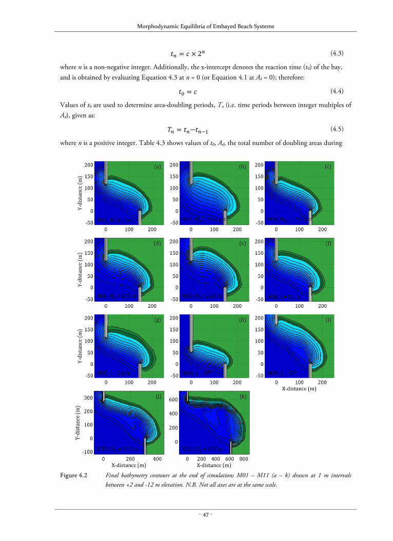
Morphodynamic Equilibria of Embayed Beach Systems
– 47 –
2 (4.3)
where n is a non-negative integer. Additionally, the x-intercept denotes the reaction time (t0) of the bay, and is obtained by evaluating Equation 4.3 at n = 0 (or Equation 4.1 at Ab = 0); therefore:
(4.4)
Values of t0 are used to determine area-doubling periods, Tn (i.e. time periods between integer multiples of Ad), given as:
(4.5)
where n is a positive integer. Table 4.3 shows values of t0, Ad, the total number of doubling areas during
Figure 4.2 Final bathymetry contours at the end of simulations M01 – M11 (a – k) drawn at 1 m intervals
between +2 and -12 m elevation. N.B. Not all axes are at the same scale.
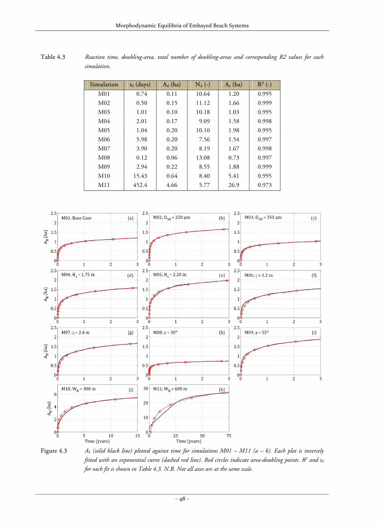
Morphodynamic Equilibria of Embayed Beach Systems
– 48 –
Table 4.3 Reaction time, doubling-area, total number of doubling-areas and corresponding R2 values for each
simulation.
Simulation t0 (days) Ad (ha) Nd (-) Az (ha) R2 (-)M01 00.74 0.11 10.64 1.20 0.995M02 00.50 0.15 11.12 1.66 0.999M03 01.01 0.10 10.18 1.03 0.995M04 02.01 0.17 09.09 1.58 0.998M05 01.04 0.20 10.10 1.98 0.995M06 05.98 0.20 07.56 1.54 0.997M07 03.90 0.20 08.19 1.67 0.998M08 00.12 0.06 13.08 0.73 0.997M09 02.94 0.22 08.55 1.88 0.999M10 15.43 0.64 08.40 5.41 0.995M11 452.4 4.66 05.77 26.9 0.973
Figure 4.3 Ab (solid black line) plotted against time for simulations M01 – M11 (a – k). Each plot is inversely
fitted with an exponential curve (dashed red line). Red circles indicate area-doubling points. R2 and t0 for each fit is shown in Table 4.3. N.B. Not all axes are at the same scale.
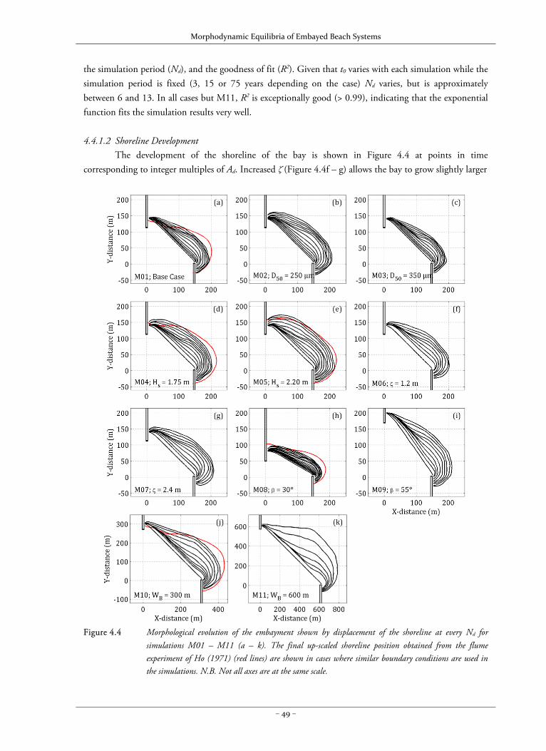
Morphodynamic Equilibria of Embayed Beach Systems
– 49 –
the simulation period (Nd), and the goodness of fit (R2). Given that t0 varies with each simulation while the simulation period is fixed (3, 15 or 75 years depending on the case) Nd varies, but is approximately between 6 and 13. In all cases but M11, R2 is exceptionally good (> 0.99), indicating that the exponential function fits the simulation results very well. 4.4.1.2 Shoreline Development
The development of the shoreline of the bay is shown in Figure 4.4 at points in time corresponding to integer multiples of Ad. Increased ζ (Figure 4.4f – g) allows the bay to grow slightly larger
Figure 4.4 Morphological evolution of the embayment shown by displacement of the shoreline at every Nd for
simulations M01 – M11 (a – k). The final up-scaled shoreline position obtained from the flume experiment of Ho (1971) (red lines) are shown in cases where similar boundary conditions are used in the simulations. N.B. Not all axes are at the same scale.
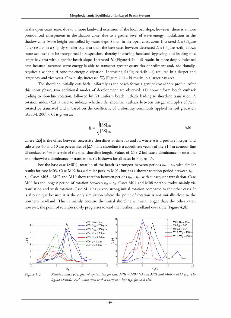
Morphodynamic Equilibria of Embayed Beach Systems
– 50 –
in the open coast zone, due to a more landward extension of the local bed slope; however, there is a more pronounced enlargement in the shadow zone, due to a greater level of wave energy modulation in the shadow zone (wave height controlled by water depth) than in the open coast zone. Increased D50 (Figure 4.4c) results in a slightly smaller bay area than the base case; however decreased D50 (Figure 4.4b) allows more sediment to be transported in suspension, thereby increasing headland bypassing and leading to a larger bay area with a gentler beach slope. Increased Hs (Figure 4.4c – d) results in more deeply indented bays because increased wave energy is able to transport greater quantities of sediment and, additionally, requires a wider surf zone for energy dissipation. Increasing β (Figure 4.4h – i) resulted in a deeper and larger bay and vice versa. Obviously, increased WB (Figure 4.4j – k) results in a larger bay area.
The shoreline initially cuts back uniformly as the beach forms a gentler cross-shore profile. After this short phase, two additional modes of development are observed: (1) non-uniform beach cutback leading to shoreline rotation, followed by (2) uniform beach cutback leading to shoreline translation. A rotation index (CR) is used to indicate whether the shoreline cutback between integer multiples of Ad is rotated or translated and is based on the coefficient of uniformity commonly applied in soil gradation (ASTM, 2009). CR is given as:
|∆ ||∆ |
(4.6)
where |ΔS| is the offset between successive shorelines at time tn-1 and tn, where n is a positive integer; and subscripts 60 and 10 are percentiles of |ΔS|. The shoreline is a coordinate vector of the +1.5m contour line discretized at 5% intervals of the total shoreline length. Values of CR > 2 indicate a dominance of rotation, and otherwise a dominance of translation. CR is shown for all cases in Figure 4.5. For the base case (M01), rotation of the beach is strongest between periods t04 – t09, with similar results for case M03. Case M02 has a similar peak to M01, but has a shorter rotation period between t05 – t07. Cases M05 – M07 and M10 show rotation between periods t02 – t06, with subsequent translation. Case M09 has the longest period of rotation between t02 – t08. Cases M04 and M08 notably evolve mainly via translation and weak rotation. Case M11 has a very strong initial rotation compared to the other cases. It is also unique because it is the only simulation where the point of rotation is not initially close to the northern headland. This is mainly because the initial shoreline is much longer than the other cases; however, the point of rotation slowly progresses toward the northern headland over time (Figure 4.3k).
Figure 4.5 Rotation index (CR) plotted against Nd for cases M01 – M07 (a) and M01 and M08 – M11 (b). The
legend identifies each simulation with a particular line type for each plot.
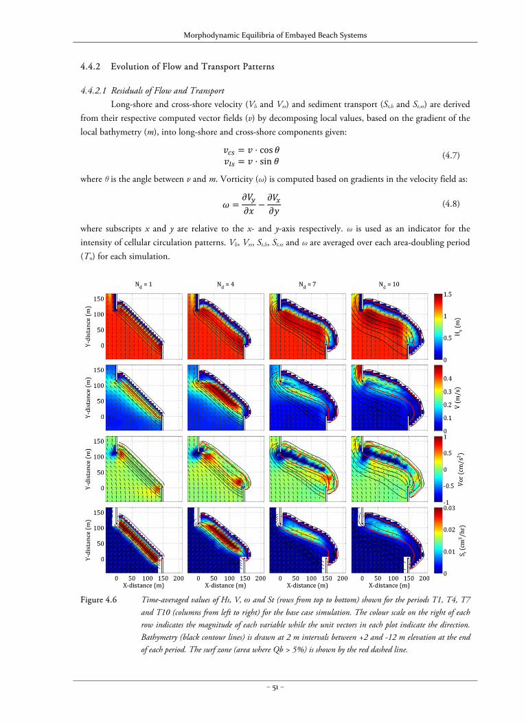
Morphodynamic Equilibria of Embayed Beach Systems
– 51 –
4.4.2 Evolution of Flow and Transport Patterns
4.4.2.1 Residuals of Flow and Transport Long-shore and cross-shore velocity (Vls and Vxs) and sediment transport (St,ls and St,xs) are derived
from their respective computed vector fields (v) by decomposing local values, based on the gradient of the local bathymetry (m), into long-shore and cross-shore components given:
⋅ cos⋅ sin (4.7)
where θ is the angle between v and m. Vorticity (ω) is computed based on gradients in the velocity field as:
(4.8)
where subscripts x and y are relative to the x- and y-axis respectively. ω is used as an indicator for the intensity of cellular circulation patterns. Vls, Vxs, St,ls, St,xs and ω are averaged over each area-doubling period (Tn) for each simulation.
Figure 4.6 Time-averaged values of Hs, V, ω and St (rows from top to bottom) shown for the periods T1, T4, T7
and T10 (columns from left to right) for the base case simulation. The colour scale on the right of each row indicates the magnitude of each variable while the unit vectors in each plot indicate the direction. Bathymetry (black contour lines) is drawn at 2 m intervals between +2 and -12 m elevation at the end of each period. The surf zone (area where Qb > 5%) is shown by the red dashed line.
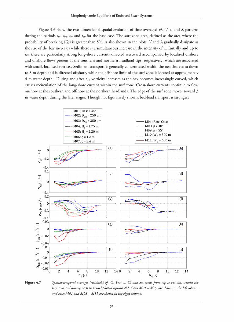
Morphodynamic Equilibria of Embayed Beach Systems
– 52 –
Figure 4.6 show the two-dimensional spatial evolution of time-averaged Hs, V, ω and St patterns during the periods t01, t04, t07 and t10 for the base case. The surf zone area, defined as the area where the probability of breaking (Qb) is greater than 5%, is also shown in the plots. V and St gradually dissipate as the size of the bay increases while there is a simultaneous increase in the intensity of ω. Initially and up to t04, there are particularly strong long-shore currents directed westward accompanied by localised onshore and offshore flows present at the southern and northern headland tips, respectively, which are associated with small, localised vortices. Sediment transport is generally concentrated within the nearshore area down to 8 m depth and is directed offshore, while the offshore limit of the surf zone is located at approximately 4 m water depth. During and after t07, vorticity increases as the bay becomes increasingly curved, which causes recirculation of the long-shore current within the surf zone. Cross-shore currents continue to flow onshore at the southern and offshore at the northern headlands. The edge of the surf zone moves toward 3 m water depth during the later stages. Though not figuratively shown, bed-load transport is strongest
Figure 4.7 Spatial-temporal averages (residuals) of Vls, Vxs, ω, Sls and Sxs (rows from top to bottom) within the
bay area and during each tn period plotted against Nd. Cases M01 – M07 are shown in the left column and cases M01 and M08 – M11 are shown in the right column.
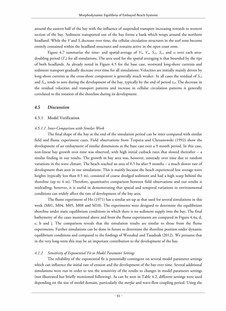
Morphodynamic Equilibria of Embayed Beach Systems
– 53 –
around the eastern half of the bay with the influence of suspended transport increasing towards to western section of the bay. Sediment transported out of the bay forms a bank which wraps around the northern headland. While the V and St decrease over time, the cellular circulation structures in the surf zone become entirely contained within the headland structures and remains active in the open coast zone. Figure 4.7 summarize the time- and spatial-average of Vls, Vxs, St,ls, St,xs and ω over each area-doubling period (Tn) for all simulations. The area used for the spatial averaging is that bounded by the tips of both headlands. As already noted in Figure 4.5 for the base case, westward long-shore currents and sediment transport gradually decrease over time for all simulations. Velocities are initially mainly driven by long-shore currents as the cross-shore component is generally much weaker. In all cases the residual of St,ls and St,xs tends to zero during the development of the bay, typically by the end of period t10. The decrease in the residual velocities and transport patterns and increase in cellular circulation patterns is generally correlated to the rotation of the shoreline during its development.
4.5 Discussion
4.5.1 Model Verification
4.5.1.1 Inter-Comparison with Similar Work The final shape of the bay at the end of the simulation period can be inter-compared with similar
field and flume experiment cases. Field observations from Terpstra and Chrzastowski (1992) show the development of an embayment of similar dimensions as the base case over a 9 month period. In this case, non-linear bay growth over time was observed, with high initial cutback rates that slowed thereafter – a similar finding in our results. The growth in bay area was, however, unsteady over time due to random variations in the wave climate. The beach reached an area of 0.5 ha after 9 months – a much slower rate of development than seen in our simulations. This is mainly because the beach experienced low average wave heights (typically less than 0.5 m), consisted of coarse dredged sediment and had a high scarp behind the shoreline (up to 4 m). Therefore, quantitative comparison between field observations and our results is misleading; however, it is useful in demonstrating that spatial and temporal variations in environmental conditions can widely affect the rate of development of the bay area.
The flume experiment of Ho (1971) has a similar set-up as that used for several simulations in this work (M01, M04, M05, M08 and M10). The experiments were designed to determine the equilibrium shoreline under static equilibrium conditions in which there is no sediment supply into the bay. The final bathymetry of the cases mentioned above and from the flume experiments are compared in Figure 4.4a, d, e, h and j. The comparison reveals that the simulation results are similar to those from the flume experiments. Further simulations can be done in future to determine the shoreline position under dynamic equilibrium conditions and compared to the findings of Weesakul and Tasaduak (2012). We presume that in the very long-term this may be an important contribution to the development of the bay.
4.1.2 Sensitivity of Exponential Fit to Model Parameter Settings
The reliability of the exponential fit is potentially contingent on several model parameter settings which can influence the initial rate of erosion and the development of the bay over time. Several additional simulations were run in order to test the sensitivity of the results to changes in model parameter settings (not illustrated but briefly mentioned following). As can be seen in Table 4.2, different settings were used depending on the size of model domain, particularly the morfac and wave-flow coupling period. Using the
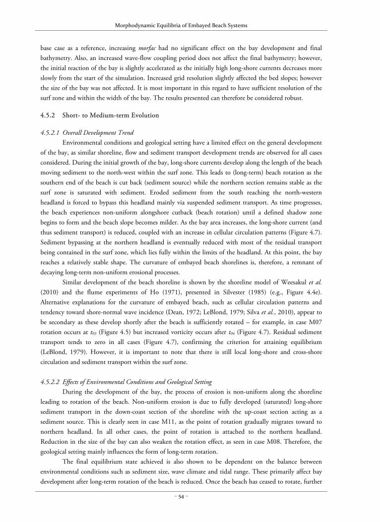
Morphodynamic Equilibria of Embayed Beach Systems
– 54 –
base case as a reference, increasing morfac had no significant effect on the bay development and final bathymetry. Also, an increased wave-flow coupling period does not affect the final bathymetry; however, the initial reaction of the bay is slightly accelerated as the initially high long-shore currents decreases more slowly from the start of the simulation. Increased grid resolution slightly affected the bed slopes; however the size of the bay was not affected. It is most important in this regard to have sufficient resolution of the surf zone and within the width of the bay. The results presented can therefore be considered robust.
4.5.2 Short- to Medium-term Evolution
4.5.2.1 Overall Development Trend Environmental conditions and geological setting have a limited effect on the general development
of the bay, as similar shoreline, flow and sediment transport development trends are observed for all cases considered. During the initial growth of the bay, long-shore currents develop along the length of the beach moving sediment to the north-west within the surf zone. This leads to (long-term) beach rotation as the southern end of the beach is cut back (sediment source) while the northern section remains stable as the surf zone is saturated with sediment. Eroded sediment from the south reaching the north-western headland is forced to bypass this headland mainly via suspended sediment transport. As time progresses, the beach experiences non-uniform alongshore cutback (beach rotation) until a defined shadow zone begins to form and the beach slope becomes milder. As the bay area increases, the long-shore current (and thus sediment transport) is reduced, coupled with an increase in cellular circulation patterns (Figure 4.7). Sediment bypassing at the northern headland is eventually reduced with most of the residual transport being contained in the surf zone, which lies fully within the limits of the headland. At this point, the bay reaches a relatively stable shape. The curvature of embayed beach shorelines is, therefore, a remnant of decaying long-term non-uniform erosional processes.
Similar development of the beach shoreline is shown by the shoreline model of Weesakul et al. (2010) and the flume experiments of Ho (1971), presented in Silvester (1985) (e.g., Figure 4.4e). Alternative explanations for the curvature of embayed beach, such as cellular circulation patterns and tendency toward shore-normal wave incidence (Dean, 1972; LeBlond, 1979; Silva et al., 2010), appear to be secondary as these develop shortly after the beach is sufficiently rotated – for example, in case M07 rotation occurs at t03 (Figure 4.5) but increased vorticity occurs after t04 (Figure 4.7). Residual sediment transport tends to zero in all cases (Figure 4.7), confirming the criterion for attaining equilibrium (LeBlond, 1979). However, it is important to note that there is still local long-shore and cross-shore circulation and sediment transport within the surf zone. 4.5.2.2 Effects of Environmental Conditions and Geological Setting
During the development of the bay, the process of erosion is non-uniform along the shoreline leading to rotation of the beach. Non-uniform erosion is due to fully developed (saturated) long-shore sediment transport in the down-coast section of the shoreline with the up-coast section acting as a sediment source. This is clearly seen in case M11, as the point of rotation gradually migrates toward to northern headland. In all other cases, the point of rotation is attached to the northern headland. Reduction in the size of the bay can also weaken the rotation effect, as seen in case M08. Therefore, the geological setting mainly influences the form of long-term rotation.
The final equilibrium state achieved is also shown to be dependent on the balance between environmental conditions such as sediment size, wave climate and tidal range. These primarily affect bay development after long-term rotation of the beach is reduced. Once the beach has ceased to rotate, further
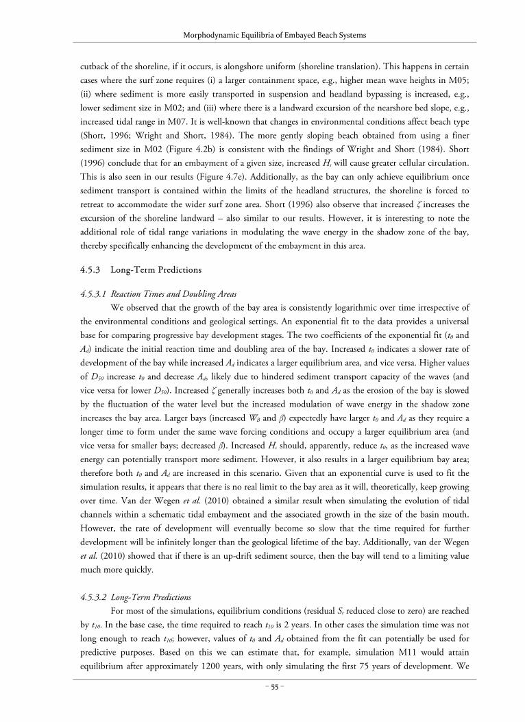
Morphodynamic Equilibria of Embayed Beach Systems
– 55 –
cutback of the shoreline, if it occurs, is alongshore uniform (shoreline translation). This happens in certain cases where the surf zone requires (i) a larger containment space, e.g., higher mean wave heights in M05; (ii) where sediment is more easily transported in suspension and headland bypassing is increased, e.g., lower sediment size in M02; and (iii) where there is a landward excursion of the nearshore bed slope, e.g., increased tidal range in M07. It is well-known that changes in environmental conditions affect beach type (Short, 1996; Wright and Short, 1984). The more gently sloping beach obtained from using a finer sediment size in M02 (Figure 4.2b) is consistent with the findings of Wright and Short (1984). Short (1996) conclude that for an embayment of a given size, increased Hs will cause greater cellular circulation. This is also seen in our results (Figure 4.7e). Additionally, as the bay can only achieve equilibrium once sediment transport is contained within the limits of the headland structures, the shoreline is forced to retreat to accommodate the wider surf zone area. Short (1996) also observe that increased ζ increases the excursion of the shoreline landward – also similar to our results. However, it is interesting to note the additional role of tidal range variations in modulating the wave energy in the shadow zone of the bay, thereby specifically enhancing the development of the embayment in this area.
4.5.3 Long-Term Predictions
4.5.3.1 Reaction Times and Doubling Areas We observed that the growth of the bay area is consistently logarithmic over time irrespective of
the environmental conditions and geological settings. An exponential fit to the data provides a universal base for comparing progressive bay development stages. The two coefficients of the exponential fit (t0 and Ad) indicate the initial reaction time and doubling area of the bay. Increased t0 indicates a slower rate of development of the bay while increased Ad indicates a larger equilibrium area, and vice versa. Higher values of D50 increase t0 and decrease Ad, likely due to hindered sediment transport capacity of the waves (and vice versa for lower D50). Increased ζ generally increases both t0 and Ad as the erosion of the bay is slowed by the fluctuation of the water level but the increased modulation of wave energy in the shadow zone increases the bay area. Larger bays (increased WB and β) expectedly have larger t0 and Ad as they require a longer time to form under the same wave forcing conditions and occupy a larger equilibrium area (and vice versa for smaller bays; decreased β). Increased Hs should, apparently, reduce t0, as the increased wave energy can potentially transport more sediment. However, it also results in a larger equilibrium bay area; therefore both t0 and Ad are increased in this scenario. Given that an exponential curve is used to fit the simulation results, it appears that there is no real limit to the bay area as it will, theoretically, keep growing over time. Van der Wegen et al. (2010) obtained a similar result when simulating the evolution of tidal channels within a schematic tidal embayment and the associated growth in the size of the basin mouth. However, the rate of development will eventually become so slow that the time required for further development will be infinitely longer than the geological lifetime of the bay. Additionally, van der Wegen et al. (2010) showed that if there is an up-drift sediment source, then the bay will tend to a limiting value much more quickly. 4.5.3.2 Long-Term Predictions
For most of the simulations, equilibrium conditions (residual St reduced close to zero) are reached by t10. In the base case, the time required to reach t10 is 2 years. In other cases the simulation time was not long enough to reach t10; however, values of t0 and Ad obtained from the fit can potentially be used for predictive purposes. Based on this we can estimate that, for example, simulation M11 would attain equilibrium after approximately 1200 years, with only simulating the first 75 years of development. We
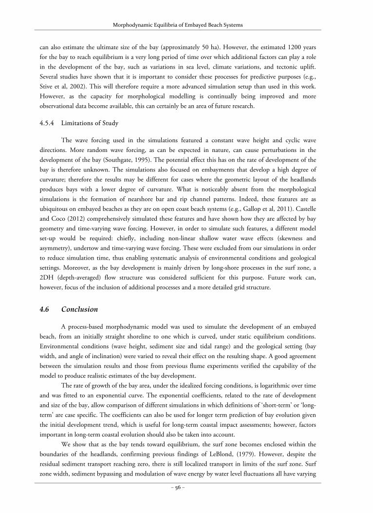
Morphodynamic Equilibria of Embayed Beach Systems
– 56 –
can also estimate the ultimate size of the bay (approximately 50 ha). However, the estimated 1200 years for the bay to reach equilibrium is a very long period of time over which additional factors can play a role in the development of the bay, such as variations in sea level, climate variations, and tectonic uplift. Several studies have shown that it is important to consider these processes for predictive purposes (e.g., Stive et al, 2002). This will therefore require a more advanced simulation setup than used in this work. However, as the capacity for morphological modelling is continually being improved and more observational data become available, this can certainly be an area of future research.
4.5.4 Limitations of Study
The wave forcing used in the simulations featured a constant wave height and cyclic wave directions. More random wave forcing, as can be expected in nature, can cause perturbations in the development of the bay (Southgate, 1995). The potential effect this has on the rate of development of the bay is therefore unknown. The simulations also focused on embayments that develop a high degree of curvature; therefore the results may be different for cases where the geometric layout of the headlands produces bays with a lower degree of curvature. What is noticeably absent from the morphological simulations is the formation of nearshore bar and rip channel patterns. Indeed, these features are as ubiquitous on embayed beaches as they are on open coast beach systems (e.g., Gallop et al, 2011). Castelle and Coco (2012) comprehensively simulated these features and have shown how they are affected by bay geometry and time-varying wave forcing. However, in order to simulate such features, a different model set-up would be required: chiefly, including non-linear shallow water wave effects (skewness and asymmetry), undertow and time-varying wave forcing. These were excluded from our simulations in order to reduce simulation time, thus enabling systematic analysis of environmental conditions and geological settings. Moreover, as the bay development is mainly driven by long-shore processes in the surf zone, a 2DH (depth-averaged) flow structure was considered sufficient for this purpose. Future work can, however, focus of the inclusion of additional processes and a more detailed grid structure.
4.6 Conclusion
A process-based morphodynamic model was used to simulate the development of an embayed beach, from an initially straight shoreline to one which is curved, under static equilibrium conditions. Environmental conditions (wave height, sediment size and tidal range) and the geological setting (bay width, and angle of inclination) were varied to reveal their effect on the resulting shape. A good agreement between the simulation results and those from previous flume experiments verified the capability of the model to produce realistic estimates of the bay development.
The rate of growth of the bay area, under the idealized forcing conditions, is logarithmic over time and was fitted to an exponential curve. The exponential coefficients, related to the rate of development and size of the bay, allow comparison of different simulations in which definitions of ‘short-term’ or ‘long-term’ are case specific. The coefficients can also be used for longer term prediction of bay evolution given the initial development trend, which is useful for long-term coastal impact assessments; however, factors important in long-term coastal evolution should also be taken into account.
We show that as the bay tends toward equilibrium, the surf zone becomes enclosed within the boundaries of the headlands, confirming previous findings of LeBlond, (1979). However, despite the residual sediment transport reaching zero, there is still localized transport in limits of the surf zone. Surf zone width, sediment bypassing and modulation of wave energy by water level fluctuations all have varying
Morphodynamic Equilibria of Embayed Beach Systems
– 57 –
levels of influence on the final shape of the bay, but are generally in agreement with observations from Wright and Short (1984) and Short (1996).
Most importantly, the development of the bay follows a unique trend, regardless of the environmental conditions or geological setting, whereby long-term alongshore non-uniform cutback (shoreline rotation) is potentially followed by alongshore uniform cutback (shoreline translation). The curvature of the beach is shown to be a remnant of the decaying shoreline rotation processes during the growth of the bay. Furthermore, the results indicate that a certain threshold, at which the bay is sufficiently indented, is required before cellular circulation patterns can develop.
4.7 Acknowledgements
The authors acknowledge funding from the German Research Foundation (DFG) via the International Research Training Group: Integrated Coastal Zone and Shelf Sea Research (INTERCOAST). C.J. Daly is grateful to the German Academic Exchange Service (DAAD) Stibet Program for additional funding at the end of the doctoral promotion period. The authors thank Dr. Marius Becker for his critical review and helpful comments on the manuscript.

Morphodynamic Equilibria of Embayed Beach Systems
– 58 –
Morphodynamic Equilibria of Embayed Beach Systems
– 59 –
Chapter 5 – Wave Climate & Equilibrium Bathymetry
This Chapter is based on a manuscript selected for potential publication in the Journal of Ocean Dynamics after
initial review by the scientific committee of the 7th International Conference on Coastal Dynamics, titled:
“Wave Climate Control of Embayed Beach Equilibrium Bathymetry”
Christopher J. Daly 1,2, Karin R. Bryan 2, Mauricio E. Gonzalez 3, Antonio H.F. Klein 4, and Christian Winter 1
1 MARUM – Center for Marine Environmental Sciences, University of Bremen, Bremen, Germany.
2 Department of Earth and Ocean Sciences, University of Waikato, Hamilton, New Zealand. 3 IH Cantabria, Santander, Spain.
4 Universidade Federal de Santa Catarina, Florianópolis, Brasil.
5.1 Abstract
In order to decrease the simulation time of morphodynamic models, often-complex wave climates are reduced to a few representative wave conditions (RWC). When applied to embayed beaches, a test of whether a reduced wave climate is representative or not is to see whether it can recreate the observed equilibrium (long-term averaged) bathymetry of the bay. In this study, the wave climate experienced at Milagro Beach, Tarragona, Spain was discretized into ‘average’ and ‘extreme’ RWCs. The results of process-based, morphodynamic simulations were merged and used to estimate the equilibrium bathymetry of the bay, which were then compared to measurements. The most accurate outcome was obtained when at least 16 wave conditions were used. The effect of extreme wave events appeared to have less influence on the equilibrium of the bay, as indicated by improved results when average conditions were simulated. The importance of accounting for directional variability is essential to accurately balance the impact of beach rotation.
Morphodynamic Equilibria of Embayed Beach Systems
– 60 –
5.2 Introduction
The morphology of beaches is highly dependent on the local and regional wave climate as waves affect the beach orientation, beach slope, residual circulation pattern, and net sediment transport, both in the short- and long-term (Short, 1996; Wright and Short, 1984). The understanding of the variability and stability of sediment volumes on beaches is integral to sustainable coastal zone management and defense (Reeve and Li, 2009). This has led to much research interest in the long-term stability of beaches focusing on equilibrium concepts related to beach profiles (Bruun, 1954; Dean, 1991), and, with respect to embayed beaches, shoreline planforms (Hsu and Evans, 1989; Moreno and Kraus, 1999; Yasso, 1965). Open-coast beaches generally respond to wave forcing by shifting in the cross-shore direction, such as the on- and off-shore migration of sandbars (Pape and Ruessink, 2008). This holds true for embayed beaches; however, this usually results in beach rotation (Harley et al., 2011; Klein at al., 2002). Strong long-shore currents (and transport) may also develop within embayments when the incident wave direction is in disequilibrium with the existing bathymetry. These currents are reduced over time as the beach adjusts itself by rotating to form a more stable position (Daly et al., 2011). Alternating rotation events within an embayment may, over time, maintain some central tendency or equilibrium (LeBlond, 1979; Short and Masselink, 1999).
The combination of both equilibrium planform and profile formulae can be used to estimate the equilibrium bathymetry of an embayment (Hsu et al., 2010). However, this will tend to be over-simplified as the complexities of the geological setting and wave climate of the bay are largely ignored. For example, the equilibrium planform is usually determined based on a peak wave direction, therefore, the effect of other potentially morphologically-significant wave directions are ignored. In order to accurately determine the equilibrium bathymetry of an embayment, the variance of the wave climate and its influence on the net long-shore sediment transport (beach rotation events) should be taken into account. This can be done using process-based morphological models, which have proven to be useful tools in coastal research (e.g., Castelle and Coco, 2012; Reniers et al., 2004). However, as morphological simulations can be quite time consuming, it becomes necessary to reduce the wave climate to a number of representative wave conditions (hereafter RWC) (de Vriend et al., 1993; Lesser, 2009; Plecha et al., 2007).
The wave climate in many parts of the world can be quite variable; some locations may have more than one dominant wave direction (bi-modal), while others may be frequently affected by random storm events. As such, it can be a challenge to reduce the wave climate to only a few RWCs while maintaining the important aspects of its variability. Accordingly, the performance of a reduced number of RWCs is best judged based on how well the morphology of the area of interest is reproduced. While there are several input reduction methods and approaches for applying or sequencing RWCs (e.g., Benedet et al., submitted; Walstra et al., 2013), there is still no standard method of doing so. Several uncertainties arise when trying to determine RWCs. For example, how many RWCs are necessary? What is the best way to discretize the wave climate? How do we account for storm conditions? Are storms important in the long run or do they get averaged out by more frequent, low-energy (average) conditions? What criteria should be used to determine weighting factors (frequency of occurrence, wave energy, sediment transport capacity, initial sedimentation-erosion (ISE) patterns)?
RWCs can be determined from the wave climate using one or two discretization stages, depending on the type of weighting factor used to scale the morphological influence of each RWC. The most common method to discretize the wave climate is to bin the data according to direction and wave height. When binned over a single stage, RWCs are determined directly from the data contained in each bin. This
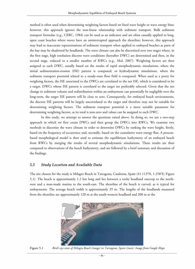
Morphodynamic Equilibria of Embayed Beach Systems
– 61 –
method is often used when determining weighting factors based on fixed wave height or wave energy bins; however, this approach ignores the non-linear relationship with sediment transport. Bulk sediment transport formulae (e.g., CERC, 1984) can be used as an indicator and are often casually applied to long, open coast beaches where waves have an uninterrupted approach the shoreline; however, this approach may lead to inaccurate representations of sediment transport when applied to embayed beaches as parts of the bay may be shadowed by headlands. The wave climate can also be discretized over two stages where, in the first stage, high resolution discrete wave conditions (hereafter DWC) are determined and then, in the second stage, reduced to a smaller number of RWCs (e.g., Mol, 2007). Weighting factors are then assigned to each DWC, usually based on the results of rapid morphodynamic simulations, where the initial sedimentation-erosion (ISE) pattern is computed, or hydrodynamic simulations, where the sediment transport potential related to a steady-state flow field is computed. When used as a proxy for weighting factors, the ISE associated to the DWCs are correlated to the net ISE, which is considered to be a target. DWCs whose ISE pattern is correlated to the target are preferably selected. Given that the net change in sediment volume and redistribution within an embayment can potentially be negligible over the long-term, the target ISE pattern will lie close to zero. Consequently, for embayed beach environments, the discrete ISE patterns will be largely uncorrelated to the target and therefore may not be suitable for determining weighting factors. The sediment transport potential is a more suitable parameter for determining weighting factors, as its total is non-zero and values can be assigned to each DWC.
In this study, we attempt to answer the questions raised above. In doing so, we use a two-step approach in which we first create DWCs and then group the DWCs into RWCs. We examine two methods to discretize the wave climate in order to determine DWCs by ranking the wave height, firstly, based on the frequency of occurrence and, secondly, based on the cumulative wave energy flux. A process-based morphological model is then used to estimate the equilibrium bathymetry of an embayed beach from RWCs by merging the results of several morphodynamic simulations. These results are then compared to observations of the beach bathymetry, and are followed by a brief summary and discussion of the findings.
5.3 Study Location and Available Data
The site chosen for the study is Milagro Beach in Tarragona, Catalonia, Spain (41.113°N, 1.258°E; Figure 5.1). The beach is approximately 1.2 km long and lies between a rocky headland outcrop to the north-west and a man-made marina to the south-east. The shoreline of the beach is curved, as is typical for embayments. The average beach width is approximately 35 m. The lengths of the headlands measured from the shoreline are approximately 120 m at the south-western headland and 200 m at the
Figure 5.1 Bird’s-eye view of Milagro Beach (image) in Tarragona, Spain (inset). Image from Google Maps
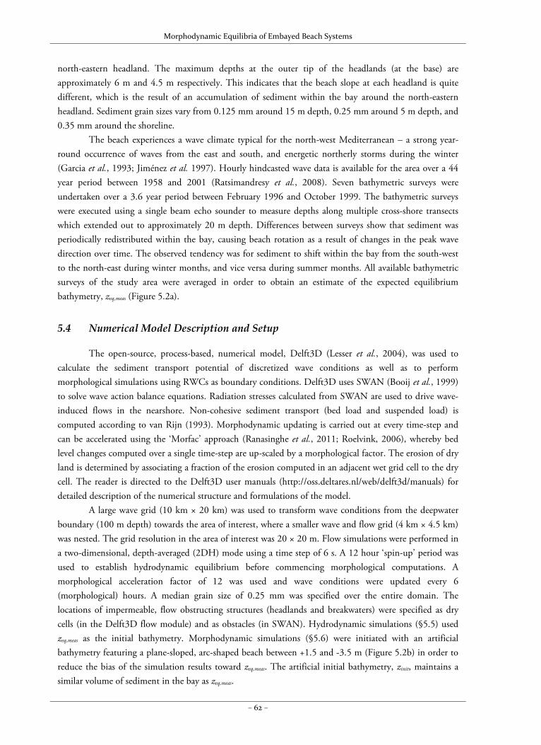
Morphodynamic Equilibria of Embayed Beach Systems
– 62 –
north-eastern headland. The maximum depths at the outer tip of the headlands (at the base) are approximately 6 m and 4.5 m respectively. This indicates that the beach slope at each headland is quite different, which is the result of an accumulation of sediment within the bay around the north-eastern headland. Sediment grain sizes vary from 0.125 mm around 15 m depth, 0.25 mm around 5 m depth, and 0.35 mm around the shoreline.
The beach experiences a wave climate typical for the north-west Mediterranean – a strong year-round occurrence of waves from the east and south, and energetic northerly storms during the winter (Garcia et al., 1993; Jiménez et al. 1997). Hourly hindcasted wave data is available for the area over a 44 year period between 1958 and 2001 (Ratsimandresy et al., 2008). Seven bathymetric surveys were undertaken over a 3.6 year period between February 1996 and October 1999. The bathymetric surveys were executed using a single beam echo sounder to measure depths along multiple cross-shore transects which extended out to approximately 20 m depth. Differences between surveys show that sediment was periodically redistributed within the bay, causing beach rotation as a result of changes in the peak wave direction over time. The observed tendency was for sediment to shift within the bay from the south-west to the north-east during winter months, and vice versa during summer months. All available bathymetric surveys of the study area were averaged in order to obtain an estimate of the expected equilibrium bathymetry, zeq,meas (Figure 5.2a).
5.4 Numerical Model Description and Setup
The open-source, process-based, numerical model, Delft3D (Lesser et al., 2004), was used to calculate the sediment transport potential of discretized wave conditions as well as to perform morphological simulations using RWCs as boundary conditions. Delft3D uses SWAN (Booij et al., 1999) to solve wave action balance equations. Radiation stresses calculated from SWAN are used to drive wave-induced flows in the nearshore. Non-cohesive sediment transport (bed load and suspended load) is computed according to van Rijn (1993). Morphodynamic updating is carried out at every time-step and can be accelerated using the ‘Morfac’ approach (Ranasinghe et al., 2011; Roelvink, 2006), whereby bed level changes computed over a single time-step are up-scaled by a morphological factor. The erosion of dry land is determined by associating a fraction of the erosion computed in an adjacent wet grid cell to the dry cell. The reader is directed to the Delft3D user manuals (http://oss.deltares.nl/web/delft3d/manuals) for detailed description of the numerical structure and formulations of the model.
A large wave grid (10 km × 20 km) was used to transform wave conditions from the deepwater boundary (100 m depth) towards the area of interest, where a smaller wave and flow grid (4 km × 4.5 km) was nested. The grid resolution in the area of interest was 20 × 20 m. Flow simulations were performed in a two-dimensional, depth-averaged (2DH) mode using a time step of 6 s. A 12 hour ‘spin-up’ period was used to establish hydrodynamic equilibrium before commencing morphological computations. A morphological acceleration factor of 12 was used and wave conditions were updated every 6 (morphological) hours. A median grain size of 0.25 mm was specified over the entire domain. The locations of impermeable, flow obstructing structures (headlands and breakwaters) were specified as dry cells (in the Delft3D flow module) and as obstacles (in SWAN). Hydrodynamic simulations (§5.5) used zeq,meas as the initial bathymetry. Morphodynamic simulations (§5.6) were initiated with an artificial bathymetry featuring a plane-sloped, arc-shaped beach between +1.5 and -3.5 m (Figure 5.2b) in order to reduce the bias of the simulation results toward zeq,meas. The artificial initial bathymetry, zinit, maintains a similar volume of sediment in the bay as zeq,meas.
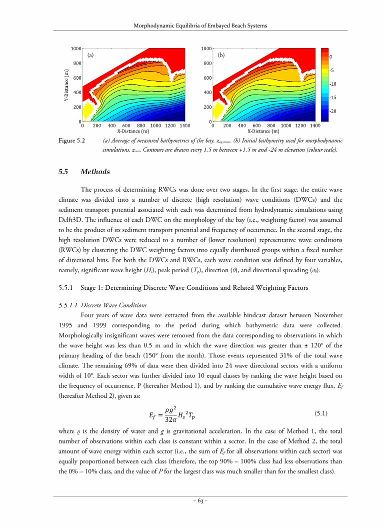
Morphodynamic Equilibria of Embayed Beach Systems
– 63 –
Figure 5.2 (a) Average of measured bathymetries of the bay, zeq,meas. (b) Initial bathymetry used for morphodynamic
simulations, zinit. Contours are drawn every 1.5 m between +1.5 m and -24 m elevation (colour scale).
5.5 Methods
The process of determining RWCs was done over two stages. In the first stage, the entire wave climate was divided into a number of discrete (high resolution) wave conditions (DWCs) and the sediment transport potential associated with each was determined from hydrodynamic simulations using Delft3D. The influence of each DWC on the morphology of the bay (i.e., weighting factor) was assumed to be the product of its sediment transport potential and frequency of occurrence. In the second stage, the high resolution DWCs were reduced to a number of (lower resolution) representative wave conditions (RWCs) by clustering the DWC weighting factors into equally distributed groups within a fixed number of directional bins. For both the DWCs and RWCs, each wave condition was defined by four variables, namely, significant wave height (Hs), peak period (Tp), direction (θ), and directional spreading (σθ).
5.5.1 Stage 1: Determining Discrete Wave Conditions and Related Weighting Factors
5.5.1.1 Discrete Wave Conditions Four years of wave data were extracted from the available hindcast dataset between November
1995 and 1999 corresponding to the period during which bathymetric data were collected. Morphologically insignificant waves were removed from the data corresponding to observations in which the wave height was less than 0.5 m and in which the wave direction was greater than ± 120° of the primary heading of the beach (150° from the north). Those events represented 31% of the total wave climate. The remaining 69% of data were then divided into 24 wave directional sectors with a uniform width of 10°. Each sector was further divided into 10 equal classes by ranking the wave height based on the frequency of occurrence, P (hereafter Method 1), and by ranking the cumulative wave energy flux, Ef (hereafter Method 2), given as:
32 (5.1)
where ρ is the density of water and g is gravitational acceleration. In the case of Method 1, the total number of observations within each class is constant within a sector. In the case of Method 2, the total amount of wave energy within each sector (i.e., the sum of Ef for all observations within each sector) was equally proportioned between each class (therefore, the top 90% – 100% class had less observations than the 0% – 10% class, and the value of P for the largest class was much smaller than for the smallest class).
(a) (b)
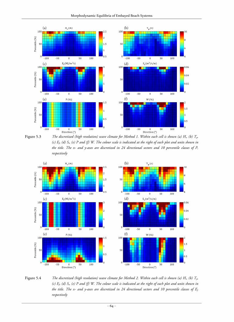
Morphodynamic Equilibria of Embayed Beach Systems
– 64 –
Figure 5.3 The discretized (high resolution) wave climate for Method 1. Within each cell is shown (a) Hs, (b) Tp,
(c) Ef, (d) St, (e) P and (f) W. The colour scale is indicated at the right of each plot and units shown in the title. The x- and y-axes are discretized in 24 directional sectors and 10 percentile classes of P, respectively
Figure 5.4 The discretized (high resolution) wave climate for Method 2. Within each cell is shown (a) Hs, (b) Tp, (c) Ef, (d) St, (e) P and (f) W. The colour scale is indicated at the right of each plot and units shown in the title. The x- and y-axes are discretized in 24 directional sectors and 10 percentile classes of Ef, respectively
(a) (b)
(c) (d)
(e) (f)
(a) (b)
(c) (d)
(e) (f)
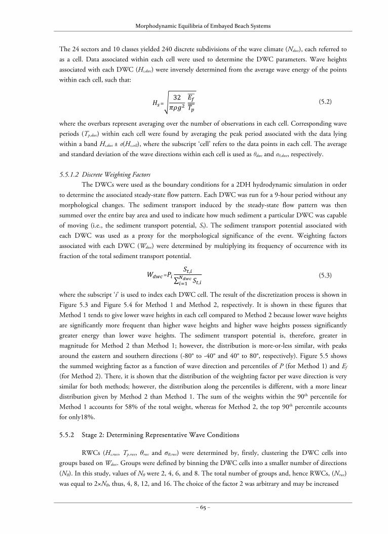
Morphodynamic Equilibria of Embayed Beach Systems
– 65 –
The 24 sectors and 10 classes yielded 240 discrete subdivisions of the wave climate (Ndwc), each referred to as a cell. Data associated within each cell were used to determine the DWC parameters. Wave heights associated with each DWC (Hs,dwc) were inversely determined from the average wave energy of the points within each cell, such that:
=32
(5.2)
where the overbars represent averaging over the number of observations in each cell. Corresponding wave periods (Tp,dwc) within each cell were found by averaging the peak period associated with the data lying within a band Hs,dwc ± σ(Hs,cell), where the subscript ‘cell’ refers to the data points in each cell. The average and standard deviation of the wave directions within each cell is used as θdwc and σθ,dwc, respectively. 5.5.1.2 Discrete Weighting Factors
The DWCs were used as the boundary conditions for a 2DH hydrodynamic simulation in order to determine the associated steady-state flow pattern. Each DWC was run for a 9-hour period without any morphological changes. The sediment transport induced by the steady-state flow pattern was then summed over the entire bay area and used to indicate how much sediment a particular DWC was capable of moving (i.e., the sediment transport potential, St). The sediment transport potential associated with each DWC was used as a proxy for the morphological significance of the event. Weighting factors associated with each DWC (Wdwc) were determined by multiplying its frequency of occurrence with its fraction of the total sediment transport potential.
= ,
∑ , (5.3)
where the subscript ‘i’ is used to index each DWC cell. The result of the discretization process is shown in Figure 5.3 and Figure 5.4 for Method 1 and Method 2, respectively. It is shown in these figures that Method 1 tends to give lower wave heights in each cell compared to Method 2 because lower wave heights are significantly more frequent than higher wave heights and higher wave heights possess significantly greater energy than lower wave heights. The sediment transport potential is, therefore, greater in magnitude for Method 2 than Method 1; however, the distribution is more-or-less similar, with peaks around the eastern and southern directions (-80° to -40° and 40° to 80°, respectively). Figure 5.5 shows the summed weighting factor as a function of wave direction and percentiles of P (for Method 1) and Ef
(for Method 2). There, it is shown that the distribution of the weighting factor per wave direction is very similar for both methods; however, the distribution along the percentiles is different, with a more linear distribution given by Method 2 than Method 1. The sum of the weights within the 90th percentile for Method 1 accounts for 58% of the total weight, whereas for Method 2, the top 90th percentile accounts for only18%.
5.5.2 Stage 2: Determining Representative Wave Conditions
RWCs (Hs,rwc, Tp,rwc, θrwc and σθ,rwc) were determined by, firstly, clustering the DWC cells into groups based on Wdwc. Groups were defined by binning the DWC cells into a smaller number of directions (Nθ). In this study, values of Nθ were 2, 4, 6, and 8. The total number of groups and, hence RWCs, (Nrwc) was equal to 2×Nθ, thus, 4, 8, 12, and 16. The choice of the factor 2 was arbitrary and may be increased
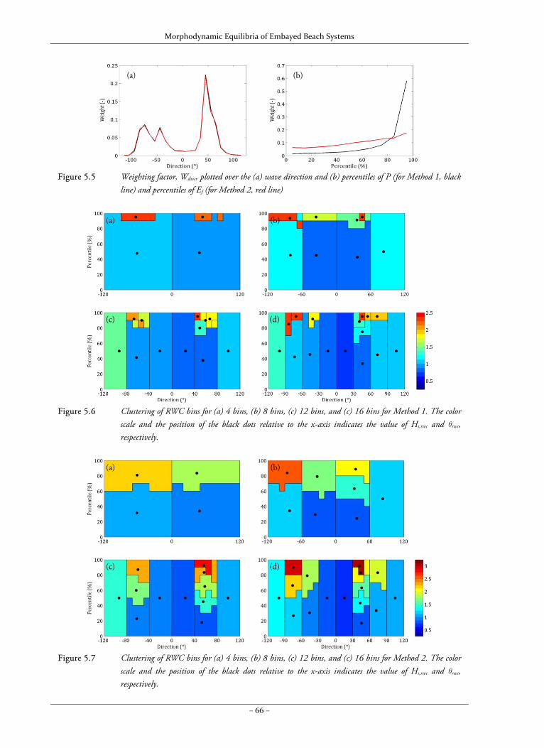
Morphodynamic Equilibria of Embayed Beach Systems
– 66 –
Figure 5.5 Weighting factor, Wdwc, plotted over the (a) wave direction and (b) percentiles of P (for Method 1, black
line) and percentiles of Ef (for Method 2, red line)
Figure 5.6 Clustering of RWC bins for (a) 4 bins, (b) 8 bins, (c) 12 bins, and (c) 16 bins for Method 1. The color
scale and the position of the black dots relative to the x-axis indicates the value of Hs,rwc and θrwc, respectively.
Figure 5.7 Clustering of RWC bins for (a) 4 bins, (b) 8 bins, (c) 12 bins, and (c) 16 bins for Method 2. The color
scale and the position of the black dots relative to the x-axis indicates the value of Hs,rwc and θrwc, respectively.
(a) (b)
(a) (b)
(c) (d)
(a) (b)
(c) (d)
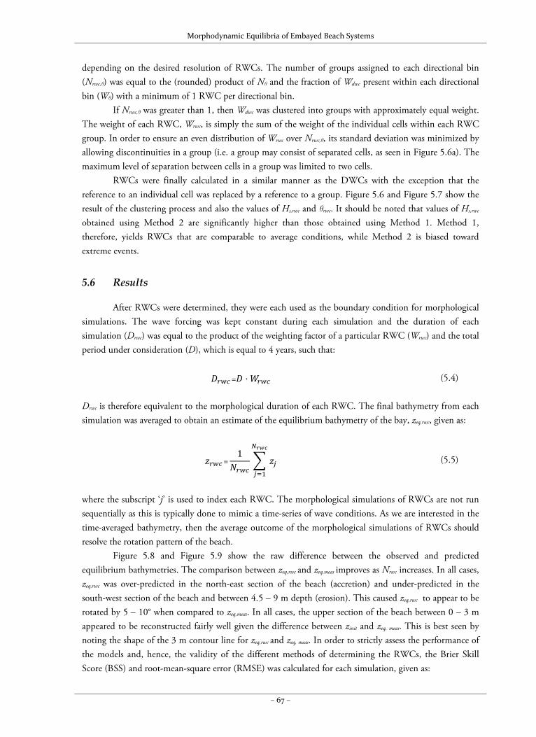
Morphodynamic Equilibria of Embayed Beach Systems
– 67 –
depending on the desired resolution of RWCs. The number of groups assigned to each directional bin (Nrwc,θ) was equal to the (rounded) product of Nθ and the fraction of Wdwc present within each directional bin (Wθ) with a minimum of 1 RWC per directional bin.
If Nrwc,θ was greater than 1, then Wdwc was clustered into groups with approximately equal weight. The weight of each RWC, Wrwc, is simply the sum of the weight of the individual cells within each RWC group. In order to ensure an even distribution of Wrwc over Nrwc,θ, its standard deviation was minimized by allowing discontinuities in a group (i.e. a group may consist of separated cells, as seen in Figure 5.6a). The maximum level of separation between cells in a group was limited to two cells.
RWCs were finally calculated in a similar manner as the DWCs with the exception that the reference to an individual cell was replaced by a reference to a group. Figure 5.6 and Figure 5.7 show the result of the clustering process and also the values of Hs,rwc and θrwc. It should be noted that values of Hs,rwc
obtained using Method 2 are significantly higher than those obtained using Method 1. Method 1, therefore, yields RWCs that are comparable to average conditions, while Method 2 is biased toward extreme events.
5.6 Results
After RWCs were determined, they were each used as the boundary condition for morphological simulations. The wave forcing was kept constant during each simulation and the duration of each simulation (Drwc) was equal to the product of the weighting factor of a particular RWC (Wrwc) and the total period under consideration (D), which is equal to 4 years, such that:
= ⋅ (5.4)
Drwc is therefore equivalent to the morphological duration of each RWC. The final bathymetry from each simulation was averaged to obtain an estimate of the equilibrium bathymetry of the bay, zeq,rwc, given as:
=1
(5.5)
where the subscript ‘j’ is used to index each RWC. The morphological simulations of RWCs are not run sequentially as this is typically done to mimic a time-series of wave conditions. As we are interested in the time-averaged bathymetry, then the average outcome of the morphological simulations of RWCs should resolve the rotation pattern of the beach.
Figure 5.8 and Figure 5.9 show the raw difference between the observed and predicted equilibrium bathymetries. The comparison between zeq,rwc and zeq,meas improves as Nrwc increases. In all cases, zeq,rwc was over-predicted in the north-east section of the beach (accretion) and under-predicted in the south-west section of the beach and between 4.5 – 9 m depth (erosion). This caused zeq,rwc to appear to be rotated by 5 – 10° when compared to zeq,meas. In all cases, the upper section of the beach between 0 – 3 m appeared to be reconstructed fairly well given the difference between zinit and zeq, meas. This is best seen by noting the shape of the 3 m contour line for zeq,rwc and zeq, meas. In order to strictly assess the performance of the models and, hence, the validity of the different methods of determining the RWCs, the Brier Skill Score (BSS) and root-mean-square error (RMSE) was calculated for each simulation, given as:
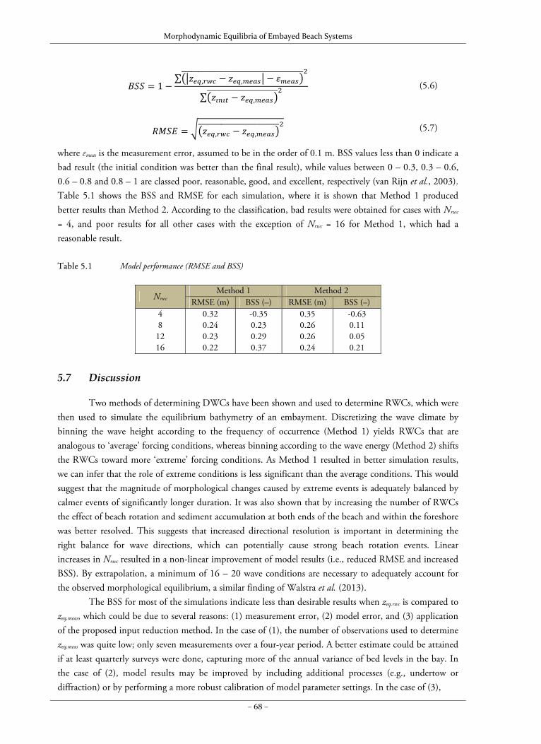
Morphodynamic Equilibria of Embayed Beach Systems
– 68 –
1∑ , ,
∑ ,
(5.6)
, , (5.7)
where εmeas is the measurement error, assumed to be in the order of 0.1 m. BSS values less than 0 indicate a bad result (the initial condition was better than the final result), while values between 0 – 0.3, 0.3 – 0.6, 0.6 – 0.8 and 0.8 – 1 are classed poor, reasonable, good, and excellent, respectively (van Rijn et al., 2003). Table 5.1 shows the BSS and RMSE for each simulation, where it is shown that Method 1 produced better results than Method 2. According to the classification, bad results were obtained for cases with Nrwc = 4, and poor results for all other cases with the exception of Nrwc = 16 for Method 1, which had a reasonable result.
Table 5.1 Model performance (RMSE and BSS)
Nrwc Method 1 Method 2
RMSE (m) BSS (–) RMSE (m) BSS (–)4 8 12 16
0.320.24 0.23 0.22
-0.350.23 0.29 0.37
0.350.26 0.26 0.24
-0.630.11 0.05 0.21
5.7 Discussion
Two methods of determining DWCs have been shown and used to determine RWCs, which were then used to simulate the equilibrium bathymetry of an embayment. Discretizing the wave climate by binning the wave height according to the frequency of occurrence (Method 1) yields RWCs that are analogous to ‘average’ forcing conditions, whereas binning according to the wave energy (Method 2) shifts the RWCs toward more ‘extreme’ forcing conditions. As Method 1 resulted in better simulation results, we can infer that the role of extreme conditions is less significant than the average conditions. This would suggest that the magnitude of morphological changes caused by extreme events is adequately balanced by calmer events of significantly longer duration. It was also shown that by increasing the number of RWCs the effect of beach rotation and sediment accumulation at both ends of the beach and within the foreshore was better resolved. This suggests that increased directional resolution is important in determining the right balance for wave directions, which can potentially cause strong beach rotation events. Linear increases in Nrwc resulted in a non-linear improvement of model results (i.e., reduced RMSE and increased BSS). By extrapolation, a minimum of 16 – 20 wave conditions are necessary to adequately account for the observed morphological equilibrium, a similar finding of Walstra et al. (2013).
The BSS for most of the simulations indicate less than desirable results when zeq,rwc is compared to zeq,meas, which could be due to several reasons: (1) measurement error, (2) model error, and (3) application of the proposed input reduction method. In the case of (1), the number of observations used to determine zeq,meas was quite low; only seven measurements over a four-year period. A better estimate could be attained if at least quarterly surveys were done, capturing more of the annual variance of bed levels in the bay. In the case of (2), model results may be improved by including additional processes (e.g., undertow or diffraction) or by performing a more robust calibration of model parameter settings. In the case of (3),
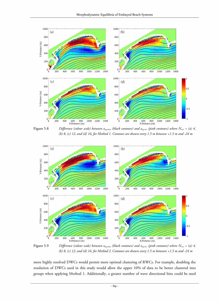
Morphodynamic Equilibria of Embayed Beach Systems
– 69 –
Figure 5.8 Difference (colour scale) between zeq,meas (black contours) and zeq,rwc (pink contours) where Nrwc = (a) 4,
(b) 8, (c) 12, and (d) 16, for Method 1. Contours are drawn every 1.5 m between +1.5 m and -24 m
Figure 5.9 Difference (colour scale) between zeq,meas (black contours) and zeq,rwc (pink contours) where Nrwc = (a) 4,
(b) 8, (c) 12, and (d) 16, for Method 2. Contours are drawn every 1.5 m between +1.5 m and -24 m
more highly resolved DWCs would permit more optimal clustering of RWCs. For example, doubling the resolution of DWCs used in this study would allow the upper 10% of data to be better clustered into groups when applying Method 1. Additionally, a greater number of wave directional bins could be used
(a) (b)
(c) (d)
(a) (b)
(c) (d)
Morphodynamic Equilibria of Embayed Beach Systems
– 70 –
for the RWCs. In this study, the smallest bin size was 30°; however, a 15° bin size may increase the accuracy of the results by accounting for a greater number of wave directions. Lastly, it was shown that waves greater than ± 100° of the shore normal have a very weak influence on the morphology of the bay, therefore, these conditions may be ignored in order to improve the assignment of RWCs.
Despite the abovementioned limitations, the results obtained from this study support the proposition that an equilibrium state exists for embayed beaches, which is largely controlled by the wave climate, and in particular, the wave direction. This equilibrium state may be transient if the long-term wave climate gradually changes over time. It should be noted that single observations of the embayment bathymetry may be significantly different from the equilibrium case depending on the short-term wave conditions (Reeve and Li, 2009). However, the proposed input reduction method can be used to provide information on the expected maxima and minima (and, hence, expected variance) of bed levels within embayed beach environments, which may be useful for coastal zone management and defense strategies.
5.8 Conclusion
The equilibrium bathymetry of an embayed beach was determined using a varied number of RWCs. Two methods of calculating the weight assigned to the RWCs were also compared. Results indicate that binning wave heights in terms of frequency of occurrence gives better results than binning according to wave energy. A minimum of 16 RWCs produced reasonably skillful results despite using rather standard model settings. Given that there is enough room for improvement, the present results are promising and indicate that the equilibrium bathymetry within embayments is largely determined by a variable wave climate, especially in relation to the wave direction. It is therefore necessary to ensure that a suitable level of directional resolution is accounted for when determining RWCs for embayed beach environments.
5.9 Acknowledgements
C.J. Daly acknowledges research funding from the German Research Foundation (DFG) via the International Research Training Group: Integrated Coastal Zone and Shelf Sea Research (INTERCOAST). The field data has been kindly provided by Dr. Jordi Galofré (Spanish Ministry of Environment), and its support is hereby gratefully acknowledged.
Morphodynamic Equilibria of Embayed Beach Systems
– 71 –
Chapter 6 – Short‐ to Medium‐Term Dynamics
This Chapter presents the outline for a manuscript in preparation based on data collected during a 9-month field campaign at Tairua and Pauanui Beaches, New Zealand, titled:
“Reconstructing Short-Term Sediment Exchange within an Embayed Beach”
Christopher J. Daly 1,2, Karin R. Bryan 2, and Christian Winter 1
1 MARUM – Center for Marine Environmental Sciences, University of Bremen, Bremen, Germany
2 Department of Earth and Ocean Sciences, University of Waikato, Hamilton, New Zealand
6.1 Introduction
Beaches change over varying temporal and spatial scales, mainly in response to wave-induced hydrodynamic forcing. Changes in shoreline position may be short-term (event-driven) or medium-term (seasonal), e.g., Dubois, (1988) and Quartel et al., (2007), or occur over a longer period in the order of several years (Ranasinghe et al., 2004a; Short and Trembanis, 2004). Seasonal erosion and accretion cycles of beaches have been related to fluctuations in wave energy (e.g. Yates et al., 2009). This is often exemplified as erosion during stormy winter months and accretion during calmer summer months. Despite this generalisation, there are locations where weather tends to be more episodic; hence, a greater irregularity in wave forcing such that there may be more frequent storms during summer and, likewise, calm periods during winter. In such cases, forcing conditions are more dynamic and there is potentially less recovery time between storms. This leads to an often non-linear relationship between hydrodynamic forcing and beach response in which the present state of the beach may not be directly correlated to the immediate forcing conditions (Pape & Ruessink, 2008). However, current research has indicated that some degree of correlation may be obtained by considering the average wave conditions over a certain period immediately prior to a given beach state (Quartel et al., 2008). The length of the averaging time period should account for event-driven changes in the order of a few days; otherwise increased temporal averaging can lead to reduced model performance (Davidson et al., 2011).
Equilibrium shoreline models, such as Yates et al. (2009), determine whether a beach will accrete or erode at given point in time depending on the disequilibrium between the current wave forcing conditions and a predetermined equilibrium state related to the seaward (or shoreward) position of the shoreline. This has been successfully applied to embayed beaches (van de Lageweg et al., 2013), taking into account the distance between the outer bar and the shoreline and the rotation of the beach. The accuracy of data-driven shoreline models is dependent on the length of the observation period used for calibration
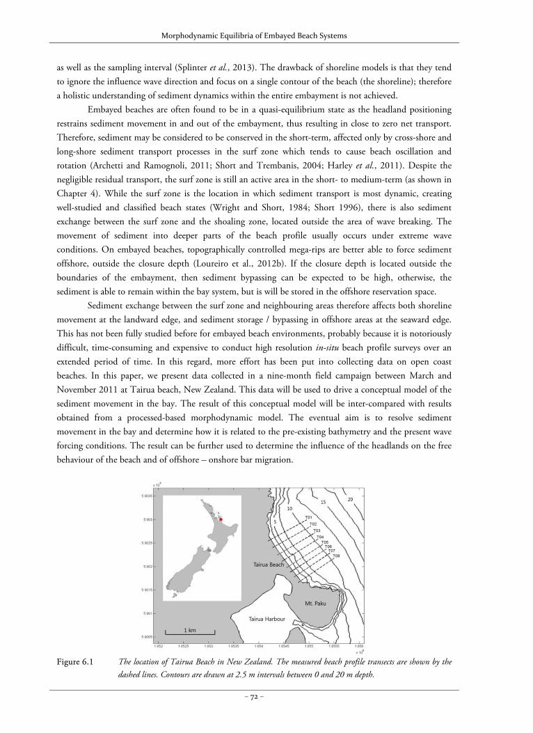
Morphodynamic Equilibria of Embayed Beach Systems
– 72 –
as well as the sampling interval (Splinter et al., 2013). The drawback of shoreline models is that they tend to ignore the influence wave direction and focus on a single contour of the beach (the shoreline); therefore a holistic understanding of sediment dynamics within the entire embayment is not achieved.
Embayed beaches are often found to be in a quasi-equilibrium state as the headland positioning restrains sediment movement in and out of the embayment, thus resulting in close to zero net transport. Therefore, sediment may be considered to be conserved in the short-term, affected only by cross-shore and long-shore sediment transport processes in the surf zone which tends to cause beach oscillation and rotation (Archetti and Ramognoli, 2011; Short and Trembanis, 2004; Harley et al., 2011). Despite the negligible residual transport, the surf zone is still an active area in the short- to medium-term (as shown in Chapter 4). While the surf zone is the location in which sediment transport is most dynamic, creating well-studied and classified beach states (Wright and Short, 1984; Short 1996), there is also sediment exchange between the surf zone and the shoaling zone, located outside the area of wave breaking. The movement of sediment into deeper parts of the beach profile usually occurs under extreme wave conditions. On embayed beaches, topographically controlled mega-rips are better able to force sediment offshore, outside the closure depth (Loureiro et al., 2012b). If the closure depth is located outside the boundaries of the embayment, then sediment bypassing can be expected to be high, otherwise, the sediment is able to remain within the bay system, but is will be stored in the offshore reservation space.
Sediment exchange between the surf zone and neighbouring areas therefore affects both shoreline movement at the landward edge, and sediment storage / bypassing in offshore areas at the seaward edge. This has not been fully studied before for embayed beach environments, probably because it is notoriously difficult, time-consuming and expensive to conduct high resolution in-situ beach profile surveys over an extended period of time. In this regard, more effort has been put into collecting data on open coast beaches. In this paper, we present data collected in a nine-month field campaign between March and November 2011 at Tairua beach, New Zealand. This data will be used to drive a conceptual model of the sediment movement in the bay. The result of this conceptual model will be inter-compared with results obtained from a processed-based morphodynamic model. The eventual aim is to resolve sediment movement in the bay and determine how it is related to the pre-existing bathymetry and the present wave forcing conditions. The result can be further used to determine the influence of the headlands on the free behaviour of the beach and of offshore – onshore bar migration.
Figure 6.1 The location of Tairua Beach in New Zealand. The measured beach profile transects are shown by the
dashed lines. Contours are drawn at 2.5 m intervals between 0 and 20 m depth.
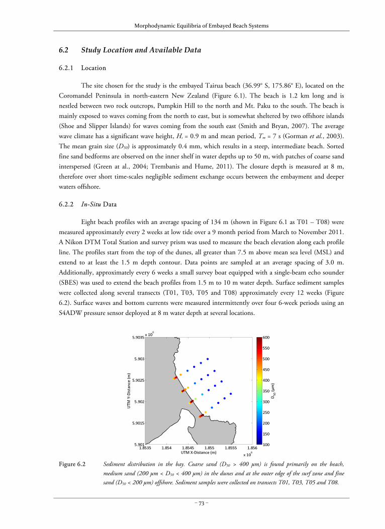
Morphodynamic Equilibria of Embayed Beach Systems
– 73 –
6.2 Study Location and Available Data
6.2.1 Location
The site chosen for the study is the embayed Tairua beach (36.99° S, 175.86° E), located on the Coromandel Peninsula in north-eastern New Zealand (Figure 6.1). The beach is 1.2 km long and is nestled between two rock outcrops, Pumpkin Hill to the north and Mt. Paku to the south. The beach is mainly exposed to waves coming from the north to east, but is somewhat sheltered by two offshore islands (Shoe and Slipper Islands) for waves coming from the south east (Smith and Bryan, 2007). The average wave climate has a significant wave height, Hs = 0.9 m and mean period, Tm = 7 s (Gorman et al., 2003). The mean grain size (D50) is approximately 0.4 mm, which results in a steep, intermediate beach. Sorted fine sand bedforms are observed on the inner shelf in water depths up to 50 m, with patches of coarse sand interspersed (Green at al., 2004; Trembanis and Hume, 2011). The closure depth is measured at 8 m, therefore over short time-scales negligible sediment exchange occurs between the embayment and deeper waters offshore.
6.2.2 In-Situ Data
Eight beach profiles with an average spacing of 134 m (shown in Figure 6.1 as T01 – T08) were measured approximately every 2 weeks at low tide over a 9 month period from March to November 2011. A Nikon DTM Total Station and survey prism was used to measure the beach elevation along each profile line. The profiles start from the top of the dunes, all greater than 7.5 m above mean sea level (MSL) and extend to at least the 1.5 m depth contour. Data points are sampled at an average spacing of 3.0 m. Additionally, approximately every 6 weeks a small survey boat equipped with a single-beam echo sounder (SBES) was used to extend the beach profiles from 1.5 m to 10 m water depth. Surface sediment samples were collected along several transects (T01, T03, T05 and T08) approximately every 12 weeks (Figure 6.2). Surface waves and bottom currents were measured intermittently over four 6-week periods using an S4ADW pressure sensor deployed at 8 m water depth at several locations.
Figure 6.2 Sediment distribution in the bay. Coarse sand (D50 > 400 μm) is found primarily on the beach,
medium sand (200 μm < D50 < 400 μm) in the dunes and at the outer edge of the surf zone and fine sand (D50 < 200 μm) offshore. Sediment samples were collected on transects T01, T03, T05 and T08.
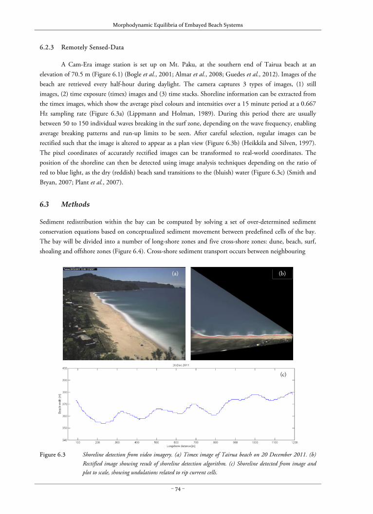
Morphodynamic Equilibria of Embayed Beach Systems
– 74 –
6.2.3 Remotely Sensed-Data
A Cam-Era image station is set up on Mt. Paku, at the southern end of Tairua beach at an elevation of 70.5 m (Figure 6.1) (Bogle et al., 2001; Almar et al., 2008; Guedes et al., 2012). Images of the beach are retrieved every half-hour during daylight. The camera captures 3 types of images, (1) still images, (2) time exposure (timex) images and (3) time stacks. Shoreline information can be extracted from the timex images, which show the average pixel colours and intensities over a 15 minute period at a 0.667 Hz sampling rate (Figure 6.3a) (Lippmann and Holman, 1989). During this period there are usually between 50 to 150 individual waves breaking in the surf zone, depending on the wave frequency, enabling average breaking patterns and run-up limits to be seen. After careful selection, regular images can be rectified such that the image is altered to appear as a plan view (Figure 6.3b) (Heikkila and Silven, 1997). The pixel coordinates of accurately rectified images can be transformed to real-world coordinates. The position of the shoreline can then be detected using image analysis techniques depending on the ratio of red to blue light, as the dry (reddish) beach sand transitions to the (bluish) water (Figure 6.3c) (Smith and Bryan, 2007; Plant et al., 2007).
6.3 Methods
Sediment redistribution within the bay can be computed by solving a set of over-determined sediment conservation equations based on conceptualized sediment movement between predefined cells of the bay. The bay will be divided into a number of long-shore zones and five cross-shore zones: dune, beach, surf, shoaling and offshore zones (Figure 6.4). Cross-shore sediment transport occurs between neighbouring
Figure 6.3 Shoreline detection from video imagery. (a) Timex image of Tairua beach on 20 December 2011. (b)
Rectified image showing result of shoreline detection algorithm. (c) Shoreline detected from image and plot to scale, showing undulations related to rip current cells.
(a) (b)
(c)
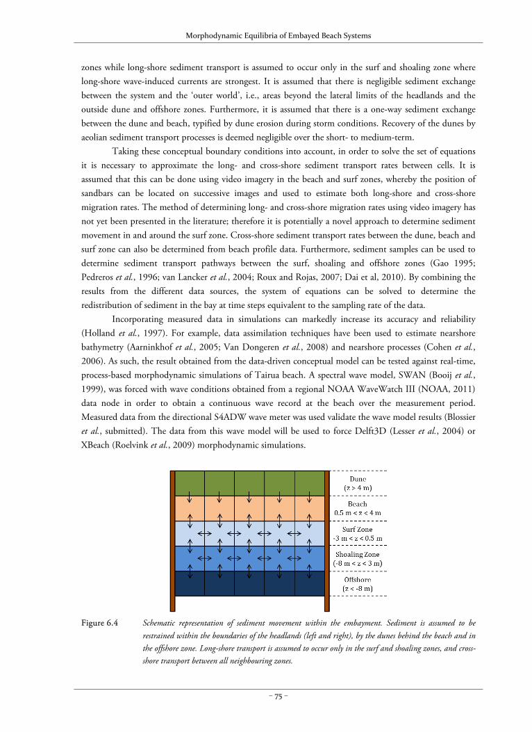
Morphodynamic Equilibria of Embayed Beach Systems
– 75 –
zones while long-shore sediment transport is assumed to occur only in the surf and shoaling zone where long-shore wave-induced currents are strongest. It is assumed that there is negligible sediment exchange between the system and the ‘outer world’, i.e., areas beyond the lateral limits of the headlands and the outside dune and offshore zones. Furthermore, it is assumed that there is a one-way sediment exchange between the dune and beach, typified by dune erosion during storm conditions. Recovery of the dunes by aeolian sediment transport processes is deemed negligible over the short- to medium-term.
Taking these conceptual boundary conditions into account, in order to solve the set of equations it is necessary to approximate the long- and cross-shore sediment transport rates between cells. It is assumed that this can be done using video imagery in the beach and surf zones, whereby the position of sandbars can be located on successive images and used to estimate both long-shore and cross-shore migration rates. The method of determining long- and cross-shore migration rates using video imagery has not yet been presented in the literature; therefore it is potentially a novel approach to determine sediment movement in and around the surf zone. Cross-shore sediment transport rates between the dune, beach and surf zone can also be determined from beach profile data. Furthermore, sediment samples can be used to determine sediment transport pathways between the surf, shoaling and offshore zones (Gao 1995; Pedreros et al., 1996; van Lancker et al., 2004; Roux and Rojas, 2007; Dai et al, 2010). By combining the results from the different data sources, the system of equations can be solved to determine the redistribution of sediment in the bay at time steps equivalent to the sampling rate of the data.
Incorporating measured data in simulations can markedly increase its accuracy and reliability (Holland et al., 1997). For example, data assimilation techniques have been used to estimate nearshore bathymetry (Aarninkhof et al., 2005; Van Dongeren et al., 2008) and nearshore processes (Cohen et al., 2006). As such, the result obtained from the data-driven conceptual model can be tested against real-time, process-based morphodynamic simulations of Tairua beach. A spectral wave model, SWAN (Booij et al., 1999), was forced with wave conditions obtained from a regional NOAA WaveWatch III (NOAA, 2011) data node in order to obtain a continuous wave record at the beach over the measurement period. Measured data from the directional S4ADW wave meter was used validate the wave model results (Blossier et al., submitted). The data from this wave model will be used to force Delft3D (Lesser et al., 2004) or XBeach (Roelvink et al., 2009) morphodynamic simulations.
Figure 6.4 Schematic representation of sediment movement within the embayment. Sediment is assumed to be
restrained within the boundaries of the headlands (left and right), by the dunes behind the beach and in the offshore zone. Long-shore transport is assumed to occur only in the surf and shoaling zones, and cross-shore transport between all neighbouring zones.
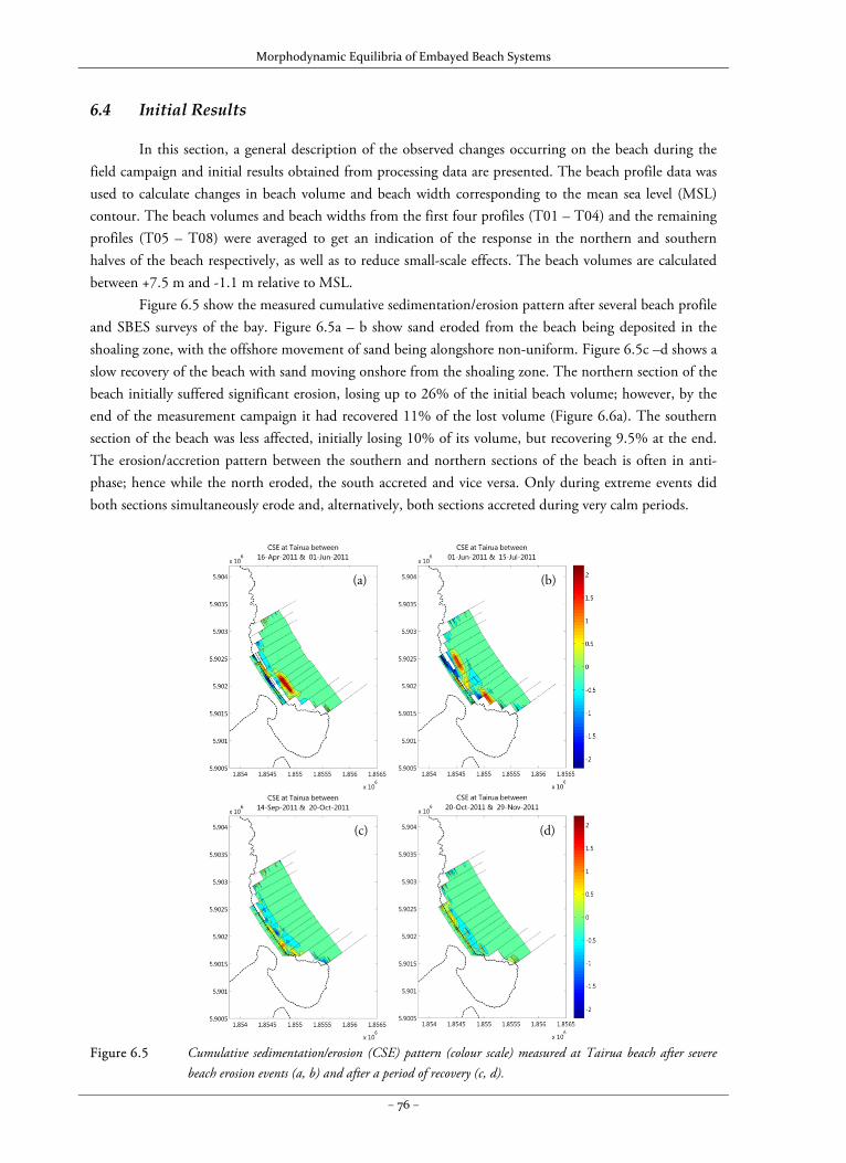
Morphodynamic Equilibria of Embayed Beach Systems
– 76 –
6.4 Initial Results
In this section, a general description of the observed changes occurring on the beach during the field campaign and initial results obtained from processing data are presented. The beach profile data was used to calculate changes in beach volume and beach width corresponding to the mean sea level (MSL) contour. The beach volumes and beach widths from the first four profiles (T01 – T04) and the remaining profiles (T05 – T08) were averaged to get an indication of the response in the northern and southern halves of the beach respectively, as well as to reduce small-scale effects. The beach volumes are calculated between +7.5 m and -1.1 m relative to MSL.
Figure 6.5 show the measured cumulative sedimentation/erosion pattern after several beach profile and SBES surveys of the bay. Figure 6.5a – b show sand eroded from the beach being deposited in the shoaling zone, with the offshore movement of sand being alongshore non-uniform. Figure 6.5c –d shows a slow recovery of the beach with sand moving onshore from the shoaling zone. The northern section of the beach initially suffered significant erosion, losing up to 26% of the initial beach volume; however, by the end of the measurement campaign it had recovered 11% of the lost volume (Figure 6.6a). The southern section of the beach was less affected, initially losing 10% of its volume, but recovering 9.5% at the end. The erosion/accretion pattern between the southern and northern sections of the beach is often in anti-phase; hence while the north eroded, the south accreted and vice versa. Only during extreme events did both sections simultaneously erode and, alternatively, both sections accreted during very calm periods.
Figure 6.5 Cumulative sedimentation/erosion (CSE) pattern (colour scale) measured at Tairua beach after severe
beach erosion events (a, b) and after a period of recovery (c, d).
(a) (b)
(c) (d)
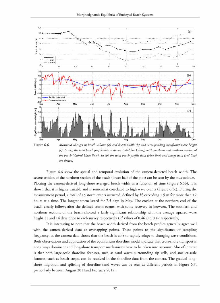
Morphodynamic Equilibria of Embayed Beach Systems
– 77 –
Figure 6.6 Measured changes in beach volume (a) and beach width (b) and corresponding significant wave height
(c). In (a), the total beach profile data is shown (solid black line), with northern and southern sections of the beach (dashed black lines). In (b) the total beach profile data (blue line) and image data (red line) are shown.
Figure 6.6 show the spatial and temporal evolution of the camera-detected beach width. The
severe erosion of the northern section of the beach (lower half of the plot) can be seen by the blue colours. Plotting the camera-derived long-shore averaged beach width as a function of time (Figure 6.5b), it is shown that it is highly variable and is somewhat correlated to high wave events (Figure 6.5c). During the measurement period, a total of 15 storm events occurred, defined by Hs exceeding 1.5 m for more than 12 hours at a time. The longest storm lasted for 7.5 days in May. The erosion at the northern end of the beach clearly follows after the defined storm events, with some recovery in between. The southern and northern sections of the beach showed a fairly significant relationship with the average squared wave height 11 and 14 days prior to each survey respectively (R2 values of 0.46 and 0.42 respectively).
It is interesting to note that the beach width derived from the beach profiles generally agree well with the camera-derived data at overlapping points. These points to the significance of sampling frequency, as the camera data shows that the beach is able to rapidly adapt to changing wave conditions. Both observations and application of the equilibrium shoreline model indicate that cross-shore transport is not always dominant and long-shore transport mechanisms have to be taken into account. Also of interest is that both large-scale shoreline features, such as sand waves surrounding rip cells, and smaller-scale features, such as beach cusps, can be resolved in the shoreline data from the camera. The gradual long-shore migration and splitting of shoreline sand waves can be seen at different periods in Figure 6.7, particularly between August 2011and February 2012.
(a)
(b)
(c)
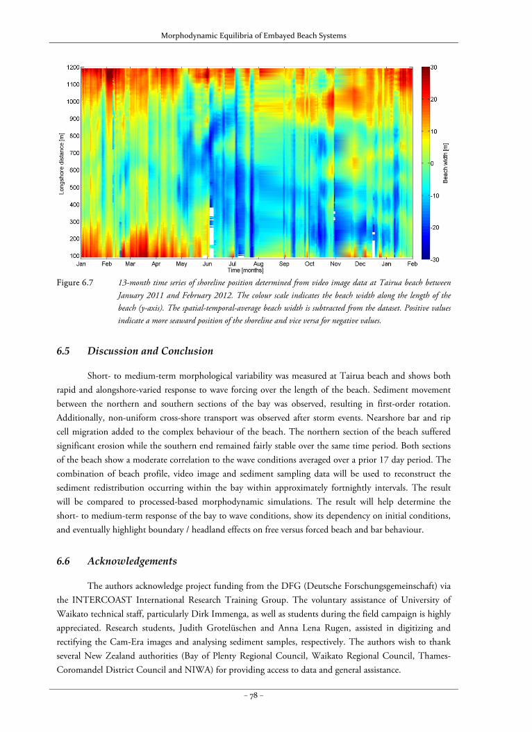
Morphodynamic Equilibria of Embayed Beach Systems
– 78 –
Figure 6.7 13-month time series of shoreline position determined from video image data at Tairua beach between
January 2011 and February 2012. The colour scale indicates the beach width along the length of the beach (y-axis). The spatial-temporal-average beach width is subtracted from the dataset. Positive values indicate a more seaward position of the shoreline and vice versa for negative values.
6.5 Discussion and Conclusion
Short- to medium-term morphological variability was measured at Tairua beach and shows both rapid and alongshore-varied response to wave forcing over the length of the beach. Sediment movement between the northern and southern sections of the bay was observed, resulting in first-order rotation. Additionally, non-uniform cross-shore transport was observed after storm events. Nearshore bar and rip cell migration added to the complex behaviour of the beach. The northern section of the beach suffered significant erosion while the southern end remained fairly stable over the same time period. Both sections of the beach show a moderate correlation to the wave conditions averaged over a prior 17 day period. The combination of beach profile, video image and sediment sampling data will be used to reconstruct the sediment redistribution occurring within the bay within approximately fortnightly intervals. The result will be compared to processed-based morphodynamic simulations. The result will help determine the short- to medium-term response of the bay to wave conditions, show its dependency on initial conditions, and eventually highlight boundary / headland effects on free versus forced beach and bar behaviour.
6.6 Acknowledgements
The authors acknowledge project funding from the DFG (Deutsche Forschungsgemeinschaft) via the INTERCOAST International Research Training Group. The voluntary assistance of University of Waikato technical staff, particularly Dirk Immenga, as well as students during the field campaign is highly appreciated. Research students, Judith Grotelüschen and Anna Lena Rugen, assisted in digitizing and rectifying the Cam-Era images and analysing sediment samples, respectively. The authors wish to thank several New Zealand authorities (Bay of Plenty Regional Council, Waikato Regional Council, Thames-Coromandel District Council and NIWA) for providing access to data and general assistance.
Morphodynamic Equilibria of Embayed Beach Systems
– 79 –
Chapter 7 – Summary, Conclusions & Outlook
This Chapter summarizes the work presented in the previous five Chapters, highlights the main conclusions of the thesis and offers an outlook for the future.
7.1 Summary
The main aims of this study were to (i) determine the processes governing long-term embayed beach evolution in order gain a comprehensive understanding of the role played by wave forcing, environmental conditions and the geological setting; and (ii) to identify how embayed beaches respond to short-term and seasonal wave forcing in terms of forced offshore sediment transport and beach rotation during storm events. Much of the work presented in this thesis is based on long-term schematic simulations of embayed beaches, in which a state-of-the-art morphodynamic model was used to simulate the long-term evolution of a schematic embayment under idealized wave forcing conditions. Additionally, seasonal and event-driven changes occurring on a real-world embayed beach were measured over a nine-month period.
In Chapter 2 we see that process-based models can be used effectively for simulating beach rotation by varying the mean wave direction. The final equilibrium shape of the bay varies depending on the wave conditions. In all cases, reasonable estimates of the cross-shore profile are obtained. The gradual reduction of the long-shore current during the simulation under constant wave forcing is consistent with generalized theories of embayed beach development in which the long-shore transport tends to zero (e.g., LeBlond, 1979).
In Chapter 3, the model complexity was increased by using time-varying wave conditions and turning on and off diffraction in the wave computations. Based on these simulations, we demonstrate that the main forcing mechanism leading to the formation of the curved shoreline planform is wave directional variance. Other mechanisms, such as wave height variance and directional spreading also play a role in distributing wave energy throughout the bay. The interaction between wave forcing and the bay geometry is highlighted, whereby the headland orientation directly influences the level of sheltering from waves coming from different directions. Chapter 3 also describes the influence of high wave events on the evolution of the bay. Extreme events result in a greater shoreward position of the shoreline; however, the effect is mainly seen in highly exposed sections of the bay rather than in the shadow zone. Embayed beach environments exposed to extreme events with high magnitude or high frequency require a greater accommodation space within the confines of the headlands.
Chapter 4 follows from the previous chapters in describing how flow and transport patterns change during the evolution of the beach until a stable shape is formed. Notably, it is shown to be consistently related to long-term, non-uniform shoreline cutback leading to beach rotation, which progressively weakens the residual long-shore current and sediment transport. Thus, the curvature of the shoreline is primarily a remnant of decaying erosion processes resulting from long-term beach rotation. In
Morphodynamic Equilibria of Embayed Beach Systems
– 80 –
all cases, the evolution of the bay is logarithmic over time and can be defined by two exponential coefficients related to the response time and the maximum size of the bay. The values of these coefficients are dependent on the geometric configuration of the beach: a larger bay requires a substantially longer time to reach equilibrium. Wave forcing and environmental conditions play an additional role by affecting the sediment transport capacity and distribution of wave energy in the bay.
Moving to a real-world embayed beach in Chapter 5, we observe that the wave climate, in particular, the wave direction, is the most important variable controlling the quasi-equilibrium shape of the beach. This quasi-equilibrium state is the long-term time-average of short-term and seasonal fluctuations of the beach bathymetry. It is interesting to note that extreme events do not have such a dramatic impact of the bay orientation, and that the average wave conditions mostly define the quasi-equilibrium shape of the bay. However, this does not discount the immediate effect of storms, which can potentially cause devastating changes within a matter of hours. Despite this, embayed beaches display a high resilience to storm events compared to open coast beach systems because of the restrictions imposed on sediment transport pathways. In Chapter 6, it is shown just how dynamic embayed beaches can be. Short-term observations of embayed beach morphology at Tairua beach indicate that sediment moves periodically between the beach, surf zone, and the shoaling zone. During high wave events between May and June 2011, a substantial amount of sediment was eroded from the beach and driven offshore towards the lower shelf in depths of 6 – 7 m. Only gradually can this sediment return to the shore to replenish the beach. These cross-shore transitions of sediment will be further investigated in order to determine whether or not the volume of sand removed from the beach is retained within the confines of the embayment. As shown in Chapters 3 and 4, long-term sediment bypassing into and out of the bay can affect the long-term equilibrium of the beach and should be therefore be taken into account for future planning.
7.2 Conclusions
The conclusions firstly address the hypothesis raised in Chapter 1. The results presented in this thesis have shown that residual sediment transport tends to zero as
the bay approaches equilibrium, in keeping with findings from the literature. However, the results show that waves do not necessarily arrive normal to the shoreline, as long-shore currents are still present in the surf zone once the equilibrium criteria has been met. Additionally, it has been shown that diffraction is not necessarily as influential as previously though, as other wave process also account for the curvature of the shoreline. The proposed hypothesis has been validated as it has been comprehensively shown that wave directional variability largely controls the orientation, planform, and equilibrium morphology of embayed beaches. Extreme wave events are important in the short-term; however, in the long-term the average conditions dominate.
Lastly, the conclusions are presented in response to the research questions proposed in Chapter 1.
7.2.1 What are the main processes affecting the morphological evolution of embayed beaches on a medium- to long-term timescale?
This question is addressed in Chapters 2, 3 and 4; however, the most important conclusions are derived from Chapter 4. The influence of directional spreading is closely linked to the configuration of headland structures as they potentially limit the range of wave directions directly impacting the bay.
Morphodynamic Equilibria of Embayed Beach Systems
– 81 –
Diffraction is important when directional spreading is low. The main forcing mechanism leading to the formation of the curved shoreline planform is shown to be wave directional variance. The effect of diffraction is reduced (or is at least coincident) as the directional variance of the wave climate is increased. The curvature of the beach is mainly derived from decaying shoreline rotation. Equilibrium is achieved when the residual sediment transport approaches zero and the active surf zone becomes enclosed within the boundaries of the headlands.
7.2.2 What are the effects of extreme events versus average forcing on the equilibrium state?
This question is addressed in Chapters 3, 4, and 5. In Chapter 3, during the long-term development of the bay, increased wave energy from high wave events causes the shoreline to recede shoreward in exposed sections of the bay, eventually leading to a slightly larger equilibrium area. In Chapter 4, increased average wave heights also results in a larger bay area; however, the shadow zone is also up-scaled as it is exposed to higher energy conditions over a longer period of time. Chapter 5 also shows that the magnitude of morphological changes caused by extreme events appears to be adequately balanced by calmer events of significantly longer duration over the medium-term.
7.2.3 How do short- to medium-term dynamics affect long-term residuals?
This question is addressed in Chapters 4, 5, and 6. In Chapter 4, the short-term beach rotation events steer the long-term evolution of the embayment and directly influence residual sediment transport patterns. In Chapter 5, a number of representative wave conditions that reduce a variable, medium-term, wave climate into distinctive groups were used to determine the quasi-equilibrium bathymetry of an embayed beach. At Tairua Beach (Chapter 6), there is both rapid and alongshore-varied morphological response to short- to medium-term wave forcing. The net residual transport patterns have not yet been resolved; however, this will be determined in the near future through the combination of beach profile, video imagery, and sediment sample data.
7.2.4 Can process-based models be used to simulate the morphological evolution of different boundary and initial conditions?
This question is addressed in Chapters 2 to 6. In particular, Chapter 2 shows that the equilibrium shape of the bay is variable and is dependent on combinations of wave height, period and direction. Chapter 4 shows that, despite this variability, the development of the bay follows a general trend regardless of the boundary or initial conditions, whereby long-term alongshore non-uniform cutback is potentially followed by alongshore uniform cutback and can be defined by an exponential function whose coefficients are related to the rate of development and the maximum bay size. Chapter 5 demonstrates that a wave climate can be discretized, individually simulated, and subsequently merged to obtain at least a first-order estimate of the quasi-equilibrium bathymetry of the bay.
7.3 Outlook
Although the simulations presented in this thesis are highly schematized and simplified, it has been shown that processed-based models can be successfully used to explain the process of development of embayed beaches. Further work in this area can yield even more promising results by refining the methods used. For example, the simulations carried out focused on beaches that approach static equilibrium. It
Morphodynamic Equilibria of Embayed Beach Systems
– 82 –
would be interesting to see how sediment input into the bay affects the dynamic equilibrium shape. Additionally, the simulations used a simplified or cyclic wave conditions. More random and complex forcing conditions can be used to test the outcome of the simulations. Furthermore, more varied geometric layouts can be used. It is therefore perceived that this line of research will be continued in future.
There are still many open questions concerning embayed beach dynamics over short to medium timescales. Some of these will be addressed in the second and third phases of the INTERCOAST project. For example, while it is known that beach state transitions are related to changes in wave forcing, the effect of the coupling between the bar and shoreline on beach state transitions is not known. This can be investigated by looking in depth at characteristic events such, as short-term, storm-induced rotation.
Chapter 6 showed that the supposedly frequent fortnightly beach profile surveys were unable to capture rapid changes occurring on the beach as observed using remote sensing video imagery techniques. This indicates that long-term, high resolution data is required to fully capture the dynamics of the surf zone and enable a better understanding of the interaction between morphology, flow, and non-linear wave processes. Dedicated in-situ surveys are difficult and expensive to implement and maintain. As such, further work is needed on the side of collecting and processing remotely sensed data, simplifying in-situ measurement techniques, and improving techniques to merge multiple data sources for reconstructing past events.
In a broader context, the work done in this INTERCOAST project can be used by other scientific disciplines. For example, in terms of environmental magnetics studies, hydrodynamics on the inner shelf can determine the fate of sediment deposits and zones of heavy metal enrichment (Badesab et al., 2012). On the topic of coastal management, Simeone et al. (2012) investigate the human impact of increased tourist activity on embayed beaches in terms of sediment removal by beach-goers. The structuring of future research into cross-cutting projects, whereby research is centred on a common theme, will enhance the communication between disciplines. Future INTERCOAST projects will contribute to this ideal, as projects such as this are not only continued, but eventually become more involved with biological sciences, social sciences and legal contexts.
Morphodynamic Equilibria of Embayed Beach Systems
– 83 –
References
Aarninkhof, S.G.J., B.G. Ruessink, and J.A. Roelvink, 2005. Nearshore subtidal bathymetry from time-
exposure video images, J. Geophysical Research, 110, C06011, doi:10.1029/2004JC002791. Almar, R., G. Coco, K.R. Bryan, D.A. Huntley, A.D. Short, and N. Senechal, 2008. Video observations of
beach cusp morphodynamics, J. Marine Geology, 254, 216–223. Archetti, R., and C. Romagnoli, 2011. Analysis of the effects of different storm events on shoreline dynamics of
an artificially embayed beach, J. Earth surface Processes and Landforms, 36, 1449–1463. ARGE BLMP (Working Group for the North Sea and Baltic Sea Monitoring Programme), 2011. The
preparation of Germany´s marine strategies, http://www.blmp-online.de/Seiten/Berichte.html. ASTM (American Society for Testing and Materials), 2009. Standard test methods for particle-size
distribution (gradation) of soils using sieve analysis, Active Standard ASTM D6913, volume 04.09. Badesab, F., T. von Dobeneck, K.R. Bryan, H. Müller, R.M. Briggs, T. Frederichs, and E. Kwoll, 2012.
Formation of magnetite-enriched zones in and offshore of a mesotidal estuarine lagoon: An environmental magnetic study of Tauranga Harbour and Bay of Plenty, J. Geochemistry, Geophysics and Geosystems, 13(6), 20 pp., doi: 10.1029/2012GC004125.
Benedet, L., J. Dobrochinski, R. Ranasinghe, A. Klein, and D.J.R. Walstra, submitted. Wave climate schematization for morphological modeling of open ocean beaches: analysis of methods and application to the Delray Beach case study, J. Coastal Engineering.
Blossier, B., C.J. Daly, S. Harrison, K.R. Bryan, and C. Winter, submitted. Wave Hindcasting in the Bay of Plenty-Coromandel Region, New Zealand, J. Coastal Research.
Bogle, J.A., K.R. Bryan, K.P. Black, T.M. Hume, and T.R. Healy, 2000. Video observations of rip formation and evolution, J. Coastal Research, Special Issue 34, 117–127.
Booij, N., R.C. Ris, and L.C. Hotlhuijsen, 1999. A third-generation wave generation model for coastal regions, Part I: Model description and validation, J. Geophysical Research, 104, 7649–7666.
Bruun, P., 1954. Coastal erosion and the development of beach profiles, Technical Memorandum No. 44, U.S. Army Corps of Engineers, Beach Erosion Board, Washington D.C.
Castelle, B., and G. Coco, 2012. The morphodynamics of rip channels on embayed beaches, J. Continental Shelf Research, 43, 10–23.
Castelle, B., and B.G. Ruessink, 2011. Modeling formation and subsequent non-linear evolution of rip channels: Time-varying versus time-invariant forcing, J. Geophysical Res., 116, F04008, doi:10.1029/2011JF001997.
CERC (Coastal Engineering Research Center), 1984. Shore Protection Manual, U.S. Army Corps of Engineers, Waterways Experiment Station, Washington D.C.
Cohen, A.B., A.R. Van Dongeren, J.A. Roelvink, N.G. Plant, S.G.A. Aarninkhof, M.C. Haller, and P. Catalan, 2006. Nowcasting of coastal processes through assimilation of model computations and remote observations, Proc. 30th Int. Conference on Coastal Engineering, A.S.C.E.
Dai, Z., J.T. Liu, Y.-P. Lei, and X.-L. Zhang, 2010. Patterns of sediment transport pathways on a headland bay beach – Nanwan Beach, South China: A case study, J. Coastal Research, 26(6), 1096–1103.
Morphodynamic Equilibria of Embayed Beach Systems
– 84 –
Daly, C.J., K.R. Bryan, J.A. Roelvink, A.H.F. Klein, D. Hebbeln, and C. Winter, 2011. Morphodynamics of embayed beaches: The role of wave conditions, J. Coastal Research, Special Issue 64, 1003–1007.
Davidson, M.A., I.L. Turner, and R.T. Guza, 2011. The effect of temporal wave averaging on the performance of an empirical shoreline evolution model, J. Coastal Engineering, 58, 802 – 805.
Dean, R.G, 1978. Diffraction calculations of shoreline planforms, Proc. 16th Int. Conference Coastal on Engineering, A.S.C.E., 1903–1917.
Dean, R.G., 1991. Equilibrium beach profiles: Characteristics and applications, J. Coastal Research, 7(1), 53–84.
Dehouck, A., H. Dupuis, and N. Senechal, 2009. Pocket beach hydrodynamics: The example of four macrotidal beaches, Brittany, France, J. Marine Geology, 266, 1–17.
de Vriend, H., M. Capobianco, T. Chesher, H.E. de Swart, B. Latteux, and M.J.F. Stive, 1993. Approaches to long term modeling of coastal morphology: A review, J. Coastal Engineering, 21, 225–269.
Dissanayake, D.M.P.K., J.A. Roelvink, and M. van der Wegen, 2009. Modeled channel patterns in a schematized tidal inlet, J. Coastal Engineering, 56, 1069–1083.
Dubios, R.N., 1988, Seasonal changes in beach topography and beach volume in Delaware, J. Marine Geology, 81, 79-96.
FAO (Food and Agriculture Organization of the United Nations), 2006. Integrated coastal management law – Establishing and strengthening legal frameworks for integrated coastal management, 262 pp.
Gallop, S.L., K.R. Bryan, and G. Coco, 2009. Video observations of rip currents on an embayed beach, J. Coastal Research, Special Issue 56(6), 49–53.
Gallop, S.L., K.R. Bryan, G. Coco, and S.A. Stephens, 2011. Storm-driven changes in rip channel patterns on an embayed beach, J. Geomorphology, 127, 179–188.
Gama, C., C. Coelho, P. Baptista, and L. Albardeiro, 2011. Equilibrium configuration of sandy embayed beaches from the Southwest Portuguese rocky coast, J. Coastal Research, Special Issue 64, 2037–2041.
Gao, S., 1996. A FORTRAN program for grain-size trend analysis to define net sediment transport pathways, J. Computers and Geosciences, 22(4), 449–452.
Garcia, M.A., A. Sánchez-Arcilla, J.P. Sierra, J. Sospedra, and J. Gómez, 1993. Wind waves off the Ebro Delta, NW Mediterranean, J. Marine Systems, 4(2/3), 235–262.
Gonzalez, M., and R. Medina, 2001. On the application of static equilibrium bay formulations to natural and man-made beaches, J. Coastal Engineering, 43, 209–225.
Gonzalez, M., R. Medina, and M. Losada, 2010. On the design of beach nourishment projects using static equilibrium concepts: Application to the Spanish coast, J. Coastal Engineering, 57, 227–240.
Gorman, R.M., K.R. Bryan, and A.K. Laing, 2003. Wave hindcast for the New Zealand region: Nearshore validation and coastal wave climate, New Zealand J. Marine and Freshwater Research, 37, 567–588.
Green, M.O., C.E. Vincent, and A.C. Trembanis, 2004. Suspension of coarse and fine sand on a wave-dominated shoreface, with implications for the development of rippled scour depressions, J. Continental Shelf Research, 24, 317–335.
Groeneweg, J., and G. Klopman, 1998. Changes of the mean velocity profiles in the combined wave-current motion in a GLM formulation, J. Fluid Mechanics, 370, 271–296.
Guedes, R.M.C., K.R. Bryan, and G. Coco, 2012. Observations of alongshore variability of swash motions on an intermediate beach, J. Continental Shelf Research, 48, 61–74.
Harley, M.D., I.L. Turner, A.D. Short, and R. Ranasinghe, 2011. A re-evaluation of coastal embayment rotation: The dominance of cross-shore versus alongshore sediment transport processes, Collaroy-
Morphodynamic Equilibria of Embayed Beach Systems
– 85 –
Narrabeen Beach, southeast Australia, J. Geophysical Research, 116, F04033, doi:10.1029/2011JF001989.
Heikkila, J., and O. Silven, 1997. A four-step camera calibration procedure with implicit image correction, Proc. IEEE Computer Society Conference on Computer Vision and Pattern Recognition, 1106–1112.
Ho, S.K., 1971. Crenulate shaped bays, M.Eng. Thesis No. 346, Asian Institute of Technology, Bangkok. Holland, K.T., R.A. Holman, T.C. Lippmann, J. Stanley, and N. Plant, 1997. Practical use of video
imagery in nearshore oceanographic field studies, IEEE J. Oceanic Engineering, 22, 81–92. Holman, R.A., and J. Stanley, 2007. The history and technical capabilities of Argus, J. Coastal Engineering,
53, 477–491. Holthuijsen, L.H., A. Herman, and N. Booij, 2003. Phase-decoupled refraction-diffraction for spectral wave
models, J. Coastal Engineering, 49, 291–305. Hsu, J.R.C., and C. Evans, 1989. Parabolic bay shapes and applications, Proc. Institute of Civil Engineers,
87, 557–570. Hsu, J.R.C., R. Silvester, and Y.M. Xia, 1989. Generalities on static equilibrium bays, J. Coastal
Engineering, 12, 353–369. Hsu, J.R.C., M.J. Yu, F.C. Lee, and L. Benedet, 2010. Static bay beach concepts for scientists and engineers:
A review, J. Coastal Engineering, 57, 76–91. Iglesias, G., I. Lopez, A. Castro, and R. Carballo, 2009. Neural network modelling of planform geometry of
headland-bay beaches, J. Geomorphology, 103, 577–587. Ikeda, S., 1982. Incipient motion of sand particles on side slopes, Journal of the Hydraulics Division, A.S.C.E.,
108 (1), 95–114. Inman, D.L., and C.E. Nordstrom, 1971. On the tectonic and morphologic classification of coasts, J. Geology,
79(1), 1–21. Jiménez, J.A., A. Sánchez-Arcilla, H.I. Valdemoro, V. Gracia, and F. Nieto, 1997. Processes reshaping the
Ebro Delta, J. Marine Geology, 144, 59–79. Klein, A.H.F., L.F. Benedet, and H.S. Delamar, 2002. Short-term beach rotation processes in distinct
headland bay beach systems, J. Coastal Research, 18(3), 442–458. Klein, A.H.F., Ó. Ferreira, J.M.A. Dias, M.G. Tessler, L.F. Silveira, L. Benedet, J.T. de Menezes, and
J.G.N. de Abreu, 2010. Morphodynamics of structurally controlled headland-bay beaches in southeastern Brazil: A review, J. Coastal Engineering, 57, 98–111.
Klein, A.H.F., and J.T. Menezes, 2001. Beach morphodynamics and profile sequence for a headland bay coast, J. Coastal Research, 17(4), 812–835.
Krumbein, W.C., 1944. Shore processes and beach characteristics, Technical Memorandum, vol. 3, Beach Erosion Board, U.S. Army Corps of Engineers, 47 pp.
Lausman, R., A. Klein, and M. Stive, 2010. Uncertainty in the application of the parabolic bay shape equation: Part 1, J. Coastal Engineering, 57(2), 132–141.
Lavalle, P.D., and V.C. Lakhan, 1997. A spatial–temporal analysis of the development of a log-spiral shaped embayment, J. Earth Surface Processes and Landforms, 22, 657–667.
Le Blond, P.H., 1972. On the formation of spiral beaches, Proc. 13th Int. Conference on Coastal Engineering, American Society of Civil Engineers, 1331–1345.
LeBlond, P.H., 1979. An explanation of the logarithmic spiral plan shape of headland-bay beaches, J. Sedimentary Petrology, 49(4), 1093–1100.
Le Roux, J.P., and E.M. Rojas, 2007. Sediment transport patterns determined from grain size parameters: Overview and state of the art, J. Sedimentary Geology, 202, 473–488.
Morphodynamic Equilibria of Embayed Beach Systems
– 86 –
Lesser, G.R., 2009. An approach to medium-term coastal morphological modelling, Ph.D. Thesis, Delft University of Technology, CRC Press/Balkema, ISBN 978-0-415-55668-2.
Lesser, G.R., J.A. Roelvink, J.A.T.M. van Kester, and G.S. Stelling, 2004. Development and validation of a three-dimensional morphological model, J. Coastal Engineering, 51, 883–915.
Lippmann, T.C., and R.A. Holman, 1989. Quantification of sandbar morphology: A video technique based on wave dissipation, J. Geophysical Research, 94, 995–1011.
Loureiro C., Ó. Ferreira, and J.A.G. Cooper, 2012a. Extreme erosion on high-energy embayed beaches: Influence of megarips and storm grouping, J. Geomorphology, 139–140, 155–171.
Loureiro, C., Ó. Ferreira, and J.A.G. Cooper, 2012b. Geologically constrained morphological variability and boundary effects on embayed beaches, J. Marine Geology, 329–331, 1–15.
Martins, C.C.; de Mahiques, M.M. and Dias, J.M.A., 2010. Daily morphological changes determined by high-energy events on an embayed beach: a qualitative model, Letters to Earth Surface Processes and Landforms, 35, 487–495.
Mol, A.C.S., 2007. Schematization of boundary conditions for morphological simulations, Research report, WL | Delft Hydraulics, The Netherlands.
Moreno, L.J. and Kraus, N.C., 1999. Equilibrium shape of headland-bay beaches for engineering design, Proc. 4th Int. Symposium on Coastal Sediments, American Society of Civil Engineers, 860–875.
NOAA (National Oceanic and Atmospheric Administration), 2011. WaveWatchIII global ocean wave model, http:/ /polar.ncep.noaa.gov/waves, (accessed 05.12.2011).
Pape, L. and Ruessink, B. G., 2008. Multivariate analysis of nonlinearity in sandbar behavior, J. Nonlinear Processes in Geophysics, 15, 145–58.
Pattiaratchi C., D. Olsson, Y. Hetzel, and R. Lowe, 2009. Wave-driven circulation patterns in the lee of groynes, J. Continental Shelf Research, 29, 1961–1974.
Pedreros, R., H.L. Howa, and D. Michel, 1996. Application of grain size trend analysis for the determination of sediment transport pathways in intertidal areas, J. Marine Geology, 135, 35–49.
Plant, N.G., S.G.J. Aarninkhof, I.L. Turner, and K.S. Kingston, 2007. The performance of shoreline detection models applied to video imagery, J. Coastal Research, 23, 658–670.
Plecha, S., Sancho, F., Silva, P. and Dias, J.M., 2007. Representative waves for morphological simulations, J. Coastal Research, Special Issue 50, 995–999.
Price, T.D., and B.G. Ruessink, 2011. State dynamics of a double sandbar system, J. Continental Shelf Research, 31, 659–674.
Quartel, S., B.G. Ruessink, and A. Kroon, 2007. Daily to seasonal cross-shore behaviour of quasi-persistent intertidal beach morphology, J. Earth Surface Processes and Landforms, 32, 1293–1307.
Quartel, S., A. Kroon, and B.G. Ruessink 2008. Seasonal accretion and erosion patterns of a microtidal sandy beach, J. Marine Geology, 250, 19–13.
Ranasinghe, R., R. McLoughlin, A. Short, and G. Symonds, 2004a. The Southern Oscillation Index, wave climate, and beach rotation, J. Marine Geology, 204, 273–287.
Ranasinghe, R., G. Symonds, K. Black, and R. Holman, 2004b. Morphodynamics of intermediate beaches: a video imaging and numerical modelling study, J. Coastal Engineering, 51, 629–655.
Ranasinghe, R., C. Swinkels, A. Luijendijk, J.A. Roelvink, J. Bosboom, M.J.F. Stive, and D.J.R. Walstra, 2011. Morphodynamic upscaling with the MorFac approach: dependencies and sensitivities, J. Coastal Engineering, 58, 806–811.
Morphodynamic Equilibria of Embayed Beach Systems
– 87 –
Ratsimandresy, A.W., M.G. Sotillo, J.C. Carretero Albiach, E. Álvarez Fanjul, and H. Hajji, 2008. A 44-year high-resolution ocean and atmospheric hindcast for the Mediterranean Basin developed within the HIPOCAS Project, J. Coastal Engineering, 55, 827–842.
Rea, C.C., and P.D. Komar, 1977. Computer simulation models of a hooked beach shoreline configuration, J. Sedimentary Petrology, 45(4), 866–872.
Reeve, D.E. and Y. Li, 2009. Stochastic model for embayed beaches, J. Waterway, Port, Coastal and Ocean Engineering, American Society of Civil Engineers,135(4), 144–153.
Reniers, A.J.H.M., J.A. Roelvink, and E.B. Thornton, 2004. Morphodynamic modelling of an embayed beach under wave group forcing, J. Geophysical Research, 109, C01030, doi:10.1029/2002JC001586.
Roelvink, J.A., 2006. Coastal morphodynamic evolution techniques, J. Coastal Engineering, 53, 277–287. Roelvink, D., and A. Reniers, 2012. A Guide To Modelling Coastal Morphology, Advances in Coastal and
Ocean Engineering Volume 12, World Scientific Publishing, 274 pp. Roelvink, J.A., A.J.H.M. Reniers, A.R. van Dongeren, J.S.M. van Thiel de Vries, J. Lescinski, and R.
McCall, 2009. Modelling storm impacts on beaches, dunes and barrier islands, J. Coastal Engineering, 56, 1133–1152.
Roelvink, J.A., and G.K.F.M. van Banning, 1994. Design and development of Delft3D and application to coastal morphodynamics, Proc. Hydroinformatics ’94, Balkema, Rotterdam, 451–456.
Ruggiero, P., D.J.R. Walstra, G. Gelfenbaum, and M. van Ormondt, 2009. Seasonal-scale nearshore morphological evolution: Field observations and numerical modeling, J. Coastal Engineering, 56, 1153–1172.
Schiaffino, C.F., M. Brignone, and M. Ferrari, 2011. Application of the parabolic bay shape equation to sand and gravel beaches on Mediterranean coasts, J. Coastal Engineering, 59, 57–63.
Short, A.D., 1996. The role of wave height, period, slope, tide range and embaymentisation in beach classifications: A review, J. Revista Chilena de Historia Natural, 69, 589–604.
Short, A.D., 2010. Role of geological inheritance in Australian beach morphodynamics, J. Coastal Engineering, 57, 92–97.
Short, A.D., and G. Masselink, 1999. Embayed and structurally controlled beaches, Handbook of Beach and Shoreface Morphodynamics, John Wiley and Sons, New York, 230–249.
Short. A.D., and A.C. Trembanis, 2004, Decadal scale patterns in beach oscillation and rotation Narrabeen Beach, Australia-Time series, PCA and wavelet analysis, J. Coastal Research, 20(2) 523–532.
Silva, R., A. Baquerizo, M.Á. Losada, and E. Mendoza, 2010. Hydrodynamics of a headland-bay beach–Nearshore current circulation, J. Coastal Engineering, 57, 160–175.
Silvester, R., 1960. Stabilization of sedimentary coastlines, Nature, 188, 467–469. Silvester, R., 1985. Natural headland control of beaches, J. Continental Shelf Research, 4(5), 581–596. Silvester, R., and S.K. Ho, 1972. Use of crenulated shaped bays to stabilize coasts, Proc. 13th Int. Conference
on Coastal Engineering, American Society of Civil Engineers, 1347–1365. Silvester, R., and J.R.C. Hsu, 1997. Coastal stabilization, Advanced Series on Ocean Engineering Volume 14,
World Scientific, 578 pp. Simeone S., A.G.L. Palombo, and I. Guala, 2012. Impact of frequentation on a Mediterranean embayed
beach: Implicationon carrying capacity, J. Ocean & Coastal Management, 62, 9–14. Smit, M.W.J., A.J.H.M. Reniers, B.G. Ruessink, and J.A. Roelvink, 2008. The morphological response of a
double sandbar system to constant wave forcing, J. Coastal Engineering, 55, 761–770. Smith, R.K. and K.R. Bryan, 2007. Monitoring beach face volume with a combination of intermittent
profiling and video imagery, J. Coastal Research, 23(4), 892-898.
Morphodynamic Equilibria of Embayed Beach Systems
– 88 –
Southgate, H.N., 1995. The effects of wave chronology on medium and long term coastal morphology, J. Coastal Engineering, 26, 251–270.
Splinter, K.D., I.L. Turner, and M.A. Davidson, 2013. How much data is enough? The importance of morphological sampling interval and duration for calibration of empirical shoreline models, J. Coastal Engineering, 77, 14–27.
Stive M.J.F., S.G.J. Aarninkhof, L. Hamm, H. Hanson, M. Larson, K.M. Wijnberg, R.J. Nicholls, and M. Capobianco, 2002.Variability of shore and shoreline evolution, J. Coastal Engineering, 47, 211–235.
Terpstra, P.D., and M.J. Chrzatowski 1992. Geometric trends in the evolution of a small log-spiral embayment on the Illinois shore of lake Michigan, J. Coastal Research, 8(3), 603–617.
Trembanis, A.C.. and T.M. Hume, 2011. Sorted bedforms on the inner shelf off northeastern New Zealand: spatiotemporal relationships and potential paleo-environmental implications, J. Geo-Marine Letters, 31, 203–214.
Turner, I.L., S.G.J. Aarninkhof, T.D.T. Dronkers, and J. McGrath, 2004. CZM applications of Argus Coastal Imaging at the Gold Coast, Australia, J. Coastal Research, 20, 739–752.
Valle-Levinson, A., and J. Moraga-Opazo, 2006. Observations of bipolar residual circulation in two equatorward-facing semiarid bays, J. Continental Shelf Research, 26, 179–193.
van de Lageweg, W.I., K.R. Bryan, G. Coco, and B.G. Ruessink, 2013. Observations of shoreline-sandbar coupling on an embayed beach, J. Marine Geology, doi: 10.1016/j.margeo.2013.07.018.
van der Wegen M., A. Dastgheib, and J.A. Roelvink, 2010. Morphodynamic modeling of tidal channel evolution in comparison to empirical PA relationship, J. Coastal Engineering, 57, 827–837.
van Dongeren, A., N. Plant, A. Cohen, D. Roelvink, M.C. Haller, and P. Catalán, 2008. Beach Wizard: Nearshore bathymetry estimation through assimilation of model computations and remote observations, J. Coastal Engineering, 55, 1016–1027.
van Lancker, V., J. Lanckneus, S. Hearn, P. Hoekstra, F. Levoy, J. Miles, G. Moerkerke, O. Monfort, and R. Whitehouse, 2004. Coastal and nearshore morphology, bedforms and sediment transport pathways at Teignmouth (UK), J. Continental Shelf Research, 24, 1171–1202.
van Maanen B., P.J. Ruiter, G. Coco, K.R. Bryan and B.G. Ruessink, 2008. Onshore sandbar migration at Tairua Beach (New Zealand): Numerical simulations and field measurements, J. Marine Geology,
253, 99–106.
van Rijn, L.C., 1993. Principles of Sediment Transport in Rivers, Estuaries and Coastal Seas. Aqua Publications, the Netherlands.
van Rijn, L.C., D.J.R. Walstra, B. Grasmeijer, J. Sutherland, S. Pan, and J.P. Sierra, 2003. The predictability of cross-shore bed evolution of sandy beaches at the time scale of storms and seasons using process-based profile models, J. Coastal Engineering, 47, 295–327.
Walstra, D.J.R., Hoekstra, R., Tonnon, P.K. and Ruessink, B.G., 2013. Input reduction for long-term morphodynamic simulations in wave-dominated coastal settings, J. Coastal Engineering, 77, 57–70.
Walstra, D.J.R., J.A. Roelvink, and J. Groeneweg, 2000. Calculation of wave driven currents in a 3D mean flow model, Proc. 27th Int. Conference on Coastal Engineering, American Society of Civil Engineers, 1050–1063.
Wang, Z.Q., S.K. Tan, N.S. Cheng, and K.W. Goh, 2008. A simple relationship for crenulated shaped bays in static equilibrium. J. Coastal Engineering, 55, 73–78.
Winter, C., 2006. Meso-scale morphodynamics of the Eider Estuary: analysis and numerical modelling, J. Coastal Research, Special Issue 39, 498–503.
Morphodynamic Equilibria of Embayed Beach Systems
– 89 –
Weesakul, S., T. Rasmeemasmuang, S. Tasaduak, and C. Thaicharoen, 2010. Numerical modelling of crenulate bay shapes, J. Coastal Engineering, 57, 184–193.
Weesakul, S., and S. Tasaduak, 2012. Experimental investigation on dynamic equilibrium bay shape, Proc. 33rd Int. Conference on Coastal Engineering, American Society of Civil Engineers, 13 pp.
Wright, L.D., and Short, A.D., 1984. Morphodynamic variability of surf zones and beaches: A synthesis, J. Marine Geology, 56, 93–118.
Yamashita, T., and Y. Tsuchiya, 1992. Numerical simulation of pocket beach formation, Proc. 23rd Int. Conference on Coastal Engineering, American Society of Civil Engineers, 2556–2566.
Yasso, W.E., 1965. Plan geometry of headland bay beaches, J. Geology, 73, 702–714. Yates, M.L., R.T. Guza, W.C. O’Reilly, and R.J. Seymour, 2009. Overview of seasonal sand level changes on
Southern California beaches, J. Shore & Beach, 77, 39–46.

Morphodynamic Equilibria of Embayed Beach Systems
– 90 –

Morphodynamic Equilibria of Embayed Beach Systems
– 91 –
Curriculum Vitae
Vitae
24.08.1984 Born, Kingston Jamaica
09.1995 – 06.2002 High School and A-Levels, Campion College, Kingston, Jamaica.
09.2002 – 06.2005 B.Sc. Civil Engineering, University of the West Indies, St. Augustine, Trinidad and Tobago.
07.2005 – 10.2005 Junior Civil Engineer, Wallace Evans Jamaica Limited, Kingston, Jamaica.
10.2005 – 07.2007 Junior Coastal Engineer, Smith Warner International Limited, Kingston, Jamaica.
08.2007 – 06.2009 M.Sc. Coastal and Marine Engineering and Management, EU Erasmus Mundus CoMEM Programme: Norwegian University of Science and Technology, Trondheim, Norway; Delft University of Technology, Delft, the Netherlands; and Polytechnic University of Catalonia, Barcelona, Spain.
08.2009 – 11.2009 Junior Researcher, Deltares, Delft, the Netherlands. 01.2010 – 08.2013 Ph.D. Coastal Geomorphology,
DFG INTERCOAST International Research Training Group: University of Bremen, Bremen, Germany; University of Waikato, Hamilton, New Zealand.
09.2013 – 03.2014 Junior Research Fellow, WIMO, Hanse Wissenschaftkolleg, Delmenhorst, Germany.
Publications
Daly, C., D. Roelvink, A. van Dongeren, J. van Thiel de Vries, R. McCall, 2010. Short wave breaking effects on low-frequency waves, Proc. 32nd Int. Conference on Coastal Engineering, American Society of Civil Engineers, 13 pp.
Daly, C.J., K.R. Bryan, J.A. Roelvink, A.H.F. Klein, D. Hebbeln, and C. Winter, 2011. Morphodynamics of embayed beaches: The role of wave conditions, J. Coastal Research, Special Issue 64, 1003–1007.
Daly, C., D. Roelvink, A. van Dongeren, J. van Thiel de Vries, R. McCall, 2012. Validation of an advective-deterministic approach to short wave breaking in a surf-beat model, J. Coastal Engineering, 60, 69–83.
Daly, C.J., K.R. Bryan, E.M. Gonzalez, A.H.F. Klein and C. Winter, 2013. Process-based prediction of equilibrium embayed beach morphology, Proc. 7th Int. Conference on Coastal Dynamics, Arcachon, France.

Morphodynamic Equilibria of Embayed Beach Systems
– 92 –