N = 1 and non-supersymmetric open string theories in six ...

N = 1 and non-supersymmetric open string theories

in six and four space-time dimensions

D I S S E R T A T I O N

zur Erlangung des akademischen Gradesdoctor rerum naturalium

(Dr. rer. nat.)im Fach Physik

eingereicht an derMathematisch-Naturwissenschaftlichen Fakultat I

Humboldt-Universitat zu Berlin

vonHerrn Dipl.-Phys. Lars Gorlichgeboren am 01.01.1973 in Kassel

Prasident der Humboldt-Universitat zu Berlin:Prof. Dr. Jurgen Mlynek

Dekan der Mathematisch-Naturwissenschaftlichen Fakultat I:Prof. Dr. Michael Linscheid

Gutachter:

1. Prof. Dr. Dieter Lust2. Prof. Dr. Stefan Theisen3. Prof. Dr. Jan Louis

eingereicht am: 11. August 2003Tag der mundlichen Prufung: 22. Oktober 2003

Zusammenfassung

Die vorliegende Arbeit beinhaltet ein einfuhrendes Kapitel uber Orbifold-Kon-struktionen in dem neben rudimentaren Grundlagen bereits speziellere Themenwie Diskrete Torsion und asymmetrische Orbifold-Gruppen behandelt werden.Als Beispiele fur Orbifolde werden Kompaktifizierungen auf Tori sowie dasasymmetrische T 4/ZL

3 × ZR3 Orbifold behandelt.

Danach wird eine allgemein gehaltene Einfuhrung in Orientifolde gegeben,einschließlich des offenen String Sektors samt Chan-Paton Freiheitsgraden.

Die darauf folgenden Kapitel 4-7 behandeln von mir durchgefuhrte For-schungsarbeiten.

Kapitel 4 beschaftigt sich mit der Quantisierung des offenen Strings mitlinearen Randbedingungen, wie sie bei Strings in elektro-magnetischen Feldernauftreten. Weiterhin wird die Quantisierung der Null- und Impuls-Moden desoffenen Strings in Torus-Kompaktifizierungen durchgefuhrt. Außerdem wird furden Fall allgemeiner konstanter Hintergrund Neveu-Schwarz U(1)-Hintergrund-felder der Kommutator der Stringkoordinaten berechnet. Dieser stutzt bishe-rige Resultate zur Nicht-Kommutativitat von offenen Stringtheorien in Neveu-Schwarz Hintergrunden.

Kapitel 5 gibt, zusammen mit einigen neuen Erkenntnissen, Resultate von [1]uber asymmetrische Orientifolde, insbesondere deren D-Branen Inhalt wieder.Kapitel 6 faßt die Veroffentlichung [2] zusammen, in der untersucht wurde, in-wieweit sich phanomenolgisch interessante Modelle in Orientifolden von Torus-Kompaktifizierungen finden lassen. Insbesondere tragen die D9-Branen magne-tische Flusse, womit chirale Fermionen im Spektrum auftreten. Die Rechnungenwerden großtenteils im gleichwertigen, T-dualen Bild ausgefuhrt. In diesem istdie Anzahl der chiralen Fermionen durch die topologische Schnittzahl der D-Branen gegeben.

Existieren auf Torus-Kompaktifizierungen entweder nur nicht-chirale odernicht-supersymmetrische Modelle, so lassen sich auf gewissen Orbifolden beideEigenschaften miteinander vereinbaren. Kapitel 7 behandelt das σΩ-Orienti-fold auf einem T 6/Z4 Orbifold. Als besonders interessantes Beispiel wird einsupersymmetrisches U(4) × U(2)3L × U(2)3R Modell vorgestellt, daß durch Ein-schalten geeigneter Hintergrundfelder in der effektiven Niederenergie-Wirkungauf ein Modell gebrochen wird, daß dem MSSM (minimalem supersymmetri-schen Standard Modell) sehr ahnlich ist. Dieses Kapitel basiert auf unsererPublikation [3].

Ferner ist der Arbeit ein Anhang beigefugt, der einige der verwendeten For-meln sowie Beweise zu zwei Satzen enthalt, die im Text verwendet wurden.

Schlagworter:String Theorie, Orientifolds, offene Strings, D-Branen, supersymmetrische Mo-delle, String Phanomenologie

Abstract

This thesis contains an introductory chapter on orbifolds. Besides rudimentarybasics we discuss more advanced topics like discrete torsion and asymmetricorbifold groups. As examples we investigate torus compactifications and anasymmetric T 4/ZL

3 × ZR3 orbifold.

The following chapter explains the foundations of orientifolds, includingopen strings with Chan-Paton degrees of freedom.

Chapters 4-7 present own research.In chapter 4 we quantize open strings with linear boundary conditions, as

they show up in electro-magnetic fields. We quantize the zero- and momentum-modes for toroidal compactifications, too. As an application we calculate thecommutator of the coordinate fields in the case of general constant Neveu-Schwarz U(1)-field strengths. Thereby we confirm previous results on non-commutativity of open string theories in Neveu-Schwarz backgrounds.

Chapter 5 reviews the results of a former publication [1] on asymmetricorientifolds, supplemented by some recent insights in connection with the pre-ceeding chapter.

Chapter 6 is a summary of [2]. In this publication we investigated to whatextend one can build phenomenologically interesting models from toroidal orien-tifolds. By turning on magnetic fluxes on D9-branes we induce chiral fermions.Most calculations are performed in an (equivalent) T-dual picture. Here thenumber of chiral fermions is given by the topological intersection number ofD-branes.

In orientifolds of toroidal compactifications one obtains either non-chiralor non-supersymmetric orientifold solutions. However both properties can bereconciled in orientifolds that are obtained from specific supersymmetric or-bifold compactifications. In chapter 7 we present the σΩ-Orientifold on aT 6/Z4 orbifold. As a very attractive example we investigate a supersymmet-ric U(4) × U(2)3L × U(2)3R model that is broken to an MSSM 1 -like model byswitching on suitable background fields in the low energy effective action. Thischapter is based on our publication [3].

The thesis is supplemented by an appendix with formulæ applied in thetext, as well as proofs to two theorems that were used as well.

Keywords:string theory, orientifolds, open strings, D-branes,supersymmetric models,stringphenomenology

1 “MSSM”= minimal supersymmetric Standard Model

Contents

List of Figures vii

List of Tables ix

1 Introduction 21.1 String theory . . . . . . . . . . . . . . . . . . . . . . . . . . . . . 21.2 Quantization of classical strings . . . . . . . . . . . . . . . . . . . 31.3 String theory as a theory of quantum gravity . . . . . . . . . . . 81.4 Supersymmetric string theories . . . . . . . . . . . . . . . . . . . 111.5 Compactifications . . . . . . . . . . . . . . . . . . . . . . . . . . . 181.6 Open strings and unoriented string theories . . . . . . . . . . . . 191.7 Chiral fermions in open string theories . . . . . . . . . . . . . . . 21

2 Orbifolds 252.1 General construction of orbifolds . . . . . . . . . . . . . . . . . . 252.2 Torus compactification as an orbifold . . . . . . . . . . . . . . . . 30

2.2.1 Moduli-space of toroidal compactifications, T-duality groupand symmetries . . . . . . . . . . . . . . . . . . . . . . . . 33

2.2.2 Compactification on T 2, T-duality and symmetries . . . . 362.2.2.1 Points of enhanced symmetry in the moduli

space SO(2, 2,R) . . . . . . . . . . . . . . . . . . 382.2.2.2 The world-sheet-parity on T 2 . . . . . . . . . . . 40

2.3 Toroidal orbifolds . . . . . . . . . . . . . . . . . . . . . . . . . . . 432.3.1 Space-time supersymmetric (toroidal) orbifolds . . . . . . 45

2.4 The asymmetric (T 2 × T 2)/(ZL3 × ZR

3 )) orbifold . . . . . . . . . 47

3 Orientifolds 543.1 Basic concepts . . . . . . . . . . . . . . . . . . . . . . . . . . . . 543.2 SΩ-invariant closed-string spectra and Klein bottle amplitude . . 55

3.2.1 Closed-string tadpoles . . . . . . . . . . . . . . . . . . . . 613.3 Open-strings . . . . . . . . . . . . . . . . . . . . . . . . . . . . . 64

3.3.1 Chan Paton factors and gauge symmetries . . . . . . . . . 663.3.1.1 Open-strings on orbifolds . . . . . . . . . . . . . 68

3.3.2 sΩ-invariant open-string sector . . . . . . . . . . . . . . . 743.3.3 Mobius amplitude . . . . . . . . . . . . . . . . . . . . . . 783.3.4 Orientifolds of supersymmetric strings . . . . . . . . . . . 82

3.3.4.1 Fermionic sector of the Klein bottle . . . . . . . 83

iii

3.3.4.2 Fermionic sector of the Cylinder . . . . . . . . . 853.3.4.3 Fermionic sector of the Mobius strip . . . . . . . 85

Concluding remarks . . . . . . . . . . . . . . . . . . . . . . . . . . . . 85

4 Open Strings in Electro-Magnetic Background-Fields 874.1 Action and boundary conditions of the open string . . . . . . . . 88

4.1.1 Open strings with two boundaries . . . . . . . . . . . . . 914.1.2 Solution to linear boundary conditions for the cylinder . . 92

4.1.2.1 World sheet momentum and Hamiltonian . . . . 934.2 Quantization of open strings with linear boundary conditions . . 94

4.2.1 Canonical two-form and canonical quantization . . . . . . 954.2.1.1 Quantization of zero- and linear-modes . . . . . 954.2.1.2 Quantization of oscillator modes . . . . . . . . . 984.2.1.3 Quantization of zero and momentum modes in

toroidal compactifications . . . . . . . . . . . . . 1004.2.2 Hilbert-space, further quantization . . . . . . . . . . . . . 105

4.3 The commutator [X(τ, σ), X(τ, σ′)] . . . . . . . . . . . . . . . . 1064.3.1 The commutator [X(τ, 0), X(τ, 0)] . . . . . . . . . . . . . 1064.3.2 The commutator [X(τ, π), X(τ, π)] . . . . . . . . . . . . . 110

4.4 Space-time supersymmetry of open strings in constant backgrounds1124.4.1 Closed form of the Eigenvalues λi in d = 4, 6. . . . . . . . 113


5 Asymmetric Orientifolds 1175.1 Introduction . . . . . . . . . . . . . . . . . . . . . . . . . . . . . . 1175.2 D-branes in asymmetric orbifolds . . . . . . . . . . . . . . . . . . 119

5.2.1 Definition of the T-dual torus . . . . . . . . . . . . . . . . 1205.2.2 The Z3 torus . . . . . . . . . . . . . . . . . . . . . . . . . 1215.2.3 Asymmetric rotations of D-branes . . . . . . . . . . . . . 1225.2.4 Kaluza-Klein and winding modes, zero mode degeneracy . 124

5.2.4.1 D2-branes with F -flux on T 2 . . . . . . . . . . . 1245.2.4.1.1 D-branes in the asymmetric Z3 orbifold 127

5.2.4.2 D1-branes on T 2 . . . . . . . . . . . . . . . . . . 1285.3 Asymmetric rotations and non-commutative geometry . . . . . . 129

5.3.1 Two-point function on the disc . . . . . . . . . . . . . . . 1305.3.2 The OPE of vertex operators . . . . . . . . . . . . . . . . 1305.3.3 The commutator of the coordinates . . . . . . . . . . . . . 131

5.4 Asymmetric orientifolds . . . . . . . . . . . . . . . . . . . . . . . 1335.4.1 Orientifolds on the

(T 2 × T 2

)/(ZL3 ×ZR3

)orbifold back-

ground . . . . . . . . . . . . . . . . . . . . . . . . . . . . . 1345.4.1.1 Tadpole cancellation . . . . . . . . . . . . . . . . 1355.4.1.2 The massless spectrum . . . . . . . . . . . . . . 137


iv

6 Toroidal orientifolds with magnetized versus intersecting D-Branes 1396.1 Introduction . . . . . . . . . . . . . . . . . . . . . . . . . . . . . . 1396.2 One loop amplitudes . . . . . . . . . . . . . . . . . . . . . . . . . 142

6.2.1 D9-branes with magnetic fluxes . . . . . . . . . . . . . . . 1436.2.2 D(9− d)-branes at angles . . . . . . . . . . . . . . . . . . 1446.2.3 Klein bottle amplitude . . . . . . . . . . . . . . . . . . . . 1466.2.4 Annulus amplitude . . . . . . . . . . . . . . . . . . . . . . 1466.2.5 Mobius amplitude . . . . . . . . . . . . . . . . . . . . . . 148

6.3 Compactifications to six dimensions . . . . . . . . . . . . . . . . 1486.3.1 Six-dimensional models . . . . . . . . . . . . . . . . . . . 149

6.4 Four dimensional models . . . . . . . . . . . . . . . . . . . . . . . 1516.4.1 A 24 generation SU(5) model . . . . . . . . . . . . . . . . 1526.4.2 A four generation model . . . . . . . . . . . . . . . . . . . 154

6.5 (In-) Stability of purely toroidal orientifolds . . . . . . . . . . . . 1566.5.1 Supersymmetric brane configurations and special Lagran-

gian submanifolds (sLags) . . . . . . . . . . . . . . . . . . 1576.5.2 Tachyons in toroidal orientifolds . . . . . . . . . . . . . . 159


7 The σΩ-Orientifold on (T 2 × T 2 × T 2)/Z4 1627.1 Intersecting Brane Worlds on Calabi-Yau spaces . . . . . . . . . 1637.2 3-cycles in the Z4 orbifold . . . . . . . . . . . . . . . . . . . . . . 165

7.2.1 Crystallographic actions . . . . . . . . . . . . . . . . . . . 1667.2.2 A non-integral basis of 3-cycles . . . . . . . . . . . . . . . 1677.2.3 An integral basis of 3-cycles . . . . . . . . . . . . . . . . . 169

7.3 Orientifolds of the Z4 Type IIA orbifold . . . . . . . . . . . . . . 1717.3.1 O6-planes in the Z4 orientifold . . . . . . . . . . . . . . . 1717.3.2 Supersymmetric cycles . . . . . . . . . . . . . . . . . . . . 172

7.4 A four generation supersymmetric Pati-Salam model . . . . . . . 1767.4.1 Green-Schwarz mechanism . . . . . . . . . . . . . . . . . . 178

7.5 Three generation supersymmetric Pati-Salam model . . . . . . . 1787.5.1 Brane recombination . . . . . . . . . . . . . . . . . . . . . 1807.5.2 D-flatness . . . . . . . . . . . . . . . . . . . . . . . . . . . 1837.5.3 Gauge symmetry breaking . . . . . . . . . . . . . . . . . . 1887.5.4 Getting the Standard Model . . . . . . . . . . . . . . . . 192

7.5.4.1 Adjoint Pati-Salam breaking . . . . . . . . . . . 1927.5.4.2 Bifundamental Pati-Salam breaking . . . . . . . 1947.5.4.3 Electroweak symmetry breaking . . . . . . . . . 196


Conclusions 200

Acknowledgments 203

Hilfsmittel 204

v

Selbstandigkeitserklarung 205

A Theta-functions and related functions 206A.1 η and ϑ-functions, identities and transformation under SL(2,Z) . 206

A.1.1 Transformation under SL(2,Z): . . . . . . . . . . . . . . . 206A.1.2 Identities between ϑ-functions . . . . . . . . . . . . . . . . 207

A.2 Poisson resummation formula for lattice sums . . . . . . . . . . . 207A.3 Conformal blocks in D = 6 . . . . . . . . . . . . . . . . . . . . . 208

B Equivalence classes of unitary symmetric and anti-symmetricmatrices. 210

C Spectrum and Eigenvectors of Lorentz transformations 213

D Quantities of the(T 2 × T 2 × T 2

)/Z4-Orientifold 217

D.1 Orientifold planes . . . . . . . . . . . . . . . . . . . . . . . . . . . 217D.2 Supersymmetry conditions . . . . . . . . . . . . . . . . . . . . . . 218D.3 Fractional boundary states . . . . . . . . . . . . . . . . . . . . . . 219

Bibliography 221

vi

List of Figures

1.1 Closed-string evolving in time . . . . . . . . . . . . . . . . . . . . 61.2 Open-string evolving in time . . . . . . . . . . . . . . . . . . . . 61.3 String perturbation series . . . . . . . . . . . . . . . . . . . . . . 91.4 QED perturbation series . . . . . . . . . . . . . . . . . . . . . . . 101.5 Open string with Chan-Paton charges . . . . . . . . . . . . . . . 191.6 Open-string with endpoints located on intersecting D-branes . . 221.7 Open-string in magnetic background fields . . . . . . . . . . . . . 221.8 Open-string located at a singularity . . . . . . . . . . . . . . . . 23

2.1 Torus lattice Γ with complex structure τ . . . . . . . . . . . . . . 272.2 Fundamental region F0 of the complex structure . . . . . . . . . 282.3 A torus and B torus . . . . . . . . . . . . . . . . . . . . . . . . . 41

3.1 Periodicities of the Klein bottle . . . . . . . . . . . . . . . . . . . 573.2 Construction of the Klein bottle . . . . . . . . . . . . . . . . . . 583.3 Klein bottle in tree-channel . . . . . . . . . . . . . . . . . . . . . 603.4 Periodicities of the cylinder with boundary conditions . . . . . . . 653.5 Cylinder diagram . . . . . . . . . . . . . . . . . . . . . . . . . . . 663.6 Non-planar open-string one-loop diagram with four external states 703.7 Cut of the non-planar open-string one-loop diagram with exter-

nal states . . . . . . . . . . . . . . . . . . . . . . . . . . . . . . . 703.8 Construction of the Mobius strip . . . . . . . . . . . . . . . . . . 783.9 Periodicities of the Mobius strip embedded in the underlying

annulus . . . . . . . . . . . . . . . . . . . . . . . . . . . . . . . . 793.10 Mobius strip in tree-channel . . . . . . . . . . . . . . . . . . . . . 80

4.1 Time-like and light-like branes . . . . . . . . . . . . . . . . . . . 89

5.1 T-duality relation . . . . . . . . . . . . . . . . . . . . . . . . . . . 1205.2 D1-brane with wrapping numbers (n,m) = (3, 2) on T 2 . . . . . 1235.3 Branes at angles . . . . . . . . . . . . . . . . . . . . . . . . . . . 131

6.1 D7-Brane configuration on T 4. . . . . . . . . . . . . . . . . . . . 1496.2 D6-brane configuration of the 24 generation model . . . . . . . . 1536.3 D6-brane configuration of the 4 generation model . . . . . . . . . 1556.4 Tachyon region . . . . . . . . . . . . . . . . . . . . . . . . . . . . 160

7.1 Anti-holomorphic involutions . . . . . . . . . . . . . . . . . . . . 166

vii

7.2 Orientations of the third T 2 . . . . . . . . . . . . . . . . . . . . . 1667.3 Orbifold fixed points . . . . . . . . . . . . . . . . . . . . . . . . . 1687.4 Recombined branes . . . . . . . . . . . . . . . . . . . . . . . . . . 1767.5 Adjoint higgsing . . . . . . . . . . . . . . . . . . . . . . . . . . . 1837.6 Quiver diagram for the branes 1, 2, 3, 4 . . . . . . . . . . . . . . 1907.7 Quiver diagram for the branes 2, 3, 4, 5, 6, 7 . . . . . . . . . . . 1917.8 Gauge symmetry breaking of U(4)× U(2)L × U(2)R . . . . . . . 196

viii

List of Tables

1.1 Massless closed-string spectra of Type IIA theory . . . . . . . . . 16

2.1 ZN groups preserving N = 1 supersymmetry in D = 6. . . . . . . 462.2 ZN groups preserving N = 1 supersymmetry in D = 4. . . . . . . 462.3 Different traces in the partition function . . . . . . . . . . . . . . 502.4 Closed-string spectra of the

(T 2 × T 2

)/(ZL

3 × ZR3

)orbifold . . . 52

3.1 Massless closed-string spectra of Type IIB and Type I . . . . . . 623.2 Relation between the parameters t and l in the loop- and tree-

channel. . . . . . . . . . . . . . . . . . . . . . . . . . . . . . . . . 643.3 Klein bottle, Cylinder: Relation between fermionic sectors in

tree- and loop-channel . . . . . . . . . . . . . . . . . . . . . . . . 853.4 Mobius strip: Relation between fermionic sectors in tree- and

loop-channel. . . . . . . . . . . . . . . . . . . . . . . . . . . . . . 85

5.1 Closed string spectra of the(T 2 × T 2

)/(ZL3 × ZR3

)-orientifold . . 137

5.2 Open string spectra of the(T 2 × T 2

)/(ZL3 × ZR3

)-orientifold . . . 138

6.1 Chiral 6D massless open string spectrum . . . . . . . . . . . . . . 1516.2 Chiral 4D massless open string spectrum. . . . . . . . . . . . . . 1526.3 Chiral left-handed fermions for 24 generation model . . . . . . . 1546.4 Chiral left-handed fermions for 4 generation model . . . . . . . . 1546.5 Chiral left-handed fermions for 4 generation model including

anomaly-free U(1)-charges . . . . . . . . . . . . . . . . . . . . . . 155

7.1 Chiral spectrum in d = 4 . . . . . . . . . . . . . . . . . . . . . . 1657.2 O6-planes for ABB model . . . . . . . . . . . . . . . . . . . . . . 1727.3 Allowed exceptional cycles . . . . . . . . . . . . . . . . . . . . . . 1757.4 D6-branes for a 4 generation PS-model . . . . . . . . . . . . . . . 1777.5 Chiral spectrum for 4 generation PS-model . . . . . . . . . . . . 1777.6 D6-branes for 3 generation PS-model . . . . . . . . . . . . . . . . 1797.7 Chiral spectrum for a 7-stack model . . . . . . . . . . . . . . . . 1807.8 Non-chiral spectrum (Higgs fields) . . . . . . . . . . . . . . . . . 1847.9 Chiral spectrum for 3 stack PS-model . . . . . . . . . . . . . . . 1897.10 Non-chiral spectrum for 3 stack PS-model . . . . . . . . . . . . . 1927.11 Chiral spectrum for 4 stack left-right symmetric SM . . . . . . . 1937.12 Chiral spectrum for 5 stack SM . . . . . . . . . . . . . . . . . . . 194

ix

7.13 Chiral spectrum for 4 stack SM . . . . . . . . . . . . . . . . . . . 195

D.1 O6-planes of the T 6/Z4 orientifold . . . . . . . . . . . . . . . . . 217

x

Chapter 1

Introduction

In this chapter we will give a short motivation for string theory and its su-persymmetric extension. By doing so we will expose some of the basic ideasunderlying this theory. As the main part of the thesis and the whole part ofour own research presented here deals with open strings, we devote a section tothis topic as well. In chapter 6 and 7 we will investigate the chance to find real-istic models in a special class of unoriented open-string theories. Therefore wewill make some comments on these orientifolds as well. Since we have includedtwo more extended chapters on orbifolds and orientifolds in this thesis, thisintroductory chapter is rather condensed, only concentrating on the rudimentswithout going into details. General texts on string theory are the classical workof Green, Schwarz and Witten [4, 5], the book of Lust and Theisen [6] and thetwo volumes by Polchinski [7, 8]. The latter reference is especially interestingas it includes a chapter on D-branes and gives a D-brane interpretation of ori-entifolds. The book of Bailin and Love provides a good introduction to bothsupersymmetric field theory and superstring theory (cf. [9]).

1.1 String theory

String theory is a quantum theory of string-like (i.e. one-dimensional) objects.Even though it has many similarities to quantum mechanics of point-like par-ticles and known quantum field-theories, there are many striking differences aswell. We will recall some principles used to quantize classical systems and tryto apply those to the string as well. It turns out that string theory is in somerespect much more restrictive, but offers a lot of promising features at the sametime. The most interesting one is surely that string theory is automatically a(presumably) consistent theory of quantum gravity, already at the perturba-tive level. Other interesting features are gauge-symmetries in the low-energyeffective action of a huge class of string theories. A third feature is that chiralfermions appear in many string theories, thereby making string theory a goodcandidate for a unified theory of nature.

2

3

1.2 Quantization of classical strings

In many approaches to quantum theory one starts with a classical system incanonical formalism. A main ingredient in this formulation is the symplecticphase space of the system, which is the cotangent bundle T ∗(M) of a manifoldM. For example in classical mechanics M is the 3n-dimensional manifold de-scribing the positions of n point-like particles. In a system with infinitely manydegrees of freedom (dofs) one often does not bother about the precise structureof M, which is in this case infinite, too. On the (finite-dimensional) mani-fold T ∗(M) an algebra of C∞-functions exists, which we denote by T

(T ∗(M)

).

What is now important, is that the symplectic structure of the phase-spaceinduces a bilinear map from the space of C∞-function to itself. This map iscommonly known as the Poisson-bracket:

T(T ∗(M)

)× T

(T ∗(M)

)→ T

(T ∗(M)

)(f, g) 7→ f, gPB

(1.1)

By quantizing the system the classical algebra of observables T(T ∗(M)

)gets

exchanged by some operator algebra.1 Since both the Poisson-bracket and thecommutator of an operator algebra share three important properties (bilinearity,anti-symmetry and Jacobian identity) it is natural to map the Poisson-bracketof two functions f, g to the commutator of the corresponding operators f , g inthe operator algebra.2

In contrast to point-particles, strings are one-dimensional objects, but theyadmit a classical description in terms of a Lagrangian (density), a derived sym-plectic form and a Hamiltonian as well. Functions on its phase space, especiallythe coordinate functions of the string and the canonical momentum might besubstituted by operators as well, thereby preparing the grounds for a quan-tum theory of strings. Quantum mechanics has still a richer structure. Theprobability interpretation of quantum mechanics requires that the operator al-gebra has to act on some vector space which admits a hermitian scalar product.In the best case the vector space is closed (w.r.t. the scalar product) i.e. aHilbert space. Observable quantities are the spectra (Eigenvalues) of operatorscorresponding to classical quantities, and as these are real, one requires theseoperators to be self-adjoint.

While in the simplest case of point particles such a Hilbert space and op-erator algebra are relatively easy to find,3 it turns out that more complicatedsystems (i.e. infinitely many degrees of freedom, like quantum field-theories)a direct map from the classical- to the quantum-system is often problematic.This may have many reasons and up to now there exists no prescription, howto quantize an arbitrary classical system. For example in classical field theory

1These statements should be taken with a grain of salt. We are not very precise about theoperator algebra involved, and especially not about the map form T

(T ∗(M)

)to this algebra.

Furthermore there might appear additional subtleties.2Usually one maps the Poisson bracket to ~/i times the commutator, but the normalization

is somehow redundant.3Even though one encounters already ambiguities in the map from the function- to the

operator-algebra (e.g. ordering of operators).

4

there is no obstruction in multiplying two fields φ(x), ψ(y), even if both fieldshave the same argument x = y. In quantum field theory the product of thecorresponding fields (which are in a naive approach operator valued functions)with coinciding arguments x = y will in general be singular, i.e. not properly de-fined. In many quantum field theories, these infinities can be “regularized” anda program called renormalization expresses the parameters that are introducedin the regularization procedure by physical, i.e. measurable quantities.

While the problem discussed above usually becomes important if one consid-ers some kind of interaction, it might already be a challenge to find the correctHilbert space even if one neglects interactions. This is the case for the electro-magnetic Maxwell field, but also for the string. It is well known that a naivequantization of the electromagnetic field Aµ induces states of negative normdue to the minkowskian scalar product in space-time. Some classical equalitiescan lead to contradictions if directly translated into operator equations. Thisproblem can be solved by the so called Gupta-Bleuler quantization. The ideais to split the state-space into a physical one, and a redundant space. Thephysical Hilbert-space is obtained by requiring that the classical conditions arefulfilled by the positive frequency (or annihilation-) part of the correspondingquantum fields:4

Fclass = 0 ⇒ F (+)qm |ψ,phys〉 = 0 (1.2)

For Gupta-Bleuler quantization of the electromagnetic field, F equals the (four-dimensional) divergence of the vector potential: F = ∂µA

µ = 0. These condi-tions are linear, therefore the physical space is a linear subspace of the vectorspace from which one starts. This physical subspace has a positive semi-definitenorm. In electrodynamics there is still a redundancy in this subspace. Physicalstates belong to equivalence classes of the subspace and measurable quantitiesare not affected by the representative chosen. The redundancy corresponds tothe (unphysical) longitudinal and time-like polarization part whose non-zeroexcitations are of zero-norm. Requiring that the longitudinal part admits azero-excitation contribution with non-vanishing norm ensures that the stateis normalizable, thereby turning the space of equivalence classes into a (pre-)Hilbert space, i.e. a vector space of positive definite scalar product. It is veryassuring, that the (non-physical) longitudinal excitations decouple from the S-matrix. The gauge invariance of electromagnetism might be regarded as theorigin of the split. Analogous features are encountered if one quantizes moregeneral quantum field theories (QFTs) like non-abelian gauge theories and evenmore interesting for us: Something similar occurs for the string as well.

The classical action for the string is proportional to the area of the stringworld sheet. The string world sheet is the two-dimensional analog of the worldline for point-particles. The name Nambu-Goto action is devoted to its inven-tors:

SNG = − 12πα′

∫d2σ

√−det

αβ

((∂σαXµ

)(∂σβXµ

))(1.3)

4As the creation-part F (−) is the hermitian conjugate of F (+) matrix elements betweenphysical states involving normal-ordered combinations of F (±) will vanish.

5

α′ is the so called Regge-slope.5 The solutions of the equations of motion (eoms)for the embedding fields Xµ justify this identification. The eoms of the Nambu-Goto action are highly nonlinear, even if the background on which the stringpropagates is flat and consequently difficult to solve. Therefore the followingmore tractable action (Polyakov-action) was proposed:6

SP = − 14πα′

∫d2σ√−dethhαβ

(∂σαXµ

)(∂σβXµ

)(1.4)

hαβ is a metric defined on the world sheet. Solving the eoms for hαβ andreinserting the (formal) solution into the Polyakov action (1.4) results in theNambu-Goto action (1.3). At this classical level the two actions are there-fore equivalent. It is however an open issue to show that they coincide ifone takes the quantum fluctuations in hαβ into account as well. Taking thePolyakov-action as our starting point, there are several possibilities to quan-tize the theory, all (of the explicitly known) leading to the same result. Werestrict to the case of flat space-time metric, which implies the maximal (i.e.D-dimensional) Poincare-invariance of the string Lagrangian-density and ac-tion. Like the Nambu-Goto action, SP is invariant under diffeomorphisms ofthe two-dimensional world-sheet. In addition, the Polyakov-action is invariantunder a Weyl rescaling of the world-sheet metric:7

X ′(τ, σ) = X(τ, σ)

hαβ = e2ω(τ,σ)hαβ , with ω(τ, σ) arbitrary(1.5)

Reparameterization invariance is sufficient to transform the metric h (at leastlocally) to diagonal form proportional to diag(−1, 1). Using in addition Weylinvariance allows one to obtain the following gauge:

hαβ = ηαβ ηαβ ≡ diag(−1, 1) (1.6)

The gauge (1.6) is called conformal gauge because it is preserved by a combi-nation of general conformal transformations (which leave hαβ invariant up toa scale factor) and a subsequent Weyl transformation, that rescales the metricto its original form (1.6). The quantization procedure might be performed asfollows: First one solves the eoms for the Xµ coordinate fields which becomewave equations for flat space-time metric:

∂2σ0X

µ = ∂2σ1X

µ µ = 0 . . . D (1.7)

Furthermore the X-fields are subjected to boundary conditions. The mostcommon boundary conditions are periodic ones in the world sheet coordinateσ ≡ σ1 (τ ≡ σ0):

Xµ(τ, σ + 2π) = Xµ(τ, σ) (1.8)5In general the Regge-slope is defined as the maximal angular momentum per energy2.6This action was found by Brink, Di Vecchia, Howe, Deser and Zumino. Polyakov used it

to perform path-integral quantization.7The Weyl-invariance would not be present for higher or lower dimensional objects like

membranes or point-particles.

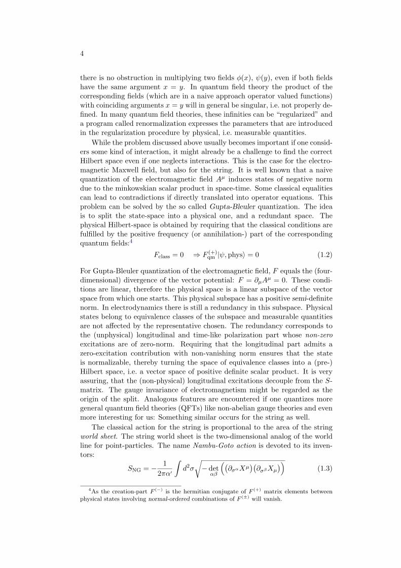
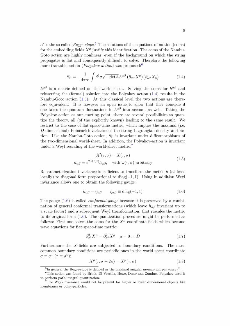
6

X0

Figure 1.1: Closed-string (blue)evolving in time. The world-sheet,which is a classical solution is indi-cated in transparent orange.8

X0

Figure 1.2: Open-string (blue)evolving in time. Both world-sheetboundaries (green) belong to thesame stack of D-branes. This classi-cal solution can be associated witha gauge-boson of the quantized the-ory.8

and open string boundary conditions which are of Neumann-type:

∂σXµ(τ, σ)

∣∣σ=0,π

= 0 (1.9)

Classical closed and open strings fulfilling these eoms and boundary conditionsare depicted in figure 1.1 and 1.2.8 Then one quantizes the classical degrees offreedom. The world-sheet Hamiltonian suggests a splitting into creation andannihilation operators. Like in the case of electrodynamics one encounters how-ever necessarily states of zero-, and even worse: negative-norm. Much alike inthe case of electrodynamics one now tries to impose further classical constraints.The additional classical conditions stem from the eoms of the world-sheet met-ric hαβ i.e. the vanishing of the world sheet energy-momentum tensor T . Itstrace vanishes already by the Weyl-invariance of the classical action.9 T can beexpressed in terms of X and consequently in terms of operators. The Fouriercomponents are the famous Virasoro generators Ln. In calculating the Pois-

8However the depicted world-sheet does not fulfill the classical constraint equations. Thesewould imply that no oscillator modes are excited for a light-like center of mass momentum p.The normal-ordering of the quantum theory enforces however that oscillators are excited forp2 = 0.

9However the Weyl-symmetry might get spoiled by quantum effects. Actually in orderthat Weyl-anomalies are absent in the path integral formalism, one is restricted to D = 26space-time dimensions under certain assumptions on the background. This is especially truefor constant background fields.

7

son brackets of the classical Virasoro generators10 and comparing it with thequantum mechanical commutator obtained by expressing the Ln in terms ofoperators encountered in quantizing X, one discovers a c-number anomaly, theso called Virasoro anomaly. Unlike to electrodynamics, the condition that thepositive frequency part of the energy-momentum tensor T (+) has to vanish onthe physical Hilbert-space Hphys, does not remove negative-norm states fromHphys. It does so if a previously obtained normal ordering constant a equals oneand if the space-time dimensions D equals 26. Higher space-time dimensionsare not possible, while there are examples for a < 1 and D < 26 that emergefrom projecting the 26-dimensional theory to lower dimensions. Looking atthe massless spectrum, one can however not single out the case D = 26 anda = 1. This might be done by looking at vertex operators, or probably moreconveniently: to choose the method of light-cone quantization.

In light-cone quantization one transforms the time-coordinate X0 and onearbitrary space-coordinate, say X1 to new coordinates X± = 1/

√2(X0 ±X1).

The constraints T = 0 take the following simple form in light-cone coordinates:

∂τX+∂τX− + (τ ↔ σ) =12

D∑i=2

(∂τXi)2 + τ ↔ σ

∂τX+∂σX− + (τ ↔ σ) =12

D∑i=2

(∂τXi)(∂σXi)

(1.10)

The interesting observation is that X− appears only linear in the above con-straint equations. If we would be able to bring X+ to a particular simple form,i.e. one which is linear in τ (or σ), we could solve these equations directly. Dueto the formerly mentioned residual conformal symmetry (which leaves the formof the gauge fixed action and metric h invariant) and due to the fact that theX-fields have the same periodicity as the conformal transformations, which areharmonic functions on the world-sheet as well, this is indeed possible. Theresulting spectrum can be shown to be ghost-free. However Lorentz-symmetryis no longer manifest. It turns out that in general the Lorentz-symmetry isplagued with anomalies, except for the case of space-time dimension D = 26.

Another method to quantize strings is the path-integral approach. It isrelatively complicated, although leading to most insights in mathematical re-spects. In path-integral formalism the absence of quantum anomaly in Weyl-transformations (1.5) restricts the space time dimension to D = 26 which alsoremoves a possible BRST-anomaly.11

10The Virasoro generators together with its commutators are called the (central extensionof the) Virasoro algebra.

11Anomalies in symmetries that are used to split the Hilbert space into a physical and anunphysical part (and this is exactly what the BRST-symmetry is used for) would indicatethat this split is ruined by quantum corrections.

8

1.3 String theory as a theory of quantum gravity

Up to now we explained how string theory is quantized in principle, and howthe corresponding Hilbert space can be obtained. We saw that this Hilbertspace only exists for bosonic strings moving in D = 26 space-time dimensions,which already puts surprisingly many constraints on the geometry. (For su-persymmetric strings the number of flat dimensions turns out to be 10.) Upto now we restricted to a flat target space. However the form of the stringaction suggests some generalization. If one computes the spectrum, one seesthat it is quantized due to the constraint on the energy-momentum tensor, orits Fourier-components, the Ln’s. The linear mode pcom of the fields

X(τ, σ) ∼ xcom + τ · pcom + oscillator modes (1.11)

is interpreted as the center of mass (com.) momentum. Its (minkowskian)square determines the mass of the state. It turns out that for the bosonicstring on flat space-time there exist tachyons for both open and closed strings.The mass2= 0 level consist of an excitation that has exactly the degrees offreedom of a U(1)-gauge field for the open string. The closed string mass2= 0can be identified with a scalar (the dilaton), an antisymmetric tensor, and atraceless symmetric tensor, the latter interpreted as the graviton. This makesstring theory particularly interesting. String theory gives further evidence thatthis identification is justified. According to the massless particle content, it issuggestive to include further terms in the Polyakov action, which are compat-ible with two-dimensional diffeomorphism and Weyl invariance at the classicallevel:12

Sσ = − 14πα′

∫d2σ√−|h|

((hαβG(X) + εαβB(X)

)µν

Xµ

∂σα∂Xν

∂σβ+α′R(h)Φ(X)

)(1.12)

G is the space-time dependent D-dimensional metric, B the antisymmetrictensor, Φ the dilaton field, while R is the two dimensional Ricci-scalar. Thebackground fields in the above action might be interpreted as coherent states ofstrings, which might be represented by insertions of vertex operators into thepath-integral.13 The action (1.12) describes a coupled two-dimensional fieldtheory with the couplings G, B and Φ depending on the fields Xµ in a possiblynon-linear way. (Such an action is therefore called a non-linear σ-model.) Thesecoupling functionals will admit β functions like any coupling in a QFT. Weylinvariance at the quantum level requires, that these β-functions vanish. It ispossible to obtain the β functions (of the two dimensional world-sheet theory)corresponding to the three fields G, B and Φ as eoms of the following D-

12We neglect for the moment a possible boundary action that would include a vector-potential Aµ corresponding to the open string massless mode.

13States can be created by so called vertex operators. This is similar to the case of QFT,where in and out states are created by corresponding fields. Vertex operators play an essentialrole in calculating string interactions.

9

+ +

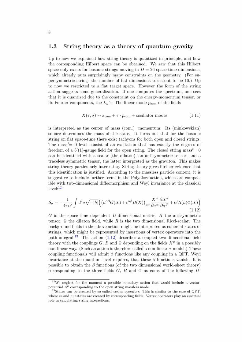
Figure 1.3: First three terms of the string perturbation series with four externalclosed string states involved

dimensional action:14

SS =1

2κ20

∫dDx√−Ge−2Φ

(− 2(D−26)

3α′ +R(G)− 112H∧∗H+4dΦ∧∗dΦ+O(α′)

)(1.13)

H is the field strength of the antisymmetric tensor: H = dB. Upon a Weylrescaling of the metric G(x) = exp(2ω(x))G(x), ω(x) = 2(Φ0 − Φ(x))/(D − 2)together with the induced transformation of the Ricci scalar R(G) and a furtherfield redefinition of the dilaton Φ = Φ(x)− Φ0 the action (1.13) becomes (κ =κ0 exp(Φ0)):

SE =1

2κ2

∫dDx

√−G(− 2(D−26)

3α′ e4ΦD−2 +R(G)

− 112e

− 8ΦD−2H ∧ ∗H − 4

D−2dΦ ∧ ∗dΦ +O(α′))

(1.14)

Because the action (1.14) is the Einstein-Hilbert action of gravity supplementedwith some additional fields, the metric G is denoted as the Einstein metric, whileG is called string metric. The action (1.14) governing the background fields isthe most impressive justification for identifying the symmetric traceless modeof the perturbative closed string with the quantum excitation of the gravitonfield.

String theory perturbation series are defined as integrals over the modulispace of Riemann surfaces with insertions of vertex operators (whose positionsare also moduli).15 The vertex operators correspond to external (i.e. incomingand outcoming) particles. For closed strings there exists only one diagramat a given genus. It includes implicitly all possible string excitations in theinternal part of the diagram. A four-particle closed string scattering process isdepicted up to third order in figure 1.3. Besides the sphere it includes a toruswith one and another torus with two handles. From the aspect of simplicity(i.e. one diagram at each level of closed-string perturbation series, and stillcomparatively few, if one includes open strings and unoriented diagrams) string

14The β-function leading to this action were obtained by expanding the background fieldup to first order in coordinate fields X. Higher order corrections are included in O(α′).

15To be more precise, one only integrates over a region in moduli space, which is notconnected to another one by an holomorphic transormation.

10

theory is very economic. If one considers for example all diagrams contributingto the one-loop level of electron-electron scattering (e−e− → e−e−) one getsa variety of diagrams which are shown in figure 1.4. We even suppressed the

tree-level:

+

one-loop:

+

+

+3 other electron-self-energy insertions

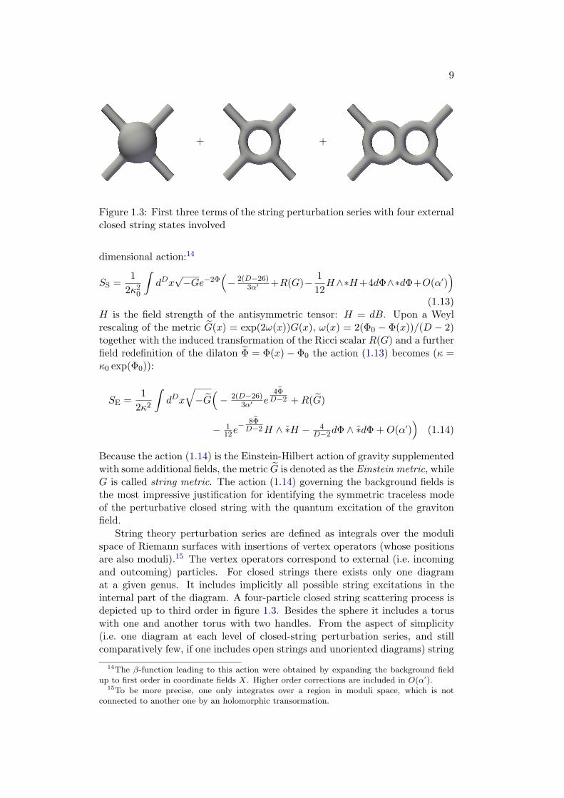
Figure 1.4: Perturbative expansion of electron-electron scattering in QED withone fermion generation.

different combinations of legs, which would lead to a multiple of the depicteddiagrams. Similar combinatorics occur however in string theory as well, ifseveral open strings participate as external states. We also have to admit thatthe actual calculation of the few string-diagrams is a highly non-trivial task, atleast at higher loop orders, or for many external strings participating.

As string theory has the graviton in its spectrum, we can (at least formally)calculate scattering amplitudes that include this excitation as an external state.In loop diagrams the graviton is implicitly included as an internal state aswell. If one tries to include the graviton in conventional QFT, one is leadto serious problems in performing the perturbative expansion (while little isknown about a non-perturbative treatment of a QFT of gravitation). This isdue to the fact that the usual renormalization program, that allows to absorball divergencies in a finite number of (measurable) constants, fails. This kindof non-renormalizibility can be traced back to the fact that the gravitationalconstant has negative mass dimension (in units where ~ = 1).

In string theory the problems with (UV-) divergencies are circumventedin a very elegant way: In field theory the dangerous divergencies are UV-divergencies, i.e. divergencies that appear for high momenta. In coordinatespace an one-loop UV divergence would correspond to the limit, where the loopsize shrinks to zero. In principle this divergence is also seen in string theory,if one considers the limit, when the modular parameter (or complex structure)

11

that describes the shape of the torus, approaches zero. However the symme-tries of string theory, in this case: modular invariance, require that one onlyintegrates the modular parameter over a region that describes inequivalent tori.A convenient integration region for the torus modulus is given by the shadedregion in figure 2.2 on page 28. The regions including possible singularitiesare explicitly excluded by this choice. Therefore one-loop torus amplitudes areUV-finite (Shapiro [10]). Modular invariance extends to higher loop-levels aswell. Even though not strictly proven yet, it is believed that the finiteness ofstring-scattering amplitudes extends to all orders of string perturbation theory.It would imply that string theory describes perturbative quantum gravitation.This is one (maybe even the strongest) motivation to consider string theory asa unifying theory.

Up to now we concentrated on the massless modes of string theory. There isstill an infinite tower of massive states. For flat backgrounds the different mass-levels are equally spaced. Bosonic string theory contains a tachyon, which seemsto indicate an instability. Some researchers undertake however considerablyeffort in order to stabilize the theory via some kind of tachyon condensation.Another way out of this problem is to look for a string theory where tachyonsare manifestly absent. This is the case for:

1.4 Supersymmetric string theories

An obvious shortcoming of the bosonic string is the absence of space-time fermi-ons in its spectrum.16 Furthermore it is desirable to have a supersymmetrictheory in space time, at least to a good approximation. In any phenomenologi-cally relevant theory this supersymmetry has to be broken at some scale, and ifstring-theory serves as a unifying theory, this breaking must be compatible withthe underlying principles of string theory. In this thesis, we will not concentrateon the supersymmetry breaking mechanism.

To include space-time fermions, the bosonic string action 1.4 is extended byterms that involve fermionic dofs. There are two common ways to achieve this.One is the Green-Schwarz (GS) superstring(-formalism) [14,15]. Instead of thepurely bosonic action one considers (α′ set to 1/2):

S1 = − 12π

∫d2σ√−dethhαβ Πµ

α(Πβ)µ, Πµα = ∂αX

µ − iθAΓµ∂αθA (1.15)

In this approach θA, A = 1 . . . N are N space-time spinors. Each of the spinorcomponents is a world sheet scalar. This action is reparameterization invariant.Requiring a so called κ-symmetry in order to reduce the number of fermionicdofs lets one introduce an additional action piece S2. κ-symmetry restrictsthen the maximal number of spacetime spinors to N = 2. Requiring S2 to besupersymmetric reduces the possible space-time dimensions considerably. Thequantized version singles out D = 10 in which case already supersymmetry ofthe action S2 requires that both spinors θ1 and θ2 are of Majorana-Weyl type.

16It has however been suggested that the bosonic string includes even the supersymmetricstring-theories in a rather subtle manner (cf. [11,12,13]).

12

The Green-Schwarz formalism has the advantage to be manifestly supersym-metric in space-time. However the resulting eoms are extremely complicated,as they are non-linear. They can be drastically simplified by choosing light-cone gauge, and simplifying the X+-coordinate as in the bosonic case. As theLorentz-algebra can only be realized in D = 10 space-time dimensions this caseis considered as the only consistent. Depending on the relative handedness ofθ1 and θ2 one obtains either the Type IIA (θ1 and θ2 have opposite chirality)or Type IIB (θ1 and θ2 have equal chirality). In the case of Type I both spinorsare identified (by moding out the world sheet-parity Ω). We come back tothis case in section 1.6. There is still a third kind of ten-dimensional super-string known, the heterotic string. As its name suggests, the construction ofthe heterotic string is composed from several pieces. The heterotic string takesadvantage from the fact that the closed string-states can be decomposed intoleft and right moving parts. The same is true for the fields. Roughly speaking,the theories considered so far are constructed from a tensor product of left-and right moving degrees of freedom. This does not mean that the resultingtheories are tensor products as well, since in general some additional conditionshave to be imposed. The probably most famous construction of the heteroticstring starts from ten-dimensional superstring of one (say the right-moving)sector and the 26-dimensional bosonic string in the other (here: left-moving)sector. In order to have a sensible space-time interpretation, one compactifiesthe sixteen surplus bosonic dimensions. Especially one considers flat toroidalcompactifications that are obtained by identifying points x ∼ x + 2πγ with γa vector of a sixteen dimensional lattice Λ16. Associated with the torus lat-tice Λ is an even self dual lattice, the so called Narain-lattice Γ16, which is ingeneral not unique (cf. chapter 2). However there are only two 16-dimensionalNarain-lattices:

1. Γ16 is the weight-lattice of the Spin(32)/Z217(

Γroot(SO(32)) ⊂ Γweight(Spin(32)/Z2))

2. Γ16 = Γ8 × Γ8 with Γ8 the root-lattice of the E8 Lie-algebra

What makes heterotic string-theories so extremely interesting is the fact thatthey admit non-abelian Lie-algebras as gauge-symmetries of their low-energy-effective field theory. In the first case this symmetry is SO(32) while in thesecond it is E8 × E8. These symmetries are also manifest in the operatorproduct expansion (OPE) of the formerly mentioned vertex operators.18 Com-pactifications of the heterotic string to four space-time dimensions have led tomany interesting models, especially such that come pretty close the StandardModel (SM) of electro-weak and strong interactions.

17By this we mean the sub-lattice of the weight-lattice of Spin(32) which is generated by theweights of one spinor representation together with the the roots of SO(32). (Remember thatthe weight lattice of Spin(32) consist of four conjugacy classes: adjoint (i.e. roots), vector,spinor, spinor’.)

18In the heterotic string there exist currents on the world-sheet (associated with charges)that build up the corresponding Kac-Moody algebras. A Kac-Moody algebra is an infinitedimensional extension of a Lie algebra.

13

In parallel to the Green-Schwarz superstring there exists the so called Neveu-Schwarz-Ramond (NSR) superstring.19 It turns out that the GS- and theNSR-superstring describe the same physics, though they use other formalisms.While the GS-superstring exhibits manifest space-time supersymmetry, its co-variant quantization is not at all obvious. The NSR superstring however canbe quantized by path-integral formalism in parallel with the bosonic string,up to some generalizations. It becomes space-time supersymmetric, if one im-poses the so called Gliozzi-Scherk-Olive (GSO) projection (which is absent inGS-formalism) [16, 17]. From the world-sheet point of view the bosonic stringaction 1.4 might be considered as a two dimensional gravity theory (after in-clusion of the R(h)-term like in (1.12)) coupled to D world-sheet scalars Xµ.It is now quite natural (and actually necessary in order to use path-integralformalism in a subsequent analysis) to extend this theory to N = 1 local su-persymmetry (or: N = 1 supergravity) on the world sheet. Supersymmetrizingthe scalar part of the bosonic action is achieved by adding the following termto the Polyakov action (1.4):

SF = − 12πα′

∫d2σ√−deth

(iψµρα∂σαψµ + FµFµ

)(1.16)

Some comments are in order: Each ψµ, µ = 0, . . . , D − 1 is a two dimensional(world-sheet) Majorana-spinor. The D world-sheet spinors ψµ make up a space-time Lorentz-vector. (This is in contrast to the GS-formalism, where the θA arespace-time spinors as well as world-sheet scalars.) The Fµ are auxiliary fieldswhich are needed to realize the off-shell supersymmetry-algebra. Their eomshowever require them to vanish on-shell. Each of the Fµ is a world-sheet scalarwhile in total they make up a D dimensional space-time Lorentz-vector. Themetric h can be expressed by world-sheet Vielbeins eαa (or more precisely asthey live in two dimensions: by Zweibeins.):

eαaeβbhαβ = ηab a, b, α, β ∈ 0, 1, η = diag(−1, 1) (1.17)

As GL(d,R) does not admit finite-dimensional spinor-representations, Vielbeinsare a way to define spinors on curved space-time, in our case: on a curved world-sheet. The two dimensional matrices ρα are obtained from the two dimensionalDirac matrices (cf. eq. (4.5),(4.6), p. 88) by:

ρα ≡ eαaρa (1.18)

The sum of the bosonic action (1.4) and the fermionic action (1.16) does notyet admit local supersymmetry. This goal is achieved by adding a third pieceto the action:

S3 =i

4πα′

∫d2σ√−deth χαρβραψµ

(∂σβXµ − i

4 χβψµ)

(1.19)

χα is the superpartner of the world-sheet metric hαβ (or of the Zweibein eαa). Ithas a world-sheet vector- and a world-sheet spinor-index. The resulting actionhas a variety of symmetries:

• Local world-sheet supersymmetry19The NSR formalism was developed before the GS-formalism

14

• Local Weyl-invariance (The Weyl transformation rescales also the Majo-rana-fermions ψµ and the gravitino χα besides the Zweibein eαa)

• Local super-Weyl-invariance (λ(τ, σ) a Majorana spinor parameter):

δλχα = ραλ δλ(others) = 0 (1.20)

• World-sheet (or: two-dimensional) Lorentz-invariance

• World-sheet reparameterization- (or: diffeomorphism-) invariance

Very similar to the purely bosonic case, one could use some of the symmetries toeliminate some degrees of freedom. Using local supersymmetry, reparameteri-zation and Lorentz-invariance, one can reduce the two-dimensional supergravityaction to a much simpler action (cf. eq. (4.1), (4.3), p. 88). The correspondinggauge where the gravitino is efficiently eliminated while h is brought to thestandard minkowskian form is called superconformal-gauge. Besides the confor-mal symmetry encountered in the bosonic conformal gauge, this action admitsa further symmetry, generated by the fermionic current TF . TF is determinedby varying the (non-gauge fixed) action with respect to the gravitino χα:

TF =2π

idet e· δSδχ

(1.21)

Along the lines of light-cone gauge in the bosonic case, one can eliminate in ad-dition the ψ+ component from the world-sheet Majorana spinor.20 In contrastto the bosonic case the critical space-time dimension D turns out to be ten,rather than 26. (The formerly mentioned normal ordering constant a equalsnow one half in the bosonic (Neveu-Schwarz) sector instead of one, while it iszero in the fermionic (Ramond) sector. These sectors will be explained below.)Equivalent results can also be derived via path-integral quantization.

There is still a peculiar feature in the NSR superstring which we now want toaddress: So far we have not specified the boundary conditions of the Majoranaspinor ψ. For several reasons, and the most striking one is modular invariance(to be explained in chapter 2), one is forced to allow ψ to be both periodic andantiperiodic for closed strings:21

ψµ±(τ, σ) = κ±ψµ±(τ, σ + 2π) κ± ∈ −1,+1 (1.22)

Here we have denoted the two components of the Majorana spinor ψµ by ψµ+ andψµ− which is suggested by the fact that after solving the eoms the first componentonly depends on τ+σ while the second only depends on τ−σ. A similar freedom

20ψ+ ∝ ψ0 + ψ1 should not be confused with the spinor component ψµ+ which will be

introduced below.21In calculating partition functions, a fermion-field is anti-periodic in time (if no further

trace-insertion acts on this field in operator formalism). The modular group (which is aimportant symmetry in string theory) maps sectors in the partition that correspond to certainperiodicities to other sectors. Thereby a spinor ψ that is periodic in σ and anti-periodic intime will get mapped to a different sector. This explains the presence of different boundary(or periodicity) conditions as well as the presence of the GSO-projection.

15

like in (1.22) exists also for open strings, where the supersymmetric partner ofthe bosonic boundary condition (eg. Neumann-type: ∂σX

µ = 0 ⇒ ∂+Xµ =

∂−Xµ, ∂± ≡ 1/2(∂τ ± ∂σ)) becomes:22

ψ+(τ, σ) = κ(σ)ψ−(τ, σ) for σ ∈ 0, π, κ(σ) ∈ ±1 (1.23)

Depending on the sign κ one distinguishes between Ramond (R) (κ = 1) andNeveu-Schwarz (NS) (κ = −1) fermions. It turns out that unless one imposes aprojection, the GSO-projection, the NS-sector contains a tachyon. The GSO-projection is also needed for modular invariance. Even though defined on thewhole string-spectrum, the action of the GSO-projection on the R-ground-statesis particularly interesting. Solving the equations of motion subjected to theboundary conditions, one discovers a zero-mode in each ψµ-coordinate. In light-cone-gauge one has therefore 8 zero-modes bi which are anti-commuting andfulfill a Clifford-algebra:

bi, bj = ηij i, j ∈ 2 . . . D − 1 (1.24)

Thus one can represent the above algebra on a vector space with the followingbasis: |s1, s2, s3, s4〉 with si = ±1

2 . The resulting vector space can then bedescribed as the sum of a vector space of positive chirality and another one ofnegative chirality. Performing the GSO-projection eliminates one chirality fromthe massless ground-state. In the closed string sector there are two sectors con-taining fermions depending on the combination of left- and right-moving sectors:These are the NSR and the RNS sectors, while the NSNS- and the RR-sectormake up space-time bosons. In the open string there are just two sectors, theNS- and the R-sector, the latter containing the space-time fermions. As theGSO projection picks up one chirality, there is still the freedom to choose equalor opposite chiralities on left- and right-movers. Equal chiralities lead to theType IIB superstring, while opposite chiralities yield Type IIA. Upon compact-ification on a circle, this does not make big difference, since both theories arethen related by a perturbative duality, the so called T-duality. The masslessspectrum of Type IIA theory can be found in table 1.1, its Type IIB pendant isgiven in table 3.1, page 62. While the resulting spectrum is supersymmetric, itis much harder to show that the interacting theory is supersymmetric as well.We will not investigate this topic.

It is possible to build modular-invariant partition functions that consistonly of RR and NSNS sectors. The resulting theories are called Type 0A andType 0B. They do not contain any fermions in the closed string sectors and areplagued with tachyons. However there exist interesting generalizations of theseType 0A/B by performing an orientifold 23 projection of these theories. Thisremoves the closed-string tachyon and introduces fermions via a necessary openstring sector (cf. [18] and references therein). There exist non-supersymmetricorientifolds of Type 0B that are completely tachyon free. Something similar is

22There is still a redundancy in the following equations: By a field redefinition one can setκ(0) = +1.

23We will introduce orientifolds in section 1.6. In addition we devoted a whole chapter tothese constructions (cf. chap. 3).

16

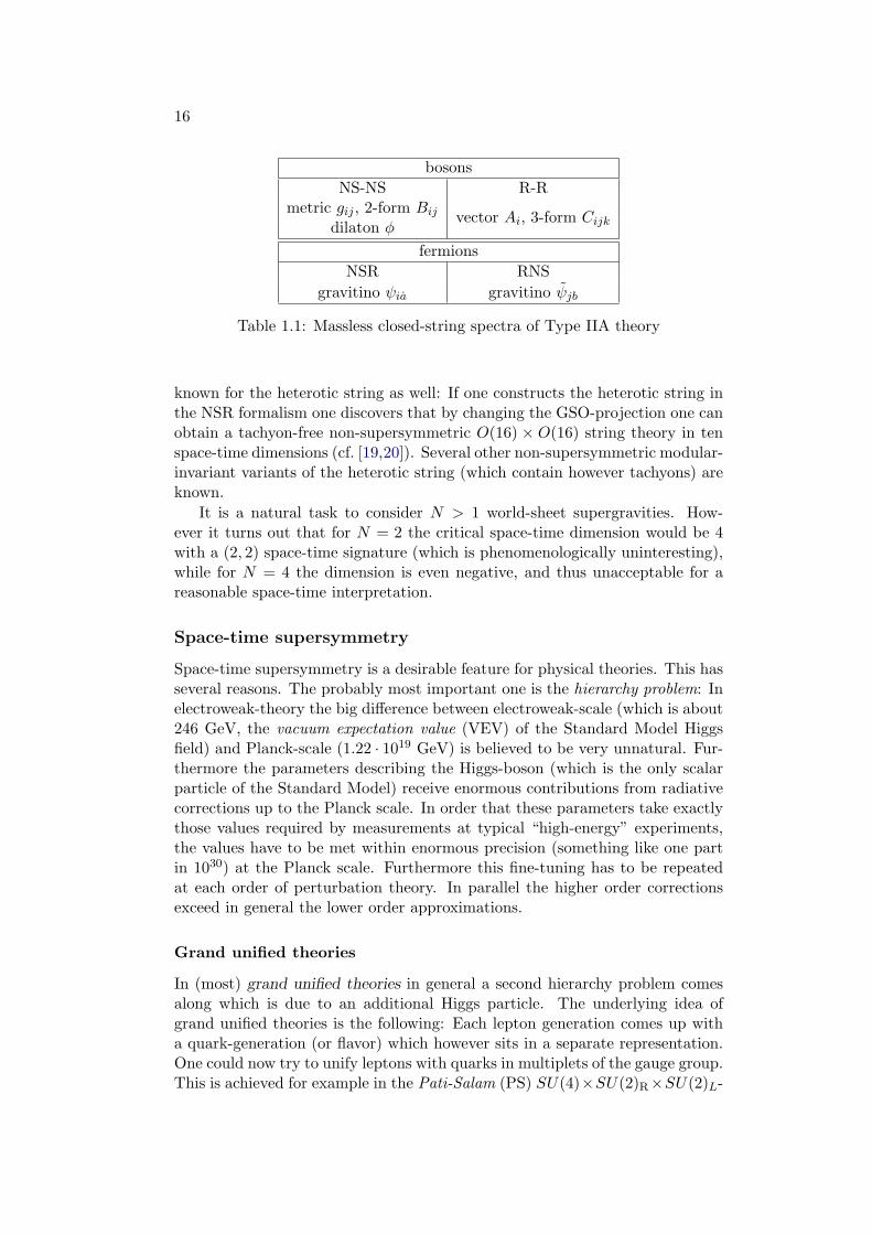
bosonsNS-NS R-R

metric gij , 2-form Bijdilaton φ

vector Ai, 3-form Cijk

fermionsNSR RNS

gravitino ψia gravitino ψjb

Table 1.1: Massless closed-string spectra of Type IIA theory

known for the heterotic string as well: If one constructs the heterotic string inthe NSR formalism one discovers that by changing the GSO-projection one canobtain a tachyon-free non-supersymmetric O(16) × O(16) string theory in tenspace-time dimensions (cf. [19,20]). Several other non-supersymmetric modular-invariant variants of the heterotic string (which contain however tachyons) areknown.

It is a natural task to consider N > 1 world-sheet supergravities. How-ever it turns out that for N = 2 the critical space-time dimension would be 4with a (2, 2) space-time signature (which is phenomenologically uninteresting),while for N = 4 the dimension is even negative, and thus unacceptable for areasonable space-time interpretation.

Space-time supersymmetry

Space-time supersymmetry is a desirable feature for physical theories. This hasseveral reasons. The probably most important one is the hierarchy problem: Inelectroweak-theory the big difference between electroweak-scale (which is about246 GeV, the vacuum expectation value (VEV) of the Standard Model Higgsfield) and Planck-scale (1.22 · 1019 GeV) is believed to be very unnatural. Fur-thermore the parameters describing the Higgs-boson (which is the only scalarparticle of the Standard Model) receive enormous contributions from radiativecorrections up to the Planck scale. In order that these parameters take exactlythose values required by measurements at typical “high-energy” experiments,the values have to be met within enormous precision (something like one partin 1030) at the Planck scale. Furthermore this fine-tuning has to be repeatedat each order of perturbation theory. In parallel the higher order correctionsexceed in general the lower order approximations.

Grand unified theories

In (most) grand unified theories in general a second hierarchy problem comesalong which is due to an additional Higgs particle. The underlying idea ofgrand unified theories is the following: Each lepton generation comes up witha quark-generation (or flavor) which however sits in a separate representation.One could now try to unify leptons with quarks in multiplets of the gauge group.This is achieved for example in the Pati-Salam (PS) SU(4)×SU(2)R×SU(2)L-

17

model where the leptons correspond to a fourth color (cf. [21]). Each generationof matter transforms in a (4, 2, 0) and (4, 0, 2) representation of the gauge group.This Pati-Salam model has two interesting features, that are common to mostother GUTs as well:

• Additional matter that is absent in the (“minimal”) Standard Model (InPati-Salam SU(4)× SU(2)R × SU(2)L: right-handed neutrinos)

• The electric-charge is quantized

Quantization of electric-charge is in general true for models with simple gauge-group but also for this semi-simple example. In unifications with simple gauge-group the SM gauge-group is embedded into a larger, simple Lie-group G:

SU(3)× SU(2)× U(1)Y → G (1.25)

Thus not only leptons and quarks become unified, but gauge-bosons of differentgauge-groups as well. Well known examples for GUTs with simple gauge groupG are SU(5), SO(32) and even E(6) GUTs, the latter based on the exceptionalgroup E(6).24 Among several interesting and attractive features of GUTs wewant to mention the probably best known: GUTs in general predict protondecay. Proton decay, if present, can be measured (up to a certain bound) byexperiments. Several GUTs have already been ruled out by experimental data.Supersymmetry suppresses the decay rate considerably. For example the non-supersymmetric SU(5) GUT is forbidden, while its supersymmetric extensionis still in accord with the bound given by current proton decay experiments.Analogous statements can be made for SO(10).

Now we address a second hierarchy problem that comes along with mostGUTs. What is important in GUTs, is that the unifying gauge-symmetry hasto be broken at some scale, which is of course above the electro-weak scale.This will be done in general by some Higgs mechanism with the correspondingHiggs-field acquiring a VEV 〈0|Φ|0〉 = w which is of the order of the unificationscale. We assume that the unification scale a priori does not coincide with thePlanck scale. The running of the couplings strongly suggests that it is of theorder of 1015 to 1016 GeV.25 The second gauge-breaking is the usual electro-weak symmetry breaking which occurs at a VEV of 〈0|φe.w.|0〉 = v ≈ 246 GeV.A generic Higgs potential looks like:26

V = −A2

Φ2 +B

4Φ4 − a

2φ2 +

b

4φ4 +

λ

2Φ2φ2 (1.26)

The term proportional to λ is generic and thus has to be included. The GUTscale value is obtained, if we tune A and B such that: w2 = A/B. The problem

24The SU(5) model was proposed by Georgi and Glashow [22], the SO(32) theory by Georgi[23] in parallel to Fritzsch and Minkowski [24]. The E(6) model was found by Gursey, Ramondand Sikivie [25].

25The first value is already excluded by experiment, and assuming solely the SM particlecontent will not lead to gauge coupling unification.

26We have suppressed group indices which are present since the Higgs fields transform underthe gauge group.

18

occurs for the VEV of the second (i.e. the electroweak) Higgs: Since v2 =(a−λw2)/b has to be obeyed this requires a fine tuning of a to one part in 1026.Radiative corrections will require this fine tuning at each order in perturbationtheory. If present, supersymmetry ensures however that radiative correctionsdo not destroy the hierarchy and parameters do not have to be retuned. Onthe other hand supersymmetry has to be broken. Requiring the hierarchy tobe preserved by this breaking leads to the prediction, that supersymmetricpartners of the known particles should show up at 1 TeV.

Other mechanism like composite Higgs-particles have been proposed to cir-cumvent the hierarchy problem without the use of supersymmetry. Howeverthese approaches are plagued with other difficulties.

Inspired from string-theory, it has been suggested that extra large dimen-sions could solve the hierarchy problem as well. In these scenarios the knowngauge interactions are restricted to a lower dimensional subspace (a brane) whilegravity propagates in the entire space (often denoted by “bulk”), which in mostmodels has relatively large,27 but compact directions. Future experiments canput severe constraints on the size of possible extra large dimensions, whichmight sustain or rule out these proposals.

As a third argument for supersymmetry, we mention the unification of theStandard Model couplings at a scale of 1016 GeV if one assumes the supersym-metry-breaking scale at about one TeV.

1.5 Compactifications

It goes back to the early twenties of the 20th century that Kaluza suggested atheory with an additional small dimension. Even though this dimension mightnot be discovered directly due to its smallness, it influences the four dimen-sional physics indirectly. As string theory on flat backgrounds has too manydimensions of unrestricted size, one has to figure out some explanation, whyonly four space-time dimensions are seen. A very fruitful idea is to compactifystring theory on some tiny space Xd:

M = R(1,D−d−1) ×Xd (1.27)

By this we obtain effectively a theory with one time and D − d − 1 space di-mensions. The exact form of the space Xd has big influence on the theory seenin uncompactified space. If we compactify a 10-dimensional N = 1 superstringtheory on a Calabi-Yau (CY) space, N = 1 will be present in 10 − d dimen-sional space time.28 Furthermore the chiral massless spectrum is determinedby topological data of Xd. The Calabi-Yau space admits in general additionalstructures like gauge-bundles. Physical requirements like anomaly-cancellationput further constraints on the geometry. The topic is too extended in order to

27By “large” we mean much bigger than the Planck length, and in order to solve thehierarchy problem: in the region up to a few TeV.

28To be precise, one has to deform the CY space to take the α′-string corrections to thesupersymmetry algebra into account.

19

enter into details. For some geometric aspects of compactifications we refer thereader to the book of GSW [5].

A special case of compactification spaces are orbifolds to which we havedevoted the next chapter. Roughly speaking, an orbifold is the orbit-space ofsome discrete group G that acts on a manifold B:

Xd = B/G (1.28)

The action of G may admit fixed-points, which usually result in singularitieson Xd. If the string theory on B is known, it is comparatively easy to constructthe orbifold by G. Even though Xd might be singular in some points, stringpropagation turns out to be regular (in most cases). In all of our thesis weencounter either tori (that can also be interpreted as fixed-point free orbifolds)or toroidal orbifolds of ZN -groups or products thereof.

1.6 Open strings and unoriented string theories

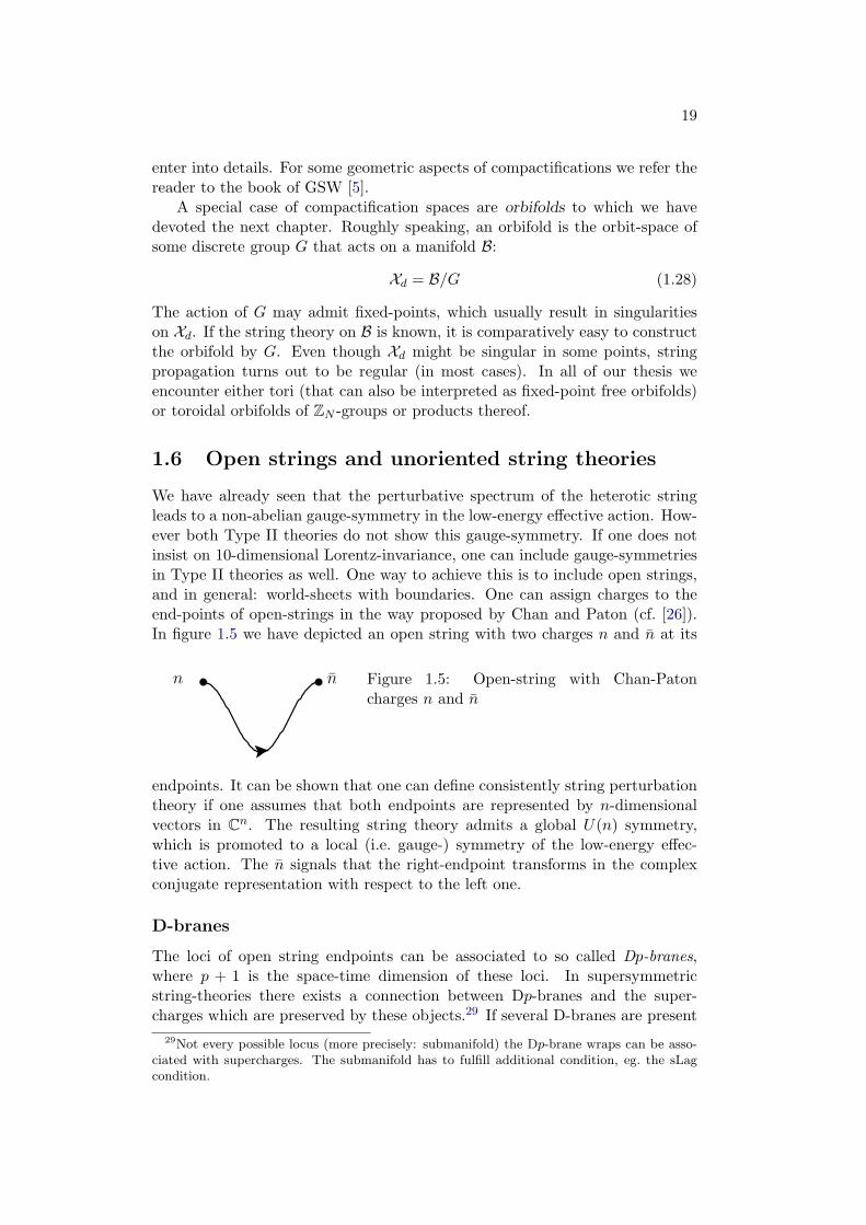
We have already seen that the perturbative spectrum of the heterotic stringleads to a non-abelian gauge-symmetry in the low-energy effective action. How-ever both Type II theories do not show this gauge-symmetry. If one does notinsist on 10-dimensional Lorentz-invariance, one can include gauge-symmetriesin Type II theories as well. One way to achieve this is to include open strings,and in general: world-sheets with boundaries. One can assign charges to theend-points of open-strings in the way proposed by Chan and Paton (cf. [26]).In figure 1.5 we have depicted an open string with two charges n and n at its

n n Figure 1.5: Open-string with Chan-Patoncharges n and n

endpoints. It can be shown that one can define consistently string perturbationtheory if one assumes that both endpoints are represented by n-dimensionalvectors in Cn. The resulting string theory admits a global U(n) symmetry,which is promoted to a local (i.e. gauge-) symmetry of the low-energy effec-tive action. The n signals that the right-endpoint transforms in the complexconjugate representation with respect to the left one.

D-branes

The loci of open string endpoints can be associated to so called Dp-branes,where p + 1 is the space-time dimension of these loci. In supersymmetricstring-theories there exists a connection between Dp-branes and the super-charges which are preserved by these objects.29 If several D-branes are present

29Not every possible locus (more precisely: submanifold) the Dp-brane wraps can be asso-ciated with supercharges. The submanifold has to fulfill additional condition, eg. the sLagcondition.

20

they may or may not preserve some or several supercharges. The numberof supercharges preserved by a D-brane configuration determines the amountof supersymmetry of the particular string model. Supersymmetric Dp-branesare usually Bogomolnyi-Prasad-Sommerfield (BPS) states, i.e. states with a re-duced amount of supersymmetry that saturate the BPS-bound. BPS-statescarry a central charge Z of the super-symmetry algebra which is a conservedcharge. This fact made D-branes so important in the second “string revolution”.String-theory was defined so far by a perturbative expansion, very similar to theway in which Feynman rules may be introduced by hand in electrodynamics.Whatever the correct non-perturbative definition of string-theory would be, itis extremely likely that it preserves the BPS-property, especially in the processof renormalization. On the other hand BPS-solutions were known to appearin the form of p-dimensional soliton-like solutions in the low-energy effectiveactions of string theories. Besides D-branes there exist other BPS-states instring theory as well. By identifying BPS states in perturbatively inequivalenttheories the notion of an M-theory was born. M-theory is considered to bethe unifying theory which includes all superstring theories as special limits ofthe M-theory moduli-space.30 D-branes have also proven extremely useful inexplaining Bekenstein-Hawking entropy at a microscopic level.31

Type I and orientifolds

We have claimed so far that Type II theories, if they contain open-strings,will break 10-dimensional Lorentz-symmetry. This is not disastrous, since forphenomenological reasons we will break this symmetry anyway at some point.So far we did not explain why we are not allowed to introduce freely some D9-branes in Type II, thereby maintaining Lorentz-invariance. It will become soonclear, that D-branes carry a special type of charge, a so called Ramond-Ramond(RR) charge, which is of topological type, and that this charge has to cancel intotal. The RR-charge of a D-brane constitutes its central charge.

The low energy limit of Type I theory is a 10-dimensional N = 1 supergrav-ity coupled to 10-dimensional N = 1 supersymmetric Yang-Mills with gaugegroup SO(32). Both open and closed strings admit a further symmetry, whichis world-sheet parity. World-sheet parity reverses the orientation of the worldsheet, while leaving the action invariant. This has two effects:

• Only closed string-states that are invariant under the world-sheet parityΩ are kept in the spectrum.

• Due to the formula χ = 2− 2h− b− c for the Euler-character χ we needto include the Klein-bottle (h = 0 handles, b = 0 boundaries, c = 2cross-caps) as the second closed-string one-loop vacuum amplitude.

It turns out that the Klein-bottle amplitude has severe divergences. They areinterpreted as uncanceled RR-charges under which the so called orientifold plane

3011-dimensional supergravity is another limit in the M-theory moduli-space.31At least for some supersymmetric black hole configurations.

21

(O-plane) is charged. (The O-plane corresponds to the cross-caps in the Klein-bottle). In analogy to field theory these divergences are called RR-tadpoles.As D-branes carry RR-charges as well they may serve as a neutralizer of theO-plane charge, provided that their charge has the right sign and value. This isindeed the case. In Type I the RR-charge is exactly canceled by 32 D9-branes.In computing the open string partition function we have to include the parityprojection Ω as well. This implies that we have to introduce the Mobius-strip(b = 1, c = 1) besides the cylinder (b = 2, c = 0). The projection togetherwith the RR-tadpole cancellation conditions implies that the U(32)-symmetrygets broken to SO(32). The only gauge groups which can be obtained in theperturbative spectrum of Type I and compactifications thereof are orthogonal,symplectic and (under certain circumstances) unitary groups.

The Type I construction can be generalized. On one hand Type I can becompactified on some space Xd. As before Xd might be an orbifold. We canalso gauge a combination sΩ, where s acts on space-time such that sΩ is asymmetry of the string theory under consideration. We can even try to includeseveral such elements. However we will show in section 3 that this does notlead to new consistent models in most cases. Given a projection via sΩ and acompactification space Xd there might be several inequivalent ways to cancelthe RR-tadpole of the O-plane(s).32 All these generalizations which include theworld sheet-parity in some way are summarized by the term: “orientifold”.

1.7 Chiral fermions in open string theories

As half of the thesis deals with chiral fermions from the open string sector inone way or the other, we want to make some comments here. Chiral-fermionsare an essential feature of the SM. In string theory they can be obtained inmany ways (cf. the introduction to chap. 6, p. 139). For open string theoriesthree mechanism are very prominent:

1. Open strings with endpoints on D-branes with non-trivial topological in-tersection number

2. Open strings with endpoints on D-branes which carry different magneticbackground fields

3. Open strings stuck to a singularity

For flat space-time, the first method was discovered in [27]. The second methodwas (to our knowledge) first applied to model building in [28]. Both methodsare related by T-duality, if the branes intersect as lines when restricted to a T 2.T-duality acts on each T 2 in one coordinate by R/

√α′ →

√α′/R. The classical

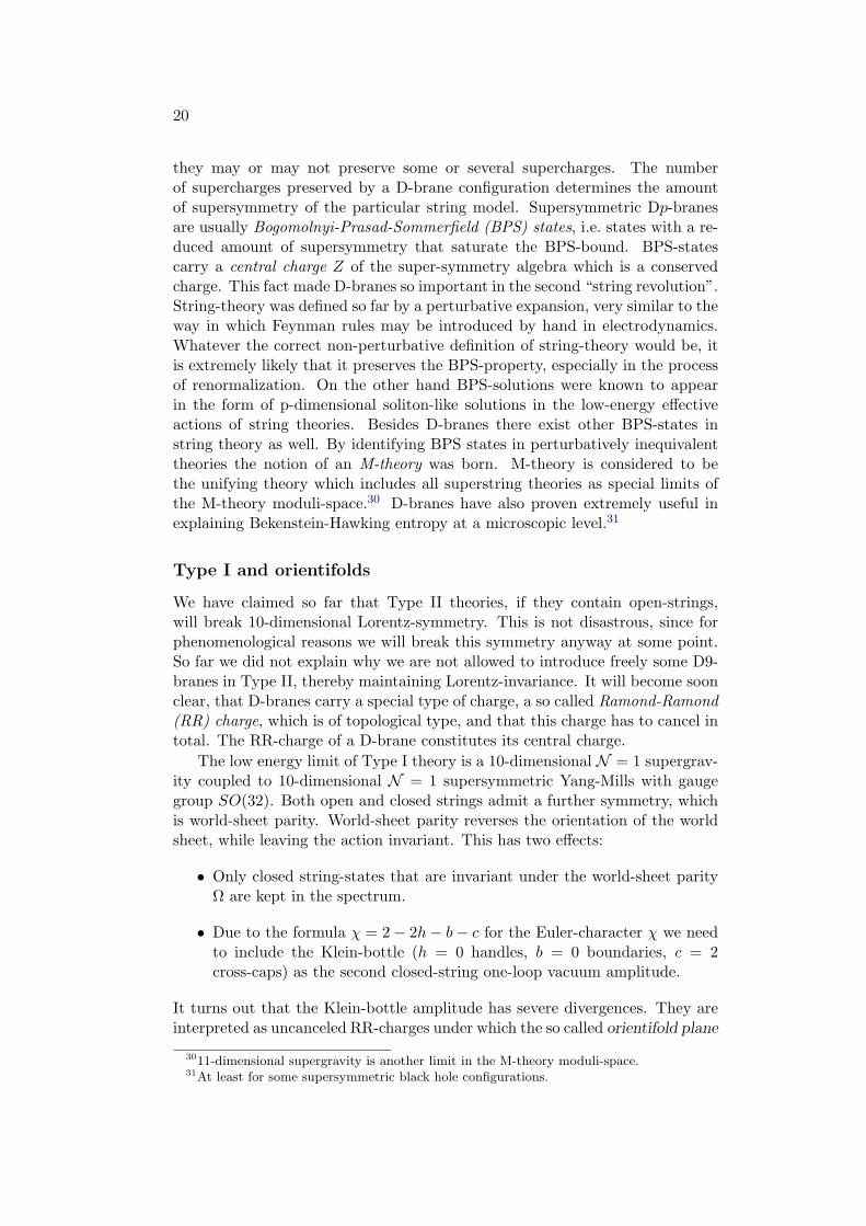
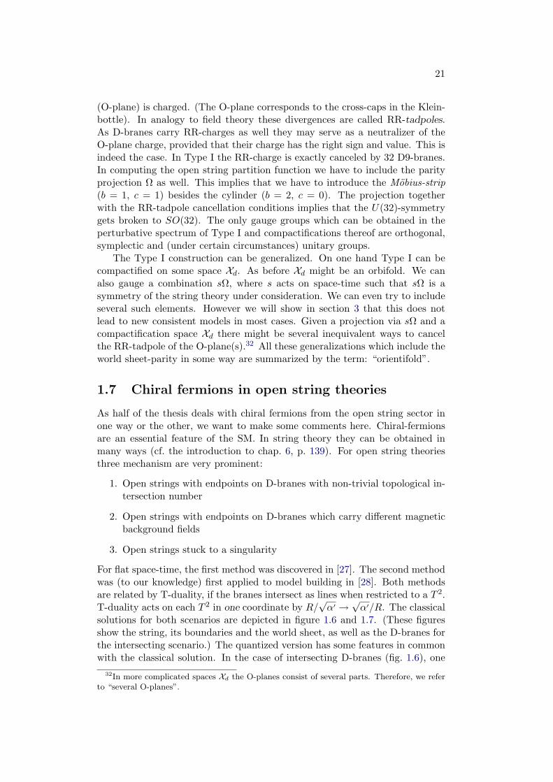
solutions for both scenarios are depicted in figure 1.6 and 1.7. (These figuresshow the string, its boundaries and the world sheet, as well as the D-branes forthe intersecting scenario.) The quantized version has some features in commonwith the classical solution. In the case of intersecting D-branes (fig. 1.6), one

32In more complicated spaces Xd the O-planes consist of several parts. Therefore, we referto “several O-planes”.

22

X0

Figure 1.6: Time evolution of anopen-string with endpoints locatedon D-branes intersecting at an an-gle. The classical string oscillatesaround the intersection point. Upontoroidal compactification on a T 2

angled D-branes are T-dual to mag-netic backgrounds (right figure).

X0

Figure 1.7: Time evolution of abosonic open-string in constantmagnetic background fields. Theclassical string rotates around apoint, whose position is howevernot determined by the NS-fields onits boundaries.

The string is a blue line, while the world-sheet boundaries are in red and“skyblue”. The string depicted obeys the classical eoms. Its lowest (non-zero)mode is excited. In fig. 1.6 the D-branes are drawn in transparent colors, whilein fig. 1.7 the branes are two-dimensional. The world sheet is in transp. orange.

sees that the string oscillates around the intersection point. The string which iscoupled to the magnetized D-branes circulates around some point as well. Thispoint is classically not restricted. In the quantized version it corresponds to aLandau level. The infinite Landau degeneracy gets finite after compactification,e.g. compactification on a torus. The easiest way to see the appearance of chiralfermions is first to note that by the altered boundary conditions the numberof Ramond-zero-modes bi (cf. section 1.4) is reduced, such that (for suitableboundary condition) only one Ramond-state survives:

homogenous inhomogenousboundary conditions boundary conditions

|s1, s2, s3, s4〉∣∣GSO-proj.

−→∣∣+ 1

2

⟩ (1.29)

By “homogenous” we mean that there are identical boundary conditions onthe left- and right-endpoint of the string (at least concerning the derivatives).Each chiral fermion obtained this way appears with a multiplicity that is deter-mined by the bosonic zero-modes, where the sign has to be properly taken intoaccount. This multiplicity is the topological intersection number or the Lan-

23

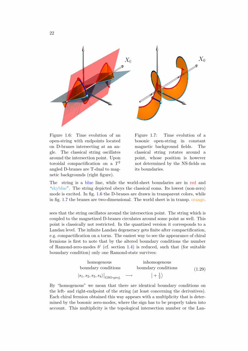
Figure 1.8: Open-stringlocated at a singularity(schematic): A D-brane whichis bound to a singularityin compactification spaceis the locus of open-stringend-points. (The string ispainted in blue, its endpointsare red and green). Opensuperstrings in this sectormight admit chiral fermions.If the string end-points belongto different stacks of D-branes(denoted by a and b), thiscan lead to chiral fermions inbifundamental representation(na, nb) of the associatedgauge group U(na)× U(nb).

dau degeneracy which might be calculate via the Atiyah-Singer index theoremfor twisted spin-complexes. Lower dimensional D-branes which have exactlyhalf the dimension of the embedding space like in figure 1.6 are encounteredin σΩ-orientifolds. In these orientifold σ acts as complex conjugation on eachT 2. (The compactification space is a product of T 2‘s or an orbifold thereof.)We use σΩ-orientifold constructions in chapter 6 and 7 and obtain interestingchiral spectra. In chapter 6 we alternatively consider the T-dual magnetizedsituation as well. Even though we do not apply it in this thesis, we want tomention that chiral fermions can be obtained from D-branes which are locatedat singularities (cf. [29, 30]). The orbifold case, especially the T 2/Z3 case hasbeen exhaustively explored (cf. [29,31] and references therein). A D-brane thatis stuck to an (orbifold) singularity is called a fractional brane. This is dueto the fact that it carries only a fractional amount of untwisted RR-charge incomparison to an ordinary D-brane. Open string states in the Ramond-sectorare described by:33

|s1, s2, s3, s4; Λij〉∣∣GSO-proj.

(1.30)

Λij is the Chan-Paton matrix that encodes the CP-dofs. In symmetrizing thestate with respect to an orbifold group G one encounters conditions like:

|g(s1, s2, s3, s4); (g−1Λg)ij〉∣∣GSO-proj.

= |s1, s2, s3, s4; Λij〉∣∣GSO-proj.

∀g ∈ G(1.31)

This will in general reduce the number of CP-dofs such that the gauge groupgets broken. In addition many zero-modes |s1, s2, s3, s4〉 will be projected out.Depending on the orbifold group G this can result in a single chiral fermion.

33For untwisted boundary conditions.

24

We have illustrated the situation where an open string is stuck to a singularityin figure 1.8.34

34Of course such a singularity can not exist in one dimension. In order to get chiral fermionsin four space-time dimensions, the singularity has to be complex three-dimensional.

Chapter 2

Orbifolds

In this chapter we will introduce the notion of a (string-theoretic) orbifold.While we give several refenrences during this chapter, the fundamental publi-cations for string-theoretic orbifolds are the two papers by Dixon, Harvey, Vafaand Witten [32,33].

We will present orientifolds in the next chapter. Orientifolds are stringtheories with an orbifold group containing elements which interchange left- andright-moving sectors of the theory.

It is assumed that the reader is familiar with the basic concepts of stringtheory. After giving the ideas of orbifold constructions we will present the ddimensional torus T d as a concrete example. The formally introduced orbifoldtorsion can be identified with the exponential of closed NSNS two-form fluxesBµν in this case. We will explain the T-duality group SO(2, 2,Z) for the two-torus, because we will use these results in later chapters. A good review forT-duality is the report by Giveon, Porrati and Rabinovici [34]. Finally, we willpresent the asymmetric T 4/ZL3 ×ZR3 orbifold in some detail. This introductorychapter on orbifolds is far from being exhaustive. Even though the notion of anorbifold is introduced, it is impossible to enter into the details. This chapter ismeant as a tool to understand the concrete models which are presented in thefollowing chapters, especially chapter 5 and 7.

2.1 General construction of orbifolds

Compactifications in superstring theory are usually of the form:

M = R(1,9−d) ×Xd (2.1)

Whereas R(1,9−d) is the flat Minkowski space, Xd is a small d dimensional,compact space. Even though an orbifold can be of any dimension we willconcentrate on the dimension d ≤ 6 case since it seems to be the most relevantone for superstring compactifications to 10 − d dimensional space-time. Incommon orbifold constructions Xd is obtained as a quotient of a manifold B bya group G acting in a discrete way on B:

Xd = B/G (2.2)

25

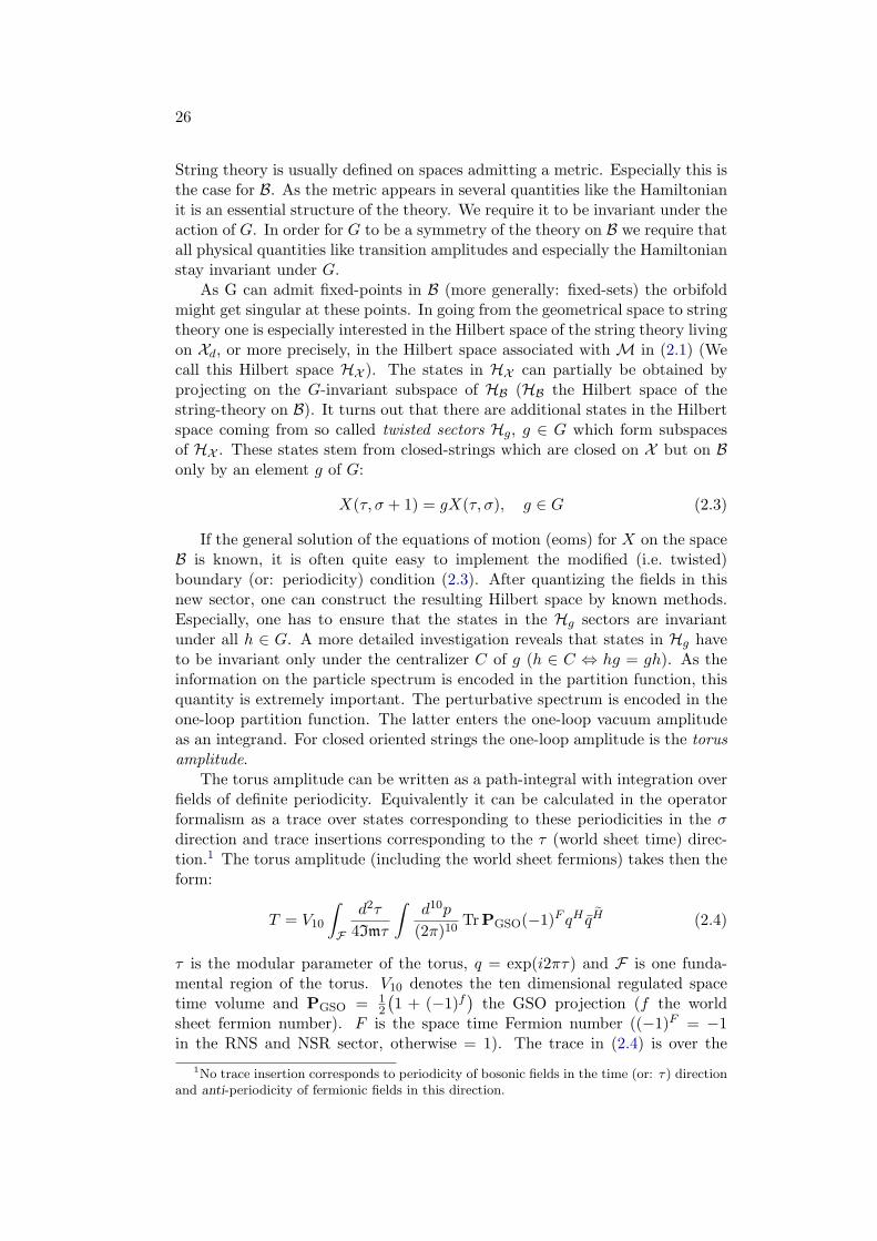
26

String theory is usually defined on spaces admitting a metric. Especially this isthe case for B. As the metric appears in several quantities like the Hamiltonianit is an essential structure of the theory. We require it to be invariant under theaction of G. In order for G to be a symmetry of the theory on B we require thatall physical quantities like transition amplitudes and especially the Hamiltonianstay invariant under G.

As G can admit fixed-points in B (more generally: fixed-sets) the orbifoldmight get singular at these points. In going from the geometrical space to stringtheory one is especially interested in the Hilbert space of the string theory livingon Xd, or more precisely, in the Hilbert space associated with M in (2.1) (Wecall this Hilbert space HX ). The states in HX can partially be obtained byprojecting on the G-invariant subspace of HB (HB the Hilbert space of thestring-theory on B). It turns out that there are additional states in the Hilbertspace coming from so called twisted sectors Hg, g ∈ G which form subspacesof HX . These states stem from closed-strings which are closed on X but on Bonly by an element g of G:

X(τ, σ + 1) = gX(τ, σ), g ∈ G (2.3)

If the general solution of the equations of motion (eoms) for X on the spaceB is known, it is often quite easy to implement the modified (i.e. twisted)boundary (or: periodicity) condition (2.3). After quantizing the fields in thisnew sector, one can construct the resulting Hilbert space by known methods.Especially, one has to ensure that the states in the Hg sectors are invariantunder all h ∈ G. A more detailed investigation reveals that states in Hg haveto be invariant only under the centralizer C of g (h ∈ C ⇔ hg = gh). As theinformation on the particle spectrum is encoded in the partition function, thisquantity is extremely important. The perturbative spectrum is encoded in theone-loop partition function. The latter enters the one-loop vacuum amplitudeas an integrand. For closed oriented strings the one-loop amplitude is the torusamplitude.

The torus amplitude can be written as a path-integral with integration overfields of definite periodicity. Equivalently it can be calculated in the operatorformalism as a trace over states corresponding to these periodicities in the σdirection and trace insertions corresponding to the τ (world sheet time) direc-tion.1 The torus amplitude (including the world sheet fermions) takes then theform:

T = V10

∫F

d2τ

4Imτ

∫d10p

(2π)10TrPGSO(−1)F qH qH (2.4)

τ is the modular parameter of the torus, q = exp(i2πτ) and F is one funda-mental region of the torus. V10 denotes the ten dimensional regulated spacetime volume and PGSO = 1

2

(1 + (−1)f

)the GSO projection (f the world

sheet fermion number). F is the space time Fermion number ((−1)F = −1in the RNS and NSR sector, otherwise = 1). The trace in (2.4) is over the

1No trace insertion corresponds to periodicity of bosonic fields in the time (or: τ) directionand anti-periodicity of fermionic fields in this direction.

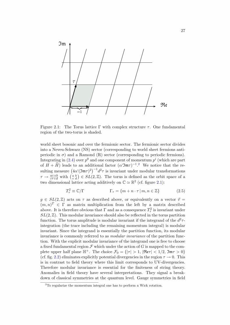
27

Im

Re︸︷︷︸=1

τ

Figure 2.1: The Torus lattice Γ with complex structure τ . One fundamentalregion of the two-torus is shaded.

world sheet bosonic and over the fermionic sector. The fermionic sector dividesinto a Neveu-Schwarz (NS) sector (corresponding to world sheet fermions anti-periodic in σ) and a Ramond (R) sector (corresponding to periodic fermions).Integrating in (2.4) over p0 and one component of momentum pi (which are partof H + H) leads to an additional factor (α′Imτ)−1.2 We notice that the re-sulting measure

(4α′(Imτ)2

)−1d2τ is invariant under modular transformations

τ → aτ+bcτ+d with

(a bc d

)∈ SL(2,Z). The torus is defined as the orbit space of a

two dimensional lattice acting additively on C ' R2 (cf. figure 2.1):

T 2τ ≡ C/Γ Γτ = m+ n · τ |m,n ∈ Z (2.5)

g ∈ SL(2,Z) acts on τ as described above, or equivalently on a vector ~v =(m,n)T ∈ Γ as matrix multiplication from the left by a matrix describedabove. It is therefore obvious that Γ and as a consequence T 2

τ is invariant underSL(2,Z). This modular invariance should also be reflected in the torus partitionfunction. The torus amplitude is modular invariant if the integrand of the d2τ -integration (the trace including the remaining momentum integral) is modularinvariant. Since the integrand is essentially the partition function, its modularinvariance is commonly referred to as modular invariance of the partition func-tion. With the explicit modular invariance of the integrand one is free to choosea fixed fundamental region F which under the action of G is mapped to the com-plete upper half plane H+. The choice F0 = |τ | > 1, |Reτ | < 1/2, Imτ > 0(cf. fig. 2.2) eliminates explicitly potential divergencies in the region τ → 0. Thisis in contrast to field theory where this limit corresponds to UV-divergencies.Therefore modular invariance is essential for the finiteness of string theory.Anomalies in field theory have several interpretations. They signal a break-down of classical symmetries at the quantum level. Gauge symmetries in field

2To regularize the momentum integral one has to perform a Wick rotation.

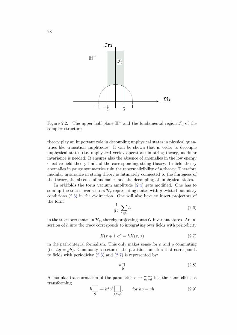
28

Im

Re

H+

−1 −12

112

F0

Figure 2.2: The upper half plane H+ and the fundamental region F0 of thecomplex structure.

theory play an important role in decoupling unphysical states in physical quan-tities like transition amplitudes. It can be shown that in order to decoupleunphysical states (i.e. unphysical vertex operators) in string theory, modularinvariance is needed. It ensures also the absence of anomalies in the low energyeffective field theory limit of the corresponding string theory. In field theoryanomalies in gauge symmetries ruin the renormalizibility of a theory. Thereforemodular invariance in string theory is intimately connected to the finiteness ofthe theory, the absence of anomalies and the decoupling of unphysical states.

In orbifolds the torus vacuum amplitude (2.4) gets modified. One has tosum up the traces over sectors Hg representing states with g-twisted boundaryconditions (2.3) in the σ-direction. One will also have to insert projectors ofthe form

1|G|

∑h∈G

h (2.6)

in the trace over states inHg, thereby projecting onto G-invariant states. An in-sertion of h into the trace corresponds to integrating over fields with periodicity

X(τ + 1, σ) = hX(τ, σ) (2.7)

in the path-integral formalism. This only makes sense for h and g commuting(i.e. hg = gh). Commonly a sector of the partition function that correspondsto fields with periodicity (2.3) and (2.7) is represented by:

hg

(2.8)

A modular transformation of the parameter τ → aτ+bcτ+d has the same effect as

transforminghg→ hagb

hcgd, for hg = gh (2.9)

29

with τ unchanged. If one knows all trace insertions in the σ untwisted sectors,i.e. all contributions h

1one can construct a big part of the twisted sectors hn

hm

by applying eq. (2.9). This proves extremely useful in the construction of socalled left-right asymmetric orbifolds, where solving of the boundary conditions(2.3) is not problematic. This is due to the fact that the asymmetric action onthe center of mass (com.) coordinate of the string is not well defined. Worldsheet fermions which correspond to anti-commuting fields come in four differenttypes for each h, g ∈ G: The NS fermions have an additional twist of −1 in theσ direction and the (−1)f trace insertion of the GSO projection corresponds toan additional twist of −1 in the world sheet time direction that is also denotedby τ . The whole one-loop partition function of the closed-string sector is thengiven by:

ZX (q, q) =1|G|

∑h,g∈Ghg=gh

hg

(2.10)

Although this expression is formally modular invariant there are some sub-tleties. They appear especially in so called asymmetric orbifolds. Eq. (2.2)defines an orbifold as a geometric space. Typically a string theory admits moresymmetries than the background on which the string propagates. As the stringsplits into left- and right-moving parts, a symmetry can interchange these parts(like in orientifolds) or act differently on left- and right-movers. A generalizedorbifold group might also contain elements which do both. It has been ob-served that in asymmetric orbifolds the naive partition function (2.10) mightbe ill defined. If certain conditions are not fulfilled3 a sector which shouldbe transformed to an equivalent sector by some element of the modular group,might however gain a non-trivial phase. (The modular group is represented onlyprojectively on the partition function.) One remark is in order: If one wants toextract the spectrum from Z(q, q) one still has to impose the condition that thenumber of left-moving excitations equals the number of right-moving excita-tions (N = N). If G is a product of groups, i.e. G = G1×G2, ZX in eq. (2.10)is not the only modular invariant partition function. In general ZX can splitinto sectors which are not related by modular transformations. These sectorsare allowed to aquire U(1) phases ε(g, h) where g is the twist in the τ -, h thetwist in the σ-direction. However higher loop consistency of string theory putsfurther constraints (cf. [35]) (in form of co-cycle conditions) on ε(c, d):

ε(g1g2, h) = ε(g1, h)ε(g2, h) (2.11)

ε(g, h) = ε(h, g)−1 (2.12)ε(g, g) = 1 (2.13)

Imposing ε(h, g) to be invariant under the modular transformation ε(h, g) →ε(hagb, hcgd) the sectors h

gin the partition function (2.10) get multiplied by

ε(h, g). The phase ε is commonly called discrete torsion.

3These obstructions are described for instance in [35].

30

We will now consider toroidal compactifications which are the starting man-ifold B (eq. (2.2)) for so called toroidal orbifolds. Toroidal orbifolds and com-pactifications play an essential role in chapters 5-7.

2.2 Torus compactification as an orbifold

If one wants to build orbifolds which descent form string theory on flat ten di-mensional Minkowski space (with constant NSNS two-from potential B), wherethe string can be explicitly quantized, G is allowed to be a subgroup of theeuclidian group acting on the base space B = Rd (cf. eq. (2.1)). This groupleaves the Hamiltonian of the string theory on B invariant. As the Hamiltonianon B splits into independent left- and right-moving parts (in light cone gauge:Hbos. , L/R = ‖∂±X‖2transv. + aL/R) one can mod out independent subgroups ofEuc(Rd) in the left- and right-moving sector of the theory. However in con-structing the twisted sector of an asymmetric orbifold one faces the questionwhat the fixed points are. We will discuss this topic in section 2.3. As toroidalorbifolds (i.e. Xd = T d/G with T d a flat d dimensional torus) are of specialinterest, we will first consider strings living on

M = R(1,9−d) × T d (2.14)

The bosonic string action on this background has the form:

Sbos = − 14πα′

∫Md2σ

(∂αX

µ∂αXµ −Bµνεαβ∂αXµ∂βXν)

(2.15)

We note that the equations of motion of a closed-string are not affected bya constant B-field as the variation of the action w.r.t. Xµ only contributes aboundary piece which is assumed to vanish. (The τ → ±∞ pieces of the bound-ary for an infinite cylinder are assumed to give no contribution. Quantizing theclosed-string on a torus circumvents this problem because the torus has noboundary.) However the canonical momentum gets modified by the constantB-field:

Pµ(τ, σ) =∂

∂Xµ

L(X, ∂X) =1

2πα′(Xµ +Bµ

νX′ ν) (2.16)

The integrated momentum∫dσPµ is τ -independent which follows from the

equation of motion and the fact that ∂M = ∅. Since

T d = Rd/2πΓ (2.17)

Γ =niei| ni ∈ Z, ei, i = 1 . . . d a fixed basis of Rd

the torus is an orbifold itself, with a discrete, but fix-point free acting groupG = Γ ' Zn. As Γ acts additively the g = ni twisted sector is characterized asfollows:4 , 5

X(τ, σ + 2π) = 2πniei +X(τ, σ) (2.18)4X, ei, P and Π should be understood as vectors, not just as numbers.5Here we set the closed-string length to 2π in world sheet coordinates, because this choice

seems to be in common use for concrete mode expansions. The periodicities in formulæ like(2.3), (2.7) then changes from 1 to 2π.

31

This sector is usually called the winding sector since a string in a twisted sectorwith g = ni corresponds to a string winding ni times around the ith one-cycle. Asolution in flat Euclidian space for the d Xj(τ, σ) coordinates involved in (2.18)has an oscillator part which is unchanged compared to the 2π periodic sector. Inaddition a piece linear in σ is needed to accomplish equation (2.18). Altogetherthe bosonic string coordinate in the ni-twisted sector takes the following form:

X(τ, σ) = x+√

2α′p·τ+niei ·σ+i

√α′

2

∑k,∈Z∗

(αkkeik(σ−τ)+

αkke−ik(σ+τ)

)(2.19)

Whereas the separation into left- and right-movers for the oscillators in theabove expression is completely obvious, we will have a closer look at the partslinear in σ and τ . The condition that momentum states are invariant under si,i.e. 6

si |p〉 = |p〉 (2.20)

puts constraints on the allowed spectrum for p. With the momentum (2.16)one finds the following commutators for the modes in (2.19):7

[xi, pj ] = i√α′/2Gij [αil, α

jm] = [αil, α

jm] = l · δl+m,0Gij (2.21)

Since8 iΠj ≡∫dσPj = i

(√2/α′Gjkpk+(1/α′)Bjknk

)is the generator of trans-

lations in the ej direction, sj acts as:9

sj |p〉 = exp(i2πsjΠj

)|p〉 (2.22)

Therefore sj-invariant states have to fulfill:10

~s ·Π ∈ Γ∗, Γ∗ =mie

i| mi ∈ Z, eiej = δij , i, j = 1 . . . d

(2.23)

Γ∗ is the lattice dual to Γ in the sense that its elements ~v∗ have integer scalarproducts with vectors ~w ∈ Γ and that the fundamental cells have inverse vol-umes. Invariance of the states under the full translation group Γ requires ofcourse that Π ∈ Γ∗. With this information the p’s in the ni-twisted and sj-invariant sector of eq. (2.19) can be expressed as:

p(~m)~s,~n = ekpk = ek

√α′

2

(Gkj

mj

sj−Bk

i

α′ni), ~m ∈ Zd (2.24)

The Hamiltonian of the theory is not explicitly B dependent when expressedin terms of X and X ′, or equivalently in terms of ∂±X:

Hbos =1

4πα′

∫dσ(X2 +X ′ 2) =

12πα′

∫dσ((∂+X

)2 +(∂−X

)2) (2.25)

6By acting with sj we mean a translation by 2πsjej . This condition puts no constraintson the oscillator part of the state (both the bosonic and fermionic) since ni acts trivially onthe oscillators.

7Gij is the metric of the torus dual to T d.8Bij ≡ eµ

i Bµνeνj

9The metric Gij of T d which is dual to Gij satisfies: GijGjk = δik.

10The following product ~s ·Π is defined by (~s ·Π)µ ≡∑

j sjΠjeµ

j and Πj = GjkΠk.

32

where we have defined:∂± ≡ 1

2

(∂τ ± ∂σ

)(2.26)

The bosonic oscillator part of H is:11

Hbos, osc = H + H =12

∑k∈Z∗

(α−k · αk + α−k · αk)

=∑k∈N∗

(α−k · αk − abos + α−k · αk − abos)(2.27)

with a the normal ordering constant which is 1/24 for each transverse bosoniccoordinate in light cone gauge. The oscillator part of the Hamiltonian is notaffected by a constant B. It is the same as in the non-compactified theory.Requiring that the states |p〉 to be invariant under the whole lattice group Γrestricts the sj in eq. (2.24): sj = 1∀j. We call the ~m excitations the KaluzaKlein (KK) modes because they correspond to the quantized momentum modesof a point particle compactified on the torus T d. In contrast to the oscillatorpart, the part linear in τ and σ gets affected by the torus compactification. Wewill call it the lattice part since it depends on Γ. With the definition

p(~m,~n)± ≡1√2p(~m)sj=1, ~n ±

niei

2√α′

=ek

2

(√α′mk +

1√α′

(±G−B

)kjnj) (2.28)

the lattice part of the bosonic field can be rewritten:

XΓ(τ, σ) = x+√α′(p+ · (τ + σ) + p−(τ − σ)

)(2.29)

The lattice Hamiltonian HΓ takes the form:

HΓ = p(~m,~n) 2+ + p(~m,~n) 2

−

=12(mi, n

j)(α′Gik −Bi

l

B kj

1α′

(G−B2

)jl

)(mk

nl

) (2.30)

and

p(~m,~n) 2± = 1

4

(mi, n

j)( α′Gik

(±G−B

)il(

±G+B) kj

1α′

(G−B2

)jl

)(mk

nl

)(2.31)

As the splitting of the linear part of P (τ, σ) into p(~m,~n)± is unambiguous wecan embed naturally p(~m,~n) into a 2d dimensional lattice Γ(d,d) by the map:12

Γd × Γd ∗ Υ−→ Γ(d,d)

(niei,mjej) 7−→

(p(~m,~n)+, p(~m,~n)−

) (2.32)

11The dot product is meant to be the product w.r.t. the (dual) metric Gij12The product structure Γd×Γd ∗ should be understood set theoretically. It is not of physical

relevance because the Hamiltonian (2.30) couples vectors in both lattices.

33

Υ has the following matrix representation:

Υ =12

(√α′G i

k1√α′

(G−B

)kj√

α′G il − 1√

α′

(G+B

)kj

)(2.33)

For later use in asymmetric orbifolds we calculate the inverse of Υ:(mi

nj

)= Υ−1

((p+)(p−)

)=

(1√α′

(G+B

) ki

1√α′

(G−B

) li√

α′Gjk −√α′Gjl

)((p+)k(p−)l

)(2.34)

Besides a positive definite and non degenerate quadratic form given by theHamiltonian (2.30) we can define another non degenerate but non definitequadratic form of signature (d, d) which is of physical importance:

12Ξ(p(~n, ~m)

)≡ HΓ+ −HΓ− =

(mi, n

j)( 0 1

2δil

12δ

kj 0

)(mk

nl

)= mkn

k (2.35)

As Ξ naturally induces a nondegenerate metric (also denoted by Ξ) of signature(d, d) the 2d dimensional lattice is denoted by Γ(d,d):

Ξ(p(~k,~l), p(~n, ~m)

)=(ki, l

j)( 0 δil

δ kj 0

)(mk

nl

)(2.36)

We note that lattice Γ(d,d) is self dual w.r.t. Ξ. The scalar product Ξ is clearlyZ-valued, and furthermore the norm Ξ of a vector is an even number. A latticewith this property is called called even. A part of the physical relevance of Ξis clear by the definition (2.35): In order to fulfill the physical state conditionH − H |phys〉 = 0 we require:

Hbos, osc − Hbos, osc = −Ξ(p(~n, ~m)

)2

on physical states (2.37)

2.2.1 Moduli-space of toroidal compactifications,T-duality group and symmetries

For the modular invariance of the partition function ZT d(q, q) the above equalityneeds to hold only mod Z. Therefore the fact that Γ(d,d) is even ensures themodular invariance of the partition function. Since any other even self-duallattice of signature (d, d) can be reached by performing an O(d, d,R) rotationon a given lattice Γ(d,d), the moduli space should be locally isomorphic to thisLorentz group. However separate O(d,R) rotations (which implicitly transformboth the d-dimensional lattice Γd, i.e. the metric Gij , as well as the B-field)on the left- and the right-movers do not change the spectrum (cf. eq. (2.27)and (2.30)) and are therefore (at this level, i.e. one-loop vacuum) physicallyirrelevant. These O(d,R) rotations leave not only the spectrum, but also themass of an individual state |m,n〉 invariant. Furthermore there are rotations,which leave the whole spectrum, but not necessarily the mass of the individualstates |m,n〉 invariant, thereby leading to an equivalent theory (at this level

34

again), too. These are exactly the elements of O(d, d,Z), the so called T-dualitygroup (or Target space duality group) of the d-torus. O(d, d,Z) transformationsonly permute the basis vectors of Γd,d (possibly changing the orientation of agiven, ordered basis). Therefore the moduli space of toroidal compactificationswith constant G and B takes the form:

MT d 'O(d, d,R)

O(d,R)×O(d,R)×O(d, d,Z)(2.38)

It has been shown that the T-duality group O(d, d,Z) has a well defined actionon the oscillators αk, αl, too (which respects the commutation relations (2.21)).We shall mention that under world sheet parity Ω : σ 7→ −σ which has the effect:

αnΩ←→ αn

(mk

nl

)Ω−→(δ ik −2Bkj/α′

0 −δlj

)(mi

nj

)(2.39)

the scalar product Ξ changes its sign. Even though the mass formula (2.30)is invariant under the above transformation, for Ω to be a symmetry (and notjust a duality), B is quantized (cf. [36]):

Bki/α′ ∈ 1

2· Z (2.40)

such that the lattice Γ(d,d) is mapped to itself. The world sheet parity Ω shouldnot be confused with the following kind of SO(d, d,Z) transformation:

Θ :(mk

nl

)−→

(δ ik θkj0 δlj

)(mi

nj

), θkj ∈ Z, θ = −θT (2.41)

which is equivalent to shifting Bij/α′ → Bij/α′−θij . Even though the spectrum

is unchanged under Θ, it is in general not a symmetry of the theory since states|p〉 are mapped to states of different masses. If we want to mod out by theworld sheet parity Ω by using this duality, we only need to distinguish the cases:

Bkl ∈0, 1

2

, l, i = 1 . . . d (2.42)

We will consider these constructions later (cf. section 2.2.2.2 and chap. 5-7).The partition function is constructed according to eq. (2.10). The transla-

tion group G ' Γd ' Zd is abelian but infinite. We have to be careful with theregularization of the projector PΓd . Vd is the regularized d-dimensional volume(cf. (2.4)) while N is the order of Γ, which is infinite as well, but the ratio isjust the volume VΓ of the elementary d-cycle:

PΓd =VdN

∑2πsj∈Γd

exp(i2πsjΠj

)(2.43)

= VΓ

∑2πsj∈Γd

exp(i2πsj

(√2/α′Gjkpk + (1/α′)Bjknk

))(2.44)

= VΓ

∑2πsj∈Γd

ε(sj , nk) · exp(i2πsj

√2/α′Gjkpk

)(2.45)

with ε(sj , nk) ≡ exp(i(2π/α′)sjBjknk

)(2.46)

35

(2.45) is just a rewriting of (2.44). However ε(sj , nk) is recovered as the discretetorsion introduced at the end of section 2. Consistency condition (2.11) isfulfilled due to the defining properties of exp. Taking into account that Bijis antisymmetric, (2.12) and (2.13) are obeyed. The integral

∫ddp over the

projector (2.43) restricts the canonical momenta to lie on the dual lattice Γd ∗

whereas in the torsion form (2.45) the kinematical momentum p is restricted tothe dual torus lattice. After we perform the p integration, the partition functionfor the d real bosons takes the form (τ = τ1 + iτ2):

ZT d(q, q) = tr(qHosc + qHosc

)·∑~n∈Zd

∑~m∈Zd

qHΓ + qHΓ (2.47)

= |η(q)|−2d ·∑

~n, ~m∈Zd

exp(−2πτ2(HΓ + HΓ)

)exp(2iπτ1(HΓ − HΓ)

)(2.48)

We will prove its modular invariance. We will first consider invariance underT : τ 7→ τ + 1. From (A.6) (p. 207) we see that the oscillator part transformstrivially (because of |η|2 which eliminates the twelfth root of unity). The shiftof τ1 in the lattice part introduces a phase, that is however trivial as the latticeis even. To investigate the transformation of ZT d(q, q) under S : τ → −1/τ(⇒ τ1 → −τ1/|τ |2 and τ2 → τ2/|τ |2) we note that we can split the exponentialof the lattice part as follows:

τ2|τ |2

2(HΓ + HΓ) =τ2|τ |2

((~m−B~n)Tα′G∗(~m−B~n) + ~n

G

α′~n)

(2.49)

−i τ1|τ |2

(HΓ − HΓ) = −i τ1|τ |2

~n · (~m−B~n) (2.50)

In (2.50) we have added a term which vanishes because of B being anti-symmet-ric. Therefore we can apply the Poisson-resummation formula (A.14) (p. 208)for the ~m resummation. For the lattice part we obtain after this resummation:

(|τ |2

τ2

)d2√|G|α′

∑~n∈Zd

∑~w∈Zd

e−i2π ~wB~neπτ2

(~n+τ1 ~w)T Gα′ (~n+τ1 ~w)+τ2 ~w

Gα′ ~w (2.51)

A second Poisson resummation (now in the opposite direction) with respect tothe ~n sum turns the above expression into:

|τ |d∑~v∈Zd

∑~w∈Zd

ei2πτ1~v ~we−πτ2(~v−B~w)Tα′G∗(~v−B~w)+τ2 ~wGα′ ~w (2.52)

where we surpressed a vanishing expression ∝ iπτ1 ~wB ~w. Taking into accountthat |η(q)|2d with q = exp(i2π(−1/τ)) equals |τ |−d|η(q)|2d with q = exp(i2πτ)(cf. (A.5), p. 206), we have proven the modular invariance of a bosonic stringcompactified on a torus that is described by constant background fields G andB. The fermionic part is untouched by the torus compactification. This is due tothe fact that the world sheet fermions (in the RNS-formalism) are insensitive tospace-time translations. The complete partition function of the super string is

36

merely a product of the toroidal bosonic partition function times the unchangedfermionic partition function.

Before we present as a concrete example the two-torus T 2 we want to men-tion that it can be shown that the duality group O(d, d,Z) of string theorycompactified on T d is also preserved by string interactions and at higher looporders. By considering higher loop vacuum amplitudes it turns out that alsothe dilaton VEV is transformed under the duality group. First work on thelattice Γ(d,d) has been done by Narain, Sarmadi and Witten [37,38]. ThereforeΓ(d,d) is commonly called a Narain lattice. The construction generalizes natu-rally to heterotic compactifications. There the Narain lattice Γ(d+16,d) is 2d+16dimensional and has the indicated signature.

2.2.2 Compactification on T 2, T-duality and symmetries

The main part of the work in this thesis consists of orientifolds which are derivedeither from:

Type II on T 2 × T 2(×T 2) (2.53)

or from orbifolds of this special torus. Thus we will have a closer look onstring theory on T 2, especially the lattice part. The Narain lattice Γ(2,2) ofT 2 is four dimensional. Its Lorentz group SO(2, 2,R) ' SL(2,R) × SL(2,R)has dimension 3 + 3 = 6. Excluding world sheet parity for the moment, whichchanges the sign of Ξ, we note that the T-duality group is a semi-direct productof the normal subgroupN = SL(2,Z)1×SL(2,Z)2 and anH = Z2×Z′2 subgroupsharing only the identity with N :

SO(2, 2,Z) =(SL(2,Z)1 × SL(2,Z)2

)o(Z2 × Z′2

)(2.54)

The (real two-dimensional) fundamental representation of SL(2,Z) is equivalentto its complex one-dimensional representation. We embed the two SL(2,Z) inthe following way: SL(2,Z)1 acts on τ → SO(2, 2,R) by:13

SL(2,Z)1 × SO(2, 2,R) −→ SO(2, 2,R)(a bc d

)(τ) 7−→ aτ+b

cτ+d

(2.55)

with

τ ≡ τ1 + iτ2 ≡G12

G11+ i

√detGG11

(2.56)

The action of the second SL(2,Z) is defined analogously by the following em-bedding of the modular parameter ρ → SO(2, 2,R):

ρ ≡ ρ1 + iρ2 ≡ B12/α′ + i

√det(G/α′) (2.57)

The two Z2 subgroups are:

Z2 =

Id, D|τ D←→ ρ

(2.58)

Z′2 =

Id, R|(τ, ρ) R←→ −(τ , ρ)

(2.59)

13τ parametrizes SL(2,R)/SO(2,R) and can therefore be embedded into SO(2, 2,R).

37

In order to discover the role of the subgroups in terms of their action on thebackground fields we will rewrite the transformations. The SL(2,Z)1 is purelygeometric. It just describes the change to a new basis of the torus lattice Γ2.We define the mass matrix M2 by

M2

2≡ 1

2

(α′Gik −Bi

l

B kj

1α′

(G−B2

)jl

)(2.60)

Then SL(2,Z)1 transforms M2 under (2.55) in the following way (not distin-guishing lower and upper indices in M2 this time):

M2 7→ STM2S, S =(

d −c−b a 0

0 a bc d

),

(a bc d

)∈ SL(2,Z) (2.61)

where we have taken into account that a linear map transforms the dual ba-sis with the transposed inverse. An alternative expression of the mass2 matrix(2.60) in terms of the parameters τ (called complex structure 14) and ρ (com-monly denoted as Kahler structure 14) is (c.f. eq. (2.31)):

M2

2=(p2+ + p2

−)

(2.62)

p2+ =

14

1τ2ρ2|(τm1 −m2)− ρ(n1 + τn2)|2

p2− =

14

1τ2ρ2|(τm1 −m2)− ρ(n1 + τn2)|2

ni,mi ∈ Z (2.63)

The SL(2,Z)2 is stringy. The generators have the following correspondences:

ρ→ ρ+ 1 ρ→ −1ρ

(2.64)

B12/α′ → B12/α

′ + 1 B12/α′ → − α′B12

B212 + detG

(2.65)

√det(G/α′)→ α′

√detG

B212 + detG

S =(12

0 1−1 0

0 12

)S =

(0 12

12 0

)(2.66)

However, the det g = 1-condition (g ∈ SL(Z)) is not so easily imposed, sothat we have presented only the action of the generators of the latter SL(2,Z)2transformation on the background fields and not the action of a general elementof SL(2,Z)2. ρ→ ρ+1 represents an integer shift on B. ρ→ −1/ρ correspondsto T-duality along both directions of the torus. The two nontrivial elements D

14The flat torus is a Calabi-Yau space. τ is called the complex structure as it parametrizesthe different complex structures of the two-torus (cf. fig. 2.1). The origin of the name Kahlerstructure comes from the observation that ρ can be interpreted as a complex (1, 1)-form. InCY-spaces (1, 1) forms correspond to deformations of the Kahler structure (that preserve theCY-property). This point is a bit subtle as the (1, 1) forms that describe the CY-preservingdeformations of the metric are real. However they can be complexified by combining themwith the NSNS B-field (cf. [39]).

38

and R of the Z2×Z′2 subgroup are a stringy T-duality respectively a reflectionin either the e1 or e2 direction:15

D R

G12

G11↔ B12/α

′ G12 ↔ −G12

√detGG11

↔√

(detG)/α′ B12 ↔ −B12

SD =( 0 0

0 1−1 00 0

−1 00 0

0 00 1

)SR =

( −1 00 1 00 −1 0

0 1

)(2.67)

2.2.2.1 Points of enhanced symmetry in the moduli space SO(2, 2,R)

As toroidal orbifolds are obtained by modding out symmetries of the torus, weare especially interested in points of the moduli space which are fixed by certainelements of the T-duality group. In these cases the dualities are enhanced tosymmetries of the string compactification, so that they can be modded out. Inchapter 7 we consider a Z4 orbifold which is obtained from a special T 6:

T 2 × T 2 × T 2

Z4(2.68)

The Z4 acts on each of the first two T 2s as exp(i2π/4) and as exp(−i2π/2) onthe last torus (written in terms of complexified coordinates). The exp(i2π/4)rotation restricts the moduli in the following way:

Z4 : τ = i =⇒ G11 = G22, G12 = 0 (2.69)

The corresponding matrix acting on M2 (leaving it invariant) and consequentlyon the vectors of Γ(d,d)

Z4is:

SZ4 =( 0 −1

1 0 00 0 −1

1 0

)(2.70)

This means that the torus lattice has a basis consisting of two vectors of equalbut unrestricted length, making an angle of π/2. The Z2 symmetry exp(−i2π/2)does not restrict the values of G and B. It multiplies all vectors in the Narainlattice by −1: SZ2 = −14. In section 2.4 we will consider an orbifold where wedivide out a special four torus T 2×T 2 by the product ZL3 ×ZR3 with one Z3 onlyacting on the left-moving degrees of freedom and the other only on the right-moving part of the string. Since this direct product contains the symmetric Z3

as a subgroup with the generator acting as exp(i2π/3), we will first look at thelattice having this symmetry:

Z3 : τ =12

+ i

√3

2=⇒ G11 = G22, G12 =

12G11 (2.71)

15SD represents usual T-duality along e1 times a reflection in the same direction, while SR

is a reflection along e1

39

This describes a lattice admitting a basis with vectors of equal length and amutual angle of 2π/3. It is up to a scale factor the root lattice of the SU(3)Lie algebra. The action of the symmetric Z3 is given by (in terms of the basiswhich was described above):

Sθ = SZ3 =( 0 −1

1 −1 00 −1 −1

1 0

)(2.72)

We note that the two-torus described by (2.72) admits in addition a Z6 sym-metry, namely the geometric rotation by π/3. Since the asymmetric ZL3 × ZR3can be generated by the symmetric exp(i2π/3) and an element θ rotating theleft-movers by exp(i2π/3) and the right-movers by the reversed angle, we willsearch for Narain lattices Γ(d,d) admitting this latter symmetry. Especially theassociated matrix Sθ acting on the (mi, n

j) has to have integer entries. In prin-ciple we could determine the form of Sθ by mapping (mi, n

j) to (p+, p−) (wherethe form of the asymmetric θ is explicitly known), performing the rotation θand mapping back to the (mi, n

j) basis. The map between the two basis isdescribed by Υ and Υ−1 (eq. (2.33) and (2.34)):

Sθ(p+, p−) = Υ−1Sθ(m,n)Υ (2.73)

However, we will proceed differently. We know (from (2.28), (2.67)) that at theself dual radius with vanishing B-field, the T-Duality D from (2.67) reflects theX2 coordinate on the right-movers, leaving the rest unchanged. By acting withD−1θD we achieve (on the T 2 at the self dual radius, B = 0) that the right-movers get rotated in the inverse direction w.r.t. the left-movers (if we choosethe metric of the dual T 2 to admit the symmetric Z3 action). Via the D-duality(2.58), (2.67) the metric (2.71) of the symmetric Z3 maps to the backgroundfields of the asymmetric Z3 (in terms of the old background fields):

Z3 :GZ3ij

α′=

(α′

G11

B12G11

B12G11

α′(

34G11 + (B12)2

G11

)) BZ312

α′= 1/2 (2.74)

ρ =12

+ i

√3

2(2.75)

The Z3 action takes the following form in the momentum and winding numberbasis:

Sθ = S−1D SθSD =

(−1 0 1

−1 00 1−1 0 0

)(2.76)

The Z3 action on the left- and right-moving momenta (ek(p+)k, (elp−)l is:

Sθ(p+, p−) = ΥZ3Sθ Υ−1

Z3=(θ 00 θ−1

), θ ji =

(−(

B12G11

+ 12

)α′

G11

4B212+3G2

114α′G11

B12G11

− 12

)(2.77)

Therefore the action Sθ represents for all allowed backgrounds (even those withB 6= 0 in the D dual geometry) an asymmetric rotation of the form (θL, θR) =

40

(θ, θ−1). If we want to have the full ZL3 × ZR3 symmetry, we are restricted tobackgrounds of the form:

ZL3 × ZR3 : τ = ρ =12

+ i

√3

2(2.78)

In the same way we get for the asymmetric Z4:

Z4 : ρ = i (2.79)

If we want to maintain the asymmetric Z4 as well as symmetric Z4 action weneed:

Z4 × Z4 : τ = ρ = i (2.80)

However Z4 × Z4 does not generate the full ZL4 × ZR4 since it does not containelements like (θL, θR) = (θ, Id). In chapter 5 we will investigate the orientifoldof the asymmetric ZL3 × ZR3 orbifold.16

2.2.2.2 The world-sheet-parity on T 2

We mentioned already that the world-sheet parity Ω : σ → −σ is a symmetryof the compactified theory, iff the B-field obeys condition (2.40). This meansespecially that Ω is a symmetry of the ZL3 × ZR3 -symmetric background (2.78).In the next chapter we will see how symmetries involving Ω are gauged, leadingto so called orientifolds. One can also combine Ω with an element s which actson the space(-time) and more generally, on the Narain lattice, s.th. the resultingsΩ is still a symmetry of the theory. In chapter 6 and 7 we will gauge by σΩwith σ acting as:(

X1

X2

)σ−→(X1

−X2

)or in complex coords.: Z

σ−→ Z (2.81)

This action is a symmetry of bosonic string theory on T 2 iff the complex struc-ture τ fulfills either

τ1 = 0 or τ1 = 1/2 (2.82)

For σΩ to be a symmetry of the superstring, it has to be compatible with theGSO projection: σ acts on a Ramond zero mode |s〉 by s = ±1/2 σ−→ s = ∓1/2.If the GSO-projection takes the form:17

|s0 . . . sn 〉L :n∑i=0

εisLi = a mod 2, εi ∈ −1, 1 (2.83)

16The four dimensional T 6/(Z4× Z4) orientifold is presumably fraught with the same prob-lems as the four dimensional T 6/Z4 Ω-orientifold of [40]. We will make some comments aboutthis in the following chapter.

17This is true for sectors which are untwisted or twisted by a left-right symmetric twist. ais an integer which can be chosen to be one.

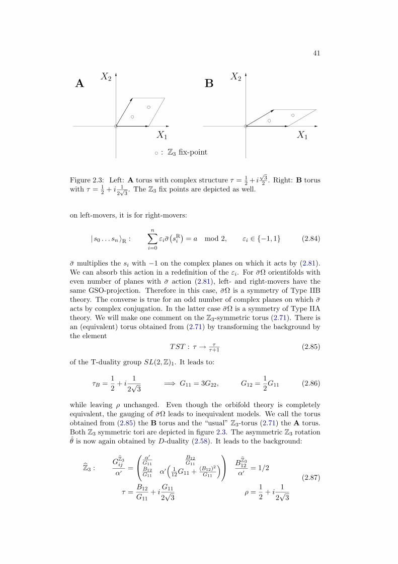
41

: Z3 fix-point

X1

BX2

X1

X2A

Figure 2.3: Left: A torus with complex structure τ = 12 + i

√3

2 . Right: B toruswith τ = 1

2 + i 12√

3. The Z3 fix points are depicted as well.

on left-movers, it is for right-movers:

|s0 . . . sn 〉R :n∑i=0

εiσ(sRi)

= a mod 2, εi ∈ −1, 1 (2.84)

σ multiplies the si with −1 on the complex planes on which it acts by (2.81).We can absorb this action in a redefinition of the εi. For σΩ orientifolds witheven number of planes with σ action (2.81), left- and right-movers have thesame GSO-projection. Therefore in this case, σΩ is a symmetry of Type IIBtheory. The converse is true for an odd number of complex planes on which σacts by complex conjugation. In the latter case σΩ is a symmetry of Type IIAtheory. We will make one comment on the Z3-symmetric torus (2.71). There isan (equivalent) torus obtained from (2.71) by transforming the background bythe element

TST : τ → ττ+1 (2.85)

of the T-duality group SL(2,Z)1. It leads to:

τB =12

+ i1

2√

3=⇒ G11 = 3G22, G12 =

12G11 (2.86)

while leaving ρ unchanged. Even though the orbifold theory is completelyequivalent, the gauging of σΩ leads to inequivalent models. We call the torusobtained from (2.85) the B torus and the “usual” Z3-torus (2.71) the A torus.Both Z3 symmetric tori are depicted in figure 2.3. The asymmetric Z3 rotationθ is now again obtained by D-duality (2.58). It leads to the background:

Z3 :GZ3ij

α′=

α′

G11

B12G11

B12G11

α′(

112G11 + (B12)2

G11

) BZ312

α′= 1/2

τ =B12

G11+ i

G11

2√

3ρ =

12

+ i1

2√

3

(2.87)

42

Symmetry under the asymmetric ZL3 × ZR3 rotation group then requires thebackground:

ZL3 × ZR3 : τB = ρB =12

+ i1

2√

3(2.88)

Instead of acting with σΩ (or Ω) on the B torus, we can alternatively implementthe action of (2.85) directly into σΩ (or Ω):

σΩB ≡ (TST )−1 σΩ (TST ) (2.89)

The action of σΩ takes the following form on the (m,n)-basis of the Z3 back-ground (2.71):

Z3 : σΩA =( −1 0

−1 1 00 1 1

0 −1

)σΩB =

( 0 11 0 00 0 −1

−1 0

)(2.90)

Under the T-duality D (2.58) these symmetries become symmetries of the Z3

background (2.74):18

Z3 : ΩA =(1 0 −1

1 0

0 −1

)ΩB =

(0 0 −1

1 00 1−1 0 0

)(2.91)

At the ZL3 ×ZR3 symmetric point (2.78) all four actions of (σ)Ω (2.90),(2.91) aresymmetries of the theory and can be gauged. These symmetries extend to thesector of the zero- and oscillator-modes as well. While the bosonic zero-modes(i.e. the center of mass coordinates) are sensitive to the distinction between Aand B lattices (equivalently: sensitive to ..ΩA and ..ΩB) as well, fermionic andoscillator parts are unaffected in the end.19

The σΩ action has the interesting property that it maps a g-twisted sectoronto itself (g a geometric rotation in the complex plane, on that σ acts bycomplex conjugation). This is in contrast to the pure world sheet parity Ω thatmaps a g-twisted sector to the g−1 twisted sector (which is different if g /∈ Z2).Another interesting feature of the σΩ action is, that its invariant closed-stringoscillator excitations on each T 2 are of the form:20∣∣∣αk1i1 αk2i2 . . . αkn

in, αl1j1α

l2j2. . . αlnjm

⟩⊗∣∣∣ ¯αk1i1 ¯αk2i2 . . .

¯αknin, αl1j1α

l2j2. . . αlnjm

⟩(2.92)

We used here a complexified basis for the oscillators. In this basis a (symmetric)rotation g ∈ U(1) ' SO(2) acts as

g : Z 7→ ei2πφgZ Z 7→ e−i2πφg Z (2.93)18 ΩA is indeed a symmetry of the Z3 background (2.71) if we impose in addition: B12/α

′ =1/2 (cf. (2.40)). ΩB requires however the full ZL

3 × ZR3 symmetric point (2.78) in order to be

a symmetry.19Of course the coordinate representation is different even for the oscillator modes. How-

ever in physical quantities like partition functions the oscillator and w.s.-fermionic parts areunaffected by the distinction between A and B lattices (or ..Ω-action).

20We present only bosonic degrees of freedom schematically, but the world sheet fermions aretreated analogously, implementing the fact that fermionic occupation numbers for individualmodes are either one or zero.

43

on the complex coordinates (2.81). This implies that σΩ-invariant oscillatorstates (2.92) and its fermionic counterparts are automatically invariant undergeometric U(1) rotations g. Remark: this is in general not true for linearexcitations (i.e. excitations in the Narain lattice). These properties extendnaturally to direct products of two-tori.

2.3 Toroidal orbifolds

In this section we will consider orbifolds of the type:

Xd = T d/G (2.94)

with G a symmetry of the torus T d. For the sake of simplicity, we will restrictto the case of abelian groups G. However, we will also consider the case whereG acts differently on left- and right-movers, such that the action of G is welldefined on the Narain lattice Γ(d,d) and on the left- and right-moving parts.The group G can consist of rotations ∈ O(d, d,Z) and translations. We willrestrict in this work to the case where G is purely rotational, even thoughtranslations (or shifts) can give rise to interesting effects. The untwisted sectorof the orbifold is obtained by projection on G-invariant states. The untwistedpartition function consists of all trace insertions of elements g ∈ G. We willhave a closer look at the sector twisted by gs, (g ∈ G, s ∈ Γ) in the σ direction(c.f. eq. (2.3)). These boundary conditions are solved by the following modeexpansion (lattice momenta and center of mass coordinate are left out):

Xosc+ (τ + σ)µ = i

√α′

2

∑j

∑′

nj∈Z+βj

Cµjαj−nj

njeinj(τ+σ)

Xosc− (τ − σ)µ = i

√α′

2

∑k

∑′

nk∈Z+γk

Dµk

αk−nk

nke−ink(τ−σ)

(2.95)

We split g into (g+, g−), a part acting on X+ which is g+ and g− acting onX−. Then the Cµj are defined as Eigenvectors of g+ with Eigenvalue κj =exp i2πβj . (Analogously, the Dµ

j are Eigenvectors of g− with Eigenvalue λj =exp i2πγj). Since g+ is a rotation, the Cj form an orthogonal system (whichcan be normalized) w.r.t. the hermitian form that is induced by the euclidianscalar product on Rd. They can be interpreted as Vielbeins. This is analogousto the discussion of open strings in constant background fields (cf. chapter 4).For each complex Cj there exists a complex conjugate C−j with c.c. Eigenvalueλ−j = λj . The Dk fulfill analogous properties w.r.t. the rotation g−. Theoscillators obey the following commutation relations:[αili , α

kmk

]= li · δ(li+mk),0

⟨Ci, Ck

⟩,[αili , α

kmk

]= li · δ(li+mk),0

⟨Di, Dk

⟩(2.96)

In this case⟨Ci, Ck

⟩is the inverse of

⟨Ci, Ck

⟩. The lattice part obeys:

XΓ+(τ, σ) =

√α′(p+(τ + σ) + p−(τ − σ)

)with p+ = g+p+ and p− = g−p−,

(p+, p−

)∈ Γ(d,d)

(2.97)

44

The center of mass xcom has a priori no well defined splitting into left- and right-movers. Therefore g has a clear interpretation in terms of a geometric actiononly in the symmetric case: (gL, gR) = (g, g). Then the boundary conditionreads:

(Id−g)xcom = −2π√α′(p+ − p−) + s, s ∈ Γd (2.98)

If Ig ⊂ Γd is the lattice invariant under g and Ng = u ∈ Γ|u · v = 0 ∀v ∈ Igthe lattice perpendicular to Ig, the right hand side of (2.98) is also containedin Ng. (Proof: multiply both sides by v ∈ Ig. The left side vanishes sincev · (Id−g)x = (Id−g−1)v · x.) For g = Id we get exactly the result of thetoroidal compactification. For g 6= Id the com. coordinate is restricted to befixed up to addition of a lattice vector. xcom + w, with w an arbitrary latticevector, fulfills eq. (2.98) if s is shifted by (1− g)w which is a vector lying in thesub-lattice Ng. Therefore such a shifted com. coordinate is equivalent to thenon shifted one. In [41] the number of inequivalent fixed points (more general:fixed planes) was thereby determined to be:21

nfix,g =∣∣∣∣ N

(1− g)Γd

∣∣∣∣ (2.99)

This formula has a simple generalization for left-right asymmetric twists g =(g+, g−): In [41] the authors gave a definition that only refers to the Narainlattice:22

nfix,g =

√∣∣∣∣ N

(1− g)Γd,d

∣∣∣∣ (2.100)

N from our former definition has to be replaced by the lattice which is or-thogonal to the invariant sub-lattice I of the Narain lattice Γd,d. In the samepublication the authors proved that (2.100) is always an integer. The proof israther lengthy. It involves the embedding of the Narain lattice Γd,d into a latticeof doubled dimension. Especially in the path-integral formalism the splittinginto holomorphic and anti-holomorphic fields is a priori not possible. The num-ber of h-invariant fixed-points in the g-twisted sector is of big importance, too.It appears as an overall constant in the sector h

g. In a subsequent publication

(cf. [42]) the same authors determined this number to be the square root of:

Ch,g =∣∣∣∣ N

(1− g)N∗ ∪ (1− h)N

∣∣∣∣ (2.101)

N∗ is the lattice dual to N . In the example which we present in the follow-ing, most of the numbers Ch,g are determined by modular transformations ofuntwisted parts in the partition function. (By applying (2.101) in combina-tion with modular transformations we will relate in fact all these numbers topartition functions in the (σ-) untwisted sector of the T 4

/(ZL

3 × ZR3

)orbifold.)

For the superstring there exists an analog of the mode expansion (2.97)for the twisted world-sheet fermions (in the NSR formalism). World sheet

21By (1− g)Γ we mean the lattice (~r − g~r) |~r ∈ Γ.22In fact they consider heterotic compactifications where the Narain lattice is of the more

general form Γd,p.

45

fermions do not have extra com. degrees of freedom. As the Hilbert spaceis a tensor product of the fermionic and the bosonic sector, the bosonic zero-modes (i.e. the com. coordinates) determine the multiplicity of fermionic statesas well. If the space-time fermionic sector (e.g. the R-sector of the heteroticstring or the Ω-symmetrized NSR-sector of an orientifold) has only one masslessexcitation, the number of fixed points (=inequivalent com. coordinates) in thissector determines the number of chiral fermions. This is similar to the caseof intersecting D-branes, where the number of chiral fermions in the respectiveopen string sector is determined by the intersection number of the two D-branesto which the string is attached (c.f. chapter 6, 7, and [43]). There are additionalconditions for a group G to be a symmetry of the superstring: G must be asymmetry not only of the bosonic and fermionic Hamiltonian (or: world-sheetenergy-momentum tensor) (i.e. TB ), but also of the world sheet supercurrent(TF ). Of course G must preserve interactions, especially the OPE, as well. Inaddition, the partition function has to be modular invariant.

Before we will turn to an (asymmetric) example, we will summarize somewell known facts about space-time supersymmetric, geometric toroidal orbi-folds.

2.3.1 Space-time supersymmetric (toroidal) orbifolds

In [32,33] orbifolds were introduced in the context of superstring theory. How-ever this was not the first time orbifolds appeared in physics (cf. referencesin [32]). In mathematics they go back to Satake [44]. Our intention is to re-state (sufficient) conditions for the orbifold to be supersymmetric. Even thoughan orbifold is not a manifold, certain orbifolds can be deformed into a manifold.An interesting class of obifolds are those which can be deformed into a Calabi-Yau manifold, as superstrings compactified on such an orbifold yield space-timesupersymmetry. A complex n-dimensional compact manifoldM that is Calabi-Yau (i.e. Kahler and first Chern class c1 = 0) admits a unique Ricci-flat metricfor a given Kahler class and complex structure.23 This does not mean thatevery metric on M is Ricci flat, but it means that such a metric exists. Theproperty of a complex n-dimensional manifold to be kahler restricts its holon-omy to be at most U(n). Ricci flatness implies that the holonomy group withrespect to the Ricci-flat metric is contained even in SU(n), iff c1(M) = 0.24 Asa consequence the manifold as a spin-manifold admits one Killing-spinor (=co-variantly constant spinor) of each chirality. Unbroken supersymmetry requiresthe supersymmetry variation of the gravitino to vanish. In the absence of anNSNS 3-form field strength H this is equivalent to the statement that the co-variant derivative of the supersymmetry parameter η vanishes: Dη = 0 (i.e. η isa Killing spinor). If one covariant constant spinor exists on the compactification

23Sometimes CY manifolds are defined as the triple (M, J, g) with M a complex n-dimensional Kahler manifold with c1 = 0, J its complex structure, and g the Kahler metric,which in addition should be Ricci-flat. In section 6.5.1 we will give a third definition makingexplicit use of a holomorphic (n, 0)-form Ω which always exist on a CYn-fold.

24In Kahler manifolds, SU(n) holonomy implies also Ricci-flatness. Conversely Ricci-flatKahler manifolds admit SU(n) holonomy, if they are simply-connected.

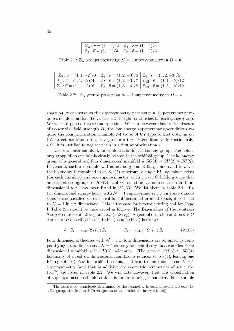
46

Z2 : ~v = (1,−1)/2 Z4 : ~v = (1,−1)/4Z3 : ~v = (1,−1)/3 Z6 : ~v = (1,−1)/6

Table 2.1: ZN groups preserving N = 1 supersymmetry in D = 6.

Z3 : ~v = (1, 1,−2)/3 Z′6 : ~v = (1, 2,−3)/6 Z′8 : ~v = (1, 2,−3)/8Z4 : ~v = (1, 1,−2)/4 Z7 : ~v = (1, 2,−3)/7 Z12 : ~v = (1, 4,−5)/12Z6 : ~v = (1, 1,−2)/6 Z8 : ~v = (1, 3,−4)/8 Z′12 : ~v = (1, 5,−6)/12

Table 2.2: ZN groups preserving N = 1 supersymmetry in D = 4.

space M, it can serve as the supersymmetry parameter η. Supersymmetry re-quires in addition that the variation of the gluino vanishes for each gauge group.We will not pursue this second question. We note however that in the absenceof non-trivial field strength H, the low energy supersymmetry-conditions re-quire the compactification manifold M to be of CY-type to first order in α′.(α′-corrections from string theory deform the CY-condition only continiously,s.th. it is justified to neglect them in a first approximation.)

Like a smooth manifold, an orbifold admits a holonomy group. The holon-omy group of an orbifold is closely related to the orbifold group. The holonomygroup of a general real four dimensional manifold is SO(4) ' SU(2) × SU(2).In general, such a manifold will admit no global Killing spinors. If howeverthe holonomy is contained in an SU(2) subgroup, a single Killing spinor exists(for each chirality) and one supersymmetry will survive. Orbifold groups thatare discrete subgroups of SU(2), and which admit geometric action on four-dimensional tori, have been listed in [32, 33]. We list them in table 2.1. If aten dimensional string-theory with N = 1 supersymmetry in ten space dimen-sions is compactified on such real four dimensional orbifold space, it will leadto N = 1 in six dimensions. This is the case for heterotic string and for TypeI. Table 2.1 should be understood as follows: The Eigenvalues of the rotationsθ ' g ∈ G are exp(±2iπv1) and exp(±2iπv2). A general orbifold-rotation θ ∈ Gcan then be described in a suitable (complexified) basis by:

θ : Zi 7→ exp (2πivi)Zi Zi 7→ exp (−2πivi) Zi (2.102)

Four dimensional theories with N = 1 in four dimensions are obtained by com-pactifying a ten-dimensional N = 1 supersymmetric theory on a complex threedimensional manifold with SU(3) holonomy. (The general SO(6) ' SU(4)holonomy of a real six dimensional manifold is reduced to SU(3), leaving oneKilling spinor.) Possible orbifold actions, that lead to four dimensional N = 1supersymmetry (and that in addition are geometric symmetries of some six-tori25) are listed in table 2.2. We will note however, that this classificationof supersymmetric orbifold actions is far from being exhaustive. For example

25The torus is not completely determined by the symmetry. In general several tori exist fora ZN group, that lead to different spectra of the orbifolded theory (cf. [45]).

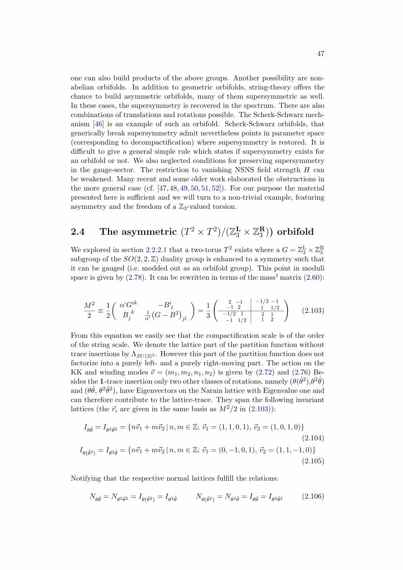
47

one can also build products of the above groups. Another possibility are non-abelian orbifolds. In addition to geometric orbifolds, string-theory offers thechance to build asymmetric orbifolds, many of them supersymmetric as well.In these cases, the supersymmetry is recovered in the spectrum. There are alsocombinations of translations and rotations possible. The Scherk-Schwarz mech-anism [46] is an example of such an orbifold. Scherk-Schwarz orbifolds, thatgenerically break supersymmetry admit nevertheless points in parameter space(corresponding to decompactification) where supersymmetry is restored. It isdifficult to give a general simple rule which states if supersymmetry exists foran orbifold or not. We also neglected conditions for preserving supersymmetryin the gauge-sector. The restriction to vanishing NSNS field strength H canbe weakened. Many recent and some older work elaborated the obstructions inthe more general case (cf. [47, 48, 49, 50, 51, 52]). For our purpose the materialpresented here is sufficient and we will turn to a non-trivial example, featuringasymmetry and the freedom of a Z3-valued torsion.

2.4 The asymmetric (T 2 × T 2)/(ZL3 × ZR

3 )) orbifold

We explored in section 2.2.2.1 that a two-torus T 2 exists where a G = ZL3 ×ZR

3

subgroup of the SO(2, 2,Z) duality group is enhanced to a symmetry such thatit can be gauged (i.e. modded out as an orbifold group). This point in modulispace is given by (2.78). It can be rewritten in terms of the mass2 matrix (2.60):

M2

2≡ 1

2

(α′Gik −Bi

l

B kj

1α′

(G−B2

)jl

)=

13

(2 −1−1 2

−1/2 −11 1/2

−1/2 1−1 1/2

2 11 2

)(2.103)

From this equation we easily see that the compactification scale is of the orderof the string scale. We denote the lattice part of the partition function withouttrace insertions by ΛSU(3)2 . However this part of the partition function does notfactorize into a purely left- and a purely right-moving part. The action on theKK and winding modes ~v = (m1,m2, n1, n2) is given by (2.72) and (2.76) Be-sides the 1-trace insertion only two other classes of rotations, namely (θ(θ2),θ2θ)and (θθ, θ2θ2), have Eigenvectors on the Narain lattice with Eigenvalue one andcan therefore contribute to the lattice-trace. They span the following invariantlattices (the ~ri are given in the same basis as M2/2 in (2.103)):

Iθθ = Iθ2θ2 = n~v1 +m~v2 |n,m ∈ Z; ~v1 = (1, 1, 0, 1), ~v2 = (1, 0, 1, 0)(2.104)

Iθ(θ2) = Iθ2θ = n~v1 +m~v2 |n,m ∈ Z; ~v1 = (0,−1, 0, 1), ~v2 = (1, 1,−1, 0)(2.105)

Notifying that the respective normal lattices fulfill the relations:

Nθθ = Nθ2θ2 = Iθ(θ2) = Iθ2θ Nθ(θ2) = Nθ2θ = Iθθ = Iθ2θ2 (2.106)

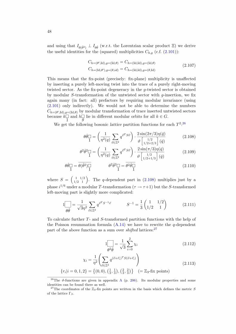
48

and using that Iθ(θ2) ⊥ Iθθ (w.r.t. the Lorentzian scalar product Ξ) we derivethe useful identities for the (squared) multiplicities Ch,g (c.f. (2.101)):

Ch=(θ′,Id),g=(Id,θ) = Ch=(Id,Id),g=(Id,θ)

Ch=(Id,θ′),g=(θ,id) = Ch=(Id,Id),g=(θ,Id)

(2.107)

This means that the fix-point (precisely: fix-plane) multiplicity is unaffectedby inserting a purely left-moving twist into the trace of a purely right-movingtwisted sector. As the fix-point degeneracy in the g-twisted sector is obtainedby modular S-transformation of the untwisted sector with g-insertion, we fixagain many (in fact: all) prefactors by requiring modular invariance (using(2.101) only indirectly). We would not be able to determine the numbersCh=(θ′,Id),g=(Id,θ) by modular transformation of trace inserted untwisted sectorsbecause k

1and h

glie in different modular orbits for all k ∈ G.

We get the following bosonic lattice partition functions for each T 2:26

θθ1

=(

1η2(q)

∑~v∈Z2

q~vTS~v

)· 2 sin(2π/3)η(q)

ϑ[

1/21/2+2/3

](q)

(2.108)

θ2θ21

=(

1η2(q)

∑~v∈Z2

q~vTS~v

)· 2 sin(π/3)η(q)

ϑ[

1/21/2+1/3

](q)

(2.109)

θθ1

= θ(θ2)1

θ2θ21

= θ2θ1

(2.110)

where S =(

1 1/21/2 1

). The q-dependent part in (2.108) multiplies just by a

phase i1/6 under a modular T -transformation (τ → τ+1) but the S-transformedleft-moving part is slightly more complicated:

1θθ

=1√3η2

∑~v∈Z2

q~vTS−1~v S−1 =

13

(1 1/2

1/2 1

)(2.111)

To calculate further T - and S-transformed partition functions with the help ofthe Poisson resummation formula (A.14) we have to rewrite the q-dependentpart of the above function as a sum over shifted lattices:27

1θ2θ

=1√3

2∑i=0

χi (2.112)

χi =1η2

(∑~v∈Z2

q(~v+~ri)TS(~v+~ri)

)ri|i = 0, 1, 2 =

(0, 0),

(13 ,

13

),(

23 ,

23

)(= Z3-fix points)

(2.113)

26The ϑ-functions are given in appendix A (p. 206). Its modular properties and someidentities can be found there as well.

27The coordinates of the Z3-fix points are written in the basis which defines the metric Sof the lattice ΓS .

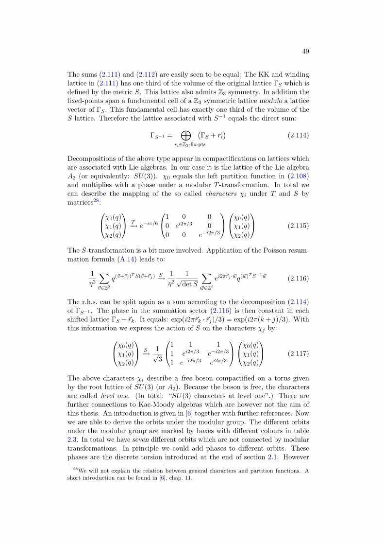
49

The sums (2.111) and (2.112) are easily seen to be equal: The KK and windinglattice in (2.111) has one third of the volume of the original lattice ΓS which isdefined by the metric S. This lattice also admits Z3 symmetry. In addition thefixed-points span a fundamental cell of a Z3 symmetric lattice modulo a latticevector of ΓS . This fundamental cell has exactly one third of the volume of theS lattice. Therefore the lattice associated with S−1 equals the direct sum:

ΓS−1 =⊕

ri∈Z3-fix-pts

(ΓS + ~ri

)(2.114)

Decompositions of the above type appear in compactifications on lattices whichare associated with Lie algebras. In our case it is the lattice of the Lie algebraA2 (or equivalently: SU(3)). χ0 equals the left partition function in (2.108)and multiplies with a phase under a modular T -transformation. In total wecan describe the mapping of the so called characters χi under T and S bymatrices28:χ0(q)

χ1(q)χ2(q)

T−→ e−iπ/6

1 0 00 ei2π/3 00 0 e−i2π/3

χ0(q)χ1(q)χ2(q)

(2.115)

The S-transformation is a bit more involved. Application of the Poisson resum-mation formula (A.14) leads to:

1η2

∑~v∈Z2

q(~v+~rj)TS(~v+~rj) S−→ 1

η2

1√detS

∑~w∈Z2

ei2π~rj ·~wq(~w)TS−1 ~w (2.116)

The r.h.s. can be split again as a sum according to the decomposition (2.114)of ΓS−1 . The phase in the summation sector (2.116) is then constant in eachshifted lattice ΓS + ~rk. It equals: exp(i2π~rk · ~rj)/3) = exp(i2π(k+ j)/3). Withthis information we express the action of S on the characters χj by:χ0(q)

χ1(q)χ2(q)

S−→ 1√3

1 1 11 ei2π/3 e−i2π/3

1 e−i2π/3 ei2π/3

χ0(q)χ1(q)χ2(q)

(2.117)

The above characters χi describe a free boson compactified on a torus givenby the root lattice of SU(3) (or A2). Because the boson is free, the charactersare called level one. (In total: “SU(3) characters at level one”.) There arefurther connections to Kac-Moody algebras which are however not the aim ofthis thesis. An introduction is given in [6] together with further references. Nowwe are able to derive the orbits under the modular group. The different orbitsunder the modular group are marked by boxes with different colours in table2.3. In total we have seven different orbits which are not connected by modulartransformations. In principle we could add phases to different orbits. Thesephases are the discrete torsion introduced at the end of section 2.1. However

28We will not explain the relation between general characters and partition functions. Ashort introduction can be found in [6], chap. 11.

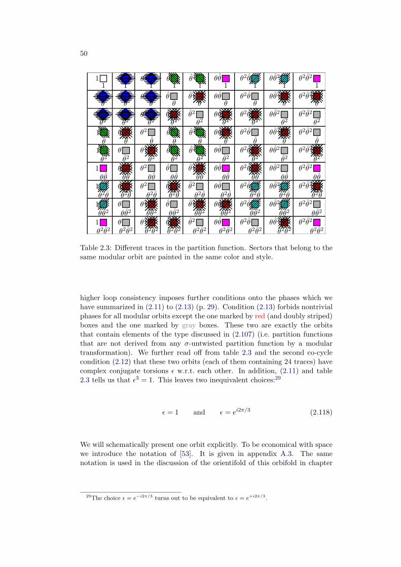
50

11

θ1

θ2

1θ

1θ2

1θθ

1θ2θ

1θθ2

1θ2θ2

1

1θ

θθ

θ2

θθ

θθ2

θθθ

θθ2θ

θθθ2

θθ2θ2

θ

1θ2

θθ2

θ2

θ2θθ2

θ2

θ2θθ

θ2θ2θ

θ2θθ2

θ2θ2θ2

θ2

1θ

θθ

θ2

θθ

θθ2

θ

θθθ

θ2θθ

θθ2

θθ2θ2

θ

1θ2

θθ2

θ2

θ2θθ2

θ2

θ2θθ

θ2θ2θ

θ2θθ2

θ2θ2θ2

θ2

1θθ

θθθ

θ2

θθθθθ

θ2

θθθθ

θθθ2θ

θθθθ2

θθθ2θ2

θθ1θ2θ

θθ2θ

θ2

θ2θθθ2θ

θ2

θ2θθθ

θ2θθ2θ

θ2θθθ2

θ2θθ2θ2

θ2θ1θθ2

θθθ2

θ2

θθ2θθθ2

θ2

θθ2θθ

θθ2θ2θ

θθ2θθ2

θθ2θ2θ2

θθ2

1θ2θ2

θθ2θ2

θ2

θ2θ2θθ2θ2

θ2

θ2θ2θθ

θ2θ2θ2θ

θ2θ2θθ2

θ2θ2θ2θ2

θ2θ2

Table 2.3: Different traces in the partition function. Sectors that belong to thesame modular orbit are painted in the same color and style.

higher loop consistency imposes further conditions onto the phases which wehave summarized in (2.11) to (2.13) (p. 29). Condition (2.13) forbids nontrivialphases for all modular orbits except the one marked by red (and doubly striped)boxes and the one marked by gray boxes. These two are exactly the orbitsthat contain elements of the type discussed in (2.107) (i.e. partition functionsthat are not derived from any σ-untwisted partition function by a modulartransformation). We further read off from table 2.3 and the second co-cyclecondition (2.12) that these two orbits (each of them containing 24 traces) havecomplex conjugate torsions ε w.r.t. each other. In addition, (2.11) and table2.3 tells us that ε3 = 1. This leaves two inequivalent choices:29

ε = 1 and ε = ei2π/3 (2.118)

We will schematically present one orbit explicitly. To be economical with spacewe introduce the notation of [53]. It is given in appendix A.3. The samenotation is used in the discussion of the orientifold of this orbifold in chapter

29The choice ε = e−i2π/3 turns out to be equivalent to ε = e+i2π/3.

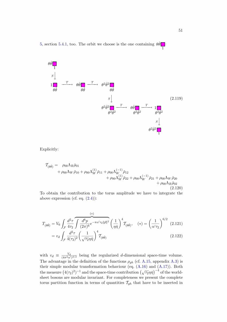
51

5, section 5.4.1, too. The orbit we choose is the one containing θθ1

:

θθ1

S

y

1θθ

T−−−−→ θθθθ

T−−−−→ θ2θ2

θθ

S

y

θ2θ2

θ2θ2

T−−−−→ θθθ2θ2

T−−−−→ 1θ2θ2

S

y

θ2θ2

1

(2.119)

Explicitly:

T(θθ) = ρ00ΛR ρ01

+ ρ00ΛW ρ10 + ρ00Λ(1)W ρ11 + ρ00Λ

(−1)W ρ12

+ ρ00Λ(1)W ρ22 + ρ00Λ

(−1)W ρ21 + ρ00ΛW ρ20

+ ρ00ΛR ρ02

(2.120)To obtain the contribution to the torus amplitude we have to integrate theabove expression (cf. eq. (2.4)):

T(θθ) = V6

∫F

d2τ

4τ2

(∗)︷︸︸︷∫d6p

(2π)6e−πα

′τ2‖~p‖2(

1ηη

)4

T(θθ), (∗) =(

1α′τ2

)6/2

(2.121)

= vd

∫F

d2τ

4(τ2)2

(1

√τ2ηη

)4

T(θθ) (2.122)

with vd ≡ Vd

(4π2α′)d/2 being the regularized d-dimensional space-time volume.The advantage in the definition of the functions ρgh (cf. A.15, appendix A.3) istheir simple modular transformation behaviour (eq. (A.16) and (A.17)). Boththe measure

(4(τ2)2)−1 and the space-time contribution

(√τ2ηη

)−4 of the world-sheet bosons are modular invariant. For completeness we present the completetorus partition function in terms of quantities Tgh that have to be inserted in

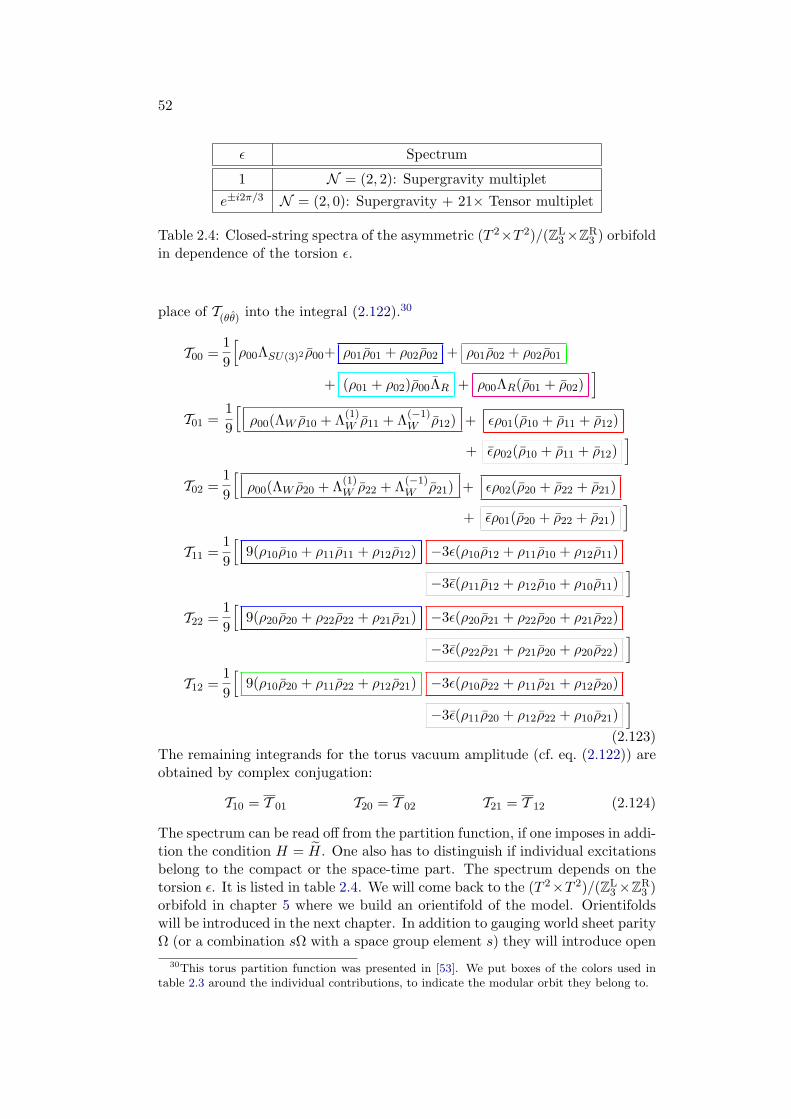
52

ε Spectrum

1 N = (2, 2): Supergravity multiplet

e±i2π/3 N = (2, 0): Supergravity + 21× Tensor multiplet

Table 2.4: Closed-string spectra of the asymmetric (T 2×T 2)/(ZL3×ZR

3 ) orbifoldin dependence of the torsion ε.

place of T(θθ) into the integral (2.122).30

T00 =19

[ρ00ΛSU(3)2 ρ00+ ρ01ρ01 + ρ02ρ02 + ρ01ρ02 + ρ02ρ01

+ (ρ01 + ρ02)ρ00ΛR + ρ00ΛR(ρ01 + ρ02)]

T01 =19

[ρ00(ΛW ρ10 + Λ(1)

W ρ11 + Λ(−1)W ρ12) + ερ01(ρ10 + ρ11 + ρ12)

+ ερ02(ρ10 + ρ11 + ρ12)]

T02 =19

[ρ00(ΛW ρ20 + Λ(1)

W ρ22 + Λ(−1)W ρ21) + ερ02(ρ20 + ρ22 + ρ21)

+ ερ01(ρ20 + ρ22 + ρ21)]

T11 =19

[9(ρ10ρ10 + ρ11ρ11 + ρ12ρ12) −3ε(ρ10ρ12 + ρ11ρ10 + ρ12ρ11)

−3ε(ρ11ρ12 + ρ12ρ10 + ρ10ρ11)]

T22 =19

[9(ρ20ρ20 + ρ22ρ22 + ρ21ρ21) −3ε(ρ20ρ21 + ρ22ρ20 + ρ21ρ22)

−3ε(ρ22ρ21 + ρ21ρ20 + ρ20ρ22)]

T12 =19

[9(ρ10ρ20 + ρ11ρ22 + ρ12ρ21) −3ε(ρ10ρ22 + ρ11ρ21 + ρ12ρ20)

−3ε(ρ11ρ20 + ρ12ρ22 + ρ10ρ21)]

(2.123)The remaining integrands for the torus vacuum amplitude (cf. eq. (2.122)) areobtained by complex conjugation:

T10 = T 01 T20 = T 02 T21 = T 12 (2.124)

The spectrum can be read off from the partition function, if one imposes in addi-tion the condition H = H. One also has to distinguish if individual excitationsbelong to the compact or the space-time part. The spectrum depends on thetorsion ε. It is listed in table 2.4. We will come back to the (T 2×T 2)/(ZL

3 ×ZR3 )

orbifold in chapter 5 where we build an orientifold of the model. Orientifoldswill be introduced in the next chapter. In addition to gauging world sheet parityΩ (or a combination sΩ with a space group element s) they will introduce open

30This torus partition function was presented in [53]. We put boxes of the colors used intable 2.3 around the individual contributions, to indicate the modular orbit they belong to.

53

strings. We will find out that the asymmetric action ZR, LN contains D-branes

with magnetic fluxes in its orbit. D-branes with electro-magnetic fluxes are thetopic of chapter 4.

Chapter 3

Orientifolds

String theories which contain non-orientable world-sheets are called orientifolds.Closed-string theories containing non-orientable diagrams (like the Klein bottleat Euler-characteristic χ = 0) admit tadpoles which lead to inconsistencies.These inconsistencies can often be cured by adding world-sheets with holes andthereby open-strings. At the χ = 0-level these are the Mobius-strip and theCylinder. By introducing open-strings via D-branes of appropriate number andtype, all tadpoles can be eliminated in many cases.1 Often there exist differentD-bane spectra which lead to tadpole cancellation. By this many (attractive)spectra can arise in orientifold models as we will see in the following chapters.After presenting a heuristic definition of a general orbifold, we will enter intothe details and consequences like tadpoles, open-strings and associated particlespectra. References and overview articles can be found in the “concludingremarks” on page 86.

3.1 Basic concepts

All of our orientifold models are based on orbifold constructions, where anelement sΩ, with Ω the world sheet parity and s an element acting on spacetime but not on the world-sheet, is added to the orbifold group. More generallywe define:

Definition 1 An orientifold is a string theory, which is obtained by moddingout a symmetry group O of the original theory:

O = G ∪ SΩ (3.1)

G is a group which does not mix left- and right-movers. Ω is the world sheetparity (which exchanges left- and right-movers). S is a set, which defines a

1In order to cancel both the NSNS and the RR tadpoles the parent closed-string theoryshould be supersymmetric. Even though this is not strictly proven, this is likely to be true.There exist also cases (e.g. the Ω orientifold of Type IIB on T 6/ZN , N ∈ 4, 8, 12 c.f. [40])where the Klein bottle is supersymmetric but so far no attempt to cancel its tadpoles byD-branes in a supersymmetric manner has been successful and there are hints that this mightbe impossible.

54

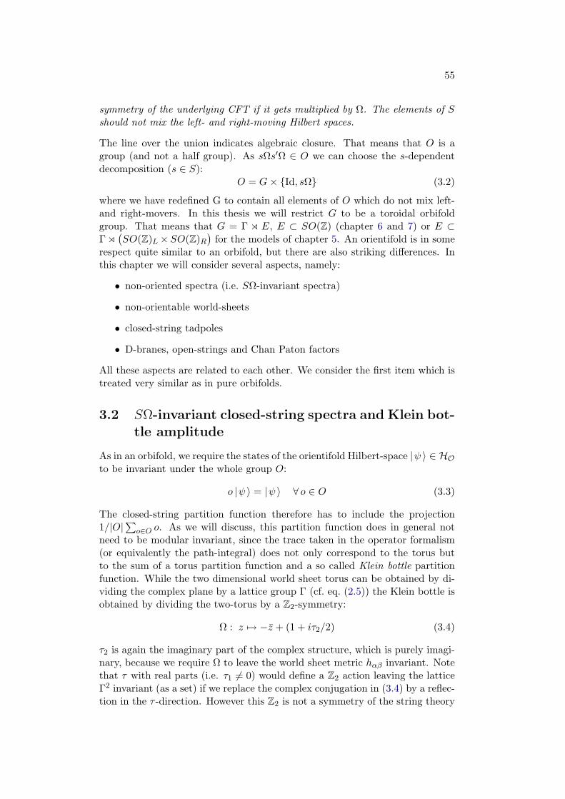
55

symmetry of the underlying CFT if it gets multiplied by Ω. The elements of Sshould not mix the left- and right-moving Hilbert spaces.

The line over the union indicates algebraic closure. That means that O is agroup (and not a half group). As sΩs′Ω ∈ O we can choose the s-dependentdecomposition (s ∈ S):

O = G× Id, sΩ (3.2)

where we have redefined G to contain all elements of O which do not mix left-and right-movers. In this thesis we will restrict G to be a toroidal orbifoldgroup. That means that G = Γ o E, E ⊂ SO(Z) (chapter 6 and 7) or E ⊂Γ o

(SO(Z)L×SO(Z)R

)for the models of chapter 5. An orientifold is in some

respect quite similar to an orbifold, but there are also striking differences. Inthis chapter we will consider several aspects, namely:

• non-oriented spectra (i.e. SΩ-invariant spectra)

• non-orientable world-sheets

• closed-string tadpoles

• D-branes, open-strings and Chan Paton factors

All these aspects are related to each other. We consider the first item which istreated very similar as in pure orbifolds.

3.2 SΩ-invariant closed-string spectra and Klein bot-tle amplitude

As in an orbifold, we require the states of the orientifold Hilbert-space |ψ 〉 ∈ HOto be invariant under the whole group O:

o |ψ 〉 = |ψ 〉 ∀ o ∈ O (3.3)

The closed-string partition function therefore has to include the projection1/|O|

∑o∈O o. As we will discuss, this partition function does in general not

need to be modular invariant, since the trace taken in the operator formalism(or equivalently the path-integral) does not only correspond to the torus butto the sum of a torus partition function and a so called Klein bottle partitionfunction. While the two dimensional world sheet torus can be obtained by di-viding the complex plane by a lattice group Γ (cf. eq. (2.5)) the Klein bottle isobtained by dividing the two-torus by a Z2-symmetry:

Ω : z 7→ −z + (1 + iτ2/2) (3.4)

τ2 is again the imaginary part of the complex structure, which is purely imagi-nary, because we require Ω to leave the world sheet metric hαβ invariant. Notethat τ with real parts (i.e. τ1 6= 0) would define a Z2 action leaving the latticeΓ2 invariant (as a set) if we replace the complex conjugation in (3.4) by a reflec-tion in the τ -direction. However this Z2 is not a symmetry of the string theory

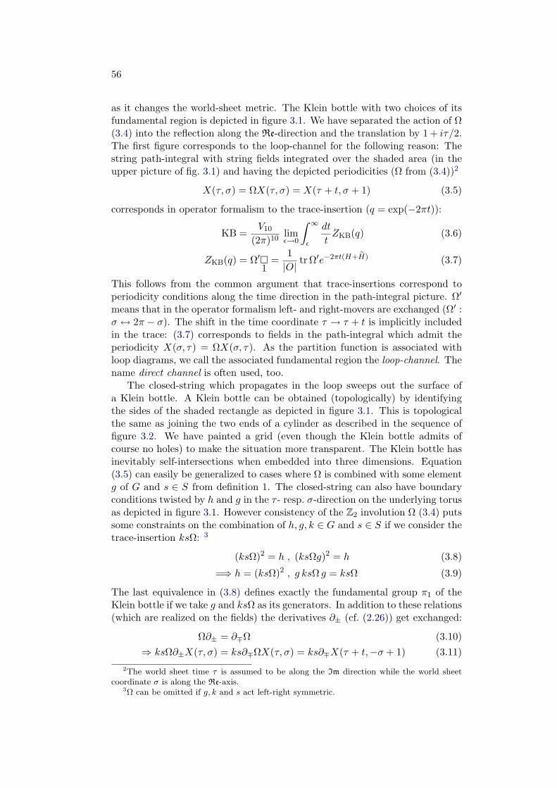
56

as it changes the world-sheet metric. The Klein bottle with two choices of itsfundamental region is depicted in figure 3.1. We have separated the action of Ω(3.4) into the reflection along the Re-direction and the translation by 1 + iτ/2.The first figure corresponds to the loop-channel for the following reason: Thestring path-integral with string fields integrated over the shaded area (in theupper picture of fig. 3.1) and having the depicted periodicities (Ω from (3.4))2

X(τ, σ) = ΩX(τ, σ) = X(τ + t, σ + 1) (3.5)

corresponds in operator formalism to the trace-insertion (q = exp(−2πt)):

KB =V10

(2π)10limε→0

∫ ∞

ε

dt

tZKB(q) (3.6)

ZKB(q) = Ω′1

=1|O|

trΩ′e−2πt(H+H) (3.7)

This follows from the common argument that trace-insertions correspond toperiodicity conditions along the time direction in the path-integral picture. Ω′

means that in the operator formalism left- and right-movers are exchanged (Ω′ :σ ↔ 2π − σ). The shift in the time coordinate τ → τ + t is implicitly includedin the trace: (3.7) corresponds to fields in the path-integral which admit theperiodicity X(σ, τ) = ΩX(σ, τ). As the partition function is associated withloop diagrams, we call the associated fundamental region the loop-channel. Thename direct channel is often used, too.

The closed-string which propagates in the loop sweeps out the surface ofa Klein bottle. A Klein bottle can be obtained (topologically) by identifyingthe sides of the shaded rectangle as depicted in figure 3.1. This is topologicalthe same as joining the two ends of a cylinder as described in the sequence offigure 3.2. We have painted a grid (even though the Klein bottle admits ofcourse no holes) to make the situation more transparent. The Klein bottle hasinevitably self-intersections when embedded into three dimensions. Equation(3.5) can easily be generalized to cases where Ω is combined with some elementg of G and s ∈ S from definition 1. The closed-string can also have boundaryconditions twisted by h and g in the τ - resp. σ-direction on the underlying torusas depicted in figure 3.1. However consistency of the Z2 involution Ω (3.4) putssome constraints on the combination of h, g, k ∈ G and s ∈ S if we consider thetrace-insertion ksΩ: 3

(ksΩ)2 = h , (ksΩg)2 = h (3.8)

=⇒ h = (ksΩ)2 , g ksΩ g = ksΩ (3.9)

The last equivalence in (3.8) defines exactly the fundamental group π1 of theKlein bottle if we take g and ksΩ as its generators. In addition to these relations(which are realized on the fields) the derivatives ∂± (cf. (2.26)) get exchanged:

Ω∂± = ∂∓Ω (3.10)⇒ ksΩ∂±X(τ, σ) = ks∂∓ΩX(τ, σ) = ks∂∓X(τ + t,−σ + 1) (3.11)

2The world sheet time τ is assumed to be along the Im direction while the world sheetcoordinate σ is along the Re-axis.

3Ω can be omitted if g, k and s act left-right symmetric.

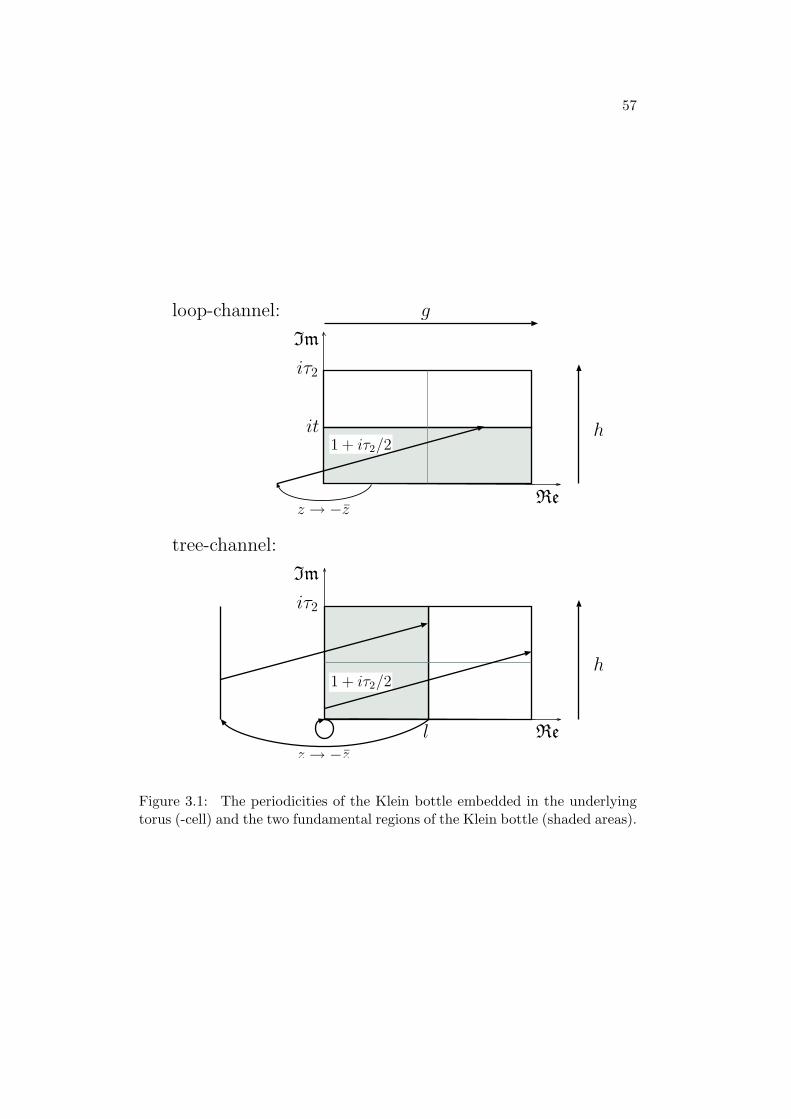
57

loop-channel: g

Im

iτ2

it h1 + iτ2/2

z → −zRe

tree-channel:

Im

iτ2

h1 + iτ2/2

l

z → −z

Re

Figure 3.1: The periodicities of the Klein bottle embedded in the underlyingtorus (-cell) and the two fundamental regions of the Klein bottle (shaded areas).

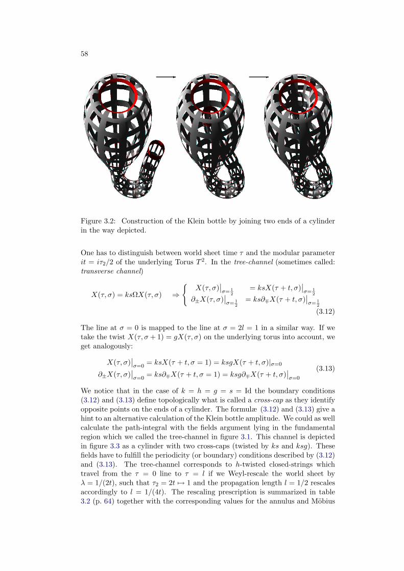
58

Figure 3.2: Construction of the Klein bottle by joining two ends of a cylinderin the way depicted.

One has to distinguish between world sheet time τ and the modular parameterit = iτ2/2 of the underlying Torus T 2. In the tree-channel (sometimes called:transverse channel)

X(τ, σ) = ksΩX(τ, σ) ⇒

X(τ, σ)

∣∣σ= 1

2= ksX(τ + t, σ)

∣∣σ= 1

2

∂±X(τ, σ)∣∣σ= 1

2= ks∂∓X(τ + t, σ)

∣∣σ= 1

2

(3.12)

The line at σ = 0 is mapped to the line at σ = 2l = 1 in a similar way. If wetake the twist X(τ, σ+ 1) = gX(τ, σ) on the underlying torus into account, weget analogously:

X(τ, σ)∣∣σ=0

= ksX(τ + t, σ = 1) = ksgX(τ + t, σ)|σ=0

∂±X(τ, σ)∣∣σ=0

= ks∂∓X(τ + t, σ = 1) = ksg∂∓X(τ + t, σ)∣∣σ=0

(3.13)

We notice that in the case of k = h = g = s = Id the boundary conditions(3.12) and (3.13) define topologically what is called a cross-cap as they identifyopposite points on the ends of a cylinder. The formulæ (3.12) and (3.13) give ahint to an alternative calculation of the Klein bottle amplitude. We could as wellcalculate the path-integral with the fields argument lying in the fundamentalregion which we called the tree-channel in figure 3.1. This channel is depictedin figure 3.3 as a cylinder with two cross-caps (twisted by ks and ksg). Thesefields have to fulfill the periodicity (or boundary) conditions described by (3.12)and (3.13). The tree-channel corresponds to h-twisted closed-strings whichtravel from the τ = 0 line to τ = l if we Weyl-rescale the world sheet byλ = 1/(2t), such that τ2 = 2t 7→ 1 and the propagation length l = 1/2 rescalesaccordingly to l = 1/(4t). The rescaling prescription is summarized in table3.2 (p. 64) together with the corresponding values for the annulus and Mobius

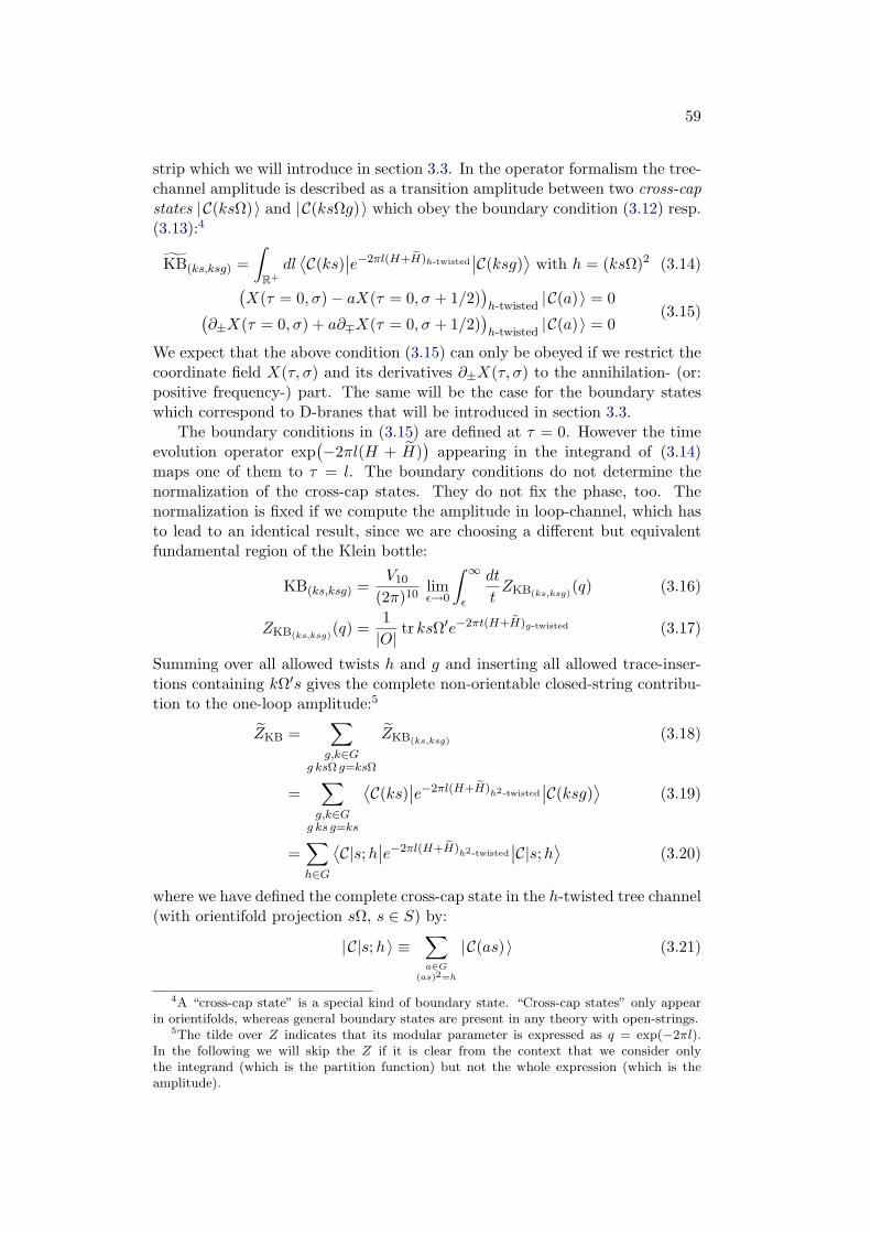
59

strip which we will introduce in section 3.3. In the operator formalism the tree-channel amplitude is described as a transition amplitude between two cross-capstates |C(ksΩ)〉 and |C(ksΩg)〉 which obey the boundary condition (3.12) resp.(3.13):4

KB(ks,ksg) =∫

R+

dl⟨C(ks)

∣∣e−2πl(H+H)h-twisted∣∣C(ksg)⟩ with h = (ksΩ)2 (3.14)(

X(τ = 0, σ)− aX(τ = 0, σ + 1/2))h-twisted

|C(a)〉 = 0(∂±X(τ = 0, σ) + a∂∓X(τ = 0, σ + 1/2)

)h-twisted

|C(a)〉 = 0(3.15)

We expect that the above condition (3.15) can only be obeyed if we restrict thecoordinate field X(τ, σ) and its derivatives ∂±X(τ, σ) to the annihilation- (or:positive frequency-) part. The same will be the case for the boundary stateswhich correspond to D-branes that will be introduced in section 3.3.

The boundary conditions in (3.15) are defined at τ = 0. However the timeevolution operator exp

(−2πl(H + H)

)appearing in the integrand of (3.14)

maps one of them to τ = l. The boundary conditions do not determine thenormalization of the cross-cap states. They do not fix the phase, too. Thenormalization is fixed if we compute the amplitude in loop-channel, which hasto lead to an identical result, since we are choosing a different but equivalentfundamental region of the Klein bottle:

KB(ks,ksg) =V10

(2π)10limε→0

∫ ∞

ε

dt

tZKB(ks,ksg)

(q) (3.16)

ZKB(ks,ksg)(q) =

1|O|

tr ksΩ′e−2πt(H+H)g-twisted (3.17)

Summing over all allowed twists h and g and inserting all allowed trace-inser-tions containing kΩ′s gives the complete non-orientable closed-string contribu-tion to the one-loop amplitude:5

ZKB =∑g,k∈G

g ksΩ g=ksΩ

ZKB(ks,ksg)(3.18)

=∑g,k∈G

g ks g=ks

⟨C(ks)

∣∣e−2πl(H+H)h2-twisted

∣∣C(ksg)⟩ (3.19)

=∑h∈G

⟨C|s;h


∣∣C|s;h⟩ (3.20)

where we have defined the complete cross-cap state in the h-twisted tree channel(with orientifold projection sΩ, s ∈ S) by:

|C|s;h〉 ≡∑a∈G

(as)2=h

|C(as)〉 (3.21)

4A “cross-cap state” is a special kind of boundary state. “Cross-cap states” only appearin orientifolds, whereas general boundary states are present in any theory with open-strings.

5The tilde over Z indicates that its modular parameter is expressed as q = exp(−2πl).In the following we will skip the Z if it is clear from the context that we consider onlythe integrand (which is the partition function) but not the whole expression (which is theamplitude).

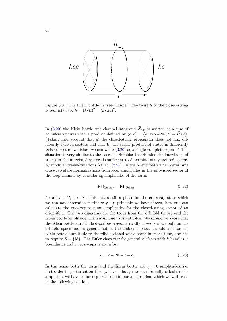
60

ks

h

ksg

-

l

Figure 3.3: The Klein bottle in tree-channel. The twist h of the closed-stringis restricted to: h = (ksΩ)2 = (ksΩg)2.

In (3.20) the Klein bottle tree channel integrand ZKB is written as a sum ofcomplete squares with a product defined by (a, b) =

⟨a∣∣ exp−2πl(H + H)

∣∣b⟩.(Taking into account that a) the closed-string propagator does not mix dif-ferently twisted sectors and that b) the scalar product of states in differentlytwisted sectors vanishes, we can write (3.20) as a single complete square.) Thesituation is very similar to the case of orbifolds: In orbifolds the knowledge oftraces in the untwisted sectors is sufficient to determine many twisted sectorsby modular transformations (cf. eq. (2.9)). In the orientifold we can determinecross-cap state normalizations from loop amplitudes in the untwisted sector ofthe loop-channel by considering amplitudes of the form:

KB(ks,ks) = KB(ks,ks) (3.22)

for all k ∈ G, s ∈ S. This leaves still a phase for the cross-cap state whichwe can not determine in this way. In principle we have shown, how one cancalculate the one-loop vacuum amplitudes for the closed-string sector of anorientifold. The two diagrams are the torus from the orbifold theory and theKlein bottle amplitude which is unique to orientifolds. We should be aware thatthe Klein bottle amplitude describes a geometrically closed surface only on theorbifold space and in general not in the ambient space. In addition for theKlein bottle amplitude to describe a closed world-sheet in space time, one hasto require S = Id. The Euler character for general surfaces with h handles, bboundaries and c cross-caps is given by:

χ = 2− 2h− b− c, (3.23)

In this sense both the torus and the Klein bottle are χ = 0 amplitudes, i.e.first order in perturbation theory. Even though we can formally calculate theamplitude we have so far neglected one important problem which we will treatin the following section.

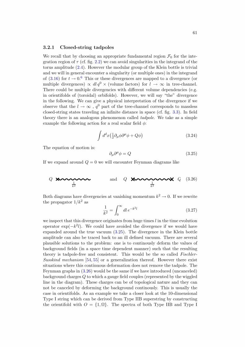
61

3.2.1 Closed-string tadpoles

We recall that by choosing an appropriate fundamental region F0 for the inte-gration region of τ (cf. fig. 2.2) we can avoid singularities in the integrand of thetorus amplitude (2.4). However the modular group of the Klein bottle is trivialand we will in general encounter a singularity (or multiple ones) in the integrandof (3.16) for t→ 0.6 This or these divergences are mapped to a divergence (ormultiple divergences) ∝ dl q0 × (volume factors) for l → ∞ in tree-channel.There could be multiple divergencies with different volume dependencies (e.g.in orientifolds of (toroidal) orbifolds). However, we will say “the” divergencein the following. We can give a physical interpretation of the divergence if weobserve that the l → ∞ , q0 part of the tree-channel corresponds to masslessclosed-string states traveling an infinite distance in space (cf. fig. 3.3). In fieldtheory there is an analogous phenomenon called tadpole. We take as a simpleexample the following action for a real scalar field φ:∫

ddx(

12∂µφ∂

µφ+Qφ)

(3.24)

The equation of motion is:∂µ∂

µφ = Q (3.25)

If we expand around Q = 0 we will encounter Feynman diagrams like

1k2

Q and1k2

Q Q (3.26)

Both diagrams have divergencies at vanishing momentum k2 → 0. If we rewritethe propagator 1/k2 as

1k2

=∫ ∞

0dl e−k

2l (3.27)

we inspect that this divergence originates from huge times l in the time evolutionoperator exp(−k2l). We could have avoided the divergence if we would haveexpanded around the true vacuum (3.25). The divergence in the Klein bottleamplitude can also be traced back to an ill defined vacuum. There are severalplausible solutions to the problem: one is to continously deform the values ofbackground fields (in a space time dependent manner) such that the resultingtheory is tadpole-free and consistent. This would be the so called Fischler-Susskind mechanism [54, 55] or a generalization thereof. However there existsituations where this continuous deformation does not remove the tadpole. TheFeynman graphs in (3.26) would be the same if we have introduced (uncanceled)background chargesQ to which a gauge field couples (represented by the wiggledline in the diagram). These charges can be of topological nature and they cannot be canceled by deforming the background continously. This is usually thecase in orientifolds. As an example we take a closer look at the 10-dimensionalType I string which can be derived from Type IIB superstring by constructingthe orientifold with O = 1,Ω. The spectra of both Type IIB and Type I

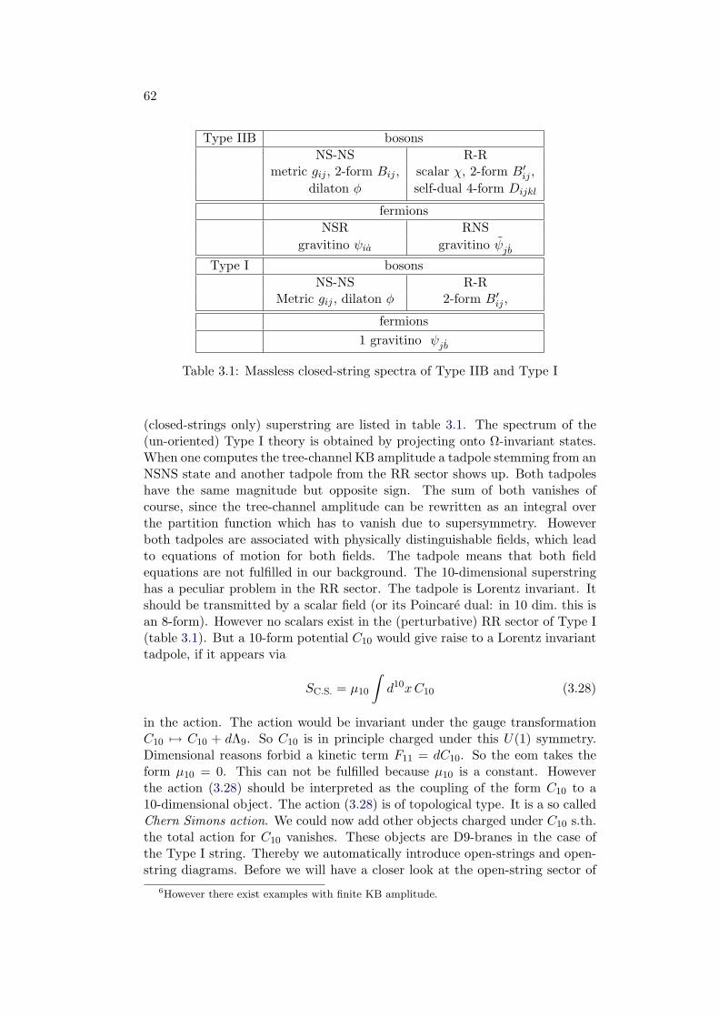
62

Type IIB bosonsNS-NS R-R

metric gij , 2-form Bij , scalar χ, 2-form B′ij ,

dilaton φ self-dual 4-form Dijkl

fermionsNSR RNS

gravitino ψia gravitino ψjbType I bosons

NS-NS R-RMetric gij , dilaton φ 2-form B′

ij ,

fermions1 gravitino ψjb

Table 3.1: Massless closed-string spectra of Type IIB and Type I

(closed-strings only) superstring are listed in table 3.1. The spectrum of the(un-oriented) Type I theory is obtained by projecting onto Ω-invariant states.When one computes the tree-channel KB amplitude a tadpole stemming from anNSNS state and another tadpole from the RR sector shows up. Both tadpoleshave the same magnitude but opposite sign. The sum of both vanishes ofcourse, since the tree-channel amplitude can be rewritten as an integral overthe partition function which has to vanish due to supersymmetry. Howeverboth tadpoles are associated with physically distinguishable fields, which leadto equations of motion for both fields. The tadpole means that both fieldequations are not fulfilled in our background. The 10-dimensional superstringhas a peculiar problem in the RR sector. The tadpole is Lorentz invariant. Itshould be transmitted by a scalar field (or its Poincare dual: in 10 dim. this isan 8-form). However no scalars exist in the (perturbative) RR sector of Type I(table 3.1). But a 10-form potential C10 would give raise to a Lorentz invarianttadpole, if it appears via

SC.S. = µ10

∫d10xC10 (3.28)

in the action. The action would be invariant under the gauge transformationC10 7→ C10 + dΛ9. So C10 is in principle charged under this U(1) symmetry.Dimensional reasons forbid a kinetic term F11 = dC10. So the eom takes theform µ10 = 0. This can not be fulfilled because µ10 is a constant. Howeverthe action (3.28) should be interpreted as the coupling of the form C10 to a10-dimensional object. The action (3.28) is of topological type. It is a so calledChern Simons action. We could now add other objects charged under C10 s.th.the total action for C10 vanishes. These objects are D9-branes in the case ofthe Type I string. Thereby we automatically introduce open-strings and open-string diagrams. Before we will have a closer look at the open-string sector of

6However there exist examples with finite KB amplitude.

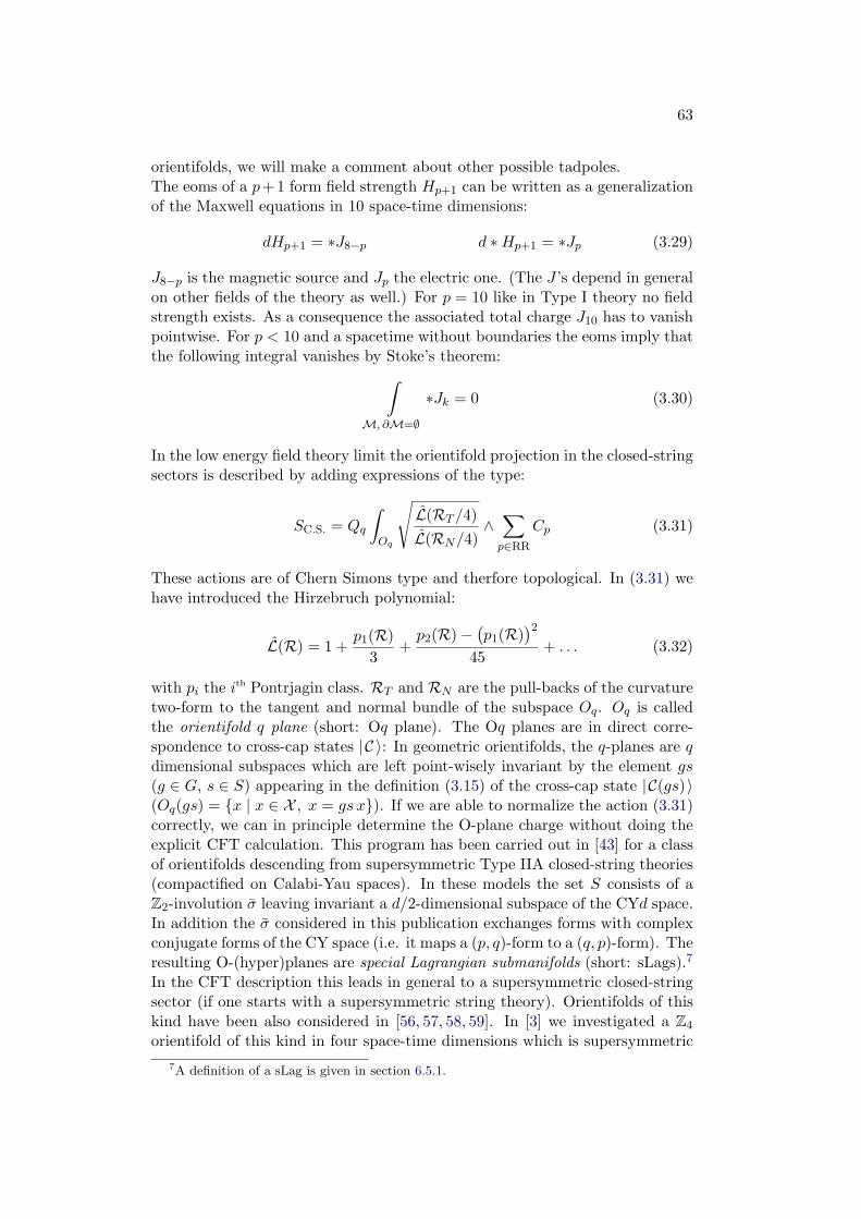
63

orientifolds, we will make a comment about other possible tadpoles.The eoms of a p+1 form field strength Hp+1 can be written as a generalizationof the Maxwell equations in 10 space-time dimensions:

dHp+1 = ∗J8−p d ∗Hp+1 = ∗Jp (3.29)

J8−p is the magnetic source and Jp the electric one. (The J ’s depend in generalon other fields of the theory as well.) For p = 10 like in Type I theory no fieldstrength exists. As a consequence the associated total charge J10 has to vanishpointwise. For p < 10 and a spacetime without boundaries the eoms imply thatthe following integral vanishes by Stoke’s theorem:∫

M, ∂M=∅

∗Jk = 0 (3.30)

In the low energy field theory limit the orientifold projection in the closed-stringsectors is described by adding expressions of the type:

SC.S. = Qq

∫Oq

√L(RT /4)L(RN/4)

∧∑p∈RR

Cp (3.31)

These actions are of Chern Simons type and therfore topological. In (3.31) wehave introduced the Hirzebruch polynomial:

L(R) = 1 +p1(R)

3+p2(R)−

(p1(R)

)245

+ . . . (3.32)

with pi the ith Pontrjagin class. RT and RN are the pull-backs of the curvaturetwo-form to the tangent and normal bundle of the subspace Oq. Oq is calledthe orientifold q plane (short: Oq plane). The Oq planes are in direct corre-spondence to cross-cap states |C 〉: In geometric orientifolds, the q-planes are qdimensional subspaces which are left point-wisely invariant by the element gs(g ∈ G, s ∈ S) appearing in the definition (3.15) of the cross-cap state |C(gs)〉(Oq(gs) = x | x ∈ X , x = gs x). If we are able to normalize the action (3.31)correctly, we can in principle determine the O-plane charge without doing theexplicit CFT calculation. This program has been carried out in [43] for a classof orientifolds descending from supersymmetric Type IIA closed-string theories(compactified on Calabi-Yau spaces). In these models the set S consists of aZ2-involution σ leaving invariant a d/2-dimensional subspace of the CYd space.In addition the σ considered in this publication exchanges forms with complexconjugate forms of the CY space (i.e. it maps a (p, q)-form to a (q, p)-form). Theresulting O-(hyper)planes are special Lagrangian submanifolds (short: sLags).7

In the CFT description this leads in general to a supersymmetric closed-stringsector (if one starts with a supersymmetric string theory). Orientifolds of thiskind have been also considered in [56, 57, 58, 59]. In [3] we investigated a Z4

orientifold of this kind in four space-time dimensions which is supersymmetric7A definition of a sLag is given in section 6.5.1.

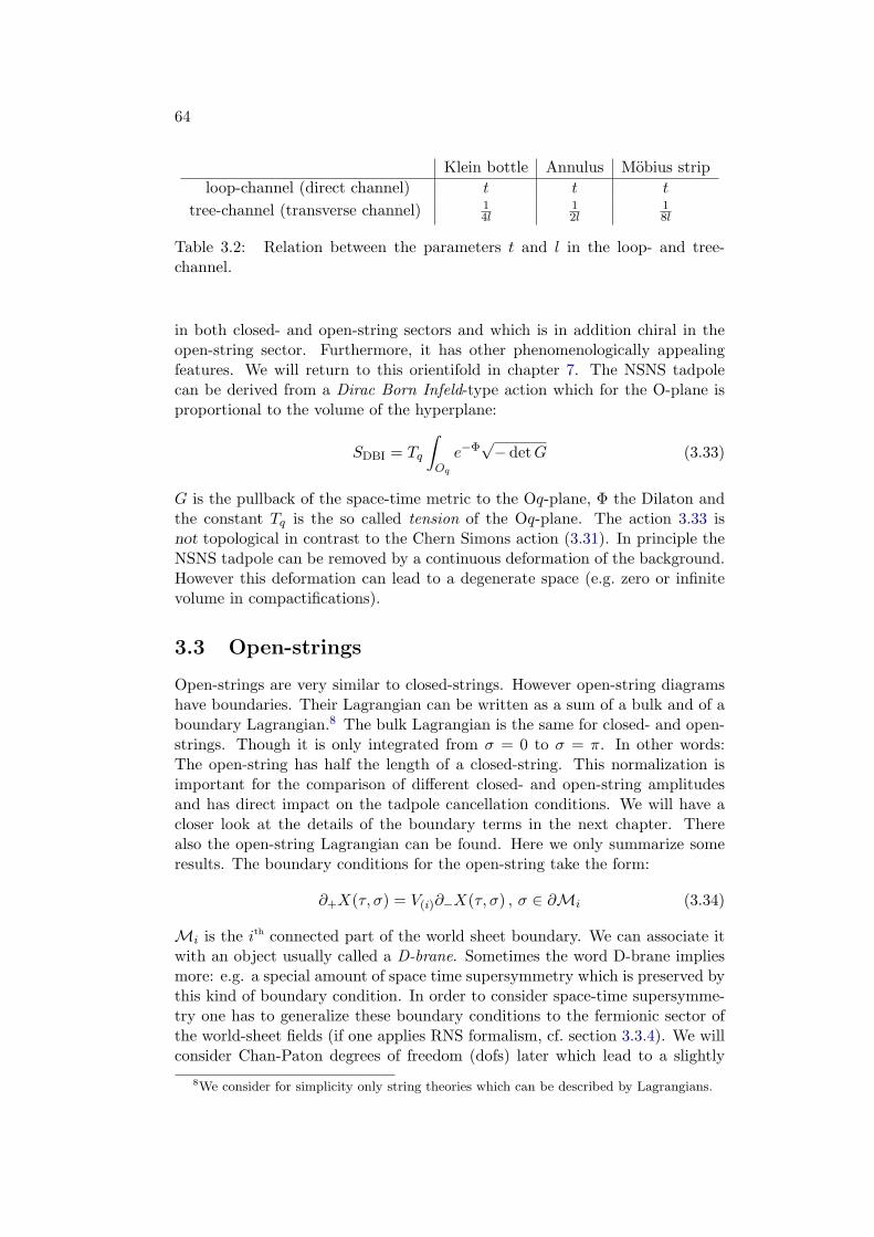
64

Klein bottle Annulus Mobius striploop-channel (direct channel) t t t

tree-channel (transverse channel) 14l

12l

18l

Table 3.2: Relation between the parameters t and l in the loop- and tree-channel.

in both closed- and open-string sectors and which is in addition chiral in theopen-string sector. Furthermore, it has other phenomenologically appealingfeatures. We will return to this orientifold in chapter 7. The NSNS tadpolecan be derived from a Dirac Born Infeld-type action which for the O-plane isproportional to the volume of the hyperplane:

SDBI = Tq

∫Oq

e−Φ√−detG (3.33)

G is the pullback of the space-time metric to the Oq-plane, Φ the Dilaton andthe constant Tq is the so called tension of the Oq-plane. The action 3.33 isnot topological in contrast to the Chern Simons action (3.31). In principle theNSNS tadpole can be removed by a continuous deformation of the background.However this deformation can lead to a degenerate space (e.g. zero or infinitevolume in compactifications).

3.3 Open-strings

Open-strings are very similar to closed-strings. However open-string diagramshave boundaries. Their Lagrangian can be written as a sum of a bulk and of aboundary Lagrangian.8 The bulk Lagrangian is the same for closed- and open-strings. Though it is only integrated from σ = 0 to σ = π. In other words:The open-string has half the length of a closed-string. This normalization isimportant for the comparison of different closed- and open-string amplitudesand has direct impact on the tadpole cancellation conditions. We will have acloser look at the details of the boundary terms in the next chapter. Therealso the open-string Lagrangian can be found. Here we only summarize someresults. The boundary conditions for the open-string take the form:

∂+X(τ, σ) = V(i)∂−X(τ, σ) , σ ∈ ∂Mi (3.34)

Mi is the ith connected part of the world sheet boundary. We can associate itwith an object usually called a D-brane. Sometimes the word D-brane impliesmore: e.g. a special amount of space time supersymmetry which is preserved bythis kind of boundary condition. In order to consider space-time supersymme-try one has to generalize these boundary conditions to the fermionic sector ofthe world-sheet fields (if one applies RNS formalism, cf. section 3.3.4). We willconsider Chan-Paton degrees of freedom (dofs) later which lead to a slightly

8We consider for simplicity only string theories which can be described by Lagrangians.

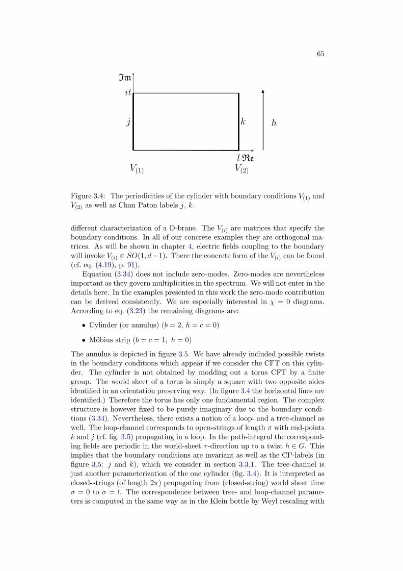
65

Im

it

j k h

l Re

V(1) V(2)

Figure 3.4: The periodicities of the cylinder with boundary conditions V(1) andV(2) as well as Chan Paton labels j, k.

different characterization of a D-brane. The V(i) are matrices that specify theboundary conditions. In all of our concrete examples they are orthogonal ma-trices. As will be shown in chapter 4, electric fields coupling to the boundarywill invoke V(i) ∈ SO(1, d−1). There the concrete form of the V(i) can be found(cf. eq. (4.19), p. 91).

Equation (3.34) does not include zero-modes. Zero-modes are neverthelessimportant as they govern multiplicities in the spectrum. We will not enter in thedetails here. In the examples presented in this work the zero-mode contributioncan be derived consistently. We are especially interested in χ = 0 diagrams.According to eq. (3.23) the remaining diagrams are:

• Cylinder (or annulus) (b = 2, h = c = 0)

• Mobius strip (b = c = 1, h = 0)

The annulus is depicted in figure 3.5. We have already included possible twistsin the boundary conditions which appear if we consider the CFT on this cylin-der. The cylinder is not obtained by modding out a torus CFT by a finitegroup. The world sheet of a torus is simply a square with two opposite sidesidentified in an orientation preserving way. (In figure 3.4 the horizontal lines areidentified.) Therefore the torus has only one fundamental region. The complexstructure is however fixed to be purely imaginary due to the boundary condi-tions (3.34). Nevertheless, there exists a notion of a loop- and a tree-channel aswell. The loop-channel corresponds to open-strings of length π with end-pointsk and j (cf. fig. 3.5) propagating in a loop. In the path-integral the correspond-ing fields are periodic in the world-sheet τ -direction up to a twist h ∈ G. Thisimplies that the boundary conditions are invariant as well as the CP-labels (infigure 3.5: j and k), which we consider in section 3.3.1. The tree-channel isjust another parameterization of the one cylinder (fig. 3.4). It is interpreted asclosed-strings (of length 2π) propagating from (closed-string) world sheet timeσ = 0 to σ = l. The correspondence between tree- and loop-channel parame-ters is computed in the same way as in the Klein bottle by Weyl rescaling with

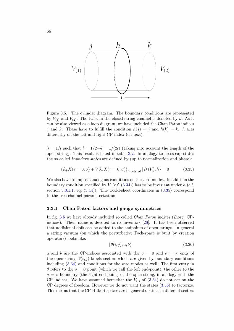
66

V(2)

hj k

V(1)

-

l

Figure 3.5: The cylinder diagram. The boundary conditions are representedby V(1) and V(2). The twist in the closed-string channel is denoted by h. As itcan be also viewed as a loop diagram, we have included the Chan Paton indicesj and k. These have to fulfill the condition h(j) = j and h(k) = k. h actsdifferently on the left and right CP index (cf. text).

λ = 1/t such that l = 1/2 7→l = 1/(2t) (taking into account the length of theopen-string). This result is listed in table 3.2. In analogy to cross-cap statesthe so called boundary states are defined by (up to normalization and phase):(

∂+X(τ = 0, σ) + V ∂−X(τ = 0, σ))h-twisted

|D (V );h〉 = 0 (3.35)

We also have to impose analogous conditions on the zero-modes. In addition theboundary condition specified by V (c.f. (3.34)) has to be invariant under h (c.f.section 3.3.1.1, eq. (3.44)). The world-sheet coordinates in (3.35) correspondto the tree-channel parameterization.

3.3.1 Chan Paton factors and gauge symmetries

In fig. 3.5 we have already included so called Chan Paton indices (short: CP-indices). Their name is devoted to its inventors [26]. It has been observedthat additional dofs can be added to the endpoints of open-strings. In generala string vacuum (on which the perturbative Fock-space is built by creationoperators) looks like:

|θ(i, j); a; b〉 (3.36)

a and b are the CP-indices associated with the σ = 0 and σ = π ends ofthe open-string, θ(i, j) labels sectors which are given by boundary conditionsincluding (3.34) and conditions for the zero modes as well. The first entry inθ refers to the σ = 0 point (which we call the left end-point), the other to theσ = π boundary (the right end-point) of the open-string, in analogy with theCP indices. We have assumed here that the V(i) of (3.34) do not act on theCP degrees of freedom. However we do not want the states (3.36) to factorize.This means that the CP-Hilbert spaces are in general distinct in different sectors

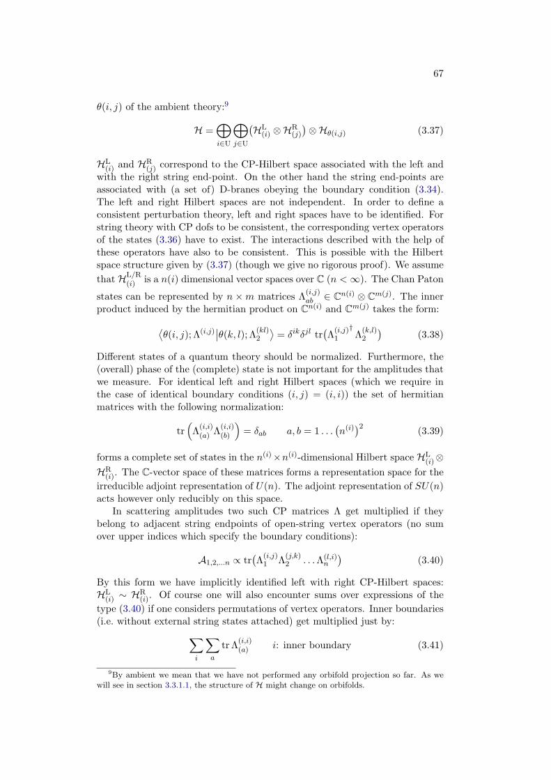
67

θ(i, j) of the ambient theory:9

H =⊕i∈U

⊕j∈U

(HL

(i) ⊗HR(j)

)⊗Hθ(i,j) (3.37)

HL(i) and HR

(j) correspond to the CP-Hilbert space associated with the left andwith the right string end-point. On the other hand the string end-points areassociated with (a set of) D-branes obeying the boundary condition (3.34).The left and right Hilbert spaces are not independent. In order to define aconsistent perturbation theory, left and right spaces have to be identified. Forstring theory with CP dofs to be consistent, the corresponding vertex operatorsof the states (3.36) have to exist. The interactions described with the help ofthese operators have also to be consistent. This is possible with the Hilbertspace structure given by (3.37) (though we give no rigorous proof). We assumethat HL/R

(i) is a n(i) dimensional vector spaces over C (n <∞). The Chan Paton

states can be represented by n ×m matrices Λ(i,j)ab ∈ Cn(i) ⊗ Cm(j). The inner

product induced by the hermitian product on Cn(i) and Cm(j) takes the form:⟨θ(i, j); Λ(i,j)

∣∣θ(k, l); Λ(kl)2

⟩= δikδjl tr

(Λ(i,j)

1

†Λ(k,l)

2

)(3.38)

Different states of a quantum theory should be normalized. Furthermore, the(overall) phase of the (complete) state is not important for the amplitudes thatwe measure. For identical left and right Hilbert spaces (which we require inthe case of identical boundary conditions (i, j) = (i, i)) the set of hermitianmatrices with the following normalization:

tr(Λ(i,i)

(a) Λ(i,i)(b)

)= δab a, b = 1 . . .

(n(i))2 (3.39)

forms a complete set of states in the n(i)×n(i)-dimensional Hilbert space HL(i)⊗

HR(i). The C-vector space of these matrices forms a representation space for the

irreducible adjoint representation of U(n). The adjoint representation of SU(n)acts however only reducibly on this space.

In scattering amplitudes two such CP matrices Λ get multiplied if theybelong to adjacent string endpoints of open-string vertex operators (no sumover upper indices which specify the boundary conditions):

A1,2,...n ∝ tr(Λ(i,j)

1 Λ(j,k)2 . . .Λ(l,i)

n

)(3.40)

By this form we have implicitly identified left with right CP-Hilbert spaces:HL

(i) ∼ HR(i). Of course one will also encounter sums over expressions of the

type (3.40) if one considers permutations of vertex operators. Inner boundaries(i.e. without external string states attached) get multiplied just by:∑

i

∑a

tr Λ(i,i)(a) i: inner boundary (3.41)

9By ambient we mean that we have not performed any orbifold projection so far. As wewill see in section 3.3.1.1, the structure of H might change on orbifolds.

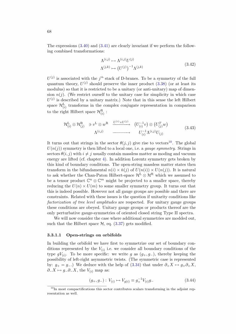
68

The expressions (3.40) and (3.41) are clearly invariant if we perform the follow-ing combined transformations:

Λ(i,j) 7→ Λ(i,j)U (j)

Λ(j,k) 7→(U (j)

)−1Λ(j,k)(3.42)

U (j) is associated with the jth stack of D-branes. To be a symmetry of the fullquantum theory, U (j) should preserve the inner product (3.38) (or at least itsmodulus) so that it is restricted to be a unitary (or anti-unitary) map of dimen-sion n(j). (We restrict ourself to the unitary case for simplicity in which caseU (j) is described by a unitary matrix.) Note that in this sense the left Hilbertspace HL

(i) transforms in the complex conjugate representation in comparisonto the right Hilbert space HR

(i) :

HL(i) ⊗H

R(j) 3 v

L ⊗ wR U(i)×U(j)

−−−−−−→(U−1

(i) v)⊗(UT(j)w

)Λ(i,j) −−−−−−→ U−1

(i) Λ(i,j)U(j)

(3.43)

It turns out that strings in the sector θ(j, j) give rise to vectors10. The globalU(n(j)) symmetry is then lifted to a local one, i.e. a gauge symmetry. Strings insectors θ(i, j) with i 6= j usually contain massless matter as moding and vacuumenergy are lifted (cf. chapter 4). In addition Lorentz symmetry gets broken bythis kind of boundary conditions. The open-string massless matter states thentransform in the bifundamental n(i)× n(j) of U(n(i))× U(n(j)). It is naturalto ask whether the Chan-Paton Hilbert-space HL ⊗ HR which we assumed tobe a tensor product Cn ⊗ Cm might be projected to a smaller space, therebyreducing the U(n)× U(m) to some smaller symmetry group. It turns out thatthis is indeed possible. However not all gauge groups are possible and there areconstraints. Related with these issues is the question if unitarity conditions likefactorization of tree level amplitudes are respected. For unitary gauge groupsthese conditions are obeyed. Unitary gauge groups or products thereof are theonly perturbative gauge-symmetries of oriented closed string Type II spectra.

We will now consider the case where additional symmetries are modded out,such that the Hilbert space H, eq. (3.37) gets modified.

3.3.1.1 Open-strings on orbifolds

In building the orbifold we have first to symmetrize our set of boundary con-ditions represented by the V(i) i.e. we consider all boundary conditions of thetype gV(i). To be more specific: we write g as (g+, g−), thereby keeping thepossibility of left-right asymmetric twists. (The symmetric case is representedby: g+ = g−.) We deduce with the help of (3.34) that under ∂+X 7→ g+∂+X,∂−X 7→ g−∂−X, the V(i) map as:

(g+, g−) : V(i) 7→ Vg(i) ≡ g−1+ V(i)g− (3.44)

10In most compactifications this sector contributes scalars transforming in the adjoint rep-resentation as well.

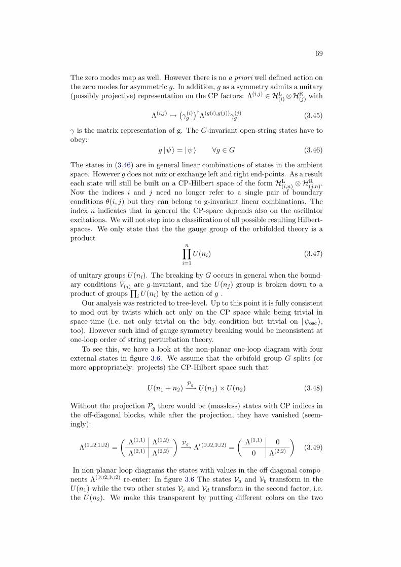
69

The zero modes map as well. However there is no a priori well defined action onthe zero modes for asymmetric g. In addition, g as a symmetry admits a unitary(possibly projective) representation on the CP factors: Λ(i,j) ∈ HL

(i)⊗HR(j) with

Λ(i,j) 7→(γ(i)g

)†Λ(g(i),g(j))γ(j)g (3.45)

γ is the matrix representation of g. The G-invariant open-string states have toobey:

g |ψ 〉 = |ψ 〉 ∀g ∈ G (3.46)

The states in (3.46) are in general linear combinations of states in the ambientspace. However g does not mix or exchange left and right end-points. As a resulteach state will still be built on a CP-Hilbert space of the form HL

(i,n) ⊗HR(j,n).

Now the indices i and j need no longer refer to a single pair of boundaryconditions θ(i, j) but they can belong to g-invariant linear combinations. Theindex n indicates that in general the CP-space depends also on the oscillatorexcitations. We will not step into a classification of all possible resulting Hilbert-spaces. We only state that the the gauge group of the orbifolded theory is aproduct

n∏i=1

U(ni) (3.47)

of unitary groups U(ni). The breaking by G occurs in general when the bound-ary conditions V(j) are g-invariant, and the U(nj) group is broken down to aproduct of groups

∏i U(ni) by the action of g .

Our analysis was restricted to tree-level. Up to this point it is fully consistentto mod out by twists which act only on the CP space while being trivial inspace-time (i.e. not only trivial on the bdy.-condition but trivial on |ψosc 〉,too). However such kind of gauge symmetry breaking would be inconsistent atone-loop order of string perturbation theory.

To see this, we have a look at the non-planar one-loop diagram with fourexternal states in figure 3.6. We assume that the orbifold group G splits (ormore appropriately: projects) the CP-Hilbert space such that

U(n1 + n2)Pg−→ U(n1)× U(n2) (3.48)

Without the projection Pg there would be (massless) states with CP indices inthe off-diagonal blocks, while after the projection, they have vanished (seem-ingly):

Λ(1∪2,1∪2) =(

Λ(1,1) Λ(1,2)

Λ(2,1) Λ(2,2)

)Pg−→ Λ′ (1∪2,1∪2) =

(Λ(1,1) 0

0 Λ(2,2)

)(3.49)

In non-planar loop diagrams the states with values in the off-diagonal compo-nents Λ(1∪2,1∪2) re-enter: In figure 3.6 The states Va and Vb transform in theU(n1) while the two other states Vc and Vd transform in the second factor, i.e.the U(n2). We make this transparent by putting different colors on the two

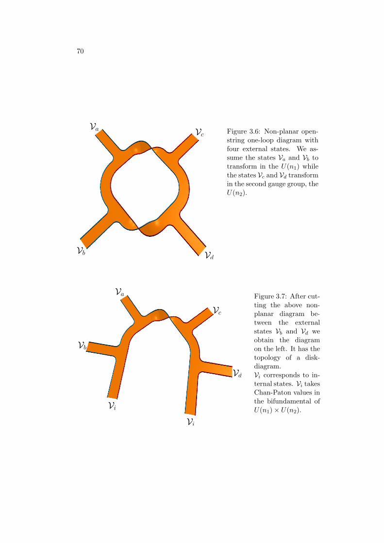
70

Va

Vb

Vc

Vd

Figure 3.6: Non-planar open-string one-loop diagram withfour external states. We as-sume the states Va and Vb totransform in the U(n1) whilethe states Vc and Vd transformin the second gauge group, theU(n2).

Va

Vb

Vc

Vd

ViVi

Figure 3.7: After cut-ting the above non-planar diagram be-tween the externalstates Vb and Vd weobtain the diagramon the left. It has thetopology of a disk-diagram.Vi corresponds to in-ternal states. Vi takesChan-Paton values inthe bifundamental ofU(n1)× U(n2).

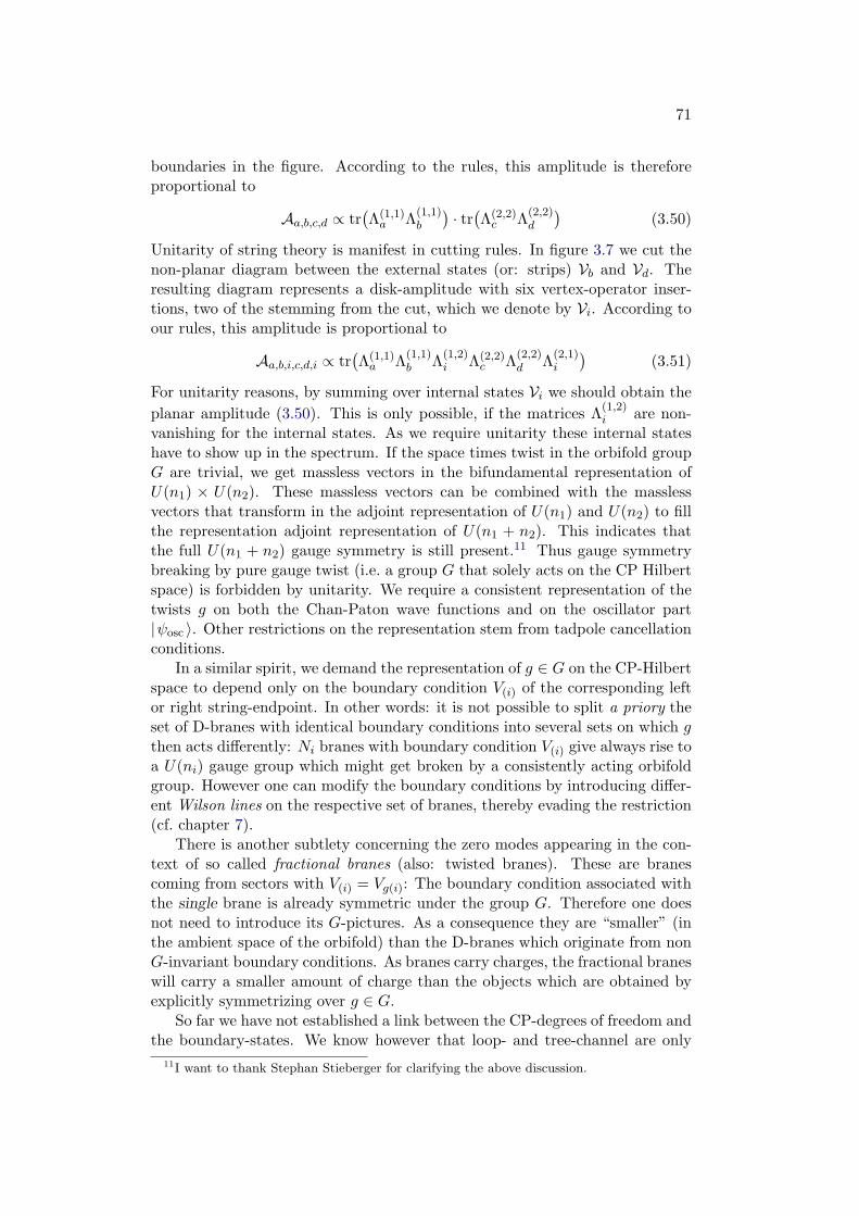
71

boundaries in the figure. According to the rules, this amplitude is thereforeproportional to

Aa,b,c,d ∝ tr(Λ(1,1)a Λ(1,1)

b

)· tr(Λ(2,2)c Λ(2,2)

d

)(3.50)

Unitarity of string theory is manifest in cutting rules. In figure 3.7 we cut thenon-planar diagram between the external states (or: strips) Vb and Vd. Theresulting diagram represents a disk-amplitude with six vertex-operator inser-tions, two of the stemming from the cut, which we denote by Vi. According toour rules, this amplitude is proportional to

Aa,b,i,c,d,i ∝ tr(Λ(1,1)a Λ(1,1)

b Λ(1,2)i Λ(2,2)

c Λ(2,2)d Λ(2,1)

i

)(3.51)

For unitarity reasons, by summing over internal states Vi we should obtain theplanar amplitude (3.50). This is only possible, if the matrices Λ(1,2)

i are non-vanishing for the internal states. As we require unitarity these internal stateshave to show up in the spectrum. If the space times twist in the orbifold groupG are trivial, we get massless vectors in the bifundamental representation ofU(n1) × U(n2). These massless vectors can be combined with the masslessvectors that transform in the adjoint representation of U(n1) and U(n2) to fillthe representation adjoint representation of U(n1 + n2). This indicates thatthe full U(n1 + n2) gauge symmetry is still present.11 Thus gauge symmetrybreaking by pure gauge twist (i.e. a group G that solely acts on the CP Hilbertspace) is forbidden by unitarity. We require a consistent representation of thetwists g on both the Chan-Paton wave functions and on the oscillator part|ψosc 〉. Other restrictions on the representation stem from tadpole cancellationconditions.

In a similar spirit, we demand the representation of g ∈ G on the CP-Hilbertspace to depend only on the boundary condition V(i) of the corresponding leftor right string-endpoint. In other words: it is not possible to split a priory theset of D-branes with identical boundary conditions into several sets on which gthen acts differently: Ni branes with boundary condition V(i) give always rise toa U(ni) gauge group which might get broken by a consistently acting orbifoldgroup. However one can modify the boundary conditions by introducing differ-ent Wilson lines on the respective set of branes, thereby evading the restriction(cf. chapter 7).

There is another subtlety concerning the zero modes appearing in the con-text of so called fractional branes (also: twisted branes). These are branescoming from sectors with V(i) = Vg(i): The boundary condition associated withthe single brane is already symmetric under the group G. Therefore one doesnot need to introduce its G-pictures. As a consequence they are “smaller” (inthe ambient space of the orbifold) than the D-branes which originate from nonG-invariant boundary conditions. As branes carry charges, the fractional braneswill carry a smaller amount of charge than the objects which are obtained byexplicitly symmetrizing over g ∈ G.

So far we have not established a link between the CP-degrees of freedom andthe boundary-states. We know however that loop- and tree-channel are only

11I want to thank Stephan Stieberger for clarifying the above discussion.

72

different parameterizations of the same world sheet, and therefore the ampli-tudes are identical. However closed strings do not carry CP-degrees of freedom.They also do not appear in the definition of the V(i). Keeping in mind thetensor product structure of the CP Hilbert space of the non-orbifolded theory(eq. (3.37)) we notice that the loop-channel trace (in the operator formalism)splits into a product of traces over the CP-Hilbert space times a trace over theboundary conditions. Suppressing the trace over the CP-Hilbert space we getfor each CP-sector Λ(i,j):12

Aijab(h) =

V10

(2π)dlimε→0

∫ ∞

ε

dt

tZ

Aijab

(3.52)

=∫dl⟨D(V(i));h; a

∣∣e−2πl(H+H)h-twisted∣∣D(V(j));h; b

⟩(3.53)

ZAij(h) = ZAij

ab(h)≡ 1|O|

trh e−2πt(Hθ(j,l)) (3.54)

Tracing both expressions over the CP-Hilbert space HL(i)⊗H

R(j) and taking into

account that h acts on it by γ(i)h ⊗ γ

(j)h we can rewrite the complete annulus

amplitude in the sector given by θ(i, j) as:

Aij(h) ≡(tr γ(i)

h

)(tr γ(j)

h

) V10

(2π)dlimε→0

∫ ∞

ε

dt

tZAij(h) (3.55)

=(tr γ(i)

h

)(tr γ(j)

h

)∫dl⟨D(V(i));h; b

∣∣e−2πl(H+H)h-twisted∣∣D(V(j));h; b

⟩(3.56)∣∣D(V(j));h

⟩≡ tr γ(j)

h ·∣∣D(V(j));h; b

⟩(3.57)

Therefore the trace-insertion in loop-channel is mapped to the normalizationand to the closed-string twist h of the boundary state. (Note that

∣∣D(V(j));h; b⟩

does not depend on the CP-index b due to the assumption that h preserves thestructure HCP ⊗ Hθ(ij).) The whole annulus contribution can be written as asum over perfect squares:

A ≡∑h∈G

∑i

∑j

Aij(h) (3.58)

=∑h∈G

∫dl 〈D;h | e−2πl(H+H)h-twisted |D;h〉 (3.59)

|D;h〉 ≡∑j

∣∣D(V(j));h⟩

(3.60)

j runs over a set of G-symmetrized boundary conditions. Taking into accountthat vacua of different h-twists have vanishing scalar products and observ-ing that the closed-string propagator Pcl =

∑h

∫dl exp

(−2πl(H + H)h-twisted

)12As we have assumed that the V(i) act trivially on the CP-Hilbert space of the ambient

space, we assume that this is the case for the orbifold, too. (I.e. the Vg(i), g ∈ G do not carryCP-indices.)

73

does not mix the twisted sectors, we can rewrite:

A =∫dl

∑i∈G-inv.

set

∑j∈G-inv.

set

⟨D(V(i))

∣∣ e−2πl(H+H)∣∣D(V(j))

⟩(3.61)

∣∣D(V(j))⟩≡ Sj

∑h∈G

∣∣D(V(j));h⟩

no sum over j (3.62)

Sj defines a symmetrization of the boundary conditions in the sector describedby V(j). The choice of Sj leaves some freedom: if a brane is symmetric underh ∈ G its image may (which would be just a doubling of dofs) or may not beincluded. Invariance under h includes also the invariance of the zero modes.By the doubling, a non-trivial action γh on the CP dofs can be chosen (cf. eq.(3.45)). As the amplitude is proportional to the product of the traces of both γh-matrices (cf. eq. (3.55)), the h-twisted part of the corresponding boundary statevanishes, if the corresponding trace tr γh equals zero. In geometric orbifoldsthe massless closed-string states of the twisted sectors can be associated withblowing up modes of the singularity. (For Calabi-Yau orbifolds, these fields arecontained in H(1,1)(M).) tr γh = 0 would mean that the Dp-brane does notwrap an (exceptional) cycle of the blow-up whereas for tr γh 6= 0 the contraryis true. As we mentioned, without the doubling and γh = Id the h-invariantbranes (or: boundary states) are called fractional branes. For the D6-branesdiscussed in chapter 7 this means that fractional branes have to intersect Z2-fix-points. As they are stuck to fix-points which in turn are associated withcertain twisted closed-string sectors, we also refer to these branes as twistedbranes. Like the cross-cap states, also the boundary states couple to RR andNSNS fields. The coupling to the untwisted (i.e. h = 0) closed-string fields fora fractional D-brane is a fraction of what it would be for a brane which wasoriginally not G-invariant in ambient space.

As we have noticed that D-branes have similar couplings to closed-stringfields as O-planes, we could check if the addition of D-branes could cancel thetadpole of the Klein bottle. We are especially interested in the cancellation ofRR tadpoles as they can not be cured by a Fischler Susskind mechanism. Wewould also be glad to cancel the NSNS tadpoles as well, because the NSNStadpoles can also lead to a deformation of the theory to a singular limit. Ifthe model is supersymmetric in both the open- and the closed-string sector,we also have other phenomenologically appealing features like possible solutionto the hierarchy problem etc. We will have a closer look at a Z4-orientifold inchapter 7 which admits supersymmetric solutions.13 Similar to the Op-planes,the Dp-branes have a low energy effective action, too. The Chern Simons actionlooks like (cf. [60, 61]):

S(Dp)C.S. = µp

∫Dp

ch(F)

√A(RT )A(RN )

∧∑q∈RR

Cq (3.63)

13Condiditions for a D-brane to be supersymmetric are given in section 4.4 and in section6.5.1.

74

µp is the Dp-brane charge. ch is the Chern character, F = F + B the sum ofthe electro-magnetic U(1) NS-gauge field F and B is the NSNS two-form. Adenotes the A-roof (or Dirac) genus:

A(R) = 1− p1(R)24

+7(p1(R)

)2 − 4p2(R)5760

+ . . . (3.64)

Like for the Op-plane, RT (and RN ) are the pull-backs of the curvature two-form to the tangent- (and normal-) bundle of the Dp-brane (and pi are Pontr-jagin classes). The Dirac-Born-Infeld action also contains a term that couplesto the combination of NS and NSNS fields F :

S(Dp)DBI = Tp

∫Dqe−Φ

√−det(G+ F) (3.65)

Tp is the D-brane tension. However it is still a field of research how the non-abelian gauge degrees of freedom are correctly incorporated. One method,which is sufficient for all of our tadpole considerations, is simply to trace over thegauge degrees of freedom. Several non-abelian extensions of the above actionshave been suggested, motivated by different approaches ( [62,63,64,65,66,67]).

For consistency we also have to project on SΩ-invariant states in the open-string sector. This leads to non-orientable diagrams with boundaries in theperturbation series. At one-loop level this is the Mobius strip.

3.3.2 sΩ-invariant open-string sector

The sΩ-projection must be also imposed in the open-string sector. We assumethat we have already created the orbifold including oriented open-strings asdiscussed in the last section. We do not expect that the orbifolded theory is fullyconsistent at this stage. It will in general still suffer from tadpoles. Consistencyof the string perturbation expansion will force us to include non-orientablediagrams with boundaries. We will first have a closer look at the spectrum.For sΩ to be a symmetry, we have to include all sΩ images of the brane. In thecase without U(1)-valued electro-magnetic NSNS fields F (i), we only have tomake sure that the configuration (i.e. the Hilbert space) is s-invariant. Withnon-trivial U(1)-fields we note that Ω : (F(i), F(j)) 7→ −(F(j), F(i)) (cf. chapter4).Since Ω acts as an orientation reversal on X(τ, σ) there are two possibilities:

1. sΩ interchanges the sector (i) with a different sector sΩ(i) ((i) describesa G-invariant combination of boundary conditions). In this case the sΩprojection breaks the gauge group:

U(ni)× U(nsΩ(i))PsΩ−−→ U(ni) (3.66)

2. The sector (i) is mapped to itself by sΩ. We will consider this case inmore detail:

As Ω acts as orientation-reversal, left and right CP-degrees also have to getexchanged in the sector (ii) under the sΩ action. Ω includes a transposition of

75

Λ: ∣∣∣Λ(i,i)⟩

Ω−→∣∣∣(Λ(i,i)

)T ⟩ (3.67)

(A hermitian conjugation would leave the hermitian matrix Λ(i,i) invariant.Hermitian or anti-hermitian matrices do however not form a C-vector space.)sΩ could also contain an additional U(n)-rotation UsΩ. In total we have for sΩin this case:

sΩ : |ψ(i, i), osc〉 ⊗∣∣∣Λ(i,i)

⟩7→ |sΩ(ψ)(i, i), osc〉 ⊗

∣∣∣(U (i)sΩ

)−1(Λ(i,i))TU

(i)sΩ

⟩(3.68)

We note that(U

(i)sΩ

)−1 =(U

(i)sΩ

)† =(U

(i)sΩ

)T . Under a unitary basis-change V (i)

in the left or right CP-Hilbert space H(i)CP (belonging to the boundary condition

(i)), U (i)sΩ will not transform by conjugation:

Λ(i,j) 7→ Λ′ (i,j) =(V (i)

)−1Λ(i,j)V (j) ⇒ U(i)sΩ 7→ U

′ (i)sΩ =

(V (i)

)TU

(i)sΩV

(i) (3.69)

Hence a basis of H(i)CP in which U (i)

sΩ is diagonal, does not exist in generic cases.However it turns out that U (i)

sΩ is either symmetric (or anti-symmetric) in whichcase simple representations exist:The relation (sΩ)2 = h, h ∈ G has to be obeyed at least up to a phase inboth the oscillator and the CP-part of the state (and in total without a phase).Because we have already performed the G-projection (and assuming that theresulting state can be written as a direct product of a CP-part and a part|ψ(i, j), osc〉) this reduces to:14

(sΩ)2 |ψ(i, j), osc〉 =exp(iφ(i,j)osc ) |ψ(i, j), osc〉 (3.70)

(sΩ)2∣∣Λ(i,j)

⟩=exp(i(φ(i)

CP − φ(j)CP)

·∣∣∣(((U (i)

sΩ)−1)TU

(i)sΩ

)−1Λ(i,j)

(((U (i)

sΩ)−1)TU

(i)sΩ

)⟩ (3.71)

with the phase depending on the super-selection sector (i, j). We have used thatthe right CP space transforms in the complex conjugate representation withrespect to the left one. We also deduce that for identical boundary conditionson left- and right-movers (including the effect of the GSO-projection):

φ(i,i)osc = 0 mod 2π (3.72)

If (sΩ)2 equals the identity,15 U(i)sΩ is either symmetric or anti-symmetric in

sectors in which sΩ leaves the boundary condition invariant:

U(i)sΩ = (U (i)

sΩ)T or U(i)sΩ = −(U (i)

sΩ)T for sΩ(i) = i (3.73)

14By this we assume that |ψ〉 is G-invariant. The split of a general G-invariant state into aproduct of a CP and an oscillator part is in general not possible. However there should exist abasis of G-invariant states that admits this product structure. Relation (3.72) holds for eachof these basis vectors.

15In the bosonic string, and on GSO-projected states of the superstring.

76

By a unitary base change of the form (3.69) we can achieve U (i)sΩ to be:

U(i)sΩ symmetric: U

(i)sΩ = 1ni (3.74)

U(i)sΩ anti-symmetric: U

(i)sΩ =

(0 i1ni/2

−i1ni/2 0

)(3.75)

This fact is proven in appendix B. The situation is more complicated if (sΩ)2 =h 6= Id. To the knowledge of the author, this case is not classified in physicsliterature. If an element (sΩ)2 = Id is contained in the orientifold-group O, wetake this element as the representative in eq. (3.2) (p. 55). This element doesnot need to be unique, of course. If we know the form of U (i)

sΩ for this element,we may determine the form of the remaining U (i)

sΩg, g ∈ G by requiring that theU matrices (often called γ-matrices as well, which should not be confused withthe generators of the Dirac-algebra) form a representation of the orientifoldgroup O.

Even though all models considered in this thesis belong to the class (sΩ)2 =Id, we explain a problem in the case that such an element is not included in O.This case implies that the Klein bottle only leads to twisted-sector tadpoles.The twist corresponds to (ksΩ)2 = h, with k, h ∈ G. It is not clear, if such kindof twisted tadpoles can be canceled. However it is obvious that the cancellationof purely twisted tadpoles by adding D-branes and leaving the background oth-erwise unmodified, is impossible. D-branes always couple to untwisted closed-string fields as the partition function can be written in terms of traces (cf. eq.(3.58)). The Id-trace-insertion (which is not allowed to vanish) corresponds tountwisted closed-string exchange in the tree-channel. Therefore each individualannulus amplitude has non-vanishing untwisted closed-string contribution. Asthe Klein bottle does not contribute to this untwisted closed-string exchange (inthe case at hand), the total untwisted annulus tadpole has to vanish by itself.For the RR-tadpole this would imply that both branes and anti-branes (whichhave the opposite coupling to the RR-fields) are present. As anti-branes haveidentical boundary conditions as branes, except for the GSO-projection, whichis reversed, supersymmetry gets broken. The annulus NSNS tadpole howevercan not be eliminated since it has the same sign for branes and anti-branes. Asa consequence we do not expect that supersymmetric orientifolds exist, with(hsΩ)2 6= Id ∀h ∈ G.

Assuming from now onwards, that an order two element sΩ is contained inthe orientifold group O, we still have not derived if sΩ is represented on the CPdofs by a symmetric (3.74) or anti-symmetric matrix (3.75). This is in generalnot easy to decide. It may get derived from the tadpole-cancellation conditions.However it is often possible to derive relations between different U (i)

sΩ acting ondifferent boundary conditions by the use of the vertex operator algebra. Wewill sketch one method. We assume that we have a (GSO-invariant) vertexoperator V (i,i) that corresponds to the boundary condition (i, i) on which weassume sΩ to act trivially: sΩ(i) = i. The same we assume for a secondboundary condition: sΩ(j) = j. The CP factors are not yet included in thevertex operators. We further assume that we know the explicit form of the

77

vertex operators in the following OPE: 16

V(i,j)V(j,i) ∼ V(i,i) (3.76)

In addition we require V(i,i) and V(j,j) to be sΩ-Eigenstates with known Eigen-value λi resp. λj . We are then able to determine the relative sign in the (sΩ)2

projection on the CP-dofs: Since sΩ interchanges the left boundary conditioni with the right boundary condition j without changing the level (mass) of thevertex operator, we deduce:

V(i,j) = ξsΩ(V(j,i)

), ξ ∈ C (3.77)

(The proof relies very much on this fact, i.e. on sΩ invariant boundary condi-tions i and j.) Now we use that:17

sΩ(V(i,j)V(j,i)

)= sΩ

(V(j,i)

)sΩ(V(i,j)

)∼ sΩ

(V(i,i)

)= λiV(i,i) (3.78)

Inserting relation (3.77) and denoting the (sΩ)2 Eigenvalue of V(j,i) by ε we get:

εξsΩ(V(j,i)

)V(j,i) = εV(i,j)V(j,i) ∼ sΩ

(V(i,i)

)= λiV(i,i) (3.79)

If (3.76) and sΩ(i) = i holds, we directly deduce:

(sΩ)2(V(i,j)

)= ε(V(i,j)

)sΩ(V(i,i)

)= λiV(i,i)

=⇒ ε = λi (3.80)

Given an sΩ invariant sector i with sΩ Eigenvalue λi = −1 for a specific bound-ary vertex operator V(i,i) we require that (sΩ)2 acts as the identity in the (i, j)sector (i.e. on the whole state including the CP dofs). This imposes opposite(sΩ)2 projections on the CP Hilbert space in the ith and jth sector:

U(i)sΩ = ±

(U

(i)sΩ

)U

(j)sΩ = ∓

(U

(j)sΩ

)(3.81)

(In other words: The action on the CP dofs has to compensate the phase −1 of(sΩ)2 acting on the oscillators.) This method was used in [68] to derive oppositeΩ-projections on D9- and D5-branes. Even though we might have reduced thechoices of U (i)

sΩ in this way, we cannot deduce the spectrum directly. First wehave to determine the tadpole cancellation conditions, which in addition to thealgebraic restrictions further constrain the form of the U (i)

sΩ and U(i)g . We will

however state the result, that the only gauge groups that can be obtained inthe perturbative spectrum of orientifold theories are the SO(n), USp(n) andU(n) groups, as well as direct products of these groups. These restrictions arise

16For illustrative reasons, we assume to have operators with this simple OPE. Of course,an asymptotic expansion of the OPE involves in general a sum over vertex operators on theright hand side which are multiplied by different (not necessarily constant) coefficients.

17Here we made the assumption that sΩ exchanges two vertex operators. In principle itcould also exchange the vertex operators and multiply the resulting product by −1. Thissecond possibility would reverse the conclusions in such a way that both matrices U

(i)sΩ and

U(j)sΩ would have the same symmetry properties in (3.81).

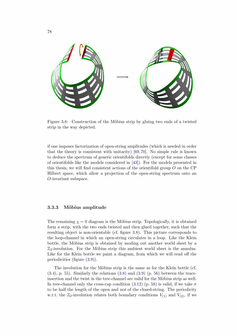
78

Figure 3.8: Construction of the Mobius strip by gluing two ends of a twistedstrip in the way depicted.

if one imposes factorization of open-string amplitudes (which is needed in orderthat the theory is consistent with unitarity) [69, 70]. No simple rule is knownto deduce the spectrum of generic orientifolds directly (except for some classesof orientifolds like the models considered in [43]). For the models presented inthis thesis, we will find consistent actions of the orientifold group O on the CPHilbert space, which allow a projection of the open-string spectrum onto anO-invariant subspace.

3.3.3 Mobius amplitude

The remaining χ = 0 diagram is the Mobius strip. Topologically, it is obtainedform a strip, with the two ends twisted and then glued together, such that theresulting object is non-orientable (cf. figure 3.8). This picture corresponds tothe loop-channel in which an open-string circulates in a loop. Like the Kleinbottle, the Mobius strip is obtained by moding out another world sheet by aZ2-involution. For the Mobius strip this ambient world sheet is the annulus.Like for the Klein bottle we paint a diagram, from which we will read off theperiodicities (figure (3.9)).

The involution for the Mobius strip is the same as for the Klein bottle (cf.(3.4), p. 55). Similarly the relations (3.8) and (3.9) (p. 56) between the trace-insertion and the twist in the tree-channel are valid for the Mobius strip as well.In tree-channel only the cross-cap condition (3.12) (p. 58) is valid, if we take σto be half the length of the open and not of the closed-string. The periodicityw.r.t. the Z2-involution relates both boundary conditions V(1) and V(2), if we

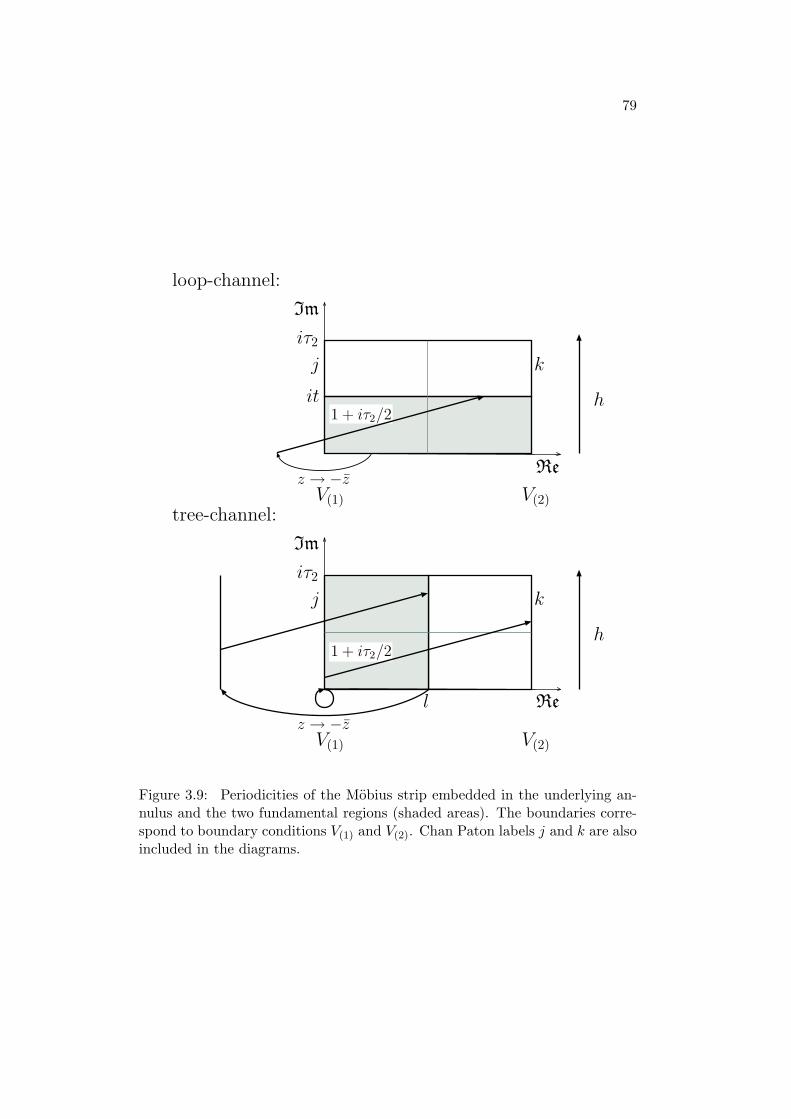
79

loop-channel:

Im

iτ2

it h1 + iτ2/2

z → −zRe

tree-channel:

Im

iτ2

h1 + iτ2/2

l

z → −z

Re

j k

V(1) V(2)

j k

V(1) V(2)

Figure 3.9: Periodicities of the Mobius strip embedded in the underlying an-nulus and the two fundamental regions (shaded areas). The boundaries corre-spond to boundary conditions V(1) and V(2). Chan Paton labels j and k are alsoincluded in the diagrams.

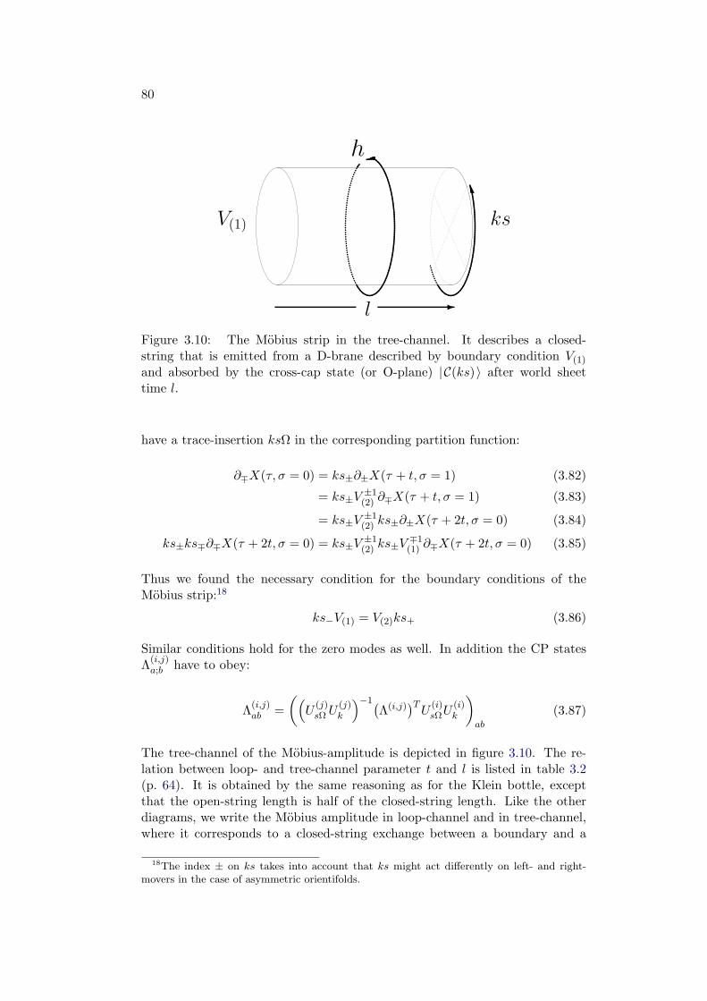
80

ks

h

V(1)

-

l

Figure 3.10: The Mobius strip in the tree-channel. It describes a closed-string that is emitted from a D-brane described by boundary condition V(1)

and absorbed by the cross-cap state (or O-plane) |C(ks)〉 after world sheettime l.

have a trace-insertion ksΩ in the corresponding partition function:

∂∓X(τ, σ = 0) = ks±∂±X(τ + t, σ = 1) (3.82)

= ks±V±1(2) ∂∓X(τ + t, σ = 1) (3.83)

= ks±V±1(2) ks±∂±X(τ + 2t, σ = 0) (3.84)

ks±ks∓∂∓X(τ + 2t, σ = 0) = ks±V±1(2) ks±V

∓1(1) ∂∓X(τ + 2t, σ = 0) (3.85)

Thus we found the necessary condition for the boundary conditions of theMobius strip:18

ks−V(1) = V(2)ks+ (3.86)

Similar conditions hold for the zero modes as well. In addition the CP statesΛ(i,j)a;b have to obey:

Λ(i,j)ab =

((U

(j)sΩU

(j)k

)−1(Λ(i,j)

)TU

(i)sΩU

(i)k

)ab

(3.87)

The tree-channel of the Mobius-amplitude is depicted in figure 3.10. The re-lation between loop- and tree-channel parameter t and l is listed in table 3.2(p. 64). It is obtained by the same reasoning as for the Klein bottle, exceptthat the open-string length is half of the closed-string length. Like the otherdiagrams, we write the Mobius amplitude in loop-channel and in tree-channel,where it corresponds to a closed-string exchange between a boundary and a

18The index ± on ks takes into account that ks might act differently on left- and right-movers in the case of asymmetric orientifolds.

81

cross-cap state.

Mi(ks) = tr(γ

(i)ksΩ

(γ

(i)ks

)−1γ

(i)ksΩ

(γ

(i)ks

))· V10

(2π)dlimε→0

∫ ∞

ε

dt

tZMi (3.88)

=∫dl⟨C(ks)

∣∣e−2πl(H+H)h=(kΩs)2-twisted∣∣D(V(i));h

⟩+ c.c. (3.89)

ZMi(h) = ZMiab(ksΩ) ≡

1|O|

tr(Vi,(ks)−1Vi(ks))

\HCP

ksΩ e−2πt(Hθ(jl)) (3.90)

The subscript under the tr indicates that the CP-trace is excluded in this ex-pression in accordance with eq. (3.55). Condition (3.86) is already imposed.We have used the common notation U

(i)g = γ

(i)g for the representation of O on

the CP Hilbert space. Summing Mi(ks) over all i ∈ bdy-conditions as wellas over all trace-insertions ksΩ compatible with (3.86), we obtain the wholeMobius amplitude. Written in tree-channel it takes the form:

M =∫dl∑h∈G

⟨C|s;h


∣∣D;h⟩

+ c.c. (3.91)

The fact that eq. (3.89) and (3.91) take this special form is highly non-trivial(and we do not prove it). It follows from the normalization of the cross-capand boundary states, which is determined by rewriting the Klein bottle andannulus loop-amplitudes as tree-channel amplitudes. This form (especially theprefactor) is deeply linked to the dimension of the target space. For generalCFTs it can be different. However in all models presented in this paper, thisfactor is present. It is important for rewriting the whole amplitude as a perfectsquare:

KB + M + A

=∫dl∑h∈G

(〈C|s;h |+ 〈D;h |

)e−2πl(H+H)h2-twisted

(|C|s;h〉+ |D;h〉

)(3.92)

In addition, this factorization imposes conditions on the representation matri-ces γ(i)

... . The ability to write this amplitude as a perfect square leads to itsfactorization in the limit of huge world-sheet-times l. The cancellation of theoverall tadpole requires the l→∞ limit of the integrand in (3.92) to vanish sep-arately for each physically distinguishable closed-string excitation. In this limitonly the closed-string q0-term, i.e. massless modes can contribute. Each inde-pendent tadpole must be canceled separately. In the Z4-orientifold of chapter 7this means that branes wrapped around blown up fix-points have to cancel theirtwisted sector charges on each fix-point individually. Furthermore, physicallydifferent tadpoles might be distinguished by their dependence on geometricaldata like the volume (complex structure, etc. ). The tadpole cancellation con-ditions impose constraints both on the allowed boundary conditions V(i) andon the representation matrices γ of the orientifold group O. These constraintsstill leave some freedom in many cases. Requiring supersymmetry can furtherreduce this freedom and leads in some cases to a unique solution. To be more

82

specific: The Id trace-insertion determines the dimension(s) of the CP-Hilbertspace(s). This is usually identified with the number of D-branes (though differ-ent authors sometimes include or exclude the sΩ and/or G images of the branesin their counting). The sΩ-insertion (i.e. the Mobius amplitude without furtherinsertions) also fixes the form of the U (i)

sΩ matrices. Usually the Id sector leads

to a binomial formula of the type (N − C)2 != 0. C is associated with the cou-pling of the cross-cap to the field that generates the tadpole. In the simplestcase N counts the number of branes. More generally it includes topologicaldata for the RR sector and data which depends on differential (i.e. not purelytopological) properties of the brane for NSNS sector tadpoles. If different un-twisted sectors are present one gets several of these binomial formulæ. Nontrivial trace-insertions lead generically to twisted sector tadpoles. They con-strain the form of the U (i)

g (or γ(i)g ) matrices. Often a geometrical interpretation

of some invariants like trU (i)g is accessible. In the Z4 models of chapter 7 this

trace is interpreted as the wrapping number of the brane (i) around (blown-up) g ∈ Z2-twisted cycles. As boundary states have often an interpretation interms of geometrical D-branes, which are (connected) sub-manifolds, one couldalso determine the tadpole conditions via the low-energy effective actions like(3.31) (p. 63) and (3.63) (p. 73). However one should have in mind, that aninterpretation in terms of partition functions always has to exist in order togive a sensible string interpretation.

Instead of modifying the open-string background, one could also try to mod-ify the closed string background, thereby solving the eoms [71]. For examplethe NSNS 3-form field strength couples naturally to the RR 4-form potential aswell as to the RR 3-form field strength in the CS-action of Type IIB theory.19

One could also combine both possibilities. However the stringy description (inform of a CFT solution) of a non-trivially modified closed-string backgroundis often not known. This is also true for most non-linear, i.e. X-dependentboundary conditions V(i), that relate the left- and right-moving parts of theopen-string in addition to specifying its zero-modes. However linear boundaryconditions are solved more easily. By this one obtains usually a great varietyof different, and often phenomenological appealing solutions including chiralfermions transforming in interesting gauge-groups.20

3.3.4 Orientifolds of supersymmetric strings

In this section we will make some comments about orientifolds of supersym-metric string theories. In addition to the bosonic string sector, world-sheetfermions appear. The fermionic term of the gauge fixed fermionic action lookslike:

Sferm = − 14πα′

∫Md2σ 2i ψµρα∂αψµ (3.93)

19This fact was used in [72] to construct orientifolds with background fluxes20However exceptional groups are not contained in perturbative orientifold spectra.

83

The ψ´s are world-sheet majorana spinors. The two dimensional Dirac matricesρα are in this gauge (h =

(hττ hτσhστ hσσ

)= diag(−1, 1)) :

ρ0 =(

0 1−1 0

), ρ1 =

(0 11 0

)(3.94)

For open-strings it is well known, that one has to include altered boundaryconditions (cf. (3.34)):

ψ+(τ, σ) = κiV(i)ψ−(τ, σ) , σ ∈ ∂Mi (3.95)

The relative sign κiκj = ±1 of a string in the (i, j) sector determines whetherthe open-string belongs to the Ramond (+) or Neveu Schwarz sector (−). Aswe have to fix the κi, this choice is obviously asymmetric in the Neveu Schwarzsector. In the following we write a spinor as:

ψ(τ, σ) =(ψ+

ψ−

)(τ, σ) (3.96)

We have not yet determined how the Z2-involution sΩ (cf. eq. (3.4) , p. 55) actson the world sheet fermions. The trace includes a GSO projection as well. Foropen-strings:

PGSO =1 + (−1)f

2(3.97)

with f the world sheet fermion number and for closed-strings:

PGSO =1 + (−1)fL

2· 1 + (−1)fR

2(3.98)

In order to have a sensible mapping between path-integral and operator formal-ism we have to be able to describe the action of sΩ on the fermionic fields insuch a way, that they are compatible with allowed boundary conditions in thepath-integral. We will consider the three amplitudes seperately:

3.3.4.1 Fermionic sector of the Klein bottle

In the ferionic sector, additional signs can be inserted in the boundary condi-tions compared to the bosonic sector. For example a fermion is usually anti-periodic in τ -direction. The GSO projection adds however the time-periodicboundary condition as well. In operator formalism, this corresponds to a (−1)f

insertion, f being the world sheet fermion number (possibly restricted to theleft- or right-moving sector). A Ramond fermion is periodic in σ, while a Neveu-Schwarz fermion is antiperiodic in this direction. This describes the situationfor the torus amplitude. For the Klein bottle and the two remaining χ = 0amplitudes, we will proceed in the spirit of [73]: We will first add all possiblesigns in to the bosonic boundary conditions and determine further restrictionson these signs afterwards. For the following discussion we refer again to figure3.1 (p. 57). There are two possible signs in the τ -direction:

hψ(τ, σ) = diag(ε1, ε2)ψ(τ + 2t, σ) (3.99)

84

Furthermore, we know that ksΩ exchanges left- and right-movers. In thefermionic sector there are possibly additional signs. We will write the fermionicanalog of ksΩ as

ksΩ = ks

(0 χ1

χ2 0

)(3.100)

Furthermore there is a twist that determines if the string is in the NS or R(precisely NSNS, RR, NSR or RNS) sector of the loop-channel:

gψ(τ, σ) = diag(κ1, κ2)ψ(τ, σ + 1) (3.101)

From condition (3.8) we derive:

(ksΩ)2 = h =⇒ χ1χ2 = ε1 = ε2 (3.102)

(gksΩ)2 = h =⇒ χ1χ2κ1κ2 = ε1 (3.103)

With (3.102) we get from (3.103):

κ1 = κ2 (3.104)

The above formula states that in the Klein bottle fields have to be either ofRR- or NSNS-type in the loop-channel. The same is also true for the tree-channel due to (3.102). One sign in (3.100), e.g. χ2 can be eliminated by a fieldredefinition. The fermionic part of the two crosscaps is now determined by theconditions:

KB(ks,ksg) =∫

R+

dl⟨C(ks)

∣∣e−2πl(H+H)h-twisted∣∣C(ksg)⟩ with h = (ksΩ)2

(3.105)(ψ−(τ = 0, σ)− ksψ+(τ = 0, σ + 1/2)

)hε-twisted

|C(ks)〉 = 0(ψ+(τ = 0, σ)− χksψ−(τ = 0, σ + 1/2)

)hε-twisted

|C(ks)〉 = 0(3.106)

Similarly we get at the other end:(ψ−(τ = l, σ)− κgksψ+(τ = l, σ + 1/2)

)hε-twisted

|C(ks)〉 = 0(ψ+(τ = l, σ)− (χκ)gksψ−(τ = l, σ + 1/2)

)hε-twisted

|C(gks)〉 = 0(3.107)

The interpretation is as follows: χ determines the GSO projection in the loop-channel. As χ = ε its sign determines whether a state belongs to the RR orNSNS sector in tree-channel. The sign of κ determines whether a state belongsto the NSNS or RR sector in loop-channel. In tree-channel it shows up in anadditional sign in the l-direction. This sign is the analog of a trace-insertion inthe torus amplitude. We will therefore distinguish the tree-channel sector by asign as well. In table 3.3, where all tree-loop channel relations are listed, κ isdenoted by +1 or −1. A general crosscap state is now denoted as follows:(

ψ−(τ = 0, σ)− κaψ+(τ = 0, σ + 1/2))a2ε-twisted

|C(a)|χ, κ〉 = 0(ψ+(τ = 0, σ)− (χκ)aψ−(τ = 0, σ + 1/2)

)a2ε-twisted

|C(a)|χ, κ〉 = 0(3.108)

χ = +1 is the NSNS, χ = −1 the RR sector. The bosonic part fulfills the sameconditions as in (3.15) (p. 59). The complete boundary state is a sum over allfour possible choices for χ, κ.

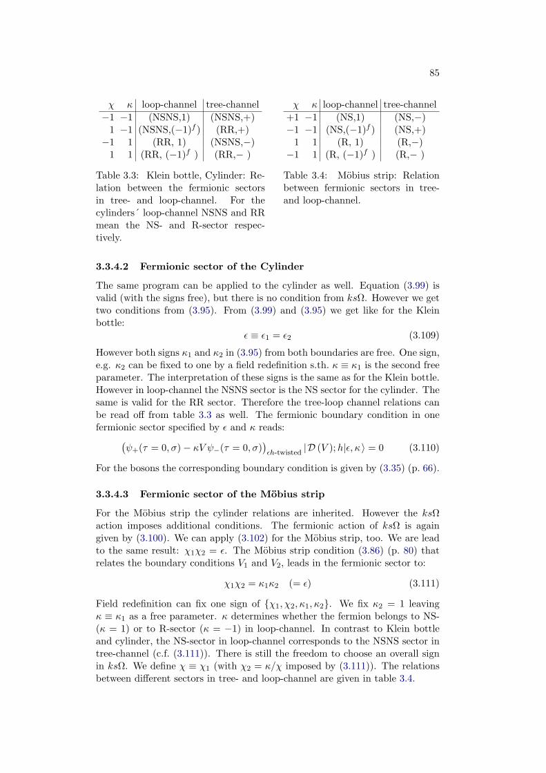
85

χ κ loop-channel tree-channel−1 −1 (NSNS,1) (NSNS,+)

1 −1 (NSNS,(−1)f ) (RR,+)−1 1 (RR, 1) (NSNS,−)

1 1 (RR, (−1)f ) (RR,− )

Table 3.3: Klein bottle, Cylinder: Re-lation between the fermionic sectorsin tree- and loop-channel. For thecylinders´ loop-channel NSNS and RRmean the NS- and R-sector respec-tively.

χ κ loop-channel tree-channel+1 −1 (NS,1) (NS,−)−1 −1 (NS,(−1)f ) (NS,+)

1 1 (R, 1) (R,−)−1 1 (R, (−1)f ) (R,− )

Table 3.4: Mobius strip: Relationbetween fermionic sectors in tree-and loop-channel.

3.3.4.2 Fermionic sector of the Cylinder

The same program can be applied to the cylinder as well. Equation (3.99) isvalid (with the signs free), but there is no condition from ksΩ. However we gettwo conditions from (3.95). From (3.99) and (3.95) we get like for the Kleinbottle:

ε ≡ ε1 = ε2 (3.109)

However both signs κ1 and κ2 in (3.95) from both boundaries are free. One sign,e.g. κ2 can be fixed to one by a field redefinition s.th. κ ≡ κ1 is the second freeparameter. The interpretation of these signs is the same as for the Klein bottle.However in loop-channel the NSNS sector is the NS sector for the cylinder. Thesame is valid for the RR sector. Therefore the tree-loop channel relations canbe read off from table 3.3 as well. The fermionic boundary condition in onefermionic sector specified by ε and κ reads:(

ψ+(τ = 0, σ)− κV ψ−(τ = 0, σ))εh-twisted

|D (V );h|ε, κ〉 = 0 (3.110)

For the bosons the corresponding boundary condition is given by (3.35) (p. 66).

3.3.4.3 Fermionic sector of the Mobius strip

For the Mobius strip the cylinder relations are inherited. However the ksΩaction imposes additional conditions. The fermionic action of ksΩ is againgiven by (3.100). We can apply (3.102) for the Mobius strip, too. We are leadto the same result: χ1χ2 = ε. The Mobius strip condition (3.86) (p. 80) thatrelates the boundary conditions V1 and V2, leads in the fermionic sector to:

χ1χ2 = κ1κ2 (= ε) (3.111)

Field redefinition can fix one sign of χ1, χ2, κ1, κ2. We fix κ2 = 1 leavingκ ≡ κ1 as a free parameter. κ determines whether the fermion belongs to NS-(κ = 1) or to R-sector (κ = −1) in loop-channel. In contrast to Klein bottleand cylinder, the NS-sector in loop-channel corresponds to the NSNS sector intree-channel (c.f. (3.111)). There is still the freedom to choose an overall signin ksΩ. We define χ ≡ χ1 (with χ2 = κ/χ imposed by (3.111)). The relationsbetween different sectors in tree- and loop-channel are given in table 3.4.

86

Concluding remarks

We presented basic notions of orientifolds, including subjects like tadpoles,cross-cap- and more generally: boundary-states, Chan Paton factors and non-orientable world-sheets. Special emphasis was put on the open-closed stringcorrespondence of the one-loop vacuum amplitudes. Of course, we could notcover all subjects. Boundary states for examples can be defined via more gen-eral symmetries than the ones derived from the chiral fields ∂±Xµ (cf. [74,75]).We also excluded the ghost sector from our discussion, as we work in light-conequantization in most of the following chapters. We have not been very precisein specifying the boundary states, i.e. solving the boundary state conditions.This will however be done in some examples in the following chapters.

We also restricted to the case of orientifolds that stem from orbifolds ofsmooth manifolds. We want to mention that other interesting constructionsexist including for example orientifolds on WZNW-models (describing smoothmanifolds as well) and Coset-spaces (cf. [76,77,78,79]). The spectrum of stringsand D-branes can be investigated by advanced means of the corresponding CFT.Also more geometrical approaches to D-branes and open strings have been un-dertaken (cf. [31] and references given there). The relatively simple orbifolds(though interesting as they usually contain singularities) serve as valuable ex-amples and give hints to more general (mathematical) descriptions of D-branes.

There exists a huge amount of literature on orientifolds and it is impossibleto cite all of the publications. Some articles with major contributions to the fieldhave been cited in the text, many others not. In the remaining chapters we willmention additional publications, many dealing directly with orientifolds. Notmany survey articles have been written on orientifolds however, so it is not toohard to mention some. Polchinski, who did many important work, introducesorientifolds in his two books on string theory [7, 8]. Even though the name“orientifold” was not in use around that time, some basics about open (orientedand non-oriented) superstring theories can be found in the two volumes writtenby Green, Schwarz and Witten [4, 5]. In 1997, Atish Dabholkar gave a lectureon orientifolds in Trieste. The notes can be found in the internet [80]. Morerecently Angelantonj and Sagnotti published an overview article [18] that isdevoted to the CFT-oriented approach to orientifolds, developed by Sagnottiand collaborators from the mid-eighties onwards.

Even though the material is not complete, we hope that it gives the readernecessary tools to follow the sucsessive text.

Chapter 4

Open Strings in Electro-Magnetic Background-Fields

In this chapter we will quantize the bosonic open string with linear boundaryconditions in flat space-time. These are given both by the fact that D-branesare lower dimensional hypersurfaces the string end-points are confined to and bythe constant NSNS two-form B in combination with the NS U(1)-field strengthF . The generalization to superstrings is straightforward and simpler than thebosonic case.1 We will generalize the result of [83,84] on the non-commutativityof string fields Xµ(τ, σ) located at the boundary to the one loop case (in com-parison with [83]) and to the case where the boundary conditions on bothboundaries are given by NS field-strengths F1 and F2 that are constant, butcompletely independent form each other (in comparison with [84]). There aremany other approaches to derive the commutator as well. A prominent one isby deformation quantization [85], others are guided by constrained (or Dirac)quantization [86, 87]. Laidlaw calculated the propagator for the cylinder withindependent, constant U(1) F -fields at the boundaries and reproduced the re-sult for the commutator as well [88]. The list is surely not complete. We wantto mention that the approach to solve the string boundary conditions, which isactually a variant of a doubling trick, was motivated by [89, 90, 91] where theboundary condition problem for open strings on intersecting D-branes of arbi-trary dimension without NS and NSNS background fields was solved.2 Howeverwe adopted another quantization method here: We first calculate the canonicaltwo-form in terms of the individual modes. Then we restrict to its invertiblepart. The inverse is (up to a factor) the Poisson-bracket.

We present a new and (to our knowledge) first direct derivation of the open

1There is a subtlety in deriving the boundary conditions for the world sheet fermions fromthe action. Instead of coupling the fermions to the boundary-U(1)-field strength F via aboundary term in the action, which might over-constrain the problem, we impose fermionicboundary conditions by hand. We demand these fermionic boundary conditions to be com-patible with super-symmetry transformations which also have to be reduced (to one half ofthe bulk super-symmetry) at the boundary (i.e. super-symmetry invariance under the fullMajorana spinor ε (cf. eq. (4.7)) over-constrains the problem, too). See also [81,82].

2Of course the term D-brane was not used around that time. The authors also gave nospace-time interpretation of the boundary conditions in the spirit of [92].

87

88

string mass formula for toroidally compactified D-branes with magnetic fields(section 4.2.1.3).

4.1 Action and boundary conditionsof the open string

We consider the following superconformal-gauge action (space-time metric Gµνis of signature (1, d− 1) ):

S = Sbos + Sferm (4.1)

with the convention ετσ = 1:

Sbos = Sbulkbos + Sbdy

bos

= − 14πα′

(∫Md2σ ∂αX

µ∂αXµ −Bµνεαβ∂αXµ∂βXν + 2

∫∂M

dτ XµAµ

)(4.2)

Sferm = − 14πα′

∫Md2σ 2i ψµρα∂αψµ (4.3)

In case of a constant U(1)-field strength with the gauge Aν = Xµ

2 Fµν , (Fµν =∂µAν − ∂νAµ) and constant Bµν equation (4.2) reduces to:3

Sbos = − 14πα′

(∫Md2σ ∂αX

µ∂αXµ − 2Xµ(B)µνX ′ ν −∫∂M

dτ Xµ(F )µνXν

)(4.4)

The ψ‘s are world-sheet Majorana spinors. The two dimensional Dirac matricesρα are in this gauge (h =

(hττ hτσhστ hσσ

)= diag(−1, 1)) :

ρ0 =(

0 1−1 0

), ρ1 =

(0 11 0

)(4.5)

They satisfy the algebra: ρα, ρβ

= 2hαβ (4.6)

The spinor conjugate to λ :=( λ+

λ−

)is λ := λ†ρ0 = (−λ−, λ+). The charge

conjugation matrix C is defined as ρ0. Then a Majorana spinor is real. Theaction 4.1 is invariant under the following bulk super-symmetry transformation:

δεXµ = iεψµ δεψ

µ =12ρα(∂αX

µ)ε (4.7)

In the case of constant Gµν the variation of the bosonic action with respect toXµ gives the bulk equation of motion(

∂2τ − ∂2

σ

)Xµ = 4∂+∂−X

µ = 0 (4.8)

3Then Bµνεαβ∂αX

µ∂βXν = Bµνd(X

µ · dXν) = d(Bµν(Xµ · dXν)) with d the exteriorderivative on the world sheet.

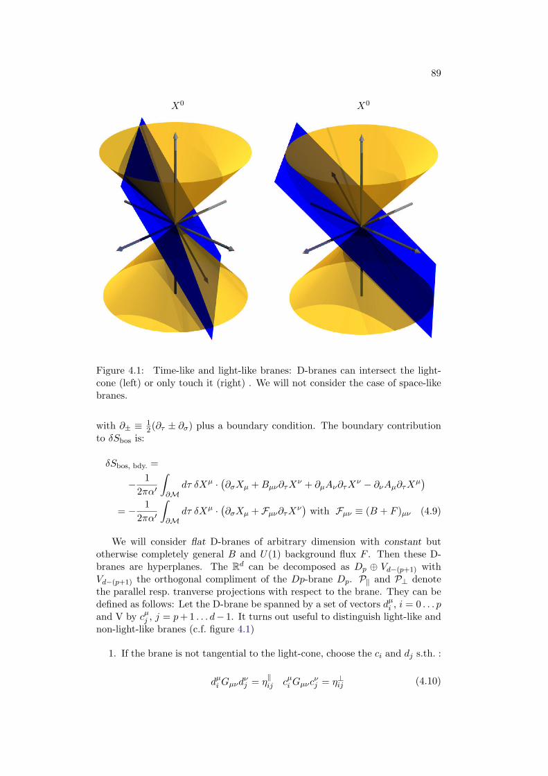
89

X0 X0

Figure 4.1: Time-like and light-like branes: D-branes can intersect the light-cone (left) or only touch it (right) . We will not consider the case of space-likebranes.

with ∂± ≡ 12(∂τ ± ∂σ) plus a boundary condition. The boundary contribution

to δSbos is:

δSbos, bdy. =

− 12πα′

∫∂M

dτ δXµ ·(∂σXµ +Bµν∂τX

ν + ∂µAν∂τXν − ∂νAµ∂τXµ

)= − 1

2πα′

∫∂M

dτ δXµ ·(∂σXµ + Fµν∂τXν

)with Fµν ≡ (B + F )µν (4.9)

We will consider flat D-branes of arbitrary dimension with constant butotherwise completely general B and U(1) background flux F . Then these D-branes are hyperplanes. The Rd can be decomposed as Dp ⊕ Vd−(p+1) withVd−(p+1) the orthogonal compliment of the Dp-brane Dp. P‖ and P⊥ denotethe parallel resp. tranverse projections with respect to the brane. They can bedefined as follows: Let the D-brane be spanned by a set of vectors dµi , i = 0 . . . pand V by cµj , j = p+1 . . . d− 1. It turns out useful to distinguish light-like andnon-light-like branes (c.f. figure 4.1)

1. If the brane is not tangential to the light-cone, choose the ci and dj s.th. :

dµi Gµνdνj = η

‖ij cµi Gµνc

νj = η⊥ij (4.10)

90

By definition, dµi Gµνcνj = 0. η(·) = diag(−1, 1 . . . 1) or = Id, if the sub-

space contains a space-like direction or not.

(P‖)µν≡∑i∈Dp

(η‖)iidµi d

λiGλν

(P⊥)µν≡

d∑i∈Vd−p+1

(η⊥)iicµi c

λiGλν

(4.11)

2. If the brane is tangential to the light-cone let dµ0 ∈ Dp be light-like. Thenwe choose dν0 and cνp+1 s.th. dµ0Gµνc

νp+1 = 1 which is always possible. All

other inner products involving one of the light-like dν0 and cνp+1 with theother basis-vectors should vanish. This means that the other vectors liein a subspace that is perpendicular to the one spanned by d0 and cp+1

For the remaining vectors we can achieve:

dµi Gµνdνj = δij i, j = 1 . . . p; cµi Gµνc

νj = δij i, j = p + 2 . . . d

(4.12)In this case: (

P‖)µν≡ dµ0c

λp+1Gλν +

p∑i=1

dµi dλiGλν

(P⊥)µν≡ cµp+1d

λ0Gλν +

d∑i=p+2

cµi cλiGλν

(4.13)

We further choose cp+1 to be light-like as well (which is achieved by addingλd0 with appropriate λ). This will ensure the relation R = R−1 in (4.15).

The two cases are not continuously connected. In some of the following for-mulæ we will omit the indices. They can be added by taking into account thatin matrix-multiplication an upper index is contracted with a lower one. Inaddition, matrix inversion changes an upper to a lower index and vice versa.Indices are raised and lowered by Gµν and Gµν . Then

P‖ + P⊥ = G (4.14)

P‖ − P⊥ ≡ R, R invertible, R = R−1 (4.15)

The resulting bdy.-conditions are valid even for non-constant G and F (F‖ ≡PT‖ FP‖): (

PT‖ G∂σ + F‖ ∂τ)X(τ, σ)

∣∣σ∈∂M =(

PT‖ G (∂+ − ∂−) + F‖ (∂+ + ∂−))X(τ, σ)

∣∣σ∈∂M =0

(4.16)

P⊥X(τ, σ)∣∣σ∈∂M = U ici i = p+ 1 . . . d U i ∈ R, const. (4.17)

P⊥ is constant for a hyperplane. We can differentiate (4.17) w.r.t. τ . The bdy.-condition can be reformulated as a relation between the left- and right-movingpart of the open string. One has to distinguish light-like and other branes. Inthe non-light-like case PTG = GP. Therefore:

∂−X(τ, σ) =(GR−F‖

)−1(G+ F‖

)∂+X(τ, σ)

=(G−F‖

)−1(GR+ F‖

)∂+X(τ, σ)

for σ ∈ ∂M (4.18)

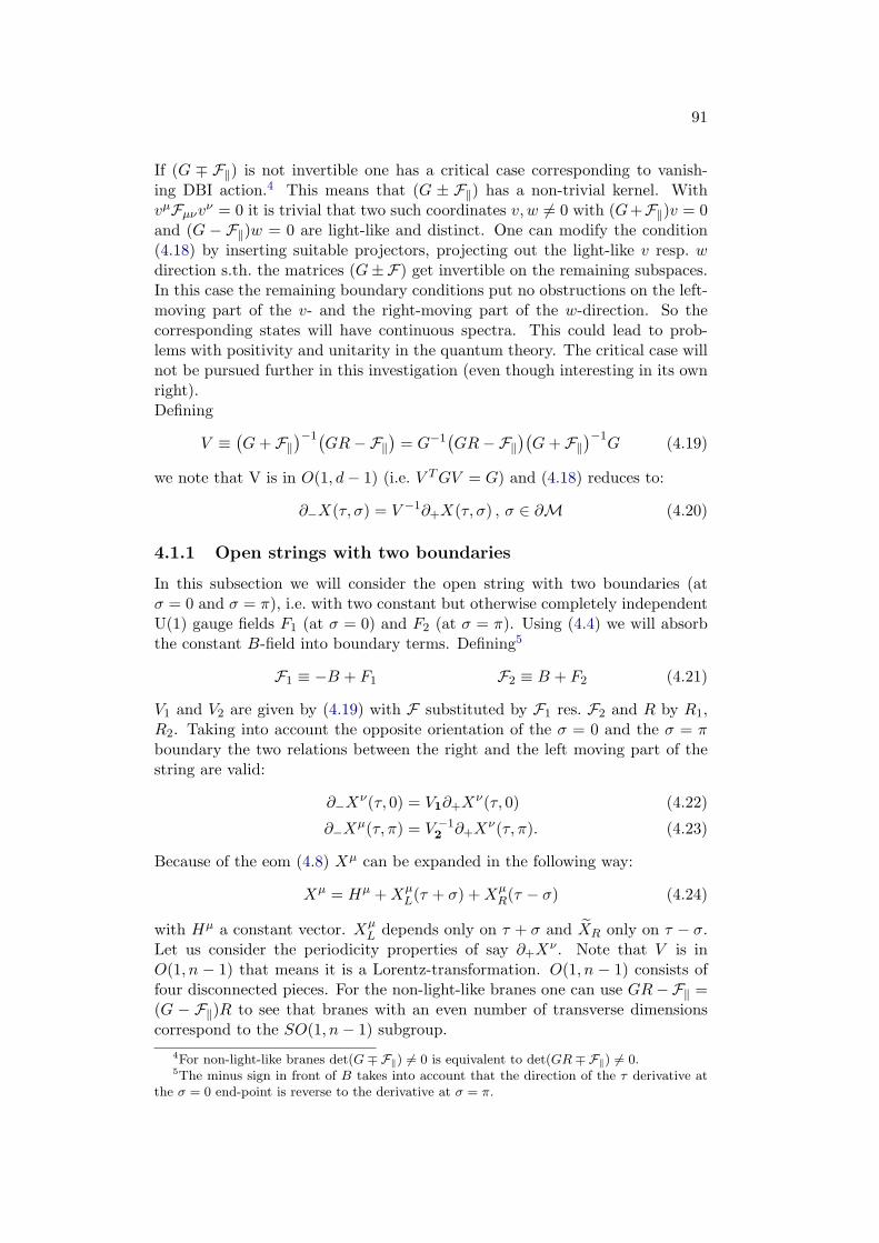
91

If (G ∓ F‖) is not invertible one has a critical case corresponding to vanish-ing DBI action.4 This means that (G ± F‖) has a non-trivial kernel. WithvµFµνvν = 0 it is trivial that two such coordinates v, w 6= 0 with (G+F‖)v = 0and (G − F‖)w = 0 are light-like and distinct. One can modify the condition(4.18) by inserting suitable projectors, projecting out the light-like v resp. wdirection s.th. the matrices (G±F) get invertible on the remaining subspaces.In this case the remaining boundary conditions put no obstructions on the left-moving part of the v- and the right-moving part of the w-direction. So thecorresponding states will have continuous spectra. This could lead to prob-lems with positivity and unitarity in the quantum theory. The critical case willnot be pursued further in this investigation (even though interesting in its ownright).Defining

V ≡(G+ F‖

)−1(GR−F‖

)= G−1

(GR−F‖

)(G+ F‖

)−1G (4.19)

we note that V is in O(1, d− 1) (i.e. V TGV = G) and (4.18) reduces to:

∂−X(τ, σ) = V −1∂+X(τ, σ) , σ ∈ ∂M (4.20)

4.1.1 Open strings with two boundaries

In this subsection we will consider the open string with two boundaries (atσ = 0 and σ = π), i.e. with two constant but otherwise completely independentU(1) gauge fields F1 (at σ = 0) and F2 (at σ = π). Using (4.4) we will absorbthe constant B-field into boundary terms. Defining5

F1 ≡ −B + F1 F2 ≡ B + F2 (4.21)

V1 and V2 are given by (4.19) with F substituted by F1 res. F2 and R by R1,R2. Taking into account the opposite orientation of the σ = 0 and the σ = πboundary the two relations between the right and the left moving part of thestring are valid:

∂−Xν(τ, 0) = V1∂+X

ν(τ, 0) (4.22)

∂−Xµ(τ, π) = V −1

2 ∂+Xν(τ, π). (4.23)

Because of the eom (4.8) Xµ can be expanded in the following way:

Xµ = Hµ +XµL(τ + σ) +Xµ

R(τ − σ) (4.24)

with Hµ a constant vector. XµL depends only on τ + σ and XR only on τ − σ.

Let us consider the periodicity properties of say ∂+Xν . Note that V is in

O(1, n − 1) that means it is a Lorentz-transformation. O(1, n − 1) consists offour disconnected pieces. For the non-light-like branes one can use GR−F‖ =(G − F‖)R to see that branes with an even number of transverse dimensionscorrespond to the SO(1, n− 1) subgroup.

4For non-light-like branes det(G∓F‖) 6= 0 is equivalent to det(GR∓F‖) 6= 0.5The minus sign in front of B takes into account that the direction of the τ derivative at

the σ = 0 end-point is reverse to the derivative at σ = π.

92

4.1.2 Solution to linear boundary conditions for the cylinder

Defining another w.s.-time τ = τ + π (π the open string length) the first bdy.-condition (4.22) reads:

∂−Xµ(τ − π, 0)︸︷︷︸

=∂−Xµ(τ ,π)

=(V1

)µν∂+X

ν(τ, 0) (4.25)

Plugging the left hand side into the second condition (4.23) one gets:

∂−Xµ(τ , π) =

(V −12

)µν∂+X

ν(τ , π)︸︷︷︸=∂+Xµ(τ,2π)

(4.26)

Combining the last two equations we see that the following quasi-periodicityholds for ∂+X

µ:

∂+Xµ(τ + σ + 2π) =

(V2V1

)µν∂+X

ν(τ + σ) (4.27)

As V1,2 (and therefore their product) are in O(1, n − 1) ⊂ U(1, n − 1), V2V1

admits in general n− 1 complex Eigenvectors Cµλiwith Eigenvalues λ (|λ| = 1)

and two real Eigenvalues ξ, ξ−1 which belong to two real Eigenvectors Cµξand Cµ

ξ−1 .6 We assume the Cµλito be ”ortho-normalized”(always possible in

the case at hand) with respect to the hermitian scalar product 〈C1, C2〉 ≡∑µC

µ1∗GµνC

ν2 . As V2V1 is real, for every λi, λ∗i is Eigenvalue (with Eigenvector

Cµλ∗ = Cµλ∗), too. For ξ 6= ±1, Cµξ and Cµ

ξ−1 are light-like. As their scalarproduct is non-vanishing, we will normalize Cµξ and Cµ

ξ−1 such that⟨Cξ−1 , Cξ

⟩=

1. Cξ−1 , Cξ are perpendicular to the Cλi. Let us represent λi as

λ1 = exp(i2π(−i2π ln ξ) = exp(i2πθ1) (4.28)λ2 = exp(i2π( i

2π ln ξ) = exp(i2πθ2) (4.29)λi = exp(i2πθi) (4.30)

−1/2 < θi ≤ 1/2, i = 3 . . . n and Im 3 θ1,2 = ± i2π ln ξ. Denote λ∗i by λ−i for

i = 3 . . . n and λ−1 = λ2. Similarly θ−i = −θi represents λ−i. Note howeverthat there are cases without light-like Eigenvectors. For example a pure spacerotation could lead (in odd space dimensions) to a time-like Eigenvector withEigenvalue λ = 1. The following useful identity holds:∑

i

Cµi Cν−i = Gµν (4.31)

We will abbreviate the λ` = 1 Eigenvectors as C`, C, etc. With ∂±Xµ =

∂±XµL/R we see that XL/R is of the form:

XµL = const+

( ∑`:λ`=1

Cµ` p`(τ +σ)

)+

√α′

i√

2

∑j

Cµj∑′

nj∈Z+θj

aj−nj

njeinj(τ+σ) (4.32)

6This is derived in appendix C, where also the other stated facts on the Eigenvectors areproven. We exclude a degenerate case (in which our statement about the Eigenvectors wouldbe wrong and) that might show up for some special light-like Eigenvectors with Eigenvalueλ = ±1, from our further analysis. We shed some light on this case in appendix C as well.For a purely magnetic Fi-field the transformation Vi is actually a rotation (i.e. ∈ O(n)).

93

In the following we will absorb the constant part of the XL and XR-field intothe common constant Hµ (eq. (4.24)). Boundary condition (4.22) prescribeswhat XR has to be:

∂−XµR(τ − σ, 0) =

(V1

)µν∂+X

νL(τ − σ, 0) (4.33)

∂−XµR(τ − σ) =

(V1

)µν∂+X

νL(τ + (−σ)) (4.34)

In the last equation the differentials act on the functions argument. This thenleads to:

XµR =

( ∑`:λ`=1

(V1

)µνCν` p

`(τ − σ))

+

√α′

i√

2

∑j

(V1

)µνCνj

∑′

nj∈Z+θj

aj−nj

njeinj(τ−σ)

(4.35)Thus we have the following mode expansion of Xµ(τ, σ):

Xµ =

0-modes︷︸︸︷Hµ +

linear modes︷︸︸︷∑`:λ`=1

((τ + σ) Id+(τ − σ)V1)µν Cν` p

`

+

√α′

i√

2

∑j

∑′

nj∈Z+θj

aj−nj

nj

(einj(τ+σ)Cµj +

(V1

)µνCνj e

inj(τ−σ))

︸︷︷︸oscillator-modes

(4.36)

The Dirichlet condition (4.17) imposes further restriction on the zero-mode partof the string. At σ = 0 the brane (hyperplane) is located at P⊥,1U = U1. ThenP⊥,2U2 = U2 specifies the position of the σ = π brane. We become aware that

P⊥,1V ±11 = −P⊥,1 P⊥,2V ±1

2 = −P⊥,2 (4.37)

as well asV1Cλ`

= V −12 Cλ`

for λ` = 1 (4.38)

with λ` the Eigenvalue of V2V1. Let us rewrite the zero- and linear-modes ofX:

Xµ0 = Hµ +

( ∑`:λ`=1

(τ (Id+V1)µν + σ (Id−V1)µν)Cν` p

`

)(4.39)

4.1.2.1 World sheet momentum and Hamiltonian

In order to quantize the string one has to know the (gauge-dependent) canonicalmomentum:

Pµ(σ) =∂

∂Xµ

L(X, ∂X)

=1

2πα′(Xµ +Bµ

νX′ ν −

(δ(σ)Aµ1 + δ(σ − π)Aµ2

))(4.40)

=1

2πα′(Xµ +Bµ

νX′ ν +

12(δ(σ)F µ

1 νXν + δ(σ − π)F µ

2 νXν))

(4.41)

94

Equation (4.40) is valid for all U(1)-field strengths, (4.41) only for constantfield strengths in our particular gauge. The momentum is not conserved sincethe Lagrangian varies under pure translations.7

Another important quantity is the world sheet Hamiltonian:

H =∫ π

0dσ Pµ(σ)Xµ − L(σ) =

14πα′

∫ π

0dσ XµXµ +X ′µX ′

µ

=1

2πα′

∫ π

0dσ ∂+X

µ∂+Xµ + ∂−Xµ∂−Xµ =

1πα′

∫ π

0dσ ∂+X

µ∂+Xµ (4.42)

H is gauge invariant in terms of the Xµ’s and its derivatives. With

∂+Xµ0 = Cµ` p

` (4.43)

the momentum-mode part of the Hamiltonian is:

Hlin =1α′Cµ GµνC

ν`︸︷︷︸

≡G`

pp` (4.44)

Similarly one obtains the oscillator-part (which still has to be normal ordered):

Hosc. =12

∑k

∑′

nk∈Z+θk

Cµ−kGµνCνk︸︷︷︸

≡G−k k

a−knkak−nk

(4.45)

4.2 Quantization of open strings with linear bound-ary conditions

In the following we will quantize the classical solution. To do this, we firstcalculate the canonical two-form Ω(P,X) in terms of the classical solution whichwe restrict in a second step to a subspace on which Ω(P,X) is nondegenerate.The inverse of Ω(P,X) (on this subspace) defines the Poisson-bracket. Bysubstitution of the Poisson bracket by −i times the commutator we performthe transition to the quantized string. Alternatively one could have tried toimplement the boundary conditions via a Dirac-bracket. However we thinkthat the method applied here is more direct and less complicated.

7By momentum we mean also the integral∫dσP .

95

4.2.1 Canonical two-form and canonical quantization

In order to quantize the system lets look at the canonical two-form8

Ω(P,X) =∫ π

0dσ DPµ ∧DXµ (4.46)

=1

2πα′

∫ π

0dσ(DXµ ∧ DXµ

+ 12(δ(σ)F1 + δ(σ − π)F2)µνDX

ν ∧DXµ + 12B

µν

∂

∂σ

(DXν ∧DXµ

))=

12πα′

∫ π

0dσ(DXµ ∧ DXµ

+ 12 (δ(σ)F1 + δ(σ − π)F2)µν DX

ν ∧DXµ

)(4.47)

which is time independent in case of constant field strengths, two-form potentialB and on-shell Xµ:9

d

dτΩ(P,X) =

12πα′

∫ π

0dσ(=DX′′µ︷︸︸︷DXµ ∧DXµ + (δ(σ)F1 + δ(σ − π)F2)µνDX

ν ∧DXµ

)=

12πα′

∫ π

0dσ d

(DX ′µ ∧ DXµ

)+DX ′µ ∧ DX ′

µ︸︷︷︸=0

+(δ(σ)F‖1 + δ(σ − π)F‖2

)µνDXν ∧DXµ = 0

Therefore one can neglect the τ -dependent parts of Ω.

4.2.1.1 Quantization of zero- and linear-modes

The following two expressions are useful to follow the discussion:

Xµ0 = (G+ V1)µνC

ν` p

` Xµτ -indep. = Hµ + σ(G− V1)µνC

ν` p

` (4.48)

The Poisson bracket is the inverse of the restriction Ω|U of the canonical two-form Ω to a subspace U s.th. Ω|U is invertible. To shorten the notation, we willnot write down the derivative D explicitly. We will now quantize the individual

8 DP and DX means the derivative with respect to the target space. Therefore Ω ismanifestly U(1)-gauge invariant since P → P +D ξ and X is invariant.

9In the last line only parallel components of the F fields contribute, as the perpendicularcomponents of Xµ vanish at boundary.

96

(zero) modes:10

Ω0(P,X)

=∫ π

0dσ

( from Xµ∧Xµ︷︸︸︷1

2πα′((G+ V1)µνCν` p

` ∧Hµ + σCµ` (V T1 − V1)µνCν p

` ∧ p))

+1

4πα′(F‖1 + F‖2

)µνHν ∧Hµ

+1

2α′(F2(G− V1)

)µνCν` p

` ∧Hµ +π

4α′Cµ((G− V T

1 )F2(G− V1))µνCν` p

` ∧ p

Summarizing,

Ω0(P,X) =1

4πα′(F‖1 + F‖2

)µνHν ∧Hµ

+1

2α′((G+ V1) +

(F2(G− V1)

))µνCν` p

` ∧Hµ

+π

4α′Cµ((G− V T

1 )F2(G− V1) + (V1 − V T1 ))µνCν` p

` ∧ p (4.49)

Now we will restrict to an invertible subspace. We introduce a system of vectorseµi such that

(A1)ij ≡14πeµi(F‖1 + F‖2

)µνeνj i, j = 1 . . . p (4.50)

is invertible (such a system, (including possibly the empty set) always exists asF‖ i is anti-symmetric). Then we define H i and Ha by:

Hµ = eµiHi + dµaH

a (4.51)

The dµa are made orthogonal to the eµi . Hµ is real as the string coordinate Xµ

is real. This leads to some restrictions on the phase of the H i and Ha. In thequantized version of the string Xµ becomes a hermitian operator. The classicalrestrictions on the H i and Ha lead to some restrictions on their properties asoperators.

In some special cases (i.e. when Dirichlet conditions are absent), the eµiare chosen to be (G + F1)Ci with λi 6= 1. This leads to the simple relationH−i = H i †. The analogous definition da ≡ (G+ F1)Ca with λa = 1 forces thecorresponding Ha to be hermitian in this case.

With this choice and taking into account (4.49) the general form of Ω0|u is(in matrix form):

Ω0|U =1α′

A1 0 K0 0 N−KT −NT A2

(4.52)

10The perpendicular components of Bµν in the term ∝(F1 + F2

)µνHν ∧Hµ cancel.

97

By comparison with (4.49) we identify in addition to (4.50):

(K)i` ≡14eµi

((G+ V1) +

(F2(G− V1)

))µνCν`

(N)a` ≡14dµa

((G+ V1) +

(F2(G− V1)

))µνCν`

(A2)` ≡π

4Cµ((G− V T

1 )F2(G− V1) + (V1 − V T1 ))µνCν`

(4.53)

with i = 1 . . . p; a, `, = p+ 1 . . . r (4.54)

While p is the dimension of im(F‖1 +F‖2

)(or equivalently: the dimension of

A1), (r − p) is the dimension of its kernel. In (4.54) we already used that thematrix N has to be a square matrix. This is true for the following reasons:

1. In order for Ω0|U to be invertible, NT has to be of maximal rank (i.e.dimA2). Therefore the column number of N equals the number of p` dofs(or equivalently: the number of Eigenvalue λ = 1 Eigenvectors of V2V1).

2. In order for (4.52) to be invertible, its determinant has to be 6= 0. If thenumber of rows in N exceeds the dimension of the square matrix A2, atleast two column vectors of Ω0|U would be linear dependent. As a conse-quence the determinant would vanish which contradicts the invertibilityof Ω0|U . As Ω0|U is invertible by definition, N must be a square matrix.

3. As N has maximal rank, it is invertible.

In other words: the space spanned by the dµa has to be reduced such that Ngets invertible which is needed to ensure invertibility of Ω0|U . While A1 andA2 are antisymmetric, K is in general not a square matrix.11 In this notation

Ω0(P,X)|U = xi(Ω0)ij ∧ xj , ~x = (H i,Ha, p) (4.55)

To get the Poisson bracket of the bosonic zero-modes one has to invert Ω0:xi, xj

P.B.

=12(Ω−1

0 )ij (4.56)

The solution is

Ω−10 = α′

A−11 −A−1

1 KN−1 0−(NT)−1

KTA−11

(NT)−1(A2 −KTA−1

1 K)N−1 −(NT)−1

0 N−1 0

(4.57)

As Ω0 is a symplectic form it can be transformed into a more convenient formby a general linear transformation of the zero modes H i, Ha, p.

Ω0 = STΩ0S =1α′

A1 0 00 0 N0 −NT 0

(4.58)

11We found that the dimensions of the spaces 〈da〉 and 〈C;λ = 1〉 is equal. For the specificsituation where the Dirichlet directions are the same for both branes we can even identify:d = C.

98

with

S =

1 0 0−(NT)−1

KT 1(NT)−1

A2/20 0 1

(4.59)

The transformed zero modes H i, H`, p are defined by:

H i

Ha

p

= S−1

H i

Ha

p

=

1 0 0(NT)−1

KT 1 −(NT)−1

A2/20 0 1

H i

Ha

p

(4.60)

The H i, Ha, p have rather simple Poisson-brackets and commutators (all othersvanishing):12

H i, Hk

=α′

2(A−1

1

)ikHa, p

=− α′

2Na

. , . →−i[ . , . ]−−−−−−−−−→

[H i, Hk

]=α′

2i(A−1

1

)ik[Ha, p

]=iα′

2(N−1

)a (4.61)

4.2.1.2 Quantization of oscillator modes

Now we look at the oscillator part of Ω, which is also time independent. Forsimplicity we split Ωosc. into Ω1 + Ω2 and Ω3 where Ω1 + Ω2 ∝ X ∧X is fromthe bulk integral and Ω3 is the boundary term.

12πα′

Xµosc.(τ, σ) ∧Xosc. µ(τ, σ)

=1

2πα′−iα′

2·∑j, l

∑′

nj∈Z+θjml∈Z+θl

eiτ(nj+ml)(Geinjσ + V1e

−injσ)µεCεj

Gµν(Geimlσ + V1e

−imlσ)νκCκl

aj−nj∧ al−ml

ml(4.62)

As we consider only the τ -independent terms, we impose nj = −ml, j = −l.

12πα′

Xµosc.(τ, σ) ∧Xosc. µ(τ, σ) =

−i4π

∑l

∑′

ml∈Z+θl(Cε−l

(Ge−imlσ + V T

1 eimlσ

) µ

ε

(Geimlσ + V1e

−imlσ)µκ︸︷︷︸

=(2G+V −11 ·exp(i2mlσ)+V1·exp(−i2mlσ))εκ

Cκl

)a−lml∧ al−ml

ml(4.63)

12Na is the inverse transposed of Nıb

99

From this we get Ω1 + Ω2:

Ω1 + Ω2 =1

2πα′

∫ π

0dσXµ

osc. ∧Xosc.µ

=

≡Ω1︷︸︸︷−i2

∑l

G−l,l∑′

ml∈Z+θl

a−lml∧ al−ml

ml

−∑l

∑′

ml∈Z+θl

18πCµ−l

(λlCT−l=((V2V1)−1C−l)

T︷︸︸︷V −1

1 (λl −G) −

V1λ−lCl=V−1

2 Cl︷︸︸︷V1(λ−l −G)

)µνCνl

a−lml∧ al−ml

m2l︸︷︷︸

≡Ω2

(4.64)

Ω2 = − 18π

∑′

lml∈Z+θl

Cµ−l

((V2 − V −1

2

)+(V1 − V −1

1

))µνCνl

a−lml∧ al−ml

m2l

(4.65)

Next we will show that Ω2 + Ω3 vanishes. If we assume that this is true weimmediately obtain the Poisson-bracket for the modes (all others vanishing):

al−ml, a−lml

= imlG

−l l (4.66)

Ω3 is the dσ-integral over:

14πα′

(δ(σ)(F1)µνXνosc. + δ(σ − π)(F2)µνXν

osc.) ∧Xosc.µ

= − 18π

(δ(σ)(F1)µν + δ(σ − π)(F2)µν) eiτ(nj+ml)

∑j, l

∑′

nj∈Z+θjml∈Z+θl

(Geinjσ + V1e

−injσ)νεCεj(Geimlσ + V1e

−imlσ)µκCκl

aj−nj∧ al−ml

njml

(4.67)

We only need to consider the τ -independent terms (nj = −ml). Using againλlC

T−l = CT−l(V2V1) = CT−lV2(V T

1 )−1 we can split Ω3 into F‖1 respectively F‖2

dependent terms:

Ω3 = − 18π

∑l

Σ−l,l∑′

ml∈Z+θl

a−lml∧ al−ml

m2l

(4.68)

where we have defined:13

Σ−l,l = Cµ−l((G+ V T

1 )F‖1(G+ V1) + (G+ λlVT1 )F‖2(G+ V1λ

−1l ))µνCνl

= Cµ−l((G+ V −1

1 )F‖1(G+ V1) + (G+ V2)F‖2(G+ V −12 )

)µνCνl (4.69)

13We have projected onto parallel components of the Fi-fields, because G+ Vi contains theprojector P‖,i, that removes the perpendicular components.

100

As Ω2 and Ω3 are symmetric w.r.t. an exchange F‖1 ↔ F‖2 we consider onlyone part, e.g. the F‖1 dependent part:

(Ω2 + Ω3)|F‖ 1

= − 18π

∑l

Cµ−l(G+ V T

1 )

(∗)︷︸︸︷(F‖1(G+ V1)− (G− V1)

)µνCνl

∑′

ml∈Z+θl

a−lml∧ al−ml

m2l

(4.70)

(∗) vanishes: The matrix R1 that determines the Dirichlet conditions on thefirst brane, commutes with V1 and F‖1:

(∗) =(F‖1(G+ V1)− (G− V1)

)µν

= R(2F‖1− 2F‖1

)(G+F‖1)−1 = 0 (4.71)

The F‖2 dependent terms cancel analogously. Therefore Ω2 + Ω3 vanishes andwe end up with the Poisson brackets (4.56), (4.57) and (4.66) for the zero-,linear- and oscillator-modes. The commutators that are obtained by the sub-stitution . , . → 1

i [ . , . ] are (all others vanishing):[al−ml

, a−lml

]= mlG

−l l (4.72)[H, p`

]= i

α′

2(N−1

)` (4.73)[H,H`

]= i

α′

2

((NT)−1(KTA−1

1 K −A2)N−1)`

(4.74)[Hj ,Hk

]=α′

2i(A−1

1

)jk (4.75)[Hj ,H`

]= i

α′

2(A−1

1 KN−1)j` (4.76)

We observe that in contrast to the zero and linear modes the quantizationof the oscillator modes is not affected by the B-field.

As an application we will calculate the commutator [X(τ, σ), X(τ, σ′)] atthe string end-points for the case without Dirichlet conditions. It turns outthat this commutator is ill-defined for σ = σ′ = 0, π and that it has to beregularized.

4.2.1.3 Quantization of zero and momentum modes in toroidal com-pactifications

We already noted that the canonical momentum (4.41) is not a constant ofmotion, even though the field strengths F do not depend on space. This is dueto the fact that the Lagrangian (4.2) contains the vector potential A. ThereforeSbos, bdy. is explicitly space dependent for any nontrivial NS field strength F :

Xµ → Xµ + δXµ ⇒ Aµ → Aµ + δXν∂νAµ (4.77)

In the gauge chosen (Aν = Xµ

2 Fµν) we note however that the combination of atranslation δX and a gauge transformation A → A − ∂χ with χ = δXµ

2 FµνXν

101

leaves the action invariant. We consider the following “generalized momentum”:

Πµ = Pµ +1

4πα′(δ(σ)F µ


2 νXν)

(4.78)

=1

2πα′(Xµ +Bµ

νX′ ν +

(δ(σ)F µ


2 νXν))

(4.79)

In contrast to the canonical momentum (4.41),∫dσΠµ(τ, σ) is a constant of

motion. It generates combined translations and gauge transformations. ForF = 0 it reduces to the ordinary canonical momentum, which is conservedin the F = 0 case. Therefore we interpret (4.78) as a generalization of thegenerators for translations. This is very similar to the magnetic translationgroup introduced in condensed matter physics (cf. [93, 94]). In string theorythe momentum (4.78) already showed up in [95]. For simplicity, we considerthe case without Dirichlet conditions. Inserting the solution (4.36) into (4.79)and integrating Πµ(τ, σ) over σ we end up with the τ independent expression:

Π =F1 + F2

2πα′H +

1α′(G+ F2F1

)(G+ F1

)−1∑

` :λ`=1

C`p` (4.80)

We use some of the results of the following section 4.3.1 to further simplifythis expression. Especially the relations (4.117) and (4.123) turn out to beuseful. Using in addition

(G + F1

)−1C` =

(G − F2

)−1C` (for λ` = 1), which

can be deduced from the characteristic polynomial (4.106), we can rewrite themagnetic translation generator Π:14

Π =F1 + F2

2πα′∑

k :λk 6=1

CkHk +

(G∓F 1

2

) ∑` :λ`=1

C`p` (4.81)

We calculate the following commutator of the magnetic translation operatorsΠµ: [

Πµ,Πν]

=i

2πα′(F1 + F2)µν (4.82)

Finite translations T by a vector Rµ are generated via the exponential map:

T (R) ≡ ei〈Π,R〉 (4.83)

By using the Campbell-Hausdorff Formula we get the following multiplicationlaw for the algebra of magnetic translations:

T(R(1)

)T(R(2)

)= T

(R(2)

)T(R(1)

)e

i2πα′R

(1)(F1+F2)R(2)

(4.84)

Furthermore, the magnetic translation group is associative. (This justifies thename “group”. The inverse of T (R) is T (−R).)

We will now have a closer look to the restrictions that arise if we compactifythe theory on a d-torus. Strings on a torus generated by a lattice 2πΓd (cf.section 2.2, eq. (2.17)) are described by wave functions that are invariant under

14This term is used as Π is very similar to the generators of the group introduced in [93,94].

102

all translations R(i) ∈ 2πΓd. This implies that the commutator of two suchtranslations T

(R(1)

)and T

(R(2)

)has to vanish:

T(R(1)

)T(R(2)

)− T

(R(1)

)T(R(2)

)= 0 ∀ e(1), e(2) ∈ Γd

=⇒ e(1)(F1 + F2)

α′e(2) ∈ Z (4.85)

This condition is equivalent to the condition that15∫Cc1((F1 + F2)/α′

)=∫C

F1 + F2

α′∈ 4πZ ∀ C ∈ C2 (4.86)

The normalization in the above formula is unconventional, but one observesthat the result is also a consequence of the mathematical observation that the

first Chern class of a U(1)-connection on a d-torus takes values in Z(

d2

).16

The matrix 1/α′(F1 + F2) is an antisymmetric map over the free module Zd.According to [96], chapter XIV, the corresponding matrix can be brought to ablock diagonal form by a change of base:

1α′ST (F1 + F2)S =

dd/2e⊕j=1

(0 f (j)

−f (j) 0

), f (j) ∈ Z, S ∈ SL(d,Z) (4.87)

The above sum does not need to be an orthogonal one, because in general theredoes not exist a change in basis described by S that is contained in SO(d,Z)leading at the same time to the block-diagonal form (4.87).

In section 4.3.1 we will see, that the space spanned by Cl with λl 6= 1is perpendicular to the one spanned by C` with λ` = 1. Furthermore theprojection on these spaces splits the field strengths Fi according to eq. (4.137)and eq. (4.138) (p. 112). We write the torus lattice Γd as a direct sum (whichis not necessarily an orthogonal sum17):

Γd = Γd−p ⊕ Γp (4.88)

d − p is the number of Eigenvectors with Eigenvalue λ` = 1, that lie in thelattice Γd. p is the number of Eigenvalues λi 6= 1, with Eigenvectors lying inthe (complexified) space that is isomorphic (though not necessarily identical)to the C-vector space spanned Γp. Note however that the orthogonal splitdescribed by eq. (4.137) and eq. (4.138) is in general not compatible with thedecomposition (4.87). Only the space spanned over R by the Eigenvectors C`is identical with the space spanned by the kernel of (4.87). (The kernel of amatrix is unique, and C` spans the kernel of (F1 + F2).)

15C2 denotes the group of two-cycles on the torus T d = Rd/Γd. c1(F1 + F2) is the firstChern class w.r.t. the U(1) field strength F1 + F2.

16(

d2

)is the dimension of H2

(T d

).

17This means that two lattice vectors v1 ∈ Γp and v2 ∈ Γd−p might have non-vanishingscalar product.

103

Requiring that T(2πΓd−p

)is represented trivially on all Eigenfunctions of

the Hamiltonian18 leads via (4.83) to the condition:

Π ∈ Γ∗ (d−p) (4.89)

It is very convenient, though not necessary, to choose the C` to form a basisof lattice Γ(d−p). Writing the vector Π in the dual basis: Π = me

withe ∈ Γ∗ (d−p) we obtain:19∑

ep(~m) =

(G∓F 1

2

)−1∑

me ~m ∈ Z(d−p) (4.90)

The Hamiltonian (4.44) for the linear (or momentum) modes takes the followingform:

Hlin(~m) =1α′p 〈e, e`〉︸︷︷︸

G`

p` =1α′m

((G−F2

k

)−1)`m` k ∈ 1, 2 (4.91)

The expression in the big parentheses might be called the dual of the open stringmetric in a slight generalization of the open string metric introduced by Seibergand Witten [83]. The metric introduced there does not include the U(1) fieldstrength. Eq. (4.91) is independent of k. Note however, that the G` is themetric of the lattice Γ(d−p), i.e. the lattice spanned by e with (F1 + F2)e = 0,and not of the full lattice Γd.

After solving the linear modes, we are still left with the zero modes, i.e.with the operators H i, λi 6= 1. Their quantization is dictated by the invarianceof the wavefunctions under translations by 2πΓp. (The translations by 2πΓp−d,are projected out in 〈2πΓp−d, (F1+F2)H〉.) As the H i (in contrast to the p`) donot commute, we can not get simultaneous Eigenfunctions of all H i. Howeverwe can find a basis, such that (F1 + F2) becomes block-diagonal (cf. (4.87)).20

The respective pairs(H

(i)1 e

(1)i ,H

(i)2 e

(2)i

)(no sums over i), then fulfill (cf. (4.87)):

e(1)i

(F1 + F2)α′

e(2)j = f (i)δij (4.92)

We want the wavefunctions to be Eigenfunctions of one of the H(i)j . Without

loss of generality we choose the set H(i)1 . Under the translation ni · 2πe(2)i an

H1-Eigenfunction with Eigenvalue H1 acquires a phase:

〈Π, n · 2πe(2)i 〉 = 2πni

(f (i)

2πH

(i)1 +

1α′〈e(2)i , (G−F1)e`〉p`(~m)

)(4.93)

Single valuedness of the wavefunction requires for the Eigenvalue of H(i)1 :

H(i)1

(l(i))

= 2πl(i)

f (i)l(i) ∈ Z (4.94)

18As Π commutes with the Hamiltonian, the Eigenfunctions of the magnetic translations Tare Eigenfunctions of the Hamiltonian as well.

19By this we abandon the C` to form an ortho-normalized set of vectors.20Note that the block-diagonal form in (4.87) does of course not imply that the (lattice)

vectors belonging to the individual blocks are perpendicular w.r.t. G.

104

(as the second term on the r.h.s. in (4.93) vanishes). The inequivalent choices ofH

(i)1 are given by l(i) ∈

1 . . . f (i)

. The wavefunctions are completely localized

in the H(i)1 coordinate. Translations by 2πe(1)i map a wavefunction localized at

H(i)1 to one localized at H(i)

1 + 2π. Therefore we do not need to forbid thatthe wavefunction picks up a phase under such a translation. Symmetrizing thewavefunction in the e(1)

i direction now means to add up all translated wave-functions.

The algebra[H

(i)1 ,H

(2)2

]= i2π

f (i) is not finitely represented by matrices, butadmits the usual infinite-dimensional representation:

φ(H

(i)1

(l(i))

)= exp

(− iH(i)

1 (l(i))x(i)), H1 ' i∂x(i) , H2 ' 2π

f (i)x(i) (4.95)

The number of inequivalent states (i.e. the number that enters partitionfunctions) is given by:21

n0 =p/2∏j=1

f (j)

(= (−1)dp/2e Pf

((F1 + F2)ij

α′

))(4.96)

From the representation of the Pfaffian we see that the multiplicity n0 can berewritten as:

n0 = chp/2((F1 + F2)ij

)(4.97)

If we are only interested in chiral degrees of freedom, which appear in super-string compactifications, we do not need to restrict to the invertible matrix(F1 +F2)ij . Possible bosonic momentum-modes imply vanishing chiral fermionnumber. Denoting the multiplicity of chiral states by ν0 we can replace Cherncharacter chp/2 by the top Chern character chd/2 in the following way:22

ν0 = chd/2((F1 + F2)

)=∫T d

ch(F1 ⊗ F2) =∫T d

chF1 ∧ chF2 (4.98)

This chiral multiplicity ν0 is a special case of the Atiyah-Singer index theoremfor twisted spin-complexes: 23

ν0 =∫MA(R) chE =

∫T d

chF1 ∧ chF2 (4.99)

Like in chapter 3, A(R) denotes the A-roof genus of the tangent bundle TM.chE is the Chern character of the vector-bundle to which the gauge field F isthe curvature two-form.

The multiplicities ν0 can be interpreted as Landau levels that appear in thecase of quantized point particles in a (constant) magnetic background field. Infinite systems the degeneracy of Landau levels is finite as well. If spin is included(Pauli-equation), the Landau levels are split according to the spin s = ±1/2.

21(F1 + F2)ij denotes the restriction of (F1 + F2)ij to the subspace on which (F1 + F2) isinvertible.

22We assume the number of compactified dimension to be even.23Cf. [97], p. 331-334 and [98], p. 420-424).

105

We want to conclude with a remark on the quantization condition for theF -fields (4.85). The torus group 2πΓd of the open string might be a proper sub-group of the closed string torus group (which we denote for clarity by 2πΓd). Interms of the Γd basis, (F1 +F2)/α′ might then be Q-valued. The physical inter-pretation is as follows: The D-brane wraps the torus n-times (n ∈ Z). WithoutF -field this would imply that additional massless modes appear, promoting thegauge symmetry from the U(1) of the single D-brane to a U(n)-symmetry of nD-branes. Due to the F -field, even though the brane is multiply wrapped, nofurther massless modes show up, and the gauge symmetry stays a U(1).

In what follows, we will make some comments on the further quantizationprocedure.

4.2.2 Hilbert-space, further quantization

So far we quantized oscillators as well as zero and linear (momentum) modes. Ifno electric components are present, and if the X0 (time direction) has Neumannboundary condition, light-cone quantization might be applied. This procedureis then completely analogous to the quantization of branes at angles [89, 90,91, 27, 99], except for the zero modes. There should exist a description for thevertex operators as well. For open strings with B-field (the general F-field caseworks the same way with F1 = −F2) the vertex operators and their OPEs weregiven explicitly in [85,83]. However the situation of F1 6= F2 , has not yet beencompletely explored to our knowledge.

If electric components are present, the conditions for applying light-conequantization are no longer fulfilled.24 One could then apply path-integral quan-tization.25 The boundary conditions of the ghosts are unaffected by the F-fields.The partition function is a product of the bosonic part and the ghost part.Roughly speaking, the ghost part is the inverse of the partition function ofone complex boson with Neumann boundary conditions. From the Hamilto-nian (4.45) and the Poisson bracket (4.66) we see that light-like Eigenvectorsof V2V1 with Eigenvalues ξ 6= ±1 would imply the existence of particles withcomplex mass2. This indicates surely an instability. Complex mass2 are usuallyinserted into propagators of unstable particles. The instability encountered inthe presence of electric fields was observed in string theory by Burgess [100],who considered the case of strings with independent charges on the end pointsbut with identical F -field. For consistent quantization we will require for theEigenvalue spectrum of V2V1:

|λi| = 1 ∀ Eigenvalues λi (4.100)24This condition means that there exist at least one light-cone coordinate whose boundary

condition is Neumann. Otherwise this coordinate can not be identified with a (transformed)world sheet time because the world sheet coordinate- and conformal transformations obey∂σ τ(τ, σ = 0, π) = ∂σσ(τ, σ = 0, π) = 0 reflecting the fact that the boundary is mapped toitself.

25Even though the path integral formalism does not require the very special form of themode expansion of light-like coordinates, as the light-cone formalism does, there are still someobstacles left. For example the path integral is only defined for euclidian space(-time). Eventhough one might argue that the minkowskian answer is obtained by (a second) Wick rotation,it is not clear if this method does not miss some points.

106

As the quantization of the remaining cases is completely analogous to the knowncases cited above from now onwards, we will skip the rest of the procedure andturn to some aspect on non-commutativity that arise in the context of stringscoupled to B and F fields.

4.3 The commutator [X(τ, σ), X(τ, σ′)]

In what follows, we will calculate [X(τ, σ), X(τ, σ′)] and confirm by this thedisk result of Seiberg and Witten for the one-loop case with general constantF-fluxes on both branes. This is of course expected as the commutator usuallyonly depends on local properties. For simplicity we restrict to the case withoutDirichlet boundary conditions at some point. To make things simpler, we set τto zero. However it is easily checked that the expressions that we calculate, i.e.the oscillator part and the part of the linear modes (the p`’s) are independentof τ . The commutator part linear in the p`’s cancels out and a part quadraticin the p`’s does not exist, as the p`’s commute (cf. (4.57)). The τ dependenceof the oscillator part would drop out explicitly in (4.102) anyway since thecommutator

aj−nj

, a−lml

selects oscillators with opposite τ dependence in the

exponential.

4.3.1 The commutator [X(τ, 0), X(τ, 0)]

We divide the Poisson bracket for the world sheet fieldX(τ, σ) into an oscillator,a zero-mode and a linear part. For σ = σ′ = 0 only the oscillator and zero modepart contribute:

Xµ(τ = 0, σ), Xν(τ = 0, σ′)

=Xµ(τ = 0, σ)osc, Xν(τ = 0, σ′)osc

+ Hµ,Hν (4.101)

The oscillator part turns out to be:Xµ(τ = 0, σ = 0)osc, X

ν(τ = 0, σ′ = 0)osc

= −α′

2

∑j

∑l

(G+ V1)Cj∑′

nj∈Z+θj

∑′

ml∈Z+θl

aj−nj

, a−lml

nj(−ml)

Cl(G+ V T1 )

= −α′

2

∑j

∑l

(G+ V1)Cj∑′

nj∈Z+θj

i

n−jC−j(G+ V T

1 ) (4.102)

The above expression is meaningless unless we do not regularize the divergentterm

∑′

nj∈Z+θj

in−j

. We regularize by substituting this term:

∑′

nj∈Z+θj

1n−j

=∑n∈Z

n−θj 6=0

1n− θj

→

( ∑n∈Z∗

n−θj 6=0

1n− θj

− 1n

)− 1θj

= π cot(−πθj)

(4.103)

107

Using cot(−πθj) = i(λ12j + λ

− 12

j )/(λ− 1

2j − λ

12j ) as well as orthogonality of the Cj ,

we can rewrite the regularized Poisson bracket as

Xµ(τ, σ = 0)osc, X

ν(τ, σ′ = 0)osc

=πα′

2

∑j : θj 6=0

l : θl 6=0

((G+ V1)ClC−l(V2V1 − 1)−1(V2V1 + 1)CjC−j(G+ V T

1 ))µν

(4.104)

The zero mode expression can be written as:

Hµ,Hν =α′

2

∑i,j

∑a,b

((ei − da

(N−1

)TKT)(A−1

1

)(ej −K

(N−1db

)))µν+∑a,b

(daA2db

)µν (4.105)

We will now restrict ourselves to the case without Dirichlet conditions. (Thesituation where the Dirichlet conditions are in directions which are perpendic-ular to both F-fields is a trivial generalization of the case under consideration.Non-trivial is the calculation of the commutator if the Dirichlet conditions ofone brane interfere with the directions in which the F-field of the other branepoints.) If all Eigenvalues λ are equal to one the oscillator part vanishes, as wellas (A1)−1 and therefore only the A2 term survives. A bit more complicated isthe situation where λ 6= 1 for all Eigenvalues λ. However F1 + F2 is invertibleas it stands in this case and the ei can be an arbitrary basis of Rn. A2 vanishesas well as K and the resulting terms are easily summed up to yield the resultstated by Seiberg and Witten in [83]. A generalization is to allow the Eigenval-ues to be of both types. With the R-matrices (eq. (4.15)) that determine theDirichlet direction now being the identity, the situation simplifies drastically.The Eigenvalue equation for λi is given by the vanishing of the determinant ofthe following matrix:

(V2V1 − λ Id)µν =((G+ F2)−1

[(1− λ)(G+ F2GF1)− (1 + λ)(F2 + F1)

](G+ F1)−1G

)µν

(4.106)

We deduce that the (G+ F1)−1GCi or (G− F2)−1GCi with eigenvalue λi 6= 1can be chosen as the ei in eq. (4.50) and the da from equation (4.53) (which areperpendicular to the ei) are then given by (G + F1)−1GC` = (G − F2)−1GC`.We can read of both quantities (V2V1 ± Id) from (4.106). We will now rewritethe oscillator part in such a way, that the matrix A1 appears on one side. Thisenables us to sum up this term with the ei(A1)−1ej term from the zero modepart (4.105) as the “denominator” is then identical and isolated at one side.

108

We define the following two (orthogonal) projectors:

Pr1 ≡∑λi 6=1

CiC−i Pr2 ≡∑λ`=1

C`C` (4.107)

⇒ Pr1Pr2 = Pr2Pr1 = 0 Pr1 + Pr2 = Id (4.108)

• We choose ei ≡ (G+ F1)−1Ci d` ≡ (G±F 12)−1C`.

• The matrices A1 (eq. (4.50)), A2, K and N (eq. (4.53)) now simplify to:26

(A1)ik =14πCi(G−F1)−1(F1 + F2)(G+ F1)−1Ck λi, λk 6= 1

(K)i` =12Ci(G−F1)−1(G+ F2)C` (= 0) λi 6= 1, λ` = 1

(N)` =12CGC` λ = λ` = 1

(A2)` = πC`F2C(4.109)

and we note that∑λm 6=1

C−k((C−l(V2V2 − 1)Cj)−1)−kmCmC−m(V2V2 + 1)Cn =

−14πC−k

((A1)−1

)k,−m =Cm(G−F1)−1︷︸︸︷Cm(G−F1)−1(G+ F2)Pr1(G+ F2)−1(G+ F2F1)Cn

(4.110)

Using this result we sum up the oscillator contribution (4.104) with the termei(A1)−1ej from the zero mode contribution (4.105):

(Xµ(τ = 0, σ)osc, X

ν(τ = 0, σ′)osc

+α′

2ei(A−1

1

)ijej

)µν=α′

2

(−(G+ F1)Ci

((A1)−1

)i,jC−j

((G−F1)−1(G+ F2F1)(G+ F1)−1Pr1(G−F1)−1

+ (G−F1)−1))µν

(4.111)

As

C−j(G−F1)−1

= C−j(G−F1)−1(G−F1)(G+ F1)(G+ F1)−1(Pr1 + Pr2)(G−F1)−1

= C−j(G−F1)−1(G−F1F1)(G+ F1)−1Pr1(G−F1)−1 (4.112)

26With the help of relation (4.123) which will be derived in this section, we can even show,that Ki` vanishes completely.

109

for λj 6= 1 (as it is the case), the oscillator part simplifies to:(Xµ(τ, 0)osc, X

ν(τ, 0)osc

+α′

2ei(A1)−1ej

)µν= −2πα′

((G+ F1)−1Ci

((A1)−1

)i,j(A1)i,jPr1F1Pr1(G−F1)−1)µν

= −2πα′((G+ F1)−1Pr1F1Pr1(G−F1)−1

)µν(4.113)

Thus we already obtained a first part of the Poisson bracket. Before we continueto calculate other parts of the zero-mode contribution, we will derive someextremely useful relations. As annotated, we will see that with our choice ofthe d`, the matrix K cf. (4.109) vanishes. We read of from equation (4.106)that

PrI ≡ (G+ F1)−1Pr2(G+ F1) and PrII ≡ (G−F2)−1Pr2(G−F2)

= (G−F2)−1Pr2(G+ F1) = (G+ F1)−1Pr2(G−F2)(4.114)

are projectors. As PrIII ≡ PrIPrII turns out to be a projector, too, PrI andPrII commute:

PrIPrII = PrIIPrI (4.115)

⇒ (G+ F1)−1Pr2(G−F2) =(G∓F 2

1

)−1Pr2(G+ F1) (4.116)

By multiplying the last result with the (invertible) matrix (G + F1) we notethat:

Pr2F1 = −Pr2F2 and F1Pr2 = −F2Pr2 (4.117)

with the right equality being the transpose of the left. We also observe nowthat PrI = PrII. As the projectors

PrA ≡ (G+ F1)−1Pr1(G+ F1) and PrB ≡ (G−F2)−1Pr1(G−F2)(4.118)

fulfill:

PrAPrI = 0 PrBPrI = 0 PrA + PrI = PrB + PrI = Id (4.119)

we conclude:PrA = PrB (4.120)

Rewriting Cj(G − F1)−1(G + F2)C` = 0 (λi 6= 1, λ` = 1) (cf. eq. (4.117) ) weget:

Ci(G−F1)−1(G−F1)C`︸︷︷︸=0

+Ci(G−F1)−1(F1 + F2)C` = 0 (4.121)

Inserting into this expression the identity (G+ F1)−1(Pr1 + Pr2)(G+ F1) weobtain (the term ∝ (F1 + F2)(G+ F1)−1(Pr2) vanishes):

Ci(G−F1)−1(F1 + F2)(G+ F1)−1C−kCk(G+ F1)C` = 0 ∀i (4.122)

110

As (A1)i,−k = Ci(G−F1)−1(F1 +F2)(G+F1)−1C−k is a non-singular matrix,we finally arrive at:

CkF1C = CkF2C` = 0 λk 6= 1, λ` = 1 (4.123)

As a consequence K in (4.109) and (4.105) vanish as well. The remainingterm in (4.105) is ∝

∑,` dN

−1A−12 N−1d`. It can be rewritten by (4.117):∑

,`

dN−1A2N

−1d` = −2πα′(G+ F1)−1Pr2F1Pr2(G+ F1)−1 (4.124)

The last line in (4.124) equals −(G−F2)−1F2Pr2(G+F2)−1 and cancels there-fore the A2 term in (4.105). We finally arrive at:

[X(τ, 0), X(τ, 0)] = i2πα′F1

G−F21

(4.125)

4.3.2 The commutator [X(τ, π), X(τ, π)]

In this section we will calculate the commutator at the other end of an openstring stretching between two branes. The situation is very similar compared tothe σ = 0 case. The zero mode part Hµ,Hν is unchanged and the linear (or:momentum modes) do not contribute for the following reason: The Poissonbracket for the zero- and momentum-modes (4.57) does not contain a term∝ pı, p. The τ -linear term that is proportional to H ı, p is symmetric, anddoes not contribute to the commutator (c.f. (4.48) and (4.57)). We read offfrom (4.57) that there are no terms H i, p with H i coupling to (G+F1)−1Ci(Ci an Eigenvector with Eigenvalue λi 6= 1). However a new term proportionalto σH, p` (and its transpose) contributes now (c.f. (4.48)):

2π((G+ F1)CH, p`C`(−F1)(G−F1)

)µν= +2πα′

((G+ F1)Pr2F1(G−F1)

)µν(4.126)

This term cancels (4.124). However there is the “transposed” term as wellwhich gives the final momentum contribution to the commutator:

2π((G+ F1)F1Cp,H`C`(G−F1)

)µν= −2πα′

((G−F2)Pr2F2Pr2(G+ F2)

)µν (4.127)

The Poisson-bracket of the oscillator part changes however slightly: Due toterms of the type

(Geini(τ+σ) + V1eini(τ−σ))Ci (4.128)

appearing in the mode expansion of X(τ, σ) (eq. (4.36)) the (G + V1) term in(4.102) changes to(

Geinjπ + V1e−inj(π)

)Cj = (−1)n

(λ− 1

2j (λjGCj + V1Cj︸︷︷︸

λjV−12 Cj

))

= (−1)nλ12j (G+ V −1

2 )Cj = (−1)nλ12j (G−F2)−1Cj (4.129)

111

In the same way C−j(G+ V T1 ) changes to

C−j(Ge−injπ + V T

1 e+inj(π)

)= (−1)nλ

12−jC−j

(G+

(V −1

2

)T) = (−1)nλ12−jC−j

(G+ F2

)−1 (4.130)

As λ12j λ

12−j = 1 this factor cancels out and the analog of (4.104) becomes:

Xµ(τ, σ = π)osc, Xν(τ, σ′ = π)osc

=πα′

2

∑j : θj 6=0

l : θl 6=0

((G+ V2)ClC−l(V2V1 + 1)(V2V1 − 1)−1CjC−j(G+ V T

2 ))µν

(4.131)

where we interchanged the order of (V2V1 + 1) and (V2V1 − 1)−1. We expressthe above equation now partially in terms of F1 and F2:

Xµ(τ, σ = π)osc, Xν(τ, σ′ = π)osc

= −2πα′

∑i : θi 6=0j : θj 6=0

((G−F2)−1Pr1(G−F2)−1(G+ F2F1)(G+ F1)−1Ci

(V2V1 − 1)−1−i,jC−j(G+ F2)−1

)µν(4.132)

Next we will rewrite the term ei(A−1

1

)ijej that stems from the zero mode part:

4π(A1)−i,k = C−i(G−F1)−1(G+ F2)(G+ F2)−1(F1 + F2)(G+ F1)−1C−k

=∑

j : θj 6=0

C−i(G−F1)−1(G+ F2)C−jCj(G+ F2)−1(F1 + F2)(G+ F1)−1C−k

(4.133)

With the help of (4.133) we get:

ei((A1)−1

)i,jej = 4π(G+ F1)−1Ci(Ci

(V2V1 − 1)Cj)−1

)−i,jC−j(G+ F2)−1

(4.134)We can now add up the above expression with the oscillator part (4.132). Fur-thermore we multiply (4.134) by Id = (G−F2)−1(Pr1 + Pr2)(G+ F2)−1(G−F2

2 ):27(Xµ(τ, π)osc, X

ν(τ, π)osc

+α′

2ei(A−1

1

)ijej

)µν= −2πα′

((G−F2)−1Pr1(G+ F2)−1F2(F1 + F2)(G+ F1)−1Ci

(Ci(V2V1 − 1)Cj)−1

)−i,jC−j(G+ F2)−1

)µν= −2πα′

((G−F2)−1Pr1F2Pr1(G+ F2)−1

)µν(4.135)

27Only the Pr1 contributes after multiplying with ei(A1)−1ej .

112

Finally we rewrite the commutator:

[X(τ, π), X(τ, π)] = i2πα′F2

G−F22

(4.136)

Besides this result, we found that in the basis (Ci, C`) both F-fields are of theform: (

CiC

)F1

(CkC`

)=(Ci(F1

)Ck 0

0 C(F1

)C`

)(4.137)(

CiC

)F2

(CkC`

)=(Ci(F2

)Ck 0

0 −C(F1

)C`

)(4.138)

The lower block can be brought again to block-diagonal form with 2×2 blocks.The upper blocks can of course not be brought to such a form simultaneously.Summarizing, we reproduced and generalized the commutator relation pre-sented in the cited papers to the one-loop case with constant, but otherwisecompletely unrestricted28 electro-magnetic NS-U(1) field strengths F1 and F2

at both boundaries, in addition to a constant NSNS two-form flux B.

4.4 Space-time supersymmetry of open strings inconstant backgrounds

Supersymmetry in string-theory (as well as in field theory) implies in generalvanishing of the (complete) partition function. At one loop-level this is due toBose-Fermi degeneracy. For simplicity we restrict ourselves to the case withoutEigenvectors Cλ belonging to an Eigenvalue |λ| 6= 1 in this section. We assumefurthermore, that the we have Neumann boundary conditions in at least four(or six) space-time dimensions, while the remaining six (or four) dimensionsof the superstring might have both Dirichlet and mixed boundary conditions.29

By the identity (A.12) (and for orbifolds: (A.13)) in appendix A.1.2 we see thata necessary condition for a vanishing cylinder partition function Aij in a sectorgiven by the boundary conditions ViVj is a condition on its Eigenvalues:

d = 4 d = 60 = θ1 + θ2 0 = θ1 + θ2 + θ3

(4.139)

with Eigenvalues λi, λi and λi = ei2πθi

By an exchange λi → λi the equations (4.139) will no longer be fulfilled. Themeaning of (4.139) is clear: the rotation ViVj is not only ∈ O(n) but evencontained in the much smaller group SU(n/2) with n = 4 (or n = 6). Iftwo branes should be supersymmetric w.r.t. each other, it is sufficient,30 thatV2V1 ∈ SU(n/2). With several D-branes we will distinguish two cases:

1. Given a set of boundary conditions specified by matrices Vi some prod-ucts VjVi do not allow to choose Eigenvalues λ(j,i)

k s.th.∑n/2

k=1 θk vanishes28Neglecting some degenerate cases.29By “mixed” we mean that an F field can be included.30Not quite, but we will come to that point soon.

113

(with θk in the sum belonging to Eigenvectors that are not obtained bycomplex conjugation). This means that supersymmetry is broken in thissector, and VjVi /∈ SU(n/2).

2. For all sectors VjVi there exists a set of Eigenvaluesλi = exp(i2πθi)| λi 6=λj, s.th.

∑n/2i=1 θi vanishes. This implies that VjVi ∈ SUj,i(n/2).31

While it is clear that in the first case all supersymmetry is broken by theD-branes, the second case is more subtle. Even though in this case all prod-ucts VjVi lie in an SU(n/2), the embedding of the individual SU(n/2) intoSO(n) might differ for different choices of different pairs (i, j). There is alsono warranty that the bulk supersymmetry will be preserved. In general, super-symmetry will only be preserved iff there exists a spinor εL (of definite chirality,namely the one of the left-moving closed string sector), such that the followingspinor equation holds:32

εL = Σ(ViVj)εL ∀i, j (4.140)

This can be seen as follows: Writing the left-moving supercharge as: QL =∑α(εL)αQL,α and the right moving one as QR =

∑α(εR)αQR,α the combina-

tion QL +QR will be preserved by the D-brane with boundary condition i, iff:

εR = Σ(Vj)εL (4.141)

So far we omitted spinor indices in order to leave the possibility to considereither type IIA (with opposite chiralities for left and right movers) or typeIIB (with identical chiralities for left and right movers). Therefore (4.140) and(4.141) should be understood with correct indices (i.e. projections). If forexample eq. (4.141) has no solutions for given chiralities of εL and εR, thismeans that the single brane breaks already all bulk supersymmetry. On theother hand, (4.141) can admit several solutions. Combining (4.141) for twodifferent boundary conditions i and j implies equation (4.140).33

Our analysis is very close to the one described in [8], chap. 13 and [101].

4.4.1 Closed form of the Eigenvalues λi in d = 4, 6.

The (truncated34) characteristic polynomial for an O(n) rotation is very re-stricted, as its Eigenvalues are forced to have modulus one. Furthermore weassume to have even an SO(n) rotation, which is the case, if the dimension ofthe brane is the correct one for the theory under consideration (type IIA or type

31The subscript j, i denotes that the SUj,i belongs to the sector given by VjVi. Differentsectors might lead to different embeddings of the associated SU(n/2) into SO(n).

32Σ denotes the spinor representation.33Deriving eq. (4.27),p. 92 we implicitly assumed, that the i = 2 boundary has F -flux −F2

(cf. (4.23), p. 91). This explains why in (4.140) instead of V −1i Vj we have to take: ViVj .

34By truncated we mean that we divided by (1 − λ)(10−d) in order to remove the λ = 1Eigenvalues of the 10− d dimensional space-time.

114

IIB). From Vietas’ theorem on roots we conclude that the characteristic poly-nomial χ(λ) is symmetric and takes the following form in d = 4 dimensions:35

χ4(λ) ∝ aλ4 + bλ3 + cλ2 + bλ+ a (4.142)

In four dimensions all three coefficients a, b, c can be extracted by insertingλ = 0 and λ = ±1 into χ4(λ):

a = χ4(0), b =14(χ4(1)− χ4(−1)

), c =

12(χ4(1) + χ4(−1)

)− 2χ4(0)

(4.143)

Dividing (4.142) by λ2 and applying a basic identity for cosnφ, transforms thisequation into a second order polynomial in cosπθ.36 The two solutions forcos(πθ) are given by:

cos(πθ1/2) =−b±

√b2 + 8 a2 − 4 ac

4 a(4.144)

In d = 6 two additional terms show up:

χ6(λ) ∝ aλ6 + bλ5 + cλ4 + dλ3 + cλ2 + bλ+ a (4.145)

To extract all four coefficients in χ6 one has to insert λ = i as well. Doingso we get:

a = χ6(0) b =χ6(1)− χ6(−1)

2− iχ6(i)

4

c =χ6(1) + χ6(−1)

4− χ6(0) d =

χ6(1)− χ6(−1)4

+ iχ6(i)

2

(4.146)

By dividing (4.145) by λ3, the Eigenvalue equation can be rewritten as a thirdorder polynomial in x = cosπθ:

x3 +b

2a︸︷︷︸≡r

x2 +c− 3 a

4 a︸︷︷︸≡s

x+d− 2 b

8 a︸︷︷︸≡t

= 0 (4.147)

The above equation must admit three real solutions (possibly some of themcoincident) if we express the coefficients via (4.146). We can now apply a wellknown formula to solve this equation in closed form. However expressed interms of a, b, c, d these solutions are quite lengthy. The explicit solutions blowup even more if we express the result in terms of χ6(0), χ6(±1) and χ6(i).Therefore we forego without printing the three solutions. To make numericalcalculations simpler, one can also multiply the characteristic polynomial bydet(G+ F2) · det(G+ F1) thereby saving two matrix inversions.

35The characteristic polynomial is the determinant of (V2V1−λ Id), cf. eq. (4.19), p. 91 andeq. (4.106), p. 107.

36Remember that λ is related to θ by λ = exp(−i2πθ).

115

It is very simple to impose the necessary supersymmetry condition (4.139)to the d = 4 dimensional case. This leads to one equation: (4.139) implies thatthe char. polynomial χ4(λ) can be written as:

χ4(λ) = a(λ1 − λ)2(λ1 − λ)2 (4.148)

As two solutions coincide in that case, the root in (4.144) must vanish:

b2 + 8a4 = 4ac (4.149)

It is an easy exercise to check that this condition is indeed fulfilled in the simplecases of tilted D-branes extending in two directions of the four dimensional spaceif the sum of their (oriented) angles vanishes. The same is true for the case ofself-dual and anti-self dual field strengths.

We conclude this section with a reference to the publications [102] and [103].In both publications the condition for membranes and D-branes to preservesupersymmetry were investigated. The approach pursued there is to look atthe low energy effective action of the D-brane (membrane). It also capturesthe case of curved branes and non-constant NS F -fields. The classification ofthe different branes with their supersymmetry conditions is quite involved, andone has to consider branes of different dimensions separately. While [102] isrestricted to vanishing background fields F and B, [103] considers the case thatthese fields are switched on. In [103] it was also derived that supersymmetricD-branes of real dimension three embedded in six-dimensions are not allowed tohave an F‖-field living on it. This is not true for for supersymmetric D-branesof real dimension two embedded in a complex two-dimensional space. We willmake some further comments in section 6.5.1 on configurations with F‖ = 0and D-branes with half the dimension of the embedding space in which case thesupersymmetry condition reduces to a so called special Lagrangian submanifold(short sLag) condition.

Concluding remarks

In this chapter we quantized the open string for linear boundary conditions,that arise if two constant U(1) field strengths couple to the string’s boundaries.This quantization is new compared to what has been published in literature inseveral respects:

• Both field strengths are independent from each other.

• We can include Dirichlet conditions as well as so called mixed boundaryconditions.

• We have in addition to non equal NS field strengths F1 and F2 the NSNStwo-form potential B included.

• A quantization for the zero and momentum modes in arbitrary toroidalcompactifications is derived from first principles (for the case withoutDirichlet boundary conditions).

116

Some of the results are employed in chapter 5 and 6. However the methoddeveloped is applicable for far more general toroidal orbifold- and orientifold-constructions.

Chapter 5

Asymmetric Orientifolds

5.1 Introduction

As is known since the work of Connes, Douglas and Schwarz [104], matrixtheory compactifications on tori with background three-form flux lead to non-commutative geometry. Starting with the early work [105] one has subsequentlyrealized that open strings moving in backgrounds with non-zero two-form fluxor non-zero gauge fields have mixed boundary conditions leading to a non-commutative geometry on the boundary of the string world-sheet [106,107,108,85, 87, 83, 109, 110, 111, 112, 84, 86, 113]. We calculated the commutator at thestring boundary in the last chapter for the one loop case and found agreementwith the literature.

As pointed out in [83], also the effective theory on the D-branes becomes anon-commutative Yang-Mills theory.

We know from the discovery of D-branes, that Dirichlet branes made theirfirst appearance by studying the realization of T-duality on a circle in the openstring sector [114]. For instance, starting with a D9 brane, the application of T-duality leads to a D8-brane where the ninth direction changes from a Neumannboundary condition to a Dirichlet boundary condition. Thus, one may pose thequestion how D-branes with mixed Neumann-Dirichlet boundary conditions fitinto this picture. Does there exist a transformation relating pure Dirichlet orNeumann boundary conditions to mixed Neumann-Dirichlet boundary condi-tions?1 At first sight unrelated, there exists the so far unresolved problem ofwhat the D-brane content of asymmetric orbifolds is. The simplest asymmet-ric orbifold is defined by modding out by T-duality itself, which is indeed asymmetry as long as one chooses the circle at the self-dual radius. Thus, aswas argued in [115] and applied to Type I compactifications in [116], in thisspecial case D9- and D5-branes are identified under the asymmetric orbifoldaction. However, the general T-duality group for compactifications on higherdimensional tori contains more general asymmetric operations. For instance,

1Even though we answered this question already partially in section 3.3 (p. 64), the discus-sion presented in this chapter is very close to our original paper [1]. We think it is illustrativeto adopt main parts of the paper, while being even more specific in some points. Therebymost parts of this chapter can be read independently from the previous chapter.

117

118

the root lattice of SU(3) allows an asymmetric Z3 action.2 We made contactwith this symmetry already in section 2.2.2.1 of the introductory chapter onorbifolds. In section 2.4 (p. 47) we considered the orbifold T 4/(ZL

3 × ZR3 ).

The closed string sector can very well live with such non-geometric sym-metries [41] but what about the open string sector? Since all Type II stringtheories contain open strings in the non-perturbative D-brane sector, in orderfor asymmetric orbifolds to be non-perturbatively consistent, one has to find arealization of such non-geometric symmetries in the open string sector, as well.Thus, the question arises what the image of a D9-brane under an asymmetricZN action is.

The third motivation for the investigation performed in this chapter is dueto recently introduced orientifolds with D-branes at angles [27,56,117,57,118].We investigated orientifold models for which the world-sheet parity transfor-mation, Ω, is combined with a complex conjugation, σ, of the compact coordi-nates. After dividing by a further left-right symmetric ZN space-time symmetrythe cancellation of tadpoles required the introduction of so-called twisted openstring sectors. These sectors were realized by open strings stretching betweenD-branes intersecting at non-trivial angles. As was pointed out in [56], thesemodels are related to ordinary Ω orientifolds by T-duality. However, under thisT-duality the former left-right symmetric ZN action is turned into an asymmet-ric ZN action in the dual model. Thus, we are led to the problem of describingasymmetric orientifolds in a D-brane language. Note, that using pure conformalfield theory methods asymmetric orientifolds were discussed recently in [53].

In this chapter, we study the three conceptually important problems men-tioned above, for simplicity, in the case of compactifications on direct productsof two-dimensional tori. It turns out that all three problems are deeply related.The upshot is that asymmetric rotations turn Neumann boundary conditionsinto mixed Neumann-Dirichlet boundary conditions. This statement is the so-lution to the first problem and allows us to rederive the non-commutative ge-ometry arising on D-branes with background gauge fields simply by applyingasymmetric rotations to ordinary D-branes. The solution to the second prob-lem is that asymmetric orbifolds necessarily contain open strings with mixedboundary conditions. In other words: D-branes manage to incorporate left-right asymmetric symmetries by turning on background gauge fluxes, whichrenders their world-volume geometry non-commutative3. Gauging the left-rightasymmetric symmetry can then lead to an identification of commutative andnon-commutative geometries. In this sense asymmetric Type II orbifolds aredeeply related to non-commutative geometry. Apparently, the same holds forasymmetric orientifolds, orbifolds of Type I. Via T-duality the whole plethoraof Ωσ orientifold models of [56, 117, 57] is translated into a set of asymmetricorientifolds with D-branes of different commutative and non-commutative typesin the background. We will further present a D-brane interpretation of some ofthe non-geometric models studied in [53] and generalizations thereof.

2A left-right asymmetric ZN symmetry is denoted by ZN (cf. section 2.2.2.1).3There is an exception for asymmetric orbifolds with Z2-action. The orientifold in [116] of

such a model is consistent with D9- and D5-branes without any fluxes.

119

In section 5.2 we describe a special class of asymmetric orbifolds on T 2.Employing T-duality we first determine the tori allowing an asymmetric ZNaction, where we discuss the Z3 example in some detail. Afterwards we studyD-branes in such models and also determine the zero-mode spectrum for somespecial values of the background gauge flux. In section 5.3 we apply asymmetricrotations to give an alternative derivation of the propagator on the disc withmixed Neumann-Dirichlet boundary conditions. In the final section of thischapter we apply all our techniques to the explicit construction of a Z3 × Z3

orientifold containing D-branes with mixed boundary conditions.Remark: If the string scale α′ is not written explicitly, we have set it to one.

5.2 D-branes in asymmetric orbifolds

In this section we investigate in which way open strings manage to implementleft-right asymmetric symmetries. Naively, one might think that asymmetricsymmetries are an issue only in the closed string sector, as open strings canbe obtained by projecting onto the left-right symmetric part of the space-time.However, historically just requiring the left-right asymmetric symmetry underT-duality on a circle led to the discovery of D-branes. This T-duality acts onthe space-time coordinates as

(XL, XR)→ (−XL, XR) (5.1)

Thus, the open string sector deals with T-duality by giving rise to a new kind ofboundary condition leading in this case to the well known Dirichlet boundarycondition. Compactifying on a higher dimensional torus T d, in general withnon-zero B-fields, the T-duality group gets enlarged, so that one may ask whatthe image of Neumann boundary conditions under these actions actually is.

In the course of this chapter we restrict ourselves to the two-dimensionaltorus T 2 and direct products thereof. For concreteness consider Type IIB com-pactified on a T 2 with complex coordinate Z = X1 + iX2 allowing a discreteZN symmetry acting as

Θ : (ZL, ZR)→(eiθZL, e

iθZR

)(5.2)

with θ = 2π/N . The essential observation is that performing a usual T-dualityoperation in the x1-direction4

T : (ZL, ZR)→ (−ZL, ZR) (5.3)

yields an asymmetric action on the T-dual torus T 2

Θ = TΘT−1 : (ZL, ZR)→(e−iθZL, e

iθZR

)(5.4)

The aim of this chapter is to investigate the properties of asymmetric orbifoldsdefined by actions like (5.4). The strategy we will follow is depicted in thefollowing commuting diagram (figure 5.1): In order to obtain the features of

4This T-duality is the same as the D-duality introduced in section 2.2.2.1 (p. 38).

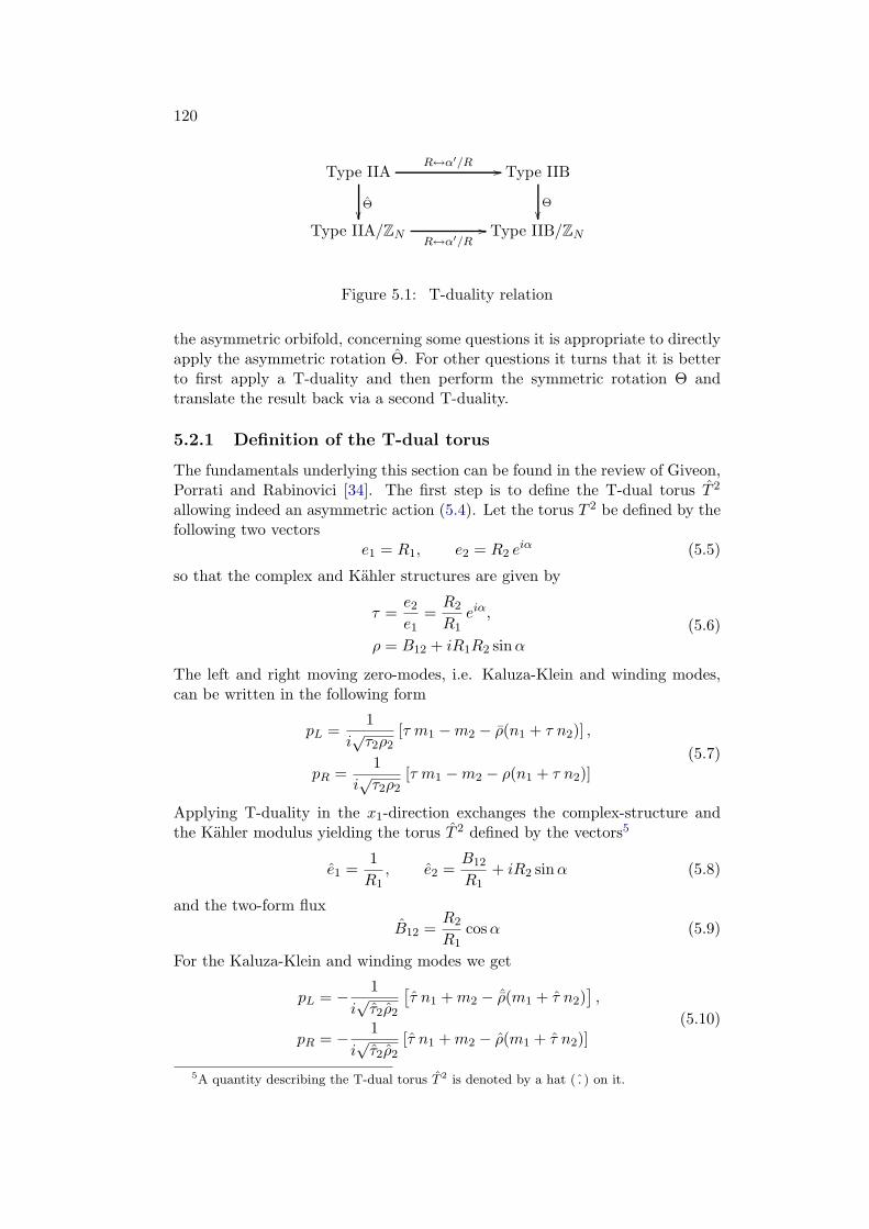
120

Type IIA

Θ

R↔α′/R// Type IIB

Θ

Type IIA/ZNR↔α′/R

// Type IIB/ZN

Figure 5.1: T-duality relation

the asymmetric orbifold, concerning some questions it is appropriate to directlyapply the asymmetric rotation Θ. For other questions it turns that it is betterto first apply a T-duality and then perform the symmetric rotation Θ andtranslate the result back via a second T-duality.

5.2.1 Definition of the T-dual torus

The fundamentals underlying this section can be found in the review of Giveon,Porrati and Rabinovici [34]. The first step is to define the T-dual torus T 2

allowing indeed an asymmetric action (5.4). Let the torus T 2 be defined by thefollowing two vectors

e1 = R1, e2 = R2 eiα (5.5)

so that the complex and Kahler structures are given by

τ =e2e1

=R2

R1eiα,

ρ = B12 + iR1R2 sinα(5.6)

The left and right moving zero-modes, i.e. Kaluza-Klein and winding modes,can be written in the following form

pL =1

i√τ2ρ2

[τ m1 −m2 − ρ(n1 + τ n2)] ,

pR =1

i√τ2ρ2

[τ m1 −m2 − ρ(n1 + τ n2)](5.7)

Applying T-duality in the x1-direction exchanges the complex-structure andthe Kahler modulus yielding the torus T 2 defined by the vectors5

e1 =1R1

, e2 =B12

R1+ iR2 sinα (5.8)

and the two-form fluxB12 =

R2

R1cosα (5.9)

For the Kaluza-Klein and winding modes we get

pL = − 1i√τ2ρ2

[τ n1 +m2 − ˆρ(m1 + τ n2)

],

pR = − 1i√τ2ρ2

[τ n1 +m2 − ρ(m1 + τ n2)](5.10)

5A quantity describing the T-dual torus T 2 is denoted by a hat ( . ) on it.

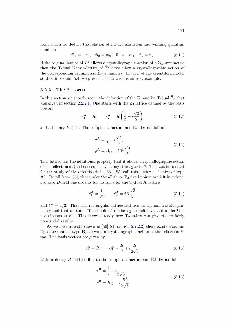
121

from which we deduce the relation of the Kaluza-Klein and winding quantumnumbers

m1 = −n1, m2 = m2, n1 = −m1, n2 = n2 (5.11)

If the original lattice of T 2 allows a crystallographic action of a ZN symmetry,then the T-dual Narain-lattice of T 2 does allow a crystallographic action ofthe corresponding asymmetric ZN symmetry. In view of the orientifold modelstudied in section 5.4, we present the Z3 case as an easy example.

5.2.2 The Z3 torus

In this section we shortly recall the definition of the Z3 and its T-dual Z3 thatwas given in section 2.2.2.1. One starts with the Z3 lattice defined by the basisvectors

eA1 = R, eA2 = R

(12

+ i

√3

2

)(5.12)

and arbitrary B-field. The complex-structure and Kahler moduli are

τA =12

+ i

√3

2,

ρA = B12 + iR2

√3

2

(5.13)

This lattice has the additional property that it allows a crystallographic actionof the reflection at (and consequently: along) the x2-axis, σ. This was importantfor the study of Ωσ orientifolds in [56]. We call this lattice a “lattice of typeA”. Recall from [56], that under Ωσ all three Z3 fixed points are left invariant.For zero B-field one obtains for instance for the T-dual A lattice

eA1 =1R, eA2 = iR

√3

2(5.14)

and bA = 1/2. That this rectangular lattice features an asymmetric Z3 sym-metry and that all three “fixed points” of the Z3 are left invariant under Ω isnot obvious at all. This shows already how T-duality can give rise to fairlynon-trivial results.

As we have already shown in [56] (cf. section 2.2.2.2) there exists a secondZ3 lattice, called type B, allowing a crystallographic action of the reflection σ,too. The basis vectors are given by

eB1 = R, eB2 =R

2+ i

R

2√

3(5.15)

with arbitrary B-field leading to the complex-structure and Kahler moduli

τB =12

+ i1

2√

3,

ρB = B12 + iR2

2√

3

(5.16)

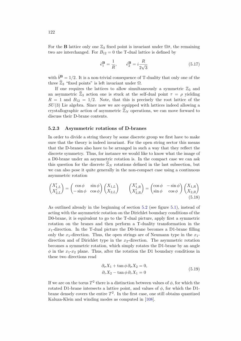
122

For the B lattice only one Z3 fixed point is invariant under Ωσ, the remainingtwo are interchanged. For B12 = 0 the T-dual lattice is defined by

eB1 =1R, eB2 = i

R

2√

3(5.17)

with bB = 1/2. It is a non-trivial consequence of T-duality that only one of thethree Z3 “fixed points” is left invariant under Ω.

If one requires the lattices to allow simultaneously a symmetric Z3 andan asymmetric Z3 action one is stuck at the self-dual point τ = ρ yieldingR = 1 and B12 = 1/2. Note, that this is precisely the root lattice of theSU(3) Lie algebra. Since now we are equipped with lattices indeed allowing acrystallographic action of asymmetric ZN operations, we can move forward todiscuss their D-brane contents.

5.2.3 Asymmetric rotations of D-branes

In order to divide a string theory by some discrete group we first have to makesure that the theory is indeed invariant. For the open string sector this meansthat the D-branes also have to be arranged in such a way that they reflect thediscrete symmetry. Thus, for instance we would like to know what the image ofa D0-brane under an asymmetric rotation is. In the compact case we can askthis question for the discrete ZN rotations defined in the last subsection, butwe can also pose it quite generally in the non-compact case using a continuousasymmetric rotation(X ′

1,L

X ′2,L

)=(

cosφ sinφ− sinφ cosφ

)(X1,L

X2,L

) (X ′

1,R

X ′2,R

)=(

cosφ − sinφsinφ cosφ

)(X1,R

X2,R

)(5.18)

As outlined already in the beginning of section 5.2 (see figure 5.1), instead ofacting with the asymmetric rotation on the Dirichlet boundary conditions of theD0-brane, it is equivalent to go to the T-dual picture, apply first a symmetricrotation on the branes and then perform a T-duality transformation in thex1-direction. In the T-dual picture the D0-brane becomes a D1-brane fillingonly the x1-direction. Thus, the open strings are of Neumann type in the x1-direction and of Dirichlet type in the x2-direction. The asymmetric rotationbecomes a symmetric rotation, which simply rotates the D1-brane by an angleφ in the x1-x2 plane. Thus, after the rotation the D1 boundary conditions inthese two directions read

∂σX1 + tanφ∂σX2 = 0,∂τX2 − tanφ∂τX1 = 0

(5.19)

If we are on the torus T 2 there is a distinction between values of φ, for which therotated D1-brane intersects a lattice point, and values of φ, for which the D1-brane densely covers the entire T 2. In the first case, one still obtains quantizedKaluza-Klein and winding modes as computed in [108].

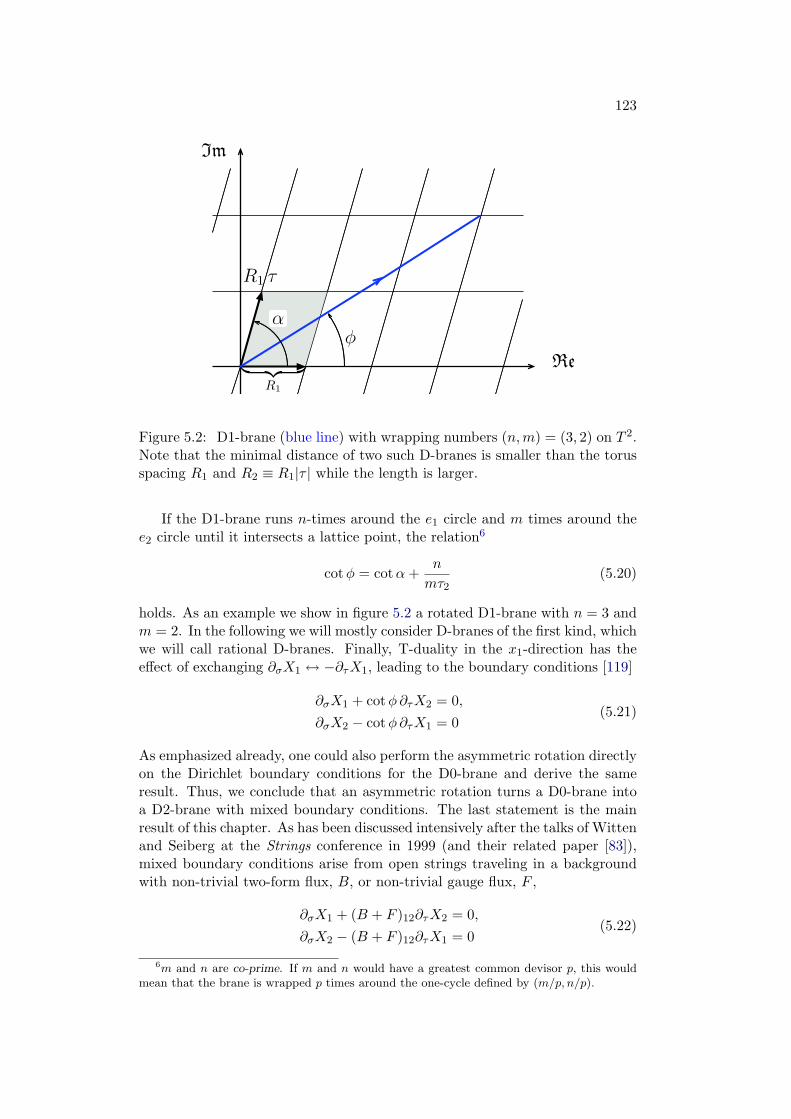
123

Im

Re︸︷︷︸R1

R1 τ

φ

α

Figure 5.2: D1-brane (blue line) with wrapping numbers (n,m) = (3, 2) on T 2.Note that the minimal distance of two such D-branes is smaller than the torusspacing R1 and R2 ≡ R1|τ | while the length is larger.

If the D1-brane runs n-times around the e1 circle and m times around thee2 circle until it intersects a lattice point, the relation6

cotφ = cotα+n

mτ2(5.20)

holds. As an example we show in figure 5.2 a rotated D1-brane with n = 3 andm = 2. In the following we will mostly consider D-branes of the first kind, whichwe will call rational D-branes. Finally, T-duality in the x1-direction has theeffect of exchanging ∂σX1 ↔ −∂τX1, leading to the boundary conditions [119]

∂σX1 + cotφ∂τX2 = 0,∂σX2 − cotφ∂τX1 = 0

(5.21)

As emphasized already, one could also perform the asymmetric rotation directlyon the Dirichlet boundary conditions for the D0-brane and derive the sameresult. Thus, we conclude that an asymmetric rotation turns a D0-brane intoa D2-brane with mixed boundary conditions. The last statement is the mainresult of this chapter. As has been discussed intensively after the talks of Wittenand Seiberg at the Strings conference in 1999 (and their related paper [83]),mixed boundary conditions arise from open strings traveling in a backgroundwith non-trivial two-form flux, B, or non-trivial gauge flux, F ,

∂σX1 + (B + F )12∂τX2 = 0,∂σX2 − (B + F )12∂τX1 = 0

(5.22)

6m and n are co-prime. If m and n would have a greatest common devisor p, this wouldmean that the brane is wrapped p times around the one-cycle defined by (m/p, n/p).

124

Thus, we can generally identify

cotφ = F = B + F (5.23)

which in the rational case becomes (note that cotφ is not necessarily rational)

cotφ = cotα+n

mτ2= B + F (5.24)

Since the B field is related to the shape of the torus T 2 and the F field to theD-branes, from (5.24) we extract the following identifications7

B = cotα, F =n

mτ2(5.25)

In section 5.3 we will further elaborate the relation between asymmetric rota-tions and D-branes with mixed boundary conditions. We will present an alter-native derivation of some of the non-commutativity properties known for suchboundary conditions. In the remainder of this section we will focus our attentionon the momentum- and zero-mode spectrum for open strings stretched betweenD-branes with mixed boundary conditions. In particular, we will demonstratethat in the compact case open strings stretched between identical rational D-branes do have a non-trivial momentum-mode spectrum. This is in sharp con-trast to some statements in the literature [120] saying that Neumann boundaryconditions allow Kaluza-Klein momentum, Dirichlet boundary conditions allownon-trivial winding but general mixed D-branes do have neither of them.

5.2.4 Kaluza-Klein and winding modes, zero mode degeneracy

In this section we will calculate the spectrum of the linear modes for two di-mensional D-branes with U(1)-F fluxes and for the T-dual configuration i.e.one dimensional D-branes on a T 2. The results are easily generalized to toruscompactifications of the more general form:

M10 = R1,9−2d ×d∏j=1

T 2(j) (5.26)

We will also explain the zero mode degeneracy that appears if the F fluxes aredifferent at the two ends of a string. In the T-dual picture this degeneracycorresponds to the topological intersection number of two branes on a torus.

5.2.4.1 D2-branes with F -flux on T 2

Since we can not easily visualize a D-brane with mixed boundary conditions,we first determine the zero-mode spectrum in the closed string tree channeland then transform the result into the open string loop channel. In contrastto the underlying publication [1], we have now a direct method to quantize

7The F given in the following formula is written in the euclidian basis. In terms of a latticebasis for T 2 it is simply: F = n/m. m and n are co-prime.

125

open strings with mixed boundary conditions in toroidal compactifications (cf.chap. 4). However, we first calculate the spectrum by the use of boundarystate formalism. After this, we use the results of the canonical quantization ofthe preceeding chapter, to derive an independent mass formula. These massformulæ perfectly agree for the case m = 1 (cf. eq. (5.24)) without furtherexplanation.

However for m 6= 1 (or fractional valued F -flux) there is a slight mismatchif we do not make further assumptions. In section 4.2.1.3 it was argued, thatF/α′ has to be integer-valued (in a basis of the torus lattice Γd). It was howevermentioned that fractional valued F/α′ corresponds to multiply wrapped branes,i.e. the lattice Γd of the closed string sector should be substituted by a biggerlattice Γd, s.th. F/α′ is integer valued in a basis of Γd. Alternatively, we candemand the string wave function to be invariant only under shifts ∈ m2πΓd.By this we get perfect agreement even in the case m 6= 1.

We are looking for boundary states (see also [121]) in the closed string theorysatisfying the following boundary state conditions

[∂τX1,cl + cotφ∂σX2,cl] |B〉 = 0,[∂τX2,cl − cotφ∂σX1,cl] |B〉 = 0

(5.27)

Rewriting (5.27) in terms of the complex coordinate the boundary conditionreads

[∂τZcl − i cotφ∂σZcl] |B〉 = 0 (5.28)

There is an analogous condition for the hermitian conjugate field Zcl. Usingthe mode expansion

Zcl =z02

+12(pL + pR)τ +

12(pL − pR)σ

+i√2

∑n6=0

(αnne−in(τ+σ) +

αnne−in(τ−σ)

),

Zcl =z02

+12(pL + pR)τ +

12(pL − pR)σ

− i√2

∑n6=0

(αnne−in(τ+σ) +

¯αnne−in(τ−σ)

)(5.29)

one obtains[(pL + pR)− i cotφ (pL − pR)] |B〉 = 0,[

αn + e2iφα−n]|B〉 = 0

(5.30)

with similar conditions for the fermionic modes. Inserting (5.10) and (5.11)into the first equation of (5.30) one can solve for the Kaluza-Klein and windingmodes

m1 = − nmn2, m2 =

n

mn1 (5.31)

giving rise to the following momentum mode spectrum:

M2cl(~r) =

|r1 + r2 τ |2

τ2

|n+mρ|2

ρ2, ~r ∈ Z2 (5.32)

126

with r, s ∈ Z. We observe that this agrees with the spectrum derived in [108] byemploying T-duality. The oscillator part of a bosonic boundary state satisfying(5.30) is given by

|B〉(n,m) =∑r,s∈Z

exp(∑n∈Z

1ne2iφα−nα−n

)|r, s〉(n,m) (5.33)

Using this boundary state we compute the tree channel annulus partition func-tion. Transforming the result via a modular transformation into loop chan-nel, we can extract the momentum-mode contribution and conclude that openstrings stretching between identical rational D-branes carry non-vanishing lin-ear modes giving rise to masses

M2op(~s) =

|s1 + s2 τ |2

τ2

ρ2

|n+mρ|2, ~s ∈ Z2 (5.34)

As announced, due to the results of the preceding chapter, we have an alterna-tive way at hand to derive this formula. The mass formula for an open stringon a lattice Γd (without Dirichlet bdy.-conditions) is given by formula (4.91)(p. 103). However we interpret m as the wrapping number of the D2 brane andrequire invariance only under m2πΓ2 which is only a subgroup of the closedstring torus 2πΓ2. This means that we consider the m2-fold cover of the torusdefined by 2πΓ2. The single valuedness condition of the wavefunction underm2πΓ2 now reads (cf. eq. (4.90), p. 103):

2∑i=1

eipi(~s) =

(G∓F 1

2

)−1 1m

2∑i=1

siei ~s ∈ Z2 (5.35)

This leads via (4.44) (p. 94) to the mass-formula for open strings in F -fieldbackgrounds:

M2op(~s) =

~sT G~s

det(mG) + (n+mB12)2(5.36)

Using the definitions (2.56) and (2.57) (p. 36), we note that (5.34) and (5.36)agree.

Summarizing, we now have the means to compute annulus amplitudes foropen strings stretched between different kinds of D-branes with rational mixedboundary conditions.

There is still the question of the number of Landau levels that occur if bothfield strength F1 and F2 do not agree. By the means of section (4.2.1.3) wehave a concrete formula to calculate this degeneracy. However, we have to takeinto account, that the two branes appearing in ni,j have in general differentwrapping numbers mi and mj . Therefore we expect that wavefunctions canonly be invariant under translations mimj2πΓ2 instead of being invariant under2πΓ2. Taking this into account in the derivation of (4.94) (p. 103) we see thatthe degeneracy on each T 2 is given by:

ni,j = (−1) Pf(mimj(Fi + Fj)

)= (njmi − nimj) (5.37)

127

The Landau degeneracy (5.37) equals the topological intersection number inthe T-dual picture where the two dimensional F -flux branes correspond to one-dimensional branes with non-trivial intersection.

We observed in chapter 2 that the NSNS B field has to be quantized, if wewant to gauge the world sheet parity Ω (cf. eq. (2.40), p. 34). For the two-torusthis means that B12/α

′ = 1/2. Ω exchanges the σ = 0 with the σ = π boundaryof the string. Thereby the τ -derivative changes sign. This can be absorbed inredefining Fi → −Fi. (We have to include boundary conditions with reversedF -field.) For Ω to be a symmetry, the open string mass spectrum has to beinvariant. From eq. (5.36) we deduce that the action of Ω for backgrounds withB12/α

′ = 1/2 is:

ΩB12=1/2 :

n → n′ = n+mm → m′ = −m

F = 1m

(0 n−n 0

)→ F ′ = 1

m

(0 −(n+m)

n+m 0

) (5.38)

For vanishing B-field we simply get:

ΩB12=0 :n → n′ = nm → m′ = −m (5.39)

This has an important consequence (especially for model-building, as we willsee in the next chapter): the difference between the multiplicity of states

nij − niΩ(j) ∈ 2Z for B12 = 0 (5.40)

nij − niΩ(j) ∈ Z for B12 = α′/2 (5.41)

has always to be an even number for vanishing B field, while it can be bothodd and even for B12 = α′/2.

As an example, we discuss the Z3 case in some more detail.

5.2.4.1.1 D-branes in the asymmetric Z3 orbifold Consider the Z3

lattice of type A and start with a D1-brane with pure Dirichlet boundary con-ditions (φ = 0)

∂τX1 = 0,∂τX2 = 0

(5.42)

Successively applying the asymmetric Z3 this D-brane is mapped to a mixedD2-brane with boundary conditions (φ = 2π/3)

∂σX1 −1√3∂τX2 = 0,

∂σX2 +1√3∂τX1 = 0

(5.43)

and a mixed D3-brane with boundary conditions (φ = −2π/3)

∂σX1 +1√3∂τX2 = 0,

∂σX2 −1√3∂τX1 = 0

(5.44)

128

In the orbifold theory these three kinds of D-branes are identified. This reflectsthat their background fields are being identified according to

F ∼ F +1√3

(5.45)

or equivalently

φ ∼ φ+2π3

(5.46)

The two coordinates X1 and X2 yield the following contribution to the annuluspartition function for open strings stretched between identical D-branes

Aαβii =ϑ[αβ

]η3

(∑r∈Z

e−2πt r2

R2

)(∑s∈Z

e−2πt 3s2

4R2

)(5.47)

independent of i ∈ 1, 2, 3. Open strings stretched between different kinds ofD-branes give rise to shifted moding and yield the partition function

Aαβi,i+1 = ni,i+1

ϑ[

13+α

β

]ϑ

[13+α12

] (5.48)

which looks like a twisted open string sector. As we know from [56, 117, 57](and the preceding discussion) we have to take into account extra multiplicities,ni,i+1, which have a natural geometric interpretation as multiple intersectionpoints of D-branes at angles in the T-dual picture. By this reasoning we findthat for the A type lattice the extra factor is one. However, for the three D-branes generated by Z3 when one starts with a D-brane with pure Neumannboundary conditions, φ ∈ π/2, π/6,−π/6, T-duality tells us that there mustappear an extra factor of three in front of the corresponding annulus amplitude(5.48). In the orientifold construction presented in section 5.4 these multiplici-ties are important to give consistent models.

5.2.4.2 D1-branes on T 2

In this section we will calculate the masses of the linear (i.e. momentum) modesof a D-brane that has Dirichlet bdy.-cond. in one direction and Neumann con-ditions in the perpendicular direction. This situation is depicted in figure 5.2(p. 123). We denote the vector tangential to the brane by ~t and the one normalto the brane by ~n:

~t ≡ ne1 +me2 ~n ≡ (me∗1 − ne∗2)((

m−n)TG∗(m−n))−1/2

(5.49)

With these conventions, we see that the linear part of the field X becomes (cf.(4.48), p. 95):

Xlin = τ ~t p~t + σ ~n p~n (5.50)

129

~np~n points perpendicular to the D-brane. Therfore πp~n must be an integermultiple of the minimal distance of two branes on the torus. Therfore we get:8

p~n(s2) = s2

((m−n)TG∗(m−n))−1/2

s2 ∈ Z (5.51)

The momentum in the τ -direction is conserved. It reads (c.f. eq. (4.79), p. 101):

Π~t =12π

(‖~t‖p~t +

=B12︷︸︸︷~t

‖~t‖B12~n p~n(s2)

)(5.52)

Requiring invariance of the wavefunction under a translation by 2π‖~t‖ in the ~tdirection leads to

p~t(s1, s2) =((

nm

)TG(nm

))−1/2 (s1 −B12 p~n(s2)

)s1, s2 ∈ Z (5.53)

The resulting mass2 formula takes the form:

M2op(~s) =

~sT(

1 −B12

−B12 det(G)+B212

)~s(

nm

)G(nm

) , ~s ∈ Z2 (5.54)

This formula is T-dual (under the duality denoted by “D” in section 2.2.2.1, eq.(2.58)) to the mass formula (5.36) and (5.34). Of course we can rewrite (5.54)in terms of the complex-structure τ and the Kahler structure ρ:

M2op(~s) =

|s1 + s2 ρ|2

ρ2

τ2|n+mτ |2

, ~s ∈ Z2 (5.55)

5.3 Asymmetric rotations and non-commutative ge-ometry

In section 5.2 we have pointed out that on T 2 or R2 D-branes with mixed bound-ary conditions can be generated by simply applying an asymmetric rotation toan ordinary D-brane with pure Neumann or Dirichlet boundary conditions.Thus, it should be possible to rederive earlier results for the two-point functionon the disc

〈Xi(z)Xj(z′)〉 (5.56)

for the operator product expansion (OPE) between vertex operators on theboundary

eipX(τ) eiqX(τ ′) (5.57)

by applying an asymmetric rotation on the corresponding quantities for openstrings ending on D0-branes in flat space-time.

8To calculate the minimal distance between two D1-branes we use an elementary theoremof number theory: The units in the ring Z/nZ consist of those residue classes mod nZ whichare represented by integers m 6= 0 and prime to n (cf. [96], chapter II, §2 ). This implies thatgiven two integers n and m which are prime w.r.t. each other there exist two integers a, bs.th.: an+ bm = 1.

130

5.3.1 Two-point function on the disc

The two-point function on the disc for both X1 and X2 of Dirichlet type reads

〈Xi(z)Xj(z′)〉 = −α′δij(ln |z − z′| − ln |z − z′|

)= −α′δij

12(ln(z − z′) + ln(z − z′)− ln(z − z′)− ln(z − z′)

)(5.58)

from which, formally using

Xi(z) = Xi,L(z) +Xi,R(z) (5.59)

we can directly read off the individual contributions from the left- and right-movers. Performing the asymmetric rotation

XL → AXL, XR → ATXR (5.60)

where A denotes an element of SO(2), leads to the following expression for thepropagator in the rotated coordinates

〈Xi(z)Xj(z′)〉 =− α′δij ln |z − z′| − α′δij(sin2 φ− cos2 φ

)ln |z − z′|

− α′εij sinφ cosφ ln(z − z′

z − z′

) (5.61)

This expression agrees precisely with the propagator derived in [105] with theidentification

F =(

0 cotφ− cotφ 0

)(5.62)

Thus, by applying an asymmetric rotation we have found an elegant and shortway of deriving this propagator without explicit reference to the boundaryconditions or the background fields. Moreover, since the commutative D0-braneis related in this smooth way to a non-commutative D2-brane, it is suggestingthat also both effective theories arising on such branes are related by somesmooth transformation. Such an explicit map between the commuting and thenon-commuting effective gauge theories has been determined in [83].

5.3.2 The OPE of vertex operators

In this subsection we apply an asymmetric rotation also to the operator productexpansion of tachyon vertex operators O(z) = eipX(z) on the boundary. Ofcourse this OPE is a direct consequence of the correlator (5.61) restricted tothe boundary, but nevertheless we would like to see whether we can generatethe non-commutative ∗-product directly via an asymmetric rotation. Takingcare of the left- and right-moving contributions in the OPE between vertexoperators living on a pure Dirichlet boundary we can write for |z| > |z′|

eipX(z) eiqX(z′) =(z − z′)

α′2pLqL (z − z′)

α′2pRqR

(z − z′)α′2pLqR (z − z′)

α′2pRqL

ei(p+q)X(z′) + . . . (5.63)

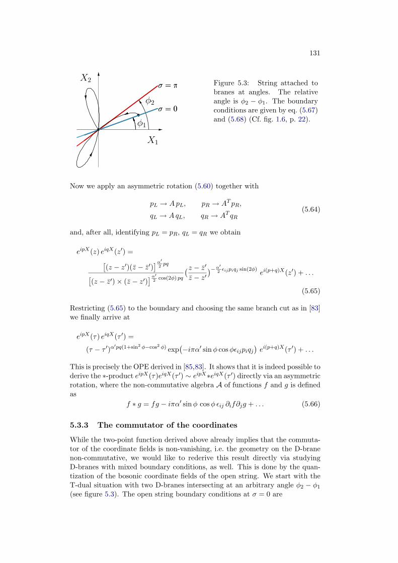
131

X1

X2

σ = 0

σ = π

φ2σ = 0

σ = π

φ1

Figure 5.3: String attached tobranes at angles. The relativeangle is φ2 − φ1. The boundaryconditions are given by eq. (5.67)and (5.68) (Cf. fig. 1.6, p. 22).

Now we apply an asymmetric rotation (5.60) together with

pL → ApL, pR → AT pR,

qL → AqL, qR → AT qR(5.64)

and, after all, identifying pL = pR, qL = qR we obtain

eipX(z) eiqX(z′) =[(z − z′)(z − z′)

]α′2pq[

(z − z′)× (z − z′)]α′

2cos(2φ) pq

(z − z′z − z′

)−α′2εijpiqj sin(2φ)

ei(p+q)X(z′) + . . .

(5.65)

Restricting (5.65) to the boundary and choosing the same branch cut as in [83]we finally arrive at

eipX(τ) eiqX(τ ′) =

(τ − τ ′)α′pq(1+sin2 φ−cos2 φ) exp(−iπα′ sinφ cosφεijpiqj

)ei(p+q)X(τ ′) + . . .

This is precisely the OPE derived in [85,83]. It shows that it is indeed possible toderive the ∗-product eipX(τ)eiqX(τ ′) ∼ eipX∗eiqX(τ ′) directly via an asymmetricrotation, where the non-commutative algebra A of functions f and g is definedas

f ∗ g = fg − iπα′ sinφ cosφ εij ∂if∂jg + . . . (5.66)

5.3.3 The commutator of the coordinates

While the two-point function derived above already implies that the commuta-tor of the coordinate fields is non-vanishing, i.e. the geometry on the D-branenon-commutative, we would like to rederive this result directly via studyingD-branes with mixed boundary conditions, as well. This is done by the quan-tization of the bosonic coordinate fields of the open string. We start with theT-dual situation with two D-branes intersecting at an arbitrary angle φ2 − φ1

(see figure 5.3). The open string boundary conditions at σ = 0 are

132

∂σX1 + tanφ1 ∂σX2 = 0,∂τX2 − tanφ1 ∂τX1 = 0

(5.67)

and at σ = π we require

∂σX1 + tanφ2 ∂σX2, = 0,∂τX2 − tanφ2 ∂τX1 = 0

(5.68)

The mode expansion satisfying these two boundary conditions looks like

X1 = x1+i√α′∑n∈Z

αn+ν

n+ νe−i(n+ν)τ cos[(n+ ν)σ + φ1]+

i√α′∑m∈Z

αm−νm− ν

e−i(m−ν)τ cos[(m− ν)σ − φ1],

X2 = x2+i√α′∑n∈Z

αn+ν

n+ νe−i(n+ν)τ sin[(n+ ν)σ + φ1]−

i√α′∑m∈Z

αm−νm− ν

e−i(m−ν)τ sin[(m− ν)σ − φ1]

(5.69)

with ν = (φ2 − φ1)/π. Using the usual commutation relation

[αn+ν , αm−ν ] = (n+ ν) δm+n,0 (5.70)

and the vanishing of the commutator of the center of mass coordinates x1 andx2 one can easily show that for D-branes at angles the general equal timecommutator vanishes

[Xi(τ, σ), Xj(τ, σ′)] = 0 (5.71)

Therefore, the geometry of D-branes at angles, but without background gaugefields, is always commutative.

Performing T-duality in the x1 direction one gets the two mixed boundaryconditions for the open strings

∂σX1 + cotφ1 ∂τX2 = 0,∂σX2 − cotφ1 ∂τX1 = 0

(5.72)

at σ = 0 and∂σX1 + cotφ2 ∂τX2 = 0,∂σX2 − cotφ2 ∂τX1 = 0

(5.73)

at σ = π. This is a very special case of what we considered in chapter 4. Itcorresponds to the following field strengths:

F1 =(

0 − cotφ1

cotφ1 0

)F2 =

(0 cotφ2

− cotφ2 0

)(5.74)

In section 4.3 we proved that the commutator of the coordinate fields X takesthe following values at its boundaries:

[X(τ, σ), X(τ, σ)]∣∣σ∈∂Mj

= i2πα′Fj

G−F2j

j = 1, 2 (5.75)

133

This result was obtained for the two-torus [112,84] as well.At the end of this section let us briefly comment on the algebraic structure

of the non-commutative torus we have obtained by the asymmetric rotation onthe D-branes. As shown in the previous section, the tachyon vertex operatorO = eipX(τ) leads to a non-commutative algebra A, defined in eq. (5.66). Asexplained in [83], the algebra A of tachyon vertex operators can be taken ateither end of the open string. Therefore the open string states form a bi-moduleA×A′, where A is acting on the boundary σ = 0 and A′ on the boundary σ = πof the open string. Specifically, for an open string whose first boundary σ = 0is related to a D-brane with parameter φ1 and whose second boundary σ = πis attached to a D-brane with parameter φ2, the algebra A of functions on thenon-commutative torus is generated by

U1 = exp(iy1 −

2π2α′F1

1 + F21

(∂/∂y2)),

U2 = exp(iy2 +

2π2α′F1

1 + F21

(∂/∂y1)) (5.76)

which obey

U1U2 = exp(− 2πi

2πα′F1

1 + F21

)U2U1 (5.77)

On the other hand, the algebra A′ is generated by

U1 = exp(iy1 +

2π2α′F2

1 + F22

(∂/∂y2)),

U2 = exp(iy2 −

2π2α′F2

1 + F22

(∂/∂y1)) (5.78)

obeying

U1U2 = exp(2πi

2πα′F2

1 + F22

)U2U1 (5.79)

5.4 Asymmetric orientifolds

Another motivation for studying such asymmetric orbifolds arises in the con-struction of Type I vacua. In [56,57] we have considered so-called supersymmet-ric orientifolds with D-branes at angles in six and four space-time dimensionswhich in the six-dimensional case were defined as

Type IIB on T 4

Ωσ,Θ(5.80)

with σ : zi → −zi, the zi being the complex coordinates of the T 4. Upon T-dualities in the directions of their real parts one obtains an ordinary orientifoldwhere, however, the space-time symmetry becomes asymmetric

Type IIB on T 4

Ω, Θ(5.81)

134

In the entire derivation in section 5.2 we have identified the two constructionsexplicitly via T-duality, relating branes with background fields to branes atangles. While in the Ωσ orientifolds Θ identified branes at different locations onthe tori, Θ now maps branes with different values of their background gauge fluxupon each other. As the background fields determine the parameter which rulesthe non-commutative geometry, branes with different geometries are identifiedaccording to (5.45). However the non-commutativity is solely restricted to thecompactification space, i.e. (∏

i

T 2(i)

)/ZN (5.82)

Each T 2(i) has to admit the respective ZN symmetry. The Z3 tori (2.74), p. 39

(A-torus) and (2.87), p. 41 (B-torus) both have a ρ2 component of order one. Asρ2 is the volume of the two-torus measured in terms of α′, the compactificationsize is roughly speaking the string scale. No large volume of the asymmetric Z3

(and more general: ZN ) orbifold exists. Even though we will get SO(N) gaugegroups in the ZL3 × ZR3 orientifold on T 4 this is not in contradiction with theobservation that no non-commutative gauge theories with gauge-groups otherthan U(n) seem to exist (c.f. [83, 122, 123]): The ZL3 × ZR3 orientifold does notadmit a decompactification limit.

From the above mentioned identification it is now clear that the N = (0, 1)supersymmetric asymmetric ZN orientifolds (5.81) have the same one loop par-tition functions as the corresponding symmetric ZN orientifolds (5.80). Theonly difference is that instead of D7-branes at angles, we introduce D9-braneswith appropriate background fields. Thus, a whole class of asymmetric ori-entifolds has already been studied in the T-dual picture involving D-branesat angles. One could repeat the whole computation for the asymmetric ori-entifolds (5.81), getting of course identical results. Note, the model (5.81) isreally a Type I vacuum, as Ω itself is gauged. Thus, in principle there exist thepossibility that heterotic dual models exist. Of course, in six dimensions mostmodels have more than one tensor-multiplet so that no perturbative heteroticdual model can exist. It would be interesting to look for heterotic duals for thefour dimensional models discussed in [57].

5.4.1 Orientifolds on the(T 2 × T 2

)/(ZL

3 × ZR3

)orbifold back-

ground

In the following we will construct the even more general six-dimensional Z3×Z3

orientifoldType IIB on T 4

Ω,Θ, Θwhich is T-dual to

Type IIB on T 4

Ωσ, Θ,Θ

where in fact, as shown in section 5.2.2, the two tori are identical T 4 = T 4 =SU(3)2. The freedom to choose their complex-structures gives rise to a variety

135

of three distinct models, which are denoted by AA,AB,BB as in [56]. Note,that the same orbifold group is generated by a pure left-moving Z3L, ΘL =ΘΘ−1, and a pure right-moving Z3R, ΘR = ΘΘ. As was also shown in [53]this model actually has N = (1, 1) supersymmetry, but one can get N = (0, 1)supersymmetry by turning on non-trivial discrete torsion.

5.4.1.1 Tadpole cancellation

The computation of the various one-loop amplitudes is straightforward. For theloop channel Klein bottle amplitude we obtain

K(ab) =16c12

∫ ∞

0

dt

t41η4

[ρ00 ΛaΛb + ρ01 + ρ02

+ n(ab)

Θ,Ωρ10 + n

(ab)

Θ,ΩΘ2ερ11 + n

(ab)

Θ,ΩΘερ12

+ n(ab)

Θ2,Ωρ20 + n

(ab)

Θ2,ΩΘ2ερ21 + n

(ab)

Θ2,ΩΘερ22

] (5.83)

where c ≡ V6/(8π2α′

)3 and ε is a phase factor defining the discrete torsion.Furthermore we use functions ρgh that are adopted from [53]. We alreadyexpressed the torus partition function of the orbifold theory in terms of thesefunctions (section 2.4). They are given in appendix A.3 (p. 208) together withtheir modular properties. g and h denote the twists resp. the projections in thepartition function ρgh: g, h ∈ (0, 1/3,−1/3), (0, 2/3,−2/3) for which we usethe shorter notation g, h ∈ 0, 1, 2. The index (ab) denotes the three possiblechoices of lattices, AA, AB and BB, and Λa are the zero mode contributions(5.34) to the partition function

ΛA =1η2

∑m1,m2

e−πt

[m2

1+ 43(

m12−m2)2

]=

2∑i=0

χi

ΛB =1η2

∑m1,m2

e−πt

[m2

1+12(m12−m2)2

]= χ0

(5.84)

χi are SU(3) characters with argument q = exp(−4πt) (cf. eq. (2.113), p. 48).Finally, n(ab)

Σ1,Σ2denotes the trace of the action of Σ2 on the fixed points in the

Σ1 twisted sector. Taking into account that the origin is the only common fixedpoint of Z3 and Z3, they can be determined to be

n(ab)

Θ,Ω=

9 for (AA)3 for (AB)1 for (BB)

(5.85)

and

n(ab)

Θ,ΩΘ= n

(ab)

Θ2,ΩΘ2=

−3 for (AA)i√

3 for (AB)1 for (BB)

(5.86)

136

The remaining numbers are given by complex conjugation of (5.86). Applying amodular transformation to (5.83) yields the tree channel Klein bottle amplitude

K(ab) = 232c3

∫ ∞

0dl

1η4

[ρ00 ΛaΛb +

13n

(ab)

Θ2,Ωρ01 +

13n

(ab)

Θ,Ωρ02

+ 3ρ10 − n(ab)

Θ2,ΩΘ2ερ11 − n(ab)

Θ,ΩΘ2ερ12

+ 3ρ20 − n(ab)

Θ2,ΩΘερ21 − n(ab)

Θ,ΩΘερ22

] (5.87)

The lattice contributions are9

ΛA =√

3η2

∑m1,m2

e−3πl

[m2

1+ 43(

m12−m2)2

]=√

3χ0

ΛB =1√3η2

∑m1,m2

e−πl

[13m2

1+4(m12−m2)2

]=

1√3

2∑i=0

χi

(5.88)

In order to cancel these tadpoles we now introduce D-branes with mixed bound-ary conditions. For both the A and the B lattice we choose three kinds ofD-branes with θ ∈ π/2, π/6,−π/6. The asymmetric Z3 cyclically permutesthese three branes, whereas the symmetric Z3 leaves every brane invariant andacts with a γΘ,i matrix on the Chan-Paton factors of each brane. Since Z3

permutes the branes, all three γΘ,i actions must be the same. The computationof the annulus amplitude gives

A(ab) =2c12

∫ ∞

0

dt

t41η4

[M2ρ00 ΛaΛb + (Tr γΘ)2 ρ01 + (Tr γΘ2)2 ρ02+

M2 n(ab)

Θ,1ρ10 + (Tr γΘ)2 n(ab)

Θ,Θερ11 + (Tr γΘ2)2 n(ab)

Θ,Θ2ερ12+

M2 n(ab)

Θ2,1ρ20 + (Tr γΘ)2 n(ab)

Θ2,Θερ21 + (Tr γΘ2)2 n(ab)

Θ2,Θ2ερ22

](5.89)

where the θ twisted sector is given by open strings stretched between D-braneswith θi and θi+1. Thus, n(ab)

Θ,1denotes the intersection number of two such

branes and n(ab)

Θ,Θthe number of intersection points invariant under Θ. The

actual numbers turn out to be the same as the multiplicities of the closed stringtwisted sectors in (5.85) and (5.86). For the tree channel amplitude we obtain

A(ab) = 2c

6

∫ ∞

0dl

1η4

[M2(ρ00 ΛaΛb +

13n

(ab)

Θ2,1ρ01 +

13n

(ab)

Θ,1ρ02

)+ (Tr γΘ)2

(3ρ10 − n(ab)

Θ2,Θερ11 − n(ab)

Θ,Θερ12

)+ (Tr γΘ2)2

(3ρ20 − n(ab)

Θ2,Θ2ερ21 − n(ab)

Θ,Θ2ερ22

)] (5.90)

9The argument of the SU(3) characters is q = exp(−4πl).

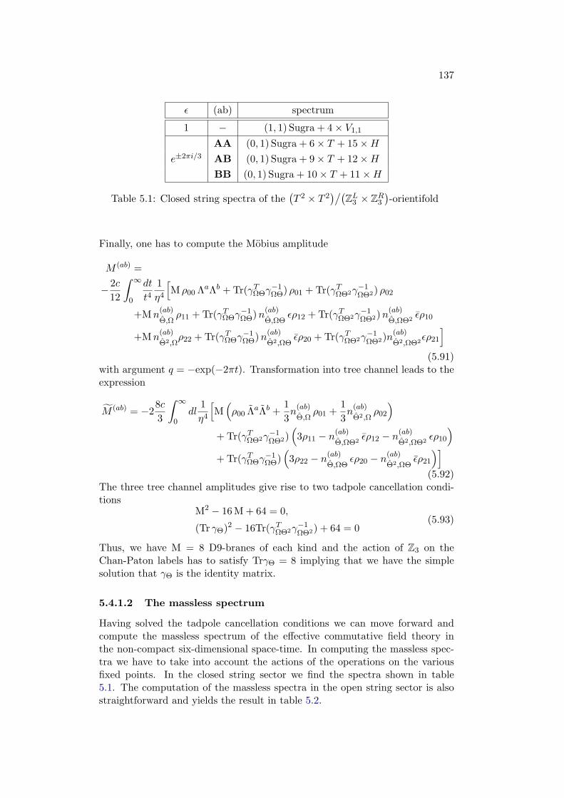
137

ε (ab) spectrum

1 − (1, 1) Sugra + 4× V1,1

AA (0, 1) Sugra + 6× T + 15×He±2πi/3 AB (0, 1) Sugra + 9× T + 12×H

BB (0, 1) Sugra + 10× T + 11×H

Table 5.1: Closed string spectra of the(T 2 × T 2

)/(ZL3 × ZR3

)-orientifold

Finally, one has to compute the Mobius amplitude

M (ab) =

−2c12

∫ ∞

0

dt

t41η4

[M ρ00 ΛaΛb + Tr(γTΩΘγ

−1ΩΘ) ρ01 + Tr(γTΩΘ2γ

−1ΩΘ2) ρ02

+Mn(ab)

Θ,Ωρ11 + Tr(γTΩΘγ

−1ΩΘ)n(ab)

Θ,ΩΘερ12 + Tr(γTΩΘ2γ

−1ΩΘ2)n

(ab)

Θ,ΩΘ2ερ10

+Mn(ab)

Θ2,Ωρ22 + Tr(γTΩΘγ

−1ΩΘ)n(ab)

Θ2,ΩΘερ20 + Tr(γTΩΘ2γ

−1ΩΘ2)n

(ab)

Θ2,ΩΘ2ερ21

](5.91)

with argument q = −exp(−2πt). Transformation into tree channel leads to theexpression

M (ab) = −28c3

∫ ∞

0dl

1η4

[M(ρ00 ΛaΛb +

13n

(ab)

Θ,Ωρ01 +

13n

(ab)

Θ2,Ωρ02

)+ Tr(γTΩΘ2γ

−1ΩΘ2)

(3ρ11 − n(ab)

Θ,ΩΘ2ερ12 − n(ab)

Θ2,ΩΘ2ερ10

)+ Tr(γTΩΘγ

−1ΩΘ)

(3ρ22 − n(ab)

Θ,ΩΘερ20 − n(ab)

Θ2,ΩΘερ21

)](5.92)

The three tree channel amplitudes give rise to two tadpole cancellation condi-tions

M2 − 16 M + 64 = 0,

(Tr γΘ)2 − 16Tr(γTΩΘ2γ−1ΩΘ2) + 64 = 0

(5.93)

Thus, we have M = 8 D9-branes of each kind and the action of Z3 on theChan-Paton labels has to satisfy TrγΘ = 8 implying that we have the simplesolution that γΘ is the identity matrix.

5.4.1.2 The massless spectrum

Having solved the tadpole cancellation conditions we can move forward andcompute the massless spectrum of the effective commutative field theory inthe non-compact six-dimensional space-time. In computing the massless spec-tra we have to take into account the actions of the operations on the variousfixed points. In the closed string sector we find the spectra shown in table5.1. The computation of the massless spectra in the open string sector is alsostraightforward and yields the result in table 5.2.

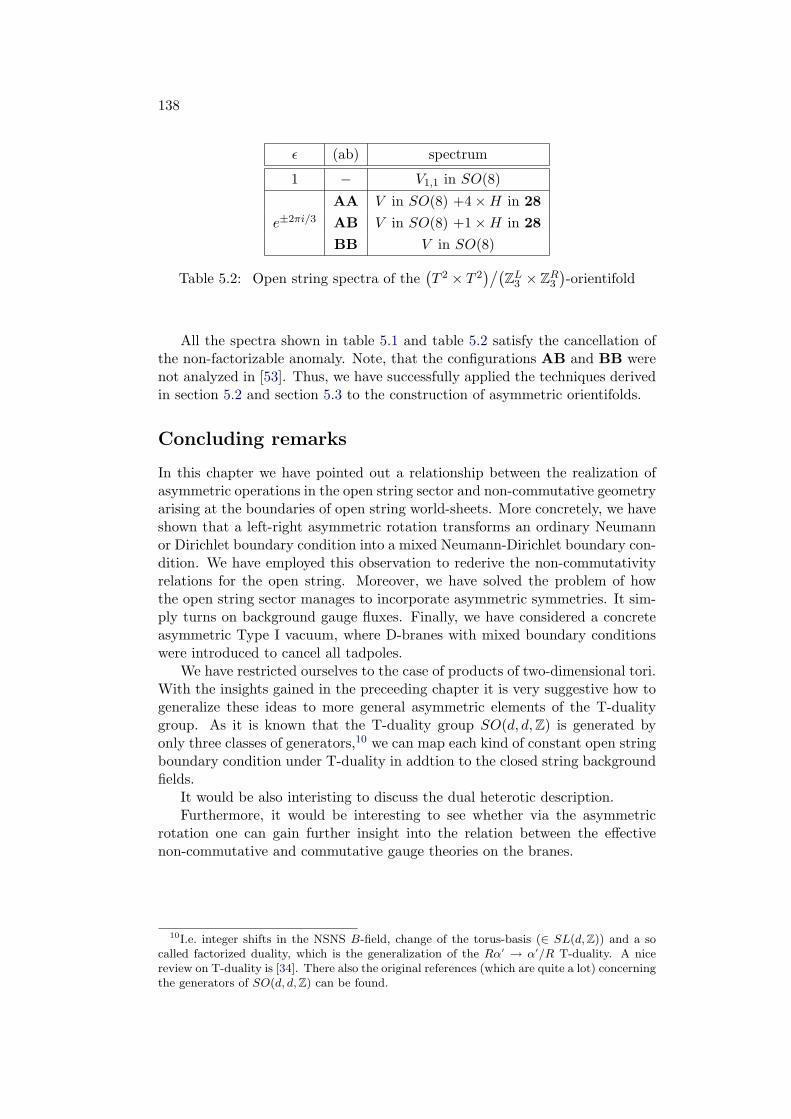
138

ε (ab) spectrum

1 − V1,1 in SO(8)

AA V in SO(8) +4×H in 28e±2πi/3 AB V in SO(8) +1×H in 28

BB V in SO(8)

Table 5.2: Open string spectra of the(T 2 × T 2

)/(ZL3 × ZR3

)-orientifold

All the spectra shown in table 5.1 and table 5.2 satisfy the cancellation ofthe non-factorizable anomaly. Note, that the configurations AB and BB werenot analyzed in [53]. Thus, we have successfully applied the techniques derivedin section 5.2 and section 5.3 to the construction of asymmetric orientifolds.

Concluding remarks

In this chapter we have pointed out a relationship between the realization ofasymmetric operations in the open string sector and non-commutative geometryarising at the boundaries of open string world-sheets. More concretely, we haveshown that a left-right asymmetric rotation transforms an ordinary Neumannor Dirichlet boundary condition into a mixed Neumann-Dirichlet boundary con-dition. We have employed this observation to rederive the non-commutativityrelations for the open string. Moreover, we have solved the problem of howthe open string sector manages to incorporate asymmetric symmetries. It sim-ply turns on background gauge fluxes. Finally, we have considered a concreteasymmetric Type I vacuum, where D-branes with mixed boundary conditionswere introduced to cancel all tadpoles.

We have restricted ourselves to the case of products of two-dimensional tori.With the insights gained in the preceeding chapter it is very suggestive how togeneralize these ideas to more general asymmetric elements of the T-dualitygroup. As it is known that the T-duality group SO(d, d,Z) is generated byonly three classes of generators,10 we can map each kind of constant open stringboundary condition under T-duality in addtion to the closed string backgroundfields.

It would be also interisting to discuss the dual heterotic description.Furthermore, it would be interesting to see whether via the asymmetric

rotation one can gain further insight into the relation between the effectivenon-commutative and commutative gauge theories on the branes.

10I.e. integer shifts in the NSNS B-field, change of the torus-basis (∈ SL(d,Z)) and a socalled factorized duality, which is the generalization of the Rα′ → α′/R T-duality. A nicereview on T-duality is [34]. There also the original references (which are quite a lot) concerningthe generators of SO(d, d,Z) can be found.

Chapter 6

Toroidal orientifolds withmagnetized versus

intersecting D-Branes

In this chapter we will mainly present the results published in publication [2,124]. We investigated strings on toroidal orientifolds with D9-branes which areallowed to carry arbitrary magnetic background fluxes. We restricted ourselvesto block diagonal NS U(1) fields F . Therefore the pure Ω-orientifold is T-dualto a σΩ-orientifold with σ being a reflection which has a fixed point locus of halfthe dimension of the compact space. As a consequence the T-dual picture leadsto an orientifold 6-plane (O6-plane) in compactifications on six-tori (and to anO7-plane in compactifications on four-tori). The O6-plane is charged under aRR 7-form while the O7-plane carries RR 8-form charge. The RR charge willbe canceled by D6- (resp. D7-) branes without any U(1) background field. TheT-dual picture has the advantage to admit a purely geometric interpretation,with multiplicities of open string states given by the intersection numbers ofthe corresponding Dp branes. Because the interpretation of the intersectionnumbers in the F -field picture is less direct though possible (cf. section 4.2.1.3,p. 100), we will from time to time switch between the description in termsof fluxes and the purely geometrical description in terms of intersecting Dpbranes. We will discuss both the technical description as well as applicationsto phenomenology.

6.1 Introduction

The search for realistic string vacua is one of the burning open problems withinsuperstring theory. A phenomenologically viable string compactification shouldcontain at least three chiral fermion generations, the Standard Model gaugegroup and broken space-time supersymmetry. In the context of ‘conventional’string compactifications the requirement of getting chiral fermions is usuallyachieved by considering compact, internal background spaces with nontrivialtopology rather than simple tori. In particular, when analyzing the Kaluza-Klein fermion spectra [125] a net-fermion generation number arises if the inter-

139

140

nal Dirac operator has zero modes. For example, considering heterotic stringcompactifications on Calabi-Yau threefolds [47] , the net-generation number isequal to |χ|/2, where χ is the Euler number of the Calabi-Yau space. Chi-ral fermions are also present in a large class of heterotic orbifold compact-ifications [32], as well as in free bosonic [126] and fermionic [127, 128] con-structions. Type II string models with chiral fermions can be constructed bylocating D-branes at transversal orbifold or conifold singularities [29, 30], orby considering intersections of D-branes and NS-branes [129, 130, 131]; chiralType I models were first proposed in [132]. Moreover orbifold compactifica-tions of eleven-dimensional M-theory can lead to chiral fermions, as discussede.g. in [133,134,135,136,137].

The phenomenological requirement of breaking space-time supersymme-try can be met in various ways. In the context of heterotic string compact-ifications gaugino condensation [138, 139] or the Scherk-Schwarz mechanism[46, 140, 141, 142, 143, 144] lead to potentially interesting models with super-symmetry broken at low energies. In addition, as it was realized more re-cently, Type II models on nontrivial background spaces with certain D-braneconfigurations possess broken space-time supersymmetry. Especially, whenchanging the GSO-projections tachyon free Type 0 orientifolds in four dimen-sions can be constructed [145, 146, 147, 148]. Alternatively, orientifolds on six-dimensional orbifolds with brane-antibrane configurations provide interestingscenarios [149, 150, 151, 152, 153, 154], where supersymmetry is left unbrokenin the gravity bulk, but broken in the open string sector living on the brane-antibrane system.

Finally the quest for a realistic gauge group with sufficiently low rank ismet in heterotic strings by choosing appropriate gauge vector bundles on theCalabi-Yau spaces [155], which can be alternatively described by turning onWilson lines in Calabi-Yau or also in orbifold compactifications [156]. 1 On theType II side the gauge group can be reduced by Wilson lines or, in the T-dualpicture, by placing the branes at different positions inside the internal space.

As it should have become clear from the previous discussion, ‘standard’heterotic, Type I or Type II compactifications on simple 6-tori do not meet anyof the three above requirements. However, as we will discuss in 6.2.1, turningon magnetic fluxes in the internal directions of the D-branes, thereby inducingmixed Neumann-Dirichlet boundary conditions for open strings equivalent toa non-commutative internal geometry [104, 157] on the branes, all three goalscan be achieved in one single stroke.2 Specifically, we will discuss Type I stringcompactifications on a product of d non-commutative two-tori to 10− 2d non-compact Minkowski dimensions (d = 2, 3), i.e. the ten-dimensional background

1A Wilson line defines an embedding of the fundamental group π1(X ) into the gauge bundleof the theory. Wilson lines on compactification spaces X with abelian fundamental group onlylead to rank conserving symmetry breaking. However in manifolds with nonabelian π1(X ) onecan achieve rank reducing gauge-symmetry breaking via Wilson lines.

2In chapter 5 which is mainly based on [1] we have discussed Type I string compactificationson non-commutative asymmetric orbifold spaces.

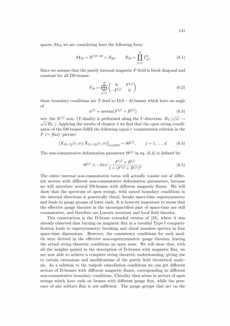
141

spaces M10 we are considering have the following form:

M10 = R1,9−2d ×X2d, X2d =d∏j=1

T 2(j) (6.1)

Since we assume that the purely internal magnetic F -field is block diagonal andconstant for all D9-branes:

Fab =d⊕j=1

(0 F (j)

−F (j) 0

)(6.2)

these boundary conditions are T-dual to D(9− d)-branes which have an angleof

φ(j) = arctan(F (j) +B(j)) (6.3)

wrt. the X(j) axis. (T-duality is performed along the Y -direction: RY /√α′ →√

α′RY .) Applying the results of chapter 4 we find that the open string coordi-nates of the D9-branes fulfill the following equal-τ commutation relation in theF (= flux) -picture:

[X10−2j(τ, σ), X11−2j(τ, σ)]∣∣σ∈∂M = iΘ(j) , j = 1, . . . , d (6.4)

The non-commutative deformation parameter Θ(j) in eq. (6.4) is defined by:

Θ(j) ≡ −2πα′F (j) +B(j)

1 + (F (j) +B(j))2(6.5)

The entire internal non-commutative torus will actually consist out of differ-ent sectors with different non-commutative deformation parameters, becausewe will introduce several D9-branes with different magnetic fluxes. We willshow that the spectrum of open strings, with mixed boundary conditions inthe internal directions is generically chiral, breaks space-time supersymmetryand leads to gauge groups of lower rank. It is however important to stress thatthe effective gauge theories in the uncompactified part of space-time are stillcommutative, and therefore are Lorentz invariant and local field theories.

This construction is the D-brane extended version of [28], where it wasalready observed that turning on magnetic flux in a toroidal Type I compacti-fication leads to supersymmetry breaking and chiral massless spectra in fourspace-time dimensions. However, the consistency conditions for such mod-els were derived in the effective non-supersymmetric gauge theories, leavingthe actual string theoretic conditions an open issue. We will show that, withall the insights gained in the description of D-branes with magnetic flux, weare now able to achieve a complete string theoretic understanding, giving riseto certain extensions and modifications of the purely field theoretical analy-sis. As a solution to the tadpole cancellation conditions we can get differentsectors of D-branes with different magnetic fluxes, corresponding to differentnon-commutative boundary conditions. Chirality then arises in sectors of openstrings which have ends on branes with different gauge flux, while the pres-ence of any solitary flux is not sufficient. The gauge groups that act on the

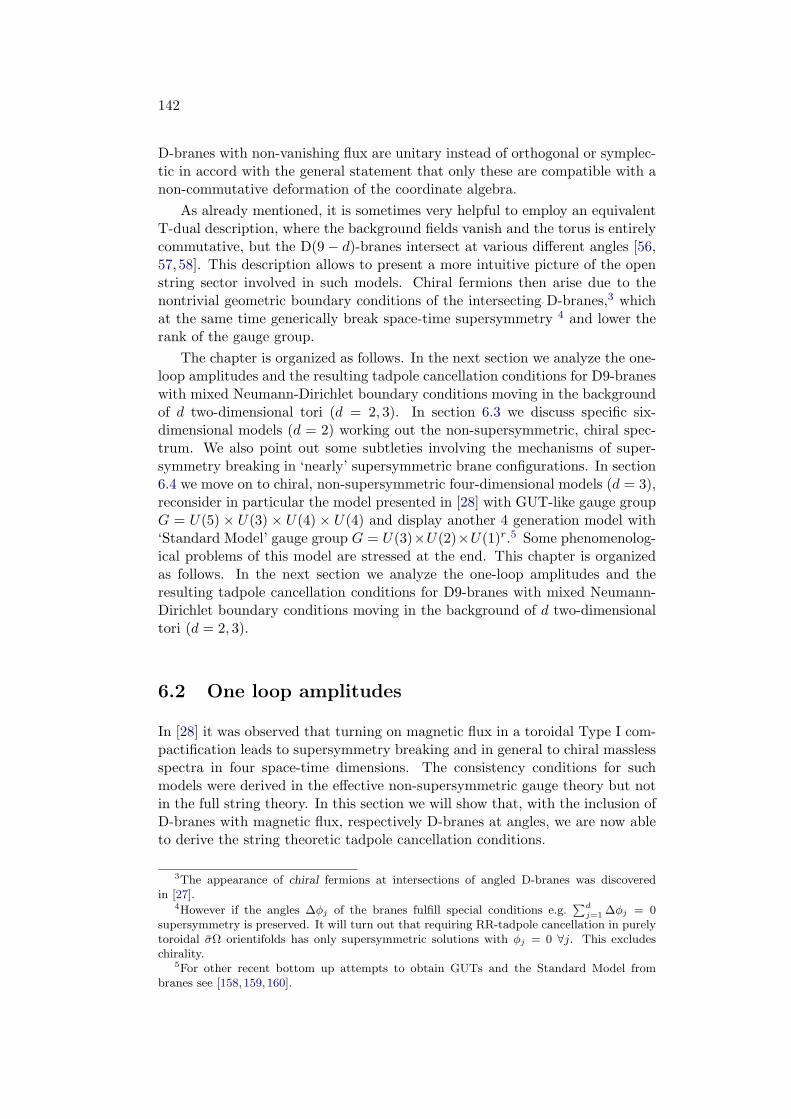
142

D-branes with non-vanishing flux are unitary instead of orthogonal or symplec-tic in accord with the general statement that only these are compatible with anon-commutative deformation of the coordinate algebra.

As already mentioned, it is sometimes very helpful to employ an equivalentT-dual description, where the background fields vanish and the torus is entirelycommutative, but the D(9− d)-branes intersect at various different angles [56,57, 58]. This description allows to present a more intuitive picture of the openstring sector involved in such models. Chiral fermions then arise due to thenontrivial geometric boundary conditions of the intersecting D-branes,3 whichat the same time generically break space-time supersymmetry 4 and lower therank of the gauge group.

The chapter is organized as follows. In the next section we analyze the one-loop amplitudes and the resulting tadpole cancellation conditions for D9-braneswith mixed Neumann-Dirichlet boundary conditions moving in the backgroundof d two-dimensional tori (d = 2, 3). In section 6.3 we discuss specific six-dimensional models (d = 2) working out the non-supersymmetric, chiral spec-trum. We also point out some subtleties involving the mechanisms of super-symmetry breaking in ‘nearly’ supersymmetric brane configurations. In section6.4 we move on to chiral, non-supersymmetric four-dimensional models (d = 3),reconsider in particular the model presented in [28] with GUT-like gauge groupG = U(5) × U(3) × U(4) × U(4) and display another 4 generation model with‘Standard Model’ gauge group G = U(3)×U(2)×U(1)r.5 Some phenomenolog-ical problems of this model are stressed at the end. This chapter is organizedas follows. In the next section we analyze the one-loop amplitudes and theresulting tadpole cancellation conditions for D9-branes with mixed Neumann-Dirichlet boundary conditions moving in the background of d two-dimensionaltori (d = 2, 3).

6.2 One loop amplitudes

In [28] it was observed that turning on magnetic flux in a toroidal Type I com-pactification leads to supersymmetry breaking and in general to chiral masslessspectra in four space-time dimensions. The consistency conditions for suchmodels were derived in the effective non-supersymmetric gauge theory but notin the full string theory. In this section we will show that, with the inclusion ofD-branes with magnetic flux, respectively D-branes at angles, we are now ableto derive the string theoretic tadpole cancellation conditions.

3The appearance of chiral fermions at intersections of angled D-branes was discoveredin [27].

4However if the angles ∆φj of the branes fulfill special conditions e.g.∑d

j=1 ∆φj = 0supersymmetry is preserved. It will turn out that requiring RR-tadpole cancellation in purelytoroidal σΩ orientifolds has only supersymmetric solutions with φj = 0 ∀j. This excludeschirality.

5For other recent bottom up attempts to obtain GUTs and the Standard Model frombranes see [158,159,160].

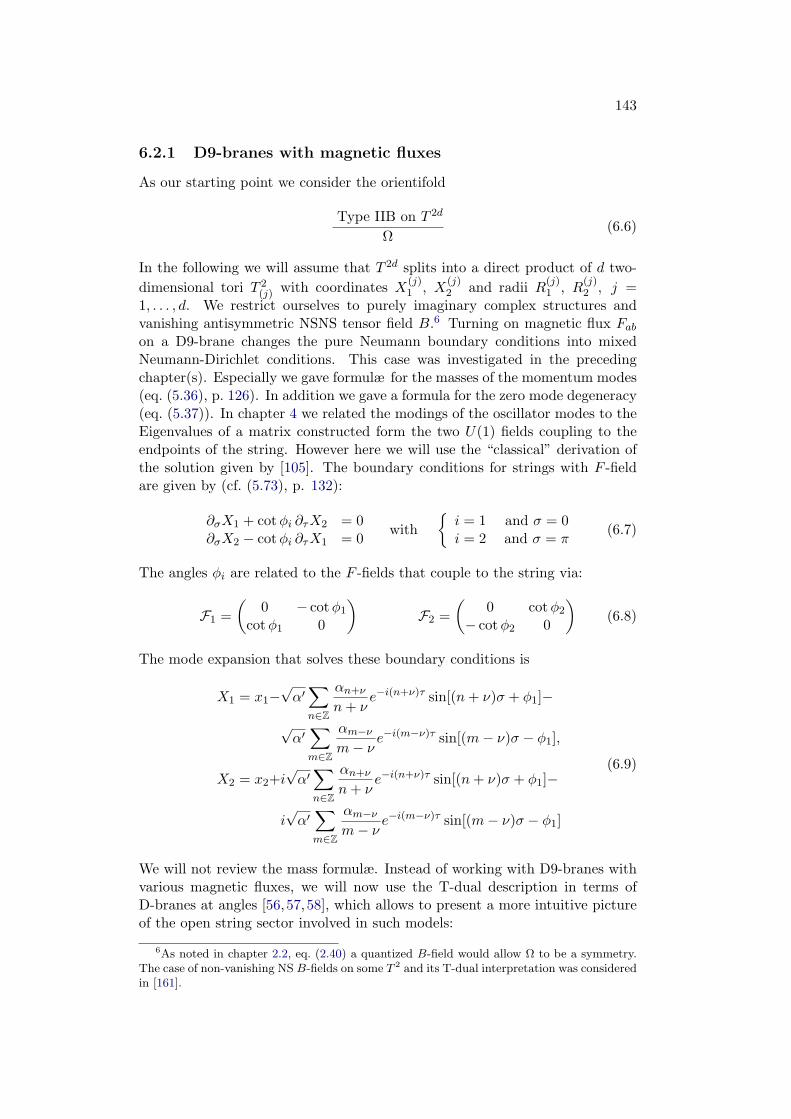
143

6.2.1 D9-branes with magnetic fluxes

As our starting point we consider the orientifold

Type IIB on T 2d

Ω(6.6)

In the following we will assume that T 2d splits into a direct product of d two-dimensional tori T 2

(j) with coordinates X(j)1 , X(j)

2 and radii R(j)1 , R(j)

2 , j =1, . . . , d. We restrict ourselves to purely imaginary complex structures andvanishing antisymmetric NSNS tensor field B.6 Turning on magnetic flux Fabon a D9-brane changes the pure Neumann boundary conditions into mixedNeumann-Dirichlet conditions. This case was investigated in the precedingchapter(s). Especially we gave formulæ for the masses of the momentum modes(eq. (5.36), p. 126). In addition we gave a formula for the zero mode degeneracy(eq. (5.37)). In chapter 4 we related the modings of the oscillator modes to theEigenvalues of a matrix constructed form the two U(1) fields coupling to theendpoints of the string. However here we will use the “classical” derivation ofthe solution given by [105]. The boundary conditions for strings with F -fieldare given by (cf. (5.73), p. 132):

∂σX1 + cotφi ∂τX2 = 0∂σX2 − cotφi ∂τX1 = 0

withi = 1 and σ = 0i = 2 and σ = π

(6.7)

The angles φi are related to the F -fields that couple to the string via:

F1 =(

0 − cotφ1

cotφ1 0

)F2 =

(0 cotφ2

− cotφ2 0

)(6.8)

The mode expansion that solves these boundary conditions is

X1 = x1−√α′∑n∈Z

αn+ν


√α′∑m∈Z

αm−νm− ν

e−i(m−ν)τ sin[(m− ν)σ − φ1],

X2 = x2+i√α′∑n∈Z

αn+ν


i√α′∑m∈Z

αm−νm− ν

e−i(m−ν)τ sin[(m− ν)σ − φ1]

(6.9)

We will not review the mass formulæ. Instead of working with D9-branes withvarious magnetic fluxes, we will now use the T-dual description in terms ofD-branes at angles [56,57,58], which allows to present a more intuitive pictureof the open string sector involved in such models:

6As noted in chapter 2.2, eq. (2.40) a quantized B-field would allow Ω to be a symmetry.The case of non-vanishing NS B-fields on some T 2 and its T-dual interpretation was consideredin [161].

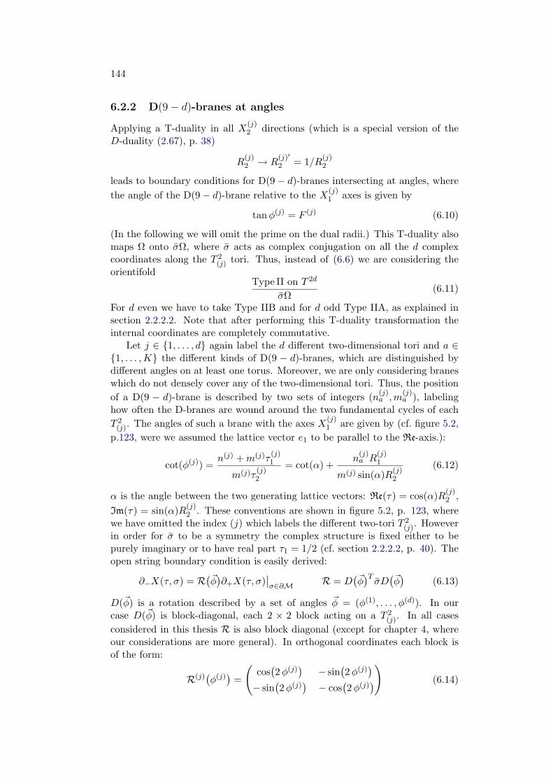
144

6.2.2 D(9− d)-branes at angles

Applying a T-duality in all X(j)2 directions (which is a special version of the

D-duality (2.67), p. 38)

R(j)2 → R

(j)′

2 = 1/R(j)2

leads to boundary conditions for D(9− d)-branes intersecting at angles, wherethe angle of the D(9− d)-brane relative to the X(j)

1 axes is given by

tanφ(j) = F (j) (6.10)

(In the following we will omit the prime on the dual radii.) This T-duality alsomaps Ω onto σΩ, where σ acts as complex conjugation on all the d complexcoordinates along the T 2

(j) tori. Thus, instead of (6.6) we are considering theorientifold

Type II on T 2d

σΩ(6.11)

For d even we have to take Type IIB and for d odd Type IIA, as explained insection 2.2.2.2. Note that after performing this T-duality transformation theinternal coordinates are completely commutative.

Let j ∈ 1, . . . , d again label the d different two-dimensional tori and a ∈1, . . . ,K the different kinds of D(9 − d)-branes, which are distinguished bydifferent angles on at least one torus. Moreover, we are only considering braneswhich do not densely cover any of the two-dimensional tori. Thus, the positionof a D(9 − d)-brane is described by two sets of integers (n(j)

a ,m(j)a ), labeling

how often the D-branes are wound around the two fundamental cycles of eachT 2

(j). The angles of such a brane with the axes X(j)1 are given by (cf. figure 5.2,

p.123, were we assumed the lattice vector e1 to be parallel to the Re-axis.):

cot(φ(j)) =n(j) +m(j)τ

(j)1

m(j)τ(j)2

= cot(α) +n

(j)a R

(j)1

m(j) sin(α)R(j)2

(6.12)

α is the angle between the two generating lattice vectors: Re(τ) = cos(α)R(j)2 ,

Im(τ) = sin(α)R(j)2 . These conventions are shown in figure 5.2, p. 123, where

we have omitted the index (j) which labels the different two-tori T 2(j). However

in order for σ to be a symmetry the complex structure is fixed either to bepurely imaginary or to have real part τ1 = 1/2 (cf. section 2.2.2.2, p. 40). Theopen string boundary condition is easily derived:

∂−X(τ, σ) = R(~φ)∂+X(τ, σ)

∣∣σ∈∂M R = D

(~φ)TσD(~φ)

(6.13)

D(~φ) is a rotation described by a set of angles ~φ = (φ(1), . . . , φ(d)). In ourcase D(~φ) is block-diagonal, each 2 × 2 block acting on a T 2

(j). In all casesconsidered in this thesis R is also block diagonal (except for chapter 4, whereour considerations are more general). In orthogonal coordinates each block isof the form:

R(j)(φ(j)

)=

(cos(2φ(j)

)− sin

(2φ(j)

)− sin

(2φ(j)

)− cos

(2φ(j)

)) (6.14)

145

In complex coordinates (i.e. Z = 1/√

2(X1 + iX2)) R(j)(φ(j)

)this combination

of a reflection and a subsequent rotation by −2φ(j) looks very simple:

R(j)(φ(j)

)(Z(j)

)= e−2φ(j)

Z(j) R(j)(φ(j)

)(Z(j)

)= e2φ

(j)Z(j) (6.15)

Since σΩ reflects the D-branes at the axis X(j)1 , for each brane labeled by(

n(j)a ,m

(j)a

)we must also introduce the mirror brane with

(n

(j)a′ ,m

(j)a′)

=(n

(j)a ,−m(j)

a

). The values m(j)

a = 0 6= n(j)a and n

(j)a = 0 6= m

(j)a correspond

to branes located along one of the axis. The horizontal D-branes translate viaT-duality into D9-branes with vanishing flux and the vertical ones into branesof lower dimension with pure Dirichlet boundary conditions. A solution to theboundary conditions (6.13) was given in section 5.2.4.2, p. 128 and section 5.3.3,p. 131.

The questions we are going to deal with in the following are: Is it possibleto cancel all or at least the RR tadpoles originating from the Klein bottle am-plitude by D9-branes with non-vanishing magnetic fluxes F (j), or equivalentlyby D(9 − d)-branes at nontrivial angles φ(j)? Taken that supersymmetry isbroken generically by such a background, are there configuration which stillpreserve some amount of supersymmetry? This would provide a string scenariowith partial supersymmetry breaking. Finally, what are the phenomenologicalproperties of such compactifications? Concerning the first question we find apositive answer in the sense that the RR tadpole can be canceled, while su-persymmetry is always broken entirely. This shows up both in the spectrumand a non-vanishing NSNS tadpole. Tachyons are always present in compact-ifications on T 4 and for some region in parameter space of the four dimen-sional compactifications as well. However it was shown after our publicationappeared ( [162,163,164]) that there exist toroidal models, which are free fromtachyons (but still suffering from NSNS tadpoles). Interestingly, models withnon-trivially intersecting D-branes generically contain chiral fermions motivat-ing us to study how far one can get in deriving the Standard Model in thissetting. However, later we will mention an obstacle to construct phenomeno-logically realistic models in this simple approach on a T 6 = (T 2)3 which is aproduct of only A-type two-tori.

Technically we first have to compute all contributions to the massless RRtadpole. The cancellation conditions will then imply relations for the numberof D9-branes and their respective background fluxes. This computation will beperformed in the T-dual picture, where D9-branes with background fields aremapped to D(9 − d)-branes, and the background fields translate into relativeangles. This picture allows to visualize the D-branes easily and gives a muchbetter intuition than dealing with sets of D9-branes, all filling the same spacebut differing by background fields.

146

6.2.3 Klein bottle amplitude

The loop channel Klein bottle amplitude for (6.11) can be computed straight-forwardly

K = 2(5−d)c (1− 1)∫ ∞

0

dt

t(6−d)14

ϑ[

01/2

]4η12

d∏j=1

(∑r,s∈Z

e−πt

(r2/(

R(j)1

)2+s2(R

(j)2

)2))(6.16)

with c = V10−2d/(8π2α′

)5−d. Transforming (6.16) into tree channel, one obtainsthe following massless RR tadpole∫ ∞

0dl 2(13−d)

d∏j=1

(R

(j)1

R(j)2

). (6.17)

The tree channel Klein bottle amplitude allows to determine the normalizationof the corresponding cross-cap states

|C〉 = 2(d/2−4)

(d∏j=1

R(j)1

R(j)2

) 12

(|CNS〉+ |CR〉) (6.18)

6.2.4 Annulus amplitude

Next we calculate all contributions of open strings stretching between the var-ious D(9 − d)-branes, generically located at nontrivial relative angles. We willboth include the case, where the relative angle is vanishing, i.e. the backgroundgauge flux is equal on both branes, and the case, where the angle is π/2 andthe field gets infinitely large on, say, p of the tori.

We start with the contributions of strings with both ends on the same brane.The T-dual of the Kaluza-Klein and winding spectrum in eq. (5.34) (p. 126)is given by (5.55) and (5.55) (p. 129). With our simplifying assumptions thatB = 0 it reads:7

M2a =

d∑j=1

( r(j)a

V(j)a

)2

+(s(j)a)2(R(j)

1 R(j)2

V(j)a

)2 (6.19)

with

V (j)a =

√(R

(j)1 n

(j)a

)2+(R

(j)2 m

(j)a

)2(6.20)

denoting the volume of the brane on T 2(j). It is now straightforward to compute

the loop channel annulus amplitude for open strings starting and ending on thesame brane and transform it to the tree channel

Aaa = cN2a (1− 1)

∫ ∞

0dl

12(d+1)

d∏j=1

(V

(j)a

)2

R(j)1 R

(j)2

ϑ[

1/20

]4η12

∑r,s

e−πlM2a (6.21)

7B 6= 0 does not modify the the RR tadpole conditions, as they are topological. It alsodoes not change the moding of the oscillators, as it does not enter the boundary conditions.Therefore B = 0 is a very mild simplification.

147

with

M2a =

d∑j=1

(r(j)a )2(V (j)a

)2+(s(j)a)2( V

(j)a

R(j)1 R

(j)2

)2 (6.22)

Na counts the numbers of different kinds of branes. Using (6.21) one can de-termine the normalization of the boundary state, which has the schematic form

|Da 〉 = 2−(d/2+1)

d∏j=1

V(j)a√

R(j)1 R

(j)2

(|Da,NS 〉+ |Da,R 〉) (6.23)

Reflecting the brane on a single T 2(j) by a π rotation onto itself corresponds

to (n(j)a ,m

(j)a ) → (−n(j)

a ,−m(j)a ) and, as can be determined in the boundary

state approach, changes the sign of the RR charge, thus exchanging branes andanti-branes.

Using the boundary state (6.23) we can compute the tree channel annulusamplitude for an open string stretched between two different D-branes

Aab =∫ ∞

0dl 〈Da|e−lHcl |Db〉

=c

2NaNbIab

∫ ∞

0dl(−1)d

∑α,β

∈0, 12

(−1)2(α+β)ϑ[αβ

]4−d ∏dj=1 ϑ

[α

∆(φ(j))ab+β

]η12−3d

∏dj=1 ϑ

[1/2

∆(φ(j))ab+1/2

](6.24)

where the coefficient

Iab =d∏j=1

(n(j)a m

(j)b −m

(j)a n

(j)b

)(6.25)

is the (oriented) intersection number of the two branes. We have defined theoriented angle between brane a and b on the torus T 2

(j) by:

∆(φ(j))ab ≡(φ

(j)b − φ

(j)a

)/π (6.26)

It gives rise to an extra multiplicity in the annulus loop channel, which wehave to take into account, when we compute the massless spectrum. In orderto properly include the case where some φ(j)

a = φ(j)b , one needs to employ the

relationlimψ→0

2 sin(πψ)

ϑ[

1/21/2+ψ

] = − 1η3

(6.27)

and include a sum over KK momenta and windings as in (6.21). The contribu-tion to the massless RR tadpole due to (6.21) and (6.24) is

∫ ∞

0dl NaNb 2(3−d)

d∏j=1

(R

(j)1

)2n

(j)a n

(j)b +

(R

(j)2

)2m

(j)a m

(j)b

R(j)1 R

(j)2

(6.28)

148

The loop channel annulus can be obtained by a modular transformation:

Aab = c NaNb Iab

∫ ∞

0

dt

t(6−d)14· 1η12−3d

·∑

α,β∈0,1/2

(−1)2(α+β)ϑ[βα

]4−d ∏dj=1 e

i2π( 12−α)∆(φ(j))abϑ

[∆(φ(j))ab+β

α

]∏dj=1 ϑ

[∆(φ(j))ab+1/2

1/2

] (6.29)

6.2.5 Mobius amplitude

Computing the overlap between the crosscap state (6.18) and a boundary state(6.23) yields the contribution of the brane D(9− p)a to the Mobius amplitude

Ma = ∓cNa 25 (−1)d∫ ∞

0dl

d∏j=1

m(j)a

·∑

α,β∈0,1/2

(−1)2(α+β)ϑ[αβ

]4−d ∏dj=1 ϑ

[α

φ(j)a /π+β

]η12−3d

∏dj=1 ϑ

[1/2

φ(j)a /π+1/2

] (6.30)

with argument q = − exp(−4πl). Therefore the contribution to the RR tadpoleis

∓∫ ∞

0dl Na 2(9−d)

d∏j=1

(R

(j)1

R(j)2

n(j)a

)(6.31)

The overall sign in (6.30) and (6.31) is fixed by the tadpole cancellation con-dition. In the loop channel the contribution of the Mobius strip results fromstrings starting on one brane and ending on its mirror partner. The extra multi-plicity given by the numbers m(j)

a of intersection points invariant under σ needsto be regarded as before. Now we have all the ingredients to study the relationswhich derive from the cancellation of massless RR tadpoles.

6.3 Compactifications to six dimensions

We are compactifying Type I strings on a four-dimensional torus and cancel thetadpoles by introducing stacks of D9-branes with magnetic fluxes. The T-dualarrangement of D7-branes at angles looks like the situation depicted in figure6.1, where we have drawn only two types of D7-branes labeled by a and b andtheir mirror partners a′ and b′, the angles being chosen arbitrary.

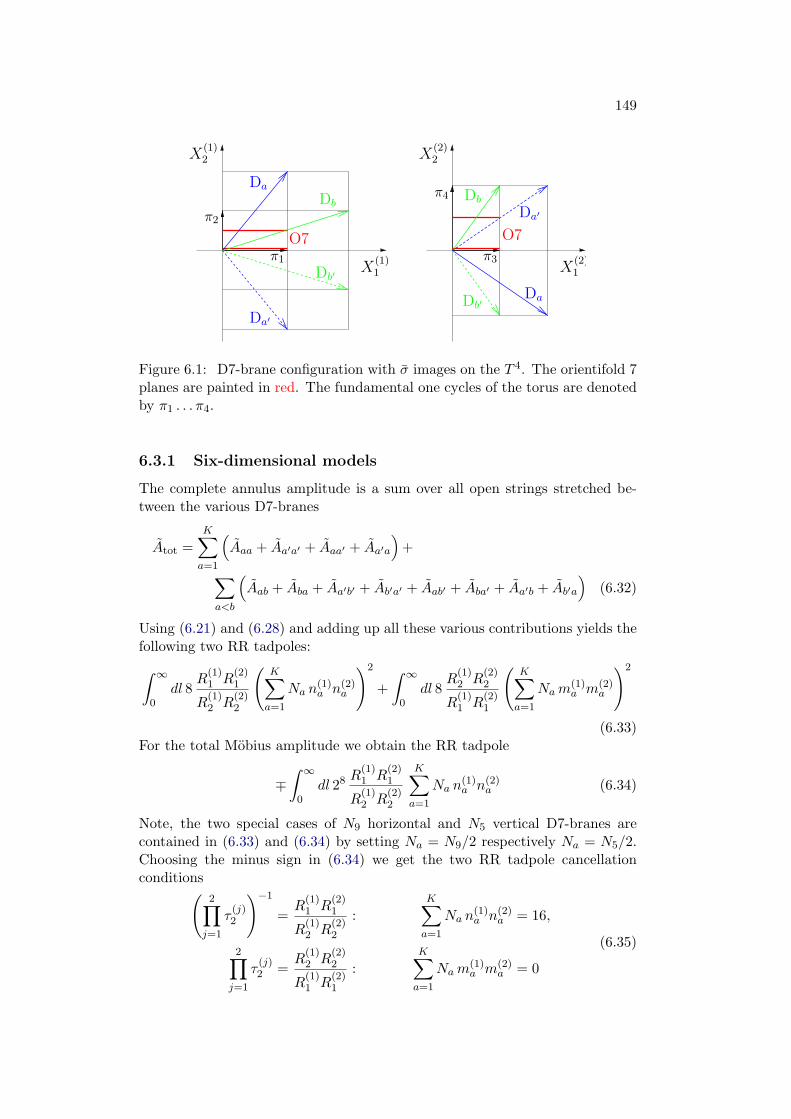
149

X(1)2 X

(2)2

π3

π4

π1

π2

X(2)1X

(1)1

Da

O7 O7

Da′

Db′

DbDb

Db′

Da′

Da

Figure 6.1: D7-brane configuration with σ images on the T 4. The orientifold 7planes are painted in red. The fundamental one cycles of the torus are denotedby π1 . . . π4.

6.3.1 Six-dimensional models

The complete annulus amplitude is a sum over all open strings stretched be-tween the various D7-branes

Atot =K∑a=1

(Aaa + Aa′a′ + Aaa′ + Aa′a

)+∑

a<b

(Aab + Aba + Aa′b′ + Ab′a′ + Aab′ + Aba′ + Aa′b + Ab′a

)(6.32)

Using (6.21) and (6.28) and adding up all these various contributions yields thefollowing two RR tadpoles:∫ ∞

0dl 8

R(1)1 R

(2)1

R(1)2 R

(2)2

(K∑a=1

Na n(1)a n(2)

a

)2

+∫ ∞

0dl 8

R(1)2 R

(2)2

R(1)1 R

(2)1

(K∑a=1

Nam(1)a m(2)

a

)2

(6.33)For the total Mobius amplitude we obtain the RR tadpole

∓∫ ∞

0dl 28 R

(1)1 R

(2)1

R(1)2 R

(2)2

K∑a=1

Na n(1)a n(2)

a (6.34)

Note, the two special cases of N9 horizontal and N5 vertical D7-branes arecontained in (6.33) and (6.34) by setting Na = N9/2 respectively Na = N5/2.Choosing the minus sign in (6.34) we get the two RR tadpole cancellationconditions(

2∏j=1

τ(j)2

)−1

=R

(1)1 R

(2)1

R(1)2 R

(2)2

:K∑a=1

Na n(1)a n(2)

a = 16,

2∏j=1

τ(j)2 =

R(1)2 R

(2)2

R(1)1 R

(2)1

:K∑a=1

Nam(1)a m(2)

a = 0

(6.35)

150

As one might have expected, pure D9-branes with m(j)a = 0 only contribute to

the tadpole proportional to the product of the inverse imaginary parts of thecomplex structures of the two-tori. The D5-branes with n

(j)a = 0 are respon-

sible only for the tadpole that is proportional to the product of the imaginaryparts of the complex structures. Remarkably, by choosing multiple windingnumbers, n(j)

a > 1, one can reduce the rank of the gauge group. As usual innon-supersymmetric models, there remains an uncanceled NSNS tadpole, whichneeds to be canceled by a Fischler-Susskind mechanism. However it is also pos-sible that the equations of motion lead to a degenerate compactification space(i.e. a degenerate torus).

In the section 6.5.1 we shall show that except for the trivial case, whenm

(1)a = m

(2)a = 0 for all a, i.e. vanishing gauge flux on all the D9-branes, super-

symmetry is broken and tachyons develop for open strings stretched betweendifferent branes. In contrast to the breaking of supersymmetry in a brane-antibrane system these tachyons cannot be removed by turning on Wilson-lines,which is related via T-duality to shifting the position of the branes by some con-stant vector. At any non trivial angle there always remains an intersection pointof two D7-branes where the tachyons can localize. Also the lowest lying bosonicspectrum depends on the radii of the torus, which determine the relative an-gles. The zero point energy in the NS sector of a string stretching between twodifferent branes is shifted by

∆E0,NS =12

d∑j=1

φ(j)a − φ(j)

b

π(6.36)

using the convention φ(j)a − φ

(j)b ∈ (0, π/2]. Even assuming a standard GSO

projection, the lightest physical state can easily be seen to be tachyonic exceptfor the supersymmetric situation with φ(1)

a −φ(1)b = φ

(2)a −φ(2)

b . We shall find inthe next section that tadpole cancellation prohibits this solution, except whenall fluxes vanish.

On the contrary, the chiral fermionic massless spectrum is independent ofthe moduli and we display it in table 6.1. (Aa and Sa denote the antisymmet-ric resp. symmetric tensor representations with respect to U(Na), SO(Na) orSp(Na).) Since σΩ exchanges a brane with its mirror brane, the Chan-Patonindices of strings ending on a stack of branes with non-vanishing gauge flux haveno Ω projection and the gauge group is U(Na). If σΩ leaves branes invariant,i.e. the flux vanishes or is infinite, corresponding to pure D9- or D5-branes, thegauge factor is SO(Na) or Sp(Na), respectively.

The degeneracy of states stated in the third column of table 6.1 is essentiallygiven by the intersection numbers of the D7-branes. Whenever it is formallynegative, one has to pick the (2, 1) spinor of opposite chirality taking intoaccount the opposite orientation of the branes at the intersection. As waspointed out earlier, a change of the orientation switches the RR charge in thetree channel translating into the opposite GSO projection in the loop channel.Therefore the other chirality survives the GSO projection in the R sector. If themultiplicity is zero, this does not mean that there are no massless open string

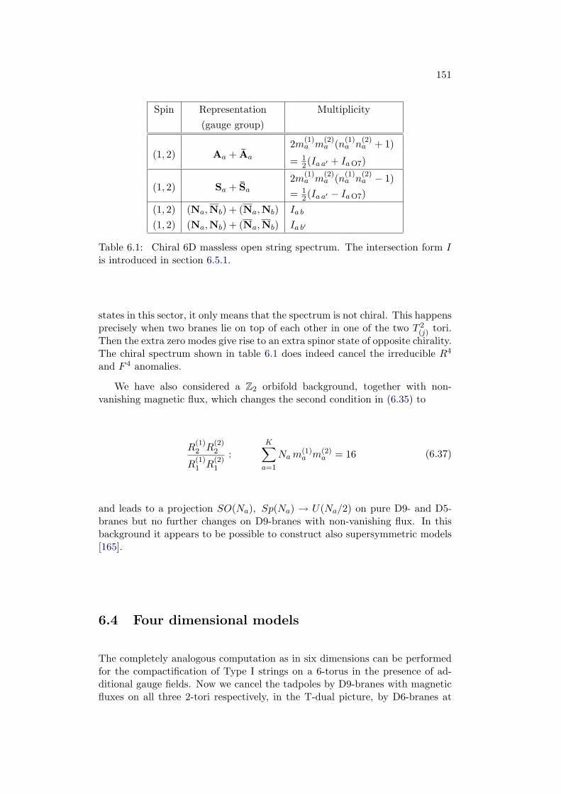
151

Spin Representation Multiplicity(gauge group)

2m(1)a m

(2)a (n(1)

a n(2)a + 1)

(1, 2) Aa + Aa = 12(Ia a′ + IaO7)

2m(1)a m

(2)a (n(1)

a n(2)a − 1)

(1, 2) Sa + Sa = 12(Ia a′ − IaO7)

(1, 2) (Na,Nb) + (Na,Nb) Ia b

(1, 2) (Na,Nb) + (Na,Nb) Ia b′

Table 6.1: Chiral 6D massless open string spectrum. The intersection form Iis introduced in section 6.5.1.

states in this sector, it only means that the spectrum is not chiral. This happensprecisely when two branes lie on top of each other in one of the two T 2

(j) tori.Then the extra zero modes give rise to an extra spinor state of opposite chirality.The chiral spectrum shown in table 6.1 does indeed cancel the irreducible R4

and F 4 anomalies.

We have also considered a Z2 orbifold background, together with non-vanishing magnetic flux, which changes the second condition in (6.35) to

R(1)2 R

(2)2

R(1)1 R

(2)1

:K∑a=1

Nam(1)a m(2)

a = 16 (6.37)

and leads to a projection SO(Na), Sp(Na) → U(Na/2) on pure D9- and D5-branes but no further changes on D9-branes with non-vanishing flux. In thisbackground it appears to be possible to construct also supersymmetric models[165].

6.4 Four dimensional models

The completely analogous computation as in six dimensions can be performedfor the compactification of Type I strings on a 6-torus in the presence of ad-ditional gauge fields. Now we cancel the tadpoles by D9-branes with magneticfluxes on all three 2-tori respectively, in the T-dual picture, by D6-branes at

152

Representation Multiplicity

4m(1)a m

(2)a m

(3)a (n(1)

a n(2)a n

(3)a + 1)

(Aa)L = 12(Ia′ a + IO6 a)

4m(1)a m

(2)a m

(3)a (n(1)

a n(2)a n

(3)a − 1)

(Sa)L = 12(Ia′ a − IO6 a)

(Na,Nb)L Ia b

(Na,Nb)L Ia′b

Table 6.2: Chiral 4D massless open string spectrum.

angles. One obtains four independent tadpole cancellation conditions(3∏j=1

τ(j)2

)−1

=R

(1)1 R

(2)1 R

(3)1

R(1)2 R

(2)2 R

(3)2

:K∑a=1

Na n(1)a n(2)

a n(3)a = 16

(τ

(1)2

)−13∏j=2

τ(j)2 =

R(1)1 R

(2)2 R

(3)2

R(1)2 R

(2)1 R

(3)1

:K∑a=1

Na n(1)a m(2)

a m(3)a = 0

τ(1)2

(τ

(2)2

)−1τ

(3)2 =

R(1)2 R

(2)1 R

(3)2

R(1)1 R

(2)2 R

(3)1

:K∑a=1

Nam(1)a n(2)

a m(3)a = 0

3∏j=1

τ(j)2 =

R(1)2 R

(2)2 R

(3)1

R(1)1 R

(2)1 R

(3)2

:K∑a=1

Nam(1)a m(2)

a n(3)a = 0

(6.38)

(For convenience they are given in the picture with D6-branes at angles.) Againthe gauge group contains a U(Na) factor for each stack of D9-branes with non-vanishing flux, an SO(Na) gauge factor for a stack with vanishing flux and anSp(Na) factor for a stack of D5-branes. The general spectrum of chiral fermionswith respect to the gauge group factors is presented in table 6.2. Whenever theintersection number in the second column is formally negative, one again has totake the conjugate representation. The spectrum in table 2 is free of non-abeliangauge anomalies.

In the next subsections we discuss some examples and point out some phe-nomenological issues for these models.

6.4.1 A 24 generation SU(5) model

Having found a way to break supersymmetry, to reduce the rank of the gaugegroup and to produce chiral spectra in four space-time dimensions, it is temptingto search in a compact bottom-up approach for brane configurations producingmassless spectra close to the Standard Model. The tachyons are not that dan-gerous from the effective field theory point of view, as they simply may serve asHiggs-bosons for spontaneous gauge symmetry breaking, anticipating a mecha-nism to generate a suitable potential keeping their vacuum expectation values fi-nite. In [28] a three generation GUT model was presented, which we shall revisit

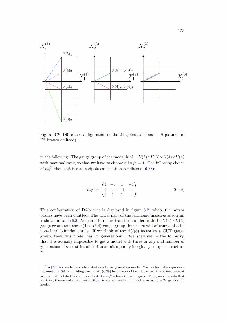
153

X(1)2

X(1)1

X(2)2

X(2)1

X(3)2

X(3)1

U(5)1

U(4)3

U(4)4

U(3)2

U(5)1, U(3)2

U(4)3, U(4)4

Figure 6.2: D6-brane configuration of the 24 generation model (σ-pictures ofD6 branes omitted).

in the following. The gauge group of the model is G = U(5)×U(3)×U(4)×U(4)with maximal rank, so that we have to choose all n(j)

a = 1. The following choiceof m(j)

a then satisfies all tadpole cancellation conditions (6.38):

m(j)a =

3 −5 1 −11 1 −1 −11 1 1 1

(6.39)

This configuration of D6-branes is displayed in figure 6.2, where the mirrorbranes have been omitted. The chiral part of the fermionic massless spectrumis shown in table 6.3. No chiral fermions transform under both the U(5)×U(3)gauge group and the U(4)×U(4) gauge group, but there will of course also benon-chiral bifundamentals. If we think of the SU(5) factor as a GUT gaugegroup, then this model has 24 generations8. We shall see in the followingthat it is actually impossible to get a model with three or any odd number ofgenerations if we restrict all tori to admit a purely imaginary complex structureτ .

8In [28] this model was advocated as a three generation model. We can formally reproducethe model in [28] by dividing the matrix (6.39) by a factor of two. However, this is inconsistent

as it would violate the condition that the m(j)a ’s have to be integers. Thus, we conclude that

in string theory only the choice (6.39) is correct and the model is actually a 24 generationmodel.

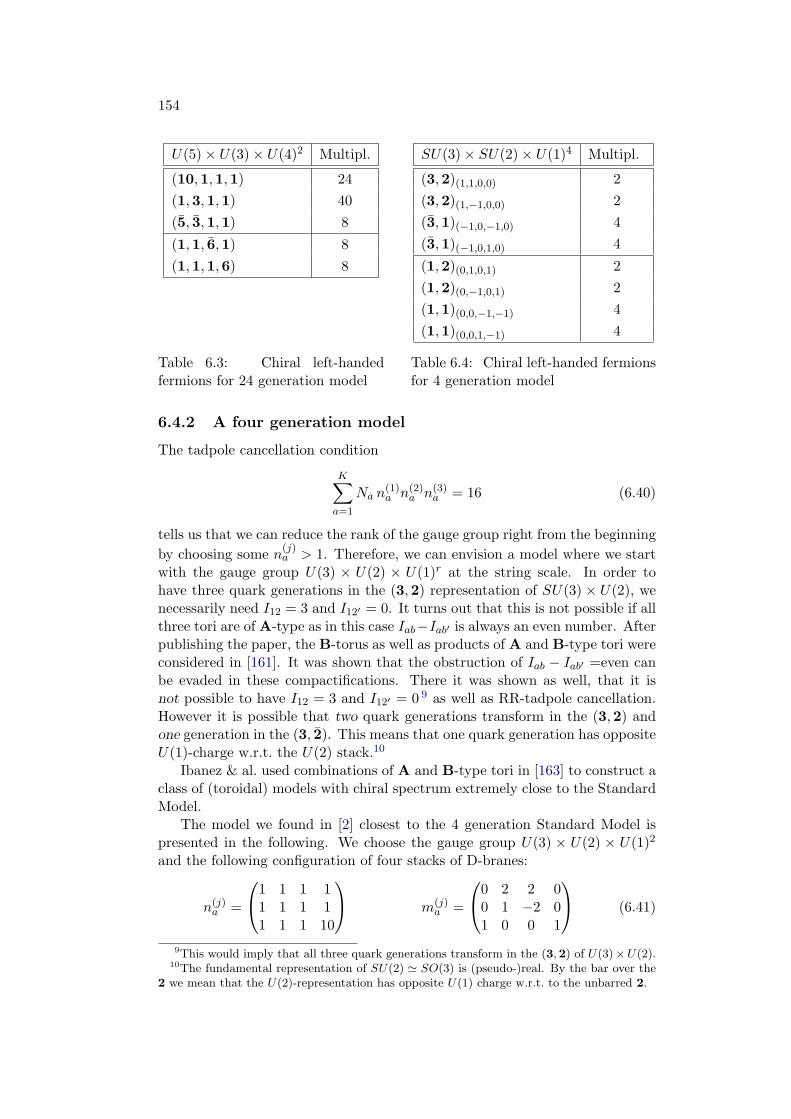
154

U(5)× U(3)× U(4)2 Multipl.

(10,1,1,1) 24(1,3,1,1) 40(5, 3,1,1) 8

(1,1, 6,1) 8(1,1,1,6) 8

Table 6.3: Chiral left-handedfermions for 24 generation model

SU(3)× SU(2)× U(1)4 Multipl.

(3,2)(1,1,0,0) 2(3,2)(1,−1,0,0) 2(3,1)(−1,0,−1,0) 4(3,1)(−1,0,1,0) 4

(1,2)(0,1,0,1) 2(1,2)(0,−1,0,1) 2(1,1)(0,0,−1,−1) 4(1,1)(0,0,1,−1) 4

Table 6.4: Chiral left-handed fermionsfor 4 generation model

6.4.2 A four generation model

The tadpole cancellation condition

K∑a=1

Na n(1)a n(2)

a n(3)a = 16 (6.40)

tells us that we can reduce the rank of the gauge group right from the beginningby choosing some n(j)

a > 1. Therefore, we can envision a model where we startwith the gauge group U(3) × U(2) × U(1)r at the string scale. In order tohave three quark generations in the (3,2) representation of SU(3) × U(2), wenecessarily need I12 = 3 and I12′ = 0. It turns out that this is not possible if allthree tori are of A-type as in this case Iab−Iab′ is always an even number. Afterpublishing the paper, the B-torus as well as products of A and B-type tori wereconsidered in [161]. It was shown that the obstruction of Iab − Iab′ =even canbe evaded in these compactifications. There it was shown as well, that it isnot possible to have I12 = 3 and I12′ = 0 9 as well as RR-tadpole cancellation.However it is possible that two quark generations transform in the (3,2) andone generation in the (3, 2). This means that one quark generation has oppositeU(1)-charge w.r.t. the U(2) stack.10

Ibanez & al. used combinations of A and B-type tori in [163] to construct aclass of (toroidal) models with chiral spectrum extremely close to the StandardModel.

The model we found in [2] closest to the 4 generation Standard Model ispresented in the following. We choose the gauge group U(3) × U(2) × U(1)2

and the following configuration of four stacks of D-branes:

n(j)a =

1 1 1 11 1 1 11 1 1 10

m(j)a =

0 2 2 00 1 −2 01 0 0 1

(6.41)

9This would imply that all three quark generations transform in the (3,2) of U(3)×U(2).10The fundamental representation of SU(2) ' SO(3) is (pseudo-)real. By the bar over the

2 we mean that the U(2)-representation has opposite U(1) charge w.r.t. to the unbarred 2.

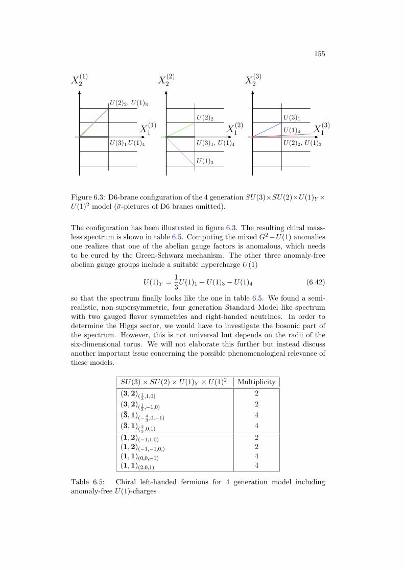
155

X(1)2

X(1)1

X(2)2

X(2)1

X(3)2

X(3)1

U(2)2, U(1)3

U(3)1 U(1)4

U(2)2

U(3)1, U(1)4

U(1)3

U(3)1

U(1)4

U(2)2, U(1)3

Figure 6.3: D6-brane configuration of the 4 generation SU(3)×SU(2)×U(1)Y ×U(1)2 model (σ-pictures of D6 branes omitted).

The configuration has been illustrated in figure 6.3. The resulting chiral mass-less spectrum is shown in table 6.5. Computing the mixed G2−U(1) anomaliesone realizes that one of the abelian gauge factors is anomalous, which needsto be cured by the Green-Schwarz mechanism. The other three anomaly-freeabelian gauge groups include a suitable hypercharge U(1)

U(1)Y =13U(1)1 + U(1)3 − U(1)4 (6.42)

so that the spectrum finally looks like the one in table 6.5. We found a semi-realistic, non-supersymmetric, four generation Standard Model like spectrumwith two gauged flavor symmetries and right-handed neutrinos. In order todetermine the Higgs sector, we would have to investigate the bosonic part ofthe spectrum. However, this is not universal but depends on the radii of thesix-dimensional torus. We will not elaborate this further but instead discussanother important issue concerning the possible phenomenological relevance ofthese models.

SU(3)× SU(2)× U(1)Y × U(1)2 Multiplicity

(3,2)( 13,1,0) 2

(3,2)( 13,−1,0) 2

(3,1)(− 43,0,−1) 4

(3,1)( 23,0,1) 4

(1,2)(−1,1,0) 2(1,2)(−1,−1,0,) 2(1,1)(0,0,−1) 4(1,1)(2,0,1) 4

Table 6.5: Chiral left-handed fermions for 4 generation model includinganomaly-free U(1)-charges

156

Since we break supersymmetry already at the string scale Ms, in order tosolve the gauge hierarchy problem we must choose Ms in the TeV region. Let usemploy the T-dual picture of D6-branes at angles again to analyze the situationin more detail. Using the relations

M2Pl ∼

M8s V6

g2s

1

(g(a)YM)2

∼ M3s Vags

(6.43)

where Va denotes the volume of some D6-brane in the internal directions

Va =3∏j=1

V (j)a (6.44)

and g(a)YM the gauge coupling on this brane. They imply

Ms ∼ α(a)YMMPl

Va√V6

(6.45)

Therefore, for the TeV scenario to work one needs

Va√V6 1 (6.46)

for all D6-branes. However, chirality for the fermionic spectrum of an openstring stretched between any two D6-branes implies that the two branes inquestion do not lie on top of each other on any of the three T 2

(j) tori. In otherwords the two branes already span the entire torus and the condition (6.46)cannot be realized.

6.5 (In-) Stability of purely toroidal orientifolds

In this chapter we will make some comments about the stability of purelytoroidal orientifolds. Stability usually demands the vanishing of the partitionfunction, as the partition function in string theory is interpreted as a dilatonpotential. To do consistent string perturbation theory, no tadpoles are allowedat any order of the string perturbation theory. (Otherwise one could hopethat higher order contributions could “repair” a tadpole that originates fromlower order terms.) Actually the dilaton does not couple to χ = 0 amplitudes,however other string-excitations do. Supersymmetry guarantees the vanishingof the partition function11. Therefore imposing supersymmetry is a very generalmethod to get stable models. Compactifications on flat tori, which are thestarting point of our construction, have a supersymmetric closed string sector.The three unoriented χ = 0 diagrams (Klein-bottle, Cylinder and Mobius strip)are divergent only due to closed string tadpoles. However also in the openstring sector we can often isolate a single excitation that is responsible for an

11In the light-cone quantized string on the pp-wave the partition function does not vanish,but this is believed to be connected to the fact that the light-cone gauge does not cover allstring states (i.e. p+ = 0). (Private communication with Matthias Gaberdiel.)

157

instability: the tachyon. Due to the tachyon relation M2tach < 0 it has been

suggested that the tachyon can condense like a Higgs field φ whose potentialV (φ) ∝ −µ2|φ|2 + λ2|φ|4 if expanded around φ = 0 contains a negative mass2-term as well. Tachyon condensation in terms of string field theory has beeninvestigated in a variety of papers. We only mention two of the first [166,167], a complete list would require more than hundred entries. However wewill mention the conditions for absence of tachyons, which where publishedafter the paper this chapter is based on, was finished. First however we showthat chiral supersymmetric Ωσ orientifolds of the torus are impossible. Thisrestriction does not apply for all toroidal orbifolds.12 The first example of a fourdimensional, chiral supersymmetric Ωσ-orientifold was the Z2 × Z2 orientifoldinvestigated by Cvetic & al. which in addition has the nice feature to admitquasi-realistic models. The second example is the Z4 Ωσ-orientifold on a sixtorus [57] which admits chiral supersymmetric models as well [43, 3]. Some ofthem are even phenomenological interesting.13 We will postpone this discussionto the next chapter.

6.5.1 Supersymmetric brane configurations and special Lagran-gian submanifolds (sLags)

The mathematical foundations of calibrations and sLags are described for ex-ample in the classic publication [169] and a newer article by Joyce [170]. Herewe will state some important definitions and consequences. Without going intothe details, we state the common fact that D-branes that are wrapped aroundso called special Lagrangian submanifolds (sLags) preserve some amount of thebulk (or closed string) supersymmetry [102], if no NS F field is switched on andif no NSNS B-field component is along the D-brane. There are many ways tointroduce the notion of a sLag. One is to start by defining what a calibrationis. Roughly speaking a calibration is a closed k-form φ on a manifoldM (withvolume form vol) such that given any oriented k plane V in the tangent bun-dle TM the induced k-volume volk|V form is always bigger or equal than therestriction of φ:

φ|V ≤ volk|V (6.47)

In this sense a φ-calibrated submanifold N ⊂M is a submanifold of dimensionk s.th. for all oriented tangent planes TxN of N the restriction of φ equals therestriction of the volume form:

φ|TxN = volk|TxN ∀x ∈ N (6.48)

The striking result (of a theorem) is that a calibrated submanifold is alwaysvolume-minimizing in its homology class.

CYn-spaces M (cf. 2.3.1, p. 45) consist of a quadruple14 (M, J, g,Ω). M12However the Z3 orientifold investigated in [59] is always non-supersymmetric for chiral

models.13Meanwhile similar features have been found in the Ωσ-orientifold of the Z4 × Z2-orbifold

[168].14This follows either from the definition of the CY space, or if the CY space is introduced

differently, by further theorems.

158

is the complex compact manifold (of complex dimension n) itself, J the cor-responding complex structure. g is the Kahler metric with the Levi-Civitaconnection leading to SU(n) holonomy. (The Kahler form ω is is obtained fromJ and g). Ω is a non-zero covariantly constant (n, 0)-form s.th.:

ωm

m!= (−1)m(m−1)/2

( i2

)mΩ ∧ Ω (6.49)

By the above definition of Ω the real part Re(Ω) is automatically a calibrationon M.15 A Re(Ω)-calibrated submanifold of a CYn-fold is called a “specialLagrangian submanifold” (sLag). SLags have real dimension n.

A theorem states that given a CYn-fold M (defined as above) and a realn-dimensional submanifold N , then N admits an orientation making it into asLag iff both ω|N = 0 and Im(Ω|N ) = 0 are fulfilled.16

In C2 the sLags are given by holomorphic curves.The case of σΩ orientifolds with sLags has been studied in great generality

in [43]. We will now take advantage of some of the facts inherited by sLags.Applying these properties to the four dimensional case of compactification onT 2×T 2, Ω is given by dz1∧dz2. The D6-branes projected on this four-torus arereal two-dimensional. We have restricted ourselves to flat branes, each a productof two one-cycles, a one-cycle on each two-torus T 2

(j). The sLag condition thengives rise to the condition that the sum of the two oriented angles vanishes:

φ(1) + φ(2) = 0 (6.50)

The O7-plane, i.e. the fixed locus of σ has φ1 = φ2 = 0.17 In other words:the O7-plane is parallel to the X(i)

1 -axis. Canceling the RR-tadpole means thatthe complete holonomy-class of the cycle associated with the D-branes cancelsexactly the holonomy of the O7-plane:18∑

a

Na(πa + πa′) = 8πO7 (6.51)

The πa are elements of the homology generated by the basis (cf. figure 6.1):19

〈p1 ≡ π1 ⊗ π3, p2 ≡ π2 ⊗ π4, p3 ≡ π2 ⊗ π3, p4 ≡ π1 ⊗ π4〉⊕ 〈π1 ⊗ π2, π3 ⊗ π4〉 = H2

(T 4)

(6.52)

15Re(exp(iθ)Ω) is another calibration form. In what follows, we will consider only calibra-tions w.r.t. exp(iθ) = 1.

16If only the condition ω|N = 0 is obeyed, N is called a “Lagrangian submanifold”. Thesupplement “special” means the additional property Im(Ω|N ) = 0. Langrangian submanifoldsare defined more generally in symplectic geometry, where ω denotes the symplectic form.

17The fact that O(9− d)-planes can be interpreted as fixed loci of σ is explained in [43].18The factor of 8 in front of πO7 is determined by the tadpole cancellation conditions (6.35).

πa′ denotes the σ-image of πa.19We have split the basis. Element of the second summand do not appear in our models.

159

In the p-basis the cycle wrapped by the D7-brane a is expressed by:20

πa =

n

(1)a n

(2)a

m(1)a m

(2)a

m(1)a n

(2)a

n(1)a m

(2)a

I =

0 11 0

0

0 101 0

(6.53)

In the above basis the homology class of the O7-plane (i.e. the σ-invariant locus)is given by:

πO7 = 4 p1 = (4, 0, 0, 0)T (6.54)

It is now clear that the configuration with the smallest volume that lies in thesame Homology class as the O7 plane, is the one in which all D-branes areparallel to the X(i)

1 axis. Any flat tilted brane with identical πO7-componentand non-zero angle wrt. the X(i)

1 -axis will have larger volume. Such a braneconfiguration can not be a sLag since sLags are volume minimizing in their ho-mology class. Thus, in the absence of NSNS B-fields with components parallelto the branes and in the absence of an NS F -flux, the only supersymmetry pre-serving D7-brane configurations that cancel the RR-tadpole, are the ones whereall branes are parallel to the O7-plane.21 These configurations are however theones without chiral fermions.

The same arguments go through for the six-torus (i.e. the four-dimensionalmodels). In contrast to the four compact dimensions, the six-dimensional torusforces B-field components along the D6-brane to vanish, as well as F = 0 forthe NS U(1)-fields. This was shown in [103]. Therefore we conclude that puretoroidal compactifications can not reconcile both supersymmetry and chiralityw.r.t. the gauge group.

In the next section, we summarize what has been found out on the existenceand non-existence of (open-) string tachyons in toroidal compactifications.

6.5.2 Tachyons in toroidal orientifolds

As we already noted, tachyons can only appear in the open string sector, asthe closed string sector is supersymmetric. In our original publication we con-cluded that in six-dimensional models open string tachyons generically appeardue to the fact that two D7-branes that are rotated by an angle (φ1, φ2) al-ways imply negative ground state energy, except for the supersymmetric caseφ1 = −φ2. Thus in Ωσ-orientifolds on T 4 we always encounter one or severalopen string tachyons, iff supersymmetry is broken. However for open strings

20I denotes the intersection matrix. It can be used to calculate the intersection number aswell (cf. table 6.1).

21However the brane might be deformed, s.th. it is no longer flat: a theorem by McLeanstates that the dimension of the moduli space of a sLag N equals the first Betti number b1(N )(cf. [171, 170]). In the case of the flat tow-torus however, b1(N ) just equals the number ofindependent translations of the D-brane in its normal direction, which is two. Therefore weconclude that a deformation that transforms a flat D-brane to a non-flat one, will spoil thesLag condition and as a consequence will break supersymmetry. Similar to the CY-case wherethe geometric Kahler cone gets complexified by the NSNS B-field, we can add Wilson lines,

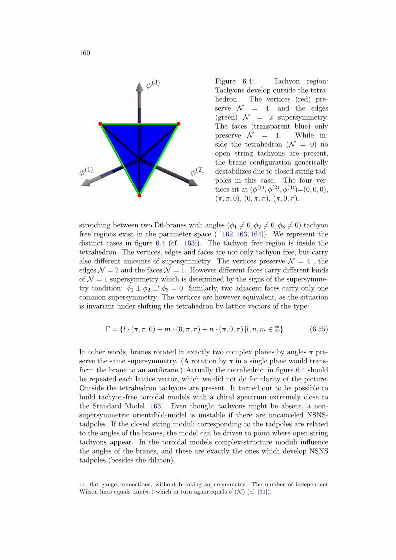
160

φ(1)

φ(2)

φ(3) Figure 6.4: Tachyon region:

Tachyons develop outside the tetra-hedron. The vertices (red) pre-serve N = 4, and the edges(green) N = 2 supersymmetry.The faces (transparent blue) onlypreserve N = 1. While in-side the tetrahedron (N = 0) noopen string tachyons are present,the brane configuration genericallydestabilizes due to closed string tad-poles in this case. The four ver-tices sit at (φ(1), φ(2), φ(3))=(0, 0, 0),(π, π, 0), (0, π, π), (π, 0, π).

stretching between two D6-branes with angles (φ1 6= 0, φ2 6= 0, φ3 6= 0) tachyonfree regions exist in the parameter space ( [162, 163, 164]). We represent thedistinct cases in figure 6.4 (cf. [163]). The tachyon free region is inside thetetrahedron. The vertices, edges and faces are not only tachyon free, but carryalso different amounts of supersymmetry. The vertices preserve N = 4 , theedges N = 2 and the faces N = 1. However different faces carry different kindsof N = 1 supersymmetry which is determined by the signs of the supersymme-try condition: φ1 ± φ2 ±′ φ3 = 0. Similarly, two adjacent faces carry only onecommon supersymmetry. The vertices are however equivalent, as the situationis invariant under shifting the tetrahedron by lattice-vectors of the type:

Γ = l · (π, π, 0) +m · (0, π, π) + n · (π, 0, π) |l, n,m ∈ Z (6.55)

In other words, branes rotated in exactly two complex planes by angles π pre-serve the same supersymmetry. (A rotation by π in a single plane would trans-form the brane to an antibrane.) Actually the tetrahedron in figure 6.4 shouldbe repeated each lattice vector, which we did not do for clarity of the picture.Outside the tetrahedron tachyons are present. It turned out to be possible tobuild tachyon-free toroidal models with a chiral spectrum extremely close tothe Standard Model [163]. Even thought tachyons might be absent, a non-supersymmetric orientifold-model is unstable if there are uncanceled NSNS-tadpoles. If the closed string moduli corresponding to the tadpoles are relatedto the angles of the branes, the model can be driven to point where open stringtachyons appear. In the toroidal models complex-structure moduli influencethe angles of the branes, and these are exactly the ones which develop NSNStadpoles (besides the dilaton).

i.e. flat gauge connections, without breaking supersymmetry. The number of independentWilson lines equals dim(π1) which in turn again equals b1(N ) (cf. [31]).

161

Concluding remarks

In this paper we have investigated Type I string compactifications on non-commutative tori, which are due to constant magnetic fields along the worldvolumes of the D9-branes being wrapped around the internal space. The num-ber of chiral fermions (arising from strings “stretched” between two braneswith different NS F -field-strength on each T 2) can be interpreted as a Lan-dau degeneracy. It is given by the Atiyah-Singer index theorem for twistedspin-complexes.

In the T-dual picture the magnetized D9-branes become lower-dimensionalbranes, while the Ω-parity projection now includes a complex conjugation onall T 2’s: Ω

T-duality−−−−−−→ σΩ. In this picture, the chiral fermions are located atthe brane intersection-points. The analog of the Landau degeneracy is thetopological intersection number of two D-branes.

In the given setting, we found a four-dimensional model with StandardModel gauge group SU(3) × SU(2) × U(1)Y (times some abelian flavor gaugegroups) with four generations of Standard Model fermions and also a four-dimensional 24 generation SU(5) GUT-like model. However it turned out, thatthe Ansatz T 6 =

∏j T

2(j)A involving only A-type tori leads always to an even

number of left handed quark generation, as the difference of the intersectionnumber Iab − Iab′ is always even. As shown in a subsequent publication [161],this problem can be evaded by considering more general T 6-tori involving B-type two-tori, as well.

We found that in chiral toroidal orientifolds, supersymmetry is always bro-ken. This could lead to open string tachyons. However many models havebeen found after our publication, in which tachyons are absent (cf. [163]).Nevertheless, closed string tadpoles tend to destabilize the model and driveit to a singular limit of the T 6. Dilaton tadpoles can in general push a non-supersymmetric model to either a strongly-coupled or free regime. Investiga-tions if a non-supersymmetric string model could be stabilized by the Fischler-Susskind mechanism [54, 55] have been undertaken as well (cf. [172,173]).

The stability problems would be absent, if one can construct supersymmetricmodels. That it is indeed possible to reconcile both supersymmetry and chiralityhas been shown by Cvetic & al. [174] who considered a (left-right symmetric)T 6/(Z2 × Z2) Type IIA orientifold. This orientifold has phenomenologicallyappealing solutions. The second example of a Type IIA orientifold involvingbranes at angles and admitting chiral supersymmetric solutions was publishedby us some time later (cf. [3]). We found a solution with a gauge-group that canbe broken down to the SM gauge group in a supersymmetry preserving way bygiving VEVs to fields in the low energy effective action. The matter content ofthe resulting model is extremely close to the MSSM. We will review the T 6/Z4

σΩ-orientifold in the next chapter.

Chapter 7

The σΩ-Orientifoldon (T 2 × T 2 × T 2)/Z4

Intersecting brane world models have been the subject of elaborate string modelbuilding for several years [2,165,124,175,162,176,161,163,177,164,59,178,174,179,180,181,182,183,184,185,186,187,188,189,190,191,192,193,194,43,195,196,197,198,199,200,201,202]. The main new ingredient in these models is that theycontain intersecting D-branes and open strings in a consistent manner provid-ing simple mechanisms to generate chiral fermions and to break supersymme-try [28, 27]. Most attempts for constructing realistic models were dealing withnon-supersymmetric configurations of D-branes, mainly because non-trivial,chiral supersymmetric intersecting brane world models are not easy to find.It is known for instance that flat factorizing D-branes on the six-dimensionaltorus as well as on the T 6/Z3 orbifold can never give rise to supersymmetricmodels except for the trivial non-chiral configuration where all D6-branes arelocated on top of the orientifold plane [59]. Supersymmetric models clearlyhave some advantages over the non supersymmetric ones. From the stringypoint of view such models are stable, as not only the Ramond-Ramond (R-R)tadpoles cancel but also the Neveu-Schwarz-Neveu-Schwarz (NS-NS) tadpoles.From the phenomenological point of view, since the gauge hierarchy problemis solved by supersymmetry, one can work in the conventional scenarios with alarge string scale close to the Planck scale or in an intermediate regime [203].For an overview on other Type I constructions see [18].

The only semi-realistic supersymmetric models that have been found sofar are defined in the T 6/Z2 ×Z2 orientifold background and were studied in aseries of papers [178,174,192,193,200].1 Besides their phenomenological impact,Type IIA supersymmetric intersecting brane worlds with orientifold six-planesand D6-branes are also interesting from the stringy point of view, as they areexpected to lift to M-theory on singular G2 manifolds [204].

The aim of this chapter (and the underlying publication [3]) is to pursuethe study of intersecting brane worlds on orientifolds with a particular emphasison the systematic construction of semi-realistic supersymmetric configurations.

1Meanwhile the Z4 × Z2 orientifold with σΩ-projection has been studied. Interesting non-chiral supersymmetric solutions have been found as well (cf. [168]).

162

163

Note, that without the orientifold projection supersymmetric intersecting braneconfigurations do not exist, as the overall tension always would be positive.Interestingly, from the technical point of view, the Z4 orbifold involves somenew insights, as not all 3-cycles are inherited from the torus. In fact, a coupleof 3-cycles arise in the Z2 twisted sector implying that this model containsso-called fractional D6-branes, which have been absent in the Z2 × Z2 and Z3

orbifolds. To treat these exceptional cycles accordingly, we will make extensiveuse of the formalism developed in [43].

It will turn out that supersymmetric models in general can be constructedin a straightforward way. But as in other model building approaches, findingsemi-realistic three generation models turns out to be quite difficult. Fortu-nately, we will finally succeed in constructing a globally supersymmetric threegeneration Pati-Salam model with gauge group SU(4)×SU(2)L×SU(2)R andthe Standard Model matter in addition to some exotic matter in the symmet-ric and antisymmetric representation of the two SU(2) gauge groups. In thischapter, we will mainly focus on the new and interesting string model buildingaspects and leave a detailed investigation of the phenomenological implicationsof the discussed models for future work.

This chapter is organized as follows. In section 7.1 we review some of thematerial presented in [43] about the general structure of intersecting braneworlds on Calabi-Yau manifolds. We will review those formulæ which will beextensively used in the rest of the paper. In section 7.2 we start to investigatethe X = T 6/Z4 orbifold and in particular derive an integral basis for the homol-ogy group H3(X ,Z), for which the intersection form involves the Cartan-matrixof the Lie-algebra E8. The main ingredient in the construction of such an in-tegral basis will be the physical motivated introduction of fractional D-braneswhich also wrap around exceptional (twisted) 3-cycles in X . In section 7.3 weconstruct the orientifold models of Type IIA on the orbifold X and discuss theorientifold planes, the action of the orientifold projection on the homology andthe additional conditions arising for supersymmetric configurations. In section7.4 we construct as a first example a globally supersymmetric four generationPati-Salam model. Finally, in section 7.5 we elaborate on a supersymmetricmodel with initial gauge symmetry U(4) × U(2)3 × U(2)3 and argue that bybrane recombination it becomes a supersymmetric three generation Pati-Salammodel. By using conformal field theory methods, for this model we determinethe chiral and also the massless non-chiral spectrum, which turns out to provideHiggs fields in just the right representations in order to break the model downto the Standard Model. At the end of the paper we describe both the GUTbreaking and the electroweak breaking via brane recombination processes. Wealso make a prediction for the Weinberg angle at the string scale.

7.1 Intersecting Brane Worlds on Calabi-Yau spaces

Before we present our new model, we would like to briefly summarize some ofthe results presented in [43] about Type IIA orientifolds on smooth Calabi-Yauspaces. If the manifold admits an anti-holomorphic involution σ, the combi-

164

nation Ωσ is indeed a symmetry of the Type IIA model. Taking the quotientwith respect to this symmetry introduces an orientifold six-plane into the back-ground, which wraps a special Lagrangian 3-cycle of the Calabi-Yau.2 In orderto cancel the induced RR-charge, one introduces stacks of Na D6-branes whichare wrapped on 3-cycles πa. Since under the action of σ such a 3-cycle, πa, is ingeneral mapped to a different 3-cycle, π′a, one has to wrap the same number ofD6-branes on the latter cycle, too. The equation of motion for the RR 7-formimplies the RR-tadpole cancellation condition,∑

a

Na (πa + π′a)− 4πO6 = 0. (7.1)

If it is possible to wrap a connected smooth D-brane on such a homology class,the stack of D6-branes supports a U(Na) gauge factor. Note, that it is not atrivial question if in a given homology class such a connected smooth manifolddoes exist. However, as we will see in section 7.5 for special cases, there arephysical arguments ensuring that such smooth D-branes exist.

The Born-Infeld action provides an expression for the open string tree-levelscalar potential which by differentiation leads to an equation for the NS-NStadpoles

V = T6e−φ4

M3s

√Vol(X )

(∑a

Na

(Vol(D6a) + Vol(D6′a)

)− 4 Vol(O6)

)(7.2)

with the four-dimensional dilaton given by e−φ4 = M3s

√Vol(X )e−φ10 and T6

denoting the tension of the D6-branes. By Vol(D6a) we mean the three di-mensional internal volume of the D6-branes. Generically, this scalar potentialis non-vanishing reflecting the fact that intersecting branes do break super-symmetry. If the cycles (more precisely: the corresponding submanifolds) arespecial Lagrangian (sLag) but calibrated with respect to 3-forms Re(eiθΩ3,0)with different constant phase factors exp(iθ), the expression gets simplified to3

V = T6 e−φ4

(∑a

Na

∣∣∣∣∫πa

Ω3,0

∣∣∣∣+∑a

Na

∣∣∣∣∣∫π′a

Ω3,0

∣∣∣∣∣− 4∣∣∣∣∫πO6

Ω3,0

∣∣∣∣)

(7.3)

In this case, all D6-branes preserve some supersymmetry but not all of themthe same. Models of this type have been discussed in [184, 186]. In the case ofa completely supersymmetric model, all 3-cycles are calibrated with respect tothe same 3-form as the O6-plane implying that the disc level scalar potentialvanishes due to the RR-tadpole condition (7.1).

In [43] it was argued and confirmed by many examples that the chiral mass-less spectrum charged under the U(N1)×. . .×U(Nk) gauge group of a configura-tion of k intersecting stacks of D6-branes can be computed from the topologicalintersection numbers as shown in table 7.1. Since in six dimensions the in-

2By “special Lagrangian 3-cycle” we mean the real three-dimensional special Lagrangiansubmanifold, that lies in the same homology class as the 3-cycle.

3Ω3,0 = eiθΩ3,0

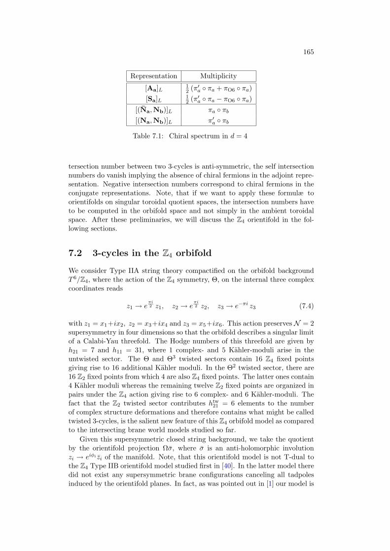
165

Representation Multiplicity

[Aa]L 12 (π′a πa + πO6 πa)

[Sa]L 12 (π′a πa − πO6 πa)

[(Na,Nb)]L πa πb[(Na,Nb)]L π′a πb

Table 7.1: Chiral spectrum in d = 4

tersection number between two 3-cycles is anti-symmetric, the self intersectionnumbers do vanish implying the absence of chiral fermions in the adjoint repre-sentation. Negative intersection numbers correspond to chiral fermions in theconjugate representations. Note, that if we want to apply these formulæ toorientifolds on singular toroidal quotient spaces, the intersection numbers haveto be computed in the orbifold space and not simply in the ambient toroidalspace. After these preliminaries, we will discuss the Z4 orientifold in the fol-lowing sections.

7.2 3-cycles in the Z4 orbifold

We consider Type IIA string theory compactified on the orbifold backgroundT 6/Z4, where the action of the Z4 symmetry, Θ, on the internal three complexcoordinates reads

z1 → eπi2 z1, z2 → e

πi2 z2, z3 → e−πi z3 (7.4)

with z1 = x1+ix2, z2 = x3+ix4 and z3 = x5+ix6. This action preserves N = 2supersymmetry in four dimensions so that the orbifold describes a singular limitof a Calabi-Yau threefold. The Hodge numbers of this threefold are given byh21 = 7 and h11 = 31, where 1 complex- and 5 Kahler-moduli arise in theuntwisted sector. The Θ and Θ3 twisted sectors contain 16 Z4 fixed pointsgiving rise to 16 additional Kahler moduli. In the Θ2 twisted sector, there are16 Z2 fixed points from which 4 are also Z4 fixed points. The latter ones contain4 Kahler moduli whereas the remaining twelve Z2 fixed points are organized inpairs under the Z4 action giving rise to 6 complex- and 6 Kahler-moduli. Thefact that the Z2 twisted sector contributes htw

21 = 6 elements to the numberof complex structure deformations and therefore contains what might be calledtwisted 3-cycles, is the salient new feature of this Z4 orbifold model as comparedto the intersecting brane world models studied so far.

Given this supersymmetric closed string background, we take the quotientby the orientifold projection Ωσ, where σ is an anti-holomorphic involutionzi → eiφi zi of the manifold. Note, that this orientifold model is not T-dual tothe Z4 Type IIB orientifold model studied first in [40]. In the latter model theredid not exist any supersymmetric brane configurations canceling all tadpolesinduced by the orientifold planes. In fact, as was pointed out in [1] our model is

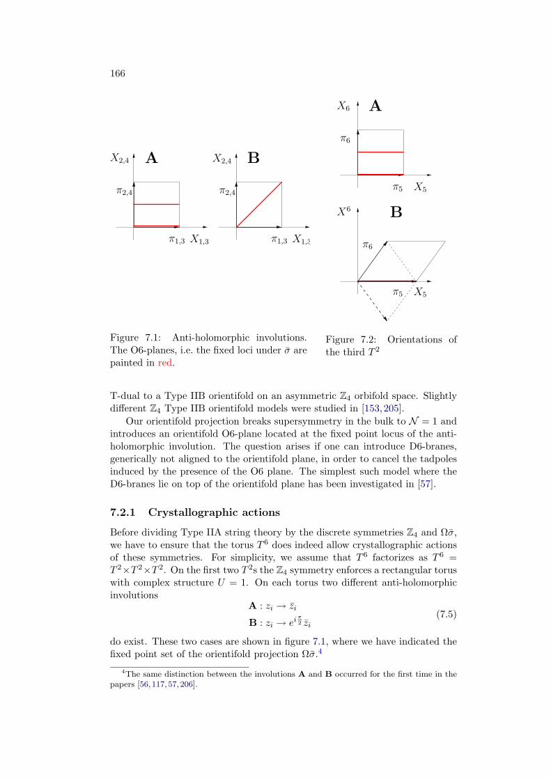
166

X1,3

BA

X1,3

π2,4

π1,3

π2,4

π1,3

X2,4X2,4

Figure 7.1: Anti-holomorphic involutions.The O6-planes, i.e. the fixed loci under σ arepainted in red.

X5

X5

A

B

π5

π5

π6

π6

X6

X6

Figure 7.2: Orientations ofthe third T 2

T-dual to a Type IIB orientifold on an asymmetric Z4 orbifold space. Slightlydifferent Z4 Type IIB orientifold models were studied in [153,205].

Our orientifold projection breaks supersymmetry in the bulk to N = 1 andintroduces an orientifold O6-plane located at the fixed point locus of the anti-holomorphic involution. The question arises if one can introduce D6-branes,generically not aligned to the orientifold plane, in order to cancel the tadpolesinduced by the presence of the O6 plane. The simplest such model where theD6-branes lie on top of the orientifold plane has been investigated in [57].

7.2.1 Crystallographic actions

Before dividing Type IIA string theory by the discrete symmetries Z4 and Ωσ,we have to ensure that the torus T 6 does indeed allow crystallographic actionsof these symmetries. For simplicity, we assume that T 6 factorizes as T 6 =T 2×T 2×T 2. On the first two T 2s the Z4 symmetry enforces a rectangular toruswith complex structure U = 1. On each torus two different anti-holomorphicinvolutions

A : zi → zi

B : zi → eiπ2 zi

(7.5)

do exist. These two cases are shown in figure 7.1, where we have indicated thefixed point set of the orientifold projection Ωσ.4

4The same distinction between the involutions A and B occurred for the first time in thepapers [56,117,57,206].

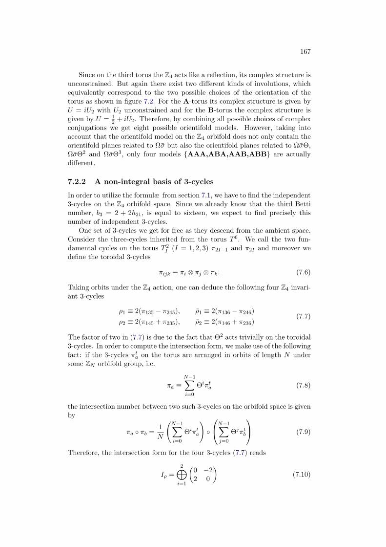
167

Since on the third torus the Z4 acts like a reflection, its complex structure isunconstrained. But again there exist two different kinds of involutions, whichequivalently correspond to the two possible choices of the orientation of thetorus as shown in figure 7.2. For the A-torus its complex structure is given byU = iU2 with U2 unconstrained and for the B-torus the complex structure isgiven by U = 1

2 + iU2. Therefore, by combining all possible choices of complexconjugations we get eight possible orientifold models. However, taking intoaccount that the orientifold model on the Z4 orbifold does not only contain theorientifold planes related to Ωσ but also the orientifold planes related to ΩσΘ,ΩσΘ2 and ΩσΘ3, only four models AAA,ABA,AAB,ABB are actuallydifferent.

7.2.2 A non-integral basis of 3-cycles

In order to utilize the formulæ from section 7.1, we have to find the independent3-cycles on the Z4 orbifold space. Since we already know that the third Bettinumber, b3 = 2 + 2h21, is equal to sixteen, we expect to find precisely thisnumber of independent 3-cycles.

One set of 3-cycles we get for free as they descend from the ambient space.Consider the three-cycles inherited from the torus T 6. We call the two fun-damental cycles on the torus T 2

I (I = 1, 2, 3) π2I−1 and π2I and moreover wedefine the toroidal 3-cycles

πijk ≡ πi ⊗ πj ⊗ πk. (7.6)

Taking orbits under the Z4 action, one can deduce the following four Z4 invari-ant 3-cycles

ρ1 ≡ 2(π135 − π245), ρ1 ≡ 2(π136 − π246)ρ2 ≡ 2(π145 + π235), ρ2 ≡ 2(π146 + π236)

(7.7)

The factor of two in (7.7) is due to the fact that Θ2 acts trivially on the toroidal3-cycles. In order to compute the intersection form, we make use of the followingfact: if the 3-cycles πta on the torus are arranged in orbits of length N undersome ZN orbifold group, i.e.

πa ≡N−1∑i=0

Θiπta (7.8)

the intersection number between two such 3-cycles on the orbifold space is givenby

πa πb =1N

(N−1∑i=0

Θiπta

)

N−1∑j=0

Θjπtb

(7.9)

Therefore, the intersection form for the four 3-cycles (7.7) reads

Iρ =2⊕i=1

(0 −22 0

)(7.10)

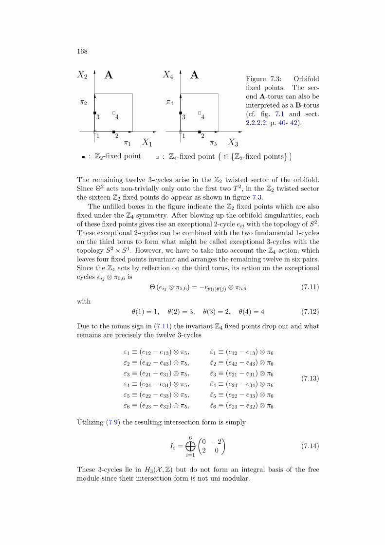
168

X4X2

: Z2-fixed point : Z4-fixed point(∈ Z2-fixed points

)

3 4

X3

21

3 4

X1

1

AA

2

π4

π1 π3

π2

Figure 7.3: Orbifoldfixed points. The sec-ond A-torus can also beinterpreted as a B-torus(cf. fig. 7.1 and sect.2.2.2.2, p. 40- 42).

The remaining twelve 3-cycles arise in the Z2 twisted sector of the orbifold.Since Θ2 acts non-trivially only onto the first two T 2, in the Z2 twisted sectorthe sixteen Z2 fixed points do appear as shown in figure 7.3.

The unfilled boxes in the figure indicate the Z2 fixed points which are alsofixed under the Z4 symmetry. After blowing up the orbifold singularities, eachof these fixed points gives rise an exceptional 2-cycle eij with the topology of S2.These exceptional 2-cycles can be combined with the two fundamental 1-cycleson the third torus to form what might be called exceptional 3-cycles with thetopology S2 × S1. However, we have to take into account the Z4 action, whichleaves four fixed points invariant and arranges the remaining twelve in six pairs.Since the Z4 acts by reflection on the third torus, its action on the exceptionalcycles eij ⊗ π5,6 is

Θ (eij ⊗ π5,6) = −eθ(i)θ(j) ⊗ π5,6 (7.11)

withθ(1) = 1, θ(2) = 3, θ(3) = 2, θ(4) = 4 (7.12)

Due to the minus sign in (7.11) the invariant Z4 fixed points drop out and whatremains are precisely the twelve 3-cycles

ε1 ≡ (e12 − e13)⊗ π5, ε1 ≡ (e12 − e13)⊗ π6

ε2 ≡ (e42 − e43)⊗ π5, ε2 ≡ (e42 − e43)⊗ π6

ε3 ≡ (e21 − e31)⊗ π5, ε3 ≡ (e21 − e31)⊗ π6

ε4 ≡ (e24 − e34)⊗ π5, ε4 ≡ (e24 − e34)⊗ π6

ε5 ≡ (e22 − e33)⊗ π5, ε5 ≡ (e22 − e33)⊗ π6

ε6 ≡ (e23 − e32)⊗ π5, ε6 ≡ (e23 − e32)⊗ π6

(7.13)

Utilizing (7.9) the resulting intersection form is simply

Iε =6⊕i=1

(0 −22 0

)(7.14)

These 3-cycles lie in H3(X ,Z) but do not form an integral basis of the freemodule since their intersection form is not uni-modular.

169

7.2.3 An integral basis of 3-cycles

The cycles which are missing so far are the ones corresponding to what is calledfractional D-branes [29, 207]. In our context these are D-branes wrapping onlyone-half times around the toroidal cycles ρ1, ρ1, ρ2, ρ2 while wrapping simul-taneously around some of the exceptional 3-cycles. Therefore in the orbifoldlimit such branes are stuck at the fixed points and one needs at least two suchfractional D-branes in order to form a brane which can be moved into the bulk.

To proceed, we need a rule of what combinations of toroidal and exceptionalcycles are allowed for a fractional D-brane. Such a rule can be easily gainedfrom our physical intuition. A D-brane wrapping for instance the toroidal cycle12ρ1 can only wrap around those exceptional 3-cycles that correspond to the Z2

fixed points the flat D-brane is passing through. In our case, when the brane islying along the X1,3,5-axis on the three T 2s, the allowed exceptional cycles areε1, ε3, ε5. Therefore, the total homological cycle the D-brane is wrapping oncan be for instance

πa =12ρ1 +

12(ε1 + ε3 + ε5) (7.15)

The relative signs for the four different terms in (7.15) are still free parametersand at the orbifold point do correspond to turning on a discrete Wilson linealong a longitudinal internal direction of the D-brane. Note, that this con-struction is completely analogous to the construction of boundary states forfractional D-branes [208,209,210] carrying also a charge under some Z2 twistedsector states.

As an immediate consequences of this rule, only unbarred respectively barredcycles can be combined into fractional cycles, as they wrap the same fundamen-tal 1-cycle on the third T 2. Apparently, the only non-vanishing intersectionnumbers are between barred and unbarred cycles. Any unbarred fractionalD-brane can be expanded as

πa = va,1ρ1 + va,2ρ2 +6∑i=1

va,i+2 εi (7.16)

with half-integer valued coefficients va,i. By exchanging the two fundamentalcycles on the third T 2, we can associate to it a barred brane

πa = va,1ρ1 + va,2ρ2 +6∑i=1

va,i+2 εi (7.17)

with the same coefficients va,i+8 = va,i for i ∈ 1, . . . , 8. Using our rule we canconstruct all linear combinations with “self”-intersection number π π = −2,where we also have to keep in mind that the cycles form a lattice, i.e. integerlinear combinations of cycles are again cycles.In the following we list all the fractional 3-cycles with “self”-intersection numberπ π = −2. These cycles can be divided into 3 sets:

a) (v1, v2; v3, v4; v5, v6; v7, v8) | v1 + v2 = ±1/2, v3 + v4 = ±1/2, v5 + v6 =±1/2, v7 + v8 = ±1/2; v1 + v3 + v5 + v7 = 0 mod 1. These combinations

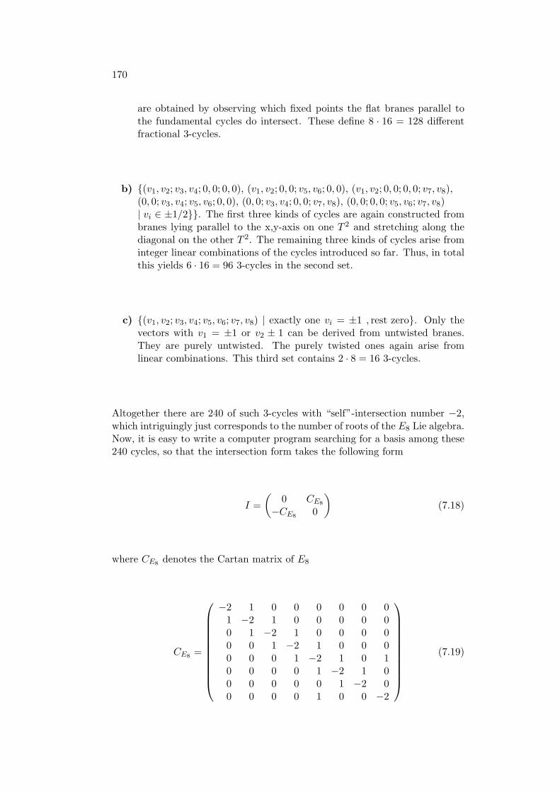
170

are obtained by observing which fixed points the flat branes parallel tothe fundamental cycles do intersect. These define 8 · 16 = 128 differentfractional 3-cycles.

b) (v1, v2; v3, v4; 0, 0; 0, 0), (v1, v2; 0, 0; v5, v6; 0, 0), (v1, v2; 0, 0; 0, 0; v7, v8),(0, 0; v3, v4; v5, v6; 0, 0), (0, 0; v3, v4; 0, 0; v7, v8), (0, 0; 0, 0; v5, v6; v7, v8)| vi ∈ ±1/2. The first three kinds of cycles are again constructed frombranes lying parallel to the x,y-axis on one T 2 and stretching along thediagonal on the other T 2. The remaining three kinds of cycles arise frominteger linear combinations of the cycles introduced so far. Thus, in totalthis yields 6 · 16 = 96 3-cycles in the second set.

c) (v1, v2; v3, v4; v5, v6; v7, v8) | exactly one vi = ±1 , rest zero. Only thevectors with v1 = ±1 or v2 ± 1 can be derived from untwisted branes.They are purely untwisted. The purely twisted ones again arise fromlinear combinations. This third set contains 2 · 8 = 16 3-cycles.

Altogether there are 240 of such 3-cycles with “self”-intersection number −2,which intriguingly just corresponds to the number of roots of the E8 Lie algebra.Now, it is easy to write a computer program searching for a basis among these240 cycles, so that the intersection form takes the following form

I =(

0 CE8

−CE8 0

)(7.18)

where CE8 denotes the Cartan matrix of E8

CE8 =

−2 1 0 0 0 0 0 01 −2 1 0 0 0 0 00 1 −2 1 0 0 0 00 0 1 −2 1 0 0 00 0 0 1 −2 1 0 10 0 0 0 1 −2 1 00 0 0 0 0 1 −2 00 0 0 0 1 0 0 −2

(7.19)

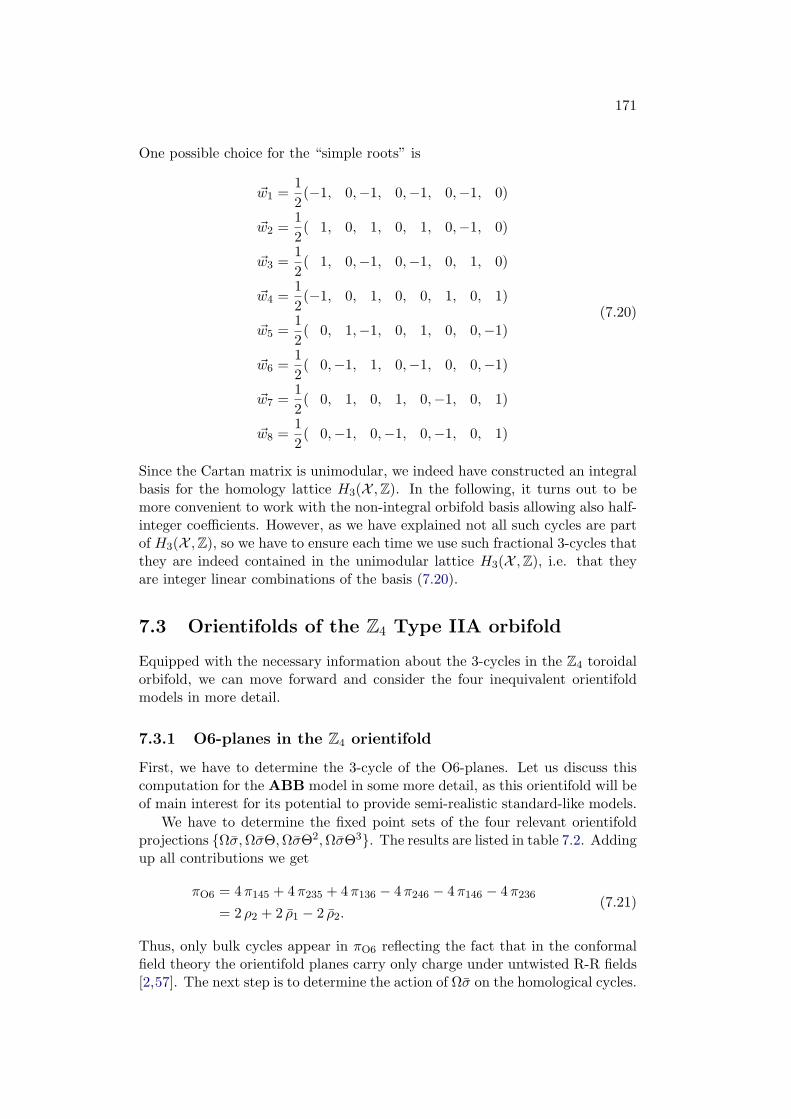
171

One possible choice for the “simple roots” is

~w1 =12(−1, 0,−1, 0,−1, 0,−1, 0)

~w2 =12( 1, 0, 1, 0, 1, 0,−1, 0)

~w3 =12( 1, 0,−1, 0,−1, 0, 1, 0)

~w4 =12(−1, 0, 1, 0, 0, 1, 0, 1)

~w5 =12( 0, 1,−1, 0, 1, 0, 0,−1)

~w6 =12( 0,−1, 1, 0,−1, 0, 0,−1)

~w7 =12( 0, 1, 0, 1, 0,−1, 0, 1)

~w8 =12( 0,−1, 0,−1, 0,−1, 0, 1)

(7.20)

Since the Cartan matrix is unimodular, we indeed have constructed an integralbasis for the homology lattice H3(X ,Z). In the following, it turns out to bemore convenient to work with the non-integral orbifold basis allowing also half-integer coefficients. However, as we have explained not all such cycles are partof H3(X ,Z), so we have to ensure each time we use such fractional 3-cycles thatthey are indeed contained in the unimodular lattice H3(X ,Z), i.e. that theyare integer linear combinations of the basis (7.20).

7.3 Orientifolds of the Z4 Type IIA orbifold

Equipped with the necessary information about the 3-cycles in the Z4 toroidalorbifold, we can move forward and consider the four inequivalent orientifoldmodels in more detail.

7.3.1 O6-planes in the Z4 orientifold

First, we have to determine the 3-cycle of the O6-planes. Let us discuss thiscomputation for the ABB model in some more detail, as this orientifold will beof main interest for its potential to provide semi-realistic standard-like models.

We have to determine the fixed point sets of the four relevant orientifoldprojections Ωσ,ΩσΘ,ΩσΘ2,ΩσΘ3. The results are listed in table 7.2. Addingup all contributions we get

πO6 = 4π145 + 4π235 + 4π136 − 4π246 − 4π146 − 4π236

= 2 ρ2 + 2 ρ1 − 2 ρ2.(7.21)

Thus, only bulk cycles appear in πO6 reflecting the fact that in the conformalfield theory the orientifold planes carry only charge under untwisted R-R fields[2,57]. The next step is to determine the action of Ωσ on the homological cycles.

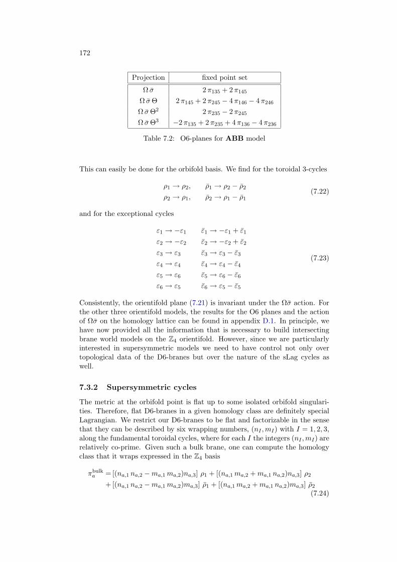
172

Projection fixed point set

Ω σ 2π135 + 2π145

Ω σΘ 2π145 + 2π245 − 4π146 − 4π246

Ω σΘ2 2π235 − 2π245

Ω σΘ3 −2π135 + 2π235 + 4π136 − 4π236

Table 7.2: O6-planes for ABB model

This can easily be done for the orbifold basis. We find for the toroidal 3-cycles

ρ1 → ρ2, ρ1 → ρ2 − ρ2

ρ2 → ρ1, ρ2 → ρ1 − ρ1(7.22)

and for the exceptional cycles

ε1 → −ε1 ε1 → −ε1 + ε1

ε2 → −ε2 ε2 → −ε2 + ε2

ε3 → ε3 ε3 → ε3 − ε3ε4 → ε4 ε4 → ε4 − ε4ε5 → ε6 ε5 → ε6 − ε6ε6 → ε5 ε6 → ε5 − ε5

(7.23)

Consistently, the orientifold plane (7.21) is invariant under the Ωσ action. Forthe other three orientifold models, the results for the O6 planes and the actionof Ωσ on the homology lattice can be found in appendix D.1. In principle, wehave now provided all the information that is necessary to build intersectingbrane world models on the Z4 orientifold. However, since we are particularlyinterested in supersymmetric models we need to have control not only overtopological data of the D6-branes but over the nature of the sLag cycles aswell.

7.3.2 Supersymmetric cycles

The metric at the orbifold point is flat up to some isolated orbifold singulari-ties. Therefore, flat D6-branes in a given homology class are definitely specialLagrangian. We restrict our D6-branes to be flat and factorizable in the sensethat they can be described by six wrapping numbers, (nI ,mI) with I = 1, 2, 3,along the fundamental toroidal cycles, where for each I the integers (nI ,mI) arerelatively co-prime. Given such a bulk brane, one can compute the homologyclass that it wraps expressed in the Z4 basis

πbulka = [(na,1 na,2 −ma,1ma,2)na,3] ρ1 + [(na,1ma,2 +ma,1 na,2)na,3] ρ2

+ [(na,1 na,2 −ma,1ma,2)ma,3] ρ1 + [(na,1ma,2 +ma,1 na,2)ma,3] ρ2

(7.24)

173

For the ABB orientifold, the condition that such a D6-brane preserves the samesupersymmetry as the orientifold plane is simply

ϕa,1 + ϕa,2 + ϕa,3 =π

4mod 2π (7.25)

with

tanϕa,1 =ma,1

na,1, tanϕa,2 =

ma,2

na,2, tanϕa,3 =

U2ma,3

na,3 + 12ma,3

(7.26)

Taking the tan(...) on both sides of equation (7.25) we can reformulate thesupersymmetry condition in terms of wrapping numbers (Note, that this onlyyields a necessary condition as tan(...) is just periodic mod π.)

U2 =

(na,3 + 1

2ma,3

)ma,3

(na,1 na,2 −ma,1ma,2 − na,1ma,2 −ma,1 na,2)(na,1 na,2 −ma,1ma,2 + na,1ma,2 +ma,1 na,2)

(7.27)

Therefore, the complex structure of the third torus in general is already fixedby one supersymmetric D-brane. In case one introduces more D6-branes, onegets non-trivial conditions on the wrapping numbers of these D-branes. Thesupersymmetry conditions for the other three orientifold models are summarizedin appendix D.2 (p. 218).

Working only with the bulk branes (7.24), the model building possibilitiesare very restricted. In particular, it seems to be impossible to get large enoughgauge groups to accommodate the Standard Model gauge symmetry, U(3) ×U(2) × U(1), of at least rank six. One such supersymmetric model with onlybulk branes and rank four has been constructed in [43]. Now, to enlarge thenumber of possibilities, we also allow such flat, factorizable branes to passthrough Z2 fixed points and split into fractional D-branes. Thus, according toour rule we allow fractional D-branes wrapping the cycle

πfraca =

12πbulka +

na,32

6∑j=1

wa,jεj

+ma,3

2

6∑j=1

wa,j εj

(7.28)

with wa,j ∈ 0,±1. To make contact with the formerly introduced coefficientsva,j , we define

va,j =na,32

wa,j , va,j+8 =ma,3

2wa,j (7.29)

for j ∈ 1, . . . , 8. In (7.28) we have taken into account that the Z2 fixedpoints all lie on the first two two-dimensional tori and that on the third torusfractional D-branes do have winding numbers along the two fundamental 1-cycles. Moreover, since εj and εj only differ by the cycle on the third torus,their coefficients in (7.28) must indeed be equal.

These fractional D6-branes do correspond to the following boundary states

174

in the conformal field theory of the T 6/Z4 orbifold model∣∣∣Dfrac; (nI ,mI), αij⟩

=

14√

2

2∏j=1

√n2j +m2

j

√n2

3 + n3m3 + m23

2

(∣∣D; (nI ,mI)⟩U

+∣∣D; Θ(nI ,mI)

⟩U

)

+1

2√

2

√n2

3 + n3m3 + m23

2

×( 4∑i,j=1

αij∣∣D; (nI ,mI), eij

⟩T

+4∑

i,j=1

αij∣∣D; Θ(nI ,mI),Θ(eij)

⟩T

)(7.30)

In the schematic form of the boundary state (7.30) there are contributions fromboth the untwisted and the Z2 twisted sector and we have taken the orbit underthe Z4 symmetry Θ with the following action on the winding numbers

Θ(n1,2,m1,2) = (−m1,2, n1,2), Θ(n3,m3) = −(n3,m3) (7.31)

implying that Θ2 acts like the identity on the boundary states. This explainswhy only two and not four untwisted boundary states do appear in (7.30).Note, that in the sum over the Z2 fixed points, for each D6-brane precisely fourcoefficients take values αij ∈ −1,+1 and the remaining ones are vanishing.The αij are of course directly related to the coefficients wi appearing in thedescription of the corresponding fractional 3-cycles. For the interpretation ofthese coefficients αij , one has to remember that changing the sign of αij corre-sponds to turning on a discrete Z2 Wilson line along one internal direction ofthe brane [208, 210]. The action of Θ on the twisted sector ground states eijis the same as in (7.11). The elementary boundary states like |D; (nI ,mI)〉Uare the usual ones for a flat D6 brane with wrapping numbers (nI ,mI) onT 6 = T 2×T 2×T 2 and can be found in Appendix C. The important normaliza-tion factors in (7.30) are fixed by the Cardy condition (cf. [211]), stating thatthe result for the annulus partition function must coincide for the loop- and thetree-channel computation.

Since the brane and its Z4 image only break the supersymmetry down toN = 2 , one gets a N = 2 U(N) vector multiplet on each stack of fractionalD-branes. The scalars in these vector multiplets correspond to the position ofthe D6-brane on the third T 2 torus, which is still an open string modulus.

Coming back to the homology cycles, following our general rule for frac-tional branes imposes further constraints on the coefficients because only thoseexceptional cycles are allowed to contribute which are intersected by the flatD-brane. The only allowed exceptional 3-cycles are summarized in table 7.3,depending on the wrapping numbers of the first two tori T 2. At first glance,there is a mismatch between the number of parameters describing a 3-cycleand the corresponding boundary state. For each D6-brane there are three non-vanishing parameters wi but four αij . However, a flat fractional brane and itsZ4 image always intersect in precisely one Z4 fixed point times a circle on thethird T 2.

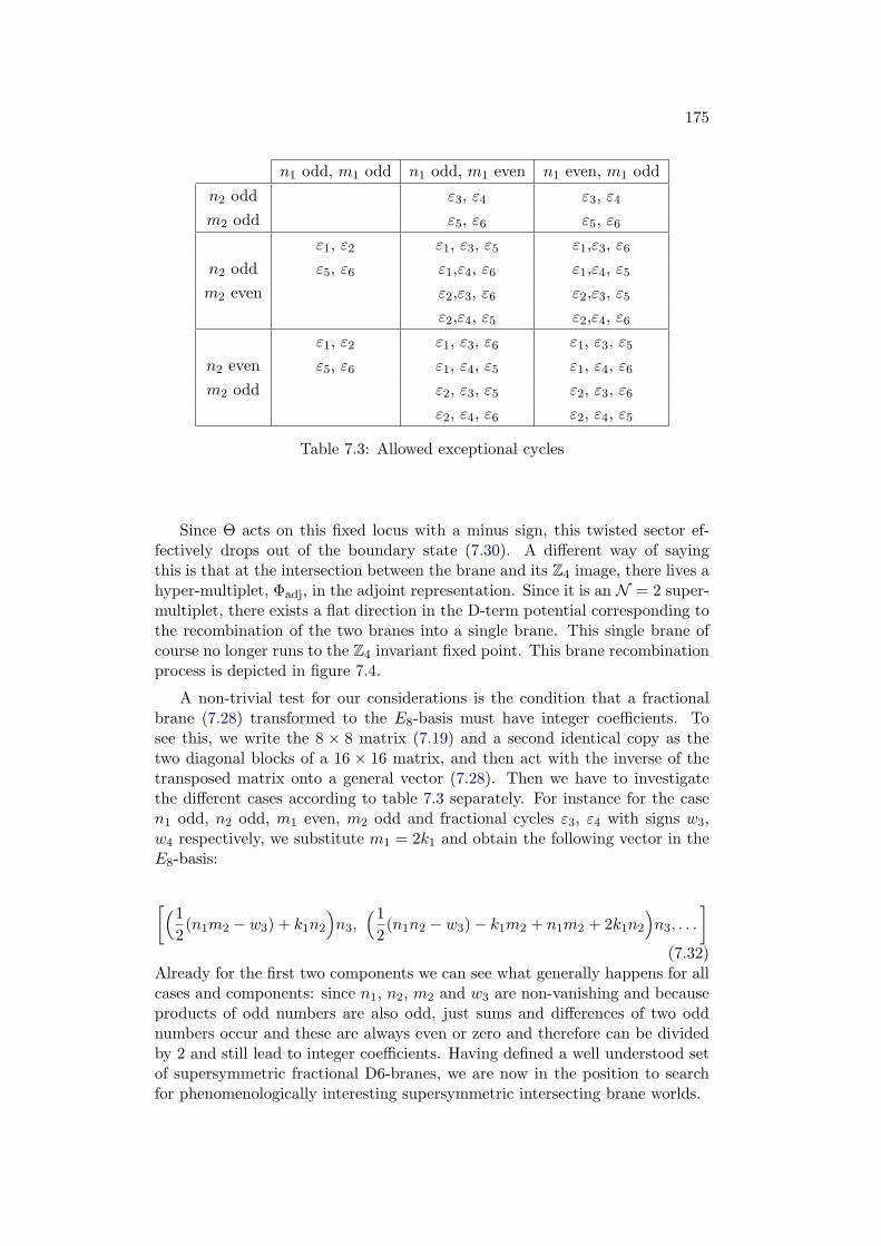
175

n1 odd, m1 odd n1 odd, m1 even n1 even, m1 odd

n2 odd ε3, ε4 ε3, ε4m2 odd ε5, ε6 ε5, ε6

ε1, ε2 ε1, ε3, ε5 ε1,ε3, ε6n2 odd ε5, ε6 ε1,ε4, ε6 ε1,ε4, ε5m2 even ε2,ε3, ε6 ε2,ε3, ε5

ε2,ε4, ε5 ε2,ε4, ε6ε1, ε2 ε1, ε3, ε6 ε1, ε3, ε5

n2 even ε5, ε6 ε1, ε4, ε5 ε1, ε4, ε6m2 odd ε2, ε3, ε5 ε2, ε3, ε6

ε2, ε4, ε6 ε2, ε4, ε5

Table 7.3: Allowed exceptional cycles

Since Θ acts on this fixed locus with a minus sign, this twisted sector ef-fectively drops out of the boundary state (7.30). A different way of sayingthis is that at the intersection between the brane and its Z4 image, there lives ahyper-multiplet, Φadj, in the adjoint representation. Since it is an N = 2 super-multiplet, there exists a flat direction in the D-term potential corresponding tothe recombination of the two branes into a single brane. This single brane ofcourse no longer runs to the Z4 invariant fixed point. This brane recombinationprocess is depicted in figure 7.4.

A non-trivial test for our considerations is the condition that a fractionalbrane (7.28) transformed to the E8-basis must have integer coefficients. Tosee this, we write the 8 × 8 matrix (7.19) and a second identical copy as thetwo diagonal blocks of a 16 × 16 matrix, and then act with the inverse of thetransposed matrix onto a general vector (7.28). Then we have to investigatethe different cases according to table 7.3 separately. For instance for the casen1 odd, n2 odd, m1 even, m2 odd and fractional cycles ε3, ε4 with signs w3,w4 respectively, we substitute m1 = 2k1 and obtain the following vector in theE8-basis:

[(12(n1m2 − w3) + k1n2

)n3,

(12(n1n2 − w3)− k1m2 + n1m2 + 2k1n2

)n3, . . .

](7.32)

Already for the first two components we can see what generally happens for allcases and components: since n1, n2, m2 and w3 are non-vanishing and becauseproducts of odd numbers are also odd, just sums and differences of two oddnumbers occur and these are always even or zero and therefore can be dividedby 2 and still lead to integer coefficients. Having defined a well understood setof supersymmetric fractional D6-branes, we are now in the position to searchfor phenomenologically interesting supersymmetric intersecting brane worlds.

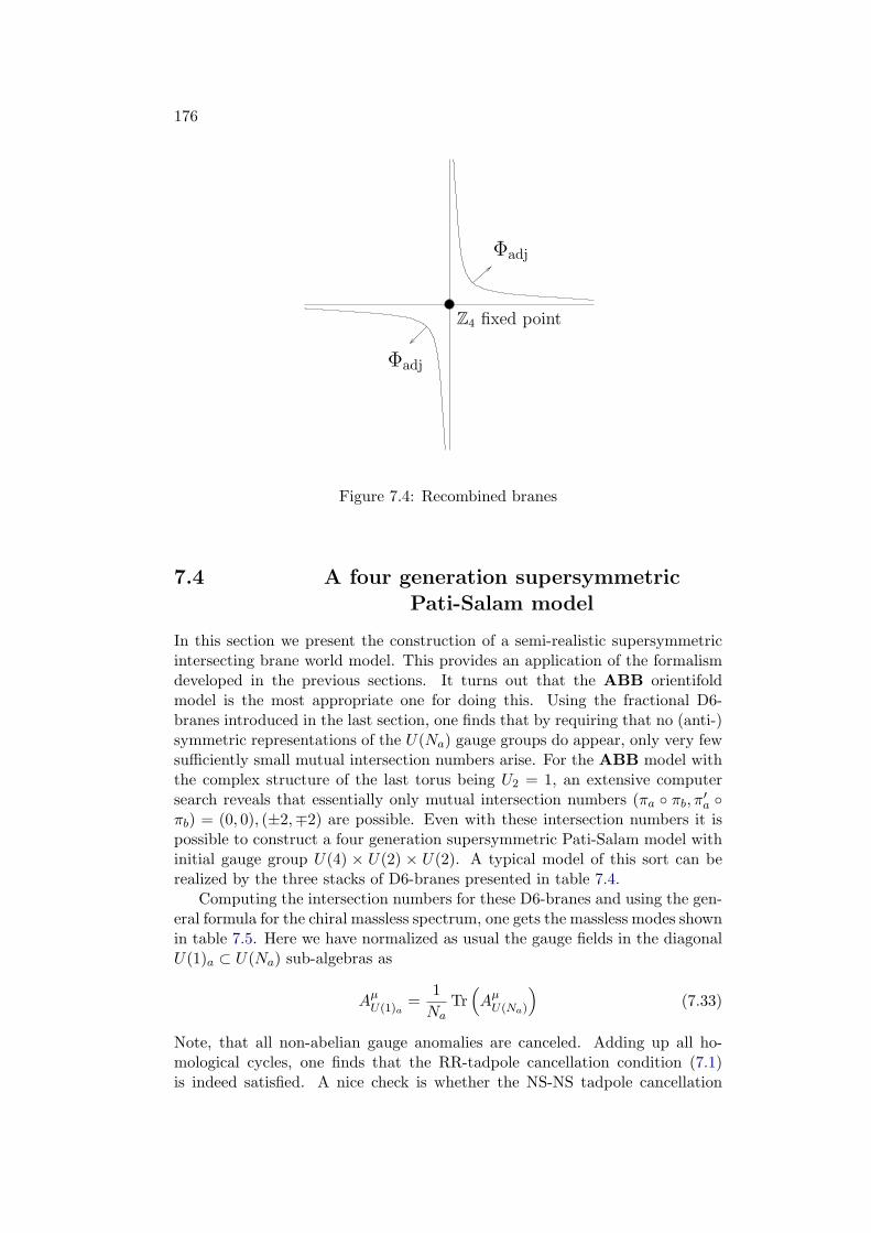
176

Φadj

Z4 fixed point

Φadj

Figure 7.4: Recombined branes

7.4 A four generation supersymmetricPati-Salam model

In this section we present the construction of a semi-realistic supersymmetricintersecting brane world model. This provides an application of the formalismdeveloped in the previous sections. It turns out that the ABB orientifoldmodel is the most appropriate one for doing this. Using the fractional D6-branes introduced in the last section, one finds that by requiring that no (anti-)symmetric representations of the U(Na) gauge groups do appear, only very fewsufficiently small mutual intersection numbers arise. For the ABB model withthe complex structure of the last torus being U2 = 1, an extensive computersearch reveals that essentially only mutual intersection numbers (πa πb, π′a πb) = (0, 0), (±2,∓2) are possible. Even with these intersection numbers it ispossible to construct a four generation supersymmetric Pati-Salam model withinitial gauge group U(4) × U(2) × U(2). A typical model of this sort can berealized by the three stacks of D6-branes presented in table 7.4.

Computing the intersection numbers for these D6-branes and using the gen-eral formula for the chiral massless spectrum, one gets the massless modes shownin table 7.5. Here we have normalized as usual the gauge fields in the diagonalU(1)a ⊂ U(Na) sub-algebras as

AµU(1)a=

1Na

Tr(AµU(Na)

)(7.33)

Note, that all non-abelian gauge anomalies are canceled. Adding up all ho-mological cycles, one finds that the RR-tadpole cancellation condition (7.1)is indeed satisfied. A nice check is whether the NS-NS tadpole cancellation

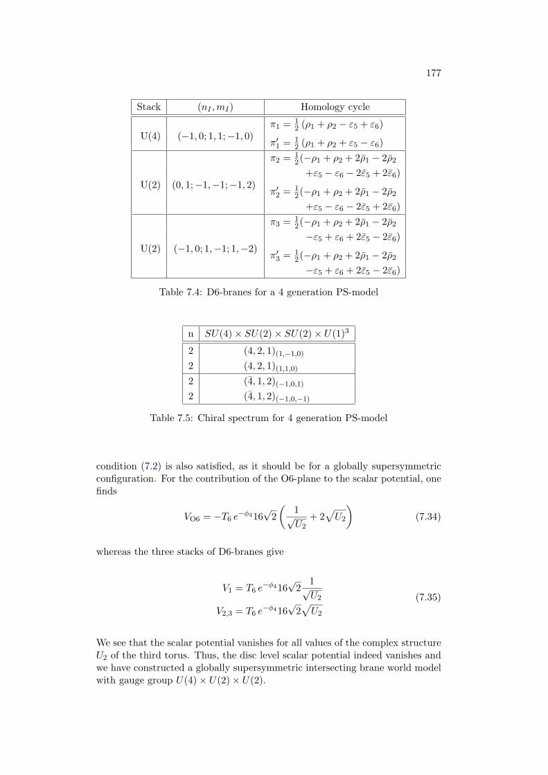
177

Stack (nI ,mI) Homology cycle

π1 = 12 (ρ1 + ρ2 − ε5 + ε6)

U(4) (−1, 0; 1, 1;−1, 0)π′1 = 1

2 (ρ1 + ρ2 + ε5 − ε6)π2 = 1

2(−ρ1 + ρ2 + 2ρ1 − 2ρ2

+ε5 − ε6 − 2ε5 + 2ε6)U(2) (0, 1;−1,−1;−1, 2)

π′2 = 12(−ρ1 + ρ2 + 2ρ1 − 2ρ2

+ε5 − ε6 − 2ε5 + 2ε6)

π3 = 12(−ρ1 + ρ2 + 2ρ1 − 2ρ2

−ε5 + ε6 + 2ε5 − 2ε6)U(2) (−1, 0; 1,−1; 1,−2)

π′3 = 12(−ρ1 + ρ2 + 2ρ1 − 2ρ2

−ε5 + ε6 + 2ε5 − 2ε6)

Table 7.4: D6-branes for a 4 generation PS-model

n SU(4)× SU(2)× SU(2)× U(1)3

2 (4, 2, 1)(1,−1,0)

2 (4, 2, 1)(1,1,0)2 (4, 1, 2)(−1,0,1)

2 (4, 1, 2)(−1,0,−1)

Table 7.5: Chiral spectrum for 4 generation PS-model

condition (7.2) is also satisfied, as it should be for a globally supersymmetricconfiguration. For the contribution of the O6-plane to the scalar potential, onefinds

VO6 = −T6 e−φ416

√2(

1√U2

+ 2√U2

)(7.34)

whereas the three stacks of D6-branes give

V1 = T6 e−φ416

√2

1√U2

V2,3 = T6 e−φ416

√2√U2

(7.35)

We see that the scalar potential vanishes for all values of the complex structureU2 of the third torus. Thus, the disc level scalar potential indeed vanishes andwe have constructed a globally supersymmetric intersecting brane world modelwith gauge group U(4)× U(2)× U(2).

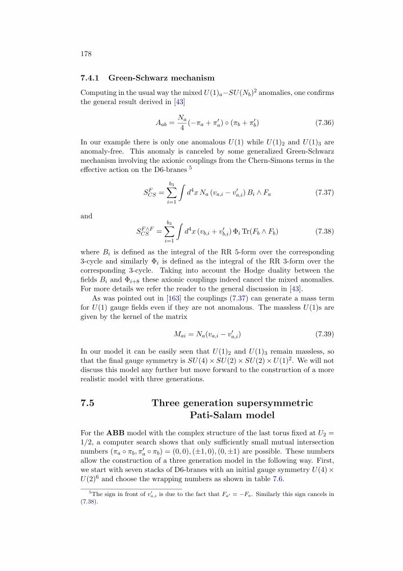
178

7.4.1 Green-Schwarz mechanism

Computing in the usual way the mixed U(1)a−SU(Nb)2 anomalies, one confirmsthe general result derived in [43]

Aab =Na

4(−πa + π′a) (πb + π′b) (7.36)

In our example there is only one anomalous U(1) while U(1)2 and U(1)3 areanomaly-free. This anomaly is canceled by some generalized Green-Schwarzmechanism involving the axionic couplings from the Chern-Simons terms in theeffective action on the D6-branes 5

SFCS =b3∑i=1

∫d4xNa (va,i − v′a,i)Bi ∧ Fa (7.37)

and

SF∧FCS =b3∑i=1

∫d4x (vb,i + v′b,i) Φi Tr(Fb ∧ Fb) (7.38)

where Bi is defined as the integral of the RR 5-form over the corresponding3-cycle and similarly Φi is defined as the integral of the RR 3-form over thecorresponding 3-cycle. Taking into account the Hodge duality between thefields Bi and Φi+8 these axionic couplings indeed cancel the mixed anomalies.For more details we refer the reader to the general discussion in [43].

As was pointed out in [163] the couplings (7.37) can generate a mass termfor U(1) gauge fields even if they are not anomalous. The massless U(1)s aregiven by the kernel of the matrix

Mai = Na(va,i − v′a,i) (7.39)

In our model it can be easily seen that U(1)2 and U(1)3 remain massless, sothat the final gauge symmetry is SU(4)×SU(2)×SU(2)×U(1)2. We will notdiscuss this model any further but move forward to the construction of a morerealistic model with three generations.

7.5 Three generation supersymmetricPati-Salam model

For the ABB model with the complex structure of the last torus fixed at U2 =1/2, a computer search shows that only sufficiently small mutual intersectionnumbers (πa πb, π′a πb) = (0, 0), (±1, 0), (0,±1) are possible. These numbersallow the construction of a three generation model in the following way. First,we start with seven stacks of D6-branes with an initial gauge symmetry U(4)×U(2)6 and choose the wrapping numbers as shown in table 7.6.

5The sign in front of v′a,i is due to the fact that Fa′ = −Fa. Similarly this sign cancels in(7.38).

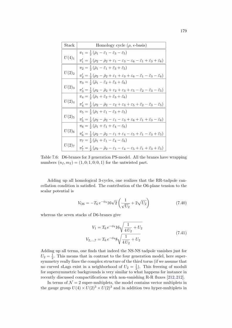
179

Stack Homology cycle (ρ, ε-basis)

π1 = 12 (ρ1 − ε1 − ε3 − ε5)

U(4)1 π′1 = 12 (ρ2 − ρ2 + ε1 − ε3 − ε6 − ε1 + ε3 + ε6)

π2 = 12 (ρ1 − ε1 + ε3 + ε5)

U(2)2 π′2 = 12 (ρ2 − ρ2 + ε1 + ε3 + ε6 − ε1 − ε3 − ε6)

π3 = 12 (ρ1 − ε2 + ε3 + ε6)

U(2)3 π′3 = 12 (ρ2 − ρ2 + ε2 + ε3 + ε5 − ε2 − ε3 − ε5)

π4 = 12 (ρ1 + ε2 + ε3 + ε6)

U(2)4 π′4 = 12 (ρ2 − ρ2 − ε2 + ε3 + ε5 + ε2 − ε3 − ε5)

π5 = 12 (ρ1 + ε1 − ε3 + ε5)

U(2)5 π′5 = 12 (ρ2 − ρ2 − ε1 − ε3 + ε6 + ε1 + ε3 − ε6)

π6 = 12 (ρ1 + ε1 + ε4 − ε6)

U(2)6 π′6 = 12 (ρ2 − ρ2 − ε1 + ε4 − ε5 + ε1 − ε3 + ε5)

π7 = 12 (ρ1 + ε1 − ε4 − ε6)

U(2)7 π′7 = 12 (ρ2 − ρ2 − ε1 − ε4 − ε5 + ε1 + ε3 + ε5)

Table 7.6: D6-branes for 3 generation PS-model. All the branes have wrappingnumbers (nI ,mI) = (1, 0; 1, 0; 0, 1) for the untwisted part.

Adding up all homological 3-cycles, one realizes that the RR-tadpole can-cellation condition is satisfied. The contribution of the O6-plane tension to thescalar potential is

VO6 = −T6 e−φ416

√2(

1√U2

+ 2√U2

)(7.40)

whereas the seven stacks of D6-branes give

V1 = T6 e−φ416

√1

4U2+ U2

V2,...,7 = T6 e−φ48

√1

4U2+ U2

(7.41)

Adding up all terms, one finds that indeed the NS-NS tadpole vanishes just forU2 = 1

2 . This means that in contrast to the four generation model, here super-symmetry really fixes the complex structure of the third torus (if we assume thatno curved sLags exist in a neighborhood of U2 = 1

2). This freezing of modulifor supersymmetric backgrounds is very similar to what happens for instance inrecently discussed compactifications with non-vanishing R-R fluxes [212,212].

In terms of N = 2 super-multiplets, the model contains vector multiplets inthe gauge group U(4)×U(2)3 ×U(2)3 and in addition two hyper-multiplets in

180

Field n U(4)× U(2)3 × U(2)3

Φ1′2 1 (4; 2, 1, 1; 1, 1, 1)Φ1′3 1 (4; 1, 2, 1; 1, 1, 1)Φ1′4 1 (4; 1, 1, 2; 1, 1, 1)

Φ1′5 1 (4; 1, 1, 1; 2, 1, 1)Φ1′6 1 (4; 1, 1, 1; 1, 2, 1)Φ1′7 1 (4; 1, 1, 1; 1, 1, 2)

Φ2′3 1 (1; 2, 2, 1; 1, 1, 1)Φ2′4 1 (1; 2, 1, 2; 1, 1, 1)Φ3′4 1 (1; 1, 2, 2; 1, 1, 1)

Φ5′6 1 (1; 1, 1, 1; 2, 2, 1)Φ5′7 1 (1; 1, 1, 1; 2, 1, 2)Φ6′7 1 (1; 1, 1, 1; 1, 2, 2)

Table 7.7: Chiral spectrum for a 7-stack model

the adjoint representation of each unitary gauge factor. The complex scalar inthe vector multiplet corresponds to the unconstrained position of each stack ofD6-branes on the third T 2. As described at the end of section 7.3.2, the hyper-multiplet appears on the intersection between a stack of branes and its Z4

image. By computing the intersection numbers, we derive the chiral spectrumas shown in table 7.7, where n denotes the number of chiral multiplets in therespective representation as given by the intersection number.

First, we notice that all non-abelian anomalies cancel including formallyalso the U(2) anomalies.

In order to proceed and really get a three generation model, it is necessary tobreak the two triplets U(2)3 down to their diagonal subgroups. Potential gaugesymmetry breaking candidates in this way are the chiral fields Φ2′3,Φ2′4,Φ3′4and Φ5′6,Φ5′7,Φ6′7 from table 7.7. However, one has to remember that theseare chiral N = 1 super-multiplets living on the intersection of two D-branesin every case. Let us review what massless bosons localized on intersectingD-branes indicate.

7.5.1 Brane recombination

If two stacks of D-branes preserve a common N = 2 supersymmetry, then amassless hyper-multiplet, H, localized on the intersection, signals a possibledeformation of the two stacks of D-branes into recombined D-branes whichwrap a complex cycle. Note, that two factorizable branes can only preserveN = 2 supersymmetry if they are parallel on one of the three T 2

I tori. Thecomplex cycle has the same volume as the sum of volumes of the two D-branesbefore the recombination process occurs. In the effective low energy theory,this recombination can be understood as a Higgs effect where a flat direction

181

〈h1〉 = 〈h2〉 in the D-term potential

VD =1

2g2

(h1h1 − h2h2

)2 (7.42)

exists, along which the U(N)×U(N) gauge symmetry is broken to the diagonalsubgroup.6 Here h1 and h2 denote the two complex bosons inside the hyper-multiplet. Thus, in this case without changing the closed string background,there exists an open string modulus, which has the interpretation of a Higgsfield in the low energy effective theory. Note, that in the T-dual picture, this isjust the deformation of a small instanton into an instanton of finite size. In ourconcrete models such N = 2 Higgs sectors are coupled at brane intersections tochiral N = 1 sectors. Note, that the brane recombination in the effective gaugetheory cannot simply be described by the renormalizable couplings. In order toget the correct light spectrum, one also has to take into account stringy higherdimensional couplings.

When the two D-branes only preserve N = 1 supersymmetry and supporta massless chiral super-multiplet Φ on the intersection [213, 101], the situationgets a little bit more involved. In this case, the analogous D-term potential isof the form

VD =1

2g2

(φφ)2 (7.43)

which tells us that, unless there are more chiral fields involved, simply by givinga VEV to the massless boson φ, we do not obtain a flat direction of the D-termpotential and therefore break supersymmetry. Nevertheless, the massless modesindicate that the intersecting brane configuration lies on a line of marginalstability in the complex structure moduli space. By a small variation of thecomplex structure, a Fayet-Iliopoulos (FI) term, r, is introduced that changesthe D-term potential to

VD =1

2g2

(φφ+ r

)2 (7.44)

Therefore, for r < 0 the field φ becomes tachyonic and there exists a new sta-ble supersymmetric minimum of the D-term potential. The intersecting branesthen have combined into one D-brane wrapping a special Lagrangian 3-cycle inthe underlying Calabi-Yau. For a finite FI-term r, this 3-cycle has smaller vol-ume than the two intersecting branes. However, the two volumes are preciselyequal on the line of marginal stability. This means that on the line of marginalstability, there exists a different configuration with only a single brane whichalso preserves the same N = 1 supersymmetry and has the same volume as theformer pair of intersecting D-branes. Again the gauge symmetry is broken tothe diagonal subgroup. It has to be emphasized that in this case the two config-urations are not simply linked by a Higgs mechanism in the effective low energygauge theory. As mentioned before, in order to deform the intersecting braneconfiguration into the non-flat D-brane wrapping a special Lagrangian 3-cycle,

6If on one of the two stacks there sits only a single D6-brane, the F-term potential φh1h2

forbids the existence of a flat direction with 〈h1〉 = 〈h2〉. This is the field theoretic correspon-dence of the fact that there do not exist large instantons in the U(1) gauge group. We thankA. Uranga for pointing this out to us.

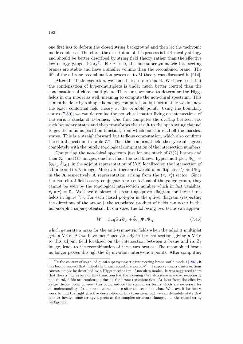
182

one first has to deform the closed string background and then let the tachyonicmode condense. Therefore, the description of this process is intrinsically stringyand should be better described by string field theory rather than the effectivelow energy gauge theory7. For r > 0, the non-supersymmetric intersectingbranes are stable and have a smaller volume than the recombined brane. Thelift of these brane recombination processes to M-theory was discussed in [214].

After this little excursion, we come back to our model. We have seen thatthe condensation of hyper-multiplets is under much better control than thecondensation of chiral multiplets. Therefore, we have to determine the Higgsfields in our model as well, meaning to compute the non-chiral spectrum. Thiscannot be done by a simple homology computation, but fortunately we do knowthe exact conformal field theory at the orbifold point. Using the boundarystates (7.30), we can determine the non-chiral matter living on intersections ofthe various stacks of D-branes. One first computes the overlap between twosuch boundary states and then transforms the result to the open string channelto get the annulus partition function, from which one can read off the masslessstates. This is a straightforward but tedious computation, which also confirmsthe chiral spectrum in table 7.7. Thus the conformal field theory result agreescompletely with the purely topological computation of the intersection numbers.

Computing the non-chiral spectrum just for one stack of U(2) branes andtheir Z4- and Ωσ-images, one first finds the well known hyper-multiplet, Φadj =(φadj, φadj), in the adjoint representation of U(2) localized on the intersection ofa brane and its Z4 image. Moreover, there are two chiral multiplets, ΨA and ΨA,in the A respectively A representation arising from the (πi, π′i) sector. Sincethe two chiral fields carry conjugate representations of the gauge group, theycannot be seen by the topological intersection number which in fact vanishes,πi π′i = 0. We have depicted the resulting quiver diagram for these threefields in figure 7.5. For each closed polygon in the quiver diagram (respectingthe directions of the arrows), the associated product of fields can occur in theholomorphic super-potential. In our case, the following two terms can appear

W = φadjΨAΨA + φadjΨAΨA (7.45)

which generate a mass for the anti-symmetric fields when the adjoint multipletgets a VEV. As we have mentioned already in the last section, giving a VEVto this adjoint field localized on the intersection between a brane and its Z4

image, leads to the recombination of these two branes. The recombined braneno longer passes through the Z4 invariant intersection points. After computing

7In the context of so-called quasi-supersymmetric intersecting brane world models [186] , ithas been observed that indeed the brane recombination of N = 1 supersymmetric intersectionscannot simply be described by a Higgs mechanism of massless modes. It was suggested therethat the stringy nature of this transition has the meaning that also some massive, necessarilynon-chiral, fields are condensing during the brane recombination. At least from the effectivegauge theory point of view, this could induce the right mass terms which are necessary foran understanding of the new massless modes after the recombination. We leave it for futurework to find the right effective description of this transition, but we can definitely state thatit must involve some stringy aspects as the complex structure changes, i.e. the closed stringbackground.

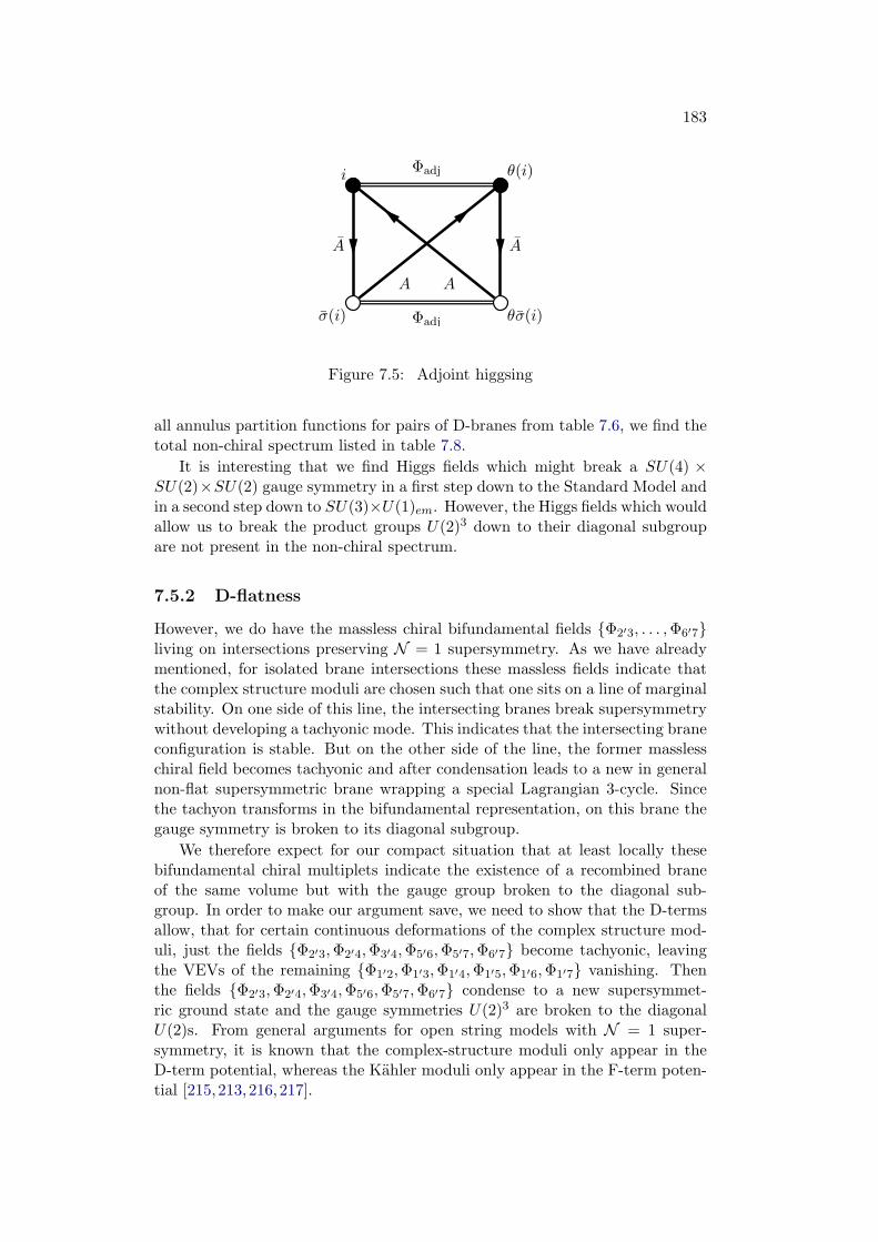
183

A

Φadj

A

A

Φadj

A

i θ(i)

σ(i) θσ(i)

Figure 7.5: Adjoint higgsing

all annulus partition functions for pairs of D-branes from table 7.6, we find thetotal non-chiral spectrum listed in table 7.8.

It is interesting that we find Higgs fields which might break a SU(4) ×SU(2)×SU(2) gauge symmetry in a first step down to the Standard Model andin a second step down to SU(3)×U(1)em. However, the Higgs fields which wouldallow us to break the product groups U(2)3 down to their diagonal subgroupare not present in the non-chiral spectrum.

7.5.2 D-flatness

However, we do have the massless chiral bifundamental fields Φ2′3, . . . ,Φ6′7living on intersections preserving N = 1 supersymmetry. As we have alreadymentioned, for isolated brane intersections these massless fields indicate thatthe complex structure moduli are chosen such that one sits on a line of marginalstability. On one side of this line, the intersecting branes break supersymmetrywithout developing a tachyonic mode. This indicates that the intersecting braneconfiguration is stable. But on the other side of the line, the former masslesschiral field becomes tachyonic and after condensation leads to a new in generalnon-flat supersymmetric brane wrapping a special Lagrangian 3-cycle. Sincethe tachyon transforms in the bifundamental representation, on this brane thegauge symmetry is broken to its diagonal subgroup.

We therefore expect for our compact situation that at least locally thesebifundamental chiral multiplets indicate the existence of a recombined braneof the same volume but with the gauge group broken to the diagonal sub-group. In order to make our argument save, we need to show that the D-termsallow, that for certain continuous deformations of the complex structure mod-uli, just the fields Φ2′3,Φ2′4,Φ3′4,Φ5′6,Φ5′7,Φ6′7 become tachyonic, leavingthe VEVs of the remaining Φ1′2,Φ1′3,Φ1′4,Φ1′5,Φ1′6,Φ1′7 vanishing. Thenthe fields Φ2′3,Φ2′4,Φ3′4,Φ5′6,Φ5′7,Φ6′7 condense to a new supersymmet-ric ground state and the gauge symmetries U(2)3 are broken to the diagonalU(2)s. From general arguments for open string models with N = 1 super-symmetry, it is known that the complex-structure moduli only appear in theD-term potential, whereas the Kahler moduli only appear in the F-term poten-tial [215,213,216,217].

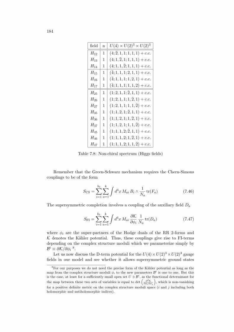
184

field n U(4)× U(2)3 × U(2)3

H12 1 (4; 2, 1, 1; 1, 1, 1) + c.c.

H13 1 (4; 1, 2, 1; 1, 1, 1) + c.c.

H14 1 (4; 1, 1, 2; 1, 1, 1) + c.c.

H15 1 (4; 1, 1, 1; 2, 1, 1) + c.c.

H16 1 (4; 1, 1, 1; 1, 2, 1) + c.c.

H17 1 (4; 1, 1, 1; 1, 1, 2) + c.c.

H25 1 (1; 2, 1, 1; 2, 1, 1) + c.c.

H26 1 (1; 2, 1, 1; 1, 2, 1) + c.c.

H27 1 (1; 2, 1, 1; 1, 1, 2) + c.c.

H35 1 (1; 1, 2, 1; 2, 1, 1) + c.c.

H36 1 (1; 1, 2, 1; 1, 2, 1) + c.c.

H37 1 (1; 1, 2, 1; 1, 1, 2) + c.c.

H45 1 (1; 1, 1, 2; 2, 1, 1) + c.c.

H46 1 (1; 1, 1, 2; 1, 2, 1) + c.c.

H47 1 (1; 1, 1, 2; 1, 1, 2) + c.c.

Table 7.8: Non-chiral spectrum (Higgs fields)

Remember that the Green-Schwarz mechanism requires the Chern-Simonscouplings to be of the form

SCS =b3∑i=1

k∑a=1

∫d4xMaiBi ∧

1Na

tr(Fa) (7.46)

The supersymmetric completion involves a coupling of the auxiliary field Da

SFI =b3∑i=1

k∑a=1

∫d4xMai

∂K∂φi

1Na

tr(Da) (7.47)

where φi are the super-partners of the Hodge duals of the RR 2-forms andK denotes the Kahler potential. Thus, these couplings give rise to FI-termsdepending on the complex structure moduli which we parameterize simply byBi ≡ ∂K/∂φi 8.

Let us now discuss the D-term potential for the U(4)×U(2)3×U(2)3 gaugefields in our model and see whether it allows supersymmetric ground states

8For our purposes we do not need the precise form of the Kahler potential as long as themap from the complex structure moduli φi to the new parameters Bi is one to one. But thisis the case, at least for a sufficiently small open set U 3 Bi, as the functional determinant for

the map between these two sets of variables is equal to det(

∂2K∂φi∂φj

), which is non-vanishing

for a positive definite metric on the complex structure moduli space (i and j including bothholomorphic and antiholomorphic indices).

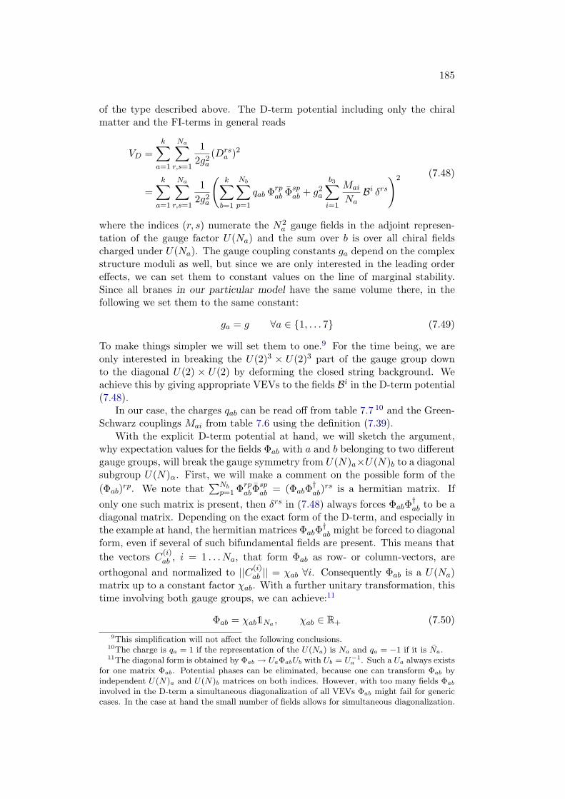
185

of the type described above. The D-term potential including only the chiralmatter and the FI-terms in general reads

VD =k∑a=1

Na∑r,s=1

12g2a

(Drsa )2

=k∑a=1

Na∑r,s=1

12g2a

(k∑b=1

Nb∑p=1

qab Φrpab Φsp

ab + g2a

b3∑i=1

Mai

NaBi δrs

)2(7.48)

where the indices (r, s) numerate the N2a gauge fields in the adjoint represen-

tation of the gauge factor U(Na) and the sum over b is over all chiral fieldscharged under U(Na). The gauge coupling constants ga depend on the complexstructure moduli as well, but since we are only interested in the leading ordereffects, we can set them to constant values on the line of marginal stability.Since all branes in our particular model have the same volume there, in thefollowing we set them to the same constant:

ga = g ∀a ∈ 1, . . . 7 (7.49)

To make things simpler we will set them to one.9 For the time being, we areonly interested in breaking the U(2)3 × U(2)3 part of the gauge group downto the diagonal U(2) × U(2) by deforming the closed string background. Weachieve this by giving appropriate VEVs to the fields Bi in the D-term potential(7.48).

In our case, the charges qab can be read off from table 7.7 10 and the Green-Schwarz couplings Mai from table 7.6 using the definition (7.39).

With the explicit D-term potential at hand, we will sketch the argument,why expectation values for the fields Φab with a and b belonging to two differentgauge groups, will break the gauge symmetry from U(N)a×U(N)b to a diagonalsubgroup U(N)α. First, we will make a comment on the possible form of the(Φab)rp. We note that

∑Nbp=1 Φrp

abΦspab = (ΦabΦ

†ab)

rs is a hermitian matrix. Ifonly one such matrix is present, then δrs in (7.48) always forces ΦabΦ

†ab to be a

diagonal matrix. Depending on the exact form of the D-term, and especially inthe example at hand, the hermitian matrices ΦabΦ

†ab might be forced to diagonal

form, even if several of such bifundamental fields are present. This means thatthe vectors C(i)

ab , i = 1 . . . Na, that form Φab as row- or column-vectors, areorthogonal and normalized to ||C(i)

ab || = χab ∀i. Consequently Φab is a U(Na)matrix up to a constant factor χab. With a further unitary transformation, thistime involving both gauge groups, we can achieve:11

Φab = χab1Na , χab ∈ R+ (7.50)9This simplification will not affect the following conclusions.

10The charge is qa = 1 if the representation of the U(Na) is Na and qa = −1 if it is Na.11The diagonal form is obtained by Φab → UaΦabUb with Ub = U−1

a . Such a Ua always existsfor one matrix Φab. Potential phases can be eliminated, because one can transform Φab byindependent U(N)a and U(N)b matrices on both indices. However, with too many fields Φab

involved in the D-term a simultaneous diagonalization of all VEVs Φab might fail for genericcases. In the case at hand the small number of fields allows for simultaneous diagonalization.

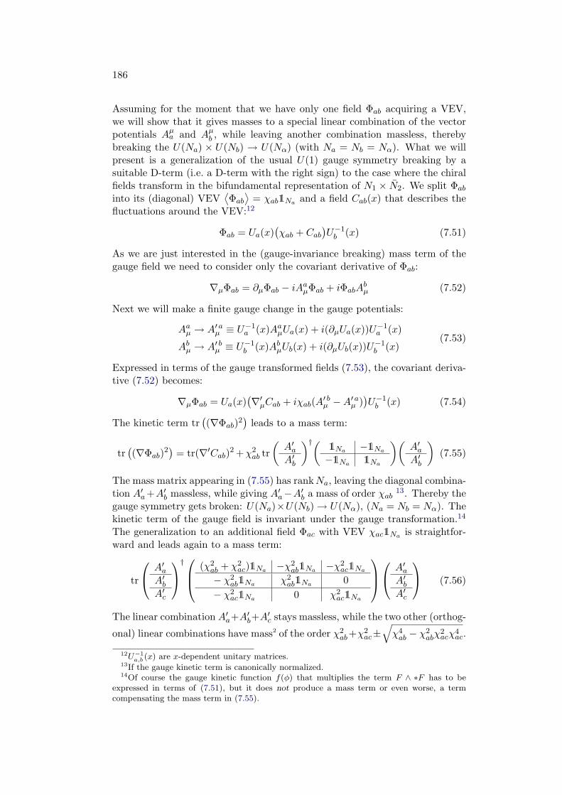
186

Assuming for the moment that we have only one field Φab acquiring a VEV,we will show that it gives masses to a special linear combination of the vectorpotentials Aµa and Aµb , while leaving another combination massless, therebybreaking the U(Na) × U(Nb) → U(Nα) (with Na = Nb = Nα). What we willpresent is a generalization of the usual U(1) gauge symmetry breaking by asuitable D-term (i.e. a D-term with the right sign) to the case where the chiralfields transform in the bifundamental representation of N1 × N2. We split Φab

into its (diagonal) VEV⟨Φab

⟩= χab1Na and a field Cab(x) that describes the

fluctuations around the VEV:12

Φab = Ua(x)(χab + Cab

)U−1b (x) (7.51)

As we are just interested in the (gauge-invariance breaking) mass term of thegauge field we need to consider only the covariant derivative of Φab:

∇µΦab = ∂µΦab − iAaµΦab + iΦabAbµ (7.52)

Next we will make a finite gauge change in the gauge potentials:

Aaµ → A′ aµ ≡ U−1a (x)AaµUa(x) + i(∂µUa(x))U−1

a (x)

Abµ → A′ bµ ≡ U−1b (x)AbµUb(x) + i(∂µUb(x))U−1

b (x)(7.53)

Expressed in terms of the gauge transformed fields (7.53), the covariant deriva-tive (7.52) becomes:

∇µΦab = Ua(x)(∇′µCab + iχab(A′ bµ −A′ aµ )

)U−1b (x) (7.54)

The kinetic term tr((∇Φab)2

)leads to a mass term:

tr((∇Φab)2

)= tr(∇′Cab)2 +χ2

ab tr(A′aA′b

)†(1Na −1Na

−1Na 1Na

)(A′aA′b

)(7.55)

The mass matrix appearing in (7.55) has rankNa, leaving the diagonal combina-tion A′a+A′b massless, while giving A′a−A′b a mass of order χab 13. Thereby thegauge symmetry gets broken: U(Na)×U(Nb)→ U(Nα), (Na = Nb = Nα). Thekinetic term of the gauge field is invariant under the gauge transformation.14

The generalization to an additional field Φac with VEV χac1Na is straightfor-ward and leads again to a mass term:

tr

A′aA′bA′c

† (χ2ab + χ2

ac)1Na −χ2ab1Na −χ2

ac1Na

− χ2ab1Na χ2

ab1Na 0− χ2

ac1Na 0 χ2ac1Na

A′a

A′bA′c

(7.56)

The linear combination A′a+A′b+A

′c stays massless, while the two other (orthog-

onal) linear combinations have mass2 of the order χ2ab+χ

2ac±

√χ4ab − χ2

abχ2acχ

4ac.

12U−1a,b (x) are x-dependent unitary matrices.

13If the gauge kinetic term is canonically normalized.14Of course the gauge kinetic function f(φ) that multiplies the term F ∧ ∗F has to be

expressed in terms of (7.51), but it does not produce a mass term or even worse, a termcompensating the mass term in (7.55).

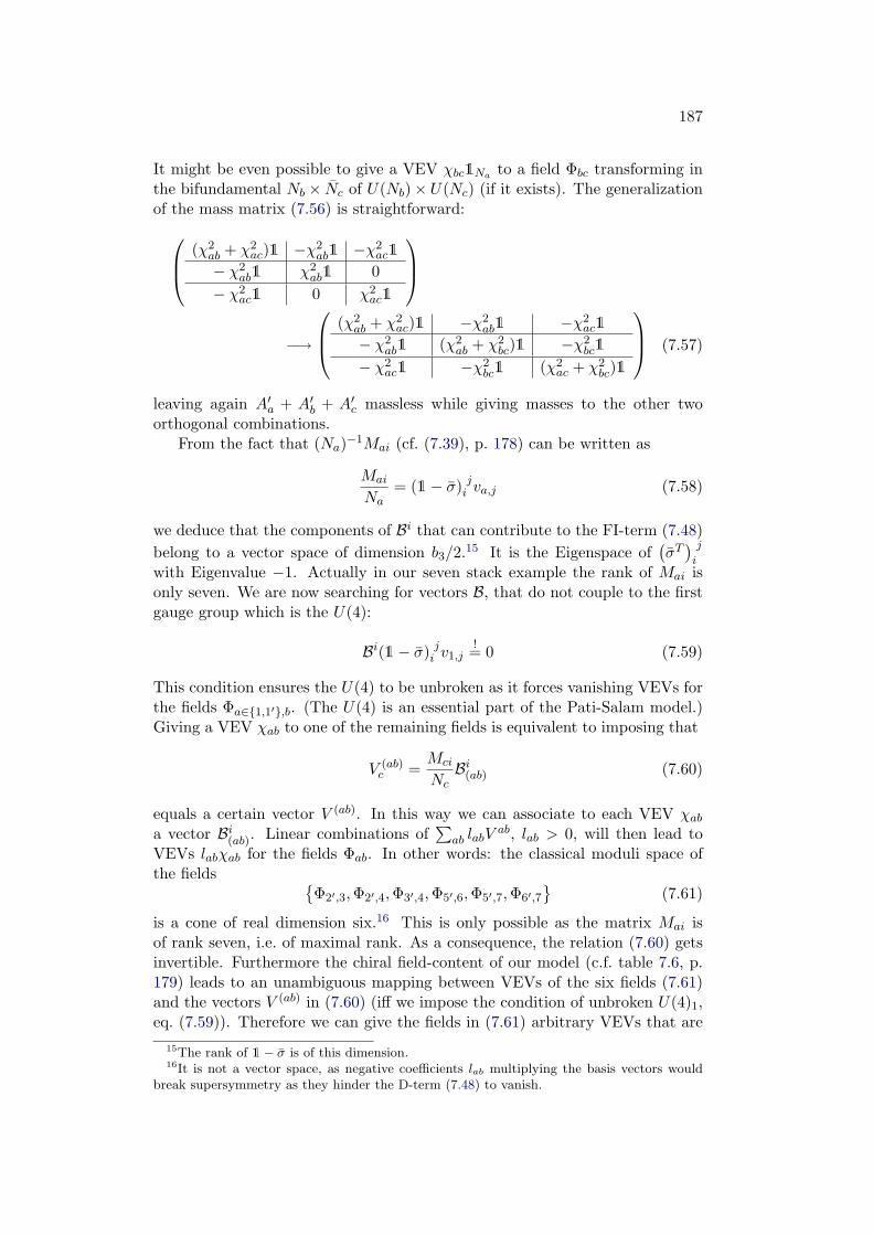
187

It might be even possible to give a VEV χbc1Na to a field Φbc transforming inthe bifundamental Nb × Nc of U(Nb)× U(Nc) (if it exists). The generalizationof the mass matrix (7.56) is straightforward: (χ2

ab + χ2ac)1 −χ2

ab1 −χ2ac1

− χ2ab1 χ2

ab1 0− χ2

ac1 0 χ2ac1

−→

(χ2ab + χ2

ac)1 −χ2ab1 −χ2

ac1

− χ2ab1 (χ2

ab + χ2bc)1 −χ2

bc1

− χ2ac1 −χ2

bc1 (χ2ac + χ2

bc)1

(7.57)

leaving again A′a + A′b + A′c massless while giving masses to the other twoorthogonal combinations.

From the fact that (Na)−1Mai (cf. (7.39), p. 178) can be written as

Mai

Na= (1− σ) ji va,j (7.58)

we deduce that the components of Bi that can contribute to the FI-term (7.48)belong to a vector space of dimension b3/2.15 It is the Eigenspace of

(σT) ji

with Eigenvalue −1. Actually in our seven stack example the rank of Mai isonly seven. We are now searching for vectors B, that do not couple to the firstgauge group which is the U(4):

Bi(1− σ) ji v1,j!= 0 (7.59)

This condition ensures the U(4) to be unbroken as it forces vanishing VEVs forthe fields Φa∈1,1′,b. (The U(4) is an essential part of the Pati-Salam model.)Giving a VEV χab to one of the remaining fields is equivalent to imposing that

V (ab)c =

Mci

NcBi(ab) (7.60)

equals a certain vector V (ab). In this way we can associate to each VEV χaba vector Bi(ab). Linear combinations of

∑ab labV

ab, lab > 0, will then lead toVEVs labχab for the fields Φab. In other words: the classical moduli space ofthe fields

Φ2′,3,Φ2′,4,Φ3′,4,Φ5′,6,Φ5′,7,Φ6′,7

(7.61)

is a cone of real dimension six.16 This is only possible as the matrix Mai isof rank seven, i.e. of maximal rank. As a consequence, the relation (7.60) getsinvertible. Furthermore the chiral field-content of our model (c.f. table 7.6, p.179) leads to an unambiguous mapping between VEVs of the six fields (7.61)and the vectors V (ab) in (7.60) (iff we impose the condition of unbroken U(4)1,eq. (7.59)). Therefore we can give the fields in (7.61) arbitrary VEVs that are

15The rank of 1− σ is of this dimension.16It is not a vector space, as negative coefficients lab multiplying the basis vectors would

break supersymmetry as they hinder the D-term (7.48) to vanish.

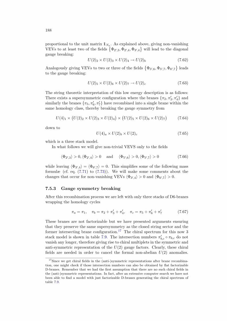
188

proportional to the unit matrix 1Na . As explained above, giving non-vanishingVEVs to at least two of the fields

Φ2′,3,Φ2′,4,Φ3′,4

will lead to the diagonal

gauge breaking:U(2)2 × U(2)3 × U(2)4 → U(2)b (7.62)

Analogously giving VEVs to two or three of the fieldsΦ5′,6,Φ5′,7,Φ6′,7

leads

to the gauge breaking:

U(2)5 × U(2)6 × U(2)7 → U(2)c (7.63)

The string theoretic interpretation of this low energy description is as follows:There exists a supersymmetric configuration where the branes π2, π

′3, π

′4 and

similarly the branes π5, π′6, π

′7 have recombined into a single brane within the

same homology class, thereby breaking the gauge symmetry from

U(4)1 ×(U(2)2 × U(2)3 × U(2)4

)×(U(2)5 × U(2)6 × U(2)7

)(7.64)

down toU(4)a × U(2)b × U(2)c (7.65)

which is a three stack model.In what follows we will give non-trivial VEVS only to the fields

〈Φ2′,3〉 > 0, 〈Φ2′,4〉 > 0 and 〈Φ5′,6〉 > 0, 〈Φ5′,7〉 > 0 (7.66)

while leaving 〈Φ3′,4〉 = 〈Φ6′,7〉 = 0. This simplifies some of the following massformulæ (cf. eq. (7.71) to (7.73)). We will make some comments about thechanges that occur for non-vanishing VEVs 〈Φ3′,4〉 > 0 and 〈Φ6′,7〉 > 0.

7.5.3 Gauge symmetry breaking

After this recombination process we are left with only three stacks of D6-braneswrapping the homology cycles

πa = π1, πb = π2 + π′3 + π′4, πc = π5 + π′6 + π′7 (7.67)

These branes are not factorizable but we have presented arguments ensuringthat they preserve the same supersymmetry as the closed string sector and theformer intersecting brane configuration.17 The chiral spectrum for this now 3stack model is shown in table 7.9. The intersection numbers π′b,c πb,c do notvanish any longer, therefore giving rise to chiral multiplets in the symmetric andanti-symmetric representation of the U(2) gauge factors. Clearly, these chiralfields are needed in order to cancel the formal non-abelian U(2) anomalies.

17Since we get chiral fields in the (anti-)symmetric representations after brane recombina-tion, one might check if those intersection numbers can also be obtained by flat factorizableD-branes. Remember that we had the first assumption that there are no such chiral fields inthe (anti-)symmetric representations. In fact, after an extensive computer search we have notbeen able to find a model with just factorizable D-branes generating the chiral spectrum oftable 7.9.

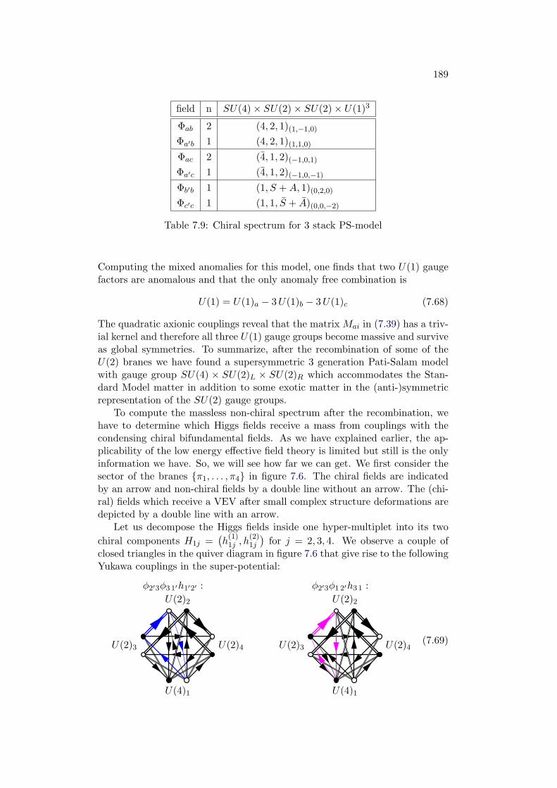
189

field n SU(4)× SU(2)× SU(2)× U(1)3

Φab 2 (4, 2, 1)(1,−1,0)

Φa′b 1 (4, 2, 1)(1,1,0)Φac 2 (4, 1, 2)(−1,0,1)

Φa′c 1 (4, 1, 2)(−1,0,−1)

Φb′b 1 (1, S +A, 1)(0,2,0)Φc′c 1 (1, 1, S + A)(0,0,−2)

Table 7.9: Chiral spectrum for 3 stack PS-model

Computing the mixed anomalies for this model, one finds that two U(1) gaugefactors are anomalous and that the only anomaly free combination is

U(1) = U(1)a − 3U(1)b − 3U(1)c (7.68)

The quadratic axionic couplings reveal that the matrix Mai in (7.39) has a triv-ial kernel and therefore all three U(1) gauge groups become massive and surviveas global symmetries. To summarize, after the recombination of some of theU(2) branes we have found a supersymmetric 3 generation Pati-Salam modelwith gauge group SU(4) × SU(2)L × SU(2)R which accommodates the Stan-dard Model matter in addition to some exotic matter in the (anti-)symmetricrepresentation of the SU(2) gauge groups.

To compute the massless non-chiral spectrum after the recombination, wehave to determine which Higgs fields receive a mass from couplings with thecondensing chiral bifundamental fields. As we have explained earlier, the ap-plicability of the low energy effective field theory is limited but still is the onlyinformation we have. So, we will see how far we can get. We first consider thesector of the branes π1, . . . , π4 in figure 7.6. The chiral fields are indicatedby an arrow and non-chiral fields by a double line without an arrow. The (chi-ral) fields which receive a VEV after small complex structure deformations aredepicted by a double line with an arrow.

Let us decompose the Higgs fields inside one hyper-multiplet into its twochiral components H1j =

(h

(1)1j , h

(2)1j

)for j = 2, 3, 4. We observe a couple of

closed triangles in the quiver diagram in figure 7.6 that give rise to the followingYukawa couplings in the super-potential:

φ2′3φ3 1′h1′2′ : φ2′3φ1 2′h3 1 :

U(2)3 U(2)4

U(2)2

U(4)1

U(2)3 U(2)4

U(2)2

U(4)1

(7.69)

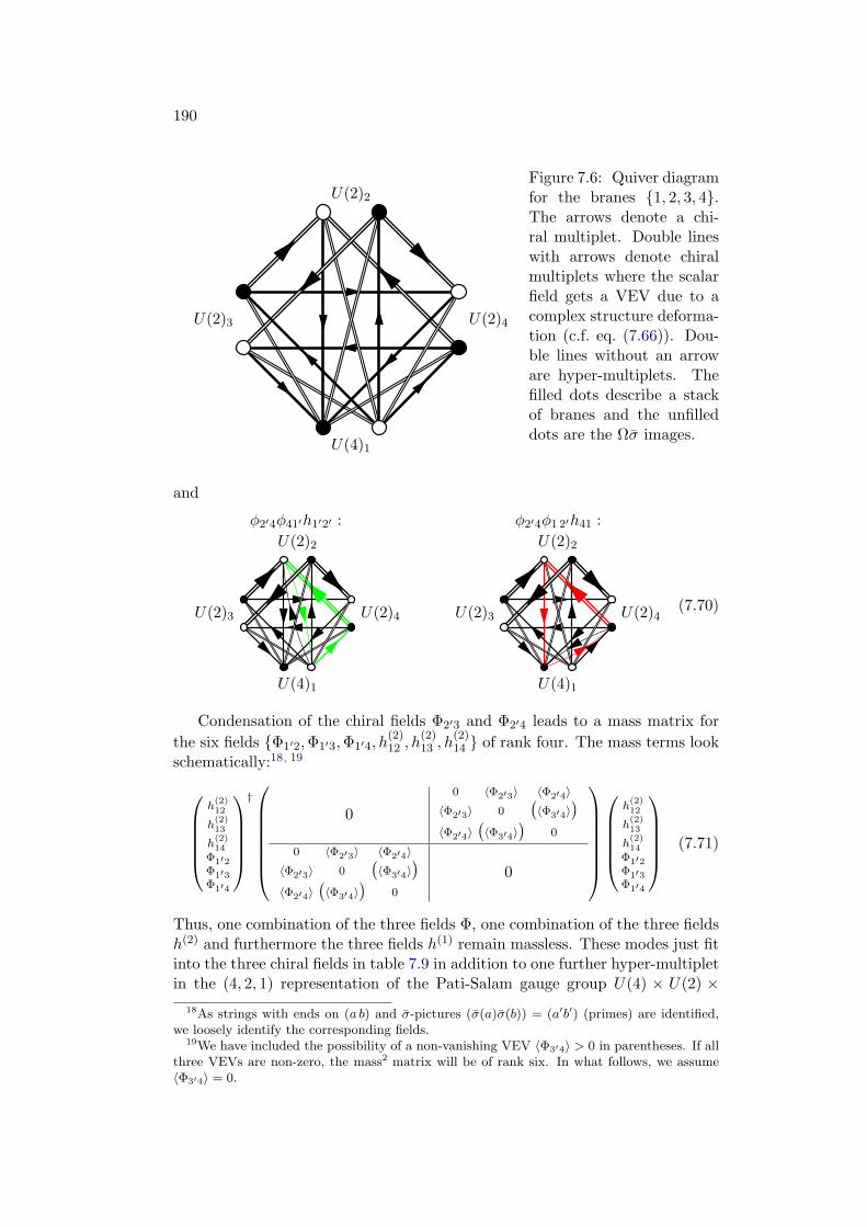
190

U(2)3 U(2)4

U(2)2

U(4)1

Figure 7.6: Quiver diagramfor the branes 1, 2, 3, 4.The arrows denote a chi-ral multiplet. Double lineswith arrows denote chiralmultiplets where the scalarfield gets a VEV due to acomplex structure deforma-tion (c.f. eq. (7.66)). Dou-ble lines without an arroware hyper-multiplets. Thefilled dots describe a stackof branes and the unfilleddots are the Ωσ images.

and

φ2′4φ41′h1′2′ : φ2′4φ1 2′h41 :

U(2)3 U(2)4

U(2)2

U(4)1

U(2)3 U(2)4

U(2)2

U(4)1

(7.70)

Condensation of the chiral fields Φ2′3 and Φ2′4 leads to a mass matrix forthe six fields Φ1′2,Φ1′3,Φ1′4, h

(2)12 , h

(2)13 , h

(2)14 of rank four. The mass terms look

schematically:18, 19

h(2)12

h(2)13

h(2)14

Φ1′2Φ1′3Φ1′4

†

00 〈Φ2′3〉〈Φ2′4〉

〈Φ2′3〉 0(〈Φ3′4〉

)〈Φ2′4〉

(〈Φ3′4〉

)0

0 〈Φ2′3〉〈Φ2′4〉〈Φ2′3〉 0

(〈Φ3′4〉

)〈Φ2′4〉

(〈Φ3′4〉

)0

0

h(2)12

h(2)13

h(2)14

Φ1′2Φ1′3Φ1′4

(7.71)

Thus, one combination of the three fields Φ, one combination of the three fieldsh(2) and furthermore the three fields h(1) remain massless. These modes just fitinto the three chiral fields in table 7.9 in addition to one further hyper-multipletin the (4, 2, 1) representation of the Pati-Salam gauge group U(4) × U(2) ×

18As strings with ends on (a b) and σ-pictures (σ(a)σ(b)) = (a′b′) (primes) are identified,we loosely identify the corresponding fields.

19We have included the possibility of a non-vanishing VEV 〈Φ3′4〉 > 0 in parentheses. If allthree VEVs are non-zero, the mass2 matrix will be of rank six. In what follows, we assume〈Φ3′4〉 = 0.

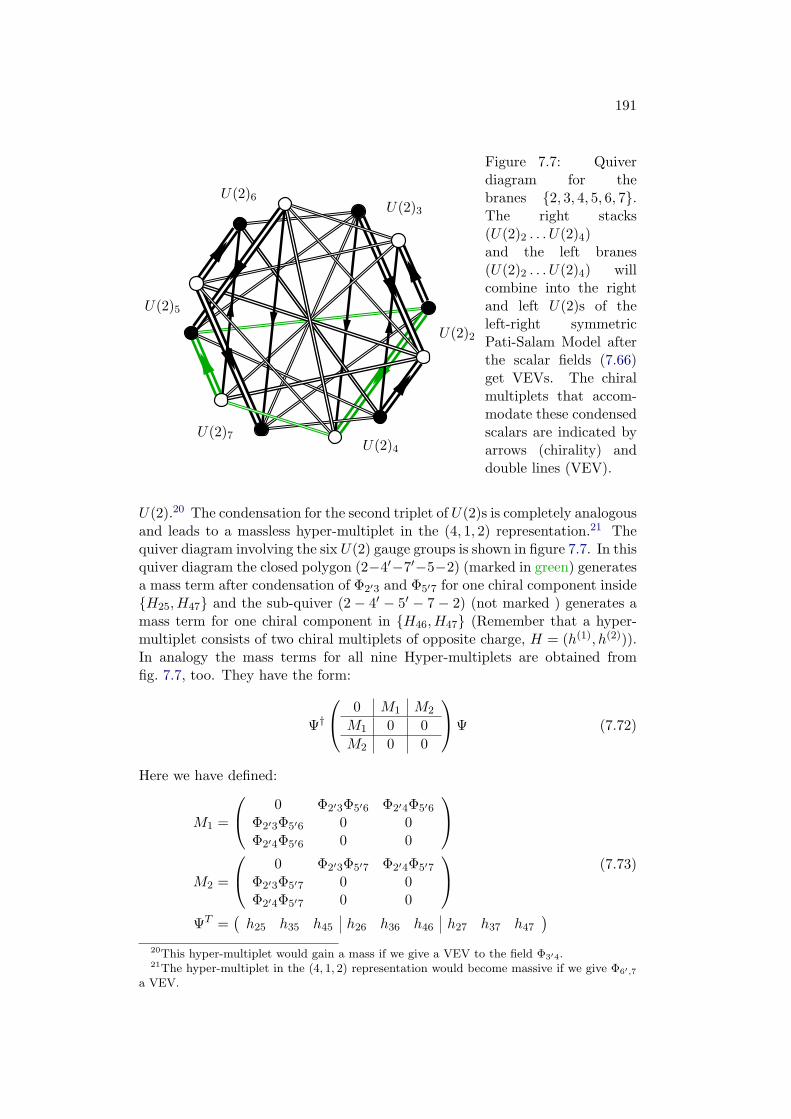
191

U(2)2

U(2)3U(2)6

U(2)5

U(2)7U(2)4

Figure 7.7: Quiverdiagram for thebranes 2, 3, 4, 5, 6, 7.The right stacks(U(2)2 . . . U(2)4)and the left branes(U(2)2 . . . U(2)4) willcombine into the rightand left U(2)s of theleft-right symmetricPati-Salam Model afterthe scalar fields (7.66)get VEVs. The chiralmultiplets that accom-modate these condensedscalars are indicated byarrows (chirality) anddouble lines (VEV).

U(2).20 The condensation for the second triplet of U(2)s is completely analogousand leads to a massless hyper-multiplet in the (4, 1, 2) representation.21 Thequiver diagram involving the six U(2) gauge groups is shown in figure 7.7. In thisquiver diagram the closed polygon (2−4′−7′−5−2) (marked in green) generatesa mass term after condensation of Φ2′3 and Φ5′7 for one chiral component insideH25,H47 and the sub-quiver (2 − 4′ − 5′ − 7 − 2) (not marked ) generates amass term for one chiral component in H46,H47 (Remember that a hyper-multiplet consists of two chiral multiplets of opposite charge, H = (h(1), h(2))).In analogy the mass terms for all nine Hyper-multiplets are obtained fromfig. 7.7, too. They have the form:

Ψ†

0 M1 M2

M1 0 0M2 0 0

Ψ (7.72)

Here we have defined:

M1 =

0 Φ2′3Φ5′6 Φ2′4Φ5′6

Φ2′3Φ5′6 0 0Φ2′4Φ5′6 0 0

M2 =

0 Φ2′3Φ5′7 Φ2′4Φ5′7

Φ2′3Φ5′7 0 0Φ2′4Φ5′7 0 0

ΨT =

(h25 h35 h45 h26 h36 h46 h27 h37 h47

)(7.73)

20This hyper-multiplet would gain a mass if we give a VEV to the field Φ3′4.21The hyper-multiplet in the (4, 1, 2) representation would become massive if we give Φ6′,7

a VEV.

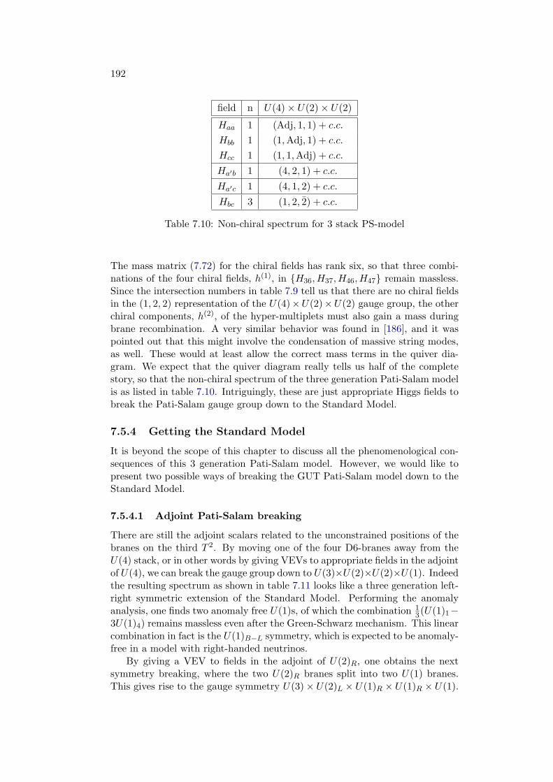
192

field n U(4)× U(2)× U(2)

Haa 1 (Adj, 1, 1) + c.c.

Hbb 1 (1,Adj, 1) + c.c.

Hcc 1 (1, 1,Adj) + c.c.

Ha′b 1 (4, 2, 1) + c.c.

Ha′c 1 (4, 1, 2) + c.c.

Hbc 3 (1, 2, 2) + c.c.

Table 7.10: Non-chiral spectrum for 3 stack PS-model

The mass matrix (7.72) for the chiral fields has rank six, so that three combi-nations of the four chiral fields, h(1), in H36,H37,H46,H47 remain massless.Since the intersection numbers in table 7.9 tell us that there are no chiral fieldsin the (1, 2, 2) representation of the U(4)×U(2)×U(2) gauge group, the otherchiral components, h(2), of the hyper-multiplets must also gain a mass duringbrane recombination. A very similar behavior was found in [186], and it waspointed out that this might involve the condensation of massive string modes,as well. These would at least allow the correct mass terms in the quiver dia-gram. We expect that the quiver diagram really tells us half of the completestory, so that the non-chiral spectrum of the three generation Pati-Salam modelis as listed in table 7.10. Intriguingly, these are just appropriate Higgs fields tobreak the Pati-Salam gauge group down to the Standard Model.

7.5.4 Getting the Standard Model

It is beyond the scope of this chapter to discuss all the phenomenological con-sequences of this 3 generation Pati-Salam model. However, we would like topresent two possible ways of breaking the GUT Pati-Salam model down to theStandard Model.

7.5.4.1 Adjoint Pati-Salam breaking

There are still the adjoint scalars related to the unconstrained positions of thebranes on the third T 2. By moving one of the four D6-branes away from theU(4) stack, or in other words by giving VEVs to appropriate fields in the adjointof U(4), we can break the gauge group down to U(3)×U(2)×U(2)×U(1). Indeedthe resulting spectrum as shown in table 7.11 looks like a three generation left-right symmetric extension of the Standard Model. Performing the anomalyanalysis, one finds two anomaly free U(1)s, of which the combination 1

3(U(1)1−3U(1)4) remains massless even after the Green-Schwarz mechanism. This linearcombination in fact is the U(1)B−L symmetry, which is expected to be anomaly-free in a model with right-handed neutrinos.

By giving a VEV to fields in the adjoint of U(2)R, one obtains the nextsymmetry breaking, where the two U(2)R branes split into two U(1) branes.This gives rise to the gauge symmetry U(3)× U(2)L × U(1)R × U(1)R × U(1).

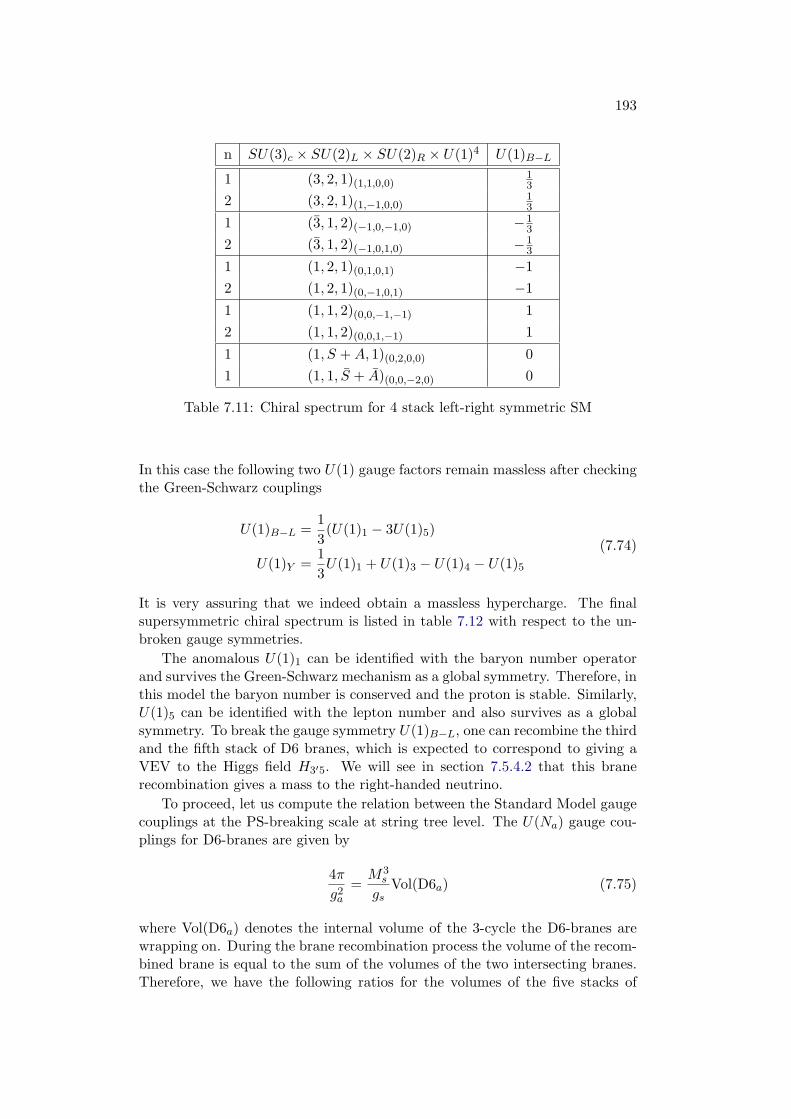
193

n SU(3)c × SU(2)L × SU(2)R × U(1)4 U(1)B−L

1 (3, 2, 1)(1,1,0,0) 13

2 (3, 2, 1)(1,−1,0,0)13

1 (3, 1, 2)(−1,0,−1,0) −13

2 (3, 1, 2)(−1,0,1,0) −13

1 (1, 2, 1)(0,1,0,1) −12 (1, 2, 1)(0,−1,0,1) −1

1 (1, 1, 2)(0,0,−1,−1) 12 (1, 1, 2)(0,0,1,−1) 1

1 (1, S +A, 1)(0,2,0,0) 01 (1, 1, S + A)(0,0,−2,0) 0

Table 7.11: Chiral spectrum for 4 stack left-right symmetric SM

In this case the following two U(1) gauge factors remain massless after checkingthe Green-Schwarz couplings

U(1)B−L =13(U(1)1 − 3U(1)5)

U(1)Y =13U(1)1 + U(1)3 − U(1)4 − U(1)5

(7.74)

It is very assuring that we indeed obtain a massless hypercharge. The finalsupersymmetric chiral spectrum is listed in table 7.12 with respect to the un-broken gauge symmetries.

The anomalous U(1)1 can be identified with the baryon number operatorand survives the Green-Schwarz mechanism as a global symmetry. Therefore, inthis model the baryon number is conserved and the proton is stable. Similarly,U(1)5 can be identified with the lepton number and also survives as a globalsymmetry. To break the gauge symmetry U(1)B−L, one can recombine the thirdand the fifth stack of D6 branes, which is expected to correspond to giving aVEV to the Higgs field H3′5. We will see in section 7.5.4.2 that this branerecombination gives a mass to the right-handed neutrino.

To proceed, let us compute the relation between the Standard Model gaugecouplings at the PS-breaking scale at string tree level. The U(Na) gauge cou-plings for D6-branes are given by

4πg2a

=M3s

gsVol(D6a) (7.75)

where Vol(D6a) denotes the internal volume of the 3-cycle the D6-branes arewrapping on. During the brane recombination process the volume of the recom-bined brane is equal to the sum of the volumes of the two intersecting branes.Therefore, we have the following ratios for the volumes of the five stacks of

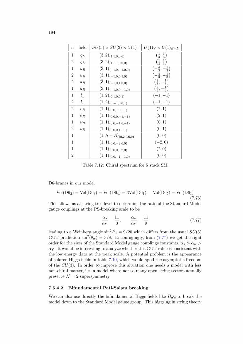
194

n field SU(3)× SU(2)× U(1)3 U(1)Y × U(1)B−L

1 qL (3, 2)(1,1,0,0,0)(

13 ,

13

)2 qL (3, 2)(1,−1,0,0,0)

(13 ,

13

)1 uR (3, 1)(−1,0,−1,0,0)

(−4

3 ,−13

)2 uR (3, 1)(−1,0,0,1,0)

(−4

3 ,−13

)2 dR (3, 1)(−1,0,1,0,0)

(23 ,−

13

)1 dR (3, 1)(−1,0,0,−1,0)

(23 ,−

13

)1 lL (1, 2)(0,1,0,0,1) (−1,−1)2 lL (1, 2)(0,−1,0,0,1) (−1,−1)

2 eR (1, 1)(0,0,1,0,−1) (2, 1)1 eR (1, 1)(0,0,0,−1,−1) (2, 1)1 νR (1, 1)(0,0,−1,0,−1) (0, 1)2 νR (1, 1)(0,0,0,1,−1) (0, 1)

1 (1, S +A)(0,2,0,0,0) (0, 0)1 (1, 1)(0,0,−2,0,0) (−2, 0)1 (1, 1)(0,0,0,−2,0) (2, 0)2 (1, 1)(0,0,−1,−1,0) (0, 0)

Table 7.12: Chiral spectrum for 5 stack SM

D6-branes in our model

Vol(D62) = Vol(D63) = Vol(D64) = 3Vol(D61), Vol(D65) = Vol(D61)(7.76)

This allows us at string tree level to determine the ratio of the Standard Modelgauge couplings at the PS-breaking scale to be

αsαY

=113,

αwαY

=119

(7.77)

leading to a Weinberg angle sin2 θw = 9/20 which differs from the usual SU(5)GUT prediction sin2(θw) = 3/8. Encouragingly, from (7.77) we get the rightorder for the sizes of the Standard Model gauge couplings constants, αs > αw >αY . It would be interesting to analyze whether this GUT value is consistent withthe low energy data at the weak scale. A potential problem is the appearanceof colored Higgs fields in table 7.10, which would spoil the asymptotic freedomof the SU(3). In order to improve this situation one needs a model with lessnon-chiral matter, i.e. a model where not so many open string sectors actuallypreserve N = 2 supersymmetry.

7.5.4.2 Bifundamental Pati-Salam breaking

We can also use directly the bifundamental Higgs fields like Ha′c to break themodel down to the Standard Model gauge group. This higgsing in string theory

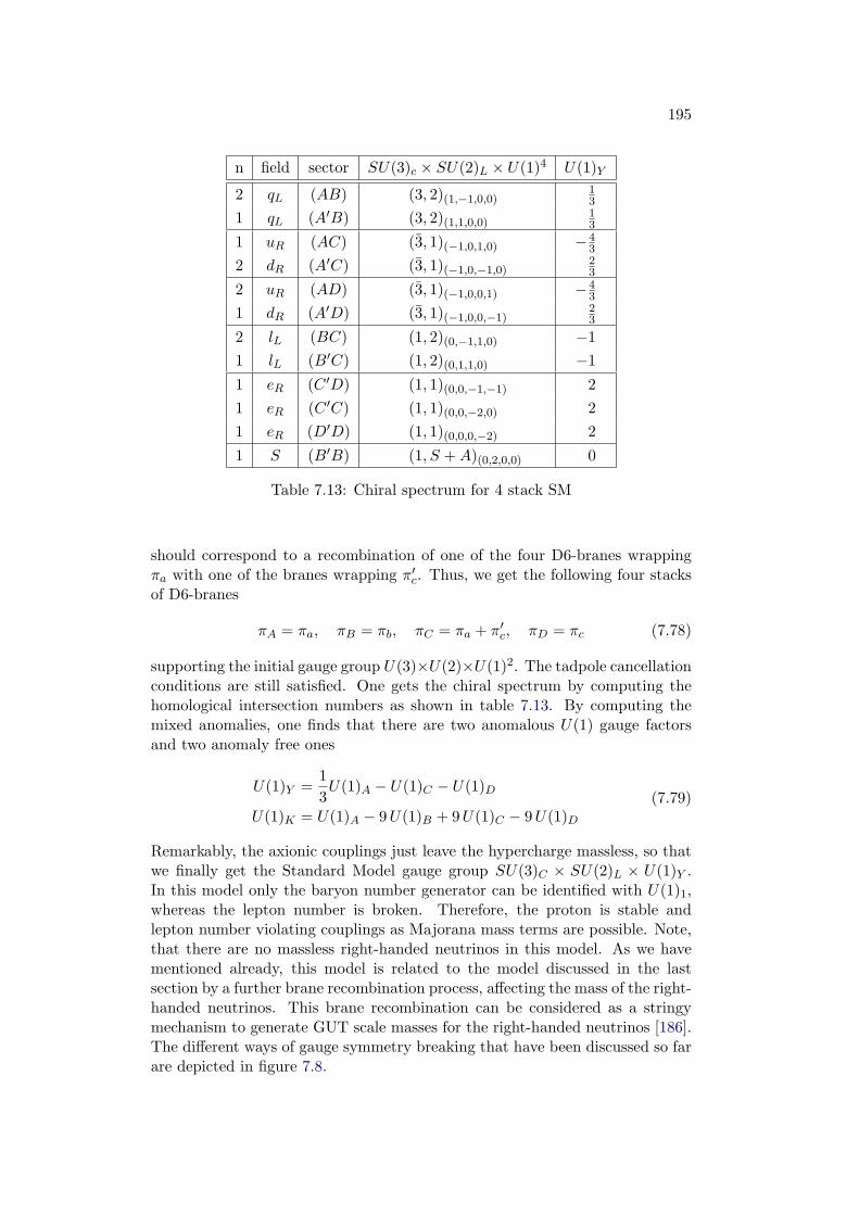
195

n field sector SU(3)c × SU(2)L × U(1)4 U(1)Y

2 qL (AB) (3, 2)(1,−1,0,0)13

1 qL (A′B) (3, 2)(1,1,0,0) 13

1 uR (AC) (3, 1)(−1,0,1,0) −43

2 dR (A′C) (3, 1)(−1,0,−1,0)23

2 uR (AD) (3, 1)(−1,0,0,1) −43

1 dR (A′D) (3, 1)(−1,0,0,−1)23

2 lL (BC) (1, 2)(0,−1,1,0) −11 lL (B′C) (1, 2)(0,1,1,0) −1

1 eR (C ′D) (1, 1)(0,0,−1,−1) 21 eR (C ′C) (1, 1)(0,0,−2,0) 21 eR (D′D) (1, 1)(0,0,0,−2) 2

1 S (B′B) (1, S +A)(0,2,0,0) 0

Table 7.13: Chiral spectrum for 4 stack SM

should correspond to a recombination of one of the four D6-branes wrappingπa with one of the branes wrapping π′c. Thus, we get the following four stacksof D6-branes

πA = πa, πB = πb, πC = πa + π′c, πD = πc (7.78)

supporting the initial gauge group U(3)×U(2)×U(1)2. The tadpole cancellationconditions are still satisfied. One gets the chiral spectrum by computing thehomological intersection numbers as shown in table 7.13. By computing themixed anomalies, one finds that there are two anomalous U(1) gauge factorsand two anomaly free ones

U(1)Y =13U(1)A − U(1)C − U(1)D

U(1)K = U(1)A − 9U(1)B + 9U(1)C − 9U(1)D(7.79)

Remarkably, the axionic couplings just leave the hypercharge massless, so thatwe finally get the Standard Model gauge group SU(3)C × SU(2)L × U(1)Y .In this model only the baryon number generator can be identified with U(1)1,whereas the lepton number is broken. Therefore, the proton is stable andlepton number violating couplings as Majorana mass terms are possible. Note,that there are no massless right-handed neutrinos in this model. As we havementioned already, this model is related to the model discussed in the lastsection by a further brane recombination process, affecting the mass of the right-handed neutrinos. This brane recombination can be considered as a stringymechanism to generate GUT scale masses for the right-handed neutrinos [186].The different ways of gauge symmetry breaking that have been discussed so farare depicted in figure 7.8.

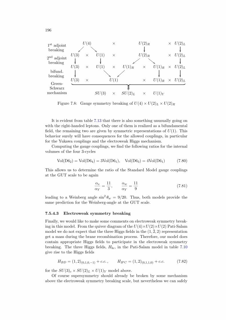
196

1st adjointbreaking

U(4)

~~~~

!!CCC

CC× U(2)R

× U(2)L

2nd adjointbreaking

U(3)

× U(1)

× U(2)R

wwww

w

""EEEE

E× U(2)L

U(3)

× U(1)

??

????× U(1)R

~~||||

||× U(1)R

× U(2)L

bifund.breaking

U(3) × U(1)

× U(1)R × U(2)LGreen-Schwarz

mechanism SU(3) × SU(2)L × U(1)Y

︸︷︷︸

Figure 7.8: Gauge symmetry breaking of U(4)× U(2)L × U(2)R

It is evident from table 7.13 that there is also something unusually going onwith the right-handed leptons. Only one of them is realized as a bifundamentalfield, the remaining two are given by symmetric representations of U(1). Thisbehavior surely will have consequences for the allowed couplings, in particularfor the Yukawa couplings and the electroweak Higgs mechanism.

Computing the gauge couplings, we find the following ratios for the internalvolumes of the four 3-cycles

Vol(D62) = Vol(D64) = 3Vol(D61), Vol(D63) = 4Vol(D61) (7.80)

This allows us to determine the ratio of the Standard Model gauge couplingsat the GUT scale to be again

αsαY

=113,

αwαY

=119

(7.81)

leading to a Weinberg angle sin2 θw = 9/20. Thus, both models provide thesame prediction for the Weinberg-angle at the GUT scale.

7.5.4.3 Electroweak symmetry breaking

Finally, we would like to make some comments on electroweak symmetry break-ing in this model. From the quiver diagram of the U(4)×U(2)×U(2) Pati-Salammodel we do not expect that the three Higgs fields in the (1, 2, 2) representationget a mass during the brane recombination process. Therefore, our model doescontain appropriate Higgs fields to participate in the electroweak symmetrybreaking. The three Higgs fields, Hbc, in the Pati-Salam model in table 7.10give rise to the Higgs fields

HBD = (1, 2)(0,1,0,−1) + c.c. , HB′C = (1, 2)(0,1,1,0) + c.c. (7.82)

for the SU(3)c × SU(2)L × U(1)Y model above.Of course supersymmetry should already be broken by some mechanism

above the electroweak symmetry breaking scale, but nevertheless we can safely

197

discuss the expectations from the purely topological data of the correspondingbrane recombination process. Since we do not want to break the color SU(3),we still take a stack of three D6-branes which are wrapped on the cycle πα =πA. Giving a VEV to the fields HBD is expected to correspond to the branerecombination

πβ = πB + πD (7.83)

However, for the brane recombination

πγ = π′B + πC (7.84)

the identification with the corresponding field theory deformation is slightlymore subtle, as the intersections between these two branes support both themassless chiral multiplet lB

′CL as listed in table 7.13 and the Higgs field HB′C .

Thus, the intersection preserves only N = 1 supersymmetry and one mightexpect that some combination of lB

′CL and HB′C are involved in the brane

recombination process. Even without knowing all the details, in the followingwe can safely compute the chiral spectrum via intersection numbers.

After the brane recombination we have a naive gauge group U(3)× U(1)×U(1), which however is broken by the Green-Schwarz couplings to SU(3)c ×U(1)em with

U(1)em =16U(1)α −

12U(1)β +

12U(1)γ (7.85)

Interestingly, just U(1)em survives this brane recombination process. Moreover,all intersection numbers vanish, so that there are no chiral massless fields, i.e. allquarks and leptons in table 7.13 have gained a mass including the left-handedneutrinos and the exotic matter. Looking at the charges in table 7.13, onerealizes that in the leptonic sector this Higgs effect cannot be the usual one,where simply lL and eR receive a mass via some Yukawa couplings. Here alsohigher dimensional couplings, like the dimension five coupling

W ∼ 1Ms

HBD HBD S eD′DR (7.86)

are relevant. These couplings induce a mixing of the Standard Model matterwith the exotic field, S. Thus we can state, that by realizing some of the right-handed leptons in the (anti-)symmetric representation, the exotic field is neededto give all leptons a mass during electroweak symmetry breaking. It remainsto be seen whether the induced masses can be consistent with the low-energydata.

Concluding remarks

In this chapter we have studied intersecting brane worlds for the T 6/Z4 ori-entifold background with special emphasis on supersymmetric configurations.We have found as a first non-trivial result a supersymmetric three generationPati-Salam type extension of the Standard Model with some exotic matter. Thechiral matter content is only slightly extended by one chiral multiplet in the

198

(anti-)symmetric representation of SU(2)L. The presence of this exotic mattercan be traced back to the fact that we were starting with a Pati-Salam gaugegroup, where the anomaly constraints forced us to introduce additional mat-ter. Issues which arose for non-supersymmetric models will also appear in thesupersymmetric setting. Since the Green-Schwarz mechanism produces globalU(1) symmetries, the allowed couplings in the effective gauge theory are usuallymuch more constrained than for the Standard Model.

With such model at hand, many phenomenological issues deserve to bestudied, as for instance mechanisms for supersymmetry breaking, the generationof soft breaking terms, Yukawa and higher dimensional couplings, the generationof µ-terms and gauge coupling unification.22 It also remains to be seen whetherthe electroweak Higgs effect indeed produces the correct masses for all quarksand leptons. Moreover, one should check whether the renormalization of thegauge couplings from the string respectively the PS-breaking scale down to theweak scale can lead to acceptable values for the Weinberg angle.23

The motivation for this analysis was to start a systematic search for realisticsupersymmetric intersecting brane world models. We have worked out some ofthe technical model building aspects when one is dealing with more complicatedorbifold backgrounds containing in particular twisted sector 3-cycles. Thesetechniques can be directly generalized to, for instance, the Z6 orientifolds [57]or the ZN ×ZM orientifold models [206].24 It could be worthwhile to undertakea similar study for these orbifold models, too.

The final goal would be to find a realization of the MSSM in some simpleintersecting brane world model. As should have become clear from our analy-sis, while phenomenologically interesting non-supersymmetric models are fairlyeasy to get, the same is not true for the supersymmetric ones. Requiring super-symmetry imposes very strong constraints on the possible configurations andas we have observed in the Z4 example, also the supply of possible intersec-tion numbers is very limited. These obstructions appear to be less surprising,when one contemplates that for smooth backgrounds, by lifting to M-theory,the construction of an N = 1 chiral intersecting brane world background withO6 planes and D6 branes is equivalent to the construction of a compact singularG2 manifold. In this respect it would be interesting whether certain M-theoryorbifold constructions like the one discussed in [222] are dual to the kind ofmodels discussed in this chapter.

At a certain scale close to the TeV scale supersymmetry has to be broken.For the intersecting brane world scenario one might envision different mecha-nisms for such a breaking. First, we might use the conventional mechanism ofgaugino condensation via some non-perturbative effect. Alternatively, one could

22Yukawa couplings for toroidal σΩ-orientifolds have been calculated in [218] and [219] (alsofour-point couplings). However it is not clear if these calculations might be generalized to thecase of recombined D-branes that appear in the models discussed in this chapter. The evolutionof gauge-couplings including threshold corrections was investigated for supersymmetric σΩ-orientifolds in [220].

23In [221] issues concerning gauge-coupling unification were addressed in the context ofsupersymmetric σΩ-orientifolds with D6-branes.

24Meanwhile the Z4 × Z2 σΩ-orientifold with projection has been studied [168].

199

build models where the MSSM is localized on a number of D-branes, but wherethe RR-tadpole cancellation conditions requires the introduction of hidden sec-tor branes, on which supersymmetry might be broken. This breaking could bemediated gravitationally to the Standard Model branes. A third possibility isto get D-term supersymmetry breaking by generating effective Fayet-Iliopoulosterms via complex structure deformations. We think that these issues and otherphenomenological questions deserve to be studied in the future.

Conclusions

In this thesis we have investigated specific kinds of open-string theories. Astriking feature of all constructions we considered is that they potentially con-tain chiral fermions. From the string theoretic point of view, chiral fermionsarise due to non-trivial boundary conditions of the open-string. In the caseof world-sheet supersymmetry the Ramond sector yields a reduced number ofzero-modes. To be more specific, this could lead to a single zero-mode afterGSO projection. By compactification to four space-time dimensions this re-sults in a single Weyl fermion. However the number of world-sheet bosoniczero modes (e.g. intersection points or Landau levels) can be increased by theboundary conditions. As the Hilbert space of the string states is a product ofworld-sheet bosons and fermions: Hbos ⊗Hferm, the degeneracy of world-sheetbosonic zero modes is inherited by the Ramond-sector. Furthermore one hasto take into account, that there might appear space-time fermions of both chi-ralities. Therefore the multiplicity of world-sheet bosons encounters possiblesigns. As a result the total number of fermions with definite chirality is givenby purely topological quantities like the intersection number of D-branes orthe index of the twisted spin complex. In model-building this degeneracy is(roughly speaking) interpreted as the number of generations of a specific parti-cle type. Therefore the degenerate states should be split by some mechanism25

into states of different masses, but otherwise identical quantum numbers. Byadjusting the topological data in a bottom-up approach, we could generatemany phenomenologically appealing spectra.

As a basis for the subsequent chapters we quantized the open string withlinear, but independent boundary conditions that are induced by D-branes ofarbitrary dimension with constant NSNS B- and NS F -field(s) in chapter 4. Weconfirmed the disk result of Seiberg and Witten on the non-commutativity ofopen-string boundaries for the one-loop case (with arbitrary, constant F-fluxeson the string-endpoints, but without Dirichlet conditions). Furthermore weinvestigated the zero- and momentum-mode spectrum in toroidal compactifica-tions. It was shown that a kind of Landau degeneracy shows up, if the stringend-points couple to different NS F -fields. This is an example of the degeneracymentioned above.

Chapter 5 mainly reviews the content of our publication [1]. In this articlewe investigated the D-brane spectrum of asymmetric orbifolds and orientifolds.

25Such a mechanism should have a string-theoretic interpretation. For example differentmasses could arise due to Yukawa-couplings which are associated to some area of the world-sheet in intersecting brane-world models (cf. [218,219]).

200

201

It turned out that left-right asymmetric twists imply in many cases the presenceof D-branes with magnetic background fluxes, since the D-brane configurationhas to be symmetrized under the (asymmetric) orbifold Group G. As an exam-ple we presented a space-time six-dimensional model that was obtained fromorientifolding a T 4/ZL

3 × ZR3 -orbifold.26 This article was finished before the

work presented in chapter 4 was done. With some new insights gained in thischapter it was now possible to answer some so far open questions, like thequantization of the open-string momentum modes on toroidally compactifiedD-branes both for magnetized branes and lower dimensional branes from firstprinciples.27 This quantization was derived up to now only indirectly via theopen-closed string correspondence (i.e. boundary states, cf. [223,224]).

Chapter 6 is devoted to purely toroidal orientifolds. We considered bothspace-time six- and four-dimensional compactifications, i.e. compactificationson T 6 resp. T 4. Computations can be either done in the pure Ω-orientifoldwith D9-branes carrying NS U(1)-fluxes in the compact directions, or in theT-dual picture, where Ω is combined with complex conjugation σ. Here theO-plane fills only a real subspace of the torus and its RR charge is canceledby D-branes of the same dimensionality. This means that we introduce D7-branes for the T 4-compactification and D6-branes on the six-torus T 6. Chiralfermions arise in the σΩ-orientifold at the intersection points of the D7- resp.D6-branes. The number of chiral fermion generations is then given by thetopological intersection numbers, while in the flux picture it is due to Landaudegeneracies, which can be calculated by an index-theorem.28 In order to getan interesting spectrum, one tries to distribute D-branes in such a way thata) they cancel the RR tadpole (thereby ensuring anomaly cancellation) andb) they yield the desired intersection numbers (resp. index). We were ableto construct a four generation model with SM-like spectrum and gauge groupSU(3)×SU(2)×U(1)Y ×U(1)2. The obstruction that the number of generationshas to be even can be overcome by including so called B-type tori as shownin the subsequent publication [161].29 However chiral configurations in purelytoroidal constructions always break supersymmetry. Therefore the solutionsmight be unstable (i.e. divergent to a singular limit). Besides the Fischler-Susskind mechanism30 there might exist further (yet unknown) mechanisms to

26We considered three variations of this orientifold. The main difference in these threedifferent orientifolds is due to two alternative actions of the world sheet parity Ω on the zero-and momentum-modes. This is equivalent to different choices for the complex- and Kahler-structure of each of the two two-tori (T 4 = T 2×T 2). The two different choices result in threeinequivalent orientifold models. One of these models was investigated before in [53] by meansof conformal field theory. However a D-brane interpretation of the open-string sector couldnot be given in this former publication.

27The quantization for open strings on lower dimensional branes was done earlier for van-ishing NSNS B-field.

28There are some subtleties, like the impossibility of obtaining the complete left-handedquark sector just from two kinds of branes (cf. section 6.4.2).

29B-type means on the in the “flux” picture that the NSNS B-field is set to α′/2, which isstill an Ω-symmetric background. In the T-dual “branes at angles” picture, the real part ofthe complex-structure τ of the B-type two-torus is fixed to τ1 = 1/2.

30It is however not clear, if the Fischler-Susskind mechanism does lead to a non-degenerateand non-supersymmetric limit.

202

stabilize the non-supersymmetric vacua.Chapter 7 deals with the σΩ-orientifold of an N = 2 supersymmetric T 6/Z4

orbifold. It is the second example besides the Z2 × Z2 orientifold models(cf. [174]) that a σΩ-orientifold admits chiral supersymmetric solutions. Thischapter is mainly based on our publication [3], however more detailed in somepoints. We concentrate in the second half on an U(4)× U(2)3L × U(2)3R-modelwhich we can break down to a three generation Pati Salam U(4)×U(2)L×U(2)R-model, while preserving supersymmetry. This is done by giving VEVs to fieldsin the low energy effective action. The chiral fermion spectrum in the lattermodel is given again by topological intersection numbers, while the non-chiralspectrum (i.e. hypermultiplets) is obtained by field theoretic considerations.Fields in the non-chiral spectrum serve as Higgs-particles for breaking the modeldown to an MSSM like spectrum.

While non-supersymmetric models have to deal with instabilities due toNSNS tadpoles (and potentially with open string tachyons, too), the super-symmetric models are stable.31 However it is still an open issue how to breaksupersymmetry in a way that is manifestly compatible with string-theory.32

The brane recombination process deserves a microscopic explanation.33 Sincespecial Lagrangian submanifolds play a prominent role in the construction of su-persymmetric intersecting brane worlds, a richer knowledge about these objectsis desirable, also in the more general context than Calabi-Yau orbifolds.

As another aim one could consider other toroidal orientifolds, searchingagain for a stringy realization of the MSSM.

We want to conclude with these few suggestions, even though many otherquestions related to this kind of orientifold constructions should be addressed,too.

31However instabilities might be induced by quantum or instanton corrections or so farunknown mechanisms.

32Field-theoretic considerations in related models do exist, some of them involving non-perturbative effects.

33This topic has recently been addressed by Hashimoto at the Strings 2003 conference,however in a more general context.

Acknowledgments

First of all I would like to thank Professor Dieter Lust who offered me thepossibility to do my Ph.D. under his supervision. I am very grateful to RalphBlumenhagen, who taught me a lot of things in string theory. I would also liketo thank Boris Kors who was Ph.D. student in Berlin during my Diploma andearly Ph.D. time. With all of these three gentlemen I published several papers,two of them during the time of my Ph.D. thesis. I would also like to thankTassilo Ott. With him I had an extremely fruitful collaboration at the end ofmy thesis resulting in a publication, too.

I thank the colleagues who shared the office with me for providing a pleasantatmosphere: Matthias Brandle, Volker Braun, Stefano Chiantese, Claus Jeschekand Christoph Sieg.

I am indebted to Stephan Stieberger for proof-reading my thesis.With many other current and former members of our group I had extended

and fruitful discussions. I would like to thank: Gianguido Dall’Agata, OlegAndreev, Klaus Behrndt, Gabriel Cardoso, Gottfried Curio, Bernd-DietrichDorfel, Harald Dorn, Johanna Erdmenger, Andrea Gregori, Johannes Grosse,Zachary Guralnik, Robert Helling, Albrecht Klemm, Georgios Kraniotis, IngoKirsch, Axel Krause, Karl Landsteiner, Calin Lazaroiu, Andre Miemiec, AalokMisra, Hans-Jorg Otto, Nikolaos Prezas, Ingo Runkel, Mario Salizzoni and RaduTatar.

I am also grateful to our secretary Sylvia Richter and our former secretarySusanne Preisser for helping me with administrative problems.

I would like to express my gratitude to my parents, who supported meduring my University studies.

203

Hilfsmittel

Außer der angegebenen Literatur habe ich die Computeralgebra-Programme“Maple” und “Mathematica” verwendet. Ferner kam ein “C++” Compiler zumEinsatz. Die drei-dimensionalen Grafiken wurden mit dem “Ray-Tracing” Pro-gamm “Povray” erstellt, wobei die Daten einiger drei-dimensionaler Objektemit “Mathematica” berechnet wurden.

204

Selbstandigkeitserklarung

Hiermit erklare ich, die vorliegende Arbeit selbstandig ohne fremde Hilfe ver-faßt und nur die angegebene Literatur und Hilfsmittel verwendet zu haben.

Lars Gorlich

11. August 2003

205

Appendix A

Theta-functions and relatedfunctions

A.1 η and ϑ-functions, identities and transformationunder SL(2, Z)

The ϑ-functions are defined as follows

ϑ[ab

](τ) =

∑n∈Z

q12(n+a)2 e2iπ(n+a)b (A.1)

q is defined by q = e2πiτ (Imτ > 0). The ϑ-functions admit the followingrepresentation as an infinite product:

ϑ[ab

]η

= e2iπab q12a2− 1

24

∞∏n=1

(1 + qn+a− 1

2 e2iπb) (

1 + qn−a−12 e−2iπb

), (A.2)

with η being the Dedekind η-function:

η = q124

∞∏n=1

(1− qn) (A.3)

A.1.1 Transformation under SL(2, Z):

The ϑ- and η-functions transform under the generators S, T of the modulargroup SL(2,Z) and under P = TST 2S as follows:

S-transformation:

τS→ −1/τ (A.4)

1ηϑ[ab

](τ) = e2πi ab

1ηϑ

[b

−a

](−1/τ) η(τ) =

√i

τη(−1/τ) (A.5)

206

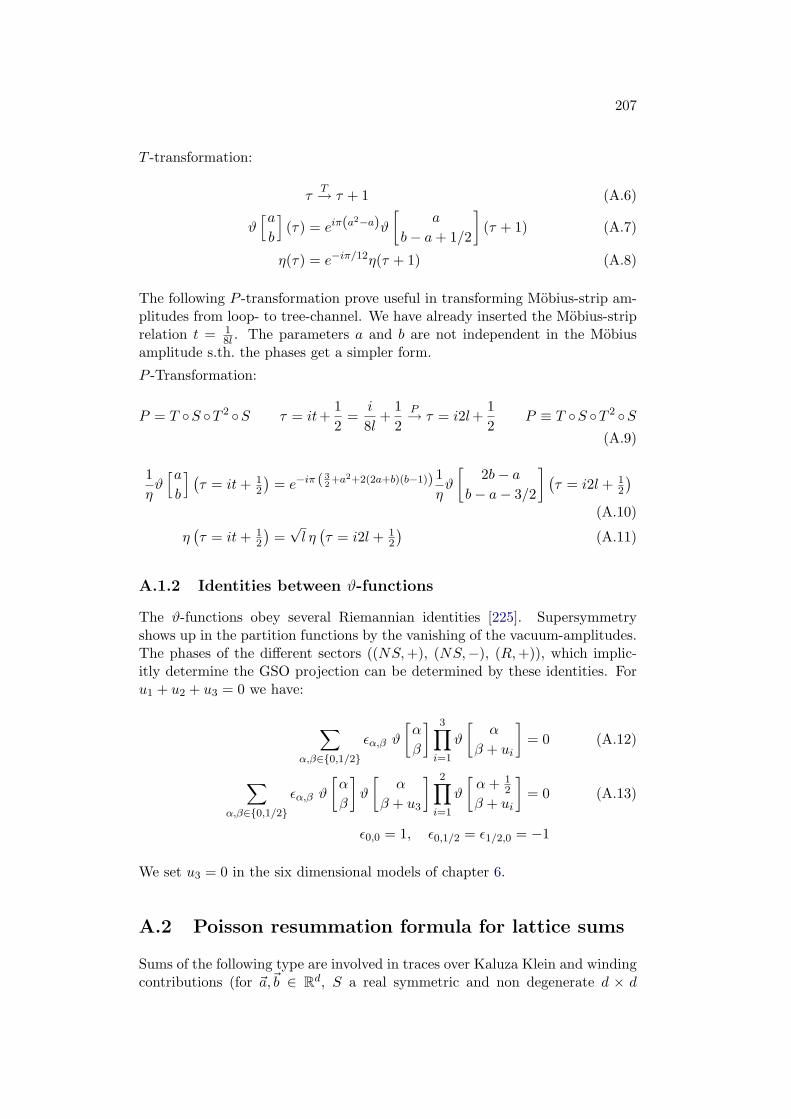
207

T -transformation:

τT→ τ + 1 (A.6)

ϑ[ab

](τ) = eiπ(a

2−a)ϑ[

a

b− a+ 1/2

](τ + 1) (A.7)

η(τ) = e−iπ/12η(τ + 1) (A.8)

The following P -transformation prove useful in transforming Mobius-strip am-plitudes from loop- to tree-channel. We have already inserted the Mobius-striprelation t = 1

8l . The parameters a and b are not independent in the Mobiusamplitude s.th. the phases get a simpler form.

P -Transformation:

P = T S T 2 S τ = it+12

=i

8l+

12

P→ τ = i2l+12

P ≡ T S T 2 S(A.9)

1ηϑ[ab

] (τ = it+ 1

2

)= e−iπ ( 3

2+a2+2(2a+b)(b−1)) 1

ηϑ

[2b− a

b− a− 3/2

] (τ = i2l + 1

2

)(A.10)

η(τ = it+ 1

2

)=√l η(τ = i2l + 1

2

)(A.11)

A.1.2 Identities between ϑ-functions

The ϑ-functions obey several Riemannian identities [225]. Supersymmetryshows up in the partition functions by the vanishing of the vacuum-amplitudes.The phases of the different sectors ((NS,+), (NS,−), (R,+)), which implic-itly determine the GSO projection can be determined by these identities. Foru1 + u2 + u3 = 0 we have:

∑α,β∈0,1/2

εα,β ϑ

[α

β

] 3∏i=1

ϑ

[α

β + ui

]= 0 (A.12)

∑α,β∈0,1/2

εα,β ϑ

[α

β

]ϑ

[α

β + u3

] 2∏i=1

ϑ

[α+ 1

2

β + ui

]= 0 (A.13)

ε0,0 = 1, ε0,1/2 = ε1/2,0 = −1

We set u3 = 0 in the six dimensional models of chapter 6.

A.2 Poisson resummation formula for lattice sums

Sums of the following type are involved in traces over Kaluza Klein and windingcontributions (for ~a,~b ∈ Rd, S a real symmetric and non degenerate d × d

208

matrix):∑~v∈Zd

ei2π(~v+~a)·~be−πt((~v+~a)T S (~v+~a))

= t−d/21√

detS

∑~w∈Zd

e−i2π ~w·~ae−πt ((~w+~b)T S−1 (~w+~b)) (A.14)

A.3 Conformal blocks in D = 6

In this section we summarize the conformal blocks that we use to shorten thenotation for the asymmetric ZL3 ×ZR3 orbifold on T 2× T 2 in section 2.4 (p. 47)and its orientifolded version (or open descendants) in section 5.4 (p. 133). Wedefine:1

ρ00 =12

∑α,β=0, 1

2

(−1)2α+2β+4αβϑ[αβ

]4η4

,

ρ0h =12

∑α,β=0, 1

2


]2η2

2∏i=1

2 sin(πhi)ϑ[

αβ+hi

]ϑ

[12

12+hi

] h 6= 0

ρgh =12

∑α,β=0, 1

2


]2η2

2∏i=1

ϑ[α+giβ+hi

]ϑ

[12+gi

12+hi

] g, h 6= 0

(A.15)

The functions (A.15) transform under τ S−→ −1/τ like:

ρ00 → ρ00

ρ0h → (2 sinπh)2 ρh0 h 6= 0

ρh0 → (2 sinπh)−2 ρ0,−h h 6= 0ρgg → −ρg,−g g 6= 0

ρg,−g → −ρ−g,−g g 6= 0

(A.16)

The modular T transformation τ T−→ τ + 1 acts by:ρghη2

τ→τ+1−−−−−→ρg,g+hη2

(A.17)

As abbreviations for lattice sums we define (cf. [53]):

ΛSU(3)2 ≡(|χ0|2 + |χ1|+ |χ2|2

)2ΛR ≡ χ2

0

ΛωW ≡(χ0 + ei2πω/3χ1 + e−i2πω/3χ2

)2ΛW ≡ Λ0

W

1We adopted our notation from [53] and restricted it to the case d = 4, i.e. compactificationon a T 4.

209

where χ0, χ1 and χ2 are the SU(3) characters at level one defined by formula(2.113) (p. 48).

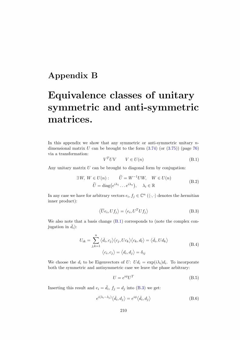
Appendix B

Equivalence classes of unitarysymmetric and anti-symmetricmatrices.

In this appendix we show that any symmetric or anti-symmetric unitary n-dimensional matrix U can be brought to the form (3.74) (or (3.75)) (page 76)via a transformation:

V TUV V ∈ U(n) (B.1)

Any unitary matrix U can be brought to diagonal form by conjugation:

∃W, W ∈ U(n) : U = W−1UW, W ∈ U(n)

U = diag(eiλ1 . . . eiλn

), λi ∈ R

(B.2)

In any case we have for arbitrary vectors ei, fj ∈ Cn (〈·, ·〉 denotes the hermitianinner product): ⟨

Uei, Ufj⟩

=⟨ei, U

TUfj⟩

(B.3)

We also note that a basis change (B.1) corresponds to (note the complex con-jugation in di):

Uik =n∑

j,k=1

⟨di, cj

⟩⟨cj , Uck

⟩⟨ck, dl

⟩=⟨di, Udk

⟩⟨ci, cj

⟩=⟨di, dj

⟩= δij

(B.4)

We choose the di to be Eigenvectors of U : Udi = exp(iλi)di. To incorporateboth the symmetric and antisymmetric case we leave the phase arbitrary:

U = eiφUT (B.5)

Inserting this result and ei = di, fj = dj into (B.3) we get:

ei(λi−λj)⟨di, dj

⟩= eiφ

⟨di, dj

⟩(B.6)

210

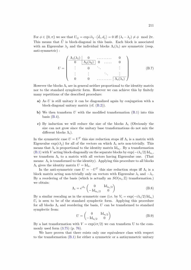
211

For φ ∈ 0, π we see that Uij = exp iλj ·⟨di, dj

⟩= 0 iff (λi−λj) 6= φ mod 2π.

This means that U is block-diagonal in this basis. Each block is associatedwith an Eigenvalue λj and the individual blocks Λi(λi) are symmetric (resp.anti-symmetric) :

U =

Λ1(λ1) 0 . . . . . . . . . 0

0 Λ2(λ2) 0 . . . . . 0... 0

. . ....

......

. . ....

0 0 . . . . . . . . . Λs(λs)

(B.7)

However the blocks Λi are in general neither proportional to the identity matrixnor to the standard symplectic form. However we can achieve this by finitelymany repetitions of the described procedure:

a) As U is still unitary it can be diagonalized again by conjugation with ablock-diagonal unitary matrix (cf. (B.2)).

b) We then transform U with the modified transformation (B.1) into thisbasis (B.4).

c) By induction we will reduce the size of the blocks Λi (Obviously thesize can not grow since the unitary base transformations do not mix thedifferent blocks Λi).

In the symmetric case U = UT this size reduction stops iff Λi is a matrix withEigenvalue exp(iλj) for all of the vectors on which Λi acts non-trivially. Thismeans that Λi is proportional to the identity matrix Idni . By a transformation(B.1) with V acting block-diagonally on the separate blocks by exp(−iλi/2) Idni ,we transform Λi to a matrix with all vectors having Eigenvalue one. (Thatmeans: Λi is transformed to the identity). Applying this procedure to all blocksΛi gives the identity matrix U = Idn.

In the anti-symmetric case U = −UT this size reduction stops iff Λi is ablock matrix acting non-trivially only on vectors with Eigenvalue λi and −λi.By a reordering of the basis (which is actually an SO(ni,Z) transformation.)we obtain:

Λi = eiλi

(0 Idni/2

− Idni/2 0

)(B.8)

By a similar rescaling as in the symmetric case (i.e. by Vi = exp(−iλi/2) Idni)Ui is seen to be of the standard symplectic form. Applying this procedurefor all blocks Λi and reordering the basis, U can be transformed to standardsymplectic from:

U =(

0 Idn/2− Idn/2 0

)(B.9)

By a last transformation with V = exp(iπ/2) we can transform U to the com-monly used form (3.75) (p. 76).

We have proven that there exists only one equivalence class with respectto the transformation (B.1) for either a symmetric or a antisymmetric unitary

212

matrix U . In the symmetric case this class can be represented by the identitymatrix. In the anti-symmetric case this class can be represented by the standardsymplectic form (B.9).

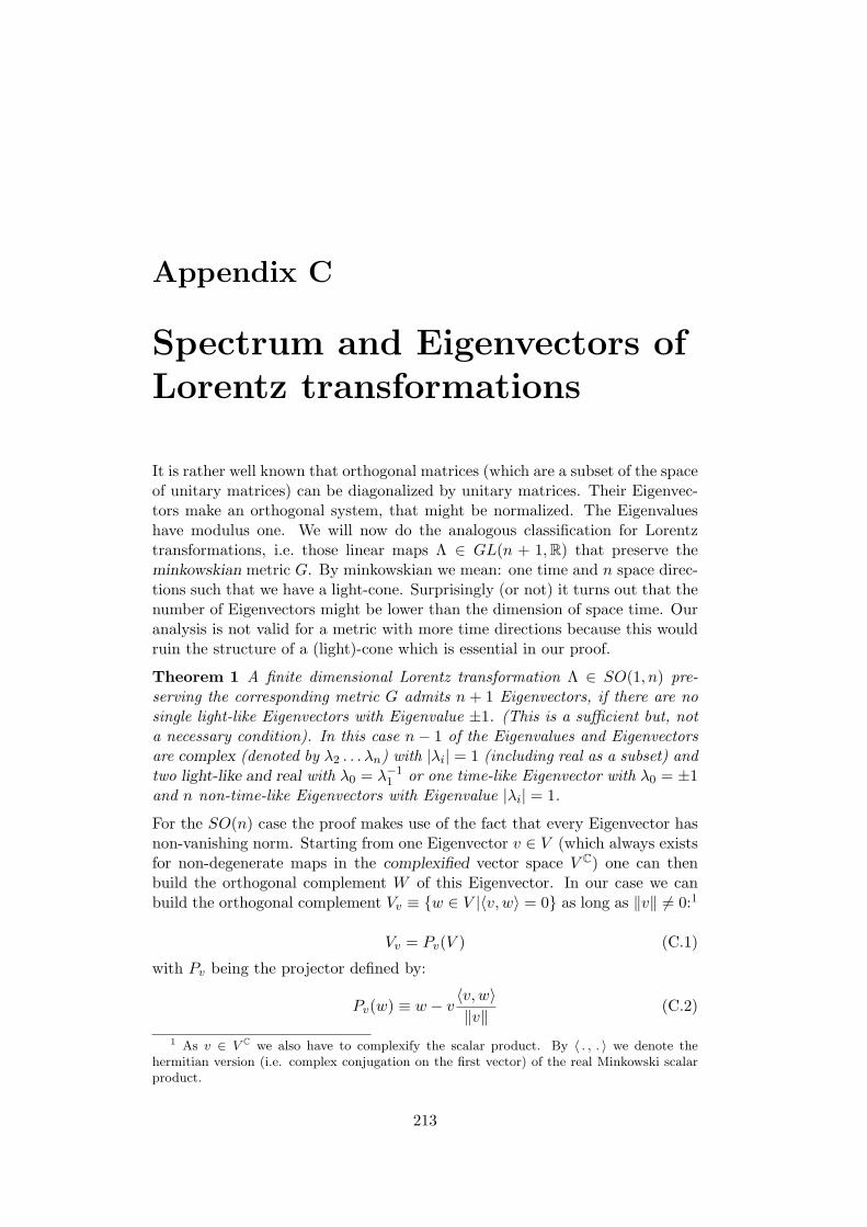
Appendix C

Spectrum and Eigenvectors ofLorentz transformations

It is rather well known that orthogonal matrices (which are a subset of the spaceof unitary matrices) can be diagonalized by unitary matrices. Their Eigenvec-tors make an orthogonal system, that might be normalized. The Eigenvalueshave modulus one. We will now do the analogous classification for Lorentztransformations, i.e. those linear maps Λ ∈ GL(n + 1,R) that preserve theminkowskian metric G. By minkowskian we mean: one time and n space direc-tions such that we have a light-cone. Surprisingly (or not) it turns out that thenumber of Eigenvectors might be lower than the dimension of space time. Ouranalysis is not valid for a metric with more time directions because this wouldruin the structure of a (light)-cone which is essential in our proof.

Theorem 1 A finite dimensional Lorentz transformation Λ ∈ SO(1, n) pre-serving the corresponding metric G admits n + 1 Eigenvectors, if there are nosingle light-like Eigenvectors with Eigenvalue ±1. (This is a sufficient but, nota necessary condition). In this case n− 1 of the Eigenvalues and Eigenvectorsare complex (denoted by λ2 . . . λn) with |λi| = 1 (including real as a subset) andtwo light-like and real with λ0 = λ−1

1 or one time-like Eigenvector with λ0 = ±1and n non-time-like Eigenvectors with Eigenvalue |λi| = 1.

For the SO(n) case the proof makes use of the fact that every Eigenvector hasnon-vanishing norm. Starting from one Eigenvector v ∈ V (which always existsfor non-degenerate maps in the complexified vector space V C) one can thenbuild the orthogonal complement W of this Eigenvector. In our case we canbuild the orthogonal complement Vv ≡ w ∈ V |〈v, w〉 = 0 as long as ‖v‖ 6= 0:1

Vv = Pv(V ) (C.1)

with Pv being the projector defined by:

Pv(w) ≡ w − v 〈v, w〉‖v‖

(C.2)

1 As v ∈ V C we also have to complexify the scalar product. By 〈 . , . 〉 we denote thehermitian version (i.e. complex conjugation on the first vector) of the real Minkowski scalarproduct.

213

214

We can now proceed by induction starting from one Eigenvector v:

a) If v is not light-like we note that λv has modulus one. As we have assumedΛ to be real (appropriate to our application in chapter 4) we also deducethat v is an Eigenvector with Eigenvalue λv = λv. We will then projectonto W = Pv(V ) which is left invariant by Λ (〈v,Λw〉 = λv〈Λv,Λw〉 =〈v, w〉 = 0).

b) If v is light-like its Eigenvalue is assumed to be real: λ complex wouldimply that v is also Eigenvector with Eigenvalue λ. If 〈v, v〉 6= 0 thisimplies λ2 = 1. This implies that v is real (up to a phase). This con-tradicts 〈v, v〉 6= 0. The second possibility, 〈v, v〉 = 0 implies that v andv are linear dependent and up to a phase: real. (One can see this byexplicitly writing down the scalar product for two light-like vectors. Ifone normalizes the time component v0 = w0 = a ∈ R one discovers forthe space component that the vectors should be perpendicular wrt. theminkowskian scalar product: 〈~v,~v〉herm. = 〈~w, ~w〉herm. = 〈~w,~v〉herm.. Thisimplies that ~v = ~w. By 〈 . , . 〉herm. we mean the hermitian, positive defi-nite scalar product of the space components.) We denote the Eigenvalueof the light-like v by λ0. If λ0 6= ±1 we note that there is another light-likeEigenvector: As all non-light-like Eigenvectors only contribute Eigenval-ues with |λ| = 1, in order for detΛ = ±1 there has to exist at least oneother light-like Eigenvector w with λ1 ≡ λw 6= λ0. Due to the structure ofthe light cone, w has non-vanishing scalar product with v. This impliesλ1 = λ−1

0 (∈ R). We can now linearly combine v and w into non-light-likevectors and project (by (C.2) ) on the orthogonal complement which hastwo dimensions less. The orthogonal complement Wv,w fulfills of courseΛ(Wv,w

)⊂Wv,w.

c) If v is light-like with Eigenvalue λ = ±1 the determinant argument doesnot apply. There might or might not be additional time-like Eigenvectors.If another linear indep. light-like Eigenvector exists, we could projectout the space spanned by the two light-like Eigenvectors. If not, wecan make no further general and simple statement, if other non-light-likeEigenvectors exist.2 We simply have to exclude this latter case for oursolution in chapter 4.

The procedure can be applied on the remaining subspace W until all Eigenvec-tors are found. There is one comment in order about the time-like Eigenvectorwhich might exist. In principle it could have Eigenvalue λ = exp(iφ), φ ∈ R.However only λ = ±1 is actually possible: v time-like implies v time-like. Be-cause there are no two orthogonal time-like directions, v is real up to a phase.This restricts the Eigenvalue of time-like Eigenvectors to be either plus or minusone.

2One could think to project by the projector P‖ or P⊥ (cf. eq. (4.13) ,p. 90 ) definedin chapter 4. The resulting two spaces have however non-vanishing scalar-products. The sodefined complement of the light-like Eigenvector v: Wv ≡ ker(1− Pv) is not invariant underthe Lorentz-transformation Λ: Λ

(Wv

)6⊂Wv

215

Of course there can be maximally two lin. indep. light-like Eigenvectors vand w. This follows from considerations on the different scalar products andfrom the fact that linear independent light-like vectors have non-vanishing scalarproducts.

In the case that Λ ∈ O(1, n+ 1) (and not only SO(1, n+ 1)) it can happenthat a time-like Eigenvector with λ = −1 exists. This would correspond to atime reversal. Applied to the discussion on boundary conditions in chapter 4this is interpreted as a brane localized in time, i.e. an instanton (of possiblyhigher space dimension).

We will now make some comments about the situation with only one light-like Eigenvector with Eigenvalue λ = ±1.We consider the case λ = +1 first:Investigations seem to exclude the degenerate case for SO(1, n) rotations withn < 4. A light-like Eigenvector with λ = +1 implies (probably) always asecond, lin. indep. light-like Eigenvector with λ = +1.3 However in five spacetime dimensions one can construct Lorentz transformations by Λ(F ) = (G +F )−1(G − F ) with an antisymmetric F that has precisely one light-like Null-vector. The Null-vectors of F are the Eigenvectors of Λ(F ) with Eigenvalue oneand vice versa. Numerical analysis gives some hints that in the case (i.e. n = 4)of precisely one light like Eigenvector the number of Eigenvectors decreases,but we can not yet make a definite statement in terms of a proof. As a quitegeneral example we choose for n = 4:

Fµν =

0 0 a b c0 0 −a −b −c−a a 0 d e−b b −d 0 h−c c −e −h 0

(C.3)

F has a one dimensional light-like Null-space λ · v with v = (1, 1, 0, 0, 0). Thisleads to the following Jordan decomposition of the associated Lorentz transfor-mation Λ:

1 1 00 1 10 0 1

0

0−

(−1+d2+e2+h2+2

√−d2−e2−h2

1+d2+e2+h2

)0

0 −(−1+d2+e2+h2−2

√−d2−e2−h2

1+d2+e2+h2

)

(C.4)

Of course the base change in (C.4) destroys the property of preserving G =(−1, 1, 1, 1, 1). However it shows that the number of Eigenvectors is smaller than

3We can not yet completely exclude this case as we made the Ansatz Λ(F ) = (G+F )−1(G−F ) with an antisymmetric F for a Lorentz rotation which is not the most general one. Also the

Ansatz Λ(F ) = expF (each SO(1, n)+ transformation might be written that way [226], butnot general O(1, n) transformation) does not necessarily imply that each light-like Eigenvector

of Λ is a Nullvector of F . This one observes already from the fact that there exist F 6= 0which imply 1 = exp F . In fact these are exactly those F with Eigenvalues λ ∈ i2πZ [227].The statement we could make is that no antisymmetric matrices F exist below five dimensionswhich admit exactly one light-like Nullvector but no further Nullvector.

216

the dimension of space-time. It is also interesting that this effect only occursabove four space-time dimensions. We do not yet know if this degenerate casehas physical consequences. At least our method for generating a general solutionto the boundary conditions misses some dofs. It seems to be complicated tofind the general solution and if possible to quantize it. We will leave this as apurpose for future work.The case with exactly one light-like Eigenvector with Eigenvalue λ = −1 occursif we consider a D-brane of the type described above at the σ = 0 end-point,and a light-like D-brane without any F-field at the σ = π end-point of thestring, with the light-like Eigenvector of (G+F)−1(G−F) being perpendicularto the second brane. The R-matrix (cf. eq. (4.15), p. 90) would then reflectthe light-like Eigenvector of the first matrix, resulting in exactly one light-likeEigenvector with Eigenvalue minus one. Therefore both the light-like λ = 1and the light-like λ = −1 case are connected.

Appendix D

Quantities of the(T 2 × T 2 × T 2

)/Z4-Orientifold

In this appendix we present some useful quantities of the (T 2 × T 2 × T 2)/Z4-orientifold that we discussed in chapter 7.

D.1 Orientifold planes

We present the results for the O6-planes and the action of Ωσ on the homologylattice for the other three orientifold models. The result is summarized in tableD.1. For the action of Ωσ on the orbifold basis we find:

• AAA: For the toroidal 3-cycles we get

ρ1 → ρ1, ρ1 → −ρ1

ρ2 → −ρ2, ρ2 → ρ2(D.1)


εi → εi εi → −εi ∀i ∈ 1, . . . , 6 (D.2)

• AAB: For the toroidal 3-cycles we get

ρ1 → ρ1, ρ1 → ρ1 − ρ1

ρ2 → −ρ2, ρ2 → −ρ2 + ρ2(D.3)

model O6-plane

AAA 4 ρ1 − 2 ρ2

AAB 2 ρ1 + ρ2 − 2 ρ2

ABA 2 ρ1 + 2 ρ2 + 2 ρ1 − 2 ρ2

ABB 2 ρ2 + 2 ρ1 − 2 ρ2

Table D.1: O6-planes of the T 6/Z4 orientifold

217

218


εi → εi εi → εi − εi ∀i ∈ 1, . . . , 6 (D.4)

• ABA: For the toroidal 3-cycles we get

ρ1 → ρ2, ρ1 → −ρ2

ρ2 → ρ1, ρ2 → −ρ1(D.5)


ε1 → −ε1 ε1 → ε1

ε2 → −ε2 ε2 → ε2

ε3 → ε3 ε3 → −ε3ε4 → ε4 ε4 → −ε4ε5 → ε6 ε5 → −ε6ε6 → ε5 ε6 → −ε5

(D.6)

D.2 Supersymmetry conditions

In this appendix we list the supersymmetry conditions for the remaining threeorientifold models.

• AAA: The condition that such a D6-brane preserves the same supersym-metry as the orientifold plane is simply

ϕa,1 + ϕa,2 + ϕa,3 = 0 mod 2π (D.7)

with

tanϕa,1 =ma,1

na,1, tanϕa,2 =

ma,2

na,2, tanϕa,3 =

U2ma,3

na,3(D.8)

This implies the following necessary condition in terms of the wrappingnumbers

U2 = − na,3ma,3

· (na,1ma,2 +ma,1 na,2)(na,1 na,2 −ma,1ma,2)

(D.9)

• AAB: The condition that such a D6-brane preserves the same supersym-metry as the orientifold plane is simply

ϕa,1 + ϕa,2 + ϕa,3 = 0 mod 2π (D.10)

with

tanϕa,1 =ma,1

na,1, tanϕa,2 =

ma,2

na,2, tanϕa,3 =

U2ma,3

na,3 + 12ma,3

(D.11)


U2 = −(na,3 + 1

2ma,3

)ma,3

· (na,1ma,2 +ma,1 na,2)(na,1 na,2 −ma,1ma,2)

(D.12)

219

• ABA: The condition that such a D6-brane preserves the same supersym-metry as the orientifold plane is simply

ϕa,1 + ϕa,2 + ϕa,3 =π

4mod 2π (D.13)

with

tanϕa,1 =ma,1

na,1, tanϕa,2 =

ma,2

na,2, tanϕa,3 =

U2ma,3

na,3(D.14)


U2 =na,3ma,3

· (na,1 na,2 −ma,1ma,2 − na,1ma,2 −ma,1 na,2)(na,1 na,2 −ma,1ma,2 + na,1ma,2 +ma,1 na,2)

(D.15)

D.3 Fractional boundary states

The unnormalized boundary states in light cone gauge for D6-branes at anglesin the untwisted sector are given by

|D; (nI ,mI)〉U =|D; (nI ,mI),NSNS, η = 1〉U + |D; (nI ,mI),NSNS, η = −1〉U+|D; (nI ,mI),RR, η = 1〉U + |D; (nI ,mI),RR, η = −1〉U

(D.16)with the coherent state

|D; (nI ,mI), η〉

=∫dk2dk3

∑~r,~s

exp(−

3∑µ=2

∑n>0

1nαµ−nα

µ−n

−3∑I=1

∑n>0

12n

(e2iϕI ζI−nζ

I−n + e−2iϕI ζI−n

˜ζI−n)

+ iη[fermions

])|~r,~s,~k, η〉

(D.17)

Here αµ denotes the two real non-compact directions and ζI the three complexcompact directions. The angles ϕI of the D6-brane relative to the horizontalaxis on each of the three internal tori T 2 can be expressed by the wrappingnumbers (nI ,mI) as listed in appendix D.2. The boundary state (D.17) involvesa sum over the internal Kaluza-Klein and winding ground states parameterizedby (~r,~s). The mass of these KK and winding modes on each T 2 in general reads

M2I =|rI + sI UI |2

UI,2

|nI +mI TI |2

TI,2(D.18)

with rI , sI ∈ Z as above and UI and TI denote the complex and Kahler structureon the torus [2]. If the brane carries some discrete Wilson lines, ϑ = 1/2,appropriate factors of the form eisRϑ have to be introduced into the windingsum in (5.21).

220

In the Θ2 twisted sector, the boundary state involves the analogous sum overthe fermionic spin structures (5.19) with

|D; (nI ,mI), eij , η⟩T

=∫dk2dk3

∑r3,s3

exp(−

3∑µ=2

∑n>0

1nαµ−nα

µ−n

−2∑I=1

∑r∈Z+

0 + 12

12r

(e2iϕI ζI−r ζ

I−r + e−2iϕI ζI−r

˜ζI−r)

−∑n>0

12n

(e2iϕ3ζ3

−nζ3−n + e−2iϕ3 ζ3

−n˜ζ3−n

)+ iη

[fermions

])|r3, s3,~k, eij , η〉

(D.19)

where eij denote the 16 Z2 fixed points. Here, we have taken into account thatthe twisted boundary state can only have KK and winding modes on the thirdT 2 torus and that the bosonic modes on the two other T 2 tori carry half-integermodes.

Bibliography

[1] R. Blumenhagen, L. Gorlich, B. Kors, and D. Lust, Asymmetricorbifolds, noncommutative geometry and type I string vacua, Nucl. Phys.B582 (2000) 44–64, [hep-th/0003024].

[2] R. Blumenhagen, L. Gorlich, B. Kors, and D. Lust, Noncommutativecompactifications of type I strings on tori with magnetic background flux,JHEP 10 (2000) 006, [hep-th/0007024].

[3] R. Blumenhagen, L. Gorlich, and T. Ott, Supersymmetric intersectingbranes on the type IIA T 6/Z4 orientifold, JHEP 01 (2003) 021,[hep-th/0211059].

[4] M. B. Green, J. H. Schwarz, and E. Witten, Superstring Theory. Vol. 1:Introduction. Cambridge, UK: Univ. Pr. (1987) 469 p. ( CambridgeMonographs On Mathematical Physics).

[5] M. B. Green, J. H. Schwarz, and E. Witten, Superstring Theory. Vol. 2:Loop Amplitudes, Anomalies and Phenomenology. Cambridge, UK:Univ. Pr. (1987) 596 p. ( Cambridge Monographs On MathematicalPhysics).

[6] D. Lust and S. Theisen, Lectures on String Theory. Berlin, Germany:Springer (1989) 346 p. (Lecture notes in physics, 346).

[7] J. Polchinski, String Theory. Vol. 1: An Introduction to the BosonicString. Cambridge, UK: Univ. Pr. (1998) 422 p. (CambridgeMonographs On Mathematical Physics).

[8] J. Polchinski, String Theory. Vol. 2: Superstring Theory and Beyond.Cambridge, UK: Univ. Pr. (1998) 552 p. (Cambridge Monographs OnMathematical Physics).

[9] D. Bailin and A. Love, Supersymmetric gauge field theory and stringtheory. Graduate student series in physics. Institute of PhysicsPublishing, Bristol and Philadelphia, 1994. UK: IOP.

[10] J. A. Shapiro, Loop graph in the dual tube model, Phys. Rev. D5 (1972)1945–1948.

[11] P. G. O. Freund, Superstrings from 26-dimensions?, Phys. Lett. B151(1985) 387.

221

http://xxx.lanl.gov/abs/hep-th/0003024



222

[12] A. Casher, F. Englert, H. Nicolai, and A. Taormina, Consistentsuperstrings as solutions of the D = 26 bosonic string theory, Phys. Lett.B162 (1985) 121.

[13] F. Englert, H. Nicolai, and A. Schellekens, Superstrings from26-dimensions, Nucl. Phys. B274 (1986) 315–348.

[14] M. B. Green and J. H. Schwarz, Supersymmetrical dual string theory,Nucl. Phys. B181 (1981) 502–530.

[15] M. B. Green and J. H. Schwarz, Supersymmetrical string theories, Phys.Lett. B109 (1982) 444–448.

[16] F. Gliozzi, J. Scherk, and D. I. Olive, Supergravity and the spinor dualmodel, Phys. Lett. B65 (1976) 282.

[17] F. Gliozzi, J. Scherk, and D. I. Olive, Supersymmetry, supergravitytheories and the dual spinor model, Nucl. Phys. B122 (1977) 253–290.

[18] C. Angelantonj and A. Sagnotti, Open strings, Phys. Rept. 371 (2002)1–150, [hep-th/0204089].

[19] L. Alvarez-Gaume, P. Ginsparg, G. W. Moore, and C. Vafa, AnO(16)×O(16) heterotic string, Phys. Lett. B171 (1986) 155.

[20] N. Seiberg and E. Witten, Spin structures in string theory, Nucl. Phys.B276 (1986) 272.

[21] J. C. Pati and A. Salam, Unified lepton - hadron symmetry and a gaugetheory of the basic interactions, Phys. Rev. D8 (1973) 1240.

[22] H. Georgi and S. L. Glashow, Unity of all elementary particle forces,Phys. Rev. Lett. 32 (1974) 438–441.

[23] H. Georgi in Particles and Fields - 1974, Williamsburg 1974. AIPConference Proceedings No. 23 (C. E. Carlson, ed.). New York 1975,688p.

[24] H. Fritzsch and P. Minkowski, Unified interactions of leptons andhadrons, Ann. Phys. 93 (1975) 193–266.

[25] F. Gursey, P. Ramond, and P. Sikivie, A universal gauge theory modelbased on E6, Phys. Lett. B60 (1976) 177.

[26] J. E. Paton and H.-M. Chan, Generalized Veneziano model with isospin,Nucl. Phys. B10 (1969) 516–520.

[27] M. Berkooz, M. R. Douglas, and R. G. Leigh, Branes intersecting atangles, Nucl. Phys. B480 (1996) 265–278, [hep-th/9606139].

[28] C. Bachas, A way to break supersymmetry, hep-th/9503030.




223

[29] M. R. Douglas and G. W. Moore, D-branes, quivers, and ALEinstantons, hep-th/9603167.

[30] I. R. Klebanov and E. Witten, Superconformal field theory onthreebranes at a Calabi-Yau singularity, Nucl. Phys. B536 (1998)199–218, [hep-th/9807080].

[31] M. R. Douglas, D-branes on Calabi-Yau manifolds, in 2001 SpringSchool on Supersymmetry and related Matters (C. Bachas,J. Maldacena, K. Narain, and S. Randjbar-Daemi, eds.), pp. 211–271.Abdus Salam International Center for Theoretical Physics, 2002.

[32] L. Dixon, J. A. Harvey, C. Vafa, and E. Witten, Strings on orbifolds,Nucl. Phys. B261 (1985) 678–686.

[33] L. Dixon, J. A. Harvey, C. Vafa, and E. Witten, Strings on orbifolds. 2,Nucl. Phys. B274 (1986) 285–314.

[34] A. Giveon, M. Porrati, and E. Rabinovici, Target space duality in stringtheory, Phys. Rept. 244 (1994) 77–202, [hep-th/9401139].

[35] C. Vafa, Modular invariance and discrete torsion on orbifolds, Nucl.Phys. B273 (1986) 592.

[36] Z. Kakushadze, G. Shiu, and S. H. H. Tye, Type IIB orientifolds withNS-NS antisymmetric tensor backgrounds, Phys. Rev. D58 (1998)086001, [hep-th/9803141].

[37] K. S. Narain, New heterotic string theories in uncompactified dimensions< 10, Phys. Lett. B169 (1986) 41.

[38] K. S. Narain, M. H. Sarmadi, and E. Witten, A note on toroidalcompactification of heterotic string theory, Nucl. Phys. B279 (1987) 369.

[39] P. Candelas and X. C. de la Ossa, Moduli space of Calabi-Yaumanifolds, Nucl. Phys. B355 (1991) 455–481.

[40] G. Aldazabal, A. Font, L. E. Ibanez, and G. Violero, D = 4, N = 1, typeIIB orientifolds, Nucl. Phys. B536 (1998) 29, [hep-th/9804026].

[41] K. S. Narain, M. H. Sarmadi, and C. Vafa, Asymmetric orbifolds, Nucl.Phys. B288 (1987) 551.

[42] K. S. Narain, M. H. Sarmadi, and C. Vafa, Asymmetric orbifolds: Pathintegral and operator formulations, Nucl. Phys. B356 (1991) 163–207.

[43] R. Blumenhagen, V. Braun, B. Kors, and D. Lust, Orientifolds of K3and Calabi-Yau manifolds with intersecting D-branes, JHEP 07 (2002)026, [hep-th/0206038].

[44] I. Satake, On a generalization of the notion of manifold,Proc. Nat. Acad. Sci. U.S.A. 42 (1956) 359–363.







224

[45] J. Erler and A. Klemm, Comment on the generation number in orbifoldcompactifications, Commun. Math. Phys. 153 (1993) 579–604,[hep-th/9207111].

[46] J. Scherk and J. H. Schwarz, Spontaneous breaking of supersymmetrythrough dimensional reduction, Phys. Lett. B82 (1979) 60.

[47] P. Candelas, G. T. Horowitz, A. Strominger, and E. Witten, Vacuumconfigurations for superstrings, Nucl. Phys. B258 (1985) 46–74.

[48] A. Strominger, Superstrings with torsion, Nucl. Phys. B274 (1986) 253.

[49] J. Polchinski and A. Strominger, New vacua for type ii string theory,Phys. Lett. B388 (1996) 736–742, [hep-th/9510227].

[50] S. Gukov, Solitons, superpotentials and calibrations, Nucl. Phys. B574(2000) 169–188, [hep-th/9911011].

[51] T. R. Taylor and C. Vafa, RR flux on Calabi-Yau and partialsupersymmetry breaking, Phys. Lett. B474 (2000) 130–137,[hep-th/9912152].

[52] G. L. Cardoso, G. Curio, G. Dall’Agata, and D. Lust, BPS action andsuperpotential for heterotic string compactifications with fluxes, JHEP10 (2003) 004, [hep-th/0306088].

[53] M. Bianchi, J. F. Morales, and G. Pradisi, Discrete torsion innon-geometric orbifolds and their open- string descendants, Nucl. Phys.B573 (2000) 314–334, [hep-th/9910228].

[54] W. Fischler and L. Susskind, Dilaton tadpoles, string condensates andscale invariance, Phys. Lett. B171 (1986) 383.

[55] W. Fischler and L. Susskind, Dilaton tadpoles, string condensates andscale invariance. 2, Phys. Lett. B173 (1986) 262.

[56] R. Blumenhagen, L. Gorlich, and B. Kors, Supersymmetric orientifoldsin 6d with D-branes at angles, Nucl. Phys. B569 (2000) 209,[hep-th/9908130].

[57] R. Blumenhagen, L. Gorlich, and B. Kors, Supersymmetric 4dorientifolds of type IIA with D6-branes at angles, JHEP 01 (2000) 040,[hep-th/9912204].

[58] R. Blumenhagen, L. Gorlich, and B. Kors, A new class ofsupersymmetric orientifolds with D-branes at angles, PRHEPtmr99/010 (1999) [hep-th/0002146].

[59] R. Blumenhagen, B. Kors, D. Lust, and T. Ott, The standard modelfrom stable intersecting brane world orbifolds, Nucl. Phys. B616 (2001)3–33, [hep-th/0107138].











225

[60] M. R. Douglas, Branes within branes, hep-th/9512077.

[61] M. B. Green, J. A. Harvey, and G. W. Moore, I-brane inflow andanomalous couplings on D-branes, Class. Quant. Grav. 14 (1997) 47–52,[hep-th/9605033].

[62] A. A. Tseytlin, On non-abelian generalisation of the Born-Infeld actionin string theory, Nucl. Phys. B501 (1997) 41–52, [hep-th/9701125].

[63] A. A. Tseytlin, Born-Infeld action, supersymmetry and string theory,hep-th/9908105.

[64] R. C. Myers, Dielectric-branes, JHEP 12 (1999) 022, [hep-th/9910053].

[65] P. Koerber and A. Sevrin, The non-abelian D-brane effective actionthrough order α′4, JHEP 10 (2002) 046, [hep-th/0208044].

[66] S. Stieberger and T. R. Taylor, Non-abelian Born-Infeld action and typeI - heterotic duality. I: Heterotic F 6 terms at two loops, Nucl. Phys.B647 (2002) 49–68, [hep-th/0207026].

[67] S. Stieberger and T. R. Taylor, Non-abelian Born-Infeld action and typeI - heterotic duality. II: Nonrenormalization theorems, Nucl. Phys.B648 (2003) 3–34, [hep-th/0209064].

[68] E. G. Gimon and J. Polchinski, Consistency conditions for orientifoldsand D-manifolds, Phys. Rev. D54 (1996) 1667–1676, [hep-th/9601038].

[69] N. Marcus and A. Sagnotti, Tree level constraints on gauge groups fortype I superstrings, Phys. Lett. B119 (1982) 97.

[70] N. Marcus and A. Sagnotti, Group theory from ’quarks’ at the ends ofstrings, Phys. Lett. B188 (1987) 58.

[71] A. M. Uranga, D-brane, fluxes and chirality, JHEP 04 (2002) 016,[hep-th/0201221].

[72] R. Blumenhagen, D. Lust, and T. R. Taylor, Moduli stabilization inchiral type IIB orientifold models with fluxes, Nucl. Phys. B663 (2003)319–342, [hep-th/0303016].

[73] J. Polchinski and Y. Cai, Consistency of open superstring theories, Nucl.Phys. B296 (1988) 91.

[74] N. Ishibashi, The boundary and crosscap states in conformal fieldtheories, Mod. Phys. Lett. A4 (1989) 251.

[75] T. Onogi and N. Ishibashi, Conformal field theories on surfaces withboundaries and crosscaps, Mod. Phys. Lett. A4 (1989) 161.

[76] G. Pradisi, A. Sagnotti, and Y. S. Stanev, Planar duality in SU(2)WZW models, Phys. Lett. B354 (1995) 279–286, [hep-th/9503207].













226

[77] G. Pradisi, A. Sagnotti, and Y. S. Stanev, The open descendants ofnondiagonal SU(2) WZW models, Phys. Lett. B356 (1995) 230–238,[hep-th/9506014].

[78] Y. Hikida, Orientifolds of SU(2)/U(1) WZW models, JHEP 11 (2002)035, [hep-th/0201175].

[79] N. Couchoud, D-branes and orientifolds of SO(3), JHEP 03 (2002) 026,[hep-th/0201089].

[80] A. Dabholkar, Lectures on orientifolds and duality, hep-th/9804208.

[81] C. Albertsson, U. Lindstrom, and M. Zabzine, N = 1 supersymmetricsigma model with boundaries. I, Commun. Math. Phys. 233 (2003)403–421, [hep-th/0111161].

[82] C. Albertsson, U. Lindstrom, and M. Zabzine, N = 1 supersymmetricsigma model with boundaries. II, hep-th/0202069.

[83] N. Seiberg and E. Witten, String theory and noncommutative geometry,JHEP 09 (1999) 032, [hep-th/9908142].

[84] C.-S. Chu, Noncommutative open string: Neutral and charged,hep-th/0001144.

[85] V. Schomerus, D-branes and deformation quantization, JHEP 06 (1999)030, [hep-th/9903205].

[86] C.-S. Chu and P.-M. Ho, Constrained quantization of open string inbackground B field and noncommutative D-brane, Nucl. Phys. B568(2000) 447–456, [hep-th/9906192].

[87] F. Ardalan, H. Arfaei, and M. M. Sheikh-Jabbari, Dirac quantization ofopen strings and noncommutativity in branes, Nucl. Phys. B576 (2000)578–596, [hep-th/9906161].

[88] M. Laidlaw, Noncommutative geometry from string theory: Annuluscorrections, JHEP 03 (2001) 004, [hep-th/0009068].

[89] S. M. Roy and V. Singh, Bosonic string theories with new boundaryconditions, Pramana 26 (1986) L85.

[90] S. M. Roy and V. Singh, The quasiopen string, Phys. Rev. D35 (1987)1939–1942.

[91] S. M. Roy and V. Singh, Ramond-Neveu-Schwarz string with newboundary conditions, Phys. Lett. B214 (1988) 182–186.

[92] J. Polchinski, Dirichlet-branes and Ramond-Ramond charges, Phys. Rev.Lett. 75 (1995) 4724–4727, [hep-th/9510017].

[93] E. Brown, Bloch electrons in a uniform magnetic field, Phys. Rev. 133(1964), no. 4A 1038–1044.














227

[94] J. Zak, Magnetic translation group, Phys. Rev. 134 (1964), no. 6A1602–1606.

[95] E. J. Ferrer and V. de la Incera, Mass eigenvalues of the open chargedstring in a magnetic background, Phys. Rev. 52 (1995), no. 2 1011–1018.

[96] S. Lang, Algebra. Addison-Wesley Publishing Company, 1984.

[97] T. Eguchi, P. B. Gilkey, and A. J. Hanson, Gravitation, Gauge Theoriesand Differential Geometry, Phys. Rept. 66 (1980), no. 6 213–393.

[98] M. Nakahara, Geometry, Topology and Physics. Institute of PhysicsPublishing, 1990.

[99] J. C. Breckenridge, G. Michaud, and R. C. Myers, New angles onD-branes, Phys. Rev. D56 (1997) 5172–5178, [hep-th/9703041].

[100] C. P. Burgess, Open string instability in background electric fields, Nucl.Phys. B294 (1987) 427–444.

[101] E. Witten, BPS bound states of D0-D6 and D0-D8 systems in a B-field,JHEP 04 (2002) 012, [hep-th/0012054].

[102] K. Becker, M. Becker, and A. Strominger, Five-branes, membranes andnonperturbative string theory, Nucl. Phys. B456 (1995) 130–152,[hep-th/9507158].

[103] M. Marino, R. Minasian, G. W. Moore, and A. Strominger, Nonlinearinstantons from supersymmetric p-branes, JHEP 01 (2000) 005,[hep-th/9911206].

[104] A. Connes, M. R. Douglas, and A. Schwarz, Noncommutative geometryand matrix theory: Compactification on tori, JHEP 02 (1998) 003,[hep-th/9711162].

[105] A. Abouelsaood, J. Callan, Curtis G., C. R. Nappi, and S. A. Yost,Open strings in background gauge fields, Nucl. Phys. B280 (1987) 599.

[106] Y.-K. E. Cheung and M. Krogh, Noncommutative geometry from0-branes in a background b- field, Nucl. Phys. B528 (1998) 185–196,[hep-th/9803031].

[107] J. Frohlich, O. Grandjean, and A. Recknagel, Supersymmetric quantumtheory and non-commutative geometry, Commun. Math. Phys. 203(1999) 119–184, [math-ph/9807006].

[108] F. Ardalan, H. Arfaei, and M. M. Sheikh-Jabbari, Noncommutativegeometry from strings and branes, JHEP 02 (1999) 016,[hep-th/9810072].

[109] H. Arfaei and D. Kamani, Branes with back-ground fields in boundarystate formalism, Phys. Lett. B452 (1999) 54, [hep-th/9909167].







http://xxx.lanl.gov/abs/math-ph/9807006



228

[110] B. Chen, H. Itoyama, T. Matsuo, and K. Murakami, p-p’ system with Bfield, branes at angles and noncommutative geometry, Nucl. Phys. B576(2000) 177–195, [hep-th/9910263].

[111] T. Lee, Canonical quantization of open string and noncommutativegeometry, Phys. Rev. D62 (2000) 024022, [hep-th/9911140].

[112] C.-S. Chu and P.-M. Ho, Noncommutative open string and D-brane,Nucl. Phys. B550 (1999) 151–168, [hep-th/9812219].

[113] R. Banerjee, B. Chakraborty, and S. Ghosh, Noncommutativity in openstring: A gauge independent analysis, Phys. Lett. B537 (2002) 340–350,[hep-th/0203199].

[114] J. Dai, R. G. Leigh, and J. Polchinski, New connections between stringtheories, Mod. Phys. Lett. A4 (1989) 2073–2083.

[115] M. Dine and E. Silverstein, New M-theory backgrounds with frozenmoduli, hep-th/9712166.

[116] R. Blumenhagen and L. Gorlich, Orientifolds of non-supersymmetric,asymmetric orbifolds, Nucl. Phys. B551 (1999) 601, [hep-th/9812158].

[117] C. Angelantonj and R. Blumenhagen, Discrete deformations in type Ivacua, Phys. Lett. B473 (2000) 86–93, [hep-th/9911190].

[118] G. Pradisi, Type I vacua from diagonal Z(3)-orbifolds, Nucl. Phys.B575 (2000) 134–150, [hep-th/9912218].

[119] M. M. Sheikh-Jabbari, More on mixed boundary conditions and D-branesbound states, Phys. Lett. B425 (1998) 48–54, [hep-th/9712199].

[120] Z. Kakushadze, G. Shiu, and S. H. H. Tye, Type IIB orientifolds,F-theory, type I strings on orbifolds and type I heterotic duality, Nucl.Phys. B533 (1998) 25–87, [hep-th/9804092].

[121] I. Brunner, A. Rajaraman, and M. Rozali, D-branes on asymmetricorbifolds, Nucl. Phys. B558 (1999) 205–215, [hep-th/9905024].

[122] K. Matsubara, Restrictions on gauge groups in noncommutative gaugetheory, Phys. Lett. B482 (2000) 417–419, [hep-th/0003294].

[123] H. Dorn and C. Sieg, Some remarks on Feynman rules fornon-commutative gauge theories based on groups G 6= U(N), JHEP 07(2002) 018, [hep-th/0205286].

[124] R. Blumenhagen, L. Gorlich, B. Kors, and D. Lust, Magnetic flux intoroidal type I compactification, Fortsch. Phys. 49 (2001) 591–598,[hep-th/0010198].

[125] E. Witten, Search for a realistic Kaluza-Klein theory, Nucl. Phys. B186(1981) 412.















229

[126] W. Lerche, D. Lust, and A. N. Schellekens, Chiral four-dimensionalheterotic strings from selfdual lattices, Nucl. Phys. B287 (1987) 477.

[127] H. Kawai, D. C. Lewellen, and S. H. H. Tye, Construction of fermionicstring models in four- dimensions, Nucl. Phys. B288 (1987) 1.

[128] I. Antoniadis, C. P. Bachas, and C. Kounnas, Four-dimensionalsuperstrings, Nucl. Phys. B289 (1987) 87.

[129] K. Landsteiner, E. Lopez, and D. A. Lowe, Duality of chiral n = 1supersymmetric gauge theories via branes, JHEP 02 (1998) 007,[hep-th/9801002].

[130] I. Brunner, A. Hanany, A. Karch, and D. Lust, Brane dynamics andchiral non-chiral transitions, Nucl. Phys. B528 (1998) 197–217,[hep-th/9801017].

[131] A. Hanany and A. Zaffaroni, On the realization of chiralfour-dimensional gauge theories using branes, JHEP 05 (1998) 001,[hep-th/9801134].

[132] C. Angelantonj, M. Bianchi, G. Pradisi, A. Sagnotti, and Y. S. Stanev,Chiral asymmetry in four-dimensional open- string vacua, Phys. Lett.B385 (1996) 96–102, [hep-th/9606169].

[133] P. Horava and E. Witten, Heterotic and type I string dynamics fromeleven dimensions, Nucl. Phys. B460 (1996) 506–524,[hep-th/9510209].

[134] E. Witten, Strong coupling expansion of Calabi-Yau compactification,Nucl. Phys. B471 (1996) 135–158, [hep-th/9602070].

[135] M. Faux, D. Lust, and B. A. Ovrut, Intersecting orbifold planes andlocal anomaly cancellation in M-theory, Nucl. Phys. B554 (1999)437–483, [hep-th/9903028].

[136] V. Kaplunovsky, J. Sonnenschein, S. Theisen, and S. Yankielowicz, Onthe duality between perturbative heterotic orbifolds and M-theory onT 4/Zn, Nucl. Phys. B590 (2000) 123–160, [hep-th/9912144].

[137] M. Faux, D. Lust, and B. A. Ovrut, Local anomaly cancellation,M-theory orbifolds and phase- transitions, Nucl. Phys. B589 (2000)269–291, [hep-th/0005251].

[138] J. P. Derendinger, L. E. Ibanez, and H. P. Nilles, On the low-energy d =4, N=1 supergravity theory extracted from the d = 10, N=1 superstring,Phys. Lett. B155 (1985) 65.

[139] M. Dine, R. Rohm, N. Seiberg, and E. Witten, Gluino condensation insuperstring models, Phys. Lett. B156 (1985) 55.










230

[140] E. Cremmer, J. Scherk, and J. H. Schwarz, Spontaneously broken N=8supergravity, Phys. Lett. B84 (1979) 83.

[141] S. Ferrara, C. Kounnas, M. Porrati, and F. Zwirner, Superstrings withspontaneously broken supersymmetry and their effective theories, Nucl.Phys. B318 (1989) 75.

[142] I. Antoniadis, E. Dudas, and A. Sagnotti, Supersymmetry breaking, openstrings and M-theory, Nucl. Phys. B544 (1999) 469–502,[hep-th/9807011].

[143] I. Antoniadis, G. D’Appollonio, E. Dudas, and A. Sagnotti, Partialbreaking of supersymmetry, open strings and M- theory, Nucl. Phys.B553 (1999) 133–154, [hep-th/9812118].

[144] I. Antoniadis, G. D’Appollonio, E. Dudas, and A. Sagnotti, Opendescendants of Z2 × Z2 freely-acting orbifolds, Nucl. Phys. B565 (2000)123–156, [hep-th/9907184].

[145] C. Angelantonj, Non-tachyonic open descendants of the 0B stringtheory, Phys. Lett. B444 (1998) 309–317, [hep-th/9810214].

[146] R. Blumenhagen, A. Font, A. Kumar, and D. Lust, Aspects of type 0string theory, Class. Quant. Grav. 17 (2000) 989–996,[hep-th/9908155].

[147] R. Blumenhagen, A. Font, and D. Lust, Tachyon-free orientifolds of type0B strings in various dimensions, Nucl. Phys. B558 (1999) 159,[hep-th/9904069].

[148] R. Blumenhagen and A. Kumar, A note on orientifolds and dualities oftype 0B string theory, Phys. Lett. B464 (1999) 46–52,[hep-th/9906234].

[149] I. Antoniadis, E. Dudas, and A. Sagnotti, Brane supersymmetrybreaking, Phys. Lett. B464 (1999) 38–45, [hep-th/9908023].

[150] G. Aldazabal and A. M. Uranga, Tachyon-free non-supersymmetric typeIIB orientifolds via brane-antibrane systems, JHEP 10 (1999) 024,[hep-th/9908072].

[151] G. Aldazabal, L. E. Ibanez, and F. Quevedo, Standard-like models withbroken supersymmetry from type i string vacua, JHEP 01 (2000) 031,[hep-th/9909172].

[152] G. Aldazabal, L. E. Ibanez, and F. Quevedo, A D-brane alternative tothe mssm, JHEP 02 (2000) 015, [hep-ph/0001083].

[153] C. Angelantonj, I. Antoniadis, G. D’Appollonio, E. Dudas, andA. Sagnotti, Type I vacua with brane supersymmetry breaking, Nucl.Phys. B572 (2000) 36–70, [hep-th/9911081].











http://xxx.lanl.gov/abs/hep-ph/0001083


231

[154] C. Angelantonj, R. Blumenhagen, and M. R. Gaberdiel, Asymmetricorientifolds, brane supersymmetry breaking and non-BPS branes, Nucl.Phys. B589 (2000) 545–576, [hep-th/0006033].

[155] E. Witten, New issues in manifolds of SU(3) holonomy, Nucl. Phys.B268 (1986) 79.

[156] L. E. Ibanez, H. P. Nilles, and F. Quevedo, Reducing the rank of thegauge group in orbifold compactifications of the heterotic string, Phys.Lett. B192 (1987) 332.

[157] M. R. Douglas and C. M. Hull, D-branes and the noncommutative torus,JHEP 02 (1998) 008, [hep-th/9711165].

[158] I. Antoniadis, E. Kiritsis, and T. N. Tomaras, A D-brane alternative tounification, Phys. Lett. B486 (2000) 186–193, [hep-ph/0004214].

[159] G. Aldazabal, L. E. Ibanez, F. Quevedo, and A. M. Uranga, D-branes atsingularities: A bottom-up approach to the string embedding of thestandard model, JHEP 08 (2000) 002, [hep-th/0005067].

[160] A. Krause, A small cosmological constant, grand unification and warpedgeometry, hep-th/0006226.

[161] R. Blumenhagen, B. Kors, and D. Lust, Type I strings with F- andB-flux, JHEP 02 (2001) 030, [hep-th/0012156].

[162] G. Aldazabal, S. Franco, L. E. Ibanez, R. Rabadan, and A. M. Uranga,D = 4 chiral string compactifications from intersecting branes, J. Math.Phys. 42 (2001) 3103–3126, [hep-th/0011073].

[163] L. E. Ibanez, F. Marchesano, and R. Rabadan, Getting just the standardmodel at intersecting branes, JHEP 11 (2001) 002, [hep-th/0105155].

[164] R. Rabadan, Branes at angles, torons, stability and supersymmetry,Nucl. Phys. B620 (2002) 152–180, [hep-th/0107036].

[165] C. Angelantonj, I. Antoniadis, E. Dudas, and A. Sagnotti, Type-I stringson magnetised orbifolds and brane transmutation, Phys. Lett. B489(2000) 223–232, [hep-th/0007090].

[166] N. Moeller, A. Sen, and B. Zwiebach, D-branes as tachyon lumps instring field theory, JHEP 08 (2000) 039, [hep-th/0005036].

[167] N. Berkovits, A. Sen, and B. Zwiebach, Tachyon condensation insuperstring field theory, Nucl. Phys. B587 (2000) 147–178,[hep-th/0002211].

[168] G. Honecker, Chiral supersymmetric models on an orientifold of Z4 × Z2

with intersecting D6-branes, Nucl. Phys. B666 (2003) 175–196,[hep-th/0303015].














232

[169] R. Harvey and H. B. Lawson, Calibrated geometries, Acta Mathematica148 (1982) 47–157.

[170] D. Joyce, Lectures on Calabi-Yau and special Lagrangian geometry,math.DG/0108088.

[171] R. McLean, Deformations of calibrated submanifolds, Communicationsin Analysis and Geometry 6 (1998) 705–747.

[172] E. Dudas and J. Mourad, Brane solutions in strings with brokensupersymmetry and dilaton tadpoles, Phys. Lett. B486 (2000) 172–178,[hep-th/0004165].

[173] R. Blumenhagen and A. Font, Dilaton tadpoles, warped geometries andlarge extra dimensions for non-supersymmetric strings, Nucl. Phys.B599 (2001) 241–254, [hep-th/0011269].

[174] M. Cvetic, G. Shiu, and A. M. Uranga, Chiral four-dimensional N = 1supersymmetric type IIA orientifolds from intersecting D6-branes, Nucl.Phys. B615 (2001) 3–32, [hep-th/0107166].

[175] C. Angelantonj and A. Sagnotti, Type-i vacua and brane transmutation,hep-th/0010279.

[176] G. Aldazabal, S. Franco, L. E. Ibanez, R. Rabadan, and A. M. Uranga,Intersecting brane worlds, JHEP 02 (2001) 047, [hep-ph/0011132].

[177] S. Forste, G. Honecker, and R. Schreyer, Orientifolds with branes atangles, JHEP 06 (2001) 004, [hep-th/0105208].

[178] M. Cvetic, G. Shiu, and A. M. Uranga, Three-family supersymmetricstandard like models from intersecting brane worlds, Phys. Rev. Lett. 87(2001) 201801, [hep-th/0107143].

[179] D. Bailin, G. V. Kraniotis, and A. Love, Standard-like models fromintersecting D4-branes, Phys. Lett. B530 (2002) 202–209,[hep-th/0108131].

[180] L. E. Ibanez, Standard model engineering with intersecting branes,hep-ph/0109082.

[181] R. Blumenhagen, B. Kors, D. Lust, and T. Ott, Intersecting braneworlds on tori and orbifolds, Fortsch. Phys. 50 (2002) 843–850,[hep-th/0112015].

[182] G. Honecker, Non-supersymmetric orientifolds with D-branes at angles,Fortsch. Phys. 50 (2002) 896–902, [hep-th/0112174].

[183] G. Honecker, Intersecting brane world models from D8-branes on(T 2 × T 4/Z3)/ΩR1 type IIA orientifolds, JHEP 01 (2002) 025,[hep-th/0201037].

http://xxx.lanl.gov/abs/math.DG/0108088













233

[184] D. Cremades, L. E. Ibanez, and F. Marchesano, Susy quivers,intersecting branes and the modest hierarchy problem, JHEP 07 (2002)009, [hep-th/0201205].

[185] R. Blumenhagen, B. Kors, D. Lust, and T. Ott, Hybrid inflation inintersecting brane worlds, Nucl. Phys. B641 (2002) 235–255,[hep-th/0202124].

[186] D. Cremades, L. E. Ibanez, and F. Marchesano, Intersecting branemodels of particle physics and the higgs mechanism, JHEP 07 (2002)022, [hep-th/0203160].

[187] C. Kokorelis, GUT model hierarchies from intersecting branes, JHEP 08(2002) 018, [hep-th/0203187].

[188] J. Garcia-Bellido and R. Rabadan, Complex structure moduli stability intoroidal compactifications, JHEP 05 (2002) 042, [hep-th/0203247].

[189] D. Cremades, L. E. Ibanez, and F. Marchesano, Standard model atintersecting D5-branes: Lowering the string scale, Nucl. Phys. B643(2002) 93–130, [hep-th/0205074].

[190] C. Kokorelis, New standard model vacua from intersecting branes, JHEP09 (2002) 029, [hep-th/0205147].

[191] M. Serna and K. Cahill, Riemannian gauge theory and chargequantization, JHEP 10 (2003) 054, [hep-th/0205250].

[192] M. Cvetic, P. Langacker, and G. Shiu, Phenomenology of a three-familystandard-like string model, Phys. Rev. D66 (2002) 066004,[hep-ph/0205252].

[193] M. Cvetic, P. Langacker, and G. Shiu, A three-family standard-likeorientifold model: Yukawa couplings and hierarchy, Nucl. Phys. B642(2002) 139–156, [hep-th/0206115].

[194] M. Klein, Couplings in pseudo-supersymmetry, Phys. Rev. D66 (2002)055009, [hep-th/0205300].

[195] A. M. Uranga, Local models for intersecting brane worlds, JHEP 12(2002) 058, [hep-th/0208014].

[196] D. Bailin, G. V. Kraniotis, and A. Love, New standard-like models fromintersecting D4-branes, Phys. Lett. B547 (2002) 43–50,[hep-th/0208103].

[197] C. P. Burgess, E. Filotas, M. Klein, and F. Quevedo, Low-energybrane-world effective actions and partial supersymmetry breaking, JHEP10 (2003) 041, [hep-th/0209190].

[198] C. Kokorelis, Deformed intersecting D6-brane GUTs. I, JHEP 11 (2002)027, [hep-th/0209202].
















234

[199] R. Blumenhagen, V. Braun, B. Kors, and D. Lust, The standard modelon the quintic, hep-th/0210083.

[200] G. Pradisi, Magnetized (shift-)orientifolds, hep-th/0210088.

[201] C. Kokorelis, Deformed intersecting D6-brane GUTs. II,hep-th/0210200.

[202] D. Bailin, Standard-like models from D-branes, hep-th/0210227.

[203] C. P. Burgess, L. E. Ibanez, and F. Quevedo, Strings at the intermediatescale or is the Fermi scale dual to the Planck scale?, Phys. Lett. B447(1999) 257–265, [hep-ph/9810535].

[204] S. Kachru and J. McGreevy, M-theory on manifolds of G(2) holonomyand type IIA orientifolds, JHEP 06 (2001) 027, [hep-th/0103223].

[205] M. Klein and R. Rabadan, D = 4, N = 1 orientifolds with vectorstructure, Nucl. Phys. B596 (2001) 197–230, [hep-th/0007087].

[206] S. Forste, G. Honecker, and R. Schreyer, Supersymmetric ZN × ZMorientifolds in 4D with D-branes at angles, Nucl. Phys. B593 (2001)127–154, [hep-th/0008250].

[207] M. R. Douglas, Enhanced gauge symmetry in M(atrix) theory, JHEP 07(1997) 004, [hep-th/9612126].

[208] A. Sen, Stable non-BPS bound states of BPS D-branes, JHEP 08 (1998)010, [hep-th/9805019].

[209] D.-E. Diaconescu and J. Gomis, Fractional branes and boundary statesin orbifold theories, JHEP 10 (2000) 001, [hep-th/9906242].

[210] M. R. Gaberdiel, Lectures on non-BPS dirichlet branes, Class. Quant.Grav. 17 (2000) 3483–3520, [hep-th/0005029].

[211] J. L. Cardy, Boundary conditions, fusion rules and the Verlindeformula, Nucl. Phys. B324 (1989) 581–596.

[212] S. B. Giddings, S. Kachru, and J. Polchinski, Hierarchies from fluxes instring compactifications, Phys. Rev. D66 (2002) 106006,[hep-th/0105097].

[213] S. Kachru and J. McGreevy, Supersymmetric three-cycles and(super)symmetry breaking, Phys. Rev. D61 (2000) 026001,[hep-th/9908135].

[214] A. M. Uranga, Localized instabilities at conifolds, hep-th/0204079.

[215] I. Brunner, M. R. Douglas, A. E. Lawrence, and C. Romelsberger,D-branes on the quintic, JHEP 08 (2000) 015, [hep-th/9906200].

















235

[216] S. Kachru, S. Katz, A. E. Lawrence, and J. McGreevy, Mirror symmetryfor open strings, Phys. Rev. D62 (2000) 126005, [hep-th/0006047].

[217] M. Aganagic and C. Vafa, Mirror symmetry, D-branes and countingholomorphic discs, hep-th/0012041.

[218] D. Cremades, L. E. Ibanez, and F. Marchesano, Yukawa couplings inintersecting D-brane models, hep-th/0302105.

[219] M. Cvetic and I. Papadimitriou, Conformal field theory couplings forintersecting D-branes on orientifolds, Phys. Rev. D68 (2003) 046001,[hep-th/0303083].

[220] D. Lust and S. Stieberger, Gauge threshold corrections in intersectingbrane world models, hep-th/0302221.

[221] R. Blumenhagen, D. Lust, and S. Stieberger, Gauge unification insupersymmetric intersecting brane worlds, JHEP 07 (2003) 036,[hep-th/0305146].

[222] C. F. Doran and M. Faux, Intersecting branes in M-theory and chiralmatter in four dimensions, JHEP 08 (2002) 024, [hep-th/0207162].

[223] H. Arfaei and D. Kamani, Mixed-branes at angle in compact spacetime,Phys. Lett. B475 (2000) 39–45, [hep-th/9909079].

[224] H. Arfaei and D. Kamani, Mixed branes interaction in compactspacetime, Nucl. Phys. B561 (1999) 57–76, [hep-th/9911146].

[225] D. Mumford, The Tata Lectures on Theta I, vol. I. Birkhauser, 1983.

[226] M. Nishikawa, On the exponential map of the group O(p, q)0, Memoriesof the Faculty of Sience, Kyushu Univ. 37, ser. A (1983) 63–69.

[227] D. H. Gottlieb, Fields of Lorentz transformations on space-time,Topology and its Applications 116 (2001), no. 102-122.










N = 1 and non-supersymmetric open string theories in six ...

Documents

Transcript of N = 1 and non-supersymmetric open string theories in six ...