NUMERICAL GAUGE / GRAVITY DUALITY

Disorder in strongly coupled matter

Mario Araujo Edo

Munchen 2015

NUMERICAL GAUGE / GRAVITY DUALITY

Disorder in strongly coupled matter

Dissertation

an der Fakultat fur Physik

der Ludwig–Maximilians–Universitat

Munchen

vorgelegt von

Mario Araujo Edo

aus Barcelona

Munchen, den 30.09.2015

Dissertation

an der Fakultat fur Physikder Ludwig-Maximilians-Universitat Munchenvorgelegt von Mario Araujo Edoaus Barcelona am 30. September 2015.

Erstgutachter: Prof. Dr. Johanna Erdmenger

Zweitgutachter: Prof. Dr. Dieter Lust

Tag der mundlichen Prufung: 16. November 2015

Max-Planck-Institut fur Physik,Munchen, den 30. September 2015.

Zusammenfassung

In der vorliegenden Dissertation werden elektrische Eigenschaften stark ge-koppelter Systeme in Anwesenheit von Storungen untersucht. Dies erfolgt an-hand der Dualitat zwischen Eich- und Gravitationstheorien, die eine Beschrei-bung solcher Systeme mittels einer schwach gekoppelten Gravitationstheorieermoglicht. Besondere Aufmerksamkeit wird hierbei der Berechnung von La-dungsdichten und Leitfahigkeiten gewidmet, sowie der Untersuchung der vonden Storungen hervorgerufenen Auswirkungen auf diese.

Unseren Rechnungen liegt die AdS/CFT-Korrespondenz zugrunde. Diese be-sagt, dass konforme Quantenfeldtheorien im flachen Minkowskiraumhoherdimensionalen Stringtheorien im Anti-de-Sitter Raum gleichzusetzen sind.Einen besonders interessanten Grenzfall stellt der Limes dar, in dem die Quan-tenfeldtheorie einer sehr stark gekoppelten mit vielen internen Freiheitsgradenausgestatteten Eichsymmetrie unterliegt. Die duale Stringtheorie kann in die-sem Falle zu einer klassischen Gravitationstheorie im Anti-de-Sitter Raum ver-einfacht werden. Ein relevantes Merkmal, aus dem der große praktische Wertder Dualitat entspringt, liegt hierbei in der Tatsache, dass aus schwach gekop-pelten Gravitationstheorien stammende Ergebnisse im Rahmen stark gekop-pelter Quantenfeldtheorien interpretierbar sind. Angesichts des hohen techni-schen Schwierigkeitsgrades, den stark gekoppelte Theorien aufweisen, machtdiese Eigenschaft die Dualitat zu einem machtigen mathematischen Werkzeughinsichtlich eines besseren Verstandnisses der Physik letzterer.Trotz fehlendem formellem Beweis ihrer allgemeinen Gultigkeit hat dieAdS/CFT-Korrespondenz im Laufe der letzten Jahre wichtige Fortschrittein diesem Zusammenhang zuwege gebracht. Hervorzuheben sind Berechnun-gen von Transportkoeffizienten stark gekoppelter Theorien wie Viskositaten,Leitfahigkeiten und Diffusionskonstanten.

Storungen treten in realen physikalischen Systemen immer auf. Jedoch istwenig uber deren Auswirkungen auf stark gekoppelte Materie bekannt. DieAdS/CFT-Korrespondenz ebnet den Weg zu einem besseren Verstandnis hier-von.

v

vi Abstract

Um den Einfluß von Unreiheiten auf die oben genannten Transporteigenschaf-ten stark gekoppelter Systeme mithilfe der AdS/CFT-Korrespondenz zu un-tersuchen muss die Abhangigkeit der Felder von mindestens zwei Koordina-ten vorausgesetzt werden. Die zugehorigen Bewegungsgleichungen sind par-tielle Differentialgleichungen, deren analytische Handhabung technisch nichtdurchfurchbar ist. Rechnergestutzte numerische Methoden stellen die einzigeMoglichkeit dar, diesem Problem beizukommen. Besonders geeignet hierfurerweisen sich die sogenannten Spektralmethoden, deren Anwendung auf Rech-nungen im Rahmen der AdS/CFT-Korrespondenz in Detail erlautert wird.

In der vorliegenden Arbeit bedienen wir uns der oben erwahnten Methoden,um numerische Losungen von Gravitationstheorien zu ermitteln, die aufgrundder Dualitat inhomogenen stark gekoppelten Systemen fundamentaler Teil-chen entsprechen. Die Storungen, deren Auswirkungen auf die Transportei-genschaften des dualen Systems zu untersuchen sind, werden durch eine nicht-triviale raumliche Struktur von physikalischen Großen der Gravitationstheorieeingefuhrt. Diese wird in einer ersten Ausfuhrung von einem stufigen raum-abhangigen Massenprofil dargestellt, das eine lokalisierte Storung in Form ei-ner Grenzoberflache bildet. Der Analyse der resultierenden Ladungsdichtenund Leitfahigkeiten kann entnommen werden, dass die Prasenz der Grenzober-flache eine Lokalisierung der Ladungsdichte in derer unmittelbaren Umgebungbewirkt. Des Weiteren wird eine lokale Erhohung der Leitfahigkeit bei nied-rigen Frequenzen in der zur Grenzoberflache parallelen Richtung festgestellt.In der senkrechten Richtung nimmt die Leitfahigkeit bei niedrigen Frequen-zen einen konstanten Wert an und wird in Vergleich zur parallelen Richtungabgeschwacht. Das Hochfrequenzverhalten der Leitfahigkeiten in beiden Rich-tungen wird nicht von der Inhomogenitat gestort und weist keine Unterschiedeauf.In einem zweiten Fall wird die nichttriviale raumliche Struktur in Form einerzufalligen Raumabhangigkeit des chemischen Potenzials entlang einer Richtungeingefuhrt, die die Storungen in der lokalen Energie der Ladungstrager nach-bildet. Dabei wird festgestellt, dass diese Art von delokalisierten Storungen einglobales Anwachsen der Ladungsdichte des Systems herbeifuhrt. DieLeitfahigkeit wird von den Storungen abgeschwacht und ihr Verhalten weistqualitative Ubereinstimmung mit Modellen der Transporteigenschaften vonGraphen in der Physik der kondensierten Materie.

Resumen

En la presente tesis se estudian propiedades electricas de sistemas fuertementeacoplados en presencia de desorden. Dicho estudio se lleva a cabo mediantela dualidad entre teorıas de gauge y teorıas de gravedad que posibilita unadescripcion de tales sistemas en terminos de una teorıa de gravedad con acopledebil. Reciben especial atencion el calculo de densidades de carga y de conduc-tividades, ası como el analisis de los efectos provocados por el desorden sobreellas.

Nuestros calculos se basan en la correspondencia AdS/CFT. Esta establecela equivalencia entre teorıas cuanticas de campos conformes en espaciotiemposplanos de Minkowski y teorıas de cuerdas en espacios Anti de Sitter con unmayor numero de dimensiones. Un caso lımite particularmente interesante esaquel en el que la teorıa cuantica de campos esta muy fuertemente acopladay regida por una simetrıa interna de gauge con muchos grados de libertad. Lateorıa gravitacional dual puede en este caso reducirse a una teorıa clasica degravedad en un espacio Anti de Sitter. Una caracterıstica destacable, de la cualse deriva la gran utilidad practica de la dualidad, radica en la posibilidad deinterpretar resultados procedentes de teorıas gravitacionales con acople debilen el marco de teorıas cuanticas de campos con acople fuerte. Dadas las difi-cultades tecnicas ligadas a las teorıas fuertemente acopladas, esta propiedadhace de la dualidad una poderosa herramienta matematica de cara a un mejorentendimiento de la fısica de tales teorıas.Aun a falta de pruebas formales de su validez general, la correspondenciaAdS/CFT ha posibilitado en los ultimos anos avances importantes en estecontexto. Cabe destacar el calculo de coeficientes de transporte de teorıas conacople fuerte tales como viscosidades, conductividades y constantes de difusion.

A pesar de ser un rasgo comun de sistemas reales, se sabe bien poco acer-ca de los efectos que el desorden tiene sobre la materia fuertemente acoplada.La correspondencia AdS/CFT abre por ello la puerta a una mejor comprensionde estos.El estudio del efecto de las impurezas sobre las mencionadas propiedades de

vii

viii Abstract

transporte en sistemas con acople fuerte mediante la correspondencia AdS/CFTimplica la dependencia de los campos de al menos dos coordenadas. Las ecua-ciones de movimiento resultantes son ecuaciones diferenciales parciales, cu-yo tratamiento analıtico resulta tecnicamente irrealizable. El uso de tecnicasnumericas computacionales supone la unica posibilidad de atacar este proble-ma. Especialmente adecuados para tales fines resultan ser los conocidos comometodos espectrales, cuya aplicacion a calculos en el marco de la dualidad Ad-S/CFT presentamos detalladamente.

En la presente tesis nos servimos de los metodos arriba mencionados parahallar soluciones numericas de teorıas gravitacionales que son mediante la dua-lidad equivalentes a teorıas cuanticas de campos inhomogeneas y fuertementeacopladas de partıculas fundamentales. Las impurezas, cuyos efectos sobre laspropiedades de transporte del sistema dual se desea analizar, se introducen me-diante una estructura espacial no trivial de las cantidades fısicas de la teorıade gravedad. Esta viene representada en una primera realizacion por un perfilde masas con una dependencia espacial en forma de escalon que constituyeuna impureza localizada en la forma de una interfaz. El estudio de la densi-dad de carga y las conductividades resultantes revela que la presencia de lainterfaz induce una localizacion de la densidad de carga en las inmediacionesde aquella. Ası mismo se observa que la presencia del perfil de masas inho-mogeneo considerado provoca un incremento local de la conductividad a bajasfrecuencias en la direccion paralela a la interfaz. En la direccion perpendiculara ella la conductividad a bajas frecuencias adquiere un valor constante y se vedebilitada en comparacion a la direccion paralela. El comportamiento a altasfrecuencias de ambas conductividades no se ve afectado por la inhomogeneidady no se aprecian diferencias entre ellas.En un segundo caso la estructura espacial no trivial viene introducida median-te una dependencia espacial aleatoria del potencial quımico en una direccionque reproduce el desorden en la energıa local de los portadores de carga. Eneste caso se advierte que este tipo de impureza deslocalizada provoca un cre-cimiento global de la densidad de carga del sistema. La conductividad se vedebilitada por el desorden y su comportamiento coincide cualitativamente conmodelos sobre las propiedades de transporte del grafeno en fısica de la materiacondensada.

Abstract

In this thesis electrical properties of strongly coupled systems are studied inthe presence of disorder. This is done by means of the duality between gaugetheories and gravity theories, which allows a description of such systems interms of a weakly coupled gravity theory. Special attention is devoted to thecomputation of charge densities and conductivities as well as to the analysisof the effects triggered by the disorder upon these.

Our computations are based on the AdS/CFT correspondence. It establishesthat conformal quantum field theories in flat Minkowski space are equivalentto string theories in a higher dimensional Anti-de-Sitter space. A particularlyinteresting extremal case is given by the limit in which the quantum field the-ory is underpinned by a very strongly coupled gauge symmetry with greatmany internal degrees of freedom. In that case the dual string theory may besimplified to a classical theory of gravity in Anti-de-Sitter space. A remarkablefeature hereof giving rise to the great practical value of the duality is the factthat results stemming from a weakly coupled theory of gravity find an inter-pretation within a strongly coupled quantum field theory. Given the technicaldifficulties inherent to strongly coupled theories, this property renders the du-ality a powerful mathematical tool with regard to the physics of the latter.Despite lacking formal proofs of its general validity, during the last years theAdS/CFT correspondence has brought about important progresses in this con-text. The computation of transport coefficients in strongly coupled theoriessuch as viscosities, conductivities and diffusion constants are some examplesworth emphasising.

In spite of its being a common feature in real world systems, little is knownabout the effects disorder has on strongly coupled matter. The AdS/CFT cor-respondence paves the way to a better understanding thereof.The study of the effects of impurities upon the transport properties mentionedabove in strongly coupled systems by means of the AdS/CFT correspondenceimplies the dependence of the fields on at least two coordinates. The resultingequations of motion are partial differential equations, whose analytical treat-

ix

x Abstract

ment is technically unfeasible. The use of computational numerical techniquesprovides the only way of attacking this problem. The so-called spectral meth-ods turn out to be specially well-suited for this purpose. We cover in detailtheir application to computations within the AdS/CFT correspondence.

In the present thesis we make use of the mentioned methods to find numericalsolutions to gravity theories which correspond via the duality to inhomoge-neous strongly coupled systems of fundamental particles. The disorder, whoseeffects upon the transport properties of the dual system are to be analysed,is introduced by a non-trivial spatial structure of physical quantities in thegravity theory. This is given in a first realisation by a step-like spatially de-pendent mass profile which constitutes a localised impurity in the form of aninterface. The study of the resulting charge density and conductivities revealsthat the presence of the interface induces a localisation of the charge densityin its vicinity. Furthermore, a local increase of the conductivity at low fre-quencies in the direction parallel to the interface caused by the presence ofthe interface is observed. In the direction transverse to it the conductivity atlow frequencies takes a constant value and is supressed in comparison to theparallel direction. The high frequency behaviour of both conductivities is notaffected by the inhomogeneity and no differences between them are found.In a second case the non-trivial spatial structure is introduced by a randomspatial dependence of the chemical potential along a differentiated directionthat mimics disorder in the on-site energy of the charge carriers. In this caseit is observed that this kind of impurity leads to a global enhancement of thecharge density of the system. The conductivity is suppressed by the disorderand its behaviour displays qualitative agreement with models within condensedmatter physics for the transport properties of graphene.

Contents

1 Introduction 11.1 What is physics? . . . . . . . . . . . . . . . . . . . . . . . . . . 11.2 Symmetry . . . . . . . . . . . . . . . . . . . . . . . . . . . . . . 41.3 The state of the art . . . . . . . . . . . . . . . . . . . . . . . . . 91.4 String theory . . . . . . . . . . . . . . . . . . . . . . . . . . . . 131.5 Gauge/gravity duality . . . . . . . . . . . . . . . . . . . . . . . 141.6 From fundamental forces to disorder in strongly coupled matter 16

2 Roadmap of this thesis 172.1 The need for numerics . . . . . . . . . . . . . . . . . . . . . . . 172.2 Motivation . . . . . . . . . . . . . . . . . . . . . . . . . . . . . . 182.3 Results . . . . . . . . . . . . . . . . . . . . . . . . . . . . . . . . 202.4 Outline of the thesis . . . . . . . . . . . . . . . . . . . . . . . . 21

I Conceptual grounds and numerical tools 23

3 Gauge/gravity duality 253.1 Pre-requisites . . . . . . . . . . . . . . . . . . . . . . . . . . . . 26

3.1.1 Supersymmetric gauge theories . . . . . . . . . . . . . . 263.1.2 Supergravity and string theory . . . . . . . . . . . . . . 293.1.3 p-branes . . . . . . . . . . . . . . . . . . . . . . . . . . . 32

3.2 A stack of D3-branes: different perspectives . . . . . . . . . . . 363.2.1 Gauge theory from the branes: open string perspective . 363.2.2 Gravity theory from the branes: closed string perspective 363.2.3 The AdS/CFT correspondence . . . . . . . . . . . . . . . 383.2.4 Holography . . . . . . . . . . . . . . . . . . . . . . . . . 403.2.5 Matching of symmetries . . . . . . . . . . . . . . . . . . 41

3.3 The dictionary: practicalities . . . . . . . . . . . . . . . . . . . . 423.4 Generalisations of AdS/CFT . . . . . . . . . . . . . . . . . . . . 44

3.4.1 Finite temperature and chemical potential . . . . . . . . 443.4.2 Fundamental matter . . . . . . . . . . . . . . . . . . . . 47

xi

xii CONTENTS

3.5 Applications of AdS/CFT to condensed matter physics . . . . . 553.5.1 Holographic optical conductivity . . . . . . . . . . . . . . 563.5.2 Top down vs bottom up and what things really are . . . 58

4 Numerical computations using spectral methods 614.1 Discretisation and differentiation matrices . . . . . . . . . . . . 624.2 Non-linearity . . . . . . . . . . . . . . . . . . . . . . . . . . . . 684.3 Boundary value problems . . . . . . . . . . . . . . . . . . . . . . 704.4 Taking profit of symmetry . . . . . . . . . . . . . . . . . . . . . 72

4.4.1 Parity . . . . . . . . . . . . . . . . . . . . . . . . . . . . 724.4.2 Periodicity . . . . . . . . . . . . . . . . . . . . . . . . . . 74

4.5 Numerical PDE solving in AdS/CFT . . . . . . . . . . . . . . . 754.6 Final remarks . . . . . . . . . . . . . . . . . . . . . . . . . . . . 76

II Holographic strongly coupled fundamental matterwith inhomogeneities 79

5 Holographic charge localisation at brane intersections 815.1 Holographic set-up . . . . . . . . . . . . . . . . . . . . . . . . . 82

5.1.1 Inhomogeneous embeddings and charge localisation . . . 845.2 Numerical machinery . . . . . . . . . . . . . . . . . . . . . . . . 855.3 Background solution and charge density . . . . . . . . . . . . . 875.4 Conductivities . . . . . . . . . . . . . . . . . . . . . . . . . . . . 90

5.4.1 DC conductivity . . . . . . . . . . . . . . . . . . . . . . 945.5 Numerics for the fluctuations . . . . . . . . . . . . . . . . . . . 96

5.5.1 Damping boundary conditions. Long systems . . . . . . 975.5.2 Boundary conditions. Short systems . . . . . . . . . . . 97

5.6 Solution of the fluctuations and conductivities . . . . . . . . . . 985.7 Concluding remarks . . . . . . . . . . . . . . . . . . . . . . . . . 110

6 Holographic charged disorder at brane intersections 1136.1 Introducing disorder . . . . . . . . . . . . . . . . . . . . . . . . 1146.2 Numerics . . . . . . . . . . . . . . . . . . . . . . . . . . . . . . 1176.3 Background solution and charge density . . . . . . . . . . . . . 1186.4 Solution of the fluctuations and conductivities . . . . . . . . . . 122

6.4.1 Effects of charged disorder upon the DC conductivity . . 1236.4.2 DC conductivity as a function of the charge density . . . 125

6.5 Concluding remarks . . . . . . . . . . . . . . . . . . . . . . . . . 127

7 Conclusion 1297.1 Outlook . . . . . . . . . . . . . . . . . . . . . . . . . . . . . . . 130

A Group theory, Lie algebras and highest weights. 133A.1 Dynkin labels in supergravity . . . . . . . . . . . . . . . . . . . 136

Contents xiii

B Equations of motion for the background fields 139

C Quadratic action for the fluctuations 141

D Schematic presentation of Mathematica codes 143D.1 Codes for chapter 5 . . . . . . . . . . . . . . . . . . . . . . . . . 143

D.1.1 Setting up the grid . . . . . . . . . . . . . . . . . . . . . 143D.1.2 Solving the background equations of motion . . . . . . . 145D.1.3 Solving the equations of motion for the fluctuations . . . 148

D.2 Codes for chapter 6 . . . . . . . . . . . . . . . . . . . . . . . . . 153D.2.1 Setting up the grid . . . . . . . . . . . . . . . . . . . . . 153D.2.2 Solving the background and the fluctuation equations of

motion . . . . . . . . . . . . . . . . . . . . . . . . . . . . 154

Acknowledgments 163

xiv Contents

Chapter 1Introduction

String theory is nowadays one of the most promising candidates to a theory ac-counting for all interactions we observe in nature, including gravity. How cansuch a fundamental theory be employed to explore the properties of stronglycoupled matter in the presence of impurities or disorder? What is the sense ofsuch an unexpected usage? We would like to take the reader on a trip throughthe beauties of theoretical physics whose final stop shall be an answer to thisquestion.

In this first chapter we present a review of the current state of fundamentalphysics concerning its current goals, still unaccomplished aims and successfulachievements. It is aimed at non-specialised readers and no technical skills arerequired to read it in accordance with the author’s opinion that science shouldbe made as accessible as possible to the broad public. It reflects to some ex-tent the personal opinion of the author on the different topics and is thereforesubject to criticism and disagreement. The reason why we start with such ageneral introduction is so as to provide a logical access to the line of reasoningthat allows for an answer to the question risen in the previous paragraph. Amore technical introduction to this thesis is presented in chapter 2.

1.1 What is physics?

About three million years ago a spectacular process of far-reaching conse-quences for the human race was set in motion for which no scientific expla-nation has yet been found. The development of the brain became one of themost remarkable traits of our biological evolution up to present days. As itseems, this evolution was not just driven by the need to adapt to a chang-ing environment. Many other species have successfully adapted to varying lifeconditions without having to resort to an explosively fast evolving brain. Evo-lution gave other animals a sharp vision, a great strength or a dazzling senseof smell. We humans were blessed with a powerful mind. As a result of this

1

2 1. Introduction

we evolved to become beings not just able to master our ecosystem in orderto survive but also capable of abstract thinking. In the course of time, westopped seeing nature as a mere source of the necessary nutrients for life andof regrettable deadly threats to avoid. We began to feel the urge to renderthat entire environment around us understandable to our mind. We startedasking ourselves questions about things. That mixture of seemingly unjusti-fied biological capacity and emergent inherent curiosity derived into what wenowadays call physics.

Physics is an attempt to describe how nature works. Emphasis should bemade in the use of an indeterminate article as well as in the words describeand how. A description does not always comprise an explanation, nor doesit imply a justification. A how question is essentially different to a what ora why question. Physics, as we understand it nowadays, is not about whynature works or what it ultimately is but rather about how it works and abouthow we can understand the regular patterns we observe in it. Physicists tryto make use of these regularities to establish models of the universe. At themost fundamental level, this comprises the elementary components of matterand the interactions they are subject to.Since the formulation of physical laws is based on the recognition of regularitypatterns, we resort to the most eminent case of a general language to expressobjective regularities. This is the language of mathematics. Whenever a scien-tist wishes to formulate a law, that means that they want to make a statementas general and broad as possible about how things work. This requires a min-imum degree of universality, for a law cannot be called such if it needs to beapplied in a distinct way to each particular case. Whenever universality comesinto play, mathematics arises as the natural tool to resort to. A mathematicalstatement is by definition one which applies to any element of its domain ofvalidity.Whether mathematics is an objective truth in the platonic sense [1], with anexistence not dependent on the presence of any conscious observer to appre-ciate its beauties or if, as naturalism defends, it is a creation of the humanmind due to its very structure [2] remains an interesting ongoing discussionamong philosophers of science. Be it as it may, the power of mathematicsalong these lines is incontestable. As it is its capacity to flourish by itself toevolve later on to more and more complex sub-disciplines and to find applica-tions within the most different fields of knowledge. It is what Wigner calledthe unreasonable effectiveness of mathematics [3]. The question about its ul-timate character remains a mystery and is one that escapes for the time beingthe realm of physically addressable questions. Interesting and legitimate asthey are, questions like this, together with the ones about the meaning of ex-istence, the distinction between good and evil, the possibility of a God in anyof its versions or the true sense of life are intrinsically impossible to addressthrough the methods of the physical sciences. It is so due to the impossibility

1.1 What is physics? 3

of putting any thinkable answers to the validity test of experience, on whichnatural sciences ultimately rely.

What renders physics distinct as a method to explore reality is indeed, apartfrom the universality of its mathematical character, the solidity provided bythe validity criterion of observational experience.The requirement that the consequences of a predicted scientific model be ob-served experimentally creates the need for a rubbish bin in the office of a theo-retical physicist as opposed to that of a philosopher. It provides us with a con-venient criterion to tell scientifically acceptable theories from non-acceptableones. While it is by no means true that human sensory experience is alwaysa reliable validity criterion, we must concede that we do not have many otherpossibilities to put reasonable limits to our abstraction. It is a guiding prin-ciple in modern physics that theories which are contradicted by experimentbe declared invalid. On the same grounds, a theoretical model which cannotpossibly be experimentally tested by any means is not considered to be a sci-entifically valid theory.

Scientific progress is mostly achieved by a mixture of experimental evidenceand theoretical looking ahead. Mostly several rebounds and retries are neededuntil a theory is finally satisfactory enough to be accepted. Theory and exper-iment are interwoven. They backreact upon each other and guide us towardsscientific advances. Sometimes, unexpected experimental results might lead tonew theoretical perspectives. In other occasions, the beauty and elegance of agiven theoretical model can suggest experimentalists which evidences to lookfor. True physics can only evolve when both theory and experiment agree. Asingle rigorous experimental contradiction suffices to throw overboard an en-tire theoretical model, beautiful and elegant as it may be. Good examples ofmathematically elegant theories that have been discarded due to the lack of ex-perimental evidences in its favour are the symmetric Maxwell equations withmagnetic monopoles and great unification theories using the SO(10) group.Instead, in other occasions it is mathematical elegance what paves the way toa successful theory and to the corresponding experimental results. The mosteminent example is probably Einstein’s theory of general relativity.In fundamental physics this interplay between experiment and theory has beenguided by the latter for a long time now. Experimentalists focus their attentiontowards the empirical confirmation of theoretically predicted models. Theseare somewhat directed by aesthetic criteria. A theory is said to be beautifulwhen it can be reduced to simple equations which apply to as general a fieldas possible.

The possibility of trading the object of a mathematical statement by anotheris called symmetry. Symmetry is thus the most key concept in our fundamen-tal description of nature. Indeed whether we should talk about laws of nature

4 1. Introduction

or rather just about symmetries seems to be a matter of controversy amongphilosophers of science [4, 5]. Whatever the case is, it is through the conceptof symmetry that laws about the working principles of the universe can beformulated.

1.2 Symmetry

Symmetry allows to exchange the objects to which a law is applied, giving riseto the objectivity of the law and the possibility of classifying or labelling ob-jects with regard to it. This general interpretation of symmetry has a particularrealisation in physics which acts as a cornerstone of our entire comprehensionof nature.In physics, a symmetry is a transformation that can be made to a systemwithout changing the outcomes of physical observation. The laws of physicsshould be the same no matter how the phenomena are described. Simple as itmay sound, this assertion reveals itself as a really powerful and profound one.It was probably Einstein who first eminently profited from his belief in suchimportant a role for symmetry. In a sense, he changed the way physics isdone by bringing his theory of relativity into being basing it on symmetryconsiderations, namely on the beautiful assumption that the laws of physicsmay not depend on the observer. The confirmation of some of the predictionsof the theory of relativity, like the deviation of Mercury’s perihelion, sealedthe success of the principle. Later on Emmy Noether proved her celebratedtheorem connecting symmetry to conserved quantities. According to it, everycontinuous symmetry in physics allows to define a quantity which is conservedin time. It is through Noether’s theorem that we now know that conservedquantities usually mentioned in everyday life such as “energy” or “charge” area consequence of symmetry. By then, the paradigm had already been changed.Symmetries were no longer seen as a special property of some of the laws ofphysics. It is precisely what respects symmetries that we call ever since a lawof physics.Nevertheless, physics remains a science subject to the experimental criterionof validity mentioned above. Observable predictions must be possible. Thenthey must be observed. Only then is joy allowed to a physicist.

It is in the very concept of symmetry where the entire physical informationabout a system is contained from a theoretical point of view, namely whatforms of matter and energy are present and how they evolve and interact inspace-time.It is by no means exaggerated to state that what the hammer is to the carpen-ter is the concept of symmetry to the theoretical physicist. Whenever a modelis attempted to describe nature, the question about the present symmetries isthe first to be posed, for models ought to be as simple and elegant as natureitself allows. Indeed some think that the ultimate goal of physics is the formu-

1.2 Symmetry 5

lation of a universal theory, namely one with no need for external parametersor fine adjusting. Just symmetry as the ultimate essence of the laws of nature.

Symmetries may be classified according to the stage on which they play theirrole. According to this criterion, in elementary particle theory it is common todistinguish two general types of symmetry: space-time symmetries and internalsymmetries.

Space-time symmetries

In high energy physics entities - particles - sharing a given number of propertiesare called a field. A field might come in several variants according to the dif-ferent ways of transporting energy and momentum through space-time. Everydistinct way that a field can transport energy and momentum in space-time isknown as a degree of freedom. We also say that a field may represent severalparticles, that is one for each distinct way of moving energy in space-time.Space-time symmetries change the mathematical description of space-time it-self without affecting the physical output. So for example when the outcomeof a measurement does not depend on the precise moment in which it is carriedout, we say that translations in time are a symmetry of the system. Analo-gously, whenever the result of physical measurements is not affected by theprecise location in space where the measurement takes place, we talk aboutspatial translations as of a symmetry of the system.Once a space-time symmetry of the system has been identified, it might beso that this transformation affects different particles in different ways, eventhough by definition, the results of physical observation do not vary. So forexample it may well be that a particular particle remains unchanged under thetransformation, in which case physicists call it scalar. Or maybe it changesthe orientation of some physical quantity, like it happens to the photon withits polarisation, which is called a vector particle. This is what is meant bythe earlier expression “different ways of transporting energy and momentumin space-time”. In the mathematical jargon, particles transforming differentlyunder the same space-time symmetry are said to be transforming in different“representations” of the symmetry group, as it is within group theory wheresymmetry considerations are realised mathematically.

When formulating general physical laws, we must assume that both trans-lations in time and in space cannot affect the outcome of physical observation,for which both symmetries are often assumed. Furthermore, Einstein taughtus through his theory of special relativity that the laws of physics are thesame for observers moving with respect to one another at constant velocityand that space and time are actually two sides of the same coin and cannot beunderstood as separate entities. This is a symmetry which is in fact requiredin fundamental physics for general formulations about the (3+1)-dimensional

6 1. Introduction

world we perceive. It goes under the name of Poincare symmetry.Nonetheless, there exist some physical systems for which such symmetries arenot verified. For example, inside a solid material atoms are arranged in a lat-tice structure which breaks translational symmetry, for not all points of spaceare equivalent. Only some of them belong to the lattice. In this thesis, suchsystems, in which translational invariance is broken, will be the main objectof our attention.

Internal symmetries

Internal symmetries are not concerned with space-time but with the parti-cles themselves. They relate different ways of mathematically representing thedegrees of freedom of the fields, not grouping them according to how theyrespond to different descriptions of space-time but to how they interact withother particles. So for example, if an experiment can be done with differentsets of particles while delivering the same result, there is bound to be an in-ternal symmetry relating the different sets of particles to each other. It issometimes useful to think of this as a relabelling of the fields, for we are ex-changing entities which display identical properties with respect to a givenkind of interaction. It is possible though, that two particles behave the sameway with respect to a given interaction but react differently by means of an-other one, which can then be used to tell one particle from the other. We thensay that they respectively have equal or different charges under the interactionwith respect to which they behave equally, or, recovering the mathematicaljargon, that they transform under the same or a different representation of thecorresponding symmetry group.This relabelling of the fields, or transformation in the internal space, may fur-thermore be applied differently at each point in space-time. The requirementthat such local transformations have no effects upon the physical laws is abeautiful symmetric principle known as the “gauge principle”, which is thebase of our understanding of all interactions among particles we know of.Thanks to the gauge principle, we have by now quite a good understanding ofthe kind of interactions to which the fundamental constituents of nature aresubject.

It sometimes happens that the number of degrees of freedom of a field doesnot match the number of components in the mathematical object chosen todescribe it. This might be due to the extra components making the descriptionmore convenient. For example, even though the photon has just two degrees offreedom or polarisation modes, it is commonly described by a four-componentvector. Space-time being four-dimensional, this turns out to make things eas-ier. Still, this adding extra components is just on behalf of convenience andshould by no means change the physical content of the theory. Hence theremust be a symmetry behind it allowing non-physical information or redundan-

1.2 Symmetry 7

cies to be disposed of. The setting of this overload of information goes underthe name of “gauge fixing” and is nothing but a choice among equivalent de-scriptions of a system. This concept of “gauge fixing” should nonetheless notbe confused with the more general “gauge principle” referred to above.

Supersymmetry

According to their space-time symmetry properties, particles may additionallybe classified into two general categories: bosons and fermions. Fermions arethe elementary matter particles, like the electron or the quarks that make upthe protons. Bosons are the particles which mediate the interactions amongthe fermions, like the photon mediating the electromagnetic interaction. Bothfamilies of particles display quite different physical behaviours and have cor-respondingly a different mathematical treatment for their description.Fermions underlie the so called Pauli exclusion principle, which states theimpossibility of two identical fermions being mathematically represented inexactly the same way, that is being assigned the same descriptive labels, andfinding themselves at the same point of space-time. This interesting feature,which is not observed in bosons, is reflected in the mathematical objects thatproperly describe such a behaviour by a property called anticommutation. Wesay that two elements commute when they can be exchanged without conse-quences. Instead, we speak about anticommutation when in the process ofexchanging the two elements a minus sign appears, which means that one ver-sion of the ordered pair is equal to minus the other version of the ordered pair.During the second half of the 20th century, it was noticed that the mathemat-ical description of the Poincare symmetry might be consistently extended toinclude objects having fermionic properties, namely obeying anticommutationrules. Physically this implies the mixing of bosons and fermions by a symme-try, so that each matter particle is predicted to have a force carrier partnerparticle, a so-called “superpartner”, and vice versa, always in fermion-bosonpairs. So the electron, being a fermion, should have according to supersymme-try a bosonic partner, the selectron. This applies to all existing particles. Thegeneral idea is that the laws of physics are invariant under the swap of matterfor force.Supersymmetry is a beautiful and elegant theoretical consideration. It presentsseveral conceptual advantages and solves some of the open problems of thecurrently accepted models, which makes it very appealing to theorists. Math-ematically, it is a normal thing to expect, for is a natural generalisation ofspace-time symmetries. Nonetheless, it is facing a major shortcoming for itsacceptance: lack of experimental confirmation. No superpartner particles haveyet been detected. Nevertheless, because they are predicted by symmetry con-siderations, superparticles are one of the things scientists are currently lookingfor.

8 1. Introduction

Symmetry breaking

In some cases, symmetry does not enter the game by being present but ratherby being surprisingly absent. A mechanism known as symmetry breaking is asconceptually important as symmetry itself. Symmetry breaking might happenat the level of the equations of motion, that is of the theory itself, in which casewe talk about an explicit symmetry breaking. In this thesis we are concernedwith systems in which translational symmetry is explicitly broken in a givendirection of space-time and about the consequences this may have.Symmetry may also be broken spontaneously by the ground state, also calledvacuum, of the theory. This phenomenon, known as spontaneous symmetrybreaking is behind phenomena such as the by now famous Higgs mechanismthat explains how the mediators of the electroweak interaction acquire theirmass. The question of why a given symmetry spontaneously breaks in a par-ticular way remains a mystery. Physical constants are actually a consequenceof symmetries breaking the way they do.Symmetry breakings are ubiquitous in physics. They somewhat disturb theformal elegance of a theory but produce at the same time predictable phenom-ena that are in agreement with experiment.

Gravity

As mentioned above, Einstein revealed to us at the beginning of the 20th cen-tury that space and time are part of the same entity, space-time, and thatobservers uniformly moving with respect to one another perceive the samephysics. That is part of his theory of special relativity, which is very wellintegrated into our current models to describe the fundamental constituentsof matter or particles. But Einstein actually went far beyond that in the wayhe changed our view of nature. Some years after publishing the theory of spe-cial relativity, he presented a more general version of it, the theory of generalrelativity. According to it, space-time is not flat but curved and its curvatureis determined by its energy and matter content. The key idea here was therealisation that different observers at different points of a curved space-timemight use different coordinate systems to describe what they see and still theobserved realities must agree to each other. In a sense, it is an extension ofthe gauge principle we introduced above for the internal field space to the caseof space-time.General relativity produced explanations to various phenomena that were notcorrectly predicted at the time and was quickly accepted as a valid theory.Nowadays physics undergraduates learn general relativity and are astonishedat its beauty. There is no doubt about its validity or its theoretical foun-dations. Still, it has been impossible this far to bring general relativity andquantum mechanics together in a consistent way, the way it was done withspecial relativity. Both theories work perfectly separately. Quantum mechan-ics accounts for the physics of very high energies at a microscopic level whereas

1.3 The state of the art 9

general relativity accounts for the macroscopic phenomena of objects movingat velocities close to that of light, like it is commonly the case in cosmology.Nevertheless, a theory of quantum gravity that combines both is missing andremains one of the biggest challenges of theoretical physics.

Thus our current understanding of nature very much relies upon the conceptof symmetry. Our theories are characterised by the global symmetries un-derpinning them. Matter and energy quanta, namely particles, are classifiedaccording to their transformation properties under space-time symmetries andthe way they interact with each other is dictated by their different behavioursunder the internal symmetries. The intensities of each interaction, which aredetermined by the constants in the theory, can be mostly derived from sym-metry breakings. Gravity itself, despite our problems in conciliating it withthe remaining fundamental theories of nature, is purely based on symmetricprinciples.

Symmetry is a beautiful concept of far-reaching consequences. The belief in itled Einstein to the theory of general relativity, which changed our conceptionof physics forever. It also led to the hunt and later discovery of the Higgsboson and leads us nowadays to keep seeking supersymmetric particles. It isall motivated by our confidence in the predicting power of our mathematicalmodels of reality. Theorists stick to them once they are formulated until theexperimental evidences against their validity are undeniable. No deviationfrom this method is in sight, since it is by means of this method that the mostprecise and powerful models of nature mankind ever had have been produced.

1.3 The state of the art

The 20th century was the century of physics. Our vision of the world wassubstantially changed by the irruption of quantum theory and of relativity.Both new theories introduced deep changes in our conception of reality. Theyboth revealed themselves as more complete theories than the ones we had beenusing previously while tending to the latter in the corresponding limits. Boththeories have also been able to provide very good experimental predictionsand have hitherto withstand all tests of their validity based on experimentalevidence. The marriage of quantum mechanics and special relativity resultedin the advent of quantum field theory. Despite initial scepticism about itscorrectness due to internal inconsistencies, quantum field theory managed notonly to survive as a model, but to improve and to deliver the most precise pre-dictions of physical measurement human beings have produced. In particular,quantum field theory provides the foundations on which the standard modelof particle physics rests. It provides a successful model of nature at the mostfundamental level up to energies of around 100 GeV. By combining our entireknowledge about the mathematical structure of nature, high energy physicists

10 1. Introduction

were able to combine the concepts of relativity, quantum theory, symmetrybreaking and unification to give rise to a theory that satisfactorily accountsfor three of the four known interactions at the most fundamental level. Its lat-est culmination was the very celebrated discovery of the Higgs boson in 2012at the Large Hadron Collider at CERN [6, 7]. It confirmed a long-anticipatedresult based on the concept of spontaneous symmetry breaking that had beentheoretically predicted in 1964 by three independent groups: by Robert Broutand Francois Englert [8], by Peter Higgs [9] and by Gerald Guralnik, C. R.Hagen, and Tom Kibble [10].All in all, the standard model of particle physics based on quantum field theoryhas granted us a good command of the electroweak and the strong interactionas well as precise knowledge of the fundamental particles subject to them mak-ing up observable matter.

Gravity continues to resist its incorporation to the quantum theory and henceits combination with the standard model of particle physics. Still, since its for-mulation within the context of Einstein’s general theory of relativity in 1915it has provided a large list of successful predictions and results and has passedall experimental tests it has been subject to. General relativity provides satis-factory theoretical foundations on which to build macroscopic explanations forthe behaviour of the physics escaping the quantum regime. A model that hasrisen in its light to provide a solid theoretical background on which to developcosmology is the so-called Lambda Cold Dark Matter Model (Lambda-CDM-Model). It gives good account of the main properties of the cosmos that havebeen observationally established and can consistently incorporate inflation.Inflation is a model suggesting that the universe experienced a phase of expo-nential expansion right after the Big Bang. It provides explanations to manya cosmological observation and is therefore normally assumed. The Lambda-CDM-Model based on general relativity offers a conceptual ground on whichour current understanding of the cosmological structure of the universe rests.

Unification

The history of physics has evolved as an ever-expanding place for symmetryin the understanding of the universe. In a reductionist attempt to simplifythe laws that allow us to predict the behaviour of nature we see the ultimategoal of physics in the unification of an ever-larger amount of phenomena undera single theoretical domain. Every time physical phenomena that had previ-ously been assumed to be independent of each other are brought under thesame conceptual framework we talk about unification. One of the first rel-evant examples occurring in physics was the realisation by Newton that theinteraction responsible for the fall of objects on Earth is the same that theone governing the orbit of celestial objects. An even more eminent case wasthe unification by Maxwell of electricity and magnetism under the broader

1.3 The state of the art 11

concept of electromagnetism based on the insight that they are nothing buttwo manifestations of the same phenomenon, as seen by observers in differentreference frames. Such a realisation is mostly triggered by the unveiling of aformerly unknown underlying symmetry that allows to convert between theaffected phenomena.

From this reductionist perspective, the natural hope arises that physics be oneday culminated by a theory of everything. A theory of everything would unifyall fundamental interactions under a single mathematical tenet. It would fur-thermore reduce to the known theories in the corresponding limits and shouldnot require the introduction by hand of any external parameters.Whether such a theory shall some day be in reach remains an open question.Whether the mere remote possibility of getting it is worth the effort is beyondany doubt.

The missing pieces

Despite the tremendous success they represent, our most fundamental theoriesof nature are far from being complete. Both the standard model of particlephysics and the Lambda-CDM-Model present a long list of phenomena andfacts they provide no explanation for.The standard model requires the ad-hoc introduction of 18 parameters thatmust be determined experimentally and inserted into the model. This requiresa high degree of fine-tuning and no satisfactory theoretical understanding be-yond anthropic arguments is available to justify an apparent conspiration tomake the universe we observe possible. It is also unknown why the forces ofnature seem to be linked to the symmetry group U(1)× SU(2)× SU(3), whywe can distinguish three families of fermions and four fundamental interactionsor why the scales of masses of the fundamental particles differ by up to fiveorders of magnitude.The Lambda-CDM-Model also requires the introduction of external parame-ters, 6 in total and fails to address the microscopic origin of dark matter anddark energy, which account respectively for 27% and 68% of the content of theuniverse.Further aspects of our fundamental understanding of nature not being con-sidered complete comprise the part of the standard model accounting for thestrong interaction, namely quantum chromodynamics or QCD. At low energiesthe coupling constant of QCD becomes large and bound states of the funda-mental degrees of freedom of the theory form. Since the coupling is strong, thetheory is not accessible through the common perturbative methods used forthe electroweak interaction. This is the reason why a complete understand-ing of the strong interaction, and concretely of the mechanism bounding thefundamental degrees of freedom together, which also goes under the name ofconfinement, is lacking.

12 1. Introduction

Another side of QCD that currently escapes the domain of our physical under-standing due to its strong coupling is the physics of the quark-gluon plasma.It is a newly discovered state of matter arising under extremely high temper-atures and baryon densities. Such conditions might have been relevant duringthe early stages of the universe evolution and are believed to play a role in thephysics of heavy ion collisions at large particle accelerators like the LHC andat the interior of neutron stars.However, QCD is not the only field in which strong coupling impedes a com-plete command of the underlying physics. The strongly correlated regime ofmany field theories arising in condensed matter systems cannot be describedby the traditional effective theory methods applied to other condensed matterphenomena. Interesting cases of which a full theoretical explanation is lackingcomprise high temperature superconductivity [11] and the fractional quantumHall effect [12].A further aspect of strongly coupled condensed matter systems for which nosatisfactory conceptual framework has been found is that of disordered sys-tems. Disorder is a common feature of real world physical systems but it isnot known yet how to model it at strong coupling using conventional fieldtheoretical methods. Such systems are of particular relevance to this thesis.

It is legitimate to also list gravitational waves among the topics predictedby well-established theories which are still awaiting an experimental confirma-tion. Early celebrations of the results provided by the BICEPS experiment,which contained at first glance the first empirical evidences of gravitationalradiation, were later faced with disappointment when the responsible groupsprofessionally admitted that their conclusions were due to systematic errors[13, 14]. The existence of gravitational waves is nonetheless beyond doubt formost theoreticians due to the solid foundation on which it stands namely gen-eral relativity. Still, their detection remains an unaccomplished task.

Another piece of the theoretical puzzle which for the moment is not fittingproperly is supersymmetry. Experimental evidence of supersymmetry has beensought for many years at the biggest existing testing devices, like the LHC atCERN. So far though, no traces of superparticles have been observed. Both theATLAS and the CMS experiments have published reviews of the current situa-tion of searches for supersymmetry and the corresponding limits on parameters[15, 16]. Depite all these efforts the search for supersymmetric particles hasbeen fruitless up to date. This however seems not to be an obstacle for the-orists, who apart from appreciating the undeniable conceptual appealing ofsupersymmetry, see in it a tool that enables them to access terrains of mathe-matics that would otherwise be impenetrable. A good example comes by thehand of another aspect of the current state of the art in theoretical physicsfalling short of completeness, the aforementioned quantisation of gravity.

1.4 String theory 13

1.4 String theory

Probably the most remarkable missing piece in our current understanding ofnature is the absence of a complete quantum theory of gravity. The quantisa-tion of space-time reveals itself indeed as an arduous problem which has thisfar resisted all attempts to approach it from a field theoretical point of view.Gravity adamantly resists quantisation attempts following the path of effectivefield theories based on the renormalisation group flow. Its coupling constanthas positive dimensions and hence render the theory non-renormalisable. Ex-cluding the high energy sector and seeing gravity as an effective theory validwithin a given range of energies is an approach falling afoul of fundamentalityand is not entirely satisfactory from a conceptual point of view.

String theory is nowadays the most promising candidate to a framework thatcomprises all known interactions, including gravity, at the quantum level. It in-cludes Einstein’s gravity as a limiting case and can furthermore account for therest of the known interactions. Its main idea is quite a simple one: replacingpoint particles by extended strings. Yet the consequences of such a seeminglyinnocent step are far-reaching. Among other things, this has the consequencethat the one-dimensional word-lines of traditional particles are replaced bytwo-dimensional world-sheets. Upon quantisation of these two-dimensionalworld-sheets a restriction upon the number of space-time dimensions is found.In the presence of supersymmetry, which guarantees the stability of the theory,this number is found to be ten.

Fundamental strings may furthermore have two different topologies accord-ing to whether they are open or closed. Open strings are assumed to havetheir endpoints fixed on surfaces in space-time which go under the name ofbranes. An open string ending on such an object is seen by an observer whoseperspective is limited to the brane as a charged particle sourcing a gauge field.In these regards, the physics of gauge fields accounting for fundamental in-teractions like the ones known from common quantum field theories unfoldwithin string theory. Closed strings instead are not subject to such boundaryconditions and may propagate freely in space-time. They have the relevantproperty that one of their oscillating modes corresponds to a massless field ofspin two, which is interpreted as the graviton, the boson mediating the grav-itational force. Hence both the kind of quantum field theories we use in ourmost precise models of nature and Einstein’s theory of gravity seem to be con-tained within string theory. This is the reason why so many hopes have beenput on it as a candidate to a theory describing all known interactions. Yetin order for string theory to be accepted as such further requirements shouldbe fulfilled. Firstly, it ought to reproduce the structure of nature and hencenot only contain general quantum field theories but be able to reproduce thestandard model of particle physics in particular. The field of research known

14 1. Introduction

as string phenomenology is devoted to seeking connecting threads betweenstring theoretic models and particle physics [17]. Moreover supersymmetry isan essential ingredient of superstring theory. As explained above, the lack ofexperimental evidences in its favour continues to be an important barrier onthe way towards the definitive upgrade of supersymmetry from a useful math-ematical tool to a true feature of nature.

In this context it is worth emphasising that string theory may not only be seenas a candidate to a theory of everything. Contrarily to the traditional orderof things, string theory has allowed mathematics for the first time to benefitdirectly from theoretical physics. Along these lines, many see string theoryas a mathematical tool that may open new perspectives in our mathemati-sation of reality irrespective of its capacity to describe physically observablephenomena. A remarkable example of this usefulness is provided by the fieldof gauge/gravity duality, which lays the theoretical foundations of this thesis.

1.5 Gauge/gravity duality

Towards the end of the 1990s symmetry considerations led to the conjecturethat some superstring theories on certain ten-dimensional background geome-tries are equivalent to supersymmetric gauge theories in a common-life four-dimensional space-time. The conjecture was originally formulated by JuanMartın Maldacena [18] and made precise in technical terms shortly thereafterby Steven Gubser, Igor Klebanov, Alexander M. Polyakov and Edward Witten[19, 20]. Since the mentioned background geometries are those of a so-calledAnti de Sitter space-time and the supersymmetric gauge theory in four di-mensions displays a symmetry known as conformal symmetry and may hencebe called a conformal field theory, this equivalence was given the name ofAdS/CFT correspondence. Additionally, given the fact that by its virtue atheory in a higher number of dimensions is mapped to a lower-dimensionalone, which is somewhat reminiscent of what an hologram does, the correspon-dence is sometimes referred to as holographic and the entire field of researchabout its consequences as holography.This conjectured AdS/CFT correspondence caught very quickly the interest oftheorists given the many research directions it might make accessible. Firstly,it relates a theory containing gravity, superstring theory, to one in which grav-ity is not present. Furthermore, the main advantage of the correspondenceconsists in the fact that it relates both theories in such a way that wheneverone of them is in its technically hardest regime to tackle the other one happensto be in the regime in which calculations are most easy to deal with. Hencethe equivalence might be used as a dictionary translating between two differ-ent equivalent descriptions in two different languages, but turning a difficultdescription to an easy one and the other way around. The implications of thiseasy-to-hard translation are many. Most notably the possibility to explore

1.5 Gauge/gravity duality 15

the not yet understood quantum regime of gravity, mapping it to a tractablequantum field theory, and the feasibility of using the regime in which gravitytheories are simple to better understand complicated theories of matter. Thisthesis explores ways in the latter direction.

When taken to its simplest form via convenient limit cases, restrictions andassumptions, the AdS/CFT correspondence offers a very good playground onwhich to create models for quantum field theories which are otherwise eitherimpossible or technically very involved to handle. While the resulting physicsis sometimes distant from the original rigorous formulation of the correspon-dence, which is by itself far away enough from being an experimentally testabletheory, such toy-models may help grasping some aspects of physics that arenot accessible by other means. Examples of this are holographic models forcondensed matter physics phenomena our current understanding of which isnot yet complete. Some representative instances are theories of strongly cou-pled matter displaying superconductivity, superfluidity or disorder. This isdone with awareness of the leap of faith it implies but in the hope that theproduced results contribute to a better understanding of the surveyed theories.In fact, there have already been some results which might be enlightening inthis sense. In some cases, the holographic approach to a theory rendered moreaccessible by specially convenient symmetry considerations might have moreof a direct connection to real-world physics than apparent at first glance. Thishappens whenever the studied properties overlap with the universal behaviouroccasionally displayed by field theories, which makes the resulting features in-dependent of the particular regime at which they are found. This means thatthe properties at hand, addressed by means of gauge/gravity duality, mayindeed belong to a class of characteristics common to a broad range of fieldtheories. The most celebrated result in this direction is the computation of theratio of shear viscosity to entropy density for strongly coupled field theorieswith a gravity dual [21]

η

s=

1

4π

kB, (1.5.1)

about which more shall be said below. Were any of such results to find exper-imental confirmation, the physicists community would agree to add it to thelist of arguments in favour of string theory as a powerful mathematical tool tofurther expand our theoretical knowledge about nature.

It is with this idea in mind that AdS/CFT has evolved from a purely the-oretical field to a kind of an applied theoretical discipline. Some researchers,to which the author of this thesis counts himself, do not point their worktowards an ultimate mathematical proof of the duality. Instead, the corre-spondence is assumed to work and results extracted from it are applied todifferent quantum field theories that might be related to real-world physicsvia the universal behaviours mentioned above. This is done in the hope that

16 1. Introduction

mutual feedback between the duality and the addressed field theories resultsnot only in a better understanding of the duality itself but eventually in usefulinsights into the physics modelled by those very field theories.This thesis clearly finds a place inside this kind of research. We benefit fromgauge/gravity duality to access information about field theories that wouldotherwise remain beyond computational reach.

1.6 From fundamental forces to disorder in stronglycoupled matter

This is the final station of the trip we promised the reader at the beginningof this chapter. String theory, a theory originally devised to explain just thestrong interaction, has evolved into the most promising candidate to a funda-mental theory accounting for all interactions present in nature. Furthermore,symmetry considerations within string theory suggest an unexpected aspectthrough the description of charged extended objects present in it called D-branes. The low energy limit of the theory is conjectured to be physicallyequivalent to some strongly coupled gauge theories. Such theories might haveproperties in common with the quantum field theories that govern the stronglycoupled regime of matter and might therefore be useful in their exploration.

One of the aspects of strongly coupled theories of matter still awaiting a com-plete theoretical understanding is disorder. Impurities of all kinds percolatereal materials and are a mandatory factor to take into account for condensedmatter physicists. Disorder is a very common feature of real world condensedmatter systems, which might present different realisations but always impliesthe breaking of translational symmetry. This effectively gives charge carriersthe chance to dissipate energy and allows to access more realistic physics thanis reflected by perfectly symmetric systems. Despite its importance, little con-ceptual command is available about the role of disorder in strongly coupledmaterials due to the difficulty of modelling it using traditional field theories[22].

Given that the AdS/CFT correspondence connects the strongly coupled regimeof some quantum field theories to the tractable weakly coupled regime of grav-ity, there is legitimate hope that it may lead us to a better understanding ofthe strongly coupled regime of matter. The scope of this thesis is the employ-ment of the duality so as to gain insights into the physics of strongly coupledmatter and in particular into the role played by disorder.We design theories of gravity such that their interpretation in terms of thecorresponding field theories mimics disorder so as to study its effects on theproperties of the system.

Chapter 2Roadmap of this thesis

2.1 The need for numerics

Gauge/gravity duality has been since its formulation object of many studiesboth from a formal and from an applied point of view. Consequently, mostof the problems that can be addressed analytically have already been solved.One of the current trends, specially as far as the applications of the dualityare concerned, consists in moving on to more involved models, which requirethe solution of more complicated equations. This thesis contains some exam-ples of such models. We work with gravity theories whose field theory dualsmimic the physics of strongly coupled disorder. The technical difficulty lies inthe apparition of complicated systems of coupled partial differential equationstriggered by the dependence of fields on at least one spatial coordinate besidesthe common dependence on the AdS radial coordinate. Very hard as theyare to attack analytically, partial differential equations pose the need to resortto numerical methods to explore the solutions to problems involving spatialdependence, such as the ones related to interfaces or impurities we face here.

The use of numerics lets the theorist play being an experimentalist. The pro-cedure to arrive at conclusions might deviate a bit from the common practicein theoretical physics in that it does not only consist in formulating a modeland derive results from it by means of analytic calculations. Instead, once themodel has been formulated theoretically - mostly so as to emulate the desiredphysical situation on the field theory side of the duality - numerical calculationsfollow and results are read out in a rather empirical way. The correspondingtheoretical interpretation takes place a posteriori in a manner that resemblesthe traditional scientific method applied in experimental laboratories.In this sense, the numerical approach to AdS/CFT is a step towards a testof its predictive power and hence of its validity as a physical theory. All ofthis is done while taking good notice of the caveat that the direct way fromtheory to predictability is far too complicated. The technical difficulty of the

17

18 2. Roadmap of this thesis

theory from which the duality is derived, IIB Supergravity, renders its directanalytical exploration a very involved task. This job is being done by researchgroups working on string theory phenomenology, see [23] for a good review.The approach followed in the field of applied AdS/CFT is one consisting inassuming the validity of the duality and working in limits that simplify itand make it tractable. While this removes part of its generality, it provides amethod to pioneer the exploration of new-land in physical terms, which shouldby all means be eventually conquered by the incontestable strength of formalmathematical means.

2.2 Motivation

The main motivation of this thesis was the perspective of reaching a betterunderstanding of the role played by disorder and by the associated breaking oftranslational symmetry in strongly coupled matter by means of the AdS/CFTcorrespondence. In spite of its undeniable relevance for the understanding ofrealistic materials, no complete theoretical explanations of disorder are avail-able at the quantum level. The holographic approach may lead to new insightsin these regards.In the first stage, our work was inspired by the conjectures presented in [24],which was at its time a follow-up to the ideas developed in [25, 26]. The basicthought is the use of probe D7-branes with a space-dependent embedding pro-file that translates into a spatially dependent mass in the dual field theoreticalperspective. In particular this spatially varying mass profile interpolates be-tween a constant value M and a localised zero at a given value of the spatialcoordinate along which the profile changes, M(x0) = 0. In field theories in thepresence of a chemical potential, µ, it is the relationship between µ and Mwhat dictates whether the system has a finite electrical conductivity or not.With this kind of spatially varying embedding it is therefore possible to transitfrom a conducting system to an isolating one over space. If the spatial profileis sharp enough, the transition is effectively localised in space and the systemmimics a conducting interface between two isolating materials.Topological considerations lead to an interpretation according to which one ofsaid materials is a topological insulator. In our approach, we decided to cir-cumvent the complications linked to the presence of topological terms by usinga D5 probe brane instead of a D7-brane to introduce flavour degrees of free-dom. While the system has very similar dynamics to the D7-brane case, thishas the advantage of not having to take the topological Chern-Simons termof the action into account, since it has a zero contribution. This renders thesystem much more tractable in computational terms. Under these conditionswe are able to compute conductivities for the first time in such systems andcompare the results to the expectations based on the theoretical backgroundand to provide a solid framework which could serve as a basis for future similarprojects.

2.2 Motivation 19

A substantial amount of the time invested in this thesis was devoted to thedevelopment of the codes aiming at providing numerical solutions to the sys-tem of partial differential equations in which the equations of motion of thedescribed systems result. Getting such complicated codes to work properlywhen starting from scratch is a highly non-trivial task that demands a greatdeal of dedication and effort. Fortunately our work was rewarded with results.We managed to produce a stable code that solves the equations of motioninvolved with reasonable speed and provides results in a systematic way. Asecondary scope of this thesis is to serve as a handbook to our numerical codesso as to make them accessible to future researchers wishing to further pursueour line of research.

Once the necessary machinery was in good working condition, we set off toexploit the generality of our codes and methods to use them in the resolutionof similar systems that reproduce different kind of inhomogeneities. In thiscase, inspired by previous works analysing the role of disorder in holographicmatter [27, 28], we launched a new project in which the inhomogeneities atthe brane intersections were no longer localised at a given point but extendedalong a differentiated direction in a random space-dependent way. We choosea chemical potential with this spatial structure. Since the chemical potentialdefines the local energy of the charge carriers at different positions, this choiceof disorder replicates local disorder in their on-site energy [28]. This is remi-niscent of the presence of impurities or noise in real-world condensed mattersystems. Similar approaches have been applied in the context of holographyby other authors [29, 30, 31].The disorder introduced in the chemical potential extends to the entire systemand in particular to the charge density and the conductivities of the system.The behaviour of the conductivity in such disordered systems was studied holo-graphically in [32], also with the presence of fundamental degrees of freedomintroduced by a probe D-brane. The conclusion was drawn there, that randomdisorder in the charge density increases the conductivity at high temperaturesand suppresses it as the temperature goes down.Additionally, there have been attempts within condensed matter physics tobetter understand the transport properties of graphene in the presence ofcharged impurities. Graphene is a natural material to refer to when dealingwith the transport properties of strongly coupled materials. At low energies,it is described by a relativistic theory in 2+1 dimensions with a chemical po-tential and its dynamics can be reproduced holographically [33]. The currentmodels for graphene in condensed matter theory are not universally accepted,nor do they provide an explanation to all experimental observations. The im-provement of the existing models for graphene is therefore a relevant goal incondensed matter physics given its theoretical and technological interest.One of the most studied properties of graphene is its electrical conductivity as

20 2. Roadmap of this thesis

a function of the applied gate voltage, which is directly related to the carrierdensity [34]. In [35, 36], different models were presented to account for theeffect of spatially correlated impurity disorder in two-dimensional graphenelayers upon the dependence between the charge density and the conductivity.In our second project we solve gravitational systems that reproduce randomdisorder in the chemical potential of the system and study its effects on thecharge density and the conductivities. We compare our results to the predic-tions made in the cited works.

Other recent results related to the exploration of holographic systems withtranslational symmetry breaking and the consequent momentum dissipationby the charge carriers include [37, 38, 39] as well as models of massive gravity[40, 41].

2.3 Results

As main results of this thesis we underline the explicit numerical computationfor the first time of charge densities and the related conductivities in systemswith a D5 probe brane and a spatially dependent quantities. In a first reali-sation, the spatial dependence is induced by the spatially varying embeddingprofile resulting in an interface with differentiated electrical properties in com-parison with the rest of the spatial interval. In particular the following resultsare worth emphasising:

• We compute the charge density of the system and observe that our con-struction leads to its localisation around the defect interface.

• We compute the AC and DC conductivities both in the direction paralleland transverse to the interface and establish that the presence of theinterface affects the low-frequency behaviour of both conductivities inits vicinity, increasing the former and suppressing the latter.

• We obtain an expression for the DC conductivity in the direction trans-verse to the interface analogous to the ones in [42, 32] that allows for itscomputation based on background horizon data, thereby rendering theresolution of the equation of motion of the fluctuations unnecessary forthis purpose.

• We realise that the low-frequency value of the conductivity at the inter-face in the direction transverse to it is dominated by the values of Mand µ away from the interface, while the conductivity at the interface inthe direction parallel to it is determined by the parameter configurationat the interface.

2.4 Outline of the thesis 21

• Furthermore we study the effects of the spatial size of the system uponits electrical properties and the effects sourced by the translational sym-metry breaking induced by the interface.

In our second main project we extend our studies to the case in which theinhomogeneity is not given by a localised interface but by a spatial randomdependence of the chemical potential along a spatial direction, which mimicsthe effect of disorder in the on-site energy of real-world materials. We studyprobe brane systems with such kind of noise for the first time and analysedtheir electrical properties focusing our attention on the effects of the disorderupon the charge density and the electrical conductivities. We have producedthe following results:

• We analyse the effects of the disorder upon the charge density of thesystem and observe an increase in the mean value of the latter withrespect to the homogeneous case. Thus we can assert that the presenceof the noise enhances the global charge density of the system.

• We study the dependence of the DC conductivity in the direction alongwhich the disorder extends on the chemical potential, which in our systemis related to the temperature, and find good qualitative agreement withthe predictions formulated in [32] that random disorder in the chargedensity increases the conductivity at high temperature and suppresses itas the temperature goes down. We furthermore find that said suppressionincreases quadratically with the strength of disorder.

• We find a linear relationship between the DC conductivity in the di-rection along which the disorder extends and the mean charge densityof the system. Disorder seems to lead to a sublinear behaviour at highcharge densities in this behaviour. These results show qualitative agree-ment with predictions formulated within condensed matter theory mod-els for the transport properties of graphene reproducing experimentaldata [35, 36].

2.4 Outline of the thesis

This thesis is structured in two parts. Part I includes a review of gauge/grav-ity duality in chapter 3. Chapter 4 is devoted to the numerical techniquesemployed to obtain of our results. Both chapters make special emphasis onthose aspects of the respective topics which are most relevant to this thesisbut do not go beyond the extent of a review. They contain no original workof the author.Part II contains the original work of this thesis. It is based on the applicationof gauge/gravity duality and the numerical techniques covered in part I toaddress the problem of solving systems of partial differential equations arising

22 2. Roadmap of this thesis

in non-homogeneous systems so as to extract holographic information fromthem, like charge densities and conductivities. Chapter 5 presents our modelof charge localisation at brane intersections. In chapter 6 a different kind ofdisorder in the form of a random noise is studied. These chapters respectivelyreflect the content of the author’s original work, produced under the supervi-sion of Prof. Dr. Johanna Erdmenger at the Max-Planck-Institute for Physics inMunich, Germany, between October 2012 and September 2015. Both projectswere carried out in collaboration with Dr. Daniel Arean and Javier M. Lizana.The work presented in chapter 5 has been published in

• M. Araujo, D. Arean, J. Erdmenger and J. M. Lizana, Holographic chargelocalization at brane intersections, JHEP 08 (2015) 146 [1505.05883]

The work presented in chapter 6 is part of an ongoing project which is aboutto be submitted for publication

• M. Araujo, D. Arean and J. M. Lizana, Noisy brane intersections, Toappear

In chapter 7 we briefly review the results of our work within the current stateof the art and suggest some possible directions of future research.We have included four appendices. Appendix A is a review of representationtheory in the context of Lie algebras. We develop in it the necessary conceptsto follow our presentation of supergravity in chapter 3. Appendices B and Cpresent mathematical expressions we did not wish to include in the main bodyof the text due to its length. Finally in appendix D we present simplified andcommented versions of the codes we use in the elaboration of this thesis, whichsupport and enforce our introduction to numerics in chapter 4.

ConventionsUnless otherwise explicitly mentioned, along this thesis we work in units inwhich the reduced Planck’s constant, Boltzmann’s constant and the speed oflight are all unity, = 1, kB = 1, c = 1. We use the Minkowski metric withmainly plus convention.

Part I

Conceptual grounds andnumerical tools

23

Chapter 3Gauge/gravity duality

It is sometimes possible to establish mathematical relations between seem-ingly different physical phenomena. When this happens, we recognise in thisrelation an equivalence of descriptions and hence identify the involved physicalphenomena with one another. We then talk about a duality. The most eminentcase of a duality might be Maxwell’s electrodynamics, based on the realisationthat the electric and the magnetic field are actually two different descriptionsof one same thing, just depending on the observer’s reference frame.

Gauge/gravity duality is an equivalence in this sense between certain quan-tum field theories in a d-dimensional flat space-time and theories of gravity ina d+ 1-dimensional space-time.Sometimes dualities may involve equivalent descriptions which prove useful atdifferent physical regimes. Gauge/gravity is such a case. The two equivalentdescriptions, a quantum theory of fields and a theory of gravity with one extradimension, happen to be tractable in different physical situations. In spite ofbeing equivalent descriptions of one and the same thing, one or the other sideof the duality may be the most convenient one in a given configuration of thephysical system. In particular, in the regime at which the quantum field the-ory description can be assumed to be strongly coupled, the dual gravity theorydescription corresponds to a weakly curved space-time, accessible through thecommon methods of general relativity. This renders gauge/gravity duality amagnificent tool for studying strongly coupled quantum field theories, whichare otherwise utterly difficult to tackle. At the same time though, this factmakes a formal proof of the duality extremely difficult to achieve. Such aproof would require computations on both sides of the duality, including thestrongly coupled quantum field theory description, in which it is not knownhow to perform reliable calculations.Still, since its original formulation in 1997 by Juan Martın Maldacena [18], theduality has seen lots of evidences being collected in its favour. Even thoughthe set of theories accessible through the duality is still quite limited and farfrom describing any observable physical system, the assumption of its validity

25

26 3. Gauge/gravity duality

opens the door to capturing some of the features that the accessible theorieshave in common with the ones describing real world physical systems. Thismay not only provide further evidence of the correctness of the duality but alsoexpand our knowledge and intuition about important issues at the frontier ofthe current human understanding of nature.

In this chapter we present the most eminent case of gauge/gravity duality, thatis the AdS/CFT correspondence, of which this work is an application. Manygood and self-complete reviews of the topic are available [45, 46, 47] so we willfocus on showing the basic ideas of the correspondence and on those aspectsof it which are most relevant to our work. We begin by reviewing the requiredingredients to understand the derivation of the conjectured duality, namelysupersymmetric N = 4 super Yang-Mills gauge theory and 10-dimensional su-pergravity theory. We then go on to present the two equivalent descriptions ofthe same object, a stack of D3-branes, that motivate the following formulationof the duality. Finally, we present some practical aspects of the duality onwhich its usefulness is based.

3.1 Pre-requisites

3.1.1 Supersymmetric gauge theories

Supersymmetry is a particular kind of space-time symmetry that relates fer-mions to bosons, that is matter particles to force carriers. It was mathe-matically postulated after noticing that the mathematical group-theoretic de-scription of the Poincare symmetry might be consistently extended to includeobjects having fermionic properties, namely obeying anticommutation rules.Physically, this implies the mixing of bosons and fermions by a symmetry, sothat each matter particle is predicted to have a force carrier partner particle,a so-called “superpartner”, and vice versa, always in fermion-boson pairs.Supersymmetry is a very elegant symmetry in mathematical terms which hasfurthermore the potential to solve some of the most significant problems of thestandard model, like the naturalness issue [48]. Additionally, it provides thebest candidates for dark matter particles and simplifies the study of stronglycoupled quantum field theories [48]. Yet supersymmetry is facing a majorobstacle in its way to broad acceptance by the scientific community: lack ofexperimental evidence. No supersymmetric particles have yet been discovered.Nevertheless this does not prevent theoreticians from assuming its validity andexploiting its many analytical advantages. In an optimistic scenario, this justrepresents a leap of faith ahead of experimental evidence to come. In theworst of cases though, it might just be a convenient detour to access featuresof real world physical systems that would otherwise remain beyond our tech-nical reach.

3.1 Pre-requisites 27

Supersymmetry assumes the existence of fermionic generators that extend thePoincare algebra to a graded algebra including both commutation and anti-commutation relations. This has been proved to be the only consistent wayof embedding the Poincare algebra in a bigger symmetry algebra. So apartfrom the common bosonic generators of translations P µ and Lorentz trans-formations Mµν , the supersymmetry algebra entails generators transformingin the spinor representations of the Lorentz group SO(1, 3) also called super-charges. In order to visualise better the role played by the different spinorrepresentations, it is useful to recall that the Lorentz algebra is double-coveredby the complexified algebra SL(2,C), the group of 2 × 2 matrices with unitdeterminant

SO(1, 3) = SU(2)× SU(2)∗ = SL(2,C)/Z2, (3.1.1)

which means that the representations of the Lorentz group may be labelled bytwo SU(2) spins. This is the notation conventionally used in supersymmetry.Thereafter, spinors are denoted as 2-vectors transforming under one of the twonon-equivalent fundamental spinor representations. The supercharges beingspinors, they are represented by

Qaα, Qα

a with α = 1, 2 and a = 1, . . . ,N . (3.1.2)

The indices α and α signal the spinor components in the left and right spinorrepresentations and N is the number of independent supersymmetries of thealgebra. When talking about Weyl spinors in this context, it is understoodthat

(ψα)∗ = ψα. (3.1.3)

The requirement that CPT symmetry be preserved together with renormalis-ability restricts the possible number of supercharges to N ≤ 41 and the pos-sible spectra of particles to those symmetric under a sign change in helicity.Thus the largest supersymmetric realisation of renormalisable field theories isN = 4, which is our case of interest.

N = 4 super Yang-Mills

Since we will further down be interested in the low-energy limit of the theory,we restrict ourselves to the massless supersymmetric multiplet. In this case, anumber of relevant facts follow from the relations

Qaα, Q

βb = 2σµ

αβPµδ

ab Qα, Qβ = 0 Qα, Qβ = 0. (3.1.4)

Considering P µ = (E, 0, 0, E)

Qaα, Q

βb = 2δab

(4E 00 0

), (3.1.5)

1Recall that gravity is not renormalisable so that this is not in conflict with the existenceof the N = 8 multiplet.

28 3. Gauge/gravity duality

hence the vanishing of the central charges implies that the second componentof the supercharges must be zero

Q2 = 0. (3.1.6)

Furthermore, Qa1 and Q1

a respectively lower and increase helicity by 1/2.

Qa1|E, λ〉 = |E, λ− 1/2〉, Q1

a|E, λ〉 = |E, λ+ 1/2〉, (3.1.7)

where E stands for the energy and λ for the helicity that characterise a state.Note that by virtue of the spin-statistics theorem, this fact means that thesupersymmetry generators relate bosons to fermions and vice-versa.So the field content of the N = 4 supermultiplet will be the generated bythe different choices among the 4 supercharges when generating superpartnerstates from the lowest or highest helicity state and then adding the corre-sponding CPT conjugates, that is the states with the flipped helicities. In thecase N = 4, it is then clear that departing from a lowest helicity state withλ = −1, we have

(41

)possibilities to get to a state with λ = −1/2 and

(42

)to

obtain a scalar. This means that the theory contains 1 vector field, 4 fermionsand 6 scalars and the corresponding CPT-conjugates, for a total of 16 differentstates. This is referred to as the gauge multiplet

N = 4 gauge multiplet: (Aµ, ψaα, X

i) a = 1, . . . , 4 i = 1, . . . , 6. (3.1.8)

Taking into account the different choice possibilities of the supercharges togenerate the states, it is possible to realise that these transform under anSU(4)R = SO(6)R symmetry that rotates the supercharges globally into oneanother, the so-called R-symmetry, hence the R label. Under this symmetry,Aµ is a singlet, the fermions ψ transform in the fundamental 4-dimensionalrepresentation ans the scalars X transform in the adjoint 6-dimensional rep-resentation.With respect to the gauge theory group, all fields are obliged by supersymme-try to transform in the same representation, namely in the adjoint.

Apart from having the maximal possible amount of supersymmetry in fourspace-time dimensions, N = 4 Super Yang-Mills also has the very relevantcharacteristic of being a conformal theory, that is a theory with no physicalscale. This conformal symmetry does not only hold at the classical level butalso at the quantum level, as can be seen from the vanishing β-function (seefor example [49]). The presence of the conformal symmetry is manifest in theform of the Lagrangian of the theory, which might be obtained by dimensionalreduction from the 10-dimensional N = 1 gauge theory [50] and has beenknown for a long time now [51]

L = Tr

(1

4F 2 +

1

2DµXiD

µX i − g2YM

4[Xi, Xj][X

i, Xj] + ψaσµDµψa

−igYM2

σabi ψa[Xi, ψb]−

igYM2

σiabψa[Xi, ψ

b]

),

(3.1.9)

3.1 Pre-requisites 29

where σµ and σi are respectively the chiral projections of the gamma matricesin four and six dimensions.All terms in this Lagrangian have dimension 4,from which scale invariance follows. The scale invariance extends Poincareinvariance to conformal symmetry in four dimensions, with symmetry groupSO(2, 4) ' SU(2, 2). This symmetry group must be added to the alreadymentioned R-symmetry group SU(4) ' SO(6), so that the bosonic symmetrygroup of N = 4 Super Yang-Mills is

Bosonic symmetry of N = 4 SYM SO(2, 4)× SO(6).

Together with the supersymmetry generators, the entire symmetry group ofthe theory is extended to the graded Lie group SU(2, 2|4), known as the N = 4superconformal group in four dimensions [50].

Summing up, N = 4 super Yang-Mills is the gauge theory with the maxi-mal possible amount of supersymmetry in four space-time dimensions. It fur-thermore displays superconformal symmetry with symmetry group SU(2, 2|4),whose bosonic subgroup is SO(2, 4) × SO(6). The field content consists of agauge field Aµ, four chiral fermions ψα, six real scalars X i and the correspond-ing CPT conjugates.

3.1.2 Supergravity and string theory

We now want to turn to supergravity, the low-energy limit to the most emi-nent candidate to a complete theory that includes gravity and supersymmetry,namely superstring theory. Supergravity arises from string theory when weconsider the limit in which strings are massless, i.e. point-like, and interactonly at tree-level. Purely symmetric considerations suffice to derive a lot ofinformation about the theory.Firstly, although no formal proof has been provided, there is strong believein physics that no particles with spin higher than 2 can exist in more thanfour space-time dimensions. Their existence would break causality, imply theexistence of more than one gravity particle or graviton and present the impos-sibility of coupling to any known conserved currents [47, 48]. This restricts ingeneral the content of supermultiplets in any physical theory, excluding parti-cles with spin > 2.In higher dimensions the massless supersymmetry algebras are given by

Qaα, Q

βb = 2δab

(4E 00 0

)Qα, Qβ = 0 Qα, Qβ = 0, (3.1.10)

which as in the four-dimensional case implies the effective vanishing of half ofthe supercharges. The supercharges transform in space-time under the spinorrepresentation, which in d-dimensional space-times has dimensions 2d/2 foreven d and 2(d−1)/2 for odd d. The requirement that no particle with spin > 2

30 3. Gauge/gravity duality

is present in the theory then implies that the number of raising/lowering op-erators is restricted to be at most 8. Thus in the massless case, when only onefourth of the supercharges are left to act as raising/lowering operators, theseconsiderations result in a restriction in the number of space-time dimensions,d ≤ 11.

Taking all of the above into account, the field content of supergravity in d = 11is uniquely specified. Fields are classified according to their representationunder the little group, namely according to their propagating degrees of free-dom. In a d-dimensional space-time, the little group for massless particles isSO(d − 2). Hence the maximal supergravity multiplet in d = 11 is obtainedby considering different irreducible representations of the little group SO(9).Considering the necessity of presence of the graviton, gµν , to account for grav-ity, which always transforms in the second symmetric traceless representationof the space-time symmetry group, and the imposition by supersymmetry thatthere be a superpartner gravitino, ψµα, and that the number of bosonic de-grees of freedom be equal to the number of fermionic degrees of freedom, whichrequires the presence of a bosonic 3-form, C

(3)µ1µ2µ3 , the only possible multiplet

consists of the three mentioned fields, with 44, 128 and 84 propagating degreesof freedom each

11D SUGRAgµν (44) C

(3)µ1µ2µ3 (84) ψµα (128)

graviton 3-form gravitino

They constitute the so-called massless gravity supermultiplet in 11-dimensionalspace-time. The language of group theory based on the use of Dynkin labelsis quite useful for these considerations. A review of the necessary ideas is pre-sented in appendix A. In these terms, the field content of 11-dimensional su-pergravity can be obtained from the basic irreducible representations of SO(9),

SO(9) has 4 basic irrepsirrep dofs

[1, 0, 0, 0]9 9

[0, 1, 0, 0]9 36

[0, 0, 1, 0]9 84

[0, 0, 0, 1]9 16 ,

by combining them properly as tensor products as follows:

11d SUGRA irreps obtained from

gµν [2, 0, 0, 0]9 Sym2([1, 0, 0, 0]9)

C(3)µ1µ2µ3 [0, 0, 1, 0]9 Λ3([1, 0, 0, 0]9)

ψµα [1, 0, 0, 1]9 ([1, 0, 0, 0]9 ⊗ [0, 0, 0, 1]9) .

3.1 Pre-requisites 31

With this in mind, it is possible to obtain the dimensional reduction of 11-dimensional supergravity to 10 space-time dimensions by assuming that thedependence of the fields on the 11th coordinate may be ignored. The dimen-sional reduction of the representations of SO(9) to those of SO(8) is easy totrack by means of the Dynkin labels, which help keeping an overview of therepresentations and the degrees of freedom involved. The bosonic sector re-duces as follows. The metric is dimensionally reduced to a lower-dimensionalmetric, a vector field or 1-form and a scalar:

[2, 0, 0, 0]9 −→ [2, 0, 0, 0]8 ⊕ [1, 0, 0, 0]8 ⊕ [0, 0, 0, 0]8gµν −→ gij + gi10 + g1010

44 −→ 35 + 8 + 1 .

The 3-form reduces to another 3-form and a 2-form,

[0, 0, 1, 0]9 −→ [0, 0, 1, 1]8 ⊕ [0, 1, 0, 0]8C

(3)µ1µ2µ3 −→ C

(3)ijk + B

(2)ij10

84 −→ 56 + 28 .

The dimensional reduction of the gravitino is slightly more complicated. Itsderivation via tensor products can be seen in appendix A. It is given by

[0, 0, 1, 1]9 −→ [1, 0, 1, 0]8 ⊕ [0, 0, 0, 1]8 ⊕ [1, 0, 0, 1]8 ⊕ [0, 0, 1, 0]8ψµα −→ ψµα + ψα + ψµα + ψα128 −→ 56 + 8 + 56 + 8 .

The dimensional reduction of 11d supergravity to 10 dimensions results in theso-called Type IIA supergravity with field content

Type IIA SUGRAbosonic sector

[2, 0, 0, 0]8 [0, 1, 0, 0]8 [0, 0, 0, 0]8 [0, 0, 1, 1]8 [1, 0, 0, 0]8

gµν (35) B(2)µν (28) φ (1) C

(3)µνσ (56) A

(1)µ (8)

graviton 2-form dilaton 3-form 1-form

fermionic sector

[0, 0, 1, 0]8 [0, 0, 0, 1]8 [1, 0, 1, 0]8 [1, 0, 0, 1]8ψα (8) ψα (8) ψµα (56) ψµα (56)

L gravifermion R gravifermion L gravitino R gravitino

It is iseful to note that the Type IIA supergravity multiplet admits a factorizedform (see appendix A for some useful tensor factorisations)

Type IIA 10d SUGRA: ([1, 0, 0, 0]8 ⊕ [0, 0, 1, 0]8)⊗ ([1, 0, 0, 0]8 ⊕ [0, 0, 0, 1]8)(3.1.11)

32 3. Gauge/gravity duality

This suggests that a new supermultiplet may be constructed by performing achange in the fermionic sector, taking both fermions to be of the same chirality.The resulting supermultiplet is

Type IIB 10d SUGRA: ([1, 0, 0, 0]8 ⊕ [0, 0, 0, 1]8)2 = [2, 0, 0, 0]8 ⊕ [0, 1, 0, 0]8

⊕ [0, 0, 0, 0]8 ⊕ 2[1, 0, 0, 1]8 ⊕ 2[0, 0, 1, 0]8 ⊕ [0, 0, 0, 2]8 ⊕ [0, 1, 0, 0]8 ⊕ [0, 0, 0, 0]8(3.1.12)

which is known as Type IIB supergravity. It shares the bosonic sector withType IIA supergravity but presents only fermions with the same chirality. Thedetailed field content is

Type IIB SUGRAbosonic sector

[2, 0, 0, 0]8 2× [0, 1, 0, 0]8 2× [0, 0, 0, 0]8 [0, 0, 0, 2]8

gµν (35) A(2)µν , B

(2)µν (2× 28) φ,C (2× 1) C

(4)+µ (35)

graviton 2-forms dilaton, axion 4-form (self-dual)

fermionic sector

2× [0, 0, 1, 0]8 2× [1, 0, 0, 1]82× ψα (2× 8) 2× ψµα (2× 56)

2 gravifermions 2 gravitini

The two gravifermions have the same chirality, which is opposite to that ofthe two gravitini. A remarkable fact about Type IIB theory is that the 4-formhas a self-dual field strength. This has made it this far impossible to writean action for Type IIB supergravity. The self-duality must be imposed as aseparated field equation. More will be said about this further down. So wehave derived the maximal supergravity in 11 space-time dimensions mostlyfrom symmetry arguments and then arrived at the field content of Type IIAand Type IIB supergravity theory, at whose bosonic field content we are goingto give now a closer look.

3.1.3 p-branes

All the supergravity theories presented above contain antisymmetric formfields, which allow for the definition of their corresponding field-strengths.Such field strengths can then be included in an action from which the equa-tions of motion may be obtained. Given an n-form C(n), we may define afield-strength n+ 1-form, G(n+1), by means of the exterior derivative

G = dC. (3.1.13)

Using G, Maxwell-like equations may be written in any number of dimensionsd with the corresponding sources

d ∗G = δ(d−n)QE, dG = δ(n+2)QM , (3.1.14)

3.1 Pre-requisites 33

which are characterised by charges QE and QM by analogy with the magneticand electric charges of the classical four-dimensional Maxwell case. The sourcesare then localised in d − n and n + 2 dimensions respectively, i.e. extendedin n and d − n − 2 dimensions and are named p-branes, with p = n − 1 andp = d− n− 3 respectively. This is somewhat a generalisation of the commonprocedure in Maxwell electromagnetism.The charges associated to the forms present in the theories described aboveresulting in the tensor factorisations (3.1.11) and (3.1.12) from a fermion-fermion product are furthermore named Dp-branes and will be object of specialattention for us. What kind of p-branes are present in the theory depends onthe differential forms contained in it. In the case of the 11-dimensional maximalsupergravity, there is only one 3-form present in the theory, which gives riseto

d ∗G(4) = δ(8)QE → M2-brane,

dG(4) = δ(5)QM → M5-brane.(3.1.15)

We say that an M2-brane is electrically charged under the C(3) whereas an M5-brane is magnetically charged. We also say that an M5-brane is the magneticdual of an M2-brane. Following the same procedure it is possible to find thebrane solutions present in Type IIA supergravity and Type IIB supergravity:

Type IIA: F1 NS5 D0 D2 D4 D6 D8Type IIB: F1 NS5 D(-1) D1 D3 D5 D7

The fundamental string, F1, and its magnetic dual, the NS5, which are com-mon to both theories, receive special names because they arise from the so-called NSNS-sector, namely the boson-boson product in the tensor factorisa-tions (3.1.11) and (3.1.12).A p-brane is hence a (p + 1)-dimensional object, located at a point in a(9−p)-dimensional space. That means that its existence spontaneously breaksPoincare invariance in 9−p dimensions, giving rise to 9−p massless Goldstoneboson scalars living on the brane. The 9 − p scalar fields describe the fluc-tuations of the brane in the transverse directions. Furthermore, a Dp-braneis defined to be an object on which a fundamental string may end, restrict-ing the motion of the string in the 9 − p dimensions transverse to it. Hencethe name Dp-brane, the D standing for Dirichlet. An observer living on theDp-brane does not see the string, just sees its end as a charged point particlepropagating in p + 1 dimensions. This allows the world-volume observer tomake use of Gauss’s law and associate an abelian gauge field to the end ofthe string on the brane. This abelian gauge field might as well be understoodas Goldstone modes associated to large gauge transformations spontaneouslybroken by the brane [52, 53, 54]. It is the lowest excitation of an open stringwith both ends on the brane. The presence of the brane furthermore breakssupersymmetry spontaneously preserving just 16 of the 32 supersymmetries.The corresponding massless Goldstone modes are fermionic and complete the

34 3. Gauge/gravity duality

supermultiplet of Goldstone modes generated by the presence of the brane inspace-time. Hence the spectrum of degrees of freedom on the brane consists ofan abelian gauge field, Aµ, µ = 0, . . . , 9−p, 9−p scalar fields φi, i = 1, . . . , 9−pand the corresponding fermionic superpartners.

A very interesting property of D-branes is their capacity of giving raise tonon-abelian gauge theories when several branes come close to each other [55].Consider for example the case in which 2 D-branes stay close to one another.In addition to the degrees of freedom corresponding to each of the branes,strings may now also stretch between different branes. As shown in figure 3.1there are now four different types of strings, depending on where the startingand ending points lie. The strings starting and ending on the same brane arejust two massless vector fields like the one we had in the single-brane case.Additionally there are now two massive vector fields for the two possibilities ofa string starting on one brane and ending on the other one. Thus the configu-ration has furthermore a scale given by the distance between the branes, whichdetermines the minimal mass of the strings stretching between them. Whenthe branes overlap, this scale is lost. In this limit all strings must be masslessand hence it corresponds to a low energy limit. The two massive vector fieldsmentioned loose now their masses and there are four massless vector propa-gating degrees of freedom, which corresponds to a gauge field transformingunder the adjoint representation of a U(2) gauge group. Since supersymme-try commutes with gauge rotations, the entire supermultiplet must transformunder the same representation of the group, so that the 9− p scalars and thefermionic superpartners (gauginos) will also be in the adjoint representation ofthe U(2). In a sense, if we start with the two branes lying on top of each other,the process of separation may be seen as a kind of Higgs mechanism wherebythe U(2) is spontaneously broken to a U(1)2 with 2 massive gauge bosons.

It is now interesting to consider the case of a number, say N , of neighbouringD-branes. By analogy with the 2-brane case, there are now have N masslessgauge bosons and N(N − 1) massive gauge bosons besides the correspondingscalar and fermionic fields. The situation is illustrated in figure 3.2. When theN branes lie on top of each other there are N2 massless gauge bosons, whichcorresponds to a gauge group U(N). An U(N) group contains a U(1) factor

U(N) = SU(N)× U(1), (3.1.16)

which is interpreted as a global excitation of the centre of mass of the branesand might therefore be factored out. Thereby the gauge group relevant for thedynamics of the branes with respect to one another is SU(N).All in all, this means that a system of N Dp-branes might be used to studythe physics of SU(N) supersymmetric gauge theories in p+ 1 dimensions with16 supercharges.

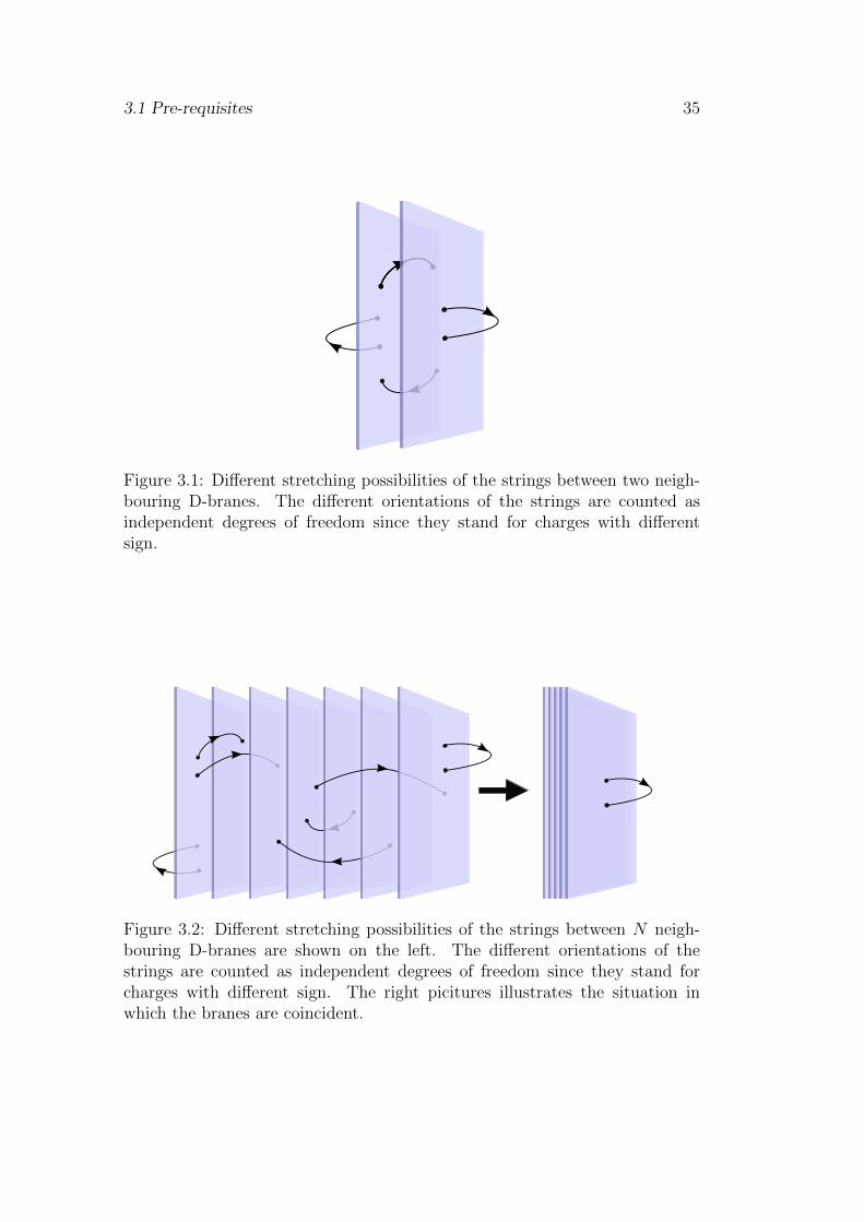
3.1 Pre-requisites 35

Figure 3.1: Different stretching possibilities of the strings between two neigh-bouring D-branes. The different orientations of the strings are counted asindependent degrees of freedom since they stand for charges with differentsign.

Figure 3.2: Different stretching possibilities of the strings between N neigh-bouring D-branes are shown on the left. The different orientations of thestrings are counted as independent degrees of freedom since they stand forcharges with different sign. The right picitures illustrates the situation inwhich the branes are coincident.

36 3. Gauge/gravity duality

3.2 A stack of D3-branes: different perspectivesAf all the possible D-branes presented in the previous section, the case of D3-branes present in Type IIB supergravity is of special interest for a numberof reasons. Firstly, their world-volume is a 4-dimensional Poincare invariantspace-time, which is much appreciated when trying to get closer to real-worldphysics. Furthermore it happens to be self-dual, for a D3-brane sources a4-form, which is self-dual in a 10-dimensional space-time

dG(5) = δ(6)Q = d ∗G(5). (3.2.1)

That is, a D3-brane carries both electric and magnetic charge. This self-dualitycondition is imposed separately when writing the equations of motion in theform

∗G(5) = G(5), (3.2.2)

for no action is known which is otherwise complete.

3.2.1 Gauge theory from the branes: open string perspective

In the light of the above considerations, a stack of D3-branes lying on topof each other will support a supermultiplet living on their world-volume con-sisting of a gauge field, six scalar fields and four Weyl fermions, all of themtransforming in the adjoint representation of an SU(N) gauge group. Thisis exactly the field content of N=4 super Yang-Mills theory (3.1.8) with anSU(N) gauge group. Indeed at the two-derivative level2, the low-energy effec-tive action for the massless supermultiplet living on the world-volume of theD3-branes is precisely the action ofN=4 super Yang-Mills in (3+1) space-timedimensions with a gauge group SU(N) [56]. The Yang-Mills coupling constantis then given by

g2YM = 4πgs, (3.2.3)

gs being the string coupling.Hence in the low energy limit, N coincident D3-branes reproduce the dynamicsof N=4 super Yang-Mills theory in 4 dimensions with an SU(N) gauge group.

3.2.2 Gravity theory from the branes: closed string perspec-tive

Branes are not only sources to the differential forms but also sources of cur-vature to space-time as dictated by Einstein’s general relativity, given that

2The Lagrangian receives higher-derivative corrections suppressed by α′E2 with α beingthe inverse string tension and E the energy. Such corrections can therefore be neglected inthe low-energy limit.

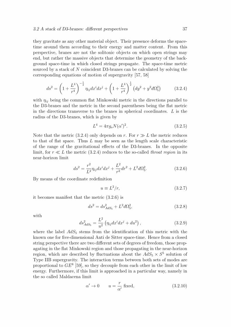
3.2 A stack of D3-branes: different perspectives 37

they gravitate as any other material object. Their presence deforms the space-time around them according to their energy and matter content. From thisperspective, branes are not the solitonic objects on which open strings mayend, but rather the massive objects that determine the geometry of the back-ground space-time in which closed strings propagate. The space-time metricsourced by a stack of N coincident D3-branes can be calculated by solving thecorresponding equations of motion of supergravity [57, 58]

ds2 =

(1 +

L4

r4

)− 12

ηijdxidxj +

(1 +

L4

r4

) 12 (dy2 + y2dΩ2

5

)(3.2.4)

with ηij being the common flat Minkowski metric in the directions parallel tothe D3-branes and the metric in the second parentheses being the flat metricin the directions transverse to the branes in spherical coordinates. L is theradius of the D3-branes, which is given by

L4 = 4πgsN(α′)2. (3.2.5)

Note that the metric (3.2.4) only depends on r. For r L the metric reducesto that of flat space. Thus L may be seen as the length scale characteristicof the range of the gravitational effects of the D3-branes. In the oppositelimit, for r L the metric (3.2.4) reduces to the so-called throat region in itsnear-horizon limit

ds2 =r2

L2ηijdx

idxj +L2

r2dr2 + L2dΩ2

5. (3.2.6)

By means of the coordinate redefinition

u ≡ L2/r, (3.2.7)

it becomes manifest that the metric (3.2.6) is

ds2 = ds2AdS5

+ L2dΩ25, (3.2.8)

with

ds2AdS5

=L2

u2

(ηijdx

idxj + du2), (3.2.9)

where the label AdS5 stems from the identification of this metric with theknown one for five-dimensional Anti de Sitter space-time. Hence from a closedstring perspective there are two different sets of degrees of freedom, those prop-agating in the flat Minkowski region and those propagating in the near-horizonregion, which are described by fluctuations about the AdS5 × S5 solution ofType IIB supergravity. The interaction terms between both sets of modes areproportional to GE8 [59], so they decouple from each other in the limit of lowenergy. Furthermore, if this limit is approached in a particular way, namely inthe so called Maldacena limit

α′ → 0 u =r

α′fixed, (3.2.10)

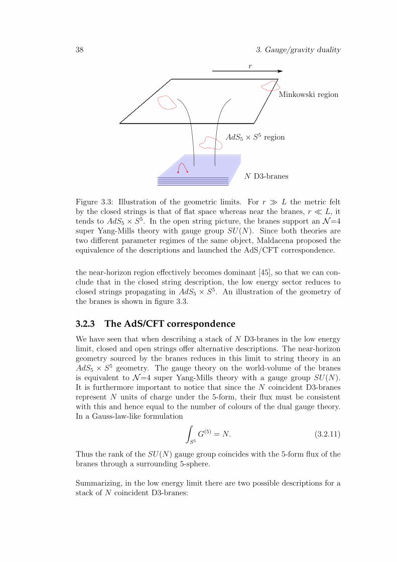
38 3. Gauge/gravity duality

N D3-branes

AdS5 × S5 region

Minkowski region

r

Figure 3.3: Illustration of the geometric limits. For r L the metric feltby the closed strings is that of flat space whereas near the branes, r L, ittends to AdS5 × S5. In the open string picture, the branes support an N=4super Yang-Mills theory with gauge group SU(N). Since both theories aretwo different parameter regimes of the same object, Maldacena proposed theequivalence of the descriptions and launched the AdS/CFT correspondence.

the near-horizon region effectively becomes dominant [45], so that we can con-clude that in the closed string description, the low energy sector reduces toclosed strings propagating in AdS5 × S5. An illustration of the geometry ofthe branes is shown in figure 3.3.

3.2.3 The AdS/CFT correspondence

We have seen that when describing a stack of N D3-branes in the low energylimit, closed and open strings offer alternative descriptions. The near-horizongeometry sourced by the branes reduces in this limit to string theory in anAdS5 × S5 geometry. The gauge theory on the world-volume of the branesis equivalent to N=4 super Yang-Mills theory with a gauge group SU(N).It is furthermore important to notice that since the N coincident D3-branesrepresent N units of charge under the 5-form, their flux must be consistentwith this and hence equal to the number of colours of the dual gauge theory.In a Gauss-law-like formulation ∫

S5

G(5) = N. (3.2.11)

Thus the rank of the SU(N) gauge group coincides with the 5-form flux of thebranes through a surrounding 5-sphere.

Summarizing, in the low energy limit there are two possible descriptions for astack of N coincident D3-branes:

3.2 A stack of D3-branes: different perspectives 39

• Type IIB superstring theory on AdS5 × S5with AdS and S5 having thesame radius L, the string coupling being gs and the self-dual 5-form G(5)

having integer flux N ;

• N=4 super Yang-Mills theory in 4-dimensions with gauge group SU(N)and Yang-Mills coupling gYM ;

with

g2YM = 4πgs, L4 = 4πgsN(α′)2. (3.2.12)

The fact that descriptions are equivalent in the low energy limit led JuanMartin Maldacena to conjecture that they are actually equivalent things evenbeyond this limit, giving birth to the AdS/CFT correspondence in its strongestformulation. Equivalence is understood here as a map between fields of thestring theory and operators of the gauge theory, which transform under thesame representations of the corresponding symmetries and as the equivalence ofthe respective dynamics. Yet the statement of the equality of both descriptionsin its broadest sense remains a conjecture inasmuch as no proof of it has beenprovided. Given that it involves the full quantum type IIB supersting theoryit is difficult to access and to test. Nevertheless, there are more restrictiveversions of the duality which, while being less general are easier to handlewith.

The t’Hooft limit

The t’Hooft limit [60] consists in taking the number of coulours N to be verylarge while keeping the so called t’Hooft coupling λ ≡ g2

YMN = gsN fixed,

N →∞, with λ ≡ g2YMN = gsN fixed. (3.2.13)

In this limit, all non-planar Feynman diagrams in the perturbative expansionof the gauge theory are suppressed [46], whereas in the string theory, sincegs = λ

N, the theory becomes weakly coupled string perturbation theory. Hence

in this limit the AdS/CFT duality reduces to a correspondence between theclassical tree-level string theory and the large N limit of the gauge theory, inwhich non-planar diagrams are suppressed.

The Maldacena limit

Additionally, the limit

λ 1 (3.2.14)

can be taken together with N →∞. The combination of both limits is knownas the Maldacena limit. λ can be interpreted as the dimensionless effectivecoupling of the super Yang-Mills gauge theory, hence in this limit the gaugetheory evolves to a strongly coupled one. In the gravity side of the duality,

40 3. Gauge/gravity duality

one sees through the relation resulting from combining equations (3.2.5) and(3.2.13) that

L4 = λ(α′)2 (3.2.15)

which means the the limit of big λ is tantamount to taking α′ → 0 and hencerecovering the supergravity regime of massless modes from which we got theinspiration of the duality. Thus in this limit the AdS/CFT duality is reflectedas a correspondence between classical supergravity and the large N and strongcoupling limit of the gauge theory.

Summing up, depending on the parameter regime, one or the other of thetwo possible perspectives of the stack of D3-branes becomes tractable. In par-ticular when gsN 1 the closed string description is not useful, whereas whengsN 1 it simplifies to classical supergravity, which is basically Einstein grav-ity coupled to various matter fields. The open string description is tractablewhen gsN 1 and expansions in series of Feynman diagrams are possiblewhereas it becomes effectively strongly coupled and hence difficult to handleat gsN 1. Nevertheless both descriptions exist in both limiting regimes andalso in between, the crucial question is when they become technically tractable.This thesis is based on the most restrictive version of the duality, that is inthe Maldacena limit, N → ∞, λ. We have seen that, as stated in [59], thestrong coupling limit in the gauge theory suppresses the stringy nature of thedual string theory taking it to the supergravity regime, whereas the large Nlimit suppresses the quantum nature of the string theory, restricting it to thetree-level. When both limits are taken together, the full string theory reducesto a tractable classical theory of supergravity. In that regime we are ableto perform computations that are dual to, and hence offer an interpretationwithin, a planar strongly coupled N=4 super Yang-Mills theory with gaugegroup SU(N →∞).Since both theories are seen as different descriptions of the same physics, itis conjectured that they are dynamically equivalent in the sense that all thephysics present in one of the descriptions, including fields and their interac-tions, must be mapped onto the physics in the other description.

3.2.4 Holography

The tractable version of string theory that enters the correspondence is com-pactified on an AdS5 × S5space-time. Since the S5 part of the metric is com-pact, any 10-dimensional field may be expressed as a tower of states by expand-ing it in terms of harmonics on the S5. So if for example, x and ω denote thecoordinates in AdS5 and S5 respectively, a scalar field X(x, ω) in AdS5×S5maybe written as

X(x, ω) =∑k

Xk(x)Yk(ω), (3.2.16)

3.2 A stack of D3-branes: different perspectives 41

where Yk(ω) are the spherical harmonics on the S5. This allows to practi-cally see the duality as a correspondence between the four-dimensional N=4super Yang-Mills theory and a gravity theory on AdS5, thereby providing arealisation of the holographic principle [61, 18], which states that a theory ofquantum gravity in a given space ought to be described by a theory withoutgravity living on the boundary of that space. In fact the gauge theory mightbe seen as living on the boundary of AdS space and the extra radial directionis interpreted as an RG flow, namely as an energy scale above which fields havebeen integrated out in the wilsonian sense [19]. Indeed if a scale transforma-tion xµ → Cxµ is carried out in the gauge theory and the energy E is rescaledby E → E/C the transformation is a symmetry of the system. In the metric(3.2.9) such a scale transformation is accompanied by u → u/C, which leadsto the identification

E ∼ 1/u ∼ r. (3.2.17)

So the radial coordinate of AdS is identified with the energy scale in the dualfield theory. Now as pointed out in [62], if the gauge theory with no degreesof freedom integrated out is seen as the most fundamental, it is natural forit to be situated at r = ∞ (u = 0), namely at the boundary of AdS. Thisis the basis of the holographic nature of the AdS/CFT correspondence. Thedual gauge field theory sits at the boundary of the AdS part of the space-timegeometry. It also makes sense to notice that since all energies scales are presentin a conformal field theory, it is no surprise that the geometry extend all theway from r = 0 to r →∞.This is also the reason why in the AdS/CFT jargon, the near boundary regionis referred to as UV, whereas close to the lowest value of the radial coordinate(highest in terms of u) people talk about the infra-red.

3.2.5 Matching of symmetries

If the two alternative approaches to the stack of N D3-branes presented aboveare really to be equivalent, the physics in both sides must be the same, whichnecessarily requires the global symmetries in both sides of the duality to bethe same.In section 3.1.1 we saw that the global symmetries of N=4 super Yang-Mills is given by the group SU(2, 2|4), whose maximal bosonic subgroup isSO(2, 4)×SO(6), that is the product of the conformal group in four dimensionsand the SU(4) = SO(6) group of R-symmetries that rotate the supersymme-tries into one another. This bosonic subgroup can immediately be identified onthe string theory side of the duality as the group of isometries of AdS5 × S5.Furthermore, since the presence of the branes breaks half of the number ofsupersymmetries, reducing them from the initial 32 to 16 and these are sup-plemented in the AdS limit by another 16 conformal supersymmetries, thetotal global symmetry is also seen to be SU(2, 2|4) on the string theory sideand hence perfectly matches on both sides of the duality.

42 3. Gauge/gravity duality

Given that gauge symmetries express a redundancy in the mathematical de-scription of the physics, there is no need for them to be the same on bothsides of the duality as is the case for global symmetries. Still they play animportant role in AdS/CFT as they do in general in gauge/gravity duality.There is a correspondence between global symmetries in the gauge theory andgauge symmetries in the dual string theory. We will see more about this later.

Once we have seen that the global symmetries in both sides of the dualityare the same, it is natural to expect that the objects transforming under thesame representations of the symmetry group are physically related by means ofthe correspondence. This is indeed the case. It can be shown that the spectrumof operators on the gauge theory side of the duality can be mapped to fields inthe massless Type IIB supergravity multiplet compactified on AdS5 × S5 [47].

3.3 The dictionary: practicalitiesBeyond the collection of intuitive evidences in favour of the duality we haveso far gone over, a systematic and consistent approach to the duality was pre-sented in [19] in which the foundations of the utilisation of the duality werelaid. There it was shown that there is indeed a one-to-one correspondencebetween operators of the boundary gauge theory and gravity fields that trans-form in the same representation of the symmetry groups as the former. Aprecise prescription was given relating the boundary values of the bulk fieldsto the field operators of the dual gauge theory. The bulk path integral for thefields φ with boundary values φ0

Zstring(φ) =

∫φ0

Dφe−Sstring , (3.3.1)

is identified with the generating functional for correlation functions of an op-erator O in the dual field theory⟨

e∫dx4 φ0O

⟩CFT

, (3.3.2)

by seeing the boundary value of the gravity theory field as a source for thegauge theory operator, which comes into the action via a term of the form∫

d4xφ0(x)O(x), (3.3.3)

withφ0(x) = φ(u, x)|u=0. (3.3.4)

where the coordinate u is the same as in (3.2.9). Hence the prescription tomake use of the duality given in [19] may be summarized as

Zstring [φ(x, u)|u=0 = φ0(x)] =⟨e∫dx4 φ0O

⟩CFT

. (3.3.5)

3.3 The dictionary: practicalities 43

Note though that no general explicit form of Zstring is known. Still, in the weakversion of the correspondence presented above, in which both the quantumnessand the stringiness of the strings are suppressed by the limits N → ∞ andλ 1, a saddle point approximation to the supergravity action is appropriateand the partition function may be approximated by

Zstring ≈ e−Ssugra∣∣on−shell , (3.3.6)

in which case, the on-shell bulk action of supergravity acts as the generatingfunctional for the correlation functions of the operators in the gauge theory.Via this prescription, arbitrary n-point functions of the gauge theory may becomputed, which in a conformal theory provide all physical information. Thisidentification of the partition function of both dual theories is a beautiful reali-sation of the physical principle that the information contained in both theoriesbe equivalent.

Even though no complete systematic recipe is known to find the field dualto a given operator, some of the entries of the dictionary are straightforwardfrom (3.3.3) and the fact that both the field and the operator must have thesame quantum numbers with respect to the global symmetries. In particular itis not difficult to find the dual fields to operators in the gauge theory which areconserved currents associated to global symmetries. So for example a gaugefield in the gravity theory Aµ(u, x) with a boundary value Aµ(x)

Aµ(x) = Aµ(u, x)|∂AdS = limu→0

Aµ(u, x) (3.3.7)

is naturally coupled to a conserved current Jµ(x) as∫d4xAµ(x)Jµ(x). (3.3.8)

This identification realises the fact mentioned above that continuous globalsymmetries in the boundary field theory correspond to gauge transformationsin the gravity theory.Analogously, the conserved charge associated to translational invariance, theenergy momentum tensor T µν(x) is associated to a source gµν(x), which is theasymptotic boundary form of the bulk metric gµν(u, x) at the boundary of AdS∫

dx4 gµν(x)T µν(x). (3.3.9)

This makes manifest that any dual of a translationally-invariant gauge theorymust involve dynamical gravity.

The previous discussion about the connection between fields of the gravitytheory and operators of the dual gauge theory was based on symmetry argu-ments. It can be made more explicit by looking at the boundary asymptotics

44 3. Gauge/gravity duality

of the gravity fields in a bit more detail. Let us assume that our fields arein the lowest excitation state with respect to the S5 harmonics, so that theycan de facto be treated as (4+1)-dimensional fields in AdS5. In the geome-try (3.2.9) a gauge field Aµ can be shown to obey the following asymptoticbehaviour close the boundary, u→ 0

Aµ(u→ 0, x) = sµ + u2vµ + . . . , (3.3.10)

and the relevant part of the typical action of the gravity theory will have theform

S ∼∫du

∫d4x√

det g FµνFµν . (3.3.11)

It is then possible to make explicit use of the AdS/CFT prescription (3.3.5),(3.3.6), ⟨

e∫dx4 φ0O

⟩CFT

= e−Ssugra∣∣u=0, on−shell , (3.3.12)

to compute the vacuum expectation value (vev henceforth) of the current Jµ

via

〈Jµ〉 =δSsugraδAµ

∣∣∣∣u=0 on−shell

. (3.3.13)

By assuming the relevant supergravity action to be of the form (3.3.11) andtaking into account the metric (3.2.9), this can be evaluated to

〈Jµ〉 = −∫∂AdS

∂L∂(∂uAt)

∣∣∣∣u=0

∼ Lvt, (3.3.14)

giving raise to a very concrete interpretation of the terms in the asymptoticexpansion (3.3.10): the leading term in the boundary expansion sµ is the fieldtheory source and the sub-leading term vµ is the vacuum expectation value ofthe field theory operator sourced by sµ.

The derivation we just showed has been done for the case of a gauge fieldAµ in AdS5 but it can be generalised to other kinds of fields in a dimension-independent way [19]. The conclusions drawn from the particular exampleshown apply in general in gauge/gravity.

3.4 Generalisations of AdS/CFT

3.4.1 Finite temperature and chemical potential

In previous sections we have considered the ground state of the D3-branes,which corresponds to zero temperature. There is a natural generalisation tothe non-zero temperature case by replacing the pure AdS metric (3.2.9) bythat of the so-called black D3-branes in AdS5 [63]

ds2 =r2

L2

(−f(r)dt2 + d~x2

)+

L2

r2f(r)dr2, (3.4.1)

3.4 Generalisations of AdS/CFT 45

or in our u coordinate (3.2.7)

ds2 =L2

u2

(−f(u)dt2 + d~x2

)+

L2

u2f(u)du2, (3.4.2)

where d~x = (dx1, dx2, dx3) and the blackening factor f(r) or f(u) is

f(r) = 1− r4h

r4, f(u) = 1− u4

u4h

. (3.4.3)

This metric has an event horizon at r = rh, u = uh. This horizon may berelated to the Hawking temperature of the black brane by the conventionalmethod [64], namely by imposing that the Wick rotated space-time τ = it beregular at the horizon. By regular it is meant that a conical singularity beavoided, which requires that the Euclidean time τ be periodic. As usually,the period is identified with the inverse temperature β = 1/T setting theBoltzmann constant to 1, kb = 1. If the near-horizon limit is taken in (3.4.2)by making use of the coordinate

ρ2 = u− uh, (3.4.4)

the metric becomes

ds2 =L2

u2

4

f ′(uh)

[ρ2

(f ′(uh)

2

)2

dτ 2 + dρ2 +f ′(uh)

4δijdx

idxj

]. (3.4.5)

Now defining

Φ =f ′(uh)

2, (3.4.6)

the metric in the (τ, ρ) plane turns into

ds2 = dρ2 + ρ2dΦ2, (3.4.7)

which for regularity requires the periodicity of Φ, Φ = Φ + 2π, otherwise thegeometry of space-time would not be regular everywhere. Given the definition(3.4.6), this is tantamount to having τ = τ + πuh. The period of the euclidiantime is the quantity that is identified in thermal field theory with the temper-ature. By analogy, if we assume a temperature of the boundary gauge theoryT , by virtue of the above the duality suggests the identification

β =1

T= πuh. (3.4.8)

The thermodynamic duals in gauge/gravity allow for the definition of fur-ther interesting quantities, such as the entropy, which is identified with theBekenstein-Hawking entropy of the associated black brane, or the free energy.Still, since these quantities are not relevant to our work we do not review themhere and refer the reader to [45] for more details about them.

46 3. Gauge/gravity duality

In addition to temperature, another thermodynamic quantity of interest whichcan be introduced within gauge/gravity duality is a finite density and the as-sociated chemical potential. Let us follow [45] in considering a quantum fieldtheory containing fermionic matter and a U(1) gauge field under which thefermion is charged

L = −1

4FµνF

µν + iψγµDµψ, (3.4.9)

with covariant derivative Dµ = ∂µ + iAµ and γµ being the Dirac matrices. Ifthe gauge field has a non-vanishing time component At = µ, this generates apotential term in the Lagrangian of the form

V = −µψ†ψ, (3.4.10)

with ψ = ψ†γ0. This term presents the common form of a density operatorwith chemical potential µ. Hence in the light of the considerations at theend of section 3.3, it is straightforward to propose that the inclusion of finitedensity and of a chemical potential be translated into the bulk gravity theoryby including a gauge field with a non-vanishing time component At whoseboundary asymptotic behaviour shall be of the form

At(u→ 0) ≈ µ− u2 ρ+ . . . , (3.4.11)

with µ being the chemical potential and ρ being proportional to the densityassociated to µ. So just as the way of introducing temperature in AdS/CFT isby moving from the pure AdS geometry (3.2.9) to a black brane AdS geometry(3.4.2), finite density and chemical potentials are introduced in the context ofgauge/gravity duality by turning on a gauge field in the bulk gravity theorywith a non-vanishing temporal component and the proper boundary asymp-totic behaviour (3.4.11).

Whenever both possibilities are exploited at a time to have chemical potentialand temperature, further regularity conditions imposed by the presence of ablack hole horizon must be observed. We will be more explicit about this insection 3.5.

Moreover, the presence of a gauge field that introduces a chemical potentialinto the game would in principle imply the presence of a radial electric fieldin the gravity theory, which in the case of non-zero temperature would alsoimply that the black branes are charged. The degree of complication involvedis actually rarely faced, for the familiar physical quantities presented, like thechemical potential, are most often referred to fundamental matter, that is tofields transforming under the fundamental representations of the gauge groupnot in the adjoint representation as is the case of all the fields in the super-gravity multiplet of the D3-branes. The question arises then of how to includefundamental matter in AdS/CFT and we devote the following section to it.

3.4 Generalisations of AdS/CFT 47

3.4.2 Fundamental matter

As mentioned before, all matter degrees of freedom supported by the stackof D3-branes on which we base our derivation of AdS/CFT transform in theadjoint representation of the gauge group as required by supersymmetry. How-ever, if any connections to the phenomenology of real-world physics are to bemade, we are to take contact to fundamental matter, that is to degrees of free-dom transforming under the fundamental representations of the gauge group.In the high energy physics jargon one talks about introducing flavour degreesof freedom in analogy to the case of real particles.There is a rather simple way to do this in AdS/CFT by introducing so-calledprobe branes in the background geometry sourced by the D3-branes. Theopen strings stretching between the D3-branes and the probe brane have onlyone end on the D3-branes and are hence seen as a point-like excitation byan observer living in the world-volume of the D3-branes. This is why suchexcitations transform in the fundamental representation of the SU(N) gaugegroup and generate matter in the fundamental representation. To signal howbranes are embedded in space-time, tables are used which display along whichof the space-time coordinates x0, . . . , x9 each brane is extended. For instance,it is usually assumed that the four first directions are the ones along which theD3-branes extend. This is signalled by

x0 x1 x2 x3 x4 x5 x6 x7 x8 x9

D3 × × × × - - - - - -(3.4.12)

If the probe brane can be separated from the stack of D3-branes in some direc-tions transverse to all branes, then the strings stretching between both typeof branes must have a minimum length and hence a non-zero energy, whichmeans that the corresponding matter particles are massive. Instead if theprobe brane intersects the D3-branes at some point, the minimum length ofthe strings stretching between it and the D3-branes is zero so that the corre-sponding matter particles are massless.Strings with both ends on the flavour brane transform in the adjoint repre-sentation of the flavour symmetry group and the dual particles are thereforeinterpreted as mesons. Strings with only one end on the probe-brane are in-terpreted as fundamental particles and hence seen as quarks.In principle the presence of the probe brane should modify the space-timesourced by the D3-branes. Still, as long as we assume that the number ofprobe branes Nf is much smaller than the number of D3-branes Nc, the back-reaction of the probe branes on the geometry generated by the D3-branes maybe neglected. This is called the probe approximation.A depiction of the position of the probe brane with respect to the stack ofD3-branes is shown in figure 3.4.

The low-energy dynamics of a probe Dp-brane in a background created byclosed string modes is given by the Dirac-Born-Infeld action, which is usually

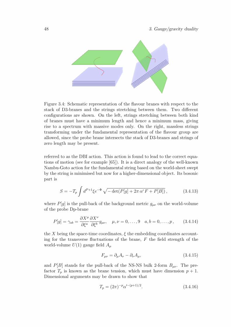
48 3. Gauge/gravity duality

Figure 3.4: Schematic representation of the flavour branes with respect to thestack of D3-branes and the strings stretching between them. Two differentconfigurations are shown. On the left, strings stretching between both kindof branes must have a minimum length and hence a minimum mass, givingrise to a spectrum with massive modes only. On the right, massless stringstransforming under the fundamental representation of the flavour group areallowed, since the probe brane intersects the stack of D3-branes and strings ofzero length may be present.

referred to as the DBI action. This action is found to lead to the correct equa-tions of motion (see for example [65]). It is a direct analogy of the well-knownNambu-Goto action for the fundamental string based on the world-sheet sweptby the string is minimised but now for a higher-dimensional object. Its bosonicpart is

S = −Tp∫dP+1ξe−Φ

√− det(P [g] + 2π α′ F + P [B]) , (3.4.13)

where P [g] is the pull-back of the background metric gµν on the world-volumeof the probe Dp-brane

P [g] = γab =∂Xµ

∂ξa∂Xν

∂ξbgµν , µ, ν = 0, . . . , 9 a, b = 0, . . . , p , (3.4.14)

the X being the space-time coordinates, ξ the embedding coordinates account-ing for the transverse fluctuations of the brane, F the field strength of theworld-volume U(1) gauge field Aµ

Fµν = ∂µAν − ∂νAµ, (3.4.15)

and P [B] stands for the pull-back of the NS-NS bulk 2-form Bµν . The pre-factor Tp is known as the brane tension, which must have dimension p + 1.Dimensional arguments may be drawn to show that

Tp = (2π)−pα′−(p+1)/2. (3.4.16)

3.4 Generalisations of AdS/CFT 49

See [66] for a detailed derivation. The dilaton field is given by

eΦ = gsH3−p4

p , (3.4.17)

with

Hp(r) = 1 +(r0

r

)7−p, (3.4.18)

stemming from the metric sourced by a black Dp-brane with horizon locatedat r = rp. For the case of interest p = 3, the dilaton takes a constant value,Φ = Φ0. If we now consider the action for the fundamental string in theabsence of a dilaton potential

S ∝∫

Σ

ΦRd2σ = Φ0

∫Σ

Rd2σ = Φ0(2− 2G) (3.4.19)

where Σ stands for the world-sheet swept by the fundamental string, parametrisedby the coordinates σ, R is the curvature of the world-sheet and in the thirdequality we have made use of the Gauss-Bonet theorem relating the geometryof surfaces to their topology. G is the genus of the corresponding Riemannsurface. In the light of this, it is clear by considering Feynmann path integrals

e−S ∼ e−Φ0(2−2G), (3.4.20)

that the dilaton is related to the perturbative expansion of the string, since fora 2-dimensional world-sheet, G gives the order of string perturbation theory

eΦ0 = gs. (3.4.21)

So if for simplicity we consider action (3.4.13) in flat space with B = 03 and aconstant dilaton and expand it using

det(1 +M) = 1− 1

2Tr (M2) + . . . , (3.4.22)

we obtain to leading order in α′

S = −(2πα′)2 Tp4gs

∫dp+1ξ Tr F 2, (3.4.23)

which is reminiscent of an abelian Yang-Mills action with coupling

gYM =gs

Tp(2πα′)2= (2π)p−2gsα

′ p−32 . (3.4.24)

To analyse the dynamics of a D3/Dp-brane system, we must pay attention tothe ’t Hooft couplings of the D3-branes

λ3 ≡ g2YM(3)N = 2πgsN, (3.4.25)

3We always assume B = 0 in this thesis if not otherwise specified.

50 3. Gauge/gravity duality

and to that of the probe flavour branes, which in light of (3.4.24) is given by

λp ≡ g2YM(p)Nf = (2π)p−2gsα

′ p−32 Nf . (3.4.26)

Hence the quotient signalling the relative importance of the dynamics of thestrings with both ends on the flavour brane is

λpλ3

=Nf

N(2π)p−2α′

p−32 . (3.4.27)

This means that in order for the string starting and ending on the p-brane,the so-called pp-strings, to decouple in the Maldacena limit α′ → 0 we mustconsider p > 3. Moreover, the requirement that the probe branes can separatefrom the stack of D3-branes excludes the case of the D9-brane. This leaves uswith D5-branes and D7-branes as proper candidates for a probe brane.There are some further requirements to be satisfied by the flavour probe branes[45]:

1. The brane intersection must be free from tachyonic modes and super-symmetric.

2. The flavour branes and the colour branes always share the time direction,x0.

3. The flavour branes extend at least in one of the directions perpendicu-lar to the D3-branes, x4, . . . , x9, since they should extend in the radialdirection for flavour degrees of freedom to be present at all energy scales.

The D7-brane was for a long time somewhat the canonical choice for a probebrane and has been studied in depth [67, 68, 69, 70]. Our work here though,will mainly deal with the probe D5-brane with finite temperature and chemicalpotential.

Probe D5-brane at finite temperature

From the above considerations, if the fundamental matter is to be present insome spatial directions, only one of the possible configurations of the D5-braneis to be taken into consideration, namely

x0 x1 x2 x3 x4 x5 x6 x7 x8 x9

D3 × × × × - - - - - -D5 × × × - × × × - - -

(3.4.28)

which is indeed the configuration we shall be working with. According to it,there is one direction in which the D3-branes extend but the D5-branes not,which implies that the fundamental matter fields are constrained to live in 2+1dimensions out of the 3+1 dimensions of the dual gauge theory fields to whichthey couple. This is why such a field theory is called a defect field theory. The

3.4 Generalisations of AdS/CFT 51

degrees of freedom in the fundamental representation only exist along a defect,that is a plane in the x0, x1, x2 directions.

In addition to the DBI-action (3.4.13), the presence of the C(4) of Type IIBsupergravity makes it in general necessary to include a Chern-Simons term inthe action accounting for its coupling to the U(1) gauge field on the probebrane. In the case of the D5-brane, this extends the action to

S = SDBI + SCS = SDBI +Tpgs

(2πα′)2

2

∫∂W

P [C(4)] ∧ F. (3.4.29)

A form of C(4) which is known to provide a solution to the equations of motionof supergravity is

C(4) =

(1

H3(r)− 1

)dξ0 ∧ · · · ∧ dξ3 + . . . (3.4.30)

with H3(r) given by (3.4.18). The dots in the previous equation stand forthe extra term that ensures that the self-duality condition (3.2.2) is fulfilled.In our configuration, the pull-back of the four-form vanishes.4 This allows usto neglect the Chern-Simons term of the action, thus the bosonic low-energydynamics of a probe D5-brane as in (3.4.28) is hence described by the action

S = −NfTD5

∫d6ξ√− det(P [g] + 2π α′ F ) , (3.4.31)

from which its dynamics can be derived.

For considering a probe D5-brane at finite temperature, we must embed itas described above in the background generated by the stack of black D3-branes (3.4.2). A more convenient description can be used by introducing thecoordinates [68]

z2 =2L4

u2 +√u4 − u4

0

, (3.4.32)

after which the metric takes the form

ds2 =L2

z2

(−f(z)2

h(z)dt2 + h(z) d~x2 + dz2

)+ L2 dΩ2

5 , (3.4.33)

where ~x = (x1, x2, x3), dΩ25 is the metric of a unit radius S5, and

f(z) = 1− z4

z40

, h(z) = 1 +z4

z40

. (3.4.34)

4The topological term might be activated by assuming a different form of C(4) as in [26].

52 3. Gauge/gravity duality

This geometry becomes asymptotic to AdS5 × S5 in the small z limit, withthe boundary of AdS5 being at z = 0, while it presents a horizon at z = z0.Accordingly, the Hawking temperature of the black hole reads

T =

√2

πz0 . (3.4.35)

It is useful to define the dimensionless coordinates

(z, xµ) =1

z0

(z, xµ) , (3.4.36)

in terms of which the metric takes the form (3.4.33) with z0 = 1. From nowon we always use these dimensionless coordinates and drop the tilde for pre-sentational purposes.

Furthermore the embedding is better described by writing the metric of theS5 in terms of two S2 as follows

dΩ25 = dθ2 + sin2 θ dΩ2

2 + cos2 θ dΩ22 . (3.4.37)

Thus (3.4.28) turns into

t x1 x2 x3 z Ω2 Ω2 θD3 × × × ×D5 × × × × ×

(3.4.38)

where the D5-brane shares two Minkowski directions with the D3-branes gen-erating the background, is extended along the radial direction z, and wraps anS2 (Ω2) inside the S5, while it is located at a fixed point of the remaining S2

(Ω2). The embedding is then described by the coordinate θ, which determinesthe radius of the S2 wrapped by the D5-brane. In order to simplify the analysiswe define

cos θ = χ , (3.4.39)

in terms of which we describe the embedding. Thus the form of χ as a functionof space-time coordinates determines the separation between the probe flavourbrane and the stack of D3-branes. This separation is naturally related to themass of the fundamental matter particles or quarks. If the probe brane is sep-arated from the D3-branes in some of the transverse directions to both branes,the minimum length of a string stretching between the branes has a non-zeroenergy and the dual quarks are massive. This is confirmed by the equations ofmotion derived from (3.4.31). From them, it is possible to show that the fieldcontaining the information about the embedding, χ, asymptotically behavesclose to the AdS boundary (z → 0) as

χ = mz + ψz2 +O(z3) (3.4.40)

3.4 Generalisations of AdS/CFT 53

m =2√

2

π√λ

Mq

T. (3.4.41)

with√λ = L2/(

√2α′). The dimensionless constant m is proportional to the

quantity that is dual to the quark mass [71, 72]. The precise relation is derivedin detail in [72, 73]Since this work considers models at finite chemical potential, we now want toadd the necessary ingredients to account for it.

Adding finite chemical potential

As elucidated above, in order to introduce a chemical potential holographically,we must turn on the temporal component of a gauge field as in (3.4.11). If wewant our chemical potential and the associated charge density to be referred tothe fundamental matter particles, this gauge field cannot be anything but theU(1) gauge field living on the world-volume of the probe brane. We assume itto be

A = At dt. (3.4.42)

Since it is mostly preferable to work with dimensionless quantities, we define

φ = 2πα′z0

L2At , (3.4.43)

from whose asymptotic boundary expansion

φ = µ− π√2T ρ z +O(z2) (3.4.44)

it is possible to obtain the dual chemical potential µ and the associated chargedensity ρ.Note that we are working in a black brane geometry (3.4.33) with an horizonat z = z0. The physics of black holes dictates some extra conditions that affectthe fields present in the geometry. As pointed out in [67], the event horizonat z = z0 is a Killing horizon, which means that it is a surface where theKilling vector field ∂t becomes null. For the gauge field A to be well definedas a one-form it is then necessary that its time component be zero there. Thiscan also be seen by considering the necessity that gµνAµAν = gtt(At)

2 not beinfinite, which can only be true if

At(z = z0) = φt(z = z0) = 0. (3.4.45)

Additionally, as can be seen from the asymptotic horizon expansion of theequations of motion derived from (3.4.31), the embedding field χ must fulfil inthis geometry

∂zχ(z = z0) = 0. (3.4.46)

The last two restrictions reduce the number of free parameters of the fields Aand χ in (3.4.40) and (3.4.44) from four down to two. This means that the

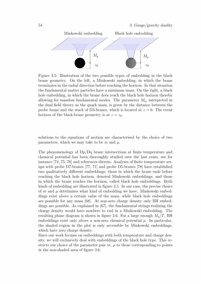
54 3. Gauge/gravity duality

Mq Mq

z0 z0

Minkowski embedding Black hole embedding

Figure 3.5: Illustration of the two possible types of embedding in the blackbrane geometry. On the left, a Minkowski embedding, in which the braneterminates in the radial direction before reaching the horizon. In that situationthe fundamental matter particles have a minimum mass. On the right, a blackhole embedding, in which the brane does reach the black hole horizon therebyallowing for massless fundamental modes. The parameter Mq, interpreted inthe dual field theory as the quark mass, is given by the distance between theprobe brane and the stack of D3-branes, which is located at z = 0. The eventhorizon of the black-brane geometry is at z = z0.

solutions to the equations of motion are characterised by the choice of twoparameters, which we may take to be m and µ.

The phenomenology of Dp/Dq brane intersections at finite temperature andchemical potential has been thoroughly studied over the last years, see forinstance [74, 75, 76] and references therein. Analyses of finite temperature set-ups with probe D7-branes [77, 71] and probe D5-branes [78] have establishedtwo qualitatively different embeddings: those in which the brane ends beforereaching the black hole horizon, denoted Minkowski embeddings, and thosein which the brane reaches the horizon, called black hole embeddings. Bothkinds of embedding are illustrated in figure 3.5. In our case, the precise choiceof m and µ determines what kind of embedding we have. Minkowski embed-dings exist above a certain value of the mass, while black hole embeddingsare possible for any mass [68]. At non-zero charge density only BH embed-dings are possible. As explained in [67], the fundamental strings realizing thecharge density would have nowhere to end in a Minkowski embedding. Theresulting phase diagram is shown in figure 3.6. For a large enough Mq/T , BHembeddings exist only above a non-zero chemical potential µ. In particular,the shaded region in the plot is only accessible by Minkowski embeddings,which have zero charge density.Since our work focuses on embeddings with both temperature and charge den-sity, we will exclusively deal with embeddings of the black hole type. This re-stricts our choice of the parameter pair m, µ to those corresponding to pointsin the non-shaded area of figure 3.6.

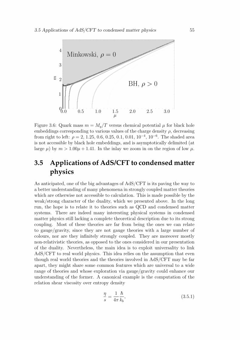
3.5 Applications of AdS/CFT to condensed matter physics 55

0.0 0.5 1.0 1.5 2.0 2.5 3.00

1

2

3

4m

µ

Minkowski, ρ = 0

BH, ρ > 0

Figure 3.6: Quark mass m = Mq/T versus chemical potential µ for black holeembeddings corresponding to various values of the charge density ρ, decreasingfrom right to left: ρ = 2, 1.25, 0.6, 0.25, 0.1, 0.01, 10−4, 10−6. The shaded areais not accessible by black hole embeddings, and is asymptotically delimited (atlarge µ) by m > 1.00µ+ 1.41. In the inlay we zoom in on the region of low µ.

3.5 Applications of AdS/CFT to condensed matterphysics

As anticipated, one of the big advantages of AdS/CFT is its paving the way toa better understanding of many phenomena in strongly coupled matter theorieswhich are otherwise not accessible to calculation. This is made possible by theweak/strong character of the duality, which we presented above. In the longrun, the hope is to relate it to theories such as QCD and condensed mattersystems. There are indeed many interesting physical systems in condensedmatter physics still lacking a complete theoretical description due to its strongcoupling. Most of these theories are far from being the ones we can relateto gauge/gravity, since they are not gauge theories with a large number ofcolours, nor are they infinitely strongly coupled. They are moreover mostlynon-relativistic theories, as opposed to the ones considered in our presentationof the duality. Nevertheless, the main idea is to exploit universality to linkAdS/CFT to real world physics. This idea relies on the assumption that eventhough real world theories and the theories involved in AdS/CFT may be farapart, they might share some common features which are universal to a widerange of theories and whose exploration via gauge/gravity could enhance ourunderstanding of the former. A canonical example is the computation of therelation shear viscosity over entropy density

η

s=

1

4π

~kb, (3.5.1)

56 3. Gauge/gravity duality

with η being the shear viscosity coefficient and s the entropy density. Thisresult was computed within gauge/gravity [21] and is common to all stronglycoupled theories with a gravity dual involving the Einstein-Hilbert action cou-pled to matter fields. Experimental measurements of this ratio in a stronglycoupled fluid resulting from heavy ion collisions known as the quark gluonplasma at the Relativistic Heavy Ion Collider (RHIC), at Brookhaven Na-tional Laboratory near New York and at the LHC in Geneva display goodagreement with this predicted value. This behaviour is remarkably differentto the one predicted for weakly coupled fluids and for common fluids such aswater or liquid helium. This celebrated result is considered to be one of thegreatest successes of gauge/gravity duality up to date, given that it is the firstexample of a theoretical prediction by gauge/gravity which has been confirmedexperimentally. It gives us hope that gauge/gravity may indeed be seen as atool that may provide us a better understanding of strongly coupled matter.

Along this lines it is interesting to exploit the duality to test models wichcan be linked to strongly coupled condensed matter systems. In order to doso though, we must know how to compute observables which have a concreteinterpretation within the dual gauge theory. One of the most common quan-tities computed in applications of AdS/CFT to condensed matter physics isthe optical conductivity, measuring the response of the charge current to anapplied electric field. Since conductivity computations constitute the core ofour work, we want to pay close attention to them.

3.5.1 Holographic optical conductivity

The optical conductivity, also denoted AC conductivity (σ) is understood hereas within the linear response formalism in the context of the well-known Ohm’slaw, which relates the spatial electric current in a medium ~J to the electricfield ~E

~J = σ ~E. (3.5.2)

As we saw in section 3.3, the introduction of a spatial current along one ofthe directions of the gauge theory, say Jx, requires the presence of a dual bulktheory gauge field that acts as a source, Ax. We introduce an electric field offrequency ω by considering

Ex = Ftx|z=0 = iωexeiωt, (3.5.3)

where ex is the modulus of the electric field. Assuming that the fields onlydepend on the radial coordinate z we find

Ex = Ftx|z=0 = (∂tAx − ∂xAt)|z=0 = ∂tAx|z=0 = iωexeiωt, (3.5.4)

Now if the boundary asymptotic behaviour of Ax is

Ax(z → 0) = A(0)x + zA(1)

x + . . . , (3.5.5)

3.5 Applications of AdS/CFT to condensed matter physics 57

we know

A(0)x = exe

iωt. (3.5.6)

and know from our previous discussion (3.3.14) that the sub-leading term A(1)x

corresponds to the vacuum expectation value of the current sourced by theleading term A

(0)x . So assuming that we are in a gauge where Az = 0, we can

apply Ohm’s law

σ(ω) =〈Jx〉Ex

= limz→0

FxzFtx

= −∂zAx∂tAx

= − A(1)x

iωexeiωt=

jxiωex

. (3.5.7)

In the last equality we have redefined A(1)x = −jxeiωt. Note that the third

expression in the equation involves only the field-strength tensor and thereforedefines the conductivity in a gauge invariant way. This is indeed the definitionwe shall be using later on

σ(ω) = limz→0

FxzFtx

. (3.5.8)

The last two equations show how to compute a holographic conductivity oncethe solution for the gauge field Ax is known. To obtain this solution the cor-responding equations of motion must be solved paying attention to the properboundary conditions. Again, in the presence of a black hole such boundaryconditions must guarantee the preservation of causality, which requires that noinformation escapes the event horizon. This is formally implemented by meansof the so-called in-falling wave boundary condition at the horizon. Considerthe metric (3.4.33)

ds2 =L2

z2

(−f(z)2

h(z)dt2 + h(z) d~x2 + dz2

)+ L2 dΩ2

5 , (3.5.9)

which has a coordinate singularity at z = z0 = 1 (see (3.4.36)). In order tostudy causality issues we must analyse light-like geodesics and for this purposeit is convenient to switch to the tortoise coordinate

z∗ = ±∫ z

1

√h(z)

f(z)2dz, (3.5.10)

which reminding ourselves of (3.4.34) is in the vicinity of the black hole horizon

z∗ = ± log(1− z)

2√

2± 1− z

2√

2+O(1− z)2. (3.5.11)

In these coordinates, light-like plane waves moving towards and from the hori-zon in the radial direction correspond to a behaviour of the form eiω(t±z∗).Since causality requires that nothing escapes the black hole, we discard the

58 3. Gauge/gravity duality

solutions with a negative sign. Going back to the original coordinates, we seethat our causal in-falling waves take the form

eiω(t+z∗) = eiωt(1− z)iα(a(0) + a(1)(1− z) +O(1− z)2

), (3.5.12)

withα =

ω

2√

2, (3.5.13)

anda(1)

a(0)=

iω

4√

2. (3.5.14)

Thus the last three equations correspond to the ansatz we must take for thehorizon boundary condition in order for causality to be preserved there. It hasalso been shown that this boundary condition corresponds to the selection inthe dual field theory of the retarded Green’s function, which is the one ensuringcausal propagation there [79].

3.5.2 Top down vs bottom up and what things really are

In this chapter we have seen how AdS/CFT is motivated by Type IIB su-pergravity. The field spectrum of the theory is made up of a bosonic sectorconsisting of two scalars (axion and dilaton), two 2-forms (one is obtained bysquaring the vectors and the other one by squaring the spinors), a self-dual4-form and the metric.

Type IIB SUGRAbosonic sector

[2, 0, 0, 0]8 2× [0, 1, 0, 0]8 2× [0, 0, 0, 0]8 [0, 0, 0, 2]8

gµν (35) A(2)µν , B

(2)µν (2× 28) φ,C (2× 1) C

(4)+µ (35)

graviton 2-forms dilaton, axion 4-form (self-dual)

fermionic sector

2× [0, 0, 1, 0]8 2× [1, 0, 0, 1]82× ψα (2× 8) 2× ψµα (2× 56)

2 gravifermions 2 gravitini

When using AdS/CFT to produce models for condensed matter systems thereare two main roads one can follow. One approach consists in departing fromthe 10-dimensional Type IIB theory, in general setting some of the fields ofthe theory to zero, and then trying to find the dual field theory Lagrangianthat enables a proper interpretation of physical quantities on both sides of theduality. This approach, which goes under the name of top-down has the ad-vantage of being somewhat authentic, in the sense that the resulting theoriesstem from the original Type IIB supergravity theory on which the formulation

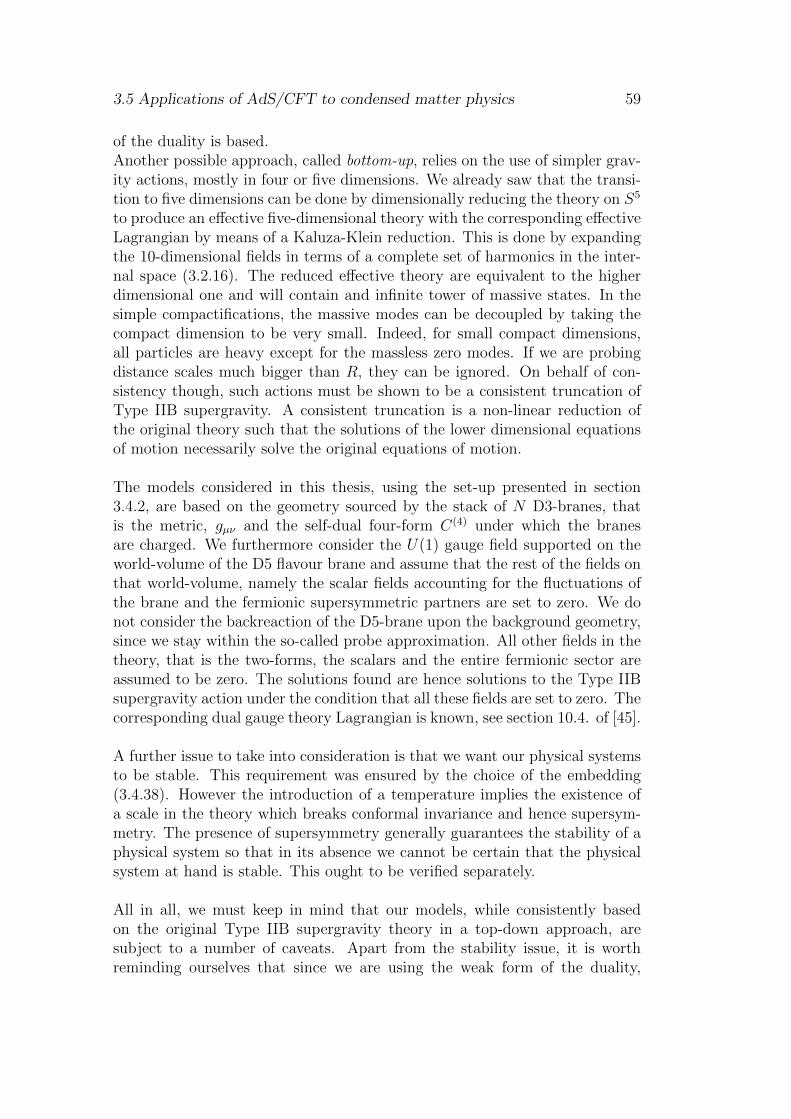
3.5 Applications of AdS/CFT to condensed matter physics 59

of the duality is based.Another possible approach, called bottom-up, relies on the use of simpler grav-ity actions, mostly in four or five dimensions. We already saw that the transi-tion to five dimensions can be done by dimensionally reducing the theory on S5

to produce an effective five-dimensional theory with the corresponding effectiveLagrangian by means of a Kaluza-Klein reduction. This is done by expandingthe 10-dimensional fields in terms of a complete set of harmonics in the inter-nal space (3.2.16). The reduced effective theory are equivalent to the higherdimensional one and will contain and infinite tower of massive states. In thesimple compactifications, the massive modes can be decoupled by taking thecompact dimension to be very small. Indeed, for small compact dimensions,all particles are heavy except for the massless zero modes. If we are probingdistance scales much bigger than R, they can be ignored. On behalf of con-sistency though, such actions must be shown to be a consistent truncation ofType IIB supergravity. A consistent truncation is a non-linear reduction ofthe original theory such that the solutions of the lower dimensional equationsof motion necessarily solve the original equations of motion.

The models considered in this thesis, using the set-up presented in section3.4.2, are based on the geometry sourced by the stack of N D3-branes, thatis the metric, gµν and the self-dual four-form C(4) under which the branesare charged. We furthermore consider the U(1) gauge field supported on theworld-volume of the D5 flavour brane and assume that the rest of the fields onthat world-volume, namely the scalar fields accounting for the fluctuations ofthe brane and the fermionic supersymmetric partners are set to zero. We donot consider the backreaction of the D5-brane upon the background geometry,since we stay within the so-called probe approximation. All other fields in thetheory, that is the two-forms, the scalars and the entire fermionic sector areassumed to be zero. The solutions found are hence solutions to the Type IIBsupergravity action under the condition that all these fields are set to zero. Thecorresponding dual gauge theory Lagrangian is known, see section 10.4. of [45].

A further issue to take into consideration is that we want our physical systemsto be stable. This requirement was ensured by the choice of the embedding(3.4.38). However the introduction of a temperature implies the existence ofa scale in the theory which breaks conformal invariance and hence supersym-metry. The presence of supersymmetry generally guarantees the stability of aphysical system so that in its absence we cannot be certain that the physicalsystem at hand is stable. This ought to be verified separately.

All in all, we must keep in mind that our models, while consistently basedon the original Type IIB supergravity theory in a top-down approach, aresubject to a number of caveats. Apart from the stability issue, it is worthreminding ourselves that since we are using the weak form of the duality,

60 3. Gauge/gravity duality

the dual gauge field theory has an infinite number of colours and is at verystrong coupling. Nevertheless, as already mentioned, it is interesting to studysuch systems in the hope that universal properties common to more realisticstrongly coupled systems be unveiled. In any case, the holographic models wedeal with might pave the way to a better understanding of the phenomenologyof strongly coupled systems.

Chapter 4Numerical computations using spectralmethods

Given that most of the results of this thesis have been obtained by means ofnumerical computations, we consider it appropriate to devote a chapter to thetechniques used to this purpose, the so-called spectral methods. This thesiswould not be complete without it. Yet presenting a complete review of thebroad field of pseudospectral methods as a tool for solving partial differentialequations is far beyond the scope of this thesis. The reader wanting to learnmore about them is referred to some of the very good existing references inthe literature [80, 81]. Instead, we would like to offer an introduction to thegeneral idea of pseudospectral methods with special emphasis on those aspectswhich are most relevant for holographic computations in general and in par-ticular for this work.The results obtained in this thesis have all been produced using Mathematica1

and explicit reference is given to the concrete Mathematica functions whereappropriate so as to facilitate the reproduction and extension of our results.Examples are provided which are directly related to our final codes, schematicversions of which are shown in appendix D. The reader may feel free to usethem, adapt them or reproduce them.

Before going to the matter though, let us point out that having to resortto complicated codes to solve equations is not something a physicist generallydoes for the fun of it but rather because of it being the only feasible way. Inmany AdS/CFT applications to condensed matter systems, specially in thoseaiming at reproducing realistic every day situations, one has to renounce tomore and more symmetries, like for example, translational symmetry, which isvery often not present in condensed matter systems. This is indeed the casein systems with disorder or impurities, to which this work is devoted. Theinvolved fields do not only depend on the radial AdS coordinate as usually but

1Wolfram Research, Inc., Mathematica, Version 9.0, Champaign, IL (2012).

61

62 4. Numerical computations using spectral methods

also on at least one spatial coordinate. This turns the equations of motionof the fields into partial differential equations (PDEs), whose analytical res-olution is only possible in a very reduced number of highly symmetric cases.Beyond those cases, such PDEs cannot be solved analytically and numericsposes the only realistic way of attacking the problem.

4.1 Discretisation and differentiation matricesComputers cannot cope with an infinite amount of data. This excludes thepossibility of using them to perform numerical computations in a continuum.Whenever a computer comes into play, things have to be discretised. Space-time is no exception to this statement. The discretisation of space-time impliesthat only a finite amount of space-time points is used in the calculations,thereby reducing space-time to a grid of points at which functions of space-time take a numerical value. The more points one uses for such computations,the more trustworthy the discrete approximation of continuum space-time is.But only at the cost of computational resources, for more points also meanmore required computing power and longer computation times. Hence the artconsists in finding an equilibrium between affordable computation conditionsand precision.Once space-time has turned into a collection of discrete points at which theknown functions are evaluated, the question arises of how this data can beused to estimate derivatives. The method most probably striking the mindof the reader is that of finite differences. Let us assume that a 1-dimensionalspace described by the spatial coordinate x is discretised in a uniform grid of3 points x0, x1, x2 with an interval xi+1− xi = h for each i. A function of x,say f(x) will correspondingly take numerical values at each of the grid pointsf0, f1, f2. The question is how to estimate the value of f ′(x) at the gridpoints.The simplest possible method is the second-order difference approximation,which assumes

f ′i =fi+1 − fi−1

2h. (4.1.1)

Following this rule and assuming on behalf of simplicity periodic boundaryconditions, in our simple case with only three grid points, the vector containingthe values of the derivative of a function f with respect to x at each of the gridpoints is obtained from the vector containing the value of the function itselfat those points via a matrixf ′0f ′1

f ′2

=1

h

0 12−1

2

−12

0 12

12−1

20

f0

f1

f2

. (4.1.2)

Such a matrix is called a differentiation matrix. This has been a very basicexample, in which the order of convergence would be just O(h2), but the mainidea is that of defining differentiation matrices to implement differentiation in

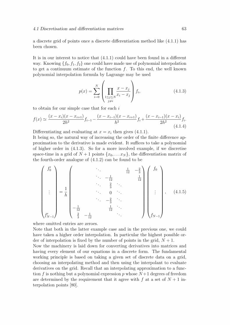
4.1 Discretisation and differentiation matrices 63

a discrete grid of points once a discrete differentiation method like (4.1.1) hasbeen chosen.

It is in our interest to notice that (4.1.1) could have been found in a differentway. Knowing f0, f1, f2 one could have made use of polynomial interpolationto get a continuum estimate of the function f . To this end, the well knownpolynomial interpolation formula by Lagrange may be used

p(x) =N∑i=0

∏1≤j≤Nj 6=i

x− xjxi − xj

fi, (4.1.3)

to obtain for our simple case that for each i

f(x) ' (x− xi)(x− xi+1)

2h2fi−1−

(x− xi−1)(x− xi+1)

h2fi+

(x− xi−1)(x− xi)2h2

fi.

(4.1.4)Differentiating and evaluating at x = xi then gives (4.1.1).It being so, the natural way of increasing the order of the finite difference ap-proximation to the derivative is made evident. It suffices to take a polynomialof higher order in (4.1.3). So for a more involved example, if we discretisespace-time in a grid of N + 1 points x0, . . . xN, the differentiation matrix ofthe fourth-order analogue of (4.1.2) can be found to be

f ′0

...

f ′N−1

=

1

h

. . . 112−2

3. . . − 1

12112

. . . 23

. . .. . . 0

. . .. . . −2

3

. . .

− 112

112

. . .

23− 1

12

. . .

f0

...

fN−1

, (4.1.5)

where omitted entries are zeroes.Note that both in the latter example case and in the previous one, we couldhave taken a higher order interpolation. In particular the highest possible or-der of interpolation is fixed by the number of points in the grid, N + 1.Now the machinery is laid down for converting derivatives into matrices andhaving every element of our equations in a discrete form. The fundamentalworking principle is based on taking a given set of discrete data on a grid,choosing an interpolating method and then using the interpolant to evaluatederivatives on the grid. Recall that an interpolating approximation to a func-tion f is nothing but a polynomial expression p whose N+1 degrees of freedomare determined by the requirement that it agree with f at a set of N + 1 in-terpolation points [80].

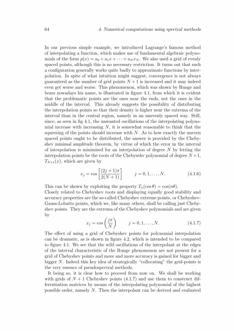
64 4. Numerical computations using spectral methods

In our previous simple example, we introduced Lagrange’s famous methodof interpolating a function, which makes use of fundamental algebraic polyno-mials of the form p(x) = a0 + a1x+ · · ·+ aNxN . We also used a grid of evenlyspaced points, although this is no necessary restriction. It turns out that sucha configuration generally works quite badly to approximate functions by inter-polation. In spite of what intuition might suggest, convergence is not alwaysguaranteed as the number of grid points N + 1 is increased and it may indeedeven get worse and worse. This phenomenon, which was shown by Runge andbears nowadays his name, is illustrated in figure 4.1, from which it is evidentthat the problematic points are the ones near the ends, not the ones in themiddle of the interval. This already suggests the possibility of distributingthe interpolation points so that their density is higher near the extrema of theinterval than in the central region, namely in an unevenly spaced way. Still,since, as seen in fig 4.1, the unwanted oscillations of the interpolating polyno-mial increase with increasing N , it is somewhat reasonable to think that thesqueezing of the points should increase with N . As to how exactly the unevenspaced points ought to be distributed, the answer is provided by the Cheby-shev minimal amplitude theorem, by virtue of which the error in the intervalof interpolation is minimised for an interpolation of degree N by letting theinterpolation points be the roots of the Chebysehv polynomial of degree N+1,TN+1(x), which are given by

xj = cos

[(2j + 1)π

2(N + 1)

]j = 0, 1, . . . , N. (4.1.6)

This can be shown by exploiting the property Tn(cos θ) = cos(nθ).Closely related to Chebyshev roots and displaying equally good stability andaccuracy properties are the so-called Chebyshev extreme points, or Chebyshev-Gauss-Lobatto points, which we, like many others, shall be calling just Cheby-shev points. They are the extrema of the Chebyshev polynomials and are givenby

xj = cos

(jπ

N

)j = 0, 1, . . . , N. (4.1.7)

The effect of using a grid of Chebyshev points for polynomial interpolationcan be dramatic, as is shown in figure 4.2, which is intended to be comparedto figure 4.1. We see that the wild oscillations of the interpolant at the edgesof the interval characteristic of the Runge phenomenon are not present for agrid of Chebyshev points and more and more accuracy is gained for bigger andbigger N . Indeed this key idea of strategically “collocating” the grid-points isthe very essence of pseudospectral methods.

It being so, it is clear how to proceed from now on. We shall be workingwith grids of N + 1 Chebyshev points (4.1.7) and use them to construct dif-ferentiation matrices by means of the interpolating polynomial of the highestpossible order, namely N . Then the interpolant can be derived and evaluated

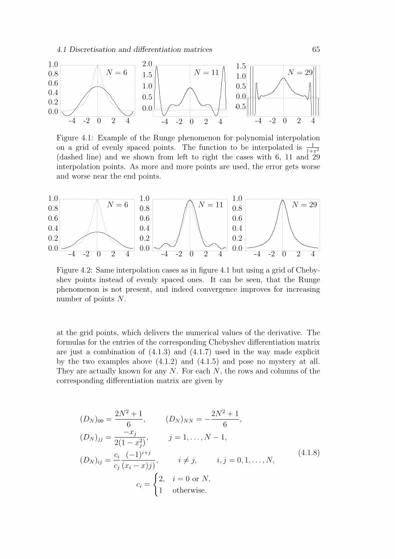
4.1 Discretisation and differentiation matrices 65

-4 -2 0 2 4

-0.5

0.0

0.5

1.0

1.5

-4 -2 0 2 4

0.0

0.5

1.0

1.5

2.0N = 6 N = 11 N = 29

-4 -2 0 2 40.00.20.40.60.81.0

Figure 4.1: Example of the Runge phenomenon for polynomial interpolationon a grid of evenly spaced points. The function to be interpolated is 1

1+x2

(dashed line) and we shown from left to right the cases with 6, 11 and 29interpolation points. As more and more points are used, the error gets worseand worse near the end points.

N = 6 N = 11 N = 29

-4 -2 0 2 40.0

0.2

0.4

0.6

0.8

1.0

-4 -2 0 2 40.0

0.2

0.4

0.6

0.8

1.0

-4 -2 0 2 40.0

0.2

0.4

0.6

0.8

1.0

Figure 4.2: Same interpolation cases as in figure 4.1 but using a grid of Cheby-shev points instead of evenly spaced ones. It can be seen, that the Rungephenomenon is not present, and indeed convergence improves for increasingnumber of points N .

at the grid points, which delivers the numerical values of the derivative. Theformulas for the entries of the corresponding Chebyshev differentiation matrixare just a combination of (4.1.3) and (4.1.7) used in the way made explicitby the two examples above (4.1.2) and (4.1.5) and pose no mystery at all.They are actually known for any N . For each N , the rows and columns of thecorresponding differentiation matrix are given by

(DN)00 =2N2 + 1

6, (DN)NN = −2N2 + 1

6,

(DN)jj =−xj

2(1− x2j), j = 1, . . . , N − 1,

(DN)ij =cicj

(−1)i+j

(xi − x)j), i 6= j, i, j = 0, 1, . . . , N,

ci =

2, i = 0 or N,

1 otherwise.

(4.1.8)

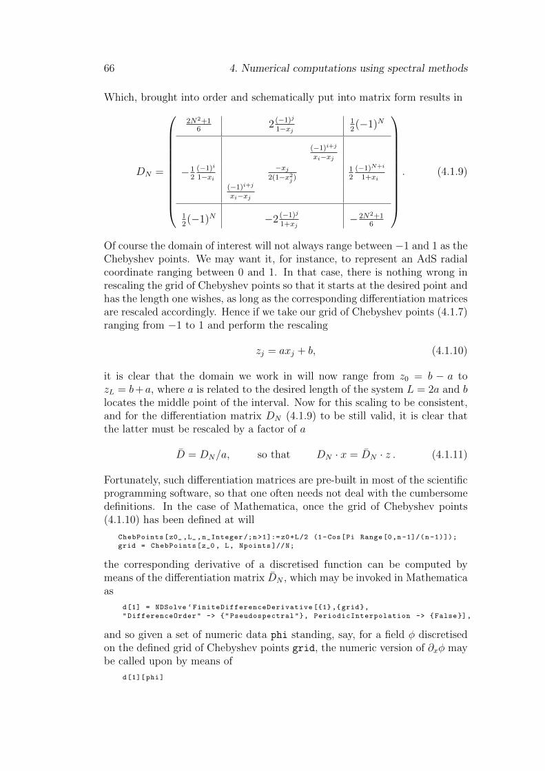
66 4. Numerical computations using spectral methods

Which, brought into order and schematically put into matrix form results in

DN =

2N2+16

2 (−1)j

1−xj12(−1)N

(−1)i+j

xi−xj

−12

(−1)i

1−xi−xj

2(1−x2j )12

(−1)N+i

1+xi(−1)i+j

xi−xj

12(−1)N −2 (−1)j

1+xj−2N2+1

6

. (4.1.9)

Of course the domain of interest will not always range between −1 and 1 as theChebyshev points. We may want it, for instance, to represent an AdS radialcoordinate ranging between 0 and 1. In that case, there is nothing wrong inrescaling the grid of Chebyshev points so that it starts at the desired point andhas the length one wishes, as long as the corresponding differentiation matricesare rescaled accordingly. Hence if we take our grid of Chebyshev points (4.1.7)ranging from −1 to 1 and perform the rescaling

zj = axj + b, (4.1.10)

it is clear that the domain we work in will now range from z0 = b − a tozL = b+a, where a is related to the desired length of the system L = 2a and blocates the middle point of the interval. Now for this scaling to be consistent,and for the differentiation matrix DN (4.1.9) to be still valid, it is clear thatthe latter must be rescaled by a factor of a

D = DN/a, so that DN · x = DN · z . (4.1.11)

Fortunately, such differentiation matrices are pre-built in most of the scientificprogramming software, so that one often needs not deal with the cumbersomedefinitions. In the case of Mathematica, once the grid of Chebyshev points(4.1.10) has been defined at will

ChebPoints[z0_ ,L_,n_Integer /;n>1]:= z0+L/2 (1-Cos[Pi Range[0,n -1]/(n -1)]);

grid = ChebPoints[z_0 , L, Npoints ]//N;

the corresponding derivative of a discretised function can be computed bymeans of the differentiation matrix DN , which may be invoked in Mathematicaas

d[1] = NDSolve ‘FiniteDifferenceDerivative [1, grid,

"DifferenceOrder" -> "Pseudospectral", PeriodicInterpolation -> False],

and so given a set of numeric data phi standing, say, for a field φ discretisedon the defined grid of Chebyshev points grid, the numeric version of ∂xφ maybe called upon by means of

d[1][ phi]

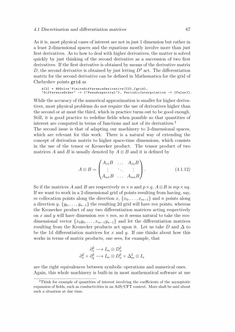
4.1 Discretisation and differentiation matrices 67

As it is, most physical cases of interest are not in just 1 dimension but rather ina least 2-dimensional spaces and the equations mostly involve more than justfirst derivatives. As to how to deal with higher derivatives, the matter is solvedquickly by just thinking of the second derivative as a succession of two firstderivatives. If the first derivative is obtained by means of the derivative matrixD, the second derivative is obtained by just letting D2 act. The differentiationmatrix for the second derivative can be defined in Mathematica for the grid ofChebyshev points grid as

d[2] = NDSolve ‘FiniteDifferenceDerivative [2, grid,

"DifferenceOrder" -> "Pseudospectral", PeriodicInterpolation -> False ].

While the accuracy of the numerical approximation is smaller for higher deriva-tives, most physical problems do not require the use of derivatives higher thanthe second or at most the third, which in practice turns out to be good enough.Still, it is good practice to redefine fields when possible so that quantities ofinterest are computed in terms of functions and not of its derivatives.2

The second issue is that of adapting our machinery to 2-dimensional spaces,which are relevant for this work. There is a natural way of extending theconcept of derivation matrix to higher space-time dimensions, which consistsin the use of the tensor or Kronecker product. The tensor product of twomatrices A and B is usually denoted by A⊗B and it is defined by

A⊗B =

A11B . . . A1nB...

. . ....

Am1B . . . AmnB

. (4.1.12)

So if the matrices A and B are respectively m×n and p×q, A⊗B is mp×nq.If we want to work in a 2-dimensional grid of points resulting from having, say,m collocation points along the direction x, x0, . . . , xm−1 and n points alonga direction y, y0, . . . , yn−1 the resulting 2d grid will have mn points, whereasthe Kronecker product of any two differentiation matrices acting respectivelyon x and y will have dimension mn×mn, so it seems natural to take the mn-dimensional vector x0y0, . . . , xm−1yn−1 and let the differentiation matricesresulting from the Kronecker products act upon it. Let us take D and ∆ tobe the 1d differentiation matrices for x and y. If one thinks about how thisworks in terms of matrix products, one sees, for example, that

∂2x −→ Im ⊗D2

n

∂2x + ∂2

y −→ Im ⊗D2n + ∆2

m ⊗ In

are the right equivalences between symbolic operations and numerical ones.Again, this whole machinery is built-in in most mathematical software at use

2Think for example of quantities of interest involving the coefficients of the asymptoticexpansion of fields, such as conductivities in an AdS/CFT context. More shall be said aboutsuch a situation at due time.

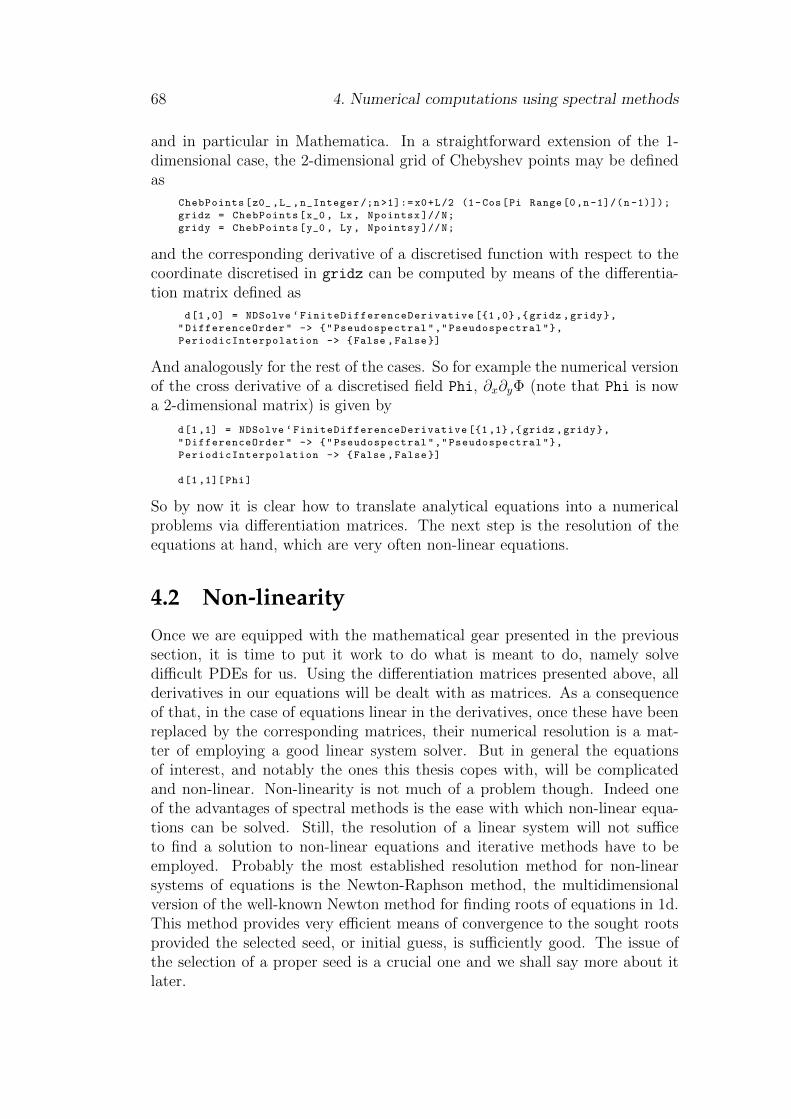
68 4. Numerical computations using spectral methods

and in particular in Mathematica. In a straightforward extension of the 1-dimensional case, the 2-dimensional grid of Chebyshev points may be definedas

ChebPoints[z0_ ,L_,n_Integer /;n>1]:= x0+L/2 (1-Cos[Pi Range[0,n -1]/(n -1)]);

gridz = ChebPoints[x_0 , Lx, Npointsx ]//N;

gridy = ChebPoints[y_0 , Ly, Npointsy ]//N;

and the corresponding derivative of a discretised function with respect to thecoordinate discretised in gridz can be computed by means of the differentia-tion matrix defined as

d[1,0] = NDSolve ‘FiniteDifferenceDerivative [1,0,gridz ,gridy,

"DifferenceOrder" -> "Pseudospectral","Pseudospectral",

PeriodicInterpolation -> False ,False]

And analogously for the rest of the cases. So for example the numerical versionof the cross derivative of a discretised field Phi, ∂x∂yΦ (note that Phi is nowa 2-dimensional matrix) is given by

d[1,1] = NDSolve ‘FiniteDifferenceDerivative [1,1,gridz ,gridy,

"DifferenceOrder" -> "Pseudospectral","Pseudospectral",

PeriodicInterpolation -> False ,False]

d[1 ,1][Phi]

So by now it is clear how to translate analytical equations into a numericalproblems via differentiation matrices. The next step is the resolution of theequations at hand, which are very often non-linear equations.

4.2 Non-linearity

Once we are equipped with the mathematical gear presented in the previoussection, it is time to put it work to do what is meant to do, namely solvedifficult PDEs for us. Using the differentiation matrices presented above, allderivatives in our equations will be dealt with as matrices. As a consequenceof that, in the case of equations linear in the derivatives, once these have beenreplaced by the corresponding matrices, their numerical resolution is a mat-ter of employing a good linear system solver. But in general the equationsof interest, and notably the ones this thesis copes with, will be complicatedand non-linear. Non-linearity is not much of a problem though. Indeed oneof the advantages of spectral methods is the ease with which non-linear equa-tions can be solved. Still, the resolution of a linear system will not sufficeto find a solution to non-linear equations and iterative methods have to beemployed. Probably the most established resolution method for non-linearsystems of equations is the Newton-Raphson method, the multidimensionalversion of the well-known Newton method for finding roots of equations in 1d.This method provides very efficient means of convergence to the sought rootsprovided the selected seed, or initial guess, is sufficiently good. The issue ofthe selection of a proper seed is a crucial one and we shall say more about itlater.

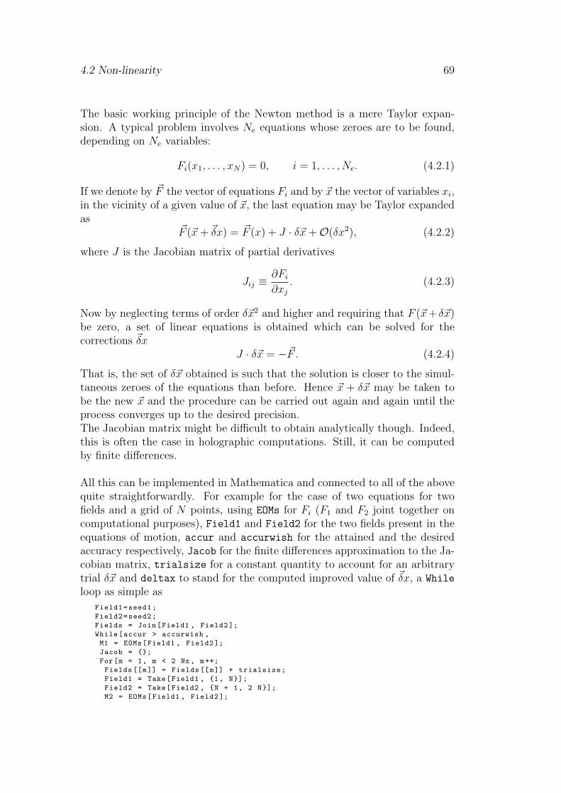
4.2 Non-linearity 69

The basic working principle of the Newton method is a mere Taylor expan-sion. A typical problem involves Ne equations whose zeroes are to be found,depending on Ne variables:

Fi(x1, . . . , xN) = 0, i = 1, . . . , Ne. (4.2.1)

If we denote by ~F the vector of equations Fi and by ~x the vector of variables xi,in the vicinity of a given value of ~x, the last equation may be Taylor expandedas

~F (~x+ ~δx) = ~F (x) + J · δ~x+O(δx2), (4.2.2)

where J is the Jacobian matrix of partial derivatives

Jij ≡∂Fi∂xj

. (4.2.3)

Now by neglecting terms of order δ~x2 and higher and requiring that F (~x+ δ~x)be zero, a set of linear equations is obtained which can be solved for thecorrections ~δx

J · δ~x = −~F . (4.2.4)

That is, the set of δ~x obtained is such that the solution is closer to the simul-taneous zeroes of the equations than before. Hence ~x + δ~x may be taken tobe the new ~x and the procedure can be carried out again and again until theprocess converges up to the desired precision.The Jacobian matrix might be difficult to obtain analytically though. Indeed,this is often the case in holographic computations. Still, it can be computedby finite differences.

All this can be implemented in Mathematica and connected to all of the abovequite straightforwardly. For example for the case of two equations for twofields and a grid of N points, using EOMs for Fi (F1 and F2 joint together oncomputational purposes), Field1 and Field2 for the two fields present in theequations of motion, accur and accurwish for the attained and the desiredaccuracy respectively, Jacob for the finite differences approximation to the Ja-cobian matrix, trialsize for a constant quantity to account for an arbitrarytrial δ~x and deltax to stand for the computed improved value of ~δx, a While

loop as simple as

Field1=seed1;

Field2=seed2;

Fields = Join[Field1 , Field2 ];

While[accur > accurwish ,

M1 = EOMs[Field1 , Field2 ];

Jacob = ;

For[m = 1, m < 2 Nx, m++;

Fields [[m]] = Fields [[m]] + trialsize;

Field1 = Take[Field1 , 1, N];

Field2 = Take[Field2 , N + 1, 2 N];

M2 = EOMs[Field1 , Field2 ];

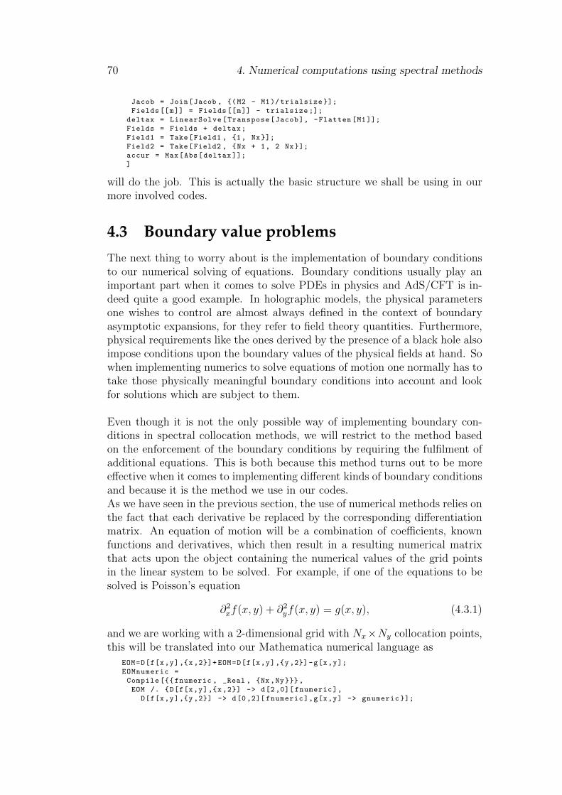
70 4. Numerical computations using spectral methods

Jacob = Join[Jacob , (M2 - M1)/ trialsize ];

Fields [[m]] = Fields [[m]] - trialsize ;];

deltax = LinearSolve[Transpose[Jacob], -Flatten[M1]];

Fields = Fields + deltax;

Field1 = Take[Field1 , 1, Nx];

Field2 = Take[Field2 , Nx + 1, 2 Nx];

accur = Max[Abs[deltax ]];

]

will do the job. This is actually the basic structure we shall be using in ourmore involved codes.

4.3 Boundary value problemsThe next thing to worry about is the implementation of boundary conditionsto our numerical solving of equations. Boundary conditions usually play animportant part when it comes to solve PDEs in physics and AdS/CFT is in-deed quite a good example. In holographic models, the physical parametersone wishes to control are almost always defined in the context of boundaryasymptotic expansions, for they refer to field theory quantities. Furthermore,physical requirements like the ones derived by the presence of a black hole alsoimpose conditions upon the boundary values of the physical fields at hand. Sowhen implementing numerics to solve equations of motion one normally has totake those physically meaningful boundary conditions into account and lookfor solutions which are subject to them.

Even though it is not the only possible way of implementing boundary con-ditions in spectral collocation methods, we will restrict to the method basedon the enforcement of the boundary conditions by requiring the fulfilment ofadditional equations. This is both because this method turns out to be moreeffective when it comes to implementing different kinds of boundary conditionsand because it is the method we use in our codes.As we have seen in the previous section, the use of numerical methods relies onthe fact that each derivative be replaced by the corresponding differentiationmatrix. An equation of motion will be a combination of coefficients, knownfunctions and derivatives, which then result in a resulting numerical matrixthat acts upon the object containing the numerical values of the grid pointsin the linear system to be solved. For example, if one of the equations to besolved is Poisson’s equation

∂2xf(x, y) + ∂2

yf(x, y) = g(x, y), (4.3.1)

and we are working with a 2-dimensional grid with Nx×Ny collocation points,this will be translated into our Mathematica numerical language as

EOM=D[f[x,y],x,2]+ EOM=D[f[x,y],y,2]-g[x,y];

EOMnumeric =

Compile [ fnumeric , _Real , Nx,Ny,

EOM /. D[f[x,y],x,2] -> d[2,0][ fnumeric],

D[f[x,y],y,2] -> d[0 ,2][ fnumeric],g[x,y] -> gnumeric ];

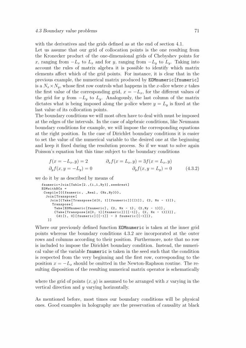
4.3 Boundary value problems 71

with the derivatives and the grids defined as at the end of section 4.1.Let us assume that our grid of collocation points is the one resulting fromthe Kronecker product of the one-dimensional grids of Chebyshev points forx, ranging from −Lx to Lx and for y, ranging from −Ly to Ly. Taking intoaccount the rules of matrix algebra it is possible to identify which matrixelements affect which of the grid points. For instance, it is clear that in theprevious example, the numerical matrix produced by EOMnumeric[fnumeric]

is a Nx×Ny, whose first row controls what happens in the x-slice where x takesthe first value of the corresponding grid, x = −Lx, for the different values ofthe grid for y from −Ly to Ly. Analogously, the last column of the matrixdictates what is being imposed along the y-slice where y = Ly is fixed at thelast value of its collocation points.The boundary conditions we will most often have to deal with must be imposedat the edges of the intervals. In the case of algebraic conditions, like Neumannboundary conditions for example, we will impose the corresponding equationsat the right position. In the case of Dirichlet boundary conditions it is easierto set the value of the numerical variable to the desired one at the beginningand keep it fixed during the resolution process. So if we want to solve againPoisson’s equation but this time subject to the boundary conditions

f(x = −Lx, y) = 2 ∂xf(x = Lx, y) = 3f(x = Lx, y)

∂yf(x, y = −Ly) = 0 ∂yf(x, y = Ly) = 0 (4.3.2)

we do it by as described by means offnumeric=Join[Table [2.,i,1,Ny],seedrest]

EOMwithBCs =

Compile [ fnumeric , _Real , Nx,Ny,

Join[Transpose[

Join[Take[Transpose[d[0, 1][ fnumeric ]][[1]] , 2, Nx - 1],

Transpose[

Take[EOMnumeric[fnumeric], 2, Nx - 1, 2,Ny - 1]],

Take[Transpose[d[0, 1][ fnumeric ]][[-1]], 2, Nx - 1]]] ,

d1[1, 0][ fnumeric ][[ -1]] - 3 fnumeric [[-1]],

]]

Where our previously defined function EOMnumeric is taken at the inner gridpoints whereas the boundary conditions 4.3.2 are incorporated at the outerrows and columns according to their position. Furthermore, note that no rowis included to impose the Dirichlet boundary condition. Instead, the numeri-cal value of the variable fnumeric is taken in the seed such that the conditionis respected from the very beginning and the first row, corresponding to theposition x = −Lx should be omitted in the Newton-Raphson routine. The re-sulting disposition of the resulting numerical matrix operator is schematically

where the grid of points (x, y) is assumed to be arranged with x varying in thevertical direction and y varying horizontally.

As mentioned before, most times our boundary conditions will be physicalones. Good examples in holography are the preservation of causality at black

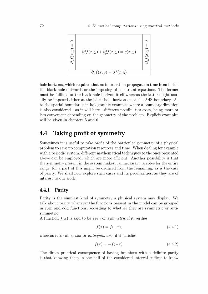
72 4. Numerical computations using spectral methods

∂yf

(x,y

)=

0

∂yf

(x,y

)=

0

∂2xf(x, y) + ∂2

yf(x, y) = g(x, y)

∂xf(x, y) = 3f(x, y)

hole horizons, which requires that no information propagate in time from insidethe black hole outwards or the imposing of constraint equations. The formermust be fulfilled at the black hole horizon itself whereas the latter might usu-ally be imposed either at the black hole horizon or at the AdS boundary. Asto the spatial boundaries in holographic examples where a boundary directionis also considered - as it will here - different possibilities exist, being more orless convenient depending on the geometry of the problem. Explicit exampleswill be given in chapters 5 and 6.

4.4 Taking profit of symmetrySometimes it is useful to take profit of the particular symmetry of a physicalproblem to save up computation resources and time. When dealing for examplewith a periodic system, different mathematical techniques to the ones presentedabove can be employed, which are more efficient. Another possibility is thatthe symmetry present in the system makes it unnecessary to solve for the entirerange, for a part of this might be deduced from the remaining, as is the caseof parity. We shall now explore such cases and its peculiarities, as they are ofinterest to our work.

4.4.1 Parity

Parity is the simplest kind of symmetry a physical system may display. Wetalk about parity whenever the functions present in the model can be groupedin even and odd functions, according to whether they are symmetric or anti-symmetric.A function f(x) is said to be even or symmetric if it verifies

f(x) = f(−x), (4.4.1)

whereas it is called odd or antisymmetric if it satisfies

f(x) = −f(−x). (4.4.2)

The direct practical consequence of having functions with a definite parityis that knowing them in one half of the considered interval suffices to know

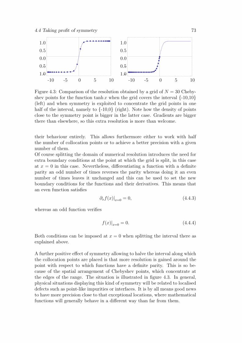
4.4 Taking profit of symmetry 73

-10 -5 0 5 10

-

-

1.0

0.5

0.0

0.5

1.0

-10 -5 0 5 10

-

-

1.0

0.5

0.0

0.5

1.0

Figure 4.3: Comparison of the resolution obtained by a grid of N = 30 Cheby-shev points for the function tanhx when the grid covers the interval -10,10(left) and when symmetry is exploited to concentrate the grid points in onehalf of the interval, namely to -10,0 (right). Note how the density of pointsclose to the symmetry point is bigger in the latter case. Gradients are biggerthere than elsewhere, so this extra resolution is more than welcome.

their behaviour entirely. This allows furthermore either to work with halfthe number of collocation points or to achieve a better precision with a givennumber of them.Of course splitting the domain of numerical resolution introduces the need forextra boundary conditions at the point at which the grid is split, in this caseat x = 0 in this case. Nevertheless, differentiating a function with a definiteparity an odd number of times reverses the parity whereas doing it an evennumber of times leaves it unchanged and this can be used to set the newboundary conditions for the functions and their derivatives. This means thatan even function satisfies

∂xf(x)|x=0 = 0, (4.4.3)

whereas an odd function verifies

f(x)|x=0 = 0. (4.4.4)

Both conditions can be imposed at x = 0 when splitting the interval there asexplained above.

A further positive effect of symmetry allowing to halve the interval along whichthe collocation points are placed is that more resolution is gained around thepoint with respect to which functions have a definite parity. This is so be-cause of the spatial arrangement of Chebyshev points, which concentrate atthe edges of the range. The situation is illustrated in figure 4.3. In general,physical situations displaying this kind of symmetry will be related to localiseddefects such as point-like impurities or interfaces. It is by all means good newsto have more precision close to that exceptional locations, where mathematicalfunctions will generally behave in a different way than far from them.

74 4. Numerical computations using spectral methods

4.4.2 Periodicity

Another kind of symmetry which helps simplifying things substantially is peri-odicity. This is so on computational grounds due to the possibility of invokingthe convenient properties of the Fourier transform if the functions involvedare periodic. It is well known that any periodic function may be expandedas a Fourier series, which helps when it comes to interpolate. Furthermore,the implementation of the well-known Fast Fourier Transform, an algorithmto compute discrete Fourier transforms, provides a remarkable enhancementin computation speed3.The Fourier transform enters our game via its close connection to Chebyshevpolynomials, based on a relationship between any grid of Chebyshev pointsand an equivalent periodic grid of evenly spaced points. Once such a grid isavailable, the great computational power of the FFT can be exploited.

To see the close connection mentioned above, it suffices to recall equation4.1.7 and see that our set of Chebyshev points is defined from the set of evenlyspaced points

θj =jπ

Nj = 0, 1, . . . , N, (4.4.5)

and hence straightforwardly related to it. This suggest that when dealing withperiodicity it might be more convenient not to work with the grid of Chebyshevpoints and the differentiation matrices shown above but rather to turn to thecorresponding grid of evenly distributed points 4.4.5 and then use trigonomet-ric functions as interpolants. For more mathematical detail on the equivalenceof both procedures the reader is referred to [81].

The implementation in Mathematica that takes profit from periodicity is veryeasy to realize as a deviation from our previous codes. It just requires thedefinition of a grid of evenly distributed points instead of one of Chebyshevpoints.

gridz = Range[x_0 , x_0 + Lx, Lx/( Npointsx - 1)] // N;

gridy = ChebPoints[y_0 , Ly, Npointsy ]//N;

and the specification of periodicity in the definition of the differentiation ma-trices, like for example

d[1,1] = NDSolve ‘FiniteDifferenceDerivative [1,1,gridz ,gridy,

"DifferenceOrder" -> "Pseudospectral","Pseudospectral",

PeriodicInterpolation -> True ,False ]

d[1 ,1][Phi]

It is no problem at all combining such a grid in one dimension with one ofChebyshev points in another dimension. Indeed this combination is quite aninteresting possibility in holography, given that no periodicity can be assumed

3For more information about the FFT, see for example [82]. Since we do not use itdirectly here but just use Mathematica built-in functions based on its use, we do not getinto details about it.

4.5 Numerical PDE solving in AdS/CFT 75

in the AdS radial direction. Of course periodicity also eliminates the need tofix boundary conditions at the spatial edges. A further advantage is the pos-sibility of ignoring the numerical values corresponding to the first or the lastpoint of the periodic coordinate, since they are equal to the last or the firstpoint values due to periodicity.

Once the required tools have been presented, we are now well prepared topresent and analyse the more involved codes we use for our codes.

4.5 Numerical PDE solving in AdS/CFTIn the light of all of the above, we are now in a good position to start employingthe skills we have collected this far for holographic purposes. Along well-known time-saving techniques common to all numerically-oriented codes thereare some tricks specific to Mathematica which are worth taking notice of. Anexample of the former is the storing of numerical data which is used repeatedlyto avoid its computation over and over. It is a very simple idea that may savelots of time. So for example if our radial coordinate, z, is discretised in thevariable gridz, we might as well assign names to the quantities z2, z3, . . . andsave them so that Mathematica does not have to multiply the vector gridz byitself each time it appears but rather substitutes the variable by its pre-storednumerical value.As an instance of a practical detail specific to Mathematica, it is good pointingout the convenience of using the built-in Compile function wherever possible toperform numerical computations, for it speeds up the code drastically4. Thisis why we have been including this function in our listings this far. So forexample, once it comes to turn the analytical form of the equations of motion,say EOMa and EOMb into numerical values, we shall turn to such an object

EOMa_num = Compile [ ChiNum , _Real , Nx, Nyh, A0Num , _Real , Nx, Nyh,

EOMa /. numvalues ];

where the substitution rule introduces the corresponding numerical values forthe analytical variables

numvalues= D[Chi[z, x], x, 2] -> d[0, 2][ ChiNum],

D[Chi[z, x], z, 2] -> d[2, 0][ ChiNum],

D[Chi[z, x], z, 2] -> d[2, 0][ ChiNum],

D[Chi[z, x], z, 1] -> d[1, 0][ ChiNum],

D[Chi[z, x], x, 1] -> d[0, 1][ ChiNum],

D[Chi[z, x], z, 1, x, 1] -> d[1, 1][ ChiNum], Chi[z, x] ->

ChiNum , D[A0[z, x], x, 2] -> d[0, 2][ A0Num],

D[A0[z, x], z, 2] -> d[2, 0][ A0Num],

D[A0[z, x], z, 2] -> d[2, 0][ A0Num],

D[A0[z, x], z, 1] -> d[1, 0][ A0Num],

D[A0[z, x], x, 1] -> d[0, 1][ A0Num],

D[A0[z, x], z, 1, x, 1] -> d[1, 1][ A0Num], A0[z, x] -> A0Num ,

h[z] -> hnum , h’[z] -> hnumdr , h’’[z] -> hnumdr2 , f[z] -> fnum ,

f’[z] -> fnumdr , f’’[z] -> fnumdr2 , z^2 -> gridz2 , z^3 -> gridz3 ,

4See https://reference.wolfram.com/language/Compile/tutorial/Introduction.html#8903121for detailed information

76 4. Numerical computations using spectral methods

z^4 -> gridz4 , z^5 -> gridz5 , z^6 -> gridz6 , z^7 -> gridz7 ,

z^8 -> gridz8 , z^9 -> gridz9 , z^10 -> gridz10 , z^11 -> gridz11 ,

z^12 -> gridz12 , z^13 -> gridz13 , z -> gridz , x -> gridy;

Where the fields χ and φ are analytically represented in Mathematica byChi[z,x] and A0[z,x] respectively, whereas their numerical values are storedas ChiNum and A0Num respectively.A further relevant issue is that of the choice of a proper seed or initial guess forour numerical resolution methods, like the Newton-Raphson iteration, to con-verge. We make use of two different approaches to this matter. One of themconsists in first solving the easier homogeneous problem, in which nothing de-pends on the spatial coordinate x and taking the homogeneous solution as astarting point for the non-homogeneous one. This method is specially well-suited for configurations with deviations from an average value like noises,whence we shall employ it in chapter 6.Our second approach is based on the use of smaller grids of collocation pointsat the beginning whose solution is then extrapolated to a bigger grid to con-tinue with the proper calculation. Small grids of 15 × 15 collocation pointsusually provide with a good starting base. We will make use of this methodin the computation in chapter 5.

It is furthermore very recommendable to perform as many numerical testsas possible to make sure that things are working properly. One clear exampleis the monitoring of the propagation of the constraint equation when it is setto zero at one of the boundaries of the numerical domain. If things are in goodorder, the numerical value of the constraint should not get bigger to numericalaccuracy than the values of the equations of motion that are being explicitlyimposed.Further possible checks include the comparison of the numerical results in thenon-homogeneous case to the ones obtained when solving the homogeneousproblem. Note that using the homogeneous problem as an easier way to esti-mate values and behaviours is mostly a clever thing to do.

All in all, our codes will not be much than a combination of the techniques wehave reviewed in this chapter. Detailed commented version of the real codesare offered in appendix D. It should be taken into account though, that ourcodes have been written by a physicist and are very far from being optimal.For sure there is great room for improvement and optimisation, though ourlack of these compensates with simplicity and makes the codes more accessibleto the dummy user.

4.6 Final remarks

The main motivation of our use of numerical methods is our necessity to attackproblems in which translation invariance is broken. Thereby we reckon some

4.6 Final remarks 77

words on the current state of research along this line in an holographic contextwould not go amiss.Recently, significant progress has been achieved in studying holographic sys-tems with broken translation invariance by numerically solving the resultingequations of motion, which are in general partial differential equations. Theseinclude set-ups with different holographic realisations of lattices [83, 84, 85, 86,87, 41, 88, 89] through periodically space-dependent sources, and also set-upsimplementing disordered sources [27, 28, 30, 90]. Moreover, a lattice realisationwhere PDEs are avoided, which goes under the name of Q-lattices given itsresemblance to the construction of Q-balls [91], was introduced in [92] and fur-ther explored in [93, 94]. Alternatively to introducing translational symmetrybreaking by spatially modulating the sources of conserved currents, momentumrelaxation may also be realised by explicitly breaking diffeomorphism invari-ance in the bulk [95, 96, 97, 98, 99, 100, 101], which in [102] led to progress onthe study of the conductivity for systems with broken translational symmetry.

78 4. Numerical computations using spectral methods

Part II

Holographic strongly coupledfundamental matter with

inhomogeneities

79

Chapter 5Holographic charge localisation atbrane intersections

In chapter 3 we laid down the principles of AdS/CFT duality and the prescrip-tion to exploit its power. In chapter 4 we introduced the necessary machineryto perform numerical computations involving partial differential equations inan holographic context. It is now time to combine both pieces of knowledgeto investigate interesting phenomena in strongly coupled matter.

In all of the above we only considered fields depending on the radial coordinateof AdS, which implies the assumption of translation invariance in all other di-rections. Nevertheless, a number of relevant phenomena in condensed matterphysics do not display this translation invariance. For example, those whichinvolve the presence of an interface between materials of different kind. Suchinterfaces represent a localised impurity which breaks translational symmetryin the system. Broken translational symmetry allows the charge carriers todissipate their momentum. In the case of strong coupling, where the standardquasiparticle picture does not apply, many questions about the exact form ofthis mechanism are still open. Gauge/gravity duality reveals itself as a naturaltool to further explore momentum dissipation at strong coupling, given that itprovides a method for describing strongly coupled systems by mapping themto weakly coupled gravity theories as we showed above.

It is this step of introducing translational symmetry breaking which requiresthe fields to depend not just on the radial AdS coordinate but at least onan additional spatial coordinate, we shall call x. When doing so, the result-ing equations of motion are in general partial differential equations, which weknow now how to handle.

In this chapter, based on the author’s publication [43], we consider the break-ing of translation invariance by an interface. We consider a top-down modelinvolving a D5 probe brane with a kink geometry. The basic idea is to in-

81

82 5. Holographic charge localisation at brane intersections

corporate the existence of massless fundamental matter modes localised on aninterface by letting the embedding of the flavour probe brane vary over the dis-tinguished boundary coordinate x, in addition to being a function of the radialcoordinate. This way, the corresponding dual gauge theory physical quanti-ties also display spatial dependence, whose effects we wish to study. This isimplemented by an embedding function that asymptotes to a positive value m(with mq = 2πα′m the quark mass, see (3.4.41)) for x → ∞ and to −m forx → −∞, while it vanishes at x = 0, therefore introducing a defect surfacethere. The original idea was introduced in [25] to design a holographic modelfor topological insulators using the D7/D3 intersection and further exploredin [24].

5.1 Holographic set-upWe consider a D3/D5 intersection, that is a probe D5 flavour brane in thebackground geometry generated by the stack of D3 black branes (3.4.33)

ds2 =L2

z2

(−f(z)2

h(z)dt2 + h(z) d~x2 + dz2

)+ L2 dΩ2

5 , (5.1.1)

We do it in the presence of temperature and chemical potential for the funda-mental matter dual to the open strings stretching between the flavour braneand the D3-branes. We work in the probe limit approximation presented insubsection 3.4.2, hence using a DBI action like (3.4.31):

S = −NfTD5

∫d6ξ√− det(P [g] + 2π α′ F ) , (5.1.2)

and embedding the D5 probe brane according to (3.4.38)

t x1 x2 x3 z Ω2 Ω2 θD3 × × × ×D5 × × × × ×

(5.1.3)

We use the χ defined in (3.4.39) to describe the embedding and introduce anon-zero temporal component of the U(1) gauge field on the world-volume ofthe probe brane, At, (3.4.42), whose dimensionless version φ we defined in(3.4.43). However, since we now wish to introduce a spatial dependence, welet the fields χ and φ that specify the embedding depend not only on the radialcoordinate of AdS but also on the distinguished spatial coordinate x

χ = χ(z, x) φ = φ(z, x). (5.1.4)

With this set-up, reminding ourselves of the fact that we need not include aChern-Simons term, the DBI action can be written as

S = −Nf TD5 L6

∫dt d2x dz dΩ2 f z

−4√h (1− χ2) (Sχ + Sφ + Sint) , (5.1.5)

5.1 Holographic set-up 83

with

Sχ = 1− χ2 + z2χ′2 +z2 χ2

h, (5.1.6)

Sφ = −z4(1− χ2)

f 2

(hφ′2 + φ2

), (5.1.7)

Sint = −z6(χφ′ − χ′φ)2

f 2, (5.1.8)

where a tilde denotes a derivative with respect to z and a dot a derivative withrespect to x. The equations of motion for φ(z, x) and χ(z, x) can be readilyobtained from the action (5.1.5). They are shown in appendix B.Once they are known we can proceed to analyse their near-horizon (z → 1) andnear-boundary (z → 0) asymptotic behaviours by expanding the correspondinglimits of the equations of motion.

IR Asymptotics

As we saw in subsubsection 3.4.2, we are interested in solutions describing blackhole embeddings for which the brane ends at the horizon. Hence regularity atthe horizon requires φ to vanish there. The geometry furthermore requires thatχ′ also vanish there, restricting the infra-red solution to the following form

φ(z, x) = a(2)(x) (1− z)2 +O((1− z)3) , (5.1.9a)

χ(z, x) = C(0)(x) + C(2)(x) (1− z)2 +O((1− z)3) , (5.1.9b)

with

C(2)(x) =

(2− a(2)(x)2

) [C(0)′′(x)(C(0)(x)2 − 1)− C(0)(x)

(3C(0)′(x)2 + 4

)+ 4C(0)(x)3

]8 [C(0)′(x)2 − 2C(0)(x)2 + 2]

.

(5.1.10)

UV Asymptotics

At the boundary, the asymptotic form of the fields χ(z, x) and A(z, x) is ofthe same form as in (3.4.40) and (3.4.44) but taking now the x-dependence ofthe fields into account

φ(z, x) = µ(x)− ρ(x)z +O(z2) , (5.1.11a)

χ(z, x) = m(x) z + ψ(x)z2 +O(z3) . (5.1.11b)

Let us recall that the holographic dictionary relates µ(x), and ρ(x) respectivelyto the chemical potential and charge density of the U(1) flavour symmetry sup-ported by the D5-brane. As for the asymptotic form of χ, the leading piecem(x) is proportional to the asymptotic distance M between the probe D5 andthe D3-branes generating the background, and is therefore interpreted as the

84 5. Holographic charge localisation at brane intersections

quark mass.

As is clear from (5.1.11), the UV solutions depend on four parameters (func-tions of x): µ, ρ, m, and ψ, while as we see in (5.1.9),the IR behaviour isdetermined by two free functions, namely C(0)(x) and a(2)(x). Thus we expecta two-parameter family of solutions, which we choose to describe in terms ofthe chemical potential µ, which we assume to be independent of x, and themass m(x). Consequently, once µ and m(x) are fixed, the embedding of theprobe D5-brane is completely fixed.

5.1.1 Inhomogeneous embeddings and charge localisation

As we saw in subsection 3.4.2, at non-zero charge density only embeddings ofthe black hole type are possible in the Dp/Dq model. As explained in [67], thefundamental strings realizing the charge density would have nowhere to endin a Minkowski embedding. Moreover, as illustrated in figure 3.6, for a largeenough Mq/T , black hole embeddings exist only above a non-zero chemicalpotential µ/T . In particular, the shaded region in the plot is only accessibleby Minkowski embeddings, which have zero charge density.Our purpose is to construct an embedding depending on one spatial directionx, that localises charge density along an interface situated at x = 0. Thiscan be done following [25] by means of an embedding with constant chemicalpotential µ = µ/T and an x-dependent mass (m = Mq/T )

m(x) = M

(2

1 + e−a x− 1

), (5.1.12)

that interpolates between two constant values; M at x = −L, and −M atx = L, while vanishing at the origin, m(0) = 0.1 a is a constant parameterthat fixes the steepness of the kink. If we were to choose µ and M to lie withinthe shaded region of figure 3.6, asymptotically, at x → ±L, the embeddingwould be of the Minkowski type and the charge density would vanish there. Atthe interface (x = 0) though, the mass would vanish, the brane would intersectthe black hole and, for a non-zero µ, some charge density would be induced.In such a construction the charge density would exactly vanish towards thespatial edges while it would peak at the interface. Notice that by increasinga in (5.1.12) the transition can be made as abrupt as desired, and thereforethe charge may be localised around x = 0. However, such an embedding,with a varying topology along x, turns out to be too challenging in numerical

1As explained in [26], embeddings with positive and negative m correspond respectivelyto the D5-brane sitting at opposite poles of the Ω2 in (3.4.38). We take L to be the spatialboundary, which may also be L = ∞. More shall be said on this further down. As in [25]we account for the case m < 0 by letting χ become negative.

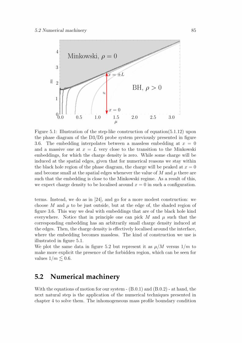
5.2 Numerical machinery 85

0.0 0.5 1.0 1.5 2.0 2.5 3.00

1

2

3

4m

µ

Minkowski, ρ = 0

BH, ρ > 0

x = 0

x = ±L

x

Figure 5.1: Illustration of the step-like construction of equation(5.1.12) uponthe phase diagram of the D3/D5 probe system previously presented in figure3.6. The embedding interpolates between a massless embedding at x = 0and a massive one at x = L very close to the transition to the Minkowskiembeddings, for which the charge density is zero. While some charge will beinduced at the spatial edges, given that for numerical reasons we stay withinthe black hole region of the phase diagram, the charge will be peaked at x = 0and become small at the spatial edges whenever the value of M and µ there aresuch that the embedding is close to the Minkowski regime. As a result of this,we expect charge density to be localised around x = 0 in such a configuration.

terms. Instead, we do as in [24], and go for a more modest construction: wechoose M and µ to be just outside, but at the edge of, the shaded region offigure 3.6. This way we deal with embeddings that are of the black hole kindeverywhere. Notice that in principle one can pick M and µ such that thecorresponding embedding has an arbitrarily small charge density induced atthe edges. Then, the charge density is effectively localised around the interface,where the embedding becomes massless. The kind of construction we use isillustrated in figure 5.1.We plot the same data in figure 5.2 but represent it as µ/M versus 1/m tomake more explicit the presence of the forbidden region, which can be seen forvalues 1/m . 0.6.

5.2 Numerical machinery

With the equations of motion for our system - (B.0.1) and (B.0.2) - at hand, thenext natural step is the application of the numerical techniques presented inchapter 4 to solve them. The inhomogeneous mass profile boundary condition

86 5. Holographic charge localisation at brane intersections

2.5

2.0

1.5

1.0

0.5

0.0

0.0 0.5 1.0 1.5 2.0 2.5 3.0 3.51/m

µ/m

Figure 5.2: As in fig. 3.6 we plot lines of constant charge density for blackhole embeddings. From bottom (light grey) to top (black) they correspond toρ = 10−6, 0.25, 0.6, 1.25, 2, 3, 10.

(5.1.12) implies that we have to deal with two coupled second order partialdifferential equations. The role played by the boundary conditions turns outto be crucial, since it is through them that we set the values of m and µ andhence the kind of embedding we have.At the boundary, from (5.1.11) and (5.1.12), we must impose

χ′(0, x) = M

(2

1 + e−ax− 1

), φ(0, x) = µ , (5.2.1)

where µ determines the homogeneous chemical potential of the solution, whileM fixes the mass of the embedding at the edges of the system. On the otherhand, at the horizon, z = 1 , the asymptotic solutions (5.1.9) and the require-ment of regularity in the sense elucidated in (3.4.45) result in the followingboundary conditions

φ(1, x) = 0 , χ′(1, x) = 0 . (5.2.2)

As for the boundary conditions at the spatial edges, given that the symmetryof our set-up with a step-like configuration does not allow the use of periodicboundary conditions as is commonly done, we take our system to have a finitelength (x ∈ [−L,L]), but require it to be large enough so that it resembles anhomogeneous embedding towards the spatial edges. Consequently we imposethe following Neumann boundary conditions

χ(z,±L) = 0 , φ(z,±L) = 0 , (5.2.3)

which ensure that the effects of the inhomogeneity sourced by the mass profile(5.1.12) fade away towards the spatial edges.

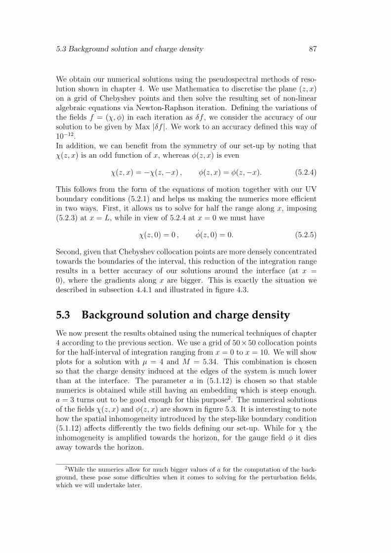
5.3 Background solution and charge density 87

We obtain our numerical solutions using the pseudospectral methods of reso-lution shown in chapter 4. We use Mathematica to discretise the plane (z, x)on a grid of Chebyshev points and then solve the resulting set of non-linearalgebraic equations via Newton-Raphson iteration. Defining the variations ofthe fields f = (χ, φ) in each iteration as δf , we consider the accuracy of oursolution to be given by Max |δf |. We work to an accuracy defined this way of10−12.In addition, we can benefit from the symmetry of our set-up by noting thatχ(z, x) is an odd function of x, whereas φ(z, x) is even

χ(z, x) = −χ(z,−x) , φ(z, x) = φ(z,−x). (5.2.4)

This follows from the form of the equations of motion together with our UVboundary conditions (5.2.1) and helps us making the numerics more efficientin two ways. First, it allows us to solve for half the range along x, imposing(5.2.3) at x = L, while in view of 5.2.4 at x = 0 we must have

χ(z, 0) = 0 , φ(z, 0) = 0. (5.2.5)

Second, given that Chebyshev collocation points are more densely concentratedtowards the boundaries of the interval, this reduction of the integration rangeresults in a better accuracy of our solutions around the interface (at x =0), where the gradients along x are bigger. This is exactly the situation wedescribed in subsection 4.4.1 and illustrated in figure 4.3.

5.3 Background solution and charge densityWe now present the results obtained using the numerical techniques of chapter4 according to the previous section. We use a grid of 50×50 collocation pointsfor the half-interval of integration ranging from x = 0 to x = 10. We will showplots for a solution with µ = 4 and M = 5.34. This combination is chosenso that the charge density induced at the edges of the system is much lowerthan at the interface. The parameter a in (5.1.12) is chosen so that stablenumerics is obtained while still having an embedding which is steep enough.a = 3 turns out to be good enough for this purpose2. The numerical solutionsof the fields χ(z, x) and φ(z, x) are shown in figure 5.3. It is interesting to notehow the spatial inhomogeneity introduced by the step-like boundary condition(5.1.12) affects differently the two fields defining our set-up. While for χ theinhomogeneity is amplified towards the horizon, for the gauge field φ it diesaway towards the horizon.

2While the numerics allow for much bigger values of a for the computation of the back-ground, these pose some difficulties when it comes to solving for the perturbation fields,which we will undertake later.

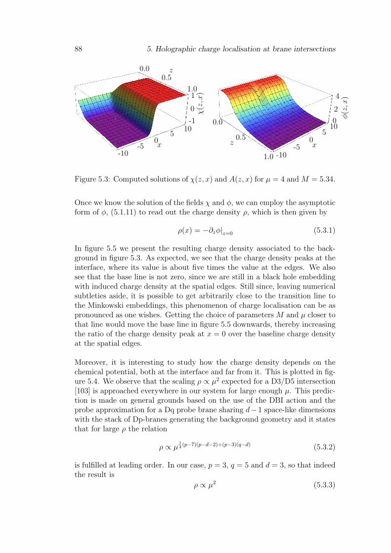
88 5. Holographic charge localisation at brane intersections

-1

0

1

0.00.5

1.0

z

-10-5

05

10

x

χ(z,x

)

-10-5

05

10

x

0

2

4

φ(z,x

)

1.0

0.5

0.0

z

Figure 5.3: Computed solutions of χ(z, x) and A(z, x) for µ = 4 and M = 5.34.

Once we know the solution of the fields χ and φ, we can employ the asymptoticform of φ, (5.1.11) to read out the charge density ρ, which is then given by

ρ(x) = −∂zφ|z=0 (5.3.1)

In figure 5.5 we present the resulting charge density associated to the back-ground in figure 5.3. As expected, we see that the charge density peaks at theinterface, where its value is about five times the value at the edges. We alsosee that the base line is not zero, since we are still in a black hole embeddingwith induced charge density at the spatial edges. Still since, leaving numericalsubtleties aside, it is possible to get arbitrarily close to the transition line tothe Minkowski embeddings, this phenomenon of charge localisation can be aspronounced as one wishes. Getting the choice of parameters M and µ closer tothat line would move the base line in figure 5.5 downwards, thereby increasingthe ratio of the charge density peak at x = 0 over the baseline charge densityat the spatial edges.

Moreover, it is interesting to study how the charge density depends on thechemical potential, both at the interface and far from it. This is plotted in fig-ure 5.4. We observe that the scaling ρ ∝ µ2 expected for a D3/D5 intersection[103] is approached everywhere in our system for large enough µ. This predic-tion is made on general grounds based on the use of the DBI action and theprobe approximation for a Dq probe brane sharing d−1 space-like dimensionswith the stack of Dp-branes generating the background geometry and it statesthat for large ρ the relation

ρ ∝ µ14

(p−7)(p−d−2)+(p−3)(q−d) (5.3.2)

is fulfilled at leading order. In our case, p = 3, q = 5 and d = 3, so that indeedthe result is

ρ ∝ µ2 (5.3.3)

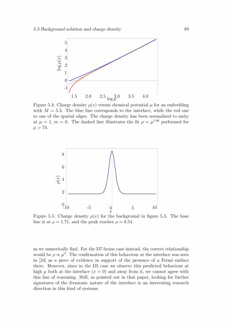
5.3 Background solution and charge density 89

1.5 2.0 2.5 3.0 3.5 4.0

-1

0

1

2

3

4

5

logρ(x

)

log µ

Figure 5.4: Charge density ρ(x) versus chemical potential µ for an embeddingwith M = 5.3. The blue line corresponds to the interface, while the red oneto one of the spatial edges. The charge density has been normalised to unityat µ = 1, m = 0. The dashed line illustrates the fit ρ = µ1.96 performed forµ > 74.

0

2

4

6

8

-10 -5 0 5 10x

ρ(x

)

Figure 5.5: Charge density ρ(x) for the background in figure 5.3. The baseline is at ρ = 1.71, and the peak reaches ρ = 8.54.

as we numerically find. For the D7-brane case instead, the correct relationshipwould be ρ ∝ µ3. The confirmation of this behaviour at the interface was seenin [24] as a piece of evidence in support of the presence of a Fermi surfacethere. However, since in the D5 case we observe this predicted behaviour athigh µ both at the interface (x = 0) and away from it, we cannot agree withthis line of reasoning. Still, as pointed out in that paper, looking for furthersignatures of the fermionic nature of the interface is an interesting researchdirection in this kind of systems.

90 5. Holographic charge localisation at brane intersections

5.4 ConductivitiesAfter constructing a holographic set-up localizing charge along a (1+1)-dimensionaldefect, we go on to study its response to an applied electric field, namely itselectrical conductivity. We do this according to what we developed in subsec-tion 3.5.1 so as to study the conductivities of our system both in the directionparallel, y, and orthogonal to the defect, x. For reasons that will soon becomeapparent, we also differentiate between the so-called DC conductivity, which isthe optical conductivity at zero frequency and the so-called AC conductivity,by which the conductivity at any frequency is meant.

In order to bring the required electric field into the game as in (3.5.3), weconsider fluctuations around our background solution with vanishing spatialcomponents of the gauge field (Ax = Ay = 0) and compute the linear responseof our background when an electric field is switched on along the boundary.So as to analyse these transport properties at the interface generated by themass profile (5.1.12) we study the fluctuations of the gauge field on the world-volume of the D5 probe brane along the spatial directions it shares with thestack of D3 branes, which we have labelled x and y. In general these fluctu-ations couple among them and to the fluctuations of the embedding field χ,thus we have to solve for the whole set of coupled fields.

We hence switch on fluctuations of the gauge field realizing an electric field ofconstant modulus and frequency ω along the boundary. That is at z = 0 werequire the fluctuations to satisfy

fti = (iω ei) eiω t , (i = x, y) . (5.4.1)

where fti stands for the field strength of the fluctuations of the gauge field,and we are considering both the case when the electric field is orthogonaland parallel to the interface. ex and ey are respectively the correspondingconstant moduli. Once these fluctuations are defined, we may plug them intoour expression for the conductivity (3.5.8) to obtain

σi(ω, x) =jiiω ei

= limz→0

fizfti

, (i = x, y) . (5.4.2)

Consequently, it will be necessary to analyse the following set of fluctuations3

Aµ = Aµ(z, x) + ε aµ(z, x)eiωt , (5.4.3a)

χ = χ(z, x) + ε c(z, x)eiωt , (5.4.3b)

where ε just keeps track of the fluctuation order, φµ and χ stand for the back-ground fields, while aµ and c refer to the fluctuations of the gauge field and the

3Since we are working with the dimensionless coordinates (3.4.36), ω is dimensionless,and in terms of the dimension-full frequency w, one has ω =

√2w/(π T ).

5.4 Conductivities 91

embedding scalar respectively. Note that the gauge field and its fluctuationsare intended to be renormalised according to (3.4.43) so as to be dimension-less.Our background, described by At(z, x) and χ(z, x), is time invariant. Thisallows us to Fourier transform along the time direction, t and justifies theform of the fluctuations considered. Given that we are interested only in theconductivity, we wish not consider our fluctuations to have any net spatialmomentum. In addition, we choose to work in the radial gauge and thereforeset

az(z, x) = 0 . (5.4.4)

We are working in the linear response regime. The equations of motion for thefluctuations (5.4.3) follow from expanding the DBI lagrangian of the action(5.1.5) up to second order in those fluctuations

L = L0 + εL1 + ε2 L2 + . . . . (5.4.5)

Upon imposing the equations of motion for the background fields L1 van-ishes and the linearised equations for the fluctuations can be found from thequadratic part of the action, L2, which is shown explicitly in appendix C. Al-though straightforward to derive from it, the resulting equations of motion arelengthy and we do not reproduce them here.

However, it is worth mentioning that the component of the gauge field fluc-tuations parallel to the defect, ay, decouples from the rest of the fluctuations.Hence to study the conductivity σy we only need to solve the correspondinglinear partial differential equation (PDE) for ay. Instead, ax is coupled to bothat, and c. Their dynamics is described by a system of three second order linearPDEs plus a first order constraint PDE resulting from the equation of motionfor az.

Boundary conditions at the horizon

In order to compute the conductivity, we must proceed as in section 3.5.1and solve the equations of motion of the fluctuations with in-falling boundaryconditions at the horizon (3.5.12) - (3.5.14) so as to preserve causality. Thuswe assume that in the IR (z → 1) the fluctuation fields take the form

aµ = (1− z)iα±(a(0)µ (x) + a(1)

µ (x) (1− z) +O((1− z)2)), (5.4.6)

c = (1− z)iα±(c(0)(x) + c(1)(x) (1− z) +O((1− z)2)

), (5.4.7)

withα =

ω

2√

2. (5.4.8)

where we recall that we have taken the negative sign in (3.5.11), since the neg-ative is associated to the outgoing wave. For the coefficients in the expansions

92 5. Holographic charge localisation at brane intersections

(5.4.6) and (5.4.7) we require in accordance with (3.5.14)

c(1) =iω

4√

2c(0) , a

(0)t = 0 , a

(1)i =

iω

4√

2a

(0)i ; (i = x, y) , (5.4.9)

while higher order coefficients are determined in terms of these. The vanishingof the term a

(0)t is found in the IR expansion of the equation of motion for

at. At this stage, on behalf of simplicity it is useful to redefine the fields suchthat the (1− z)iα factor be conveniently disposed of our computations can beperformed using the fields

aµ(z, x) = (1− z)−iα+ aµ(z, x) , c(z, x) = (1− z)−iα+ c(z, x) . (5.4.10)

in terms of which we impose at the horizon the following mixed Dirichlet andRobin boundary conditions

at(1, x) = 0 , a′i(1, x) =iω

4√

2ai(1, x) , c′(1, x) =

iω

4√

2c(1, x) .

(5.4.11)Of course when interpreting the results physically, like in the computation ofthe conductivity, the field redefinition (5.4.10) must be reversed to convertback to the original fields we use in our definition of the conductivity (3.5.8),which would otherwise be altered. Notice in particular, that the asymptoticUV expansions to follow are written in terms of the original fluctuation fields(without tilde).

Boundary conditions at the AdS boundary

At the AdS boundary, z → 0, we want our fluctuations to source an ho-mogeneous electric field (5.4.1). The fluctuation fields behave asymptoticallylike the background fields, as can be verified by expanding the correspondingequations of motion

aµ(z, x) = a(b)µ (x)− jµ(x) z +O(z2) , (µ = t, x, y) , (5.4.12a)

c(z, x) = c(b)(x) z +O(z2) . (5.4.12b)

When computing the conductivity in the direction parallel to the defect, sincewe need only solve for ay, which decouples from the rest of the fluctuations, itis convenient to just impose

ay(0, x) = 1 , (5.4.13)

which is tantamount to taking a normalisation in which the modulus of theelectric field Ey is taken to be unity, ey = 1. Instead, to compute σx we mustsolve for ax, at, and c. Again, we want our fluctuations to source solely anelectric field in the x direction

Ex = ftx = ∂tax − ∂xat = iωax − ∂xat (5.4.14)

5.4 Conductivities 93

and would also like to avoid fluctuations in the mass parameter. Hence wetake

c′(0, x) = 0 , (5.4.15a)

ax(0, x)− 1

iω∂xat(0, x) = 1 , (5.4.15b)

where the second condition implies that an homogeneous electric field alongx, normalised to ex = 1, is turned on at the boundary. In addition, in the UVwe impose the fulfilment of the constraint equation resulting from the equationof motion for az, which reduces to

iω ∂zat(0, x)− ∂x∂zax(0, x) = 0 . (5.4.16)

Notice that in terms of the asymptotic solutions (5.4.12a) this boundary con-dition is nothing else than the conservation of current

∂t(eiω tjt(x)

)− eiω t ∂xjx(x) = 0 . (5.4.17)

As expected, it is straightforward to check that the partial derivative along zof the constraint equation vanishes for solutions of the equations of motion.This ensures that the constraint is satisfied for all z by any solution of theequations of motion that obeys the constraint on a constant z slice, thus itis sufficient to impose it at the boundary for it to be satisfied everywhere.Therefore, the constraint may be numerically monitored as a correctness testwhen performing computations.

It is worth pointing out that although we have allowed for both at and axto be non-zero at the boundary, one can proceed as in [92, 89] and apply agauge transformation eiωt Λ(z, x) that brings the boundary field configurationto

aµ(0, x) eiω t dxµ → (aµ + ∂µΛ(0, x)) eiωt dxµ = eiω tdx , (5.4.18)

which makes clear that the only boundary source is that corresponding to anhomogeneous electric field, and other non-zero sources are just gauge artefacts.Note that one can always choose Λ(z, x) such that it vanishes at the horizonand also satisfies ∂zΛ(0, x) = 0 and hence az(0, x) = 0.

Summing up, in order to compute the conductivity σy(ω) we must solve theequation of motion of ay with boundary conditions (5.4.11) and (5.4.13), andthen read the conductivity from (5.4.2). On the other hand, to calculate σx itis necessary to solve the equations of motion of ax, at, and c, imposing (5.4.11)at the horizon, and (5.4.15 - 5.4.16) at the boundary; and again read σx(ω)from (5.4.2). We will discuss the boundary conditions at the spatial bound-aries when describing our numerical methods. But before that, in the nextsection we analyse the DC limit of the conductivity, and show how σDC

x canbe computed from the background horizon data, with no need to solve for thefluctuations.

94 5. Holographic charge localisation at brane intersections

5.4.1 DC conductivity

We can follow the procedure of [42] (as applied for instance in [32] to a DBIaction) and compute the DC conductivity along the direction perpendicularto the interface σDC

x in terms of the background functions evaluated at thehorizon. It proves useful to define the radial coordinate ζ through

dζ =

√h(z)

f(z)2dz , (5.4.19)

and note that the horizon (at z = 1) is located at ζ =∞ in the new coordinate.When expressed in this coordinate, the equations of motion for the fluctuationfields ax(z, x) and az(z, x) in the DC limit, ω → 0, respectively take the form

∂ζ (F(ζ, x) ∂ζax) = 0 , ∂x (F(ζ, x) ∂ζax) = 0 , (5.4.20)

where we have defined

F(z, x) = f(1− χ2

)3/2

√h

Γ, (5.4.21)

with

Γ = −z4hφ′2[h(1− χ2) + z2 χ2

]− 2z2φ′ φ χ′ χ+ φ2(1− χ2 + z2 χ′2)

− f 2

[h(χ2 − 1− z2 χ′2

)− z2 χ2

].

(5.4.22)

The equations of motion (5.4.20) ensure that the combination F ∂ζax is aconstant. It is thanks to the existence of this conserved quantity that one canexpress σDC

x in terms of the background functions evaluated at the horizon.First, notice that at the boundary

F(0, x) = 1, (5.4.23)

and let us define the function

X(ζ, x) = −∂ζax(ζ, x)

ax(ζ, x), (5.4.24)

which at the horizon satisfies

X(∞, x) = iω , (5.4.25)

due to the ingoing wave boundary condition imposed on ax. In terms ofX(ζ, x), the conductivity from (5.4.2) reads

σx(ω, x) =X(0, x)

iωax(0, x) , (5.4.26)

5.4 Conductivities 95

where we have normalised the modulus of the electric field to one. Next, inthe DC limit we can expand X in a power series in ω as

X(ζ, x) = iω a(ζ, x) +O(ω2) , (5.4.27)

and ax and at at the boundary as

at(0, x) = iω p(x) +O(ω2) , (5.4.28a)

ax(0, x) = 1 + ∂xp(x) +O(ω) , (5.4.28b)

where a(ζ, x) and p(x) are fixed by the equations of motion (5.4.20). Moreover,notice that (5.4.28) is such that the condition (5.4.1) of having a constantelectric field (with ex = 1) at the boundary is automatically satisfied. At thehorizon, the ingoing wave condition (5.4.25) translates into

a(∞, x) = 1 . (5.4.29)

Plugging the expansions (5.4.27, 5.4.28) into eq. (5.4.26) we obtain

σDCx = a(0, x)(1 + ∂xp(x)) . (5.4.30)

Using the definition (5.4.24) together with the expansions (5.4.27, 5.4.28), theequations of motion (5.4.20) imply that

F(ζ, x) a(ζ, x) (1 + ∂xp(x)) (5.4.31)

is a constant. We have taken into account that ax(ζ, x) = ax(0, x) + O(ω).Now, notice that (5.4.31) when evaluated at ζ = 0 reduces precisely to theexpression (5.4.30) for the conductivity. Hence we conclude that σDC

x is aconstant. By evaluating (5.4.31) at the horizon we arrive at the followingexpression for the DC conductivity

σDCx = F(z = 1, x) (1 + ∂xp(x)) , (5.4.32)

which is indeed a constant as required by current conservation. Notice though,that this expression for σDC

x still depends on the fluctuations through the fieldp(x) which should in principle be determined by solving the correspondingequations of motion. However, this dependence can be eliminated and σDC

x

expressed solely in terms of the background horizon data. Integrating theexpression (5.4.32) over the whole sample we can write

σDCx

1

2L

∫ L

−L

dx

F(1, x)=

1

2L

∫ L

−Ldx (1 + ∂xp(x)) , (5.4.33)

and assuming the condition

1

2L

∫ L

−Ldx (1 + ∂xp(x)) = 1 , (5.4.34)

96 5. Holographic charge localisation at brane intersections

(to be justified below) we arrive at the following expression for the DC con-ductivity

σDCx =

2L∫ L−L

dxF(1,x)

, (5.4.35)

which allows us to calculate σDCx purely in terms of background functions

evaluated at the horizon. In terms of the IR asymptotic solutions for φ and χ,given in eq. (5.1.9), F(z = 1, x) can be written as

F(z = 1, x) =2(C(0)(x)

2 − 1)3/2

√(a(2)(x)2 − 2)

(2− 2C(0)(x)

2+ C(0)′(x)

2) . (5.4.36)

Let us discuss at this point the condition (5.4.34) that must be satisfied bythe fluctuations. First, notice that when rewritten in terms of at(z, x) it boilsdown to ∫ L

−Ldx ∂xat(0, x) = 0 . (5.4.37)

This would be automatically satisfied for a periodic system, but also in a set-up like ours if we assume that the system is long enough for the effects of theinterface to fade away towards the edges of the sample. As we discuss below,it can be checked that in that case the solution for the fluctuations asymptotestowards the edges to that of an homogeneous system, for which at = 0 andthen (5.4.37) holds. A more general argument for requiring (5.4.37) to hold isas follows. Notice that even though we allow at to be non-zero at the boundary,as illustrated by (5.4.18) our configuration is gauge equivalent to one where axis the only source at the boundary [92, 89]. Then, at(0, x) is pure gauge, i.e.Λ(0, x), and gauge invariance of the action in presence of a conserved current

implies that∫ L−L dx ∂xΛ(0, x) = 0, which justifies the assumption (5.4.37).

5.5 Numerics for the fluctuationsWe now proceed to present our numerical resolution of the equations of motionfor the fluctuation fields and the subsequent extraction of the conductivities.We start by briefly describing the numerical methods employed, and specifyingthe boundary conditions imposed at the spatial edges of the system.We solve the equations of motion of the fluctuation fields (5.4.10) on the sameChebyshev grid used for the background fields χ and φ, that is on a grid of50× 50 collocation points for the half-interval of integration. To simplify thenumerics, again we make use of the parity along x of the fields in our problem,namely

at(z, x) = −at(z,−x) , ax(z, x) = ax(z,−x) ,

c(z, x) = c(z,−x) , ay(z, x) = ay(z,−x) ,(5.5.1)

5.5 Numerics for the fluctuations 97

which follows straightforwardly from the linear equations of motion taking intoaccount that the background fields satisfy (5.2.4). As in the case of the back-ground, this allows us to actually solve for half the system, between x = −Land x = 0, and given the distribution of points in a Chebyshev grid, greatlyincreases the resolution close to the interface, where the gradients in x arelarger. The IR and UV boundary conditions are given by eqs. (5.4.9, and5.4.13 -5.4.16) as discussed above.

Regarding the boundary conditions at the spatial edges, x = ±L, again, peri-odic boundary conditions cannot be used due to the symmetry of the problem.Let us focus first on the the three coupled fields at, ax, and c, which allowus to compute σx. By studying the asymptotic form of the coupled PDEs atthe spatial boundaries, one can show that a solution is completely determinedonce the values of at and c, or those of their derivatives ∂xat and ∂xc, are fixedat each spatial boundary. Solving the system asymptotically at one edge, oncethe values of at and c and their derivatives, ∂xat and ∂xc, are fixed, and takinginto consideration the UV and IR boundary conditions, the asymptotic solu-tions for ax, at and c are completely fixed. Then, to fully determine a solutionof the system one may set the values of at and c, and their derivatives, at oneedge, or equivalently impose two conditions at one edge and two more at theother. We consider fixing at and c both at x = L and x = −L, or, alternatively,fix ∂xat and ∂xc at x = ±L. The case of ay is simpler, for a single linear PDEhas to be solved and as spatial boundary conditions we either fix the value ofthe function or of its derivative ∂xay, at the spatial boundaries.Both when computing σx and σy two different sets of boundary conditions maybe considered, which we now describe.

5.5.1 Damping boundary conditions. Long systems

A reasonable boundary condition is derived from the assumption that thesystem is long enough for all the inhomogeneities sourced by the interface todie away towards the edges, that is from the requirement that the fluctuationsbecome independent of x there, namely

∂xat(z,±L) = 0 , ∂xc(z,±L) = 0 , (5.5.2)

while ax is left free as discussed above.To compute the conductivity in the direction parallel to the interface (σy) weonly need to solve for ay. The damping boundary condition at the spatialboundaries is then

∂xay(z,±L) = 0 . (5.5.3)

5.5.2 Boundary conditions. Short systems

One can instead be interested in a situation in which the system is not longenough for the inhomogeneities of the fluctuations to vanish towards the spa-

98 5. Holographic charge localisation at brane intersections

tial edges. In this case these fields may reach the boundary with a non-zeroderivative along x, then, those fields have a non-zero derivative at the bound-ary, and Dirichlet boundary conditions may be imposed there instead of Neu-mann ones. As discussed in the previous section, at, which is odd, must obey(5.4.37), hence an alternative boundary condition that allows for a non-zero∂xat at the boundary is

at(z,±L) = 0 . (5.5.4)

Analogously we require c to also vanish at the boundaries

c(z,±L) = 0 . (5.5.5)

Notice that these boundary conditions are nothing else than the requirementthat at and c reach the solution of the homogeneous problem exactly at theedge. We should bear in mind that when computing the conductivity σx of anhomogeneous system, only ax has to be turned on, hence c and at, which de-couple from ax, vanish identically. It is straightforward to check, both analyt-ically and numerically, that these boundary conditions are satisfied wheneverthe previous more restricting damping boundary conditions are imposed. Yetthe opposite is not true, and for short enough systems the solutions are suchthat ∂xat and ∂xc are non-vanishing at the spatial boundaries.Finally, for ay one could also consider a Dirichlet boundary condition whichrequires that ay reach the homogeneous solution at the boundary, namely thesolution for ay in a homogeneous background characterised by the values ofthe chemical potential and the mass far away from the interface

ay(z,±L) = ahomy (z) . (5.5.6)

Except for when we specifically focus on long systems and so specify (fig. 5.14),in the rest of this work we consider our systems to be short, and consequentlyimpose the boundary conditions above. In particular, we set L = 10 and fixa = 3 in (5.1.12), as discussed in section 5.3. Moreover, as for the background,we use grids of size 50 × 50, except for the results plotted in figures 5.11 and5.12 which were obtained with a grid of size Nz ×Nx = 50× 35.

5.6 Solution of the fluctuations and conductivi-ties

We now present our numerical results for the fluctuation fields and the conduc-tivities extracted from them via the expressions (5.4.2) for the AC conductivityand (5.4.32) for the DC conductivity. The codes employed are shown in detailin appendix D. In figures 5.6 and 5.7 we show a case of the solutions found forthe fluctuation fields in the middle frequency range. In figures 5.8 and 5.9 weshow results in the smallest frequency we achieve numerically for comparison.Note in particular how the fields de-localise in the direction transverse to the

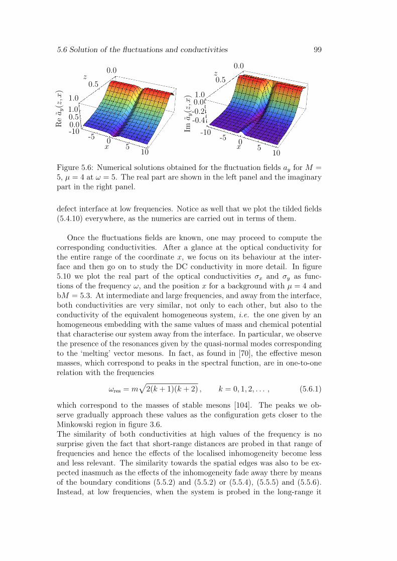
5.6 Solution of the fluctuations and conductivities 99

-10-5

05

10x

1.0

0.5

0.0

1.0

0.00.5

z

Reay(z,x

)

-10-5

05

10x

1.0

0.5

0.0

-0.20.0

z

Imay(z,x

)

-0.4

Figure 5.6: Numerical solutions obtained for the fluctuation fields ay for M =5, µ = 4 at ω = 5. The real part are shown in the left panel and the imaginarypart in the right panel.

defect interface at low frequencies. Notice as well that we plot the tilded fields(5.4.10) everywhere, as the numerics are carried out in terms of them.

Once the fluctuations fields are known, one may proceed to compute thecorresponding conductivities. After a glance at the optical conductivity forthe entire range of the coordinate x, we focus on its behaviour at the inter-face and then go on to study the DC conductivity in more detail. In figure5.10 we plot the real part of the optical conductivities σx and σy as func-tions of the frequency ω, and the position x for a background with µ = 4 andbM = 5.3. At intermediate and large frequencies, and away from the interface,both conductivities are very similar, not only to each other, but also to theconductivity of the equivalent homogeneous system, i.e. the one given by anhomogeneous embedding with the same values of mass and chemical potentialthat characterise our system away from the interface. In particular, we observethe presence of the resonances given by the quasi-normal modes correspondingto the ‘melting’ vector mesons. In fact, as found in [70], the effective mesonmasses, which correspond to peaks in the spectral function, are in one-to-onerelation with the frequencies

ωres = m√

2(k + 1)(k + 2) , k = 0, 1, 2, . . . , (5.6.1)

which correspond to the masses of stable mesons [104]. The peaks we ob-serve gradually approach these values as the configuration gets closer to theMinkowski region in figure 3.6.The similarity of both conductivities at high values of the frequency is nosurprise given the fact that short-range distances are probed in that range offrequencies and hence the effects of the localised inhomogeneity become lessand less relevant. The similarity towards the spatial edges was also to be ex-pected inasmuch as the effects of the inhomogeneity fade away there by meansof the boundary conditions (5.5.2) and (5.5.2) or (5.5.4), (5.5.5) and (5.5.6).Instead, at low frequencies, when the system is probed in the long-range it

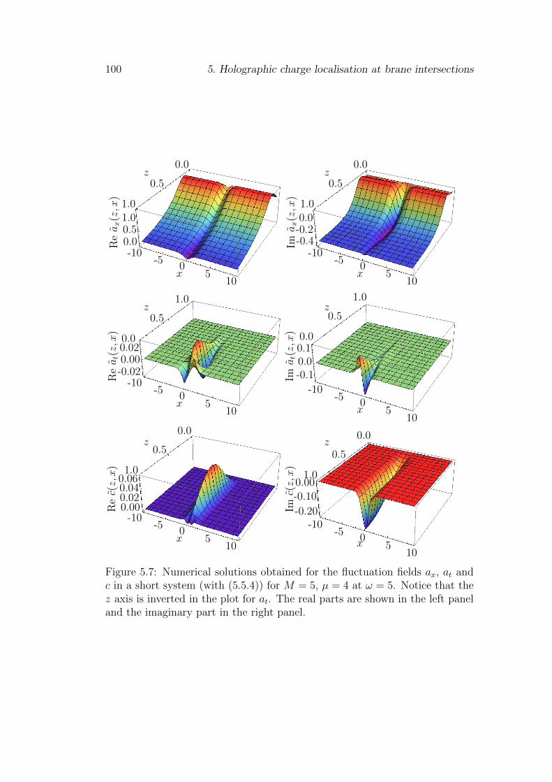
100 5. Holographic charge localisation at brane intersections

-10-5

05

10x

1.0

0.5

0.0

0.00.51.0

z

Reax(z,x

)

-10-5

05

10x

1.0

0.5

0.0

-0.4-0.20.0

z

Imax(z,x

)

-10-5

05

10x

1.0

0.5

0.0

0.000.020.040.06

z

Rec(z,x

)

-10-5

05

10x

0.0

0.5

1.0

-0.020.000.02

z

Reat(z,x

)

-10-5

05

10x

0.0

0.5

1.0

-0.10.00.1

z

Imat(z,x

)

-10-5

05

10x

1.0

0.5

0.0z

Imc(z,x

)

-0.20

-0.10

0.00

Figure 5.7: Numerical solutions obtained for the fluctuation fields ax, at andc in a short system (with (5.5.4)) for M = 5, µ = 4 at ω = 5. Notice that thez axis is inverted in the plot for at. The real parts are shown in the left paneland the imaginary part in the right panel.

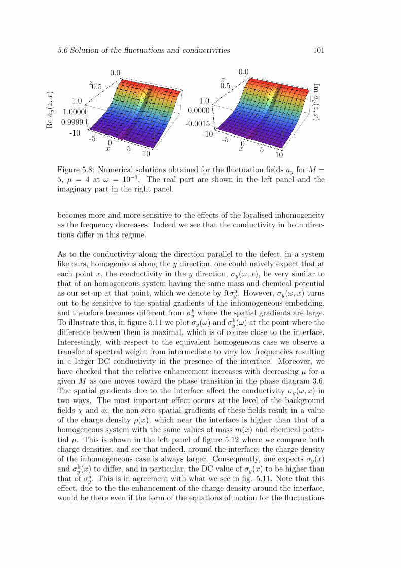
5.6 Solution of the fluctuations and conductivities 101

-10-5

05

10x

1.0

0.5

0.0

1.0000

0.9999

z

Reay(z,x

)

-10-5

05

10x

1.0

0.5

0.0

0.0000

z Imay (z,x

)

-0.0015

Figure 5.8: Numerical solutions obtained for the fluctuation fields ay for M =5, µ = 4 at ω = 10−3. The real part are shown in the left panel and theimaginary part in the right panel.

becomes more and more sensitive to the effects of the localised inhomogeneityas the frequency decreases. Indeed we see that the conductivity in both direc-tions differ in this regime.

As to the conductivity along the direction parallel to the defect, in a systemlike ours, homogeneous along the y direction, one could naively expect that ateach point x, the conductivity in the y direction, σy(ω, x), be very similar tothat of an homogeneous system having the same mass and chemical potentialas our set-up at that point, which we denote by ftσh

y . However, σy(ω, x) turnsout to be sensitive to the spatial gradients of the inhomogeneous embedding,and therefore becomes different from σh

y where the spatial gradients are large.To illustrate this, in figure 5.11 we plot σy(ω) and σh

y (ω) at the point where thedifference between them is maximal, which is of course close to the interface.Interestingly, with respect to the equivalent homogeneous case we observe atransfer of spectral weight from intermediate to very low frequencies resultingin a larger DC conductivity in the presence of the interface. Moreover, wehave checked that the relative enhancement increases with decreasing µ for agiven M as one moves toward the phase transition in the phase diagram 3.6.The spatial gradients due to the interface affect the conductivity σy(ω, x) intwo ways. The most important effect occurs at the level of the backgroundfields χ and φ: the non-zero spatial gradients of these fields result in a valueof the charge density ρ(x), which near the interface is higher than that of ahomogeneous system with the same values of mass m(x) and chemical poten-tial µ. This is shown in the left panel of figure 5.12 where we compare bothcharge densities, and see that indeed, around the interface, the charge densityof the inhomogeneous case is always larger. Consequently, one expects σy(x)and σh

y (x) to differ, and in particular, the DC value of σy(x) to be higher thanthat of σh

y . This is in agreement with what we see in fig. 5.11. Note that thiseffect, due to the the enhancement of the charge density around the interface,would be there even if the form of the equations of motion for the fluctuations

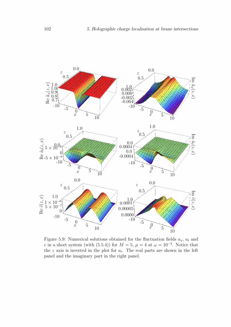
102 5. Holographic charge localisation at brane intersections

-10-5

05

10x

1.0

0.5

0.0

1.0

0.70.80.9

z

Reax(z,x

)

-10-5

05

10x

1.0

0.5

0.0

-0.0020.0000.002

z

Imax (z,x

)

-0.004

-10-5

05

10x

1.0

0.5

0.0

05× 10−71× 10−6

z

Rec(z,x

)

-10-5

05

10x

0.0

0.5

1.0

-5× 10−60

5× 10−6

z

Reat(z,x

)

-10-5

05

10x

0.0

0.5

1.0

-0.00040.0

0.0004

z Imat (z,x

)

-10-5

05

10x

1.0

0.5

0.0z

Imc(z,x

)

0.0000

0.000050.0001

Figure 5.9: Numerical solutions obtained for the fluctuation fields ax, at andc in a short system (with (5.5.4)) for M = 5, µ = 4 at ω = 10−3. Notice thatthe z axis is inverted in the plot for at. The real parts are shown in the leftpanel and the imaginary part in the right panel.

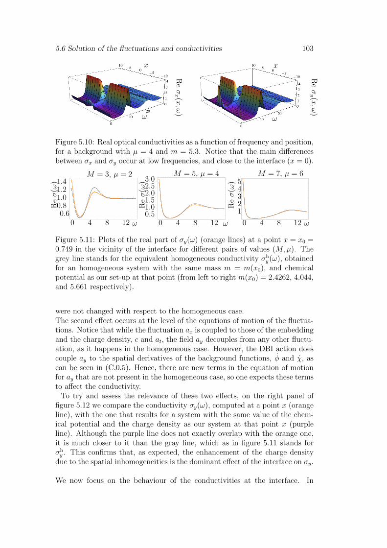
5.6 Solution of the fluctuations and conductivities 103

x

Reσx (x

,ω)

ω

x

ω

Reσy (x

,ω)

Figure 5.10: Real optical conductivities as a function of frequency and position,for a background with µ = 4 and m = 5.3. Notice that the main differencesbetween σx and σy occur at low frequencies, and close to the interface (x = 0).

0 4 8 12

12345

0 4 8 120.51.01.52.02.53.0

Reσ

(ω)

0 4 8 120.6

0.81.01.21.4

Reσ

(ω)

Reσ

(ω)

M = 3, µ = 2 M = 7, µ = 6M = 5, µ = 4

ω ω ω

Figure 5.11: Plots of the real part of σy(ω) (orange lines) at a point x = x0 =0.749 in the vicinity of the interface for different pairs of values (M,µ). Thegrey line stands for the equivalent homogeneous conductivity σh

y (ω), obtainedfor an homogeneous system with the same mass m = m(x0), and chemicalpotential as our set-up at that point (from left to right m(x0) = 2.4262, 4.044,and 5.661 respectively).

were not changed with respect to the homogeneous case.The second effect occurs at the level of the equations of motion of the fluctua-tions. Notice that while the fluctuation ax is coupled to those of the embeddingand the charge density, c and at, the field ay decouples from any other fluctu-ation, as it happens in the homogeneous case. However, the DBI action doescouple ay to the spatial derivatives of the background functions, φ and χ, ascan be seen in (C.0.5). Hence, there are new terms in the equation of motionfor ay that are not present in the homogeneous case, so one expects these termsto affect the conductivity.

To try and assess the relevance of these two effects, on the right panel offigure 5.12 we compare the conductivity σy(ω), computed at a point x (orangeline), with the one that results for a system with the same value of the chem-ical potential and the charge density as our system at that point x (purpleline). Although the purple line does not exactly overlap with the orange one,it is much closer to it than the gray line, which as in figure 5.11 stands forσhy . This confirms that, as expected, the enhancement of the charge density

due to the spatial inhomogeneities is the dominant effect of the interface on σy.

We now focus on the behaviour of the conductivities at the interface. In

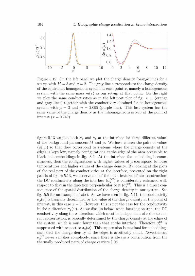
104 5. Holographic charge localisation at brane intersections

0 2 4 6 8 10 12

0.6

0.8

1.0

1.2

1.4

ω

Reσ

(ω)

-10 -5 0 5 10

2.0

2.5

3.0

x

ρ(x

)/T

2

Figure 5.12: On the left panel we plot the charge density (orange line) for aset-up with M = 3 and µ = 2. The gray line corresponds to the charge densityof the equivalent homogeneous system at each point x, namely a homogeneoussystem with the same mass m(x) as our set-up at that point. On the rightwe plot the same conductivities as in the leftmost plot of fig. 5.11 (orangeand gray lines) together with the conductivity obtained for an homogeneoussystem with µ = 3 and m = 2.095 (purple line). This last system has thesame value of the charge density as the inhomogeneous set-up at the point ofinterest (x = 0.749).

figure 5.13 we plot both σx and σy at the interface for three different valuesof the background parameters M and µ. We have chosen the pairs of values(M,µ) so that they correspond to systems where the charge density at theedges is kept low, namely configurations at the edge of the area accessible toblack hole embeddings in fig. 3.6. At the interface the embedding becomesmassless, thus the configurations with higher values of µ correspond to lowertemperatures and higher values of the charge density. By looking at the plotsof the real part of the conductivities at the interface, presented on the rightpanels of figure 5.13, we observe one of the main features of our construction:the DC conductivity along the interface (σDC

y ) is considerably enhanced withrespect to that in the direction perpendicular to it (σDC

x ). This is a direct con-sequence of the spatial distribution of the charge density in our system. Seefig. 5.5 for an example of ρ(x). As we have seen in fig. 5.11, the conductivityσy(ω) is basically determined by the value of the charge density at the point ofinterest, in this case x = 0. However, this is not the case for the conductivityin the x direction σx(ω). As we discuss below, when focusing on σDC

x , the DCconductivity along the x direction, which must be independent of x due to cur-rent conservation, is basically determined by the charge density at the edges ofthe system, which is much lower than that at the interface. Therefore σDC

x issuppressed with respect to σy(ω). This suppression is maximal for embeddingssuch that the charge density at the edges is arbitrarily small. Nevertheless,σDCx never vanishes completely, since there is always a contribution from the

thermally produced pairs of charge carriers [105].

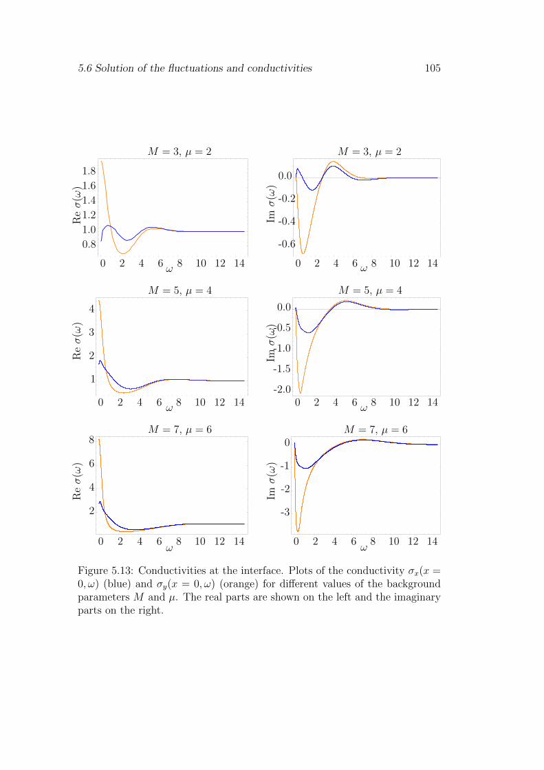
5.6 Solution of the fluctuations and conductivities 105

0 2 4 6 8 10 12 14

-3

-2

-1

0

ω ω

Reσ

(ω)

Imσ

(ω)

0 2 4 6 8 10 12 14

2

4

6

8

ω ω

Reσ

(ω)

Imσ

(ω)

0 2 4 6 8 10 12 14-2.0

-1.5

-1.0

-0.5

0.0

0 2 4 6 8 10 12 14

1

2

3

4

ω ω

Reσ

(ω)

Imσ

(ω)

0 2 4 6 8 10 12 14

-0.6

-0.4

-0.2

0.0

0 2 4 6 8 10 12 14

0.8

1.0

1.2

1.4

1.6

1.8

M = 3, µ = 2 M = 3, µ = 2

M = 5, µ = 4

M = 7, µ = 6

M = 5, µ = 4

M = 7, µ = 6

Figure 5.13: Conductivities at the interface. Plots of the conductivity σx(x =0, ω) (blue) and σy(x = 0, ω) (orange) for different values of the backgroundparameters M and µ. The real parts are shown on the left and the imaginaryparts on the right.

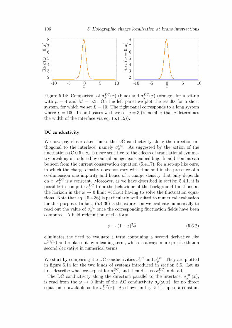
106 5. Holographic charge localisation at brane intersections

-10 -5 0 5 10

2

3

4

5

6

7

8

x x

Reσ

(ω=

0,x

)

Reσ

(ω=

0,x

)

-10 -5 0 5 10

2

3

4

5

6

7

8

Figure 5.14: Comparison of σDCx (x) (blue) and σDCy (x) (orange) for a set-upwith µ = 4 and M = 5.3. On the left panel we plot the results for a shortsystem, for which we set L = 10. The right panel corresponds to a long systemwhere L = 100. In both cases we have set a = 3 (remember that a determinesthe width of the interface via eq. (5.1.12)).

DC conductivity

We now pay closer attention to the DC conductivity along the direction or-thogonal to the interface, namely σDC

x . As suggested by the action of thefluctuations (C.0.5), σx is more sensitive to the effects of translational symme-try breaking introduced by our inhomogeneous embedding. In addition, as canbe seen from the current conservation equation (5.4.17), for a set-up like ours,in which the charge density does not vary with time and in the presence of aco-dimension one impurity and hence of a charge density that only dependson x, σDC

x is a constant. Moreover, as we have described in section 5.4.1, it ispossible to compute σDC

x from the behaviour of the background functions atthe horizon in the ω → 0 limit without having to solve the fluctuation equa-tions. Note that eq. (5.4.36) is particularly well suited to numerical evaluationfor this purpose. In fact, (5.4.36) is the expression we evaluate numerically toread out the value of σDC

x once the corresponding fluctuation fields have beencomputed. A field redefinition of the form

φ→ (1− z)2φ (5.6.2)

eliminates the need to evaluate a term containing a second derivative likea(2)(x) and replaces it by a leading term, which is always more precise than asecond derivative in numerical terms.

We start by comparing the DC conductivities σDCx and σDC

y . They are plottedin figure 5.14 for the two kinds of systems introduced in section 5.5. Let usfirst describe what we expect for σDC

y , and then discuss σDCx in detail.

The DC conductivity along the direction parallel to the interface, σDCy (x),

is read from the ω → 0 limit of the AC conductivity σy(ω, x), for no directequation is available as for σDC

x (x). As shown in fig. 5.11, up to a constant

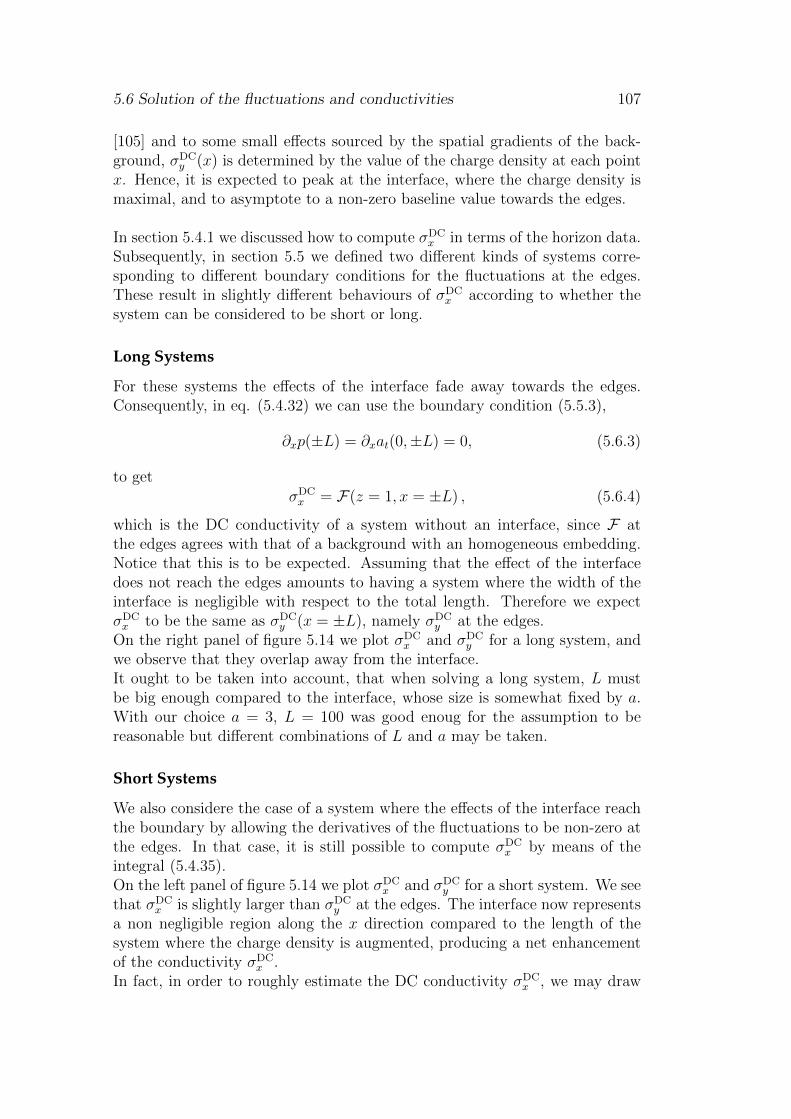
5.6 Solution of the fluctuations and conductivities 107

[105] and to some small effects sourced by the spatial gradients of the back-ground, σDC

y (x) is determined by the value of the charge density at each pointx. Hence, it is expected to peak at the interface, where the charge density ismaximal, and to asymptote to a non-zero baseline value towards the edges.

In section 5.4.1 we discussed how to compute σDCx in terms of the horizon data.

Subsequently, in section 5.5 we defined two different kinds of systems corre-sponding to different boundary conditions for the fluctuations at the edges.These result in slightly different behaviours of σDC

x according to whether thesystem can be considered to be short or long.

Long Systems

For these systems the effects of the interface fade away towards the edges.Consequently, in eq. (5.4.32) we can use the boundary condition (5.5.3),

∂xp(±L) = ∂xat(0,±L) = 0, (5.6.3)

to getσDCx = F(z = 1, x = ±L) , (5.6.4)

which is the DC conductivity of a system without an interface, since F atthe edges agrees with that of a background with an homogeneous embedding.Notice that this is to be expected. Assuming that the effect of the interfacedoes not reach the edges amounts to having a system where the width of theinterface is negligible with respect to the total length. Therefore we expectσDCx to be the same as σDC

y (x = ±L), namely σDCy at the edges.

On the right panel of figure 5.14 we plot σDCx and σDC

y for a long system, andwe observe that they overlap away from the interface.It ought to be taken into account, that when solving a long system, L mustbe big enough compared to the interface, whose size is somewhat fixed by a.With our choice a = 3, L = 100 was good enoug for the assumption to bereasonable but different combinations of L and a may be taken.

Short Systems

We also considere the case of a system where the effects of the interface reachthe boundary by allowing the derivatives of the fluctuations to be non-zero atthe edges. In that case, it is still possible to compute σDC

x by means of theintegral (5.4.35).On the left panel of figure 5.14 we plot σDC

x and σDCy for a short system. We see

that σDCx is slightly larger than σDC

y at the edges. The interface now representsa non negligible region along the x direction compared to the length of thesystem where the charge density is augmented, producing a net enhancementof the conductivity σDC

x .In fact, in order to roughly estimate the DC conductivity σDC

x , we may draw

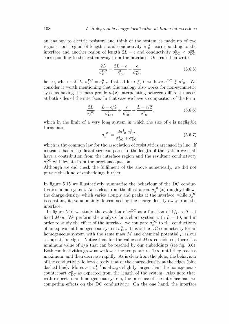
108 5. Holographic charge localisation at brane intersections

an analogy to electric resistors and think of the system as made up of tworegions: one region of length ε and conductivity σint

DC, corresponding to theinterface and another region of length 2L − ε and conductivity σ0

DC < σintDC,

corresponding to the system away from the interface. One can then write

2L

σDCx

=2L− εσ0

DC

+ε

σintDC

(5.6.5)

hence, when ε L, σDCx = σ0

DC. Instead for ε . L we have σDCx & σ0

DC. Weconsider it worth mentioning that this analogy also works for non-symmetricsystems having the mass profile m(x) interpolating between different massesat both sides of the interface. In that case we have a composition of the form

2L

σDCx

=L− ε/2σ1

DC

+ε

σintDC

+L− ε/2σ2

DC

, (5.6.6)

which in the limit of a very long system in which the size of ε is negligibleturns into

σDCx =

2σ1DCσ

2DC

σ1DC + σ2

DC

, (5.6.7)

which is the common law for the association of resistivities arranged in line. Ifinstead ε has a significant size compared to the length of the system we shallhave a contribution from the interface region and the resultant conductivityσDCx will deviate from the previous equation.

Although we did check the fulfilment of the above numerically, we did notpursue this kind of embeddings further.

In figure 5.15 we illustratively summarise the behaviour of the DC conduc-tivities in our system. As is clear from the illustration, σDC

y (x) roughly followsthe charge density, which varies along x and peaks at the interface, while σDC

x

is constant, its value mainly determined by the charge density away from theinterface.

In figure 5.16 we study the evolution of σDCx as a function of 1/µ ∝ T , at

fixed M/µ. We perform the analysis for a short system with L = 10, and inorder to study the effect of the interface, we compare σDC

x to the conductivityof an equivalent homogeneous system σ0

DC. This is the DC conductivity for anhomogeneous system with the same mass M and chemical potential µ as ourset-up at its edges. Notice that for the values of M/µ considered, there is aminimum value of 1/µ that can be reached by our embeddings (see fig. 3.6).Both conductivities grow as we lower the temperature, 1/µ, until they reach amaximum, and then decrease rapidly. As is clear from the plots, the behaviourof the conductivity follows closely that of the charge density at the edges (bluedashed line). Moreover, σDC

x is always slightly larger than the homogeneouscounterpart σ0

DC as expected from the length of the system. Also note that,with respect to an homogeneous system, the presence of the interface has twocompeting effects on the DC conductivity. On the one hand, the interface

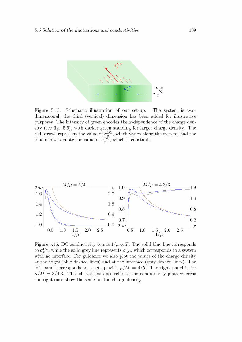
5.6 Solution of the fluctuations and conductivities 109

σDCy

σDCx y

x

Figure 5.15: Schematic illustration of our set-up. The system is two-dimensional; the third (vertical) dimension has been added for illustrativepurposes. The intensity of green encodes the x-dependence of the charge den-sity (see fig. 5.5), with darker green standing for larger charge density. Thered arrows represent the value of σDC

y , which varies along the system, and theblue arrows denote the value of σDC

x , which is constant.

M/µ = 5/4 M/µ = 4.3/3

σDC ρ

σDC ρ

1.6

1.4

1.2

1.00.5 1.0 1.5 2.0 2.5

1/µ

2.7

1.8

0.9

0.0

1/µ0.5 1.0 1.5 2.0 2.5

1.0

0.9

0.8

0.7

1.9

1.3

0.8

0.2

Figure 5.16: DC conductivity versus 1/µ ∝ T . The solid blue line correspondsto σDC

x , while the solid grey line represents σ0DC, which corresponds to a system

with no interface. For guidance we also plot the values of the charge densityat the edges (blue dashed lines) and at the interface (gray dashed lines). Theleft panel corresponds to a set-up with µ/M = 4/5. The right panel is forµ/M = 3/4.3. The left vertical axes refer to the conductivity plots whereasthe right ones show the scale for the charge density.

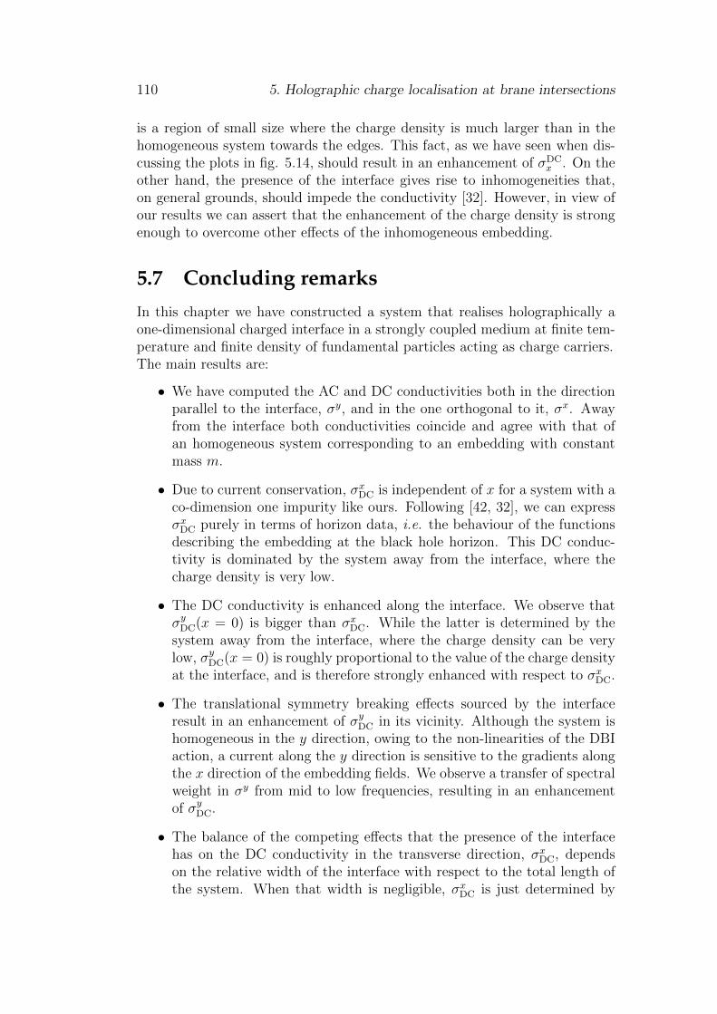
110 5. Holographic charge localisation at brane intersections

is a region of small size where the charge density is much larger than in thehomogeneous system towards the edges. This fact, as we have seen when dis-cussing the plots in fig. 5.14, should result in an enhancement of σDC

x . On theother hand, the presence of the interface gives rise to inhomogeneities that,on general grounds, should impede the conductivity [32]. However, in view ofour results we can assert that the enhancement of the charge density is strongenough to overcome other effects of the inhomogeneous embedding.

5.7 Concluding remarksIn this chapter we have constructed a system that realises holographically aone-dimensional charged interface in a strongly coupled medium at finite tem-perature and finite density of fundamental particles acting as charge carriers.The main results are:

• We have computed the AC and DC conductivities both in the directionparallel to the interface, σy, and in the one orthogonal to it, σx. Awayfrom the interface both conductivities coincide and agree with that ofan homogeneous system corresponding to an embedding with constantmass m.

• Due to current conservation, σxDC is independent of x for a system with aco-dimension one impurity like ours. Following [42, 32], we can expressσxDC purely in terms of horizon data, i.e. the behaviour of the functionsdescribing the embedding at the black hole horizon. This DC conduc-tivity is dominated by the system away from the interface, where thecharge density is very low.

• The DC conductivity is enhanced along the interface. We observe thatσyDC(x = 0) is bigger than σxDC. While the latter is determined by thesystem away from the interface, where the charge density can be verylow, σyDC(x = 0) is roughly proportional to the value of the charge densityat the interface, and is therefore strongly enhanced with respect to σxDC.

• The translational symmetry breaking effects sourced by the interfaceresult in an enhancement of σyDC in its vicinity. Although the system ishomogeneous in the y direction, owing to the non-linearities of the DBIaction, a current along the y direction is sensitive to the gradients alongthe x direction of the embedding fields. We observe a transfer of spectralweight in σy from mid to low frequencies, resulting in an enhancementof σyDC.

• The balance of the competing effects that the presence of the interfacehas on the DC conductivity in the transverse direction, σxDC, dependson the relative width of the interface with respect to the total length ofthe system. When that width is negligible, σxDC is just determined by

5.7 Concluding remarks 111

the homogeneous system away from the interface. On the other hand,when the interface has a sizeable width, it enhances σxDC. The interfaceintroduces two competing effects: an increase of the charge density onthe one hand and the presence of inhomogeneities along x on the other.Although, as discussed in [32], these inhomogeneities should suppress theconductivity, we observe that the interface always produces an increaseof σxDC with respect to an embedding with constant mass m.

112 5. Holographic charge localisation at brane intersections

Chapter 6Holographic charged disorder at braneintersections

In the previous chapter we used the material presented in chapters 3 and 4to solve real cases of holographic systems in which translation invariance isbroken in one of the boundary directions, which we usually call x. There, itwas the presence of a kink profile which introduced a localised inhomogene-ity and hence broke translational symmetry having notable effects on physicalvariables like the conductivities. In this chapter, we want to build on what wasmade in the previous one but instead of dealing with localised inhomogeneitieswe turn our attention to de-localised random disorder or noise.

In realistic condensed matter systems disorder plays an eminent part. If itis sufficiently pronounced it may lead to the localised of electron wavefunc-tions in a metal, thereby suppressing the conductivity. Such a phenomenon isknown as Anderson localisation and Anderson metal-insulator phase transition[106, 107, 108, 109], see [110] for a review.Given the difficulties inherent to disorder, there is still no theoretical full con-trol of many aspects of it. In particular, very little is known about disorderat strong coupling. AdS/CFT again provides a natural framework to studysuch systems, given that it gives us access to that regime via a weakly coupledtheory of gravity. It is therefore interesting to learn how to model disorder inan holographic way so as to better understand how strongly coupled systemsbehave in its presence.

In this chapter, based on the author’s work [44] we adapt the set up of chap-ter 5 ([43]) to the inclusion of random noise. Again, we consider a top-downmodel involving a D5 probe brane. The embedding is now exactly the sameone presented in 5.1. In particular equations (5.1.1) to (5.1.11) apply hereexactly as they are. The difference lies within the way in which we introduceinhomogeneities. We now wish to study the effect of impurities, whose pres-ence we incorporate by means of a random spatial dependence in the chemical

113

114 6. Holographic charged disorder at brane intersections

potential. We do this inspired by previous works in the context of supercon-ductors in [27, 28]. Given that the chemical potential defines the local energyof the charge carriers, such a construction mimics the disorder in their local en-ergy and reproduces better the physics of real materials [28]. With this systemwe study the effects of the noise upon the charge density and the conductivities

The behaviour of the conductivity in 2+1 dimensional disordered systems likeours was analysed from an AdS/CFT perspective by means of D-brane probesystems in [32]. The conclusion was drawn there, that random disorder in thecharge density increases the conductivity at high temperature and suppressesit as the temperature goes down. We compare our results to this predictionand find good qualitative agreement.Our studies are furthermore motivated by attempts within condensed mat-ter physics to better understand the transport properties of graphene in thepresence of charged impurities. Graphene is a natural material to refer towhen dealing with the transport properties of strongly coupled materials. Atlow energies, it is described by a relativistic theory in 2+1 dimensions with achemical potential and its dynamics can be reproduced holographically [33].The current models for graphene in condensed matter theory transport theoriesare not universally accepted, nor do they provide an explanation to all exper-imental observations. The improvement of the existing models for graphene istherefore a relevant goal in condensed matter physics given its theoretical andtechnological interest.One of the most studied properties of graphene is its electrical conductivity asa function of the applied gate voltage, which is directly related to the carrierdensity [34]. In [35, 36], different models were presented to account for theeffect of spatially correlated impurity disorder in two-dimensional graphenelayers upon the dependence between the charge density and the conductivity.Here we also pay attention to this dependence between the charge density andthe conductivity and compare our results with the ones in the cited works.

6.1 Introducing disorder

As in chapter 5, the solutions to the background equations of motion are char-acterised by two parameters, the chemical potential µ and the mass m. There,we chose a spatially varying step-like mass profile m(x) while the chemicalpotential was kept constant. In this case, we work with a constant mass anda spatially varying chemical potential µ which contains the disorder. So as tomimic the random on-site potential use by Anderson in [106], we introduce achemical potential of the form used in [28]

µ(x) = µ0 +µ0

25w

k∗∑k=k0

cos(k x+ δk) , (6.1.1)

6.1 Introducing disorder 115

with δk being a random phase for each wave number k, and w a parameterthat determines the strength of the disorder. The factor of 1/25 is chosen forconvenience to guarantee that the noise oscillates moderately around the meanvalue µ0. In the limit of a large number of modes a noise of this form tends toa Gaussian distributed random function [28]. In figure 6.1 we show differentrealizations of (6.1.1) for different choices of k∗ and w. Broadly speaking, thedisorder strength w regulates the amplitude of the noise, whereas the numberof modes in the sum, given by k∗, somewhat determines how smooth the noiseis. Note though, that both parameters have an influence upon the final formof the noise.As pointed out in [28], this choice of the noise corresponds to a low correlation,which from a condensed matter perspective is more realistic. In particular thecorrelation function of (6.1.1) is given by

〈µ(x)µ(0)〉 − µ20 =

k∗∑k=k0

cos(kx) = Re

(eik0x

ei(k∗−k0+1)x − 1

eix − 1

), (6.1.2)

so the correlation length can be seen to be inversely proportional to the num-ber of modes included in the sum in (6.1.1), which is determined by k∗.

As opposed to the situation in the previous chapter, nothing prevents us herefrom using periodic boundary conditions along the x direction. Indeed thispossibility is already suggested by the form of (6.1.1). So in the discrete gridof collocation points in that direction, the wave numbers k take values

kn =2π

Lx(n+ 1) with 0 ≤ n < Nx − 2 =

k∗k0

, (6.1.3)

where the upper limit of Nx − 1 is explained by the fact that the N thx grid

point is actually equivalent to the 1st one by virtue of the periodic boundarycondition. k0 is the minimum wavenumber and k∗ the maximum wavenumberat which we truncate the sum. k∗ can be at most the so-called Nyquist limit,which signals half the highest frequency that can be reconstructed from a givensample, namely, that at which aliasing sets in. In our case, this limit is givenby

kNyquist =π

Lx(Nx − 1), (6.1.4)

Henceforth we characterise the noise by the choice of w and of κ, by which thefraction of kNiquist in k∗ is meant

κ =k∗

kNyquist. (6.1.5)

Again, as explained in section 5.1.1, we will restrict ourselves to the region ofthe diagram 3.6 corresponding to the black hole embeddings. Furthermore,the massless case is treated separately given the additional simplicity it offers.

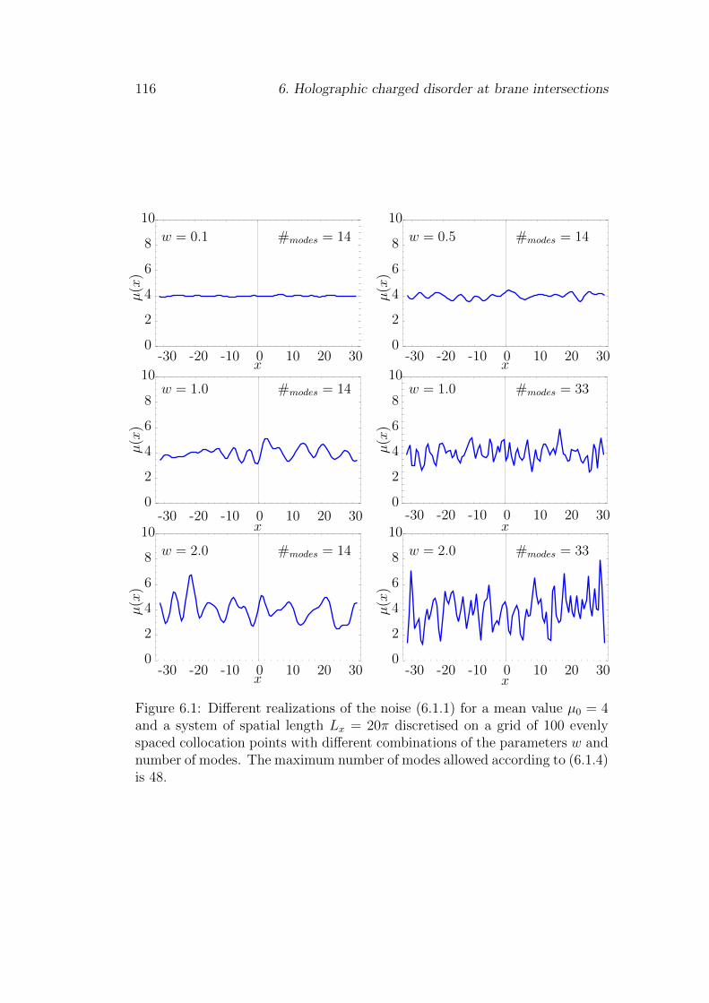
116 6. Holographic charged disorder at brane intersections

-30 -20 -10 0 10 20 300

2

4

6

8

10

x

µ(x

)

-30 -20 -10 0 10 20 30

-30 -20 -10 0 10 20 30

-30 -20 -10 0 10 20 30

-30 -20 -10 0 10 20 30

-30 -20 -10 0 10 20 30xx

xx

x

0

2

4

6

8

10

0

2

4

6

8

10

0

2

4

6

8

10

0

2

4

6

8

10

0

2

4

6

8

10

µ(x

)µ

(x)

µ(x

)µ

(x)

µ(x

)

w = 0.1 #modes = 14 #modes = 14

#modes = 14

#modes = 14 #modes = 33

#modes = 33

w = 0.5

w = 1.0w = 1.0

w = 2.0 w = 2.0

Figure 6.1: Different realizations of the noise (6.1.1) for a mean value µ0 = 4and a system of spatial length Lx = 20π discretised on a grid of 100 evenlyspaced collocation points with different combinations of the parameters w andnumber of modes. The maximum number of modes allowed according to (6.1.4)is 48.

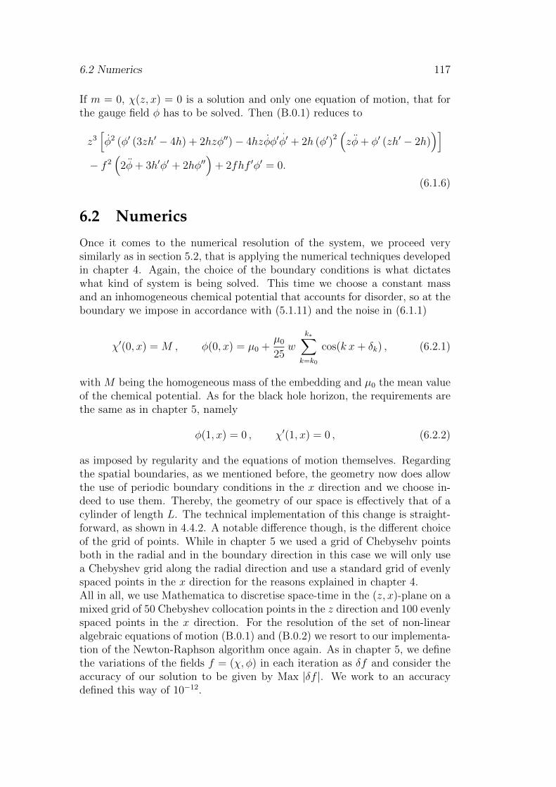
6.2 Numerics 117

If m = 0, χ(z, x) = 0 is a solution and only one equation of motion, that forthe gauge field φ has to be solved. Then (B.0.1) reduces to

z3[φ2 (φ′ (3zh′ − 4h) + 2hzφ′′)− 4hzφφ′

.

φ′ + 2h (φ′)2(zφ+ φ′ (zh′ − 2h)

)]− f 2

(2φ+ 3h′φ′ + 2hφ′′

)+ 2fhf ′φ′ = 0.

(6.1.6)

6.2 Numerics

Once it comes to the numerical resolution of the system, we proceed verysimilarly as in section 5.2, that is applying the numerical techniques developedin chapter 4. Again, the choice of the boundary conditions is what dictateswhat kind of system is being solved. This time we choose a constant massand an inhomogeneous chemical potential that accounts for disorder, so at theboundary we impose in accordance with (5.1.11) and the noise in (6.1.1)

χ′(0, x) = M , φ(0, x) = µ0 +µ0

25w

k∗∑k=k0

cos(k x+ δk) , (6.2.1)

with M being the homogeneous mass of the embedding and µ0 the mean valueof the chemical potential. As for the black hole horizon, the requirements arethe same as in chapter 5, namely

φ(1, x) = 0 , χ′(1, x) = 0 , (6.2.2)

as imposed by regularity and the equations of motion themselves. Regardingthe spatial boundaries, as we mentioned before, the geometry now does allowthe use of periodic boundary conditions in the x direction and we choose in-deed to use them. Thereby, the geometry of our space is effectively that of acylinder of length L. The technical implementation of this change is straight-forward, as shown in 4.4.2. A notable difference though, is the different choiceof the grid of points. While in chapter 5 we used a grid of Chebysehv pointsboth in the radial and in the boundary direction in this case we will only usea Chebyshev grid along the radial direction and use a standard grid of evenlyspaced points in the x direction for the reasons explained in chapter 4.All in all, we use Mathematica to discretise space-time in the (z, x)-plane on amixed grid of 50 Chebyshev collocation points in the z direction and 100 evenlyspaced points in the x direction. For the resolution of the set of non-linearalgebraic equations of motion (B.0.1) and (B.0.2) we resort to our implementa-tion of the Newton-Raphson algorithm once again. As in chapter 5, we definethe variations of the fields f = (χ, φ) in each iteration as δf and consider theaccuracy of our solution to be given by Max |δf |. We work to an accuracydefined this way of 10−12.

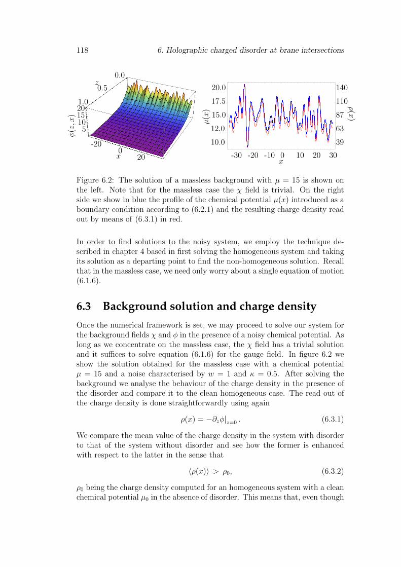
118 6. Holographic charged disorder at brane intersections

-30 -20 -10 0 10 20 30

10.0

12.0

15.0

17.5

20.0

39

63

87

110

140

51015201.0

0.5

0.0

-200

20x

φ(z,x

)

z

µ(x

)

ρ(x

)

x

Figure 6.2: The solution of a massless background with µ = 15 is shown onthe left. Note that for the massless case the χ field is trivial. On the rightside we show in blue the profile of the chemical potential µ(x) introduced as aboundary condition according to (6.2.1) and the resulting charge density readout by means of (6.3.1) in red.

In order to find solutions to the noisy system, we employ the technique de-scribed in chapter 4 based in first solving the homogeneous system and takingits solution as a departing point to find the non-homogeneous solution. Recallthat in the massless case, we need only worry about a single equation of motion(6.1.6).

6.3 Background solution and charge densityOnce the numerical framework is set, we may proceed to solve our system forthe background fields χ and φ in the presence of a noisy chemical potential. Aslong as we concentrate on the massless case, the χ field has a trivial solutionand it suffices to solve equation (6.1.6) for the gauge field. In figure 6.2 weshow the solution obtained for the massless case with a chemical potentialµ = 15 and a noise characterised by w = 1 and κ = 0.5. After solving thebackground we analyse the behaviour of the charge density in the presence ofthe disorder and compare it to the clean homogeneous case. The read out ofthe charge density is done straightforwardly using again

ρ(x) = −∂zφ|z=0 . (6.3.1)

We compare the mean value of the charge density in the system with disorderto that of the system without disorder and see how the former is enhancedwith respect to the latter in the sense that

〈ρ(x)〉 > ρ0, (6.3.2)

ρ0 being the charge density computed for an homogeneous system with a cleanchemical potential µ0 in the absence of disorder. This means that, even though

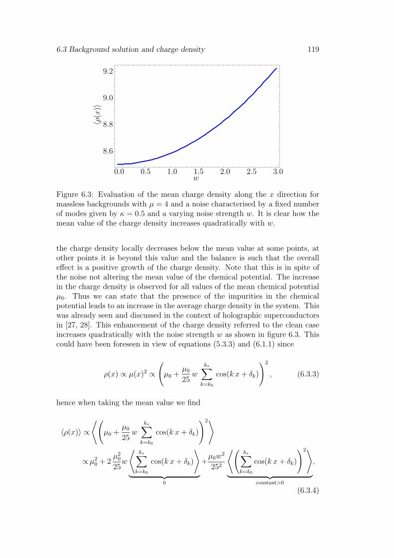
6.3 Background solution and charge density 119

0.0 0.5 1.0 1.5 2.0 2.5 3.0

8.6

8.8

9.0

9.2

w

〈ρ(x

)〉

Figure 6.3: Evaluation of the mean charge density along the x direction formassless backgrounds with µ = 4 and a noise characterised by a fixed numberof modes given by κ = 0.5 and a varying noise strength w. It is clear how themean value of the charge density increases quadratically with w.

the charge density locally decreases below the mean value at some points, atother points it is beyond this value and the balance is such that the overalleffect is a positive growth of the charge density. Note that this is in spite ofthe noise not altering the mean value of the chemical potential. The increasein the charge density is observed for all values of the mean chemical potentialµ0. Thus we can state that the presence of the impurities in the chemicalpotential leads to an increase in the average charge density in the system. Thiswas already seen and discussed in the context of holographic superconductorsin [27, 28]. This enhancement of the charge density referred to the clean caseincreases quadratically with the noise strength w as shown in figure 6.3. Thiscould have been foreseen in view of equations (5.3.3) and (6.1.1) since

ρ(x) ∝ µ(x)2 ∝

(µ0 +

µ0

25w

k∗∑k=k0

cos(k x+ δk)

)2

, (6.3.3)

hence when taking the mean value we find

〈ρ(x)〉 ∝

⟨(µ0 +

µ0

25w

k∗∑k=k0

cos(k x+ δk)

)2⟩

∝µ20 + 2

µ20

25w

⟨k∗∑k=k0

cos(k x+ δk)

⟩︸ ︷︷ ︸

0

+µ0w

2

252

⟨(k∗∑k=k0

cos(k x+ δk)

)2⟩︸ ︷︷ ︸

constant>0

,

(6.3.4)

120 6. Holographic charged disorder at brane intersections

0.0 0.5 1.0 1.5 2.0 2.5 3.0

8.6

8.8

9.0

9.2

9.4

w

〈ρ(x

)〉

Figure 6.4: Same evaluation as in figure 6.3 but comparing the case of differentvalues of κ. In ascending order from the bottom we have κ = 0.3, 0.5, 0.7. Wesee how for a given w, a bigger number of modes in the sum in (6.1.1) leadsto a bigger enhancement of the charge density.

where 〈ρ(x)〉 is the mean value of the charge density averaged over the spatialinterval1. In the last row we have made used of the fact that, since we areintegrating over whole periods of the cosinus present in the sum, the secondterm in the last line of the equation vanishes whereas the last term is a constantdependent on the particular choice of κ. Thus this confirms our observationsbased on figure 6.3 that indeed

〈ρ(x)〉 ∝ w2. (6.3.5)

Moreover, the enhancement of the charge density by the impurities also in-creases with the number of modes included in the sum in (6.1.1), signalledby κ for a given w, as can be seen in figure 6.4. This is understood from aqualitative perspective in the light of figure 6.1. A higher number of modes inthe sum endows the disorder with a peakier structure, thereby increasing theeffect that spatial derivatives play in the corresponding equations of motion.This effect is clearly a net enhancement of the charge density.

Let us now analyse the results obtained in the presence of mass. To see whatthe effects of the mass are upon the different quantities we compare the mass-less case in figure 6.2 to backgrounds with the same chemical potential, µ = 15and finite values of the mass. In figure 6.5 we show for example the solutionobtained for M = 5 as well as the chemical potential introduced in the systemand the resulting charge density distribution. The characterising parameters

1Note that in the computations of averages the last or the first point in the grid isexcluded, since it is respectively equivalent to the first or last point by virtue of the periodicboundary condition.

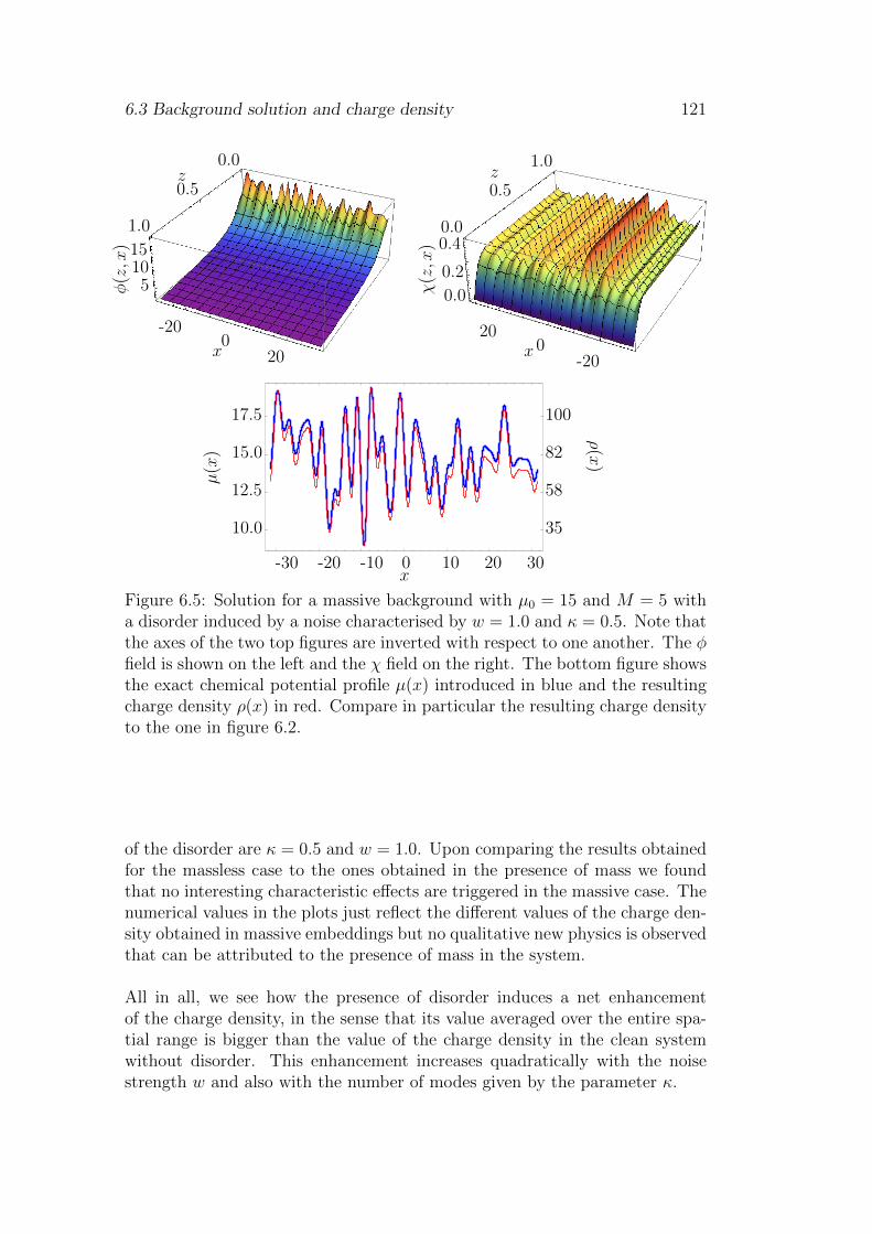
6.3 Background solution and charge density 121

ρ(x

)

µ(x

)

0.4

0.2

0.0

200

-20

1.0

0.0

0.5

x

z

χ(z,x

)

-200

20x

0.0

1.0

0.5z

φ(z,x

) 15105

x-30 -20 -10 0 10 20 30

10.0

12.5

15.0

17.5

35

58

82

100

Figure 6.5: Solution for a massive background with µ0 = 15 and M = 5 witha disorder induced by a noise characterised by w = 1.0 and κ = 0.5. Note thatthe axes of the two top figures are inverted with respect to one another. The φfield is shown on the left and the χ field on the right. The bottom figure showsthe exact chemical potential profile µ(x) introduced in blue and the resultingcharge density ρ(x) in red. Compare in particular the resulting charge densityto the one in figure 6.2.

of the disorder are κ = 0.5 and w = 1.0. Upon comparing the results obtainedfor the massless case to the ones obtained in the presence of mass we foundthat no interesting characteristic effects are triggered in the massive case. Thenumerical values in the plots just reflect the different values of the charge den-sity obtained in massive embeddings but no qualitative new physics is observedthat can be attributed to the presence of mass in the system.

All in all, we see how the presence of disorder induces a net enhancementof the charge density, in the sense that its value averaged over the entire spa-tial range is bigger than the value of the charge density in the clean systemwithout disorder. This enhancement increases quadratically with the noisestrength w and also with the number of modes given by the parameter κ.

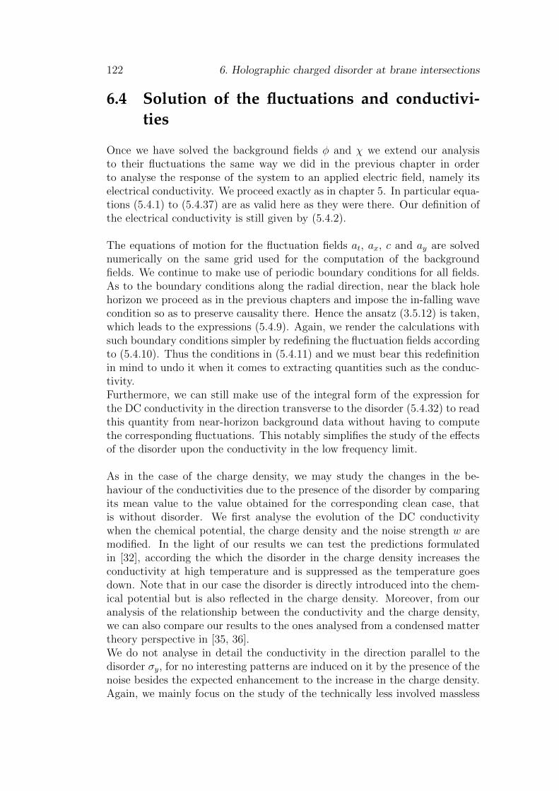
122 6. Holographic charged disorder at brane intersections

6.4 Solution of the fluctuations and conductivi-ties

Once we have solved the background fields φ and χ we extend our analysisto their fluctuations the same way we did in the previous chapter in orderto analyse the response of the system to an applied electric field, namely itselectrical conductivity. We proceed exactly as in chapter 5. In particular equa-tions (5.4.1) to (5.4.37) are as valid here as they were there. Our definition ofthe electrical conductivity is still given by (5.4.2).

The equations of motion for the fluctuation fields at, ax, c and ay are solvednumerically on the same grid used for the computation of the backgroundfields. We continue to make use of periodic boundary conditions for all fields.As to the boundary conditions along the radial direction, near the black holehorizon we proceed as in the previous chapters and impose the in-falling wavecondition so as to preserve causality there. Hence the ansatz (3.5.12) is taken,which leads to the expressions (5.4.9). Again, we render the calculations withsuch boundary conditions simpler by redefining the fluctuation fields accordingto (5.4.10). Thus the conditions in (5.4.11) and we must bear this redefinitionin mind to undo it when it comes to extracting quantities such as the conduc-tivity.Furthermore, we can still make use of the integral form of the expression forthe DC conductivity in the direction transverse to the disorder (5.4.32) to readthis quantity from near-horizon background data without having to computethe corresponding fluctuations. This notably simplifies the study of the effectsof the disorder upon the conductivity in the low frequency limit.

As in the case of the charge density, we may study the changes in the be-haviour of the conductivities due to the presence of the disorder by comparingits mean value to the value obtained for the corresponding clean case, thatis without disorder. We first analyse the evolution of the DC conductivitywhen the chemical potential, the charge density and the noise strength w aremodified. In the light of our results we can test the predictions formulatedin [32], according the which the disorder in the charge density increases theconductivity at high temperature and is suppressed as the temperature goesdown. Note that in our case the disorder is directly introduced into the chem-ical potential but is also reflected in the charge density. Moreover, from ouranalysis of the relationship between the conductivity and the charge density,we can also compare our results to the ones analysed from a condensed mattertheory perspective in [35, 36].We do not analyse in detail the conductivity in the direction parallel to thedisorder σy, for no interesting patterns are induced on it by the presence of thenoise besides the expected enhancement to the increase in the charge density.Again, we mainly focus on the study of the technically less involved massless

6.4 Solution of the fluctuations and conductivities 123

-30 -20 -10 0 10 20 30

1.0

1.2

1.4

1.6

1.8

2.0

x

σDC

(x)

-30 -20 -10 0 10 20 302

4

6

8

10

12

x

σDC

(x)

Figure 6.6: Computed conductivities for two massless backgrounds in whichthe different effect of the disorder upon σDCx is shown. The black line shows theDC conductivity of the corresponding clean system σDC0 . The DC conductivityin the y direction, σDCy , is shown in red and the dashed red line signals its meanvalue. The blue line stands for the constant DC conductivity in the x direction,σDCx . On the left we plot a background with µ = 0.7 and a noise characterisedby w = 5 and κ = 0.5. The noise must be made stronger than elsewhere tomake its effects more visible. Both σDCx and σDCy are over σDC0 . On the rightwe show the situation for µ = 5. Here σDCx is clearly suppressed with respectto σDC0 .

case to observe the effects the disorder has upon the conductivity and thenproceed to analyse the massive case, so that we can appreciate how the pres-ence of mass affects the results.Our analysis of the conductivities does not extend to the AC conductivities,for we have no interesting results to report in these regards. The randomly dis-ordered chemical potential is seen to affect only the low-frequency behaviour ofthe conductivities. This is consistent with the supposition that the extendeddisorder introduced by the noise be only noticed in the low-frequency regimewhen long distance scales are probed.

6.4.1 Effects of charged disorder upon the DC conductivity

The DC conductivity in the direction of the disorder, σDCx can be extractedfrom the IR background data via equation (5.4.35). For information about theDC conductivity in the direction transverse to the disorder, σDCy , the resolutionof the corresponding equation of motion for the fluctuation field ay is neces-sary. From this computations we find that the qualitative effect of the disorderupon the DC conductivities depends on the value of the chemical potential µ.Examples are provided in figure 6.6 for values of the chemical potential ofµ = 0.7 and µ = 5. The disorder always enhances the charge density and theDC conductivity in the y direction compared to the clean homogeneous case.Instead the DC conductivity in the x-direction is suppressed in the first caseand enhanced in the second example.

124 6. Holographic charged disorder at brane intersections

We understand this as a competition between the effect of the enhanced chargedensity on the one side, which lets the conductivities tend to increase and thedirect effects of the gradients in x upon the conductivities. This competitionwas also analysed in chapter 5, see figure 5.11. When the value of the chem-ical potential is low, the enhancement of the charge density seems to be thedominant effect. The fact that σDCx takes the same value as 〈σDCy 〉 reinforcesthis interpretation. Both conductivities are just feeling the enhancement inthe charge density and hence are equally increased from their equal values inthe clean homogeneous embedding. At bigger values of the chemical potentialthe direct effects of the gradients seem to overtake the dominant role and leadto a suppression of σDCx .

The analysis may be extended to a whole range of values of the chemicalpotential. Recalling that, according to (3.4.43)

1

µ∝ T, (6.4.1)

this analysis may be performed sweeping over different values of µ and di-rectly compared to the evolution of the DC conductivity with the temperaturepredicted in [32]. Our results are displayed in figure 6.7. As it can be seenthere, the presence of the noise affects the low-temperature behaviour of theDC conductivity in the x-direction, notably suppressing it with respect to theclean case with no disorder. The suppression furthermore increases with thestrength of the disorder w, as can be visualised in the right panel of figure6.9. This results are physically understood as the disorder causing the chargecarriers trouble to move within the conducting medium. The spatial gradientsdifficult the transport of charge and hence the conductivity.At higher temperatures, we find a range of values of the chemical potential,µ, in which the DC conductivity in the x-direction is over the conductivityof the clean case. This is more difficult to see, for the numerical differenceswith respect to the clean case are small. The effect can be made stronger andhence more visible by increasing the strength of disorder. The correspondingvalues are consistently above the homogeneous clean ones and a monotonousgrowth in this enhancement can be observed when the strength of disorder wis increased. This excludes the possibility that it be due to numerical effects.The situation is illustrated in the left panel of figure 6.9. In the light of thiswe can state that there is a range of µ for which the net effect upon the DCconductivity is an enhancement with respect to the clean case. This is alsoillustrated in figure 6.8, which is equivalent to figure 6.7 but for a strongernoise. The range of the plot is furthermore cut so that the region at which thecrossover from the enhanced to the suppressed conductivity be clearly seen.These results may be compared to the discussion in [32]. There the predictionis formulated, that the DC conductivity should be suppressed with respect tothe clean case below a given temperature while it ought to increase beyondthat temperature. We confirm this expectation in the light of our numerical

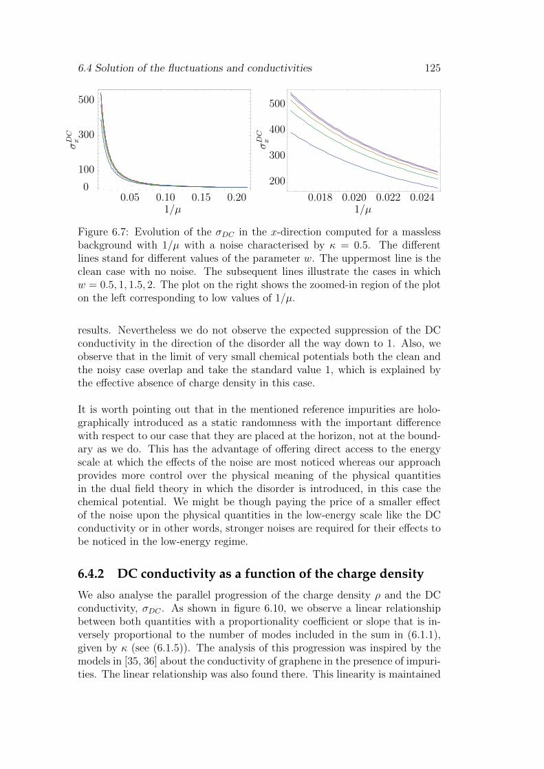
6.4 Solution of the fluctuations and conductivities 125

0.05 0.10 0.15 0.200

100

300

500

1/µ

σDC

x

1/µ

σDC

x

0.018 0.020 0.022 0.024

200

300

400

500

Figure 6.7: Evolution of the σDC in the x-direction computed for a masslessbackground with 1/µ with a noise characterised by κ = 0.5. The differentlines stand for different values of the parameter w. The uppermost line is theclean case with no noise. The subsequent lines illustrate the cases in whichw = 0.5, 1, 1.5, 2. The plot on the right shows the zoomed-in region of the ploton the left corresponding to low values of 1/µ.

results. Nevertheless we do not observe the expected suppression of the DCconductivity in the direction of the disorder all the way down to 1. Also, weobserve that in the limit of very small chemical potentials both the clean andthe noisy case overlap and take the standard value 1, which is explained bythe effective absence of charge density in this case.

It is worth pointing out that in the mentioned reference impurities are holo-graphically introduced as a static randomness with the important differencewith respect to our case that they are placed at the horizon, not at the bound-ary as we do. This has the advantage of offering direct access to the energyscale at which the effects of the noise are most noticed whereas our approachprovides more control over the physical meaning of the physical quantitiesin the dual field theory in which the disorder is introduced, in this case thechemical potential. We might be though paying the price of a smaller effectof the noise upon the physical quantities in the low-energy scale like the DCconductivity or in other words, stronger noises are required for their effects tobe noticed in the low-energy regime.

6.4.2 DC conductivity as a function of the charge density

We also analyse the parallel progression of the charge density ρ and the DCconductivity, σDC . As shown in figure 6.10, we observe a linear relationshipbetween both quantities with a proportionality coefficient or slope that is in-versely proportional to the number of modes included in the sum in (6.1.1),given by κ (see (6.1.5)). The analysis of this progression was inspired by themodels in [35, 36] about the conductivity of graphene in the presence of impuri-ties. The linear relationship was also found there. This linearity is maintained

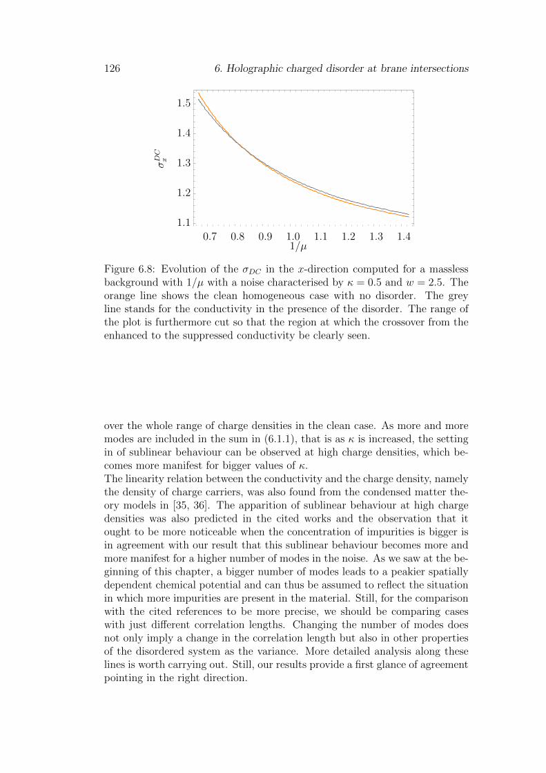
126 6. Holographic charged disorder at brane intersections

0.7 0.8 0.9 1.0 1.1 1.2 1.3 1.4

1.1

1.2

1.3

1.4

1.5

1/µ

σDC

x

Figure 6.8: Evolution of the σDC in the x-direction computed for a masslessbackground with 1/µ with a noise characterised by κ = 0.5 and w = 2.5. Theorange line shows the clean homogeneous case with no disorder. The greyline stands for the conductivity in the presence of the disorder. The range ofthe plot is furthermore cut so that the region at which the crossover from theenhanced to the suppressed conductivity be clearly seen.

over the whole range of charge densities in the clean case. As more and moremodes are included in the sum in (6.1.1), that is as κ is increased, the settingin of sublinear behaviour can be observed at high charge densities, which be-comes more manifest for bigger values of κ.The linearity relation between the conductivity and the charge density, namelythe density of charge carriers, was also found from the condensed matter the-ory models in [35, 36]. The apparition of sublinear behaviour at high chargedensities was also predicted in the cited works and the observation that itought to be more noticeable when the concentration of impurities is bigger isin agreement with our result that this sublinear behaviour becomes more andmore manifest for a higher number of modes in the noise. As we saw at the be-ginning of this chapter, a bigger number of modes leads to a peakier spatiallydependent chemical potential and can thus be assumed to reflect the situationin which more impurities are present in the material. Still, for the comparisonwith the cited references to be more precise, we should be comparing caseswith just different correlation lengths. Changing the number of modes doesnot only imply a change in the correlation length but also in other propertiesof the disordered system as the variance. More detailed analysis along theselines is worth carrying out. Still, our results provide a first glance of agreementpointing in the right direction.

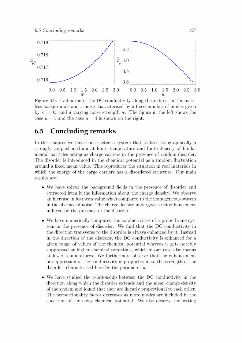
6.5 Concluding remarks 127

0.0 0.5 1.0 1.5 2.0 2.5 3.0

3.6

3.8

4.0

4.2

0.716

0.717

0.718

0.719

0.0 0.5 1.0 1.5 2.0 2.5 3.0w

σDC

x

w

σDC

x

Figure 6.9: Evaluation of the DC conductivity along the x direction for mass-less backgrounds and a noise characterised by a fixed number of modes givenby κ = 0.5 and a varying noise strength w. The figure in the left shows thecase µ = 1 and the case µ = 4 is shown on the right.

6.5 Concluding remarksIn this chapter we have constructed a system that realises holographically astrongly coupled medium at finite temperature and finite density of funda-mental particles acting as charge carriers in the presence of random disorder.The disorder is introduced in the chemical potential as a random fluctuationaround a fixed mean value. This reproduces the situation in real materials inwhich the energy of the carge carriers has a disordered structure. Our mainresults are:

• We have solved the background fields in the presence of disorder andextracted from it the information about the charge density. We observean increase in its mean value when compared to the homogeneous systemin the absence of noise. The charge density undergoes a net enhancementinduced by the presence of the disorder.

• We have numerically computed the conductivities of a probe brane sys-tem in the presence of disorder. We find that the DC conductivity inthe direction transverse to the disorder is always enhanced by it. Insteadin the direction of the disorder, the DC conductivity is enhanced for agiven range of values of the chemical potential whereas it gets notablysuppressed at higher chemical potentials, which in our case also meansat lower temperatures. We furthermore observe that the enhancementor suppression of the conductivity is proportional to the strength of thedisorder, characterised here by the parameter w.

• We have studied the relationship between the DC conductivity in thedirection along which the disorder extends and the mean charge densityof the system and found that they are linearly proportional to each other.The proportionality factor decreases as more modes are included in thespectrum of the noisy chemical potential. We also observe the setting

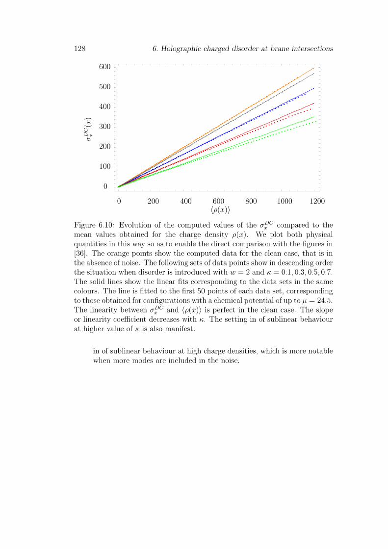
128 6. Holographic charged disorder at brane intersections

0 200 400 600 800 1000 1200

0

100

200

300

400

500

600

〈ρ(x)〉

σDC

x(x

)

Figure 6.10: Evolution of the computed values of the σDCx compared to themean values obtained for the charge density ρ(x). We plot both physicalquantities in this way so as to enable the direct comparison with the figures in[36]. The orange points show the computed data for the clean case, that is inthe absence of noise. The following sets of data points show in descending orderthe situation when disorder is introduced with w = 2 and κ = 0.1, 0.3, 0.5, 0.7.The solid lines show the linear fits corresponding to the data sets in the samecolours. The line is fitted to the first 50 points of each data set, correspondingto those obtained for configurations with a chemical potential of up to µ = 24.5.The linearity between σDCx and 〈ρ(x)〉 is perfect in the clean case. The slopeor linearity coefficient decreases with κ. The setting in of sublinear behaviourat higher value of κ is also manifest.

in of sublinear behaviour at high charge densities, which is more notablewhen more modes are included in the noise.

Chapter 7Conclusion

In this thesis we use gauge/gravity duality and in particular the weak versionof the AdS/CFT correspondence with a large number of colours N →∞ in thegauge theory and a large t’Hooft coupling λ 1 to study phenomena relatedto the presence of inhomogeneities and noise in strongly coupled matter.We are able to do so in spite of the complicated equations of motion arisingthanks to the numerical techniques we present in chapter 4. Details on thecodes employed are given in appendix D.

In chapter 5 we construct a holographic system that realises a (1+1)-dimensionalcharged interface in a strongly coupled medium at finite temperature and finitedensity of fundamental particles acting as charge carriers. We do it by meansof a D5 flavour brane in the probe approximation having a step-like spatiallydependent prifile.From the numerical solutions of the background we obtain the data corre-sponding to the charge density profile. We check that this profile is indeedlocalised around the interface, being around five times larger there than at thespatial edges. The non-vanishing charge density at the spatial edges is dueto our being in a black hole embedding but in principle this could be circum-vented by getting closer and closer to the Minkowski embeddings.The study of the fluctuation fields allows to compute the conductivities of thesystem. The analysis of their behaviour reveals agreement with broad expec-tations for a system with localised charge on a (1+1)-dimensional interface.The effects of the interface are mostly reflected in the low-frequency behaviourof the conductivities. In the direction of the defect, the conductivity is mainlydetermined by the local conditions at the interface. The DC conductivity in-creases its value with respect to the homogeneous case. This is likely to bea characteristic particular to strongly coupled systems, since it is induced bythe form of the DBI action. In the direction transverse to the defect, the DCconductivity is influenced by the global conditions of the system and mostlydetermined by the properties of the system outside the interface. Its valuetherefore decreases with respect to the equivalent homogeneous case.

129

130 7. Conclusion

In chapter 6 we develop a system at finite temperature and finite density offundamental particles that holographically accounts for impurities in the formof random disorder in the chemical potential. The system is a follow-up of theone in chapter 5 and also consists in the use of a D5 flavour brane in the probeapproximation.By numerically solving the background we extract information about the chargedensity of the system and about the effects the disorder has upon it. We ob-serve a net enhancement in the charge density induced by the presence of theimpurities. This enhancement increases quadratically with the strength of thedisorder.From the analysis of the fluctuations we obtain information about the conduc-tivities of the system and the changes in their behaviour due to the disorder.Our analysis reveals that the DC conductivity in the direction along which thedisorder extends is enhanced by the disorder within a given range of temper-atures and is notably suppressed at lower temperatures. We furthermore findthat said suppression increases quadratically with the strength of disorder. Inthe direction transverse to the disorder, the conductivity is always enhancedby the disorder. Our results along these lines are a confirmation of the pre-dictions formulated theoretically by means of the AdS/CFT correspondenceapplied to systems of probe D-branes in [32].We also analyse the relationship between the DC conductivity in the directionalong which the disorder extends and the mean charge density of the systemand find linearity. The coefficient of linearity decreases as the disordered chem-ical potential acquires a rougher spatial structure. Moreover the disorder seemsto lead to a sublinear behaviour at high charge densities. These results showqualitative agreement with predictions formulated within condensed mattertheory models for the transport properties of graphene reproducing experi-mental data [35, 36].

In spite of the limitations introduced by the conditions under which the weakversion of the duality works when it comes to relating our results to real worldphysics, underlying universalities might underpin our predictions. Such uni-versalities have already been unveiled in other holographic studies and shallremain our best hope of a better comprehension of some of the phenomena instrongly coupled matter as long as gauge/gravity duality is not better under-stood beyond the limits of its weak version.

7.1 Outlook

The use of the AdS/CFT correspondence as a tool to explore the stronglycoupled regime of matter in the presence of disorder provides many interestingdirections of research. The projects pursued in this thesis have possible exten-sions and follow-ups, which would not be very difficult to implement once thenumerical techniques we have covered are mastered.

7.1 Outlook 131

For once, the inclusion of topological terms in the action would open the doorto more detailed studies of the physics of topological insulators and the quan-tum Hall effect. This might be done using a D7 probe brane like in [25] butis also possible using a D5-brane, as shown in [26]. The addition of a mag-netic field to the system may also lead to the activation of topological effects,as explored in [111]. Another interesting continuation of our work would bethe use of a system with an interface like the one in chapter 5 to analyse thepredicted fermionic nature of the massless degrees of freedom at the interface.This would require the consideration of fluctuation fields with spatial momen-tum.The project presented in chapter 6 also leaves room for extensions. It wouldbe by all means interesting to study how different realisations of the disorderaffect the properties of the system. The noise could for example be introducedin the IR so as to make the connection to the predictions in [32] even moredirect. Morevoer, the random fluctuations that mimic the impurities in realmaterials could also be introduced in the mass.

There are still plenty of phenomena in condensed matter physics awaiting atheoretical explanation. AdS/CFT shall continue to prove its solidity in theseregards. With the unveiling of new universalities common to strongly coupledfield theories, the domain of applicability of AdS/CFT and its predictive powercould be enhanced. Besides providing a better understanding of the otherwiseinaccessible strongly coupled regime of matter, studies like ours may be pavingthe way to a better command of the duality and hence maybe to an improvedgrasp of string theory.

132 7. Conclusion

Appendix AGroup theory, Lie algebras and highestweights.

Since the very beginning of this thesis, we have been stressing how relevant arole symmetry plays in theoretical physics. Most of the time symmetries arenaturally dealt with by means of mathematical group theory. Group theorycan be considered to be the mathematics of symmetries. In fact, the three keymathematical properties of any symmetry, namely associativity, the existenceof an identity element and of the inverse element are precisely the three defin-ing properties of a group.Both space-time and most of the internal field spaces are considered to have acontinuous and smooth character. This is why high energy physics is mostlyconcerned with symmetries supported on continuous and smooth spaces ormanifolds. It being so, we shall be interested in groups that intrinsically re-flect this fact. These groups are quite well known in mathematics and go underthe name of Lie groups. Lie groups are formally defined as groups which de-pend continuously on one or more parameters. Our treatment of Lie groupsand their representations here focuses on their applicability to gauge theoriesof trivial topology (i.e. without instantons or topological terms), thus we willconcentrate on compact Lie groups, whose general treatment, due to Cartan,Weyl and Dynkin is well developed.In chapter 3, we used the highest weight formalism to analyse the propertiesof irreducible representations of the little group, perform dimensional reduc-tions and tensor products. Here, we wish to present the basics of this formal-ism to the unfamiliar reader. For more information on the topic, we refer to[112, 113, 114].

A group is generally defined in a broad sense accepting different embodimentsin terms of matrices which adjust to the definition. Each of such embodiments,that is, each map from the group elements to a set of matrices acting on a q-dimensional vector space preserving the composition law of the group is calleda representation of the group. From all possible representations there is one

133

134 A. Group theory, Lie algebras and highest weights.

deserving special attention. This is the representation in which the genera-tors of the group are themselves seen as vectors and goes under the name ofadjoint representation. It is spanned by the generators of the group andhence has dimension equal to the number of generators. Since we are dealingwith compact symmetry groups, their representation can be assumed to beunitary. This implies that the corresponding generators can be taken to behermitian. Now from the generators T1, . . . , Tn we pick the maximal set ofmutually commuting elements, H1, . . . , Hm

[Hi, Hj] = 0. (A.0.1)

This is called the Cartan subalgebra and the Hi are the Cartan generators. Agroup with m mutually commuting Cartan generators is said to be of rank m.The m Cartan generators can be diagonalised at a time and their eigenvectorsspan the whole vector space. This means that we may assign a set of meigenvalues or weights, hi, to each state in the vector space

Hi |hi〉 = hi |hi〉 (A.0.2)

Each vector in the space is simultaneously an eigenstate of the m Cartan gen-erators. When referring to the adjoint representation, weights are commonlycalled roots, which we shall denote by αi. Thus the m-component vector ofroots specifies the state uniquely. Actually this is so as long as the eigenstatesare non-degenerate, but this is proven by the fundamental theorem of Cartan.Since the generators form an algebra, they satisfy the Jacobi identity. Thenon-Cartan generators Tm+1, . . . , Tn can be linearly combined into a new setEm+1, . . . , En that satisfies

[Hi, Ej] = αjEj, (A.0.3)

which suffices to assert that the Ei can be interpreted as ladder operators

HE |h〉 = ([H,E] + EH) |h〉 = Eα |h〉+ Eh |h〉 = (α + h)E |h〉 . (A.0.4)

Note in particular that since the Ei are not hermitian

[Hi, E†j ] = −αjE†j . (A.0.5)

If the representation is finite, there must be a state in the group which isannihilated by all step operators. That state is characterised by the highestweight. Thus once the highest weight is known, all other weights may be foundby laddering down using the set of Ei.

Let us recap and illustrate with an example what has been said this far withan example. If we consider an n-dimensional representation of the rank-l Liealgebra G, then the Cartan generators Hi with i = 1, . . . , l are n× n diagonalmatrices with diagonal elements µai for a = 1, . . . , n. Such matrices live in the

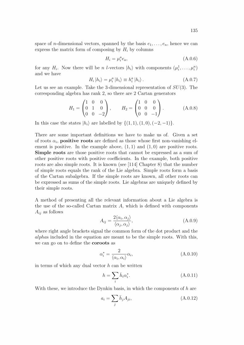
135

space of n-dimensional vectors, spanned by the basis e1, . . . , en, hence we canexpress the matrix form of composing by Hi by columns

Hi = µai ea, (A.0.6)

for any Hi. Now there will be n l-vectors |hi〉 with components (µ1i , . . . , µ

ni )

and we haveHi |hi〉 = µai |hi〉 ≡ hai |hi〉 . (A.0.7)

Let us see an example. Take the 3-dimensional representation of SU(3). Thecorresponding algebra has rank 2, so there are 2 Cartan generators

H1 =

1 0 00 1 00 0 −2

, H2 =

1 0 00 0 00 0 −1

. (A.0.8)

In this case the states |hi〉 are labelled by (1, 1), (1, 0), (−2,−1).

There are some important definitions we have to make us of. Given a setof roots αi, positive roots are defined as those whose first non-vanishing el-ement is positive. In the example above, (1, 1) and (1, 0) are positive roots.Simple roots are those positive roots that cannot be expressed as a sum ofother positive roots with positive coefficients. In the example, both positiveroots are also simple roots. It is known (see [114] Chapter 8) that the numberof simple roots equals the rank of the Lie algebra. Simple roots form a basisof the Cartan subalgebra. If the simple roots are known, all other roots canbe expressed as sums of the simple roots. Lie algebras are uniquely defined bytheir simple roots.

A method of presenting all the relevant information about a Lie algebra isthe use of the so-called Cartan matrix A, which is defined with componentsAij as follows

Aij =2〈αi, αj〉〈αj, αj〉

, (A.0.9)

where right angle brackets signal the common form of the dot product and thealphas included in the equation are meant to be the simple roots. With this,we can go on to define the coroots as

α∗i =2

〈αi, αi〉αi, (A.0.10)

in terms of which any dual vector h can be written

h =∑i

hiα∗i . (A.0.11)

With these, we introduce the Dynkin basis, in which the components of h are

ai =∑j

hjAji, (A.0.12)

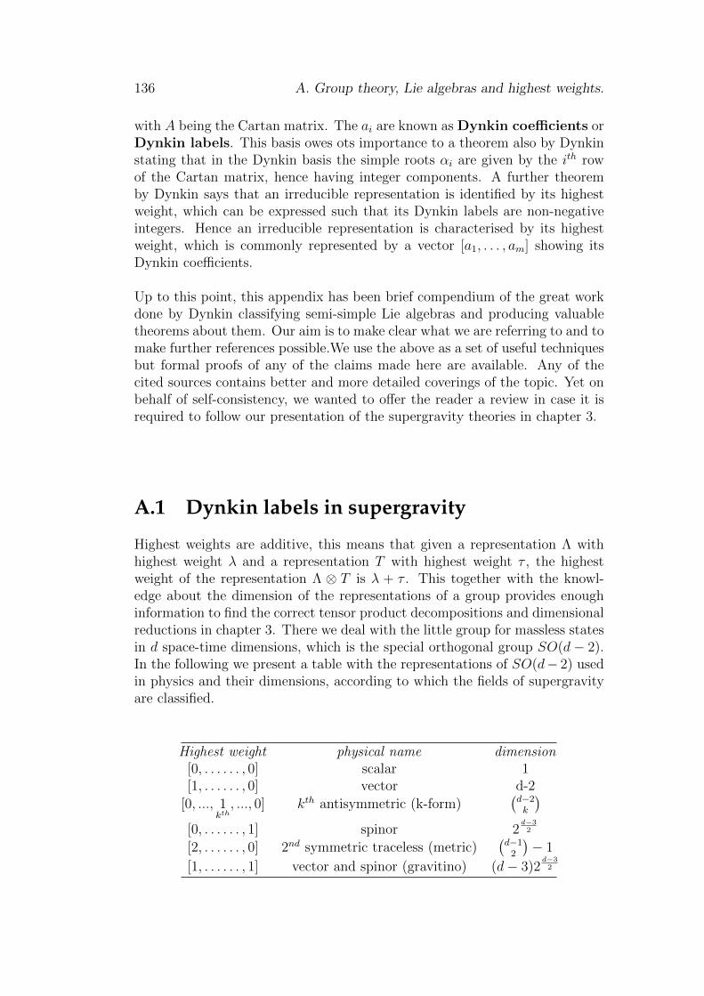
136 A. Group theory, Lie algebras and highest weights.

with A being the Cartan matrix. The ai are known as Dynkin coefficients orDynkin labels. This basis owes ots importance to a theorem also by Dynkinstating that in the Dynkin basis the simple roots αi are given by the ith rowof the Cartan matrix, hence having integer components. A further theoremby Dynkin says that an irreducible representation is identified by its highestweight, which can be expressed such that its Dynkin labels are non-negativeintegers. Hence an irreducible representation is characterised by its highestweight, which is commonly represented by a vector [a1, . . . , am] showing itsDynkin coefficients.

Up to this point, this appendix has been brief compendium of the great workdone by Dynkin classifying semi-simple Lie algebras and producing valuabletheorems about them. Our aim is to make clear what we are referring to and tomake further references possible.We use the above as a set of useful techniquesbut formal proofs of any of the claims made here are available. Any of thecited sources contains better and more detailed coverings of the topic. Yet onbehalf of self-consistency, we wanted to offer the reader a review in case it isrequired to follow our presentation of the supergravity theories in chapter 3.

A.1 Dynkin labels in supergravity

Highest weights are additive, this means that given a representation Λ withhighest weight λ and a representation T with highest weight τ , the highestweight of the representation Λ ⊗ T is λ + τ . This together with the knowl-edge about the dimension of the representations of a group provides enoughinformation to find the correct tensor product decompositions and dimensionalreductions in chapter 3. There we deal with the little group for massless statesin d space-time dimensions, which is the special orthogonal group SO(d− 2).In the following we present a table with the representations of SO(d− 2) usedin physics and their dimensions, according to which the fields of supergravityare classified.

Highest weight physical name dimension[0, . . . . . . , 0] scalar 1[1, . . . . . . , 0] vector d-2

[0, ..., 1kth, ..., 0] kth antisymmetric (k-form)

(d−2k

)[0, . . . . . . , 1] spinor 2

d−32

[2, . . . . . . , 0] 2nd symmetric traceless (metric)(d−1

2

)− 1

[1, . . . . . . , 1] vector and spinor (gravitino) (d− 3)2d−32

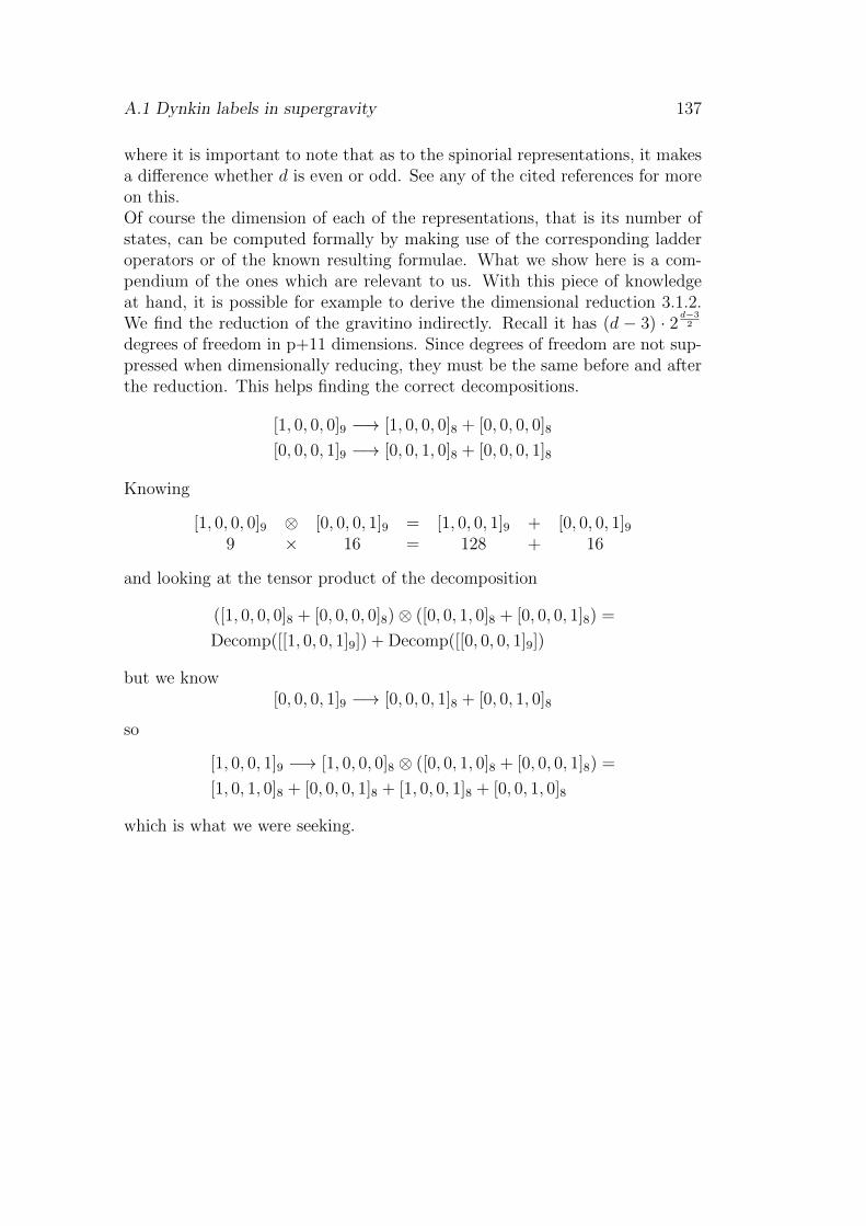
A.1 Dynkin labels in supergravity 137

where it is important to note that as to the spinorial representations, it makesa difference whether d is even or odd. See any of the cited references for moreon this.Of course the dimension of each of the representations, that is its number ofstates, can be computed formally by making use of the corresponding ladderoperators or of the known resulting formulae. What we show here is a com-pendium of the ones which are relevant to us. With this piece of knowledgeat hand, it is possible for example to derive the dimensional reduction 3.1.2.We find the reduction of the gravitino indirectly. Recall it has (d − 3) · 2 d−3

2

degrees of freedom in p+11 dimensions. Since degrees of freedom are not sup-pressed when dimensionally reducing, they must be the same before and afterthe reduction. This helps finding the correct decompositions.

[1, 0, 0, 0]9 −→ [1, 0, 0, 0]8 + [0, 0, 0, 0]8

[0, 0, 0, 1]9 −→ [0, 0, 1, 0]8 + [0, 0, 0, 1]8

Knowing

[1, 0, 0, 0]9 ⊗ [0, 0, 0, 1]9 = [1, 0, 0, 1]9 + [0, 0, 0, 1]99 × 16 = 128 + 16

and looking at the tensor product of the decomposition

([1, 0, 0, 0]8 + [0, 0, 0, 0]8)⊗ ([0, 0, 1, 0]8 + [0, 0, 0, 1]8) =

Decomp([[1, 0, 0, 1]9]) + Decomp([[0, 0, 0, 1]9])

but we know[0, 0, 0, 1]9 −→ [0, 0, 0, 1]8 + [0, 0, 1, 0]8

so

[1, 0, 0, 1]9 −→ [1, 0, 0, 0]8 ⊗ ([0, 0, 1, 0]8 + [0, 0, 0, 1]8) =

[1, 0, 1, 0]8 + [0, 0, 0, 1]8 + [1, 0, 0, 1]8 + [0, 0, 1, 0]8

which is what we were seeking.

138 A. Group theory, Lie algebras and highest weights.

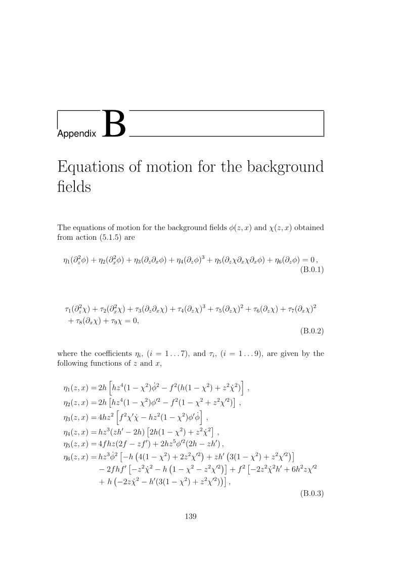
Appendix BEquations of motion for the backgroundfields

The equations of motion for the background fields φ(z, x) and χ(z, x) obtainedfrom action (5.1.5) are

η1(∂2zφ) + η2(∂2

xφ) + η3(∂z∂xφ) + η4(∂zφ)3 + η5(∂zχ∂xχ∂xφ) + η6(∂zφ) = 0 ,(B.0.1)

τ1(∂2zχ) + τ2(∂2

xχ) + τ3(∂z∂xχ) + τ4(∂zχ)3 + τ5(∂zχ)2 + τ6(∂zχ) + τ7(∂xχ)2

+ τ8(∂xχ) + τ9χ = 0,

(B.0.2)

where the coefficients ηi, (i = 1 . . . 7), and τi, (i = 1 . . . 9), are given by thefollowing functions of z and x,

η1(z, x) = 2h[hz4(1− χ2)φ2 − f 2(h(1− χ2) + z2χ2)

],

η2(z, x) = 2h[hz4(1− χ2)φ′2 − f 2(1− χ2 + z2χ′2)

],

η3(z, x) = 4hz2[f 2χ′χ− hz2(1− χ2)φ′φ

],

η4(z, x) =hz3(zh′ − 2h)[2h(1− χ2) + z2χ2

],

η5(z, x) = 4fhz(2f − zf ′) + 2hz5φ′2(2h− zh′) ,η6(z, x) =hz3φ2

[−h(4(1− χ2) + 2z2χ′2

)+ zh′

(3(1− χ2) + z2χ′2

)]− 2fhf ′

[−z2χ2 − h

(1− χ2 − z2χ′2

)]+ f 2

[−2z2χ2h′ + 6h2zχ′2

+ h(−2zχ2 − h′(3(1− χ2) + z2χ′2)

)],

(B.0.3)

139

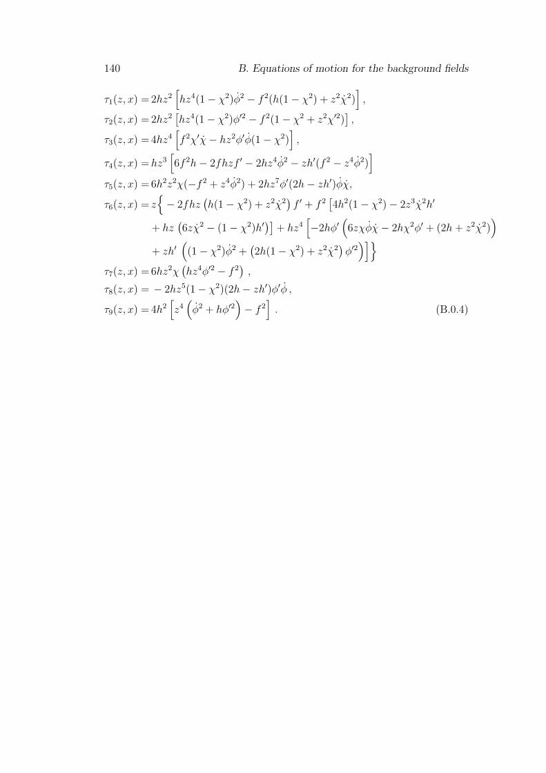
140 B. Equations of motion for the background fields

τ1(z, x) = 2hz2[hz4(1− χ2)φ2 − f 2(h(1− χ2) + z2χ2)

],

τ2(z, x) = 2hz2[hz4(1− χ2)φ′2 − f 2(1− χ2 + z2χ′2)

],

τ3(z, x) = 4hz4[f 2χ′χ− hz2φ′φ(1− χ2)

],

τ4(z, x) =hz3[6f 2h− 2fhzf ′ − 2hz4φ2 − zh′(f 2 − z4φ2)

]τ5(z, x) = 6h2z2χ(−f 2 + z4φ2) + 2hz7φ′(2h− zh′)φχ,

τ6(z, x) = z− 2fhz

(h(1− χ2) + z2χ2

)f ′ + f 2

[4h2(1− χ2)− 2z3χ2h′

+ hz(6zχ2 − (1− χ2)h′

)]+ hz4

[−2hφ′

(6zχφχ− 2hχ2φ′ + (2h+ z2χ2)

)+ zh′

((1− χ2)φ2 +

(2h(1− χ2) + z2χ2

)φ′2)]

τ7(z, x) = 6hz2χ(hz4φ′2 − f 2

),

τ8(z, x) = − 2hz5(1− χ2)(2h− zh′)φ′φ ,

τ9(z, x) = 4h2[z4(φ2 + hφ′2

)− f 2

]. (B.0.4)

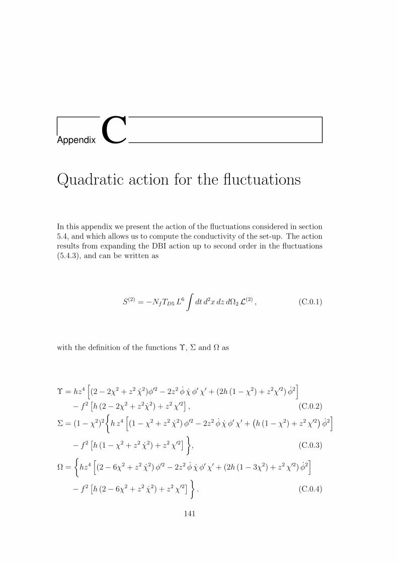
Appendix CQuadratic action for the fluctuations

In this appendix we present the action of the fluctuations considered in section5.4, and which allows us to compute the conductivity of the set-up. The actionresults from expanding the DBI action up to second order in the fluctuations(5.4.3), and can be written as

S(2) = −NfTD5 L6

∫dt d2x dz dΩ2 L(2) , (C.0.1)

with the definition of the functions Υ, Σ and Ω as

Υ = hz4[(2− 2χ2 + z2 χ2)φ′2 − 2z2 φ χ φ′ χ′ + (2h (1− χ2) + z2χ′2) φ2

]− f 2

[h (2− 2χ2 + z2χ2) + z2 χ′2

], (C.0.2)

Σ = (1− χ2)2

h z4

[(1− χ2 + z2 χ2)φ′2 − 2z2 φ χ φ′ χ′ +

(h (1− χ2) + z2 χ′2

)φ2]

− f 2[h (1− χ2 + z2 χ2) + z2 χ′2

], (C.0.3)

Ω =

hz4

[(2− 6χ2 + z2 χ2)φ′2 − 2z2 φ χ φ′ χ′ + (2h (1− 3χ2) + z2 χ′2) φ2

]− f 2

[h (2− 6χ2 + z2 χ2) + z2 χ′2

]. (C.0.4)

141

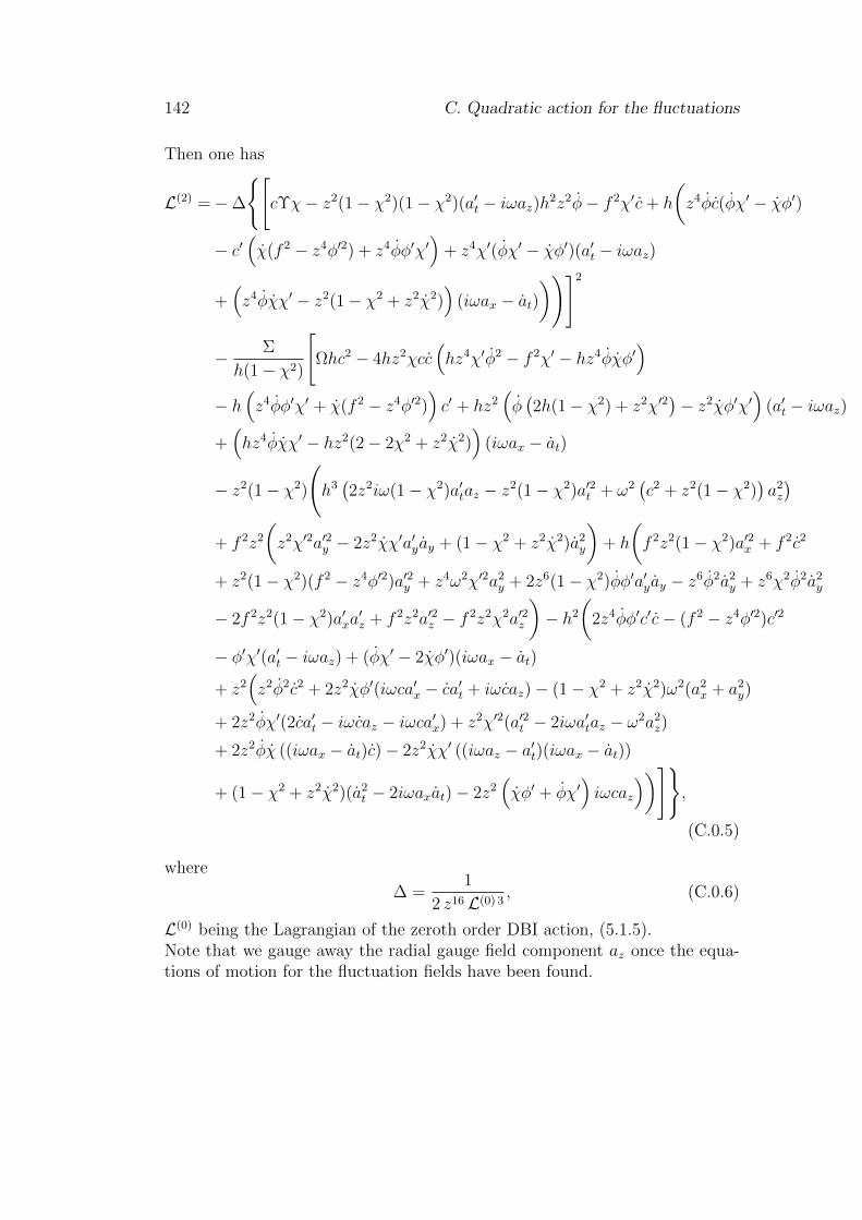
142 C. Quadratic action for the fluctuations

Then one has

L(2) =−∆

[cΥχ− z2(1− χ2)(1− χ2)(a′t − iωaz)h2z2φ− f 2χ′c+ h

(z4φc(φχ′ − χφ′)

− c′(χ(f 2 − z4φ′2) + z4φφ′χ′

)+ z4χ′(φχ′ − χφ′)(a′t − iωaz)

+(z4φχχ′ − z2(1− χ2 + z2χ2)

)(iωax − at)

))]2

− Σ

h(1− χ2)

[Ωhc2 − 4hz2χcc

(hz4χ′φ2 − f 2χ′ − hz4φχφ′

)− h

(z4φφ′χ′ + χ(f 2 − z4φ′2)

)c′ + hz2

(φ(2h(1− χ2) + z2χ′2

)− z2χφ′χ′

)(a′t − iωaz)

+(hz4φχχ′ − hz2(2− 2χ2 + z2χ2)

)(iωax − at)

− z2(1− χ2)

(h3(2z2iω(1− χ2)a′taz − z2(1− χ2)a′2t + ω2

(c2 + z2(1− χ2)

)a2z

)+ f 2z2

(z2χ′2a′2y − 2z2χχ′a′yay + (1− χ2 + z2χ2)a2

y

)+ h

(f 2z2(1− χ2)a′2x + f 2c2

+ z2(1− χ2)(f 2 − z4φ′2)a′2y + z4ω2χ′2a2y + 2z6(1− χ2)φφ′a′yay − z6φ2a2

y + z6χ2φ2a2y

− 2f 2z2(1− χ2)a′xa′z + f 2z2a′2z − f 2z2χ2a′2z

)− h2

(2z4φφ′c′c− (f 2 − z4φ′2)c′2

− φ′χ′(a′t − iωaz) + (φχ′ − 2χφ′)(iωax − at)

+ z2(z2φ2c2 + 2z2χφ′(iωca′x − ca′t + iωcaz)− (1− χ2 + z2χ2)ω2(a2

x + a2y)

+ 2z2φχ′(2ca′t − iωcaz − iωca′x) + z2χ′2(a′2t − 2iωa′taz − ω2a2z)

+ 2z2φχ ((iωax − at)c)− 2z2χχ′ ((iωaz − a′t)(iωax − at))

+ (1− χ2 + z2χ2)(a2t − 2iωaxat)− 2z2

(χφ′ + φχ′

)iωcaz

))],

(C.0.5)

where

∆ =1

2 z16 L(0) 3, (C.0.6)

L(0) being the Lagrangian of the zeroth order DBI action, (5.1.5).Note that we gauge away the radial gauge field component az once the equa-tions of motion for the fluctuation fields have been found.

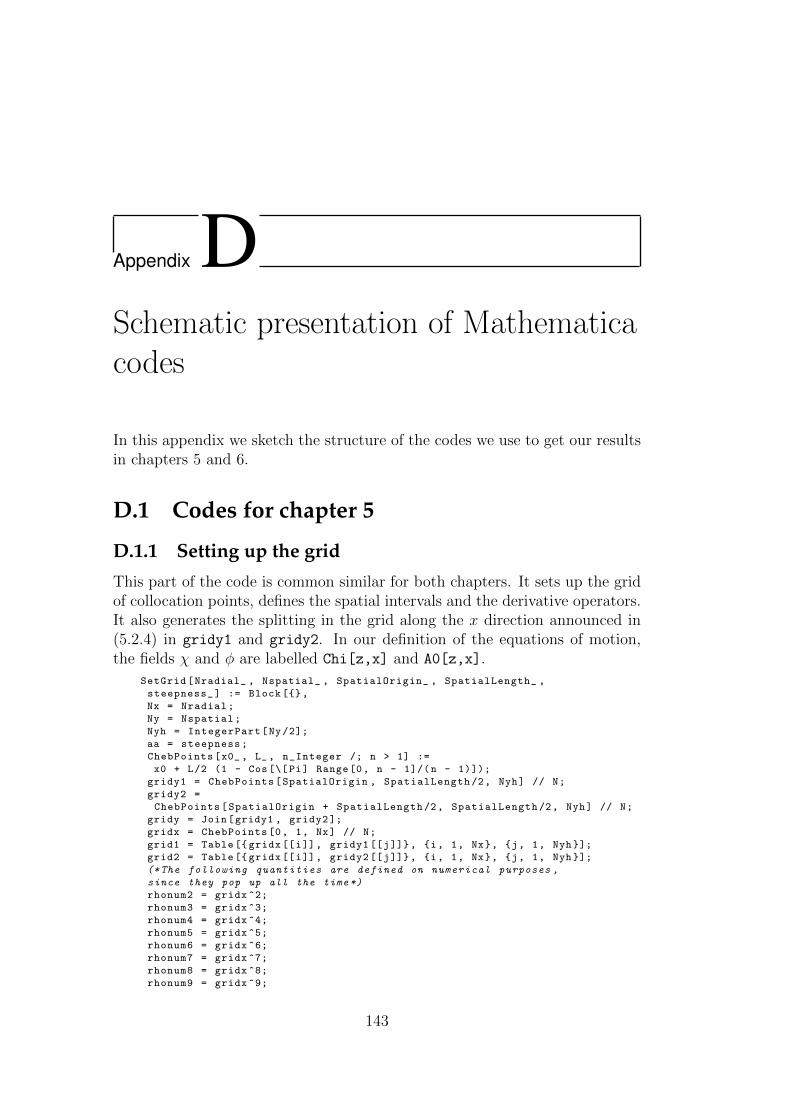
Appendix DSchematic presentation of Mathematicacodes

In this appendix we sketch the structure of the codes we use to get our resultsin chapters 5 and 6.

D.1 Codes for chapter 5

D.1.1 Setting up the grid

This part of the code is common similar for both chapters. It sets up the gridof collocation points, defines the spatial intervals and the derivative operators.It also generates the splitting in the grid along the x direction announced in(5.2.4) in gridy1 and gridy2. In our definition of the equations of motion,the fields χ and φ are labelled Chi[z,x] and A0[z,x].

SetGrid[Nradial_ , Nspatial_ , SpatialOrigin_ , SpatialLength_ ,

steepness_] := Block[,

Nx = Nradial;

Ny = Nspatial;

Nyh = IntegerPart[Ny/2];

aa = steepness;

ChebPoints[x0_ , L_ , n_Integer /; n > 1] :=

x0 + L/2 (1 - Cos[\[Pi] Range[0, n - 1]/(n - 1)]);

gridy1 = ChebPoints[SpatialOrigin , SpatialLength /2, Nyh] // N;

gridy2 =

ChebPoints[SpatialOrigin + SpatialLength /2, SpatialLength /2, Nyh] // N;

gridy = Join[gridy1 , gridy2 ];

gridx = ChebPoints [0, 1, Nx] // N;

grid1 = Table [ gridx[[i]], gridy1 [[j]], i, 1, Nx, j, 1, Nyh];

grid2 = Table [ gridx[[i]], gridy2 [[j]], i, 1, Nx, j, 1, Nyh];

(* The following quantities are defined on numerical purposes ,

since they pop up all the time *)

rhonum2 = gridx ^2;

rhonum3 = gridx ^3;

rhonum4 = gridx ^4;

rhonum5 = gridx ^5;

rhonum6 = gridx ^6;

rhonum7 = gridx ^7;

rhonum8 = gridx ^8;

rhonum9 = gridx ^9;

143

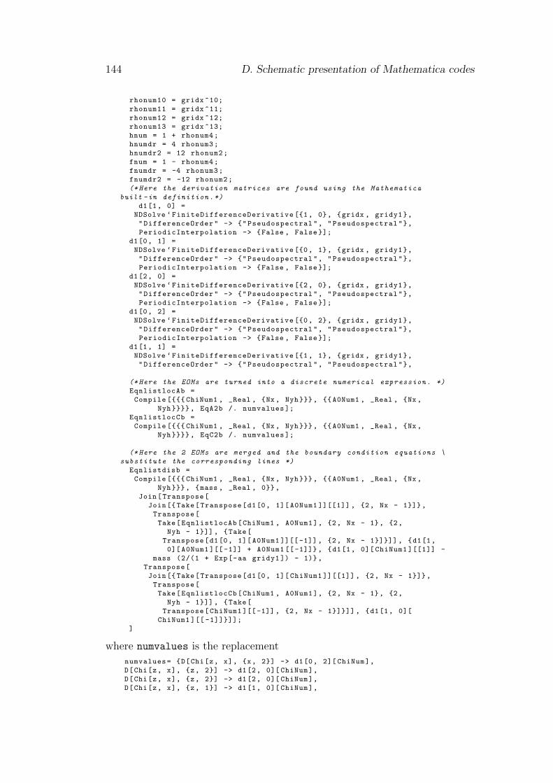
144 D. Schematic presentation of Mathematica codes

rhonum10 = gridx ^10;

rhonum11 = gridx ^11;

rhonum12 = gridx ^12;

rhonum13 = gridx ^13;

hnum = 1 + rhonum4;

hnumdr = 4 rhonum3;

hnumdr2 = 12 rhonum2;

fnum = 1 - rhonum4;

fnumdr = -4 rhonum3;

fnumdr2 = -12 rhonum2;

(* Here the derivation matrices are found using the Mathematica

built -in definition .*)

d1[1, 0] =

NDSolve ‘FiniteDifferenceDerivative [1, 0, gridx , gridy1,

"DifferenceOrder" -> "Pseudospectral", "Pseudospectral",

PeriodicInterpolation -> False , False ];

d1[0, 1] =

NDSolve ‘FiniteDifferenceDerivative [0, 1, gridx , gridy1,

"DifferenceOrder" -> "Pseudospectral", "Pseudospectral",

PeriodicInterpolation -> False , False ];

d1[2, 0] =

NDSolve ‘FiniteDifferenceDerivative [2, 0, gridx , gridy1,

"DifferenceOrder" -> "Pseudospectral", "Pseudospectral",

PeriodicInterpolation -> False , False ];

d1[0, 2] =

NDSolve ‘FiniteDifferenceDerivative [0, 2, gridx , gridy1,

"DifferenceOrder" -> "Pseudospectral", "Pseudospectral",

PeriodicInterpolation -> False , False ];

d1[1, 1] =

NDSolve ‘FiniteDifferenceDerivative [1, 1, gridx , gridy1,

"DifferenceOrder" -> "Pseudospectral", "Pseudospectral",

(* Here the EOMs are turned into a discrete numerical expression . *)

EqnlistlocAb =

Compile [ ChiNum1 , _Real , Nx, Nyh, A0Num1 , _Real , Nx,

Nyh, EqA2b /. numvalues ];

EqnlistlocCb =

Compile [ ChiNum1 , _Real , Nx, Nyh, A0Num1 , _Real , Nx,

Nyh, EqC2b /. numvalues ];

(* Here the 2 EOMs are merged and the boundary condition equations \

substitute the corresponding lines *)

Eqnlistdisb =

Compile [ ChiNum1 , _Real , Nx, Nyh, A0Num1 , _Real , Nx,

Nyh, mass , _Real , 0,

Join[Transpose[

Join[Take[Transpose[d1[0, 1][ A0Num1 ]][[1]] , 2, Nx - 1],

Transpose[

Take[EqnlistlocAb[ChiNum1 , A0Num1], 2, Nx - 1, 2,

Nyh - 1]], Take[

Transpose[d1[0, 1][ A0Num1 ]][[-1]], 2, Nx - 1]]] , d1[1,

0][ A0Num1 ][[ -1]] + A0Num1 [[-1]], d1[1, 0][ ChiNum1 ][[1]] -

mass (2/(1 + Exp[-aa gridy1 ]) - 1),

Transpose[

Join[Take[Transpose[d1[0, 1][ ChiNum1 ]][[1]] , 2, Nx - 1],

Transpose[

Take[EqnlistlocCb[ChiNum1 , A0Num1], 2, Nx - 1, 2,

Nyh - 1]], Take[

Transpose[ChiNum1 ][[-1]], 2, Nx - 1]]] , d1[1, 0][

ChiNum1 ][[ -1]]]];

]

where numvalues is the replacement

numvalues= D[Chi[z, x], x, 2] -> d1[0, 2][ ChiNum],

D[Chi[z, x], z, 2] -> d1[2, 0][ ChiNum],

D[Chi[z, x], z, 2] -> d1[2, 0][ ChiNum],

D[Chi[z, x], z, 1] -> d1[1, 0][ ChiNum],

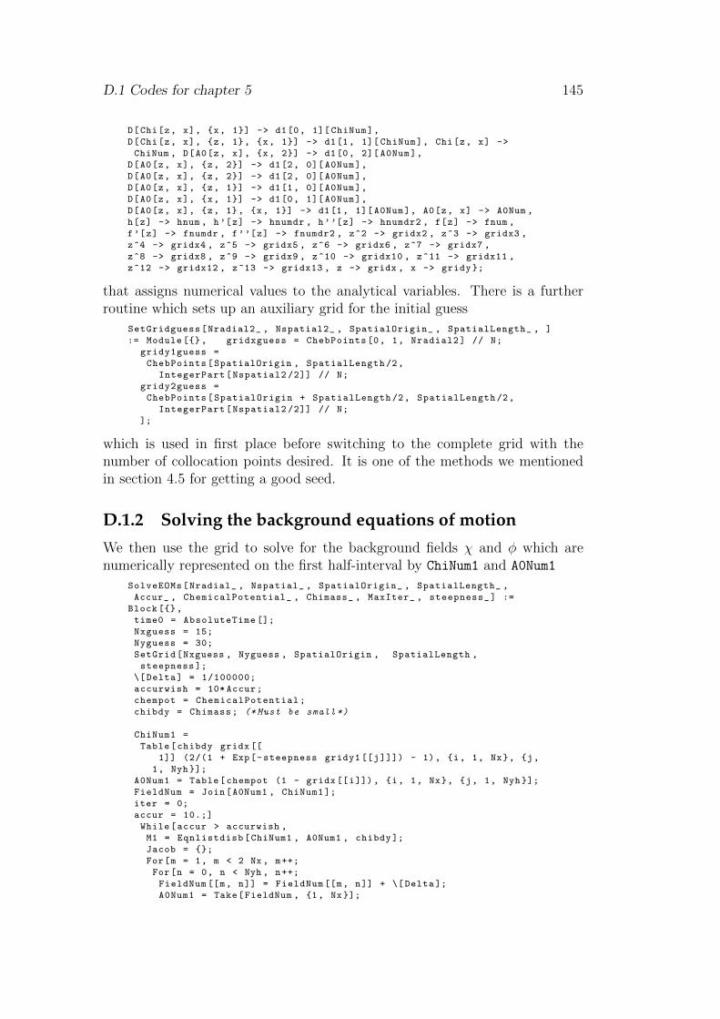
D.1 Codes for chapter 5 145

D[Chi[z, x], x, 1] -> d1[0, 1][ ChiNum],

D[Chi[z, x], z, 1, x, 1] -> d1[1, 1][ ChiNum], Chi[z, x] ->

ChiNum , D[A0[z, x], x, 2] -> d1[0, 2][ A0Num],

D[A0[z, x], z, 2] -> d1[2, 0][ A0Num],

D[A0[z, x], z, 2] -> d1[2, 0][ A0Num],

D[A0[z, x], z, 1] -> d1[1, 0][ A0Num],

D[A0[z, x], x, 1] -> d1[0, 1][ A0Num],

D[A0[z, x], z, 1, x, 1] -> d1[1, 1][ A0Num], A0[z, x] -> A0Num ,

h[z] -> hnum , h’[z] -> hnumdr , h’’[z] -> hnumdr2 , f[z] -> fnum ,

f’[z] -> fnumdr , f’’[z] -> fnumdr2 , z^2 -> gridx2 , z^3 -> gridx3 ,

z^4 -> gridx4 , z^5 -> gridx5 , z^6 -> gridx6 , z^7 -> gridx7 ,

z^8 -> gridx8 , z^9 -> gridx9 , z^10 -> gridx10 , z^11 -> gridx11 ,

z^12 -> gridx12 , z^13 -> gridx13 , z -> gridx , x -> gridy;

that assigns numerical values to the analytical variables. There is a furtherroutine which sets up an auxiliary grid for the initial guess

SetGridguess[Nradial2_ , Nspatial2_ , SpatialOrigin_ , SpatialLength_ , ]

:= Module [, gridxguess = ChebPoints [0, 1, Nradial2] // N;

gridy1guess =

ChebPoints[SpatialOrigin , SpatialLength /2,

IntegerPart[Nspatial2 /2]] // N;

gridy2guess =

ChebPoints[SpatialOrigin + SpatialLength /2, SpatialLength /2,

IntegerPart[Nspatial2 /2]] // N;

];

which is used in first place before switching to the complete grid with thenumber of collocation points desired. It is one of the methods we mentionedin section 4.5 for getting a good seed.

D.1.2 Solving the background equations of motion

We then use the grid to solve for the background fields χ and φ which arenumerically represented on the first half-interval by ChiNum1 and A0Num1

SolveEOMs[Nradial_ , Nspatial_ , SpatialOrigin_ , SpatialLength_ ,

Accur_ , ChemicalPotential_ , Chimass_ , MaxIter_ , steepness_] :=

Block[,

time0 = AbsoluteTime [];

Nxguess = 15;

Nyguess = 30;

SetGrid[Nxguess , Nyguess , SpatialOrigin , SpatialLength ,

steepness ];

\[Delta] = 1/100000;

accurwish = 10* Accur;

chempot = ChemicalPotential;

chibdy = Chimass; (* Must be small *)

ChiNum1 =

Table[chibdy gridx[[

1]] (2/(1 + Exp[-steepness gridy1 [[j]]]) - 1), i, 1, Nx, j,

1, Nyh];

A0Num1 = Table[chempot (1 - gridx[[i]]), i, 1, Nx, j, 1, Nyh];

FieldNum = Join[A0Num1 , ChiNum1 ];

iter = 0;

accur = 10.;]

While[accur > accurwish ,

M1 = Eqnlistdisb[ChiNum1 , A0Num1 , chibdy ];

Jacob = ;

For[m = 1, m < 2 Nx, m++;

For[n = 0, n < Nyh , n++;

FieldNum [[m, n]] = FieldNum [[m, n]] + \[ Delta];

A0Num1 = Take[FieldNum , 1, Nx];

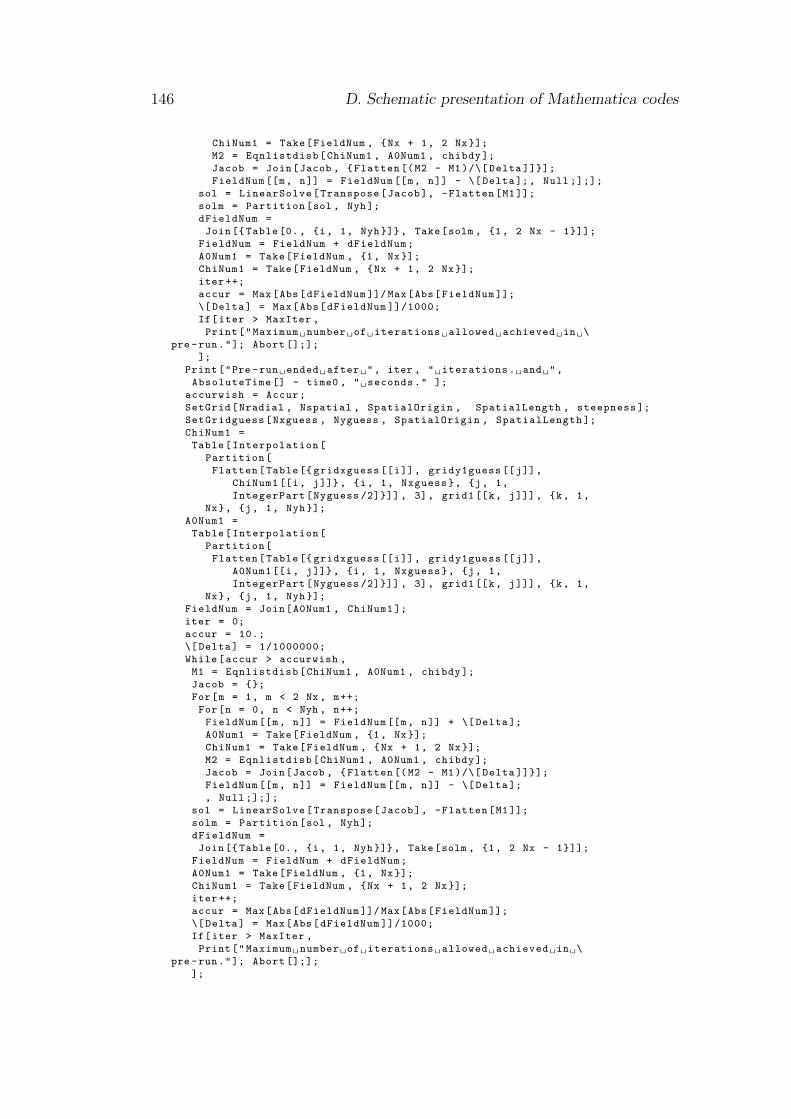
146 D. Schematic presentation of Mathematica codes

ChiNum1 = Take[FieldNum , Nx + 1, 2 Nx];

M2 = Eqnlistdisb[ChiNum1 , A0Num1 , chibdy ];

Jacob = Join[Jacob , Flatten [(M2 - M1)/\[ Delta ]]];

FieldNum [[m, n]] = FieldNum [[m, n]] - \[Delta];, Null ;];];

sol = LinearSolve[Transpose[Jacob], -Flatten[M1]];

solm = Partition[sol , Nyh];

dFieldNum =

Join[ Table[0., i, 1, Nyh], Take[solm , 1, 2 Nx - 1]];

FieldNum = FieldNum + dFieldNum;

A0Num1 = Take[FieldNum , 1, Nx];

ChiNum1 = Take[FieldNum , Nx + 1, 2 Nx];

iter ++;

accur = Max[Abs[dFieldNum ]]/ Max[Abs[FieldNum ]];

\[Delta] = Max[Abs[dFieldNum ]]/1000;

If[iter > MaxIter ,

Print["Maximum number of iterations allowed achieved in \

pre -run."]; Abort [];];

];

Print["Pre -run ended after ", iter , " iterations. and ",

AbsoluteTime [] - time0 , " seconds." ];

accurwish = Accur;

SetGrid[Nradial , Nspatial , SpatialOrigin , SpatialLength , steepness ];

SetGridguess[Nxguess , Nyguess , SpatialOrigin , SpatialLength ];

ChiNum1 =

Table[Interpolation[

Partition[

Flatten[Table [ gridxguess [[i]], gridy1guess [[j]],

ChiNum1 [[i, j]], i, 1, Nxguess, j, 1,

IntegerPart[Nyguess /2]]] , 3], grid1 [[k, j]]], k, 1,

Nx, j, 1, Nyh];

A0Num1 =

Table[Interpolation[

Partition[

Flatten[Table [ gridxguess [[i]], gridy1guess [[j]],

A0Num1 [[i, j]], i, 1, Nxguess, j, 1,

IntegerPart[Nyguess /2]]] , 3], grid1 [[k, j]]], k, 1,

Nx, j, 1, Nyh];

FieldNum = Join[A0Num1 , ChiNum1 ];

iter = 0;

accur = 10.;

\[Delta] = 1/1000000;

While[accur > accurwish ,

M1 = Eqnlistdisb[ChiNum1 , A0Num1 , chibdy ];

Jacob = ;

For[m = 1, m < 2 Nx, m++;

For[n = 0, n < Nyh , n++;

FieldNum [[m, n]] = FieldNum [[m, n]] + \[Delta ];

A0Num1 = Take[FieldNum , 1, Nx];

ChiNum1 = Take[FieldNum , Nx + 1, 2 Nx];

M2 = Eqnlistdisb[ChiNum1 , A0Num1 , chibdy ];

Jacob = Join[Jacob , Flatten [(M2 - M1)/\[ Delta ]]];

FieldNum [[m, n]] = FieldNum [[m, n]] - \[Delta ];

, Null ;];];

sol = LinearSolve[Transpose[Jacob], -Flatten[M1]];

solm = Partition[sol , Nyh];

dFieldNum =

Join[ Table[0., i, 1, Nyh], Take[solm , 1, 2 Nx - 1]];

FieldNum = FieldNum + dFieldNum;

A0Num1 = Take[FieldNum , 1, Nx];

ChiNum1 = Take[FieldNum , Nx + 1, 2 Nx];

iter ++;

accur = Max[Abs[dFieldNum ]]/ Max[Abs[FieldNum ]];

\[Delta] = Max[Abs[dFieldNum ]]/1000;

If[iter > MaxIter ,

Print["Maximum number of iterations allowed achieved in \

pre -run."]; Abort [];];

];

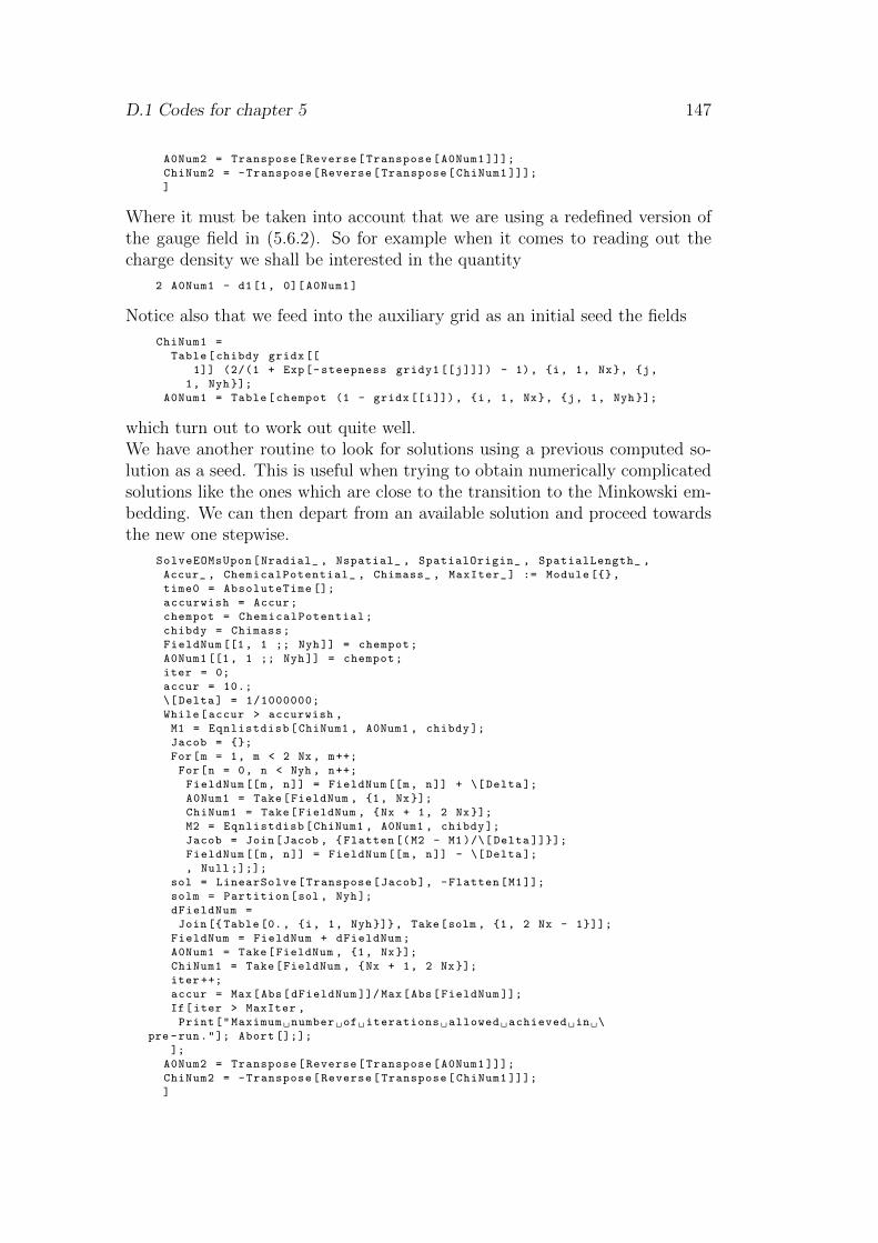
D.1 Codes for chapter 5 147

A0Num2 = Transpose[Reverse[Transpose[A0Num1 ]]];

ChiNum2 = -Transpose[Reverse[Transpose[ChiNum1 ]]];

]

Where it must be taken into account that we are using a redefined version ofthe gauge field in (5.6.2). So for example when it comes to reading out thecharge density we shall be interested in the quantity

2 A0Num1 - d1[1, 0][ A0Num1]

Notice also that we feed into the auxiliary grid as an initial seed the fields

ChiNum1 =

Table[chibdy gridx[[

1]] (2/(1 + Exp[-steepness gridy1 [[j]]]) - 1), i, 1, Nx, j,

1, Nyh];

A0Num1 = Table[chempot (1 - gridx[[i]]), i, 1, Nx, j, 1, Nyh];

which turn out to work out quite well.We have another routine to look for solutions using a previous computed so-lution as a seed. This is useful when trying to obtain numerically complicatedsolutions like the ones which are close to the transition to the Minkowski em-bedding. We can then depart from an available solution and proceed towardsthe new one stepwise.

SolveEOMsUpon[Nradial_ , Nspatial_ , SpatialOrigin_ , SpatialLength_ ,

Accur_ , ChemicalPotential_ , Chimass_ , MaxIter_] := Module [,

time0 = AbsoluteTime [];

accurwish = Accur;

chempot = ChemicalPotential;

chibdy = Chimass;

FieldNum [[1, 1 ;; Nyh]] = chempot;

A0Num1 [[1, 1 ;; Nyh]] = chempot;

iter = 0;

accur = 10.;

\[Delta] = 1/1000000;

While[accur > accurwish ,

M1 = Eqnlistdisb[ChiNum1 , A0Num1 , chibdy ];

Jacob = ;

For[m = 1, m < 2 Nx, m++;

For[n = 0, n < Nyh , n++;

FieldNum [[m, n]] = FieldNum [[m, n]] + \[ Delta];

A0Num1 = Take[FieldNum , 1, Nx];

ChiNum1 = Take[FieldNum , Nx + 1, 2 Nx];

M2 = Eqnlistdisb[ChiNum1 , A0Num1 , chibdy ];

Jacob = Join[Jacob , Flatten [(M2 - M1)/\[ Delta ]]];

FieldNum [[m, n]] = FieldNum [[m, n]] - \[ Delta];

, Null ;];];

sol = LinearSolve[Transpose[Jacob], -Flatten[M1]];

solm = Partition[sol , Nyh];

dFieldNum =

Join[ Table[0., i, 1, Nyh], Take[solm , 1, 2 Nx - 1]];

FieldNum = FieldNum + dFieldNum;

A0Num1 = Take[FieldNum , 1, Nx];

ChiNum1 = Take[FieldNum , Nx + 1, 2 Nx];

iter ++;

accur = Max[Abs[dFieldNum ]]/ Max[Abs[FieldNum ]];

If[iter > MaxIter ,

Print["Maximum number of iterations allowed achieved in \

pre -run."]; Abort [];];

];

A0Num2 = Transpose[Reverse[Transpose[A0Num1 ]]];

ChiNum2 = -Transpose[Reverse[Transpose[ChiNum1 ]]];

]

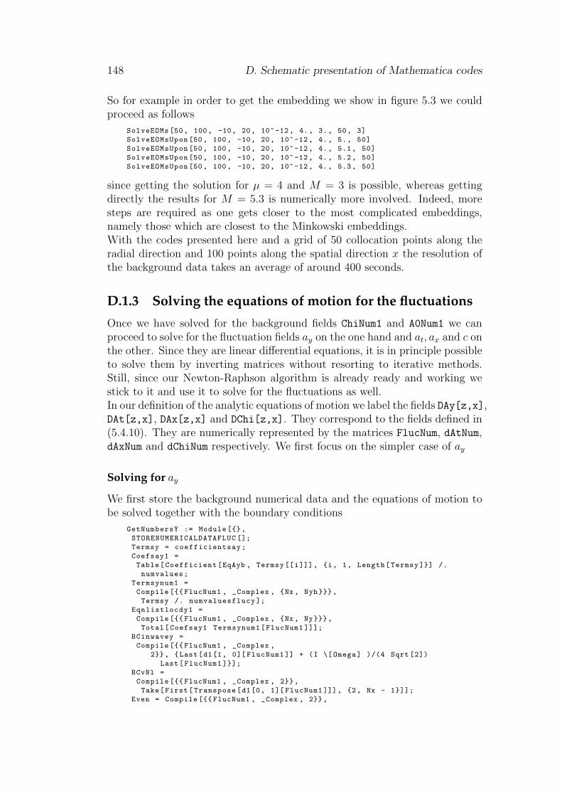
148 D. Schematic presentation of Mathematica codes

So for example in order to get the embedding we show in figure 5.3 we couldproceed as follows

SolveEOMs [50, 100, -10, 20, 10^-12, 4., 3., 50, 3]

SolveEOMsUpon [50, 100, -10, 20, 10^-12, 4., 5., 50]

SolveEOMsUpon [50, 100, -10, 20, 10^-12, 4., 5.1, 50]

SolveEOMsUpon [50, 100, -10, 20, 10^-12, 4., 5.2, 50]

SolveEOMsUpon [50, 100, -10, 20, 10^-12, 4., 5.3, 50]

since getting the solution for µ = 4 and M = 3 is possible, whereas gettingdirectly the results for M = 5.3 is numerically more involved. Indeed, moresteps are required as one gets closer to the most complicated embeddings,namely those which are closest to the Minkowski embeddings.With the codes presented here and a grid of 50 collocation points along theradial direction and 100 points along the spatial direction x the resolution ofthe background data takes an average of around 400 seconds.

D.1.3 Solving the equations of motion for the fluctuations

Once we have solved for the background fields ChiNum1 and A0Num1 we canproceed to solve for the fluctuation fields ay on the one hand and at, ax and c onthe other. Since they are linear differential equations, it is in principle possibleto solve them by inverting matrices without resorting to iterative methods.Still, since our Newton-Raphson algorithm is already ready and working westick to it and use it to solve for the fluctuations as well.In our definition of the analytic equations of motion we label the fields DAy[z,x],DAt[z,x], DAx[z,x] and DChi[z,x]. They correspond to the fields defined in(5.4.10). They are numerically represented by the matrices FlucNum, dAtNum,dAxNum and dChiNum respectively. We first focus on the simpler case of ay

Solving for ay

We first store the background numerical data and the equations of motion tobe solved together with the boundary conditions

GetNumbersY := Module [,

STORENUMERICALDATAFLUC [];

Termsy = coefficientsay;

Coefsay1 =

Table[Coefficient[EqAyb , Termsy [[i]]], i, 1, Length[Termsy ]] /.

numvalues;

Termsynum1 =

Compile [ FlucNum1 , _Complex , Nx , Nyh,

Termsy /. numvaluesflucy ];

Eqnlistlocdy1 =

Compile [ FlucNum1 , _Complex , Nx , Ny,

Total[Coefsay1 Termsynum1[FlucNum1 ]]];

BCinwavey =

Compile [ FlucNum1 , _Complex ,

2, Last[d1[1, 0][ FlucNum1 ]] + (I \[Omega] )/(4 Sqrt [2])

Last[FlucNum1 ]];

BCvNl =

Compile [ FlucNum1 , _Complex , 2,

Take[First[Transpose[d1[0, 1][ FlucNum1 ]]], 2, Nx - 1]];

Even = Compile [ FlucNum1 , _Complex , 2,

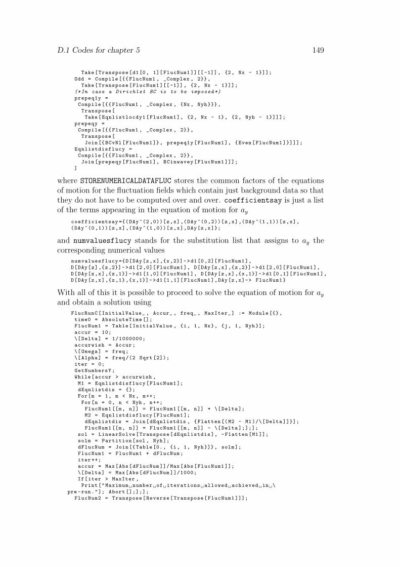
D.1 Codes for chapter 5 149

Take[Transpose[d1[0, 1][ FlucNum1 ]][[-1]], 2, Nx - 1]];

Odd = Compile [ FlucNum1 , _Complex , 2,

Take[Transpose[FlucNum1 ][[-1]], 2, Nx - 1]];

(*In case a Dirichlet BC is to be imposed *)

prepeq1y =

Compile [ FlucNum1 , _Complex , Nx, Nyh,

Transpose[

Take[Eqnlistlocdy1[FlucNum1], 2, Nx - 1, 2, Nyh - 1]]];

prepeqy =

Compile [ FlucNum1 , _Complex , 2,

Transpose[

Join[ BCvNl[FlucNum1], prepeq1y[FlucNum1], Even[FlucNum1 ]]]];

Eqnlistdisflucy =

Compile [ FlucNum1 , _Complex , 2,

Join[prepeqy[FlucNum1], BCinwavey[FlucNum1 ]]];

]

where STORENUMERICALDATAFLUC stores the common factors of the equationsof motion for the fluctuation fields which contain just background data so thatthey do not have to be computed over and over. coefficientsay is just a listof the terms appearing in the equation of motion for ay

coefficientsay =(DAy ^(2 ,0))[z,x],(DAy ^(0 ,2))[z,x],(DAy ^(1 ,1))[z,x],

(DAy ^(0 ,1))[z,x],(DAy ^(1 ,0))[z,x],DAy[z,x];

and numvaluesflucy stands for the substitution list that assigns to ay thecorresponding numerical values

numvaluesflucy =D[DAy[z,x],x,2]->d1[0,2][ FlucNum1],

D[DAy[z],z,2]->d1[2 ,0][ FlucNum1], D[DAy[z,x],z,2]->d1[2,0][ FlucNum1],

D[DAy[z,x],z,1]->d1[1,0][ FlucNum1], D[DAy[z,x],x,1]->d1[0,1][ FlucNum1],

D[DAy[z,x],z,1,x,1]->d1[1,1][ FlucNum1],DAy[z,x]-> FlucNum1

With all of this it is possible to proceed to solve the equation of motion for ayand obtain a solution using

FlucRunC[InitialValue_ , Accur_ , freq_ , MaxIter_] := Module [,

time0 = AbsoluteTime [];

FlucNum1 = Table[InitialValue , i, 1, Nx, j, 1, Nyh];

accur = 10;

\[Delta] = 1/1000000;

accurwish = Accur;

\[Omega] = freq;

\[Alpha] = freq /(2 Sqrt [2]);

iter = 0;

GetNumbersY;

While[accur > accurwish ,

M1 = Eqnlistdisflucy[FlucNum1 ];

dEqnlistdis = ;

For[m = 1, m < Nx , m++;

For[n = 0, n < Nyh , n++;

FlucNum1 [[m, n]] = FlucNum1 [[m, n]] + \[ Delta];

M2 = Eqnlistdisflucy[FlucNum1 ];

dEqnlistdis = Join[dEqnlistdis , Flatten [(M2 - M1)/\[ Delta ]]];

FlucNum1 [[m, n]] = FlucNum1 [[m, n]] - \[ Delta ];];];

sol = LinearSolve[Transpose[dEqnlistdis], -Flatten[M1]];

solm = Partition[sol , Nyh];

dFlucNum = Join[Table [0., i, 1, Nyh], solm];

FlucNum1 = FlucNum1 + dFlucNum;

iter ++;

accur = Max[Abs[dFlucNum ]]/ Max[Abs[FlucNum1 ]];

\[Delta] = Max[Abs[dFlucNum ]]/1000;

If[iter > MaxIter ,

Print["Maximum number of iterations allowed achieved in \

pre -run."]; Abort [];];];

FlucNum2 = Transpose[Reverse[Transpose[FlucNum1 ]]];

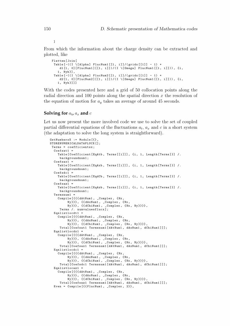
150 D. Schematic presentation of Mathematica codes

]

From which the information about the charge density can be extracted andplotted, like

Flatten[Join[

Table[-((I \[Alpha] FlucNum1 [[1, i]]/( gridx [[1]] - 1) +

d1[1, 0][ FlucNum1 ][[1, i]])/(I \[ Omega] FlucNum1 [[1, i]])), i,

1, Nyh],

Table[-((I \[Alpha] FlucNum2 [[1, i]]/( gridx [[1]] - 1) +

d2[1, 0][ FlucNum2 ][[1, i]])/(I \[ Omega] FlucNum1 [[1, i]])), i,

1, Nyh ]]]

With the codes presented here and a grid of 50 collocation points along theradial direction and 100 points along the spatial direction x the resolution ofthe equation of motion for ay takes an average of around 45 seconds.

Solving for at, ax and c

Let us now present the more involved code we use to solve the set of coupledpartial differential equations of the fluctuations at, ax and c in a short system(the adaptation to solve the long system is straightforward).

GetNumbersX := Module [,

STORENUMERICALDATAFLUCX [];

Terms = coefficientsx;

Coefsat1 =

Table[Coefficient[EqAtb , Terms[[i]]], i, 1, Length[Terms ]] /.

backgroundnum1;

Coefsax1 =

Table[Coefficient[EqAxb , Terms[[i]]], i, 1, Length[Terms ]] /.

backgroundnum1;

Coefsdc1 =

Table[Coefficient[EqdCb , Terms[[i]]], i, 1, Length[Terms ]] /.

backgroundnum1;

Coefsaz1 =

Table[Coefficient[EqAzb , Terms[[i]]], i, 1, Length[Terms ]] /.

backgroundnum1;

Termsnum1 =

Compile [ dAtNum1 , _Complex , Nx,

Ny, dAxNum1 , _Complex , Nx,

Ny, dChiNum1 , _Complex , Nx, Ny,

Terms /. numvaluesflucx ];

Eqnlistlocdt1 =

Compile [ dAtNum1 , _Complex , Nx,

Ny, dAxNum1 , _Complex , Nx,

Ny, dChiNum1 , _Complex , Nx, Ny,

Total[Coefsat1 Termsnum1[dAtNum1 , dAxNum1 , dChiNum1 ]]];

Eqnlistlocdx1 =

Compile [ dAtNum1 , _Complex , Nx,

Ny, dAxNum1 , _Complex , Nx ,

Ny, dChiNum1 , _Complex , Nx, Ny,

Total[Coefsax1 Termsnum1[dAtNum1 , dAxNum1 , dChiNum1 ]]];

Eqnlistlocdc1 =

Compile [ dAtNum1 , _Complex , Nx,

Ny, dAxNum1 , _Complex , Nx ,

Ny, dChiNum1 , _Complex , Nx, Ny,

Total[Coefsdc1 Termsnum1[dAtNum1 , dAxNum1 , dChiNum1 ]]];

Eqnlistlocaz1 =

Compile [ dAtNum1 , _Complex , Nx,

Ny, dAxNum1 , _Complex , Nx ,

Ny, dChiNum1 , _Complex , Nx, Ny,

Total[Coefsaz1 Termsnum1[dAtNum1 , dAxNum1 , dChiNum1 ]]];

Even = Compile [ FlucNum1 , _Complex , 2,

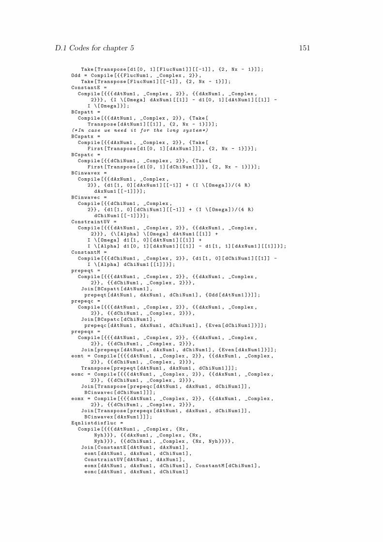
D.1 Codes for chapter 5 151

Take[Transpose[d1[0, 1][ FlucNum1 ]][[-1]], 2, Nx - 1]];

Odd = Compile [ FlucNum1 , _Complex , 2,

Take[Transpose[FlucNum1 ][[-1]], 2, Nx - 1]];

ConstantE =

Compile [ dAtNum1 , _Complex , 2, dAxNum1 , _Complex ,

2, I \[ Omega] dAxNum1 [[1]] - d1[0, 1][ dAtNum1 ][[1]] -

I \[ Omega ]];

BCspatt =

Compile [ dAtNum1 , _Complex , 2, Take[

Transpose[dAtNum1 ][[1]] , 2, Nx - 1]];

(*In case we need it for the long system *)

BCspatx =

Compile [ dAxNum1 , _Complex , 2, Take[

First[Transpose[d1[0, 1][ dAxNum1 ]]], 2, Nx - 1]];

BCspatc =

Compile [ dChiNum1 , _Complex , 2, Take[

First[Transpose[d1[0, 1][ dChiNum1 ]]], 2, Nx - 1]];

BCinwavex =

Compile [ dAxNum1 , _Complex ,

2, d1[1, 0][ dAxNum1 ][[ -1]] + (I \[Omega ])/(4 R)

dAxNum1 [[ -1]]];

BCinwavec =

Compile [ dChiNum1 , _Complex ,

2, d1[1, 0][ dChiNum1 ][[ -1]] + (I \[Omega ])/(4 R)

dChiNum1 [[ -1]]];

ConstraintUV =

Compile [ dAtNum1 , _Complex , 2, dAxNum1 , _Complex ,

2, \[ Alpha] \[Omega] dAtNum1 [[1]] +

I \[ Omega] d1[1, 0][ dAtNum1 ][[1]] +

I \[ Alpha] d1[0, 1][ dAxNum1 ][[1]] - d1[1, 1][ dAxNum1 ][[1]]];

ConstantM =

Compile [ dChiNum1 , _Complex , 2, d1[1, 0][ dChiNum1 ][[1]] -

I \[ Alpha] dChiNum1 [[1]]];

prepeqt =

Compile [ dAtNum1 , _Complex , 2, dAxNum1 , _Complex ,

2, dChiNum1 , _Complex , 2,

Join[BCspatt[dAtNum1],

prepeqt[dAtNum1 , dAxNum1 , dChiNum1], Odd[dAtNum1 ]]];

prepeqc =

Compile [ dAtNum1 , _Complex , 2, dAxNum1 , _Complex ,

2, dChiNum1 , _Complex , 2,

Join[BCspatc[dChiNum1],

prepeqc[dAtNum1 , dAxNum1 , dChiNum1], Even[dChiNum1 ]]];

prepeqx =

Compile [ dAtNum1 , _Complex , 2, dAxNum1 , _Complex ,

2, dChiNum1 , _Complex , 2,

Join[prepeqx[dAtNum1 , dAxNum1 , dChiNum1], Even[dAxNum1 ]]];

eomt = Compile [ dAtNum1 , _Complex , 2, dAxNum1 , _Complex ,

2, dChiNum1 , _Complex , 2,

Transpose[prepeqt[dAtNum1 , dAxNum1 , dChiNum1 ]]];

eomc = Compile [ dAtNum1 , _Complex , 2, dAxNum1 , _Complex ,

2, dChiNum1 , _Complex , 2,

Join[Transpose[prepeqc[dAtNum1 , dAxNum1 , dChiNum1]],

BCinwavec[dChiNum1 ]]];

eomx = Compile [ dAtNum1 , _Complex , 2, dAxNum1 , _Complex ,

2, dChiNum1 , _Complex , 2,

Join[Transpose[prepeqx[dAtNum1 , dAxNum1 , dChiNum1]],

BCinwavex[dAxNum1 ]]];

Eqnlistdisfluc =

Compile [ dAtNum1 , _Complex , Nx ,

Nyh, dAxNum1 , _Complex , Nx,

Nyh, dChiNum1 , _Complex , Nx, Nyh,

Join[ConstantE[dAtNum1 , dAxNum1],

eomt[dAtNum1 , dAxNum1 , dChiNum1],

ConstraintUV[dAtNum1 , dAxNum1],

eomx[dAtNum1 , dAxNum1 , dChiNum1], ConstantM[dChiNum1],

eomc[dAtNum1 , dAxNum1 , dChiNum1]

152 D. Schematic presentation of Mathematica codes

]];

];

where STORENUMERICALDATAFLUCX stores the common factors of the equationsof motion for the fluctuation fields which contain just background data so thatthey do not have to be computed over and over. coefficientsax is just a listof the terms appearing in the equation of motion for the fields

coefficientsax (DAt ^(2 ,0))[z,x],(DAt ^(0 ,2))[z,x],(DAt ^(1 ,1))[z,x],(DAt ^(0 ,1))[z,x],

(DAt ^(1 ,0))[z,x],DAt[z,x],(DAx ^(2 ,0))[z,x],(DAx ^(0 ,2))[z,x],(DAx ^(1 ,1))[z,x],

(DAx ^(0 ,1))[z,x],(DAx ^(1 ,0))[z,x],DAx[z,x],(DChi ^(2 ,0))[z,x],(DChi ^(0 ,2))[z,x],

(DChi ^(1 ,1))[z,x],(DChi ^(0 ,1))[z,x],(DChi ^(1 ,0))[z,x],DChi[z,x]

With this code it is possible to proceed to solve the equations of motion of thefluctuation fields at, ax and c by means of

FlucRunXOut[InitialValuet_ , InitialValuex_ , InitialValuec_ , Accur_ ,

freq_ , MaxIter_] := Block[,

time0 = AbsoluteTime [];

dAtNum1 = Table[InitialValuet , i, 1, Nx, j, 1, Nyh];

dAxNum1 = Table[InitialValuex , i, 1, Nx, j, 1, Nyh];

dChiNum1 = Table[InitialValuec , i, 1, Nx, j, 1, Nyh];

accur = 10;

accurwish = Accur;

\[Omega] = freq;

\[Alpha] = freq /(2 R);

GetNumbersX;

iter = 0;

\[Delta] = 1/1000000;

FlucNum = Join[dAtNum1 , dAxNum1 , dChiNum1 ];

While[accur > accurwish ,

M1 = Eqnlistdisfluc[dAtNum1 , dAxNum1 , dChiNum1 ];

dEqnlistdis = ;

For[m = 0, m < 3 Nx, m++;

If[m != Nx ,

For[n = 0, n < Nyh , n++;

FlucNum [[m, n]] = FlucNum [[m, n]] + \[ Delta];

dAtNum1 = Take[FlucNum , 1, Nx];

dAxNum1 = Take[FlucNum , Nx + 1, 2 Nx];

dChiNum1 = Take[FlucNum , 2 Nx + 1, 3 Nx];

M2 = Eqnlistdisfluc[dAtNum1 , dAxNum1 , dChiNum1 ];

dEqnlistdis =

Join[dEqnlistdis , Flatten [(M2 - M1)/\[ Delta ]]];

FlucNum [[m, n]] = FlucNum [[m, n]] - \[ Delta];, Null ;];];];

sol = LinearSolve[Transpose[dEqnlistdis], -Flatten[M1]];

solm = Partition[sol , Nyh];

dFlucNum =

Join[Take[solm , 1, Nx - 1], Table[0., i, 1, Nyh],

Take[solm , Nx, 3 Nx - 1]];

FlucNum = FlucNum + dFlucNum;

dAtNum1 = Take[FlucNum , 1, Nx];

dAxNum1 = Take[FlucNum , Nx + 1, 2 Nx];

dChiNum1 = Take[FlucNum , 2 Nx + 1, 3 Nx];

iter ++;

accur = Max[Abs[dFlucNum ]]/Max[Abs[FlucNum ]];

(* Print [" accur= ",accur ,

" \[ Delta ]= ", \[ Delta ]]; *)

\[Delta] = Max[Abs[dFlucNum ]]/1000;

If[iter > MaxIter ,

Print["Maximum number of iterations allowed achieved."]; Abort [];];

];

dAtNum2 = -Transpose[Reverse[Transpose[dAtNum1 ]]];

dAxNum2 = Transpose[Reverse[Transpose[dAxNum1 ]]];

dChiNum2 = Transpose[Reverse[Transpose[dChiNum1 ]]];

]

D.2 Codes for chapter 6 153

from which the information about the conductivity along the direction trans-verse to the interface can be extracted as

Flatten[

Join[Table[(

I \[ Alpha] dAxNum1 [[1, i]]/( gridx [[1]] - 1) +

d1[1, 0][ dAxNum1 ][[1, i]])/(-I \[ Omega] dAxNum1 [[1, i]] +

d1[0, 1][ dAtNum1 ][[1, i]]), i, 1, Nyh],

Table[(I \[ Alpha] dAxNum2 [[1, i]]/( gridx [[1]] - 1) +

d2[1, 0][ dAxNum2 ][[1, i]])/(-I \[ Omega] dAxNum2 [[1, i]] +

d2[0, 1][ dAtNum2 ][[1, i]]), i, 1, Nyh ]]]

It is furthermore convenient to keep an eye on the numerical fulfilment of theconstraint equation as a sign of good numerical work

ListPlot3D[

Partition[

Flatten[Table [gridx[[i]], gridy[[j]],

If[j <= Nyh ,

Re[Eqnlistlocaz1[dAtNum1 , dAxNum1 , dChiNum1 ][[i, j]]],

Re[Eqnlistlocaz1[dAtNum2 , dAxNum2 , dChiNum2 ][[i,

Nyh - j]]]], i, 1, Nx - 1, j, 1, 2 Nyh]], 3]]

With the codes presented here and a grid of 50 collocation points along theradial direction and 100 points along the spatial direction x the resolution ofthe coupled equations of motion for at, ax and c takes an average of around2000 seconds.

D.2 Codes for chapter 6There are minimal differences in the codes we use in the resolution of theequations of motion of chapter 6 compared to the codes above. These basicallyrespond to the different boundary conditions at the spatial boundaries, whichare now periodic, and to the way in which solutions in the presence of disorderare found departing from homogeneous solutions.

D.2.1 Setting up the grid

The grid is set up by the same routine as in the previous section, with the onlydifference that periodic boundary conditions are required when invoking thedifferentiation matrices

d[1, 0] =

NDSolve ‘FiniteDifferenceDerivative [1, 0, gridx , gridy,

"DifferenceOrder" -> "Pseudospectral", "Pseudospectral",

PeriodicInterpolation -> False , True ];

d[0, 1] =

NDSolve ‘FiniteDifferenceDerivative [0, 1, gridx , gridy,

"DifferenceOrder" -> "Pseudospectral", "Pseudospectral",

PeriodicInterpolation -> False , True ];

d[2, 0] =

NDSolve ‘FiniteDifferenceDerivative [2, 0, gridx , gridy,

"DifferenceOrder" -> "Pseudospectral", "Pseudospectral",

PeriodicInterpolation -> False , True ];

d[0, 2] =

NDSolve ‘FiniteDifferenceDerivative [0, 2, gridx , gridy,

"DifferenceOrder" -> "Pseudospectral", "Pseudospectral",

PeriodicInterpolation -> False , True ];

154 D. Schematic presentation of Mathematica codes

d[1, 1] =

NDSolve ‘FiniteDifferenceDerivative [1, 1, gridx , gridy,

"DifferenceOrder" -> "Pseudospectral", "Pseudospectral",

PeriodicInterpolation -> False , True ];

d[1] = NDSolve ‘FiniteDifferenceDerivative [1, gridx,

"DifferenceOrder" -> "Pseudospectral",

PeriodicInterpolation -> False ];

d[2] = NDSolve ‘FiniteDifferenceDerivative [2, gridx,

"DifferenceOrder" -> "Pseudospectral",

PeriodicInterpolation -> False ];

and that the homogeneous equation of motion and that of the massless caseare considered separately for practical reasons, that is we also define

Eqnlistloc1hom =

Compile [ ChiNumhom , _Real , Nx, A0Numhom , _Real , Nx,

EqAhom /. numericalvalueshomog ];

Eqnlistloc2hom =

Compile [ ChiNumhom , _Real , Nx,

Ny, A0Numhom , _Real , Nx, Ny,

EqChom /. numericalvalueshomog ];

Eqnlistdishom[ChiNumhom_ , A0Numhom_ , mass_] :=

Join[Take[

Eqnlistloc1hom[ChiNumhom , A0Numhom], 2,

Nx - 1], d[1][ A0Numhom ][[ -1]] +

A0Numhom [[-1]], d[1][ ChiNumhom ][[1]] - mass,

Take[Eqnlistloc2hom[ChiNumhom , A0Numhom], 2,

Nx - 1], d[1][ ChiNumhom ][[ -1]]];

with numericalvalueshomog standing for

D[Chi[z], z, 2] -> d[2][ ChiNumhom],

D[Chi[z], z, 1] -> d[1][ ChiNumhom], Chi[z] -> ChiNumhom ,

D[A0[z], z, 2] -> d[2][ A0Numhom],

D[A0[z], z, 1] ->

d[1][ A0Numhom], A0[z] -> A0Numhom , h[z] -> hnum ,

h’[z] -> hnumdr , h’’[z] -> hnumdr2 , f[z] -> fnum , f’[z] -> fnumdr ,

f’’[z] -> fnumdr2 , z^2 -> rhonum2 , z^3 -> rhonum3 , z^4 -> rhonum4 ,

z^5 -> rhonum5 , z^6 -> rhonum6 , z^7 -> rhonum7 , z^8 -> rhonum8 ,

z^9 -> rhonum9 , z^10 -> rhonum10 , z^11 -> rhonum11 , z^12 -> rhonum12 ,

z^13 -> rhonum13 , z -> gridx

and EqAhom and EqChom are the analytic expressions for the homogeneousbackground equations of motion, that is those with no x dependence.

D.2.2 Solving the background and the fluctuation equationsof motion

Apart from the differences in the output, which now mainly consists of meanvalues and from structure changes due to the different way in which solutionsare found by building upon the homogeneous clean solution, no relevant mod-ifications of the codes that solve the equations of motion are necessary. Thesame codes may be used as in chapter 5.

Bibliography

[1] A. Burov and L. Burov, Genesis of a Pythagorean Universe., .

[2] M. S. Leifer, Mathematics Is Physics, ArXiv e-prints (Aug., 2015)[1508.02770].

[3] E. Wigner, The Unreasonable Effectiveness of Mathematics in theNatural Sciences, Communications in Pure and Applied Mathematics13 (Feb., 1960).

[4] J. Earman, Laws, symmetry, and symmetry breaking: Invariance,conservation principles, and objectivity, Philosophy of Science 71(2004), no. 5 1227–1241.

[5] B. C. Van Fraassen, Laws and Symmetry. Oxford University Press,1989.

[6] ATLAS Collaboration, G. Aad et. al., Observation of a new particle inthe search for the Standard Model Higgs boson with the ATLAS detectorat the LHC, Phys. Lett. B716 (2012) 1–29 [1207.7214].

[7] CMS Collaboration, S. Chatrchyan et. al., Observation of a new bosonat a mass of 125 GeV with the CMS experiment at the LHC, Phys.Lett. B716 (2012) 30–61 [1207.7235].

[8] F. Englert and R. Brout, Broken Symmetry and the Mass of GaugeVector Mesons, Physical Review Letters 13 (Aug., 1964) 321–323.

[9] P. W. Higgs, Broken symmetries and the masses of gauge bosons, Phys.Rev. Lett. 13 (Oct, 1964) 508–509.

[10] G. S. Guralnik, C. R. Hagen and T. W. B. Kibble, Global conservationlaws and massless particles, Phys. Rev. Lett. 13 (Nov, 1964) 585–587.

[11] A. S. Alexandrov, Strong-Coupling Theory of High TemperatureSuperconductivity, eprint arXiv:cond-mat/0508769 (Aug., 2005)[cond-mat/0508769].

155

156 BIBLIOGRAPHY

[12] H. L. Stormer, D. C. Tsui and A. C. Gossard, The fractional quantumhall effect, Rev. Mod. Phys. 71 (Mar, 1999) S298–S305.

[13] BICEP2 Collaboration, P. A. R. Ade et. al., Detection of B-ModePolarization at Degree Angular Scales by BICEP2, Phys. Rev. Lett. 112(2014), no. 24 241101 [1403.3985].

[14] BICEP2 Collaboration, P. A. R. Ade et. al., BICEP2 II: Experimentand Three-Year Data Set, Astrophys. J. 792 (2014), no. 1 62[1403.4302].

[15] ATLAS Collaboration, G. Aad et. al., Summary of the ATLASexperiment’s sensitivity to supersymmetry after LHC Run 1 -interpreted in the phenomenological MSSM, 1508.06608.

[16] CMS Collaboration, V. Khachatryan et. al., Search for supersymmetrywith photons in pp collisions at

√s = 8 TeV, 1507.02898.

[17] L. Ibanez and A. Uranga, String Theory and Particle Physics: AnIntroduction to String Phenomenology. Cambridge University Press,2012.

[18] J. M. Maldacena, The Large N limit of superconformal field theories andsupergravity, Int.J.Theor.Phys. 38 (1999) 1113–1133 [hep-th/9711200].

[19] E. Witten, Anti-de Sitter space and holography, Adv. Theor. Math.Phys. 2 (1998) 253–291 [hep-th/9802150].

[20] S. Gubser, I. R. Klebanov and A. M. Polyakov, Gauge theorycorrelators from noncritical string theory, Phys.Lett. B428 (1998)105–114 [hep-th/9802109].

[21] P. Kovtun, D. T. Son and A. O. Starinets, Viscosity in stronglyinteracting quantum field theories from black hole physics, Phys. Rev.Lett. 94 (2005) 111601 [hep-th/0405231].

[22] D. K. OKeeffe and A. W. Peet, Perturbatively charged holographicdisorder, Phys. Rev. D92 (2015), no. 4 046004 [1504.03288].

[23] U. A. M. Ibanez, Luıs E., String Theory and Particle Physics. AnIntroduction to String Phenomenology. Cambridge University Press,2012.

[24] M. Rozali, Compressible Matter at an Holographic Interface,Phys.Rev.Lett. 109 (2012) 231601 [1210.0029].

[25] C. Hoyos-Badajoz, K. Jensen and A. Karch, A Holographic FractionalTopological Insulator, Phys.Rev. D82 (2010) 086001 [1007.3253].

BIBLIOGRAPHY 157

[26] A. Karch, J. Maciejko and T. Takayanagi, Holographic fractionaltopological insulators in 2+1 and 1+1 dimensions, Phys.Rev. D82(2010) 126003 [1009.2991].

[27] D. Arean, A. Farahi, L. A. Pando Zayas, I. S. Landea andA. Scardicchio, A Dirty Holographic Superconductor, Phys.Rev. D89(2014) 106003 [1308.1920].

[28] D. Arean, A. Farahi, L. A. Pando Zayas, I. S. Landea andA. Scardicchio, Holographic p-wave Superconductor with Disorder,JHEP 07 (2015) 046 [1407.7526].

[29] H. B. Zeng, Possible Anderson localization in a holographicsuperconductor, Phys. Rev. D88 (2013), no. 12 126004 [1310.5753].

[30] S. A. Hartnoll and J. E. Santos, Disordered horizons: Holography ofrandomly disordered fixed points, Phys.Rev.Lett. 112 (2014) 231601[1402.0872].

[31] A. Lucas, S. Sachdev and K. Schalm, Scale-invarianthyperscaling-violating holographic theories and the resistivity of strangemetals with random-field disorder, Phys. Rev. D89 (2014), no. 6 066018[1401.7993].

[32] S. Ryu, T. Takayanagi and T. Ugajin, Holographic Conductivity inDisordered Systems, JHEP 1104 (2011) 115 [1103.6068].

[33] S. A. Hartnoll, Lectures on holographic methods for condensed matterphysics, Class. Quant. Grav. 26 (2009) 224002 [0903.3246].

[34] S. Das Sarma, S. Adam, E. H. Hwang and E. Rossi, Electronic transportin two-dimensional graphene, Rev. Mod. Phys. 83 (May, 2011) 407–470.

[35] E. H. Hwang, S. Adam and S. D. Sarma, Carrier transport intwo-dimensional graphene layers, Phys. Rev. Lett. 98 (May, 2007)186806.

[36] Q. Li, E. H. Hwang, E. Rossi and S. Das Sarma, Theory of 2d transportin graphene for correlated disorder, Phys. Rev. Lett. 107 (Oct, 2011)156601.

[37] S. A. Hartnoll and D. M. Hofman, Locally Critical Resistivities fromUmklapp Scattering, Phys. Rev. Lett. 108 (2012) 241601 [1201.3917].

[38] J. Sonner, On universality of charge transport in AdS/CFT, JHEP 07(2013) 145 [1304.7774].

[39] C. P. Herzog, K.-W. Huang and R. Vaz, Linear Resistivity fromNon-Abelian Black Holes, JHEP 11 (2014) 066 [1405.3714].

158 BIBLIOGRAPHY

[40] D. Vegh, Holography without translational symmetry, 1301.0537.

[41] M. Blake, D. Tong and D. Vegh, Holographic Lattices Give theGraviton an Effective Mass, Phys.Rev.Lett. 112 (2014), no. 7 071602[1310.3832].

[42] N. Iqbal and H. Liu, Universality of the hydrodynamic limit inAdS/CFT and the membrane paradigm, Phys.Rev. D79 (2009) 025023[0809.3808].

[43] M. Araujo, D. Arean, J. Erdmenger and J. M. Lizana, Holographiccharge localization at brane intersections, JHEP 08 (2015) 146[1505.05883].

[44] M. Araujo, D. Arean and J. M. Lizana, Noisy brane intersections, Toappear.

[45] M. Ammon and J. Erdmenger, Gauge/Gravity Duality. Foundationsand Applications. Cambridge University Press, 2015.

[46] O. Aharony, S. S. Gubser, J. M. Maldacena, H. Ooguri and Y. Oz,Large N field theories, string theory and gravity, Phys.Rept. 323 (2000)183–386 [hep-th/9905111].

[47] E. D’Hoker and D. Z. Freedman, Supersymmetric gauge theories andthe AdS / CFT correspondence, hep-th/0201253.

[48] F. Quevedo, S. Krippendorf and O. Schlotterer, Cambridge Lectures onSupersymmetry and Extra Dimensions, 1011.1491.

[49] J. A. Minahan, Review of AdS/CFT Integrability, Chapter I.1: SpinChains in N=4 Super Yang-Mills, Lett. Math. Phys. 99 (2012) 33–58[1012.3983].

[50] D. Serban, Integrability and the AdS/CFT correspondence, J. Phys.A44 (2011) 124001 [1003.4214].

[51] R. Grimm, M. Sohnius and J. Wess, Extended Supersymmetry andGauge Theories, Nucl. Phys. B133 (1978) 275.

[52] C. G. Callan, Jr., J. A. Harvey and A. Strominger, Worldbrane actionsfor string solitons, Nucl. Phys. B367 (1991) 60–82.

[53] D. M. Kaplan and J. Michelson, Zero modes for the D = 11 membraneand five-brane, Phys. Rev. D53 (1996) 3474–3476 [hep-th/9510053].

[54] T. Adawi, M. Cederwall, U. Gran, B. E. W. Nilsson and B. Razaznejad,Goldstone tensor modes, JHEP 02 (1999) 001 [hep-th/9811145].

BIBLIOGRAPHY 159

[55] E. Witten, Bound states of strings and p-branes, Nucl. Phys. B460(1996) 335–350 [hep-th/9510135].

[56] E. Witten, Baryons in the 1n expansion, Nuclear Physics B 160(1979), no. 1 57 – 115.

[57] L. Brink, J. H. Schwarz and J. Scherk, Supersymmetric yang-millstheories, Nuclear Physics B 121 (1977), no. 1 77 – 92.

[58] F. Gliozzi, J. Scherk and D. Olive, Supersymmetry, supergravitytheories and the dual spinor model, Nuclear Physics B 122 (1977),no. 2 253 – 290.

[59] J. Casalderrey-Solana, H. Liu, D. Mateos, K. Rajagopal and U. A.Wiedemann, Gauge/String Duality, Hot QCD and Heavy IonCollisions, 1101.0618.

[60] G. ’t Hooft, A Planar Diagram Theory for Strong Interactions, Nucl.Phys. B72 (1974) 461.

[61] A. Beraudo, J. P. Blaizot and C. Ratti, Real and imaginary-time Qanti-Q correlators in a thermal medium, Nucl. Phys. A806 (2008)312–338 [0712.4394].

[62] K. Becker, M. Becker and J. Schwarz, String Theory and M-Theory: AModern Introduction. Cambridge University Press, 2006.

[63] E. Witten, Anti-de Sitter space, thermal phase transition, andconfinement in gauge theories, Adv. Theor. Math. Phys. 2 (1998)505–532 [hep-th/9803131].

[64] G. W. Gibbons and S. W. Hawking, Action Integrals and PartitionFunctions in Quantum Gravity, Phys. Rev. D15 (1977) 2752–2756.

[65] D. Tong, String Theory, 0908.0333.

[66] J. Polchinski, String Theory, Voluyme I. Cambridge University Press,2007.

[67] S. Kobayashi, D. Mateos, S. Matsuura, R. C. Myers and R. M.Thomson, Holographic phase transitions at finite baryon density, JHEP0702 (2007) 016 [hep-th/0611099].

[68] D. Mateos, S. Matsuura, R. C. Myers and R. M. Thomson, Holographicphase transitions at finite chemical potential, JHEP 0711 (2007) 085[0709.1225].

[69] J. Mas, J. P. Shock, J. Tarrio and D. Zoakos, Holographic SpectralFunctions at Finite Baryon Density, JHEP 0809 (2008) 009[0805.2601].

160 BIBLIOGRAPHY

[70] J. Erdmenger, M. Kaminski and F. Rust, Holographic vector mesonsfrom spectral functions at finite baryon or isospin density, Phys.Rev.D77 (2008) 046005 [0710.0334].

[71] D. Mateos, R. C. Myers and R. M. Thomson, Holographic phasetransitions with fundamental matter, Phys.Rev.Lett. 97 (2006) 091601[hep-th/0605046].

[72] D. Mateos, R. C. Myers and R. M. Thomson, Thermodynamics of thebrane, JHEP 0705 (2007) 067 [hep-th/0701132].

[73] M. Kruczenski, D. Mateos, R. C. Myers and D. J. Winters, Towards aholographic dual of large N(c) QCD, JHEP 05 (2004) 041[hep-th/0311270].

[74] D. Arean and A. V. Ramallo, Open string modes at brane intersections,JHEP 0604 (2006) 037 [hep-th/0602174].

[75] R. C. Myers and R. M. Thomson, Holographic mesons in variousdimensions, JHEP 0609 (2006) 066 [hep-th/0605017].

[76] J. Erdmenger, N. Evans, I. Kirsch and E. Threlfall, Mesons inGauge/Gravity Duals - A Review, Eur. Phys. J. A35 (2008) 81–133[0711.4467].

[77] J. Babington, J. Erdmenger, N. J. Evans, Z. Guralnik and I. Kirsch,Chiral symmetry breaking and pions in nonsupersymmetric gauge /gravity duals, Phys.Rev. D69 (2004) 066007 [hep-th/0306018].

[78] N. Evans and E. Threlfall, Chemical Potential in the Gravity Dual of a2+1 Dimensional System, Phys.Rev. D79 (2009) 066008 [0812.3273].

[79] D. T. Son and A. O. Starinets, Minkowski space correlators in AdS /CFT correspondence: Recipe and applications, JHEP 09 (2002) 042[hep-th/0205051].

[80] J. P. Boyd, Chebyshev and Fourier Spectral Methods. DOVERPublications Inc., 2000.

[81] L. N. Trefethen, Spectral Methods in Matlab. Society for Industrial andApplied Mathematics, 2000.

[82] P. M. J. B. C. C. Landau, Rubin H., Computational Physics.Wiley-VCH, 2013.

[83] S. Kachru, A. Karch and S. Yaida, Holographic Lattices, Dimers, andGlasses, Phys.Rev. D81 (2010) 026007 [0909.2639].

BIBLIOGRAPHY 161

[84] S. Kachru, A. Karch and S. Yaida, Adventures in Holographic DimerModels, New J.Phys. 13 (2011) 035004 [1009.3268].

[85] G. T. Horowitz, J. E. Santos and D. Tong, Optical Conductivity withHolographic Lattices, JHEP 1207 (2012) 168 [1204.0519].

[86] G. T. Horowitz, J. E. Santos and D. Tong, Further Evidence forLattice-Induced Scaling, JHEP 1211 (2012) 102 [1209.1098].

[87] G. T. Horowitz and J. E. Santos, General Relativity and the Cuprates,JHEP 1306 (2013) 087 [1302.6586].

[88] S. A. Hartnoll and J. E. Santos, Cold planar horizons are floppy,Phys.Rev. D89 (2014), no. 12 126002 [1403.4612].

[89] A. Donos and J. P. Gauntlett, The thermoelectric properties ofinhomogeneous holographic lattices, 1409.6875.

[90] S. A. Hartnoll, D. M. Ramirez and J. E. Santos, Emergent scaleinvariance of disordered horizons, 1504.03324.

[91] S. R. Coleman, Q Balls, Nucl.Phys. B262 (1985) 263.

[92] A. Donos and J. P. Gauntlett, Holographic Q-lattices, JHEP 1404(2014) 040 [1311.3292].

[93] A. Donos and J. P. Gauntlett, Novel metals and insulators fromholography, JHEP 1406 (2014) 007 [1401.5077].

[94] Y. Ling, P. Liu, C. Niu, J.-P. Wu and Z.-Y. Xian, HolographicSuperconductor on Q-lattice, JHEP 1502 (2015) 059 [1410.6761].

[95] T. Andrade and B. Withers, A simple holographic model of momentumrelaxation, JHEP 1405 (2014) 101 [1311.5157].

[96] B. Gouteraux, Charge transport in holography with momentumdissipation, JHEP 1404 (2014) 181 [1401.5436].

[97] E. Mefford and G. T. Horowitz, Simple holographic insulator, Phys.Rev.D90 (2014), no. 8 084042 [1406.4188].

[98] M. Taylor and W. Woodhead, Inhomogeneity simplified, 1406.4870.

[99] K.-Y. Kim, K. K. Kim, Y. Seo and S.-J. Sin, Coherent/incoherent metaltransition in a holographic model, JHEP 1412 (2014) 170 [1409.8346].

[100] R. A. Davison and B. Gouteraux, Momentum dissipation and effectivetheories of coherent and incoherent transport, JHEP 1501 (2015) 039[1411.1062].

162 BIBLIOGRAPHY

[101] T. Andrade and S. A. Gentle, Relaxed superconductors, 1412.6521.

[102] R. A. Davison and B. Goutraux, Dissecting holographic conductivities,1505.05092.

[103] F. Nogueira and J. B. Stang, Density versus chemical potential inholographic field theories, Phys.Rev. D86 (2012) 026001 [1111.2806].

[104] M. Kruczenski, D. Mateos, R. C. Myers and D. J. Winters, Mesonspectroscopy in AdS / CFT with flavor, JHEP 0307 (2003) 049[hep-th/0304032].

[105] A. Karch and A. O’Bannon, Metallic AdS/CFT, JHEP 0709 (2007)024 [0705.3870].

[106] P. W. Anderson, Absence of Diffusion in Certain Random Lattices,Phys. Rev. 109 (1958) 1492–1505.

[107] E. Abrahams, P. W. Anderson, D. C. Licciardello and T. V.Ramakrishnan, Scaling Theory of Localization: Absence of QuantumDiffusion in Two Dimensions, Phys. Rev. Lett. 42 (1979) 673–676.

[108] P. A. Lee and T. V. Ramakrishnan, Disordered electronic systems, Rev.Mod. Phys. 57 (1985) 287–337.

[109] D. Belitz and T. R. Kirkpatrick, The Anderson-Mott transition, Rev.Mod. Phys. 66 (1994) 261–380.

[110] F. Evers and A. D. Mirlin, Anderson transitions, Rev. Mod. Phys. 80(2008) 1355–1417.

[111] C. Kristjansen and G. W. Semenoff, Giant D5 Brane Holographic HallState, JHEP 06 (2013) 048 [1212.5609].

[112] H. Jones, Groups, Representations and Physics. CRC Press, 1998.

[113] H. Samelson, Notes on Lie Algebras. Universitext. Springer New York,2012.

[114] H. Georgi, Lie Algebras in Particle Physics: From Isospin to UnifiedTheories. Frontiers in Physics Series. Westview Press, 1999.

Acknowledgments

Little can single individuals achieve by themselves. The completion of this doc-toral thesis turned out to be more of a challenge than I had initially expected.Both at a scientific and at a personal level, difficulties were found along theway and I sincerely doubt I would have been able to overpower them, had itnot been for the long list of people to whom I feel very much indebted.

I would like to thank Prof. Bartomeu Fiol, without whose encouragement,help and advice, this brief but exciting career in theoretical physics would nothave ever been even considered at all.I am most thankful to my supervisor Prof. Dr. Johanna Erdmenger for givingme the opportunity to work in her research group and supporting me in thepursue of this doctoral thesis. I am indebted to Prof. Dr. Dieter Lust, forbeing my second supervisor and for providing such an unmatched environmentfor the exercise of theoretical physics in the lovely city of Munich. My grat-itude goes to Frank Steffen for directing the IMPRS program and organisingour incredible Workshops in the paradisiac Castle Ringberg. Many tanks toMonika Goldammer and Rosita Jurgeleit for being the best secretaries one canimagine: competent, nice, effective, always helpful and smiling. I am thankfulthat whenever my computer decided to strike for a while, Thomas Hahn waspromptly able to fix it magically within seconds. I can think of no betterworking environment than the Max Planck Institute for Physics in Munich. Along list of technicians and people working in the building make it possible,from co-workers in the administration, to cleaning ladies and the personnel ofthe canteen. I am thankful for their job.

In this travel along the motivational roller coaster of a doctoral thesis, past thebeauties of physics and against the head wind of frustration, I had the privilegeof being accompanied among others by Andreas Deser, Charlotte Sleight, CyrilPietsch, Daniela Herrschmann, Felix Rennecke, Hansjorg Zeller, Hendrik Vo-gel, Jan Keitel, Julia Stadler, Mario Flory, Mathias Weissenbacher, MaximilianTotzauer, Migael Strydom, Severin Lust, Steffen Klug, Stephan Hassenberger,Stephan Steinfurt, and Tania Geib. It was furthermore a pleasure to epically

163

164

work alongside Daniel Arean and Javier Lizana. A special mention is in orderfor Max-Niklas Nerzwella and Ann-Kathrin Straub, who in addition to it all,had to put up with my presence in their office during all this time, making itmuch more pleasant and enjoyable. They also helped a lot by proofreading thisthesis. Getting to know all these people and being given the chance to learnfrom them and disscus with them was for sure the most satisfactory aspect ofmy job as a physicist.

Ich mochte mich außerdem ganz herzlich bei all denjenigen bedanken, die dazubeigetragen haben, dass ich mich in den letzten drei Jahren weit weg von derHeimat und zugleich in der Heimat gefuhlt habe. Vielen Dank an Isabelle,die immer wieder irgendwie da war. Danke auch an Sascha, dass er ob furBergwanderungen oder spontanes Weintrinken immer zu haben war. Dankean Felix und Eva, dass sie einen dermaßen spießiegen Mitbewohner ausgehal-ten haben. An Herrn Dr. Manhart fur die sehr erleuchtenden Gesprache undLebensweissheiten. Danke auch an Judith, von der ich eine Menge gelernthabe.Gracies a l’Ana. Es un plaer tenir-la a prop despres dels anys. Gracias a Igna-cio, por sus empenos en llevarme por el buen mal camino y por trepar conmigoa lo mas alto de la autoironıa.

Por ultimo, pero sin duda alguna por encima de todo, mi agradecimientomas profundo a mi familia: a mis padres, Juan Carlos y Gloria, a mi hermanoDaniel, a Laura, a mis tıos y primos. A todos ellos debo lo que soy. La certezade tenerlos a mi lado donde quiera que este, su carino y apoyo incondicional yla tranquilidad del hogar al que siempre regresar son la mayor fuente de fuerzay felicidad que puede tenerse.

To each and everyone of them goes my sincerest gratitude.

Gracias.

Munich, 30th september 2015.