Discussion Paper No. 04-38

On the Profitability of Innovative Assets

Dirk Czarnitzki and Kornelius Kraft

Discussion Paper No. 04-38

On the Profitability of Innovative Assets

Dirk Czarnitzki and Kornelius Kraft

Die Discussion Papers dienen einer möglichst schnellen Verbreitung von neueren Forschungsarbeiten des ZEW. Die Beiträge liegen in alleiniger Verantwortung

der Autoren und stellen nicht notwendigerweise die Meinung des ZEW dar.

Discussion Papers are intended to make results of ZEW research promptly available to other economists in order to encourage discussion and suggestions for revisions. The authors are solely

responsible for the contents which do not necessarily represent the opinion of the ZEW.

Download this ZEW Discussion Paper from our ftp server:

ftp://ftp.zew.de/pub/zew-docs/dp/dp0438.pdf

Non-technical Summary

Innovative activity is an important contribution to growth and wealth in an economy. Despite

the obvious macroeconomic benefits, it is unclear whether the individual firm actually realizes

higher profits due to R&D projects. The problems associated with innovation are the risk of

failure, the rather long lags between (successful) R&D and the introduction of new products

or processes, spill-overs of the research results to competitors and possibly imitation by

others.

We present the results of an empirical test on the effects of innovation on profitability

employing a representative sample of German manufacturing firms. Depending on the

specification, between 595 and 1,382 observations from the year 2002 can be used.

Profitability is defined as profits divided by revenues, which is equal to the price-cost margin.

Innovative activity is specified as the patent stock. Several control variables like

concentration, market share, exports and firm size are included in the regression analysis.

Information whether the firm is led by a capital owner or a manager is also considered. First,

we consider the full sample of firms, and second, we repeat the estimations with the

subsample of Western German firms, because the Eastern German economy is still in

transition since the German unification and firms are highly subsidized in order to foster their

catching-up process. Hence, competition indicators like sellers concentration may play a less

significant role in Eastern Germany and their relationship to profits are less informative than

in Western Germany.

The patent stock has a strong and robust positive impact on profitability. For example, the

average profit margin in the sample of Western German firms amounts to 3.98%. A Western

German firm with an average innovation activity (i.e. mean of the patent stock among

innovating firms) will ceteris paribus realize a profit margin that is 0.67% points higher

compared to patent stock equal to zero. In addition owner-led firms realize higher profits. A

Western German firm that is led by its owners exhibits a 1.6% points higher return on sales

than a firm that is led by managers who do not hold any capital shares. On the background of

the distribution of profits in our sample, this 1.6% points represent a substantial difference in

firm performance. As studies on the effect of leadership are rare in Germany, we think this is

a valuable result. In addition, we find that the return on sales increases with the degree of

sellers concentration measured by the Herfindahl index. Moreover, the capital intensity has a

positive effects on profitability. We interpret this result as evidence on barriers to entry.

On the Profitability of Innovative Assets

Dirk Czarnitzki* and Kornelius Kraft**

May 2004

Abstract

Successful innovative activity is a major contribution to the intangiblecapital of firms. Although its importance is generally acknowledged,the contribution to companies’ profits is a priori unclear. We presentthe results of an empirical study on the effects of the patent stock onprofitability. The data base is a representative sample of Germanmanufacturing firms and we use a number of control variablesincluding measures of competition and firm leadership. It turns outthat the patent stock has a strong and robust effect on profitability.

Keywords: Innovation, Patents, Profitability, Discrete Regression ModelsJEL-Classification: C25, L11, O31, O32

* Centre for European Economic Research (ZEW)P.O.Box 10 34 4368034 MannheimGermanyPhone: +49 621 1235-158Fax: +49 621 1235-170E-mail: czarnitzki@zew.de

** University of DortmundVogelpothsweg 8744227 DortmundGermanyPhone: +49 231 755-3152Fax: +49 231 755-3155E-Mail: k.kraft@wiso.uni-dortmund.de

*, ** The authors thank Thorsten Doherr for providing his search engine to link the patent data with firm leveldata, Jürgen Moka for extracting the information on firm leadership from the Creditreform database and theMIP-Team for providing the company data.

1

1 Introduction

Innovation is generally considered as a major cause of economic growth and is one important

source (along with human capital) of the wealth of the developed countries. A necessary

condition for private innovative activity is however that innovation has a significant impact

on profits of a firm. In the presence of

a) the considerable risk of failure of R&D projects,

b) long lags between R&D activities and the introduction of new products

and processes (if at all),

c) spill-over effects to other firms and imitation,

it is not clear that innovation has actually a positive impact on a firm’s profits.

In this paper, we report the results of an empirical study on the effects of innovation on firms

profits. Innovation is measured as the patent stock being the depreciated sum of all past patent

applications at the individual firm level. Thus, the patent stock reflects previous R&D

investment of a firm and approximates its knowledge capital. Using the patent stock as

innovation indicator avoids complicated lag structures of past values of patents.

This study extends previous research in at least two respects: First, we use a representative

sample of firms from which the majority is not required to publish accounting data. This is a

major difference to nearly all existing studies, which are based on data from stock

corporations. These firms are clearly not representative for an economy as they are on average

quite large. Moreover, as they are required to publish their balance sheets, it is not clear how

reliable this information is. We use the Mannheim Innovation Panel (MIP) which contains

information on a representative sample of German manufacturing firms with more than five

employees. The median value of employment is 67 and therefore they are much smaller than

the comparable firm of a typical data set previously used for profitability studies.

Second, aside of standard measures, we use some control variables that are usually neglected,

but at least of a potential importance in order to explain profitability. In particular, we

consider capital ownership of the top management. It is a long discussed issue whether the

managerial-led firm shows the same behavior as the owner-led company. The survey by

Shleifer and Vishny (1997) discusses this question in detail (cf. Gugler et al., 2002, for a

recent empirical study). Many authors argue that managers favor growth in comparison to

profit maximization. If this is true, profitability would be lower in such firms.

2

2 On the profitability of innovation

The relationship between innovation and profits is a priori unclear. R&D is clearly a costly

and risky process as several projects might fail and the return, if any, will be realized with a

long delay. Furthermore, knowledge on innovation may leak out to competitors, which have

not had the large expenditures on research and can thus produce at lower costs. It is also

questionable, whether patents effectively prevent imitation.1 However, the importance of

innovation for economic growth is undisputed and therefore it is indispensable for an

economy to make sure that sufficient incentives exist for innovation at the firm level. This

question is certainly not only of academic relevance, but also a major concern of policy

makers in all industrial countries.

Hence it is by no means clear that innovative activities really lead to higher returns at the

microeconomic level. As said above, one problem is the number of lags between R&D

expenditures and the effect on profits. There exist not many studies which explicitly consider

the lag structure between R&D expenditures and profits or sales. An exception is Ravenscraft

and Scherer (1982). They use PIMS data on individual business lines of 26 and 42 businesses

(the number depends on the time periods available). The firms participating in the survey

report the typical time lag between the beginning of the development and introduction of the

resulting new product. For 45% of all companies this is only one to two years, while 40%

express that two to five years are needed and 5% reported of a time lag of more than five

years. The empirical results of Ravenscraft and Scherer point to a mean lag of four to six

years, but the first returns are realized in the next year after starting the project and the effect

for the second and third year .

We circumvent the problem of long lag structures by using a patent stock. The patent stock

(PS) of firm i in period t is calculated by the perpetual inventory method with a constant

depreciation rate as

( ) , 11it i t itPS PS PAδ −= − + ,

1 This has already been pointed out by Arrow (1962).

3

where PA is the number of patent applications in year t and d is the constant depreciation rate

that is set to 15% (see Griliches and Mairesse, 1984, and Hall, 1990, for more detailed

descriptions).

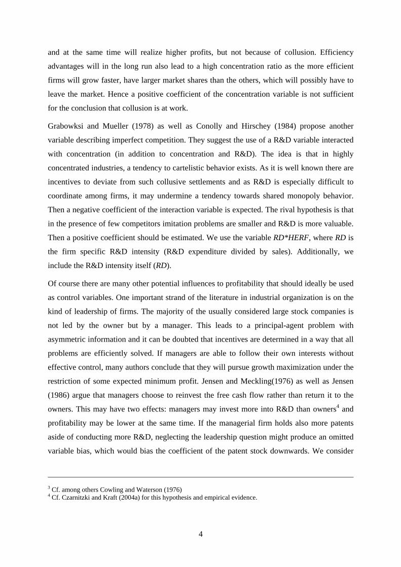
The dependent variable is the profit margin. This variable is sometimes called excess return

on sales and expresses the following:

- labor cost - capitalcost - materialcost= SS Sπ

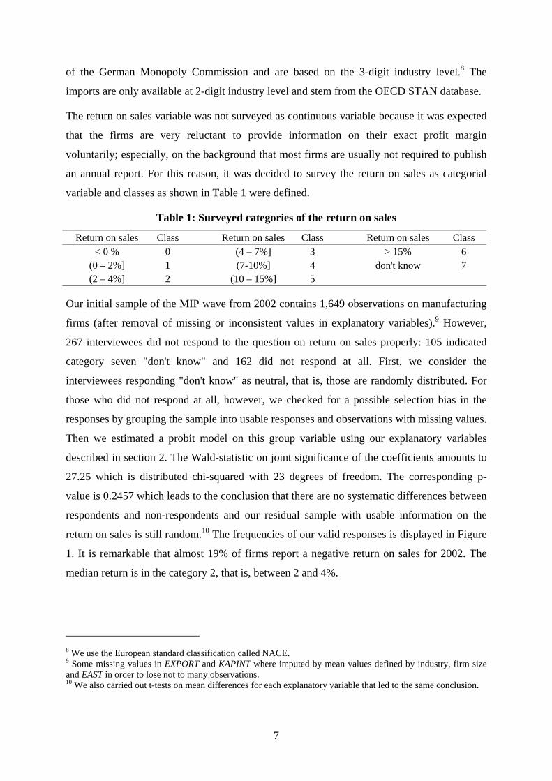
with p denoting profits and S being sales. If firms are in the long-run equilibrium and are

operating in the range of their production functions with constant returns to scale, the excess

profit return on sales will, on average across all products produced by the firm, equal the

Lerner index. With constant returns to scale marginal costs (MC) are equal to average costs

(AC). One can therefore write:

pq ACq p MCS pq pπ − −= =

with p being the price and q the quantity produced. Hence, our measure is the price-cost

margin, where the capital costs have been subtracted and need not to be taken into account by

capital divided by sales as an explanatory variable as in other empirical models considering

the price cost margin.2

The price-cost margin is usually explained by concentration in the industry and the market

share of the firm in question. Some studies (e.g. like Geroski et al., 1993) additionally

consider the interaction variable concentration times market share. We use the Herfindahl

concentration index (HERF) in order to take account of imperfect competition. The market

share (SHARE) is included here as well, because from a theoretical perspective there is a close

relationship between the market share and the price-cost margin.3 The coefficient of the

market share estimated simultaneously with the effect of the concentration variable is also

interpreted as a measure on firm efficiency. If, for example, concentration is high in a

particular market, all firms should benefit from a high price if concentration implies collusion.

However if some firms are more efficient than others, they will receive a larger market share

2 The usual way to estimate price-cost margins was introduced by Collins and Preston (1969). There arenumerous studies that follow the same methodology.

4

and at the same time will realize higher profits, but not because of collusion. Efficiency

advantages will in the long run also lead to a high concentration ratio as the more efficient

firms will grow faster, have larger market shares than the others, which will possibly have to

leave the market. Hence a positive coefficient of the concentration variable is not sufficient

for the conclusion that collusion is at work.

Grabowksi and Mueller (1978) as well as Conolly and Hirschey (1984) propose another

variable describing imperfect competition. They suggest the use of a R&D variable interacted

with concentration (in addition to concentration and R&D). The idea is that in highly

concentrated industries, a tendency to cartelistic behavior exists. As it is well known there are

incentives to deviate from such collusive settlements and as R&D is especially difficult to

coordinate among firms, it may undermine a tendency towards shared monopoly behavior.

Then a negative coefficient of the interaction variable is expected. The rival hypothesis is that

in the presence of few competitors imitation problems are smaller and R&D is more valuable.

Then a positive coefficient should be estimated. We use the variable RD*HERF, where RD is

the firm specific R&D intensity (R&D expenditure divided by sales). Additionally, we

include the R&D intensity itself (RD).

Of course there are many other potential influences to profitability that should ideally be used

as control variables. One important strand of the literature in industrial organization is on the

kind of leadership of firms. The majority of the usually considered large stock companies is

not led by the owner but by a manager. This leads to a principal-agent problem with

asymmetric information and it can be doubted that incentives are determined in a way that all

problems are efficiently solved. If managers are able to follow their own interests without

effective control, many authors conclude that they will pursue growth maximization under the

restriction of some expected minimum profit. Jensen and Meckling(1976) as well as Jensen

(1986) argue that managers choose to reinvest the free cash flow rather than return it to the

owners. This may have two effects: managers may invest more into R&D than owners4 and

profitability may be lower at the same time. If the managerial firm holds also more patents

aside of conducting more R&D, neglecting the leadership question might produce an omitted

variable bias, which would bias the coefficient of the patent stock downwards. We consider

3 Cf. among others Cowling and Waterson (1976)4 Cf. Czarnitzki and Kraft (2004a) for this hypothesis and empirical evidence.

5

this question by the variable OWN that is the percentage of capital ownership held by the top

management.

More “conventional” control variables are the share of sales exported (EXPORT) and imports

by production of domestic firms plus imports on the industry level divided (IMPORT) The

dummy variable EAST stands for firms located in Eastern Germany (the former GDR). If

firms are members of a group, the dummy variable GROUP controls for synergy

(dis)advantages. In addition, the dummy variable FOREIGN identifies if the group is led by a

foreign parent company. STARTUP denotes that the firm in question has been founded during

the recent three years. Size effects are considered by the number of employees (EMP). In

contrast to results from other countries, size disadvantages have been estimated for Germany

(see Neumann et al., 1979, 1981) and therefore a negative coefficient is not implausible. In a

dynamic world, barriers to entry are crucial in order to explain profitability. We use the

capital intensity (KAPINT) defined as fixed assets divided by the number of employees as a

variable that indicates capital requirements. As at least a part of these capital expenditures is

sunk, this variable is expected to represent barriers to entry. Ten industry dummies are

included as well.

Earlier research

One of the earliest studies on this question is Mansfield et al. (1977). They use data from a

sample of firms that agreed to provide private data on the returns from innovation. They

compare this profitability impact with the social rate of return and found quite large figures.

Conolly and Hirschey (1984) use a sample of 390 "Fortune 500" firms to estimate a

simultaneous equation model with R&D intensity (R&D/Sales), advertising intensity, market

value in excess of book value of assets and concentration as endogenous variables. They find

a positive impact of R&D and a negative one of R&D intensity interacted with concentration.

Jaffe (1986) estimates a three equation model with patents, R&D and market value as

dependent variables. According to his results the gross rate of return of R&D is 27%. Geroski

et al. (1993) consider a sample of British firms and estimate the returns to innovations using a

number of control variables.5 An indirect way to evaluate the effect of innovation on

profitability is to use the market value as dependent variable, because it should represent the

discounted future profits of a firm. The seminal study in this strand of literature is Griliches

6

(1981).6 The major disadvantage of this approach is its limitation to publicly traded stock

companies. This may still be suitable for the US or the UK, but would lead to highly selective

samples in continental European countries where the vast majority of firms is privately

owned. Czarnitzki and Kraft (2004b) suggest to use a credit rating as a proxy variable for

market value, because credit ratings are available for almost every firm and they should

reflect the wealth and thus profitability of rated companies. In line with the market value

studies, Czarnitzki and Kraft find that different innovation indicators including the patent

stock exhibit a positive impact on ratings.

3 Databases, descriptive statistics and econometric method

In order to receive a database including all the variables mentioned above, we had to link

several sources. Most firm level information is taken from the Mannheim Innovation Panel

(MIP). The MIP is an innovation survey conducted by the Centre for European Economic

Research (ZEW) on behalf of the German Federal Ministry for Education and Research

(BMBF) and is carried out annually since 1992. However, the question regarding the return

on sales has only been included in its most recent wave concerning the year 2002. Thus, our

sample is a cross-section of manufacturing firms with five or more employees.7 The

information to construct the patent stock stems from the patent database of the German Patent

and Trademark Office (DPMA) that includes all patent applications since 1980. The patents

were linked to the MIP by assignee names and addresses using a text field search. The initial

patent stock in 1980 was set to zero for all firms. As our data concern the year 2002, the bias

arising from the initial value of zero in 1980 is vanished over time due to the depreciation rate

of the knowledge capital, and is hence negligible. The ownership information of firms is taken

from the Creditreform database. Creditreform is the largest German credit rating agency and

makes its database available to the ZEW for scientific purposes. The concentration index and

the industry sales (in order to compute the market share variable) are taken from publications

5 Other relevant studies include Pakes (1986) as well as Schankerman and Pakes (1986).6 See Hall (2000) for a survey on market value studies and Hall et al. (2004) for a recent article on the calculationcitation weighted patent stocks in order to improve the approximation of the value of a firm's knowledge capital.7 A few firms are actually smaller than five employees due to differences between the population database usedfor drawing the sample of the MIP and the firms' response in the questionnaire.

7

of the German Monopoly Commission and are based on the 3-digit industry level.8 The

imports are only available at 2-digit industry level and stem from the OECD STAN database.

The return on sales variable was not surveyed as continuous variable because it was expected

that the firms are very reluctant to provide information on their exact profit margin

voluntarily; especially, on the background that most firms are usually not required to publish

an annual report. For this reason, it was decided to survey the return on sales as categorial

variable and classes as shown in Table 1 were defined.

Table 1: Surveyed categories of the return on sales

Return on sales Class Return on sales Class Return on sales Class< 0 % 0 (4 – 7%] 3 > 15% 6

(0 – 2%] 1 (7-10%] 4 don't know 7(2 – 4%] 2 (10 – 15%] 5

Our initial sample of the MIP wave from 2002 contains 1,649 observations on manufacturing

firms (after removal of missing or inconsistent values in explanatory variables).9 However,

267 interviewees did not respond to the question on return on sales properly: 105 indicated

category seven "don't know" and 162 did not respond at all. First, we consider the

interviewees responding "don't know" as neutral, that is, those are randomly distributed. For

those who did not respond at all, however, we checked for a possible selection bias in the

responses by grouping the sample into usable responses and observations with missing values.

Then we estimated a probit model on this group variable using our explanatory variables

described in section 2. The Wald-statistic on joint significance of the coefficients amounts to

27.25 which is distributed chi-squared with 23 degrees of freedom. The corresponding p-

value is 0.2457 which leads to the conclusion that there are no systematic differences between

respondents and non-respondents and our residual sample with usable information on the

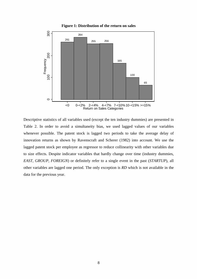
return on sales is still random.10 The frequencies of our valid responses is displayed in Figure

1. It is remarkable that almost 19% of firms report a negative return on sales for 2002. The

median return is in the category 2, that is, between 2 and 4%.

8 We use the European standard classification called NACE.9 Some missing values in EXPORT and KAPINT where imputed by mean values defined by industry, firm sizeand EAST in order to lose not to many observations.10 We also carried out t-tests on mean differences for each explanatory variable that led to the same conclusion.

8

Figure 1: Distribution of the return on sales

261

284

255 256

165

100

65

010

020

030

0Fr

eque

ncy

<0 0-<2% 2-<4% 4-<7% 7-<10% 10-<15% >=15%Return on Sales Categories

Descriptive statistics of all variables used (except the ten industry dummies) are presented in

Table 2. In order to avoid a simultaneity bias, we used lagged values of our variables

whenever possible. The patent stock is lagged two periods to take the average delay of

innovation returns as shown by Ravenscraft and Scherer (1982) into account. We use the

lagged patent stock per employee as regressor to reduce collinearity with other variables due

to size effects. Despite indicator variables that hardly change over time (industry dummies,

EAST, GROUP, FOREIGN) or definitely refer to a single event in the past (STARTUP), all

other variables are lagged one period. The only exception is RD which is not available in the

data for the previous year.

9

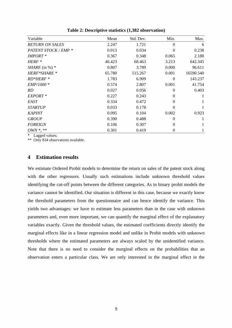
Table 2: Descriptive statistics (1,382 observation)

Variable Mean Std. Dev. Min. Max.RETURN ON SALES 2.247 1.721 0 6PATENT STOCK / EMP * 0.013 0.034 0 0.238IMPORT * 0.367 0.348 0.065 2.188HERF * 46.423 68.463 3.213 642.345SHARE (in %) * 0.807 3.789 0.000 96.611HERF*SHARE * 65.780 515.267 0.001 16590.540RD*HERF * 1.783 6.909 0 143.237EMP/1000 * 0.574 2.807 0.001 41.754RD 0.027 0.056 0 0.403EXPORT * 0.227 0.243 0 1EAST 0.334 0.472 0 1STARTUP 0.033 0.178 0 1KAPINT 0.095 0.104 0.002 0.923GROUP 0.390 0.488 0 1FOREIGN 0.106 0.307 0 1OWN *, ** 0.301 0.419 0 1* Lagged values;** Only 834 observations available.

4 Estimation results

We estimate Ordered Probit models to determine the return on sales of the patent stock along

with the other regressors. Usually such estimations include unknown threshold values

identifying the cut-off points between the different categories. As in binary probit models the

variance cannot be identified. Our situation is different in this case, because we exactly know

the threshold parameters from the questionnaire and can hence identify the variance. This

yields two advantages: we have to estimate less parameters than in the case with unknown

parameters and, even more important, we can quantify the marginal effect of the explanatory

variables exactly. Given the threshold values, the estimated coefficients directly identify the

marginal effects like in a linear regression model and unlike in Probit models with unknown

thresholds where the estimated parameters are always scaled by the unidentified variance.

Note that there is no need to consider the marginal effects on the probabilities that an

observation enters a particular class. We are only interested in the marginal effect in the

10

underlying "true" latent model (see the appendix for an outline of the Ordered Probit model

with known thresholds).11

We present estimations on two different samples: First, we consider the full sample, and

second, only the subsample of Western German firms, because the Eastern German economy

is still in transition since the German unification in 1990. Most firms were newly founded

since then and are therefore younger than Western German companies, on average. Moreover,

Eastern German firms are still highly subsidized in order to foster their catching-up process.

Hence, competition indicators like sellers' concentration may play a less significant role in

Eastern Germany and as many firms in this region of Germany are still struggling to survive

in the market economy, the relationship between profits and the considered indicators might

be less informative than in Western Germany where the industry structure has evolved in a

framework of a market economy since the Second World-War.

As the variable OWN is only available for a subsample of 834 firms, we first run the

estimations with the initial sample of 1,382 observations omitting OWN, and repeat them for

the subsample where OWN is available.

In addition to the estimations for different subsamples, we tested for heteroscedasticity using

LR tests. Multiplicative groupwise heteroscedasticity was considered and modeled by a set of

ten industry dummies, five size dummies based on the number of employees and the dummy

variable EAST. The regression results for the full sample are presented in Table 3. The LR

tests rejected homoscedasticity in both samples, and therefore the interpretation of results

focuses on the heteroscedastic models. As expected, the relationship between the return on

sales and its covariates appears to be stronger in the Western German sample than in the

sample including Eastern German firms, too.

The most important result is the positive and significant coefficient of the patent stock. Hence,

there is some effect of innovative activity on profits and an incentive for innovation exists.

For example, the average profit margin in the sample of Western German firms amounts to

3.98%.12 A Western German firm with an average innovation activity (i.e. mean of the patent

11 Verbeek (2000, pp. 192-4) does also present a good example for an Orderd Probit model with known thresholdvalues.12 In this case of a categorial variable, this result is obtained by an Orderd Probit estimation with knownthreshold values including a constant term only.

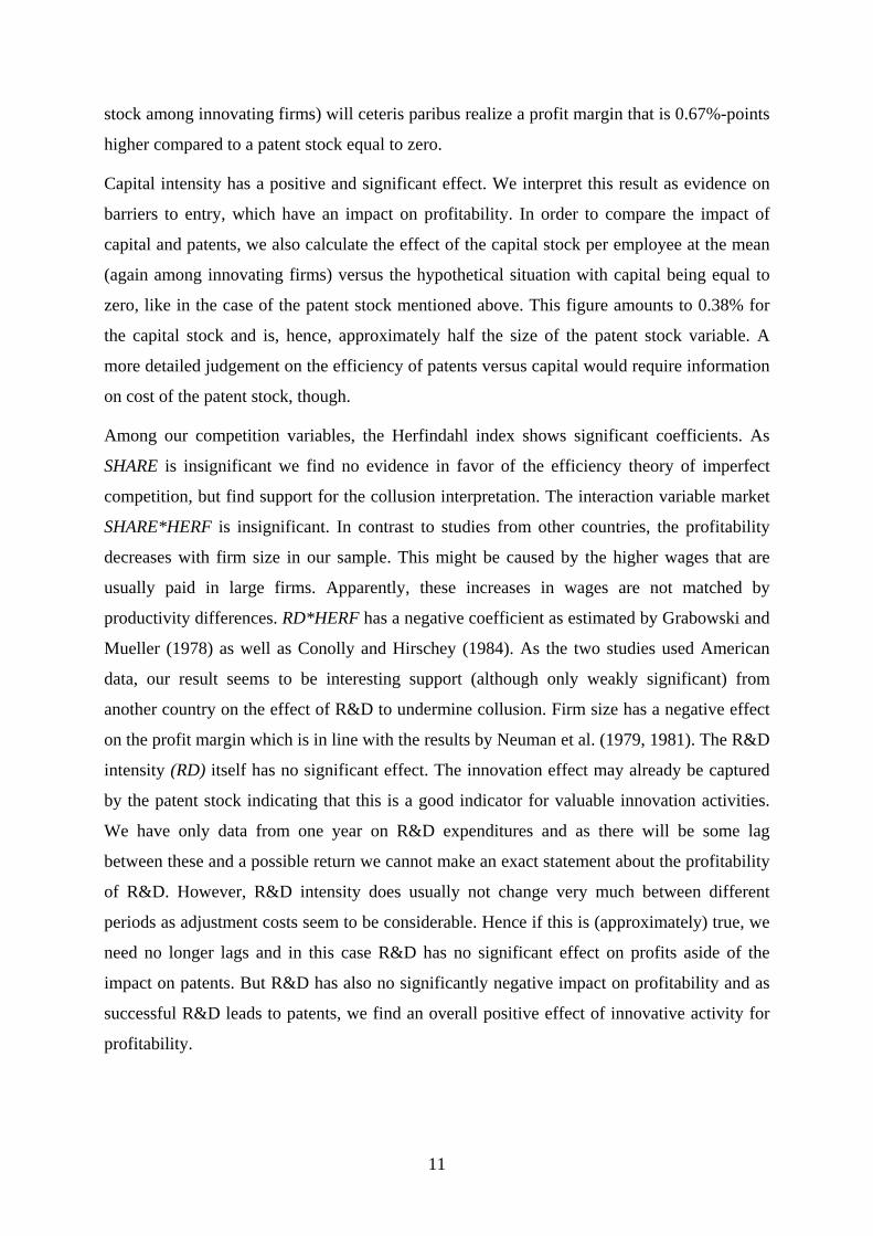
11

stock among innovating firms) will ceteris paribus realize a profit margin that is 0.67%-points

higher compared to a patent stock equal to zero.

Capital intensity has a positive and significant effect. We interpret this result as evidence on

barriers to entry, which have an impact on profitability. In order to compare the impact of

capital and patents, we also calculate the effect of the capital stock per employee at the mean

(again among innovating firms) versus the hypothetical situation with capital being equal to

zero, like in the case of the patent stock mentioned above. This figure amounts to 0.38% for

the capital stock and is, hence, approximately half the size of the patent stock variable. A

more detailed judgement on the efficiency of patents versus capital would require information

on cost of the patent stock, though.

Among our competition variables, the Herfindahl index shows significant coefficients. As

SHARE is insignificant we find no evidence in favor of the efficiency theory of imperfect

competition, but find support for the collusion interpretation. The interaction variable market

SHARE*HERF is insignificant. In contrast to studies from other countries, the profitability

decreases with firm size in our sample. This might be caused by the higher wages that are

usually paid in large firms. Apparently, these increases in wages are not matched by

productivity differences. RD*HERF has a negative coefficient as estimated by Grabowski and

Mueller (1978) as well as Conolly and Hirschey (1984). As the two studies used American

data, our result seems to be interesting support (although only weakly significant) from

another country on the effect of R&D to undermine collusion. Firm size has a negative effect

on the profit margin which is in line with the results by Neuman et al. (1979, 1981). The R&D

intensity (RD) itself has no significant effect. The innovation effect may already be captured

by the patent stock indicating that this is a good indicator for valuable innovation activities.

We have only data from one year on R&D expenditures and as there will be some lag

between these and a possible return we cannot make an exact statement about the profitability

of R&D. However, R&D intensity does usually not change very much between different

periods as adjustment costs seem to be considerable. Hence if this is (approximately) true, we

need no longer lags and in this case R&D has no significant effect on profits aside of the

impact on patents. But R&D has also no significantly negative impact on profitability and as

successful R&D leads to patents, we find an overall positive effect of innovative activity for

profitability.

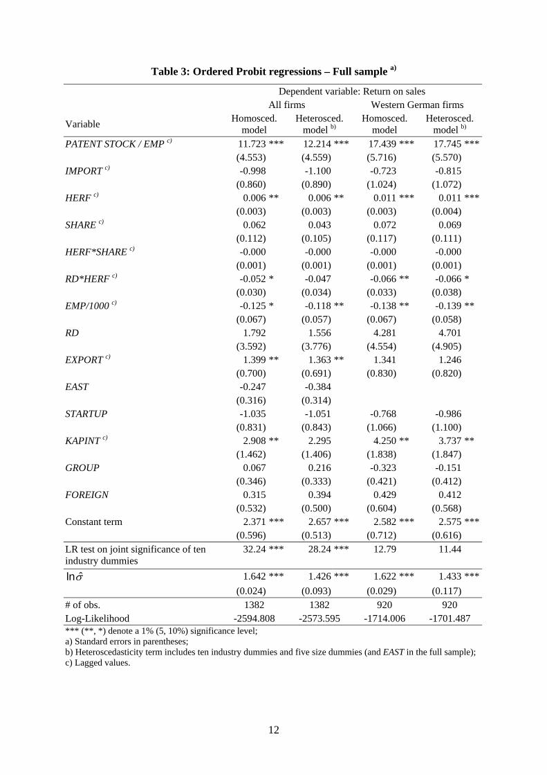
12

Table 3: Ordered Probit regressions – Full sample a)

Dependent variable: Return on salesAll firms Western German firms

Variable Homosced.model

Heterosced.model b)

Homosced.model

Heterosced.model b)

PATENT STOCK / EMP c) 11.723 *** 12.214 *** 17.439 *** 17.745 ***(4.553) (4.559) (5.716) (5.570)

IMPORT c) -0.998 -1.100 -0.723 -0.815(0.860) (0.890) (1.024) (1.072)

HERF c) 0.006 ** 0.006 ** 0.011 *** 0.011 ***(0.003) (0.003) (0.003) (0.004)

SHARE c) 0.062 0.043 0.072 0.069(0.112) (0.105) (0.117) (0.111)

HERF*SHARE c) -0.000 -0.000 -0.000 -0.000(0.001) (0.001) (0.001) (0.001)

RD*HERF c) -0.052 * -0.047 -0.066 ** -0.066 *(0.030) (0.034) (0.033) (0.038)

EMP/1000 c) -0.125 * -0.118 ** -0.138 ** -0.139 **(0.067) (0.057) (0.067) (0.058)

RD 1.792 1.556 4.281 4.701(3.592) (3.776) (4.554) (4.905)

EXPORT c) 1.399 ** 1.363 ** 1.341 1.246(0.700) (0.691) (0.830) (0.820)

EAST -0.247 -0.384(0.316) (0.314)

STARTUP -1.035 -1.051 -0.768 -0.986(0.831) (0.843) (1.066) (1.100)

KAPINT c) 2.908 ** 2.295 4.250 ** 3.737 **(1.462) (1.406) (1.838) (1.847)

GROUP 0.067 0.216 -0.323 -0.151(0.346) (0.333) (0.421) (0.412)

FOREIGN 0.315 0.394 0.429 0.412(0.532) (0.500) (0.604) (0.568)

Constant term 2.371 *** 2.657 *** 2.582 *** 2.575 ***(0.596) (0.513) (0.712) (0.616)

LR test on joint significance of tenindustry dummies

32.24 *** 28.24 *** 12.79 11.44

σln ˆ 1.642 *** 1.426 *** 1.622 *** 1.433 ***(0.024) (0.093) (0.029) (0.117)

# of obs. 1382 1382 920 920Log-Likelihood -2594.808 -2573.595 -1714.006 -1701.487*** (**, *) denote a 1% (5, 10%) significance level;a) Standard errors in parentheses;b) Heteroscedasticity term includes ten industry dummies and five size dummies (and EAST in the full sample);c) Lagged values.

13

Finally, EXPORT shows a significant positive coefficient in the full sample only. The other

control variables have no impact. Those results are partly unexpected, for example for imports

and exports, as international trade has frequently a strong impact. Note that in the sample of

Western German firms a test on joint significance of the ten industry dummies does not reject

the null hypothesis of all ten coefficients being zero. We conclude that our various

competition indicators capture the industry differences well and differences in the return on

sales are to a large extent driven by innovation.

The regression for the reduced sample including the firm leadership variable OWN are

presented in Table 4. Once again, we checked for selectivity in this sample. The full sample

was grouped according to the variable OWN, and we defined one group for non-missing

values of OWN and the other group where OWN is missing. Again, we estimated a Probit

model on the group dummy and additionally carried out t-test on mean differences for all

explanatory variables. In this case, it turns out that some selectivity is present. As OWN is

taken from the Creditreform database we have several missing values where we did not find

information on the ownership of the corresponding firm in the database. We find that no

information is available especially for younger firms and Eastern German firms. Therefore,

we omit the variable STARTUP from the regression (because there are only very few cases

left in the sample) and point out that the regression including Eastern German firms should

interpreted with some care. Unfortunately it is not possible to account for selection within the

econometric model as we have no appropriate instruments at hand to model a selection

equation. It is important to note that the profitability does not differ significantly between

both groups and we therefore conclude that the selectivity problem is not too serious in the

upcoming regression analysis.

14

Table 4: Ordered Probit - Reduced sample including OWN a)

Dependent variable: Return on salesAll firms Western German firms

Variable Homosced.model

Heterosced.model b)

Homosced.model

Heterosced.model b)

PATENT STOCK / EMP c) 14.740 ** 14.075 ** 19.663 *** 18.805 ***(6.642) (6.263) (7.603) (7.140)

OWN c) 1.089 ** 1.036 ** 1.567 *** 1.646 ***(0.494) (0.501) (0.573) (0.587)

IMPORT c) -0.470 -0.889 0.757 0.423(1.163) (1.126) (1.386) (1.352)

HERF c) 0.007 * 0.007 * 0.014 *** 0.014 ***(0.004) (0.004) (0.005) (0.005)

SHARE c) 0.374 ** 0.390 ** 0.454 *** 0.468 ***(0.173) (0.161) (0.175) (0.165)

HERF*SHARE c) -0.003 * -0.003 * -0.003 ** -0.004 **(0.001) (0.001) (0.002) (0.001)

RD*HERF c) -0.002 -0.006 -0.027 -0.033(0.051) (0.048) (0.057) (0.055)

EMP/1000 c) -0.161 -0.165 * -0.180 * -0.180 **(0.101) (0.091) (0.099) (0.091)

RD -3.481 -3.039 5.363 6.288(6.112) (6.270) (7.909) (8.026)

EXPORT c) 1.314 1.217 1.244 1.249(0.916) (0.896) (1.052) (1.031)

EAST -0.768 * -0.754 *(0.429) (0.428)

KAPINT c) 3.850 ** 3.479 * 6.900 *** 6.701 ***(1.956) (1.978) (2.425) (2.522)

GROUP 0.286 0.378 -0.243 -0.155(0.469) (0.453) (0.533) (0.526)

FOREIGN 0.039 -0.011 0.445 0.424(0.696) (0.646) (0.781) (0.737)

Constant term 1.799 *** 2.051 *** 1.432 1.483(0.786) (0.777) (0.918) (0.916)

LR test on joint significance of tenindustry dummies

21.47 ** 23.53 *** 12.39 12.62

σln ˆ 1.638 *** 1.865 *** 1.616 *** 1.823 ***(0.031) (0.076) (0.036) (0.092)

# of obs. 834 834 595 595Log-Likelihood -1546.525 -1536.661 -1095.855 -1090.282*** (**, *) denote a 1% (5, 10%) significance level;a) Standard errors in parentheses;b) Heteroscedasticity term includes five size dummiesc) Lagged values.

15

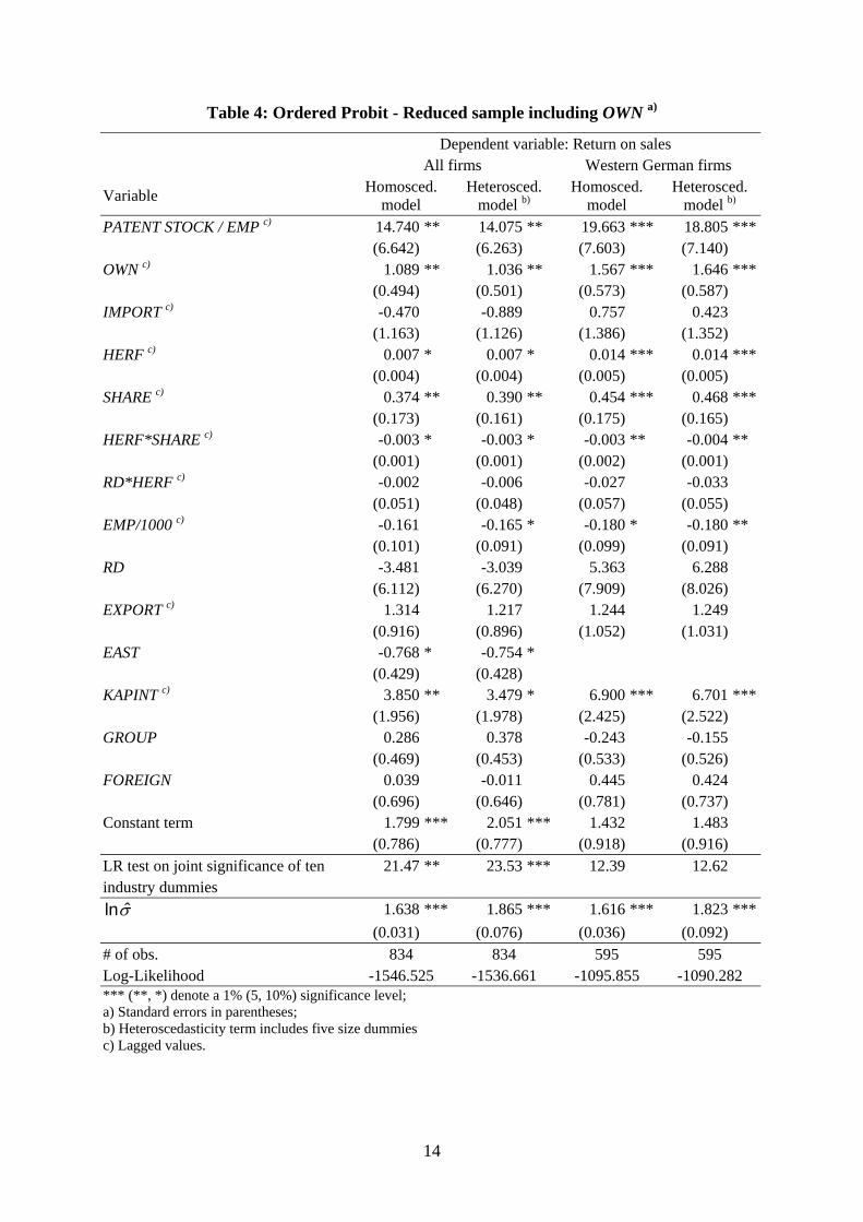
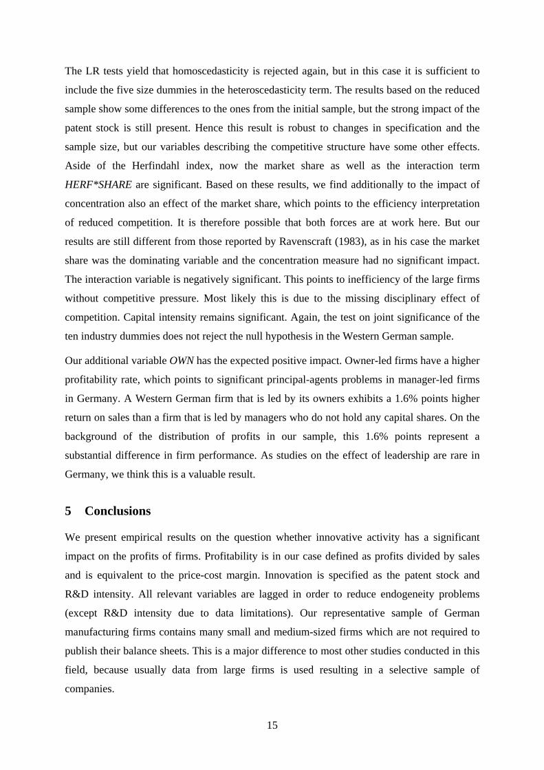
The LR tests yield that homoscedasticity is rejected again, but in this case it is sufficient to

include the five size dummies in the heteroscedasticity term. The results based on the reduced

sample show some differences to the ones from the initial sample, but the strong impact of the

patent stock is still present. Hence this result is robust to changes in specification and the

sample size, but our variables describing the competitive structure have some other effects.

Aside of the Herfindahl index, now the market share as well as the interaction term

HERF*SHARE are significant. Based on these results, we find additionally to the impact of

concentration also an effect of the market share, which points to the efficiency interpretation

of reduced competition. It is therefore possible that both forces are at work here. But our

results are still different from those reported by Ravenscraft (1983), as in his case the market

share was the dominating variable and the concentration measure had no significant impact.

The interaction variable is negatively significant. This points to inefficiency of the large firms

without competitive pressure. Most likely this is due to the missing disciplinary effect of

competition. Capital intensity remains significant. Again, the test on joint significance of the

ten industry dummies does not reject the null hypothesis in the Western German sample.

Our additional variable OWN has the expected positive impact. Owner-led firms have a higher

profitability rate, which points to significant principal-agents problems in manager-led firms

in Germany. A Western German firm that is led by its owners exhibits a 1.6% points higher

return on sales than a firm that is led by managers who do not hold any capital shares. On the

background of the distribution of profits in our sample, this 1.6% points represent a

substantial difference in firm performance. As studies on the effect of leadership are rare in

Germany, we think this is a valuable result.

5 Conclusions

We present empirical results on the question whether innovative activity has a significant

impact on the profits of firms. Profitability is in our case defined as profits divided by sales

and is equivalent to the price-cost margin. Innovation is specified as the patent stock and

R&D intensity. All relevant variables are lagged in order to reduce endogeneity problems

(except R&D intensity due to data limitations). Our representative sample of German

manufacturing firms contains many small and medium-sized firms which are not required to

publish their balance sheets. This is a major difference to most other studies conducted in this

field, because usually data from large firms is used resulting in a selective sample of

companies.

16

The patent stock has a strong and robust effect on profitability. An innovating firm realizes an

about 0.67% points higher return on sales than a firm not performing innovation activities, on

average. Therefore we conclude that an incentive for innovation exists in Germany. In

contrast, the R&D intensity has no separate, additional effect. The results with respect to the

variables representing the competitive structure are mixed. The Herfindahl concentration

index has always a strong positive impact on profits. The market share and the interaction

variable market share times the Herfindahl index are both only significant in a subsample of

companies for which information on firm leadership is available. Hence, we have limited

evidence in favor of the hypothesis that a high concentration is the result of efficiency

advantages of the larger firms. In contrast, capital intensity has a stable positive impact on

profits. We interpret this result as evidence on barriers to entry that have an impact on

profitability. Moreover, our results point to the conclusion that owner-led firms have a

significantly larger profit rate. There exist leadership inefficiencies in German firms and the

managers may require better incentives or closer supervision in order to solve the principal-

agent problems.

Although we find evidence on the positive impact of innovation on profits, this is only one

part of the story. The returns have to be compared with the costs, and at present we have only

limited information on those. One would need a long times series on R&D expenditures as the

input to the innovative process (and not just the data from one year as in the present study).

Then the effects of the overall outlays for profits in later years have to be calculated. This

would be the “true” test on the profit effects of innovative activity. In such a study, one could

also test whether patents have a significant effect on profits aside of past R&D activities as,

on the one hand, patents are a measure of R&D output or success and, on the other hand,

patents are expected to reduce (or even eliminate) imitation possibilities by competitors.

References

Arrow, K.J. (1962), Economic Welfare and the Allocation of Resources for Invention, in:R.R. Nelson (ed.), The Rate and Direction of Inventive Activity: Economic and SocialFactors, Princeton, N.J., 609-625.

Cowling, K. and M. Waterson (1976), Price-Cost Margins and Market Structure, Economica43, 87-92.

Collins, N. and L.E. Preston (1969), Price-Cost Margins and Industry Structure, Review ofEconomics and Statistics 51, 271-286.

17

Conolly R.A. and M. Hirschey (1984), R&D, Market Structure and Profits: A Value-BasedApproach, Review of Economics and Statistics 66, 682-686.

Czarnitzki, D. and K. Kraft (2004a), Management Control and Innovative Activity,forthcoming in Review of Industrial Organization.

Czarnitzki, D. and K. Kraft (2004b), Innovation Indicators and Corporate Credit Ratings:Evidence from German Firms, Economics Letters 82(3), 377-384.

Geroski, P., S. Machin and J. van Reenen (1993), The Profitability of Innovating Firms,RAND Journal of Economics 24, 198-211.

Grabowski, H.G. and D.C. Mueller (1978), Industrial Research and Development, IntangibleCapital Stocks and Firm Profit Rates, Bell Journal of Economics 9, 328-343.

Griliches, Z. (1981), Market value, R&D and patents, Economics Letters 7, 183-187.

Griliches, Z. and J. Mairesse (1984), Productivity and R&D at the Firm Level, in Z. Griliches(ed.), R&D, Patents and Productivity, Chicago, 339-374.

Gugler, K., D.C. Mueller and B.B. Yurtoglu (2002), The Impact of Corporate Governance onInvestment Returns in Developed Countries, Economic Journal 113, F511-F539.

Hall, B.H. (1990), The manufacturing sector master file: 1959-1987, NBER Working PaperSeries No. 3366, Cambridge, MA.

Hall, B.H. (2000), Innovation and Market Value, in: R. Barrell, G. Mason and M. O'Mahony(eds.), Productivity, Innovation, and Economic Performance, Cambridge, 177-198.

Hall, B.H., A. Jaffee and M. Trajtenberg (2004), Market Value and Patent Citations,forthcoming in: RAND Journal of Economics.

Jaffe, A.B. (1986), Technological Opportunity and Spillovers of R&D: Evidence from Firms’Patents, Profits, and Market Value, American Economic Review 76, 984-1001.

Mansfield, E., J. Rapoport, A. Romeo, S. Wagner and G. Beardsley (1977), Social and PrivateReturn from Industrial Innovations, Quarterly Journal of Economics 91, 221-240.

Neumann, M., I. Böbel and A. Haid (1979), Profitability, Risk and Market Structure in WestGerman Industries, Journal of Industrial Economics 27, 227-242

Neumann, M., I. Böbel and A. Haid (1981), Market Structure and the Labour Market in WestGerman Industries – A Contribution Towards Interpreting the Structure-PerfomanceRelationship, Journal of Economics/Zeitschrift für Nationalökonomie, vol. 41, 97-109.

Jensen, M. (1986), Agency Costs of Free Cash Flow, Corporate Finance, and Takeovers,American Economic Review 76, 323-329.

Jensen, M. and W. Meckling (1976), Theory of the Firm: Managerial Behavior, AgencyCosts, and Ownership Structure, Journal of Financial Economics 3, 305-360.

Pakes, A. (1986), Patents as Options: Some Estimates of the Value of Holding EuropeanPatent stocks, Econometrica 54, 755-784.

Ravenscraft, D.J. (1983): Structure-Profit Relationships at the Line of Business and IndustryLevel, Review of Economics and Statisitics 65, 22-31.

18

Ravenscraft, D.J. and F.M. Scherer (1982), The Lag Structure of Returns to Research andDevelopment, Applied Economics 14, 603-620.

Schankerman, M. and A. Pakes (1986), Estimates of the Value of Patent Rights in EuropeanCountries during the Post-1950 Period: Economic Journal 96, 1052-1077.

Schleifer, A. and R.W. Vishny (1997), A Survey of Corporate Governance, Journal ofFinance 52, 737-783.

Verbeek, M. (2000), A Guide to Modern Econometrics, Chichester.

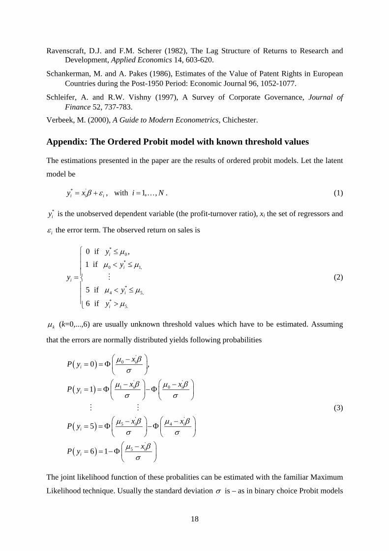
Appendix: The Ordered Probit model with known threshold values

The estimations presented in the paper are the results of ordered probit models. Let the latent

model be

* ' , with 1, ,i i iy x i Nβ ε= + = … . (1)

*iy is the unobserved dependent variable (the profit-turnover ratio), xi the set of regressors and

iε the error term. The observed return on sales is

*0

*0 1,

*4 5,

*5.

0 if ,

1 if

5 if

6 if

i

i

i

i

i

y

yy

y

y

µ

µ µ

µ µ

µ

⎧ ≤⎪

< ≤⎪⎪= ⎨⎪ < ≤⎪⎪ >⎩

(2)

kµ (k=0,...,6) are usually unknown threshold values which have to be estimated. Assuming

that the errors are normally distributed yields following probabilities

( )

( )

( )

( )

'0

' '1 0

' '5 4

'5

0 ,

1

5

6 1

ii

i ii

i ii

ii

xP y

x xP y

x xP y

xP y

µ βσ

µ β µ βσ σ

µ β µ βσ σ

µ βσ

⎛ ⎞−= = Φ⎜ ⎟

⎝ ⎠⎛ ⎞ ⎛ ⎞− −

= = Φ −Φ⎜ ⎟ ⎜ ⎟⎝ ⎠ ⎝ ⎠

⎛ ⎞ ⎛ ⎞− −= = Φ −Φ⎜ ⎟ ⎜ ⎟

⎝ ⎠ ⎝ ⎠⎛ ⎞−

= = −Φ⎜ ⎟⎝ ⎠

(3)

The joint likelihood function of these probalities can be estimated with the familiar Maximum

Likelihood technique. Usually the standard deviation σ is – as in binary choice Probit models

19

– not identified. All estimated coefficients are scaled by σ . In this case, however, we are in a

situation, where we know the threshold values kµ . Recall that the profit variable has been

categorized in the survey, but we know the threshold values for each class. Using the true

threshold values, allows us to identify the variance (and the constant term) and reduces the

parameters to be estimated. The coefficients can directly be interpreted as marginal effects in

the "true" latent model.

Finally, the tests on heteroscedasticity allow the variance to vary over industries, firm size and

EAST. Firm size is specified as five size classes categorized by the number of employees. The

homoscedastic standard deviation σ̂ is replaced by ˆ iσ as

( )'expi iσ σ ωα= + (4)

where α are the additional parameters to be estimated and iω are the variables which are

considered to model the heteroscedasticity. Although likelihood ratio tests do reject the

hypothesis of homoscedasticity, the results concerning the patent stock and most control

variables remain similar.