On the Role of Productivity and Factor - COnnecting · PDF filewould have only a limited...
48
econstor www.econstor.eu Der Open-Access-Publikationsserver der ZBW – Leibniz-Informationszentrum Wirtschaft The Open Access Publication Server of the ZBW – Leibniz Information Centre for Economics Standard-Nutzungsbedingungen: Die Dokumente auf EconStor dürfen zu eigenen wissenschaftlichen Zwecken und zum Privatgebrauch gespeichert und kopiert werden. Sie dürfen die Dokumente nicht für öffentliche oder kommerzielle Zwecke vervielfältigen, öffentlich ausstellen, öffentlich zugänglich machen, vertreiben oder anderweitig nutzen. Sofern die Verfasser die Dokumente unter Open-Content-Lizenzen (insbesondere CC-Lizenzen) zur Verfügung gestellt haben sollten, gelten abweichend von diesen Nutzungsbedingungen die in der dort genannten Lizenz gewährten Nutzungsrechte. Terms of use: Documents in EconStor may be saved and copied for your personal and scholarly purposes. You are not to copy documents for public or commercial purposes, to exhibit the documents publicly, to make them publicly available on the internet, or to distribute or otherwise use the documents in public. If the documents have been made available under an Open Content Licence (especially Creative Commons Licences), you may exercise further usage rights as specified in the indicated licence. zbw Leibniz-Informationszentrum Wirtschaft Leibniz Information Centre for Economics Daude, Christian; Fernandez-Arias, Eduardo Working Paper On the Role of Productivity and Factor Accumulation in Economic Development in Latin America and the Caribbean IDB Working Paper Series, No. IDB-WP-155 Provided in Cooperation with: Inter-American Development Bank, Washington, DC Suggested Citation: Daude, Christian; Fernandez-Arias, Eduardo (2010) : On the Role of Productivity and Factor Accumulation in Economic Development in Latin America and the Caribbean, IDB Working Paper Series, No. IDB-WP-155 This Version is available at: http://hdl.handle.net/10419/89170
Transcript of On the Role of Productivity and Factor - COnnecting · PDF filewould have only a limited...

econstor www.econstor.eu
Der Open-Access-Publikationsserver der ZBW – Leibniz-Informationszentrum WirtschaftThe Open Access Publication Server of the ZBW – Leibniz Information Centre for Economics
Standard-Nutzungsbedingungen:
Die Dokumente auf EconStor dürfen zu eigenen wissenschaftlichenZwecken und zum Privatgebrauch gespeichert und kopiert werden.
Sie dürfen die Dokumente nicht für öffentliche oder kommerzielleZwecke vervielfältigen, öffentlich ausstellen, öffentlich zugänglichmachen, vertreiben oder anderweitig nutzen.
Sofern die Verfasser die Dokumente unter Open-Content-Lizenzen(insbesondere CC-Lizenzen) zur Verfügung gestellt haben sollten,gelten abweichend von diesen Nutzungsbedingungen die in der dortgenannten Lizenz gewährten Nutzungsrechte.
Terms of use:
Documents in EconStor may be saved and copied for yourpersonal and scholarly purposes.
You are not to copy documents for public or commercialpurposes, to exhibit the documents publicly, to make thempublicly available on the internet, or to distribute or otherwiseuse the documents in public.
If the documents have been made available under an OpenContent Licence (especially Creative Commons Licences), youmay exercise further usage rights as specified in the indicatedlicence.
zbw Leibniz-Informationszentrum WirtschaftLeibniz Information Centre for Economics
Daude, Christian; Fernandez-Arias, Eduardo
Working Paper
On the Role of Productivity and Factor Accumulationin Economic Development in Latin America and theCaribbean
IDB Working Paper Series, No. IDB-WP-155
Provided in Cooperation with:Inter-American Development Bank, Washington, DC
Suggested Citation: Daude, Christian; Fernandez-Arias, Eduardo (2010) : On the Role ofProductivity and Factor Accumulation in Economic Development in Latin America and theCaribbean, IDB Working Paper Series, No. IDB-WP-155
This Version is available at:http://hdl.handle.net/10419/89170

1
IDB WORKING PAPER SERIES # IDB-WP-155
On the Role of Productivity and Factor Accumulation in Economic Development in Latin America and the Caribbean
Christian Daude Eduardo Fernández-Arias
Inter-American Development Bank
Department of Research and Chief Economist
February 2010

2
On the Role of Productivity and Factor Accumulation in Economic
Development in Latin America and the Caribbean
Christian Daude* Eduardo Fernández-Arias**
*OECD Development Centre **Inter-American Development Bank
Inter-American Development Bank 2010
3
Cataloging-in-Publication data provided by the Inter-American Development Bank Felipe Herrera Library Daude, Christian. On the role of productivity and factor accumulation in economic development in Latin America and the Caribbean / Christian Daude, Eduardo Fernández-Arias.
p. cm. (IDB working paper series ; 155) Includes bibliographical references. 1. Industrial productivity—Latin America. 2. Industrial productivity—Caribbean Area. 3. Economic Development—Latin America. 4. Economic Development—Caribbean Area. I. Fernández-Arias, Eduardo. II. Inter-American Development Bank. Research Dept. III. Title. IV. Series. HC79.I52 D38 2010 338.06 D235—dc22
© Inter-American Development Bank, 2010 www.iadb.org Documents published in the IDB working paper series are of the highest academic and editorial quality. All have been peer reviewed by recognized experts in their field and professionally edited. The views and opinions presented in this working paper are entirely those of the author(s), and do not necessarily reflect those of the Inter-American Development Bank, its Board of Executive Directors or the countries they represent. This paper may be freely reproduced provided credit is given to the Inter-American Development Bank.
4
Abstract*
This paper combines development and growth accounting exercises with economic theory to estimate the relative importance of total factor productivity and the accumulation of factors of production in the economic development performance of Latin America. The region’s development performance is assessed by contrast with various alternative benchmarks, both advanced countries and peer countries in other regions. The paper finds that total factor productivity is the predominant factor: low productivity and slow productivity growth, as opposed to impediments to factor accumulation, are the key to understanding Latin America’s low income relative to developed economies and its stagnation relative to other developing countries. While policies easing factor accumulation would help somewhat in improving productivity, for the most part, closing the productivity gap requires productivity-specific policies. JEL Classification: O11, O47 Keywords: Economic growth, Total factor productivity, Development
* The authors wish to acknowledge insightful comments by Peter Klenow, Diego Restuccia, Andrés Rodríguez-Clare and participants in IDB Research Department seminars as well as Karina Otero for excellent research assistance. The views expressed are those of the authors and should not be attributed to the Inter-American Development Bank or the OECD.
5
1. Introduction
Most countries in Latin America and the Caribbean (LAC) have been growing slowly for a long
time and see themselves increasingly poor relative to the rest of the world, both advanced
countries and peer countries in other regions. Actual declines in income per capita for substantial
periods of time are common. However, as we show in this paper, it would be misleading to
blame low investment for this failure. Low productivity and slow productivity growth, as
opposed to impediments to factor accumulation, is the key to understanding LAC’s low income
relative to developed economies and its stagnation relative to other developing countries that are
catching up. A fortiori, the main development policy challenge in the region involves diagnosing
the causes of poor productivity and acting on its roots.
This paper is organized in the following way. In Section 2 we explain how and why we
use total factor productivity (TFP, henceforth) as our measure of productivity to understand
growth and development in LAC. In the following two sections we establish the basic stylized
facts of aggregate productivity using some of the traditional tools of development and growth
accounting, and then test their robustness to technical assumptions. Section 5 analyzes the
interplay between aggregate productivity and factor accumulation. There we show that
traditional tools underestimate the relevance of productivity: once it is recognized that factor
accumulation reacts to TFP, it becomes clear that productivity is by far the key to the economic
development problematic in the region. We further show that promoting factor accumulation
would have only a limited impact on the productivity shortfall. Finally, in Section 6 we conclude
by discussing some policy implications of our findings and areas for future research.
2. Measuring Aggregate Productivity
The first question to deal with is how to measure aggregate productivity. Standard economic
analysis estimates aggregate productivity, or TFP, by looking at the annual output Y (measured
by the gross domestic product, GDP) that is produced on the basis of the accumulated factors of
production, or capital, which are available as inputs. For any given stock of capital, the higher
the output the more productive the economy. Capital is composed by physical capital, K, and
human capital H. Physical capital takes the form of means of production, such as machines and
buildings. Human capital is the productive capacity of the labor force, which in turn corresponds
to the headcount of the labor force or raw labor, L, multiplied by its average level of skill or
6
education h, so that H=hL. TFP measures the effectiveness with which accumulated factors of
production, or capital, are used to produce output.
Therefore output Y results from the combination of factors of production K and H at a
certain degree of TFP. Likewise, output growth over time results from accumulation of factors
of production and productivity growth. The attribution of output level and growth to factors and
productivity is done by using production functions mapping factors into output: what is not
accounted for by factors of production as estimated by the production function is attributed to
productivity. In particular, we use a standard Cobb-Douglas production function given by:
( ) aaaa hLAKHAKY −− == 11 (1)
where a is the output elasticity to (physical) capital. The production function parameter a is set
equal to 1/3, a standard value in the literature (see Klenow and Rodríguez-Clare, 2005).
Although there is some debate in the literature regarding the validity of this assumption, Gollin
(2002) shows that once informal labor and household entrepreneurship are taken into account,
there is no systematic difference across countries associated with level of development (GDP per
capita), nor any time trend. Hence its uniformity across countries and time appears to be a
reasonable assumption.
We construct the relevant series for output, physical capital and human capital (Y,K,H
respectively) based on available statistics and following methods detailed in the Statistical
Appendix. It is useful to note that we filter the raw annual data to obtain smooth series reflecting
their trends, thus filtering out the business cycle. Using these series, we can compute our
measure of TFP by:
aa hLKYA −= 1)(
, (2)
which is a comprehensive measure of the efficiency with which the economy is able to transform
its accumulated factors of production K and H into output Y. In this way, as noted, we estimate
trend TFP series for each country.1
1 In this formulation, TFP would also reflect the natural resource base (natural capital) of each country. Resource-rich countries would tend to exhibit larger (but possibly less dynamic) measured TFP. Since LAC is a resource-rich region, this observation implies that a symptom of low productivity would signal an even more serious ailment. (On the other hand, it could be argued that natural resources give rise to backward development and ultimately lower productivity (the “natural resource curse hypothesis”); see Lederman and Maloney, 2008, for a critical view.) In any
7
In terms of the sample of countries utilized, on top of the availability of all these data, we
introduce as a further restriction a population size of at least 1 million as of 1960. The resulting
sample of 76 countries is shown in Table 1. The data extend from 1960 to 2005.
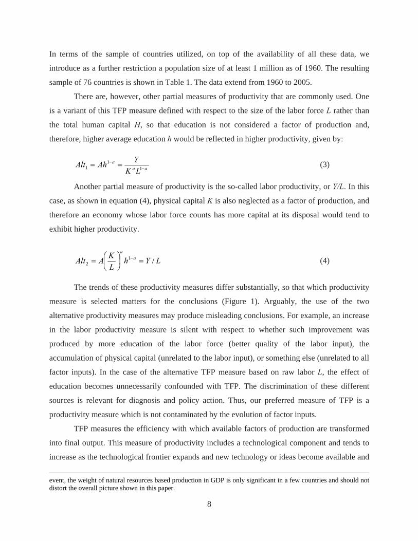
There are, however, other partial measures of productivity that are commonly used. One
is a variant of this TFP measure defined with respect to the size of the labor force L rather than
the total human capital H, so that education is not considered a factor of production and,
therefore, higher average education h would be reflected in higher productivity, given by:
aaa
LKYAhAlt −
− == 11
1 (3) Another partial measure of productivity is the so-called labor productivity, or Y/L. In this
case, as shown in equation (4), physical capital K is also neglected as a factor of production, and
therefore an economy whose labor force counts has more capital at its disposal would tend to
exhibit higher productivity.
LYhLKAAlt a
a
/12 =⎟
⎠⎞
⎜⎝⎛= − (4)
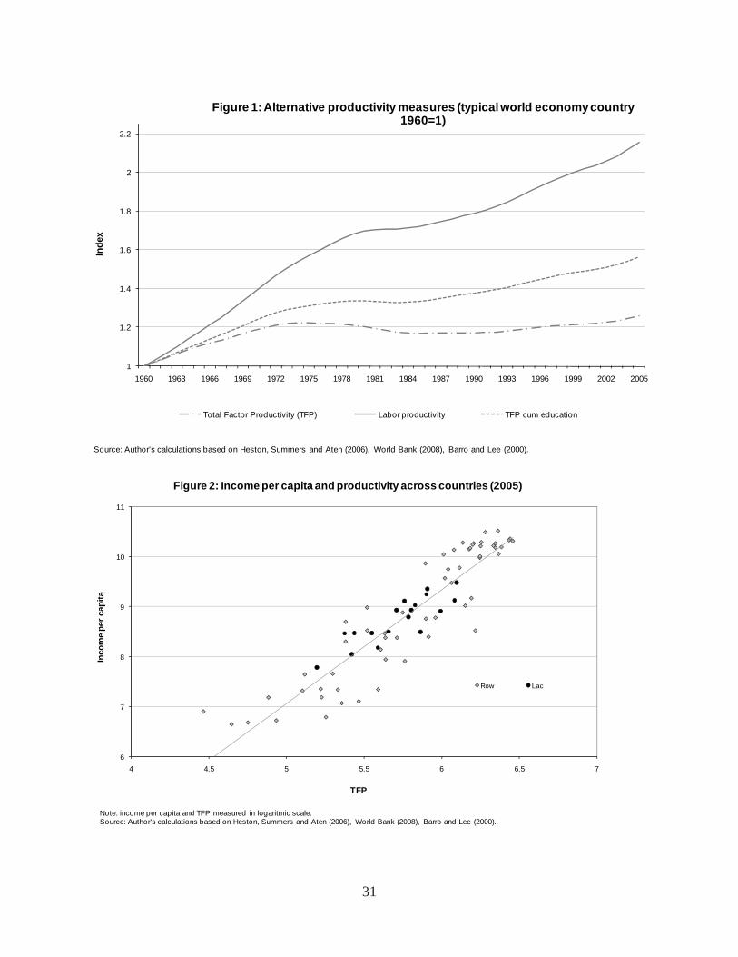
The trends of these productivity measures differ substantially, so that which productivity
measure is selected matters for the conclusions (Figure 1). Arguably, the use of the two
alternative productivity measures may produce misleading conclusions. For example, an increase
in the labor productivity measure is silent with respect to whether such improvement was
produced by more education of the labor force (better quality of the labor input), the
accumulation of physical capital (unrelated to the labor input), or something else (unrelated to all
factor inputs). In the case of the alternative TFP measure based on raw labor L, the effect of
education becomes unnecessarily confounded with TFP. The discrimination of these different
sources is relevant for diagnosis and policy action. Thus, our preferred measure of TFP is a
productivity measure which is not contaminated by the evolution of factor inputs.
TFP measures the efficiency with which available factors of production are transformed
into final output. This measure of productivity includes a technological component and tends to
increase as the technological frontier expands and new technology or ideas become available and
event, the weight of natural resources based production in GDP is only significant in a few countries and should not distort the overall picture shown in this paper.
8
are adopted, but it is also affected by the efficiency with which markets work and are served by
public services. For example, an economy populated by technologically advanced firms may
produce inefficient aggregate results and therefore translate into low aggregate productivity. In
particular, market and policy failures may distort the efficiency with which factors are allocated
across sectors, and across firms within sectors, thus depressing efficiency at the aggregate level.
The upshot is that, while increasing the stock of accumulated factors may require resources that
are unavailable in low-income countries and may even be wasteful if productivity is low,
boosting productivity directly may “simply” require willingness to reform policies and
institutions by taking advantage of successful experiences elsewhere.
It is important to understand what TFP includes and does not include in this paper.
Because we are not considering effectively employed labor force and physical capital but the
entire stocks available for production, partially utilized factors (e.g., unemployment) would be
reflected in low productivity. As noted, in order to avoid the fluctuations this accounting would
induce in productivity due to the business cycle, we filtered the annual series of output and
factors to retain only their trends, thus obtaining trend productivity. Therefore, in our
calculations, only structural underutilization of resources would be reflected in low productivity.2
At the same time, because we chose to measure labor input as labor force, variations in the share
of the population in the labor force (whether because of demographic reasons or the choice of
working age population to participate in the labor force) do not affect TFP. In other words, a
smaller labor force as a share of the population is not reflected in lower productivity. On the
other hand, as discussed above, the quality of education, which may differ significantly across
countries, would be reflected in the productivity measure inasmuch as it impinges on the
working capacity of the labor force.3 Similarly, the age profile of the labor force would also
entail differences in experience akin to the quality of education.
The above production function framework can be directly applied to account for output
per worker Y/L (or “labor productivity”) in terms of TFP and per-worker factor intensities:
k=K/L (“capital intensity”) and h=H/L (education of the labor force). It is useful to relate this
production function framework to a welfare framework, such as the traditional measure of GDP
2 Our choice of measurement implies that an economy with higher structural unemployment is less productive because it wastes available resources. 3 To the extent that quality differences affect uniformly the education spectrum, the aggregative measure h would not be distorted and they would only be reflected in TFP differences (see Appendix).
9
per capita (y=Y/N), where N is the size of the population. This is an income measure commonly
used to gauge welfare across countries. In this case, differences in income per capita, or in its
growth, can be attributed to TFP and per-worker factor intensities, as before, and an extra term
reflecting the share of the population in the labor force (L/N, denoted by f ), given by:4
fhAkNLh
LKA
NYy aaa
a−− =⎟
⎠⎞
⎜⎝⎛== 11 (5)
The enormous diversity of income per capita that exists across countries can be well
explained statistically by differences in their aggregate productivity levels as measured by TFP.
TFP and income per capita move in tandem (see Figure 2), with a correlation coefficient of 0.91.
Thus, in statistical terms, 83 percent of the cross-country income variation in the world today
would disappear if TFP were the same across countries in the world. TFP appears central to
understanding income per capita diversity across countries and to acting on the root causes of
underdevelopment. In the remainder of the paper we will explore the economic determinants of
this strong relationship.
In most of the analysis, we consider the productivity of the typical country in LAC,
represented by a simple (logarithmic) average of country productivities, irrespective of whether
the country is large or small. Thus, the typical LAC country’s TFP is measured by:
nn
iilac AA
1
1⎟⎟⎠
⎞⎜⎜⎝
⎛= ∏
=
. (6)
Similarly, we consider the simple (logarithmic) average of income per capita (y), and the
corresponding per-worker factor of production intensities (k,h,f).5 To represent the region as a
whole, however, where the productivity of larger countries is more influential because it applies
to larger stocks of productive factors, we consider a synthetic region country summing up inputs
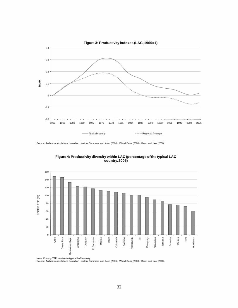
and outputs over countries. For example, Figure 3 shows productivity in LAC (as opposed to the
world’s TFP shown in Figure 1) for both the typical country and the region as a whole.6 (More
4 The parameter f depends on the share of working age population (a demographic factor) and the rate of its participation in the labor force. 5 The use of a logarithmic transformation is needed to ensure that the TFP of the typical country so defined coincides with the typical TFP previously defined. 6 Since technology in principle can only improve over time, we note in passing that a declining TFP over some periods reinforces the notion that TFP is only partially technologically determined.
10
generally, we represent various country groupings as the typical country and the region following
similar methods for the analysis of a number of variables.)
Before embarking in the analysis of regional aggregates, it may be useful to keep in mind
that there is substantial diversity in productivity levels across countries in the LAC region.
Figure 4 shows our estimation of current productivity levels in each country relative to the
typical country in Latin America (as of 2005).7 For example, TFP in Chile is 2.5 times higher
than in Honduras.8 The diversity within the region, as expected, is highly correlated with income
per capita (with a correlation coefficient of 0.86; see Figure 2).
3. Stylized Facts of Aggregate Productivity in LAC
In this section we review the patterns of the evolution of aggregate productivity in the economic
development of the LAC region, both in growth and levels.9 This is done using traditional tools
of growth and development accounting.
Concerning growth accounting, the growth rate of TFP ( A ) is obtained as a residual after
accounting for the growth rates of output and factor inputs (measured as their logarithmic
increase from equation (5)):10
( ) fhakaAy ˆˆ1ˆˆˆ +−++= . (7) The above equation can also be used to account for the growth gaps between two
countries or group of countries, so that the growth gap in income per capita can be decomposed
into the sum of the growth gap in TFP, the (weighed) factors’ growth gaps, and the gap in the
growth of labor force intensity:
( ) )ˆ()ˆ(1)ˆ()ˆ()ˆ( fGaphGapakaGapAGapyGap +−++= (8)
7 Country TFP estimations may be subject to measurement errors of the underlying economic variables which would tend to cancel out in regional TFP estimations, for example that of the typical country, which we regard as substantially more reliable. 8 This particular difference is larger than the TFP gap of the typical country in the region with respect to the United States, as we will show below. 9 The 18 LAC countries included in the sample are Argentina, Bolivia, Brazil, Chile, Colombia, Costa Rica, Dominican Republic, Ecuador, El Salvador, Honduras, Jamaica, Mexico, Nicaragua, Panama, Paraguay, Peru, Uruguay and Venezuela. 10 We follow the convention to denote the growth rate of a variable x by . x
11
Development accounting looks at levels rather than growth rates. It utilizes equation 5 to
compare the components behind income per capita between an economy of interest and a
benchmark economy taken as a development yardstick, denoted by “*”, or level gaps:
fhkAff
hh
kk
AA
yyy aa
aa−
−
=⎟⎠⎞
⎜⎝⎛
⎟⎠⎞
⎜⎝⎛== 1
*
1
**** (9)
A logarithmic transformation of the above equation can then be used to account for the
contribution of the TFP gap and that of factor intensities to the overall income per capita gap at a
point in time:
( ) ( ) ( )fhakaAy loglog)1(log()log()log( +−++= (10) In order to highlight LAC’s weaknesses and anomalies, these gaps (the growth gaps in
equation (8) and the log-level gaps in equation (10) are computed against the rest of the world
(ROW) and selected groups of countries, such as the East Asian tigers (EA), currently Developed
countries (DEV), and “Twin” countries (TWIN, countries whose income was initially, by 1960,
comparable to that of LAC countries).11,12 Unless noted, comparisons are made between the
typical countries of each one of the regions. Following convention, we take the US economy as
the technological frontier against which “absolute” gaps in productivity are estimated.
It is worth noting that equation (10) contains all the information needed for this analysis.
The time difference over a period of p years (say from t-p to t) yields a decomposition of how the
level gaps opened during the period, to be interpreted as a decomposition of the accumulated
growth gap in the period, found in equation (11). In fact, for a period of one year (p=1, so that
the period runs between t-1 and t), the time difference yields the annual growth gap in equation
(8).
11 The latter group of “twin” countries was constructed by selecting all countries in the sample whose 1960 income per capita fell in the inter-quartile range of Latin American countries (incomes within the second and third quartile). 12 East Asian tigers are Hong-Kong, Korea, Malaysia, Singapore and Thailand; Developed countries are Australia, Austria, Belgium, Canada, Denmark, Finland, France, Germany, Greece, Hungary, Ireland, Italy, Japan, Korea, Netherlands, New Zealand, Norway, Portugal, Spain, Sweden, United Kingdom and United States; Twin countries are Algeria, Fiji, Greece, Hong Kong, Hungary, Iran, Japan, Jordan, Portugal and Singapore; countries of Rest of the World include Benin, Cameroon, China, Egypt, Ghana, India, Indonesia, Israel, Kenya, Lesotho, Malawi, Malaysia, Mali, Mozambique, Nepal, Niger, Pakistan, Papua, New Guinea, Philippines, Senegal, Sierra Leone, South Africa, Sri Lanka, Syria, Thailand, Togo, Tunisia, Turkey, Uganda and Zambia.
12
( ) ⎟⎟⎠
⎞⎜⎜⎝
⎛+⎟
⎟⎠
⎞⎜⎜⎝
⎛−+⎟
⎟⎠
⎞⎜⎜⎝
⎛+⎟
⎟⎠
⎞⎜⎜⎝
⎛=⎟
⎟⎠
⎞⎜⎜⎝
⎛=Δ
−−−−− pt
t
pt
t
pt
t
pt
t
pt
ttp f
fhh
kk
AA
yy
y loglog1loglogloglog αα (11)
In what follows, we highlight three stylized facts of total factor productivity in Latin
America and the Caribbean that are central to diagnosing some main weaknesses in the region’s
economic development.
Fact 1: Slower growth in LAC is due to slower productivity growth. It is well known that Latin America income per capita grows systematically more slowly than in
the rest of the world (there is a negative gap in income per capita growth ). The first stylized
fact is that this gap can be largely attributed to a negative gap in TFP growth, rather than to
differences in the pace of factor accumulation: the per capita income growth gap is essentially
due to a gap in TFP growth. The growth gaps since 1960 in GDP per capita and in TFP relative
to the rest of the world appear equally large and systematic (Panel A of Figure 5). Factor
accumulation in Latin America was in line with the rest of the world; what sets apart Latin
American growth is TFP stagnation.
y
13 This finding coincides with the analysis in Blyde and
Fernández-Arias (2006). While a gap in the rate of factor accumulation with respect to the
typical East Asian country was important until about a decade ago (Panel C of Figure 5), this
pattern is more a peculiarity of East Asian development than a Latin American weakness.
Systematically slower growth has meant an ever-increasing income per capita gap
relative to most countries. Figure 6 depicts the evolution of both income per capita and TFP in
the typical LAC country relative to its counterpart among countries in the Rest of the World, and
specifically in East Asian countries, the United States, and Twin countries, to show the
progressive relative impoverishment of the region and how it can be traced to slower TFP
growth. For example, had the typical country in LAC grown at the same pace as its counterpart
in the rest of the world since 1960, by now its income per capita would be some 55 per cent
higher. The claim is that this accumulated growth gap is mostly due to slower productivity
growth. An estimation of the contribution of productivity to this gap compared to the Rest of the
World can be obtained from equation (11) and yields about 90 percent. The predominant
13 In our sample, similar to the regional statistics, most of the variability in growth gaps in individual Latin American countries can be explained by their TFP growth gaps.
13
contribution of slower productivity growth to account for slower income growth of the typical
LAC country holds true in the comparisons with all our benchmarks (see Table 2, where the
relative income deteriorations since 1960 are decomposed using equation (11)).
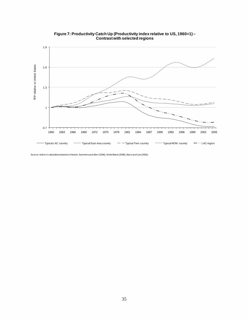
Fact 2: LAC productivity is not catching up with the frontier, in contrast to theory and evidence elsewhere. Endogenous growth theory suggests that less productive countries should be able to increase
their productivity faster because they can adopt technologies from more advanced economies,
benefitting from advances at the frontier without incurring the costs of exploration. While it is
true that TFP is not just technology—it also reflects inefficiencies in how markets work, as we
argued above—but the catching-up argument works just as well for policies and institutions:
backward countries have the benefit of being able to improve by learning, rather than inventing.
The rest of the world tends to follow this expected convergent pattern, but not LAC.
Figure 7 shows the evolution of productivity in LAC and other regions relative to the frontier,
customarily taken as the United States (normalizing the indexes to 1 by 1960). Until the debt
crisis of the 1980s, catching up in the typical country was slower than in LAC but faster since
then. This divergent pattern in recent decades holds true not only for the typical LAC country but
for the region as a whole (LAC Region in the figure) as Brazil’s earlier dynamism during the
1960s and 1970s slowed down. Other benchmarks further highlight LAC’s anomalous
productivity trends.
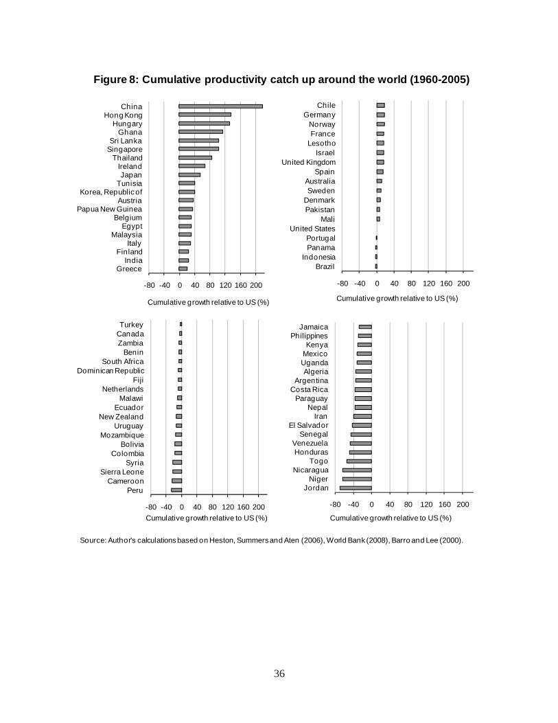
The failure to catch up on productivity is widespread across LAC countries. Figure 8
shows all countries in the sample ranked by overall TFP catch-up (relative to the United States)
in the period examined (1960-2005): there is a substantial concentration of Latin American
countries in the fourth quartile. Brazil is about the median, and only Chile shows some degree of
convergence with the US over the long-run.
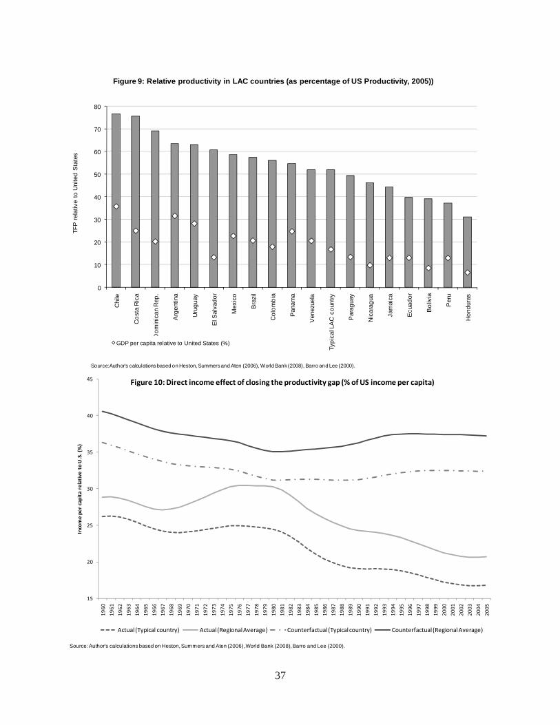
Fact 3: LAC’s productivity is about half its potential. Current levels of estimated TFP for Latin American countries relative to that of the United
States, taken as the frontier, are uniformly subpar (see Figure 9). In particular, in 2005 the
aggregate productivity of the typical LAC country (which being an average is subject to less
statistical error than that of individual countries) is about half (52 percent).
14
If factor inputs are kept constant, income per capita would move together with TFP.
Therefore if TFP increased to its potential, the income per capita of the typical LAC country
would double (to about a third of the US level). In this thought experiment, a better combination
of the same inputs emulating what is feasible in other economies, using existing technologies,
would render an output substantially larger. More generally, what would have been the evolution
of LAC income per capita if its historical production inputs had been applied with US
productivity at each point in time? This is an artificial question because, as analyzed in the next
section, productivity and factor accumulation are interlinked and changes in productivity are
bound to have indirect effects on factor accumulation (and vice versa). Nevertheless, the direct
income effect of closing the productivity gap provides a measure of the relevance of such gap.
Figure 10 shows the counterfactual scenarios of relative income per capita in which the TFP gap
is closed for both the typical LAC country and the region as a whole.
The sizable room for improvement associated with productivity catching-up is in some
sense good news for LAC to the extent that rapid progress in income per capita (i.e., high
growth) may be unlocked by economic policy reform even in the absence of the burden of
increased investment. The potential for improving productivity in the typical LAC country by
around 100 percent is not available to the typical East Asian country (40 percent), twin country
(40 percent) or developed country (only 15 percent).
Figure 11 shows the evolution over time of the development accounting exercise based
on equation (10). Physical capital accounts for almost 40 percent of the income per capita gap,
with a stable contribution over time. However, the contribution of human capital has declined
from around one fourth of the gap in 1960 to 16 percent in 2005. Similarly, while labor force
intensity explained an important share (around one fourth) of the income gap during the early
1980s, today its contribution to the income per capita gap between the typical LAC country and
the United States is only 8 percent. By contrast, from 1980 onwards, the contribution of TFP to
the income gap has been increasing steadily doubling its importance to reach a level similar to
that of physical capital by 2005 of 37 percent.
Figure 12 shows this decomposition country-by-country in 2005. There are clearly
differences across countries in the importance of TFP in accounting for the income per capita
gap with respect to the U.S. For example, while in Costa Rica and the Dominican Republic TFP
15
accounts “only” for a fifth or a quarter of the gap, in other countries like Ecuador and Peru it
accounts for almost 50 percent of the gap.
4. Robustness of the Stylized Facts
The use of alternative methodologies confirms the robustness of the previous key stylized facts.
In particular, we consider first the following three interesting variations of the standard
methodology employed:
a) A production function giving more weight to physical capital and less weight to
human capital. In this alternative we use a higher capital share a=1/2, instead of
the standard value of 1/3.
b) The use of working age population instead of labor force to measure L, with the
effect that TFP becomes sensitive to changes in the participation rate in the labor
force (everything else equal, lower participation would translate into lower
aggregate productivity, even if lower participation is the result of a stronger
preference for leisure).14
c) A different method to estimate the series of physical capital K that is also
commonly used in the technical literature (Caselli, 2005); see Appendix.
In order to test Fact 1: Slower growth in LAC is due to slower productivity growth, the
annual TFP growth gap between LAC and ROW based on equation (8) shown in the previous
section is contrasted with the annual TFP growth gaps produced by the three alternative
methodological variations (Figure 13). The contrast demonstrates that the negative TFP growth
gap persists under the alternatives and is similar to the baseline case.
The robustness of Fact 2: LAC productivity is not catching up with the frontier is tested
by looking at the evolution of the typical LAC country’s TFP relative to the frontier under the
various alternative methodologies (Figure 14). The remarkable lack of convergence persists
under the alternative scenarios.
14 Blyde and Fernández-Arias (2006) show that the use of employed labor instead of labor force to measure factor input makes little difference in LAC. We do not attempt to use actual hours worked, which would be a more accurate measure of labor input, because data are not available for a large number of countries over a long period of time, limiting the possibility of a broad and structural comparison across countries. However, it is known that such refinement does not substantially alter measured TFP (see Restuccia, 2008).
16
Finally, the alternative methodologies broadly confirm Fact 3: Latin America’s
productivity is about half its potential, as shown in Figure 15 where the TFP gap between the
typical Latin American country and the frontier is estimated under the various alternatives.15
So far the analysis has been based on standard Cobb-Douglas production functions. The
use of this family of functions is the conventional approach for a number of good reasons, but
has the empirical drawback of collapsing all productivity concerns to a single parameter, the
factor-neutral productivity parameter A or TFP. Rather than experimenting with other families of
production functions with more parameters—in particular considering a more general Constant
Elasticity of Substitution (CES) production function with lower levels of substitutability between
factors—to explore the robustness of the stylized facts in more general settings, we move to the
extreme and consider a non-parametric method of estimation that only requires the standard
assumptions of free disposal and consider that the production function has constant returns to
scale.
This alternative methodology, which is based on the estimation of production possibility
frontiers developed by Koopsman (1951) and Farell (1957), has recently been applied to growth
accounting exercises by Färe et al. (1994) and Kumar and Russell (2002), and to development
accounting by Jermanowski (2007). In this non-parametric approach, the estimation of the degree
of aggregate efficiency with which a country produces is only based on the possibilities revealed
by the production achievements of the rest of the countries, without the use of an explicit
production function. In particular, we estimate a production possibility frontier using a data
envelope analysis (DEA) following Jermanowski (2007). Once the production frontier
theoretically attainable with the country’s factor inputs using “best practices” is estimated, a
relative efficiency or total factor productivity index E can be estimated reflecting actual output
relative to the frontier (so E is an index between 0 and 1). This index tests the robustness of the
previous estimation of TFP relative to that of the United States (taken as the frontier), or A/A*.
In this methodology, output in a given country can be written as Y=EF(K,H) where F(.)
has constant returns to scale. However, rather than specifying an explicit functional form whose
parameters are estimated to fit the data, it is numerically inferred from picking the feasible “best
practices” revealed by the data. Any country n could replicate the economies of the whole
15 Nevertheless, the extreme weight on physical capital in alternative (a) weakens the relevance of the productivity gap somewhat.
17
universe of countries at arbitrary scales λ and piece them together as long as the required
aggregate factor inputs in this combination do not exceed available stocks of factor inputs
(Kn,Hn). Its frontier is the best of such combinations, i.e., the one yielding the highest output. In
particular, we solve the following linear programming problem. Given N countries and inputs in
per worker terms (k, h), country n’s program is given by:
0,,,
max
1
,, 1
≥⋅≥⋅≥⋅≤
×Nn
nnn
n
hhkkyy
tosubjectNn
λλλλθ
θλλθ K
(12)
It turns out that this index of aggregate relative efficiency E in LAC countries is quite
similar to the TFP parameter estimated in the standard Cobb-Douglas model (relative to the
United States, taken as the frontier), which buttresses the previous findings.16 In Figure 16, we
plot the resulting estimates for relative efficiency E with respect to our previous estimates of
relative TFP. As shown, the correlation between both measures is extremely high (with a simple
correlation coefficient of 0.92!). Furthermore, the efficiency level of the typical Latin American
country in 2005 is similar: 62 percent compared with the previously estimated relative TFP of 52
percent.17 More generally, the time evolution of both measures for the typical LAC country is
roughly similar, with an initial period of convergence followed by divergence (Figure 17).
Therefore, as an additional robustness test to our results in the previous section, this non-
parametric approach also confirms the stylized facts of LAC productivity previously found.
5. Productivity and Factor Accumulation In an accounting sense, a gap in income per capita can be attributed to a gap in productivity (A),
physical capital intensity (k), human capital intensity (h), or labor force intensity (f) (equation
(10)). For example, as shown in Figure 10, a development accounting exercise benchmarking the
typical Latin American country with the United States would indicate, as mentioned in Fact 3,
that if the productivity gap is closed then relative income would roughly double (TFP in the 16 It is important to point out that, according to this methodology, the United States turns out to be almost always on the production possibility frontier (i.e., cannot improve by emulating any other country), and it is on the frontier currently (2005). 17 Since in this non-parametric method the frontier is inferred from observed levels of output of countries which may be less than fully efficient, the estimated efficiency index E should be interpreted as an upper bound.
18
typical LAC country would increase by A*/A = 1.93 times or roughly twice, and so would income).
Furthermore, as shown in Figure 11, discussed above, an accounting decomposition of the
contributions of each underlying gap to the current income gap with the United States on the
basis of equation (10) would indicate that the productivity gap accounts for about 37 percent and
accumulated factors for the rest, or 63 percent, as of 2005.
While the income boost produced by closing the productivity gap in this simple
accounting calculation is sizable, it would apparently leave most of the observed income gap.
This metric would suggest that productivity is an important but not predominant variable behind
income gaps, but then why is it that income is so closely associated with productivity across
countries (as shown in Figure 2)? An appreciation of the relevance of productivity for the overall
economic development process requires the exploration of the interplay between productivity
and factor accumulation: the indirect effects of productivity gaps on the incentives to accumulate
production factors may account for a substantial portion of the observed development gaps. In
fact, the traditional tools previously utilized underestimate the importance that closing the
productivity gap would have on welfare. We show in what follows that after a full measure is
obtained, it becomes clear that:
Claim 1: The income per capita gap with respect to the United States would largely disappear if the productivity gap were closed. The previous exercises on the contribution of the productivity gaps to development gaps assume
that k and h are exogenous to TFP levels. Next, we show gap decompositions where these
exogeneity assumptions are relaxed. First, we consider the case where human capital continues
to be considered exogenous, but physical capital is endogenous. In market economies, private
investment in physical capital is such that the marginal return to investing equals the cost of
capital as perceived by individual investors, within the financing conditions accessible to them.
The private return appropriated by an individual investor may very well be a fraction of the
social return to investing, for example if it provides positive externalities to other firms (e.g. non-
patentable innovations) or if the firm’s returns are taxed away. In particular, let us assume that
the representative firm solves the following static maximization problem:
, (13) ( )krphAkt kaa
kδ+−− −1)1(max
19
where pk, r and δ are the relative price of capital goods, the real interest rate and the depreciation
rate, respectively. We assume the tax rate t to capture all elements that reduce the private
appropriability of output proceeds. The first order condition is given by:
(14) )()1( 11 δ+=− −− rphAakt kaa
Dividing the right-hand side of equation (14) by output per worker yields:
)()1( δ+=− rpKYat k (15)
Thus, we have that the equilibrium capital-output ratio κ is given by:
)()1(δ
κ+
−==
rpat
YK
k
(16)
This shows that the capital-output ratio does not depend on the level of productivity but
does depend on the interest rate, the degree of private appropriability of returns and the price of
capital goods. Therefore distortions to these price-like conditions will be reflected in the capital-
output ratio: “price” impediments to physical capital investment leading to a wedge between net
marginal returns (net of cost of capital) across countries correspond to lower capital-output
ratios. Solving for k, plugging it into equation 5 and solving for output per capita, we can write
the production function in per capita terms in “intensive form” as labeled by Klenow and
Rodríguez-Clare (2005):
fhAy aa
a −−= 111
κ (17)
Dividing equation (17) by the benchmark y*, following the notation introduced in
equation (9), and taking logs we can decompose the GDP per capita gap as:
( ) ( ) ( ) ( ) ( )fha
aAa
yyy logloglog
1log
11loglog * ++
−+
−==⎟⎟
⎠
⎞⎜⎜⎝
⎛κ (18)
Irrespective of the size of the impediments to physical capital accumulation, as measured
by the gap in the capital-output ratio, an increase in TFP would boost private returns relative to
the status quo and lead to a higher stock of accumulated physical capital.18 In fact, in all cases,
18 This process would of course take time; here we are abstracting from transitional issues.
20
closing the TFP gap would alter incentives boosting physical capital investment relative to the
status quo, an indirect effect of closing the productivity gap which ought to be attributed to it.
Thus, the overall contribution of the TFP gap to the income gap in equation (18) results from the
direct effect estimated with equation (10) plus this additional indirect effect:
( ) ( ) ( )Aa
aAAa
log1
loglog1
1−
+=−
(19)
How large is the overall effect of closing the TFP gap, inclusive of indirect effects on
factor accumulation? Under the conservative assumption in equation (18) that human capital is
exogenously given, meaning that investment in education does not increase with higher TFP, the
overall TFP contribution for the typical LAC country (as of 2005) would amount to 55 percent of
the income gap, of which 37 percent is the direct effect mentioned above and 18 percent is the
additional indirect effect via induced physical capital accumulation.
In this model of physical capital intensity endogenously reacting to changes in
productivity and exogenously given education expressed in equation (18), the remaining 45
percent to make up the entire income gap is divided into the contribution of impediments to
physical investment, which as explained are reflected in the capital-output ratio κ (12 percent),
human capital intensity or education h (25 percent), and labor force intensity f (8 percent); see
Figure 18. According to these results, a development agenda exclusively focused on physical
capital investment by easing impediments such as undue spreads in the financial system, high
taxation and uncertain property rights would be circumscribed to a margin of just 12 percent
(unless they also foster productivity, an issue we explore at the end of the section). There is, of
course, some variation across countries—for example, in the Dominican Republic investment
impediments appear to be as important as TFP shortfalls—but the conclusion holds broadly. The
relevance of the productivity gap appears to have been growing over time since 1980 (Figure
19).
If investment in human capital (education), which as shown is dominant among the
remaining factor-related gaps, is also recognized as an endogenous variable which would likely
react to an increase in productivity, the case for a predominant contribution of the productivity
gap becomes stronger. In our context, its consideration will add an additional indirect effect of
21
closing the productivity gap.19 This more complete decomposition where both types of capital
react to productivity changes crucially depends on how elastic education demand is to increased
productivity.20
When the level of education of the labor force is also allowed to adjust to changes in
returns, equation (17) becomes the “superintensive” form:
bbbaa
ba fAy −−−−−−= 11
11
)1)(1()1)(1(1
ϕκ , (20)
where human capital is assumed to endogenously adjust to income per capita according to h=
φyb, following standard growth models where endogenous human capital displays this type of
log-linear relationship with income. The parameter φ reflects country-specific, non-income
factors affecting education, or education propensity, so that a shortfall in this parameter is
interpreted as an impediment to human capital investment. Correspondingly, equation (18)
becomes
( ) ( )( ) ( ) ( )( ) ( ) ( ) ( )fbbba
aAba
y log1
1log1
1log11
log11
1log−
+−
+−−
+−−
= ϕκ (21)
There are no reliable estimations of the income elasticity of education b. If education is
totally inelastic (b=0), education is exogenous and equation (21) collapses to equation (20),
where φ=h. Erosa, Koreshkova and Restuccia (2007) calibrate a model with this specification
obtaining a high elasticity of b=0.48. This parameter would actually imply that the work force in
LAC is, relative to the US, substantially overeducated for its level of income as measured by φ.
This calibration would imply that closing the productivity gap would lead to LAC surpassing the
US income per capita (by some 11 percent) despite the gap in labor force intensity and the
impediments to physical capital investment (both working to LAC’s disadvantage). We therefore
pick a conservative intermediate elasticity of b=0.24 that cancels any contemporaneous
differences in this education propensity between the typical LAC country and the US (e.g., ϕ =1
in 2005).
This elasticity would yield an overall contribution of closing the TFP gap of 73 percent,
of which about half are indirect effects through both physical capital and education, each one 19 Both indirect effects would actually reinforce each other because of the complementary between physical and human capital in the production function. 20 However, economic returns are clearly not the only motivation behind individual education decisions.
22
contributing roughly the same (Figure 20). This reinforces the conclusion that LAC’s income per
capita gap would largely disappear if the productivity gap is closed.21 In this formulation, the
relevance of the productivity gap also appears to grow over time since 1980.
The key development policy question is then how to close the productivity gap. As
mentioned, the aggregate productivity gap reflects a variety of shortcomings in the workings of
the overall economy and should not be narrowly interpreted as a technological gap. However, in
answering this question it is important to recognize that factor accumulation, both physical and
in terms human capital, may be important to facilitate the objective of reducing the productivity
gap. For example, physical capital investment may embody new technologies to help in catching
up with the frontier, and human capital investment may facilitate innovation and the adoption of
more advanced technologies. This amounts to studying the effects of capital accumulation on
productivity, a direction of causation which is opposite to the one we explored to trace the effects
of closing the productivity gap. This analysis would answer the question of how far would
addressing distortions in capital accumulation go in increasing income via its indirect effects on
increased productivity, in addition to the direct effects noted above. (These indirect effects would
of course also take into account that increased productivity further boosts capital accumulation
and so on.)
In order to explore this issue, we try to quantify the impact of eliminating investment
distortions as measured by the capital-output gap and of closing education gaps and arrive at:
Claim 2: Fixing the shortcomings of factor accumulation in LAC would help productivity but still leave most of the productivity gap open. The calibrated model in Cordoba and Ripoll (2008) posits a similar Cobb-Douglas production
function in which investment impacts TFP because factors affect the accumulation of
knowledge, leading to the adjusted intensive form:
( )
fhAy cc
+−+
= 111~ α
α
κ , (22)
where A~ corresponds to “core TFP,” that is TFP purged from the negative influence of physical
and human capital accumulation shortcomings, and the parameter c captures the amplification
21 At the same time, the contribution of impediments to physical capital investment would increase to almost 16 percent (because higher education boosts returns to physical capital investment).
23
effect of factors on TFP (for details see Córdoba and Ripoll, 2008). In this formulation,
education is taken as exogenous (not affected by productivity) and therefore the entire education
gap is attributed to accumulation shortcomings. The following equation in decomposition form
would account for the exogenous contribution of “core productivity” (first term on the right-hand
side), leaving out the productivity benefits of factor accumulation:
( ) ( ) ( ) ( ) ( ) ( )fhcacaAy loglog1log
1)1(~loglog +++
−+
+= κ (23)
Thus, the indirect effect of physical capital-related frictions is given by ( )κlog1 a
ac−
and
that of human capital is given by ( )hc log .
Extending the model to allow for education being elastic to income along the lines above
would yield a revised decomposition in which shortcomings in investment in education are only
those reflected in the gap in education propensity (the parameter ϕ ), not the entire education
gap.
( ) ( ) ( ) ( ) ( )( ) ( ) ( )
( ) ( )fcb
cbcbacaA
cby
log111
)log(111log
111)1(~log
111log
+−+
+−+
+−−+
++−
= ϕκ (24)
The contributions of “core productivity” according to equation (23) and (24) and
considering a value of c=0.5 (following Córdoba and Ripoll, 2008), and imposing again that
ϕ =1 in 2005, are shown in Figures 21 and 22, respectively. Under the assumption that education
is totally inelastic to increased returns, the contribution of the core productivity gap in the first
term of equation (23), which would remain after all factor accumulation shortcomings are fixed,
is only one third smaller than the previously estimated overall contribution of 55 percent (of
which impediments to physical capital accumulation would be responsible for only 6 percentage
points of the drop and the education gap would account for the remaining 12 percentage points)
(see Figure 21). Thus, two-thirds of the overall contribution of the productivity gap would
remain even after these drastic adjustments to factor accumulation gaps.22 It is important to note
22 The contributions of factors are correspondingly boosted by about half; for example, the attribution to impediments to physical capital, including its effect on productivity, increases from 12 percent to 18 percent but is still far less important than core productivity.
24
that this pure productivity shortfall appeared negligible by 1980 and has been growing since
then.
Under the alternative assumption that education is elastic to income, then the productivity
gap contribution of 73 percent previously estimated would be marginally reduced to a core
productivity gap contribution of 58 percent, so that the bulk of the productivity shortfall would
remain (see Figure 22). The drop in this case is lower because education is driven by income and
therefore does not play an autonomous role in boosting productivity. These results confirm that
policies focused on shortcomings of factor accumulation are relevant but not decisive for
addressing the productivity gap: the productivity gap is not the result of insufficient investment,
but largely of other, more specific productivity shortcomings.
6. Conclusions Low productivity and slow productivity growth as measured by total factor productivity, rather
than impediments to factor accumulation, are the key to understanding Latin America’s low
income relative to developed economies and its stagnation relative to other developing countries
that are catching up, as summarized by the following stylized facts:
a) Slower growth in LAC is due to slower productivity growth;
b) LAC productivity is not catching up with the frontier, in contrast to theory and
evidence elsewhere;
c) LAC’s productivity is about half its potential Higher productivity would entail not only a more efficient use of accumulated capital
stocks, both physical and human, but also faster accumulation of these production factors in
reaction to the increased returns prompted by the productivity boost. All things considered,
closing the productivity gap with the frontier would actually close most of the income gap with
developed countries.
Therefore it is clear that the key to the economic development problematic in the region
is how to close the productivity gap. The main development policy challenge in the region
involves diagnosing the causes of poor productivity and acting on its roots. The analysis shows
that policies easing physical and human capital accumulation would be relevant to improving
productivity but would leave most of the productivity problem untouched. Consequently, the
25
core of the aggregate productivity problematic will require specific productivity policies. While
impediments to technological improvement at the firm level is part of the problem, aggregate
productivity depends on the efficiency with which private markets and public inputs support
individual producers. Since firms’ productivities may be heterogeneous, aggregate productivity
also depends on the extent to which the workings of the economy allocate productive factors to
the most productive firms. These considerations open up a rich agenda for productivity
development policies.
26
Statistical Appendix Gross output (Y) is computed as PPP adjusted real GDP from the Penn World Tables version 6.2
(PWT), resulting from multiplying the real GDP per capita (constant prices: chain series)—
denoted by rgdpch in the database –by the population (pop) also provided by the PWT. While
data are available only until 2004, we extend the data to 2005 using PPP GDP growth reported
by the World Bank’s World Development Indicators (WDI).
Labor input is measured by the total labor force from the WDI. It is often argued that
hours worked are a more accurate measure. However, these data are not available for a large
number of countries over a long period of time, limiting the possibility of a broad and structural
comparison across countries in Latin America. Furthermore, short-run fluctuations in labor
market participation would not have an influence on the TFP measure because we focus on HP-
filtered trends (only permanent differences in unemployment rates, a failure to productively
utilize available labor inputs, would affect TFP).
We follow the standard approach by Hall and Jones (1999) by constructing the human
capital index h as a function of the average years of schooling given by:
)(seh φ= , (A.1)
where the function (.)φ is such that (0) 0φ = and )(sφ′ is the Mincerian return on education. In
particular, we approximate this function by a piece-wise linear function. As shown in equation
(A.2), we assume the following rates of return for all the countries: 13.4 percent for the first four
years of schooling, 10.1 percent for the next four years and 6.8 percent for education beyond the
eighth year (based on Psacharopoulos, 1994).
(A.2) ⎪⎩
⎪⎨
⎧
>−×+≤<−×+
≤×=
8)8(068.094.084)4(101.0536.0
4134.0)(
sifssifs
sifssφ
For each country we then compute the average using the data on years of schooling in the
population (older than 15 years) from the Barro-Lee database.23
23 Linear extrapolations are used to complete the five-year data. Missing values were interpolated using a fixed-effects regression of the average school years on primary, secondary and tertiary enrollment rates. For China and Egypt the Barro-Lee data on average years of schooling are not available before 1975 and in Benin before 1970. We
27
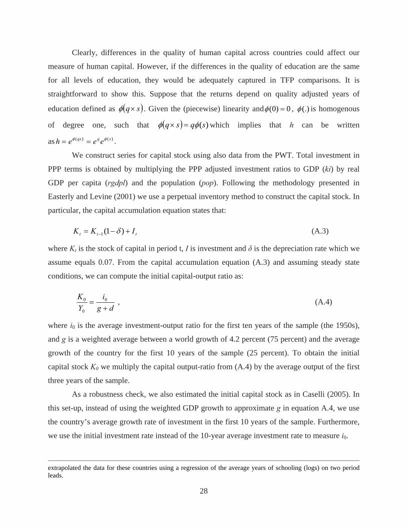
Clearly, differences in the quality of human capital across countries could affect our
measure of human capital. However, if the differences in the quality of education are the same
for all levels of education, they would be adequately captured in TFP comparisons. It is
straightforward to show this. Suppose that the returns depend on quality adjusted years of
education defined as ( sq× )φ . Given the (piecewise) linearity and (0) 0φ = , (.)φ is homogenous
of degree one, such that ( ) )(sqsq φφ =× which implies that h can be written
as . )()( sqqs eeeh φφ ==
We construct series for capital stock using also data from the PWT. Total investment in
PPP terms is obtained by multiplying the PPP adjusted investment ratios to GDP (ki) by real
GDP per capita (rgdpl) and the population (pop). Following the methodology presented in
Easterly and Levine (2001) we use a perpetual inventory method to construct the capital stock. In
particular, the capital accumulation equation states that:
ttt IKK +−= − )1(1 δ (A.3)
where Kt is the stock of capital in period t, I is investment and δ is the depreciation rate which we
assume equals 0.07. From the capital accumulation equation (A.3) and assuming steady state
conditions, we can compute the initial capital-output ratio as:
dgi
YK
+= 0
0
0 , (A.4)
where i0 is the average investment-output ratio for the first ten years of the sample (the 1950s),
and g is a weighted average between a world growth of 4.2 percent (75 percent) and the average
growth of the country for the first 10 years of the sample (25 percent). To obtain the initial
capital stock K0 we multiply the capital output-ratio from (A.4) by the average output of the first
three years of the sample.
As a robustness check, we also estimated the initial capital stock as in Caselli (2005). In
this set-up, instead of using the weighted GDP growth to approximate g in equation A.4, we use
the country’s average growth rate of investment in the first 10 years of the sample. Furthermore,
we use the initial investment rate instead of the 10-year average investment rate to measure i0.
extrapolated the data for these countries using a regression of the average years of schooling (logs) on two period leads.
28
References Blyde, J., and E. Fernández-Arias. 2006. “Why Does Latin America Grow More Slowly?”
Seminar Papers S-856. Washington, DC, United States: Inter-American Development
Bank.
Caselli, F. 2005. “Accounting for Cross-Country Income Differences.” In: P. Aghion and S.
Durlauf. Handbook of Economic Growth. Volume 1. Amsterdam, The Netherlands:
North-Holland.
Córdoba, J.C., and M. Ripoll. 2008. “Endogenous TFP and Cross-Country Income Differences.”
Journal of Monetary Economics 55: 1158-1170.
Easterly, W., and R. Levine. 2001. “What Have We Learned from a Decade of Empirical
Research on Growth? It’s Not Factor Accumulation: Stylized Facts and Growth Models.”
World Bank Economic Review 15(2): 177-219.
Erosa, A., T. Koreshkova and D. Restuccia. 2007. “How Important is Human Capital? A
Quantitative Theory Assessment of World Income Inequality.” Department of Economics
Working Paper 280. Toronto, Canada: University of Toronto.
Farrell, M.J. 1957. “The Measurement of Production Efficiency.” Journal of the Royal Statistical
Society A 120(3): 253–281.
Färe, R. et al. 1994. “Productivity Growth, Technical Progress, and Efficiency Change in
Industrialized Countries.” American Economic Review 84(1): 66–83.
Gollin, D. 2002. “Getting Income Shares Right.” Journal of Political Economy 110(2): 458–474.
Hall, R., and C.I. Jones. 1999. “Why Do Some Countries Produce So Much More Output per
Worker than Others?” Quarterly Journal of Economics 114(1): 83-116.
Jermanowski, M. 2007. “Total Factor Productivity Differences: Appropriate Technology versus
Efficiency.” European Economic Review 51: 2080-2110.
Klenow, P., and A. Rodríguez-Clare. 1997. “The Neoclassical Revival in Growth Economics:
Has It Gone Too Far?” In: B. Bernanke and J. Rotemberg, editors. NBER
Macroeconomics Annual 1997. Cambridge, United States: MIT Press.
----. 2005. “Externalities and Growth.” In: P Aghion and S. Durlauf, editors. Handbook of
Economic Growth. Volume 1A. Amsterdam, The Netherlands: North-Holland.
Koopmans, T.C. 1951. “Efficient Allocation of Resources.” Econometrica 19(4): 455–465.
29
Kumar, S., and R.R. Russell. 2002. “Technological Change, Technological Catch-Up, and
Capital Deepening: Relative Contributions to Growth and Convergence.” American
Economic Review 92(3): 527–548.
Lederman, D., and W.F. Maloney, 2008. “Natural Resources and Economic Growth.” Economía
9(1): 1-57.
Psacharopoulos, G. 1994. “Returns to Investment in Education: A Global Update.” World
Development 22(9): 1325-1343.
Restuccia, D. 2008. “The Latin American Development Problem.” Department of Economics
Working Paper 318. Toronto, Canada: University of Toronto.
30
1
1.2
1.4
1.6
1.8
2
2.2
1960 1963 1966 1969 1972 1975 1978 1981 1984 1987 1990 1993 1996 1999 2002 2005
Inde
xFigure 1: Alternative productivity measures (typical world economy country
1960=1)
Total Factor Productivity (TFP) Labor productivity TFP cum education
Source: Author's calculations based on Heston, Summers and Aten (2006), World Bank (2008), Barro and Lee (2000).
6
7
8
9
10
11
4 4.5 5 5.5 6 6.5 7
Inco
me
per c
apita
TFP
Figure 2: Income per capita and productivity across countries (2005)
Row Lac
Note: income per capita and TFP measured in logaritmic scale.Source: Author's calculations based on Heston, Summers and Aten (2006), World Bank (2008), Barro and Lee (2000).
31
0.8
0.9
1
1.1
1.2
1.3
1.4
1960 1963 1966 1969 1972 1975 1978 1981 1984 1987 1990 1993 1996 1999 2002 2005
Inde
xFigure 3: Productivity indexes (LAC, 1960=1)
Typical country Regional Average
Source: Author's calculations based on Heston, Summers and Aten (2006), World Bank (2008), Barro and Lee (2000).
0
20
40
60
80
100
120
140
160
Chi
le
Cos
ta R
ica
Dom
inic
an R
ep.
Arg
entin
a
Uru
guay
El S
alva
dor
Mex
ico
Bra
zil
Col
ombi
a
Pan
ama
Ven
ezue
la lac
Par
agua
y
Nic
arag
ua
Jam
aica
Ecu
ador
Bol
ivia
Per
u
Hon
dura
s
Rel
ativ
e TF
P (%
)
Figure 4: Productivity diversity within LAC (percentage of the typical LAC country, 2005)
Note: Country TFP relative to typical LAC country.Source: Author's calculations based on Heston, Summers and Aten (2006), World Bank (2008), Barro and Lee (2000).
32
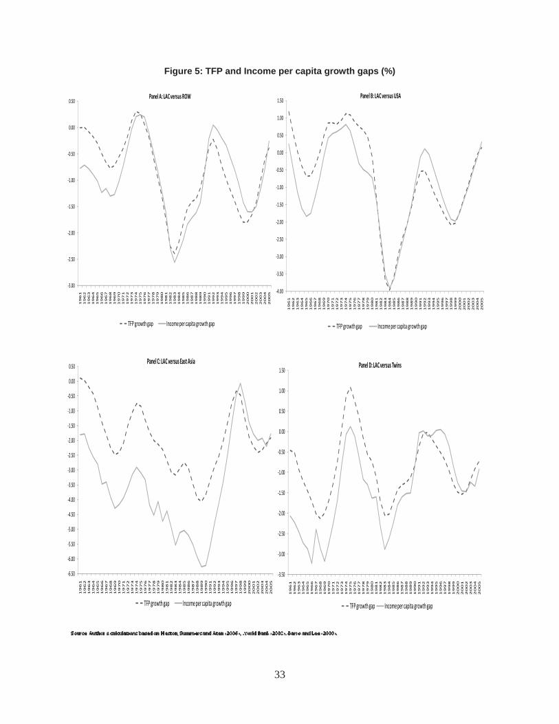
Figure 5: TFP and Income per capita growth gaps (%)
‐3.00
‐2.50
‐2.00
‐1.50
‐1.00
‐0.50
0.00
0.50
1961
1962
1963
1964
1965
1966
1967
1968
1969
1970
1971
1972
1973
1974
1975
1976
1977
1978
1979
1980
1981
1982
1983
1984
1985
1986
1987
1988
1989
1990
1991
1992
1993
1994
1995
1996
1997
1998
1999
2000
2001
2002
2003
2004
2005
Panel A: LAC versus ROW
TFP growth gap Income per capita growth gap
‐4.00
‐3.50
‐3.00
‐2.50
‐2.00
‐1.50
‐1.00
‐0.50
0.00
0.50
1.00
1.50
1961
1962
1963
1964
1965
1966
1967
1968
1969
1970
1971
1972
1973
1974
1975
1976
1977
1978
1979
1980
1981
1982
1983
1984
1985
1986
1987
1988
1989
1990
1991
1992
1993
1994
1995
1996
1997
1998
1999
2000
2001
2002
2003
2004
2005
Panel B: LAC versus USA
TFP growth gap Income per capita growth gap
‐6.50
‐6.00
‐5.50
‐5.00
‐4.50
‐4.00
‐3.50
‐3.00
‐2.50
‐2.00
‐1.50
‐1.00
‐0.50
0.00
0.50
1961
1962
1963
1964
1965
1966
1967
1968
1969
1970
1971
1972
1973
1974
1975
1976
1977
1978
1979
1980
1981
1982
1983
1984
1985
1986
1987
1988
1989
1990
1991
1992
1993
1994
1995
1996
1997
1998
1999
2000
2001
2002
2003
2004
2005
Panel C: LAC versus East Asia
TFP growth gap Income per capita growth gap
‐3.50
‐3.00
‐2.50
‐2.00
‐1.50
‐1.00
‐0.50
0.00
0.50
1.00
1.50
1961
1962
1963
1964
1965
1966
1967
1968
1969
1970
1971
1972
1973
1974
1975
1976
1977
1978
1979
1980
1981
1982
1983
1984
1985
1986
1987
1988
1989
1990
1991
1992
1993
1994
1995
1996
1997
1998
1999
2000
2001
2002
2003
2004
2005
Panel D: LAC versus Twins
TFP growth gap Income per capita growth gap
33
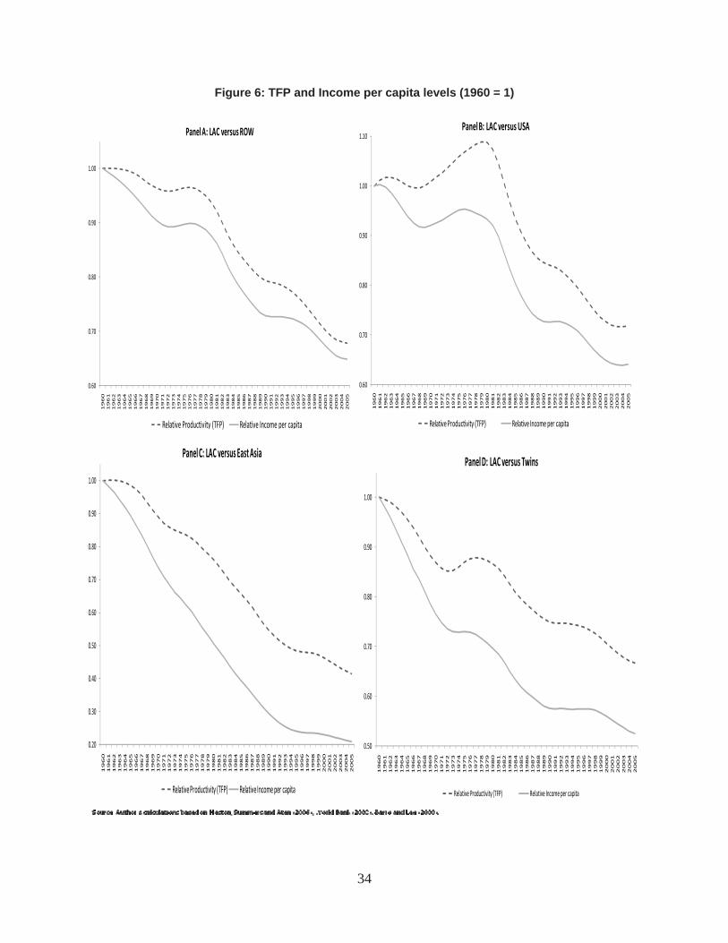
Figure 6: TFP and Income per capita levels (1960 = 1)
0.60
0.70
0.80
0.90
1.00
1960
1961
1962
1963
1964
1965
1966
1967
1968
1969
1970
1971
1972
1973
1974
1975
1976
1977
1978
1979
1980
1981
1982
1983
1984
1985
1986
1987
1988
1989
1990
1991
1992
1993
1994
1995
1996
1997
1998
1999
2000
2001
2002
2003
2004
2005
Panel A: LAC versus ROW
Relative Productivity (TFP) Relative Income per capita
0.60
0.70
0.80
0.90
1.00
1.10
1960
1961
1962
1963
1964
1965
1966
1967
1968
1969
1970
1971
1972
1973
1974
1975
1976
1977
1978
1979
1980
1981
1982
1983
1984
1985
1986
1987
1988
1989
1990
1991
1992
1993
1994
1995
1996
1997
1998
1999
2000
2001
2002
2003
2004
2005
Panel B: LAC versus USA
Relative Productivity (TFP) Relative Income per capita
0.20
0.30
0.40
0.50
0.60
0.70
0.80
0.90
1.00
1960
1961
1962
1963
1964
1965
1966
1967
1968
1969
1970
1971
1972
1973
1974
1975
1976
1977
1978
1979
1980
1981
1982
1983
1984
1985
1986
1987
1988
1989
1990
1991
1992
1993
1994
1995
1996
1997
1998
1999
2000
2001
2002
2003
2004
2005
Panel C: LAC versus East Asia
Relative Productivity (TFP) Relative Income per capita
0.50
0.60
0.70
0.80
0.90
1.00
1960
1961
1962
1963
1964
1965
1966
1967
1968
1969
1970
1971
1972
1973
1974
1975
1976
1977
1978
1979
1980
1981
1982
1983
1984
1985
1986
1987
1988
1989
1990
1991
1992
1993
1994
1995
1996
1997
1998
1999
2000
2001
2002
2003
2004
2005
Panel D: LAC versus Twins
Relative Productivity (TFP) Relative Income per capita
34
0.7
1
1.3
1.6
1.9
1960 1963 1966 1969 1972 1975 1978 1981 1984 1987 1990 1993 1996 1999 2002 2005
TFP
rela
tive
to U
nite
d S
tate
sFigure 7: Productivity Catch Up (Productivity index relative to US, 1960=1) –
Contrast with selected regions
Typical LAC country Typical East Asia country Typical Twin country Typical ROW country LAC region
Source: Author's calculations based on Heston, Summers and Aten (2006), World Bank (2008), Barro and Lee (2000).
35
-80 -40 0 40 80 120 160 200
GreeceIndia
FinlandItaly
MalaysiaEgypt
BelgiumPapua New Guinea
AustriaKorea, Republic of
TunisiaJapan
IrelandThailand
SingaporeSri Lanka
GhanaHungary
Hong KongChina
Cumulative growth relative to US (%)
-80 -40 0 40 80 120 160 200
BrazilIndonesia
PanamaPortugal
United StatesMali
PakistanDenmarkSweden
AustraliaSpain
United KingdomIsrael
LesothoFranceNorway
GermanyChile
Cumulative growth relative to US (%)
-80 -40 0 40 80 120 160 200
PeruCameroon
Sierra LeoneSyria
ColombiaBolivia
MozambiqueUruguay
New ZealandEcuador
MalawiNetherlands
FijiDominican Republic
South AfricaBenin
ZambiaCanadaTurkey
Cumulative growth relative to US (%)
-80 -40 0 40 80 120 160 200
JordanNiger
NicaraguaTogo
HondurasVenezuela
SenegalEl Salvador
IranNepal
ParaguayCosta Rica
ArgentinaAlgeria
UgandaMexicoKenya
PhilippinesJamaica
Cumulative growth relative to US (%)
Figure 8: Cumulative productivity catch up around the world (1960-2005)
Source: Author's calculations based on Heston, Summers and Aten (2006), World Bank (2008), Barro and Lee (2000).
36
0
10
20
30
40
50
60
70
80C
hile
Cos
ta R
ica
Dom
inic
an R
ep.
Arg
entin
a
Uru
guay
El S
alva
dor
Mex
ico
Bra
zil
Col
ombi
a
Pan
ama
Ven
ezue
la
Typi
cal L
AC
cou
ntry
Par
agua
y
Nic
arag
ua
Jam
aica
Ecu
ador
Bol
ivia
Per
u
Hon
dura
s
TFP
rela
tive
to U
nite
d S
tate
sFigure 9: Relative productivity in LAC countries (as percentage of US Productivity, 2005))
GDP per capita relative to United States (%)
Source:Author's calculations based on Heston, Summers and Aten (2006), World Bank (2008), Barro and Lee (2000).
15
20
25
30
35
40
45
1960
1961
1962
1963
1964
1965
1966
1967
1968
1969
1970
1971
1972
1973
1974
1975
1976
1977
1978
1979
1980
1981
1982
1983
1984
1985
1986
1987
1988
1989
1990
1991
1992
1993
1994
1995
1996
1997
1998
1999
2000
2001
2002
2003
2004
2005
Income pe
r capita relative to U.S. (%)
Figure 10: Direct income effect of closing the productivity gap (% of US income per capita)
Actual (Typical country) Actual (Regional Average) Counterfactual (Typical country) Counterfactual (Regional Average)
Source: Author's calculations based on Heston, Summers and Aten (2006), World Bank (2008), Barro and Lee (2000).
37
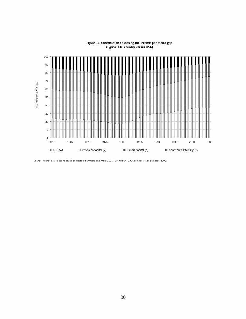
0
10
20
30
40
50
60
70
80
90
100
1960 1965 1970 1975 1980 1985 1990 1995 2000 2005
Inco
me-
per-c
apita
gap
TFP (A) Physical capital (k) Human capital (h) Labor force Intensity (f)
Source: Author's calculations based on Heston, Summers and Aten (2006), World Bank 2008 and Barro‐Lee database 2000.
Figure 11: Contribution to closing the income per capita gap (Typical LAC country versus USA)
38
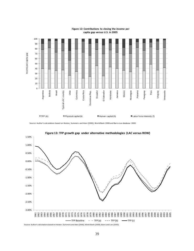
0
10
20
30
40
50
60
70
80
90
100
Arg
entin
a
Bol
ivia
Bra
zil
Typi
cal L
AC
cou
ntry
Chi
le
Col
ombi
a
Cos
ta R
ica
Dom
inic
an R
ep.
Ecu
ador
El S
alva
dor
Hon
dura
s
Jam
aica
Mex
ico
Nic
arag
ua
Pan
ama
Par
agua
y
Per
u
Uru
guay
Ven
ezue
la
Inco
me-
per-c
apita
gap
TFP (A) Physical capital (k) Human capital (h) Labor force Intensity (f )
Source: Author's calculations based on Heston, Summers and Aten (2006), World Bank 2008 and Barro‐Lee database 2000.
Figure 12: Contributions to closing the income per capita gap versus U.S. in 2005
‐3.00%
‐2.50%
‐2.00%
‐1.50%
‐1.00%
‐0.50%
0.00%
0.50%
1.00%
1.50%
1961
1962
1963
1964
1965
1966
1967
1968
1969
1970
1971
1972
1973
1974
1975
1976
1977
1978
1979
1980
1981
1982
1983
1984
1985
1986
1987
1988
1989
1990
1991
1992
1993
1994
1995
1996
1997
1998
1999
2000
2001
2002
2003
2004
2005
Figure 13: TFP growth gap under alternative methodologies (LAC versus ROW)
TFP Baseline TFP (a) TFP (b) TFP (c)
Source: Author's calculations based on Heston, Summers and Aten (2006), World Bank (2008), Barro and Lee (2000).
39
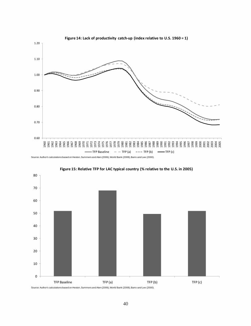
0.60
0.70
0.80
0.90
1.00
1.10
1.201960
1961
1962
1963
1964
1965
1966
1967
1968
1969
1970
1971
1972
1973
1974
1975
1976
1977
1978
1979
1980
1981
1982
1983
1984
1985
1986
1987
1988
1989
1990
1991
1992
1993
1994
1995
1996
1997
1998
1999
2000
2001
2002
2003
2004
2005
Figure 14: Lack of productivity catch‐up (index relative to U.S. 1960 = 1)
TFP Baseline TFP (a) TFP (b) TFP (c)
Source: Author's calculations based on Heston, Summers and Aten (2006), World Bank (2008), Barro and Lee (2000).
0
10
20
30
40
50
60
70
80
TFP Baseline TFP (a) TFP (b) TFP (c)
Figure 15: Relative TFP for LAC typical country (% relative to the U.S. in 2005)
Source: Author's calculations based on Heston, Summers and Aten (2006), World Bank (2008), Barro and Lee (2000).
40
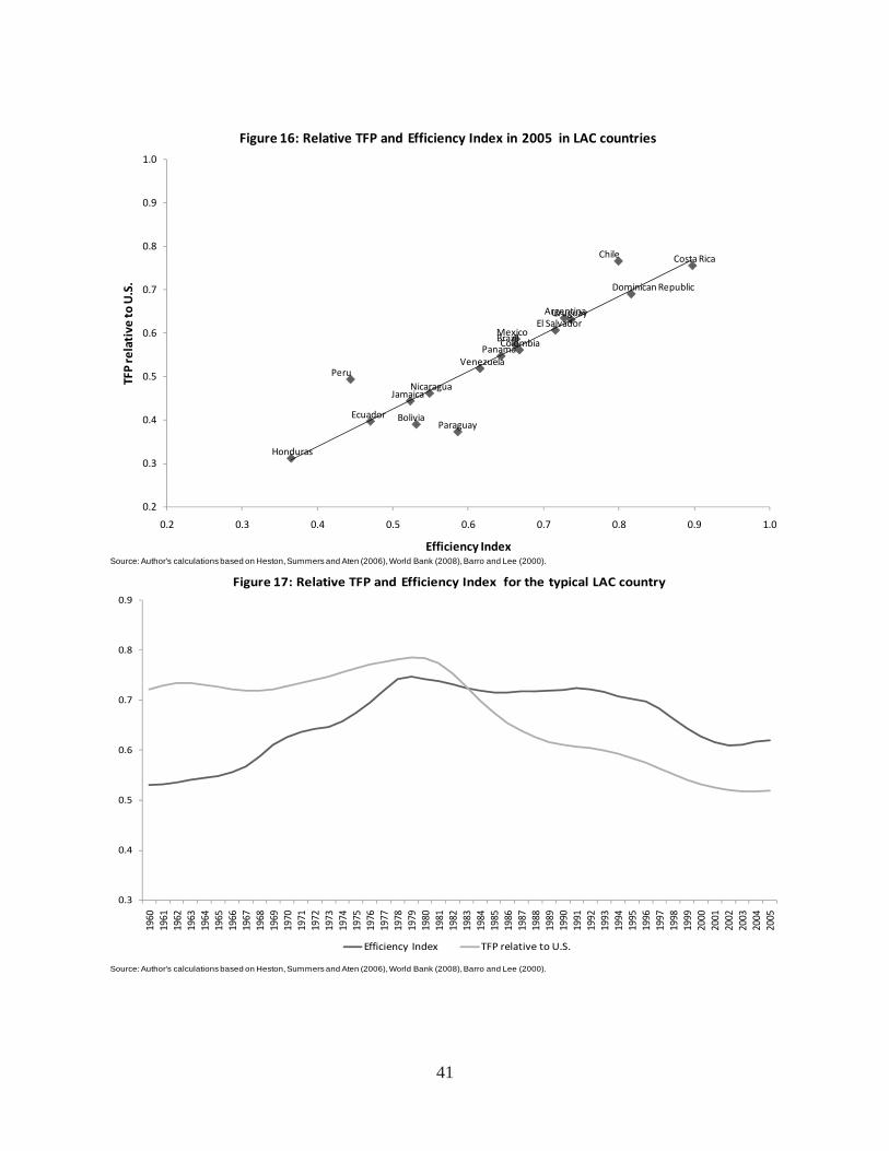
Argentina
Bolivia
Brazil
Chile
Colombia
Costa Rica
Dominican Republic
Ecuador
Honduras
Jamaica
Mexico
Nicaragua
Panama
Peru
Paraguay
El SalvadorUruguay
Venezuela
0.2
0.3
0.4
0.5
0.6
0.7
0.8
0.9
1.0
0.2 0.3 0.4 0.5 0.6 0.7 0.8 0.9
TFP relative
to U.S.
Efficiency Index
Figure 16: Relative TFP and Efficiency Index in 2005 in LAC countries
Source: Author's calculations based on Heston, Summers and Aten (2006), World Bank (2008), Barro and Lee (2000).
1.0
0.3
0.4
0.5
0.6
0.7
0.8
0.9
1960
1961
1962
1963
1964
1965
1966
1967
1968
1969
1970
1971
1972
1973
1974
1975
1976
1977
1978
1979
1980
1981
1982
1983
1984
1985
1986
1987
1988
1989
1990
1991
1992
1993
1994
1995
1996
1997
1998
1999
2000
2001
2002
2003
2004
2005
Figure 17: Relative TFP and Efficiency Index for the typical LAC country
Efficiency Index TFP relative to U.S.
Source: Author's calculations based on Heston, Summers and Aten (2006), World Bank (2008), Barro and Lee (2000).
41
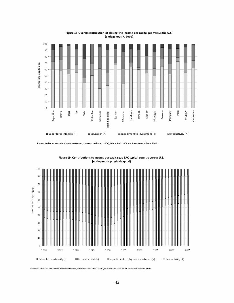
0
10
20
30
40
50
60
70
80
90
100
Argen
tina
Bolivia
Brazil
lac
Chile
Colombia
Costa Rica
Dom
inican
Rep
.
Ecuado
r
El Salvado
r
Hon
duras
Jamaica
Mexico
Nicaragua
Panama
Paraguay
Peru
Uruguay
Ven
ezuela
Income‐per‐capita gap
Figure 18:Overall contribution of closing the income per capita gap versus the U.S. (endogenous K, 2005)
Labor force Intensity (f) Education (h) Impediment to investment (к) Productivity (A)
Source: Author's calculations based on Heston, Summers and Aten (2006), World Bank 2008 and Barro‐Lee database 2000.Source: Author's calculations based on Heston, Summers and Aten (2006), World Bank 2008 and Barro‐Lee database 2000.
42
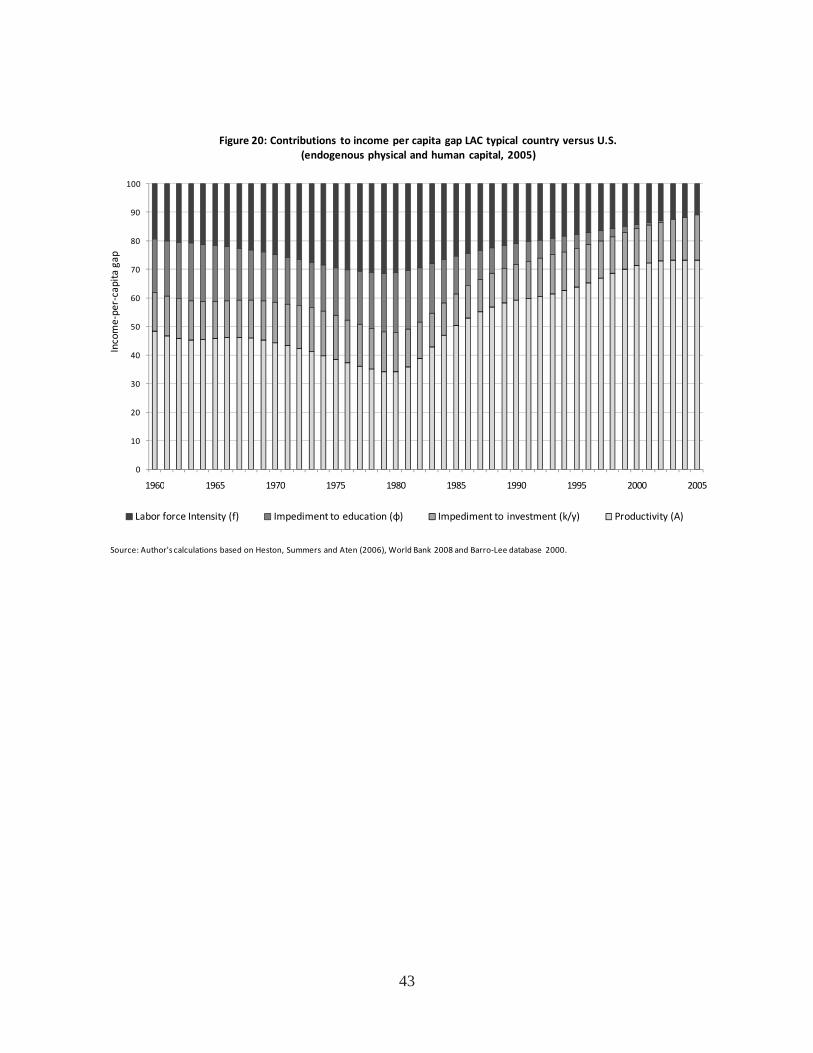
0
10
20
30
40
50
60
70
80
90
100
1960 1965 1970 1975 1980 1985 1990 1995 2000 2005
Income‐per‐capita gap
Figure 20: Contributions to income per capita gap LAC typical country versus U.S. (endogenous physical and human capital, 2005)
Labor force Intensity (f) Impediment to education (φ) Impediment to investment (k/y) Productivity (A)
Source: Author's calculations based on Heston, Summers and Aten (2006), World Bank 2008 and Barro‐Lee database 2000.
43
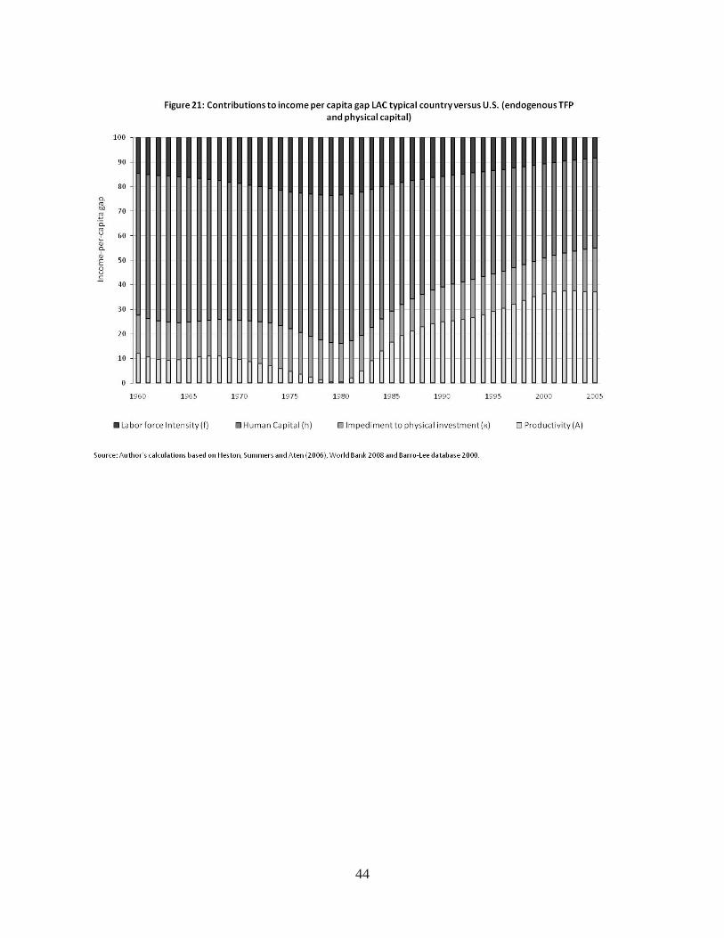
44
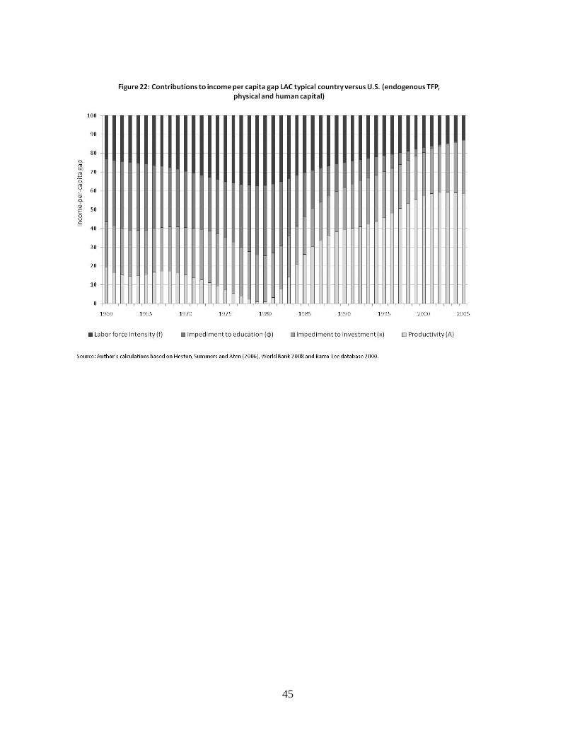
45

46
Table 1. Sample
Argentina Hong Kong New Zealand Australia Honduras Pakistan Austria Hungary Panama Belgium Indonesia Peru Benin India Philippines Bolivia Ireland Papua New Guinea Brazil Iran Portugal Canada Israel Paraguay Chile Italy Senegal China Jamaica Singapore Cameroon Jordan Sierra Leone Colombia Japan El Salvador Costa Rica Kenya Sweden Denmark Korea, Republic of Syria Dominican Republic Sri Lanka Togo Algeria Lesotho Thailand Ecuador Mexico Tunisia Egypt Mali Turkey Spain Mozambique Uganda Finland Malawi Uruguay Fiji Malaysia United States France Niger Venezuela, RB United Kingdom Nicaragua South Africa Germany Netherlands Zambia Ghana Norway Greece Nepal
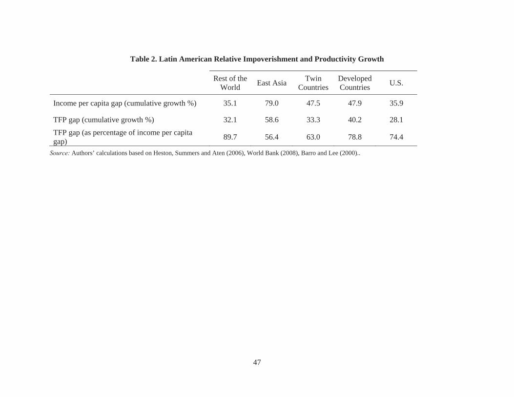
Table 2. Latin American Relative Impoverishment and Productivity Growth
Rest of the
World East Asia Twin Countries
Developed Countries U.S.
Income per capita gap (cumulative growth %) 35.1 79.0 47.5 47.9 35.9
TFP gap (cumulative growth %) 32.1 58.6 33.3 40.2 28.1 TFP gap (as percentage of income per capita gap) 89.7 56.4 63.0 78.8 74.4
Source: Authors’ calculations based on Heston, Summers and Aten (2006), World Bank (2008), Barro and Lee (2000)..
47