
Online Model Checking with UPPAAL SMC - Institute | … Work Sascha Lehmann Online Model Checking...
55
-
Upload
nguyenkien -
Category
Documents
-
view
223 -
download
0
Transcript of Online Model Checking with UPPAAL SMC - Institute | … Work Sascha Lehmann Online Model Checking...
Project Work
Sascha Lehmann
Online Model Checking with UPPAAL SMC
February 4, 2016
supervised by:Prof. Dr. Sibylle Schupp
M.Sc. Xintao Ma
Hamburg University of Technology (TUHH)Technische Universität Hamburg-Harburg
Institute for Software Systems21073 Hamburg


Eidesstattliche Erklärung
Ich versichere an Eides statt, dass ich die vorliegende Projektarbeit selbstständig verfasstund keine anderen als die angegebenen Quellen und Hilfsmittel verwendet habe. DieArbeit wurde in dieser oder ähnlicher Form noch keiner Prüfungskommission vorgelegt.
Hamburg, den 04. Februar 2016Sascha Lehmann
iii


Contents
Contents
1 Introduction 1
2 Conceptual Foundations 32.1 Model Veri�cation . . . . . . . . . . . . . . . . . . . . . . . . . . . . . . . 32.2 Model Checking . . . . . . . . . . . . . . . . . . . . . . . . . . . . . . . . . 32.3 Explicit-State / Symbolic Model Checking . . . . . . . . . . . . . . . . . . 52.4 Online Model Checking . . . . . . . . . . . . . . . . . . . . . . . . . . . . 62.5 Statistical Model Checking . . . . . . . . . . . . . . . . . . . . . . . . . . . 7
2.5.1 DTMC (Discrete-Time Markov Chain) and PCTL . . . . . . . . . 82.5.2 CTMC (Continuous-Time Markov Chain) and CSL . . . . . . . . . 92.5.3 NSTA (Network of Stochastic Timed Automata) and MITL . . . . 10
3 Existing Solutions 133.1 Available Model Checking Environments . . . . . . . . . . . . . . . . . . . 13
3.1.1 UPPAAL . . . . . . . . . . . . . . . . . . . . . . . . . . . . . . . . 133.1.2 PRISM . . . . . . . . . . . . . . . . . . . . . . . . . . . . . . . . . 14
3.2 UPPAAL Solutions . . . . . . . . . . . . . . . . . . . . . . . . . . . . . . . 153.2.1 UPPAAL-SMC . . . . . . . . . . . . . . . . . . . . . . . . . . . . . 15
4 The Statistical Online Model Checking (SOMC) Approach 174.1 Applicable OMC Concepts . . . . . . . . . . . . . . . . . . . . . . . . . . . 174.2 New SOMC Concepts . . . . . . . . . . . . . . . . . . . . . . . . . . . . . 184.3 Implementation and Integration . . . . . . . . . . . . . . . . . . . . . . . . 23
5 SOMC Experimental Applications 275.1 Proof-of-Concept Sample Models . . . . . . . . . . . . . . . . . . . . . . . 27
5.1.1 The Dice Game . . . . . . . . . . . . . . . . . . . . . . . . . . . . . 275.1.2 The Call Centre . . . . . . . . . . . . . . . . . . . . . . . . . . . . 28
6 Evaluation of Analysis Results 316.1 Experiment Results . . . . . . . . . . . . . . . . . . . . . . . . . . . . . . . 316.2 In�uencing Factors . . . . . . . . . . . . . . . . . . . . . . . . . . . . . . . 326.3 Computation Times . . . . . . . . . . . . . . . . . . . . . . . . . . . . . . 36
6.3.1 Impact of the Query Properties . . . . . . . . . . . . . . . . . . . . 366.3.2 Impact of the Java Implementation . . . . . . . . . . . . . . . . . . 37
6.4 SOMC Capabilities and Limitations . . . . . . . . . . . . . . . . . . . . . 38
7 Conclusion 43
v


List of Figures
List of Figures
2.1 The basic model checking work�ow . . . . . . . . . . . . . . . . . . . . . . 4
2.2 A comparison of the static and online veri�cation approaches . . . . . . . 7
2.3 A sample model of a Discrete-Time Markov Chain . . . . . . . . . . . . . 8
2.4 A sample model of a Continuous-Time Markov Chain . . . . . . . . . . . . 9
2.5 A sample model of a Network of Priced Timed Automata . . . . . . . . . 11
3.1 The (graphical) model editor view of the UPPAAL model checker . . . . . 13
3.2 The (code-based) model editor view of the PRISM model checker . . . . . 14
3.3 The model veri�cation view of the UPPAAL model checker . . . . . . . . 15
4.1 Examples of probabilistic branching constructs . . . . . . . . . . . . . . . 18
4.2 Supported model elements for distributions over time . . . . . . . . . . . . 20
4.3 A basic example for using rates as di�erential equations . . . . . . . . . . 22
4.4 The parent and child models for dynamic instance spawning . . . . . . . . 22
4.5 General structure of the original OMC framework . . . . . . . . . . . . . . 23
4.6 General structure of the modi�ed SOMC framework . . . . . . . . . . . . 24
5.1 UPPAAL model of the dice game example . . . . . . . . . . . . . . . . . . 28
5.2 UPPAAL model of the call centre example . . . . . . . . . . . . . . . . . . 29
6.1 Dice game distribution developing over time . . . . . . . . . . . . . . . . . 31
6.2 Dice game veri�cation results of various queries . . . . . . . . . . . . . . . 32
6.3 Call centre rate developing over time . . . . . . . . . . . . . . . . . . . . . 32
6.4 Call centre veri�cation results of various queries . . . . . . . . . . . . . . . 33
6.5 Impacts of the data bu�er size . . . . . . . . . . . . . . . . . . . . . . . . . 33
6.6 Developing of parameters with great value di�erence . . . . . . . . . . . . 34
6.7 Impact of di�erent UPPAAL parameters on the veri�cation process . . . . 35
6.8 Impact of the probability comparison query (Binary event with varied closeprobabilities) . . . . . . . . . . . . . . . . . . . . . . . . . . . . . . . . . . 35
6.9 Duration times of di�erent SMC queries . . . . . . . . . . . . . . . . . . . 36
6.10 Duration impact of di�erent query scope values . . . . . . . . . . . . . . . 37
6.11 Duration times of data generation and approximation . . . . . . . . . . . . 38
6.12 Comparison of system and model data . . . . . . . . . . . . . . . . . . . . 39
6.13 Comparison of real and simulated data distributions (branch point) . . . . 40
6.14 Comparison of real and simulated data distributions (exponential rate) . . 40
vii
List of Tables
4.1 Possible query functions with parameters . . . . . . . . . . . . . . . . . . . 25
List of Algorithms
1 Routine for probabilistic branches . . . . . . . . . . . . . . . . . . . . . . . 19
List of Code Snippets
1 Java implementation of the exponential data generation routine . . . . . . 202 Java implementation of the parameter approximation routine . . . . . . . 21

Abstract
Abstract � Based on the general principles of a newly developed �Online Model Check-ing� framework for real-time, interval-based and temporary model veri�cation utilizingthe interface with the model checker UPPAAL, we extend the system with statisticalfunctionalities to allow online veri�cation for a broader range of models and weaken theimpact of state space explosion. For this purpose, we implement a Java add-on for theOMC framework taking advantage of the integrated Uppaal SMC functions, evaluateits capabilities and �nally use it for two experiments including components for both theonline model checking and the statistical model checking approach, in order to derivestatements about its performance, bene�ts and limitations in comparison to the originalframework. While extending the range of models and components enabled for veri�ca-tion, the project results show that the interpretation of �online� may need to be altered,and the main focus needs to lie on the real-time constraint and - for further research -on the model simulation synchronously to the real system.
ix


1 Introduction
1 Introduction
The application of model checking to verify both software and hardware systems andshow the satis�ability of propositions derived from given speci�cations has been a majortopic in the process of system engineering for several decades. In the beginning � atthe time when many systems were still mostly separated from their surrounding and didnot need to react to environment changes extensively as their design was rather singlepurpose � it was su�cient to analyse a system once at the end of its development phase inorder to guarantee its intended behaviour. But over time, systems became more complexand connected, and at the latest with the emergence of cyber-physical systems, they�nally came to a point where it was no longer enough to follow this separated and staticview. In fact, a static model checking approach could now lead to false negative results,as it supposes speci�c global constraints to hold forever without adjusting the modelparameters to the dynamic and non-deterministic system environment. This fact ledto a growing need for a new approach that involves the consideration of unpredictableparameter data and therefore derives only temporarily valid satis�ability statements.
One solution for this problem is called �Online Model Checking� (OMC) and it providesthe basis for the following framework additions that we develop in the course of thisproject. While the OMC approach itself provides the necessary functionality to verify areal-time system for overlapping time intervals and therefore provides su�cient validityinformation during system observations, it builds up on methods of explicit symbolicmodel checking for the time-limited paths and may still su�er from state space explo-sion. In order to overcome some of the resultant restrictions of this approach, we willextend the OMC framework with methods of statistical model checking, and �nally com-bine them to a new statistical online model checking framework (SOMC). This meansthat instead of deriving logic formulas from the system, we will subsequently simulate themodel with multiple runs at given times simultaneously to the observed real-time system,and only estimate the validity of proportions instead of providing a mathematically de-rived guarantee. Besides lessening the in�uence of state space explosion in certain cases,the SOMC approach also allows us to incorporate statistical elements like probabilisticbranches into the model.
We start this project thesis with a broad overview of conceptual foundations in Chapter 2,which are necessary to understand the SOMC approach, including general explanations ofmodel veri�cation and model checking as well as more detailed information about onlinemodel checking and the di�erences of symbolic and statistical approaches. In Chapter 3,we have a look at already existing solutions of the statistical model checking approachas well as their software environments, and show the potential of an online variant of it.Afterwards we develop the actual statistical online model checking framework in Chap-ter 4, covering its mathematical background as well as the algorithmic concepts for itsimplementation. Given the new system, we apply the principles to analyse two di�erent
1

1 Introduction
proof-of-concept models - an experiment to observe variably loaded dice games and acall centre system with varying agent amounts and call parameters - in Chapter 5. Afterthe application, Chapter 6 provides the evaluation results of the simulation processesand compares the performance, complexity and overall usability of the SOMC approachto the basic OMC and SMC systems. At last, we come to a conclusion in Chapter 7,assessing the general advantages of the new system, and discussing prospects for furtherdevelopment of the SOMC framework as well as the �eld of online model checking.
2
2 Conceptual Foundations
2 Conceptual Foundations
We begin this project on statistical online model checking with the most common con-cepts of the model veri�cation process. This chapter introduces into the �eld of modelveri�cation and its subtopic of model checking with general de�nitions, logics, and con-structs. After that, we get involved into the two more speci�c concepts of Online ModelChecking (OMC) and Statistical Model Checking (SMC), which we want to bring to-gether to a single approach in the subsequent chapters. For a better understanding ofthe SMC technique, a short explanation of the mostly opposing mechanism of explicit-state and symbolic model checking is provided as well.
2.1 Model Veri�cation
The superordinate discipline of Veri�cation covers a large range of techniques to math-ematically deduce the correctness of a system or entity by derivation from underlyingattributes or axiomatic assumptions. These assumptions may be part of a proof con-struct - as in the formal veri�cation approach for algorithms - or originate from a givenspeci�cation during software or model veri�cation. The veri�cation process can eitherbe of static or dynamic nature: The former one - also containing the formal veri�ca-tion technique - is used to analyse the system using logics and mathematical methods,whereas the latter one is realised by embedding and checking the system in a testingenvironment.
To assure that a model represents a real world system with adequate precision, it isnecessary to extract the system-relevant attributes from the real world, and to show thatthese attributes hold for the model as well. The veri�cation technique applied for thatpurpose will be explained next.
2.2 Model Checking
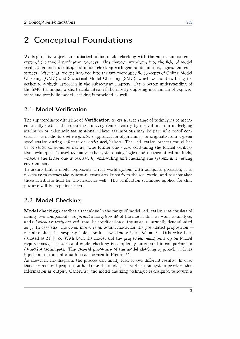
Model checking describes a technique in the range of model veri�cation that consists ofmainly two components: A formal description M of the model that we want to analyse,and a logical property derived from the speci�cation of the system, normally denominatedas �. In case that the given model is an actual model for the postulated proposition �meaning that the property holds for it � we denote it as M j= �. Otherwise it isdenoted as M 6j= �. With both the model and the properties being built up on formalrequirements, the process of model checking is completely automated in comparison todeductive techniques. The general procedure of the model checking approach with itsinput and output information can be seen in Figure 2.1.
As shown in the diagram, the process can �nally lead to two di�erent results. In casethat the required proposition holds for the model, the veri�cation system provides thisinformation as output. Otherwise, the model checking technique is designed to return a
3
2 Conceptual Foundations
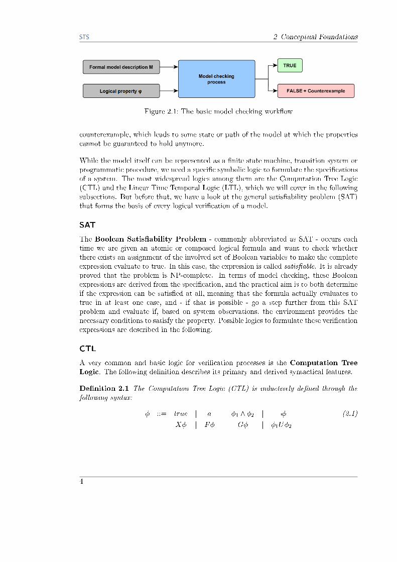
Figure 2.1: The basic model checking work�ow
counterexample, which leads to some state or path of the model at which the propertiescannot be guaranteed to hold anymore.
While the model itself can be represented as a �nite state machine, transition system orprogrammatic procedure, we need a speci�c symbolic logic to formulate the speci�cationsof a system. The most widespread logics among them are the Computation Tree Logic(CTL) and the Linear Time Temporal Logic (LTL), which we will cover in the followingsubsections. But before that, we have a look at the general satis�ability problem (SAT)that forms the basis of every logical veri�cation of a model.
SAT
The Boolean Satis�ability Problem - commonly abbreviated as SAT - occurs eachtime we are given an atomic or composed logical formula and want to check whetherthere exists an assignment of the involved set of Boolean variables to make the completeexpression evaluate to true. In this case, the expression is called satis�able. It is alreadyproved that the problem is NP-complete. In terms of model checking, these Booleanexpressions are derived from the speci�cation, and the practical aim is to both determineif the expression can be satis�ed at all, meaning that the formula actually evaluates totrue in at least one case, and - if that is possible - go a step further from this SATproblem and evaluate if, based on system observations, the environment provides thenecessary conditions to satisfy the property. Possible logics to formulate these veri�cationexpressions are described in the following.
CTL
A very common and basic logic for veri�cation processes is the Computation Tree
Logic. The following de�nition describes its primary and derived syntactical features.
De�nition 2.1 The Computation Tree Logic (CTL) is inductively de�ned through thefollowing syntax:
� ::= true j a j �1 ^ �2 j :� (2.1)
X� j F� j G� j �1U�2
4

2 Conceptual Foundations
By combining the basic connectives and adding path quanti�ers, we can furthermore de-rive the following adequate set of expressions:
� ::= false j �1 _ �2 j �1 ) �2 j �1 , �2 (2.2)
AX� j EX� j AF� j EF�
AG� j EG� j A[�1U�2] j E[�1U�2]
At this point, a represents an arbitrary atomic proposition, and � is any CTL formulacomposed from these propositions. As CTL falls in the category of branching-time logics,the logical expressions cover all possible paths at every given point of time. This factenables the use of path-spanning quanti�ers - A (all) or E (exists) - to specify on whichpaths a certain property needs to hold. The possible combinations of temporal operatorsare listed in the last two rows of De�nition 2.2.
LTL
The second commonly used temporal logic is the Linear Time Temporal Logic, whichis - similar to CTL - a sub-logic of the subordinate CTL* set. The following de�nitiongives an overview of the syntactical elements included in LTL.
De�nition 2.2 The Linear Time Temporal Logic (LTL) is inductively de�ned throughthe following syntax:
� ::= true j a j �1 ^ �2 j :� (2.3)
X� j F� j G� j �1U�2
By combining the basic connectives, we can furthermore derive the following adequate setof expressions:
� ::= false j �1 _ �2 j �1 ) �2 j �1 , �2 (2.4)
In contrast to CTL, the LTL logic is designed to be applied to individual program execu-tions and therefore only takes single paths into account. For that reason, the de�nitiondoes not include any A (all) or E (exists) path quanti�ers.
2.3 Explicit-State / Symbolic Model Checking
The most basic approaches to model checking - the so called Explicit-State and
Symbolic Model Checking - have already been used for decades and are the mostwidespread ones in the range of model veri�cation. Provided some properties built upwith temporal operators, the Explicit-State Model Checking performs a depth-�rst ex-haustive search through the complete state space for each of those operators in order toderive a logical statement about their satis�ability. This explicit traversal through thestate space leads to one of the most limiting problems of model checking: The complexity
5

2 Conceptual Foundations
increase of the state space, which is mostly exponential in regards to the amount of statesand transition relations.
The �rst attempt to attenuate the impact of state space explosion was made by usingSymbolic Model Checking, a �xed-point based method that treats the states of a modelas sets instead of analysing them individually. This iterative process, combined with asuitable data structure such as Binary Decision Diagrams (BDD), allowed a more ef-�cient model checking process, even though the core state space limitations remainedunchanged. Therefore, in order to tackle this core problem - paired with other limit-ing factors like its missing capability to deal with dynamically changing systems - newapproaches needed to be introduced, which we will investigate in the following.
2.4 Online Model Checking
As a relatively new approach � a technique which was not examined in detail until thebeginning of the twenty-�rst century � Online Model Checking was introduced todeal with the emerging need for a concept which can be applied to the growing amountof cyber-physical systems embedded into a dynamically changing environment. A �rstmentioning of real-time and concurrent model checking can be found in publications ofR. Alur in the early 90s, with the very basics covered in their work �Model-checking forreal-time systems� [1]. Although it could be used for a �rst shallow analysis of real-timesystems by involving dynamic time delays, it treated the environment in a static manner,meaning that it was still applied to a system model before deployment and the actualrun-time situation.
In the early 2000s, the concept of Runtime Veri�cation came up - introduced by thecorrespondent annual workshop with a monitoring concept by Geilen [2] amongst others- and initially moved the veri�cation focus from the pre-deployment to the run-time phaseof a system cycle. For the �rst time, it was then possible to turn the formal veri�cationprocess into a dynamic technique which could be continuously adapted to observationsof a real system in order to respond to property violations. Nevertheless, even thoughthis concept allowed possibly preventing the recurrence of failures, it was still followinga post-checking approach, only reacting to violations instead of fully preventing them.
This kind of system view changed essentially with the emergence of the online approach.In a publication by Rammig et al. [3], this technique was brought to a �rst application asan operating system service. It was now possible to check a system during its execution,observing tasks at run-time and applying necessary adjustments to the system model incase that its con�guration gets changed. Instead of relying on a plain check of alreadygiven model execution traces to adjust the system model, this new approach allowed a sortof pre-checking, verifying the possible model behaviour in the immediate future before ittakes place in the observed system, and hereby actively preventing malfunctioning. Inthe scope of that publication, the technique was only applied to the rather speci�c �eldof task management in operating systems, so it still did not deliver a general framework
6

2 Conceptual Foundations
for online model checking which could be applied to any sort of state machine.
The development of such a framework was �nally started by Rinast [4], and in the courseof this elaboration it forms the basis of the statistical extension of the online approach.Figure 2.2 illustrates the technique behind Online Model Checking as pointed out bythe author: The original procedure of model checking (2.2a) takes up the complete statespace of the model execution at once. In case that a single state in this total space doesnot satisfy any of the safety conditions, the property is considered to be false for thewhole model and countermeasures need to be taken directly. A less restrictive concept isgiven by the OMC approach (2.2b), where the current state space in focus - representedby the overlapping triangles - is reduced to a �xed time interval on each veri�cation step.Besides the fact that we can now progress with the �rst two execution steps without evenencountering a potentially non-satisfying state, the overlapping intervals also guaranteethat the following two execution steps will still satisfy the conditions and hence providea time interval during which we can safely initiate the necessary countermeasures.
2.5 Statistical Model Checking
The second technique which we need to compose our new approach is the one of Sta-tistical Model Checking (SMC). It is a static approach like Explicit Model Checking,but in contrast to that, it utilises statistical methods rather than exhaustive explorationof the complete state space. The bene�ts gained with this approach are apparent: Bysimulating the system model several times and combining the Boolean results of thesesimulation runs, it becomes unnecessary to review the complete state space, as we onlyneed to focus on the current path each time. Therefore, the limiting factor for manyveri�cation attempts - some case of state space explosion - is eliminated. With this prop-erty, the SMC approach is predestined to complement the real-time capabilities of thepreviously described Online Model Checking attempt.
(a) Static veri�cation (b) Online veri�cation
Figure 2.2: A comparison of the static and online veri�cation approaches
7

2 Conceptual Foundations
Figure 2.3: A sample model of a Discrete-Time Markov Chain
In the following, we will have a look at di�erent model and logic types which are com-monly used to describe probabilistic systems. The �rst two speci�cation and veri�cationlogics - PCTL and CSL - are extensively used by the model checker PRISM [5], whilethe last ones - MITL and its reduced form WMTL - provide the basis for the UPPAALmodel checking process.
2.5.1 DTMC (Discrete-Time Markov Chain) and PCTL
A very basic kind of probabilistic model with elements that are used in all statisticalmodel checkers, is the so called Discrete-Time Markov Chain. An example of such modelsis provided in Figure 2.3. While its general structure is similar to a �nite state machine,the transitions are not guarded by an invariant, but are weighted with probability values,summing up to 1 for all outgoing transitions of a state. Corresponding to these relativeprobabilities, one transition is randomly chosen and triggered. For example, when states2 is active, the transitions s2 ! s3, s2 ! s4 and s2 ! s5 will be triggered withprobabilities of 40%, 20% and 40%.
To actually take advantage of the additional capabilities of the model, we need to usean extended logic which can also handle probabilistic properties. One way to achievethis is the use of the Probabilistic Computation Tree Logic, which adds exactly theseprobability queries to the standard CTL language.
De�nition 2.3 The Probabilistic Computation Tree Logic (PCTL) is inductively de�nedthrough the following syntax:
� ::= true j a j �1 ^ �2 j :� j P�p[ ] (2.5)
::= X� j �1U�k�2 j �1U�2 j F� j G� (2.6)
In the given de�nition, a represents an arbitrary atomic proposition, p 2 [0; 1] a pathprobability value, � 2 f<;�;�; >g one of the possible inequalities, and k 2 N an
8

2 Conceptual Foundations
Figure 2.4: A sample model of a Continuous-Time Markov Chain
arbitrary natural number. The formulas � in Expression 2.5 describe properties onstates, whereas the formulas in Expression 2.6 can be used to establish the satisfactoryconstraints of a path.Comparing the PCTL logic to the basic CTL version reveals that they accord with eachother in most de�nitions, except for two expressions: The state formula de�nition nowprovides an additional probabilistic operator P�p[ ], which is applicable to describe anddetermine if the probability of some path formula lies above or below a certain thresh-old value. In the logics of PCTL, this formula provides the basis for all probabilisticveri�cations. Besides that, a more general bounded-until expression �1U
�k�2 is intro-duced, extending the usability of the former unbounded one. These de�nitions allow usto formulate di�erent semantic properties for PCTL veri�cation:
s j= � (Example: s j=fair _ loaded) (2.7)
! j= �1U�k�2 (Example: !j=fairU�50loaded) (2.8)
s j= P�p[ ] (Example: s j=P�0:7[F six]) (2.9)
The �rst formula (2.7) represents the fact that a die is either fair or loaded at every pointin time. The second formula (2.8) states that the die will be fair until it �nally switchesto a loaded state, which needs to take place at some point within 50 time units. Anexample for a probabilistic constraint is given in the last formula (2.9), expressing thatthe probability of getting a �six� in the future is greater than or equal to 0:7. Additionalinformation on the semantics of PCTL can be found in Principles of Model Checking [6].
2.5.2 CTMC (Continuous-Time Markov Chain) and CSL
In those case where a discrete view of our system clocks is not su�cient, we can utilise aContinuous-Time Markov Chain (CTMC) to model a system. In contrast to the discreteversion, the transitions are not triggered by probabilities, but they provide certain ratevalues with which the individual transitions are triggered. Figure 2.4 shows a samplemodel with these rates. In each of the intermediate states, the transition leading backto the predecessor is triggered at rate 1, while the transition to the subsequent state willbe activated periodically at a rate of 1=2.
Just as with DTMC models, we want to formulate probabilistic properties for the veri�-cation process, and therefore need a logic that is also capable of describing the eventual
9
2 Conceptual Foundations
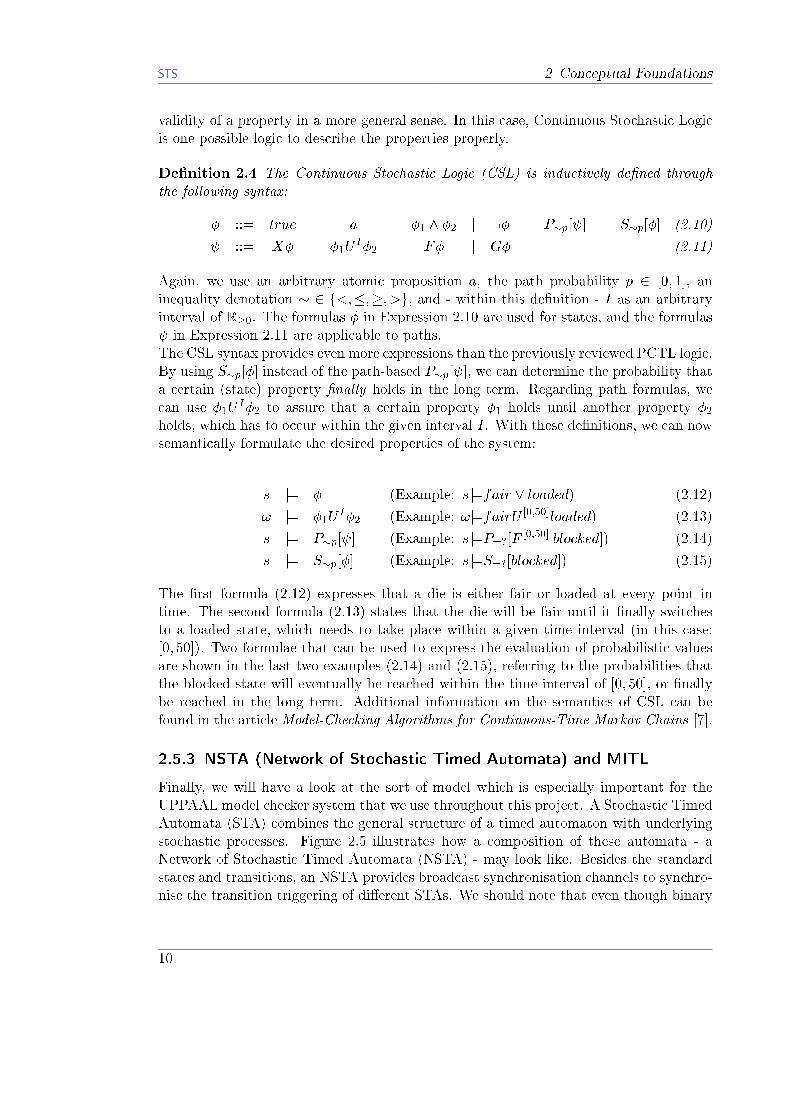
validity of a property in a more general sense. In this case, Continuous Stochastic Logicis one possible logic to describe the properties properly.
De�nition 2.4 The Continuous Stochastic Logic (CSL) is inductively de�ned throughthe following syntax:
� ::= true j a j �1 ^ �2 j :� j P�p[ ] j S�p[�] (2.10)
::= X� j �1UI�2 j F� j G� (2.11)
Again, we use an arbitrary atomic proposition a, the path probability p 2 [0; 1], aninequality denotation � 2 f<;�;�; >g, and - within this de�nition - I as an arbitraryinterval of R�0. The formulas � in Expression 2.10 are used for states, and the formulas in Expression 2.11 are applicable to paths.
The CSL syntax provides even more expressions than the previously reviewed PCTL logic.By using S�p[�] instead of the path-based P�p[ ], we can determine the probability thata certain (state) property �nally holds in the long term. Regarding path formulas, wecan use �1U
I�2 to assure that a certain property �1 holds until another property �2holds, which has to occur within the given interval I. With these de�nitions, we can nowsemantically formulate the desired properties of the system:
s j= � (Example: s j=fair _ loaded) (2.12)
! j= �1UI�2 (Example: !j=fairU [0;50]loaded) (2.13)
s j= P�p[ ] (Example: s j=P=?[F[0;50] blocked]) (2.14)
s j= S�p[�] (Example: s j=S=?[blocked]) (2.15)
The �rst formula (2.12) expresses that a die is either fair or loaded at every point intime. The second formula (2.13) states that the die will be fair until it �nally switchesto a loaded state, which needs to take place within a given time interval (in this case:[0; 50]). Two formulae that can be used to express the evaluation of probabilistic valuesare shown in the last two examples (2.14) and (2.15), referring to the probabilities thatthe blocked state will eventually be reached within the time interval of [0; 50], or �nallybe reached in the long term. Additional information on the semantics of CSL can befound in the article Model-Checking Algorithms for Continuous-Time Markov Chains [7].
2.5.3 NSTA (Network of Stochastic Timed Automata) and MITL
Finally, we will have a look at the sort of model which is especially important for theUPPAAL model checker system that we use throughout this project. A Stochastic TimedAutomata (STA) combines the general structure of a timed automaton with underlyingstochastic processes. Figure 2.5 illustrates how a composition of these automata - aNetwork of Stochastic Timed Automata (NSTA) - may look like. Besides the standardstates and transitions, an NSTA provides broadcast synchronisation channels to synchro-nise the transition triggering of di�erent STAs. We should note that even though binary
10

2 Conceptual Foundations
Figure 2.5: A sample model of a Network of Priced Timed Automata
synchronisation channels are generally supported as well, they are not applied in orderkeep all components in an unblocked state.
The most important feature in terms of clock implementations are the di�erent ratesthat can be applied to each clock variable. In the example, the rate of x starts with avalue 4, meaning that the clock will proceed by 4 steps during each universal time step,and this rate will be gradually decremented in the following states.
The logic which was chosen to describe the validation properties of those NPTAs consid-ering the di�erent clock variables is a form of Metric Interval Temporal Logic (MITL).
De�nition 2.5 The Metric Interval Temporal Logic (MITL) is inductively de�ned throughthe following syntax:
� ::= a j �1 ^ �2 j :� j O� j �1Ux�d�2 (2.16)
This de�nition uses an arbitrary atomic proposition a, a clock variable x and an arbitrarynatural number k 2 N. Besides the usual logical operators used in the other logic speci�-cations as well, MITL o�ers an extended bounded-until operator �1U
x�d�2 which makes
it possible to not only de�ne the maximum time value until which �2 must eventually besatis�ed, but also the actual clock variable we are referring to. Hence, we are allowed touse multiple di�erent clocks in parallel.
As it is not decidable whether the probability of a run of the system model M satisfying lies above a given threshold value, i.e. PM ( ) � p, we need to restrict the logic tothe cost-bounded case, so we are geared to the principles of Weighted Metric TemporalLogic (WMTL).
De�nition 2.6 The cost-bounded form of MITL is expressed as: PM (�x�C�)
11

2 Conceptual Foundations
Here, x again represents a clock variable, and the arbitrary natural number C 2 N
is generally bound. Using this representation, we are able to formulate the followingdi�erent queries regarding probability values:
Probability Evaluation: PM (�x�C�)? (2.17)
Hypothesis Testing: PM (�x�C�) � p 2 [0; 1]? (2.18)
Probability Comparison: PM (�x�C�1) > PM (�x�C�2)? (2.19)
All of the expressions in Eq. 2.17, Eq. 2.18 and Eq. 2.19 can be approximated by simu-lation runs, whose Boolean outcomes are �nally gathered and statistically analysed.
12

3 Existing Solutions
3 Existing Solutions
In this chapter, we will focus on two di�erent model checkers - Uppaal and Prism - thatprovide the necessary functionality to create and verify probabilistic models. Afterwards,we will take a look at the modular software solutions of Uppaal that actually provide thenecessary veri�cation query routines used in this project to integrate stochastic capabil-ities into the OMC framework.
3.1 Available Model Checking Environments
3.1.1 UPPAAL
The Uppaal model checker - developed in a cooperative project at the Uppsala andAalborg universities by Larsen, Yi et al. - forms the central modelling and veri�cationcomponent of our work, and is integrated into the framework via several interfaces pro-vided by the integrated tool environment to communicate with the model construction,simulation and veri�cation processes. As the Uppaal environment was already used bythe original OMC framework, we use it for our extended approach as well, including theUppaal SMC extension.The general user interface together with the model editor section is shown in Figure 3.1.A model can be created in both a code-based (as �processes�) or graphical manner, andcan be extended by custom function calls and data type declarations created in a C-likesyntax. By using states and transitions with corresponding invariants and guards, modelsin Uppaal can represent several types of state machines, and di�erent sub-model tem-plates can be instantiated as often as desired to build up systems of arbitrary complexity.Multiple clock variables for global and local processes can be used to create a form of
Figure 3.1: The (graphical) model editor view of the UPPAAL model checker
13

3 Existing Solutions
Figure 3.2: The (code-based) model editor view of the PRISM model checker
independence between the sub-systems, and the synchronization of processes is achievedvia either binary or broadcast synchronisation channels. A more detailed description ofthe components and capabilities of Uppaal can be found in the corresponding sectionabout Uppaal provided in the thesis covering the OMC framework [4] or in the moreextensive main tutorial of the program [8].
3.1.2 PRISM
Another integrated environment for the model checking process that we could have usedfor the SOMC approach is the probabilistic symbolic model checker Prism [9], which isspeci�cally designed to deal with models containing stochastic elements. As we pointedout in the Conceptual Foundations chapter, the model checker can be used to build abroad range of probabilistic model types, including the described DTMCs and CTMCsas well as the completely non-deterministic probabilistic (timed) automata and Markovdecision processes.Figure 3.2 shows the basic GUI of Prism as well the speci�c view in which the models aredescribed. In contrast to Uppaal, the model creation process of Prism completely relieson a modelling language without providing a graphical modelling tool. Structured inmodules, the states (e.g., p1: [0..15]) and transitions paired with transition conditions(e.g., [] p1=2 & (none_lht | some_a) -> (p1'=3)) are de�ned. Additional formulae(e.g., formula none_lht = !(p2>=4&p2<=13)&!(p3>=4&p3<=13)) can be used to expressmore complex conditions for the transition process.Especially for the fact that Prism supports more probabilistic model types than Uppaal,it could be a reasonable addition to the SOMC framework for prospective research. Asthe user interface itself as well as the parsers are written in Java, the program couldeasily be integrated in the existing work�ow. Additional information about the tooland its supported models and concepts can be found in the manual distributed with theprogram.
14

3 Existing Solutions
3.2 UPPAAL Solutions
3.2.1 UPPAAL-SMC
The Uppaal module we will use exclusively for the framework add-on is the Uppaal SMCextension, which adds probabilistic modelling and veri�cation capabilities to the toolenvironment. The formerly described Figure 3.1 already shows an example of a proba-bilistically extended model, and a more in-depth investigation of the added componentsregarding its use for our purpose will be provided in the next chapter.The graphical user interface for accessing the stochastic veri�cation tools from withinUppaal is shown in Figure 3.3. At this point, we can insert our own queries - composedof logical properties regarding the variables of template instances or global model param-eters - and evaluate them to determine several types of bounds and probability valuesusing methods such as sequential hypothesis testing and monte carlo simulation. Themost important query types among them are the following:
Simulation: simulate 1 [<= 100] fD:One;D:Sixg (3.1)
Probability Evaluation: Pr[<= 100] (<> D:One) (3.2)
Hypothesis Testing: Pr[<= 100] (<> D:One) >= 0:6 (3.3)
Probability Comparison: Pr[<= 100] (<> D:One)
>= Pr[<= 100] (<> D:Six) (3.4)
Value Bound Determination: E[<= 100; 1000] (max : D:RollCount) (3.5)
The aspect that all of these queries have in common is the scope value, de�ning thetime interval - starting from the moment of query evaluation - in which the propertyshould be considered. The �rst query (3.1) initiates a single simulation run of the model
Figure 3.3: The model veri�cation view of the UPPAAL model checker
15
3 Existing Solutions
(referring to a dice game example we will introduce later on) and tracks the activitydata of the �One� and �Six� states, which can be graphically reviewed afterwards. Thesecond query (3.2) performs a basic proability evaluation step. In this case, we try to�nd out how likely it is to reach the state �One� at least once within the next 100 timeunits. Using the result evaluation tools provided by Uppaal SMC, it is possible to furtheranalyse the probability, probability density, and cumulative probability distributions ofthe simulation result.The next two queries (3.3) and (3.4) allow us to review probabilities in comparison toother �xed or event-bound probability values. In contrast to the concrete data of the �rstquery and the probability data of the second query, the evaluation of these two formulaereturn the Boolean result data indicating whether the hypothesis is con�rmed by theperformed simulation runs or not.Finally, Uppaal SMC also allows determining the expected (abbreviated as E) valuebounds that are reached throughout the simulation runs. The last query (3.5) showshow such queries are formulated for a selected number of 1000 runs. In this case, we lookfor the maximum value of the roll counter. A more detailed explanation of the querytypes and the methods behind them can be found in the documentation [10].
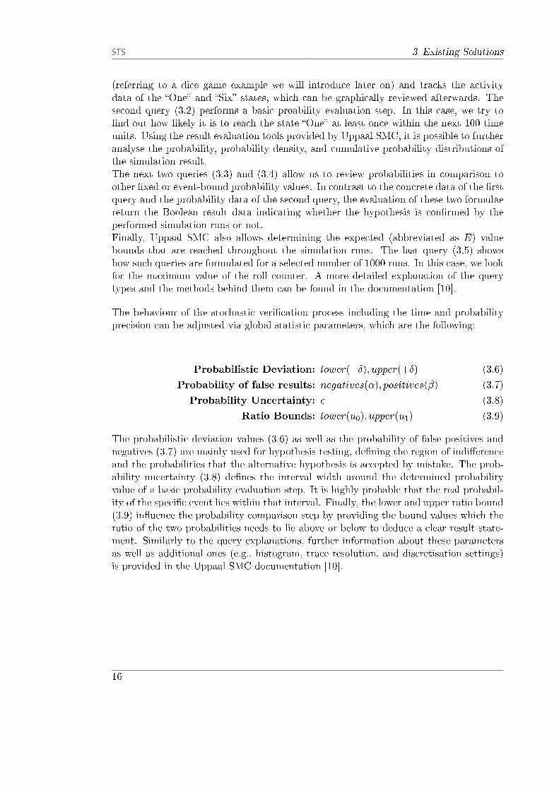
The behaviour of the stochastic veri�cation process including the time and probabilityprecision can be adjusted via global statistic parameters, which are the following:
Probabilistic Deviation: lower(��); upper(+�) (3.6)
Probability of false results: negatives(�); positives(�) (3.7)
Probability Uncertainty: � (3.8)
Ratio Bounds: lower(u0); upper(u1) (3.9)
The probabilistic deviation values (3.6) as well as the probability of false positives andnegatives (3.7) are mainly used for hypothesis testing, de�ning the region of indi�erenceand the probabilities that the alternative hypothesis is accepted by mistake. The prob-ability uncertainty (3.8) de�nes the interval width around the determined probabilityvalue of a basic probability evaluation step. It is highly probable that the real probabil-ity of the speci�c event lies within that interval. Finally, the lower and upper ratio bound(3.9) in�uence the probability comparison step by providing the bound values which theratio of the two probabilities needs to lie above or below to deduce a clear result state-ment. Similarly to the query explanations, further information about these parametersas well as additional ones (e.g., histogram, trace resolution, and discretisation settings)is provided in the Uppaal SMC documentation [10].
16

4 The Statistical Online Model Checking (SOMC) Approach
4 The Statistical Online Model Checking(SOMC) Approach
Now that we gathered all necessary information on the systematic background of di�erentmodel checking techniques for both static and real-time veri�cation, and concluded thebene�ts of using UPPAAL for our purpose, we �rst take a deeper look at those speci�cconcepts of online model checking which can be applied to our new statistical onlinemodel checking approach as well. Afterwards, we complement the given OMC approachwith additional concepts that allow us to not only deal with OMC enabled models,but also with a broader range of probabilistic models containing statistical and non-deterministic elements. We support the most relevant SOMC speci�c constructs with anunderlying algorithmic construct, before we �nally transfer the complete framework to anactual implementation � an add-on for the already existent OMC framework developedby Rinast [4].
4.1 Applicable OMC Concepts
In order to provide online capabilities built up on continuous up-to-date real world param-eters, two basic processing steps need to be applied to the real-time model: The StateSpace Reconstruction (SSR) process tracks the simulation trace of the current modelexecution run, and reduces it to a minimal path by deleting looped and redundant sub-paths as well as those paths without further e�ect on reaching the current state causedby subsequent variable resets. After deriving a valid and minimized path to the currentstate, the OMC Framework performs State Space Adaption (SSA) steps on existing ornewly inserted transitions within the path to �nally reach the desired state that matchesreal system observations. Rinast describes two concepts to implement these steps - agraph-based and a use-def-chain-based reconstruction and adaption procedure - whichare further explained in his thesis [4].
In their basic form, these techniques need to be applied for the SOMC concept as well.But as we will see in the next Section 4.2, some features enabled by the statisticalapproach such as varying clock rates and non-deterministic stay times of unconstrainedstates prohibit a direct use of their OMC implementation for our purpose.
The limitations regarding the general structure of the model that are already mentionedfor the original OMC framework hold for our concept as well. We still need to restrict ouradaption step to data variables which are not constrained in any location of the model,as this would require us to perform additional checks on whether the constrains are stillmet and the currently active state is actually allowed.
Even though the SOMC approach does not require viewing the complete spate spacefor its queries, the state space itself still plays a role during the SSR process. For thatreason, we are limited to models where the clocks in question are restricted, i.e., are reset
17

4 The Statistical Online Model Checking (SOMC) Approach
(a) A probabilistic branching point (b) Branching point with partial clock reset
Figure 4.1: Examples of probabilistic branching constructs
at some point on each possible path. This ensures that we get an upper bound for thesequence length and thus for the execution time of the SSR process.
4.2 New SOMC Concepts
The statistic model checking approach itself together with its concrete implementationin Uppaal SMC provides �ve di�erent main conceptions, which we could consider totransfer to the online framework: Probabilistic branching, exponential rates, dynamicpattern creation, di�erential equations using clock rates, and user-de�ned custom delaydistributions. In the following, we give an overview of each of these elements and evaluatetheir individual use and importance for the SOMC framework.
Probabilistic Branches
The concept of Probabilistic Branches can be found at every place in a model where atransition leads to a branching point which in turn provides multiple outgoing edges, eachof which is not guarded by some invariant, but parameterised with an integral weight, rep-resenting their relative trigger probability. A basic example of such a non-deterministicmodel component can be seen in Figure 4.1a, with one transition for decrementing avariable having an 80% and the other transition for incrementation having a 20% prob-ability. In a probabilistic system, these branches form one of the two additional maincomponents and need to be further investigated at this point.
The probabilistic branches in�uence the state space reconstruction (SSR) process as wellas the variable developing throughout a path, so we need to consider both in order tointegrate them properly into the work�ow of the OMC framework.
We already saw that the crucial requirement for the SSR is the reset of each involvedclock variable at some point of a path inside the model to run inside desired time bounds.Figure 4.1b illustrates the case that could possibly occur in a branched system: Onepossible path � in this example the one with the greater probability � will be traversedwithout resetting the clock variable, while the less probable path �nally triggers a resetof the clock. For the purpose of our implementation, we will choose the most restrictive
18
4 The Statistical Online Model Checking (SOMC) Approach
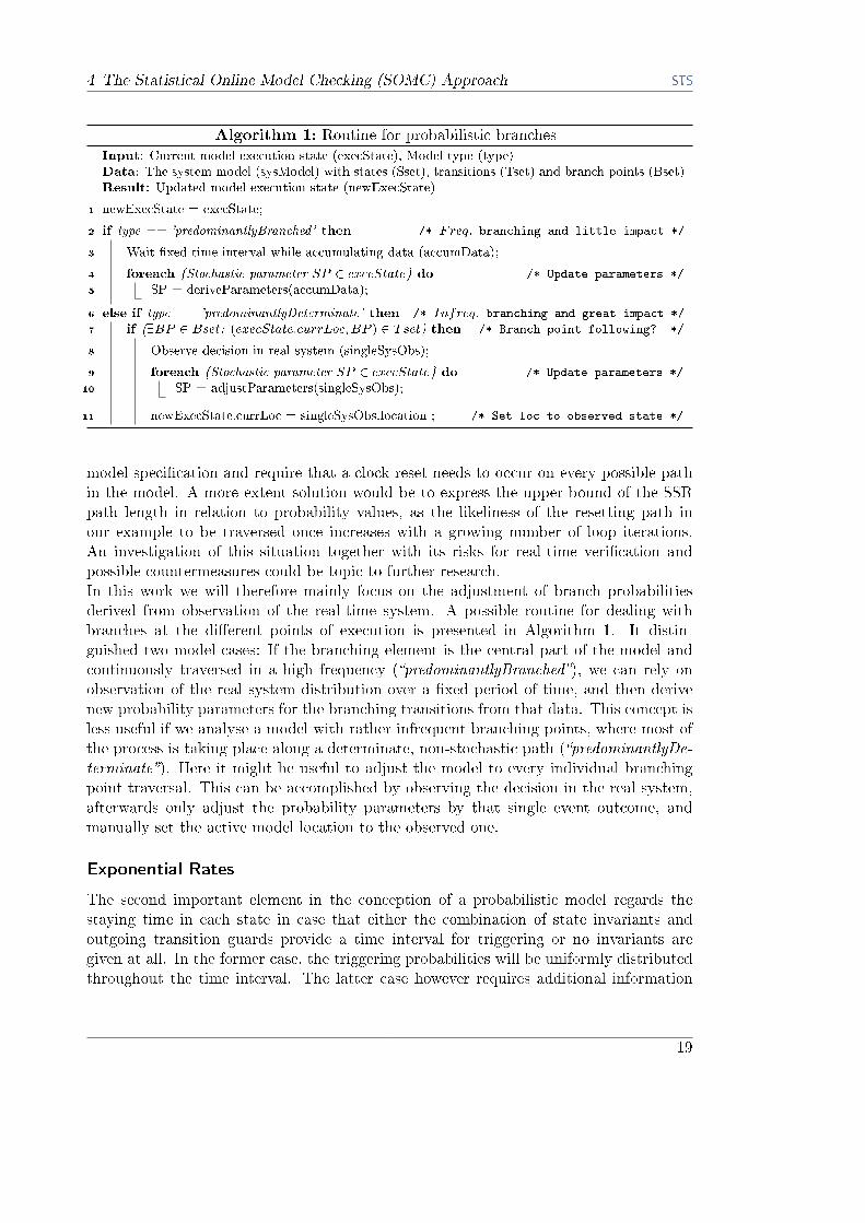
Algorithm 1: Routine for probabilistic branchesInput: Current model execution state (execState), Model type (type)Data: The system model (sysModel) with states (Sset), transitions (Tset) and branch points (Bset)Result: Updated model execution state (newExecState)
1 newExecState = execState;
2 if type == 'predominantlyBranched' then /* Freq: branching and little impact */
3 Wait �xed time interval while accumulating data (accumData);
4 foreach {Stochastic parameter SP 2 execState} do /* Update parameters */
5 SP = deriveParameters(accumData);
6 else if type == 'predominantlyDeterminate' then /* Infreq: branching and great impact */
7 if (9BP 2 Bset: (execState:currLoc;BP ) 2 Tset) then /* Branch point following? */
8 Observe decision in real system (singleSysObs);
9 foreach {Stochastic parameter SP 2 execState} do /* Update parameters */
10 SP = adjustParameters(singleSysObs);
11 newExecState.currLoc = singleSysObs.location ; /* Set loc to observed state */
model speci�cation and require that a clock reset needs to occur on every possible pathin the model. A more extent solution would be to express the upper bound of the SSRpath length in relation to probability values, as the likeliness of the resetting path inour example to be traversed once increases with a growing number of loop iterations.An investigation of this situation together with its risks for real-time veri�cation andpossible countermeasures could be topic to further research.In this work we will therefore mainly focus on the adjustment of branch probabilitiesderived from observation of the real-time system. A possible routine for dealing withbranches at the di�erent points of execution is presented in Algorithm 1. It distin-guished two model cases: If the branching element is the central part of the model andcontinuously traversed in a high frequency (�predominantlyBranched�), we can rely onobservation of the real system distribution over a �xed period of time, and then derivenew probability parameters for the branching transitions from that data. This concept isless useful if we analyse a model with rather infrequent branching points, where most ofthe process is taking place along a determinate, non-stochastic path (�predominantlyDe-terminate�). Here it might be useful to adjust the model to every individual branchingpoint traversal. This can be accomplished by observing the decision in the real system,afterwards only adjust the probability parameters by that single event outcome, andmanually set the active model location to the observed one.
Exponential Rates
The second important element in the conception of a probabilistic model regards thestaying time in each state in case that either the combination of state invariants andoutgoing transition guards provide a time interval for triggering or no invariants aregiven at all. In the former case, the triggering probabilities will be uniformly distributedthroughout the time interval. The latter case however requires additional information
19
4 The Statistical Online Model Checking (SOMC) Approach
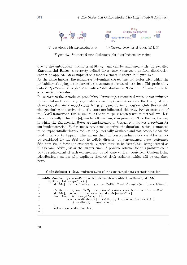
(a) Locations with exponential rates (b) Custom delay distribution (cf. [10])
Figure 4.2: Supported model elements for distributions over time
due to the unbounded time interval [0; inf ] and can be addressed with the so-calledExponential Rates, a property de�ned for a state whenever a uniform distributioncannot be applied. An example of this model element is shown in Figure 4.2a.
As the name implies, the parameter determines the exponential factor with which theprobability of staying in the currently active state is decreased over time. This probabilitydata is represented through the cumulative distribution function 1� e�at, where a is theexponential rate value.
In contrast to the introduced probabilistic branching, exponential rates do not in�uencethe simulation trace in any way under the assumption that we view the trace just as achronological chain of model states being activated during execution. Only the variablechanges during the active time of a state are in�uenced this way. For an extension ofthe OMC framework, this means that the state space reconstruction method, which isalready formally de�ned in [4], can be left unchanged in principle. Nevertheless, the wayin which the Exponential Rates are implemented in Uppaal still induces a problem forour implementation: While such a state remains active, the duration - which is supposedto be exponentially distributed - is only internally available and not accessible for theused interfaces to Uppaal. This means that the corresponding clock variables cannotbe considered for the SSR and its DBMs directly. In consequence, every performedSSR step would force the exponentially rated state to be 'reset', i.e. being treated asif it became active just at the current time. A possible solution for this problem couldbe the replacement of each exponentially rated state with an equivalent Custom DelayDistribution structure with explicitly declared clock variables, which will be explainednext.
Code-Snippet 1: Java implementation of the exponential data generation routine
1 public double [ ] generateExpDistrDoubleSamples (double lowerBound , double
expRate , int sampleNum) {2 double [ ] randomDoubles = generateEqDistrDoubleSamples (0 , 1 , sampleNum) ;3
4 // Return e xponen t i a l l y d i s t r i b u t e d va lue s with the inve r s i on method5 double [ ] randomExpDoubles = new double [ sampleNum ] ;6 for ( int i =0; i<sampleNum ; i++) {7 randomExpDoubles [ i ] = (Math . l og (1 � randomDoubles [ i ] ) /
(�expRate ) ) + lowerBound ;8 }9 return randomExpDoubles ;10 }
20

4 The Statistical Online Model Checking (SOMC) Approach
Code-Snippet 2: Java implementation of the parameter approximation routine
1 public Dist r ibut ionData getDistr ibut ionFromData (double [ ] data ) {2
3 double dis t r ibut ionSum = 0 ;4 for ( int i =0; i<data . l ength ; i++) {5 dis t r ibut ionSum += data [ i ] ;6 }7 double lambdaEstimation = 1 / ( d i s t r ibut ionSum / data . l ength ) ;8 Dist r ibut ionData d i s t r i bu t i onData = new
Dist r ibut ionData ( Distr ibut ionType .EXPONENTIAL_DISTRIBUTION,9 new double [ ] { lambdaEstimation }) ;10 return d i s t r i bu t i onData ;11
12 }
Our contribution at this point will rather be a method to measure the potentially activetime of each state during run-time and to use the gathered data for an adjustment ofexponential rates of the model to �t the current behaviour of the real system.The two code snippets show the basic procedures for exponential data generation as wellas exponential parameter approximation. In the �rst code section (Code-Snippet 1), weuse the inversion method to generate exponential data from a formerly equally distributeddata series. This method is applicable to di�erent distributions with a de�ned inverseor quantile function. The second code section (Code-Snippet 2) shows how the observeddata series can then be used to derive approximated distribution parameters. In the caseof Exponential Rates, we focus on the routine for exponential distributions. The inverseof the arithmetic mean of observed values already provides a feasible approximation of the�-parameter (in our notation the exponential rate value a) for the cumulative distributionfunction.
Custom Delay Distributions
The next element enabled through our use of SMC - which is related to the explainedExponential Rate states and can be seen as a generalization of the principle behind it -is the Custom Delay Distribution. The general structure of this construct is shownin Figure 4.2b.Using this element, we are allowed to calculate values with any desired distributionby providing a custom delay function. An initially reset and explicitly given clock thencounts up to this delay value, and �nally a leaving transition is triggered. In case that thecustom delay function produces exponentially distributed data, this structure is similarto Exponential Rates, with the di�erence that here the clock variables can be externallyaccessed.
Clock Rates and Di�erential Equations
Another new concept allows us to use multiple time domains progressing independentlyat di�erent speed levels: The Clock Rates. Figure 4.3 illustrates how these rates areimplemented. By manually setting the �rst derivation of a clock with the instruction
21

4 The Statistical Online Model Checking (SOMC) Approach
Figure 4.3: A basic example for using rates as di�erential equations
x0 == 0 in the �nal location of the example, we force the clock to stay at its currentvalue, as it will now advance by 0 time units per global tick. In the same way, the clockprogression rate is set to 1 in the initial state, and therefore acts like a clock without acustom clock rate at this point. In this manner, we can move one step further from theoriginal synchronized clock rate concept and even use the rates to represent Di�erentialEquations of arbitrary order by chaining the �rst order di�erential rates. It is hence thecentral component if a system modelling process involves the need for hybrid automata,and extends the lineup of potential use cases.But even though this concept may be of great use for a comprehensive SOMC approach,a di�erential equation requires much e�ort on several levels. For one respect, it mayin�nitely extend the state space during a simulation, as its size is directly dependent onthe possible interval size and granularity of the clock variables involved. This, in turn,has a direct impact on the state space reconstruction process, and may break the real-time constraint which the framework is based on. Besides that, we would need to extendthe concept of DBM transformations in order to cover clocks with di�erent progressionbehaviour. For that reason, this concept is only described in this project and will requirefurther mathematical investigation before being fully usable.
Dynamic Instance Spawning
The last element that we want to consider for the SOMC framework is the concept ofDynamic Instance Spawning. Its general structure, consisting of a parent automatathat triggers the spawning of child model instances with a lifetime lasting until a child's�nal call of the exit() instruction, is shown in Figure 4.4. As long as the limit of spawn-Num children is not reached, the parent model in this example continuously creates childinstances in an exponentially distributed manner (caused by the exponential rate of 1 inthe initial state as previously explained). These instances will now increment a variable- again with an exponential time distribution - until reaching the spawnLT value andeventually initiating their own deletion.
(a) Parent model (b) Child model
Figure 4.4: The parent and child models for dynamic instance spawning
22

4 The Statistical Online Model Checking (SOMC) Approach
Figure 4.5: General structure of the original OMC framework
This concept would be suitable in those case where we deal with changing amountsof individual and rather complex entities, which cannot be represented by a plain arrayentry anymore, but which manifest their own behaviour. Groups of visitors in a museum,scheduled and executed threads, or - as we will pick up again in one of our proof-of-conceptexperiments - the number of agents in a call centre could be modelled this way.
We may then consider to frequently update parameters for the number of entities andtheir probability for creation and elimination during an experiment. We need to keepin mind that the varying entity amount will directly in�uence the state space size andtherefore its reconstruction time.
4.3 Implementation and Integration
The implementation of the derived requirements for the framework takes place at di�erentparts of the software system. In general, the OMC framework itself is divided into severalmodules responsible for distinct tasks of the application work�ow. Figure 4.5 gives anoverview of the main components which the OMC framework consists of.
The upper half shows the Data Acquisition section. It contains all the necessary steps ofcollecting, structuring, and providing data. It ranges from modules for system observa-tion (SensorAdapter, FileProvider), to data processing steps like linear approximation ofdata sets (LinearRegressor), and interfaces usable for applications to access the prepareddata (ProviderAdapter).
23
4 The Statistical Online Model Checking (SOMC) Approach
Figure 4.6: General structure of the modi�ed SOMC framework
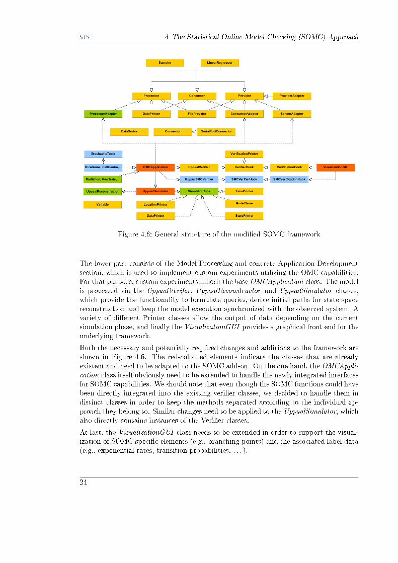
The lower part consists of the Model Processing and concrete Application Developmentsection, which is used to implement custom experiments utilizing the OMC capabilities.For that purpose, custom experiments inherit the base OMCApplication class. The modelis processed via the UppaalVerifer, UppaalReconstructor and UppaalSimulator classes,which provide the functionality to formulate queries, derive initial paths for state spacereconstruction and keep the model execution synchronized with the observed system. Avariety of di�erent Printer classes allow the output of data depending on the currentsimulation phase, and �nally the VisualizationGUI provides a graphical front end for theunderlying framework.
Both the necessary and potentially required changes and additions to the framework areshown in Figure 4.6. The red-coloured elements indicate the classes that are alreadyexistent and need to be adapted to the SOMC add-on. On the one hand, the OMCAppli-cation class itself obviously need to be extended to handle the newly integrated interfacesfor SOMC capabilities. We should note that even though the SOMC functions could havebeen directly integrated into the existing veri�er classes, we decided to handle them indistinct classes in order to keep the methods separated according to the individual ap-proach they belong to. Similar changes need to be applied to the UppaalSimulator, whichalso directly contains instances of the Veri�er classes.
At last, the VisualizationGUI class needs to be extended in order to support the visual-ization of SOMC speci�c elements (e.g., branching points) and the associated label data(e.g., exponential rates, transition probabilities, . . . ).
24
4 The Statistical Online Model Checking (SOMC) Approach
Query function Input Output
All functions veri�cation property, scope query success
performSimulationRuns(...) data names tracked datadetermineValueBounds(...) - value bounds
determineProbability(...) - prob. boundsdetermineTimeRangeProbability(...) lower time bound prob. bounds
testHypothesis(...) prob. threshold, inequality boolean eval
compareProbability(...) prob. 1, prob. 2, inequality boolean evalcompareIntervalProbability(...) prob. 1, prob. 2, di�. limit intersection info
Table 4.1: Possible query functions with parameters
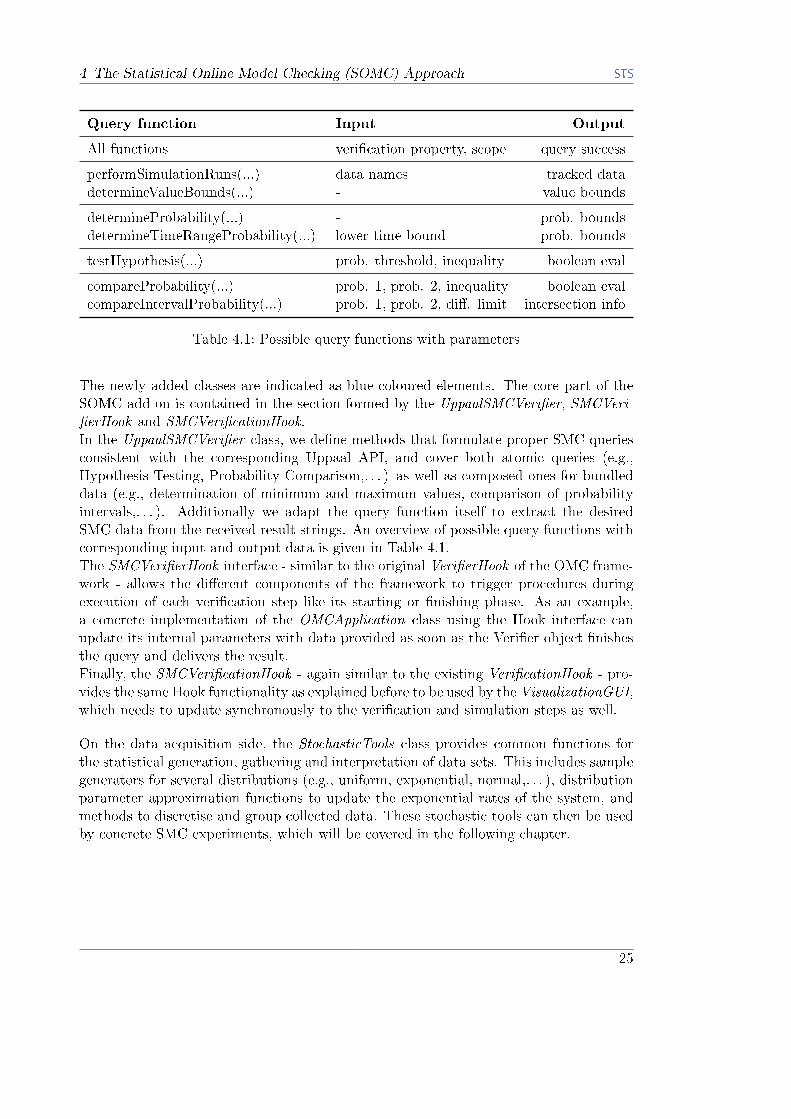
The newly added classes are indicated as blue-coloured elements. The core part of theSOMC add-on is contained in the section formed by the UppaalSMCVeri�er, SMCVeri-�erHook and SMCVeri�cationHook.In the UppaalSMCVeri�er class, we de�ne methods that formulate proper SMC queriesconsistent with the corresponding Uppaal API, and cover both atomic queries (e.g.,Hypothesis Testing, Probability Comparison,. . . ) as well as composed ones for bundleddata (e.g., determination of minimum and maximum values, comparison of probabilityintervals,. . . ). Additionally we adapt the query function itself to extract the desiredSMC data from the received result strings. An overview of possible query functions withcorresponding input and output data is given in Table 4.1.The SMCVeri�erHook interface - similar to the original Veri�erHook of the OMC frame-work - allows the di�erent components of the framework to trigger procedures duringexecution of each veri�cation step like its starting or �nishing phase. As an example,a concrete implementation of the OMCApplication class using the Hook interface canupdate its internal parameters with data provided as soon as the Veri�er object �nishesthe query and delivers the result.Finally, the SMCVeri�cationHook - again similar to the existing Veri�cationHook - pro-vides the same Hook functionality as explained before to be used by the VisualizationGUI,which needs to update synchronously to the veri�cation and simulation steps as well.
On the data acquisition side, the StochasticTools class provides common functions forthe statistical generation, gathering and interpretation of data sets. This includes samplegenerators for several distributions (e.g., uniform, exponential, normal,. . . ), distributionparameter approximation functions to update the exponential rates of the system, andmethods to discretise and group collected data. These stochastic tools can then be usedby concrete SMC experiments, which will be covered in the following chapter.
25

5 SOMC Experimental Applications
5 SOMC Experimental Applications
In this chapter, we apply the implemented SOMC framework to multiple models in orderto show its general applicability to di�erent scenarios as well as its bene�ts and limitationsfor an online model checking approach.
5.1 Proof-of-Concept Sample Models
The focus of this section lies on two speci�c models - a DiceGame and a CallCentreexperiment - which show the utilisation of the stochastic branching point and exponentialrate components explained in Chapter 4 in more tangible scenarios. We will have adeeper look at the model components and their interaction, the relevant parameters forthe experiments and possible queries for the veri�cation step.
5.1.1 The Dice Game
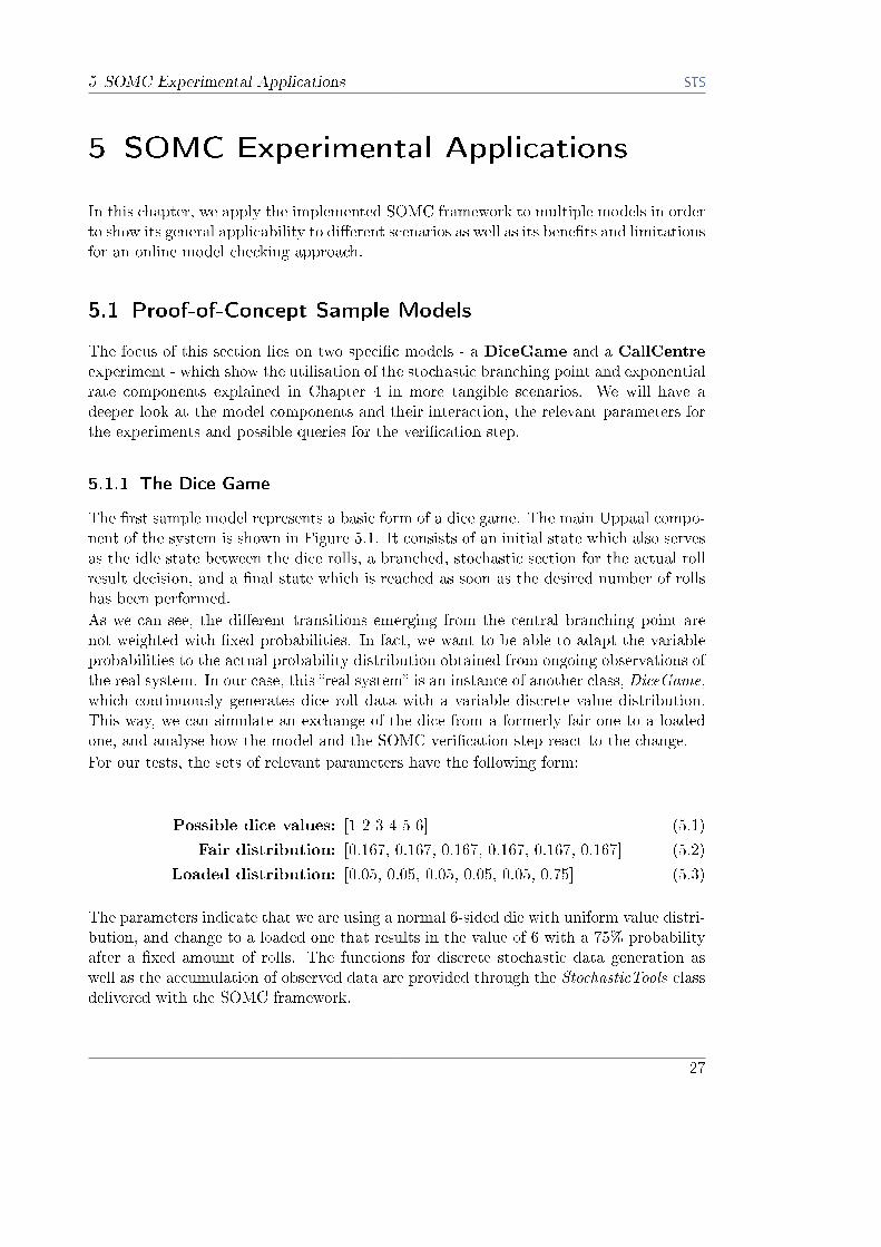
The �rst sample model represents a basic form of a dice game. The main Uppaal compo-nent of the system is shown in Figure 5.1. It consists of an initial state which also servesas the idle state between the dice rolls, a branched, stochastic section for the actual rollresult decision, and a �nal state which is reached as soon as the desired number of rollshas been performed.
As we can see, the di�erent transitions emerging from the central branching point arenot weighted with �xed probabilities. In fact, we want to be able to adapt the variableprobabilities to the actual probability distribution obtained from ongoing observations ofthe real system. In our case, this �real system� is an instance of another class, DiceGame,which continuously generates dice roll data with a variable discrete value distribution.This way, we can simulate an exchange of the dice from a formerly fair one to a loadedone, and analyse how the model and the SOMC veri�cation step react to the change.
For our tests, the sets of relevant parameters have the following form:
Possible dice values: [1 2 3 4 5 6] (5.1)
Fair distribution: [0.167, 0.167, 0.167, 0.167, 0.167, 0.167] (5.2)
Loaded distribution: [0.05, 0.05, 0.05, 0.05, 0.05, 0.75] (5.3)
The parameters indicate that we are using a normal 6-sided die with uniform value distri-bution, and change to a loaded one that results in the value of 6 with a 75% probabilityafter a �xed amount of rolls. The functions for discrete stochastic data generation aswell as the accumulation of observed data are provided through the StochasticTools classdelivered with the SOMC framework.
27

5 SOMC Experimental Applications
Figure 5.1: UPPAAL model of the dice game example
For the SOMC veri�cation step, there are now multiple checking variants that we canperform to derive statistical information, and the following ones will be applied in ouranalysis:
Determine single value probability: D.One? (5.4)
Compare interval probabilities: D.Six > D.One + 0.2? (5.5)
Test hypothesis: D.Six <= 0.95? (5.6)
Depending on the veri�cation interval that we set for the experiment, the �rst Query 5.4will result in the probability value that the value 1 will occur at least once within thattime interval. By setting the interval size to 1 and assuming that no delay is caused bythe query itself, the result value should be equivalent to the current probability value weset for the corresponding transition.Besides this basic determination of a single probability value, we will also perform com-parison (Query 5.5) and hypothesis tests (Query 5.6). They give information about howthe speci�c probability compares to either another probability or a �xed value. In casethat the probability of getting a 6 grows beyond 95% within the given interval, we will beinformed about it. The same holds for the case that the interval probability of 1 exceedsthe probability of 6 by more than 20%. In the actual implementation, Query 5.5 does notneed to be provided a speci�c direction of inequality, as it will be false as soon as thetwo probabilities in question di�er by more than the absolute 0:2 value in any direction.
5.1.2 The Call Centre
The second showcase model for the SOMC approach represents a Call Centre scenario,built up on the fact that the time distributions of both call duration and the time between
28

5 SOMC Experimental Applications
(a) Call Centre Main (b) Call Checker
(c) Call Agent (d) Call Agent Updater
Figure 5.2: UPPAAL model of the call centre example
calls is assumed to be mostly exponentially distributed. Therefore we will use the modelfor two purposes: One the one hand we want to apply the insights from Chapter 4 regard-ing Exponential Rates and test the relevant stochastic tool functions, and on the otherhand we can analyse the model regarding future extensions that could be implementedutilizing the remaining SOMC elements not covered by now.
The di�erent components of the Uppaal model can be seen in Figure 5.2. The modelconsists of 4 distinct parts: The Call Centre Main (5.2a) triggers a signal through the�call� synchronization channel at an alterable exponential rate callFreqRate and thereforeserves as the incoming call provider. The Call Checker (5.2b) will then get informed aboutthe call and - depending on whether there exist agents in a free state or not - delegatesthe incoming call to one of the free agents. Otherwise, the call will be rejected. Thethird component is the Call Agent (5.2c) itself, where we can �nd the second ExponentialRate value callDurRate. On delegation, the call agent switches to the active �Call� stateand remains there until the exponential distributed call time is up. A �callFinished�synchronization channel �nally informs the Call Agent Updater (5.2d) about the stateof the agent, which then performs the enqueue step to re-add the agent to the waitingqueue.
The main focus lies on the two Exponential Rates callFreqRate and callDurRate. Us-ing the features of the new SOMC framework, we want to be able to track the actualcall frequency and duration in the real world, and repeatedly use the observations toderive updated distribution parameters which are then applied to the model to keep itsynchronized with the system in question. Again, the necessary functions for both expo-nential data generation and exponential distribution approximation are provided by theStochasticTools class.
29

5 SOMC Experimental Applications
Similar to the Dice Game example, we are then able to apply di�erent sorts of queries tothe constantly updated model, and the most signi�cant ones are listed in the following:
Determine blocking probability: CH.Blocked? (5.7)
Determine queue value bounds: max/min: occupiedAgentCount? (5.8)
Test hypothesis: CH.Blocked <= 0.5? (5.9)
The central point of focus lies on the question whether the given number of call agents issu�cient to handle all incoming calls based on the current frequency and time durationvalues. With the �rst Query 5.7, we are able to track exactly this probability over time.Additionally, we may want to obtain even more precise data and demand the exactpotential maximum and minimum number of free or blocked agents in the near futureof each veri�cation step. For this purpose, Query 5.8 provides us with that desireddata, which we can then use to perform countermeasures if needed. In case we onlywant to make sure that the probability of reaching a blocked state lies below a certainthreshold, we can use the third Query 5.9. With that, we may assume that as long asthe probability of an empty agent queue is smaller that 50%, we can tolerate the smallpotential probability of denying a call, and otherwise may need to increase the overallnumber of agents. Again, all of these veri�cation queries are applied to an up-to-datemodel, and thus only hold for a �xed period of time.
30

6 Evaluation of Analysis Results
6 Evaluation of Analysis Results
After conducting the aforementioned SOMC experiments, we will evaluate the obtaineddata in this chapter, starting with the presentation of the experiment results in Sec-tion 6.1. We will identify di�erent factors that have an impact on the experiment out-comes throughout the stages of model adaption and stochastic veri�cation in Section 6.2,and relate both these factors and the underlying Java implementation to the computationtimes in Section 6.3. In the end, Section 6.4 will deal with a more general evaluation ofthe SOMC framework capabilities and limitations.
6.1 Experiment Results
In this section, we take a look at the parameter data and veri�cation outcome duringthe DiceGame and CallCentre experiments. Starting with the DiceGame, Figure 6.1shows both the probability distributions of the real system and the distribution sensedvia the stochastic tools and therefore used by the system model. Due to the probabilisticproperty of the data, we can make two noticeable observations: In the sections I and IIIof diagram 6.1b, where the probabilities of the roll results remain constant in the realsystem (see 6.1a), we recognize dithering around the �xed real distributions. The abruptjump from one probability distribution to the other additionally creates the section II ofdiagram 6.1b, where we observe a rather continuous change between probability valuesinstead of the original jump. Several factors in�uence this behaviour, and they will beexplained in-depth in Section 6.2. Figure 6.2 provides the veri�cation results over timeusing the queries prepared in the previous chapter. In the �rst diagram (6.2a), theprobability developing for the roll result of 1 is shown for di�erent veri�cation intervallengths. The second diagram (6.2b) shows the comparison of interval probabilities asBoolean value, meaning that the probabilities of the two outcomes 1 and 6 di�er by a�xed amount or not. The last diagram (6.2c) shows the Boolean results of a hypothesistest, checking if the probability of the result 6 lies below 0:95.
0 10 20 30 40 50 60 70 80 90 1000
0:2
0:4
0:6
0:8
1
Time
ResultProbability One
Two
Three
Four
Five
Six
(a) Distributions of real system
0 20 40 60 80 100 120 140 160 1800
0:2
0:4
0:6
0:8
1
Time
(b) Distributions of observed data
Figure 6.1: Dice game distribution developing over time
31

6 Evaluation of Analysis Results
0 20 40 60 80 1000
0:2
0:4
0:6
0:8
1
Time
ProbabilityofOne
(a) Probability of One withinfollowing 5 time units
0 20 40 60 80 1000
0:2
0:4
0:6
0:8
1
Time
Abs.
Prob.Di�erence
(b) Probability interval com-parison of One and Six
0 20 40 60 80 1000
1
Time
BooleanResult
(c) Boolean hypothesis test(<= 0:95) of Six prob.
Figure 6.2: Dice game veri�cation results of various queries
The CallCentre experiment was conducted in a similar way. Figure 6.3 illustrates how thestochastic parameters - in this case the exponential rates of call frequency and duration -changed in the observed system and the system model. The two diagrams in Figure 6.3aand Figure 6.3b show the same phenomena of parameter dithering during constant phasesand continuous developing in actual jump situations. The veri�cation results of the threeprepared queries are shown in Figure 6.4. While the �rst diagram (6.4a) again depictsthe absolute probability of the attribute in focus - the probability of reaching a stateof a completely occupied agent queue - with varying veri�cation intervals, the seconddiagram (6.4b) shows the maximum and minimum amount of occupied agents over time.Finally, a hypothesis test is performed in the last diagram (6.4c), which evaluates if theprobability of a blocked queue is still smaller than 0:5.
6.2 In�uencing Factors
As our experiments show, multiple parameters in�uence the signi�cance of veri�cationdata, computation times, model parameter integrity, and the overall simulation sequence.
0 10 20 30 40 50 60 70 80 90 1000
1
2
3
4
5
Time
Parameter
Value Call Frequency Rate
Call Duration Rate
(a) Distributions of real system
0 10 20 30 40 50 60 70 80 90 1000
1
2
3
4
5
Time
Call Frequency Rate
Call Duration Rate
(b) Distributions of observed data
Figure 6.3: Call centre rate developing over time
32

6 Evaluation of Analysis Results
0 20 40 60 80 1000
0:2
0:4
0:6
0:8
1
Time
Block
Probability
(a) Probability of blockedqueue within following 5
time units
0 20 40 60 80 1000
1
2
3
4
5
6
Time
AgentValueBounds
(b) Value bounds of occupiedagents
0 20 40 60 80 1000
1
Time
BooleanResult
(c) Hypothesis test (<= 0:5)of blocked queue
Figure 6.4: Call centre veri�cation results of various queries
The Time Interval Length parameter already had a great in�uence on the originalOMC framework, and needs to be carefully considered at this point as well. By settingthe interval length, we decide on the temporal scale which is suitable to obtain su�cientup-to-date validity predictions while still maintaining a tolerable prediction deviationcaused by the stochastic and therefore non-deterministic model elements. For instance,the DiceGame model is more e�cient for predictions on a smaller scale, as the event cycleis rather short and we want to instantly react to exchanged dice, while the CallCentreexample takes more time to accumulate representative data, which we want to use toderive queue boundaries and judge on the best amount of agents on the long run.
Within the data acquisition section, the most in�uential value for our experiments is theData Bu�er Size chosen for each DataSeries provider. We can distinguish between twodi�erent cases: If we set the bu�er size to a small value, we achieve a �faster� reactiontime on changes of the data distribution. In the DiceGame experiment, this will lead toa more synchronized model adaption, but only within certain bounds. Using a value toosmall for the experiment, every natural stochastic deviation will instantly cause a changeof the model parameters, and we will �nally observe a parameter oscillation that may lead
0 50 100 1500
0:2
0:4
0:6
0:8
1
Time
ProbabilityofSix
Observed
Real
(a) Small bu�er (10) - osc.
0 50 100 1500
0:2
0:4
0:6
0:8
1
Time
ProbabilityofSix
(b) Big bu�er (50) - delay
0 50 100 1500
0:2
0:4
0:6
0:8
1
Time
ProbabilityofSix
(c) Big bu�er (50) - average
Figure 6.5: Impacts of the data bu�er size
33

6 Evaluation of Analysis Results
0 50 100 1500
2
4
6
8
10
Time
Parameter
Value
Real frequency rate
Real duration rate
Model frequency rate
Model duration rate
Figure 6.6: Developing of parameters with great value di�erence
to false interpretations. Both phenomena can be observed in Figure 6.5a. In the othercase - meaning that we choose a rather high bu�er size value - we can circumvent theseoscillations, but highly decrease the reaction time in return. We will only slowly adaptthe model to abrupt distribution changes, or might even miss the actual distributiondeveloping in detail. Figure 6.5b illustrates the delay of the model parameter adaption,and the result of distribution data, which sums up to an average distribution on the largescale is shown in Figure 6.5c.
Looking deeper into the stochastic aspects of our experiments, we �nd another set ofrelevant parameters that in�uence the model developing. One of them is the ParameterDi�erence, i.e., the maximum di�erence between two sequential distribution parametervalues. Figure 6.6 illustrates the impact on the CallCentre example throughout the periodof time in which the model adapts from one parameter value to the next one. Even thoughan abrupt change from a frequency rate of 1 and duration rate of 9 to a frequency rateof 9 and duration rate of 1 takes place in the real world, the model parameters developfrom one to another only stepwise, depending on the previously explained bu�er sizefactor. This results in an intermediate situation with both a frequency and durationrate of around 2 within the model, which creates distribution scenarios that did neveroccur in reality, and might lead to undesired positive or negative peaks and thus to falseveri�cation results.
Strongly connected to the parameter di�erence appears the actual Distribution Ap-
proximation Method chosen for the data preprocessing step. The current implementa-tion is built up on the assumption that the distribution parameters stay at some discretevalues most of the time, and only rarely switch from one parameter con�guration toanother. This allows us to directly transfer the currently observed data to model pa-rameters without further processing, but temporarily fails during those time periods inwhich two or more distributions are mixed up in the bu�er. Using this insight, we mayconsider to extend the distribution approximation method in a way that it sticks to aprevious distribution as long as the deviation of the current bu�er data from its deriveddistribution lies above a certain value.
As last aspect on the stochastic side, the Uppaal SMC Parameters themselves in�u-ence the model simulation and veri�cation process, as we further explained in Chapter 3already. Figure 6.7 shows the probability values and hypothesis testing results during the
34
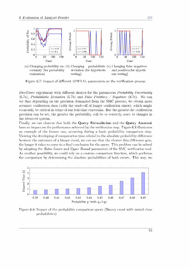
6 Evaluation of Analysis Results
0 50 100 1500
0:2
0:4
0:6
0:8
1
Time
ProbabilityofSix
0.01
0.1
(a) Changing probability un-certainty (for probabilityevaluation)
0 50 100 1500
1
Time
TestingResult
0.05
0.001
(b) Changing probabilisticdeviation (for hypothesistesting)
0 50 100 1500
1
Time
TestingResult
0.5
0.05
(c) Changing false negativesand positives(for hypoth-esis testing)
Figure 6.7: Impact of di�erent UPPAAL parameters on the veri�cation process
DiceGame experiment with di�erent choices for the parameters Probability Uncertainty(6.7a), Probabilistic Deviation (6.7b) and False Positives / Negatives (6.7c). We cansee that depending on the precision demanded from the SMC process, we obtain moreaccurate veri�cation data (with the trade-o� of longer veri�cation times), which mighteventually be critical in terms of our real-time constraint. But the greater the veri�cationprecision can be set, the greater the probability will be to correctly react to changes inthe observed system.
Finally, we can observe that both the Query Formulation and the Query Amount
have an impact on the performance achieved by the veri�cation step. Figure 6.8 illustratesan example of the former one, occurring during a basic probability comparison step.Viewing the developing of computation time related to the absolute probability di�erencebetween the outcomes of a binary event, we can see that the shorter this di�erence gets,the longer it takes to come to a �nal conclusion for the query. This problem can be solvedby adapting the Ratio Lower and Upper Bound parameters of the SMC veri�cation tool.As another possibility, we could rely on a custom comparison function, which performsthe comparison by determining the absolute probabilities of both events. This way, we
0.39 0.40 0.41 0.42 0.43 0.44 0.45 0.46 0.47 0.48 0.490
1
2
3
4
5
Probability p (with q=1-p)
ElapsedTim
e[s]
Figure 6.8: Impact of the probability comparison query (Binary event with varied closeprobabilities)
35

6 Evaluation of Analysis Results
10 20 30 40 500
400
800
1200
1600
2000
Run
Duration[m
s]
(a) Absolute ProbabilityQuery Duration
10 20 30 40 500
400
800
1200
1600
2000
Number of Run
Duration[m
s]
(b) Probability ComparisonQuery Duration
10 20 30 40 500
400
800
1200
1600
2000
Run
Duration[m
s]
(c) Hypothesis Test QueryDuration
Figure 6.9: Duration times of di�erent SMC queries
are more �exible to choose the absolute or relative comparison condition on our ownwhile relying on fewer SMC parameters. By using an extended composed function (likeour Probability Interval Comparison method), we can get a reasonable result in the timeof two probability evaluation queries, treating as temporarily undecidable the case ofinterval overlapping caused by a too coarse-grained simulation resolution, and comparingthe events by their absolute probability di�erence. This adds to the desired real-timeconstraint of the SOMC framework.
The query formulation and amount will now lead us to the next section, where we aregoing to gather the data regarding computation times of the involved processes, andafterwards evaluate it regarding our real-time constraint to derive information about theallowed complexity of the query and the model.
6.3 Computation Times
Regarding the computation times of the involved functions and procedures, we needto consider three di�erent parts of the SOMC process: Model Complexity, QueryProperties, and the Java Implementation. The �rst factor includes the complexityof the model components as well as their composition, and it is already covered in [4].Generally - depending on the actual implementation of the model - a veri�cation querywith �xed scope will consume an increasing amount of time to determine a result. Thesecond factor describes the queries themselves, which take up di�erent amounts of timedepending on their extent, scope, and number of atomic sub-queries. The third and lastfactor deals with the actual Java implementation, and covers the impact of utilized 3rdparty libraries and our own approximation functions. The last two aspects will be furtherinvestigated in the following.
6.3.1 Impact of the Query Properties
The greatest impact in terms of the duration of a query processing step is caused by theIndividual Query itself. Figure 6.9 illustrates the computation times of three di�er-
36

6 Evaluation of Analysis Results
ent queries for absolute probability evaluation, probability comparison and hypothesistesting. They are captured during test executions of the DiceGame experiment, wherethey are applied every 2 seconds for an scope of 10 time units. At �rst sight, all of themalready indicate that the execution time is not constant over time, but highly variesduring the simulation. The �rst diagram (6.9a) shows that the absolute probability eval-uation requires time between 10ms and 1s, depending on the distribution parametersat the given time. In the second diagram (6.9b), we observe an even greater intervalof time values, ranging from 67ms to 2s. For this comparison query, we used our ownfunction built up on two separate probability evaluations, and by comparing the �rsttwo diagrams, we can in fact see that it takes at maximum around twice the time of asingle probability evaluation. The last diagram (6.9c) shows the duration results of ahypothesis test, and compared to the former queries, it takes only a short time, between15ms and only sporadically 350ms. But again, the duration is not constant, and can behigher in di�erent experiments.
It is apparent that this query factor may be critical for reaching a real-time constraint insome experiments with a high frequent, dynamic behaviour. Nevertheless, by choosinga reasonable amount and formulation of queries adapted to the individual experiment,it may still be possible to achieve real-time veri�cation. An applicable preprocessingconcept for this query and parameter adaption step needs to be subject to further inves-tigation.
Another factor which we can use to adapt the query execution times to a desired bound isthe Scope of the veri�cation step. Figure 6.10 illustrates the duration of the probabilityevaluation query during the DiceGame experiment for di�erent scope values. We can seethat the maximum execution time increases with a growing veri�cation interval and - infact - is not bound in that respect. But as the scope itself is limited in most applications,its impact on the execution time will be bounded as well. Finding the right balancebetween veri�cation duration and result viability is the critical part at this point.
6.3.2 Impact of the Java Implementation
Even with a reasonable choice of model complexity, query composition and parametervalues, the real-time factor can still remain unsatis�ed by the code implementation itself.
10 20 30 40 500
400
800
1200
1600
2000
Run
Duration[m
s]
Scope: 4
Scope: 8
Scope: 16
Figure 6.10: Duration impact of di�erent query scope values
37

6 Evaluation of Analysis Results
10 20 30 40 500
0:250:5
0:751
RunDuration[m
s]
(a) Data Generation
10 20 30 40 500
0:51
1:52 �10�2
Run
Duration[m
s]
(b) Data Approximation
Figure 6.11: Duration times of data generation and approximation
Besides the factors already given by the original OMC framework and covered in [4],the two most frequently used components of the SOMC framework are the functions fordata generation and data approximation. The duration of 50 individual executions ofboth functions are given in Figure 6.11. The data generation routine of the �rst diagram(6.11a) builds up on the uniform, random data generator provided by the 3rd partylibrary of Apache Commons Math. The graphs indicate that all time measures lie in thedimension of microseconds, ranging from 100�s to 500�s. An even shorter period of timeis required for the data approximation method in the second diagram (6.11b). At thispoint, the duration values lie between 1�s and 15�s.
In both cases, the duration dimensions are low enough to allow multiple (100 � 10000)executions of the functions within a second without a�ecting the overall performanceof real-time simulation and veri�cation, compared to the much greater in�uence of thequeries and model composition.
6.4 SOMC Capabilities and Limitations
When we recall the underlying process that needs to be executed for every SOMC elementwe explained in Chapter 4 and combine it with our new insights from its application inChapter 5, we notice that we can break down the SOMC approach - or rather the waywe would like it to behave - into three consecutive steps:
1. Obtain updated information from the observed system
2. Derive statistical information from the model using updated data and simulationruns based on formulated queries
3. Simulate the model completely synchronized with the observed system (includingboth the parameter data and actual simulation trace)
With the functions we provided through the StochasticTools class, the accomplishmentof the �rst step was quite straight-forward. Instead of only collecting the way it isperformed by the original OMC framework, we take an additional step to interpret thegathered data in order to derive statistical parameters from it. Even though the dataacquisition process is manageable in general, we need to understand the probabilistic
38

6 Evaluation of Analysis Results
0 50 100 1500
0:2
0:4
0:6
0:8
1
Time
Probability
Model simulated distribution
Real system distribution
(a) Re�ecting distributions
0 10 20 30 40 50
1
2
3
Number of Event
AtomicOutcome (Potential) model simulated data
System observed data
(b) Not re�ecting atomic outcomes
Figure 6.12: Comparison of system and model data
relations behind the system to derive usable parameters. In our sample models, thestatistical elements were clearly separable, which allowed an easy transfer from the realsystem to the model. Systems with a more complex probabilistic background may createthe need for additional statistical preprocessing of data, and the StochasticTools may beextended correspondingly.
After data acquisition, the following step - which is the core part of the SOMC framework- always consisted in the integration of the derived parameters into the system model aswell as the model simulation and veri�cation. A look at the results from the DiceGameand CallCentre examples shows that we are able to get valuable information from theSOMC veri�cation: The developing of the observed data in comparison to the datapredicted by the model is shown in Figure 6.12, and there are two aspects we need toconsider. On the one hand, Figure 6.12a shows that we are able to correctly re�ectthe observed value distributions throughout the model simulation process, taking intoaccount the transition regions between two successive distributions (compare ParameterDi�erence in 6.2). Figure 6.12b though indicates that the individual outcome of eachrandom, atomic experiment will not correspond to the real world observations, which isclear considering the stochastic nature of both the real and the simulated system. For anexactly modelled copy of the real world during the whole experiment, we would thereforeneed to frequently update the result value counts as well and/or manually switch to themodel location that was chosen in the real world directly after the stochastic componentwas evaluated (which speci�cally counts for models traversing an extensive and complexnon-stochastic part after a stochastic element). In the DiceGame example with activatedcounts for the roll outcomes, we may consider to update these counts as well during eachmodel adaption step, or alternatively activate the speci�c result state which correspondsto the real world outcome after each roll.
The third step - a completely synchronized simulation - �nally creates critical problemsfor our SOMC approach due to current technical limitations of Uppaal, the (S)OMCframework itself and an incomplete mathematical foundation that covers all possiblestochastic elements together. In Chapter 4, we already mentioned the framework restric-tion that disallows us to include Exponential Rates as used in the CallCentre example.This happens due to the fact that the model proceeds much slower than the real system,
39
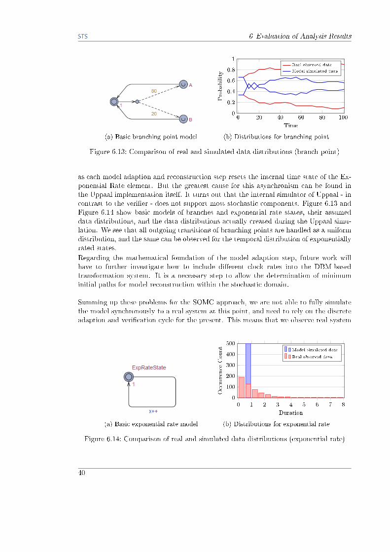
6 Evaluation of Analysis Results
(a) Basic branching point model
0 20 40 60 80 1000
0:2
0:4
0:6
0:8
1
Time
Probability
Real observed data
Model simulated data
(b) Distributions for branching point
Figure 6.13: Comparison of real and simulated data distributions (branch point)
as each model adaption and reconstruction step resets the internal time state of the Ex-ponential Rate element. But the greatest cause for this asynchronism can be found inthe Uppaal implementation itself. It turns out that the internal simulator of Uppaal - incontrast to the veri�er - does not support most stochastic components. Figure 6.13 andFigure 6.14 show basic models of branches and exponential rate states, their assumeddata distributions, and the data distributions actually created during the Uppaal simu-lation. We see that all outgoing transitions of branching points are handled as a uniformdistribution, and the same can be observed for the temporal distribution of exponentiallyrated states.
Regarding the mathematical foundation of the model adaption step, future work willhave to further investigate how to include di�erent clock rates into the DBM-basedtransformation system. It is a necessary step to allow the determination of minimuminitial paths for model reconstruction within the stochastic domain.
Summing up these problems for the SOMC approach, we are not able to fully simulatethe model synchronously to a real system at this point, and need to rely on the discreteadaption and veri�cation cycle for the present. This means that we observe real system
(a) Basic exponential rate model
0 1 2 3 4 5 6 7 80
100
200
300
400
500
Duration
Occurrence
Count
Model simulated data
Real observed data
(b) Distributions for exponential rate
Figure 6.14: Comparison of real and simulated data distributions (exponential rate)
40

6 Evaluation of Analysis Results
data, preprocess it to derive stochastic parameters, update the model accordingly andverify the given attributes for a �xed time interval, without simulating the model betweenthese steps in real-time, which is possible with the non-stochastic OMC framework. Thisspeci�c problem of probabilistic simulation still needs to be addressed, and may requirean alternative view of the term �online� used in the original OMC approach.
41


7 Conclusion
7 Conclusion
Reviewing the extended SOMC framework as a whole, we could see that even though theapproach o�ers several advantages compared to the original OMC framework, many ofthese advantages are linked to di�erent trade-o�s that need to be thoroughly consideredbefore making the decision to practically apply it to a certain system. In general, theapplication of SOMC principles can be useful when either time-critical bounds preventthe use of symbolic mechanisms provided by the OMC framework, or when the realsystem itself contains probabilistic components, which cannot be taken into accountby a deterministic approach. In both cases, the SOMC methods can provide weaker,probabilistically weighted satis�ability statements instead of completely abandoning themodel checking process. Unfortunately, these weakened statements can lead to criticalsituations in di�erent applications. Especially for safety-critical systems like medicaldevices, the outcome of this statistical model checking process needs to be considered withcaution, as the safety of derived constrains will always lie between none and the assurancelevel of symbolic model checking. There is always a chance that the probabilistic outcomeof a real event completely di�ers from the predictions during the veri�cation phase, evenwhen high probabilities are predicted. Nevertheless, the SOMC approach provides usefuladditional veri�cation data and can be utilized to initiate countermeasures as soon asthe probability of misbehaviour or malfunction exceed a set bound. Especially when abig data amount of previous events can be provided, the safety level of future predictionsincreases. But in the end, there can never be a way to predict probabilistic and futureevents with total certainty, and as long as parts of a system are non-deterministic, themodel checking approach needs to be of a statistical nature as well.
In the course of this thesis, we showed that it is generally possible to transfer the statis-tical components of SMC to an online approach, but up to this point only within certainbounds. To reach the full potential of the framework, several aspects need to be subjectto further investigation and implementation: The internal framework routines regardingthe representation and processing of model variables only supports integer values at themoment. As both exponential rate parameters and branch probabilities can also takeFloat Point values (and only the latter one could be circumvented as the Uppaal SMCveri�er internally converts absolute integer probabilities into relative �oat point proba-bilities), the framework needs to be adapted respectively. Additionally, we pointed outthat aMathematical Foundation for the SOMC components needs to be developed aswell. Especially a suitable integration for stochastic features (e.g., di�erent clock rates,exponential rates, alterable instance counts,. . . ) into the state space reconstruction pro-cess is still missing, and will be necessary to keep the observed system state and themodel state synchronized. This synchronization leads to the next point, a solution toenable the Simulation of SMC Components. This aspect cannot be faced solely bythe framework, but it also needs corresponding functionality of the UPPAAL simulatoritself.
43

7 Conclusion
In terms of application, we could only provide tests regarding probability data and exe-cution times for proof-of-concept models with limited extent. As soon as a mathematicalfoundation is completed, the SOMC framework needs to be evaluated for practical CaseStudies as well. One example could be the Radiosurgery experiment that was alreadyused by Rinast [4] to showcase the capabilities and limitations of the OMC framework.But not only the conceptual aspect will be important at that point. In fact, the centralpoint we need to keep in mind will always be the real-time constraint, whose neglectcan �nally make any promising concept useless. For that reason, an even more extendedComputation Time Analysis needs to be performed, including factors like the threadscheduler impact, the number of concurrent component instances, and any additionaldata preprocessing routines.Finally, we could think of Additional Modules to increase the usability of the SOMCframework. As the concept-related restrictions of and assumptions about the modelare known in advance (e.g., the necessary reset of all clock variables on every possiblepath cycle), it might be helpful to provide a tool that analyses a model beforehand andindicates con�icts with these restrictions.
If all these aspects are taken into consideration, the SOMC approach may eventuallyturn out to be a reasonable replacement or useful assistance for the symbolic and explicitonline concept, and enable an even broader range of models to be veri�ed at run-time inthe future.
44

Bibliography
Bibliography
[1] R. Alur, C. Courcoubetis, and D. Dill, �Model-checking for real-time systems,� inLogic in Computer Science, 1990. LICS '90, Proceedings., Fifth Annual IEEE Sym-posium, pp. 414�425, 1990.
[2] M. Geilen, �On the construction of monitors for temporal logic properties,� in Elec-tronic Notes in Theoretical Computer Science: Vol. 55, Paris, France, pp. 181�199,2001.
[3] F. J. Rammig, Y. Zhao, and S. Samara, �On-line model checking as operating systemservice,� in Software Technologies for Embedded and Ubiquitous Systems: 7th IFIPWG 10.2 International Workshop, SEUS 2009 Newport Beach, CA, USA, November16-18, 2009 Proceedings, pp. 131�143, 2009.
[4] J. Rinast, An Online Model-Checking Framework for Timed Automata - ApplyingFormal Veri�cation to Medical Cyber-Physical Systems. PhD thesis, Hamburg Uni-versity of Technology, 2015.
[5] M. Kwiatkowska, G. Norman, and D. Parker, �Stochastic model checking,� tech.rep., School of Computer Science, University of Birmingham, 2007.
[6] C. Baier and J.-P. Katoen, Principles of Model Checking. MIT Press, 2008.
[7] C. Baier, B. Haverkort, H. Hermanns, and J.-P. Katoen, �Model-checking algorithmsfor continuous-time markov chains,� IEEE Transactions on Software Engineering,Vol. 29, No. 6, June, 2003.
[8] G. Behrmann, A. David, and K. G. Larsen, �A tutorial on Uppaal 4.0,� tech. rep.,Department of Computer Science, Aalborg University, Denmark, 2006.
[9] M. Kwiatkowska, G. Norman, and D. Parker, �PRISM 4.0: Veri�cation of proba-bilistic real-time systems,� Proc. 23rd International Conference on Computer AidedVeri�cation (CAV11), Vol. 6806 of LNCS, pp. 585�591, 2011.
[10] A. David, K. G. Larsen, A. Legay, M. Mikucionis, and D. B. Poulsen, �Uppaal SMCtutorial,� International Journal on Software Tools for Technology Transfer: Vol. 17,pp. 397�415, 2015.
45