Diffraction Patterns Obtained by Scanning Electron Microscope
Till Kleinebecker Patterns and gradients in South Patagonian ombrotrophic peatland vegetation Münster 2007


Landschaftsökologie
Patterns and gradients
in South Patagonian ombrotrophic bog vegetation
Inauguraldissertation
zur Erlangung des Doktorgrades der Naturwissenschaften
im Fachbereich Geowissenschaften
der Mathematisch-Naturwissenschaftlichen Fakultät
der Westfälischen Wilhelms-Universität Münster
Vorgelegt von
Till Kleinebecker (geb. Hanneforth)
aus Gütersloh
2007

Dekan: Prof. Dr. Hans Kerp
Erster Gutachter: Prof. Dr. Norbert Hölzel
Zweiter Gutachter: Prof. Dr. Friedrich-Karl Holtmeier
Tag der mündlichen Prüfung: 07.09.2007
Tag der Promotion: 07.09.2007


Table of contents
Table of contents .................................................................................................................................V
List of figures.................................................................................................................................... VII
List of tables ........................................................................................................................................ X
Chapter 1: Introduction ...................................................................................................................... 1
1.1 Motivation and relevance of the study................................................................................... 1
1.1.1 State of research ................................................................................................................. 1
1.1.2 Peatlands and Global Change .......................................................................................... 3
1.1.3 Study area ............................................................................................................................ 4
2.2 Objectives of the study............................................................................................................. 8
2.3 Structure of this thesis .............................................................................................................. 8
Chapter 2: Gradients of continentality and moisture in South Patagonian ombrotrophic peatland vegetation ........................................................................................................ 11
2.1 Introduction ............................................................................................................................. 12
2.2 Materials and methods............................................................................................................ 13
2.3 Results....................................................................................................................................... 17
2.4 Discussion ................................................................................................................................ 24
Chapter 3: South Patagonian ombrotrophic bog vegetation reflects biogeochemical gradients at the landscape level .................................................................................... 31
3.1 Introduction ............................................................................................................................. 32
3.2 Materials and methods............................................................................................................ 34
3.3 Results....................................................................................................................................... 38
3.4 Discussion ................................................................................................................................ 42
Chapter 4: Patterns and gradients of diversity in South Patagonian ombrotrophic peat bogs.................................................................................................................................. 47
4.1 Introduction ............................................................................................................................. 48
4.2 Materials and methods............................................................................................................ 51
4.3 Results....................................................................................................................................... 54
4.4 Discussion ................................................................................................................................ 62
V

Table of contents
Chapter 5: Synthesis...........................................................................................................................69
Summary ..............................................................................................................................................73
Zusammenfassung..............................................................................................................................77
Resumen ..............................................................................................................................................81
References ...........................................................................................................................................85
Danksagung.........................................................................................................................................99
Curriculum Vitae ..............................................................................................................................101
VI
List of figures
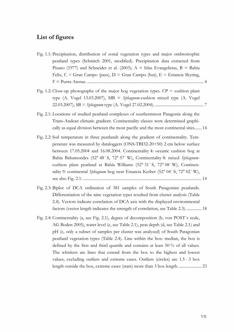
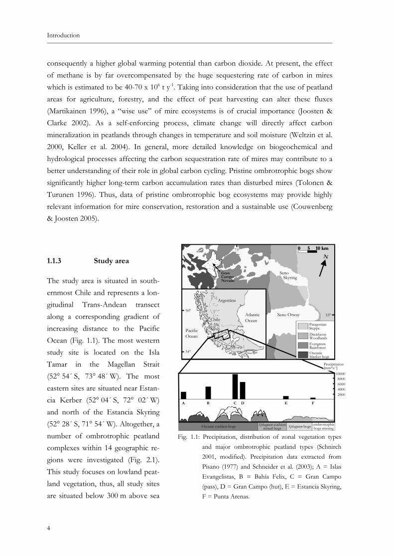
Fig. 1.1: Precipitation, distribution of zonal vegetation types and major ombrotrophic peatland types (Schnirch 2001, modified). Precipitation data extracted from Pisano (1977) and Schneider et al. (2003); A = Islas Evangelistas, B = Bahía Felix, C = Gran Campo (pass), D = Gran Campo (hut), E = Estancia Skyring, F = Punta Arenas. ................................................................................................................ 4
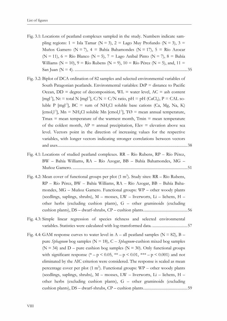
Fig. 1.2: Close-up photographs of the major bog vegetation types. CP = cushion plant type (A. Vogel 13.03.2007), MB = Sphagnum-cushion mixed type (A. Vogel 22.03.2007), SB = Sphagnum type (A. Vogel 27.02.2004). ............................................... 7
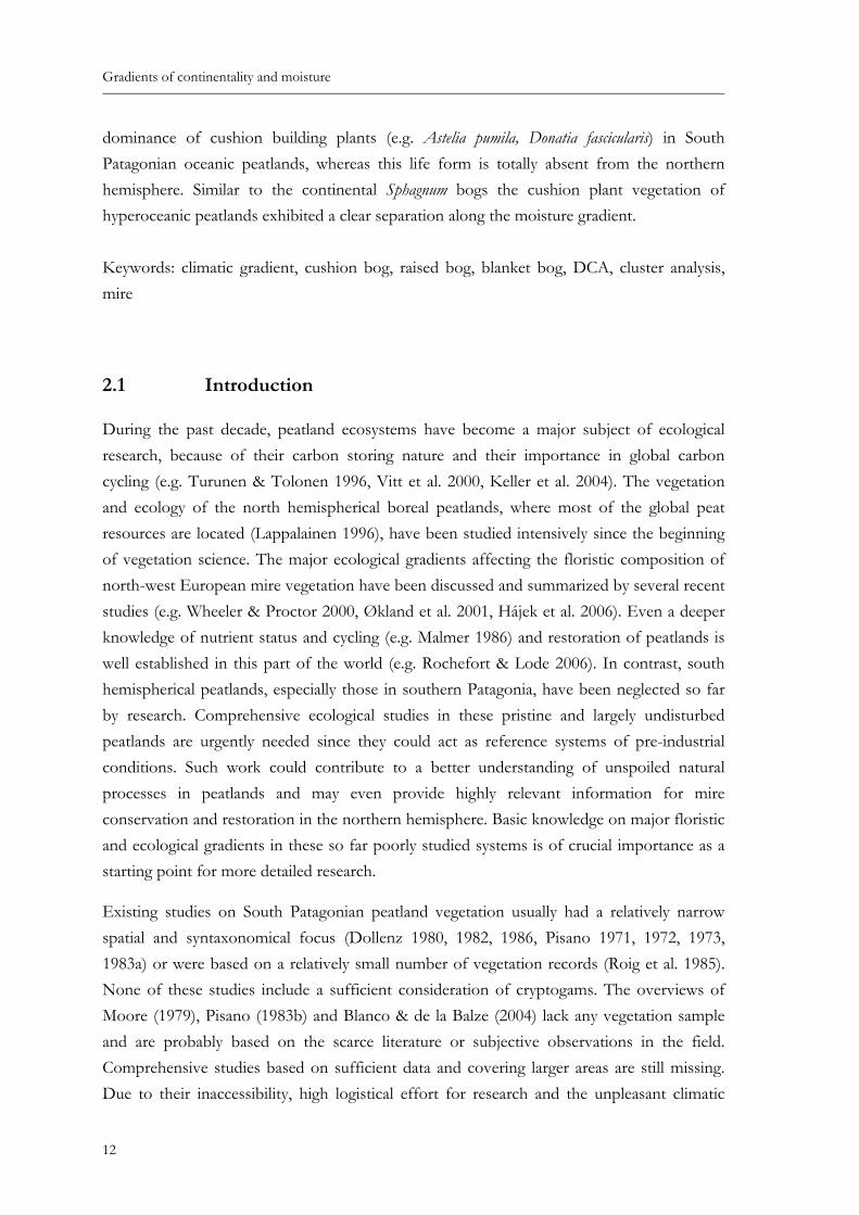
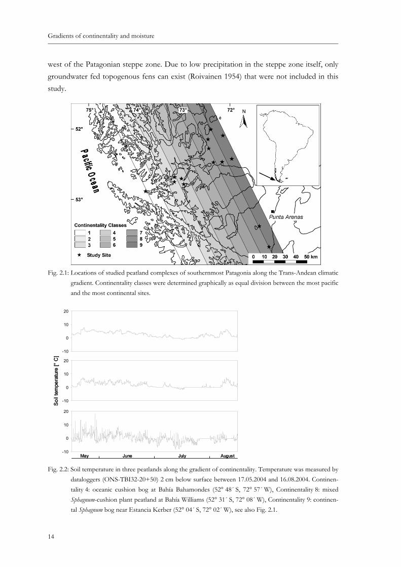
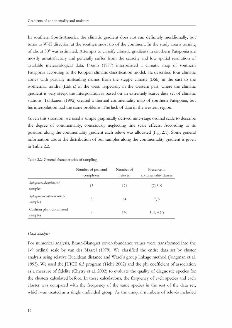
Fig. 2.1: Locations of studied peatland complexes of southernmost Patagonia along the Trans-Andean climatic gradient. Continentality classes were determined graphi-cally as equal division between the most pacific and the most continental sites....... 14
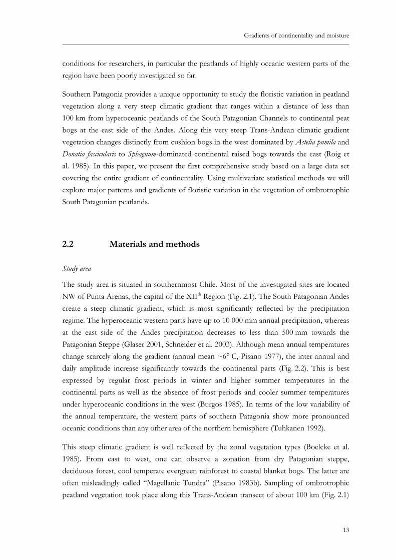
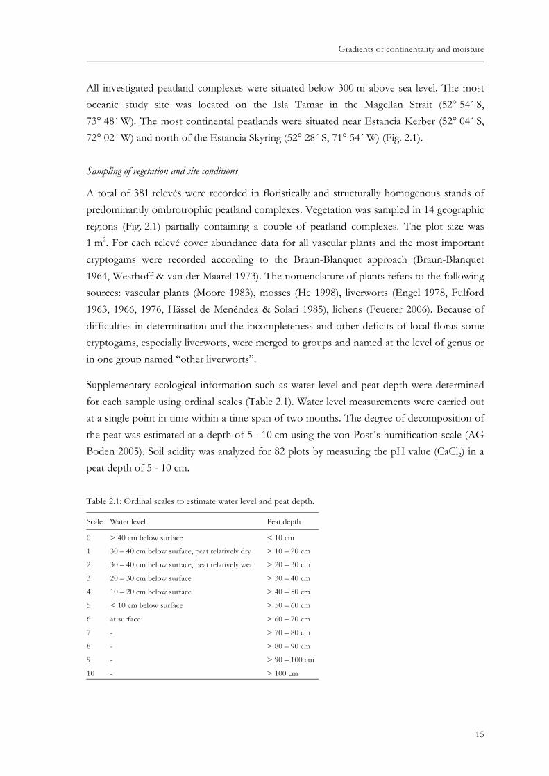
Fig. 2.2: Soil temperature in three peatlands along the gradient of continentality. Tem-perature was measured by dataloggers (ONS-TBI32-20+50) 2 cm below surface between 17.05.2004 and 16.08.2004. Continentality 4: oceanic cushion bog at Bahía Bahamondes (52° 48´ S, 72° 57´ W), Continentality 8: mixed Sphagnum-cushion plant peatland at Bahía Williams (52° 31´ S, 72° 08´ W), Continen-tality 9: continental Sphagnum bog near Estancia Kerber (52° 04´ S, 72° 02´ W), see also Fig. 2.1. .................................................................................................................. 14
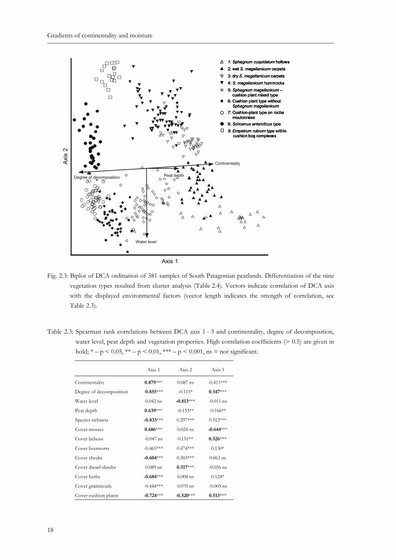
Fig. 2.3: Biplot of DCA ordination of 381 samples of South Patagonian peatlands. Differentiation of the nine vegetation types resulted from cluster analysis (Table 2.4). Vectors indicate correlation of DCA axis with the displayed environmental factors (vector length indicates the strength of correlation, see Table 2.3). .............. 18
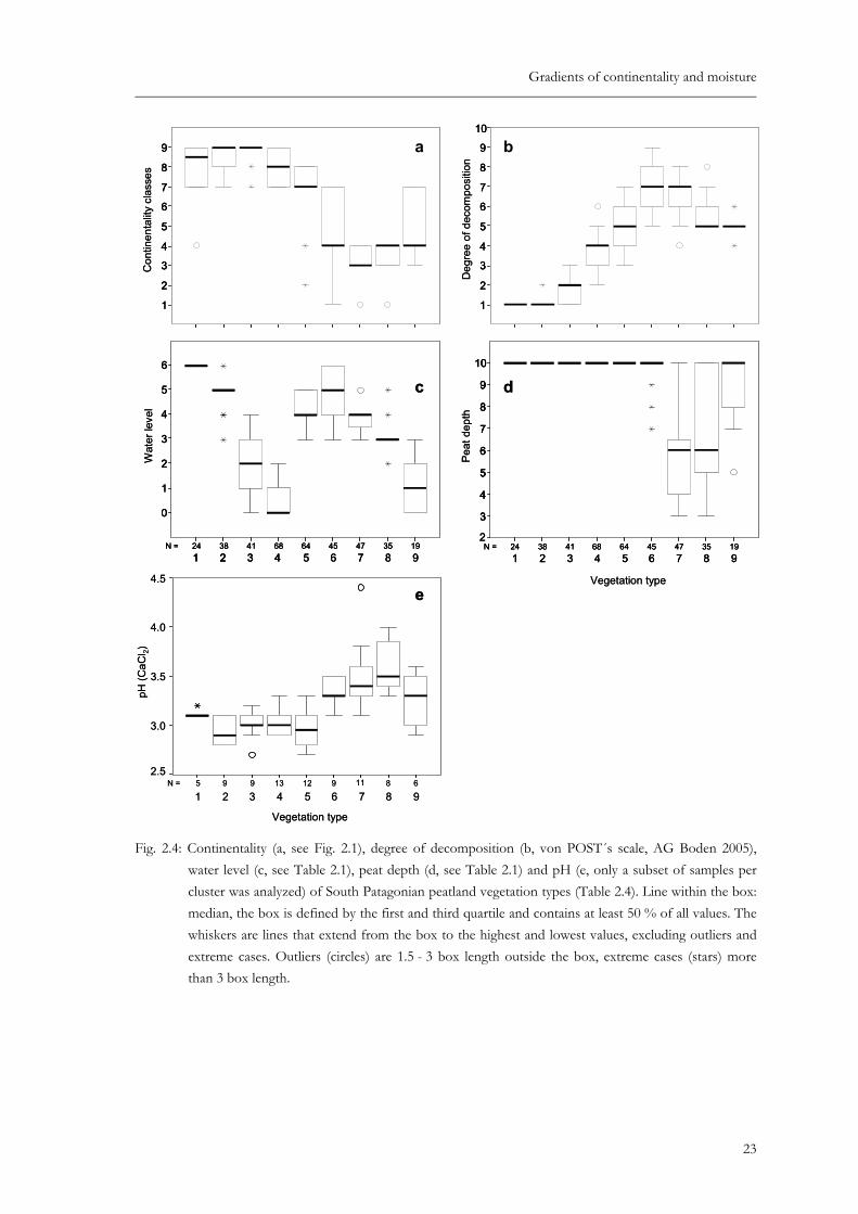
Fig. 2.4: Continentality (a, see Fig. 2.1), degree of decomposition (b, von POST´s scale, AG Boden 2005), water level (c, see Table 2.1), peat depth (d, see Table 2.1) and pH (e, only a subset of samples per cluster was analyzed) of South Patagonian peatland vegetation types (Table 2.4). Line within the box: median, the box is defined by the first and third quartile and contains at least 50 % of all values. The whiskers are lines that extend from the box to the highest and lowest values, excluding outliers and extreme cases. Outliers (circles) are 1.5 - 3 box length outside the box, extreme cases (stars) more than 3 box length. ...................... 23
VII
List of figures
Fig. 3.1: Locations of peatland complexes sampled in the study. Numbers indicate sam-pling regions: 1 = Isla Tamar (N = 3), 2 = Lago Muy Profundo (N = 3), 3 = Muños Gamero (N = 7), 4 = Bahía Bahamondes (N = 17), 5 = Río Azocar (N = 11), 6 = Río Blanco (N = 5), 7 = Lago Aníbal Pinto (N = 7), 8 = Bahía Williams (N = 10), 9 = Río Rubens (N = 9), 10 = Río Pérez (N = 5), and, 11 = San Juan (N = 4). ................................................................................................................35
Fig. 3.2: Biplot of DCA ordination of 82 samples and selected environmental variables of South Patagonian peatlands. Environmental variables: DtP = distance to Pacific Ocean, DD = degree of decomposition, WL = water level, AC = ash content [mgl-1], Nt = total N [mgl-1], C/N = C/N ratio, pH = pH (CaCl2), P = CAL so-luble P [mgl-1], BC = sum of NH4Cl soluble base cations (Ca, Mg, Na, K) [cmolcl-1], Mn = NH4Cl soluble Mn [cmolcl-1], TØ = mean annual temperature, Tmax = mean temperature of the warmest month, Tmin = mean temperature of the coldest month, AP = annual precipitation, Elev = elevation above sea level. Vectors point in the direction of increasing values for the respective variables, with longer vectors indicating stronger correlations between vectors and axes.................................................................................................................................38
Fig. 4.1: Locations of studied peatland complexes. RR – Río Rubens, RP – Río Pérez, BW – Bahía Williams, RA – Río Azogar, BB – Bahía Bahamondes, MG – Muñoz Gamero. ..................................................................................................................51
Fig. 4.2: Mean cover of functional groups per plot (1 m2). Study sites: RR – Río Rubens, RP – Río Pérez, BW – Bahía Williams, RA – Río Azogar, BB – Bahía Baha-mondes, MG – Muñoz Gamero. Functional groups: WP – other woody plants (seedlings, saplings, shrubs), M – mosses, LW – liverworts, Li – lichens, H – other herbs (excluding cushion plants), G – other graminoids (excluding cushion plants), DS – dwarf-shrubs, CP – cushion plants............................................56
Fig. 4.3: Simple linear regression of species richness and selected environmental variables. Statistics were calculated with log-transformed data. ...................................57
Fig. 4.4: GAM response curves to water level in A – all peatland samples (N = 82), B – pure Sphagnum bog samples (N = 18), C – Sphagnum-cushion mixed bog samples (N = 34) and D – pure cushion bog samples (N = 30). Only functional groups with significant response (* – p < 0.05, ** – p < 0.01, *** – p < 0.001) and not eliminated by the AIC criterion were considered. The response is scaled as mean percentage cover per plot (1 m2). Functional groups: WP – other woody plants (seedlings, saplings, shrubs), M – mosses, LW – liverworts, Li – lichens, H – other herbs (excluding cushion plants), G – other graminoids (excluding cushion plants), DS – dwarf-shrubs, CP – cushion plants............................................59
VIII
List of figures
Fig. 4.5: GAM response curves to total nitrogen content (Nt, g*l-1) in A – all peatland samples (N = 82), B – pure Sphagnum bog samples (N = 18), C – Sphagnum-cushion mixed bog samples (N = 34) and D – pure cushion bog samples (N = 30). Only functional groups with significant response (* – p < 0.05, ** – p < 0.01, *** – p < 0.001) and not eliminated by the AIC criterion were considered. The response is scaled in mean percentage cover per plot (1 m2). Functional groups: WP – other woody plants (seedlings, saplings, shrubs), M – mosses, LW – liverworts, Li – lichens, H – other herbs (excluding cushion plants), G – other graminoids (excluding cushion plants), DS – dwarf-shrubs, CP – cushion plants. Be aware of different scaling of the x-axes!............................... 60
Fig. 4.6: GAM response curves to NH4Cl soluble calcium (cmolc*l-1) in A – all peatland samples (N = 82), B – pure Sphagnum bog samples (N = 18), C – Sphagnum-cushion mixed bog samples (N = 34). Only functional groups with significant response (* – p < 0.05, ** – p < 0.01, *** – p < 0.001) and not eliminated by the AIC criterion were considered. In pure cushion bogs no significant response of any functional group could be measured. The response is scaled in mean percentage cover per plot (1 m2). Functional groups: WP – other woody plants (seedlings, saplings, shrubs), M – mosses, LW – liverworts, Li – lichens, H – other herbs (excluding cushion plants), G – other graminoids (excluding cushion plants), DS – dwarf-shrubs, CP – cushion plants. Be aware of different scaling of the x-axes! .......................................................................................................... 61
IX
List of tables
Table 2.1: Ordinal scales to estimate water level and peat depth. .................................................15
Table 2.2: General characteristics of sampling. ................................................................................16
Table 2.3: Spearman rank correlations between DCA axis 1 - 3 and continentality, degree of decomposition, water level, peat depth and vegetation properties. High correlation coefficients (> 0.5) are given in bold; * – p < 0.05, ** – p < 0.01, *** – p < 0.001, ns = not significant...............................................................................18
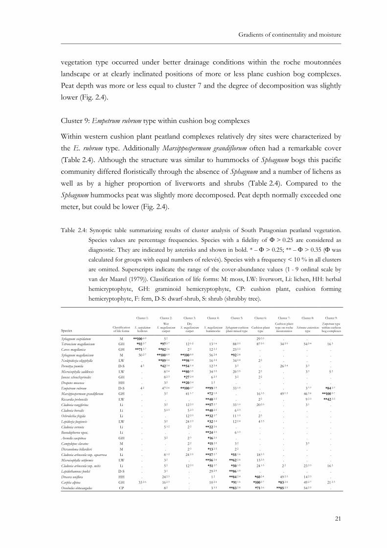
Table 2.4: Synoptic table summarizing results of cluster analysis of South Patagonian peatland vegetation. Species values are percentage frequencies. Species with a fidelity of Φ > 0.25 are considered as diagnostic. They are indicated by asterisks and shown in bold. * – Φ > 0.25; ** – Φ > 0.35 (Φ was calculated for groups with equal numbers of relevés). Species with a frequency < 10 % in all clusters are omitted. Superscripts indicate the range of the cover-abundance values (1 - 9 ordinal scale by van der Maarel (1979)). Classification of life forms: M: moss, LW: liverwort, Li: lichen, HH: herbal hemicryptophyte, GH: graminoid hemicryptophyte, CP: cushion plant, cushion forming hemicryp-tophyte, F: fern, DS: dwarf-shrub, S: shrub, shrubby tree. ..........................................21
Table 3.1: Mean and standard error of environmental variables in the three major types of South Patagonian bog vegetation. Different letters indicate significant diffe-rences (P < 0.05) after parametric Tukey-Test (a, b, c) or non-parametric Mann-Whitney U-Test (A, B, C; Bonferroni corrected: correction of signifi-cance level due to multiple testing). * – p < 0.05, ** – p < 0.01, *** – p < 0.001. ....................................................................................................................................39
Table 3.2: Spearman rank correlations between Axes 1, 2 and 3 from the DCA analysis, and the measured environmental variables. Significant correlation coefficients are given as: * – p < 0.05, ** – p < 0.01, *** – p < 0.001 See Table 3.1 for the units of variables. ................................................................................................................40
Table 3.3: Results of various CCA analyses isolating the effect of the variable “distance to Pacific” on floristic composition including Covariable, Eigenvalue (sum of all canonical eigenvalues – measure for explanatory power of the variables (Total inertia: 3.826)), % = percentage of explained variance, F (F-ratio statistics for the test on the trace), p = corresponding probability value obtained by the Monte-Carlo-permutation test (499 permutations). * Variables with strong colinearity (degree of decomposition, C/N ratio, mean temperature of warmest month; Variance Inflation Factor > 10) were excluded. See Table 3.1 for the units of variables....................................................................................................41
X
List of tables
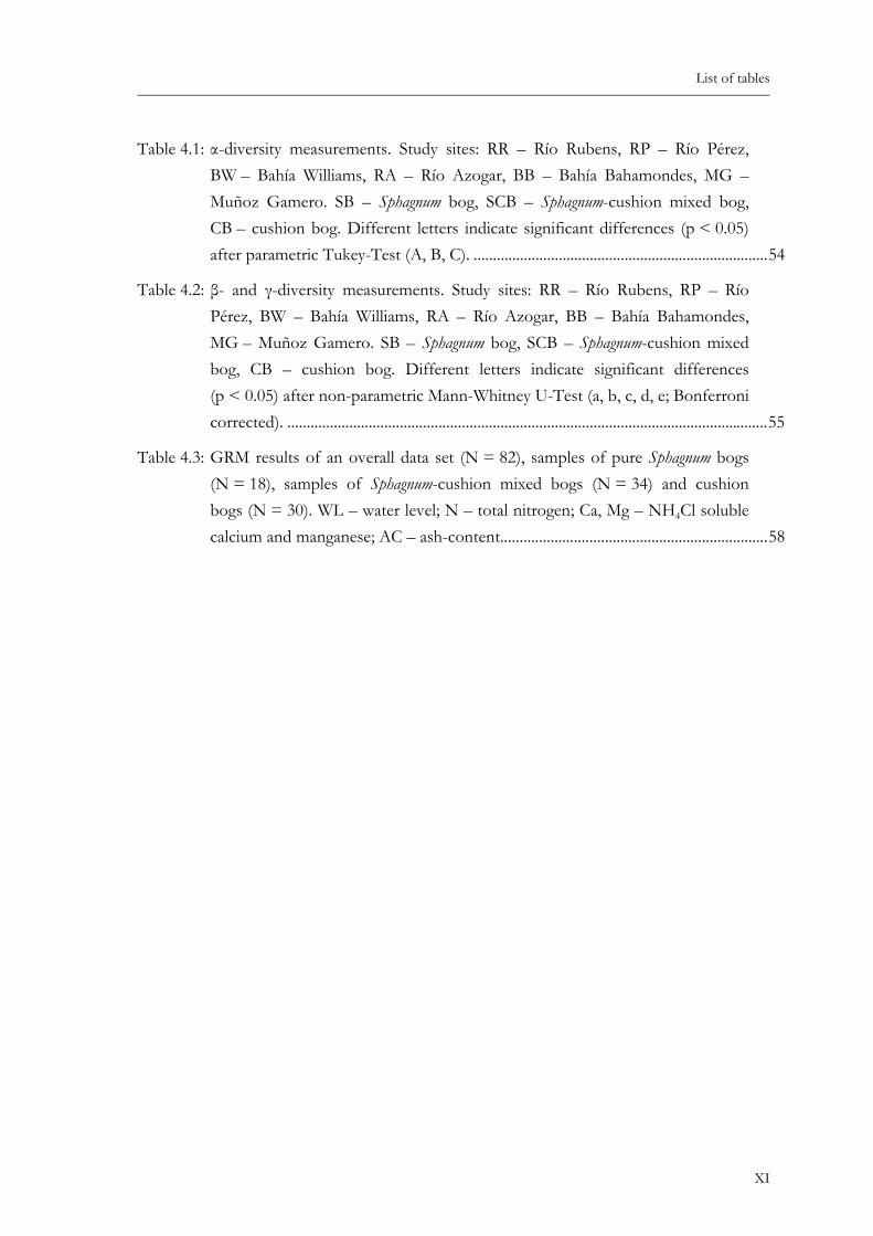
Table 4.1: α-diversity measurements. Study sites: RR – Río Rubens, RP – Río Pérez, BW – Bahía Williams, RA – Río Azogar, BB – Bahía Bahamondes, MG – Muñoz Gamero. SB – Sphagnum bog, SCB – Sphagnum-cushion mixed bog, CB – cushion bog. Different letters indicate significant differences (p < 0.05) after parametric Tukey-Test (A, B, C). ............................................................................54
Table 4.2: β- and γ-diversity measurements. Study sites: RR – Río Rubens, RP – Río Pérez, BW – Bahía Williams, RA – Río Azogar, BB – Bahía Bahamondes, MG – Muñoz Gamero. SB – Sphagnum bog, SCB – Sphagnum-cushion mixed bog, CB – cushion bog. Different letters indicate significant differences (p < 0.05) after non-parametric Mann-Whitney U-Test (a, b, c, d, e; Bonferroni corrected). ............................................................................................................................55
Table 4.3: GRM results of an overall data set (N = 82), samples of pure Sphagnum bogs (N = 18), samples of Sphagnum-cushion mixed bogs (N = 34) and cushion bogs (N = 30). WL – water level; N – total nitrogen; Ca, Mg – NH4Cl soluble calcium and manganese; AC – ash-content.....................................................................58
XI


Chapter 1
Introduction
1.1 Motivation and relevance of the study
1.1.1 State of research
The vegetation and ecology of north hemispherical peatlands have been studied intensively since the beginning of vegetation science. Du Rietz (1954) defined a precise and consistent nomenclature with the three major categories (ombrotrophic) bog, poor-fen and rich-fen. This division of peatland passed into general use, although in parts complementary to it, the concept of ecological gradients was emphasized by e.g. Malmer (1986) and discussed and summarized by several recent studies (e.g. Wheeler & Proctor 2000, Økland et al. 2001, Hájek et al. 2006).
The minerotrophic-ombrotrophic gradient is considered to be the most fundamental ecological gradient within mires. A clear division of ombrotrophic vs. minerotrophic as proposed by Du Rietz (1954) who based his division exclusively on floristics by defining “Mineralbodenwasserzeiger” is disproved by several studies (Daniels 1978, Malmer 1986, Gignac et al. 1991, Damman 1995a). The atmospherical input of material of terrestrial origin received by ombrotrophic bogs can vary within a wide range and can exceed the telluric inputs into poor fens (Wheeler & Proctor 2000). Additionally, the input of sea-born cations depending on the distance to the ocean significantly affects bog vegetation (van Groenen-dael et al. 1982, Vitt et al. 1990, Damman 1995a). Thus, ombrotrophy is not an absolute state with mires exclusively fed by precipitation or not, but a continuous nutritional gradient. This conclusion was critically discussed by Økland et al. (2001) and Hájek et al. (2006) who pointed out that the limit between bog and fen can be determined as a relatively narrow borderline zone that is characterized by at least a local set of fen indicator species.
Summarizing the ongoing debate, the question if the fen - bog border is discontinuously or not could definitely not be answered in a general way. Wheeler & Proctor (2000) focussed on British and Dutch mires, whereas Økland et al. (2001) argued from a Scandinavian point of view, with obvious differences in atmospheric deposition. Such regional differences concerning atmospherical inputs in ombrotrophic bogs were described by Bragazza et al.
1
Introduction
(2003) comparing the biogeochemistry of a mire in central-eastern Sweden and a mire in the south-eastern Alps. The mires of the two regions clearly showed different contributions of major ions from bulk precipitation in the mire pore-water that were attributed to both, anthropogenic pollutions and natural phenomena such as sea spray and dry and wet deposition of minerogenic dust. A change in floristic composition due to changing mire surface water chemistry that was traced back to a different input of sea-born base cations was documented by e.g. Vitt et al. (1990). In Europe heavy atmospherical nitrogen inputs caused by anthropogenic emissions have been measured (Bragazza et al. 2004). A floristic change to more minerotrophic vegetation properties attributed mainly to increased atmospheric N-deposition caused by agriculture has been evidenced by many recent studies (e.g. Gunnarsson et al. 2002, Limpens et al. 2003, Malmer & Wallén 2005). The border between minerotrophic and ombrotrophic can be obscured by atmospherical deposition as it highly depends on the investigated region as well as on the length of the measured gradient (Hájek et al. 2006).
The current bog - fen debate documents a clear focus on north hemispherical peatlands. Data from the southern hemisphere are scarcely included in the scientific discussion. In particular, broad-scaled investigations presenting data of South Patagonian peatlands beyond rough phytosociological descriptions do simply not exist. This situation is hard to understand because this region provides exceptionally suitable conditions for ecological research in mire ecosystems. Due to the strong westerly winds bringing unpolluted air masses from the Pacific Ocean, the low human population density, and the lack of intense agriculture the anthropogenic input is marginal (Galloway & Keene 1996, Godoy et al. 2001). Given this situation, comprehensive studies of the vegetation of South Patagonian peatlands may provide a reference for the trophical status of corresponding north hemispherical peatlands. Such studies in unspoiled peatlands would shed new light on the bog - fen debate or could be used for the testing of ecological theory such as the humpback model of diversity patterns along trophical gradients.
The more continental South Patagonian peatlands are structurally (hollows and hummocks) and floristically very similar to their counterparts in North-America and Eurasia (Schwaar 1976, 1980, Moen 2005). In contrast, the blanket bogs of the hyperoceanic western parts are dominated by cushion forming vascular plants, which are totally absent from the northern hemisphere. The reasons for this strong shift in floristic composition are poorly known. The existing studies dealing at least partially with South Patagonian peatland vegetation (e.g. Dollenz 1980, 1982, 1986, Pisano 1971, 1972, 1973, 1983a) cannot give a satisfying answer to that question for various reason. Usually these studies have a relatively narrow spatial and syntaxonomical focus. The overviews of Moore (1979), Pisano (1983b), Roig et al. (1985),
2
Introduction
and Blanco & de la Balze (2004) are mostly based on this literature, a small number of own vegetation records, and subjective observations in the field. Rough interpolations of the scarce climatic data are used to assess major ecological gradients affecting the floristic composition. Investigations on broad-scale vegetation-environment relationships that include biogeochemical measurements of the mire surface water or the peat substrate are totally missing. The only publication presenting peat chemical data describes ecological site characteristics of a single mire complex on Chiloé island that is situated about 1 500 km further north at the border to the subtropical region (Ruthsatz & Villagran 1991).
None of the studies dealing with South Patagonian peatland vegetation include a sufficient consideration of cryptogams. Keys to determine cryptogams are scarce and, if present, a definite classification at the species level is difficult due to the difficult verification. The recent publications dealing with South Patagonian cryptogams usually focus on the taxonomy of single species or a genus which means that it is laborious for ecologists considering cryptogams in their records. Thus, the potential of cryptogams in vegetation analyses is largely unutilized, although temperate Chile and Argentina are a hot spot of diversity especially for the group of liverworts (Engel 1978).
1.1.2 Peatlands and Global Change
Peatlands play an important role in the biosphere and are linked with fundamental processes such as biogeochemical cycling and hydrological dynamics. They also provide habitats for many highly adapted and often endangered plant and animal species (Maltby & Proctor 1996). The global peatland area is estimated with 4.16 x 10⁶ km2. That is about 3 % of the globe´s total land surface (Rydin & Jeglum 2006). The database of this rough estimation refers to areas with at least 30 cm peat thickness. The amount of carbon bound in the peat of mires has been estimated to contribute more than 15 % to the total amount of carbon fixed in the global soil pool (Lappalainen 1996). Other estimations reach up to 30 % which is the same amount of carbon that is stored in all terrestrial biomass on the earth (Marti-kainen 1996, Joosten & Clarke 2002). The mineral subsoil under mires may account for some additional 5 % of the unaccounted carbon of the global carbon budget (Turunen et al. 1999). These figures indicate the important role that play peatlands in the global carbon cycle and underline their relevance in the recent global change debate.
On the one hand, growing boreal peatlands actually represent important sinks accumulating huge amounts of carbon (Turunen & Tolonen 1996). On the other hand, peatlands are net sources of methane that has a greater capacity to absorb infra-red radiation and has
3
Introduction
consequently a higher global warming potential than carbon dioxide. At present, the effect of methane is by far overcompensated by the huge sequestering rate of carbon in mires which is estimated to be 40-70 x 106 t y-1. Taking into consideration that the use of peatland areas for agriculture, forestry, and the effect of peat harvesting can alter these fluxes (Martikainen 1996), a “wise use” of mire ecosystems is of crucial importance (Joosten & Clarke 2002). As a self-enforcing process, climate change will directly affect carbon mineralization in peatlands through changes in temperature and soil moisture (Weltzin et al. 2000, Keller et al. 2004). In general, more detailed knowledge on biogeochemical and hydrological processes affecting the carbon sequestration rate of mires may contribute to a better understanding of their role in global carbon cycling. Pristine ombrotrophic bogs show significantly higher long-term carbon accumulation rates than disturbed mires (Tolonen & Turunen 1996). Thus, data of pristine ombrotrophic bog ecosystems may provide highly relevant information for mire conservation, restoration and a sustainable use (Couwenberg & Joosten 2005).
2000400060008000
10000
Sphagnum bogsSphagnum-cushion mixed bogsOceanic cushion bogs
A B C D E F
0 5 10 km
N
SenoSkyring
Seno Otway
Patagonian SteppeDeciduous WoodlandsEvergreen RainforestOceanic blanket bogs
Gran Campo Nevado
Atlantic Ocean
Pacific Ocean
54°
50°
73°
53°
Argentina
Chile
ombrotrophic bogs missing
Precipitation [mm*a-1]
2000400060008000
10000
Sphagnum bogsSphagnum-cushion mixed bogsOceanic cushion bogs
A B C D E F
0 5 10 km0 5 10 km
N
SenoSkyring
Seno Otway
Patagonian SteppeDeciduous WoodlandsEvergreen RainforestOceanic blanket bogs
Gran Campo Nevado
Atlantic Ocean
Pacific Ocean
54°
50°
73°
53°
Argentina
Chile
ombrotrophic bogs missing
Precipitation [mm*a-1]
Fig. 1.1: Precipitation, distribution of zonal vegetation typesand major ombrotrophic peatland types (Schnirch2001, modified). Precipitation data extracted fromPisano (1977) and Schneider et al. (2003); A = IslasEvangelistas, B = Bahía Felix, C = Gran Campo(pass), D = Gran Campo (hut), E = Estancia Skyring,F = Punta Arenas.
1.1.3 Study area
The study area is situated in south-ernmost Chile and represents a lon-gitudinal Trans-Andean transect along a corresponding gradient of increasing distance to the Pacific Ocean (Fig. 1.1). The most western study site is located on the Isla Tamar in the Magellan Strait (52° 54´ S, 73° 48´ W). The most eastern sites are situated near Estan-cia Kerber (52° 04´ S, 72° 02´ W) and north of the Estancia Skyring (52° 28´ S, 71° 54´ W). Altogether, a number of ombrotrophic peatland complexes within 14 geographic re-gions were investigated (Fig. 2.1). This study focuses on lowland peat-land vegetation, thus, all study sites are situated below 300 m above sea
4
Introduction
level. Due to the inaccessibility of some areas and the logistical restrictions during the field work, the sampled peatland complexes did not show a perfectly even distribution along the measured gradient of increasing distance to the Pacific Ocean. However, as the results presented in this study show, the entire gradient seems to be covered sufficiently.
Climate
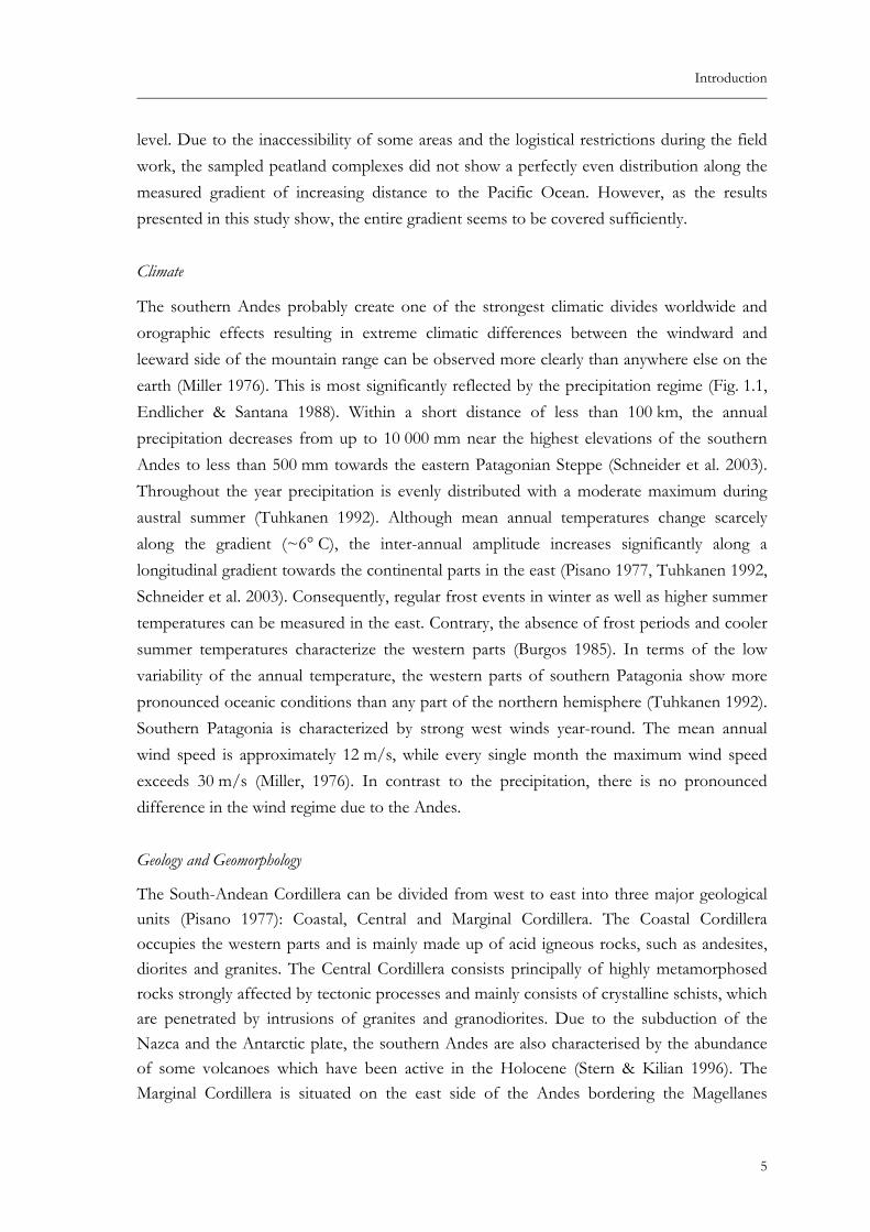
The southern Andes probably create one of the strongest climatic divides worldwide and orographic effects resulting in extreme climatic differences between the windward and leeward side of the mountain range can be observed more clearly than anywhere else on the earth (Miller 1976). This is most significantly reflected by the precipitation regime (Fig. 1.1, Endlicher & Santana 1988). Within a short distance of less than 100 km, the annual precipitation decreases from up to 10 000 mm near the highest elevations of the southern Andes to less than 500 mm towards the eastern Patagonian Steppe (Schneider et al. 2003). Throughout the year precipitation is evenly distributed with a moderate maximum during austral summer (Tuhkanen 1992). Although mean annual temperatures change scarcely along the gradient (~6° C), the inter-annual amplitude increases significantly along a longitudinal gradient towards the continental parts in the east (Pisano 1977, Tuhkanen 1992, Schneider et al. 2003). Consequently, regular frost events in winter as well as higher summer temperatures can be measured in the east. Contrary, the absence of frost periods and cooler summer temperatures characterize the western parts (Burgos 1985). In terms of the low variability of the annual temperature, the western parts of southern Patagonia show more pronounced oceanic conditions than any part of the northern hemisphere (Tuhkanen 1992). Southern Patagonia is characterized by strong west winds year-round. The mean annual wind speed is approximately 12 m/s, while every single month the maximum wind speed exceeds 30 m/s (Miller, 1976). In contrast to the precipitation, there is no pronounced difference in the wind regime due to the Andes.
Geology and Geomorphology
The South-Andean Cordillera can be divided from west to east into three major geological units (Pisano 1977): Coastal, Central and Marginal Cordillera. The Coastal Cordillera occupies the western parts and is mainly made up of acid igneous rocks, such as andesites, diorites and granites. The Central Cordillera consists principally of highly metamorphosed rocks strongly affected by tectonic processes and mainly consists of crystalline schists, which are penetrated by intrusions of granites and granodiorites. Due to the subduction of the Nazca and the Antarctic plate, the southern Andes are also characterised by the abundance of some volcanoes which have been active in the Holocene (Stern & Kilian 1996). The Marginal Cordillera is situated on the east side of the Andes bordering the Magellanes
5
Introduction
Sedimentary Basin further east (Palmer & Dalziel 1973) and is made up of sedimentary rocks such as sandstones, claystones and conglomerates. In general, one can conclude that the bedrock of the whole study area is uniformly acidic and base-poor resulting in very similar nutritional substrate conditions.
The geomorphology of the South Patagonian landscape is strongly affected by various glaciations during the ice ages of the Quaternary (Clapperton et al. 1995). The glacially eroded landscape of the western parts is characterised by giant roche moutonnées and U-valleys on islands and peninsulas that are separated by flooded U-valleys (channels and fjords) (Frederiksen 1988). Only the highest peaks of the Andean Range were not covered by the ice masses during the glaciations of the Pleistocene. Even presently, icefields with various outlet glaciers calving into the fiords or into pro-glacial lakes characterize the landscape (Schneider et al. 2007). In the study area, the highest elevations of the Andean range do not exceed 2 000 m above sea level. East of the Cordillera the landscape is dominated by various glacial lakes and bays such as the Seno Skyring and the Seno Otway (Fig. 1.1), which were carved out by the glaciers. Despite these glacial erosional forms, the eastern foreland of the Andes is basically characterised by different glacial accumulation features such as moraines and drumlins and generally by glacial drift (Clapperton et al. 1995, Weischet, 1970).
Soils
Within the study area, soil forming processes are strongly affected by i) the changing climatic constraints along the steep climatic gradient created by the southern Andes and ii) the different effects of the glaciations on site conditions in terms of erosion or sedimentation. The landscape of the western channel region is predominantly composed of rounded ice-sheets, eroded landforms such as roche moutonnées, and rounded to elongated depressions inbetween. Areas covered with loose fluvio-glacial sediments are not common (Frederiksen 1988). Due to the cool and extremely humid climate, the tendency to peat-forming is high and soils are mostly histosols. These peat-soils occur in depressions and on plain areas but also as continuous cover overlaying the massive bedrock. Due to the better drainage conditions at strongly inclinated slopes poorly developed mineral soils can be found or the pure bedrock is at surface (Pisano 1977). The mainly forested area on the east side of the Andean range towards the Patagonian Steppe is characterized by a cool and humid climate resulting in acidic brown forest soils and podzols (Tuhkanen et al. 1989-1990). If drainage is poor, the soils develop into gley-podzols. On these gleyic soils Sphagnum bogs can grow up. Soils of the steppe zone further east are not relevant for this study because under the semiarid to arid climatic conditions ombrotrophic bogs can not develop (Roivainen 1954).
6
Introduction
Vegetation
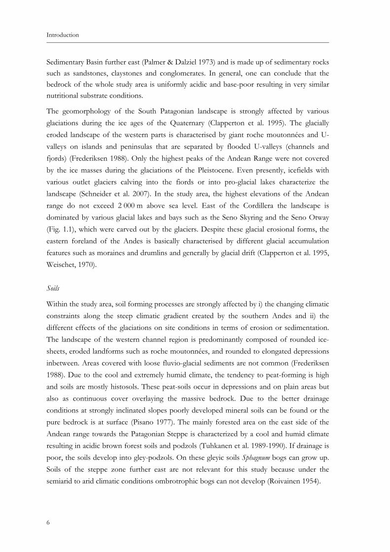
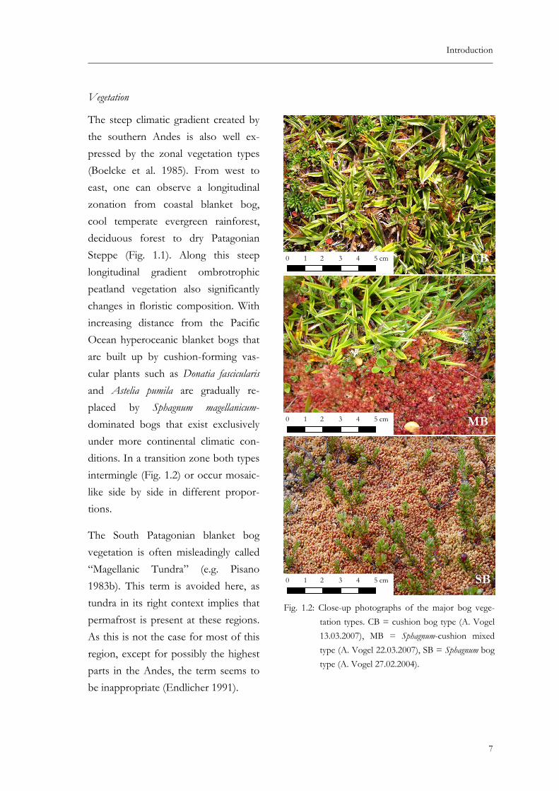
The steep climatic gradient created by the southern Andes is also well ex-pressed by the zonal vegetation types (Boelcke et al. 1985). From west to east, one can observe a longitudinal zonation from coastal blanket bog, cool temperate evergreen rainforest, deciduous forest to dry Patagonian Steppe (Fig. 1.1). Along this steep longitudinal gradient ombrotrophic peatland vegetation also significantly changes in floristic composition. With increasing distance from the Pacific Ocean hyperoceanic blanket bogs that are built up by cushion-forming vas-cular plants such as Donatia fascicularis and Astelia pumila are gradually re-placed by Sphagnum magellanicum-dominated bogs that exist exclusively under more continental climatic con-ditions. In a transition zone both types intermingle (Fig. 1.2) or occur mosaic-like side by side in different propor-tions.
CB1 20 3 4 5 cm
1 20 3 4 5 cm MB
SB1 20 3 4 5 cm
Fig. 1.2: Close-up photographs of the major bog vege-tation types. CB = cushion bog type (A. Vogel13.03.2007), MB = Sphagnum-cushion mixedtype (A. Vogel 22.03.2007), SB = Sphagnum bogtype (A. Vogel 27.02.2004).
The South Patagonian blanket bog vegetation is often misleadingly called “Magellanic Tundra” (e.g. Pisano 1983b). This term is avoided here, as tundra in its right context implies that permafrost is present at these regions. As this is not the case for most of this region, except for possibly the highest parts in the Andes, the term seems to be inappropriate (Endlicher 1991).
7
Introduction
1.2 Objectives of the study
This thesis is designed to give the first comprehensive broad-scaled floristic and ecological characterization of South Patagonian ombrotrophic peatland vegetation. In addition to vegetation data, a broad set of biogeochemical peat characteristics and other environmental variables will be used for the causal explanation of floristic gradients and differences in diversity patterns along a Trans-Andean transect. In detail, the thesis has the following main goals:
• the description and classification of the vegetation that include a better consideration of cryptogams,
• the detection of the major environmental gradients affecting the floristic composition at the landscape level with a special focus on biogeochemical features,
• to assess differences in species-richness and functional diversity and relate them to environmental gradients,
• to provide reference data from unspoiled bog-ecosystems for the comparison with north hemispherical peatlands,
• to test ecological theory with data from a pristine system.
1.3 Structure of this thesis
This thesis consists of three papers that all deal with environmental gradients affecting the floristic composition and diversity patterns of South Patagonian ombrotrophic bog vegetation. Two papers have been accepted for publication in international peer-reviewed journals, one has been submitted. Each paper has a different focus and adresses specific scientific questions.
Chapter 2 concentrates on the detection of major vegetation types within South Patagonian ombrotrophic peatlands applying a cluster analysis to 381 phytosociological relevés. The impact of the distance to the Pacific Ocean, the degree of peat decomposition, the peat depth, and the edaphic moisture regime on the floristic composition of the studied peatlands is evaluated by detrended correspondence analysis (DCA). Finally, floristic and structural similarities and dissimilarities of South Patagonian ombrotrophic peat bogs compared to their north hemispherical counterparts are discussed.
8
Introduction
9
Chapter 3 deals with the detection of the most relevant environmental factors affecting the floristic composition of South Patagonian ombrotrophic peat bogs at the landscape level. Climatic constraints as well as biogeochemical peat characteristics and the edaphic moisture regime are considered. For the estimation of the most important factors, direct and indirect gradient analyses are performed. In the discussion, a particular emphasis is given to the impact of sea spray depending on the distance to the Pacific Ocean as an important source of nutrient supply. Finally, the role of South Patagonian peat bogs as a reference for pre-industrial conditions in peatlands in the northern hemisphere is discussed.
Chapter 4 focuses on diversity patterns of the investigated ombrotrophic bog vegetation. Bog complexes along a Trans-Andean transect are characterized by α-, β- and γ-diversity measurements. The species richness of individual phytosociological relevés is related to major environmental gradients by performing a General Regression Model (GRM). Functional group response to major environmental gradients is demonstrated by performing Generalized Additive Models (GAMs). Based on the results ecological theories on biodiversity are evaluated.
Chapter 5 provides a general synthesis of this study. The results of the different research topics are linked together and the most important conclusions are put in a lager context with respect to their relevance for mire research. Finally, an outlook for future research is given.

Chapter 2
Gradients of continentality and moisture in South Patagonian ombrotrophic peatland vegetation
Till Kleinebecker*1; Norbert Hölzel1 & Andreas Vogel1
1Institute of Landscape Ecology, University of Münster, Robert-Koch-Straße 26, 48149 Münster, Germany
*Corresponding author
Folia Geobotanica, accepted 22.07.2007
Abstract
This study presents the analysis of 381 phytosociological relevés describing predominantly ombrotrophic South Patagonian lowland peatland vegetation along a gradient of increasing continentality. Numerical methods such as cluster analysis and detrended correspondence analysis (DCA) were carried out to explore the data set. Cluster analysis resulted in nine vegetation types that were also distinctly separated in DCA ordination. The major floristic coenocline along the first DCA axis reflected a gradient of continentality ranging from pacific blanket bogs dominated by cushion plants to Sphagnum-dominated continental raised bogs. Increasing continentality along the first axis went parallel with decreasing peat decomposition and increasing peat depth and acidity. Contrary, floristic variation along the second DCA axis represented a water level gradient.
The typical sequence of vegetation types along the hollow-hummock moisture gradient that is well established for north hemispherical peatlands could also be observed in Sphagnum-dominated South Patagonian raised bogs with a surprising similarity in floristic and structural features. Concerning the gradient of continentality significant differences in comparison with the northern hemisphere could be established. Most obvious was the
11
Gradients of continentality and moisture
dominance of cushion building plants (e.g. Astelia pumila, Donatia fascicularis) in South Patagonian oceanic peatlands, whereas this life form is totally absent from the northern hemisphere. Similar to the continental Sphagnum bogs the cushion plant vegetation of hyperoceanic peatlands exhibited a clear separation along the moisture gradient.
Keywords: climatic gradient, cushion bog, raised bog, blanket bog, DCA, cluster analysis, mire
2.1 Introduction
During the past decade, peatland ecosystems have become a major subject of ecological research, because of their carbon storing nature and their importance in global carbon cycling (e.g. Turunen & Tolonen 1996, Vitt et al. 2000, Keller et al. 2004). The vegetation and ecology of the north hemispherical boreal peatlands, where most of the global peat resources are located (Lappalainen 1996), have been studied intensively since the beginning of vegetation science. The major ecological gradients affecting the floristic composition of north-west European mire vegetation have been discussed and summarized by several recent studies (e.g. Wheeler & Proctor 2000, Økland et al. 2001, Hájek et al. 2006). Even a deeper knowledge of nutrient status and cycling (e.g. Malmer 1986) and restoration of peatlands is well established in this part of the world (e.g. Rochefort & Lode 2006). In contrast, south hemispherical peatlands, especially those in southern Patagonia, have been neglected so far by research. Comprehensive ecological studies in these pristine and largely undisturbed peatlands are urgently needed since they could act as reference systems of pre-industrial conditions. Such work could contribute to a better understanding of unspoiled natural processes in peatlands and may even provide highly relevant information for mire conservation and restoration in the northern hemisphere. Basic knowledge on major floristic and ecological gradients in these so far poorly studied systems is of crucial importance as a starting point for more detailed research.
Existing studies on South Patagonian peatland vegetation usually had a relatively narrow spatial and syntaxonomical focus (Dollenz 1980, 1982, 1986, Pisano 1971, 1972, 1973, 1983a) or were based on a relatively small number of vegetation records (Roig et al. 1985). None of these studies include a sufficient consideration of cryptogams. The overviews of Moore (1979), Pisano (1983b) and Blanco & de la Balze (2004) lack any vegetation sample and are probably based on the scarce literature or subjective observations in the field. Comprehensive studies based on sufficient data and covering larger areas are still missing. Due to their inaccessibility, high logistical effort for research and the unpleasant climatic
12
Gradients of continentality and moisture
conditions for researchers, in particular the peatlands of highly oceanic western parts of the region have been poorly investigated so far.
Southern Patagonia provides a unique opportunity to study the floristic variation in peatland vegetation along a very steep climatic gradient that ranges within a distance of less than 100 km from hyperoceanic peatlands of the South Patagonian Channels to continental peat bogs at the east side of the Andes. Along this very steep Trans-Andean climatic gradient vegetation changes distinctly from cushion bogs in the west dominated by Astelia pumila and Donatia fascicularis to Sphagnum-dominated continental raised bogs towards the east (Roig et al. 1985). In this paper, we present the first comprehensive study based on a large data set covering the entire gradient of continentality. Using multivariate statistical methods we will explore major patterns and gradients of floristic variation in the vegetation of ombrotrophic South Patagonian peatlands.
2.2 Materials and methods
Study area
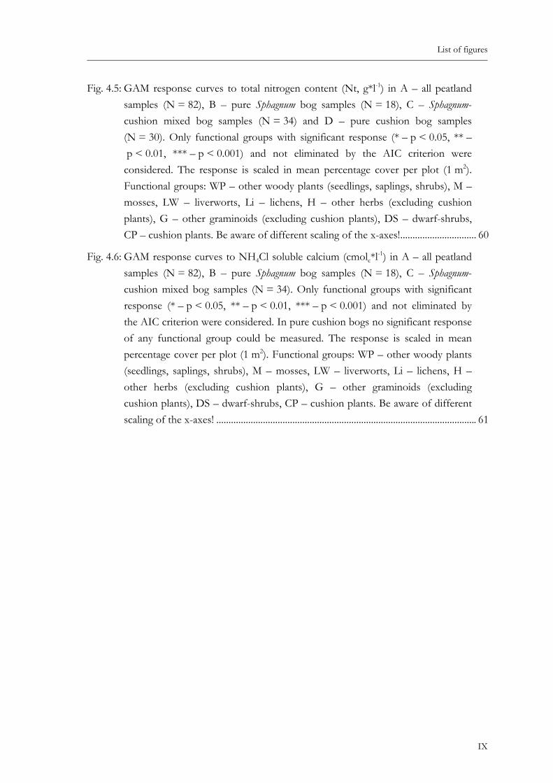
The study area is situated in southernmost Chile. Most of the investigated sites are located NW of Punta Arenas, the capital of the XIIth Region (Fig. 2.1). The South Patagonian Andes create a steep climatic gradient, which is most significantly reflected by the precipitation regime. The hyperoceanic western parts have up to 10 000 mm annual precipitation, whereas at the east side of the Andes precipitation decreases to less than 500 mm towards the Patagonian Steppe (Glaser 2001, Schneider et al. 2003). Although mean annual temperatures change scarcely along the gradient (annual mean ~6° C, Pisano 1977), the inter-annual and daily amplitude increase significantly towards the continental parts (Fig. 2.2). This is best expressed by regular frost periods in winter and higher summer temperatures in the continental parts as well as the absence of frost periods and cooler summer temperatures under hyperoceanic conditions in the west (Burgos 1985). In terms of the low variability of the annual temperature, the western parts of southern Patagonia show more pronounced oceanic conditions than any other area of the northern hemisphere (Tuhkanen 1992).
This steep climatic gradient is well reflected by the zonal vegetation types (Boelcke et al. 1985). From east to west, one can observe a zonation from dry Patagonian steppe, deciduous forest, cool temperate evergreen rainforest to coastal blanket bogs. The latter are often misleadingly called “Magellanic Tundra” (Pisano 1983b). Sampling of ombrotrophic peatland vegetation took place along this Trans-Andean transect of about 100 km (Fig. 2.1)
13
Gradients of continentality and moisture
west of the Patagonian steppe zone. Due to low precipitation in the steppe zone itself, only groundwater fed topogenous fens can exist (Roivainen 1954) that were not included in this study.
Fig. 2.1: Locations of studied peatland complexes of southernmost Patagonia along the Trans-Andean climatic gradient. Continentality classes were determined graphically as equal division between the most pacific and the most continental sites.
-10
0
10
20
-10
0
10
20
-10
0
10
20
Soi
ltem
pera
ture
[° C
]
May June July August
-10
0
10
20
-10
0
10
20
-10
0
10
20
Soi
ltem
pera
ture
[° C
]
May June July AugustMay June July August
Fig. 2.2: Soil temperature in three peatlands along the gradient of continentality. Temperature was measured by dataloggers (ONS-TBI32-20+50) 2 cm below surface between 17.05.2004 and 16.08.2004. Continen-tality 4: oceanic cushion bog at Bahía Bahamondes (52° 48´ S, 72° 57´ W), Continentality 8: mixed Sphagnum-cushion plant peatland at Bahía Williams (52° 31´ S, 72° 08´ W), Continentality 9: continen-tal Sphagnum bog near Estancia Kerber (52° 04´ S, 72° 02´ W), see also Fig. 2.1.
14
Gradients of continentality and moisture
All investigated peatland complexes were situated below 300 m above sea level. The most oceanic study site was located on the Isla Tamar in the Magellan Strait (52° 54´ S, 73° 48´ W). The most continental peatlands were situated near Estancia Kerber (52° 04´ S, 72° 02´ W) and north of the Estancia Skyring (52° 28´ S, 71° 54´ W) (Fig. 2.1).
Sampling of vegetation and site conditions
A total of 381 relevés were recorded in floristically and structurally homogenous stands of predominantly ombrotrophic peatland complexes. Vegetation was sampled in 14 geographic regions (Fig. 2.1) partially containing a couple of peatland complexes. The plot size was 1 m2. For each relevé cover abundance data for all vascular plants and the most important cryptogams were recorded according to the Braun-Blanquet approach (Braun-Blanquet 1964, Westhoff & van der Maarel 1973). The nomenclature of plants refers to the following sources: vascular plants (Moore 1983), mosses (He 1998), liverworts (Engel 1978, Fulford 1963, 1966, 1976, Hässel de Menéndez & Solari 1985), lichens (Feuerer 2006). Because of difficulties in determination and the incompleteness and other deficits of local floras some cryptogams, especially liverworts, were merged to groups and named at the level of genus or in one group named “other liverworts”.
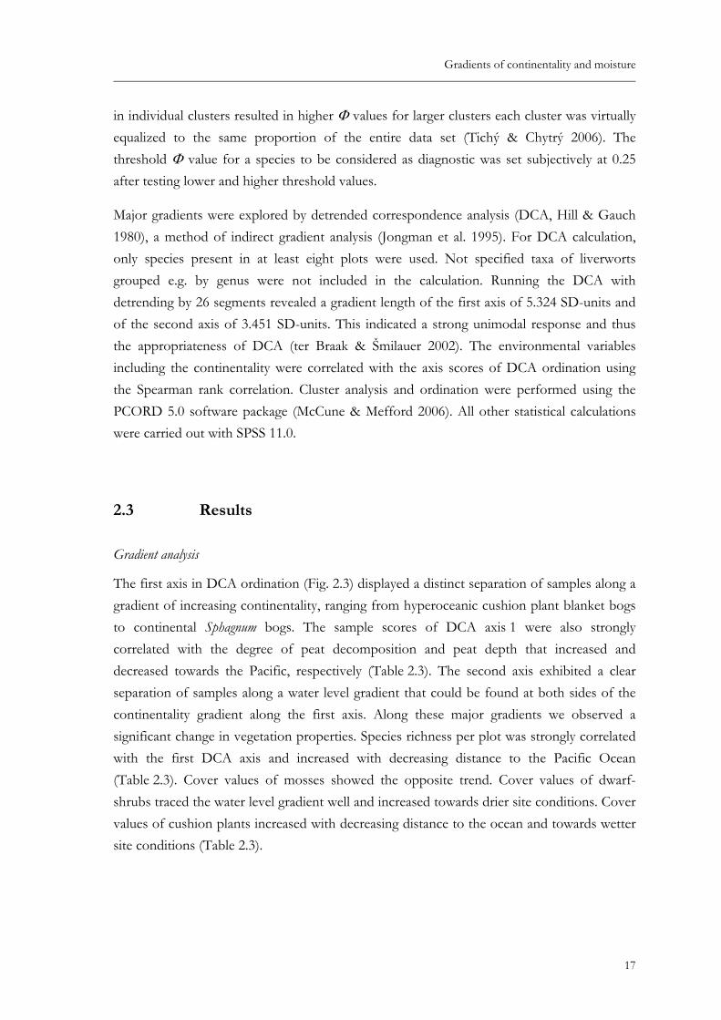
Supplementary ecological information such as water level and peat depth were determined for each sample using ordinal scales (Table 2.1). Water level measurements were carried out at a single point in time within a time span of two months. The degree of decomposition of the peat was estimated at a depth of 5 - 10 cm using the von Post´s humification scale (AG Boden 2005). Soil acidity was analyzed for 82 plots by measuring the pH value (CaCl2) in a peat depth of 5 - 10 cm.
Table 2.1: Ordinal scales to estimate water level and peat depth.
Scale Water level Peat depth
0 > 40 cm below surface < 10 cm
1 30 – 40 cm below surface, peat relatively dry > 10 – 20 cm
2 30 – 40 cm below surface, peat relatively wet > 20 – 30 cm
3 20 – 30 cm below surface > 30 – 40 cm
4 10 – 20 cm below surface > 40 – 50 cm
5 < 10 cm below surface > 50 – 60 cm
6 at surface > 60 – 70 cm
7 - > 70 – 80 cm
8 - > 80 – 90 cm
9 - > 90 – 100 cm
10 - > 100 cm
15
Gradients of continentality and moisture
In southern South-America the climatic gradient does not run definitely meridionally, but turns to W-E direction at the southernmost tip of the continent. In the study area a turning of about 30° was estimated. Attempts to classify climatic gradients in southern Patagonia are mostly unsatisfactory and generally suffer from the scarcity and low spatial resolution of available meteorological data. Pisano (1977) interpolated a climatic map of southern Patagonia according to the Köppen climatic classification model. He described four climatic zones with partially misleading names from the steppe climate (BSk) in the east to the isothermal tundra (Etik´c) in the west. Especially in the western part, where the climatic gradient is very steep, the interpolation is based on an extremely scarce data set of climatic stations. Tuhkanen (1992) created a thermal continentality map of southern Patagonia, but his interpolation had the same problems: The lack of data in the western region.
Given this situation, we used a simple graphically derived nine-stage ordinal scale to describe the degree of continentality, consciously neglecting fine scale effects. According to its position along the continentality gradient each relevé was allocated (Fig. 2.1). Some general information about the distribution of our samples along the continentality gradient is given in Table 2.2.
Table 2.2: General characteristics of sampling.
Number of peatland
complexes Number of
relevés Presence in
continentality classes
Sphagnum-dominated samples
15 171 (7) 8, 9
Sphagnum-cushion mixed samples
5 64 7, 8
Cushion plant-dominated samples
7 146 1, 3, 4 (7)
Data analysis
For numerical analysis, Braun-Blanquet cover-abundance values were transformed into the 1-9 ordinal scale by van der Maarel (1979). We classified the entire data set by cluster analysis using relative Euclidean distance and Ward´s group linkage method (Jongman et al. 1995). We used the JUICE 6.3 program (Tichý 2002) and the phi coefficient of association as a measure of fidelity (Chytrý et al. 2002) to evaluate the quality of diagnostic species for the clusters calculated before. In these calculations, the frequency of each species and each cluster was compared with the frequency of the same species in the rest of the data set, which was treated as a single undivided group. As the unequal numbers of relevés included
16
Gradients of continentality and moisture
in individual clusters resulted in higher Φ values for larger clusters each cluster was virtually equalized to the same proportion of the entire data set (Tichý & Chytrý 2006). The threshold Φ value for a species to be considered as diagnostic was set subjectively at 0.25 after testing lower and higher threshold values.
Major gradients were explored by detrended correspondence analysis (DCA, Hill & Gauch 1980), a method of indirect gradient analysis (Jongman et al. 1995). For DCA calculation, only species present in at least eight plots were used. Not specified taxa of liverworts grouped e.g. by genus were not included in the calculation. Running the DCA with detrending by 26 segments revealed a gradient length of the first axis of 5.324 SD-units and of the second axis of 3.451 SD-units. This indicated a strong unimodal response and thus the appropriateness of DCA (ter Braak & Šmilauer 2002). The environmental variables including the continentality were correlated with the axis scores of DCA ordination using the Spearman rank correlation. Cluster analysis and ordination were performed using the PCORD 5.0 software package (McCune & Mefford 2006). All other statistical calculations were carried out with SPSS 11.0.
2.3 Results
Gradient analysis
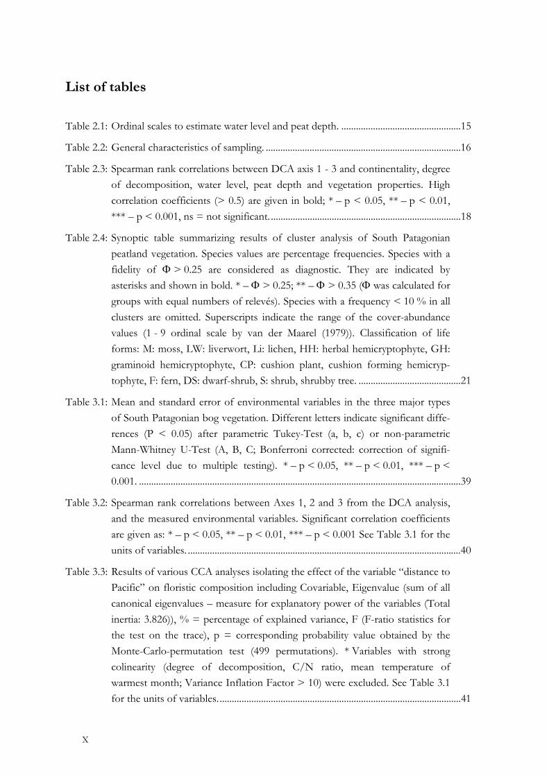
The first axis in DCA ordination (Fig. 2.3) displayed a distinct separation of samples along a gradient of increasing continentality, ranging from hyperoceanic cushion plant blanket bogs to continental Sphagnum bogs. The sample scores of DCA axis 1 were also strongly correlated with the degree of peat decomposition and peat depth that increased and decreased towards the Pacific, respectively (Table 2.3). The second axis exhibited a clear separation of samples along a water level gradient that could be found at both sides of the continentality gradient along the first axis. Along these major gradients we observed a significant change in vegetation properties. Species richness per plot was strongly correlated with the first DCA axis and increased with decreasing distance to the Pacific Ocean (Table 2.3). Cover values of mosses showed the opposite trend. Cover values of dwarf-shrubs traced the water level gradient well and increased towards drier site conditions. Cover values of cushion plants increased with decreasing distance to the ocean and towards wetter site conditions (Table 2.3).
17
Gradients of continentality and moisture
Water level
Degree of decomposition
Continentality
Axis 1
Axis
2Sphagnum cuspidatum hollowswet S. magellanicum typedry S. magellanicum typeS. magellanicum hummocksS. magellanicum cushion plantmixed typecushion plant type
cushion plant type on roche moutonnéesSchoenus antarcticus dominated typeEmpetrum rubrum type
Water level
Degree of decomposition
Continentality
Axis 1
Axis
21: Sphagnum cuspidatum hollows
2: wet S. magellanicum carpets
3: dry S. magellanicum carpets
4: S. magellanicum hummocks
5: Sphagnum magellanicum –cushion plant mixed type
6: Cushion plant type without Sphagnum magellanicum
7: Cushion-plant type on roche moutonnées
8: Schoenus antarcticus type
9: Empetrum rubrum type withincushion bog complexes
Water level
Degree of decomposition
Continentality
Axis 1
Axis
2Sphagnum cuspidatum hollowswet S. magellanicum typedry S. magellanicum typeS. magellanicum hummocksS. magellanicum cushion plantmixed typecushion plant type
cushion plant type on roche moutonnéesSchoenus antarcticus dominated typeEmpetrum rubrum type
Water level
Degree of decomposition
Continentality
Axis 1
Axis
2
Water level
Degree of decomposition
Continentality
Axis 1
Axis
2Sphagnum cuspidatum hollowswet S. magellanicum typedry S. magellanicum typeS. magellanicum hummocksS. magellanicum cushion plantmixed typecushion plant type
cushion plant type on roche moutonnéesSchoenus antarcticus dominated typeEmpetrum rubrum type
Water level
Degree of decomposition Peat depth
Continentality
Axis 1
Axis
21: Sphagnum cuspidatum hollows
2: wet S. magellanicum carpets
3: dry S. magellanicum carpets
4: S. magellanicum hummocks
5: Sphagnum magellanicum –cushion plant mixed type
6: Cushion plant type without Sphagnum magellanicum
7: Cushion-plant type on roche moutonnées
8: Schoenus antarcticus type
9: Empetrum rubrum type withincushion bog complexes
1: Sphagnum cuspidatum hollows1: Sphagnum cuspidatum hollows
2: wet S. magellanicum carpets2: wet S. magellanicum carpets
3: dry S. magellanicum carpets3: dry S. magellanicum carpets
4: S. magellanicum hummocks4: S. magellanicum hummocks
5: Sphagnum magellanicum –cushion plant mixed type
5: Sphagnum magellanicum –cushion plant mixed type
6: Cushion plant type without Sphagnum magellanicum
6: Cushion plant type without Sphagnum magellanicum
7: Cushion-plant type on roche moutonnées
7: Cushion-plant type on roche moutonnées
8: Schoenus antarcticus type8: Schoenus antarcticus type
9: Empetrum rubrum type withincushion bog complexes
9: Empetrum rubrum type withincushion bog complexes
Fig. 2.3: Biplot of DCA ordination of 381 samples of South Patagonian peatlands. Differentiation of the nine vegetation types resulted from cluster analysis (Table 2.4). Vectors indicate correlation of DCA axis with the displayed environmental factors (vector length indicates the strength of correlation, see Table 2.3).
Table 2.3: Spearman rank correlations between DCA axis 1 - 3 and continentality, degree of decomposition, water level, peat depth and vegetation properties. High correlation coefficients (> 0.5) are given in bold; * – p < 0.05, ** – p < 0.01, *** – p < 0.001, ns = not significant.
Axis 1 Axis 2 Axis 3
Continentality 0.879*** 0.087 ns -0.411***
Degree of decomposition -0.855*** -0.115* 0.547***
Water level 0.042 ns -0.813*** -0.011 ns
Peat depth 0.639*** -0.153** -0.166**
Species richness -0.833*** 0.297*** 0.312***
Cover mosses 0.686*** 0.024 ns -0.644***
Cover lichens -0.047 ns 0.151** 0.526***
Cover liverworts -0.465*** 0.474*** 0.130*
Cover shrubs -0.604*** 0.303*** 0.063 ns
Cover dwarf-shrubs 0.089 ns 0.517*** -0.056 ns
Cover herbs -0.684*** 0.008 ns 0.124*
Cover graminoids -0.444*** 0.070 ns -0.005 ns
Cover cushion plants -0.724*** -0.520*** 0.513***
18
Gradients of continentality and moisture
Classification and ecological characterization
The cluster analysis resulted in nine major vegetation types (Table 2.4) that were also clearly split in ordination space (Fig. 2.3). The first cut level separated the pacific cushion bogs from more continental bogs characterized by Sphagnum magellanicum. In line with the results of DCA ordination, the second cut level differentiated mainly along a moisture gradient. In detail, cluster analysis resulted in the following types:
Cluster 1: Sphagnum cuspidatum hollows
This species-poor community was dominated by S. cuspidatum and occurred exclusively in continental Sphagnum and mixed Sphagnum-cushion bogs. Constant species were Carex magellanica and Tetroncium magellanica (Table 2.4). The water level was at the surface and the peat was scarcely decomposed. Like in all investigated peatland complexes dominated by Sphagnum peat depth always exceeded one meter (Fig. 2.4).
Cluster 2: Wet Sphagnum magellanicum carpet
This community could be found in wet parts of continental peat bogs with water levels mainly close to surface, often surrounding hollows. The dense intensively red carpet of S. magellanicum allowed only few other plants to grow with relatively low cover (Table 2.4). Merely graminoids contributed a nameable portion of the vegetation cover. The degree of peat decomposition was very low (Fig. 2.4).
Cluster 3: Dry Sphagnum magellanicum carpet
This community occurred, where water level dropped to 20 - 30 cm below ground. Frequent species of wet communities disappeared and dwarf-shrubs prevailed (Table 2.3 and 2.4). In particular, Empetrum rubrum became more dominant growing above a dense but pale S. magel-lanicum carpet with minute liverworts frequently occurring between the capitulae (Table 2.4). Degree of decomposition was slightly higher than in the previous types (Fig. 2.4).
Cluster 4: Hummocks of Sphagnum magellanicum
Hummocks showed a decreasing dominance and vitality of S. magellanicum, which was even absent at some plots. Empetrum rubrum became the dominant species, and also Marsippo-spermum grandiflorum was an important constituent. A number of cryptogams frequently grew within the carpet of the dwarf-shrubs (Table 2.4). Water level was usually below 40 cm and the degree of peat decomposition was slightly higher than in the previous types. Soil pH values in Sphagnum bogs (Cluster 1 - 4) were slightly lower than in their oceanic counterparts (Fig. 2.4).
19
Gradients of continentality and moisture
Cluster 5: Sphagnum magellanicum-cushion plant mixed type
With a decreasing continentality, cushion building vascular plants typical of the oceanic peatlands progressively more intermingled with S. magellanicum. The dwarf-shrub conifer Lepidothamnus fonkii and a number of species either predominantly occurring in Sphagnum-dominated bogs or in mires dominated by cushion plants exhibited high constancies (Table 2.4). The water level was about 10 cm below surface and the degree of decom-position was remarkably higher than in pure Sphagnum stands. Soil acidity was similar to pure Sphagnum stands (Fig. 2.4).
Cluster 6: Cushion plant type without Sphagnum magellanicum
In pacific peatland complexes S. magellanicum was totally absent and vegetation was characterized by the dominance of cushion building vascular plants such as Donatia fascicularis and Astelia pumila dominating with changing cover (Table 2.4). The cushion plant type occurred at flat sites on fluvio-glacial planes or larger smooth areas within roche moutonnées. In general, water level was close to surface. Peat depth normally exceeded one meter and degree of decomposition was high. Soil acidity was slightly higher than in Sphagnum-dominated communities (Fig. 2.4).
Cluster 7: Cushion plant type on roche moutonnées
This community occurred on slopes and little plains within the glacially eroded landscape of the South Patagonian Channels. In addition to the dominance of cushion plants, vegetation was characterized by the constant occurrence of species typical for the following vegetation type (Table 2.4). Despite the better drainage, the water level was relatively high, but lower than in the latter type. Degree of decomposition was high and peat depth rarely exceeded one meter (Fig. 2.4). The roche moutonnées of the South Chilean Channels were typically dominated by this and the following vegetation type giving the landscape a blanket bog character. Vegetation might have a soligenous influence caused by permanent water flow. This made it difficult to separate clearly ombrotrophic systems from those that might have minerotrophic influence. This may also be indicated by slightly higher pH values (Fig. 2.4). Tree growth was restricted to well drained and strongly inclinated slopes.
Cluster 8: Schoenus antarcticus type
Gramineous species constituted the aspect of the Schoenus antarcticus type. A number of species also occurring in the previous community showed higher constancies and cover values (Table 2.4). Besides the well developed grass layer and the less dominant cushion plants a number of liverworts were characteristic of this community. In general, this
20
Gradients of continentality and moisture
vegetation type occurred under better drainage conditions within the roche moutonnées landscape or at clearly inclinated positions of more or less plane cushion bog complexes. Peat depth was more or less equal to cluster 7 and the degree of decomposition was slightly lower (Fig. 2.4).
Cluster 9: Empetrum rubrum type within cushion bog complexes
Within western cushion plant peatland complexes relatively dry sites were characterized by the E. rubrum type. Additionally Marsippospermum grandiflorum often had a remarkable cover (Table 2.4). Although the structure was similar to hummocks of Sphagnum bogs this pacific community differed floristically through the absence of Sphagnum and a number of lichens as well as by a higher proportion of liverworts and shrubs (Table 2.4). Compared to the Sphagnum hummocks peat was slightly more decomposed. Peat depth normally exceeded one meter, but could be lower (Fig. 2.4).
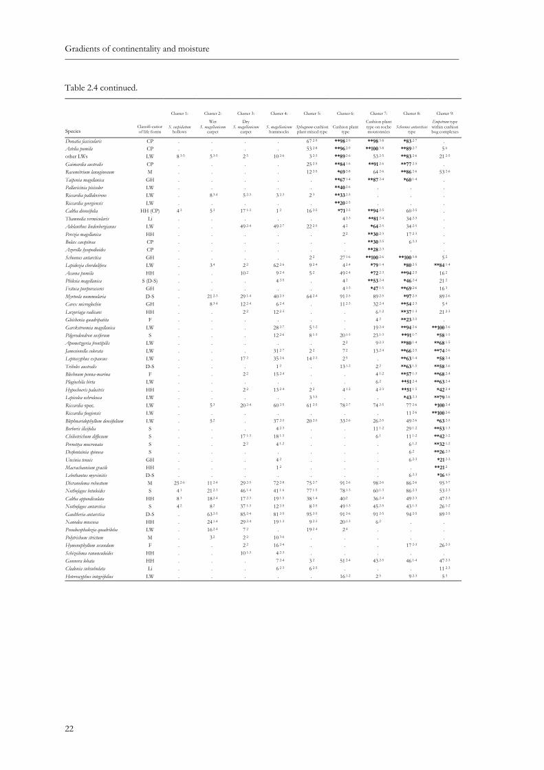
Table 2.4: Synoptic table summarizing results of cluster analysis of South Patagonian peatland vegetation. Species values are percentage frequencies. Species with a fidelity of Φ > 0.25 are considered as diagnostic. They are indicated by asterisks and shown in bold. * – Φ > 0.25; ** – Φ > 0.35 (Φ was calculated for groups with equal numbers of relevés). Species with a frequency < 10 % in all clusters are omitted. Superscripts indicate the range of the cover-abundance values (1 - 9 ordinal scale by van der Maarel (1979)). Classification of life forms: M: moss, LW: liverwort, Li: lichen, HH: herbal hemicryptophyte, GH: graminoid hemicryptophyte, CP: cushion plant, cushion forming hemicryptophyte, F: fern, D-S: dwarf-shrub, S: shrub (shrubby tree).
Species Classification of life forms
Cluster 1:
S. cuspidatum
hollows
Cluster 2:
Wet S. magellanicum
carpet
Cluster 3:
Dry S. magellanicum
carpet
Cluster 4:
S. magellanicum
hummocks
Cluster 5:
Sphagnum-cushion plant mixed type
Cluster 6:
Cushion plant
type
Cluster 7:
Cushion plant type on roche moutonnées
Cluster 8:
Schoenus antarcticus
type
Cluster 9:
Empetrum type within cushion bog complexes
Sphagnum cuspidatum M **100 6-9 5 2 . . . 29 2-5 . . . Tetroncium magellanicum GH *92 2-7 *97 2-7 12 1-2 13 1-6 88 2-5 87 2-5 34 2-5 54 2-4 16 3 Carex magellanica GH **71 2-7 **82 2-6 2 2 12 2-3 23 2-5 . . . . Sphagnum magellanicum M 50 2-7 **100 6-9 **100 8-9 56 2-8 *92 2-8 . . . . Neolepidozia oligophylla LW . **89 2-4 **98 2-4 16 2-4 34 2-4 2 2 . . . Pernettya pumila D-S 4 2 *42 2-4 **54 1-4 12 2-4 3 2 . 26 2-4 3 3 . Microisophylla saddlensis LW . 8 2-4 **80 2-5 34 2-5 20 2-5 2 2 . 3 3 5 2 Juncus scheuchzerioides GH . 8 2-3 *27 2-4 6 2-3 3 2 2 2 . . . Drapetes muscosa HH . 3 2 **20 2-4 1 2 . . . . . Empetrum rubrum D-S 4 2 47 2-6 **100 2-7 **99 2-9 33 1-5 . . 3 7-7 *84 2-7 Marsippospermum grandiflorum GH . 3 2 41 1-7 *72 1-9 . 16 1-5 49 1-3 46 2-6 **100 5-7 Riccardia prehensilis LW . . . **40 2-5 . 2 2 . 9 2-3 **42 2-5 Cladonia rangiferina Li . 3 2 12 2-3 **57 2-7 33 1-5 20 2-5 . 3 1 . Cladonia borealis Li . 5 2-3 5 2-3 **40 2-5 6 2-3 . . . . Ochrolechia frigida Li . . 12 2-3 **32 2-7 11 1-3 2 3 . . . Lepidozia fuegiensis LW . 3 2 24 2-3 *32 2-4 12 2-4 4 2-3 . . . Cladonia cornuta Li . 5 1-2 2 2 **22 2-6 . . . . . Bunodophoron spec. Li . . . **24 2-5 6 1-3 . . . . Avenella caespitosa GH . 3 2 2 3 *16 2-5 . . . . . Campylopus clavatus M . . 2 2 *15 2-5 3 2 . . 3 5 . Dicranoloma billardieri M . . 2 3 *13 2-5 2 2 . . . . Cladonia arbuscula ssp. squarrosa Li . 8 1-2 24 2-5 **57 2-7 *55 1-6 18 2-3 . . . Microisophylla setiformis LW . 3 2 . **56 2-6 **62 2-6 13 2-5 . . . Cladonia arbuscula ssp. mitis Li . 5 2 12 2-3 *51 2-7 *50 1-5 24 1-3 2 2 23 2-3 16 2 Lepidothamnus fonkii D-S . 3 1 . 29 2-9 **86 1-9 . . . . Drosera uniflora HH . 24 2-3 . 1 2 **84 2-4 *60 2-4 49 2-3 14 2-3 . Carpha alpina GH 33 2-6 16 2-3 . 10 2-6 *91 1-6 *100 2-7 *83 2-6 49 2-7 21 2-3 Oreobulus obtusangulus CP . 8 2 . 3 3-5 **83 2-8 *71 2-6 **85 2-5 54 2-5 .
21
Gradients of continentality and moisture
Table 2.4 continued.
Species Classifi-cation of life forms
Cluster 1:
S. cuspidatum
hollows
Cluster 2:
Wet S. magellanicum
carpet
Cluster 3:
Dry S. magellanicum
carpet
Cluster 4:
S. magellanicum
hummocks
Cluster 5:
Sphagnum-cushion plant mixed type
Cluster 6:
Cushion plant
type
Cluster 7:
Cushion plant type on roche moutonnées
Cluster 8:
Schoenus antarcticus
type
Cluster 9:
Empetrum type within cushion bog complexes
Donatia fascicularis CP . . . . 67 2-9 **98 2-9 **98 3-8 *83 2-7 . Astelia pumila CP . . . . 53 2-8 **96 2-9 **100 3-8 **89 2-7 5 6 other LWs LW 8 3-5 5 3-5 2 5 10 2-6 3 2-3 **89 2-6 53 2-5 **83 2-6 21 2-5 Gaimardia australis CP . . . . 25 2-5 **84 1-6 **91 2-6 **77 2-5 . Racomitrium lanuginosum M . . . . 12 2-5 *69 2-8 64 2-6 **86 2-6 53 2-6 Taipenia magellanica GH . . . . . **67 1-4 **87 2-4 *60 1-4 . Pallavicinia pisicolor LW . . . . . **40 2-6 . . . Riccardia pallidevirens LW . 8 3-4 5 2-3 3 2-3 2 3 **33 2-5 . . . Riccardia georgiensis LW . . . . . **20 2-5 . . . Caltha dioneifolia HH (CP) 4 3 5 3 17 1-3 1 2 16 2-5 *71 2-5 **94 2-5 60 2-5 . Thamnolia vermicularis Li . . . . . 4 2-3 **81 2-4 34 2-3 . Adelanthus lindenbergianus LW . . 49 2-4 49 2-7 22 2-5 4 2 *64 2-5 34 2-5 . Perezia magellanica HH . . . . . 2 2 **30 2-3 17 2-3 . Bolax caespitosa CP . . . . . . **30 2-5 6 2-3 . Azorella lycopodioides CP . . . . . . **28 2-3 . . Schoenus antarctica GH . . . . 2 2 27 1-6 **100 2-6 **100 5-8 5 2 Lepidozia chordulifera LW . 3 4 2 2 62 2-6 9 2-4 4 2-4 *79 1-4 *80 2-5 **84 1-4 Acaena pumila HH . . 10 2 9 2-4 5 2 49 2-4 *72 2-3 **94 2-5 16 2 Philesia magellanica S (D-S) . . . 4 2-5 . 4 2 **53 2-4 *46 2-4 21 2 Festuca purpurascens GH . . . . . 4 1-3 *47 1-5 **69 2-6 16 3 Myrteola nummularia D-S . 21 2-3 29 1-4 40 2-5 64 2-4 91 2-5 89 2-5 *97 2-5 89 2-6 Carex microglochin GH . 8 3-4 12 2-4 6 2-4 . 11 2-3 32 2-4 **54 2-3 5 4 Luzuriaga radicans HH . . 2 2 12 2-3 . . 6 1-2 **37 1-3 21 2-3 Gleichenia quadripatita F . . . . . . 4 2 **23 2-5 . Garckstroemia magellanica LW . . . 28 2-7 5 1-2 . 19 2-4 **94 2-6 **100 2-6 Pilgerodendron uviferum S . . . 12 2-6 8 1-3 20 1-5 23 1-3 **91 1-7 *58 1-5 Apometzgeria frontipilis LW . . . . . 2 2 9 2-3 **80 1-4 **68 1-5 Jamesionella colorata LW . . . 31 2-7 2 2 7 2 13 2-4 **66 2-5 **74 2-6 Leptoscyphus expansus LW . . 17 2 35 2-6 14 2-3 2 5 . **63 1-4 *58 2-4 Tribeles australis D-S . . . 1 2 . 13 1-2 2 2 **63 1-5 **58 2-6 Blechnum penna-marina F . . 2 2 15 2-4 . . 4 1-2 **57 1-3 **68 2-4 Plagiochila hirta LW . . . . . . 6 2 **51 2-4 **63 2-4 Hypochoeris palustris HH . . 2 2 13 2-4 2 2 4 1-2 4 2-3 **51 1-5 *42 2-4 Lepicolea ochroleuca LW . . . . 3 3-5 . . *43 2-3 **79 2-6 Riccardia spec. LW . 5 3 20 2-4 60 2-5 61 2-5 78 2-7 74 2-5 77 2-6 *100 2-4 Riccardia fuegiensis LW . . . . . . . 11 2-6 **100 2-6 Blephnaridophyllum densifolium LW . 5 2 . 37 2-5 20 2-5 33 2-6 26 2-5 49 2-6 *63 2-5 Berberis ilicifolia S . . . 4 2-3 . . 11 1-2 29 1-2 **53 1-3 Chiliotrichum diffusum S . . 17 1-3 18 1-3 . . 6 1 11 1-2 **42 1-2 Pernettya mucronata S . . 2 2 4 1-2 . . . 6 1-2 **32 1-2 Desfontainia spinosa S . . . . . . . 6 2 **26 2-3 Uncinia tenuis GH . . . 4 2 . . . 6 2-3 *21 2-3 Macrachaenium gracile HH . . . 1 2 . . . . **21 2 Lebethantus myrsinitis D-S . . . . . . . 6 2-3 *16 4-5 Dicranoloma robustum M 25 2-6 11 2-4 29 2-5 72 2-8 75 2-7 91 2-6 98 2-6 86 2-6 95 3-7 Nothofagus betuloides S 4 1 21 2-3 46 1-4 41 1-6 77 1-5 78 1-3 60 1-3 86 2-3 53 2-3 Caltha appendiculata HH 8 3 18 2-4 17 2-3 19 1-5 38 1-4 40 2 36 2-4 49 2-3 47 2-3 Nothofagus antarctica S 4 2 8 2 37 1-3 12 2-5 8 2-5 49 1-3 45 2-5 43 1-3 26 1-2 Gaultheria antarctica D-S . 63 2-5 85 2-4 81 2-5 95 2-5 91 2-6 91 2-5 94 2-5 89 2-5 Nanodea muscosa HH . 24 1-4 29 2-4 19 1-3 9 2-3 20 1-3 6 2 . . Pseudocephalozia quadriloba LW . 16 2-4 7 2 . 19 2-4 2 4 . . . Polytrichum strictum M . 3 2 2 2 10 3-6 . . . . . Hymenophyllum secundum F . . 2 2 16 2-4 . . . 17 2-3 26 2-3 Schizeilema ranunculoides HH . . 10 1-3 4 2-3 . . . . . Gunnera lobata HH . . . 7 2-4 3 2 51 2-4 43 2-5 46 1-4 47 2-3 Cladonia subsubulata Li . . . 6 2-3 6 2-5 . . . 11 2-3 Heteroscyphus integrifolius LW . . . . . 16 1-2 2 5 9 2-3 5 3
22
Gradients of continentality and moisture
Con
tinen
talit
ycl
asse
s9
8
7
6
5
4
3
2
1
Deg
ree
of d
ecom
posi
tion
10
9
8
7
6
5
4
3
2
1
193547456468413824N =
Vegetation type
987654321
Pea
tdep
th
10
9
8
7
6
5
4
3
2193547456468413824N =987654321
Wat
er le
vel
6
5
4
3
2
1
0
a b
c d
681191213995N =
Vegetation type
987654321
pH (C
aCl 2)
4.5
4.0
3.5
3.0
2.5
e
Con
tinen
talit
ycl
asse
s9
8
7
6
5
4
3
2
1
9
8
7
6
5
4
3
2
1
Deg
ree
of d
ecom
posi
tion
10
9
8
7
6
5
4
3
2
1
10
9
8
7
6
5
4
3
2
1
193547456468413824N = 193547456468413824N =
Vegetation type
987654321 987654321
Pea
tdep
th
10
9
8
7
6
5
4
3
2
10
9
8
7
6
5
4
3
10
9
8
7
6
5
4
3
2193547456468413824N = 193547456468413824N =987654321 987654321 4321
Wat
er le
vel
6
5
4
3
2
1
0
6
5
4
3
2
1
0
a b
c d
681191213995N =
Vegetation type
987654321
pH (C
aCl 2)
4.5
4.0
3.5
3.0
2.5
e
Fig. 2.4: Continentality (a, see Fig. 2.1), degree of decomposition (b, von POST´s scale, AG Boden 2005), water level (c, see Table 2.1), peat depth (d, see Table 2.1) and pH (e, only a subset of samples per cluster was analyzed) of South Patagonian peatland vegetation types (Table 2.4). Line within the box: median, the box is defined by the first and third quartile and contains at least 50 % of all values. The whiskers are lines that extend from the box to the highest and lowest values, excluding outliers and extreme cases. Outliers (circles) are 1.5 - 3 box length outside the box, extreme cases (stars) more than 3 box length.
23
Gradients of continentality and moisture
2.4 Discussion
The floristic variation in the vegetation of Patagonian peatlands correlated with two major environmental gradients: Continentality and soil water level.
Continentality gradient
Most of the floristic variability was explained by continentality. With an increasing distance of our plots from the Pacific Ocean hyperoceanic cushion plant bogs were gradually replaced by Sphagnum bogs that existed exclusively under more continental climatic conditions. Within a transition zone both types intermingled.
Our samples did not show a perfectly even distribution along the measured gradient of continentality. This bias was caused by the inaccessibility of the respective areas and the logistical restrictions during field work. However, since the pure Sphagnum stands were only found in continentality classes 8 and 9, the mixed type in the classes 7 and 8, and pure cushion bogs in the classes 1, 3 and 4 we suppose we covered the entire gradient sufficiently (Table 2.2).
Pisano (1983b) interpreted this continentality gradient mainly as a consequence of the strong change in precipitation regime. Also Moore (1979) and Roig et al. (1985) pointed out that peatlands with annual precipitation of more than 2 000 mm are dominated by cushion forming vascular plants such as Astelia pumila and Donatia fascicularis. In contrast, Sphagnum-dominated raised bogs occur in regions having a yearly precipitation between 600 and 1 500 mm (Pisano 1983b). According to the precipitation regime the Sphagnum-cushion plant mixed type is supposed to be somewhere in between (Roig et al. 1985). Considering European mires, S. magellanicum is regarded as a hummock Sphagnum species with an ecological optimum of water level about 20 cm below the surface (Dierssen & Dierssen 1984). In general, the hyperoceanic climatic conditions of the South Patagonian Channels lead to a higher water level in the peatlands. However, also relatively dry sites exist, exhibiting more or less optimal water level conditions for S. magellanicum growth. Thus, precipitation regime alone does not provide a sufficient explication for the lack of S. magellanicum in the west.
Other important consequences of the degree of continentality such as distinct frost periods in winter or the duration of snow cover, which also play an important role along continentality gradients in the north hemispherical peatlands (Dierssen 1982, Sjörs 1983), were neglected so far. Gerdol (1995) showed the dependence of the growth rate of S. magellanicum to different temperature and light intensity. The combination of low
24
Gradients of continentality and moisture
temperature and low light intensity reduced growth and may even lead to dormancy of Sphagnum species. Exactly this combination of environmental conditions is realized in the hyperoceanic parts of southern Patagonia, where the frequent cloudiness lowers the direct solar radiation and the proximity to the ocean results in a constantly cool climate.
Gignac et al. (1991) emphasize the influence of several environmental factors on species composition along a gradient of increasing continentality. One important gradient caused by the distance to the ocean is the mineral input by sea spray. Malmer et al. (1992) presented distinct west-east concentration gradients for most elements in plants and surface water of western Canadian mires. In general, competition for mineral nutrients has an important influence on the floristic composition of peatland vegetation. Van Groenendael et al. (1982) emphasize the significant effect of sea spray on floristic composition of western European peatlands via the input of mineral nutrients. Also for the southern hemisphere Damman (1995a) showed that differences in precipitation chemistry had a significant impact on the floristic composition of Tasmanian peatland vegetation, in particular via the increased input of base cations in proximity to the ocean. Sphagnum species catch inputs of the wet deposition very quickly with the whole plant surface area (Dierssen & Dierssen 2001). This is a strong competitive advantage in comparison with vascular plants under low deposition conditions. Ionic concentration in peat varies with the season and the climatic conditions. Fluctuation of ionic concentrations in oceanic peatlands is low, which indicates a well buffered system (Proctor 1994). As a result of higher and constant inputs the strong ion-catching ability of Sphagnum becomes less important in oceanic regions. This might reduce it’s strength in competition with oceanic cushion plants and could be another factor for the lack of S. magellanicum in western Patagonia. In contrast, Vitt et al. (1990) described a higher diversity of Sphagnum species in western British Columbian peatlands compared to continental bogs. However, there are two differences compared to the situation in southern Patagonia: First the annual precipitation is remarkably lower in British Columbia, and second, there are only three Sphagnum species in the South Patagonian flora, among them only S. fimbriatum preferring minerotrophic conditions. Besides these floristic differences, Vitt et al. (1990) could also demonstrate a significant change in peatland vegetation along a continentality gradient that was highly correlated with surface water chemistry indicating (at least partially) the effect of sea spray.
By the accumulation of peat mire plants create their own environmental conditions. Along the gradient of continentality the degree of decomposition increased significantly towards the oceanic peatlands. The controlling factor in this situation is most likely the resistance to decomposition processes of the peat creating plants (Dierssen & Dierssen 2001, Bragazza et al. 2006). Sphagnae, especially the hummock species, show a high resistance to decomposition
25
Gradients of continentality and moisture
processes (Johnson & Damman 1991). Under oceanic conditions decomposition is presumably significantly enhanced by the input of base cations via sea spray and the resulting higher quality of litter indicated by slightly higher pH values (Fig. 2.4). The higher decomposition rates in this situation are supposed to have a significant impact on the degree of nutrient cycling and trophic conditions.
Water level gradient
Floristic variation along the second DCA axis was highly correlated with the measured water level. Along the whole continentality gradient corresponding with the first DCA axis one could observe a distinct floristic separation between relatively dry and wet sites. Due to the high logistical effort, our water level measurements were carried out at a single point in time. It has to be considered that the water table is variable and can show large seasonal differences (Wheeler & Proctor 2000). In the study area, precipitation rates do not show significant seasonal differences (Schneider et al. 2003). In line with this finding, Baumann (2006) described a surprisingly low variation of the water table in a Sphagnum-dominated raised bog in Tierra del Fuego, although he measured time spans with low and high precipitation. Thus, since our sampling was done during a relatively narrow time span of less than two months effects of seasonal differences are expected to be low and the water table data should give a sufficiently sound description of the moisture gradient.
Vegetation types exhibited a relatively clear grouping along the moisture gradient even in the most western parts. Pisano (1983b) and Moore (1979) described the Empetrum rubrum type (Cluster 9 in Table 2.4) as a relatively dry community within western cushion bog complexes occurring under slightly better drainage conditions because of the underlying substrate. The cushion plant type (Cluster 6 in Table 2.4) showed the wettest site conditions on poorly drained plane or scarcely inclinated surfaces (Dollenz 1986). The abundance and dominance of graminoid plants increased under better drainage conditions (Dollenz 1982, Pisano 1983b). The vegetation types of Cluster 7 and 8 (Table 2.4) predominantly occurred on inclinated slopes and showed both, drier site conditions because of better drainage and a high proportion of graminoids in the vegetation.
A floristic separation along a moisture gradient of Patagonian Sphagnum magellanicum raised bogs has already been described by other authors, e.g. Pisano (1983b). Teneb & Dollenz (2004) and Baumann (2006) emphasized the importance of microtopography for the hydrology of Patagonian Sphagnum bogs. Our study showed a differentiation into four major vegetation types (Cluster 1 - 4 in Table 2.4) following the hollow-hummock moisture gradient that is also well established for Sphagnum-dominated bogs of the northern hemisphere (Couwenberg & Joosten 2005).
26
Gradients of continentality and moisture
All older publications dealing with South Patagonian bogs described S. fimbriatum as the most important constituent of the hollows (Pisano 1983b, Roig et al. 1985). Surprisingly, we found hollows of continental South Patagonian bogs to be generally dominated by Sphagnum cuspidatum whereas S. fimbriatum could only be found at the margins of ombrotrophic continental raised bogs under clear minerotrophic conditions. Our findings are supported by Moen (2005), who described similar patterns of distribution.
The wet S. magellanicum carpets (Cluster 2 in Table 2.4) were intermediate in terms of moisture and floristic composition, situated between the hollows and dry S. magellanicum carpets (Cluster 3 in Table 2.4) dominated by dwarf-shrubs (Schwaar 1976). The driest site conditions were observed in S. magellanicum hummocks (Cluster 4 in Table 2.4) showing a distinct floristic composition. The S. magellanicum-cushion plant mixed type (Cluster 5 in Table 2.4) is separated as an own type of relatively high water table at more pacific sites in the transition zone to hyperoceanic cushion bogs (Roig et al. 1985). Floristically this type was characterized by elements of both, the western cushion bogs and the continental Sphagnum bogs with only the conifer dwarf-shrub Lepidothamnus fonkii showing a clear preference for this community.
Comparison with north-hemispherical mires
In Europe the gradient of continentality and its effect on peatlands and their floristic composition is well known and described comprehensively (Dierssen & Dierssen 2001, Jeschke et al. 2001). In southern Patagonia the distance from the oceanic peatlands to the continental Sphagnum bogs is very short. Within less than 100 km bog vegetation changes from hyperoceanic blanket bogs to Sphagnum-dominated raised bogs near the limit of the occurrence of ombrotrophic peatlands towards the Patagonian Steppe (Roig et al. 1985). In Central Europe the gradient of continentality is much longer and smoother. A barrier such as the Andes in southern Patagonia creating a steep climatic gradient with a strong rain shadow effect is lacking. Western North America and Fennoscandia also show a steep gradient in precipitation, but, in contrast to South Patagonia the annual range of temperatures even in oceanic regions is quite large (Banner et al. 1988, Damman 1995b).
In the western parts of Europe the boundary between clearly ombrotrophic and minerotrophic peatlands becomes indistinct (Dierssen 1982) resulting in a typical mosaic of blanket bog and moist heath vegetation (Rodwell 1991). Similar observations were made by Banner et al. (1988) and Wells (1996) for Canadian oceanic wetlands. Atmospherical inputs can vary within wide limits along the gradient of continentality that overlap the range of telluric inputs into poor fens, so that there is no universal distinction between the water or peat chemistry signatures of ombrotrophic bogs and minerotrophic poor fens (Wheeler &
27
Gradients of continentality and moisture
Proctor 2000). Damman (1995a) emphasized the floristic affinities of Sphagnum-dominated bogs and poor fens, which is in line with multivariate floristic analyses of oceanic peatland vegetation of the northern hemisphere that did not identify bog vs. fen as the primary split (Daniels 1978, Gignac et al. 1991). As indicated by a higher deviation of pH values in South Patagonian oceanic blanket bogs a clear separation of minerotrophic and ombrotrophic parts is presumably also not realized.
European oceanic blanket bog vegetation is characterized by dwarf-shrubs and some hemicryptophytes such as Schoenus nigricans, Narthecium ossifragum or Molinia caerulea usually indicating minerotrophic conditions in more continental regions (Dierssen 1982, Damman 1995a). This phenomenon is also described by Sjörs (1983) for southern Alaska pointing out similarities and differences to Fennoscandian bogs. South Patagonian blanket bogs exhibited the same tendency with some species such as Schoenus antarcticus or Festuca purpurascens considered indicative of telluric water. Especially vegetation of inclinated roche moutonnées areas do have soligenous influence, but this influence might be buffered by the generally base-poor bedrock (Pisano 1977) and the immense and continuous precipitation.
Schwaar (1976, 1980) and Moen (2005) pointed out the structural (hollows and hummocks) and even floristic similarity between continental South Patagonian and European Sphagnum bogs (e.g. Oberdorfer 1992). Closely related taxa such as Empetrum rubrum in the southern and E. nigrum in the northern hemisphere are constituents of Sphagnum-dominated peatlands. Partly the same species such as Sphagnum magellanicum itself, Carex magellanica or lichens of the genus Cladonia occur in raised bogs of both hemispheres.
In contrast to the Sphagnum bogs the oceanic peatlands of both hemispheres differ significantly. South hemispherical oceanic peatlands are characterized by cushion building plants (Gibson & Kirkpatrick 1985, Pisano 1983b), which are totally absent in the northern hemisphere. The taxa of cushion building plants such as Astelia, Donatia or Oreobulus show a south hemispherical distribution due to their gondwanic origin (Dawson 1963), but even convergent forms are lacking in Eurasia and North-America.
European oceanic bogs are treeless. With increasing distance to the ocean a higher importance of trees, up to forested peat bogs in continental areas, can be observed (Dierssen & Dierssen 2001, Jeschke et al. 2001). In oceanic mires of southern Alaska the high abun-dance of trees is a feature that differentiates to the atlantic European peatlands (Sjörs 1983), whereas in Canadian atlantic blanket bogs – similar to the situation in western Europe – trees are nearly lacking (Wells 1996). In southern Patagonia trees do not expand into central parts of continental raised bogs. If tree species (e.g. Nothofagus antarctica) occur they do not grow higher than 1 m. In pacific cushion bog complexes trees such as Nothofagus betuloides or
28
Gradients of continentality and moisture
29
Pilgerodendron uviferum grow exclusively on well drained sites (Pisano 1983b) even though seedlings may be abundant.
Human impact over a long time on nearly all oceanic peatlands make it difficult to describe the natural vegetation of the Western Europe blanket bog complexes (Dierssen 1982). Many of the blanket bog complexes are even of an anthropogenic origin. They expanded through grazing and burning at the cost of woodland (Dierssen 1996). In South Patagonia direct human impact is nearly absent in the western parts. In the continental parts peat harvesting has been developed in the last decade (Caspers 2002), but has not yet destroyed all natural peat bog ecosystems like in Central Europe (Succow 2001). In Great Britain, Central Europe and southern Fennoscandia heavy atmospherical input of nutrients caused by emissions from industry and agriculture have been measured that often reach critical loads for ombrotrophic peatland ecosystems. The anthropogenic enhancement of nutrient supply is accompanied by significant changes in ecological processes such as decomposition and mineralization (Bragazza et al. 2004, 2006). In contrast, the input in southern Patagonian ecosystems is marginal (Godoy et al. 2001), which gives the unique opportunity to study peatlands under unspoiled pre-industrial conditions. More ecological data of South Patagonian peatland ecosystems could provide useful facts in the discussion of the major gradients affecting species composition in mire ecosystems (Wheeler & Proctor 2000, Økland et al. 2001, Hájek et al. 2006).
Acknowledgements
We would like to thank Rolf Kilian, chief of the Gran Campo Nevado Project, for logistic support during field work. Orlando Dollenz (Instituto de la Patagonia, Punta Arenas, Chile) gave helpful hints to find study sites and socialized with persons knowing the study area. We are grateful to Barbara Ruthsatz and Friedrich-Karl Holtmeier for lively discussions and useful suggestions. Kerstin Anschlag made valuable comments and corrections to a former version of this manuscript. Lillian Harris polished our English.

Chapter 3
South Patagonian ombrotrophic bog vegetation reflects biogeochemical gradients at the landscape level
Till Kleinebecker*1; Norbert Hölzel1 & Andreas Vogel1
1Institute of Landscape Ecology, University of Münster, Robert-Koch-Straße 26, 48149 Münster, Germany
*Corresponding author
Journal of Vegetation Science, accepted 27.07.2007
Abstract
Question: Which environmental variables affect the floristic composition of South Patagonian bog vegetation along a gradient of climate and biogeochemical changes with increasing distance from the Pacific Ocean?
Location: Trans-Andean transect (53° S), southernmost Patagonia
Materials and methods: Floristic composition, peat characteristics (water level, decompo-sition, pH, total nitrogen, total carbon, ash content, and plant available P, K, Na, Ca, Mg, Fe, Mn, Zn, and Al), and climatic constraints of ombrotrophic peatlands were measured at 82 plots along a gradient of increasing distance from the Pacific Ocean.
Results: Climatic constraints and biogeochemical peat characteristics significantly change with increasing distance from the Pacific and peatland vegetation shifted from hyperoceanic blanket bogs dominated by cushion-forming vascular plants to the west to Sphagnum bogs to the east. Climatic and biogeochemical variables explained a high proportion of the floristic variation along the first DCA axis. The second axis represented a water level gradient. When “distance to the Pacific” was defined as a covariable in partial CCA, the proportion of
31
Bog vegetation reflects biogeochemical gradients
variance explained declined for most other variables, especially in the case of annual pre-cipitation and exchangeable base cations and related traits. The differences in biogeochemi-cal characteristics related to peat were mainly attributed to the input of sea-born cations.
Conclusions: While variation in vegetation composition along a longitudinal gradient crossing the southern Andes was attributed to climatic constraints as expected, vegetation composition was also strongly affected by the biogeochemical characteristics of peat. Sea spray was of high ecological importance to peat chemistry and consequently, to floristic composition. Presumably, South Patagonian peat bogs represent a glimpse of pre-industrial environments, so that these peat bogs may act as reference systems with respect to atmos-pheric inputs in mire ecology research.
Keywords: cushion bog, raised bog, blanket bog, Sphagnum, sea spray, ordination, CCA, Chile, base cations
3.1 Introduction
The world’s natural vegetation is mainly affected by latitudinal, longitudinal and altitudinal gradients that are related to changes in climatic factors (Archibold 1995, Schulz 1995, Breckle 2002). In coastal situations, the longitudinal gradient is created by the temperature-buffering influence of the sea and the changing precipitation regime with increasing distance to the ocean. These changing climatic constraints can have a strong impact on the distribution and floristic composition of species (e.g. Senterre et al. 2004, Fang & Lechowicz 2006, Franklin et al. 2006). Besides climatic environmental conditions, the distance to the ocean also influences precipitation chemistry and enhances the supply of sea-born base cations (Erisman et al. 1998, Vitousek 2002, Haragushi et al. 2003). Such trophic gradients have a significant effect on plant growth (e.g. Sánchez-Blanco et al. 2003) and floristic composition (e.g. Vitt et al. 1990, Griffith 2006).
Nutrient supply and mineral availability are well established as key factors affecting the eco-logy and the floristic composition of peatlands (e.g. Wheeler & Proctor 2000). Due to the disconnection from groundwater, ombrotrophic bogs receive all their nutrients from atmos-pheric sources. Thus, these ecosystems are particular sensitive to spatial changes in the chemical composition of precipitation that could originate from natural or anthropogenic processes (Vitt et al. 1990, Gunnarsson et al. 2002). Given this situation, the effect of sea-born nutrients on floristic composition of ombrotrophic bog ecosystems should be clearly visible along longitudinal gradients near ocean environments. Such an impact has often been assumed (Damman 1995a) but rarely confirmed by biogeochemical data.
32
Bog vegetation reflects biogeochemical gradients
In general, there is considerable spatial bias in the ecological knowledge of peatlands. In the northern hemisphere, the major ecological gradients affecting the floristic composition of mire vegetation are well known and have been summarized and discussed in several recent studies (e.g. Wheeler & Proctor 2000, Økland et al. 2001, Hájek et al. 2006). The bog - fen gradient (e.g. Wheeler & Proctor 2000), as well as the ecological consequences of anthropo-genic nitrogen input and shifts in vegetation caused by climate change (e.g. Berendse et al. 2001, Gunnarsson & Flodin 2007) have been documented comprehensively. There are even a few studies that have explored the influence of sea-born cations on the floristic composi-tion of mires in relation to the distance to the ocean (e.g. Vitt et al. 1990).
In contrast, research on the peatlands of the southern hemisphere, especially those in southern Patagonia, has been neglected. Existing studies on South Patagonian peatland vegetation usually has focussed on syntaxonomical descriptions (e.g. Pisano 1983b, Boelcke et al. 1985). Pisano (1983b) interpreted the change in floristic composition of bog vegetation along a W-E transect in South Patagonia as a climatic gradient, mainly as a consequence of the precipitation regime. Also, Moore (1979) and Boelcke et al. (1985) pointed out that peatlands with an annual precipitation of more than 2 000 mm are dominated by cushion-forming vascular plants such as Astelia pumila and Donatia fascicularis. In contrast, Sphagnum-dominated raised bogs occur in regions having a yearly precipitation between 600 and 1 500 mm (Pisano 1983b). In a transition zone, both types intermingle in the South Patago-nian peatlands (Boelcke et al. 1985).
Investigations on broad-scale vegetation-environment relationships that include biogeoche-mical measurements and lead to a better ecological understanding of vegetation patterns at a landscape level (e.g. Vitt et al. 1990, Virtanen et al. 2006) do not exist for the southern hemi-sphere. One study of the southern hemisphere presented peat chemical data and focussed on a local scale description of ecological characteristics of a single mire complex (Ruthsatz & Villagran 1991). The South Patagonian region provides particularly suitable conditions for ecological research in mire ecosystems across longitudinal gradients. Due to the strong wes-terly winds bringing unpolluted air masses, the low human population density, and the lack of intense agriculture, the atmospherical nitrogen input in southern Patagonia is marginal (Godoy et al. 2001). Thus, southern Patagonia provides the unique opportunity to study the ecology of ombrotrophic peatlands under pristine conditions with almost no anthropogenic input. Such studies could provide a reference for the trophical status of corresponding north hemispherical peatlands under pre-industrial conditions (e.g. Wassen et al. 2005).
Here, we present the first comprehensive study that combines vegetation data with climatic constraints and biogeochemical peat characteristics along the entire Trans-Andean climatic gradient. In particular, we will address the following questions:
33
Bog vegetation reflects biogeochemical gradients
1. Are climatic constraints the major determinants affecting South Patagonian peatland vegetation?
2. How important are biogeochemical peat characteristics, and is there a detectable effect of sea spray on peatland vegetation?
3. Do South Patagonian peat bogs show biogeochemical constraints that could give us an idea about the pre-industrial conditions of peatlands in other regions including the northern hemisphere?
3.2 Materials and methods
Study area
The steep climatic gradient created by the southern Andes probably is the strongest climatic divide worldwide and its orographic effects can be observed more clearly there than anywhere else on earth (Miller 1976). This climate gradient is most significantly reflected by the precipitation regime (Endlicher & Santana 1988). The hyperoceanic western Chilean Channel region has up to 10 000 mm annual precipitation, whereas on the eastern side of the Andes, precipitation decreases to less than 500 mm towards the Patagonian Steppe (Schneider et al. 2003). Although mean annual temperatures hardly change along that gradient (~6° C), the inter-annual amplitude of temperature increases significantly towards the more continental parts of the gradient (Pisano 1977). This temperature difference is best expressed by regular frost events in winter and higher summer temperatures in the east, as well as the absence of frost periods and cool summer temperatures in the hyperoceanic west (Tuhkanen 1992).
This steep climatic gradient is reflected in the vegetation types across these zones (Boelcke et al. 1985). From west to east, one can observe a clear zonation pattern from coastal blanket bog, to cool temperate evergreen rainforest, deciduous forest, and dry Patagonian Steppe. Along this longitudinal gradient, ombrotrophic peatland vegetation also changes in its floristic composition. With increasing distance from the Pacific Ocean, hyperoceanic blanket bogs, which were built by cushion-forming vascular plants such as Donatia fascicularis and Astelia pumila are gradually replaced by Sphagnum magellanicum dominated bogs that exist exclusively under more continental climatic conditions (Kleinebecker et al. 2007a).
Sampling of ombrotrophic peatland vegetation took place along a Trans-Andean transect of about 100 km west of the Patagonian Steppe zone in southernmost Chile. Most of the
34
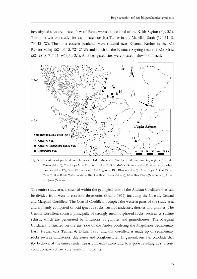
Bog vegetation reflects biogeochemical gradients
investigated sites are located NW of Punta Arenas, the capital of the XIIth Region (Fig. 3.1). The most western study site was located on Isla Tamar in the Magellan Strait (52° 54´ S, 73° 48´ W). The most eastern peatlands were situated near Estancia Kerber in the Río Rubens valley (52° 04´ S, 72° 2´ W) and north of the Estancia Skyring near the Río Pérez
The entire study area is situated within the geological unit of the Andean Cordillera th
(52° 28´ S, 71° 54´ W) (Fig. 3.1). All investigated sites were located below 300 m a.s.l.
at can
conditions, which are very similar in nutrients.
1 2
34
5
6
7
8
9
10
11
Fig. 3.1: Locations of peatland complexes sampled in the study. Numbers indicate sampling regions: 1 = Isla Tamar (N = 3), 2 = Lago Muy Profundo (N = 3), 3 = Muños Gamero (N = 7), 4 = Bahía Baha-mondes (N = 17), 5 = Río Azocar (N = 11), 6 = Río Blanco (N = 5), 7 = Lago Aníbal Pinto (N = 7), 8 = Bahía Williams (N = 10), 9 = Río Rubens (N = 9), 10 = Río Pérez (N = 5), and, 11 = San Juan (N = 4).
be divided from west to east into three units (Pisano 1977) including the Coastal, Central and Marginal Cordillera. The Coastal Cordillera occupies the western parts of the study area and is mainly comprised of acid igneous rocks, such as andesites, diorites and granites. The Central Cordillera consists principally of strongly metamorphosed rocks, such as crystalline schists, which are penetrated by intrusions of granites and granodiorites. The Marginal Cordillera is situated on the east side of the Andes bordering the Magellanes Sedimentary Basin further east (Palmer & Dalziel 1973) and this cordillera is made up of sedimentary rocks such as sandstones, claystones and conglomerates. In general, one can conclude that the bedrock of the entire study area is uniformly acidic and base-poor resulting in substrate
35
Bog vegetation reflects biogeochemical gradients
Sampling and biogeochemical analysis
A total of 82 relevés were made in floristically and structurally homogenous stands in predominantly ombrotrophic peatland complexes. Sampling took place during March and
was sampled in 11 geographic regions with the number of
0 = ground water at the soil surface to 7 = groundwater > 40 cm below the soil surface (see Kleinebecker et
le in the field. Samples were dried at 50° C and screened through a sieve with 2 mm mesh wire. Total contents of C and N
April 2004 and 2005. Vegetationplots per region ranging from three to 17, depending on accessibility and logistic necessities during field work (Fig. 3.1). The plot size was 1 m2. Cover-abundance data was recorded following the Braun-Blanquet approach (Braun-Blanquet 1964, Westhoff & van der Maarel 1973). Because of difficulties in determination and differentiation in the field of some cryptogams, uncertain species were named at the level of genus, or, in the case of some liverworts, species were merged into one group named “other liverworts”.
Ground water level was measured by digging a hole and measuring the distance of the water level to the surface of the ground. We used an ordinal scale reaching from
al. 2007a). While water table can be variable and display large seasonal differences (Wheeler & Proctor 2000), continental Patagonian Sphagnum bogs show a surprisingly low variation of water table depth (Baumann 2006). Thus, the water table data of this investigation may be utilized for an approximate description of the edaphic moisture regime. The degree of decomposition of the peat was estimated to a depth of 5 - 10 cm below surface using the ten-stage scale of von Post (AG Boden 2005). Annual precipitation, mean annual temperature, and mean temperature of the coldest and the warmest month were interpolated from available data (Pisano 1977, Tuhkanen 1992, Schneider et al. 2003, Schneider & Kilian unpubl. data). The distance to the Pacific Ocean of the sampled sites was estimated using a graphically derived ordinal scale of nine stages, which differentiates distances to the Pacific Ocean using equal divisions between the sites closest and farthest from the Pacific Ocean (Kleinebecker et al. 2007a). The influence of the Atlantic Ocean was considered to be marginal and was not included in the ordination due to the strong and constant westerly winds creating a steep west to east climatic gradient.
For each relevé, volumetric mixed surface samples of peat were taken at a depth of 5 -10 cm. Roots were eliminated as precisely as possib
(Element autoanalyzer, CARLO ERBER NA 1500), the ash content (ashing overnight in a muffle furnace at 550° C), CAL-soluble P (Schüller 1969, photometrical measurement with 578 nm, PERKIN ELMER), and NH4Cl exchangeable fractions of K, Na, Ca, Mg, Fe, Mn, Zn, and Al (Meiwes et al. 1984, determination with an AAS, PERKIN ELMER) were measured in the laboratory.
36
Bog vegetation reflects biogeochemical gradients
Data analysis
For numerical analysis, Braun-Blanquet cover-abundance values were transformed into the 1 - 9 ordinal scale of van der Maarel (1979). For ordination, only abundant species were used
re defined as species that were present on at least three plots. Liverworts and
ignificance Test (HSD) for unequal sample size for the normally distributed environmental variables with homogeneous variances. Non-normal and ordinal-scaled data
howing a high correlation to DCA axes were extracted and reapplied for the following direct gradient analysis (Ejrnaers
and these welichens that could not be determined at species level were not included in the calculations. Major gradients were explored by detrended correspondence analysis (DCA, Hill & Gauch 1980), a method of indirect gradient analysis (Jongman et al. 1995). Running the DCA with detrending by 26 segments revealed a gradient length on the first axis of 4.599 standard deviation units and on the second axis of 2.814. All relevés were allocated to three major vegetation types including the hyperoceanic cushion plant type (n = 34) dominated by cushion-forming vascular plants, the Sphagnum magellanicum type (n = 36) at the east side of the Andes and the transitional cushion-Sphagnum mixed type (n = 12) (see Kleinebecker et al. 2007a).
We compared means of the three major vegetation types using the parametric Tukey Honest-S
were analyzed using the Kruskal-Wallis H-Test with pairwise comparisons analyzed using the Mann-Whitney U-Tests. Probability values from multiple pairwise comparisons were adjusted using Bonferroni corrections (Sokal & Rohlf 1981).
Spearman rank correlations between the environmental variables and the axis scores of DCA ordination were calculated. Environmental variables s
2000). For a further reduction of the number of explanatory variables, Ca, Mg, Na, and K were merged to one group (base cations) by building up the sum of the respective contents. To estimate the relative importance of the measured environmental variables, we applied a Canonical Correspondence Analysis (CCA), which gave a gradient length of 3.837 standard deviation units for the first axis and 2.559 for the second. We performed a decomposition of variance by running a series of partial CCAs to isolate and specify the relative importance of the variable “distance to the Pacific Ocean” on species composition in relation to other environmental variables. For all statistical calculations, metric environmental variables were log-transformed. DCA was performed using the PCORD 5.0 software package (McCune & Mefford 2006), CCA using CANOCO 4.5 (ter Braak & Šmilauer 2002). ANOVA and Spearman rank correlation were carried out using SPSS 11.0.
37
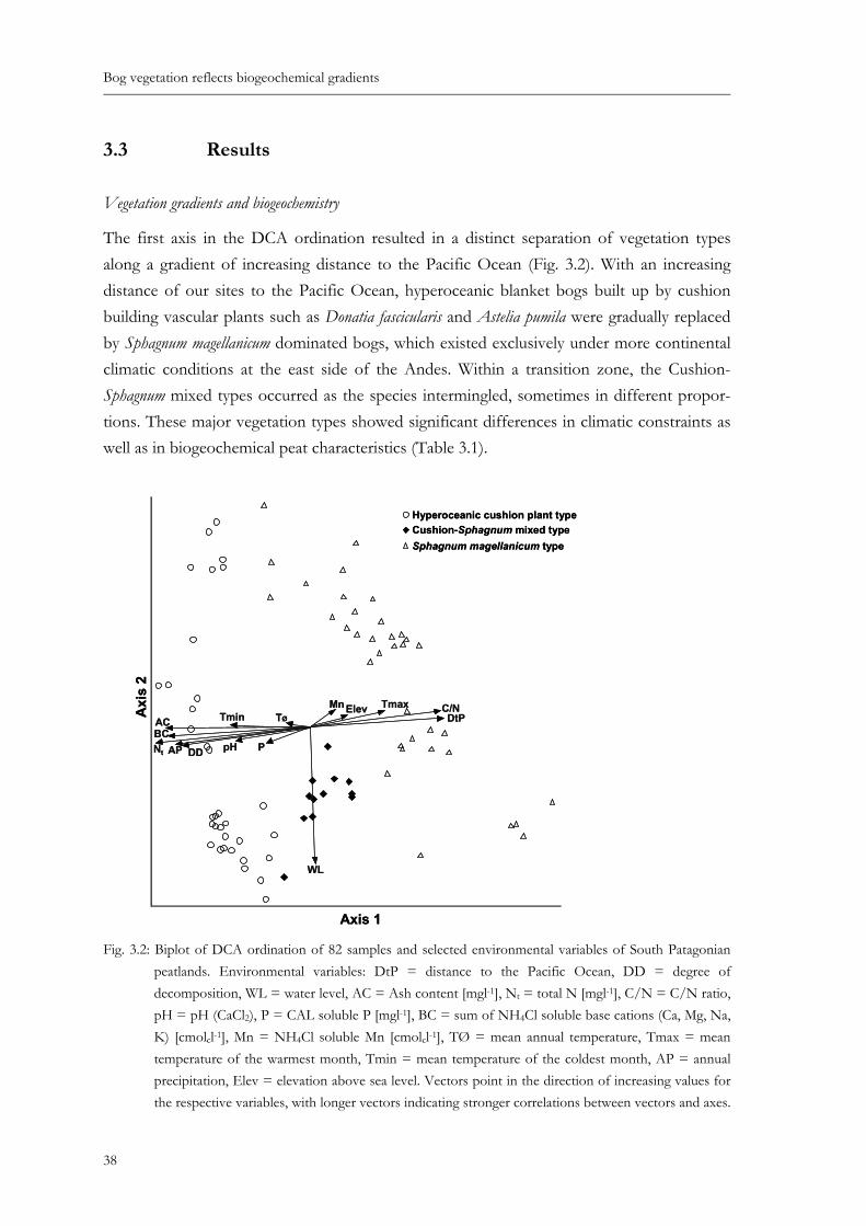
Bog vegetation reflects biogeochemical gradients
3.3 Results
Vegetation gradients and biogeochemistry
The first axis in the DCA ordination resulted in a distinct separation of vegetation types along a gradient of increasing distance to the Pacific Ocean (Fig. 3.2). With an increasing distance of our sites to the Pacific Ocean, hyperoceanic blanket bogs built up by cushion building vascular plants such as Donatia fascicularis and Astelia pumila were gradually replaced by Sphagnum magellanicum dominated bogs, which existed exclusively under more continental climatic conditions at the east side of the Andes. Within a transition zone, the Cushion-Sphagnum mixed types occurred as the species intermingled, sometimes in different propor-tions. These major vegetation types showed significant differences in climatic constraints as well as in biogeochemical peat characteristics (Table 3.1).
DtP
DD
WL
C/N
P
Mn
Nt
ACBC
Axis 1
Axi
s2
Sphagnum magellanicum typeCushion-Sphagnum mixed typeHyperoceanic cushion plant type
pH
Elev TmaxTØTmin
AP
DtP
DD
WL
C/N
P
Mn
Nt
ACBC
Axis 1
Axi
s2
Sphagnum magellanicum typeCushion-Sphagnum mixed typeHyperoceanic cushion plant type
pH
Elev TmaxTØTmin
AP
Fig. 3.2: Biplot of DCA ordination of 82 samples and selected environmental variables of South Patagonian peatlands. Environmental variables: DtP = distance to the Pacific Ocean, DD = degree of decomposition, WL = water level, AC = Ash content [mgl-1], Nt = total N [mgl-1], C/N = C/N ratio, pH = pH (CaCl2), P = CAL soluble P [mgl-1], BC = sum of NH4Cl soluble base cations (Ca, Mg, Na, K) [cmolcl-1], Mn = NH4Cl soluble Mn [cmolcl-1], TØ = mean annual temperature, Tmax = mean temperature of the warmest month, Tmin = mean temperature of the coldest month, AP = annual precipitation, Elev = elevation above sea level. Vectors point in the direction of increasing values for the respective variables, with longer vectors indicating stronger correlations between vectors and axes.
38
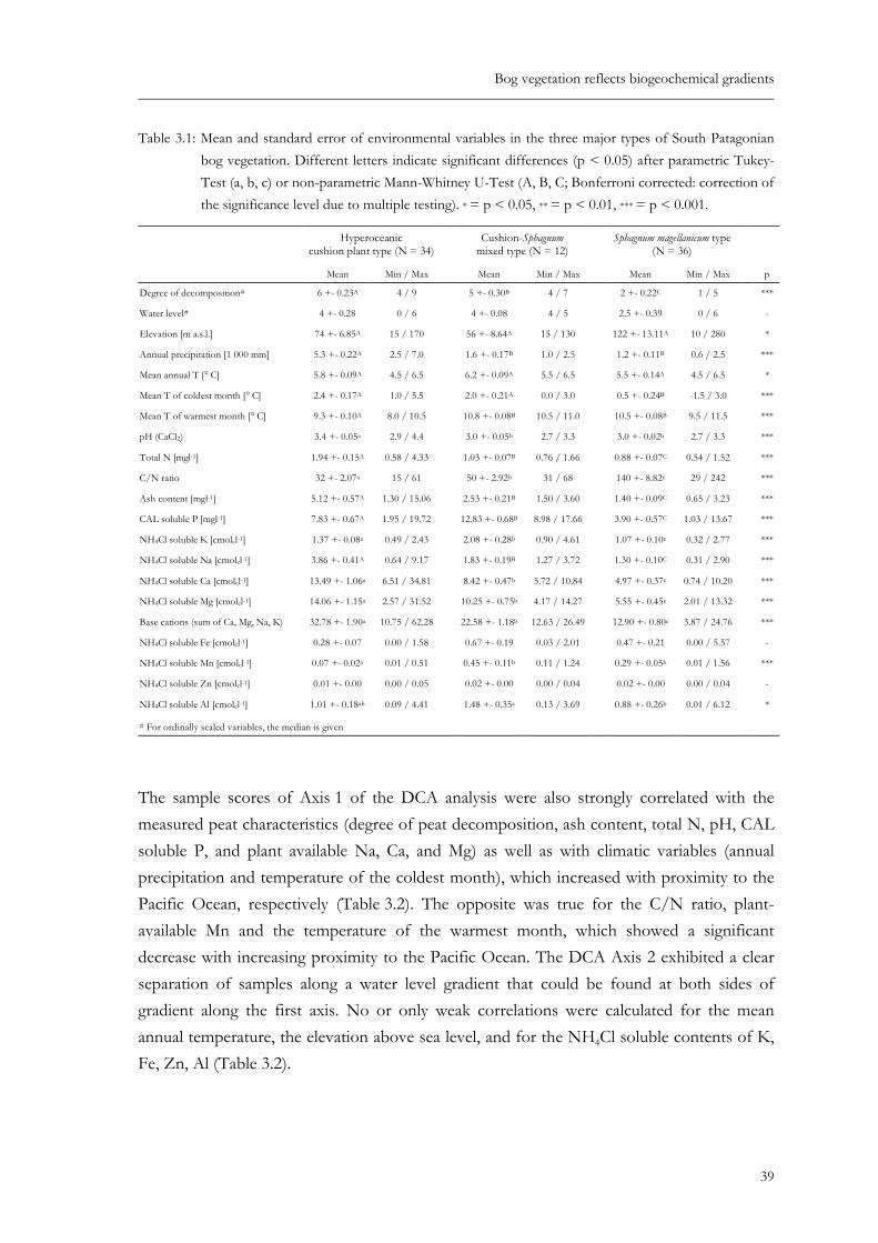
Bog vegetation reflects biogeochemical gradients
Table 3.1: Mean and standard error of environmental variables in the three major types of South Patagonian bog vegetation. Different letters indicate significant differences (p < 0.05) after parametric Tukey-Test (a, b, c) or non-parametric Mann-Whitney U-Test (A, B, C; Bonferroni corrected: correction of the significance level due to multiple testing). * = p < 0.05, ** = p < 0.01, *** = p < 0.001.
Hyperoceanic cushion plant type (N = 34)
Cushion-Sphagnum mixed type (N = 12)
Sphagnum magellanicum type (N = 36)
Mean Min / Max Mean Min / Max Mean Min / Max p
Degree of decomposition# 6 +- 0.23A 4 / 9 5 +- 0.30B 4 / 7 2 +- 0.22C 1 / 5 ***
Water level# 4 +- 0.28 0 / 6 4 +- 0.08 4 / 5 2.5 +- 0.39 0 / 6 -
Elevation [m a.s.l.] 74 +- 6.85A 15 / 170 56 +- 8.64A 15 / 130 122 +- 13.11A 10 / 280 *
Annual precipitation [1 000 mm] 5.3 +- 0.22A 2.5 / 7.0 1.6 +- 0.17B 1.0 / 2.5 1.2 +- 0.11B 0.6 / 2.5 ***
Mean annual T [° C] 5.8 +- 0.09A 4.5 / 6.5 6.2 +- 0.09A 5.5 / 6.5 5.5 +- 0.14A 4.5 / 6.5 *
Mean T of coldest month [° C] 2.4 +- 0.17A 1.0 / 5.5 2.0 +- 0.21A 0.0 / 3.0 0.5 +- 0.24B -1.5 / 3.0 ***
Mean T of warmest month [° C] 9.3 +- 0.10A 8.0 / 10.5 10.8 +- 0.08B 10.5 / 11.0 10.5 +- 0.08B 9.5 / 11.5 ***
pH (CaCl2) 3.4 +- 0.05a 2.9 / 4.4 3.0 +- 0.05b 2.7 / 3.3 3.0 +- 0.02b 2.7 / 3.3 ***
Total N [mgl-1] 1.94 +- 0.15A 0.58 / 4.33 1.03 +- 0.07B 0.76 / 1.66 0.88 +- 0.07C 0.54 / 1.52 ***
C/N ratio 32 +- 2.07a 15 / 61 50 +- 2.92b 31 / 68 140 +- 8.82c 29 / 242 ***
Ash content [mgl-1] 5.12 +- 0.57A 1.30 / 15.06 2.53 +- 0.21B 1.50 / 3.60 1.40 +- 0.09C 0.65 / 3.23 ***
CAL soluble P [mgl-1] 7.83 +- 0.67A 1.95 / 19.72 12.83 +- 0.68B 8.98 / 17.66 3.90 +- 0.57C 1.03 / 13.67 ***
NH4Cl soluble K [cmolcl-1] 1.37 +- 0.08a 0.49 / 2.43 2.08 +- 0.28b 0.90 / 4.61 1.07 +- 0.10c 0.32 / 2.77 ***
NH4Cl soluble Na [cmolcl-1] 3.86 +- 0.41A 0.64 / 9.17 1.83 +- 0.19B 1.27 / 3.72 1.30 +- 0.10C 0.31 / 2.90 ***
NH4Cl soluble Ca [cmolcl-1] 13.49 +- 1.06a 6.51 / 34.81 8.42 +- 0.47b 5.72 / 10.84 4.97 +- 0.37c 0.74 / 10.20 ***
NH4Cl soluble Mg [cmolcl-1] 14.06 +- 1.15a 2.57 / 31.52 10.25 +- 0.75b 4.17 / 14.27 5.55 +- 0.45c 2.01 / 13.32 ***
Base cations (sum of Ca, Mg, Na, K) 32.78 +- 1.90a 10.75 / 62.28 22.58 +- 1.18b 12.63 / 26.49 12.90 +- 0.80c 3.87 / 24.76 ***
NH4Cl soluble Fe [cmolcl-1] 0.28 +- 0.07 0.00 / 1.58 0.67 +- 0.19 0.03 / 2.01 0.47 +- 0.21 0.00 / 5.57 -
NH4Cl soluble Mn [cmolcl-1] 0.07 +- 0.02a 0.01 / 0.51 0.45 +- 0.11b 0.11 / 1.24 0.29 +- 0.05b 0.01 / 1.56 ***
NH4Cl soluble Zn [cmolcl-1] 0.01 +- 0.00 0.00 / 0.05 0.02 +- 0.00 0.00 / 0.04 0.02 +- 0.00 0.00 / 0.04 -
NH4Cl soluble Al [cmolcl-1] 1.01 +- 0.18ab 0.09 / 4.41 1.48 +- 0.35a 0.13 / 3.69 0.88 +- 0.26b 0.01 / 6.12 *
# For ordinally scaled variables, the median is given
The sample scores of Axis 1 of the DCA analysis were also strongly correlated with the measured peat characteristics (degree of peat decomposition, ash content, total N, pH, CAL soluble P, and plant available Na, Ca, and Mg) as well as with climatic variables (annual precipitation and temperature of the coldest month), which increased with proximity to the Pacific Ocean, respectively (Table 3.2). The opposite was true for the C/N ratio, plant-available Mn and the temperature of the warmest month, which showed a significant decrease with increasing proximity to the Pacific Ocean. The DCA Axis 2 exhibited a clear separation of samples along a water level gradient that could be found at both sides of gradient along the first axis. No or only weak correlations were calculated for the mean annual temperature, the elevation above sea level, and for the NH4Cl soluble contents of K, Fe, Zn, Al (Table 3.2).
39
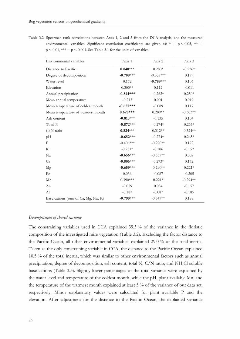
Bog vegetation reflects biogeochemical gradients
Table 3.2: Spearman rank correlations between Axes 1, 2 and 3 from the DCA analysis, and the measured environmental variables. Significant correlation coefficients are given as: * = p < 0.05, ** = p < 0.01, *** = p < 0.001. See Table 3.1 for the units of variables.
Environmental variables Axis 1 Axis 2 Axis 3
Distance to Pacific 0.848*** 0.280* -0.226* Degree of decomposition -0.789*** -0.357*** 0.179 Water level 0.172 -0.789*** 0.106 Elevation 0.300** 0.112 -0.0Annual precipitation -0.844*** -0.262* 0.250* Mean annual temperature -0.213 0.001 0.019 Mean temperature of coldest month -0.627*** -0.089 0.117 Mean temperature of warmest month 0.628*** 0.289** -0.303** Ash content -0.810*** -0.135 0.104 Total N -0.872*** -0.274* 0.265* C/N ratio 0.824*** 0.312** -0.324** pH -0.652*** -0.274* 0.265* P -0.406*** -0.290** 0.17K -0.251* -0.106 -0.1Na -0.656*** -0.337** 0.002 Ca -0.806*** -0.273* 0.172 Mg -0.659*** -0.290** 0.221* Fe 0.036 -0.087 -0.2Mn 0.390*** 0.221* -0.294**Zn -0.059 0.034 -0.157 Al -0.187 -0.087 -0.1Base cations (sum of Ca, Mg, Na, K) -0.790*** -0.347** 0.188
85
52
05
2
11
Decomposition of shared variance
The constraining variables used in CCA explained 39.5 % of the variance in the floristic composition of the investigated mire vegetation (Table 3.2). Excluding the factor distance to the Pacific Ocean, all other environmental variables explained 29.0 % of the total inertia. Taken as the only constraining variable in CCA, the distance to the Pacific Ocean explained 10.5 % of the total inertia, which was similar to other environmental factors such as annual precipitation, degree of decomposition, ash content, total N, C/N ratio, and NH4Cl soluble base cations (Table 3.3). Slightly lower percentages of the total variance were explained by the water level and temperature of the coldest month, while the pH, plant available Mn, and the temperature of the warmest month explained at least 5 % of the variance of our data set, respectively. Minor explanatory values were calculated for plant available P and the elevation. After adjustment for the distance to the Pacific Ocean, the explained variance
40
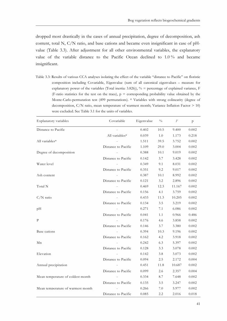
Bog vegetation reflects biogeochemical gradients
dropped most drastically in the cases of annual precipitation, degree of decomposition, ash content, total N, C/N ratio, and base cations and became even insignificant in case of pH-value (Table 3.3). After adjustment for all other environmental variables, the explanatory value of the variable distance to the Pacific Ocean declined to 1.0 % and became insignificant.
Table 3.3: Results of various CCA analyses isolating the effect of the variable “distance to Pacific” on floristic composition including Covariable, Eigenvalue (sum of all canonical eigenvalues – measure for explanatory power of the variables (Total inertia: 3.826)), % = percentage of explained variance, F (F-ratio statistics for the test on the trace), p = corresponding probability value obtained by the Monte-Carlo-permutation test (499 permutations). * Variables with strong colinearity (degree of decomposition, C/N ratio, mean temperature of warmest month; Variance Inflation Factor > 10) were excluded. See Table 3.1 for the units of variables.
41
Explanatory variables Covariable Eigenvalue % F p
Distance to Pacific - 0.402 10.5 9.400 0.002
All variables* 0.039 1.0 1.173 0.218All variables* - 1.511 39.5 3.752 0.002 Distance to Pacific 1.109 29.0 3.004 0.002Degree of decomposition - 0.388 10.1 9.019 0.002
Distance to Pacific 0.142 3.7 3.428 0.002Water level - 0.349 9.1 8.031 0.002 Distance to Pacific 0.351 9.2 9.017 0.002Ash content - 0.387 10.1 8.992 0.002 Distance to Pacific 0.121 3.2 2.896 0.002Total N - 0.469 12.3 11.167 0.002 Distance to Pacific 0.156 4.1 3.759 0.002C/N ratio - 0.433 11.3 10.205 0.002 Distance to Pacific 0.134 3.5 3.219 0.002pH - 0.271 7.1 6.0 0.002
Distance to Pacific 0.041 1.1 0.966 0.486P - 0.176 4.6 3.8 0.002 Distance to Pacific 0.146 3.7 3.380 0.002Base cations - 0.394 10.3 9.196 0.002 Distance to Pacific 0.162 4.2 3.918 0.002Mn - 0.242 6.3 5.3 0.002 Distance to Pacific 0.128 3.3 3.078 0.002Elevation - 0.142 3.8 3.0 0.002 Distance to Pacific 0.094 2.5 2.172 0.004Annual precipitation - 0.451 11.8 10.687 0.002
Distance to Pacific 0.099 2.6 2.357 0.004Mean temperature of coldest month - 0.334 8.7 7.648 0.002
Distance to Pacific 0.135 3.5 3.247 0.002Mean temperature of warmest month - 0.266 7.0 5.977 0.002 Distance to Pacific 0.085 2.2 2.016 0.018
86
58
97
73
Bog vegetation reflects biogeochemical gradients
All these figures indicate a high degree of shared variance between the distance to the Pacific Ocean and all of the biogeochemical and climatic variables mentioned above. The water level was the only environmental variable that did not show a noteworthy proportion of shared variance when using the distance to the Pacific Ocean as a covariable. This means that the water level had a significant effect on the floristic composition of the investigated bog complexes irrespective of their position along the Trans-Andean transect.
3.4 Discussion
Importance of climatic constraints
The striking differences in floristic composition of South Patagonian bog vegetation from west to east has been attributed to climate in past studies (Pisano 1983b, Boelcke et al. 1985, Blanco & de la Balze 2004), but climate is not sufficient to explain these differences in vegetation. In our study, biogeochemical variables that were related to the distance to the Pacific Ocean explained a high proportion of the variance. These results concur with Nicholson et al. (1996), who found that biogeochemical variables such as pH and surface water chemistry explained more of the floristic variation in North American peatlands than climatic variables. Also, Gignac et al. (1991) emphasized the importance of biogeochemical factors on species composition along a gradient of increasing distance to the Pacific Ocean in western Canada. Thus, in addition to the hygric and thermic component of the gradient, the shift in biogeochemical properties along the gradient should be considered, because these also affect the vegetation of these peatlands.
On the one hand, climatic factors directly affect plant growth and biogeochemical peat characteristics by controlling processes such as mineralization and decomposition rates (Aerts 2006), so that climatic factors should not be neglected while considering floristic composition of peatlands. On the other hand, the importance of precipitation that is considered to be the controlling factor of the floristic composition of South Patagonian peatland vegetation (e.g. Pisano 1983b) may be overestimated. Although the explanatory value of the annual precipitation was high in our study, the ground water level clearly separated our vegetation samples on both sides of the longitudinal gradient. This ground water level difference means that both edaphically wet and relatively dry sites occurred under hyper-humid Pacific as well as under less humid and more continental climatic conditions. Consequently, even in the hyperoceanic western parts of the gradient, water level conditions should be suitable for Sphagnum magellanicum, which is known to be a hummock species with a preference to drier site conditions (Hájková & Hájek 2004). However, this species
42
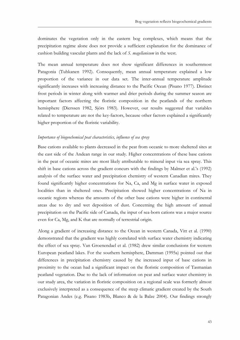
Bog vegetation reflects biogeochemical gradients
dominates the vegetation only in the eastern bog complexes, which means that the precipitation regime alone does not provide a sufficient explanation for the dominance of cushion building vascular plants and the lack of S. magellanicum in the west.
The mean annual temperature does not show significant differences in southernmost Patagonia (Tuhkanen 1992). Consequently, mean annual temperature explained a low proportion of the variance in our data set. The inter-annual temperature amplitude significantly increases with increasing distance to the Pacific Ocean (Pisano 1977). Distinct frost periods in winter along with warmer and drier periods during the summer season are important factors affecting the floristic composition in the peatlands of the northern hemisphere (Dierssen 1982, Sjörs 1983). However, our results suggested that variables related to temperature are not the key-factors, because other factors explained a significantly higher proportion of the floristic variability.
Importance of biogeochemical peat characteristics, influence of sea spray
Base cations available to plants decreased in the peat from oceanic to more sheltered sites at the east side of the Andean range in our study. Higher concentrations of these base cations in the peat of oceanic mires are most likely attributable to mineral input via sea spray. This shift in base cations across the gradient concurs with the findings by Malmer et al.’s (1992) analysis of the surface water and precipitation chemistry of western Canadian mires. They found significantly higher concentrations for Na, Ca, and Mg in surface water in exposed localities than in sheltered ones. Precipitation showed higher concentrations of Na in oceanic regions whereas the amounts of the other base cations were higher in continental areas due to dry and wet deposition of dust. Concerning the high amount of annual precipitation on the Pacific side of Canada, the input of sea-born cations was a major source even for Ca, Mg, and K that are normally of terrestrial origin.
Along a gradient of increasing distance to the Ocean in western Canada, Vitt et al. (1990) demonstrated that the gradient was highly correlated with surface water chemistry indicating the effect of sea spray. Van Groenendael et al. (1982) drew similar conclusions for western European peatland lakes. For the southern hemisphere, Damman (1995a) pointed out that differences in precipitation chemistry caused by the increased input of base cations in proximity to the ocean had a significant impact on the floristic composition of Tasmanian peatland vegetation. Due to the lack of information on peat and surface water chemistry in our study area, the variation in floristic composition on a regional scale was formerly almost exclusively interpreted as a consequence of the steep climatic gradient created by the South Patagonian Andes (e.g. Pisano 1983b, Blanco & de la Balze 2004). Our findings strongly
43
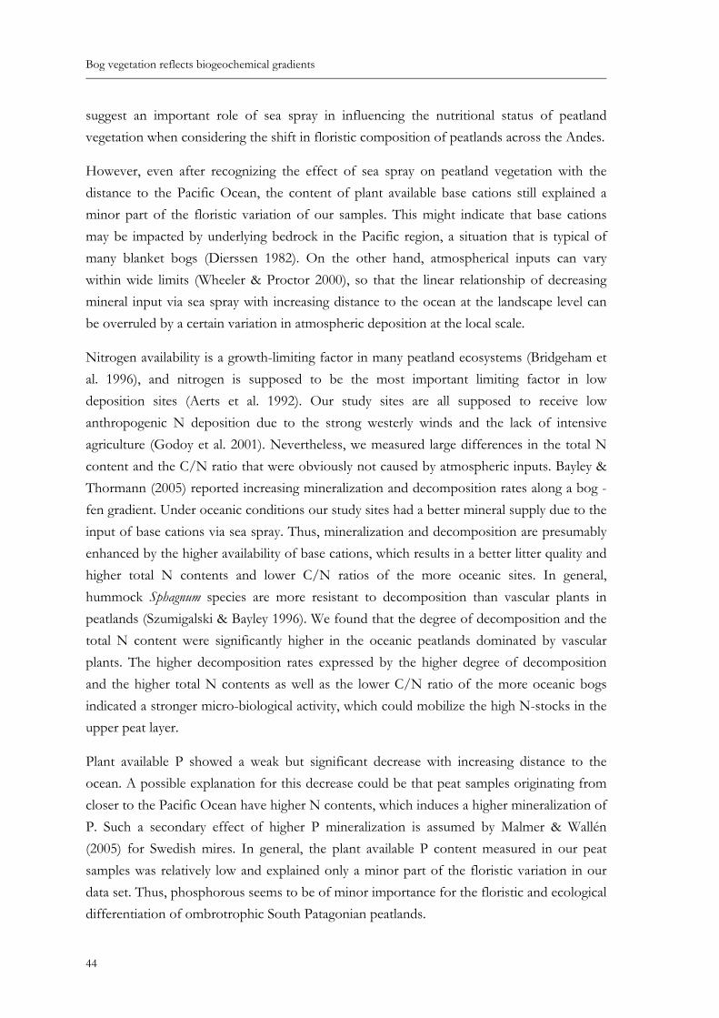
Bog vegetation reflects biogeochemical gradients
suggest an important role of sea spray in influencing the nutritional status of peatland vegetation when considering the shift in floristic composition of peatlands across the Andes.
However, even after recognizing the effect of sea spray on peatland vegetation with the distance to the Pacific Ocean, the content of plant available base cations still explained a minor part of the floristic variation of our samples. This might indicate that base cations may be impacted by underlying bedrock in the Pacific region, a situation that is typical of many blanket bogs (Dierssen 1982). On the other hand, atmospherical inputs can vary within wide limits (Wheeler & Proctor 2000), so that the linear relationship of decreasing mineral input via sea spray with increasing distance to the ocean at the landscape level can be overruled by a certain variation in atmospheric deposition at the local scale.
Nitrogen availability is a growth-limiting factor in many peatland ecosystems (Bridgeham et al. 1996), and nitrogen is supposed to be the most important limiting factor in low deposition sites (Aerts et al. 1992). Our study sites are all supposed to receive low anthropogenic N deposition due to the strong westerly winds and the lack of intensive agriculture (Godoy et al. 2001). Nevertheless, we measured large differences in the total N content and the C/N ratio that were obviously not caused by atmospheric inputs. Bayley & Thormann (2005) reported increasing mineralization and decomposition rates along a bog - fen gradient. Under oceanic conditions our study sites had a better mineral supply due to the input of base cations via sea spray. Thus, mineralization and decomposition are presumably enhanced by the higher availability of base cations, which results in a better litter quality and higher total N contents and lower C/N ratios of the more oceanic sites. In general, hummock Sphagnum species are more resistant to decomposition than vascular plants in peatlands (Szumigalski & Bayley 1996). We found that the degree of decomposition and the total N content were significantly higher in the oceanic peatlands dominated by vascular plants. The higher decomposition rates expressed by the higher degree of decomposition and the higher total N contents as well as the lower C/N ratio of the more oceanic bogs indicated a stronger micro-biological activity, which could mobilize the high N-stocks in the upper peat layer.
Plant available P showed a weak but significant decrease with increasing distance to the ocean. A possible explanation for this decrease could be that peat samples originating from closer to the Pacific Ocean have higher N contents, which induces a higher mineralization of P. Such a secondary effect of higher P mineralization is assumed by Malmer & Wallén (2005) for Swedish mires. In general, the plant available P content measured in our peat samples was relatively low and explained only a minor part of the floristic variation in our data set. Thus, phosphorous seems to be of minor importance for the floristic and ecological differentiation of ombrotrophic South Patagonian peatlands.
44
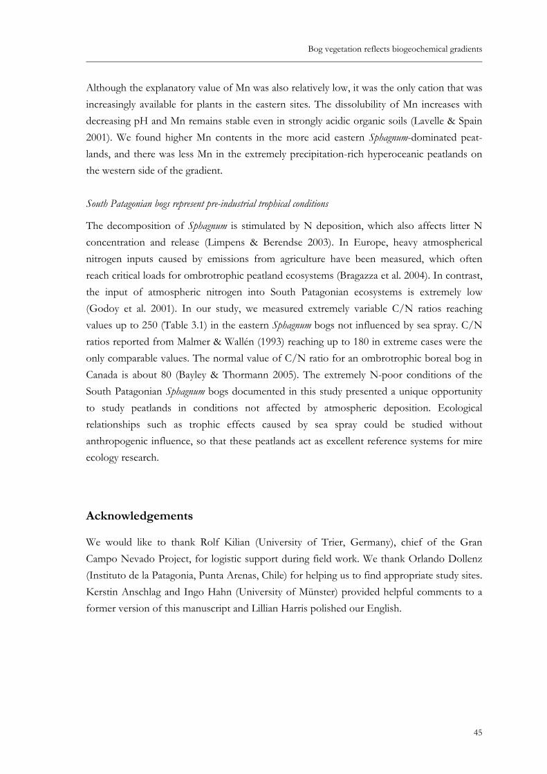
Bog vegetation reflects biogeochemical gradients
45
Although the explanatory value of Mn was also relatively low, it was the only cation that was increasingly available for plants in the eastern sites. The dissolubility of Mn increases with decreasing pH and Mn remains stable even in strongly acidic organic soils (Lavelle & Spain 2001). We found higher Mn contents in the more acid eastern Sphagnum-dominated peat-lands, and there was less Mn in the extremely precipitation-rich hyperoceanic peatlands on the western side of the gradient.
South Patagonian bogs represent pre-industrial trophical conditions
The decomposition of Sphagnum is stimulated by N deposition, which also affects litter N concentration and release (Limpens & Berendse 2003). In Europe, heavy atmospherical nitrogen inputs caused by emissions from agriculture have been measured, which often reach critical loads for ombrotrophic peatland ecosystems (Bragazza et al. 2004). In contrast, the input of atmospheric nitrogen into South Patagonian ecosystems is extremely low (Godoy et al. 2001). In our study, we measured extremely variable C/N ratios reaching values up to 250 (Table 3.1) in the eastern Sphagnum bogs not influenced by sea spray. C/N ratios reported from Malmer & Wallén (1993) reaching up to 180 in extreme cases were the only comparable values. The normal value of C/N ratio for an ombrotrophic boreal bog in Canada is about 80 (Bayley & Thormann 2005). The extremely N-poor conditions of the South Patagonian Sphagnum bogs documented in this study presented a unique opportunity to study peatlands in conditions not affected by atmospheric deposition. Ecological relationships such as trophic effects caused by sea spray could be studied without anthropogenic influence, so that these peatlands act as excellent reference systems for mire ecology research.
Acknowledgements
We would like to thank Rolf Kilian (University of Trier, Germany), chief of the Gran Campo Nevado Project, for logistic support during field work. We thank Orlando Dollenz (Instituto de la Patagonia, Punta Arenas, Chile) for helping us to find appropriate study sites. Kerstin Anschlag and Ingo Hahn (University of Münster) provided helpful comments to a former version of this manuscript and Lillian Harris polished our English.


Chapter 4
Patterns and gradients of diversity in South Patagonian ombrotrophic peat bogs
Till Kleinebecker*1; Norbert Hölzel1 & Andreas Vogel1
1Institute of Landscape Ecology, University of Münster, Robert-Koch-Straße 26, 48149 Münster, Germany
*Corresponding author
Submitted to Journal of Ecology
Abstract
1 Due to the lack of human impact, South Patagonian ombrotrophic bogs are particularly suitable to study diversity patterns under pristine environmental conditions and to relate them to ecological theory. With increasing distance from the Pacific Ocean, hyperoceanic blanket bogs built up by cushion-forming vascular plants are gradually replaced by Sphagnum-dominated bogs that exist exclusively east of the Andes. In a transition zone, both types intermingle. This study presents α-, β- and γ-diversity measurements of bog complexes along this transandine transect. Species richness and the response of functional groups were related to environmental variables by GRM and GAM modelling.
2 α-diversity significantly decreased from hyperoceanic cushion bogs via transitional Sphagnum-cushion mixed bogs to more continental Sphagnum bogs. Dissimilarity was highest in the transition zone. γ-diversity was lowest in Sphagnum bogs and similar in cushions bogs and bog complexes of the transition zone.
3 The GRM resulted in three major environmental variables (water level, total N, NH4Cl soluble Ca) altogether explaining a high degree of variance in species richness (r² = 0.76). Within the three particular bog types, GRM resulted in different models. In pure Sphagnum
47
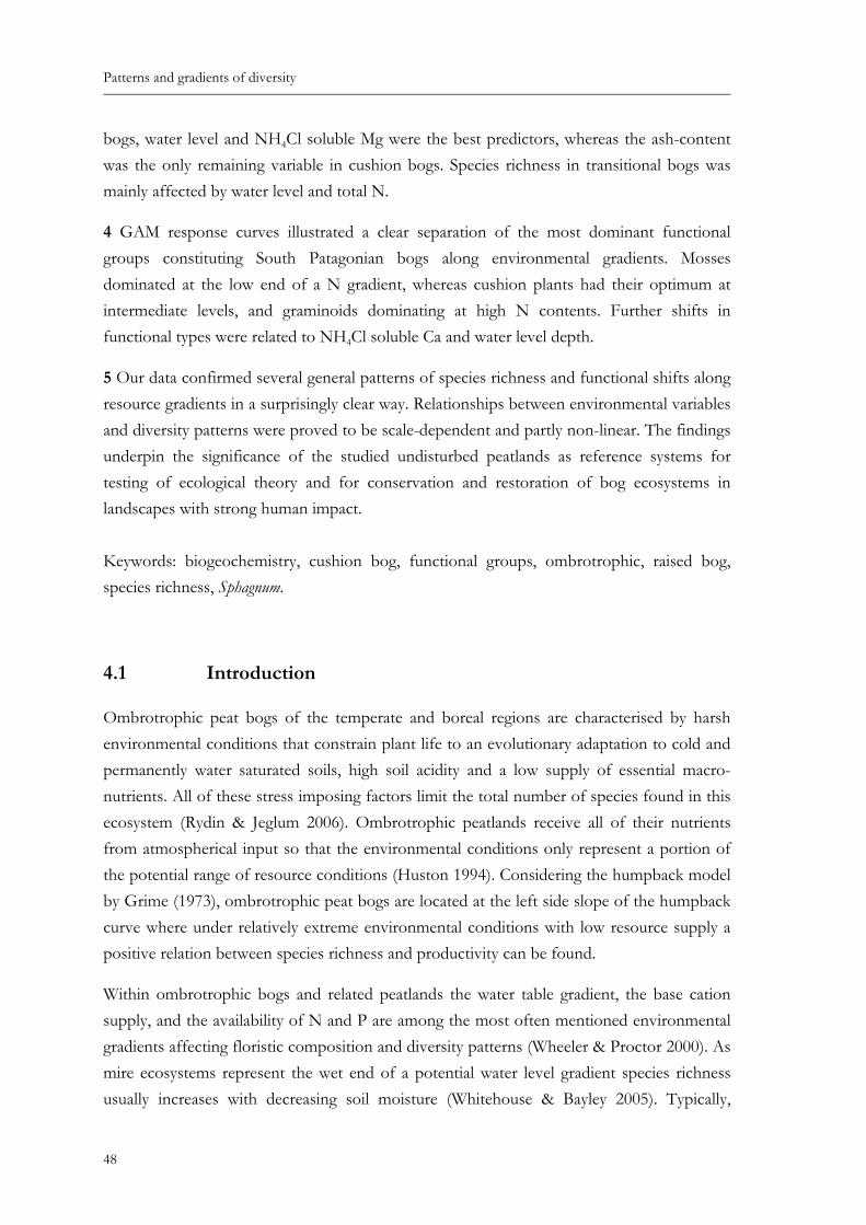
Patterns and gradients of diversity
bogs, water level and NH4Cl soluble Mg were the best predictors, whereas the ash-content was the only remaining variable in cushion bogs. Species richness in transitional bogs was mainly affected by water level and total N.
4 GAM response curves illustrated a clear separation of the most dominant functional groups constituting South Patagonian bogs along environmental gradients. Mosses dominated at the low end of a N gradient, whereas cushion plants had their optimum at intermediate levels, and graminoids dominating at high N contents. Further shifts in functional types were related to NH4Cl soluble Ca and water level depth.
5 Our data confirmed several general patterns of species richness and functional shifts along resource gradients in a surprisingly clear way. Relationships between environmental variables and diversity patterns were proved to be scale-dependent and partly non-linear. The findings underpin the significance of the studied undisturbed peatlands as reference systems for testing of ecological theory and for conservation and restoration of bog ecosystems in landscapes with strong human impact.
Keywords: biogeochemistry, cushion bog, functional groups, ombrotrophic, raised bog, species richness, Sphagnum.
4.1 Introduction
Ombrotrophic peat bogs of the temperate and boreal regions are characterised by harsh environmental conditions that constrain plant life to an evolutionary adaptation to cold and permanently water saturated soils, high soil acidity and a low supply of essential macro-nutrients. All of these stress imposing factors limit the total number of species found in this ecosystem (Rydin & Jeglum 2006). Ombrotrophic peatlands receive all of their nutrients from atmospherical input so that the environmental conditions only represent a portion of the potential range of resource conditions (Huston 1994). Considering the humpback model by Grime (1973), ombrotrophic peat bogs are located at the left side slope of the humpback curve where under relatively extreme environmental conditions with low resource supply a positive relation between species richness and productivity can be found.
Within ombrotrophic bogs and related peatlands the water table gradient, the base cation supply, and the availability of N and P are among the most often mentioned environmental gradients affecting floristic composition and diversity patterns (Wheeler & Proctor 2000). As mire ecosystems represent the wet end of a potential water level gradient species richness usually increases with decreasing soil moisture (Whitehouse & Bayley 2005). Typically,
48
Patterns and gradients of diversity
ombrotrophic bog ecosystems are characterized by a microtope zonation from wet pools and hollows to relatively dry hummocks which is often associated with a clear floristic gradient (Wheeler 1993). A decrease of species richness with increasing water table has not been explicitly described for bog vegetation so far, but can be presumed from phytosociological studies (e.g. Dierssen 1982, Wells 1996). Given the particularly acidic and nutrient poor conditions of ombrotrophic bogs, species richness was often found to be positively correlated with increasing soil-pH, base cation supply, and the availability of N and P (Vermeer & Berendse 1983, Glaser et al. 1990, Gunnarsson et al. 2000). In the extreme habitat of an ombrotrophic bog other factors such as dispersal limitation affecting diversity patterns (Pärtel & Zobel 2007) are of minor importance.
Diversity patterns along resource gradients are often more distinctly indicated by shifts in functional types than by changes in overall species-richness (Pausas & Austin 2001). This is probably particularly relevant in relatively species poor systems such as ombrotrophic bogs. E.g. Vitt & Chee (1990) and Weltzin et al. (2000) documented a divergent response of different functional groups to resource gradients in mires. On the contrary, Hájek et al. (2002) reported that cryptogams and vascular plants respond similarly to environmental gradients in spring fens.
The goal of this study is to describe the variation in plant species-richness and functional diversity in relation to environmental variables in three major types of ombrotrophic peat bogs along a Trans-Andean transect in southern Patagonia. In contrast to many bog regions in Europe and North America, this region provides the unique opportunity to study diversity patterns in ombrotrophic peat bogs under almost pristine conditions with nearly zero input of atmospherical pollutants (Galloway & Keene 1996, Godoy et al. 2001).
Ombrotrophic peatlands in South Patagonia show a clear floristic differentiation from pacific blanket bogs dominated by cushion-forming vascular plants to more continental Sphagnum-dominated raised bogs (Pisano 1983b, Boelcke et al. 1985). A third main type can be found in a transition zone where cushion bogs and Sphagnum bogs intermingle. Cushion forming of vascular plants in peatlands is a phenomenon that is only known from the southern hemisphere due to the gondwanic origin of the corresponding taxa (Dawson 1963). So far, information on patterns and gradients of diversity within this unique bog type and in comparison with Sphagnum-dominated raised bogs is lacking completely. The comparison of the three main ombrotrophic bog types in Patagonia allowed us to test the following hypothesis: (i) The three main bog types along the trans-andine gradient will differ in patterns of α-, β-, and γ-diversity. All these diversity measures are supposed to be highest in the ecotonal mixed type. (ii) According to the humpback model species richness will increase with increasing pH-value, base cations (Ca, Mg), nitrogen and phosphorous supply
49
Patterns and gradients of diversity
and decreasing anoxic stress due to lower soil water levels. (iii) Different functional groups will show a different response to the most important environmental gradients: Mosses and dwarf-shrubs will dominate under the poorest nutrient conditions whereas grasses and herbs will increase with improving nutrient supply.
To compare diversity patterns two intensively sampled complexes of each of the three main bog types were analysed with respect to α- , β-, and γ-diversity, Shannon-Wiener diversity and Evenness. Regression models (GRM, GAM) were used to assess the impact of environmental variables on species and functional diversity.
The vegetation of mires seemingly untouched by drainage and cultivation is mostly influenced by a diffuse sum of man-made environmental changes such as a lowering of the regional ground water level (Malmer & Wallén 1999) as well as acidification and nitrogen input due to atmospheric pollution (Bobbink et al. 1998, Lee 1998). Hidden patterns of underlying processes along environmental gradients (Wilson 2007) may be better observed in those pristine regions. Therefore, there is a need of data with pristine mire ecosystems that could also provide important information for conservation and restoration ecology (Couwenberg & Joosten 2005). The chance that South Patagonian mires offer for research and consequently for practical environmental conservation is largely unutilized, although ecological objectives could be studied under perfect conditions there.
This research was conducted to determine diversity patterns of South Patagonian ombrotrophic bogs and we wanted to put an emphasis on the following main objectives:
1. to provide a first description of plant diversity patterns of South Patagonian ombrotrophic peatlands with respect to the floristic gradient from pacific blanket bogs dominated by cushion-building vascular plants to more continental Sphagnum-dominated raised bogs,
2. to find out the major environmental variables affecting species richness at different spatial scales,
3. to find out if different functional groups show different responses to the most important environmental gradients,
4. to provide data of pristine peatland ecosystems to evaluate ecological theories such as the humpback model and to contribute to a better understanding of peatland ecosystems with respect to conservation and restoration ecology.
50
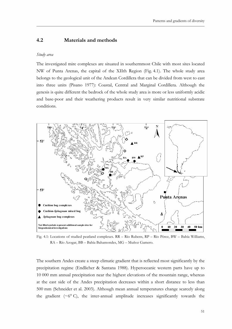
Patterns and gradients of diversity
4.2 Materials and methods
Study area
The investigated mire complexes are situated in southernmost Chile with most sites located NW of Punta Arenas, the capital of the XIIth Region (Fig. 4.1). The whole study area belongs to the geological unit of the Andean Cordillera that can be divided from west to east into three units (Pisano 1977): Coastal, Central and Marginal Cordillera. Although the genesis is quite different the bedrock of the whole study area is more or less uniformly acidic and base-poor and their weathering products result in very similar nutritional substrate conditions.
RR
RPBWRA
BBMG
Cushion bog complexes
Cushion-Sphagnum mixed bog
Sphagnum bog complexes
Not filled symbols represent additional sample sites for biogeochemical investigations
RR
RPBWRA
BBMG
Cushion bog complexes
Cushion-Sphagnum mixed bog
Sphagnum bog complexes
Not filled symbols represent additional sample sites for biogeochemical investigations
Fig. 4.1: Locations of studied peatland complexes. RR – Río Rubens, RP – Río Pérez, BW – Bahía Williams,RA – Río Azogar, BB – Bahía Bahamondes, MG – Muñoz Gamero.
The southern Andes create a steep climatic gradient that is reflected most significantly by the precipitation regime (Endlicher & Santana 1988). Hyperoceanic western parts have up to 10 000 mm annual precipitation near the highest elevations of the mountain range, whereas at the east side of the Andes precipitation decreases within a short distance to less than 500 mm (Schneider et al. 2003). Although mean annual temperatures change scarcely along the gradient (~6° C), the inter-annual amplitude increases significantly towards the
51
Patterns and gradients of diversity
continental parts (Pisano 1977). Consequently, regular frost events in winter as well as higher summer temperatures could be measured in the east, whereas the absence of frost periods and cooler summer temperatures characterize the hyperoceanic conditions in the west (Tuhkanen 1992).
This climatic gradient is well expressed by zonal vegetation types (Boelcke et al. 1985). From west to east, one can observe a clear zonation from coastal blanket bog, via cool temperate evergreen rainforest, and deciduous forest to dry Patagonian Steppe. Variation in ombrotrophic peatland vegetation also reflects the steep climatic gradient. With increasing distance from the Pacific Ocean, hyperoceanic blanket bogs built up by cushion-forming vascular plants such as Donatia fascicularis (Forster & Forster f.) and Astelia pumila (Forster f.) are gradually replaced by Sphagnum magellanicum (Brid. f.) that exists exclusively under more continental climatic conditions (Kleinebecker et al. 2007a). Both types intermingle within a transition zone.
Sampling and biogeochemical analysis
In a first subset, vegetation of six geographic regions was sampled with two regions per one of the three major mire types, respectively (Fig. 4.1): cushion bog, Sphagnum-cushion mixed bog and Sphagnum bog. Our westerly study areas represented cushion bog complexes and were situated at the entrance to the Lago Muños Gamero (MG, 52° 42´ S, 73° 14´ W) NW of the Gran Campo Nevado ice field and at the west bank of the Bahía Bahamondes (BB, 52° 47´ S, 72° 57´ W) at the east side of the ice field. The two study areas representing the transitional Sphagnum-cushion mixed type were located west of the Río Azogar (RA, 52° 32´ S, 72° 21´ W) and west of the Río Pinto at the north shore of the Bahía Williams (BW, 52° 31´ S, 72° 07´ W). The most continental and Sphagnum-dominated peatlands were situated near Estancia Kerber in the Río Rubens valley (RR, 52° 04´ S, 72° 02´ W) and north of the Estancia Skyring, east of the Río Pérez (RP, 52° 28´ S, 71° 54´ W). A total of 263 relevés were made and distributed almost equally over the six study areas. With a plot size of 1 m2 cover-abundance data was recorded following the Braun-Blanquet approach (Westhoff & van der Maarel 1973) and translated in a medial percentage cover scale. All recorded species were categorized into the following functional groups: cushion plants (CP), other herbs (H), other graminoids (G), mosses (M), liverworts (LW), lichens (Li), dwarf-shrubs (DS) and other woody plants (WP). The nomenclature of plant species mentioned in the text refers to the following sources: vascular plants Moore (1983) and mosses He (1998). The second subset contains 44 samples of the first subset and additional 38 samples of other peatland complexes (Fig. 4.1). For these 82 samples, additionally to the vegetation,
52
Patterns and gradients of diversity
volumetric mixed surface samples of peat were taken in a depth of 5 - 10 cm. Samples were dried at 50° C and screened through a sieve with 2 mm mesh wire. The following chemical analyses were carried out in the laboratory: Total contents of C and N: Element autoanalyzer (CARLO ERBER NA 1500); ash-content: ashing overnight in a muffle furnace at 550° C; CAL-soluble P (Schüller 1969): photometrical measurement (PERKIN ELMER) with 578 nm; extraction of exchangeable fractions of K, Na, Ca, Mg with NH4Cl (Meiwes et al. 1984): determination with an AAS (PERKIN ELMER). As additional ecological information the edaphic moisture regime was described using an ordinal scale reaching from 0 = ground water at soil surface to 7 = groundwater > 40 cm below soil surface by digging a hole. It has to be considered that the water table is variable and can show large seasonal differences (Wheeler & Proctor 2000). However, in previous studies this estimation method provided reasonable results (Kleinebecker et al. 2007a, b).
Data analysis
α-diversity was measured as the average number of species per sample for each of the six geographic regions. The Shannon-Wiener diversity index and the Evenness were calculated to incorporate the relative abundance of the different species. β-diversity as a measure of among site variability was expressed by the Bray Curtis dissimilarity index. γ-diversity was estimated as total species richness calculated over all samples for each of the six study areas. γ-diversity was also calculated for the differentiated functional groups.
A General Regression Model (GRM) with backward elimination was used to find the best predictors of species richness among the measured environmental variables. When variables were strongly inter-correlated, the variable with the best correlation with α-diversity was chosen. Functional group response curves to the best predicting environmental variables based on a cover matrix were created by generalized additive models (GAMs, Hastie & Tibshirani 1990) using Poisson distribution. The fitted model was compared to the null model, and only life forms with significant response were considered. Smooth term complexity was selected using the Akaike information criterion (AIC, Lepš & Šmilauer 2003).
Not specified taxa (mostly liverworts) were not included in calculation of diversity patterns, but were included with their cover values in the GAM modelling. For all statistical calculations variables were log-transformed. SPSS 11.0 software was used for common correlation analysis, STATISTICA 7.1 software was used for calculating the GRM and the CANOCO 4.5 software package (ter Braak & Šmilauer 2002) was used for GAM modelling.
53
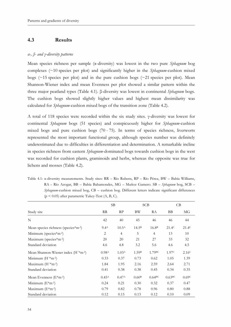
Patterns and gradients of diversity
4.3 Results
α-, β- and γ-diversity patterns
Mean species richness per sample (α-diversity) was lowest in the two pure Sphagnum bog complexes (~10 species per plot) and significantly higher in the Sphagnum-cushion mixed bogs (~15 species per plot) and in the pure cushion bogs (~21 species per plot). Mean Shannon-Wiener index and mean Evenness per plot showed a similar pattern within the three major peatland types (Table 4.1). β-diversity was lowest in continental Sphagnum bogs. The cushion bogs showed slightly higher values and highest mean dissimilarity was calculated for Sphagnum-cushion mixed bogs of the transition zone (Table 4.2).
A total of 118 species were recorded within the six study sites. γ-diversity was lowest for continental Sphagnum bogs (51 species) and conspicuously higher for Sphagnum-cushion mixed bogs and pure cushion bogs (70 - 75). In terms of species richness, liverworts represented the most important functional group, although species number was definitely underestimated due to difficulties in differentiation and determination. A remarkable incline in species richness from eastern Sphagnum-dominated bogs towards cushion bogs in the west was recorded for cushion plants, graminoids and herbs, whereas the opposite was true for lichens and mosses (Table 4.2).
Table 4.1: α-diversity measurements. Study sites: RR – Río Rubens, RP – Río Pérez, BW – Bahía Williams, RA – Río Azogar, BB – Bahía Bahamondes, MG – Muñoz Gamero. SB – Sphagnum bog, SCB – Sphagnum-cushion mixed bog, CB – cushion bog. Different letters indicate significant differences (p < 0.05) after parametric Tukey-Test (A, B, C).
SB SCB CB
Study site RR RP BW RA BB MG
N 42 40 45 46 46 44
Mean species richness (species*m-2) 9.4A 10.5A 14.5B 16.8B 21.4C 21.4C Minimum (species*m-2) 2 4 5 4 13 10 Maximum (species*m-2) 20 20 21 27 33 32 Standard deviation 4.6 4.8 3.2 5.6 4.6 4.5
Mean Shannon-Wiener index (H´*m-2) 0.98A 1.03A 1.59B 1.79BC 1.97C 2.16C Minimum (H´*m-2) 0.33 0.37 0.73 0.62 1.05 1.39 Maximum (H´*m-2) 1.84 1.95 2.16 2.59 2.64 2.71 Standard deviation 0.41 0.38 0.38 0.45 0.34 0.35
Mean Evenness (E*m-2) 0.45A 0.47A 0.60B 0.64BC 0.63BC 0.69C Minimum (E*m-2) 0.24 0.21 0.30 0.32 0.37 0.47 Maximum (E*m-2) 0.79 0.82 0.78 0.96 0.80 0.88 Standard deviation 0.12 0.15 0.13 0.12 0.10 0.09
54
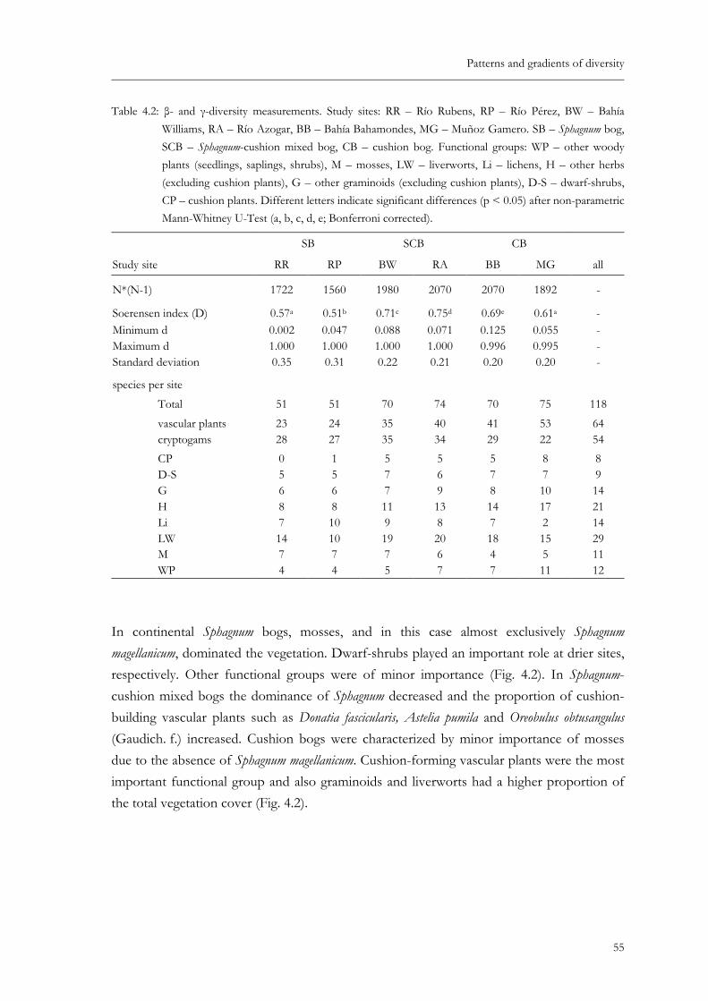
Patterns and gradients of diversity
Table 4.2: β- and γ-diversity measurements. Study sites: RR – Río Rubens, RP – Río Pérez, BW – Bahía Williams, RA – Río Azogar, BB – Bahía Bahamondes, MG – Muñoz Gamero. SB – Sphagnum bog, SCB – Sphagnum-cushion mixed bog, CB – cushion bog. Functional groups: WP – other woody plants (seedlings, saplings, shrubs), M – mosses, LW – liverworts, Li – lichens, H – other herbs (excluding cushion plants), G – other graminoids (excluding cushion plants), D-S – dwarf-shrubs, CP – cushion plants. Different letters indicate significant differences (p < 0.05) after non-parametric Mann-Whitney U-Test (a, b, c, d, e; Bonferroni corrected).
SB SCB CB
Study site RR RP BW RA BB MG all
N*(N-1) 1722 1560 1980 2070 2070 1892 -
Soerensen index (D) 0.57a 0.51b 0.71c 0.75d 0.69e 0.61a - Minimum d 0.002 0.047 0.088 0.071 0.125 0.055 - Maximum d 1.000 1.000 1.000 1.000 0.996 0.995 - Standard deviation 0.35 0.31 0.22 0.21 0.20 0.20 -
species per site
Total 51 51 70 74 70 75 118
vascular plants 23 24 35 40 41 53 64 cryptogams 28 27 35 34 29 22 54 CP 0 1 5 5 5 8 8 D-S 5 5 7 6 7 7 9 G 6 6 7 9 8 10 14 H 8 8 11 13 14 17 21 Li 7 10 9 8 7 2 14 LW 14 10 19 20 18 15 29 M 7 7 7 6 4 5 11 WP 4 4 5 7 7 11 12
In continental Sphagnum bogs, mosses, and in this case almost exclusively Sphagnum magellanicum, dominated the vegetation. Dwarf-shrubs played an important role at drier sites, respectively. Other functional groups were of minor importance (Fig. 4.2). In Sphagnum-cushion mixed bogs the dominance of Sphagnum decreased and the proportion of cushion-building vascular plants such as Donatia fascicularis, Astelia pumila and Oreobulus obtusangulus (Gaudich. f.) increased. Cushion bogs were characterized by minor importance of mosses due to the absence of Sphagnum magellanicum. Cushion-forming vascular plants were the most important functional group and also graminoids and liverworts had a higher proportion of the total vegetation cover (Fig. 4.2).
55
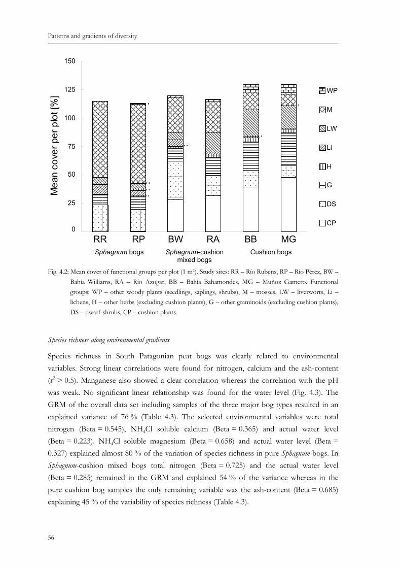
Patterns and gradients of diversity
150
CP
DS
G
H
Li
LW
M
WP 125
Mea
nco
ver p
erpl
ot[%
]
100
75
50
25
0RR RP BW RA BB MG Sphagnum bogs Sphagnum-cushion
mixed bogs Cushion bogs
Fig. 4.2: Mean cover of functional groups per plot (1 m2). Study sites: RR – Río Rubens, RP – Río Pérez, BW – Bahía Williams, RA – Río Azogar, BB – Bahía Bahamondes, MG – Muñoz Gamero. Functional groups: WP – other woody plants (seedlings, saplings, shrubs), M – mosses, LW – liverworts, Li – lichens, H – other herbs (excluding cushion plants), G – other graminoids (excluding cushion plants), DS – dwarf-shrubs, CP – cushion plants.
Species richness along environmental gradients
Species richness in South Patagonian peat bogs was clearly related to environmental variables. Strong linear correlations were found for nitrogen, calcium and the ash-content (r2 > 0.5). Manganese also showed a clear correlation whereas the correlation with the pH was weak. No significant linear relationship was found for the water level (Fig. 4.3). The GRM of the overall data set including samples of the three major bog types resulted in an explained variance of 76 % (Table 4.3). The selected environmental variables were total nitrogen (Beta = 0.545), NH4Cl soluble calcium (Beta = 0.365) and actual water level (Beta = 0.223). NH4Cl soluble magnesium (Beta = 0.658) and actual water level (Beta = 0.327) explained almost 80 % of the variation of species richness in pure Sphagnum bogs. In Sphagnum-cushion mixed bogs total nitrogen (Beta = 0.725) and the actual water level (Beta = 0.285) remained in the GRM and explained 54 % of the variance whereas in the pure cushion bog samples the only remaining variable was the ash-content (Beta = 0.685) explaining 45 % of the variability of species richness (Table 4.3).
56
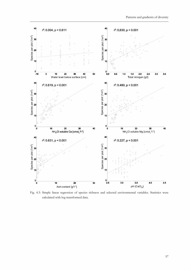
Patterns and gradients of diversity
3.53.02.52.01.51.00.50.0
40
30
20
10
050403020100-10
40
30
20
10
0
403020100
40
30
20
10
0403020100
40
30
20
10
0
3020100
40
30
20
10
04.54.03.53.02.5
40
30
20
10
0
3.53.02.52.01.51.00.50.0
40
30
20
10
050403020100-10
40
30
20
10
0
403020100
40
30
20
10
0403020100
40
30
20
10
0
3020100
40
30
20
10
04.54.03.53.02.5
40
30
20
10
0
r2: 0,630, p < 0.001r2: 0.004, p = 0.611
r2: 0.480, p < 0.001r2: 0.619, p < 0.001
r2: 0.227, p < 0.001r2: 0.631, p < 0.001
T3.53.02.52.01.51.00.50.0
40
30
20
10
050403020100-10
40
30
20
10
0
4Cl soluble Ca [cmolc*l-1]403020100
40
30
20
10
0403020100
40
30
20
10
0
3020100
40
30
20
10
0
pH (CaCl 2)4.54.03.53.02.5
40
30
20
10
0
Total nit rogen [g/l]3.53.02.52.01.51.00.50.0
Spe
cies
perp
lot(
1m2 )
40
30
20
10
0
Water level below surface [cm]50403020100-10
Spe
cies
perp
lot(
1m2 )
40
30
20
10
0
NH4Cl soluble Ca [cmolc*l-1]403020100
Spe
cies
perp
lot(
1m2 )
40
30
20
10
0
NH4Cl soluble Mg [cmolc*l-1]403020100
Spe
cies
perp
lot(
1m2 )
40
30
20
10
0
Ash-content [g*l-1]3020100
Spe
cies
perp
lot(
1m2 )
40
30
20
10
0
2)4.54.03.53.02.5
Spe
cies
perp
lot(
1m2 )
40
30
20
10
0
r2: 0,630, p < 0.001r2: 0.004, p = 0.611
r2: 0.480, p < 0.001r2: 0.619, p < 0.001
r2: 0.227, p < 0.001r2: 0.631, p < 0.001
r2: 0,630, p < 0.001r2: 0.004, p = 0.611
r2: 0.480, p < 0.001r2: 0.619, p < 0.001
r2: 0.227, p < 0.001r2: 0.631, p < 0.001
Fig. 4.3: Simple linear regression of species richness and selected environmental variables. Statistics were calculated with log-transformed data.
57
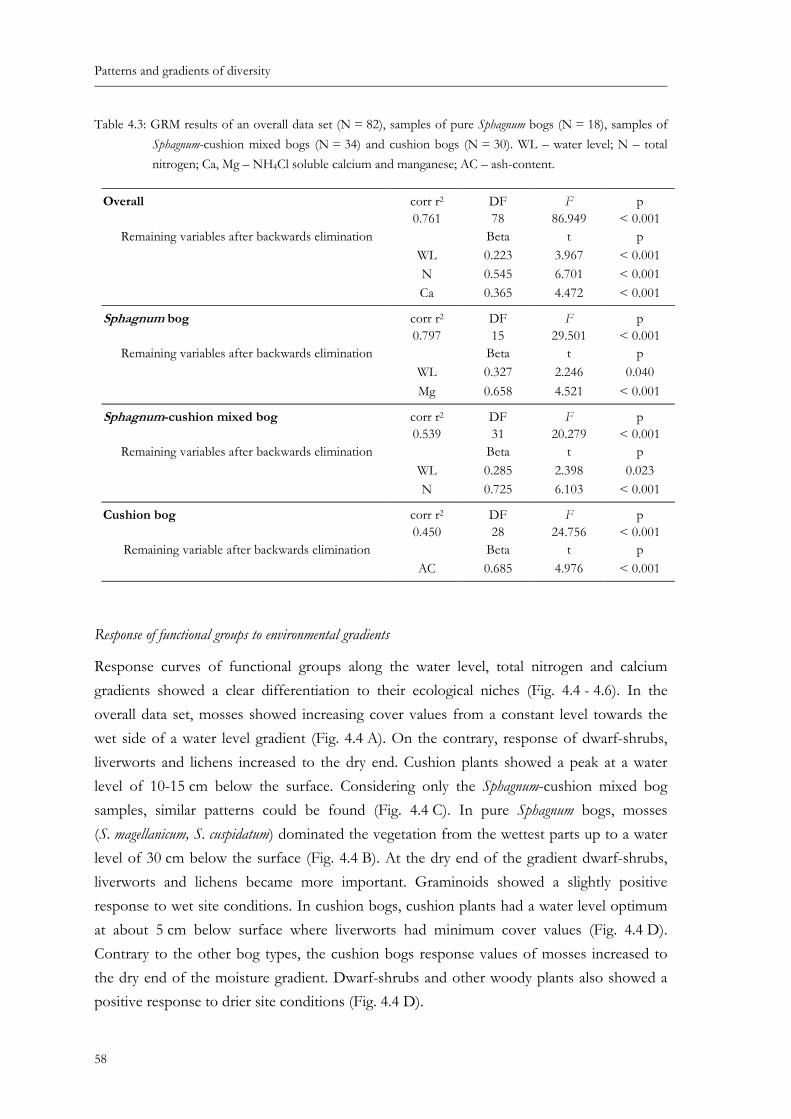
Patterns and gradients of diversity
Table 4.3: GRM results of an overall data set (N = 82), samples of pure Sphagnum bogs (N = 18), samples of Sphagnum-cushion mixed bogs (N = 34) and cushion bogs (N = 30). WL – water level; N – total nitrogen; Ca, Mg – NH4Cl soluble calcium and manganese; AC – ash-content.
Overall corr r2 DF F p 0.761 78 86.949 < 0.001
Remaining variables after backwards elimination Beta t p
WL 0.223 3.967 < 0.001 N 0.545 6.701 < 0.001 Ca 0.365 4.472 < 0.001
Sphagnum bog corr r2 DF F p 0.797 15 29.501 < 0.001
Remaining variables after backwards elimination Beta t p
WL 0.327 2.246 0.040 Mg 0.658 4.521 < 0.001
Sphagnum-cushion mixed bog corr r2 DF F p 0.539 31 20.279 < 0.001
Remaining variables after backwards elimination Beta t p
WL 0.285 2.398 0.023 N 0.725 6.103 < 0.001
Cushion bog corr r2 DF F p 0.450 28 24.756 < 0.001
Remaining variable after backwards elimination Beta t p AC 0.685 4.976 < 0.001
Response of functional groups to environmental gradients
Response curves of functional groups along the water level, total nitrogen and calcium gradients showed a clear differentiation to their ecological niches (Fig. 4.4 - 4.6). In the overall data set, mosses showed increasing cover values from a constant level towards the wet side of a water level gradient (Fig. 4.4 A). On the contrary, response of dwarf-shrubs, liverworts and lichens increased to the dry end. Cushion plants showed a peak at a water level of 10-15 cm below the surface. Considering only the Sphagnum-cushion mixed bog samples, similar patterns could be found (Fig. 4.4 C). In pure Sphagnum bogs, mosses (S. magellanicum, S. cuspidatum) dominated the vegetation from the wettest parts up to a water level of 30 cm below the surface (Fig. 4.4 B). At the dry end of the gradient dwarf-shrubs, liverworts and lichens became more important. Graminoids showed a slightly positive response to wet site conditions. In cushion bogs, cushion plants had a water level optimum at about 5 cm below surface where liverworts had minimum cover values (Fig. 4.4 D). Contrary to the other bog types, the cushion bogs response values of mosses increased to the dry end of the moisture gradient. Dwarf-shrubs and other woody plants also showed a positive response to drier site conditions (Fig. 4.4 D).
58
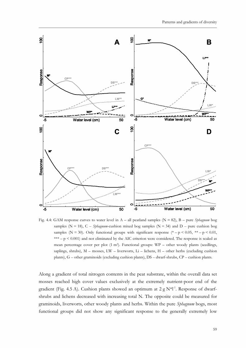
Patterns and gradients of diversity
-5 50Water level (cm)
01
Res
pons
e
CP***DS***
Li***
LW**
M*
WP*
-5 50Water level (cm)
01
Res
pons
e
CP***DS***
Li***
LW**
M*
WP*
-5 50Water level (cm)
01
Res
pons
e
DS***
G*
Li***
LW*
M*
WP**
-5 50Water level (cm)
01
Res
pons
e
DS***
G*
Li***
LW*
M*
WP**
-5 50Water level (cm)
010
0R
espo
nse
CP*** DS***
LW***
M*
-5 50Water level (cm)
010
0R
espo
nse
CP*** DS***
LW***
M*
-5 50Water level (cm)
010
0R
espo
nse
CP***
DS***
LW*
M*
WP**
-5 50Water level (cm)
010
0R
espo
nse
CP***
DS***
LW*
M*
WP**
A B
C D
-5 50Water level (cm)
01
Res
pons
e
CP***DS***
Li***
LW**
M*
WP*
-5 50Water level (cm)
01
Res
pons
e
CP***DS***
Li***
LW**
M*
WP*
-5 50Water level (cm)
01
Res
pons
e
DS***
G*
Li***
LW*
M*
WP**
-5 50Water level (cm)
01
Res
pons
e
DS***
G*
Li***
LW*
M*
WP**
-5 50Water level (cm)
010
0R
espo
nse
CP*** DS***
LW***
M*
-5 50Water level (cm)
010
0R
espo
nse
CP*** DS***
LW***
M*
-5 50Water level (cm)
010
0R
espo
nse
CP***
DS***
LW*
M*
WP**
-5 50Water level (cm)
010
0R
espo
nse
CP***
DS***
LW*
M*
WP**
A B
C D0000000000000000
Fig. 4.4: GAM response curves to water level in A – all peatland samples (N = 82), B – pure Sphagnum bog samples (N = 18), C – Sphagnum-cushion mixed bog samples (N = 34) and D – pure cushion bog samples (N = 30). Only functional groups with significant response (* – p < 0.05, ** – p < 0.01, *** – p < 0.001) and not eliminated by the AIC criterion were considered. The response is scaled as mean percentage cover per plot (1 m2). Functional groups: WP – other woody plants (seedlings, saplings, shrubs), M – mosses, LW – liverworts, Li – lichens, H – other herbs (excluding cushion plants), G – other graminoids (excluding cushion plants), DS – dwarf-shrubs, CP – cushion plants.
Along a gradient of total nitrogen contents in the peat substrate, within the overall data set mosses reached high cover values exclusively at the extremely nutrient-poor end of the gradient (Fig. 4.5 A). Cushion plants showed an optimum at 2 g N*l-1. Response of dwarf-shrubs and lichens decreased with increasing total N. The opposite could be measured for graminoids, liverworts, other woody plants and herbs. Within the pure Sphagnum bogs, most functional groups did not show any significant response to the generally extremely low
59
Patterns and gradients of diversity
nitrogen content (Fig. 4.5 B). In the Sphagnum-cushion mixed bog samples, a clear separation of the mosses at the nitrogen-poor end of the gradient and the cushion plants on the other side could be found (Fig. 4.5 C). In the pure cushion bogs, graminoids dominated on nitrogen-rich sites whereas the cushion plants occupied the other end of the gradient. Other
Fig. 4.5: GAM response curves to total nitrogen content (Nt, g*l-1) in A – all peatland samples (N =
00000000
herbs showed increasing response values with increasing total nitrogen (Fig. 4.5 D).
82), B – pure Sphagnum bog samples (N = 18), C – Sphagnum-cushion mixed bog samples (N = 34) and D –
0 5
01
Res
pons
e CP***
DS*
G***
H***Li**
LW**
M***
WP***
Nt [g*l-1]0 5
01
Res
pons
e CP***
DS*
G***
H***Li**
LW**
M***
WP***
Nt [g*l-1] 0 0Nt [g*l-1]
01
Res
pons
e
LW**
0 0Nt [g*l-1]
01
Res
pons
e
LW**
0 1.5Nt [g*l-1]
010
0R
espo
nse
CP***
H**
M***
0 1.5Nt [g*l-1]
010
0R
espo
nse
CP***
H**
M***
0 5Nt [g*l-1]
010
0R
espo
nse
CP*
H*
0 5Nt [g*l-1]
010
0R
espo
nse
CP*
G**
H*
A B
C D
.6.6.6.6
00000000
pure cushion bog samples (N = 30). Only functional groups with significant response (* – p < 0.05, ** – p < 0.01, *** – p < 0.001) and not eliminated by the AIC criterion were considered. The response is scaled in mean percentage cover per plot (1 m2). Functional groups: WP – other woody plants (seedlings, saplings, shrubs), M – mosses, LW – liverworts, Li – lichens, H – other herbs (excluding cushion plants), G – other graminoids (excluding cushion plants), DS – dwarf-shrubs, CP – cushion plants. Be aware of different scaling of the x-axes!
60
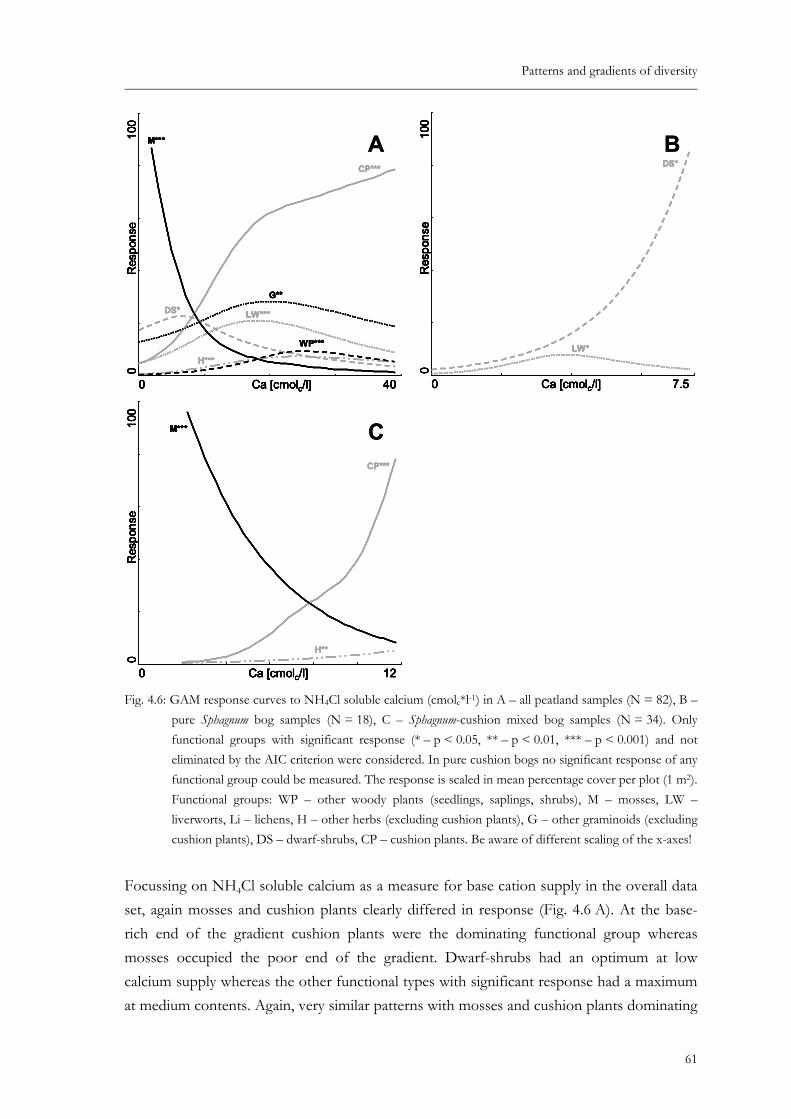
Patterns and gradients of diversity
0 40Ca [cmolc/l]
01
Res
pons
e
CP***
DS*G**
H***
LW***
M***
WP***
0 40Ca [cmolc/l]
01
Res
pons
e
CP***
DS*G**
H***
LW***
M***
WP***
0 7Ca [cmolc/l]
01
Res
pons
e
DS*
LW*
0 7Ca [cmolc/l]
01
Res
pons
e
DS*
LW*
0 12Ca [cmolc/l]
010
0R
espo
nse
CP***
H**
M***
0 12Ca [cmolc/l]
010
0R
espo
nse
CP***
H**
M***
A B
C
0 40Ca [cmolc/l]
01
Res
pons
e
CP***
DS*G**
H***
LW***
M***
WP***
0 40Ca [cmolc/l]
01
Res
pons
e
CP***
DS*G**
H***
LW***
M***
WP***
0 7Ca [cmolc/l]
01
Res
pons
e
DS*
LW*
0 7Ca [cmolc/l]
01
Res
pons
e
DS*
LW*
0 12Ca [cmolc/l]
010
0R
espo
nse
CP***
H**
M***
0 12Ca [cmolc/l]
010
0R
espo
nse
CP***
H**
M***
0 40Ca [cmolc/l]
01
Res
pons
e
CP***
DS*G**
H***
LW***
M***
WP***
0 40Ca [cmolc/l]
01
Res
pons
e
CP***
DS*G**
H***
LW***
M***
WP***
0 7Ca [cmolc/l]
01
Res
pons
e
DS*
LW*
0 7Ca [cmolc/l]
01
Res
pons
e
DS*
LW*
0 12Ca [cmolc/l]
010
0R
espo
nse
CP***
H**
M***
0 12Ca [cmolc/l]
010
0R
espo
nse
CP***
H**
M***
A B
C
.5
00
.5
00
.5
00
.5
00
.5
00
.5
00000000000000
Fig. 4.6: n mixed bog samples (N = 34). Only
functional groups with significant response (* – p < 0.05, ** – p < 0.01, *** – p < 0.001) and not
Focussset, agarich end of the gradient cushion plants were the dominating functional group whereas
GAM response curves to NH4Cl soluble calcium (cmolc*l-1) in A – all peatland samples (N = 82), B – pure Sphagnum bog samples (N = 18), C – Sphagnum-cushio
eliminated by the AIC criterion were considered. In pure cushion bogs no significant response of any functional group could be measured. The response is scaled in mean percentage cover per plot (1 m2). Functional groups: WP – other woody plants (seedlings, saplings, shrubs), M – mosses, LW – liverworts, Li – lichens, H – other herbs (excluding cushion plants), G – other graminoids (excluding cushion plants), DS – dwarf-shrubs, CP – cushion plants. Be aware of different scaling of the x-axes!
ing on NH4Cl soluble calcium as a measure for base cation supply in the overall data in mosses and cushion plants clearly differed in response (Fig. 4.6 A). At the base-
mosses occupied the poor end of the gradient. Dwarf-shrubs had an optimum at low calcium supply whereas the other functional types with significant response had a maximum at medium contents. Again, very similar patterns with mosses and cushion plants dominating
61
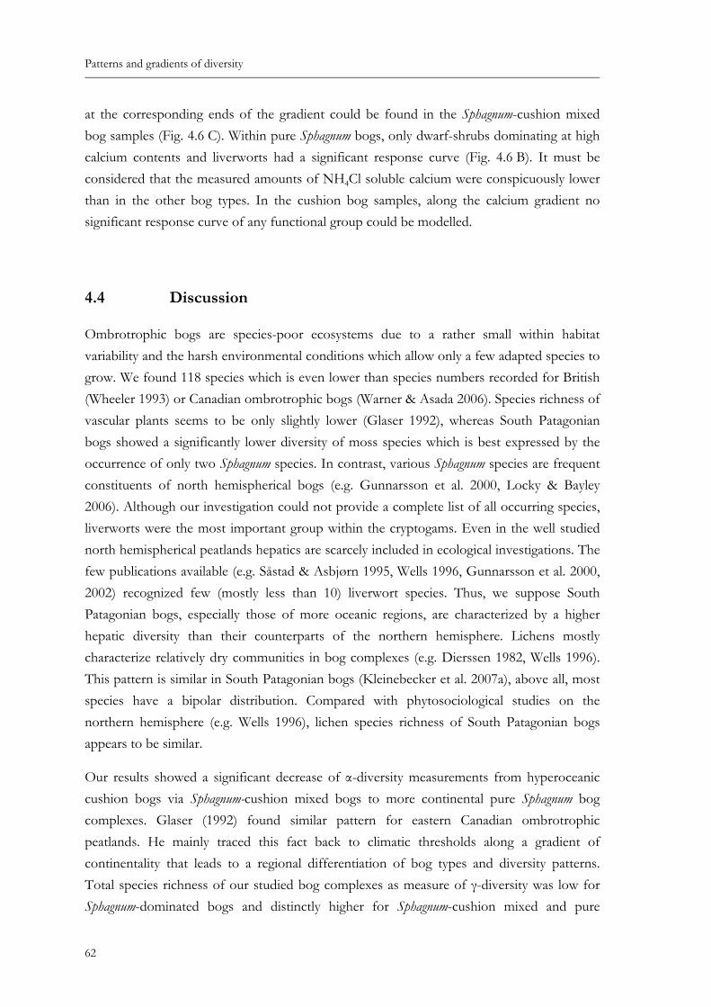
Patterns and gradients of diversity
at the corresponding ends of the gradient could be found in the Sphagnum-cushion mixed bog samples (Fig. 4.6 C). Within pure Sphagnum bogs, only dwarf-shrubs dominating at high calcium contents and liverworts had a significant response curve (Fig. 4.6 B). It must be considered that the measured amounts of NH4Cl soluble calcium were conspicuously lower than in the other bog types. In the cushion bog samples, along the calcium gradient no significant response curve of any functional group could be modelled.
4.4 Discussion
Ombrotrophic bogs are species-poor ecosystems due to a rather small within habitat d ental conditions which allow only a few adapted species to
grow. We found 118 species which is even lower than species numbers recorded for British
agnum-cushion mixed bogs to more continental pure Sphagnum bog complexes. Glaser (1992) found similar pattern for eastern Canadian ombrotrophic
variability an the harsh environm
(Wheeler 1993) or Canadian ombrotrophic bogs (Warner & Asada 2006). Species richness of vascular plants seems to be only slightly lower (Glaser 1992), whereas South Patagonian bogs showed a significantly lower diversity of moss species which is best expressed by the occurrence of only two Sphagnum species. In contrast, various Sphagnum species are frequent constituents of north hemispherical bogs (e.g. Gunnarsson et al. 2000, Locky & Bayley 2006). Although our investigation could not provide a complete list of all occurring species, liverworts were the most important group within the cryptogams. Even in the well studied north hemispherical peatlands hepatics are scarcely included in ecological investigations. The few publications available (e.g. Såstad & Asbjørn 1995, Wells 1996, Gunnarsson et al. 2000, 2002) recognized few (mostly less than 10) liverwort species. Thus, we suppose South Patagonian bogs, especially those of more oceanic regions, are characterized by a higher hepatic diversity than their counterparts of the northern hemisphere. Lichens mostly characterize relatively dry communities in bog complexes (e.g. Dierssen 1982, Wells 1996). This pattern is similar in South Patagonian bogs (Kleinebecker et al. 2007a), above all, most species have a bipolar distribution. Compared with phytosociological studies on the northern hemisphere (e.g. Wells 1996), lichen species richness of South Patagonian bogs appears to be similar.
Our results showed a significant decrease of α-diversity measurements from hyperoceanic cushion bogs via Sph
peatlands. He mainly traced this fact back to climatic thresholds along a gradient of continentality that leads to a regional differentiation of bog types and diversity patterns. Total species richness of our studied bog complexes as measure of γ-diversity was low for Sphagnum-dominated bogs and distinctly higher for Sphagnum-cushion mixed and pure
62
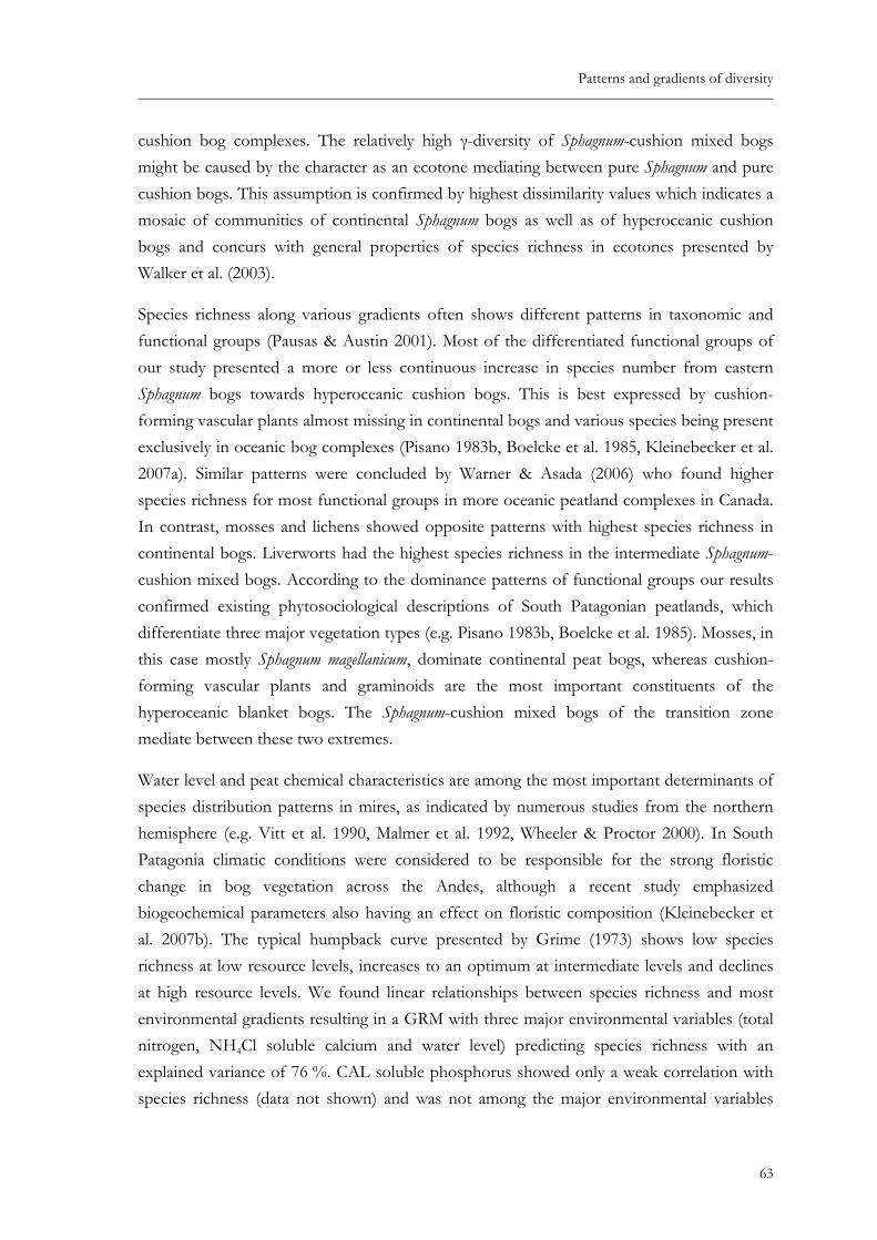
Patterns and gradients of diversity
cushion bog complexes. The relatively high γ-diversity of Sphagnum-cushion mixed bogs might be caused by the character as an ecotone mediating between pure Sphagnum and pure cushion bogs. This assumption is confirmed by highest dissimilarity values which indicates a mosaic of communities of continental Sphagnum bogs as well as of hyperoceanic cushion bogs and concurs with general properties of species richness in ecotones presented by Walker et al. (2003).
Species richness along various gradients often shows different patterns in taxonomic and functional groups (Pausas & Austin 2001). Most of the differentiated functional groups of our study presented a more or less continuous increase in species number from eastern
as indicated by numerous studies from the northern hemisphere (e.g. Vitt et al. 1990, Malmer et al. 1992, Wheeler & Proctor 2000). In South
Sphagnum bogs towards hyperoceanic cushion bogs. This is best expressed by cushion-forming vascular plants almost missing in continental bogs and various species being present exclusively in oceanic bog complexes (Pisano 1983b, Boelcke et al. 1985, Kleinebecker et al. 2007a). Similar patterns were concluded by Warner & Asada (2006) who found higher species richness for most functional groups in more oceanic peatland complexes in Canada. In contrast, mosses and lichens showed opposite patterns with highest species richness in continental bogs. Liverworts had the highest species richness in the intermediate Sphagnum-cushion mixed bogs. According to the dominance patterns of functional groups our results confirmed existing phytosociological descriptions of South Patagonian peatlands, which differentiate three major vegetation types (e.g. Pisano 1983b, Boelcke et al. 1985). Mosses, in this case mostly Sphagnum magellanicum, dominate continental peat bogs, whereas cushion-forming vascular plants and graminoids are the most important constituents of the hyperoceanic blanket bogs. The Sphagnum-cushion mixed bogs of the transition zone mediate between these two extremes.
Water level and peat chemical characteristics are among the most important determinants of species distribution patterns in mires,
Patagonia climatic conditions were considered to be responsible for the strong floristic change in bog vegetation across the Andes, although a recent study emphasized biogeochemical parameters also having an effect on floristic composition (Kleinebecker et al. 2007b). The typical humpback curve presented by Grime (1973) shows low species richness at low resource levels, increases to an optimum at intermediate levels and declines at high resource levels. We found linear relationships between species richness and most environmental gradients resulting in a GRM with three major environmental variables (total nitrogen, NH4Cl soluble calcium and water level) predicting species richness with an explained variance of 76 %. CAL soluble phosphorus showed only a weak correlation with species richness (data not shown) and was not among the major environmental variables
63
Patterns and gradients of diversity
affecting plant diversity. Thus, we suppose that in contrast to mire ecosystems that receive high atmospherical nitrogen input (Olde Venterink et al. 2003, Wassen et al. 2005), phosphorus availability has a minor effect on species competition and diversity patterns in pristine South Patagonian bogs.
Species richness increased with increasing nitrogen and calcium contents and decreasing water level. Although the negative correlation between species richness and the water level was relatively weak, the moisture gradient seems to explain an important part of the
elonging more or less to the three major gradients calculated for the overall data set: water level, base cation availability and
A reduction in species number along a gradient of soil acidity, as observed from e.g. Glaser et al. (1990) and Gunnarsson et al. (2000, 2002) could also be confirmed by our results,
remaining variance not explained by biogeochemical variables. Calcium supply as a measure of base cation supply and nitrogen contents as a measure for turn-over processes and finally the nutrient supply showed a highly significant linear relationship to species richness. A linear increase of richness across defined trophic gradients was also found by Vermeer & Berendse (1983) and they hypothesized that at low productivity levels only the initial rise of the optimum curve becomes evident. This is confirmed by our findings, because of generally low resource levels in pristine ombrotrophic peatlands.
Within the three major peatland types we calculated different GRMs predicting total species richness, but all resulting in environmental variables b
nitrogen content as a measure of mineralization conditions or nitrogen supply. In continental Sphagnum bogs, water level and NH4Cl soluble magnesium explained 80 % of the variability in species richness of our samples. In this case, base cation availability was documented by magnesium as the best predicting variable. The water level represents the hummock-hollow gradient. Nitrogen contents were extremely low (Kleinebecker et al. 2007b) and had no significant impact on species richness in continental Sphagnum bogs. Within Sphagnum cushion mixed bogs, the nitrogen content was a well predicting variable reflecting the mosaic of more divers and nitrogen-rich cushion plant dominated sites and nitrogen- and species-poor Sphagnum-dominated communities. In a recent study, Teneb & Dollenz (2004) demonstrated the relevance of the moisture gradient in a Sphagnum-cushion mixed bog on the floristic composition. Our results confirm the water level also being important for diversity pattern. The ash-content as the only predictor in the GRM of cushion bog samples could be seen as a more or less integrating environmental variable that includes effects of minerotrophy and drainage such as the position within the glacially eroded landscape of the South Chilean Channels. Drainage conditions are considered to be a major environmental factor affecting species composition in hyperoceanic cushion bogs (Moore 1979).
64
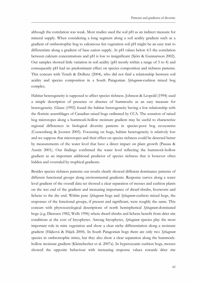
Patterns and gradients of diversity
although the correlation was weak. Most studies used the soil pH as an indirect measure for mineral supply. When considering a long segment along a soil acidity gradient such as a gradient of ombrotrophic bog to calcareous fen vegetation soil pH might be an easy trait to
c assemblages of Canadian raised bogs ordinated by CCA. The zonation of raised bog microtopes along a hummock-hollow moisture gradient may be useful to characterize
g importance of dwarf-shrubs, liverworts and lichens to the dry end. Within pure Sphagnum bogs and Sphagnum-cushion mixed bogs, the
differentiate along a gradient of base cation supply. At pH values below 4.5 the correlation between calcium concentrations and pH is low to insignificant (Sjörs & Gunnarsson 2002). Our samples showed little variation in soil acidity (pH mostly within a range of 3 to 4) and consequently pH had no predominant effect on species composition and richness patterns. This concurs with Teneb & Dollenz (2004), who did not find a relationship between soil acidity and species composition in a South Patagonian Sphagnum-cushion mixed bog complex.
Habitat heterogeneity is supposed to affect species richness. Johnson & Leopold (1994) used a simple description of presence or absence of hummocks as an easy measure for heterogeneity. Glaser (1992) found the habitat heterogeneity having a low relationship with the floristi
regional differences in biological diversity patterns in species-poor bog ecosystems (Couwenberg & Joosten 2005). Focussing on bogs, habitat heterogeneity is relatively low and we suppose that microtopes and their effect on species richness could be detected better by measurements of the water level that have a direct impact on plant growth (Pausas & Austin 2001). Our findings confirmed the water level reflecting the hummock-hollow gradient as an important additional predictor of species richness that is however often hidden and overruled by trophical gradients.
Besides species richness patterns our results clearly showed different dominance patterns of different functional groups along environmental gradients. Response curves along a water level gradient of the overall data set showed a clear separation of mosses and cushion plants on the wet end of the gradient and increasin
responses of the functional groups, if present and significant, were roughly the same. This concurs with phytosociological descriptions of north hemispherical Sphagnum-dominated bogs (e.g. Dierssen 1982, Wells 1996) where dwarf-shrubs and lichens benefit from drier site conditions at the cost of bryophytes. Among bryophytes, Sphagnum species play the most important role in mire vegetation and show a clear niche differentiation along a moisture gradient (Hájková & Hájek 2004). In South Patagonian bogs there are only two Sphagnum species in ombrotrophic mires, but they also show a clear separation along the hummock-hollow moisture gradient (Kleinebecker et al. 2007a). In hyperoceanic cushion bogs, mosses showed the opposite behaviour with increasing response values towards drier site
65
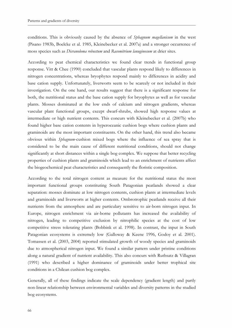
Patterns and gradients of diversity
conditions. This is obviously caused by the absence of Sphagnum magellanicum in the west (Pisano 1983b, Boelcke et al. 1985, Kleinebecker et al. 2007a) and a stronger occurrence of moss species such as Dicranoloma robustum and Racomitrium lanuginosum at drier sites.
According to peat chemical characteristics we found clear trends in functional group response. Vitt & Chee (1990) concluded that vascular plants respond likely to differences in nitrogen concentrations, whereas bryophytes respond mainly to differences in acidity and base cation supply. Unfortunately, liverworts seem to be scarcely or not included in their
te levels and graminoids and liverworts at higher contents. Ombrotrophic peatlands receive all their
non-linear relationship between environmental variables and diversity patterns in the studied bog ecosystems.
investigation. On the one hand, our results suggest that there is a significant response for both, the nutritional status and the base cation supply for bryophytes as well as for vascular plants. Mosses dominated at the low ends of calcium and nitrogen gradients, whereas vascular plant functional groups, except dwarf-shrubs, showed high response values at intermediate or high nutrient contents. This concurs with Kleinebecker et al. (2007b) who found higher base cation contents in hyperoceanic cushion bogs where cushion plants and graminoids are the most important constituents. On the other hand, this trend also became obvious within Sphagnum-cushion mixed bogs where the influence of sea spray that is considered to be the main cause of different nutritional conditions, should not change significantly at short distances within a single bog complex. We suppose that better recycling properties of cushion plants and graminoids which lead to an enrichment of nutrients affect the biogeochemical peat characteristics and consequently the floristic composition.
According to the total nitrogen content as measure for the nutritional status the most important functional groups constituting South Patagonian peatlands showed a clear separation: mosses dominate at low nitrogen contents, cushion plants at intermedia
nutrients from the atmosphere and are particulary sensitive to air-born nitrogen input. In Europe, nitrogen enrichment via air-borne pollutants has increased the availability of nitrogen, leading to competitive exclusion by nitrophilic species at the cost of low competitive stress tolerating plants (Bobbink et al. 1998). In contrast, the input in South Patagonian ecosystems is extremely low (Galloway & Keene 1996, Godoy et al. 2001). Tomassen et al. (2003, 2004) reported stimulated growth of woody species and graminoids due to atmospherical nitrogen input. We found a similar pattern under pristine conditions along a natural gradient of nutrient availability. This also concurs with Ruthsatz & Villagran (1991) who described a higher dominance of graminoids under better trophical site conditions in a Chilean cushion bog complex.
Generally, all of these findings indicate the scale dependency (gradient length) and partly
66
Patterns and gradients of diversity
67
erlapping anthropogenic influence. Several theory derived general assumptions about patterns of species richness and functional
conservation and restoration in landscapes highly affected by human
o Project, for logistic support during field work. Orlando Dollenz (Instituto de la Patagonia, Punta Arenas, Chile) gave helpful hints to find good study sites and
cialized with persons knowing the study area. Verena Möllenbeck (University of Münster) provided helpful comments to a former version of this manuscript and Lillian Harris polished our English.
Our results also underpin that South Patagonian peatlands provide the unique opportunity to study ecological relationships without ov
diversity along resource gradients in peatlands could be confirmed in a surprisingly clear way. Such data are of particular value not only for the testing of ecological theory but also as a reference for interferences.
Acknowledgements
We would like to thank Rolf Kilian (University of Trier, Germany), chief of the Gran Campo Nevad
so

Chapter 5
Synthesis
The major floristic coenocline found in cluster analysis and DCA ordination for South Pata-gonian peatland vegetation represented a gradient of increasing continentality ranging from pacific blanket bogs dominated by cushion-forming vascular plants to Sphagnum-dominated continental raised bogs. In a transition zone between theses contrasting types a mixed type prevailed that was characterized by the occurrence of both, cushion-building plants and Sphagnum. Often these contrasting plant types intermingle at a small scale without a clear definition of dominance. Within these three major bog types, the water level was found to be the most important environmental factor of further floristic differentiation, which was not a big surprise. In contrast, the steep floristic east-west gradient that was documented by this thesis for the first time in a comprehensive way turned out to be the most striking and interesting feature of the studied bog vegetation. Consequently, the detection of major environmental variables that could explain this pattern became a major focus of study.
The obtained results clearly documented a significant change in climatic constraints and biogeochemical peat characteristics with increasing distance to the Pacific Ocean that runs parallel with the shift in peatland vegetation from hyperoceanic blanket bogs to eastern Sphagnum-dominated bogs. Due to the lack of biogeochemical data, the strong climatic gradient was formerly thought to be decisive for the floristic composition of South Patagonian peatlands (Pisano 1983b, Boelcke et al. 1985, Blanco & de la Balze 2004). This study clearly established that the ombrotrophic mire vegetation is also strongly affected by biogeochemical peat characteristics. In particular, the plant available amounts of base cations explained a high proportion of the floristic variance at the landscape level. The differences in base cation availability were highly correlated with the distance to the Pacific Ocean. The contents of Ca, Mg, Na, and K significantly decreased with increasing distance to the Ocean. Thus, the input of sea-born cations was identified to be a major nutritional source for the pacific peatlands, whereas the continental peatlands received low fertilization via atmos-pheric deposition. Due to the strong and continuous westerly winds a significant mineral input of terrestrial origin could be ruled out.
Nitrogen availability is a growth-limiting factor in many peatland ecosystems (Bridgeham et al. 1996). Due to the strong westerly winds bringing unpolluted air masses and the lack of
69
Synthesis
intensive agriculture, anthropogenic N deposition is marginal in southern Patagonia (Godoy et al. 2001). Nevertheless, this study presented big differences in the total N content and the C/N ratio that can obviously not be caused by different amounts in atmospheric N-deposition. The total N content in the peat was also highly correlated with the distance to the Pacific Ocean and explained a similar proportion of the floristic variation as the availability of base cations did. The oceanic peatlands were characterized by a better mineral supply, most likely due to the input of base cations via sea spray. Thus, mineralization and decomposition are presumably enhanced by the higher availability of base cations, which results in higher total N contents and lower C/N ratios of the more oceanic sites. The higher decomposition rates of the more oceanic bogs indicate a stronger micro-biological activity, thereby mobilizing the high N-stocks of the upper peat layer.
In Europe, heavy atmospherical nitrogen inputs caused by emissions from agriculture often reach critical loads for ombrotrophic peatland ecosystems (Bragazza et al. 2004) and obscure the major environmental gradients and the nature of ecological processes. In this study, extremely variable C/N ratios were measured reaching values up to 250 in the eastern Sphagnum bogs that were not influenced by sea spray. This natural gradient and in particular the extremely N-poor conditions of the South Patagonian Sphagnum bogs present a unique opportunity to study peatlands in conditions not affected by enhanced atmospheric deposition. Ecological relationships such as trophic effects caused by sea spray can be studied without anthropogenic influence, so that these peatlands can act as excellent reference systems in mire ecology research.
The major gradients explored in this study also significantly affect the diversity properties of the respective vegetation. In a GRM as few as three predicting environmental variables explained as much as 76 % of the total variance in species richness in the analyzed data set. Species richness increased with increasing total N and NH4Cl soluble Ca contents (as a measure for base cation supply) and decreased with increasing water level. The water level on its own showed only a weak negative correlation to the species richness. Nevertheless, the moisture gradient seems to explain a significant part of the remaining variance not explained by biogeochemical variables. Generally, these results confirmed in a surprisingly clear way expectations derived from literature and gave striking support to ecological theory such as the humpback model by Grime (1973).
Besides the species richness patterns, the major environmental gradients had a significant effect on dominance patterns of different functional groups. Along a water level gradient functional groups were clearly separated. On the wet side of the gradient mosses and cushion plants were the dominating functional groups, whereas the importance of dwarf-shrubs, liverworts, and lichens increased to the dry end. Peat chemical characteristics also
70
Synthesis
71
significantly affected functional group response. Mosses and dwarf-shrubs dominated at the low end of a nitrogen gradient, whereas other vascular plant functional groups and liverworts showed high response values at intermediate or high nutrient contents. Calcium turned out to be another important factor controlling the distribution of functional groups along supply gradients with mosses dominating at low calcium levels and cushion plants at high levels. This patter yields further evidence for the significance of base cation input via sea spray along the analyzed east-west bog vegetation gradient. Generally, the observed behaviour of functional groups along resource gradients concurs with expectations from literature (e.g. Vitt & Chee 1990, Pausas & Austin 2001, Hájková & Hájek 2004).
Due to its unique floristic composition indicating high spatial heterogeneity and non-equilibrium conditions the mixed bogs of the transition zone proved to be complicated but also particularly interesting systems. In such an ecotone, conditions become marginal for some species, potentially resulting in a small-scale community mosaic (Gosz 1992). This assumption is confirmed by the highest dissimilarity values which indicate a mosaic of communities of continental Sphagnum bogs and hyperoceanic cushion bogs. The relatively high γ-diversity of mixed bogs concurs with this finding. Thus, in particular the area of mixed bogs situated in the transition zone between pure cushion plant and Sphagnum domi-nance is probably the most interesting starting point to ask questions for future research:
• Why is Sphagnum magellanicum such a poor competitor under highly oceanic condi-tions in southern Patagonia? Which environmental factors are decisive?
• What makes cushion plants so competitive under hyperoceanic conditions? Why is this functional type completely absent from the northern hemisphere?
• How strong is the impact of minerotrophic groundwater in relation to atmospheric inputs?
• Do the differentiated bog types differ in the kind of nutrient limitation (N, P or K)?
• What are exactly the ecological and physiological mechanisms causing the domi-nance of cushion plants over Sphagnum and vice versa in the transition zone?
• Is it possible to trace back the better supply of base cations and other nutrients in cushion plant bogs to inputs via sea spray by direct measurement of wet and dry deposition as well as by pore water measurements?
To find answers to all these highly interesting and relevant questions further explorative and experimental research is required.

Summary
This thesis consists of three interrelated papers that address different aspects of the vegetation and the ecology of South Patagonian ombrotrophic peatlands. The floristic composition, as well as the major environmental gradients and vegetation properties such as diversity patterns were studied.
Paper 1: Gradients of continentality and moisture in South Patagonian ombrotrophic
peatland vegetation
Numerical methods (Cluster Analysis and Detrended Correspondence Analysis) were carried out to explore 381 phytosociological relevés of South Patagonian ombrotrophic bog vegetation. This resulted in nine major vegetation types that were clearly separated in ordination space along two major gradients that were standing orthogonal on each other. First, along a gradient of increasing continentality hyperoceanic blanket bog vegetation dominated by cushion-forming vascular plants such as Donatia fascicularis and Astelia pumila were gradually replaced by communities of continental Sphagnum-dominated raised bogs. A transitional type was characterized by a small-scaled floristic mixture of both extremes. Second, samples were clearly separated along a water level gradient that could be found at both sides of the continentality gradient. In eastern Sphagnum-dominated bogs, the water level gradient reflected the hummock-hollow microtope zonation. In hyperoceanic blanket bogs, the separation of vegetation types along the water level gradient was attributed to different drainage conditions. The position within the roche moutonnées landscape strongly affected the edaphic moisture regime and consequently the floristic composition. Finally, similarities and dissimilarities of South Patagonian ombrotrophic peat bogs compared to their north hemispherical counterparts were discussed.
Paper 2: South Patagonian ombrotrophic bog vegetation reflects biogeochemical
gradients at the landscape level
Ordination methods (Detrended Correspondence Analysis and Canonical Correspondence Analysis) were applied to find out the major environmental gradients affecting the floristic composition of South Patagonian ombrotrophic bog vegetation. For 82 phytosociological relevés biogeochemical peat characteristics were determined on the basis of volumetric mixed surface samples. Climatic constrains were interpolated by interpreting the available climatic data. Ordination revealed climatic variables as well as biogeochemical constraints
73
Summary
and the water level as major determinants of floristic composition. Among the climatic variables annual precipitation was most important. Within the biogeochemical variables, the total N content and the contents of plant available base cations explained a high proportion of the floristic variation.
Both, climatic and biogeochemical variables were highly correlated with the distance to the Pacific Ocean. Independent of this, the water level described a discrete gradient. It was concluded that the variation in vegetation along a longitudinal gradient crossing the southern Andes that was formerly mainly attributed to climatic constraints is also strongly affected by biogeochemical peat characteristics. According to the trophical status of the investigated peat bogs the variation in the input of sea-born cations depending on the distance to the ocean was supposed to be a key factor affecting the peat chemistry and consequently the floristic composition. Finally, the appropriateness of South Patagonian peatlands as reference systems for conservation and restoration ecology in particular in landscapes highly affected by human interferences was emphasized.
Paper 3: Patterns and gradients of diversity in South Patagonian ombrotrophic peat
bogs
Along a transect crossing the southern Andes, α-, β- and γ-diversity measurements within ombrotrophic bog complexes were performed. α-diversity significantly decreased from hyperoceanic blanket bogs dominated by cushion-forming vascular plants via transitional cushion-Sphagnum mixed bogs to eastern Sphagnum bogs. This trend became evident within most functional groups. Dissimilarity (β-diversity) was highest in the transition zone. γ-diversity was lowest in Sphagnum bogs and similar in cushion bogs and Sphagnum-cushion mixed bogs. Found out by simple linear regressions, species richness was highly correlated to biogeochemical peat characteristics. To determine the best predictors of species richness a General Regression Model was performed. The model resulted in three environmental factors (total N, plant available Ca and water level) predicting species richness with an explained variance of 76 %. Within the three particular bog types different models were calculated. In continental Sphagnum bogs the water level and the content of plant available Mg were the best predictors, whereas in hyperoceanic cushion bogs the ash-content was the only remaining environmental variable. Species richness in Sphagnum-cushion mixed bogs was mainly affected by the water level and the total N content.
Dominance patterns of different functional groups along the major environmental gradients were explored by performing Generalized Additive Models. Response curves of the most dominant functional groups constituting South Patagonian peat bogs illustrated clear
74

Summary
75
preferences to specific environmental conditions such as mosses dominating at the low end of a nitrogen gradient, whereas cushion plants had their optimum at intermediate levels, and graminoids dominated at high nitrogen contents. Within the three particular bog types similar and contrary dominance patterns could be observed. The investigated relationships between environmental variables and diversity patterns were clearly scale-dependent and partly non-linear. The findings underpin the significance of the studied undisturbed peatlands in terms of testing ecological theory.

Zusammenfassung
Diese Arbeit besteht aus drei inhaltlich verknüpften Manuskripten, die jeweils unterschied-liche Aspekte der Vegetation und der Ökologie südpatagonischer ombrotropher Moore beleuchten. Es wurden sowohl die floristische Zusammensetzung und die bestimmenden Umweltfaktoren als auch Diversitätsmuster untersucht.
Paper 1: Gradients of continentality and moisture in South Patagonian ombrotrophic
peatland vegetation
381 pflanzensoziologische Aufnahmen aus südpatagonischen ombrotrophen Mooren wurden mit Hilfe numerischer Methoden (Cluster Analyse und Detrended Correspondence Analysis) analysiert. Die Klassifikation ergab neun Vegetationstypen, die auch im Ordina-tionsdiagramm entlang zweier orthogonal zueinander stehender Hauptgradienten klar voneinander getrennt angeordnet waren. Mit zunehmender Kontinentalität wurden ozeani-sche Polstermoorgesellschaften durch Gesellschaften kontinentaler, Sphagnum-dominierter Hochmoore ersetzt. In Moorkomplexen einer Übergangszone kamen Arten beider Typen mosaikartig nebeneinander vor oder bildeten einen Mischtyp. Unabhängig von diesem Kon-tinentalitätsgradienten untergliedert sich die Vegetation entlang eines Feuchtegradienten. In den östlichen Sphagnum-dominierten Hochmooren spiegelt der Moorwasserstand die typische Bult-Schlenken-Zonierung wider. In den ozeanischen Deckenmooren wurde der Feuchtegradient von den standörtlichen Drainagebedingungen bestimmt. Die Lage im Relief innerhalb der südpatagonischen Rundhöckerlandschaft hatte entscheidenden Einfluss auf das edaphische Feuchteregime und damit die floristische Zusammensetzung der entspre-chenden Pflanzengesellschaften. Abschließend werden Ähnlichkeiten und Unterschiede südpatagonischer ombrotropher Moore im Vergleich zu nordhemisphärischen Mooren erörtert.
Paper 2: South Patagonian ombrotrophic bog vegetation reflects biogeochemical
gradients at the landscape level
Multivariate numerische Methoden (Detrended Correspondence Analysis und Canonical Correspondence Analysis) wurden eingesetzt um die entscheidenden Standortfaktoren für die floristische Zusammensetzung südpatagonischer ombrotropher Torfmoore zu ermitteln. Für 82 pflanzensoziologische Aufnahmen wurden biogeochemische Torfeigenschaften anhand von volumenechten Flächenmischproben bestimmt. Klimatische Standortfaktoren
77
Zusammenfassung
wurden mittels verfügbarer publizierter und nicht publizierter Klimadaten interpoliert. Die Ordination ergab, dass sowohl klimatische und biogeochemische Faktoren als auch der Grundwasserstand entscheidenden Einfluss auf die floristische Zusammensetzung der untersuchten Moore hatten. Unter den klimatischen Variablen hatte die jährliche Nieder-schlagsmenge den größten Einfluss. Innerhalb der biogeochemischen Torfeigenschaften zeigten der Gesamt-Stickstoffgehalt und der Gehalt an pflanzenverfügbaren Basenkationen die größte Varianzaufklärung.
Sowohl die klimatischen als auch die biogeochemischen Variablen korrelierten stark mit der Entfernung zum Pazifischen Ozean. Unabhängig davon beschrieb der Moorwasserstand einen eigenständigen Gradienten. Die Ergebnisse zeigten, dass die floristische Zusammen-setzung südpatagonischer ombrotropher Moore entlang eines transandinen Transekts im Gegensatz zu früheren Studien nicht ausschließlich auf klimatische Unterschiede zurückzu-führen ist, sondern auch stark von den biogeochemischen Torfeigenschaften bestimmt wird. Trophische Unterschiede in den untersuchten Torfmooren wurden in erster Linie auf den Eintrag von Seesalzen in Abhängigkeit von der Entfernung zum Pazifischen Ozean zurück-geführt. Abschließend wird die Eignung unberührter südpatagonischer Moore als Referenz-systeme für den Schutz und die Wiederherstellung von Mooren herausgestellt, insbesondere auch für Moore in stark vom Menschen beeinflussten Landschaften.
Paper 3: Patterns and gradients of diversity in South Patagonian ombrotrophic peat
bogs
Entlang eines transandinen Transekts wurde die α-, β- und γ-Diversität innerhalb verschiedener Moorkomplexen untersucht. Die α-Diversität nahm deutlich von ozeanischen Polstermooren über Mischmoore in einem Übergangsbereich zu kontinentalen Sphagnum-Mooren ab. Dieser Trend bestätigte sich auch innerhalb der meisten funktionalen Gruppen. Die β-Diversität war in der Übergangszone am höchsten. Die γ-Diversität war im Bereich der kontinentalen Sphagnum-Moore deutlich niedriger als in Polstermooren und Mooren der Übergangszone. Einfache lineare Regressionen ergaben starke Korrelationen zwischen dem Artenreichtum und den biogeochemischen Torfeigenschaften. Die entscheidenden Wir-kungsvariablen wurden mit einem General Regression Model ermittelt. Das Modell ergab drei Umweltvariablen (Gesamt-N, pflanzenverfügbares Ca und Moorwasserstand) mit einer Varianzaufklärung von 76 %. Für die drei verschiedenen Moortypen wurden zudem unter-schiedliche Modelle berechnet: für die kontinentalen Sphagnum-Moore waren der Moorwas-serstand und pflanzenverfügbares Mg die besten Wirkungsvariablen, wohingegen für ozeanische Polstermoore der Aschegehalt als aussagekräftigste Umweltvariable ermittelt
78
Zusammenfassung
79
wurde. Der Artenreichtum im Übergangsbereich wurde hauptsächlich vom Moorwasser-stand und dem N-Gehalt bestimmt.
Dominanzmuster verschiedener funktionaler Gruppen wurde mit Hilfe von Generalized Additive Models ermittelt. Es wurden klare Präferenzen der wichtigsten funktionalen Grup-pen südpatagonischer Moore festgestellt, so dominierten Moose bei niedrigen, Polsterpflan-zen bei mittleren und Gräser bei hohen N-Gehalten. Innerhalb der drei unterschiedlichen Moortypen wurden sowohl unterschiedliche als auch ähnliche Muster ermittelt. Die ermit-telten Diversitätsmuster zeigten eine klare Abhängigkeit von der Länge des betrachteten Gradienten und erwiesen sich als teilweise nicht-linear. Die Ergebnisse dieser Untersuchung unterstreichen die Relevanz unberührter Lebensräume im Hinblick auf die Überprüfung allgemeiner ökologischer Theorien.

Resumen
Esta obra esta compuesta de tres manuscritos vinculados en cuanto al contenido, cada uno con aspectos distintos de la vegetación y de la ecología de turberas ombrotróficos de la Patagonia del Sur. Tanto la composición florística y los factores medioambientales como en modelos de diversidad han sido investigados.
Paper 1: Gradients of continentality and moisture in South Patagonian ombrotrophic
peatland vegetation
Con la ayuda de métodos numéricos (Cluster Analyse y Detrended Correspondence Analysis) se analizaron 381 relevamientos fitosociológicos de turberas ombrotróficos de Patagonia del Sur. La clasificación produce nueve tipos de vegetación que han sido separados claramente en un diagrama ordinal a través de dos graduaciones que se han opuesto ortogonal entre si. Primero, a través de un gradiente de continentalidad creciente la vegetación hiperoceánico de plantas en cojín como Donatia fascicularis y Astelia pumila se ha sustituido por comunidades continentales dominadas por Sphagnum. Un tipo de transición se caracterizó por un mosaico de ambos tipos donde existen juntos uno al lado del otro. Segundo, independente de la continentalidad, las muestras han sido separadas claramente a través de un gradiente de la humedad edáfica. En los turberas del este, dominadas por Sphagnum, el nivel freático refleja la zonación típica de depresiones y montículos. En las turberas hiperoceánicas, la separación de los tipos de vegetación esta determinado por las distintas condiciones del drenaje. La posición en el relieve dentro del paisaje surpatagónico de colinas redondeadas tenía una influencía decisiva al régimen de humedad edáfíca y, así pues, a la composición florística. Finalmente se discuten semejanzas y diferencías de las turberas ombrotróficas en la Patagonia del Sur en comporación con turberas en el hemisfero del Norte.
Paper 2: South Patagonian ombrotrophic bog vegetation reflects biogeochemical
gradients at the landscape level
Métodos numéricos (Detrended Correspondence Analysis y Canonical Correspondence Analysis) han sido aplicados para descubrir los factores ambientales determinantes que affectan la composición florística de las turberas ombrotróficos de Patagonia del sur. Para 82 relevamientos fitosociológicos se determinaron las características de turba mediante muestras volumétricas mixtas. Los factores climáticos se interpolaron analizando los datos
81
Resumen
disponibles de la región. La ordinación produjó que tanto en factores climáticos y biogeoquímicos así como el nivel freático eran los mayores determinantes de la composición florístca. Dentro de los factores climáticos la precipitación anual era lo más importante. Dentro de las características biogeoquímicas, el contenido total de nitrógeno y la cantidad de cationes básicos disponibles para las plantas explica la alta proporción de la variación florística.
Las variables climáticas y las variables biogeoquímicas correlacionaron con la distancia al Océano Pacífico. En cambio, el nivel freático describe un gradiente independiente. Los resultados indican, en oposición con estudios anteriores, que la variación de la vegetación a lo largo de un trayecto transandino no está basado únicamente en diferencias climáticas, sino que también está determinado por las características biogeoquímicas de la turba. Las diferencias tróficas y en consecuencia la variación florística en los turberas investigadas se explicaron, primero, por la salinidad de la deposición dependiente de la distancia al Océano Pacífico. Por último, se destaca la altitud de las turberas de Patagonia del Sur como sistema de referencia para la conservación y la restauración de turberas, en particular en paisajes bajo una intensa influencia humana.
Paper 3: Patterns and gradients of diversity in South Patagonian ombrotrophic peat
bogs
A lo largo de un trayecto transandino se investigó la α-, β- und γ-diversidad dentro de complejos de turberas ombrotróficos. La α-diversidad disminuyó evidentamente desde las turberas oceánicas de plantas en cojín vía turberas mixtas de transición hasta turberas continentales de Sphagnum. Esta tendencia también surgió en la mayoría de los grupos funcionales. La β-diversidad tenía su máximo en la zona de transición. La γ-diversidad tenía su mínimo en las turberas de Sphagnum y era similar en las turberas de plantas en cojín y en las turberas mixtas de los dos tipos. Regresiones lineales indicaron que la riqueza de las especias era correlacionada con las características biogeoquímicas de la turba. Para determinar los mejores predictores de la riqueza de especies se formó un General Regression Model. El modelo resultó en tres factores ambientales (contenido total de N, Ca disponible para plantas y nivel freático) prediciendo la riqueza de especies con una variación explicada de 76 %. Para los tres tipos de turberas se calcularon modelos distintos. En las turberas continentales de Sphagnum el nivel freático y el contenido de Mg disponible para plantas eran los mejores predictores mientras para las turberas oceánicas de las plantas en cojines se determinó el contenido de ceniza como la variable más expresiva. La riqueza de especies en
82
Resumen
83
las turberas mixtas de transición se determinó en primer lugar por el nivel freático y el contenido de nitrógeno.
Modelos de dominancia de distintos grupos funcionales por medio de majores gradientes ambientales se calcularon por Generalized Additive Models y se obsevaron preferencias claras de los grupos funcionales más importantes de las turberas de Patagonia del Sur. Musgos dominaron en un ambiente de un contenido bajo de nitrógeno, las plantas en cojín dominaron a un nivel intermedio y las hierbas en contenidos altos de nitrógeno. Dentro de los tres tipos de turberas se observaron tanto modelos similares como modelos distintos. Los modelos de diversidad calculados muestran una dependencia de la longitud de los grandientes investigados y se resultaron en parte como non-linear. Los resultados de esta investigación destacan la relevancia de biótopos inalterados e intactos en cuanto a la revisión de teorías ambientales.

References
Aerts, R., Wallén, B. & Malmer, N. (1992): Growth-limiting nutrients in Sphagnum-domi-nated bogs subject to low and high atmospheric nitrogen supply. Journal of Ecology 80: 131-140.
Aerts, R. (2006): The freezer defrosting: global warming and litter decomposition rates in cold biomes. Journal of Ecology 94: 713-724.
AG Boden (2005): Bodenkundliche Kartieranleitung. 5th ed. Schweizerbart´sche Verlagsbuch-handlung, Hannover, Germany.
Archibold, O.W. (1995): Ecology of world vegetation. Chapman & Hall, New York, United States.
Banner, A., Hebda, R.J., Oswald, E.T., Pojar, J. & Trowbridge, R. (1988): Wetlands of pa-cific Canada. In: Wetlands of Canada, National Wetlands Working Group, Ecological Land Classification 24: 307-346.
Baumann, M.A. (2006): Water flow, spatial patterns, and hydrological self-regulation of a raised bog in Tierra del Fuego (Argentina). Diploma Thesis. Ernst-Moritz-Arndt University Greifswald, Germany.
Bayley, S.F. & Thormann, M.N. (2005): Nitrogen mineralization and decomposition in west-ern boreal bog and fen peat. Ecoscience 12: 455-465.
Berendse, F., van Breemen, N., Rydin, H., Buttler, A., Heijmans, M., Hoosbeek, M.R., Lee, J.A., Mitchell, E., Saarinen, T., Vasander, H. & Wallén, B. (2001): Raised atmospheric CO2 levels and increased N deposition cause shifts in plant species composition and production in Sphagnum bogs. Global Change Biology 7: 591-598.
Blanco, D.E. & de la Balze, V.M. (eds.) (2004): Los Turbales de la Patagonia. Bases para su inven-tario y la conservación de su biodiversidad. Wetlands International - América del Sur, Bue-nos Aires, Argentina.
Bobbink, R., Hornung, M. & Roelofs, J.G.M. (1998): The effects of air-borne nitrogen pollutants on species diversity in natural and semi-natural European vegetation. Jour-nal of Ecology 86: 717-738.
Boelcke, O., Moore, D.M. & Roig, F.A. (eds.) (1985): Transecta Botánica de la Patagonia Austral. CONICET Argentina, Instituto de la Patagonia Chile, Royal Society Gran Bretaña, Buenos Aires, Argentina.
85
References
Bragazza, L., Gerdol, R. & Rydin, H. (2003): Effects of mineral and nutrient input on mire biogeochemistry in two geographical regions. Journal of Ecology 91: 417-426.
Bragazza, F., Tahvanainen, T., Kutnar, L., Rydin, H., Limpens, J., Hájek, M., Grosvernier, P., Hájek, T., Hajkova, P., Hansen, I., Lacumin, P. & Gerdol, R. (2004): Nutritional constraints in ombrotrophic Sphagnum plants under increasing atmospheric nitrogen deposition in Europe. New Phytologist 163: 609-616.
Bragazza, L., Freeman, C., Jones, T., Rydin, H., Limpens, J., Fenner, N., Ellis, T., Gerdol, R., Hajek, M., Lacumin, P., Kutnar, L., Tahvanainen, T., & Toberman, H. (2006): At-mospheric nitrogen deposition promotes carbon loss from peat bogs. Proceedings of the National Academy of Sciences of the United States of America 103: 19386-19389.
Braun-Blanquet, J. (1964): Pflanzensoziologie. Springer, Wien, Austria.
Breckle, S.-W. (2002): Walter´s ecology of the earth. Springer, Heidelberg, Germany.
Bridgeham, S.D., Pastor, J., Janssens, J.A., Chapin, C. & Malterer, T.J. (1996): Multiple limiting gradients in peatlands: A call for a new paradigm. Wetlands 16: 45-65.
Burgos, J.J. (1985): Clima del extremo sur de Sudamerica. In: Boelcke, O., Moore, D.M. & Roig, F.A. (eds.), Transecta Botánica de la Patagonia Austral. CONICET Argentina, In-stituto de la Patagonia Chile, Royal Society Gran Bretaña, Buenos Aires, Argentina: 10-40.
Caspers, G. (2002): Die Sphagnum-Moore in Süd-Patagonien und auf West-Feuerland, Chile. Telma 32: 37-50.
Chytrý, M., Tichý, L., Holt, J. & Botta-Dukát, Z. (2002): Determination of diagnostic species with statistical fidelity measures. Journal of Vegetation Science 13: 79-90.
Clapperton, C.M., Sugden, D.E., Kaufman, D.S. & McCulloch, R.D. (1995): The last glacia-tion in central Magellan Strait, southernmost Chile. Quaternary Research 44: 133-148.
Couwenberg, J. & Joosten, H. (2005): Self-organization in raised bog patterning: the origin of microtope zonation and mesotope diversity. Journal of Ecology 93: 1238-1248.
Damman, A.W.H. (1995a): Major mire vegetation units in relation to the concepts of om-brotrophy and minerotrophy: a worldwide perspective. Gunneria 70: 23-34.
Damman, A.W.H. (1995b): Boreal peatlands in Norway and eastern North America: a com-parison. Gunneria 70: 43-65.
Daniels, R.E. (1978): Floristic analyses of British mires and mire communities. Journal of Eco-logy 66: 773-802.
86
References
Dawson, J.W. (1963): Origins of the New Zealand alpine flora. Proceedings of the New Zealand Ecological Society 10: 12-15.
Dierssen, B. & Dierssen, K. (1984): Vegetation und Flora der Schwarzwaldmoore. Beihefte zu den Veröffentlichungen für Naturschutz und Landschaftspflege in Baden-Württemberg 39. Karlsruhe, Germany.
Dierssen, K. (1982): Die wichtigsten Pflanzengesellschaften der Moore NW-Europas. Conservatoire et Jardin Botanique Genéve hors sér 6. Genève, Switzerland.
Dierssen, K. (1996): Die Vegetation Nordeuropas. Ulmer, Stuttgart, Germany.
Dierssen, K. & Dierssen, B. (2001): Moore. In: Pott, R. (ed.), Ökosysteme Mitteleuropas aus geo-botanischer Sicht. Ulmer, Stuttgart, Germany.
Dollenz, O. (1980): Estudios fitosociológicos en el Archipelago Cabo de Hornos. Anales del Instituto de la Patagonia 11: 223-238.
Dollenz, O. (1982): Estudios fitosociológicos en las Reservas Forestales Alacalufes e Isla Riesco. Anales del Instituto de la Patagonia 13: 161-169.
Dollenz, O. (1986): Relevamientos fitosociológicos en la Península Muños Gamero, Magal-lanes. Anales del Instituto de la Patagonia 16: 55-62.
Du Rietz, G.E. (1954): Die Mineralbodenwasserzeigergrenze als Grundlage einer natürlichen Zweigliederung der nord- und mitteleuropäischen Moore. Vegetatio 5-6: 571-585.
Ejrnaers, R. (2000): Can we trust gradients extracted by Detrended Correspondence Analy-sis? Journal of Vegetation Science 11: 565-572.
Endlicher, W. & Santana, A. (1988): El clima del sur de la Patagonia y sus aspectos ecológi-cos. Un siglo de mediciones climatológicas en Punta Arenas. Anales del Instituto de la Patagonia 18: 57-86.
Endlicher, W. (1991): Zur Klimageographie und Klimaökologie von Südpatagonien – 100 Jahre klimatologische Messungen in Punta Arenas. Freiburger Geographische Hefte 32: 181-211.
Engel, J.J. (1978): A taxonomic and phytogeographic study of Brunswick Península. Hepati-cae and Anthocerotae. Fieldiana Botany 41: 1-319.
Erisman, J.W., Mennen, M.G., Fowler, D., Flechard, C.R., Spindler, G., Gruner, A., Duyzer, J.H., Ruigrok W. & Wyers, G.P. (1998): Deposition monitoring in Europe. Environmental Monitoring and Assessment 53: 279-295.
Fang, J.Y. & Lechowicz, M.J. (2006): Climatic limits for the present distribution of beech (Fagus L.) species in the world. Journal of Biogeography 33: 1804-1819.
87
References
Feuerer, T. (ed.) (2006): Checklists of lichens and lichenicolous fungi of Chile. http://www.biologie.uni-hamburg.de/checklists/southamerica/chile_l.htm (Novem-ber 2006).
Franklin, J., Wiser, S.K., Drake, D.R., Burrows, L.E. & Sykes, W.R. (2006): Environment, disturbance history and rain forest composition across the islands of Tonga, Western Polynesia. Journal of Vegetation Science 17: 233-244.
Frederiksen, P. (1988): Soils of Tierra del Fuego. C. A. Reitzels Forlag, Copenhagen, Denmark.
Fulford, M. (1963): Manual of the leafy Hepaticae of Latin America, Part I. Memoirs of the New York Botanical Garden 11: 1-172.
Fulford, M. (1966): Manual of the leafy Hepaticae of Latin America, Part II. Memoirs of the New York Botanical Garden 11: 173-276.
Fulford, M. (1976): Manual of the leafy Hepaticae of Latin America, Part IV. Memoirs of the New York Botanical Garden 11: 393-535.
Galloway, J.N. & Keene, W.C. (1996): Processes controlling the composition of precipita-tion at a remote southern hemispheric location: Torres del Paine National Park, Chile. Journal of Geophysical Research 101: 6883-6897.
Gerdol, R. (1995): The growth dynamics of Sphagnum based on field measurements in a tem-perate bog and on laboratory cultures. Journal of Ecology 83: 431-437.
Gibson, N. & Kirkpatrick, J.B. (1985): A comparison of the cushion plant communities of New Zealand and Tasmania. New Zealand Journal of Botany 23: 549-566.
Gignac, L.D., Vitt, D.H., Zoltai, S.C. & Bayley, S.E. (1991): Bryophyte response surfaces along climatic, chemical and physical gradients in peatlands of western Canada. Nova Hedwigia 53: 27-71.
Glaser, M. (2001): Zur raumzeitlichen Klimavariabilität am Gran Campo Nevado, Patagonien. Mag-ister Thesis. Albert-Ludwigs University Freiburg, Germany.
Glaser, P.H., Janssens, J.A. & Siegel, D.I. (1990): The response of vegetation to chemical and hydrological gradients in the Lost River Peatland, Northern Minnesota. Journal of Ecology 78: 1021-1048.
Glaser, P.H. (1992): Raised bogs in eastern North-America – regional controls for species richness and floristic assemblages. Journal of Ecology 80: 535-554.
Godoy, R., Oyarzún, C. & Gerding, V. (2001): Precipitation chemistry in deciduous and evergreen Nothofagus forests of southern Chile under a low-deposition climate. Basic and Applied Ecology 2: 65-72.
88
References
Gosz, J.R. (1992): Ecological function in a biome transition zone: translating local response to broad-scale dynamics. In: Hansen, A.J. & di Castri, F. (eds.), Landscape boundaries: consequences for abiotic diversity and ecological flows. Springer, New York, United States: 55-75.
Griffiths, M.E. (2006): Salt spray and edaphic factors maintain dwarf structure and commu-nity composition in coastal sandplain heathlands. Plant Ecology 186: 69-86.
Grime, J. P. (1973): Competitive exclusion in herbaceous vegetation. Nature 242: 344-347.
Gunnarsson, U., Rydin, H. & Sjörs, H. (2000): Diversity and pH changes after 50 years on the boreal mire Skattlosbergs Stormosse, Central Sweden. Journal of Vegetation Science 11: 277-286.
Gunnarsson, U., Malmer, N. & Rydin, H. (2002): Dynamics or constancy in Sphagnum domi-nated mire ecosystems? A 40-year study. Ecography 25: 685-704.
Gunnarsson, U. & Flodin, L.-Å. (2007): Vegetation shifts towards wetter site conditions on oceanic ombrotrophic bogs in southwestern Sweden. Journal of Vegetation Science 18: 595-604.
Hájek, M., Hekera, P. & Hájková, P. (2002): Spring fen vegetation and water chemistry in the western Carpathian flysch zone. Folia Geobotanica 37: 364-364.
Hájek, M., Horsak, M., Hájková, P. & Dite, D. (2006): Habitat diversity of central European fens in relation to environmental gradients and an effort to standardise fen termino-logy in ecological studies. Perspectives in Plant Ecology Evolution and Systematics 8: 97-114.
Hájková, P. & Hájek, M. (2004): Bryophyte and vascular plant responses to base-richness and water level gradients in Western Carpathian Sphagnum-rich mires. Folia Geo-botanica 39: 335-351.
Haraguchi, A., Iyobe, T., Nishijima, H. & Tomizawa, H. (2003): Acid and sea-salt accumula-tion in coastal peat mires of a Picea glehnii forest in Ochiishi, eastern Hokkaido, Japan. Wetlands 23: 229-235.
Hässel de Menendez, G.G. & Solari, S.S. (1985): Catalogo de las hepaticas. In: Boelcke, O., Moore, D.M. & Roig, F.A. (eds.), Transecta Botánica de la Patagonia Austral, CONICET Argentina, Instituto de la Patagonia Chile, Royal Society Gran Bretaña, Buenos Aires, Argentina: 299-232.
Hastie, T.J. & Tibshirani, R.J. (1990): Generalized additive models. Chapman and Hall, London, England.
89
References
He, S. (1998): A checklist of the mosses of Chile. Journal of the Hattori Botanical Laboratory 85: 23-109.
Hill, M.O. & Gauch, H.G. (1980): Detrended correspondence analysis: an improved ordina-tion technique. Vegetatio 42: 47-58.
Huston, M.A. (1994): Biological diversity. The coexistence of species on changing landscapes. Cambridge University Press, Cambridge, England.
Jeschke, L., Knapp, H.D. & Succow, M. (2001): Moorregionen Europas. In: Succow, M. & Joosten, H. (eds.), Landschaftsökologische Moorkunde, Schweizerbart´sche Verlagsbuch-handlung, Stuttgart, Germany: 256-316.
Johnson, A.M. & Leopold, D.J. (1994): Vascular plant-species richness and rarity across a minerotrophic gradient in wetlands of St-Lawrence-Country, New York, USA. Biodi-versity and Conservation 3: 606-627.
Johnson, L.C. & Damman, A.W.H. (1991): Species-controlled Sphagnum decay on a South Swedish raised bog. Oikos 61: 234-242.
Jongman, R.H.G., ter Braak, C.J.F. & van Tongeren, O.F.R. (1995): Data analysis in community and landscape ecology. Cambridge University Press, Cambridge, England.
Joosten, H. & Clarke, D. (2002): Wise use of mires and peatlands – background and principles includ-ing a framework for decision-making. International Mire Conservation Group / Interna-tional Peat Society, Saarijärvi, Finland.
Keller, J.K., White, J.R., Bridgham, S.D. & Pastor, J. (2004): Climate change effects on carbon and nitrogen mineralization in peatlands through changes in soil quality. Global Change Biology 10: 1053-1064.
Kleinebecker, T., Hölzel, N. & Vogel, A. (2007a): Gradients of continentality and moisture in South Patagonian peatland vegetation. Folia Geobotanica (accept.).
Kleinebecker, T., Hölzel, N. & Vogel, A. (2007b): South Patagonian ombrotrophic bog vegetation reflects biogeochemical gradients at the landscape level. Journal of Vegeta-tion Science (accept.).
Lappalainen, E. (1996): General Review on world peatland resources. In: Lappalainen, E. (ed.), Global peat resources, International Peat Society, Saarijärvi, Finnland: 53-56.
Lavelle, P. & Spain, A.V. (2001): Soil ecology. Kluwer, Dordrecht, Netherlands.
Lee, J.A. (1998): Unintentional experiments with terrestrial ecosystems: ecological effects of sulphur and nitrogen pollutants. Journal of Ecology 86: 1-12.
90
References
Lepš, J. & Šmilauer, P. (2003): Multivariate analysis of ecological data using CANOCO. Cambridge University Press, Cambridge.
Limpens, J. & Berendse, F. (2003): How litter quality affects mass loss and N loss from decomposing Sphagnum. Oikos 103: 537-547.
Limpens, J., Berendse, F. & Klees, H. (2003): N deposition affects N availability in intersti-tial water, growth of Sphagnum and invasion of vascular plants in bog vegetation. New Phytologist 157: 339-347.
Locky, D.A. & Bayley, S.E. (2006): Plant diversity, composition, and rarity in the southern boreal peatlands of Manitoba, Canada. Canadian Journal of Botany 84: 940-955.
Malmer, N. (1986): Vegetational gradients in relation to environmental conditions in north-western European mires. Canadian Journal of Botany 64: 375-383.
Malmer, N., Horton, D.G. & Vitt, D.H. (1992): Element concentrations in mosses and surface waters of western Canadian mires relative to precipitation chemistry and hydrology. Ecography 15: 114-128.
Malmer, N. & Wallén, B. (1993): Accumulation and release of organic matter in ombrotro-phic bog hummocks – processes and regional variation. Ecography 16: 193-211.
Malmer, N. & Wallén, B. (1999): The dynamics of peat accumulation on bogs: mass balance of hummocks and hollows and its variation throughout a millennium. Ecography 22: 736-750.
Malmer, N. & Wallén, B. (2005): Nitrogen and phosphorus in mire plants: variation during 50 years in relation to supply rate and vegetation type. Oikos 109: 539-554.
Maltby, E. & Proctor, M.C.F. (1996): Peatlands: their nature and role in the biosphere. In: Lappalainen, E. (ed.), Global peat resources, International Peat Society, Saarijärvi, Finnland: 11-19.
Martikainen, P.J. (1996): The fluxes of greenhouse gases CO2, CH4 and NO2 in northern peatlands. In: Lappalainen, E. (ed.), Global peat resources, International Peat Society, Saarijärvi, Finnland: 29-36.
McCune, B. & Mefford, M.J. (2006): PC-ORD. Multivariate analysis of ecological data. Version 5. MjM Software, Gleneden Beach, Oregon, United States.
Meiwes, K.J., König, N., Khana, P.K., Prenzel, G. & Ulrich, B. (1984): Chemische Unter-suchungsverfahren für Mineralboden, Auflagehumus und Wurzeln zur Charakteri-sierung und Bewertung der Versauerung von Waldböden. Berichte des Forschungszen-trums Waldökosysteme / Waldsterben (Göttingen) 7: 1-67.
91
References
Miller, A. (1976): The Climate of Chile. In: Schwerdtfeger, W. (ed.), Climates of Central and South America, World Survey of Climatology 12, Elsevier, Amsterdam, Netherlands: 113-145.
Moen, A. (2005): Comments on the regional variation and mires in Tierra del Fuego – a comparison with Fennoscandia. In: Couwenberg, J. & Joosten, H. (eds.), International Mire Conserva-tion Group, Newsletter 2005/4: 11-13.
Moore, D.M. (1979): Southern oceanic wet-heathlands (including Magellanic moorland). In: Specht, R.L. (ed.), Heathlands and related shrublands, Ecosystems of the World 9A, El-sevier, Amsterdam, Netherlands: 489-497.
Moore, B.M. (1983): Flora of Tierra del Fuego. Anthony Nelson, Shropshire, England.
Nicholson, B.J., Gignac, L.D. & Bayley, S.E. (1996): Peatland distribution along a north-south transect in the Mackenzie River Basin in relation to climatic and environmental gradients. Vegetatio 126: 119-133.
Oberdorfer, E. (1992) (ed.): Süddeutsche Pflanzengesellschaften Teil I: Fels- und Mauergesellschaften, alpine Fluren, Wasser-, Verlandungs- und Moorgesellschaften. Gustav Fischer Verlag, Jena, Germany.
Økland, R.H., Økland, T., & Rydgren, K. (2001): A Scandinavian perspective on ecological gradients in north-west European mires: reply to Wheeler and Proctor. Journal of Ecology 89: 481-486.
Olde Venterink, H., Wassen, M.J., Verkroost, A.W.M., & de Ruiter, P.C. (2003): Species richness-productivity patterns differ between N-, P-, and K-limited wetlands. Ecology 84: 2191-2199.
Pärtel, M. & Zobel, M. (2007): Dispersal limitation may result in the unimodal productivity-diversity relationship: a new explanation for a general pattern. Journal of Ecology 95: 90-94.
Palmer, K.F. & Dalziel, I.W.D. (1973): Structural studies in the Scotia Arc: Cordillera Dar-win, Tierra del Fuego. Antarctic Journal of the United States 8: 11-14.
Pausas, J.G. & Austin, M.P. (2001): Patterns of plant species richness in relation to different environments: An appraisal. Journal of Vegetation Science 12: 153-166.
Pisano, E. (1971): Comunidades vegetales del area del Fiordo Parry, Tierra del Fuego. Anales del Instituto de la Patagonia 2: 93-133.
92
References
Pisano, E. (1972): Comunidades Vegetales del Area de Bahia Morris, Isla Capitan Aracena, Tierra del Fuego (Parque Nacional "Hernando de Magallanes"). Anales del Instituto de la Patagonia 3: 103-130.
Pisano, E. (1973): Fitogeografía de la Peninsula Brunswick, Magallanes. Anales del Instituto de la Patagonia 4: 141-205.
Pisano, E. (1977): Fitogeografía de Fuego-Patagonia Chilena – Comunidades vegetales entre las latitudes 52 y 56° S. Anales del Instituto de la Patagonia 8: 121-250.
Pisano, E. (1983a): Comunidades en el sector norte de la Peninsula Muños Gamero (Ultima Esperanza, Magallanes). Anales del Instituto de la Patagonia 14: 83-101.
Pisano, E. (1983b): The Magellanic tundra complex. In: Gore, A.J.P. (ed.), Mires: swamp, bog, fen and moor, B. Regional studies, Ecosystems of the world 4, Elsevier, Amsterdam, Netherlands: 295-329.
Proctor, M.C.F. (1994): Seasonal and shorter-term changes in surface-water chemistry on four English ombrogenous bogs. Journal of Ecology 82: 597-610.
Rochefort, L. & Lode, E. (2006): Restoration of degraded boreal peatlands. In: Wieder, R.K. & Vitt, D.H. (eds.), Boreal peatland ecosystems, Ecological Studies 188: 381-423.
Rodwell, J.S. (ed.) (1991): British plant communities. Volume 2, Mires and heaths. Cambridge Uni-versity Press, Cambridge, England.
Roig, F.A., Dollenz, O. & Menendez, E. (1985): Las comunidades vegetales de la Transecta Botánica de la Patagonia Austral. La vegetación en los canales. In: Boelcke, O., Moore, D.M. & Roig, F.A. (eds.), Transecta Botánica de la Patagonia Austral, CONICET Argentina, Instituto de la Patagonia Chile, Royal Society Gran Bretaña, Buenos Aires, Argentina: 457-520.
Roivainen, H. (1954): Studien über die Moore Feuerlands. Annales Botanici Societatis Zoologicae Botanicae Fennicae „Vanamo“ 28: 1-205.
Ruthsatz, B. & Villagran, C. (1991): Vegetation pattern and soil nutrients of a Magellanic moorland on the Cordillera de Piuchué, Chiloé Island, Chile. Revista Chilena de Historia Natural 64: 461-478.
Rydin, H. & Jeglum, J. (2006): The biology of peatlands. Oxford University Press, New York, United States.
Sánchez-Blanco, M.J., Rodríguez, P., Morales, M.A. & Torrecillas, A. (2003): Contrasting physiological responses of dwarf sea-lavender and marguerite to simulated sea aero-sol deposition. Journal of Environmental Quality 32: 2238-2244.
93
References
Såstad, S. & Asbjørn, M. (1995): Classification of mire localities and mire species in central Norway by vegetational regions, Ellenberg species indicator values and climatic data. Gunneria 70: 177-198.
Schneider, C., Glaser, M., Kilian, R., Santana, A., Butorovic, N. & Casassa, G. (2003): Weather observations across the southern Andes at 53°S. Physical Geography. 24: 97-119.
Schneider, C., Schnirch, M., Acuna, C., Casassa, G. & Kilian, R. (2007): Glacier inventory of the Gran Campo Nevado Ice Cap in the Southern Andes and glacier changes observed during recent decades. Global and Planetary Change (in press).
Schnirch, M. (2001): Ableitung eines digitalen Geländemodells mit Hilfe photogrammetrischer Verfahren zur Erstellung eines Gletscherinventars des Gran Campo Nevado, Chile. Magister Thesis. Albert-Ludwigs University Freiburg, Germany.
Schüller, H. (1969): Die CAL-Methode, eine neue Methode zur Bestimmung des pflanzen-verfügbaren Phosphates im Boden. Zeitschrift für Pflanzenernährung und Bodenkunde 123: 48–63.
Schulz, J. (1995): The ecozones of the world. The ecological divisions of the geosphere. 2nd ed. Springer, Berlin, Germany.
Schwaar, J. (1976): Die Hochmoore Feuerlands und ihre Pflanzengesellschaften. Telma 6: 51-59.
Schwaar, J. (1980): Pflanzengesellschaften der Oxycocco-Sphagnetea und Scheuchzerio-Caricetea fuscae in Feuerland. In: Dierschke, H. (ed.), Berichte der Internationalen Sympo-sien der Internationalen Vereinigung für Vegetationskunde, Syntaxonomie: 397-401.
Senterre, B., Lejoly, J. & Sonké, B. (2004): Analysis of the climatic gradient of continentality and identification of plant communities in central African rain forests using the mega-transect method. Phytocoenologia 34: 491-516.
Sjörs, H. (1983): A comparison between mires of southern Alaska and Fennoscandia. Aquilo Series of Botany 21: 89-94.
Sjörs, H. & Gunnarsson, U. (2002): Calcium and pH in north and central Swedish mire waters. Journal of Ecology 90: 650-657.
Sokal, R.R. & Rohlf, F.J. (1981): Biometry. Freeman, San Francisco, United States.
Stern, C.R. & Kilian, R. (1996): Role of the subducted slab, mantle wedge and continental crust in the generation of adakites from the Andean Austral Vulcanic Zone. Contri-butions to Mineralogy and Petrology 123: 263-281.
94
References
Succow, M. (2001): Kurzer Abriß der Nutzungsgeschichte mitteleuropäischer Moore. In: Succow, M. & Joosten, H. (eds.), Landschaftsökologische Moorkunde, Schweizerbart´sche Verlagsbuchhandlung, Stuttgart, Germany: pp. 404-406.
Szumigalski, A.R. & Bayley, S.E. (1996): Decomposition along a bog to rich fen gradient in central Alberta, Canada. Canadian Journal of Botany 74: 573-581.
Teneb, E. & Dollenz, O. (2004): Distribución especial de la Flora vascular, la humedad y el pH en un turbal de esfagno (Sphagnum magellanicum Brid.), Magallanes, Chile. Anales del Instituto de la Patagonia 32: 5-12.
ter Braak, C.F.J. & Šmilauer, P. (2002): CANOCO reference manual and user´s guide to Canoco for Windows: Software for canonical community ordination (version 4.5). Microcomputer Power, Ithaca, United States.
Tichý, L. (2002): JUICE, software for vegetation classification. Journal of Vegetation Science 13: 451-453.
Tichý, L. & Chytrý, M. (2006): Statistical determination of diagnostic species for site groups of unequal size. Journal of Vegetation Science 17: 809-818.
Tolonen, K. & Turunen, J. (1996): Accumulation rates of carbon in mires in Finland and implications for climate change. Holocene 6: 171-178.
Tomassen, H.B.M., Smolders, A.J.P., Lamers, L.P.M. & Roelofs, J.G.M. (2003): Stimulated growth of Betula pubescens and Molinia caerulea on ombrotrophic bogs: role of high levels of atmospheric nitrogen deposition. Journal of Ecology 91: 357-370.
Tomassen, H.B.M., Smolders, A.J.P., Limpens, J., Lamers, L.P.M. & Roelofs, J.G.M. (2004): Expansion of invasive species on ombrotrophic bogs: desiccation or high N deposi-tion? Journal of Applied Ecology 41: 139-150.
Tuhkanen, S, Kuokka, I., Hyvönen, J., Stenroos, S. & Niemelä, J. (1989-1990): Tierra del Fuego as a target for biogeographical research in the past and present. Anales del Instituto de la Patagonia 19: 1-107.
Tuhkanen, S. (1992): The climate of Tierra del Fuego from a vegetation geographical point of view and its ecoclimatic counterparts elsewhere. Acta Botanica Fennica 145: 1-64.
Turunen, J. & Tolonen, K. (1996): Rate of carbon accumulation in boreal peatlands and climate change. In: Lappalainen, E. (ed.), Global peat resources, International Peat So-ciety, Saarijärvi, Finnland: 21-28.
95
References
Turunen, J., Tolonen, K., Tolvanen, S., Remes, M., Ronkainen, J. & Jungner, H. (1999): Car-bon accumulation in the mineral subsoil of boreal mires. Global and Biogeochemical Cycles 13: 71-79.
van der Maarel, E. (1979): Transformation of cover-abundance values in phytosociology and its effects on community similarity. Vegetatio 39: 97-114.
van Groenendael, J.M., Hochstenbach, S.M.H., van Mansfeld, M.J.M., Roozen, M.J.M. & Westhoff, V. (1982): The influence of the sea on the vegetation of lakes in southwest Connemara. Journal of Life Sciences of the Royal Dublin Society 3: 221-242.
Vermeer, J.G. & Berendse, F. (1983): The relationship between nutrient availability, shoot biomass and species richness in grassland and wetland communities. Vegetatio 53: 121-126.
Virtanen, R., Oksanen, J., Oksanen, L. & Razzhivin, V.Y. (2006): Broad-scale vegetation-environment relationships in Eurasian high-latitude areas. Journal of Vegetation Science 17: 519-528.
Vitousek, P.M. (2002): Oceanic islands as model systems for ecological studies. Journal of Biogeography 29: 573-582.
Vitt, D.H. & Chee, W.-L. (1990): The relationship of vegetation to surface water chemistry and peat chemistry in fens of Alberta, Canada. Vegetatio 89: 87-106.
Vitt, D.H., Horton, D.G., Slack, N.G. & Malmer, N. (1990): Sphagnum-dominated peatlands of the hyperoceanic British Columbia coast: patterns in surface water chemistry and vegetation. Canadian Journal of Forest Research 20: 696-711.
Vitt, D.H., Halsey, L.A., Bauer, I.E. & Campbell, C. (2000): Spatial and temporal trends in carbon storage of peatlands of continental western Canada through the Holocene. Canadian Journal of Earth Sciences 37: 683-693.
Walker, S., Wilson, J.B., Steel, J.B., Rapson, G.L., Smith, B., King, W.M. & Cottam, Y.H. (2003): Properties of ecotones: Evidence from five ecotones objectively determined from a coastal vegetation gradient. Journal of Vegetation Science 14: 579-590.
Warner, B.G. & Asada, T. (2006): Biological diversity of peatlands in Canada. Aquatic Sciences 68: 240-253.
Wassen, M.J., Olde Venterink, H., Lapshina, E.D. & Tanneberger, F. (2005): Endangered plants persist under phosphorus limitation. Nature 437: 547-550.
Weischet, W. (1970): Chile – seine länderkundliche Individualität und Struktur. Wissenschaftliche Buchgesellschaft, Darmstadt, Germany.
96
References
97
Wells, E.D. (1996): Classification of peatland vegetation in Atlantic Canada. Journal of Vegetation Science 7: 847-878.
Weltzin, J.F., Pastor, J., Harth, C., Bridgham, S.D., Updegraff K. & Chapin, C.T. (2000): Response of bog and fen plant communities to warming and water-table manipula-tions. Ecology 81: 3464-3478.
Westhoff, V. & van der Maarel, E. (1973): The Braun-Blanquet approach. In: Whittaker R.H. (ed.), Ordination and Classification of Communities, Junk, The Hague, Netherlands: 617-737.
Wheeler, B.D. (1993): Botanical diversity in British mires. Biodiversity and Conservation 2: 490-512.
Wheeler, B.D. & Proctor, M.C.F. (2000): Ecological gradients, subdivisions and terminology of north-west European mires. Journal of Ecology 88: 187-203.
Whitehouse, H.E. & Bayley, S.E. (2005): Vegetation patterns and biodiversity of peatland plant communities surrounding mid-boreal wetland ponds in Alberta, Canada. Canadian Journal of Botany 83: 621-637.
Wilson, M.V. (2007): Measuring the components of competition along productivity gradients. Journal of Ecology 95: 301-308.

Danksagung
Viele Personen haben mich direkt oder indirekt bei der Anfertigung dieser Arbeit unter-stützt. Einigen möchte ich hier ein besonderes „Dankeschön“ sagen:
Mein ganz besonderer Dank für die gute Betreuung und die hilfreiche Kritik gilt zunächst meinen Betreuern PD Dr. Norbert Hölzel und Prof. Dr. Karl-Friedrich Holtmeier, sowie Dr. Andreas Vogel und Prof. Dr. Barbara Ruthsatz.
Für die Logistik und die angenehme Arbeitsatmosphäre während der Geländearbeit möchte ich PD Dr. Rolf Kilian danken. Für tatkräftige Hilfe, fachliche Diskussion oder nicht zuletzt viel Spaß im Gelände haben viele Mitarbeiterinnen und Mitarbeiter des Gran Campo Nevado Projektes und nette Menschen im Süden Chiles gesorgt. Stellvertretend seien Prof. Dr. Christoph Schneider, Markus Stickling, Christian Donoso, Prof. Dr. Orlando Dollenz und Misael Perez genannt.
Die reibungslose Durchführung der Bodenanalysen im landschaftsökologischen Labor der Universität Münster habe ich der Unterstützung der Technischen Assistentinnen Ulrike Ber-ning-Mader, Madeleine Supper und Melanie Tappe zu verdanken.
Ganz besonders möchte ich mich außerdem bei den fleißigen Korrekturleserinnen und Korrekturlesern für wertvolle Anregungen und ihre Mühe bedanken. Dies waren: Dr. Kerstin Anschlag, Lillian Harris, Verena Möllenbeck, PD Dr. Ingo Hahn, Tomás Peña und Sebastian Schmidt.
Mein ganz besonderer Dank gilt meinen Eltern, Ilse-Lotte und Wilfried Hanneforth, durch deren Unterstützung mein Studium und die anschließende Promotion überhaupt erst möglich gewesen ist. Sie haben mich stets dazu ermutigt, das zu tun, was ich für richtig hielt.
Für das Verständnis, die seelische und moralische Unterstützung während der gesamten Zeit der Dissertation, insbesondere während der mehrmonatigen Geländekampagnen, geht ein ganz lieber Dank an meine Ehefrau Isabell und den kleinen Detlef.
99

Curriculum Vitae
Till Kleinebecker (né Hanneforth), born on 28th September 1974 in Gütersloh, Germany
Education
2003 – 2007 PhD-student at the Institute of Landscape Ecology, University of Münster
1997 – 2003 Student of Landscape Ecology, University of Münster
1994 – 1997 Apprenticeship as carpenter in Bielefeld
1985 – 1994 Evangelisch Stiftisches Gymnasium Gütersloh
1981 – 1985 Grundschule Isselhorst in Gütersloh
Employment Record
2003 – 2007 Graduate assistant at the Institute of Landscape Ecology, University of Münster
2001 – 2003 Student assistant at the Institute of Landscape Ecology, University of Münster
101


![Bioenergy Use Patterns in Mexico 2003 [ ]](https://static.fdokument.com/doc/165x107/61fb1af32e268c58cd5a35cf/bioenergy-use-patterns-in-mexico-2003-.jpg)