Phase-Space Berry Phases in Chiral Magnets · Phase-Space Berry Phases in Chiral Magnets Skyrmion...
177
Phase-Space Berry Phases in Chiral Magnets Skyrmion Charge, Hall Effect, and Dynamics of Magnetic Skyrmions Inaugural-Dissertation zur Erlangung des Doktorgrades der Mathematisch-Naturwissenschaftlichen Fakult¨ at der Universit¨ atzuK¨oln vorgelegt von Robert Bamler aus M¨ unchen K¨ oln 2016
Transcript of Phase-Space Berry Phases in Chiral Magnets · Phase-Space Berry Phases in Chiral Magnets Skyrmion...
Phase-Space Berry Phases in Chiral Magnets
Skyrmion Charge, Hall Effect, and
Dynamics of Magnetic Skyrmions
Inaugural-Dissertation
zur
Erlangung des Doktorgrades
der Mathematisch-Naturwissenschaftlichen Fakultat
der Universitat zu Koln
vorgelegt von
Robert Bamler
aus
Munchen
Koln 2016
Berichterstatter: Prof. Dr. Achim Rosch(Gutachter)
Prof. Dr. Alexander Altland
Tag der mundlichen Prufung: 11. Juli 2016
Abstract
The dynamics of electrons in solids is influenced by Berry phases in phase space (com-bined position and momentum space). Phase-space Berry phases lead to an effectiveforce on the electrons, an anomalous contribution to the group velocity, and a correctionto the density of states in phase space. In addition, Berry phases in position and inmomentum space are related to topological winding numbers and can be used to char-acterize topologically distinct phases of matter. We study theoretically the effects ofphase-space Berry phases in magnetic materials with weak spin-orbit coupling and asmoothly varying magnetization texture. Such magnetic textures appear generically innon-centrosymmetric magnetic materials with weak spin-orbit coupling due to a com-petition between the ferromagnetic exchange interaction and the weaker Dzyaloshinskii-Moriya interaction. In particular, the discovery of topologically stable whirls, so-calledskyrmions, in the magnetization texture of these materials has attracted considerableattention due to prospects of applications in future magnetic storage devices.
In part I of this thesis, we investigate the influence of phase-space Berry phases on theequilibrium properties of electrons in chiral magnets with weak spin-orbit coupling. Weshow that the strength of the Dzyaloshinskii-Moriya interaction in the long-wavelengthlimit can be calculated from Berry phases in mixed position/momentum space and thatthe same Berry phases lead to an electric charge of skyrmions in metallic chiral magnets.In insulators, the skyrmion charge of magnetic skyrmions turns out to be proportional tothe topologically quantized second Chern number in phase space. This establishes a linkbetween skyrmions in chiral magnets and the charged excitations in integer quantumHall systems with small Zeeman splitting.
In part II, we consider the Hall effect in the skyrmion lattice phase of chiral magnetsin presence of spin-orbit coupling. It has been previously known that Berry phases inmomentum space lead to the intrinsic part of the anomalous Hall effect, and that Berryphases in position space lead to an effective Lorentz force, resulting in the so-calledtopological Hall effect. By expanding the Kubo-Streda Formula for the Hall conductivityin gradients in position and momentum space, we show that the interplay betweensmooth magnetic textures and spin-orbit coupling leads to a previously disregardedcontribution to the Hall effect, and we find a correction to the semiclassical formulationof the topological Hall effect.
In part III, we study the influence of phase-space Berry phases on the dynamics ofskyrmions in chiral magnets. Berry phases in mixed position/momentum space leadto a dissipationless momentum transfer from conduction electrons to skyrmions that isproportional to an applied electric field and independent of the (spin or electric) current.We further show that the electric charge of skyrmions, discussed in part I, influences theskyrmion motion only via hydrodynamic drag and ohmic friction in metals. In insulators,the quantized skyrmion charge couples directly to an applied electric field.

Kurzzusammenfassung
Phasenraum-Berryphasen beeinflussen die Bewegung von Elektronen in Festkorpern. Siefuhren zu einer effektiven Kraft auf die Elektronen, einem anomalen Beitrag zur Grup-pengeschwindigkeit und einer Korrektur der Zustandsdichte im Phasenraum. Außer-dem stehen Ortsraum- und Impulsraum-Berryphasen im Zusammenhang mit topologis-chen Windungszahlen, welche topologisch unterschiedliche Materiezustande unterschei-den. In dieser theoretischen Arbeit untersuchen wir die Effekte von Phasenraumber-ryphasen in magnetischen Materialien mit schwacher Spin-Bahn-Kopplung und einerglatten Magnetisierungstextur im Ortsraum. Solche magnetischen Texturen entstehengenerisch in Magneten ohne Inversionszentrum (chiralen Magneten) mit schwacher Spin-Bahn-Kopplung aufgrund einer Konkurrenz zwischen ferromagnetischer Austauschwech-selwirkung und der schwachern Dzyaloschinskii-Moriya-Wechselwirkung. Insbesonderehat die Entdeckung topologisch geschutzter Wirbel der Magnetisierung, sogenannterSkyrmionen, aufgrund moglicher Anwendungen in zukunftigen magnetischen Datenspe-ichern große Aufmerksamkeit hervorgerufen.
In Teil I dieser Arbeit untersuchen wir den Einfluss von Phasenraumberryphasen aufdie Gleichgewichtseigenschaften von Elektronen in chiralen Magneten mit schwacherSpin-Bahn-Kopplung. Wir zeigen dass die Starke der Dzyaloshinskii-Moriya–Wechsel-wirkung im langwelligen Limes mithilfe von Berryphasen im gemischten Orts/Impulsraumberechnet werden kann und dass dieselben Berryphasen zu einer elektrischen Ladung vonSkyrmionen in metallischen chiralen Magneten fuhren. In Isolatoren ist die Skyrmio-nenladung proportional zur topologisch quantisierten zweiten Chernzahl im Phasen-raum. Mit dieser Erkenntnis schlagen wir eine Brucke zwischen Skyrmionen in chi-ralen Magneten und den geladenen Anregungen im ganzzahligen Quanten-Hall-Effektbei schwacher Zeemanaufspaltung.
In Teil II beschaftigen wir uns mit dem Hall-Effekt in der Skyrmiongitterphase chi-raler Magnete unter Berucksichtigung der Spin-Bahn-Kopplung. Es ist bereits bekanntdass Impulsraum-Berryphasen zur intrinsischen Komponente des anomalen Hall-Effektsfuhren, und dass Ortsraum-Berryphasen eine effektive Lorentzkraft generieren, welchezum sogenannten topologischen Hall-Effekt fuhrt. Indem wir die Kubo-Streda-Formel furdie Hallleitfahigkeit in Gradienten im Orts- und Impulsraum entwickeln zeigen wir, dassdie Kombination aus der langwelligen magnetischen Textur und Spin-Bahn-Kopplungzu einem bisher unberucksichtigten Beitrag zum Hall-Effekt fuhren, und wir finden eineKorrektur zur semiklassischen Formel fur den topologischen Hall-Effekt.
In Teil III untersuchen wir den Einfluss von Phasenraum-Berryphasen auf die Dynamicvon Skyrmionen in chiralen Magneten. Berryphasen im gemischten Orts/Impulsraumfuhren zu einem dissipationslosen Impulsubertrag von den Leitungselektronen auf dieSkyrmionen, der proportional zu einem angelegten elektrischen Feld und unabhangig
vom (Spin- oder Ladungs-)Strom ist. Wir zeigen weiterhin dass die elektrische Ladungvon Skyrmionen (siehe Teil I) deren Bewegung in Metallen nur durch hydrodynamis-ches Mitschleppen (drag) und Ohmsche Reibung beeinflusst. In Isolatoren koppelt diequantisierte Skyrmionladung direkt an ein angelegtes elektrisches Feld.
Contents
1. Introduction 1
2. Skyrmions in chiral magnets 3
2.1. Skyrmions as topologically stable objects . . . . . . . . . . . . . . . . . . 3
2.2. Skyrmion lattice phase in chiral magnets . . . . . . . . . . . . . . . . . . . 6
2.3. Recent trends . . . . . . . . . . . . . . . . . . . . . . . . . . . . . . . . . . 9
3. Berry phases 11
3.1. Origin of Berry phases in physical systems . . . . . . . . . . . . . . . . . . 11
3.2. Geometrical phase in a time-dependent system . . . . . . . . . . . . . . . 14
3.3. Gauge invariant formulation and geometric interpretation of Berry phases 16
3.4. Example . . . . . . . . . . . . . . . . . . . . . . . . . . . . . . . . . . . . . 22
3.5. Quantification of adiabaticity . . . . . . . . . . . . . . . . . . . . . . . . . 25
4. Phase-space Berry phases in chiral magnets 29
4.1. Position-space Berry phases and emergent electrodynamics . . . . . . . . 29
4.2. Berry phases in momentum space and anomalous velocity . . . . . . . . . 33
4.3. Berry phases in mixed position/momentum space . . . . . . . . . . . . . . 37
4.4. Relevance of phase-space Berry phases in chiral magnets . . . . . . . . . . 43
I. Dzyaloshinskii-Moriya interaction and the electric charge of skyrmions 45
5. Semiclassical approach to energy and charge density in chiral magnets 47
5.1. Semiclassical dynamics of wave packets . . . . . . . . . . . . . . . . . . . . 48
5.2. Correction to the density of states. . . . . . . . . . . . . . . . . . . . . . . 54
5.3. Berry-phase effects on energy and charge density . . . . . . . . . . . . . . 56
5.4. DM energy and skyrmion charge in a minimal model . . . . . . . . . . . . 58
5.5. Numerical results for DM energy and skyrmion charge in MnSi . . . . . . 60
6. Skyrmion charge from a gradient expansion 63
6.1. Wigner transformation on a lattice . . . . . . . . . . . . . . . . . . . . . . 63
6.2. Local Green’s function and gradient expansion . . . . . . . . . . . . . . . 69
6.3. Skyrmion charge . . . . . . . . . . . . . . . . . . . . . . . . . . . . . . . . 74
Contents
II. Hall effect in chiral magnets with weak spin-orbit coupling 79
7. Hall effects in chiral magnets 817.1. Overview over experiments and theoretical methods . . . . . . . . . . . . 817.2. Semiclassical theory of Hall effects in chiral magnets . . . . . . . . . . . . 84
8. Hall effect from a systematic gradient expansion 918.1. Bastin Equation and intrinsic anomalous Hall effect . . . . . . . . . . . . 928.2. First-order gradient corrections to the Hall conductivity . . . . . . . . . . 938.3. Topological Hall effect from the Kubo-Streda formula . . . . . . . . . . . 978.4. Discussion . . . . . . . . . . . . . . . . . . . . . . . . . . . . . . . . . . . . 99
III. Dynamics of rigid skyrmions in the presence of spin-orbit coupling 101
9. Theories of magnetization dynamics 1039.1. The Landau-Lifshitz-Gilbert equation and the Thiele Equation . . . . . . 1039.2. Open questions . . . . . . . . . . . . . . . . . . . . . . . . . . . . . . . . . 107
10.Derivation of the equation of motion for skyrmions 10910.1. Model and outline of the derivation . . . . . . . . . . . . . . . . . . . . . . 10910.2. Wigner transform and diagonalized local Green’s function . . . . . . . . . 11410.3. Transport equation and local charge conservation . . . . . . . . . . . . . . 11910.4. Formal equation of motion . . . . . . . . . . . . . . . . . . . . . . . . . . . 127
11.Results in Metals and insulators 13311.1. Equation of motion for skyrmions in metals . . . . . . . . . . . . . . . . . 13311.2. Equation of motion for skyrmions in insulators . . . . . . . . . . . . . . . 13511.3. Discussion of the coupling to the electric charge . . . . . . . . . . . . . . . 137
12.Conclusions and outlook 141
A. Derivation of the quantized skyrmion charge in insulators 155A.1. General expression for the skyrmion charge in insulators . . . . . . . . . . 155A.2. Factorization of the skyrmion charge in two-dimensional insulators with
Abelian Berry curvature . . . . . . . . . . . . . . . . . . . . . . . . . . . . 157A.3. Skyrmion charge per length in three-dimensional insulators with Abelian
Berry curvature . . . . . . . . . . . . . . . . . . . . . . . . . . . . . . . . . 158
B. Coupling of the quantized skyrmion charge to an electric field 161


1. Introduction
The concept of Berry phases is a fundamental aspect of quantum mechanics. Berryphases arise naturally in systems with many degrees of freedom whose dynamics aregoverned by different time scales, whenever the dynamics of the fast modes depends onthe configuration of the slow modes. In such a scenario, which is ubiquitous in nature,the system picks up a geometric phase as the slow modes evolve in time and the fastmodes follow adiabatically the changing environment dictated by the slow modes. Theremarkable aspect of Berry phases is that they are insensitive to the velocity with whichthe slow modes change in time and depend only on the geometry of the trajectory [1].A classical analog of the connection between geometry and dynamics can be seen in theFoucault pendulum. Due to the rotation of the earth, the orientation of the pendulumchanges over the course of one day. Interestingly, the rotation angle per day of thependulum is independent of the oscillation frequency of the pendulum or the angularvelocity of the earth. It only depends on a geometric property: as the earth turns aroundits axis, the location at which the experiment is carried out encloses a certain solid angleon the surface of the earth. The orientation of the pendulum rotates by 2π minus theenclosed solid angle per day.
The notion of Berry phases has been employed in a wide variety of physical disciplines.Examples include solid state physics [2], quantum computing [3], and astrophysics [4].In condensed matter physics, Berry phases influence the semiclassical dynamics of Blochelectrons, leading to additional forces [5], an anomalous contribution to the group ve-locity [6], and an effective change of the density of states in phase space [7]. Apartfrom their influence on the dynamics of the system, the close relation of Berry phaseswith the geometry of the configuration space provides new tools for the classificationof different states of matter. In condensed matter physics, the topological properties ofthe band structure are characterized by Berry phases of Bloch electrons. For example,the topological winding number of the integer quantum Hall state is related to Berryphases of Bloch electrons in the magnetic Brillouin zone [8]. This classification of statesof matter by Berry phases is not limited to momentum space. In 2009, Muhlbauer andcollaborators discovered a novel magnetic state in the chiral magnet MnSi [9]. Here,the magnetization texture in the so-called skyrmion-lattice phase is characterized by aregular arrangement of smooth magnetic whirls (skyrmions) with a topologically pro-tected winding number. It turns out that this position-space winding number translatesto Berry phases picked up by conduction electrons as they traverse the magnetizationtexture. Mathematically, the Berry phase in position space is equivalent to a spin-dependent Ahronov-Bohm phase and it manifests itself in an emergent (spin-dependent)Lorentz force on the electrons. The effect can be measured in Hall experiments [10]. Thecounter force from the electrons on the skyrmions leads to a very efficient coupling of
1
1. Introduction
spin currents and skyrmions [11, 12], which raises expectations for applications in novelspin-tronic devices.
Microscopically, the formation of smooth skyrmions in chiral magnets such as MnSiis a consequence of weak spin-orbit coupling. Spin-orbit coupling is also a commonmechanism that generates Berry phases in momentum space. Thus, chiral magnetsare prime materials to study in general the effects of Berry phases in phase space,i.e., combined position and momentum space. As quantum-mechanical phases are onlydetectable through interference, only Berry phases picked up on closed loops are physical.While Berry-phase effects corresponding to closed loops in either position or momentumspace have been studied in separate systems to considerable extent, the same can notbe said for Berry-phase effects involving both position and momentum space.
In this thesis, we study the effects of Berry phases in the whole phase space onskyrmions in chiral magnets. In part I (Chapters 5–6), we focus on equilibrium propertiesof electrons in a static and long-wavelength skyrmion lattice. Using both semiclassicalarguments and a systematic gradient expansion of the Green’s function, we show thatthe Dzyaloshinskii-Moriya interaction energy, which is responsible for magnetic texture,is a consequence of Berry phases in mixed position/momentum space. In addition, weshow that these mixed phase-space Berry phases lead to an electric charge of skyrmionsin metals. In insulators, the electric charge of skyrmions is given by the product ofthe Berry curvature in position and momentum space, and is quantized. An exampleof skyrmions with a quantized electric charge has been known from quantum Hall sys-tems [13,14]. We thus provide a link between the charge of skyrmions in quantum Hallsystems and in metallic chiral magnets.
In part II (Chapters 7–8), we consider the transport of electrons in the presence of astatic skyrmion lattice. Using again a systematic gradient expansion method, we derivea formula for the Hall conductivity in the presence of Berry phases in phase space. Wefind a previously disregarded contribution to the Hall conductivity that arises due toa combination of smooth modulations in position space and spin-orbit coupling. Evenin absence of spin-orbit coupling, a comparison between our result for the topologicalHall effect shows a correction to the semiclassical theory if more than one orbital bandparticipate in the electronic transport.
In part III (Chapters 9–11), we turn to the dynamics of skyrmions in chiral magnets inthe presence of an electric field. Starting from a single skyrmion with only a translationaldegree of freedom, we develop a general method to derive an equation of motion for thetranslational degree of freedom, taking Berry phases in the whole of phase space intoaccount. Of particular focus is the influence of the electric charge of the skyrmion,derived in part I, on its dynamics. In metals, we find that the charge couples onlyvia hydrodynamic drag and ohmic friction to an applied electric field. In insulators, thedrag and friction forces vanish, and the quantized electric charge of the skyrmion couplesinstead directly to the applied electric field, as it would for an elementary particle.
2
2. Skyrmions in chiral magnets
2.1. Skyrmions as topologically stable objects
The concept of emergent degrees of freedom is ubiquitous in modern physics. It is basedon the notion that “the whole is greater than the sum of its parts,” usually attributed toAristotle. A very general mechanism under which emergent degrees of freedom can ariseis expressed by the Goldstone theorem. It is based on a local symmetry analysis of theconstituent fields and it predicts the existence of bosonic low-energy degrees of freedomif the ground state in the thermodynamic limit breaks a local symmetry. For example,if many atoms are brought together and condense to a crystal, then the Goldstonetheorem predicts the existence of three branches of acoustic phonons. Similarly, theemergent degree of freedom in a Bose-Einstein condensate is the phase of the global wavefunction. The Goldstone bosons are different from the individual degrees of freedom ofthe constituents since they exist only in the thermodynamic limit. For example, unlikethe acoustic phonons in an infinitely extended solid, the vibrational modes of a two-atomic molecule have a finite energy gap to the ground state. Yet, the Goldstone bosonsare merely a coherent superposition of individual degrees of freedom of the constituents.They can therefore be regarded as the quantized version of collective excitations.
A more intricate kind of emergent degree of freedom arises when not only the localvalue and the gradients of the fields are considered but rather the topology of the globalfield configuration is taken into account. In 1961, in an attempt to resolve the microscopicstructure of nucleons in the core of an atom, Skyrme proposed a non-linear sigma modelfor the pion fields [15]. The three pion fields π+, π−, and π0 are encoded in the threereal parameters of a matrix U ∈ SU(2) and the Lagrangian density is given by
L ∝ −κ2 1
2Tr(
(∂µU †)(∂µU))
+1
16Tr(
[U †∂µU,U †∂νU ]2)
(2.1)
where ∂µ and ∂µ are covariant and contravariant derivatives in space time, respectively,and κ is a parameter of the model with mass dimension 1. The important observationof Skyrme was that the stationary points of the action S =
∫d4xL are solitons, i.e.,
field configurations with finite energy that are inhomogeneous in a finite region of spaceand constant in the limit |r| → ∞. Moreover, Skyrme found an integer constant ofmotion, which he called particle number, and which can be understood as follows. SinceU is constant for |r| → ∞, position space R3 can be compactified to the surface S3 ofa four-dimensional sphere by identifying all points that are far away from any solitons.The matrix U ∈ SU(2) can be parametrized as
U(t, r) =
(φ1(t, r) + iφ2(t, r) −φ3(t, r) + iφ4(t, r)φ3(t, r) + iφ4(t, r) φ1(t, r)− iφ2(t, r)
)(2.2)
3
2. Skyrmions in chiral magnets
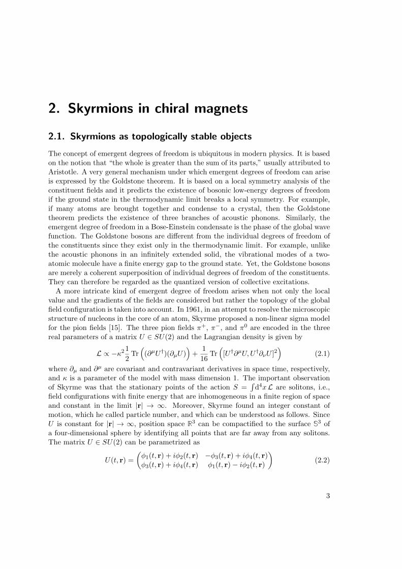
Figure 2.1.: Examples of two-dimensional skyrmions. In both cases, M winds oncearound the unit sphere and both skyrmions have winding number W = −1and can be continuously deformed into each other. Arrows are spaced inarbitrary distances not related to the lattice distance and colored accordingto their z component. a) Bloch-type skyrmion, typically found in bulk chiralmagnets such as MnSi. b) Neel-type skyrmion, typically found in thin films.
where the real fields fields φα, α = 1, . . . , 4 have to satisfy the condition
φ21 + φ2
2 + φ23 + φ2
4 = 1. (2.3)
Thus, for a fixed time t, the combined field φ ≡ (φ1, φ2, φ3, φ4) defines a mapping fromthe compactified position space S3 to S3. Generally, the space of mappings from Sn
to Sm separates into topologically disconnected classes, which form the nth homotopygroup of Sm, or πn(Sm) for short. In the present scenario we have n = m = 3 and sinceπn(Sn) is always isomorphic to Z (for n ≥ 1) [16], the field configuration at any giventime can be labeled by an integer winding number,
W =1
2π2
∫d3r εijkl φi
∂φj∂rx
∂φk∂ry
∂φl∂rz
(2.4)
where εijkl is the totally antisymmetric tensor. Time evolution, described on a classicallevel by the Euler-Lagrange equations of L, is continuous and therefore the windingnumber is a constant of motion.
The integer winding number counts the number of times that φ(r) covers S3 when ris varied over the whole space. A given field configuration with winding number W can
4
2.1. Skyrmions as topologically stable objects
always be continuously deformed into a configuration of W “elementary” solitons thatare located far away from each other. These elementary solitons are nowadays referredto as skrymions and their properties are similar to those of particles: skyrmions canmove in space and they possess internal degrees of freedom in the sense that the fieldconfiguration can be deformed locally. However, continuous deformations cannot changethe overall number of skyrmions since the winding number is a topological invariant.Thus, we started with a theory, Eq. (2.1), that contained the pion fields as the onlyparticle fields, and we identified the topologically stable excitations of the pion field as anew emergent type of particles. In contrast to the collective excitations discussed above,skyrmions are not a coherent superposition of local excitations since they are not linear.Scaling a skyrmion solutions φ by a factor of 2 does not lead to a configuration with twoskyrmions but instead would violate the normalization condition Eq. (2.3).
The concept of topological excitations as emergent particles is not limited to threedimensions and it turns out that two-dimensional skrmions naturally appear in magneticsystems. These magnetic skyrmions are the topic of this thesis. The magnetizationM(r) in a magnetic material is a three-component vector field. Below the transitiontemperature, the magnitude |M| of the magnetization becomes finite. Fluctuations ofthe magnitude are energetically expensive, while long-wavelength fluctuations of thedirection M := M/|M| are governed by the energy scale of crystal anisotropies, whichis often much lower in bulk materials. It is therefore often a good approximation toassume a constant |M| and consider only the free energy as a function of M. Two kindsof two-dimensional skyrmions are depicted in Figure 2.1. Bloch-type skyrmions whereM winds like a screw on paths through the skyrmion center are typically found in bulkchiral magnets such as MnSi (Figure 2.1a). Neel-type skyrmions are often realized inthin films where inversion symmetry is broken by the existence of a substrate on only oneside of the film (Figure 2.1b). Far away from the skyrmion, the magnetization is constantand we can again compactify position space to the sphere S2. The map M : S2 → S2
has an integer winding number, which can be calculated from
W =1
4πM ·
(∂M
∂x× ∂M
∂y
). (2.5)
The winding number counts the number of times that the unit sphere S2 is covered whenr varies over the whole plane, as depicted in the right part of the Figure. One obtains thevalue of W = −1 for both configurations in Figure 2.1. The configurations are thereforesometimes called anti-skyrmions. Note, however, that the sign of W depends on the wayin which the order parameter space S2 is embedded in R3. If we had looked at the twoplanes in Figure 2.1 from below, we would have obtained W = 1.
From a mathematical point of view, the winding number cannot be changed by con-tinuous deformations of the magnetization texture. However, the topological protectiononly holds if the order parameter is always well-defined and the magnetization nevervanishes. In real magnetic systems, the topological invariance of the winding numbertranslates into an energy scale for a barrier that has to be overcome in order to changethe winding number.
5
2. Skyrmions in chiral magnets
0.03
0.08
0.21
0.55
1.47
3.87
10.2
27.1
71.5
189
500
Counts
/Std.m
on.
0.08
0
-0.08
q y(Å
-1)
0.080-0.08qx(Å-1)
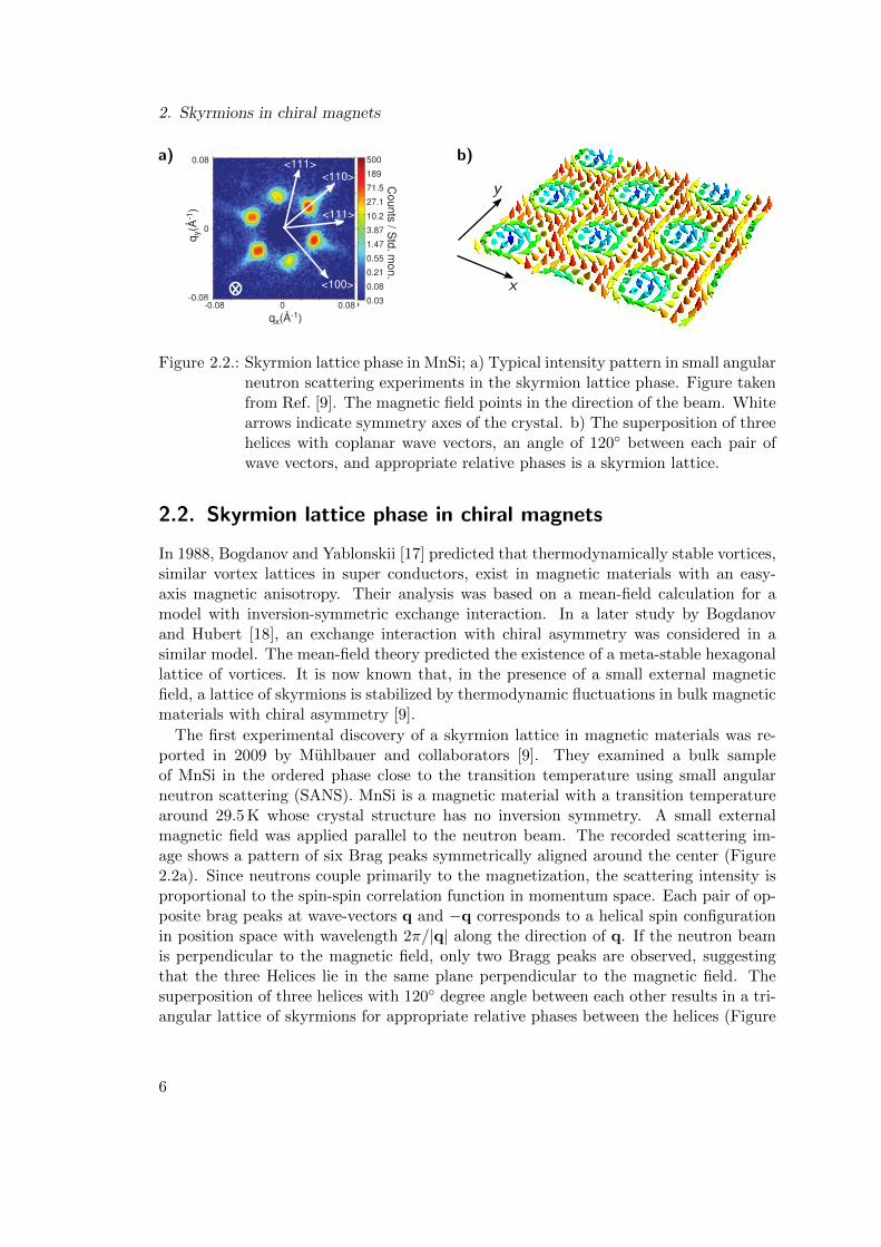
Figure 2.2.: Skyrmion lattice phase in MnSi; a) Typical intensity pattern in small angularneutron scattering experiments in the skyrmion lattice phase. Figure takenfrom Ref. [9]. The magnetic field points in the direction of the beam. Whitearrows indicate symmetry axes of the crystal. b) The superposition of threehelices with coplanar wave vectors, an angle of 120 between each pair ofwave vectors, and appropriate relative phases is a skyrmion lattice.
2.2. Skyrmion lattice phase in chiral magnets
In 1988, Bogdanov and Yablonskii [17] predicted that thermodynamically stable vortices,similar vortex lattices in super conductors, exist in magnetic materials with an easy-axis magnetic anisotropy. Their analysis was based on a mean-field calculation for amodel with inversion-symmetric exchange interaction. In a later study by Bogdanovand Hubert [18], an exchange interaction with chiral asymmetry was considered in asimilar model. The mean-field theory predicted the existence of a meta-stable hexagonallattice of vortices. It is now known that, in the presence of a small external magneticfield, a lattice of skyrmions is stabilized by thermodynamic fluctuations in bulk magneticmaterials with chiral asymmetry [9].
The first experimental discovery of a skyrmion lattice in magnetic materials was re-ported in 2009 by Muhlbauer and collaborators [9]. They examined a bulk sampleof MnSi in the ordered phase close to the transition temperature using small angularneutron scattering (SANS). MnSi is a magnetic material with a transition temperaturearound 29.5 K whose crystal structure has no inversion symmetry. A small externalmagnetic field was applied parallel to the neutron beam. The recorded scattering im-age shows a pattern of six Brag peaks symmetrically aligned around the center (Figure2.2a). Since neutrons couple primarily to the magnetization, the scattering intensity isproportional to the spin-spin correlation function in momentum space. Each pair of op-posite brag peaks at wave-vectors q and −q corresponds to a helical spin configurationin position space with wavelength 2π/|q| along the direction of q. If the neutron beamis perpendicular to the magnetic field, only two Bragg peaks are observed, suggestingthat the three Helices lie in the same plane perpendicular to the magnetic field. Thesuperposition of three helices with 120 degree angle between each other results in a tri-angular lattice of skyrmions for appropriate relative phases between the helices (Figure
6
2.2. Skyrmion lattice phase in chiral magnets
2.2b). The figure shows a cut through the system perpendicular to the applied magneticfield. The magnetization texture is translationally invariant in the direction along themagnetic field. It was confirmed by theoretical calculations that the skyrmion lattice isindeed the thermodynamically stable configuration.
In addition to SANS measurements, the existence of a skyrmion lattice phase in mag-netic materials without inversion symmetry has now been confirmed with a number ofcomplementary methods. These scattering experiments were later supported by observa-tions of skyrmion lattices in real space using Lorentz Transmission Electron Microscopyfor thin films [19], as well as magnetic force microscopy on the surface of bulk sam-ples [20]. In addition to these direct observations, the phase boundaries to the skyrmionlattice can also be inferred from electron transport experiments. Here, the existence of askyrmion lattice leads to a strong additional contribution to the Hall resistivity [21,22].We provide a more detailed discussion of the so-called topological Hall effect in Chapter7.
The skyrmion lattice phase is not limited to MnSi and it has been observed in a varietyof systems. The doped semiconductor Fe1−xCoxSi was studied in [19, 23]. In thin filmsof FeGe [24], a skyrmion lattice phase was reported to exist up to approximately 260 K.A strategy to engineer thin-film structures that can host skyrmions at room temperaturehas been proposed in Ref. [25] and single skyrmions at room temperature have recentlybeen observed by Boulle and collaborators [26]. The discovery of a skyrmion latticein the insulating multiferroic compound Cu2OSeO3 [27] promises new possibilities tomanipulate skyrmions via electric fields without resistive losses. All these systems havein common that the atomic structure has no inversion center. In thin films, inversionsymmetry is broken due to the presence of a substrate on one side of the film. Bulkmaterials in which a skyrmion lattice phase has been observed all have a crystal structurewhose space group has no inversion center, usually the P213 space group. Magneticmaterials without inversion center are commonly referred to as chiral magnets. Eachchiral magnet comes in two variants, a left-handed and a right-handed one, which arerelated to each other by space inversion. Due to the absence of inversion symmetry, thefree energy functional F [M] contains non-inversion symmetric terms. In the Ginzburg-Landau theory of spontaneous symmetry breaking, one obtains F [M] by expanding ingradients of M and retaining all terms allowed by symmetry. Following the notationin [9], the free energy is given by
F [M] =
∫d3r [r0M
2 + J(∂iMj)(∂iMj) + 2DM · (∇×M) + U(M2)2 −B ·M]. (2.6)
Here, r0 = 0 marks the transition from the unordered to the ordered state on a mean-field level, D is the strength of the so-called Dzyaloshinskii-Moriya (DM) interaction, seebelow, J is the ferromagnetic exchange coupling, U > 0 is needed so that the free energyis bounded from below and B is the external magnetic field. The term proportionalto D is odd under space inversion and therefore only allowed in chiral magnets. Itssign depends on the chirality of the crystal structure and it describes an anisotropicexchange interaction derived by Dzyaloshinksii and Moriya [28,29]. The form of the DM
7
2. Skyrmions in chiral magnets
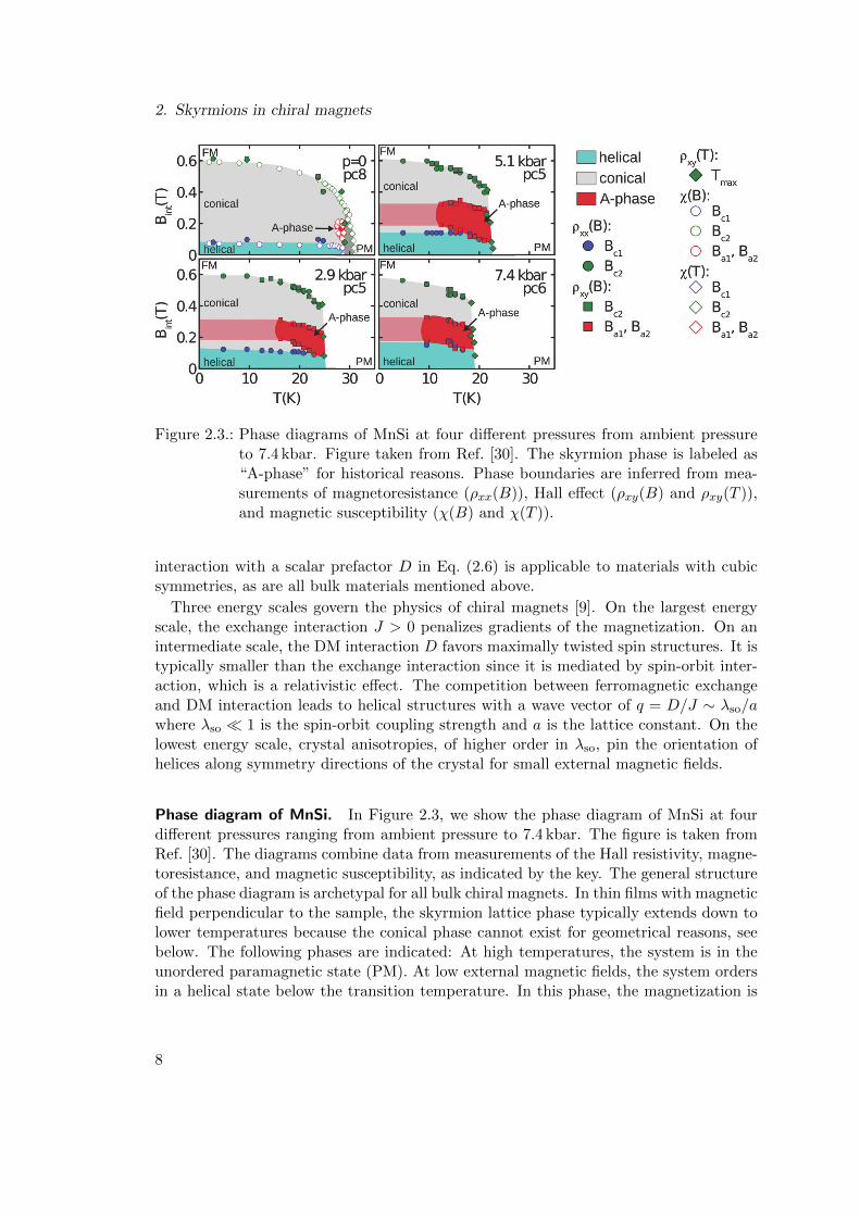
Figure 2.3.: Phase diagrams of MnSi at four different pressures from ambient pressureto 7.4 kbar. Figure taken from Ref. [30]. The skyrmion phase is labeled as“A-phase” for historical reasons. Phase boundaries are inferred from mea-surements of magnetoresistance (ρxx(B)), Hall effect (ρxy(B) and ρxy(T )),and magnetic susceptibility (χ(B) and χ(T )).
interaction with a scalar prefactor D in Eq. (2.6) is applicable to materials with cubicsymmetries, as are all bulk materials mentioned above.
Three energy scales govern the physics of chiral magnets [9]. On the largest energyscale, the exchange interaction J > 0 penalizes gradients of the magnetization. On anintermediate scale, the DM interaction D favors maximally twisted spin structures. It istypically smaller than the exchange interaction since it is mediated by spin-orbit inter-action, which is a relativistic effect. The competition between ferromagnetic exchangeand DM interaction leads to helical structures with a wave vector of q = D/J ∼ λso/awhere λso 1 is the spin-orbit coupling strength and a is the lattice constant. On thelowest energy scale, crystal anisotropies, of higher order in λso, pin the orientation ofhelices along symmetry directions of the crystal for small external magnetic fields.
Phase diagram of MnSi. In Figure 2.3, we show the phase diagram of MnSi at fourdifferent pressures ranging from ambient pressure to 7.4 kbar. The figure is taken fromRef. [30]. The diagrams combine data from measurements of the Hall resistivity, magne-toresistance, and magnetic susceptibility, as indicated by the key. The general structureof the phase diagram is archetypal for all bulk chiral magnets. In thin films with magneticfield perpendicular to the sample, the skyrmion lattice phase typically extends down tolower temperatures because the conical phase cannot exist for geometrical reasons, seebelow. The following phases are indicated: At high temperatures, the system is in theunordered paramagnetic state (PM). At low external magnetic fields, the system ordersin a helical state below the transition temperature. In this phase, the magnetization is
8
2.3. Recent trends
described byM(r) = M1 cos(q · r) + M2 sin(q · r) (2.7)
where M1, M2, and q are all perpendicular on each other. The wavelength 2π/|q| of thehelix in MnSi increases from 165 A near the transition temperature to 180 A for the lowestmeasured temperatures [31–33]. The direction of q is weakly pinned to along a [111]direction due to crystal anisotropies. In the diagram for p = 0, a narrow fluctuationdisordered phase is indicated in dark gray. In this regime, mean-field theory wouldalready predict an ordered state, but helical fluctuations with wave vectors q uniformelydistributed on a sphere in momentum space give rise to corrections to the mean-fieldbehavior and drive the transition weakly first order [31].
As the magnetic field is increased in the ordered state, the magnetization changesinto a conical state. In this state the magnetization is again described by Eq. (2.7), butthe wave vector q aligns parallel to the magnetic field and M1 and M2 are no longerperpendicular on q but obtain a component in direction of the magnetic field. Thenature of the transition from the helical to the conical state depends on the orientationof the crystal. In the general case it is a crossover but it may be a second-order transitionif the magnetic field is applied along a [111] direction [34]. The angle between M andB decreases with increasing magnetic field up to the point that the two are parallel andthe system is in the ferromagnetic state.
The skyrmion lattice phase, labeled “A-phase” in Figure 2.3 for historical reasons,forms a small pocket close to the transition temperature at a small external field B ∼0.2 T at ambient pressure. The phase extends to lower temperatures as pressure isincreased [30]. Due to the topological protection of skyrmions, the skyrmion latticeremains metastable if the system is prepared in the in the skyrmion lattice phase closeto the transition temperature and then the temperature is lowered (field cooling). Thisis indicated by the light red shaded area. If the system is cooled down at zero magneticfield (zero-field cooling) and then the magnetic field is turned on, the system prefersthe conical phase. The fate of a metastable skyrmion lattice when the magnetic field isslowly reduced and then inverted has been studied in Refs. [20,35]. In a three-dimensionalsample, this “unwinding” happens by a process in which two skyrmions first merge at asingle point in space at which the magnetization vanishes. This singular point then runsthrough the system like a zipper. It turns out that the singular point is a source or sinkof an emergent magnetic field, see Section 4.1.
2.3. Recent trends
A major reason for the recent interest in magnetic skyrmions lies in their prospectfor future data storage devices. The topological protection of skyrmions makes thempromising candidates for non-volatile storage devices, especially since single skyrmionsin a ferromagnetic background can be realized in thin magnetic films [25,26]. In addition,it turns out that skyrmions can be very efficiently manipulated with electric currents [12].This has two reasons. First, skyrmions couple to currents via a particular gyro-coupling,which is related to the winding number of the skyrmion [11,36]. Second, unlike magnetic
9
2. Skyrmions in chiral magnets
bubbles, which have been known to exist in materials without chiral asymmetry since the1970s [37], skyrmions in chiral magnets turn out to be rather rigid objects and forces onskyrmions couple predominantly to their translational mode rather than internal degreesof freedom [38]. In a numerical study, Fert and collaborators [39] proposed a setup bywhich a pattern of skyrmions that encodes a series of bits can be driven in a controlledway through a wire. Appropriately placed grooves in at the edge of the wire may helpto control the placements of the skyrmions, or to nucleate skyrmions at sharp edges [40].We study the dynamics of skyrmions with an emphasis on the influence of phase-spaceBerry phases in part III of this thesis (Chapters 9–11).
A different approach to the controlled manipulation of skyrmions is to selectedly createor destroy single skyrmions in a ferromagnetic background. In thin films, skyrmions canbe created and destroyed by injecting a spin-polarized current from the magnetic tip of ascanning tunneling microscope [41,42]. Recent experiments by Hsu and collaborators [43]indicate that it may be possible to generate and destroy skyrmions by electric fieldswithout a current. In part I of this thesis (Chapters 5–6), we show that skyrmions carryan electric charge, which might provide an explanation for this mechanism.
10
3. Berry phases
In 1983, Michael Berry made the observation [1] that the wave function of a quantum-mechanical system picks up a geometric phase when the parameters in the Hamiltonianare changed slowly. A similar geometrical phase had already been identified by Pan-charatnam in 1956 in the context of classical optics [44]. This phase, today known asthe Berry phase, influences the dynamics of the system and is ubiquitous in modernphysics [2]. In this chapter, we discuss the mathematical and physical properties ofBerry phases in a general setting. The application of these concepts onto chiral magnetsis deferred to the next chapter.
This chapter is structured as follows. In Section 3.1, we discuss the general require-ments that lead to the appearance of Berry phases in a physical system. We derive ageneral expression for the Berry phase in section 3.2 and discuss the range of its ap-plicability in section 3.5. In Section 3.3, we discuss gauge invariance of Berry phaseeffects and give a geometric interpretation of the introduced quantities. In Section 3.4,we explicitly derive the Berry curvature for a spin in an external magnetic field. Finally,we discuss the validity of the adiabatic assumption in Section 3.5.
3.1. Origin of Berry phases in physical systems
If the Hamiltonian H(t) of a quantum system depends on time, the instantaneous eigen-states of H(t) are not stationary solutions of the time-dependent Schrodinger equation.However, if the time dependency of H(t) is sufficiently slow (to be quantified in sec-tion 3.5) and if the energy levels are non-degenerate for all times, then the adiabatictheorem [45, 46] states that a system that is prepared in the nth eigenstate of H(t0) atsome initial time t0 evolves in time by following the nth eigenstate of H(t) for t ≥ t0.Transitions into other eigenstates are exponentially suppressed as the time dependencyof H(t) becomes slower.
While the adiabatic theorem guarantees that the system remains in the nth eigenstateof H(t), it makes no statement about the phase factor eiϕ that the wave function acquiresif the Hamiltonian returns to its original form, i.e. if H(t1) = H(t0) for some timet1 > t0. Berry’s observation [1] was that the phase picked up by a quantum system underadiabatic time evolution can be understood as a sum of two contributions. First, the so-called dynamical phase is the straight-forward generalization of the phase acquired by astationary state, and is given by the integral over time of the instantaneous eigenenergydivided by ~. Second, there is an additional contribution, which Berry denoted as thegeometrical phase, and which is nowadays commonly referred to as the Berry phase. Incontrast to the dynamical phase, the Berry phase depends only on the instantaneous
11
3. Berry phases
eigenstates of H(t) and is insensitive to the eigenenergies.
The concept of Berry phases has been successfully applied in many branches of physics(see, e.g., Refs. [2–4]). This popularity may be explained by a combination of propertiesof the Berry phase.1 First, Berry phases are physically measurable. Although the globalphase factor of a wave function cannot be detected, Berry phases lead to interferencewhen the adiabatic change from the initial Hamiltonian H(t0) to some final HamiltonianH(t′) may be realized in more than one way. This is the generic situation if H(t) ≡H(λ1(t), . . . , λN (t)) is an effective Hamiltonian for the fast modes of a system where thedynamics of some slow degrees of freedom λi(t), i = 1, . . . , N , is neglected (see below).In this case, the parameters λi may evolve from some initial to some final set of valueson different trajectories. The different Berry phases picked up on these trajectorieslead to interference and, ultimately, influence the effective equations of motion for theslow modes λi once their dynamics is reintroduced into the theory. As interferenceexperiments can only measure phase differences, only differences between Berry phasesare physical. In contrast, the Berry phase along a single (not closed) trajectory inparameter space depends on the choice of basis at the initial and final time. We willcome back to this gauge degree of freedom in section 3.3.
Second, there exists an intuitive geometric interpretation of Berry phases, allowingfor the application of powerful tools from differential geometry and from topology toquantum mechanical problems. The Berry phase along an infinitesimal path in parame-ter space λii=1,...,N may be interpreted as an affine connection, so that adiabatic timeevolution becomes equivalent to parallel transport of the wave function along a path inparameter space [47]. While an affine connection depends on the local coordinate sys-tem (i.e., the choice of gauge), it gives rise to a gauge-independent quantity called the(Riemann) curvature tensor. In absence of degeneracies, the so-called Berry curvatureis simply the Berry phase along an infinitesimal loop in parameter space. For a compactparameter space, the total curvature is a topological invariant, i.e. it only depends onglobal properties of the connection and is insensitive to local perturbations. This opensup powerful tools from the field of topology that can be used to explain physical phe-nomena and classify states of mater. For example, the quantization of the transverseconductivity in the quantum anomalous Hall effect [48] is a direct consequence of thequantization of the total Berry curvature in the Brillouin zone [8, 49].
Finally, Berry phases are ubiquitous in nature, since they appear whenever a quantum-mechanical system exhibits a clear separation of time scales. The time dependency ofthe Hamiltonian H(t) may either be explicit due to an externally applied slowly time-dependent perturbation; or it may be an implicit time-dependency of an effective Hamil-tonian for the fast degrees of freedom of a system whose constituents are governed bydynamics on clearly separated energy scales. Both scenarios are particularly commonin condensed matter physics. Many experiments on solids, for example, measure macro-scopic quantities such as thermal properties or transport coefficients in a macroscopicsample, while a microscopic description of the constituents is characterized by a much
1For an argumentation that focuses more on the mathematical properties of Berry phases, see also [2]and references therein.
12
3.1. Origin of Berry phases in physical systems
smaller length scale (the lattice constant) and therefore much larger momenta and ener-gies. In addition, the characteristic energy scales for the constituents themselves span awide range from the Debye frequency for phonons (~ωD ∼ 10 . . . 100 meV) to the bandwidth of the electronic system (∼ eV).
Let us illustrate the link between the separation of time scales and the appearance of ageometric phase by means of a classical analog. We consider a Foucault pendulum. Here,the two time scales are the short period τ of the oscillating pendulum and the long periodT of the earth’s rotation, which is a sidereal day (about four minutes short of a solar day).Except at the reversal points, the angular momentum L of the pendulum is primarilygoverned by the fast mode and therefore horizontally aligned. The gravitational forceFg on the mass of the pendulum is downwards by definition, and therefore the torqueL = r × Fg is also in the horizontal plane (r points from the suspension point of thependulum to the oscillating mass). However, the notion of “horizontal” changes slowlyover time due to the rotation of the earth, and the angular momentum of the pendulumhas to follow the horizontal plane. Microscopically, this process is mediated by a tinytorque due to the Coriolis force. It is rather cumbersome to solve the resulting equationsof motion explicitly, since the Coriolis force depends on the velocity of the pendulum,which oscillates on the short time scale. To leading order in τ/T , it turns out that thedirection of L follows the path that is defined by the smallest possible change consistentwith the condition of staying in the horizontal plane [50]. The trajectory of the directionof L is therefore only governed by geometric aspects, namely the curvature of the surfaceof the earth and the latitude φ at which the experiment is carried out. It turns out thatthe direction of L, and therefore the orientation of the pendulum, rotates by an angle of2π sin(φ) per sidereal day, where φ is measured from the equator. This is precisely 2πminus the solid angle enclosed by the location of the experiment on the surface of theearth as it rotates around the earth’s axis during one day.
In the classical example of the Foucault pendulum, the rotation angle can be observeddirectly. Quantum-mechanical phases, on the other hand, can only be observed if twowave functions interfere with each other. Therefore, Berry phases only play a role if theprocess that happens on the long time scale T is itself dynamic rather than externallyimposed. Bloch electrons in an external electric field E are a prime example of such aseparation of time scales. We may treat the electric field either in the current gauge,E = −∂A/∂t, where A(t) is the vector potential. This treatment is an example of anexplicitly time-dependent Hamiltonian. The vector potential enters the Hamiltonian viathe minimal coupling p = π + eA(t), where p and π are the kinetic and canonicalmomentum of the electrons with charge −e, respectively. A natural time scale τpert
associated with the external perturbation is given by the time in which the differencep− π = eA(t) traverses the Brillouin zone once. This leads to the estimate
~a
= e
∣∣∣∣∂A
∂t
∣∣∣∣ τpert = e|E|τpert (3.1)
where a ∼ A is the lattice constant. Thus, the characteristic energy ~/τpert = ea|E|of the external perturbation is the energy an electron gains when it travels one lattice
13
3. Berry phases
constant in the direction of the electric field. Even for very large electric fields, this valueis much smaller than the band separation ∆E ∼ eV, which is the characteristic energyscale for electrons in the unperturbed system.
Alternatively, we could have described the external electric field in the potential gauge,E = −∇φ, where φ(r) is the electric potential. In this treatment, the Hamiltonian isformally independent of time, but it gives rise to dynamics on two different time scales.The fast dynamics are described by the unperturbed Hamiltonian, whose eigenstatesΨn,k(r) = eik·run,k(r) are labeled by a band index n and a lattice momentum ~k andmay be written as a product of a plane wave and a Bloch function un,k(r). The latterhas the same periodicity as the atomic lattice. The electric potential φ(r) breaks thediscrete translational symmetry and therefore the wave functions Ψn,k(r) are no longerstationary. If we require again that ea|E| ∆E, then matrix elements 〈Ψn′,k′ |φ(r)|Ψn,k〉between two different bands n 6= n′ are small since the Bloch functions oscillate on amuch shorter length scale than the electric potential. Thus, inter-band transitions aresuppressed. On the other hand, intra-band matrix elements 〈Ψn,k′ |φ(r)|Ψn,k〉 betweento close-by wave vectors k and k′ are not suppressed (in a finite system) since thequickly oscillating factor u∗n,k′(r)un,k(r) in the integrand is almost everywhere positivefor k′ ≈ k. To a good approximation, the effect of intra-band transitions can be describedby a slow time evolution of the lattice wave vector k(t). The remaining (fast) degreesof freedom are captured by the Bloch function, which follows, in this approximation,adiabatically the trajectory of k(t) in the Brillouin zone. Thus, the electron dynamicsin the presence of an external electric field is described by a time-dependent effectiveHamiltonian Heff(t) = H(k(t)), where H(k) := e−ik·rHeik·r is the band Hamiltonian.We will see in section 5.1, that the time dependency of Heff leads to Berry phases, whichinfluence the trajectory of k(t).
3.2. Geometrical phase in a time-dependent system
In this section, we derive a general equation for the geometric phase picked up by a wavefunction under adiabatic time evolution due to a slowly time-dependent Hamiltonian.We follow the original derivation by Berry in [1].
We consider a quantum mechanical system whose Hamiltonian H(λ(t)) depends onsome time-dependent parameters λ(t) ≡ (λ1(t), . . . , λN (t)) ∈ M , where the parameterspace M is a real manifold. As discussed in the introduction to this chapter, the param-eters λ(t) may either be externally applied time-dependent fields, or H(λ(t)) may bethe effective Hamiltonian of a more complicated system that contains some slow modesλi(t)i=1,...,N , whose dynamics is neglected for the moment. For example, if λi ≡ ki arethe lattice wave vectors in an N -dimensional crystal, then M is the Brillouin zone, whichis an N -torus. For fixed λ, the Hamiltonian has eigenenergies En(λ) and correspondingnormalized eigenstates |Φn(λ)〉, defined by
H(λ)|Φn(λ)〉 = En(λ)|Φn(λ)〉, 〈Φn(λ)|Φn(λ)〉 = 1. (3.2)
We refer to En(λ) and |Φn(λ)〉 as the instantaneous eigenenergies and eigenstates,
14
3.2. Geometrical phase in a time-dependent system
respectively, and assume that the instantaneous eigenenergies are discrete and non-degenerate for all times. Note that Eq. (3.2) defines each instantaneous eigenstate onlyup to a global phase. We require that these phases are chosen such that the mapsλ 7→ |Φn(λ)〉 are differentiable. It is important to keep in mind that such a differen-tiable choice of instantaneous eigenstates is not always possible on the whole parameterspace M (see example at the end of section 3.3). For the present purpose, however, weonly require that the maps are differentiable on an open subset of M that contains thetrajectory λ(t) during the (finite) time interval of interest, which is always possible.
Suppose that at some initial time t0, the wave function |Ψ〉 of the system is preparedin the nth instantaneous eigenstate, |Ψ(t0)〉 ∝ |Φn(λ(t0))〉. Time evolution is describedby the Schrodinger equation,
i~∂
∂t|Ψ(t)〉 = H(λ(t)) |Ψ(t)〉. (3.3)
If λ(t) varies sufficiently slowly (see section 3.5), then |Ψ(t)〉 follows adiabatically thenth instantaneous eigenstate. We thus make the ansatz
|Ψ(t)〉 = eiϕ(t) |Φn(λ(t))〉 (3.4)
where ϕ(t) ∈ R is a yet to be determined phase. Combining Eqs. (3.2), (3.3) and (3.4)and projecting onto 〈Φn(λ(t))| leads to
∂ϕ(t)
∂t= −En(λ(t))
~+
N∑i=1
∂λi∂t
An,i(λ(t)) (3.5)
where
An,i(λ) = i〈Φn(λ)| ∂∂λi|Φn(λ)〉 (3.6)
is the ith component of the Berry connection of the nth energy level, which is real dueto the normalization 〈Φn(λ)|Φn(λ)〉 = 1. By integrating Eq. (3.5) we find for the phasepicked up by a quantum state subject to adiabatic time evolution from t0 to t1,
∆ϕ0→1 ≡ ϕ(t1)− ϕ(t0) = −1
~
∫ t1
t0
En(λ(t)) dt+ ∆ϕC (3.7)
with
∆ϕC =
∫C
dλ ·An (3.8)
where C := λ([t0, t1]) ⊂ M is the path in parameter space on which the parameters arevaried and the notation dλ ·An denotes the scalar product (i.e., sum over all componentsi = 1, . . . , N).
Eq. (3.7) describes the phase under adiabatic time evolution as a sum of two contri-butions. The term involving the integral over time is called the dynamical phase. Itgeneralizes the phase factor e−iEnt/~ of a stationary state in a time-independent system
15
3. Berry phases
to the situation where the eigenenergy En depends slowly on time. The second term,∆ϕC , is a correction to this naıve generalization. ∆ϕC is the Berry phase for an adiabaticchange of parameters along the path C. Note that the Berry phase depends only on the(directed) contour C on which the parameters λ are varied, and is independent of thevelocity with which λ(t) changes as a function of time (provided that the change remainsadiabatic). For this reason, the Berry phase is sometimes called a geometrical phase.Note also that the Berry phase along the reversed path C is given by ∆ϕC = −∆ϕC .
3.3. Gauge invariant formulation and geometric interpretationof Berry phases
The Berry connection, Eq. (3.6), cannot be a physically measurable quantity since itdepends on the choice of phases for the instantaneous eigenstates |Φn(λ)〉. The freedomto choose an arbitrary phase factor for each instantaneous eigenstate at all λ ∈ Mconstitutes a U(1) gauge degree of freedom for the solutions of Eq. (3.2). For a givenchoice of phases, we may define an alternative set of instantaneous eigenstates via thegauge transformation
|Φn(λ)〉 7−→ eiαn(λ)|Φn(λ)〉 (3.9)
where αn : M → R are arbitrary differentiable functions. The Berry connection,Eq. (3.6), changes under the gauge transformation,
An,i(λ) 7−→ An,i(λ)− ∂αn(λ)
∂λi. (3.10)
Therefore, the Berry phase, Eq. (3.8), is also gauge dependent,
∆ϕC 7−→ ∆ϕC −∫C
dλ · ∂αn(λ)
∂λ= ∆ϕC − αn(λ(t1)) + αn(λ(t0)). (3.11)
Eq. (3.11) simply reflects the fact that the gauge transformation, Eq. (3.9), changes thereference states to which the phases at times t0 and t1 are measured.
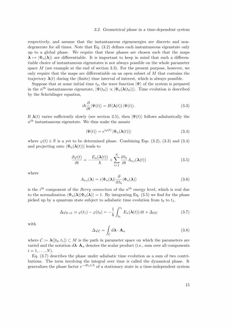
Berry curvature. When one derives semiclassical theories that include Berry phaseeffects, it is of advantage to formulate the semiclassical theory only in terms of gauge-invariant quantities. The gauge dependency of results obtained from a semiclassicaltheory can sometimes be quite subtle [51] if the semiclassical theory does not excludegauge-dependent quantities right away. An important gauge-invariant quantity is givenby the Berry phase along a loop in parameter space. If λ(t1) = λ(t0), the last two termson the right-hand side of Eq. (3.11) cancel and ∆ϕC is gauge invariant. In the same way,the difference ∆ϕC1 −∆ϕC2 between the Berry phases along two different paths C1 andC2 with common start and end points is gauge invariant, since it is equal to the Berryphase ∆ϕC picked up along the loop C that results from attaching the reverse of C2 tothe end of the path C1 (Figure 3.1).
16
3.3. Gauge invariant formulation and geometric interpretation of Berry phases
Figure 3.1.: The difference ∆ϕC1 −∆ϕC2 between the Berry phases along two paths C1
and C2 with common start and end points is gauge invariant since it is equalto the Berry phase ∆ϕC along a loop C resulting from attaching the reverseof C2 to the end of C1. If C is contractible, then ∆ϕC can be calculatedby integrating the Berry curvature Ωn over any surface S with ∂S = C,Eq. (3.12).
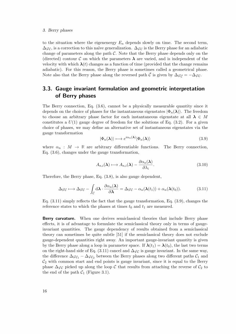
While the Berry phase along a loop C ⊂M is gauge-invariant, it is difficult to includein a semiclassical theory due to its non-locality. This obstacle can be overcome if Ccan be contracted to a point, in which case the Berry phase along C can be expressed interms of a local, gauge-invariant quantity known as Berry curvature. A contractible loopC can be expressed as the boundary ∂S of some surface S ⊂ M . According to Stokes’theorem, one has for the Berry phase along C,
∆ϕC =
∫∂Sdλ ·An =
1
~
∫S
Ωn (3.12)
where the two-form
Ωn =1
2
N∑i,j=1
Ωn,ij(λ) dλi ∧ dλj with Ωn,ij(λ) =∂Aj∂λi− ∂Ai∂λj
(3.13)
is the Berry curvature in the energy level n, which is invariant under the gauge transfor-mation Eq. (3.10) (“∧” denotes the totally anti-symmetric wedge product). The com-ponents Ωn,ij = −Ωn,ji of the Berry curvature form a skew symmetric tensor, usuallyreferred to as the Berry curvature tensor, and satisfy the Jacobi identity
∂Ωn,ij
∂λk+∂Ωn,ki
∂λj+∂Ωn,jk
∂λi= 0 (3.14)
which can be easily checked.
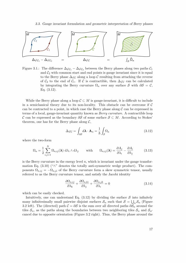
Intuitively, one can understand Eq. (3.12) by dividing the surface S into infinitelymany infinitesimally small pairwise disjoint surfaces Sα such that S =
⋃α Sα (Figure
3.2 left). The (directed) path C = ∂S is the sum over all directed paths ∂Sα around thetiles Sα, as the paths along the boundaries between two neighboring tiles Sα and Sα′cancel due to opposite orientation (Figure 3.2 right). Thus, the Berry phase around the
17
3. Berry phases
Figure 3.2.: The Berry curvature along the boundary ∂S of a surface S may be ex-pressed by dividing S into small tiles Sα (left), and summing over the Berrycurvatures along the boundary of each tile (right). The paths along a sharedboundary cancel due to opposite orientation.
whole surface S is equal to the sum of the Berry phases around each tile Sα. It is easyto see that, in the limit of infinitesimally small tiles, the Berry phase around a tile Sαthat lies in the plane spanned by λi and λj is given by the area of the tile multiplied byΩn,ij .
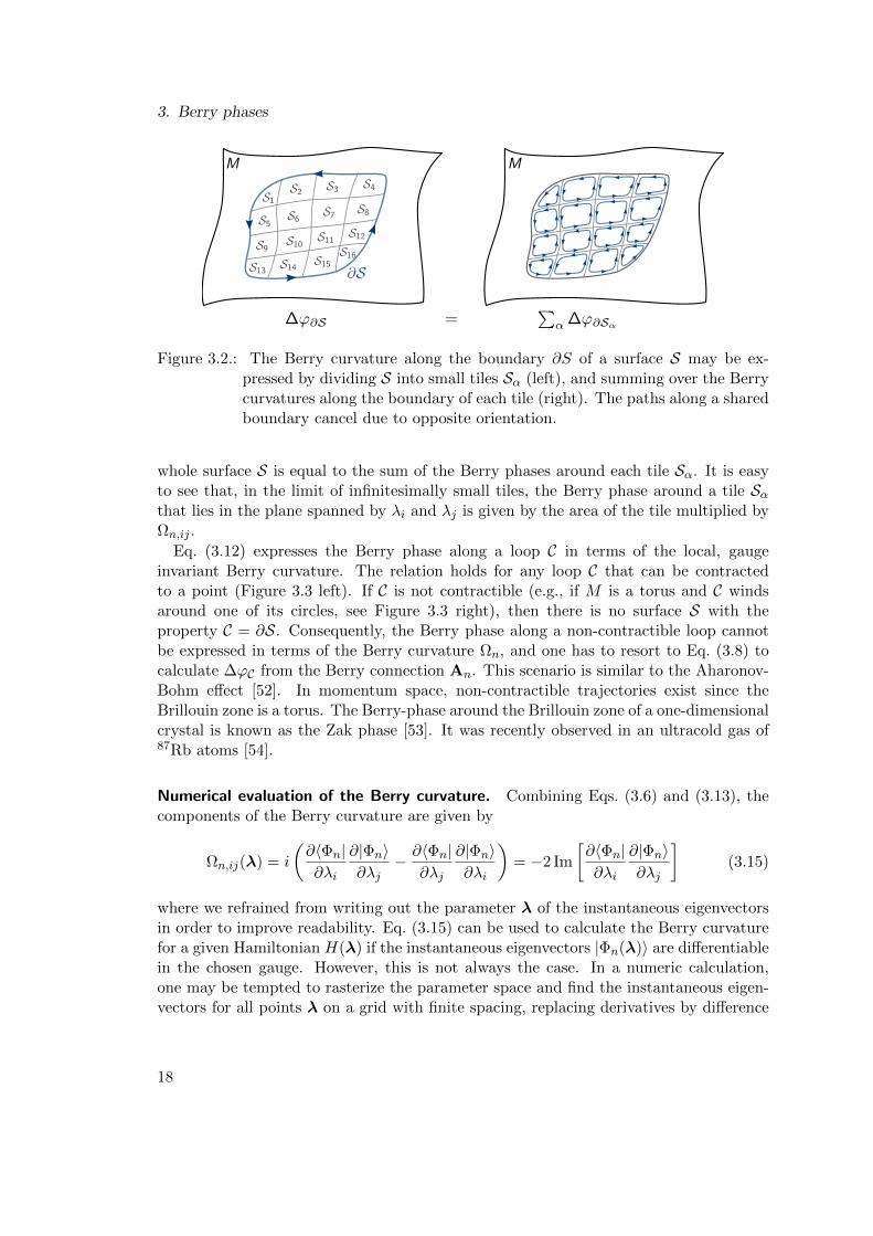
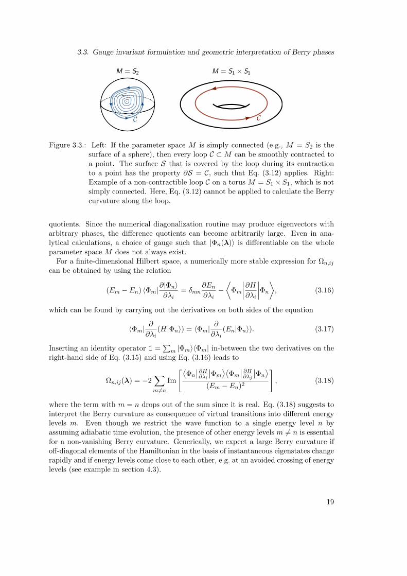
Eq. (3.12) expresses the Berry phase along a loop C in terms of the local, gaugeinvariant Berry curvature. The relation holds for any loop C that can be contractedto a point (Figure 3.3 left). If C is not contractible (e.g., if M is a torus and C windsaround one of its circles, see Figure 3.3 right), then there is no surface S with theproperty C = ∂S. Consequently, the Berry phase along a non-contractible loop cannotbe expressed in terms of the Berry curvature Ωn, and one has to resort to Eq. (3.8) tocalculate ∆ϕC from the Berry connection An. This scenario is similar to the Aharonov-Bohm effect [52]. In momentum space, non-contractible trajectories exist since theBrillouin zone is a torus. The Berry-phase around the Brillouin zone of a one-dimensionalcrystal is known as the Zak phase [53]. It was recently observed in an ultracold gas of87Rb atoms [54].
Numerical evaluation of the Berry curvature. Combining Eqs. (3.6) and (3.13), thecomponents of the Berry curvature are given by
Ωn,ij(λ) = i
(∂〈Φn|∂λi
∂|Φn〉∂λj
− ∂〈Φn|∂λj
∂|Φn〉∂λi
)= −2 Im
[∂〈Φn|∂λi
∂|Φn〉∂λj
](3.15)
where we refrained from writing out the parameter λ of the instantaneous eigenvectorsin order to improve readability. Eq. (3.15) can be used to calculate the Berry curvaturefor a given Hamiltonian H(λ) if the instantaneous eigenvectors |Φn(λ)〉 are differentiablein the chosen gauge. However, this is not always the case. In a numeric calculation,one may be tempted to rasterize the parameter space and find the instantaneous eigen-vectors for all points λ on a grid with finite spacing, replacing derivatives by difference
18
3.3. Gauge invariant formulation and geometric interpretation of Berry phases
Figure 3.3.: Left: If the parameter space M is simply connected (e.g., M = S2 is thesurface of a sphere), then every loop C ⊂M can be smoothly contracted toa point. The surface S that is covered by the loop during its contractionto a point has the property ∂S = C, such that Eq. (3.12) applies. Right:Example of a non-contractible loop C on a torus M = S1 × S1, which is notsimply connected. Here, Eq. (3.12) cannot be applied to calculate the Berrycurvature along the loop.
quotients. Since the numerical diagonalization routine may produce eigenvectors witharbitrary phases, the difference quotients can become arbitrarily large. Even in ana-lytical calculations, a choice of gauge such that |Φn(λ)〉 is differentiable on the wholeparameter space M does not always exist.
For a finite-dimensional Hilbert space, a numerically more stable expression for Ωn,ij
can be obtained by using the relation
(Em − En) 〈Φm|∂|Φn〉∂λi
= δmn∂En∂λi−⟨
Φm
∣∣∣∣∂H∂λi∣∣∣∣Φn
⟩, (3.16)
which can be found by carrying out the derivatives on both sides of the equation
〈Φm|∂
∂λi(H|Φn〉) = 〈Φm|
∂
∂λi(En|Φn〉). (3.17)
Inserting an identity operator 1 =∑
m |Φm〉〈Φm| in-between the two derivatives on theright-hand side of Eq. (3.15) and using Eq. (3.16) leads to
Ωn,ij(λ) = −2∑m 6=n
Im
[⟨Φn
∣∣ ∂H∂λi
∣∣Φm
⟩⟨Φm
∣∣ ∂H∂λj
∣∣Φn
⟩(Em − En)2
], (3.18)
where the term with m = n drops out of the sum since it is real. Eq. (3.18) suggests tointerpret the Berry curvature as consequence of virtual transitions into different energylevels m. Even though we restrict the wave function to a single energy level n byassuming adiabatic time evolution, the presence of other energy levels m 6= n is essentialfor a non-vanishing Berry curvature. Generically, we expect a large Berry curvature ifoff-diagonal elements of the Hamiltonian in the basis of instantaneous eigenstates changerapidly and if energy levels come close to each other, e.g. at an avoided crossing of energylevels (see example in section 4.3).
19
3. Berry phases
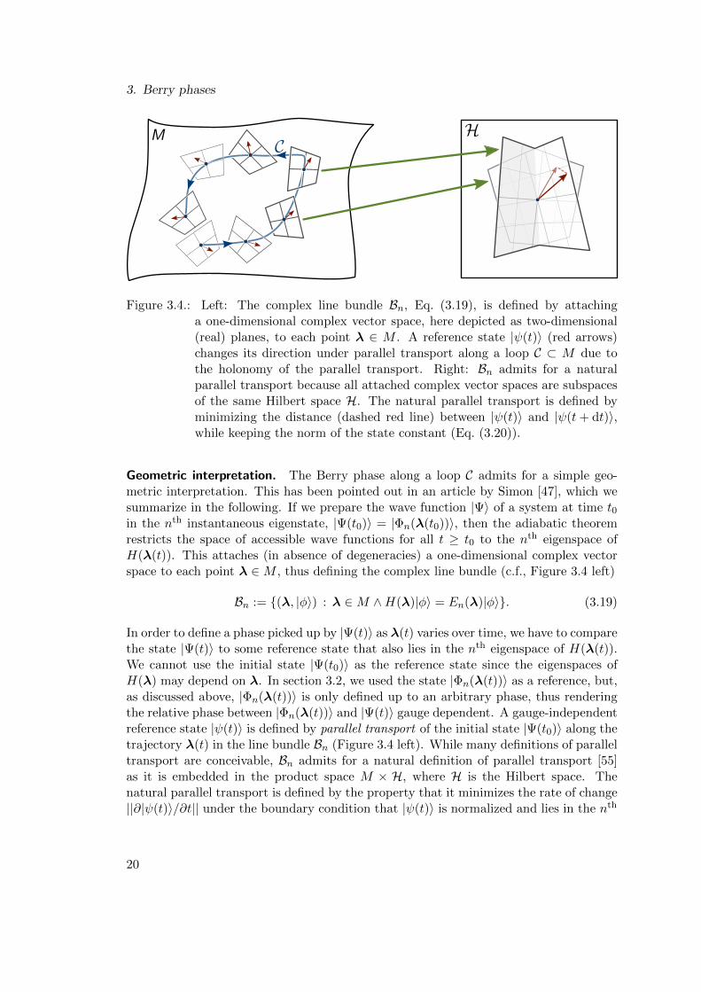
Figure 3.4.: Left: The complex line bundle Bn, Eq. (3.19), is defined by attachinga one-dimensional complex vector space, here depicted as two-dimensional(real) planes, to each point λ ∈ M . A reference state |ψ(t)〉 (red arrows)changes its direction under parallel transport along a loop C ⊂ M due tothe holonomy of the parallel transport. Right: Bn admits for a naturalparallel transport because all attached complex vector spaces are subspacesof the same Hilbert space H. The natural parallel transport is defined byminimizing the distance (dashed red line) between |ψ(t)〉 and |ψ(t+ dt)〉,while keeping the norm of the state constant (Eq. (3.20)).
Geometric interpretation. The Berry phase along a loop C admits for a simple geo-metric interpretation. This has been pointed out in an article by Simon [47], which wesummarize in the following. If we prepare the wave function |Ψ〉 of a system at time t0in the nth instantaneous eigenstate, |Ψ(t0)〉 = |Φn(λ(t0))〉, then the adiabatic theoremrestricts the space of accessible wave functions for all t ≥ t0 to the nth eigenspace ofH(λ(t)). This attaches (in absence of degeneracies) a one-dimensional complex vectorspace to each point λ ∈M , thus defining the complex line bundle (c.f., Figure 3.4 left)
Bn := (λ, |φ〉) : λ ∈M ∧H(λ)|φ〉 = En(λ)|φ〉. (3.19)
In order to define a phase picked up by |Ψ(t)〉 as λ(t) varies over time, we have to comparethe state |Ψ(t)〉 to some reference state that also lies in the nth eigenspace of H(λ(t)).We cannot use the initial state |Ψ(t0)〉 as the reference state since the eigenspaces ofH(λ) may depend on λ. In section 3.2, we used the state |Φn(λ(t))〉 as a reference, but,as discussed above, |Φn(λ(t))〉 is only defined up to an arbitrary phase, thus renderingthe relative phase between |Φn(λ(t))〉 and |Ψ(t)〉 gauge dependent. A gauge-independentreference state |ψ(t)〉 is defined by parallel transport of the initial state |Ψ(t0)〉 along thetrajectory λ(t) in the line bundle Bn (Figure 3.4 left). While many definitions of paralleltransport are conceivable, Bn admits for a natural definition of parallel transport [55]as it is embedded in the product space M × H, where H is the Hilbert space. Thenatural parallel transport is defined by the property that it minimizes the rate of change||∂|ψ(t)〉/∂t|| under the boundary condition that |ψ(t)〉 is normalized and lies in the nth
20
3.3. Gauge invariant formulation and geometric interpretation of Berry phases
eigenspace of H(λ(t)) for all t (Figure 3.4 right). This is equivalent to the condition2
〈ψ(t)|∂|ψ(t)〉∂t
≡ −∂〈ψ(t)|∂t
|ψ(t)〉 = 0. (3.20)
One can calculate the phase that the wave function |Ψ(t)〉 picks up relative to thereference state |ψ(t)〉 following the same steps that lead to Eq. (3.7) and finds that itconsists only of the dynamical phase. Thus, the choice of reference state |ψ(t)〉, definedby the natural parallel transport of the initial wave function along the trajectory λ(t),gauges away the Berry phase.
Let us now consider the case that the trajectory λ(t) describes a loop in the parameterspace M , i.e., λ(t1) = λ(t0) for some t1 > t0. Since the Berry phase along a loop isgauge invariant, it cannot be eliminated by a clever choice of gauge. Indeed, measuringphases relative to the reference state |ψ(t)〉 is not the same as a gauge transformation ofthe form of Eq. (3.9) if the trajectory is a loop. The reason is that, in general, |ψ(t1)〉 6=|ψ(t0)〉. While both |ψ(t1)〉 and |ψ(t0)〉 lie in the nth eigenspace of H(λ(t1)) = H(λ(t0)),they may differ by a phase. The property that a vector is not invariant under paralleltransport along a loop is known as holonomy of the chosen parallel transport. In caseof a contractible loop, the holonomy is a measure of the curvature of a surface enclosedby the loop. The relative phase between |ψ(t1)〉 and |ψ(t0)〉 can easily be calculated byparameterizing |ψ(t)〉 = eiϕ(t)|Φn(λ(t))〉. Inserting into Eq. (3.20) and combining withEq. (3.6) shows that the phase picked up under parallel transport of the initial wavefunction |Ψ(t0)〉 along a loop C in parameter space is precisely the Berry phase ∆ϕC ,Eq. (3.8).
The above geometric picture justifies the choice of the names “Berry connection” and“Berry curvature”. The Berry connection An is related to an affine connection on thecomplex line bundle Bn in the sense that it defines parallel transport of a vector |ψ〉along a trajectory λ(t) by
|ψ(t+ dt)〉 = T (t+ dt , t) |ψ(t)〉 (3.21)
where the operator
T (t+ dt , t) = |Φn(λ(t+ dt))〉(
1 + dtλj(t)
∂tiAn,j(λ(t))
)〈Φn(λ(t))|+O(dt2) (3.22)
transports |ψ〉 from the one-dimensional complex vector space attached to λ(t) to theone attached to λ(t + dt). It is easy to see that Eqs. (3.21)–(3.22) are equivalent toEq. (3.20). Thus, we identify iAn,j as the natural affine connection on Bn [56].3 In
2The fact that Eq. (3.20) minimizes ||∂|ψ(t)〉/∂t|| can be seen by writing an alternative normalizedtrial wave function as |ψ′(t)〉 = eiγ(t)|ψ(t)〉 and observing that Eq. (3.20) ensures ||∂|ψ′(t)〉/∂t||2 =||∂|ψ(t)〉/∂t||2 + (∂γ/∂t)2.
3Note that iAn,j defines a different affine connection on each line bundle Bn and that the affine con-nection carries only a single index j instead of three indices since the attached vector spaces areone-dimensional, i.e. the sum over all basis vectors is trivial. For the same reason, the Berry curva-ture Ωn,ij of the energy level n carries only two (rather than of four) indices i, j.
21
3. Berry phases
physics context, it is common to leave the factor of i out of the definition and to denoteAn,j as the Berry connection. The curvature associated with the connection An,j isprecisely the Berry curvature.
3.4. Example
We conclude the discussion of the Berry curvature with the calculation of Ω for a spinin a time-dependent external magnetic field B(t). This was originally discussed in [1].Here, we use a more general approach that requires only the knowledge of the anti-commutation relations of angular momentum operators and can therefore more easilybe generalized to other symmetry groups than SU(2).
We consider a particle with total spin quantum number s ∈ 0, 12 , 1,
32 , . . ., i.e.,
S2|Ψ〉 = ~2s(s + 1)|Ψ〉 for all states |Ψ〉 in the Hilbert space. Here, S is the vector ofspin operators, whose components satisfy the commutation relations of the Lie-algebrasu(2),
[Si, Sj ] = i~εijkSk (3.23)
with the totally anti-symmetric tensor ε. The Hamiltonian of a spin in an externalmagnetic field B is given by
H(B) = −γB · S (3.24)
where γ is the gyromagnetic ratio of the particle carrying the spin (for electrons, γ =qg/(2m) with electron charge q = −e, mass m, and g-factor g ≈ 2). To keep the energyspectrum non-degenerate, we restrict the discussion to the case where B 6= 0, i.e., theparameter space is M = R3 \ 0. Thus, for any B ∈M , there exists a gB ∈ SU(2) thatrotates the vector B into the z-direction, i.e.,
H(B) = −γ|B|U(gB)Sz U(g−1B ) = −γ|B|U(g(B))Sz U
†(gB) (3.25)
where U is the (2s + 1)-dimensional irreducible representation of SU(2). Thus, theeigenvectors and eigenvalues of H(B) are given by
|Φm(B)〉 = U(gB) |m〉 and Em(B) = −m~γ|B| (3.26)
respectively, where |m〉 denotes the eigenvectors of Sz and m ∈ −s,−s+ 1, . . . , s. Thechoice of gB ∈ SU(2) admits a gauge degree of freedom since the spin quantization axisis invariant under rotation around itself. Therefore, the map B 7→ |Φm(B)〉 is also gaugedependent. As we will see below, there is no gauge such that the map B 7→ |Φm(B)〉is differentiable on the whole parameter space M . Nevertheless, for a given B ∈M , wecan always choose a gauge such that the map is differentiable on an open neighborhoodof B. Then, by inserting Eq. (3.24) into the identity
〈Φm(B)|(H(B)− Em(B))|Φm(B)〉 = 0 (3.27)
and differentiating with respect to Bα, one finds
〈Φm(B)|Sα|Φm(B)〉 = m~Bα|B|
. (3.28)
22
3.4. Example
Differentiating both sides of Eq. (3.28) by Bβ leads to
∂〈Φm(B)|∂Bβ
Sα |Φm(B)〉+ 〈Φm(B)|Sα∂|Φm(B)〉∂Bβ
= m~(δαβ|B|−BαBβ
|B|3
). (3.29)
Since the Lie-algebra su(2) is spanned by the generators i~Sx,i~Sy,
i~Sz, and U is a
representation of SU(2), its derivatives can be written as
∂U(gB)
∂Bβ=i
~fβγSγU(gB) (3.30)
with some (gauge-dependent) real coefficients fβγ . Thus, we find from Eq. (3.26),
∂ |Φm(B)〉∂Bβ
=∂U(gB)
∂Bβ|m〉 =
i
~fβγSγ |Φm(B)〉 . (3.31)
Inserting into Eq. (3.29) leads to
ifβγ 〈Φm(B)|[Sα, Sγ ]|Φm(B)〉 = m~2
(δαβ|B|−BαBβ
|B|3
)(3.32)
and thus, using Eqs. (3.23) and (3.28),
εαγδ fβγ Bδ =BαBβ
|B|2− δαβ. (3.33)
Finally, we find for the components of the Berry curvature Ωm in the coordinatesBx, By, Bz,
Ωm,ij(B)(3.15)
= i
(∂〈Φm(B)|
∂Bi
∂ |Φm(B)〉∂Bj
− ∂〈Φm(B)|∂Bj
∂ |Φm(B)〉∂Bi
)(3.31)
=i
~2fiα fjβ 〈Φm(B)|[Sα, Sβ]|Φm(B)〉
(3.23)= −1
~εαβγ fiα fjβ 〈Φm(B)|Sγ |Φm(B)〉
(3.28)= − m
|B|εαβγ fiα fjβ Bγ
= − m
|B|3εµνλ εµαρ ενβγ fiα fjβ BλBρBγ
(3.33)= − m
|B|3εµνλBλ
(BµBi
|B|2− δµi
)(BνBj
|B|2− δνj
)= −mεijk
Bk
|B|3. (3.34)
If we restrict the parameter space to the surface of a sphere SB ⊂ M of radiusB > 0 around the degeneracy at B = 0, then the right-hand side of Eq. (3.34) is simply
23

3. Berry phases
Figure 3.5.: The Berry phase along a loop C picked up by a particle in a magnetic fieldB, Eq. (3.24), is given by (−m) times the solid angle covered by C. Here,m is the magnetic quantum number. Since both surfaces A (left) and B(right) have C as their boundaries, the Berry phase may be calculated byintegrating over either one of the two and is only defined up to a multiple of4mπ, see Eq. (3.36). Note that A and B have opposite orientation relativeto the sphere SB since they lie on opposite sides of the oriented path C.
(−m/B2) times the volume form on SB. Therefore, the Berry phase along a loop C ⊂Mis given by (−m) times the solid angle covered by a surface A whose boundary is C(Figure 3.5 left) and the integral of the total Berry curvature over SB is, independentlyof the radius B, given by ∫
SBΩm = −4πm. (3.35)
Thus, in analogy to electromagnetism, the degeneracy at B = 0 can be regarded as apoint-source of Berry flux of strength (−m) in band m. A loop C ⊂ SB divides SB intotwo disjoint surfaces A and B (Figure 3.5). The Berry phase ∆ϕC along the loop maybe calculated by integrating Ωm either over A or over B, leading, in general, to differentvalues for ∆ϕC ,
∆ϕC =
∫AΩm or∫B Ωm =
∫AΩm + 4πm
(3.36)
if the orientations of A and B are chosen appropriately. This apparent contradictionis resolved by the fact that there is no gauge such that the eigenvectors |Φm(B)〉 aredifferentiable on the whole sphere SB. Therefore, there always exists some (gauge-dependent) point B′ ∈ SB where the Berry connection, Eq. (3.6), is not well-definedand Stokes theorem, Eq. (3.12), cannot be applied if B′ lies in the integration region.This does not impair our results, however, since we can always shift B′ between A andB with an appropriate gauge transformation without changing Ωm (where it is defined).Therefore, both branches in Eq. (3.36) have to be regarded as valid choices for theBerry curvature along C. Physically, only the phase factor ei∆ϕC is relevant, which isindependent of the choice of branch in Eq. (3.36) since 2m ∈ Z.
24
3.5. Quantification of adiabaticity
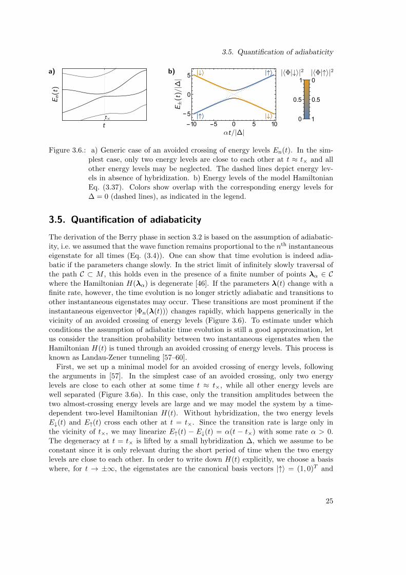
Figure 3.6.: a) Generic case of an avoided crossing of energy levels En(t). In the sim-plest case, only two energy levels are close to each other at t ≈ t× and allother energy levels may be neglected. The dashed lines depict energy lev-els in absence of hybridization. b) Energy levels of the model HamiltonianEq. (3.37). Colors show overlap with the corresponding energy levels for∆ = 0 (dashed lines), as indicated in the legend.
3.5. Quantification of adiabaticity
The derivation of the Berry phase in section 3.2 is based on the assumption of adiabatic-ity, i.e. we assumed that the wave function remains proportional to the nth instantaneouseigenstate for all times (Eq. (3.4)). One can show that time evolution is indeed adia-batic if the parameters change slowly. In the strict limit of infinitely slowly traversal ofthe path C ⊂ M , this holds even in the presence of a finite number of points λα ∈ Cwhere the Hamiltonian H(λα) is degenerate [46]. If the parameters λ(t) change with afinite rate, however, the time evolution is no longer strictly adiabatic and transitions toother instantaneous eigenstates may occur. These transitions are most prominent if theinstantaneous eigenvector |Φn(λ(t))〉 changes rapidly, which happens generically in thevicinity of an avoided crossing of energy levels (Figure 3.6). To estimate under whichconditions the assumption of adiabatic time evolution is still a good approximation, letus consider the transition probability between two instantaneous eigenstates when theHamiltonian H(t) is tuned through an avoided crossing of energy levels. This process isknown as Landau-Zener tunneling [57–60].
First, we set up a minimal model for an avoided crossing of energy levels, followingthe arguments in [57]. In the simplest case of an avoided crossing, only two energylevels are close to each other at some time t ≈ t×, while all other energy levels arewell separated (Figure 3.6a). In this case, only the transition amplitudes between thetwo almost-crossing energy levels are large and we may model the system by a time-dependent two-level Hamiltonian H(t). Without hybridization, the two energy levelsE↓(t) and E↑(t) cross each other at t = t×. Since the transition rate is large only inthe vicinity of t×, we may linearize E↑(t) − E↓(t) = α(t − t×) with some rate α > 0.The degeneracy at t = t× is lifted by a small hybridization ∆, which we assume to beconstant since it is only relevant during the short period of time when the two energylevels are close to each other. In order to write down H(t) explicitly, we choose a basiswhere, for t → ±∞, the eigenstates are the canonical basis vectors |↑〉 = (1, 0)T and
25
3. Berry phases
|↓〉 = (0, 1)T . With the simplifications that we may always set t× = 0 and shift bothenergies such that E↓(t) = −E↑(t), we arrive at the model Hamiltonian (c.f., Figure3.6b)
H(t) =
(12αt ∆∆∗ −1
2αt
)(3.37)
where ∆∗ denotes the complex conjugate of ∆.
The Hamiltonian, Eq. (3.37), has instantaneous eigenenergies E±(t) = ±√
14α
2t2 + |∆|2
and the corresponding instantaneous eigenstates |Φ+(t)〉 (|Φ−(t)〉) carry the state |↓〉(|↑〉) from t → −∞ to the state |↑〉 (|↓〉) for t → +∞, respectively (see Figure 3.6b).However, the wave function |Ψ(t)〉 of a system that is prepared in the eigenstate |Φ−(t)〉at time t→ −∞ will have a finite overlap with |Φ+(t)〉 at time t→ +∞. The probabilityof such a non-adiabatic transition,
Pn.a. := limt→∞|〈Φ+(t)|Ψ(t)〉|2 (3.38)
has been studied independently by Landau, Zener, Stueckelberg, and Majorana in 1932[57–60] (for a more modern derivation, see [61]). For the Hamiltonian in Eq. (3.37), theexact result is
Pn.a. = e−2π|∆|2/(~α). (3.39)
Thus, non-adiabatic transitions between instantaneous eigenstates are exponentially sup-pressed if the rate of change α |∆|2/~, where 2|∆| is the minimal separation betweenthe two energy levels. For the methods developed in this thesis, it will be most naturalto express the Hamiltonian in the basis of instantaneous eigenstates |Φ±(t)〉 (as opposedto the constant basis |↑〉 , |↓〉 used in Eq. (3.37)). While the Hamiltonian, Eq. (3.37), isby definition diagonal in the basis of |Φ±(t)〉, its time-derivative has off-diagonal termsthat mediate (real or virtual) transitions between instantaneous eigenstates. We alreadysaw that virtual transitions between instantaneous eigenstates influence adiabatic timeevolution (Eq. (3.18)). Non-adiabatic corrections can be interpreted as real transitions.For the model in Eq. (3.37), one finds,∣∣∣∣⟨Φ−(t)
∣∣∣∂H(t)
∂t
∣∣∣Φ+(t)⟩∣∣∣∣ =
α√4 + α2t2/|∆|2
(3.40)
and therefore,
Pn.a. = e−π/(4 maxt(κn.a.(t))) (3.41)
where maxt(· · · ) denotes the maximum value over all times and the dimensionless pa-rameter
κn.a.(t) :=~∣∣∣⟨Φ−(t)
∣∣∂H(t)∂t
∣∣Φ+(t)⟩∣∣∣
(E+(t)− E−(t))2(3.42)
quantifies non-adiabaticity. Adiabatic time evolution is a good approximation if κn.a.(t)1 for all times.
26
3.5. Quantification of adiabaticity
In this thesis, we study the electronic properties in magnetic materials with a smoothmagnetization texture. The smooth inhomogeneity leads to Berry phase effects withineach band and, in principle, also to non-adiabatic transitions between different bands.The relevance of the latter may be estimated by substituting ∂H
∂t ≈ vF∂H∂r + k ∂H∂k in
Eq. (3.42) where vF is a characteristic group velocity of the electrons, k ≈ eE/~ withelectric field E and elementary charge e, and H is the band-Hamiltonian that dependson some averaged position coordinate r (c.f., section 5.1). The range of validity of ourmethods is characterized by κn.a. 1.
27

4. Phase-space Berry phases in chiralmagnets
Berry phases play an important role in chiral magnets for two reasons. First, chiralmagnets with weak spin-orbit coupling exhibit a smooth magnetization texture belowthe transition temperature (section 2.2). In the reference frame of a moving electron,the smooth spatial inhomogeneity of the magnetization acts like a slowly time-dependentexchange field (c.f., Eq. (3.24)), leading to Berry-phase effects in position space [62,63].Second, spin-orbit coupling leads to a non-vanishing Berry curvature in momentumspace, which can be detected in measurements of the anomalous Hall effect [30]. Thepresence of both position and momentum-space Berry phases makes chiral magnets idealexample systems to study the effects of Berry phases in combined phase space (r,k).In general, Berry-phase effects in phase space are described by an antisymmetric 6 × 6Berry curvature tensor Ωn,ij , whose off-diagonal blocks describe the geometric phasespicked up by a wave packet on an infinitesimal loop in the plane spanned by positiondirection ri and momentum direction kj . If an explicit, slow time dependency of theHamiltonian is allowed, the Berry curvature becomes a 7×7 tensor where the additionalentries describe an emergent electric field in direct and in reciprocal space.
In this chapter, we present the origin and physical interpretation of Berry phasesin position and momentum space (sections 4.1 and 4.2, respectively), and introducesimple models to estimate the relative strengths of position-, momentum-, and mixedposition/momentum-space Berry phases in chiral magnets (section 4.3).
4.1. Position-space Berry phases and emergentelectrodynamics
It was pointed out by Volovik [64] in 1986 that the total mass current in an itinerantmagnet is the sum of two momenta: the momentum due to coherent motion (i.e., motionof the magnetization texture) and the momentum due to incoherent motion of the elec-trons. While the total mass current is well-defined, the partitioning between coherentand incoherent motion depends on a gauge. Thus, when either of the two components(coherent or incoherent motion) is treated in isolation, the natural description involvesa gauge theory, where the gauge field shifts the canonical momentum. In the following,we summarize the derivation of the emergent gauge theory for the electron motion. Wefollow the conventions for signs and prefactors in Refs. [30, 65], which differ from someearlier treatments [62,63] of emergent electrodynamics in chiral magnets.
29
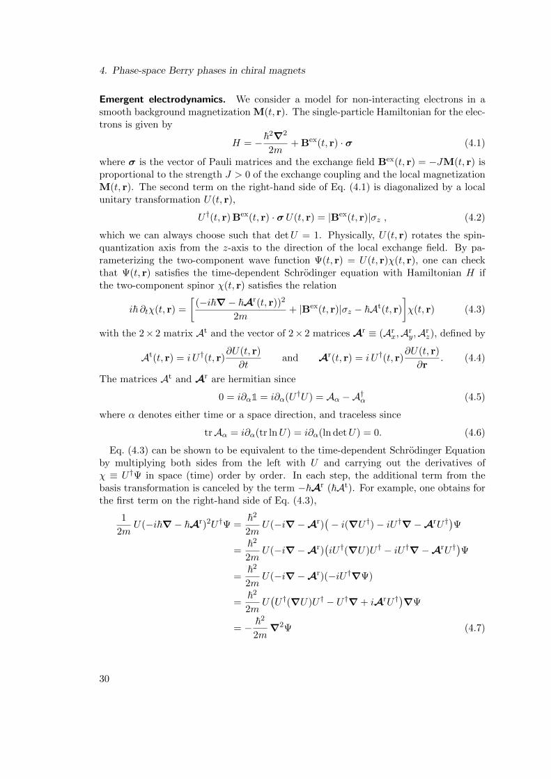
4. Phase-space Berry phases in chiral magnets
Emergent electrodynamics. We consider a model for non-interacting electrons in asmooth background magnetization M(t, r). The single-particle Hamiltonian for the elec-trons is given by
H = −~2∇2
2m+ Bex(t, r) · σ (4.1)
where σ is the vector of Pauli matrices and the exchange field Bex(t, r) = −JM(t, r) isproportional to the strength J > 0 of the exchange coupling and the local magnetizationM(t, r). The second term on the right-hand side of Eq. (4.1) is diagonalized by a localunitary transformation U(t, r),
U †(t, r) Bex(t, r) · σU(t, r) = |Bex(t, r)|σz , (4.2)
which we can always choose such that detU = 1. Physically, U(t, r) rotates the spin-quantization axis from the z-axis to the direction of the local exchange field. By pa-rameterizing the two-component wave function Ψ(t, r) = U(t, r)χ(t, r), one can checkthat Ψ(t, r) satisfies the time-dependent Schrodinger equation with Hamiltonian H ifthe two-component spinor χ(t, r) satisfies the relation
i~ ∂tχ(t, r) =
[(−i~∇− ~Ar(t, r))2
2m+ |Bex(t, r)|σz − ~At(t, r)
]χ(t, r) (4.3)
with the 2× 2 matrix At and the vector of 2× 2 matrices Ar ≡ (Arx,Ar
y,Arz), defined by
At(t, r) = i U †(t, r)∂U(t, r)
∂tand Ar(t, r) = i U †(t, r)
∂U(t, r)
∂r. (4.4)
The matrices At and Ar are hermitian since
0 = i∂α1 = i∂α(U †U) = Aα −A†α (4.5)
where α denotes either time or a space direction, and traceless since
trAα = i∂α(tr lnU) = i∂α(ln detU) = 0. (4.6)
Eq. (4.3) can be shown to be equivalent to the time-dependent Schrodinger Equationby multiplying both sides from the left with U and carrying out the derivatives ofχ ≡ U †Ψ in space (time) order by order. In each step, the additional term from thebasis transformation is canceled by the term −~Ar (~At). For example, one obtains forthe first term on the right-hand side of Eq. (4.3),
1
2mU(−i~∇− ~Ar)2U †Ψ =
~2
2mU(−i∇−Ar)
(− i(∇U †)− iU †∇−ArU †
)Ψ
=~2
2mU(−i∇−Ar)
(iU †(∇U)U † − iU †∇−ArU †
)Ψ
=~2
2mU(−i∇−Ar)(−iU †∇Ψ)
=~2
2mU(U †(∇U)U † − U †∇ + iArU †
)∇Ψ
= − ~2
2m∇2Ψ (4.7)
30
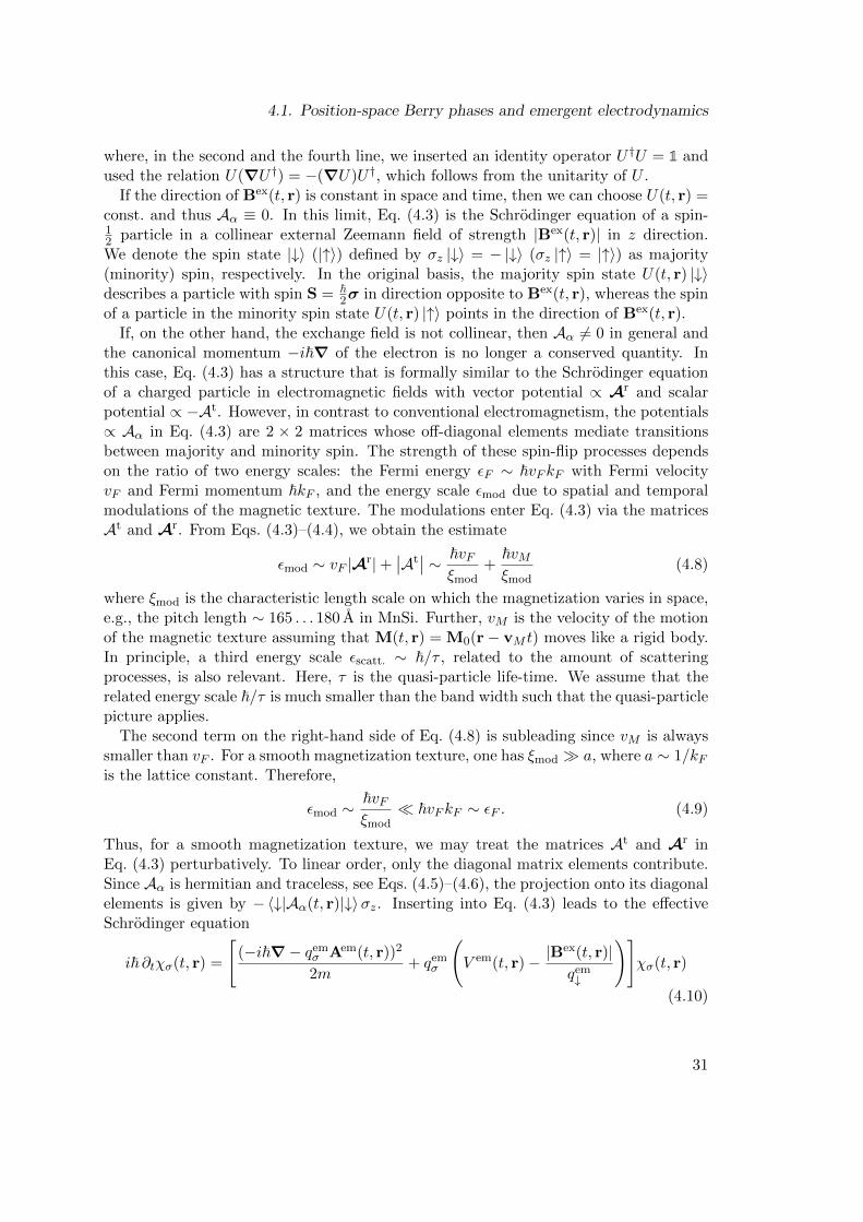
4.1. Position-space Berry phases and emergent electrodynamics
where, in the second and the fourth line, we inserted an identity operator U †U = 1 andused the relation U(∇U †) = −(∇U)U †, which follows from the unitarity of U .
If the direction of Bex(t, r) is constant in space and time, then we can choose U(t, r) =const. and thus Aα ≡ 0. In this limit, Eq. (4.3) is the Schrodinger equation of a spin-12 particle in a collinear external Zeemann field of strength |Bex(t, r)| in z direction.We denote the spin state |↓〉 (|↑〉) defined by σz |↓〉 = − |↓〉 (σz |↑〉 = |↑〉) as majority(minority) spin, respectively. In the original basis, the majority spin state U(t, r) |↓〉describes a particle with spin S = ~
2σ in direction opposite to Bex(t, r), whereas the spinof a particle in the minority spin state U(t, r) |↑〉 points in the direction of Bex(t, r).
If, on the other hand, the exchange field is not collinear, then Aα 6= 0 in general andthe canonical momentum −i~∇ of the electron is no longer a conserved quantity. Inthis case, Eq. (4.3) has a structure that is formally similar to the Schrodinger equationof a charged particle in electromagnetic fields with vector potential ∝ Ar and scalarpotential ∝ −At. However, in contrast to conventional electromagnetism, the potentials∝ Aα in Eq. (4.3) are 2 × 2 matrices whose off-diagonal elements mediate transitionsbetween majority and minority spin. The strength of these spin-flip processes dependson the ratio of two energy scales: the Fermi energy εF ∼ ~vFkF with Fermi velocityvF and Fermi momentum ~kF , and the energy scale εmod due to spatial and temporalmodulations of the magnetic texture. The modulations enter Eq. (4.3) via the matricesAt and Ar. From Eqs. (4.3)–(4.4), we obtain the estimate
εmod ∼ vF |Ar|+∣∣At∣∣ ∼ ~vF
ξmod+
~vMξmod
(4.8)
where ξmod is the characteristic length scale on which the magnetization varies in space,e.g., the pitch length ∼ 165 . . . 180 A in MnSi. Further, vM is the velocity of the motionof the magnetic texture assuming that M(t, r) = M0(r− vM t) moves like a rigid body.In principle, a third energy scale εscatt. ∼ ~/τ , related to the amount of scatteringprocesses, is also relevant. Here, τ is the quasi-particle life-time. We assume that therelated energy scale ~/τ is much smaller than the band width such that the quasi-particlepicture applies.
The second term on the right-hand side of Eq. (4.8) is subleading since vM is alwayssmaller than vF . For a smooth magnetization texture, one has ξmod a, where a ∼ 1/kFis the lattice constant. Therefore,
εmod ∼~vFξmod
~vFkF ∼ εF . (4.9)
Thus, for a smooth magnetization texture, we may treat the matrices At and Ar inEq. (4.3) perturbatively. To linear order, only the diagonal matrix elements contribute.Since Aα is hermitian and traceless, see Eqs. (4.5)–(4.6), the projection onto its diagonalelements is given by −〈↓|Aα(t, r)|↓〉σz. Inserting into Eq. (4.3) leads to the effectiveSchrodinger equation
i~ ∂tχσ(t, r) =
[(−i~∇− qem
σ Aem(t, r))2
2m+ qem
σ
(V em(t, r)− |B
ex(t, r)|qem↓
)]χσ(t, r)
(4.10)
31
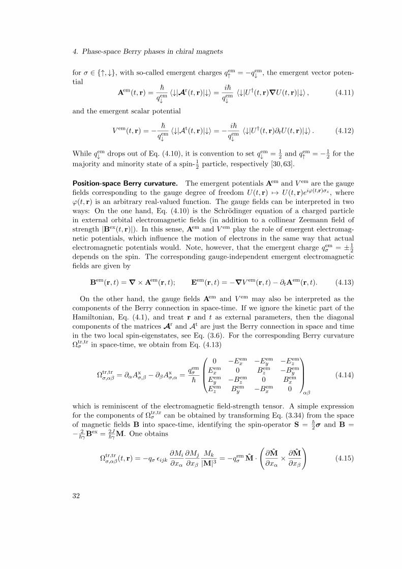
4. Phase-space Berry phases in chiral magnets
for σ ∈ ↑, ↓, with so-called emergent charges qem↑ = −qem
↓ , the emergent vector poten-tial
Aem(t, r) =~qem↓〈↓|Ar(t, r)|↓〉 =
i~qem↓〈↓|U †(t, r)∇U(t, r)|↓〉 , (4.11)
and the emergent scalar potential
V em(t, r) = − ~qem↓〈↓|At(t, r)|↓〉 = − i~
qem↓〈↓|U †(t, r)∂tU(t, r)|↓〉 . (4.12)
While qem↓ drops out of Eq. (4.10), it is convention to set qem
↓ = 12 and qem
↑ = −12 for the
majority and minority state of a spin-12 particle, respectively [30,63].
Position-space Berry curvature. The emergent potentials Aem and V em are the gaugefields corresponding to the gauge degree of freedom U(t, r) 7→ U(t, r)eiϕ(t,r)σz , whereϕ(t, r) is an arbitrary real-valued function. The gauge fields can be interpreted in twoways: On the one hand, Eq. (4.10) is the Schrodinger equation of a charged particlein external orbital electromagnetic fields (in addition to a collinear Zeemann field ofstrength |Bex(t, r)|). In this sense, Aem and V em play the role of emergent electromag-netic potentials, which influence the motion of electrons in the same way that actualelectromagnetic potentials would. Note, however, that the emergent charge qem
σ = ±12
depends on the spin. The corresponding gauge-independent emergent electromagneticfields are given by
Bem(r, t) = ∇×Aem(r, t); Eem(r, t) = −∇V em(r, t)− ∂tAem(r, t). (4.13)
On the other hand, the gauge fields Aem and V em may also be interpreted as thecomponents of the Berry connection in space-time. If we ignore the kinetic part of theHamiltonian, Eq. (4.1), and treat r and t as external parameters, then the diagonalcomponents of the matrices Ar and At are just the Berry connection in space and timein the two local spin-eigenstates, see Eq. (3.6). For the corresponding Berry curvatureΩtr,trσ in space-time, we obtain from Eq. (4.13)
Ωtr,trσ,αβ = ∂αA
xσ,β − ∂βAx
σ,α =qemσ
~
0 −Eem
x −Eemy −Eem
z
Eemx 0 Bem
z −Bemy
Eemy −Bem
z 0 Bemx
Eemz Bem
y −Bemx 0
αβ
(4.14)
which is reminiscent of the electromagnetic field-strength tensor. A simple expressionfor the components of Ωtr,tr
σ can be obtained by transforming Eq. (3.34) from the spaceof magnetic fields B into space-time, identifying the spin-operator S = ~
2σ and B =− 2
~γBex = 2J~γM. One obtains
Ωtr,trσ,αβ(t, r) = −qσ εijk
∂Mi
∂xα
∂Mj
∂xβ
Mk
|M|3= −qem
σ M ·
(∂M
∂xα× ∂M
∂xβ
)(4.15)
32
4.2. Berry phases in momentum space and anomalous velocity
where M(t, r) := M(t, r)/|M(t, r)|. The right-hand side of Eq. (4.15) is (−4πqσ) timesthe winding number density of the magnetization in the plane spanned by the space-timedirections α and β (cf., Eq. (2.5)). For a Skyrmion lattice in the (rx, ry)-plane, whereeach Skyrmion contributes −1 to the total winding number, the total flux of emergentmagnetic field in the z direction works out to be +4π~ per Skyrmion. The emergentmagnetic field influences the motion of electrons with majority spin ↓ and electric charge
−e in the same way as an actual magnetic field with fluxqem↓−e · 4π~ = −Φ0 per Skyrmion
would, where Φ0 = 2π~/e is the magnetic flux quantum. In MnSi, the wavelength of themagnetic modulation close to the transition temperature is given by λS ≈ 165 A [31],
and and one obtains the valueqem↓−e 〈B
emz 〉 ≈ −13 T for the average emergent magnetic
field [30]. The emergent magnetic field can be detected experimentally as an additionalcontribution to the Hall effect that appears only in the skyrmion lattice phase, see Section7.1.
4.2. Berry phases in momentum space and anomalous velocity
In a study of the Hall effect in ferromagnets, Karplus and Luttinger [6] found already in1954 that the group velocity of electrons in a crystal in presence of an external electricfield differs from the semiclassically expected value of ∂εnk
~ ∂k , where εnk is the energydispersion of band n. They obtained an additional term, called “anomalous velocity”,which they were able to explain either by the fact that the electric field E changesthe Bloch states of the crystal, or, equivalently, in terms of virtual transitions betweendifferent bands mediated by E (cf., discussion following Eq. (3.18)).
Berry curvature in the Brillouin zone. In the more modern framework of Berry phases,the anomalous velocity can be understood as the product of the electric field E with theBerry curvature in momentum space. We review the definition of the momentum-spaceBerry curvature, wee Eq. (4.20) below, following arguments by Xiao, Chang, and Niu [2].In local density approximation, electrons in a crystal are described by a periodic single-particle Hamiltonian H. According to the Bloch theorem (see any textbook on solidstate theory, e.g., Ref. [66]), the eigenfunctions Ψnk(r) of H are labeled by a band indexn and a crystal momentum ~k and can be written as a product
Ψnk(r) = eik·r unk(r) (4.16)
where unk(r) is the lattice-periodic part of the Bloch wave function, satisfying
unk(r + R) = unk(r) (4.17)
for all lattice vectors R. From the eigenvalue equation HΨnk(r) = εnkΨnk(r) it followsthat the functions unk(r) satisfy the relation
H(k)unk(r) = εnkunk(r). (4.18)
33
4. Phase-space Berry phases in chiral magnets
where the band Hamiltonian H(k) is defined by
H(k) = e−ik·rHeik·r. (4.19)
Here, the Hamiltonian H on the right-hand side is understood as a differential operatorthat acts, according to the usual product rule of differentiation, both on eik·r and onany state on which H(k) is applied. Thus, starting from a single eigenvalue equationfor the wave functions Ψnk(r), we arrived at a whole family of eigenvalue equations,Eq. (4.18), labeled by a parameter k ∈ BZ, where BZ is the Brillouin zone of the crystal.In compensation for the larger number of eigenvalue equations, the Hilbert space for theeigenfunctions un,k(r) is restricted by the boundary condition Eq. (4.17). We emphasizethat the boundary condition is independent of k and therefore the Hilbert spaces ofH(k) for all k can be identified.
In the language of section 3.2, the states |unk〉 with 〈r|unk〉 = unk(r) are the instan-taneous eigenstates of the band Hamiltonian H(k). Since k is only well-defined up toa reciprocal lattice vector, one has to identify opposite edges of the Brillouin zone witheach other, so that the Brillouin zone has the topology of a d-dimensional torus, whered is the spatial dimension. If k varies slowly in time (e.g., due to an external electricfield E), the wave function explores a finite part of the Brillouin zone and its dynamics
are influenced by the Berry curvature Ωk,kn in momentum space, whose components are
Ωk,kn,ij(k)
(3.15)= −2 Im
[∂〈un,k|∂ki
∂|un,k〉∂kj
](4.20)
(3.18)= −2
∑m 6=n
Im
〈un,k|∂H(k)∂ki|um,k〉 〈um,k|∂H(k)
∂kj|un,k〉
(εn,k − εm,k)2
.It turns out that the group velocity of a wave packet in band n contains a termvanomn,i = e
~Ωk,kn,ijEj [5, 67], in agreement with the anomalous velocity found by Karplus
and Luttinger. We defer a review of the derivation to Section 5.1. In the present sec-tion, we focus instead on the physical origin of a non-vanishing Berry curvature Ωk,k
n inmomentum space.
Requirements for a non-vanishing momentum-space Berry curvature. In order to ob-tain a complete list of physical mechanisms that can lead to a non-vanishing momentum-space Berry curvature we first derive a set of conditions under which the momentum-space Berry curvature vanishes. Then, we show that relaxing any of the conditions canindeed generate a non-vanishing momentum-space Berry curvature. We consider non-interacting electrons with an effective single-particle (Kohn-Sham) Hamiltonian H. Thecorresponding band Hamiltonian H(k), Eq. (4.19), transforms under time-reversal Tand spatial inversion P as
H(k)T7−−→ σy(H(−k))∗σy and H(k)
P7−−→ H(−k) (4.21)
34
4.2. Berry phases in momentum space and anomalous velocity
where the star denotes complex conjugation and σy is the second Pauli matrix, actingon the spin degree of freedom of the electrons. We start from the simplest case of a non-magnetic system in absence of an external magnetic field and neglect, for the moment,spin-orbit coupling. In this scenario, the Hamiltonian is essentially spinless and thereforeH(k) commutes with σy. The combined space-time inversion T P therefore maps H(k)to (H(k))∗ and, if we assume that the system is invariant under T P, then H(k) isreal. Thus, if un,k(r) solves the eigenvalue equation (H(k) − εn,k)un,k(r) = 0, then sodoes the complex conjugate u∗n,k(r) and we can choose all eigenfunctions un,k(r) to bereal-valued. It is clear from Eq. (4.20) that the Berry curvature vanishes for real-valued
eigenfunctions. In conclusion, we find that Ωk,kn,ij = 0 for a non-magnetic inversion-
symmetric system in absence of a magnetic field when spin-orbit coupling is neglected.By reading this statement in reverse we identify four mechanisms that can lead to anon-vanishing momentum-space Berry curvature.
(i) Break T symmetry explicitly with an orbital magnetic field. A magnetic field B =∇×A breaks the discrete translational invariance of the system, thus invalidatingthe Bloch theorem, Eqs. (4.16)–(4.17). However, if the number of magnetic fluxquanta per atomic unit cell is a rational number m/n, then a generalized Blochtheorem holds in a unit cell that is enlarged by a factor of n. This case has beenstudied by Thouless and collaborators [8] and it turns out that the Brillouin zonethat corresponds to the enlarged unit cell has a non-vanishing Berry curvatureΩk,kn . In presence of an external electric field E, the Berry curvature leads to an
anomalous velocity perpendicular to E and B, which manifests itself in a non-vanishing Hall conductivity, as expected due to the magnetic field. The case of anirrational number of magnetic flux quanta per atomic unit cell in a perfectly cleansystem has been studied by Hofstadter [68].
(ii) Break SU(2) symmetry with a spin-dependent potential. An effective Zeeman cou-pling BZ · σ that breaks the spin-symmetry can be achieved either explicitly byan external magnetic field or spontaneously by exchange interaction in a magneticsystem. If the effective Zeeman field BZ(r) is collinear, it alone cannot lead to amomentum-space Berry curvature. In this case we can choose a coordinate sys-tem such that BZ · σ = |BZ|σz. The band Hamiltonian H(k) is thus diagonalin the eigenbasis of σz and, assuming that inversion symmetry P is still presentand neglecting spin-orbit coupling, H(k) is still real. The same arguments as inthe spinless case thus lead to a vanishing Berry curvature in momentum space incase of a collinear Zeeman field. In case of a smooth but non-collinear BZ(r), arotation of the local spin-quantization axis into the direction of BZ(r) introducesan emergent orbital magnetic field Bem, as reviewed in section 4.1. According tothe discussion following Eq. (4.15), the number of emergent magnetic flux quantaper magnetic unit cell in case of a spatially periodic BZ(r) is an integer, so that theproblem can be mapped to case (i) above. Thus, if we had done the discussion ofthe Hamiltonian in Eq. (4.1) by applying the Bloch theorem in the magnetic unitcell, then no emergent magnetic field would have appeared and we would instead
35
4. Phase-space Berry phases in chiral magnets
have obtained a non-vanishing Berry curvature in momentum space. Physically ob-servable phenomena, such as the topological Hall effect (see section 7.1) [63], can inprinciple be explained in either picture. The perturbative approach of section 4.1 ispreferable over an explicit calculation in the magnetic unit cell if the magnetizationvaries only smoothly on the atomic length scale so that the magnetic unit cell istoo large to allow for an efficient treatment (e.g., in the Skyrmion lattice phase ofMnSi, the magnetic unit cell contains on the order of 104 atoms [69]).
(iii) Break SU(2) symmetry by including spin-orbit coupling. The argument belowEq. (4.21) for a vanishing Berry curvature in momentum space was based on theassumption that H(k) commutes with σy. This assumption breaks down if spin-orbit coupling is taken into account. Spin-orbit coupling is described by an extraterm
Hso = − i~2
4m2c2εijk σi
∂V (r)
∂rj
∂
∂rk(4.22)
in the Hamiltonian H, where m is the bare electron mass, c the speed of light, εthe totally antisymmetric tensor, σ the vector of Pauli matrices acting on the spindegree of freedom of the electrons, and V the effective crystal potential within theapproximation of non-interacting electrons. In the band Hamiltonian, Eq. (4.19),the corresponding term reads
Hso(k) =~
4m2c2εijk σi
∂V (r)
∂rj
(~kk − i~
∂
∂rk
). (4.23)
Spin-orbit coupling is a relativistic effect and matrix elements 〈um,k|Hso(k)|un,k〉are usually small compared to the non-relativistic part of the Hamiltonian, althoughit can become larger for heavy atoms. Treating Hso(k) perturbatively, we can write
the unperturbed Bloch functions as |u(0)n,k〉 = |u(0)
n,k〉 |σ〉 where n ≡ (n, σ) is a com-
bined band index for orbital degrees of freedom n and spin σ ∈ ↑, ↓, and |u(0)n,k〉 is
the (purely orbital) eigenstate of the spinless unperturbed band Hamiltonian. Tofirst order in perturbation theory, one finds
Hso(k) ≈∑n
gson (k) · σ |u(0)
n,k〉 〈u(0)n,k| (4.24)
where the vectors
gson (k) =
~4m2c2
〈u(0)n,k|(∇V )× (−i~∇ + ~k)|u(0)
n,k〉 (4.25)
can be regarded as a Zeeman field in reciprocal space. The calculation of the Berrycurvature in momentum space is analogous to the derivation of the position-spaceBerry curvature, Eq. (4.15), and yields the result
Ωk,kn,σ(k) = ±1
2gn ·
(∂gn∂ki× ∂gn∂kj
)(4.26)
36
4.3. Berry phases in mixed position/momentum space
where gn(k) = gn(k)/|gn(k)| and the plus (minus) sign is for σ parallel (anti-parallel) to gn, respectively. The right-hand side of Eq. (4.26) is the windingnumber density of the vector field gn(k). Its integral over two-dimensional cuts ofthe Brillouin zone is quantized to integer multiples of 2π [2]. In two-dimensionalinsulators, this property translates to a quantized transverse conductivity calledquantum anomalous Hall effect [48, 49]. The preparation and study of materialswith strong spin-orbit coupling that are insulating in the bulk is of central interestin the field of topological insulators.
(iv) Break P symmetry. In order to break space-inversion symmetry, the atomic unitcell has to contain at least two atoms which are either of a different element orlocated at positions that are inequivalent under space-inversion. This leads to aniso-spin degree of freedom τ , and the band Hamiltonian H(k) will, in general,couple k and τ , in a similar way in which spin-orbit coupling couples k and spinσ, see Eq. (4.24). In general, this iso-spin-orbit coupling leads to a non-vanishingBerry curvature in momentum space by a similar argument as discussed for scenario(iii) above. Thus, a material without inversion symmetry can have a non-zero Berrycurvature in momentum space even in absence of spin-orbit coupling.
4.3. Berry phases in mixed position/momentum space
Chiral magnets like MnSi exhibit an inhomogeneous magnetization texture, which leadsto a Berry curvature in position space (section 4.1). The chiral magnetization texture isrealized because the magnetization knows about the chirality of the underlying atomiccrystal structure due to spin-orbit coupling. At the same time, both chirality (i.e.,absence of inversion symmetry) and spin-orbit coupling are also sources of a Berry cur-vature in momentum space, see Section 4.2. Due to the presence of both position-spaceand momentum-space Berry phases, chiral magnets are ideal systems to study in a moregeneral setting the effects of Berry phases in phase space. The Berry phase is onlygauge-invariant along a loop in parameter space, and the combination of both positionand momentum dependence of the Hamiltonian allows for new types of loops that lie inplanes spanned by one position and one momentum direction. This can be seen in theBerry curvature Ωn of a given band n, whose components form an anti-symmetric 7× 7tensor,
Ωn,ij = −2 Im
[∂〈n, t, r,k|
∂ξi
∂|n, t, r,k〉∂ξj
]=
0 Ωt,rn Ωt,k
n
Ωr,tn Ωr,r
n Ωr,kn
Ωk,tn Ωk,r
n Ωk,kn
ij
. (4.27)
Here, ξ ≡ (t, r,k) is a coordinate in combined time, position, and momentum space, and|n, t, r,k〉 is the nth eigenstate of a band Hamiltonian H(t, r,k) that depends on time tand crystal momentum ~k, as well as on an average position r. The precise definitionof H(t, r,k) will be the subject of Sections 5.1 and 6.1. For the discussion at hand, it issufficient to require that H(t, r,k) is a smooth function of r on the atomic length scaleand a smooth function of t on the time scale of the inverse Fermi energy. The space-time
37
4. Phase-space Berry phases in chiral magnets
part of the tensor on the right-hand side of Eq. (4.27) was discussed in Section 4.1, see
Eqs. (4.14)–(4.15). The 3× 3 block Ωk,kn is the Berry curvature in momentum space, see
Eq. (4.26). The new components Ωt,k = −(Ωk,t)T and Ωr,k = −(Ωk,r)T only appear insystems with Berry phases in both space-time and momentum space. In the following,we discuss the relative magnitudes of the components of the Berry curvature by meansof two model systems.
Minimal model for phase-space Berry phases with a single orbital band. In thesimplest model of a chiral magnet, the orbital bands are energetically well-separatedand only the spin-degree of freedom σ leads to Berry phases. In Ref. [65], we discusseda toy model for chiral magnets with a single orbital band with energy dispersion εk. TheHamiltonian is given by
H(r,k) = εk + [Bex(r) + gso(k)] · σ = εk + n(ξ) · σ (4.28)
where Bex is the exchange field as in section 4.1, gso is defined in Eq. (4.25) and is aconsequence of spin-orbit coupling, and n := Bex + gso. For weak spin orbit coupling,|Bex| > |gso|, so that n(ξ) never vanishes and the energy levels are never degenerate.The Berry curvature is given by the winding number density of n,
Ωσ,ij = qemσ n · (∂in× ∂jn) =
qemσ
|n|3n · (∂in× ∂jn) (4.29)
where i and j run over time, position, and momentum, n := n/|n|, and, as in section 4.1,σ = ↓ and σ = ↑ denote majority and minority spin configuration with emergent chargesqem↓ = 1
2 and qem↑ = −1
2 , respectively. For simplicity, we assume that the magnetictexture Bex(t, r) = Bex
0 (r − vM t) moves as a rigid structure with some velocity vM .
Thus, Ωr,tn,i = Ωr,r
n,ijvM,j and Ωk,tn,i = Ωk,r
n,ijvM,j , and we can focus on the 6× 6 tensor
Ωx,xσ,ij =
(Ωr,rσ Ωr,k
σ
Ωk,rσ Ωk,k
σ
)ij
. (4.30)
where the label “x” denotes phase-space, i.e., combined position and momentum space.To estimate the relative strengths of the components of Ωx,x
σ , we consider the limit wherespin-orbit coupling is weak compared to the ferromagnetic exchange interaction. Moreprecisely, we assume that the dimensionless parameter λso ∼ |gso|/|Bex| 1 is small.In chiral magnets, the length scale ξmod of modulations in position space is controlledby a competition between ferromagnetic exchange interaction and Dzyaloshinskii-Moriyainteraction. The latter is a consequence of spin-orbit coupling and one finds ξmod ∼ a/λso
where a is the atomic lattice constant [9]. Thus, spatial derivatives ∂/∂ri in Eq. (4.29)
38
4.3. Berry phases in mixed position/momentum space
are generically of order λso/a. Expanding Eq. (4.29) to leading order in λso, we find
Ωr,rσ,ij ≈
qemσ
|Bex|3Bex ·
(∂Bex
∂ri× ∂Bex
∂rj
)∼ λ2
so (4.31)
Ωk,kσ,ij ≈
qemσ
|Bex|3Bex ·
(∂gso
∂ki× ∂gso
∂kj
)∼ λ2
so (4.32)
Ωr,kσ,ij = −Ωk,r
σ,ji ≈qemσ
|Bex|3Bex ·
(∂Bex
∂ri× ∂gso
∂kj
)∼ λ2
so. (4.33)
Minimal model for phase-space Berry phases with orbital degrees of freedom. Iftwo orbital bands are energetically close to each other, then the Berry curvature isno longer perturbative in the spin-orbit coupling strength λso. We consider a systemwith two orbital bands, whose dispersion relations in absence of exchange and spin-orbitcoupling are given by ε+,k and ε−,k, respectively (Figure 4.1a). For simplicity, we assumethat ε+,k and ε−,k are separated by a direct gap ∆. Since a simultaneous shift of theenergies of all bands does not affect the Berry curvature, we may further simplify thatε+,k = −ε−,k > 0. Each orbital band comes in two spin configurations. The Hamiltonianis given by
H(r,k) = H0(r,k) +Hso(k) with H0(r,k) = τz ε+,k + Bex(r) · σ (4.34)
where the spin-orbit coupling part Hso(k) is defined in Eq. (4.23), Bex(r) is a smoothlyposition-dependent exchange field as in Eq. (4.28), and the operator τz acts only on theorbital degree of freedom and has eigenvalue +1 for the upper and −1 for the lower
orbital band. We denote the eigenstates of H0(r,k) by |u(0)τσ (r,k)〉, where τ = “ + ”
(τ = “ − ”) labels the upper (lower) orbial band and σ = ↑ (σ = ↓) labels the spin-configuration parallel (anti-parallel) to Bex(r), see Figure 4.1b and 4.1c. We restrict thediscussion again to the limit where spin-orbit coupling is weak compared to exchangeinteraction, i.e., all matrix elements of Hso(k) are much smaller than |Bex|.
If ∆ 2|Bex|, the orbital bands are energetically well-separated (Figure 4.1b) and, toleading order in the spin-orbit coupling strength, the Hamiltonian, Eq. (4.34), decouplesinto two copies of the Hamiltonian in Eq. (4.28).
We now focus on the case ∆ < 2|Bex| (Figure 4.1c). The large exchange field separates
the two bands |u(0)−,↓〉 and |u(0)
+,↑〉 from the rest of the spectrum and the Berry curvature inthese Bands is again described by relations similar to Eqs. (4.31)–(4.33). The remaining
two bands |u(0)−,↑〉 and |u(0)
+,↓〉, however, show a qualitatively new behavior. If Hso(k) isneglected, there exist points in momentum space where the two bands are degenerate
(Figure 4.1c). Spin-orbit coupling, Hso(k), leads to a hybridization of |u(0)−,↑〉 and |u(0)
+,↓〉.Therefore, the energies of the eigenstates |un(r,k)〉 of the full Hamiltonian with spin-orbit coupling exhibit an avoided crossing1 (Figure 4.1d). In order to estimate the
1For a generic Hamiltonian on a finite-dimensional Hilbert space in the absence of symmetries, itis sufficient to fine-tune three parameters in order to realize an accidental degeneracy. Therefore,
39
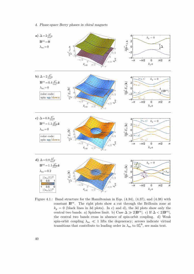
4. Phase-space Berry phases in chiral magnets
Figure 4.1.: Band structure for the Hamiltonian in Eqs. (4.34), (4.37), and (4.38) withconstant Bex. The right plots show a cut through the Brillouin zone atky = 0 (black lines in 3d plots). In c) and d), the 3d plots show only thecentral two bands. a) Spinless limit. b) Case ∆ 2|Bex|. c) If ∆ < 2|Bex|,the central two bands cross in absence of spin-orbit coupling. d) Weakspin-orbit coupling λso 1 lifts the degeneracy; arrows indicate virtualtransitions that contribute to leading order in λso to Ωr,k
n , see main text.
40
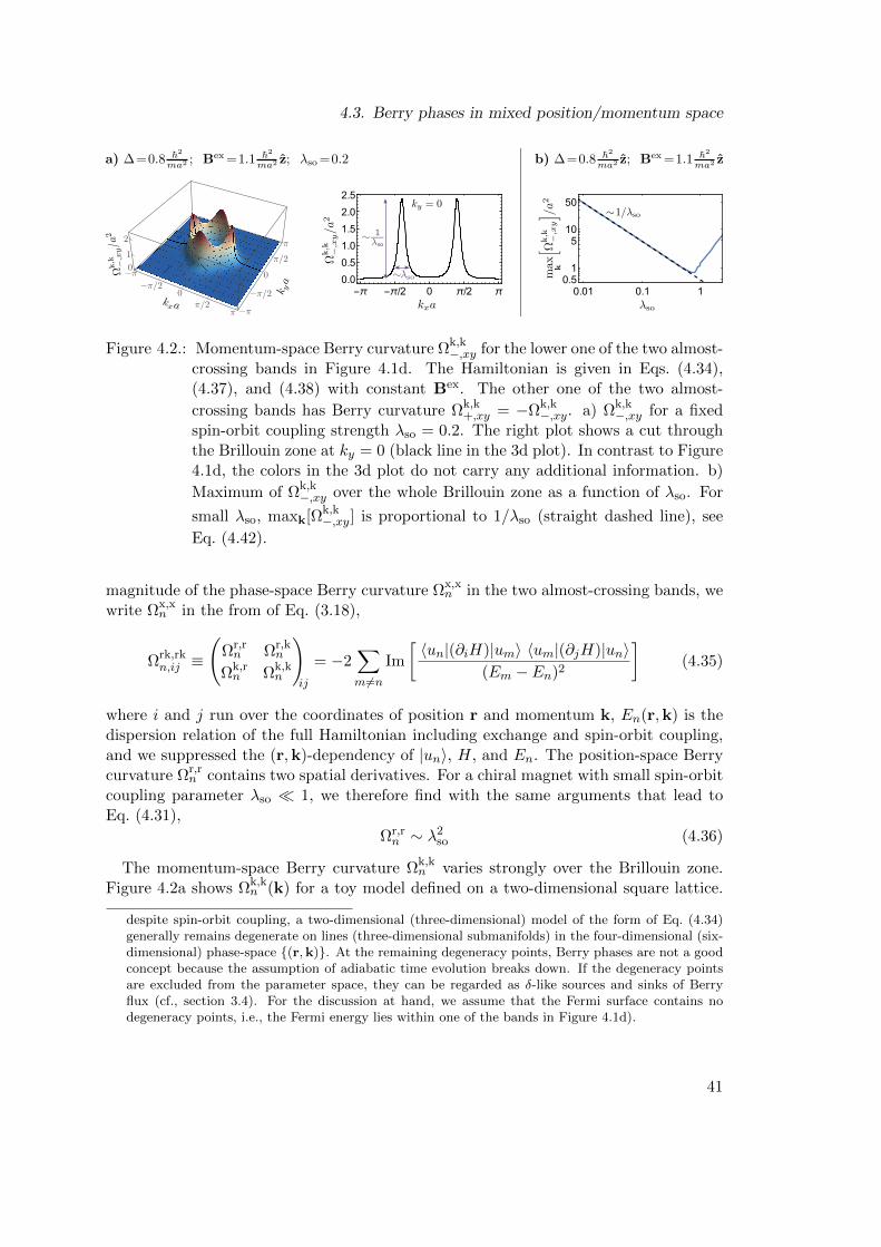
4.3. Berry phases in mixed position/momentum space
Figure 4.2.: Momentum-space Berry curvature Ωk,k−,xy for the lower one of the two almost-
crossing bands in Figure 4.1d. The Hamiltonian is given in Eqs. (4.34),(4.37), and (4.38) with constant Bex. The other one of the two almost-
crossing bands has Berry curvature Ωk,k+,xy = −Ωk,k
−,xy. a) Ωk,k−,xy for a fixed
spin-orbit coupling strength λso = 0.2. The right plot shows a cut throughthe Brillouin zone at ky = 0 (black line in the 3d plot). In contrast to Figure4.1d, the colors in the 3d plot do not carry any additional information. b)
Maximum of Ωk,k−,xy over the whole Brillouin zone as a function of λso. For
small λso, maxk[Ωk,k−,xy] is proportional to 1/λso (straight dashed line), see
Eq. (4.42).
magnitude of the phase-space Berry curvature Ωx,xn in the two almost-crossing bands, we
write Ωx,xn in the from of Eq. (3.18),
Ωrk,rkn,ij ≡
(Ωr,rn Ωr,k
n
Ωk,rn Ωk,k
n
)ij
= −2∑m 6=n
Im
[〈un|(∂iH)|um〉 〈um|(∂jH)|un〉
(Em − En)2
](4.35)
where i and j run over the coordinates of position r and momentum k, En(r,k) is thedispersion relation of the full Hamiltonian including exchange and spin-orbit coupling,and we suppressed the (r,k)-dependency of |un〉, H, and En. The position-space Berrycurvature Ωr,r
n contains two spatial derivatives. For a chiral magnet with small spin-orbitcoupling parameter λso 1, we therefore find with the same arguments that lead toEq. (4.31),
Ωr,rn ∼ λ2
so (4.36)
The momentum-space Berry curvature Ωk,kn varies strongly over the Brillouin zone.
Figure 4.2a shows Ωk,kn (k) for a toy model defined on a two-dimensional square lattice.
despite spin-orbit coupling, a two-dimensional (three-dimensional) model of the form of Eq. (4.34)generally remains degenerate on lines (three-dimensional submanifolds) in the four-dimensional (six-dimensional) phase-space (r,k). At the remaining degeneracy points, Berry phases are not a goodconcept because the assumption of adiabatic time evolution breaks down. If the degeneracy pointsare excluded from the parameter space, they can be regarded as δ-like sources and sinks of Berryflux (cf., section 3.4). For the discussion at hand, we assume that the Fermi surface contains nodegeneracy points, i.e., the Fermi energy lies within one of the bands in Figure 4.1d).
41
4. Phase-space Berry phases in chiral magnets
The Hamiltonian is given by Eq. (4.34) with Bex in z-direction and
ε+,k =~2
ma2(2− cos(kxa)− cos(kya)) +
∆
2; (4.37)
Hso(k) = λso |Bex| τx (σx sin(kxa) + σy sin(kya)) (4.38)
where m is the effective electron mass, a the lattice constant and the operator τx is
defined by τx |u(0)±,σ〉 = |u(0)
∓,σ〉. Projecting this model onto the subspace spanned by
|u(0)−,↑〉 and |u(0)
+,↓〉, one finds the effective 2× 2 Hamiltonian
Heff(k) = geff(k) · γ (4.39)
where γ is a vector of Pauli matrices acting in the subspace spanned by |u(0)−,↑〉 and
|u(0)+,↓〉, and
geff(k) =
λso |Bex| sin(kxa)λso |Bex| sin(kya)|Bex| − ε+,k
. (4.40)
The Berry curvature for this specific model is the winding number density of geff(k),
Ωk,k±,xy(k) = ∓
geff(k) ·[(∂kxg
eff(k))× (∂kygeff(k))
]2|geff(k)|3
(4.41)
where the upper (lower) sign corresponds to the upper (lower) band, respectively. The
Berry curvature Ωk,k±,xy(k) has a pronounced peak in the vicinity of the avoided crossing,
where the denominator on the right-hand side of Eq. (4.41) becomes small (Figure 4.2a).By writing out the right-hand side of Eq. (4.41) explicitly, one finds (see also Figure4.2b)
Ωk,k± ∼
1/λso close to the avoided crossing
λ2so away from the avoided crossing.
(4.42)
These estimates are not limited to the specific form of Hso(k), Eq. (4.38), as can be seenby the following arguments. Close to the avoided crossing, the denominator in Eq. (4.35)is of order λ2
so since the energy splitting is a consequence of spin-orbit coupling. In thenumerator, off-diagonal matrix elements of ∂kH0 become large because the states |un〉interpolate between |u(0)
+↓〉 and |u(0)−↑〉 as k scans through the avoided crossing. However,
for the momentum-momentum component of the Berry curvature, at least one of thetwo matrix-elements in Eq. (4.35) must come from ∂kHso ∼ λso since the term whereboth matrix elements come from ∂kH0 does not contribute to the Berry curvature (itcorresponds to a reduction of the parameter space to the one-dimensional space of ε±,k,
and there is no curvature in one dimension). This implies Ωk,k± ∼ 1/λso close to the
avoided crossing. Far away from the avoided crossing, the denominator in Eq. (4.35) isindependent of λso and off-diagonal matrix elements of ∂kH0 are suppressed by a factorof λso each because the states |un〉 and |um〉 are well-approximated by the unperturbed
42
4.4. Relevance of phase-space Berry phases in chiral magnets
states |u(0)±,σ〉. This confirms that also the second case covered in Eq. (4.42) applies
beyond the specific model of Eqs. (4.37)–(4.38).
We emphasize that Ωk,k± is non-perturbative in λso in the vicinity of an avoided crossing
(Eq. (4.42); see also [70]). This is the case even though our model, Eq. (4.34), relies on
spin-orbit coupling to generate a non-vanishing Ωk,k± in the first place. Note that, while
Ωk,k± ∼ 1/λso close to an avoided crossing, the width of the region around the avoided
crossing where this estimate applies is of order λso (Figure 4.2a). This is consistent withthe fact that the total Berry flux of a two-dimensional cut through the Brillouin zone isquantized.
Finally, we turn to the Berry curvature Ωr,kn in mixed position/momentum-space.
The expression for Ωr,kn in Eq. (4.35) contains one spatial derivative ∂rH ∼ λso. The
denominator is always of order |Bex|2 since ∂rH = ∂rBex · σ couples only states within
the same orbital band. In Eq. (4.35), Ωr,kn is expressed in terms of virtual transitions
between the bands n → m → n, which are mediated by the operators ∂rH and ∂kH,respectively. Exactly which kinds of virtual transitions are allowed depends on whetherk is close to the avoided crossing (see purple arrows in Figure 4.1d), or far away from it(green arrows in Figure 4.1d). Away from the avoided crossing, the states |un〉 are well-
approximated by the unperturbed states |u(0)±,σ〉, and thus ∂rH couples only states with
opposite spin. The only contribution to the matrix elements of ∂kH between states withopposite spin comes from ∂kHso, since ∂kH0 is spin-independent (green arrows in Figure
4.1d). This leads to a suppression of Ωr,kn away from the avoided crossing by another
factor of λso. Close to the avoided crossing, the states |u(0)+,↓〉 and |u(0)
−,↑〉 hybridize andtherefore ∂rH also mediates transitions between states whose spin components have anon-vanishing overlap (purple arrows in Figure 4.1d). The matrix element of ∂kH is inthis case dominated by ∂kH0, which is independent of λso. In conclusion, we find
Ωr,k± ∼
λso close to the avoided crossing
λ2so away from the avoided crossing.
(4.43)
4.4. Relevance of phase-space Berry phases in chiral magnets
Due to the combination of both a smooth magnetic texture and weak spin-orbit couplingthe physics of chiral magnets is influenced by Berry phases in phase space. It is well-established that the Berry curvature in position space, Ωr,r
n , plays an important role,allowing for a natural explanation of the so-called topological Hall effect [63] (see section7.1). Position-space Berry phases affect also the dynamics of the magnetization [62],leading, e.g., to a gyro-coupling G×R = F between the velocity R of Skyrmions and anexternal force F [11] (see section 9.1). Here, the gyro-coupling vector G is proportionalto the emergent magnetic field Bem.
Measurements on MnSi [30] show a large signal of the anomalous Hall resistivity (seesection 7.1), which is an indication that the electron dynamics is also strongly influenced
by the momentum-space Berry curvature Ωk,kn . This is in agreement with our qualitative
43
4. Phase-space Berry phases in chiral magnets
estimates in section 4.3, which showed that all components Ωr,rn , Ωk,k
n , and Ωr,kn of the
phase-space Berry curvature are quadratic in the small spin-orbit coupling strength λso aslong as k lies far away from any avoided band crossing. In this regime, our results for thetwo-band model, Eqs. (4.36), (4.42), and (4.43), agree with the results we obtained in thesimpler one-band model, Eqs. (4.31)–(4.33). While the position-space Berry curvatureΩr,rn ∼ λ2
so remains small regardless of details of the band structure (Eq. (4.36)), the Berry
curvatures in momentum-space and in mixed position/momentum-space, Ωk,kn and Ωr,k
n ,are enhanced if spin-orbit coupling leads to an avoided crossing of otherwise degeneratebands (Eqs. (4.42) and (4.43)). These kinds of avoided crossings appear to be a typicalfeature of the band structure of chiral magnets [71]. Therefore, one should expect that
Ωk,kn and Ωr,k
n play an important role in the physics of chiral magnets. Yet, in contrastto the position-space Berry curvature Ωr,r
n , the roles of Ωk,kn and especially Ωr,k
n in chiralmagnets have not yet enjoyed the same attention in the literature.
44
Part I.
Dzyaloshinskii-Moriya interactionand the electric charge of skyrmions
45

5. Semiclassical approach to energy andcharge density in chiral magnets
Chiral magnets exhibit phases with a smooth magnetization texture due to Dzyaloshinskii-Moriya (DM) interactions (see Section 2.2). As discussed in section 4.3, the combinationof a smooth magnetization texture and spin-orbit (SO) interaction leads a Berry cur-vature Ωx,x
n in phase space x ≡ (r,k) that is non-vanishing for all three combinations
of position/momentum directions, i.e. Ωr,rn , Ωk,k
n , and Ωr,kn are all non-zero. It is well-
established that the diagonal blocks, Ωr,rn and Ωk,k
n , strongly influence the physics of chiralmagnets, leading to the topological [22] and the anomalous Hall effect [70, 72], respec-tively (see Section 7.1). On the other hand, physical consequences of the off-diagonal
block Ωr,kn of the Berry curvature tensor in chiral magnets have received less attention.
For antiferromagnets with a smooth spin texture, it has been argued by Cheng andNiu [73] that Ωr,k
n crucially influences the dynamics electrons. In this and the followingchapter we will argue that Berry phases in mixed position/momentum space determinethe strength of DM interactions in chiral magnets and lead to an electric charge ofskyrmions. We thereby identify phase-space Berry phases as a mechanism that gener-ates magnetic textures, and we establish ties between Skyrmions in chiral magnets andskyrmions in quantum Hall systems at filling factor ν ≈ 1, which carry a quantizedelectric charge [13, 14]. We have published the results of this and the following chapterin Ref. [65].
We use two complementary approaches to treat the effects of a smooth magnetic tex-ture on the equilibrium electronic properties of chiral magnets. In the present chapter,we employ a semiclassical method, which has the advantage that its intermediate resultscan be interpreted classically as the equations of motion for the center-of-mass coordi-nates of a wave packet. The semiclassical approach is, however, only valid to lowestorder in gradients of the magnetization texture. In chapter 6, we will present an alterna-tive approach based on a gradient expansion of the Green’s function, which is consistentwith the semiclassical approach and extends the range of validity to higher orders in thegradients. The higher order terms are crucial in insulating systems, where the leadingcontribution to the electric charge of skyrmions is of second order.
This chapter is organized as follows. We review the semiclassical theory of wave-packet dynamics in the presence of Berry phases in Sections 5.1 and 5.2 and showhow these results affect the energy and charge density in chiral magnets in Section 5.3.We continue with analytical results for model systems (section 5.4) and conclude withnumerical results for the strength of DM interactions and the electric charge of skyrmionsin MnSi (Section 5.5).
47
5. Semiclassical approach to energy and charge density in chiral magnets
5.1. Semiclassical dynamics of wave packets
As discussed in section 4.3, the combination of smooth magnetic textures and SO cou-pling in chiral magnets leads to a Berry curvature Ωx,x
n in phase space x ≡ (r,k). Inthis section, we summarize the results from two articles, by Sundaram and Niu [5] andby Xiao, Shi, and Niu [7], in which the influence of Ωx,x
n on the semiclassical dynamicsof electrons was derived. We illustrate the derivation at the example of a magnet witha smooth magnetization texture in external electromagnetic fields, treating the electro-magnetic potentials on an equal footing with the smooth magnetization. This has theadvantage that all terms in the resulting semiclassical equations of motion will directlybe independent of the electromagnetic gauge.
The semiclassical equations of motion of an electron in d-dimensional space are ageneralization of the classical equations of motion. In absence of a magnetic field, thelatter are given by
dridt
=∂H(t, r,p)
∂piand
dpidt
= −∂H(t, r,p)
∂ri(5.1)
where r, p, and t are position, momentum, and time, respectively, and H(t, r,p) =p2/(2m)− eφ(t, r) is the Hamilton function of an electron with mass m and charge −ein an electric potential φ(t, r). A more compact way of writing Eq. (5.1) is
dxidt
= Jij∂H(t, x)
~ ∂xj(5.2)
where x ≡ (r,k) with k := p/~ is the particle’s coordinate in 2d-dimensional phasespace and J is the canonical symplectic form,
J =
(0 1d×d
−1d×d 0
)(5.3)
with 1d×d being the identity in d-dimensional space. At this stage, the factor of ~ dropsout of Eq. (5.2). We include it here to simplify the notation when we generalize tosemiclassical dynamics below.
Semiclassical approximation. For electrons in a periodic crystal, the coherence lengthis typically much larger than the lattice constant, rendering a purely classical descriptionuseless in most cases. However, one can often obtain good predictions for physicalquantities within a semiclassical approximation. Semiclassical theories are ubiquitousin solid state physics. For example, even a seemingly purely classical theory such asthe Drude formula for the electric conductivity is usually applied with a renormalizedelectron mass, which is a quantum-mechanical effect due to coherent scattering off thecrystal potential. In a semiclassical approximation, the motion of electrons is describedby classical equations of motion similar to Eq. (5.2), i.e., differential equations for thetrajectory of a point in 2d-dimensional phase space, as opposed to an equation for the
48
5.1. Semiclassical dynamics of wave packets
evolution of a wave function in Hilbert space. Quantum-mechanical effects are takeninto account by modifications of Eq. (5.2), and by an appropriate re-quantization rule.
Due to the uncertainty principle, the phase-space coordinates r and k cannot be si-multaneously known to arbitrary precision. Therefore, the semiclassical equations ofmotion are differential equations for the center-of-mass coordinates xc ≡ (rc,kc) ofa wave packet. In a naıve semiclassical treatment, one might be tempted to simplyreplace the classical Hamilton function H(t, x) in Eq. (5.2) by the expectation value〈Ψt,rc,kc |H(t)|Ψt,rc,kc〉 of the Hamiltonian operator in an appropriate wave packet state|Ψt,rc,kc〉, see below. We shall see, however, that this naıve substitution misses importanteffects if the crystal is subject to smooth modulations, such as small external electro-magnetic fields or a smooth magnetization texture. In particular, an equation of motionof the form of Eq. (5.1) cannot include the emergent Lorentz force dpc
dt = qemσ
drcdt ×Bem
one expects due to the emergent magnetic field Bem discussed in section 4.1, nor doesit include the anomalous velocity drc
dt ∝ E discussed in section 4.2.Sundaram and Niu [5] derived the effective equations of motion for wave packets in a
smoothly perturbed crystal using a variational approach over wave packets. It turns outthat the smooth modulations lead to three modifications of the semiclassical description:
(i) a correction δE(1)n to the energy of the wave packet;
(ii) terms proportional to the Berry curvature Ωx,xn in the equations of motion for the
center-of-mass coordinates xc; among others, these terms account for the emergentmagnetic field Bem and the anomalous velocity (see sections 4.1 and 4.2, respec-tively); and
(iii) a correction to the density of states in phase space that restores particle numberconservation [7].
The derivation of (i) and (ii) in Ref. [5] is based on wave packates that have a narrowsupport in both position and momentum space at all times. The non-zero width of thewave packets in phase space is taken into account only to leading order in gradients ofthe smooth modulations, and the fact that the wave function disperses (spreads out)over time is neglected. In addition, the derivation neglects (real) inter-band transitions,which is a good approximation in the adiabatic limit κn.a. 1, see Eq. (3.42).
Model. We review the derivation of items (i) and (ii) above from Ref. [5] and the deriva-tion of (iii) from Ref. [7], using the example of a magnet with a smooth magnetizationtexture M(t, r) (Figure 5.1a). In preparation for Section 7.2, we also include externalelectromagnetic fields E = −∇φ−∂tA and B = ∇×A, and assume that the potentialsφ and A vary smoothly in time and space. In the approximation of non-interactingelectrons, the single-particle Hamiltonian is given by
H(t) =(−i~∇ + eA(t, r))2
2m+ V (r) +Hso + Bex(t, r) · σ − eφ(t, r) (5.4)
Here, m and −e are the bare mass and the charge of the electron, respectively, V is thelattice-periodic effective potential, σ is the vector of Pauli matrices acting on the spin
49
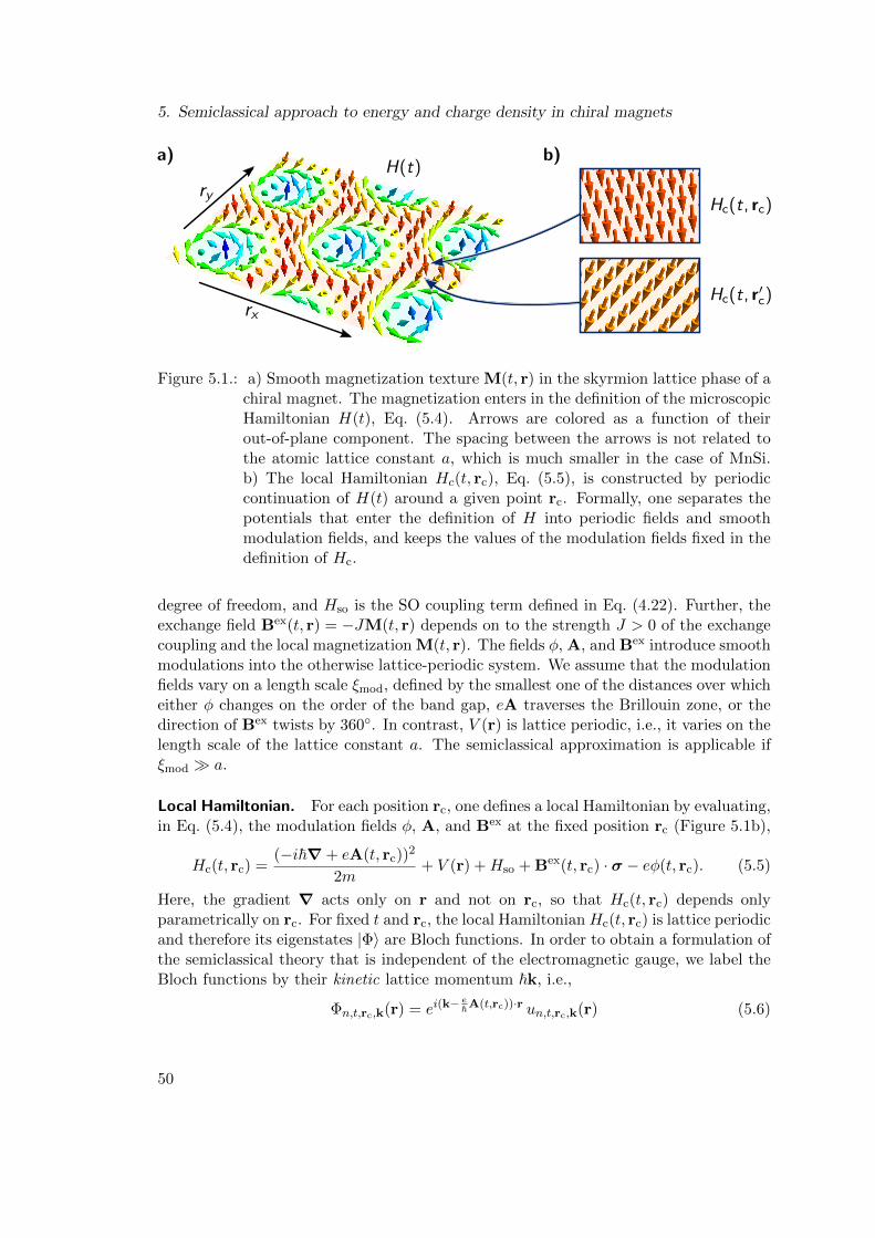
5. Semiclassical approach to energy and charge density in chiral magnets
Figure 5.1.: a) Smooth magnetization texture M(t, r) in the skyrmion lattice phase of achiral magnet. The magnetization enters in the definition of the microscopicHamiltonian H(t), Eq. (5.4). Arrows are colored as a function of theirout-of-plane component. The spacing between the arrows is not related tothe atomic lattice constant a, which is much smaller in the case of MnSi.b) The local Hamiltonian Hc(t, rc), Eq. (5.5), is constructed by periodiccontinuation of H(t) around a given point rc. Formally, one separates thepotentials that enter the definition of H into periodic fields and smoothmodulation fields, and keeps the values of the modulation fields fixed in thedefinition of Hc.
degree of freedom, and Hso is the SO coupling term defined in Eq. (4.22). Further, theexchange field Bex(t, r) = −JM(t, r) depends on to the strength J > 0 of the exchangecoupling and the local magnetization M(t, r). The fields φ, A, and Bex introduce smoothmodulations into the otherwise lattice-periodic system. We assume that the modulationfields vary on a length scale ξmod, defined by the smallest one of the distances over whicheither φ changes on the order of the band gap, eA traverses the Brillouin zone, or thedirection of Bex twists by 360. In contrast, V (r) is lattice periodic, i.e., it varies on thelength scale of the lattice constant a. The semiclassical approximation is applicable ifξmod a.
Local Hamiltonian. For each position rc, one defines a local Hamiltonian by evaluating,in Eq. (5.4), the modulation fields φ, A, and Bex at the fixed position rc (Figure 5.1b),
Hc(t, rc) =(−i~∇ + eA(t, rc))
2
2m+ V (r) +Hso + Bex(t, rc) · σ − eφ(t, rc). (5.5)
Here, the gradient ∇ acts only on r and not on rc, so that Hc(t, rc) depends onlyparametrically on rc. For fixed t and rc, the local Hamiltonian Hc(t, rc) is lattice periodicand therefore its eigenstates |Φ〉 are Bloch functions. In order to obtain a formulation ofthe semiclassical theory that is independent of the electromagnetic gauge, we label theBloch functions by their kinetic lattice momentum ~k, i.e.,
Φn,t,rc,k(r) = ei(k−e~A(t,rc))·r un,t,rc,k(r) (5.6)
50
5.1. Semiclassical dynamics of wave packets
where n is the band index and the lattice-periodic part un,t,rc,k(r) is independent of theelectromagnetic gauge. Formally, the fact that two different wave vectors k and k− e
~Aappear on the right-hand side of Eq. (5.6) may be regarded as being merely a peculiarway to label the Bloch functions Φ. In particular, we emphasize that u is still strictlylattice-periodic.1
The lattice-periodic part un,t,rc,k(r) of the Bloch functions satisfy the eigenvalue equa-tion
Hc(t, rc,k)un,t,rc,k(r) = E(0)n (t, rc,k)un,t,rc,k(r) (5.7)
where we define the gauge-invariant local band Hamiltonian as
Hc(t, rc,k) = e−i(k−e~A)·rHc(t, rc) e
i(k− e~A)·r + eφ(t, rc) (5.8)
Note that both Hc(t, rc,k) and the local eigenenergy E(0)n (t, rc,k) are functions of the
kinetic momentum ~k, and are defined in such a way that they are both independent ofthe electromagnetic potentials φ and A. We point out that the local band HamiltonianHc(t, rc,k) is not the same as the Wigner-transformed Hamiltonian H(t, r,k) we willintroduce in Section 6.2 (see there for a comparison between the two).
Energy correction. The main idea of the derivation of the semiclassical equations ofmotion, Ref. [5], is to vary over wave packets that contain only contributions from asingle band n. For a given time t and point xc ≡ (rc,kc) in phase space, one constructsa wave packet
Ψt,rc,kc(r) =
∫ddk a(k)Φn,t,rc,k(r) (5.9)
where the complex envelope function a(k) is chosen such that (i) it reproduces the correctexpectation value of the position operator, i.e., 〈Ψt,rc,kc |r|Ψt,rc,kc〉 = rc; (ii) its supportin reciprocal space is small compared to the size ∼ 1/a of the Brillouin zone; and (iii)it is centered around kc, i.e.,
∫ddk k|a(k)|2 = kc (with normalization
∫ddk |a(k)|2 = 1).
In this sense, xc ≡ (rc,kc) is the center-of-mass coordinate of the wave packet in phasespace, where ~kc is its “physical” momentum: A measurement of the gauge-invariantmomentum operator p = −i~∇ + eA in the wave-packet state |Ψt,rc,kc〉 would yielda value close to ~kc (modulo reciprocal lattice vectors). According to the uncertaintyprinciple, the narrow support of a(k) in momentum space implies that the wave packet|Ψt,rc,kc〉 extends over many unit cells in position space. The semiclassical approach isbased on the assumption that the part of the system that is probed by |Ψt,rc,kc〉 is wellapproximated by the local Hamiltonian H(t, rc). This is the case if the width ∆r of thewave packet in position space is small compared to the length scale ξmod of the smoothmodulations. In summary, we assume that the following hierarchy of length scales holds
a ∆r ξmod. (5.10)
1Notice that A in Eq. (5.6) is evaluated at the fixed position rc. This is different than in the case ofthe magnetic Bloch theorem, in which the functions u are no longer lattice periodic (see, e.g., [8]). Inthe situation discussed here, the local Hamiltonian Hc(t, rc) does not have a magnetic field, becauseA is a constant in Eq. (5.5).
51
5. Semiclassical approach to energy and charge density in chiral magnets
We split the expectation value of the energy into two terms,
En(t, rc,kc) := 〈Ψt,rc,kc |H(t)|Ψt,rc,kc〉 = 〈Ψt,rc,kc |Hc(t, rc)|Ψt,rc,kc〉+ δE(1)n (t, rc,kc)
(5.11)with
δE(1)n (t, rc,kc) = 〈Ψt,rc,kc |(H(t)−Hc(t, rc))|Ψt,rc,kc〉 . (5.12)
Using Eqs. (5.7)–(5.8) and the fact that the envelope function a(k) is peaked aroundk ≈ kc, we find for the first term on the right-hand side of Eq. (5.11),
〈Ψt,rc,kc |H(t)|Ψt,rc,kc〉 ≈ E(0)n (t, rc,kc)− eφ(t, rc). (5.13)
The second term on the right-hand side of Eq. (5.11) is a correction due to gradientsof the modulation fields A, and Bex. The evaluation of this term in Ref. [5] yields toleading order in the gradients,
δE(1)n (t, rc,kc) ≈ −
d∑i=1
Im
[∂〈un,t,rc,k|∂rc,i
(E(0)n (t, rc,kc)− Hc(t, rc,kc)
) ∂|un,t,rc,k〉∂ki
]∣∣∣∣k=kc
(5.14)
which we rewrite with the help of Eq. (3.16) in a form that is more convenient fornumerical evaluation,
δE(1)n (t, rc,kc) ≈ −
d∑i=1
∑m6=n
Im
〈un,t,rc,kc | ∂Hc∂rc,i|um,t,rc,kc〉 〈um,t,rc,kc |∂Hc
∂ki|un,t,rc,kc〉
E(0)n (t, rc,kc)− E(0)
m (t, rc,kc)
(5.15)
where the derivatives of the local band Hamiltonian Hc, Eq. (5.8), are evaluated at
(t, rc,kc). The energy correction δE(1)n is sometimes called magnetic energy because it
contains a term of the form −m·(∇×A). Here, m can be identified as the magnetizationof the single electron under consideration, which couples to the external magnetic fieldB = ∇×A.
Equations of motion. The time evolution of the wave packet |Ψt,rc,kc〉 is described bythe Hamiltonian, Eq. (5.4). Solutions of the time-dependent Schrodinger Equation arestationary points of the action S =
∫dt L with Lagrangian
L[|Ψ〉] = 〈Ψ|(i~
d
dt−H(t)
)|Ψ〉 . (5.16)
Semiclassical equations of motion for the trajectory xc(t) ≡ (rc(t),kc(t)) in phase spaceare obtained by restricting the domain of L to wave packets of the form of Eq. (5.9). As
52
5.1. Semiclassical dynamics of wave packets
discussed above, this ansatz neglects inter-band scattering and the dispersion (spreading)of wave packets. One obtains
L(t, xc, xc) ≡ L[|Ψt,rc,kc〉] = 〈Ψt,rc,kc |(i~
d
dt−H(t)
)|Ψt,rc,kc〉
= −En(t, xc) + eφ(t, rc) + i~ 〈Ψt,rc,kc |(∂
∂t+ rc ·
∂
∂rc+ kc ·
∂
∂kc
)|Ψt,rc,kc〉
≈ −En + eφ+ ~At + rc · (~kc + ~Ar − eA) + kc · ~Ak (5.17)
where, in the last step, we used again the fact that the envelope function a(k) is peakedat kc. In Eq. (5.17), At, Ar, and Ak are the components of the Berry connection forthe local band Hamiltonian Hc(t, rc, rc), as defined in Eq. (3.6). Explicitly,
At = i 〈un,t,xc |∂
∂t|un,t,xc〉 and Ax
i ≡ (Ar,Ak)i = i 〈un,t,xc |∂
∂xc,i|un,t,xc〉 (5.18)
where the partial time derivative is evaluated at constant xc. The semiclassical equationsof motion for the center-of-mass coordinates xc ≡ (rc,kc) in phase space are obtainedfrom the Euler-Lagrange equations for L(t, xc, xc). One finds
drc,i
dt
∣∣∣∣n
=∂En
~ ∂kc,i− Ωk,t
n,i − Ωk,rn,ij rc,j − Ωk,k
n,ij kc,j ; (5.19)
~dkc,i
dt
∣∣∣∣n
= − ∂En∂rc,i
− eEi + ~Ωr,tn,i +
(~Ωr,r
n,ij − eεijlBl)rc,j + ~Ωr,k
n,ij kc,j (5.20)
where the notation “|n” is merely a reminder that rc and kc are the center-of-masscoordinates of a wave packet formed from band n, and that the semiclassical equationsof motion are different in different bands. On the right-hand sides of Eqs. (5.19)–(5.20),we used the electric field E = −∇φ−∂tA, the magnetic field B = ∇×A, and the usualdefinition of the Berry curvature (cf., Eq. (3.13)),
Ωx,tn,i =
∂At
∂xc,i− ∂Ax
i
∂tand Ωx,x
n,ij ≡
(Ωr,rn Ωr,k
n
Ωk,rn Ωk,k
n
)ij
=∂Ax
j
∂xc,i− ∂Ax
i
∂xc,j. (5.21)
The first term on the right-hand side of Eqs. (5.19) and (5.20), respectively, is analogousto the classical equations of motion, Eq. (5.1), where the Hamilton functionH is replaced
by the energy expectation value En ≈ E(0)n + δE(1)
n . The remaining terms are gradientcorrections. The Berry curvatures Ωr,t
n and Ωr,rn appear in the same places as the electric
and magnetic field, respectively. Indeed, by inserting Eq. (4.14), one obtains an emergentLorentz force Fem
σ = qemσ (Eem + rc × Bem) in the majority (minority) band σ = ↓
(σ = ↑) of a chiral magnet, where qemσ , Eem, and Bem are the emergent charge, emergent
electric field, and emergent magnetic field, respectively (see Section 4.1). Similarly, the
momentum-space Berry curvature Ωk,kn in Eq. (5.19) plays the role of a magnetic field
in reciprocal space. The term vanomn,i = −Ωk,k
n,ij kc,j ≈ e~Ωk,k
n,ijEj is the anomalous velocity
discussed in section 4.2, which is perpendicular to E due to the skew-symmetry of Ωk,kn .
53
5. Semiclassical approach to energy and charge density in chiral magnets
In a more compact form, Eqs. (5.19)–(5.20) can be written as
(Jij − Ω′x,xn,ij)xc,j = − ∂En
~ ∂xc,i+ Ω′
x,tn,i (5.22)
where the primed Berry curvatures are the same as the unprimed ones defined inEq. (5.21), except for the components
Ω′r,tn,i := Ωr,t
n,i −e
~Ei and Ω′
r,rn,ij := Ωr,r
n,ij −e
~εijlBl . (5.23)
Using the anti-symmetry of J and Ωx,xn , Eq. (5.22) is equivalent, to linear order in Ω′x,x
n ,to
xc,i = (J − JΩ′x,xn J)ij
(∂En
~ ∂xc,j− Ω′
x,tn,j
)(5.24)
5.2. Correction to the density of states.
The semiclassical equation of motion, Eq. (5.22), describes the dynamics of a singleelectron in phase space. To calculate measurable quantities in a many-electron system,one needs to sum over all occupied states. This requires an appropriate (re-)quantizationscheme. For example, the expectation value of single-particle observable O at time t isgiven by
〈O〉t =∑n
∫d2dxcDn(t, xc)fn(t, xc) 〈Φn,t,rc,kc |O|Φn,t,rc,kc〉 . (5.25)
Here, n is the band index, the distribution function fn is the expectation value of thenumber of particles in band n at point xc in phase space (0 ≤ fn(t, xc) ≤ 1 for fermions),and Dn(t, xc) is the density of states in phase space at time t. In absence of Berry-phases,the latter is a constant, Dn = (2π)−d. This can be seen, for example, by restricting thesystem to a cube of volume Ld and performing the limit L→∞. On a more fundamentallevel, the constant Dn is a consequence of the fact that, in absence of Berry phases, rand k satisfy canonical Poisson brackets ri, ~kj = δij , see below and Ref. [74]. It hasbeen pointed out by Xiao, Shi, and Niu [7] that a constant Dn is, however, incompatiblewith the semiclassical equations of motion Eq. (5.22) as soon as either Ω′r,k 6= 0 or bothΩ′r,r 6= 0 and Ω′k,k 6= 0. As we will see below, a constant Dn in this case would violatethe conservation of the total number of particles,
N(t) =∑n
∫d2dxcDn(t, xc)fn(t, xc). (5.26)
Liouville theorem and particle number conservation. In a consistent semiclassicaltheory, the total particle number N has to be conserved. Assuming a non-interactingsystem, the distribution function fn(t, xc) at a given time t can be expressed in terms of
54
5.2. Correction to the density of states.
fn(t0, xc) at some reference time t0 by integration of the equation of motion, Eq. (5.22),
fn(t, xc) =
∫d2dx′c δ
(x′c +
∫ t
t0
xc(t′) dt′ − xc
)fn(t0, x
′c)
= fn
(t0, xc −
∫ t
t0
xc(t′) dt′
)(5.27)
Thus, we have∂fn(t, xc)
∂t= −∂fn(t, xc)
∂xc,ixc,i (5.28)
and the time derivative of the total particle number is
dN
dt=∑n
∫d2dxc
[∂Dn(t, xc)
∂tfn(t, xc)−Dn(t, xc)
∂fn(t, xc)
∂xc,ixc,i
]=∑n
∫d2dxc
[∂Dn(t, xc)
∂t+∂Dn(t, xc)
∂xc,ixc,i +Dn(t, xc)
∂xc,i
∂xc,i
]fn(t, xc) (5.29)
where we integrated by parts in the last step.In a purely classical system governed by the Hamilton equations of motion, Eq. (5.2),
the last term in the bracket on the right-hand side of Eq. (5.29) vanishes due to theLiouville theorem, ∂xi/∂xi = 0, which is a direct consequence of Eq. (5.2) and the factthat Jij , Eq. (5.3), is constant and skew-symmetric. Therefore, in absence of Berryphases, the right-hand side of Eq. (5.29) vanishes for a constant phase-space densityDn = (2π)−d, as it should.
Under the semiclassical dynamics described by Eq. (5.22), the factor ∂xc,i/∂xc,i doesnot vanish in general. The correct density of states Dn in this case is specified by thepartial differential equation that results from setting the right-hand side of Eq. (5.29) tozero for all fn(t, xc). In Ref. [7], the solution
Dn(t, xc) =
√det(J − Ω′x,x
n (t, xc))
(2π)d(5.30)
was proposed. Here, the numerator is known as the Pfaffian of the skew-symmetricmatrix M := J − Ω′x,x
n , which is analytic in the components of Ω′x,xn despite the ap-
pearance of the square root [75]. A derivation of Eq. (5.30) was given in Ref. [74] (seealso our alternative derivation in Appendix B in Ref. [65]). To convince ourselves thatEq. (5.30) is indeed the correct density of states, we first consider the limit where allmodulation fields are switched off at some reference time t0. Therefore, Ω′r,rn = 0 = Ω′r,knat time t0 and one finds that Eq. (5.30) correctly reduces to the classical density ofstates Dn = (2π)−d. We now ramp up the modulation fields adiabatically from timet0 to t > t0 and send t0 → −∞. A direct calculation shows that Eq. (5.30) sets theright-hand side of Eq. (5.29) to zero for all fn(t, xc), as claimed. This can be checked byusing Eq. (5.22), the Jacobi identity (Eq. (3.14)), and the relation
∂ det(M)
∂xc,i= det(M) tr
[M−1 ∂M
∂xc,i
](5.31)
55
5. Semiclassical approach to energy and charge density in chiral magnets
which follows from the identity log det(M) = tr log(M). Thus, Eq. (5.30) satisfies thedefining partial differential equation and the correct initial condition for the density ofstates in phase space.
Formally, Eq. (5.30) restores particle number conservation under the dynamics ofEq. (5.22) exactly. We emphasize, however, that the semiclassical equation of motion,Eq. (5.22), is only valid to leading order in the gradient corrections Ω′x,x
n and Ω′x,tn .
Therefore, the density of states, Eq. (5.30), is in general also only valid to first order inthe components of Ω′x,x
n . To first order, one obtains
Dn(t, xc) ≈1
(2π)d
(1− Tr
[Ωr,kn (t, xc)
])+O
((Ω′
x,xn )2
)(5.32)
where Tr[Ωr,kn
]=∑d
i=1 Ωr,kn,ii.
5.3. Berry-phase effects on energy and charge density
While the semiclassical equation of motion, Eq. (5.22), describes the dynamics of elec-trons, the energy shift δEn, Eq. (5.14), and the density of states Dn, Eq. (5.30), affectalso equilibrium properties. In the remaining sections of this chapter, we discuss theeffects of phase-space Berry phases on the energy and charge density of chiral magnets,which we published in Ref. [65]. Within the semiclassical approximation, the free energyof a non-interacting many-particle system is given by F =
∫f(rc) ddrc with the free
energy density
f(rc) = −kBT∑n
∫ddkc Dn(xc) ln
(1 + e−(En(xc)−µ)/(kBT )
)≈ f (0)(rc) + δf (1)(rc).
(5.33)Here, kB is the Boltzmann constant, T the temperature, µ the chemical potential, D(xc)is the semiclassical density of states in phase space, see Eq. (5.32), and En(xc) is theenergy expectation value of a wave packet with center-of-mass coordinates xc ≡ (rc,kc),see Eq. (5.11). In absence of phase-space Berry phases, the free energy density reducesto
f (0)(rc) = −kBT∑n
∫ddkc
(2π)dln(
1 + e−(E(0)n (xc)−µ)/(kBT )
). (5.34)
Berry-phases in mixed position/momentum space lead to a change of the energy density.To leading order in the gradient terms, we obtain
δf (1)(rc) =∑n
∫ddkc
(2π)d
[δE(1)n (xc) nF (E(0)
n (xc)− µ)
+kBT Tr(
Ωr,kn (xc)
)ln(
1 + e−(E(0)n (xc)−µ)/(kBT )
)](5.35)
where nF (ε) = 1/(1 + eε/(kBT )) is the Fermi distribution and δE(1)n and Ωr,k
n are definedin Eqs. (5.15) and (5.21), respectively. Note that both terms on the right-hand side of
56
5.3. Berry-phase effects on energy and charge density
Eq. (5.35) are non-zero only in the presence of both SO interaction and a smooth spatialinhomogeneity (magnetization texture). We will identify δf (1) as the DM energy in thenext section.
The charge density ρ(rc) is also influenced by Berry phases. To leading order in thegradient correction terms, we obtain2
δρ(1)(rc) = e∂δf (1)(rc)
∂µ=
= −e∑n
∫ddkc
(2π)d
[δE(1)n (xc)n
′F (E(0)
n (xc)− µ)− Tr(
Ωr,kn (xc)
)nF (E(0)
n (xc)− µ))
](5.36)
where n′F (ε) = ∂nF (ε)/∂ε.
Electrostatic screening. In Eq. (5.36), the correction to the charge density was cal-culated at fixed µ and the effect of screening due to Coulomb interaction was ignored.In a metal, Coulomb interactions lead to screening of charges (see, e.g., Ref. [76]) andthe total charge density δρtot(rc) ≈ δρ(1)(rc) + δρsc(rc) is a sum of the charge densityδρ(1)(rc) due to phase-space Berry curvatures and a redistribution
δρsc(rc) = −e2νF δV (rc) (5.37)
of charges due to screening. Here, νF is the density of states at the Fermi level and δVis the electrostatic screening potential, which is related to the total charge density viathe Maxwell relation
− ε0∇2δV (rc) = ρtot(rc) (5.38)
where ε0 is the permittivity of the vacuum. To solve Eqs. (5.37)–(5.38) for δρtot, we goto Fourier space and obtain
δρtotq = −q2λ2
TFδρscq = −q2λ2
TF
(δρtot
q − δρ(1)q
)(5.39)
where q is the wave vector and λTF =√ε0/(e2νF ) the Thomas-Fermi screening length.
Therefore,
δρtotq =
q2λ2TF
q2λ2TF + 1
δρ(1)q (5.40)
where q is the wave vector. In good metals and for long-wavelength skyrmions, one hasqλTF 1 (see numerical results below). Therefore, the denominator on the right-handside of Eq. (5.40) is close to unity and we obtain in position space
δρtot(rc) ≈ −λ2TF∇2δρ(1)(rc). (5.41)
2We are using SI units here with electron charge −e, which is a different sign convention than inRef. [65].
57
5. Semiclassical approach to energy and charge density in chiral magnets
As expected, the total charge of the system∫
d3rc δρtot(rc) vanishes when screening
is taken into account, and the charge density δρtot(rc) that includes screening effectsis positive (negative) when the charge density δρ(1) due to phase-space Berry phaseshas a maximum (minimum). While screening happens only at the Fermi surface, theunscreened charge density δρ(1) has contributions both from the Fermi surface and theFermi sea, see Eq. (5.35). Therefore, δρ(1) is still an interesting quantity to estimatethe amount of charge-redistribution due to phase-space Berry phases. Moreover, thereis no screening in insulators and we will show in chapter 6.3 that Berry phases in phasespace lead to a quantized skyrmion charge in insulators. Interestingly, Eq. (5.30) for thedensity of states Dn in phase space turns out to be valid beyond the linear order in Ωx,x
n
in insulators (this is not true for metals, though).
5.4. DM energy and skyrmion charge in a minimal model
In order to estimate qualitatively how the Berry-phase corrections to the energy andthe skyrmion charge depend on the strength of SO interaction, we consider the min-imal model of a chiral magnet without avoided band crossings, Eq. (4.28), with atime-independent exchange field Bex(r) and a SO-coupling field gso(k). We obtainthe local band Hamiltonian by evaluating Eq. (4.28) at the center-of-mass coordinatesxc ≡ (rc,kc),
Hc(rc,kc) = εkc + [Bex(rc) + gso(kc)] · σ =: εkc + n(xc) · σ (5.42)
with n = Bex +gso. The Berry curvature in phase space is given by the winding numberdensity of n(xc), Eq. (4.29). In particular, one has Ωx,x
↓ = −Ωx,x↑ where σ = ↓ and σ = ↑
denote the majority and minority spin configuration, respectively (see section 4.1). FromEq. (5.14), we obtain for the energy shift,
δE(1)↑ (xc) = δE(1)
↓ (xc) = |n|Tr[Ωr,k↑
]. (5.43)
DM interaction strength. From Eq. (5.35), we obtain for the correction to the freeenergy density,
δf (1)(rc) =
∫ddkc
(2π)dTr[Ωr,k↑
][|n|(nF (E(0)
↑ − µ) + nF (E(0)↓ − µ)
)+kBT ln
1 + e−(E(0)↑ −µ)/(kBT )
1 + e−(E(0)↓ −µ)/(kBT )
]. (5.44)
We consider the limit of a small band splitting compared to the Fermi energy and expand
in E(0)↑ − E
(0)↓ = 2|n| µ. The first two terms in the expansion cancel and we obtain to
leading order
δf (1)(rc) ≈2
3
∫ddkc
(2π)d|n|3 Tr
[Ωr,k↑
]n′′F (εkc − µ). (5.45)
58
5.4. DM energy and skyrmion charge in a minimal model
To make further progress, we assume, as in section 4.3, that SO interactions are smallcompared to the exchange interaction and expand to leading order in the SO-interactionstrength λso ∼ |gso|/|Bex| 1. In this limit, Ωr,k
↑ ∼ λ2so is given by Eq. (4.33) and we
obtain
δf (1)(rc) = Dij
(Bex(rc)×
∂Bex(rc)
∂rc,j
)i
(5.46)
where Bex = Bex/|Bex| and
Dij ≈ −|Bex|2
3
∫ddkc
(2π)d∂gso
i
∂kjn′′F (εkc − µ) . (5.47)
In a cubic lattice, such as MnSi, the vector field gso(k) (Eq. (4.25)) is covariant underrotations by 120 around the [111] direction, i.e. cyclic permutations of the directionsx, y, and z. This implies Dij ∝ δij in a cubic system. In order to obtain a qualitativeestimate, we recall that gso varies on the order of the SO interaction energy Eso ∼λso|Bex|. For an order-of-magnitude, we approximate |∂gso
i /∂kj | ∼ Esoa where a is theatomic lattice constant. Assuming a cubic crystal structure, we obtain,
Dij = −Dδij with D ∼ Eso1
ad−1
B20
E2F
. (5.48)
Inserting into Eq. (5.46), we find for the Berry-phase contribution to the total freeEnergy,
δF (1) :=
∫ddrc δf
(1)(rc) ≈ D∫
ddrc M · (∇× M) (5.49)
where M = −Bex is the unit vector in the direction of the magnetization M ∝ −Bex. Weidentify δF (1) as the DM interaction (cf., Eq. (2.6)). The relation between phase-spaceBerry phases and Dzyaloshinskii-Moriya interaction was also pointed out in Ref. [77].As expected, the DM interaction strength D, Eq. (5.48), is proportional to the energyscale Eso of SO interactions and quadratic in the magnetization.
Skyrmion charge. For the Berry-phase correction to the charge density, we obtain fromEq. (5.46)
δρ(1)(rc) = e∂f (1)(rc)
∂µ≈ e∂Dij
∂µ
(Bex(rc)×
∂Bex(rc)
∂rc,j
)i
. (5.50)
In section 2.2, we discussed the experimental observation of the skyrmion lattice phasein MnSi. The magnetization texture is well described by [9, 78]
Bex(r) = B0 z +B1
2∑n=0
[(z× ξn) sin
(q0 ξn · r
)+ z cos
(q0 ξn · r
)]. (5.51)
where q0 ≈ 2π/(190 A), z = (0, 0, 1) is the unit vector in the direction of a small externalmagnetic field that stabilizes the skyrmion lattice, ξn = (cos(2πn/3), sin(2πn/3), 0),
59
5. Semiclassical approach to energy and charge density in chiral magnets
and, according to mean-field calculations [9], B1/B0 ≈ −1.5. See Figure 5.1a for anillustration. Since the non-collinear magnetization texture results from a competitionbetween DM interactions (which are a consequence of SO interactions) and ferromagneticexchange interactions, q0 is proportional to |gso|/|Bex| ∼ λso. For our estimate, we setq0 = λso2π/a. The area of a single skyrmion in the (x, y)-plane is proportional to(2π/q0)2. Thus, we obtain from Eqs. (5.50) for the electric charge of a skyrmion peratomic layer in z direction (without screening),
δQ(1) := a
∫skyrmion
drc,x drc,y δρ(1)(rc) ∼ e
B30
E3F
(5.52)
where the integral runs over a single magnetic unit cell in the plane perpendicular tothe small external magnetic field. Note that the skyrmion charge δQ(1) is independentof the SO coupling strength λso, since the smallness of the charge density δρ(1) ∼ λ2
so
is compensated by the large size O(1/λ2so) of the skyrmions. This qualitative result is
confirmed by ab initio calculations that use the real band structure of MnSi (see nextsection), as long as screening is neglected.
5.5. Numerical results for DM energy and skyrmion charge inMnSi
Numerical values for the DM interaction strength D and the skyrmion charge δQ(1)
in the skyrmion lattice phase of MnSi were obtained from ab initio methods by ourcollaborators F. Freimuth and Y. Mokrousov [65]. The calculations were done for theleft-handed crystal structure, with the atomic coordinates from Ref. [71].
Method. While the semiclassical description we reviewed in section 5.1 was origi-nally derived for non-interacting systems, it can also be applied to interacting systemsby using density functional theory (DFT). In DFT, the interacting Hamiltonian H ismapped to a noninteracting one using the following iterative procedure [79]. Accordingto the Hohenberg-Kohn theorem [80, 81], the ground-state |Ψ[n(r)]〉 of H is completelydetermined by the electron density n(r). Therefore, finding the ground state of His equivalent to finding the density profile n(r) that minimizes the energy functionalE[n] := 〈Ψ[n(r)]|H|Ψ[n(r)]〉. The minimization of E[n] for the interacting HamiltonianH can be mapped to a minimization of the energy of non-interacting electrons in anexternal potential V [n](r). Here, V [n](r) is a functional of the density n(r) and con-tains an exchange-correlation term that has to be approximated in practice. The resultspresented in this section were obtained in a relativistic calculation in local density ap-proximation [82], i.e., the exchange-correlation at any given position r is approximatedby the exchange-correlation in a system with homogeneous electron density and collinearmagnetization in a fixed direction. From the ground state |Φ〉 of the non-interacting sys-tem (with spin-orbit coupling), the density n′(r) = 〈Φ|ψ†(r)ψ(r)|Φ〉 is obtained. Thisdensity is inserted back into the original problem and the procedure is iterated until a
60
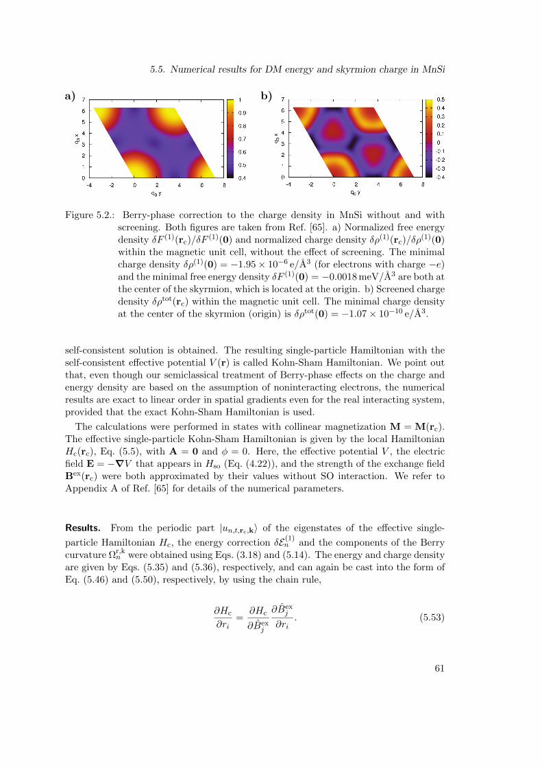
5.5. Numerical results for DM energy and skyrmion charge in MnSi
Figure 5.2.: Berry-phase correction to the charge density in MnSi without and withscreening. Both figures are taken from Ref. [65]. a) Normalized free energydensity δF (1)(rc)/δF
(1)(0) and normalized charge density δρ(1)(rc)/δρ(1)(0)
within the magnetic unit cell, without the effect of screening. The minimalcharge density δρ(1)(0) = −1.95× 10⁻⁶ e/A3 (for electrons with charge −e)and the minimal free energy density δF (1)(0) = −0.0018 meV/A3 are both atthe center of the skyrmion, which is located at the origin. b) Screened chargedensity δρtot(rc) within the magnetic unit cell. The minimal charge densityat the center of the skyrmion (origin) is δρtot(0) = −1.07× 10⁻¹⁰ e/A3.
self-consistent solution is obtained. The resulting single-particle Hamiltonian with theself-consistent effective potential V (r) is called Kohn-Sham Hamiltonian. We point outthat, even though our semiclassical treatment of Berry-phase effects on the charge andenergy density are based on the assumption of noninteracting electrons, the numericalresults are exact to linear order in spatial gradients even for the real interacting system,provided that the exact Kohn-Sham Hamiltonian is used.
The calculations were performed in states with collinear magnetization M = M(rc).The effective single-particle Kohn-Sham Hamiltonian is given by the local HamiltonianHc(rc), Eq. (5.5), with A = 0 and φ = 0. Here, the effective potential V , the electricfield E = −∇V that appears in Hso (Eq. (4.22)), and the strength of the exchange fieldBex(rc) were both approximated by their values without SO interaction. We refer toAppendix A of Ref. [65] for details of the numerical parameters.
Results. From the periodic part |un,t,rc,k〉 of the eigenstates of the effective single-
particle Hamiltonian Hc, the energy correction δE(1)n and the components of the Berry
curvature Ωr,kn were obtained using Eqs. (3.18) and (5.14). The energy and charge density
are given by Eqs. (5.35) and (5.36), respectively, and can again be cast into the form ofEq. (5.46) and (5.50), respectively, by using the chain rule,
∂Hc
∂ri=
∂Hc
∂Bexj
∂Bexj
∂ri. (5.53)
61
5. Semiclassical approach to energy and charge density in chiral magnets
The DFT calculations yield, to a good approximation, Dij ≈ −Dδij with DM interactionstrength
D = −4.1 meV A/a3 (5.54)
where a3 is the volume of the eight-atom unit cell with lattice constant a = 4.558 A. Anexperimental value for D can be extracted from the free energy F (q) ∝ Dq+ Jq2 in thehelical phase of MnSi, which has a minimum for a helix with wave vector q0 = −D/(2J).Using q0 = 2π/(190 A) and the exchange coupling J = 52 meV A2/a3 from neutronscattering experiments [69], one obtains an experimental value of D = −3.4 meV A/a3,in good agreement with our result.
Due to the lattice symmetry, the energy and charge density are proportional to eachother and we show both in the same plot, Figure 5.2a, using the magnetization texturefrom Eq. (5.51). Both δf (1)(rc) and δρ(1)(rc), Eqs. (5.46) and (5.50), are maximal in thecenter of the skyrmion, located at the origin in Figure 5.2. By integrating δρ(1)(rc) overthe magnetic unit cell, we obtain a total skyrmion charge3 of δQ(1) = −0.25e. However,this result neglects Coulomb interactions, which lead screening of charges on the length-scale of the Thomas-Fermi screening length λTF =
√ε0/(e2νF ), see Eq. (5.41). From our
DFT calculations, we obtain νF ≈ 0.11/(eV A3) and therefore λTF ≈ 0.224 A 1/q0.The short λTF leads to a strong suppression of the charge density ρtot ≈ −λ2
TF∇2δρ(1),
see Fig. 5.2b.
3Note again the different sign convention than in Ref. [77]. In this thesis, SI units with electron charge−e are used.
62
6. Skyrmion charge from a gradientexpansion
In this chapter, we extend our discussion of the electric charge of skyrmions beyond thesemiclassical approximation used in chapter 5. To do so, we introduce a complemen-tary method to calculate electronic properties in systems with a smooth magnetizationtexture, which is based on a systematic gradient expansion of the Green’s function. Toleading order, the gradient expansion is equivalent to the semiclassical approximation,while higher order contributions lead to corrections to the semiclassical picture. In in-sulators, we argue that the total electric charge of a skyrmion is quantized and given bythe second-order term of the gradient expansion.
This chapter is organized as follows. In section 6.1, we introduce the so-called Wignerrepresentation of quantum-mechanical operators, which separates oscillations on theatomic length scale from modulations on a long length scale. In section 6.2, we use theWigner representation to expand the equilibrium Green’s function of an inhomogeneoussystem in terms of only local quantities. We use this gradient expansion in section 6.3to calculate the electric charge of skyrmions in metals and in insulators and we compareto the results obtained within the semiclassical treatment of chapter 5. Parts of thischapter can also be found in our publication, Ref. [65].
6.1. Wigner transformation on a lattice
In this section, we present an efficient representation of quantum-mechanical operatorsin a system with modulations on a long length scale, such as a smooth magnetization tex-ture. This so-called Wigner representation is defined in Eq. (6.5) below. The remainingparts of this chapter are devoted to some technical issues of the Wigner transformationin presence of a lattice. The impatient reader may decide to skip those more techni-cal parts and return to them once problems with Wigner transformations turn up incalculations.
We consider an operator A that is approximately periodic in space on a short lengthscale set by the lattice constant a, but that is subject to smooth modulations on alength scale ξmod a. For example, consider the Hamiltonian of a magnet with a smoothmagnetization texture. Our aim is to find a representation of A in which dependencies onthe two length scales are separated into two different coordinates. While periodic systemsare most efficiently described in momentum space, modulations on the long length scaleξmod are more naturally expressed in position space. The Wigner representation usesboth position and momentum coordinates. In the literature, the Wigner transform of a
63
6. Skyrmion charge from a gradient expansion
function f(r1, r2) that depends on two position coordinates is commonly defined as theFourier transform w.r.t. the relative coordinate r1 − r2 (see, e.g., [83, 84]),
f(r,k) :=
∫ddρ e−ik·ρ f
(r +
ρ
2, r− ρ
2
)(without a lattice). (6.1)
One can recover the original function f(r1, r2) from its Wigner transform via the inversetransformation
f(r1, r2) =
∫ddk
(2π)deik·(r1−r2) f
(r1 + r2
2,k
)(without a lattice). (6.2)
In presence of a lattice, however, the definition Eq. (6.1) does not lead to the in-tended separation of length scales. While Eq. (6.1) encodes short-wavelength oscilla-tions w.r.t. the relative coordinate r1 − r2 in the k-dependency of f as intended, short-wavelength oscillations w.r.t. the center-of-mass coordinate (r1 + r2)/2 still manifestthemselves in the r-dependency of f . In particular, the Wigner transform G(ω; r,k) ofthe Green’s function of an almost-periodic system would oscillate as a function of r onthe short length-scale a if one used the definition in Eq. (6.1).
Definition of the Wigner transform on a lattice. In order to separate the two lengthscales ξmod a into position and momentum dependency, respectively, we use an alter-native definition of the Wigner transform in the presence of a lattice. Our descriptionwill be valid for a single-particle operator
A = A[λ1(r), λ2(r), . . .] (6.3)
that is a functional of some smooth modulation fields λi(r), which vary on the lengthscale ξmod. If all modulation fields are constant in space, A becomes exactly periodic inspace with periodicities (in the d space dimensions) on the order of a. An example ofan operator of the form of Eq. (6.3) is given by the Hamiltonian of our model of a chiralmagnet, Eq. (5.4), with time-independent modulation fields Bex, A, and φ. We requirethat the Hamiltonian H[λ1(r), λ2(r), . . .] of the system is also of the form of Eq. (6.3),and we introduce a reference Hamiltonian H0 := H[Λ1,Λ2, · · · ], which is obtained byfixing all modulations fields λi(r) to constant values Λi. The eigenstates |n,k〉 of H0
form a complete set of basis states, and we will use these states as reference states toexpress the Wigner transform. Since H0 is a periodic Hamiltonian, its eigenstates areBloch states,
〈r|n,k〉 = eik·r un,k(r) (6.4)
where un,k(r) is lattice periodic. We assumed that the vector potential A was set tozero when we fixed the modulation fields to constant values, so that the kinetic and thecanonical momentum coincide (cf., discussion below Eq. (5.6)). An important propertyof the reference states |n,k〉 defined in this way is that they are differentiable by keven at the boundary of the Brillouin zone (BZ), where k is “wrapped around” to theopposite side of the BZ (see Figure 6.1). This is the main reason why we constructed the
64
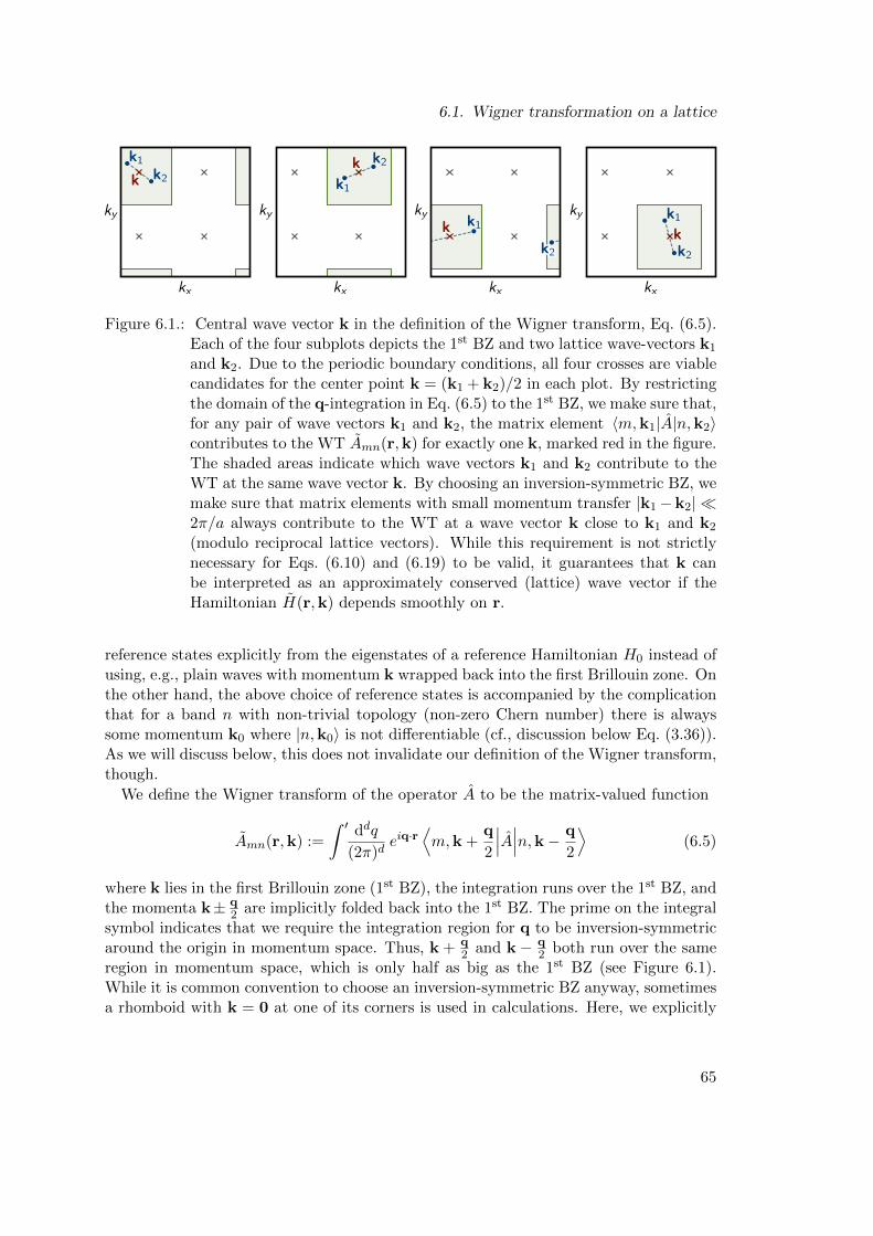
6.1. Wigner transformation on a lattice
Figure 6.1.: Central wave vector k in the definition of the Wigner transform, Eq. (6.5).Each of the four subplots depicts the 1st BZ and two lattice wave-vectors k1
and k2. Due to the periodic boundary conditions, all four crosses are viablecandidates for the center point k = (k1 + k2)/2 in each plot. By restrictingthe domain of the q-integration in Eq. (6.5) to the 1st BZ, we make sure that,for any pair of wave vectors k1 and k2, the matrix element 〈m,k1|A|n,k2〉contributes to the WT Amn(r,k) for exactly one k, marked red in the figure.The shaded areas indicate which wave vectors k1 and k2 contribute to theWT at the same wave vector k. By choosing an inversion-symmetric BZ, wemake sure that matrix elements with small momentum transfer |k1−k2| 2π/a always contribute to the WT at a wave vector k close to k1 and k2
(modulo reciprocal lattice vectors). While this requirement is not strictlynecessary for Eqs. (6.10) and (6.19) to be valid, it guarantees that k canbe interpreted as an approximately conserved (lattice) wave vector if theHamiltonian H(r,k) depends smoothly on r.
reference states explicitly from the eigenstates of a reference Hamiltonian H0 instead ofusing, e.g., plain waves with momentum k wrapped back into the first Brillouin zone. Onthe other hand, the above choice of reference states is accompanied by the complicationthat for a band n with non-trivial topology (non-zero Chern number) there is alwayssome momentum k0 where |n,k0〉 is not differentiable (cf., discussion below Eq. (3.36)).As we will discuss below, this does not invalidate our definition of the Wigner transform,though.
We define the Wigner transform of the operator A to be the matrix-valued function
Amn(r,k) :=
∫ ′ ddq
(2π)deiq·r
⟨m,k +
q
2
∣∣∣A∣∣∣n,k− q
2
⟩(6.5)
where k lies in the first Brillouin zone (1st BZ), the integration runs over the 1st BZ, andthe momenta k± q
2 are implicitly folded back into the 1st BZ. The prime on the integralsymbol indicates that we require the integration region for q to be inversion-symmetricaround the origin in momentum space. Thus, k + q
2 and k− q2 both run over the same
region in momentum space, which is only half as big as the 1st BZ (see Figure 6.1).While it is common convention to choose an inversion-symmetric BZ anyway, sometimesa rhomboid with k = 0 at one of its corners is used in calculations. Here, we explicitly
65
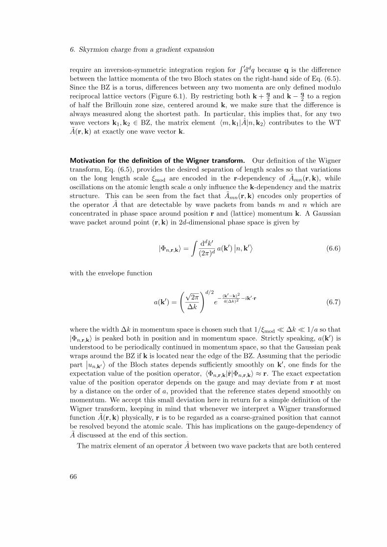
6. Skyrmion charge from a gradient expansion
require an inversion-symmetric integration region for∫ ′
ddq because q is the differencebetween the lattice momenta of the two Bloch states on the right-hand side of Eq. (6.5).Since the BZ is a torus, differences between any two momenta are only defined moduloreciprocal lattice vectors (Figure 6.1). By restricting both k + q
2 and k− q2 to a region
of half the Brillouin zone size, centered around k, we make sure that the difference isalways measured along the shortest path. In particular, this implies that, for any twowave vectors k1,k2 ∈ BZ, the matrix element 〈m,k1|A|n,k2〉 contributes to the WTA(r,k) at exactly one wave vector k.
Motivation for the definition of the Wigner transform. Our definition of the Wignertransform, Eq. (6.5), provides the desired separation of length scales so that variationson the long length scale ξmod are encoded in the r-dependency of Amn(r,k), whileoscillations on the atomic length scale a only influence the k-dependency and the matrixstructure. This can be seen from the fact that Amn(r,k) encodes only properties ofthe operator A that are detectable by wave packets from bands m and n which areconcentrated in phase space around position r and (lattice) momentum k. A Gaussianwave packet around point (r,k) in 2d-dimensional phase space is given by
|Φn,r,k〉 =
∫ddk′
(2π)da(k′)
∣∣n,k′⟩ (6.6)
with the envelope function
a(k′) =
(√2π
∆k
)d/2e− (k′−k)2
4(∆k)2−ik′·r
(6.7)
where the width ∆k in momentum space is chosen such that 1/ξmod ∆k 1/a so that|Φn,r,k〉 is peaked both in position and in momentum space. Strictly speaking, a(k′) isunderstood to be periodically continued in momentum space, so that the Gaussian peakwraps around the BZ if k is located near the edge of the BZ. Assuming that the periodicpart
∣∣un,k′⟩ of the Bloch states depends sufficiently smoothly on k′, one finds for theexpectation value of the position operator, 〈Φn,r,k|r|Φn,r,k〉 ≈ r. The exact expectationvalue of the position operator depends on the gauge and may deviate from r at mostby a distance on the order of a, provided that the reference states depend smoothly onmomentum. We accept this small deviation here in return for a simple definition of theWigner transform, keeping in mind that whenever we interpret a Wigner transformedfunction A(r,k) physically, r is to be regarded as a coarse-grained position that cannotbe resolved beyond the atomic scale. This has implications on the gauge-dependency ofA discussed at the end of this section.
The matrix element of an operator A between two wave packets that are both centered
66
6.1. Wigner transformation on a lattice
around (r,k) in phase space is given by
〈Φm,r,k|A|Φn,r,k〉 =
∫ddk′1(2π)d
∫ddk′2(2π)d
a∗(k′1) a(k′2)⟨m,k′1
∣∣A∣∣n,k′2⟩=
∫ddk′
(2π)d
∫ddq
(2π)da∗(k′ +
q
2
)a(k′ − q
2
)⟨m,k′ +
q
2
∣∣∣A∣∣∣n,k′ − q
2
⟩(6.8)
where all momentum integrations are over the first Brillouin zone and momentum argu-ments of Bloch states are implicitly wrapped back into the 1st BZ. If A is of the formof Eq. (6.3), then it mediates only small momentum transfer (modulo reciprocal latticevectors) and the matrix element on the last line of Eq. (6.8) vanishes unless q . 1/ξmod.Assuming further that the matrix element depends smoothly on the central momen-tum k, we can use the fact that the envelope function a(k′) is strongly peaked at kand approximate k′ ≈ k in the matrix element. Thus, the two momentum integrationsfactorize,
〈Φm,r,k|A|Φn,r,k〉 ≈
(√2π
∆k
)d ∫ddk′
(2π)de− (k′−k)2
2(∆k)2
××[∫
ddq
(2π)de− q2
8(∆k)2+iq·r ⟨
m,k +q
2
∣∣∣A∣∣∣n,k− q
2
⟩]≈Amn(r,k) (6.9)
where the integral over k′ evaluates approximately to 1 since we assumed that the peak-width ∆k is small compared to the size of the BZ. For q . 1/ξmod ∆k, the factor
e− q2
8(∆k)2 ≈ 1 in the q-integration can be dropped and the right-hand side of Eq. (6.9)reduces to Amn(r,k). Thus, in the limit a/ξmod → 0, the Wigner transform Amn(r,k)is the matrix element of A between two wave packets localized around point (r,k) inphase space.
Inverse Wigner transformation. Eq. (6.5) defines the Wigner transformation Amn(r,k)of an operator A by a Fourier transform in the relative momentum coordinate. In orderto recover the matrix elements of the oberator A in the reference basis from A, one hasto perform the inverse Fourier transform,
〈m,k1|A|n,k2〉 ≈∫
ddr e−i(k1−k2)·rAmn
(r,
k1 + k2
2
). (6.10)
The inverse transformation is not exact, however, due to the fact that the q-integrationin Eq. (6.5) is restricted to a finite area. This issue has been discussed by Genske andRosch [85] for the Wigner transform of a function A(t1, t2) that depends on two times. Intheir discussion, a filter function was introduced in the defining integrand for the Wigner
67
6. Skyrmion charge from a gradient expansion
transform, which is equal to one if the both t1 and t2 are close to the central time. Inour definition of the Wigner transformation we effectively introduced a hard-edge filterfunction by the fact that the contributions where k ± q
2 is more than half a reciprocallattice vector away from k are cut off from the integral in Eq. (6.5). Eq. (6.10) is agood approximation for the inverse Wigner transformation if the matrix elements of theoperator A fall of rapidly for large momentum transfer q. This is valid if the separationof length scales ξmod a holds.
If A is the Hamiltonian of the system, then matrix elements with large momentumtransfer on the order of reciprocal lattice vectors are related to Landau-Zener tunneling(see Section 3.5). The gradient expansion derived in the next section will therefore notbe able to account for Landau-Zener tunneling. This should not come as a surprisesince the Landau-Zenter tunnelling probability, Eqs. (3.41)–(3.42) is non-analytic in theparameter κn.a..
Gauge-dependency. The basis states |n,k〉 are only defined up to a gauge transforma-tion
|n,k〉 7−→ |n,k〉′ := eiϕn(k) |n,k〉 (6.11)
where ϕn is a family of real-valued functions. For the Wigner transform, we find toleading order in gradients of ϕn,
|m,k〉 Amn(r,k) 〈n,k| =∫
ddq
(2π)deiq·r+i(ϕm(k+q
2)−ϕm(k))−i(ϕn(k−q
2)−ϕn(k))×
× |m,k〉′′⟨m,k +
q
2
∣∣∣A∣∣∣n,k− q
2
⟩′ ′〈n,k|≈ |m, k〉′ A′mn
(r +
1
2
∂(ϕm(k) + ϕn(k))
∂k,k
)′〈n,k| (6.12)
where the Wigner transform in the new gauge, A′mn(r′,k), is defined by
A′mn(r′,k) =
∫ddq
(2π)deiq·r
′ ′⟨m,k +
q
2
∣∣∣A∣∣∣n,k− q
2
⟩′(6.13)
and we neglected terms with higher-order derivatives. In Eq. (6.12), A′mn(r′,k) is evalu-ated at position r′ = r+ 1
2∂∂k(ϕm + ϕn). The difference between r and r′ is a consequence
of the fact that the Wigner transform is a function of the canonical position. To firstorder in the gradients, the canonical position differs from the kinetic (i.e., physical) po-sition by the momentum-space Berry connection An,k = i 〈un,k| ∂∂k |un,k〉, which changesunder the gauge transformation Eq. (6.11).
Note that the interpretation, Eq. (6.9), of the Wigner transformation in terms ofwave-packets is only valid in a gauge in which the periodic part |un,k〉 of the Blochstates depends smoothly on k (only then are the wave packets localized in positionspace). For gauge transformations that preserve this property, the shift in position r′−ris at most on the order of the lattice constant a, which cannot be resolved by the wave
68
6.2. Local Green’s function and gradient expansion
packets defined in Eq. (6.6). In the following, we will therefore interpret the parameter rof a Wigner transform A(r,k) as a coarse-grained physical position that does not resolveoscillations on the atomic length scale a, and we will thus neglect the gauge-dependencyof r when we interpret, e.g., the charge density ρ(r) physically. The fact that A(r,k)is a function of the canonical position r is related to the non-constant density of statesin the presence of phase-space Berry phases (see section 5.2): If the momentum-spaceBerry curvature An,k depends on position r, then close-by points of the kinetic positionr −An,k increase or reduce in density by moving closer together or further apart. Wewill show in Section 6.3 that the resulting change of charge density δρ(r) is correctlycaptured by our method even though we neglect the gauge dependency of r. The onlydownside is that the precise position where the increased or decreased charge densityappears cannot be resolved beyond the length scale a ξmod.
There is a subtle issue with the choice of gauge for the Wigner transform Amn(r,k)in case of a topologically non-trivial band structure. If either of the bands m or nhas a non-zero Chern number, the Bloch states of that band cannot be differentiableby k on the whole Brillouin zone. To make sure that Amn(r,k) is differentiable on anopen neighborhood of k, we choose a gauge such that all Bloch states are differentiableon the whole region accessible to k ± q
2 in Eq. (6.5), i.e., we push the singularities of
∇k |n,k〉 out of the integration region. Using this gauge, we define Amn(r,k) accordingto Eq. (6.5) for all k ∈ U1 where the open region U1 ⊂ BZ is defined by the conditionthat k is more than half a reciprocal lattice vector away from all singularities. Once kcomes closer than half a reciprocal lattice vector to a singularity, a different gauge has tobe used, which will become a valid choice on some other open region U2 ⊂ BZ. Thus, fortopologically non-trivial bands, one has to cover the BZ with a finite set of open regionsUi and define Amn(r,k) for k ∈ Ui using an appropriate gauge on each patch. Whenevertwo patches Ui and Uj overlap, the two corresponding definitions for Amn(r,k) have toagree on the intersection Ui ∩ Uj . The author is not aware of a rigorous proof that thisprocedure is always possible.
6.2. Local Green’s function and gradient expansion
Based on the Wigner transform introduced in the preceding section, we derive in thissection a perturbative expression of the Green’s function of an almost-periodic system.We consider a time-independent system of non-interacting electrons whose single-particleHamiltonian H is of the form of Eq. (6.3). The equilibrium Green’s function is definedby
Gσ1,σ2(i~ωn; r1, r2) = − 1
Z
∫ β
0dτ eiωnτ Tr
[e−(β−τ)H ψσ1(r1) e−τH ψ†σ2
(r2)]
(6.14)
where Z = Tr[e−βH
]is the partition function, β = 1/(kBT ) is the inverse temperature,
ωn = 2π(n+ 12)kBT/~ is a fermionic Matsubara frequency, ψ†σ(r) (ψσ(r)) creates (annihi-
lates) an electron with spin σ at position r, andH =∫
ddr ψ†(r)Hψ(r) is the Hamiltonian
69
6. Skyrmion charge from a gradient expansion
in second quantized form. The Green’s function satisfies the matrix relation
(i~ωn1spin −Hr1)G(iωn; r1, r2) = 1spin δ(r1 − r2) (6.15)
where the notation Hr1 indicates that the Hamiltonian acts as a differential operator onthe argument r1 of the Green’s function, and 1spin is the identity operator in spin space.Thus, the Green’s function can formally be obtained by inversion of the single-particleHamiltonian,
G(i~ωn) = (iωn −H)−1 (6.16)
where G(iωn) is understood as an operator on the single-particle Hilbert space,
G(iωn) :=∑σ1,σ2
∫ddr1
∫ddr2 |σ1, r1〉Gσ1,σ2(iωn; r1, r2) 〈σ2, r2| (6.17)
where |σ, r〉 are eigenstates of the position operator and of the z-component of the spinoperator.
Moyal product. If H is lattice-periodic, the operator inversion on the right-hand side ofEq. (6.16) can be reduced to the inversion of a matrix in band space using Bloch theorem.If H is not lattice-periodic, it is in general difficult to calculate its inverse G(iωn) exactly.However, one can use a perturbative expansion of G(iωn) if H is of the form of Eq. (6.3),i.e., if there is a separation of the length scales a and ξmod a of the lattice constant andsmooth modulations, respectively. To make the separation of length scales explicit, weuse Wigner representation and denote by H(r,k) and G(iωn; r,k) the Wigner transform,defined in Eq. (6.5), of H and G(iωn), respectively. In Wigner representation, Eq. (6.15)becomes ∑
l
(i~ωnδml − Hml(r,k)) Glj(iωn; r,k) = δmj . (6.18)
where the symbol “” denotes the so-called Moyal product [83, 86], which is defined forthe Wigner transforms of two operators A and B by
A(r,k) B(r,k) := A(r,k) ei2
(←−∂r·−→∂k−←−∂k·−→∂r) B(r,k) = A(x) e
i2Jij←−∂i−→∂j B(x). (6.19)
Here, the exponential function is understood as a formal power series and the symbol←−∂ (−→∂ ) denotes a partial derivative that acts on the function to the left (right). In the
last equality in Eq. (6.19), we introduce a shorthand notation where x ≡ (r,k) is thecombined phase-space coordinate, J is the canonical symplectic form defined in Eq. (5.3),and summation over repeated indices is implied. Eq. (6.19) can be shown by explicitlyinserting the definition of Wigner transform for both A and B and integrating by parts.
Gradient expansion of the Green’s function. In order to calculate local properties ofthe inhomogeneous system, we express the Wigner transform G(iωn;x) of the Green’sfunction in a perturbative gradient expansion by truncating the exponential series in
70
6.2. Local Green’s function and gradient expansion
Eq. (6.19). Both terms in the exponent in Eq. (6.19) involve one differentiation inposition and one in momentum space. We expect that all Wigner transforms vary ona length scale ξmod in position space and on a scale of 1/a in momentum space, sothat an expansion of the exponential series in Eq. (6.19) corresponds to an expansion ina/ξmod 1.
Technically, we write G(iωn;x) as
G(iωn;x) ≈ G(0)(iωn;x) + G(1)(iωn;x) + G(2)(iωn;x) +O(∂3r ) (6.20)
where the superscript denotes the total order of spatial gradients. In this chapter, ouraim is to calculate the leading order contribution to the charge density in a skyrmion,which turns out to be linear in ∂r in metals and quadratic in insulators (see Section 6.3).Therefore, we truncate the expansion in Eq. (6.20) after the second order.
Local Green’s function. To zero’th order in the gradients, we obtain from Eqs. (6.18)–(6.20),
G(0)(iωn;x) = (i~ωn − H(x))−1 =: g(iωn;x). (6.21)
Here, the notation (· · · )−1 is to be understood as a pointwise inversion of (iωn− H(x)),which is a matrix in band space for every point x in phase space. Computationally, thepointwise inversion of a band-matrix is an easier operation than the original operatorinversion in the full Hilbert space, Eq. (6.16). We refer to g(iωn;x) as the local Green’sfunction, since a truncation of Eq. (6.19) at zero’th order is analogous to a local densityapproximation.
Gradient corrections. To first order in the gradients, Eqs. (6.18)–(6.20) yield the rela-tion
g−1(iωn;x) G(1)(iωn;x) +i
2Jij (∂ig
−1(iωn;x)) (∂j g(iωn;x)) = 0 (6.22)
which can be solved for G(1)(iωn;x),
G(1) =i
2Jij g (∂iH) g (∂jH) g ≡
i j(6.23)
where we omitted all dependencies on ωn and x to improve readability, with the under-standing that all matrix inversions are again pointwise. In the last step in Eq. (6.23),we introduce a pictorial notation. Each solid line in our diagrams corresponds to a localGreen’s function g, a vertex with label i represents a factor of ∂iH, and a dashed arrowfrom vertex i to vertex j denotes multiplication with i
2Jij and summation over i and j.
The second-order part of Eqs. (6.18)–(6.20) is
g−1 G(2) +i
2Jij (∂ig
−1) (∂jG(1)) +
1
2
(i
2
)2
JijJkl (∂i∂kg−1) (∂j∂lg) = 0 (6.24)
71
6. Skyrmion charge from a gradient expansion
which has the solution (using the pictorial notation introduced in Eq. (6.23))
G(2) = + +
+ + + +1
2
( )(6.25)
where, e.g., the first diagram on the second line represents the term
≡(i
2
)2
JijJkl g (∂i∂kH) g (∂jH) g (∂lH) g. (6.26)
Comparison between local Hamiltonian Hc and Wigner transformed Hamiltonian H.In Eq. (6.21), we defined the local Green’s function g(iωn; r,k) as the pointwise inverseof (iωn− H(r,k)). Thus, for a fixed position rc, g(iωn; rc,k) is the Green’s function of a(fictitious) homogeneous system described by the band Hamiltonian H(rc,k). While, inthis sense, H(rc,k) describes electron dynamics locally in the vicinity of rc, it is worthnoting the differences between H(rc,k) and the local band Hamiltonian Hc(rc,k) definedin Eqs. (5.5) and (5.8). As an example, we consider the time-independent Hamiltonian
H = H0 + Bex(r) · σ (6.27)
where H0 is lattice periodic, the exchange field Bex varies on a length scale (ξmod a),and σ is the vector of Pauli matrices. The local Hamiltonian, Eq. (5.5), is obtained byevaluating Bex at position rc. Its eigenstates are the Bloch states |Φn,rc,k〉 defined inEq. (5.6), so that, in its eigenbasis, the local band Hamiltonian Hc(rc,k), Eq. (5.8), isthe matrix-valued function(
Hc(rc,k))mn≡ 〈Φm,rc,k|(H0 + Bex(rc))|Φn,rc,k〉 = δmn E(0)
n (rc,k). (6.28)
In order to compare the local band Hamiltonian Hc to the Wigner transformed Hamil-tonian H, we express the exchange field in terms of its Fourier transform Bex(q),
Bex(r) =
∫ddq
(2π)dBex(q) eiq·r (6.29)
and evaluate H at position rc in the same basis states |Φn,rc,k〉,
Hmn(rc,k) = 〈Φm,rc,k|H0|Φn,rc,k〉+
∫ddq
(2π)d
∫ddq′
(2π)d
∫ddr′ eiq·rc+i(q′−q)·r′×
× u∗m,rc,k+q2(r′) Bex(q′) · σ un,rc,k−q
2(r′)
(6.30)
72
6.2. Local Green’s function and gradient expansion
where u is the lattice-periodic part of the Bloch functions Φ. Assuming that Bex(q′)is non-vanishing only for small momenta q′ . 1/ξmod 1/a and neglecting Umklapp-scattering off the magnetic texture, the integral over r′ vanishes unless q = q′. Therefore,we find
Hmn(rc,k) = 〈Φm,rc,k|H0|Φn,rc,k〉+
∫ddq
(2π)deiq·rc Bex(q) · 〈um,rc,k+q
2|σ|un,rc,k−q
2〉 .
(6.31)
If one neglects the momentum-dependency of the lattice-periodic states |un,rc,k±q2〉, then
the right-hand side of Eq. (6.31) reduces to the local band Hamiltonian, Eq. (6.28).Gradient corrections lead to differences between H and Hc. Expanding the matrix-element on the right-hand side of Eq. (6.31) to first order in q, one obtains
Hmn(rc,k) ≈(Hc(rc,k)
)mn− i ∂B
exi (r)
∂rc,j〈um,rc,k|σi
∂ |un,rc,k〉∂kj
+O((a/ξmod)2). (6.32)
If H0 is spin-independent (i.e., without SO-coupling), the states |un,rc,k〉 are eigenstatesof Bex(rc) · σ for all n and k, so that
Hmn(rc,k) ≈(Hc(rc −Ak
mn(rc,k),k))mn
+O((a/ξmod)2) (6.33)
where the hermitian matrix
Akmn(rc,k) := i 〈um,rc,k|
∂ |un,rc,k〉∂k
(6.34)
contains the momentum-space Berry connection on its diagonal components. In a chiralmagnet, SO-coupling is smaller than exchange interaction by a factor of ∼ a/ξmod, sothat Eq. (6.33) is even valid in presence of SO-coupling.
Therefore, we find that, in the limit a/ξmod → 0, the Wigner transformed HamiltonianH coincides with the local band Hamiltonian Hc. To first order in the spatial gradients,the two Hamiltonians differ only due to the fact that we defined H as a function of thecanonical position, see also discussion below Eq. (6.13). To second order in the spa-tial gradients, the Wigner transformed Hamiltonian H and the local band HamiltonianHc are different. Philosophically, Hc(rc,k) is an educated guess of a lattice-periodicHamiltonian around which the full Hamiltonian, Eq. (6.27), can be efficiently expandedin order to describe physical properties in the vicinity of rc. The Wigner-transformedHamiltonian H(r,k), on the other hand, is an effective Hamiltonian that is “felt” bywave packets centered around a position close to r, where the exact center-of-mass po-sition of the wave packets depends on the gauge. We allowed for a small deviation ∼ abetween r and the exact center-of-mass position of the wave packets in order to simplifythe definition of the Wigner transform.
73
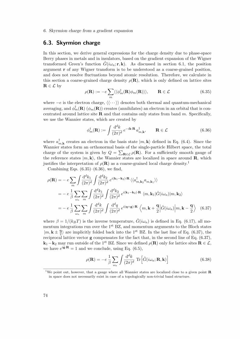
6. Skyrmion charge from a gradient expansion
6.3. Skyrmion charge
In this section, we derive general expressions for the charge density due to phase-spaceBerry phases in metals and in insulators, based on the gradient expansion of the Wignertransformed Green’s function G(iωn; r,k). As discussed in section 6.1, the positionargument r of any Wigner transform is to be understood as a coarse-grained position,and does not resolve fluctuations beyond atomic resolution. Therefore, we calculate inthis section a coarse-grained charge density ρ(R), which is only defined on lattice sitesR ∈ L by
ρ(R) := −e∑m
〈〈φ†m(R)φm(R)〉〉, R ∈ L (6.35)
where −e is the electron charge, 〈〈· · · 〉〉 denotes both thermal and quantum-mechanical
averaging, and φ†m(R) (φm(R)) creates (annihilates) an electron in an orbital that is con-centrated around lattice site R and that contains only states from band m. Specifically,we use the Wannier states, which are created by
φ†m(R) :=
∫ddk
(2π)de−ik·R a†m,k, R ∈ L (6.36)
where a†m,k creates an electron in the basis state |m,k〉 defined in Eq. (6.4). Since theWannier states form an orthonormal basis of the single-particle Hilbert space, the totalcharge of the system is given by Q =
∑R∈L ρ(R). For a sufficiently smooth gauge of
the reference states |m,k〉, the Wannier states are localized in space around R, whichjustifies the interpretation of ρ(R) as a coarse-grained local charge density.1
Combining Eqs. (6.35)–(6.36), we find,
ρ(R) =− e∑m
∫ddk1
(2π)d
∫ddk2
(2π)dei(k1−k2)·R 〈〈a†m,k2
am,k1〉〉
=− e 1
β
∑ωn
∑m
∫ddk1
(2π)d
∫ddk2
(2π)dei(k1−k2)·R 〈m,k1|G(iωn)|m,k2〉
=− e 1
β
∑ωn
∑m
∫ddk
(2π)d
∫ddq
(2π)dei(q+g)·R
⟨m,k +
q
2
∣∣∣G(iωn)∣∣∣m,k− q
2
⟩(6.37)
where β = 1/(kBT ) is the inverse temperature, G(iωn) is defined in Eq. (6.17), all mo-mentum integrations run over the 1st BZ, and momentum arguments to the Bloch states|m,k± q
2 〉 are implicitly folded back into the 1st BZ. In the last line of Eq. (6.37), thereciprocal lattice vector g compensates for the fact that, in the second line of Eq. (6.37),k1−k2 may run outside of the 1st BZ. Since we defined ρ(R) only for lattice sites R ∈ L,we have eig·R = 1 and we conclude, using Eq. (6.5),
ρ(R) = −e 1
β
∑ωn
∫ddk
(2π)dTr[G(iωn; R,k)
](6.38)
1We point out, however, that a gauge where all Wannier states are localized close to a given point Rin space does not necessarily exist in case of a topologically non-trivial band structure.
74
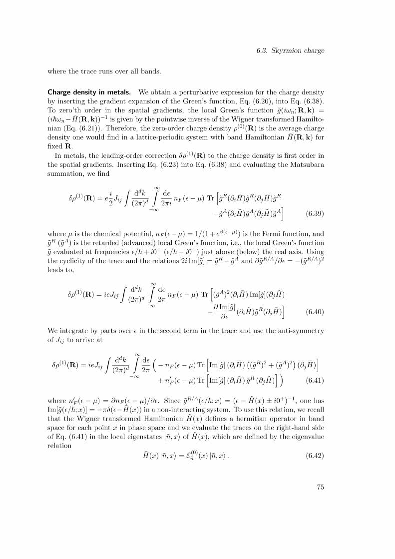
6.3. Skyrmion charge
where the trace runs over all bands.
Charge density in metals. We obtain a perturbative expression for the charge densityby inserting the gradient expansion of the Green’s function, Eq. (6.20), into Eq. (6.38).To zero’th order in the spatial gradients, the local Green’s function g(iωn; R,k) =(i~ωn−H(R,k))−1 is given by the pointwise inverse of the Wigner transformed Hamilto-nian (Eq. (6.21)). Therefore, the zero-order charge density ρ(0)(R) is the average chargedensity one would find in a lattice-periodic system with band Hamiltonian H(R,k) forfixed R.
In metals, the leading-order correction δρ(1)(R) to the charge density is first order inthe spatial gradients. Inserting Eq. (6.23) into Eq. (6.38) and evaluating the Matsubarasummation, we find
δρ(1)(R) = ei
2Jij
∫ddk
(2π)d
∞∫−∞
dε
2πinF (ε− µ) Tr
[gR(∂iH)gR(∂jH)gR
−gA(∂iH)gA(∂jH)gA]
(6.39)
where µ is the chemical potential, nF (ε−µ) = 1/(1 + eβ(ε−µ)) is the Fermi function, andgR (gA) is the retarded (advanced) local Green’s function, i.e., the local Green’s functiong evaluated at frequencies ε/~ + i0+ (ε/~− i0+) just above (below) the real axis. Usingthe cyclicity of the trace and the relations 2i Im[g] = gR− gA and ∂gR/A/∂ε = −(gR/A)2
leads to,
δρ(1)(R) = ieJij
∫ddk
(2π)d
∞∫−∞
dε
2πnF (ε− µ) Tr
[(gA)2(∂iH) Im[g](∂jH)
−∂ Im[g]
∂ε(∂iH)gR(∂jH)
](6.40)
We integrate by parts over ε in the second term in the trace and use the anti-symmetryof Jij to arrive at
δρ(1)(R) = ieJij
∫ddk
(2π)d
∞∫−∞
dε
2π
(− nF (ε− µ) Tr
[Im[g] (∂iH)
((gR)2 + (gA)2
)(∂jH)
]+ n′F (ε− µ) Tr
[Im[g] (∂iH) gR (∂jH)
] )(6.41)
where n′F (ε − µ) = ∂nF (ε − µ)/∂ε. Since gR/A(ε/~;x) = (ε − H(x) ± i0+)−1, one hasIm[g(ε/~;x)] = −πδ(ε−H(x)) in a non-interacting system. To use this relation, we recallthat the Wigner transformed Hamiltonian H(x) defines a hermitian operator in bandspace for each point x in phase space and we evaluate the traces on the right-hand sideof Eq. (6.41) in the local eigenstates |n, x〉 of H(x), which are defined by the eigenvaluerelation
H(x) |n, x〉 = E(0)n (x) |n, x〉 . (6.42)
75
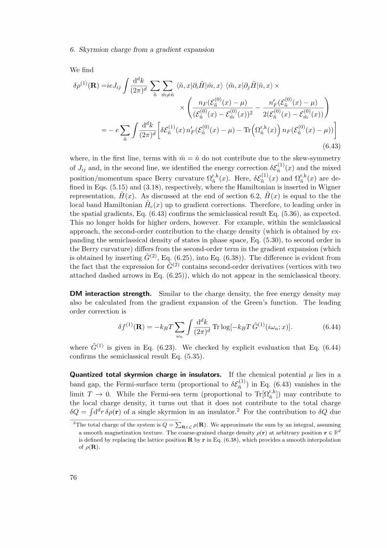
6. Skyrmion charge from a gradient expansion
We find
δρ(1)(R) =ieJij
∫ddk
(2π)d
∑n
∑m 6=n
〈n, x|∂iH|m, x〉 〈m, x|∂jH|n, x〉×
×
(nF (E(0)
n (x)− µ)
(E(0)n (x)− E(0)
m (x))2−
n′F (E(0)n (x)− µ)
2(E(0)n (x)− E(0)
m (x))
)
=− e∑n
∫ddk
(2π)d
[δE(1)n (x)n′F (E(0)
n (x)− µ)− Tr(
Ωr,kn (x)
)nF (E(0)
n (x)− µ))
](6.43)
where, in the first line, terms with m = n do not contribute due to the skew-symmetry
of Jij and, in the second line, we identified the energy correction δE(1)n (x) and the mixed
position/momentum space Berry curvature Ωr,kn (x). Here, δE(1)
n (x) and Ωr,kn (x) are de-
fined in Eqs. (5.15) and (3.18), respectively, where the Hamiltonian is inserted in Wignerrepresentation, H(x). As discussed at the end of section 6.2, H(x) is equal to the thelocal band Hamiltonian Hc(x) up to gradient corrections. Therefore, to leading order inthe spatial gradients, Eq. (6.43) confirms the semiclassical result Eq. (5.36), as expected.This no longer holds for higher orders, however. For example, within the semiclassicalapproach, the second-order contribution to the charge density (which is obtained by ex-panding the semiclassical density of states in phase space, Eq. (5.30), to second order inthe Berry curvature) differs from the second-order term in the gradient expansion (whichis obtained by inserting G(2), Eq. (6.25), into Eq. (6.38)). The difference is evident fromthe fact that the expression for G(2) contains second-order derivatives (vertices with twoattached dashed arrows in Eq. (6.25)), which do not appear in the semiclassical theory.
DM interaction strength. Similar to the charge density, the free energy density mayalso be calculated from the gradient expansion of the Green’s function. The leadingorder correction is
δf (1)(R) = −kBT∑ωn
∫ddk
(2π)dTr log[−kBT G(1)(iωn;x)]. (6.44)
where G(1) is given in Eq. (6.23). We checked by explicit evaluation that Eq. (6.44)confirms the semiclassical result Eq. (5.35).
Quantized total skyrmion charge in insulators. If the chemical potential µ lies in a
band gap, the Fermi-surface term (proportional to δE(1)n ) in Eq. (6.43) vanishes in the
limit T → 0. While the Fermi-sea term (proportional to Tr[Ωr,kn ]) may contribute to
the local charge density, it turns out that it does not contribute to the total chargeδQ =
∫ddr δρ(r) of a single skyrmion in an insulator.2 For the contribution to δQ due
2The total charge of the system is Q =∑
R∈L ρ(R). We approximate the sum by an integral, assuming
a smooth magnetization texture. The coarse-grained charge density ρ(r) at arbitrary position r ∈ Rd
is defined by replacing the lattice position R by r in Eq. (6.38), which provides a smooth interpolationof ρ(R).
76
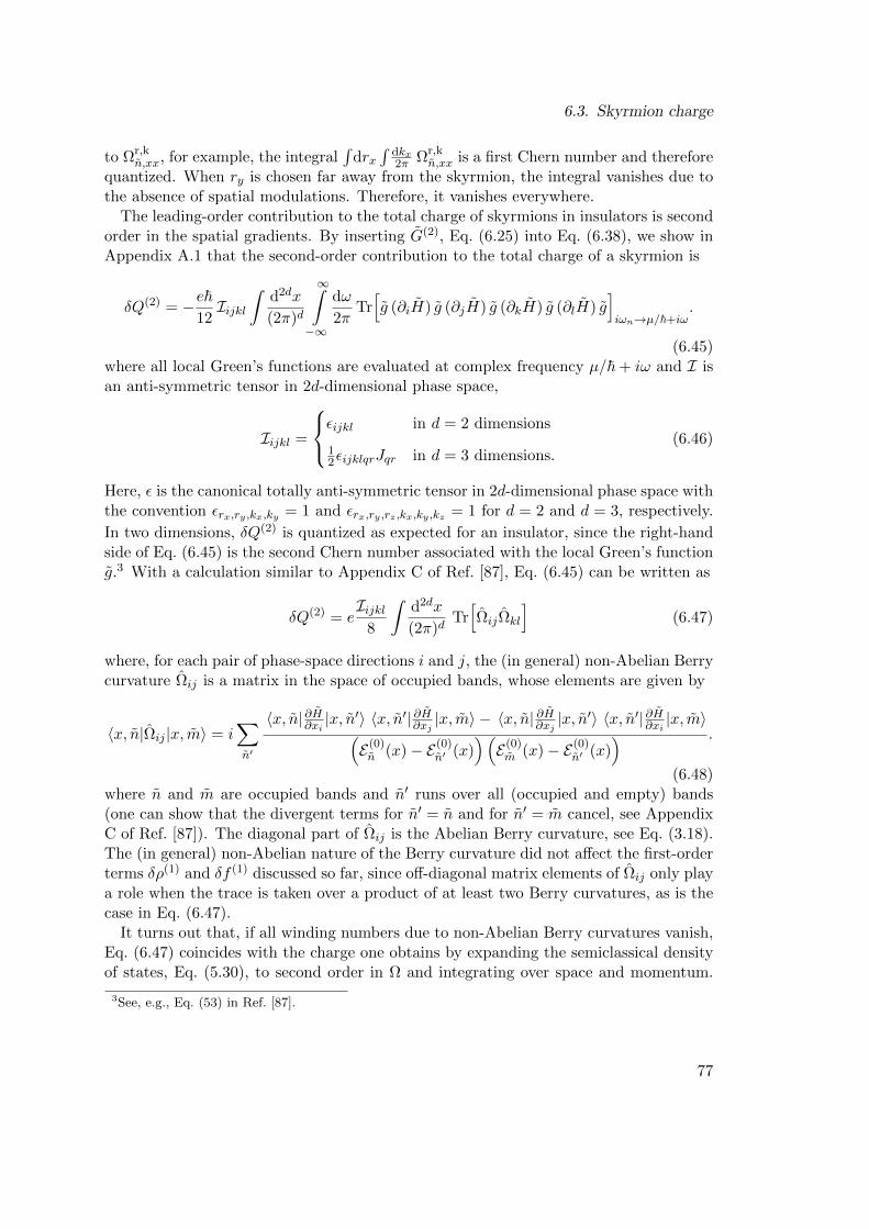
6.3. Skyrmion charge
to Ωr,kn,xx, for example, the integral
∫drx
∫dkx2π Ωr,k
n,xx is a first Chern number and thereforequantized. When ry is chosen far away from the skyrmion, the integral vanishes due tothe absence of spatial modulations. Therefore, it vanishes everywhere.
The leading-order contribution to the total charge of skyrmions in insulators is secondorder in the spatial gradients. By inserting G(2), Eq. (6.25) into Eq. (6.38), we show inAppendix A.1 that the second-order contribution to the total charge of a skyrmion is
δQ(2) = −e~12Iijkl
∫d2dx
(2π)d
∞∫−∞
dω
2πTr[g (∂iH) g (∂jH) g (∂kH) g (∂lH) g
]iωn→µ/~+iω
.
(6.45)where all local Green’s functions are evaluated at complex frequency µ/~ + iω and I isan anti-symmetric tensor in 2d-dimensional phase space,
Iijkl =
εijkl in d = 2 dimensions
12εijklqrJqr in d = 3 dimensions.
(6.46)
Here, ε is the canonical totally anti-symmetric tensor in 2d-dimensional phase space withthe convention εrx,ry ,kx,ky = 1 and εrx,ry ,rz ,kx,ky ,kz = 1 for d = 2 and d = 3, respectively.
In two dimensions, δQ(2) is quantized as expected for an insulator, since the right-handside of Eq. (6.45) is the second Chern number associated with the local Green’s functiong.3 With a calculation similar to Appendix C of Ref. [87], Eq. (6.45) can be written as
δQ(2) = eIijkl
8
∫d2dx
(2π)dTr[ΩijΩkl
](6.47)
where, for each pair of phase-space directions i and j, the (in general) non-Abelian Berrycurvature Ωij is a matrix in the space of occupied bands, whose elements are given by
〈x, n|Ωij |x, m〉 = i∑n′
〈x, n| ∂H∂xi |x, n′〉 〈x, n′| ∂H∂xj |x, m〉 − 〈x, n|
∂H∂xj|x, n′〉 〈x, n′| ∂H∂xi |x, m〉(
E(0)n (x)− E(0)
n′ (x))(E(0)m (x)− E(0)
n′ (x)) .
(6.48)where n and m are occupied bands and n′ runs over all (occupied and empty) bands(one can show that the divergent terms for n′ = n and for n′ = m cancel, see AppendixC of Ref. [87]). The diagonal part of Ωij is the Abelian Berry curvature, see Eq. (3.18).The (in general) non-Abelian nature of the Berry curvature did not affect the first-orderterms δρ(1) and δf (1) discussed so far, since off-diagonal matrix elements of Ωij only playa role when the trace is taken over a product of at least two Berry curvatures, as is thecase in Eq. (6.47).
It turns out that, if all winding numbers due to non-Abelian Berry curvatures vanish,Eq. (6.47) coincides with the charge one obtains by expanding the semiclassical densityof states, Eq. (5.30), to second order in Ω and integrating over space and momentum.
3See, e.g., Eq. (53) in Ref. [87].
77
6. Skyrmion charge from a gradient expansion
Thus, while the semiclassical theory is generally only valid to linear order in the spatialgradients, it predicts the correct result beyond linear order in the specific case of the totalskyrmion charge in an insulator at filling factor 1. For larger filling factors, however,non-Abelian Berry curvatures have to be taken into account in general, see Eqs. (6.47)–(6.48).
We show in Appendix A.2 that, for a single occupied band in d = 2 dimensions, theright-hand side of Eq. (6.47) reduces to the product of two quantized winding numbers,
δQ(2) = σxyΦ0 (6.49)
where
σxy =e2
~
∫d2k
(2π)2Ωk,kxy (6.50)
is the quantized Hall conductivity and
Φ0 =~e
∫d2rΩr,r
xy = ±2π~e
(6.51)
is the total emergent magnetic flux (the real-space winding number of the skyrmion).Eq. (6.49) is a well-known result in the context of quantum Hall systems at filling
factor close to ν = 1 [13,88]. In a two-dimensional electron gas in a strong perpendicularmagnetic field, the degeneracy of each Landau level is equal to the number of magneticflux quanta in the system. Since each skyrmion carries a quantized emergent magneticflux qem
e
∫d2r Bem
z = ~e
∫d2rΩr,r
xy = Φ0 (cf., Eq. (4.14)), the system can increase thedegeneracy of each Landau level by one by forming a skyrmion. This is energeticallyfavorable if ν lies slightly above an integer value and the ferromagnetic exchange energyis large compared to the Zeeman splitting [13, 88–90]. Evidence for the formation ofskyrmions in a quantum Hall system has been observed in GaAs/AlGaAs quantumwells [14].
In d = 3 dimensions, skyrmions form line defects and the total charge of a skyrmionis proportional to its length L. In Appendix A.3, we show that the skyrmion charge perlength in a three-dimensional insulator is
δQ(2)
L= e
3∑α=1
s · gα2π
nkα (6.52)
where s is a unit vector that points in the direction of the skyrmion tube, gα, α ∈ 1, 2, 3are reciprocal lattice vectors, and nk
α ∈ Z is the momentum-space winding number inthe plane perpendicular to the corresponding real-space lattice vector aα.
78
Part II.
Hall effect in chiral magnets withweak spin-orbit coupling
79

7. Hall effects in chiral magnets
One of the most striking manifestations of Berry phases in chiral magnets can be ob-served in measurements of transverse electron transport. It is well-known that the Berrycurvature in position space leads to a large Hall response in the skyrmion lattice phase,dubbed the topological Hall effect [21, 22]. An additional contribution to the trans-verse current comes from the anomalous Hall effect [70, 72], whose intrinsic part is aconsequence of a non-zero Berry curvature in momentum space. Both topological andanomalous Hall effect can be much larger than the ordinary Hall effect generated by thesmall external magnetic field that stabilizes the skyrmion lattice phase.
In this chapter, we briefly review the experimental observations of Hall effects inchiral magnets (Section 7.1). We then present a simple semiclassical derivation of theHall conductivity that takes Berry phases in all of phase space into account (Section 7.2).In the next chapter, we go beyond the semiclassical approximation and derive the Hallresponse using a field-theoretical approach based on the gradient expansion introducedin Section 6.2.
7.1. Overview over experiments and theoretical methods
In measurements of the Hall response, a small current I is driven through a sample andone measures the voltage UH that builds up perpendicular to the current direction. Ifthe voltage is measured in x direction and the current runs through the system in ydirection, the Hall resistivity is given by
ρxy =Exjy
=
UH/I in d = 2 dimensions
Lz UH/I in d = 3 dimensions(7.1)
where Ex is the electric field that builds up perpendicular to the current direction, jy isthe current density, and Lz is the thickness of the three-dimensional sample.
Contributions to the Hall signal. The rich phase diagram of chiral magnets leads toan intricate dependency of ρxy on the external magnetic field, temperature, and samplequality. We show measurement data for the Hall resistivity in MnSi in Figure 7.1, whichis taken from Ref. [30]. Here, Ba1 and Ba2 indicate the boundary of the Skyrmion latticephase, and Bc2 marks the transition from the conical to the field polarized state (cf.,Figure 2.3). Three major contributions to the Hall resistivity can be identified: thenormal Hall effect, the topological Hall effect, and the anomalous Hall effect.
81
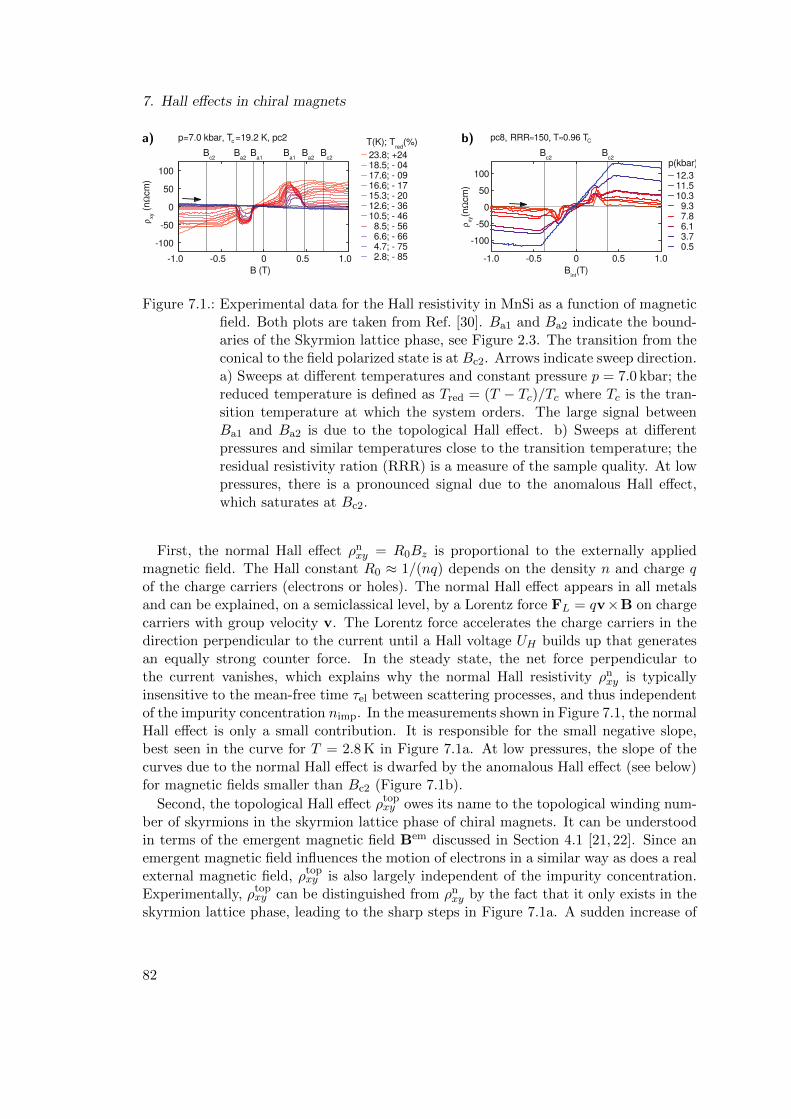
7. Hall effects in chiral magnets
B (T)
-100
-50
0
50
100
ρ xy(n
Ωcm
)Bc2 Ba2 Ba1 Ba1 Ba2 Bc2
T(K); Tred(%)23.8; +2418.5; - 0417.6; - 0916.6; - 1715.3; - 2012.6; - 3610.5; - 468.5; - 566.6; - 664.7; - 75
c =19.2 K, pc2
-100-50
050
100 12.311.510.39.37.86.13.7
ρ xy(n
Ωcm
)
p(kbar)
Bint(T)
≈ ≈0.96 TC
Bc2 Bc2
Figure 7.1.: Experimental data for the Hall resistivity in MnSi as a function of magneticfield. Both plots are taken from Ref. [30]. Ba1 and Ba2 indicate the bound-aries of the Skyrmion lattice phase, see Figure 2.3. The transition from theconical to the field polarized state is at Bc2. Arrows indicate sweep direction.a) Sweeps at different temperatures and constant pressure p = 7.0 kbar; thereduced temperature is defined as Tred = (T − Tc)/Tc where Tc is the tran-sition temperature at which the system orders. The large signal betweenBa1 and Ba2 is due to the topological Hall effect. b) Sweeps at differentpressures and similar temperatures close to the transition temperature; theresidual resistivity ration (RRR) is a measure of the sample quality. At lowpressures, there is a pronounced signal due to the anomalous Hall effect,which saturates at Bc2.
First, the normal Hall effect ρnxy = R0Bz is proportional to the externally applied
magnetic field. The Hall constant R0 ≈ 1/(nq) depends on the density n and charge qof the charge carriers (electrons or holes). The normal Hall effect appears in all metalsand can be explained, on a semiclassical level, by a Lorentz force FL = qv×B on chargecarriers with group velocity v. The Lorentz force accelerates the charge carriers in thedirection perpendicular to the current until a Hall voltage UH builds up that generatesan equally strong counter force. In the steady state, the net force perpendicular tothe current vanishes, which explains why the normal Hall resistivity ρn
xy is typicallyinsensitive to the mean-free time τel between scattering processes, and thus independentof the impurity concentration nimp. In the measurements shown in Figure 7.1, the normalHall effect is only a small contribution. It is responsible for the small negative slope,best seen in the curve for T = 2.8 K in Figure 7.1a. At low pressures, the slope of thecurves due to the normal Hall effect is dwarfed by the anomalous Hall effect (see below)for magnetic fields smaller than Bc2 (Figure 7.1b).
Second, the topological Hall effect ρtopxy owes its name to the topological winding num-
ber of skyrmions in the skyrmion lattice phase of chiral magnets. It can be understoodin terms of the emergent magnetic field Bem discussed in Section 4.1 [21, 22]. Since anemergent magnetic field influences the motion of electrons in a similar way as does a realexternal magnetic field, ρtop
xy is also largely independent of the impurity concentration.Experimentally, ρtop
xy can be distinguished from ρnxy by the fact that it only exists in the
skyrmion lattice phase, leading to the sharp steps in Figure 7.1a. A sudden increase of
82
7.1. Overview over experiments and theoretical methods
the Hall resistivity in MnSi as a function of magnetic field was first reported by Lee andcollaborators [91]. However, the effect was observed under high pressures and it remainedan open question for some time whether the magnetic fields at which the increased Hallresistivity was observed corresponds to the skyrmion lattice phase [30]. Experiments byNeubauer and collaborators [10, 22] at ambient pressure showed an increase of the Hallresistivity that occurred indeed at the transition to the skyrmion lattice phase. In MnSi,the average strength of the emergent magnetic field is on the order of 13 T, which is muchlarger than the external field B ≈ 0.2 . . . 0.4 T required to stabilize the skyrmion lattice.On the other hand, the resulting force F = qem
σ v×Bem on the electrons is proportionalto the emergent charge qem
σ = ±12 , which has a different sign for majority and minority
spins. The topological Hall resistivity may thus be estimated by ρtopxy = PR0B
emz where
R0 is the ordinary Hall constant and P is the average spin polarization. Despite the av-eraging over different signs, the topological Hall effect can become much larger than theordinary Hall effect, see Figure 7.1a. The definition of P involves a rather complicatedaveraging over the Fermi surface [30], which makes calculations for real materials chal-lenging. Recent numerical calculations of the topological Hall response from ab-initiocan be found in Refs. [92, 93]. The emergent magnetic field is inversely proportional tothe size of the magnetic unit cell. Therefore, the topological Hall effect becomes largein chiral magnets with a short pitch length, see, e.g., Ref. [94]. In the extreme limit,position-space Berry phases have also been considered in materials where the spin tex-ture varies on the atomic length scale. This includes materials where the non-coplanarspin texture is a result of double-exchange [95, 96] or of frustration [97, 98]. In thesesystems, however, the adiabatic assumption breaks down and spin-flip processes, nottaken into account by the Berry phase picture, become important.
Finally, the anomalous Hall effect ρAHExy , well-known from ferromagnetic materials, also
appears in chiral magnets. Topological and anomalous Hall effect can be regarded as op-posite limits of a coupling between the spin and a real-space structure. In the topologicalHall effect, the coupling is to the effective exchange field due to the spontaneous magne-tization. In chiral magnets with weak spin-orbit coupling, the latter varies on a lengthscale much larger than the lattice constant. In the opposite limit, electric fields dueto variations of the periodic crystal potential couple to the electron spins via spin-orbitinteraction, leading to a momentum-space Berry curvature and to the anomalous Hall ef-fect. Since a (charge) Hall current is only possible for broken time-reversal symmetry, theanomalous Hall effect depends on the magnetization M and it can be distinguished fromthe normal Hall signal in experimental data by its hysteretic behavior and its saturationat large magnetic fields. The latter is clearly visible in Figure 7.1b. In the literature, oneoften finds the relation ρAHE
xy = RsM with an anomalous Hall constant Rs. The propor-
tionality should be taken with a grain of salt, however, and the relation between ρAHExy
and M is often more complex and can even be non-monotonic [99,100]. This can be ex-plained by the fact that the system changes its magnetization by redistributing electronsbetween different bands. Since the momentum-space Berry curvature has sharp peaksin the vicinity of avoided band crossings, see Section 4.3, the anomalous Hall effect canbe very sensitive to such electron redistributions. The dependency of Rs on temperature
83
7. Hall effects in chiral magnets
and on impurity concentrations remained a source of debate for decades [101–104]. Itis now understood that three different physical mechanisms mainly contribute to theanomalous Hall effect, which all relate differently to scattering processes. First, Berryphases in momentum space lead to an anomalous electron velocity [6] perpendicular tothe applied electric field, see Section 5.1. The resulting contribution σAHE,int
xy to the Hallconductivity is called the intrinsic anomalous Hall effect, and is independent of impurityconcentrations. In experiments, one measures the Hall resistivity ρxy ≈ −ρ2
xxσxy whereρxx is the longitudinal resistivity assumed to be much larger than ρxy. As ρxx is approx-imately proportional to the impurity concentration, the Hall resistivity in systems wherethe intrinsic contribution dominates is approximately quadratic in the impurity concen-tration. Second, asymmetric scattering at impurities, so-called skew-scattering, leadsto a Hall resistivity approximately proportional to ρxx [105]. Third, due to spin-orbitinteraction, scattering processes are accompanied with a transverse shift of the electronwave packet, which leads to the so-called side-jump contribution to the anomalous Halleffect [106]. Although side-jump is a disorder effect, the disorder strength cancels outin the contribution to the Hall conductivity in the simplest model [107]. This makesit difficult to distinguish the side jump from the intrinsic contribution in experimentaldata [108].
Theoretical methods. In the literature, topological and anomalous Hall effect are usu-ally discussed independently of each other. For the anomalous Hall effect, sophisticatedand field-theoretical techniques exist to calculate the transverse conductivity σxy, takinginto account both intrinsic and extrinsic mechanisms [109–112]. The link between thefield-theoretical approach and a semiclassical theory of the anomalous Hall effect wasestablished by Sinitsyn and collaborators in Ref. [113]. In recent years, the existence ofthese field-theoretical techniques has fueled a refinement of numerical methods, whichare now able to reproduce the experimentally measured Hall response in real materialson a semi-quantitative level [109,110,114]. For the topological Hall effect, however, theo-retical descriptions in the literature are based on a semiclassical approach [22,63], whichis difficult to combine with the field-theoretical methods for the anomalous Hall effect.We review the semiclassical approach in Section 7.2. In Chapter 8, we show that thetopological Hall effect can be expressed within a field-theoretical framework by meansof the gradient expansion introduced in Section 6.2.
7.2. Semiclassical theory of Hall effects in chiral magnets
There exists a vast literature on the application of semiclassical methods to both theanomalous Hall effect [105,107,115] and the topological Hall effect [21,30,63]. However,the two phenomena are usually treated in separation of each other. In this section, weprovide a brief review of the semiclassical approach, using a general model that accountsfor both spin-orbit coupling and an inhomogeneous magnetization texture. It turns outthat the interplay between spin-orbit coupling and the inhomogeneous magnetizationtexture leads to an additional contribution to the Hall effect already on a semiclas-
84
7.2. Semiclassical theory of Hall effects in chiral magnets
sical level. We focus on intrinsic contributions to the Hall conductivity and considerscattering processes in the most basic relaxation time approximation. A discussion ofscattering effects in the semiclassical approach of the anomalous Hall effect can be foundin Ref. [107].
The derivation in this section is based on the semiclassical Boltzmann equation, whichdescribes the evolution of a classical distribution of electrons in phase space. Quantum-mechanical corrections due to the non-commutativity of the phase space coordinates rand p are taken into account to leading order by including Berry-curvature terms in thesemiclassical equations of motion, see Section 5.1. Since the semiclassical equations ofmotion are only valid to linear order in the gradient corrections, we retain results fromthe semiclassical Boltzmann equation only to linear order in the Berry curvature. Asystematic gradient expansion that is not limited to the semiclassical approximation willbe presented in Chapter 8.
Model and hierarchy of energy and length scales. We describe the chiral magnet bya similar model as in Section 5.1, see Eq. (7.2). The Hamiltonian is given by
H = H0 + Vdis(r) (7.2)
with
H0 =(−i~∇ + eA)2
2m+ V (r) +Hso + Bex(r) · σ (7.3)
Here, V is the periodic crystal potential, Hso is the spin-orbit coupling, see Eq. (4.22),and Bex(t, r) is an effective Zeeman field that couples to the spin of the electron andincludes both the usual Zeeman coupling and the exchange coupling to the backgroundmagnetization. Further, m and −e are the bare mass and the charge of the electron,respectively, and A is the electromagnetic vector potential, where we chose a gaugein which the scalar potential vanishes. In contrast to Eq. (7.2), we include a disorderpotential Vdis in the Hamiltonian so that the system has a well-defined conductivity.
We assume, as in Chapter 5, that Bex describes a skyrmion lattice with a skyrmionsize ξmod much larger than the lattice constant a. Disorder leads to a finite life-timeof excitations given by the elastic mean-free time τel. We use the simplest possibleapproximation of a spin and momentum-independent τel. Its value is related to thedisorder strength. For example, if we assume a Gaussian white-noise disorder potential,the second moment 〈Vdis(r)Vdis(r
′)〉dis ∼~
νF τelδ(r − r′) is inversely proportional to τel,
where 〈· · ·〉dis denotes averaging over disorder configurations and νF is the density ofstates at the Fermi level [116]. We assume that the decay rate 1/τel is small compared tothe band width ∆E so that quasi-particle excitations have a well-defined energy. On theother hand, 1/τel should be large compared to the cyclotron frequency ωc = eBem/m∗
so that the Shubnikov–de Haas effect may be neglected. Here, Bem ≈ Φ0/ξ2mod is the
emergent magnetic field with one flux quantum Φ0 = 2π~/e per skyrmion, and m∗ is thecyclotron mass of the electrons. In summary, we assume that the following hierarchy ofenergy scales holds,
∆E ~τel ~ωc. (7.4)
85

7. Hall effects in chiral magnets
This is the relevant regime for typical samples of chiral magnets with small spin-orbitcoupling in the skyrmion-lattice phase. The band gap may be estimated by ∆E ∼~2/(m∗a2) where a is the lattice constant. Defining the mean-free path `el = vF τel, withFermi velocity vF = ∂E
~ ∂k ∼a~∆E , we find that Eq. (7.4) is equivalent to the hierarchy of
length scalesa `el . ξmod. (7.5)
Hall conductivity and Hall resistivity. In experiments, one usually measures the Hallvoltage UH perpendicular to a small current I through the sample. If the current runs iny direction and UH is measured in x direction, the Hall resistivity ρxy can be calculatedfrom Eq. (7.1). In the experimental setup, the Hall bar has a finite width in x directionand no current can run in x direction in the steady state. In theoretical models, on theother hand, it is usually easier assume an infinite system and to calculate the transverseconductivity σxy rather than the transverse resistivity. Here, σxy := ∂jx/∂Ey quantifiesthe current density in x direction in response to an applied electric field in y direction.Since one assumes a system without boundaries, no transverse electric counter-field Exbuilds up. Both conductivity σ and resistivity ρ form a d × d tensor, and in a trans-lationally invariant system the two are related by a simple matrix inversion, ρ = σ−1.The situation is more complicated in an inhomogeneous system. Since the properties ofthe system depend on position, so does the conductivity, and one should expect that aninhomogeneous current density j(r) and an inhomogeneous electric field E(r) build up inthe sample. We will, however, only derive expressions for the homogeneous componentof the current in response to a homogeneous electric field. This is the experimentallymost relevant part of the conductivity, as can be seen by the following arguments. InFourier space, j(q) and E(q′) are related by Ohm’s law
jα(q) =∑β
∑q′
σαβ(q,q′)Eβ(q′) (7.6)
where α, β = 1, . . . , d and, in a skyrmion lattice, q and q′ are reciprocal lattice vec-tors of the skyrmion lattice. Assuming that the position-dependency of σ(r) is weak,momentum is approximately conserved and the components of σ(q,q′) with q = q′ arelarge compared to the components with q 6= q′. In the experiment, one measures theHall voltage UH ∝ Ex(q′ = 0) in response to the total current I ∝ jy(q = 0) throughthe sample. The experimental setup imposes the additional boundary conditions thatthe components of the total current j(q = 0) perpendicular to the y direction vanish,and that the divergence q · j(q) vanishes in the steady state. By solving Eq. (7.6) per-turbatively in the small parameter σ(q 6= q′)/σ(q = q′) subject to the above boundaryconditions, we find for the measured Hall resistivity to leading order,
Ex(q′ = 0)
jy(q = 0)≈(σ(q = 0,q′ = 0)−1
)xy. (7.7)
We will therefore only be concerned with the homogeneous conductivity tensor σ(q =0,q′ = 0), and we drop the arguments q and q′ in the following.
86
7.2. Semiclassical theory of Hall effects in chiral magnets
In a further simplification, we only calculate the anti-symmetric part
σHαβ :=
1
2(σαβ − σβα) (7.8)
of the conductivity tensor. In absence of cubic symmetries, the symmetric part σsymαβ =
12(σαβ + σβα) may in principle also have non-vanishing off-diagonal elements. However,the off-diagonal components of σsym describe a sheer conductivity, not related to brokentime-reversal symmetry, which can always be avoided by cutting the sample perpendic-ular to the main axes of σsym.
Boltzmann Equation. Within a semiclassical framework, electronic transport is de-scribed by the Boltzmann Equation [84,117],(
∂
∂t+
dr
dt
∣∣∣∣n
· ∂∂r
+dk
dt
∣∣∣∣n
· ∂∂k
)nn(t, r,k) = Icoll[n]. (7.9)
The Boltzmann Equation is the equation of motion for the semiclassical occupationnumber nn(t, r,k) ∈ [0, 1], which denotes the probability that at time t, the electronstate with crystal momentum ~k in band n at position r is occupied. We use the name“occupation number” and the non-standard notation n to avoid confusion with the dis-tribution function f to be introduced in Chapter 10, which is related to n but dependsalso on frequency. The left-hand side of Eq. (7.9) describes the change of the occupa-tion number due to ballistic motion of electrons. Here, dr
dt
∣∣n
and dkdt
∣∣n
are given by thesemiclassical equations of motion, Eqs. (5.19)–(5.20), where we dropped the subscript“c” to improve readability. The collision integral Icoll on the right-hand side of Eq. (7.9)describes scattering processes that drive the system back towards equilibrium. A thor-ough semiclassical treatment of collisions would have to account for two effects. First,momentum transfer from impurities to the electrons leads to relaxation and, for asym-metric scattering cross-sections, to the skew-scattering contribution to the anomalousHall effect [105]. In the literature, the momentum transfer from impurities is usuallyobtained from the golden rule in the lowest Born approximation [107, 113]. Second,Berry curvatures in momentum-space lead to a coordinate shift during the scatteringprocess [106,118], which is responsible for the side-jump contribution to the anomalousHall effect. A gauge-invariant formula for the coordinate shift was derived by Sinitsynand collaborators in Ref. [51]. In the present work we focus on intrinsic contributionsto the Hall conductivity and use a very simple phenomenological approximation of thecollision integral that describes only relaxation towards equilibrium. We set for thecollision integral
Icoll[n]n(t, r,k) = −nn(t, r,k)− neqn (r,k)
τel(7.10)
where τel is the elastic mean-free time, approximated by a momentum and spin-independentscalar, and
neqn (r,k) = nF (En(r,k)− µ) (7.11)
87
7. Hall effects in chiral magnets
is the occupation number in equilibrium. Here, nF is the Fermi function, µ the chemical
potential, and En ≈ E(0)n + δE(1)
n is the expectation value of the energy of a wave packetlocated around position r and momentum ~k in phase space, which includes the gradient
correction δE(1)n , see Eq. (5.14).
For a constant external electric field E = −∂A/∂t, the system establishes a steadyafter time ∼ τel and the term ∂nn/∂t in Eq. (7.9) vanishes. Once a solution of theBoltzmann equation is found, the charge current density is obtained from
j(r) = −e∑n
∫ddkDn(r,k)
dr
dt
∣∣∣∣n
nn(r,k). (7.12)
Here, Dn = 1(2π)d
(1− 12JijΩ
x,xn,ij) is the semiclassical density of states in phase space, see
Eq. (5.32), with symplectic matrix J and Berry curvature tensor in phase space Ωx,xn .
The anti-symmetric part of the conductivity tensor is then given by
σHαβ =
1
2V
∫ddr
(∂jα∂Eβ
−∂jβ∂Eα
)E=0
(7.13)
where V is the volume of the sample.
Perturbative solution of the Boltzmann equation. We solve Eq. (7.9) perturbativelyaround the equilibrium state neq
n . Technically, we perform an expansion in the smallparameter τel ~/(eaE), which is valid in the linear-response regime. It turns out tobe helpful for the calculation to rewrite the Boltzmann equation, Eq. (7.9), in the steadystate in a more compact form using Eqs. (5.23)–(5.24),
− 1
~∂(En(x) + eE · r)
∂xi
(J − JΩ′
x,xn (x)J
)ij
∂nn(x)
∂xj= −nn(x)− neq
n (x)
τel(7.14)
and the current density, Eq. (7.12), in the form
jα(r) = − e~∑n
∫ddk
(1− 1
2JijΩ
′x,xn,ij(x)
)(J − J Ω′
x,xn (x) J
)αl
∂(En(x) + eE · r)
∂xlnn(x).
(7.15)Here, x ≡ (r,k) is the combined phase-space coordinate, J is the symplectic matrix, seeEq. (5.3), and the anti-symmetric tensor Ω′x,x
n is the Berry curvature in phase space thatincludes also the effect of an external magnetic field, see Eq. (5.23).
To zeroth order in τel, the occupation number neqn is given by Eq. (7.11). We obtain the
q = 0 component of the current density by inserting neqn into Eq. (7.15) and integrating
over space. Using partial integration and the Jacobi identity, Eq. (3.14), we find that
only the term proportional to Ωk,kn,αβEβ contributes and all other terms cancel. We thus
obtain the Hall conductivity to zeroth order in τel,
σAHE,intαβ = − e2
~V∑n
∫ddr
∫ddk
(2π)dΩk,kn,αβ(x)nF (En(x)− µ) (7.16)
88
7.2. Semiclassical theory of Hall effects in chiral magnets
Eq. (7.16) is the intrinsic part of the anomalous Hall effect, averaged over the volume.This is a well-known result.
An out-of-equilibrium electron distribution due to the applied electric field leads to
corrections to Eq. (7.16). We expand the occupation number nn(x) ≈ neqn (x)+δn
(1)n (x)+
δn(2)n (x) in orders of τel. For the first order correction δn
(1)n , we obtain from Eq. (7.14),
δn(1)n (x) =
τel
~∂(En(x) + eE · r)
∂xi
(J − JΩ′
x,xn (x)J
)ij
∂neqn (x)
∂xj
=eτel
~Eβ
(J − JΩ′
x,xn (x)J
)βj
∂En(x)
∂xjn′F (En(x)− µ) (7.17)
where β runs only over spatial directions, n′F (En − µ) := ∂nF (En − µ)/∂En, and weused the anti-symmetry of the matrix (J − JΩ′x,x
n J) in the second equality. The current
jα in response to the electric field Eβ is obtained by inserting δn(1)n into Eq. (7.15).
The resulting expression is symmetric in the indices α and β to linear order in E, andtherefore does not contribute to the Hall conductivity.
We obtain the second-order term δn(2)n by substituting δn
(1)n for nn on the left-hand
side of Eq. (7.14). Neglecting terms quadratic in E and using the anti-symmetry of(J − JΩ′x,x
n J), we obtain
δn(2)n =
eτ2elEβ~2
∂En∂xi
(J − JΩ′
x,xn J
)ij
∂
∂xj
[(J − JΩ′
x,xn J
)βl
∂En∂xl
]n′F (En(x)− µ). (7.18)
Inserting δn(2)n into Eq. (7.15) leads to a number of additional contributions to the
current. We keep only terms up to quadratic order in the spin-orbit coupling strengthλso, where we count spatial derivatives as first order in λso and, according to Eqs. (4.31)–(4.33), all components of the Berry curvature as second order in λso. We split the resultinto two contributions, σH,(1) and σH,(2). The first contribution is independent of theBerry curvature,
σH,(1)αβ =
e2τ2el
~3VJij∑n
∫ddr
∫ddk
(2π)d∂2En∂kα ∂xi
∂2En∂kβ ∂xj
nF (En − µ). (7.19)
In absence of spin-orbit coupling, the group velocity 1~∂En/∂k is independent of the
magnetization and therefore of position. Thus, σH,(1) vanishes in absence of spin-orbitcoupling. The situation is different if spin-orbit coupling is taken into account. Fullbands do not contribute to σH,(1) because the integrand is a total derivative by xi dueto the anti-symmetry in i and j. It is easy to see that the same is not true for partiallyfilled bands. For example, if the chemical potential in a two-dimensional system lies ina band n whose local energy is given by
En(r,k) = − ~2
ma2(cos(kxa) + cos(kya+ qrx)) (7.20)
then σH,(1) assumes a finite value. Here, q ∼ 1/ξmod is the wave vector of some spatialmodulation in x direction.
89
7. Hall effects in chiral magnets
The second contribution from δn(2)n to the Hall conductivity is proportional to the
Berry curvature in position space,
σH,(2)αβ = −
e2τ2el
2~3V
∑n
∫ddr
∫ddk
(2π)dΩ′
r,rn,ij
∂En∂ki
(∂En∂kα
∂2En∂kj ∂kβ
− ∂En∂kβ
∂2En∂kj ∂kα
)n′F (En − µ)
(7.21)
where Ω′r,rn , is given in Eq. (5.23). For a single orbital band, we obtain from Eq. (4.14),
Ω′r,rn,ij =
1
~εijl (q
emσ Bem
l − eBl) (7.22)
where B is the (real) magnetic field, Bem is the emergent magnetic field discussed inSection 4.1, and qem
↓ = 12 (qem
↑ = −12) is the emergent charge in the majority (minority)
spin band. The Berry curvature Ω′r,rn is already quadratic in λso. Neglecting higherorders in λso we may assume that energy En is independent of position. For a quadraticdispersion Eσ(k) = ~2k2/(2m∗) with effective electron mass m∗, Eq. (7.21) simplifies to
σH,(2)αβ = −
e2τ2el
m∗εαβγ
∑σ=↓,↑
(1
V
∫ddr
(qemσ Bem
γ − eBγ))(∫ ddk
(2π)dv2α + v2
β
2
)n′F (En − µ)
(7.23)
which describes the normal and the topological Hall effect [22].In summary, we obtain the Hall conductivity
σHαβ = σAHE,int
αβ + σH,(1)αβ + σ
H,(2)αβ (7.24)
where the three contributions on the right-hand side are given in Eqs. (7.16), (7.19), and(7.23), respectively. Here, the intrinsic anomalous Hall effect σAHE,int and the topologi-cal hall effect σH,(2) are well-known, while the additional contribution σH,(1) only occursif both spin-orbit interaction and the inhomogeneous magnetization texture are takeninto account. We derived this result from a semiclassical theory which is only valid toleading order in the Berry curvature Ωn. Quantum-mechanically, Ωn can be interpretedin terms of virtual transitions into another band, see Eq. (3.18). Therefore, the semi-classical theory can only capture processes with at most a single virtual transition intoa different band and it stands to reason that the results from this section may be mod-ified by processes with more than one virtual transition. In the following chapter, wecalculate the Hall conductivity from a systematic gradient expansion that goes beyondthe semiclassical approximation.
90
8. Hall effect from a systematic gradientexpansion
In this chapter, we derive the Hall conductivity in chiral magnets from a field-theoreticalmethod based on the Kubo formula. We focus on intrinsic effects and model scatteringprocesses by a spin and momentum-independent imaginary self-energy, and we neglectvertex corrections due to impurity scattering. As a consequence, our result for the Hallconductivity will not contain any extrinsic contributions known from the anomalousHall effect, such as side-jump and skew scattering processes. A consistent description,based on the Kubo-Streda formula, of side-jump and skew-scattering contributions tothe anomalous Hall effect was presented by Sinitsyn et al. [113]. Recently, Ado andco-workers pointed out [119] that diagrams with crossing impurity lines must also beconsidered as they contribute on the same order of magnitude as side-jump and skewscattering terms. The same treatment can also be applied to the formalism derived inthis chapter, but this would go beyond the scope of this work.
Our calculation is based on a gradient expansion of the Kubo formula for the con-ductivity tensor. We identify the zeroth order term in the gradient expansion as theanomalous Hall conductivity, while the topological Hall conductivity arises at second
order in spatial gradients. In addition, we obtain a contribution σ(1)xy linear in spatial
gradients, which is only present in systems with both spin-orbit coupling and an inho-mogeneous magnetization texture.
This chapter is organized as follows. In Section 8.1, we introduce the field-theoreticaldescription of the Hall conductivity and we briefly review how the intrinsic contributionto the anomalous Hall effect can be derived within this framework. In Section 8.2, weextend the method by a gradient expansion and we calculate the contribution to the
Hall conductivity linear in spatial gradient, which turns out to confirm the term σ(1)xy
obtained in the semiclassical calculation of Section 7.2. In Section 8.3, we derive ageneral expression for the topological Hall effect from a gradient expansion to secondorder in the spatial gradients, neglecting terms of higher than second order in the spin-orbit coupling strength λso. We conclude in Section 8.4 with a comparison between theresults obtained within the semiclassical theory and the gradient expansion.
91
8. Hall effect from a systematic gradient expansion
8.1. Bastin Equation and intrinsic anomalous Hall effect
We consider the model described by Eqs. (7.2)–(7.3). Our starting point for the deriva-tion of the Hall conductivity is the Bastin Equation [120,121],
σαβ =e2~2πV
∫dωTr
[vα(GR −GA)vβ
∂GA
∂ω− vα
∂GR
∂ωvβ(GR −GA)
]nF (~ω − µ). (8.1)
Here, V is the volume of the system, Tr[· · ·] denotes summation over all single-particlestates, v is the velocity operator, and GR/A denote the retarded and advanced Green’sfunction, respectively. The Bastin Equation describes the homogeneous current responseto a constant homogeneous electric field. It can be derived from the Kubo formula [122]in the DC limit by analytic continuation of the Matsubara Green’s functions to realfrequencies. In Wigner representation, the velocity operator is given by
v(r,k) =∂H0(r,k)
~ ∂k. (8.2)
where H0,ml(r,k) is the Wigner transform of the disorder-free Hamiltonian H0, seeEq. (7.3). We do not consider vertex corrections from impurity scattering, as discussedin the introduction to this chapter. The Green’s functions satisfy the relation (cf.,Eq. (6.18)) ∑
l
(~ωδml − H0,ml(r,k)− ΣR/A) GR/Alj (ω; r,k) = δmj (8.3)
where the symbol “” denotes the Moyal product, see Eq. (6.19). In contrast to theequilibrium case, Eq. (6.18), we evaluate the Green’s function here at real frequencies ωand we introduce the self-energy ΣR/A to include disorder effects. As in the semiclassicaltreatment, we restrict the discussion to intrinsic contributions to the Hall conductivityand we model disorder effects only by a momentum-independent purely imaginary selfenergy
ΣR/A = ∓ i~2τel
(8.4)
where τel is the elastic mean-free time. Approximating the self-energy by Eq. (8.4) andneglecting vertex corrections are the most serious approximations of our model.
In Wigner representation, products between velocity operators and Green’s functionsin Eq. (8.1) have to be replaced by Moyal products and the trace Tr[· · ·] is given by anintegral over phase space and a sum over all bands. We obtain for the anti-symmetricpart of the conductivity tensor,
σHαβ =
e2
2π~V
∫dω
∫ddx
(2π)dRe Tr
[∂H0
∂kα (GR − GA) ∂H0
∂kβ ∂(GR + GA)
∂ω
]nF (~ω − µ)
(8.5)where the trace is now only in band space. The inhomogeneous magnetization textureenters Eq. (8.5) in two places. First, the Moyal products contain derivatives in position
92
8.2. First-order gradient corrections to the Hall conductivity
space. Second, in order to obtain the retarded and advanced Green’s functions fromEq. (8.3), we have to perform a gradient expansion similar to the discussion in Section6.2. To zeroth order in the spatial gradients, the Green’s function is given by
gR/A(ω; r,k) =∑n
|n,k〉 gR/An (ω; r,k) 〈n,k| (8.6)
with
gR/An (ω; r,k) =1
~ω − E(0)n (r,k)± i~/(2τel)
(8.7)
where E(0)n (r,k) is the local eigenvalue of H0(r,k) in band n. Using the relation gRn−gAn ≈
−2πiδ(~ω − E(0)n ) in the limit of large τel, we obtain from Eq. (8.5) to zeroth order in
the spatial gradients
σH,(0)αβ ≈ −2e2
~V
∫ddx
(2π)d
∑m,n
Im
〈n,k|∂H0∂kβ|m,k〉 〈m,k|∂H0
∂kα|n,k〉(
E(0)n (x)− E(0)
m (x))2
nF (E(0)n (x)− µ)
= − e2
~V
∫ddx
(2π)d
∑m,n
Ωk,kn,αβ(x)nF (E(0)
n (x)− µ) (8.8)
where we used Eq. (3.18) in the second step. A comparison with Eq. (7.16) yields
σH,(0) = σAHE,int up to the fact that the energy E(0)n in Eq. (8.8) does not contain
the energy correction δE(1)n contained in the semiclassical formula Eq. (7.16), which
is of higher order in the gradient corrections. Thus, the intrinsic contribution to theanomalous Hall effect can be obtained from the Bastin Equation without vertex andgradient corrections. This is a well-known result [113]. In the following two sections,we derive contributions to the Hall conductivity due to spatial gradients up to secondorder.
8.2. First-order gradient corrections to the Hall conductivity
We now turn our attention to contributions to the Hall conductivity σH due to the inho-mogeneous magnetization texture. We begin by rewriting the Bastin equation Eq. (8.1)in the form of the Kubo-Streda formula [123]. In the limit T → 0, the conductivity
93
8. Hall effect from a systematic gradient expansion
tensor is given by σαβ = σIaαβ + σIb
αβ + σIIαβ with
σIaαβ =
e2~2πV
Tr[vαG
RvβGA]~ω=EF
; (8.9)
σIbαβ = − e2~
4πVTr[vαG
RvβGR + vαG
AvβGA]~ω=EF
; (8.10)
σIIαβ =
e2~4πV
∫dω Tr
[vαG
Rvβ∂GR
∂ω− vα
∂GR
∂ωvβG
R
− vαGAvβ∂GA
∂ω+ vα
∂GA
∂ωvβG
A
]nF (~ω − EF )
= −e εαβγ∂ne∂Bγ
∣∣∣∣B=0, EF=const.
(8.11)
where EF is the Fermi energy. The term σIbαβ is symmetric in α and β and therefore
does not contribute to the Hall conductivity σH. The last equality in Eq. (8.11) wasderived by Streda [123]. Here, ∂ne/∂Bγ is the derivative of the electron density ne byan external orbital magnetic field B at constant Fermi level. In this and the followingsection, we derive the Hall conductivity in the skyrmion lattice phase of a chiral magnetusing Eqs. (8.9) and (8.11) and an expansion in spatial gradients. Assuming the hierarchyof length scales given in Eq. (7.5), the gradient expansion is equivalent to an expansionin the small parameter a/ξmod. For each order in a/ξmod, we keep only the highest ordercontribution in τel∆E/~, assuming that the hierarchy of energy scales Eq. (7.4) holds.To zeroth order in a/ξmod, the Hall conductivity is given by σH,(0), Eq. (8.8). The termσII ∝ ∂ne/∂B is an equilibrium property of the system. As argued in Ref. [113], disordercorrections to σII are small since the right-hand side of Eq. (8.11) contains poles eitheronly above or only below the real axis. Since all contributions to σH except for thezeroth order term σH,(0) turn out to be at least linear in τel, we neglect the term σII inthe gradient expansion.
We thus focus on the contribution σH,Iaαβ := 1
2
(σIaαβ − σIa
βα
)to the Hall conductivity. In
Wigner representation, it is given by
σH,Iaαβ =
e2~4πV
∫ddx
(2π)dTr
[((∂H0
~ ∂kα GR
) ∂H0
~ ∂kβ
) GA
−((
∂H0
~ ∂kα GA
) ∂H0
~ ∂kβ
) GR
]~ω=EF
≡ e2~4πV
[R
A
vα vβ −A
R
vα vβ
]~ω=EF
(8.12)
where we added parentheses inside the trace only to make the following steps of thecalculation more clear. The placement of parentheses is arbitrary since the Moyal prod-uct is associative. The last equality in Eq. (8.12) defines our conventions for Feynman
94
8.2. First-order gradient corrections to the Hall conductivity
diagrams: double lines denote a full Green’s function GR/A, a vertex labeled vα (vβ) de-notes a Moyal product with the velocity operator ∂H0/~∂kα (∂H0/~∂kβ), and a closed
Fermi loop implies integration∫
ddx(2π)d
over phase space and trace over all bands.
We now expand the right-hand side of Eq. (8.12) in spatial gradients. In the Moyalproduct, Eq. (6.19), gradients in phase space always come as a pair of a derivativein position and a derivative in momentum space. Since the Green’s function varies inmomentum space on the scale of 1/a and in position space on the scale of ξmod, each pairof position and momentum derivatives leads to a small factor of a/ξmod 1 assumingthat the hierarchy of length scales Eq. (7.5) holds. To zeroth order in a/ξmod, the Hallconductivity is given by σH,(0), Eq. (8.8). We denote the contribution to first order ina/ξmod by σH,(1) := σH,(1A) + σH,(1B). Here, the part σH,(1A) comes from an expansionof the Moyal products on the right-hand side of Eq. (8.12) and σH,(1B) comes froman expansion of the Green’s functions GR/A in terms of gradients of the local Green’sfunction gR/A, see below.
We first consider the contribution due to the Moyal products in Eq. (8.12). Gra-dient contributions from the outermost Moyal products do not contribute since theanti-symmetric combination of position and momentum derivatives cancels by partialintegration over phase space. From the inner Moyal products, we obtain
σH,(1A) =e2~4πV
[R
A
vα vβ +
R
A
vα vβ +
R
A
vα vβ − “R↔ A”
]EF
(8.13)
Here, “R ↔ A” denotes the term where gR and gA are swapped. As in Section 6.2,single solid lines represent a local Green’s function gR/A, see Eqs. (8.6)–(8.7), unlabeledvertices denote a factor of ∂H0/∂xi, and a dashed line pointing from ∂H0/∂xi to ∂H0/∂xjdenotes contraction with i
2Jij where J is the symplectic form, see Eq. (5.3). For example,the first diagram on the right-hand side of Eq. (8.13) is short for
R
A
vα vβ ≡i
2~2Jij
∫ddx
(2π)dTr
[∂2H0
∂kα ∂xigR
∂H0
∂xjgR
∂H0
∂kβgA
]EF
. (8.14)
Eq. (8.13) can be simplified by partial integration over xi in the last diagram,
R
A
vα vβ =
R
A
vα vβ −
R
A
vα vβ . (8.15)
Here, the fact that we drew one vertex as an empty circle is meant only as a guide to theeye in order to mark the derivative in phase space over which we integrated by parts.For consistency, we inverted the arrowhead in the first diagram on the right-hand side,
95
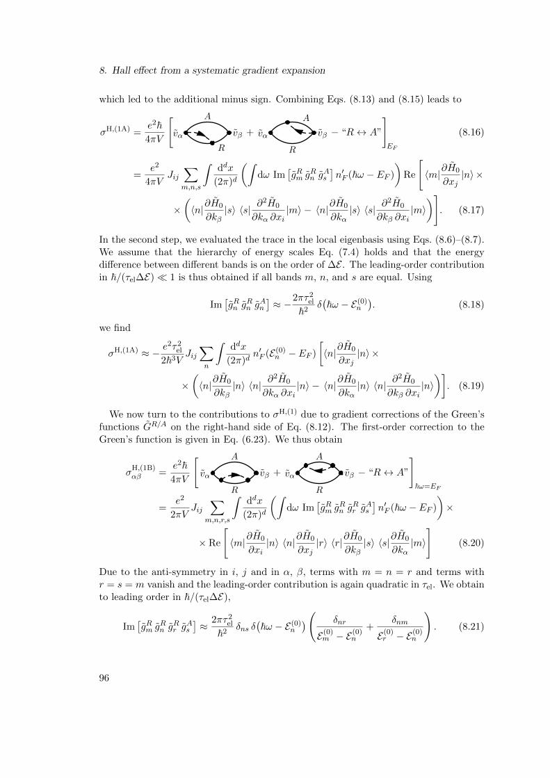
8. Hall effect from a systematic gradient expansion
which led to the additional minus sign. Combining Eqs. (8.13) and (8.15) leads to
σH,(1A) =e2~4πV
[R
A
vα vβ +
R
A
vα vβ − “R↔ A”
]EF
(8.16)
=e2
4πVJij
∑m,n,s
∫ddx
(2π)d
(∫dω Im
[gRm g
Rn g
As
]n′F (~ω − EF )
)Re
[〈m|∂H0
∂xj|n〉×
×(〈n|∂H0
∂kβ|s〉 〈s| ∂
2H0
∂kα ∂xi|m〉 − 〈n|∂H0
∂kα|s〉 〈s| ∂
2H0
∂kβ ∂xi|m〉)]
. (8.17)
In the second step, we evaluated the trace in the local eigenbasis using Eqs. (8.6)–(8.7).We assume that the hierarchy of energy scales Eq. (7.4) holds and that the energydifference between different bands is on the order of ∆E . The leading-order contributionin ~/(τel∆E) 1 is thus obtained if all bands m, n, and s are equal. Using
Im[gRn g
Rn g
An
]≈ −
2πτ2el
~2δ(~ω − E(0)
n
). (8.18)
we find
σH,(1A) ≈ −e2τ2
el
2~3VJij∑n
∫ddx
(2π)dn′F (E(0)
n − EF )
[〈n|∂H0
∂xj|n〉×
×(〈n|∂H0
∂kβ|n〉 〈n| ∂
2H0
∂kα ∂xi|n〉 − 〈n|∂H0
∂kα|n〉 〈n| ∂
2H0
∂kβ ∂xi|n〉)]. (8.19)
We now turn to the contributions to σH,(1) due to gradient corrections of the Green’sfunctions GR/A on the right-hand side of Eq. (8.12). The first-order correction to theGreen’s function is given in Eq. (6.23). We thus obtain
σH,(1B)αβ =
e2~4πV
[R
A
vα vβ +
R
A
vα vβ − “R↔ A”
]~ω=EF
=e2
2πVJij
∑m,n,r,s
∫ddx
(2π)d
(∫dω Im
[gRm g
Rn g
Rr g
As
]n′F (~ω − EF )
)×
× Re
[〈m|∂H0
∂xi|n〉 〈n|∂H0
∂xj|r〉 〈r|∂H0
∂kβ|s〉 〈s|∂H0
∂kα|m〉
](8.20)
Due to the anti-symmetry in i, j and in α, β, terms with m = n = r and terms withr = s = m vanish and the leading-order contribution is again quadratic in τel. We obtainto leading order in ~/(τel∆E),
Im[gRm g
Rn g
Rr g
As
]≈
2πτ2el
~2δns δ
(~ω − E(0)
n
)( δnr
E(0)m − E(0)
n
+δnm
E(0)r − E(0)
n
). (8.21)
96
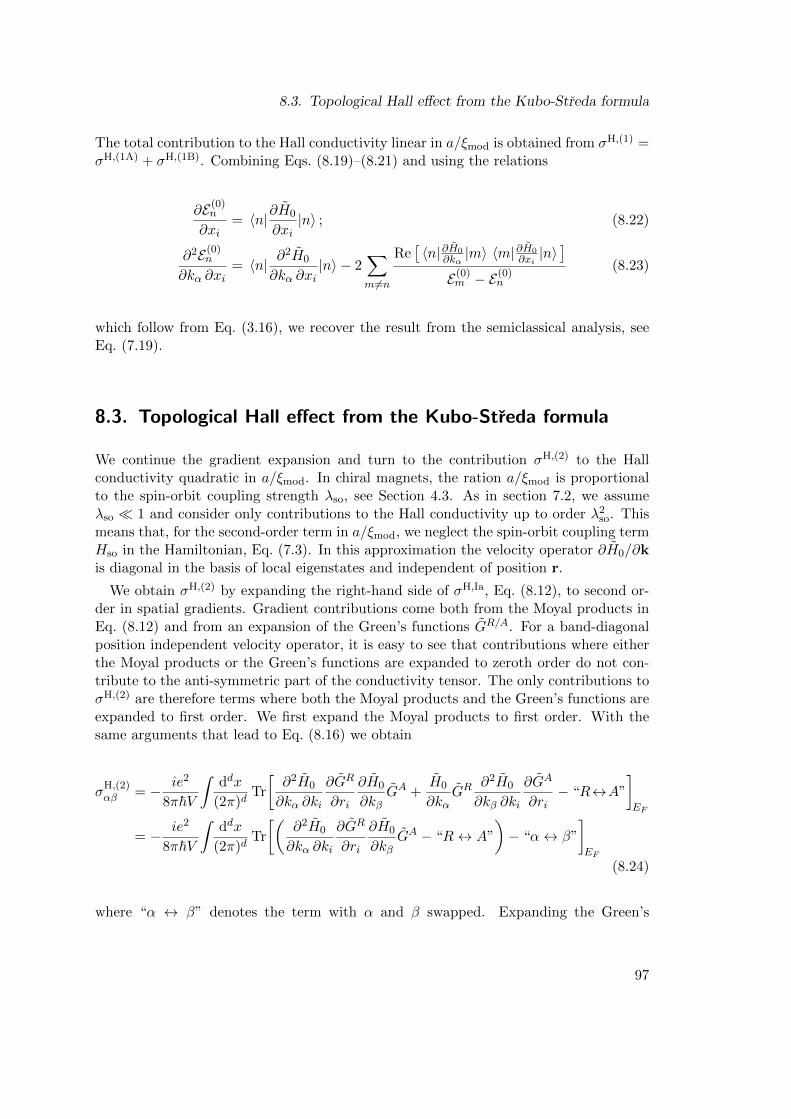
8.3. Topological Hall effect from the Kubo-Streda formula
The total contribution to the Hall conductivity linear in a/ξmod is obtained from σH,(1) =σH,(1A) + σH,(1B). Combining Eqs. (8.19)–(8.21) and using the relations
∂E(0)n
∂xi= 〈n|∂H0
∂xi|n〉 ; (8.22)
∂2E(0)n
∂kα ∂xi= 〈n| ∂
2H0
∂kα ∂xi|n〉 − 2
∑m 6=n
Re[〈n|∂H0
∂kα|m〉 〈m|∂H0
∂xi|n〉]
E(0)m − E(0)
n
(8.23)
which follow from Eq. (3.16), we recover the result from the semiclassical analysis, seeEq. (7.19).
8.3. Topological Hall effect from the Kubo-Streda formula
We continue the gradient expansion and turn to the contribution σH,(2) to the Hallconductivity quadratic in a/ξmod. In chiral magnets, the ration a/ξmod is proportionalto the spin-orbit coupling strength λso, see Section 4.3. As in section 7.2, we assumeλso 1 and consider only contributions to the Hall conductivity up to order λ2
so. Thismeans that, for the second-order term in a/ξmod, we neglect the spin-orbit coupling termHso in the Hamiltonian, Eq. (7.3). In this approximation the velocity operator ∂H0/∂kis diagonal in the basis of local eigenstates and independent of position r.
We obtain σH,(2) by expanding the right-hand side of σH,Ia, Eq. (8.12), to second or-der in spatial gradients. Gradient contributions come both from the Moyal products inEq. (8.12) and from an expansion of the Green’s functions GR/A. For a band-diagonalposition independent velocity operator, it is easy to see that contributions where eitherthe Moyal products or the Green’s functions are expanded to zeroth order do not con-tribute to the anti-symmetric part of the conductivity tensor. The only contributions toσH,(2) are therefore terms where both the Moyal products and the Green’s functions areexpanded to first order. We first expand the Moyal products to first order. With thesame arguments that lead to Eq. (8.16) we obtain
σH,(2)αβ = − ie2
8π~V
∫ddx
(2π)dTr
[∂2H0
∂kα ∂ki
∂GR
∂ri
∂H0
∂kβGA +
H0
∂kαGR
∂2H0
∂kβ ∂ki
∂GA
∂ri− “R↔A”
]EF
= − ie2
8π~V
∫ddx
(2π)dTr
[(∂2H0
∂kα ∂ki
∂GR
∂ri
∂H0
∂kβGA − “R↔ A”
)− “α↔ β”
]EF
(8.24)
where “α ↔ β” denotes the term with α and β swapped. Expanding the Green’s
97
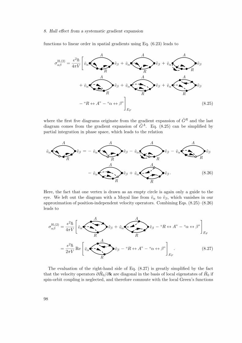
8. Hall effect from a systematic gradient expansion
functions to linear order in spatial gradients using Eq. (6.23) leads to
σH,(2)αβ =
e2~4πV
[R
A
vα vβ +
R
A
vα vβ +
R
A
vα vβ
+
R
A
vα vβ +
R
A
vα vβ +
R
A
vα vβ
− “R↔ A”− “α↔ β”
]EF
(8.25)
where the first five diagrams originate from the gradient expansion of GR and the lastdiagram comes from the gradient expansion of GA. Eq. (8.25) can be simplified bypartial integration in phase space, which leads to the relation
R
A
vα vβ = −
R
A
vα vβ −
R
A
vα vβ −R
A
vα vβ
−
R
A
vα vβ +
R
A
vα vβ . (8.26)
Here, the fact that one vertex is drawn as an empty circle is again only a guide to theeye. We left out the diagram with a Moyal line from vα to vβ, which vanishes in ourapproximation of position-independent velocity operators. Combining Eqs. (8.25)–(8.26)leads to
σH,(2)αβ =
e2~4πV
[R
A
vα vβ +
R
A
vα vβ − “R↔ A”− “α↔ β”
]EF
=e2~2πV
Re
[R
A
vα vβ − “R↔ A”− “α↔ β”
]EF
. (8.27)
The evaluation of the right-hand side of Eq. (8.27) is greatly simplified by the factthat the velocity operators ∂H0/∂k are diagonal in the basis of local eigenstates of H0 ifspin-orbit coupling is neglected, and therefore commute with the local Green’s functions
98
8.4. Discussion
gR/A. We obtain
σH,(2)αβ = −e
2~2
2πV
∑m,n
∫ddx
(2π)d
(∫dω Im
[gRm g
Am
(gRn)2gAn]n′F (~ω − EF )
)×
× vn,i vn,α∂2E(0)
m
∂kj ∂kβIm
[〈n|∂H0
∂ri|m〉 〈m|∂H0
∂rj|n〉]− “α↔ β”. (8.28)
For terms with m = n, the last factor Im[· · · ] vanishes. For m 6= n, we find in the limitof small ~/(τel∆E),
Im[gRm g
Am
(gRn)2gAn]
=1
2igRm g
Am g
Rn g
An
(gRn − gAn
)= −
2πτ2el/~2(
E(0)n − E(1)
m
)2 δ(~ω − E(0)n
)(8.29)
which leads to
σH,(2)αβ =
e2τ2el~V
∑n
∑m6=n
∫ddx
(2π)dn′F(E(0)n − EF
)vn,i
(vn,α
∂2E(0)m
∂kj ∂kβ− vn,β
∂2E(0)m
∂kj ∂kα
)×
× Im
〈n|∂H0∂ri|m〉 〈m|∂H0
∂rj|n〉(
E(0)n − E(1)
m
)2 . (8.30)
Eq. (8.30) is a general expression for the topological Hall effect if spin-orbit coupling isneglected, and it is the main result of this chapter. A comparison to the semiclassicalformula Eq. (7.21) follows in the next section.
8.4. Discussion
In this chapter, we derived the Hall conductivity in chiral magnets based on a system-atic gradient expansion of the Kubo formula. In addition to the well-known anomalousand topological Hall effect, we obtain a contribution σH,(1), Eq. (7.19), linear in spa-tial derivatives, which occurs only in the presence of both spin-orbit interaction andan inhomogeneous magnetization texture. The existence of σH,(1) is confirmed by thesemiclassical calculation in Section 7.2.
To second order in the spatial gradients, the Hall conductivity is given by Eq. (8.30).
For a model with only a single orbital band, the terms ∂2E(0)σ /∂kα∂ki and ∂2E(0)
σ /∂kβ∂kiare independent of the spin σ in absence of spin-orbit coupling, and we can identify theposition-space Berry curvature using Eq. (3.18). In this case, we obtain
σH,(2)αβ = −
e2τ2el
2~V∑σ=↓/↑
∫ddx
(2π)dΩr,rσ,ij vi
(vα
∂2E(0)
∂kj ∂kβ− vβ
∂2E(0)
∂kj ∂kα
)n′F(E(0)σ − EF
)(8.31)
in agreement with our result from the semiclassical calculation, see Eq. (7.21). For anisotropic quadratic dispersion the term in the brace is given by ~2(vαδjβ − vβδjα)/m∗
99
8. Hall effect from a systematic gradient expansion
and Eq. (8.31) simplifies to Eq. (7.23), which is more commonly used to describe thetopological Hall effect. We thus identify the diagram on the right-hand side of Eq. (8.27)as the term responsible for the topological Hall effect in a perturbative expansion ina/ξmod 1 for chiral magnets with weak spin-orbit coupling.
If more than one orbital band participates in the coupling to the effective exchangefield, then Eq. (8.30) suggests that the effective electron mass in the empty bands shouldalso play a role. Physically, the diagram on the right-hand side of Eq. (8.27) sums upamplitudes of virtual transitions from occupied bands n into empty bands m and back.If no additional physical process happens while the electron is in band m, then theamplitude of such a virtual transition can be expressed in terms of the Berry curvatureΩn, see discussion below Eq. (3.18). Here, Ωn may be regarded as a property of theoccupied band n in the sense that it can be calculated from the Bloch states in bandn only. Thus, the system can in this case be described in a semiclassical picture wherethe physics in each band is treated in isolation. The equivalence between the Berrycurvature and the amplitude of a virtual transition is what allowed us to identify the zero-order Hall conductivity σH,(0), Eq. (8.8), with the anomalous Hall conductivity σAHE,int,Eq. (7.16). Eq. (8.30), however, goes slightly beyond the semiclassical approximation
by including additional mass operators ∂2E(0)m /∂kj∂kβ and ∂2E(0)
m /∂kj∂kα during thevirtual transition. This effect has no precise semiclassical counterpart.
100
Part III.
Dynamics of rigid skyrmions in thepresence of spin-orbit coupling
101

9. Theories of magnetization dynamics
The discovery of the giant magnetoresistance (GMR) effect by Grunberg and Fert[124, 125] demonstrated that electrical currents can be efficiently manipulated by tinymagnetic structures. The GMR effect is widely used in computer hard disks today.Nowadays, one of the main goals in the field of spintronics is the reverse mechanism:the controlled manipulation of magnetic structures with currents and electric fields.There are strong indications that this goal can be achieved with so-called spin-transfertorques [126,127], a mechanism by which angular momentum is transferred from conduc-tion electrons to the magnetization texture. Parkin and collaborators demonstrated [128]that spin-transfer torques could find use in future devices for data storage. In their pro-totype of a so-called racetrack memory, data is stored as a pattern of magnetic domainwalls on a wire, similar to the way data is stored on magnetic tapes. In contrast totraditional magnetic tapes, however, it is not the wire itself that is moved around whenthe data is accessed. Instead, one pushes the domain-wall pattern along the wire by driv-ing an electric current through the system, using the principle of spin-transfer torques.Recently, skyrmions have become increasingly popular as candidate alternatives for do-main walls in race-track type memories [39]. Due to the smooth magnetization textureand the rigidness of skyrmions, pinning forces on skyrmions are weak and the currentdensities required to move skyrmions are around a factor of 105 lower than in the caseof domain-walls [12].
In this part of the thesis we focus on the influence of phase-space Berry phases on thedynamics of skyrmions in an externally applied electric field. In particular, we addressthe question of how the electric charge of skyrmions discussed in Chapters 5 and 6couples to an external electric field. This chapter is an introduction to the topic. Weprovide an overview of the most common theoretical models for magnetization dynamicsin Section 9.1. In Section 9.2 we give a brief outline of the open questions that weaddress in Chapters 10 and Chapter 11.
9.1. The Landau-Lifshitz-Gilbert equation and the ThieleEquation
The coupling of a spin S to a magnetic field B is described by the Hamiltonian
H = −γB · S. (9.1)
Here, the gyromagnetic ratio γ is the ratio between the spin expectation value and themagnetic moment m = γ 〈S〉. For a single electron, γ = −ge/(2m) < 0 follows from theDirac equation in the non-relativistic limit, where the electron has electric charge −e,
103
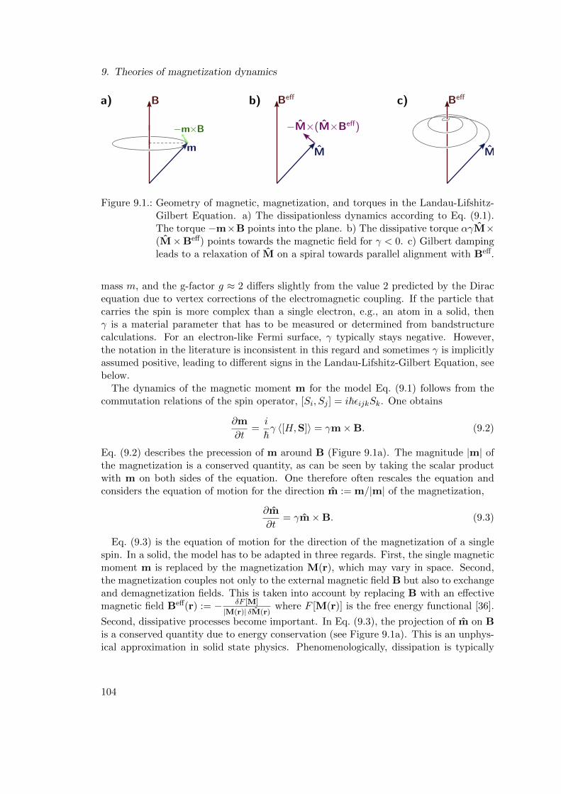
9. Theories of magnetization dynamics
Figure 9.1.: Geometry of magnetic, magnetization, and torques in the Landau-Lifshitz-Gilbert Equation. a) The dissipationless dynamics according to Eq. (9.1).The torque −m×B points into the plane. b) The dissipative torque αγM×(M×Beff) points towards the magnetic field for γ < 0. c) Gilbert dampingleads to a relaxation of M on a spiral towards parallel alignment with Beff.
mass m, and the g-factor g ≈ 2 differs slightly from the value 2 predicted by the Diracequation due to vertex corrections of the electromagnetic coupling. If the particle thatcarries the spin is more complex than a single electron, e.g., an atom in a solid, thenγ is a material parameter that has to be measured or determined from bandstructurecalculations. For an electron-like Fermi surface, γ typically stays negative. However,the notation in the literature is inconsistent in this regard and sometimes γ is implicitlyassumed positive, leading to different signs in the Landau-Lifshitz-Gilbert Equation, seebelow.
The dynamics of the magnetic moment m for the model Eq. (9.1) follows from thecommutation relations of the spin operator, [Si, Sj ] = i~εijkSk. One obtains
∂m
∂t=i
~γ 〈[H,S]〉 = γm×B. (9.2)
Eq. (9.2) describes the precession of m around B (Figure 9.1a). The magnitude |m| ofthe magnetization is a conserved quantity, as can be seen by taking the scalar productwith m on both sides of the equation. One therefore often rescales the equation andconsiders the equation of motion for the direction m := m/|m| of the magnetization,
∂m
∂t= γm×B. (9.3)
Eq. (9.3) is the equation of motion for the direction of the magnetization of a singlespin. In a solid, the model has to be adapted in three regards. First, the single magneticmoment m is replaced by the magnetization M(r), which may vary in space. Second,the magnetization couples not only to the external magnetic field B but also to exchangeand demagnetization fields. This is taken into account by replacing B with an effectivemagnetic field Beff(r) := − δF [M]
|M(r)| δM(r)where F [M(r)] is the free energy functional [36].
Second, dissipative processes become important. In Eq. (9.3), the projection of m on Bis a conserved quantity due to energy conservation (see Figure 9.1a). This is an unphys-ical approximation in solid state physics. Phenomenologically, dissipation is typically
104
9.1. The Landau-Lifshitz-Gilbert equation and the Thiele Equation
described by adding a torque T = αγM× (M×Beff) to the right-hand side of Eq. (9.3).This term was introduced by Landau and Lifshitz in Ref. [129]. The dimensionless pa-rameter α is known today as the Gilbert damping parameter. For α > 0 and γ < 0, thetorque points towards the direction of Beff (Figure 9.1b), as required for a relaxationprocess. For γ > 0 the torque points in the opposite direction, consistent with the factthat the energy is minimized in this case by anti-parallel alignment of M and Beff. Theresulting equation of motion for m with damping is usually written in the form of theLandau-Lifshitz-Gilbert (LLG) Equation [130]. In the absence of currents, it is given by
∂M
∂t= γ′ M×Beff + αM× ∂M
∂t(9.4)
where γ′ = (1 + α)γ is a renormalized gyromagnetic ratio. We will drop the primeon γ in the following and always consider the renormalized gyromagnetic ratio. As aconsequence of the damping term the magnetization direction moves on a spiral towardsparallel alignment with Beff on the time scale 1/(α|γBeff|) (Figure 9.1c).
It has proven difficult to calculate α from microscopic theories due to the fact thatany processes that does not conserve the electronic spin can contribute to α. The micro-scopic origin of Gilbert damping was discussed in Refs. [131–134]. Generally, a changeof the magnetization is accompanied by a small deformation of the Fermi surface dueto spin-orbit coupling [135,136]. This deformation brings the system out of equilibriumand is therefore followed by relaxation processes during which phonons or magnons areemitted. In numerical calculations from ab-initio [136, 137], inter-band transitions havebeen identified as the dominant process contributing to Gilbert damping. Experimen-tally, the value of α can be determined from the line-width of the ferromagnetic reso-nance [138,139]. Typical values lie in the range of α = 10−3 . . . 10−1. The LLG Equationis the basis of powerful micromagnetic simulation codes that integrate Eq. (9.4) numer-ically over time on a lattice [140]. Simulations with an additional stochastic torque dueto thermal noise were presented in Ref. [35]. If only the final magnetization profile inthe ground state or in a metastable state is of interest, then often values of α that arelarger than the actual material parameters are used to speed up the calculations.
In metals, a spin current couples to the magnetization via spin-transfer torques [126,127]. When conduction electrons traverse a smooth magnetic texture, a torque is exertedon their spin that causes the spin to follow the background magnetization. Since thetotal angular momentum is conserved (unless it is passed to the crystal), there has to bean opposite counter-torque on the magnetization [126, 141]. This counter-torque leadsto both dissipative and non-dissipative effects. Phenomenologically, the effects of spin-transfer torques are described by the LLG Equation with two additional terms [142],
(∂t + vs ·∇) M = γM×Beff + αM×(∂t +
β
αvs ·∇
)M. (9.5)
Here, vs is an effective spin velocity and β is sometimes called the non-adiabatic dampingparameter. The term on the left-hand side of Eq. (9.5) is the total time derivative of themagnetization direction in the co-moving frame. For β = α the total time derivative also
105
9. Theories of magnetization dynamics
appears in the Gilbert damping term on the right-hand side. This is only the correctdamping term in a Galileo-invariant system. In a solid the crystal potential breaksGalileo invariance and β 6= α. However, the two damping parameters are usually on thesame order of magnitude. Derivations of the value of β from microscopic models can befound in Refs. [131, 134]. It can be measured by observing the motion of domain wallsgenerated by an applied current [143].
Eq. (9.5) is the standard form of the LLG Equation. The dissipative torques propor-tional to α and β are phenomenological terms based on symmetry arguments. It waspointed out in Refs. [36, 62, 133] that an additional dissipative term is allowed due tospin-orbit coupling. It is described by adding the torque
− α′[M ·
(∂iM×
(∂t +
β′
α′vs ·∇
)M
)]∂iM (9.6)
to the right-hand side of Eq. (9.5). Physically Eq. (9.6) describes the effect that thechange of magnetization generates a current due to spin-orbit coupling, which leads toohmic friction [36].
The LLG Equation is an equation of motion for the field M(r). In absence of cur-rents, vs = 0, it describes precessing magnetic moments that ultimately relax to a localminimum of the free energy due to the Gilbert damping α. In chiral magnets, singleskyrmions exist as metastable states of the magnetization texture [144]. A finite current,related to vs 6= 0 drives the magnetization texture out of its static configuration. It turnsout that for low current densities, deformations of the magnetic texture are weak andthe current couples mainly to the translational mode of the magnetization texture [36].The magnetization texture is thus described by a M(t, r) = M0(r−R(t)) where M0(r)is a time-independent function of position, for example a domain wall or a skyrmion,and R(t) is the trajectory of the magnetic texture. Following Refs. [11,36], an equationof motion for R(t) can be obtained from the LLG Equation by multiplying both sideswith ∂iM and integrating over space. In Ref. [36], the resulting equation of motion isgiven in the form of a balance of forces,
G× (vs − R) + D(βvs − αR) + Fpin = 0 (9.7)
with
G =
∫d2rM(r) Bem(r); (9.8)
Dij =
∫d2rM(r) (∂iM(r)) · (∂jM(r)); (9.9)
D′ =∫
d2rM(r) |Bem(r)|2; (9.10)
α = α+ α′D′/D; (9.11)
β = β + β′D′/D. (9.12)
Here, Bem is the emergent magnetic field due to a non-coplanar magnetization texture,see Section 4.1, and Fpin is a pinning force due to disorder. Eq. (9.7) is known as the
106
9.2. Open questions
Thiele equation. The first term on the left-hand side describes a gyro-coupling of theskyrmion velocity and the effective spin velocity to applied forces, and the remainingtwo terms are forces related to dissipation and pinning, respectively. The gyro-couplingvector G is proportional to the topological winding number of the magnetization texture.Therefore, skyrmions, which have a non-trivial winding number, couple efficiently toforces and external currents. According to Eq. (9.7), a current vs 6= 0 or an appliedforce directly generate a non-zero skyrmion velocity R without retardation. This is aconsequence of the fact that only the translational mode was considered in the derivationof Eq. (9.7). Excitations of the magnetization texture, not taken into account by theThiele Equation, can lead to a finite memory of the system. In Ref. [38], the authorsfound that, while the retardation can be large if the magnetization texture is driven bytime-dependent magnetic fields, it is usually negligible in current-driven systems.
9.2. Open questions
The LLG Equation, Eq. (9.5), and the Thiele Equation, Eq. (9.7) have been successfullyemployed to model the magnetization dynamics of chiral magnets. Their derivation is,however, of mainly phenomenological nature based on symmetry arguments. In particu-lar, while the gyro-coupling term in the Thiele Equation is clearly related to Berry phasesin position space, other Berry phase effects in phase space are only taken into accountin the prefactors of the dissipative terms. There are two reasons why Berry phases inphase space can be expected to lead to non-dissipative forces on skyrmions. First, theBerry curvature Ωr,k
n in mixed position/momentum space leads to a renormalization ofthe force on Bloch electrons in presence of an electric field, see Eq. (5.20) in Section 5.1.Due to momentum conservation, one should expect a counter-force on the magnetizationtexture. Second, as discussed in Chapters 5 and 6, skyrmions carry an electric chargerelated to a Berry-phase correction to the density of states in phase space. It is thereforea natural question to ask whether the skyrmion charge couples to an external electricfield. In Chapter 10, we derive an equation of motion for skyrmions in the presence ofphase-space Berry phases. We present results for metals and insulators in Chapter 11.
107

10. Derivation of the equation of motionfor skyrmions
In this chapter, we derive a formal equation of motion for the translational mode of asingle rigid skyrmion in presence of an electric field, taking into account all Berry phasesin phase space. The resulting equation is given by a balance of forces, Ftot = 0, wherethe total force will turn out to be given by
F toti =
∑n
∫ddr
∫ddk
(2π)d
[(1− Ωr,k
n,jj)∂En∂ri− Ωr,r
n,ij
(∂En∂kj− ~Rj
)+ Ωr,k
n,ij
(∂En∂rj
+ eEj
)]¯nn. (10.1)
Here, Ωr,rn and Ωr,k
n are the Berry curvature in position space and in mixed position/mo-mentum space, respectively. Further n labels an eigenstate of a diagonalized Hamiltonianthat is adiabatically connected to a Bloch band n, r and k are kinetic phase-spacecoordinates, and En(r, k) is the semiclassical energy that contains the gradient correctionδE(1), see Eq. (5.14). In Chapter 11, we will evaluate Eq. (10.1) in the case of a metaland an insulator.
10.1. Model and outline of the derivation
We consider a magnetic material with a rigid magnetization texture
M(t, r) = M0(r−R(t)) (10.2)
where M0 is a known function of position that describes a single skyrmion in a ferro-magnetic background (see, e.g., Ref. [144]), and R(t) is the trajectory of the skyrmioncenter. The goal of this chapter is to derive an equation of motion for R(t) in a disorderedmagnetic metal in presence of an electric field.
Hamiltonian. We model the electronic properties by the Hamiltonian
H(t) = Hlatt(t) +HM (t) + Vdis(r). (10.3)
where Hlatt is the lattice-periodic part of the Hamiltonian, HM describes the couplingto the smooth background magnetization, and Vdis is a random disorder potential. We
109
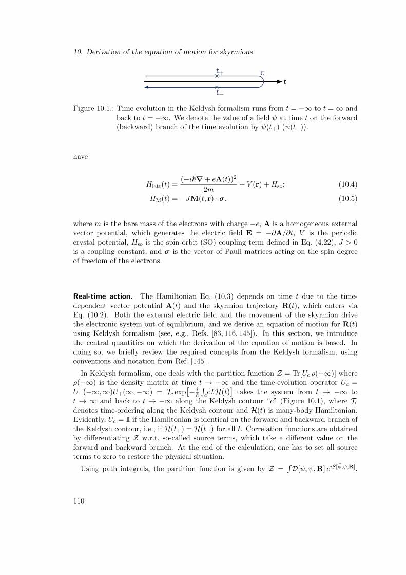
10. Derivation of the equation of motion for skyrmions
Figure 10.1.: Time evolution in the Keldysh formalism runs from t = −∞ to t =∞ andback to t = −∞. We denote the value of a field ψ at time t on the forward(backward) branch of the time evolution by ψ(t+) (ψ(t−)).
have
Hlatt(t) =(−i~∇ + eA(t))2
2m+ V (r) +Hso; (10.4)
HM(t) = −JM(t, r) · σ. (10.5)
where m is the bare mass of the electrons with charge −e, A is a homogeneous externalvector potential, which generates the electric field E = −∂A/∂t, V is the periodiccrystal potential, Hso is the spin-orbit (SO) coupling term defined in Eq. (4.22), J > 0is a coupling constant, and σ is the vector of Pauli matrices acting on the spin degreeof freedom of the electrons.
Real-time action. The Hamiltonian Eq. (10.3) depends on time t due to the time-dependent vector potential A(t) and the skyrmion trajectory R(t), which enters viaEq. (10.2). Both the external electric field and the movement of the skyrmion drivethe electronic system out of equilibrium, and we derive an equation of motion for R(t)using Keldysh formalism (see, e.g., Refs. [83, 116, 145]). In this section, we introducethe central quantities on which the derivation of the equation of motion is based. Indoing so, we briefly review the required concepts from the Keldysh formalism, usingconventions and notation from Ref. [145].
In Keldysh formalism, one deals with the partition function Z = Tr[Uc ρ(−∞)] whereρ(−∞) is the density matrix at time t → −∞ and the time-evolution operator Uc =U−(−∞,∞)U+(∞,−∞) = Tc exp
[− i
~∫cdtH(t)
]takes the system from t → −∞ to
t → ∞ and back to t → −∞ along the Keldysh contour “c” (Figure 10.1), where Tcdenotes time-ordering along the Keldysh contour and H(t) is many-body Hamiltonian.Evidently, Uc = 1 if the Hamiltonian is identical on the forward and backward branch ofthe Keldysh contour, i.e., if H(t+) = H(t−) for all t. Correlation functions are obtainedby differentiating Z w.r.t. so-called source terms, which take a different value on theforward and backward branch. At the end of the calculation, one has to set all sourceterms to zero to restore the physical situation.
Using path integrals, the partition function is given by Z =∫D[ψ, ψ,R] eiS[ψ,ψ,R],
110
10.1. Model and outline of the derivation
where the real-time action S for our model, Eqs. (10.2)–(10.5), is given by
S[ψ, ψ,R] =
∫c
dt L[ψ(t), ψ(t),R(t)]
=
∞∫−∞
dt L[ψ(t+), ψ(t+),R(t+)] +
−∞∫∞
dt L[ψ(t−), ψ(t−),R(t−)]. (10.6)
Here, ψ ≡ (ψ↑, ψ↓) and ψ ≡ (ψ↑, ψ↓)T are spinors of Graßmann fields, the time integral
runs along the Keldysh contour (Figure 10.1), t+ (t−) denotes that the correspondingGraßmann field is evaluated on the forward (backward) part of the Keldysh contour,and the Lagrangian is given by
L[ψ(t), ψ(t),R(t)] =
∫ddr ψ(t, r) (i~∂t −H(t))ψ(t, r). (10.7)
We apply the usual Keldysh rotation for fermionic systems [145],
ψ1(t, r) :=1√2
(ψ(t+, r) + ψ(t−, r)); ψ2(t, r) :=1√2
(ψ(t+, r)− ψ(t−, r));
ψ1(t, r) :=1√2
(ψ(t+, r)− ψ(t−, r)
); ψ2(t, r):=
1√2
(ψ(t+, r) + ψ(t−, r)), (10.8)
which leads to
S[ψ, ψ,R] =
∞∫−∞
dt1
∞∫−∞
dt2
∫ddr1
∫ddr2 ψα(t1, r1) g−1
αβ (t1, r1; t2, r2)ψβ(t2, r2) (10.9)
where summation over repeated Keldysh indices α, β ∈ 1, 2 is implied and the localinverse Green’s function is given by
g−1αβ =
((gR)−1 (
g−1)K
0(gA)−1
)αβ
. (10.10)
Here, R, A, and K denote the retarded, advanced, and Keldysh part, respectively. Thelatter is an infinitesimal regularization term that encodes the initial state at t → −∞,while the former two are given by(
gR)−1
= g−10 + δ(t1 − t2)δ(r1 − r2)(Vdis(r1) + i0+); (10.11)(
gA)−1
= g−10 + δ(t1 − t2)δ(r1 − r2)(Vdis(r1)− i0+) (10.12)
where 0+ is an infinitesimal positive number and the disorder-free part of the inverseGreen’s function is
g−10 (t1, r1; t2, r2) = i~δ′(t1 − t2)δ(r1 − r2)− δ(t1 − t2)δ(r1 − r2)H(t2) (10.13)
where δ′ is the derivative of the delta distribution, defined by∫
dx δ′(x)f(x) := −f ′(0),and H(t2) is understood to act as a differential operator on ψβ(t2, r2) in Eq. (10.9).
111
10. Derivation of the equation of motion for skyrmions
Formal equation of motion. We obtain an effective action Seff[R] for the skyrmiontrajectory R(t) from Eq. (10.6) by integrating out the fermionic fields,
Seff[R] = −i log
[∫D[ψ, ψ] e
i~S[ψ,ψ,R]
]= −i log
[∫D[ψ, ψ] e
i~∫∞−∞dt L++ i
~∫−∞∞ dt L−
](10.14)
where L+ (L−) denotes the Lagrangian, Eq. (10.7), evaluated on the forward (backward)part of the Keldysh contour. We parameterize the skyrmion trajectory R(t) by a classicaland a quantum component (cf., Ref. [145]),
R(t+) = Rcl(t) + Rq(t) and R(t−) = Rcl(t)−Rq(t). (10.15)
The solution of the classical equation of motion is a stationary point of Seff[R] and isidentical on the forward and backward part of the time contour. The latter condition isequivalent to Rq(t) = 0 for all t. To find the stationary solution, one has to solve thesaddle point equations δSeff/δR
cl(t) = 0 and δSeff/δRq(t) = 0. The former is trivially
satisfied since Seff[R] = 0 as long as the quantum component Rq(t) vanishes for all t,because the forward and backward parts on the right-hand side of Eq. (10.14) cancel fora purely classical trajectory. Thus, the saddle point equation for the classical skyrmiontrajectory R(t) is
δSeff[R]
δRq(t)
∣∣∣∣Rq=0
= 0. (10.16)
Inserting the Hamiltonian Eqs. (10.3)–(10.5), the Lagrangian Eq. (10.7), and the Keldyshrotation Eq. (10.8), we find
1
Z[R]
∫ddr tr
[∂H(t)
∂R(t)
∫D[ψ, ψ] e
i~S[ψ,ψ,R]
(ψ2(t, r)ψ1(t, r) + ψ1(t, r)ψ2(t, r)
)]= 0
(10.17)where HM is evaluated at position r, the trace tr[· · ·] runs over the spin configurations,and Z[R] =
∫D[ψ, ψ] eiS[ψ,ψ,R] = 1 is the partition function, which is equal to 1 for a
classical trajectory R(t) [145]. The left-hand side of Eq. (10.17) is a two-point correlationfunction. We denote by G the disorder-averaged Green’s function,
Gαβ(t1, r1; t2, r2) := − i~
⟨∫D[ψ, ψ] e
i~S[ψ,ψ,R] ψα(t1, r1)ψβ(t2, r2)
⟩dis
=
(GR GK
0 GA
)αβ
(10.18)where 〈· · ·〉dis denotes averaging over all disorer configurations and α, β ∈ 1, 2 areKeldysh indices. The last equality in Eq. (10.18) defines the retarded (GR), advanced(GA), and Keldysh (GK) component, as is customary, and the lower left componentvanishes due to causality [145]. By averaging Eq. (10.17) over all disorder configurations,we obtain the formal equation of motion for the skyrmion trajectory,
Ftot(t) :=i~2
∫ddr tr
[∂H(t)
∂R(t)GK(t, r; t, r)
]= 0 (10.19)
112
10.1. Model and outline of the derivation
where we included a prefactor of i~2 in anticipation of the interpretation of Ftot as the
sum of all forces on the skyrmion, which have to balance, see below. The aim of thischapter is to obtain an explicit expression for Ftot(t). To this end, we will transform intoa basis in which the Keldysh Green’s function GK is diagonal in band space, see Section10.2 below. In a time-dependent system, the Green’s function does, in general, notcommute with the single-particle Hamiltonian H(t) and thus the basis that diagonalizesGK does not necessarily diagonalize H(t). Using Eq. (10.13), we can express Ftot(t) interms of only the Green’s function and the inverse Green’s function,
Ftot(t) = − i~2
∫ddr
∫ddr′
∫dt′ tr
[∂g−1
0 (t, r; t′, r′)
∂R(t)GK(t′, r′; t, r)
]≡ − i~
2
∫ddr tr
[(∂g−1
0
∂R(t)⊗GK
)(t, r; t, r)
](10.20)
where, in the second step, we introduced the notation “⊗”, which denotes convolutionin position, time, and spin space.
Dyson Equation. The disorder-averaged Keldysh Green’s function GK in Eq. (10.20)is obtained from the Dyson equation,(
g−10 − ΣR −ΣK
0 g−10 − ΣA
)⊗(GR GK
0 GA
)= 1 (10.21)
where Σ is the self-energy, which encodes disorder, and 1 is the identity in the space of allparameters, i.e., position, time, spin, and Keldysh space. With the usual parametrizationof the Keldysh Green’s function
GK = GR ⊗ f − f ⊗GA (10.22)
in terms of a hermitian distribution function f(t1, r1; t2, r2), the upper-right componentof Eq. (10.21) can be written as a formal transport equation (cf., [145])
f ⊗ g−10 − g
−10 ⊗ f = ΣK −
(ΣR ⊗ f − f ⊗ ΣA
)(10.23)
and the retarded and advanced Green’s functions are obtained from the diagonal partsof Eq. (10.21),
(g−10 − ΣR/A)⊗GR/A = 1. (10.24)
Outline of the remaining derivation. In this section, we derived a formal equation ofmotion Ftot = 0 for the skyrmion, where Ftot is given by Eq. (10.20). The skyrmion tra-jectory R(t) enters in the equation of motion indirectly via the Keldysh Green’s functionGK , which is given by Eq. (10.22), where f and GR/A are the solutions of Eqs. (10.23)and (10.24), respectively. In the remaining sections of this chapter we derive a generalexpression for Ftot that depends explicitly on the skyrmion velocity R. The derivationis organized as follows. In Section 10.2, we review a method from Ref. [84] to pertur-batively diagonalize the inverse Green’s function. We apply this methods first to the
113
10. Derivation of the equation of motion for skyrmions
transport equation Eq. (10.23) in order to obtain the distribution function f (Section10.3). It turns out that, in order to account for local particle number conservation, aposition-dependent chemical potential has to be introduced. In Section 10.4, we ap-ply the perturbative band-diagonalization to the expression for the total force on theskyrmion.
10.2. Wigner transform and diagonalized local Green’s function
Wigner transform in space and time. The Hamiltonian Eq. (10.3) contains a lattice-periodic part Hlatt(t), whose instantaneous eigenstates are Bloch states |n, t,k〉 givenby
〈r|n, t,k〉 = eik·run,k+ e~A(t)(r) (10.25)
that satisfy the instantaneous eigenvalue equation
Hlatt(t) |n, t,k〉 = εn
(k +
e
~A(t)
)|n, t,k〉 (10.26)
where n is a band index, the canonical momentum k lies in the 1st Brillouin zone (BZ),un,k+ e
~A(t)(r) is the lattice-periodic part of the Bloch function, and εn(k + e~A(t)) is the
instantaneous eigenenergy of Hlatt(t) for the state with kinetic momentum ~k + eA(t).Here, we chose to label the Bloch states |n, t,k〉 by their canonical lattice momentum~k rather than the kinetic lattice momentum ~k + eA(t). In this way, Eq. (10.25)differs from our definition of Bloch states, Eq. (5.6), that we used for the semiclassicaldescription of Section 5.1. Here, we choose to define the Bloch states in terms of thekinetic momentum in order to avoid an unbounded term −eE ·r in the WT of the inverseGreen’s function, see Eqs. (10.31)–(10.33) below, which would complicate the treatmentof a steady-state electric current in a system with open boundary conditions. With ourchoice of Bloch states, Eq. (10.25), we will be able to treat the influence of the electricfield E = −∂A/∂t within the same gradient expansion that we will also use to deriveBerry-phase effects.
The magnetization M(t, r) in Eq. (10.3) breaks the discrete translation symmetryso that the states |n, t,k〉 are not eigenstates of H(t). Assuming that M varies ona large length scale ξmod a where a is the lattice constant, correlation functionsare most efficiently described in Wigner representation, see Section 6.1. The Wignerrepresentation A(r; k) of an operator A has the advantage that variations on the twolength scales ξmod and a are separated into the dependency on a “central” position rand a “central” wave vector k, respectively. For the non-equilibrium system discussedin this chapter, we define the WT in both position and time domain. Here, position andtime require a different treatment due to the existence of a periodic lattice in positionspace, which lacks a corresponding counterpart in the time domain. We define the WTin the time domain according to Eq. (6.1) and in position domain according to Eq. (6.5),
114
10.2. Wigner transform and diagonalized local Green’s function
so that the WT of a correlation function A(t1, r1; t2, r2) is defined as
Amn(t, r;ω,k) :=
∞∫−∞
dτ
∫ ′ ddq
(2π)d
∫ddr1
∫ddr2 e
iωτ+iq·r×
×⟨m, t+
τ
2,k +
q
2
∣∣∣r1
⟩A(t+
τ
2, r1; t− τ
2, r2
)⟨r2
∣∣∣n, t− τ
2,k− q
2
⟩(10.27)
where the prime on the momentum integral is a reminder that the BZ should be chosensuch that k + q
2 and k− q2 both run over the same integration region, see discussion in
Section 6.1.
Moyal product. For two correlation functions A(t1, r1; t2, r2) and B(t1, r1; t2, r2), theconvolution C = A⊗B is defined by
C(t1, r1; t2, r2) =
∫dt′∫
ddr′A(t1, r1; t′, r′)B(t′, r′; t2, r2). (10.28)
In Wigner representation, the convolution is given by the Moyal product
Cmn(t, r;ω,k) =∑l
Aml(t, r;ω,k) ei2
(←−∂ω−→∂t−←−∂t−→∂ω+←−∂r·−→∂k−←−∂k·−→∂r) Bln(t, r;ω,k)
≡∑l
Aml(t, r;ω,k) ei2Jµν←−∂µ−→∂ν Bln(t, r;ω,k) (10.29)
where we introduced a short-hand notation in the second equality. Here, the derivatives∂µ ≡ (∂t, ∂r, ∂ω, ∂k)µ are in the full space of time, position, frequency, and momentum,and the anti-symmetric matrix J is given by
Jµν =
0 0 −1 00 0 0 1d×d1 0 0 00 −1d×d 0 0
µν
(10.30)
where 1d×d is the d-dimensional identity matrix. In Eq. (10.29), the exponential function
is understood as a formal power series and←−∂ (−→∂ ) denotes a partial derivative that acts
only on the factor to the left (right). We use the symbol “⊗” for Moyal products inboth position/momentum and time/frequency space, while the symbol “” is reservedfor Moyal products in position/momentum space only.
Local inverse Green’s function. We obtain the WT of g−10 from Eqs. (10.13) and
(10.27),
g−10,mn(t, r;ω,k) = ~ωδmn − Hmn(t, r; k) + E(t) · Dmn(t, r; k) (10.31)
115
10. Derivation of the equation of motion for skyrmions
where, in the basis of Eq. (10.25),
Hmn(t, r; k) = δmn εm
(k +
e
~A(t)
)+ HM,mn(t, r; k). (10.32)
Here, HM,mn is the WT of HM, Eq. (10.5), the electric field is E(t) = −∂A(t)/∂t, andDmn(t, r; k) is the WT of the electric dipole operator,
Dmn(t, r; k) = ie
∫ddq
(2π)d
∫ddr′ eiq·(r−r
′) ∂
∂q
[u∗m,k+ e
~A(t)+q2(r′)un,k+ e
~A(t)−q2(r′)]
= −e∫
ddq
(2π)deiq·r
⟨m, t,k +
q
2
∣∣∣(r− r)∣∣∣n, t,k− q
2
⟩(10.33)
where r is the position operator, while r is the position argument of Dmn(t, r; k), andthe subtraction (r − r) leads to a cancellation of unbounded terms that would growproportionally to the size of the sample. The appearance of the position coordinate ron the right-hand side of Eq. (10.33) is a consequence of our choice to label the Blochstates by their canonical momentum ~k, see Eq. (10.25). The fact that the electricdipole energy −E · D appears naturally in the denominator of the Green’s function,Eq. (10.31), demonstrates the benefit of using a well-defined WT, Eq. (10.27), thattakes the underlying lattice into account.
So far, Eqs. (10.31)–(10.33) are exact relations. To obtain an approximate expressionfor HM, we expand in gradients of the magnetization. To linear order, we obtain fromEqs. (10.2) and (10.5),
HM,mn(t, r; k) ≈ −JM0(r−R(t)) · 〈m, t,k|σ|n, t,k〉
− J
2
∂M0,j(r−R(t))
∂ri
(∂〈m, t,k|∂ki
σj |n, t,k〉 − 〈m, t,k|σj∂|n, t,k〉∂ki
)(10.34)
where the second term vanishes in absence of SO coupling.
Perturbative band-diagonalization. In Wigner representation for a system with Nbands, the transport equation Eq. (10.23) is a system of N×N coupled partial differentialequations for the components fmn(t, r;ω,k) of the distribution function. Even if thetransport equation is expressed in the local eigenbasis of g−1
0 (t, r;ω,k), derivatives ∂ig−10
coming from the Moyal products in Eq. (10.23) introduce couplings between differentbands. Wickles and Belzig [84] developed a method to decouple the system of N ×N equations order-by-order in the gradients. It turns out that, in a system out ofequilibrium, off-diagonal components of fmn in the local eigenbasis of g−1
0 become finite.As we will show in Section 10.4, a gauge-invariant total force Ftot on the skyrmion canonly be obtained if the contribution from these off-diagonal components of fmn is takeninto account.
In the following, we summarize the method from Ref. [84]. The main idea is tointroduce a unitary transformation U that diagonalizes the WT g−1
0 of the inverse Green’s
116
10.2. Wigner transform and diagonalized local Green’s function
function. For simplicity, we consider only situations where g−10 has no degeneracies.
Degeneracies can be taken into account by generalizing the diagonalization of g−10 to a
block-diagonalization, see Ref. [84]. In absence of degeneracies, U(t, r;ω,k) is definedsuch that
¯g−10 := U ⊗ g−1
0 ⊗ U† (10.35)
is diagonal in band space. We denote the N eigenstates of ¯g−10 by |n〉. Note that
Eq. (10.35) is not just a pointwise diagonalization of the (N × N)-matrix-valued func-tion g−1
0 (t, r;ω,k), but rather a diagonalization of the full inverse Green’s function g−10
understood as an operator in time and single-particle Hilbert space. Due to the Moyalproducts on the right-hand side of Eq. (10.35), the transformation U(t, r;ω,k) dependsnot only on the value of g−1
0 at the point (t, r;ω,k), but also on its gradients. Oneformally expands
U(t, r;ω,k) =(1 + U1(t, r;ω,k) + U2(t, r;ω,k) + . . .
)U0(t, r;ω,k) (10.36)
where the subscript denotes the order in spatial and temporal gradients. UnitarityU ⊗ U† = 1 must hold to each order in the gradients, which implies
U0U†0 = 1; and U1 + U†1 +i
2Jµν(∂µU0)(∂νU†0) = 0. (10.37)
Since U is a non-local transformation, it also affects the coordinates r, ω, and k, whichbecome matrices in band-space. We will refer to the coordinates in the new frame ofreference as the kinetic coordinates r, ω, and k. Their diagonal components in band nare given by
rn := 〈n|U ⊗ r⊗ U†|n〉 ≈ r + Akn; (10.38)
ωn := 〈n|U ⊗ ω ⊗ U†|n〉 ≈ ω +Atn; (10.39)
kn := 〈n|U ⊗ k⊗ U†|n〉 ≈ k−Arn . (10.40)
In the second equality on each line, we expanded to linear order in the gradients usingEq. (10.37). Here, the Berry connections At
n, Arn, and Ak
n are the diagonal componentsin band n of the matrices
At/r/k := U0
(i∂t/r/k U
†0
). (10.41)
For symmetry reasons, one would also expect a Berry-phase correction to the time,t = t − Aωn , but it turns out that Aωn vanishes in a non-interacting system [84]. Dueto our choice of reference states for the WT, Eq. (10.25), the inverse Green’s functiong−1
0 is a function of k + e~A(t). Neglecting the small position-dependency of the electric
dipole energy −E · D in Eq. (10.31), the position-dependency of g−10 is described by a
function of r−R(t). Thus, the time dependency of g−10 , and therefore also of U0, comes
from the vector potential A(t) and the skyrmion position R(t), and we find
∂U0
∂t= − e
~E(t) · ∂U0
∂k− R(t) · ∂U
∂r(10.42)
117
10. Derivation of the equation of motion for skyrmions
and therefore,
At = − e~
E(t) ·Ak − R(t) ·Ar (10.43)
where we used E(t) = −∂A(t)/∂t.
Correlation functions ¯A in the new frame of reference are most naturally expressedin terms of the kinetic coordinates. For any Wigner transformed correlation functionA(t, r;ω,k), we define
¯A(t, r; ω, k) := U(t, r;ω,k)⊗ A(t, r;ω,k)⊗ U†(t, r;ω,k). (10.44)
In the calculations in this chapter, we will only encounter correlation functions ¯A(t, r; ω, k)which are band-diagonal in the new frame of reference. For the diagonal component of¯A in band n, the kinetic coordinates rn, ωn, and kn on the left-hand side of Eq. (10.44)are always understood to be evaluated in the same band and we will drop the subscriptn to improve readability.
Integrals over the canonical phase-space coordinates r and k can be transformed intointegrals over the kinetic coordinates using the Jacobi determinant
Dn(t, r; k) :=1
(2π)ddet
[(∂(rn, kn)
∂(r,k)
)−1]≈ 1
(2π)d
(1−
d∑i=1
Ωr,kn,ii(t, r; k)
)(10.45)
where we included a factor of 1/(2π)d to be consistent with Section 5.2 and Ref. [65]and we evaluated the determinant to linear order in the Berry curvature Ωn. The Jacobideterminant Dn is precisely the density of states in phase space discussed in Section 5.2,see Eq. (5.32). Here, Ωr,k
n,ii is the (ri, ki)-component of the Berry curvature tensor Ωn in
time, position, and momentum,1
Ωn,µν := ∂µAn,ν − ∂νAn,µ = i 〈n|(∂µU0)(∂νU†0)|n〉 (10.46)
where µ and ν are placeholders for any component of t, r, or k, and Berry curvaturesw.r.t. frequency ω vanish in a non-interacting system. Using Eq. (10.42), we obtain forthe Berry curvatures with a time component,
Ωr,tn,i = − e
~Ωr,kn,ijEj − Ωr,r
n,ijRj (10.47)
Ωk,tn,i = − e
~Ωk,kn,ijEj − Ωk,r
n,ijRj (10.48)
For completeness, we note that one can express the Moyal product “⊗”, Eq. (10.29),in terms of derivatives w.r.t. the kinetic coordinates. To leading order in the Berrycurvature, one obtains [84],
( ¯A⊗ ¯B)n(t, r; ω, k) = ¯An(t, r; ω, k) ei2
(J−JΩnJ)µν←−∂µ−→∂ν ¯Bn(t, r; ω, k) (10.49)
1Note that our notation differs from the one in Ref. [84], where Berry curvatures are denoted by Θ andthe symbol Ω is used for a different quantity.
118
10.3. Transport equation and local charge conservation
where the matrix J is defined in Eq. (10.30) and←−∂µ (−→∂ν) denotes the partial derivative
on component µ (ν) of the kinetic coordinates (t, r; ω, k), acting on the factor to the left(right). For our calculations, however, it turns out that it is easier to perform all Moyalproducts in canonical coordinates, as defined in Eq. (10.29).
Diagonalized local inverse Green’s function. Using kinetic coordinates and keepinggradient corrections only to leading order, the band-diagonal inverse Green’s function¯g−1
0 , Eq. (10.35), was derived in Ref. [84] for a general non-interacting system. Itscomponent in band n is given by
¯g−10,n(t, r; ω, k) ≈ ~ωn − En(t, r; k) (10.50)
with
En(t, r; k) = E(0)n (t, r; k) + δE(1)
n (t, r; k) (10.51)
where E(0)n is the (local instantaneous) eigenvalue of (H−E·D), see Eq. (10.31), evaluated
at the kinetic coordinates r and k, and δE(1)n is the gradient correction to the local energy,
which we already encountered in the semiclassical treatment of Section 5.1. The latteris given by Eqs. (5.14) and (5.15), which, in the notation of this chapter, read as
δE(1)n (t, r; k) = −
d∑i=1
Im
[⟨n
∣∣∣∣∣∂U0
∂ri
(E(0)n −
(H −E · D
)) ∂U†0∂ki
∣∣∣∣∣n⟩]
= −d∑i=1
∑m6=n
Im
〈n|U0∂g−1
0∂riU†0 |m〉 〈m|U0
∂g−10
∂kiU†0 |n〉
E(0)n − E
(0)m
. (10.52)
10.3. Transport equation and local charge conservation
We now turn to the transport equation Eq. (10.23). In the new frame of reference definedby Eq. (10.44), the transport equation reads as
¯f ⊗ ¯g−1
0 − ¯g−10 ⊗
¯f = ¯ΣK −
(¯ΣR ⊗ ¯
f − ¯f ⊗ ¯ΣA
)(10.53)
where the band-diagonal inverse local Green’s function ¯g−10 is given in Eq. (10.50) and
the Moyal product “⊗” is defined in Eq. (10.49). The distribution function¯f(t, r;ω,k)
encodes the probability that a single-particle state with energy ~ω, position r, andmomentum ~k (to zeroth order in the gradients) is occupied at time t. In a time-independent system, Eq. (10.53) is solved by the scalar equilibrium distribution function¯f eq(ω) = tanh(~ω/(2kBT )) = (1− 2nF (~ω)), where T is the temperature and nF is theFermi distribution [145]. The external electric field E = −∂A/∂t and the motion of theskyrmion drive the system out of equilibrium, and the solution of the transport equation
deviates from¯f eq.
119
10. Derivation of the equation of motion for skyrmions
The left-hand side of Eq. (10.53) describes ballistic motion of electrons. Gradient termsfrom the Moyal products lead to a coupling to the electric field, the skyrmion velocityR, and to Berry-phase effects that influence the electron trajectories. The right-handside describes scattering processes that drive the system back towards local equilibrium.In this work, we focus on the discussion of intrinsic Berry-phase effects on the skyrmiondynamics, i.e., we take gradient-corrections into account only on the left-hand side ofthe transport equation and neglect the influence of Berry phases on scattering processes(e.g., side-jump scattering). A more more elaborate discussion that takes Berry-phaseeffects on scattering processes into account remains the subject for future investigations.
We further neglect inter-band scattering so that the self-energies ¯ΣR/A/K are diagonalin band space. Since the inverse Green’s function ¯g−1
0 is band-diagonal by construction,
Eq. (10.53) is solved by a diagonal distribution function¯fn. This is the main reason why
we introduced the transformation Eq. (10.44): we started out from a transport equationEq. (10.23) that is a system of N × N coupled partial differential equations for thecomponents of fmn; in the new frame of reference, the transport equation Eq. (10.53)
reduces to N independent partial differential equations for the components of¯fn. In
the original frame of reference, the distribution function f = U† ⊗ ¯f ⊗ U obtains non-
vanishing off-diagonal elements, which would be difficult to obtain by solving the systemof N × N partial differential equations directly. The detour to the band-diagonalizedrepresentation allows us to calculate off-diagonal elements of f perturbatively in spatialand temporal gradients.
Left-hand side of the transport equation. The left-hand side of Eq. (10.53) has beenderived to leading order in the gradients in Ref. [84]. The authors found the result
l.h.s. = −i[~∂t + ~
drndt· ∂∂r
+ ~dkndt· ∂∂k
+
(∂En∂t
+(Ωr,tn −
e
~E)· ∂En∂k−Ωk,t
n ·∂En∂r
)∂
∂ωn
]¯fn (10.54)
where drndt and dkn
dt are given by the semiclassical equations of motion, see Eqs. (5.19)–(5.20); explicitly, in absence of an orbital magnetic field,
drn,idt
=∂En
~ ∂kn,i− Ωk,t
n,i − Ωk,rn,ij
drn,jdt− Ωk,k
n,ij
dkn,jdt
; (10.55)
~dkn,i
dt= − ∂En
∂rc,i− eEi + ~Ωr,t
n,i + ~Ωr,rn,ij
drn,jdt
+ ~Ωr,kn,ij
dkn,jdt
. (10.56)
Right-hand side of the transport equation. For the quadratic action Eq. (10.9), onlydisorder diagrams contribute to the self-energy Σ. Since our focus lies on intrinsic forceson the skyrmion we use a very simple approximation for the self-energy, neglecting bothgradient-corrections and inter-band scattering. With these simplifications the right-handside of Eq. (10.53) is obtained with the following standard techniques (cf., Ref. [145]). We
120
10.3. Transport equation and local charge conservation
model the disorder potential Vdis(r) =∑
i Vi δ(r−ri) by a random configuration of short-ranged non-magnetic scattering centers with uncorrelated amplitudes Vi and positionsri. The amplitudes Vi are assumed to obey a Gaussian distribution characterized by〈Vi〉dis = 0, 〈ViVj〉dis = δijV
20 , and vanishing higher cumulants, where V0 characterizes
the typical amplitude of individual scattering centers (V0 has dimension of energy timesvolume). Within this model, the disorder average of any quantity can be expressed byWick’s theorem in terms of the first two cumulants,
〈Vdis(r)〉dis = 0 and⟨Vdis(r)Vdis(r
′)⟩
dis= nimpV
20 δ(r− r′) (10.57)
where nimp is the impurity concentration. In the self-consistent Born approximation,the self-energy is given by
Σαβ(t1, r1; t2, r2) ≈ Gαβ(t1, r1; t2, r2) 〈Vdis(r1)Vdis(r2)〉dis = (10.58)
where α and β are Keldysh indices, the solid line indicates a disorder-averaged Green’sfunction G, crosses denote scattering centers, and the dotted line indicates Wick con-traction for the disorder average. This approximation neglects disorder diagrams withcrossing impurity lines, such as
(10.59)
whose contribution to G is suppressed in good metals due to the short range of theindividual scattering potentials.
Neglecting both gradient corrections and inter-band scattering, we obtain for the WTof the self-energy in the diagonalized basis,
¯Σn(t, r; ω, k) ≡ 〈n|U ⊗ Σ(t, r;ω,k)⊗ U†|n〉
≈ nimpV2
0
∫ddk′Dn(t, r; k′)
∣∣〈un,k|un,k′〉∣∣2 ¯G(t, r; ω, k′) (10.60)
where |un,k〉 is the periodic part of the Bloch function in the band n that is adiabaticallyconnected to band n in the limit of infinitely smooth modulation fields. While we neglectgradient corrections, such as side-jump scattering, in the evaluation of U ⊗ Σ ⊗ U† inEq. (10.60), we do include the phase-space volume Dn, Eq. (10.45), in order to treat thetransformation to kinetic coordinates r and k consistent with the left-hand-side of theBoltzmann equation. Using Eq. (10.22), we find for the right-hand side of Eq. (10.53),
r.h.s. = −inimpV2
0
∫ddk′
(2π)dDn(t, r; k′)
∣∣〈un,k|un,k′〉∣∣2 ¯An(t, r; ω, k′)×
×[
¯fn(t, r; ω, k′)− ¯
fn(t, r; ω, k)]
(10.61)
where ¯A := i( ¯GR − ¯GA) is the spectral function.
121
10. Derivation of the equation of motion for skyrmions
Boltzmann equation with Berry phases. The transport equation (Eqs. (10.54) and
(10.61)) is a partial differential equation for the distribution function¯fn(t, r; ω, k). It
turns out, however, that only the value of¯fn at frequency Ωn = En/~ enters in the
equation of motion for the skyrmion trajectory Eq. (10.20). This is a consequence of thewell-known fact that, in physical observables, the distribution function always appears in
a product with the spectral function ¯A = i( ¯GR− ¯GA) (see, e.g., [145]), which is stronglypeaked at the eigenenergies assuming a small imaginary part of the self-energy (i.e., lowimpurity concentration in our non-interacting model).
Inspired by the form of the equilibrium distribution function¯f eq(ω) = 1 − 2nF (~ω),
where nF is the Fermi distribution, we define the occupation number
¯nn(t, r; k) :=1
2
(1− ¯
fn(t, r; En(t, r; k)/~, k)). (10.62)
Combining Eqs. (10.54), (10.61), and (10.62) and dropping all terms quadratic in theBerry curvature Ωn one can show by direct evaluation that ¯nn satisfies the Boltzmannequation, [
∂
∂t+
drndt· ∂∂r
+dkndt· ∂∂k
]¯nn(t, r; k) = Icoll(t, r; k) (10.63)
where drndt , dkn
dt are given in Eqs. (10.55) and (10.56), respectively, and the collisionintegral is given by
Icoll(t, r; k) ≈ 2πnimpV
20
~
∫ddk′ Dn(t, r; k′) δ
(En(t, r; k′)− En(t, r; k)
)×
×∣∣〈un,k|un,k′〉∣∣2 [¯nn(t, r; k′)− ¯nn(t, r; k)
](10.64)
where we used the approximation ¯An(t, r; ω, k) ≈ 2πδ(~ω − En(t, r; k)
). Note that, while
we neglected gradient corrections to the convolutions, the self-energies, and the inversionof Eq. (10.50) in the derivation of the collision term, we evaluate the spectral function¯An in the rotated basis |n〉 and do include the energy correction δE(1)
n , Eq. (10.52), inthe eigenenergies En. This makes sure that our theory conserves energy during scatteringprocesses.
Local particle number conservation. In a time-independent system (i.e., R = 0 andE = −∂A/∂t = 0), both the left-hand-side and the right-hand-side of the BoltzmannEquation Eq. (10.63) are set to zero by any occupation number ¯nn that is a function onlyof the energy En(r; k). If the system is in contact with a bath at temperature T , thatfunction of energy is the Fermi function nF (ε) = 1/(1 + eε/(kBT )) and the occupationnumber in global equilibrium is given by
¯neqn (r; k) = nF (En(r; k)). (10.65)
In presence of a small electric field or for a slowly moving skyrmion the occupation num-ber will deviate from ¯neq
n , but we expect that it will still be close to a local equilibrium.
122
10.3. Transport equation and local charge conservation
The collision integral Eq. (10.64) drives the system back towards local equilibrium andthe Boltzmann equation Eq. (10.63) may then be solved perturbatively around the lo-cal equilibrium. An important property of the collision integral is that it conserves theparticle number locally in space,∫
ddk Dn(t, r; k) Icoll(t, r; k) = 0 (10.66)
which can be easily checked.2 Local particle number conservation imposes a constrainton the dynamics of the system, which prevents it from smoothing out an inhomogeneouselectron density and returning to the global equilibrium ¯neq
n on the short time scale ofthe elastic mean-free time
τel ∼~
νFnimpV 20
(10.67)
where νF is the density of states at the Fermi surface. For this reason, we expect thelocal equilibrium to be different from the global equilibrium ¯neq
n .Local particle number conservation is expressed by the equation of continuity
∂ρ(t, r)
∂t+
d∑i=1
∂ji(t, r)
∂ri= 0 (10.68)
with the charge density ρ(t, r) and the charge current density j(t, r). In order to find thecorrect expressions for ρ and j in presence of Berry phases in phase space, we multiplythe Boltzmann equation Eq. (10.63) by Dn and integrate over momentum. This leadsto ∫
ddk
[Dn
∂¯nn∂t
+ Dndrndt· ∂
¯nn∂r− ∂
∂k·(Dn
dkndt
)¯nn
]=
∫ddk Dn Icoll = 0 (10.69)
where the last term on the left-hand side is obtained by partial integration. Summingover all bands and using the defining equation for the density of states (c.f., Eq. (5.29)),
∂Dn
∂t+
∂
∂r·(Dn
drndt
)+
∂
∂k·(Dn
dkndt
)= 0 (10.70)
leads to the equation of continuity, Eq. (10.68), with
ρ(t, r) = −e∑n
∫ddk Dn(t, r; k) ¯nn(t, r; k); (10.71)
j(t, r) = −e∑n
∫ddk Dn(t, r; k)
drndt
¯nn(t, r; k). (10.72)
2Note that side-jump scattering processes, not considered here, break the local particle number con-servation of the collision integral weakly and lead to an additional term on the right-hand side ofEq. (10.72). However, side jumps only lead to a finite current proportional to the electric field.Therefore, a hydrodynamic treatment of the local chemical potential similar to the one presentedhere is still required even if side-jump scattering is taken into account. The influence of side-jumpscattering on the steady-state distribution function in presence of an electric field has been discussedin Ref. [113].
123
10. Derivation of the equation of motion for skyrmions
In order to find the local equilibrium, taking local particle number conservation intoaccount, we introduce the local chemical potential µ(t, r) and make the following ansatzfor the solution of the Boltzmann equation,
¯nn(t, r; k) = nF (En(t, r; k)− µ(t, r)) + δ¯nn(t, r; k). (10.73)
Here, the first term on the right-hand side is the occupation number in local equilibriumand δ¯nn describes out-of-equilibrium electron redistribution in momentum space. Wechoose µ(t, r) such that the charge density ρ(t, r) is completely determined by the localequilibrium, i.e., ∑
n
∫ddk Dn(t, r; k) δ¯nn(t, r; k) = 0. (10.74)
In principle, one should expect to have a different chemical potential µn for each bandn since Eq. (10.66) holds for each band separately. This is, however, an artifact of ourapproximation to neglect inter-band scattering. In real materials, inter-band (i.e., spin-flip) scattering processes balance out the individual chemical potentials on a short timescale, and only the global chemical potential µ defined by Eqs. (10.73)–(10.74) is a goodhydrodynamic quantity. We expect δ¯nn ∼ O(τel) to be small since scattering processescan redistribute electrons in momentum space on the short time scale of τel. In positionspace, on the other hand, fast equilibration is prohibited by local particle conservationand we expect that the deviation from global equilibrium is more pronounced in positionspace, i.e., |µn′F | |δ¯nn|.
Local equilibrium in the steady-state. For a constant skyrmion velocity R and con-stant electric field E, the charge density in the steady state moves with the skyrmion.Therefore, the first term in the equation of continuity Eq. (10.68) is given by ∂ρ
∂t = −∂ρ∂r ·R.
We expand the current j = σE + σ′
e ∇µ in Eq. (10.68) to linear order in the electric fieldand in the gradient of the chemical potential. Here, σ is the usual conductivity tensor,while σ′ describes diffusive transport towards global equilibrium µ(r) = const (recallthat the electron charge is −e in our conventions). In general, σ and σ′ are not thesame since the term σE contains, for example, the intrinsic anomalous Hall currentjanom = − e2
~∑
n
∫ddk
(2π)dnF Ωk,k
n E, see Eq. (10.56), which has no diffusive counterpart.
Here, we use only the simplest approximation of a scalar conductivity, assuming thatthe Hall angle is small. The consideration of the topological and anomalous Hall effectat this point remains an open topic. In total, we obtain from Eq. (10.68) for the steadystate,
∂
∂r·(σ′
e
∂µ
∂r− ρR + σE
)= 0 (10.75)
To obtain a deeper understanding of the steady-state solution we assume that onlytwo bands are partially filled and that the spin configuration of the majority (minority)band is parallel (anti-parallel) to the magnetization M(t, r), thus neglecting the weakposition-dependency of the spin-orbit coupling. We also neglect the weak dependency of
124
10.3. Transport equation and local charge conservation
the dipole operator D on position, so that we obtain from Eq. (10.34) to lowest order,
∂E(0)↓/↑(t, r; k)
∂r≈ ∓J ∂M(t, r)
∂r(10.76)
where M(t, r) = |M(t, r)| and the upper (lower) sign is for majority band ↓ (minorityband ↑). Within this model, we obtain for the gradient of the charge density fromEq. (10.71),
∂ρ
∂r≈ −eνF
∂µ
∂r+∂(δρ(0) + δρ(1))
∂r. (10.77)
Here, νF = νF,↓ + νF,↑ is the local density of states at the Fermi level3with
ν↓/↑(t, r) = −∫
ddk
(2π)dn′F(E(0)↓/↑(t, r; k)− µ(t, r)
). (10.78)
Further, δρ(1)(t, r) is the Berry-phase contribution to the skyrmion charge density dis-cussed in Sections 5.3 and 6.3, see Eq. (5.36). It is obtained from an expansion ofEq. (10.71) to first order in the gradient corrections. Apart from phase-space Berryphases, an inhomogeneous magnitude of the magnetization also causes charges to accu-mulate at the skyrmion. Within our model Eq. (10.76), this effect is described by
δρ(0)(t, r) = −eνFJP (M(t, r)−M∞) (10.79)
where M∞ is the magnetization far away from the skyrmion and P = (νF,↓ − νF,↑)/νFis the average spin polarization of the Fermi surface.
Inserting Eq. (10.77) into Eq. (10.75) leads to a partial differential equation for thechemical momentum in the steady state,
∂
∂r·(σ′
e
∂µ
∂r+(eνFµ− δρ(0) − δρ(1)
)R + σE
)= 0 (10.80)
where we neglected the dependency of νF on position. Far away from the skyrmion,the magnetization is constant and δρ(0) and δρ(1) vanishe so that Eq. (10.80) is solvedby a constant chemical potential µ∞. In the vicinity of the skyrmion, two mechanismscause a gradient of the chemical potential to build up in the steady state. First, amoving skyrmion drags along excess charges δρ(0) +δρ(1), which lag behind the skyrmiontrajectory because of ohmic friction. For a skyrmion that carries extra (fewer) electronsthan its environment the lagging of the electrons is described by a decrease (increase)of µ(r) ahead of the skyrmion and an increase (decrease) of µ(r) in its wake (Figure10.2). Second, the conductivities σ and σ′ depend on position. In the Drude modelσ and σ′ are described by the same scalar quantity that is proportional to the densityn(r) = −ρ(r)/e of conduction electrons. Therefore,
∂σ
∂r≈ ∂σ′
∂r≈ −1
e
∂ρ
∂r
∂σ
∂n. (10.81)
3Note that, if the long-range Coulomb interaction between the electrons is taken into account, therelation between µ and ρ is given by the compressibility rather than the density of states νF at theFermi level.
125
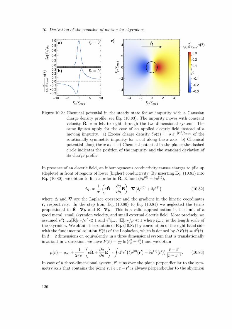
10. Derivation of the equation of motion for skyrmions
Figure 10.2.: Chemical potential in the steady state for an impurity with a Gaussiancharge density profile, see Eq. (10.83). The impurity moves with constantvelocity R from left to right through the two-dimensional system. Thesame figures apply for the case of an applied electric field instead of amoving impurity. a) Excess charge density δρ(r) = ρ0e
−|r|2/ξmod of therotationally symmetric impurity for a cut along the x-axis. b) Chemicalpotential along the x-axis. c) Chemical potential in the plane; the dashedcircle indicates the position of the impurity and the standard deviation ofits charge profile.
In presence of an electric field, an inhomogeneous conductivity causes charges to pile up(deplete) in front of regions of lower (higher) conductivity. By inserting Eq. (10.81) intoEq. (10.80), we obtain to linear order in R, E, and (δρ(0) + δρ(1)),
∆µ ≈ 1
σ′
(eR +
∂σ
∂nE
)·∇(δρ(0) + δρ(1)
)(10.82)
where ∆ and ∇ are the Laplace operator and the gradient in the kinetic coordinatesr, respectively. In the step from Eq. (10.80) to Eq. (10.81) we neglected the termsproportional to R · ∇µ and E · ∇µ. This is a valid approximation in the limit of agood metal, small skyrmion velocity, and small external electric field. More precisely, weassumed e2ξmod|R|νF /σ′ 1 and e2ξmod|E|νF /ρ 1 where ξmod is the length scale ofthe skyrmion. We obtain the solution of Eq. (10.82) by convolution of the right-hand sidewith the fundamental solution F (r) of the Laplacian, which is defined by ∆F (r) = δd(r).In d = 2 dimensions or, equivalently, in a three dimensional system that is translationallyinvariant in z direction, we have F (r) = 1
4π ln(r2x + r2
y
)and we obtain
µ(r) = µ∞ +1
2πσ′
(eR +
∂σ
∂nE
)·∫
d2r′(δρ(0)(r′) + δρ(1)(r′)
) r− r′
|r− r′|2. (10.83)
In case of a three-dimensional system, r′ runs over the plane perpendicular to the sym-metry axis that contains the point r, i.e., r− r′ is always perpendicular to the skyrmion
126
10.4. Formal equation of motion
tube.In Figure 10.2, we show the chemical µ(r) in the steady state of a two-dimensional
system in the case that a local peak of the charge density moves from left to right. Thesame figure applies to the case of an applied electric field that points to the right. Theexcess charge density is modeled by a Gaussian peak δρ(0)(r) + δρ(1)(r) = ρ0 e
−|r|/ξmod
(Figure 10.2a). For ρ0 > 0, the impurity repels (negatively charged) electrons. Whenit moves from left to right, excess electrons from the environment are pushed into theimpurity, resulting in a rise of the chemical potential at the right side. The impurityleaves behind a region of depleted electron density, corresponding to a decrease of µ onthe left side.
10.4. Formal equation of motion
We now turn to the dynamics of the skyrmion. The general equation of motion for theskyrmion trajectory R(t) is Ftot = 0 where Ftot is given in Eq. (10.20). In Wignerrepresentation, we obtain
Ftot(t) =i~2
∫ddr
∫ddk
(2π)d
∫dω
2πTr
[∂g−1
0 (t, r;ω,k)
∂r⊗ GK(t, r;ω,k)
](10.84)
where we used that ∂g−10 /∂R ≈ −∂g−1
0 /∂r. We remark that this approximation neglectsthe weak position-dependency of the electric dipole energy −E · D in Eq. (10.31), whichis lattice-periodic but may have a non-vanishing overlap with GK if not forbidden bysymmetries of the atomic lattice. In order to calculate Ftot in the electron distributionobtained in Section 10.3, we transform Eq. (10.84) into the frame of reference in which¯g−1
0 is diagonal in band space. Using Eq. (10.44), we obtain,
∂g−10 (t, r;ω,k)
∂r=∂(U†(t, r;ω,k)⊗ ¯g−1
0 (t, r; ω, k)⊗ U(t, r;ω,k))
∂r
=∂U†
∂r⊗ ¯g−1
0 ⊗ U + U† ⊗ ¯g−10 ⊗
∂U∂r
+ U† ⊗ ∂ ¯g−10 (t, r; ω, k)
∂r⊗ U .(10.85)
Here, the last term contains a derivative of ¯g−10 , which is a function of the kinetic
coordinates r, ω, and k, by the canonical position r. Using the inverse of Eqs. (10.38)–(10.40), we obtain in band n,
∂ ¯g−10,n(t, r; ω, k)
∂ri=∂ ¯g−1
0,n
∂rj
(δij +
∂Akn,j
∂ri
)+∂ ¯g−1
0,n
∂ω
∂Atn
∂ri−∂ ¯g−1
0,n
∂kj
∂Arn,j
∂ri. (10.86)
Combining Eqs. (10.84)–(10.85) and writing the WT of the Keldysh Green’s function as
GK = U† ⊗ ¯GK ⊗ U , we find
Ftot(t) = F(0)(t) + F(1a)(t) + F(1b)(t) (10.87)
127
10. Derivation of the equation of motion for skyrmions
with
F(0)(t) =i~2
∫ddr
∫ddk
(2π)d
∫dω
2πTr
[∂ ¯g−1
0
∂r⊗ ¯GK
]; (10.88)
F(1a)(t) =i~2
∫ddr
∫ddk
(2π)d
∫dω
2πTr
[U ⊗ ∂U†
∂r⊗(
¯g−10 ⊗
¯GK − ¯GK ⊗ ¯g−10
)]; (10.89)
F(1b)(t) =i~2
∫ddr
∫ddk
(2π)d
∫dω
2π
∑n
[(∂ ¯g−1
0,n
∂rj
∂Akn,j
∂r+∂ ¯g−1
0,n
∂ω
∂Atn
∂r−∂ ¯g−1
0,n
∂kj
∂Arn,j
∂r
)¯GKn
].
(10.90)
Here, we used in the expression for F(1a) that U ⊗U† = 1, which implies (∂U/∂ri)⊗U† =−U ⊗ (∂U†/∂ri). Further, we used that F(1b) is already of first order in the Berrycurvatures and neglected higher-order gradient corrections. Finally, in the derivation ofall Eqs. (10.88)–(10.90), we used the cyclicity of the trace∫
ddr
∫ddk
(2π)d
∫dω
2πTr[A⊗ B − B ⊗ A
]= 0 (in steady state) (10.91)
which can be shown by writing out the Moyal product in canonical coordinates, Eq. (10.29),and integrating by parts. Since there is no integration over time, Eq. (10.91) is only validif temporal derivatives can be expressed in terms of gradients in position and momen-tum space. In our model, this is the case for all terms that depend only on the spectralproperties of the system, i.e., U , U†, ¯g−1
0 , and the Berry connections At/r/k, see, e.g.,
Eq. (10.42). For ¯GK , which depends on the distribution function, a similar relation holdsonly in the steady state with constant skyrmion velocity R.
Force to zeroth order in gradient corrections. The term F(0), Eq. (10.88), describes aforce on the skyrmion due to pressure from an out-of-equilibrium electron distribution.
In the steady state, the Moyal product between ∂ ¯g−10 /∂r and ¯GK can be replaced by
a simple pointwise product in Wigner representation since gradient terms cancel eachother out by partial integration. From Eq. (10.22) we obtain for the Keldysh Green’sfunction,
¯GKn = ¯GRn ⊗¯fn − ¯
fn ⊗ ¯GAn =1
2
¯GRn −
¯GAn⊗,
¯fn
+
1
2
[¯GRn + ¯GAn
⊗,¯fn
](10.92)
where the notation ¯A ⊗, ¯B := ¯A⊗ ¯B + ¯B ⊗ ¯A denotes the anti-commutator under the
Moyal product and [ ¯A ⊗, ¯B] := ¯A⊗ ¯B− ¯B⊗ ¯A is the commutator. Since ¯GR, ¯GA, and¯f
are all diagonal in band space, only gradient terms contribute to the commutator termon the right-hand side of Eq. (10.92). It turns out that this term is suppressed in cleansystems since it is proportional to a small factor of nimpV
20 , which is not compensated by
any additional momentum integrations. This can be seen by rewriting its contribution
128
10.4. Formal equation of motion
to F(0) using the exact relation
i~4
∫ddr
∫ddk
(2π)d
∫dω
2πTr
[∂ ¯g−1
0
∂r⊗[
¯GRn + ¯GAn⊗,
¯fn
] ]=
=i~4
∫ddr
∫ddk
(2π)d
∫dω
2πTr
[([¯GRn⊗, ¯ΣR
n
]+[
¯GAn⊗, ¯ΣA
n
])⊗ ∂
¯fn∂r
−(
¯ΣKn −
¯ΣRn ⊗
¯fn +
¯fn ⊗ ¯ΣA
n
)⊗ ∂( ¯GRn + ¯GAn )
∂r
](10.93)
which follows from Eqs. (10.23), (10.24), and (10.91). The force described by Eq. (10.93)can be attributed to the influence of the skyrmion on the cross section of impurityscattering, and it vanishes in the limit of dilute impurities nimpV
20 → 0, see Eq. (10.60).
In this work, we focus on intrinsic forces on the skyrmion and leave the discussion ofextrinsic forces such as Eq. (10.93) open for future work.
In the anti-commutator term on the right-hand sice of Eq. (10.92), only even ordersof the Moyal product contribute. Thus, if we neglect terms beyond linear order in theGradient corrections, only the zero-order term survives. We obtain
F(0)(t) ≈ i~2
∫ddr
∫ddk
(2π)d
∫dω
2π
∑n
[∂ ¯g−1
0,n
∂r
(¯GRn −
¯GAn
)¯fn
](10.94)
Due to the product with the spectral function i( ¯GR − ¯GA), the distribution function¯f
is only evaluated at quasi-particle energies of the system. The advanced and retarded
Green’s function ¯GR/A are obtained from (¯g−10 −
¯ΣR/A)⊗ ¯GR/A = 1. We focus, as before,on intrinsic forces on the skyrmion and neglect off-diagonal components of the self-energy¯ΣR/A. Thus, using Eq. (10.50), the Green’s function is given by
¯GR/An (t, r; ω, k) =
1
~ω − En(t, r; k)− ¯ΣR/An
. (10.95)
The fact that we work in the band-diagonalized frame of reference leads to two differencesbetween Eq. (10.95) and treatment of the Green’s function in Section 6.2. First, the
position of the pole at ~ω = En + ¯ΣR/An ≈ E(0)
n + δE(1)n + ¯Σ
R/An already accounts for the
gradient correction δE(1)n to the quasi-particle energy. Second, a gradient expansion of
the Green’s function ¯GR/A as presented in Section 6.2 is not necessary. Indeed, since¯g−1
0 (t, r; ω, k) is by definition diagonal for all t, r, ω, and k, the gradient expansion of¯GR/A terminates after the zero-order term given in Eq. (10.95).
In the limit of small impurity concentration, ¯ΣR/An → ±i0+, the spectral function is
i( ¯GRn −¯GAn )→ 2πδ(~ω − En) and we obtain from Eq. (10.94),
F(0)(t) =∑n
∫ddr
∫ddk Dn(t, r; k)
∂En(t, r; k)
∂r¯nn(t, r; k) (10.96)
129
10. Derivation of the equation of motion for skyrmions
where we used the definition Eq. (10.62) of the occupation number ¯nn, and we trans-formed the integrals into kinetic coordinates, thus introducing the density of states Dn,see Eq. (10.45). Neglecting for the moment all gradient corrections, the density of statesDn is approximately constant and the zeroth order force is given by
F(0)(t) ≈ −∑n
∫ddr
∫ddk
(2π)d∂En(t, r; k)
∂R¯nn(t, r; k) +O(Ωr,k) (10.97)
where we used ∂En/∂r = −∂En/∂R. Thus, if the skyrmion position R moves by dR inthe direction of F(0), the total energy of the system is reduced by F(0) · dR to zerothorder in the gradient corrections. This explains our choice of prefactors in the definitionEq. (10.20) of the total force Ftot. The role of the gradient corrections due to the non-constant density of states Dn in Eq. (10.96) will become clear when we combine F(0)
with F(1a) and F(1b) below.
First-order gradient corrections. The terms F(1a) and F(1b), Eqs. (10.89)–(10.90) de-scribe corrections to Eq. (10.96) due to Berry phases. We consider only gradient correc-
tions to linear order in the Berry curvature Ωn. In Eq. (10.90), the factor (¯g−10 ⊗
¯GK −¯GK ⊗ ¯g−1
0 ) vanishes to zeroth order in the Moyal product. Therefore, the leading-ordercontribution to F(1a) is
F(1a)(t) = −~2Jµν
∫ddr
∫ddk
(2π)d
∫dω
2πTr
[U0∂U†0∂r
(∂µ ¯g−10 )(∂ν
¯GK)
](10.98)
where we evaluated the Moyal products between ¯g−10 and ¯GK in canonical coordinates,
see Eq. (10.29). Since ¯g−10 and ¯GK are band-diagonal for all points in Wigner represen-
tation, so are their derivatives. Therefore, only the diagonal components 〈n|U0∂U†0∂∂r |n〉 =
−iArn of the first factor contribute. By integrating by parts, which is allowed in the
steady state, we obtain
F(1a)(t) = − i~2
∑n
∫ddr
∫ddk
(2π)d
∫dω
2π
[(∂ ¯g−1
0,n
∂rj
∂Arn
∂kj+∂ ¯g−1
0,n
∂ω
∂Arn
∂t−∂ ¯g−1
0,n
∂kj
∂Arn
∂rj
)¯GKn
](10.99)
where we used ∂Ar/∂ω = 0. Since F(1a)(t) is already linear in the Berry curvatures,we may replace derivatives w.r.t. canonical coordinates by derivatives w.r.t. kinetic co-ordinates, e.g., ∂ ¯g−1
0 /rj ≈ ∂ ¯g−10 /rj . Combining with F(1b), Eq. (10.90), and using
¯GKn ≈ ( ¯GRn −¯GAn )(1 − 2¯nn) to zeroth order in the gradient corrections, we obtain to
leading order
F(1a)i (t) + F
(1b)i (t) =
∑n
∫ddr
∫ddk
(2π)d
[Ωr,kn,ij
∂En∂rj− Ωr,r
n,ij
∂En∂kj− ~Ωr,t
n,i
]¯nn. (10.100)
Here, we transformed the integrals from canonical to kinetic coordinates, neglecting thegradient corrections in Dn since F(1) is already linear in the Berry curvatures.
130
10.4. Formal equation of motion
Combining Eqs. (10.87), (10.96), and (10.100) and using Eqs. (10.45) and (10.47), weobtain the total force on the skyrmion to leading order in E, R, and Ω,
F toti (t) =
∑n
∫ddr
∫ddk
(2π)d
[(1− Ωr,k
n,jj)∂En∂ri− Ωr,r
n,ij
(∂En∂kj− ~Rj
)+ Ωr,k
n,ij
(∂En∂rj
+ eEj
)]¯nn. (10.101)
Eq. (10.101) is a central result of this chapter. In Chapter 11, we evaluate Ftot in metalsand in insulators.
Vanishing force in global equilibrium. In absence of an electric field, the equation ofmotion Ftot = 0 must be solved by a resting skyrmion if the electronic system is inglobal equilibrium and the skyrmion is located at a minimum of the potential energy.This is a consequence of the fact that, for R = 0 and E = 0, the Hamiltonian istime-independent, and the equation of motion Eq. (10.16) is solved exactly by a time-independent Hamiltonian that commutes with the density matrix at time t → −∞.This can be seen as follows. The formal classical equation of motion for the skyrmioncoordinate is given by the saddlepoint equation, Eq. (10.16), which is equivalent to
δZ[R]
δRq(t)
∣∣∣∣Rq=0
= 0. (10.102)
Here, Z[R] = −i log(Seff[R]) is the partition function of the electronic system for a givenskyrmion trajectory R(t), where Seff is the effective action defined in Eq. (10.14), andRq(t) = 1
2(R(t+)−R(t−)) is the quantum component of the skyrmion trajectory. In theKeldysh formalism, the partition function for a fixed skyrmion trajectory is given by
Z[R] = Tr[U−(−∞,∞)U+(∞,−∞) ρ(−∞)] (10.103)
where U± is the time-evolution operator for the electronic subsystem on the forward(backward) branch of the Keldysh contour, ρ(−∞) is the density matrix at time t →−∞, and the trace is over the full many-particle Hilbert space (Fock space). The timeevolution of the electronic degrees of freedom depends on the skyrmion trajectory, andwe find, on the two branches,
δU+(∞,−∞)
δRq(t)= −iU+(∞, t) ∂H(t+)
∂R(t+)U+(t,−∞);
δU−(−∞,∞)
δRq(t)= −iU−(−∞, t) ∂H(t−)
∂R(t−)U−(t,∞). (10.104)
where H(t±) is the Hamiltonian in second-quantized form evaluated on the forward(backward) branch of the Keldysh contour. Inserting into Eq. (10.103), we obtain
δZ[R]
δRq(t)
∣∣∣∣Rq=0
= −2iTr
[U(−∞, t) ∂H(t)
∂R(t)U(t,−∞) ρ(−∞)
]Rq=0
(10.105)
131
10. Derivation of the equation of motion for skyrmions
where we used the fact that for Rq = 0 the time evolution is identical on the forward andbackward branch. To solve Eq. (10.102), one has to set the right-hand side of Eq. (10.105)to zero. In the presence of an electric field or for an out-of-equilibrium initial densitymatrix ρ(−∞), this may in general only be achieved by a moving skyrmion. For E = 0,however, we can make H independent of time by choosing a constant skyrmion positionR(t) = const. This trivial trajectory solves the equation of motion if the initial stateis given by the equilibrium density matrix ρ(−∞) = Z−1
0 e−H/(kBT ), since the right-hand side of Eq. (10.105) reduces in this case to −2i ∂∂R 〈H〉 where 〈H〉 = Tr[Hρ(−∞)]denotes thermal and quantum-mechanical averaging. Impurities render the energy land-scape 〈H〉 position-dependent, which leads to pinning forces, but we assumed that theskyrmion is in a minimum of the potential energy so that ∂
∂R 〈H〉 = 0.Thus, in an equilibrium system with E = 0, a resting skyrmion solves the equation
of motion Ftot = 0 exactly. In praxis, Ftot can only be obtained within some setof approximations, and a consistent approximation must not violate Ftot = 0 for aresting skyrmion and equilibrium electron distribution. In our above derivation of Ftot,Eq. (10.1), our main approximations were (i) the assumption of non-interacting electrons,(ii) a gradient expansion to linear order in all components of the Berry curvature tensorΩn, and (iii) the limit of dilute impurities, nimpV
20 → 0. To check that we did not
inadvertently break translational invariance within our approximations, we evaluate Ftot
in global equilibrium, characterized by an occupation number ¯nn(r; k) ≡ nF (En(r; k))that depends only on energy. Inserting ¯nn(r; k) into Eq. (10.1) and integrating by parts,we obtain for the total force in equilibrium,
F eqi =
∑n
∫ddr
∫ddk
(2π)d
[∂Ωr,k
n,jj
∂ri+∂Ωr,r
n,ij
∂kj−∂Ωr,k
n,ij
∂rj
]¯N eqn (En) = 0 (10.106)
where ¯N eq(En) is the antiderivative of the Fermi function, i.e., ∂ ¯N eq(En)/∂En = nF (En).The terms in the bracket cancel, as they should, due to the Jacobi identity, Eq. (3.14).Here, the first term in the bracket originates from the density of states Dn(r; k) inphase space, while the other two terms come from forces due to Berry phases in positionand in mixed position/momentum space, respectively. Not surprisingly, the Berry-phasecorrection to the density of states in phase space, related to Liouville’s theorem, isessential to restore the correct behavior in equilibrium by canceling forces due to Berryphases. We encountered a similar cancellation of unphysical terms in the discussion ofparticle-number conservation in section 5.2, where the use of the correct density of statesin phase space was also key.
132
11. Results in Metals and insulators
In this chapter, we apply the general Equation of motion derived in the preceding chapter(Eq. (10.101)) and evaluate it for the case of a metal and an insulator. In the metal, weobtain a result that is similar to the Thiele Equation, Eq. (9.7),
G× (vs − R) + Fso + FOhm + Fdrag = 0. (11.1)
Here, G is the gyro-coupling vector, vs is the effective spin velocity, and the last threeterms describe a new kind of force due to Berry phases in mixed position/momentumspace, ohmic friction, and current drag, respectively. The equation of motion does notcontain the damping terms proportional to the Gilbert damping parameter α of thestandard Thiele equation Eq. (9.7).
In an insulator, the forces described above vanish and instead the electric field couplesdirectly to the charge of the skyrmion. The equation of motion will turn out to be givenby
−G× R + δQ(2)E = 0. (11.2)
11.1. Equation of motion for skyrmions in metals
Forces in local equilibrium. We insert the occupation number ¯nn obtained in Section10.3 into Eq. (10.1) for the total force on the skyrmion. Our ansatz Eq. (10.73) for¯nn, is a sum of the occupation number in local equilibrium and an out-of-equilibriumredistribution of electrons in momentum space. In local equilibrium, ¯nn(t, r; k) =nF (En(t, r; k)− µ(t, r)), we obtain the force
F leqi (t) =
∑n
∫ddr
∫ddk
(2π)d
[~Ωr,r
n,ijRj + Ωr,kn,ij
(eEj +
∂µ
∂rj
)+ (1− Ωr,k
n,jj)∂µ
∂ri
]nF (En − µ)
= F gyro,Ri (t) + F so
i (t) + FOhmi (t) + F drag
i (t) (11.3)
where the first equality follows from partial integration and the Jacobi identity, Eq. (3.14),similar to the derivation of Eq. (10.106). In second equality, we split the total force intofour different physical contributions. First, the term proportional to Ωr,r
n leads to thewell-known gyro-coupling force Fgyro,R. For our simple model of a chiral magnet with asingle orbital band and weak SO coupling, cf., Eq. (10.76), it is given by
Fgyro,R(t) = −G× R with G ≈ 1
2JνF
∑n
∫ddr M(r)Bem(r). (11.4)
133
11. Results in Metals and insulators
Here, G is the gyro-coupling vector, M is the magnetization, and Bem is the emergentmagnetic field defined in Eq. (4.13), which carries a quantized flux.
The force Fso comes from the term proportional to Ωr,kn,ij in Eq. (11.3),
F soi (t) =
∑n
∫ddr
∫ddk
(2π)dΩr,kn,ij
(eEj +
∂µ
∂rj
)nF (En − µ). (11.5)
This force is a new result not previously considered to our knowledge. The force is non-zero only in presence of spin-orbit coupling. Semiclassically, Fso can be understood asthe recoil-force on the skyrmion due to the additional force −eΩr,k
n,ijEj in the equationof motion of electrons, see Eq. (10.55). With the considerations from section 4.3, weestimate its magnitude to be on the order of F so ∼ eE, which is consistent with numericalresults for MnSi [65].
The remaining two forces on the right-hand side of Eq. (11.3) come from the term
proportional to (1−Ωr,kn,jj). expanding to leading order in the the variation of M(r) and
in the gradient corrections leads to
FOhmi + F drag
i = −1
e
∫ddr (δρ(0) + δρ(1))
∂µ
∂ri
≈ − 1
4πσ′
(Rj +
1
e
∂σ
∂nEj
)∫ddr
∫d2r′ δρ(r) δρ(r′)
∂2 ln(|r− r′|2
)∂ri ∂rj
(11.6)
where δρ(0) (δρ(1)) is the excess charge density of the skyrmion due to variations in themagnitude of M of the magnetization (phase-space Berry phases). In the last step, weinserted the chemical potential in the steady state from Eq. (10.83) and we used theshort-hand notation δρ = δρ(0) + δρ(1). In a three-dimensional system the integrationregion of r′ is again restricted to the plane perpendicular to the symmetry axis of theskyrmion that contains the point r. The integral can be simplified if the charge densityis rotationally symmetric. Terms with i 6= j vanish since the integrand is odd under thecombined mirror reflection ri → −ri, r′i → −r′i. For the remaining contribution withi = j, we use the symmetry of the integrand under exchange of rx with ry and r′x with r′yto replace ∂2
ri ln(|r− r′|2
)by 1
2(∂2rx + ∂2
ry) ln(|r− r′|2
)= 2πδ2(r− r′). We thus identify
the two forces
FOhm(t) = − 1
2σ′
∫ddr (δρ(0) + δρ(1))2 R; (11.7)
Fdrag(t) =1
−2eσ′∂σ
∂n
∫ddr (δρ(0) + δρ(1))2 E. (11.8)
Here, FOhm points in the direction opposite to the skyrmion velocity R and describesOhmic friction due to the fact that the skyrmion drags along electrons. The force Fdrag
points approximately in the direction of the particle current σ−eE and accounts for the
fact an external electric field leads to a drift velocity of the electrons, which exerts a drag
134
11.2. Equation of motion for skyrmions in insulators
force on the skyrmion. Both FOhm and Fdrag are quadratic in the excess charge densityδρ(0) +δρ(1). This is consistent with the requirement that the dissipated power R ·FOhm
due to Ohmic friction always has to be negative (see also discussion in Section 11.3).The prefactor of 1
2 in Eqs. (11.7)–(11.8) results from the substitution of ∂2ri ln
(|r− r′|2
)by 1
2(∂2rx + ∂2
ry) ln(|r− r′|2
), which is specific to a charge distribution with cylindrical
symmetry. More generally, the corresponding prefactor in case of a rotationally symmet-ric charge distribution in d dimensions is 1/d. This prefactor accounts for the fact thatthe presence of a local inhomogeneity (skyrmion) influences the flow of electrons and,for d > 1, electrons can evade the local inhomogeneity (see Figure 10.2). Since electronsthat evade the local inhomogeneity do not contribute to Ohmic friction or current drag,FOhm and Fdrag are suppressed by a factor of 1/d.
Force out of local equilibrium. In our ansatz for the occupation number, Eq. (10.73),we includes a term δ¯nn(t, r; k) that accounts for electron re-distribution in momentumspace out of local equilibrium. For a low skyrmion velocity and small electric field,we expect that the system is always close to local equilibrium and that δ¯nn is small.In addition, δ¯nn by definition does not contribute to the charge density ρ(t, r). Wetherefore only consider the the contribution from δ¯nn to Ftot that comes from the termproportional to ∂En/∂k in Eq. (10.1), which has the stronges momentum-dependency.The out-of-local-equilibrium correction δ¯nn thus leads to the remaining part of the gyro-coupling force,
F gyro,si (t) = −
∑n
∫ddr
∫ddk
(2π)dΩr,rn,ij
∂En∂kj
δ¯nn(t, r; k) ≈ (G× vs)i (11.9)
where vs is an effective spin velocity. In the toy model with only a single orbital band,it is given by
vs =
∫ddr
∫ddk
(2π)d
(∂E↓~ ∂kδ
¯n↓ −∂E↑~ ∂kδ
¯n↑
)∫
ddr∫
ddk(2π)d
(nF (E↓ − µ)− nF (E↑ − µ))(11.10)
where we neglected the small position-dependency of δ¯n↓/↑.
11.2. Equation of motion for skyrmions in insulators
In insulators, all forces on the skyrmion to first order in the gradient expansion vanish, ex-cept for the gyro-coupling term Fgyro,R = −G·R in Eq. (11.1). This is evident for the theforces Fgyro,s, FOhm, and Fdrag, Eqs. (11.9), (11.7), and (11.8), respectively, which occuronly for an out-of-equilibrium electron distribution. The force Fso, Eq. (11.5), vanishesin insulators by the same arguments that the first-order skyrmion charge δQ(1) vanishes,see Section 6.3. For example, for an electric field in y direction, the x-component ofFso is proportional to the integral
∫drx
∫dky Ωr,k
xy , which is quantized (first Chern num-ber). Since the integral vanishes for positions ry far away from the skyrmion, it vanisheseverywhere.
135
11. Results in Metals and insulators
The leading order contribution to the force on skyrmions in insulators is quadratic inspatial derivatives and linear in the electric field. The evaluation of Ftot, Eq. (10.84), issimplified in insulators since it is not necessary to apply transformation Eq. (10.44) in
order to obtain a band-diagonal distribution function¯f . In spite of the external driving
due to the electric field E, all states below (above) the Fermi energy are always occupied(empty) in an insulator. Therefore, the distribution function f(ω) = 1− 2nF (~ω− µ) isa scalar function of frequency only and trivially band-diagonal. Here, nF is the Fermifunction and µ is the chemical potential, which lies in a band gap. The Keldysh Green’sfunction is thus readily obtained in canonical coordinates,
GK(t, r;ω,k) =(GR(t, r;ω,k)− GA(t, r;ω,k)
)(1− 2nF (~ω − µ)). (11.11)
On the other hand, staying in the canonical frame of reference comes at the cost thatthe retarded and advanced Green’s functions depend in a non-trivial way on the inverselocal Green’s function g−1
0 . We obtain GR and GA from a gradient expansion similar tothe discussion in Section 6.2. Here, the gradient expansion has to be performed in spaceand time. In our model, temporal derivatives translate into gradients in position andmomentum space via the relation
∂g−10
∂t= − e
~E · ∂g
−10
∂k− R · ∂g
−10
∂r(11.12)
where we assumed again that external electric field E is homogeneous in space. We referto Appendix B for the calculation, which is rather technical. To leading order in E, R,and spatial gradients, we obtain the equation of motion
−G× R + δQ(2)E = 0. (11.13)
Here, δQ(2) is the quantized electric charge of the skyrmion, see Eq. (6.45). The chargecouples to the electric field in the expected way, leading to the force Fc = δQ(2)E. Dueto the gyro-coupling −G× R, the skyrmion velocity R is perpendicular to the force andthe dissipated power R · Fc vanishes, as it should in an insulator.
For a single occupied band in d = 2 dimensions, the force Fc due to the electric chargeof the skyrmion admits an alternative semiclassical interpretation. In this case, theskyrmion charge δQ(2) = σxyΦ0 factorizes into a product of the quantized Hall conduc-tivity σxy and the quantized total emergent magnetic flux Φ0, see Eqs. (6.50) and (6.51),respectively. An external electric field E = Eyey in y direction generates a Hall currentjx = σxyEy in x direction. This current leads to the force Fy = −~
e
∫d2rΩr,r
yxjx = Φ0jxin y direction via a process similar to the force Fgyro,s in metals, see Eq. (11.9). In total,one obtains again the force Fc = δQ(2)E. This interpretation breaks down if more thanone band is occupied. In this case, the second Chern number δQ(2) is given in terms ofnon-Abellian Berry curavtures in Eq. (6.48), and it does not factorize into a product offirst Chern numbers Φ0 and σxy in position and momentum space, respectively. Nev-ertheless, even if δQ(2) does not factorize into real-space and momentum-space windingnumbers, it still couples to the electric field in the usual way via Eq. (11.13).
136
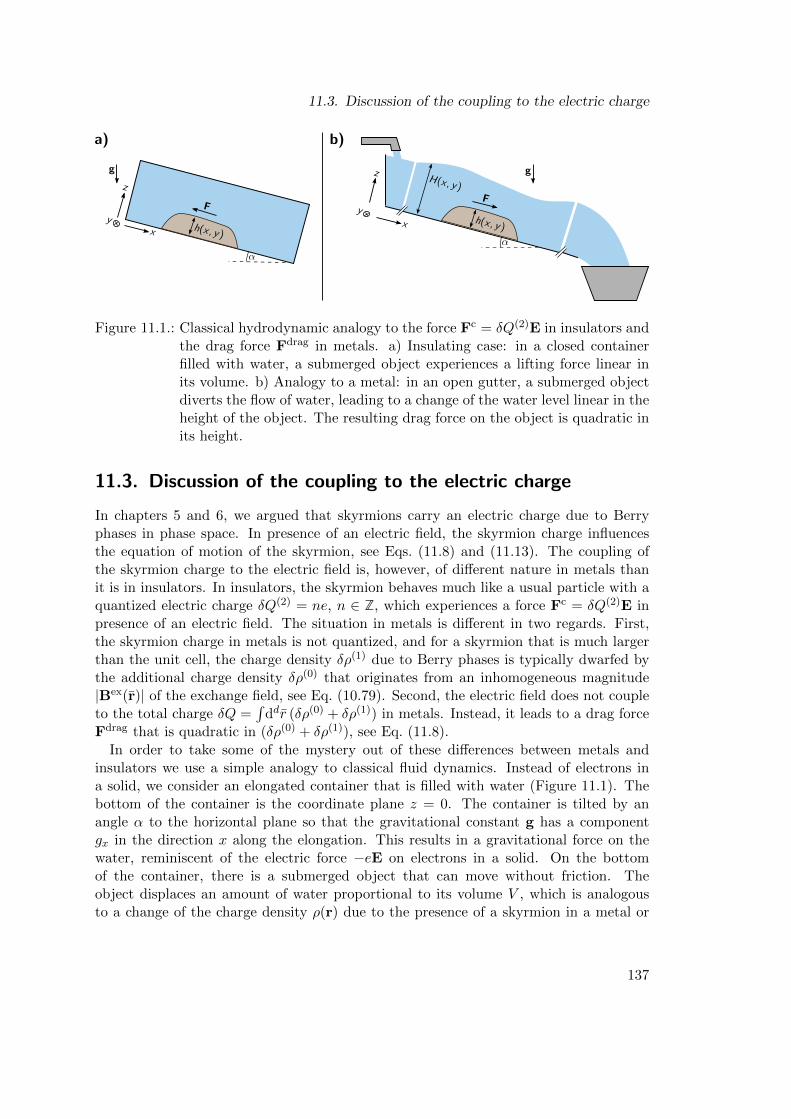
11.3. Discussion of the coupling to the electric charge
Figure 11.1.: Classical hydrodynamic analogy to the force Fc = δQ(2)E in insulators andthe drag force Fdrag in metals. a) Insulating case: in a closed containerfilled with water, a submerged object experiences a lifting force linear inits volume. b) Analogy to a metal: in an open gutter, a submerged objectdiverts the flow of water, leading to a change of the water level linear in theheight of the object. The resulting drag force on the object is quadratic inits height.
11.3. Discussion of the coupling to the electric charge
In chapters 5 and 6, we argued that skyrmions carry an electric charge due to Berryphases in phase space. In presence of an electric field, the skyrmion charge influencesthe equation of motion of the skyrmion, see Eqs. (11.8) and (11.13). The coupling ofthe skyrmion charge to the electric field is, however, of different nature in metals thanit is in insulators. In insulators, the skyrmion behaves much like a usual particle with aquantized electric charge δQ(2) = ne, n ∈ Z, which experiences a force Fc = δQ(2)E inpresence of an electric field. The situation in metals is different in two regards. First,the skyrmion charge in metals is not quantized, and for a skyrmion that is much largerthan the unit cell, the charge density δρ(1) due to Berry phases is typically dwarfed bythe additional charge density δρ(0) that originates from an inhomogeneous magnitude|Bex(r)| of the exchange field, see Eq. (10.79). Second, the electric field does not coupleto the total charge δQ =
∫ddr (δρ(0) + δρ(1)) in metals. Instead, it leads to a drag force
Fdrag that is quadratic in (δρ(0) + δρ(1)), see Eq. (11.8).
In order to take some of the mystery out of these differences between metals andinsulators we use a simple analogy to classical fluid dynamics. Instead of electrons ina solid, we consider an elongated container that is filled with water (Figure 11.1). Thebottom of the container is the coordinate plane z = 0. The container is tilted by anangle α to the horizontal plane so that the gravitational constant g has a componentgx in the direction x along the elongation. This results in a gravitational force on thewater, reminiscent of the electric force −eE on electrons in a solid. On the bottomof the container, there is a submerged object that can move without friction. Theobject displaces an amount of water proportional to its volume V , which is analogousto a change of the charge density ρ(r) due to the presence of a skyrmion in a metal or
137
11. Results in Metals and insulators
insulator. We denote the height profile of the object by h(x, y). Our aim is to calculatethe force in direction x that acts on the submerged object due to differences in the waterpressure p(r) on its two ends. From simple geometric considerations, the force is givenby
Fx =
∫dx
∫dy p(x, y, h(x, y))
∂h(x, y)
∂x. (11.14)
The submerged object also experiences a gravitational force proportional to its mass, butthis is only a shortcoming of the analogy and we are not interested in the gravitationalforce on the object.
The closest classical analogy to an insulator is obtained if the container is closed to allsides and completely filled (Figure 11.1a). In this case, the pressure field p(r) is obtainedfrom the Bernouilli Equation,
p(r)− ρwg · r +1
2ρwv(r)2 = const, (11.15)
where ρw is the density of water, assumed to be constant, and v(r) = 0 is the velocityof the water at position r, which vanishes in equilibrium. We thus obtain p(r) = ρwg · r,and, by Eq. (11.14), the force Fx = −V ρwgx is just the usual lifting force. This resultis analogous to the force Fc = δQ(2)E in insulators, recalling that the presence of thesubmerged object changes the total mass of the water in the container by −V ρw.
Let us now consider a different setup, in which the upper and lower ends of thecontainer are connected to a constant source and sink of water, respectively, and the topof the container is open (Figure 11.1b). This is analogous to a metal that is connectedto a battery, where the role of the local chemical potential µ(r) is taken by the distanceH(x, y) of the water surface measured from the bottom of the container. Water flowsdown the pipe and the system can establish a steady state only in presence of friction,described by the viscosity η in the Navier-Stokes Equation
ρw∂v
∂t+(v ·∇− η∇2
)v = −∇p+ ρwg. (11.16)
If the submerged object is held at a fixed position, the steady state is defined by ∂v/∂t =0. The object influences the velocity and pressure fields via the boundary conditions.For non-slip boudary conditions at the bottom, one has,
v = 0 at the bottom, z = h(x, y) (11.17)
p = 0 at the water surface, z = H(x, y). (11.18)
We assume that the water level H is large compared to the height h of the submergedobject. To zeroth order in h/H, Eqs. (11.16)–(11.18) are solved by a constant fillingH(x, y) = H0 and
p0(r) = ρwgz(z −H0); (11.19)
v0(r) =ρwgx2η
(H2
0 − (z −H0)2)ex. (11.20)
138
11.3. Discussion of the coupling to the electric charge
Since p0 is independent of x, the force Fx, Eq. (11.14), generated by p0 vanishes. Correc-tions to p0 are of linear order in h, and thus the leading contribution to Fx is quadraticin h. This is analogous to the fact that Fdrag, Eq. (11.8), is quadratic in the change ofthe charge density. Physically, the submerged object is an obstacle for the flow of water,leading to a rise (lowering) of the water level H(x, y) linear in h in front of (behind) theobject, as indicated in Figure 11.1b. In the metal, this corresponds to the non-constantlocal chemical potential µ(r), which is linear in the excess charge density δρ(0)+δρ(1), seeEq. (10.83). The gradient of the water level is associated with a pressure gradient, whichleads to a drag force quadratic in h on the submerged object. Similar arguments can bemade if the object moves with a constant velocity, leading a frictional force analogousto FOhm, Eq. (11.7).
139

12. Conclusions and outlook
We studied the effects of phase-space Berry phases in chiral magnets with weak spin-orbitcoupling. Chiral magnets develop a smooth magnetization textures at low temperaturesdue to a competition between ferromagnetic exchange and Dzyaloshinskii-Moriya *DM)interaction. Most notably, topologically protected whirls, so-called skyrmions, are ther-modynamically stable in a small pocket of the phase diagram and exist as metastableobjects in a wider range of the phase diagram. Based on a minimal analytic model,we argued that the combination of spin-orbit coupling and smooth magnetic texturesin position space leads a non-vanishing Berry curvature in mixed position/momentumspace.
In part I, we showed that the Berry curvature in mixed position/momentum spaceleads to an electric charge of skyrmions due to an accumulation of electrons. We esti-mated the charge to be on the order of one electron charge per skyrmion if screeningis neglected. This was confirmed in numerical calculations for MnSi by our collabora-tors. In insulators, the electric charge of skyrmions is quantized (second Chern number).If all non-abelian Berry curvatures vanishes, the charge is equal to the product of thequantized Hall conductivity and the quantized total flux of emergent magnetic field. Wealso showed that the strength of DM interactions can be expressed in terms of the Berrycurvature in mixed position/momentum space if the magnetic texture varies on a longlength scale. Numerical results by our collaborators for the DM interaction strength inMnSi agree well with experimental data.
In part II, we showed that the combination of spin-orbit coupling and smooth magnetictextures leads to an additional contribution to the Hall conductivity in chiral magnets.We developed a diagrammatic theory for the topological Hall effect based on a gradientexpansion of the Kubo-Streda formula and derived a correction to the semiclassicalformula.
In part III, we studied the dynamics of rigid skyrmions in chiral magnets. We derivean equation of motion for the translational mode, taking into account Berry phases inall of phase space. In presence of an externally applied electric field, the Berry curvaturein mixed position/momentum space leads to a dissipationless momentum transfer fromconduction electrons to the skyrmions, which is independent of the current. In metals,the electric charge of skyrmions influences the motion of the skyrmion in two ways. First,a moving electron carries along excess charges, which leads to ohmic friction. Second,if an electric field is applied, a spacially inhomogeneous conductivity leads to a pile-upup of charge carriers at one side of the skyrmion and to a depletion of charge carrierson the other side. This imbalance leads to a drag force on the skyrmion. The electriccharge of skyrmions in metallic chiral magnets does, however, not couple directly to theelectric field. The situation is different in insulators. Here, both drag and ohmic friction
141
12. Conclusions and outlook
vanish, and the quantized electric charge couples instead directly to the electric field.
Outlook. In a recent series of experiments, Hsu and collaborators were able to selec-tively create and destroy skyrmions in a three atomic layer thick film of Iron on anIr(111) substrate using only the electric field from the tip of a scanning tunneling mi-croscope [43]. While it is not yet definitely settled that no current flowed from the tipto the sample, switching the sign of the tip voltage allowed to change from skyrmioncreation to skyrmion destruction, indicating that the electric field is the main drivingforce of the process. It is possible that these experiments can be explained by the electriccharge of skyrmions discussed in part I of this thesis. The voltage difference betweenthe tip and the substrate leads to electric fields with an in-plane component that pointsradially either towards the tip or away from it, depending on the sign of the voltage.Once electrons accumulate or deplete below the tip, the system may be able to lower itsenergy by building a skyrmion, as this is accompanied with a change of the density ofstates in phase space. In order to investigate if the Berry-phase effect is indeed respon-sible for the creation an destruction skyrmions, numerical data for the phase-space Berycurvature in the materials used in the experiment are necessary.
The quantized skyrmion charge in insulators promises an exciting method to manip-ulate skyrmions with electric fields without the losses accompanied by ohmic friction inmetals. In order to achieve this, an insulating chiral magnet with a non-trivial topologyin momentum space would be required.
Finally, we presented a method to derive an equation of motion for the translationalmode of skyrmions in part III of this thesis. The method is general in that it is notlimited to electron-skyrmion interaction. Recently, the interaction between skyrmionsand magnons due to a temperature gradient has been in the focus of a number ofpublications [144, 146, 147]. Due to a combination of two gyro-couplings, it turns outthat skyrmions move towards the heat source. Adapting the method presented in partIII of this thesis would allow to account for spin-orbit effects in the magnon-skyrmioncoupling. We point out, however, that the separation between magnon modes and thetranslational mode of the skyrmion is more subtle than in the case of electron-magnoninteraction.
142
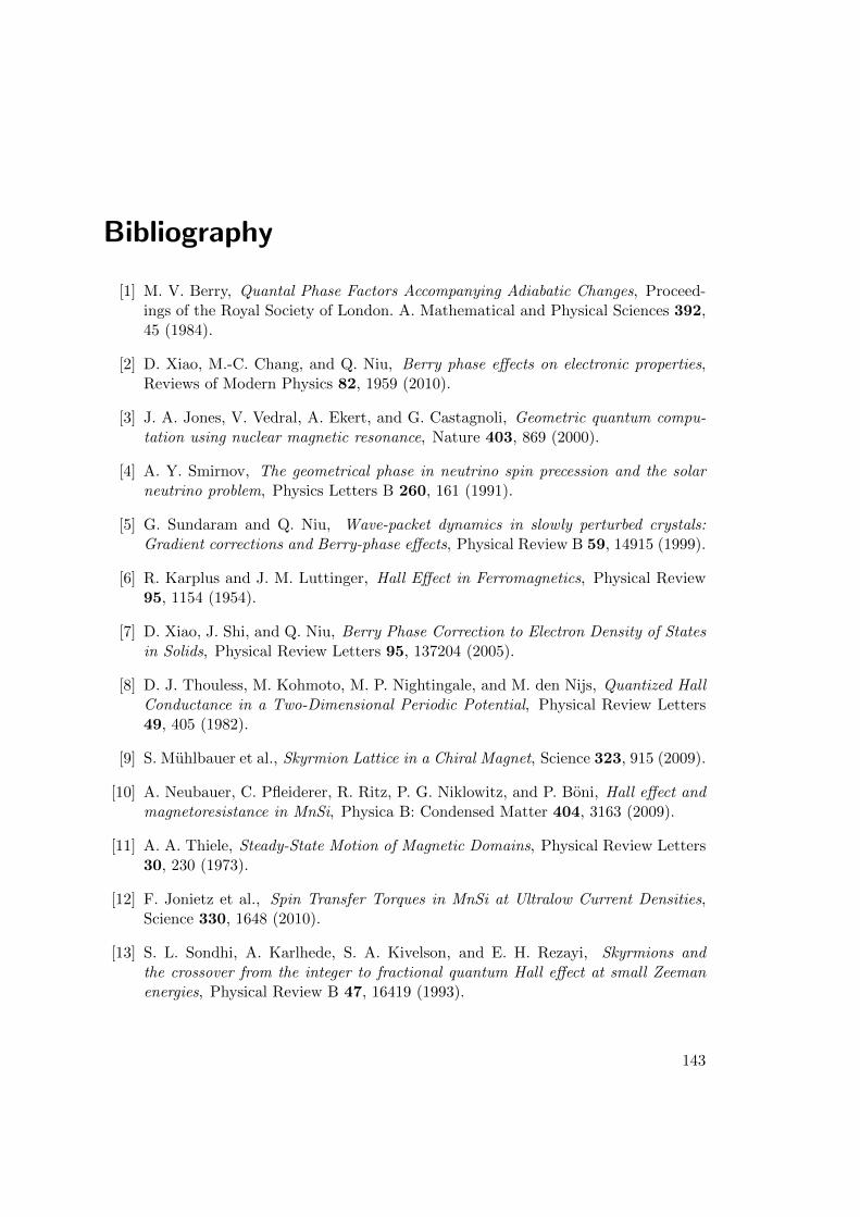
Bibliography
[1] M. V. Berry, Quantal Phase Factors Accompanying Adiabatic Changes, Proceed-ings of the Royal Society of London. A. Mathematical and Physical Sciences 392,45 (1984).
[2] D. Xiao, M.-C. Chang, and Q. Niu, Berry phase effects on electronic properties,Reviews of Modern Physics 82, 1959 (2010).
[3] J. A. Jones, V. Vedral, A. Ekert, and G. Castagnoli, Geometric quantum compu-tation using nuclear magnetic resonance, Nature 403, 869 (2000).
[4] A. Y. Smirnov, The geometrical phase in neutrino spin precession and the solarneutrino problem, Physics Letters B 260, 161 (1991).
[5] G. Sundaram and Q. Niu, Wave-packet dynamics in slowly perturbed crystals:Gradient corrections and Berry-phase effects, Physical Review B 59, 14915 (1999).
[6] R. Karplus and J. M. Luttinger, Hall Effect in Ferromagnetics, Physical Review95, 1154 (1954).
[7] D. Xiao, J. Shi, and Q. Niu, Berry Phase Correction to Electron Density of Statesin Solids, Physical Review Letters 95, 137204 (2005).
[8] D. J. Thouless, M. Kohmoto, M. P. Nightingale, and M. den Nijs, Quantized HallConductance in a Two-Dimensional Periodic Potential, Physical Review Letters49, 405 (1982).
[9] S. Muhlbauer et al., Skyrmion Lattice in a Chiral Magnet, Science 323, 915 (2009).
[10] A. Neubauer, C. Pfleiderer, R. Ritz, P. G. Niklowitz, and P. Boni, Hall effect andmagnetoresistance in MnSi, Physica B: Condensed Matter 404, 3163 (2009).
[11] A. A. Thiele, Steady-State Motion of Magnetic Domains, Physical Review Letters30, 230 (1973).
[12] F. Jonietz et al., Spin Transfer Torques in MnSi at Ultralow Current Densities,Science 330, 1648 (2010).
[13] S. L. Sondhi, A. Karlhede, S. A. Kivelson, and E. H. Rezayi, Skyrmions andthe crossover from the integer to fractional quantum Hall effect at small Zeemanenergies, Physical Review B 47, 16419 (1993).
143
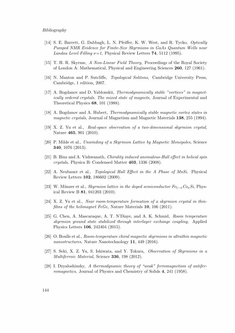
Bibliography
[14] S. E. Barrett, G. Dabbagh, L. N. Pfeiffer, K. W. West, and R. Tycko, OpticallyPumped NMR Evidence for Finite-Size Skyrmions in GaAs Quantum Wells nearLandau Level Filling ν=1, Physical Review Letters 74, 5112 (1995).
[15] T. H. R. Skyrme, A Non-Linear Field Theory, Proceedings of the Royal Societyof London A: Mathematical, Physical and Engineering Sciences 260, 127 (1961).
[16] N. Manton and P. Sutcliffe, Topological Solitons, Cambridge University Press,Cambridge, 1 edition, 2007.
[17] A. Bogdanov and D. Yablonskii, Thermodynamically stable ”vortices” in magnet-ically ordered crystals. The mixed state of magnets, Journal of Experimental andTheoretical Physics 68, 101 (1988).
[18] A. Bogdanov and A. Hubert, Thermodynamically stable magnetic vortex states inmagnetic crystals, Journal of Magnetism and Magnetic Materials 138, 255 (1994).
[19] X. Z. Yu et al., Real-space observation of a two-dimensional skyrmion crystal,Nature 465, 901 (2010).
[20] P. Milde et al., Unwinding of a Skyrmion Lattice by Magnetic Monopoles, Science340, 1076 (2013).
[21] B. Binz and A. Vishwanath, Chirality induced anomalous-Hall effect in helical spincrystals, Physica B: Condensed Matter 403, 1336 (2008).
[22] A. Neubauer et al., Topological Hall Effect in the A Phase of MnSi, PhysicalReview Letters 102, 186602 (2009).
[23] W. Munzer et al., Skyrmion lattice in the doped semiconductor Fe1−xCoxSi, Phys-ical Review B 81, 041203 (2010).
[24] X. Z. Yu et al., Near room-temperature formation of a skyrmion crystal in thin-films of the helimagnet FeGe, Nature Materials 10, 106 (2011).
[25] G. Chen, A. Mascaraque, A. T. N’Diaye, and A. K. Schmid, Room temperatureskyrmion ground state stabilized through interlayer exchange coupling, AppliedPhysics Letters 106, 242404 (2015).
[26] O. Boulle et al., Room-temperature chiral magnetic skyrmions in ultrathin magneticnanostructures, Nature Nanotechnology 11, 449 (2016).
[27] S. Seki, X. Z. Yu, S. Ishiwata, and Y. Tokura, Observation of Skyrmions in aMultiferroic Material, Science 336, 198 (2012).
[28] I. Dzyaloshinsky, A thermodynamic theory of “weak” ferromagnetism of antifer-romagnetics, Journal of Physics and Chemistry of Solids 4, 241 (1958).
144
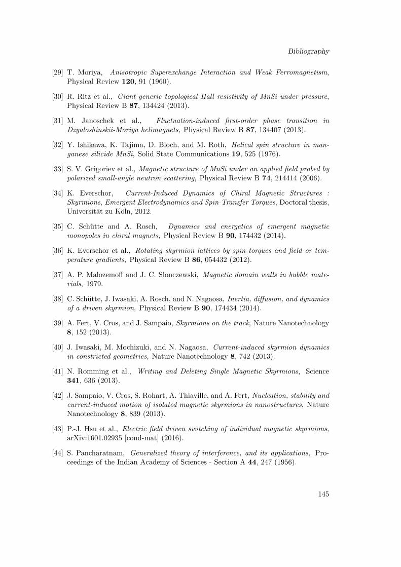
Bibliography
[29] T. Moriya, Anisotropic Superexchange Interaction and Weak Ferromagnetism,Physical Review 120, 91 (1960).
[30] R. Ritz et al., Giant generic topological Hall resistivity of MnSi under pressure,Physical Review B 87, 134424 (2013).
[31] M. Janoschek et al., Fluctuation-induced first-order phase transition inDzyaloshinskii-Moriya helimagnets, Physical Review B 87, 134407 (2013).
[32] Y. Ishikawa, K. Tajima, D. Bloch, and M. Roth, Helical spin structure in man-ganese silicide MnSi, Solid State Communications 19, 525 (1976).
[33] S. V. Grigoriev et al., Magnetic structure of MnSi under an applied field probed bypolarized small-angle neutron scattering, Physical Review B 74, 214414 (2006).
[34] K. Everschor, Current-Induced Dynamics of Chiral Magnetic Structures :Skyrmions, Emergent Electrodynamics and Spin-Transfer Torques, Doctoral thesis,Universitat zu Koln, 2012.
[35] C. Schutte and A. Rosch, Dynamics and energetics of emergent magneticmonopoles in chiral magnets, Physical Review B 90, 174432 (2014).
[36] K. Everschor et al., Rotating skyrmion lattices by spin torques and field or tem-perature gradients, Physical Review B 86, 054432 (2012).
[37] A. P. Malozemoff and J. C. Slonczewski, Magnetic domain walls in bubble mate-rials, 1979.
[38] C. Schutte, J. Iwasaki, A. Rosch, and N. Nagaosa, Inertia, diffusion, and dynamicsof a driven skyrmion, Physical Review B 90, 174434 (2014).
[39] A. Fert, V. Cros, and J. Sampaio, Skyrmions on the track, Nature Nanotechnology8, 152 (2013).
[40] J. Iwasaki, M. Mochizuki, and N. Nagaosa, Current-induced skyrmion dynamicsin constricted geometries, Nature Nanotechnology 8, 742 (2013).
[41] N. Romming et al., Writing and Deleting Single Magnetic Skyrmions, Science341, 636 (2013).
[42] J. Sampaio, V. Cros, S. Rohart, A. Thiaville, and A. Fert, Nucleation, stability andcurrent-induced motion of isolated magnetic skyrmions in nanostructures, NatureNanotechnology 8, 839 (2013).
[43] P.-J. Hsu et al., Electric field driven switching of individual magnetic skyrmions,arXiv:1601.02935 [cond-mat] (2016).
[44] S. Pancharatnam, Generalized theory of interference, and its applications, Pro-ceedings of the Indian Academy of Sciences - Section A 44, 247 (1956).
145
Bibliography
[45] M. Born and V. Fock, Beweis des Adiabatensatzes, Zeitschrift fur Physik 51, 165(1928).
[46] T. Kato, On the Adiabatic Theorem of Quantum Mechanics, Journal of the Phys-ical Society of Japan 5, 435 (1950).
[47] B. Simon, Holonomy, the Quantum Adiabatic Theorem, and Berry’s Phase, Phys-ical Review Letters 51, 2167 (1983).
[48] F. Haldane, Model for a Quantum Hall Effect without Landau Levels: Condensed-Matter Realization of the ”Parity Anomaly”, Physical Review Letters 61, 2015(1988).
[49] J. E. Avron and R. Seiler, Quantization of the Hall Conductance for General,Multiparticle Schrodinger Hamiltonians, Physical Review Letters 54, 259 (1985).
[50] M. I. Krivoruchenko, Rotation of the swing plane of Foucault’s pendulum andThomas spin precession: two sides of one coin, Physics-Uspekhi 52, 821 (2009).
[51] N. A. Sinitsyn, Q. Niu, and A. H. MacDonald, Coordinate shift in the semiclassicalBoltzmann equation and the anomalous Hall effect, Physical Review B 73, 075318(2006).
[52] Y. Aharonov and D. Bohm, Significance of Electromagnetic Potentials in theQuantum Theory, Physical Review 115, 485 (1959).
[53] J. Zak, Berry’s phase for energy bands in solids, Physical Review Letters 62, 2747(1989).
[54] M. Atala et al., Direct measurement of the Zak phase in topological Bloch bands,Nature Physics 9, 795 (2013).
[55] R. Bott and S. S. Chern, Hermitian vector bundles and the equidistribution of thezeroes of their holomorphic sections, Acta Mathematica 114, 71 (1965).
[56] S. Kobayashi and K. Nomizu, Foundations of Differential Geometry, Vol. 2, Wiley-Interscience, New York, volume 2 edition edition, 1996.
[57] C. Zener, Non-Adiabatic Crossing of Energy Levels, Proceedings of the RoyalSociety of London. Series A 137, 696 (1932).
[58] L. D. Landau, Zur theorie der energieubertragung. II, Physics of the Soviet Union2, 28 (1932).
[59] E. Stueckelberg, Theorie der unelastischen Stosse zwischen Atomen, HelveticaPhysica Acta 5, 369 (1932).
[60] E. Majorana, Atomi orientati in campo magnetico variabile, Il Nuovo Cimento 9,43 (1932).
146
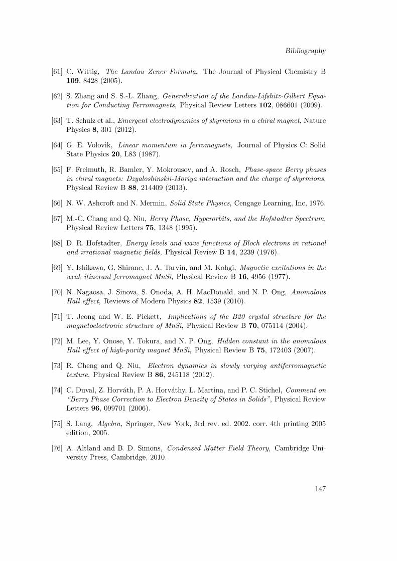
Bibliography
[61] C. Wittig, The Landau–Zener Formula, The Journal of Physical Chemistry B109, 8428 (2005).
[62] S. Zhang and S. S.-L. Zhang, Generalization of the Landau-Lifshitz-Gilbert Equa-tion for Conducting Ferromagnets, Physical Review Letters 102, 086601 (2009).
[63] T. Schulz et al., Emergent electrodynamics of skyrmions in a chiral magnet, NaturePhysics 8, 301 (2012).
[64] G. E. Volovik, Linear momentum in ferromagnets, Journal of Physics C: SolidState Physics 20, L83 (1987).
[65] F. Freimuth, R. Bamler, Y. Mokrousov, and A. Rosch, Phase-space Berry phasesin chiral magnets: Dzyaloshinskii-Moriya interaction and the charge of skyrmions,Physical Review B 88, 214409 (2013).
[66] N. W. Ashcroft and N. Mermin, Solid State Physics, Cengage Learning, Inc, 1976.
[67] M.-C. Chang and Q. Niu, Berry Phase, Hyperorbits, and the Hofstadter Spectrum,Physical Review Letters 75, 1348 (1995).
[68] D. R. Hofstadter, Energy levels and wave functions of Bloch electrons in rationaland irrational magnetic fields, Physical Review B 14, 2239 (1976).
[69] Y. Ishikawa, G. Shirane, J. A. Tarvin, and M. Kohgi, Magnetic excitations in theweak itinerant ferromagnet MnSi, Physical Review B 16, 4956 (1977).
[70] N. Nagaosa, J. Sinova, S. Onoda, A. H. MacDonald, and N. P. Ong, AnomalousHall effect, Reviews of Modern Physics 82, 1539 (2010).
[71] T. Jeong and W. E. Pickett, Implications of the B20 crystal structure for themagnetoelectronic structure of MnSi, Physical Review B 70, 075114 (2004).
[72] M. Lee, Y. Onose, Y. Tokura, and N. P. Ong, Hidden constant in the anomalousHall effect of high-purity magnet MnSi, Physical Review B 75, 172403 (2007).
[73] R. Cheng and Q. Niu, Electron dynamics in slowly varying antiferromagnetictexture, Physical Review B 86, 245118 (2012).
[74] C. Duval, Z. Horvath, P. A. Horvathy, L. Martina, and P. C. Stichel, Comment on“Berry Phase Correction to Electron Density of States in Solids”, Physical ReviewLetters 96, 099701 (2006).
[75] S. Lang, Algebra, Springer, New York, 3rd rev. ed. 2002. corr. 4th printing 2005edition, 2005.
[76] A. Altland and B. D. Simons, Condensed Matter Field Theory, Cambridge Uni-versity Press, Cambridge, 2010.
147
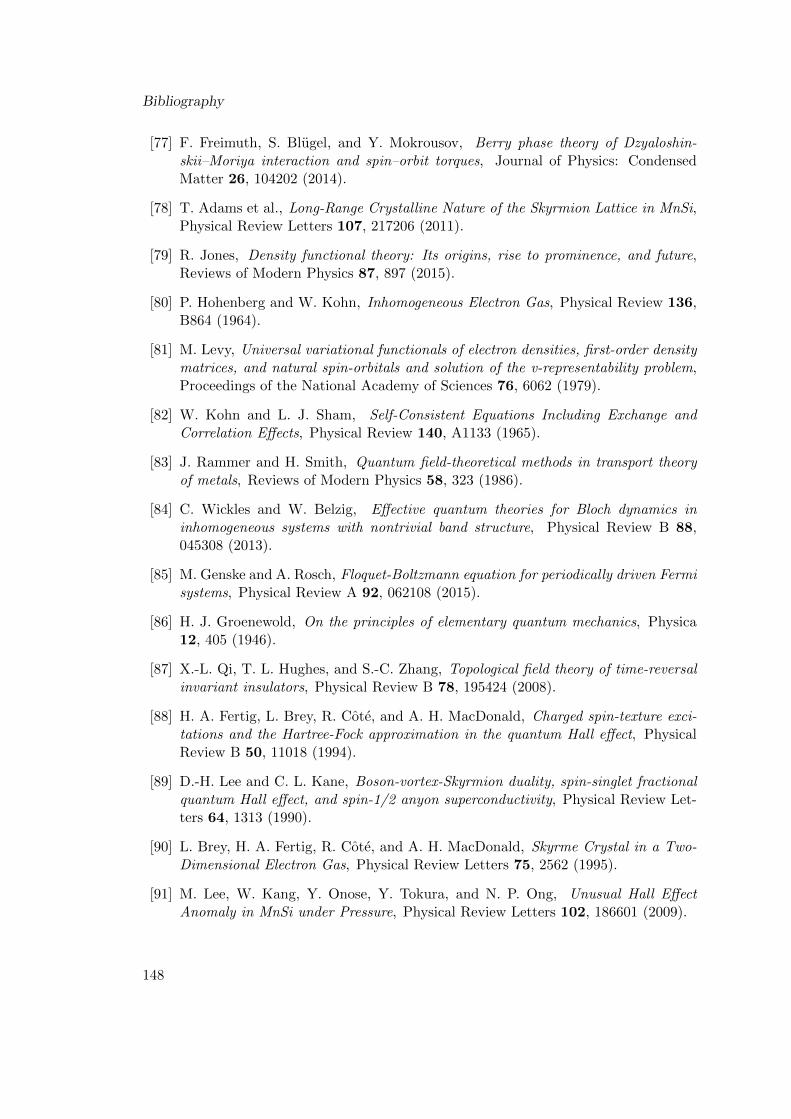
Bibliography
[77] F. Freimuth, S. Blugel, and Y. Mokrousov, Berry phase theory of Dzyaloshin-skii–Moriya interaction and spin–orbit torques, Journal of Physics: CondensedMatter 26, 104202 (2014).
[78] T. Adams et al., Long-Range Crystalline Nature of the Skyrmion Lattice in MnSi,Physical Review Letters 107, 217206 (2011).
[79] R. Jones, Density functional theory: Its origins, rise to prominence, and future,Reviews of Modern Physics 87, 897 (2015).
[80] P. Hohenberg and W. Kohn, Inhomogeneous Electron Gas, Physical Review 136,B864 (1964).
[81] M. Levy, Universal variational functionals of electron densities, first-order densitymatrices, and natural spin-orbitals and solution of the v-representability problem,Proceedings of the National Academy of Sciences 76, 6062 (1979).
[82] W. Kohn and L. J. Sham, Self-Consistent Equations Including Exchange andCorrelation Effects, Physical Review 140, A1133 (1965).
[83] J. Rammer and H. Smith, Quantum field-theoretical methods in transport theoryof metals, Reviews of Modern Physics 58, 323 (1986).
[84] C. Wickles and W. Belzig, Effective quantum theories for Bloch dynamics ininhomogeneous systems with nontrivial band structure, Physical Review B 88,045308 (2013).
[85] M. Genske and A. Rosch, Floquet-Boltzmann equation for periodically driven Fermisystems, Physical Review A 92, 062108 (2015).
[86] H. J. Groenewold, On the principles of elementary quantum mechanics, Physica12, 405 (1946).
[87] X.-L. Qi, T. L. Hughes, and S.-C. Zhang, Topological field theory of time-reversalinvariant insulators, Physical Review B 78, 195424 (2008).
[88] H. A. Fertig, L. Brey, R. Cote, and A. H. MacDonald, Charged spin-texture exci-tations and the Hartree-Fock approximation in the quantum Hall effect, PhysicalReview B 50, 11018 (1994).
[89] D.-H. Lee and C. L. Kane, Boson-vortex-Skyrmion duality, spin-singlet fractionalquantum Hall effect, and spin-1/2 anyon superconductivity, Physical Review Let-ters 64, 1313 (1990).
[90] L. Brey, H. A. Fertig, R. Cote, and A. H. MacDonald, Skyrme Crystal in a Two-Dimensional Electron Gas, Physical Review Letters 75, 2562 (1995).
[91] M. Lee, W. Kang, Y. Onose, Y. Tokura, and N. P. Ong, Unusual Hall EffectAnomaly in MnSi under Pressure, Physical Review Letters 102, 186601 (2009).
148
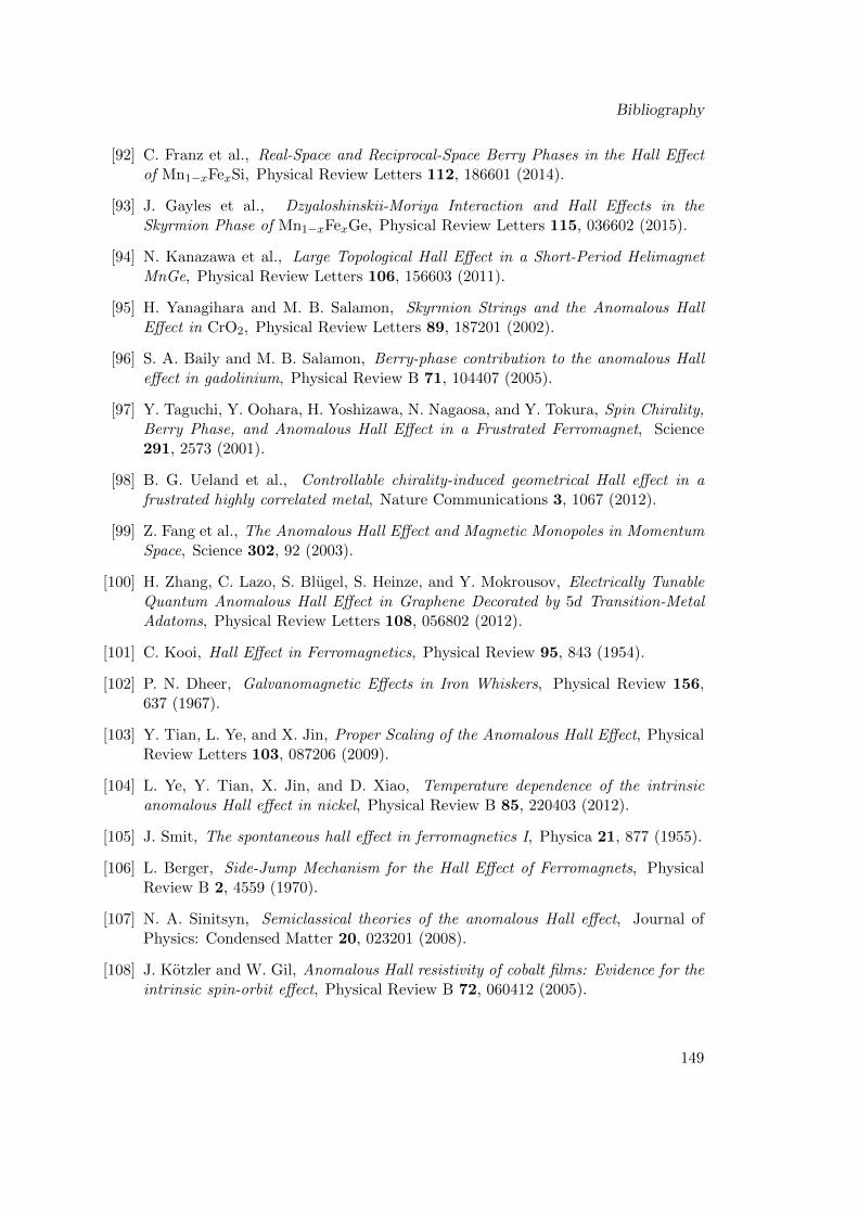
Bibliography
[92] C. Franz et al., Real-Space and Reciprocal-Space Berry Phases in the Hall Effectof Mn1−xFexSi, Physical Review Letters 112, 186601 (2014).
[93] J. Gayles et al., Dzyaloshinskii-Moriya Interaction and Hall Effects in theSkyrmion Phase of Mn1−xFexGe, Physical Review Letters 115, 036602 (2015).
[94] N. Kanazawa et al., Large Topological Hall Effect in a Short-Period HelimagnetMnGe, Physical Review Letters 106, 156603 (2011).
[95] H. Yanagihara and M. B. Salamon, Skyrmion Strings and the Anomalous HallEffect in CrO2, Physical Review Letters 89, 187201 (2002).
[96] S. A. Baily and M. B. Salamon, Berry-phase contribution to the anomalous Halleffect in gadolinium, Physical Review B 71, 104407 (2005).
[97] Y. Taguchi, Y. Oohara, H. Yoshizawa, N. Nagaosa, and Y. Tokura, Spin Chirality,Berry Phase, and Anomalous Hall Effect in a Frustrated Ferromagnet, Science291, 2573 (2001).
[98] B. G. Ueland et al., Controllable chirality-induced geometrical Hall effect in afrustrated highly correlated metal, Nature Communications 3, 1067 (2012).
[99] Z. Fang et al., The Anomalous Hall Effect and Magnetic Monopoles in MomentumSpace, Science 302, 92 (2003).
[100] H. Zhang, C. Lazo, S. Blugel, S. Heinze, and Y. Mokrousov, Electrically TunableQuantum Anomalous Hall Effect in Graphene Decorated by 5d Transition-MetalAdatoms, Physical Review Letters 108, 056802 (2012).
[101] C. Kooi, Hall Effect in Ferromagnetics, Physical Review 95, 843 (1954).
[102] P. N. Dheer, Galvanomagnetic Effects in Iron Whiskers, Physical Review 156,637 (1967).
[103] Y. Tian, L. Ye, and X. Jin, Proper Scaling of the Anomalous Hall Effect, PhysicalReview Letters 103, 087206 (2009).
[104] L. Ye, Y. Tian, X. Jin, and D. Xiao, Temperature dependence of the intrinsicanomalous Hall effect in nickel, Physical Review B 85, 220403 (2012).
[105] J. Smit, The spontaneous hall effect in ferromagnetics I, Physica 21, 877 (1955).
[106] L. Berger, Side-Jump Mechanism for the Hall Effect of Ferromagnets, PhysicalReview B 2, 4559 (1970).
[107] N. A. Sinitsyn, Semiclassical theories of the anomalous Hall effect, Journal ofPhysics: Condensed Matter 20, 023201 (2008).
[108] J. Kotzler and W. Gil, Anomalous Hall resistivity of cobalt films: Evidence for theintrinsic spin-orbit effect, Physical Review B 72, 060412 (2005).
149
Bibliography
[109] J. Weischenberg, F. Freimuth, J. Sinova, S. Blugel, and Y. Mokrousov, Ab InitioTheory of the Scattering-Independent Anomalous Hall Effect, Physical ReviewLetters 107, 106601 (2011).
[110] D. Kodderitzsch, K. Chadova, J. Minar, and H. Ebert, Impact of finite temper-atures and correlations on the anomalous Hall conductivity from ab initio theory,New Journal of Physics 15, 053009 (2013).
[111] P. Czaja, F. Freimuth, J. Weischenberg, S. Blugel, and Y. Mokrousov, AnomalousHall effect in ferromagnets with Gaussian disorder, Physical Review B 89, 014411(2014).
[112] S. Lowitzer, D. Kodderitzsch, and H. Ebert, Coherent Description of the Intrinsicand Extrinsic Anomalous Hall Effect in Disordered Alloys on an Ab Initio Level,Physical Review Letters 105, 266604 (2010).
[113] N. A. Sinitsyn, A. H. MacDonald, T. Jungwirth, V. K. Dugaev, and J. Sinova,Anomalous Hall effect in a two-dimensional Dirac band: The link between theKubo-Streda formula and the semiclassical Boltzmann equation approach, PhysicalReview B 75, 045315 (2007).
[114] I. Turek, J. Kudrnovsky, and V. Drchal, Ab initio theory of galvanomagneticphenomena in ferromagnetic metals and disordered alloys, Physical Review B 86,014405 (2012).
[115] J. Schliemann and D. Loss, Anisotropic transport in a two-dimensional electrongas in the presence of spin-orbit coupling, Physical Review B 68, 165311 (2003).
[116] A. Kamenev, Field Theory of Non-Equilibrium Systems, Cambridge UniversityPress, first edition, 2011.
[117] J. M. Ziman, Electrons and Phonons: The Theory of Transport Phenomena inSolids, Oxford University Press, 2001.
[118] N. A. Sinitsyn, Q. Niu, J. Sinova, and K. Nomura, Disorder effects in the anoma-lous Hall effect induced by Berry curvature, Physical Review B 72, 045346 (2005).
[119] I. A. Ado, I. A. Dmitriev, P. M. Ostrovsky, and M. Titov, Anomalous Hall effectwith massive Dirac fermions, EPL (Europhysics Letters) 111, 37004 (2015).
[120] A. Bastin, C. Lewiner, O. Betbeder-matibet, and P. Nozieres, Quantum oscilla-tions of the hall effect of a fermion gas with random impurity scattering, Journalof Physics and Chemistry of Solids 32, 1811 (1971).
[121] A. Crepieux and P. Bruno, Theory of the anomalous Hall effect from the Kuboformula and the Dirac equation, Physical Review B 64, 014416 (2001).
[122] G. D. Mahan, Many Particle Physics, Springer, 3rd ed. 2000 edition, 2000.
150
Bibliography
[123] P. Streda, Theory of quantised Hall conductivity in two dimensions, Journal ofPhysics C: Solid State Physics 15, L717 (1982).
[124] M. N. Baibich et al., Giant Magnetoresistance of (001)Fe/(001)Cr Magnetic Su-perlattices, Physical Review Letters 61, 2472 (1988).
[125] G. Binasch, P. Grunberg, F. Saurenbach, and W. Zinn, Enhanced magnetoresis-tance in layered magnetic structures with antiferromagnetic interlayer exchange,Physical Review B 39, 4828 (1989).
[126] J. C. Slonczewski, Current-driven excitation of magnetic multilayers, Journal ofMagnetism and Magnetic Materials 159, L1 (1996).
[127] L. Berger, Emission of spin waves by a magnetic multilayer traversed by a current,Physical Review B 54, 9353 (1996).
[128] S. S. P. Parkin, M. Hayashi, and L. Thomas, Magnetic Domain-Wall RacetrackMemory, Science 320, 190 (2008).
[129] L. D. Landau and E. Lifshitz, On the theory of the dispersion of magnetic perme-ability in ferromagnetic bodies, Phys. Z. Sowjetunion 8, 101 (1935).
[130] T. L. Gilbert, A phenomenological theory of damping in ferromagnetic materials,IEEE Transactions on Magnetics 40, 3443 (2004).
[131] S. Zhang and Z. Li, Roles of Nonequilibrium Conduction Electrons on the Magne-tization Dynamics of Ferromagnets, Physical Review Letters 93, 127204 (2004).
[132] M. C. Hickey and J. S. Moodera, Origin of Intrinsic Gilbert Damping, PhysicalReview Letters 102, 137601 (2009).
[133] Y. Tserkovnyak and C. H. Wong, Theory of spin magnetohydrodynamics, PhysicalReview B 79, 014402 (2009).
[134] R. A. Duine, A. S. Nunez, J. Sinova, and A. H. MacDonald, Functional Keldyshtheory of spin torques, Physical Review B 75, 214420 (2007).
[135] L. Hodges, D. R. Stone, and A. V. Gold, Field-Induced Changes in the BandStructure and Fermi Surface of Nickel, Physical Review Letters 19, 655 (1967).
[136] J. Kunes and V. Kambersky, First-principles investigation of the damping offast magnetization precession in ferromagnetic 3d metals, Physical Review B 65,212411 (2002).
[137] K. Gilmore, Y. U. Idzerda, and M. D. Stiles, Identification of the DominantPrecession-Damping Mechanism in Fe, Co, and Ni by First-Principles Calcula-tions, Physical Review Letters 99, 027204 (2007).
151
Bibliography
[138] S. M. Bhagat and P. Lubitz, Temperature variation of ferromagnetic relaxation inthe 3d transition metals, Physical Review B 10, 179 (1974).
[139] D. J. Twisselmann and R. D. McMichael, Intrinsic damping and intentional ferro-magnetic resonance broadening in thin Permalloy films, Journal of Applied Physics93, 6903 (2003).
[140] OOMMF Project at NIST, http://math.nist.gov/oommf/, accessed May 2016.
[141] G. Tatara and H. Kohno, Theory of Current-Driven Domain Wall Motion: SpinTransfer versus Momentum Transfer, Physical Review Letters 92, 086601 (2004).
[142] M. E. Lucassen, H. J. van Driel, C. M. Smith, and R. A. Duine, Current-driven andfield-driven domain walls at nonzero temperature, Physical Review B 79, 224411(2009).
[143] C. Burrowes et al., Non-adiabatic spin-torques in narrow magnetic domain walls,Nature Physics 6, 17 (2010).
[144] C. Schutte and M. Garst, Magnon-skyrmion scattering in chiral magnets, PhysicalReview B 90, 094423 (2014).
[145] A. Kamenev and A. Levchenko, Keldysh technique and non-linear sigma-model:basic principles and applications, Advances in Physics 58, 197 (2009).
[146] M. Mochizuki et al., Thermally driven ratchet motion of a skyrmion microcrystaland topological magnon Hall effect, Nature Materials 13, 241 (2014).
[147] S. Schroeter and M. Garst, Scattering of high-energy magnons off a magneticskyrmion, Low Temperature Physics 41, 817 (2015).
[148] B.-J. Yang and N. Nagaosa, Skyrmion quantum numbers and quantized pumping intwo-dimensional topological chiral magnets, Physical Review B 84, 245123 (2011).
[149] S. Ryu, A. P. Schnyder, A. Furusaki, and A. W. W. Ludwig, Topological insulatorsand superconductors: tenfold way and dimensional hierarchy, New Journal ofPhysics 12, 065010 (2010).
152
Bibliography
153

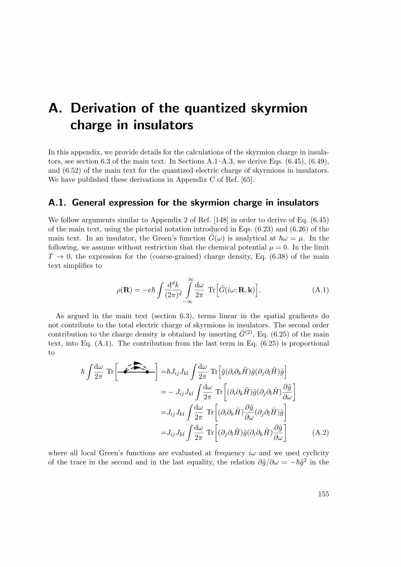
A. Derivation of the quantized skyrmioncharge in insulators
In this appendix, we provide details for the calculations of the skyrmion charge in insula-tors, see section 6.3 of the main text. In Sections A.1–A.3, we derive Eqs. (6.45), (6.49),and (6.52) of the main text for the quantized electric charge of skyrmions in insulators.We have published these derivations in Appendix C of Ref. [65].
A.1. General expression for the skyrmion charge in insulators
We follow arguments similar to Appendix 2 of Ref. [148] in order to derive of Eq. (6.45)of the main text, using the pictorial notation introduced in Eqs. (6.23) and (6.26) of themain text. In an insulator, the Green’s function G(ω) is analytical at ~ω = µ. In thefollowing, we assume without restriction that the chemical potential µ = 0. In the limitT → 0, the expression for the (coarse-grained) charge density, Eq. (6.38) of the maintext simplifies to
ρ(R) = −e~∫
ddk
(2π)d
∞∫−∞
dω
2πTr[G(iω; R,k)
]. (A.1)
As argued in the main text (section 6.3), terms linear in the spatial gradients donot contribute to the total electric charge of skyrmions in insulators. The second ordercontribution to the charge density is obtained by inserting G(2), Eq. (6.25) of the maintext, into Eq. (A.1). The contribution from the last term in Eq. (6.25) is proportionalto
~∫
dω
2πTr
[ ]=~JijJkl
∫dω
2πTr[g(∂i∂kH)g(∂j∂lH)g
]=− JijJkl
∫dω
2πTr
[(∂i∂kH)g(∂j∂lH)
∂g
∂ω
]=JijJkl
∫dω
2πTr
[(∂i∂kH)
∂g
∂ω(∂j∂lH)g
]=JijJkl
∫dω
2πTr
[(∂j∂lH)g(∂i∂kH)
∂g
∂ω
](A.2)
where all local Green’s functions are evaluated at frequency iω and we used cyclicityof the trace in the second and in the last equality, the relation ∂g/∂ω = −~g2 in the
155
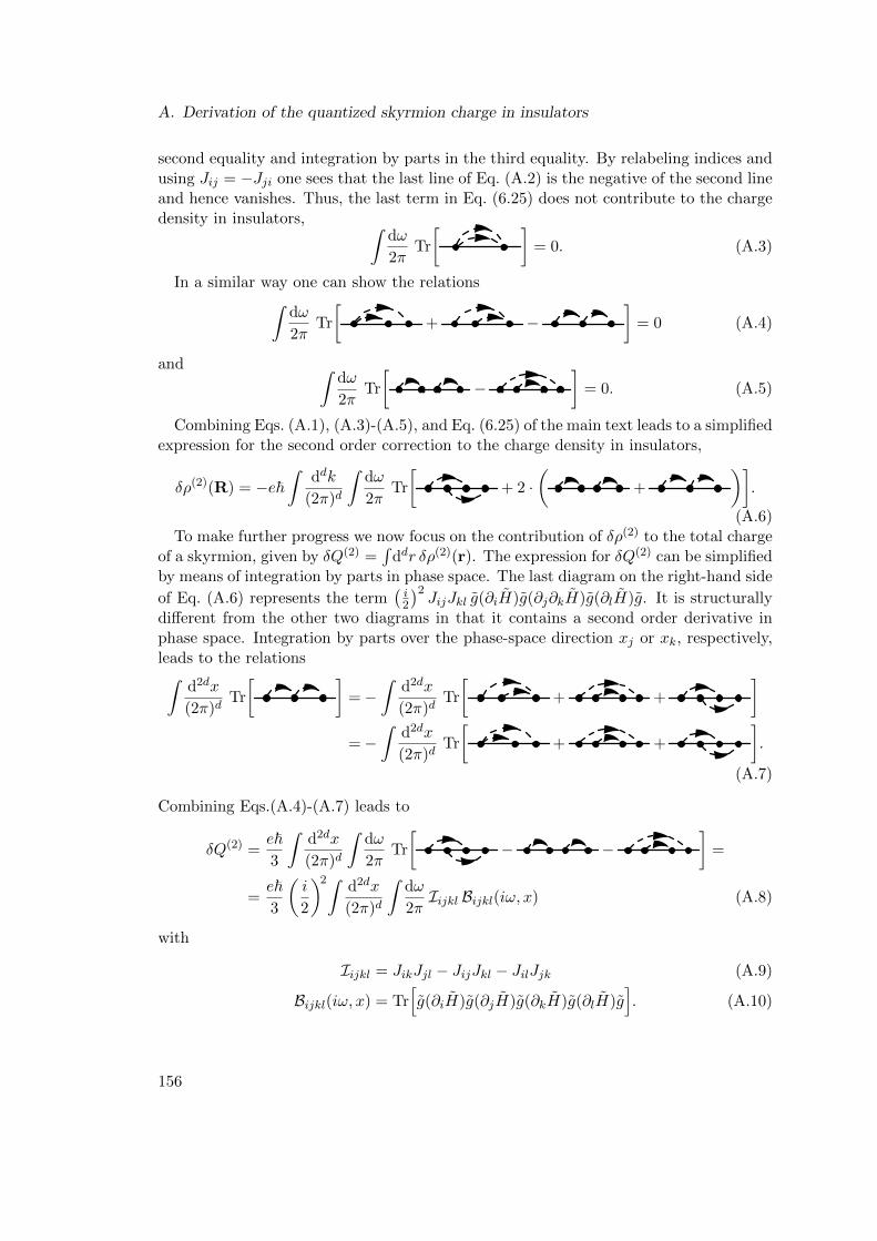
A. Derivation of the quantized skyrmion charge in insulators
second equality and integration by parts in the third equality. By relabeling indices andusing Jij = −Jji one sees that the last line of Eq. (A.2) is the negative of the second lineand hence vanishes. Thus, the last term in Eq. (6.25) does not contribute to the chargedensity in insulators, ∫
dω
2πTr
[ ]= 0. (A.3)
In a similar way one can show the relations∫dω
2πTr
[+ −
]= 0 (A.4)
and ∫dω
2πTr
[−
]= 0. (A.5)
Combining Eqs. (A.1), (A.3)-(A.5), and Eq. (6.25) of the main text leads to a simplifiedexpression for the second order correction to the charge density in insulators,
δρ(2)(R) = −e~∫
ddk
(2π)d
∫dω
2πTr
[+ 2 ·
(+
)].
(A.6)To make further progress we now focus on the contribution of δρ(2) to the total charge
of a skyrmion, given by δQ(2) =∫
ddr δρ(2)(r). The expression for δQ(2) can be simplifiedby means of integration by parts in phase space. The last diagram on the right-hand side
of Eq. (A.6) represents the term(i2
)2JijJkl g(∂iH)g(∂j∂kH)g(∂lH)g. It is structurally
different from the other two diagrams in that it contains a second order derivative inphase space. Integration by parts over the phase-space direction xj or xk, respectively,leads to the relations∫
d2dx
(2π)dTr
[ ]=−
∫d2dx
(2π)dTr
[+ +
]=−
∫d2dx
(2π)dTr
[+ +
].
(A.7)
Combining Eqs.(A.4)-(A.7) leads to
δQ(2) =e~3
∫d2dx
(2π)d
∫dω
2πTr
[− −
]=
=e~3
(i
2
)2∫ d2dx
(2π)d
∫dω
2πIijkl Bijkl(iω, x) (A.8)
with
Iijkl = JikJjl − JijJkl − JilJjk (A.9)
Bijkl(iω, x) = Tr[g(∂iH)g(∂jH)g(∂kH)g(∂lH)g
]. (A.10)
156
A.2. Factorization of the skyrmion charge in two-dimensional insulators with Abelian Berry curvature
Evidently, Iijkl is totally anti-symmetric in all indices. For d = 2 and d = 3 dimensions,one finds that Iijkl is given by Eq. (6.46) of the main text. This concludes the derivationof Eq. (6.45) of the main text.
A.2. Factorization of the skyrmion charge in two-dimensionalinsulators with Abelian Berry curvature
In this section we show that the Berry curvature contribution to the charge in a two-dimensional insulator with Abelian Berry curvature is given by the product of the quan-tized Hall conductivity σxy and the skyrmion number Φ0, see Eq. (6.49) of the maintext. A purely Abelian Berry curvature arises, e.g., if only a single band is occupied.
For a two-dimensional system with only one occupied band, Eq. (6.47) of the maintext reduces to
δQ(2) =e
8εijkl
∫d4x
(2π)2ΩijΩkl =
e
4εijkl
(∫dxj dxk dxl
(2π)2AjΩkl
)xi=+∞
xi=−∞(A.11)
where, for a space (momentum) direction xi, the symbols ±∞ denote positions far awayfrom the skyrmion (the boundaries of the Brillouin zone). In the second equality ofEq. (A.11), we used the relation
εijkl8
ΩijΩkl =εijkl
2
∂Aj∂xi
∂Al∂xk
=εijkl
2
∂
∂xi
(Aj
∂Al∂xk
)=εijkl
4
∂
∂xi(AjΩkl) (A.12)
where A is the Berry connection.
In Eq. (A.11), Ωkl only enters at the boundary of the xi coordinate. At the boundaryin a spatial direction (i.e., far away from the skyrmion), the magnetization is collinearand therefore Ωr,r = 0 = Ωr,k. Thus, if xi is a spatial coordinate, only terms of the formArjΩ
k,kkl contribute to the integrand in Eq. (A.11). If xi is a momentum coordinate, Ωkl
is evaluated at the boundary of the Brillouin zone. In an insulator, the charge mustbe quantized and we can adiabatically deform the Bloch functions such that they areindependent of momentum in a narrow stripe around the Brillouin zone boundary. This isalways possible since, in absence of further symmetries, all non-interacting Hamiltoniansof one-dimensional insulators are adiabatically connected [149]. Therefore, only termsof the form Ak
jΩr,rkl contribute if xi is a momentum coordinate. In total, Eq. (A.11) can
be written as δQ(2) = δQ(2),r + δQ(2),k where
δQ(2),r =e
2εij
(∫drj d2k
(2π)2ArjΩ
k,kxy
)ri=+∞
ri=−∞(A.13)
and δQ(2),k is defined by formally exchanging all r and k. As the Berry curvature Ωk,kxy
in Eq. (A.13) is gauge independent, it cannot depend on rj for a collinear magnetization
157
A. Derivation of the quantized skyrmion charge in insulators
at ri = ±∞. This implies
δQ(2),r =e
2εij
∫d2k
(2π)2
(Ωk,kxy
∫drj(Ar
j)ri=+∞ri=−∞
)=e
2
∫d2k
(2π)2
(Ωk,kxy
∫d2r εij
∂Arj
∂ri
)=e
2
∫d2k
(2π)2
(Ωk,kxy
∫d2rΩr,r
xy
)=
1
2σxyΦ0 (A.14)
where σxy (Φ0) is the quantized integral over e2
~ Ωk,kxy (~eΩr,r
xy) defined in Eqs. (6.50) and
(6.51) of the main text. An analogous calculation leads to the same value for δQ(2),k.Thus, we conclude that the Berry curvature contribution to the skyrmion charge in atwo-dimensional insulator with Abelian Berry curvature is given by Eq. (6.49) of themain text.
A.3. Skyrmion charge per length in three-dimensionalinsulators with Abelian Berry curvature
In three dimensional systems, skyrmions form line defects. In this section, we derive anexpression for the charge per length of a skyrmion line, see Eq. (6.52) of the main text.From Eqs. (6.46) and (6.47) of the main text, the Berry curvature contribution to thecharge in a three dimensional insulator is given by
δQ(2) = eεijklqrJqr
16
∫d6x
(2π)3Tr[ΩijΩkl
](A.15)
We introduce dimensionless phase-space coordinates x ≡ (r, k) such that r = rαaαand k = kαgα/(2π). Here, latin indices run from 1 to 6 while greek indices run from 1 to3, the vectors aα are lattice vectors of the atomic lattice and gα are the correspondingreciprocal lattice vectors. We chose the coordinates x such that momentum space isperiodic in the three coordinate directions kα and the Jacobian of the transformationx = x(x) is one. Thus, in the dimensionless coordinates, Eq. (A.15) becomes
δQ(2) =e εijklqr
16
∫d6x
(2π)3ΩijΩklJqr
= e
3∑α=1
∫drα
∫dkα2π
εijklα(α+3)
8
∫d4x
(2π)2ΩijΩkl
= e
3∑α=1
∫drα
∫dkα2π
nrαn
kα (A.16)
158
A.3. Skyrmion charge per length in three-dimensional insulators with Abelian Berry curvature
with1
nrα =
εαβγ4π
∫drβdrγ Ωr,r
βγ ∈ Z; nkα =
εαµν4π
∫dkµdkν Ωk,k
µν ∈ Z. (A.17)
In the first line of Eq. (A.16), Ωij denotes the elements of the Berry curvature tensorin coordinates x. The components of the symplectic tensor Jqr are invariant underthe transformation from coordinates x to x due to the relation aα · gβ = 2πδij . Thisallowed us to set β = α + 3 in the second line of Eq. (A.16). The last integral inthe second line of Eq. (A.16) runs over the four dimensional subspace of phase spaceperpendicular to (0,aα) and (gα,0). Its value is given by the product of the real-spaceand the momentum-space winding numbers, nr
α and nkα, by the same arguments that
lead to the factorization of winding numbers in the two-dimensional case discussed inAppendix A.2.
The remaining integral over kα in Eq. (A.16) equates to a factor of 1 and the integralover rα gives ∫
drα =∂rα∂rβ
∫drβ =
(gα)β2π
Lβ =s · gα
2πL (A.18)
where the unit vector s points along along the skyrmion line and Lβ = Lsβ is the projec-tion of the length L of the skyrmion line onto the coordinate direction rβ. For a genericskyrmion line that pierces all three position-space coordinate planes, the skyrmion num-ber is nr
α = 1 for all α. Combining Eqs. (A.16) and (A.18), we arrive at Eq. (6.52) ofthe main text.
1In Appendix C.4 of Ref. [65], we defined nrα and nk
α with different prefactors. Here, we opted forprefactors that make both winding numbers integer quantities.
159

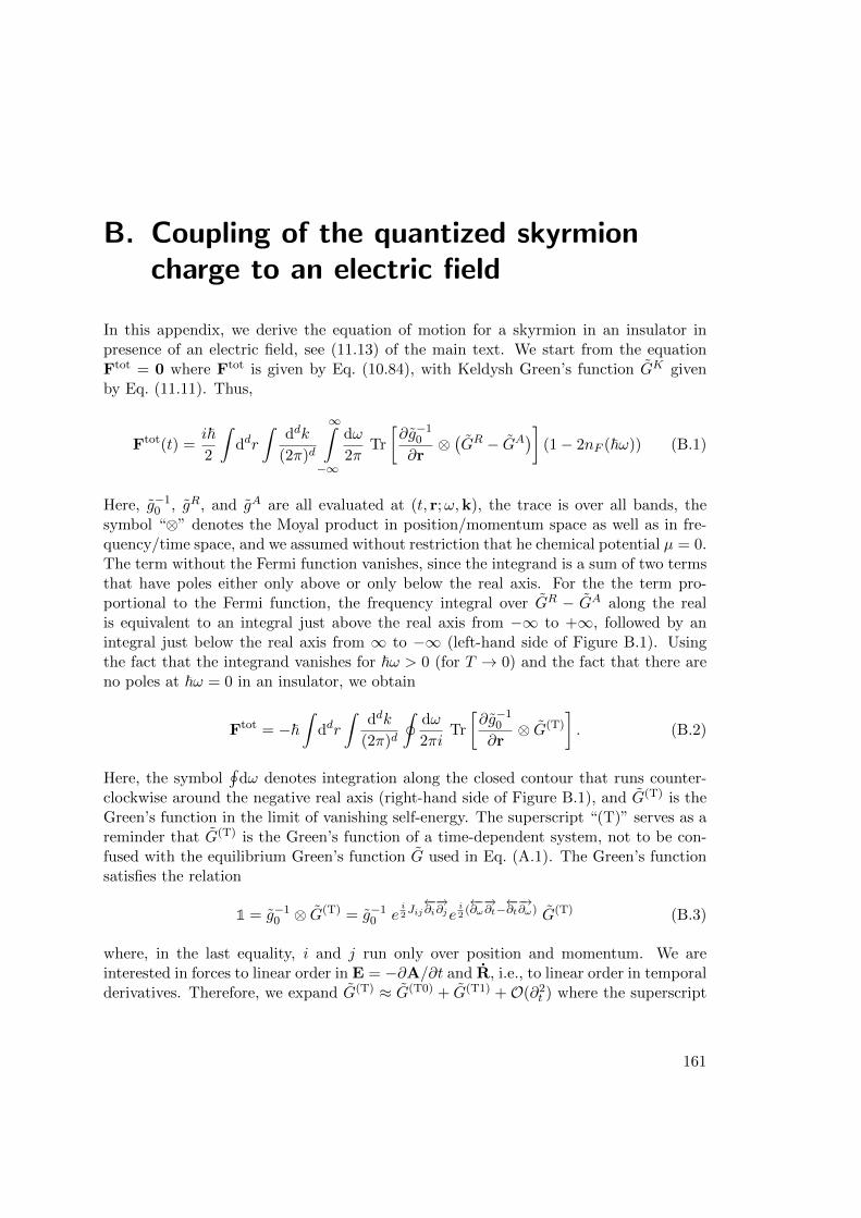
B. Coupling of the quantized skyrmioncharge to an electric field
In this appendix, we derive the equation of motion for a skyrmion in an insulator inpresence of an electric field, see (11.13) of the main text. We start from the equationFtot = 0 where Ftot is given by Eq. (10.84), with Keldysh Green’s function GK givenby Eq. (11.11). Thus,
Ftot(t) =i~2
∫ddr
∫ddk
(2π)d
∞∫−∞
dω
2πTr
[∂g−1
0
∂r⊗(GR − GA
)](1− 2nF (~ω)) (B.1)
Here, g−10 , gR, and gA are all evaluated at (t, r;ω,k), the trace is over all bands, the
symbol “⊗” denotes the Moyal product in position/momentum space as well as in fre-quency/time space, and we assumed without restriction that he chemical potential µ = 0.The term without the Fermi function vanishes, since the integrand is a sum of two termsthat have poles either only above or only below the real axis. For the the term pro-portional to the Fermi function, the frequency integral over GR − GA along the realis equivalent to an integral just above the real axis from −∞ to +∞, followed by anintegral just below the real axis from ∞ to −∞ (left-hand side of Figure B.1). Usingthe fact that the integrand vanishes for ~ω > 0 (for T → 0) and the fact that there areno poles at ~ω = 0 in an insulator, we obtain
Ftot = −~∫
ddr
∫ddk
(2π)d
∮dω
2πiTr
[∂g−1
0
∂r⊗ G(T)
]. (B.2)
Here, the symbol∮
dω denotes integration along the closed contour that runs counter-clockwise around the negative real axis (right-hand side of Figure B.1), and G(T) is theGreen’s function in the limit of vanishing self-energy. The superscript “(T)” serves as areminder that G(T) is the Green’s function of a time-dependent system, not to be con-fused with the equilibrium Green’s function G used in Eq. (A.1). The Green’s functionsatisfies the relation
1 = g−10 ⊗ G
(T) = g−10 e
i2Jij←−∂i−→∂je
i2
(←−∂ω−→∂t−←−∂t−→∂ω) G(T) (B.3)
where, in the last equality, i and j run only over position and momentum. We areinterested in forces to linear order in E = −∂A/∂t and R, i.e., to linear order in temporalderivatives. Therefore, we expand G(T) ≈ G(T0) + G(T1) +O(∂2
t ) where the superscript
161
B. Coupling of the quantized skyrmion charge to an electric field
Figure B.1.: Transformation of the interal∫∞−∞dω (GR −GA) into an integral around a
closed contour, see Eqs. (B.1)–(B.2). The blue shaded regions indicate thepositions of poles of the Green’s function.
denotes the order in temporal derivatives. From Eq. (B.3), we obtain
1 = g−10 G
(T0); (B.4)
0 = g−10 G
(T1) +i
2
(~∂G(T0)
∂t− ∂g−1
0
∂t ∂G
(T0)
∂ω
). (B.5)
Here, the symbol “” denotes the Moyal product in position/momentum space only,and we used ∂g−1
0 /∂ω = ~. Eq. (B.4) is equivalent to the the defining equation of theequilibrium Green’s function G in a time-independent system, see Eq. (6.18) of the maintext, and therefore G(T0) = G. Inserting G into Eq. (B.2), one obtains the force on aresting skyrmion in absence of an electric field, which vanishes as argued at the end ofSection 10.4 of the main text. By solving Eqs. (B.4)–(B.5) for G(T1) and inserting intoEq. (B.3), we obtain after some partial integrations,
F (T1)α = − i~
2
2
∫ddr
∫ddk
(2π)d
∮dω
2πiTr
[G
(∂g−1
0
∂rα ∂G∂t− ∂g−1
0
∂t ∂G∂rα
)]. (B.6)
In the derivation of Eq. (B.6), we used g−10 G = 1, cf., Eq. (B.4), ∂g−1
0 /∂ω = ~, andpartial integration. While there is no integral over time, we can nevertheless use partialintegration for temporal derivatives, since they are equivalent to derivatives in positionand momentum space via the relation
∂t = − e~
E · ∂k − R · ∂r. (B.7)
We now expand F(T1)α = F
(T1,0)α + F
(T1,1)α + . . . in spatial gradients. The lowest order
contribution is
F (T1,0)α = − i~
2
2
∫ddr
∫ddk
(2π)d
∮dω
2πiTr
[g0
(∂g−1
0
∂rα
∂g0
∂t− ∂g−1
0
∂t
∂g0
∂rα
)]= +
i~2
∫ddr
∫ddk
(2π)d
∮dω
2πiJ ′ij Tr
[g0(∂iH)g0(∂jH)g0
]. (B.8)
Here, i and j run over position, momentum, time, and frequency, and J ′ is an anti-symmetric tensor whose only non-vanishing components are
J ′rα,t = 1 and J ′t,rα = −1. (B.9)
162
We evaluate the frequency integral using residue theorem and the relation
g0(t, r;ω,k) =∑n
|un,t,k〉〈un,t,k|~ω − E(0)(t, r;ω,k)
. (B.10)
Finally, using Eq. (3.18) of the main text, we obtain
F (T1,0)α =
∑n occ.
∫ddr
∫ddk
(2π)d
(~Ωr,r
n,αjRj + eΩr,kn,αjEj
)(B.11)
where the sum runs over all occupied bands n. The first term on the right-hand side ofEq. (B.11) is the gyro-coupling −G × R, cf., Eqs. (11.3) and (11.4) of the main text.The second term is the first chern number in the plane spanned by rα and kj . As arguedin the main text, this term vanishes if position space can be compactified, i.e., if themagnetization is collinear far away from the skyrmion.
Gradient corrections to F(T1,0)α come in two varieties. First gradient corrections to
the Green’s functions G in Eq. (B.6) are given to first order by Eq. (6.23) of the maintext. Second, the Moyal products in Eq. (B.6) contain gradient corrections. Here, onlythe inner Moyal products have to be takein into account, since all gradient contributionsfrom the outer Moyal product vanish by partial integration. We obtain for the leading
correction to F(T1,0)α ,
F (T1,1)α = ~2
∫ddr
∫ddk
(2π)d
∮dω
2πiTr
[ ′+
′
+1
2
( ′
+
′ )]. (B.12)
Here, we used again the pictorial notation introduced in Section 6.2 with one additionalbuilding block: a primed line with an arrow denotes contraction with the matrix J ′
instead of J , see Eq. (B.9). For example, the last diagram on the right-hand side ofEq. (B.12) denotes the term
′
≡(i
2
)2
JijJ′kl g0(−∂iH)g0(−∂j∂kH)g0(−∂lH)g0. (B.13)
One can easily generalize Eqs. (A.4), (A.5), and (A.7) to the situation where thetwo Moyal contractions are performed with different matrices J and J ′. Using theserelations, we find
F (T1,1)α = −~2
3
∫ddr
∫ddk
(2π)d
∮dω
2πiTr
[ ′
+
′
−′
−′
−′
−′ ]
= −~2
3
(i
2
)2 ∫ddr
∫ddk
(2π)d
∮dω
2πiI ′ijkl Bijkl(t, r;ω,k) (B.14)
163
B. Coupling of the quantized skyrmion charge to an electric field
where Bijkl is given in Eq. (A.10) and
I ′ijkl = J ′ikJjl + JikJ′jl − J ′ijJkl − JijJ ′kl − J ′ilJjk − JilJ ′jk. (B.15)
Evidently, I ′ijkl is totally antisymmetric in all indices. Of the coordinates i, j, k, and l,exactly one is the time, one is rα, and the other two are a pair (rβ, kβ) of conjugatedposition and momentum directions, with α 6= β due to the anti-symmetry. When weexpress the temporal derivative in terms of position and momentum derivatives viaEq. (B.7), only the term − e
~Eα∂kα survives the anti-symmetrization in a two-dimensionalsystem. This is also true for a skyrmion tube in a three-dimensional system if we assumethat the electric field is perpendicular to the skyrmion tube, since spatial derivativesalong the symmetry axis of the skyrmion tube vanish. Thus, we obtain
F (T1,1)α =
e~3
(i
2
)2
Eα
∫ddr
∫ddk
(2π)d
∮dω
2πiIijklBijkl(t, r;ω,k) (B.16)
where the indices i, j, k, and l run over position and momentum and Iijkl is given inEq. (A.9). Opening the integration contour at ω → −∞ and deforming it to run alongthe imaginary axis from −i∞ to +i∞ leads to
F (T1,1)α = −δQ(2)Eα (B.17)
where δQ(2) is given in Eq. (A.8). Eqs. (B.11) and (B.17) conclude the derivation ofEq. (11.13) of the main text.
164
Acknowledgments
I would like to thank my thesis supervisor Prof. Dr. Achim Rosch for his invaluablesupport and guidance during the past years. It has been a great pleasure to work withhim and to learn from him about physics and beyond. His deeply respectful treatmentof any questions and his clearly visible joy in both identifying and solving physicalproblems have provided great conditions for working on this thesis. Fruitful discussionswith PD Dr. Markus Garst, Dr. Dmitry Bagrets, and Prof. Dr. Philipp Strack at theInstitute for Theoretical Physics in Cologne have cleared up many problems, for whichI am thankful. I thank Dr. Frank Freimuth and Prof. Dr. Yuriy Mokrousov for theconstructive cooperation and their openness for exchanging ideas. Discussions withProf. Dr. Christian Pfleiderer, Prof. Dr. Jairo Sinova, and Prof. Dr. Stefan Blugel havehelped me stay focused on the right topics. I also thank Prof. Dr. Alexander Altlandand Prof. Dr. Paul van Loosdrecht for reviewing this thesis.
I am grateful for financial and intellectual support by Deutsche Telekom Stiftungand I would like to express my thanks to Christiane Frense-Heck for providing personalguidance. I am equally grateful to the Bonn-Cologne Graduate School of Physics andAstronomy, and to Dr. Petra Neubauer-Guenther.
Over the past years, I have had exchanges with many fellow students at the physicsinstitute and I have greatly enjoyed the working environment and the team spirit thatarises from our joint seminars and activities. Of the many people, I would like to mentionin particular the ones I shared an office with: Karin Everschor-Sitte, Stephan Mandt,Christoph Schutte, Maximilian Genske, Sarah Schroeter, Laura Kohler, and JohannesWaizner, in order of appearance. It has been a pleasure working with you all! Thanksespecially to Karin, who helped me getting started during my first weeks in Cologne,and Maximilian, who has been a great colleague both at the physics institute and atphysics outreach programs.
Thanks to Mariela Boevska, Ute Graffenberger, Dorothea Hochscheid, Birgit Micheel,and Yasemin Tieben for great administrative support, to Dr. Andreas Sindermann fortechnical support and for so efficiently coordinating all correspondence with the centraladministration, and to Torsten Held and Daniel Klemmer for managing the supply ofthe Joyful Coffee Community of the University of Cologne.
Finally, I would like to express my sincere thanks to all my friends, my brother RichardBamler, and my parents for their unconditional support.

Erklarung
Ich versichere, dass ich die von mir vorgelegte Dissertation selbstandig angefertigt, diebenutzten Quellen und Hilfsmittel vollstandig angegeben und die Stellen der Arbeit – ein-schließlich Tabellen, Karten und Abbildungen –, die anderen Werken im Wortlaut oderdem Sinn nach entnommen sind, in jedem Einzelfall als Entlehnung kenntlich gemachthabe; dass diese Dissertation noch keiner anderen Fakultat oder Universitat zur Prufungvorgelegen hat; dass sie – abgesehen von unten angegebenen Teilpublikationen – nochnicht veroffentlicht worden ist sowie, dass ich eine solche Veroffentlichung vor Abschlussdes Promotionsverfahrens nicht vornehmen werde. Die Bestimmungen der Promotion-sordnung sind mir bekannt. Die von mir vorgelegte Dissertation ist von Prof. Dr. AchimRosch betreut worden.
Koln, den 22. August 2016
Teilpublikationen
• R. Ritz, M. Halder, C. Franz, A. Bauer, M. Wagner, R. Bamler, A. Rosch, and C.Pfleiderer,Giant generic topological Hall resistivity of MnSi under pressure,Phys. Rev. B 87, 134424 (2013)
• F. Freimuth, R. Bamler, Y. Mokrousov, and A. Rosch,Phase-space Berry phases in chiral magnets: Dzyaloshinskii-Moriya interactionand the charge of skyrmions,Phys. Rev. B 88, 214409 (2013)
• R. Bamler and A. Rosch,Equilibration and approximate conservation laws: Dipole oscillations and perfectdrag of ultracold atoms in a harmonic trap,Phys. Rev. A 91, 063604 (2015)