Practical Numerical Training UKNum - MPIA.demordasini/UKNUM/statistics.pdf · Practical Numerical...

Practical Numerical Training UKNumStatistik, Datenmodellierung

PD. Dr. C. Mordasini

Max-Planck-Institute für Astronomie, Heidelberg

Programm:1) Repetition elementare Statistik2) Regressionsanalyse3) Lineare Regression 4) Nicht-lineare Regression

1 Elementare Statistik

•Studiere ein statistisches Datensample mit n Werten, z.b. Messwerten.•Das Sample/Stichprobe kann mit sogenannten Momenten charakterisiert werden. Dies sind Summen von ganzzahligen Potenzen der Werte.

Einfache statistische Grössen I

Arithmetischer MittelwertGibt den mittleren Wert der Messwerte an

06.01.2 Chapter 06.01

characteristics) or not. The arithmetic mean of a sample is a measure of its central tendency and is evaluated by dividing the sum of individual data points by the number of points. Consider Table 1 which 14 measurements of the concentration of sodium chlorate produced in a chemical reactor operated at a pH of 7.0. Table 1 Chlorate ion concentration in 3mmol/cm

12.0 15.0 14.1 15.9 11.5 14.8 11.2 13.7 15.9 12.6 14.3 12.6 12.1 14.8 The arithmetic mean y is mathematically defined as

n

yy

n

ii¦

1 (1)

which is the sum of the individual data points iy divided by the number of data points n . One of the measures of the spread of the data is the range of the data. The range R is defined as the difference between the maximum and minimum value of the data as minmax yyR � (2) where maxy is the maximum of the values of iy , ,,...,2,1 ni miny is the minimum of the values of iy , .,...,2,1 ni . However, range may not give a good idea of the spread of the data as some data points may be far away from most other data points (such data points are called outliers). That is why the deviation from the average or arithmetic mean is looked as a better way to measure the spread. The residual between the data point and the mean is defined as yye ii � (3) The difference of each data point from the mean can be negative or positive depending on which side of the mean the data point lies (recall the mean is centrally located) and hence if one calculates the sum of such differences to find the overall spread, the differences may simply cancel each other. That is why the sum of the square of the differences is considered a better measure. The sum of the squares of the differences, also called summed squared error (SSE), tS , is given by

� �¦

� n

iit yyS

1

2 (4)

Since the magnitude of the summed squared error is dependent on the number of data points, an average value of the summed squared error is defined as the variance, 2V

� �

111

2

2

�

�

�

¦

n

yy

nS

n

ii

tV (5)

The variance, 2V is sometimes written in two different convenient formulas as

Alternativen sind der Median oder der Mode.

Range

06.01.2 Chapter 06.01



n

yy

n

ii¦

1 (1)


� �¦

� n

iit yyS

1

2 (4)


� �

111

2

2

�

�

�

¦

n

yy

nS

n

ii

tV (5)


06.01.2 Chapter 06.01



n

yy

n

ii¦

1 (1)


� �¦

� n

iit yyS

1

2 (4)


� �

111

2

2

�

�

�

¦

n

yy

nS

n

ii

tV (5)


Problem: Ausreisser

Residuum/FehlerDas Residuum i zwischen einem Datenwert i und dem Mittelwert ist

06.01.2 Chapter 06.01



n

yy

n

ii¦

1 (1)


� �¦

� n

iit yyS

1

2 (4)


� �

111

2

2

�

�

�

¦

n

yy

nS

n

ii

tV (5)


Das Residuum kann positiv oder negativ sein, daher kann die Summe der Residuen über das ganze Datensample (zufällig) gleich Null sein da sich die Residuen gegenseitig auslöschen können. Daher ist die Summe der Quadrate der Residuen ein besseres Mass.

Summe der Fehlerquadrate

06.01.2 Chapter 06.01



n

yy

n

ii¦

1 (1)


� �¦

� n

iit yyS

1

2 (4)


� �

111

2

2

�

�

�

¦

n

yy

nS

n

ii

tV (5)


Der Betrag der Summe der Fehlerquadrate ist offensichtlich von der Anzahl Datenpunkte abhängig. Daher suchen wir einen Mittelwert.

Einfache statistische Grössen II

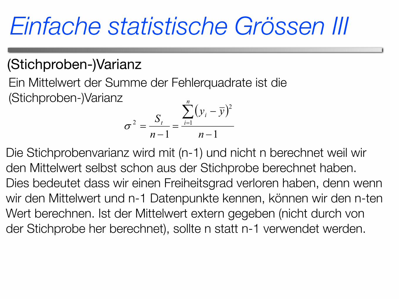
(Stichproben-)VarianzEin Mittelwert der Summe der Fehlerquadrate ist die (Stichproben-)Varianz

06.01.2 Chapter 06.01



n

yy

n

ii¦

1 (1)


� �¦

� n

iit yyS

1

2 (4)


� �

111

2

2

�

�

�

¦

n

yy

nS

n

ii

tV (5)

The variance, 2V is sometimes written in two different convenient formulas as Die Stichprobenvarianz wird mit (n-1) und nicht n berechnet weil wir den Mittelwert selbst schon aus der Stichprobe berechnet haben. Dies bedeutet dass wir einen Freiheitsgrad verloren haben, denn wenn wir den Mittelwert und n-1 Datenpunkte kennen, können wir den n-ten Wert berechnen. Ist der Mittelwert extern gegeben (nicht durch von der Stichprobe her berechnet), sollte n statt n-1 verwendet werden.

Einfache statistische Grössen III

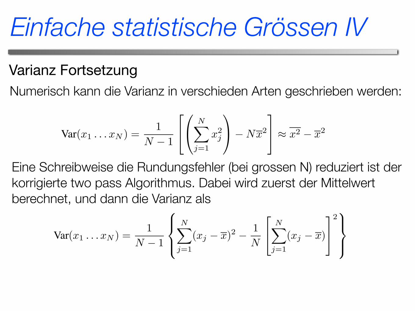
Varianz FortsetzungNumerisch kann die Varianz in verschieden Arten geschrieben werden:

14.1 Moments of a Distribution: Mean, Variance, Skewness 607Sam

ple page from NUM

ERICAL RECIPES IN FORTRAN 77: THE ART O

F SCIENTIFIC COM

PUTING (ISBN 0-521-43064-X)

Copyright (C) 1986-1992 by Cambridge University Press.Program

s Copyright (C) 1986-1992 by Numerical Recipes Software.

Permission is granted for internet users to m

ake one paper copy for their own personal use. Further reproduction, or any copying of machine-

readable files (including this one) to any servercomputer, is strictly prohibited. To order Num

erical Recipes booksor CDRO

Ms, visit website

http://www.nr.com or call 1-800-872-7423 (North Am

erica only),or send email to directcustserv@

cambridge.org (outside North Am

erica).where the !3 term makes the value zero for a normal distribution.

The standard deviation of (14.1.6) as an estimator of the kurtosis of an underlyingnormal distribution is

!

96/N when ! is the true standard deviation, and!

24/Nwhen it is the sample estimate (14.1.3). However, the kurtosis depends on sucha high moment that there are many real-life distributions for which the standarddeviation of (14.1.6) as an estimator is effectively infinite.

Calculation of the quantities defined in this section is perfectly straightforward.Many textbooks use the binomial theorem to expand out the definitions into sumsof various powers of the data, e.g., the familiar

Var(x1 . . . xN ) =1

N ! 1

"

#

$

%

N&

j=1

x2j

'

( ! Nx2

)

* " x2 ! x2 (14.1.7)

but this can magnify the roundoff error by a large factor and is generally unjustifiablein terms of computing speed. A clever way to minimize roundoff error, especiallyfor large samples, is to use the corrected two-pass algorithm [1]: First calculate x,then calculate Var(x1 . . . xN ) by

Var(x1 . . . xN ) =1

N ! 1

+

,

-

,

.

N&

j=1

(xj ! x)2 ! 1N

"

#

N&

j=1

(xj ! x)

)

*

2/

,

0

,

1

(14.1.8)

The second sum would be zero if x were exact, but otherwise it does a good job ofcorrecting the roundoff error in the first term.

SUBROUTINE moment(data,n,ave,adev,sdev,var,skew,curt)INTEGER nREAL adev,ave,curt,sdev,skew,var,data(n)

Given an array of data(1:n), this routine returns its mean ave, average deviation adev,standard deviation sdev, variance var, skewness skew, and kurtosis curt.

INTEGER jREAL p,s,epif(n.le.1)pause ’n must be at least 2 in moment’s=0. First pass to get the mean.do 11 j=1,n

s=s+data(j)enddo 11

ave=s/nadev=0. Second pass to get the first (absolute), second, third, and fourth

moments of the deviation from the mean.var=0.skew=0.curt=0.ep=0.do 12 j=1,n

s=data(j)-aveep=ep+sadev=adev+abs(s)p=s*svar=var+pp=p*sskew=skew+pp=p*scurt=curt+p

enddo 12

Eine Schreibweise die Rundungsfehler (bei grossen N) reduziert ist der korrigierte two pass Algorithmus. Dabei wird zuerst der Mittelwert berechnet, und dann die Varianz als

14.1 Moments of a Distribution: Mean, Variance, Skewness 607Sam

ple page from NUM

ERICAL RECIPES IN FORTRAN 77: THE ART O

F SCIENTIFIC COM

PUTING (ISBN 0-521-43064-X)

Copyright (C) 1986-1992 by Cambridge University Press.Program

s Copyright (C) 1986-1992 by Numerical Recipes Software.

Permission is granted for internet users to m

ake one paper copy for their own personal use. Further reproduction, or any copying of machine-

readable files (including this one) to any servercomputer, is strictly prohibited. To order Num

erical Recipes booksor CDRO

Ms, visit website

http://www.nr.com or call 1-800-872-7423 (North Am

erica only),or send email to directcustserv@

cambridge.org (outside North Am

erica).where the !3 term makes the value zero for a normal distribution.

The standard deviation of (14.1.6) as an estimator of the kurtosis of an underlyingnormal distribution is

!

96/N when ! is the true standard deviation, and!

24/Nwhen it is the sample estimate (14.1.3). However, the kurtosis depends on sucha high moment that there are many real-life distributions for which the standarddeviation of (14.1.6) as an estimator is effectively infinite.

Calculation of the quantities defined in this section is perfectly straightforward.Many textbooks use the binomial theorem to expand out the definitions into sumsof various powers of the data, e.g., the familiar

Var(x1 . . . xN ) =1

N ! 1

"

#

$

%

N&

j=1

x2j

'

( ! Nx2

)

* " x2 ! x2 (14.1.7)

but this can magnify the roundoff error by a large factor and is generally unjustifiablein terms of computing speed. A clever way to minimize roundoff error, especiallyfor large samples, is to use the corrected two-pass algorithm [1]: First calculate x,then calculate Var(x1 . . . xN ) by

Var(x1 . . . xN ) =1

N ! 1

+

,

-

,

.

N&

j=1

(xj ! x)2 ! 1N

"

#

N&

j=1

(xj ! x)

)

*

2/

,

0

,

1

(14.1.8)

The second sum would be zero if x were exact, but otherwise it does a good job ofcorrecting the roundoff error in the first term.

SUBROUTINE moment(data,n,ave,adev,sdev,var,skew,curt)INTEGER nREAL adev,ave,curt,sdev,skew,var,data(n)

Given an array of data(1:n), this routine returns its mean ave, average deviation adev,standard deviation sdev, variance var, skewness skew, and kurtosis curt.

INTEGER jREAL p,s,epif(n.le.1)pause ’n must be at least 2 in moment’s=0. First pass to get the mean.do 11 j=1,n

s=s+data(j)enddo 11

ave=s/nadev=0. Second pass to get the first (absolute), second, third, and fourth

moments of the deviation from the mean.var=0.skew=0.curt=0.ep=0.do 12 j=1,n

s=data(j)-aveep=ep+sadev=adev+abs(s)p=s*svar=var+pp=p*sskew=skew+pp=p*scurt=curt+p

enddo 12

Einfache statistische Grössen IV

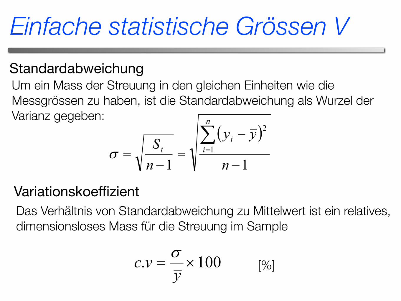
StandardabweichungUm ein Mass der Streuung in den gleichen Einheiten wie die Messgrössen zu haben, ist die Standardabweichung als Wurzel der Varianz gegeben:

Statistics Background of Regression Analysis 06.01.3

1

1

2

12

2

�

¸¹

·¨©

§

� ¦

¦

nn

yy

n

i

n

ii

i

V (6)

or

11

22

2

�

� ¦

n

ynyn

ii

V (7)

However, why is the variance divided by )1( �n and not n as we have n data points? This is because with the use of the mean in calculating the variance, we lose the independence of one of the data points. That is, if you know the mean of n data points, then the value of one of the n data points can be calculated by knowing the other )1( �n data points. To bring the variation back to the same level of units as the original data, a new term called standard deviation, V , is defined as

� �

111

2

�

�

�

¦

n

yy

nS

n

ii

tV (8)

Furthermore, the ratio of the standard deviation to the mean, known as the coefficient variation vc. is also used to normalize the spread of a sample.

100. u

yvc V

(9) Example 1 Use the data in Table 1 to calculate the

a) mean chlorate concentration, b) range of data, c) residual of each data point, d) sum of the square of the residuals. e) sample standard deviation, f) variance, and g) coefficient of variation.

Solution Set up a table (see Table 2) containing the data, the residual for each data point and the square of the residuals. Table 2 Data and data summations for statistical calculations.

i iy 2iy yyi � � �2yyi �

1 12 144 -1.6071 2.5829 2 15 225 1.3929 1.9401 3 14.1 198.81 0.4929 0.24291

VariationskoeffizientDas Verhältnis von Standardabweichung zu Mittelwert ist ein relatives, dimensionsloses Mass für die Streuung im Sample

Statistics Background of Regression Analysis 06.01.3

1

1

2

12

2

�

¸¹

·¨©

§

� ¦

¦

nn

yy

n

i

n

ii

i

V (6)

or

11

22

2

�

� ¦

n

ynyn

ii

V (7)

However, why is the variance divided by )1( �n and not n as we have n data points? This is because with the use of the mean in calculating the variance, we lose the independence of one of the data points. That is, if you know the mean of n data points, then the value of one of the n data points can be calculated by knowing the other )1( �n data points. To bring the variation back to the same level of units as the original data, a new term called standard deviation, V , is defined as

� �

111

2

�

�

�

¦

n

yy

nS

n

ii

tV (8)

Furthermore, the ratio of the standard deviation to the mean, known as the coefficient variation vc. is also used to normalize the spread of a sample.

100. u

yvc V

(9) Example 1 Use the data in Table 1 to calculate the

a) mean chlorate concentration, b) range of data, c) residual of each data point, d) sum of the square of the residuals. e) sample standard deviation, f) variance, and g) coefficient of variation.

Solution Set up a table (see Table 2) containing the data, the residual for each data point and the square of the residuals. Table 2 Data and data summations for statistical calculations.

i iy 2iy yyi � � �2yyi �

1 12 144 -1.6071 2.5829 2 15 225 1.3929 1.9401 3 14.1 198.81 0.4929 0.24291

[%]

Einfache statistische Grössen V

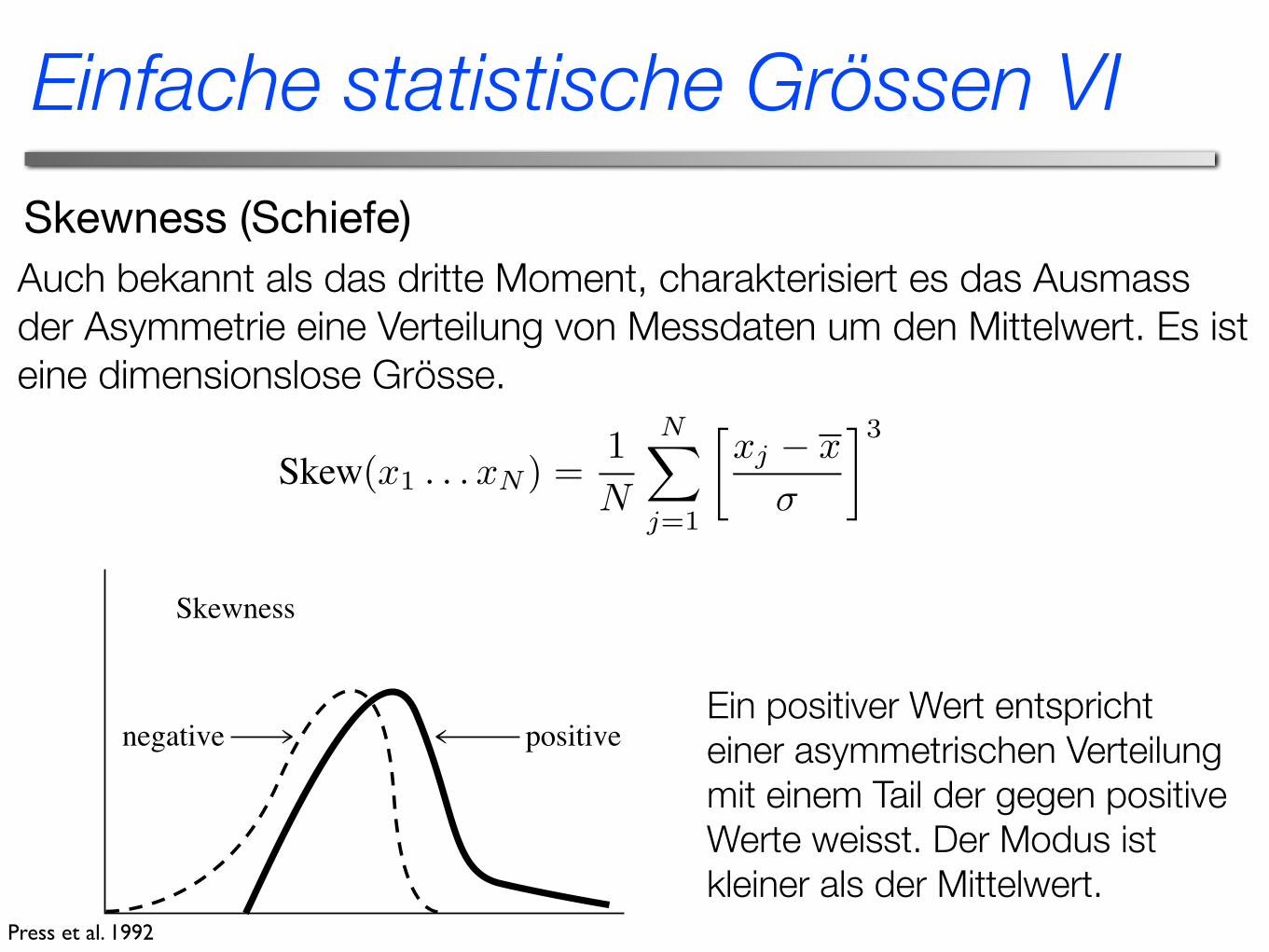
Skewness (Schiefe)Auch bekannt als das dritte Moment, charakterisiert es das Ausmass der Asymmetrie eine Verteilung von Messdaten um den Mittelwert. Es ist eine dimensionslose Grösse.

606 Chapter 14. Statistical Description of Data

Sample page from

NUMERICAL RECIPES IN FO

RTRAN 77: THE ART OF SCIENTIFIC CO

MPUTING

(ISBN 0-521-43064-X)Copyright (C) 1986-1992 by Cam

bridge University Press.Programs Copyright (C) 1986-1992 by Num

erical Recipes Software. Perm

ission is granted for internet users to make one paper copy for their own personal use. Further reproduction, or any copying of m

achine-readable files (including this one) to any servercom

puter, is strictly prohibited. To order Numerical Recipes books

or CDROM

s, visit websitehttp://www.nr.com

or call 1-800-872-7423 (North America only),or send em

ail to directcustserv@cam

bridge.org (outside North America).

(b)(a)

Skewness

negative positive

positive(leptokurtic)negative

(platykurtic)

Kurtosis

Figure 14.1.1. Distributions whose third and fourth moments are significantly different from a normal(Gaussian) distribution. (a) Skewness or third moment. (b) Kurtosis or fourth moment.

That being the case, the skewness or third moment, and the kurtosis or fourthmoment should be used with caution or, better yet, not at all.

The skewness characterizes the degree of asymmetry of a distribution around itsmean. While the mean, standard deviation, and average deviation are dimensionalquantities, that is, have the same units as the measured quantities xj , the skewnessis conventionally defined in such a way as to make it nondimensional. It is a purenumber that characterizes only the shape of the distribution. The usual definition is

Skew(x1 . . . xN ) =1N

N!

j=1

"

xj ! x

!

#3

(14.1.5)

where ! = !(x1 . . . xN ) is the distribution’s standard deviation (14.1.3). A positivevalue of skewness signifies a distribution with an asymmetric tail extending outtowards more positive x; a negative value signifies a distribution whose tail extendsout towards more negative x (see Figure 14.1.1).

Of course, any set of N measured values is likely to give a nonzero value for(14.1.5), even if the underlying distribution is in fact symmetrical (has zero skewness).For (14.1.5) to be meaningful, we need to have some idea of its standard deviationas an estimator of the skewness of the underlying distribution. Unfortunately, thatdepends on the shape of the underlying distribution, and rather critically on its tails!For the idealized case of a normal (Gaussian) distribution, the standard deviation of(14.1.5) is approximately

$

15/N when x is the true mean, and$

6/N when it isestimated by the sample mean, (14.1.1). In real life it is good practice to believe inskewnesses only when they are several or many times as large as this.

The kurtosis is also a nondimensional quantity. It measures the relativepeakedness or flatness of a distribution. Relative to what? A normal distribution,what else! A distribution with positive kurtosis is termed leptokurtic; the outlineof the Matterhorn is an example. A distribution with negative kurtosis is termedplatykurtic; the outline of a loaf of bread is an example. (See Figure 14.1.1.) And,as you no doubt expect, an in-between distribution is termed mesokurtic.

The conventional definition of the kurtosis is

Kurt(x1 . . . xN ) =

%

&

'

1N

N!

j=1

"

xj ! x

!

#4(

)

*

! 3 (14.1.6)


Sample page from



MPUTING







or CDROM





(b)(a)

Skewness

negative positive


(platykurtic)

Kurtosis




Skew(x1 . . . xN ) =1N

N!

j=1

"

xj ! x

!

#3

(14.1.5)



$





Kurt(x1 . . . xN ) =

%

&

'

1N

N!

j=1

"

xj ! x

!

#4(

)

*

! 3 (14.1.6)

Ein positiver Wert entspricht einer asymmetrischen Verteilung mit einem Tail der gegen positive Werte weisst. Der Modus ist kleiner als der Mittelwert.

Press et al. 1992

Einfache statistische Grössen VI

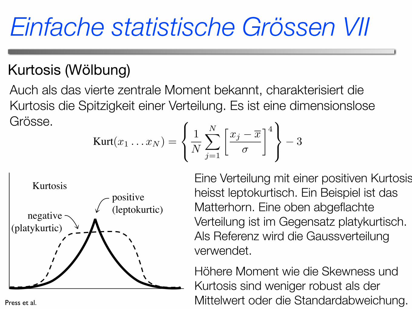
Kurtosis (Wölbung)Auch als das vierte zentrale Moment bekannt, charakterisiert die Kurtosis die Spitzigkeit einer Verteilung. Es ist eine dimensionslose Grösse.

Press et al.


Sample page from



MPUTING







or CDROM





(b)(a)

Skewness

negative positive


(platykurtic)

Kurtosis




Skew(x1 . . . xN ) =1N

N!

j=1

"

xj ! x

!

#3

(14.1.5)



$





Kurt(x1 . . . xN ) =

%

&

'

1N

N!

j=1

"

xj ! x

!

#4(

)

*

! 3 (14.1.6)


Sample page from



MPUTING







or CDROM





(b)(a)

Skewness

negative positive


(platykurtic)

Kurtosis




Skew(x1 . . . xN ) =1N

N!

j=1

"

xj ! x

!

#3

(14.1.5)



$





Kurt(x1 . . . xN ) =

%

&

'

1N

N!

j=1

"

xj ! x

!

#4(

)

*

! 3 (14.1.6)

Eine Verteilung mit einer positiven Kurtosis heisst leptokurtisch. Ein Beispiel ist das Matterhorn. Eine oben abgeflachte Verteilung ist im Gegensatz platykurtisch. Als Referenz wird die Gaussverteilung verwendet.Höhere Moment wie die Skewness und Kurtosis sind weniger robust als der Mittelwert oder die Standardabweichung.

Einfache statistische Grössen VII

Median

Press et al.

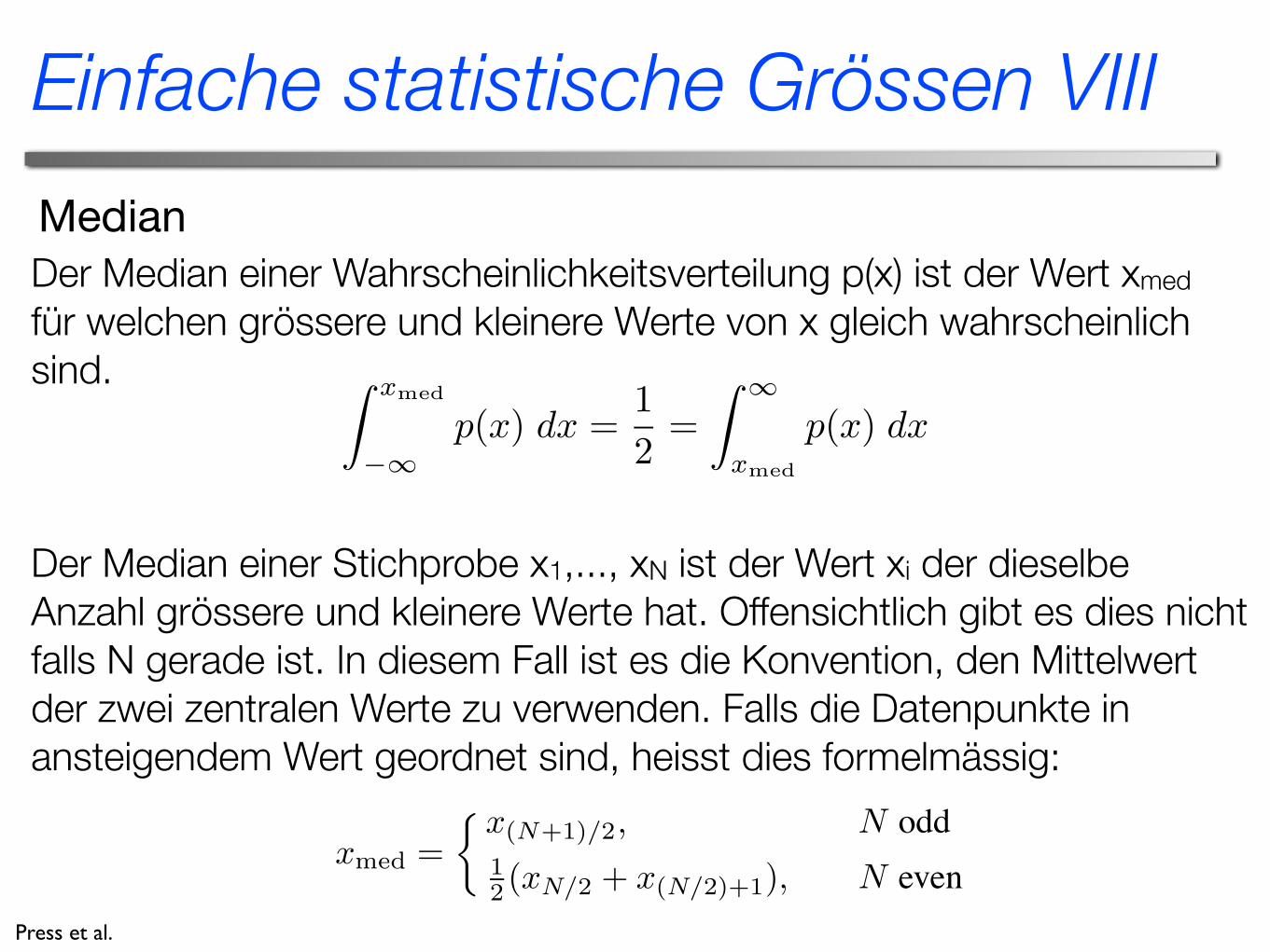
Der Median einer Wahrscheinlichkeitsverteilung p(x) ist der Wert xmed für welchen grössere und kleinere Werte von x gleich wahrscheinlich sind.


Sample page from



MPUTING







or CDROM





adev=adev/n Put the pieces together according to the conventional definitions.var=(var-ep**2/n)/(n-1) Corrected two-pass formula.sdev=sqrt(var)if(var.ne.0.)then

skew=skew/(n*sdev**3)curt=curt/(n*var**2)-3.

elsepause ’no skew or kurtosis when zero variance in moment’

endifreturnEND

Semi-InvariantsThe mean and variance of independent random variables are additive: If x and y are

drawn independently from two, possibly different, probability distributions, then

(x + y) = x + y Var(x + y) = Var(x) + Var(x) (14.1.9)Higher moments are not, in general, additive. However, certain combinations of them,

called semi-invariants, are in fact additive. If the centered moments of a distribution aredenoted Mk ,

Mk !!

(xi " x)k"

(14.1.10)

so that, e.g., M2 = Var(x), then the first few semi-invariants, denoted Ik are given by

I2 = M2 I3 = M3 I4 = M4 " 3M22

I5 = M5 " 10M2M3 I6 = M6 " 15M2M4 " 10M23 + 30M3

2

(14.1.11)

Notice that the skewness and kurtosis, equations (14.1.5) and (14.1.6) are simple powersof the semi-invariants,

Skew(x) = I3/I3/22 Kurt(x) = I4/I2

2 (14.1.12)

A Gaussian distribution has all its semi-invariants higher than I2 equal to zero. A Poissondistribution has all of its semi-invariants equal to its mean. For more details, see [2].

Median and Mode

The median of a probability distribution function p(x) is the value xmed forwhich larger and smaller values of x are equally probable:

# xmed

!"p(x) dx =

12

=# "

xmed

p(x) dx (14.1.13)

The median of a distribution is estimated from a sample of values x1, . . . ,xN by finding that value xi which has equal numbers of values above it and belowit. Of course, this is not possible when N is even. In that case it is conventionalto estimate the median as the mean of the unique two central values. If the valuesxj j = 1, . . . , N are sorted into ascending (or, for that matter, descending) order,then the formula for the median is

xmed =$x(N+1)/2, N odd

12 (xN/2 + x(N/2)+1), N even

(14.1.14)

Der Median einer Stichprobe x1,..., xN ist der Wert xi der dieselbe Anzahl grössere und kleinere Werte hat. Offensichtlich gibt es dies nicht falls N gerade ist. In diesem Fall ist es die Konvention, den Mittelwert der zwei zentralen Werte zu verwenden. Falls die Datenpunkte in ansteigendem Wert geordnet sind, heisst dies formelmässig:


Sample page from



MPUTING







or CDROM





adev=adev/n Put the pieces together according to the conventional definitions.var=(var-ep**2/n)/(n-1) Corrected two-pass formula.sdev=sqrt(var)if(var.ne.0.)then

skew=skew/(n*sdev**3)curt=curt/(n*var**2)-3.

elsepause ’no skew or kurtosis when zero variance in moment’

endifreturnEND

Semi-InvariantsThe mean and variance of independent random variables are additive: If x and y are

drawn independently from two, possibly different, probability distributions, then

(x + y) = x + y Var(x + y) = Var(x) + Var(x) (14.1.9)Higher moments are not, in general, additive. However, certain combinations of them,

called semi-invariants, are in fact additive. If the centered moments of a distribution aredenoted Mk ,

Mk !!

(xi " x)k"

(14.1.10)

so that, e.g., M2 = Var(x), then the first few semi-invariants, denoted Ik are given by

I2 = M2 I3 = M3 I4 = M4 " 3M22

I5 = M5 " 10M2M3 I6 = M6 " 15M2M4 " 10M23 + 30M3

2

(14.1.11)

Notice that the skewness and kurtosis, equations (14.1.5) and (14.1.6) are simple powersof the semi-invariants,

Skew(x) = I3/I3/22 Kurt(x) = I4/I2

2 (14.1.12)

A Gaussian distribution has all its semi-invariants higher than I2 equal to zero. A Poissondistribution has all of its semi-invariants equal to its mean. For more details, see [2].

Median and Mode

The median of a probability distribution function p(x) is the value xmed forwhich larger and smaller values of x are equally probable:

# xmed

!"p(x) dx =

12

=# "

xmed

p(x) dx (14.1.13)

The median of a distribution is estimated from a sample of values x1, . . . ,xN by finding that value xi which has equal numbers of values above it and belowit. Of course, this is not possible when N is even. In that case it is conventionalto estimate the median as the mean of the unique two central values. If the valuesxj j = 1, . . . , N are sorted into ascending (or, for that matter, descending) order,then the formula for the median is

xmed =$x(N+1)/2, N odd

12 (xN/2 + x(N/2)+1), N even

(14.1.14)

Einfache statistische Grössen VIII

Modus

Press et al.

Der Modus einer Wahrscheinlichkeitsfunktion p(x) ist der Wert x wo p den maximalen Wert annimmt. Bei einer empirischen Häufigkeitsverteilung ist es einfach der häufigste Wert. Der Modus ist vor allem hilfreich wenn die Verteilung ein einziges, relativ scharfes Maximum enthält. Gelegentlich treten aber bimodale Verteilungen mit zwei relativen Maxima auf. Dann sollte man beide Werte individuell kennen. Denn sowohl Modus wie auch Mittelwert sind in diesem Fall keine sehr nützlichen Grössen, da sie nur einen “Kompromiss” zwischen dein zwei Maxima darstellen.

In der Physik können solche bimodalen Verteilungen ein Hinweis sein, dass zwei unterschiedliche Mechanismen wirken.

Einfache statistische Grössen VIII

2 Regressionsanalyse

RegressionsanalyseWas ist Regressionsanalyse?Die Regressionsanalyse liefert (quantitative) Informationen über die Beziehung einer abhängigen Variable und einer oder mehrerer unabhängiger Variablen, soweit eine solche Beziehung in einem Datensatz enthalten ist. Sie wir benützt für

1. Prognosen2. Modellanpassung (Parameter Bestimmung)3. Modellvalidierung

Bei der Regressionsanalyse liegt die Betonung auf der Untersuchung der Art der Beziehung zwischen physikalischen Grössen (die als nicht fehlerbehaftet angenommen werden). Bei der verwandten Ausgleichsrechnung (Fitting) geht es hingegen primär darum, die Parameter eines gegeben Modells zu bestimmen, unter Beachtung der Fehler der einzelnen Messungen.

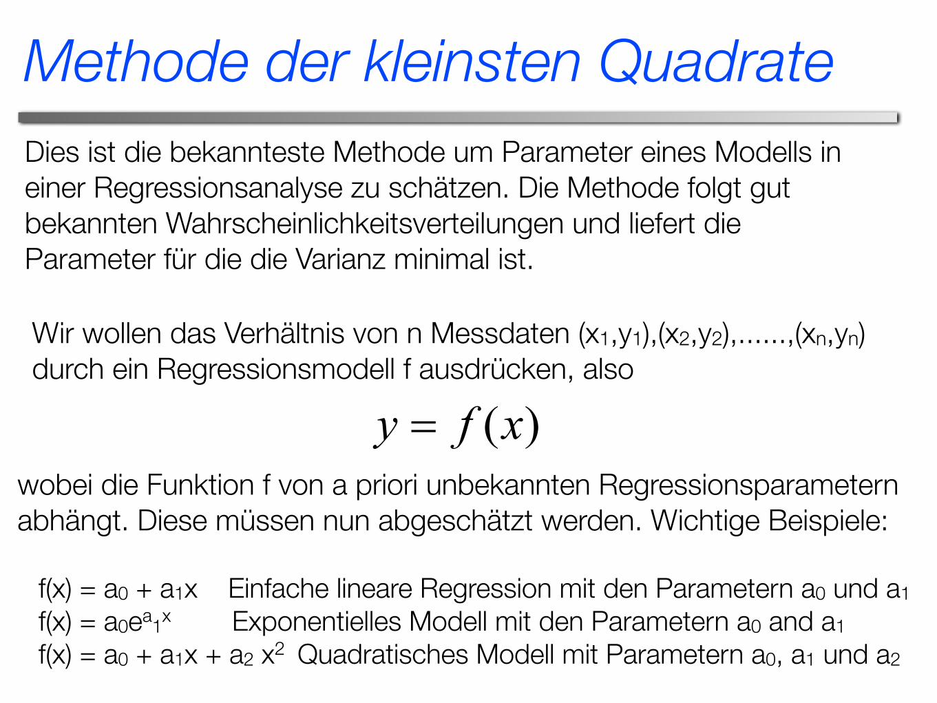
Methode der kleinsten QuadrateDies ist die bekannteste Methode um Parameter eines Modells in einer Regressionsanalyse zu schätzen. Die Methode folgt gut bekannten Wahrscheinlichkeitsverteilungen und liefert die Parameter für die die Varianz minimal ist.

Wir wollen das Verhältnis von n Messdaten (x1,y1),(x2,y2),......,(xn,yn) durch ein Regressionsmodell f ausdrücken, also

Introduction to Regression Analysis 06.02.5

study carried out about the behavior of men might have inadvertently restricted the survey to Caucasian men only. Shall we then generalize the result as the attributes of all men irrespective of race? Such use of regression equation is an abuse since the limitations imposed by the data restrict the use of the prediction equations to Caucasian men. Misidentification Finally, misidentification of causation is a classic abuse of regression analysis equations. Regression analysis can only aid in the confirmation or refutation of a causal model - the model must however have a theoretical basis. In a chemical reacting system in which two species react to form a product, the amount of product formed or amount of reacting species vary with time. Although a regression equation of species concentration and time can be obtained, one cannot attribute time as the causal agent for the varying species concentration. Regression analysis cannot prove causality, rather it can only substantiate or contradict causal assumptions. Anything outside this is an abuse of regression analysis method. Least Squares Methods This is the most popular method of parameter estimation for coefficients of regression models. It has well known probability distributions and gives unbiased estimators of regression parameters with the smallest variance. We wish to predict the response to n data points ),(),......,,(),,( 2211 nn yxyxyx by a regression model given by )(xfy (6) where, the function )(xf has regression constants that need to be estimated. For example xaaxf 10)( � is a straight-line regression model with constants 0a and 1a

xaeaxf 10)( is an exponential model with constants 0a and 1a

2210)( xaxaaxf �� is a quadratic model with constants 0a , 1a and 2a

A measure of goodness of fit, that is how the regression model )(xf predicts the response variable y is the magnitude of the residual, iE at each of the n data points. nixfyE iii ,....2,1),( � (7) Ideally, if all the residuals iE are zero, one may have found an equation in which all the points lie on a model. Thus, minimization of the residual is an objective of obtaining regression coefficients. In the least squares method, estimates of the constants of the models are chosen such that minimization of the sum of the squared residuals is achieved, that is

minimize ¦

n

iiE

1

2 .

Why minimize the sum of the square of the residuals?

wobei die Funktion f von a priori unbekannten Regressionsparametern abhängt. Diese müssen nun abgeschätzt werden. Wichtige Beispiele:

f(x) = a0 + a1x Einfache lineare Regression mit den Parametern a0 und a1f(x) = a0ea1x Exponentielles Modell mit den Parametern a0 and a1f(x) = a0 + a1x + a2 x2 Quadratisches Modell mit Parametern a0, a1 und a2

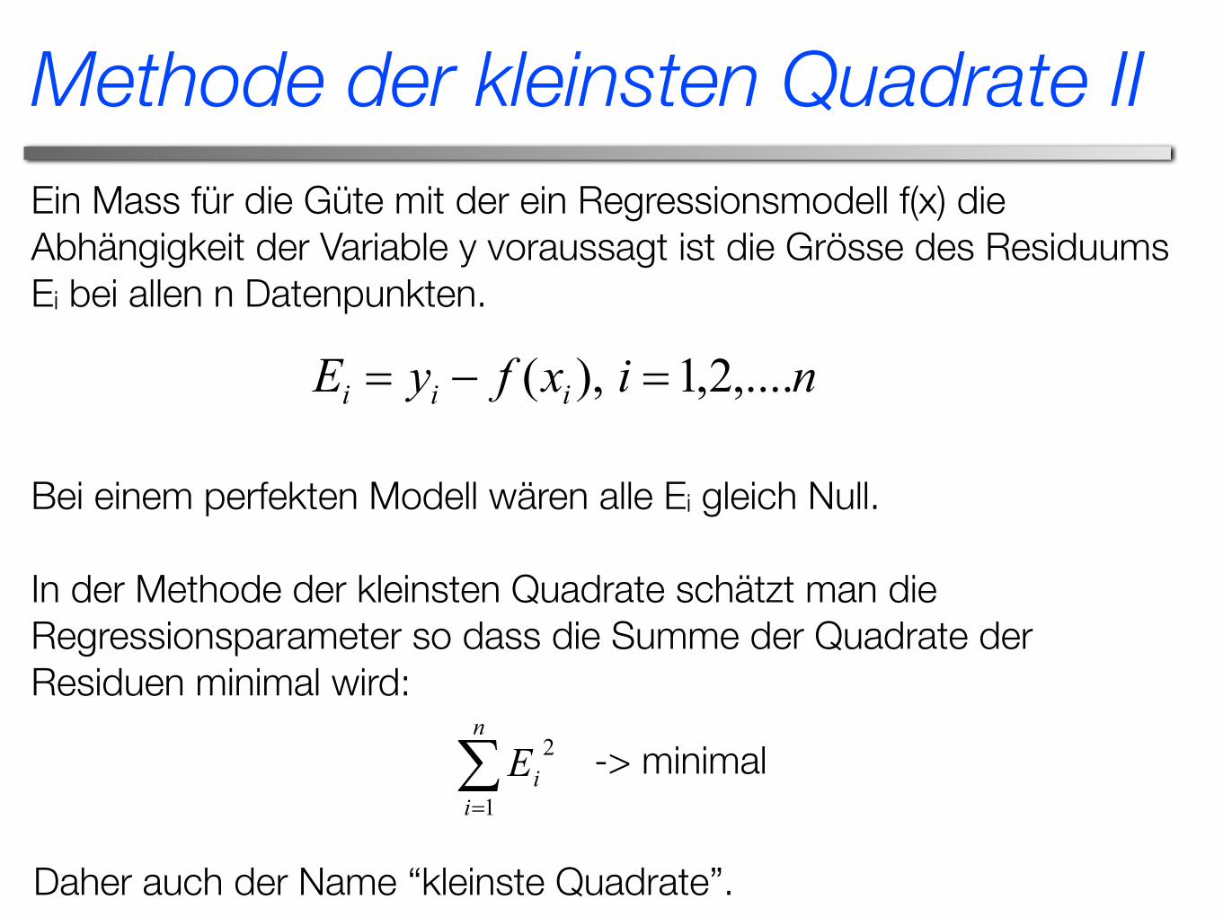
Ein Mass für die Güte mit der ein Regressionsmodell f(x) die Abhängigkeit der Variable y voraussagt ist die Grösse des Residuums Ei bei allen n Datenpunkten.






minimize ¦

n

iiE

1

2 .

Why minimize the sum of the square of the residuals?

Bei einem perfekten Modell wären alle Ei gleich Null.

In der Methode der kleinsten Quadrate schätzt man die Regressionsparameter so dass die Summe der Quadrate der Residuen minimal wird:






minimize ¦

n

iiE

1

2 .

Why minimize the sum of the square of the residuals? Daher auch der Name “kleinste Quadrate”.

Methode der kleinsten Quadrate II

-> minimal

3 Lineare Regression

Lineare Regression

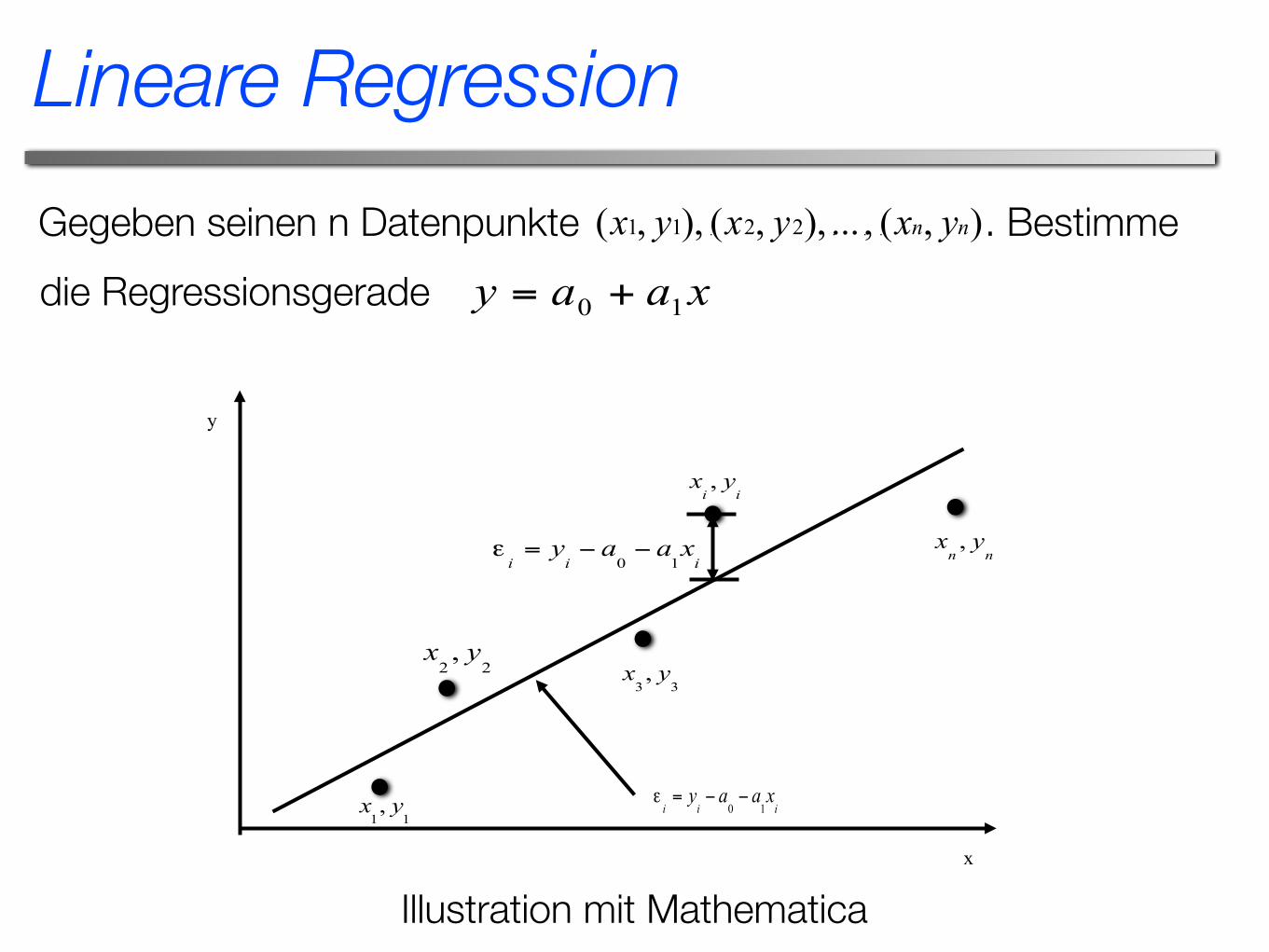
Gegeben seinen n Datenpunkte . Bestimmedie Regressionsgerade

x

y

Illustration mit Mathematica

Parameterschätzung I

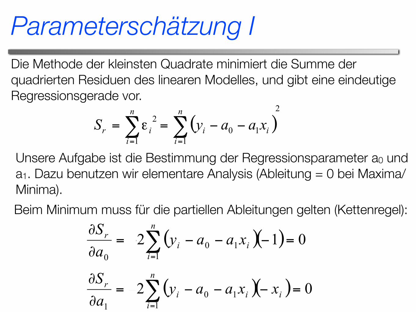
Die Methode der kleinsten Quadrate minimiert die Summe der quadrierten Residuen des linearen Modelles, und gibt eine eindeutige Regressionsgerade vor.

Unsere Aufgabe ist die Bestimmung der Regressionsparameter a0 und a1. Dazu benutzen wir elementare Analysis (Ableitung = 0 bei Maxima/Minima).Beim Minimum muss für die partiellen Ableitungen gelten (Kettenregel):

Dies gibtLinear Regression 06.03.5

01 1

21

10 ��¦ ¦¦

n

i

n

ii

n

iiii xaxaxy (13)

Noting that 00001

0 ... naaaaan

i �� ¦

¦¦

�n

ii

n

ii yxana

1110 (14)

¦¦¦

�n

iii

n

ii

n

ii yxxaxa

11

21

10 (15)

Figure 3 Linear regression of y vs. x data showing residuals and square of residual at a typical point, ix . Solving the above Equations (14) and (15) gives

2

11

2

1111

¸¹

·¨©

§�

�

¦¦

¦¦¦

n

ii

n

ii

n

ii

n

ii

n

iii

xxn

yxyxna (16)

2

11

2

1111

2

0

¸¹

·¨©

§�

�

¦¦

¦¦¦¦

n

ii

n

ii

n

iii

n

ii

n

ii

n

ii

xxn

yxxyxa (17)

Redefining

� �11 , yx

� �33, yx

� �22 , yx

),( nn yx� �ii yx ,

iii xaayE 10 ��

y

x

xaay 10 �

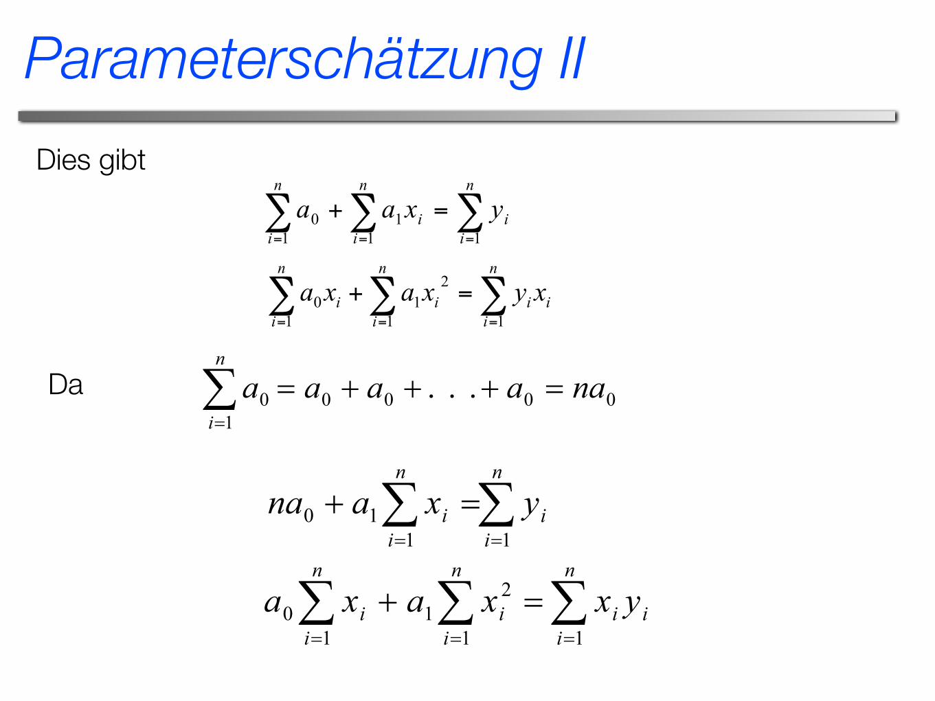
Da

Linear Regression 06.03.5

01 1

21

10 ��¦ ¦¦

n

i

n

ii

n

iiii xaxaxy (13)

Noting that 00001

0 ... naaaaan

i �� ¦

¦¦

�n

ii

n

ii yxana

1110 (14)

¦¦¦

�n

iii

n

ii

n

ii yxxaxa

11

21

10 (15)


2

11

2

1111

¸¹

·¨©

§�

�

¦¦

¦¦¦

n

ii

n

ii

n

ii

n

ii

n

iii

xxn

yxyxna (16)

2

11

2

1111

2

0

¸¹

·¨©

§�

�

¦¦

¦¦¦¦

n

ii

n

ii

n

iii

n

ii

n

ii

n

ii

xxn

yxxyxa (17)

Redefining

� �11 , yx

� �33, yx

� �22 , yx


iii xaayE 10 ��

y

x

xaay 10 �

Parameterschätzung II


01 1

21

10 ��¦ ¦¦

n

i

n

ii

n

iiii xaxaxy (13)

Noting that 00001

0 ... naaaaan

i �� ¦

¦¦

�n

ii

n

ii yxana

1110 (14)

¦¦¦

�n

iii

n

ii

n

ii yxxaxa

11

21

10 (15)


2

11

2

1111

¸¹

·¨©

§�

�

¦¦

¦¦¦

n

ii

n

ii

n

ii

n

ii

n

iii

xxn

yxyxna (16)

2

11

2

1111

2

0

¸¹

·¨©

§�

�

¦¦

¦¦¦¦

n

ii

n

ii

n

iii

n

ii

n

ii

n

ii

xxn

yxxyxa (17)

Redefining

� �11 , yx

� �33, yx

� �22 , yx


iii xaayE 10 ��

y

x

xaay 10 �

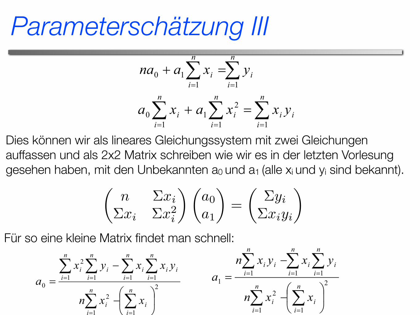
Dies können wir als lineares Gleichungssystem mit zwei Gleichungen auffassen und als 2x2 Matrix schreiben wie wir es in der letzten Vorlesung gesehen haben, mit den Unbekannten a0 und a1 (alle xi und yi sind bekannt).


01 1

21

10 ��¦ ¦¦

n

i

n

ii

n

iiii xaxaxy (13)

Noting that 00001

0 ... naaaaan

i �� ¦

¦¦

�n

ii

n

ii yxana

1110 (14)

¦¦¦

�n

iii

n

ii

n

ii yxxaxa

11

21

10 (15)


2

11

2

1111

¸¹

·¨©

§�

�

¦¦

¦¦¦

n

ii

n

ii

n

ii

n

ii

n

iii

xxn

yxyxna (16)

2

11

2

1111

2

0

¸¹

·¨©

§�

�

¦¦

¦¦¦¦

n

ii

n

ii

n

iii

n

ii

n

ii

n

ii

xxn

yxxyxa (17)

Redefining

� �11 , yx

� �33, yx

� �22 , yx


iii xaayE 10 ��

y

x

xaay 10 �


01 1

21

10 ��¦ ¦¦

n

i

n

ii

n

iiii xaxaxy (13)

Noting that 00001

0 ... naaaaan

i �� ¦

¦¦

�n

ii

n

ii yxana

1110 (14)

¦¦¦

�n

iii

n

ii

n

ii yxxaxa

11

21

10 (15)


2

11

2

1111

¸¹

·¨©

§�

�

¦¦

¦¦¦

n

ii

n

ii

n

ii

n

ii

n

iii

xxn

yxyxna (16)

2

11

2

1111

2

0

¸¹

·¨©

§�

�

¦¦

¦¦¦¦

n

ii

n

ii

n

iii

n

ii

n

ii

n

ii

xxn

yxxyxa (17)

Redefining

� �11 , yx

� �33, yx

� �22 , yx


iii xaayE 10 ��

y

x

xaay 10 �

Parameterschätzung III

✓n ⌃xi

⌃xi ⌃x2i

◆✓a0

a1

◆=

✓⌃yi⌃xiyi

◆

Für so eine kleine Matrix findet man schnell:

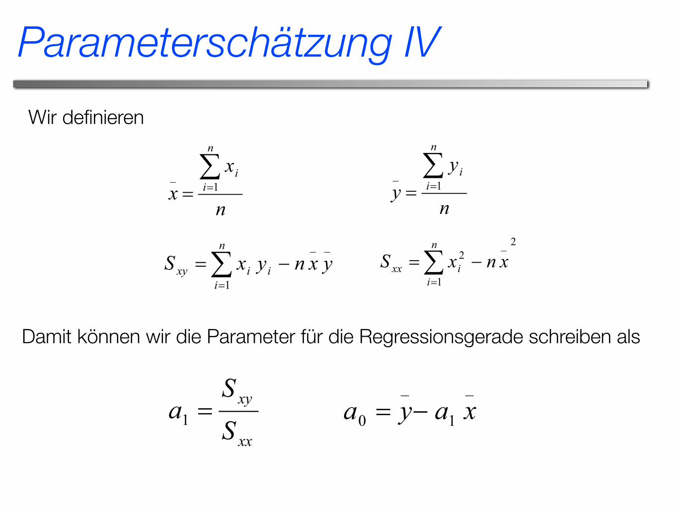
Wir definieren

06.03.6 Chapter 06.03

__

1

yxnyxSn

iiixy � ¦

(18)

2_

1

2 xnxSn

iixx � ¦

(19)

n

xx

n

ii¦

1_

(20)

n

yy

n

ii¦

1_

(21)

we can rewrite

xx

xy

SS

a 1 (22)

_

1

_

0 xaya � (23) Example 1 The torque T needed to turn the torsional spring of a mousetrap through an angle, T is given below Table 5 Torque versus angle for a torsion spring.

Angle, T Radians

Torque, T mN �

0.698132 0.188224 0.959931 0.209138 1.134464 0.230052 1.570796 0.250965 1.919862 0.313707

Find the constants 1k and 2k of the regression model T21 kkT � Solution Table 6 shows the summations needed for the calculation of the constants of the regression model. Table 6 Tabulation of data for calculation of needed summations.

i T T 2T TT 1 radians mN � radians 2 mN � 2 0.698132 0.188224 11087388.4 �u 11031405.1 �u 3 0.959931 0.209138 11021468.9 �u 11000758.2 �u 4 1.134464 0.230052 1.2870 11060986.2 �u

06.03.6 Chapter 06.03

__

1

yxnyxSn

iiixy � ¦

(18)

2_

1

2 xnxSn

iixx � ¦

(19)

n

xx

n

ii¦

1_

(20)

n

yy

n

ii¦

1_

(21)

we can rewrite

xx

xy

SS

a 1 (22)

_

1

_


Angle, T Radians

Torque, T mN �

0.698132 0.188224 0.959931 0.209138 1.134464 0.230052 1.570796 0.250965 1.919862 0.313707



06.03.6 Chapter 06.03

__

1

yxnyxSn

iiixy � ¦

(18)

2_

1

2 xnxSn

iixx � ¦

(19)

n

xx

n

ii¦

1_

(20)

n

yy

n

ii¦

1_

(21)

we can rewrite

xx

xy

SS

a 1 (22)

_

1

_


Angle, T Radians

Torque, T mN �

0.698132 0.188224 0.959931 0.209138 1.134464 0.230052 1.570796 0.250965 1.919862 0.313707



06.03.6 Chapter 06.03

__

1

yxnyxSn

iiixy � ¦

(18)

2_

1

2 xnxSn

iixx � ¦

(19)

n

xx

n

ii¦

1_

(20)

n

yy

n

ii¦

1_

(21)

we can rewrite

xx

xy

SS

a 1 (22)

_

1

_


Angle, T Radians

Torque, T mN �

0.698132 0.188224 0.959931 0.209138 1.134464 0.230052 1.570796 0.250965 1.919862 0.313707



Damit können wir die Parameter für die Regressionsgerade schreiben als

06.03.6 Chapter 06.03

__

1

yxnyxSn

iiixy � ¦

(18)

2_

1

2 xnxSn

iixx � ¦

(19)

n

xx

n

ii¦

1_

(20)

n

yy

n

ii¦

1_

(21)

we can rewrite

xx

xy

SS

a 1 (22)

_

1

_


Angle, T Radians

Torque, T mN �

0.698132 0.188224 0.959931 0.209138 1.134464 0.230052 1.570796 0.250965 1.919862 0.313707



06.03.6 Chapter 06.03

__

1

yxnyxSn

iiixy � ¦

(18)

2_

1

2 xnxSn

iixx � ¦

(19)

n

xx

n

ii¦

1_

(20)

n

yy

n

ii¦

1_

(21)

we can rewrite

xx

xy

SS

a 1 (22)

_

1

_


Angle, T Radians

Torque, T mN �

0.698132 0.188224 0.959931 0.209138 1.134464 0.230052 1.570796 0.250965 1.919862 0.313707



Parameterschätzung IV

Beispiel I

x y

0.698132 0.188224

0.959931 0.209138

1.134464 0.230052

1.570796 0.250965

1.919862 0.313707

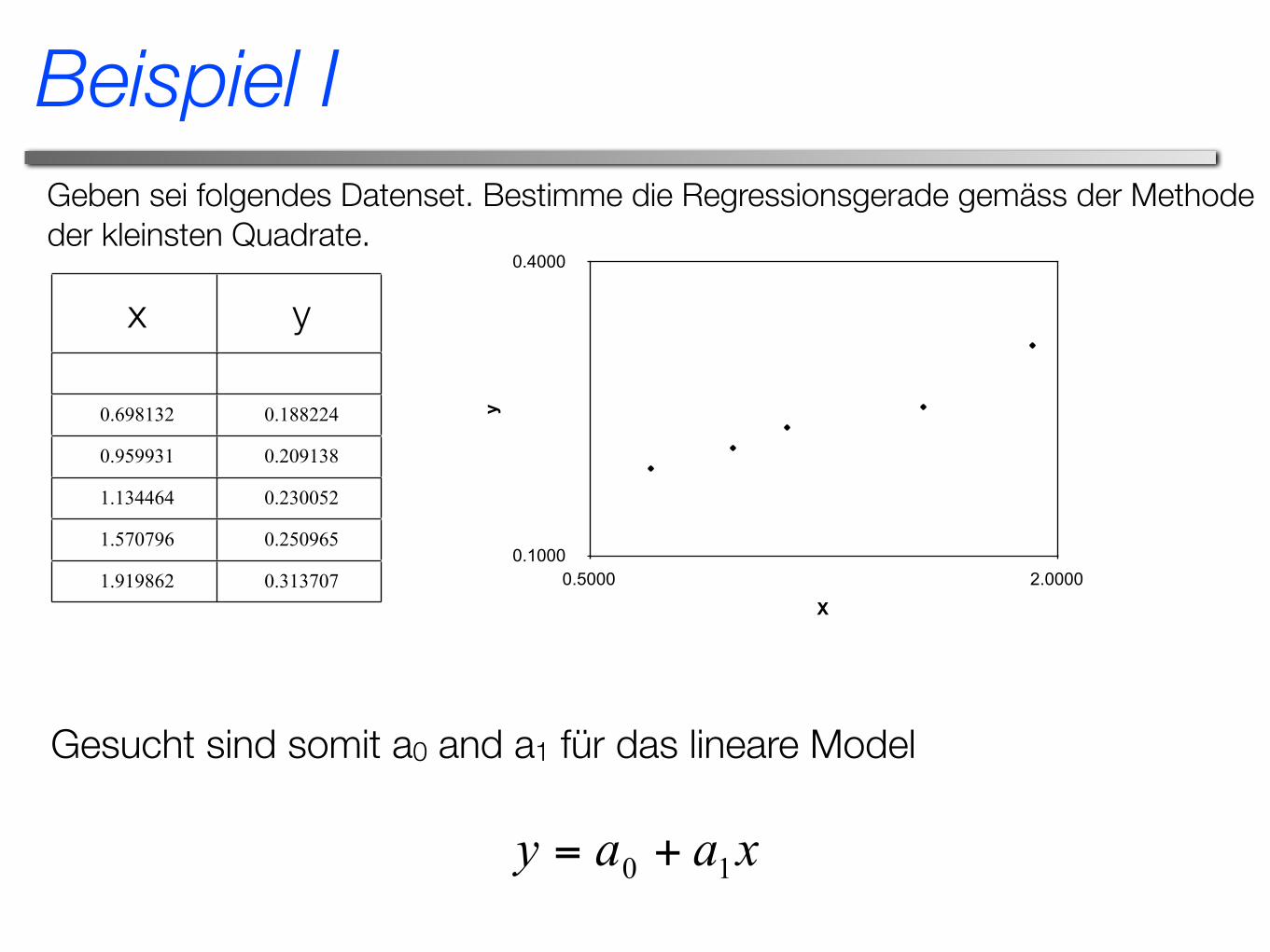
Gesucht sind somit a0 and a1 für das lineare Model

0.1000

0.4000

0.5000 2.0000

y

X

Geben sei folgendes Datenset. Bestimme die Regressionsgerade gemäss der Methode der kleinsten Quadrate.

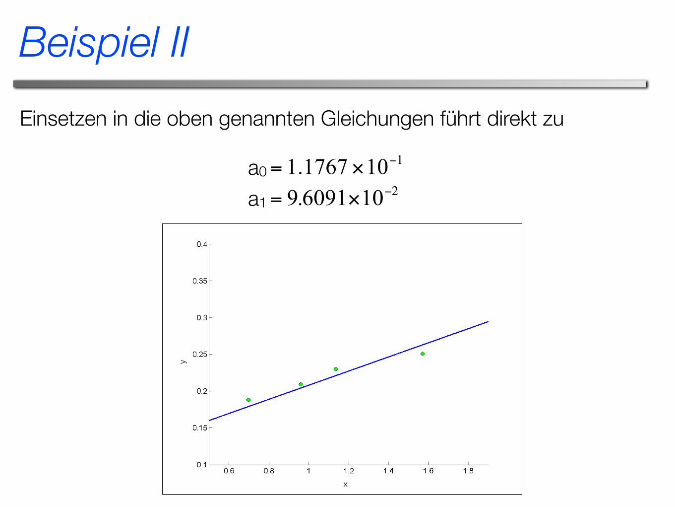
Einsetzen in die oben genannten Gleichungen führt direkt zu

a0

a1

x

y

Beispiel II

4 Nichtlineare Regression

Nichtlineare Regression

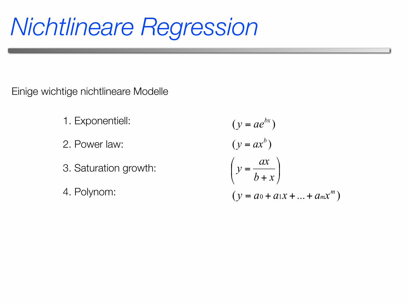
Einige wichtige nichtlineare Modelle

1. Exponentiell:

2. Power law:

3. Saturation growth:

4. Polynom:

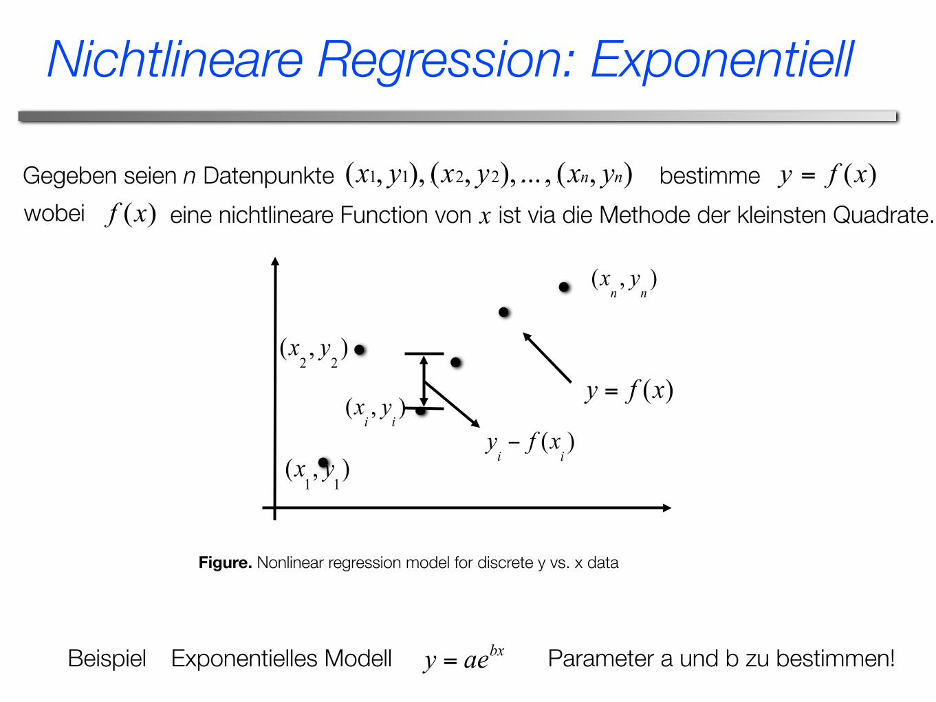
Nichtlineare Regression: Exponentiell

Gegeben seien n Datenpunkte bestimme eine nichtlineare Function von ist via die Methode der kleinsten Quadrate.

Figure. Nonlinear regression model for discrete y vs. x data

Beispiel Exponentielles Modell

wobei

Parameter a und b zu bestimmen!

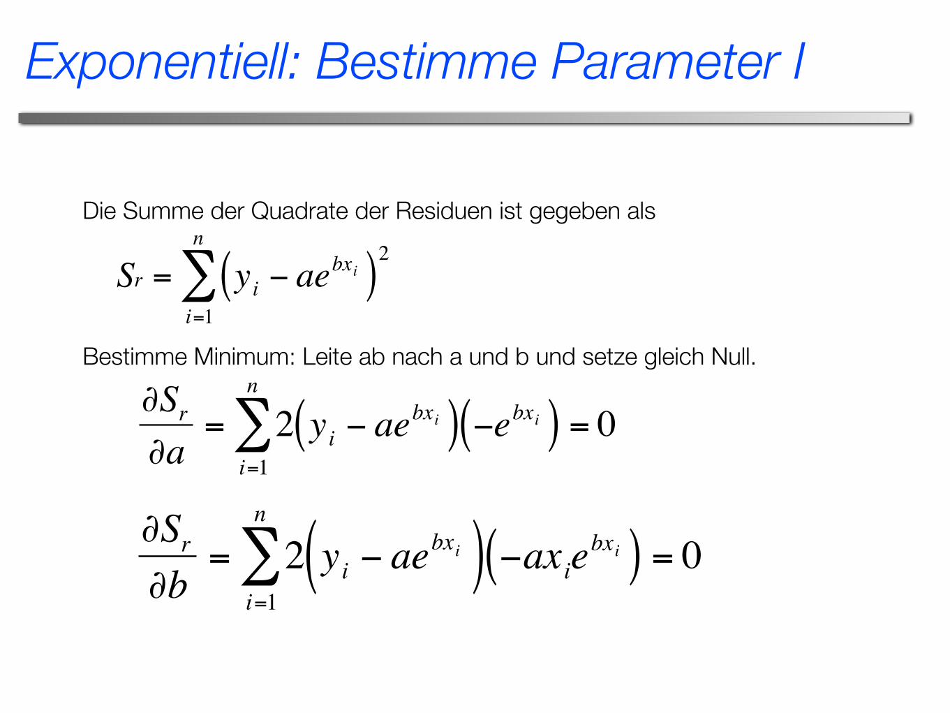
Exponentiell: Bestimme Parameter I

€

Sr = yi − aebxi( )2

i=1

n

∑Die Summe der Quadrate der Residuen ist gegeben als

Bestimme Minimum: Leite ab nach a und b und setze gleich Null.

€

∂Sr∂a

= 2 yi − aebxi( )

i=1

n

∑ −ebxi( ) = 0

€

∂Sr∂b

= 2 yi − aebxi( )

i=1

n

∑ −axiebxi( ) = 0

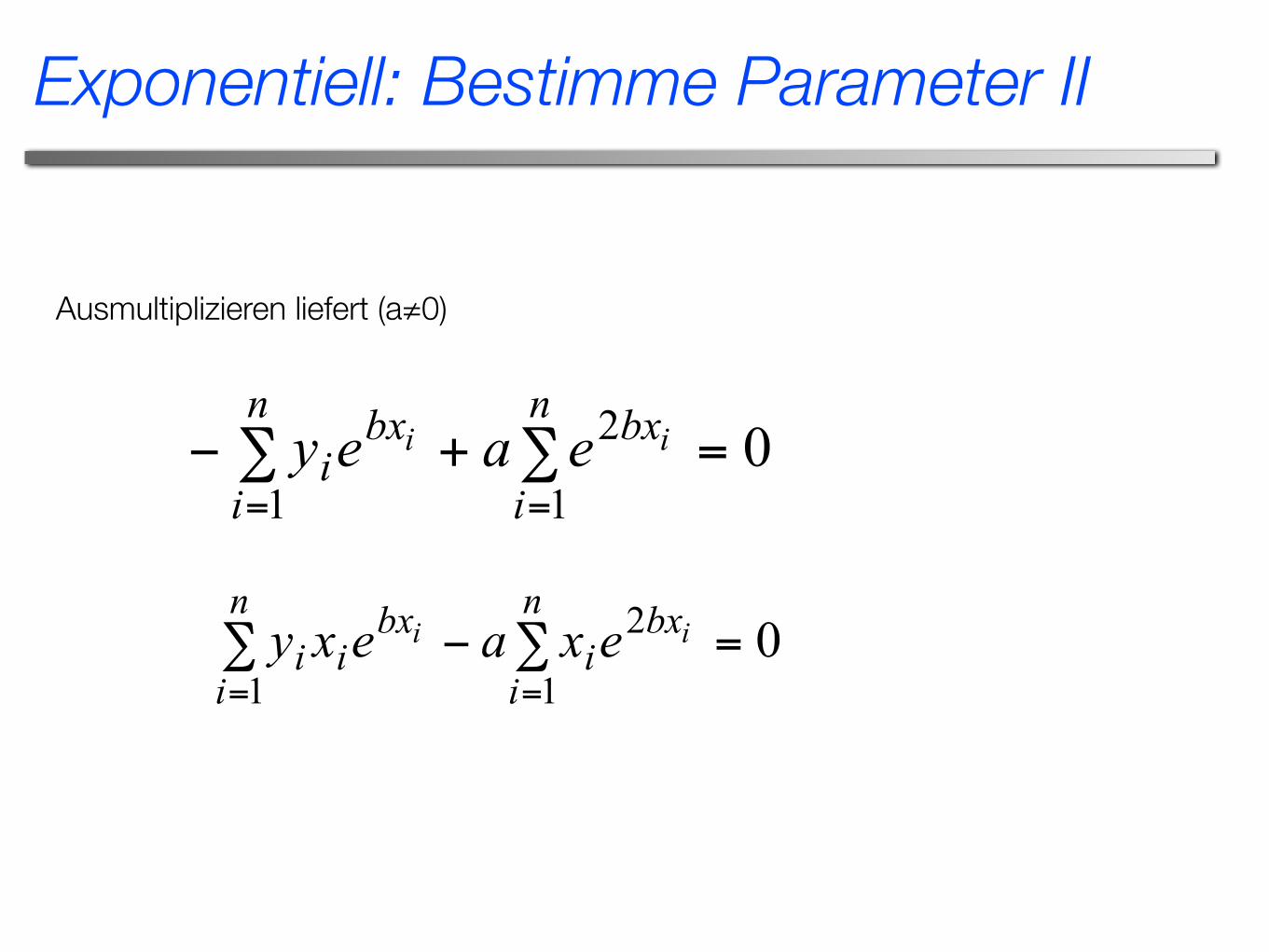
Ausmultiplizieren liefert (a≠0)

Exponentiell: Bestimme Parameter II

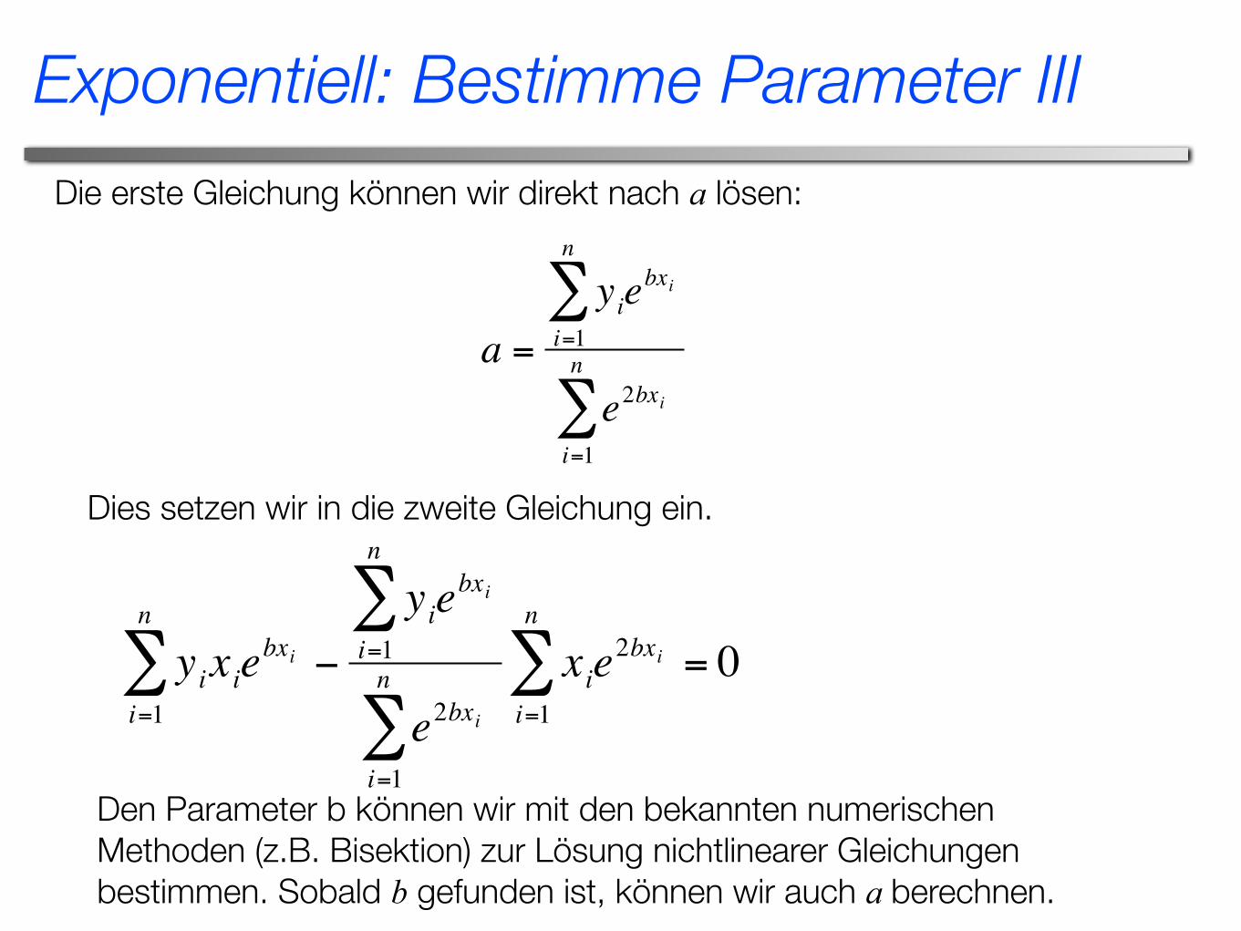
Dies setzen wir in die zweite Gleichung ein.

€

yii=1

n

∑ xiebxi −

yii=1

n

∑ ebxi

e2bxii=1

n

∑xie

2bxi

i=1

n

∑ = 0

Den Parameter b können wir mit den bekannten numerischen Methoden (z.B. Bisektion) zur Lösung nichtlinearer Gleichungen bestimmen. Sobald b gefunden ist, können wir auch a berechnen.

€

a =

yiebxi

i=1

n

∑

e2bxii=1

n

∑

Die erste Gleichung können wir direkt nach a lösen:

Exponentiell: Bestimme Parameter III

Beispiel - Exponentielles Modell I

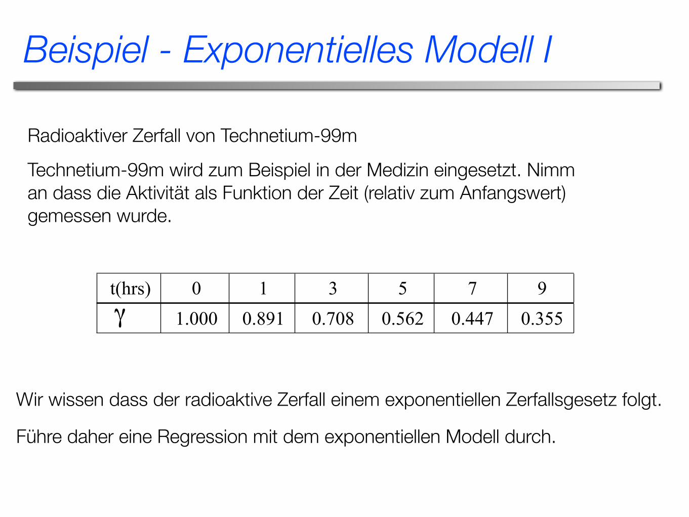
t(hrs) 0 1 3 5 7 91.000 0.891 0.708 0.562 0.447 0.355

Radioaktiver Zerfall von Technetium-99m

Technetium-99m wird zum Beispiel in der Medizin eingesetzt. Nimm an dass die Aktivität als Funktion der Zeit (relativ zum Anfangswert) gemessen wurde.

Wir wissen dass der radioaktive Zerfall einem exponentiellen Zerfallsgesetz folgt.

Führe daher eine Regression mit dem exponentiellen Modell durch.

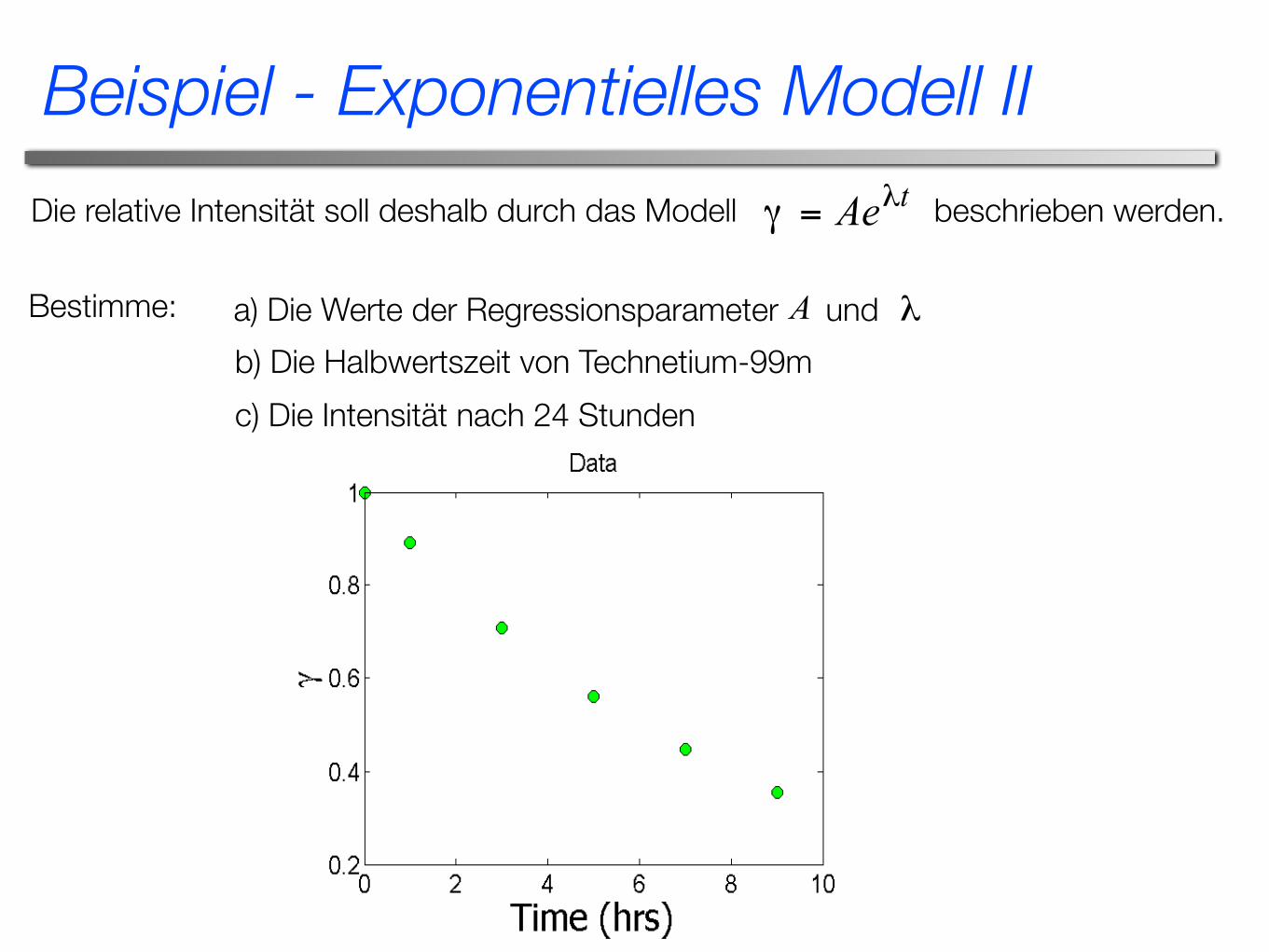
Bestimme: a) Die Werte der Regressionsparameter undb) Die Halbwertszeit von Technetium-99mc) Die Intensität nach 24 Stunden

Die relative Intensität soll deshalb durch das Modell beschrieben werden.

Beispiel - Exponentielles Modell II

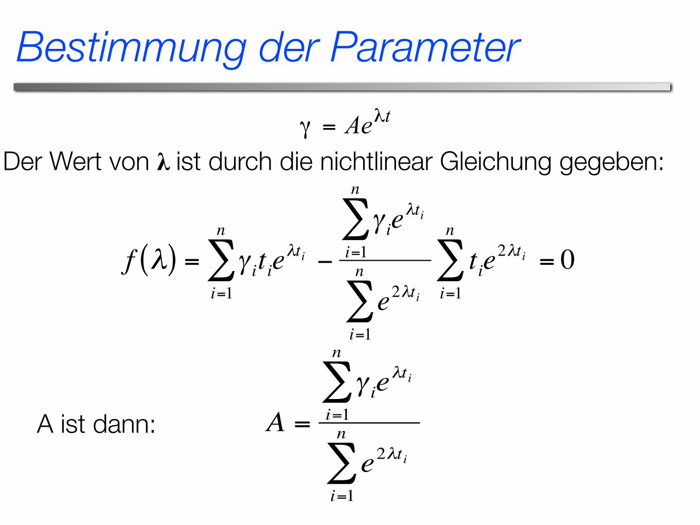
Bestimmung der Parameter

Der Wert von λ ist durch die nichtlinear Gleichung gegeben:

€

f λ( ) = γ ii=1

n

∑ tieλti −

γ ieλti

i=1

n

∑

e2λtii=1

n

∑tie

2λti

i=1

n

∑ = 0

€

A =

γ ieλti

i=1

n

∑

e2λtii=1

n

∑A ist dann:

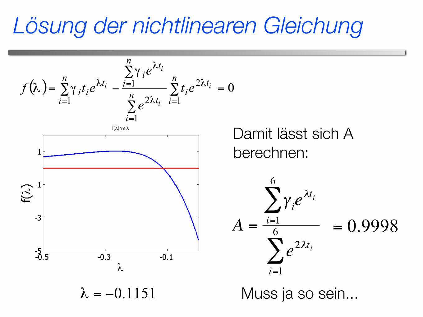
Lösung der nichtlinearen Gleichung

Damit lässt sich A berechnen:

€

A =

γ ieλti

i=1

6

∑

e2λtii=1

6

∑

Muss ja so sein...

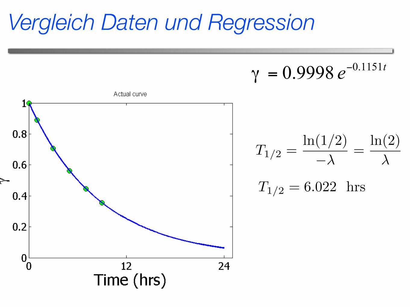
Vergleich Daten und Regression

T1/2 =ln(1/2)

��=

ln(2)

�

T1/2 = 6.022 hrs

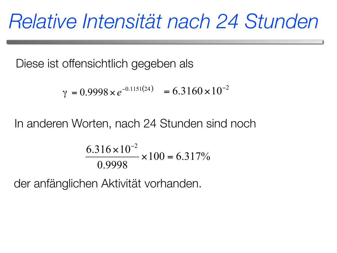
Relative Intensität nach 24 Stunden

Diese ist offensichtlich gegeben als

In anderen Worten, nach 24 Stunden sind noch

der anfänglichen Aktivität vorhanden.

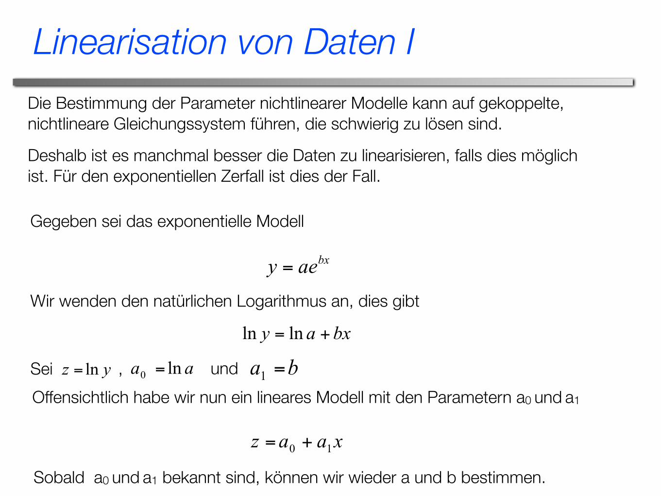
Linearisation von Daten IDie Bestimmung der Parameter nichtlinearer Modelle kann auf gekoppelte, nichtlineare Gleichungssystem führen, die schwierig zu lösen sind.

Deshalb ist es manchmal besser die Daten zu linearisieren, falls dies möglich ist. Für den exponentiellen Zerfall ist dies der Fall.

Gegeben sei das exponentielle Modell

Wir wenden den natürlichen Logarithmus an, dies gibt

Sei ,

Sobald a0 und a1 bekannt sind, können wir wieder a und b bestimmen.

Offensichtlich habe wir nun ein lineares Modell mit den Parametern a0 und a1

und

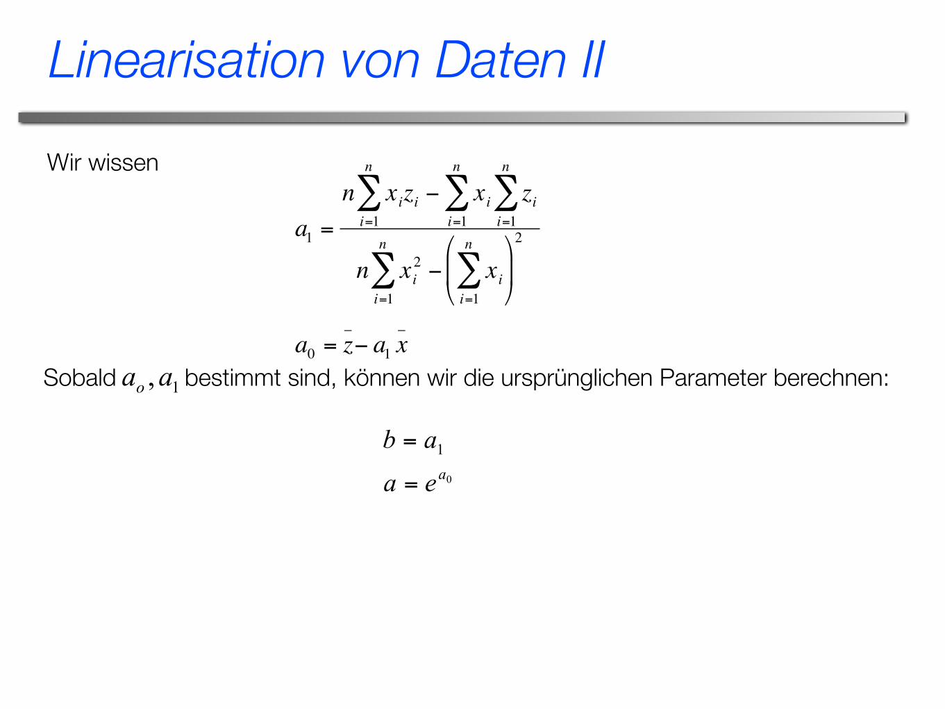
Wir wissen

€

a1 =

n xizi − xii=1

n

∑i=1

n

∑ zii=1

n

∑

n xi2 − xi

i=1

n

∑⎛

⎝ ⎜

⎞

⎠ ⎟

2

i=1

n

∑

a0 = z_− a1 x

_

Sobald bestimmt sind, können wir die ursprünglichen Parameter berechnen:

Linearisation von Daten II

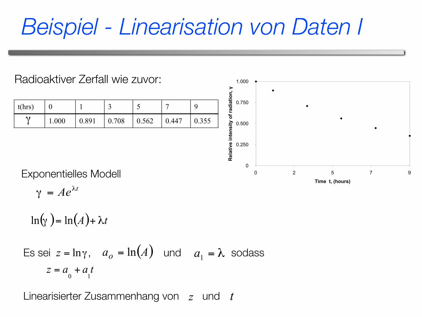
Beispiel - Linearisation von Daten I

t(hrs) 0 1 3 5 7 9

1.000 0.891 0.708 0.562 0.447 0.355

0

0.250

0.500

0.750

1.000

0 2 5 7 9

Rel

ativ

e in

tens

ity o

f rad

iatio

n, γ

Time t, (hours)

Radioaktiver Zerfall wie zuvor:

Exponentielles Modell

Es sei , und sodass

Linearisierter Zusammenhang von und

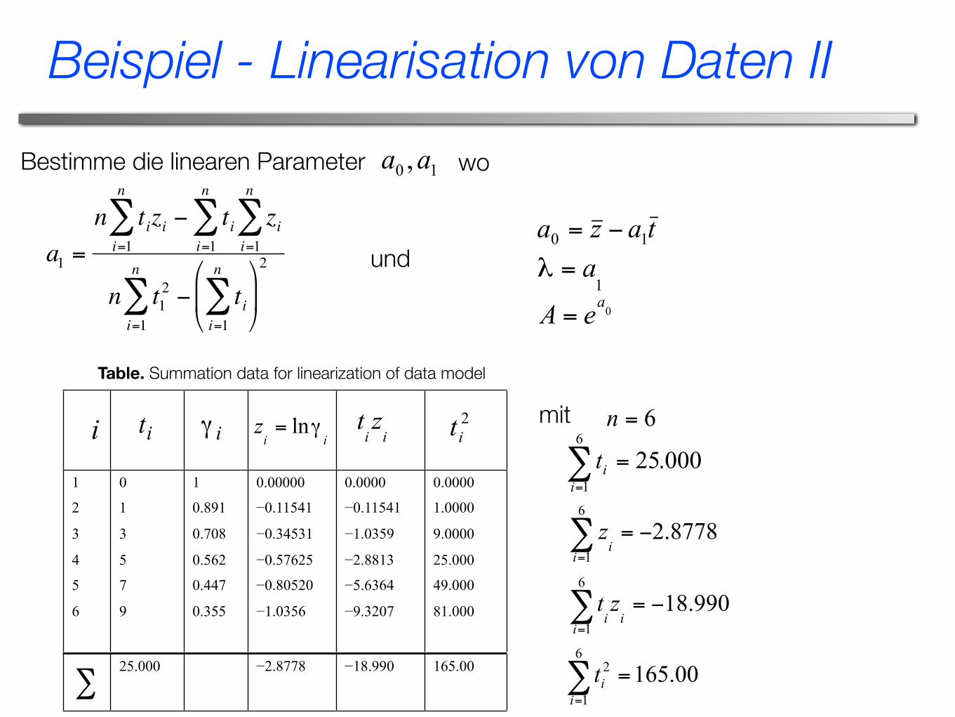
Bestimme die linearen Parameter

€

a1 =

n tizi − tii=1

n

∑i=1

n

∑ zii=1

n

∑

n t12 − ti

i=1

n

∑⎛

⎝ ⎜

⎞

⎠ ⎟

2

i=1

n

∑und

wo

1

2

3

4

5

6

0

1

3

5

7

9

1

0.891

0.708

0.562

0.447

0.355

0.00000

−0.11541

−0.34531

−0.57625

−0.80520

−1.0356

0.0000

−0.11541

−1.0359

−2.8813

−5.6364

−9.3207

0.0000

1.0000

9.0000

25.000

49.000

81.000

25.000 −2.8778 −18.990 165.00

Table. Summation data for linearization of data model

mit

Beispiel - Linearisation von Daten II

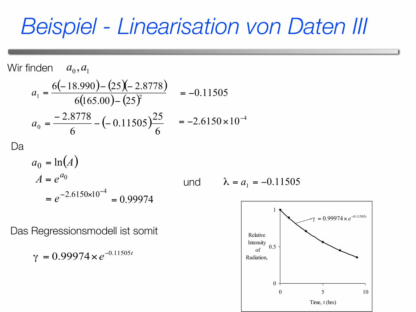
Wir finden

Da

und

Das Regressionsmodell ist somit

Beispiel - Linearisation von Daten III

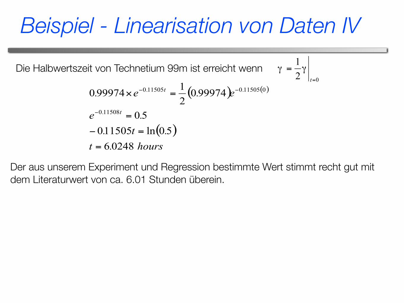
Die Halbwertszeit von Technetium 99m ist erreicht wenn

Der aus unserem Experiment und Regression bestimmte Wert stimmt recht gut mit dem Literaturwert von ca. 6.01 Stunden überein.

Beispiel - Linearisation von Daten IV

Referenzen

•Dieses Script basiert auf http://numericalmethods.eng.usf.eduby Autar Kaw, Jai Paul und Numerical Recipes (2nd/3rd Edition) by Press et al., Cambridge University Press

http://www.nr.com/oldverswitcher.html

http://numericalmethods.eng.usf.edu

http://numericalmethods.eng.usf.edu



Practical Numerical Training UKNum - MPIA.demordasini/UKNUM/statistics.pdf · Practical Numerical...

Documents

Transcript of Practical Numerical Training UKNum - MPIA.demordasini/UKNUM/statistics.pdf · Practical Numerical...