Primal-dual methods for dynamicprogramming equations arising in

non-linear option pricing

Dissertation zur Erlangung des Grades des

Doktors der Naturwissenschaften

der Fakultat Mathematik und Informatik

der Universitat des Saarlandes

eingereicht im September 2017

in Saarbrucken

von

Christian Gartner

Tag des Kolloquiums: 06.02.2018

Mitglieder des Prufungsausschusses:

Vorsitzender: Professor Dr. Thomas Schuster

1. Berichterstatter: Professor Dr. Christian Bender

2. Berichterstatter: PD Dr. John Schoenmakers(wahrend des Kolloquiums vertretendurch Professor Dr. Henryk Zahle)

Protokollfuhrer: Dr. Tobias Mai

Dekan: Professor Dr. Frank-Olaf Schreyer

ii

To my parents and my brother

To Robin

iii

iv

Acknowledgements

First of all, I would like to express my gratitude to my supervisor Professor Christian Bender forgiving me the opportunity to work in the Stochastics group at Saarland university (with financialsupport by the Deutsche Forschungsgemeinschaft under grant BE3933/5-1 raised by him), forintroducing me to this interesting topic, and for sharing his knowledge with me. It would have notbeen possible to write this thesis without his constant support and encouragement.

Furthermore, I would like to thank my co-author Dr. Nikolaus Schweizer for all the hours, whichhe spent for helpful discussions even after he left the Stochastics group at Saarland university andfor proof-reading parts of thesis. I am also very thankful for all his experience and knowledgeconcerning numerical implementations, which he shared with me during the last years. It hasalways been a pleasure to work with him.

I also would like to thank PD John Schoenmakers for being the co-referee of this thesis.

I would like to thank all my present and former colleagues for welcoming me with open arms. Iwill never forget all the (more or less mathematical) discussions we had throughout the years.

Moreover, I would like to express my deep gratitude to my parents and my brother for alwayssupporting me and for giving me the possibility to achieve all this. Without their constant believein me, I would have never come so far.

Finally, I want to thank my friends for all the fun and serious discussions we had in the last years.

v

vi

Contents

Abstract ix

Zusammenfassung ix

Introduction 1

Notation 5

1 Systems of convex dynamic programming equations 9

1.1 Examples . . . . . . . . . . . . . . . . . . . . . . . . . . . . . . . . . . . . . . . . . . 9

1.2 Setup . . . . . . . . . . . . . . . . . . . . . . . . . . . . . . . . . . . . . . . . . . . . 14

1.3 The monotone case . . . . . . . . . . . . . . . . . . . . . . . . . . . . . . . . . . . . . 18

1.4 Characterizations of the comparison principle . . . . . . . . . . . . . . . . . . . . . . 25

1.5 The general case . . . . . . . . . . . . . . . . . . . . . . . . . . . . . . . . . . . . . . 30

1.6 Influence of martingale approximations . . . . . . . . . . . . . . . . . . . . . . . . . . 38

1.7 Implementation . . . . . . . . . . . . . . . . . . . . . . . . . . . . . . . . . . . . . . . 43

1.7.1 Computation of approximate solutions and upper and lower bounds . . . . . 44

1.7.2 Numerical examples . . . . . . . . . . . . . . . . . . . . . . . . . . . . . . . . 53

2 Concave-convex stochastic dynamic programs 67

2.1 Setup . . . . . . . . . . . . . . . . . . . . . . . . . . . . . . . . . . . . . . . . . . . . 67

2.2 The monotone case . . . . . . . . . . . . . . . . . . . . . . . . . . . . . . . . . . . . . 70

2.3 Relation to the information relaxation approach . . . . . . . . . . . . . . . . . . . . . 74

2.4 The general case . . . . . . . . . . . . . . . . . . . . . . . . . . . . . . . . . . . . . . 83

2.5 Numerical example . . . . . . . . . . . . . . . . . . . . . . . . . . . . . . . . . . . . . 93

3 Iterative improvement of upper and lower bounds for convex dynamic programs 99

3.1 Improvement of supersolutions . . . . . . . . . . . . . . . . . . . . . . . . . . . . . . 99

3.2 Improvement of subsolutions . . . . . . . . . . . . . . . . . . . . . . . . . . . . . . . 103

3.3 Improving families of super- and subsolutions . . . . . . . . . . . . . . . . . . . . . . 107

vii

3.4 Implementation . . . . . . . . . . . . . . . . . . . . . . . . . . . . . . . . . . . . . . . 111

3.4.1 Martingale minimization approach . . . . . . . . . . . . . . . . . . . . . . . . 111

3.4.2 Iterative improvement algorithm . . . . . . . . . . . . . . . . . . . . . . . . . 113

3.4.3 Numerical example . . . . . . . . . . . . . . . . . . . . . . . . . . . . . . . . . 115

A Appendix to Chapter 1 123

A.1 Derivation of the Malliavin Monte Carlo weights in Example 1.1.3 . . . . . . . . . . 123

A.2 Convex conjugate for a class of piecewise-linear functions . . . . . . . . . . . . . . . 125

A.3 Conditional expectations for basis functions in Section 1.7.2.1 . . . . . . . . . . . . . 126

A.4 Closed-form representations for conditional expectations . . . . . . . . . . . . . . . . 131

B Appendix to Chapter 2 135

B.1 Conditional expectations for basis functions in Section 2.5 . . . . . . . . . . . . . . . 135

C Appendix to Chapter 3 139

C.1 Estimation of the truncation error . . . . . . . . . . . . . . . . . . . . . . . . . . . . 139

List of Figures 143

List of Tables 145

Bibliography 147

viii

Abstract

When discretizing non-linear pricing problems, one ends up with stochastic dynamic programswhich often possess a concave-convex structure. The key challenge in solving these dynamic pro-grams numerically is the high-order nesting of conditional expectations. In practice, these con-ditional expectations have to be replaced by some approximation operator, which can be nestedseveral times without leading to exploding computational costs.

In the first part of this thesis, we provide a posteriori criteria for validating approximate solutionsto such dynamic programs. To this end, we rely on a primal-dual approach, which takes anapproximate solution of the dynamic program as an input and allows the computation of upperand lower bounds to the true solution. The approach proposed here unifies and extends existingresults and applies regardless of whether a comparison principle holds or not.

The second part of this thesis establishes an iterative improvement approach for upper and lowerbounds in the special case of convex dynamic programs. This approach allows the computation oftight confidence intervals for the true solution, even if the input upper and lower bounds stem froma possibly crude approximate solution to the dynamic program.

The applicability of the presented approaches is demonstrated in various numerical examples.

Zusammenfassung

Die Diskretisierung nicht linearer Preisprobleme fuhrt typischerweise zu stochastischen dynamis-chen Programmen, die eine konkav-konvexe Struktur aufweisen. Mochte man solche dynamischenProgramme numerisch losen, stellen die hochgradig verschachtelten bedingten Erwartungen diegroßte Herausforderung dar. In Anwendungen mussen diese bedingten Erwartungen mit Hilfe einesgeeigneten Operators approximiert werden, der mehrfach angewendet werden kann, ohne zu ex-plodierenden Rechenkosten zu fuhren.

Im ersten Teil dieser Arbeit stellen wir Kriterien zur nachtraglichen Validierung approximativerLosungen solcher dynamischer Programme bereit. Dazu stutzen wir uns auf einen primal-dualenAnsatz, der ausgehend von einer approximativen Losung des dynamischen Programms die Kon-struktion oberer und unterer Schranken an die wahre Losung ermoglicht. Der hier vorgeschlageneAnsatz vereinheitlicht und verallgemeinert bisher bekannte Resultate und kann ungeachtet derExistenz eines Vergleichsprinzips genutzt werden.

Der zweite Teil der Arbeit befasst sich mit einem iterativen Ansatz zur Verbesserung oberer undunterer Schranken im Spezialfall konvexer dynamischer Programme. Dieser Ansatz erlaubt dieKonstruktion enger Konfidenzintervalle an die wahre Losung, selbst wenn die gegebenen Schrankenauf einer moglicherweise groben approximativen Losung des dynamischen Programms beruhen.

In verschiedenen numerischen Beispielen demonstrieren wir die Anwendbarkeit der vorgeschlagenenAnsatze.

ix

x

Introduction

In the wake of the financial crisis, non-linear pricing problems received an increased interest inboth, academia and practice. These nonlinearities arise, e.g., due to early-exercise features, fund-ing risk (see Bergman (1995); Crepey et al. (2013); Laurent et al. (2014)), counterparty risk (seee.g. Crepey et al. (2013); Brigo et al. (2013)), model uncertainty (see Guyon and Henry-Labordere(2011); Alanko and Avellaneda (2013)), collateralization (see Nie and Rutkowski (2016)) or trans-action costs (see Guyon and Henry-Labordere (2011)). In practice, an option is written on riskyassets and its payoff is given as a deterministic function of the evolution of these assets over agiven time horizon. In order to model the evolution of these risky assets one typically relies onMarkovian processes. As a consequence, the value of an option under non-linear pricing can oftenbe described as a solution of a non-linear partial differential equation (PDE). In general, thesedifferential equations do not possess a closed-form solution, so that discretization schemes need tobe applied for the computation of an approximate solution of the PDE and, thus, an approximateprice. As long as the underlying Markovian process is low-dimensional standard tools for approxi-mately solving PDEs (such as finite-difference schemes) can be applied. For derivatives dependingon multiple risk factors, this is however not the case and PDE-methods quickly turn out to beinfeasible. This phenomenon is well-known as the curse of dimensionality. A standard trick inmathematical finance to circumvent this problem is to exploit the link between non-linear PDEsand backward stochastic differential equations (BSDEs) established by Pardoux and Peng (1992).This allows the application of Monte Carlo methods which are known to be less sensitive to thedimension of the considered problem. Discretizing the resulting BSDE with respect to time, onetypically ends up with concave-convex stochastic dynamic programs of the form

YJ = ξ,

Yj = Gj(Ej [βj+1Yj+1], Fj(Ej [βj+1Yj+1])) (1)

for j = J − 1, . . . , 0. Here, Ej [·] denotes the conditional expectation with respect to Fj for agiven filtration (Fj)j=0,...,J . Furthermore, the function Gj is concave and increasing in its secondargument, while the function Fj is convex. The terminal condition ξ is assumed to be FJ -measurableand reflects the payments of the option that arise at maturity. The process β is adapted and allowsus to capture possible dependencies of the value process on its Delta and Gamma, i.e., its first- andsecond-order derivative with respect to the space variable.

Although we consider dynamic programs like (1) mainly in the context of non-linear option pricing,we emphasize that such problems also arise in other applications. Among others, these applicationsinclude multistage sequential decision problems under uncertainty (see e.g. Bertsekas (2005); Powell(2011)), evaluation of recursive utility functionals as in Kraft and Seifried (2014) or discretizationschemes for fully non-linear second-order parabolic PDEs as discussed in Fahim et al. (2011).

The key challenge in solving dynamic programming equations of this form is the high-order nestingof conditional expectations, which stems from the recursive structure of the problem. Indeed,

1

0 1 2 3 4 5-5

-4

-3

-2

-1

0

1

2

3

4

5

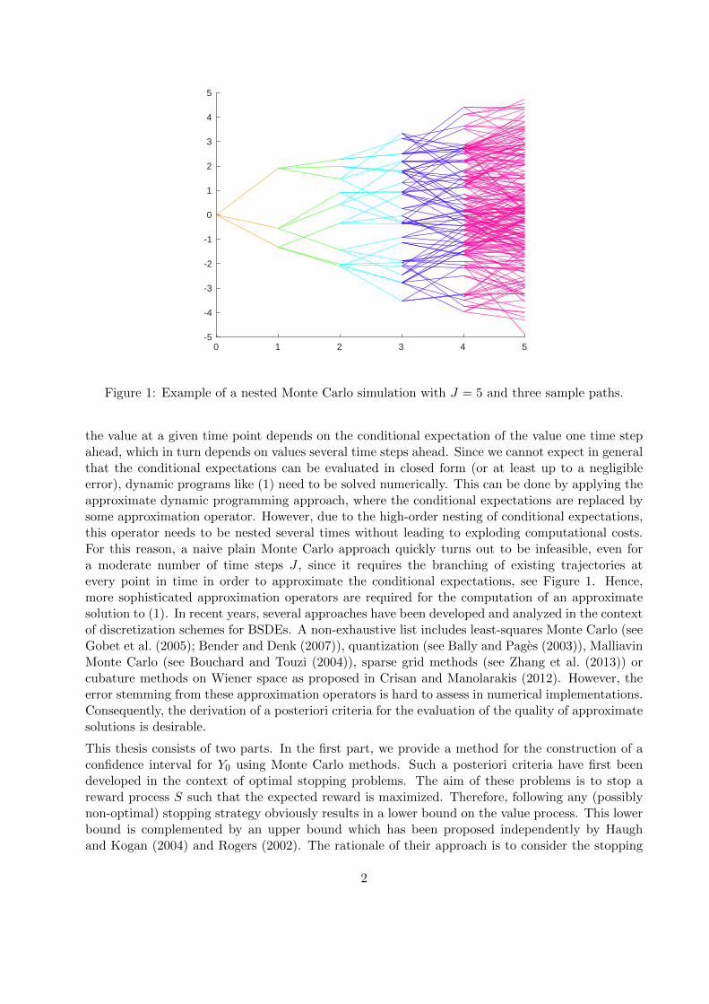
Figure 1: Example of a nested Monte Carlo simulation with J = 5 and three sample paths.

the value at a given time point depends on the conditional expectation of the value one time stepahead, which in turn depends on values several time steps ahead. Since we cannot expect in generalthat the conditional expectations can be evaluated in closed form (or at least up to a negligibleerror), dynamic programs like (1) need to be solved numerically. This can be done by applying theapproximate dynamic programming approach, where the conditional expectations are replaced bysome approximation operator. However, due to the high-order nesting of conditional expectations,this operator needs to be nested several times without leading to exploding computational costs.For this reason, a naive plain Monte Carlo approach quickly turns out to be infeasible, even fora moderate number of time steps J , since it requires the branching of existing trajectories atevery point in time in order to approximate the conditional expectations, see Figure 1. Hence,more sophisticated approximation operators are required for the computation of an approximatesolution to (1). In recent years, several approaches have been developed and analyzed in the contextof discretization schemes for BSDEs. A non-exhaustive list includes least-squares Monte Carlo (seeGobet et al. (2005); Bender and Denk (2007)), quantization (see Bally and Pages (2003)), MalliavinMonte Carlo (see Bouchard and Touzi (2004)), sparse grid methods (see Zhang et al. (2013)) orcubature methods on Wiener space as proposed in Crisan and Manolarakis (2012). However, theerror stemming from these approximation operators is hard to assess in numerical implementations.Consequently, the derivation of a posteriori criteria for the evaluation of the quality of approximatesolutions is desirable.

This thesis consists of two parts. In the first part, we provide a method for the construction of aconfidence interval for Y0 using Monte Carlo methods. Such a posteriori criteria have first beendeveloped in the context of optimal stopping problems. The aim of these problems is to stop areward process S such that the expected reward is maximized. Therefore, following any (possiblynon-optimal) stopping strategy obviously results in a lower bound on the value process. This lowerbound is complemented by an upper bound which has been proposed independently by Haughand Kogan (2004) and Rogers (2002). The rationale of their approach is to consider the stopping

2

problem pathwise rather than in conditional expectation, i.e., instead of solving the optimal stop-ping problem, one maximizes the reward along each path. In order to make this bound tight, theresulting additional information is penalized by subtracting a martingale increment. Taking theinfimum over the set of martingales, they prove that the value process possesses a representation asdual minimization problem. Relying on this pair of primal-dual optimization problems, Haugh andKogan (2004) and Andersen and Broadie (2004) propose a primal-dual approach for the construc-tion of upper and lower bounds: in a first step, one approximately solves the dynamic programassociated with this problem, which is given by choosing Gj(z, y) = y, Fj(z) = maxSj , z, ξ = SJ ,and β ≡ 1 for an adapted process (Sj)j=0,...,J in (1). Then, an approximate stopping rule and amartingale are constructed from this approximate solution. Taking these suboptimal controls asan input, upper and lower bounds can be constructed from the primal-dual representations.

The information relaxation approach of Haugh and Kogan (2004) and Rogers (2002) was furthergeneralized by Rogers (2007) and Brown et al. (2010) to stochastic control problems in discretetime. While Rogers (2007) only considers perfect information relaxation and martingale penaltiesas in the optimal stopping problem, Brown et al. (2010) allow for information relaxations to avarying extent and a broader class of penalties.

Bender et al. (2017) extended the primal-dual approach to the class of monotone and convexdynamic programs. Starting from a dynamic programming equation, they derive primal and dualoptimization problems with value Y for which optimal controls exist and are given in terms ofthe true solution Y . Following Haugh and Kogan (2004) and Andersen and Broadie (2004) in thenumerical implementation, they construct upper and lower bounds by first solving the dynamicprogram approximately and use this approximate solution to derive suboptimal controls. Takingthese suboptimal controls as an input, they recursively compute super- and subsolutions to thedynamic program. Here, a supersolution (respectively subsolution) is an adapted process whichsatisfies (1) with ”≥” (respectively ”≤”) instead of ”=”. Assuming a comparison principle, whichensures that supersolutions lie above subsolutions, Bender et al. (2017) show that the constructedprocesses constitute bounds to the solution of the dynamic program.

The first two chapters aim at generalizing the primal-dual approach proposed by Bender et al. (2017)in various directions. In the first chapter, we generalize their approach to the multi-dimensionalsetting and consider systems of convex dynamic programs. Assuming a componentwise comparisonprinciple, the results of Bender et al. (2017) can be transferred to this new setting in a straightfor-ward way. Since, in general, super- and subsolutions to (1) need not be ordered and, thus, do notconstitute bounds, we discuss the comparison principle in more detail. In many one-dimensionalapplications like the optimal stopping problem or the examples considered in Bender et al. (2017)this assumption is either not an issue or it can be established by mild truncations of the process β.However, in the context of systems of dynamic programming equations, we show that the existenceof a componentwise comparison principle requires that each component does not depend on thespace derivative of the other components and that it only depends on the other components in amonotonically increasing way. Consequently, the comparison principle can be a huge drawback inthis setting and the remainder of the first chapter is dedicated to remove this assumption.

The main result of this chapter is, thus, concerned with the construction of a pair of super- andsubsolutions for which a componentwise comparison principle holds, although it fails to hold ingeneral. This is achieved by a modification of the recursions for upper and lower bounds proposedby Bender et al. (2017). The rationale of the construction is to allow that the lower bound enters thedefining recursion for the upper bound and vice versa. Going backwards in time, we check in eachrecursion step if a violation of the comparison principle occurs on any given path. If the comparison

3

principle is violated, the dependence of each recursion on both bounds applies and ensures theordering of the bounds. In this way, we end up with coupled recursions for the construction ofupper and lower bounds, which need to be computed simultaneously. As a consequence, thesebounds cannot be interpreted as stemming from distinct primal and dual optimization problemsin general. The applicability of this approach is then demonstrated in two numerical examples,namely pricing under collateralization and pricing under uncertain volatility. To this end, we firstprovide a general way to implement an algorithm based on this approach in a Markovian framework.For the construction of an approximate solution, we rely on least-squares Monte Carlo (LSMC).In particular, we provide a variant of the regression-later approach by Glasserman and Yu (2004)respectively the martingale basis approach proposed by Bender and Steiner (2012), which is moreflexible concerning its applicability.

Thereafter, we pass in Chapter 2 to concave-convex dynamic programs of the form (1). Assum-ing this structure has essentially two reasons: first, many functions, which are neither convex orconcave, can be expressed as a composition of suitable convex and concave functions. Indeed, weshow that such a situation arises in the context of pricing under bilateral counterparty risk, i.e.,in situations where both parties involved in a contract may default prior to maturity. The secondreason is that convex respectively concave structures naturally arise in many maximization respec-tively minimization problems. Assuming the concave-convex structure, thus allows us to considerdynamic programming equations arising in stochastic two-player games. In mathematical financea well-known example for such stochastic two-player games is the problem of pricing convertiblebonds, see e.g. Beveridge and Joshi (2011).

The aim of this chapter is to transfer the results derived in Chapter 1 to this new setting. In order tosimplify the exposition, we restrict ourselves to the case of a single equation, but emphasize that theresults can be transferred in a straightforward way to systems of concave-convex dynamic programs.As before, we first derive recursions for the construction of super- and subsolutions in a monotonesetting, i.e., when a comparison principle holds. These are obtained by a suitable composition ofthe upper and lower bounds for the respective concave and convex problems. We further providesufficient conditions for the comparison principle to hold, but, compared to the convex setting ofChapter 1, we are not able to give equivalent characterizations. This is essentially due to theadditional concave structure. Finally, we relax the assumption of a comparison principle andgeneralize the coupled bounds from Chapter 1 to the concave-convex setting. As in the monotonecase, this construction relies on a suitable composition of the coupled bounds for the respectiveconcave and convex problem. Finally, we apply our approach in a numerical example concernedwith pricing under bilateral counterparty risk.

The second part of this thesis aims at the derivation of an iterative improvement algorithm forupper and lower bounds in the convex setting of Chapter 1. We call a supersolution (respectivelysubsolution) to a convex dynamic program an improvement if it lies below (respectively above) agiven input supersolution (respectively subsolution). Developing such an improvement approach ismotivated by the observation that the width of a confidence interval for Y0 constructed from theprimal-dual approach derived in the first two chapters strongly depends on the input approximation.This is due to the derivation of suboptimal controls required for the computation of upper and lowerbounds from an approximate solution to the dynamic programming equation.

When computing an approximate solution using LSMC, the resulting error stems to a large partfrom the so-called projection error, which is hard to control. This error occurs by replacing theprojection onto an (in general) infinite-dimensional subspace of L2(Ω, P ) by the projection onto afinite-dimensional subspace spanned by the basis functions. In order to keep this error moderate,

4

a suitable choice of basis functions is required. Intuitively, a ”good” function basis should captureboth, the terminal condition ξ and the non-linearities modeled by the functions Gj and Fj . As thereis no constructive way to obtain such basis functions, searching for these can be rather cumbersome.

In the context of optimal stopping problems, Kolodko and Schoenmakers (2006) propose an iterativeimprovement approach for lower bounds as an alternative to solving the dynamic program usingLSMC. This approach converges to the true solution after finitely many iteration steps and avoidsthe choice of basis functions. The rationale of this approach is to start from a family of stoppingtimes, and to derive new exercise criteria, from which an increasing sequence of lower boundsis obtained. This kind of policy iteration has first been proposed in the context of stochasticcontrol problems, see Howard (1960); Puterman (1994). Complementing the approach of Kolodkoand Schoenmakers (2006), Chen and Glasserman (2007) propose an algorithm which iterativelyimproves a given upper bound. Taking the martingale part of the Doob decomposition of a givensupersolution as an input for the dual approach of Haugh and Kogan (2004) and Rogers (2002),they show that the resulting upper bound lies below the given supersolution.

The aim of the third chapter is to generalize the approaches of Kolodko and Schoenmakers (2006)and Chen and Glasserman (2007) to the class of monotone systems of convex dynamic programsdiscussed in Chapter 1. For the construction of such an improvement algorithm we rely on therecursions for upper and lower bounds derived in the first chapter. Starting from given super- andsubsolutions, the main idea of this construction is to derive controls in terms of the input super- andsubsolutions. Taking the resulting controls as an input for the upper and lower bound recursions,we end up with an improvement for the given super- and subsolutions. We further demonstratethat this approach can be iterated in a straightforward way and show that it converges in finitelymany iteration steps. Moreover, we show that the true solution Y to the dynamic program isthe only fixed point of this iteration. Hence, even when starting with possibly crude super- andsubsolutions, this approach does not get stuck in any suboptimal upper and lower bounds.

The results of this thesis are already available in two papers, which are joint work with ChristianBender and Nikolaus Schweizer:

Christian Bender, Christian Gartner, and Nikolaus Schweizer. Pathwise Dynamic Pro-gramming. Mathematics of Operations Research. forthcoming.

Christian Bender, Christian Gartner, and Nikolaus Schweizer. Iterative Improvement ofUpper and Lower Bounds for Backward SDEs. SIAM Journal of Scientific Computing.39(2):B442-B466, 2017.

Based on these papers, Chapters 1 and 3 are concerned with systems of convex dynamic programs.While Chapter 1 provides a more detailed discussion of such systems compared to the correspondingSection 6 in the first paper, Chapter 3 generalizes the results of the second paper to this multi-dimensional setting wherever possible.

5

6

Notation

In the following, we introduce some notation, which is frequently used:

Let x ∈ R be a real number. Then, we denote by (x)+ and (x)− the positive respectively negativepart of x, i.e., (x)+ := maxx, 0 and (x)− := max−x, 0. Further, we denote by |x| the absolutevalue of x.

For a vector y ∈ RD, we denote by ‖y‖ the Euclidean norm of y. We say that y1 ≥ y2 for two

vectors y1, y2 ∈ RD if y(ν)1 ≥ y

(ν)2 for all ν = 1, . . . , D. Moreover, we denote by 1 the vector in

RD consisting of ones and for any matrix A, A> is the matrix transposition of A. For a vectorz ∈ RND, we denote by z[n] the vector in RD consisting of the ((n− 1)D+ 1)-th up to the (nD)-thentry of z, i.e. z = (z[1], . . . , z[N ]).

Further let (Ω,F , (Fj)j=0,...,J , P ) be a filtered probability space. Then we denote by L∞−(Rm),m ∈ N, the set of Rm-valued random variables that are in Lp(Ω, P ) for all p ≥ 1. The set of Fj-measurable random variables that are in L∞−(Rm) is denoted by L∞−j (Rm). In addition, L∞−ad (Rm)

denotes the set of adapted processes Z such that Zj ∈ L∞−j (Rm) for every j = 0, . . . , J .

For a D-dimensional Brownian motion W and a partition 0 = t0 < t1 < . . . < tJ = T of the interval[0, T ], we denote by ∆Wj+1 := Wtj+1−Wtj , j = 0, . . . , J−1, the increment of the Brownian motionover the interval [tj , tj+1]. The length of the interval [tj , tj+1] is denoted by ∆j+1. If the partitionis assumed to be equidistant, we simply write ∆ instead of ∆j+1 for all j = 0, . . . , J − 1.

Moreover, N and ϕ denote respectively the cumulative distribution function and the density func-tion of the standard normal distribution.

Finally, all equalities and inequalities are meant to hold P -a.s, unless otherwise noted.

7

8

Chapter 1

Systems of convex dynamicprogramming equations

In this chapter, we consider systems of dynamic programming equations, which arise, e.g., in thecontext of multiple stopping problems or as discretization schemes for systems of partial differ-ential equations. The scope of this chapter is to derive upper and lower bounds to the solutionof such systems. To do this, we generalize the pathwise approach of Bender et al. (2017) to thismulti-dimensional setting. Section 1.1 presents some examples for systems of convex dynamic pro-gramming equations arising in option pricing. In Section 1.2, we introduce the setting as well asthe required definitions and notations. Section 1.3 is dedicated to the pathwise approach of Benderet al. (2017). We recall the main ideas of this approach and, at the same time, generalize them toour multi-dimensional setting. In Section 1.4, we give equivalent characterizations of the compar-ison principle and explain its restrictiveness by an example. Building on these considerations, wegeneralize the approach of Bender et al. (2017) in Section 1.5 in such a way that upper and lowerbounds to the solution of the dynamic program can be derived without relying on the comparisonprinciple. Section 1.6 provides a first insight in the numerical implementation of the theoreticalresults presented before. More precisely, we show how the application of approximation methodsrequired in the numerical implementation may lead to an additional bias in the upper and lowerbounds. Section 1.7 explains how the theoretical results from Sections 1.3 and 1.5 can be appliedin practice. To this end, we first explain how the bounds can be computed in a general setting.Finally, we demonstrate the applicability of our approach with two numerical examples, namelythe problem of pricing a European-style option under funding costs and negotiated collateral andpricing under uncertain volatility.

1.1 Examples

In this chapter, we focus on systems of dynamics programs of the form

Y(ν)J = ξ(ν)

Y(ν)j = F

(ν)j

(Ej

[βj+1Y

(1)j+1

], . . . , Ej

[βj+1Y

(N)j+1

]), ν = 1, . . . , N, j = J − 1, . . . , 0, (1.1)

where, Ej [·] denotes the conditional expectation with respect to Fj for a given filtration (Fj)j=0,...,J

and the functions F(ν)j are convex. In the following, we present three examples arising in mathe-

matical finance, which motivate the investigation of such systems.

9

Example 1.1.1. We first consider the multiple stopping problem. In mathematical finance, thisproblem occurs e.g. in the context of swing option pricing problems, see e.g. Carmona and Touzi(2008) and Bender et al. (2015). In the multiple stopping problem, one is interested in stopping areward process S ∈ L∞−ad (R) N -times over a given time horizon such that the expected reward ismaximized. In this example, we consider a discrete time situation, where all exercise rights need tobe executed at different time points and that all remaining rights at maturity need to be executedsimultaneously. Hence, the corresponding value process is given by

Y(N)j = esssup

τ∈Sj(N)Ej

[N∑k=1

Sτ (k)

]

for every j = 0, . . . , J and where Sj(N) is the set of stopping vectors τ = (τ (1), . . . , τ (N)) such thatj ≤ τ (1) ≤ . . . ≤ τ (N) ≤ J and τ (k) = τ (k+1) implies τ (k) = J . As it is well-known in the literature,this pricing problem can be transferred to solving a system of dynamic programming equations. Inour setting, this system is given by

Y(ν)j = max

Ej

[Y

(ν)j+1

], Sj + Ej

[Y

(ν−1)j+1

], Y

(ν)J = νSJ ,

for j = 0, . . . , J − 1, ν = 1, . . . , N and with the convention that Y (0) ≡ 0. Here, Y(ν)j is the value of

the problem at time index j if ν rights can be executed. For a vector z ∈ RND, denote by z[n] thevector in RD consisting of the ((n−1)D+1)-th up to the (nD)-th entry of z, i.e. z = (z[1], . . . , z[N ]).

By taking D = 1, the process β ≡ 1, ξ(ν) = νSJ , and F(ν)j (z) = maxz[ν], Sj + z[ν−1], we then

observe that the multiple stopping problem fits our framework.

Example 1.1.2. As a second example, we consider the problem of pricing under negotiated collater-alization in the presence of funding costs as discussed in Nie and Rutkowski (2016). Collateralizedcontracts differ from ”standard” contracts in the way that the involved parties not only agree ona payment stream until maturity but also on the collateral posted by both parties. By providingcollateral, both parties can reduce the possible loss resulting from a default of the respective coun-terparty prior to maturity. In the following, we consider the problem of pricing a contract undernegotiated collateral, i.e. the imposed collateral depends on the valuations of the contract madeby the two parties. More precisely, the party (”hedger”) wishes to perfectly hedge the stream ofpayments consisting of the option payoff and the posted collateral under funding costs, while thecounterparty hedges the negative payment stream under funding costs. As hedging under fundingcosts is known to be non-linear, both hedges do not cancel each other. Hence, one ends up witha coupled system of two equations where the coupling is due to the fact that the counterparty’shedging strategy influences the hedger’s payment stream due to the negotiated collateral and viceversa.

We first translate the original backward SDE formulation of the problem in Nie and Rutkowski(2016) into a parabolic PDE setting. To this end let g : Rd → R be a function of polynomial growthwhich represents the payoff of a European-style option written on d risky assets with maturityT . The dynamics of the risky assets X = (X(1), . . . , X(d)) are given by independent identicallydistributed Black-Scholes models

X(l)t = x0 exp

(RL − 1

2σ2

)t+ σW

(l)t

, l = 1, . . . , d,

where RL ≥ 0 is the risk-free lending rate, σ > 0 is the assets volatility, and W = (W (1), . . . ,W (d))is a d-dimensional Brownian motion. We, moreover, denote by RB the risk-free borrowing rate.

10

Hence, we have that RB ≥ RL. Further, we denote by RC the collateralization rate, which is theinterest that the receiver of the collateral has to pay to the provider of the collateral. As in Example3.2 in Nie and Rutkowski (2016) we consider the case that the collateral is a convex combinationq(v(1),−v(2)) = αv(1) + (1 − α)(−v(2)) of the hedger’s price v(1) (i.e., the party’s hedging cost)and the counterparty’s price −v(2) (i.e, the negative of the counterparty’s hedging cost) for someα ∈ [0, 1]. Following Proposition 3.3 in Nie and Rutkowski (2016) with zero initial endowment thesystem of PDEs then reads as follows:

v(ν)t (t, x) +

1

2

d∑k,l=1

v(ν)xk,xl

(t, x) = −H(ν)(v(1)(t, x),∇xv(1)(t, x), v(2)(t, x),∇xv(2)(t, x)), ν = 1, 2,

(t, x) ∈ [0, T )× Rd, with terminal conditions

v(ν)(T, x) = (−1)ν−1g

((x0 exp

(RL − 1

2σ2

)t+ σx(k)

)k=1,...,d

), x = (x(1), . . . , x(d)) ∈ Rd

and non-linearities given by

H(ν)(v(1)(t, x),∇xv(1)(t, x), v(2)(t, x),∇xv(2)(t, x))

= −RLaν(v(1)(t, x) + v(2)(t, x)) + (−1)νRC(αv(1)(t, x)− (1− α)v(2)(t, x))

+(RB −RL)

(aν(v(1)(t, x) + v(2)(t, x))− 1

σ(∇xv(ν)(t, x))>1

)−,

where, (a1, a2) = (1 − α, α). With this notation, v(1)(t,Wt) and −v(2)(t,Wt) denote the hedger’sprice and counterparty’s price of the collateralized contract at time t.

This problem is a special case of general systems of semilinear parabolic PDEs of the form

v(ν)t (t, x) +

1

2

d∑k,l=1

(σσ>)k,l(t, x)v(ν)xk,xl

(t, x) +d∑

k=1

bk(t, x)v(ν)xk

(t, x)

= −H(ν)(t, x, v(1)(t, x), σ(t, x)∇xv(1)(t, x), . . . , v(N)(t, x), σ(t, x)∇xv(N)(t, x)), (1.2)

(t, x) ∈ [0, T ) × Rd, ν = 1, . . . , N with terminal conditions v(ν)(T, x) = g(ν)(x). This systemhas a unique classical solution, if the coefficients σ : [0, T ] × Rd → Rd×d, b : [0, T ] × Rd → Rd,H(ν) : [0, T ]× Rd × RN(1+d) → R, and g(ν) : Rd → R satisfy suitable conditions, see e.g. Friedman(1964). In order to derive a discretization of (1.2), which fits into our framework, we exploit thelink between semilinear parabolic PDEs and backward stochastic differential equations (BSDEs)(see e.g. Pardoux, 1998). Let v be a classical solution to (1.2). Then, we have that the process(Ys, Zs)0≤s≤T := (v(s,Xs), σ(s,Xs)∇xv(s,Xs))0≤s≤T is a solution to the BSDE

Ys = g(XT ) +

∫ T

sH(r,Xr, Yr, Zr) dr −

∫ T

sZ>r dWr, 0 ≤ s ≤ T. (1.3)

Here, W is a d-dimensional Brownian motion and the process (Xs)0≤s≤T is given by the stochasticdifferential equation

Xs = x+

∫ s

0b(r,Xr) dr +

∫ s

0σ(r,Xr) dWr, 0 ≤ s ≤ T. (1.4)

Discretizing (1.3) and (1.4), leads to a discretization scheme for (1.2): To this end, let π =(t0, . . . , tJ) be a partition of [0, T ] and denote by ∆Wi+1 := Wti+1 − Wti the increments of the

11

Brownian motion W over time increments of size ∆i+1 = ti+1− ti. Further, let Fj be the σ-algebragenerated by W up to time tj , j = 0, . . . , J . Then, we consider the Euler-type scheme

Xj+1 = Xj + b(tj , Xj)∆j+1 + σ(tj , Xj)∆Wj+1, X0 = x,

Y(ν)J = g(ν)(XJ),

Y(ν)j = Ej

[Y

(ν)j+1

]+H(ν)

(tj , Xj , Ej

[βj+1Y

(1)j+1

], . . . , Ej

[βj+1Y

(N)j+1

])∆j+1,

βj+1 =

(1,

∆W(1)j+1

∆j+1, . . . ,

∆W(d)j+1

∆j+1

)>, (1.5)

for j = 0, . . . , J − 1 and ν = 1, . . . , N , where Ej [·] denotes the conditional expectation with respectto Fj . Taking D = d + 1, we observe that this scheme is of the form (1.15) for any function H,which is convex in the last ND variables, if the coefficients satisfy suitable growth conditions.

Such discretization schemes are well-studied in the BSDE-literature, see e.g. Bouchard and Touzi(2004), Zhang (2004), Gobet and Labart (2007), and Gobet and Makhlouf (2010). Note that,

convergence rates for the approximation error supν=1,...,N |v(ν)(0, x)−Y (ν)0 | induced by this kind of

approximation schemes are available. Indeed, Zhang (2004) shows that it converges at order 1/2in the mesh size of the partition, if the non-linearities H(ν) and the terminal conditions g(ν) satisfycertain Lipschitz conditions.

Example 1.1.3. We finally consider an example for a dynamic program of the form (1.15) with onlyone equation (i.e. N = 1), namely the problem of pricing a European-style option under uncertainvolatility. This problem has first been studied in Avellaneda et al. (1995) and Lyons (1995). Hence,let Xσ be the value process of a risky asset whose dynamics under the risk-neutral measure and indiscounted units are given by

Xσt = x0 exp

∫ t

0σudWu −

1

2

∫ t

0σ2udu

,

where x0 ∈ R, W is a Brownian motion and the volatility σ is a stochastic process which is adaptedto the filtration (Ft)0≤t≤T generated by W . Further, let g : R → R be the payoff of a Europeanoption. Then, the value of this option under uncertain volatility is given by

Y0 = supσE[g(Xσ

T )], (1.6)

where the supremum is taken over all nonanticipating volatility processes σ, which take values in[σlow, σup]. By considering the supremum over all processes ranging in this interval, Y0 providesa worst case price which reflects the volatility uncertainty. In the following, we assume that theconstants satisfy 0 < σlow ≤ σup <∞.

Since (1.6) is a stochastic control problem in continuous time, we can write down the Hamilton-Jacobi-Bellman equation, which is given by

ut(t, x) + maxσ∈σlow,σup

1

2σ2x2uxx(t, x) = 0, (t, x) ∈ [0, T )× R

u(T, x) = g(x), x ∈ R. (1.7)

Note that the PDE (1.7) possesses a classical solution, which satisfies appropriate growth conditions,under suitable assumptions on the terminal condition g, see Pham (2009).

12

Similar to Example (1.1.2), we want to derive a discretization scheme for (1.6), which is of the form(1.15), from (1.7). To this end, we fix a constant volatility ρ and consider the transformation

v(t, x) := u

(t, x0 exp

ρx− 1

2ρ2t

), x ∈ R,

in the space variable. Then, (1.7) can be rewritten in the following form:

vt(t, x) +1

2vxx(t, x) + max

σ∈σlow,σup

1

2

(σ2

ρ2− 1

)(vxx(t, x)− ρvx(t, x))

= 0,

(t, x) ∈ [0, T )× R,

v(T, x) = g

(x0 exp

ρx− 1

2ρ2T

), x ∈ R. (1.8)

In order to derive an approximate solution of (1.8), we apply an operator splitting scheme. There-fore, let 0 = t0 < t1 < . . . < tJ = T be an equidistant discretization of the time interval [0, T ] withmesh size ∆. Building on this discretization, we consider, for fixed J , the system

yJ(x) = g(x0e

ρx− 12ρ2T), x ∈ R,

yjt (t, x) = −1

2yjxx(t, x), (t, x) ∈ [tj , tj+1)× R, (1.9)

yj(tj+1, x) = yj+1(x), x ∈ R, (1.10)

yj(x) = yj(tj , x) + ∆ maxσ∈σlow,σup

1

2

(σ2

ρ2− 1

)(yjxx(tj , x)− ρyjx(tj , x)

), x ∈ R, (1.11)

for j = J−1, . . . , 0. Hence, the idea of this approach is to solve the linear subproblem (1.9) – (1.10),which is a Cauchy problem for the heat equation, of (1.8) on each of the intervals [tj , tj+1] and toplug the corresponding solution in the non-linearity (1.11). Evaluating yj(x) along the Brownianpaths leads to Yj := yj(Wtj ). A straightforward application of the Feynman-Kac representation forthe solution of (1.9) – (1.10), see e.g. Karatzas and Shreve (1991), on each interval, then yields

yj(tj ,Wtj ) = Ej [yj+1(Wtj+1)] = Ej [Yj+1],

where Ej [·] denotes the conditional expectation with respect to Fj . For the space derivatives yjx(t, x)

and yjxx(t, x), we obtain by integration by parts that

yjx(tj ,Wtj ) = Ej

[∆Wj+1

∆Yj+1

](1.12)

and

yjxx(tj ,Wtj ) = Ej

[(∆W 2

j+1

∆2− 1

∆

)Yj+1

], (1.13)

where ∆Wj = Wtj−Wtj−1 . A detailed derivation of (1.12) and (1.13) can be found in the AppendixA.1. Note that (1.12) and (1.13) are the Malliavin Monte Carlo weights derived in Fournie et al.(1999).

Finally, we end up with the following discrete-time dynamic programming equation

YJ = g(X ρT ),

13

Yj = Ej [Yj+1] + ∆ maxσ∈σlow,σup

(1

2

(σ2

ρ2− 1

)Ej

[(∆W 2

j+1

∆2− ρ∆Wj+1

∆− 1

∆

)Yj+1

]), (1.14)

where X ρT denotes the price of the asset at time T under the constant reference volatility ρ. Such

type of time-discretization scheme is proposed and analyzed for a general class of fully non-linearparabolic PDEs by Fahim et al. (2011). In the particular case of the uncertain volatility model,the scheme was suggested by Guyon and Henry-Labordere (2011) by a slightly different derivation.They rely on the connection between fully non-linear parabolic PDEs and second order backwardstochastic differential equations, see Cheridito et al. (2007). Choosing

Fj(z) = z(1) + ∆ maxs∈slow,sup

sz(2),

where sι = 12(σ

2ιρ2 − 1) for ι ∈ up, low, and

βj =

(1,

∆W 2j

∆2− ρ∆Wj

∆− 1

∆

)>, j = 1, . . . , J,

we observe that (1.14) is of the form (1.15) with N = 1 and D = 2.

1.2 Setup

Let (Ω,F , (Fj)j=0,...,J , P ) be a complete filtered probability space. Throughout the chapter weconsider systems of convex dynamic programs of the form

Y(ν)J = ξ(ν)

Y(ν)j = F

(ν)j

(Ej

[βj+1Y

(1)j+1

], . . . , Ej

[βj+1Y

(N)j+1

]), ν = 1, . . . , N, j = J − 1, . . . , 0, (1.15)

where Ej [·] denotes the conditional expectation with respect to Fj . If this system is one-dimensional,i.e. if N = 1, we use the shorthand notation Y := Y (1). For our considerations, the following con-vexity and regularity assumptions are required:

Assumption 1.2.1. (i) For every j = 0, . . . , J − 1 and ν = 1, . . . , N , F(ν)j : Ω × RND → R is

measurable and, for every z ∈ RND, the process (j, ω) 7→ F(ν)j (ω, z) is adapted.

(ii) The map z 7→ F(ν)j (ω, z) is convex in z for every j = 0, . . . , J − 1, ν = 1, . . . , N and ω ∈ Ω.

(iii) For every ν = 1, . . . , N , F (ν) is of polynomial growth in z in the following sense: There exist

a constant q ≥ 0 and a non-negative adapted process (α(ν)j )j=0,...,J−1 ∈ L∞−ad (R) such that for

all z ∈ RND and j = 0, . . . , J − 1

∣∣∣F (ν)j (z)

∣∣∣ ≤ α(ν)j

(1 +

N∑n=1

∥∥∥z[n]∥∥∥q) , P -a.s..

(iv) The process β = (βj)j=1,...,J is an element of L∞−ad (RD).

(v) For each ν = 1, . . . , N , the terminal conditions ξ(ν) are elements of L∞−J (R).

14

From these assumptions, we obtain immediately the following lemma.

Lemma 1.2.2. Under Assumption 1.2.1 the P -almost surely unique solution Y to (1.15) is anelement of L∞−ad (RN ).

Proof. The proof is by backward induction on j = J, . . . , 0. For j = J the assertion is triviallytrue as ξ = (ξ(1), . . . , ξ(N)) ∈ L∞−J (RN ) by assumption. Now suppose that the assertion is true

for j + 1. Then, Yj is Fj-measurable, since Ej [βj+1Y(ν)j+1] and F

(ν)j (z) are Fj-measurable for every

ν = 1, . . . , N and z ∈ RND.

For the integrability, we first note, that the case q = 0 is trivial, since this corresponds to the

situation, where the functions F(ν)j , and thus the solution Y , are bounded by a sufficiently integrable

process. Hence, we suppose in the following that q > 0. Moreover, we assume without loss of

generality that p ≥ 1 satisfies 2pq ≥ 1. From the polynomial growth condition on F(ν)j , we first

observe that

E[∣∣∣Y (ν)

j

∣∣∣p] 1p

= E[∣∣∣F (ν)

j

(Ej

[βj+1Y

(1)j+1

], . . . , Ej

[βj+1Y

(N)j+1

])∣∣∣p] 1p

≤ E

[∣∣∣∣∣α(ν)j

(1 +

N∑n=1

∥∥∥Ej [βj+1Y(n)j+1

]∥∥∥q)∣∣∣∣∣p] 1

p

.

Applying Holder’s inequality and the Minkowski inequality twice then yields

E[∣∣∣Y (ν)

j

∣∣∣p] 1p ≤ E

[∣∣∣α(ν)j

∣∣∣2p] 12p

E

∣∣∣∣∣1 +

N∑n=1

∥∥∥Ej [βj+1Y(n)j+1

]∥∥∥q∣∣∣∣∣2p 1

2p

≤ E[∣∣∣α(ν)

j

∣∣∣2p] 12p

1 + E

∣∣∣∣∣N∑n=1

∥∥∥Ej [βj+1Y(n)j+1

]∥∥∥q∣∣∣∣∣2p 1

2p

≤ E

[∣∣∣α(ν)j

∣∣∣2p] 12p

(1 +

N∑n=1

E

[∥∥∥Ej [βj+1Y(n)j+1

]∥∥∥2qp] 1

2p

).

Finally, we obtain by Jensen’s inequality (applied to the convex function y 7→ ‖y‖2pq) that

E[∣∣∣Y (ν)

j

∣∣∣p] 1p ≤ E

[∣∣∣α(ν)j

∣∣∣2p] 12p

(1 +

N∑n=1

E

[∥∥∥βj+1Y(n)j+1

∥∥∥2qp] 1

2p

)<∞.

Here, the last inequality is a consequence of the Assumption 1.2.1 and the induction hypothesis.

The aim of this chapter is to construct upper and lower bounds to the solution Y , which can becomputed pathwise. These build on the concept of super- and subsolutions to (1.15).

Definition 1.2.3. A process Y up (resp. Y low) ∈ L∞−ad (RN ) is called supersolution (resp. subsolu-tion) to the dynamic program (1.15) if Y up

J ≥ YJ (resp. Y lowJ ≤ YJ) and for every ν = 1, . . . , N

and j = 0, . . . , J − 1 it holds that

Y(up,ν)j ≥ F (ν)

j

(Ej

[βj+1Y

(up,1)j+1

], . . . , Ej

[βj+1Y

(up,N)j+1

])P -a.s.,

(and with ”≥” replaced by ”≤” for a subsolution).

15

In what follows, the construction of supersolutions builds on the choice of a suitable martingale.We thus denote in the following byMND the set of martingales M , which satisfy M ∈ L∞−ad (RND).For a process U ∈ L∞−ad (Rm), we refer to the martingale part of the Doob decomposition of U ,which is given by

j−1∑i=0

Ui+1 − Ei[Ui+1], j = 0, . . . , J,

as Doob martingale of U . In particular, we get from Assumption 1.2.1 that the Doob martingaleof the process βU is in MD for any U ∈ L∞−ad (R).

In contrast to supersolutions, subsolutions are constructed by rewriting (1.15) as a stochastic controlproblem using convex duality techniques and taking an admissible control. To this end, recall that

the convex conjugate of F(ν)j is, for every ω ∈ Ω, given by

F(ν,#)j (ω, u) := sup

z∈RND

(N∑n=1

(u[n])>

z[n] − F (ν)j (ω, z)

), (1.16)

with effective domain

D(j,ω)

F (ν,#) =u ∈ RND

∣∣∣ F (ν,#)j (ω, u) <∞

.

As we will see below, the sets of admissible controls in our problem are given by

AF (ν)

j =

(r

(ν)i

)i=j,...,J−1

∣∣∣∣ r(ν)i ∈ L∞−i

(RND

), F

(ν,#)i

(r

(ν)i

)∈ L∞−(R) for i = j, . . . , J − 1

,

where j = 0, . . . , J − 1 and ν = 1, . . . , N . By continuity of F(ν)i , we obtain that

F(ν,#)i (ri) = sup

z∈QND

(N∑n=1

(r

(ν),[n]i

)>z[n] − F (ν)

i (z)

)

is Fi-measurable for every r(ν) ∈ AF (ν)

j and i = j, . . . , J − 1. Moreover, from the integrability

condition on the controls we deduce that F(ν,#)i (r

(ν)i ) <∞, i.e., controls take values in the effective

domain of the convex conjugate of F(ν)i . The following lemma shows that the set AF (ν)

j is nonemptyfor every j = 0, . . . , J − 1 and ν = 1, . . . , N under the given assumptions.

Lemma 1.2.4. Fix j ∈ 0, . . . , J − 1 and let fj : Ω× Rd → R be a mapping such that, for everyω ∈ Ω, the map x 7→ fj(ω, x) is convex, and for every x ∈ Rd, the map ω 7→ fj(ω, x) is Fj-measurable. Moreover, suppose that fj satisfies the following polynomial growth condition: Thereare a constant q ≥ 0 and a non-negative random variable αj ∈ L∞−j (R) such that

|fj(x)| ≤ αj(1 + ‖x‖q), P -a.s.,

for every x ∈ Rd. Then, for every Z ∈ L∞−(Rd) there exists a random variable ρj ∈ L∞−(Rd) such

that f#j (ρj) ∈ L∞−(R) and

fj(Z) = ρ>j Z − f#j (ρj), P -a.s. (1.17)

If, additionally, Z is Fj-measurable, then we can take ρj Fj-measurable.

16

Proof. Let Z ∈ L∞−(Rd). Notice first that, since fj is convex and closed, we have f##j = fj by

Theorem 12.2 in Rockafellar (1970) and thus

fj(Z) = supu∈Rd

u>Z − f#j (u) ≥ ρ>Z − f#

j (ρ) (1.18)

holds ω-wise for any random variable ρ. We next show that there exists a random variable ρj forwhich (1.18) holds with P -almost sure equality. To this end, we apply Theorem 7.4 in Cheriditoet al. (2015) which yields the existence of a measurable subgradient to fj , i.e., existence of a randomvariable ρj such that for all Rd-valued random variables Z

fj(Z + Z

)− fj

(Z)≥ ρ>j Z, P -a.s. (1.19)

Choosing Z = z − Z for z ∈ Qd in (1.19), we conclude that

ρ>j Z − fj(Z)≥ ρ>j z − fj (z) . (1.20)

Since (1.20) holds for any z ∈ Qd, we obtain

ρ>j Z − fj(Z)≥ sup

z∈Qdρ>j z − fj (z) = f#

j (ρj), P -a.s., (1.21)

by continuity of fj , which is the converse of (1.18), proving P -almost sure equality for ρ = ρj andthus (1.17).

We next show that ρj satisfies the required integrability conditions, i.e., ρj ∈ L∞−(Rd) and f#j (ρj) ∈

L∞−(R). To this end, we first prove that ρ>j Z ∈ L∞−(R) for any Z ∈ L∞−(Rd). Due to (1.19)

and the Minkowski inequality and since a ≤ b implies a+ ≤ |b|, it follows for Z ∈ L∞−(Rd) that,for every p ≥ 1,(

E

[∣∣∣∣(ρ>j Z)+

∣∣∣∣p]) 1p

≤(E[∣∣fj (Z + Z

)∣∣p]) 1p +

(E[∣∣fj (Z)∣∣p]) 1

p <∞,

since fj is of polynomial growth with ‘random constant’ αj ∈ L∞−j (R) and Z, Z are elements of

L∞−(Rd) by assumption. Applying the same argument to Z = −Z yields

E

[∣∣∣∣(ρ>j Z)−∣∣∣∣p] = E

[∣∣∣∣(ρ>j Z)+

∣∣∣∣p] <∞,since (1.19) holds for all random variables Z and Z inherits the integrability of Z. We thus concludethat

E[∣∣∣ρ>j Z∣∣∣p] <∞ and E [|ρj |p] <∞,

where the second claim follows from the first by taking Z = sgn(ρj) with the sign function applied

componentwise. In order to show that f#j (ρj) ∈ L∞−(R), we start with (1.17) and apply the

Minkowski inequality to conclude that(E[∣∣∣f#

j (ρj)∣∣∣p]) 1

p ≤(E[∣∣∣ρ>j Z∣∣∣p]) 1

p+(E[∣∣fj (Z)∣∣p]) 1

p <∞.

Finally, we show that for Fj-measurable random variables Z there exists an Fj-measurable randomvariable ρj satisfying (1.17). To this end, let Z ∈ L∞−j (Rd) and let ρj be the possibly not Fj-measurable random variable for which (1.17) holds and whose existence is already shown. We show

17

that ρj = Ej [ρj ] is the asserted random variable. By taking the conditional expectation of (1.21)

and applying Jensen’s inequality to the convex function f#j , we conclude that

Ej [ρj ]> Z ≥ fj

(Z)

+ Ej

[f#j (ρj)

]≥ fj

(Z)

+ f#j (Ej [ρj ]) .

In combination with (1.18), we thus end up with

fj(Z) = Ej [ρj ]> Z − f#

j (Ej [ρj ]) = ρ>j Z − f#j (ρj)

as claimed. The integrability of ρj ∈ L∞−(Rd) and f#j (ρj) ∈ L∞−(R) follows by the same argu-

ments applied before.

1.3 The monotone case

In this section, we construct upper and lower bounds to the solution Y to (1.15). To do this, werely on the pathwise approach proposed by Bender et al. (2017) in the context of one-dimensionalconvex dynamic programs. This approach builds on the construction of super- and subsolutions to(1.15) and requires an additional monotonicity assumption on the functions F (ν) in the sense thata comparison principle holds. We begin this section by imposing the comparison principle. Then,we briefly recall the main ideas of Bender et al. (2017) and generalize them at the same time toour present setting.

In general, it is not clear that super- and subsolutions are ordered, i.e., it need not hold, thatY upj ≥ Yj ≥ Y low

j for all j = 0, . . . , J and, hence, they typically do not constitute bounds. Thefollowing assumption, to which we refer as comparison principle, ensures this.

Assumption 1.3.1. For every supersolution Y up and every subsolution Y low to the dynamic pro-gram (1.15) it holds that

Y upj ≥ Y low

j , P -a.s.,

for every j = 0, . . . , J .

The main idea of Bender et al. (2017) in the construction of the upper bound is to drop theconditional expectations in (1.15) and instead subtract a martingale increment. Hence, let j ∈0, . . . , J − 1 be fixed. Then, for a given martingale M ∈ MND, we define the typically non-adapted process Θup := Θup(M) recursively by

Θ(up,ν)J = ξ(ν)

Θ(up,ν)i = F

(ν)i

(βi+1Θ

(up,1)i+1 −∆M

[1]i+1, . . . , βi+1Θ

(up,N)i+1 −∆M

[N ]i+1

), i = J − 1, . . . , j, ν = 1, . . . , N,

(1.22)

where ∆M[n]i+1 := M

[n]i+1 −M

[n]i .

Lemma 1.3.2. Suppose Assumptions 1.2.1. Then, for every j ∈ 0, . . . , J and M ∈ MND, theprocess Θup(M) defined by (1.22) satisfies Θup

i (M) ∈ L∞−(RN ) for all i = j, . . . , J .

18

The proof of this lemma follows the same lines of reasoning as the one of Lemma 1.2.2, so that weomit the details here.

Based on the recursion (1.22), we define the adapted process Y up by

Y upj := Ej

[Θupj

], j = 0, . . . , J,

which is well-defined by Lemma 1.3.2. Then, Y up is a supersolution to (1.15). To see this, we firstapply Jensen’s inequality and obtain

Y(up,ν)j = Ej

[Θ

(up,ν)j

]= Ej

[F

(ν)j

(βj+1Θ

(up,1)j+1 −∆M

[1]j+1, . . . , βj+1Θ

(up,N)j+1 −∆M

[N ]j+1

)]≥ F (ν)

j

(Ej

[βj+1Θ

(up,1)j+1 −∆M

[1]j+1

], . . . , Ej

[βj+1Θ

(up,N)j+1 −∆M

[N ]j+1

]).

From the martingale property of M and the tower property of the conditional expectation, wefinally conclude that

Y(up,ν)j ≥ F (ν)

j

(Ej

[βj+1Θ

(up,1)j+1

], . . . , Ej

[βj+1Θ

(up,N)j+1

])= F

(ν)j

(Ej

[βj+1Ej+1

[Θ

(up,1)j+1

]], . . . , Ej

[βj+1Ej+1

[Θ

(up,N)j+1

]])= F

(ν)j

(Ej

[βj+1Y

(up,1)j+1

], . . . , Ej

[βj+1Y

(up,N)j+1

])for every j = 0, . . . , J−1 and ν = 1, . . . , N showing the supersolution property for the process Y up.

In order to construct a subsolution to (1.15), we rely on duality techniques from convex analysis.More precisely, we linearize the dynamic programming equation (1.15) in the following way: By

convexity and closedness of F(ν)j , we have due to Theorem 12.2 in Rockafellar (1970) that F

(ν,##)j =

F(ν)j for every j = 0, . . . , J − 1, ν = 1, . . . , N and ω ∈ Ω. Hence, for every j = 0, . . . , J − 1,

ν = 1, . . . , N , ω ∈ Ω, and z ∈ RND, it holds that

F(ν)j (ω, z) = sup

u∈RND

N∑n=1

(u[n])>

z[n] − F (ν,#)j (ω, u), (1.23)

where F(ν,#)j denotes the convex conjugate of F

(ν)j defined in (1.16). From Lemma 1.2.4, we get

existence of an adapted process r(ν,∗) ∈ AF (ν)

0 which solves

N∑n=1

(r

(ν,∗),[n]j

)>Ej

[βj+1Y

(n)j+1

]− F (ν,#)

j

(r

(ν,∗)j

)= F

(ν)j

(Ej

[βj+1Y

(1)j+1

], . . . , Ej

[βj+1Y

(N)j+1

])(1.24)

for every j = 0, . . . , J − 1 and ν = 1, . . . , N .

Following Bender et al. (2017), we now fix admissible controls r(ν) ∈ AF (ν)

j , ν = 1, . . . , N , and

define the typically non-adapted process Θlow := Θlow(r(1), . . . , r(N)) by

Θ(low,ν)J = ξ(ν),

Θ(low,ν)i =

N∑n=1

(r

(ν),[n]i

)>βi+1Θ

(low,n)i+1 − F (ν,#)

i

(r

(ν)i

), i = J − 1, . . . , j, ν = 1, . . . , N, (1.25)

for j ∈ 0, . . . , J − 1.

19

Lemma 1.3.3. Suppose Assumptions 1.2.1. Then, for every j ∈ 0, . . . , J and any admissible

controls r(ν) ∈ AF (ν)

j , ν = 1, . . . , N , the process Θlow(r(1), . . . , r(N)) defined by (1.25) satisfies

Θlowi (r(1), . . . , r(N)) ∈ L∞−(RN ) for all i = j, . . . , J .

Proof. Let j ∈ 0, . . . , J − 1 and r(ν) ∈ AF (ν)

j , ν = 1, . . . , N , be fixed from now on and define

Θlow := Θlow(r(1), . . . , r(N)) by (1.25). The proof is by backward on induction on i = j, . . . , J − 1with the case i = J being trivial, since ξ(ν) ∈ L∞−J (R) by assumption for each ν. Now suppose thatthe assertion is true for i+ 1. Then, the Minkowski inequality and the Holder inequality yield

E[∣∣∣Θ(low,ν)

i

∣∣∣p] 1p

= E

[∣∣∣∣∣N∑n=1

(r

(ν),[n]i

)>βi+1Θ

(low,n)i+1 − F (ν,#)

i

(r

(ν)i

)∣∣∣∣∣p] 1

p

≤ E

[∣∣∣∣∣N∑n=1

(r

(ν),[n]i

)>βi+1Θ

(low,n)i+1

∣∣∣∣∣p] 1

p

+ E[∣∣∣F (ν,#)

i

(r

(ν)i

)∣∣∣p] 1p

≤N∑n=1

E

[∣∣∣∣(r(ν),[n]i

)>βi+1Θ

(low,n)i+1

∣∣∣∣p] 1p

+ E[∣∣∣F (ν,#)

i

(r

(ν)i

)∣∣∣p] 1p

≤N∑n=1

E

[∣∣∣∣(r(ν),[n]i

)>βi+1

∣∣∣∣2p] 1

2p

E

[∣∣∣Θ(low,n)i+1

∣∣∣2p] 12p

+ E[∣∣∣F (ν,#)

i

(r

(ν)i

)∣∣∣p] 1p

From the admissibility of the controls r(ν), ν = 1, . . . , N , the integrability assumptions on β, and

the induction hypothesis we obtain that E[|Θ(low,ν)i |p]

1p <∞ and the proof is complete.

As in the case of supersolutions, we rely on (1.25) to define a subsolution Y low to (1.15). To this

end, let r(ν) ∈ AF (ν)

0 , ν = 1, . . . , N and let Θlow := Θlow(r(1), . . . , r(N)) be given by (1.25) withj = 0. Then, we define the adapted process Y low by

Y lowj := Ej

[Θlowj

], j = 0, . . . , J.

By Lemma 1.3.3, this process is well-defined. From the adaptedness of the controls r(ν), we observethat

Y(low,ν)j = Ej

[Θ

(low,ν)j

]= Ej

[N∑n=1

(r

(ν),[n]j

)>βj+1Θ

(low,n)j+1 − F (ν,#)

j

(r

(ν)j

)]

=

N∑n=1

(r

(ν),[n]j

)>Ej

[βj+1Θ

(low,n)j+1

]− F (ν,#)

j

(r

(ν)j

).

A straightforward application of the tower property of the conditional expectation and (1.23) showsthat

Y(low,ν)j =

N∑n=1

(r

(ν),[n]j

)>Ej

[βj+1Ej+1

[Θ

(low,n)j+1

]]− F (ν,#)

j

(r

(ν)j

)=

N∑n=1

(r

(ν),[n]j

)>Ej

[βj+1Y

(low,n)j+1

]− F (ν,#)

j

(r

(ν)j

)20

≤ F (ν)j

(Ej

[βj+1Y

(low,1)j+1

], . . . , Ej

[βj+1Y

(low,N)j+1

]),

for every j = 0, . . . , J − 1 and ν = 1, . . . , N and, thus, Y low is a subsolution to (1.15).

Summarizing, we obtain by the comparison principle that

Ej

[Θlowj

(r(1), . . . , r(N)

)]≤ Yj ≤ Ej

[Θupj (M)

]for every j = 0, . . . , J , M ∈ MND and all admissible controls r(ν) ∈ AF (ν)

0 , ν = 1, . . . , N . Inparticular, we have that

esssupr(1)∈AF (1)

0 ,...,r(N)∈AF (N)0

E0

[Θ

(low,ν)0

(r(1), . . . , r(N)

)]≤ Y (ν)

0 ≤ essinfM∈MND

E0

[Θ

(up,ν)0 (M)

](1.26)

for every ν = 1, . . . , N . We emphasize that the essential supremum is taken over all admissiblecontrols r(1), . . . , r(N), since Θ(low,ν) depends on r(n), n 6= ν, implicitly through the processesΘ(low,n). The following theorem generalizes (1.26) to arbitrary j ∈ 0, . . . ., J − 1 and establishes,at the same time, existence of optimal controls and martingales for these inequalities.

Theorem 1.3.4. Suppose Assumptions 1.2.1 and 1.3.1. Then, for every j = 0, . . . , J and ν =1, . . . , N ,

Y(ν)j = essinf

M∈MND

Ej

[Θ

(up,ν)j (M)

]= esssup

r(1)∈AF (1)

j ,...,r(N)∈AF (N)

j

Ej

[Θ

(low,ν)j

(r(1), . . . , r(N)

)], P -a.s.

Moreover,

Y(ν)j = Θ

(up,ν)j (M∗) = Ej

[Θ

(low,ν)j

(r(1,∗), . . . , r(N,∗)

)]P -almost surely, whenever each r(ν,∗) satisfies the duality relation (1.24), i.e.,

N∑n=1

(r

(ν,∗),[n]i

)>Ei

[βi+1Y

(n)i+1

]− F (ν,#)

i

(r

(ν,∗)i

)= F

(ν)i

(Ei

[βi+1Y

(1)i+1

], . . . , Ei

[βi+1Y

(N)i+1

])P -almost surely for every i = j, . . . , J − 1 and each M∗,[ν] is the Doob martingale of βY (ν).

The following example illustrates the construction of the proposed upper and lower bounds in thecontext of stopping problems and relates Theorem 1.3.4 to existing results for this kind of problems.

Example 1.3.5. (i) Recall that the system of dynamic programming equations for the multiplestopping problem considered in Example 1.1.1 is given by

Y(ν)j = max

Ej

[Y

(ν)j+1

], Sj + Ej

[Y

(ν−1)j+1

], Y

(ν)J = νSJ ,

for j = 0, . . . , J − 1, ν = 1, . . . , N , and Y (0) ≡ 0. Due to the monotonicity of the maximum,it is straightforward to show, that this system of dynamic programs satisfies the comparisonprinciple. Indeed, let Y up and Y low be a super- respectively subsolution to the dynamicprogram and suppose that Y up

j+1 ≥ Y lowj+1 holds by induction hypothesis. Then, the monotonicity

21

of the maximum and the conditional expectation as well as the super- respectively subsolutionproperty of Y up and Y low yield

Y(up,ν)j ≥ max

Ej

[Y

(up,ν)j+1

], Sj + Ej

[Y

(up,ν−1)j+1

]≥ max

Ej

[Y

(low,ν)j+1

], Sj + Ej

[Y

(low,ν−1)j+1

]≥ Y (low,ν)

j

for every ν = 1, . . . , N . Taking a martingale M ∈ MN (since D = 1) and applying (1.22) tothis problem, we obtain that the upper bound Θup is given by

Θ(up,ν)J = νSJ

Θ(up,ν)j = max

Θ

(up,ν)j+1 −∆M

[ν]j+1, Sj + Θ

(up,ν−1)j+1 −∆M

[ν−1]j+1

, j = J − 1, . . . , 0 (1.27)

for ν = 1, . . . , N and with Θ(up,0) ≡ 0. This system of equations can be solved explicitly andwe conclude that

Θ(up,ν)j = max

j≤i1≤···≤iν ,ik=ik+1⇒ ik=J

ν∑k=1

(Sik −M

[ν−k+1]ik

+M[ν−k+1]ik−1

), i0 := j.

This is indeed the pure martingale dual proposed by Schoenmakers (2012), for which thenumerically more tractable recursion (1.27) is due to Balder et al. (2013). This upper boundhas also been derived by Chandramouli and Haugh (2012) in the more general context ofinformation relaxation. In the case of single stopping (i.e. N = 1), this dual minimizationproblem collapses to the one derived independently by Rogers (2002) and Haugh and Kogan(2004).

(ii) In the case N = 1, we next explain, how the maximization problem in Theorem 1.3.4 relates

to optimal stopping. By Appendix A.2, we get that the convex conjugate F#j of the function

Fj(z) = maxSj , z is given by

F#j (u) = (u− 1)Sj

on the effective domain D(j,ω)

F# = [0, 1]. Hence, for any j ∈ 0, . . . , J and r ∈ AFj , one obtainsby backward induction, that

Θlowj (r) = rjΘ

lowj+1(r) + (1− rj)Sj = SJ

J−1∏i=j

ri +J−1∑i=j

(1− ri)Sii−1∏k=j

rk. (1.28)

We thus conclude by Theorem 1.3.4, that

Yj = esssupr∈AFj

Ej [Θlowj (r)],

where the set AFj of admissible controls is given by

AFj = (ri)i=j,...,J−1| ri Fi −measurable, ri ∈ [0, 1] .

Since the duality relation (1.24) is given by

r∗iEi[Yi+1] + (1− r∗i )Si = maxSi, Ei[Yi+1], i = 0, . . . , J − 1,

22

we observe, that the supremum can be restricted to 0, 1-valued controls. If r ∈ AFj takesvalues in 0, 1, then

τr := inf j ≤ i ≤ J − 1|ri = 0 ∧ J

is a stopping time in Sj and, by (1.28), Θlowj (r) = Sτr . Conversely, given any stopping

time τ ∈ Sj , we have that τ = τr for the admissible control r ∈ AFj given by ri = 1τ 6=i,i = j, . . . , J − 1. Hence, we obtain that

esssupr∈AFj

Ej [Θlowj (r)] = esssup

τ∈SjEj [Sτ ],

i.e., the primal maximization problem in Theorem 1.3.4 is a reformulation of the originalstopping problem. The multiple stopping case, i.e. N > 1, can be handled analogously.

We now give the proof of Theorem 1.3.4.

Proof of Theorem 1.3.4. Let j ∈ 0, . . . , J − 1 be fixed from now on. Further, let M ∈MND be a

martingale, r(ν) ∈ AF (ν)

j , ν = 1, . . . , N , be admissible controls and let Θup := Θup(M) respectively

Θlow := Θlow(r(1), . . . , r(N)) be given by (1.22) and (1.25). We first show that

Ej

[Θlowj

]≤ Yj ≤ Ej

[Θupj

]holds by the comparison principle. To this end, we define the processes Y up,j and Y low,j by

Y(up,ν),ji =

Ei[Θ

(up,ν)i

], i ≥ j

F(ν)i

(Ei

[βi+1Y

(up,1),ji+1

], . . . , Ei

[βi+1Y

(up,N),ji+1

]), i < j

and

Y(low,ν),ji =

Ei[Θ

(low,ν)i

], i ≥ j

F(ν)i

(Ei

[βi+1Y

(low,1),ji+1

], . . . , Ei

[βi+1Y

(low,N),ji+1

]), i < j

for every ν = 1, . . . , N . Then, Y up,j and Y low,j are super- and subsolutions to (1.15). Indeed, fori ≥ j, this follows by the same arguments applied at the beginning of this section. For i < j,this is an immediate consequence of the definition of Y up,j and Y low,j . Hence, we obtain by thecomparison principle that

Y(low,ν),ji ≤ Y (ν)

i ≤ Y (up,ν),ji

holds for every i = 0, . . . , J and ν = 1, . . . , N . In particular, we have that

Y(low,ν),jj ≤ Y (ν)

j ≤ Y (up,ν),jj

and thus

Ej

[Θ

(low,ν)j

]≤ Y (ν)

j ≤ Ej[Θ

(up,ν)j

].

As this chain of inequalities holds for all admissible controls r(ν) ∈ AF (ν)

j , ν = 1, . . . , N , andmartingales M ∈MND, we conclude that

esssupr(1)∈AF (1)

j ,...,r(N)∈AF (N)

j

Ej

[Θ

(low,ν)j

(r(1), . . . , r(N)

)]≤ Y (ν)

j ≤ essinfM∈MND

Ej

[Θ

(up,ν)j (M)

].

23

It remains to show that

Y(ν)j = Θ

(up,ν)j (M∗) = Ej

[Θ

(low,ν)j

(r(1,∗), . . . , r(N,∗)

)]P -almost surely for every ν = 1, . . . , N . The proof is by backward induction on i = j, . . . , J . LetM∗,[ν] be the Doob martingale of βY (ν) and let r(ν,∗) ∈ AF (ν)

j satisfy the duality relation (1.24)for every ν = 1, . . . , N . The case i = J is trivial, since by definition of Θup,∗ := Θup(M∗) and

Θlow,∗ := Θlow(r(1,∗), . . . , r(N,∗)), we have YJ = Θup,∗

J = Θlow,∗J . Now suppose that the assertion is

true for i+ 1. Then, it follows from the induction hypothesis and the definition of M∗ that

Θ(up,∗,ν)i = F

(ν)i

(βi+1Θ

(up,∗,1)i+1 −∆M

∗,[1]i+1 , . . . , βi+1Θ

(up,∗,N)i+1 −∆M

∗,[N ]i+1

)= F

(ν)i

(βi+1Y

(1)i+1 −∆M

∗,[1]i+1 , . . . , βi+1Y

(N)i+1 −∆M

∗,[N ]i+1

)= F

(ν)i

(βi+1Y

(1)i+1 −

(βi+1Y

(1)i+1 − Ei

[βi+1Y

(1)i+1

]), . . . ,

βi+1Y(N)i+1 −

(βi+1Y

(N)i+1 − Ei

[βi+1Y

(N)i+1

]))= F

(ν)i

(Ei

[βi+1Y

(1)i+1

], . . . , Ei

[βi+1Y

(N)i+1

])= Y

(ν)i

for every ν = 1, . . . , N and thus Yj = Θup,∗j . For the lower bound, we first observe that

Ei

[Θ

(low,∗,ν)i

]= Ei

[N∑n=1

(r

(ν,∗),[n]i

)>βi+1Θ

(low,∗,n)i+1 − F (ν,#)

i

(r

(ν,∗)i

)]

=N∑n=1

(r

(ν,∗),[n]i

)>Ei

[βi+1Θ

(low,∗,n)i+1

]− F (ν,#)

i

(r

(ν,∗)i

).

by the admissibility of r(ν,∗). Then, we obtain by the tower property of the conditional expectationand the induction hypothesis that

Ei

[Θ

(low,∗,ν)i

]=

N∑n=1

(r

(ν,∗),[n]i

)>Ei

[βi+1Ei+1

[Θ

(low,∗,n)i+1

]]− F (ν,#)

i

(r

(ν,∗)i

)=

N∑n=1

(r

(ν,∗),[n]i

)>Ei

[βi+1Y

(n)i+1

]− F (ν,#)

i

(r

(ν,∗)i

).

Exploiting the duality relation (1.24), we conclude that

Ei

[Θ

(low,∗,ν)i

]= F

(ν)i

(Ei

[βi+1Y

(1)i+1

], . . . , Ei

[βi+1Y

(N)i+1

])= Y

(ν)i

for every ν = 1, . . . , N and thus Yj = Ej [Θlow,∗j ], which completes the proof.

Remark 1.3.6. Note that, we do not require the adaptedness of the martingale M in the proof ofTheorem 1.3.4 but only that Ej [∆Mj+1] = 0 for all j = 0, . . . , J − 1. Thus, for the construction ofupper bounds, we need not restrict ourselves to the setMND of martingales. Indeed, we may takeany V from the set VND of RND-valued processes which satisfy Vj ∈ L∞−(RND) and Ej−1[Vj ] = 0for every j = 1, . . . , J and replace the martingale increment ∆Mj+1 in the recursion (1.22) for Θup

by the random variable Vj+1.

24

Besides its theoretical relevance, Theorem 1.3.4 provides some guidance on the numerical imple-mentation of the recursions (1.22) and (1.25). If we are given an approximate solution Y to (1.15),we can obtain approximations M [ν] and r(ν) of the Doob martingales M∗,[ν] and the optimal controlr(ν,∗), ν = 1, . . . , N , by replacing the true solution Y by the approximation Y in the definitions.More precisely, for given ν = 1, . . . , N , we define M [ν] by

M[ν]j =

j−1∑i=0

βi+1Y(ν)i+1 − Ei

[βi+1Y

(ν)i+1

], j = 0, . . . , J,

and the process r(ν) is given by a (possibly approximate) solution of

N∑n=1

(r

(ν),[n]j

)>Ej

[βj+1Y

(n)j+1

]− F (ν,#)

j

(r

(ν)j

)= F

(ν)j

(Ej

[βj+1Y

(1)j+1

], . . . , Ej

[βj+1Y

(N)j+1

])for j = 0, . . . , J − 1. With these approximations at hand, we can go through the recursions(1.22) and (1.25) path by path and apply a standard Monte Carlo estimator at the initial timeto obtain an upper and lower bound on Y0. Indeed, we obtain by Theorem 1.3.4 that the upperbound estimator should benefit from a low variance if F0 is trivial (which is typically the casein numerical applications) and the approximate Doob martingales M [ν] are close to the Doobmartingales M∗,[ν]. Since we do not have this pathwise optimality for the controls r(ν,∗) in the lowerbound, the corresponding estimator typically suffers from a larger variance. This problem is alsodiscussed in Bender et al. (2017) and Brown and Haugh (2016). In order to avoid this problem,Bender et al. (2017) propose the modified recursion Θlow := Θlow(r(1), . . . , r(N),M) initiated at

Θ(low,ν)J = ξ(ν) and given by

Θ(low,ν)j =

N∑n=1

(r

(ν),[n]j

)>βj+1Θ

(low,n)j+1 −

N∑n=1

(r

(ν),[n]j

)>∆M

[n]j+1 − F

(ν,#)j

(r

(ν)j

), (1.29)

for j = J−1, . . . , 0 and ν = 1, . . . , N . This recursion mainly coincides with (1.25) but, additionally,it takes martingale increments into account. From now on, we consider the recursion (1.29) forthe lower bound and use the shorthand notation Θlow(r(1), . . . , r(N)) := Θlow(r(1), . . . , r(N), 0) to

denote the recursion (1.25). Since we have that Ej [Θ(low,ν)j ] = Ej [Θ

(low,ν)j (r(1), . . . , r(N))] for every

j = 0, . . . , J and ν = 1, . . . , N by backward induction, we observe that these increments play therole of control variates. A straightforward modification in the proof of Theorem 1.3.4 then showsthat

Yj = Θlowj

(r(1,∗), . . . , r(N,∗),M∗

)P -a.s.

for every j = 0, . . . , J , where, for every ν = 1, . . . , N , r(ν,∗) is given by (1.24) and M∗,[ν] is the Doobmartingale of βY (ν).

1.4 Characterizations of the comparison principle

In the previous section, we observed that the comparison principle plays a key role in the pathwiseapproach of Bender et al. (2017) for the construction of upper and lower bounds. The followingtheorem states further characterizations of the comparison principle and is the basis for our furtherconsiderations.

Theorem 1.4.1. Under Assumptions 1.2.1 the following assertions are equivalent:

25

(a) The comparison principle as stated in Assumption 1.3.1 is satisfied.

(b) For every ν = 1, . . . , N and r(ν) ∈ AF (ν)

0 the following positivity condition is fulfilled: For everyj = 0, . . . , J − 1 and n = 1, . . . , N(

r(ν),[n]j

)>βj+1 ≥ 0, P -a.s.

(c) For every j = 0, . . . , J − 1, ν = 1, . . . , N and any two random variables Y (1), Y (2) ∈ L∞−(RN )with Y (1) ≥ Y (2) P -a.s., the following monotonicity condition is satisfied:

F(ν)j

(Ej

[βj+1Y

(1,1)], . . . , Ej

[βj+1Y

(1,N)])≥ F (ν)

j

(Ej

[βj+1Y

(2,1)], . . . , Ej

[βj+1Y

(2,N)]),

P -almost surely.

Proof. (b)⇒ (c) : Fix j ∈ 0, . . . , J − 1 and ν ∈ 1, . . . , N. Further, let Y (1) and Y (2) be tworandom variables which are in L∞−(RN ) and satisfy Y (1) ≥ Y (2) P -a.s. From Lemma 1.2.4,

we have existence of a control r(ν) ∈ AF (ν)

0 satisfying

F(ν)j

(Ej

[βj+1Y

(2,1)], . . . , Ej

[βj+1Y

(2,N)])

=

N∑n=1

(r

(ν),[n]j

)>Ej

[βj+1Y

(2,n)]−F (ν,#)

j

(r

(ν)j

).

Hence, (b) and (1.23) yield

F(ν)j

(Ej

[βj+1Y

(2,1)], . . . , Ej

[βj+1Y

(2,N)])

=N∑n=1

(r

(ν),[n]j

)>Ej

[βj+1Y

(2,n)]− F (ν,#)

j

(r

(ν)j

)=

N∑n=1

Ej

[(r

(ν),[n]j

)>βj+1Y

(2,n)

]− F (ν,#)

j

(r

(ν)j

)≤

N∑n=1

Ej

[(r

(ν),[n]j

)>βj+1Y

(1,n)

]− F (ν,#)

j

(r

(ν)j

)≤ F

(ν)j

(Ej

[βj+1Y

(1,1)], . . . , Ej

[βj+1Y

(1,N)]).

(c)⇒ (a) : Let Y up and Y low be super- respectively subsolutions to (1.15). The proof is by back-ward induction on j = J, . . . , 0. The assertion is trivially true for j = J , since Y up

J ≥ YJ ≥Y lowJ holds by definition of Y up and Y low. Now suppose that the assertion is true for j + 1,

i.e. Y upj+1 ≥ Y low

j+1 P -a.s. Then, we conclude by the definition of super- and subsolutions, (c)and the induction hypothesis that

Y(up,ν)j ≥ F (ν)

j

(Ej

[βj+1Y

(up,1)j+1

], . . . , Ej

[βj+1Y

(up,N)j+1

])≥ F (ν)

j

(Ej

[βj+1Y

(low,1)j+1

], . . . , Ej

[βj+1Y

(low,N)j+1

])≥ Y (low,ν)

j

for every ν = 1, . . . , N and, thus, Y upj ≥ Y low

j .

26

(a)⇒ (b) : We prove the contraposition. Hence, we assume that there exist j0 ∈ 0, . . . , J − 1,ν0, n0 ∈ 1, . . . , N and r(ν0) ∈ AF (ν0)

0 such that

P

((r

(ν0),[n0]j0

)>βj0+1 < 0

)> 0.

Further, let r(ν) ∈ AF (ν)

0 , ν = 1, . . . , N , ν 6= ν0, be admissible controls. Based on thesecontrols, we define the process Y by

Y(n0)j =

Y

(n0)j , j > j0 + 1

Y(n0)j − k1(r(ν0),[n0]

j0)>βj0+1<0, j = j0 + 1∑N

n=1

(r

(n0),[n]j

)>Ej

[βj+1Y

(n)j+1

]− F (n0,#)

j

(r

(n0)j

), j < j0 + 1,

where k ∈ N will be fixed later on, and by

Y(ν)j =

Y(ν)j , j ≥ j0 + 1∑Nn=1

(r

(ν),[n]j

)>Ej

[βj+1Y

(n)j+1

]− F (ν,#)

j

(r

(ν)j

), j < j0 + 1,

for ν 6= n0. Then, the process Y is a subsolution to (1.15). To see this, we consider threedifferent cases: For j > j0 + 1 this is obvious as Y (ν) coincides with the solution Y (ν) for eachν. Next, we consider the case, that j < j0 + 1. From (1.23), we conclude that

Y(ν)j =

N∑n=1

(r

(ν),[n]j

)>Ej

[βj+1Y

(n)j+1

]− F (ν,#)

j

(r

(ν)j

)≤ F (ν)

j

(Ej

[βj+1Y

(1)j+1

], . . . , Ej

[βj+1Y

(N)j+1

])for every ν = 1, . . . , N . Finally, we consider the case j = j0 + 1. For ν 6= n0, the proof iscompletely analog to the case j > j0 + 1, so that we only consider the case ν = n0 in moredetail. A straightforward application of the definition of Y and Y , shows that

Y(n0)j = Y

(n0)j − k1(r(ν0),[n0]

j0)>βj0+1<0

≤ Y (n0)j

= F(n0)j

(Ej

[βj+1Y

(1)j+1

], . . . , Ej

[βj+1Y

(N)j+1

])= F

(n0)j

(Ej

[βj+1Y

(1)j+1

], . . . , Ej

[βj+1Y

(N)j+1

]),

and, thus, Y is a subsolution.

Now, let r(ν0,∗) ∈ AF (ν0)

0 be given by the duality relation (1.24), i.e.,

N∑n=1

(r

(ν0,∗),[n]j

)>Ej

[βj+1Y

(n)j+1

]− F (ν0,#)

j

(r

(ν0,∗)j

)= F

(ν0)j

(Ej

[βj+1Y

(1)j+1

], . . . , Ej

[βj+1Y

(N)j+1

])27

for every j = 0, . . . , J − 1. From this and the definition of Y , we conclude that

Y(ν0)j0− Y (ν0)

j0

=

N∑n=1

(r

(ν0),[n]j0

)>Ej0

[βj0+1Y

(n)j0+1

]− F (ν0,#)

j0

(r

(ν0)j0

)−

N∑n=1

(r

(ν0,∗),[n]j0

)>Ej0

[βj0+1Y

(n)j0+1

]+ F

(ν0,#)j0

(r

(ν0,∗)j0

)=

N∑n=1,n6=n0

(r

(ν0),[n]j0

)>Ej0

[βj0+1Y

(n)j0+1

]

+(r

(ν0),[n0]j0

)>Ej0

[βj0+1

(Y

(n0)j0+1 − k1(r(ν0),[n0]

j0)>βj0+1<0

)]− F (ν0,#)

j0

(r

(ν0)j0

)−

N∑n=1

(r

(ν0,∗),[n]j0

)>Ej0

[βj0+1Y

(n)j0+1

]+ F

(ν0,#)j0

(r

(ν0,∗)j0

)=

N∑n=1

(r

(ν0),[n]j0

− r(ν0,∗),[n]j0

)>Ej0

[βj0+1Y

(n)j0+1

]−kEj0

[(r

(ν0),[n0]j0

)>βj0+11(r(ν0),[n0]

j0)>βj0+1<0

]− F (ν0,#)

j0

(r

(ν0)j

)+ F

(ν0,#)j0

(r

(ν0,∗)j

)=

N∑n=1

(r

(ν0),[n]j0

− r(ν0,∗),[n]j0

)>Ej0

[βj0+1Y

(n)j0+1

]+ kEj0

[((r

(ν0),[n0]j0

)>βj0+1

)−

]−F (ν0,#)

j0

(r

(ν0)j

)+ F

(ν0,#)j0

(r

(ν0,∗)j

).

Based on these considerations, we define the set Aj0,ν0,n0,K by

Aj0,ν0,n0,K =

Ej0

[((r

(ν0),[n0]j0

)>βj0+1

)−

]>

1

K

∩

N∑n=1

(r

(ν0),[n]j0

− r(ν0,∗),[n]j0

)>Ej0

[βj0+1Y

(n)j0+1

]−F (ν0,#)

j0

(r

(ν0)j

)+ F

(ν0,#)j0

(r

(ν0,∗)j

)> −K

.

Taking K ∈ N sufficiently large (which is fixed from now on), we get that P (Aj0,ν0,n0,K) > 0and therefore, for k > K2,(

Y(ν0)j0− Y (ν0)

j0

)1Aj0,ν0,n0,K

> −K +k

K> 0.

Hence, the comparison principle is violated for the subsolution Y with this choice of k andthe supersolution Y .

The following example further illustrates the restrictiveness of assertion (b), and hence of thecomparison principle.

28

Example 1.4.2. We consider the problem of pricing under negotiated collateral introduced in Ex-ample 1.1.2. Applying the discretization scheme (1.5) proposed there on an equidistant time gridwith increments ∆, we end up with the following system of convex dynamic programs

X(k)j+1 = X

(k)j exp

(RL − 1

2σ2

)∆ + σ∆W

(k)j+1

, X

(k)0 = x0, k = 1, . . . , d

Y(1)J = −Y (2)

J = h(XJ)

Y(ν)j = Ej

[Y

(ν)j+1

]−RLaν

(Ej

[Y

(1)j+1

]+ Ej

[Y

(2)j+1

])∆

+(−1)νRC(αEj

[Y

(1)j+1

]− (1− α)Ej

[Y

(2)j+1

])∆

+(RB −RL)

(aν

(Ej

[Y

(1)j+1

]+ Ej

[Y

(2)j+1

])− 1

σ

(Ej

[∆Wj+1

∆Y

(ν)j+1

])>1

)−

∆,

for ν = 1, 2, where W is a d-dimensional Brownian motion, α ∈ [0, 1], (a1, a2) = (1 − α, α),RB, RC , RL ≥ 0, and 1 is the vector in Rd consisting of ones. Hence, we observe that this dynamic

program fits our framework with N = 2, D = d + 1 and the functions F(1)j , F

(2)j : R2(d+1) → R

given by

F(ν)j (z1, z2) = z(1)

ν +H(ν)(z1, z2)∆

for zν = (z(1)ν , . . . , z

(d+1)ν ) ∈ Rd+1. Since the non-linearity H(ν) is piecewise-linear, we conclude by

Appendix A.2 that F(ν,#)j = 0 on its effective domain D

(j,·)F (ν,#) = u(ν)(R)|R ∈ [RL, RB], ν = 1, 2,

where

u(1)(r) =

1− r(1− α)∆−RCα∆

(r−RL)∆σ · 1

(RC − r)(1− α)∆0 · 1

and u(2)(r) =

(RC − r)α∆

0 · 11− rα∆−RC(1− α)∆

(r−RL)∆σ · 1

.

Consequently, the duality relation (1.24) reads as follows:(r

(ν,∗),[1]j

)>Ej

[βj+1Y

(1)j+1

]+(r

(ν,∗),[2]j

)>Ej

[βj+1Y

(2)j+1

]= Ej

[Y

(ν)j+1

]−RLaν

(Ej

[Y

(1)j+1

]+ Ej

[Y

(2)j+1

])∆ + (−1)νRC

(αEj

[Y

(1)j+1

]− (1− α)Ej

[Y

(2)j+1

])∆

+ (RB −RL)

(aν

(Ej

[Y

(1)j+1

]+ Ej

[Y

(2)j+1

])− 1

σ

(Ej

[∆Wj+1

∆Y

(ν)j+1

])>1

)−

∆, ν = 1, 2,

with β as in Example 1.1.2. This equation can be solved explicitly and a solution is given by

r(ν,∗)j =

u(ν)(RL), aν

(Ej

[Y

(1)j+1

]+ Ej

[Y

(2)j+1

])− 1

σ

(Ej

[∆Wj+1

∆ Y(ν)j+1

])>1 ≥ 0

u(ν)(RB), aν

(Ej

[Y

(1)j+1

]+ Ej

[Y

(2)j+1

])− 1

σ

(Ej

[∆Wj+1

∆ Y(ν)j+1

])>1 < 0.

Let RB > RC , which is typically the case in this example. Taking the admissible control r(1) ≡u(1)(RB) ∈ AF (1)

0 , we observe that

P

((r

(1),[2]j

)>βj+1 < 0

)= P

((RC −RB)(1− α)∆ < 0

)= 1,

for every j = 0, . . . , J − 1, so that (b) in Theorem 1.4.1 is violated. Thus, the comparison principlefails to hold in this example for this choice of parameters.

29

Remark 1.4.3. When applying discretization schemes for PDE-systems as proposed in Example1.1.2, such problems arise, whenever v(ν) depends on v(n), n 6= ν, in a monotonically decreasingway or if H(ν) depends on the gradient of v(n) for n 6= ν (even if the Brownian increments aretruncated in a standard way).

1.5 The general case

In the previous section we have seen that the comparison principle can be a huge drawback and weare now interested in removing it. More precisely, we want to construct a pair (θup, θlow) of upperand lower bounds such that the comparison principle still holds for the corresponding super- andsubsolutions, although it may fail to hold in general.

The main idea is to couple the recursions (1.22) and (1.25) in a suitable way: To this end, let

j ∈ 0, . . . , J, M ∈ MND be a martingale and let r(ν) ∈ AF (ν)

j , ν = 1, . . . , N , be admissible

controls. Then, the in general non-adapted processes θup := θup(r(1), . . . , r(N),M) and θlow :=θlow(r(1), . . . , r(N),M) are given by the following modified pathwise recursions:

θ(up,ν)J = θ

(low,ν)J = ξ(ν)

θ(up,ν)i = max

ι∈up,lowNF

(ν)i

(βi+1θ

(ι1,1)i+1 −∆M

[1]i+1, . . . , βi+1θ

(ιN ,N)i+1 −∆M

[N ]i+1

)θ

(low,ν)i =

N∑n=1

((r

(ν),[n]i

)>βi+1

)+

θ(low,n)i+1 −

N∑n=1

((r

(ν),[n]i

)>βi+1

)−θ

(up,n)i+1

−N∑n=1

(r

(ν),[n]i

)>∆M

[n]i+1 − F

(ν,#)i

(r

(ν)i

), i = J − 1, . . . , j, ν = 1, . . . , N.(1.30)

The recursion for θlow demonstrates the idea of this construction most clearly: As we have seen in

Theorem 1.4.1, the sign of the weight (r(ν),[n]i )>βi+1 determines whether the comparison principle

holds or not. Therefore, we split up the weight into its positive and negative part. If the weight ispositive, the new recursion step coincides with the recursion (1.29). If, however, the weight becomes

negative and the comparison principle is violated, we replace θ(low,n)i+1 by θ

(up,n)i+1 in this recursion

step. Since we have by induction that θupi+1 is larger than θlowi+1, as we will see in Proposition 1.5.2,

the process θ(low,ν) becomes smaller and, thus, the order of the bounds can be maintained. By astraightforward modification of the proofs of Lemma 1.2.2 and Lemma 1.3.3, we obtain the followingregularity result for the processes θup and θlow.

Lemma 1.5.1. Suppose Assumption 1.2.1. Then, for every j ∈ 0, . . . , J − 1, M ∈ MND and

r(ν) ∈ AF (ν)

j , ν = 1, . . . , N , the processes θup(r(1), . . . , r(N),M) and θlow(r(1), . . . , r(N),M) given

by (1.30) satisfy θupi (r(1), . . . , r(N),M) ∈ L∞−(RN ) respectively θlowi (r(1), . . . , r(N),M) ∈ L∞−(RN )for all i = j, . . . , J .

Although, these recursions are a straightforward generalization of the recursions (1.22) and (1.25), itis not straightforward to show that the processes Y up and Y low given by Y up

j = Ej [θupj ] and Y low

j =

Ej [θlowj ], j = 0, . . . , J , are again super- and subsolutions to (1.15), since the arguments applied in

Section 1.3 do not apply here. Hence, a more careful analysis is required. The following propositionis the key step in this analysis. On the one hand, it provides an alternative representation for θup,which turns out to be useful for theoretical considerations. On the other hand, it states that thepair (θup, θlow) given by (1.30) is ordered.

30

Proposition 1.5.2. Suppose Assumptions 1.2.1 and let M ∈MND. Then, for every j = 0, . . . , J ,ν = 1, . . . , N and r(ν) ∈ AF (ν)

j , we have for all i = j, . . . , J − 1 the P -almost sure identity

θ(up,ν)i

(r(1), . . . , r(N),M

)= sup

u∈RNDΦ

(ν)i+1

(u, θupi+1

(r(1), . . . , r(N),M

), θlowi+1

(r(1), . . . , r(N),M

),∆Mi+1

), (1.31)

where Φ(ν)J+1(u, ϑ1, ϑ2,m) = ξ(ν) and

Φ(ν)i+1(u, ϑ1, ϑ2,m)

=

N∑n=1

((u[n])>

βi+1

)+

ϑ(n)1 −

N∑n=1

((u[n])>

βi+1

)−ϑ

(n)2 −

N∑n=1

(u[n])>

m[n] − F (ν,#)i (u) (1.32)

for i = j, . . . , J − 1 and ν = 1, . . . , N . In particular,

θlowi

(r(1), . . . , r(N),M

)≤ θupi

(r(1), . . . , r(N),M

)(1.33)

P -almost surely for every i = j, . . . , J .

Remark 1.5.3. (i) In contrast to the recursions proposed in Section 1.3, the modified recursions(1.30) are coupled in the sense that they cannot be computed separately. We have alreadyseen that the lower bound recursion decouples to (1.29), if the comparison principle holds.From (1.31) and (1.32), we, however, observe that this is insufficient for the upper bound todecouple. Indeed, we require that

P

((r(ν),[n]

)>βj+1 ≥ 0

)= 1 (1.34)

for every j = 0, . . . , J −1, n = 1, . . . , N and any random variable r(ν) ∈ L∞−(RND) satisfying

F(ν,#)j (r(ν)) ∈ L∞−(R), ν = 1, . . . , N . In this case, it is however preferable to apply the

decoupled recursions (1.22) and (1.25) for Θup and Θlow instead of (1.30), since we haveby backward induction that Θup

j (M) ≤ θupj (r(1), . . . , r(N),M) and Θlowj (r(1), . . . , r(N),M) ≥

θlowj (r(1), . . . , r(N),M) for every j = 0, . . . , J , r(ν) ∈ AF (ν)

0 , ν = 1, . . . , N , and M ∈MND.

(ii) Proposition 1.5.2 can also turn out to be useful in numerical applications. If the system ofdynamic programming equations is, e.g., high-dimensional, i.e., N is large, the valuation of

the F(ν)j in (1.30) can be burdensome. Since the supremum in (1.31) can be restricted to the

effective domain D(j,·)F (ν,#) of F

(ν,#)j , the evaluation of (1.31) may be preferred to (1.30) in such

situations, if D(j,·)F (ν,#) can be parametrized easily.

Proof. First we fix j ∈ 0, . . . , J − 1, M ∈ MND and controls r(ν) in AF (ν)

j . Then, we define

θup := θup(r(1), . . . , r(N),M) and θlow := θlow(r(1), . . . , r(N),M) by (1.30). To lighten the notation,we set

Φ(ν)i+1(u) = Φ

(ν)i+1(u, θupi+1(r(1), . . . , r(N),M), θlowi+1(r(1), . . . , r(N),M),∆Mi+1).

31

The proof is by backward induction on i = J, . . . , j, with the case i = J being trivial, since

θ(up,ν)J = θ

(low,ν)J = Φ

(ν)J+1 = ξ(ν) by definition for every ν = 1, . . . , N . Now suppose that θupi+1 ≥ θlowi+1

holds for i+ 1. From (1.23) and since θupi+1 ≥ θlowi+1 by the induction hypothesis, we conclude that

θ(up,ν)i = max

ι∈up,lowNF

(ν)i

(βi+1θ

(ι1,1)i+1 −∆M

[1]i+1, . . . , βi+1θ

(ιN ,N)i+1 −∆M

[N ]i+1

)= max

ι∈up,lowN

sup

u∈RND

N∑n=1

(u[n])>

βi+1θ(ιn,n)i+1 −

N∑n=1

(u[n])>

∆M[n]i+1 − F

(ν,#)i (u)

= maxι∈up,lowN

sup

u∈RND

N∑n=1

((u[n])>

βi+1

)+

θ(ιn,n)i+1 −

N∑n=1

((u[n])>

βi+1

)−θ

(ιn,n)i+1

−N∑n=1

(u[n])>

∆M[n]i+1 − F

(ν,#)i (u)

≤ maxι∈up,lowN

sup

u∈RND

N∑n=1

((u[n])>

βi+1

)+

θ(up,n)i+1 −

N∑n=1

((u[n])>

βi+1

)−θ

(low,n)i+1

−N∑n=1

(u[n])>

∆M[n]i+1 − F

(ν,#)i (u)

= supu∈RND

N∑n=1

((u[n])>

βi+1

)+

θ(up,n)i+1 −

N∑n=1

((u[n])>

βi+1

)−θ

(low,n)i+1

−N∑n=1

(u[n])>

∆M[n]i+1 − F

(ν,#)i (u)

= supu∈RND

Φ(ν)i+1(u)

P -almost surely for every ν = 1, . . . , N . In order to obtain the converse inequality, we fix u ∈ RND.Applying (1.23) yields

Φ(ν)i+1(u) =

N∑n=1

((u[n])>

βi+1

)+

θ(up,n)i+1 −

N∑n=1

((u[n])>

βi+1

)−θ

(low,n)i+1

−N∑n=1

(u[n])>

∆M[n]i+1 − F

(ν,#)i (u)

=N∑n=1

(u[n])>

βi+1θ(up,n)i+1 1(u[n])>βi+1≥0 +

N∑n=1

(u[n])>

βi+1θ(low,n)i+1 1(u[n])>βi+1<0

−N∑n=1

(u[n])>

∆M[n]i+1 − F

(ν,#)i (u)

=

N∑n=1

(u[n])>

βi+1

(θ

(up,n)i+1 1(u[n])>βi+1≥0 + θ

(low,n)i+1 1(u[n])>βi+1<0

)−

N∑n=1

(u[n])>

∆M[n]i+1 − F

(ν,#)i (u)

32

≤ F(ν)i

(βi+1

(θ

(up,1)i+1 1(u[1])>βi+1≥0 + θ

(low,1)i+1 1(u[1])>βi+1<0

)−∆M

[1]i+1, . . . ,

βi+1

(θ

(up,N)i+1 1(u[N ])>βi+1≥0 + θ

(low,N)i+1 1(u[N ])>βi+1<0

)−∆M

[N ]i+1

)≤ max

ι∈up,lowNF

(ν)i

(βi+1θ

(ι1,1)i+1 −∆M

[1]i+1, . . . , βi+1θ

(ιN ,N)i+1 −∆M

[N ]i+1

)= θ

(up,ν)i

for every ω ∈ Ω and ν = 1, . . . , N . Hence, we have

θ(up,ν)i = sup

u∈RNDΦ

(ν)i+1(u)

P -a.s. for every i = j, . . . , J and ν = 1, . . . , N . To complete the proof, it remains to show thatθupi ≥ θlowi . By the induction hypothesis we conclude that

θ(up,ν)i = sup

u∈RND

N∑n=1

((u[n])>

βi+1

)+

θ(up,n)i+1 −

N∑n=1

((u[n])>

βi+1

)−θ

(low,n)i+1

−N∑n=1

(u[n])>

∆M[n]i+1 − F

(ν,#)i (u)

≥ supu∈RND

N∑n=1

((u[n])>

βi+1

)+

θ(low,n)i+1 −

N∑n=1

((u[n])>

βi+1

)−θ

(up,n)i+1

−N∑n=1

(u[n])>

∆M[n]i+1 − F

(ν,#)i (u)

≥N∑n=1

((r

(ν),[n]i

)>βi+1

)+

θ(low,n)i+1 −

N∑n=1

((r

(ν),[n]i

)>βi+1

)−θ

(up,n)i+1

−N∑n=1

(r

(ν),[n]i

)>∆M

[n]i+1 − F

(ν,#)i

(r

(ν),[n]i

)= θ

(low,ν)i

P -a.s. for every ν = 1, . . . , N .

From Proposition 1.5.2 and the monotonicity of the conditional expectation, we conclude that theprocesses Y up and Y low are ordered. We next show that Y up and Y low are super- and subsolutions.

Proposition 1.5.4. Under Assumptions 1.2.1 the processes Y up and Y low, which are given byY upj = Ej [θ

upj (r(1), . . . , r(N),M)] respectively Y low

j = Ej [θlowj (r(1), . . . , r(N),M)], j = 0, . . . , J , de-

fine super- and subsolutions to (1.15) for every M ∈MND and r(ν) ∈ AF (ν)

0 , ν = 1, . . . , N .

Proof. Let M ∈ MND, r(ν) ∈ AF (ν)

0 , ν = 1, . . . , N , and define θup := θup(r(1), . . . , r(N),M) andθlow := θlow(r(1), . . . , r(N),M) according to (1.30). Then, we observe by the definition of θup and

Jensen’s inequality applied to the convex functions max and F(ν)j that

Y(up,ν)j = Ej

[θ

(up,ν)j

]33

= Ej

[max

ι∈up,lowNF

(ν)j

(βj+1θ

(ι1,1)j+1 −∆M

[1]j+1, . . . , βj+1θ

(ιN ,N)j+1 −∆M

[N ]j+1

)]≥ max

ι∈up,lowNF

(ν)j

(Ej

[βj+1θ

(ι1,1)j+1 −∆M

[1]j+1

], . . . , Ej

[βj+1θ

(ιN ,N)j+1 −∆M

[N ]j+1

]).

Now, the martingale property of M and the tower property of the conditional expectation yield

Y(up,ν)j ≥ max

ι∈up,lowNF

(ν)j

(Ej

[βj+1θ

(ι1,1)j+1

], . . . , Ej

[βj+1θ

(ιN ,N)j+1

])= max

ι∈up,lowNF

(ν)j

(Ej

[βj+1Ej+1

[θ

(ι1,1)j+1

]], . . . , Ej

[βj+1Ej+1

[θ

(ιN ,N)j+1

]]).

Using the definition of Y up shows that

Y(up,ν)j ≥ max

ι∈up,lowNF

(ν)j

(Ej

[βj+1Y

(ι1,1)j+1

], . . . , Ej

[βj+1Y

(ιN ,N)j+1

])≥ F (ν)

j

(Ej

[βj+1Y

(up,1)j+1

], . . . , Ej

[βj+1Y

(up,N)j+1

]).

It remains to show that Y low defines a subsolution. We first obtain by the definition of θlow, themartingale property of M and the admissibility of the controls that

Y(low,ν)j = Ej

[θ

(low,ν)j

]= Ej

[N∑n=1

((r

(ν),[n]j

)>βj+1

)+

θ(low,n)j+1 −

N∑n=1

((r

(ν),[n]j

)>βj+1

)−θ

(up,n)j+1

−N∑n=1

(r

(ν),[n]j

)>∆M

[n]j+1 − F

(ν,#)j

(r

(ν)j

)]

=

N∑n=1

Ej

[((r

(ν),[n]j

)>βj+1

)+

θ(low,n)j+1

]−

N∑n=1

Ej

[((r

(ν),[n]j

)>βj+1

)−θ

(up,n)j+1

]−F (ν,#)

j

(r

(ν)j

).

In a next step, we exploit the pathwise comparison (1.33) in Proposition 1.5.2 in order to observethat

Y(low,ν)j ≤

N∑n=1

Ej

[((r

(ν),[n]j

)>βj+1

)+

θ(low,n)j+1

]−

N∑n=1

Ej

[((r

(ν),[n]j

)>βj+1

)−θ

(low,n)j+1

]−F (ν,#)

j

(r

(ν)j

)=

N∑n=1

(r

(ν),[n]j

)>Ej

[βj+1θ

(low,n)j+1

]− F (ν,#)

j

(r

(ν)j

).

To complete the proof, we conclude by the tower property of the conditional expectation, thedefinition of Y low, and (1.23) that

Y(low,ν)j ≤

N∑n=1

(r

(ν),[n]j

)>Ej

[βj+1Ej+1

[θ

(low,n)j+1

]]− F (ν,#)

j

(r

(ν)j

)34

=

N∑n=1

(r

(ν),[n]j

)>Ej

[βj+1Y

(low,n)j+1

]− F (ν,#)

j

(r

(ν)j

)≤ F

(ν)j

(Ej

[βj+1Y

(low,1)j+1

], . . . , Ej

[βj+1Y

(low,N)j+1

]).

Since j ∈ 0, . . . , J − 1 was arbitrary, we conclude that Y up and Y low are super- respectivelysubsolutions to (1.15).

We are now in the position to state the main result of this section, which generalizes Theorem 1.3.4to the coupled bounds (1.30).

Theorem 1.5.5. For every j = 0, . . . , J and ν = 1, . . . , N ,

Y(ν)j = essinf

r(1)∈AF (1)

j ,...,r(N)∈AF (N)

j ,

M∈MND

Ej

[θ

(up,ν)j

(r(1), . . . , r(N),M

)]

= esssup

r(1)∈AF (1)

j ,...,r(N)∈AF (N)

j ,

M∈MND

Ej

[θ

(low,ν)j

(r(1), . . . , r(N),M

)], P -a.s.

Moreover,

Y(ν)j = θ

(up,ν)j

(r(1,∗), . . . , r(N,∗),M∗

)= θ

(low,ν)j

(r(1,∗), . . . , r(N,∗),M∗

)(1.35)

P -almost surely, whenever each r(ν,∗) satisfies the duality relation (1.24), i.e.,

N∑n=1

(r

(ν,∗),[n]i

)>Ei

[βi+1Y

(n)i+1

]− F (ν,#)

i

(r

(ν,∗)i

)= F

(ν)i

(Ei

[βi+1Y

(1)i+1

], . . . , Ei

[βi+1Y

(N)i+1

])P -almost surely for every i = j, . . . , J − 1 and each M∗,[ν] is the Doob martingale of βY (ν).

Before we turn to the proof of Theorem 1.5.5, we should emphasize the role of the martingaleincrement in the recursion (1.30) for θlow. Recall that the martingale increment only acted as acontrol variate in the modified recursion (1.29) for Θlow. In this generalized setting, it is, however,crucial, as the pathwise comparison property stated in Proposition 1.5.2, which plays a key role inthe proof of Theorem 1.5.5, requires the same choice of martingales in the recursions for θup andθlow.

Proof. Let j ∈ 0, . . . , J−1 be fixed from now on. Further, let M ∈MND be a martingale, r(ν) ∈AF (ν)

j , ν = 1, . . . , N , be admissible controls and let θup := θup(r(1), . . . , r(N),M) respectively θlow :=

θlow(r(1), . . . , r(N),M) be given by (1.30). Further, we denote by r(ν,∗) ∈ AF (ν)

j , ν = 1, . . . , N ,optimal controls satisfying the duality relation (1.24). We first show by backward induction on ithat

Ei[θlowi ] ≤ Yi ≤ Ei[θupi ] (1.36)

holds P -a.s. for every i = j, . . . , J . The case i = J is trivial, since it holds that θ(up,ν)J = θ

(low,ν)J =

ξ(ν) = Y(ν)J for every ν = 1, . . . , N by definition of θup and θlow. Suppose that (1.36) is true for

35

i + 1. From the martingale property of M and the tower property of the conditional expectation,we obtain that

Ei

[θ

(low,ν)i

]= Ei

[N∑n=1

((r

(ν),[n]i

)>βi+1

)+

θ(low,n)i+1 −

N∑n=1

((r

(ν),[n]i

)>βi+1

)−θ

(up,n)i+1

−N∑n=1

(r

(ν),[n]i

)>∆M

[n]i+1 − F

(ν,#)i

(r

(ν)i

)]

=N∑n=1

Ei

[((r

(ν),[n]i

)>βi+1

)+

θ(low,n)i+1

]−

N∑n=1

Ei

[((r

(ν),[n]i

)>βi+1

)−θ

(up,n)i+1

]−F (ν,#)

i

(r

(ν)i

)=

N∑n=1

Ei

[((r

(ν),[n]i

)>βi+1

)+

Ei+1

[θ

(low,n)i+1

]]

−N∑n=1

Ei

[((r

(ν),[n]i

)>βi+1

)−Ei+1

[θ

(up,n)i+1

]]− F (ν,#)

i

(r

(ν)i

).

Then, we observe by the induction hypothesis and (1.23) that

Ei

[θ

(low,ν)i

]≤

N∑n=1

Ei

[((r

(ν),[n]i

)>βi+1

)+

Y(n)i+1

]−

N∑n=1

Ei

[((r

(ν),[n]i

)>βi+1

)−Y

(n)i+1

]−F (ν,#)

i

(r

(ν)i

)=

N∑n=1

(r

(ν),[n]i

)>Ei

[βi+1Y

(n)i+1

]− F (ν,#)

i

(r

(ν)i

)≤ F

(ν)i

(Ei

[βi+1Y

(1)i+1

], . . . , Ei

[βi+1Y

(N)i+1

])= Y

(ν)i

for every ν = 1, . . . , N , which proves the first inequality in (1.36). By applying the alternativerepresentation for θup in Proposition 1.5.2 and essentially the same arguments as before, we concludethat

Ei

[θ

(up,ν)i

]= Ei

[sup

u∈RND

N∑n=1

((u[n])>

βi+1

)+

θ(up,n)i+1 −

N∑n=1

((u[n])>

βi+1

)−θ

(low,n)i+1

−N∑n=1

(u[n])>

∆M[n]i+1 − F

(ν,#)i (u)

]

≥ Ei

[N∑n=1

((r

(ν,∗),[n]i

)>βi+1

)+

θ(up,n)i+1 −

N∑n=1

((r

(ν,∗),[n]i

)>βi+1

)−θ

(low,n)i+1

−N∑n=1

(r

(ν,∗),[n]i

)>∆M

[n]i+1 − F

(ν,#)i

(r

(ν,∗)i

)]

=

N∑n=1

Ei

[((r

(ν,∗),[n]i

)>βi+1

)+

θ(up,n)i+1

]−

N∑n=1

Ei

[((r

(ν,∗),[n]i

)>βi+1

)−θ

(low,n)i+1

]−F (ν,#)

i

(r

(ν,∗)i

)36

=

N∑n=1

Ei

[((r

(ν,∗),[n]i

)>βi+1

)+

Ei+1

[θ

(up,n)i+1

]]

−N∑n=1

Ei

[((r

(ν,∗),[n]i

)>βi+1

)−Ei+1

[θ

(low,n)i+1

]]− F (ν,#)

i

(r

(ν,∗)i

)≥

N∑n=1

Ei

[((r

(ν,∗),[n]i

)>βi+1

)+

Y(n)i+1

]−

N∑n=1

Ei

[((r

(ν,∗),[n]i

)>βi+1

)−Y

(n)i+1

]−F (ν,#)

i

(r

(ν,∗)i

)=

N∑n=1

(r

(ν,∗),[n]i

)>Ei

[βi+1Y

(n)i+1

]− F (ν,#)

i

(r

(ν,∗)i

)= F

(ν)i

(Ei

[βi+1Y

(1)i+1

], . . . , Ei

[βi+1Y

(N)i+1

])= Y

(ν)i .

For the second last equality, we additionally used the duality relation (1.24). Since ν ∈ 1, . . . , Nis arbitrary, we obtain the second inequality in (1.36), and thus

esssup

r(n)∈AF (n)

j , n=1,...,N,

M∈MND

θ(low,ν)j

(r(1), . . . , r(N),M

)≤ Y (ν)

j

≤ essinfr(n)∈AF (n)

j , n=1,...,N,

M∈MND

θ(up,ν)j

(r(1), . . . , r(N),M

)

for all ν = 1, . . . , N .

To complete the proof, we show that

Y(ν)i = θ

(up,ν)i

(r(1,∗), . . . , r(N,∗),M∗

)= θ

(low,ν)i

(r(1,∗), . . . , r(N,∗),M∗

)holds for every i = j, . . . , J and ν = 1, . . . , N . To this end, let M∗,[ν] be the Doob martingale ofβY (ν). Then, the proof is again by backward induction on i. As before, the case i = J is triviallytrue by definition of θup,∗ := θup(r(1,∗), . . . , r(N,∗),M∗) and θlow,∗ := θlow(r(1,∗), . . . , r(N,∗),M∗).Now, suppose that the assertion is true for i + 1. Then, we conclude by the definition of M∗, theinduction hypothesis, and (1.24) that

θ(low,∗,ν)i =

N∑n=1

((r

(ν,∗),[n]i

)>βi+1

)+

θ(low,∗,n)i+1 −

N∑n=1

((r

(ν,∗),[n]i

)>βi+1

)−θ

(up,∗,n)i+1

−N∑n=1

(r

(ν,∗),[n]i

)>∆M

∗,[n]i+1 − F

(ν,#)i

(r

(ν,∗)i

)=

N∑n=1

((r

(ν,∗),[n]i

)>βi+1

)+

θ(low,∗,n)i+1 −

N∑n=1

((r

(ν,∗),[n]i

)>βi+1

)−θ

(up,∗,n)i+1

−N∑n=1

(r

(ν,∗),[n]i

)> (βi+1Y

(n)i+1 − Ei

[βi+1Y

(n)i+1

])− F (ν,#)

i

(r

(ν,∗)i

)37

=

N∑n=1

((r

(ν,∗),[n]i

)>βi+1

)+

Y(n)i+1 −

N∑n=1

((r

(ν,∗),[n]i

)>βi+1

)−Y

(n)i+1

−N∑n=1

(r

(ν,∗),[n]i

)> (βi+1Y

(n)i+1 − Ei

[βi+1Y

(n)i+1

])− F (ν,#)

i

(r

(ν,∗)i

)=

N∑n=1

(r

(ν,∗),[n]i

)>Ei

[βi+1Y

(n)i+1

]− F (ν,#)

i

(r

(ν,∗)i

)= F

(ν)i

(Ei

[βi+1Y

(1)i+1

], . . . , Ei

[βi+1Y

(N)i+1

])= Y

(ν)i

holds for every ν = 1, . . . , N . For the upper bound, the definition of M∗ and the inductionhypothesis yield

θ(up,∗,ν)i = max

ι∈up,lowNF

(ν)i

(βi+1θ

(ι1,∗,1)i+1 −∆M

∗,[1]i+1 , . . . , βi+1θ

(ιN ,∗,N)i+1 −∆M

∗,[N ]i+1

)= max

ι∈up,lowNF

(ν)i

(βi+1θ

(ι1,∗,1)i+1 −

(βi+1Y

(1)i+1 − Ei

[βi+1Y

(1)i+1

]), . . . ,

βi+1θ(ιN ,∗,N)i+1 −

(βi+1Y

(N)i+1 − Ei

[βi+1Y

(N)i+1

]))= max

ι∈up,lowNF

(ν)i

(βi+1Y

(1)i+1 −

(βi+1Y

(1)i+1 − Ei

[βi+1Y

(1)i+1

]), . . . ,

βi+1Y(N)i+1 −

(βi+1Y

(N)i+1 − Ei

[βi+1Y

(N)i+1

]))= F

(ν)i

(Ei

[βi+1Y

(1)i+1

], . . . , Ei

[βi+1Y

(N)i+1

])= Y

(ν)i

for every ν = 1, . . . , N , and, thus, the proof is complete.

1.6 Influence of martingale approximations

The numerical implementation of the bounds proposed above typically requires the approximationof the optimal martingale M∗. In this section, we want to investigate the influence of such approx-imations on the upper and lower bounds. This investigation is motivated by the following situationarising in numerical applications:

There is an RD-valued, D ≥ D, adapted process (Bj)j=1,...,J such that for every j = 1, . . . , J thefirst D components of Bj are given by βj and Bj is independent of Fj−1. Moreover, we have anRd-dimensional Markovian process X, whose dynamics are given by

Xj = hj(Xj−1, Bj), X0 = x0 ∈ R, (1.37)

for measurable functions hj : Rd × RD → Rd. Furthermore, suppose that we are given an approxi-mate solution Y to (1.15), which is given by

Yj = E[vj(Xj , . . . , XJ)|Xj ], j = 0, . . . , J,

for measurable functions vj .

38

Building on this approximate solution, we may take the Doob martingale of βY , which is for everyj = 0, . . . , J and ν = 1, . . . , N given by

M[ν]j =

j−1∑i=0

βi+1E[v

(ν)i+1(Xi+1, . . . , XJ)

∣∣∣Xi+1

]− E

[βi+1v

(ν)i+1(Xi+1, . . . , XJ)

∣∣∣Xi

], (1.38)

as an input for the computation of upper and lower bounds. In general, however, these conditionalexpectations are not available in closed form and thus need to be approximated. To this end, weapply the following subsampling approach:

For every time point j ∈ 0, . . . , J − 1, we simulate independent copies (Bi(λin, j))i≥j+1, λin =

1, . . . ,Λin, of (Bi)i≥j+1 which are independent of FJ . Then, for every j, independent copies(Xi(λ

in, j))i≥j+1 of (Xi)i≥j+1 given Xj are obtained by evaluating (1.37) along these paths, i.e.

Xj(λin, j) = Xj ,

Xi(λin, j) = hi(Xi−1(λin, j), Bi(λ

in, j)), i = j + 1, . . . , J.

With these samples at hand, we can replace the conditional expectations in (1.38) for every ν =1, . . . , N by the conditionally unbiased estimators

Ej

[v

(ν)j (Xj , . . . , XJ)

]:=

1

Λin

Λin∑λin=1

v(ν)j (Xj , Xj+1(λin, j), . . . , XJ(λin, j))

Ej

[βj+1v

(ν)j+1(Xj+1, . . . , XJ)

]:=

1

Λin

Λin∑λin=1

βj+1(λin, j)v(ν)j+1(Xj+1(λin, j), . . . , XJ(λin, j)).

However, the resulting process M is in general not a martingale, as the estimators are computedalong the same set of inner paths, and thus the increments ∆Mj+1, j = 0, . . . , J−1, are correlated.In light of Remark 1.3.6, the process M may still be taken as an input to compute upper and lowerbounds, since Ej [∆Mj+1] = 0 by construction.

The following result, which is the main result of this section, implies that the application of such asubsampling approach leads to an additional upward respectively downward bias in the upper andlower bounds.

Theorem 1.6.1. Let j ∈ 0, . . . , J − 1, r(ν) ∈ AF (ν)

j , ν = 1, . . . , N , and let M ∈MND be a mar-

tingale. Furthermore, let M be a F-measurable stochastic process which satisfies Mi ∈ L∞−(RND)and E[Mi|FJ ] = Mi for every i = 0, . . . , J . Then,

E[θupi

(r(1), . . . , r(N), M

)∣∣∣FJ] ≥ E [θupi (r(1), . . . , r(N),M)∣∣∣FJ] (1.39)

andE[θlowi

(r(1), . . . , r(N), M

)∣∣∣FJ] ≤ E [θlowi (r(1), . . . , r(N),M

)∣∣∣FJ] (1.40)

P -almost surely for every i = j, . . . , J . In particular, it holds that

E[θupi

(r(1), . . . , r(N), M

)∣∣∣Fi] ≥ E [θupi (r(1), . . . , r(N),M)∣∣∣Fi]

andE[θlowi

(r(1), . . . , r(N), M

)∣∣∣Fi] ≤ E [θlowi (r(1), . . . , r(N),M

)∣∣∣Fi]P -almost surely for every i = j, . . . , J .

39

The proof of this theorem requires some preparation. For this purpose, we first introduce somefurther notation.

We denote by π : up, lowN → 1, . . . , 2N a bijection, which assigns a natural number to eachN -tuple ι ∈ up, lowN . We further denote by π−1 the inverse function of π and by (π−1(k))n then-th component of the N -tuple π−1(k), k ∈ 1, . . . , 2N. Moreover, for each j = 0, . . . , J − 1 andν = 1, . . . , N , we choose a partition (Aj,ν,ι)ι∈up,lowN of Ω such that

Aj,ν,ι ⊂F

(ν)j

(βj+1θ

(ι1,1)j+1 −∆M

[1]j+1, . . . , βj+1θ

(ιN ,N)j+1 −∆M

[N ]j+1

)≥ F (ν)

j

(βj+1θ

(κ1,1)j+1 −∆M

[1]j+1, . . . , βj+1θ

(κN ,N)j+1 −∆M

[N ]j+1

)∀κ ∈ up, lowN

, (1.41)

where θup := θup(r(1), . . . , r(N),M) and θlow := θlow(r(1), . . . , r(N),M) are given by (1.30) for

admissible controls r(ν) ∈ AF (ν)

0 , ν = 1, . . . , N , and a martingale M ∈MND.

We are now in the position to state the following auxiliary proposition, which provides a represen-tation of the upper bound in terms of (possibly) non-adapted controls.

Proposition 1.6.2. Suppose Assumptions 1.2.1 and let j ∈ 0, . . . , J − 1. Further, let M ∈MND and r(ν) ∈ AF (ν)

j , ν = 1, . . . , N , be given and define θup := θup(r(1), . . . , r(N),M) and

θlow := θlow(r(1), . . . , r(N),M) by (1.30). Then, for every i = j, . . . , J − 1 and ν = 1, . . . , N , wehave the P -almost sure identity

θ(up,ν)i =

N∑n=1

((ρ

(ν),[n]i

)>βi+1

)+

θ(up,n)i+1 −

N∑n=1

((ρ

(ν),[n]i

)>βi+1

)−θ

(low,n)i+1

−N∑n=1

(ρ

(ν),[n]i

)>∆M

[n]i+1 − F

(ν,#)i

(ρ

(ν)i

). (1.42)

The random variable ρ(ν)i in (1.42) is for every i = j, . . . , J − 1 given by

ρ(ν)i =

2N∑k=1

ρ(ν),ki 1Aj,ν,π−1(k)

, (1.43)

where the sets Aj,ν,π−1(k) are given by (1.41) and each ρ(ν),ki = ρ

(ν),π(ι)i solves

F(ν)i

(βi+1θ

(ι1,1)i+1 −∆M

[1]i+1, . . . , βi+1θ

(ιN ,N)i+1 −∆M

[N ]i+1

)=

N∑n=1

(ρ

(ν),π(ι),[n]i

)> (βi+1θ

(ιn,n)i+1 −∆M

[n]i+1

)− F (ν,#)

i

(ρ

(ν),π(ι)i

). (1.44)

Proof. Let j ∈ 0, . . . , J − 1 be fixed from now on. Furthermore, we fix M ∈ MND and

r(ν) ∈ AF (ν)

j , ν = 1, . . . , N , and define the processes θup := θup(r(1), . . . , r(N),M) and θlow :=

θlow(r(1), . . . , r(N),M) according to (1.30).

Then, we conclude by Lemma 1.2.4, that for each i = j, . . . , J − 1 and ι ∈ up, lowN there

exist random variables ρ(ν),π(ι)i , which solve (1.44) and satisfy ρ

(ν),π(ι)i ∈ L∞−(RND) as well as

F(ν,#)i (ρ

(ν),π(ι)i ) ∈ L∞−(R). As a consequence, we obtain from the definition of ρ

(ν)i , that ρ

(ν)i ∈

40

L∞−(RND) and F(ν,#)i (ρ

(ν)i ) ∈ L∞−(R) for all i = j, . . . , J − 1. Hence, we observe by Proposition

1.5.2 that

θ(up,ν)i = sup

u∈RND

N∑n=1

((u[n])>

βi+1

)+

θ(up,n)i+1 −

N∑n=1

((u[n])>

βi+1

)−θ

(low,n)i+1

−N∑n=1

(u[n])>

∆M[n]i+1 − F

(ν,#)i (u)

≥N∑n=1

((ρ

(ν),[n]i

)>βi+1

)+

θ(up,n)i+1 −

N∑n=1

((ρ

(ν),[n]i

)>βi+1

)−θ

(low,n)i+1

−N∑n=1

(ρ

(ν),[n]i

)>∆M

[n]i+1 − F

(ν,#)i

(ρ

(ν)i

).

In order to obtain the converse inequality, we first conclude by the definition of ρ(ν),π(ι)i , π, Aj,ν,ι

and ρ(ν)i that

θ(up,ν)i = max

ι∈up,lowNF

(ν)i

(βi+1θ

(ι1,1)i+1 −∆M

[1]i+1, . . . , βi+1θ

(ιN ,N)i+1 −∆M

[N ]i+1

)= max

ι∈up,lowN

N∑n=1

(ρ

(ν),π(ι),[n]i

)> (βi+1θ

(ιn,n)i+1 −∆M

[n]i+1

)− F (ν,#)

i

(ρ

(ν),π(ι)i

)

=2N∑k=1

(N∑n=1

(ρ

(ν),k,[n]i

)> (βi+1θ

((π−1(k))n,n)i+1 −∆M

[n]i+1

)− F (ν,#)

i

(ρ

(ν),ki

))1Aj,ν,π−1(k)

=2N∑k=1

N∑n=1

(ρ

(ν),k,[n]i

)>βi+1θ

((π−1(k))n,n)i+1 1Aj,ν,π−1(k)

−2N∑k=1

N∑n=1

(ρ

(ν),k,[n]i

)>∆M

[n]i+11Aj,ν,π−1(k)

−2N∑k=1

F(ν,#)i

(ρ

(ν),ki

)1Aj,ν,π−1(k)

=

2N∑k=1

N∑n=1

(ρ

(ν),k,[n]i

)>βi+1θ

((π−1(k))n,n)i+1 1Aj,ν,π−1(k)

−N∑n=1

(ρ

(ν),[n]i

)>∆M

[n]i+1 − F

(ν,#)i

(ρ

(ν)i

).

By exploiting the pathwise ordering of θup and θlow established in Proposition 1.5.2 and the defi-

nition of ρ(ν)i once more, we finally deduce that

θ(up,ν)i =

N∑n=1

2N∑k=1

((ρ

(ν),k,[n]i

)>βi+1

)+

θ((π−1(k))n,n)i+1 1Aj,ν,π−1(k)

−N∑n=1

2N∑k=1

((ρ

(ν),k,[n]i

)>βi+1

)−θ

((π−1(k))n,n)i+1 1Aj,ν,π−1(k)

−N∑n=1

(ρ

(ν),[n]i

)>∆M

[n]i+1 − F

(ν,#)i

(ρ

(ν)i

)41

≤N∑n=1

2N∑k=1

((ρ

(ν),k,[n]i

)>βi+1

)+

θ(up,n)i+1 1Aj,ν,π−1(k)

−N∑n=1

2N∑k=1

((ρ

(ν),k,[n]i

)>βi+1

)−θ

(low,n)i+1 1Aj,ν,π−1(k)

−N∑n=1

(ρ

(ν),[n]i

)>∆M

[n]i+1 − F

(ν,#)i

(ρ

(ν)i

)=

N∑n=1

((ρ

(ν),[n]i

)>βi+1

)+

θ(up,n)i+1 −

N∑n=1

((ρ

(ν),[n]i

)>βi+1

)−θ

(low,n)i+1

−N∑n=1

(ρ

(ν),[n]i

)>∆M

[n]i+1 − F

(ν,#)i

(ρ

(ν)i

),

which completes the proof.

With this proposition at hand, we are now able to prove Theorem 1.6.1.

Proof of Theorem 1.6.1. Let j ∈ 0, . . . , J−1 be fixed from now on. In order to simplify the expo-sition, we rely on the shorthand notation Ei[·] to denote the conditional expectation with respect toFi. Furthermore, we define the processes θι := θι(r(1), . . . , r(N),M) and θι := θι(r(1), . . . , r(N), M),

ι ∈ up, low, according to (1.30), where each r(ν) ∈ AF (ν)

j . Due to the monotonicity and the towerproperty of the conditional expectation, it is sufficient to show that

EJ

[θupj

]≥ θupj respectively EJ

[θlowj

]≤ θlowj .

The proof is by backward induction on i = J, . . . , j, with the case i = J being trivial by definitionof the processes. Hence, we assume that the assertion is true for i+ 1. From Proposition 1.6.2, we

get for every ν = 1, . . . , N existence of an FJ -measurable random variable ρ(ν)i such that

θ(up,ν)i =

N∑n=1

((ρ

(ν,[n])i

)>βi+1

)+

θ(up,n)i+1 −

N∑n=1

((ρ

(ν,[n])i

)>βi+1

)−θ

(low,n)i+1

−N∑n=1

(ρ

(ν),[n]i

)>∆Mi+1 − F (ν,#)

i

(ρ

(ν)i

). (1.45)

Furthermore, we emphasize that the proof of the pathwise representation for the upper boundstated in Proposition 1.5.2 does not rely on the martingale property of the input martingale M .For this reason, Proposition 1.5.2 also applies for the upper bound θup. Therefore, it follows fromProposition 1.5.2, the assumptions on M , the induction hypothesis, and (1.45) that

EJ

[θ

(up,ν)i

]≥ EJ

[N∑n=1

((ρ

(ν,[n])i

)>βi+1

)+

θ(up,n)i+1 −

N∑n=1

((ρ

(ν,[n])i

)>βi+1

)−θ

(low,n)i+1

−N∑n=1

(ρ

(ν),[n]i

)>∆Mi+1 − F (ν,#)

i

(ρ

(ν)i

)]

=N∑n=1

((ρ

(ν,[n])i

)>βi+1

)+

EJ

[θ

(up,n)i+1

]−

N∑n=1

((ρ

(ν,[n])i

)>βi+1

)−EJ

[θ

(low,n)i+1

]42

−N∑n=1

(ρ

(ν),[n]i

)>∆Mi+1 − F (ν,#)

i

(ρ

(ν)i

)≥

N∑n=1

((ρ

(ν,[n])i

)>βi+1

)+

θ(up,n)i+1 −

N∑n=1

((ρ

(ν,[n])i

)>βi+1

)−θ

(low,n)i+1

−N∑n=1

(ρ

(ν),[n]i

)>∆Mi+1 − F (ν,#)

i

(ρ

(ν)i

)= θ

(up,ν)i

for every ν = 1, . . . , N . Similarly, we obtain for the lower bound, that

EJ

[θ

(low,ν)i

]= EJ

[N∑n=1

((r

(ν,[n])i

)>βi+1

)+

θ(low,n)i+1 −

N∑n=1

((r

(ν,[n])i

)>βi+1

)−θ

(up,n)i+1

−N∑n=1

(r

(ν),[n]i

)>∆Mi+1 − F (ν,#)

i

(r

(ν)i

)]

=N∑n=1

((r

(ν,[n])i

)>βi+1

)+

EJ

[θ

(low,n)i+1

]−

N∑n=1

((r

(ν,[n])i

)>βi+1

)−EJ

[θ

(up,n)i+1

]−

N∑n=1

(r

(ν),[n]i

)>∆Mi+1 − F (ν,#)

i

(r

(ν)i

)≤

N∑n=1

((r

(ν,[n])i

)>βi+1

)+

θ(low,n)i+1 −

N∑n=1

((r

(ν,[n])i

)>βi+1

)−θ

(up,n)i+1

−N∑n=1

(r

(ν),[n]i

)>∆Mi+1 − F (ν,#)

i

(r

(ν)i

)= θ

(low,ν)i .

1.7 Implementation

In this section, we explain how to implement an algorithm for the computation of the bounds de-rived in this chapter in a Markovian framework. Hence, we start with a description of the settingand introduce the required notation. Then, we present two approaches for the construction ofapproximate solutions to (1.15) which rely on least-squares Monte Carlo. Building on these ap-proximate solutions, we explain the construction of approximate controls and martingales requiredfor the construction of upper and lower bounds. With these inputs at hand, we demonstrate thatthe implementation of the recursions (1.30) for θup and θlow is straightforward. Finally, we applythis algorithm in two numerical examples, namely pricing under negotiated collateral and uncertainvolatility.

Throughout this section, we restrict ourselves to the Markovian framework of Section 1.6, as thisis the practically most relevant situation. To this end, we assume that (Bj)j=1,...,J is an RD-dimensional adapted process (with D ≥ D), such that the first D components of Bj are given by βj

43

and Bj is independent of Fj−1, for every j = 1, . . . , J . X is supposed to be an Rd-valued Markovianprocess of the form

Xj = hj(Xj−1, Bj), j = 1, . . . , J, (1.46)

for measurable functions hj : Rd × RD → Rd, starting at X0 = x0 ∈ Rd. Forward equations of thisform for the state process X typically arise as time discretization schemes for stochastic differential

equations. Moreover, for the generator F(ν)j of the dynamic program (1.15) we assume existence of

measurable functions f(ν)j : Rd × RND → R satisfying F

(ν)j (·) = f

(ν)j (Xj , ·), i.e., F

(ν)j depends on

ω only through the Markovian process X. Then, we consider a Markovian version of the dynamicprogram (1.15) in the form

Y(ν)J = g(ν)(XJ),

Y(ν)j = f

(ν)j

(Xj , Ej

[βj+1Y

(1)j+1

], . . . , Ej

[βj+1Y

(N)j+1

]), j = 0, . . . , J − 1, ν = 1, . . . , N, (1.47)

where g(ν) : Rd → R is measurable for each ν and satisfies E[|g(ν)(XJ)|p] < ∞ for all p ≥ 1. In

this framework, Y(ν)j is a deterministic function of Xj , i.e. there exists y

(ν)j : Rd → R such that

Y(ν)j = y

(ν)j (Xj). In particular, we have that Y

(ν)0 is a constant. Moreover, in view of (1.46), we

obtain existence of a measurable function y(ν)j : Rd × RD → R such that Y

(ν)j = y

(ν)j (Xj−1, Bj)

for every j = 1, . . . , J and ν = 1, . . . , N . Denoting by PBj the law of Bj , we can, thus, write

Ej [βj+1Y(ν)j+1] = z

[ν]j (Xj) with

z[ν]j (x) =

(∫RD

b1 y(ν)j+1(x, b)PBj+1(db), . . . ,

∫RD

bD y(ν)j+1(x, b)PBj+1(db)

)>. (1.48)

1.7.1 Computation of approximate solutions and upper and lower bounds

In order to obtain an approximate solution to (1.47), we rely in the following on two variants ofthe least-squares Monte Carlo (LSMC) approach. First, we consider the regression-now variantof LSMC proposed by Longstaff and Schwartz (2001) and Tsitsiklis and Van Roy (2001) in thecontext of Bermudan option pricing. Thereafter, we present a variant which is in the spirit of theregression-later variant of Glasserman and Yu (2004) and the martingale basis approach proposedby Bender and Steiner (2012). The main difference between these two approaches lies in the as-sumptions regarding the basis functions. While the regression-now approach only requires that thebasis functions satisfy suitable integrability conditions, the regression-later approach additionallyassumes that certain conditional expectations of the basis functions are available in closed-form.As we will explain in more detail below, this additional assumption enables us to avoid the errorstemming from possibly unfavorable regressions involving the process β.

Regression-now vs. regression-later approach

The main idea of the regression-now approach is to approximate the conditional expectations in(1.47) by an orthogonal projection onto a linear subspace of L2(Ω, P ). This subspace is spanned by

a set of predefined basis functions η(ν)j = (η

(ν)j,1 , . . . , η

(ν)j,K) such that E[|η(ν)

j (Xj)|2] < ∞. Then, theorthogonal projection on this set of basis functions is computed via regression, i.e. one computes

Y(ν)J = g(ν)(XJ),

44

Y(ν)j = fj

(Xj ,Pj

[βj+1Y

(1)j+1

], . . . ,Pj

[βj+1Y

(N)j+1

]), j = J − 1, . . . , 0, ν = 1, . . . , N

as an approximation to Y(ν)j . Here, Pj denotes the empirical regression onto a set of basis functions

for a given set of sample paths. Note that, since the process β is RD-valued, this requires thecomputation of ND regressions at every time step j = 0, . . . , J − 1.

In order to formalize this idea, we suppose that approximations y(ν)j+1 of y

(ν)j+1 have already been

computed using LSMC for every ν = 1, . . . , N . Recall that we have by the projection property ofthe conditional expectation that

Ej

[β

(n)j+1y

(ν)j+1(Xj+1)

]= argmin

zE

[∣∣∣z(Xj)− β(n)j+1y

(ν)j+1(Xj+1)

∣∣∣2] (1.49)

for every n = 1, . . . , D, where the minimum is taken over all measurable functions z : Rd → Rwhich satisfy E[z(Xj)

2] < ∞. This minimization problem is infinite-dimensional. Hence, in a

first step, we choose a set of measurable basis functions η(ν),nj = (η

(ν),nj,1 , . . . , η

(ν),nj,K )> such that

E[|η(ν),nj,k (Xj)|p] < ∞ for all p ≥ 1 and each k. Then, we restrict the minimization problem (1.49)

to the linear subspace spanned by these basis functions. In this way, we end up with the finite-dimensional minimization problem

a(ν),nj = argmin

a∈RKE

[∣∣∣a>η(ν),nj (Xj)− β(n)

j+1y(ν)j+1(Xj+1)

∣∣∣2] . (1.50)

Since this problem is in general still not solvable in closed form, we transfer it to a linear least-squaresproblem by replacing the expectation in (1.50) by the empirical mean. To this end, suppose weare given Λreg independent copies Bj(λ); j = 1, . . . , J, λ = 1, . . . ,Λreg of the process (Bj)j=1,...,J .

Then, the coefficients a(ν),nj are given by

a(ν),nj = argmin

a∈RK

1

Λreg

Λreg∑λ=1

∣∣∣a>η(ν),nj (Xj(λ))− β(n)

j+1(λ)y(ν)j+1(Xj+1(λ))

∣∣∣2 . (1.51)

It is well-known that a solution to (1.51) exists and is given by

a(ν),nj =

1√Λreg

(A(K,Λreg, ν, n)>A(K,Λreg, ν, n)

)−1

×A(K,Λreg, ν, n)>

β

(n)j+1(1)y

(ν)j+1(Xj+1(1))

...

β(n)j+1(Λreg)y

(ν)j+1(Xj+1(Λreg))

,

where

A(K,Λreg, ν, n) :=1√Λreg

(η

(ν),nj,k (Xj(λ))

)λ=1,...,Λreg ,k=1,...,K

.

If the inverse matrix (A(K,Λreg, ν, n)>A(K,Λreg, ν, n))−1 does not exist, we may instead considerthe pseudo-inverse A(K,Λreg, ν, n)+ of A(K,Λreg, ν, n) and obtain

a(ν),nj =

1√Λreg

A(K,Λreg, ν, n)+

β

(n)j+1(1)y

(ν)j+1(Xj+1(1))

...

β(n)j+1(Λreg)y

(ν)j+1(Xj+1(Λreg))

.

45

Applying this approach backwards in time for every j = J − 1, . . . , 0, we end up with the followingalgorithm for the computation of an approximate solution:

Let (Bj(λ))j=1,...,J , λ = 1, . . . ,Λreg, be independent copies of the process (Bj)j=1,...,J . In whatfollows, we refer to these copies as ”regression paths”. Further, denote by β(λ) and X(λ) the

trajectories of β and X along these paths and by η(ν),nj = (η

(ν),nj,1 , . . . , η

(ν),nj,K )> the basis functions

for the approximation of Ej [β(n)j+1Y

(ν)j+1], n = 1, . . . , D, ν = 1, . . . , N . Then, approximations y

(ν)j (x)

and z[ν]j (x), j = 0, . . . , J can be computed recursively by

y(ν)J (x) = g(ν)(x),

z[ν],nJ (x) = 0, n = 1, . . . , D,

a[ν],dj = argmin

a∈RK

1

Λreg

Λreg∑λ=1

∣∣∣a>η(ν),nj (Xj(λ))− β(n)

j+1(λ)y(ν)j+1(Xj+1(λ))

∣∣∣2z

[ν],nj (x) =

(a

[ν],nj

)>η

(ν),nj (x), n = 1, . . . , D,

y(ν)j (x) = fj

(x, z

[1]j (x), . . . , z

[ν]j (x)

), j = J − 1, . . . , 0, ν = 1, . . . , N. (1.52)

The LSMC approach explained above suffers from two error sources, namely the projection errorinduced by the choice of basis functions and the simulation error. In order to control the simulationerror, the number of regression paths has to be chosen properly. Especially, in situations wherethe process β might have large variance, this can lead to a substantial increase in the number ofrequired regression paths. This problem is discussed in Bender and Steiner (2012), where theyconsider Euler-type approximation schemes for BSDEs. As we have seen in Example 1.1.2, theprocess β is in such situations given by

βj+1 =

(1,

∆W(1)j+1

∆j+1, . . . ,

∆W(d)j+1

∆j+1

),

where ∆Wj+1 := Wtj+1 − Wtj denotes the increments of a d-dimensional Brownian motion ona time grid 0 = t0 < . . . < tJ = T with time increments ∆j+1 := tj+1 − tj . If the mesh ofthis partition tends to zero, the variance of the process β increases and therefore more regressionpaths are required to keep the simulation error small. In order to deal with this problem, Benderand Steiner (2012) propose a martingale basis variant of LSMC, which is in the spirit of theregression-later approach presented in Glasserman and Yu (2004) for the Bermudan option pricingproblem. The main idea is to choose basis functions which form martingales and for which theconditional expectations are available in closed form. This allows them to skip the regressions for

the approximation of Ej [βj+1Y(ν)j+1], and thus to avoid the corresponding simulation error. As a

consequence, the number of regression paths can be held at a moderate level, even for fine timediscretizations. These assumptions are restrictive and we consider in the following a variant whichworks under milder assumptions, making the approach more flexible.

To this end, let η(ν)j = (η

(ν)j,1 , . . . , η

(ν)j,K), j = 0, . . . , J be basis functions, where each η

(ν)j,k : Rd×RD →

R is measurable and satisfies E[|η(ν)j,k (Xj−1, Bj)|p] <∞ for all p ≥ 1. In contrast to the regression-

now approach explained above, we additionally assume that the expectations

R(ν)j,k (x) :=

(∫RD

b1 η(ν)j+1,k(x, b)PBj+1(db), . . . ,

∫RD

bD η(ν)j+1,k(x, b)PBj+1(db)

)>, (1.53)

46

x ∈ Rd, are available in closed form or can be computed numerically up to a negligible error. Twothings should be noted: first, we do not assume that the basis functions form a set of martingales,which is the key assumption in Glasserman and Yu (2004) and Bender and Steiner (2012). Re-laxing this assumption increases the applicability of the regression-later approach presented below.Second, we apply the recursive definition (1.46) of the Markovian process so that, in contrast tothe regression-now approach, the basis functions do not necessarily depend on the current value ofthe Markovian process but rather on the value one time-step before and the current value of theprocess B. As the following example demonstrates, this provides more flexibility in the choice ofbasis functions satisfying the above assumptions.

Example 1.7.1. We assume that the Markovian process X is given by an Euler scheme, i.e.,

Xj = Xj−1 + µj−1(Xj−1)∆j + σj−1(Xj−1)∆Wj , X0 = x0

where ∆Wj := Wtj −Wtj−1 denotes increments of a d′-dimensional Brownian motion with timeincrements ∆j = tj− tj−1 for an increasing family of time points 0 = t0 < t1 . . . < tJ . Moreover, weassume that the coefficient functions µj : Rd → Rd and σj : Rd×d′ → Rd are Lipschitz continuous.We consider a discretization scheme for BSDEs as discussed in Example 1.1.2 so that

βj = Bj =

(1,

∆Wj

∆j

)>,

with D = D = 1 + d′.

(i) (Global polynomials) When applying an LSMC approach, one often relies on polynomialsof the underlying Markovian process X as basis functions. We thus show in the following,that this kind of basis functions satisfies the above assumptions. To this end, we considera polynomial p : Rd → R in Xj+1 as basis function at time j + 1 and denote by w thevector consisting of the last d′ components of b ∈ R1+d′ , which correspond to the Brownianincrements. Exploiting the definition of the process X, we observe that the basis functionηj+1 can be expressed in terms of x and w by

ηj+1(x,w) = p(x+ µj(x)∆j+1 + σj(x)w).

Hence, for every x ∈ Rd, ηj(x,w) is a polynomial in w. As a consequence, the conditionalexpectation E[ηj+1(x,∆Wj+1)] (corresponding to the first component on the right-hand sideof (1.53)) can be computed in closed form. From the definition of the process (Bj)j=1,...,J , wefurther observe that the remaining components of the vector on the right-hand side of (1.53)

are given by ∆−1j+1E[∆W

(l)j+1 ηj+1(x,∆Wj+1)], l = 1, . . . , d′. Each component is thus, for fixed

x, again a polynomial in ∆Wj+1, so that E[∆Wj+1 ηj+1(x,∆Wj+1)] is also available in closedform. In contrast, the conditional expectations E[p(Xj+1)|Xi], i < j, several steps ahead arein general not available in closed form. This may only be the case in certain situations, e.g.,when µ and σ are linear and, thus, E[p(Xj+1)|Xj = x] is again a polynomial in x. Thereforeour assumptions on the function basis are less restrictive than the ones imposed by Glassermanand Yu (2004) and Bender and Steiner (2012).

(ii) (One-step-ahead localization) The following example provides the main motivation for consid-ering basis functions which can depend on (Xj ,∆Wj+1), although Yj+1 is σ(Xj+1)-measurable.In the numerical example of Section 3.4.3, we consider a non-linear option pricing problemwith a payoff function on the maximum of a basket of assets. For the basis functions, we rely

47

on functions on the largest asset, as these are known to be very successful in such situations inthe context of Bermudan options, see e.g. Andersen and Broadie (2004). For this purpose, we

denote by l(1)j the index of the largest component of X at time j. For simplicity, we consider

the case that the basis function is a one-dimensional polynomial p of X(l

(1)j+1)

j+1 . In general,

the one-step conditional expectation E[p(X(l

(1)j+1)

j+1 )|Xj = x] is however not available in closedform. In order to circumvent this problem, we check for the maximal component one timestep ahead. Then, we end up with the basis function

ηj+1(x,w) =d∑l=1

1x(l)≥x(m) ∀m=1,...,dp(x(l) + µj(x

(l))∆j+1 + σj(x(l))w

)which satisfies (1.53).

Under the given assumptions, we are able to apply the following regression-later variant of theLSMC approach:

Y(ν)J = PJ

[g(ν)(XJ)

],

Y(ν)j = Pj

[fj

(Xj , Ej

[βj+1Y

(1)j+1

], . . . , Ej

[βj+1Y

(N)j+1

])], j = J − 1, . . . , 0, ν = 1, . . . , N.

Note that, in contrast to the regression-now approach, only N regressions are computed in everytime step, since we have inductively that Yj+1 is a linear combination of the basis functions forwhich the other conditional expectations are available in closed form.

More formally, suppose that an approximation y(ν)j+1 is given by a linear combination of the basis

functions η(ν)j+1, i.e.

y(ν)j+1(x, b) =

K∑k=1

a(ν)j+1,kη

(ν)j+1,k(x, b) (1.54)

for every ν = 1, . . . , N . Then, we observe by (1.53) that the function z(ν)j can be expressed in terms

of the coefficients a(ν)j+1. Indeed, we have

z(ν)j (x) = E

[βj+1y

(ν)j+1(Xj , Bj+1)

∣∣∣Xj = x]

=

K∑k=1

a(ν)j+1,kE

[βj+1η

(ν)j+1,k(x,Bj+1)

]=

K∑k=1

a(ν)j+1,kR

(ν)j,k (x),

so that no regression is required for the computation of z(ν). This lead us to the following algorithmfor the computation of y(ν) and z(ν): Suppose, we are given a set Bj(λ); j = 1, . . . , J, λ =1, . . . ,Λreg of regression paths and denote, as before, by X(λ) the corresponding trajectories ofthe process X. Then, for every j = J − 1, . . . , 1, an approximate solution to the system of dynamicprograms can be constructed by:

a(ν)J = argmin

a∈RK

1

Λreg

Λreg∑λ=1

∣∣∣a>η(ν)J (XJ−1(λ), BJ(λ))− g(ν)(XJ(λ))

∣∣∣248

y(ν)J (x, b) =

(a

(ν)J

)>η

(ν)J (x, b),

z[ν]J (x) = 0,

z[ν]j (x) =

K∑k=1

a(ν)j+1,kR

(ν)j,k (x),

a(ν)j = argmin

a∈RK

1

Λreg

Λreg∑λ=1

∣∣∣a>η(ν)j (Xj−1(λ), Bj(λ))− f (ν)

j

(Xj(λ), z

[1]j (Xj(λ)), . . . , z

[N ]j (Xj(λ))

)∣∣∣2y

(ν)j (x, b) =

(a

(ν)j

)>η

(ν)j (x, b),

z[ν]0 (x) =

K∑k=1

a(ν)1,kR

(ν)0,k(x),

y(ν)0 (x, b) = f

(ν)0

(x0, z

[1]0 (x0), . . . , z

[N ]0 (x0)

), ν = 1, . . . , N. (1.55)

Note that compared to the regression-now approach, this algorithm requires that the terminalcondition g(ν) is regressed on the basis functions as initialization. If however, the function g(ν)

satisfies the above conditions on the basis functions, then we may include g(ν) to the set of basisfunctions and no regression is required. We also emphasize, that for j = 0, no regression on thebasis functions is performed to compute y0, as the algorithm terminates and thus no representationof y0 in terms of basis functions is required at initial time.

Computation of Upper and Lower Bounds

In a next step, we explain how upper and lower bounds can be computed if the input approximatesolution is obtained from the regression-later approach. To this end, we simulate a second setof independent copies Bj(λout); j = 1, . . . , J, λout = 1, . . . ,Λout, called ”outer paths”, which isadditionally independent of the regression paths used to compute the input approximation. The

corresponding trajectories of the process X are denoted by X(λout). Taking the coefficients a(ν)j ,

j = 1, . . . , J , ν = 1, . . . , N , from the regression step, we first compute an approximate solution to(1.47) along these new paths. The resulting approximations are given by y(ν)(X(λout), B(λout))respectively z[ν](X(λout)), ν = 1, . . . , N .

Based on these approximations, we are now able to derive approximations of the optimal controlsr(ν,∗) ∈ AF (ν)

0 , ν = 1, . . . , N . To this end, we first note that optimal controls r(ν,∗)(λout) ∈ AF (ν)

0

along the outer paths λout = 1, . . . ,Λout are given by

N∑n=1

(r

(ν,∗),[n]j (λout)

)>z

[n]j (Xj(λ

out))− f (ν,#)j

(Xj(λ

out), r(ν,∗)j (λout)

)= f

(ν)j

(Xj(λ

out), z[1]j (Xj(λ

out)), . . . , z[N ]j (Xj(λ

out)))

(1.56)

for every j = 0, . . . , J−1 and ν = 1, . . . , N . Replacing the functions z[ν]j in (1.56) by their respective

approximations, we can compute approximations r(ν)(λout) ∈ AF (ν)

0 by solving (approximately) theequation

N∑n=1

(r

(ν),[n]j (λout)

)>z

[n]j (Xj(λ

out))− f (ν,#)j

(Xj(λ

out), r(ν)j (λout)

)49

= f(ν)j

(Xj(λ

out), z[1]j (Xj(λ

out)), . . . , z[N ]j (Xj(λ

out)))

(1.57)

for every j = 0, . . . , J − 1, ν = 1, . . . , N and λout = 1, . . . ,Λout. If the convex conjugate f(ν,#)j

cannot be computed exactly, it can, of course, be replaced by a numerical approximation.

For the approximation of the Doob martingales M∗,[ν], we proceed similarly, and replace the func-tions yj(x, b) by their approximations yj(x, b). Then, we observe that we need to compute incre-ments of the form

βj+1(λout)y(ν)j+1(Xj(λ

out), Bj+1(λout))− E[βj+1y

(ν)j+1(Xj , Bj+1)

∣∣∣Xj = Xj(λout)]

(1.58)

for every j = 0, . . . , J − 1 and λout = 1, . . . ,Λout. Since we have by construction that

z[ν]j

(Xj(λ

out))

= E[βj+1y

(ν)j+1(Xj , Bj+1)

∣∣∣Xj = Xj(λout)],

we observe that the martingales M [ν] are given by

M[ν]j

(λout

)=

j−1∑i=0

βi+1

(λout

)yi+1

(Xi

(λout

), Bi+1

(λout

))− z[ν]

i

(Xi

(λout

))for every j = 0, . . . , J , ν = 1, . . . , N and any outer path λout.

With these approximations at hand, we can go through the coupled recursion (1.30) for θup(λout) :=θup(r(1)(λout), . . . , r(N)(λout), M(λout)) and θlow(λout) := θlow(r(1)(λout), . . . , r(N)(λout), M(λout))given by

θ(up,ν)J

(λout

)= θ

(low,ν)J

(λout

)= g(ν)

(XJ(λout)

)θ

(up,ν)j

(λout

)= max

ι∈up,lowNf

(ν)j

(Xj

(λout

), βj+1

(λout

)θ

(ι1,1)j+1

(λout

)−∆M

[1]j+1

(λout

), . . . ,

βj+1

(λout

)θ

(ιN ,N)j+1

(λout

)−∆M

[N ]j+1

(λout

)),

θ(low,ν)j

(λout

)=

N∑n=1

((r

(ν),[n]j

(λout

))>βj+1

(λout

))+

θ(low,n)j+1

(λout

)−

N∑n=1

((r

(ν),[n]j

(λout

))>βj+1

(λout

))−θ

(up,n)j+1

(λout

)−

N∑n=1

(r

(ν),[n]j

(λout

))>∆M

[n]j+1 − f

(ν,#)j

(Xj

(λout

), r

(ν)j

(λout

)),

for j = J − 1, . . . , 0, ν = 1, . . . , N , along each outer path λout = 1, . . . ,Λout. If θup0 (λout) andθlow0 (λout) are computed for every λout = 1, . . . ,Λout, we can apply the plain Monte Carlo estimator

Y(ι,ν)

0 :=1

Λout

Λout∑λout=1

θ(ι,ν)0 (λout) (1.59)

for every ν = 1, . . . , N and ι ∈ up, low to obtain upper and lower bounds. Denoting by σ(up,ν)

and σ(low,ν) the empirical standard deviations of Y(up,ν)

0 and Y(low,ν)

0 which are given by

σ(ι,ν) =

1

Λout(Λout − 1)

Λout∑λout=1

(θ

(ι,ν)0 (λout)− Y (ι,ν)

0

)2

12

(1.60)

50

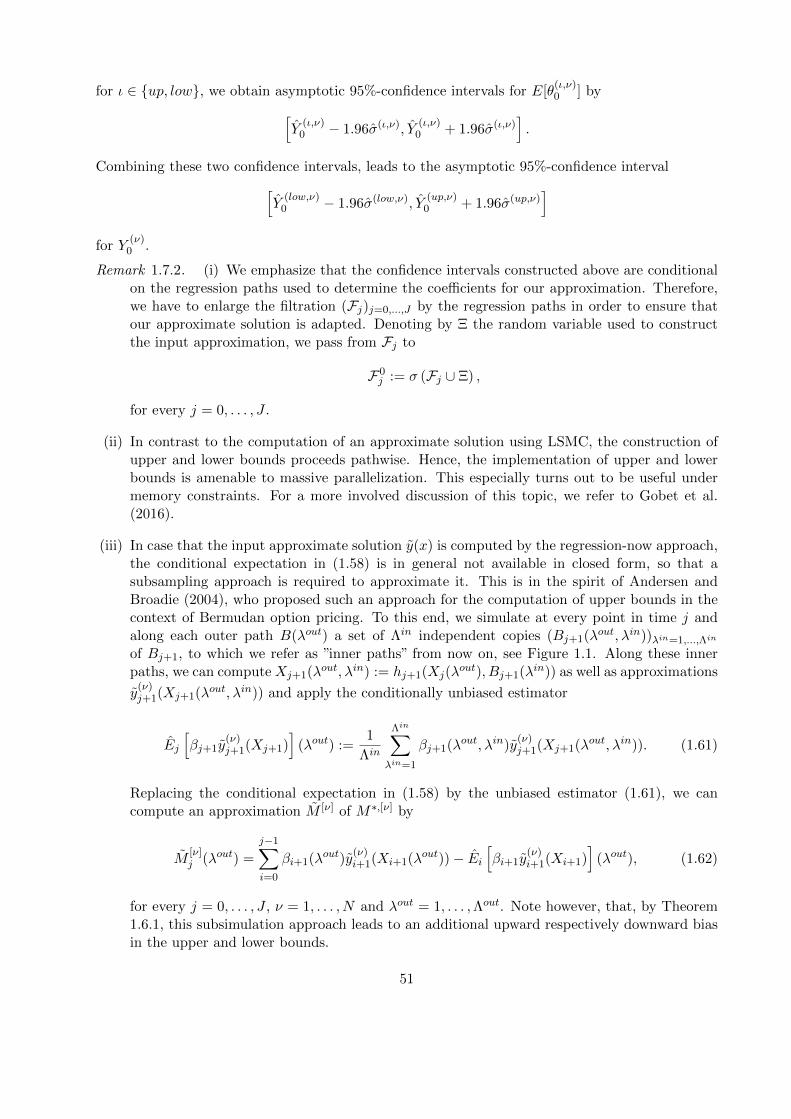
for ι ∈ up, low, we obtain asymptotic 95%-confidence intervals for E[θ(ι,ν)0 ] by[

Y(ι,ν)

0 − 1.96σ(ι,ν), Y(ι,ν)

0 + 1.96σ(ι,ν)].

Combining these two confidence intervals, leads to the asymptotic 95%-confidence interval[Y

(low,ν)0 − 1.96σ(low,ν), Y

(up,ν)0 + 1.96σ(up,ν)

]for Y

(ν)0 .

Remark 1.7.2. (i) We emphasize that the confidence intervals constructed above are conditionalon the regression paths used to determine the coefficients for our approximation. Therefore,we have to enlarge the filtration (Fj)j=0,...,J by the regression paths in order to ensure thatour approximate solution is adapted. Denoting by Ξ the random variable used to constructthe input approximation, we pass from Fj to

F0j := σ (Fj ∪ Ξ) ,

for every j = 0, . . . , J .

(ii) In contrast to the computation of an approximate solution using LSMC, the construction ofupper and lower bounds proceeds pathwise. Hence, the implementation of upper and lowerbounds is amenable to massive parallelization. This especially turns out to be useful undermemory constraints. For a more involved discussion of this topic, we refer to Gobet et al.(2016).

(iii) In case that the input approximate solution y(x) is computed by the regression-now approach,the conditional expectation in (1.58) is in general not available in closed form, so that asubsampling approach is required to approximate it. This is in the spirit of Andersen andBroadie (2004), who proposed such an approach for the computation of upper bounds in thecontext of Bermudan option pricing. To this end, we simulate at every point in time j andalong each outer path B(λout) a set of Λin independent copies (Bj+1(λout, λin))λin=1,...,Λin

of Bj+1, to which we refer as ”inner paths” from now on, see Figure 1.1. Along these innerpaths, we can compute Xj+1(λout, λin) := hj+1(Xj(λ

out), Bj+1(λin)) as well as approximations

y(ν)j+1(Xj+1(λout, λin)) and apply the conditionally unbiased estimator

Ej

[βj+1y

(ν)j+1(Xj+1)

](λout) :=

1

Λin

Λin∑λin=1

βj+1(λout, λin)y(ν)j+1(Xj+1(λout, λin)). (1.61)

Replacing the conditional expectation in (1.58) by the unbiased estimator (1.61), we cancompute an approximation M [ν] of M∗,[ν] by

M[ν]j (λout) =

j−1∑i=0

βi+1(λout)y(ν)i+1(Xi+1(λout))− Ei

[βi+1y

(ν)i+1(Xi+1)

](λout), (1.62)

for every j = 0, . . . , J , ν = 1, . . . , N and λout = 1, . . . ,Λout. Note however, that, by Theorem1.6.1, this subsimulation approach leads to an additional upward respectively downward biasin the upper and lower bounds.

51

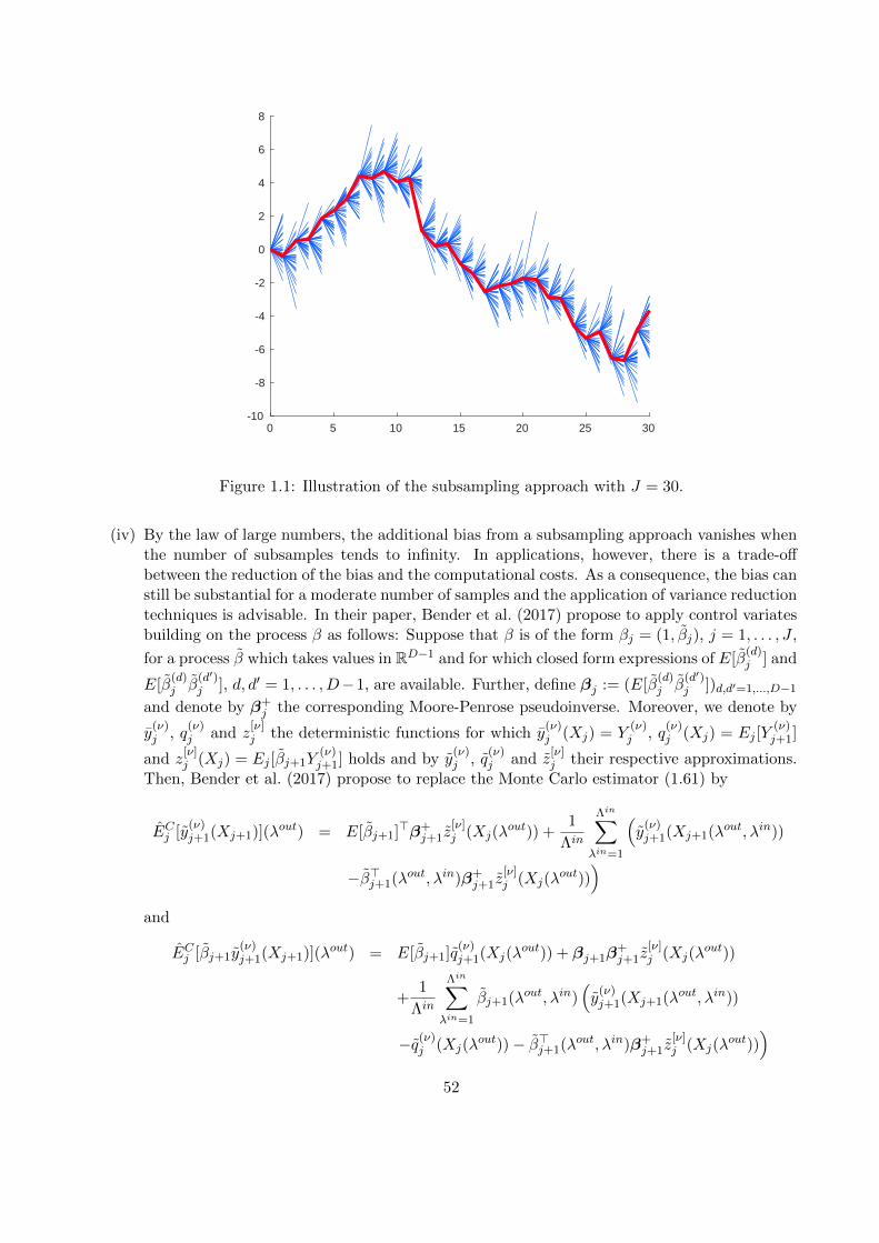
0 5 10 15 20 25 30-10

-8

-6

-4

-2

0

2

4

6

8

Figure 1.1: Illustration of the subsampling approach with J = 30.

(iv) By the law of large numbers, the additional bias from a subsampling approach vanishes whenthe number of subsamples tends to infinity. In applications, however, there is a trade-offbetween the reduction of the bias and the computational costs. As a consequence, the bias canstill be substantial for a moderate number of samples and the application of variance reductiontechniques is advisable. In their paper, Bender et al. (2017) propose to apply control variatesbuilding on the process β as follows: Suppose that β is of the form βj = (1, βj), j = 1, . . . , J ,

for a process β which takes values in RD−1 and for which closed form expressions of E[β(d)j ] and

E[β(d)j β

(d′)j ], d, d′ = 1, . . . , D−1, are available. Further, define βj := (E[β

(d)j β

(d′)j ])d,d′=1,...,D−1

and denote by β+j the corresponding Moore-Penrose pseudoinverse. Moreover, we denote by

y(ν)j , q

(ν)j and z

[ν]j the deterministic functions for which y

(ν)j (Xj) = Y

(ν)j , q

(ν)j (Xj) = Ej [Y

(ν)j+1]

and z[ν]j (Xj) = Ej [βj+1Y

(ν)j+1] holds and by y

(ν)j , q

(ν)j and z

[ν]j their respective approximations.

Then, Bender et al. (2017) propose to replace the Monte Carlo estimator (1.61) by

ECj [y(ν)j+1(Xj+1)](λout) = E[βj+1]>β+

j+1z[ν]j (Xj(λ

out)) +1

Λin

Λin∑λin=1

(y

(ν)j+1(Xj+1(λout, λin))

−β>j+1(λout, λin)β+j+1z

[ν]j (Xj(λ

out)))

and

ECj [βj+1y(ν)j+1(Xj+1)](λout) = E[βj+1]q

(ν)j+1(Xj(λ

out)) + βj+1β+j+1z

[ν]j (Xj(λ

out))

+1

Λin

Λin∑λin=1

βj+1(λout, λin)(y

(ν)j+1(Xj+1(λout, λin))

−q(ν)j (Xj(λ

out))− β>j+1(λout, λin)β+j+1z

[ν]j (Xj(λ

out)))

52

for every j = 0, . . . , J − 1 and ν = 1, . . . , N .

1.7.2 Numerical examples

We now apply the pathwise dynamic programming approach in two numerical examples, namelythe problem of pricing options under negotiated collateral respectively uncertain volatility.

1.7.2.1 Negotiated collateral

We first consider the problem of pricing under negotiated collateralization in the presence of fundingcosts as discussed in Example 1.4.2. To this end, let 0 = t0 < t1 < . . . < tJ = T be an equidistantpartition of the interval [0, T ]. Moreover, recall that we are given a d-dimensional Brownian motionW and that the dynamics of the risky assets X = (X(1), . . . , X(d)) are given by independentidentically distributed Black-Scholes models, i.e.,

X(l)t = x0 exp

(RL − 1

2σ2

)t+ σW

(l)t

, l = 1, . . . , d,

where RL ≥ 0 is the risk-free lending rate, σ > 0 is the assets volatility. Finally, we denote by gthe payoff of a European option written on the risky assets. Then, by Example 1.4.2, we end upwith the following dynamic program:

X(l)j+1 = X

(l)j exp

(RL − 1

2σ2

)∆ + σ∆W

(l)j+1

, X

(l)0 = x0, l = 1, . . . , d

Y(1)J = −Y (2)

J = g(XJ)

Z[ν]j = Ej

[∆Wj+1

∆Y

(ν)j+1

], ν = 1, 2

Y(1)j = Ej [Y

(1)j+1]−RL(1− α)(Ej [Y

(1)j+1] + Ej [Y

(2)j+1])∆−RC(αEj [Y

(1)j+1]− (1− α)Ej [Y

(2)j+1])∆

+(RB −RL)

((1− α)(Ej [Y

(1)j+1] + Ej [Y

(2)j+1])− 1

σ

(Z

[1]j

)>1

)−

∆

Y(2)j = Ej [Y

(2)j+1]−RLα(Ej [Y

(1)j+1] + Ej [Y

(2)j+1])∆ +RC(αEj [Y

(1)j+1]− (1− α)Ej [Y

(2)j+1])∆

+(RB −RL)

(α(Ej [Y

(1)j+1] + Ej [Y

(2)j+1])− 1

σ

(Z

[2]j

)>1

)−

∆, (1.63)

where RB and RC denote the risk-free borrowing rate respectively the collateralization rate andα ∈ [0, 1]. Note that, in a slight abuse of notation, we here changed from time tj to the time indexj in the notation of the stock price models X(l).

Moreover, recall that the functions F(1)j , F

(2)j : R2(1+d) → R are given by

F(ν)j (z1, z2) = z(1)

ν +H(ν)(z1, z2)∆,

for zν = (z(1)ν , . . . , z

(1+d)ν ) ∈ R1+d and that the process B is, as in Example 1.1.2, given by

Bj = βj =

(1,

∆W(1)j

∆, . . . ,

∆W(d)j

∆

)>, j = 1, . . . , J.

53

As we have already seen in Example 1.4.2, the duality relation (1.24) reads

(r

(ν,∗),[1]j

)>Ej

[βj+1Y

(1)j+1

]+(r

(ν,∗),[2]j

)>Ej

[βj+1Y

(2)j+1

]= Ej

[Y

(ν)j+1

]−RLaν

(Ej

[Y

(1)j+1

]+ Ej

[Y

(2)j+1

])∆ + (−1)νRC

(αEj

[Y

(1)j+1

]− (1− α)Ej

[Y

(2)j+1

])∆

+ (RB −RL)

(aν

(Ej

[Y

(1)j+1

]+ Ej

[Y

(2)j+1

])− 1

σ

(Ej

[∆Wj+1

∆Y

(ν)j+1

])>1

)−

∆,

for every j = 0, . . . , J − 1 and ν = 1, 2, with solution

r(ν,∗)j =

u(ν)(RL), aν

(Ej

[Y

(1)j+1

]+ Ej

[Y

(2)j+1

])− 1

σ

(Z

[ν]j

)>1 ≥ 0

u(ν)(RB), aν

(Ej

[Y

(1)j+1

]+ Ej

[Y

(2)j+1

])− 1

σ

(Z

[ν]j

)>1 < 0.

Here, the functions u(ν)(r) are defined by

u(1)(r) =

1− r(1− α)∆−RCα∆

(r−RL)∆σ · 1

(RC − r)(1− α)∆0 · 1

and u(2)(r) =

(RC − r)α∆

0 · 11− rα∆−RC(1− α)∆

(r−RL)∆σ · 1

.

As a numerical example, we consider the valuation of a European call-spread option on the maxi-mum of d assets with maturity T and payoff

g(x) =

(maxl=1,...,d

x(l) −K1

)+

− 2

(maxl=1,...,d

x(l) −K2

)+

.

Except for adding the collateralization scheme (and, hence, the coupling between the hedger’s andcounterparty’s valuation), this is the same numerical example as in Bender et al. (2017) and wefollow their parameter choices

(x0, d, T,K1,K2, σ, RL, RB, RC , α) = (100, 5, 0.25, 95, 115, 0.2, 0.01, 0.06, 0.02, 0.5)

adding only the values of α and RC . The choice α = 0.5 implies that the posted collateral is givenby the average of the two parties’ value processes Y (1) and −Y (2). Note that, we have RB > RC

in this example, as this is the practically most relevant case. As discussed in Example 1.4.2, weobserve that the system (1.63) fails the componentwise comparison principle with this choice ofparameters and, thus, the coupled bounds (1.30) need to be applied.

To do this, we first compute input approximations with the regression-later approach. We run thisalgorithm with Λreg = 1, 000 regression paths. At time j + 1 (where 0 ≤ j ≤ J − 1) we apply thesame 7 basis functions for both components (and thus skip the dependence on ν), namely

ηj+1,1(Xj , Bj+1) = 1,

ηj+1,l+1(Xj , Bj+1) = X(l)j+1, l = 1, . . . , 5,

and an approximation to Ej+1[g(XJ)]. Precisely, this basis function is defined in terms of an

optimal L-point quantization∑L

κ=1 pκ δzκ of a standard normal distribution by

54

ηj+1,7(Xj , Bj+1)

=5∑l=1

L∑κ=1

pκ

√T − tjT − tj+1

g(X

(l)j e(R

L− 12σ2)(T−tj)+σzκ

√T−tj

)ez2κ2−

(√T−tjzκ−∆W

(l)j+1

)2

2(T−tj+1)

×∏

l′∈1,...,5\l

N

1√T − tj+1

√T − tjzκ +ln(X

(l)j )− ln(X

(l′)j )

σ−∆W

(l′)j+1

,

where, δz denotes the Dirac-measure in z ∈ R and g : R→ R is given by

g(x) = (x−K1)+ − 2(x−K2)+.

As a trade-off between accuracy and computational time, we choose L = 25, but note that thisbasis function converges to Ej+1[g(XJ)], as L tends to infinity. For this choice of basis func-tions the one-step conditional expectations are available in closed form and can be expressed

as Ej [ηj+1,k(Xj , Bj+1)] =: R(0)j,k(Xj) respectively Ej [(∆W

(l)j+1/∆)ηj+1,k(Xj , Bj+1)] =: R

(l)j,k(Xj),

l = 1, . . . , 5, for deterministic functions R(0)j,k and R

(l)j,k. Note that, by a slight abuse of notation,

the upper index on the functions R(l)j,k does not correspond to the component of the process Y as

introduced in Section 1.7 but to the respective component of the process β, as we do not considerdifferent basis functions for Y (1) and Y (2). Indeed, for the first six basis functions, we observe that

R(0)j,1 (Xj) = 1,

R(0)j,l+1(Xj) = eR

L∆X(l)j , l = 1, . . . , 5,

respectively

R(l)j,1(Xj) = 0,

R(l)j,k+1(Xj) =

eR

L∆σX(l)j , l = k

0, l 6= k

for l, k = 1, . . . , 5. A straightforward computation (for which we provide the details in AppendixA.3) shows that the respective conditional expectations for the seventh basis function are given by

R(0)j,7 (Xj) =

5∑l=1

L∑κ=1

pκg(X

(l)j e(R

L− 12σ2)(T−tj)+σzκ

√T−tj

)

×∏

l′∈1,...,5\l

N

zκ +ln(X

(l)j )− ln(X

(l′)j )

σ√T − tj

and

R(k)j,7 (Xj) =

5∑l=1,l 6=k

L∑κ=1

pκg(X

(l)j e(R

L− 12σ2)(T−tj)+σzκ

√T−tj

) 1√2πe− 1

2(T−tj)(√T−tjzκ+

ln(X(l)j

)−ln(X(l′)j

)

σ)2

×∏

l′∈1,...,5\l,k

N

zκ +ln(X

(l)j )− ln(X

(l′)j )

σ√T − tj

55

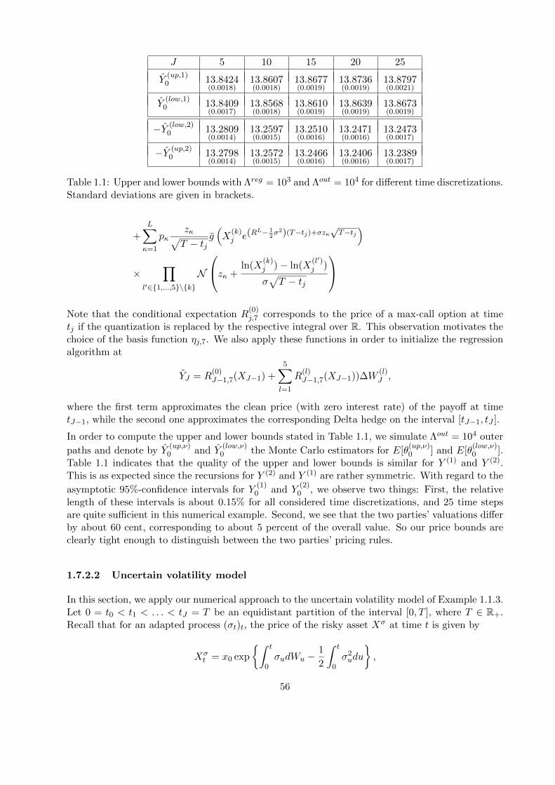
J 5 10 15 20 25

Y(up,1)

0 13.8424(0.0018)

13.8607(0.0018)

13.8677(0.0019)

13.8736(0.0019)

13.8797(0.0021)

Y(low,1)

0 13.8409(0.0017)

13.8568(0.0018)

13.8610(0.0019)

13.8639(0.0019)

13.8673(0.0019)

−Y (low,2)0 13.2809

(0.0014)13.2597(0.0015)

13.2510(0.0016)

13.2471(0.0016)

13.2473(0.0017)

−Y (up,2)0 13.2798

(0.0014)13.2572(0.0015)

13.2466(0.0016)

13.2406(0.0016)

13.2389(0.0017)

Table 1.1: Upper and lower bounds with Λreg = 103 and Λout = 104 for different time discretizations.Standard deviations are given in brackets.

+L∑κ=1

pκzκ√T − tj

g(X

(k)j e(R

L− 12σ2)(T−tj)+σzκ

√T−tj

)

×∏

l′∈1,...,5\k

N

zκ +ln(X

(k)j )− ln(X

(l′)j )

σ√T − tj

Note that the conditional expectation R

(0)j,7 corresponds to the price of a max-call option at time

tj if the quantization is replaced by the respective integral over R. This observation motivates thechoice of the basis function ηj,7. We also apply these functions in order to initialize the regressionalgorithm at

YJ = R(0)J−1,7(XJ−1) +

5∑l=1

R(l)J−1,7(XJ−1))∆W

(l)J ,

where the first term approximates the clean price (with zero interest rate) of the payoff at timetJ−1, while the second one approximates the corresponding Delta hedge on the interval [tJ−1, tJ ].

In order to compute the upper and lower bounds stated in Table 1.1, we simulate Λout = 104 outer

paths and denote by Y(up,ν)

0 and Y(low,ν)

0 the Monte Carlo estimators for E[θ(up,ν)0 ] and E[θ

(low,ν)0 ].

Table 1.1 indicates that the quality of the upper and lower bounds is similar for Y (1) and Y (2).This is as expected since the recursions for Y (2) and Y (1) are rather symmetric. With regard to the

asymptotic 95%-confidence intervals for Y(1)

0 and Y(2)

0 , we observe two things: First, the relativelength of these intervals is about 0.15% for all considered time discretizations, and 25 time stepsare quite sufficient in this numerical example. Second, we see that the two parties’ valuations differby about 60 cent, corresponding to about 5 percent of the overall value. So our price bounds areclearly tight enough to distinguish between the two parties’ pricing rules.

1.7.2.2 Uncertain volatility model

In this section, we apply our numerical approach to the uncertain volatility model of Example 1.1.3.Let 0 = t0 < t1 < . . . < tJ = T be an equidistant partition of the interval [0, T ], where T ∈ R+.Recall that for an adapted process (σt)t, the price of the risky asset Xσ at time t is given by

Xσt = x0 exp

∫ t

0σudWu −

1

2

∫ t

0σ2udu

,

56

where W is a Brownian motion. Furthermore, let g be the payoff a European option written on therisky asset. Then, by Example 1.1.3, we consider the following one-dimensional dynamic program

X ρj+1 = X ρ

j exp

ρ∆Wj+1 −

1

2ρ2∆

, X0 = x0 ∈ R,

YJ = g(X ρJ

)Γj = Ej

[(∆W 2

j+1

∆2− ρ∆Wj+1

∆− 1

∆

)Yj+1

]Yj = Ej [Yj+1] + ∆ max

s∈slow,supsΓj , (1.64)

for j = J − 1, . . . , 0, where

sι =1

2

(σ2ι

ρ2− 1

)for ι ∈ low, up and the process B is given by

Bj =

(1,

∆W 2j+1

∆2− ρ∆Wj+1

∆− 1

∆,∆Wj

), j = 1, . . . , J.

Note that X ρ denotes the value process of the risky asset under the constant volatility ρ and that,in a slight abuse of notation, we again changed from time tj to the time index j in the notation.We emphasize that the reference volatility ρ is a choice parameter in the discretization. The basicidea is to view the uncertain volatility model as a suitable correction of a Black-Scholes model withvolatility ρ.

As we have already seen in Example 1.1.3, the function Fj : R2 → R is given by

Fj(z) = z(1) + ∆ maxs∈slow,sup

sz(2),

in this example. Depending on the choice of the parameters σlow, σup and ρ, this function may failthe monotonicity condition (c) in Theorem 1.4.1. Indeed, in this setting, this condition boils downto the requirement that the prefactor

1 + s

(∆W 2

j+1

∆− ρ∆Wj+1 − 1

)of Yj+1 in equation (1.64) for Yj is P -almost surely non-negative for both of the feasible values ofs,

s ∈

1

2

(σ2low

ρ2− 1

),1

2

(σ2up

ρ2− 1

).

For s > 1, this requirement is violated for realizations of ∆Wj+1 sufficiently close to zero, while fors < 0 violations occur for sufficiently negative realizations of the Brownian increment – and thisviolation also takes place if one truncates the Brownian increments at±const.

√∆ with an arbitrarily

large constant. Consequently, we arrive at the necessary condition s ∈ [0, 1] for comparison to hold.From the possible values for s, we deduce that this condition is equivalent to ρ ∈ [σup/

√3, σlow].

For σlow = 0.1 and σup = 0.2, the numerical test case in Guyon and Henry-Labordere (2011) andAlanko and Avellaneda (2013), these two conditions cannot hold simultaneously, ruling out thepossibility of a comparison principle.

57

By Appendix A.2, we conclude again that F#j = 0 on the effective domain D

(j,·)F# = 1 ×

[slow∆, sup∆], so that the duality relation (1.24) reads as follows:

r∗,[1]j Ej [Yj+1] + r

∗,[2]j Γj = Ej [Yj+1] + ∆ max

s∈slow,supsΓj , j = 0, . . . , J − 1. (1.65)

A solution to (1.65) is given by

r∗j =

(1, sup∆), Γj ≥ 0

(1, slow∆), Γj < 0(1.66)

for every j = 0, . . . , J − 1.

As a numerical example, we consider a European call-spread option with strikes K1 and K2, i.e.,

g(x) = (x−K1)+ − (x−K2)+,

which is also studied in Guyon and Henry-Labordere (2011), Alanko and Avellaneda (2013), andKharroubi et al. (2014). Following their setting, we choose the maturity T = 1, K1 = 90, K2 = 110and x0 = 100. The reference volatility ρ as well as the volatility bounds σlow and σup are varied inour numerical experiments.

The input approximation is again computed by the regression-later variant of LSMC. We firstsimulate Λreg = 105 regression paths of the process (Bj)j=1,...,J . For the evaluation of (X ρ

j )j=0,...,J

along the regression paths, we do not start all paths at x0. Instead, we rather start Λreg/200trajectories at each of the points 31, . . . , 230. Since X is a geometric Brownian motion underρ, it can be simulated exactly. Starting the regression paths at multiple points allows to reducethe instability of regression coefficients arising at early time points. See Rasmussen (2005) for adiscussion of this stability problem and of the method of multiple starting points. For the empiricalregression we choose 163 basis functions. For a given point in time j + 1, the first three basisfunctions are given by

ηj+1,1(X ρj+1) = 1,

ηj+1,2(X ρj+1) = X ρ

j+1,

ηj+1,3(X ρj+1) = E[g(X ρ

J)|X ρj+1].

The third one is, thus, simply the Black-Scholes price (under ρ) of the spread option g. For theremaining 160 basis functions, we also choose Black-Scholes prices of spread options with respectivestrikes K(l), K(l+1) and K(l+2) for l = 1, . . . , 160, where the numbers K(1), . . . ,K(162) increase from20.5 to 230.5. Precisely, these basis functions are given by

ηj+1,k(Xρj+1) = E[(X ρ

J −K(k−3))+|X ρ

j+1]− 2E[(X ρJ −K

(k−2))+|X ρj+1] + E[(X ρ

J −K(k−1))+|X ρ

j+1]

for k = 4, . . . , 163, where

E[(X ρJ −K)+|X ρ

j+1] = X ρj+1N

(d+

(tJ − tj+1, X

ρj+1,K

))−KN

(d−

(tJ − tj+1, X

ρj+1,K

)).

Here, d+(τ, x,K) and d−(τ, x,K) are given by

d±(τ, x,K) =1

ρ√τ

(log( xK

)± 1

2ρ2τ

).

58

Note that, in contrast to the previous example, the basis functions only depend on the value of therisky asset at the given time point using that

ηj+1,k(Xρj+1) = ηj+1,k

(X ρj exp

ρ∆Wj+1 −

1

2ρ2∆

)= ηj+1,k(X

ρj , Bj+1).

Under the given assumptions, these basis functions form a set of martingales, for which the condi-

tional expectations are available in closed form. Hence, we have for R(0)j,k(X ρ

j ) := Ej [ηj+1,k(Xρj+1)]

that

R(0)j,1 (X ρ

j ) = 1, R(0)j,2 (X ρ

j ) = X ρj , R

(0)j,3 (X ρ

j ) = E[g(X ρJ)|X ρ

j ],

R(0)j,k(X ρ

j ) = E[(X ρJ −K

(k−3))+|X ρj ]− 2E[(X ρ

J −K(k−2))+|X ρ

j ] + E[(X ρJ −K

(k−1))+|X ρj ],

for k = 4, . . . , 163. For the one-step conditional expectations R(1)j,k(X ρ

j ) := Ej [β(2)j+1ηj+1,k(X

ρj+1)],

we conclude by Appendix A.4 that

R(1)j,k(x) = E

[(∆W 2

j+1

∆2− ρ∆Wj+1

∆− 1

∆

)ηj+1,k(X

ρj+1)

∣∣∣∣∣X ρj = x

]= ρ2x2 d

2

dx2ηj,k(x)

holds. Consequently, these conditional expectations are given by

R(1)j,1 (X ρ

j ) = R(1)j,2 (X ρ

j ) = 0,

R(1)j,3 (X ρ

j ) =ρX ρ

j√tJ − tj

(ϕ(d+(tJ − tj , X ρ

j ,K1))− ϕ(d+(tJ − tj , X ρj ,K2))

),

R(1)j,k(X ρ

j ) =ρX ρ

j√tJ − tj

(ϕ(d+(tJ − tj , X ρ

j ,K(k−3)))− 2ϕ(d+(tJ − tj , X ρ

j ,K(k−2)))

+ϕ(d+(tJ − tj , X ρj ,K

(k−1))))

for k = 4, . . . , 163, where ϕ denotes the density of a standard normal distribution. Hence, theone-step conditional expectations of the basis functions ηj+1,k, k ≥ 3, after multiplication with thesecond derivative weight β(2) are essentially (differences of) Black-Scholes Gammas at time j. Forthe computation of upper and lower bounds, we simulate Λout = 105 outer paths. In contrast tothe regression paths, we now take x0 = 100 for the evaluation of X ρ along each path. As before,we denote by Y up

0 and Y low0 the corresponding estimators for E[θup0 ] respectively E[θlow0 ].

We first consider the situation where σlow = 0.1 and σup = 0.2. This example is by now a standardtest case for Monte Carlo implementations of Hamilton-Jacobi-Bellman equations. The optionprice in the continuous time limit can be calculated in closed form and equals 11.2046, see Vanden(2006). Table 1.2 shows the approximated prices Y0 := y0(x0) as well as upper and lower boundsfor ρ = 0.2/

√3 ≈ 0.1155 depending on the time discretization. This is the smallest choice of ρ, for

which the monotonicity condition in Theorem 1.4.1 can only be violated when the absolute values ofthe Brownian increments are large. The numerical results suggest convergence from below towardsthe continuous-time limit for finer time discretizations. This is intuitive in this example, since finertime discretizations allow for richer choices of the process (σt)t∈[0,T ] in the maximization problem(1.6). We notice that the bounds are fairly tight (with, e.g., a relative width of 1.9% for the 95%confidence interval with J = 21 time discretization points), although the upper bound begins todeteriorate as Y0 approaches its limiting value. The impact of increasing ρ to 0.15 (as proposedin Guyon and Henry-Labordere, 2011; Alanko and Avellaneda, 2013) is shown in Table 1.3. The

59

J 3 6 9 12 15 18 21 24

Y0 10.8549 11.0494 11.1067 11.1336 11.1490 11.1590 11.1659 11.1713

Y up0 10.8604

(0.0001)11.0545(0.0003)

11.1145(0.0006)

11.1472(0.0010)

11.1754(0.0024)

11.2239(0.0121)

11.3172(0.0312)

11.4362(0.0385)

Y low0 10.8544

(0.0001)11.0497(0.0003)

11.1077(0.0005)

11.1341(0.0003)

11.1488(0.0003)

11.1596(0.0007)

11.1665(0.0008)

11.1700(0.0010)

Table 1.2: Approximated price as well as lower and upper bounds for ρ = 0.1155 for different timediscretizations. Standard deviations are given in brackets

J 5 10 15 20 25 30 35 40

Y0 10.8164 10.9981 11.0677 11.1027 11.1241 11.1383 11.1485 11.1561

Y up0 10.8184

(0.0001)11.0041(0.0001)

11.0740(0.0002)

11.1124(0.0004)

11.1561(0.0160)

11.1786(0.0019)

11.2601(0.0129)

11.3691(0.0143)

Y low0 10.8164

(0.0001)10.9982(0.0001)

11.0678(0.0001)

11.1022(0.0001)

11.1230(0.0002)

11.1365(0.0002)

11.1444(0.0008)

11.1507(0.0006)

Table 1.3: Approximated price as well as lower and upper bounds for ρ = 0.15 for different timediscretizations. Standard deviations are given in brackets

relative width of the 95%-confidence interval is now about 1.3% for up to J = 35 time steps, butalso the convergence to the continuous-time limit appears to be slower with this choice of ρ.

Comparing Table 1.3 with the results in Alanko and Avellaneda (2013), we observe that their pointestimates for Y0 at time discretization levels J = 10 and J = 20 do not lie in our confidence intervalswhich are given by [10.9985, 11.0043] and [11.1025, 11.1131], indicating that their (regression-now)least-squares Monte Carlo estimator may still suffer from large variances (although they applycontrol variates). The dependence of the time discretization error on the choice of the referencevolatility ρ is further illustrated in Table 1.4, which displays the mean and the standard deviationof 30 runs of the regression-later algorithm for different choices of ρ and up to 640 time steps. Byand large, convergence is faster for smaller choices of ρ, but the algorithm becomes unstable whenthe reference volatility is too small.

J 10 20 40 80 160 320 640

ρ = 0.06 84.6503(45.3588)

1.3012 · 105

(3.6246·105)8.6315 · 1011

(4.2492·1012)6.4425 · 1015

(2.0720·1016)3.1259 · 1011

(1.0129·1012)5.5578 · 1018

(2.6571·1018)8.1779 · 1026

(4.1892·1027)

ρ = 0.08 11.6966(0.0022)

12.0212(0.4895)

45.3317(106.5248)

11.5192(0.2348)

11.3627(0.0241)

160.9274(819.6279)

680.9364(3.5302·103)

ρ = 0.1 11.1546(0.0002)

11.1832(0.0001)

11.1946(0.0001)

11.2002(0.0001)

11.2030(0.0001)

11.2050(0.0001)

11.2061(0.0001)

ρ = 0.15 10.9981(0.0002)

11.1030(0.0001)

11.1563(0.0002)

11.1833(0.0002)

11.1969(0.0002)

11.2036(0.0002)

11.2070(0.0002)

ρ = 0.2 10.8006(0.0003)

10.9766(0.0003)

11.0846(0.0002)

11.1484(0.0002)

11.1837(0.0003)

11.2023(0.0002)

11.2116(0.0002)

ρ = 0.5 9.7087(0.0001)

9.9649(0.0002)

10.2326(0.0003)

10.5020(0.0008)

10.7548(0.0012)

10.9627(0.0015)

11.1103(0.0018)

Table 1.4: Mean of L = 30 simulations of Y0 for different ρ and discretizations. Standard deviationsare given in brackets.

In order to gain a better understanding of how the performance of the method depends on theinput parameters, we also consider the case σlow = 0.3 and σup = 0.4. Note that, for this choice,the comparison principle is in force if we choose ρ ∈ [0.4/

√3, 0.3]. Following Vanden (2006), the

price of the European call-spread option in the continuous-time limit is 9.7906 in this case. We get

60

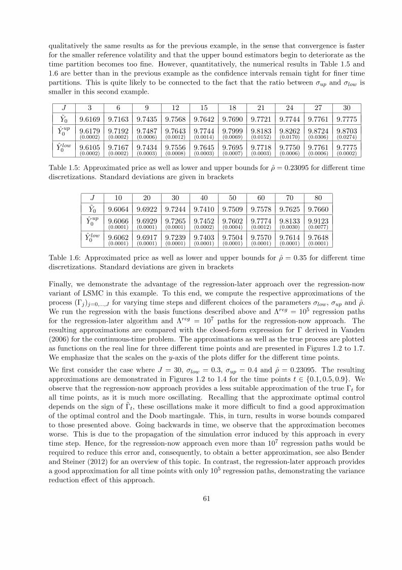
qualitatively the same results as for the previous example, in the sense that convergence is fasterfor the smaller reference volatility and that the upper bound estimators begin to deteriorate as thetime partition becomes too fine. However, quantitatively, the numerical results in Table 1.5 and1.6 are better than in the previous example as the confidence intervals remain tight for finer timepartitions. This is quite likely to be connected to the fact that the ratio between σup and σlow issmaller in this second example.

J 3 6 9 12 15 18 21 24 27 30

Y0 9.6169 9.7163 9.7435 9.7568 9.7642 9.7690 9.7721 9.7744 9.7761 9.7775

Y up0 9.6179

(0.0002)9.7192(0.0002)

9.7487(0.0006)

9.7643(0.0012)

9.7744(0.0014)

9.7999(0.0069)

9.8183(0.0152)

9.8262(0.0170)

9.8724(0.0306)

9.8703(0.0274)

Y low0 9.6105

(0.0002)9.7167(0.0002)

9.7434(0.0003)

9.7556(0.0008)

9.7645(0.0003)

9.7695(0.0007)

9.7718(0.0003)

9.7750(0.0006)

9.7761(0.0006)

9.7775(0.0002)

Table 1.5: Approximated price as well as lower and upper bounds for ρ = 0.23095 for different timediscretizations. Standard deviations are given in brackets

J 10 20 30 40 50 60 70 80

Y0 9.6064 9.6922 9.7244 9.7410 9.7509 9.7578 9.7625 9.7660

Y up0 9.6066

(0.0001)9.6929(0.0001)

9.7265(0.0001)

9.7452(0.0002)

9.7602(0.0004)

9.7774(0.0012)

9.8133(0.0030)

9.9123(0.0077)

Y low0 9.6062

(0.0001)9.6917(0.0001)

9.7239(0.0001)

9.7403(0.0001)

9.7504(0.0001)

9.7570(0.0001)

9.7614(0.0001)

9.7648(0.0001)

Table 1.6: Approximated price as well as lower and upper bounds for ρ = 0.35 for different timediscretizations. Standard deviations are given in brackets

Finally, we demonstrate the advantage of the regression-later approach over the regression-nowvariant of LSMC in this example. To this end, we compute the respective approximations of theprocess (Γj)j=0,...,J for varying time steps and different choices of the parameters σlow, σup and ρ.We run the regression with the basis functions described above and Λreg = 105 regression pathsfor the regression-later algorithm and Λreg = 107 paths for the regression-now approach. Theresulting approximations are compared with the closed-form expression for Γ derived in Vanden(2006) for the continuous-time problem. The approximations as well as the true process are plottedas functions on the real line for three different time points and are presented in Figures 1.2 to 1.7.We emphasize that the scales on the y-axis of the plots differ for the different time points.

We first consider the case where J = 30, σlow = 0.3, σup = 0.4 and ρ = 0.23095. The resultingapproximations are demonstrated in Figures 1.2 to 1.4 for the time points t ∈ 0.1, 0.5, 0.9. Weobserve that the regression-now approach provides a less suitable approximation of the true Γt forall time points, as it is much more oscillating. Recalling that the approximate optimal controldepends on the sign of Γt, these oscillations make it more difficult to find a good approximationof the optimal control and the Doob martingale. This, in turn, results in worse bounds comparedto those presented above. Going backwards in time, we observe that the approximation becomesworse. This is due to the propagation of the simulation error induced by this approach in everytime step. Hence, for the regression-now approach even more than 107 regression paths would berequired to reduce this error and, consequently, to obtain a better approximation, see also Benderand Steiner (2012) for an overview of this topic. In contrast, the regression-later approach providesa good approximation for all time points with only 105 regression paths, demonstrating the variancereduction effect of this approach.

61

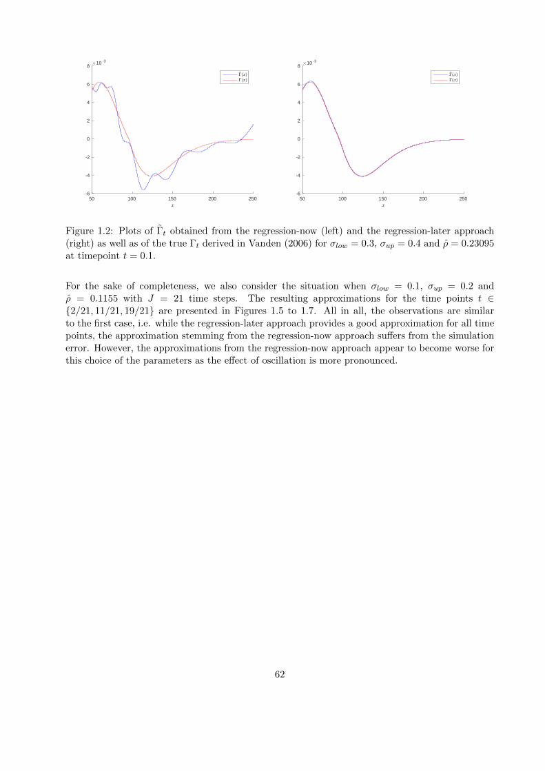
50 100 150 200 250x

-6

-4

-2

0

2

4

6

8#10 -3

~!(x)!(x)

50 100 150 200 250x

-6

-4

-2

0

2

4

6

8#10 -3

~!(x)!(x)

Figure 1.2: Plots of Γt obtained from the regression-now (left) and the regression-later approach(right) as well as of the true Γt derived in Vanden (2006) for σlow = 0.3, σup = 0.4 and ρ = 0.23095at timepoint t = 0.1.

For the sake of completeness, we also consider the situation when σlow = 0.1, σup = 0.2 andρ = 0.1155 with J = 21 time steps. The resulting approximations for the time points t ∈2/21, 11/21, 19/21 are presented in Figures 1.5 to 1.7. All in all, the observations are similarto the first case, i.e. while the regression-later approach provides a good approximation for all timepoints, the approximation stemming from the regression-now approach suffers from the simulationerror. However, the approximations from the regression-now approach appear to become worse forthis choice of the parameters as the effect of oscillation is more pronounced.

62

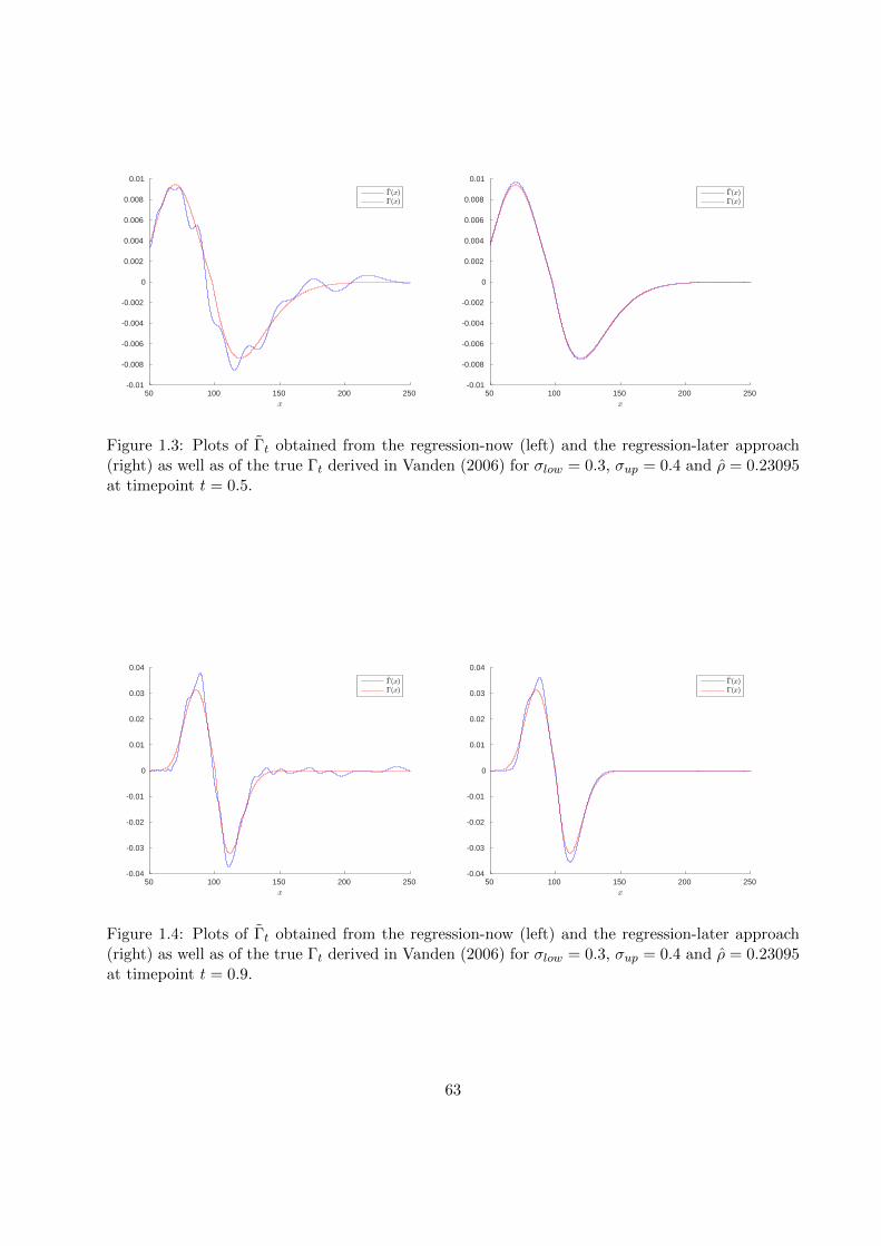
50 100 150 200 250x

-0.01

-0.008

-0.006

-0.004

-0.002

0

0.002

0.004

0.006

0.008

0.01

~!(x)!(x)

50 100 150 200 250x

-0.01

-0.008

-0.006

-0.004

-0.002

0

0.002

0.004

0.006

0.008

0.01

~!(x)!(x)

Figure 1.3: Plots of Γt obtained from the regression-now (left) and the regression-later approach(right) as well as of the true Γt derived in Vanden (2006) for σlow = 0.3, σup = 0.4 and ρ = 0.23095at timepoint t = 0.5.

50 100 150 200 250x

-0.04

-0.03

-0.02

-0.01

0

0.01

0.02

0.03

0.04

~!(x)!(x)

50 100 150 200 250x

-0.04

-0.03

-0.02

-0.01

0

0.01

0.02

0.03

0.04

~!(x)!(x)

Figure 1.4: Plots of Γt obtained from the regression-now (left) and the regression-later approach(right) as well as of the true Γt derived in Vanden (2006) for σlow = 0.3, σup = 0.4 and ρ = 0.23095at timepoint t = 0.9.

63

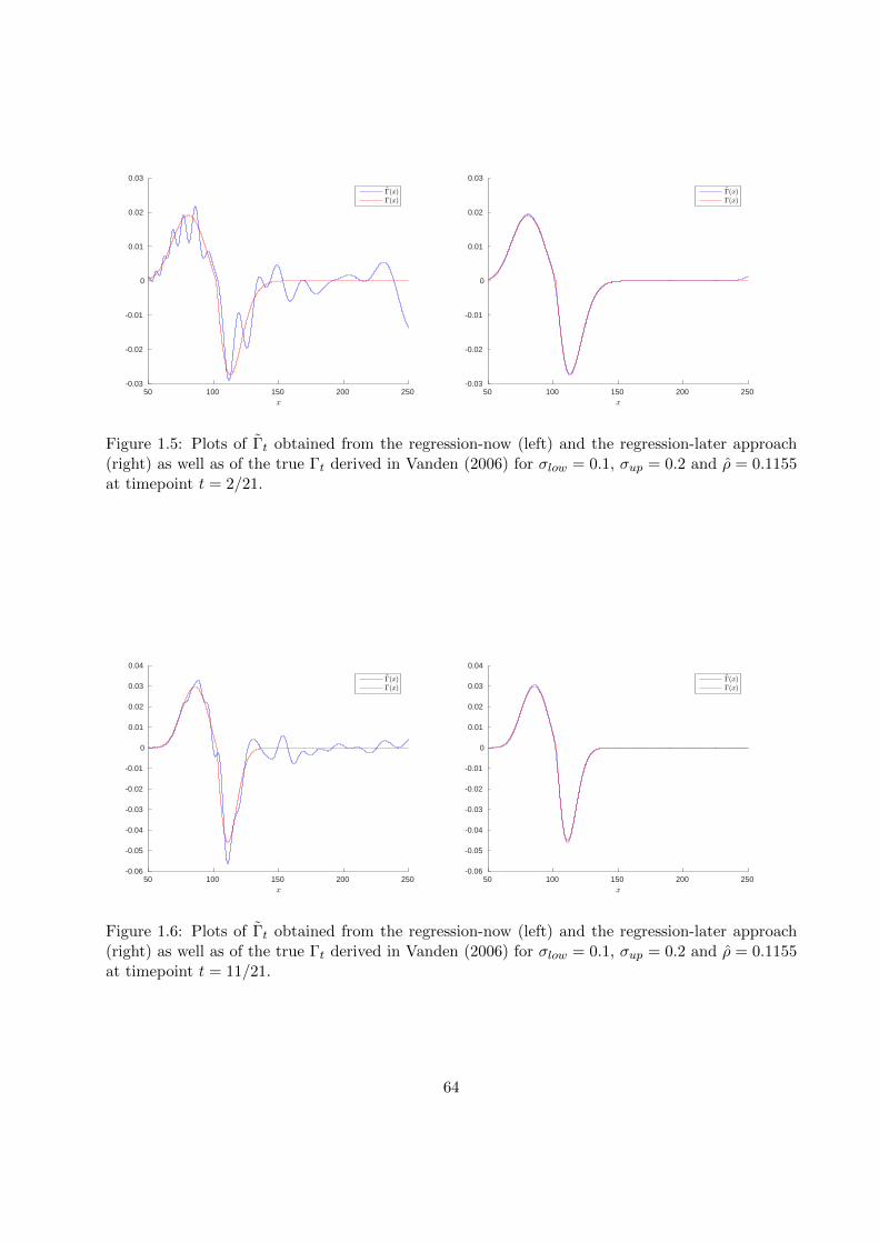
50 100 150 200 250x

-0.03

-0.02

-0.01

0

0.01

0.02

0.03

~!(x)!(x)

50 100 150 200 250x

-0.03

-0.02

-0.01

0

0.01

0.02

0.03

~!(x)!(x)

Figure 1.5: Plots of Γt obtained from the regression-now (left) and the regression-later approach(right) as well as of the true Γt derived in Vanden (2006) for σlow = 0.1, σup = 0.2 and ρ = 0.1155at timepoint t = 2/21.

50 100 150 200 250x

-0.06

-0.05

-0.04

-0.03

-0.02

-0.01

0

0.01

0.02

0.03

0.04

~!(x)!(x)

50 100 150 200 250x

-0.06

-0.05

-0.04

-0.03

-0.02

-0.01

0

0.01

0.02

0.03

0.04

~!(x)!(x)

Figure 1.6: Plots of Γt obtained from the regression-now (left) and the regression-later approach(right) as well as of the true Γt derived in Vanden (2006) for σlow = 0.1, σup = 0.2 and ρ = 0.1155at timepoint t = 11/21.

64

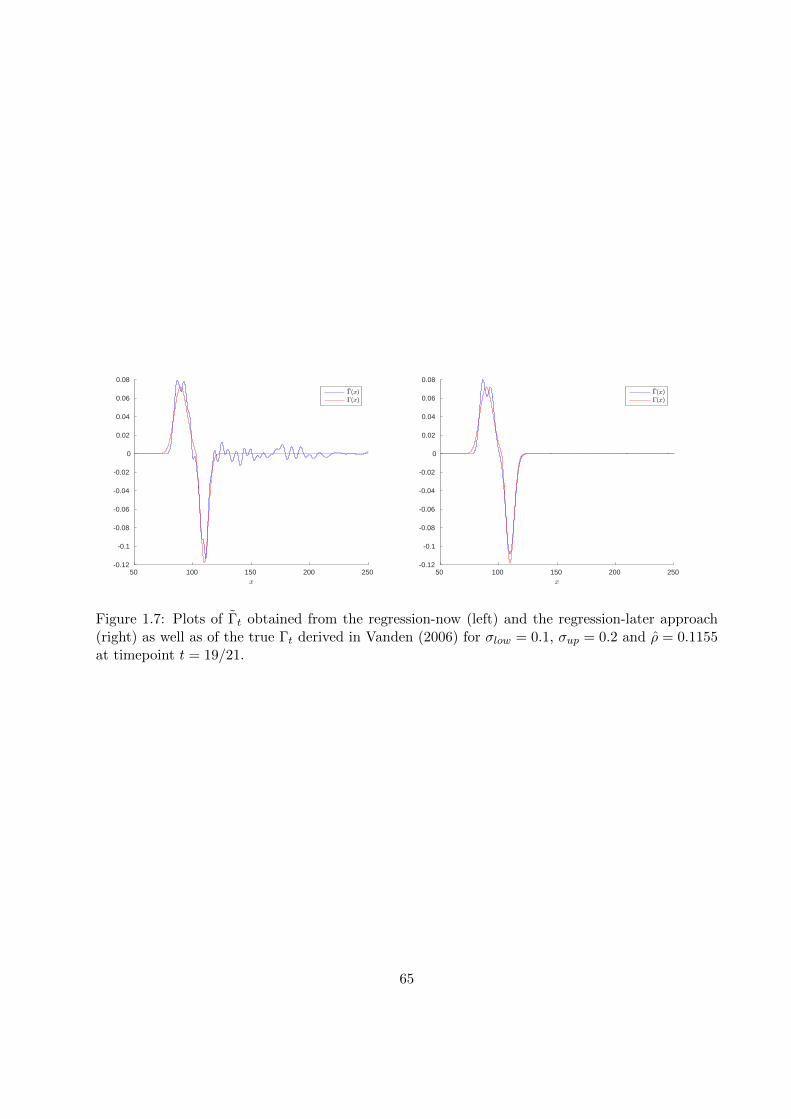
50 100 150 200 250x

-0.12

-0.1

-0.08

-0.06

-0.04

-0.02

0

0.02

0.04

0.06

0.08

~!(x)!(x)

50 100 150 200 250x

-0.12

-0.1

-0.08

-0.06

-0.04

-0.02

0

0.02

0.04

0.06

0.08

~!(x)!(x)

Figure 1.7: Plots of Γt obtained from the regression-now (left) and the regression-later approach(right) as well as of the true Γt derived in Vanden (2006) for σlow = 0.1, σup = 0.2 and ρ = 0.1155at timepoint t = 19/21.

65

66

Chapter 2

Concave-convex stochastic dynamicprograms

In this chapter, we provide a further generalization of the results in Chapter 1 by passing from theconvex to a concave-convex structure. This allows us to consider a wider class of applications. Itturns out that the constructions of upper and lower bounds are robust in the sense that the resultsfrom Chapter 1 can be transferred in a straightforward way to this new framework. Hence, weproceed similar to Chapter 1 by first assuming that a comparison principle holds and then, in asecond step, we relax this assumption and consider the general situation. Section 2.1 introducesthe assumptions and notations which are required to capture the additional concave part of thedynamic programming equation. Similar to the first chapter, we assume in Section 2.2 that acomparison principle holds and show that upper and lower bounds for concave-convex dynamicprograms can be derived by a suitable composition of the bounds for the respective concave andconvex problems. In Section 2.3, we show that, in some cases, the solution of the dynamic programis related to a stochastic two-player zero-sum game. Finally, we apply the information relaxationapproach of Brown et al. (2010) to this game and show that we end up with the bounds proposedin Section 2.2 if a special class of penalties is considered. In Section 2.4 the comparison principleis relaxed. We first provide a version of Theorem 1.4.1 which states sufficient conditions for thecomparison principle to hold. Then, we show that the main ideas and results from Section 1.5 canbe transferred immediately to this new setting. In Section 2.5, we consider the problem of pricinga swap under default risk as a numerical example.

2.1 Setup

Throughout this section, we consider the following concave-convex dynamic programming equation

YJ = ξ,

Yj = Gj(Ej [βj+1Yj+1], Fj(Ej [βj+1Yj+1])), j = J − 1, . . . , 0 (2.1)

on a complete filtered probability space (Ω,F , (Fj)j=0,...J , P ) in discrete time. As before, we denoteby Ej [·] the conditional expectation with respect to Fj . In what follows, we rely on the followingassumptions:

Assumption 2.1.1. (i) The functions Fj, j = 0, . . . , J − 1, the process β and the terminalcondition ξ satisfy the Assumptions 1.2.1 (i),(ii),(iv) and (v) with N = 1.

67

(ii) For every j = 0, . . . , J−1, Gj : Ω×RD×R→ R is measurable and, for every (z, y) ∈ RD×R,the process (j, ω) 7→ Gj(ω, z, y) is adapted.

(iii) The map (z, y) 7→ Gj(ω, z, y) is concave in (z, y) and non-decreasing in y for every j =0, . . . , J − 1 and ω ∈ Ω.

(iv) G and F are of polynomial growth in (z, y) in the following sense: There exist a constant q ≥ 0and a non-negative adapted process (αj) such that for all (z, y) ∈ RD+1 and j = 0, . . . , J − 1

|Gj(z, y)|+ |Fj(z)| ≤ αj(1 + ‖z‖q + |y|q), P -a.s.,

and αj ∈ L∞−j (R).

Lemma 2.1.2. Under Assumption 2.1.1 the P -almost surely unique solution Y to (2.1) is anelement of L∞−ad (R).

We skip the proof of this lemma as it follows by essentially the same lines of reasoning applied inthe proof of Lemma 1.2.2.

Example 2.1.3. (i) As a first example, we focus on the Bermudan option pricing problem butwith the additional twist that both, the holder and the issuer, of the option have the rightto exercise the option prior to maturity. This kind of options are sometimes referred to asIsraeli options and arise, e.g., in the context of convertible bonds. Depending on which partyexercises the option first, the holder of the option receives either the amount Lj if he exercisesfirst or Hj if the issuer cancels the option first. If both decide to exercise their right at thesame time, the holder receives the amount Hj . Here, the processes (Lj)j=0,...,J and (Hj)j=0,...,J

are adapted to a filtration (Fj)j=0,...,J and satisfy 0 ≤ Lj ≤ Hj for all j = 0, . . . , J − 1 andLJ = HJ . Since the issuer has to pay the larger amount Hj it is his intention to minimize theexpected payoff of the option while the holder of the option tries to maximize it. Hence, thevalue of the option is given by

Y0 = esssupτ∈S0

essinfσ∈S0

E

[J∑i=0

Li1τ=i<σ +Hi1σ=i≤τ

]

= essinfσ∈S0

esssupτ∈S0

E

[J∑i=0

Li1τ=i<σ +Hi1σ=i≤τ

], (2.2)

where S0 denotes the set of stopping times with values in 0, . . . , J. As it is shown e.g. inNeveu (1975), the value of the option can be represented by the dynamic program

YJ = LJ

Yj = min Hj ,max Lj , Ej [Yj+1] , (2.3)

where Ej [·] denotes the conditional expectation with respect to Fj . Choosing Gj(z, y) =minHj , y and Fj(z) = maxLj , z, we observe that (2.3) is of the form (2.1) with D = 1and β ≡ 1.

(ii) We consider the problem of pricing under credit risk, which is a well-known example in thefinancial literature, see e.g. Brigo et al. (2013) or Crepey et al. (2014). To this end, supposethat two parties, to which we refer as investor and counterparty, trade several derivatives,which all have the same maturity T . Since this is a non-linear pricing problem, the hedging

68

prices for this basket of options is different for the investor and his counterparty. Hence, wefocus in the following on the investor’s view and denote by ξ the possibly negative payoff ofthis basket which the investor receives at maturity. The random variable ξ is assumed to bemeasurable with respect to the market’s reference filtration (Ft)0≤t≤T . In what follows, weconsider the situation of bilateral counterparty risk, so that both parties may default. Forsimplicity, we rule out the possibility of simultaneous default, so that it is either the investor orthe counterparty party that defaults. As an additional difficulty, we also include the fundingcosts for the investor in our problem. From equations (2.14) and (3.8) in Crepey et al. (2013),which correspond to a CSA recovery scheme with no collateralization, we obtain that thevalue of this basket is given by the backward stochastic differential equation

Yt = Et

[ξ −

∫ T

tf(s, Ys) ds

], (2.4)

where f : [0, T ]× R→ R is defined by

f(s, y) = (rs + γs(1− 2ps)(1− r) + λ)y − (γs(1− 3ps)(1− r) + λ− λ)y+. (2.5)

Here the adapted stochastic process r describes the risk-less short rate and γt is the rateat which default of either side occurs at time t. Further, we denote by pt the conditionalprobability that it is the counterparty who defaults, if default occurs at time t. Accordingly,1−pt is the conditional probability that the investor defaults, since we ruled out the possibilityof simultaneous default. Moreover, r is associated with partial recovery and we assume forsimplicity that the free parameters ρ, ρ and r in Crepey et al. (2013) satisfy r = ρ = ρ. Finally,the constants λ and λ reflect the costs of external lending and borrowing.

Discretizing (2.4) over an equidistant time grid 0 = t0 < t1 < . . . < tJ = T with increment ∆we end up with the dynamic programming equation

YJ = ξ

Yj = (1−∆(rtj + γtj (1− r)(1− 2ptj ) + λ))Ej [Yj+1]

+∆(γtj (1− r)(1− 3ptj ) + λ− λ)Ej [Yj+1]+, j = J − 1, . . . , 0, (2.6)

which is of the form (2.1) with D = 1 and β ≡ 1. Indeed, denote by

gj = 1−∆(rtj + γtj (1− r)(1− 2ptj ) + λ)

andhj = ∆(γtj (1− r)(1− 3ptj ) + λ− λ)

the factors in the first and second summand of (2.6) and let Gj(z, y) : R2 → R and Fj(z) :R→ R be given by

Gj(z, y) = gjz + (hj)+y − (hj)−z+,

respectivelyFj(z) = z+.

Then, the functions Gj(z, y) and Fj(z) are concave respectively convex and the recursion (2.6)can be expressed in terms of Gj and Fj , i.e.

Yj = Gj(Ej [Yj+1], Fj(Ej [Yj+1])), j = 0, . . . , J − 1. (2.7)

Note that, depending on the choice of the parameters and stochastic processes, hj may changeits sign, so that the dynamic program (2.6) can be both, convex and concave. Hence, theconvex structure of Chapter 1 is insufficient to capture this pricing problem and the concave-convex structure (2.7) is required.

69

For our further considerations, we require an analogue to the set AFj := AF (1)

j introduced in Section1.2 for the function Gj . Therefore, we recall that the concave conjugate of Gj is, for every ω ∈ Ω,given by

G#j

(ω, v(1), v(0)

):= inf

(z,y)∈RD+1

((v(1))>

z + v(0)y −Gj(ω, z, y)

), (2.8)

with effective domain

D(j,ω)

G# =(

v(1), v(0))∈ RD+1

∣∣∣G#j

(ω, v(1), v(0)

)> −∞

.

Note that, similar to the convex case, we can apply Theorem 12.2 in Rockafellar (1970), since Gjis concave and closed, and thus obtain G##

j = Gj for every j = 0, . . . , J − 1 and ω ∈ Ω. Hence, for

every j = 0, . . . , J − 1, ω ∈ Ω and (z, y) ∈ RD+1 it holds that

Gj(ω, z, y) = inf(v(1),v(0))∈RD+1

(v(1))>

z + v(0)y −G#j

(ω, v(1), v(0)

). (2.9)

Then, we denote the set of admissible controls for the function G by

AGj =

(ρ

(1)i , ρ

(0)i

)i=j,...,J−1

∣∣∣∣ (ρ(1)i , ρ

(0)i

)∈ L∞−i

(RD+1

),

G#i

(ρ

(1)i , ρ

(0)i

)∈ L∞−(R), i = j, . . . , J − 1

for every j = 0, . . . , J − 1. Applying exactly the same arguments as in Section 1.3, we obtain that

G#i (ρ

(1)i , ρ

(0)i ) is Fi-measurable and G#

i (ρ(1)i , ρ

(0)i ) > −∞ for all admissible controls (ρ(1), ρ(0)) ∈ AGj

and i = j, . . . , J − 1. Moreover, we have that ρ(0)i ≥ 0 P -a.s. as the map (z, y) 7→ Gi(z, y) is non-

decreasing by assumption for all i = j, . . . , J − 1.

2.2 The monotone case

As in Chapter 1, we first suppose that a comparison principle holds:

Assumption 2.2.1. For every supersolution Y up and every subsolution Y low to the dynamic pro-gram (2.1) it holds that

Y upj ≥ Y low

j , P -a.s.,

for every j = 0, . . . , J .

The main idea in the construction of upper and lower bounds to (2.1) is to consider convex andconcave dynamic programs separately and to combine the respective bounds in a suitable way.Hence, the upper bound recursion builds on a linearization of the concave function Gj using Fenchelduality and subtracting a martingale increment in the convex function Fj . For the lower boundrecursion, we proceed the other way round, i.e. we linearize the convex part in (2.1) and subtracta martingale increment in the concave part. This leads us to the following recursions:

Let j ∈ 0, . . . , J−1. Then, for a given martingale M ∈MD and admissible controls (ρ(1), ρ(0)) ∈AGj respectively r ∈ AFj , we define the typically non-adapted processes Θup := Θup(ρ(1), ρ(0),M)

and Θlow := Θlow(r,M) by

ΘupJ = Θlow

J = ξ

70

Θupi =

(ρ

(1)i

)>βi+1Θup

i+1 −(ρ

(1)i

)>∆Mi+1 + ρ

(0)i Fi

(βi+1Θup

i+1 −∆Mi+1

)−G#

i

(ρ

(1)i , ρ

(0)i

),

Θlowi = Gi

(βi+1Θlow

i+1 −∆Mi+1, r>i βi+1Θlow

i+1 − r>i ∆Mi+1 − F#i (ri)

)(2.10)

for i = J − 1, . . . , j.

Lemma 2.2.2. Suppose Assumption 2.1.1. Then, for every j ∈ 0, . . . , J − 1, M ∈ MD,(ρ(1), ρ(0)) ∈ AGj , and r ∈ AFj , the processes Θup(ρ(1), ρ(0),M) and Θlow(r,M) given by (2.10)

satisfy Θupi (ρ(1), ρ(0),M) ∈ L∞−(R) respectively Θlow

i (r,M) ∈ L∞−(R) for all i = j, . . . , J .

As the proof of this result follows by a straightforward modification of the proofs of Lemma 1.2.2and Lemma 1.3.3, we omit the details.

Taking admissible controls (ρ(1), ρ(0)) ∈ AG0 and r ∈ AF0 as well as a martingale M ∈ MD, we candefine the processes Y up and Y low by Y up

j := Ej [Θupj (ρ(1), ρ(0),M)] and Y low

j := Ej [Θlowj (r,M)],

j = 0, . . . , J . As in Section 1.3, these processes define super- and subsolutions to (2.1). We firstshow, that Y up is a supersolution. To this end, we apply Jensen’s inequality in combination with

the non-negativity of ρ(0)j to obtain

Y upj = Ej

[Θupj

]= Ej

[(ρ

(1)j

)>βj+1Θup

j+1 −(ρ

(1)j

)>∆Mj+1 + ρ

(0)j Fj

(βj+1Θup

j+1 −∆Mj+1

)−G#

j

(ρ

(1)j , ρ

(0)j

)]≥(ρ

(1)j

)>Ej

[βj+1Θup

j+1 −∆Mj+1

]+ ρ

(0)j Fj

(Ej

[βj+1Θup

j+1 −∆Mj+1

])−G#

j

(ρ

(1)j , ρ

(0)j

).

Now, we conclude by the martingale property of M and the tower property of the conditionalexpectation that

Y upj ≥

(ρ

(1)j

)>Ej

[βj+1Θup

j+1

]+ ρ

(0)j Fj

(Ej

[βj+1Θup

j+1

])−G#

j

(ρ

(1)j , ρ

(0)j

)=(ρ

(1)j

)>Ej

[βj+1Ej+1

[Θupj+1

]]+ ρ

(0)j Fj

(Ej

[βj+1Ej+1

[Θupj+1

]])−G#

j

(ρ

(1)j , ρ

(0)j

).

Finally, the definition of Y up and (2.9) yield

Y upj ≥

(ρ

(1)j

)>Ej

[βj+1Y

upj+1

]+ ρ

(0)j Fj

(Ej

[βj+1Y

upj+1

])−G#

j

(ρ

(1)j , ρ

(0)j

)≥ Gj

(Ej

[βj+1Y

upj+1

], Fj

(Ej

[βj+1Y

upj+1

]))for every j = 0, . . . , J − 1, from which follows that Y up is indeed a supersolution. Followingessentially the same line of reasoning, except that we apply (1.23) instead of (2.9), we concludethat

Y lowj = Ej

[Θlowj

]= Ej

[Gj

(βj+1Θlow

j+1 −∆Mj+1, r>j βj+1Θlow

j+1 − r>j ∆Mj+1 − F#j (rj)

)]≤ Gj

(Ej

[βj+1Θlow

j+1 −∆Mj+1

], r>j Ej

[βj+1Θlow

j+1 −∆Mj+1

]− F#

j (rj))

= Gj

(Ej

[βj+1Θlow

j+1

], r>j Ej

[βj+1Θlow

j+1

]− F#

j (rj))

= Gj

(Ej

[βj+1Ej+1

[Θlowj+1

]], r>j Ej

[βj+1Ej+1

[Θlowj+1

]]− F#

j (rj))

71

= Gj

(Ej

[βj+1Y

lowj+1

], r>j Ej

[βj+1Y

lowj+1

]− F#

j (rj))

≤ Gj(Ej

[βj+1Y

lowj+1

], Fj

(Ej

[βj+1Y

lowj+1

])).

for every j = 0, . . . , J − 1, showing that Y low is a subsolution.

From the comparison principle we now conclude that

Ej

[Θlowj (r,M)

]≤ Yj ≤ Ej

[Θupj

(ρ(1), ρ(0),M

)]holds for every j = 0, . . . , J , M ∈ MD and admissible controls (ρ(1), ρ(0)) ∈ AG0 and r ∈ AF0 . Inparticular, it follows, similar to Section 1.3, that

esssupr∈AF0 , M∈MD

E0

[Θlow

0 (r,M)]≤ Y0 ≤ essinf

(ρ(1),ρ(0))∈AG0 , M∈MD

E0

[Θup

0

(ρ(1), ρ(0),M

)].

We now provide the analogue of Theorem 1.3.4 for this concave-convex setting.

Theorem 2.2.3. Suppose Assumptions 2.1.1 and 1.3.1. Then, for every j = 0, . . . , J ,

Yj = essinf(ρ(1),ρ(0))∈AGj , M∈MD

Ej

[Θupj

(ρ(1), ρ(0),M

)]= esssup

r∈AFj , M∈MD

Ej

[Θlowj (r,M)

], P -a.s.

Moreover,

Yj = Θupj

(ρ(1,∗), ρ(0,∗),M∗

)= Θlow

j (r∗,M∗) (2.11)

P -almost surely, for every (ρ(1,∗), ρ(0,∗)) ∈ AGj and r∗ ∈ AFj satisfying the duality relations

(ρ

(1,∗)i

)>Ei [βi+1Yi+1] + ρ

(0,∗)i Fi (Ei[βi+1Yi+1])−G#

i

(ρ

(1,∗)i , ρ

(0,∗)i

)= Gi (Ei [βi+1Yi+1] , Fi(Ei[βi+1Yi+1])) (2.12)

and

(r∗i )>Ei [βi+1Yi+1]− F#

i (r∗i ) = Fi (Ei [βi+1Yi+1]) (2.13)

P -almost surely for every i = j, . . . , J − 1, and with M∗ being the Doob martingale of βY .

We emphasize that the main difference between Theorem 2.2.3 and its convex analogue, Theorem1.3.4, is the pathwise equality (2.11) for both bounds if optimal controls and an optimal martingaleare applied. Recall that in the convex setting of Section 1.3, pathwise equality for the lower boundcould only be achieved by the modified recursion (1.29), while for the initial lower bound (1.25)equality only holds after taking conditional expectations. In contrast, it is yet impossible to dropany of the martingale increments in (2.10), since then equality would not even hold after takingconditional expectations. This is due to the fact, that either the convex or the concave part of (2.1)is linearized using Fenchel duality, but not the whole dynamic program.

72

Proof. The overall strategy is similar to the proof of Theorem 1.3.4. We first show that for givenj ∈ 0, . . . , J − 1 the chain of inequalities

Ei

[Θlowi (r,M)

]≤ Yi ≤ Ei

[Θupi

(ρ(1), ρ(0),M

)], i = j, . . . , J

holds for all admissible controls and martingales by constructing suitable super- and subsolutionsand applying the comparison principle. Finally, we show that pathwise equality holds, if optimalcontrols and an optimal martingale are taken as an input.

Let j ∈ 0, . . . , J − 1 be fixed, M ∈ MD, (ρ(1), ρ(0)) ∈ AGj and r ∈ AFj . Further, we define the

processes Θup := Θup(ρ(1), ρ(0),M) and Θlow := Θlow(r,M) according to (2.10). Building on Θup

and Θlow, we define the two processes Y up,j and Y low,j by

Y up,ji =

Ei [Θup

i ] , i ≥ jGi

(Ei

[βi+1Y

up,ji+1

], Fi

(Ei

[βi+1Y

up,ji+1

])), i < j

and

Y low,ji =

Ei[Θlowi

], i ≥ j

Gi

(Ei

[βi+1Y

low,ji+1

], Fi

(Ei

[βi+1Y

low,ji+1

])), i < j.

Then, Y up,j and Y low,j are super- and subsolutions to (1.15). Indeed, for i ≥ j, this follows bythe same arguments applied at the beginning of this section. For i < j, this is an immediateconsequence of the definition of Y up,j and Y low,j .

As an immediate consequence of the comparison principle, we obtain that

Ei

[Θlowi

]≤ Yi ≤ Ei [Θup

i ] , i = j, . . . , J.

Since this chain of inequalities holds for arbitrary choices of admissible controls and martingales,we have

esssupr∈AFj , M∈MD

Ej

[Θlowj (r,M)

]≤ Yj ≤ essinf

(ρ(1),ρ(0))∈AGj , M∈MD

Ej

[Θupj

(ρ(1), ρ(0),M

)].

Finally, we show that these inequalities turn into equalities for (ρ(1,∗), ρ(0,∗)) ∈ AGj , r∗ ∈ AFj givenby (2.12) respectively (2.13) and with M∗ being the Doob martingale of βY . To this end, letΘup,∗ := Θup(ρ(1,∗), ρ(0,∗),M∗) and Θlow,∗ := Θlow(r∗,M∗). Then, the proof is again by backwardinduction on i. As before, the case i = J is trivial by definition. Suppose that the assertion is truefor i+ 1. From the induction hypothesis, the definition of M∗, and the duality relation (2.13), weobtain that

Θlow,∗i = Gi

(βi+1Θlow,∗

i+1 −∆M∗i+1, (r∗i )> βi+1Θlow,∗

i+1 − (r∗i )>∆M∗i+1 − F

#i (r∗i )

)= Gi

(βi+1Yi+1 −∆M∗i+1, (r

∗i )> βi+1Yi+1 − (r∗i )

>∆M∗i+1 − F#i (r∗i )

)= Gi

(βi+1Yi+1 − (βi+1Yi+1 − Ei [βi+1Yi+1]) ,

(r∗i )> βi+1Yi+1 − (r∗i )

> (βi+1Yi+1 − Ei [βi+1Yi+1])− F#i (r∗i )

)= Gi

(Ei [βi+1Yi+1] , (r∗i )

>Ei [βi+1Yi+1]− F#i (r∗i )

)= Gi (Ei [βi+1Yi+1] , Fi(Ei[βi+1Yi+1])) = Yi

73

holds P -a.s. To complete the proof we apply essentially the same arguments to the upper bound,except that the duality relation (2.12) is required instead of (2.13):

Θup,∗i =

(ρ

(1,∗)i

)>βi+1Θup,∗

i+1 −(ρ

(1,∗)i

)>∆M∗i+1 + ρ

(0,∗)i Fi

(βi+1Θup,∗

i+1 −∆M∗i+1

)−G#

i

(ρ

(1,∗)i , ρ

(0,∗)i

)=

(ρ

(1,∗)i

)>βi+1Yi+1 −

(ρ

(1,∗)i

)>∆M∗i+1 + ρ

(0,∗)i Fi

(βi+1Yi+1 −∆M∗i+1

)−G#

i

(ρ

(1,∗)i , ρ

(0,∗)i

)=

(ρ

(1,∗)i

)>βi+1Yi+1 −

(ρ

(1,∗)i

)>(βi+1Yi+1 − Ei [βi+1Yi+1])

+ρ(0,∗)i Fi (βi+1Yi+1 − (βi+1Yi+1 − Ei [βi+1Yi+1]))−G#

i

(ρ

(1,∗)i , ρ

(0,∗)i

)=

(ρ

(1,∗)i

)>Ei [βi+1Yi+1] + ρ

(0,∗)i Fi (Ei [βi+1Yi+1])−G#

i

(ρ

(1,∗)i , ρ

(0,∗)i

)= Gi (Ei [βi+1Yi+1] , Fi(Ei[βi+1Yi+1]))

= Yi.

2.3 Relation to the information relaxation approach

The scope of this section is to relate our upper and lower bound recursions (2.10) to the informationrelaxation approach in the context of stochastic two-player games. To do this, we first showthat the recursions (2.10) can be expressed as pathwise minimization respectively maximizationproblems. Building on these representations, we prove that the solution Y to (2.1) is the value ofa stochastic two-player game. Applying the information relaxation approach to this game showsthat the resulting bounds coincide with our upper and lower bound recursions for a certain class ofpenalties.

We first observe that

Yj = inf(v(1),v(0))∈RD+1

(v(1))>

Ej [βj+1Yj+1] + v(0)

(supu∈RD

u>Ej [βj+1Yj+1]− F#j (u)

)−G#

j

(v(1), v(0)

)for every j = 0, . . . , J − 1 by Lemma 1.2.4. As the function (z, y) 7→ Gj(z, y) is non-decreasing iny, we know that v(0) is non-negative, and therefore we obtain that

Yj = inf(v(1),v(0))∈RD+1

supu∈RD

(v(1))>

Ej [βj+1Yj+1] + v(0)u>Ej [βj+1Yj+1]− v(0)F#j (u)

−G#j

(v(1), v(0)

)= inf

(v(1),v(0))∈RD+1supu∈RD

(v(1) + v(0)u

)>Ej [βj+1Yj+1]− v(0)F#

j (u)

−G#j

(v(1), v(0)

), (2.14)

which formally looks like a dynamic programming equation for a two-player game with Fj+1-measurable random weight (v(1) + v(0)u)>βj+1. In order to show that (2.14) is indeed the dynamic

74

programming equation of a two-player zero-sum game, the following positivity assumption is re-quired.

Assumption 2.3.1. For every j = 0, . . . , J − 1, ω ∈ Ω, (v(1), v(0)) ∈ D(j,ω)

G# , and u ∈ D(j,ω)

F# , weassume that (

v(1) + v(0)u)>

βj+1(ω) ≥ 0. (2.15)

The following theorem states that the solution Y to the concave-convex dynamic program (2.1)might be interpreted as the value of certain two-player stochastic games.

Theorem 2.3.2. Suppose Assumptions 2.1.1 and 2.3.1. Then, the solution Y to (2.1) satisfies

Y0 = essinf(ρ(1),ρ(0))∈AG0

esssupr∈AF0

E0

[wJ

(ρ(1), ρ(0), r

)ξ

−J−1∑j=0

wj

(ρ(1), ρ(0), r

)(ρ

(0)j F#

j (rj) +G#j (ρ

(1)j , ρ

(0)j ))]

= esssupr∈AF0

essinf(ρ(1),ρ(0))∈AG0

E0

[wJ

(ρ(1), ρ(0), r

)ξ

−J−1∑j=0

wj

(ρ(1), ρ(0), r

)(ρ

(0)j F#

j (rj) +G#j (ρ

(1)j , ρ

(0)j ))]

,

where

wj

(ω, v(1), v(0), u

)=

j−1∏i=0

(v

(1)i + v

(0)i ui

)>βi+1(ω) (2.16)

for every j = 0, . . . , J .

From a financial point of view, the weight wj(ρ(1), ρ(0), r) may be interpreted as a discrete-time

price deflator or as an approximation of a continuous-time price deflator given in terms of a stochas-tic exponential which can incorporate both, discounting in the real-world sense and a change ofmeasure. Then, the first term in

E0

wJ (ρ(1), ρ(0), r)ξ −

J−1∑j=0

wj

(ρ(1), ρ(0), r

)(ρ

(0)j F#

j (rj) +G#j (ρ

(1)j , ρ

(0)j ))

corresponds to the fair price of an option with payoff ξ in the price system determined by thedeflator wJ(ρ(1), ρ(0), r), which is to be chosen by the two players. The choice may come with anadditional running reward or cost which is formulated via the convex conjugates of F and G in thesecond term of the above expression. With this interpretation, Y0 is the equilibrium price for anoption with payoff ξ, on which the two players agree.

The key step in the proof of Theorem 2.3.2 are the following alternative representations of therecursions (2.10) as pathwise maximization respectively minimization problems.

Proposition 2.3.3. Suppose Assumptions 2.1.1 and 2.3.1. Further, let M ∈MD and (ρ(1), ρ(0)) ∈AG0 as well as r ∈ AF0 be admissible controls and define the processes Θup(ρ(1), ρ(0),M) and

75

Θlow(r,M) by (2.10). Then, Θup0 (ρ(1), ρ(0),M) and Θlow

0 (r,M) can be expressed by the pathwisemaximization and minimization problems

Θup0

(ρ(1), ρ(0),M

)= sup

(uj)∈RD, j=0,...,J−1

(wJ

(ρ(1), ρ(0), u

)ξ

−J−1∑j=0

wj

(ρ(1), ρ(0), u

)(ρ

(0)j F#

j (uj) + (ρ(1)j + ρ

(0)j uj)

>∆Mj+1 +G#j (ρ

(1)j , ρ

(0)j )))

(2.17)

and

Θlow0 (r,M) = inf

(v(1)j ,v

(0)j )∈RD+1, j=0,...,J−1

(wJ

(v(1), v(0), r

)ξ

−J−1∑j=0

wj

(v(1), v(0), r

)(v

(0)j F#

j (rj) + (v(1)j + v

(0)j rj)

>∆Mj+1 +G#j (v

(1)j , v

(0)j )))

, (2.18)

where wj(v(1), v(0), u) is for every j = 0, . . . , J given by (2.16).

Proof. Let M ∈ MD, (ρ(1), ρ(0)) ∈ AG0 and r ∈ AF0 be fixed from now on. Then, we definethe processes Θup(ρ(1), ρ(0),M) and Θlow(r,M) according to (2.10). Additionally, we define twoprocesses Θup := Θup(ρ(1), ρ(0),M) and Θlow := Θlow(r,M) by

Θupj = sup

(ui)∈RD, i=j,...,J−1

(wj,J

(ρ(1), ρ(0), u

)ξ

−J−1∑i=j

wj,i

(ρ(1), ρ(0), u

)(ρ

(0)i F#

i (ui) + (ρ(1)i + ρ

(0)i ui)

>∆Mi+1 +G#i (ρ

(1)i , ρ

(0)i )))

(2.19)

and

Θlowj = inf

(v(1)i ,v

(0)i )∈RD+1, i=j,...,J−1

(wj,J

(v(1), v(0), r

)ξ

−J−1∑i=j

wj,i

(v(1), v(0), r

)(v

(0)i F#

i (ri) + (v(1)i + v

(0)i ri)

>∆Mi+1 +G#i (v

(1)i , v

(0)i )))

, (2.20)

for j = 0, . . . , J . Here, the weight wj,i(v(1), v(0), u) is given by

wj,i

(v(1), v(0), u

)=

i−1∏k=j

(v

(1)k + v

(0)k uk

)>βk+1.

From this definition, we obtain immediately the following simple identity

wj,i

(v(1), v(0), u

)=(v

(1)j + v

(0)j uj

)>βj+1wj+1,i

(v(1), v(0), u

). (2.21)

We first show that Θup0 = Θup

0 . To this end, we first observe by the definition of Θup that ΘupJ =

ξ = ΘupJ . Applying (2.21), we obtain for every j = 0, . . . , J − 1 that

Θupj = sup

(ui)∈RD, i=j,...,J−1

(wj,J

(ρ(1), ρ(0), u

)ξ

76

−J−1∑i=j+1

wj,i

(ρ(1), ρ(0), u

)(ρ

(0)i F#

i (ui) + (ρ(1)i + ρ

(0)i ui)

>∆Mi+1 +G#i (ρ

(1)i , ρ

(0)i ))

−wj,j(ρ(1), ρ(0), u

)(ρ

(0)j F#

j (uj) + (ρ(1)j + ρ

(0)j uj)

>∆Mj+1 +G#j (ρ

(1)j , ρ

(0)j )))

= sup(ui)∈RD, i=j,...,J−1

((ρ

(1)j + ρ

(0)j uj

)>βj+1

(wj+1,J

(ρ(1), ρ(0), u

)ξ

−J−1∑i=j+1

wj+1,i

(ρ(1), ρ(0), u

)(ρ

(0)i F#

i (ui) + (ρ(1)i + ρ

(0)i ui)

>∆Mi+1 +G#i (ρ

(1)i , ρ

(0)i )))

−ρ(0)j F#

j (uj)−(ρ

(1)j + ρ

(0)j uj

)>∆Mj+1 −G#

j

(ρ

(1)j , ρ

(0)j

))

= supuj∈RD

sup(ui)∈RD, i=j+1,...,J−1

((ρ

(1)j + ρ

(0)j uj

)>βj+1

(wj+1,J

(ρ(1), ρ(0), u

)ξ

−J−1∑i=j+1

wj+1,i

(ρ(1), ρ(0), u

)(ρ

(0)i F#

i (ui) + (ρ(1)i + ρ

(0)i ui)

>∆Mi+1 +G#i (ρ

(1)i , ρ

(0)i )))

−ρ(0)j F#

j (uj)−(ρ

(1)j + ρ

(0)j uj

)>∆Mj+1 −G#

j

(ρ

(1)j , ρ

(0)j

)).

In a next step, we want to interchange the inner supremum with the factor (ρ(1)j + ρ

(0)j uj)

>βj+1.

To achieve this, we need to restrict the outer supremum to the effective domain D(j,·)F# , so that we

can apply the positivity assumption (2.15). Since we have by definition that F#j (u) = +∞ for all

u ∈ RD \ D(j,·)F# , the expression to be maximized would take the value −∞, which cannot be the

supremum. Hence, the restriction to the effective domain maintains the equality and we obtain

Θupj = sup

uj∈D(j,·)F#

sup(ui)∈RD, i=j+1,...,J−1

((ρ

(1)j + ρ

(0)j uj

)>βj+1

(wj+1,J

(ρ(1), ρ(0), u

)ξ

−J−1∑i=j+1

wj+1,i

(ρ(1), ρ(0), u

)(ρ

(0)i F#

i (ui) + (ρ(1)i + ρ

(0)i ui)

>∆Mi+1 +G#i (ρ

(1)i , ρ

(0)i )))

−ρ(0)j F#

j (uj)−(ρ

(1)j + ρ

(0)j uj

)>∆Mj+1 −G#

j

(ρ

(1)j , ρ

(0)j

))

= supuj∈D

(j,·)F#

((ρ

(1)j + ρ

(0)j uj

)>βj+1

(sup

(ui)∈RD, i=j+1,...,J−1

wj+1,J

(ρ(1), ρ(0), u

)ξ

−J−1∑i=j+1

wj+1,i

(ρ(1), ρ(0), u

)(ρ

(0)i F#

i (ui) + (ρ(1)i + ρ

(0)i ui)

>∆Mi+1 +G#i (ρ

(1)i , ρ

(0)i )))

−ρ(0)j F#

j (uj)−(ρ

(1)j + ρ

(0)j uj

)>∆Mj+1 −G#

j

(ρ

(1)j , ρ

(0)j

))

77

= supuj∈D

(j,·)F#

((ρ

(1)j + ρ

(0)j uj

)>βj+1Θup

j+1 − ρ(0)j F#

j (uj)−(ρ

(1)j + ρ

(0)j uj

)>∆Mj+1

−G#j

(ρ

(1)j , ρ

(0)j

)),

where the last equality follows from the definition of Θup. By the same argument as before, we

replace the supremum over D(j,·)F# by the supremum over RD and apply the non-negativity of ρ

(0)j

as well as (1.23) to observe that

Θupj = sup

uj∈RD

((ρ

(1)j + ρ

(0)j uj

)>βj+1Θup

j+1 − ρ(0)j F#

j (uj)−(ρ

(1)j + ρ

(0)j uj

)>∆Mj+1

−G#j

(ρ

(1)j , ρ

(0)j

))=

(ρ

(1)j

)> (βj+1Θup

j+1 −∆Mj+1

)+ ρ

(0)j

(supuj∈RD

u>j

(βj+1Θup

j+1 −∆Mj+1

)− F#

j (uj)

)−G#

j

(ρ

(1)j , ρ

(0)j

)=

(ρ

(1)j

)> (βj+1Θup

j+1 −∆Mj+1

)+ ρ

(0)j Fj

(βj+1Θup

j+1 −∆Mj+1

)−G#

j

(ρ

(1)j , ρ

(0)j

).

Hence the recursions for Θup(ρ(1), ρ(0),M) and Θup coincide, showing that Θupj (ρ(1), ρ(0),M) = Θup

j

for all j = 0, . . . , J and therefore

Θup0 (ρ(1), ρ(0),M) = sup

(uj)∈RD, j=0,...,J−1

(wJ

(ρ(1), ρ(0), u

)ξ

−J−1∑j=0

wj

(ρ(1), ρ(0), u

)(ρ

(0)j F#

j (uj) + (ρ(1)j + ρ

(0)j uj)

>∆Mj+1 +G#j (ρ

(1)j , ρ

(0)j )))

.

Finally, we show that Θlow0 = Θlow

0 by essentially the same line of reasoning. By definition of Θlow,we have that Θlow

J = ξ = ΘlowJ . Then, an application of (2.21) yields

Θlowj = inf

(v(1)i ,v

(0)i )∈RD+1, i=j,...,J−1

(wj,J

(v(1), v(0), r

)ξ

−J−1∑i=j+1

wj,i

(v(1), v(0), r

)(v

(0)i F#

i (ri) + (v(1)i + v

(0)i ri)

>∆Mi+1 +G#i (v

(1)i , v

(0)i ))

−wj,j(v(1), v(0), r

)(v

(0)j F#

j (rj) + (v(1)j + v

(0)j rj)

>∆Mj+1 +G#j (v

(1)j , v

(0)j )))

= inf(v

(1)i ,v

(0)i )∈RD+1, i=j,...,J−1

((v

(1)j + v

(0)j rj

)>βj+1

(wj+1,J

(v(1), v(0), r

)ξ

−J−1∑i=j+1

wj+1,i

(v(1), v(0), r

)(v

(0)i F#

i (ri) + (v(1)i + v

(0)i ui)

>∆Mi+1 +G#i (v

(1)i , v

(0)i )))

−v(0)j F#

j (rj)−(v

(1)j + v

(0)j rj

)>∆Mj+1 −G#

j

(v

(1)j , v

(0)j

))

78

= inf(v

(1)j ,v

(0)j )∈RD+1

inf(v

(1)i ,v

(0)i )∈RD+1, i=j+1,...,J−1

((v

(1)j + v

(0)j rj

)>βj+1

(wj+1,J

(v(1), v(0), r

)ξ

−J−1∑i=j+1

wj+1,i

(v(1), v(0), r

)(v

(0)i F#

i (ri) + (v(1)i + v

(0)i ri)

>∆Mi+1 +G#i (v

(1)i , v

(0)i )))

−v(0)j F#

j (rj)−(v

(1)j + v

(0)j rj

)>∆Mj+1 −G#

j

(v

(1)j , v

(0)j

))for every j = 0, . . . , J−1. By a similar argument as above, the outer infimum can be taken restricted

to such (v(1)j , v

(0)j ) ∈ RD+1 which belong to D

(j,·)G# . Then, (2.15) implies that the inner infimum can

be interchanged with the non-negative factor (v(1)j +v

(0)j rj)

>βj+1, which yields in combination with

the definition of Θlow that

Θlowj = inf

(v(1)j ,v

(0)j )∈D(j,·)

G#

inf(v

(1)i ,v

(0)i )∈RD+1, i=j+1,...,J−1

((v

(1)j + v

(0)j rj

)>βj+1

(wj+1,J

(v(1), v(0), r

)ξ

−J−1∑i=j+1

wj+1,i

(v(1), v(0), r

)(v

(0)i F#

i (ri) + (v(1)i + v

(0)i ri)

>∆Mi+1 +G#i (v

(1)i , v

(0)i )))

−v(0)j F#

j (rj)−(v

(1)j + v

(0)j rj

)>∆Mj+1 −G#

j

(v

(1)j , v

(0)j

))

= inf(v

(1)j ,v

(0)j )∈D(j,·)

G#

((v

(1)j + v

(0)j rj

)>βj+1

(inf

(v(1)i ,v

(0)i )∈RD+1, i=j+1,...,J−1

wj+1,J

(v(1), v(0), r

)ξ

−J−1∑i=j+1

wj+1,i

(v(1), v(0), r

)(v

(0)i F#

i (ri) + (v(1)i + v

(0)i ri)

>∆Mi+1 +G#i (v

(1)i , v

(0)i )))

−v(0)j F#

j (rj)−(v

(1)j + v

(0)j rj

)>∆Mj+1 −G#

j

(v

(1)j , v

(0)j

))

= inf(v

(1)j ,v

(0)j )∈D(j,·)

G#

((v

(1)j + v

(0)j rj

)>βj+1Θlow

j+1 − v(0)j F#

j (rj)−(v

(1)j + v

(0)j rj

)>∆Mj+1

−G#j

(v

(1)j , v

(0)j

)).

Passing to the infimum over RD+1 and applying (2.9), we observe that Θlow(r,M) and Θlow canbe expressed by the same recursion from which Θlow

j (r,M) = Θlowj follows for all j = 0, . . . , J .

Therefore,

Θlow0 (r,M) = inf

(v(1)j ,v

(0)j )∈RD+1, j=0,...,J−1

(wJ

(v(1), v(0), r

)ξ

−J−1∑j=0

wj

(v(1), v(0), r

)(v

(0)j F#

j (rj) + (v(1)j + v

(0)j rj)

>∆Mj+1 +G#j (v

(1)j , v

(0)j )))

.

Building on Proposition 2.3.3, we are now in the position to state the proof of Theorem 2.3.2.

79

Proof of Theorem 2.3.2. From Theorem 2.2.3 and Proposition 2.3.3, we observe that

Y0 = esssupr∈AF0 , M∈MD

E0

[Θlow

0 (r,M)]

= esssupr∈AF0 , M∈MD

E0

[inf

(v(1)j ,v

(0)j )∈RD+1, j=0,...,J−1

(wJ

(v(1), v(0), r

)ξ

−J−1∑j=0

wj

(v(1), v(0), r

)(v

(0)j F#

j (rj) + (v(1)j + v

(0)j rj)

>∆Mj+1 +G#j (v

(1)j , v

(0)j )))]

≤ esssupr∈AF0 , M∈MD

essinf(ρ(1),ρ(0))∈AG0

E0

[wJ

(ρ(1), ρ(0), r

)ξ

−J−1∑j=0

wj

(ρ(1), ρ(0), r

)(ρ

(0)j F#

j (rj) + (ρ(1)j + ρ

(0)j rj)

>∆Mj+1 +G#j (ρ

(1)j , ρ

(0)j ))].

Now, the tower property and the admissibility of the controls in combination with the martingaleproperty of M yield

Y0 ≤ esssupr∈AF0 , M∈MD

essinf(ρ(1),ρ(0))∈AG0

E0

[wJ

(ρ(1), ρ(0), r

)ξ

−J−1∑j=0

wj

(ρ(1), ρ(0), r

)(ρ

(0)j F#

j (rj) + (ρ(1)j + ρ

(0)j rj)

>Ej [∆Mj+1] +G#j (ρ

(1)j , ρ

(0)j ))]

= esssupr∈AF0

essinf(ρ(1),ρ(0))∈AG0

E0

[wJ

(ρ(1), ρ(0), r

)ξ

−J−1∑j=0

wj

(ρ(1), ρ(0), r

)(ρ

(0)j F#

j (rj) +G#j (ρ

(1)j , ρ

(0)j ))]

≤ essinf(ρ(1),ρ(0))∈AG0

esssupr∈AF0

E0

[wJ

(ρ(1), ρ(0), r

)ξ

−J−1∑j=0

wj

(ρ(1), ρ(0), r

)(ρ

(0)j F#

j (rj) +G#j (ρ

(1)j , ρ

(0)j ))].

Repeating the previous argument and applying Proposition 2.3.3 as well as Theorem 2.2.3 oncemore, we obtain

Y0 ≤ essinf(ρ(1),ρ(0))∈AG0

esssupr∈AF0

E0

[wJ

(ρ(1), ρ(0), r

)ξ

−J−1∑j=0

wj

(ρ(1), ρ(0), r

)(ρ

(0)j F#

j (rj) + (ρ(1)j + ρ

(0)j rj)

>Ej [∆Mj+1] +G#j (ρ

(1)j , ρ

(0)j ))]

≤ essinf(ρ(1),ρ(0))∈AG0 , M∈MD

E0

[sup

(uj)∈RD, j=0,...,J−1

(wJ

(ρ(1), ρ(0), u

)ξ

−J−1∑j=0

wj

(ρ(1), ρ(0), u

)(ρ

(0)j F#

j (uj) + (ρ(1)j + ρ

(0)j uj)

>∆Mj+1 +G#j (ρ

(1)j , ρ

(0)j )))]

80

= essinf(ρ(1),ρ(0))∈AG0 , M∈MD

E0

[Θup

0 (ρ(1), ρ(0),M)]

= Y0,

so that all inequalities turn into equalities, which completes the proof.

The remainder of this section is dedicated to working out the connection between our recur-sions (2.10) and the information relaxation duals proposed by Brown et al. (2010) for this kindof stochastic two-player games. To this end, we first define the set P of all dual-feasible penal-ties. A dual-feasible penalty p is a mapping p : Ω × R(D+1)×J × RD×J → R ∪ +∞, such thatE0[p(ρ(1), ρ(0), r)] ≤ 0 holds for all admissible controls (ρ(1), ρ(0)) ∈ AG0 and r ∈ AF0 .

As we have shown in Theorem 2.3.2, Y0 is the value of the following max-min-problem:

Y0 = esssupr∈AF0

essinf(ρ(1),ρ(0))∈AG0

E0

[wJ(ρ(1), ρ(0), r)ξ

−J−1∑j=0

wj(ρ(1), ρ(0), r)

(ρ

(0)j F#

j (rj) +G#j (ρ

(1)j , ρ

(0)j ))]

.

If we now suppose that player 1 fixes a control (ρ(1), ρ(0)) ∈ AG0 , we observe that

Y0 ≤ esssupr∈AF0

E0

wJ(ρ(1), ρ(0), r)ξ −J−1∑j=0

wj(ρ(1), ρ(0), r)

(ρ

(0)j F#

j (rj) +G#j (ρ

(1)j , ρ

(0)j )) . (2.22)

Applying Theorem 2.1 in Brown et al. (2010), i.e. the information relaxation dual with strongduality, we obtain that the right-hand side of (2.22) can be rewritten as

essinfp∈P

E0

[sup

(uj)∈RD,j=0,...,J−1

(wJ(ρ(1), ρ(0), u)ξ

−J−1∑j=0

wj(ρ(1), ρ(0), u)

(ρ

(0)j F#

j (uj) +G#j (ρ

(1)j , ρ

(0)j ))− p(ρ(1), ρ(0), u)

.Hence, Player 2 is allowed to consider the pathwise optimization problem, but at the same time thechoice of anticipating controls is penalized by the mapping p. There is a penalty p∗, which achievesthe infimum and forces that the optimal control for player 2 is adapted.

In a next step, we restrict ourselves to a certain class of penalties, to which we refer as martingalepenalties in the following. To this end, let M ∈ MD be a martingale and define the penaltypM,ρ : Ω× RD×J → R ∪ +∞ by

pM,ρ(u) =

J−1∑j=0

wj

(ρ(1), ρ(0), u

)(ρ

(1)j + ρ

(0)j uj

)>∆Mj+1,

where (ρ(1), ρ(0)) ∈ AG0 is the fixed control of player 1. Then, pM,ρ is a dual-feasible penalty, since,for adapted controls r ∈ AF0 ,

E0[pM,ρ(r)] =

J−1∑j=0

E0

[wj

(ρ(1), ρ(0), r

)(ρ

(1)j + ρ

(0)j rj

)>Ej [∆Mj+1]

]= 0

81

by the martingale property of M and the tower property of the conditional expectation. FromProposition 2.3.3, it now follows that

Θup0 (ρ(1), ρ(0),M) = sup

(uj)∈RD,j=0,...,J−1

(wJ

(ρ(1), ρ(0), u

)ξ

−J−1∑j=0

wj

(ρ(1), ρ(0), u

)(ρ

(0)j F#

j (uj) +G#j (ρ

(1)j , ρ

(0)j ))− pM,ρ(u)

)

and, thus, by Theorem 2.2.3

Y0 = essinf(ρ(1),ρ(0))∈AGj , M∈MD

E0

[sup

(uj)∈RD, j=0,...,J−1

(wJ

(ρ(1), ρ(0), u

)ξ

−J−1∑j=0

wj

(ρ(1), ρ(0), u

)(ρ

(0)j F#

j (uj) +G#j (ρ

(1)j , ρ

(0)j ))− pM,ρ(u)

)]. (2.23)

Hence, under the positivity condition (2.15), the upper bound E0[Θup0 (ρ(1), ρ(0),M)] can be inter-

preted in such a way that, first, player 1 fixes her strategy (ρ(1), ρ(0)) and the penalty by the choiceof the martingale M , while, then, player 2 is allowed to maximize the penalized problem pathwise.

In order to derive a similar interpretation for the lower bound, we suppose that player 2 fixes hercontrol. Then, we obtain again by the information relaxation dual with strong duality that

Y0 ≥ supp∈P

E0

[inf

(v(1)j ,v

(0)j )∈RD+1, j=0,...,J−1

(wJ

(v(1), v(0), r

)ξ

−J−1∑j=0

wj

(v(1), v(0), r

)(v

(0)j F#

j (rj) +G#j (v

(1)j , v

(0)j ))

+ p(v(1), v(0), r

))], (2.24)

where now player 1 is allowed to minimize the penalized problem pathwise. Choosing the dual-feasible penalty pM,r : Ω× R(D+1)×J → R ∪ +∞ given by

pM,r

(v(1), v(0)

)=

J−1∑j=0

wj

(v(1), v(0), r

)(v

(1)j + v

(0)j rj

)>∆Mj+1,

for a martingale M ∈MD, and applying Proposition 2.3.3 we end up with

Θlow0 (r,M) = inf

(v(1)j ,v

(0)j )∈RD+1, j=0,...,J−1

(wJ

(v(1), v(0), r

)ξ

−J−1∑j=0

wj

(v(1), v(0), r

)(v

(0)j F#

j (rj) +G#j (v

(1)j , v

(0)j ))− pM,r

(v(1), v(0)

)). (2.25)

From Theorem 2.2.3, we conclude that

Y0 = supr∈AFj , M∈MD

E0

[inf

(v(1)j ,v

(0)j )∈RD+1, j=0,...,J−1

(wJ

(v(1), v(0), r

)ξ

82

−J−1∑j=0

wj

(v(1), v(0), r

)(v

(0)j F#

j (rj) +G#j (v

(1)j , v

(0)j ))− pM,r

(v(1), v(0)

))], (2.26)

showing that a similar interpretation holds for the lower bound. Compared to the upper bound, thesituation is now vice versa, as player 2 fixes a strategy and the penalty (by choosing the martingale)and player 1 may optimize the penalized problem path by path.

In this way, we end up with the information relaxation dual of Brown et al. (2010) for each playergiven that the other player has fixed a control. Moreover, we emphasize that the above approach isanalogous to the recent information relaxation approach by Haugh and Wang (2015) for two-playergames in a classical Markovian framework which dates back to Shapley (1953).

Remark 2.3.4. We also showed by (2.23) and (2.26) that strong duality still applies when the min-imization respectively maximization is restricted from P to the corresponding subsets pM,ρ|M ∈MD, (ρ(1), ρ(0)) ∈ AG0 and pM,r|M ∈ MD, r ∈ AF0 . This can turn out to be useful in numer-ical implementations. Indeed, as discussed, e.g., in Section 4.2 of Brown and Smith (2011) and inSection 2.3 of Haugh and Lim (2012), choosing a dual-feasible penalty from P can make it moredifficult to solve the pathwise optimization problems in (2.23) and (2.26). This, however, is thekey step in the information relaxation approach. In contrast, the implementation of the approachpresented in Section 2.2 is straightforward: After a (D-dimensional) martingale M is chosen, wecan solve the pathwise maximization respectively minimization problem in (2.23) and (2.26) for thepenalties pM,ρ and pM,r by computing the pathwise recursions for Θup

0 (ρ(1), ρ(0),M) and Θlow0 (r,M)

in Theorem 2.2.3.

2.4 The general case

Similar to Section 1.5, we now consider the case when the comparison principle fails to hold. As wewill see below, the main idea in the construction of coupled upper and lower bounds from Section1.5 does not transfer immediately to the concave-convex framework. This is due to the followinganalogue of Theorem 1.4.1 in this setting.

Proposition 2.4.1. Suppose Assumption 2.1.1, and consider the following assertions:

(a) The comparison principle as stated in Assumption 2.2.1 holds.

(b) For every (ρ(1), ρ(0)) ∈ AG0 and r ∈ AF0 the following positivity condition is fulfilled: For everyj = 0, . . . , J − 1 (

ρ(1)j + ρ

(0)j rj

)>βj+1 ≥ 0, P -a.s.

(c) For every j = 0, . . . , J−1 and any two random variables Y (1), Y (2) ∈ L∞−(R) with Y (1) ≥ Y (2)

P -a.s., the following monotonicity condition is satisfied:

Gj

(Ej

[βj+1Y

(1)], Fj

(Ej

[βj+1Y

(1)]))≥ Gj

(Ej

[βj+1Y

(2)], Fj

(Ej

[βj+1Y

(2)]))

, P -a.s.

Then, (b)⇒ (c)⇒ (a).

Proof. (b) ⇒ (c): Fix j ∈ 0, . . . , J − 1 and let Y (1) and Y (2) be random variables which are inL∞−(R) and satisfy Y (1) ≥ Y (2). By Lemma 1.2.4, there are r ∈ AF0 and (ρ(1), ρ(0)) ∈ AG0such that

Fj

(Ej

[βj+1Y

(2)])

= r>j Ej

[βj+1Y

(2)]− F#

j (rj)

83

and

Gj

(Ej

[βj+1Y

(1)], Fj

(Ej

[βj+1Y

(1)]))

=(ρ

(1)j

)>Ej

[βj+1Y

(1)]

+ ρ(0)j Fj

(Ej

[βj+1Y

(1)])−G#

j

(ρ

(1)j , ρ

(0)j

),

P -almost surely. Hence, by (2.9), (b) and (1.23) we obtain

Gj

(Ej

[βj+1Y

(2)], Fj

(Ej

[βj+1Y

(2)]))

≤(ρ

(1)j

)>Ej

[βj+1Y

(2)]

+ ρ(0)j Fj

(Ej

[βj+1Y

(2)])−G#

j

(ρ

(1)j , ρ

(0)j

)= Ej

[(ρ

(1)j + ρ

(0)j rj

)>βj+1Y

(2) − ρ(0)j F#

j (rj)−G#j

(ρ

(1)j , ρ

(0)j

)]≤ Ej

[(ρ

(1)j + ρ

(0)j rj

)>βj+1Y

(1) − ρ(0)j F#

j (rj)−G#j

(ρ

(1)j , ρ

(0)j

)]≤

(ρ

(1)j

)>Ej

[βj+1Y

(1)]

+ ρ(0)j Fj

(Ej

[βj+1Y

(1)])−G#

j

(ρ

(1)j , ρ

(0)j

)= Gj

(Ej

[βj+1Y

(1)], Fj

(Ej

[βj+1Y

(1)]))

.

(c) ⇒ (a): We prove this implication by backward induction. Let Y up and Y low respectivelybe super- and subsolutions of (2.1). Then, the assertion is trivially true for j = J , sinceY lowJ ≤ YJ ≤ Y up

J by definition of super- and subsolutions. Now assume, that the assertionis true for j + 1. It follows by (c), the induction hypothesis and the definition of a sub- andsupersolution that

Y upj ≥ Gj

(Ej

[βj+1Y

upj+1

], Fj

(Ej

[βj+1Y

upj+1

]))≥ Gj

(Ej

[βj+1Y

lowj+1

], Fj

(Ej

[βj+1Y

lowj+1

]))≥ Y low

j .

Compared to Theorem 1.4.1, Proposition 2.4.1 does not provide equivalent characterizations butsufficient conditions for the comparison principle to hold. Recalling that the coupled recursions(1.30) in Section 1.5 relied on the equivalence of the comparison principle and the positivity state-ment (b) in Theorem 1.4.1, we observe that upper and lower bounds cannot be constructed in thesame way in the current setting. As in Section 2.2, the rationale of the following construction is,thus, to consider the concave and the convex part of the dynamic programming equation (2.1)separately. This allows us to rely on the equivalent characterizations of the comparison principle inTheorem 1.4.1 and to apply the coupled bounds for the concave respectively convex part. Finally,a straightforward composition of these bounds leads to the following recursion:

Let j ∈ 0, . . . , J−1 and admissible controls (ρ(1), ρ(0)) ∈ AGj , r ∈ AFj and a martingale M ∈MD

be given. Then, we define the in general non-adapted processes θupi = θupi (ρ(1), ρ(0), r,M) andθlowi = θlowi (ρ(1), ρ(0), r,M), i = j, . . . , J , via the pathwise dynamic program

θupJ = θlowJ = ξ,

84

θupi =

((ρ

(1)i

)>βi+1

)+

θupi+1 −((

ρ(1)i

)>βi+1

)−θlowi+1 −

(ρ

(1)i

)>∆Mi+1

+ρ(0)i max

ι∈up,lowFi(βi+1θ

ιi+1 −∆Mi+1)−G#

i

(ρ

(1)i , ρ

(0)i

)θlowi = min

ι∈up,lowGi

(βi+1θ

ιi+1 −∆Mi+1,

(r>i βi+1

)+θlowi+1 −

(r>i βi+1

)−θupi+1

−r>i ∆Mi+1 − F#i (ri)

), (2.27)

for i = J − 1, . . . , j. This leads to the following regularity result for which we omit the details ofthe straightforward proof.

Lemma 2.4.2. Suppose Assumption 2.1.1. Then, for every j ∈ 0, . . . , J − 1, M ∈ MD,(ρ(1), ρ(0)) ∈ AGj , and r ∈ AFj , the processes θup(ρ(1), ρ(0), r,M) and θlow(ρ(1), ρ(0), r,M) which are

given by (2.27) satisfy θupi (ρ(1), ρ(0), r,M) ∈ L∞−(R) respectively θlowi (ρ(1), ρ(0), r,M) ∈ L∞−(R)for all i = j, . . . , J .

Therefore, we next have to show that the processes Y up and Y low defined by Y upj := Ej [θ

upj ] and

Y lowj := Ej [θ

lowj ], j = 0, . . . , J , are super- and subsolutions to (2.1), which satisfy the comparison

principle. To do this, we require a generalization of Proposition 1.5.2 which provides representationsof the recursions (2.27) and states that θup and θlow are ordered.

Proposition 2.4.3. Suppose Assumption 2.1.1 and let M ∈ MD. Then, for every j = 0, . . . , J ,(ρ(1), ρ(0)

)∈ AGj , and r ∈ AFj , we have for all i = j, . . . , J the P -almost sure identities

θupi

(ρ(1), ρ(0), r,M

)= sup

u∈RDΦi+1

(ρ

(1)i , ρ

(0)i , u, θupi+1(ρ(1), ρ(0), r,M), θlowi+1(ρ(1), ρ(0), r,M),∆Mi+1

)and

θlowi

(ρ(1), ρ(0), r,M

)= inf

(v(1),v(0))∈RD+1Φi+1

(v(1), v(0), ri, θ

lowi+1(ρ(1), ρ(0), r,M), θupi+1(ρ(1), ρ(0), r,M),∆Mi+1

),

where ΦJ+1(v(1), v(0), u, ϑ1, ϑ2,m) = ξ and

Φi+1

(v(1), v(0), u, ϑ1, ϑ2,m

)=

((v(1))>

βi+1

)+

ϑ1 −((

v(1))>

βi+1

)−ϑ2 −

(v(1))>

m

+v(0)

((u>βi+1

)+ϑ1 −

(u>βi+1

)−ϑ2 − u>m− F#

i (u)

)−G#

i

(v(1), v(0)

)for i = j, . . . , J − 1. In particular,

θlowi

(ρ(1), ρ(0), r,M

)≤ θupi

(ρ(1), ρ(0), r,M

)(2.28)

for every i = j, . . . , J .

85

Proof. First we fix j ∈ 0, . . . , J − 1, M ∈ MD and controls(ρ(1), ρ(0)

)and r in AGj respectively

AFj and define θup and θlow by (2.27). To lighten the notation, we set

Φlowi+1

(v(1), v(0), ri

)= Φi+1

(v(1), v(0), ri, θ

lowi+1(ρ(1), ρ(0), r,M), θupi+1(ρ(1), ρ(0), r,M),∆Mi+1

)for i = j, . . . , J and define Φup

i+1 accordingly (interchanging the roles of θup and θlow). We show the

assertion by backward induction on i = J, . . . , j with the case i = J being trivial since θupJ = θlowJ =ΦJ+1 = ξ by definition. Now suppose that the assertion is true for i+1. For any (v(1), v(0)) ∈ RD+1

we obtain, by (2.9), the following upper bound for θlowi :

Φlowi+1

(v(1), v(0), ri

)=

(v(1))> (

βi+1

(θlowi+11(v(1))>βi+1≥0 + θupi+11(v(1))>βi+1<0

)−∆Mi+1

)+v(0)

((r>i βi+1

)+θlowi+1 −

(r>i βi+1

)−θupi+1 − r

>i ∆Mi+1 − F#

i (ri)

)−G#

i

(v(1), v(0)

)≥ Gi

(βi+1

(θlowi+11(v(1))>βi+1≥0 + θupi+11(v(1))>βi+1<0

)−∆Mi+1,(

r>i βi+1

)+θlowi+1 −

(r>i βi+1

)−θupi+1 − r

>i ∆Mi+1 − F#

i (ri)

)≥ min

ι∈up,lowGi

(βi+1θ

ιi+1 −∆Mi+1,

(r>i βi+1

)+θlowi+1 −

(r>i βi+1

)−θupi+1

−r>i ∆Mi+1 − F#i (ri)

)= θlowi .

We emphasize that this chain of inequalities holds for every ω ∈ Ω. Hence,

inf(v(1),v(0))∈RD+1

Φlowi+1

(v(1), v(0), ri

)≥ θlowi

for every ω ∈ Ω. To conclude the argument for θlowi , it remains to show that the converse inequalityholds P -almost surely. Thanks to (2.9), we get

Gi

(βi+1θ

ιi+1 −∆Mi+1,

(r>i βi+1

)+θlowi+1 −

(r>i βi+1

)−θupi+1 − r

>i ∆Mi+1 − F#

i (ri)

)= inf

(v(1),v(0))∈RD+1

(v(1))> (

βi+1θιi+1 −∆Mi+1

)+v(0)

((r>i βi+1

)+θlowi+1 −

(r>i βi+1

)−θupi+1 − r

>i ∆Mi+1 − F#

i (ri)

)−G#

i

(v(1), v(0)

).

Together with θupi+1 ≥ θlowi+1 P -a.s. (by the induction hypothesis) we obtain

θlowi = minι∈up,low

Gi

(βi+1θ

ιi+1 −∆Mi+1,

(r>i βi+1

)+θlowi+1 −

(r>i βi+1

)−θupi+1

−r>i ∆Mi+1 − F#i (ri)

)86

= minι∈up,low

inf

(v(1),v(0))∈RD+1

(v(1))>

βi+1θιi+1 −

(v(1))>

∆Mi+1

+v(0)

((r>i βi+1

)+θlowi+1 −

(r>i βi+1

)−θupi+1 − r

>i ∆Mi+1 − F#

i (ri)

)−G#

i

(v(1), v(0)

)

≥ inf(v(1),v(0))∈RD+1

((v(1))>

βi+1

)+

θlowi+1 −((

v(1))>

βi+1

)−θupi+1 −

(v(1))>

∆Mi+1

+v(0)

((r>i βi+1

)+θlowi+1 −

(r>i βi+1

)−θupi+1 − r

>i ∆Mi+1 − F#

i (ri)

)−G#

i

(v(1), v(0)

)= inf

(v(1),v(0))∈RD+1Φlowi+1

(v(1), v(0), ri

), P -a.s.

We next turn to θupi where the overall strategy of proof is similar. Recall first that the monotonicityof G in the y-component implies existence of a set Ωρ (depending on ρ(0)) of full P -measure such

that ρ(0)k (ω) ≥ 0 for every ω ∈ Ωρ and k = j, . . . , J − 1. By (1.23) we find that, for any u ∈ RD,

Φupi+1(ρ

(0)i , ρ

(1)i , u) is a lower bound for θupi on Ωρ:

Φupi+1

(ρ

(1)i , ρ

(0)i , u

)=

((ρ

(1)i

)>βi+1

)+

θupi+1 −((

ρ(1)i

)>βi+1

)−θlowi+1 −

(ρ

(1)i

)>∆Mi+1

+ρ(0)i

((u>βi+1

)+θupi+1 −

(u>βi+1

)−θlowi+1 − u>∆Mi+1 − F#

i (u)

)−G#

i

(ρ

(1)i , ρ

(0)i

)≤

((ρ

(1)i

)>βi+1

)+

θupi+1 −((

ρ(1)i

)>βi+1

)−θlowi+1 −

(ρ

(1)i

)>∆Mi+1

+ρ(0)i Fi

(βi+1

(θupi+11u>βi+1≥0 + θlowi+11u>βi+1<0

)−∆Mi+1

)−G#

i

(ρ

(1)i , ρ

(0)i

)≤

((ρ

(1)i

)>βi+1

)+

θupi+1 −((

ρ(1)i

)>βi+1

)−θlowi+1 −

(ρ

(1)i

)>∆Mi+1

+ρ(0)i max

ι∈up,lowFi(βi+1θ

ιi+1 −∆Mi+1)−G#

i

(ρ

(1)i , ρ

(0)i

)= θupi .

Hence,

supu∈RD

Φupi+1

(ρ

(1)i , ρ

(0)i , u

)≤ θupi

on Ωρ, and, thus, P -almost surely. To complete the proof of the proposition, we show the converse

inequality. As θupi+1 ≥ θlowi+1 and ρ(0)i ≥ 0 P -a.s., we conclude, by (1.23),

θupi =

((ρ

(1)i

)>βi+1

)+

θupi+1 −((

ρ(1)i

)>βi+1

)−θlowi+1 −

(ρ

(1)i

)>∆Mi+1

+ρ(0)i max

ι∈up,lowFi(βi+1θ

ιi+1 −∆Mi+1)−G#

i

(ρ

(1)i , ρ

(0)i

)=

((ρ

(1)i

)>βi+1

)+

θupi+1 −((

ρ(1)i

)>βi+1

)−θlowi+1 −

(ρ

(1)i

)>∆Mi+1

+ρ(0)i max

ι∈up,low

supu∈RD

(u>βi+1θ

ιi+1 − u>∆Mi+1 − F#

i (u))−G#

i

(ρ

(1)i , ρ

(0)i

)87

≤((

ρ(1)i

)>βi+1

)+

θupi+1 −((

ρ(1)i

)>βi+1

)−θlowi+1 −

(ρ

(1)i

)>∆Mi+1

+ρ(0)i sup

u∈RD

((u>βi+1

)+θupi+1 −

(u>βi+1

)−θlowi+1 − u>∆Mi+1 − F#

i (u)

)−G#

i

(ρ

(1)i , ρ

(0)i

)= sup

u∈RDΦupi+1

(ρ

(1)i , ρ

(0)i , u

), P -a.s.

As Φi+1

(v(1), v(0), u, ϑ1, ϑ2,m

)is increasing in ϑ1 and decreasing in ϑ2, we finally get

θupi = supu∈RD

Φi+1

(ρ

(1)i , ρ

(0)i , u, θupi+1, θ

lowi+1,∆Mi+1

)≥ sup

u∈RDΦi+1

(ρ

(1)i , ρ

(0)i , u, θlowi+1, θ

upi+1,∆Mi+1

)≥ inf

(v(1),v(0))∈RD+1Φi+1

(v(1), v(0), ri, θ

lowi+1, θ

upi+1,∆Mi+1

)= θlowi , P -a.s.,

as θupi+1 ≥ θlowi+1 P -a.s. by the induction hypothesis.

Building on this proposition, we are now in the position to show that Y up and Y low are super- andsubsolutions which constitute bounds to the solution Y to (2.1).

Proposition 2.4.4. Suppose Assumption 2.1.1. Then, the processes Y up and Y low, which are givenby Y up

j = Ej [θupj (ρ(1), ρ(0), r,M)] and Y low

j = Ej [θlowj (ρ(1), ρ(0), r,M)], j = 0, . . . , J are, respectively,

super- and subsolutions to (2.1) for every (ρ(1), ρ(0)) ∈ AG0 , r ∈ AF0 , and M ∈MD.

Proof. Let (ρ(1), ρ(0)) ∈ AG0 , r ∈ AF0 , and M ∈ MD. Moreover, let the processes θup :=θup(ρ(1), ρ(0), r,M) and θlow := θlow(ρ(1), ρ(0), r,M) be given by (2.27) and define Y up and Y low

by Y upj = Ej [θ

upj ] and Y low

j = Ej [θlowj ], j = 0, . . . , J . From the definition of θup and the martingale

property of M , we then observe that

Y upj = Ej

[θupj

]= Ej

[((ρ

(1)j

)>βj+1

)+

θupj+1 −((

ρ(1)j

)>βj+1

)−θlowj+1 −

(ρ

(1)j

)>∆Mj+1

+ ρ(0)j max

ι∈up,lowFj(βj+1θ

ιj+1 −∆Mj+1)−G#

j

(ρ

(1)j , ρ

(0)j

)]= Ej

[((ρ

(1)j

)>βj+1

)+

θupj+1 −((

ρ(1)j

)>βj+1

)−θlowj+1

]+ρ

(0)j Ej

[max

ι∈up,lowFj(βj+1θ

ιj+1 −∆Mj+1)

]−G#

j

(ρ

(1)j , ρ

(0)j

)holds. Since ρ

(0)j ≥ 0 P -almost surely, we obtain by Jensen’s inequality, applied to the convex

functions max and Fj , that

Y upj ≥ Ej

[((ρ

(1)j

)>βj+1

)+

θupj+1 −((

ρ(1)j

)>βj+1

)−θlowj+1

]88

+ρ(0)j max

ι∈up,lowFj(Ej

[βj+1θ

ιj+1 −∆Mj+1

])−G#

j

(ρ

(1)j , ρ

(0)j

).

Applying the martingale property of M once more as well as the pathwise comparison (2.28) inProposition 2.4.1 yields

Y upj ≥ Ej

[((ρ

(1)j

)>βj+1

)+

θupj+1 −((

ρ(1)j

)>βj+1

)−θupj+1

]+ρ

(0)j max

ι∈up,lowFj(Ej[βj+1θ

ιj+1

])−G#

j

(ρ

(1)j , ρ

(0)j

)=

(ρ

(1)j

)>Ej

[βj+1θ

upj+1

]+ ρ

(0)j max

ι∈up,lowFj(Ej[βj+1θ

ιj+1

])−G#

j

(ρ

(1)j , ρ

(0)j

).

By the tower property of the conditional expectation, the non-negativity of ρ(0)j and (2.9), we

conclude that

Y upj ≥

(ρ

(1)j

)>Ej

[βj+1Y

upj+1

]+ ρ

(0)j max

ι∈up,lowFj(Ej[βj+1Y

ιj+1

])−G#

j

(ρ

(1)j , ρ

(0)j

)≥

(ρ

(1)j

)>Ej

[βj+1Y

upj+1

]+ ρ

(0)j Fj

(Ej

[βj+1Y

upj+1

])−G#

j

(ρ

(1)j , ρ

(0)j

)≥ Gj

(Ej

[βj+1Y

upj+1

], Fj

(Ej

[βj+1Y

upj+1

]))holds for every j = 0, . . . , J − 1, showing that Y up is a supersolution to (2.1). For Y low we followessentially the same line of reasoning. We first apply Jensen’s inequality to the concave functionsmin and Gj and the martingale property of M to obtain

Y lowj = Ej

[θlowj

]= Ej

[min

ι∈up,lowGj

(βj+1θ

ιj+1 −∆Mj+1,(

r>j βj+1

)+θlowj+1 −

(r>j βj+1

)−θupj+1 − r

>j ∆Mj+1 − F#

j (rj))]

≤ minι∈up,low

Gj

(Ej[βj+1θ

ιj+1 −∆Mj+1

],

Ej

[(r>j βj+1

)+θlowj+1 −

(r>j βj+1

)−θupj+1 − r

>j ∆Mj+1 − F#

j (rj)

])= min

ι∈up,lowGj

(Ej[βj+1θ

ιj+1

], Ej

[(r>j βj+1

)+θlowj+1 −

(r>j βj+1

)−θupj+1

]− F#

j (rj)

).

Since the mapping y 7→ Gj(z, y) is non-decreasing, it follows from the pathwise comparison (2.28)and the tower property of the conditional expectation that

Y lowj ≤ min

ι∈up,lowGj

(Ej[βj+1θ

ιj+1

], r>j Ej

[βj+1θ

lowj+1

]− F#

j (rj))

= minι∈up,low

Gj

(Ej[βj+1Y

ιj+1

], r>j Ej

[βj+1Y

lowj+1

]− F#

j (rj)).

Finally, we observe by (1.23) and the monotonicity assumption on Gj(z, y) in the y-variable, that

Y lowj ≤ min

ι∈up,lowGj

(Ej[βj+1Y

ιj+1

], Fj

(Ej

[βj+1Y

lowj+1

]))89

≤ Gj

(Ej

[βj+1Y

lowj+1

], Fj

(Ej

[βj+1Y

lowj+1

])),

which completes the proof.

Finally, we provide the generalization of Theorem 2.2.3 to this non-monotone setting.

Theorem 2.4.5. Suppose Assumption 2.1.1. Then, for every j = 0, . . . , J ,

Yj = essinf(ρ(1),ρ(0))∈AGj , r∈AFj ,M∈MD

Ej [θupj (ρ(1), ρ(0), r,M)]

= esssup(ρ(1),ρ(0))∈AGj , r∈AFj , M∈MD

Ej [θlowj (ρ(1), ρ(0), r,M)], P -a.s.

Moreover,

Yj = θupj (ρ(1,∗), ρ(0,∗), r∗,M∗) = θlowj (ρ(1,∗), ρ(0,∗), r∗,M∗) (2.29)

P -almost surely, for every (ρ(1,∗), ρ(0,∗)) ∈ AGj and r∗ ∈ AFj satisfying the duality relations (2.12)and (2.13) P -almost surely for every i = j, . . . , J − 1, and with M∗ being the Doob martingale ofβY .

Proof. Let j ∈ 0, . . . , J − 1 be fixed from now on. We first show that Ei[θlowi ] ≤ Yi ≤ Ei[θ

upi ]

for i = j, . . . , J . We prove this by backward induction on i. To this end, we fix M ∈ MD andcontrols

(ρ(1), ρ(0)

)and r in AGj respectively AFj , as well as ”optimizers”

(ρ(1,∗), ρ(0,∗)) and r∗ in

AGj respectively AFj which satisfy the duality relations (2.12) and (2.13). By definition of θup and

θlow the assertion is trivially true for i = J . Suppose that the assertion is true for i+ 1. RecallingProposition 2.4.3 and applying the tower property of the conditional expectation, we get

Ei

[θlowi

]= Ei

[inf

(v(1),v(0))∈RD+1

((v(1))>

βi+1

)+

θlowi+1 −((

v(1))>

βi+1

)−θupi+1

−(v(1))>

∆Mi+1 + v(0)

((r>i βi+1

)+θlowi+1 −

(r>i βi+1

)−θupi+1 − r

>i ∆Mi+1

−F#i (ri)

)−G#

i

(v(1), v(0)

)]

≤ Ei

[((ρ

(1,∗)i

)>βi+1

)+

Ei+1

[θlowi+1

]−((

ρ(1,∗)i

)>βi+1

)−Ei+1

[θupi+1

]−(ρ

(1,∗)i

)>∆Mi+1 + ρ

(0,∗)i

((r>i βi+1

)+Ei+1

[θlowi+1

]−(r>i βi+1

)−Ei+1

[θupi+1

]−r>i ∆Mi+1 − F#

i (ri)

)−G#

i

(ρ

(1,∗)i , ρ

(0,∗)i

)].

Finally, the martingale property of M and the induction hypothesis yield

Ei

[θlowi

]≤ Ei

[(ρ

(1,∗)i

)>βi+1Yi+1 + ρ

(0,∗)i

(r>i βi+1Yi+1 − F#

i (ri))−G#

i

(ρ

(1,∗)i , ρ

(0,∗)i

)]≤ Gi (Ei [βi+1Yi+1] , Fi (Ei [βi+1Yi+1]))

= Yi.

90

Here, the last inequality is an immediate consequence of (2.9), the non-negativity of ρ(0,∗)i and the

duality relation (2.12). Applying an analogous argument, we obtain that Ei[θupi ] ≥ Yi. Indeed,

Ei[θupi ] = Ei

[((ρ

(1)i

)>βi+1

)+

θupi+1 −((

ρ(1)i

)>βi+1

)−θlowi+1 −

(ρ

(1)i

)>∆Mi+1

+ρ(0)i sup

u∈RD

((u>βi+1

)+θupi+1 −

(u>βi+1

)−θlowi+1 − u>∆Mi+1 − F#

i (u)

)−G#

i

(ρ

(1)i , ρ

(0)i

)]≥ Ei

[((ρ

(1)i

)>βi+1

)+

Ei+1

[θupi+1

]−((

ρ(1)i

)>βi+1

)−Ei+1

[θlowi+1

]−(ρ

(1)i

)>∆Mi+1

+ρ(0)i

(((r∗i )

> βi+1

)+Ei+1

[θupi+1

]−(

(r∗i )> βi+1

)−Ei+1

[θlowi+1

]− (r∗i )

>∆Mi+1

−F#i (r∗i )

)−G#

i

(ρ

(1)i , ρ

(0)i

)]≥

(ρ

(1)i

)>Ei [βi+1Yi+1] + ρ

(0)i

((r∗i )

>Ei [βi+1Yi+1]− F#i (r∗i )

)−G#

i

(ρ

(1)i , ρ

(0)i

)=

(ρ

(1)i

)>Ei [βi+1Yi+1] + ρ

(0)i Fi (Ei [βi+1Yi+1])−G#

i

(ρ

(1)i , ρ

(0)i

)≥ Gi (Ei [βi+1Yi+1] , Fi (Ei [βi+1Yi+1]))

= Yi.

making now use of the non-negativity of ρ(0)i , the duality relation (2.13), and (2.9). This establishes

Ei[θlowi ] ≤ Yi ≤ Ei[θupi ], for i = j, . . . , J .

To complete the proof, it remains to show that pathwise equality holds for the Doob martingale M∗

and the optimal controls (ρ(1,∗), ρ(0,∗)) and r∗. Therefore, let θup,∗ := θup(ρ(1,∗), ρ(0,∗), r∗,M∗) andθlow,∗ := θlow(ρ(1,∗), ρ(0,∗), r∗,M∗) be given by (2.27). The proof is again by backward induction oni = J, . . . , j, with the case i = J being trivial by definition. Now suppose that the assertion is truefor i+1. For the lower bound θlow,∗, we first observe by the induction hypothesis and the definitionof M∗ that

θlow,∗i = minι∈up,low

Gi

(βi+1θ

ι,∗i+1 −∆M∗i+1,

((r∗i )

> βi+1

)+θlow,∗i+1 −

((r∗i )

> βi+1

)−θup,∗i+1

− (r∗i )>∆M∗i+1 − F

#i (r∗i )

)= min

ι∈up,lowGi

(βi+1Yi+1 − (βi+1Yi+1 − Ei[βi+1Yi+1]),(

(r∗i )> βi+1

)+Yi+1 −

((r∗i )

> βi+1

)−Yi+1 − (r∗i )

> (βi+1Yi+1 − Ei[βi+1Yi+1])

−F#i (r∗i )

)= Gi

(Ei[βi+1Yi+1], (r∗i )

>Ei[βi+1Yi+1]− F#i (r∗i )

).

From the duality relation (2.13) it follows that

θlow,∗i = Gi (Ei[βi+1Yi+1]), Fi (Ei[βi+1Yi+1])) = Yi.

91

Similarly, it holds for the upper bound that

θup,∗i =

((ρ

(1,∗)i

)>βi+1

)+

θup,∗i+1 −((

ρ(1,∗)i

)>βi+1

)−θlow,∗i+1 −

(ρ

(1,∗)i

)>∆M∗i+1

+ρ(0,∗)i max

ι∈up,lowFi(βi+1θ

ι,∗i+1 −∆M∗i+1)−G#

i

(ρ

(1,∗)i , ρ

(0,∗)i

)=

((ρ

(1,∗)i

)>βi+1

)+

Yi+1 −((

ρ(1,∗)i

)>βi+1

)−Yi+1 −

(ρ

(1,∗)i

)>(βi+1Yi+1 − Ei[βi+1Yi+1])

+ρ(0,∗)i max

ι∈up,lowFi(βi+1Yi+1 − (βi+1Yi+1 − Ei[βi+1Yi+1]))−G#

i

(ρ

(1,∗)i , ρ

(0,∗)i

)=

(ρ

(1,∗)i

)>Ei[βi+1Yi+1] + ρ

(0,∗)i Fi(Ei[βi+1Yi+1])−G#

i

(ρ

(1,∗)i , ρ

(0,∗)i

)by the induction hypothesis and the definition of the Doob martingale M∗. Applying the dualityrelation (2.12), we finally conclude that

θup,∗i = Gi (Ei[βi+1Yi+1]), Fi (Ei[βi+1Yi+1])) = Yi,

and thus (2.29) is established.

Remark 2.4.6. In this chapter, we discussed the construction of super- and subsolutions to one-dimensional concave-convex dynamic programming equations. Similar to Chapter 1, we could alsoconsider systems of concave-convex dynamic programs of the form

Y(ν)J = ξ(ν)

Y(ν)j = G

(ν)j

(Ej

[βj+1Y

(1)j+1

], . . . , Ej

[βj+1Y

(N)j+1

], F

(ν)j

(Ej

[βj+1Y

(1)j+1

], . . . , Ej

[βj+1Y

(N)j+1

]))(2.30)

for j = J − 1, . . . , 0 and ν = 1, . . . , N , where the functions G(ν)j and F

(ν)j satisfy the Assumptions

2.1.1 with D replaced by ND. While the sets of admissible controls AF (ν)

j for the functions F(ν)j

coincide for every j = 0, . . . , J − 1 with those introduced in Chapter 1, the corresponding sets for

the functions G(ν)j are given by

AG(ν)

j =

(ρ

(ν)i , ρ

(ν),0i

)i=j,...,J−1

∣∣∣∣ (ρ(ν)i , ρ

(ν),0i

)∈ L∞−i (RND+1),

G(ν,#)i

(ρ

(ν)i , ρ

(ν),0i

)∈ L∞−(R) ∀i = j, . . . , J − 1

, j = 0, . . . , J − 1.

Then, the preceding results of this chapter can be transferred to the multi-dimensional situation ina straightforward way. In particular, the coupled recursions (2.27) are generalized in the followingway:

θ(up,ν)J = θ

(low,ν)J = ξ(ν),

θ(up,ν)j =

N∑n=1

((ρ

(ν),[n]j

)>βj+1

)+

θ(up,n)j+1 −

N∑n=1

((ρ

(ν),[n]j

)>βj+1

)−θ

(low,n)j+1

+ρ(ν),0j max

ι∈up,lowN

F

(ν)j

(βj+1θ

(ι1,1)j+1 −∆M

[1]j+1, . . . , βj+1θ

(ιN ,N)j+1 −∆M

[N ]j+1

)92

−N∑n=1

(ρ

(ν),[n]j

)>∆M

[n]j+1 −G

(ν,#)j

(ρ

(ν)j , ρ

(ν),0j

),

θ(low,ν)j = min

ι∈up,lowN

G

(ν)j

(βj+1θ

(ι1,1)j+1 −∆M

[1]j+1, . . . , βj+1θ

(ιN ,N)j+1 −∆M

[N ]j+1,

N∑n=1

((r

(ν),[n]j

)>βj+1

)+

θ(low,n)j+1 −

N∑n=1

((r

(ν),[n]j

)>βj+1

)−θ

(up,n)j+1

−N∑n=1

(r

(ν),[n]j

)>∆M

[n]j+1 − F

(ν,#)j

(r

(ν)j

)), j = J − 1, . . . , 0, ν = 1, . . . , N,

where (ρ(ν), ρ(ν),0) ∈ AG(ν)

0 , r ∈ AF (ν)

0 , ν = 1, . . . , N , and M ∈ MND. We emphasize that furthergeneralizations like e.g. different processes β(ν), ν = 1, . . . , N , may also be easily incorporated.

2.5 Numerical example

In Example 2.1.3 (ii), we introduced the problem of pricing a payoff at maturity under bilateralcounterparty risk as proposed in Crepey et al. (2013). In this section, we slightly generalize thisexample by introducing intermediate payments which arise at predetermined points in time. Thisgeneralization allows us to consider the problem of pricing a swap contract under bilateral coun-terparty risk as a numerical example. The rationale of a swap derivative is that an investor anda counterparty agree to exchange payments at given time points, where one party pays a fixed aleg and, in return, receives a variable leg from the other. Due to the variable leg, the signs of thepayments are random so that a consistent pricing approach should reflect the default risk of bothparties.

To this end, let 0 = t0 < t1 < . . . < tJ = T be an equidistant partition of [0, T ] with time increments∆. Then, we have seen in Example 2.1.3 (ii), that this problem is captured by the concave-convexdynamic program

YJ = CtJ ,

Yj = (1−∆(rtj + γtj (1− r)(1− 2ptj ) + λ))Ej [Yj+1]

+∆(γtj (1− r)(1− 3ptj ) + λ− λ)Ej [Yj+1]+ + Ctj . (2.31)

Recall, that the process (rt)t∈[0,T ] denotes the risk-less short rate, and that γt reflects the rate atwhich default of either side occurs at time t. Moreover, pt is the conditional probability that thecounterparty defaults, if default occurs at time t. Finally, the parameters r, λ and λ are associatedwith the recovery rate respectively the costs for external lending and borrowing. Note that thedynamic program (2.31) involves, compared to Example 2.1.3 (ii), the additional term Ctj , whichreflects intermediate payments at fixed time points t0, . . . , tJ .

Following Example 2.1.3 (ii), the dynamic program (2.31) can be represented by the functionsGj : R2 → R and Fj : R→ R defined by

Gj(z, y) = gj z + (hj)+ y − (hj)− z+ + Ctj and Fj(z) = z+,

where, as before,

gj = 1−∆(rtj + γtj (1− r)(1− 2ptj ) + λ)

93

andhj = ∆(γtj (1− r)(1− 3ptj ) + λ− λ).

Here, we slightly modified the function Gj compared to Example 2.1.3 (ii) to capture the paymentstream (Ctj )j=0,...,J . Note that β ≡ 1 in this example and therefore a sufficient condition for thecomparison principle to hold is that the function Gj is increasing in z, cp. Proposition 2.4.1 (c).This, however, depends on the choice of the stochastic processes γ, p and r, so that the comparisonprinciple is not a generic property of the dynamic program (2.31).

From Appendix A.2, we further conclude that G#j (v1, v2) = −Ctj and F#

j ≡ 0 on their effective

domains D(j,·)G# = [gj − (hj)−, gj ]×(hj)+ respectively D

(j,·)F# = [0, 1]. We emphasize that the result

in Appendix A.2 still applies for the function Gj by first passing to the convex function −Gj andthen using the relation

−((−Gj)#(−v1,−v2)) = G#j (v1, v2)

for (−v1,−v2) ∈ D(j,·)(−G)# . We thus obtain that the duality relations (2.12) and (2.13) read as

ρ(1,∗)j Ej [Yj+1] + ρ

(0,∗)j (Ej [Yj+1])+ + Ctj = gjEj [Yj+1] + (hj)+(Ej [Yj+1])+ − (hj)−(Ej [Yj+1])+ + Ctj

andr∗jEj [Yj+1] = (Ej [Yj+1])+

for j = 0, . . . , J − 1. For these equations, solutions are given by(ρ

(1,∗)j , ρ

(0,∗)j

)=

(gj − (hj)−, (hj)+), Ej [Yj+1] ≥ 0

(gj , (hj)+), Ej [Yj+1] < 0

respectively

r∗j =

1, Ej [Yj+1] ≥ 0

0, Ej [Yj+1] < 0.

In our numerical example, the payment stream Ctj is given by a swap with notional N , fixed rateR and an equidistant sequence of tenor dates T = T0, . . . , TK ⊆ t0, . . . tJ. Denote by δ thelength of the time interval between Ti and Ti+1 and by P (Ti−1, Ti) the Ti−1-price of a zero-bondwith maturity Ti. Then, the payment process Ctj is given by

CTi = N ·(

1

P (Ti−1, Ti)− (1 +Rδ)

)for Ti ∈ T \ T0 and Ctj = 0 otherwise, see Brigo and Mercurio (2006), Chapter 1.

For r and γ, we implement the model of Brigo and Pallavicini (2007), assuming that the risk-neutral dynamics of r is given by a two-factor Gaussian short rate model, a reparametrizationof the two-factor Hull-White model, while γ is a Cox-Ingersoll-Ross process. For the conditionaldefault probabilities pt we assume pt = 0 ∧ pt ∨ 1 where p is an Ornstein-Uhlenbeck process. Incontinuous time, this corresponds to the system of stochastic differential equations

dxt = −κxxtdt+ σxdWxt ,

dyt = −κyytdt+ σydWyt ,

dγt = κγ(µγ − γt)dt+ σγ√γtdW

γt ,

dpt = κp(µp − pt)dt+ σpdWpt

94

with rt = r0+xt+yt, x0 = y0 = 0. Here, W x, W y and W γ are Brownian motions with instantaneous

correlations ρxy, ρxγ and ρyγ . In addition, we assume that W pt = ργpW

γt +

√1− ρ2

γpWt where the

Brownian motion W is independent of (W x,W y,W γ). We choose the filtration generated by thefour Brownian motions as the reference filtration.

For the dynamics of x, y and p, exact time discretizations are available in closed form and are givenby

xj = xj−1e−κx∆ + σx

√1− e−2κx∆

2κx∆∆W x

j , x0 = 0,

yj = yj−1e−κy∆ + σy

√1− e−2κy∆

2κy∆∆W y

j , y0 = 0,

pj = pj−1e−κp∆ + µp

(1− e−κp∆

)+ σp

√1− e−2κp∆

2κp∆∆W p

j , p0 = p0,

see e.g. Section 3.3 in Glasserman (2004). Note that we passed, at the same time, to the shorthandnotation Uj := Utj for U ∈ x, y, p. We discretize γ by (γj)+, where γj := γtj denotes the fullytruncated scheme of Lord et al. (2010), i.e.

γj = γj−1 − κγ∆ ((γj−1)+ − µγ) + σγ

√(γj−1)+∆W γ

j , γ0 = γ0.

The bond prices P (t, s) are given as an explicit function of xt and yt in this model, namely by

P (t, s) = exp

−r0(s− t)− 1− e−κx(s−t)

κxxt −

1− e−κy(s−t)

κyyt +

1

2V (t, s)

, t, s ∈ [0, T ], t < s.

Here, the deterministic function V is defined by

V (t, s) =σ2x

κ2x

(s− t+

2

κxe−κx(s−t) − 1

2κxe−2κx(s−t) − 3

2κx

)+σ2y

κ2y

(s− t+

2

κye−κy(s−t) − 1

2κye−2κy(s−t) − 3

2κy

)+2ρxy

σxσyκxκy

(s− t+

e−κx(s−t) − 1

κx+e−κy(s−t) − 1

κy− e−(κx+κy)(s−t) − 1

κx + κy

),

see Section 4.2 of Brigo and Mercurio (2006). This implies that the swap’s “clean price”, i.e., theprice in the absence of counterparty risk, is given in closed form as well:

St = P (t, Tτ(t))CTτ(t)+N ·

K∑i=τ(t)+1

(P (t, Ti−1)− (1 +Rδ)P (t, Ti)) ,

see Section 1.5 of Brigo and Mercurio (2006). Here, τ(t) ∈ 1, . . . ,K denotes the index of the firsttenor date after t (with τ(t) = t if t is a tenor date).

We consider 60 half-yearly payments over a horizon of T = 30 years, i.e., δ = 0.5. J is alwayschosen as an integer multiple of 60 so that δ is an integer multiple of ∆ = T/J . For the modelparameters, we choose

(r0, κx, σx, κy, σy) = (0.03, 0.0558, 0.0093, 0.5493, 0.0138),

95

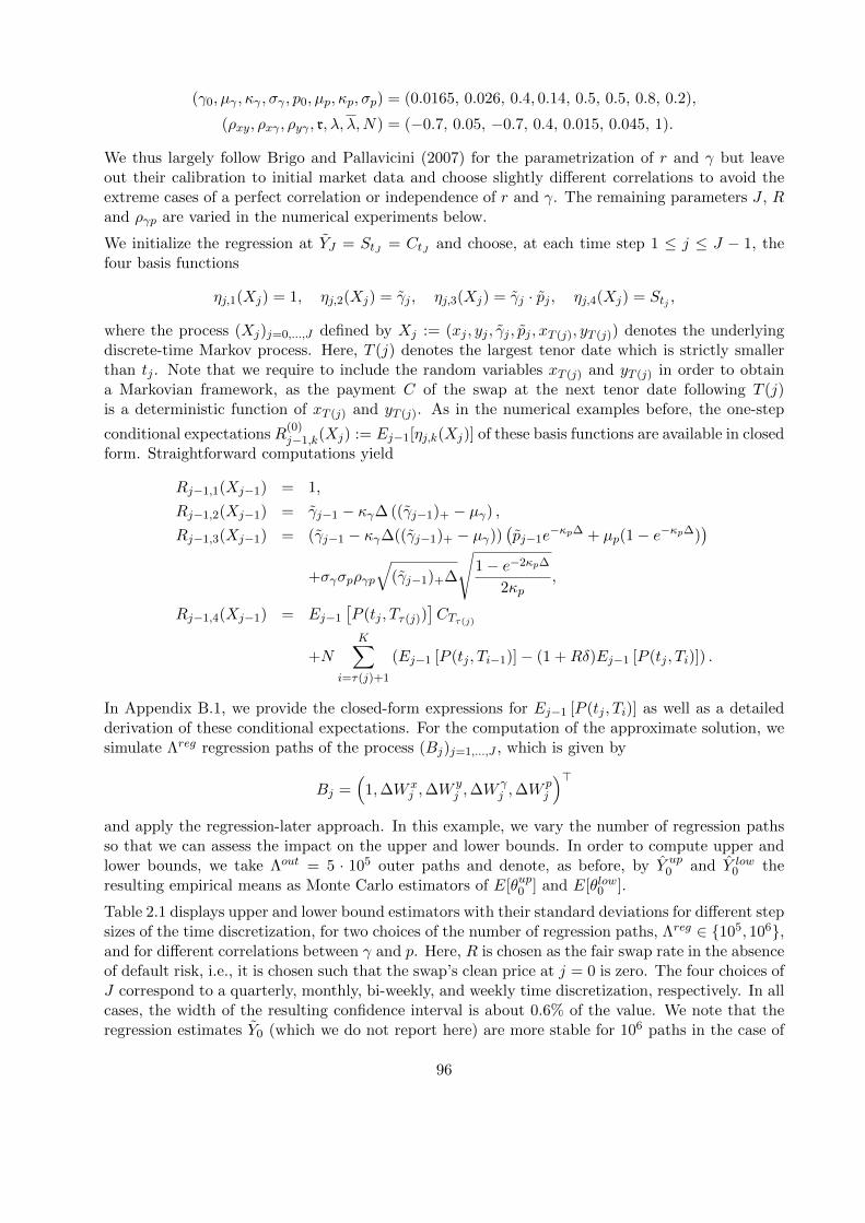
(γ0, µγ , κγ , σγ , p0, µp, κp, σp) = (0.0165, 0.026, 0.4, 0.14, 0.5, 0.5, 0.8, 0.2),

(ρxy, ρxγ , ρyγ , r, λ, λ,N) = (−0.7, 0.05, −0.7, 0.4, 0.015, 0.045, 1).

We thus largely follow Brigo and Pallavicini (2007) for the parametrization of r and γ but leaveout their calibration to initial market data and choose slightly different correlations to avoid theextreme cases of a perfect correlation or independence of r and γ. The remaining parameters J , Rand ργp are varied in the numerical experiments below.

We initialize the regression at YJ = StJ = CtJ and choose, at each time step 1 ≤ j ≤ J − 1, thefour basis functions

ηj,1(Xj) = 1, ηj,2(Xj) = γj , ηj,3(Xj) = γj · pj , ηj,4(Xj) = Stj ,

where the process (Xj)j=0,...,J defined by Xj := (xj , yj , γj , pj , xT (j), yT (j)) denotes the underlyingdiscrete-time Markov process. Here, T (j) denotes the largest tenor date which is strictly smallerthan tj . Note that we require to include the random variables xT (j) and yT (j) in order to obtaina Markovian framework, as the payment C of the swap at the next tenor date following T (j)is a deterministic function of xT (j) and yT (j). As in the numerical examples before, the one-step

conditional expectations R(0)j−1,k(Xj) := Ej−1[ηj,k(Xj)] of these basis functions are available in closed

form. Straightforward computations yield

Rj−1,1(Xj−1) = 1,

Rj−1,2(Xj−1) = γj−1 − κγ∆ ((γj−1)+ − µγ) ,

Rj−1,3(Xj−1) = (γj−1 − κγ∆((γj−1)+ − µγ))(pj−1e

−κp∆ + µp(1− e−κp∆))

+σγσpργp

√(γj−1)+∆

√1− e−2κp∆

2κp,

Rj−1,4(Xj−1) = Ej−1

[P (tj , Tτ(j))

]CTτ(j)

+NK∑

i=τ(j)+1

(Ej−1 [P (tj , Ti−1)]− (1 +Rδ)Ej−1 [P (tj , Ti)]) .

In Appendix B.1, we provide the closed-form expressions for Ej−1 [P (tj , Ti)] as well as a detailedderivation of these conditional expectations. For the computation of the approximate solution, wesimulate Λreg regression paths of the process (Bj)j=1,...,J , which is given by

Bj =(

1,∆W xj ,∆W

yj ,∆W

γj ,∆W

pj

)>and apply the regression-later approach. In this example, we vary the number of regression pathsso that we can assess the impact on the upper and lower bounds. In order to compute upper andlower bounds, we take Λout = 5 · 105 outer paths and denote, as before, by Y up

0 and Y low0 the

resulting empirical means as Monte Carlo estimators of E[θup0 ] and E[θlow0 ].

Table 2.1 displays upper and lower bound estimators with their standard deviations for different stepsizes of the time discretization, for two choices of the number of regression paths, Λreg ∈ 105, 106,and for different correlations between γ and p. Here, R is chosen as the fair swap rate in the absenceof default risk, i.e., it is chosen such that the swap’s clean price at j = 0 is zero. The four choices ofJ correspond to a quarterly, monthly, bi-weekly, and weekly time discretization, respectively. In allcases, the width of the resulting confidence interval is about 0.6% of the value. We note that theregression estimates Y0 (which we do not report here) are more stable for 106 paths in the case of

96

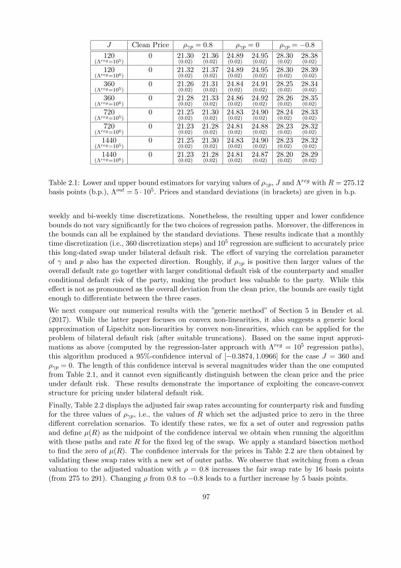
J Clean Price ργp = 0.8 ργp = 0 ργp = −0.8

120(Λreg=105)

0 21.30(0.02)

21.36(0.02)

24.89(0.02)

24.95(0.02)

28.30(0.02)

28.38(0.02)

120(Λreg=106)

0 21.32(0.02)

21.37(0.02)

24.89(0.02)

24.95(0.02)

28.30(0.02)

28.39(0.02)

360(Λreg=105)

0 21.26(0.02)

21.31(0.02)

24.84(0.02)

24.91(0.02)

28.25(0.02)

28.34(0.02)

360(Λreg=106)

0 21.28(0.02)

21.33(0.02)

24.86(0.02)

24.92(0.02)

28.26(0.02)

28.35(0.02)

720(Λreg=105)

0 21.25(0.02)

21.30(0.02)

24.83(0.02)

24.90(0.02)

28.24(0.02)

28.33(0.02)

720(Λreg=106)

0 21.23(0.02)

21.28(0.02)

24.81(0.02)

24.88(0.02)

28.23(0.02)

28.32(0.02)

1440(Λreg=105)

0 21.25(0.02)

21.30(0.02)

24.83(0.02)

24.90(0.02)

28.23(0.02)

28.32(0.02)

1440(Λreg=106)

0 21.23(0.02)

21.28(0.02)

24.81(0.02)

24.87(0.02)

28.20(0.02)

28.29(0.02)

Table 2.1: Lower and upper bound estimators for varying values of ργp, J and Λreg with R = 275.12basis points (b.p.), Λout = 5 · 105. Prices and standard deviations (in brackets) are given in b.p.

weekly and bi-weekly time discretizations. Nonetheless, the resulting upper and lower confidencebounds do not vary significantly for the two choices of regression paths. Moreover, the differences inthe bounds can all be explained by the standard deviations. These results indicate that a monthlytime discretization (i.e., 360 discretization steps) and 105 regression are sufficient to accurately pricethis long-dated swap under bilateral default risk. The effect of varying the correlation parameterof γ and p also has the expected direction. Roughly, if ργp is positive then larger values of theoverall default rate go together with larger conditional default risk of the counterparty and smallerconditional default risk of the party, making the product less valuable to the party. While thiseffect is not as pronounced as the overall deviation from the clean price, the bounds are easily tightenough to differentiate between the three cases.

We next compare our numerical results with the ”generic method” of Section 5 in Bender et al.(2017). While the latter paper focuses on convex non-linearities, it also suggests a generic localapproximation of Lipschitz non-linearities by convex non-linearities, which can be applied for theproblem of bilateral default risk (after suitable truncations). Based on the same input approxi-mations as above (computed by the regression-later approach with Λreg = 105 regression paths),this algorithm produced a 95%-confidence interval of [−0.3874, 1.0966] for the case J = 360 andργp = 0. The length of this confidence interval is several magnitudes wider than the one computedfrom Table 2.1, and it cannot even significantly distinguish between the clean price and the priceunder default risk. These results demonstrate the importance of exploiting the concave-convexstructure for pricing under bilateral default risk.

Finally, Table 2.2 displays the adjusted fair swap rates accounting for counterparty risk and fundingfor the three values of ργp, i.e., the values of R which set the adjusted price to zero in the threedifferent correlation scenarios. To identify these rates, we fix a set of outer and regression pathsand define µ(R) as the midpoint of the confidence interval we obtain when running the algorithmwith these paths and rate R for the fixed leg of the swap. We apply a standard bisection methodto find the zero of µ(R). The confidence intervals for the prices in Table 2.2 are then obtained byvalidating these swap rates with a new set of outer paths. We observe that switching from a cleanvaluation to the adjusted valuation with ρ = 0.8 increases the fair swap rate by 16 basis points(from 275 to 291). Changing ρ from 0.8 to −0.8 leads to a further increase by 5 basis points.

97

ργp Adjusted Fair Swap Rate Clean Price Bounds

0.8 290.82 −31.53 −0.02(0.02)

0.05(0.02)

0 293.65 −37.22 −0.01(0.02)

0.08(0.02)

−0.8 296.39 −42.71 −0.06(0.02)

0.04(0.02)

Table 2.2: Adjusted fair swap rates and lower and upper bound estimators for varying values of ργpwith Λreg = 105, Λout = 5 · 105 and J = 360. Rates, prices and standard deviations (in brackets)are given in b.p.

98

Chapter 3

Iterative improvement of upper andlower bounds for convex dynamicprograms

As we have seen in the previous chapters, the quality of upper and lower bounds in numericalapplications strongly depends on the quality of the input approximation. Hence, the key challenge inconstructing tight upper and lower bounds to the solution of a dynamic program of the form (1.15) or(2.1), is to compute a suitable approximate solution to these dynamic programs. Depending on theconsidered problem, this can be rather cumbersome. In this chapter, we, thus, present an iterativeimprovement algorithm for systems of convex dynamic programs which builds on the pathwiseapproach presented in Section 1.3 and allows us to obtain tight upper and lower bounds even ifthe approximate solution is rather crude. In Section 3.1 we first explain how a given supersolutioncan be improved by using the pathwise approach of Section 1.3 for the construction of upperbounds. Section 3.2 is structured similarly and transfers the results of Section 3.1 to the contextof subsolutions. Building on these results, we discuss in Section 3.3 an improvement approach forfamilies of super- and subsolutions, if the dynamic program is one-dimensional. Following this,we show that this approach generalizes the improvement approach of Kolodko and Schoenmakers(2006) proposed in the context of Bermudan option pricing. In Section 3.4, we explain how theimprovement algorithms presented in the preceding sections can be applied numerically. Finally,we demonstrate the applicability of this approach in the context of pricing under funding cost.

3.1 Improvement of supersolutions

The aim of this section is to construct an improvement of a given supersolution to the system ofconvex dynamic programs (1.15) given by

Y(ν)J = ξ(ν)

Y(ν)j = F

(ν)j

(Ej

[βj+1Y

(1)j+1

], . . . , Ej

[βj+1Y

(N)j+1

]), ν = 1, . . . , N, j = J − 1, . . . , 0.

Intuitively, such an improvement should satisfy two things: first, it should again be a supersolutionto (1.15) and second, it should lie below the given supersolution at all points in time. The followingdefinition formalizes this intuition.

99

Definition 3.1.1. Let Y be a supersolution (respectively subsolution) to (1.15). A process Y impr ∈L∞−ad (RN ) is called an improvement of Y , if Y impr is a supersolution (respectively subsolution) to(1.15) and it holds that

Y imprj ≤ Yj

P -almost surely for every j = 0, . . . , J (and with ”≤” replaced by ”≥” for a subsolution).

For our considerations, we have to restrict ourselves to the monotonic situation of Section 1.3,where we assumed that a comparison principle holds. To establish the comparison principle, we

make the following monotonicity assumption on the functions F(ν)j :

Assumption 3.1.2. For every j = 0, . . . , J − 1, ν = 1, . . . , N and any two random variablesY (1), Y (2) ∈ L∞−(RN ) with Y (1) ≥ Y (2) P -a.s., the following monotonicity condition is satisfied:

F(ν)j

(βj+1Y

(1,1), . . . , βj+1Y(1,N)

)≥ F (ν)

j

(βj+1Y

(2,1), . . . , βj+1Y(2,N)

), P -a.s. (3.1)

We briefly explain why Assumption 3.1.2 ensures the existence of the comparison principle. Sup-pose for the moment, that the underlying filtration (Fj)j=0,...,J is replaced by the full informationfiltration (Gj)j=0,...,J , where Gj = F for all j = 0, . . . , J . Then, Theorem 1.4.1 still holds truefor this enlarged filtration due to our measurability assumptions. In particular, we observe thatAssumption 3.1.2 coincides with the monotonicity statement (c) in Theorem 1.4.1. This impliesthat

P

((r(ν),[n]

)>βj+1 ≥ 0

)= 1 (3.2)

for all j = 0, . . . , J − 1, ν, n ∈ 1, . . . , N and every random variable r(ν) ∈ L∞−(RND) satisfying

F(ν,#)j (r(ν)) ∈ L∞−(R) for each j. From this, we conclude that the positivity condition especially

holds true for the admissible controls r(ν) ∈ AF (ν)

0 , ν = 1, . . . , N , as they are obviously adaptedto the filtration (Gj)j=0,...,J . Applying Theorem 1.4.1 again for the initial filtration (Fj)j=0,...,J

establishes the comparison principle.

Let Y be a supersolution to (1.15) and recall that the recursion (1.22) for Θup := Θup(M) is givenby

Θ(up,ν)J = ξ(ν)

Θ(up,ν)j = F

(ν)j

(βj+1Θ

(up,1)j+1 −∆M

[1]j+1, . . . , βj+1Θ

(up,N)j+1 −∆M

[N ]j+1

), (3.3)

for j = J − 1, . . . , 0, ν = 1, . . . , N , and any martingale M ∈ MND. The main idea of theimprovement approach is now to choose a suitable martingale M ∈MND such that

Yj ≤ Ej[Θupj

(M)]≤ Yj (3.4)

P -almost surely for every j = 0, . . . , J . In the context of Bermudan option pricing, Chen andGlasserman (2007) showed that taking the Doob martingale of a given supersolution as an inputleads to an improved upper bound. This idea can be generalized to our setting: Denote by M [n],n = 1, . . . , N , the Doob martingale of βY (n). Then, the following Theorem states that the process(Ej [Θ

upj (M)])j=0,...,J defined by (3.3) is an improvement for Y . Moreover, it shows that this ap-

proach only gets stuck, if the supersolution Y , which we want to improve, already coincides withthe true solution.

100

Theorem 3.1.3. Suppose Assumptions 1.2.1 and 3.1.2. Let j ∈ 0, . . . , J − 1 and let Y be asupersolution to (1.15). Further, let M [ν] ∈ MD be the Doob martingale of the process βY (ν) forevery ν = 1, . . . , N . Then, the process Θup(M) defined by (3.3) satisfies

Y(ν)i ≤ Ei

[Θ

(up,ν)i

(M)]≤ F (ν)

i

(Ei

[βi+1Y

(1)i+1

], . . . , Ei

[βi+1Y

(N)i+1

])≤ Y (ν)

i , (3.5)

P -almost surely for all i = 0, . . . , J and ν = 1, . . . , N . Moreover, if Yi = Yi for all i = j + 1, . . . , J ,then

Θupj (M) = Yj (3.6)

P -almost surely.

Proof. First of all, we recall that the process (Ei[Θupi (M)])i=0,...,J is a supersolution to the system of

convex dynamic programs (1.15) for every martingale M ∈MND according to Section 1.3. Hence,the first inequality in (3.5) holds by the comparison principle. Furthermore, the last inequality in(3.5) holds by the supersolution property of Y . Therefore, it only remains to show that

Ei

[Θ

(up,ν)i (M)

]≤ F (ν)

i

(Ei

[βi+1Y

(1)i+1

], . . . , Ei

[βi+1Y

(N)i+1

])(3.7)

holds for every i = 0, . . . , J − 1 and ν = 1, . . . , N . To this end, let M [ν] ∈ MD be the Doobmartingale of βY (ν) for every ν = 1, . . . , N and define Θup := Θup(M) by (3.3). In order to prove(3.7), we show the assertion

Θupi ≤ Yi

via backward induction on i = J, . . . , 0. Since we have by definition that Θ(up,ν)J = ξ(ν) ≤ Y

(ν)J ,

the case i = J is again trivial and we suppose that the assertion is true for i + 1, i.e., we haveΘupi+1 ≤ Yi+1 P -almost surely. Then, we have by Lemma 1.2.4 that

Θ(up,ν)i =

N∑n=1

(r(ν),[n]

)>βi+1Θ

(up,n)i+1 −

N∑n=1

(r(ν),[n]

)>∆Mi+1 − F (ν,#)

i

(r(ν))

for a random variable r(ν) ∈ L∞−(RND) satisfying F(ν,#)i (r) ∈ L∞−(R). Since (r(ν),[n])>βi+1 ≥ 0

P -almost surely by (3.2), we conclude by the induction hypothesis, the definition of M , and (1.23)that

Θ(up,ν)i =

N∑n=1

(r(ν),[n]

)>βi+1Θ

(up,n)i+1 −

N∑n=1

(r(ν),[n]

)>∆Mi+1 − F (ν,#)

i

(r(ν))

≤N∑n=1

(r(ν),[n]

)>βi+1Y

(n)i+1 −

N∑n=1

(r(ν),[n]

)> (βi+1Y

(n)i+1 − Ei

[βi+1Y

(n)i+1

])− F (ν,#)

i

(r(ν))

=N∑n=1

(r(ν),[n]

)>Ei

[βi+1Y

(n)i+1

]− F (ν,#)

i

(r(ν))

≤ F (ν)i

(Ei

[βi+1Y

(1)i+1

], . . . , Ei

[βi+1Y

(N)i+1

])≤ Y (ν)

i . (3.8)

Here the last inequality is due to the supersolution property of Y . Now, the asserted inequality(3.7) follows from (3.8) by the monotonicity of the conditional expectation.

101

Finally, it remains to show (3.6), i.e.Θupj = Yj

if Yi = Yi for all i = j + 1, . . . , J , where j ∈ 0, . . . , J − 1 is fixed from now on. Since Yi = Yi forall i = j + 1, . . . , J , we conclude by the definition of M that

M[ν]i+1 − M

[ν]i = βi+1Y

[ν]i+1 − Ei

[βi+1Y

[ν]i+1

]= βi+1Y

[ν]i+1 − Ei

[βi+1Y

[ν]i+1

]for every i = j, . . . , J − 1 and ν = 1, . . . , N . By exploiting that Θup

i = Yi for every i = j + 1, . . . , Jby (3.5), we thus obtain that

Θ(up,ν)j = F

(ν)j

(βj+1Θ

(up,1)j+1 −∆M

(1)j+1, . . . , βj+1Θ

(up,N)j+1 −∆M

(N)j+1

)= F

(ν)j

(βj+1Y

(1)j+1 −

(βj+1Y

(1)j+1 − Ej

[βj+1Y

(1)j+1

]), . . . ,

βj+1Θ(up,N)j+1 −

(βj+1Y

(N)j+1 − Ej

[βj+1Y

(N)j+1

]))= F

(ν)j

(Ej

[βj+1Y

(1)j+1

], . . . , Ej

[βj+1Y

(N)j+1

])= Y

(ν)j ,

which completes the proof.

When starting with an arbitrary supersolution, we typically do not obtain the solution Y by ap-plying the approach described in Theorem 3.1.3 once. This is typically the case in numericalapplications where the ”input supersolution” Y is computed by the algorithm explained in Sec-tion 1.7 and thus may stem from a possibly crude approximate solution to (1.15). Hence, we nowshow that the above construction can be iterated in a straightforward way such that a decreasingsequence of supersolutions is obtained.

To this end, let Y be a supersolution and define Θup,0 := Y . Then, we define the k-th iterationaccording to (3.3) by

Θup,k := Θup(Mk), k ≥ 1, (3.9)

where each Mk = (M [1],k, . . . ,M [N ],k) is given by

M[ν],kj =

j−1∑i=0

βi+1Ei+1

[Θ

(up,ν),k−1i+1

]− Ei

[βi+1Θ

(up,ν),k−1i+1

], j = 0, . . . , J, ν = 1, . . . , N. (3.10)

Applying Theorem 3.1.3 repeatedly, we observe that this iteration decreasingly converges in at mostJ + 1 steps as stated in the following corollary.

Corollary 3.1.4. For every k ≥ 1 and j = 0, . . . , J ,

Ej

[Θup,kj

]≤ Ej

[Θup,k−1j

]P -a.s. (3.11)

Moreover, for every i ≥ j,Θup,J−j+1i = Yi, P -a.s. (3.12)

Hence, the upper bound iteration terminates after at most J + 1 steps.

102

Proof. First note that inequality (3.11) is an immediate consequence of Theorem 3.1.3 and thedefinition of Θup,k, k ≥ 0. Hence, it only remains to show that (3.12) holds. The proof is by

backward induction on j, with the case j = J being trivial, because Θ(up,ν),1J = ξ(ν) = Y

(ν)J by

definition for every ν = 1, . . . , N . Now suppose, that the assertion is true for j ∈ 1, . . . , J. Then,we have by induction hypothesis that

Θup,J−(j−1)+1i = Θup,J−j+1

i = Yi

P -a.s. for every i = j, . . . , J . From Theorem 3.1.3 we thus conclude that

Θup,J−(j−1)+1j−1 = Θup

j−1

(MJ−(j−1)+1

)= Yj−1 P -a.s.,

where MJ−(j−1)+1 is given by (3.10).

Remark 3.1.5. Note that convergence of the above algorithm in at most J steps can be achievedby a slight modification. Let Y be an arbitrary supersolution and define Θup,0 by

Θ(up,ν),0j =

ξ(ν), j = J

Y(ν)j , j < J

for every ν = 1, . . . , N . Then, the process Θup,0 is again a supersolution. This is obvious forj < J − 1 by definition of Θup,0. For j = J − 1, we obtain that

Θ(up,ν),0J−1 = Y

(ν)J−1

≥ F (ν)J−1

(EJ−1

[βJ Y

(1)J

], . . . , EJ−1

[βJ Y

(N)J

])≥ F (ν)

J−1

(EJ−1

[βJξ

(1)], . . . , EJ−1

[βJξ

(N)J

])= F

(ν)J−1

(EJ−1

[βJΘ

(up,1),0J

], . . . , EJ−1

[βJΘ

(up,N),0J

])for every ν = 1, . . . , N by the supersolution property of Y and the monotonicity condition (3.1).Since the terminal value of Θ(up,ν),0 now coincides with the true terminal value ξ(ν), we are ableto reduce the number of iteration steps by one. In particular, the iteration converges in at most Jsteps, if the input supersolution is computed by the pathwise approach of Section 1.3.

3.2 Improvement of subsolutions

After considering the improvement approach for supersolutions, we now explain how the recursionfor lower bounds presented in Section 1.3 can be used to improve arbitrary subsolutions to (1.15).To this end, let Y be an arbitrary subsolution to (1.15). In order to construct an improvement ofY , we rely on the modified recursion (1.29) for the lower bound Θlow := Θlow(r(1), . . . , r(N),M),which is given by

Θ(low,ν)J = ξ(ν)

Θ(low,ν)j =

N∑n=1

(r

(ν),[n]j

)>βj+1Θ

(low,n)j+1 −

N∑n=1

(r

(ν),[n]j

)>∆M

[n]j+1 − F

(ν,#)j

(r

(ν)j

), (3.13)

for j = J − 1, . . . , 0, ν = 1, . . . , N , admissible controls r(ν) ∈ AF (ν)

0 , and M ∈MND.

103

Similar to the case of supersolutions, we want to find suitable controls r(ν) ∈ AF (ν)

0 such that

Yj ≤ Ej[Θlowj

(r(1), . . . , r(N),M

)]≤ Yj (3.14)

holds P -almost surely for all j = 0, . . . , J and M ∈ MND. In order to find such a candidate, wefirst note that the subsolution property of Y establishes the inequality

Y(ν)j ≤ F (ν)

j

(Ej

[βj+1Y

(1)j+1

], . . . , Ej

[βj+1Y

(N)j+1

])for every j = 0, . . . , J − 1 and ν = 1, . . . , N . By Lemma 1.2.4, we know that there exist controlsr(ν) ∈ AF (ν)

0 , ν = 1, . . . , N , such that the right hand side of this inequality can be rewritten as

F(ν)j

(Ej

[βj+1Y

(1)j+1

], . . . , Ej

[βj+1Y

(N)j+1

])=

N∑n=1

(r

(ν),[n]j

)>Ej

[βj+1Y

(n)j+1

]− F (ν,#)

j

(r

(ν)j

)for every j = 0, . . . , J − 1. Hence, solutions to these equations serve naturally as potential can-didates to establish the chain of inequalities (3.14). Note that this approach differs from existingpolicy improvement approaches like the Howard improvement. In contrast to these approaches,our approach takes an arbitrary subsolution, which need not stem from a control, as an input andconstructs a control from which an improved subsolution is derived.

The above consideration is confirmed by the following theorem, which is the main result of thissection.

Theorem 3.2.1. Suppose Assumptions 1.2.1 and 3.1.2. Let j ∈ 0, . . . , J − 1, let Y be a subso-lution to (1.15) and denote by M [ν] ∈ MD the Doob martingale of βY (ν) for every ν = 1, . . . , N .

Further let r(ν) ∈ AF (ν)

0 , ν = 1, . . . , N , be admissible controls that solve

N∑n=1

(r

(ν),[n]i

)>Ei

[βi+1Y

(n)i+1

]− F (ν,#)

i

(r

(ν)i

)= F

(ν)i

(Ei

[βi+1Y

(1)i+1

], . . . , Ei

[βi+1Y

(N)i+1

])(3.15)

P -almost surely for every i = 0, . . . , J −1 and ν = 1, . . . , N . Then, for any M ∈MND, the processΘlow(r(1), . . . , r(N),M) defined by (3.13) satisfies

Y(ν)i ≥ Ei

[Θ

(low,ν)i

(r(1), . . . , r(N),M

)]≥ F (ν)

i

(Ei

[βi+1Y

(1)i+1

], . . . , Ei

[βi+1Y

(N)i+1

])≥ Y (ν)

i ,

(3.16)

P -almost surely for all i = 0, . . . , J−1 and ν = 1, . . . , N . Moreover, if Yi = Yi for all i = j+1, . . . , J ,then

Ej

[Θlowj

(r(1), . . . , r(N),M

)]= Θlow

j

(r(1), . . . , r(N), M

)= Yj (3.17)

P -almost surely.

Remark 3.2.2. (i) As in the context of supersolutions, (3.17) states that this improvement ap-proach only gets stuck, if the input subsolution Y already coincides with the true solution.

(ii) By the chain of inequalities (3.16), we have that an improvement is obtained by taking anymartingale M ∈MND. Indeed as observed in Section 1.3, the martingale increment only actsas a control variate in this approach.

104

Proof. As we have seen in Section 1.3, the process (Ei[Θlowi (r(1), . . . , r(N),M)])i=0,...,J defines a

subsolution to (1.15) for any admissible controls r(ν) ∈ AF (ν)

0 , ν = 1, . . . , N , and M ∈ MND,so that the first inequality in (3.16) is already shown. Moreover, the last inequality in (3.16) is

immediate, as Y is assumed to be a subsolution. Now, let r(ν) ∈ AF (ν)

0 , ν = 1, . . . , N , be given by(3.15) and denote by M [ν] the Doob martingale of βY (ν) for every ν = 1, . . . , N . Then, we definethe process Θlow := Θlow(r(1), . . . , r(N), M) according to (3.13). In order to prove the remaininginequality, we proceed as in the proof of Theorem 3.1.3 and show the assertion

Θ(low,ν)i ≥ Y (ν)

i (3.18)

for every ν = 1, . . . , N by backward induction on i = J, . . . , 0. The case i = J is trivial, since we

have Θ(low,ν)J = ξ(ν) ≥ Y (ν)

J for every ν = 1, . . . , N by definition. Now suppose that the assertion istrue for i+ 1, i.e., Θlow

i+1 ≥ Yi+1 P -almost surely. Then, the definition of M [n], n = 1, . . . , N yields

Θ(low,ν)i =

N∑n=1

(r

(ν),[n]i

)>βi+1Θ

(low,n)i+1 −

N∑n=1

(r

(ν),[n]i

)>∆M

[n]i+1 − F

(ν,#)i

(r

(ν)i

)=

N∑n=1

(r

(ν),[n]i

)>βi+1Θ

(low,n)i+1 −

N∑n=1

(r

(ν),[n]i

)> (βi+1Y

(n)i+1 − Ei

[βi+1Y

(n)i+1

])− F (ν,#)

i

(r

(ν)i

)=

N∑n=1

(r

(ν),[n]i

)>βi+1

(Θ

(low,n)i+1 − Y (n)

i+1

)+

N∑n=1

(r

(ν),[n]i

)>Ei

[βi+1Y

(n)i+1

]− F (ν,#)

i

(r

(ν)i

).

Since Θ(low,n)i+1 ≥ Y

(n)i+1 for all n = 1, . . . , N by induction hypothesis and (r

(ν),[n]i )>βi+1 ≥ 0 for each

n by (3.2), we conclude that

Θ(low,ν)i ≥

N∑n=1

(r

(ν),[n]i

)>Ei

[βi+1Y

(n)i+1

]− F (ν,#)

i

(r

(ν)i

).

Finally, it follows from (3.15) and the subsolution property of Y that

Θ(low,ν)i ≥ F (ν)

i

(Ei

[βi+1Y

(1)i+1

], . . . , Ei

[βi+1Y

(N)i+1

])(3.19)

≥ Y (ν)i ,

and, thus, (3.18) is established. Recalling that Ei[Θlowi (r(1), . . . , r(N),M)] does not depend on the

choice of M , (3.16) now follows from (3.19) and the monotonicity of the conditional expectation.

To complete the proof, we fix j ∈ 0, . . . , J − 1 and assume that Yi = Yi for all i = j + 1, . . . , J .Then, we observe that (3.15) is equivalent to

N∑n=1

(r

(ν),[n]i

)>Ei

[βi+1Y

(n)i+1

]− F (ν,#)

i

(r

(ν)i

)= F

(ν)i

(Ei

[βi+1Y

(1)i+1

], . . . , Ei

[βi+1Y

(N)i+1

])for every i = j, . . . , J − 1, i.e. ri satisfies the optimality condition (1.24) for all i = j, . . . , J − 1.Moreover, we conclude, similar to the proof of Theorem 3.1.3, that

M[ν]i+1 − M

[ν]i = βi+1Y

(ν)i+1 − Ei

[βi+1Y

(ν)i+1

]105

for all ν = 1, . . . , N and i = j, . . . , J − 1. Hence, we obtain that

Θ(low,ν)j =

N∑n=1

(r

(ν),[n]j

)>βj+1Θ

(low,n)j+1 −

N∑n=1

(r

(ν),[n]j

)>∆M

[n]j+1 − F

(ν,#)j

(r

(ν)j

)=

N∑n=1

(r

(ν),[n]j

)>βj+1Y

(n)j+1 −

N∑n=1

(r

(ν),[n]j

)> (βj+1Y

(n)j+1 − Ej

[βj+1Y

(n)j+1

])− F (ν,#)

j

(r

(ν)j

)=

N∑n=1

(r

(ν),[n]j

)>Ej

[βj+1Y

(n)j+1

]− F (ν,#)

j

(r

(ν)j

)= F

(ν)j

(Ej

[βj+1Y

(1)j+1

], . . . , Ej

[βj+1Y

(N)j+1

])= Y

(ν)j ,

since Θlowi = Yi for every i = j + 1, . . . , J by (3.16).

As in Section 3.1, this improvement can be iterated several times. For a given subsolution Y defineΘlow,0 := Y and define Θlow,k according to (3.13) by

Θlow,k := Θlow(r(1),k, . . . , r(N),k,Mk

), k ≥ 1, (3.20)

where the processes r(ν),k ∈ AF (ν)

0 are for every j = 0, . . . , J − 1 and ν = 1, . . . , N given by

N∑n=1

(r

(ν),[n],kj

)>Ej

[βj+1Θ

(low,n),k−1j+1

]− F (ν,#)

j

(r

(ν),kj

)= F

(ν)j

(Ej

[βj+1Θ

(low,1),k−1j+1

], . . . , Ej

[βj+1Θ

(low,1),k−1j+1

]), (3.21)

and Mk ∈ MND is arbitrary. Then, iterative application of Theorem 3.2.1 yields the followingcorollary.

Corollary 3.2.3. For every k ≥ 1 and j = 0, . . . , J ,

Ej

[Θlow,kj

]≥ Ej

[Θlow,k−1j

], P -a.s. (3.22)

Moreover,

Ei

[Θlow,J−j+1i

]= Yi P -a.s., (3.23)

whenever i ≥ j. In the last equation, the conditional expectation on the left-hand side can be

removed, when M [ν],k is taken as the Doob martingale of the process (βjEj [Θ(low,ν),k−1j ])j=0,...,J for

each ν = 1, . . . , N and k ≥ 1 .

Proof. Let Mk ∈ MND, k ≥ 1, be arbitrary martingales. Then, we first note that the inequality(3.22) is an immediate consequence of Theorem 3.2.1 and the definition of Θlow,k, k ≥ 0. Hence, itonly remains to show (3.23). The proof is by backward induction on j, with the case j = J being

trivial, because Θ(low,ν),1J = ξ(ν) = Y

(ν)J by definition. Now suppose, that the assertion is true for

j ∈ 1, . . . , J, i.e.

Ei

[Θlow,J−j+1i

]= Yi

106

for all i ≥ j. Then, we have by induction hypothesis that

Θlow,J−(j−1)+1i = Θlow,J−j+1

i = Yi

P -a.s. for every i = j, . . . , J . From Theorem 3.2.1 we thus conclude that

Ej−1

[Θlow,J−(j−1)+1j−1

]= Ej−1

[Θlowj−1

(r(1),J−(j−1)+1, . . . , r(N),J−(j−1)+1,MJ−(j−1)+1

)]= Θlow

j−1

(r(1),J−(j−1)+1, . . . , r(N),J−(j−1)+1, MJ−(j−1)+1

)= Yj−1 P -a.s.,

where each r(ν),J−(j−1)+1 ∈ AF (ν)

0 , ν = 1, . . . , N , is given by (3.21) and MJ−(j−1)+1,[ν] is the Doob

martingale of (βiEi[Θlow,J−(j−1)+1i ])i=0,...,J .

Remark 3.2.4. As in the context of supersolutions, convergence of the above algorithm in at mostJ steps can be achieved. Let Y be an arbitrary subsolution and define Θlow,0 by

Θ(low,ν),0j =

ξ(ν), j = J

Y(ν)j , j < J

for every ν = 1, . . . , N . Applying the same arguments as in Remark 3.1.5, we observe that Θlow,0 isstill a subsolution. Consequently, convergence in at most J steps can be achieved for subsolutionsstemming from the pathwise approach of Section 1.3.

3.3 Improving families of super- and subsolutions

In Section 3.4 below, we explain that the numerical costs of algorithms based on (3.9) and (3.20)tend to grow exponentially in the number of iterations k. For this reason, a moderate number ofiterations must suffice in practical implementations. In the case of one-dimensional convex dynamicprograms, we can address this issue by improving whole families of super- and subsolutions insteadof just one. Therefore, we suppose throughout this section that N = 1 and (1.15) reduces to

YJ = ξ,

Yj = Fj (Ej [βj+1Yj+1]) , j = J − 1, . . . , 0. (3.24)

As before, we first consider the case of supersolutions. To this end, let (Y l)l∈I be a family ofsupersolutions, where I is a finite index set. Further, we denote by K(j), j = 1, . . . , J , a non-decreasing sequence of subsets of I, i.e. it holds that K(j) ⊆ K(j + 1). Then, we consider thepredictable, I-valued process

l∗(j) = infl ∈ K(j)

∣∣∣ ∀ι ∈ K(j) Fj−1

(Ej−1

[βj Y

lj

])≤ Fj−1

(Ej−1

[βj Y

ιj

])(3.25)

for every j = 1, . . . , J . This means that, at every time point j = 1, . . . , J , we only consider thosesupersolutions which are represented in the subset K(j) and the random variable l∗(j) returnsan index l ∈ K(j) at which the evaluation of Fj−1 is minimized. Considering the sets K(j)makes the approach more flexible, but, obviously, the simplest choice is to take K(j) = I for allj = 1, . . . , J . This additional flexibility turns out to be useful in situations where I is large, and

107

thus the computational costs in order to determine the process l∗ are high. More sophisticatedchoices of K(j) then allow to reduce these costs.

Building on l∗, we define the process Y by

Yj =

Yl∗(j)j , j > 0

F0

(E0

[β1Y1

]), j = 0

(3.26)

for every j = 0, . . . , J . Indeed, this process is a supersolution to (3.24), which allows us to improvethe supersolutions (Y l)l∈I simultaneously. To examine the supersolution property of Y , we firstobserve that the case j = 0 is trivial, since we have Y0 = F0(E0[β1Y1]) by definition. For the casej > 0, we get by the supersolution property of Y l for every l ∈ I that

Yj =∑l∈K(j)

Ylj 1l∗(j)=l

≥∑l∈K(j)

Fj

(Ej

[βj+1Y

lj+1

])1l∗(j)=l.

Since K(j) ⊆ K(j + 1) for all j = 1, . . . , J − 1 it follows that

Yj ≥∑l∈K(j)

Fj

(Ej

[βj+1Y

l∗(j+1)j+1

])1l∗(j)=l

= Fj(Ej[βj+1Yj+1

])P -almost surely, showing that Y is a supersolution. Hence, Theorem 3.1.3 can be applied to theprocess Y and implies, for Θup = Θup(M),

Ej

[Θupj

]≤ Fj

(Ej[βj+1Yj+1

])= min

l∈K(j+1)Fj

(Ej

[βj+1Y

lj+1

])≤ min

l∈K(j+1)Ylj

P -almost surely for all j = 0, . . . , J − 1, where M denotes the Doob martingale of βY . Thus, ifK(j) = I for all j = 1, . . . , J , we achieve a simultaneous improvement of all supersolutions (Y l)l∈Iby improving Y .

Finally, we turn to the case of subsolutions, where the overall strategy is similar. Hence, let (Y l)l∈Ibe a family of subsolutions, where I is still a finite set. Then, we consider the predictable, I-valuedprocess

l∗(j) = infl ∈ K(j)

∣∣∣ ∀ι ∈ K(j) Fj−1

(Ej−1

[βj Y

lj

])≥ Fj−1

(Ej−1

[βj Y

ιj

])(3.27)

for every j = 1, . . . , J , where K(j) is again a non-decreasing family of subsets of I. Note that,compared to (3.25), the inequality is now the other way round, since we would like to construct asubsolution, which lies above the given subsolutions (Y l)l∈I P -almost surely. Then, the processY defined by

Yj =

Y

(l∗(j))j , j > 0

F0

(E0

[β1Y1

]), j = 0

is, by similar arguments as before, a subsolution to (3.24). The case j = 0 is again trivial sinceY0 = F0(E0[β1Y1]) by definition. For j > 0, we apply the subsolution property of the processesY l, l ∈ I, and K(j) ⊆ K(j + 1) to obtain

Yj =∑l∈K(j)

Ylj 1l∗(j)=l

108

≤∑l∈K(j)

Fj

(Ej

[βj+1Y

lj+1

])1l∗(j)=l

≤∑l∈K(j)

Fj

(Ej

[βj+1Y

l∗(j+1)j+1

])1l∗(j)=l

= Fj(Ej[βj+1Yj+1

]),

from which we conclude that Y is a subsolution. Thus, by Theorem 3.2.1,

Ej

[Θlowj (r,M)

]≥ Fj

(Ej[βj+1Yj+1

])= max

l∈K(j+1)Fj

(Ej

[βj+1Y

lj+1

])≥ max

l∈K(j+1)Ylj (3.28)

P -a.s. for every j = 0, . . . , J − 1, where r is for every j = 0, . . . , J − 1 given by (3.15) andM ∈MD. Hence, in the caseK(j) = I for j = 1, . . . , J , improving Y results again in a simultaneousimprovement of all subsolutions (Y l)l∈I .

In the following example, we present a generic way to construct a family of subsolutions from agiven admissible control and show that, in the special case of optimal stopping problems, the policyimprovement approach of Kolodko and Schoenmakers (2006) can be recovered from our approach.

Example 3.3.1. (i) Suppose that we are given an input policy r ∈ AF0 . Then, we may choose areference policy r ∈ AF0 and define a family of policies (rl)l=0,...,J−1 by

rlj =

rj , j < l

rj , j ≥ l(3.29)

for j = 0, . . . , J−1. From the definition of rl, we immediately obtain that rl ∈ AF0 for eachl. Building on this family of policies, we can define a family of subsolutions (Y l)l=0,...,J−1

by

Ylj = Ej

[Θlowj

(rl)], j = 0, . . . , J.

Now let the sets (K(j))j=1,...,J be given by

K(j) = 0, . . . ,minj + κ− 1, J

for some κ ≥ 1. Then, we observe from the monotonicity assumption on Fj and the definitionof (Y l)l=0,...,J−1, that the improvement condition (3.15) can be rewritten as

r>j Ej

[βj+1Θlow

j+1

(rl∗(j+1)

)]− F#

j (rj) = maxl=j+1,...,(j+κ)∧J

Fj

(Ej

[βj+1Θlow

j+1

(rl)])

(3.30)

for every j = 0, . . . , J − 1. Note that the maximum over the set K(j + 1) can be restrictedto the subset j + 1, . . . , (j + κ) ∧ J in (3.30), as Θlow

j+1(rl) = Θlowj+1(r) for all l ≤ j + 1 by

definition of the family (rl)l=0,...,J−1. By applying (3.28) to this setting, we observe that

Ej

[Θlowj (r)

]≥ max

l=0,...,(j+κ)∧JFj

(Ej

[βj+1Θlow

j+1

(rl)])

= maxl=j+1,...,(j+κ)∧J

Fj

(Ej

[βj+1Θlow

j+1

(rl)])

,

where the last equality follows by the same argument as before.

109

(ii) We now apply the construction from part (i) to the optimal stopping case. To this end,suppose that we are given a family (τl)l=0,...,J of stopping times such that

τl ≥ l and(τl > l ⇒ τl = τl+1

)(3.31)

for every l = 0, . . . , J . Following Kolodko and Schoenmakers (2006), we call a family ofstopping times satisfying (3.31) consistent. As explained in Example 1.3.5 (ii), we can derivean admissible control r ∈ AF0 from this stopping family by setting rj = 1τj 6=j for everyj = 0, . . . , J − 1. We further choose the reference policy r ≡ 1, which corresponds to notstopping the process until terminal time. Then, we may derive from part (i) and Example1.3.5 (ii) that

Ej [Sτj ] ≥ maxl=j+1,...,(j+κ)∧J

maxSj , Ej [Sτl ], j = 0, . . . , J − 1,

where the family (τj)j=0,...,J of stopping times is given by

τj = inf

i ≥ j

∣∣∣∣Si ≥ maxl=i+1,...,(i+κ)∧J

Ei[Sτl ]

for j = 0, . . . , J . In this derivation we use that

τrl = infj ≥ 0

∣∣∣rlj = 0

= τl

by consistency of (τl)l=0,...,J and that

Sj ≥ Ej[Θlowj+1

(rl∗(j+1)

)]⇔ Sj ≥ max

Sj , Ej

[Θlowj+1

(rl∗(j+1)

)]⇔ Sj ≥ max

l=j+1,...,(j+κ)∧Jmax

Sj , Ej

[Θlowj+1

(rl)]

⇔ Sj ≥ maxl=j+1,...,(j+κ)∧J

Ej

[Θlowj+1

(rl)]

by the definition of l∗. Hence, we recover the policy improvement result in Theorem 3.1 ofKolodko and Schoenmakers (2006) as a special case of our approach.

Remark 3.3.2. The approaches presented above cannot be generalized to the multi-dimensionalsetting of Sections 3.1 and 3.2 in a straightforward way. This is mainly due to the fact that in thecase of systems of convex dynamic programs the processes l∗ and l∗ given by (3.25) respectively(3.27) additionally depend on the dimension parameter ν. Indeed, generalizing e.g. the definitionof l∗ to the multi-dimensional setting leads to

l∗(j, ν) =l ∈ K(j)

∣∣∣F (ν)j−1

(Ej−1

[βj Y

l,(1)j

], . . . , Ej−1

[βj Y

l,(N)j

])≥ F (ν)

j−1

(Ej−1

[βj Y

ι,(1)j

], . . . , Ej−1

[βj Y

ι,(N)j

])∀ι ∈ K(j)

,

for every j = 1, . . . , J and ν = 1, . . . , N , where (Y l)l∈I is a family of subsolutions to (1.15). Now,the process given by

Y(ν)j = Y

(l∗(j,ν))j 1j>0 + F

(ν)0

(E0

[β1Y

(1)1

], . . . , E0

[β1Y

(N)1

])1j=0, j = 0, . . . , J,

110

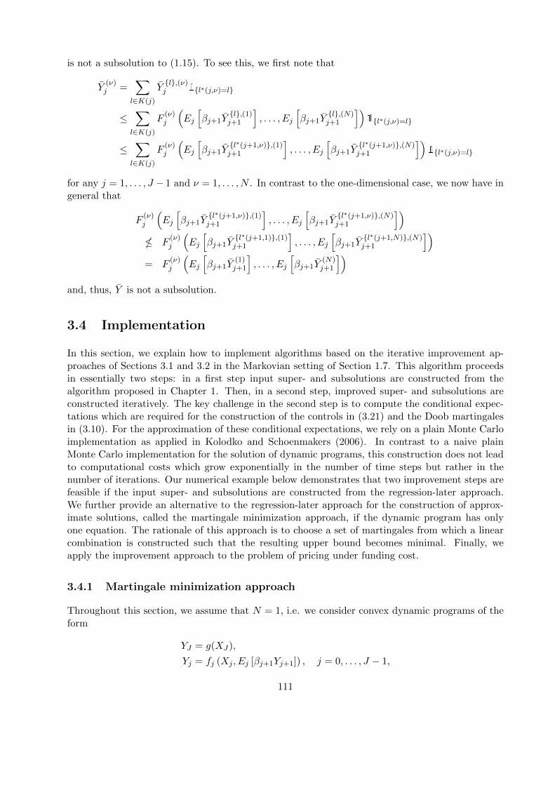
is not a subsolution to (1.15). To see this, we first note that

Y(ν)j =

∑l∈K(j)

Yl,(ν)j 1l∗(j,ν)=l

≤∑l∈K(j)

F(ν)j

(Ej

[βj+1Y

l,(1)j+1

], . . . , Ej

[βj+1Y

l,(N)j+1

])1l∗(j,ν)=l

≤∑l∈K(j)

F(ν)j

(Ej

[βj+1Y

l∗(j+1,ν),(1)j+1

], . . . , Ej

[βj+1Y

l∗(j+1,ν),(N)j+1

])1l∗(j,ν)=l

for any j = 1, . . . , J − 1 and ν = 1, . . . , N . In contrast to the one-dimensional case, we now have ingeneral that

F(ν)j

(Ej

[βj+1Y

l∗(j+1,ν),(1)j+1

], . . . , Ej

[βj+1Y

l∗(j+1,ν),(N)j+1

]) F

(ν)j

(Ej

[βj+1Y

l∗(j+1,1),(1)j+1

], . . . , Ej

[βj+1Y

l∗(j+1,N),(N)j+1

])= F

(ν)j

(Ej

[βj+1Y

(1)j+1

], . . . , Ej

[βj+1Y

(N)j+1

])and, thus, Y is not a subsolution.

3.4 Implementation

In this section, we explain how to implement algorithms based on the iterative improvement ap-proaches of Sections 3.1 and 3.2 in the Markovian setting of Section 1.7. This algorithm proceedsin essentially two steps: in a first step input super- and subsolutions are constructed from thealgorithm proposed in Chapter 1. Then, in a second step, improved super- and subsolutions areconstructed iteratively. The key challenge in the second step is to compute the conditional expec-tations which are required for the construction of the controls in (3.21) and the Doob martingalesin (3.10). For the approximation of these conditional expectations, we rely on a plain Monte Carloimplementation as applied in Kolodko and Schoenmakers (2006). In contrast to a naive plainMonte Carlo implementation for the solution of dynamic programs, this construction does not leadto computational costs which grow exponentially in the number of time steps but rather in thenumber of iterations. Our numerical example below demonstrates that two improvement steps arefeasible if the input super- and subsolutions are constructed from the regression-later approach.We further provide an alternative to the regression-later approach for the construction of approx-imate solutions, called the martingale minimization approach, if the dynamic program has onlyone equation. The rationale of this approach is to choose a set of martingales from which a linearcombination is constructed such that the resulting upper bound becomes minimal. Finally, weapply the improvement approach to the problem of pricing under funding cost.

3.4.1 Martingale minimization approach

Throughout this section, we assume that N = 1, i.e. we consider convex dynamic programs of theform

YJ = g(XJ),

Yj = fj (Xj , Ej [βj+1Yj+1]) , j = 0, . . . , J − 1,

111

where X is a time-discrete Markov process. Recall that the process X is of the form

Xj = hj(Xj−1, Bj), X0 = x0 ∈ Rd,

with measurable functions hj : Rd × RD → Rd and an RD-valued process (Bj)j=1,...,J , for whichthe first D components of Bj are given by βj and such that Bj is independent of Fj−1 for everyj = 1, . . . , J . In the LSMC approaches presented in Section 1.7, the idea is to compute coefficients(aj)j=1,...,J by an empirical regression so that an approximate solution to the dynamic program isgiven by a linear combination of chosen basis functions, i.e.

yj+1(x, b) =K∑k=1

aj+1,kηj+1,k(x, b), j = 0, . . . , J − 1.

As we have seen in the previous numerical examples and as discussed in Bender et al. (2017), theconstruction of meaningful upper bounds from such approximate solutions to the dynamic programis harder than for the lower bounds. The martingale minimization approach tackles this problemdirectly by computing the coefficients (aj)j=1,...,J differently. The idea of this approach is to choosea set of martingales and to find a linear combination of these, such that the resulting upper boundis minimized. As a consequence the resulting coefficients are global in the sense that they do notdepend on time. This is in the spirit of Desai et al. (2012) and Belomestny (2013), who proposedsuch an approach in the context of Bermudan option pricing.

To be more precisely, let basis functions ηj = (ηj,1, . . . , ηj,K), j = 1, . . . , J , be given, which satisfythe assumptions of the regression-later approach, i.e., they are sufficiently integrable and the one-step conditional expectations Rj−1 are available in closed form. From these basis functions, we canconstruct a set of martingales Mk, k = 1, . . . ,K, by

Mkj =

j−1∑i=0

βi+1ηi+1,k(Xi, Bi+1)−Ri,k(Xi).

Starting from these martingales, we define the martingale Ma by

Maj =

K∑k=1

akMkj , (3.32)

for coefficients a = (a1, . . . , aK) ∈ RK . The key step in the martingale minimization approachis now to find coefficients a∗ such that E[Θup

0 (Ma)] becomes minimal. Following the approachanalyzed in Belomestny (2013), the coefficients a∗ are given by

a∗ = argmina∈RK

E [Θup0 (Ma)] + γ

√Var (Θup

0 (Ma)) (3.33)

for fixed γ ≥ 0. Note that (3.33) involves a standard deviation penalty whose impact can becontrolled by choosing γ. The idea behind this penalty is, that the resulting upper bound shouldnot only be minimized but that it should also have low variance, since we know that Var(Θup

0 (M∗))vanishes for the martingale M∗ due to the pathwise optimality.

Since in general neither E[Θup0 (Ma)] nor Var(Θup

0 (Ma)) are available in closed form, we have toreplace them by their empirical counterparts in order to obtain an implementable algorithm. There-fore, we simulate Λmini independent copies Bj(λmini), j = 1, . . . , J, λmini = 1, . . . ,Λmini of the

112

process B to which we refer as minimization paths. Denoting by Mk(λmini) the evaluation ofthe martingales Mk for each k along these paths and computing Θup(Ma(λmini)) recursively by(1.22), we replace the optimization problem (3.33) by

a∗ = argmina∈RK

E [Θup0 (Ma)] + γ

√√√√ 1

Λmini − 1

Λmini∑λmini=1

(Θup

0 (Ma(λmini))− E [Θup0 (Ma)]

)2, (3.34)

where

E [Θup0 (Ma)] =

1

Λmini

Λmini∑λmini=1

Θup0

(Ma(λmini)

). (3.35)

Then, an approximate solution y to the dynamic program is obtained by

yj(x, b) =K∑k=1

a∗kηj,k(x, b), j = 1, . . . , J.

Remark 3.4.1. (i) The minimization approach requires the choice of the parameter γ. In ournumerical results presented in Section 3.4.3, we apply a “training and testing” approach totune this parameter. To this end, we choose a set γ1, . . . , γL, L ∈ N, of parameters. Foreach γl, l = 1, . . . , L, we compute a vector of coefficients a∗γl ∈ R

K according to (3.34) alongthe minimization paths Λmini. If vectors a∗γ1

, . . . , a∗γL are computed, we sample a new setof Λtest test paths (independent copies of B which are also independent of the minimizationpaths). The parameter γ is obtained by taking the γl such that a∗γl minimizes the expressionin (3.35) along the test paths over the set a∗γ1

, . . . , a∗γL. We note that in our numericaltest case the method’s practical performance is not particularly sensitive to the choice of γand actually chooses γ = 0 in the above “training and testing” approach in the majority oftest runs. Yet in principle, it may happen that along an “unfavorable” set of minimizationpaths, the optimal parameter vector without penalization takes rather large absolute values,minimizing (3.35) by creating a small number of very negative Θup

0 -paths. When re-computing(3.35) along an independent set of test paths, the resulting martingale does not perform wellin general. Choosing a positive γ in (3.34) may counteract such overfitting effects. In thatsense, our approach can be viewed as a safety precaution, adding another layer of flexibilityto the algorithm.

(ii) The approach presented above does not apply in the multi-dimensional setting consideredin the previous sections. This is essentially due to the fact that the process Θup becomesRN -valued and the minimization in (3.34) is not well-defined anymore. In order to circum-vent this problem, one could think of replacing the expectation and the variance of Θup by

R(E[Θ(up,1)0 ], . . . , E[Θ

(up,N)0 ]) for a function R : RN → R, which is monotonically increasing

in each variable.

3.4.2 Iterative improvement algorithm

Suppose that controls r(ν) ∈ AF (ν)

0 , ν = 1, . . . , N , and a martingale M ∈ MND, which canbe evaluated in closed form along a given path B, are given, cp. the constructions in 1.7 or3.4.1 in the one-dimensional case. Denote by Y low,0

j = Ej [Θlow(r(1), . . . , r(N), M)] and Y up,0

j =

Ej [Θup(M)] the corresponding input sub- and supersolutions. In order to compute the first itera-

tions Θup,1 in (3.9) and Θlow,1 in (3.20), we require approximations of the conditional expectations

113

Ej [βj+1Θ(low,ν)j+1 (r(1), . . . , r(N), M)], Ej [βj+1Θ

(up,ν)j+1 (M)], and Ej+1[Θup

j+1(M)] for each ν = 1, . . . , N .In the following, we focus on the supersolution case, but note that the improvement for subsolutionscan be implemented analogously.

For the approximation of the conditional expectations, we apply a plain Monte Carlo approach.To this end, we first sample Λout independent copies B(λout), λout = 1, . . .Λout, of B. Moreover,for every time step j and outer path B(λout), we apply a subsampling approach and generate anew sample of independent copies (Bi(λ

mid, j))i≥j+1, λmid = 1, . . .Λmid, of (Bi)i≥j+1. We denoteby B(λout, λmid, j) the path given by (B1(λout), . . . , Bj(λ

out), Bj+1(λmid, j), . . . , BJ(λmid, j)), whichswitches from a given outer path to the corresponding middle path at time j + 1. Similarly to thenotation introduced before, we write β(λout, λmid, j) and Θup,0(λout, λmid, j) for the trajectoriesof β and Θup(M) along the path B(λout, λmid, j). Along each outer path, we approximate themartingale M1 in (3.10) with increment

M[ν],1j+1 −M

[ν],1j = βj+1Ej+1

[Θ

(up,ν),0j+1

]− Ej

[βj+1Θ

(up,ν),0j+1

], j = 0, . . . , J − 1, ν = 1, . . . , N,

by the plain Monte Carlo estimator

M[ν],1j+1 (λout)− M [ν],1

j (λout) = βj+1(λout)Ej+1

[Θ

(up,ν),0j+1

](λout)− Ej

[βj+1Θ

(up,ν),0j+1

](λout),

where

Ej

[Θ

(up,ν),0j

](λout) :=

1

Λmid

Λmid∑λmid=1

Θ(up,ν),0j (λout, λmid, j)

Ej

[βj+1Θ

(up,ν),0j+1

](λout) :=

1

Λmid

Λmid∑λmid=1

βj+1(λout, λmid, j)Θ(up,ν),0j+1 (λout, λmid, j) (3.36)

for every ν = 1, . . . , N . We now write Θup,1(λout) for the realization of Θup(M1) along the λout-th outer path. From the estimators (1.59) and (1.60), we can compute a new upper confidencebound for Y0 based on (Θup,1(λout))λout=1,...,Λout . Since M1 converges to M1 (along each outer

path) as the number of middle paths converges to infinity, and since E0[Θup(M1)] ≤ E0[Θup(M)]by Theorem 3.1.3, the corresponding upper bound is typically tighter than the one constructedfrom (Θup,0(λout))λout=1,...,Λout , when the number of middle paths is sufficiently large.

In case that a second iteration step shall be computed (e.g., because the once improved confidenceinterval is still not tight enough), the overall procedure is similar. The only difference is that wecannot assume the input process M1 to be available in closed form along a given path. Its evalu-ation actually requires one layer of nested simulation as described above. The next iteration stepyet requires to evaluate M1 along middle paths and not along outer paths. As a consequence, wehave to sample a third layer of Λin ”inner paths” for which we omit the details of the straight-forward implementation. However, we emphasize that a similar procedure is already required inthe first iteration step, when the input martingale M is not available in closed form (e.g., whenthe approximate solution to the dynamic program is computed by the regression-now variant ofLSMC).

As discussed in Section 1.7, subsampling leads to an additional upward bias in the upper bound,which can be reduced by increasing the number of middle paths (in the first iteration step) andinner paths (in the second iteration step). Since this, in turn, increases the computational cost, thenumber of middle and inner paths should be kept at a moderate level. We thus suggest to apply

114

control variates in the plain Monte Carlo estimation (3.36) of the martingale increments. These

can, e.g., be based on the closed form expression for Ej [Θupj+1(M)] and Ej [βj+1Θ

(up,ν)j+1 (M)] or, like

in our actual implementation, as described in Remark 1.7.2 (iv).

Finally, we emphasize that this procedure can be further iterated but that each iteration steprequires an additional layer of subsimulations leading to higher computational costs. Hence, atsome point, it might be a better idea to put more effort in the construction of a better inputapproximation than performing an additional iteration step if the confidence interval is still not tightenough. This consideration is confirmed by our numerical example below, where we demonstratethat two iteration steps are feasible and that improving the input approximation can increase thequality of the resulting 95%-confidence interval substantially.

3.4.3 Numerical example

We now apply the improvement approach to the problem of pricing a European option underfunding constraints, i.e., under different interest rates for borrowing and lending. In the financeliterature, this problem goes back to Bergman (1995). The model is also a prominent example inthe literature on backward stochastic differential equations starting with El Karoui et al. (1997)and a well-established numerical test case, see Gobet et al. (2005); Lemor et al. (2006); Bender andSteiner (2012); Bender et al. (2017).

There are two riskless interest rates RL < RB ∈ R for lending respectively borrowing and d riskyassets given by geometric Brownian motions X(1), . . . , X(d) with dynamics

X(l)t = x

(l)0 exp

(µ− 1

2

d∑n=1

σ2l,n

)t+

d∑n=1

σl,nW(n)t

, l = 1, . . . , d,

at t ∈ [0, T ]. Here, x(l)0 , µ ∈ R, σ is an invertible d× d-matrix with entries in R and W (1), . . . ,W (d)

are independent Brownian motions. We consider the problem of pricing a European option on

the assets X(1), . . . , X(d) with maturity T and payoff g(X(1)T , . . . , X

(d)T ). Following El Karoui et al.

(1997), the value Y of the option is then given by the BSDE

Yt = g(X

(1)T , . . . , X

(d)T

)+

∫ T

tf(s, Ys, Zs) dt−

∫ T

tZ>s dWs, t ∈ [0, T ], (3.37)

wheref(t, y, z) = −RLy −

(µ−RL

)z>σ−11 +

(RB −RL

) (y − z>σ−11

)−.

Discretizing BSDE (3.37) over an equidistant partition 0 = t0 < t1 < . . . < tJ = T of [0, T ] withincrements ∆ as explained in Example 1.1.2, we end up with the following convex dynamic program:

X(l)j = x

(l)0 exp

(µ− 1

2

d∑n=1

σ2l,n

)∆ +

d∑n=1

σl,n∆W(n)j

, l = 1, . . . , d,

YJ = g(X

(1)J , . . . , X

(d)J

)Zj = Ej

[[∆Wj+1]c

∆Yj+1

],

Yj =(1−RL∆

)Ej [Yj+1]−

(µ−RL

)Z>j σ

−11∆ +(RB −RL

)∆(Ej [Yj+1]− Z>j σ−11

)−,

(3.38)

115

where Ej [·] denotes the conditional expectation with respect to the filtration generated by theBrownian motion W up to time tj . As before, we passed at same time to the shorthand notationXj := Xtj . Moreover, [·]c denotes a componentwise truncation at ±c for a constant c > 0. Thistruncation is required to ensure that the monotonicity assumption (3.1) holds. We emphasize, how-ever, that the corresponding truncation error becomes small for sufficiently small time increments∆. The term Z>j σ

−11 in (3.38) represents the overall position in the risky assets in the hedging

portfolio at time tj . Therefore, Ej [Yj+1]−Z>j σ−11 is an approximation of the position in the bankaccount at time tj . The sign of this expression determines which interest rate is applicable.

Taking the function Fj : Rd+1 → R given by

Fj(z) = (1−RL∆)z(1) − (µ−RL)(z(−1)

)>σ−11∆ +

(RB −RL

)∆

(z(1) −

(z(−1)

)>σ−11

)−,

with z = (z(1), z(−1)) = (z(1), . . . , z(d+1)), N = 1, D = d+ 1, and

Bj =

(1,

[∆Wj ]c∆

,∆Wj

)j = 1, . . . , J,

we observe that (3.38) is of the form (1.15). From the definition of Fj , we obtain by Appendix A.2

that F#j ≡ 0 on its effective domain D

(j,·)F# = u(R)|R ∈ [RL, RB], with u : R→ Rd+1 given by

u(1)(s) = (1− s∆) and u(l+1)(s) = −(µ− s)∆d∑

n=1

(σ−1

)l,n, l = 1, . . . , d,

Hence, the duality relation (1.24) reads

r(1,∗)j Ej [Yj+1] +

d+1∑n=2

r(n,∗)j Z

(n−1)j

= (1−RL∆)Ej [Yj+1]− (µ−RL)Z>j σ−11∆ +

(RB −RL

)∆(Ej [Yj+1]− Z>j σ−11

)−.

A solution to this equation is given by

r∗j =

u(RL), Ej [Yj+1] ≥ Z>j σ−11

u(RB), Ej [Yj+1] < Z>j σ−11.

For our numerical experiments, we consider the example discussed in Bender et al. (2017), but adda non-trivial correlation structure to the problem. This example is a multi-dimensional version ofan example going back to Gobet et al. (2005). We compute upper and lower bounds on the priceof a European call-spread option with strikes K1 and K2 on the maximum of d = 5 assets, i.e.,

g(x(1), . . . , x(5)

)=

(maxl=1,...,5

x(n) −K1

)+

− 2

(maxl=1,...,5

x(n) −K2

)+

, x ∈ R5.

The maturity T is set to three months, i.e. T = 0.25, and the strikes are K1 = 95 and K2 = 115.The interest rates RL and RB are 1% and 6%. For the geometric Brownian motions X(1), . . . , X(5)

we take x(l)0 = 100, l = 1, . . . , 5, as starting value and choose the drift µ to be 0.05. In contrast

116

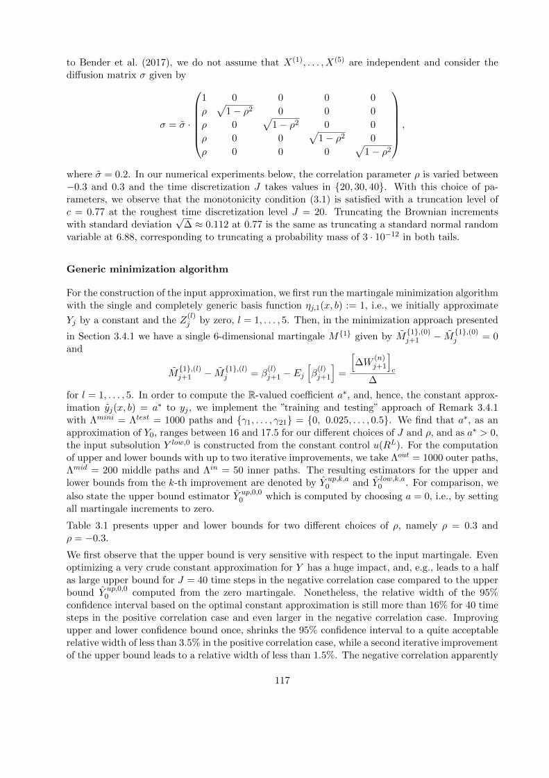
to Bender et al. (2017), we do not assume that X(1), . . . , X(5) are independent and consider thediffusion matrix σ given by

σ = σ ·

1 0 0 0 0

ρ√

1− ρ2 0 0 0

ρ 0√

1− ρ2 0 0

ρ 0 0√

1− ρ2 0

ρ 0 0 0√

1− ρ2

,

where σ = 0.2. In our numerical experiments below, the correlation parameter ρ is varied between−0.3 and 0.3 and the time discretization J takes values in 20, 30, 40. With this choice of pa-rameters, we observe that the monotonicity condition (3.1) is satisfied with a truncation level ofc = 0.77 at the roughest time discretization level J = 20. Truncating the Brownian incrementswith standard deviation

√∆ ≈ 0.112 at 0.77 is the same as truncating a standard normal random

variable at 6.88, corresponding to truncating a probability mass of 3 · 10−12 in both tails.

Generic minimization algorithm

For the construction of the input approximation, we first run the martingale minimization algorithmwith the single and completely generic basis function ηj,1(x, b) := 1, i.e., we initially approximate

Yj by a constant and the Z(l)j by zero, l = 1, . . . , 5. Then, in the minimization approach presented

in Section 3.4.1 we have a single 6-dimensional martingale M1 given by M1,(0)j+1 − M1,(0)

j = 0and

M1,(l)j+1 − M1,(l)j = β

(l)j+1 − Ej

[β

(l)j+1

]=

[∆W

(n)j+1

]c

∆

for l = 1, . . . , 5. In order to compute the R-valued coefficient a∗, and, hence, the constant approx-imation yj(x, b) = a∗ to yj , we implement the ”training and testing” approach of Remark 3.4.1with Λmini = Λtest = 1000 paths and γ1, . . . , γ21 = 0, 0.025, . . . , 0.5. We find that a∗, as anapproximation of Y0, ranges between 16 and 17.5 for our different choices of J and ρ, and as a∗ > 0,the input subsolution Y low,0 is constructed from the constant control u(RL). For the computationof upper and lower bounds with up to two iterative improvements, we take Λout = 1000 outer paths,Λmid = 200 middle paths and Λin = 50 inner paths. The resulting estimators for the upper andlower bounds from the k-th improvement are denoted by Y up,k,a

0 and Y low,k,a0 . For comparison, we

also state the upper bound estimator Y up,0,00 which is computed by choosing a = 0, i.e., by setting

all martingale increments to zero.

Table 3.1 presents upper and lower bounds for two different choices of ρ, namely ρ = 0.3 andρ = −0.3.

We first observe that the upper bound is very sensitive with respect to the input martingale. Evenoptimizing a very crude constant approximation for Y has a huge impact, and, e.g., leads to a halfas large upper bound for J = 40 time steps in the negative correlation case compared to the upperbound Y up,0,0

0 computed from the zero martingale. Nonetheless, the relative width of the 95%confidence interval based on the optimal constant approximation is still more than 16% for 40 timesteps in the positive correlation case and even larger in the negative correlation case. Improvingupper and lower confidence bound once, shrinks the 95% confidence interval to a quite acceptablerelative width of less than 3.5% in the positive correlation case, while a second iterative improvementof the upper bound leads to a relative width of less than 1.5%. The negative correlation apparently

117

ρ 0.3 −0.3

J 20 30 40 20 30 40

Y up,0,00 18.7084

(0.2193)20.9437(0.2369)

21.9248(0.2746)

26.0757(0.2624)

30.3401(0.2996)

33.9942(0.3659)

Y up,0,a∗

0 14.1415(0.1366)

14.7452(0.1316)

14.8168(0.1361)

15.8132(0.1001)

16.2220(0.0979)

16.6361(0.0986)

Y up,1,a∗

0 13.1298(0.0126)

13.2443(0.0139)

13.3392(0.0151)

14.5053(0.0120)

14.7067(0.0129)

14.9055(0.0152)

Y up,2,a∗

0 13.0608(0.0132)

13.0564(0.0140)

13.1203(0.0142)

14.2127(0.0096)

14.2593(0.0101)

14.3247(0.0104)

Y low,0,a∗

0 12.5648(0.0228)

12.6002(0.0273)

12.5813(0.0303)

13.7964(0.0271)

13.7688(0.0324)

13.7555(0.0387)

Y low,1,a∗

0 12.9757(0.0133)

12.9827(0.0159)

12.9545(0.0185)

14.0569(0.0162)

14.0400(0.0190)

13.9903(0.0268)

Table 3.1: Upper and lower bounds based on the generic minimization algorithm for different timediscretizations. Standard deviations are given in brackets.

makes the problem harder to solve numerically. But, still, after two iteration steps for the upperbound and one iteration step for the lower bound, we end up with a 95% confidence interval of arelative width of less than 3%. We also observe a significant decrease in the empirical standarddeviations of the upper bound estimators through the improvement steps, as expected since themartingales approach the pathwise optimal Doob martingale of βY .

Taking into account that no problem-specific information was used to construct the above confidenceintervals in a five-dimensional problem with non-smooth coefficients and non-trivial correlationstructure, the numerical results are convincing. We note, however, that the second iteration stepincreases the computational costs by a factor of Λin · (J/3) (e.g., a factor of 667 in our setting forJ = 40 time steps) compared to a single improvement step. Thus, we next explore to what extentthe results can be improved by putting more effort into the construction of the input approximation.

Non-generic minimization and LSMC algorithms

Following ideas of Andersen and Broadie (2004) for the pricing of Bermudan options on the max-imum of several assets, we now incorporate information about option prices on the largest andsecond-largest asset into the function basis. To this end, we define the two adapted processes l(1)

and l(2) by

l(1)j := inf

l0 ∈ 1, . . . , 5

∣∣∣X(l0)j ≥ X(l)

j ∀l = 1, . . . , 5

l(2)j := inf

l0 ∈ 1, . . . , 5 \

l(1)j

∣∣∣X(l0)j ≥ X(l)

j ∀l ∈ 1, . . . , 5 \l(1)j

for j = 0, . . . , J . Hence, l

(1)j and l

(2)j indicate the largest respectively second-largest asset at time

tj . In particular, they can be viewed as functions of Xj . Based on this, we define the followingfunctions which serve as a basis for our approximations of Y :

ηj,1(Xj−1, Xj) := 1, ηj,ι+1(Xj−1, Xj) :=

5∑l=1

X(l)j 1l(ι)j−1=l, ι = 1, 2,

ηj,ι+3(Xj−1, Xj) :=5∑l=1

E

[(X

(l)J −K1

)+− 2

(X

(l)J −K2

)+

∣∣∣∣X(l)j

]1l(ι)j−1=l, ι = 1, 2,

118

ηj,6(Xj−1, Xj) :=

5∑l=1

E

[(X

(l)J −K2

)+

∣∣∣∣X(l)j

]1l(1)

j−1=l.

Here, we write, for simplicity and in slight abuse of notation, the basis functions as functions of(Xj−1, Xj) instead of (Xj−1, Bj), cp. Example 1.7.1. Note that, e.g., the fourth basis functionrepresents the price of the corresponding call spread option at time tj on the asset which is thelargest one at time tj−1. Shifting the time index in the indicator by one time step (compared to themore intuitive function basis in Andersen and Broadie (2004) which is based on the largest assetat time tj) turned out to be inessential in this numerical example, but ensures that the one-stepconditional expectations Rj−1,k(Xj−1) in (1.53) are available in closed form (when neglecting thetruncations of the Brownian increments for the closed form computations). Indeed, we have for

R(0)j−1,k(Xj−1) := Ej−1[ηj,k(Xj−1, Xj)] that

R(0)j−1,1(Xj−1) = 1, R

(0)j−1,ι+1(Xj−1) =

5∑l=1

eµ∆X(l)j−11l(ι)j−1=l, ι = 1, 2,

R(0)j−1,ι+3(Xj−1) =

5∑l=1

E

[(X

(l)J −K1

)+− 2

(X

(l)J −K2

)+

∣∣∣∣X(l)j−1

]1l(ι)j−1=l, ι = 1, 2,

R(0)j−1,6(Xj−1) =

5∑l=1

E

[(X

(l)J −K2

)+

∣∣∣∣X(l)j−1

]1l(1)

j−1=l.

For the conditional expectations R(l)j−1,k(Xj−1) := Ej−1[(∆W

(l)j /∆)ηj,k(Xj−1, Xj)], we first note

that for each n, l ∈ 1, . . . , d

E

[∆W

(l)j

∆h(X

(n)J

)∣∣∣∣∣X(n)j−1 = x(n)

]= x(n)σn,l

∂

∂x(d)E[h(X

(n)J

) ∣∣∣X(n)j−1 = x(n)

](3.39)

for functions h : R→ R satisfying suitable growth conditions. This identity is straightforward andwe provide the details in Appendix A.4. Then, we obtain that

R(l)j−1,1(Xj−1) = 0, R

(l)j−1,ι+1(Xj−1) =

5∑n=1

σn,kX(n)j−1e

µ∆1l(ι)j−1=n, ι = 1, 2,

R(l)j−1,ι+3(Xj−1) =

5∑n=1

σn,kX(n)j−1 ·

(N (d+(tJ − tj , X(n)

j−1,K1))

−2N (d+(tJ − tj , X(n)j−1,K2))

)1l(ι)j−1=n, ι = 1, 2,

R(l)j−1,6(Xj−1) =

5∑n=1

σn,kX(n)j−1N (d+(tJ − tj , X(n)

j−1,K2))1l(1)j−1=n.

Hence we rely essentially on Black-Scholes prices and Black-Scholes deltas of European options attime tj−1 on the asset which is the (second) largest at time tj−1. Note that we, again, dropped the

truncation of the Brownian increments ∆Wj in the computation of R(l)j−1,k as the truncation error

is negligible for this choice of basis functions ηj,k, cp. Appendix C.1.

With these basis functions, we construct input approximations from both, the regression-laterand the minimization approach. For the martingale minimization algorithm, we run as before

119

Λmini = Λtest = 1000 paths and take the penalization parameter from the set γ1, . . . , γ21 =0, 0.025, . . . , 0.5. The regression-later approach is applied with Λreg = 100.000 regression paths.Tables 3.2 and 3.3 below display the corresponding upper and lower bound estimators as wellas iterative improvements up to the second order, based on these two input approximations. Asbefore, we denote by Y up,k

0 and Y low,k0 the upper respectively lower bound resulting from the k-th

improvement.

ρ 0.3 −0.3

J 20 30 40 20 30 40

Y up,0,mini0 13.2790

(0.0676)13.6548(0.0721)

13.6082(0.0748)

14.7490(0.0654)

14.9249(0.0678)

14.9845(0.0585)

Y up,1,mini0 13.0343

(0.0067)13.0548(0.0062)

13.0736(0.0074)

14.2254(0.0066)

14.2828(0.0065)

14.3574(0.0069)

Y up,2,mini0 13.0455

(0.0067)13.0635(0.0071)

13.0646(0.0072)

14.1659(0.0059)

14.2023(0.0059)

14.2234(0.0055)

Y low,0,mini0 12.9829

(0.0084)12.9750(0.0080)

12.9871(0.0093)

14.0692(0.0098)

14.0616(0.0100)

14.0820(0.0120)

Y low,1,mini0 13.0078

(0.0071)13.0136(0.0065)

13.0052(0.0081)

14.1118(0.0074)

14.1005(0.0080)

14.1022(0.0093)

Table 3.2: Upper and lower bounds based on the non-generic minimization algorithm for differenttime discretizations and RB = 0.06. Standard deviations are given in brackets.

ρ 0.3 −0.3

J 20 30 40 20 30 40

Y up,0,reg0 13.1765

(0.0673)13.5839(0.0701)

13.5552(0.0757)

14.7160(0.0714)

14.8928(0.0768)

15.0624(0.0740)

Y up,1,reg0 13.0271

(0.0058)13.0503(0.0057)

13.0675(0.0057)

14.2127(0.0060)

14.2732(0.0061)

14.3315(0.0066)

Y up,2,reg0 13.0510

(0.0064)13.0714(0.0065)

13.0874(0.0070)

14.1817(0.0060)

14.2157(0.0058)

14.2501(0.0063)

Y low,0,reg0 12.9873

(0.0073)13.0009(0.0067)

12.9945(0.0084)

14.0566(0.0100)

14.0367(0.0108)

14.0658(0.0128)

Y low,1,reg0 13.0087

(0.0070)13.0149(0.0065)

13.0089(0.0080)

14.1119(0.0073)

14.1009(0.0079)

14.1140(0.0091)

Table 3.3: Upper and lower bounds based on the regression-later approach for different time dis-cretizations and RB = 0.06. Standard deviations are given in brackets.

By and large, we find that the quality of the upper bound estimators Y up,0,mini0 and Y up,0,reg

0 ,computed from the two different methods to obtain the coefficients for the input approximation,is almost identical. They typically vary by less than two empirical standard deviations. The sameholds true for the lower bounds Y low,0,mini

0 and Y low,0,reg0 . We also observe that, compared to the

generic implementation, the input lower bounds Y low,0,mini0 and Y low,0,reg

0 are of the same quality

as the generic lower bounds in Table 3.1 Y low,1,a∗

0 after one iterative improvement. Similarly, one

improvement step of the upper bound in both non-generic cases Y up,1,mini0 and Y up,1,reg

0 is compa-

rable with two improvement steps in the generic setting Y up,2,a∗

0 . Recalling the large computationalcosts for the second improvement step, we observe that incorporating soft problem informationinto the function basis (here, the indicator function on the largest and second-largest asset onetime step before) can significantly help to pin down the non-linear option price Y0 into a rather

120

tight confidence interval after one iteration step only (and, hence, at moderate costs). For the sakeof completeness, we also report the numerical results after performing a second iteration step forthe upper bounds in the non-generic case. While in the case of negative correlation, we obtain afurther improvement and end up with a confidence interval of a relative width of less than 1.2 % forJ = 40 time steps, the situation for the positive correlation case is different. Here, the theoreticalimprovement of the upper bound is offset by the additional upward bias due to the small number ofinner paths. In this case, however, the relative width of the 95% confidence interval is about 0.75%already after one iteration step, and, thus, any further improvement seems to be unnecessary forthe option pricing problem under consideration.

We finally check the performance of our algorithm when the influence of the non-linearity is furtherincreased. To this end, we change the borrowing rate from RB = 0.06 to RB = 0.21, resulting in anincrease of the Lipschitz constant by a factor of 4. While an interest rate of 21% may be viewed asunrealistic, we note that a large value of RB penalizes borrowing and the superhedging price underthe no-borrowing constraint is known to arise in the limit RB →∞.

ρ 0.3 −0.3

J 20 30 40 20 30 40

Y up,0,mini0 15.1756

(0.0629)15.4021(0.0659)

15.6797(0.0827)

16.6270(0.0661)

17.0378(0.0873)

17.2585(0.0888)

Y up,1,mini0 14.3803

(0.0066)14.6102(0.0066)

14.8575(0.0073)

15.9797(0.0071)

16.3250(0.0067)

16.6146(0.0076)

Y up,2,mini0 14.0527

(0.0049)14.2220(0.0047)

14.3928(0.0050)

15.5550(0.0066)

16.0712(0.0097)

16.6958(0.0159)

Y low,0,mini0 13.7119

(0.0273)13.7081(0.0288)

13.6582(0.0415)

14.3663(0.0508)

14.4026(0.0596)

14.2957(0.0706)

Y low,1,mini0 13.8733

(0.0139)13.8560(0.0160)

13.8620(0.0205)

14.6236(0.0394)

14.5642(0.0464)

14.4738(0.0593)

Table 3.4: Upper and lower bounds based on the non-generic minimization algorithm for differenttime discretizations and RB = 0.21. Standard deviations are given in brackets.

ρ 0.3 −0.3

J 20 30 40 20 30 40

Y up,0,reg0 15.3014

(0.1212)16.3805(0.1762)

17.0170(0.2460)

19.6349(0.3717)

23.4699(0.6203)

26.8002(0.7822)

Y up,1,reg0 14.3939

(0.0113)14.7545(0.0135)

15.1279(0.0175)

16.7786(0.0289)

18.5106(0.0462)

20.7646(0.0700)

Y up,2,reg0 14.1012

(0.0069)14.2952(0.0072)

14.4788(0.0088)

15.7018(0.0115)

16.6096(0.0177)

17.9005(0.0282)

Y low,0,reg0 13.8339

(0.0166)13.8350(0.0179)

13.8730(0.0214)

14.6735(0.0409)

14.6399(0.0505)

14.7351(0.0502)

Y low,1,reg0 13.8745

(0.0142)13.8756(0.0168)

13.8892(0.0195)

14.6257(0.0386)

14.6864(0.0433)

14.6676(0.0509)

Table 3.5: Upper and lower bounds based on the regression-later approach for different time dis-cretizations and RB = 0.21. Standard deviations are given in brackets.

Tables 3.4 and 3.5 illustrate the numerical results for this parameter choice. Except for the borrow-ing rate, all other parameters and the choice of basis functions remain unchanged. We observe thatin this more challenging test case, the input upper bounds of the minimization algorithm are supe-rior to those computed from the regression approach, and vice versa for the lower bounds for both

121

choices of ρ. However, after one improvement step, the lower bounds based on the minimizationapproach are within two empirical standard deviations compared to the one step improvements ofthe regression lower bounds, while the upper bounds of the minimization approach are still signif-icantly below the regression upper bounds after two improvement steps for ρ = 0.3. The overallperformance of the improvement algorithm is (in spite of the larger Lipschitz constant) still veryacceptable for ρ = 0.3 and both input types. Indeed, the relative width of the 95% confidenceinterval is about 4% for 40 time steps in the minimization approach and of about 4.5% in theregression approach.

In the case of negative correlation, the results are however not fully satisfactory. Although the effectof the improvement algorithm is clearly visible, the relative width of the corresponding confidenceintervals is significantly larger, even after two improvements of the upper bounds. For J = 30time steps, the relative widths are about 10% for the minimization approach and even 12% for theregression approach. Combining the once improved regression lower bound and the twice improvedminimization upper bound, the relative width of the 95% confidence interval [14.60, 16.09] can bereduced to about 9%. This clearly indicates that a better input approximation is required for thisproblem.

122

Appendix A

Appendix to Chapter 1

A.1 Derivation of the Malliavin Monte Carlo weights in Example1.1.3

In this appendix, we provide a detailed derivation of the discretized Malliavin Monte Carlo weightsproposed in the context of the uncertain volatility model. In contrast to Fournie et al. (1999),we rely on re-writing the conditional expectation as integrals on R with respect to the Gaussiandensity. Then, a straightforward application of the integration by parts formula leads to the assertedrepresentation.

To this end, we briefly recall the setting of Example 1.1.3. Let 0 = t0 < t1 < . . . < tJ = T be apartition of [0, T ] and W be a Brownian motion. Further, the price of the risky asset X ρ underrisk-neutral dynamics and in discounted units at time tj is given by

X ρj = X ρ

j−1 exp

ρ∆Wj+1 −

1

2ρ2∆

, x0 ∈ R,

for a given constant volatility ρ > 0 and ∆Wj+1 := Wtj+1−Wtj . Then, the value process (Yj)j=0,...,J

of a European option with maturity T and payoff g(X ρJ) is given by Yj = yj(Wtj ), where the

deterministic function yj is given by the recursive scheme

yJ(x) = g(x0e

ρx− 12ρ2T), x ∈ R,

yjt (t, x) = −1

2yjxx(t, x), (t, x) ∈ [tj , tj+1)× R,

yj(tj+1, x) = yj+1(x), x ∈ R,

yj(x) = yj(tj , x) + ∆ maxσ∈σlow,σup

1

2

(σ2

ρ2− 1

)(yjxx(tj , x)− ρyjx(tj , x)

), x ∈ R.

As stated in Example 1.1.3, the partial derivatives yjx(tj , ·) and yjxx(tj , ·) may be represented viathe Malliavin Monte Carlo weights

yjx(tj ,Wtj ) = Ej

[∆Wj+1

∆Yj+1

], yjxx(tj ,Wtj ) = Ej

[(∆W 2

j+1

∆2− 1

∆

)Yj+1

].

To see this, we first note that under the given assumptions, differentiation and integration can be

123

interchanged:

yjx(tj , x) =d

dxE[Yj+1|Wtj = x

]=

d

dxE[yj+1(Wtj+1)|Wtj = x

]=

d

dxE[yj+1(Wtj + (Wtj+1 −Wtj ))|Wtj = x

]=

d

dx

∫ ∞−∞

yj+1(x+√

∆u) · 1√2πe−

12u2du

=

∫ ∞−∞

d

dxyj+1(x+

√∆u) · 1√

2πe−

12u2du.

Replacing the derivative of yj+1 with respect to x by the derivative with respect to u and integratingby parts, shows the first assertion:

yjx(tj , x) =

∫ ∞−∞

1√∆

d

du

(yj+1(x+

√∆u)

)· 1√

2πe−

12u2du

=1√

2π∆

([yj+1(x+

√∆u) · e−

12u2]∞−∞

+

∫ ∞−∞

uyj+1(x+√

∆u) · e−12u2du

)=

∫ ∞−∞

u√∆yj+1(x+

√∆u) · 1√

2πe−

12u2du

= E

[∆Wj+1

∆yj+1(Wtj+1)

∣∣∣∣Wtj = x

]= E

[∆Wj+1

∆Yj+1

∣∣∣∣Wtj = x

].

Following the same line of reasoning and integrating by parts twice, yields the second claim:

yjxx(tj , x) =d2

dx2E[Yj+1|Wtj = x

]=

d2

dx2E[yj+1(Wtj+1)|Wtj = x

]=

d2

dx2E[yj+1(Wtj + (Wtj+1 −Wtj ))|Wtj = x

]=

d2

dx2

∫ ∞−∞

yj+1(x+√

∆u) · 1√2πe−

12u2du

=

∫ ∞−∞

d2

dx2yj+1(x+

√∆u) · 1√

2πe−

12u2du

=1√

2π∆

∫ ∞−∞

(d2

du2yj+1(x+

√∆u)

)· 1√

2πe−

12u2du

=1√

2π∆

([(d

duyj+1(x+

√∆u)

)· 1√

2πe−

12u2

]∞−∞

+

∫ ∞−∞

(d

duyj+1(x+

√∆u)

)· ue−

12u2du

)=

1√2π∆

∫ ∞−∞

(d

duyj+1(x+

√∆u)

)· ue−

12u2du

124

=1√

2π∆

([yj+1(x+

√∆u) · ue−

12u2]∞−∞−∫ ∞−∞

yj+1(x+√

∆u) · (1− u2)e−12u2du

)=

∫ ∞−∞

u2 − 1

∆yj+1(x+

√∆u) · 1√

2πe−

12u2du

= E

[(∆W 2

j+1

∆2− 1

∆

)yj+1(Wtj+1)

∣∣∣∣∣Wtj = x

]

= E

[(∆W 2

j+1

∆2− 1

∆

)Yj+1

∣∣∣∣∣Wtj = x

].

A.2 Convex conjugate for a class of piecewise-linear functions

In this appendix, we derive the convex conjugate for functions f : Rd → R given by

f(x) =d∑

k=1

a(k)x(k) + c1 +

(d∑

k=1

b(k)x(k) + c2

)+

for vectors a, b ∈ Rd with b(d) 6= 0 and coefficients c1, c2 ∈ R. Note that we assume b(d) 6= 0 inorder to exclude the trivial case where f is linear. Considering this general type of piecewise linearfunctions allows us to capture the numerical examples presented in this thesis. From straightforwardmanipulations and the definition of (·)+, it follows that

f#(u) = supx∈Rd

d∑k=1

u(k)x(k) − f(x)

= supx∈Rd

d∑k=1

(u(k) − a(k)

)x(k) − c1 −

(d∑

k=1

b(k)x(k) + c2

)+

= −c1 + supx∈Rd

(min

d∑

k=1

(u(k) − a(k)

)x(k),

d∑k=1

(u(k) −

(a(k) + b(k)

))x(k) − c2

)

= −c1 −u(d) − a(d)

b(d)c2

+ supx∈Rd

(min

d∑

k=1

(u(k) − a(k)

)x(k) +

u(d) − a(d)

b(d)c2,

d∑k=1

(u(k) −

(a(k) + b(k)

))x(k) − c2 +

u(d) − a(d)

b(d)c2

)

= −c1 −u(d) − a(d)

b(d)c2

+ supx∈Rd

(min

d−1∑k=1

(u(k) − a(k)

)x(k) +

(u(d) − a(d)

)(x(d) +

c2

b(d)

),

d−1∑k=1

(u(k) −

(a(k) + b(k)

))x(k) +

(u(d) −

(a(d) + b(d)

))(x(d) +

c2

b(d)

))

125

=

−c1 − u(d)−a(d)

b(d)c2, u ∈ conv a, a+ b

+∞, else,

where conv denotes the convex hull. Hence, the effective domain of f# is given by

Df# = conv a, a+ b .

A.3 Conditional expectations for basis functions in Section 1.7.2.1

In this appendix, we provide the details for the computation of the conditional expectations involv-ing the payoff function in the numerical example of Section 1.7.2.1.

To this end, let 0 = t0 < t1 < . . . < tJ = T be an equidistant partition of the interval [0, T ]with increments ∆. Furthermore, let W = (W (1), . . . ,W (d)) be a d-dimensional Brownian motionand denote by Fj the σ-algebra generated by W up to tj . We denote by X = (X(1), . . . , X(d))d independent identically distributed geometric Brownian motions, whose dynamics on the gridt0, . . . , tJ are given by

X(k)j = x0 exp

(RL − 1

2σ2

)tj + σW

(k)tj

, k = 1, . . . , d,

with drift RL ≥ 0 and volatility σ > 0. Here, we again use the shorthand notation X(k)j := X

(k)tj

.Moreover, we define the process (Bj)j=1,...,J by

Bj =

(1,

∆Wj

∆

)>, j = 1, . . . , J.

In the following, we compute the conditional expectations

Ej [fl(Xj , Bj+1)] and Ej

[∆Wj+1

∆fl(Xj , Bj+1)

], (A.1)

where

fl(Xj , Bj+1) =

√T − tjT − tj+1

∫Rh(X

(l)j e(R

L− 12σ2)(T−tj)+σz

√T−tj

)ez2

2−

(√T−tjz−∆W

(l)j+1

)2

2(T−tj+1)

×∏

l′∈1,...,d\l

N

√ T − tjT − tj+1

z +ln(X

(l)j )− ln(X

(l′)j )

σ√T − tj+1

−∆W

(l′)j+1√

T − tj+1

× 1√

2πe−

12z2dz. (A.2)

Here, h : R → R is a function which is of polynomial growth and N denotes the cumulativedistribution function of the standard normal distribution.

In order to simplify the computation of (A.1), we first prove the following lemma.

Lemma A.3.1. Let γ ∈ R and let U be standard normally distributed random variable. Further-more, denote by N the cumulative distribution function of a standard normal distribution. Then,it holds:

126

(i) E

[exp

−1

2

(γ −

√∆

T−tj+1U)2]

=√

T−tj+1

T−tj exp−1

2T−tj+1

T−tj γ2

.

(ii) E[N(γ −

√∆

T−tj+1U)]

= N(√

T−tj+1

T−tj γ)

.

Proof. We first show (i). By straightforward calculations, we obtain that:

E

exp

−1

2

(γ −

√∆

T − tj+1U

)2

=

∫R

1√2πe−

12u2

exp

−1

2

(γ −

√∆

T − tj+1u

)2 du

=

∫R

1√2π

exp

−1

2

(γ2 − 2γ

√∆

T − tj+1u+

(∆

T − tj+1+ 1

)u2

)du

=

∫R

1√2π

exp

−1

2

(γ2 − 2γ

√∆

T − tj+1u+

T − tjT − tj+1

u2

)du

=

∫R

1√2π

exp

−1

2

(γ2 − 2γ

√∆

T − tj

√T − tjT − tj+1

u+T − tjT − tj+1

u2

)du

=

∫R

1√2π

exp

−1

2

(√∆

T − tjγ −

√T − tjT − tj+1

u

)2

− 1

2

(1− ∆

T − tj

)γ2

du

=

∫R

1√2π

exp

−1

2

T − tjT − tj+1

(√∆(T − tj+1)

(T − tj)2γ − u

)2 exp

−1

2

T − tj+1

T − tjγ2

du

=

√T − tj+1

T − tjexp

−1

2

T − tj+1

T − tjγ2

·∫R

1√2π

T−tj+1

T−tj

exp

−1

2

T − tjT − tj+1

(√∆(T − tj+1)

(T − tj)2γ − u

)2 du

=

√T − tj+1

T − tjexp

−1

2

T − tj+1

T − tjγ2

.

For the second claim, we first note that

E

[N

(γ −

√∆

T − tj+1U

)]

=

∫R

(∫ γ−√

∆T−tj+1

u

−∞

1√2πe−

12v2dv

)· 1√

2πe−

12u2du

=

∫R

∫ γ

−∞

1√2π

exp

−1

2

(y −

√∆

T − tj+1u

)2 dy

· 1√2πe−

12u2du

127

=

∫ γ

−∞

1√2π

∫R

1√2π

exp

−1

2

(y −

√∆

T − tj+1u

)2

− 1

2u2

du

dy,

due to the substitution v = y −√

∆T−tj+1

u and Fubini’s theorem. By (i) and the substitution

z =√

T−tj+1

T−tj y, we obtain

E

[N

(γ −

√∆

T − tj+1U

)]=

∫ γ

−∞

1√2π

√T − tj+1

T − tjexp

−1

2

T − tj+1

T − tjy2

dy,

=

∫ √T−tj+1T−tj

γ

−∞

1√2π

exp

−1

2z2

dz,

= N

(√T − tj+1

T − tjγ

).

With this lemma at hand, we now turn to the calculation of the conditional expectations in (A.1).First note that by Fubini’s theorem and the independence of the components of the Brownianmotion W

E [fl(Xj , Bj+1)|Xj = x]

= E [fl(x,Bj+1)]

= E

√ T − tjT − tj+1

∫Rh(x(l)e(R

L− 12σ2)(T−tj)+σz

√T−tj

)ez2

2−

(√T−tjz−∆W

(l)j+1

)2

2(T−tj+1) · 1√2πe−

12z2

×∏

l′∈1,...,d\l

N

√ T − tjT − tj+1

z +ln(X

(l)j )− ln(X

(l′)j )

σ√T − tj+1

−∆W

(l′)j+1√

T − tj+1

dz

=

√T − tjT − tj+1

∫Rh(x(l)e(R

L− 12σ2)(T−tj)+σz

√T−tj

)ez2

2 E

e− (√T−tjz−∆W

(l)j+1

)2

2(T−tj+1)

×

∏l′∈1,...,d\l

E

N√ T − tj

T − tj+1z +

ln(x(l))− ln(x(l′))

σ√T − tj+1

−∆W

(l′)j+1√

T − tj+1

· 1√2πe−

12z2dz

=

√T − tjT − tj+1

∫Rh(x(l)e(R

L− 12σ2)(T−tj)+σz

√T−tj

)ez2

2

×E

exp

−1

2

(√T − tjT − tj+1

z −∆W

(l)j+1

T − tj+1

)2

×∏

l′∈1,...,d\l

E

N√ T − tj

T − tj+1z +

ln(x(l))− ln(x(l′))

σ√T − tj+1

−∆W

(l′)j+1√

T − tj+1

· 1√2πe−

12z2dz

for every x ∈ Rd. Applying Lemma A.3.1, we end up with

128

E [fl(Xj , Bj+1)|Xj = x]

=

√T − tjT − tj+1

∫Rh(x(l)e(R

L− 12σ2)(T−tj)+σz

√T−tj

)ez2

2

×

√T − tj+1

T − tjexp

−1

2

T − tj+1

T − tj

(√T − tjT − tj+1

z

)2

×∏

l′∈1,...,d\l

N

(√T − tj+1

T − tj

(√T − tjT − tj+1

z +ln(x(l))− ln(x(l′))

σ√T − tj+1

))· 1√

2πe−

12z2dz

=

∫Rh(x(l)e(R

L− 12σ2)(T−tj)+σz

√T−tj

) ∏l′∈1,...,d\l

N

(z +

ln(x(l))− ln(x(l′))

σ√T − tj

)· 1√

2πe−

12z2dz.

Finally, we compute Ej [∆W

(k)j+1

∆ fl(Xj , Bj+1)]. To do this, we distinguish two different cases, namelyk 6= l and k = l and apply the identity

Ej

[∆W

(k)j+1

∆fl(Xj , Bj+1)

]=

d

dhEj [fl(Xj , Bj+1 + hed+1+k)]

∣∣∣∣h=0

, (A.3)

where en denotes the n-th canonical vector in R2d+1. Note that (A.3) follows by a similar compu-tation than the one in Appendix A.1.

We first consider the case k 6= l. Then, we get by (A.3) and the same arguments as above, that

E

[∆W

(k)j+1

∆fl(Xj , Bj+1)

∣∣∣∣∣Xj = x

]

=d

dhE [fl(Xj , Bj+1 + hed+1+k)|Xj = x]

∣∣∣∣h=0

=d

dhE [fl(x,Bj+1 + hed+1+k)]

∣∣∣∣h=0

=d

dhE

√ T − tjT − tj+1

∫Rh(x(l)e(R

L− 12σ2)(T−tj)+σz

√T−tj

)ez2

2−

(√T−tjz−∆W

(l)j+1

)2

2(T−tj+1)

× 1√2πe−

12z2 · N

(√T − tjT − tj+1

z +ln(x(l))− ln(x(k))

σ√T − tj+1

−(∆W

(k)j+1 + h)√T − tj+1

)

×∏

l′∈1,...,d\l,k

N

√ T − tjT − tj+1

z +ln(x(l))− ln(x(l′))

σ√T − tj+1

−∆W

(l′)j+1√

T − tj+1

dz

∣∣∣∣∣∣h=0

=d

dh

(√T − tjT − tj+1

∫Rh(x(l)e(R

L− 12σ2)(T−tj)+σz

√T−tj

)ez2

2 E

e− (√T−tjz−∆W

(l)j+1

)2

2(T−tj+1)

× 1√

2πe−

12z2 · E

[N

(√T − tjT − tj+1

z +ln(x(l))− ln(x(k))

σ√T − tj+1

−(∆W

(k)j+1 + h)√T − tj+1

)]

129

×∏

l′∈1,...,d\l,k

E

N√ T − tj

T − tj+1z +

ln(x(l))− ln(x(l′))

σ√T − tj+1

−∆W

(l′)j+1√

T − tj+1

dz)∣∣∣∣∣∣h=0

=d

dh

(√T − tjT − tj+1

∫Rh(x(l)e(R

L− 12σ2)(T−tj)+σz

√T−tj

)ez2

2

×E

exp

−1

2

(√T − tjT − tj+1

z −∆W

(l)j+1

T − tj+1

)2

× 1√2πe−

12z2 · E

[N

(√T − tjT − tj+1

z +ln(x(l))− ln(x(k))

σ√T − tj+1

−(∆W

(k)j+1 + h)√T − tj+1

)]

×∏

l′∈1,...,d\l,k

E

N√ T − tj

T − tj+1z +

ln(x(l))− ln(x(l′))

σ√T − tj+1

−∆W

(l′)j+1√

T − tj+1

dz)∣∣∣∣∣∣h=0

.

From Lemma A.3.1 we conclude, as before, that

E

[∆W

(k)j+1

∆fl(Xj , Bj+1)

∣∣∣∣∣Xj = x

]

=d

dh

(√T − tjT − tj+1

∫Rh(x(l)e(R

L− 12σ2)(T−tj)+σz

√T−tj

)ez2

2

×

√T − tj+1

T − tjexp

−1

2

T − tj+1

T − tj

(√T − tjT − tj+1

z

)2

×N

(√T − tj+1

T − tj

(√T − tjT − tj+1

z +ln(x(l))− ln(x(k))

σ√T − tj+1

− h√T − tj+1

))

×∏

l′∈1,...,d\l,k

N

(√T − tj+1

T − tj

(√T − tjT − tj+1

z +ln(x(l))− ln(x(l′))

σ√T − tj+1

))· 1√

2πe−

12z2dz

)∣∣∣∣∣∣h=0

=d

dh

(∫Rh(x(l)e(R

L− 12σ2)(T−tj)+σz

√T−tj

)N

(z +

ln(x(l))− ln(x(k))

σ√T − tj

− h√T − tj

)

×∏

l′∈1,...,d\l,k

N

(z +

ln(x(l))− ln(x(l′))

σ√T − tj

)· 1√

2πe−

12z2dz

)∣∣∣∣∣∣h=0

= − 1√T − tj

∫Rh(x(l)e(R

L− 12σ2)(T−tj)+σz

√T−tj

) 1√2π

exp

−1

2

(z +

ln(x(l))− ln(x(k))

σ√T − tj

)2

×∏

l′∈1,...,d\l,k

N

(z +

ln(x(l))− ln(x(l′))

σ√T − tj

)· 1√

2πe−

12z2dz.

For k = l, we follow the same argumentation and end up with

E

[∆W

(l)j+1

∆fl(Xj , Bj+1)

∣∣∣∣∣Xj = x

]

130

=d

dhE [fl(Xj , Bj+1 + hed+1+l)|Xj = x]

∣∣∣∣h=0

=d

dhE

√ T − tjT − tj+1

∫Rh(x(l)e(R

L− 12σ2)(T−tj)+σz

√T−tj

)ez2

2−

(√T−tjz−(∆W

(l)j+1

+h))2

2(T−tj+1) · 1√2πe−

12z2

×∏

l′∈1,...,d\l

N

√ T − tjT − tj+1

z +ln(x(l))− ln(x(l′))

σ√T − tj+1

−∆W

(l′)j+1√

T − tj+1

dz

∣∣∣∣∣∣h=0

=d

dh

(√T − tjT − tj+1

∫Rh(x(l)e(R

L− 12σ2)(T−tj)+σz

√T−tj

)ez2

2

×E

e− (√T−tjz−(∆W

(l)j+1

+h))2

2(T−tj+1)

· 1√2πe−

12z2

×∏

l′∈1,...,d\l

E

N√ T − tj

T − tj+1z +

ln(x(l))− ln(x(l′))

σ√T − tj+1

−∆W

(l′)j+1√

T − tj+1

dz)∣∣∣∣∣∣h=0

=d

dh

(√T − tjT − tj+1

∫Rh(x(l)e(R

L− 12σ2)(T−tj)+σz

√T−tj

)ez2

2

×

√T − tj+1

T − tjexp

−1

2

T − tj+1

T − tj

(√T − tjT − tj+1

z − h

T − tj+1

)2

×∏

l′∈1,...,d\l

N

(√T − tj+1

T − tj

(√T − tjT − tj+1

z +ln(x(l))− ln(x(l′))

σ(√T − tj+1)

))· 1√

2πe−

12z2dz

)∣∣∣∣∣∣h=0

=d

dh

(∫Rh(x(l)e(R

L− 12σ2)(T−tj)+σz

√T−tj

)ez2

2

× exp

−1

2

T − tj+1

T − tj

(√T − tjT − tj+1

z − h

T − tj+1

)2

×∏

l′∈1,...,d\l

N

(z +

ln(x(l))− ln(x(l′))

σ(√T − tj)

)· 1√

2πe−

12z2dz

)∣∣∣∣∣∣h=0

=

∫Rh(x(l)e(R

L− 12σ2)(T−tj)+σz

√T−tj

) z√T − tj

∏l′∈1,...,d\l

N

(z +

ln(x(l))− ln(x(l′))

σ(√T − tj)

)

× 1√2πe−

12z2dz

A.4 Closed-form representations for conditional expectations

In the numerical examples presented in this thesis, we require the computation of conditionalexpectations of basis functions which depend on geometric Brownian motions. In this appendix,

131

we provide a straightforward generalization of Example 3.1 in Bender and Steiner (2012) and showthat these conditional expectations can essentially be expressed by the first- and second-orderderivatives of the basis functions.

Let 0 = t0 < t1 < . . . < tJ = T be a partition of [0, T ] and define ∆j+1 := tj+1 − tj forj = 0, . . . , J − 1. Further, let W be a d-dimensional Brownian motion and define the d-dimensionalprocess X on the grid t0, . . . tJ by

X(n)j = x

(n)0 exp

(µ− 1

2

d∑l=1

σ2n,l

)tj +

d∑l=1

σn,lW(l)tj

, n = 1, . . . , d,

where x(1)0 , . . . , x

(d)0 , µ ∈ R+ and σ is an invertible d × d-matrix with entries in R. Then, we show

that

E

[∆W

(k)j+1

∆j+1h(X

(n)J

)∣∣∣∣∣Xj = x

]= x(n)σn,k

∂

∂x(n)E[h(X

(n)J

)∣∣∣Xj = x]

and

E

(∆W(k)j+1

∆j+1

)2

− σn,k∆W

(k)j+1

∆j+1− 1

∆j+1

h(X

(n)J

)∣∣∣∣∣∣Xj = x

=(x(n)

)2σ2n,k

∂2

∂(x(n))2E[h(X

(n)J

)∣∣∣Xj = x]

holds for all n, k = 1, . . . , d and all functions h : R→ R satisfying appropriate growth and differen-tiability conditions.

In order to simplify the following computations, we introduce some further notation. We denoteby u(−l) the Rd−1-dimensional vector (u(1), . . . , ul−1, ul+1, . . . , u(d)). Additionally, we define thefunction hn : R→ R for every n = 1, . . . , d by

hn(x) = h

(x exp

(µ− 1

2

d∑l=1

σ2n,l

)(tJ − tj+1) +

d∑l=1

σn,l

(W

(l)tJ− W (l)

tj+1

)).

Moreover, the function f : Rd → R is given by

f(u) = exp

(µ− 1

2

d∑l=1

σ2n,l

)∆j+1 +

√∆j+1

d∑l=1

σn,lu(l)

.

Then, a straightforward computation, involving Fubini’s Theorem and integration by parts, yields

x(n)σn,k∂

∂x(n)E[h(X

(n)J

)∣∣∣Xj = x]

= x(n)σn,k∂

∂x(n)E[hn

(X

(n)j+1

)∣∣∣Xj = x]

= x(n)σn,k∂

∂x(n)

∫Rdhn

(x(n)f(u)

) d∏l=1

(1√2πe−

12

(u(l))2

)d(u(1), . . . , u(d))

= x(n)σn,k

∫Rd

∂

∂x(n)hn

(x(n)f(u)

) d∏l=1

(1√2πe−

12

(u(l))2

)d(u(1), . . . , u(d))

132

= x(n)σn,k

∫Rdf(u)h′n

(x(n)f(u)

) d∏l=1

(1√2πe−

12

(u(l))2

)d(u(1), . . . , u(d))

=1√

∆j+1

∫Rd

∂

∂u(k)hn

(x(n)f(u)

) d∏l=1

(1√2πe−

12

(u(l))2

)d(u(1), . . . , u(d))

=1√

∆j+1

∫Rd−1

d∏l=1,l 6=k

(1√2πe−

12

(u(l))2

)

×

(∫R

(∂

∂u(k)hn

(x(n)f(u)

))· 1√

2πe−

12

(u(k))2du(k)

)du(−k)

=1√

∆j+1

∫Rd−1

d∏l=1,l 6=k

(1√2πe−

12

(u(l))2

)(∫Rhn

(x(n)f(u)

)· u

(k)

√2πe−

12

(u(k))2du(k)

)du(−k)

=

∫Rd

u(k)√∆j+1

hn

(x(n)f(u)

) d∏l=1

(1√2πe−

12

(u(l))2

)d(u(1), . . . , u(d))

= E

[∆W

(k)j+1

∆j+1hn

(X

(n)j+1

)∣∣∣∣∣X(n)j = x(n)

]

= E

[∆W

(k)j+1

∆j+1h(X

(n)J

)∣∣∣∣∣X(n)j = x(n)

].

For the proof of the second claim, we first observe that(x(n)

)2σ2n,k

∂2

∂(x(n))2E[h(X

(n)J

)∣∣∣Xj = x]

=(x(n)

)2σ2n,k

∂2

∂(x(n))2E[hn

(X

(n)j+1

)∣∣∣Xj = x]

=(x(n)

)2σ2n,k

∂2

∂(x(n))2

∫Rdhn

(x(n)f(u)

) d∏l=1

(1√2πe−

12

(u(l))2

)d(u(1), . . . , u(d))

=(x(n)

)2σ2n,k

∫Rd

∂2

∂(x(n))2hn

(x(n)f(u)

) d∏l=1

(1√2πe−

12

(u(l))2

)d(u(1), . . . , u(d))

=(x(n)

)2σ2n,k

∫Rdh′′n

(x(n)f(u)

)f(u)2

d∏l=1

(1√2πe−

12

(u(l))2

)d(u(1), . . . , u(d)).

From the definition of hn and f , we obtain that(x(n)

)2σ2n,k∆j+1f(u)2h′′n

(x(n)f(u)

)=

∂2

∂(u(k))2hn

(x(n)f(u)

)− σn,k

√∆j+1

∂

∂(u(k))hn

(x(n)f(u)

).

By exploiting this identity, Fubini’s theorem, and integration by parts, we conclude that(x(n)

)2σ2n,k

∂2

∂(x(n))2E[h(X

(n)J

)∣∣∣Xj = x]133

=1

∆j+1

∫Rd

(∂2

∂(u(k))2hn

(x(n)f(u)

)− σn,k

√∆j+1

∂

∂(u(k))hn

(x(n)f(u)

))×

d∏l=1

(1√2πe−

12

(u(l))2

)d(u(1), . . . , u(d))

=1

∆j+1

∫Rd−1

d∏l=1,l 6=k

(1√2πe−

12

(u(l))2

)(∫R

(∂2

∂(u(k))2hn

(x(n)f(u)

)−σn,k

√∆j+1

∂

∂(u(k))hn

(x(n)f(u)

)) 1√2πe−

12

(u(k))2du(k)

)du(−k)

=1

∆j+1

∫Rd−1

d∏l=1,l 6=k

(1√2πe−

12

(u(l))2

)

×(∫

R

((u(k)

)2− σn,k

√∆j+1u

(k) − 1

)hn

(x(n)f(u)

) 1√2πe−

12

(u(k))2du(k)

)du(−k)

=

∫Rd

((u(k)

)2∆j+1

− σn,ku(k)√∆j+1

− 1

∆j+1

)hn

(x(n)f(u)

)×

d∏l=1

(1√2πe−

12

(u(l))2

)d(u(1), . . . , u(d))

= E

(∆W(k)j+1

∆j+1

)2

− σn,k∆W

(k)j+1

∆j+1− 1

∆j+1

hn

(X

(n)j+1

)∣∣∣∣∣∣Xj = x

= E

(∆W(k)j+1

∆j+1

)2

− σn,k∆W

(k)j+1

∆j+1− 1

∆j+1

h(X

(n)J

)∣∣∣∣∣∣Xj = x

.

134

Appendix B

Appendix to Chapter 2

B.1 Conditional expectations for basis functions in Section 2.5

In this appendix, we derive the conditional expectations of the basis functions used in Section2.5. To this end, recall that the stochastic processes (xt, yt, γt, pt)t∈[0,T ] are given by the stochasticdifferential equations

dxt = −κxxtdt+ σxdWxt ,

dyt = −κyytdt+ σydWyt

dγt = κγ(µγ − γt)dt+ σγ√γtdW

γt ,

dpt = κp(µp − pt)dt+ σpdWpt

for real constants κx, κy, σx, σy, κγ , µγ , σγ , κp, µp, σp. Here, W x, W y and W γ are Brownianmotions with instantaneous correlations ρxy, ρxγ and ρyγ . Moreover, we have that W p

t = ργpWγt +√

1− ρ2γpWt where the Brownian motion W is independent of (W x,W y,W γ). Further, let 0 =

t0 < t1 < . . . < tJ = T be an equidistant partition with time increments ∆ and denote byT = T1, . . . , TK ⊆ t0, . . . , tJ the set of tenor dates. The tenor dates all have the same distancewhich is denoted by δ. For the processes γ and p, we apply the following discretization scheme

γj = γj−1 − κγ∆((γj−1)+ − µγ) + σγ

√(γj−1)+∆W γ

j ,

pj = pj−1e−κp∆ + µp(1− e−κp∆) + σp

√1− e−2κp∆

2κp∆∆W p

j ,

where we use the shorthand notation Uj := Utj for U ∈ γ, p. Then, we observe by a straightfor-ward computation that the conditional expectation Ej−1[γj ] is given by

Ej−1[γj ] = Ej−1

[γj−1 − κγ∆((γj−1)+ − µγ) + σγ

√(γj−1)+∆W γ

j

]= γj−1 − κγ∆((γj−1)+ − µγ) + σγ

√(γj−1)+Ej−1

[∆W γ

j

]= γj−1 − κγ∆((γj−1)+ − µγ)

135

for every j = 1, . . . , J . In order to compute Ej−1[γj pj ], we exploit the definition of W p and obtainthat

Ej−1[γj pj ] = Ej−1

[(γj−1 − κγ∆((γj−1)+ − µγ) + σγ

√(γj−1)+∆W γ

j

)(pj−1e

−κp∆ + µp(1− e−κp∆) + σp

√1− e−2κp∆

2κp∆∆W p

j

)]= (γj−1 − κγ∆((γj−1)+ − µγ))

(pj−1e

−κp∆ + µp(1− e−κp∆))

+ (γj−1 − κγ∆((γj−1)+ − µγ))σp

√1− e−2κp∆

2κp∆Ej−1

[∆W p

j

]+(pj−1e

−κp∆ + µp(1− e−κp∆))σγ

√(γj−1)+Ej−1

[∆W γ

j

]+σγ

√(γj−1)+σp

√1− e−2κp∆

2κp∆Ej−1

[∆W γ

j ∆W pj

]= (γj−1 − κγ∆((γj−1)+ − µγ))

(pj−1e

−κp∆ + µp(1− e−κp∆))

+σγσpργp

√(γj−1)+∆

√1− e−2κp∆

2κp.

It thus remains to compute the expected value of the clean swap price, which is given by

Stj = P (tj , Tτ(j))CTτ(j)+N ·

K∑i=τ(j)+1

(P (tj , Ti−1)− (1 +Rδ)P (tj , Ti)) ,

where τ(j) denotes the index of the first tenor date weakly after tj and P (t, s) is for t, s ∈ [0, T ],t < s, given by

P (t, s) = exp

−r0(s− t)− 1− e−κx(s−t)

κxxt −

1− e−κy(s−t)

κyyt +

1

2V (t, s)

.

Here, the deterministic function V is defined by

V (t, s) =σ2x

κ2x

(s− t+

2

κxe−κx(s−t) − 1

2κxe−2κx(s−t) − 3

2κx

)+σ2y

κ2y

(s− t+

2

κye−κy(s−t) − 1

2κye−2κy(s−t) − 3

2κy

)+2ρxy

σxσyκxκy

(s− t+

e−κx(s−t) − 1

κx+e−κy(s−t) − 1

κy− e−(κx+κy)(s−t) − 1

κx + κy

),

see Chapter 4.2 in Brigo and Mercurio (2006). Hence, in order to derive a closed form expressionfor Ej−1[Stj ] it is sufficient to compute Ej−1[P (tj , Ti)] for tenor dates Ti ≥ tj , since

Ej−1[Stj ] = Ej−1

[P (tj , Tτ(j))

]CTτ(j)

+N ·K∑

i=τ(j)+1

(Ej−1 [P (tj , Ti−1)]− (1 +Rδ)Ej−1 [P (tj , Ti)])

136

by the FTτ(j)−1-measurability of CTτ(j)

. By definition of P (t, s), the computation of this conditionalexpectation boils down to the computation of

E[expαxs + βys|Ft]

for any t, s ∈ [0, T ] with t < s and arbitrary α, β ∈ R.

Hence, let t, s ∈ [0, T ], t < s, and α, β ∈ R be fixed from now on. Then, it is well-known, that,given Ft, the random variable αxs+βys is normally distributed, see e.g. Section 3.3 in Glasserman(2004). Applying the martingale property of the stochastic integrals, we observe that the mean isgiven by

E[αxs + βys|Ft] = E

[α

(xte−κx(s−t) + σx

∫ s

te−κx(s−u) dW x

u

)∣∣∣∣Ft]+E

[β

(yte−κy(s−t) + σy

∫ s

te−κy(s−u) dW y

u

)∣∣∣∣Ft]= αxte

−κx(s−t) + σxαE

[∫ s

te−κx(s−u) dW x

u

∣∣∣∣Ft]+βyte

−κy(s−t) + σyβE

[∫ s

te−κy(s−u) dW y

u

∣∣∣∣Ft]= αxte

−κx(s−t) + βyte−κy(s−t).

For the variance, a straightforward application of the Ito-isometry shows that

Var(αxs + βys|Ft)

= α2E[

(xs − E[xs|Ft])2∣∣∣Ft]+ β2E

[(ys − E[ys|Ft])2

∣∣∣Ft]+2αβE[(xs − E[xs|Ft])(ys − E[ys|Ft])|Ft]

= α2E

[(xte−κx(s−t) + σx

∫ s

te−κx(s−u) dW x

u − xte−κx(s−t))2∣∣∣∣∣Ft]

+β2E

[(yte−κy(s−t) + σy

∫ s

te−κy(s−u) dW y

u − yte−κy(s−t))2∣∣∣∣∣Ft]

+2αβE

[(xte−κx(s−t) + σx

∫ s

te−κx(s−u) dW x

u − xte−κx(s−t))

(yte−κy(s−t) + σy

∫ s

te−κy(s−u) dW y

u − yte−κy(s−t))∣∣∣∣Ft]

= α2E

[(σx

∫ s

te−κx(s−u) dW x

u

)2∣∣∣∣∣Ft]

+ β2E

[(σy

∫ s

te−κy(s−u) dW y

u

)2∣∣∣∣∣Ft]

+2αβE

[(σx

∫ s

te−κx(s−u) dW x

u

)(σy

∫ s

te−κy(s−u) dW y

u

)∣∣∣∣Ft]= α2σ2

x

∫ s

te−2κx(s−u) du+ β2σ2

y

∫ s

te−2κy(s−u) du+ 2αβσxσyρxy

∫ s

te−(κx+κy)(s−u) du

=α2σ2

x

2κx

(1− e−2κx(s−t)

)+β2σ2

y

2κy

(1− e−2κy(s−t)

)+

2αβσxσyρxyκx + κy

(1− e−(κx+κy)(s−t)

).

Hence, we conclude that

E [ exp αxs + βys| Ft] = exp

mxy(t, s) +

1

2σ2xy(t, s)

,

137

where mxy(t, s) := E[αxs + βys|Ft] and σxy(t, s) := Var(αxs + βys|Ft). From this identity, wefinally obtain that

Ej−1[P (tj , Ti)] = exp

−r0(Ti − tj)−

(mxy(tj−1, tj) +

1

2σ2xy(tj−1, tj)

)+

1

2V (tj , Ti)

,

for every tj ∈ t0, . . . , tJ−1 and Ti ∈ T with Ti ≥ tj , where mxy(tj−1, tj) and σ2xy(tj−1, tj) are

given as above with

α =1− e−κx(tj−tj−1)

κxand β =

1− e−κy(tj−tj−1)

κy.

138

Appendix C

Appendix to Chapter 3

C.1 Estimation of the truncation error

In the following, we discuss the truncation error which arises in Section 3.4.3 when computing theconditional expectations of the basis functions. More precisely, we show that this error is negligibleif the functions satisfy certain growth conditions and the mesh of a given partition is small enough.

To this end, let W be a d′-dimensional Brownian motion and h : Rd×Rd′ → R be a function whichgrows at most exponentially in its second argument. Moreover, let 0 = t0 < t1 < . . . < tJ = T bea partition of [0, T ] and denote by ∆j+1 the distance between the discretization points tj and tj+1.Further, we denote by ∆Wj+1 := Wtj+1 −Wtj the increment of the Brownian motion between thetime points tj and tj+1 and by [∆Wj+1]c its componentwise truncation at ±c for c ≥ 0. Then, weshow that∥∥∥∥E [∆Wj+1

∆j+1h(x,∆Wj+1)

]− E

[[∆Wj+1]c

∆j+1h(x,∆Wj+1)

]∥∥∥∥2

≤(

18

πc2

) 14

∆− 3

4j+1d

′ · e−c2

4∆j+1E[h(x,∆Wj+1)2

](C.1)

for every x ∈ Rd, where ‖ · ‖ denotes the Euclidean norm on Rd′ . To see this, we require thefollowing tail estimate for standard normally distributed random variables U :

P (U ≥ c) ≤ 1

c√

2πe−

12c2 . (C.2)

This follows simply by exploiting that uc ≥ 1 for all u ∈ [c,∞):

P (U ≥ c) =

∫ ∞c

1√2πe−

12u2du ≤

∫ ∞c

u

c

1√2πe−

12u2du =

1

c√

2πe−

12c2 .

For the proof of (C.1), we first note that by Jensen’s inequality (applied to the convex functionx 7→ ‖x‖2) as well as Holder’s inequality∥∥∥∥E [∆Wj+1

∆j+1h(x,∆Wj+1)

]− E

[[∆Wj+1]c

∆j+1h(x,∆Wj+1)

]∥∥∥∥2

=1

∆2j+1

∥∥E [(∆Wj+1 − [∆Wj+1]c)h(x,∆Wj+1)

]∥∥2

139

≤ 1

∆2j+1

E[∥∥(∆Wj+1 − [∆Wj+1]c

)h(x,∆Wj+1)

∥∥2]

≤ 1

∆2j+1

(E[∥∥∆Wj+1 − [∆Wj+1]c

∥∥2] 1

2E[h(x,∆Wj+1)2

] 12

)2

holds. In the next step, the definition of the Euclidean norm on Rd′ and the fact that the componentsof W are identically distributed yield∥∥∥∥E [∆Wj+1

∆j+1h(x,∆Wj+1)

]− E

[[∆Wj+1]c

∆j+1h(x,∆Wj+1)

]∥∥∥∥2

≤ 1

∆2j+1

E[h(x,∆Wj+1)2

]E[∥∥∆Wj+1 − [∆Wj+1]c

∥∥2]

=1

∆2j+1

E[h(x,∆Wj+1)2

] d′∑n=1

E

[(∆W

(n)j+1 −

[∆W

(n)j+1

]c

)2]

=1

∆2j+1

E[h(x,∆Wj+1)2

]d′ · E

[(∆W

(1)j+1 −

[∆W

(1)j+1

]c

)2].

Since 1− 1A = 1AC for every A ∈ F , we observe by Holder’s inequality that∥∥∥∥E [∆Wj+1

∆j+1h(x,∆Wj+1)

]− E

[[∆Wj+1]c

∆j+1h(x,∆Wj+1)

]∥∥∥∥2

≤ 1

∆2j+1

E[h(x,∆Wj+1)2

]d′ · E

[(∆W

(1)j+1 −∆W

(1)j+11∆W (1)

j+1∈[−c,c]

)2]

=1

∆2j+1

E[h(x,∆Wj+1)2

]d′ · E

[(∆W

(1)j+11∆W (1)

j+1 /∈[−c,c]

)2]

=1

∆2j+1

E[h(x,∆Wj+1)2

]d′ ·

E [(∆W(1)j+11∆W (1)

j+1 /∈[−c,c]

)2] 1

2

2

≤ 1

∆2j+1

E[h(x,∆Wj+1)2

]d′ ·

(E

[(∆W

(1)j+1

)4] 1

4

)2E [(1∆W (1)

j+1 /∈[−c,c]

)4] 1

4

2

=1

∆2j+1

E[h(x,∆Wj+1)2

]d′ · E

[(∆W

(1)j+1

)4] 1

2

E

[1∆W (1)

j+1 /∈[−c,c]

] 12

.

Exploiting the symmetry of the density function of the normal distribution, we conclude that∥∥∥∥E [∆Wj+1

∆j+1h(x,∆Wj+1)

]− E

[[∆Wj+1]c

∆j+1h(x,∆Wj+1)

]∥∥∥∥2

≤ 1

∆2j+1

E[h(x,∆Wj+1)2

]d′ ·√

3∆2j+1P

(∆W

(1)j+1 /∈ [−c, c]

) 12

=

√3

∆j+1E[h(x,∆Wj+1)2

]d′ ·(P(

∆W(1)j+1 < −c

)+ P

(∆W

(1)j+1 > c

)) 12

=

√3

∆j+1E[h(x,∆Wj+1)2

]d′ ·(

2P(

∆W(1)j+1 > c

)) 12

140

=

√6

∆j+1E[h(x,∆Wj+1)2

]d′ · P

(∆W

(1)j+1 > c

) 12.

Finally, the assertion (C.1) follows from (C.2) and standard calculations:∥∥∥∥E [∆Wj+1

∆j+1h(x,∆Wj+1)

]− E

[[∆Wj+1]c

∆j+1h(x,∆Wj+1)

]∥∥∥∥2

≤√

6

∆j+1E[h(x,∆Wj+1)2

]d′ ·

1c√

∆j+1·√

2πe− 1

2·(

c√∆j+1

)2 1

2

=

√6

∆j+1E[h(x,∆Wj+1)2

]d′ ·

(√∆j+1√2πc2

e− c2

2∆j+1

) 12

=

√6

∆j+1·(

∆j+1

2πc2

) 14

E[h(x,∆Wj+1)2

]d′ · e−

c2

4∆j+1

=

(18

πc2

) 14

∆− 3

4j+1d

′ · e−c2

4∆j+1E[h(x,∆Wj+1)2

].

141

142

List of Figures

1 Example of a nested Monte Carlo simulation with J = 5 and three sample paths. . . 2

1.1 Illustration of the subsampling approach with J = 30. . . . . . . . . . . . . . . . . . 52

1.2 Plots of Γt obtained from the regression-now (left) and the regression-later approach(right) as well as of the true Γt derived in Vanden (2006) for σlow = 0.3, σup = 0.4and ρ = 0.23095 at timepoint t = 0.1. . . . . . . . . . . . . . . . . . . . . . . . . . . 62

1.3 Plots of Γt obtained from the regression-now (left) and the regression-later approach(right) as well as of the true Γt derived in Vanden (2006) for σlow = 0.3, σup = 0.4and ρ = 0.23095 at timepoint t = 0.5. . . . . . . . . . . . . . . . . . . . . . . . . . . 63

1.4 Plots of Γt obtained from the regression-now (left) and the regression-later approach(right) as well as of the true Γt derived in Vanden (2006) for σlow = 0.3, σup = 0.4and ρ = 0.23095 at timepoint t = 0.9. . . . . . . . . . . . . . . . . . . . . . . . . . . 63

1.5 Plots of Γt obtained from the regression-now (left) and the regression-later approach(right) as well as of the true Γt derived in Vanden (2006) for σlow = 0.1, σup = 0.2and ρ = 0.1155 at timepoint t = 2/21. . . . . . . . . . . . . . . . . . . . . . . . . . . 64

1.6 Plots of Γt obtained from the regression-now (left) and the regression-later approach(right) as well as of the true Γt derived in Vanden (2006) for σlow = 0.1, σup = 0.2and ρ = 0.1155 at timepoint t = 11/21. . . . . . . . . . . . . . . . . . . . . . . . . . . 64

1.7 Plots of Γt obtained from the regression-now (left) and the regression-later approach(right) as well as of the true Γt derived in Vanden (2006) for σlow = 0.1, σup = 0.2and ρ = 0.1155 at timepoint t = 19/21. . . . . . . . . . . . . . . . . . . . . . . . . . . 65

143

144

List of Tables

1.1 Upper and lower bounds with Λreg = 103 and Λout = 104 for different time dis-cretizations. Standard deviations are given in brackets. . . . . . . . . . . . . . . . . . 56

1.2 Approximated price as well as lower and upper bounds for ρ = 0.1155 for differenttime discretizations. Standard deviations are given in brackets . . . . . . . . . . . . 60

1.3 Approximated price as well as lower and upper bounds for ρ = 0.15 for different timediscretizations. Standard deviations are given in brackets . . . . . . . . . . . . . . . 60

1.4 Mean of L = 30 simulations of Y0 for different ρ and discretizations. Standarddeviations are given in brackets. . . . . . . . . . . . . . . . . . . . . . . . . . . . . . . 60

1.5 Approximated price as well as lower and upper bounds for ρ = 0.23095 for differenttime discretizations. Standard deviations are given in brackets . . . . . . . . . . . . 61

1.6 Approximated price as well as lower and upper bounds for ρ = 0.35 for different timediscretizations. Standard deviations are given in brackets . . . . . . . . . . . . . . . 61

2.1 Lower and upper bound estimators for varying values of ργp, J and Λreg with R =275.12 basis points (b.p.), Λout = 5·105. Prices and standard deviations (in brackets)are given in b.p. . . . . . . . . . . . . . . . . . . . . . . . . . . . . . . . . . . . . . . 97

2.2 Adjusted fair swap rates and lower and upper bound estimators for varying valuesof ργp with Λreg = 105, Λout = 5 · 105 and J = 360. Rates, prices and standarddeviations (in brackets) are given in b.p. . . . . . . . . . . . . . . . . . . . . . . . . . 98

3.1 Upper and lower bounds based on the generic minimization algorithm for differenttime discretizations. Standard deviations are given in brackets. . . . . . . . . . . . . 118

3.2 Upper and lower bounds based on the non-generic minimization algorithm for dif-ferent time discretizations and RB = 0.06. Standard deviations are given in brackets. 120

3.3 Upper and lower bounds based on the regression-later approach for different timediscretizations and RB = 0.06. Standard deviations are given in brackets. . . . . . . 120

3.4 Upper and lower bounds based on the non-generic minimization algorithm for dif-ferent time discretizations and RB = 0.21. Standard deviations are given in brackets. 121

3.5 Upper and lower bounds based on the regression-later approach for different timediscretizations and RB = 0.21. Standard deviations are given in brackets. . . . . . . 121

145

146

Bibliography

S. Alanko and M. Avellaneda. Reducing variance in the numerical solution of BSDEs. ComptesRendus Mathematique, 351(3):135–138, 2013.

L. Andersen and M. Broadie. Primal-dual simulation algorithm for pricing multidimensional Amer-ican options. Management Science, 50(9):1222–1234, 2004.

M. Avellaneda, A. Levy, and A. Paras. Pricing and hedging derivative securities in markets withuncertain volatilities. Applied Mathematical Finance, 2(2):73–88, 1995.

S. Balder, A. Mahayni, and J. Schoenmakers. Primal-dual linear Monte Carlo algorithm for multiplestopping—an application to flexible caps. Quantitative Finance, 13(7):1003–1013, 2013.

V. Bally and G. Pages. A quantization algorithm for solving multi-dimensional discrete-time optimalstopping problems. Bernoulli, 9(6):1003–1049, 2003.

D. Belomestny. Solving optimal stopping problems via empirical dual optimization. Annals ofApplied Probability, 23(5):1988–2019, 2013.

C. Bender and R. Denk. A forward scheme for backward SDEs. Stochastic Processes and theirApplications, 117(12):1793–1812, 2007.

C. Bender and J. Steiner. Least-squares Monte Carlo for Backward SDEs. In R. Carmona,P. Del Moral, P. Hu, and N. Oudjane, editors, Numerical Methods in Finance, pages 257–289.Springer, 2012.

C. Bender, J. Schoenmakers, and J. Zhang. Dual representations for general multiple stopping prob-lems. Mathematical Finance. An International Journal of Mathematics, Statistics and FinancialEconomics, 25(2):339–370, 2015.

C. Bender, N. Schweizer, and J. Zhuo. A primal-dual algorithm for BSDEs. Mathematical Finance,27(3):866–901, 2017.

Y. Z. Bergman. Option pricing with differential interest rates. Review of Financial Studies, 8(2):475–500, 1995.

D. P. Bertsekas. Dynamic Programming and Optimal Control, volume I. Athena Scientific, 3rdedition, 2005.

C. Beveridge and M. Joshi. Monte Carlo bounds for game options including convertible bonds.Management Science, 57(5):960–974, 2011.

147

B. Bouchard and N. Touzi. Discrete-time approximation and Monte-Carlo simulation of backwardstochastic differential equations. Stochastic Processes and their Applications, 111(2):175–206,2004.

D. Brigo and F. Mercurio. Interest Rate Models – Theory and Practice: With Smile, Inflation andCredit. Springer, 2nd edition, 2006.

D. Brigo and A. Pallavicini. Counterparty risk pricing under correlation between default andinterest rates. In J. H. Miller, D. C. Edelman, and J. A. D. Appleby, editors, Numerical Methodsfor Finance, pages 63–81. Chapman and Hall/CRC, 2007.

D. Brigo, M. Morini, and A. Pallavicini. Counterparty Credit Risk, Collateral and Funding: WithPricing Cases for All Asset Classes. John Wiley & Sons, 2013.

D. B. Brown and M. B. Haugh. Information relaxation bounds for infinite horizon markov decisionprocesses. Preprint, 2016.

D. B. Brown and J. E. Smith. Dynamic portfolio optimization with transaction costs: Heuristicsand dual bounds. Management Science, 57(10):1752–1770, 2011.

D. B. Brown, J. E. Smith, and P. Sun. Information relaxations and duality in stochastic dynamicprograms. Operations Research, 58(4):785–801, 2010.

R. Carmona and N. Touzi. Optimal multiple stopping and valuation of swing options. MathematicalFinance. An International Journal of Mathematics, Statistics and Financial Economics, 18(2):239–268, 2008.

S. S. Chandramouli and M. B. Haugh. A unified approach to multiple stopping and duality.Operations Research Letters, 40(4):258–264, 2012.

N. Chen and P. Glasserman. Additive and multiplicative duals for American option pricing. Financeand Stochastics, 11(2):153–179, 2007.

P. Cheridito, H. M. Soner, N. Touzi, and N. Victoir. Second-order backward stochastic differentialequations and fully nonlinear parabolic PDEs. Communications on Pure and Applied Mathemat-ics, 60(7):1081–1110, 2007.

P. Cheridito, M. Kupper, and N. Vogelpoth. Conditional analysis on Rd. In A. H. Hamel, F. Heyde,A. Lohne, B. Rudloff, and C. Schrage, editors, Set Optimization and Applications in Finance -The State of the Art, pages 179–211. Springer, 2015.

S. Crepey, R. Gerboud, Z. Grbac, and N. Ngor. Counterparty risk and funding: The four wings ofthe TVA. International Journal of Theoretical and Applied Finance, 16(2):1350006, 2013.

S. Crepey, T. R. Bielecki, and D. Brigo. Counterparty Risk and Funding: A Tale of Two Puzzles.Chapman and Hall/CRC, 2014.

D. Crisan and K. Manolarakis. Solving backward stochastic differential equations using the cubaturemethod: application to nonlinear pricing. SIAM Journal on Financial Mathematics, 3(1):534–571, 2012.

V. V. Desai, V. F. Farias, and C. C. Moallemi. Pathwise optimization for optimal stopping problems.Management Science, 58(12):2292–2308, 2012.

148

N. El Karoui, S. Peng, and M. C. Quenez. Backward stochastic differential equations in finance.Mathematical Finance, 7(1):1–71, 1997.

A. Fahim, N. Touzi, and X. Warin. A probabilistic numerical method for fully nonlinear parabolicPDEs. Annals of Applied Probability, 21(4):1322–1364, 2011.

E. Fournie, J.-M. Lasry, J. Lebuchoux, P.-L. Lions, and N. Touzi. Applications of Malliavin calculusto Monte Carlo methods in finance. Finance and Stochastics, 3(4):391–412, 1999.

A. Friedman. Partial differential equations of parabolic type. Prentice-Hall, 1964.

P. Glasserman. Monte Carlo Methods in Financial Engineering. Springer, 2004.

P. Glasserman and B. Yu. Simulation for American options: Regression now or regression later?In H. Niederreiter, editor, Monte Carlo and Quasi-Monte Carlo Methods 2002, pages 213–226.Springer, 2004.

E. Gobet and C. Labart. Error expansion for the discretization of backward stochastic differentialequations. Stochastic Processes and their Applications, 117(7):803–829, 2007.

E. Gobet and A. Makhlouf. L2-time regularity of BSDEs with irregular terminal functions. Stochas-tic Processes and their Applications, 120(7):1105–1132, 2010.

E. Gobet, J.-P. Lemor, and X. Warin. A regression-based Monte Carlo method to solve backwardstochastic differential equations. Annals of Applied Probability, 15(3):2172–2202, 2005.

E. Gobet, J. G. Lopez-Salas, P. Turkedjiev, and C. Vasquez. Stratified regression Monte-Carloscheme for semilinear PDEs and BSDEs with large scale parallelization on GPUs. SIAM Journalon Scientific Computing, 38(6):C652–C677, 2016.

J. Guyon and P. Henry-Labordere. The uncertain volatility model: A Monte Carlo approach.Journal of Computational Finance, 14(3):37–71, 2011.

M. Haugh and A. E. B. Lim. Linear–quadratic control and information relaxations. OperationsResearch Letters, 40(6):521–528, 2012.

M. B. Haugh and L. Kogan. Pricing American options: A duality approach. Operations Research,52(2):258–270, 2004.

M. B. Haugh and C. Wang. Information relaxations and dynamic zero-sum games. arXiv preprint1405.4347, 2015.

R. A. Howard. Dynamic Programming and Markov Processes. Technology Press and Wiley, 1960.

I. Karatzas and S. Shreve. Brownian Motion and Stochastic Calculus. Springer, 2nd edition, 1991.

I. Kharroubi, N. Langrene, and H. Pham. A numerical algorithm for fully nonlinear HJB equations:an approach by control randomization. Monte Carlo Methods and Applications, 20(2):145–165,2014.

A. Kolodko and J. Schoenmakers. Iterative construction of the optimal Bermudan stopping time.Finance and Stochastics, 10(1):27–49, 2006.

H. Kraft and F. T. Seifried. Stochastic differential utility as the continuous-time limit of recursiveutility. Journal of Economic Theory, 151:528–550, 2014.

149

J.-P. Laurent, P. Amzelek, and J. Bonnaud. An overview of the valuation of collateralized derivativecontracts. Review of Derivatives Research, 17(3):261–286, 2014.

J.-P. Lemor, E. Gobet, and X. Warin. Rate of convergence of an empirical regression method forsolving generalized backward stochastic differential equations. Bernoulli, 12(5):889–916, 2006.

F. A. Longstaff and E. S. Schwartz. Valuing American options by simulation: A simple least-squaresapproach. The Review of Financial Studies, 14(1):113–147, 2001.

R. Lord, R. Koekkoek, and D. van Dijk. A comparison of biased simulation schemes for stochasticvolatility models. Quantitative Finance, 10(2):177–194, 2010.

T. J. Lyons. Uncertain volatility and the risk-free synthesis of derivatives. Applied MathematicalFinance, 2(2):117–133, 1995.

J. Neveu. Discrete-parameter martingales. North-Holland Publishing Co.; American Elsevier Pub-lishing Co., revised edition, 1975.

T. Nie and M. Rutkowski. A BSDE approach to fair bilateral pricing under endogenous collate-ralization. Finance and Stochastics, 20(4):855–900, 2016.

E. Pardoux. Backward stochastic differential equations and viscosity solutions of systems of semi-linear parabolic and elliptic PDEs of second order. In Stochastic Analysis and Related Topics VI(Geilo 1996), pages 79–127. Birkhauser, 1998.

E. Pardoux and S. Peng. Backward stochastic differential equations and quasilinear parabolicpartial differential equations. In B. L. Rozovskii and R. B. Sowers, editors, Stochastic partialdifferential equations and their applications, pages 200–217. Springer, 1992.

H. Pham. Continuous-time Stochastic Control and Optimization with Financial Applications.Springer, 2009.

W. B. Powell. Approximate Dynamic Programming: Solving the curses of dimensionality. JohnWiley & Sons, 2nd edition, 2011.

M. L. Puterman. Markov Decision Processes: Discrete Stochastic Dynamic Programming. Wiley,1994.

N. S. Rasmussen. Control variates for Monte Carlo valuation of American options. Journal ofComputational Finance, 9(1):84–102, 2005.

R. T. Rockafellar. Convex Analysis. Princeton University Press, 1970.

L. C. G. Rogers. Monte Carlo valuation of American options. Mathematical Finance, 12(3):271–286,2002.

L. C. G. Rogers. Pathwise stochastic optimal control. SIAM Journal on Control and Optimization,46(3):1116–1132, 2007.

J. Schoenmakers. A pure martingale dual for multiple stopping. Finance and Stochastics, 16(2):319–334, 2012.

L. S. Shapley. Stochastic games. Proceedings of the National Academy of Sciences, 39(10):1095–1100, 1953.

150

J. N. Tsitsiklis and B. Van Roy. Regression methods for pricing complex American-style options.IEEE Transactions on Neural Networks, 12(4):694–703, 2001.

J. M. Vanden. Exact superreplication strategies for a class of derivative assets. Applied MathematicalFinance, 13(01):61–87, 2006.

G. Zhang, M. Gunzburger, and W. Zhao. A sparse-grid method for multi-dimensional backwardstochastic differential equations. Journal of Computational Mathematics, 31(3):221–248, 2013.

J. Zhang. A numerical scheme for BSDEs. Annals of Applied Probability, 14(1):459–488, 2004.

151