
Professur fur Wissenschaftliches Rechnen (Prof. Dr ...
233
Technische Universit¨ at M¨ unchen Fakult¨ at f¨ ur Mathematik Professur f¨ ur Wissenschaftliches Rechnen (Prof. Dr. Elisabeth Ullmann) Variance reduction with multilevel estimators Daniel Schaden Vollst¨andiger Abdruck der von der Fakult¨at f¨ ur Mathematik der Technischen Universit¨at M¨ unchen zur Erlangung des akademischen Grades eines Doktors der Naturwissenschaften (Dr. rer. nat.) genehmigten Dissertation. Vorsitzender: Prof. Dr. Michael Ulbrich Pr¨ ufer der Dissertation: 1. Prof. Dr. Elisabeth Ullmann 2. Prof. Dr. Benjamin Peherstorfer 3. Prof. Dr. Stefan Vandewalle Die Dissertation wurde am 20.01.2021 bei der Technischen Universit¨ at M¨ unchen eingere- icht und durch die Fakult¨ at f¨ ur Mathematik am 05.04.2021 angenommen.
Transcript of Professur fur Wissenschaftliches Rechnen (Prof. Dr ...
Technische Universitat Munchen
Fakultat fur MathematikProfessur fur Wissenschaftliches Rechnen (Prof. Dr. Elisabeth Ullmann)
Variance reduction with multilevel estimators
Daniel Schaden
Vollstandiger Abdruck der von der Fakultat fur Mathematik der Technischen UniversitatMunchen zur Erlangung des akademischen Grades eines
Doktors der Naturwissenschaften (Dr. rer. nat.)
genehmigten Dissertation.
Vorsitzender: Prof. Dr. Michael Ulbrich
Prufer der Dissertation:
1. Prof. Dr. Elisabeth Ullmann
2. Prof. Dr. Benjamin Peherstorfer
3. Prof. Dr. Stefan Vandewalle
Die Dissertation wurde am 20.01.2021 bei der Technischen Universitat Munchen eingere-icht und durch die Fakultat fur Mathematik am 05.04.2021 angenommen.

ii
iii
Titel in deutscher Sprache:Varianzreduzierung mit Multilevel–Schatzern
Zusammenfassung:Diese Dissertation besteht aus zwei Teilen, die sich beide mit partiellen Differentialglei-chungen mit zufalligen Koeffizienten befassen, welche bei der Uncertainty Quantificationauftreten. Ziel der Arbeit ist es kosteneffiziente Schatzer zu konstruieren indem Diskreti-sierungen der partiellen Differentialgleichungen mit unterschiedlichen Genauigkeiten kom-biniert werden.Im ersten Teil stellen wir eine multilevel Varianzreduktionstechnik vor, um den Erwar-tungswert einer relevanten Große zu schatzen. Außerdem analysieren wir diese. DieHauptidee besteht darin, die Schatzung als verallgemeinertes lineares Kleinste-Quadrate-Problem neu zu formulieren und den zugehorigen multilevel besten linearen erwartungs-treuen Schatzer herzuleiten. Wichtig ist, dass dieser Schatzer bei einer Hierarchie vonModellen anwendbar ist. In einem weiteren Schritt betrachten wir die Berechnungskostender Samples und konstruieren einen sample allocation optimal best linear unbiased esti-mator (SAOB). Dieser Schatzer erreicht die kleinste Varianz in der Klasse der linearenerwartungstreuen Schatzer mit einem vorgeschriebenen Rechenbudget. Somit verbessertder SAOB bestehende Methoden wie Monte Carlo, Multilevel Monte Carlo und Multifide-lity Monte Carlo. Man kann zeigen, dass die Komplexitat des SAOB asymptotisch optimalist fur lineare Kombinationen von Samples aus Modelldiskretisierungen, die gegen die ex-akte relevante Modellgroße konvergieren. Es ist jedoch schwierig, explizite Ausdrucke furdie Komplexitat des implizit definierten SAOB zu erhalten. Aus diesem Grund fuhren wirdie neuen Richardson–Extrapolations–Schatzer ein und analysieren sie um die Kosten desSAOB nach oben abzuschatzen. Interessanterweise ist der Richardson–Extrapolations–Schatzer eine Verallgemeinerung des Multilevel–Monte–Carlo–Schatzers.Im zweiten Teil entwickeln wir einen Multilevel–Monte–Carlo–Schatzer fur ein risikoneu-trales Optimalsteuerungsproblem mit deterministischer Kontrolle. Die Grundidee bestehtdarin, die Multilevel Monte Carlo Diskretisierung vom Erwartungswert in der Zielfunktionauf die deterministische Kontrolle zu verschieben. Dies liefert eine Folge konvexer Opti-mierungsprobleme. Wir zeigen, dass dies ahnlich wie bei der normalen Multilevel MonteCarlo Methode die Varianz des Schatzers der optimale Kontrolle verringert. Im Gegen-satz zu alternativen Methoden in der Literatur, beispielsweise stochastischen Optimie-rungsmethoden, ist keine Auswahl der Schrittweite erforderlich. Daruber hinaus kann dieKonvergenzanalyse des neuen Ansatzes mit klassischen Werkzeugen aus der numerischenAnalyse durchgefuhrt werden. Wir verifizieren die Hauptergebnisse dieser Arbeit nume-risch unter Verwendung einer elliptischen partiellen Differentialgleichung mit zufalligenKoeffizienten.

iv
v
Abstract
This thesis has two parts, both concerned with partial differential equations with randomcoefficients arising in uncertainty quantification. The goal of the thesis is to constructcost-efficient estimators by combining discretizations of the partial differential equationswith different accuracies.In the first part we introduce and analyse a multilevel variance reduction technique toestimate the expectation of a quantity of interest. The main idea is to reformulate the es-timation as a generalized linear least squares problem and derive the associated multilevelbest linear unbiased estimator. Importantly, this estimator can work with a hierarchy ofmodels. In a further step we consider the computational cost for a sample and construct asample allocation optimal best linear unbiased estimator (SAOB). This estimator achievesthe smallest variance in the class of linear unbiased estimators given a prescribed com-putational budget. Thus, the SAOB improves upon existing methods like Monte Carlo,Multilevel Monte Carlo and Multifidelity Monte Carlo. We show that the complexityof the SAOB is asymptotically optimal for linear combinations of samples from modeldiscretizations which converge to the exact model output quantity of interest. However,explicit expressions for the complexity of the implicitly defined SAOB are difficult toobtain. For this reason we introduce and analyse the novel Richardson extrapolation esti-mators that allow us to upper bound the cost of the SAOB. Interestingly, the Richardsonextrapolation estimator is a generalisation of the Multilevel Monte Carlo estimator.In the second part, we develop a Multilevel Monte Carlo estimator for a risk neutral opti-mal control problem with deterministic control. The basic idea is to push the MultilevelMonte Carlo discretization from the mean in the cost functional to the deterministic con-trol which leads to a sequence of convex optimization problems. We show that, similarto standard Multilevel Monte Carlo, the variance of the estimator for the optimal controlis reduced. In contrast to alternative methods in the literature, for example, stochasticoptimization methods, no step size selection is required. In addition, the convergence anal-ysis of the new approach can be carried out with classical tools from numerical analysis.We numerically verify the main results of this thesis using an elliptic partial differentialequation with random coefficients.

vi

vii
Acknowledgements
I express my gratitude for my advisor Elisabeth Ullmann for her knowledge, experience,patience and support throughout my doctoral research. Her suggestions and remarkstremendously improved my writing and presentation skills and thus improved the papersI contributed to as well as my presentations. Without her feedback the quality and scopeof my research and this thesis would not be the same.During my research I worked with the graduate students of the IGDK1754, in particularwith Soren Behr, Sebastian Engel, Dominik Hafemeyer, Gernot Holler (Graz), SandraMarschke (Graz), Johannes Milz, Christian Munch and Daniel Walter (Linz). I wouldlike to thank all of them for their time, help and suggestions.I would like to also thank Jonas Latz for his helpful remarks regarding Bayesian inversionfor the Helmholtz paper. I am grateful for the finite element code provided by MichaelUlbrich. A modification of this code was used for some numerical experiments in thisthesis.I thank Barbara Wohlmuth and Daniel Drzisga for the use of the local cluster and inparticular, I would like to thank Laura Scarabosio (Nijmegen) for her help with numericalexperiments. I would also like to thank my co-workers Mario Teixeira Parente and FabianWagner for helpful discussions.During my school education I had the pleasure to take part in the Robotics-AG at theGymnasium Weingarten and I express my gratitude to Hansjorg Stengel. I would also liketo thank Dominik Meidner and Boris Vexler for their help in regards to my Bachelor’sthesis. I also thank Manfred Liebmann (Graz) for his help during my Master’s thesisand his insights into high performance computing and machine learning. I would like tothank Karl Kunisch (Graz) for his comments on my work and the pleasant research stayin Graz.I acknowledge the help of Jenny Radeck, Diane Clayton-Winter and Vanessa Peinhart(Graz) for organizational aspects of my research.Finally, I thank my parents Iris and Thomas and my brothers Tobias and Benjamin fortheir help and support throughout my studies and research in Munich.

viii
I assure the single handed composition of this doctoral thesis only supported by declaredresources.
Garching bei Munchen, January 10th, 2021
...................................................................Daniel Schaden
ix
Publications by the author
Parts of this thesis contain excepts from articles that are published or submitted andunder review. These articles are part of the doctoral research and this thesis. DanielSchaden is the main author of:
[126] D. Schaden and E. Ullmann. On Multilevel Best Linear Unbiased Estimators.SIAM/ASA Journal on Uncertainty Quantification, 8(2):601–635, 2020
[125] D. Schaden and E. Ullmann. Asymptotic analysis of multilevel best linear unbiasedestimators, arXiv:2012.03658, 2020. submitted
Chapter 4 contains results of [126]. Chapter 5 and Chapter 6 contain and extend resultsfrom both [125] and [126]. Excerpts of [125, 126] may also be contained in other chapters.
Daniel Schaden also researched Bayesian inversion. The following article is not containedin this thesis:
[49] S. Engel, D. Hafemeyer, C. Munch, and D. Schaden. An application of sparse mea-sure valued Bayesian inversion to acoustic sound source identification. Inverse Problems,35(7):075005, 2019
Garching bei Munchen, January 10th, 2021
...................................................................Daniel Schaden

x
xi
Contents
1 Introduction 131.1 Organization of the thesis . . . . . . . . . . . . . . . . . . . . . . . . . . . 15
2 Partial differential equations with random coefficients 192.1 Probability Theory . . . . . . . . . . . . . . . . . . . . . . . . . . . . . . . 192.2 Karhunen–Loeve expansion . . . . . . . . . . . . . . . . . . . . . . . . . . . 282.3 Elliptic partial differential equation and discretization . . . . . . . . . . . . 31
3 Estimation and variance reduction 413.1 Sampling based estimation . . . . . . . . . . . . . . . . . . . . . . . . . . . 433.2 Monte Carlo . . . . . . . . . . . . . . . . . . . . . . . . . . . . . . . . . . . 453.3 Control Variates . . . . . . . . . . . . . . . . . . . . . . . . . . . . . . . . . 483.4 Multifidelity Monte Carlo . . . . . . . . . . . . . . . . . . . . . . . . . . . 533.5 Approximate Control Variates . . . . . . . . . . . . . . . . . . . . . . . . . 633.6 Multilevel Monte Carlo . . . . . . . . . . . . . . . . . . . . . . . . . . . . . 673.7 Other multilevel methods . . . . . . . . . . . . . . . . . . . . . . . . . . . . 71
4 Multilevel best linear unbiased estimators 734.1 Estimation as linear regression . . . . . . . . . . . . . . . . . . . . . . . . . 744.2 Lower variance bound . . . . . . . . . . . . . . . . . . . . . . . . . . . . . 854.3 Linear subspace formulation . . . . . . . . . . . . . . . . . . . . . . . . . . 884.4 Comparison of linear unbiased estimators . . . . . . . . . . . . . . . . . . . 904.5 Numerical experiments . . . . . . . . . . . . . . . . . . . . . . . . . . . . . 101
5 Sample allocation optimal BLUE 1095.1 Ideal sample allocation optimal BLUE . . . . . . . . . . . . . . . . . . . . 1095.2 First BLUE, then sample allocation . . . . . . . . . . . . . . . . . . . . . . 1135.3 First sample allocation, then BLUE . . . . . . . . . . . . . . . . . . . . . . 1225.4 Characterisation of the set of minimizers . . . . . . . . . . . . . . . . . . . 129
6 Asymptotics of the SAOB 1396.1 Asymptotic analysis for linear unbiased estimators . . . . . . . . . . . . . . 1406.2 Richardson Extrapolation Estimator . . . . . . . . . . . . . . . . . . . . . 1466.3 Lower bounds on the complexity . . . . . . . . . . . . . . . . . . . . . . . . 1576.4 Numerical experiments with explicit expansions . . . . . . . . . . . . . . . 1626.5 Numerical experiments with an elliptic PDE . . . . . . . . . . . . . . . . . 167
7 A multilevel approach for the risk neutral optimal control problem 1757.1 The risk neutral optimal control problem . . . . . . . . . . . . . . . . . . . 1767.2 Monte Carlo discretization . . . . . . . . . . . . . . . . . . . . . . . . . . . 1827.3 Multilevel Monte Carlo for the control . . . . . . . . . . . . . . . . . . . . 1897.4 Numerical experiments . . . . . . . . . . . . . . . . . . . . . . . . . . . . . 201

xii
8 Conclusion and outlook 207
Bibliography 215
List of Figures 225
List of Tables 226
List of Symbols 227
List of Abbreviations 232
Chapter 1 Introduction 13
Chapter 1
Introduction
Uncertainty quantification is an important branch of Mathematics. Uncertainties arisefrom measurement errors, unobservable or only partially known data as well as modelerrors which are incorporated into physical and mathematical models [54, 130]. Thisis done by assuming that the input of the model is random and takes on a possiblyinfinite set of values with a prescribed probability. The input can be obtained from reallife measurements, generated samples from a simple distribution or the result of anothermodel. The response or output of the model then assumes a possibly infinite set of valuesand follows a probability distribution, which allows us to study the model under differentconfigurations. This field of study is often called forward uncertainty quantification todistinguish it from the more challenging inverse uncertainty quantification, where theoutput is given and the input (distribution) has to be reconstructed, see e.g. [37, 129] or[130, Chapter 6].The infinite set of model outputs are difficult to examine and thus often collapsed in ameaningful way into fewer values. The most important statistic is the expected value oraverage output of the model. Other important statistics include the variance, moments,quantiles or risk measures, see [110] or [127, Section 6] for the latter. The models and theprobability distribution of the inputs are often complicated such that there is no analyticexpression for the probability distribution of the output. Hence, the statistics of theoutput have to be estimated or approximated with a numerical scheme. A well–knowntechnique for the estimation is the Monte Carlo method [77, 79, 118] which samples fromthe input distribution or uses representative samples from real life measurements. Themodel is then simulated and the computed or measured outputs are averaged to obtainan approximation for the expectation.There are numerous applications of the above approach. Classical use cases for proba-bility theory and estimation include financial products, where we want to compute theexpected return, estimate the risk of a default or optimize a portfolio with respect to(w.r.t.) some metric, see [59]. Similar methods are used to analyse related fields likestochastic games and gambling. Machine learning [69, 99, 132] is another use case andestimation is specifically used to train regression models like neural networks or kernelmethods. The models are trained for complicated tasks, for example image classification,face recognition, targeted advertising, knowledge discovery or reinforcement learning forboard games. Other examples include groundwater flow where the composition of theunderlying rock layers is not fully known [40, 141]. In this thesis, we concentrate on arandomized version of Poisson’s equation which models the stationary temperature profilein a material with unknown heat conductivity coefficient. This is the standard model inforward uncertainty quantification [25, 31, 63, 87, 134]. We assume that the conductiv-ity coefficient is a lognormal random field and we use the Karhunen–Loeve expansion [1,Section 3] to sample from it. We now informally describe the methods, motivation andgoals of this thesis. Afterwards, we give a brief summary of the contents and main resultsof each chapter.
Estimation. The Monte Carlo method is an extremely general method that can beused to estimate the mean. The idea is to average the model outputs for multiple inputs
14 Chapter 1 Introduction
following the same distribution. It relies only on a few weak assumptions, is often easyto implement and does not require any knowledge of the underlying distribution, exceptfor existence of the first moment. Furthermore, the Monte Carlo method does not sufferfrom “the curse of dimensionality”, which is often in contrast to deterministic quadraturerules, see [24][Section 2], [35, Section 5.4] or [46, Section 1]. The curse of dimensionalityis a phrase to emphasize that the cost of a method increases rapidly, sometimes evenexponential, with its dimension. The generality of the Monte Carlo method and its easyuse has the significant downside of not being very cost effective. Indeed, this method oftenrequires a large amount of samples and thus we have to compute the model response veryoften. Considerable research and methods have been proposed to improve and speed upbasic Monte Carlo. An often used term in this context is variance reduction since the costof the Monte Carlo method is often proportional to the variance of the random modeloutput [59, 118]. All parts in this thesis are geared towards achieving and obtaining avariance reduction with sampling based methods. We mainly focus on the control variateapproach and neglect other approaches that modify the sampling process like importancesampling, Markov chain Monte Carlo or Sequential Monte Carlo [28, 48, 54, 118].
Model discretization and variance reduction. Models like Poisson’s equation fordiffusion processes often require numerical approximations, since the respective solutioncannot be computed analytically. This requires us to discretize an infinite dimensionalfunction space and we use the well–known finite element method [21, 29] which approx-imates this space with a finite number of basis functions. The approximation qualityincreases if we increase the number of basis functions, hence the costs to obtain an ap-proximate solution also increases. This means that there is an inherent trade off betweenthe accuracy of the solution and the computational costs. Multigrid methods [67, 137] usecoarse grids to reduce the effort to solve a linear system on the fine grid. The idea to usecoarse models for estimation was used by Heinrich [70] and the Multilevel Monte Carloapproach was analysed by Giles [56, 57]. A control variate approach, where coarse gridlevels are used, is the Multifidelity Monte Carlo estimator [106, 107] or the ApproximateControl Variate approach [62]. A survey of Multifidelity methods for estimation can befound in [108]. As it turns out, if the model discretization satisfies some cost and varianceproperties, then the Multilevel Monte Carlo estimator of Giles [56] achieves a substan-tially smaller asymptotic cost than Monte Carlo. This means the actual model, whosemean we want to approximate, can be estimated much cheaper. This was also verifiedanalytically for the Multifidelity Monte Carlo estimator in [106].
Best linear unbiased estimators and sample allocation. We show that it ishelpful to view the estimation of the mean as regression problem. The best linear unbiasedestimator, which is a well–known method in Statistics [8, 64, 69, 96, 114, 116, 142] usesa linear combination of samples to estimate a parameter. We systematically developestimators that combine samples from inaccurate but cheap models with accurate butexpensive models. In contrast to Multilevel Monte Carlo methods, which exploits a similaridea to drastically reduce the costs at least in the case of hierarchical models, we emphasizethe viewpoint as regression problem. We furthermore optimize the sample allocationthat determines the used models and how often we evaluate them. This then leads toan estimator that is cost minimal in the class of linear unbiased estimators. Sampleallocation problems are crucial for a good estimator and this was already discussed in [56]and [107] for the respective estimators that allow for a unique sample allocation undermild assumptions.
Chapter 1 Introduction 15
Optimal control problems. The goal in optimal control problems is to find a controlthat steers the response of a system towards a prescribed desired state [73, 136]. Forexample, the temperature inside a material should be close to the desired temperatureand we can cool or heat the material only at the boundary. Mathematically speaking,this can be formulated as constrained minimization problem, where the solution is theoptimal control. The distinguishing feature is that the response of the system cannotbe controlled directly but only indirectly. The conductivity coefficient is often unknownand thus assumed to follow some probability distribution. This problem is a risk neutraloptimal control problem and has gained interest in the literature, where different variantsand solution methods are discussed [4, 16, 52, 82, 138]. We search for a deterministiccontrol, however, the response of the system is random. Therefore the control is chosen tobe close on average to the desired state. We propose a novel variance reduction techniquebased on the Multilevel Monte Carlo method to solve this minimization problem.
1.1 Organization of the thesis
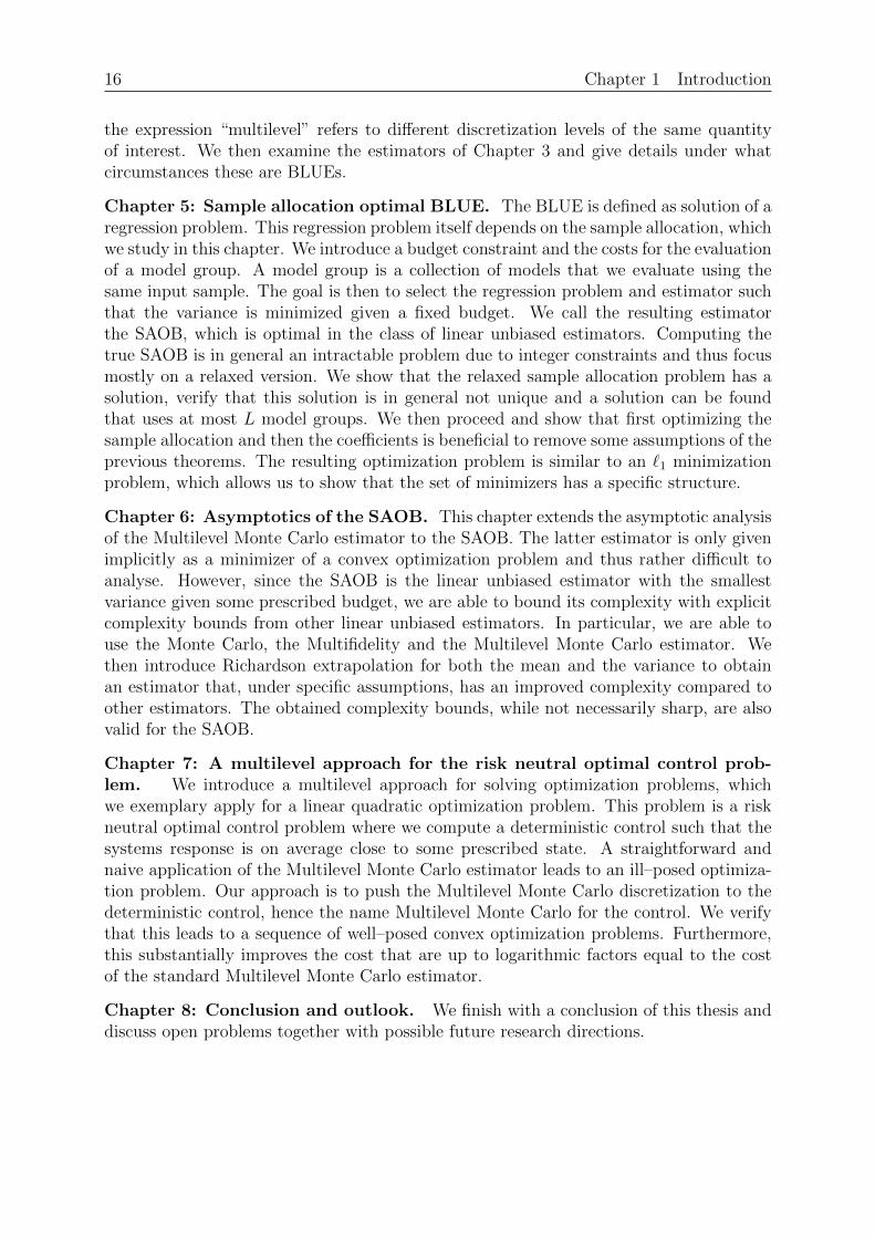
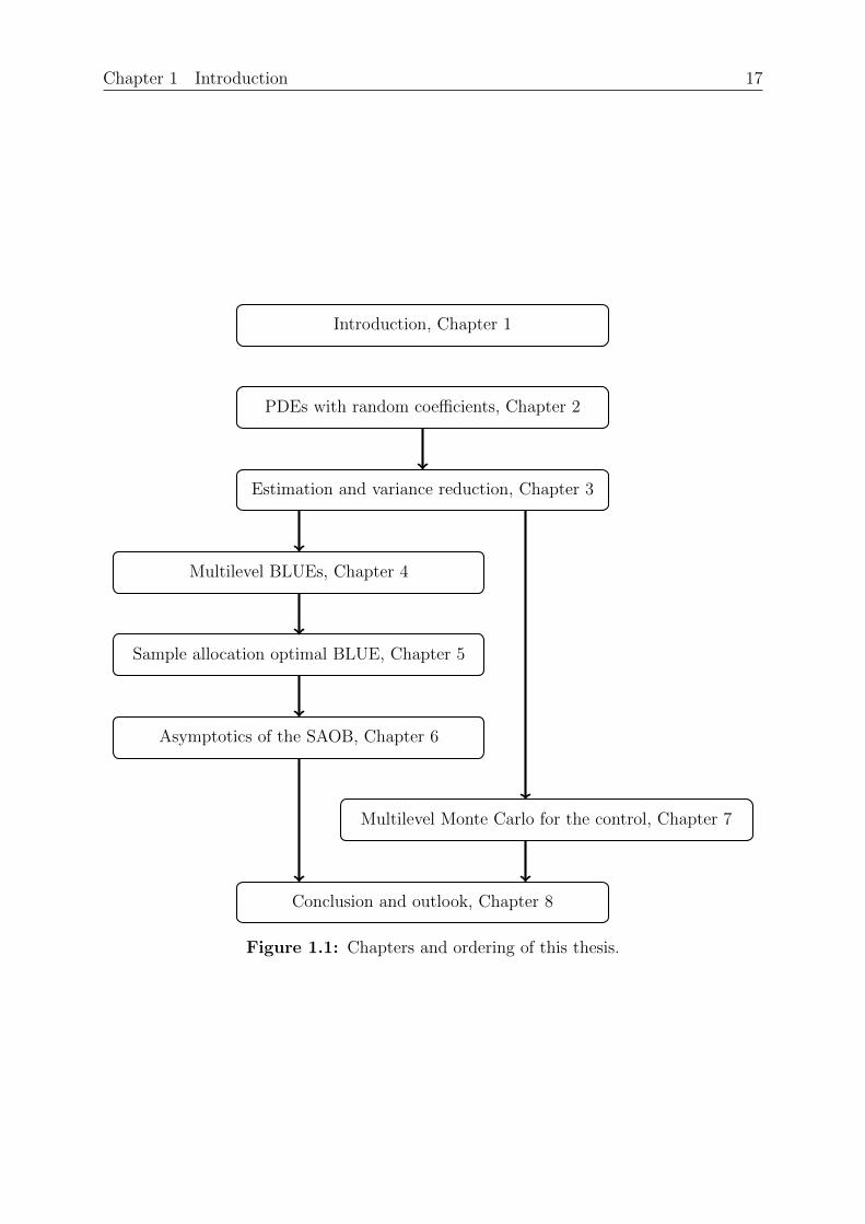
This thesis is organized in eight chapters, where the first one is the introduction. Welist the other chapters with their respective content and objective. Figure 1.1 shows theordering of the chapters.
Chapter 2: Partial differential equations with random coefficients. In thischapter we introduce concepts needed for forward uncertainty quantification. This in-cludes basic probability theory, where we introduce random variables, their expectationsand variances. We further discuss the Karhunen–Loeve expansion which is a method togenerate samples with values in an infinite dimensional Hilbert space. We conduct numer-ical experiments with the help of Poisson’s equation, which we discuss in the last sectionof this chapter. We further provide known results for the accuracy of the finite elementapproximation of the solution.
Chapter 3: Estimation and variance reduction. We present methods to estimatethe expectation of a quantity of interest. These methods are used in practice and wellknown in the literature. We start with the Monte Carlo method and introduce the con-trol variate approach to obtain a variance reduction. Practically implementable controlvariate approaches are the Multifidelity Monte Carlo and Approximate Control Variatesestimator, which improve over standard Monte Carlo in certain circumstances. We fur-ther introduce the Multilevel Monte Carlo method, which is another method to reducethe variance. We provide asymptotic results of these estimators for a model sequenceconverging to the true model and introduce the notion of a lower variance bound. We usethese methods as comparison to the best linear unbiased estimator or the SAOB in thefollowing chapters.
Chapter 4: Multilevel best linear unbiased estimators. We present the basic ideabehind multilevel best linear unbiased estimators (BLUE) in this chapter. We examine theclass of linear estimators that use linear combinations of the samples and are unbiasedw.r.t. some linear combination of the mean values. A well–known result is that thereexists a best linear unbiased estimator, where best means that the variance is smallest.Importantly, we reformulate the estimation of the mean as linear regression problemwhich allows us to use the available mathematical literature for least squares problems.The multilevel BLUE is then the (unique) solution of this regression problem, where
16 Chapter 1 Introduction
the expression “multilevel” refers to different discretization levels of the same quantityof interest. We then examine the estimators of Chapter 3 and give details under whatcircumstances these are BLUEs.
Chapter 5: Sample allocation optimal BLUE. The BLUE is defined as solution of aregression problem. This regression problem itself depends on the sample allocation, whichwe study in this chapter. We introduce a budget constraint and the costs for the evaluationof a model group. A model group is a collection of models that we evaluate using thesame input sample. The goal is then to select the regression problem and estimator suchthat the variance is minimized given a fixed budget. We call the resulting estimatorthe SAOB, which is optimal in the class of linear unbiased estimators. Computing thetrue SAOB is in general an intractable problem due to integer constraints and thus focusmostly on a relaxed version. We show that the relaxed sample allocation problem has asolution, verify that this solution is in general not unique and a solution can be foundthat uses at most L model groups. We then proceed and show that first optimizing thesample allocation and then the coefficients is beneficial to remove some assumptions of theprevious theorems. The resulting optimization problem is similar to an `1 minimizationproblem, which allows us to show that the set of minimizers has a specific structure.
Chapter 6: Asymptotics of the SAOB. This chapter extends the asymptotic analysisof the Multilevel Monte Carlo estimator to the SAOB. The latter estimator is only givenimplicitly as a minimizer of a convex optimization problem and thus rather difficult toanalyse. However, since the SAOB is the linear unbiased estimator with the smallestvariance given some prescribed budget, we are able to bound its complexity with explicitcomplexity bounds from other linear unbiased estimators. In particular, we are able touse the Monte Carlo, the Multifidelity and the Multilevel Monte Carlo estimator. Wethen introduce Richardson extrapolation for both the mean and the variance to obtainan estimator that, under specific assumptions, has an improved complexity compared toother estimators. The obtained complexity bounds, while not necessarily sharp, are alsovalid for the SAOB.
Chapter 7: A multilevel approach for the risk neutral optimal control prob-lem. We introduce a multilevel approach for solving optimization problems, whichwe exemplary apply for a linear quadratic optimization problem. This problem is a riskneutral optimal control problem where we compute a deterministic control such that thesystems response is on average close to some prescribed state. A straightforward andnaive application of the Multilevel Monte Carlo estimator leads to an ill–posed optimiza-tion problem. Our approach is to push the Multilevel Monte Carlo discretization to thedeterministic control, hence the name Multilevel Monte Carlo for the control. We verifythat this leads to a sequence of well–posed convex optimization problems. Furthermore,this substantially improves the cost that are up to logarithmic factors equal to the costof the standard Multilevel Monte Carlo estimator.
Chapter 8: Conclusion and outlook. We finish with a conclusion of this thesis anddiscuss open problems together with possible future research directions.
Chapter 1 Introduction 17
Introduction, Chapter 1
PDEs with random coefficients, Chapter 2
Estimation and variance reduction, Chapter 3
Multilevel BLUEs, Chapter 4
Sample allocation optimal BLUE, Chapter 5
Asymptotics of the SAOB, Chapter 6
Multilevel Monte Carlo for the control, Chapter 7
Conclusion and outlook, Chapter 8
Figure 1.1: Chapters and ordering of this thesis.

18 Chapter 1 Introduction
Chapter 2 Partial differential equations with random coefficients 19
Chapter 2
Partial differential equations with randomcoefficients
In this chapter we describe the basic notation, definition and results needed as foundationof this thesis. Basic in this context means that we describe well–known ideas and methodsin mathematics. We lay a common ground to present our results in later chapters. Eachsection of this chapter contains a short outline of its topic and concepts adapted for thisthesis, where proofs of statements are mostly omitted or very short to highlight the mainidea. We provide three distinct sections regarding related parts of Forward UncertaintyQuantification.
Probability Theory: Section 2.1 contains a short introduction and repetition ofbasic notation in probability theory. We explain concepts like random variables,independence, expectation, variance and provide some useful inequalities. Here weuse standard definitions from [79]. Further introductions to probability theory canalso be found in [6, 10, 77].
Karhunen–Loeve expansion: We are interested in random variables that have re-alizations in a function space and we use the Karhunen–Loeve expansion to generatesamples, which we describe in Section 2.2. We mainly focus on mean zero Gaus-sian random fields and provide results for the Whittle–Matern covariance function.We further discuss some practical methods how to compute and sample from aKarhunen–Loeve expansion.
Mathematical models: We provide the mathematical models we are using inthesis in Section 2.3. This is mostly Poisson’s equation, which can be used tomodel the temperature of a material given some heat source. We randomize theconductivity and provide results for the existence and uniqueness of the randomsolution of the weak Poisson’s equation. The finite element method is used to obtaina discretized and thus computable solution which converges to the exact solutionwith a certain rate.
2.1 Probability Theory
Random variables. The foundation of modern probability theory is a probabilityspace. We provide the standard definition and names for related concepts as well.
Definition 2.1 (Probability space [79, Definition 1.38]). The triple (Ω,F ,P) is a proba-bility space if
the set of elementary events Ω is non–empty, Ω 6= ∅,
the σ-algebra F is a suitable subset of the power set, F ⊆ 2Ω,
the probability measure P is a suitable measure, P : F → [0, 1].
20 Chapter 2 Partial differential equations with random coefficients
We use the usual definition of σ-algebra, the power set and probability measure. Thesedefinitions are available in Klenke [79, Section 1] or Kallenberg [77, Section 1, Section 2].We denote (elementary) events with ω ∈ Ω and also refer to the measure P as (probability)distribution. We call the pair (Ω,F) measurable space. The motivation for Definition 2.1is to assign every observable event F ∈ F a probability between [0, 1] which models thechance of it occurring.We are typically not interested in the probability of a random event F ∈ F but rather ona respective outcome or effect. This is modelled with the help of random variables, whichare measurable functions that map events ω to quantities that we are interested in.
Definition 2.2 (Random variable [77, Section 2]). Let (H,G) be a measurable space andZ : Ω→ H a function. Z is measurable if the preimage of a measurable set is measurable.Stated formally, we require that for all G ∈ G
Z−1(G) := ω ∈ Ω |Z(ω) ∈ G ∈ F .
If Z is measurable on a probability space then Z is called a random variable. Then, incase H is a space of vectors, we call Z a random vector and if H is a space of functions,we call Z a random field. For H := R we call Z real–valued.
The random variable Z allows us to define the probability of certain outcomes in theimage space H. For all G ∈ G the probability that Z assumes values in G is
P(Z ∈ G) := P(ω ∈ Ω |Z(ω) ∈ G) = P(Z−1(G)).
This expression is well defined since Z is measurable by its definition as random variable.As a consequence we conclude that the triple (H,G,P(Z ∈ ·)) is a well–defined probabilityspace. The map P(Z ∈ ·) is called the pushforward of P under Z. We denote this byZ ∼ P and call P the distribution of Z.The composition of measurable functions is again measurable and thus we are able tocompose new random variables in a simpler way. We precisely state this result.
Lemma 2.3 (Composition of measurable functions [79, Theorem 1.80]).Let (Ω,F), (H1,G1) and (H2,G2) be measurable spaces. Furthermore, let Z1 : Ω → H1
and Z2 : H1 → H2 be measurable functions w.r.t. the respective σ-algebras. Then thecomposition Z2 Z1 : Ω→ H2 is measurable.
Proof. For G ∈ G2 the preimage Z−12 (G) is measurable w.r.t. G1 and thus Z−1
1 (Z−12 (G))
is measurable w.r.t. F . This concludes the proof.
An important class of measurable functions are continuous functions. This often allowsus to circumvent the rather tedious direct verification of measurability from its definition.We require the notion of a topological space, which is formally defined by Klenke [79,Definition 1.20]. A topological space is a pair (H, τ) where τ is a topology. This canbe constructed from open sets which are defined in terms of a distance function. Thegenerated σ-algebra is then the smallest σ-algebra that contains these open sets. Anexample for a topological space is (R, O), where O contains all open intervals of R. Thenthe generated σ-algebra denoted by σ(O) is the well–known Borel σ-algebra.
Lemma 2.4 (Continuous functions are measurable [79, Theorem 1.88]). Let Z : H1 → H2
be a continuous function w.r.t. the topological spaces (H1, τ1) and (H2, τ2). Then Z ismeasurable w.r.t. the measurable spaces (H1,G1) and (H2,G2), where G1 := σ(τ1) andG2 := σ(τ2) denotes the generated σ-algebra.
Chapter 2 Partial differential equations with random coefficients 21
Proof. The main idea of the proof by Klenke [79, Theorem 1.88] is that the preimage ofan open set is open for the continuous function Z.
We often examine two or more random variables and their relationship. A pair of randomvariables (Z, Y ) is independent if we are allowed to examine Z and Y separately. Infor-mally, this means that we do not gain any information regarding the value of Z even ifwe know the value of Y and vice versa. We make this statement precise for a finite set ofrandom variables.
Definition 2.5 (Independence of random variables [79, Remark 2.15]). Let (Z1, . . . , ZL)be a random vector with associated probability space
(H1 × · · · ×HL,G1 × · · · × GL,P((Z1, . . . , ZL) ∈ ·)).
We denote the marginal probability measure of Z` with P` for all ` ∈ 1, . . . , L. Then therandom variables Z1, . . . , ZL are called independent if the probability measure P factorizessuch that for all G1 ∈ G1, . . . , GL ∈ GL
P((Z1, . . . , ZL) ∈ G1 × · · · ×GL) =L∏`=1
P`(Z` ∈ G`).
Simulation based techniques often require multiple realizations or samples of a randomvariable Z. The idea is to extract information by looking at independent copies of Zwhich are evaluated for some event ω ∈ Ω.
Definition 2.6 (Independent identically distributed samples). The random variablesZ1, . . . , Zm are independent identically distributed (i.i.d.) if Z1, . . . , Zm are independentand Z` ∼ P for all ` ∈ 1, . . . ,m. We always assume that random variables with differ-ent superscripts are i.i.d.. For ω ∈ Ω we call Z(ω) a sample or realization of the randomvariable Z. By slight abuse of notation we often drop the ω and denote i.i.d. samples ofZ with Z1 := Z1(ω), . . . , Zm := Zm(ω).
The computation of a sample often incurs a random computational cost. This definitionis rather vague, since the exact cost may be the actual time a computer needs to computea sample. We may also define the cost as degrees of freedom or number of operations ifcomputing the sample requires us to solve a linear system.
Definition 2.7 (Expected cost for a random variable). The cost function W maps arandom variable Z to a non–negative real number
W : Z : Ω→ H |Z measurable → R≥0.
The value of W[Z] is interpreted as expected cost to compute a sample of Z. For randomvariables Z1, . . . , ZL we abbreviate
w` := W[Z`] for all ` ∈ 1, . . . , L.
We frequently make statements about random variables that are certain and occur withprobability one. We formally define this and the equivalent formulation for a generalmeasure space.
22 Chapter 2 Partial differential equations with random coefficients
Definition 2.8 (Almost all, P–almost surely). Let (Ω,F , ν) be a measure space andf : H → 0, 1 be a measurable function. We say that the property f holds for ν–almostall ω ∈ Ω if
ν(f−1(0)) = 0.
If ν := P is a probability measure we say that f holds P–almost surely, which we sometimesabbreviate with P–a.s.. We often drop P from the notation.
There is little value in specifying the measurable space (Ω,F), since this is often givenimplicitly in terms of a probability measure P, a probability density function, a randomvariable or a cumulative distribution function. Therefore, we never attempt to describeboth Ω and F in this thesis. We however, always specify P or a corresponding randomvariable Z.
Moments. For notational purposes and throughout the rest of this chapter we assumethat Z and Y assume values in the Hilbert space H unless stated otherwise. It is oftenhelpful to summarize or compress a function or random variable Z into a single value. Weachieve this if we integrate out the domain of Z raised to some power p. This operation iswell defined for measurable functions if the function is p-integrable. We formulate this fora general measure space, where we denote the scalar product of a Hilbert space H with(·, ·)H and the induced norm with ‖ · ‖H .
Definition 2.9 (Lebesgue space Lp). Let (Ω,F , ν) be a measure space and p ∈ [1,+∞].The Lebesque space Lp(Ω, H, ν) is the space of measurable functions whose p–th momentis bounded
Lp(Ω, H, ν) :=Z : Ω→ H |Z is ν–measurable and ‖Z‖Lp(Ω,H,ν) < +∞
,
where the norm ‖ · ‖Lp(Ω,H,ν) for p ∈ [1,+∞) is defined such that
‖Z‖pLp(Ω,H,ν) :=
∫Ω
‖Z(ω)‖pHdν(ω).
For the special case p = +∞ the norm is defined as
‖Z‖L∞(Ω,H,ν) := supc ∈ R | ν(‖Z‖H ≤ c) > 0.
If the meaning of the space is clear from the context we use the abbreviation
Lp := Lp(Ω) := Lp(Ω, H) := Lp(Ω, H, ν).
It is well known that the space Lp is a Banach space if we identify functions that areequal up to a set of measure zero. Furthermore, for p = 2 the space L2 is a Hilbert spacethat inherits the inner product structure from H. We formally define this inner productsuch that for all Z, Y ∈ L2
(Z, Y )L2 :=
∫Ω
(Z(ω), Y (ω))Hdν(ω). (2.1)
The Cauchy–Schwarz inequality shows that (2.1) is well defined. This inequality is aspecial case of Holder’s inequality and we precisely state both now.
Chapter 2 Partial differential equations with random coefficients 23
Lemma 2.10 (Holder’s inequality, Cauchy–Schwarz inequality). Let p, q ∈ [1,+∞] with1p
+ 1q
= 1, Z ∈ Lp and Y ∈ Lq. Then Holder’s inequality holds
‖ (Z, Y )H ‖L1 ≤ ‖Z‖Lp‖Y ‖Lq .
The special case with p = q = 2 is the Cauchy–Schwarz inequality
‖ (Z, Y )H ‖L1 ≤ ‖Z‖L2‖Y ‖L2 .
Proof. See Klenke [79, Chapter 7].
A straightforward consequence of Holder’s inequality and P(Ω) = 1 is that for all p ∈[1,+∞] the random variable Z ∈ Lp(Ω, H,P) is also an element of the space Lq(Ω, H,P)for all q ∈ [1, p]. This implication is in general not true if we replace P with an arbitrarymeasure ν.
Expectation, Variance, Covariance and Correlation. We proceed to define specificintegrals concerning random variables. The expectation or mean of a random variabledescribes its average value. We use the variance to describe the average squared deviationfrom the mean. Both values are basic properties of random variables and exist if the firstrespectively second moment is finite.
Definition 2.11 (Expectation, Variance). For Z ∈ L1 we define the expectation or mean
E[Z] :=
∫Ω
Z(ω)dP(ω).
This definition has to be understood as Bochner integral if Z is not real–valued. If inaddition Z ∈ L2 we define the variance
V[Z] := E[‖Z − E[Z]‖2
H
]= E
[‖Z‖2
H
]− ‖E[Z]‖2
H . (2.2)
For real–valued Z the variance (2.2) coincides with the usual definition. For randomvariables Z1, . . . , ZL ∈ L2 we abbreviate the mean and variance
µ` := E[Z`] for all ` ∈ 1, . . . , L,σ2` := V[Z`] for all ` ∈ 1, . . . , L.
The mean is the constant in H that best approximates the random variable Z. It is theunique solution of the minimization problem
minµ∈H‖Z − µ‖2
L2 = E[‖Z − µ‖2
H
].
The value of the cost function at the minimizer µ = E[Z] is the variance and describesthe approximation error. The variance is zero V[Z] = 0 if and only if Z is almost surelyconstant with Z = E[Z]. In all other cases the variance is positive. We are allowed topull out constants from the variance by squaring them, that is for all β ∈ R
V[βZ] = β2V[Z].
24 Chapter 2 Partial differential equations with random coefficients
The expectation is a linear operator since for all Z1, . . . , ZL ∈ L1 and vectors β ∈ RL
E
[L∑`=1
β`Z`
]=
L∑`=1
β`E[Z`].
The mean and variance are concerned with a single random variable Z and both give asingle value. We now describe relationships between two random variables with the helpof the covariance and correlation.
Definition 2.12 (Covariance, Correlation). For real–valued random variables Z, Y ∈ L2
we define the covariance
Cov[Z, Y ] := E[(Z − E[Z])(Y − E[Y ])] = E[ZY ]− E[Z]E[Y ].
If in addition V[Z],V[Y ] > 0 we define the correlation or correlation coefficient
Corr[Z, Y ] :=Cov[Z, Y ]
(V[Y ]V[Z])1/2.
The random variables Z and Y are uncorrelated if Cov[Z, Y ] = 0.
We extend the previous definition to multiple random variables. This allows us to placemultiple covariance and correlation values into a vector or matrix.
Definition 2.13 (Covariance and Correlation matrix). For vectors of real–valued randomvariables Z := (Z1, . . . , ZL)T ∈ L2 and Y := (Y1, . . . , YN)T ∈ L2 we define the covariancematrix
Cov[Z, Y ] := E[(Z − E[Z])(Y − E[Y ])T
]∈ RL×N .
For V[Z1], . . . ,V[ZL],V[Y1], . . . ,V[YN ] > 0 we define the correlation matrix as the corre-lation between entries of Z and Y
Corr[Z, Y ] ∈ RL×N , Corr[Z, Y ]`,n := Corr[Z`, Yn] for all ` ∈ 1, . . . , L, n ∈ 1, . . . , N.
For real–valued random variables Z1, . . . , ZL ∈ L2 we abbreviate
C := Cov
Z1
...ZL
,Z1
...ZL
∈ RL×L, P := (ρij)
Li,j=1 := Corr
Z1
...ZL
,Z1
...ZL
∈ RL×L.
(2.3)We generalize the covariance to infinite dimensional Hilbert spaces. The basic idea is toreduce the Hilbert space valued random variable Z to a single value in R by testing itwith a linear functional in the dual space H∗. We identify this space with H due to theRiesz–representation theorem [79, Theorem 7.26].
Definition 2.14 (Covariance operator, Correlation operator). Let H1, H2 be real Hilbertspaces. For Z ∈ L2(Ω, H1) and Y ∈ L2(Ω, H2) we define the covariance operator
Cov[Z, Y ] : H1 ×H2 → R, Cov[Z, Y ](z, y) := E[(z, Z − E[Z])H1(y, Y − E[Y ])H2 ].
We define the correlation operator accordingly
Corr[Z, Y ] : H1 ×H2 → R, Corr[Z, Y ](z, y) :=Cov[Z, Y ](z, y)
(Cov[Z,Z](z, z)Cov[Y, Y ](y, y))1/2,
whenever the quotient is not equal to zero.
Chapter 2 Partial differential equations with random coefficients 25
The covariance operator is a generalization of the covariance matrix where the Hilbertspaces are H1 := RL and H2 := RN with the Euclidean inner product. We obtain theentries of the covariance matrix if we test with the unit vectors z := e` and y := en
Cov[Z, Y ](z, y) = E[(e`, Z − E[Z])RL(en, Y − E[Y ])RN ]
= E[(Z` − E[Z`])(Yn − E[Yn])]
= Cov[Z, Y ]`,n.
Let us now verify that the covariance is actually well defined for Z, Y ∈ L2. We fixz ∈ H1, y ∈ H2, apply the Cauchy–Schwarz inequality twice and use the linearity of theexpectation
Cov[Z, Y ](z, y)2 ≤ E[(z, Z − E[Z])2
H1
]E[(y, Y − E[Y ])2
H2
]≤ E
[‖z‖2
H1‖Z − E[Z]‖2
H1
]E[‖y‖2
H2‖Y − E[Y ]‖2
H2
]= ‖z‖2
H1‖y‖2
H2E[‖Z − E[Z]‖2
H1
]E[‖Y − E[Y ]‖2
H2
].
The last term is bounded for Z, Y ∈ L2. We summarize some well–known properties ofthe covariance.
Lemma 2.15 (Properties of the covariance). For Z,Z1, . . . , ZL ∈ L2(Ω, H1) and Y ∈L2(Ω, H2) the covariance operator Cov is
symmetric: Cov[Z, Y ](z, y) = Cov[Y, Z](y, z) for all z ∈ H1, y ∈ H2.
bilinear: Cov[∑L
`=1 β`Z`, Y]
=∑L
`=1 β`Cov[Z`, Y ] for all β ∈ RL.
positive semi–definite: Cov[Z,Z](z, z) ≥ 0 for all z ∈ H.
equal to the variance if Z is real–valued: Cov[Z,Z] = V[Z].
Proof. The properties follow directly from the definition of the covariance.
The correlation Corr inherits its properties from the covariance. The Cauchy–Schwarzinequality can be used to show that the correlations operator takes values between −1and 1. Formally, for all z ∈ H1 and y ∈ H2 where the correlation is well defined
Corr[Z, Y ](z, y) ∈ [−1, 1].
The covariance matrix C ∈ RL×L is always positive semi–definite. We now show that if theentries of Z −E[Z] with Z = (Z1, . . . , ZL)T are linearly independent, then C = Cov[Z,Z]is positive definite and thus invertible.
Lemma 2.16 (Positive definiteness of the covariance). For Z ∈ L2 the following state-ments are equivalent
Cov[Z,Z](z, z) > 0 for all z ∈ H \ 0.
(z, Z − E[Z])H 6= 0 P–almost surely for all z ∈ H \ 0.
For Z := (Z1, . . . , ZL)T with real–valued Z1, . . . , ZL this equivalence reads
βTCov[Z,Z]β > 0 for all β ∈ RL \ 0.
26 Chapter 2 Partial differential equations with random coefficients
Z1 − E[Z1], . . . , ZL − E[ZL] are linearly independent.
Furthermore, if βTCov[Z,Z]β = 0 for some β ∈ RL then P–almost surely
βT (Z − E[Z]) = 0. (2.4)
Proof. We deduce the claim by directly looking at the definition of the covariance
Cov[Z,Z](z, z) = E[(z, Z − E[Z])2
H
].
The factorization of the probability measure P for independent random variables showsthat their covariance is zero. We summarize this and further properties in the next lemma.
Lemma 2.17 (Properties of independent random variables [79, Theorem 5.4]). Let Z, Y ∈L1 be independent random variables. Then the expectation of the product is equal to theproduct of the expectations
E[(Z, Y )H ] = (E[Z],E[Y ])H .
For Z, Y ∈ L2 the random variables Z and Y are uncorrelated Cov[Z, Y ] = 0.
The previous lemma shows that independence of Z, Y implies that Z, Y are uncorrelated,however the converse is in general not true. We now state an important computationalrule for the variance of sums of random variables.
Lemma 2.18 (Variance of sums [79, Theorem 5.7]). Let Z1, . . . , ZL ∈ L2 be real–valuedrandom variables. Then the variance of the sum satisfies
V
[L∑`=1
Z`
]=
L∑`,j=1
Cov[Z`, Zj] =L∑`=1
V[Z`] +L∑
`,j=1`6=j
Cov[Z`, Zj].
If Z1, . . . , ZL are pairwise uncorrelated then the covariance terms are equal to zero
V
[L∑`=1
Z`
]=
L∑`=1
V[Z`].
Proof. We use the bilinearity of the covariance and Cov[Z`, Zj] = 0 for uncorrelatedZ`, Zj.
Convergence of random variables. There are different convergence types for randomvariables. In this thesis we distinguish between almost sure convergence and convergencein the Lebesgue space Lp.
Definition 2.19 (Almost sure convergence [79, Definition 6.2]). Let (Zn)∞n=1 be a sequenceof random variables. We say that (Zn)∞n=1 converges almost surely to the random variableZ if
P(
limn→+∞
Zn = Z
)= 1.

Chapter 2 Partial differential equations with random coefficients 27
Definition 2.20 (Convergence in Lp [79, Definition 7.2]). Let (Zn)∞n=1 ⊆ Lp and Z ∈ Lp.Then (Zn)∞n=1 converges to Z in Lp if
limn→+∞
‖Zn − Z‖Lp = 0.
Useful inequalities. The probability that a random variable deviates from its mean isbounded by its variance. This allows us to estimate the probability that the realizationsof a random variable remain within a certain distance from its mean.
Theorem 2.21 (Markov inequality, Chebyshev inequality, [79, Theorem 5.11]).Let Z be a random variable and f : [0,+∞) → [0,+∞) a monotonically increasingfunction. Then for all ε > 0 Markov’s inequality holds
P(‖Z‖H ≥ ε) ≤ E[f(‖Z‖H)]
f(ε)
provided that the right–hand side is well defined. For Z ∈ L2 the Chebyshev inequalityholds
P(‖Z − E[Z]‖H ≥ ε) ≤ V[Z]
ε2.
We state Jensen’s inequality, which allows us to exchange the expectation and a convexfunction ϕ at the cost of introducing an inequality.
Lemma 2.22 (Jensen’s inequality [79, Theorem 7.11]). Let I := (a, b) ⊆ R be an openinterval, Z ∈ L1(Ω, I) and the function ϕ : I → R convex. Then Jensen’s inequality holds
ϕ(E[Z]) ≤ E[ϕ(Z)],
provided that the right–hand side is well defined.
Proof. A formal proof is given in [79, Theorem 7.11]. We only remark that convex func-tions are continuous and thus measurable, hence ϕ(Z) is a random variable.
We finish this section with the elementary Young inequality, which we use to estimate theexpectation of a product of real–valued random variables such that 2E[ZY ] ≤ E[Z2] +E[Y 2].
Lemma 2.23 (Young inequality [79, Lemma 7.15]). For p, q ∈ (1,+∞) with 1p
+ 1q
= 1
and real numbers z, y ∈ [0,+∞) Young’s inequality holds
zy ≤ zp
p+yq
q.
In particular, for p = q = 2 the inequality holds for arbitrary z, y ∈ R.

28 Chapter 2 Partial differential equations with random coefficients
2.2 Karhunen–Loeve expansion
Construction of Gaussian random fields. The Karhunen–Loeve expansion (KLE)is a powerful tool to generate random variables with values in an infinite dimensional,separable Hilbert space. The main idea is to randomize the coefficients of a Fourier seriesin a suitable way such that the series converges almost surely. A study of orthogonalexpansions of random variables is available in [1, Section 3]. First, we provide conditionsfor the special case of real–valued random variables.
Lemma 2.24 (Khinchin and Kolmogorov [77, Lemma 3.16]). Let (ξn)∞n=1 be real–valuedindependent random variables with E[ξn] = 0 for all n ∈ N such that their variance issummable
∞∑n=1
V[ξn] < +∞.
Then the series∑∞
n=1 ξn converges almost surely.
We require the previous lemma to ensure that the KLE is well defined.
Definition 2.25 (Infinite dimensional Gaussian random field). Let H be an infinite di-mensional, separable, real Hilbert space. Furthermore, assume the following:
1. The eigenfunctions (ψn)∞n=1 form a complete orthonormal basis of H,
2. The random variables (ξn)∞n=1 are i.i.d. standard normals with ξn ∈ N(0, 1) for alln ∈ N,
3. The eigenvalues (λn)∞n=1 are non–negative values λn ≥ 0 for all n ∈ N and thesequence is summable
∞∑n=1
λn < +∞. (2.5)
We define the KLE a as series
a :=∞∑n=1
√λnξnψn.
We have a ∈ L2 and define C := Cov[a, a], which we abbreviate with a ∼ N(0, C).
We use Parseval’s identity and apply Lemma 2.24 in combination with (2.5) to show thatthe norm of a is almost surely bounded
‖a‖2H =
∞∑n=1
λnξ2n =
∞∑n=1
λn(ξ2n − 1) +
∞∑n=1
λn < +∞.
We thus conclude that a ∈ H almost surely. We use the monotone convergence theorem[77, Theorem 1.19] to exchange the mean and summation
E[‖a‖2
H
]= E
[∞∑n=1
λnξ2n
]=∞∑n=1
E[λnξ
2n
]=∞∑n=1
λn < +∞,
which shows that a ∈ L2. The dominated convergence theorem [77, Theorem 1.21] nowshows that E[a] = 0.
Chapter 2 Partial differential equations with random coefficients 29
We clarify why we call λn eigenvalues and ψn the eigenfunctions of C(ψn, ·). The functions(ψn)∞n=1 form a complete orthonormal basis and thus
C(ψn, ·) =∞∑
k,m=1
√λk√λmE[ξkξm](ψn, ψk)H(·, ψm)H =
∞∑m=1
√λn√λmE[ξnξm](·, ψm)H .
We use the independence of ξn and ξm for n 6= m, E[ξm] = 0 and E[ξ2m] = 1 to conclude
∞∑m=1
√λn√λmE[ξnξm](·, ψm)H = λn(·, ψn)H .
We interpret C(ψn, ·) as an element of H with the help of the Riesz–representation theoremand conclude that ψn is an eigenfunction of C with eigenvalue λn
C(ψn) = λnψn.
The covariance operator is diagonal C(ψn, ψj) = λnδnj, where δnj is the Kronecker delta
δnj :=
1, if n = j,
0, if n 6= j.
We are interested in random fields and thus ψn are functions. For an event ω and x ∈ Dthe KLE with arguments has the following form
a(x, ω) =∞∑n=1
√λnξn(ω)ψn(x).
We want to construct a random field such that values at close points are highly correlated.For points x, y ∈ D we require that
Cov[a(x), a(y)] = k(‖x− y‖),
where k is a stationary covariance kernel and ‖ · ‖ a suitable norm. We call a covariancekernel or random field stationary if the covariance Cov[a(x), a(y)] depends only on thedistance between x and y. We work with the commonly used Whittle–Matern covariancekernel. Practical applications of covariance kernels are Gaussian processes regression orkriging in machine learning [115], where the kernel models the similarity between thedatapoints. Another application is spatial descriptions in geostatistics [33, 140].
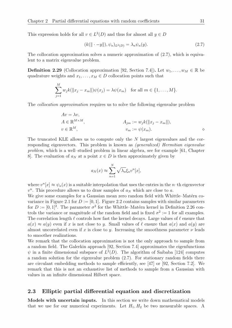
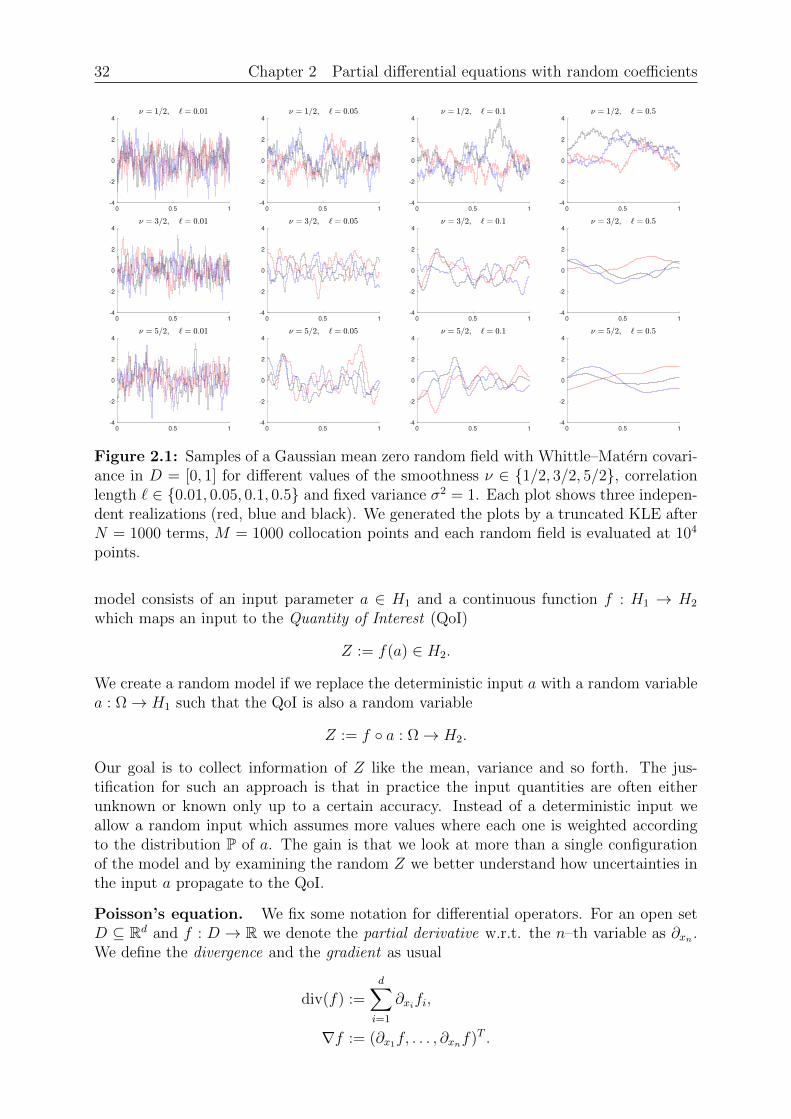
Definition 2.26 (Whittle–Matern covariance kernel [115, Chapter 4]).The Whittle–Matern covariance kernel k has three parameters, the variance σ2 > 0, thesmoothness ν > 0 and the correlation length ` > 0. We write down the kernel for differentvalues of ν for a given distance d ≥ 0
ν = 1/2 : k(d) := σ2 exp(−d/`),
ν = 3/2 : k(d) := σ2(1 +√
3d/`) exp(−√
3d/`),
ν = 5/2 : k(d) := σ2(1 +√
5d/`+ 5d2/(3`2))
exp(−√
5d/`).
The Whittle–Matern covariance kernel now defines the KLE of a Gaussian.
30 Chapter 2 Partial differential equations with random coefficients
Theorem 2.27 (Gaussian from Whittle–Matern covariance kernel [115, Chapter 4]). LetD ⊆ Rd be a bounded domain. Then there exists a ∼ N(0, C) with values in C(D) suchthat for all x, y ∈ D
Cov[a(x), a(y)] = k(‖x− y‖),where k is the Whittle–Matern covariance kernel. We express the random field a as KLE
a :=∞∑n=1
√λnψnξn.
We restrict ourselves to the random field a ∼ N(0, C) where C is induced by a Whittle–Matern covariance kernel k. Other stationary random fields are examined by Adler [1,Section 5] and a general theory on the existence of Gaussian random fields in infinitedimensions is given by Bogachev [12].
Practical implementation. The KLE for a is a series
a =∞∑n=1
√λnξnψn,
which we truncate to obtain a finite sum that we evaluate numerically. We define thetruncated KLE
aN :=N∑n=1
√λnξnψn.
The expected value of the error for this truncation in the H-norm is equal to the sum ofthe missing eigenvalues.
Lemma 2.28 (KLE truncation error). The expected truncation error for a KLE is
E[‖aN − a‖2
H
]=
∞∑n=N+1
λn. (2.6)
This error converges to zero for N → +∞.
Proof. The error (2.6) follows from the Parseval identity and converges to zero since theeigenvalues are summable by assumption (2.5).
For a fixed truncation index N we minimize the truncation error if we keep the N largesteigenvalues. We thus sort the eigenvalues in descending order
λ1 ≥ λ2 ≥ . . . .
The eigenpairs (λn, ψn) for the Whittle–Matern covariance typically cannot be computedanalytically. However, for arbitrary v ∈ L2(D) the eigenpairs are related to the kernel kin the following way
λn(ψn, v)L2(D) = Cov[a, a](ψn, v)
=
∫D
∫D
ψn(x)E[a(x)a(y)]v(y)dxdy
=
∫D
∫D
ψn(x)k(‖x− y‖)v(y)dxdy
= ((ψn, k(‖ · − · ‖))L2(D), v)L2(D).
Chapter 2 Partial differential equations with random coefficients 31
This expression holds for all v ∈ L2(D) and thus for almost all y ∈ D
(k(‖ · −y‖), ψn)L2(D) = λnψn(y). (2.7)
The collocation approximation solves a numeric approximation of (2.7), which is equiva-lent to a matrix eigenvalue problem.
Definition 2.29 (Collocation approximation [92, Section 7.4]). Let w1, . . . , wM ∈ R bequadrature weights and x1, . . . , xM ∈ D collocation points such that
M∑j=1
wjk(‖xj − xm‖)ψ(xj) = λψ(xm) for all m ∈ 1, . . . ,M.
The collocation approximation requires us to solve the following eigenvalue problem
Av = λv,
A ∈ RM×M , Ajm := wjk(‖xj − xm‖),v ∈ RM , vm := ψ(xm).
The truncated KLE allows us to compute only the N largest eigenvalues and the cor-responding eigenvectors. This problem is known as (generalized) Hermitian eigenvalueproblem, which is a well–studied problem in linear algebra, see for example [61, Chapter8]. The evaluation of aN at a point x ∈ D is then approximately given by
aN(x) ≈N∑n=1
√λnξnv
n[x],
where vn[x] ≈ ψn(x) is a suitable interpolation that uses the entries in the n–th eigenvectorvn. This procedure allows us to draw samples of aN which are close to a.We give some examples for a Gaussian mean zero random field with Whittle–Matern co-variance in Figure 2.1 for D := [0, 1]. Figure 2.2 contains samples with similar parametersfor D := [0, 1]2. The parameter σ2 for the Whittle–Matern kernel in Definition 2.26 con-trols the variance or magnitude of the random field and is fixed σ2 := 1 for all examples.The correlation length ` controls how fast the kernel decays. Large values of ` ensure thata(x) ≈ a(y) even if x is not close to y. Small values of ` ensure that a(x) and a(y) arealmost uncorrelated even if x is close to y. Increasing the smoothness parameter ν leadsto smoother realizations.We remark that the collocation approximation is not the only approach to sample froma random field. The Galerkin approach [92, Section 7.4] approximates the eigenfunctionsψ in a finite dimensional subspace of L2(D). The algorithm of Saibaba [124] computesa random solution for the eigenvalue problem (2.7). For stationary random fields thereare circulant embedding methods to sample efficiently, see [47] or [92, Section 7.2]. Weremark that this is not an exhaustive list of methods to sample from a Gaussian withvalues in an infinite dimensional Hilbert space.
2.3 Elliptic partial differential equation and discretization
Models with uncertain inputs. In this section we write down mathematical modelsthat we use for our numerical experiments. Let H1, H2 be two measurable spaces. A
32 Chapter 2 Partial differential equations with random coefficients
0 0.5 1
-4
-2
0
2
4
0 0.5 1
-4
-2
0
2
4
0 0.5 1
-4
-2
0
2
4
0 0.5 1
-4
-2
0
2
4
0 0.5 1
-4
-2
0
2
4
0 0.5 1
-4
-2
0
2
4
0 0.5 1
-4
-2
0
2
4
0 0.5 1
-4
-2
0
2
4
0 0.5 1
-4
-2
0
2
4
0 0.5 1
-4
-2
0
2
4
0 0.5 1
-4
-2
0
2
4
0 0.5 1
-4
-2
0
2
4
Figure 2.1: Samples of a Gaussian mean zero random field with Whittle–Matern covari-ance in D = [0, 1] for different values of the smoothness ν ∈ 1/2, 3/2, 5/2, correlationlength ` ∈ 0.01, 0.05, 0.1, 0.5 and fixed variance σ2 = 1. Each plot shows three indepen-dent realizations (red, blue and black). We generated the plots by a truncated KLE afterN = 1000 terms, M = 1000 collocation points and each random field is evaluated at 104
points.
model consists of an input parameter a ∈ H1 and a continuous function f : H1 → H2
which maps an input to the Quantity of Interest (QoI)
Z := f(a) ∈ H2.
We create a random model if we replace the deterministic input a with a random variablea : Ω→ H1 such that the QoI is also a random variable
Z := f a : Ω→ H2.
Our goal is to collect information of Z like the mean, variance and so forth. The jus-tification for such an approach is that in practice the input quantities are often eitherunknown or known only up to a certain accuracy. Instead of a deterministic input weallow a random input which assumes more values where each one is weighted accordingto the distribution P of a. The gain is that we look at more than a single configurationof the model and by examining the random Z we better understand how uncertainties inthe input a propagate to the QoI.
Poisson’s equation. We fix some notation for differential operators. For an open setD ⊆ Rd and f : D → R we denote the partial derivative w.r.t. the n–th variable as ∂xn .We define the divergence and the gradient as usual
div(f) :=d∑i=1
∂xifi,
∇f := (∂x1f, . . . , ∂xnf)T .
Chapter 2 Partial differential equations with random coefficients 33
Figure 2.2: Samples of a Gaussian mean zero random field with Whittle–Matern co-variance in D = [0, 1]2 for different values of the smoothness ν ∈ 1/2, 3/2, 5/2 andcorrelation lengths ` ∈ 0.1, 0.5. Each image is an independent realization of the ran-dom field. We generated the plots by truncating the KLE after N = 100 terms.
We model heat transfer through a material with the help of Poisson’s equation. Themathematical description for the temperature y is the solution of a partial differentialequation (PDE). The physical interpretation is that a constant heat source, say a chemicalreaction or the heating of a metal rod, has enough time to conduct through a material[7, Chapter 7.1]. The steady state temperature is then described with Poisson’s equation,where we first introduce the strong formulation.
Example 2.30 (Strong Poisson equation). Let D ⊆ Rd be a bounded domain. Then thestrong Poisson equation is
−div(a(x)∇y(x)) = u(x), x ∈ D,y(x) = g(x), x ∈ ∂D.
(2.8)
Let us describe the quantities and their physical meaning:
The domain D describes the volume of a material.
The function y : D → R is the temperature in the material.
The forcing function u controls how much heat is generated or lost inside the domain.
The diffusion a > 0 determines how fast the heat travels through the material.
The temperature at the boundary has fixed value g.
This model problem is also used in groundwater flow, where it models subsurface flow.Here Darcy’s law is combined with the continuity equation to obtain Poisson’s equation,see [30, 40, 141]. The existence and uniqueness of solutions of strong PDE formulations is
34 Chapter 2 Partial differential equations with random coefficients
often difficult to prove. Instead, we look at weak formulations. We further randomize thediffusion a which leads to a pathwise formulation. Weak formulations are often obtainedby multiplying the PDE with suitably smooth test functions and using integration byparts. We denote with H1
0 (D) ⊆ L2(D) the Sobolev space consisting of functions withweak first order derivative in L2(D) and zero trace [50, Section 5]. We equip this spacewith the norm ‖y‖H1
0 (D) := ‖∇y‖L2(D).
Definition 2.31 (Pathwise weak elliptic PDE). Let D ⊆ Rd be a bounded domain,u ∈ L2(D) and g := 0. We call y ∈ H1
0 (D) a weak solution of (2.8) if for all functionsv ∈ H1
0 (D)
(a∇y,∇v)L2(D) = (u, v)L2(D).
We call y a pathwise weak solution if for P–almost all ω ∈ Ω the function y(ω) ∈ H10 (D)
and for all functions v ∈ H10 (D)
(a(ω)∇y(ω),∇v)L2(D) = (u, v)L2(D). (2.9)
This model is well–studied and often used as a baseline for numerical experiments [25, 31,63, 87, 134], which is why we also use it. It is of course possible to further randomize someappearing quantities. Equation (2.9) can be generalized to account for random boundaryvalues g 6= 0 or a random right–hand side u. This is done in [26, 134]. We are oftennot directly interested in the solution y but rather some quantity that we derive from it.As an example, we might define the QoI as average over a subset of the whole domainDobs ⊆ D
Z(ω) :=1
|Dobs|
∫Dobs
y(ω, x)dx.
Properties of the solution. We have to make some assumptions on the diffusioncoefficient a to ensure existence and uniqueness of the solution y. These assumptions area reformulation of the assumptions in [26] and [134]. The authors of [26] assume a domainD ∈ C2, i.e. with smooth boundary, and [134] extend the results to piecewise polygonaldomains.
Assumption 2.32 (Properties of the diffusion a). The diffusion coefficient a satisfies thefollowing three properties:
There exists a t ∈ (0, 1] such that P–almost surely realizations of a are in Ct(D).
The diffusion a satisfies the pathwise ellipticity bound such that for almost all ω
0 < amin(ω) ≤ a(x, ω) ≤ amax(ω) < +∞ for almost all x ∈ D, (2.10)
where amin and amax are random variables.
For all s1, s2 ∈ R the bounds on the diffusion coefficient satisfy as1min, as2max ∈ L2.
Assumption 2.32 ensures that a ∈ Lp(Ω, Ct(D)) for all p ∈ [1,+∞). The lognormaldiffusion coefficient satisfies this assumption.
Chapter 2 Partial differential equations with random coefficients 35
Lemma 2.33 (Lognormal diffusion coefficient). Let κ ∼ N(0, C) with covariance suchthat the kernel k : R≥0 → R defined as
k(‖x− y‖) := Cov[κ(x), κ(y)] for all x, y ∈ D
is Lipschitz continuous. Then the lognormal diffusion coefficient
a := exp(κ)
satisfies Assumption 2.32 for all t with t < 1/2. The Whittle–Matern covariance kernelsatisfies this assumption for the smoothness ν = 1/2 for all t < 1/2 and for smoothnessν = 3/2 and ν = 5/2 with t = 1.
Proof. The result can be deduced from [25, Section 2] and by showing that the Whittle–Matern covariance kernel is Lipschitz continuous. Therefore, we only outline the mainidea. First, Kolmogorov’s Theorem [34, Theorem 3.5] is used to verify that there exists aversion of a whose realizations are Holder continuous and thus continuous. We are thenable to define the bounds
amin(ω) := minx∈D
exp(κ(x, ω)), amax(ω) := maxx∈D
exp(κ(x, ω))
and (2.10) is satisfied since the exponential maps to the positive reals. The FerniqueTheorem [34, Section 2.2] can now be used to bound the moments of amin, amax and theirinverse. This can be done similar to [25, Proposition 2.3] and [26, Proposition 2.4]. Thesmoothness of the sample paths for ν = 3/2 and ν = 5/2 follows from [111, Corollary4.4]. The assumptions of this corollary are satisfied, since the covariance kernel is twicecontinuously differentiable with Holder continuous derivative. This can be deduced fromDefinition 2.26 or from the expansion [128, Chapter 2, Equation (15)].
We use standard PDE theory [50, Chapter 6] to show the existence and uniqueness of apathwise weak solution as well as pathwise bounds under some mild assumptions.
Theorem 2.34 (Existence, uniqueness and regularity of pathwise weak solutions).Let D ⊆ Rd be a bounded Lipschitz domain and let Assumption 2.32 be true for t ∈ (0, 1].Then there exists a unique pathwise weak solution y of (2.9) such that
‖y(ω)‖H10 (D) ≤ c1(ω)‖u‖L2(D), (2.11)
‖y(ω)‖L2(D) ≤ c2(ω)‖u‖L2(D). (2.12)
Furthermore, for all 0 < s < t except s = 1/2 we have y(ω) ∈ H1+s(D) and the bound
‖y(ω)‖H1+s(D) ≤ c3(ω)‖u‖L2(D). (2.13)
The random variables c1, c2, c3 ∈ Lp for every p ∈ [1,+∞). For t = 1 the statement holdswith s = 1.
Proof. The existence, uniqueness and (2.11) is found in [25, Proposition 2.4] and is a resultof the classical Lax–Milgram Lemma [50, Section 6.2.1]. The use of Poincare’s inequalitythen shows (2.12). The bound (2.13) is given in [26, Proposition 3.1]. The moments ofc1, c2, c3 are bounded according to [26, Theorem 3.4].
A further computation shows that y is actually a well–defined random variable.
36 Chapter 2 Partial differential equations with random coefficients
Lemma 2.35 (y is a random variable). Let the assumptions of Theorem 2.34 be true.Then the unique pathwise weak solution y of (2.9) is a random variable y ∈ Lp(Ω, H1
0 (D)∩H1+s(D)) for all p ∈ [1,+∞).
Proof. We verify that y is measurable by showing that y is locally Lipschitz continuousw.r.t. a since continuous functions are measurable, see Lemma 2.4. We view the solutiony as function of the diffusion coefficient a
y : a ∈ L∞(D) |There exists amin > 0 : a(x) ≥ amin > 0 for a.a. x ∈ D → H10 (D),
where a.a. is the abbreviation for almost all. Let a, a be two diffusion coefficients andy := y(a), y := y(a) the respective solutions. A computation now shows
‖y − y‖2H1
0 (D) = ‖∇y −∇y‖2L2(D) ≤
1
amin
(a(∇y −∇y),∇y −∇y)L2(D).
We split this expression and use the weak formulation (2.9) with v = y− y once for y andonce for y to conclude
(a(∇y −∇y),∇y −∇y)L2(D) = (a∇y,∇y −∇y)L2(D) − (a∇y,∇y −∇y)L2(D)
= (u, y − y)L2(D) − (a∇y,∇y −∇y)L2(D)
= (a∇y,∇y −∇y)L2(D) − (a∇y,∇y −∇y)L2(D)
≤ ‖a− a‖L∞‖∇y‖L2(D)‖∇y −∇y‖L2(D).
We now use Poincare’s inequality to show the result
‖∇y‖2L2(D) ≤
1
amin
(a∇y,∇y)L2(D) =1
amin
(u, y)L2(D) ≤c
amin
‖u‖L2(D)‖∇y‖L2(D).
Finite element method. The numerical computation of y requires us to discretize theSobolev space H1
0 (D) to obtain a discrete formulation of (2.9). In this thesis we restrictourselves to linear finite elements and polygonal domains D. We now basically follow [29],a further introduction for finite element spaces is given by Brenner [21]. For the pathwiseformulation we use results from [25, 26, 134].
Definition 2.36 (Finite element mesh). Let D ⊆ R2 be a bounded and polygonal domain.Then T := τ1, . . . , τN is an admissible mesh if
The τn ⊆ R2 are open triangles,
D is the union of these triangles D =⋃Nn=1 τn,
The triangles are disjoint τn ∩ τj = ∅ for n 6= j,
Any face (vertex or edge) of τn is a face of another triangle τ j or is a subset of theboundary ∂D.
The mesh size h is the diameter of the largest triangle h := maxn∈1,...,N diameter(τn). Asequence of triangulations (T`)∞`=1 is called shape-regular if there exists a constant c > 0such that for all ` ∈ N and all τn ∈ T`
inscribedradius(τn)
diameter(τn)≥ c,
where inscribedradius is the radius of the largest inscribed circle of τn.
Chapter 2 Partial differential equations with random coefficients 37
Definition 2.37 (Linear finite elements). Let T` be an admissible mesh. Then the spaceof linear finite elements is
V FE` :=
v ∈ C(D) | v|τn is affine linear for all τn ∈ T` and v|∂D = 0
.
The space of linear finite elements is conforming V FE` ⊆ H1
0 (D) for all ` ∈ N, see Bren-ner [21, Chapter 3].
The finite element method replaces H10 (D) with V FE
` in the weak formulation (2.9).
Definition 2.38 (Pathwise discrete solution). We call y` a pathwise discrete solution iffor P-almost all ω ∈ Ω the function y`(ω) ∈ V FE
` and for all v` ∈ V FE`
(a(ω)∇y`(ω),∇v`)L2(D) = (u, v`)L2(D). (2.14)
We write down the discrete analogon for the existence, uniqueness and boundedness ofpathwise weak solutions.
Theorem 2.39 (Existence and uniqueness of pathwise discrete solutions). Let Assump-tion 2.32 be true. Then there exists a unique pathwise discrete solution y` of (2.14) andit is bounded by
‖y`(ω)‖H10 (D) ≤ c1(ω)‖u‖L2(D),
‖y`(ω)‖L2(D) ≤ c2(ω)‖u‖L2(D).
Furthermore, c1, c2 ∈ Lp for all p ∈ [1,+∞) and y` ∈ Lp(Ω, V FE` ).
Proof. The proof is analogous to the proof of Theorem 2.34 and Lemma 2.35.
The approximation quality of the solution is summarized in the next theorem. The con-vergence depends crucially on the mesh size h and the convergence rate on the smoothnessof the diffusion coefficient.
Theorem 2.40 (Finite element error estimate). Let Assumption 2.32 be true for t ∈ (0, 1].Then for all 0 < s < t except s = 1/2 the approximation error is bounded
‖y`(ω)− y(ω)‖H10 (D) ≤ c1(ω)hs`‖u‖L2(D),
‖y`(ω)− y(ω)‖L2(D) ≤ c2(ω)h2s` ‖u‖L2(D).
Furthermore, the constants c1, c2 ∈ Lp for all p ∈ [1,+∞) and thus
E[‖y` − y‖pH1
0 (D)
]≤ chps` ‖u‖
pL2(D),
E[‖y` − y‖pL2(D)
]≤ ch2ps
` ‖u‖pL2(D).
(2.15)
For t = 1 the statement of this theorem holds with s = 1.
Proof. The proof for the estimates in the H10 (D) can be found in [26, Theorem 3.9] and
the Aubin–Nitsche trick is used to obtain estimates for L2(D), see [26, Corollary 3.10].
38 Chapter 2 Partial differential equations with random coefficients
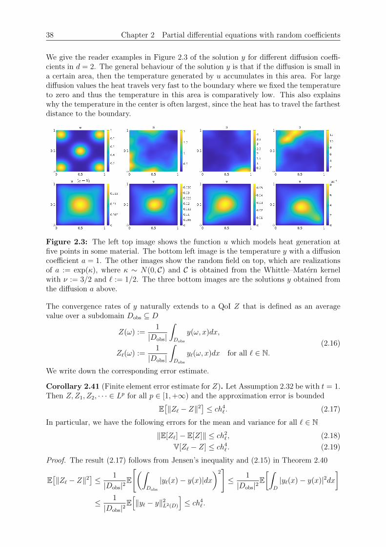
We give the reader examples in Figure 2.3 of the solution y for different diffusion coeffi-cients in d = 2. The general behaviour of the solution y is that if the diffusion is small ina certain area, then the temperature generated by u accumulates in this area. For largediffusion values the heat travels very fast to the boundary where we fixed the temperatureto zero and thus the temperature in this area is comparatively low. This also explainswhy the temperature in the center is often largest, since the heat has to travel the farthestdistance to the boundary.
Figure 2.3: The left top image shows the function u which models heat generation atfive points in some material. The bottom left image is the temperature y with a diffusioncoefficient a = 1. The other images show the random field on top, which are realizationsof a := exp(κ), where κ ∼ N(0, C) and C is obtained from the Whittle–Matern kernelwith ν := 3/2 and ` := 1/2. The three bottom images are the solutions y obtained fromthe diffusion a above.
The convergence rates of y naturally extends to a QoI Z that is defined as an averagevalue over a subdomain Dobs ⊆ D
Z(ω) :=1
|Dobs|
∫Dobs
y(ω, x)dx,
Z`(ω) :=1
|Dobs|
∫Dobs
y`(ω, x)dx for all ` ∈ N.(2.16)
We write down the corresponding error estimate.
Corollary 2.41 (Finite element error estimate for Z). Let Assumption 2.32 be with t = 1.Then Z,Z1, Z2, · · · ∈ Lp for all p ∈ [1,+∞) and the approximation error is bounded
E[‖Z` − Z‖2
]≤ ch4
` . (2.17)
In particular, we have the following errors for the mean and variance for all ` ∈ N
‖E[Z`]− E[Z]‖ ≤ ch2` , (2.18)
V[Z` − Z] ≤ ch4` . (2.19)
Proof. The result (2.17) follows from Jensen’s inequality and (2.15) in Theorem 2.40
E[‖Z` − Z‖2
]≤ 1
|Dobs|2E
[(∫Dobs
|y`(x)− y(x)|dx)2]≤ 1
|Dobs|2E[∫
D
|y`(x)− y(x)|2dx]
≤ 1
|Dobs|2E[‖y` − y‖2
L2(D)
]≤ ch4
` .
Chapter 2 Partial differential equations with random coefficients 39
We show (2.18) by pulling out the expectation, using Jensen’s inequality and (2.17)
‖E[Z`]− E[Z]‖2 ≤ E[‖Z` − Z‖2
]≤ ch4
` .
We use the fact that E[Z` − Z] is the deterministic constant that minimizes the quadraticdeviation from Z` − Z and use (2.17) to show (2.19)
V[Z` − Z] = E[‖Z` − Z − E[Z` − Z]‖2
]= min
µ∈RE[‖Z` − Z − µ‖2
]≤ E
[‖Z` − Z − 0‖2
]≤ ch4
` .
Numerical implementation. We outline how to numerically compute a solutiony`(ω) ∈ V FE
` of (2.14). Let (ϕn)Nn=1 be any finite dimensional basis of V FE` and express
the solution of y`(ω) as linear combination of the basis functions of this space
y`(ω) =N∑n=1
βn(ω)ϕn.
Then test (2.14) with all test functions ϕn ∈ V FE` to obtain the pathwise linear system of
equations of the form such that for P–almost all ω ∈ Ω
A(ω)β(ω) = b. (2.20)
The stiffness matrix A(ω) is then
A(ω) := (Anj(ω))Nn,j=1 := ((a(ω)∇ϕn,∇ϕj)L2(D))Nn,j=1 ∈ RN×N . (2.21)
The right–hand side or load vector b is given as follows
b := (bn)Nn=1 := ((u, ϕn)L2(D))Nn=1 ∈ RN . (2.22)
The solution solution vector β(ω) ∈ RN is the vector of coefficients for y`(ω) satisfying(2.20)
β(ω) := (βn(ω))Nn=1 ∈ RN .
It is often required to compute the L2(D)-norm of y` which can be achieved with the helpof the mass matrix
M := (Mnj)Nn,j=1 := ((ϕn, ϕj))
Nn,j=1
such that ‖y`‖2L2(D) = βTMβ.
Remark 2.42 (Quadrature rules). It is often necessary to use a quadrature rule to com-pute the stiffness matrix A in (2.21) and the load vector b in (2.22). This introducesadditional errors that may worsen the error rates of Theorem 2.40 if a(ω) is not suffi-ciently smooth, see [26, Section 3.3].
Remark 2.43 (Errors in the diffusion coefficient). We also replace the diffusion coefficienta by a truncated KLE in our numerical experiments. We do not state the error that getsintroduced from using a truncation and instead refer to Charrier [25, 26].
We summarize the method to compute samples of y`. First, we have to compute theKLE of the diffusion coefficient such that we are able to cheaply generate samples of a.Afterwards, we obtain a single sample by the following steps:
40 Chapter 2 Partial differential equations with random coefficients
1. Compute a realization of the diffusion coefficient a(ω).
2. Compute the stiffness matrix A(ω) according to (2.21) using some quadrature rule.
3. Compute the load vector b according to (2.22) using some quadrature rule.
4. Solve the system (2.20) to obtain the coefficients β(ω) of y`(ω) ∈ V FE` .
The most expensive step is often to solve the system (2.20). In particular, if the basisfunctions (ϕn)Nn=1 have full support over D, then A(ω) is a dense matrix and thus the coststo directly solve the system (2.20) is of order O(N3). A standard method to reduce thecomplexity is to use the nodal basis, which are functions that have local support. Thenthe stiffness matrix A is sparse, which allows us to efficiently solve the system (2.20).Multigrid methods [137, Section 3] are able to compute a solution with accuracy ε withcosts O(N log(ε)), which is optimal up to logarithmic factors.We remark that we view two solutions on two different grids y`1 and y`2 as functions inH1
0 (D). This ensures, for example, that the expression y`1 − y`2 is well defined, howeverthe corresponding expression for the vectors β`1 − β`2 is in general not well defined. Weovercome this obstacle if V FE
`1⊆ V FE
`2with a linear prolongation operator PFE
`2,`1such that
PFE`2,`1
y`1 are the coefficients of y`1 in the nodal basis of V FE`2
. That is, the coefficients ofthe difference y`1 − y`2 in the nodal basis of V FE
`2is computed as follows
PFE`2,`1
β`1 − β`2 .
Chapter 3 Estimation and variance reduction 41
Chapter 3
Estimation and variance reduction
The goal of this chapter is to give an overview for the approximation of the mean of arandom variable Z ∈ L2
E[Z] =
∫Ω
Z(ω)dP(ω). (3.1)
We divide quadrature methods into deterministic and sampling based quadrature and listcommon methods for both.
Deterministic quadrature: These methods often discretize P and approximate (3.1)as a weighted sum of evaluations of Z at quadrature points. Classical quadraturerules like the trapezoidal rule or Gaussian quadrature (see [35, Chapter 5] or [38])work well in one dimension and reach a high accuracy. The straightforward extensionto multiple dimensions is called tensor product quadrature and applies these rules forevery dimension. This is prohibitively expensive in high dimensions, since the costis exponential in the number of dimensions. A potential improvement are sparsegrids [24] where we do not use a full tensor grid but only a carefully chosen subset ofgrid points. In the context of random PDEs this is often combined with collocationmethods [102]. Sparse grids require mixed regularity of the integrand w.r.t. thedimensions, which may not always be satisfied. The stochastic Galerkin method [55]or [92, Chapter 9] discretizes the probability space with the help of polynomials. Theapproach is similar to the finite element discretization of H1
0 (D) and may result ina high dimensional problem. The drawback of this method is that it requires thesolution of a large linear system and is intrusive. Another well–known approach isquasi-Monte Carlo [46], [90, Section 5,6], which uses the same quadrature weights asMonte Carlo with deterministic evaluation points obtained from a low-discrepancysequence. This also requires the reformulation of (3.1) as integral over Rs.
Sampling based quadrature: These methods combine samples of Z. We explain gen-eral results and introduce some common notation in Section 3.1. We examine theclassical Monte Carlo estimator in Section 3.2 adapted for the PDE setting withrandom coefficients. Control Variates are a variance reduction technique and westudy them in Section 3.3. The specific implementations of Control Variates areMultifidelity Monte Carlo in Section 3.4 and Approximate Control Variates in Sec-tion 3.5. Another popular variance reduction method in the context of hierarchicalmodels is Multilevel Monte Carlo in Section 3.6. We finish this chapter with a briefreview of other sampling based methods in Section 3.7.
The thesis is mainly concerned with sampling based quadrature and we do not treatdeterministic quadrature any further. Most results in this chapter are well known and arepetition or reformulation adapted for the goal (3.1). Throughout the rest of thesis if notmentioned otherwise, we assume that Z is a real–valued random variable. Furthermore,we assume that Z ∈ L2 such that Z has finite first and second moments. Generalizationsfor Z ∈ L1 with Z 6∈ L2 are possible but complicate the analysis. For example, thestrong law of large numbers [79, Theorem 5.17] shows that the sample average converges
42 Chapter 3 Estimation and variance reduction
almost surely to the mean under the weak assumption Z ∈ L1. However, for a rate ofconvergence w.r.t. the number of samples we require higher regularity and Z ∈ L2 issufficient to obtain a usable rate.We call the next assumption General Assumption, since we assume it throughout thethesis without further mentioning it.
General Assumption 3.1. Let Z,Z1, Z2, . . . , ZL ∈ L2 be real–valued random variablesand let Z` have positive cost w` > 0 for all ` ∈ 1, . . . , L.
Challenges. Let us briefly demonstrate the challenges that arise for the computationof the mean of a random variable.
Example 3.2 (Diffusion process). Let us define the QoI as in (2.16)
Z(ω) :=1
|Dobs|
∫Dobs
y(a(ω), x)dx,
where Dobs ⊆ D and y is a pathwise weak solution of the elliptic PDE in Definition 2.31with diffusion coefficient
a(x, ω) :=∞∑n=1
√λnξn(ω)ψn(x). (3.2)
We denote the truncation of this expansion at N with aN and obtain an approximationof the integral
E[Z] =
∫Ω
Z(a(ω))dP(ω) ≈∫RNZ(aN(y))pN(y)dy,
where pN is the probability density function of the random vector (ξ1, . . . , ξN)T . We arenot able to compute the solution y or Z analytically and thus replace them with theapproximation ZL ≈ Z
E[Z] ≈∫RNZ(aN(y))pN(y)dy ≈
∫RNZL(aN(y))pN(y)dy. (3.3)
We list the three main challenges to compute the mean and list reasons why we shouldbe able to overcome them.
Curse of dimensionality: The probability space is often high–dimensional, e.g. in(3.3) of dimension N , and thus requires high-dimensional quadrature. The curse ofdimensionally describes the phenomena that the costs grow rapidly or exponentiallyw.r.t. the dimension N of the stochastic space. However, as Lemma 2.28 shows theerror of dropping the random variable ξn from the KLE in (3.2) is small if n is large,which translates to a small error for Z. Although the original problem (3.1) requiresthe evaluation of an infinite dimensional integral, the effect of large dimensions non Z decays. This intuition is formalized with the variance since V[Z] < +∞ isbounded independently of the truncation index N .
Discretization: We have approximations Z1, Z2, . . . of Z at varying degrees ofaccuracy. In Example 3.2 we use a finite element discretization for y and Theo-rem 2.40 shows that the error decreases depending on the mesh size h. As the
Chapter 3 Estimation and variance reduction 43
mesh size decreases the quadrature error decreases, however the required computa-tional resources increase significantly. The coarse discretizations have a larger errorthan the fine discretizations but are much cheaper to compute. Since the coarsegrids contain some information it is conceptionally advantageous to include themfor estimating the mean.
Cost balancing: The quadrature and the discretization error have to be balancedto achieve a computationally tractable solution. If the discretization is too fine weare only able to compute a few evaluations of Z` and the quadrature error of E[Z] islarge. On the other hand if the discretization Z` is coarse and cheap the quadratureerror is small but the discretization error is large. Furthermore, a method thatuses discretizations Z1, Z2, . . . with different costs and accuracies has to balance thecomputational effort between these models.
3.1 Sampling based estimation
The goal of this section is to define some common terminology and explain the reason forthe sampling based estimation of the mean. Sampling based estimators define a randomvariable µ that approximates the mean
µ ≈ E[Z].
We understand ≈ in the mean square error sense, which is the average squared deviationfrom the quantity E[Z]. We further define the bias that denotes how far E[µ] deviatesfrom E[Z]. This definition is rigorous if we assume µ ∈ L2, which is the case for allexamined estimators in this thesis.
Definition 3.3 (Bias, mean square error). We define the bias and mean square error(MSE) of an estimator µ as
Bias(µ) := Bias(µ, Z) := ‖E[µ]− E[Z]‖,MSE(µ) := MSE(µ, Z) := E
[‖µ − E[Z]‖2
],
where ‖ · ‖ is a suitable norm. We call an estimator µ unbiased if Bias(µ) = 0 and thusE[µ] = E[Z].
The bias and MSE are always defined w.r.t. the expectation E[Z] that we want to estimate.We often abbreviate Bias(µ) and MSE(µ) without the explicit Z if there is no ambiguity.It is well known that the MSE satisfies a bias-variance decomposition and is equal to thesquared bias plus the variance of the estimator. For unbiased estimators the MSE is equalto the variance.
Theorem 3.4 (Bias-variance decomposition). The MSE admits the decomposition
MSE(µ) = Bias(µ)2 + V[µ].
In particular, for unbiased estimators µ the MSE is equal to the variance
MSE(µ) = V[µ].
44 Chapter 3 Estimation and variance reduction
Proof. We insert E[µ] and use the properties of the inner product
E[‖µ − E[Z]‖2
]= E[‖µ − E[µ] + E[µ]− E[Z]‖2]
= E[‖E[µ]− E[Z]‖2
]+ E
[‖µ − E[µ]‖2
]+ 2E[(µ − E[µ],E[µ]− E[Z])].
The first term is the squared bias and the second term is the variance of the estimatorµ. For the third term we use the linearity of the inner product in the first argument andpull in the expectation. We then conclude that this term is zero.
The bias-variance decomposition leads to a bound on the probability that µ deviatesfrom the mean E[Z]. Both the bias and the variance is small if the MSE is small and anapplication of Chebychev’s inequality in Theorem 2.21 then bounds this probability.
Theorem 3.5 (MSE bound for probability of deviation). For all positive ε with ε2 ≥4 MSE(µ) the probability that µ deviates from E[Z] is bounded by
P(‖µ − E[Z]‖ > ε) ≤ 4
ε2MSE(µ). (3.4)
Proof. We insert E[µ] and use the triangle inequality
‖µ − E[Z]‖ ≤ ‖µ − E[µ]‖+ Bias(µ).
The expression on the left has equal or smaller probability to exceed ε than the expressionon the right
P(‖µ − E[Z]‖ > ε) ≤ P(‖µ − E[µ]‖+ Bias(µ) > ε). (3.5)
We use Theorem 3.4 and MSE(µ) ≤ ε2/4 to bound the bias
Bias(µ) ≤ (Bias(µ)2 + V[µ])1/2 = MSE(µ)1/2 ≤ ε/2.
We combine this with Chebychev’s inequality in Theorem 2.21 and V[µ] ≤ MSE(µ) fromTheorem 3.4 to conclude (3.4)
P(‖µ − E[µ]‖+ Bias(µ) > ε) ≤ V[µ]
(ε− Bias(µ))2≤ 4
ε2MSE(µ).
The previous theorem allows us to derive confidence intervals for the estimation of themean. It further allows us to upper bound the required MSE such that we do not deviatemore than ε from the mean E[Z] with some prescribed probability δ.
Example 3.6 (Confidence intervals). We determine the deviation ε > 0 such that for aprescribed confidence δ ∈ (0, 1)
P(µ ∈ [−ε+ E[Z],E[Z] + ε]) ≥ δ.
This is equivalent to demand that
P(‖µ − E[Z]‖ > ε) ≤ 1− δ. (3.6)
The use of (3.4) now gives the smallest deviation ε = 2(MSE(µ)/(1− δ))1/2.
Chapter 3 Estimation and variance reduction 45
Example 3.7 (Target MSE). Let the deviation ε > 0 and confidence level δ ∈ (0, 1) befixed. We want to determine MSE(µ) to ensure that
P(µ ∈ [−ε+ E[Z],E[Z] + ε]) ≥ δ.
Similarly to Example 3.6 we obtain (3.6) and thus (3.4) shows
1− δ ≥ 4
ε2MSE(µ).
Therefore the estimator µ has to satisfy MSE(µ) ≤ (1− δ)ε2/4.
It is of course possible to improve these estimates if more knowledge of the underlyingdistribution of µ is available, see [45, Chapter 8] or [42, Chapter 24, 25], [122, Chapter 10]for the Gaussian case. Improved results are often obtained from concentration inequalities,see [19].
3.2 Monte Carlo
Exact sampling. In this section we review the basic properties of the classical MonteCarlo (MC) estimator. The results are well known and available in most introductorybooks on probability theory [77, 79]. The MC estimator or the sample average plays acentral role for laws of large numbers, the central limit theorem and estimation in general.
Definition 3.8 (MC estimator). For m ∈ N the MC estimator is the sample average
µMC :=1
m
m∑i=1
Zi,
where the Zi are m i.i.d. samples of Z.
The MC estimator is unbiased and has variance inversely proportional to m. We providea proof since the used techniques are useful for other estimators.
Lemma 3.9 (Bias, variance of MC estimator). The MC estimator is an unbiased estima-tor for E[Z] with variance
V[µMC
]=
V[Z]
m. (3.7)
Proof. The unbiasedness is a direct consequence of the linearity of the expectation andthat all samples have the same distribution as Z. The expression for the variance cruciallyrequires that Z1, . . . , Zm are pairwise uncorrelated
V[µMC
]=
1
m2
m∑i,j=1
Cov[Zi, Zj
]=
1
m2
m∑i,j=1
V[Zi], if i = j,
0, if i 6= j.
We use V[Zi] = V[Z] for i ∈ 1, . . . ,m to conclude (3.7).
46 Chapter 3 Estimation and variance reduction
The convergence rate for the MC estimator is thus of order O(m−1/2) for the root meansquare error (RMSE)
RMSE(µMC) := MSE(µMC)1/2 =V[Z]1/2
m1/2.
The rate O(m−1/2) is rather slow compared to deterministic quadrature. However, theconvergence rate is independent of the dimension of the underlying probability space, doesnot suffer from the curse of dimensionality and does not require any regularity assumptionsexcept for Z ∈ L2.The cost to evaluate the MC estimator is the cost of a single samples times the number ofsamples. A consequence of Lemma 3.9 is that to half the RMSE we have to increase thenumber of samples by a factor of four. This also increases the cost by a factor of four.
Corollary 3.10 (Exact sampling cost). The cost to achieve MSE(µMC) ≤ ε2 is
W[µMC
]= mW[Z] =
1
ε2V[Z]W[Z] = O(ε−2). (3.8)
We did not include the practically necessary ceiling of m in (3.8) since
m =1
ε2V[Z]
is typically not an integer. We continue to do so throughout the rest of this thesis andonly mention the additional costs for ceiling if the obtained results are different. Weremark that sampling based methods often require a lot of evaluations and thus ceilingthe number of samples does not significantly increase the overall costs.
Discretized sampling. Corollary 3.10 makes the strong assumption that we are able togenerate samples from the true QoI Z, which is often not possible. Therefore let Z1, Z2, . . .be a sequence of model discretizations such that the mean converges E[Z`] → E[Z] for` → +∞. The bias-variance decomposition of the MSE now guides us how to proceed.First, select an appropriate fine level L such that the bias is smaller than a prescribedthreshold. Afterwards apply the standard MC estimator for ZL with enough samplesto sufficiently decrease the variance. We denote this estimator with µMC
L and provide awell–known result which is proved similarly to [56, Theorem 3.1].
Theorem 3.11 (Asymptotic cost). Assume that for all ` ∈ N the bias, variance and costsof the models Z` satisfy
Bias(Z`) ≤ c2−γBias`, (3.9)
V[Z`] ≤ c, (3.10)
w` ≤ c2γCost`. (3.11)
Then for all ε ∈ (0, 1/e] there exists a fine level L ∈ N and a number of samples m ∈ Nsuch that the cost to achieve MSE(µMC
L ) ≤ ε2 is bounded
W[µMCL
]≤ cε−2−γCost/γBias . (3.12)
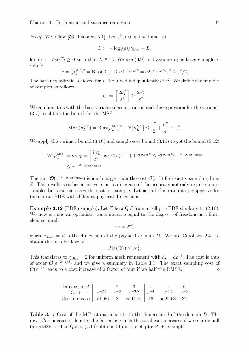
Chapter 3 Estimation and variance reduction 47
Proof. We follow [56, Theorem 3.1]. Let ε2 > 0 be fixed and set
L := − log2(ε)/γBias + L0
for L0 := L0(ε2) ≥ 0 such that L ∈ N. We use (3.9) and assume L0 is large enough tosatisfy
Bias(µMCL )2 = Bias(ZL)2 ≤ c2−2γBiasL = c2−2γBiasL0ε2 ≤ ε2/2.
The last inequality is achieved for L0 bounded independently of ε2. We define the numberof samples as follows
m :=
⌈2σ2
L
ε2
⌉≥ 2σ2
L
ε2.
We combine this with the bias-variance decomposition and the expression for the variance(3.7) to obtain the bound for the MSE
MSE(µMCL ) = Bias(µMC
L )2 + V[µMCL
]≤ ε2
2+σ2L
m≤ ε2.
We apply the variance bound (3.10) and sample cost bound (3.11) to get the bound (3.12)
W[µMCL
]= mwL =
⌈2σ2
L
ε2
⌉wL ≤ c(ε−2 + 1)2γCostL ≤ c2γCostL0ε−2−γCost/γBias
≤ cε−2−γCost/γBias .
The cost O(ε−2−γCost/γBias) is much larger than the cost O(ε−2) for exactly sampling fromZ. This result is rather intuitive, since an increase of the accuracy not only requires moresamples but also increases the cost per sample. Let us put this rate into perspective forthe elliptic PDE with different physical dimensions.
Example 3.12 (PDE example). Let Z be a QoI from an elliptic PDE similarly to (2.16).We now assume an optimistic costs increase equal to the degrees of freedom in a finiteelement mesh
w` = 2d`,
where γCost = d is the dimension of the physical domain D. We use Corollary 2.41 toobtain the bias for level `
Bias(Z`) ≤ ch2` .
This translates to γBias = 2 for uniform mesh refinement with h` = c2−`. The cost is thusof order O(ε−2−d/2) and we give a summary in Table 3.1. The exact sampling cost ofO(ε−2) leads to a cost increase of a factor of four if we half the RMSE.
Dimension d 1 2 3 4 5 6Cost ε−2.5 ε−3 ε−3.5 ε−4 ε−4.5 ε−5
Cost increase ≈ 5.66 8 ≈ 11.31 16 ≈ 22.63 32
Table 3.1: Cost of the MC estimator w.r.t. to the dimension d of the domain D. Therow “Cost increase” denotes the factor by which the total cost increases if we require halfthe RMSE ε. The QoI is (2.16) obtained from the elliptic PDE example.
48 Chapter 3 Estimation and variance reduction
Variance reduction. We outline the main idea for many variance reduction techniques.The cost of the MC estimator (3.8) is proportional to the variance V[Z] and we try todecrease this term without increasing the overall costs to much. As an example, let Y bea random variable with mean zero such that the MC estimator of Z − Y is an unbiasedestimator for E[Z]. The costs to achieve a MSE of ε2 are
W
[1
m
m∑i=1
(Zi − Y i)
]=
V[Z − Y ]
ε2W[Z, Y ],
where W[Z, Y ] is the cost to compute a sample of (Z, Y ). The cost compared to thestandard MC estimator is reduced significantly if
V[Z − Y ]W[Z, Y ] V[Z]W[Z].
This happens if Z ≈ Y and the cost to compute a sample of Y is much cheaper than Z.This approach is sensible since Y carries a lot of information required to compute E[Z]and we already know E[Y ] = 0. We give a mathematically rigorous interpretation laterin Chapter 4. In any case, the estimators in the following sections all use some variationof this basic idea to construct a cheaper estimator.
3.3 Control Variates
Single control variates. The method of control variates is a well–known variancereduction technique and results of this section are available in [59, 60, 88, 123]. We startwith the single control variate (CV) estimator and introduce multiple control variateslater in this section. To construct the CV estimators we assume that the expectationsµ1, . . . , µL−1 are known.
Definition 3.13 (Single CV estimator). For m ∈ N and β ∈ R the CV estimator isdefined as
µCVL :=
1
m
m∑i=1
ZiL − β
(1
m
m∑i=1
ZiL−1 − µL−1
).
We call the random variable ZL−1 control variate.
The β does not influence the bias of the estimator, only its variance. Since we want toobtain an estimator that minimizes the MSE it makes sense to choose a β such that thevariance is as small as possible. It turns out that the optimal value for β is unique undermild assumptions and independent of the number of samples.
Lemma 3.14 (Bias, variance). The CV estimator is an unbiased estimator for µL withvariance
V[µCVL
]=σ2L − 2βCL,L−1 + β2σ2
L−1
m. (3.13)
For σ2L−1 > 0 the variance minimizing coefficient is unique
β∗ =CL,L−1
σ2L−1
(3.14)
and the variance for this minimizer is
V[µCVL
]= (1− ρ2
L−1,L)σ2L
m. (3.15)
Chapter 3 Estimation and variance reduction 49
Proof. The unbiasedness of µCVL is obvious. The result (3.13) follows from the variance of
sums of independent random variables in Lemma 2.18. The variance (3.13) as function ofβ is a parabola with positive leading coefficient since σ2
L−1 > 0. Elementary calculus nowshows (3.14) and (3.15).
The variance of the CV estimator is never larger than the variance of the MC estimator,since ρL,L−1 ∈ [−1, 1] in (3.15), however, we have the additionally cost to compute asample of ZL−1. The next corollary states that the CV estimator improves the standardMC estimator in terms of the computational cost if the squared correlation is large enoughor the coarse model is cheap.
Corollary 3.15 (Cost). The cost of the single CV estimator to achieve MSE(µCVL ) ≤ ε2
is
W[µCVL
]=σ2L
ε2(1− ρ2
L,L−1)(wL + wL−1).
Furthermore, the cost ratio w.r.t. the MC estimator satisfies
W[µCVL
]W[µMC
L ]= (1− ρ2
L,L−1)
(1 +
wL−1
wL
).
The CV estimator is an improvement compared to the MC estimator if the conditionwL−1 < ρ2
L,L−1(wL−1 + wL) is satisfied.
Proof. The result follows from Lemma 3.9 and Lemma 3.14.
Multiple Control Variates. The results for a single CV estimator easily generalizeto multiple control variates. The basic idea is to form a linear combination of the coarsemodels Z1, . . . , ZL−1.
Definition 3.16 (Multiple CV estimator). For m ∈ N and β ∈ RL−1 the (multiple) CVestimator is
µCVL :=
1
m
m∑i=1
ZiL −
L−1∑`=1
β`
(1
m
m∑i=1
Zi` − µ`
).
We call the random variables Z1, . . . , ZL−1 control variates.
The properties of this estimator are similar to the single CV estimator in Lemma 3.14.We again want to choose β such that the variance is minimized, which yields a quadraticminimization problem. The variance minimizer is again independent of the number ofsamples.
Lemma 3.17 (Bias, variance). Let I := 1, . . . , L − 1 be the index set of the controlvariates. The CV estimator is an unbiased estimator for µL with variance
V[µCVL
]=σ2L − 2CL,Iβ + βTCI,Iβ
m. (3.16)
For positive definite CI,I the unique minimizer for the variance is
β∗ = C−1I,ICI,L. (3.17)
The variance for this minimizer is
V[µCVL
]=
1
m
(σ2L − CL,IC−1
I,ICI,L). (3.18)
50 Chapter 3 Estimation and variance reduction
Proof. The proof is a straightforward extension of the proof of Lemma 3.14 to multipledimensions.
Let us comment on the assumption that CI,I is positive definite and thus invertible. Thisis necessary for the uniqueness of a minimizer β∗. If CI,I is not positive definite then
Lemma 2.16 shows there exist coefficients β ∈ RL−1 such that
L−1∑`=1
β`(Z` − µ`) = 0.
Therefore we may w.l.o.g. remove the last control variate ZL−1 from the CV estimator
µCVL :=
1
m
m∑i=1
ZiL −
L−2∑`=1
β`
(1
m
m∑i=1
Zi` − µ`
).
We repeat this process until the remaining control variates I ′ ( 1, . . . , L − 1 satisfythat CI′,I′ is positive definite or I = ∅. A minimizer β∗ for the original problem is thus
β∗` =
eT` C
−1I′,I′CI′,L, if ` ∈ I ′,
0, if ` 6∈ I ′.
In this case the minimizer may not be unique, since linear dependence allows us to eitherremove at least two different control variates from I or Z` = µ` almost surely. In thelatter case β∗` may be chosen arbitrarily.Let us comment on the expression for the minimal variance (3.18). We write down thecovariance matrix C in block form
C =
(σ2L CL,I
CI,L CI,I
).
Then (3.18) without the factor 1/m is the Schur complement [61, Chapter 3] of the blockCI,I of the covariance matrix
C/CI,I := σ2L − CL,IC−1
I,ICI,L.
The multiple CV estimator reduced the variance compared to the MC estimator if theSchur complement is small enough and the coarse models are cheap. We obtain a resultthat is similar to Corollary 3.15.
Corollary 3.18 (Cost). Let I := 1, . . . , L − 1 and CI,I be positive definite. Then thecost to achieve V
[µCVL
]≤ ε2 is
W[µCVL
]=
1
ε2(C/CI,I)
L∑`=1
w`.
Furthermore, the cost ratio w.r.t. the MC estimator is
W[µCVL
]W[µMC
L ]=
(C/CI,Iσ2L
) L∑`=1
w`wL
.
Proof. The corollary follows from Lemma 3.17.
Chapter 3 Estimation and variance reduction 51
Lower variance bound. Let us now assume that we have an infinite amount of samplesavailable for Z1, . . . , ZL−1 but only m samples of ZL. This fits in the setting of controlvariates since by the strong law of large numbers [79, Section 5.3] we may assume thatµ1, . . . , µL−1 are known. Formally, for n → +∞ we have convergence in the almost suresense of the sample average to the mean
1
n
n∑i=1
Zi` → µ`.
This situation occurs in practice if we have a time limit for an expensive but fast computerallowing us to sample only m times from the high fidelity model ZL. Later we may samplemore often the coarser models Z1, . . . , ZL−1 on a slower computer such that the error forthe approximation of µ1, . . . , µL−1 is negligible. Another situation where this occurs isif the samples of ZL are expensive real life experiments and samples of Z1, . . . , ZL−1 aresimulations by a computer. We first assume that we only have a single sample m = 1 ofthe high fidelity model.
Definition 3.19 (Lower variance bound of an estimator). We define the lower variancebound for an estimator µ with a single evaluation mL := 1 of ZL as
Vmin[µ] := limm1,...,mL−1→+∞
V[µ],
where m1, . . . ,mL−1 denotes the number of i.i.d. realizations of Z1, . . . , ZL−1.
The restriction to a single high fidelity sample mL = 1 is often not severe, since theestimators in this thesis have the property that the lower variance bound for arbitrarymL translates to Vmin[µ]/mL.The MC estimator is special in the sense that it does not use any coarse grid samples.Therefore, the lower variance bound for MC is the variance of the high fidelity model
Vmin[µMCL ] = σ2
L.
We use (3.18) to conclude that the Schur complement is the lower variance bound for theCV estimators such that with I := 1, . . . , L− 1 and J := I ∪ L
V[µCVL
]= σ2
L − CL,IC−1I,ICI,L = CJ,J/CI,I .
In Chapter 4 we formally prove that V[µCVL
]is the minimal variance that is achievable
by any linear unbiased estimator of µL with only a single sample of ZL and an infiniteamount of samples of Z1, . . . , ZL−1.
Definition 3.20 (Lower variance bound). Let I ⊆ 1, . . . , L−1 such that CI,I is positivedefinite. Then for J := I∪L we define the lower variance bound or maximally achievablevariance reduction as the Schur complement
VminI := V
[µCVL
]= σ2
L − CL,IC−1I,ICI,L = CJ,J/CI,I ,
where the CV estimator µCVL uses a single sample m = 1 and control variates ZI1 , . . . , ZI|I| .
52 Chapter 3 Estimation and variance reduction
The CV estimator should achieve a larger variance reduction with more control variates.Every additional model Z` allows us to choose the corresponding parameter β` 6= 0.Therefore, the new estimator has more degrees of freedom which translates to an equalor smaller variance. The lower variance bounds Vmin are therefore non–increasing if weinclude more and more models.
Lemma 3.21 (Lower variance bound ordering). For I ⊆ 1, . . . , L − 1 and J ⊆ I thelower variance bound satisfies
VminI ≤ Vmin
J . (3.19)
Proof. Let us denote the CV estimator with control variates indices in I with µCVL [I] with
coefficients β. We do the same with for J with µCVL [J ] with coefficients α. We use (3.16)
and use the optimality of the coefficients to conclude
VminI = V
[µCVL [I]
]= min
β∈R|I|σ2L − 2CL,Iβ + βTCI,Iβ
VminJ = V
[µCVL [J ]
]= min
α∈R|J|σ2L − 2CL,Jα + αTCJ,Jα.
It is crucial to observe that J ⊆ I and thus the first optimization problem simply min-imizes over more coefficients. We fix β` = 0 for all ` ∈ I \ J to obtain the secondoptimization problem
minβ∈R|I|
σ2L − 2CL,Iβ + βTCI,Iβ ≤ min
β∈R|I|,β`=0 if `∈I\J
σ2L − 2CL,Iβ + βTCI,Iβ
= minα∈R|J|
σ2L − 2CL,Jα + αTCJ,Jα
and the result (3.19) now follows.
It is possible to extend the notion of a lower variance bound for multiple models, even ifthey are not high fidelity.
Remark 3.22 (Lower variance bound for multiple models). We define the set of modelsQ ⊆ 1, . . . , L as the models that are evaluated once and I ⊆ 1, . . . , L as the modelsthat we evaluate infinitely often. Then with J := Q ∪ I the covariance of the vector ofestimators (µCV
` )`∈Q with correlated samples satisfies
Covmin := Cov[(µCV
` )`∈Q, (µCV` )`∈Q
]= CJ,J/CI,I ∈ R|Q|×|Q|.
Since Covmin is however a matrix and not single number, it is not clear what a lowerbound in this context means. It is possible to reduce this (often) positive definite matrixto a single number via the trace(Covmin) or by looking at a specific linear combinationβTCovminβ.
Problems of the CV estimator. The CV estimator requires us to know the expecta-tion of the control variates µ1, . . . , µL−1. These values are often unavailable and we needto estimate them. Therefore, we could again devise a CV estimator.
Example 3.23 (Three level nested CV estimator). For the purpose of this example definethe CV estimator for µ1 as the MC estimator
µCV1 :=
1
m1
m1∑i=1
Zi1.
Chapter 3 Estimation and variance reduction 53
We then define an approximation for the CV estimator for µ2 such that
µCV2 =
1
m2
m2∑i=1
Zi2 − β1
(1
m2
m2∑i=1
(Zi1 − µCV
1 )
).
Now we continue with the third level
µCV3 =
1
m3
m3∑i=1
Zi3 −
2∑`=1
β`
(1
m3
m3∑i=1
(Zi` − µCV
` )
).
The example shows that there are a several degrees of freedom and choices to make.
We may choose the coefficients β for both estimators µCV2 and µCV
3 to dependent oneach other.
We want to distribute the number of samples m1,m2,m3 to achieve a small variance.
It is unclear how to choose the independence structure of the random variables, i.e.it might make sense to use independent samples to estimate µCV
1 and µCV2 , but not
for µCV3 .
It is trivial to generalize this estimator for more levels, however, the optimality ofthis approach is not clear.
The Multifidelity Monte Carlo method in Section 3.4 and Approximate Control Variatemethod in Section 3.5 both estimate µL in similar fashion shown in Example 3.23.
3.4 Multifidelity Monte Carlo
We continue with the Multifidelity Monte Carlo (MFMC) estimator in [107]. This methodassumes that the mean values µ1, . . . , µL−1 of the control variates are unknown and haveto be estimated. The MFMC estimator is a CV estimator with a specific number ofsamples m and independence of the realizations.
Definition 3.24 (MFMC estimator). For m1, . . . ,mL ∈ N and β ∈ RL−1 we define theMFMC estimator
µMFMCL :=
1
mL
mL∑i=1
ZiL −
L−1∑`=1
β`
(1
m`+1
m`+1∑i=1
Zi` −
1
m`
m∑i=1
Zi`
). (3.20)
Similar to the CV estimator we want to choose β and m such that the variance of theestimator is minimized. As it turns out, the optimal choice of β is independent of thechoice of m allowing us to optimize them separately. The next lemma optimizes the βand is a summary of the results of Section 3 from [107]. We simplify the notation andabbreviate ρL,0 := 0.
54 Chapter 3 Estimation and variance reduction
Lemma 3.25 (Bias, variance [107, Section 3]). Let m1 ≥ · · · ≥ mL and assume σ2` > 0
for all ` ∈ 1, . . . , L. Then the MFMC estimator is an unbiased estimator for µL withvariance
V[µMFMCL
]=
σ2L
mL
+L−1∑`=1
(1
m`+1
− 1
m`
)(−2β`CL` + β2
`σ2` ). (3.21)
A variance minimizer β∗ ∈ RL−1 is
β∗` = CL`/σ2` for all ` ∈ 1, . . . , L− 1 (3.22)
and the minimal variance satisfies
V[µMFMCL
]= σ2
L
L∑`=1
ρ2L,` − ρ2
L,`−1
m`
. (3.23)
Proof. The proof is scattered throughout Section 3 of [107]. The unbiasedness followsdirectly from the linearity of the expectation. The result in (3.21) is a straightforwardcalculation done in [107, Lemma 3.2, Lemma 3.3]. A step in the proof is to compute
Cov
[1
m`
m∑i=1
Zi`,
1
mj
mj∑i=1
Zij
]=
1
maxm`,mjC`,j.
The assumption m1 ≥ · · · ≥ mL is then used to obtain the easier manageable form (3.21).The proof of (3.22) is given in [107, Theorem 3.4]. We use m1 ≥ · · · ≥ mL to ensure thatthe expression (
1
m`+1
− 1
m`
)≥ 0
is non–negative for all ` ∈ 1, . . . , L− 1. W.l.o.g. we may assume that this expression islarger than zero, otherwise the value of β` does not influence the variance in (3.21) andwe may choose β∗` = CL`/σ
2` as in (3.22). For σ2
` > 0 equation (3.21) as function of β isa sum of L − 1 parabolas with positive leading factor. We separately minimize them toobtain the unique minimizer
β∗` = CL`/σ2` for all ` ∈ 1, . . . , L− 1.
Inserting this optimal β∗ into (3.21) then leads to (3.23).
The condition m1 ≥ · · · ≥ mL is often satisfied for hierarchical models, where we requirefew evaluations of the high fidelity model and allow for more evaluations of the coarsermodels. Furthermore, σ2
` > 0 is a mild assumption, since σ2` = 0 implies that Z` is almost
surely constant and thus CL` = 0. The corresponding term in (3.21) is then zero andwe remove Z` from the estimator. The minimizer β∗ is unique if the stricter inequalitym1 > · · · > mL is satisfied. This is desirable since for mj+1 = mj the terms associatedwith the control variate Zj are zero and we remove this model
µMFMCL =
1
mL
mL∑i=1
ZiL −
L−1∑`=1
β`
(1
m`+1
m`+1∑i=1
Zi` −
1
m`
m∑i=1
Zi`
)
=1
mL
mL∑i=1
ZiL −
L−1∑`=1,` 6=j
β`
(1
m`+1
m`+1∑i=1
Zi` −
1
m`
m∑i=1
Zi`
).
Chapter 3 Estimation and variance reduction 55
Sample allocation. We now answer the question how to optimally allocate the numberof samples m` for every level `. The goal is to minimize the variance not exceeding a fixedcomputational budget Wbudget > 0. The MFMC estimator requires m` samples of Z`and each sample incurs costs of w` > 0. This is formalized in the following relaxedoptimization problem, where we allow fractional samples:
minm1,...,mL∈R
J(m) := V[µMFMCL
]= σ2
L
L∑`=1
ρ2L,` − ρ2
L,`−1
m`
such thatL∑`=1
m`w` = Wbudget,
m` ≥ m`+1 for all ` ∈ 1, . . . , L− 1,mL ≥ 0.
(3.24)
We use the ordering constraints to apply (3.23) of Lemma 3.25 which ensures that theexpression for V
[µMFMCL
]is valid. The budget constraint
L∑`=1
m`w` ≤Wbudget
is satisfied with equality at a minimizer, otherwise we could linearly scale up m1, . . . ,mL
to further reduce the variance. We include this constraint as equality constraint, sincethese are easier to handle than inequality constraints in convex optimization.
Theorem 3.26 (Optimal sample allocation [107, Theorem 3.4, Corollary 3.5]).Let σ2
` > 0 for ` ∈ 1, . . . , L and assume the ordering
ρ2L,1 < · · · < ρ2
L,L. (3.25)
Furthermore, let the costs and correlations satisfy
w`+1(ρ2L,` − ρ2
L,`−1) > w`(ρ2L,`+1 − ρ2
L,`) (3.26)
for all ` ∈ 1, . . . , L − 1. Then the unique variance minimal sample allocation m∗ of(3.24) satisfies
m∗` =Wbudget∑L
j=1
(wj(ρ2
L,j − ρ2L,j−1)
)1/2
(ρ2L,` − ρ2
L,`−1
w`
)1/2
(3.27)
for all ` ∈ 1, . . . , L. The variance for this optimal sample allocation satisfies
V[µMFMCL
]=
σ2L
Wbudget
(L∑`=1
(w`(ρ
2L,` − ρ2
L,`−1))1/2
)2
. (3.28)
Proof. A detailed proof is given in [107, Theorem 3.4]. The assumptions (3.25) and (3.26)are used to ensure that the constraint m1 ≥ · · · ≥ mL is satisfied with strict inequalityat the optimum m∗. Then (3.24) is minimized using basic convex optimization.
56 Chapter 3 Estimation and variance reduction
The variance V[µMFMCL
]is inversely proportional to Wbudget. This allows us to compare
the cost to the MC estimator similar to Corollary 3.18 for the CV estimator. The maindifference is that the variance reduction of the MFMC estimator only depends on thecorrelations between the high fidelity model and the low fidelity models ρL,1, . . . , ρL,L−1
but no correlation between two low fidelity models. In contrast, the CV estimator dependson the Schur complement of C, which takes other correlations into account.
Lemma 3.27 (Cost). Let the assumptions of Theorem 3.26 be true. Then the cost toachieve V
[µMFMCL
]≤ ε2 is
W[µMFMCL
]=σ2L
ε2
(L∑`=1
(w`(ρ
2L,` − ρ2
L,`−1))1/2
)2
. (3.29)
Moreover, the cost compared to the MC estimator satisfies
W[µMFMCL
]W[µMC
L ]=
(L∑`=1
(w`wL
(ρ2L,` − ρ2
L,`−1)
)1/2)2
. (3.30)
Proof. The proof is a straightforward application of Theorem 3.26.
Graph based model selection. We have to devise an algorithm to ensure that theassumptions of Theorem 3.26 are satisfied. Furthermore, we want to select or order themodels in such a way that the cost of the estimator is minimized. This problem is calledmodel selection problem.
Definition 3.28 (Model selection problem). The model selection problem for MFMC isa minimization problem
minP
J(P ) :=
|P |∑`=1
(wP`(ρ
2L,P`− ρ2
L,P`−1))1/2
, (3.31)
where P = (P1, P2, . . . , P|P |−1, L)T is a vector of length |P | ≤ L with P` ∈ 1, . . . , L. Wefurther require that P satisfies
σ2P`> 0 for all ` ∈ 1, . . . , |P |, (3.32)
ρ2L,P1
< · · · < ρ2L,P|P |
, (3.33)
wP`+1(ρ2L,P`− ρ2
L,P`−1) > wP`(ρ
2L,P`+1
− ρ2L,P`
) for all ` ∈ 1, . . . , |P | − 1. (3.34)
We define ρ2L,P0
:= 0.
The conditions (3.32), (3.33) and (3.34) are used to apply Lemma 3.27. The cost functionJ in (3.31) is up to a constant equal to the square root of the cost of the MFMC estimatorin (3.29). The model selection P = (L)T corresponds to the MC estimator and thus theminimizer in (3.31) is guaranteed to lead to an estimator with variance not exceeding MC.Without model selection this property is in general not true.The algorithm originally proposed by Peherstorfer [107, Algorithm 1] applies a brute forcestrategy and checks all valid P that satisfy (3.32), (3.33), (3.34). The model selection Pwith the smallest variance is then used. This strategy has costs exponential in the numberof models L.
Chapter 3 Estimation and variance reduction 57
We propose a graph based approach where we reformulate (3.31) as a shortest pathproblem. To explain the main idea we first neglect the constraints. Let Z0 be an artificialmodel with w0 := 0, Cov[ZL, Z0] := 0, σ2
0 > 0 and define edge weights
qij :=(wi(ρ
2L,i − ρ2
L,j))1/2
.
We then define the directed graph G with vertices V , edges E and edge weights Q
G := (V,E,Q), V := 0, . . . , L, E := V × V, Q := (qij)Li,j=0.
The cost of a path P from 0 to L is exactly J(P ) in (3.31). Furthermore, every pathcorresponds to a valid model selection and vice versa. Solving the model selection problemis thus equivalent to finding a shortest path in a directed graph.Let us now introduce the constraints that are all of local nature. First, if (3.32) is notsatisfied for some model Z`, then we do not add any edges to the vertex `. This ensuresthat no path from 0 to L uses this model. Condition (3.33) is satisfied for every path P ifwe only add edges (i, j) if ρ2
L,i < ρ2L,j. The constraint (3.34) is tricky since it is a condition
between three models and thus three vertices. We solve this issue by introducing anotherdimension in the vertex set of the graph such that nodes are now pairs (i, j). We thenintroduce edges of the form ((i, j), (j, k)) if condition (3.34) is satisfied. A path whichuses this edge means that the models i, j were selected and k is the next model whichincurs costs of qjk. Let us formally define this graph G.
G := (V,E,Q),
V := 0, . . . , L × 0, . . . , L,
E :=
((i, j), (j, k)) ∈ V × V | i 6= j, i 6= k, j 6= k and
σ2i > 0, σ2
j > 0, σ2k > 0, and
ρ2L,j < ρ2
L,k, and
wk(ρ2L,j − ρ2
L,i) > wj(ρ2L,k − ρ2
L,j)
∪ ((0, 0), (0, `)) | ` ∈ 1, . . . , L∪ ((`, L), (L,L)) | ` ∈ 1, . . . , L,
Q := (qijjk)Li,j,k=0, qijjk := qjk.
(3.35)
The goal is to find a shortest path from (0, 0) to (L,L).
Lemma 3.29 (Shortest path model selection). Finding the shortest path from (0, 0) to(L,L) in (3.35) is equivalent to the model selection problem in Definition 3.28.
Proof. We first show that every path P from (0, 0) to (L,L) in G delivers a valid modelselection and vice versa. For some K ∈ 1, . . . , L the path P is
P = ((0, 0), (0, `1), (`1, `2), (`2, `3), . . . , (`K , L), (L,L)) (3.36)
and from this define the reduced path or model selection
P red := (`1, `2, `3, . . . , `K , L). (3.37)
The reduced path P red satisfies (3.32), (3.33) and (3.34) by construction. We only verifythis for last condition. For ` ∈ 1, . . . , K and with P red
0 := 0 abbreviate the verticesi := P red
`−1, j := P red` and k := P red
`+1. The construction of P red from P shows
P = (. . . , (i, j), (j, k), . . . )
58 Chapter 3 Estimation and variance reduction
and thus ((i, j), (j, k)) ∈ E. The definition of the edge set E in (3.35) shows (3.32)
wk(ρ2L,j − ρ2
L,i) > wj(ρ2L,k − ρ2
L,j).
The verification of the other conditions (3.32) and (3.33) is similar. We conclude thatP red is a valid model selection. For the other direction let P red be a valid model selectiongiven as in (3.37). From this we define P as in (3.36). It is now straightforward to verifythat P is actually a path in G from the assumption that P red is a valid model selectionsatisfying (3.32), (3.33) and (3.34).All that remains is to show that the cost of a path P is equal to the cost of the respectivemodel selection. We denote the first entry of P` = (i, j) with (P`)1 := i. The definition ofq in (3.35) shows that the cost satisfies
|P |∑`=2
q(P`−1)1(P`−1)2(P`)1(P`)2 =
|P |−1∑`=2
q(P`)1(P`)2 ,
where we used that the last term is qL,L = 0. The definition of P red in (3.37) shows
|P |−1∑`=2
q(P`)1(P`)2 =
|P red|∑`=1
qP red`−1P
red`
=
|P red|∑`=1
(wP red
`(ρ2L,P red
`− ρ2
L,P red`−1
))1/2
= J(P red),
which is exactly the cost in (3.31).
We remark that computing a shortest path in a directed graph G with non–negativeweights can be done efficiently in the sense that the costs are polynomial in the numberof models L. A well–known algorithm to compute shortest paths is Dijkstra’s algorithm,see [13, Section 1.5] or [2, Section 7.4].
Asymptotic analysis. Let us return to the setting that we know asymptotic infor-mation of the models Z`. We assume that the cost w` increases at most geometricallyand the difference ρ2
L,` − ρ2L,`−1 decreases sufficiently fast. The latter is achieved if the
difference of the variance of two consecutive levels converges to zero at a certain rate. Theoverall variance of the estimator is then given in terms of an asymptotic expansion. Wesummarize the result of [106, Lemma 2] in the next lemma.
Lemma 3.30 (Asymptotic variance). Let the assumptions of Theorem 3.26 be true andfor all ` ∈ N
Bias(Z`) ≤ c2−γBias`, (3.38)
V[Z` − Z`−1] ≤ c2−γVar`, (3.39)
w` ≤ c2γCost`. (3.40)
Furthermore, assume uniform lower and upper bounds on the variance for all ` ∈ N
0 < σ2− ≤ σ2
` ≤ σ2+ < +∞. (3.41)
Then the bias for the MFMC estimator is
Bias(µMFMCL ) ≤ c2−γBiasL (3.42)
and the variance satisfies
V[µMFMCL
]≤ c
Wbudget
(L∑`=1
2(γCost−γVar)`/2
)2
. (3.43)
Chapter 3 Estimation and variance reduction 59
Proof. The MFMC estimator µMFMCL is an unbiased estimator for µL and thus (3.38)
shows (3.42). The proof for the variance (3.43) is given in [106, Lemma 1, Lemma 2] andwe only write down the main idea. We have to bound ρ2
L,` − ρ2L,`−1 in (3.28)
V[µMFMCL
]=
σ2L
Wbudget
(L∑`=1
(w`(ρ
2L,` − ρ2
L,`−1))1/2
)2
. (3.44)
We assume 0 < ρL,1 < · · · < ρL,L, otherwise redefine some QoIs from Z` to −Z`. Combinethis with ρL,` ∈ [0, 1] to obtain the bound
ρ2L,` − ρ2
L,`−1 = (ρL,` + ρL,`−1)(ρL,` − ρL,`−1) ≤ 2(ρL,` − ρL,`−1).
W.l.o.g. we assume σ2` = 1 for all ` ∈ 1, . . . , L due to (3.41) and apply Hoelder’s
inequality to get
ρL,` − ρL,`−1 = Cov[ZL, Z` − Z`−1]
= Cov[ZL − Z`−1, Z` − Z`−1] + Cov[Z`−1, Z` − Z`−1]
≤ (V[ZL − Z`−1]V[Z` − Z`−1])1/2 + Cov[Z`−1, Z` − Z`−1].
The variance assumption (3.39) is used to bound the first term by c2−γVar`. Furthermore,the second term is non–positive
Cov[Z`−1, Z` − Z`−1] = ρ`,`−1 − 1 ≤ 0 (3.45)
and thus ρ2L,` − ρ2
L,`−1 ≤ c2−γVar`. We insert this and use the sample cost (3.40) to boundthe overall cost in (3.44), which yields (3.43).
The property (3.45) is crucially needed for the proof. We emphasize this, since since adirect application of the Cauchy–Schwarz inequality leads to only half the rate
ρL,` − ρL,`−1 = Cov[ZL, Z` − Z`−1] ≤ (V[ZL]V[Z` − Z`−1])1/2 ≤ c2−γVar`/2.
Let us summarize the asymptotic complexity of the estimator in the next theorem. Theproof is very similar to the proof of [56, Theorem 1] and [31, Theorem 1]. The statement isa slight generalization of the result in [106, Theorem 1, Corollary 1] since it takes roundinginto account.
Theorem 3.31 (Asymptotic cost [106, Theorem 1, Corollary 1]). Let the assumptions ofLemma 3.30 be true. Then for all ε ∈ (0, 1/e] there exists a fine level L and a number ofsamples m1, . . . ,mL such that cost to achieve MSE(µMFMC
L ) ≤ ε2 is bounded
W[µMFMCL
]≤ cε−γCost/γBias + c
ε−2, if γVar > γCost,
ε−2 log(ε)2, if γVar = γCost,
ε−2− γCost−γVar
γBias , if γVar < γCost.
(3.46)
Proof. Fix ε2 > 0 and choose
L := − log(ε)/γBias + L0 (3.47)
for a suitable L0 ≤ c large enough such that L ∈ N and that the result (3.42) gives
Bias(µMFMCL )2 ≤ c2−2γBiasL = c2−2γBiasL0ε2 ≤ ε2/2.
60 Chapter 3 Estimation and variance reduction
We further choose
Wbudget = cε−2
(L∑`=1
2(γCost−γVar)`/2
)2
/2
and combine these results with a bias-variance decomposition and (3.43)
MSE(µMFMCL ) = Bias(µMFMC
L )2 + V[µMFMCL
]≤ Bias(µMFMC
L )2 +c
Wbudget
(L∑`=1
2(γCost−γVar)`/2
)2
≤ ε2.
The asymptotic expression for the cost W[µMFMCL
]= Wbudget without ceiling the number
of samples m follows by looking at the three distinct cases. First, for γVar > γCost we usethe properties of the geometric sum to obtain
L∑`=1
2(γCost−γVar)`/2 ≤∞∑`=1
2(γCost−γVar)`/2 ≤ c,
where we used the fact that the exponent is negative. We thus obtain W[µMFMCL
]= cε−2.
Secondly, for γVar = γCost the sum is bounded by(L∑`=1
2(γCost−γVar)`/2
)2
=
(L∑`=1
1
)2
= L2.
Inserting L from (3.47) adds the additional logarithmic factor W[µMFMCL
]= cε−2 log(ε)2.
Finally, for γVar < γCost the geometric sum now grows faster(L∑`=1
2(γCost−γVar)`/2
)2
≤ c(2(γCost−γVar)(L+1)/2
)2= c2(γCost−γVar)L.
Again, if we insert L from (3.47) we obtain the costs of W[µMFMCL
]= cε−2ε−(γCost−γVar)/γBias .
Up until this point we have neglected the ceiling of the number of samples m. Thegeometric cost increase (3.40) ensures that the cost of ceiling is dominated by cwL, whichis a constant times the cost of a single high fidelity sample. We combine this with (3.47)to obtain
cwL ≤ c2γCostL ≤ cε−γCost/γBias ,
which is the additional term for the cost W[µMFMCL
]in (3.46).
The complexity of the MFMC estimator is significantly smaller than the complexity of theMC estimator which has the complexity expression (3.46) with γVar = 0. In particular,for γVar > γCost and assuming that the cost for rounding does not dominate, that is,
γCost/γBias ≤ 2,
we have the optimal asymptotic cost of ε−2 as for the MC estimator that samples di-rectly from Z without discretization, see Corollary 3.10. For completeness we state theasymptotic cost compared to MC.
Chapter 3 Estimation and variance reduction 61
Corollary 3.32 (Asymptotic cost quotient). Let the assumptions of Theorem 3.31 betrue. Then the cost of the MFMC estimator compared to the MC estimator to reach aMSE of ε2 ∈ (0, 1] satisfies
W[µMFMCL
]W[µMC
L ]= cε2 + c
εγCostγBias , if γVar > γCost,
εγCostγBias log(ε)2, if γVar = γCost,
εγVarγBias , if γVar < γCost.
Proof. Combine the expressions of Theorem 3.31 and Theorem 3.11.
We return to the PDE Example 3.12 and there the MFMC estimator achieves the optimalcost of O(ε−2) for low dimensions. These costs are asymptotically equal to the MCestimator that directly samples from Z.
Example 3.33 (PDE example). Let the assumptions of Theorem 3.31 be true. Then ifZ is defined as in (2.16) such that Corollary 2.41 applies, we have γBias = 2, γVar = 4 andγCost = d, where d is the dimension of D. The cost is minimal for d ≤ 3 and close tooptimal for d = 4. The result for different dimensions is summarized in Table 3.2.
Dimension d 1 2 3 4 5 6Cost ε−2 ε−2 ε−2 ε−2 log(ε)2 ε−2.5 ε−3
Cost increase 4 4 4 ≈ 4 ≈ 5.66 8
Table 3.2: Cost of the MFMC estimator w.r.t. to the dimension d of the domain D.The row “Cost increase” denotes the factor by which the total cost increases if we requirehalf the RMSE ε. The QoI is (2.16) obtained from the elliptic PDE example.
Lower variance bound. We examine the behaviour for the MFMC estimator if weincrease the number of coarse grid samples m1, . . . ,mL−1 to infinity. We might expect thesame lower variance bound Vmin
I with I = 1, . . . , L − 1 as for the CV estimator, sinceµ1, . . . , µL−1 are known. However, as the authors of [62, Theorem 1] show, this is not thecase. The MFMC estimator only reaches the bound Vmin
L−1, which is the lower variancebound for a single CV estimator using ZL−1. We provide two proofs, one were we directlyincrease the number of samples and one were we decrease the cost for the coarse modelsto zero.
Theorem 3.34 (Lower variance bound [62, Theorem 1]). Let the assumption of Theo-rem 3.26 be true. Then the lower variance bound for the MFMC estimator satisfies
Vmin[µMFMCL ] = Vmin
L−1 = σ2L(1− ρ2
L,L−1). (3.48)
Proof (sample based): Use the limit of m` → +∞ for ` ∈ 1, . . . , L−1 in (3.23) to obtainthe right side of (3.48). The resulting expression is equal to (3.15).
Proof (cost based): We have to be careful to ensure that assumption (3.26) of Theo-rem 3.26 is satisfied if we let w1, . . . , wL−1 go to zero. Let α→ 0 with α > 0 and redefinethe costs as αw1, . . . , αwL−1. Now assumption (3.26) is satisfied for all α ≤ 1. We further
62 Chapter 3 Estimation and variance reduction
define Wbudget = wL and from (3.27) we conclude m` → +∞ for ` ∈ 1, . . . , L − 1 andmL → 1 for α→ 0. We obtain the result from (3.28)
Vmin[µMFMCL ] = lim
α→0V[µMFMCL
]= lim
α→0
σ2L
Wbudget
((wL(ρ2
L,L − ρ2L,L−1))1/2 +
L−1∑`=1
(αw`(ρ
2L,` − ρ2
L,`−1))1/2
)2
= σ2L(1− ρ2
L,L−1).
The MFMC estimator is not optimal in the limit of infinitely many low fidelity models.From Lemma 3.21 we obtain a comparison to the full CV estimator
Vmin[µMFMCL ] = Vmin
L−1 ≥ Vmin1,...,L−1 = Vmin[µCV
L ].
This inequality is often strict, which we later show in numerical experiments in Section 4.We want to give the reader a deeper understanding of why the variance reduction is notoptimal. A close inspection of the MFMC estimator shows almost sure convergence to thesingle CV estimator with control variate ZL−1. In particular, the correlation informationbetween the models Z1, . . . , ZL−2 and ZL is lost. The reason is that some of the sums inthe definition of the MFMC estimator (3.20) almost surely converge to zero
limm1,...,mL−1→+∞
(1
m`+1
m`+1∑i=1
Zi` −
1
m`
m∑i=1
Zi`
)= 0 for all ` ∈ 1, . . . , L− 2.
For ` ∈ 1, . . . , L − 2 the random variables Z1` , . . . , Z
mL` that are correlated with the
samples of the fine model Z1L, . . . , Z
mLL disappear.
Lemma 3.35 (Almost sure convergence to single CV). The MFMC estimator µMFMCL
converges almost surely to the single CV estimator µCVL with control variate ZL−1 and mL
sampleslim
m1,...,mL−1→+∞µMFMCL = µCV
L .
Proof. Let us rewrite the MFMC estimator defined in (3.20) such that the firstmL samplesare all grouped together
µMFMCL =
mL∑i=1
(1
mL
ZiL −
L−1∑`=1
β`
(1
m`+1
Zi` −
1
m`
Zi`
))+ βL−1
1
mL−1
mL−1∑i=mL+1
ZiL−1 +R,
where R is the remainder of the estimator. If we take the limit m1, . . .mL−1 to infinity,the term 1
m`Zi` converges almost surely to zero. This is true for all random variables in
the left sum except for 1m`+1
Zi` with ` = L − 1. By the strong law of large numbers
R converges almost surely to zero and the remaining term converges almost surely toβL−1µL−1. We conclude almost sure convergence of the MFMC estimator to the CVestimator for m1, . . . ,mL−1 → +∞
µMFMCL → 1
mL
mL∑i=1
ZiL − βL−1
1
mL
mL∑i=1
ZiL−1 + βL−1µL−1 = µCV
L ,
where µCVL is the single CV estimator with control variate ZL−1 with mL samples.
Chapter 3 Estimation and variance reduction 63
3.5 Approximate Control Variates
We describe a different control variate framework introduced in [62] in this section. Thebasic observation of the authors is that the MFMC and the Multilevel Monte Carloestimator in Section 3.6 do not achieve the same lower variance bound as the controlvariate estimator. They propose several estimators which do not have this disadvantage.
Definition 3.36 (ACV–IS estimator [62, Definition 2]). For m1, . . . ,mL ∈ N and β ∈RL−1 we define the Approximate Control Variate Independent Samples (ACV–IS) estima-tor
µACV–ISL :=
1
mL
mL∑i=1
Zi,LL −
L−1∑`=1
β`
(1
mL
mL∑i=1
Zi,L` −
1
m`
(mL∑i=1
Zi,L` +
m∑i=mL+1
Zi,``
)).
We want to choose the coefficients β such that the variance of the estimator is minimized.In contrast to the MFMC estimator, the optimal coefficients β now depend on the numberof samples m. We denote the Hadamard or element wise product of two matrices with .
Lemma 3.37 (Bias, variance [62, Theorem 3]). Define the matrix F IS ∈ R(L−1)×(L−1)
F IS := (F IS`j )L−1
`,j=1, F IS`j :=
(m`−mL)(mj−mL)
m`mj, if ` 6= j,
m`−mL
m`, if ` = j.
Moreover, let m` ≥ mL for all ` ∈ 1, . . . , L− 1 and for I := 1, . . . , L− 1 assume thatCI,I is positive definite. Then the ACV–IS estimator is an unbiased estimator for µL andthe variance minimizing choice for β is
β∗ = (F IS CI,I)−1(diag(F IS) CI,L). (3.49)
The minimal variance at β∗ satisfies
V[µACV–ISL
]=
1
mL
(σ2L − (diag(F IS) CI,L)T (F IS CI,I)−1(diag(F IS) CI,L)). (3.50)
Proof. We refer to the proof of [62, Theorem 3].
The authors of [62, Definition 3] also define a modification of the MFMC estimator, wherethe first average of the control variates is now only summed up over the first mL samples.
Definition 3.38 (ACV–MF estimator [62, Definition 3]). For m1, . . . ,mL ∈ N and β ∈RL−1 we define the Approximate Control Variate Multifidelity (ACV–MF) estimator
µACV–MFL :=
1
mL
mL∑i=1
ZiL −
L−1∑`=1
β`
(1
mL
mL∑i=1
Zi` −
1
m`
m∑i=1
Zi`
).
Lemma 3.39 (Bias, variance [62, Theorem 4]). Define the matrix FMF ∈ R(L−1)×(L−1)
FMF := (FMF`j )L−1
`,j=1, FMF`j :=
minm`,mj−mL
minm`,mj, if ` 6= j,
m`−mL
m`, if ` = j.
64 Chapter 3 Estimation and variance reduction
Moreover, let m` ≥ mL for all ` ∈ 1, . . . , L− 1 and for I := 1, . . . , L− 1 assume thatCI,I is positive definite. Then the ACV–MF estimator is an unbiased estimator for µLand the variance minimizing choice for β is
β∗ = (FMF CI,I)−1(diag(FMF ) CI,L).
The minimal variance at β∗ satisfies
V[µACV–MFL
]=
1
mL
(σ2L − (diag(FMF ) CI,L)T (FMF CI,I)−1(diag(FMF ) CI,L)).
Proof. We refer to the proof of [62, Theorem 4].
We continue with the next estimator which is a combination of two control variate esti-mators.
Definition 3.40 (ACV–KL estimator [62, Definition 4]). Let m1, . . . ,mL ∈ N and β ∈RL−1. Then for K,N ∈ 1, . . . , L with N ≥ K we define the Approximate control variateKL (ACV–KL) estimator
µACV–KLL :=
1
mL
mL∑i=1
ZiL −
L−1∑`=K
β`
(1
mL
mL∑i=1
Zi` −
1
m`
m∑i=1
Zi`
)
−K−1∑`=1
β`
(1
mN
mN∑i=1
Zi` −
1
m`
m∑i=1
Zi`
).
(3.51)
The KL in the name ACV–KL stems from the original parameters K,L used in [62]. Theidea behind this estimator is to use the ACV–MF estimator with the last control variatesZK , . . . , ZL−1 and then use a CV scheme with the remaining control variates Z1, . . . , ZK−1.These control variates are typically cheaper and this allow us to estimate the expression
1mN
∑mN
i=1 Zi` with mN ≥ mL samples, which reduces the variance. In particular, for N = L
or K = 1 the ACV–KL estimator is equal to the ACV–MF estimator.
Lemma 3.41 (Bias, variance [62, Theorem 6]). Define the matrix FKL := (FKL`j )L−1
`,j=1 ∈R(L−1)×(L−1) such that
FKL`j :=
minm`,mj−mL
minm`,mj, if `, j ≥ K,
mL(m`−mN )(mj−mN )−mN (minm`,mj−mN )
mjm`mN, if `, j < K,
mLm`−mN
m`mN, if N > ` ≥ K, j < K,
mLmj−mN
mjmN, if N > j ≥ K, ` < K,
0, otherwise.
Moreover, let m` ≥ mL for all ` ∈ 1, . . . , L− 1, m` > mN for all ` ∈ 1, . . . , N − 1 andfor I := 1, . . . , L−1 assume that CI,I is positive definite. Then the ACV–KL estimatoris an unbiased estimator for µL and the variance minimizing choice for β is
β∗ = (FKL CI,I)−1(diag(FKL) CI,L).
The minimal variance at β∗ satisfies
V[µACV–KLL
]=
1
mL
(σ2L − (diag(FKL) CI,L)T (FKL CI,I)−1(diag(FKL) CI,L)).
Chapter 3 Estimation and variance reduction 65
Proof. We refer the reader to the proof of [62, Theorem 6].
We give the reader an intuition for the particular expression of β∗ and the variance for theACV–IS estimator. A similar result also holds for the ACV–MF and ACV–KL estimators.We define the sample modified covariance matrix as
Cm :=1
mL
(F IS diag(F IS)
diag(F IS)T 1
) C. (3.52)
With this notation we rewrite β∗ (3.49) and V[µACV–ISL
]in (3.50) to obtain an analogous
result to Lemma 3.17 for the multiple CV estimator in terms of the Schur complement
β∗ = (CmI,I)−1Cm
I,L,
V[µACV–ISL
]= Cm/Cm
I,I .
A possible interpretation, at least in terms of the variance, is that the ACV estimators areCV estimators that use control variates that depend on the number of samplesm1, . . . ,mL.For ` ∈ 1, . . . , L− 1 we define
Z` :=1
m1/2L
m` −mL
m`
Z` +
(m` −mL
m`
−(m` −mL
m`
)2)1/2
ξ`
, (3.53)
where the ξ1, . . . , ξL−1 are independent copies of Z1, . . . , ZL−1. We further define ZL :=
ZL/m1/2L . It is now straightforward to verify that the covariance matrix of Z1, . . . , ZL is
equal to (3.52). Furthermore, for m` > mL this covariance matrix is obviously invertibleif C is invertible and thus the expression (F IS CI,I)−1 in (3.49) is well defined.
Sample allocation. The ACV–IS, ACV–MF and ACV–KL estimators all depend onthe number of samples m1, . . . ,mL and the ACV–KL estimator additionally depends onthe parameters K and N . For a positive budget Wbudget > 0 the authors of [62] solve therelaxed sample allocation problem
minm1,...,mL∈R
J(m) := V[µACV–ISL
]such that
L∑`=1
m`w` = Wbudget,
m` ≥ mL for all ` ∈ 1, . . . , L− 1,mL ≥ 0.
The optimization problem for the ACV–MF estimator is similar, we simply replace thevariance V
[µACV–ISL
]with the counterpart V
[µACV–MFL
]. For the ACV–KL estimator we
have the integer parameters K and N and thus use categorical optimization. First fix Kand N and compute the optimal solution of
minm1,...,mL∈R
J(m) := V[µACV–KLL
]such that
L∑`=1
m`w` = Wbudget,
m` ≥ mL for all ` ∈ 1, . . . , L− 1,m` ≥ mN for all ` ∈ 1, . . . , N − 1,mL ≥ 0.
66 Chapter 3 Estimation and variance reduction
This is then done for every valid combination of (K,N) and the parameters with thesmallest variance is chosen. There is no known analytical form for the optimal sampleallocation m1, . . . ,mL for either of these estimators. Therefore, numerical optimizationhas to be used.At this stage we remark that the ACV estimators depend on the ordering of Z1, . . . , ZL−1.In particular, the authors of [62] do not optimize over this ordering and do not perform anymodel selection. As an example to show why this might be a disadvantage let Z1, . . . , ZL−1
be independent of ZL. Then the constraint mL ≤ m` requires the evaluation of modelsthat do not reduce the variance but have non–zero costs.
Lower variance bound. The authors of [62] changed a small but important detailfor the ACV–IS and the ACV–MF estimator compared to the MFMC estimator. If thenumber of low fidelity samples goes to infinity, then the contribution of the first term ofthe control variates 1
mL
∑mL
i=1 Zi,L` in Definition 3.36 and 1
mL
∑mL
i=1 Zi` Definition 3.38 for
` ∈ 1, . . . , L − 1 does not go to zero as for MFMC. This allows these estimators toachieve the same lower variance bound as the CV estimators. This was proven in a moregeneral setting by Gorodetsky et al. [62, Theorem 5]. The main idea of the proof is touse the convergence of the matrices F IS CI,I and FMF CI,I to CI,I for an increasingnumber of low fidelity evaluations. The result is the same lower variance bound as for theCV estimator, which is not a coincidence.
Lemma 3.42 (Almost sure convergence to CV). The ACV–IS and ACV–MF estimatorconverge almost surely to the multiple CV estimator with control variates Z1, . . . , ZL−1
and mL samples
limm1,...,mL−1→+∞
µACV–ISL = lim
m1,...,mL−1→+∞µACV–MFL = µCV
L [Z1, . . . , ZL−1]. (3.54)
The same statement holds for the ACV–KL estimator with K = 1 or N = L. For K > 1and N < L the ACV–KL estimator almost surely converges to the multiple CV estimatorwith control variates ZK , . . . , ZL−1 and mL samples
limm1,...,mL−1→+∞
µACV–KLL = µCV
L [ZK , . . . , ZL−1]. (3.55)
Proof. The proof for the ACV–IS estimator is similar to the proof for the ACV–MFestimator, thus we only prove the statement (3.54) for ACV–MF. The estimator reads
µACV–MFL =
1
mL
mL∑i=1
ZiL −
L−1∑`=1
β`
(1
mL
mL∑i=1
Zi` −
1
m`
m∑i=1
Zi`
).
If we now let m` → +∞ the terms 1m`
∑m`
i=1 Zi` → µ` almost surely, which shows the claim.
The claim for the ACV–KL estimator follows since for K = 1 or N = L it is equal to theACV–MF estimator. The proof for K > 1 and N < L is straightforward. The terms inthe sum
∑K−1`=1 in (3.51) converge almost surely to zero which shows the claim.
Another method to derive this result, at least for the ACV–IS estimator, is the interpre-tation as CV estimator with control variates Z1, . . . , ZL−1 defined in (3.53). For mL = 1and m` → +∞ for ` ∈ 1, . . . , L − 1 the control variates almost surely converge, that
is Z` → Z`. A straightforward consequence is that the lower variance bound for ACVestimators is equal to the lower variance bound for the CV estimators.
Chapter 3 Estimation and variance reduction 67
Theorem 3.43 (Lower variance bound). Let K = 1 or N = L for the ACV–KL estimator.Then the lower variance bound for ACV is
Vmin[µACV–ISL ] = Vmin[µACV–MF
L ] = Vmin[µACV–KLL ] = Vmin
1,...,L−1. (3.56)
For K > 1 and N < L the lower variance bound for ACV–KL is
Vmin[µACV–KLL ] = Vmin
K,...,L−1.
3.6 Multilevel Monte Carlo
The Multilevel Monte Carlo (MLMC) estimator has recently become popular due toits asymptotic complexity improvement over the MC estimator. Giles [56] introducedthis estimator for computing the expectation of the solution of a stochastic differentialequation. The authors of [31] extended this result to a PDE with a random diffusioncoefficient. A summary of the method and extensions are listed in [57]. Let us denoteZ0 := 0, w0 := 0 and µ0 := 0.
Definition 3.44 (MLMC estimator [56, Section 2]). For m1, . . . ,mL we define MLMCestimator
µMLMCL :=
L∑`=1
1
m`
m∑i=1
(Zi,`` − Z
i,``−1). (3.57)
The estimator differs from a CV estimator in the sense that there are no coefficients βto choose. Furthermore, the samples for every difference in (3.57) are independent. Inparticular, m` is not the number of evaluations of Z` but rather of Z` − Z`−1. The totalnumber of evaluations of Z` is m` +m`+1 for ` ∈ 1, . . . , L− 1 and of ZL is mL.It is not immediately obvious why the MLMC estimator is constructed as a telescopingsum, however the reasons will become clear when we examine its asymptotic properties.Let us write down the bias and variance of this estimator.
Lemma 3.45 (Bias, variance [56, Section 2]). The MLMC estimator is an unbiasedestimator for µL with variance
V[µMLMCL
]=
L∑`=1
V[Z` − Z`−1]
m`
. (3.58)
Proof. We use the properties of the telescoping sum, the linearity of the expectation andµ0 = 0 to conclude the unbiasedness
µMLMCL =
L∑`=1
E[Z` − Z`−1] = µL − µ0 = µL.
We use the independence of the random variables w.r.t. the levels ` and the sample indexi together with the standard MC variance estimate to conclude (3.58)
V[µMLMCL
]=
L∑`=1
V
[1
m`
m∑i=1
(Zi,`` − Z
i,``−1)
]=
L∑`=1
V[Z` − Z`−1]
m`
.
68 Chapter 3 Estimation and variance reduction
Sample allocation. Let us continue with the sample allocation for MLMC. The goalis to find the number of samples m1, . . . ,mL that minimize the variance given a fixedcomputational budget Wbudget > 0. The relaxed sample allocation problem where weallow fractional samples reads
minm1,...,mL∈R
J(m) := V[µMLMCL
]=
L∑`=1
V[Z` − Z`−1]
m`
(3.59)
such thatL∑`=1
m`(w` + w`−1) = Wbudget, (3.60)
m` ≥ 0 for all ` ∈ 1, . . . , L. (3.61)
This minimization problem has a unique solution which can be computed analytically. Thesolution was obtained by Giles [56] and generalized by Cliffe et al. [31] to accommodatethe PDE setting.
Theorem 3.46 (Optimal sample allocation [31, Section 2.1]). Let V[Z` − Z`−1] > 0 forall ` ∈ 1, . . . , L. Then the optimal sample allocation m∗ of (3.59)-(3.61) is
m∗` =Wbudget∑L
`=1(V[Z` − Z`−1](w` + w`−1))1/2
(V[Z` − Z`−1]
w` + w`−1
)1/2
.
The variance at this minimizer satisfies
V[µMLMCL
]=
1
Wbudget
(L∑`=1
(V[Z` − Z`−1](w` + w`−1))1/2
)2
. (3.62)
Proof. The proof is standard convex analysis [20, Section 5]. We however, want to repeatthe main ideas of it since a proof with similar structure will appear in a more complicatedsetting. First, we argue that a minimizer exists. We use V[Z` − Z`−1] > 0 and m` ≥ 0 toshow
limm`→0
J(m) = +∞.
Since J(m) is continuous for m` > 0, we conclude that m` ≥ c > 0 for all ` ∈ 1, . . . , Lfor some small c. Furthermore, the cost constraint (3.60) and w` > 0 ensures that
m`(w` + w`−1) ≤Wbudget
and thus m` ≤ c for all ` ∈ 1, . . . , L for sufficiently large c. The continuous function Jattains its minimum over a compact set, thus m∗ exists. The uniqueness follows since Jis strictly convex restricted to linear cost constraint. This can be seen by looking at theHessian of J , which is a diagonal matrix that is strictly positive definite
HJ(m) = (HJ(m)`j)L`,j=1, HJ(m)`j =
2V[Z` − Z`−1]m−3
` , if ` = j,
0, if ` 6= j.
This also shows that (3.59)-(3.61) is a convex optimization problem, since the constraintsare all affine. The Karush-Kuhn-Tucker (KKT) conditions are thus sufficient for a min-imizer. There exists the Lagrange multiplier λW ∈ R associated with the cost constraint
Chapter 3 Estimation and variance reduction 69
and λ` ∈ R associated with the positivity constraint of m` for every ` ∈ 1, . . . , L suchthat the KKT conditions are
−V[Z` − Z`−1]
m2`
+ λW(w` + w`−1)− λ` = 0 for all ` ∈ 1, . . . , L,
L∑`=1
m`(w` + w`−1) = Wbudget,
m` ≥ 0 for all ` ∈ 1, . . . , L,λ`m` = 0 for all ` ∈ 1, . . . , L,λ` ≥ 0 for all ` ∈ 1, . . . , L.
(3.63)
Observe that we already concluded m` > 0 and thus by the complementary slacknesscondition λ` = 0. Therefore, we have to solve the system
−V[Z` − Z`−1]
m2`
+ λW(w` + w`−1) = 0 for all ` ∈ 1, . . . , L,
L∑`=1
m`(w` + w`−1) = Wbudget.
We further conclude that λW > 0 and thus for all ` ∈ 1, . . . , L
m` =
(V[Z` − Z`−1]
λW(w` + w`−1)
)1/2
.
The cost constraint (3.60) now shows
λW =1
(Wbudget)2
(L∑`=1
(V[Z` − Z`−1](w` + w`−1))1/2
)2
.
This then yields the optimal value for m∗` for all ` ∈ 1, . . . , L
m∗` =Wbudget∑L
`=1(V[Z` − Z`−1](w` + w`−1))1/2
(V[Z` − Z`−1]
w` + w`−1
)1/2
.
The variance at the minimizer m∗ satisfies
J(m∗) =1
Wbudget
(L∑`=1
(V[Z` − Z`−1](w` + w`−1))1/2
)2
= λWWbudget.
It is straightforward to generalize the theorem if V[Z` − Z`−1] = 0 for some ` ∈ 1, . . . , L.We remove the model ` from the estimator without affecting the accuracy, which corre-sponds to m∗` = 0. The result (3.62) shows the inversely proportional relationship betweenV[µMLMCL
]and Wbudget, similar to the result for MFMC in Theorem 3.26.
Graph based model selection. The variance of the MLMC estimator (3.62) showsthat the cost is not invariant under reordering of the models. Let us formulate a modelselection problem similar to the one for the MFMC estimator in Definition 3.28.
70 Chapter 3 Estimation and variance reduction
Definition 3.47 (Model selection problem). The model selection for MLMC is to mini-mize
minP
J(P ) :=
|P |∑`=1
(V[ZP` − ZP`−1
](wP` + wP`−1
))1/2
, (3.64)
where P = (P1, P2, . . . , P|P |−1, L)T is a vector of length |P | ≤ L with P` ∈ 1, . . . , L andwe defined wP0 := 0.
The cost function J in (3.64) is up to constant equal to the square root of the variance ofthe MLMC estimator in (3.62) for P = (1, . . . , L)T . Definition 3.47 allows us to reorderthe models and if necessary, not use some of them.The goal is to find the optimal model selection P that minimizes the variance and we showthat this problem is equivalent to a shortest path problem. Let us define the directed,edge weighted graph G := (V,E,Q) defined as
V := 0, . . . , L,E := V × V,Q := (qij)
Li,j=0, qij := (V[Zj − Zi](wj + wi))
1/2.
(3.65)
A shortest path from 0 to L now describes the best model selection and can be computedefficiently, i.e. by using Dijkstra’s algorithm, see [13, Section 1.5] or [2, Section 7.4].
Lemma 3.48 (Shortest path model selection). Finding a minimizer of (3.64) is equivalentto finding a shortest path from 0 to L in G defined in (3.65).
Proof. The model selection P = (P1, P2, . . . , P|P |−1, L)T is a valid path from 0 to L in Gif we add zero in front P ′ = (0, P )T . Similarly, every path from 0 to L in G is a validmodel selection if we drop the first entry. All that remains is to show that the cost of anypath P from 0 to L is equal to J(P ) in (3.64). This however, follows from the definitionof the edge weights qij in (3.65).
Asymptotic complexity. The asymptotic cost for the MLMC estimator is an im-provement over the MC estimator and is equal to the cost of the MFMC estimator inTheorem 3.31. The proof is also quite similar. In particular, the MLMC estimatorachieves the optimal O(ε−2) complexity if the variance reduction rate γVar is larger thanthe cost increase rate γCost.
Theorem 3.49 (Asymptotic cost [56, Theorem 3.1], [31, Theorem 1]). Let the followingassumptions be true for all ` ∈ N
Bias(Z`) ≤ c2−γBias`, (3.66)
V[Z` − Z`−1] ≤ c2−γVar`, (3.67)
w` ≤ c2γCost`. (3.68)
Then for all ε ∈ (0, 1/e] there exist a final level L and a number samples m1, . . . ,mL suchthat the cost to achieve MSE(µMLMC
L ) ≤ ε2 is bounded
W[µMLMCL
]≤ cε−γCost/γBias + c
ε−2, if γVar > γCost,
ε−2 log(ε)2, if γVar = γCost,
ε−2− γCost−γVar
γBias , if γVar < γCost.
Chapter 3 Estimation and variance reduction 71
Proof. The proof is analogous to the proof for the MFMC estimator in Theorem 3.31.We only have to verify that the variance satisfies the expression
V[µMLMCL
]≤ c
Wbudget
(L∑`=1
2(γCost−γVar)`/2
)2
,
which directly follows if we combine (3.62) with (3.67) and (3.68).
Lower variance bound. The lower variance bound of MLMC does not reach thebound Vmin
L−1 as for a single CV estimator, since there is no coefficient β to choose. This
result can be found in [62, Section 2.4], we however provide a different proof.
Theorem 3.50 (Lower variance bound). The MLMC estimator almost surely converges
limm1,...,mL−1→+∞
µMLMCL =
1
mL
mL∑i=1
(ZiL − Zi
L−1) + µL−1. (3.69)
In particular, the lower variance bound for the MLMC estimator satisfies
Vmin[µMLMCL ] = V[ZL − ZL−1] ≥ Vmin
L−1. (3.70)
Proof. All MC estimators in (3.57) converge almost surely to their mean
limm1,...,mL−1→+∞
µMLMCL =
1
mL
mL∑i=1
(ZiL − Zi
L−1) +L−1∑`=1
(µ` − µ`−1),
which shows (3.69) since this is a telescoping sum with µ0 = 0. The bound (3.70) nowfollows since the right estimator in (3.69) is a single CV estimator with control variateZL−1, mL samples and potentially suboptimal coefficient β = 1.
Let us briefly outline a derivation of the expression (3.70) by decreasing the cost of thelow fidelity models to zero. We use (3.62) with Wbudget = wL to obtain
limw1,...,wL−1→0
V[µMLMCL
]= lim
w1,...,wL−1→0
1
Wbudget
(L∑`=1
(V[Z` − Z`−1](w` + w`−1))1/2
)2
= V[ZL − ZL−1].
3.7 Other multilevel methods
Multi-index Monte Carlo. The Multi-index Monte Carlo estimator [68] is an ex-tension of the MLMC estimator such that the telescoping sum idea is used in multipledirections. Let us assume that we have the models Z`,j for `, j ∈ 1, . . . , L available.Then define the two difference operators in the first and the second direction
∆1Zi,j :=
Z1,j, if i = 1,
Zi,j − Zi−1,j, if i 6= 1,∆2Zi,j :=
Zi,1, if j = 1,
Zi,j − Zi,j−1, if j 6= 1.
72 Chapter 3 Estimation and variance reduction
The estimator for E[ZL,L] now sums up over all low fidelity models
µL,L :=L∑
`,j=1
1
m`,j
m`,j∑i=1
∆2∆1Zi,j,``,j .
This is an unbiased estimator for E[ZL,L] with variance
V[µL,L
]=
L∑`,j=1
V[∆2∆1Z`,j]
m`,j
.
This expression is equivalent to the expression for the MLMC estimator (3.58) exceptthat we sum over two dimensions. Importantly, this method is viable if the variance termexhibits mixed regularity in the following sense
V[∆2∆1Z`,j] = c2−γVar2`2−γVar1j,
where γVar2, γVar1 are positive rates w.r.t. the respective dimensions.It is possible and advisable to not sum up over all `, j ∈ 1, . . . , L and instead carefullyselect the indices. The authors show in [68, Remark 2.2] that with an improved selectionand under some regularity assumptions, the convergence rate is, up to logarithmic factor,independent of the dimension d of D for the PDE setting in Example 3.12. These resultshowever, require mixed regularity assumptions w.r.t. the bias, variance and cost.
Adaptive methods. Adaptive methods seek to optimize the low fidelity modelsZ1, . . . , ZL−1 in a certain way to reduce the variance. The method of Peherstorfer [105]uses a Gaussian process to generate a cheap low fidelity model and uses this model ascontrol variate to estimate the expectation of the high fidelity model. The tradeoff hereis that the low fidelity model may be inaccurate if it is cheap.Other adaptive methods do not consider a fixed hierarchy Z1, . . . , ZL−1 and use a refine-ment scheme that depends on the particular sample, see [44, 74, 80]. This exploits featuresof the underlying QoI that may be sample dependent such as a localized forcing term,where the location is random and differs significantly for different realizations. Adaptivemesh refinement is then used to obtain sample dependent approximations of Z.
Chapter 4 Multilevel best linear unbiased estimators 73
Chapter 4
Multilevel best linear unbiased estimators
In this chapter we reformulate sampling based estimation as linear regression problem andgeneralized linear least squares problem. These problems and their respective solutionsare well known in the mathematical literature [8, 64, 69, 96, 114, 116, 142]. Therefore,a lot of work in this chapter consists of translating sampling based estimation to thelanguage of least squares problems. We restrict ourselves to a solution in the class oflinear unbiased estimators, where we form a linear combination of the samples. This classincludes the estimators presented in Chapter 3. The Gauss–Markov–Aitken Theoremasserts the existence and uniqueness of the best linear unbiased estimator (BLUE), where“best” means variance minimal. In this context the term “multilevel” means that we usethe samples of the low fidelity models Z1, . . . , ZL−1 to estimate the expectation of thehigh fidelity model ZL. The contents of this chapter is organized as follows:
We derive the BLUE from two different perspectives in Section 4.1. First, we proceedsimilar to the CV estimator by defining a general linear unbiased estimator. Thenwe choose the coefficients to satisfy a bias constraint and to be variance minimal,which in turn leads to the BLUE. The second approach reformulates the estimationproblem as linear regression problem, where we apply the Gauss–Markov–AitkenTheorem to obtain the BLUE. Both derivations lead to the same result, howeverthe latter one is more insightful.
We continue with the lower variance bound for the BLUE in Section 4.2. Since theBLUE is the linear unbiased estimator with the smallest variance, this bound is alower bound for every linear unbiased estimator. As it turns out the bound is sharpand equal to the bound for the CV and ACV estimators.
Linear unbiased estimators are formed by linear combinations of the samples. InSection 4.3 we view the samples as basis functions of a suitable subspace V . TheBLUE consists of the best approximation in V of an element in a larger space whichwe obtain from the bias constraint plus a residual orthogonal to V . This viewpointemphasizes the samples and the QoIs Z1, . . . , ZL and not the coefficients of the linearcombination.
We view the estimators of Chapter 3 as linear unbiased estimator in Section 4.4and show that some of them are the BLUE under certain circumstances. We fur-ther define the full coupling estimators, which are the BLUEs for a special sampleallocation.
Some results of this chapter are verified numerically in Section 4.5, where we havesamples of a QoI which is a monomial or a monomial plus noise. The goal is tocombine these samples in a linear fashion to reduce the variance of the estimate forthe mean of the high fidelity model µL. We further verify that Vmin in Definition 3.19is the lower variance bound.
Throughout this chapter we estimate a linear combination of the means of the discretizedQoIs E[Z1], . . . ,E[ZL] and not of the actual mean E[Z] we are interested in. This is a
74 Chapter 4 Multilevel best linear unbiased estimators
restriction that makes sense for the purpose of this chapter and we defer the estimationof the exact mean E[Z] to Chapter 6. This chapter contains results from [126].
4.1 Estimation as linear regression
Linear unbiased estimators. We estimate the mean µ = (E[Z1], . . . ,E[ZL])T bylinearly combining samples of Z1, . . . , ZL. We define subsets of these QoIs as modelgroups, where we later independently sample from them. We further define a restrictionand prolongation operator.
Definition 4.1 (Model group, restriction, prolongation). For K := 2L− 1 let S1, . . . , SK
be the K non–empty, disjoint subsets of 1, . . . , L. We call each Sk a model group. Foreach model group the restriction Rk is defined such that for all v ∈ RL
Rkv := vSk ∈ R|Sk|.
We define the prolongation as transpose of the restriction P k := (Rk)T .
We simplify the notation by deliberately not specifying which subset the model groupSk for a specific k is unless it is contextually required. We now define estimators thatlinearly combine samples with coefficients that are deterministic and thus implicitly definethe bias parameter. For every k ∈ 1, . . . , K we have mk i.i.d. samples of the QoIs withindices in Sk and denote them as usual with Z1,k
Sk, . . . , Zmk,k
Sk.
Definition 4.2 (Linear unbiased estimator). For deterministic coefficients βi,k ∈ R|Sk|and samples Zi,k
Skwe call µα a linear estimator
µα :=K∑k=1
mk∑i=1
(βi,k)TZi,kSk.
The bias (parameter) α is defined in terms of the coefficients
α :=K∑k=1
P k
mk∑i=1
βi,k. (4.1)
The estimator µα is a linear unbiased estimator (for αTµ). For unit vectors e` ∈ RL weabbreviate µ` := µe` .
We call α the bias since it determines the bias for estimating zero. The definition (4.1)ensures that µα is an unbiased estimator for αTµ irrespective of the actual value of µ,which is required since we do not know any entry of the mean µ. This becomes clear ifwe equivalently reformulate (4.1)
E[µα] =K∑k=1
mk∑i=1
(βi,k)TE[Zi,kSk
]=
K∑k=1
mk∑i=1
(βi,k)TRkµ = αTµ for all µ ∈ RL.
It is often helpful to specifically select the coefficient in front of the `-th level
βi,k[`] := eT` Pkβi,k, (4.2)
Chapter 4 Multilevel best linear unbiased estimators 75
where the coefficient is zero βi,k[`] = 0 if the model is not in the group ` 6∈ Sk. Notice that
in general βi,k[`] 6= βi,k` and that βi,k` is ill–formed if ` > |Sk|. For the set I ⊆ 1, . . . , L wedefine
βi,k[I] := (βi,k[`] )`∈I ∈ R|I|. (4.3)
We allow the number of samples for a model group to be zero, hence we distinguish modelsthat we are required to evaluate, used models and used model groups.
Definition 4.3 (Required models, used models, used model groups). We define requiredmodels that we have to evaluate
Uα := ` ∈ 1, . . . , L |α` 6= 0. (4.4)
The models that are evaluated at least once are the used models
UZ := ` ∈ 1, . . . , L | there exists k ∈ 1, . . . , K such that ` ∈ Sk and mk > 0.(4.5)
The used model groups are evaluated at least once
US := k ∈ 1, . . . , K |mk > 0. (4.6)
A step in the construction is to choose the coefficients β given a desired bias α and thenumber of samples. For every ` with α` 6= 0 we require to have at least one sample of Z`,since otherwise the estimator is biased for µ` 6= 0.
Lemma 4.4 (Existence of linear unbiased estimators). For a fixed α ∈ RL there exists alinear unbiased estimator µα if and only if Uα ⊆ UZ .
Proof. “⇒” We fix ` ∈ Uα and combine this with (4.1)
0 6= α` = eT` α =K∑k=1
eT` Pk
mk∑i=1
βi,k =K∑k=1
mk∑i=1
βi,k[`] .
Hence there exists k ∈ 1, . . . , K such that ` ∈ Sk and mk > 0, which shows ` ∈ UZ .“⇐” We verify that (4.1) is satisfied if we average the coefficients as follows
βi,k[`] :=
1Sk
(`)∑Kk=1mk1
Sk(`)α`, if ` ∈ UZ ,
0, if ` 6∈ UZ .
For ` ∈ UZ the denominator in this definition is positive and we obtain the desired bias
eT`
K∑k=1
P k
mk∑i=1
βi,k =K∑k=1
mk∑i=1
βi,k[`] = α`
K∑k=1
mk∑i=1
1Sk(`)∑Kk=1mk1Sk(`)
= α`.
For ` 6∈ UZ we use the assumption Uα ⊆ UZ and hence α` = 0, which is equal to the linearcombination of the coefficients since they all satisfy βi,k[`] = 0.
It is straightforward to extend the notion of a linear unbiased estimator for the entirevector µ or Aµ for any compatible matrix A. This is achieved by separately looking atthe rows of A. We abbreviate such an estimator with µA or µ in the case of A = Ithe identity matrix. Clearly, a linear unbiased estimator for µ requires us to evaluate allmodels at least once.
76 Chapter 4 Multilevel best linear unbiased estimators
Corollary 4.5 (Existence of linear unbiased estimators). Define the set of required models
UA := ` ∈ 1, . . . , L | there exists i such that Ai` 6= 0.
For fixed A ∈ RN×L there exists a linear unbiased estimator µA if and only if UA ⊆ UZ .In particular, for A = I ∈ RL×L we require UZ = 1, . . . , L. In the next sectionsand throughout the rest of this thesis we tacitly assume that we have samples such thatUA ⊆ UZ is satisfied and thus linear unbiased estimators exist.
Best linear unbiased estimator. We now write down the variance of a linear unbiasedestimator. The result contains expressions with the covariance matrix of a model group
Ck := RkCP k ∈ R|Sk|×|Sk|.
We assume that the samples are uncorrelated across model groups and that all samplesof every model group are also uncorrelated. The random variables Zi,k
Skhave the same
variance for different sample index i and thus the same information regarding µSk . Henceit makes sense to all weigh them exactly the same way βi,k = βj,k for all i, j ∈ 1, . . . ,mk.We formally derive this.
Lemma 4.6 (Variance, uniform coefficients). The linear unbiased estimator µα has thevariance
V[µα] =K∑k=1
mk∑i=1
(βi,k)TCkβi,k. (4.7)
For βk :=∑mk
i=1 βi,k the modified estimator
µ′α :=∑k∈US
(βk)T
(1
mk
mk∑i=1
Zi,kSk
)
uses the same samples, has the same bias and variance not larger than µα, that is
V[µ′α] =∑k∈US
(βk)TCkβk
mk
≤ V[µα]. (4.8)
Proof. The variance (4.7) follows from the independence structure of the samples
V[µα] = V
[K∑k=1
mk∑i=1
(βi,k)TZi,kSk
]=
K∑k=1
mk∑i=1
V[(βi,k)TZi,k
Sk
]=
K∑k=1
mk∑i=1
(βi,k)TCkβi,k.
The estimator µ′α clearly uses the same samples as µα and is a linear unbiased estimatorfor αTµ
E[µ′α] = E
[K∑k=1
(βk)T
(1
mk
mk∑i=1
Zi,kSk
)]=
K∑k=1
(βk)TµSk =K∑k=1
mk∑i=1
(βi,k)TµSk
= E
[K∑k=1
mk∑i=1
(βi,k)TZi,kSk
]= E[µα] = αTµ.
(4.9)
Chapter 4 Multilevel best linear unbiased estimators 77
For the variance (4.8) we separately minimize the inner sums of the variance in (4.7) suchthat we do not change the bias
minv1,...,vmk ∈R|Sk|
J(v1, . . . , vmk) :=
mk∑i=1
(vi)TCkvi
such that
mk∑i=1
vi =
mk∑i=1
βi,k = βk.
(4.10)
Clearly, if mk = 0 then the optimization problem is trivial. For k ∈ US and thus mk > 0this is a convex optimization since Ck is positive semi–definite and the constraint is affine.The KKT conditions are thus necessary and sufficient [20, Section 5]. Let λ ∈ R|Sk| bethe Lagrange multiplier such that the optimal choice for v1, . . . , vmk satisfies the KKTconditions
Ckvi + λ = 0 for all i ∈ 1, . . . ,mk,
βk =
mk∑i=1
vi.
We write down a solution of this system
vi =βk
mk
for all i ∈ 1, . . . ,mk,
λ = −Ck
mk
βk.
(4.11)
We conclude that using uniform coefficients across samples of a model group never in-creases the variance and thus (4.8) holds.
The proof of Lemma 4.6 further shows that if the covariance matrix Ck is positive definite,then the optimal choice for v1, . . . , vmk in (4.10) is unique with uniform coefficients forevery model group.Notice that we have to make the distinction between mk = 0 and mk > 0, since weotherwise divide by zero in (4.11). The estimator with equal coefficients in front of everysample for each model group is a weighted sum of correlated MC estimators
µα :=∑k∈US
(βk)T
(1
mk
mk∑i=1
Zi,kSk
)=∑k∈US
∑`∈Sk
βk[`]
(1
mk
mk∑i=1
Zi,k`
). (4.12)
The inner sum contains correlated MC estimators when changing ` and the outer sumcontains uncorrelated MC estimators when changing k. The variance of this estimator is
V[µα] =∑k∈US
(βk)TCkβk
mk
(4.13)
and the bias satisfies the simplified expression
α =∑k∈US
P kβk. (4.14)
The goal is now to choose the coefficients β such that the variance (4.13) is minimizedand the bias constraint (4.14) is satisfied. This is a quadratic optimization problem with
78 Chapter 4 Multilevel best linear unbiased estimators
positive semi–definite matrices Ck and a linear equality constraint. We define a matrixto express the solution
Ψ :=∑k∈US
mkPk(Ck)−1Rk ∈ RL×L
and write down its properties.
Lemma 4.7 (Properties of Ψ). The matrix Ψ is well defined if the model group covari-ance matrices Ck are positive definite. Then Ψ is symmetric and positive semi–definite.Furthermore, Ψ is positive definite if and only if we evaluate every model at least once,that is UZ = 1, . . . , L.
Proof. The well–definedness, symmetry and positive semi–definiteness are easy to verify.Let us now verify the statement for the positive definiteness.
“⇐”: Let v ∈ RL be arbitrary such that
0 = vTΨv =∑k∈US
mkvTP k(Ck)−1Rkv =
∑k∈US
mkvTSk(C
k)−1vSk .
For k ∈ US we use mk > 0 and that (Ck)−1 is positive definite to show
vSk = (v`)`∈Sk = 0.
For ` ∈ ∪k∈USSk = UZ we conclude v` = 0. Since we use all models UZ = 1, . . . , L weobtain v = 0 and thus Ψ is positive definite.
“⇒”: Let us assume that the model ` 6∈ UZ is not used, which implies that Rke` = 0 forall k ∈ US. Then
eT` Ψe` =∑k∈US
mkeT` P
k(Ck)−1Rke` = 0
and thus Ψ is not positive definite.
The above lemma allows us to write down the best linear unbiased estimator.
Definition 4.8 (Best linear unbiased estimator). If Ψ is well defined and positive definitewe define the best linear unbiased estimator (BLUE)
µBα :=
∑k∈US
mkαTΨ−1P k(Ck)−1
(1
mk
mk∑i=1
Zi,kSk
).
This is a linear unbiased estimator with coefficients
βk := mk(Ck)−1RkΨ−1α. (4.15)
The BLUE is the linear unbiased estimator for αTµ with the smallest variance. Thisjustifies its name.
Chapter 4 Multilevel best linear unbiased estimators 79
Theorem 4.9 (Existence and uniqueness of BLUE). Let the covariance matrices Ck bepositive definite for all k ∈ US and assume that we evaluate every model at least onceUZ = 1, . . . , L. Then the estimator µB
α is a linear unbiased estimator for αTµ withvariance
V[µBα
]= αTΨ−1α. (4.16)
Every linear unbiased estimator µα that uses the same samples as µBα satisfies
V[µα] ≥ V[µBα
]and equality holds only if µα = µB
α .
Proof. We verify that the coefficients in (4.15) are the unique best choice. First, we writedown the convex minimization problem for minimizing the variance such that the biasconstraint is satisfied
minβ
J(β) :=∑k∈US
(βk)TCkβk
mk
such that α =∑k∈US
P kβk.(4.17)
We evaluate every model UZ = 1, . . . , L and thus there exists a linear unbiased estimatorwhich is a feasible point of (4.17). The KKT conditions are thus necessary and sufficientfor a minimizer. The KKT conditions with the Lagrange-multiplier λ ∈ RL read
1
mk
Ckβk +Rkλ = 0 for all k ∈ US, (4.18)∑k∈US
P kβk = α. (4.19)
We solve for βk in (4.18) since Ck is positive and insert the result into (4.19) to obtainan expression for λ
α = −∑k∈US
mkPk(Ck)−1Rkλ = −Ψλ.
Since Ψ is invertible we solve for λ and insert the result in (4.18)
1
mk
Ckβk −RkΨ−1α = 0 for all k ∈ US.
Again we solve for βk and obtain the coefficients (4.15) which are the minimizer of (4.17).Since these coefficients satisfy the bias constraint (4.19) the BLUE is unbiased E
[µBα
]= α.
We insert the coefficients into the variance expression in (4.13)
V[µBα
]=∑k∈US
(βk)TCkβk
mk
=∑k∈US
mkαTΨ−1P k(Ck)−1RkΨ−1α = αTΨ−1ΨΨ−1α,
which is the variance (4.16). Now let µα be another linear unbiased estimator. Then tominimize the variance we are forced to choose the coefficients to be uniform for everysample in each model group. The resulting estimator then corresponds to a feasible pointin (4.17) where µB
α is the unique minimizer. Thus V[µα] > V[µBα
]if µα 6= µB
α .
80 Chapter 4 Multilevel best linear unbiased estimators
Remark 4.10 (Existence and uniqueness of BLUE for UZ ( 1, . . . , L). The conditionUZ = 1, . . . , L is not necessary to derive a BLUE. As long as there exists a linearunbiased estimator Uα ⊆ UZ we are able to construct the BLUE by removing the unusedmodels 1, . . . , L \ UZ and renumbering the remaining QoIs such that Z1, . . . , ZL′ withUZ = 1, . . . , L′. Then we apply Theorem 4.9 to this smaller set where every model isused.
Linear models. In the previous paragraph we derived the BLUE from a constructiveperspective. Fix the bias α, ensure that a linear unbiased estimator exists and selectthe coefficients β such that the variance is minimized. This follows the control variateapproach in Section 3.3. We now derive this estimator from the perspective of linearmodels and linear regression. The key observation is to reformulate the estimation andto interpret the random variable ZL as noisy observation of the unknown mean µL in thesense of a linear model
ZL = µL + (ZL − µL) = µL + ηL.
Here ηL is a mean zero noise with variance σ2L. We extend this basic idea for all QoIs
Z1, . . . , ZL, for each model group and for multiple i.i.d. samples of every model group.Recall that we want to estimate the vector µ ∈ RL or some linear combination αTµ of it.
Definition 4.11 (Linear model). For k ∈ 1, . . . , K we abbreviate
ZSk := (Z`)`∈Sk ,
ηSk := ZSk −Rkµ,
and define the linear modelZSk = Rkµ+ ηSk .
We collect mk samples of ZSk and define Y k, Bk and ηk such that
Y k :=
Z1Sk...
Zmk
Sk
=
Rk
...Rk
µ+
η1Sk...
ηmk
Sk
= Bkµ+ ηk.
We again collect these vectors in a linear model such that with Y,B and η it holds
Y :=
Y 1
...Y K
=
B1
...BK
µ+
η1
...ηK
= Bµ+ η. (4.20)
In the context of linear models Y is called the vector of observations, B the design matrix,µ the parameter that we want to estimate and η the noise vector. We give a brief examplewith three models to explicitly express such a linear model.
Example 4.12 (Linear model). Let L := 3 and the K = 7 model groups be
S1 := 1, S2 := 2, S3 := 3, S4 := 1, 2,S5 := 1, 3, S6 := 2, 3, S7 := 1, 2, 3.
Chapter 4 Multilevel best linear unbiased estimators 81
We define the number of samples as m1 := m7 := 1,m6 := 2 and mk := 0 for all othermodel groups. Ignoring the number of samples for a moment, the linear models are
Z1 =(1 0 0
)µ1
µ2
µ3
+ (Z1 − µ1) =R1µ+ η1,
(Z2
Z3
)=
(0 1 00 0 1
)µ1
µ2
µ3
+
((Z2
Z3
)−(µ2
µ3
))=R6µ+ η2,3,Z1
Z2
Z3
=
1 0 00 1 00 0 1
µ1
µ2
µ3
+
Z1
Z2
Z3
−µ1
µ2
µ3
=R7µ+ η1,2,3.
We now collect these in a block vector to account for two samples of S6. We arrive at
Z1,11
Z1,62
Z1,63
Z2,62
Z2,63
Z1,71
Z1,72
Z1,73
=
1 0 0
0 1 00 0 1
0 1 00 0 1
1 0 00 1 00 0 1
µ1
µ2
µ3
+
Z1,11 − µ1
Z1,62 − µ2
Z1,63 − µ3
Z2,62 − µ2
Z2,63 − µ3
Z1,71 − µ1
Z1,72 − µ2
Z1,73 − µ3
=
B1
B6
B7
µ+
η1
η6
η7
= Bµ+ η.
Linear models are well studied in mathematics and we derive some properties of thisspecific instance (4.20). The design matrix B ∈ RN×L is typically a tall and skinnymatrix, since we often have more samples N than levels L in the following sense
N :=K∑k=1
mk|Sk| L.
Similarly, realizations of the observations and noise Y (ω), η(ω) ∈ RN are vectors of sizeN . The covariance matrix of the noise η describes how much the observations deviatefrom the mean µ and the correlation between different observations. The noise covariancematrix of a model group is equal to the model group covariance matrix
Cov[ηSk , ηSk ] = Cov[ZSk , ZSk ] = P kCov[Z1,...,L, Z1,...,L
]Rk = P kCRk = Ck.
For the special case of i.i.d. samples across model groups and samples in the same modelgroup the covariance matrices of the combined noise vectors ηk and η are block diagonal.
Lemma 4.13 (Mean and covariance of η). The random variables ηSk, ηk and η have mean
zero. For all k ∈ 1, . . . , K with i.i.d. samples Z1Sk, . . . , Zmk
Skthe covariance matrix of
the noise ηk is block diagonal
Cov[ηk, ηk
]= diag
((Ck)mk
i=1
). (4.21)
For i.i.d. samples also across model groups Z1,kSk, . . . , Zmk,k
Skfor all k ∈ 1, . . . , K the
covariance matrix of the noise η is also block diagonal
Cov[η, η] = diag((Cov
[ηk, ηk
])Kk=1
)= diag
(((Ck)mk
i=1)Kk=1
). (4.22)
82 Chapter 4 Multilevel best linear unbiased estimators
Proof. The proof that the noises ηSk , ηk and η have mean zero follows directly from
Definition 4.11. We now show (4.21). We denote with [i] the entry of ηk that correspondsto the i-th sample η[i],k := Zi
Sk− µSk . For i, j ∈ 1, . . . ,mk the independence across the
sample index then shows the block diagonal form
Cov[η[i],k, η[j],k
]= Cov
[ZiSk , Z
jSk
]=
Ck, if i = j,
0, if i 6= j.
Similarly, for (4.22) we denote with [i, k] the entry of η that correspond to the i-th samplefor the k-th model group η[i,k] := Zi,k
Sk− µSk . For k, ` ∈ 1, . . . , K and i ∈ 1, . . . ,mk,
j ∈ 1, . . . ,m` the independence across the sample index and model group shows theblock diagonal form
Cov[η[i,k], η[j,`]
]= Cov
[Zi,kSk, Zj,`
S`
]=
Ck ∈ R|Sk|×|Sk|, if i = j and k = `,
0 ∈ R|Sk|×|S`|, otherwise.
We are now in a position to derive the BLUE from the perspective of a generalized linearleast squares problem. First, recall the linear model in (4.20)
Y = Bµ+ η.
We model η as mean zero Gaussian with covariance Cov[η, η] and thus
Y ∼ N(Bµ,Cov[η, η]).
This distribution is determined solely by the parameter µ, since we assume that C andthus Cov[η, η] is known. The goal is now to compute the the maximum likelihood estimatorfor µ, which is the point where the probability density function is maximized. This isequivalent to minimizing the negative log likelihood
µB := argmaxµ∈RL
c exp
(−1
2(Bµ− Y )TCov[η, η]−1(Bµ− Y )
)= argmin
µ∈RL
1
2(Bµ− Y )TCov[η, η]−1(Bµ− Y ).
(4.23)
The estimator µB in (4.23) is the solution of a least squares problem where the norm isdetermined by the symmetric, positive definite and block diagonal matrix Cov[η, η]. Weset the derivative of the objective function to zero such that the minimizer µB satisfiesthe normal equations
BTCov[η, η]−1BµB = BTCov[η, η]−1Y. (4.24)
Solving the normal equations means inverting the matrix on the left–hand side of (4.24)to arrive at
µB = (BTCov[η, η]−1B)−1BTCov[η, η]−1Y. (4.25)
We now verify that this estimator is the BLUE for estimating µ. We start by simplifyingthe expressions and show that the system matrix in (4.24) is equal to Ψ.
Chapter 4 Multilevel best linear unbiased estimators 83
Lemma 4.14 (Least squares solution). Let Ck be positive definite for all k ∈ US andassume that we evaluate every model UZ = 1, . . . , L. Then the estimator µB in (4.25)is well defined and
Ψ = BTCov[η, η]−1B =∑k∈US
mkPk(Ck)−1Rk, (4.26)
µB = Ψ−1∑k∈US
mkPk(Ck)−1
(1
mk
mk∑i=1
Zi,kSk
). (4.27)
Proof. We use the block diagonal structure of the covariance matrix of η in (4.22) andthe invertibility of Ck to conclude that Cov[η, η] is invertible. We further write down theinverse and recall the expression for B and Y
Cov[η, η]−1 = diag((([Ck]−1)mk
i=1)k∈US),
B = ((Rk)mki=1)k∈US ,
Y = ((Zi,kSk
)mki=1)k∈US .
A calculation now shows the expression for the matrix Ψ in (4.26)
BTCov[η, η]−1B = BT (([Ck]−1Rk)mki=1)k∈US =
∑k∈US
mk∑i=1
P k(Ck)−1Rk = Ψ.
The right–hand side of the normal equations (4.24) is
BTCov[η, η]−1Y = BT (([Ck]−1Zi,kSk
)mki=1)k∈US =
∑k∈US
mk∑i=1
P k(Ck)−1Zi,kSk.
We combine this result with (4.25), (4.26) and the invertibility of Ψ in the proof ofTheorem 4.9 to conclude (4.27).
The previous lemma allows us to show that the estimator µB is actually the BLUE forestimating the mean µ.
Theorem 4.15 (Gauss–Markov–Aitken [114, Theorem 4.4]). Let Ck be positive definitefor all k ∈ US and assume that we evaluate every model UZ = 1, . . . , L. Then theestimator µB is a linear unbiased estimator of µ with covariance
Cov[µB, µB
]= Ψ−1. (4.28)
Every linear unbiased estimator µ that uses the same samples satisfies
Cov[µ, µ] ≥ Cov[µB, µB
](4.29)
and equality holds only if µ = µB.
Proof. The proof is a translation of [114, Section 4.2] or [76, Appendix A] for our setting.We first show the unbiasedness of the BLUE
E[µB]
= Ψ−1∑k∈US
mkPk(Ck)−1
(1
mk
mk∑i=1
E[Zi,kSk
])= Ψ−1
∑k∈US
mkPk(Ck)−1Rkµ = µ.
84 Chapter 4 Multilevel best linear unbiased estimators
We use (4.27) to express the covariance matrix of the BLUE as
Cov[µB, µB
]= Ψ−1Cov
[∑k∈US
P k(Ck)−1
mk∑i=1
Zi,kSk,∑k∈US
P k(Ck)−1
mk∑i=1
Zi,kSk
]Ψ−1.
The independence across the sample index i and model groups k now shows (4.28)
Cov[µB, µB
]= Ψ−1
∑k∈US
mk∑i=1
P k(Ck)−1Cov[Zi,kSk, Zi,k
Sk
](Ck)−1RkΨ−1
= Ψ−1∑k∈US
mkPk(Ck)−1Ck(Ck)−1RkΨ−1
= Ψ−1ΨΨ−1.
Now let µ be another linear estimator for µ that uses exactly the same samples
µ = µB + βTY,
where β ∈ RN×L models the respective difference for the linear combination compared tothe BLUE. We require that µ is unbiased for all possible mean vectors µ ∈ RL
µ = E[µ] = E[µB + βTY
]= µ+ βTBµ+ βTE[η] = µ+ βTBµ,
from which we conclude βTB = 0. The covariance matrix of µ is
Cov[µ, µ] = Cov[µB, µB
]+ 2Cov
[µB, βTY
]+ βTCov[Y, Y ]β.
We use Y = Bµ+ η and βTB = 0 to conclude that the second term is zero
Cov[µB, βTY
]= Cov
[Ψ−1BTCov[η, η]−1Y, βTY
]= Cov
[Ψ−1BTCov[η, η]−1η, βTη
]= Ψ−1BTCov[η, η]−1Cov[η, η]β
= Ψ−1BTβ
= 0.
We conclude (4.28) since the matrix Cov[Y, Y ] = Cov[η, η] is positive definite and thusfor a positive semi–definite matrix A
Cov[µ, µ] = Cov[µB, µB
]+ βTCov[η, η]β = Cov
[µB, µB
]+ A.
We now verify that A = 0 implies β = 0 and therefore µ = µB is the unique BLUE. Thecovariance matrix of the noise is block diagonal, hence the matrix A satisfies
A = βTCov[η, η]β = βT ((Ckβi,k)mki=1)k∈US =
∑k∈US
mk∑i=1
(βi,k)TCkβi,k,
where βi,k ∈ R|Sk|×L are the respective entries of β. Notice that the matrix (βi,k)TCkβi,k ∈RL×L is positive semi–definite and thus A = 0 implies that for all v ∈ RL
vT (βi,k)TCkβi,kv = 0.
We use that Ck is positive definite to conclude
βi,kv = 0.
Since this result holds for all vectors v ∈ RL we conclude βi,k = 0 and thus β = 0.
Chapter 4 Multilevel best linear unbiased estimators 85
We remark that the BLUE for the specific linear combination αTµ is given by
µBα = αT µB
and thus we immediately obtain an expression for its variance
V[µBα
]= Cov
[µBα , µ
Bα
]= αTCov
[µB, µB
]α = αTΨ−1α.
We furthermore obtain the coefficients
βk = mk(Ck)−1RkΨ−1α.
This coincides with the BLUE in Definition 4.8 and Theorem 4.9 is now a straightforwardconsequence of Theorem 4.15.
4.2 Lower variance bound
We derive the lower variance bound for the BLUE and thus for all linear unbiased es-timators. We assume that we evaluate the model group S1 which contains the highfidelity model once and all other model groups with models in I∞ ⊆ 1, . . . , L − 1 anarbitrary amount of time. The fixed models IF := S1 \ I∞ are then evaluated onlyonce and the models that reduce the variance are I := I∞ ∩ S1. We assume thatUZ = 1, . . . , L = S1 ∪ I∞, otherwise some models are not used and can w.l.o.g. beremoved. This setting is a slight generalization of the control variate setting whereS1 = 1, . . . , L, I∞ = I = 1, . . . , L − 1 and IF = L. We verify that the BLUEhas the same lower variance bound as the CV or ACV estimators. Let us give a briefexample for the aforementioned sets.
Example 4.16 (Lower variance bound sets). Let S1 := 1, 3, 4 and assume that we havean arbitrary amount of model evaluations in I∞ := 2, 3, 5, 6. We want to compute thelower variance bound for the BLUE with bias α := (1, 1, 1, 1, 0, 0)T . We then have
UZ = S1 ∪ I∞ = 1, . . . , 6,IF = 1, 4,I = 3.
We will later show that the coefficients of models in IF are fixed and only samples in I canbe used to reduce the variance. The lower variance bound for the BLUE is the solutionof a minimization problem.
Lemma 4.17 (Lower variance bound optimization). The lower variance bound of theBLUE is
Vmin[µBα ] = min
ββTCI,Iβ − 2βTCI,IFαIF + αTIFCIF ,IFαIF . (4.30)
Proof. “≥”: We write down the variance of the BLUE in terms of a minimization problem
V[µBα
]= min
β(β1)TC1β1 +
∑k∈US\1
(βk)TCkβk
mk
such that α =∑k∈US
P kβk.(4.31)
86 Chapter 4 Multilevel best linear unbiased estimators
The entries of β1 corresponding to IF are fixed, since these models are evaluated onlyonce and only in S1
αIF =∑k∈US
βk[IF ] = β1[IF ].
We drop the remaining bias constraints and the variance terms not belonging to S1. Thisyields a lower bound for the variance
V[µBα
]≥ min
β1[I]
(β1
[I]
β1[IF ]
)T(CI,I CI,IFCIF ,I CIF ,IF
)(β1
[I]
β1[IF ]
).
We rename β1[IF ] = αIF and β1
[I] = −β to obtain exactly the lower bound in (4.30).
“≤”: Let β∗ be a minimizer of (4.30) and β1[IF ] = αIF . We insert these suboptimal
coefficients in (4.31) to obtain the upper bound
V[µBα
]≤(β∗
αIF
)T(CI,I CI,IFCIF ,I CIF ,IF
)(β∗
αIF
)+ min
βk
∑k∈US\1
(βk)TCkβk
mk
,
where we still have to satisfy the bias constraint with the other βk for k 6= 1. Thisconstraint can always be achieved by samples of the model group Sk
∞:= I∞
α =
(αI∞αIF
)= P 1
(β∗
αIF
)+ P k∞βk
∞+
∑k∈US\1,k∞
P kβk
if we set βk := 0 for k ∈ US \ 1, k∞, βk∞
[I] := αI − β∗ and βk∞
[I∞\I] := αI∞\I . The varianceis thus upper bounded
V[µBα
]≤(β∗
αIF
)T(CI,I CI,IFCIF ,I CIF ,IF
)(β∗
αIF
)+
(βk∞
)TCk∞βk∞
mk∞.
No coefficient here depends on the number of samples mk∞ , hence the limit procedure formk∞ → +∞ and afterwards using the definition of β∗ shows the result.
The lower variance bound is a Schur complement and for special sets and biases equal tothe bound for the control variate setting.
Corollary 4.18 (Lower variance bound for the BLUE). For positive definite CI,I thelower variance bound of the BLUE is a Schur complement
Vmin[µBα ] = αTIF
(CIF ,IF − CIF ,IC−1
I,ICI,IF)αIF .
For α := eL, I := I∞ := 1, . . . , L − 1 and S1 := 1, . . . , L this bound is equal to thelower variance bound for the control variates
Vmin[µBL] = Vmin[µCV
L ] = VminI = C \ CI,I .
Proof. The minimizer in (4.30) satisfies
CI,Iβ = CI,IFαIF ,
where β can be computed since CI,I is invertible. The proof of the remainder of thiscorollary is then a straightforward computation.
Chapter 4 Multilevel best linear unbiased estimators 87
We summarize the result of this section in the next theorem, which states a tight lowerbound for the variance of any linear unbiased estimator with a certain sample allocation.
Theorem 4.19 (Lower variance bound). Assume that CI,I is positive definite. Let µLbe a linear unbiased estimator that uses a single sample of Z1
S1 and further samples of Zi`
with ` ∈ I∞ which are uncorrelated to ZS1 . Then its variance is lower bounded
V[µL] ≥ VminI . (4.32)
A linear unbiased estimator µ for µ with the same samples as µL satisfies
Cov[µ, µ]IF ,IF ≥ CIF ,IF − CIF ,IC−1I,ICI,IF . (4.33)
Both inequalities are tight.
Proof. We prove both inequalities (4.32) and (4.33) by replacing µL with the BLUE thatuses the same sample allocation. By definition of the BLUE this never increases thevariance
V[µL] ≥ V[µBL
].
We now use V[µBL
]≥ Vmin
I from Corollary 4.18 to show (4.32). The tightness of thisbound follows if µL is the BLUE with a suitable sample allocation. We obtain (4.33) andits tightness by observing that for all α ∈ RL with α = (0, αIF )T
αTIFCov[µ, µ]IF ,IFαIF = αTCov[µ, µ]α = V[αT µ
]≥ V
[µBα
]≥ αTIF
(CIF ,IF − CIF ,IC−1
I,ICI,IF)αIF .
Up until this point we made the choice to evaluate the sample group S1. Importantly, allmodels that are evaluated only once are in this model group. We now explain this choicewith an example.
Example 4.20 (Sample allocation). Let us assume that the models in I∞ and the modelsin S1 are uncorrelated, that is
Cov[Z`, Zj] = 0, for all ` ∈ I∞, j ∈ S1.
Then clearly, no variance reduction can be achieved and we are allowed to ignore thebias constraints associated with these models. Thus w.l.o.g. I∞ = ∅. We further assumethat we have two models and α1 = α2 = 1. Then there exists a unique linear unbiasedestimator which is equal to the BLUE with variance
V[µBα
]= V[α1Z1 + α2Z2].
Notice that if we restrict the number of evaluations of Z1 and Z2 we are free to choosewhether we use dependent samples and a single evaluation of S1 := 1, 2 or independentsamples with a single evaluation of both S2 := 1 and S3 := 2. The variance of thetwo different BLUEs is then
V[µBα
]=
σ2
1 + σ22, for m1 = 1,m2 = 0,m3 = 0,
σ21 + σ2
2 + 2C1,2, for m1 = 0,m2 = 1,m3 = 1.
Clearly, depending on the sign of C1,2 either of these estimators may achieve a smallervariance than the other.
We conclude that we have two different BLUEs that achieve a different variance. Thesmallest variance is achieved if we also optimize over the possible sample allocations. Wedeal with this problem in Chapter 5.
88 Chapter 4 Multilevel best linear unbiased estimators
4.3 Linear subspace formulation
Lower variance bound. Up until this point we formulated the BLUE as a specificlinear combination
µBL =
∑k∈US
(βk)T
(1
mk
mk∑i=1
Zi,kSk
)and we chose the coefficients to minimize the variance such that a bias constraint issatisfied. This approach focuses on the coefficients β and not the linear subspace spannedby the linear combination of the MC estimators. In this rather short section, we interpretthe BLUE with the help of the best approximation in a certain Hilbert space similarly to[60], where this was done with control variates. It is well known that least square solutionscan often be interpreted as best approximations, or equivalently, that computing a bestapproximation requires the solution of a least squares problem. We define the subspaceof L2 with mean zero random variables
H := Z − E[Z] |Z ∈ L2
with the inner product(Z, Y ) := Cov[Z, Y ].
This space is a well–defined Hilbert space since the scalar product is positive definite onH due to the restriction to mean zero random variables. Formally, for Z ∈ L2 with
(Z,Z) = Cov[Z,Z] = V[Z] = 0
we conclude that Z = E[Z] is almost surely constant. The assumption Z ∈ H then showsZ = E[Z] = 0 almost surely.For an index set I ⊆ 1, . . . , L− 1 we define the subspace of control variates
VI := span((Z` − µ`)`∈I
)⊆ H.
The lower variance bound in Lemma 4.17 is thus a minimization problem over this space
VminI = min
ββTCI,Iβ − 2βTCI,L + σ2
L
= minβ
(−β1
)T(CI,I CI,LCL,I σ2
L
)(−β1
)= min
βV
[ZL −
∑`∈I
β[`]Z`
]= min
v∈VI‖ZL − v‖2
H
= dist(ZL, VI).
The minimizer β∗ now corresponds to the element v∗ ∈ VI which is the best approximationof ZL − µL ∈ H. The residual is orthogonal to all elements in VI
ZL − µL − v∗ ⊥ VI ,
in other words the residual is uncorrelated to every element in the space VI . Therefore,the best approximation v∗ is the orthogonal projection of ZL− µL onto the space VI . Weremark that the CV estimator assumes that µ1, . . . , µL−1 is known and thus the space VIis known. The best approximation is the linear combination of the control variates thatminimize the variances. This perspective is often helpful as we show in the next example.
Chapter 4 Multilevel best linear unbiased estimators 89
Example 4.21 (Linear combination). Let ZL be a linear combination of Z1, . . . , ZL−1
and let ξ denote a random variable which is uncorrelated to Z1, . . . , ZL−1
ZL :=L−1∑`=1
β`Z` + ξ, (4.34)
then ξ is the residual and its variance is the lower variance bound
Vmin1,...,L−1 = V[ξ].
Conversely, the expansion (4.34) for ZL always exists and if CI,I with I := 1, . . . , L− 1is positive definite, then the coefficients β` are unique.
Best approximation for multiple samples. Let us now write down the BLUE formultiple model groups. We restrict ourselves to the estimator with SL := 1, . . . , L andnon–zero mL, which allows us to easily express the results. We first eliminate the biasconstraint by fixing βL as
βL =∑
k∈US\L
P kβk − eL.
We insert this expression into the variance (4.13) of linear unbiased estimators and withI := 1, . . . , L− 1 we obtain
V[µBL
]=
(βL)TCβL
mL
+∑
k∈US\L
(βk)TCkβk
mk
=
∑k∈US\L
(βk)TRk
C
mL
∑k∈US\L
P kβk
− 2
∑k∈US\L
(βk)TRk
CI,LmL
+σ2L
mL
+∑
k∈US\L
(βk)TCkβk
mk
.
A computation shows that the above expression is actually equal to
V[µBL
]= V
1
mL
mL∑i=1
Zi,LL −
∑k∈US\L
(βk)T
(1
mL
mL∑i=1
Zi,LSk− 1
mk
mk∑i=1
Zi,kSk
).We define the control variate space, that now depends on the number of samples m
V mI := span
(( 1
mL
mL∑i=1
Zi,L` −
1
mk
mk∑i=1
Zi,k`
)`∈Sk
)k∈US\L
⊆ H.
The basis functions are differences of uncorrelated MC estimators which ensures that theestimator remains unbiased. Then the best approximation minimizes the distance to theMC estimator of ZL in the following sense
V[µBL
]= min
v∈VmI
∥∥∥∥∥ 1
mL
mL∑i=1
Zi,LL − v
∥∥∥∥∥2
H
= dist
(1
mL
mL∑i=1
Zi,LL , V m
I
).
90 Chapter 4 Multilevel best linear unbiased estimators
Example 4.22 (Linear combination). Let the MC estimator of ZL be a linear combinationof the functions that define V m
I plus some random variable ξ with ξ ⊥ V mI
1
mL
mL∑i=1
Zi,LL :=
∑k∈US
∑`∈Sk
βk[`]
(1
mL
mL∑i=1
Zi,L` −
1
mk
mk∑i=1
Zi,k`
)+ ξ
=∑k∈US
∑`∈Sk
βk[`]
(1
mL
mL∑i=1
Zi,L`
)−∑k∈US
∑`∈Sk
βk[`]
(1
mk
mk∑i=1
Zi,k`
)+ ξ.
It is always possible to find such a decomposition. We see that we now have two partsof the estimator that depend on the coefficients β, where the first part is correlated withthe MC estimator of ZL and the second part is not. The variance of the BLUE is
V[µBL
]= V
[1
mL
mL∑i=1
Zi,LL −
∑k∈US
∑`∈Sk
βk[`]1
mL
mL∑i=1
Zi,L`
]+ V
[∑k∈US
∑`∈Sk
βk[`]1
mk
mk∑i=1
Zi,k`
]= V[ξ].
4.4 Comparison of linear unbiased estimators
In this section we derive the circumstances under which the linear unbiased estimators ofChapter 3, that is the MC, CV, ACV, MFMC and MLMC estimators, are the BLUE orgive examples when they are not. These estimators are all of the form
µL =N∑i=1
βiZki`i
(4.35)
for suitable coefficients βi. We further write down the model groups to denote the cor-relation structure and thus the underlying linear regression problem. In this section, weassume that the covariance matrix C is positive definite to ensure that the coefficients βfor e.g. the BLUE or the CV estimator are well defined and unique.
Monte Carlo. We first look at the MC estimator
µMCL :=
1
mL
mL∑i=1
ZiL
which uses a single model groupSL = L.
We use the convention that the model ZL is in the samples group SL and we keep thisconsistent for this section.The MC estimator is the BLUE. A formal verification uses Lemma 4.6 to show that thecoefficients βi in (4.35) for the BLUE are all equal and thus βi = 1/mL, which shows thatthe BLUE is the MC estimator. If σ2
L = 0 and thus C is not positive definite, then theBLUE is not unique and any combination of coefficients with
N∑i=1
βi = 1
Chapter 4 Multilevel best linear unbiased estimators 91
delivers a BLUE with zero variance.
Control Variates. We deal with the CV estimator in a special way, since theseestimators assume that µ1, . . . , µL−1 is known
µCVL :=
1
mL
mL∑i=1
ZiL −
L−1∑`=1
β`
(1
mL
mL∑i=1
Zi` − µ`
).
The only model group that is used consists of all models
SL = 1, . . . , L.
The knowledge of µ1, . . . , µL−1 is in stark contrast to the other estimators and to the BLUEdiscussed in this chapter. Therefore, we compare it to a hypothetical linear unbiasedestimator
µL :=
mL∑i=1
(βi)TZiSL
where we only keep the bias constraint for the fine model ZL
1 =
mL∑i=1
βiL.
This can be achieved since we assume that µ1, . . . , µL−1 are known. The variance of thisestimator is
V[µL] =
mL∑i=1
(βi)TCβi.
The KKT conditions for optimizing the coefficients βi and adhering to the bias constraintrequire us to find a Lagrange multiplier λ ∈ R such that
Cβi + λeL = 0 for all i ∈ 1, . . . ,mL,mL∑i=1
eTLβi = 1.
A straightforward calculation shows that there exists a unique solution such that allcoefficients are equal w.r.t.the sample index i
βi =1
mL
C−1eL(eTLC−1eL)−1 =
1
mL
(−β1
)for a suitably chosen β that minimizes the variance. Hence the BLUE is the CV estimator
µBL =
mL∑i=1
(βi)TZiSL =
1
mL
mL∑i=1
(ZiL −
L−1∑`=1
β`Zi`
)= µCV
L .
For positive definite covariance matrix C the choice of βi is unique. This shows existenceand uniqueness of the BLUE and the optimality of the CV estimator for the special caseof knowing µ1, . . . , µL−1 with SL = 1, . . . , L.
92 Chapter 4 Multilevel best linear unbiased estimators
Multifidelity Monte Carlo. The MFMC estimator assumes that the expectationsµ1, . . . , µL−1 are unknown and have to be estimated. This estimator is
µMFMCL :=
1
nL
nL∑i=1
ZiL −
L−1∑`=1
β`
(1
n`+1
n`+1∑i=1
Zi` −
1
n`
n∑i=1
Zi`
).
The model groups for this approach are
S1 = 1, m1 = n1 − n2,
......
SL−1 = 1, . . . , L− 1, mL−1 = nL−1 − nL,SL = 1, . . . , L, mL = nL.
We verify that this estimator is the BLUE for some interesting cases.
Theorem 4.23 (Cases for which MFMC is BLUE ). Let C be positive definite. Assumethat at least one of the following is true
(i) L ≤ 2,
(ii) ZL−1 and ZL are uncorrelated to Z1, . . . , ZL−2, that is ρL,` = ρL−1,` = 0 for ` ∈1, . . . , L− 2.
Then the MFMC estimator is the BLUE µMFMCL = µB
L.
Proof. “(i)”: For L = 1 the MFMC estimator is the MC estimator and thus the BLUE.For L = 2 the bias constraint of the BLUE ensures that β2
2 = 1 and thus
µBL =
1
m2
m2∑i=1
(β2)T(Zi,2
1
Zi,22
)+
1
m1
m1∑i=1
β11Z
i,11 =
1
m2
m2∑i=1
Zi,22 +β2
1
1
m2
m2∑i=1
Zi,21 +β1
1
1
m1
m1∑i=1
Zi,11 .
A computation redefining the coefficients β21 and β1
1 in a suitable manner shows
β21
1
m2
m2∑i=1
Zi,21 + β1
1
1
m1
m1∑i=1
Zi,11 = β
2
1
1
m2
m2∑i=1
Zi,21 + β
1
1
1
m1 +m2
(m1∑i=1
Zi,11 +
m2∑i=1
Zi,21
).
The bias constraint now requires that β2
1 = −β1
1 and thus the BLUE is equal to theMFMC estimator
µBL =
1
m2
m2∑i=1
Zi,22 − β
1
1
(1
m2
m2∑i=1
Zi,21 −
1
m1 +m2
(m1∑i=1
Zi,11 +
m2∑i=1
Zi,21
))= µMFMC
L .
This result follows, since both estimators optimize over the coefficient β1
1.“(ii)”: For L > 2 with ρL,` = 0 for ` ∈ 1, . . . , L − 2 the coefficients of the MFMCestimator from (3.22) are equal to zero
β` =CL`σ2`
= ρL`(σ2
Lσ2` )
1/2
σ2`
= 0.
Therefore, this estimator is equal to the MFMC estimator with L = 2 after renamingZL−1, ZL to Z1, Z2. We prove that the BLUE and the MFMC estimator are equal if we
Chapter 4 Multilevel best linear unbiased estimators 93
verify that the BLUE also only uses ZL−1 and ZL. First, define I := L − 1, L andwith Ic = 1, . . . , L− 2 we use CI,Ic = 0 to conclude that the covariance matrix is blockdiagonal. A computation then also shows ΨI,Ic = 0 and thus Ψ is block diagonal. Wecombine this with the formula for the coefficients (4.15) of the BLUE
βk = mk(Ck)−1RkΨ−1eL
= mk
(C−1Ic∩Sk,Ic∩Sk 0
0 C−1I∩Sk,I∩Sk
)Rk
(Ψ−1Ic,Ic 00 Ψ−1
I,I
)0|Ic|01
= mk
(C−1Ic∩Sk,Ic∩Sk 0
0 C−1I∩Sk,I∩Sk
)Rk
0|Ic|
Ψ−1I,I
(01
)= mkR
k
C−1Ic∩Sk,Ic∩Sk 0 0
0 C−1I∩Sk,I∩Sk 0
0 0 0|(Sk)c|
0|Ic|
Ψ−1I,I
(01
).A careful inspection using Sk = 1, . . . , k and Ic = 1, . . . , L − 2 now shows thatβk[Ic] = 0 and thus the BLUE does not use Z1, . . . , ZL−2.
We comment on the different cases. Case (i) says that the MFMC estimator is optimalif we have two models and case (ii) says that this is still the case if we add models thatare uncorrelated to ZL−1 and ZL. For L > 2 the MFMC estimator is typically not theBLUE and we provide and example for L = 3. We exploit the property that the MFMCestimator does not depend on the correlations ρ`j for models j, ` ∈ 1, . . . , L− 1.
Example 4.24 (Noisy observations). We define the models such that
Z1 := Y + 10ξ1 + ξ2,
Z2 := 10Y + 10ξ1,
Z3 := 10Y,
where Y, ξ1, ξ2 ∼ N(0, 1) are independent random variables. Notice that the coarsestmodel Z1 is almost independent of Z3 but can be used to remove the noise ξ1 from Z2.Therefore the BLUE leverages the linear combination Z3 ≈ Z2 − Z1 which yields a smallvariance. The MFMC estimator is not able to do this. We write down the covariance andcorrelation matrices
C =
102 110 10110 200 10010 100 100
, P ≈
1 0.77 0.100.77 1 0.710.10 0.71 1
.We conclude that the ordering of the models satisfies 0 < ρ1,3 < ρ2,3 < ρ3,3 = 1 which isrequired by the MFMC Theorem 3.26. The variance of the MFMC estimator is
V[µMFMCL
]= σ2
L
L∑`=1
ρ2L,` − ρ2
L,`−1
n`≥ 100
n3
(1− 1/2) +100
n2
(1/2− 0.01) +100
n1
0.01
=50
n3
+49
n2
+1
n1
.
94 Chapter 4 Multilevel best linear unbiased estimators
Contrast this with the following MLMC estimator that uses fewer samples
µMLMCL =
1
n3
n3∑i=1
(Zi,33 − (Zi,3
2 − Zi,31 )) +
1
n2 − n3
n2−n3∑i=1
(Zi,22 − Z
i,21 ).
This is a linear unbiased estimator and thus the variance of the BLUE satisfies
V[µBL
]≤ V
[µMLMCL
]=
2
n3
+82
n2 − n3
.
A suitable choice of n2 and n3 now shows that the MFMC estimator is not the BLUE
V[µBL
]≤ V
[µMLMCL
]< V
[µMFMCL
].
Let us continue with another interesting example. The MFMC estimator only uses thecorrelations ρ`,L for ` ∈ 1, . . . , L and thus it is tempting to think that this estimator isthe BLUE if ρ`,j = 0 for `, j ∈ 1, . . . , L− 1 with ` 6= j, that is, no correlation betweenthe models Z` and Zj can be used. This is however, not the case. We derive this fromthe lower variance bound.
Example 4.25 (MFMC is not BLUE). We define the QoI as follows
Z1 := ξ1.
Z2 := ξ2,
Z3 := Y + ξ1 + ξ2,
where again Y, ξ1, ξ2 ∈ N(0, 1) are independent random variables. Clearly Z1 and Z2 areuncorrelated. However, the lower variance bound for the BLUE is tight and thus thereexists n1, n2, n3 and ε > 0 such that
V[µBL
]≤ (1 + ε)Vmin[µB
L] = (1 + ε)Vmin1,2 = (1 + ε)V[Y ] = 1 + ε.
On the other hand, we have shown that the MFMC estimator only reaches the lowervariance bound in Theorem 3.34
V[µMFMCL
]≥ Vmin[µMFMC
L ] = Vmin2 = V[Y + ξ1] = 2.
Therefore, the MFMC estimator is not the BLUE.
Approximate Control Variates. We start with the ACV–IS estimator which isdefined as follows
µACV–ISL :=
1
nL
nL∑i=1
Zi,LL −
L−1∑`=1
β`
(1
nL
nL∑i=1
Zi,L` −
1
n`
(nL∑i=1
Zi,L` +
n∑i=nL+1
Zi,``
)).
The sample groups and their respective number of samples are
S1 = 1, m1 = n1 − nL,...
...
SL−2 = L− 2, mL−2 = nL−2 − nL,SL−1 = L− 1, mL−1 = nL−1 − nL,SL = 1, . . . , L, mL = nL.
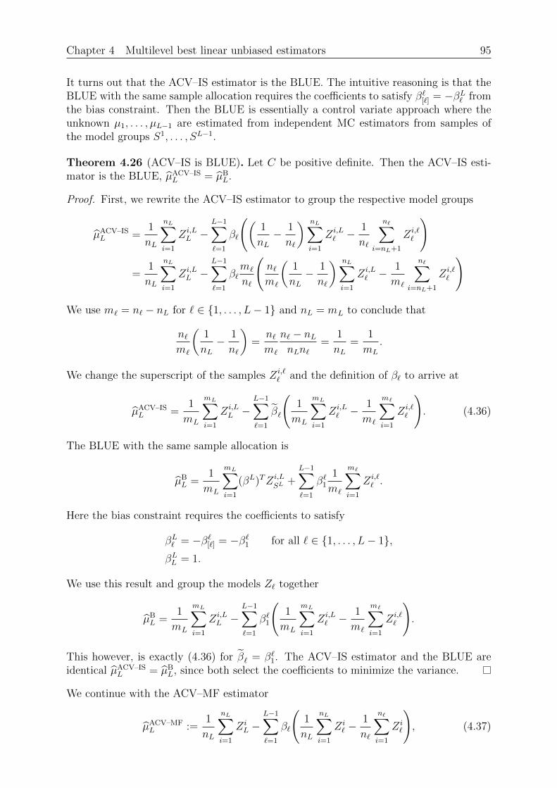
Chapter 4 Multilevel best linear unbiased estimators 95
It turns out that the ACV–IS estimator is the BLUE. The intuitive reasoning is that theBLUE with the same sample allocation requires the coefficients to satisfy β`[`] = −βL` fromthe bias constraint. Then the BLUE is essentially a control variate approach where theunknown µ1, . . . , µL−1 are estimated from independent MC estimators from samples ofthe model groups S1, . . . , SL−1.
Theorem 4.26 (ACV–IS is BLUE). Let C be positive definite. Then the ACV–IS esti-mator is the BLUE, µACV–IS
L = µBL.
Proof. First, we rewrite the ACV–IS estimator to group the respective model groups
µACV–ISL =
1
nL
nL∑i=1
Zi,LL −
L−1∑`=1
β`
((1
nL− 1
n`
) nL∑i=1
Zi,L` −
1
n`
n∑i=nL+1
Zi,``
)
=1
nL
nL∑i=1
Zi,LL −
L−1∑`=1
β`m`
n`
(n`m`
(1
nL− 1
n`
) nL∑i=1
Zi,L` −
1
m`
n∑i=nL+1
Zi,``
)
We use m` = n` − nL for ` ∈ 1, . . . , L− 1 and nL = mL to conclude that
n`m`
(1
nL− 1
n`
)=
n`m`
n` − nLnLn`
=1
nL=
1
mL
.
We change the superscript of the samples Zi,`` and the definition of β` to arrive at
µACV–ISL =
1
mL
mL∑i=1
Zi,LL −
L−1∑`=1
β`
(1
mL
mL∑i=1
Zi,L` −
1
m`
m∑i=1
Zi,``
). (4.36)
The BLUE with the same sample allocation is
µBL =
1
mL
mL∑i=1
(βL)TZi,LSL
+L−1∑`=1
β`11
m`
m∑i=1
Zi,`` .
Here the bias constraint requires the coefficients to satisfy
βL` = −β`[`] = −β`1 for all ` ∈ 1, . . . , L− 1,βLL = 1.
We use this result and group the models Z` together
µBL =
1
mL
mL∑i=1
Zi,LL −
L−1∑`=1
β`1
(1
mL
mL∑i=1
Zi,L` −
1
m`
m∑i=1
Zi,``
).
This however, is exactly (4.36) for β` = β`1. The ACV–IS estimator and the BLUE areidentical µACV–IS
L = µBL, since both select the coefficients to minimize the variance.
We continue with the ACV–MF estimator
µACV–MFL :=
1
nL
nL∑i=1
ZiL −
L−1∑`=1
β`
(1
nL
nL∑i=1
Zi` −
1
n`
n∑i=1
Zi`
), (4.37)
96 Chapter 4 Multilevel best linear unbiased estimators
where we w.l.o.g. assume that nL−1 ≤ nL−2 ≤ · · · ≤ n1, otherwise we rename Z1, . . . , ZL−1
accordingly. The model groups and number of samples are the same as for the MFMCestimator
S1 = 1, m1 = n1 − n2,
......
SL−1 = 1, . . . , L− 1, mL−1 = nL−1 − nL,SL = 1, . . . , L, mL = nL.
This estimator is the MFMC estimator if L ≤ 2 or if Z1, . . . , ZL−2 are uncorrelated toZL−1, ZL and thus this estimator is the BLUE in this case.
Theorem 4.27 (Cases for which ACV–MF is BLUE). Let C be positive definite. Assumethat at least one of the following is true
(i) L ≤ 2,
(ii) ZL−1 and ZL are uncorrelated to Z1, . . . , ZL−2, that is ρL,` = ρL−1,` = 0 for ` ∈1, . . . , L− 2,
(iii) Z1, . . . , ZL−1 are pairwise uncorrelated.
Then the ACV–MF estimator is the BLUE, µACV–MFL = µB
L.
Proof. “(i)”: The estimators are equal µMFMCL = µACV–MF
L and Theorem 4.23 now showsthe result.
“(ii)”: We reduce this case to (i) by showing that only the two fine grid models are used.With I := 1, . . . , L − 1 and J := 1, . . . , L − 2 from Lemma 3.39 we use the blockdiagonal structure of the covariance matrix such that for all ` ∈ 1, . . . , L− 2
β` = eT` (FMF CI,I)−1(diag(FMF ) CI,L)
= eT`
((FMF CJ,J)−1 0
0 (FMFL−1,L−1CL−1,L−1)−1
)(0
FMFL−1,L−1CL−1,L
)= eT`
(0
1CL−1,L−1
CL−1,L
)= 0.
Therefore the ACV–MF estimator only uses the models ZL−1 and ZL an we may w.l.o.g.assume that L = 2. Now (i) shows the result.
“(iii)”: We show that the BLUE is equal to the ACV–MF estimator. The coefficientsof the BLUE divided by the number of samples are constant for k ∈ 1, . . . , L − 1 and` ∈ 1, . . . , k. This follows from the diagonal structure of Ck = diag((σ2
` )k`=1)
βk`mk
= eT` (Ck)−1RkΨ−1eL =1
σ2`
eT` RkΨ−1eL =
1
σ2`
eT` Ψ−1eL =: β`.
Chapter 4 Multilevel best linear unbiased estimators 97
This coefficient is independent of k and only depends on `. Therefore, the BLUE is
µBL =
L∑k=1
k∑`=1
βk`mk
m∑i=1
Zi,k`
= (βL)T1
mL
mL∑i=1
Zi,LSL
+L−1∑k=1
L−1∑`=1
β`1Sk(`)
mk∑i=1
Zi,k`
= (βL)T1
mL
mL∑i=1
Zi,LSL
+L−1∑`=1
β`
L−1∑k=1
mk∑i=1
1Sk(`)Zi,k` .
Let us now collect all samples that evaluate the `-th model for ` ∈ 1, . . . , L − 1 andintroduce the coefficients β`, β`
βL`1
mL
mL∑i=1
Zi,L` + β`
L−1∑k=1
mk∑i=1
1Sk(`)Zi,k`
=
(βL`mL
− β`) mL∑
i=1
Zi,L` + β`
L∑k=1
mk∑i=1
1Sk(`)Zi,k`
= β`1
mL
mL∑i=1
Zi,L` + β`
1∑Lj=`mj
L∑k=1
mk∑i=1
1Sk(`)Zi,k` .
Notice that the right expression is a MC estimator with∑L
j=`mj = n` independent
samples. We rewrite this and use the bias constraint β` = −β` to obtain
β`1
mL
mL∑i=1
Zi,L` + β`
1∑Lj=`mj
L∑k=1
mk∑i=1
1Sk(`)Zi,k` = −β`
(1
nL
nL∑i=1
Zi` −
1
n`
n∑i=1
Zi`
).
The bias constraint is satisfied only if βLL = 1 and the combination of these results shows
µBL =
1
mL
mL∑i=1
ZiL −
L−1∑`=1
β`
(1
nL
nL∑i=1
Zi` −
1
n`
n∑i=1
Zi`
).
With mL = nL this is exactly the ACV–MF estimator in (4.37). The statement nowfollows since both estimators choose β` such that the variance is minimized.
We give an example that the ACV–MF estimator is not the BLUE for L ≥ 3 in thenumerical experiments in Section 4.5. Let us continue with the ACV–KL estimator
µACV–KLL :=
1
mL
mL∑i=1
ZiL −
L−1∑`=K
β`
(1
mL
mL∑i=1
Zi` −
1
m`
m∑i=1
Zi`
)
−K−1∑`=1
β`
(1
mN
mN∑i=1
Zi` −
1
m`
m∑i=1
Zi`
).
The model groups and number of samples are the same as for the MFMC and ACV–MFestimator
S1 = 1, m1 = n1 − n2,
......
SL−1 = 1, . . . , L− 1, mL−1 = nL−1 − nL,SL = 1, . . . , L, mL = nL.
98 Chapter 4 Multilevel best linear unbiased estimators
Since the ACV–KL estimator is equal to the ACV–MF estimator for N = L or K = 1and these parameters are chosen to minimize the variance, we use Theorem 4.27 to obtainthe following result.
Theorem 4.28 (Cases for which ACV–KL is BLUE). Let C be positive definite. Assumethat at least one of the following is true
(i) L ≤ 2,
(ii) ZL−1 and ZL are uncorrelated to Z1, . . . , ZL−2, that is ρL,` = ρL−1,` = 0 for ` ∈1, . . . , L− 2,
(iii) Z1, . . . , ZL−1 are uncorrelated.
Then the ACV–KL estimator is the BLUE µACV–KLL = µB
L and N = L or K = 1.
We postpone the verification that the ACV–KL estimator is in general not the BLUE forL ≥ 3 to the numerical experiments in Section 4.5. We only verify this for some fixedvalues of N or K by using the lower variance bound.
Example 4.29 (ACV–KL is not BLUE). The lower variance bound of the BLUE and ofthe ACV–KL estimator in Theorem 3.43 with N < L satisfies
Vmin[µACV–KL] = VminK,...,L−1 ≥ Vmin
1,...,L−1 = Vmin[µBL].
The above inequality is strict for suitably defined Z1, . . . , ZL and K. As an example,assume that Z1, . . . , ZL−1 are pairwise independent and have unit variance, that is V[Z`] :=1 for all ` ∈ 1, . . . , L− 1. Now define the high fidelity model as follows
ZL =L−1∑`=1
Z` + ξ,
where ξ ∼ N(0, 1) is independent of Z1, . . . , ZL−1. Then the inequality is strict if K < L
L−K + 1 = VminK,...,L−1 > Vmin
1,...,L−1 = 1.
Multilevel Monte Carlo. The MLMC estimator is defined as
µMLMCL :=
L∑`=1
1
m`
m∑i=1
(Zi,`` − Z
i,``−1).
Here we defined Z0 := 0 and thus the sample groups are
S1 = 1,S2 = 1, 2,
...
SL−1 = L− 2, L− 1,SL = L− 1, L.
(4.38)
It is straightforward to verify that this estimator is not the BLUE. The reason is that we donot optimize the coefficients in front of the samples. In particular, scaling Z1, . . . , ZL−1 bya non–zero constant does not change the variance of the BLUE but changes the varianceof the MLMC estimator. Furthermore, the MLMC estimator is not able to ignore modelsthat are independent of ZL by setting the coefficients in front of them to zero.
Chapter 4 Multilevel best linear unbiased estimators 99
Example 4.30 (MLMC is not BLUE). We choose Z1, Z2 ∼ N(0, 1) to be independentrandom variables. Then
V[µMLMC
2
]=
2
m2
+1
m1
.
Contrast this with the BLUE that only uses the last model
V[µB
2
]=
1
m2
.
We conclude that the MLMC estimator is not the BLUE
V[µMLMC
2
]> V
[µB
2
].
Full coupling estimator. For completeness we define the full coupling (FC) estimatorwhich we use in the numerical experiments Section 4.5. This estimator uses the identicalsample allocation as the MFMC, ACV–MF and ACV–KL estimators
S1 := 1,...
SL−1 := 1, . . . , L− 1,SL := 1, . . . , L
and is defined as the associated BLUE
µFCL := µB
L.
We further the define FC κ estimator that couples only the last κ models
SL−κ+1 := L− κ+ 1,...
SL−1 := L− κ+ 1, . . . , L− 1,SL := L− κ+ 1, . . . , L
and is again the BLUE with this sample allocation
µFCκL := µB
L. (4.39)
We clearly have µFCLL = µFC
L and that µFC 1L is the MC estimator. A calculation similar to
Section 4.3 to eliminate the bias constraint shows that this estimator is very similar to aCV estimator
µFCκL :=
1
mL
mL∑i=1
Zi,LL −
L−1∑`=L−κ+1
(β`)T
(1
mL
mL∑i=1
Zi,LS`− 1
m`
m∑i=1
Zi,`S`
).
The coefficients β` ∈ R|S`| are once again chosen such that the variance is minimized.
Summary. Let us summarize the used model groups for every estimator of this sectionin Figure 4.1. We further summarize under which circumstances the estimators are theBLUE in Table 4.1. We define the conditions
L ≤ 2 or ρL,` = ρL−1,` = 0 for all ` ∈ 1, . . . , L− 2, (4.40)
Z1, . . . , ZL−1 are pairwise uncorrelated. (4.41)
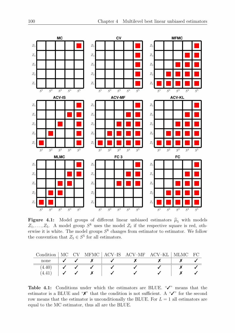
100 Chapter 4 Multilevel best linear unbiased estimators
MC CV MFMC
ACV-IS ACV-MF ACV-KL
MLMC FC 3 FC
Figure 4.1: Model groups of different linear unbiased estimators µ5 with modelsZ1, . . . , Z5. A model group Sk uses the model Z` if the respective square is red, oth-erwise it is white. The model groups Sk changes from estimator to estimator. We followthe convention that Z5 ∈ S5 for all estimators.
Condition MC CV MFMC ACV–IS ACV–MF ACV–KL MLMC FCnone 3 3 7 3 7 7 7 3
(4.40) 3 3 3 3 3 3 7 3
(4.41) 3 3 7 3 3 3 7 3
Table 4.1: Conditions under which the estimators are BLUE. “3” means that theestimator is a BLUE and “7” that the condition is not sufficient. A “3” for the secondrow means that the estimator is unconditionally the BLUE. For L = 1 all estimators areequal to the MC estimator, thus all are the BLUE.
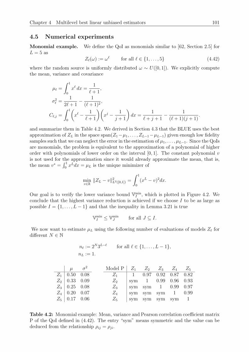
Chapter 4 Multilevel best linear unbiased estimators 101
4.5 Numerical experiments
Monomial example. We define the QoI as monomials similar to [62, Section 2.5] forL = 5 as
Z`(ω) := ω` for all ` ∈ 1, . . . , 5 (4.42)
where the random source is uniformly distributed ω ∼ U([0, 1]). We explicitly computethe mean, variance and covariance
µ` =
∫ 1
0
x` dx =1
`+ 1,
σ2` =
1
2`+ 1− 1
(`+ 1)2,
C`,j =
∫ 1
0
(x` − 1
`+ 1
)(xj − 1
j + 1
)dx =
1
`+ j + 1− 1
(`+ 1)(j + 1).
and summarize them in Table 4.2. We derived in Section 4.3 that the BLUE uses the bestapproximation of ZL in the space span(Z1−µ1, . . . , ZL−1−µL−1) given enough low fidelitysamples such that we can neglect the error in the estimation of µ1, . . . , µL−1. Since the QoIsare monomials, the problem is equivalent to the approximation of a polynomial of higherorder with polynomials of lower order on the interval [0, 1]. The constant polynomial vis not used for the approximation since it would already approximate the mean, that is,the mean v∗ =
∫ 1
0xLdx = µL is the unique minimizer of
minv∈R‖ZL − v‖2
L2([0,1]) =
∫ 1
0
(xL − v)2dx.
Our goal is to verify the lower variance bound VminI , which is plotted in Figure 4.2. We
conclude that the highest variance reduction is achieved if we choose I to be as large aspossible I = 1, . . . , L− 1 and that the inequality in Lemma 3.21 is true
VminI ≤ Vmin
J for all J ⊆ I.
We now want to estimate µL using the following number of evaluations of models Z` fordifferent N ∈ N
n` := 2N3L−` for all ` ∈ 1, . . . , L− 1,nL := 1.
µ σ2
Z1 0.50 0.08Z2 0.33 0.09Z3 0.25 0.08Z4 0.20 0.07Z5 0.17 0.06
Model P Z1 Z2 Z3 Z4 Z5
Z1 1 0.97 0.92 0.87 0.82Z2 sym 1 0.99 0.96 0.93Z3 sym sym 1 0.99 0.97Z4 sym sym sym 1 0.99Z5 sym sym sym sym 1
Table 4.2: Monomial example: Mean, variance and Pearson correlation coefficient matrixP of the QoI defined in (4.42). The entry “sym” means symmetric and the value can bededuced from the relationship ρij = ρji.
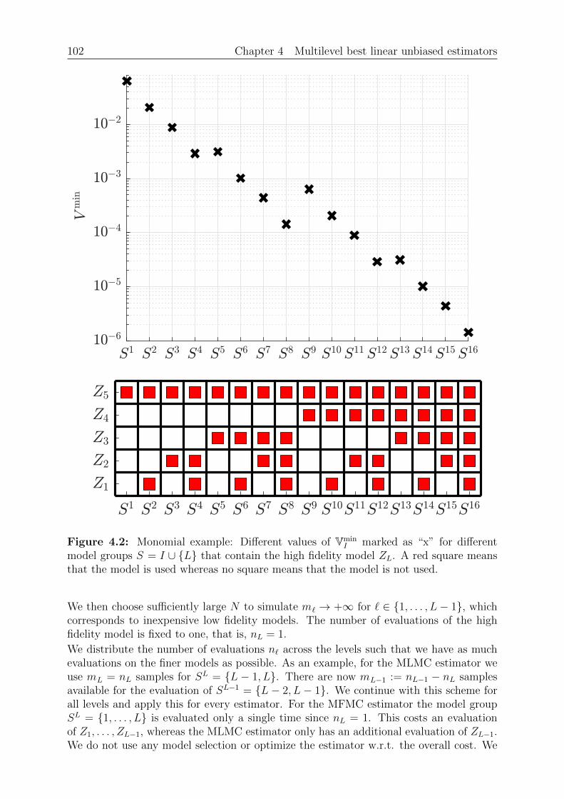
102 Chapter 4 Multilevel best linear unbiased estimators
Figure 4.2: Monomial example: Different values of VminI marked as “x” for different
model groups S = I ∪ L that contain the high fidelity model ZL. A red square meansthat the model is used whereas no square means that the model is not used.
We then choose sufficiently large N to simulate m` → +∞ for ` ∈ 1, . . . , L− 1, whichcorresponds to inexpensive low fidelity models. The number of evaluations of the highfidelity model is fixed to one, that is, nL = 1.
We distribute the number of evaluations n` across the levels such that we have as muchevaluations on the finer models as possible. As an example, for the MLMC estimator weuse mL = nL samples for SL = L − 1, L. There are now mL−1 := nL−1 − nL samplesavailable for the evaluation of SL−1 = L − 2, L − 1. We continue with this scheme forall levels and apply this for every estimator. For the MFMC estimator the model groupSL = 1, . . . , L is evaluated only a single time since nL = 1. This costs an evaluationof Z1, . . . , ZL−1, whereas the MLMC estimator only has an additional evaluation of ZL−1.We do not use any model selection or optimize the estimator w.r.t. the overall cost. We
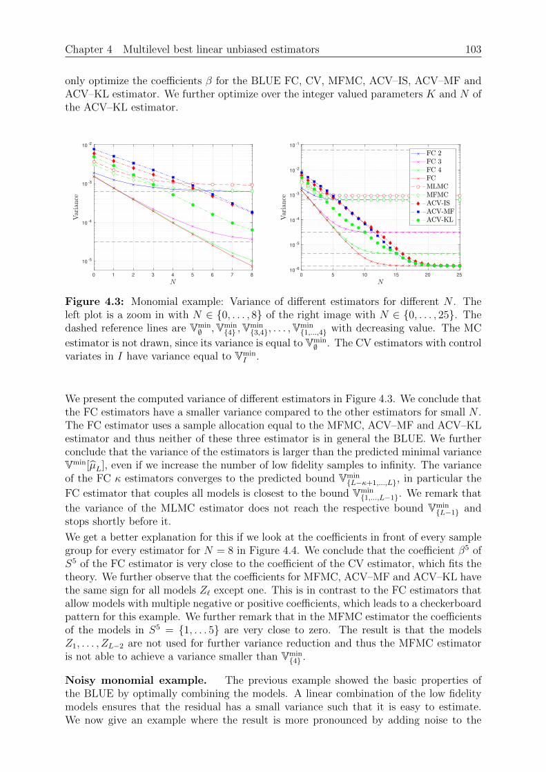
Chapter 4 Multilevel best linear unbiased estimators 103
only optimize the coefficients β for the BLUE FC, CV, MFMC, ACV–IS, ACV–MF andACV–KL estimator. We further optimize over the integer valued parameters K and N ofthe ACV–KL estimator.
0 1 2 3 4 5 6 7 8
10-5
10-4
10-3
10-2
0 5 10 15 20 25
10-6
10-5
10-4
10-3
10-2
10-1
Figure 4.3: Monomial example: Variance of different estimators for different N . Theleft plot is a zoom in with N ∈ 0, . . . , 8 of the right image with N ∈ 0, . . . , 25. Thedashed reference lines are Vmin
∅ ,Vmin4 ,Vmin
3,4, . . . ,Vmin1,...,4 with decreasing value. The MC
estimator is not drawn, since its variance is equal to Vmin∅ . The CV estimators with control
variates in I have variance equal to VminI .
We present the computed variance of different estimators in Figure 4.3. We conclude thatthe FC estimators have a smaller variance compared to the other estimators for small N .The FC estimator uses a sample allocation equal to the MFMC, ACV–MF and ACV–KLestimator and thus neither of these three estimator is in general the BLUE. We furtherconclude that the variance of the estimators is larger than the predicted minimal varianceVmin[µL], even if we increase the number of low fidelity samples to infinity. The varianceof the FC κ estimators converges to the predicted bound Vmin
L−κ+1,...,L, in particular the
FC estimator that couples all models is closest to the bound Vmin1,...,L−1. We remark that
the variance of the MLMC estimator does not reach the respective bound VminL−1 and
stops shortly before it.
We get a better explanation for this if we look at the coefficients in front of every samplegroup for every estimator for N = 8 in Figure 4.4. We conclude that the coefficient β5 ofS5 of the FC estimator is very close to the coefficient of the CV estimator, which fits thetheory. We further observe that the coefficients for MFMC, ACV–MF and ACV–KL havethe same sign for all models Z` except one. This is in contrast to the FC estimators thatallow models with multiple negative or positive coefficients, which leads to a checkerboardpattern for this example. We further remark that in the MFMC estimator the coefficientsof the models in S5 = 1, . . . 5 are very close to zero. The result is that the modelsZ1, . . . , ZL−2 are not used for further variance reduction and thus the MFMC estimatoris not able to achieve a variance smaller than Vmin
4 .
Noisy monomial example. The previous example showed the basic properties ofthe BLUE by optimally combining the models. A linear combination of the low fidelitymodels ensures that the residual has a small variance such that it is easy to estimate.We now give an example where the result is more pronounced by adding noise to the

104 Chapter 4 Multilevel best linear unbiased estimators
MC
1.00
CV 2
-0.94
1.00
CV
0.12
-0.83
2.22
-2.50
1.00
MLMC
1.00 -1.00
1.00 -1.00
1.00 -1.00
1.00 -1.00
1.00
MFMC
0.48 -0.32
0.52
-0.11
-0.35
0.58
-0.05
-0.17
-0.57
0.94
-0.00
-0.00
-0.00
-0.94
1.00
ACV-IS
0.19
-0.86
0.73
0.90
-0.19
0.86
-0.73
-0.90
1.00
ACV-MF
0.15 0.05
-0.61
0.02
-0.20
0.50
0.01
-0.10
0.25
0.91
-0.22
0.92
-0.76
-0.91
1.00
ACV-KL
-0.12 -0.04
0.95
-0.01
0.32
-0.44
-0.01
0.16
-0.22
1.64
0.18
-1.42
0.67
-1.64
1.00
FC 2
0.94 -0.94
1.00
FC 3
0.58 -1.26
1.66
0.69
-1.66
1.00
FC 4
0.52 -1.04
1.30
0.88
-2.84
2.18
-0.36
1.55
-2.18
1.00
FC
0.48 -1.03
1.19
0.77
-2.38
1.85
-0.33
2.02
-4.06
2.49
0.12
-0.83
2.21
-2.49
1.00
Figure 4.4: Monomial example: Coefficients of the linear combination for different linearunbiased estimators for N = 8. An empty box means that a model is not used for therespective model group. Each row has to sum up to 0 except for the top row which sumsup to 1. Here we do not account for rounding errors and the CV estimator has the biasproperty only for the top row, since this estimator assumes that µ1, . . . , µL−1 is known.The estimator CV 2 uses a single control variate Z4 and couples the two models Z4 andZ5. Green coefficients are positive and blue coefficients are negative.
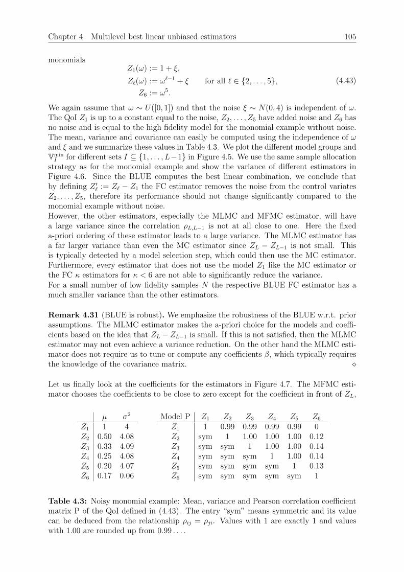
Chapter 4 Multilevel best linear unbiased estimators 105
monomialsZ1(ω) := 1 + ξ,
Z`(ω) := ω`−1 + ξ for all ` ∈ 2, . . . , 5,Z6 := ω5.
(4.43)
We again assume that ω ∼ U([0, 1]) and that the noise ξ ∼ N(0, 4) is independent of ω.The QoI Z1 is up to a constant equal to the noise, Z2, . . . , Z5 have added noise and Z6 hasno noise and is equal to the high fidelity model for the monomial example without noise.The mean, variance and covariance can easily be computed using the independence of ωand ξ and we summarize these values in Table 4.3. We plot the different model groups andVminI for different sets I ⊆ 1, . . . , L−1 in Figure 4.5. We use the same sample allocation
strategy as for the monomial example and show the variance of different estimators inFigure 4.6. Since the BLUE computes the best linear combination, we conclude thatby defining Z ′` := Z` − Z1 the FC estimator removes the noise from the control variatesZ2, . . . , Z5, therefore its performance should not change significantly compared to themonomial example without noise.However, the other estimators, especially the MLMC and MFMC estimator, will havea large variance since the correlation ρL,L−1 is not at all close to one. Here the fixeda-priori ordering of these estimator leads to a large variance. The MLMC estimator hasa far larger variance than even the MC estimator since ZL − ZL−1 is not small. Thisis typically detected by a model selection step, which could then use the MC estimator.Furthermore, every estimator that does not use the model Z1 like the MC estimator orthe FC κ estimators for κ < 6 are not able to significantly reduce the variance.For a small number of low fidelity samples N the respective BLUE FC estimator has amuch smaller variance than the other estimators.
Remark 4.31 (BLUE is robust). We emphasize the robustness of the BLUE w.r.t. priorassumptions. The MLMC estimator makes the a-priori choice for the models and coeffi-cients based on the idea that ZL −ZL−1 is small. If this is not satisfied, then the MLMCestimator may not even achieve a variance reduction. On the other hand the MLMC esti-mator does not require us to tune or compute any coefficients β, which typically requiresthe knowledge of the covariance matrix.
Let us finally look at the coefficients for the estimators in Figure 4.7. The MFMC esti-mator chooses the coefficients to be close to zero except for the coefficient in front of ZL,
µ σ2
Z1 1 4Z2 0.50 4.08Z3 0.33 4.09Z4 0.25 4.08Z5 0.20 4.07Z6 0.17 0.06
Model P Z1 Z2 Z3 Z4 Z5 Z6
Z1 1 0.99 0.99 0.99 0.99 0Z2 sym 1 1.00 1.00 1.00 0.12Z3 sym sym 1 1.00 1.00 0.14Z4 sym sym sym 1 1.00 0.14Z5 sym sym sym sym 1 0.13Z6 sym sym sym sym sym 1
Table 4.3: Noisy monomial example: Mean, variance and Pearson correlation coefficientmatrix P of the QoI defined in (4.43). The entry “sym” means symmetric and its valuecan be deduced from the relationship ρij = ρji. Values with 1 are exactly 1 and valueswith 1.00 are rounded up from 0.99 . . . .
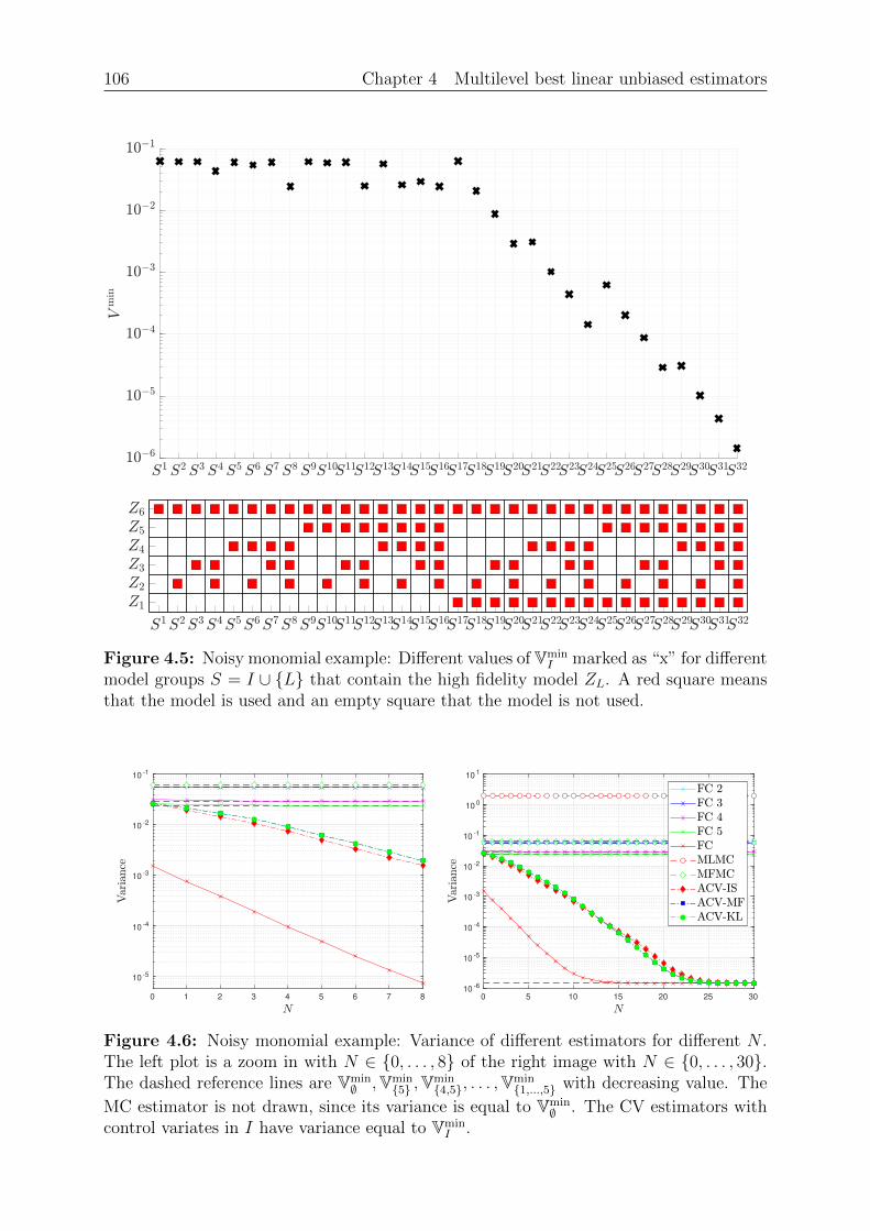
106 Chapter 4 Multilevel best linear unbiased estimators
Figure 4.5: Noisy monomial example: Different values of VminI marked as “x” for different
model groups S = I ∪ L that contain the high fidelity model ZL. A red square meansthat the model is used and an empty square that the model is not used.
0 1 2 3 4 5 6 7 8
10-5
10-4
10-3
10-2
10-1
0 5 10 15 20 25 30
10-6
10-5
10-4
10-3
10-2
10-1
100
101
Figure 4.6: Noisy monomial example: Variance of different estimators for different N .The left plot is a zoom in with N ∈ 0, . . . , 8 of the right image with N ∈ 0, . . . , 30.The dashed reference lines are Vmin
∅ ,Vmin5 ,Vmin
4,5, . . . ,Vmin1,...,5 with decreasing value. The
MC estimator is not drawn, since its variance is equal to Vmin∅ . The CV estimators with
control variates in I have variance equal to VminI .
Chapter 4 Multilevel best linear unbiased estimators 107
which does not reduce the variance in any significant way. If we add up the last columnof the FC estimator w.r.t. the noise ξ we have
0ξ − 2.49ξ + 2.21ξ − 0.83ξ + 0.12ξ + 0.99ξ ≈ 0,
which shows that the FC estimator removes the noise. We obtain a similar result forevery column of the FC estimator. We further remark that the values in this matrix withrows Z2, . . . , Z6 and columns S2, . . . , S6 are almost identical to the values of the matrixof the FC estimator for the monomial example without noise in Figure 4.7. This confirmsthat the BLUE removes the noise from every sample group. The model Z1 in S1 of theFC estimator has a coefficient very close to zero, which means that this sample group isessentially not used. This is not surprising, since Z1 and Z6 are independent and we canalways subtract a multiple of Z1 and thus ξ in the linear combination (βk)TZSk due tothe model group structure S` = 1, . . . , `.

108 Chapter 4 Multilevel best linear unbiased estimators
CV 2
-0.03
1.00
CV
0.99
0.12
-0.83
2.22
-2.50
1.00
MLMC
1.00 -1.00
1.00 -1.00
1.00 -1.00
1.00 -1.00
1.00 -1.00
1.00
MFMC
0.00 0.00
0.02
0.00
-0.01
0.02
0.00
-0.00
-0.01
0.02
0.00
-0.00
-0.01
-0.02
0.03
0.00
-0.00
-0.00
-0.00
-0.03
1.00
ACV-IS
-0.83
-0.41
0.39
0.54
0.31
0.83
0.41
-0.39
-0.54
-0.31
1.00
ACV-MF
-0.54 -0.18
-0.31
-0.06
-0.10
0.35
-0.02
-0.03
0.12
0.35
-0.01
-0.02
0.06
0.17
0.22
0.81
0.46
-0.53
-0.52
-0.22
1.00
ACV-KL
-0.54 -0.18
-0.31
-0.06
-0.10
0.35
-0.02
-0.03
0.12
0.35
-0.01
-0.02
0.06
0.17
0.22
0.81
0.46
-0.53
-0.52
-0.22
1.00
FC 2
0.03 -0.03
1.00
FC 3
0.02 1.79
-1.78
-1.81
1.78
1.00
FC 4
0.02 -0.04
0.05
-8.12
19.84
-11.73
8.14
-19.89
11.73
1.00
FC 5
0.02 -1.18
1.19
-1.77
4.48
-2.72
-1.59
5.44
-6.34
2.49
4.52
-11.11
9.06
-2.49
1.00
FC
-0.00 -0.48
0.48
-0.16
-1.03
1.19
-0.24
0.77
-2.38
1.85
-0.12
-0.33
2.02
-4.06
2.49
0.99
0.12
-0.83
2.21
-2.49
1.00
Figure 4.7: Noisy monomial example: Coefficients of the linear combination for differentlinear unbiased estimators for N = 8. An empty box means that a model is not used forthe respective model group. Each row has to sum up to 0 except for the top row, whichsums up to 1. Here we do not account for rounding errors and the CV estimator hasthe bias property only for the top row, since this estimator assumes that µ1, . . . , µL−1 isknown. Green coefficients are positive and blue coefficients are negative.

Chapter 5 Sample allocation optimal BLUE 109
Chapter 5
Sample allocation optimal BLUE
The condition that an estimator is the BLUE is not a sufficient for being an inexpensiveestimator. Chapter 4 showed that the MC estimator is the BLUE in contrast to theMLMC estimator which is in general not a BLUE. Nevertheless, MLMC has a betterasymptotic complexity than MC if we compare Theorem 3.11 with Theorem 3.49. Thereason is that both estimators use different samples such that the achievable variance issmaller for the MLMC estimator. Therefore we have to equip the BLUE with a methodto choose the linear regression problem which we call the sample allocation problem. Inthis chapter we proceed as follows:
We define the sample allocation problem in Section 5.1. We further prove theexistence of a solution which defines a sample allocation optimal BLUE and verifythat this estimator is optimal in the class of linear unbiased estimators. We furtherextend the sample allocation problem to include a coupling number κ such that onlymodel groups are evaluated with less or equal to κ models.
We relax the sample allocation problem to obtain a tractable solution and discusswhy this relaxation is sensible. The relaxed problem in Section 5.2 has a solutionthat is in general not unique. We further show that optimal solutions are sparse inthe sense that at most L of the K = 2L−1 model groups are used. This property iscrucial for a practical implementation due to the necessity for rounding the numberof samples to the next integer.
Section 5.3 provides analogous but slightly stronger results compared to Section 5.2.The main idea is to view the sample allocation problem from a different angleand first optimize the sample allocation and afterwards the coefficient of the linearunbiased estimator. These results simplify the asymptotic analysis in Chapter 6.
In Section 5.4 we prove that every minimizer of the sample allocation problem liesin the convex hull of a finite number of minimizers where each of these uses at mostL model groups.
The sections of this chapter in terms of their minimization problems are given in Fig-ure 5.1. This chapter contains results from [125, 126] and Section 5.2 together withSection 5.4 extend some of these results.
5.1 Ideal sample allocation optimal BLUE
We know from Chapter 4 that the variance of the BLUE with coefficients βk in (4.15)and number of samples m is
V[µBα
]=∑k∈US
(βk)TCkβk
mk
= αTΨ−1α = αT
(∑k∈US
mkPk(Ck)−1Rk
)−1
α.
In the following we ease the notation and make the dependence on the number of samplesm of the system matrix Ψ(m) and the estimator µB
α(m) explicit. The goal is to choose m
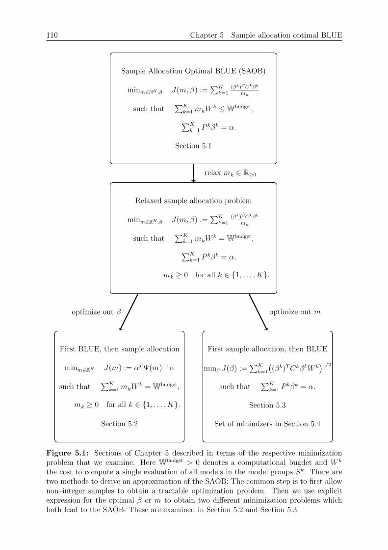
110 Chapter 5 Sample allocation optimal BLUE
Sample Allocation Optimal BLUE (SAOB)
minm∈NK ,β J(m,β) :=∑K
k=1(βk)TCkβk
mk
such that∑K
k=1mkWk ≤Wbudget,∑K
k=1 Pkβk = α.
Section 5.1
Relaxed sample allocation problem
minm∈RK ,β J(m,β) :=∑K
k=1(βk)TCkβk
mk
such that∑K
k=1mkWk = Wbudget,∑K
k=1 Pkβk = α,
mk ≥ 0 for all k ∈ 1, . . . , K.
First BLUE, then sample allocation
minm∈RK J(m) := αTΨ(m)−1α
such that∑K
k=1mkWk = Wbudget,
mk ≥ 0 for all k ∈ 1, . . . , K.
Section 5.2
First sample allocation, then BLUE
minβ J(β) :=∑K
k=1
((βk)TCkβkW k
)1/2
such that∑K
k=1 Pkβk = α.
Section 5.3
Set of minimizers in Section 5.4
relax mk ∈ R≥0
optimize out β optimize out m
Figure 5.1: Sections of Chapter 5 described in terms of the respective minimizationproblem that we examine. Here Wbudget > 0 denotes a computational bugdet and W k
the cost to compute a single evaluation of all models in the model groups Sk. There aretwo methods to derive an approximation of the SAOB: The common step is to first allownon–integer samples to obtain a tractable optimization problem. Then we use explicitexpression for the optimal β or m to obtain two different minimization problems whichboth lead to the SAOB. These are examined in Section 5.2 and Section 5.3.
Chapter 5 Sample allocation optimal BLUE 111
such that the variance is minimized and we do not exceed a known computational budgetsimilar to the MLMC, MFMC and ACV estimators in Chapter 3. This cost constraintis necessary since otherwise the variance can be made as small as desired by choosing msufficiently large. We define the cost of a model group as the sum of the costs of everycontained model
W k := W[ZSk ] =∑`∈Sk
W[Z`] =∑`∈Sk
w` for all k ∈ 1, . . . , K.
We introduce a fixed budget Wbudget > 0 and write down the sample allocation problem
minm1,...,mK∈N0
V[µBα(m)
]= αTΨ(m)−1α
such that W[µBα(m)
]=
∑k∈1,...,K
mkWk ≤Wbudget.
(5.1)
We define V[µBα(m)
]:= +∞ if m is such that the BLUE µB
α(m) is not well defined. TheBLUE is not necessarily unique, therefore we are only able to prove existence of a solutionof (5.1).
Theorem 5.1 (Existence of sample allocation optimal BLUE). Let Wbudget be such thatwe are able to evaluate the required models at least once∑
`∈Uα
w` ≤Wbudget. (5.2)
Then there exists a minimizer m∗ of (5.1) and every corresponding BLUE is a sampleallocation optimal BLUE (SAOB)
µSAOBα := µB
α(m∗).
Proof. The sample allocation problem (5.1) optimizes over a finite set of m ∈ NK0 since
the cost of every model w` > 0 is positive. We thus enumerate all values and choosem∗ such that the variance is minimized. Assumption (5.2) now ensures that the MCestimator with a single sample defines a feasible BLUE
µMCα := αTZ1
Uα .
Hence we conclude that m∗ is feasible and thus V[µBα(m∗)
]= V
[µSAOBα
]< +∞.
The SAOB is optimal in the class of linear unbiased estimators. No other linear unbiasedestimator is able to achieve a smaller variance satisfying the cost constraint.
Theorem 5.2 (Optimality of SAOB). Let µα be a linear unbiased estimator that usesmk i.i.d. samples of Sk for k ∈ 1, . . . , K, where the samples are also independent acrossmodel groups. Then every SAOB with Wbudget = W[µα] has smaller or equal variance
V[µSAOBα
]≤ V[µα].
Proof. The BLUE µBα(m) with the same sample allocation m as µα has smaller or equal
varianceV[µBα(m)
]≤ V[µα].
The Assumption (5.2) is satisfied since µBα is a feasible estimator in (5.1) and thus a SAOB
exists. However, the SAOB is the minimizer of this problem and thus we conclude thetheorem
V[µSAOBα
]= V
[µBα(m∗)
]≤ V
[µBα(m)
]≤ V[µα].
112 Chapter 5 Sample allocation optimal BLUE
The two previous theorems allow the usage of every model group Sk and similar resultsare achievable if we allow only the use of specific model groups. We are particularlyinterested in evaluating or coupling at most κ models in a single model group, that ismk = 0 if |Sk| > κ. The SAOB with coupling κ ∈ N (SAOB κ) is a BLUE with a sampleallocation that solves
minm1,...,mK∈N0
V[µBα(m)
]= αTΨ(m)−1α
such that∑
k∈1,...,K
mkWk ≤Wbudget,
mk = 0 for k ∈ 1, . . . , K with |Sk| > κ.
We denote this estimator with µSAOBκ and remark that its existence and optimality followsanalogously to SAOB. For completeness we write down the optimality result.
Corollary 5.3 (Optimality of SAOB κ). Let µα be a linear unbiased estimator that usesmk i.i.d. samples of Sk for k ∈ 1, . . . , K with |Sk| ≤ κ, where the samples are alsoindependent across model groups. Then every SAOB κ with Wbudget = W[µα] has smalleror equal variance
V[µSAOBκα
]≤ V[µα].
The coupling parameter κ of SAOB κ is important for the asymptotic analysis in Chap-ter 6. We further remark that κ also determines the lower variance bound of SAOB κ,since we are allowed to couple at most κ− 1 other models with the high fidelity model
Vmin[µSAOBκL ] = min
I⊆1,...,L,|I|=κ−1
VminI .
It is possible to weaken the assumptions of i.i.d. samples for every model group andacross different model groups. The BLUE is the solution of a generalized linear regressionproblem, where a different sample structure leads to a different noise assumption, hencea BLUE still exists. We are further able to generalize the cost constraint by simplybounding the cost of the respective BLUE
minµBα
V[µBα(m)
]such that W
[µBα(m)
]≤Wbudget.
This problem typically has a feasible point if Wbudget is large enough. Since the numberof samples are integer, the cost constraints often ensures that the number of evaluationsand thus the number of feasible BLUEs is bounded. We further have to demand that theestimator µB
α(m) only depends on m and no further other independent parameters thatmay modify the noise or covariance structure. Then the solution of this problem is againa SAOB that is now optimal in this defined class of linear unbiased estimators with costsbounded by Wbudget.The above generalization is interesting but in its generality not very useful. In practice, wehave to compute an approximation to the minimization (5.1), which we will do by allowingthe number of samples to be positive real numbers. If we additionally change the structureof the noise η for the regression problem in Definition 4.11 to include dependencies acrossmodel groups, then the dependence of the system matrix Ψ w.r.t. m is more complex.Furthermore, the covariance matrix C is often unknown in practice and introducing morecoupling requires that we estimate more entries of the covariance matrix of the noise η.
Chapter 5 Sample allocation optimal BLUE 113
5.2 First BLUE, then sample allocation
Relaxed formulation. We state reasons how and why we simplify the optimizationproblem (5.1). We relax the constraint that the number of samples m are integer tonon–negative real numbers to obtain a problem that is numerically tractable
minm1,...,mK∈R
J(m) := αTΨ(m)−1α
such thatK∑k=1
mkWk = Wbudget,
mk ≥ 0 for all k ∈ 1, . . . , K.
We have replaced the inequality for the cost constraint with equality which is alwayssatisfied at every minimizer. This problem is still difficult to handle, since Ψ might notbe well defined or not invertible, however the BLUE might still exist. We first show anexample where this is not a problem.
Example 5.4 (Ψ not invertible). Let L := 2, w1 := w2 := 1, Wbudget := 3, α := (0, 1)T
and let the covariance matrix be the identity C := I. Then the MC estimator with threesamples of Z2 is the BLUE since samples of Z1 never decrease the variance. This canformally be checked by looking at the lower variance bound Vmin
∅ = Vmin1 . Notice however
that the matrix
Ψ = m1P1(C1)−1R1 = 3
(01
)1(0 1
)=
(0 00 3
)is not invertible on R2 but on V := span(α), where it matters, that is
Ψ : V → V, Ψα = 3α.
We are thus able to compute the inverse of the linear operator Ψ on V and thus
αTΨ−1α =1
3‖α‖2 =
1
3,
which is the variance of the MC estimator with three samples of Z2.
The second and more subtle problem is that the BLUE is not well defined if we do notevaluate all models that are required by the bias. However, since we demand m ≥ 0 thenumber of evaluations of a model may tend to zero if the respective covariance matricesare close to non–invertibility. We demonstrate this in the next example.
Example 5.5 (C not invertible). Let L := 2, w1 := w2 := 1, Wbudget := 1, α := (1, 1)T
with covariance matrix C :=
(ε2 00 1
). It is straightforward to see that we obtain the
smallest variance if we evaluate the uncorrelated Z1 and Z2 separately. We compute thesystem matrix
Ψ(m) = m1P1(C1)−1R1 +m2P
2(C2)−1R2 =
(m1ε
−2 00 m2
).
This matrix is invertible for all ε2 > 0 and the variance of the BLUE is
J(m) = αTΨ(m)−1α =
(11
)T( 1m1ε2 0
0 1m2
)(11
)=
1
m1
ε2 +1
m2
.
114 Chapter 5 Sample allocation optimal BLUE
We minimize this expression w.r.t. the cost constraint and use the KKT conditions suchthat the optimal m1 and m2 satisfy
1
m21
ε2 =1
m22
,
m1 +m2 = Wbudget.
The optimal solution and the variance is then
m1 =ε
1 + ε, m2 =
1
1 + ε, J(m) = (1 + ε)ε+ (1 + ε).
The above expressions are well defined for all ε ≥ 0 and in particular for ε = 0 for whichC is not invertible. The latter is problematic, since then m1 = 0 and thus we obtain anestimator with Uα = 1, 2 6⊆ UZ = 2. Therefore, the estimator µB
α for ε = 0 withm1 = 0 and m2 = 1 is not a well defined linear unbiased estimator of αTµ.
Formulated differently, the set where the bias constraint can be satisfied is not closedm1, . . . ,mK ∈ R≥0 | there exists βk with α =∑
k |mk>0
P kβk
and minimizing J leads to a point not in this set. We circumvent this difficulty if weassume that we pay the price of having at least a single evaluation of all models SL :=1, . . . , L.Intuitively, it does not make sense to evaluate a model group Sk where Ck is not positivedefinite, since we know that the vectors (Z`−µ`)`∈Sk are linearly dependent. Ignoring themean µ for now, we are able to compute the value of any linear combination of (Z`)`∈Skwithout evaluating a particular model j ∈ Sk and thus we do not have to pay the costwj. We formalize this intuition where we do not ignore the mean µ.
Lemma 5.6 (Model groups not used). Let µα be a linear unbiased estimator with mL ≥ 1for the model group SL := 1, . . . , L and C not positive definite. Then there exists anestimator µ′α with sample allocation m with equal variance V[µ′α] = V[µα] and smaller orequal cost W[µ′α] ≤W[µα] such that all model groups Sk where Ck is not positive definiteare not used, or used only once for k = L
mk =
0, if k 6= L,
1, if k = L.
Proof. Let k ∈ 1, . . . , K \ L such that Ck is not positive definite and assume that µαuses this model group. Lemma 2.16 now shows that there exist coefficients (a`)`∈Sk 6= 0such that almost surely ∑
`∈Ska`Z` =
∑`∈Sk
a`µ`. (5.3)
This allows us to represent an arbitrary model j ∈ Sk with aj 6= 0 in terms of the otherQoIs and the mean values
Zj = −∑
`∈Sk\j
a`ajZ` + µj +
∑`∈Sk\j
a`ajµ` = −
∑`∈Sk\j
a`ajZ` +
∑`∈Sk
a`ajµ`. (5.4)
Chapter 5 Sample allocation optimal BLUE 115
W.l.o.g. we assume that the linear unbiased estimator µα uses equal coefficients for everysample in the model group Sk
µα =∑
n∈US\k
∑`∈Sn
βn[`]
(1
mn
mn∑i=1
Zi,n`
)+∑`∈Sk
βk[`]
(1
mk
mk∑i=1
Zi,k`
)
and we replace Zj in the last expression with (5.4)∑`∈Sk\j
βk[`]Zi,k` + βk[j]Z
i,kj =
∑`∈Sk\j
(βk[`] −
a`ajβk[j]
)Zi,k` + βk[j]
∑`∈Sk
a`ajµ`.
This replacement does not change the variance and we define the estimator µ∗α to be
µ∗α :=∑
n∈US\k
∑`∈Sn
βn[`]1
mn
mn∑i=1
Zi,n` +
∑`∈Sk\j
(βk[`] −
a`ajβk[j]
)1
mk
mk∑i=1
Zi,k` + βk[j]
∑`∈Sk
a`ajµ`.
The last part of this estimator is a linear combination of the mean values, which we knowfrom (5.3) if we have a sample of SL = 1, . . . , L available. Moreover, the estimator µ∗αis cheaper than µα since it does not evaluate Zj in the model group Sk
W[µα] = W[µ∗α]−mkW[Sk]
+mkW[Sk \ j
]= W[µ∗α]−mkwj. (5.5)
We now repeat the procedure outlined in this proof for µ∗α until we obtain an estimatorµ′α such that mk = 0 for all k ∈ 1, . . . , K \ L where Ck is not positive definite. Weremark that this approach works even if we remove only some samples of a model groupwith non–positive definite covariance matrix while keeping the remaining ones. Since thisproof is valid if SL is evaluated at least once, we keep a single sample mL = 1 for µ′α.
The above lemma is a justification to only look at model groups where the respectivecovariance matrix is positive definite. We view this as preliminary model selection wherewe are able to ignore some model groups without increasing the variance of the minimizer.We incorporate the evaluation of SL in an alternative way into the cost function byadding the diagonal matrix δI with δ > 0 such that Ψδ(m) := Ψ(m) + δI is invertible.We interpret δI as additional independent evaluations of Z1, . . . , ZL in the following sense:
δI =L∑`=1
δσ2`P
`(C`)−1R`.
We used that S` = ` and assumed σ2` > 0 for ` ∈ 1, . . . , L, hence adding δI corre-
sponds to δσ2` additional evaluations of Z`. We then define the relaxed sample allocation
problemmin
m1,...,mK∈RJδ(m) := αTΨδ(m)−1α
such thatK∑k=1
mkWk = Wbudget,
mk ≥ 0 for all k ∈ 1, . . . , K.
(5.6)
The matrix Ψδ and its inverse is well defined if C is positive definite or if we restrictourselves to model groups where Ck is positive definite. In the latter setting we however,may have to pay the price of an additional evaluation of all models.
116 Chapter 5 Sample allocation optimal BLUE
Remark 5.7 (Other relaxations). We are able to replace δI by δC−1 to obtain a δ–th ofan evaluation of 1, . . . , L if C is positive definite. Another alternative is to ensure thatall models are evaluated at least δ-times∑
k∈1,...,K | `∈Sk
mk ≥ δ for all ` ∈ 1, . . . , L.
Both methods complicate the analysis and our numerical results in Chapter 6 suggestthat setting δ = 0 is possible. Furthermore, in Section 5.3 we apply a different approachwhich allows us to remove the matrix δI altogether.
We derive a lower and upper bound on the error of the variance for replacing Ψ with Ψδ.Since δI can be viewed as additional samples, we expect that the error gets smaller andsmaller if we use more and more samples.
Lemma 5.8 (Variance with added δI). For positive definite Ψ and δ ≥ 0 the change inthe variance by adding δI satisfies
1
1 + δλmax(Ψ−1)αTΨ−1α ≤ αTΨ−1
δ α ≤ 1
1 + δλmin(Ψ−1)αTΨ−1α, (5.7)
where λmin and λmax are the smallest respectively largest eigenvalue of Ψ. In particular,if we increase the number of samples to infinity the relative error converges to zero in thefollowing sense
αTΨ(sm)−1α− αTΨδ(sm)−1α
αTΨ(sm)−1α≤ δλmax(Ψ−1)
s+ δλmax(Ψ−1)→ 0 for s→ +∞. (5.8)
Proof. We extract the matrix Ψ−1/2 and use the bound of the largest eigenvalue
αTΨδ−1α = αT (Ψ + δI)−1α = αTΨ−1/2(I + δΨ−1)−1Ψ−1/2α
≤ λmax((I + δΨ−1)−1)αTΨ−1α.
For positive definite matrices the largest eigenvalue of its inverse is the inverse of thesmallest eigenvalue
λmax((I + δΨ−1)−1) =1
λmin(I + δΨ−1)=
1
1 + δλmin(Ψ−1),
which shows the upper bound in (5.7). For the lower bound we use the inequality
αTΨ−1/2(I + δΨ−1)−1Ψ−1/2α ≥ λmin((I + δΨ−1)−1)αTΨ−1α,
from which the result follows similarly to before. We obtain (5.8) using the lower boundin (5.7) and
λmax(Ψ(sm)−1) = λmax((sΨ(m))−1) =1
sλmax(Ψ(m)−1).
Existence of a minimizer. We summarize and derive important properties of thecost function Jδ, which follow mostly from the fact that Jδ is the variance of a BLUE. Toavoid technical difficulties we assume that C is positive definite.
Chapter 5 Sample allocation optimal BLUE 117
Lemma 5.9 (Properties of Jδ). Let C be positive definite. The function Jδ has thefollowing properties:
(i) Jδ : R|K|≥0 → R>0,
(ii) Jδ(m/λ) = λJδ/λ(m) for all δ ≥ 0 and λ > 0,
(iii) Coupling of more models never increases the variance, that is for k, j ∈ 1, . . . , Kwith Sk ⊆ Sj we have for all λ ≥ 0 and δ > 0
Jδ(m + λek) ≥ Jδ(m + λej),
(iv) Increasing the number of samples never increases the variance, Jδ is monotonicallydecreasing in every argument,
(v) Jδ is twice continuously differentiable for δ > 0 with derivatives
∂mkJδ(m) = −αTΨδ(m)−1P k(Ck)−1RkΨδ(m)−1α,
∂mk∂mj
Jδ(m) = 2αTΨδ(m)−1P k(Ck)−1RkΨδ(m)−1P j(Cj)−1RjΨδ(m)−1α.
(vi) Jδ is convex for δ > 0,
(vii) Jδ is not strictly convex for L ≥ 3.
Proof. The properties “(i)” and “(ii)” are straightforward to verify. For “(iii)” we useSk ⊆ Sj, denote I := Sj \ Sk with |I| > 0 and w.l.o.g. assume
Cj =
(CI,I CI,SkCSk,I Ck
).
Since the covariance matrix Cj is positive definite we use the inverse of the Schur com-plement [109] and the fact that the Schur complement is positive semi–definite
(Cj)−1 =
(I 0
−(Ck)−1CSk,I I
)((Cj/Ck)−1 0
0 (Ck)−1
)(I −CI,Sk(Ck)−1
0 I
)≥(
I 0−(Ck)−1CSk,I I
)(0 00 (Ck)−1
)(I −CI,Sk(Ck)−1
0 I
)=
(0 00 (Ck)−1
).
We conclude that for all v ∈ R|Sj |
vT (Cj)−1v ≥ vTSk(Ck)−1vSk
and thusP k(Ck)−1Rk ≤ P j(Cj)−1Rj.
We use this to verify that for all λ ≥ 0
Ψ(m + λek) = Ψ(m) + λP k(Ck)−1Rk ≤ Ψ(m) + λP j(Cj)−1Rj = Ψ(m + λej).
For two symmetric positive definite matrices A,B it is well known that
A ≤ B ⇔ A−1 ≥ B−1,
118 Chapter 5 Sample allocation optimal BLUE
which we use to conclude the statement
Jδ(m + λek) = αT (Ψ(m + λek) + δI)−1α ≥ αT ((Ψ(m + λej) + δI)−1α = Jδ(m + λej).
“(iv)”: The computation is analogous to (iii), where we informally may use Sk := ∅to directly obtain the result. Alternatively (v) shows that the first derivative is zero ornegative.
“(v)”: The expression for the first derivative follows from a standard derivative rule forinverse matrices [109]
∂mk(Ψδ(m))−1 = −Ψδ(m)−1(∂mk
Ψδ(m))Ψδ(m)−1.
The expression for the second order derivative follows if we apply the derivative rule forthe matrix product [109] for matrices A and B
∂mk(A(m)B(m)) = (∂mk
A(m))B(m) + A(m)(∂mkB(m)).
“(vi)”: We verify that the Hessian is positive semi–definite. For v ∈ RK we have
vTHJδv =K∑
k,j=1
vk2αTΨδ(m)−1P k(Ck)−1RkΨδ(m)−1P j(Cj)−1RjΨδ(m)−1αvj
= 2αTΨδ(m)−1
(K∑k=1
vkPk(Ck)−1Rk
)Ψδ(m)−1
(K∑j=1
vjPj(Cj)−1Rj
)Ψδ(m)−1α
= 2αTΨδ(m)−1Ψ(v)Ψδ(m)−1Ψ(v)Ψδ(m)−1α,
which is always greater or equal to zero.
“(vii)”: The matrix Ψ is symmetric as sum of K = 2L − 1 symmetric matrices
Ψ(m) =K∑k=1
mkPk(Ck)−1Rk.
The space of symmetric matrices has dimension (L + 1)L/2 < 2L − 1 = K for L ≥ 3.Therefore, there exists coefficients β 6= 0 such that
Ψ(β) = 0
and thus with mk = 1 for all k ∈ 1, . . . , K and for all λ sufficiently small
Jδ(m) = αT (Ψ(m) + δI)−1α = αT (Ψ(m + λβ) + δI)−1α = Jδ(m + λβ).
Therefore, Jδ is constant along the non–zero direction β and thus not strictly convex.
We show that the relaxed sample allocation problem (5.6) has a minimizer, which isbasically a result of Jδ being convex.
Theorem 5.10 (Existence of a minimizer). Let C be positive definite and δ > 0. Thenthere exists a minimizer of (5.6).
Chapter 5 Sample allocation optimal BLUE 119
Proof. The function Jδ is convex due to Lemma 5.9. We optimize over the feasible regionm1, . . . ,mK ∈ RK |mk ≥ 0 for all k ∈ 1, . . . , K,
K∑k=1
mkWk = Wbudget
,
which is compact since W k > 0 for all k ∈ 1, . . . , K. All that remains to show is thatthis set is non–empty, which follows since it contains the MC estimator
mk =
Wbudget
Wk , for k with Sk = 1, . . . , L,0, otherwise.
We write down the KKT conditions for the convex optimization problem (5.6). These arenecessary and sufficient for the minimizers. Let ξW be the Lagrange multiplier associatedwith the cost constraint and ξ1, . . . , ξK with the positivity constraint. Then the minimizersatisfies
αTΨδ(m)−1P k(Ck)−1RkΨδ(m)−1α = W kξW − ξk for all k ∈ 1, . . . , K,K∑k=1
mkWk = Wbudget,
mk ≥ 0 for all k ∈ 1, . . . , K,mkξk = 0 for all k ∈ 1, . . . , K.
(5.9)
Sparsity of used model groups. The minimization problem (5.6) has K = 2L − 1variables, which is exponential in L. Furthermore, a practical implementation requires usto ceil the number of samples m to be integer. The additional cost for this operation isbounded by an additional evaluation of every model group
2L−1∑k=1
W k, (5.10)
which is a bound that is also exponential in L. Fortunately, we are always able to reducethe number of used model groups to at most L without increasing the variance or thecost. We formally denote this as |US(m)| ≤ L, where we make the dependence of theused model groups US(m) on the number of samples m explicit.
Theorem 5.11 (Sparse solution). Let C be positive definite, δ > 0 and m be a feasiblesample allocation of (5.6) with |US(m)| > L. Then there exists a feasible point m′ with|US(m′)| ≤ L and
Jδ(m′) ≤ Jδ(m).
In particular, there exists a minimizer m∗ of (5.6) with |US(m∗)| ≤ L.
Proof. Let m be a feasible point such that w.l.o.g. m1, . . . ,mL+1 > 0. We now constructa direction along which the variance Jδ is constant and the cost does not increase. Forx := Ψδ(m)−1α there exists β ∈ RL+1 \ 0 such that the following linear combination iszero
L+1∑`=1
β`R`(C`)−1P `x =
L+1∑`=1
β`x` = 0, (5.11)
120 Chapter 5 Sample allocation optimal BLUE
which follows from a dimension counting argument of the vectors x1, . . . , xL+1 ∈ RL withx` := R`(C`)−1P `x. Furthermore, we demand that these coefficients satisfy
L+1∑`=1
β`W` ≤ 0, (5.12)
which can always be achieved by suitably changing the sign of β, that is redefining β as−β if necessary. For notational purposes we now view β as a vector in RK where weset βk := 0 for k ∈ L + 2, . . . , K. We define the maximum scale parameter smax ∈ Rsuch that we are at the boundary of the feasible region with the ray originating in m indirection of β
smax := maxs ≥ 0 |m` + sβ` ≥ 0 for all ` ∈ 1, . . . , L+ 1. (5.13)
The combination of β 6= 0 and W ` > 0 with (5.12) shows that there exists a negativecoefficient β` < 0 and thus smax < +∞ is well defined. We verify that the sampleallocation m′ := m + smaxβ ≥ 0 uses at least one less model group, has smaller or equalcost and equal variance compared to m.
m′ ≥ 0: By definition of β we have m′k = mk ≥ 0 for k ∈ L + 2, . . . , K. For` ∈ 1, . . . , L + 1 we have m′` = m` + smaxβ` ≥ 0 from the definition of smax in(5.13).
m′ uses at least on less model group: By definition of smax there exists an index` ∈ 1, . . . , L + 1 such that m` + smaxβ` = 0. Therefore, m′ does not use S` andno other additional model groups are used for m′, hence |US(m′)| < |US(m)|.
m′ has smaller or equal cost: This is a consequence of (5.12) and smax ≥ 0
K∑k=1
(mk + smaxβk)Wk =
K∑k=1
mkWk + smax
L+1∑`=1
β`W` ≤
K∑k=1
mkWk.
Jδ(m′) = Jδ(m): The definition of x := Ψδ(m)−1α shows
α = Ψδ(m)x =L+1∑`=1
m`R`(C`)−1P `x+
K∑k=L+2
mkRk(Ck)−1P kx+ δx.
We now use (5.11) to insert zero into the first term
α =L+1∑`=1
(m` + smaxβ`)R`(C`)−1P `x+
K∑k=L+2
mkRk(Ck)−1P kx+ δx
= (Ψ(m + smaxβ) + δI)x
= Ψδ(m′)x.
The matrix Ψδ(m′) is positive definite and thus the variances are equal
Jδ(m) = αTΨδ(m)−1α = αTx = αTΨδ(m′)−1α = Jδ(m
′).
Chapter 5 Sample allocation optimal BLUE 121
We now inductively repeat the process outlined in this proof for m′ until we reach asample allocation m such that the initial assumption |US(m)| > L is false. Hence thereexists a sample allocation m with
|US(m)| ≤ L,
Jδ(m) = Jδ(m),
K∑k=1
mkWk ≤
K∑k=1
mkWk = Wbudget,
mk ≥ 0 for all k ∈ 1, . . . , K.
The sample allocation m is infeasible if it is truly cheaper than m. We fix this by scalingthe number of samples such that for another sample allocation m
mk := mk
Wbudget∑Kk=1mkW k
≥ mk for all k ∈ 1, . . . , K.
The cost constraint is now satisfied with equality and since the variance Jδ is monotonicallydecreasing in every argument due to Lemma 5.9 (iv)
Jδ(m) ≤ Jδ(m) = Jδ(m).
It is now trivial to find an upper bound on the additional cost introduced from theceiling since every model is evaluated additionally at most L times, which is a substantialimprovement over (5.10)
LL∑`=1
w`.
However, in practice this bound is often better since expensive models often occur onlyin few of the used model groups. We remark that ceiling the number of samples does notnecessarily lead to the SAOB. However, if the budget Wbudget is large or δ is small, thenit is straightforward to argue that the error or the additional cost can be neglected.We are now in the position to provide an example where the optimal sample allocationin (5.6) is not unique.
Example 5.12 (Non–uniqueness of an optimal solution). We know that the MFMC es-timator is the BLUE for L ≤ 2 and that the MC estimator is the BLUE for L = 1. Weshow that if the MC estimator has the same variance as the MFMC estimator, then theoptimal sample allocation for the BLUE is not unique. For α = (0, 1)T we narrow downthe possible BLUE by examining which models groups we are able to use together.
1: Impossible, bias constraint β1[1] = 0, additional costs to evaluate Z1,
2: Possible, the MC estimator,
1, 2: Impossible, bias constraint β3[1] = 0, additional costs to evaluate Z1,
1, 2: Impossible, bias constraints β1[1] = 0, additional costs to evaluate Z1,
1, 1, 2: Possible, the MFMC estimator,
1, 2, 2: Impossible, bias constraints β3[1] = 0, additional costs to evaluate Z1,
122 Chapter 5 Sample allocation optimal BLUE
1, 2, 1, 2: Possible, combination of the MC and MFMC estimator.
If the last combination 1, 2, 1, 2 has the best sample allocation, then we are ableto use Theorem 5.11 to reduce the number of active model groups to two or less, which isthe MFMC or the MC estimator. Hence, it suffices to construct an example where bothhave the same variance. We use Theorem 3.26 and require the data to satisfy
V[µMFMC
2
]=
σ22
Wbudget
((w1
(ρ2
2,1 − 0))1/2
+(w2
(ρ2
2,2 − ρ22,1
))1/2)2
=w2
Wbudgetσ2
2 = V[µMC
2
].
We choose ρ22,1 = 1/2 and w2 = 1 such that w1 has to satisfy(
w1/21
(1
2
)1/2
+
(1
2
)1/2)2
= 1,
which is true for w1 = (√
2− 1)2. With these choices for w1, w2 and ρ2,1 the assumptionsof Theorem 3.26 are satisfied and thus our derivation is valid.
5.3 First sample allocation, then BLUE
Sample allocation. In the previous section we derived some properties of the optimalsample allocation by adding the matrix δI which we interpreted as additional modelevaluations. This change was made purely because of technical reasons to avoid thedifficulty of the matrix inversion. We now derive a stronger result for δ = 0 by firstoptimizing over m and then over the coefficients β for the variance of a linear unbiasedestimator
V[µα] =K∑k=1
(βk)TCkβk
mk
.
In the first step β is not necessarily such that µα is a BLUE. We have to make sure thatthe cost constraint is satisfied and we do not divide by zero. The case βk = 0 is equivalentto not using the model group Sk and thus we w.l.o.g. may define mk = 0. On the otherhand if βk 6= 0 we w.l.o.g. assume that mk > 0. The set of used model groups is thenentirely defined by the coefficients β
Uβ := k ∈ 1, . . . , K | (βk)TCkβk > 0.
For the special case of a positive definite covariance matrix C, we have
Uβ = k ∈ 1, . . . , K | βk 6= 0 = US.
We write down the relaxed sample allocation problem for a linear unbiased estimator withfixed coefficient β
minm1,...,mK∈R
J(m) :=∑k∈Uβ
(βk)TCkβk
mk
such thatK∑k=1
mkWk = Wbudget,
mk ≥ 0 for all k ∈ 1, . . . , K.
(5.14)

Chapter 5 Sample allocation optimal BLUE 123
We remark that the MLMC estimator is a linear unbiased estimator and thus with
S1 := 1, β1 := 1,
S2 := 1, 2, β2 := (−1, 1),
......
SL := L− 1, L, βL := (−1, 1),
the cost function J is
J(m) =L∑`=1
V[Z` − Z`−1]
m`
.
This particular instance of (5.14) is exactly the sample allocation problem for the MLMCestimator, which has a unique solution according to Theorem 3.46. We show that thisis in general the case for arbitrary β in (5.14) and unsurprisingly the exact statement aswell as its proof are quite similar.
Theorem 5.13 (Optimal sample allocation for linear unbiased estimators).Let (βk)TCkβk = 0 for all k ∈ 1, . . . , K. Then any feasible point of (5.14) is optimalwith J(m) = 0. If (βk)TCkβk > 0 for some k ∈ 1, . . . , K, then the unique optimalsample allocation of (5.14) is
mk =Wbudget∑
k∈Uβ [(βk)TCkβkW k]1/2
((βk)TCkβk
W k
)1/2
for all k ∈ 1, . . . , K. (5.15)
The variance at this minimizer is
J(m) =1
Wbudget
∑k∈Uβ
[(βk)TCkβkW k
]1/22
. (5.16)
Proof. First, observe that the statement of this theorem for(βk)TCkβk = 0 for all k ∈1, . . . , K is trivial. Thus assume now that (βk)TCkβk > 0 for some k, which immediatelyshows that the denominator in (5.15) is well defined. Notice that for k with (βk)TCkβk = 0the choice mk = 0 is optimal since otherwise this incurs a cost proportional to W k > 0but does not decrease the variance. Thus (5.15) is valid for those model groups. Since wedivide by mk in J there exists a positive constant c > 0 such that the number of samplesis bounded from below
mk ≥ c for all k ∈ Uβ.
Similarly, the cost constraint and W k > 0 ensures that there exists a second positiveconstant c > 0 such that the number of samples is bounded from above
mk ≤ c for all k ∈ Uβ.
J is convex and we optimize over a compact and non–empty set, hence there exists asolution of (5.14). We write down the necessary and sufficient KKT conditions withLagrange-multiplier ξW ∈ R associated to the cost and ξk ∈ R for k ∈ Uβ associated with
124 Chapter 5 Sample allocation optimal BLUE
the positivity constraint
−(βk)TCkβk
m2k
+ ξWW k − ξk = 0 for all k ∈ Uβ, (5.17)∑k∈Uβ
mkWk = Wbudget, (5.18)
mk ≥ 0 for all k ∈ Uβ, (5.19)
ξk ≥ 0 for all k ∈ Uβ, (5.20)
mkξk = 0 for all k ∈ Uβ. (5.21)
We have already verified that mk is positive for all k ∈ Uβ and thus ξk = 0. Furthermore,since there exists a solution we conclude ξW > 0, otherwise (5.17) cannot be satisfied. Wereformulate this equation to arrive at
mk =
((βk)TCkβk
ξWW k
)1/2
and insert this into (5.18)
(ξW)1/2 =
∑k∈Uβ
[(βk)TCkβkW k
]1/2Wbudget
.
We combine the last two equations to obtain (5.15) and a straightforward computationshows (5.16).
We now choose the coefficients β to minimize the variance and respecting the bias con-straint. We achieve this if we minimize over the inner expression of (5.16)
minβ
J(β) :=K∑k=1
[(βk)TCkβkW k
]1/2such that
K∑k=1
P kβk = α.
(5.22)
The cost function J from (5.16) now includes values that are zero βk = 0. We remarkthat we now do not have any issue stating this problem w.r.t. the matrix inversion of Ψas this was the case in Section 5.2 where we have added the artificial matrix δI.
Theorem 5.14 (Existence of optimal coefficients). There exists a solution of (5.22).
Proof. First, we assume that C is positive definite. Then since W k > 0 we define thenorms ‖ · ‖k for all k ∈ 1, . . . , K
‖v‖k :=[(v)TW kCkv
]1/2for all v ∈ R|Sk|.
The cost function is a sum over different norms and thus convex
J(β) =K∑k=1
‖βk‖k.
Chapter 5 Sample allocation optimal BLUE 125
The minimization problem (5.22) has a feasible point, since the bias constraint is satisfiedfor βL = α for SL := 1, . . . , L and βk = 0 for k 6= L. We further conclude that for everyk ∈ 1, . . . , K
lim‖βk‖→+∞
J(β) = +∞.
We are thus able to w.l.o.g. restrict the set of possible coefficients to a bounded setβ |
K∑k=1
P kβk = α, ‖βk‖ ≤ c for all k ∈ 1, . . . , K
,
where c > 0 is a sufficiently large positive constant. A minimizer now exists, since J iscontinuous and we optimize over a non–empty compact set.Now let C be non–negative definite. We split R|Sk| = Xk + Y k such that Ck is positivedefinite on Xk and Y k is the space of eigenvectors with zero eigenvalue. We rewrite (5.22)such that
minx1∈X1,...,xK∈XK ,y1∈Y 1,...,yK∈Y K
J(β) =K∑k=1
‖xk‖k
such thatK∑k=1
P kxk = α−K∑k=1
P kyk.
The vectors yk do not influence the value of J which allows us to replace the bias constraintwith a constraint in a smaller space
P Y ⊥K∑k=1
P kxk = P Y ⊥α,
where P Y ⊥ is the projection onto the space Y ⊥
Y ⊥ := v ∈ R|Sk| | (v, P kyk) = 0 for all yk ∈ Y k, k ∈ 1, . . . , K.
The resulting sample allocation problem now reads
minx1∈X1,...,xK∈XK
J(β) =K∑k=1
‖xk‖k
such that P Y ⊥K∑k=1
P kxk = P Y ⊥α.
The function ‖ · ‖k is a norm on Xk, hence similarly to the case of positive definite C theexistence of a minimizer follows.
We remark that an optimizer in Theorem 5.14 corresponds to an optimizer in Theo-rem 5.10 if δ = 0 and vice versa. Furthermore, it is not straightforward to actuallycompute an optimal coefficient β, since the norm ‖ · ‖k is not differentiable at zero whichrequires an expensive case distinction w.r.t. the used model groups.Let us now assume that we have computed the optimal coefficients β. We are able tocompute the number of samples from (5.14)
mk =Wbudget∑K
k=1[(βk)TCkβkW k]1/2
((βk)TCkβk
W k
)1/2
, (5.23)
126 Chapter 5 Sample allocation optimal BLUE
however this expression is only valid if C is positive definite. It is straightforward toverify that if the denominator is zero, then we found an estimator with zero variance andthus the choice m = 0 seems reasonable. However, this violates the existence of a linearunbiased estimator with bias α 6= 0. This fact even holds if the denominator is not zero,which we show in a continuation of Example 5.5.
Example 5.15 (C not invertible). Let us assume that L := 2, w1 := w2 := 1, Wbudget :=
1, α := (1, 1)T and the covariance matrix C :=
(0 00 1
). With S1 := 1, S2 := 2 and
S3 := 1, 2 the cost function and bias constraint is
J(β) = ‖β1‖1 + ‖β2‖2 + ‖β3‖3 = |β21 |+ 2|β3
2 |,
α =
(11
)=
(β1
1
0
)+
(0β2
1
)+
(β3
2
β32
).
The minimizer is clearly β11 = β2
1 = 1 and zero for all other values. We compute thenumber of samples with (5.23)
m1 = 0, m2 = 1, m3 = 0.
However, since Uα = 1, 2 6= UZ = 2 there exists no linear unbiased estimator withthis sample allocation.
We are able to circumvent the problems of the previous example if we require a singleevaluation of the model group Uα. This step can be postponed after computing theoptimal coefficients β. We further have to ceil the number of samples in (5.23) to obtaina reasonable approximation of the SAOB. In this sense, we removed both the need foradding the additional matrix δI as well as the assumption that C is positive definite.
Sparsity of used model groups. We provide a proof of the existence of a sparsesolution β that satisfies |Uβ| ≤ L. This is a consequence of the sum of norms property,since we may view J as `1-norm over the different coefficients βk in the following sense
J(β) = ‖β‖`1 :=K∑k=1
‖βk‖k.
We keep the notation of ‖ · ‖k even though this function may only be a semi–norm if Cis not positive definite. We never implicitly rely on its norm properties. The proof of thesparsity result is in spirit similar to the proof of Theorem 5.11.
Theorem 5.16 (Sparse solution). Let β be a feasible point of (5.22) with |Uβ| > L. Thenthere exists a feasible point β′ of (5.22) with |Uβ′| ≤ L and J(β′) ≤ J(β). In particular,there exists a minimizer β∗ of (5.22) with |Uβ∗| ≤ L.
Proof. We construct a direction along which the bias remains unchanged and the variancedoes not increase. For a feasible point β with |Uβ| > L we w.l.o.g. assume β1, . . . , βL+1 6=0. Then by a dimension counting argument applied to P `β` ∈ RL there exists a linearcombination v ∈ RL+1 \ 0 such that
L+1∑`=1
v`P`β` = 0.
Chapter 5 Sample allocation optimal BLUE 127
For notational purposes we now view v as element of v ∈ RK , where we extend this vectorby zeros vk = 0 for k ∈ L + 2, . . . , K. The bias does not change along this directionsince for arbitrary s ∈ R
α =K∑k=1
P kβk =L+1∑k=1
(1 + svk)Pkβk +
K∑k=L+2
(1 + s0)P kβk =K∑k=1
P k[(1 + svk)βk].
We write down the value of the cost function
J((1 + sv1)β1, . . . , (1 + svK)βK) =K∑k=1
‖(1 + svk)βk‖k =
K∑k=1
|(1 + svk)|‖βk‖k
=L+1∑`=1
|(1 + sv`)|‖β`‖` +K∑
k=L+2
‖βk‖k.
Only the first sum depends on s and we now show that there exists an index ` ∈ 1, . . . , L+1 such that we are able to choose s = −1/v`, which removes the `–th model group. Weview J as function of s and compute the derivative for s close to zero
∂sJ(s) := ∂sJ((1 + sv1)β1, . . . , (1 + svK)βK) =L+1∑`=1
v`‖β`‖`. (5.24)
This expression is valid only for small s such that 1+sv` > 0 for all ` since the modulus | · |is not differentiable at zero. The key idea is to recognize that J as function of s is locallylinear near 0 and globally continuous, which allows to compute its exact value using onlythe first derivative. We then choose s such that 1 + sv` ≥ 0 with equality for at least onemodel group. We distinguish between three cases.
∂sJ < 0: We choose s as maximum
smax := maxs ≥ 0 | 1 + sv` ≥ 0, for all ` ∈ 1, . . . , L+ 1.
From (5.24) together with ∂sJ < 0 we conclude that there exists ` ∈ 1, . . . , L+ 1with v` < 0 and thus smax < +∞ is well defined. Since ∂sJ < 0, J is locally linearand smax > 0 we conclude that
J((1 + smaxv1)β1, . . . , (1 + smaxvK)βK) < J(β1, . . . , βK).
Moreover, by definition of smax and with β′ such that β′,k := (1 + smaxvk)βk for
all k ∈ 1, . . . , K we conclude |Uβ′ | < |Uβ|, since at least one less model group` ∈ 1, . . . , L + 1 is used. In this case, we have v` 6= 0, 1 + smaxv` = 0 and thussmax = −1/v`.
∂sJ > 0: The proof is analogous to ∂sJ > 0. Here we have to choose smin as minimals such that 1 + sv` ≥ 0 for all ` ∈ 1, . . . , L + 1. Then we have 0 > smin > −∞and the result follows.
∂sJ = 0: In this case the variance is constant and we may choose smax,min eitheras maximum or minimum s such that 1 + sv` ≥ 0 for all ` ∈ 1, . . . , L + 1 withequality for at least one model group. Once again from v 6= 0 we are able to conclude−∞ < smax,min < +∞ and thus
J((1 + smax,minv1)β1, . . . , (1 + smax,minvK)βK) = J(β1, . . . , βK).
The definition of β′ is similar to before.
128 Chapter 5 Sample allocation optimal BLUE
We started from coefficients β with |Uβ| > L and constructed other coefficients β′ suchthat
J(β′) ≤ J(β),
K∑k=1
P kβ′,k =K∑k=1
P kβk = α,
|Uβ′ | < |Uβ|.
We now inductively continue the procedure outlined in this proof until we obtain thecoefficients that satisfy the statement of the theorem.
We now return to Example 5.12 and verify that we are actually in the case ∂sJ = 0.
Example 5.17 (Non–uniqueness of SAOB). The MC estimator and the MFMC estimatorhave the same variance if ρ2,1 =
√1/2, w1 = (
√2 − 1)2 and w2 = 1. We assume
σ21 = σ2
2 = 1. The coefficients for the MC estimator are β2 = 1 and zero otherwise. Wecompute the respective value of the norm
‖β2‖2 =√
(β2)TC2β2W 2 =√w2 = 1.
We now compute the respective coefficients of the MFMC estimator. This estimator reads
µMFMC =1
m3
m3∑i=1
Zi2 − ρ2,1
(1
m3
m3∑i=1
Zi1 −
1
m1 +m3
m1+m3∑i=1
Zi1
)
=1
m3
m3∑i=1
Zi2 − ρ2,1
m1
m1 +m3
(m1 +m3
m1
[1
m3
− 1
m1 +m3
] m3∑i=1
Zi1 −
1
m1
m1+m3∑i=m3+1
Zi1
)
=1
m3
m3∑i=1
Zi2 − ρ2,1
m1
m1 +m3
(1
m3
m3∑i=1
Zi1 −
1
m1
m1+m3∑i=m3+1
Zi1
).
We insert the optimal number of samples (3.27) (where the m∗` denotes the total numberof samples) to conclude
β31 = −β1 = −ρ2,1
m1
m1 +m3
= −ρ2,1
(ρ22,1−ρ22,0
w1
)1/2
−(ρ22,2−ρ22,1
w2
)1/2
(ρ22,1−ρ22,0
w1
)1/2= −ρ2,1(1− w1/2
1 )
= −(√
2− 1) = −√w1.
For the MFMC estimator we thus have β3 = (−√w1, 1)T and β1 =√w1. We compute
the respective norms
‖β1‖1 =√
(β1)TC1β1W 1 =√w1w1 = w1,
‖β3‖3 =√
(β3)TC3β3W 3 =√
(w1 − 2√w1ρ2,1 + 1)(w1 + 1) = 2
√2− 2 = 1− w1.
We furthermore compute the linear combination v such that
0 =3∑`=1
v`P`β` = v1
(√w1
0
)+ v2
(01
)+ v3
(−√w1
1
),
Chapter 5 Sample allocation optimal BLUE 129
which is satisfied for v1 = v3 = 1 and v2 = −1. Now observe that the expression for thederivative of J w.r.t. the scaling s in (5.24) is
∂sJ(s) =3∑`=1
v`‖β`‖` = (w1)− (1) + (1− w1) = 0.
We thus conclude that for all λ ∈ [0, 1] the following values of β lead to optimal J underthe bias constraint
β1 = 0 + λ√w1,
β2 = 1− λ,
β3 = 0 + λ
(−√w1
1
),
(5.25)
where λ = 0 is the MC estimator and λ = 1 the MFMC estimator. For λ ∈ (0, 1) we havea convex combination of these two estimators.
Lower variance bound. Let us derive the lower variance from the perspective of(5.15) and (5.16). We assume that the high fidelity model is in the model group S1 andwe decrease the cost of Z1, . . . , ZL−1 to zero w1, . . . , wL−1 → 0 to conclude
mk → +∞ for all k ∈ 2, . . . , K,m1 → 1,
J(β)→ 1
Wbudget(β1)TC1β1wL = (β1)TC1β1,
where we have used Wbudget = wL. The lower variance bound for the SAOB and thus forany linear unbiased estimator is
Vmin[µSAOBL ] = Vmin
S1\L = Vmin = minβ
(β1)TC1β1,
where we have to satisfy the bias constraint in the last minimization problem
eL = α =K∑k=1
P kβk.
This is exactly the bound from Corollary 4.18.
5.4 Characterisation of the set of minimizers
Example 5.17 shows that the set of optimizers can be described as the convex hull offinitely many estimators with at most L active model groups. We verify that this isalways the case if C is positive definite. Let us define the set
P kβk | k ∈ Uβ. (5.26)
This section proceeds with the following three steps:
1. Every minimizer is a convex combination of minimizers where the vectors (5.26) arelinear independent.
130 Chapter 5 Sample allocation optimal BLUE
2. If the vectors (5.26) are linear independent for a minimizer β, then there is no otherminimizer β′ such that Uβ = Uβ′ . In this sense β is unique.
3. Therefore, every minimizer is a convex combination of finitely many minimizerswhere the vectors (5.26) are linearly independent and thus necessarily uses at mostL model groups.
We start with the first claim.
Lemma 5.18 (Convex combination of minimizers). The minimizer β of (5.22) is a convexcombination of minimizers β[1], . . . , β[N ] of (5.22)
β =N∑j=1
λjβ[j] for some λ1, . . . , λN ∈ [0, 1] with
N∑j=1
λj = 1,
where the vectors (5.26) are linear independent for each β[j].
Proof. Let β be a minimizer for which (5.26) is not linear independent such that
Vβ :=
v ∈ RK |∑k∈Uβ
vkPkβk = 0, vk = 0 for k 6∈ Uβ
has dimension dβ := dim(Vβ) > 0. We show that β is a convex combination of two
other minimizers β and β with dβ < dβ and dβ < dβ. We then repeat this argument
for both β and β until we obtain the minimizers β[1], . . . , β[N ] for which dβ[j] = 0 andthus the vectors (5.26) are linearly independent. Since a convex combination of a convexcombination is again a convex combination, the minimizer β must be a convex combinationof β[1], . . . , β[N ] and thus the statement of the theorem holds. Therefore, we only have toverify that β is a convex combination of minimizers β and β with dβ < dβ and dβ < dβ.In the proof of Theorem 5.16, whose notation we follow, there exists a vector v such thatfor all s moving along the direction
(1 + sv1)β1, . . . , (1 + svK)βK
does not change the bias. Since β is a minimizer, we are in the setting ∂sJ(s) = 0 ofTheorem 5.16, since otherwise we are able to find a feasible point with smaller value ofJ . Then there exists both smax > 0 and smin < 0 and two distinct minimizers
β := ((1 + smaxv1)β1, . . . , (1 + smaxvK)βK)T ,
β := ((1 + sminv1)β1, . . . , (1 + sminvK)βK)T .
Each of these uses at least one less model group compared to β, hence dβ < dβ and dβ < dβ.
The minimizer β is a convex combination of β and β, since for λ = −smin/(smax− smin) ∈[0, 1]
λβk
+ (1− λ)βk
= − smin
smax − smin
(1 + smaxvk)βk +
smax
smax − smin
(1 + sminvk)βk = βk.
We continue with the second statement and the uniqueness of a minimizer w.r.t. its usedmodel groups.
Chapter 5 Sample allocation optimal BLUE 131
Lemma 5.19 (Uniqueness of the minimizer). Let C be positive definite and β be aminimizer of (5.22) such that the vectors (5.26) are linearly independent. Then β is
the unique minimizer in the sense that there exists no other minimizer β of (5.22) withUβ = Uβ.
Proof. We verify that the function J has positive definite Hessian at the minimizer β if werestrict the directions v to be small, Uβ+v = Uβ and that the bias constraint is satisfied.Then J is a convex function that is strictly convex at a minimizer which must be unique.We have ‖βk‖k 6= 0 for k ∈ Uβ since ‖ · ‖k is a norm for positive definite C and thus J istwice differentiable
∂βki βkj J(β) = ∂βki βkj ‖βk‖k = ∂βki βkj
((βk)TCkβkW k
)1/2
= W kCkij
‖βk‖k− (W k)2
(eTi Ckβk)(eTj C
kβk)
‖βk‖3k
.
Notice that J as the sum of norms of βk has a block-diagonal Hessian, thus all othersecond derivatives are zero. Hence, we only have to verify that the matrices
Ak := W kCk‖βk‖2k − (W k)2(Ckβk)(Ckβk)T
are positive definite along the directions where the bias constraint is satisfied. Since Jis convex, we conclude that Ak is positive semi–definite. Now let vk ∈ R|Sk| such that0 = (vk)TAkvk. We denote the scalar product corresponding to the norm ‖ · ‖k with (·, ·)kand apply the Cauchy–Schwarz inequality
0 = (vk)TAkvk = ‖vk‖2k‖βk‖2
k − (vk, βk)2k ≥ ‖vk‖2
k‖βk‖2k − (‖vk‖k‖βk‖k)2 = 0.
The Cauchy–Schwarz inequality holds with equality if and only if vk is a scalar multipleof βk
vk = skβk,
where sk ∈ R is arbitrary. We now demand that the directions vk for k ∈ Uβ satisfy thebias constraint
α =∑k∈Uβ
P k(βk + vk) =∑k∈Uβ
P kβk +∑k∈Uβ
P kvk = α +∑k∈Uβ
skPkβk
and thus we require the sk to satisfy∑k∈Uβ
skPkβk = 0.
Since the vectors P kβk for k ∈ Uβ are linearly independent by the assumption of thetheorem, the above expression is valid only if sk = 0. We conclude that vk = 0 and thusthe Hessian of J is positive definite restricted to the linear subspace defined by the biasconstraint and the constraint of only using model groups in Uβ.
The previous lemma crucially requires that the covariance matrix is positive definite, sinceotherwise this result does not hold. A simple counter example is C = 0 such that everycoefficient β that satisfies the bias constraint is a an optimal solution and thus it is trivialto find a second minimizer β′ with Uβ′ = Uβ. Let us derive the final result of this section.
132 Chapter 5 Sample allocation optimal BLUE
Theorem 5.20 (Set of minimizers). Let C be positive definite. Then there exists mini-mizers β[1], . . . , β[N ] of (5.22) such that the derived vectors (5.26) are linearly independentfor every β[n], n ∈ 1, . . . , N. Furthermore, the set of minimizers of (5.22) is the convexhull of β[1], . . . , β[N ].
Proof. Lemma 5.19 shows that there exists at most a single minimizer β for each Uβ if theset (5.26) is linear independent. Hence we have at most finitely many different minimizerswith these two properties. Since Lemma 5.18 shows that every minimizer β is a convexcombination of those minimizers, the result follows.
Uniqueness under small perturbations. The previous theorem shows that theset of optimizers is up to convex combinations a discrete set and Example 5.17 showsthat we have to choose the cost and covariance of the models exactly right to obtainmultiple SAOBs. In this example these are the MC and MFMC estimator or any convexcombination thereof. For our numerical experiments we only obtained a single uniqueSAOB and we now show that small perturbations of the cost or covariance lead to aunique solution. The perturbed optimization problem is given by
minβ
J(β) :=K∑k=1
[(βk)TCkβk(W k + ξk)
]1/2such that
K∑k=1
P kβk = α,
(5.27)
where ξ1, . . . , ξK are perturbations in the cost, e.g. obtained from estimating the costof computing the model group. Results for perturbations in the covariance, e.g. fromestimation, are more challenging to examine. In any case, perturbations in the cost andcovariance lead to similar results, since we may redefine the covariance of every modelgroup to Ck(W k + ξk) and the cost to be equal to one without changing the minimizeror minimum of (5.27). We start with a result showing that the used model groups of theoptimizers stay fixed under small perturbations in the cost.
Lemma 5.21. Let C be positive definite, U ⊆ 1, . . . , K and β an optimizer of theunperturbed problem (5.22) restricted to U , that is we fix βk = 0 for k 6∈ U . Furthermore,assume that Uβ = U and that the vectors in (5.26) are linearly independent. Then for all
ε > 0 small enough with i.i.d. perturbations ξ1, . . . , ξK ∼ U(−ε, ε) the optimizer β forthe perturbed problem (5.27) restricted to U satisfies Uβ = U = Uβ and the vectors in
(5.26) are linearly independent with βk replaced by βk.
Proof. We w.l.o.g. assume β1, . . . , βL are not equal to zero and |Uβ| = L. We writedown the optimality conditions of (5.22) restricted to U = 1, . . . , L and denote theLagrange–multiplier with λ ∈ RL
W kCkβk −[(βk)TCkβkW k
]1/2P kλ = 0 for all k ∈ 1, . . . , L,
L∑k=1
P kβk = α.
The optimality conditions depend continuously on W k and thus the optimal β1, . . . , βL
also depend continuously on W 1, . . . ,WL. Now let β be the optimizer for the perturbed
Chapter 5 Sample allocation optimal BLUE 133
problem restricted to Uβ. Then the vectors P 1β1, . . . , PLβ
Lare again linearly independent
since the determinant is a continuous function and
det(P 1β1| . . . |PLβL) 6= 0.
due to linear independent vectors in (5.26). This also shows that the set of used modelsdoes not change under small perturbations of the costs.
In terms of Example 5.17 Lemma 5.21 means that the MFMC estimator does not decay toa MC estimator that only uses either the model group 1, 2 or 1 if we slightly perturbthe costs.We now assume that Uβ = 1, . . . , L for the optimizer β of (5.22) such that Ψ(m) ispositive definite if C is positive definite. Then the optimality conditions in the formulationof the samples m (5.9) are
αTΨ(m)−1P k(Ck)−1RkΨ(m)−1α = W kλW for all k ∈ 1, . . . , L, (5.28)
L∑k=1
mkWk = Wbudget. (5.29)
Multiplying (5.28) by mk, summing up over k = 1, . . . , L together with (5.29) and thedefinition of Ψ(m) shows that the Lagrange–multiplier satisfies
λW =αTΨ(m)−1α
Wbudget=
J(β)
Wbudget. (5.30)
Since we only compare estimators with the same budget we examine how changes inW 1, . . . ,WL changes the value of λW, which we do using the implicit function theorem.We write the optimality conditions (5.28) and (5.29) as single equation
F (W 1, . . . ,WL,Wbudget,m1, . . . ,mL, λW) = 0. (5.31)
This equation is satisfied at the unperturbed optimizer. The implicit function theoremrequires us to compute some derivatives, which we do now.
Lemma 5.22 (Derivatives of F ). Let C be positive definite and W 1, . . . ,WL, Wbudget,m1, . . . ,mL, λW satisfy (5.31) with mk > 0 for k ∈ 1, . . . , L. Then with W :=(W 1, . . . ,WL)T there holds
∂WkF = −λWek +mkeL+1,
∂WbudgetF = −eL+1,
∂m1,...,mL,λWF =
(A −WW T 0
), A = (Ak,j)
Lk,j=1 ∈ RL×L,
Ak,j = −2αTΨ(m)−1P k(Ck)−1RkΨ(m)−1P j(Cj)−1RjΨ(m)−1α,
eTL+1(∂m1,...,mL,λWF )−1 =1
Wbudget(−m1, . . . ,−mL,−2λW).
Proof. The proof for the derivatives is straightforward. The matrix −A is symmetricpositive definite, which can be verified from
vT (−A)v = 2αTΨ(m)−1Ψ(v)Ψ(m)−1Ψ(v)Ψ(m)−1α (5.32)
134 Chapter 5 Sample allocation optimal BLUE
using that Ψ(m)−1 is positive definite and Ψ(m) andΨ(v) symmetric. Hence A is invertibleand thus
(∂m1,...,mL,λWF )−1 =
(A−1 − A−1W (W TA−1W )−1W TA−1 A−1W (W TA−1W )−1
−(W TA−1W )−1W TA−1 (W TA−1W )−1
).
(5.33)We have (m1, . . . ,mL)T = −2λWA−1W since
−A(m1, . . . ,mL)T = 2
(L∑k=1
mkαTΨ(m)−1P k(Ck)−1RkΨ(m)−1P j(Cj)−1RjΨ(m)−1α
)L
j=1
= 2(αTΨ(m)−1Ψ(m)Ψ(m)−1P j(Cj)−1RjΨ(m)−1α
)Lj=1
= 2(αTΨ(m)−1P j(Cj)−1RjΨ(m)−1α
)Lj=1.
Now use the optimality condition (5.28)
− A(m1, . . . ,mL)T = 2(W jλW)Lj=1 = 2λWW. (5.34)
We use that W T (m1, . . . ,mL)T = Wbudget from the cost constraint (5.29) to conclude
(W TA−1W )−1 = −2λW(W T (−2λWA−1W ))−1 = −2λW(W T (m1, . . . ,mL)T )−1 =−2λW
Wbudget.
(5.35)This now shows that the inverse in (5.33) is well defined, since (5.35) is a well–definednegative number. We now conclude the lemma with a calculation using (5.34) and (5.35)
eTL+1(∂m1,...,mL,λWF )−1 = (−(W TA−1W )−1W TA−1, (W TA−1W )−1)
=1
Wbudget(2λWA−1W T ,−2λW)
=1
Wbudget(−m1, . . . ,−mL,−2λW).
We now derive the Taylor expansion for the optimal objective value at a minimizer w.r.t.the costs of the model groups.
Lemma 5.23 (Taylor expansion). Let C be positive definite and W 1, . . . ,WL, Wbudget,m1, . . . ,mL, λW satisfy (5.31) with mk > 0 for k ∈ 1, . . . , L. Let β be the respective
coefficients and β the coefficients of the perturbed problem with Uβ = Uβ with i.i.d.perturbations ξ1, . . . , ξK ∼ U(−ε, ε) and ε > 0 sufficiently small. Then the objectivefunction value at the minimizer satisfies the Taylor expansion
J(β) = J(β) +J(β)
Wbudget
L∑k=1
mkξk + o(‖ξ‖). (5.36)
Proof. We use the implicit function theorem to achieve
0 = F (W 1 + ξ1, . . . ,WL + ξL,Wbudget, m1, . . . , mL, λ
W) = F (W + ξ,Wbudget, g(W + ξ))
in a small neighbourhood around (W 1, . . . ,WK ,Wbudget)T ∈ RL+1. Here g : RL+1 → RL+1
is a smooth function and we are only interested in the last component since (5.30) shows
eTL+1g = λW =J(β)
Wbudget.
Chapter 5 Sample allocation optimal BLUE 135
The implicit function theorem and Lemma 5.22 now shows that
∂WkλW = ∂WkeTL+1g = −eTL+1(∂m1,...,mL,λWF )−1∂WkF
=1
Wbudget(m1, . . . ,mL, 2λ
W)(−λWek +mkeL+1
)=
λW
Wbudgetmk.
(5.37)
We now use a Taylor expansion, (5.37) and (5.30) to obtain the result (5.36)
J(β) = WbudgetλW(W + ξ)
= WbudgetλW(W ) + Wbudget(∂W 1λW(W ), . . . , ∂WLλW(W ))(ξ1, . . . , ξL)T + o(‖ξ‖)
= J(β) + λW(W )L∑k=1
mkξk + o(‖ξ‖).
Here λW(W + ξ) denotes the optimal Lagrange–multiplier of the perturbed and λW(W )of the unperturbed problem.
The Taylor expansion (5.36) shows that a perturbation which increases the cost of a singlemodel group leads to an increase in the variance proportional to the number of samplesof this model group (ignoring higher order terms). The scaling factor J(β)/Wbudget = λW
is the variance per cost ratio of the estimator at the minimizer which is multiplied by thecost change keeping the old number of samples to obtain the (linear) variance change.The result in Lemma 5.23 is thus not surprising.We now derive the main uniqueness result.
Theorem 5.24 (Almost sure uniqueness under perturbations of W k). Let C be positivedefinite, ε > 0 sufficiently small and ξ1, . . . , ξK ∼ U(−ε, ε) i.i.d. uniformly distributed.Then problem (5.27) has P–almost surely a unique solution.
Proof. We write down the Taylor expansion for minimizers restricted to a general Uβ,which is a straightforward generalization of (5.36)
J(β) = J(β) +J(β)
Wbudget
∑k∈Uβ
mkξk + o(‖ξ‖). (5.38)
Now assume that two minimizers β[1] and β[2] with Uβ[1] 6= Uβ[2] satisfy J(β[1]) = J(β[2])
and denote the respective number of samples with m[1] and m[2]. Then we use (5.38) toconclude that
J(β[1]
) = J(β[1]) +J(β[1])
Wbudget
∑k∈U
β[1]
m[1]k ξk + o(‖ξ‖)
= J(β[2]) +J(β[2])
Wbudget
∑k∈U
β[2]
m[2]k ξk + o(‖ξ‖) = J(β
[2])
happens P–almost never since we have a non–zero i.i.d. contribution of a random variablemkξk not appearing on both sides as Uβ[1] 6= Uβ[2] . Hence, if J(β[1]) = J(β[2]) for the
unperturbed problem we almost surely have that either β[1]
or β[2]
has a smaller objectivefunction value than the other. We apply this idea for the minimizers β[1], . . . , β[N ] with
136 Chapter 5 Sample allocation optimal BLUE
Uβ[1] , . . . , Uβ[N ] in Theorem 5.20 of the unperturbed problem. This means that we P–almost surely obtain a unique minimizer if we restrict the problem to the model groupsgiven as union of Uβ[1] , . . . , Uβ[N ] .
All that remains is to verify that there are no other solutions. Let U be such that (5.22)restricted to U has the solution β with J(β) > Jmin, where Jmin denotes the unrestricted
minimum. Now we verify that for sufficiently small ε we still have J(β) > Jmin for
the perturbed problem, where β is the respective minimizer and Jmin the unrestrictedminimum of the perturbed problem. We use the continuity of J , that ξ1, . . . , ξK are smalland that β minimizes J to verify that
J(β) =K∑k=1
[(β
k)TCkβ
k(W k + ξk)
]1/2
≥ (1− δ)K∑k=1
[(β
k)TCkβ
kW k]1/2
= (1− δ)J(β) ≥ (1− δ)J(β)
holds for some δ > 0 that can be made arbitrarily small if we make ε sufficiently small.The result Jmin ≥ (1− δ)Jmin follows similarly. We thus conclude
J(β) ≥ (1− δ)J(β) = (1− δ)J(β)
JminJmin ≥ (1− δ)2J(β)
JminJmin.
Now use J(β)/Jmin > 1 and that δ is sufficiently small to obtain J(β) > Jmin.
The previous result shows that small random perturbations inW k lead to unique solutions.For Example 5.17, where we had to choose the cost and correlation exactly right, thismeans that either the MC or the MFMC estimator has a smaller variance after therandom perturbation.
Let us now recall the original definition of the cost per model group
W k =∑`∈Sk
w` for all k ∈ 1, . . . , K, (5.39)
where w` denotes the cost for one evaluation of Z`. It is straightforward to derive resultsfor perturbations ξ1, . . . , ξL in w1, . . . , wL instead of W k. The perturbed problem is then
minβ
J(β) :=K∑k=1
[(βk)TCkβk
∑`∈Sk
(w` + ξ`)
]1/2
such thatK∑k=1
P kβk = α.
We use the chain rule and (5.37) to compute the derivative of λW w.r.t. w`
∂w`λW(W ) = (∂W 1,...,WLλW(W ))(∂w`W ) =
λW(W )
Wbudget(m1, . . . ,mL)
1S1(`)...
1SL(`)
=λW(W )
Wbudget
∑k | `∈Sk
mk,
(5.40)
Chapter 5 Sample allocation optimal BLUE 137
where 1Sj(`) is equal to one if ` ∈ Sj and zero otherwise. Thus we are now proportionalto the total number of evaluations of Z` instead of the number of samples of a modelgroup. No other results change. The Taylor expansion is comparable to (5.38) and reads
J(β) = J(β) +J(β)
Wbudget
L∑`=1
∑k | `∈Sk
mk
ξ` + o(‖ξ‖).
The linear change in the variance of two estimators is thus P–almost surely the same ifthe number of evaluations of each model Z` is the same since we otherwise have differentlyscaled i.i.d. combinations of the random noise similar to the proof of Theorem 5.24. Wethus obtain the following corollary, which can be proven similarly to Theorem 5.24.
Corollary 5.25 (Almost sure uniqueness under perturbations of w`). Let C be positivedefinite, ε > 0 sufficiently small and ξ1, . . . , ξL ∼ U(−ε, ε) i.i.d. uniformly distributed.Furthermore, assume that the unperturbed problem (5.22) has minimizers β[1], . . . , β[N ]
from Theorem 5.20 with respective number of samples m[1], . . . ,m[N ]. Furthermore, as-sume that the total number of evaluations for at least one model is pairwise different,that is for all i, j ∈ 1, . . . , N∑
k | `∈Sk
m[i]k 6=
∑k | `∈Sk
m[j]k for at least one ` ∈ 1, . . . , L. (5.41)
Then problem (5.40) has P–almost surely a unique solution.
In the setting of Example 5.17 this corollary ensures that we have almost sure uniquenessunder perturbations of w`, since the MC estimator does not use the coarse model Z1
whereas the MFMC estimator does. This also means that if we restrict the optimizationto a set of model groups U such that the linear system of equations∑
k∈U | `∈Sk
mk = 0 for all ` ∈ 1, . . . , L
has the unique solution mk = 0 for all k ∈ U , then (5.41) is always satisfied. As anexample, assume that we optimize only over the model groups of the MLMC estimator
S1 = 1, S2 = 1, 2, S3 = 2, 3, . . . , SL = L− 1, L.
Now let m[1] be a minimizer and we look for a second minimizer m[2] such that (5.41) isnot satisfied, that is∑
k∈1,...,L | `∈Sk
m[2]k =
∑k∈1,...,L | `∈Sk
m[1]k for all ` ∈ 1, . . . , L.
For L this condition ism
[2]L = m
[1]L
and for L− 1 we havem
[2]L +m
[2]L−1 = m
[1]L +m
[1]L−1
and thus also m[2]L−1 = m
[1]L−1. A further recursion then shows m[2] = m[1] and thus (5.41)
is always satisfied and we P–almost surely obtain a unique solution.As of the writing of the thesis it is not clear whether Corollary 5.25 can be improvedby removing the assumption (5.41) on the optimizer β[1], . . . , β[N ] of the unperturbedproblem. However, it is clear from Example 5.17 that we require at least three models,that is L ≥ 3 which complicates finding a counterexample.

138 Chapter 5 Sample allocation optimal BLUE
Chapter 6 Asymptotics of the SAOB 139
Chapter 6
Asymptotics of the SAOB
In this chapter we analyse the asymptotic behaviour of the SAOB for the convergenceof the models to the true QoI ZL → Z for L → +∞. The goal is to construct anestimator that is cheap in the sense that the cost does not increase too fast. Ideally, wewant to recover the optimal MSE of ε2 with costs of order ε−2 that is achieved with thestandard MC estimator by sampling directly from Z, which is often not possible. Wemainly analyse hierarchical models that exhibit high smoothness properties, which weexploit using Richardson Extrapolation (RE). This chapter is divided into the followingsections:
Section 6.1 is concerned with the asymptotic analysis of general linear unbiasedestimators. Here we obtain a specific complexity theorem for the estimator as wellas an upper bound on the number of samples. This result is a generalization of thecomplexity theorem of the MC and MLMC estimator, however, this result relies onthe knowledge of the coefficients βk and is thus not suitable to study the SAOB. Wethen proceed to derive that the SAOB is the linear unbiased estimator that has thesmallest asymptotic cost. Thus the goal of the following sections is to find a goodestimator to compare to.
We introduce the RE estimators in Section 6.2, which first consists of a generalrepetition of RE, which we then apply for estimation. The RE estimators areconstructed as a generalization of the MLMC estimator and improve the asymptoticcomplexity compared to the latter. In particular, we decouple the bias vector αfrom the variance reduction with the help of a weighted RE estimator. We finishthis section with the remark that if the QoI has an analytic error expansion, thenthe cost for the estimation can always be reduced to the optimal ε−2.
We derive asymptotic lower bounds on the complexity of any linear unbiased esti-mator in Section 6.3. Clearly, if the asymptotic cost is upper bounded by ε−2, thenthis bound is sharp. For the case of dominating costs on the fine level we show thatan asymptotic expression for the lower variance bound Vmin can be used to derive alower bound on the complexity. In particular, this allows us to derive a lower boundon the complexity for every linear unbiased estimator.
In Section 6.4 we study some interesting academic numerical examples. We verifythat the coefficients of the SAOB converge to the coefficients of the RE estimator ina particular setting. We then proceed to show that this is not always the case. Inparticular, the SAOB may be a strict improvement over the RE estimator in termsof variance reduction.
In Section 6.5 we compare the estimators presented in this thesis for a smooth PDEexample and numerically verify some results of this chapter. In particular, we showthat under certain circumstances the SAOB and RE estimators improve over theMC estimator. We further give a possible explanation why the CV and MFMCestimators do not improve asymptotically over the MLMC estimator, even thoughthey couple more models.
140 Chapter 6 Asymptotics of the SAOB
This chapter contains results from [126] and [125].
6.1 Asymptotic analysis for linear unbiased estimators
General linear unbiased estimators. We start by analysing the asymptotic com-plexity of a general linear unbiased estimator µα. The goal is to obtain a small MSE oforder ε2 > 0, which is the squared bias plus the variance
MSE[µα] = Bias[µα]2 + V[µα] = (αTµ− E[Z])2 + V[µα].
We achieve the desired accuracy if both the bias and the variance is sufficiently small
(αTµ− E[Z])2 ≤ ε2/2, (6.1)
V[µα] ≤ ε2/2. (6.2)
We satisfy (6.1) by choosing α = eL and the level L large enough. The variance constraint(6.2) is achieved if we compute the cost of the linear unbiased estimator from (5.16) withJ(m) = ε2/2
W[µα] = 2ε−2
(K∑k=1
((βk)TCkβkW k
)1/2
)2
. (6.3)
Here the coefficients βk have to satisfy the bias constraint
α =K∑k=1
P kβk.
Importantly, the finest level L and thus the bias α and the variance depends on theMSE ε2. Therefore, we view the estimator µα as a sequence of estimators (µαL)∞L=1 withdifferent biases (αL)∞L=1. Then clearly, also the number of model groups K, the modelgroups Sk and the coefficients βk depend on L. It is sensible to require that αL ∈ RL andthat we only use the first L models, thus µ ∈ RL. We often do not mention the extradependence on L explicitly to keep the notation simple.
The cost in (6.3) does not include the cost for ceiling the number of samples which effectsthe asymptotic complexity compared to e.g. MLMC in Theorem 3.49. It is thereforedesirable to decrease the rounding costs as much as possible and we achieve a usefulbound if we only use L model groups S1, . . . , SL such that mL+1 = · · · = mK = 0.This requirement can always be achieved according to Theorem 5.16 by changing thecoefficients without increasing the variance of the estimator. Then, the ceiling costs affectat most L model groups, which yields a tractable bound. We combine this with upperbounds for the expressions (βk)TCkβkW k in (6.3) to obtain an explicit expression for theasymptotic cost for a wide range of linear unbiased estimators.
Theorem 6.1 (Asymptotic complexity for linear unbiased estimators). Assume that thebiases satisfy
|(αL)Tµ− E[Z]| ≤ c2−γBiasL for all L ∈ N. (6.4)
Chapter 6 Asymptotics of the SAOB 141
Moreover, assume that for all L the coefficients βk of µαL satisfy
βk = 0 for all k ∈ L+ 1, . . . , K, (6.5)
αL =L∑k=1
P kβk, (6.6)
(βk)TCkβk ≤ c2−γVark for all k ∈ 1, . . . , L, (6.7)
W k ≤ c2γCostk for all k ∈ 1, . . . , L. (6.8)
Then for all ε ∈ (0, 1/e] there exists L ∈ N such that MSE[µαL ] ≤ ε2 with costs
W[µαL ] ≤ cε−γCost/γBias + c
ε−2, if γVar > γCost,
ε−2 log(ε)2, if γVar = γCost,
ε−2− γCost−γVar
γBias , if γVar < γCost.
(6.9)
Proof. The proof is a straightforward generalization of the proof of Theorem 3.31 and[31, Theorem 1], where we replace V[Z` − Z`−1] for the MLMC estimator with the moregeneral (βk)TCkβk. For completeness, we repeat the main arguments. We choose L in(6.4) such that (6.1) is satisfied
L ≥ − log2(ε)
γBias
+ c. (6.10)
We apply Theorem 5.13 and compute the cost according to (6.3) to obtain (6.2) such thatthe estimator has a MSE of ε2. We use the variance reduction (6.7) and geometric costincrease (6.8) for the L active model groups due to (6.5)
W[µα] = 2ε−2
(L∑k=1
((βk)TCkβkW k
)1/2
)2
≤ cε−2
(L∑k=1
2k2
(γCost−γVar)
)2
.
For brevity we now only verify the case γVar > γCost. Here the geometric sum with negativeexponent is bounded independently of L and thus of ε. Hence the cost excluding roundingis
W[µα] ≤ cε−2.
Finally, the cost for ceiling is upper bounded by a single evaluation of the model groupWL since we assumed a geometrical cost increase (6.8). This adds costs of order
W[ZL] ≤ WL ≤ c2γCostL ≤ cε−γCost/γBias
and shows (6.9) for γVar > γCost. The other cases γVar = γCost and γVar < γCost followsimilarly.
We derive an asymptotic upper bound for the number of samples on every level. Thisresult is interesting for practical considerations, since we often have to compute the samplecovariance matrix. If the number of high fidelity models tends to infinity and the costincrease is geometric, then this allows us to use more and more pilot samples for thesample covariance matrix without effecting the total cost of the SAOB too much.
142 Chapter 6 Asymptotics of the SAOB
Corollary 6.2 (Asymptotic upper bound on the number of samples).Let the assumptions of Theorem 6.1 be true and additionally assume that the modelgroup cost is lower bounded
W k ≥ c2γCostk for all k ∈ 1, . . . , L. (6.11)
Then for all ε ∈ (0, 1/e] the number of samples on level k ∈ 1, . . . , L to achieveMSE[µαL ] ≤ ε2 is upper bounded by
mk ≤ 1 + cε−2+
γVar+γCost2γBias
kL
1, if γVar > γCost,
| log(ε)|, if γVar = γCost,
ε− γCost−γVar
2γBias , if γVar < γCost.
(6.12)
Proof. We use (5.15), (5.16) and parts of the proof of Theorem 6.1 to conclude
mk = ε−2
[K∑j=1
((βj)TCjβjW j
)1/2
]((βk)TCkβk
W k
)1/2
≤ ε−1√φ(ε)
((βk)TCkβk
W k
)1/2
,
where φ(ε) is the asymptotic cost in (6.9) with the costs for rounding excluded
φ(ε) := ε−2
1, if γVar > γCost,
log(ε)2, if γVar = γCost,
ε− γCost−γVar
γBias , if γVar < γCost.
We use (6.7), (6.11) and insert the expression for L in (6.10) to obtain((βk)TCkβk
W k
)1/2
≤ c2−γVar+γCost
2k = c2−
γVar+γCost2
L kL ≤ cε
γVar+γCost2γBias
kL .
We combine the results of this proof and ceil the number of samples to conclude (6.12).
Upper bounds for SAOB. It is straightforward to verify that for αL = eL and coef-ficients βk of the MC or MLMC estimator from Section 4.4 we obtain the correspondingasymptotic results Theorem 3.11 and Theorem 3.49. It is however not straightforward toanalyse the SAOB, since the coefficients βk are chosen implicitly by solving (5.22), whereeven uniqueness of the coefficients is not guaranteed. Therefore, Theorem 6.1 cannot beused to analyse the SAOB. For the same reason, this theorem cannot be used to analysethe ACV and MFMC estimators. However, since the SAOB achieves the smallest varianceits costs are not larger than any of the other estimators.
Theorem 6.3 (Asymptotic optimality of SAOB). Let µα be a linear unbiased estimatorthat uses mk i.i.d. samples of Sk for all k ∈ 1, . . . , K, where the samples are alsoindependent across model groups. Furthermore, assume that
MSE[µα] ≤ ε2 with W[µα] ≤ φ(ε).
Chapter 6 Asymptotics of the SAOB 143
Then the SAOB achieves the same accuracy with the smaller or equal costs
MSE[µSAOBα ] ≤ ε2 with W
[µSAOBα
]≤ φ(ε). (6.13)
In particular, if every estimator of the sequence (µαL)∞L=1 satisfies the assumptions of thistheorem, then the asymptotic cost of the sequence (µSAOB
αL )∞L=1 is never larger comparedto the cost of (µαL)∞L=1.
Proof. We use a straightforward bias-variance decomposition. The SAOB µSAOBα has by
definition the same bias as µα, thus the only difference is their variances. Since the SAOBhas equal or smaller variance by Theorem 5.2, the statement (6.13) holds.
It is straightforward to generalize the previous theorem to other kinds of estimators wheresome model groups Sk are not used or only a fixed amount of time. We write this downfor the special case of the SAOB κ.
Corollary 6.4 (Asymptotic optimality of SAOB κ). Let µα be a linear unbiased estimatorthat uses mk i.i.d. samples of Sk for all k ∈ 1, . . . , K with mk = 0 if |Sk| > κ, wherethe samples are also independent across model groups. Furthermore, assume that
MSE[µα] ≤ ε2 with W[µα] ≤ φ(ε).
Then the SAOB κ achieves the same accuracy with the smaller or equal costs
MSE[µSAOBκα ] ≤ ε2 with W
[µSAOBκα
]≤ φ(ε).
In particular, if every estimator of the sequence (µαL)∞L=1 satisfies the assumptions of thistheorem, then the asymptotic cost of the sequence (µSAOBκ
αL )∞L=1 is never worse comparedto (µαL)∞L=1.
We informally summarize Theorem 6.3 and Corollary 6.4.
The SAOB is asymptotically optimal in the class of linear unbiased estimators.
The SAOB κ is asymptotically optimal in the class of linear unbiased estimatorsthat couple at most κ models.
Here the phrase “in the class of linear unbiased estimators” means that we have indepen-dent evaluations for samples in a model group and across different model groups. Thisshows that the SAOBs have decreasing asymptotic cost with increasing coupling κ.
Corollary 6.5 (Cost ordering for SAOB and SAOB κ). Assume that the SAOB κ achieves
MSE[µSAOBκα ] ≤ ε2 with W
[µSAOBκα
]≤ φ(ε).
Then for all κ′ ≥ κ
MSE[µSAOBκ′
α ] ≤ ε2 with W[µSAOBκ′
α
]≤ φ(ε). (6.14)
In particular, we can replace µSAOBκ′α with µSAOB
α in (6.14).
144 Chapter 6 Asymptotics of the SAOB
We now use Theorem 6.3 for upper complexity bounds of the SAOB: Find a sequence ofcomparison estimators (µαL)∞L=1 where the asymptotic complexity φ(ε) is explicitly knownand use this as bound for SAOB. Similarly, for the SAOB κ we apply Corollary 6.4, wherewe additionally have to ensure that the comparison estimator couples at most κ models.Furthermore, this allows us to choose the biases (αL)∞L=1 from the comparison estimator.This is important, since up until now we assumed that the bias for the SAOB is given apriori.The question is now of course, how to construct the comparison estimators such that thecost bound φ(ε) is as small as possible. Observe that the coefficients of the SAOB solvethe cost minimization problem (5.22)
minβJ(β) :=
K∑k=1
((βk)TCkβkW k
)1/2
such that αL =K∑k=1
P kβk.
(6.15)
Therefore we use the key Theorem 6.3 and the following strategy to obtain a sequence ofcomparison estimators and thus an upper bound on the complexity of the SAOB:
Suitably choose the sequence of biases (αL)∞L=1 such that the bias convergence rateγBias in (6.4) is large.
Choose explicitly known coefficients βk such that the variance (βk)TCkβk in (6.7)is asymptotically small and γVar is explicitly known. Additionally, ensure that thebias constraint (6.6) as well as the geometric cost increase (6.8) with known γCost issatisfied. Theorem 5.16 ensures that (6.5) is satisfied. Then also J in (6.15) is small,which is the cost of the estimator µαL with coefficients βk and optimal (fractional)sample allocation.
We use Theorem 6.1 to obtain the explicit asymptotic bound φ(ε) in (6.9) for thesequence of estimators (µαL)∞L=1.
Apply Theorem 6.3 to show that the SAOB has costs smaller or equal to (µαL)∞L=1.Hence the explicit bound φ(ε) also holds for the SAOB.
The above approach can be generalized for the SAOB κ by using model groups Sk withcoupling κ and thus βk = 0 if |Sk| > κ. We now apply the outlined procedure for boththe MC and the MLMC estimators.
Example 6.6 (MC estimator). We define αL := eL and β1 := 1 with S1 := L and zerofor all other coefficients. Then we assume that (6.4) is satisfied for some rate γBias > 0 andthat (6.8) is satisfied for some γCost > 0. Finally, if the lower bound V[ZL] ≥ c > 0 holdsindependently of L, then the only sensible choice is to use γVar = 0 in (6.7). ThereforeγVar < γCost in (6.9) holds and the cost to achieve a MSE of ε2 is
W[µSAOBL
]≤W
[µSAOBκL
]≤W
[µMCL
]≤ cε
−2− γCost−γVarγBias = cε−2−γCost/γBias .
The result for the MC estimator coincides with the well–known asymptotic complexityTheorem 3.11. It is straightforward to extend this result to the MC estimator that usesa different bias by redefining the QoI
µMCαL :=
1
m1
m1∑i=1
Zi
L =1
m1
m1∑i=1
(L∑`=1
αL` Zi`
),
Chapter 6 Asymptotics of the SAOB 145
where the bias is now (αL)Tµ with a potentially improved rate γBias.
Corollary 6.7 (MC complexity bound for SAOB and SAOB κ). Assume that the ratesγBias and γCost are positive and that for all L ∈ N
|(αL)Tµ− E[Z]| ≤ c2−γBiasL,
wL ≤ c2γCostL.
Then for all ε ∈ (0, 1/e] the SAOB and SAOB κ with κ ∈ N achieve a MSE of ε2 withcosts bounded by
W[µSAOBαL
]≤W
[µSAOBκαL
]≤ cε−2−γCost/γBias .
The previous corollary gives a weak and often non–tight bound for the cost of the SAOB.However, we have no assumption on the variance reduction rate γVar. Under additionalassumptions the MLMC estimator achieves a better asymptotic complexity which impliesa better complexity bound for the SAOB.
Example 6.8 (MLMC estimator). Similarly to the MC estimator we choose αL := eLand the standard setting for MLMC
S1 := 1, β1 := 1,
S2 := 1, 2, β2 := (−1, 1)T ,
......
SL := L− 1, L, βL := (−1, 1)T .
This is a linear unbiased estimator for µL. Crucially, the only difference compared to theMC estimator is that
(β`)TC`β` = V[Z` − Z`−1] ≤ c2−γVar`
has often a variance reduction rate γVar > 0. Therefore, we conclude (6.9) for the MLMCestimator
W[µSAOBL
]≤W
[µSAOBκL
]≤W
[µMLMCL
]≤ cε−γCost/γBias +c
ε−2, if γVar > γCost,
ε−2 log(ε)2, if γVar = γCost,
ε−2− γCost−γVar
γBias , if γVar < γCost.
We require that κ ≥ 2 for SAOB κ since the MLMC estimator couples two models. Thebound can also directly be obtained from Theorem 3.49.
Corollary 6.9 (MLMC complexity bound for SAOB and SAOB κ). Let the rates γBias,γVar and γCost be non–negative and such that for all L ∈ N
|µL − E[Z]| ≤ c2−γBiasL,
V[ZL − ZL−1] ≤ c2−γVarL,
wL ≤ c2γCostL.
Then for all ε ∈ (0, 1/e] the SAOB and SAOB κ with κ ∈ 2, 3, . . . achieve a MSE of ε2
with costs bounded by
W[µSAOBL
]≤W
[µSAOBκL
]≤ cε−γCost/γBias + c
ε−2, if γVar > γCost,
ε−2 log(ε)2, if γVar = γCost,
ε−2− γCost−γVar
γBias , if γVar < γCost.
146 Chapter 6 Asymptotics of the SAOB
We now improve the two previous examples by increasing the bias and the variancereduction rate using RE.
6.2 Richardson Extrapolation Estimator
Standard RE. Indeed, under stronger assumptions on the models we are able to useRE named after Richardson [117]. RE is a well–known technique to improve the accuracyof numerical approximations [22]. It is used for quadrature [120], for ordinary differentialequations [23] and for stochastic ordinary differential equations [104, 133]. The techniquewas also applied to PDEs in [5, 11, 113]. This technique was already used in the originalMLMC paper [56] to improve the bias. The authors of [89, 97] also considered RE toobtain an even smaller bias. Therefore, the results derived in this section concerning themean and the bias rate γBias are known or only slight variations of these results. However,we expand RE to also achieve an improved variance reduction rate γVar and we construct aweighted RE estimators such that we are able to choose both γBias and γVar independently.We achieve this by separately applying RE for the mean and pathwise for the variance.
We now write down the two basic model assumptions. The first assumption concerns themean, which we will later use improve the bias. The second assumption concerns therealizations and will be used to improve the variance reduction rate.
Assumption 6.10 (Mean expansion). There exists qmean ∈ N and 0 = γ1 < · · · < γqmean
such that for all ` ∈ N
E[Z`] = E[Z] +
qmean−1∑j=2
cj2−γj` +O(2−γqmean`), (6.16)
where O(2−γqmean`) is meant in the sense of `→ +∞.
Assumption 6.11 (Pathwise expansion). There exists qpath ∈ N and 0 = γ1 < · · · < γqpathsuch that for all ` ∈ N and P–almost surely
Z`(ω) = Z(ω) +
qpath−1∑j=2
cj(ω)2−γj` +O(2−γqpath`), (6.17)
where O(2−γqpath`) is meant in the L2-sense for `→ +∞
E
(Z` − Z − qpath−1∑j=2
cj2−γj`
)2 ≤ c2−2γqpath` for all ` ∈ N.
The random variables c2, . . . , cqpath−1 as well as the random remainder have finite secondmoments.
It is obvious that Assumption 6.11 implies Assumption 6.10 with qmean ≥ qpath by takingthe mean and using that c2, . . . , cqpath−1 and the remainder have finite second moments.However, the converse is not true.
Chapter 6 Asymptotics of the SAOB 147
Example 6.12 (Assumption 6.10 6⇒ Assumption 6.11). Let Z` satisfy (6.17) with aremainder that is not of the form 2−γ`
Z`(ω) := Z(ω) +
qpath−1∑j=2
cj(ω)2−γj` + cqpath(ω)2−γqpath−1`
log(`).
For fixed δ > 0 observe that
2−γqpath−1`
log(`)> c2−(γqpath−1+δ)` for ` sufficiently large
and thus Assumption 6.11 holds with at most γqpath−1. On the other hand, if E[cqpath
]= 0,
then Assumption 6.10 holds with a zero remainder in (6.16). Thus any qmean ≥ qpath is avalid choice and in particular strict inequality is possible.
The intuitive explanation of the previous example is that a non–smooth contribution isaveraged out to a smooth result. In this case, the mean E acts as smoothing of theexpansion, which allows us to use more terms. RE linearly combines models to achieve ahigher order of approximation. We define the RE vectors for q ≤ L and k ∈ 1, . . . , L
vk,q :=
0, if k = 0,
e1, if k = 1,
(2γkDvk−1,q − vk−1,q)/(2γk − 1), if 1 < k < q,
Dvk−1,q if k ≥ q.
∈ RL. (6.18)
Here the matrix D shifts a vector in the following sense
D :=
(0 0
IL−1,L−1 0
)∈ RL×L.
We remark that vk,q` = 0 if ` > k and thus we view vk,q ∈ RL for some L sufficiently large.The specific linear combination (6.18) removes the terms of order 2γj from (6.16).
Lemma 6.13 (Mean RE linear combination). Let Assumption 6.10 be true. Then thelinear combination
∑k`=1 v
k,q` Z`+`0 with k ∈ N and starting level `0 ∈ N0 satisfies
E
[k∑`=1
vk,q` Z`+`0
]= E[Z] +
qmean−1∑j=k+1
ckj2−γj`0 +O(2−γqmean`0), (6.19)
where ckj are suitable constants. Importantly, if k+1 > qmean−1 then the sum disappearsand only E[Z] +O(2−γqmean`0) remains.
Proof. The proof is a well–known result for RE. The basic idea is to use the (6.18) suchthat the terms of lower order cancel. We use induction over k to prove the desiredstatement. For k = 1 we have v1,q = e1 and thus (6.19) trivially holds from (6.16) ofAssumption 6.10. Now let 1 < k < q, use the properties of the shift matrix and vk−1,q
k = 0to conclude
E
[k∑`=1
vk,q` Z`+`0
]=
k∑`=1
2γk(Dvk−1,q)` − vk−1,q`
2γk − 1E[Z`+`0 ]
=2γk
2γk − 1
k−1∑`=1
vk−1,q` E[Z`+`0+1]− 1
2γk − 1
k−1∑`=1
vk−1,q` E[Z`+`0 ].
148 Chapter 6 Asymptotics of the SAOB
We use the induction hypothesis with k − 1, `0 + 1 for the first and `0 for the secondsummand
E
[k∑`=1
vk,q` Z`+`0
]=
2γk
2γk − 1
(E[Z] +
qmean−1∑j=k
ck−1j 2−γj(`0+1) +O(2−γqmean (`0+1))
)
− 1
2γk − 1
(E[Z] +
qmean−1∑j=k
ck−1j 2−γj`0 +O(2−γqmean`0)
)
= E[Z] +
qmean−1∑j=k
(2γk
2γk − 1ck−1j 2−γj(`0+1) − 1
2γk − 1ck−1j 2−γj`0
)+O(2−γqmean`0)
= E[Z] +
qmean−1∑j=k
2γk2−γj − 1
2γk − 1ck−1j 2−γj`0 +O(2−γqmean`0).
We introduce the constants c0j := cj and
ckj :=2γk2−γj − 1
2γk − 1ck−1j .
Crucially, we have that ckk = 0 and thus the order 2−γk`0 disappears from the expansionshowing (6.19). Finally, for k ≥ q the RE vector is constructed from the shift matrix
E
[k∑`=1
vk,q` Z`+`0
]= E
[k∑`=1
(Dvk−1,q)`Z`+`0
]= E
[k−1∑`=1
vk−1,q` Z`+`0+1
].
Hence, the result also follows from induction with k − 1 = q.
We now also state essentially the same result for the case of the pathwise expansion. Theproof is identical, except that instead of deterministic coefficients we have realizations ofrandom variables.
Lemma 6.14 (Pathwise RE linear combination). Let Assumption 6.11 be true. Then thelinear combination
∑k`=1 v
k,q` Z`+`0 with k ∈ N and starting level `0 ∈ N0 satisfies
k∑`=1
vk,q` Z`+`0 = Z +
qpath−1∑j=k+1
ckj2−γj`0 +O(2−γqpath`0), (6.20)
where ckj are suitable random variables with finite second moment. The remainder alsohas finite second moment. Importantly, if k + 1 > qpath − 1 then the sum disappears andonly Z +O(2−γqpath`0) remains.
Proof. The proof is identical to Lemma 6.13. We write down how the random variablesckj are defined
ckj :=2γk2−γj − 1
2γk − 1ck−1j ,
with the start of the recursion c0j := cj. These random variables and the remainder
have finite second moments as linear combinations of random variables with finite secondmoments.
Chapter 6 Asymptotics of the SAOB 149
Before we continue we want to derive an explicit expression for vq−1,q, which can then beused to derive all other RE vectors.
Lemma 6.15 (Explicit expressions for RE vectors). For all q ∈ 2, 3, 4, . . . the REvector satisfies
vq−1,q =1∏q−1
j=2(2γj − 1)
(−1)q
(−1)q−1∑
2≤i1≤q−1 2γi1
(−1)q−2∑
2≤i1<i2≤q−1 2γi1+γi2
...∑2≤i1<i2<···<iq−3≤q−1 2γi1+γi2+···+γiq−3
−∑
2≤i1<i2<···<iq−2≤q−1 2γi1+γi2+···+γiq−2∑2≤i1<i2<···<iq−1≤q−1 2γi1+γi2+···+γiq−1
∈ Rq−1. (6.21)
Now we view vq−1,q ∈ RL with suitable zero extension. Then v`,q = v`,`+1 for all ` ∈1, . . . , q − 1 and v`,q = D`−q+1vq−1,q for ` ∈ q, . . . , L.
Proof. We use induction over q. For q = 2 we have v1,2 = e1 by its definition (6.18). Forq > 2 we again use the definition (6.18), vq−2,q
1,...,q−2 = vq−2,q−1 and the induction hypothesis
vq−1,q =1
2γq−1 − 1(2γq−1Dvq−2,q − vq−2,q)
=1
(2γq−1 − 1)∏q−2
j=2(2γj − 1)
02γq−1(−1)q−1
2γq−1(−1)q−2∑
2≤i1≤q−2 2γi1
2γq−1(−1)q−3∑
2≤i1<i2≤q−2 2γi1+γi2
...2γq−1
∑2≤i1<i2<···<iq−4≤q−2 2γi1+γi2+···+γiq−4
−2γq−1∑
2≤i1<i2<···<iq−3≤q−2 2γi1+γi2+···+γiq−3
2γq−1∑
2≤i1<i2<···<iq−2≤q−2 2γi1+γi2+···+γiq−2
− 1
(2γq−1 − 1)∏q−2
j=2(2γj − 1)
(−1)q−1
(−1)q−2∑
2≤i1≤q−2 2γi1
(−1)q−3∑
2≤i1<i2≤q−2 2γi1+γi2
...∑2≤i1<i2<···<iq−3≤q−2 2γi1+γi2+···+γiq−4
−∑
2≤i1<i2<···<iq−2≤q−2 2γi1+γi2+···+γiq−3∑2≤i1<i2<···<iq−1≤q−2 2γi1+γi2+···+γiq−2
0
.
The denominator has the correct value and we further conclude that all entries of vq−1,q
have the correct sign. We now show that the absolute value of the vector also has thecorrect value, i.e. for vq−1,q
4 we have to show∑2≤i1<i2≤q−2
2γi1+γi2+γq−1 +∑
2≤i1<i2<i3≤q−2
2γi1+γi2+γi3 =∑
2≤i1<i2<i3≤q−1
2γi1+γi2+γi3 .
This is however, a combinatorial argument. All subsets of 2, . . . , q − 1 of size n can bewritten as union of sets
I ∪ q − 1 | I ⊆ 2, . . . , q − 2, |I| = n− 1 ∪ I ⊆ 2, . . . , q − 2 | |I| = n= I ⊆ 2, . . . , q − 1 | |I| = n.
150 Chapter 6 Asymptotics of the SAOB
The result (6.21) then follows. The remaining statement of this lemma is straightforwardto verify from definition (6.18).
Let us give some brief examples for the expression (6.21).
Example 6.16 (RE vectors). We use the recursion (6.18).
v1,2 = e1,
v2,3 =1
2γ2 − 1
(0 −1
2γ2 −0
)=
1
2γ2 − 1
(−12γ2
),
v3,4 =1
(2γ2 − 1)(2γ3 − 1)
0 −(−1)2γ3(−1) −2γ2
2γ32γ2 −0
=1
(2γ2 − 1)(2γ3 − 1)
1−(2γ3 + 2γ2)
2γ3+γ2
,v4,5 =
1
(2γ2 − 1)(2γ3 − 1)(2γ4 − 1)
0 −1(1)
2γ4 −(−(2γ3 + 2γ2))2γ4(−(2γ3 + 2γ2)) −(2γ3+γ2)
2γ42γ3+γ2 −0
=1
(2γ2 − 1)(2γ3 − 1)(2γ4 − 1)
−1
2γ4 + 2γ3 + 2γ2
−(2γ4+γ3 + 2γ4+γ2 + 2γ3+γ2)2γ4+γ3+γ2
.These expressions coincide with (6.21).
RE estimator. We use the same idea underlying MLMC to obtain an estimator withimproved variance reduction. The difference of two consecutive RE linear combinationsimproves the asymptotic rate.
Definition 6.17 (RE estimator). We define the RE estimator with coupling q as:
µRE qvL,q
:=L∑`=1
L∑j=1
(v`,qj − v`−1,qj )
1
m`
m∑i=1
Zi,`j . (6.22)
At first glance it looks like µRE qvL,q
uses all models on every level, however this is not truesince some entries of the difference v`,q−v`−1,q are zero. More precisely, the RE estimatorwith coupling q uses the following model groups
S` := max`− q + 1, 1,max`− q + 2, 1, . . . , ` for ` ∈ 1, . . . , L (6.23)
and thus couples at most q models. It is straightforward to verify that µRE qvL,q
is actuallya linear unbiased estimator for vL,q since this estimator is constructed from a telescopingsum similar to MLMC. Furthermore, we write down the coefficients of the RE estimatorin the form of this thesis
β`[j] = v`,qj − v`−1,qj for all j ∈ S`, ` ∈ 1, . . . , L. (6.24)
For all other model groups the coefficient is equal to zero. We further remark that forq = 2 the RE and the MLMC estimator coincide.
Chapter 6 Asymptotics of the SAOB 151
Example 6.18 (RE 2 and MLMC are equal). First, both the RE 2 and the MLMCestimator use the same model groups, which can be deduced by comparing (6.23) with(4.38). We write down the bias and coefficients of the RE estimator
vL,2 = DvL−1,2 = · · · = DL−1e1 = eL,
v`,2 − v`−1,2 = e` − e`−1,
where we define e0 := 0. Therefore the coefficients as well as the bias of the RE 2 and theMLMC estimator are equal. In particular, the linear combination of the former satisfies
L∑j=1
(v`,qj − v`−1,qj )
1
m`
m∑i=1
Zi,`j =
1
m`
m∑i=1
(Zi,`` − Z
i,``−1)
showing that both estimators are in fact equal.
We verify that the bias and coefficients of the RE estimator lead to an improved bias andvariance reduction rates if Assumption 6.10 or Assumption 6.11 are satisfied.
Lemma 6.19 (Properties of RE estimator coefficients). Let Assumption 6.10 be satisfied.Then the RE vector has the bias rate γBias = γqmean
|(vL,qmean)Tµ− E[Z]| ≤ c2−γqmeanL. (6.25)
Now, let Assumption 6.11 be true. Then the difference of RE vectors has the variancereduction rate γVar = 2γqpath
(v`,qpath − v`−1,qpath)TC(v`,qpath − v`−1,qpath) ≤ c2−2γqpath` for all ` ∈ 1, . . . , L. (6.26)
Furthermore, if the cost increase per level is geometrically bounded w` ≤ c2γCost` for all` ∈ 1, . . . , L, then so are the costs of the model groups
W ` ≤ c2γCost` for all ` ∈ 1, . . . , L. (6.27)
Proof. The proof of (6.25) follows from (6.19) in Lemma 6.13 by subtracting the meanE[Z] from both sides
((vL,qmean)Tµ− E[Z]) =
qmean−1∑j=L+1
cLj 2−γj`0 +O(2−γqmean`0).
For L ≥ qmean− 1 the sum is zero. Since the first non–zero entry of vL,qmean is the startinglevel `0 = L− qmean + 1 we conclude
|(vL,qmean)Tµ− E[Z]| ≤ c2−γqmean (L−qmean+1) ≤ c2−γqmeanL.
The statement (6.25) also holds for L < qmean − 1 if the constant c is large enough. Wenow prove (6.26). We use (6.20) in Lemma 6.14 to remove Z
(v`,qpath − v`−1,qpath)TC(v`,qpath − v`−1,qpath)
= V
[∑j=1
v`,qpathj Zj+`0 −
`−1∑j=1
v`−1,qpathj Zj+`0
]
= V
[qpath−1∑j=`+1
c`j2−γj`0 −
qpath−1∑j=`
c`−1j 2−γj`0 +O(2−γqpath`0)
].
152 Chapter 6 Asymptotics of the SAOB
For ` > qpath − 1 the two sums disappear and using `0 = `− qpath + 1 then shows (6.26).Once again, for ` ≤ qpath − 1 the constant has to be chosen sufficiently large. Finally,verifying (6.27) is straightforward due the geometric cost increase and the model groupsdefined in (6.23).
We are now in the position to write down the complexity of the RE estimator.
Theorem 6.20 (Complexity of RE estimator). Let both Assumption 6.10 and Assump-tion 6.11 be true with q = qmean = qpath. Furthermore, assume a geometric cost increaseof the models
w` ≤ c2γCost` for all ` ∈ 1, . . . , L.
Then for all ε ∈ (0, 1/e] there exists L and m1, . . . ,mL such that the RE estimatorachieves MSE[µRE q
vL,q] ≤ ε2 with costs bounded by
W[µRE qvL,q
]≤ cε−γCost/γq + c
ε−2, if 2γq > γCost,
ε−2 log(ε)2, if 2γq = γCost,
ε−2− γCost−2γq
γq , if 2γq < γCost.
(6.28)
Proof. We have to verify the assumptions of Theorem 6.1. These however, follow eitherfrom the definition of the RE estimator in case of (6.5) and (6.6), or from Lemma 6.19 incase of (6.4), (6.7) and (6.8). The result (6.28) is then (6.9).
For completeness we write down the corresponding upper cost bound for the SAOB.
Corollary 6.21 (RE complexity bound for the SAOB and SAOB κ).Let Assumption 6.10 and Assumption 6.11 be true with q = qmean = qpath. Then for allε ∈ (0, 1/e] the SAOB and SAOB κ with κ ≥ q achieve a MSE of ε2 with the cost boundin (6.28).
Weighted RE estimator. The bias and variance reduction capabilities of the REestimator are coupled together in the sense that µRE q
vL,qtypically has equal rates qmean =
qpath. This is reasonable, however, we have already seen in Example 6.12 that necessarilyqmean ≥ qpath possibly with strict inequality. We combine this with γBias = γqmean andγVar = 2γqpath from Lemma 6.19 to obtain
2γBias ≥ γVar
with possibly strict inequality. Hence it is beneficial to apply RE more often for themean than pathwise. Furthermore, we are interested in analysing the complexity of theµSAOBL and µSAOB q
L , which have a small bias eL = vL,2 but may have a large variancereduction rate comparable to µRE q
vL,qfor q > 2. We thus want to decouple the mean RE
from the pathwise RE. To accommodate this change, we first observe that the differenceof consecutive RE vectors form a basis of RL
span(v1,qpath − v0,qpath , . . . , vL,qpath − vL−1,qpath) = RL.
This follows from (6.18) observing that these vectors are linearly independent since
v`,qpath` 6= 0 for all ` ∈ 1, . . . , L,
v`,qpathj = 0 for all j ∈ `+ 1, . . . , L, ` ∈ 1, . . . , L.
Chapter 6 Asymptotics of the SAOB 153
Hence, there exists weights a := (a1, . . . , aL)T ∈ RL such that for arbitrary α ∈ RL
α =L∑`=1
a`(v`,qpath − v`−1,qpath). (6.29)
This allows us to define an RE estimator with arbitrary bias α.
Definition 6.22 (Weighted RE estimator). For α ∈ RL we define the weighted RE esti-mator as
µRE qα :=
L∑`=1
a`
L∑j=1
(v`,qj − v`−1,qj )
1
m`
m∑i=1
Zi,`j , (6.30)
where a1, . . . , aL satisfy (6.29) with q = qpath.
We verify that µRE qα is an unbiased estimator for αTµ using the definition of a in (6.29)
E[µRE qα
]=
L∑`=1
a`
L∑j=1
(v`,qj − v`−1,qj )µj =
L∑`=1
a`(v`,q − v`−1,q)Tµ = αTµ.
We verify that for α = v`,q the weighted RE estimator (6.30) is equal to the standard REestimator (6.22). We use the telescoping sum idea with a1 = · · · = aL = 1 and v0,q = 0 toconclude (6.29)
v`,q =L∑`=1
(v`,q − v`−1,q) =L∑`=1
a`(v`,q − v`−1,q).
The variance reduction properties of the weighted RE estimator compared to the standardRE estimator only differ in the additional weights a1, . . . , aL. We verify that these arebounded. In particular, we want to replace α with the RE vector vL,qmean in (6.29) topotentially achieve a better bias rate.
Lemma 6.23 (Bounded weights). For α = vL,qmean the weights a1, . . . , aL satisfying (6.29)are bounded
|a`| ≤ c‖vqmean−1,qmean‖ ≤ c for all ` ∈ 1, . . . , L, (6.31)
where the constant c is independent of the finest level L. Now let Assumption 6.11 betrue. Then for all ` ∈ 1, . . . , L the variance is bounded
(a`(v`,qpath − v`−1,qpath))TC(a`(v
`,qpath − v`−1,qpath)) ≤ ca2`2−γqpath`. (6.32)
Proof. The expression (6.32) follows from Lemma 6.19. We now show (6.31). Computinga in (6.29) means solving a linear system where the RE difference vectors
∆v` := v1,qpath − v0,qpath
are columns of a matrix(∆v1| . . . |∆vL
)a
=(∆v1| . . . |∆vqpath | D∆vqpath| D2∆vqpath | . . . |DL−qpath∆vqpath
)a = vL,qmean .
Here we assume that L is sufficiently large. This matrix is upper triangular with non–zero diagonal and since the lower right part is independent of L, the values a` for all` ∈ L− qmean + 1, . . . , L are bounded independently of L
|a`| ≤ c‖vL,qmean‖ = c‖DL−qmean+1vqmean−1,qmean‖ = c‖vqmean−1,qmean‖.
154 Chapter 6 Asymptotics of the SAOB
Now let ` ∈ qpath + 1, . . . , L − qmean. We have that vL,qmean
` = 0 and since the firstL− qpath entries of ∆v` = D`−qvq are zero due to the shift D, we obtain a` by a backwardsubstitution with zero right–hand side
∆vqpathqpatha` = −
qpath−1∑j=1
∆vqpathqpath−ja`+j.
Therefore the following recursive relationship is valid a`...
a`+qpath−1
=
(− 1
∆vqpathqpath
(∆vqpath(qpath−1,...,1))
T 0
Iqpath−1,qpath−1 0
) a`+1...
a`+qpath
= Q
a`+1...
a`+qpath
.Here we use the notation that ∆v
qpath(qpath−1,...,1) = (∆v
qpathqpath−1, . . . ,∆v
qpath1 )T and suitably
defined Q. We use this recursion to obtain an explicit term
a` = eT1QL−`−qpath+1
aL−qpath+1...aL
.We now show that Q = UΣU−1 is diagonalizable with diagonal matrix Σ with eigenvaluesλ1, . . . , λL smaller or equal to one. Then ‖ΣL−`−qpath+1‖ ≤ 1 and thus
|a`| ≤ ‖e1‖‖QL−`−qpath+1‖
∥∥∥∥∥∥∥aL−qvar+1
...aL
∥∥∥∥∥∥∥ ≤ c‖UΣL−`−qpath+1U−1‖‖vqmean−1,qmean‖
≤ c‖vqmean−1,qmean‖‖U‖‖ΣL−`−qpath+1‖‖U−1‖ ≤ c‖vqmean−1,qmean‖.
(6.33)
Clearly 0 is an eigenvalue of Q. We verify that the remaining qpath− 1 distinct eigenpairsof Q are
(λj, xj) := (2−γj , (2−γj(qpath−n+1))
qpathn=1 ) for all j ∈ 1, . . . , qpath − 1.
We compute the application of Q
Qxj =
(− 1
∆vqpathqpath
(∆vqpath(qpath−1,...,1))
T 0
Iqpath−1,qpath−1 0
)2−γjqpath...
2−γj
=
− 1
∆vqpathqpath
(∆vqpath(qpath−1,...,1))
Txj(1,...,qpath−1)
2−γjqpath
2−γj(qpath−1)
...2−γj2
.
Clearly, the equation Qxj = 2−γjxj is true if the first row satisfies
−(∆vqpath(qpath−1,...,1))
Txj(1,...,qpath−1) = ∆vqpathqpath2−γj2−γjqpath .
Chapter 6 Asymptotics of the SAOB 155
We divide both sides by 2−2γj , rearrange the terms and thus we have to show that 2−γj isa root of the polynomial
qpath∑n=1
∆vqpathn 2−γj(n−1) = 0. (6.34)
We compute the RE difference ∆vqpath = Dvqpath−1,qpath − vqpath−1,qpath with the help of theexplicit form (6.21), where a calculation and rewriting as multiplication shows
qpath∑n=1
(Dvqpath−1,qpath)n2−γj(n−1) =
qpath∑n=2
vqpath−1,qpathn−1 2−γj(n−1)
=1∏qpath−1
n=2 (2γn − 1)
qpath−1∏n=2
(1− 2γn2−γj)
qpath∑n=1
vqpath−1,qpathn 2−γj(n−1) = 2−γj
qpath−1∑n=1
vqpath−1,qpathn2−γjn
=2−γj∏qpath−1
n=2 (2γn − 1)
qpath−1∏n=2
(1− 2γn2−γj).
The condition (6.34) is thus equivalent to
qpath−1∏n=2
(1− 2γn2−γj) = 2−γjqpath−1∏n=2
(1− 2γn2−γj).
Equality now trivially holds for j = 2, . . . , qpath − 1 since then the j–th factor is equal tozero. For j = 1 we have γ1 = 0 by definition and thus 2−γ1 = 1 showing equality. Weconclude (6.33) and summarize the result so far
|a`| ≤ c‖vqmean−1,qmean‖ for all ` ∈ qpath + 1, . . . , L,
where the constant c is independent of L. Finally, the weights a1, . . . , aqpath depend linearlyon aqpath+1, . . . , a2qpath and the matrix describing this dependence is independent of L. Weconclude (6.31) and thus the lemma.
Let us formulate a corollary for the boundedness of the weights for arbitrary α ∈ RL.This allows us to use an arbitrary bias vector, even if the bias vector is not an RE vector.
Corollary 6.24 (Bounded weights). For α ∈ RL and a1, . . . , aL satisfying (6.29) thebound holds
|a`| ≤ c‖α‖`1 for all ` ∈ 1, . . . , L,
where the constant c is independent of L. In particular, if a sequence of bias vectors(αL)∞L=1 is constructed from a down shift αL := DL−qαq for some αq and some fixed q,i.e. the RE vector vL,q, then
|a`| ≤ c for all ` ∈ 1, . . . , L and all L ∈ N.
156 Chapter 6 Asymptotics of the SAOB
Proof. We express the bias in the basis of unit vectors, which are RE vectors
α =L∑j=1
bjej =L∑j=1
bjvj,2. (6.35)
The idea of the proof is now a component–by–component application of Lemma 6.23.Define weights aj that satisfy (6.29)
vj,2 =L∑`=1
aj`(v`,qpath − v`−1,qpath) for all j ∈ 1, . . . , L.
Setting aj` = 0 since vj,2` = 0 for ` > j shows
vj,2 =
j∑`=1
aj`(v`,qpath − v`−1,qpath) for all j ∈ 1, . . . , L. (6.36)
This system has a solution according to (6.31) in Lemma 6.23 with bounded components
|aj`| ≤ c‖vj,2‖ = c‖ej‖ = c. (6.37)
We use (6.35) together with (6.36)
α =L∑j=1
bjvj,2 =
L∑j=1
bj
L∑`=1
aj`(v`,qpath − v`−1,qpath) =
L∑`=1
(L∑j=1
bjaj`
)(v`,qpath − v`−1,qpath),
hence a comparison of coefficients shows that the weights satisfy a` =∑L
j=1 bjaj`. We
combine the bound (6.37) with (6.35) to conclude the corollary
|a`| =
∣∣∣∣∣L∑j=1
bjaj`
∣∣∣∣∣ ≤L∑j=1
|bj||aj`| ≤ cL∑j=1
|bj| = c‖α‖`1 .
Lemma 6.23 allows us to write down the complexity of the weighted RE estimator.
Theorem 6.25 (Complexity of weighted RE estimator). Let Assumption 6.10 and As-sumption 6.11 be true. Furthermore, assume a geometric cost increase of the models
w` ≤ c2γCost` for all ` ∈ 1, . . . , L.
Then for all ε ∈ (0, 1/e] there exists L and m1, . . . ,mL such that MSE[µRE qpathvL,qmean ] ≤ ε2 with
costs bounded by
W[µ
RE qpathvL,qmean
]≤ cε−γCost/γqmean + c
ε−2, if 2γqpath > γCost,
ε−2 log(ε)2, if 2γqpath = γCost,
ε−2−
γCost−2γqpathγqmean , if 2γqpath < γCost.
(6.38)
Proof. The proof is to combine Lemma 6.19 and Lemma 6.23 to verify Theorem 6.1.
We write down the corollary for the SAOBs.
Chapter 6 Asymptotics of the SAOB 157
Corollary 6.26 (Weighted RE complexity bound for SAOB and SAOB κ).Let Assumption 6.10 and Assumption 6.11 be true. Then for all ε ∈ (0, 1/e] the estimatorsµSAOBvL,qmean and µSAOBκ
vL,qmean with κ ≥ qpath achieve a MSE of ε2 with the cost bound in (6.38).
Analytic complexity. Both Assumption 6.10 and Assumption 6.11 have a finiteindex qmean or qpath respectively, where the series expansion ends with a remainder. It isnow straightforward to verify that a RE estimator with sufficiently high order achievesoptimal complexity. For simplicity, we only state the result with the stronger pathwiseassumption.
Theorem 6.27 (Analytic complexity of RE estimator). Let (γn)∞n=1 be a sequence with0 = γ1 < γ2 < . . . and γn → +∞ for n→ +∞ such that P–almost surely
Z`(ω) = Z(ω) +∞∑j=2
cj(ω)2−γj`,
where c2, c3, . . . have finite second moments uniformly bounded by some constant c. Fur-thermore, assume that the models satisfy the geometric cost bound
w` ≤ c2γCost` for all ` ∈ N.
Then for all ε ∈ (0, 1/e] there exists q, L and m1, . . . ,mL such that MSE[µRE qvL,q
] ≤ ε2 withcosts bounded by
W[µRE qvL,q
]≤ cε−2.
Proof. We apply Theorem 6.20 with sufficiently large q. Since γn → +∞ we choose qlarge enough such that both the rounding costs and the variance costs are smaller or equalto ε−2. This is achieved if we ensure that
−γCost/γq ≥ −2,
2γq > γCost,
which is satisfied if the second condition is true 2γq > γCost.
The SAOB is then also asymptotically optimal with costs of order ε−2.
Corollary 6.28 (Analytic RE complexity bound for SAOB and SAOB κ). Let the as-sumptions of Theorem 6.27 be true. Then for all ε ∈ (0, 1/e] there exist L, q such thatthe estimators µSAOB
vL,q and µSAOBκvL,q with κ ≥ q achieve a MSE of ε2 with costs bounded by
cε−2.
6.3 Lower bounds on the complexity
The goal of this section is to derive lower bounds on the complexity of the SAOB. Firstof all, if the complexity of the RE estimator has already the optimal costs of order ε−2
of any sampling based estimator, then this is clearly also a lower bound of SAOB. Theother interesting case is when the costs on the finest level dominate. Unsurprisingly, ifthe costs on the fine grid dominates, then we may assume low fidelity samples are for freewithout increasing the asymptotic complexity. The basic idea in this section is thus touse the lower variance bound Vmin from Definition 3.19 to obtain a lower bound on thecomplexity for the SAOB.
158 Chapter 6 Asymptotics of the SAOB
Lemma 6.29 (Lower bound for costs). Let the bias αL 6= 0 and the covariance matrix Cbe positive definite. Then the cost of every linear unbiased estimator to reach a varianceof ε2 is lower bounded by
W[µα] ≥ cε−2α2LW[ZL]Vmin. (6.39)
Proof. For fixed coefficients βk the cost to reach a variance of ε2 is (6.3)
W[µα] = cε−2
(K∑k=1
((βk)TCkβkW k
)1/2
)2
.
This expression does not include ceiling the number of samples, which we neglect since welook for a lower bound. We minimize the inner expression if we introduce more degreesof freedom by replacing βk ∈ R|Sk| with βk ∈ RL, Ck ∈ R|Sk|×|Sk| with C ∈ RL×L andsetting w` = 0 for ` = 1, . . . , L − 1. We further assume now βkL = 0 if L 6∈ Sk and wefurther relax the bias constraint to only be enforced on the finest level(
K∑k=1
((βk)TCkβkW k
)1/2
)2
≥ wL
∑k |L∈Sk
((βk)TCβk
)1/2
2
αL =∑
k |L∈Sk
βkL.
We view this now as minimization problem, remark that every summand contains thesame value and appears equally in the equality constraint and hence we w.l.o.g. assume(βk)TCβk 6= 0. We minimize over the convex inner expression to obtain the KKT condi-tions for some Lagrange-multiplier λ ∈ R
Cβk
((βk)TCβk)1/2= λeL for all k with L ∈ Sk,
αL =∑
k |L∈Sk
βkL.
From the first condition we conclude
βk
((βk)TCβk)1/2=
βj
((βj)TCβj)1/2for all k, j with L ∈ Sk ∩ Sj.
We are now able to choose these βk = β 6= 0 independently of k such that (βk)TCβk =βTCβ. The bias constraint can also be satisfied if
αL =∑
k |L∈Sk
βkL = |k |L ∈ Sk|βL.
Therefore, we are allowed to choose β1, . . . , βL−1 freely and only βL is fixed. We use thelast equation to conclude ∑
k |L∈Sk
((βk)TCβk
)1/2
2
≥(|k |L ∈ Sk|
(βTCβ
)1/2)2
= |k |L ∈ Sk|2βTCβ
=
(βαL
)TC
(βαL
)= α2
L
(β1
)TC
(β1
).
Chapter 6 Asymptotics of the SAOB 159
Since we minimize over β Lemma 4.17 shows that the last expression is equal to the lowervariance bound scaled by α2
L and thus
W[µα] ≥ cε−2wLα2LVmin.
It is often possible to derive asymptotic bounds for αL and W[ZL], e.g. using RE vectors toachieve a certain bias rate and assuming a geometric cost increase due to the discretizationof Z. However, an asymptotic expression and lower bound for Vmin is not obvious. Wefirst derive an upper bound for Vmin.
Lemma 6.30 (Asymptotic upper bound for Vmin). Let Assumption 6.11 be true. Then
Vmin ≤ c2−2Lγqpath . (6.40)
Proof. We use the definition of Vmin as minimizer (4.30) and insert the (suboptimal)difference of RE vectors, which we scale in the last component using
vL,qpathL − vL−1,qpath
L = vL,qpathL .
We then use (6.26) to asymptotically bound the variance
minβ∈RL−1
V
[ZL +
L−1∑`=1
β`Z`
]≤ (vL,qpath − vL−1,qpath)TC(vL,qpath − vL−1,qpath)
(vL,qpathL )2
≤ c2−2Lγqpath .
We give an example where the rate (6.40) is actually sharp.
Example 6.31 (Expansion with independent noise for Vmin). Define the QoI as follows
Z`(ω) := Z(ω) +
qpath−1∑j=2
cj(ω)2−γj` + ξ`(ω)2−γqpath`.
We assume that Z, c2, . . . , cqpath−1, ξ1, . . . , ξ` ∼ N(0, 1) are independent random variablesand hence Assumption 6.11 is satisfied. Then every linear combination of models satisfies
V
[L∑`=1
β`Z`
]=
(L∑`=1
β`
)2
V[Z] +
qpath−1∑j=2
(L∑`=1
β`2−γj`
)2
V[cj] +L∑`=1
β2` 2−2γqpath`V[ξ`].
The first two summands are zero for the difference of RE coefficients that use RE suffi-ciently often. We know βL = 1 and thus we lower bound the last term
V
[L∑`=1
β`Z`
]≥ β2
L2−2Lγqpath = 2−2Lγqpath .
We conclude Vmin ≥ c2−2Lγqpath and the sharpness of (6.40).
Now that we have shown the underlying statement for the variance we adapt this resultfor the mean.
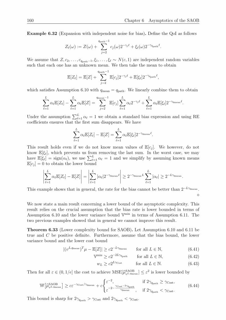
160 Chapter 6 Asymptotics of the SAOB
Example 6.32 (Expansion with independent noise for bias). Define the QoI as follows
Z`(ω) := Z(ω) +
qpath−1∑j=2
cj(ω)2−γj` + ξ`(ω)2−γqpath`.
We assume that Z, c2, . . . , cqpath−1, ξ1, . . . , ξ` ∼ N(c, 1) are independent random variablessuch that each one has an unknown mean. We then take the mean to obtain
E[Z`] = E[Z] +
qpath−1∑j=2
E[cj]2−γj` + E[ξ`]2
−γqpath`,
which satisfies Assumption 6.10 with qmean = qpath. We linearly combine them to obtain
L∑`=1
α`E[Z`]−L∑`=1
α`E[Z] =
qmean−1∑j=2
E[cj]L∑`=1
α`2−γj` +
L∑`=1
α`E[ξ`]2−γqmean`.
Under the assumption∑L
`=1 α` = 1 we obtain a standard bias expression and using REcoefficients ensures that the first sum disappears. We have
L∑`=1
α`E[Z`]− E[Z] =L∑`=1
α`E[ξ`]2−γqmean`.
This result holds even if we do not know mean values of E[cj]. We however, do notknow E[ξ`], which prevents us from removing the last sum. In the worst case, we mayhave E[ξ`] = sign(α`), we use
∑L`=1 α` = 1 and we simplify by assuming known means
E[cj] = 0 to obtain the lower bound∣∣∣∣∣L∑`=1
α`E[Z`]− E[Z]
∣∣∣∣∣ =
∣∣∣∣∣L∑`=1
|α`|2−γqmean`
∣∣∣∣∣ ≥ 2−γqmeanL
L∑`=1
|α`| ≥ 2−Lγqmean .
This example shows that in general, the rate for the bias cannot be better than 2−Lγqmean .
We now state a main result concerning a lower bound of the asymptotic complexity. Thisresult relies on the crucial assumption that the bias rate is lower bounded in terms ofAssumption 6.10 and the lower variance bound Vmin in terms of Assumption 6.11. Thetwo previous examples showed that in general we cannot improve this result.
Theorem 6.33 (Lower complexity bound for SAOB). Let Assumption 6.10 and 6.11 betrue and C be positive definite. Furthermore, assume that the bias bound, the lowervariance bound and the lower cost bound
|(vL,qmean)Tµ− E[Z]| ≥ c2−Lγqmean for all L ∈ N, (6.41)
Vmin ≥ c2−2Lγqpath for all L ∈ N, (6.42)
wL ≥ c2LγCost for all L ∈ N. (6.43)
Then for all ε ∈ (0, 1/e] the cost to achieve MSE[µSAOBvL,qmean ] ≤ ε2 is lower bounded by
W[µSAOBvL,qmean
]≥ cε−γCost/γqmean + c
ε−2, if 2γqpath ≥ γCost,
ε−2−
γCost−2γqpathγqmean , if 2γqpath < γCost.
(6.44)
This bound is sharp for 2γqpath > γCost and 2γqpath < γCost.
Chapter 6 Asymptotics of the SAOB 161
Proof. The first term in the bound (6.44) is simply the cost for a single high fidelityevaluation and thus cannot be lower bounded any further. This evaluation is required,since vL,qmean
L 6= 0. For 2γqpath ≥ γCost the bound of ε−2 is trivial. For the case 2γqpath < γCost
the bias-variance decomposition shows
E[(µSAOB
vL,qmean − E[Z])2]
= ((vL,qmean)Tµ− E[Z])2 + V[µSAOBvL,qmean
].
To achieve a bias of order ε2 we have to choose L ≥ − log2(ε)/γqmean + c using (6.41).Since we want a tight lower bound, we choose L = − log2(ε)/γqmean . We now combine thiswith (6.39), the bound (6.42) and (6.43)
W[µα] ≥ cε−2α2LW[ZL]Vmin ≥ cε−22L(γCost−2γqpath ) = cε−2ε−(γCost−2γqpath )/γqmean .
This shows the claim (6.44). The sharpness of the bound follows from Corollary 6.26.
The previous theorem shows that there is a strict lower limit on the asymptotic complexityof any linear unbiased estimator. In particular, the smoothness of Z1, Z2, . . . w.r.t. themean and pathwise can be used to offset the increased cost w.r.t. the level. However, thisonly works up to a certain degree and thus the optimal asymptotic costs of cε−2 cannotbe achieved in general for linear unbiased estimators.
Remark 6.34 (Equal costs on every level). The previous theorem does not include thecase of a sharp bound for equal costs on every level 2γqpath = γCost, in which the proofidea of Lemma 6.29 falls apart. We cannot reduce(
K∑k=1
((βk)TCkβkW k
)1/2
)2
to a single model group and we also cannot pull out the costs for only the high fidelitymodel. Intuitively, this is not possible since each non–zero term should asymptotically beof the same size. We thus expect(
K∑k=1
((βk)TCkβkW k
)1/2
)2
≥ c(L(βL)TCLβLWL)1/2)2 = cL2(βL)TCLβLWL, (6.45)
where SL is now the only model group that contains the high fidelity model. It is however,not straightforward to verify this inequality. However, if (6.45) holds, then it is straight-forward to provide a sharp bound for 2γqpath = γCost following the ideas outlined in thissection. The additional L2 compared to (6.39) adds the term log(ε)2. In any case, it isstraightforward to verify that under the assumption of Theorem 6.33 for 2γqpath = γCost
and using Corollary 6.26
cε−γCost/γqmean + cε−2 ≤W[µSAOBvL,qmean
]≤ cε−γCost/γqmean + cε−2 log(ε)2.
Therefore, the bound (6.44) is tight up to logarithmic factors.
Remark 6.35 (C positive definite in Theorem 6.33). Let us comment on the assumptionthat C in Theorem 6.33 is positive definite, which is not necessary. If C has a zeroeigenvalue and corresponding eigenvector v with vL 6= 0 then
Vmin = minβ
(β1
)TC
(β1
)≤ 1
v2L
vTCv = 0,
162 Chapter 6 Asymptotics of the SAOB
which contradicts (6.42). Therefore, C may only have zero eigenvalues with eigenvectors vwhere vL = 0. This means that linear combinations of low fidelity models may be linearlydependent (ignoring the mean). However, since we assumed w` = 0 for ` ∈ 1, . . . , L− 1we cannot use this linear dependence to further reduce the variance. Thus, we may alwaysremove enough models of Z1, . . . , ZL−1 such that C is positive definite without increasingthe variance.
6.4 Numerical experiments with explicit expansions
Convergence of SAOB to RE. We demonstrate that for a specific example the SAOBconverges to the RE estimator. We define the QoI as
Z`(ω) := Z(ω) +4∑j=2
cj2−(j−1)(`+`0) + 0.1ξ`2
−3(`+`0) (6.46)
and assume that (Z, c2, c3, c4)T ∼ N(0, Q) with covariance matrix Qij = exp(−|i − j|),which is obtained from the exponential covariance function. We further assume thatξ` ∼ N(0, 1) i.i.d. and that the ξ` are independent of Z, c2, c3, c4. The variable `0 describesthe initial accuracy of the models. We compute the covariance matrix C analytically andfix artificial costs for every model ` ∈ 1, . . . , L with w` = 22`−2. We further choose thecomputational budget Wbudget to be sufficiently large. This model fits Assumption 6.11with qpath = 4, γ2 = 1, γ3 = 2 and γ4 = 3. We compare the SAOB κ with the weightedRE κ estimator with κ = 2, 3, 4 with a bias of α := eL. We define the difference in thecoefficients as follows
dκ(`0) :=
(K∑k=1
‖βk,SAOBκ(`0)− βk,REκ‖2
)1/2
. (6.47)
The SAOB chooses the same model groups as the RE estimators for example (6.46). Wefurther compare the relative difference of the variances
vκ(`0) :=V[µREκL (`0)
]− V
[µSAOBκL (`0)
]V[µSAOBκ
L (`0)]. (6.48)
The variance of both estimators clearly depends on the covariance matrix C = C(`0)which itself depends on `0. However, the coefficients of the RE estimators βk,REκ do notdepend on `0. We plot the computed values dκ and vκ in Figure 6.1 for different valuesof `0. The respective coefficients of the SAOB 2 and the MLMC (RE 2) estimator aregiven in Figure 6.2 and for the SAOB 3 and RE 3 estimator in Figure 6.3. We concludethat both the coefficients as well as the relative variance difference converges to zero.This indicates that asymptotically, there is no difference between the SAOB κ and RE κestimator. We further conclude that the difference between the SAOB κ and the RE κestimator is larger if κ is larger, both in terms of dκ and vκ. This is not surprising, sincethe SAOB is able to optimize over more parameters achieving a larger variance reduction.
Remark 6.36 (Proof of convergence). A rigorous proof of convergence for the models(6.46) is not straightforward as it might seem. An idea is to first verify that both es-timators use the same model groups, i.e. for sufficiently large `0 the SAOB κ uses the
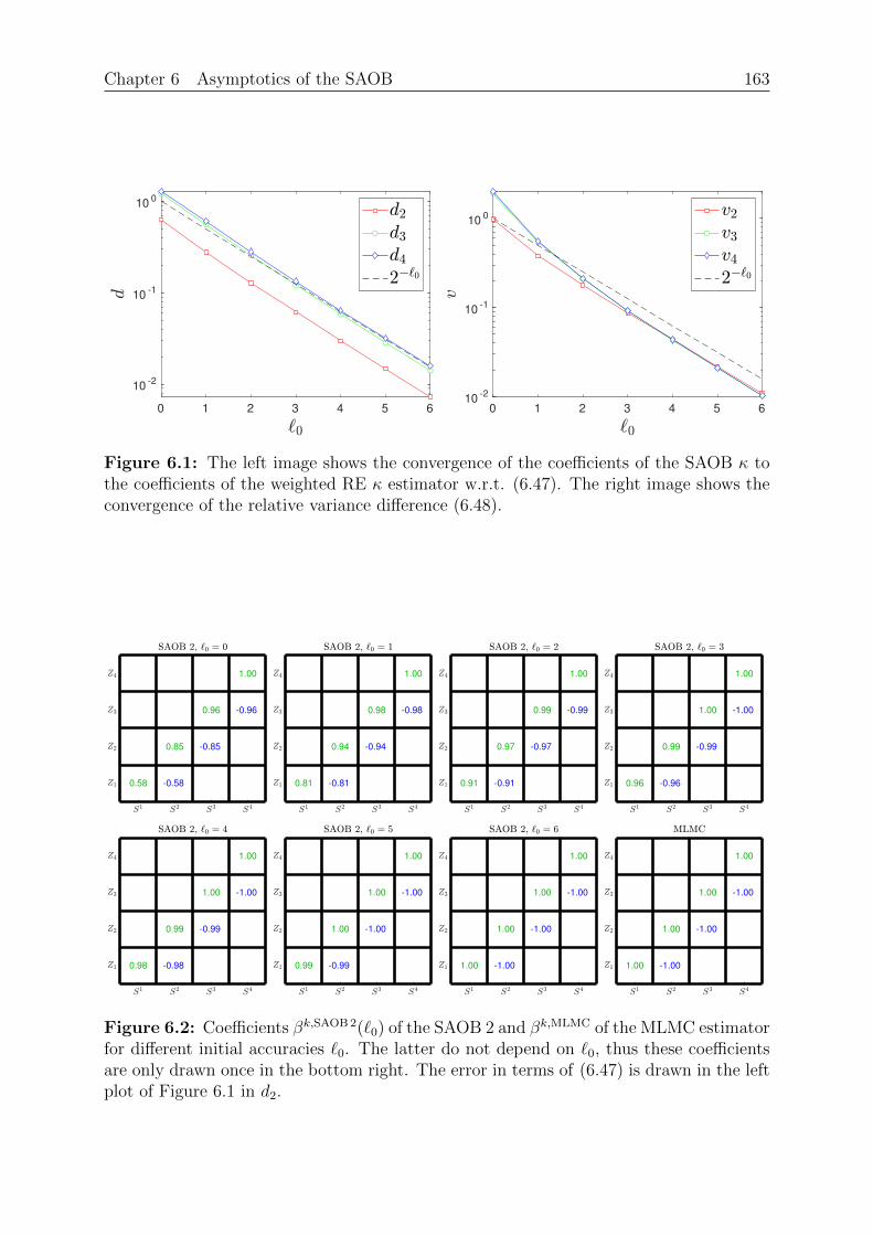
Chapter 6 Asymptotics of the SAOB 163
0 1 2 3 4 5 6
10-2
10-1
100
0 1 2 3 4 5 610
-2
10-1
100
Figure 6.1: The left image shows the convergence of the coefficients of the SAOB κ tothe coefficients of the weighted RE κ estimator w.r.t. (6.47). The right image shows theconvergence of the relative variance difference (6.48).
0.58 -0.58
0.85 -0.85
0.96 -0.96
1.00
0.81 -0.81
0.94 -0.94
0.98 -0.98
1.00
0.91 -0.91
0.97 -0.97
0.99 -0.99
1.00
0.96 -0.96
0.99 -0.99
1.00 -1.00
1.00
0.98 -0.98
0.99 -0.99
1.00 -1.00
1.00
0.99 -0.99
1.00 -1.00
1.00 -1.00
1.00
1.00 -1.00
1.00 -1.00
1.00 -1.00
1.00
1.00 -1.00
1.00 -1.00
1.00 -1.00
1.00
Figure 6.2: Coefficients βk,SAOB 2(`0) of the SAOB 2 and βk,MLMC of the MLMC estimatorfor different initial accuracies `0. The latter do not depend on `0, thus these coefficientsare only drawn once in the bottom right. The error in terms of (6.47) is drawn in the leftplot of Figure 6.1 in d2.
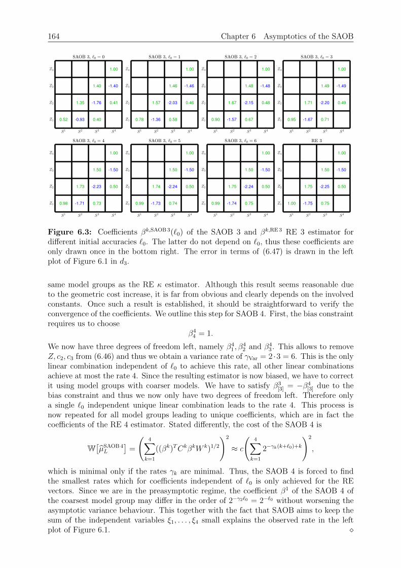
164 Chapter 6 Asymptotics of the SAOB
0.52 -0.93
1.35
0.40
-1.76
1.40
0.41
-1.40
1.00
0.78 -1.36
1.57
0.58
-2.03
1.46
0.46
-1.46
1.00
0.90 -1.57
1.67
0.67
-2.15
1.48
0.48
-1.48
1.00
0.95 -1.67
1.71
0.71
-2.20
1.49
0.49
-1.49
1.00
0.98 -1.71
1.73
0.73
-2.23
1.50
0.50
-1.50
1.00
0.99 -1.73
1.74
0.74
-2.24
1.50
0.50
-1.50
1.00
0.99 -1.74
1.75
0.75
-2.24
1.50
0.50
-1.50
1.00
1.00 -1.75
1.75
0.75
-2.25
1.50
0.50
-1.50
1.00
Figure 6.3: Coefficients βk,SAOB 3(`0) of the SAOB 3 and βk,RE 3 RE 3 estimator fordifferent initial accuracies `0. The latter do not depend on `0, thus these coefficients areonly drawn once in the bottom right. The error in terms of (6.47) is drawn in the leftplot of Figure 6.1 in d3.
same model groups as the RE κ estimator. Although this result seems reasonable dueto the geometric cost increase, it is far from obvious and clearly depends on the involvedconstants. Once such a result is established, it should be straightforward to verify theconvergence of the coefficients. We outline this step for SAOB 4. First, the bias constraintrequires us to choose
β44 = 1.
We now have three degrees of freedom left, namely β41 , β
42 and β4
3 . This allows to removeZ, c2, c3 from (6.46) and thus we obtain a variance rate of γVar = 2 ·3 = 6. This is the onlylinear combination independent of `0 to achieve this rate, all other linear combinationsachieve at most the rate 4. Since the resulting estimator is now biased, we have to correctit using model groups with coarser models. We have to satisfy β3
[3] = −β4[3] due to the
bias constraint and thus we now only have two degrees of freedom left. Therefore onlya single `0 independent unique linear combination leads to the rate 4. This process isnow repeated for all model groups leading to unique coefficients, which are in fact thecoefficients of the RE 4 estimator. Stated differently, the cost of the SAOB 4 is
W[µSAOB 4L
]=
(4∑
k=1
((βk)TCkβkW k)1/2
)2
≈ c
(4∑
k=1
2−γk(k+`0)+k
)2
,
which is minimal only if the rates γk are minimal. Thus, the SAOB 4 is forced to findthe smallest rates which for coefficients independent of `0 is only achieved for the REvectors. Since we are in the preasymptotic regime, the coefficient β1 of the SAOB 4 ofthe coarsest model group may differ in the order of 2−γ2`0 = 2−`0 without worsening theasymptotic variance behaviour. This together with the fact that SAOB aims to keep thesum of the independent variables ξ1, . . . , ξ4 small explains the observed rate in the leftplot of Figure 6.1.
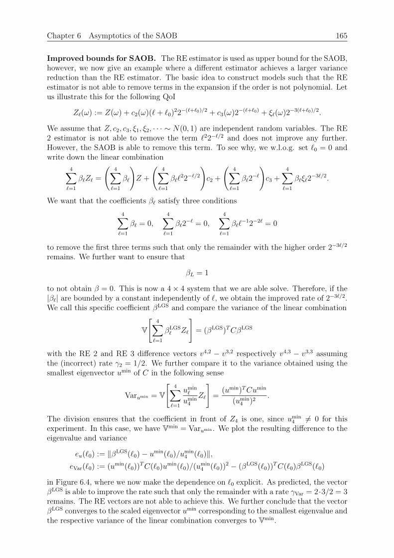
Chapter 6 Asymptotics of the SAOB 165
Improved bounds for SAOB. The RE estimator is used as upper bound for the SAOB,however, we now give an example where a different estimator achieves a larger variancereduction than the RE estimator. The basic idea to construct models such that the REestimator is not able to remove terms in the expansion if the order is not polynomial. Letus illustrate this for the following QoI
Z`(ω) := Z(ω) + c2(ω)(`+ `0)22−(`+`0)/2 + c3(ω)2−(`+`0) + ξ`(ω)2−3(`+`0)/2.
We assume that Z, c2, c3, ξ1, ξ2, · · · ∼ N(0, 1) are independent random variables. The RE2 estimator is not able to remove the term `22−`/2 and does not improve any further.However, the SAOB is able to remove this term. To see why, we w.l.o.g. set `0 = 0 andwrite down the linear combination
4∑`=1
β`Z` =
(4∑`=1
β`
)Z +
(4∑`=1
β``22−`/2
)c2 +
(4∑`=1
β`2−`
)c3 +
4∑`=1
β`ξ`2−3`/2.
We want that the coefficients β` satisfy three conditions
4∑`=1
β` = 0,4∑`=1
β`2−` = 0,
4∑`=1
β``−12−2` = 0
to remove the first three terms such that only the remainder with the higher order 2−3`/2
remains. We further want to ensure that
βL = 1
to not obtain β = 0. This is now a 4× 4 system that we are able solve. Therefore, if the|β`| are bounded by a constant independently of `, we obtain the improved rate of 2−3`/2.We call this specific coefficient βLGS and compare the variance of the linear combination
V
[4∑`=1
βLGS` Z`
]= (βLGS)TCβLGS
with the RE 2 and RE 3 difference vectors v4,2 − v3,2 respectively v4,3 − v3,3 assumingthe (incorrect) rate γ2 = 1/2. We further compare it to the variance obtained using thesmallest eigenvector umin of C in the following sense
Varumin = V
[4∑`=1
umin`
umin4
Z`
]=
(umin)TCumin
(umin4 )2
.
The division ensures that the coefficient in front of Z4 is one, since umin4 6= 0 for this
experiment. In this case, we have Vmin = Varumin . We plot the resulting difference to theeigenvalue and variance
eu(`0) := ‖βLGS(`0)− umin(`0)/umin4 (`0)‖,
eVar(`0) := (umin(`0))TC(`0)umin(`0)/(umin4 (`0))2 − (βLGS(`0))TC(`0)βLGS(`0)
in Figure 6.4, where we now make the dependence on `0 explicit. As predicted, the vectorβLGS is able to improve the rate such that only the remainder with a rate γVar = 2·3/2 = 3remains. The RE vectors are not able to achieve this. We further conclude that the vectorβLGS converges to the scaled eigenvector umin corresponding to the smallest eigenvalue andthe respective variance of the linear combination converges to Vmin.
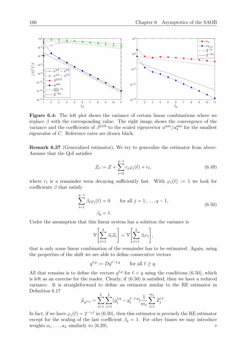
166 Chapter 6 Asymptotics of the SAOB
1 2 3 4 5 6 7 8 9 10 11
10-14
10-12
10-10
10-8
10-6
10-4
10-2
100
1 2 3 4 5 6 7 8 9 10 11
10-15
10-10
10-5
100
105
Figure 6.4: The left plot shows the variance of certain linear combinations where wereplace β with the corresponding value. The right image shows the convergence of thevariance and the coefficients of βLGS to the scaled eigenvector umin/umin
4 for the smallesteigenvalue of C. Reference rates are drawn black.
Remark 6.37 (Generalized estimator). We try to generalize the estimator from above.Assume that the QoI satisfies
Z` := Z +
q−1∑j=2
cjϕj(`) + r`, (6.49)
where r` is a remainder term decaying sufficiently fast. With ϕ1(`) := 1 we look forcoefficients β that satisfy
q−1∑`=1
β`ϕj(`) = 0 for all j = 1, . . . , q − 1,
βq = 1.
(6.50)
Under the assumption that this linear system has a solution the variance is
V
[q∑`=1
β`Z`
]= V
[q∑`=1
β`r`
],
that is only some linear combination of the remainder has to be estimated. Again, usingthe properties of the shift we are able to define consecutive vectors
y`,q := Dy`−1,q for all ` ≥ q.
All that remains is to define the vectors y`,q for ` < q using the conditions (6.50), whichis left as an exercise for the reader. Clearly, if (6.50) is satisfied, then we have a reducedvariance. It is straightforward to define an estimator similar to the RE estimator inDefinition 6.17
µyL,q =L∑`=1
L∑j=1
(y`,qj − y`−1,qj )
1
m`
m∑i=1
Zi,`j .
In fact, if we have ϕj(`) = 2−γj` in (6.50), then this estimator is precisely the RE estimatorexcept for the scaling of the last coefficient βq = 1. For other biases we may introduceweights a1, . . . , aL similarly to (6.29).
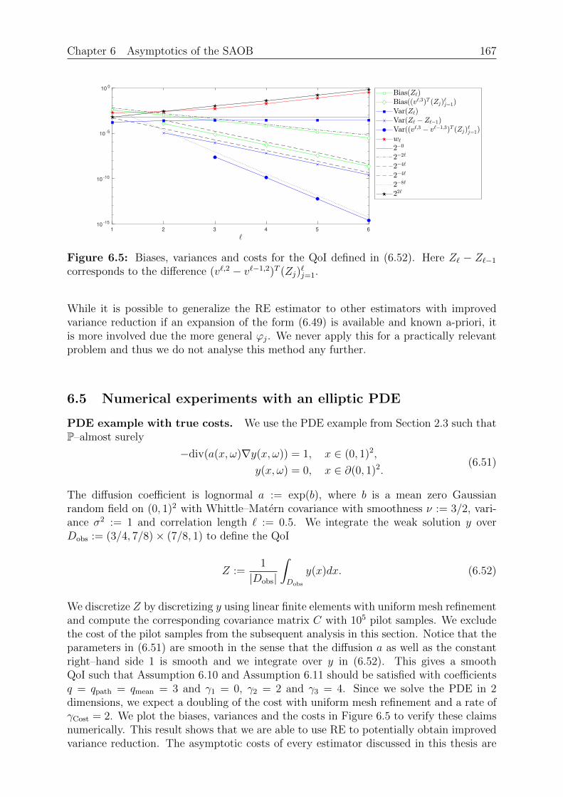
Chapter 6 Asymptotics of the SAOB 167
1 2 3 4 5 6
10-15
10-10
10-5
100
Figure 6.5: Biases, variances and costs for the QoI defined in (6.52). Here Z` − Z`−1
corresponds to the difference (v`,2 − v`−1,2)T (Zj)`j=1.
While it is possible to generalize the RE estimator to other estimators with improvedvariance reduction if an expansion of the form (6.49) is available and known a-priori, itis more involved due the more general ϕj. We never apply this for a practically relevantproblem and thus we do not analyse this method any further.
6.5 Numerical experiments with an elliptic PDE
PDE example with true costs. We use the PDE example from Section 2.3 such thatP–almost surely
−div(a(x, ω)∇y(x, ω)) = 1, x ∈ (0, 1)2,
y(x, ω) = 0, x ∈ ∂(0, 1)2.(6.51)
The diffusion coefficient is lognormal a := exp(b), where b is a mean zero Gaussianrandom field on (0, 1)2 with Whittle–Matern covariance with smoothness ν := 3/2, vari-ance σ2 := 1 and correlation length ` := 0.5. We integrate the weak solution y overDobs := (3/4, 7/8)× (7/8, 1) to define the QoI
Z :=1
|Dobs|
∫Dobs
y(x)dx. (6.52)
We discretize Z by discretizing y using linear finite elements with uniform mesh refinementand compute the corresponding covariance matrix C with 105 pilot samples. We excludethe cost of the pilot samples from the subsequent analysis in this section. Notice that theparameters in (6.51) are smooth in the sense that the diffusion a as well as the constantright–hand side 1 is smooth and we integrate over y in (6.52). This gives a smoothQoI such that Assumption 6.10 and Assumption 6.11 should be satisfied with coefficientsq = qpath = qmean = 3 and γ1 = 0, γ2 = 2 and γ3 = 4. Since we solve the PDE in 2dimensions, we expect a doubling of the cost with uniform mesh refinement and a rate ofγCost = 2. We plot the biases, variances and the costs in Figure 6.5 to verify these claimsnumerically. This result shows that we are able to use RE to potentially obtain improvedvariance reduction. The asymptotic costs of every estimator discussed in this thesis are
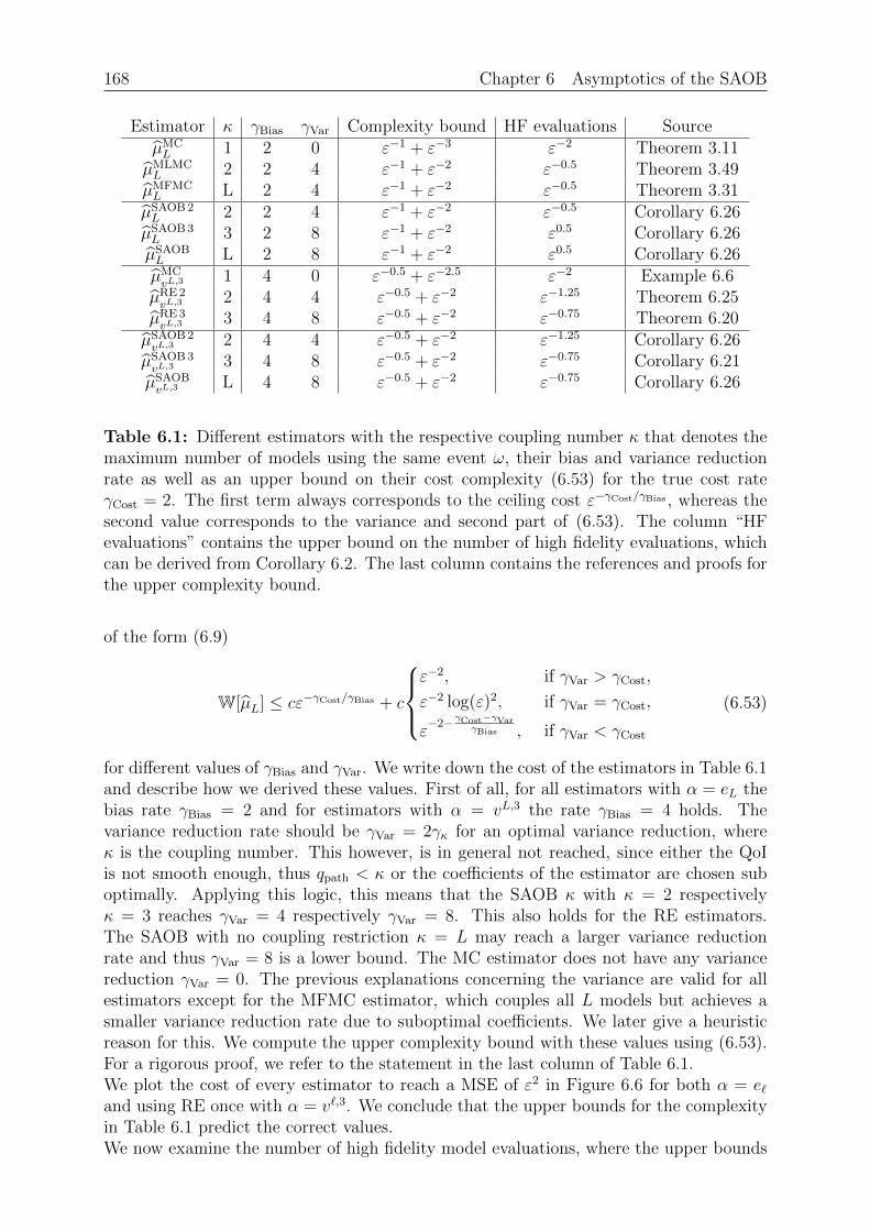
168 Chapter 6 Asymptotics of the SAOB
Estimator κ γBias γVar Complexity bound HF evaluations SourceµMCL 1 2 0 ε−1 + ε−3 ε−2 Theorem 3.11
µMLMCL 2 2 4 ε−1 + ε−2 ε−0.5 Theorem 3.49µMFMCL L 2 4 ε−1 + ε−2 ε−0.5 Theorem 3.31
µSAOB 2L 2 2 4 ε−1 + ε−2 ε−0.5 Corollary 6.26µSAOB 3L 3 2 8 ε−1 + ε−2 ε0.5 Corollary 6.26µSAOBL L 2 8 ε−1 + ε−2 ε0.5 Corollary 6.26µMCvL,3 1 4 0 ε−0.5 + ε−2.5 ε−2 Example 6.6
µRE 2vL,3 2 4 4 ε−0.5 + ε−2 ε−1.25 Theorem 6.25µRE 3vL,3 3 4 8 ε−0.5 + ε−2 ε−0.75 Theorem 6.20
µSAOB 2vL,3 2 4 4 ε−0.5 + ε−2 ε−1.25 Corollary 6.26µSAOB 3vL,3 3 4 8 ε−0.5 + ε−2 ε−0.75 Corollary 6.21µSAOBvL,3 L 4 8 ε−0.5 + ε−2 ε−0.75 Corollary 6.26
Table 6.1: Different estimators with the respective coupling number κ that denotes themaximum number of models using the same event ω, their bias and variance reductionrate as well as an upper bound on their cost complexity (6.53) for the true cost rateγCost = 2. The first term always corresponds to the ceiling cost ε−γCost/γBias , whereas thesecond value corresponds to the variance and second part of (6.53). The column “HFevaluations” contains the upper bound on the number of high fidelity evaluations, whichcan be derived from Corollary 6.2. The last column contains the references and proofs forthe upper complexity bound.
of the form (6.9)
W[µL] ≤ cε−γCost/γBias + c
ε−2, if γVar > γCost,
ε−2 log(ε)2, if γVar = γCost,
ε−2− γCost−γVar
γBias , if γVar < γCost
(6.53)
for different values of γBias and γVar. We write down the cost of the estimators in Table 6.1and describe how we derived these values. First of all, for all estimators with α = eL thebias rate γBias = 2 and for estimators with α = vL,3 the rate γBias = 4 holds. Thevariance reduction rate should be γVar = 2γκ for an optimal variance reduction, whereκ is the coupling number. This however, is in general not reached, since either the QoIis not smooth enough, thus qpath < κ or the coefficients of the estimator are chosen suboptimally. Applying this logic, this means that the SAOB κ with κ = 2 respectivelyκ = 3 reaches γVar = 4 respectively γVar = 8. This also holds for the RE estimators.The SAOB with no coupling restriction κ = L may reach a larger variance reductionrate and thus γVar = 8 is a lower bound. The MC estimator does not have any variancereduction γVar = 0. The previous explanations concerning the variance are valid for allestimators except for the MFMC estimator, which couples all L models but achieves asmaller variance reduction rate due to suboptimal coefficients. We later give a heuristicreason for this. We compute the upper complexity bound with these values using (6.53).For a rigorous proof, we refer to the statement in the last column of Table 6.1.We plot the cost of every estimator to reach a MSE of ε2 in Figure 6.6 for both α = e`and using RE once with α = v`,3. We conclude that the upper bounds for the complexityin Table 6.1 predict the correct values.We now examine the number of high fidelity model evaluations, where the upper bounds
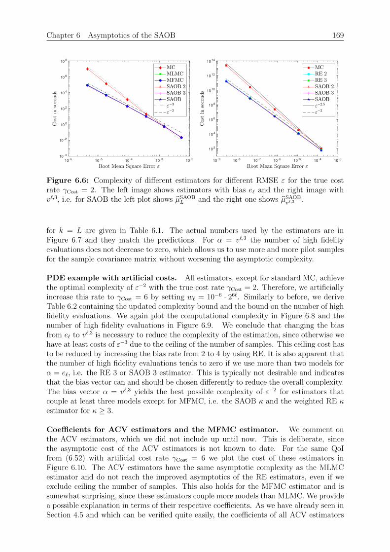
Chapter 6 Asymptotics of the SAOB 169
10-6
10-5
10-4
10-3
10-2
10-4
10-2
100
102
104
106
108
10-9
10-8
10-7
10-6
10-5
10-4
10-3
102
104
106
108
1010
1012
1014
Figure 6.6: Complexity of different estimators for different RMSE ε for the true costrate γCost = 2. The left image shows estimators with bias e` and the right image withv`,3, i.e. for SAOB the left plot shows µSAOB
L and the right one shows µSAOBv`,3
.
for k = L are given in Table 6.1. The actual numbers used by the estimators are inFigure 6.7 and they match the predictions. For α = v`,3 the number of high fidelityevaluations does not decrease to zero, which allows us to use more and more pilot samplesfor the sample covariance matrix without worsening the asymptotic complexity.
PDE example with artificial costs. All estimators, except for standard MC, achievethe optimal complexity of ε−2 with the true cost rate γCost = 2. Therefore, we artificiallyincrease this rate to γCost = 6 by setting w` = 10−6 · 26`. Similarly to before, we deriveTable 6.2 containing the updated complexity bound and the bound on the number of highfidelity evaluations. We again plot the computational complexity in Figure 6.8 and thenumber of high fidelity evaluations in Figure 6.9. We conclude that changing the biasfrom e` to v`,3 is necessary to reduce the complexity of the estimation, since otherwise wehave at least costs of ε−3 due to the ceiling of the number of samples. This ceiling cost hasto be reduced by increasing the bias rate from 2 to 4 by using RE. It is also apparent thatthe number of high fidelity evaluations tends to zero if we use more than two models forα = e`, i.e. the RE 3 or SAOB 3 estimator. This is typically not desirable and indicatesthat the bias vector can and should be chosen differently to reduce the overall complexity.The bias vector α = v`,3 yields the best possible complexity of ε−2 for estimators thatcouple at least three models except for MFMC, i.e. the SAOB κ and the weighted RE κestimator for κ ≥ 3.
Coefficients for ACV estimators and the MFMC estimator. We comment onthe ACV estimators, which we did not include up until now. This is deliberate, sincethe asymptotic cost of the ACV estimators is not known to date. For the same QoIfrom (6.52) with artificial cost rate γCost = 6 we plot the cost of these estimators inFigure 6.10. The ACV estimators have the same asymptotic complexity as the MLMCestimator and do not reach the improved asymptotics of the RE estimators, even if weexclude ceiling the number of samples. This also holds for the MFMC estimator and issomewhat surprising, since these estimators couple more models than MLMC. We providea possible explanation in terms of their respective coefficients. As we have already seen inSection 4.5 and which can be verified quite easily, the coefficients of all ACV estimators
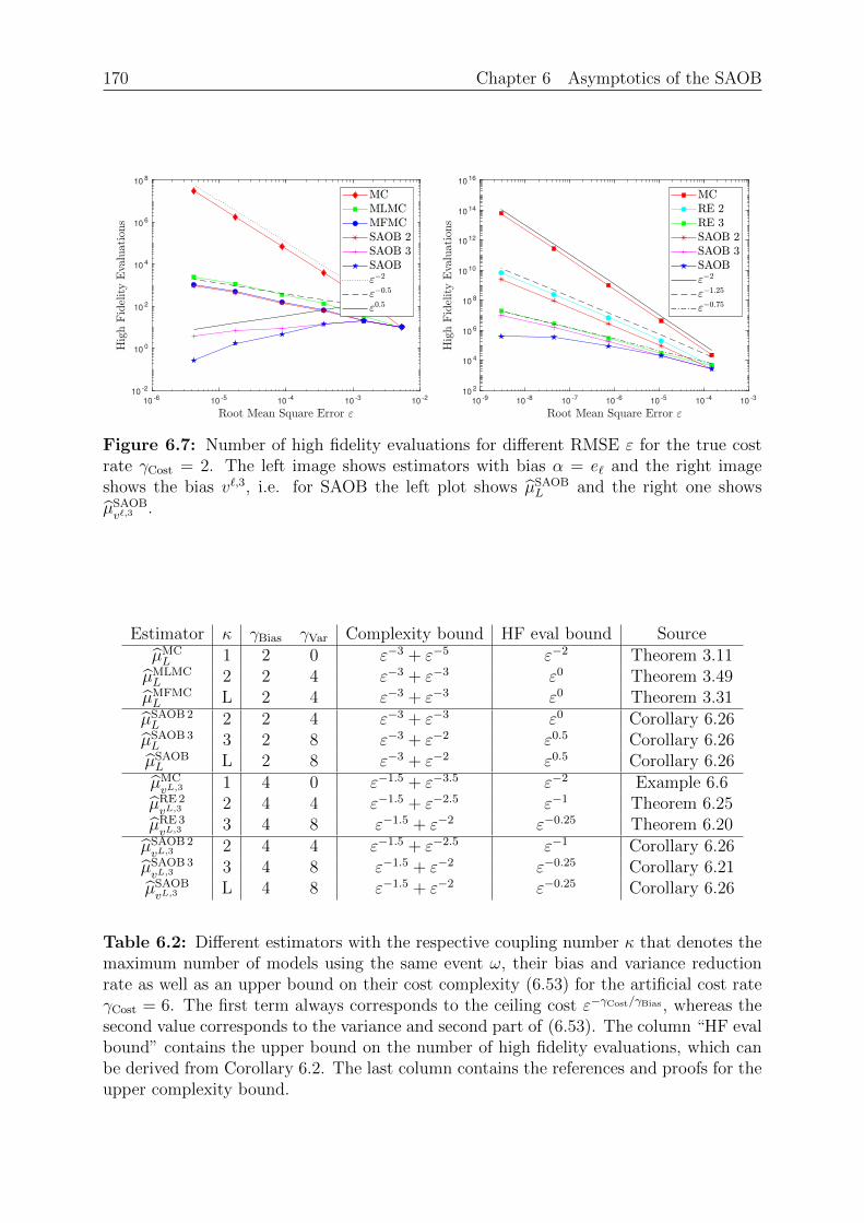
170 Chapter 6 Asymptotics of the SAOB
10-6
10-5
10-4
10-3
10-2
10-2
100
102
104
106
108
10-9
10-8
10-7
10-6
10-5
10-4
10-3
102
104
106
108
1010
1012
1014
1016
Figure 6.7: Number of high fidelity evaluations for different RMSE ε for the true costrate γCost = 2. The left image shows estimators with bias α = e` and the right imageshows the bias v`,3, i.e. for SAOB the left plot shows µSAOB
L and the right one showsµSAOBv`,3
.
Estimator κ γBias γVar Complexity bound HF eval bound SourceµMCL 1 2 0 ε−3 + ε−5 ε−2 Theorem 3.11
µMLMCL 2 2 4 ε−3 + ε−3 ε0 Theorem 3.49µMFMCL L 2 4 ε−3 + ε−3 ε0 Theorem 3.31
µSAOB 2L 2 2 4 ε−3 + ε−3 ε0 Corollary 6.26µSAOB 3L 3 2 8 ε−3 + ε−2 ε0.5 Corollary 6.26µSAOBL L 2 8 ε−3 + ε−2 ε0.5 Corollary 6.26µMCvL,3 1 4 0 ε−1.5 + ε−3.5 ε−2 Example 6.6
µRE 2vL,3 2 4 4 ε−1.5 + ε−2.5 ε−1 Theorem 6.25µRE 3vL,3 3 4 8 ε−1.5 + ε−2 ε−0.25 Theorem 6.20
µSAOB 2vL,3 2 4 4 ε−1.5 + ε−2.5 ε−1 Corollary 6.26µSAOB 3vL,3 3 4 8 ε−1.5 + ε−2 ε−0.25 Corollary 6.21µSAOBvL,3 L 4 8 ε−1.5 + ε−2 ε−0.25 Corollary 6.26
Table 6.2: Different estimators with the respective coupling number κ that denotes themaximum number of models using the same event ω, their bias and variance reductionrate as well as an upper bound on their cost complexity (6.53) for the artificial cost rateγCost = 6. The first term always corresponds to the ceiling cost ε−γCost/γBias , whereas thesecond value corresponds to the variance and second part of (6.53). The column “HF evalbound” contains the upper bound on the number of high fidelity evaluations, which canbe derived from Corollary 6.2. The last column contains the references and proofs for theupper complexity bound.
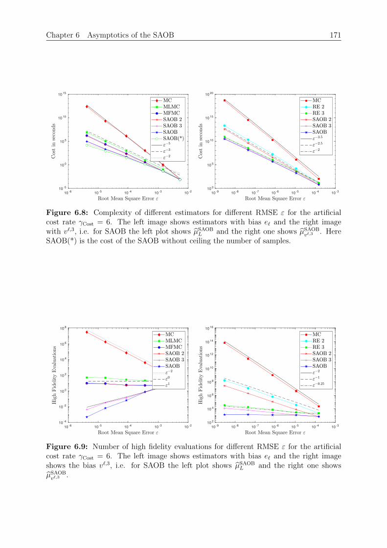
Chapter 6 Asymptotics of the SAOB 171
10-6
10-5
10-4
10-3
10-2
10-5
100
105
1010
1015
10-9
10-8
10-7
10-6
10-5
10-4
10-3
100
105
1010
1015
1020
Figure 6.8: Complexity of different estimators for different RMSE ε for the artificialcost rate γCost = 6. The left image shows estimators with bias e` and the right imagewith v`,3, i.e. for SAOB the left plot shows µSAOB
L and the right one shows µSAOBv`,3
. HereSAOB(*) is the cost of the SAOB without ceiling the number of samples.
10-6
10-5
10-4
10-3
10-2
10-4
10-2
100
102
104
106
108
10-9
10-8
10-7
10-6
10-5
10-4
10-3
102
104
106
108
1010
1012
1014
1016
Figure 6.9: Number of high fidelity evaluations for different RMSE ε for the artificialcost rate γCost = 6. The left image shows estimators with bias e` and the right imageshows the bias v`,3, i.e. for SAOB the left plot shows µSAOB
L and the right one showsµSAOBv`,3
.
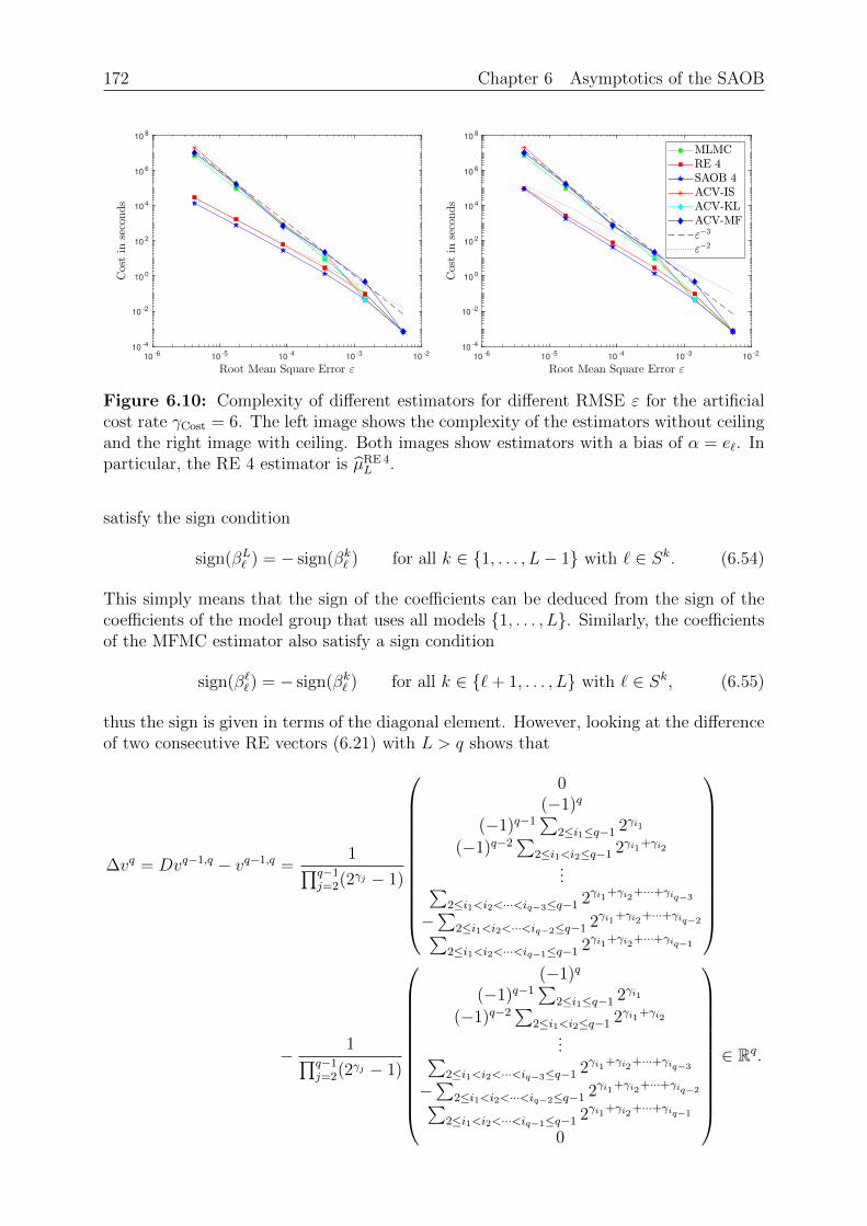
172 Chapter 6 Asymptotics of the SAOB
10-6
10-5
10-4
10-3
10-2
10-4
10-2
100
102
104
106
108
10-6
10-5
10-4
10-3
10-2
10-4
10-2
100
102
104
106
108
Figure 6.10: Complexity of different estimators for different RMSE ε for the artificialcost rate γCost = 6. The left image shows the complexity of the estimators without ceilingand the right image with ceiling. Both images show estimators with a bias of α = e`. Inparticular, the RE 4 estimator is µRE 4
L .
satisfy the sign condition
sign(βL` ) = − sign(βk` ) for all k ∈ 1, . . . , L− 1 with ` ∈ Sk. (6.54)
This simply means that the sign of the coefficients can be deduced from the sign of thecoefficients of the model group that uses all models 1, . . . , L. Similarly, the coefficientsof the MFMC estimator also satisfy a sign condition
sign(β``) = − sign(βk` ) for all k ∈ `+ 1, . . . , L with ` ∈ Sk, (6.55)
thus the sign is given in terms of the diagonal element. However, looking at the differenceof two consecutive RE vectors (6.21) with L > q shows that
∆vq = Dvq−1,q − vq−1,q =1∏q−1
j=2(2γj − 1)
0(−1)q
(−1)q−1∑
2≤i1≤q−1 2γi1
(−1)q−2∑
2≤i1<i2≤q−1 2γi1+γi2
...∑2≤i1<i2<···<iq−3≤q−1 2γi1+γi2+···+γiq−3
−∑
2≤i1<i2<···<iq−2≤q−1 2γi1+γi2+···+γiq−2∑2≤i1<i2<···<iq−1≤q−1 2γi1+γi2+···+γiq−1
− 1∏q−1j=2(2γj − 1)
(−1)q
(−1)q−1∑
2≤i1≤q−1 2γi1
(−1)q−2∑
2≤i1<i2≤q−1 2γi1+γi2
...∑2≤i1<i2<···<iq−3≤q−1 2γi1+γi2+···+γiq−3
−∑
2≤i1<i2<···<iq−2≤q−1 2γi1+γi2+···+γiq−2∑2≤i1<i2<···<iq−1≤q−1 2γi1+γi2+···+γiq−1
0
∈ Rq.
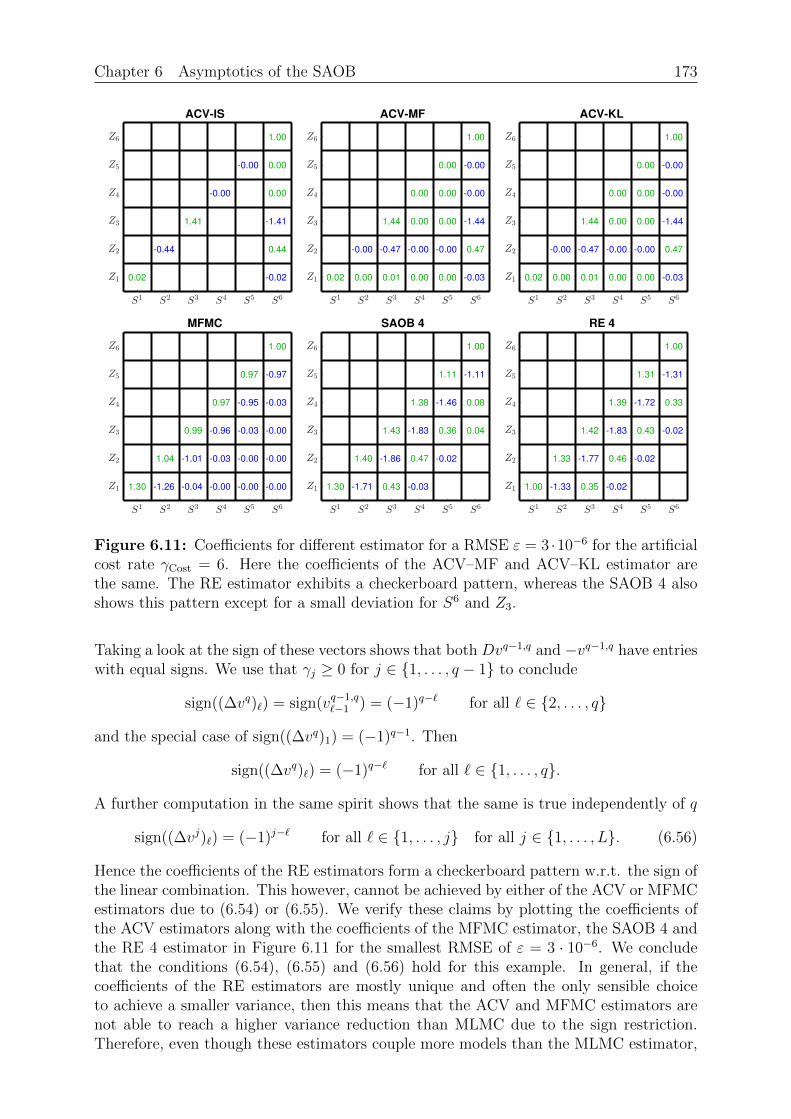
Chapter 6 Asymptotics of the SAOB 173
ACV-IS
0.02
-0.44
1.41
-0.00
-0.00
-0.02
0.44
-1.41
0.00
0.00
1.00
ACV-MF
0.02 0.00
-0.00
0.01
-0.47
1.44
0.00
-0.00
0.00
0.00
0.00
-0.00
0.00
0.00
0.00
-0.03
0.47
-1.44
-0.00
-0.00
1.00
ACV-KL
0.02 0.00
-0.00
0.01
-0.47
1.44
0.00
-0.00
0.00
0.00
0.00
-0.00
0.00
0.00
0.00
-0.03
0.47
-1.44
-0.00
-0.00
1.00
MFMC
1.30 -1.26
1.04
-0.04
-1.01
0.99
-0.00
-0.03
-0.96
0.97
-0.00
-0.00
-0.03
-0.95
0.97
-0.00
-0.00
-0.00
-0.03
-0.97
1.00
SAOB 4
1.30 -1.71
1.40
0.43
-1.86
1.43
-0.03
0.47
-1.83
1.38
-0.02
0.36
-1.46
1.11
0.04
0.08
-1.11
1.00
RE 4
1.00 -1.33
1.33
0.35
-1.77
1.42
-0.02
0.46
-1.83
1.39
-0.02
0.43
-1.72
1.31
-0.02
0.33
-1.31
1.00
Figure 6.11: Coefficients for different estimator for a RMSE ε = 3 ·10−6 for the artificialcost rate γCost = 6. Here the coefficients of the ACV–MF and ACV–KL estimator arethe same. The RE estimator exhibits a checkerboard pattern, whereas the SAOB 4 alsoshows this pattern except for a small deviation for S6 and Z3.
Taking a look at the sign of these vectors shows that both Dvq−1,q and −vq−1,q have entrieswith equal signs. We use that γj ≥ 0 for j ∈ 1, . . . , q − 1 to conclude
sign((∆vq)`) = sign(vq−1,q`−1 ) = (−1)q−` for all ` ∈ 2, . . . , q
and the special case of sign((∆vq)1) = (−1)q−1. Then
sign((∆vq)`) = (−1)q−` for all ` ∈ 1, . . . , q.
A further computation in the same spirit shows that the same is true independently of q
sign((∆vj)`) = (−1)j−` for all ` ∈ 1, . . . , j for all j ∈ 1, . . . , L. (6.56)
Hence the coefficients of the RE estimators form a checkerboard pattern w.r.t. the sign ofthe linear combination. This however, cannot be achieved by either of the ACV or MFMCestimators due to (6.54) or (6.55). We verify these claims by plotting the coefficients ofthe ACV estimators along with the coefficients of the MFMC estimator, the SAOB 4 andthe RE 4 estimator in Figure 6.11 for the smallest RMSE of ε = 3 · 10−6. We concludethat the conditions (6.54), (6.55) and (6.56) hold for this example. In general, if thecoefficients of the RE estimators are mostly unique and often the only sensible choiceto achieve a smaller variance, then this means that the ACV and MFMC estimators arenot able to reach a higher variance reduction than MLMC due to the sign restriction.Therefore, even though these estimators couple more models than the MLMC estimator,
174 Chapter 6 Asymptotics of the SAOB
they do not improve due to their design, which restricts the number of possible linearcombinations.
Remark 6.38 (Other models). Assumption 6.10 and Assumption 6.11 might not be truefor other model hierarchies and thus an improved variance reduction might be obtainedeven if condition (6.54) for ACV and condition (6.55) for MFMC holds. In any case, it is ingeneral feasible to obtain complexity expression for the MLMC and the RE estimator sincetheir coefficients βk are fixed and known, which is not the case for both MFMC and ACV.This makes it difficult to derive statements about their complexity. The coefficients βk
of the SAOB and SAOB κ are also given implicitly, however for these estimators we havethe principle that they are optimal in the class of linear unbiased estimators Theorem 6.3,which allows us to at least derive some upper bounds.
Chapter 7 A multilevel approach for the risk neutral optimal control problem 175
Chapter 7
A multilevel approach for the risk neutraloptimal control problem
In this chapter we examine the risk neutral optimal control problem. The goal is to steerthe result of a system to a prescribed desired state. The system, described by an ellipticPDE, contains random functions and is controlled by a deterministic distributed controlwithout control constraints. We account for the randomness by ensuring that the ex-pected value of the distance to the desired state is small. The use and analysis of the MCmethod to solve this problem is more or less straightforward, however, the resulting coststo compute an accurate approximation are large. A straightforward application of MLMCto reduce the asymptotic complexity often leads to an ill–posed minimization problem.We overcome this difficulty by proposing a strategy where we apply the MLMC estima-tor to the deterministic control as opposed to the cost function where the expectationappears. The result is an estimator that has the improved complexity of MLMC withoutthe drawbacks of being ill–posed. We divide this chapter into the following sections:
In Section 7.1 we introduce the risk neutral optimal control problem. In essence,this is an infinite dimensional quadratic optimization problem with a linear PDEconstraint. The cost function contains randomness, which we eliminate by takingthe mean. We show existence and uniqueness of a solution, we derive the optimalityconditions, give a short literature review and derive convergence results for thespatial discretization with finite elements. These results are standard and the focusof this chapter is the discretization of the mean, which we focus on in the remainingsections of this chapter.
We continue with the standard MC approach in Section 7.2, which we use as areference. This approach allows us to discuss the basic concepts needed for theMLMC approach. We show that the MC discretization leads to a well–posed prob-lem and derive an asymptotic complexity result. The resulting costs of this methodare typically quite large.
We improve the MC approach with an MLMC approach in Section 7.3. We call themethod Multilevel Monte Carlo for the control (MLC). The idea is to compute thedifference of the optimal controls on two consecutive levels, which itself is a solutionof an optimal control problem. This approach achieves an MLMC complexity resultsimilar to Theorem 3.49. In particular, the MLC improves the standard MC methodand is well posed in contrast to directly applying the MLMC telescoping sum ideato the cost function.
We conduct numerical experiments in Section 7.4 to verify the complexity resultsfor MC and MLC. We verify that we have substantial gains compared to the MCestimator in the order of two magnitudes.
176 Chapter 7 A multilevel approach for the risk neutral optimal control problem
7.1 The risk neutral optimal control problem
Introduction. We are interested in the risk neutral optimal control problem
minu∈U
J(u) :=1
2E[‖y(u)− yd‖2
Z
]+α
2‖u‖2
U
such that P–a. s. y(u, ω) = S(ω)u.(7.1)
This is a quadratic optimization problem with linear equality constraint. We call y therandom state such that y(ω) ∈ Y , u ∈ U the deterministic control and yd ∈ Z the desiredstate. We assume for simplicity that the desired state is deterministic, however, similarresults can be obtained for random desired states. The state and control are coupled bythe state equation such that P–almost surely
y(u, ω) = S(ω)u.
We assume that the spaces Z, Y , U are Hilbert spaces with scalar product (·, ·) andinduced norm ‖ · ‖. We drop the subscript in the norm and scalar product, since thiswill be clear from the surrounding context. We also demand that Y ⊆ Z such that theimage of S(ω) may strictly be smaller than Z. The goal is to approximate the optimalu that minimizes (7.1). In particular, the state y should be close to the desired stateyd on average in terms of the realizations of the linear solution operator S(ω) : U → Y .We furthermore use a Tikhonov regularization parameter α > 0 since (7.1) is in generalill–posed for infinite dimensional problems or for finite dimensional problems if S has zeroeigenvalues since multiple optimizers may exist. The case of not using a regularizationterm α = 0 can be handled by control constraints, for example a ≤ u ≤ b for real–valueda, b ∈ R with a ≤ b. This however, increases the technical difficulty of the analysis andthe numerical experiments contrasting the goal of this chapter to introduce a variancereduction method for optimal control problems. We provide the example we use latterfor the numerical experiments.
Example 7.1 (An optimal control problem). We give the standard example also seen in[73, Section 1.5.3.1] without control constraints and with a random state equation. Wehave Z := U := L2(D) and Y := H1
0 (D). The linear solution operator S(ω) : L2(D) →H1
0 (D) maps the distributed control u to the state y using the weak elliptic PDE with zeroDirichlet boundary conditions (2.9). We demand that P–almost surely for all v ∈ H1
0 (D)
(a(ω)∇y(ω),∇v)L2(D) = (u, v)L2(D). (7.2)
The randomness in the diffusion coefficient a carries over to the solution operator S. Weabbreviate condition (7.2) in short operator form as y(u, ω) = S(ω)u. The stochasticstate then satisfies y ∈ L2(Ω, Y ), see Theorem 2.34.
There is a lot of literature on optimization with deterministic PDE constraints [14, 15,39, 73, 136]. The authors of [16] discuss how to introduce uncertainty for optimal controlproblems. More difficult PDE constraints with randomness compared to the elliptic casethat we study was also done in [16] for a non–linear reaction–diffusion model and in [65]for the Navier–Stokes system. Shape optimization problems with random right hand sideare discussed in [36].The stochastic pathwise optimal control solves (7.1) without the mean. The optimalcontrol is then stochastic. This was examined in [16] and implemented in [121] with
Chapter 7 A multilevel approach for the risk neutral optimal control problem 177
stochastic collocation and the stochastic Galerkin method. A method to compute themean of the stochastic control with MLMC was done in [4]. However, if the randomnessis crucial for the system, then the resulting optimal control does not approximate thesolution of (7.1). Nevertheless, this is approach can be used to obtain an insight on howthe randomness effects the solution of (7.1).
The stochastic collocation method is used to approximate the mean operator E in [135].The authors of [17] combine this method with a multigrid method and apply it to anon–linear parabolic optimal control problem. Another method [18] is to obtain pathwiseoptimal controls that are used to compute a proper orthogonal decomposition. Thisdecomposition is used to obtain a low dimensional but accurate approximation of U andthus the infinite dimensional (7.1) is replaced by a low dimensional problem. A similarapproach using a reduced basis method is analysed in [27]. The collocation method wasalso used as part of a trust region algorithm, a general optimization procedure, in [83, 84].
A stochastic gradient method with approximate line search was analysed in [93] for thestandard MC discretization of the gradient. A multilevel version with detailed analysiswas performed in [94]. The authors of [138] use the MLMC estimator to improve thenumerical complexity to compute an approximation of the gradient. Under the additionalassumption that the norm of the gradient converges linearly to zero, the authors showthat the optimal asymptotic complexity of ε−2 to reach a gradient norm of ε is achieved.The same authors in [139] also apply the MG/OPT framework, which is a multileveltechnique for optimization [91, 100]. Additional to the variance reduction the idea is touse a coarse grid for the search direction along which we optimize. This framework iscombined with stochastic collocation in [82]. Another approach using stochastic gradientdescent with MC, where the descent algorithm is coupled with the mesh size, can befound in [53]. Another well–known stochastic optimization method is SAGA [41], whichwas applied in [95] for the risk neutral optimal control problem. A variance reductionmethod for optimization that reuses information from previous iterations was studied in[32, 101].
Other approaches include a full discretization of both the probability space and the finiteelement space [75], use quasi–Monte Carlo [66] or a polynomial chaos expansion with lowrank tensors [52]. Our approach for the optimal control problem is different from stochasticoptimization methods. We apply a variant of MLMC for the optimality conditions of (7.1)avoiding some of the pitfalls of classical MLMC. In particular, applying MLMC for theexpectation in (7.1) or directly for the optimality conditions leads to a potentially ill–posed and non–convex optimization problem. We push the telescoping sum idea to thedeterministic control u ∈ U to circumvent this problem while retaining the benefits ofimproved asymptotic complexity of MLMC.
Other risk measures, which we do not discuss in this chapter, are studied theoreticallyin [81]. The authors of [3] and [138] consider adding a variance term such that solutionswith smaller variance are preferred thus ideally decreasing the probability for outliers.Other, more advanced risk measures like the conditional value at risk are studied in [85].The authors of [86] study a MLMC approach for functions and include minimizationproblems. This approach is able to achieve the optimal complexity (up to logarithmicfactors). However, the authors study problems where the parameter we want to minimizeis in a compact, real–valued interval. Their approach requires the discretization of the costfunction on the entire parameter interval, which is not feasible in the high dimensionalsetting and this is acknowledged by the authors. In particular, a naive application of thismethod requires the full approximation of the cost function, i.e. if the control is a finiteelement function on a grid with 1000 degrees of freedom then we have to evaluate the entire
178 Chapter 7 A multilevel approach for the risk neutral optimal control problem
function on a 1000 dimensional space. In our opinion, this approach for minimizationseems suboptimal, since we discretize the cost function far away from the minimum thusadding additional and probably unnecessary costs.The problem (7.1) uses the mean squared deviation from the desired state, which is a riskneutral risk measure since we do not penalize large deviations from the mean of the statey.
Existence, uniqueness and optimality conditions. We want to derive that (7.1)has a unique solution for α > 0. This requires certain regularity for the solution operatorS which should be bounded by a constant whose moments are also bounded.
Assumption 7.2 (S is regular). The solution operator S and its adjoint S∗ are pathwisebounded, that is P–almost surely
‖S(ω)u‖ ≤ q(ω)‖u‖ for all u ∈ U,‖S∗(ω)y‖ ≤ q(ω)‖y‖ for all y ∈ Y.
The scalar valued random variable q has bounded fourth moment. S and S∗ are randomvariables.
We derive the necessary optimality conditions of (7.1). The directional derivative ∂v ofthe direction v ∈ U is
∂v‖u‖2 = limh→0
‖u+ hv‖2 − ‖u‖2
h= lim
h→0
(hv, 2u+ hv)
h= 2(v, u),
∂vE[‖y(u)− yd‖2
]= lim
h→0
E[‖S(u+ hv)− yd‖2]− E[‖Su− yd‖2]
h
= limh→0
E[(Shv, 2(Su− yd) + sv)]
h= 2E[(Sv, Su− yd)] = 2(v,E[S∗Su− S∗yd]).
A necessary condition for optimality is ∂vJ = 0 for all v ∈ U and thus
αu+ E[S∗S]u = E[S∗]yd.
We rewrite this as operator equation to obtain the first order necessary optimality condi-tions,
(αI +Q)u = f,
where we abbreviate Q := E[S∗S] and f := E[S∗]yd. We further define B := αI + Q toarrive at
Bu = f. (7.3)
We now formally state the existence and uniqueness results of the optimal solution u of(7.1) which is the solution of (7.3). Hence this first order necessary optimality condition isalso sufficient. This result is available in [27, 66, 75] and follows from standard arguments,e.g. in [73, Section 1.5.1].
Theorem 7.3 (Existence and uniqueness). Let α > 0 and Assumption 7.2 be true. Thenthere exists a unique minimizer u ∈ U of (7.1) satisfying (7.3) and
‖u‖ ≤ c‖yd‖. (7.4)
Furthermore, the operator B is bounded, self–adjoint and invertible with bounded inverse
‖B−1‖ ≤ c. (7.5)

Chapter 7 A multilevel approach for the risk neutral optimal control problem 179
Proof. We verify that (7.3) has a unique solution using the Lax–Milgram Lemma [50,Section 6.2.1] for the bilinear form
a(u, v) = (Bu, v).
We verify that a is bounded w.r.t. both arguments with Assumption 7.2
|a(u, v)| ≤ ‖αu+ E[S∗S]u‖‖v‖ ≤ (α‖u‖+ E[‖S∗Su‖])‖v‖≤ (α‖u‖+ E[q‖Su‖])‖v‖ ≤ (α‖u‖+ E
[q2]‖u‖)‖v‖
≤ (α + E[q2])‖u‖‖v‖ ≤ c‖u‖‖v‖.
We use α > 0 to show that a is coercive
a(u, u) = α‖u‖2 + (E[S∗S]u, u) = α‖u‖2 + E[(S∗Su, u)]
= α‖u‖2 + E[(Su, Su)] = α‖u‖2 + E[‖Su‖2
]≥ α‖u‖2.
The boundedness of the right–hand side is straightforward to verify. Hence there exists aunique solution u ∈ U of (7.3), (7.5) holds and the use of Assumption 7.2 shows
‖u‖ = ‖B−1f‖ ≤ 1
α‖E[S∗]yd‖ ≤
1
αE[‖S∗yd‖] ≤
E[q]
α‖yd‖ ≤ c‖yd‖.
B is also clearly self–adjoint. A formal derivation for the existence and uniqueness ofa minimizer of (7.1) follows from [73, Theorem 1.43]. The optimality conditions (7.3)follow from [73, Theorem 1.46] showing that J in (7.1) is Gateaux differentiable ([73,Definition 1.29]), that is directionally differentiable in all directions and the derivative isbounded. We have already shown the directionally differentiability and the boundednessis straightforward, since for all v ∈ U
|∂vJ(u)| = |(Bu− f, v)| ≤ c(‖u‖+ 1)‖v‖.
For the rest of this chapter we simplify the notation by denoting the solution of (7.3) withu if not mentioned otherwise.
Remark 7.4. The optimality conditions are often written down with the help of theadjoint equation, see [73, Section 1.6]. The equivalent formulation of (7.3) is
y(ω) = S(ω)u P–almost surely, (7.6)
p(ω) = S∗(ω)(y(ω)− yd) P–almost surely, (7.7)
αu+ E[p] = 0. (7.8)
Here (7.6) is called the state equation, (7.7) the adjoint equation and p the adjoint. Thelast equation (7.8) expresses that the gradient of J to be equal to zero. This formulation isoften used in practice since (7.6)–(7.8) offers a convenient way to compute the gradient.
Spatial discretization. The discretization of (7.3) requires the approximation of themean E, the solution operator S and the adjoint operator S∗. We first write down awell–known perturbation result for errors in the operator or right–hand side.
180 Chapter 7 A multilevel approach for the risk neutral optimal control problem
Lemma 7.5 (Perturbation error). Let (X , ‖ · ‖X ) and (B, ‖ · ‖B) be Banach spaces. LetA : X → B be a linear, bounded, invertible operator whose inverse is bounded. Assumethat x ∈ X and b ∈ B are such that
Ax = b.
Furthermore, assume that we have perturbations ∆A : X → B linear, ∆x ∈ X and∆b ∈ B such that
(A+ ∆A)(x+ ∆x) = b+ ∆b.
Let A+ ∆A : X → B be a linear, bounded, invertible operator whose inverse is bounded.Then the perturbation error in the solution is bounded as follows
‖∆x‖X ≤ ‖(A+ ∆A)−1‖op(‖∆Ax‖B + ‖∆b‖B), (7.9)
where ‖ · ‖op denotes the operator norm.
Proof. We rewrite the perturbed system and use Ax = b
(A+ ∆A)∆x = −(A+ ∆A)x+ b+ ∆b = (−Ax+ b)−∆Ax+ ∆b = −∆Ax+ ∆b.
Now use that the inverse of A+ ∆A exists and is bounded.
We spatially discretize S and its adjoint S∗. We assume that these operators are pathwisebounded and their approximation error decays geometrically.
Assumption 7.6 (S` is regular). Let ` ∈ N. The operator S` and its adjoint S∗` areP–almost surely bounded
‖S`(ω)u‖ ≤ q(ω)‖u‖ for all u ∈ U,‖S∗` (ω)y‖ ≤ q(ω)‖y‖ for all y ∈ Y.
Furthermore, there exists the rate γ > 0 such that the following error estimates areP–almost surely true
‖(S(ω)− S`(ω))u‖ ≤ q(ω)2−γ`‖u‖ for all u ∈ U,‖(S∗(ω)− S∗` (ω))y‖ ≤ q(ω)2−γ`‖y‖ for all y ∈ Y.
The scalar valued random variable q has bounded fourth moment. S` and S∗` are randomvariables.
The previous assumption is often satisfied for an elliptic PDE with uniform mesh re-finement, since a version of Theorem 2.39 and Theorem 2.40 holds. We write down thediscretized version of the optimality conditions (7.3) such that for all ` ∈ 1, . . . , L
(αI + E[S∗`S`])u` = E[S∗` ]yd,
where we again use abbreviations Q` := E[S∗`S`] and f` := E[S∗` ]yd
(αI +Q`)u` = f`.
We further abbreviate the operator B` := αI +Q`
B`u` = f`. (7.10)
We derive the optimal control problem that has the optimality conditions (7.10).
Chapter 7 A multilevel approach for the risk neutral optimal control problem 181
Remark 7.7 (Spatially discretized optimal control problem). We discretize the solutionoperator S to arive at the spatially discretized version of (7.1). For all ` ∈ 1, . . . , L thisproblem reads
minu∈U
J(u) :=1
2E[‖y`(u)− yd‖2
]+α
2‖u‖2
such that P–a.s. y`(u, ω) = S`(ω)u.(7.11)
In particular, we do not discretize the control u or the space U , which is the approachtaken in [72]. We only replaced S with S`, thus we have to do the same for the optimalityconditions in (7.3) to arrive at (7.10).
We now verify that (7.10) and thus (7.11) have the unique solution u`. We further derivean error estimate.
Theorem 7.8 (Existence, uniqueness and error). Let α > 0, Assumption 7.2 and As-sumption 7.6 be true. Then B` is bounded, self–adjoint and invertible with boundedinverse
‖B`−1‖ ≤ c. (7.12)
Furthermore, for all ` ∈ 1, . . . , L there exists a unique solution u` of (7.10) that satisfies
‖u`‖ ≤ c‖yd‖, (7.13)
‖u` − u‖ ≤ c2−γ`‖yd‖. (7.14)
Proof. The existence of the inverse B`−1 and (7.12) follows from the Lax–Milgram Lemma
similarly to the proof of Theorem 7.3. The bound (7.13) and also the self–adjointnessfollows similarly. For the error estimate (7.14) we use Lemma 7.5 with
A = αI +Q, ∆A = Q` −Q,b = f, ∆b = f` − f,x = u, ∆x = u` − u
such that (7.9) reads
‖u` − u‖ ≤ ‖(αI +Q`)−1‖(‖(Q` −Q)u‖+ ‖f` − f‖)
≤ c(‖(E[S∗`S`]− E[S∗S])u‖+ ‖(E[S∗` ]− E[S∗])yd‖)= c[(I) + (II)].
Here we used that the inverse of αI +Q` = B` is bounded. We simplify (I) with the helpof Assumption 7.6 and (7.4) to bound ‖u‖
(I) ≤ E[‖(S∗`S` − S∗S)u‖] ≤ E[‖S∗` (S` − S)u‖] + E[‖(S∗` − S∗)Su‖]≤ E[q‖(S` − S)u‖] + E
[q2−γ`‖Su‖
]≤ 2E
[q2]2−γ`‖u‖
≤ c2−γ`‖yd‖.
Similarly, we bound (II) using Assumption 7.6
(II) ≤ E[‖(S∗` − S∗)yd‖] ≤ E[q2−γ`‖yd‖
]≤ c2−γ`‖yd‖.
We thus conclude (7.14) and the theorem.
182 Chapter 7 A multilevel approach for the risk neutral optimal control problem
Similarly to before, from now throughout the remainder of this chapter we denote thesolution of (7.10) with u`.
Remark 7.9 (Constant c). The constant c in (7.12), (7.13) and (7.14) contains the factorα−1 and thus requires α > 0. We do not mention the dependence on α for norm anderror estimates of u or approximations thereof in the future. This constant also containsmoments of q.
7.2 Monte Carlo discretization
We continue with the discretization of E in (7.10) with standard MC. The fully discreteoptimality conditions for ` ∈ 1, . . . , L read(
αI +1
m
m∑i=1
S∗` (ωi)S`(ωi)
)uMC` =
1
m
m∑i=1
S∗` (ωi)yd,
where we abbreviate the operator and right–hand side to arrive at(αI + Q`
)uMC` = f`.
We further abbreviate the left operator B` := αI + Q` such that
B`uMC` = f`. (7.15)
We remark that we use the same i.i.d. samples for the discretization of the operator B`
and the right–hand side f`. We write down the corresponding optimal control problem.
Remark 7.10 (MC optimal control problem). The optimality conditions (7.15) corre-spond to the optimal control problem (7.1) where we discretize both the expectation Eand the solution operator S with S` for ` ∈ 1, . . . , L
minu∈U
J(u) :=1
2
1
m
m∑i=1
‖y`(u, ωi)− yd‖2 +α
2‖u‖2
such that y`(u, ωi) = S`(ωi)u for all i ∈ 1, . . . ,m.(7.16)
This is again a quadratic optimization problem with m linear equality constraints.
We derive existence and uniqueness of a solution of (7.15) similar to Theorem 7.3 andTheorem 7.8. This result is not surprising, since the MC discretization of the expectationin (7.16) is a norm on the product space Y m and the m equality constraints can be groupedtogether to a single equation with a block diagonal solution operator. We conclude that(7.16) is a standard deterministic optimal control problem with quadratic cost functionand linear constraint, hence the standard theory applies.
Theorem 7.11 (MC existence, uniqueness and error). Let α > 0 and Assumption 7.6
be true. Then for all ` ∈ 1, . . . , L the operator B` is self–adjoint and invertible withbounded inverse
‖B−1` ‖ ≤
1
α≤ c. (7.17)
Chapter 7 A multilevel approach for the risk neutral optimal control problem 183
Furthermore, for all ` ∈ 1, . . . , L there exists a unique solution uMC` of (7.15) that has
bounded second moment and satisfies the estimates
E[‖uMC
` ‖2]≤ c‖yd‖2, (7.18)
E[‖uMC
` − u`‖2]≤ c
1
m‖yd‖2. (7.19)
Proof. The invertibility of B`, (7.17) and that B` is self–adjoint follows similarly to theproof of Theorem 7.8. We use (7.17) and Assumption 7.6 to calculate
‖uMC` ‖ ≤ ‖B−1
` ‖‖f`‖ ≤ c
∥∥∥∥∥ 1
m
m∑i=1
S∗` (ωi)yd
∥∥∥∥∥≤ c
1
m
m∑i=1
‖S∗` (ωi)yd‖ ≤ c1
m
m∑i=1
q(ωi)‖yd‖.
We square this expression, apply the expectation operator and the Cauchy–Schwarz in-equality
E[‖uMC
` ‖2]≤ cE
( 1
m
m∑i=1
q(ωi)
)2‖yd‖2 = c‖yd‖2 1
m2
m∑i,j=1
E[q(ωi)q(ωj)]
≤ c‖yd‖2 1
m2
m∑i,j=1
E[q(ωi)
2]1/2E[q(ωj)2
]1/2= c‖yd‖2E
[q2].
The result (7.18) then follows from Assumption 7.6 using that q has a bounded secondmoment. We now analyse the error introduced from sampling. We use Lemma 7.5 with
A = αI +Q`, ∆A = Q` −Q`,
b = f`, ∆b = f` − f`,x = u`, ∆x = uMC
` − u`.
We insert these values into (7.9), square it, bound the inverse of B` = αI + Q` and useYoung’s inequality
‖uMC` − u`‖2 ≤‖(αI + Q`)
−1‖2(‖(Q` −Q`)u`‖+ ‖f` − f`‖
)2
≤ c(‖(Q` −Q`)u`‖2 + ‖f` − f`‖2
)= c[(I) + (II)].
We take the expectation, use the definition of the variance (2.2), the MC variance estimate,Assumption 7.6, bound the fourth moment of q and use (7.13) to bound ‖u`‖2
E[(I)] = E
[‖ 1
m
m∑i=1
S∗` (ωi)S`(ωi)u` − E[S∗`S`]u`‖2
]= V
[1
m
m∑i=1
S∗` (ωi)S`(ωi)u`
]
=V[S∗`S`u`]
m≤ E[‖S∗`S`u`‖2]
m≤ E[q4]‖u`‖2
m≤ c
1
m‖yd‖2.
184 Chapter 7 A multilevel approach for the risk neutral optimal control problem
We use exactly the same steps to estimate (II) from which (7.19) follows
E[(II)] = E
[‖ 1
m
m∑i=1
S∗` (ωi)yd − E[S∗` ]yd‖2
]= V
[1
m
m∑i=1
S∗` (ωi)yd
]
=V[S∗` yd]
m≤ E[‖S∗` yd‖2]
m≤ E[q2]‖yd‖2
m≤ c
1
m‖yd‖2.
Remark 7.12 (Bias of MC). It is crucial to remark that uMC` is in general not an unbiased
estimator for u` since
E[uMC`
]= E
[(αI + Q`
)−1
f`
]6= E
[(αI + Q`
)−1]E[f`
]6=(αI + E
[Q`
])−1
E[f`
]= (αI +Q`)
−1f` = u`.
This holds, since Q` is correlated with f` as both use the same samples. Furthermore,we cannot interchange the mean and the inverse. However, (7.19) shows that the biasdecreases sufficiently fast with order at least m−1/2. In fact, the actual order is m−1,
which we now verify. For a fixed v ∈ U we use E[f`
]= f` to obtain
(E[uMC`
]− u`, v) = E
[(B−1
` f` −B`−1f`, v)
]= E
[(B`
−1(B` −B`)B−1` f`, v)
].
Now crucially, we insert the mean zero term B`−1(B`−B`)B`
−1f` and use that B`−1(B`−
B`) is self–adjoint to conclude
(E[uMC`
]− u`, v) = E
[(B`
−1(B` −B`)(B−1` f` −B`
−1f`), v)]
= E[(B−1
` f` −B`−1f`, B`
−1(B` −B`)v)]
= E[(uMC
` − u`, B`−1(B` −B`)v)
].
Finally, we use the Cauchy–Schwarz inequality, the error estimate (7.19), we bound theright expression with a standard MC variance estimate and bound B`
−1 to arrive at
|E[(uMC
` − u`, B`−1(B` −B`)v)
]| ≤ E
[‖uMC
` − u`‖2]1/2E[‖B`
−1(B` −B`)v‖2]1/2
≤ c1
m1/2‖yd‖
1
m1/2‖v‖ = c
1
m‖yd‖‖v‖.
Now set v = E[uMC`
]− u` ∈ U to conclude
‖E[uMC`
]− u`‖2 ≤ c
1
m‖yd‖‖E
[uMC`
]− u`‖,
which shows that the bias of the MC estimator uMC` is at least of order m−1.
In practice we have to solve the system (7.15). For PDE constraints the operator S` and
thus Q` corresponds to a matrix that is often dense. Therefore, it is not practical tocompute the operator B` = αI + Q` or its inverse. However, some iterative methods onlyrequire the application of the matrix B` to a vector. In this case, the MC method requires
Chapter 7 A multilevel approach for the risk neutral optimal control problem 185
a state solve applying S` and an adjoint solve applying S∗` for every realization. Theconvergence rate of such iterative methods is often linear and we derive results specificallyfor the conjugate gradient (CG) algorithm. The CG–algorithm we use is standard andgiven in [103, Algorithm 5.2]. This is a Krylov subspace method originally from theauthors of [71] and well known in mathematical literature, see [131, Chapter 4], [78,Chapter 2] and [98, Chapter 2]. We denote the CG–approximation of uMC
` with uMC,CG`
starting the iteration with a zero vector.
Lemma 7.13 (Number of CG–iterations). Let α > 0 and Assumption 7.6 be true. For` ∈ 1, . . . , L let uMC,CG
` be the CG–approximation of uMC` . Then the convergence is
linear such that after n iterations the error satisfies
‖uMC,CG` − uMC
` ‖ ≤ c
[α + 1
m
∑m`=1 q
2(ωi)
α
]1/2
2−γCGn‖uMC` ‖, (7.20)
where the random rate γCG is lower bounded
γCG ≥ − log2
1−
(α
α + 1m
∑mi=1 q
2(ωi)
)1/2 > 0. (7.21)
Furthermore, for all ε ∈ (0, 1/e] the expected number of steps E[n] to achieve the error‖uMC,CG
` − uMC` ‖ ≤ ε is logarithmic in ε
E[n] ≤ c(| log2(ε)|+ E[‖uMC
` ‖2]1/2
) ≤ c| log2(ε)|. (7.22)
Proof. We use the definition of the A–norm for a symmetric positive definite matrix A,which satisfies the well–known inequalities for all z ∈ Rn
‖z‖2A := zTAz, ‖z‖2
I ≤ ‖A−1‖‖z‖2A, ‖z‖2
A ≤ ‖A‖‖z‖2I .
We further use the estimate [103, Equation 5.36], where we use the starting point to bezero. According to this equation, after n steps the CG–approximation xCG of x, where xsolves Ax = b, satisfies
‖xCG − x‖A ≤ 2
(√‖A‖‖A−1‖ − 1√‖A‖‖A−1‖+ 1
)n
‖x‖A.
We use this and define the condition number κ := ‖B`‖‖B−1` ‖ to obtain
‖uMC,CG` − uMC
` ‖2I ≤ ‖B−1
` ‖‖uMC,CG` − uMC
` ‖2B`≤ 4‖B−1
` ‖(√
κ− 1√κ+ 1
)2n
‖uMC` ‖2
B`.
A further computation then shows
‖B−1` ‖(√
κ− 1√κ+ 1
)2n
‖uMC` ‖2
B`≤ ‖B−1
` ‖‖B`‖(
1− 21√κ+ 1
)2n
‖uMC` ‖2
I
= κ
(1− 2
1√κ+ 1
)2n
‖uMC` ‖2
I .
(7.23)
186 Chapter 7 A multilevel approach for the risk neutral optimal control problem
We now upper bound the condition number using ‖B−1` ‖ ≤ 1/α and Assumption 7.6
κ ≤ 1
αsup‖v‖=1
‖(αI + Q`)v‖
≤ 1
α
(α + sup
‖v‖=1
∥∥∥∥∥ 1
m
m∑i=1
S∗` (ωi)S`(ωi)v
∥∥∥∥∥)
≤α + 1
m
∑mi=1 q
2(ωi)
α.
We insert this into (7.23) to obtain (7.20), since the linear convergence rate satisfies
2−γCG ≤ 1− 21√κ+ 1
≤ 1− 2α1/2
(α + 1m
∑m`=1 q
2(ωi))1/2 + α1/2
≤ 1− 2α1/2
(α + 1m
∑m`=1 q
2(ωi))1/2 + (α + 1m
∑m`=1 q
2(ωi))1/2.
We take the negative logarithm to conclude (7.21). For a fixed ε ∈ (0, 1/e] we achieve‖uMC,CG
` − uMC` ‖ ≤ ε using (7.20) if we choose
n = c
− log2(ε) + log2(‖uMC` ‖) + log2
([α+ 1
m
∑m`=1 q
2(ωi)
α
]1/2)
γCG
.
Here we implicitly assume that ‖uMC` ‖ > 0, since we otherwise have to iterate at most once
n = 1 for realizations with ‖uMC` ‖ = 0. We use that γCG is positive and the elementary
inequality log2(x) ≤ 2x for x > 0 to conclude
n ≤ c
− log2(ε) + ‖uMC` ‖+
[α+ 1
m
∑m`=1 q
2(ωi)
α
]1/2
γCG
.
Now take the mean and use the Cauchy–Schwarz inequality for the last two terms
E[n] ≤ c| log2(ε)|E[
1
γCG
]+
E[‖uMC
` ‖2]1/2
+ E
[α + 1
m
∑m`=1 q
2(ωi)
α
]1/2E[
1
γ2CG
]1/2
.
We use Assumption 7.6, E[1/γCG] ≤ E[1/γ2CG]
1/2and ε ∈ (0, 1/e] to conclude
E[t]≤ c(| log2(ε)|+ E
[‖uMC
` ‖2]1/2)E[ 1
γ2CG
]1/2
. (7.24)
Since the norm of uMC` is bounded due to (7.18) of Lemma 7.13, it remains to show that
the right–most term in (7.24) is bounded. The elementary inequality
− log(1− x) ≥ x for all x ∈ [0, 1) (7.25)
Chapter 7 A multilevel approach for the risk neutral optimal control problem 187
holds, which can easily be checked since equality holds for x = 0 and the derivative of theleft side is larger than the derivative of the right side
1
1− x≥ 1 for all x ∈ [0, 1).
Using that both sides of (7.25) are non–negative we obtain
log(1− x)−2 ≤ x−2 for all x ∈ [0, 1).
This inequality also holds for the logarithm with base 2 if we add an appropriate constant.We combine this with (7.21) and Assumption 7.6 to finally bound
E[1/γ2
CG
]= E
log2
1−
(α
α + 1m
∑mi=1 q
2(ωi)
)1/2−2 ≤ cE
[α + 1
m
∑m`=1 q
2(ωi)
α
]≤ c.
The previous theorem allows us to write down the complexity of the MC estimator ob-tained from the CG–method.
Theorem 7.14 (Complexity of MC). Let α > 0, Assumption 7.2 and Assumption 7.6 betrue. Let the cost increase for both an application of S` and its adjoint S∗` be at mostgeometric
W[S`] + W[S∗` ] ≤ c2γCost` for all ` ∈ 1, . . . , L. (7.26)
Then for all ε ∈ (0, 1/e] there exists L and m such that E[‖uMC,CG
L − u‖2]≤ ε2 with
expected costs bounded by
W[uMC,CGL
]≤ c| log(ε)|ε−2−γCost/γ. (7.27)
Proof. The proof is an adaptation of the MC complexity Theorem 3.11 which includesthe iteration error. We split up the error into three terms with the triangle inequality andCauchy–Schwarz inequality with (1, 1, 1)T ∈ R3
E[‖uMC,CG
L − u‖2]≤ E
[(‖uMC,CG
L − uMCL ‖+ ‖uMC
L − uL‖+ ‖uL − u‖)2]
≤
(3∑i=1
12
)(E[‖uMC,CG
L − uMCL ‖2
]+ E
[‖uMC
L − uL‖2]
+ ‖uL − u‖2)
≤ 3((I) + (II) + (III)).
We require that the iteration error (I), the variance (II) and the bias error (III) are allsmaller than ε2/9. For (III) ≤ cε2 the use of the error estimate (7.14) shows that wehave to choose
L ≥ − log2(ε)
γ+ c. (7.28)
We have (II) ≤ cε2 using the error estimate (7.19) with the number of samples
m ≥ cε−2. (7.29)
188 Chapter 7 A multilevel approach for the risk neutral optimal control problem
Finally (7.22) shows that the expected iteration count is logarithmic w.r.t. ε
E[n] ≤ c| log2(ε)|. (7.30)
We multiply the number of iterations (7.30) with the number of samples (7.29) and thecost on level L in (7.28). We then use the geometric cost increase (7.26) to obtain (7.27)
W[uMC,CGL
]= E[nm(W[S`] + W[S∗` ])] ≤ cε−22γCostL| log2(ε)| ≤ cε−2−γCost/γ| log2(ε)|.
The additional logarithmic factor in (7.27) compared to the result in Theorem 3.11 ispurely a consequence of requiring a logarithmic number of iterations for the CG–algorithm.If the system B` can explicitly be formed and (7.15) can be solved with costs independentlyof L, then the logarithmic term disappears. Importantly, the optimal cost rate withγCost = 0 leads to the optimal (up to logarithmic factors) complexity | log2(ε)|ε−2, whichis not achieved by MC.
Remark 7.15 (Removing the logarithmic factor). We outline a method for removing thelogarithmic factor | log2(ε)| in the asymptotic complexity (7.27). The idea is to use fewersamples at the start of the CG–iteration and geometrically increase their number. Forsimplicity and to avoid complications, assume that m = 4N for some N ∈ N and everyCG–iteration reduces the error by half. We then start with n = 1 and 4n samples denotingthe corresponding estimator with uMC,1
L and its CG–approximation with uMC,CG,1L . We
apply four iterations of the CG–method starting at zero and assuming ‖uMC,1L ‖ ≤ 4 to
conclude
‖uMC,CG,1L − uMC,1
L ‖ ≤ 2× 0.54‖uMC,1L ‖ ≤ 1
8‖uMC,1
L ‖ ≤ 1
2.
We continue with n = 2 and 4n samples to similarly define uMC,2L and the corresponding
CG–approximation with uMC,CG,2L . We apply four iterations of the CG–method starting
with uMC,CG,1L instead of a zero vector to conclude
‖uMC,CG,2L − uMC,2
L ‖ ≤ 2× 0.54‖uMC,CG,1L − uMC,2
L ‖
≤ 1
8‖uMC,CG,1
L − uMC,1L ‖+
1
8‖uMC,1
L − uMC,2L ‖
≤ 1
8‖uMC,CG,1
L − uMC,1L ‖+
1
8‖uMC,1
L − uL‖+1
8‖uMC,2
L − uL‖.
Repeating this procedure sequentially with n ∈ 1, . . . , N shows the recursion
‖uMC,CG,nL −uMC,n
L ‖ ≤ 1
8‖uMC,CG,n−1
L −uMC,n−1L ‖+1
8‖uMC,n−1
L −uL‖+1
8‖uMC,n
L −uL‖. (7.31)
Now we make the assumption of ‖uMC,nL − uL‖ ≤ 2−n, which is justified since we expect a
RMSE of order 2−n given 4n samples. We then use induction over n to show ‖uMC,CG,nL −
uMC,nL ‖ ≤ 2−n since (7.31) directly shows
‖uMC,CG,nL − uMC,n
L ‖ ≤ 1
8(2−n+1 + 2−n+1 + 2−n) ≤ 2−n.
We use that uMC,CG,NL = uMC,CG
L and uMC,NL = uMC
L , which shows that the iteration erroris of the same order as the RMSE ‖uMC
L − uL‖ ≤ 2−N since
‖uMC,CGL − uMC
L ‖ ≤ 2−N . (7.32)
Chapter 7 A multilevel approach for the risk neutral optimal control problem 189
We assume that the cost of applying one solution and adjoint operator is equal to one.Then the overall evaluation costs to achieve (7.32) is bounded by
4N∑n=1
(W[SL] + W[S∗L])4n ≤ 4× 4N+1 ≤ c4N .
This cost however, is proportional to a single CG–iteration using all 4N samples of uMCL .
Therefore, without making this argument rigorous, we believe that the logarithmic factor| log2(ε)| can be removed from the asymptotic complexity by modifying the CG–method.
7.3 Multilevel Monte Carlo for the control
We highlight why applying standard MLMC for the risk neutral optimal control problem(7.1) may lead to an ill–posed problem.
Remark 7.16 (Naive MLMC is ill–posed). We discretize the the expectation with thestandard MLMC estimator
minu∈U
J(u) :=1
2
L∑`=1
1
m`
m∑i=1
(‖y`(u, ωi,`)− yd‖2 − ‖y`−1(u, ωi,`)− yd‖2
)+α
2‖u‖2
such that y`(u, ωi,`) = S`(ωi,`)u for all i ∈ 1, . . . ,m`, ` ∈ 1, . . . , L.(7.33)
Here we defined y0 := yd. The cost function does not ensure J ≥ 0, although this isthe case for the original problem (7.1), the problem where only the solution operatorS is discretized (7.11) and for the MC discretized version (7.16). Even worse, since wesubtract a convex function from a convex function, it is not guaranteed that the resultingfunction is convex. We obtain such an example if we assume that L := 2, m1 = m2 := 1,S1(ω1,1) := S2(ω1,2) := 0 and S1(ω1,2) := I. We further assume that yd := 0. The costfunction is then
J(u) =1
2
(‖yd‖2 − ‖u− yd‖2 + ‖yd‖2
)+α
2‖u‖2 =
α− 1
2‖u‖2,
which is strictly concave if α < 1 and in this case does not have a minimizer. Hence, theproblem (7.33) is ill–posed. We write down the first order necessary optimality conditionsof (7.33) (
αI +L∑`=1
1
m`
m∑i=1
[S∗` (ωi,`)S`(ωi,`)− S∗`−1(ωi,`)S`−1(ωi,`)
])uMLMCL
=L∑`=1
1
m`
m∑i=1
[S∗` (ωi,`)− S∗`−1(ωi,`)
]yd.
Here the operator on the left may not be invertible since even in the finite dimensionalcase the difference of two positive definite matrices is not necessarily positive definite. Forthe example in this remark, we have to solve
(α− 1)uMLMC2 = 0,
which does not have a unique solution for α = 1 and for α < 1 we compute the maximizerinstead of the minimizer. Therefore, the naive application of MLMC is difficult to analysesince with positive probability we obtain an ill–posed minimization problem.
190 Chapter 7 A multilevel approach for the risk neutral optimal control problem
The basic idea of MLC is to apply the MLMC telescoping sum idea to the control. Werewrite uL as follows
uL =L∑`=1
u` − u`−1 =L∑`=1
δ`, (7.34)
where we define u0 := 0. We use the system (7.10) for ` and ` − 1 to show that theincrements δ` := u` − u`−1 satisfy
B`δ` = (αI +Q`)u` − (αI +Q`)u`−1
= f` − (αI +Q`−1)u`−1 + (Q`−1 −Q`)u`−1
= f` − f`−1 − (Q` −Q`−1)u`−1.
We use the difference notation ∆f` := f` − f`−1 and ∆Q` := Q` −Q`−1 to arrive at
B`δ` = ∆f` −∆Q`u`−1. (7.35)
Here we tacitly defined S0 := 0 and S∗0 := 0 and thus f0 := 0 andQ0 := 0. We approximate(7.35) using MC in a recursive fashion(
αI +1
m`
m∑i=1
S∗` (ωi,`)S`(ωi,`)
)δ` =
1
m`
m∑i=1
(S∗` (ωi,`)− S∗`−1(ωi,`))yd
−
(1
m`
m∑i=1
(S∗` (ωi,`)S`(ωi,`)− S∗`−1(ωi,`)S`−1(ωi,`))
)uMLC`−1 .
We abbreviate this as follows
B`δ` = ∆f` −∆Q`uMLC`−1 . (7.36)
The controls uMLC` are defined as MC approximation of (7.34) with the help of δ`
uMLC` :=
∑j=1
δj. (7.37)
Importantly, we assume that samples are independent across levels in the sense that∆Q`,∆f` are independent of ∆Qj,∆fj if ` 6= j. However, the increments δ` are not
independent w.r.t. each other, since they depend on uMLC`−1 and thus in (7.37) on δ`−1.
This is a key difference compared to the standard MLMC estimator and makes the erroranalysis more complicated.We outline the advantages of the MLC approach. First of all, the system (7.36) is always
invertible and in fact, uses the same operator B` as MC in (7.15). Secondly, we have avariance reduction for both terms in the right–hand side of (7.36) since the differences
are of order 2−γ`. For a sampling based method the error δ`− δ` is then of order 2−γ`/m`
for all ` ∈ 1, . . . , L and thus we need fewer samples on fine grids. We write down thecorresponding optimal control problem to further explain the main idea.
Remark 7.17 (MLC optimal control problem). We rewrite the optimality conditions(7.35) to redefine the desired state
B`δ` = E[S∗`[(I − (S∗` )
−1S∗`−1
)yd − (S∗` )
−1(S∗`S` − S∗`−1S`−1
)u`−1
]]= E[S∗` yd,`], (7.38)
Chapter 7 A multilevel approach for the risk neutral optimal control problem 191
where the updated desired state yd,` is defined accordingly
yd,` :=(I − (S∗` )
−1S∗`−1
)yd − (S∗` )
−1(S∗`S` − S∗`−1S`−1
)u`−1.
This expression is well defined if (S∗` )−1S∗`−1 is well defined, which may or may not be
true. It is straightforward to verify that (7.38) are the necessary and sufficient optimalityconditions of
minδ∈U
J(δ) :=1
2E[‖y`(δ)− yd,`‖2
]+α
2‖δ‖2
such that P–a.s. y`(δ, ω) = S`(ω)δ,(7.39)
where the desired state is now random and depends on the optimal control on the previouslevels. We thus have to solve L consecutive convex optimal control problems starting withthe coarsest level. We now discretize the expectation in (7.39) with MC and replace u`−1
with uMLC`−1 , which leads to the following optimal control problem for the `–th level
minδ∈U
J(δ) :=1
2
1
m`
m∑i=1
‖y`(δ, ωi,`)− yd,`(ωi,`)‖2 +α
2‖δ‖2
such that y`(δ, ωi,`) = S`(ωi,`)δ for all i ∈ 1, . . . ,m`,(7.40)
where the desired state is defined as
yd,`(ω) :=(I − S∗` (ω)−1S∗`−1(ω)
)yd − S∗` (ω)−1
(S∗` (ω)S`(ω)− S∗`−1(ω)S`−1(ω)
)uMLC`−1 .
As it turns out, the optimality conditions of (7.40) are exactly (7.36). Importantly, theoptimal control problem (7.40) remains convex.
We now outline why this approach leads to a variance reduction. Thus assume for amoment that the random bound q ∈ L∞ in Assumption 7.6 and that the same boundshold for the inverse (S∗` )
−1, which we also assume exists. Previous error estimates in thischapter often include the factor ‖yd‖2 and the same bounds also holds for (7.39) if wereplace ‖yd‖2 with ‖yd,`‖2 since q ∈ L∞. Then a computation using Young’s inequality,Assumption 7.6 and (7.13) shows
E[‖yd,`‖2
]≤ E
[(‖(S∗` )−1‖‖
(S∗` − S∗`−1
)yd −
(S∗`S` − S∗`−1S`−1
)u`−1‖
)2]
≤ cE[‖(S∗` − S∗`−1
)yd‖2 + ‖
(S∗`S` − S∗`−1S`−1
)u`−1‖2
]≤ c2−2γ`‖yd‖2.
We further replace uMC` with δ`, u` with δ` and assume that uMLC
`−1 = u`−1 to obtain animproved bound from (7.19)
E[‖δ` − δ`‖2
]≤ c
1
m`
E[‖yd,`‖2
]≤ c
2−2γ`
m`
‖yd‖2.
This is the same error rate as for the standard MLMC estimator in (3.58) if V[Z` − Z`−1] ≤c2−2γ`. We therefore expect that uMLC
L has similar complexity than the standard MLMCestimator. Notice that these results only hold if an exact approximation of u`−1 is availablebut the approximation error of this quantity is also reduced using the same idea on acoarser level. These results also require stronger assumptions on the solution operator,its adjoint and the inverse of it, which we will not require in the remaining section.The error analysis for the MLC estimator is more challenging than for the MLMC estima-tor since the increments δ` are not independent of each other. We first provide a technicallemma which estimates some terms required for the error analysis.
192 Chapter 7 A multilevel approach for the risk neutral optimal control problem
Lemma 7.18 (Error estimates). Let α > 0 and Assumption 7.6 be true. Then for all` ∈ 1, . . . , L
E[‖∆f` −∆f`‖2
]≤ c
2−2γ`
m`
‖yd‖2, (7.41)
E[‖∆Q`(u
MLC`−1 − u`−1)‖2
]≤ c2−2γ`E
[‖uMLC
`−1 − u`−1‖2], (7.42)
E[‖[B−1
` −B`−1](uMLC
`−1 − u`−1)‖2]≤ c
1
m`
E[‖uMLC
`−1 − u`−1‖2], (7.43)
E[‖(∆Q` −∆Q`)u`−1‖2
]≤ c
2−2γ`
m`
‖yd‖2, (7.44)
E[‖(Q` −Q`)δ`‖2
]≤ c
2−2γ`
m`
‖yd‖2. (7.45)
Proof. (7.41): We use a standard MC error estimate and Assumption 7.6
E[‖∆f` −∆f`‖2
]=
V[(S∗` − S∗`−1)yd
]m`
≤E[‖(S∗` − S∗`−1)yd‖2
]m`
≤ E[q2]2−2γ`‖yd‖2
m`
.
(7.42): We use the triangle inequality and Assumption 7.6 to conclude that for all v ∈ U
‖(S∗`S` − S∗`−1S`−1)v‖ ≤ ‖S∗` (S` − S`−1)v‖+ ‖(S∗` − S∗`−1)S`−1v‖ ≤ 2q22−γ`‖v‖. (7.46)
We remark that S∗` (ωi,`)S`(ωi,`) − S∗`−1(ωi,`)S`−1(ωi,`) is independent of uMLC`−1 − u`−1 and
thus we estimate
‖∆Q`(uMLC`−1 − u`−1)‖ ≤ 1
m`
m∑i=1
‖[S∗` (ωi,`)S`(ωi,`)− S∗`−1(ωi,`)S`−1(ωi,`)
])(uMLC
`−1 − u`−1)‖
≤ c1
m`
m∑i=1
q2(ωi,`)2−γ`‖uMLC
`−1 − u`−1‖
= c
(1
m`
m∑i=1
q2(ωi,`)
)2−γ`‖uMLC
`−1 − u`−1‖.
We square this expression, take the expectation, use the independence of uMLC`−1 and q, the
Cauchy–Schwarz inequality and Assumption 7.6
E
( 1
m`
m∑i=1
q2(ωi,`)
)2
2−2γ`‖uMLC`−1 − u`−1‖2
≤ 2−2γ`E[q4]E[‖uMLC
`−1 − u`−1‖2]
≤ c2−2γ`E[‖uMLC
`−1 − u`−1‖2].
(7.43): This expression is the difference of two solutions of a linear system with the sameright–hand side. We apply Lemma 7.5 with
A = αI +Q`, ∆A = Q` −Q`,
b = uMLC`−1 − u`−1, ∆b = 0,
x = B`−1(uMLC
`−1 − u`−1), ∆x = [B−1` −B`
−1](uMLC`−1 − u`−1).
Chapter 7 A multilevel approach for the risk neutral optimal control problem 193
The perturbation result (7.9) reads
‖[B−1` −B`
−1](uMLC`−1 − u`−1)‖ ≤ ‖B−1
` ‖‖(Q` −Q`)B`−1(uMLC
`−1 − u`−1)‖≤ c‖(Q` −Q`)B`
−1(uMLC`−1 − u`−1)‖.
Here we used the bound ‖B−1` ‖ ≤ 1/α ≤ c. We square this and take the conditional
expectation noting that Q` is independent of uMLC`−1 to obtain
E[‖(Q` −Q`)B`
−1(uMLC`−1 − u`−1)‖2|uMLC
`−1
]= V
[Q`B`
−1(uMLC`−1 − u`−1)|uMLC
`−1
].
We use the standard MC variance estimate, Assumption 7.6 and the bound ‖B`−1‖ ≤ c
V[Q`B`
−1(uMLC`−1 − u`−1)|uMLC
`−1
]=
V[S∗`S`B`
−1(uMLC`−1 − u`−1)|uMLC
`−1
]m`
≤E[‖S∗`S`B`
−1(uMLC`−1 − u`−1)‖2|uMLC
`−1
]m`
≤E[q4]‖B`
−1(uMLC`−1 − u`−1)‖2
m`
≤ c‖uMLC
`−1 − u`−1‖2
m`
.
Now use the law of total expectation E[·] = E[E[·|uMLC
`−1
]]to conclude (7.43).
(7.44): We use the standard MC variance estimate, (7.46) with v = u`−1 ∈ U andAssumption 7.6
E[‖(∆Q` −∆Q`)u`−1‖2
]= V
[(∆Q` −∆Q`)u`−1
]=
V[(S∗`S` − S∗`−1S`−1)u`−1
]m`
≤E[‖(S∗`S` − S∗`−1S`−1)u`−1‖2
]m`
≤ cE[q4]2−2γ`‖u`−1‖2
m`
≤ c2−2γ`
m`
‖u`−1‖2.
We then use (7.13) to bound u`−1 in the previous equation
‖u`−1‖2 ≤ c‖yd‖2.
(7.45): We use a MC variance estimate and Assumption 7.6
E[‖(Q` −Q`)δ`‖2
]= V
[Q`δ`
]=
V[S∗`S`δ`]
m`
≤ E[‖S∗`S`δ`‖2]
m`
≤ E[q4]
m`
‖δ`‖2.
The result then follows since q has bounded fourth moment and the error estimate (7.14)shows
‖δ`‖ = ‖u` − u`−1‖ ≤ ‖u` − u‖+ ‖u`−1 − u‖ ≤ c2−γ`‖yd‖.
The next step is again a technical lemma that derives an expression for a mixed term.This estimate is needed later to ensure that the MSE decays fast enough.
194 Chapter 7 A multilevel approach for the risk neutral optimal control problem
Lemma 7.19 (Mixed estimate). Let α > 0 and Assumption 7.6 be true. Then for all` ∈ 1, . . . , L the estimate holds
|E[(δ` − δ`, uMLC
`−1 − u`−1)]| ≤ c
2−2γ`
m`
‖yd‖2 + c
(1
m`
+ 2−γ`)E[‖uMLC
`−1 − u`−1‖2]. (7.47)
Proof. We use the definition of δ` and δ` in (7.35) and (7.36) to obtain
δ` − δ` = B−1` (∆f` − Q`u
MLC`−1 )−B`
−1(∆f` −∆Q`u`−1)
− B−1` (∆f` −∆Q`u`−1) + B−1
` (∆f` −∆Q`u`−1)
= B−1` (∆f` −∆f`)− B−1
` (∆Q`uMLC`−1 −∆Q`u`−1)
− (B`−1 − B−1
` )(∆f` −∆Q`u`−1)
= B−1` (∆f` −∆f`)− B−1
` (∆Q`uMLC`−1 −∆Q`u`−1)
− B−1` (∆Q`u`−1 −∆Q`u`−1)− (B`
−1 − B−1` )(∆f` −∆Q`u`−1)
= (I) + (II) + (III) + (IV ).
(7.48)
Let us now estimate the term (I). We use that uMLC`−1 is independent of f` to insert the
mean zero expression B`−1(∆f` −∆f`) into the scalar product
E[(B−1
` (∆f` −∆f`), uMLC`−1 − u`−1)
]= E
[([B−1
` −B`−1](∆f` −∆f`), u
MLC`−1 − u`−1)
].
We use that adjoints satisfy (A + B)∗ = A∗ + B∗, (A−1)∗ = (A∗)−1 and that both B−1`
and B`−1 are self–adjoint. We combine this with the Cauchy–Schwarz inequality
|E[([B−1
` −B`−1](∆f` −∆f`), u
MLC`−1 − u`−1)
]|
= |E[(∆f` −∆f`, [B
−1` −B`
−1](uMLC`−1 − u`−1))
]|
≤ E[‖∆f` −∆f`‖2
]1/2
E[‖[B−1
` −B`−1](uMLC
`−1 − u`−1)‖2]1/2
.
We now use (7.41) and (7.43) to conclude
|E[((I), uMLC
`−1 − u`−1)]| ≤ c
2−γ`
m`
‖yd‖E[‖uMLC
`−1 − u`−1‖2]1/2
. (7.49)
Let us now estimate (II). We use the bound ‖B−1` ‖ ≤ c and the Cauchy–Schwarz in-
equality
|E[((II), uMLC
`−1 − u`−1)]| = |E
[(B−1
` ∆Q`(uMLC`−1 − u`−1), uMLC
`−1 − u`−1)]|
≤ cE[‖∆Q`(u
MLC`−1 − u`−1)‖2
]1/2
E[‖uMLC
`−1 − u`−1‖2]1/2
.
We combine this with (7.42) to conclude
|E[((II), uMLC
`−1 − u`−1)]| ≤ c2−γ`E
[‖uMLC
`−1 − u`−1‖2]. (7.50)
Let us continue with the term (III). We use that B`−1(∆Q`u`−1 −∆Q`u`−1) has mean
zero and is independent of uMLC`−1 to conclude
E[((III), uMLC
`−1 − u`−1)]
= E[(−B−1
` (∆Q`u`−1 −∆Q`u`−1), uMLC`−1 − u`−1)
]= E
[([B`
−1 − B−1` ](∆Q` −∆Q`)u`−1, u
MLC`−1 − u`−1)
].
Chapter 7 A multilevel approach for the risk neutral optimal control problem 195
Similarly to the calculation of (I), we use the properties of the adjoints and inverses.Then we apply the Cauchy–Schwarz inequality
|E[([B`
−1 − B−1` ](∆Q` −∆Q`)u`−1, u
MLC`−1 − u`−1)
]|
= |E[((∆Q` −∆Q`)u`−1, [B`
−1 − B−1` ](uMLC
`−1 − u`−1))]|
≤ E[‖(∆Q` −∆Q`)u`−1‖2
]1/2
E[‖[B`
−1 − B−1` ](uMLC
`−1 − u`−1)‖2]1/2
.
We use (7.43) and (7.44) to bound this term
|E[((III), uMLC
`−1 − u`−1)]| ≤ c
2−γ`
(m`)1/2‖yd‖
E[‖uMLC
`−1 − u`−1‖2]1/2
(m`)1/2
= c2−γ`
m`
‖yd‖E[‖uMLC
`−1 − u`−1‖2]1/2
.
(7.51)
We now derive an expression for (IV ). A calculation and B`−1(∆f`−∆Q`u`−1) = δ` from
(7.35) shows
(IV ) = [B−1` −B`
−1](∆f` −∆Q`u`−1) = B−1` [B` − B`]B`
−1(∆f` −∆Q`u`−1)
= B−1` (Q` − Q`)δ`.
We use that B`−1(Q`− Q`)δ` has mean zero and is independent of uMLC
`−1 , which allows usto subtract it
E[((IV ), uMLC
`−1 − u`−1)]
= E[(B−1
` (Q` − Q`)δ`, uMLC`−1 − u`−1)
]= E
[([B−1
` −B`−1](Q` − Q`)δ`, u
MLC`−1 − u`−1)
].
Similarly to before, use the properties of adjoints and the Cauchy–Schwarz inequality
|E[([B−1
` −B`−1](Q` − Q`)δ`, u
MLC`−1 − u`−1)
]|
= |E[((Q` − Q`)δ`, [B
−1` −B`
−1](uMLC`−1 − u`−1))
]|
≤ E[‖(Q` − Q`)δ`‖2
]1/2
E[‖[B−1
` −B`−1](uMLC
`−1 − u`−1)‖2]1/2
.
We use (7.43) and (7.45) to bound this
|E[((IV ), uMLC
`−1 − u`−1)]| ≤ c
2−γ`
m`
‖yd‖E[‖uMLC
`−1 − u`−1‖2]1/2
. (7.52)
We combine (7.48) with (7.49), (7.50), (7.51) and (7.52) to obtain
|E[(δ` − δ`, uMLC
`−1 − u`−1)]| ≤ |E
[((I), uMLC
`−1 − u`−1)]|+ |E
[((II), uMLC
`−1 − u`−1)]|
+ |E[((III), uMLC
`−1 − u`−1)]|+ |E
[((IV ), uMLC
`−1 − u`−1)]|
≤ c2−γ`
m`
‖yd‖E[‖uMLC
`−1 − u`−1‖2]1/2
+ c2−γ`E[‖uMLC
`−1 − u`−1‖2].
196 Chapter 7 A multilevel approach for the risk neutral optimal control problem
The result (7.47) now follows from Young’s inequality
2−γ`
m`
‖yd‖E[‖uMLC
`−1 − u`−1‖2]1/2
= ‖yd‖2−γ`
(m`)1/2
(E[‖uMLC
`−1 − u`−1‖2]
m`
)1/2
≤ c‖yd‖2 2−2γ`
m`
+ cE[‖uMLC
`−1 − u`−1‖2]
m`
.
Before we continue, we verify that the increment δ` has bounded second moment andsatisfies an error estimate.
Lemma 7.20 (Bound and error estimate for δ`). Let α > 0 and Assumption 7.6 be true.
Then for all ` ∈ 1, . . . , L the increments δ` have bounded second moment and satisfythe error estimate
E[‖δ`‖2
]≤ c2−2γ`(‖yd‖2 + E
[‖uMLC
`−1 − u`−1‖2]), (7.53)
E[‖δ` − δ`‖2
]≤ c2−2γ`
(1
m`
‖yd‖2 + E[‖uMLC
`−1 − u`−1‖2]). (7.54)
Proof. We first show (7.54). We use the perturbation result (7.9) with
A = αI +Q`, ∆A = Q` −Q`,
b = ∆f` −∆Q`u`−1, ∆b = ∆f` −∆Q`uMLC`−1 −∆f` + ∆Q`u`−1,
x = δ`, ∆x = δ` − δ`.
We combine this with the triangle inequality and the bound ‖B−1` ‖ ≤ c
‖δ` − δ`‖ ≤ ‖B−1` ‖(‖(Q` −Q`)δ`‖+ ‖∆f` −∆f`‖+ ‖∆Q`u
MLC`−1 −∆Q`u`−1‖)
≤ c(‖(Q` −Q`)δ`‖+ ‖∆f` −∆f`‖+ ‖∆Q`(uMLC`−1 − u`−1)‖+ ‖(∆Q` −∆Q`)u`−1‖).
We square this, apply the Cauchy–Schwarz inequality with (1, 1, 1, 1)T ∈ R4 and take theexpectation to conclude
E[‖δ` − δ`‖2
]≤ 4c(E
[‖(Q` −Q`)δ`‖2
]+ E
[‖∆f` −∆f`‖2
]+ E
[‖∆Q`(u
MLC`−1 − u`−1)‖2
]+ E
[‖(∆Q` −∆Q`)u`−1‖2
]).
These expressions are estimated in Lemma 7.18 from which we directly deduce (7.54). Thebound (7.53) follows using the triangle inequality and the Cauchy–Schwarz inequality
E[‖δ`‖2
]≤ cE
[‖δ` − δ`‖2
]+ cE
[‖δ`‖2
]= cE
[‖δ` − δ`‖2
]+ c‖u` − u‖2 + c‖u`−1 − u‖2.
Now use the result (7.54), m` ≥ 1 and the error estimate (7.14) to obtain (7.53).
Lemma 7.20 allows us to derive an error estimate for the MLC estimator uMLC` as well as
a bound for the second moment of it.
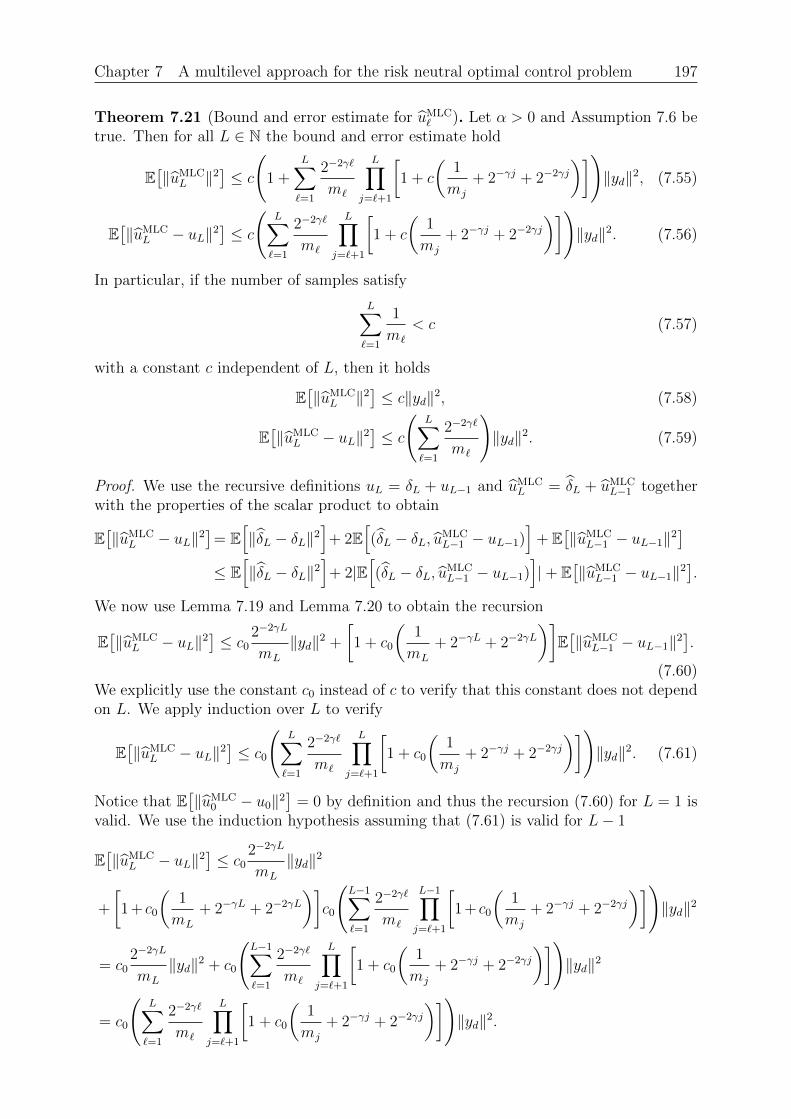
Chapter 7 A multilevel approach for the risk neutral optimal control problem 197
Theorem 7.21 (Bound and error estimate for uMLC` ). Let α > 0 and Assumption 7.6 be
true. Then for all L ∈ N the bound and error estimate hold
E[‖uMLC
L ‖2]≤ c
(1 +
L∑`=1
2−2γ`
m`
L∏j=`+1
[1 + c
(1
mj
+ 2−γj + 2−2γj
)])‖yd‖2, (7.55)
E[‖uMLC
L − uL‖2]≤ c
(L∑`=1
2−2γ`
m`
L∏j=`+1
[1 + c
(1
mj
+ 2−γj + 2−2γj
)])‖yd‖2. (7.56)
In particular, if the number of samples satisfy
L∑`=1
1
m`
< c (7.57)
with a constant c independent of L, then it holds
E[‖uMLC
L ‖2]≤ c‖yd‖2, (7.58)
E[‖uMLC
L − uL‖2]≤ c
(L∑`=1
2−2γ`
m`
)‖yd‖2. (7.59)
Proof. We use the recursive definitions uL = δL + uL−1 and uMLCL = δL + uMLC
L−1 togetherwith the properties of the scalar product to obtain
E[‖uMLC
L − uL‖2]= E
[‖δL − δL‖2
]+ 2E
[(δL − δL, uMLC
L−1 − uL−1)]
+ E[‖uMLC
L−1 − uL−1‖2]
≤ E[‖δL − δL‖2
]+ 2|E
[(δL − δL, uMLC
L−1 − uL−1)]|+ E
[‖uMLC
L−1 − uL−1‖2].
We now use Lemma 7.19 and Lemma 7.20 to obtain the recursion
E[‖uMLC
L − uL‖2]≤ c0
2−2γL
mL
‖yd‖2 +
[1 + c0
(1
mL
+ 2−γL + 2−2γL
)]E[‖uMLC
L−1 − uL−1‖2].
(7.60)We explicitly use the constant c0 instead of c to verify that this constant does not dependon L. We apply induction over L to verify
E[‖uMLC
L − uL‖2]≤ c0
(L∑`=1
2−2γ`
m`
L∏j=`+1
[1 + c0
(1
mj
+ 2−γj + 2−2γj
)])‖yd‖2. (7.61)
Notice that E[‖uMLC
0 − u0‖2]
= 0 by definition and thus the recursion (7.60) for L = 1 isvalid. We use the induction hypothesis assuming that (7.61) is valid for L− 1
E[‖uMLC
L − uL‖2]≤ c0
2−2γL
mL
‖yd‖2
+
[1 + c0
(1
mL
+ 2−γL + 2−2γL
)]c0
(L−1∑`=1
2−2γ`
m`
L−1∏j=`+1
[1 + c0
(1
mj
+ 2−γj + 2−2γj
)])‖yd‖2
= c02−2γL
mL
‖yd‖2 + c0
(L−1∑`=1
2−2γ`
m`
L∏j=`+1
[1 + c0
(1
mj
+ 2−γj + 2−2γj
)])‖yd‖2
= c0
(L∑`=1
2−2γ`
m`
L∏j=`+1
[1 + c0
(1
mj
+ 2−γj + 2−2γj
)])‖yd‖2.
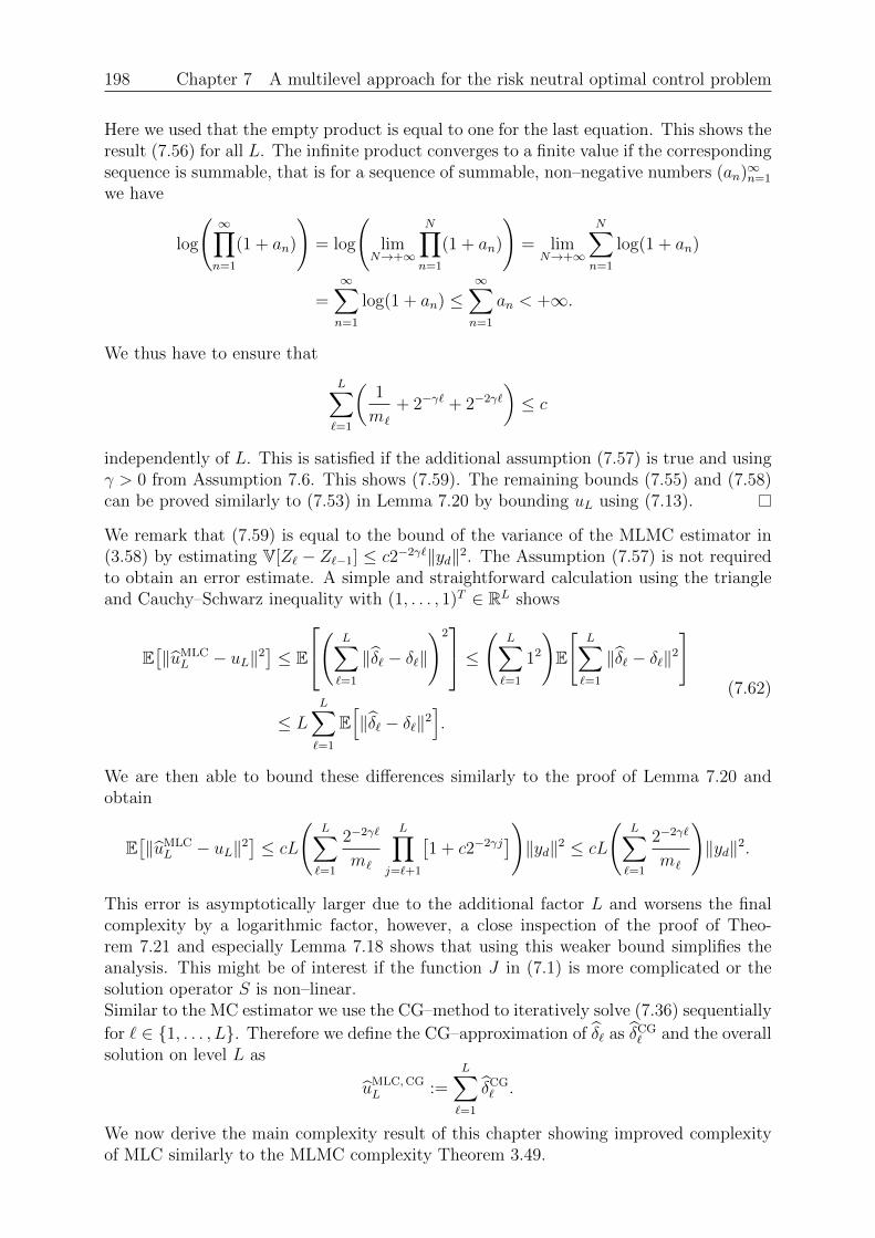
198 Chapter 7 A multilevel approach for the risk neutral optimal control problem
Here we used that the empty product is equal to one for the last equation. This shows theresult (7.56) for all L. The infinite product converges to a finite value if the correspondingsequence is summable, that is for a sequence of summable, non–negative numbers (an)∞n=1
we have
log
(∞∏n=1
(1 + an)
)= log
(lim
N→+∞
N∏n=1
(1 + an)
)= lim
N→+∞
N∑n=1
log(1 + an)
=∞∑n=1
log(1 + an) ≤∞∑n=1
an < +∞.
We thus have to ensure that
L∑`=1
(1
m`
+ 2−γ` + 2−2γ`
)≤ c
independently of L. This is satisfied if the additional assumption (7.57) is true and usingγ > 0 from Assumption 7.6. This shows (7.59). The remaining bounds (7.55) and (7.58)can be proved similarly to (7.53) in Lemma 7.20 by bounding uL using (7.13).
We remark that (7.59) is equal to the bound of the variance of the MLMC estimator in(3.58) by estimating V[Z` − Z`−1] ≤ c2−2γ`‖yd‖2. The Assumption (7.57) is not requiredto obtain an error estimate. A simple and straightforward calculation using the triangleand Cauchy–Schwarz inequality with (1, . . . , 1)T ∈ RL shows
E[‖uMLC
L − uL‖2]≤ E
( L∑`=1
‖δ` − δ`‖
)2 ≤ ( L∑
`=1
12
)E
[L∑`=1
‖δ` − δ`‖2
]
≤ LL∑`=1
E[‖δ` − δ`‖2
].
(7.62)
We are then able to bound these differences similarly to the proof of Lemma 7.20 andobtain
E[‖uMLC
L − uL‖2]≤ cL
(L∑`=1
2−2γ`
m`
L∏j=`+1
[1 + c2−2γj
])‖yd‖2 ≤ cL
(L∑`=1
2−2γ`
m`
)‖yd‖2.
This error is asymptotically larger due to the additional factor L and worsens the finalcomplexity by a logarithmic factor, however, a close inspection of the proof of Theo-rem 7.21 and especially Lemma 7.18 shows that using this weaker bound simplifies theanalysis. This might be of interest if the function J in (7.1) is more complicated or thesolution operator S is non–linear.Similar to the MC estimator we use the CG–method to iteratively solve (7.36) sequentially
for ` ∈ 1, . . . , L. Therefore we define the CG–approximation of δ` as δCG` and the overall
solution on level L as
uMLC,CGL :=
L∑`=1
δCG` .
We now derive the main complexity result of this chapter showing improved complexityof MLC similarly to the MLMC complexity Theorem 3.49.
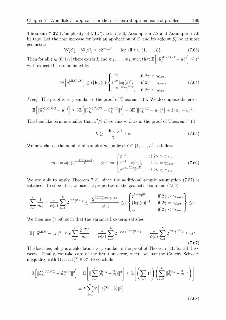
Chapter 7 A multilevel approach for the risk neutral optimal control problem 199
Theorem 7.22 (Complexity of MLC). Let α > 0, Assumption 7.2 and Assumption 7.6be true. Let the cost increase for both an application of S` and its adjoint S∗` be at mostgeometric
W[S`] + W[S∗` ] ≤ c2γCost` for all ` ∈ 1, . . . , L. (7.63)
Then for all ε ∈ (0, 1/e] there exists L and m1, . . . ,mL such that E[‖uMLC,CG
L − u‖2]≤ ε2
with expected costs bounded by
W[uMLC,CGL
]≤ c| log(ε)|
ε−2, if 2γ > γCost,
ε−2 log(ε)2, if 2γ = γCost,
ε−2− γCost−2γ
γ , if 2γ < γCost.
(7.64)
Proof. The proof is very similar to the proof of Theorem 7.14. We decompose the error
E[‖uMLC,CG
L − u‖2]≤ 3E
[‖uMLC,CG
L − uMLCL ‖2
]+ 3E
[‖uMLC
L − uL‖2]
+ 3‖uL − u‖2.
The bias like term is smaller than ε2/9 if we choose L as in the proof of Theorem 7.14
L ≥ − log2(ε)
γ+ c. (7.65)
We now choose the number of samples m` on level ` ∈ 1, . . . , L as follows
m` := φ(ε)2−(2γ+γCost)
2`, φ(ε) :=
ε−2, if 2γ > γCost,
ε−2| log(ε)|, if 2γ = γCost,
ε−2− γCost−2γ
2γ , if 2γ < γCost.
(7.66)
We are able to apply Theorem 7.21, since the additional sample assumption (7.57) issatisfied. To show this, we use the properties of the geometric sum and (7.65)
L∑`=1
1
m`
=1
φ(ε)
L∑`=1
22γ+γCost
2` ≤ c
2(2γ+γCost)
2(L+1)
φ(ε)≤ c
ε1− γCost
2γ , if 2γ > γCost,
| log(ε)|−1, if 2γ = γCost,
1, if 2γ < γCost.
≤ c.
We then use (7.59) such that the variance like term satisfies
E[‖uMLC
L − uL‖2]≤ c
L∑`=1
2−2γ`
m`
= c1
φ(ε)
L∑`=1
2−2γ`+2γ+γCost
2` = c
1
φ(ε)
L∑`=1
2γCost−2γ
2` ≤ cε2.
(7.67)The last inequality is a calculation very similar to the proof of Theorem 3.31 for all threecases. Finally, we take care of the iteration error, where we use the Cauchy–Schwarzinequality with (1, . . . , 1)T ∈ RL to conclude
E[‖uMLC,CG
L − uMLCL ‖2
]= E
[‖
L∑`=1
(δCG` − δ`)‖2
]≤ E
[(L∑`=1
12
)(L∑`=1
‖δCG` − δ`‖2
)]
= LL∑`=1
E[‖δCG
` − δ`‖2].
(7.68)
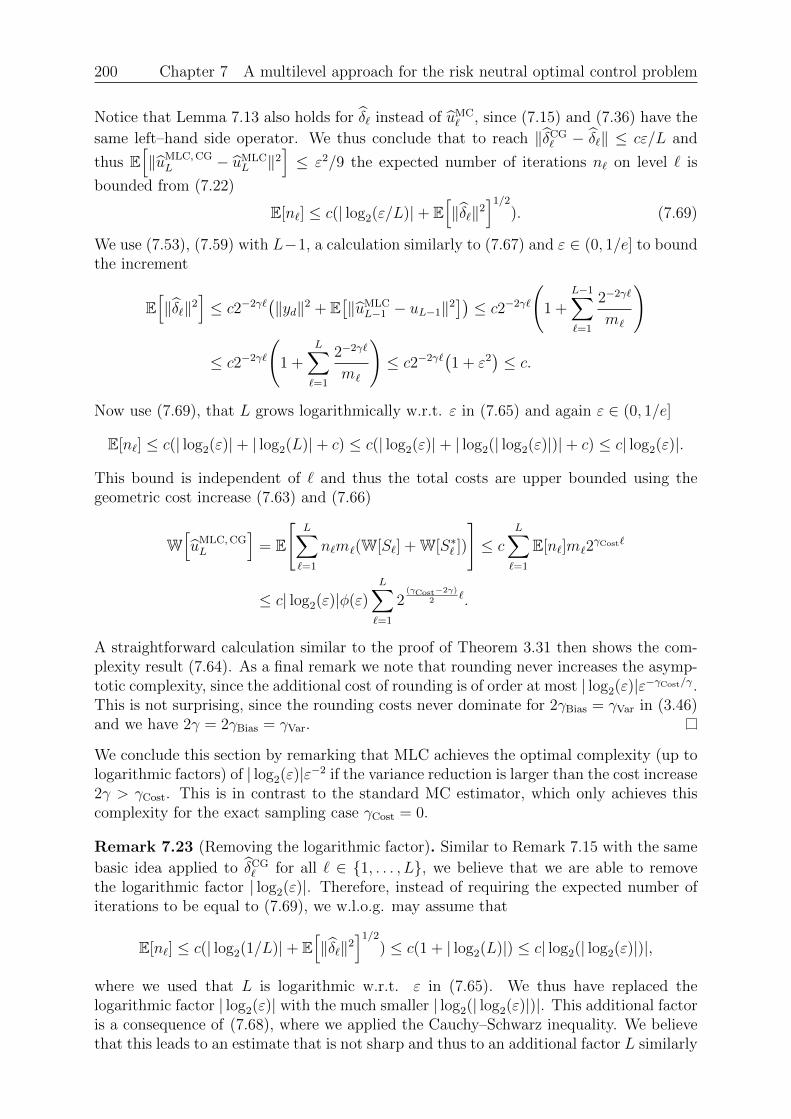
200 Chapter 7 A multilevel approach for the risk neutral optimal control problem
Notice that Lemma 7.13 also holds for δ` instead of uMC` , since (7.15) and (7.36) have the
same left–hand side operator. We thus conclude that to reach ‖δCG` − δ`‖ ≤ cε/L and
thus E[‖uMLC,CG
L − uMLCL ‖2
]≤ ε2/9 the expected number of iterations n` on level ` is
bounded from (7.22)
E[n`] ≤ c(| log2(ε/L)|+ E[‖δ`‖2
]1/2
). (7.69)
We use (7.53), (7.59) with L−1, a calculation similarly to (7.67) and ε ∈ (0, 1/e] to boundthe increment
E[‖δ`‖2
]≤ c2−2γ`
(‖yd‖2 + E
[‖uMLC
L−1 − uL−1‖2])≤ c2−2γ`
(1 +
L−1∑`=1
2−2γ`
m`
)
≤ c2−2γ`
(1 +
L∑`=1
2−2γ`
m`
)≤ c2−2γ`
(1 + ε2
)≤ c.
Now use (7.69), that L grows logarithmically w.r.t. ε in (7.65) and again ε ∈ (0, 1/e]
E[n`] ≤ c(| log2(ε)|+ | log2(L)|+ c) ≤ c(| log2(ε)|+ | log2(| log2(ε)|)|+ c) ≤ c| log2(ε)|.
This bound is independent of ` and thus the total costs are upper bounded using thegeometric cost increase (7.63) and (7.66)
W[uMLC,CGL
]= E
[L∑`=1
n`m`(W[S`] + W[S∗` ])
]≤ c
L∑`=1
E[n`]m`2γCost`
≤ c| log2(ε)|φ(ε)L∑`=1
2(γCost−2γ)
2`.
A straightforward calculation similar to the proof of Theorem 3.31 then shows the com-plexity result (7.64). As a final remark we note that rounding never increases the asymp-totic complexity, since the additional cost of rounding is of order at most | log2(ε)|ε−γCost/γ.This is not surprising, since the rounding costs never dominate for 2γBias = γVar in (3.46)and we have 2γ = 2γBias = γVar.
We conclude this section by remarking that MLC achieves the optimal complexity (up tologarithmic factors) of | log2(ε)|ε−2 if the variance reduction is larger than the cost increase2γ > γCost. This is in contrast to the standard MC estimator, which only achieves thiscomplexity for the exact sampling case γCost = 0.
Remark 7.23 (Removing the logarithmic factor). Similar to Remark 7.15 with the same
basic idea applied to δCG` for all ` ∈ 1, . . . , L, we believe that we are able to remove
the logarithmic factor | log2(ε)|. Therefore, instead of requiring the expected number ofiterations to be equal to (7.69), we w.l.o.g. may assume that
E[n`] ≤ c(| log2(1/L)|+ E[‖δ`‖2
]1/2
) ≤ c(1 + | log2(L)|) ≤ c| log2(| log2(ε)|)|,
where we used that L is logarithmic w.r.t. ε in (7.65). We thus have replaced thelogarithmic factor | log2(ε)| with the much smaller | log2(| log2(ε)|)|. This additional factoris a consequence of (7.68), where we applied the Cauchy–Schwarz inequality. We believethat this leads to an estimate that is not sharp and thus to an additional factor L similarly
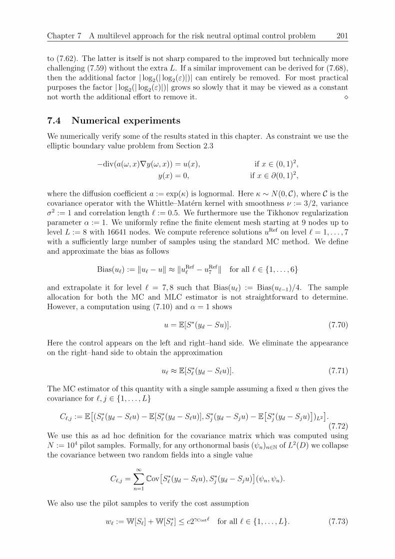
Chapter 7 A multilevel approach for the risk neutral optimal control problem 201
to (7.62). The latter is itself is not sharp compared to the improved but technically morechallenging (7.59) without the extra L. If a similar improvement can be derived for (7.68),then the additional factor | log2(| log2(ε)|)| can entirely be removed. For most practicalpurposes the factor | log2(| log2(ε)|)| grows so slowly that it may be viewed as a constantnot worth the additional effort to remove it.
7.4 Numerical experiments
We numerically verify some of the results stated in this chapter. As constraint we use theelliptic boundary value problem from Section 2.3
−div(a(ω, x)∇y(ω, x)) = u(x), if x ∈ (0, 1)2,
y(x) = 0, if x ∈ ∂(0, 1)2,
where the diffusion coefficient a := exp(κ) is lognormal. Here κ ∼ N(0, C), where C is thecovariance operator with the Whittle–Matern kernel with smoothness ν := 3/2, varianceσ2 := 1 and correlation length ` := 0.5. We furthermore use the Tikhonov regularizationparameter α := 1. We uniformly refine the finite element mesh starting at 9 nodes up tolevel L := 8 with 16641 nodes. We compute reference solutions uRef on level ` = 1, . . . , 7with a sufficiently large number of samples using the standard MC method. We defineand approximate the bias as follows
Bias(u`) := ‖u` − u‖ ≈ ‖uRef` − uRef
7 ‖ for all ` ∈ 1, . . . , 6
and extrapolate it for level ` = 7, 8 such that Bias(u`) := Bias(u`−1)/4. The sampleallocation for both the MC and MLC estimator is not straightforward to determine.However, a computation using (7.10) and α = 1 shows
u = E[S∗(yd − Su)]. (7.70)
Here the control appears on the left and right–hand side. We eliminate the appearanceon the right–hand side to obtain the approximation
u` ≈ E[S∗` (yd − S`u)]. (7.71)
The MC estimator of this quantity with a single sample assuming a fixed u then gives thecovariance for `, j ∈ 1, . . . , L
C`,j := E[(S∗` (yd − S`u)− E[S∗` (yd − S`u)], S∗j (yd − Sju)− E
[S∗j (yd − Sju)
])L2
].(7.72)
We use this as ad hoc definition for the covariance matrix which was computed usingN := 104 pilot samples. Formally, for any orthonormal basis (ψn)n∈N of L2(D) we collapsethe covariance between two random fields into a single value
C`,j =∞∑n=1
Cov[S∗` (yd − S`u), S∗j (yd − Sju)
](ψn, ψn).
We also use the pilot samples to verify the cost assumption
w` := W[S`] + W[S∗` ] ≤ c2γCost` for all ` ∈ 1, . . . , L. (7.73)
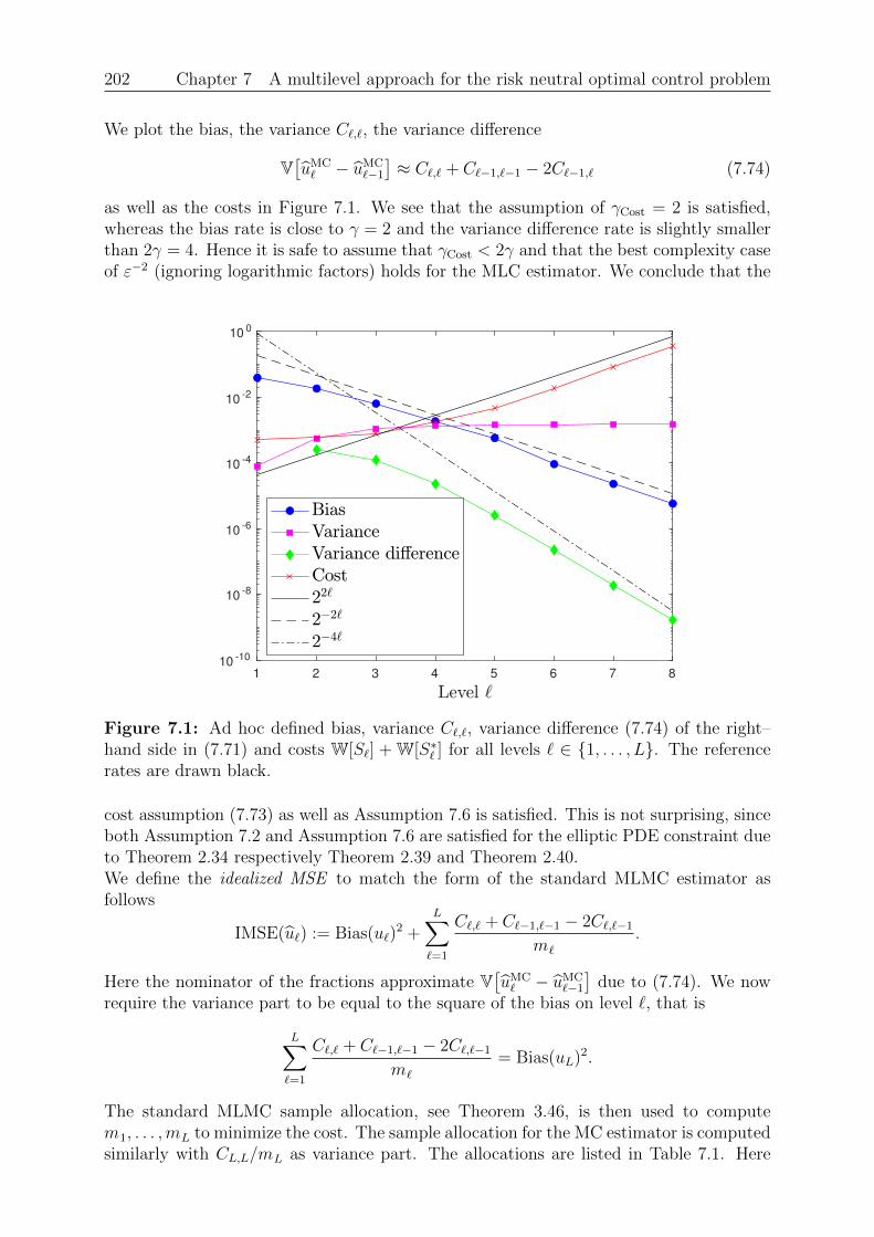
202 Chapter 7 A multilevel approach for the risk neutral optimal control problem
We plot the bias, the variance C`,`, the variance difference
V[uMC` − uMC
`−1
]≈ C`,` + C`−1,`−1 − 2C`−1,` (7.74)
as well as the costs in Figure 7.1. We see that the assumption of γCost = 2 is satisfied,whereas the bias rate is close to γ = 2 and the variance difference rate is slightly smallerthan 2γ = 4. Hence it is safe to assume that γCost < 2γ and that the best complexity caseof ε−2 (ignoring logarithmic factors) holds for the MLC estimator. We conclude that the
1 2 3 4 5 6 7 8
10-10
10-8
10-6
10-4
10-2
100
Figure 7.1: Ad hoc defined bias, variance C`,`, variance difference (7.74) of the right–hand side in (7.71) and costs W[S`] + W[S∗` ] for all levels ` ∈ 1, . . . , L. The referencerates are drawn black.
cost assumption (7.73) as well as Assumption 7.6 is satisfied. This is not surprising, sinceboth Assumption 7.2 and Assumption 7.6 are satisfied for the elliptic PDE constraint dueto Theorem 2.34 respectively Theorem 2.39 and Theorem 2.40.We define the idealized MSE to match the form of the standard MLMC estimator asfollows
IMSE(u`) := Bias(u`)2 +
L∑`=1
C`,` + C`−1,`−1 − 2C`,`−1
m`
.
Here the nominator of the fractions approximate V[uMC` − uMC
`−1
]due to (7.74). We now
require the variance part to be equal to the square of the bias on level `, that is
L∑`=1
C`,` + C`−1,`−1 − 2C`,`−1
m`
= Bias(uL)2.
The standard MLMC sample allocation, see Theorem 3.46, is then used to computem1, . . . ,mL to minimize the cost. The sample allocation for the MC estimator is computedsimilarly with CL,L/mL as variance part. The allocations are listed in Table 7.1. Here
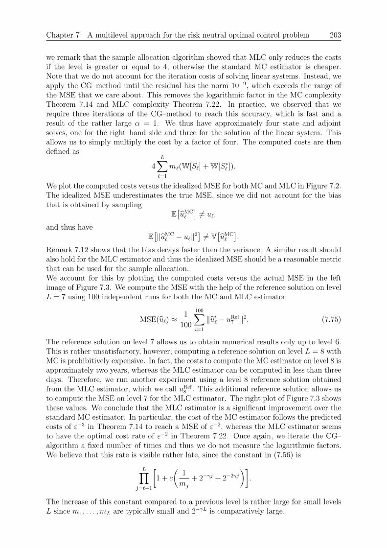
Chapter 7 A multilevel approach for the risk neutral optimal control problem 203
we remark that the sample allocation algorithm showed that MLC only reduces the costsif the level is greater or equal to 4, otherwise the standard MC estimator is cheaper.Note that we do not account for the iteration costs of solving linear systems. Instead, weapply the CG–method until the residual has the norm 10−9, which exceeds the range ofthe MSE that we care about. This removes the logarithmic factor in the MC complexityTheorem 7.14 and MLC complexity Theorem 7.22. In practice, we observed that werequire three iterations of the CG–method to reach this accuracy, which is fast and aresult of the rather large α = 1. We thus have approximately four state and adjointsolves, one for the right–hand side and three for the solution of the linear system. Thisallows us to simply multiply the cost by a factor of four. The computed costs are thendefined as
4L∑`=1
m`(W[S`] + W[S∗` ]).
We plot the computed costs versus the idealized MSE for both MC and MLC in Figure 7.2.The idealized MSE underestimates the true MSE, since we did not account for the biasthat is obtained by sampling
E[uMC`
]6= u`.
and thus haveE[‖uMC
` − u`‖2]6= V
[uMC`
].
Remark 7.12 shows that the bias decays faster than the variance. A similar result shouldalso hold for the MLC estimator and thus the idealized MSE should be a reasonable metricthat can be used for the sample allocation.We account for this by plotting the computed costs versus the actual MSE in the leftimage of Figure 7.3. We compute the MSE with the help of the reference solution on levelL = 7 using 100 independent runs for both the MC and MLC estimator
MSE(u`) ≈1
100
100∑i=1
‖ui` − uRef7 ‖2. (7.75)
The reference solution on level 7 allows us to obtain numerical results only up to level 6.This is rather unsatisfactory, however, computing a reference solution on level L = 8 withMC is prohibitively expensive. In fact, the costs to compute the MC estimator on level 8 isapproximately two years, whereas the MLC estimator can be computed in less than threedays. Therefore, we run another experiment using a level 8 reference solution obtainedfrom the MLC estimator, which we call uRef
8 . This additional reference solution allows usto compute the MSE on level 7 for the MLC estimator. The right plot of Figure 7.3 showsthese values. We conclude that the MLC estimator is a significant improvement over thestandard MC estimator. In particular, the cost of the MC estimator follows the predictedcosts of ε−3 in Theorem 7.14 to reach a MSE of ε−2, whereas the MLC estimator seemsto have the optimal cost rate of ε−2 in Theorem 7.22. Once again, we iterate the CG–algorithm a fixed number of times and thus we do not measure the logarithmic factors.We believe that this rate is visible rather late, since the constant in (7.56) is
L∏j=`+1
[1 + c
(1
mj
+ 2−γj + 2−2γj
)].
The increase of this constant compared to a previous level is rather large for small levelsL since m1, . . . ,mL are typically small and 2−γL is comparatively large.
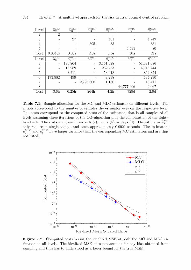
204 Chapter 7 A multilevel approach for the risk neutral optimal control problem
Level uMC2 uMC
3 uMC4 uMLC
4 uMC5 uMLC
5
2 2 - - - - -3 - 27 - 401 - 4,7494 - - 395 33 - 3815 - - - - 4,495 80
Cost 0.0048s 0.08s 2.8s 1.6s 84s 21s
Level uMC6 uMLC
6 uMC7 uMLC
7 uMC8 uMLC
8
3 - 190,864 - 3,151,628 - 51,381,0864 - 15,289 - 252,453 - 4,115,7445 - 3,211 - 53,018 - 864,3546 173,982 499 - 8,238 - 134,2907 - - 2,795,608 1,130 - 18,4118 - - - - 44,777,906 2,667
Cost 3.6h 0.25h 264h 4.2h 729d 2.9d
Table 7.1: Sample allocation for the MC and MLC estimator on different levels. Theentries correspond to the number of samples the estimator uses on the respective level.The costs correspond to the computed costs of the estimator, that is all samples of alllevels assuming three iterations of the CG–algorithm plus the computation of the right–hand side. The costs are given in seconds (s), hours (h) or days (d). The estimator uMC
1
only requires a single sample and costs approximately 0.0021 seconds. The estimatorsuMLC
2 and uMLC3 have larger variance than the corresponding MC estimators and are thus
not listed.
10-12
10-10
10-8
10-6
10-4
10-2
10-4
10-2
100
102
104
106
108
1010
Figure 7.2: Computed costs versus the idealized MSE of both the MC and MLC es-timator on all levels. The idealized MSE does not account for any bias obtained fromsampling and thus has to understood as a lower bound for the true MSE.
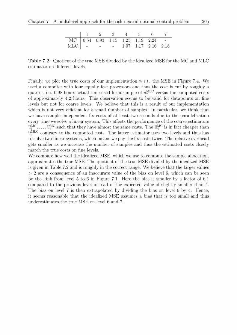
Chapter 7 A multilevel approach for the risk neutral optimal control problem 205
1 2 3 4 5 6 7MC 0.54 0.93 1.15 1.25 1.19 2.24 -
MLC - - - 1.07 1.17 2.16 2.18
Table 7.2: Quotient of the true MSE divided by the idealized MSE for the MC and MLCestimator on different levels.
Finally, we plot the true costs of our implementation w.r.t. the MSE in Figure 7.4. Weused a computer with four equally fast processors and thus the cost is cut by roughly aquarter, i.e. 0.98 hours actual time used for a sample of uMLC
7 versus the computed costsof approximately 4.2 hours. This observation seems to be valid for datapoints on finelevels but not for coarse levels. We believe that this is a result of our implementationwhich is not very efficient for a small number of samples. In particular, we think thatwe have sample independent fix costs of at least two seconds due to the parallelizationevery time we solve a linear system. This affects the performance of the coarse estimatorsuMC
1 , . . . , uMC4 such that they have almost the same costs. The uMC
4 is in fact cheaper thanuMLC
4 contrary to the computed costs. The latter estimator uses two levels and thus hasto solve two linear systems, which means we pay the fix costs twice. The relative overheadgets smaller as we increase the number of samples and thus the estimated costs closelymatch the true costs on fine levels.We compare how well the idealized MSE, which we use to compute the sample allocation,approximates the true MSE. The quotient of the true MSE divided by the idealized MSEis given in Table 7.2 and is roughly in the correct range. We believe that the larger values> 2 are a consequence of an inaccurate value of the bias on level 6, which can be seenby the kink from level 5 to 6 in Figure 7.1. Here the bias is smaller by a factor of 6.1compared to the previous level instead of the expected value of slightly smaller than 4.The bias on level 7 is then extrapolated by dividing the bias on level 6 by 4. Hence,it seems reasonable that the idealized MSE assumes a bias that is too small and thusunderestimates the true MSE on level 6 and 7.
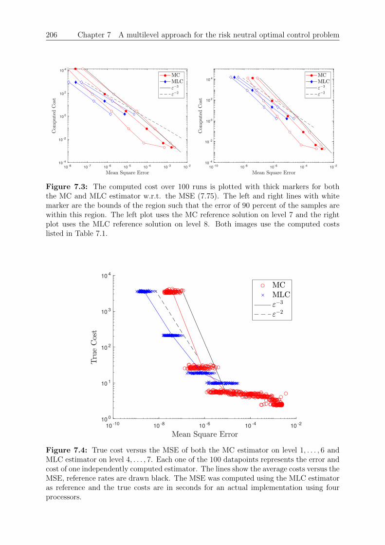
206 Chapter 7 A multilevel approach for the risk neutral optimal control problem
10-8
10-7
10-6
10-5
10-4
10-3
10-2
10-4
10-2
100
102
104
10-10
10-8
10-6
10-4
10-2
10-4
10-2
100
102
104
Figure 7.3: The computed cost over 100 runs is plotted with thick markers for boththe MC and MLC estimator w.r.t. the MSE (7.75). The left and right lines with whitemarker are the bounds of the region such that the error of 90 percent of the samples arewithin this region. The left plot uses the MC reference solution on level 7 and the rightplot uses the MLC reference solution on level 8. Both images use the computed costslisted in Table 7.1.
10-10
10-8
10-6
10-4
10-2
100
101
102
103
104
Figure 7.4: True cost versus the MSE of both the MC estimator on level 1, . . . , 6 andMLC estimator on level 4, . . . , 7. Each one of the 100 datapoints represents the error andcost of one independently computed estimator. The lines show the average costs versus theMSE, reference rates are drawn black. The MSE was computed using the MLC estimatoras reference and the true costs are in seconds for an actual implementation using fourprocessors.
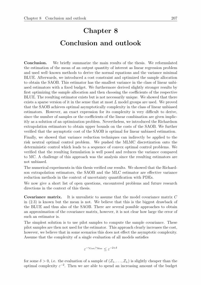
Chapter 8 Conclusion and outlook 207
Chapter 8
Conclusion and outlook
Conclusion. We briefly summarize the main results of the thesis. We reformulatedthe estimation of the mean of an output quantity of interest as linear regression problemand used well–known methods to derive the normal equations and the variance minimalBLUE. Afterwards, we introduced a cost constraint and optimized the sample allocationto obtain the SAOB. This estimator has the smallest variance in the class of linear unbi-ased estimators with a fixed budget. We furthermore derived slightly stronger results byfirst optimizing the sample allocation and then choosing the coefficients of the respectiveBLUE. The resulting estimator exists but is not necessarily unique. We showed that thereexists a sparse version of it in the sense that at most L model groups are used. We provedthat the SAOB achieves optimal asymptotically complexity in the class of linear unbiasedestimators. However, an exact expression for its complexity is very difficult to derive,since the number of samples or the coefficients of the linear combination are given implic-itly as a solution of an optimization problem. Nevertheless, we introduced the Richardsonextrapolation estimators to obtain upper bounds on the costs of the SAOB. We furtherverified that the asymptotic cost of the SAOB is optimal for linear unbiased estimation.
Finally, we showed that variance reduction techniques can indirectly be applied to therisk neutral optimal control problem. We pushed the MLMC discretization onto thedeterministic control which leads to a sequence of convex optimal control problems. Weverified that the resulting formulation is well posed and reduces the variance comparedto MC. A challenge of this approach was the analysis since the resulting estimators arenot unbiased.
The numerical experiments in this thesis verified our results. We showed that the Richard-son extrapolation estimators, the SAOB and the MLC estimator are effective variancereduction methods in the context of uncertainty quantification with PDEs.
We now give a short list of open questions, encountered problems and future researchdirections in the context of this thesis.
Covariance matrix. It is unrealistic to assume that the model covariance matrix Cin (2.3) is known but the mean is not. We believe that this is the biggest drawback ofthe BLUE and thus also of the SAOB. There are several possible approaches to obtainan approximation of the covariance matrix, however, it is not clear how large the error ofsuch an estimator is.
The simplest solution is to use pilot samples to compute the sample covariance. Thesepilot samples are then not used for the estimator. This approach clearly increases the cost,however, we believe that in some scenarios this does not effect the asymptotic complexity.Assume that the complexity of a single evaluation of all models satisfies
ε−γCost/γBias ≤ ε−2+δ
for some δ > 0, i.e. the evaluation of a sample of (Z1, . . . , ZL) is slightly cheaper than theoptimal complexity ε−2. Then we are able to spend an increasing amount of the budget
208 Chapter 8 Conclusion and outlook
of order ε−δ without worsening the asymptotic cost, that is
Cost = ε−γCost/γBias︸ ︷︷ ︸Cost for rounding
+ ε−2︸︷︷︸Cost for the estimator
+Npilotε−γCost/γBias︸ ︷︷ ︸
Cost for pilot samples
≤ cε−2,
where Npilot = ε−δ is the number of pilot samples. This means that asymptotically thenumber of pilot samples may be increased to infinity without worsening the asymptoticcomplexity. Furthermore, if we choose Npilot = ε−δ/2, then the cost for the pilot samplescompared to the cost for the estimator is negligible. Therefore, if we are able to ap-proximate the covariance matrix with Npilot samples sufficiently well, then the computedSAOB with this matrix converges to the true SAOB. However, it is not straightforward toverify that Npilot = ε−δ is sufficient to show that the sample covariance matrix convergesto the true covariance for ε → 0, since the covariance matrix changes if ε decreases dueto additional fine grid models. An error analysis for the SAOB with approximated co-variance matrix also has to be conducted to make the above statements mathematicallysound. In particular, an error analysis of the problem in (5.22) w.r.t. perturbations inthe covariance matrix Ck and costs W k should be carried out.The authors of [9] and [112] construct efficient multilevel estimators to compute the vari-ance of a QoI. These approaches may be adapted to compute an even cheaper approxi-mation of the covariance matrix compared to the sample covariance. However, similar tothe naive MLMC estimator in Chapter 7, a straightforward MLMC approximation of theentries of the covariance matrix does not ensure that this approximation is positive semi–definite. Hence, the corresponding optimization problem for the SAOB may be ill–posed.Maybe similar methods to the one outlined in Chapter 7 can be used to push the MLMCestimator to the coefficients β of the BLUE instead of the covariance matrix.Aside from the asymptotic cost increase of the estimator, it is not clear how big theconstants in front of the costs for the pilot samples are. In particular, if few samples areused, then the estimator may be overconfident, and we might assume that the correlationis much higher than it truly is. This then leads to a bad estimator. It is of coursepossible to avoid pilot samples or to reuse the pilot samples for the estimation, however,this introduces a bias. Whether this bias is actually significant and has to be avoided orcan be fully ignored is not clear as of the writing of the thesis. This may also dependon the particular estimation problem. We also did not conduct any conclusive numericalexperiments. If an unbiased estimator is desired, then clearly we are able to use theestimator
µα := µ1α/2[C
2] + µ2
α/2[C1].
Here the estimator µ1α/2[C
2] is the SAOB that uses the sample covariance matrix C
2
obtained from the samples of µ2α/2 to compute its coefficients β and vice versa. This
approach ensures that the resulting estimator is unbiased, however it is not clear if andby how much the variance increases.
Condition number of the covariance matrix. The condition of the covariancematrix C is typically large. If the quantities ZL converge to the exact model Z, thenthe covariance matrix C has, at least asymptotically, almost constant entries with valuesapproximately equal to V[Z]. Hence, there is an eigenvalue close to LV[Z] with eigenvectorconsisting of entries that are all close to one. On the other hand, a variance reductioncan often be achieved by obtaining a small value of
βTCβ = V
[L∑`=1
β`Z`
]≈ λmin
Chapter 8 Conclusion and outlook 209
with ‖β‖ = 1 and λmin denoting the smallest eigenvalue. Therefore, the larger theachievable variance reduction, the smaller the smallest eigenvalue. Since the value ofV[Z` − Z`−1] converges to zero, λmin does so as well. Hence, the condition of C divergesto +∞. Consequently, the better the variance reduction, the worse the condition of C.We thus believe that the algorithms that depend on C−1 or some (C`)−1 may be unstableor yield inaccurate results. This undesirable property also occurs for some Richardsonextrapolation methods. We verified that the coefficients of the SAOB converge to thecoefficients of the RE estimator in specific circumstances and thus we expect the SAOBmay suffer from the same inaccuracies. The significance of this problem can be reduced ifwe fix the coupling number κ to a small value or we carefully choose a small subset of all2L − 1 model groups. However, this results in a potentially decreased variance reductionwhich may or may not be significant.
Hybrid estimators. The SAOB does not use any structural assumptions about theQoI. In particular, the SAOB only requires the covariance matrix and model costs toachieve a variance reduction. However, this generality comes at the cost of requiring anestimate of the covariance matrix. The numerical experiments in Chapter 6 have shownthat the improvement of the SAOB over the MLMC and RE estimators is small if we arein the asymptotic regime. In contrast, far away from this regime the SAOB, or in generalany BLUE, is able to provide significant improvements. Therefore, it may make sense toconstruct a hybrid estimator as follows
µMLMC + SAOBL :=
L∑`=Lcoarse+1
1
m`
m∑i=1
(Zi,`` − Z
i,``−1
)+ µSAOB
Lcoarse.
The SAOB here only estimates µLcoarse and thus only needs the covariance of the coarsemodels Z1, . . . , ZLcoarse , which is in general cheap to obtain. At the same time, we use theMLMC estimator for the high fidelity models, which does not require the full covariancematrix. We thus use the SAOB in the regime of coarse models where it has the biggestadvantage over other methods. An open question is of course, that it is not clear howto choose Lcoarse or how to increase Lcoarse if we want to increase the accuracy of theestimator.
Regularization. Another approach would be to include some prior information for thecoefficients. As an example, we might add a regularization term to (5.22) in form of theMLMC estimator
minβ
K∑k=1
[(βk)TCkβkW k
]1/2+ αreg
L∑k=1
[(βk − βMLMC,k)TCk(βk − βMLMC,k)W k)
]1/2such that
K∑k=1
P kβk = α.
Here αreg is a regularization parameter, βMLMC,k the coefficients and S1, . . . , SL the modelgroups of the MLMC estimator. Depending on the size of αreg we may be close to a MLMCestimator or far away from it. In particular, the parameter αreg is allowed to contain someinformation about the accuracy of the estimate for the covariance matrix. Ideally, if we donot know much about the covariance matrix, which may be derived from error estimates,the value αreg should be large and conversely, if the estimate of the covariance is veryaccurate, the value of αreg should be small or zero. This approach ensures that the
210 Chapter 8 Conclusion and outlook
potentially inaccurate covariance matrix computed from only a few samples does not leadto an inaccurate estimator.
Efficient algorithm to solve the sample allocation problem. The sample allo-cation problem in Section 5.2 to compute m, or the equivalent problem to compute βin Section 5.3 are both convex optimization problems. However, the number of variablesdepends exponentially on the number of levels L if we do not restrict the coupling ofthe models, that is κ = +∞. Therefore, it is not clear whether there is a polynomialtime algorithm (polynomial in L) that solves this problem. Nevertheless, the optimiza-tion problem (5.22) exhibits some interesting local behaviour. Let us assume that someiterative algorithm returns a suboptimal allocation that uses the model groups S1, . . . , SL
and we want to check whether it makes sense to use the model group SL+1. Then if forall βL+1 the minimization problem
minβ1,...,βL
J(β) :=L∑`=1
(W `(β`)TC`β`
)1/2
such thatL∑`=1
P `β` = PL+1βL+1
(8.1)
has a minimum smaller than(WL+1(βL+1)TCL+1βL+1
)1/2the SAOB does not use the
model group SL+1. This can be proven by contradiction, thus assume that the SAOBdoes and write down this estimator as follows
µSAOBα = µ+
1
mL+1
mL+1∑i=1
∑`∈SL+1
βL+1[`] Zi,L+1
` , (8.2)
where µ is a suitable estimator. Now, the second part of this estimator is an unbiasedestimator for (PL+1βL+1)Tµ, however, the function J in (8.1) is the variance of anotherSAOB with, by assumption, smaller variance then the estimator using only SL+1. Due tothe independence structure, we can replace the right estimator of (8.2) with the SAOBobtained from (8.1) leading to a smaller variance and thus a contradiction. The scaleinvariance now implies that the statement we made so far is equivalent to show that themax-min problem
max‖βL+1‖=1
minβ1,...,βL
J(β) :=L∑`=1
(W `(β`)TC`β`
)1/2 −(WL+1(βL+1)TCL+1βL+1
)1/2
such thatL∑`=1
P `β` = PL+1βL+1
(8.3)
has a maximizer strictly smaller than 0. As an example why this result might be useful,assume that the MLMC estimator for µL has a smaller variance than the MC estimatorfor µL using the same budget. Then, the SAOB never uses the model group that onlycontains ZL. A possible research direction is to use this local property to exclude somemodel groups that are not useful to reduce the variance. Then the optimization problemmay have a smaller number of variables instead of exponentially many.
Flat optimization surface. The numerical experiments in Section 6.5 for the truecosts showed that the variance of the compared estimators (except for MC) are all very
Chapter 8 Conclusion and outlook 211
similar. This is not surprising, since the variance reduction ensures that most of the costsare on the coarse grids allowing a different number of fine grid evaluations, or use ofdifferent model groups without worsening the overall costs too much. More specifically,using the RE coefficients or coefficients close to it, the variance corresponding to themodel group SL with the high fidelity model is
(βL)TCLβLWL ≈ c2−(γVar−γCost)L. (8.4)
This is asymptotically for L → +∞ very small if γCost < γVar compared to the value ofthe model group S1 which only consists of the coarsest model
(β1)TC1β1W 1 ≈ c.
For hierarchical models, the cost of the discretization increases geometrically, thus addingor removing the models 1, . . . , L/2 from the model group SL, which contains the highfidelity model, is not going to significantly change WL. Furthermore, adding or remov-ing these models does not change the overall variance that much since (8.4) contributesasymptotically nothing and the variance reduction rate γVar is often achieved with onlya few fine grid levels. Now observe that there are a total of 2L/2 possible combinations ifwe keep the fine models ZL/2+1, . . . , ZL in SL and add or remove the models Z1, . . . , ZL/2.The result is thus that there are exponentially many directions that lead to an almostidentical function value. However, this means that the function J we optimize over in(5.22) is flat at the minimum. This often poses difficulties for standard numerical opti-mization methods since the gradient becomes small and the Hessian ill–conditioned. Thiscan be mitigated by choosing to optimize only over a subset of all 2L − 1 model groupsand thus removing some flat direction. If a minimizer is found, then suitably adding orremoving some model groups could be used to obtain the global minimizer.
Extension to non–linear estimators. The author of [105] used the MFMC estimatorwith a low fidelity model that is adaptively improved to reduce the variance. A similarapproach might also be viable for the BLUE. The MFMC estimator requires models thatare cheap and correlate well with the high fidelity model. Let us assume that V[Z] :=V[Z`(θ)] := 1 where Z`(θ) is the low fidelity model and θ some model parameter. Thenwe want to choose θ to minimize
1− ρ2 = 1− Cov[Z,Z`(θ)]2 = (1− Cov[Z,Z`(θ)])(1 + Cov[Z,Z`(θ)])
≤ 2(Cov[Z,Z − Z`(θ)] ≤ 2(V[Z − Z`(θ)])1/2.
It is now straightforward to generalize this idea for the SAOB with multiple low fidelitymodels. The optimization problem (5.22) then reads
minβ,θ
K∑k=1
((βk)TCk(θ)βkW k(θ)
)1/2
such thatK∑k=1
P kβk = eL.
(8.5)
Here the costs as well as the covariance matrix now depend on θ
C`,j(θ) = Cov[Z`(θ), Zj(θ)].
212 Chapter 8 Conclusion and outlook
The quantities Z1, . . . , ZL are potentially combined in a non–linear way since the costfunction is
K∑k=1
((βk)TCk(θ)βkW k(θ)
)1/2=
K∑k=1
(V
[∑`∈Sk
βk[`]Z`(θ)
]W k(θ)
)1/2
.
The pilot samples, which we use to compute the sample covariance matrix, can now beused to change the low fidelity models to reduce the variance. Let us assume that (8.5) hasa well–defined minimizer (β∗, θ∗). Then the SAOB with parameters (β∗, θ∗) achieves thesmallest variance in the class of unbiased estimators for µL that have equal or smaller cost,depend linearly on β and non–linearly on θ and only use the QoIs Z1(θ), . . . , ZL(θ). In thissense, the SAOB is still variance minimal and thus a sensible choice even if non–linearitiesarise. Furthermore, similar to the standard SAOB, once the models Z1(θ∗), . . . , ZL(θ∗)are fixed we require at most L model groups. A disadvantage may be that solving (8.5)is difficult and impractical. Nevertheless, such an approach includes non–linear surrogatemodels like Gaussian processes, support vector machines or neural networks.
Variance reduction for root-finding algorithms. The variance reduction techniquefor the optimal control problem in Chapter 7 can be generalized to root-finding algorithms.Assume that we want to find a deterministic θ ∈ Θ such that for a parametric randomvariable Z : Θ× Ω→ X
E[Z(θ)] = 0.
The discretized condition with Z1, . . . , ZL then reads
E[Z`(θ`)] = 0 for all ` ∈ 1, . . . , L.
We define δ` := θ` − θ`−1 and we linearise the left–hand side of the equation
E[Z`(θ`)] = E[Z`(θ`−1 + δ`)] = E[Z`(θ`−1)] + E[∇θZ`(θ`−1)]T δ` + o(‖δ`‖).
A single step of the Newton method, that is ignoring o(‖δ`‖), and assuming that θ`−1 isknown, solves for the Newton step s1
` with the starting iterate θ`−1
E[∇θZ`(θ`−1)]T s1` = −E[Z`(θ`−1)] = 0− E[Z`(θ`−1)] = E[Z`−1(θ`−1)− Z`(θ`−1)]. (8.6)
The next iteration of the Newton method then has to solve
E[∇θZ`(θ`−1 + s1
`)]Ts2` = E
[Z`−1(θ`−1)− Z`(θ`−1 + s1
`)].
A MC discretization method of the last equation now has a small variance if Z`−1(θ`−1)−Z`(θ`−1 + s1
`) and s2` is small. This follows, since (8.6) is a linear system similarly to the
system (7.35) in Chapter 7. However, we have to potentially use multiple Newton steps,since the expression o(‖δ`‖) might be large on coarse grids. This clearly complicates theanalysis.This root-finding algorithm can obviously be used for the optimization problem
minθ
E[Z(θ)],
where we apply Newton’s method to the first order optimality conditions
E[∇2θZ(θ)
]s = −E[∇θZ(θ)].
Chapter 8 Conclusion and outlook 213
Here ∇2θZ denotes the Hessian of Z w.r.t. the parameter θ and s the Newton step. The
proposed method for stochastic optimization is a second order method and thus differsfrom the well–known first order stochastic gradient descent methods, where multilevelvariance reduction was already incorporated [43, 51, 94, 95, 138].
Conditional value at risk and risk averse optimization problem. The conditionalvalue-at-risk (CVaR) (or average value-at-risk) describes the tail expectation of a randomvariable and is a coherent risk measure, see [127, Chapter 6] or [110, Chapter 2] for moreinformation on risk measures. The authors of [119] show that computing the CVaR canbe formulated as non–smooth minimization problem
CVaR(Z) := mintt+
1
1− τE[(Z − t)+], (8.7)
where τ ∈ (0, 1) is the risk level and (x)+ := maxx, 0. The optimal t∗ is called thevalue-at-risk, whereas the minimum is the CVaR. The authors of [86] developed a methodto compute the cumulative distribution function using the MLMC estimator. An approx-imation to the CVaR is then computed using a post processing step. Giles et al. [58]used a multilevel estimator for a nested expectation involving probabilities and then usea root-finding algorithm to obtain the value-at-risk and the CVaR. A future research di-rection would be to compute the minimum in (8.7) with a similar approach we outlinedin Chapter 7, which of course has to be adapted to deal with the non–linearity of (·)+.We write down the optimality conditions of (8.7) for t∗1, . . . , t
∗L as follows
P(Z` ≤ t∗`) = τ.
Now linearise the left–hand side to introduce an update δ` = t∗` − t∗`−1 such that
P(Z` ≤ t∗`) = P(Z` ≤ t∗`−1 + δ`) = P(Z` ≤ t∗`−1) + p`(t∗`−1)δ` + o(δ`),
where p` is the probability density function of Z`. The condition for the Newton step s1`
then reads
p`(t∗`−1)s1
` = τ − P(Z` ≤ t∗`−1) = P(Z`−1 ≤ t∗`−1)− P(Z` ≤ t∗`−1).
If δ` is not small enough, we use another Newton step
p`(t∗`−1 + s1
`)s2` = P(Z`−1 ≤ t∗`−1)− P(Z` ≤ t∗`−1 + s1
`).
We discretize the left and right–hand side using an MC estimator for the quantile anddensity independently of t∗`−1, which we assume was already estimated. This then gives
p`(t∗`−1)s` = P(Z`−1 ≤ t∗`−1)− P(Z` ≤ t∗`−1).
If the estimator for the density and the difference of the quantile estimators is sufficientlysmall, then this should yield a variance reduction comparable to the standard MLMCestimator.The goal is of course to apply this method to a risk averse optimal control problem, whichis given as follows
minu
J(u) = CVaR(‖y(u)− yd‖2) +α
2‖u‖2
such that P–a.s. y(u, ω) = S(ω)u.
214 Chapter 8 Conclusion and outlook
This problem without variance reduction was studied in [85].
Risk neutral optimal control problem with control constraints. The optimalcontrol problem in Chapter 7 does not have control constraints. With control constraintsthis problem is given as follows
minu
J(u) =1
2E[‖y(u)− yd‖2
]+α
2‖u‖2
such that P–a.s. y(u, ω) = S(ω)u,
a ≤ u ≤ b,
(8.8)
where a ≤ b are two real–valued numbers or functions in L2(D). Now assume that thesolution u`−1, that is if we discretize S by S`−1, is known. Then for δ` := u` − u`−1 thecorresponding optimal control problem is
minδ`
J(δ`) =1
2E[‖y`(u`−1 + δ`)− yd‖2
]+α
2‖u`−1 + δ`‖2
such that P–a.s. y`(u`−1 + δ`, ω) = S`(ω)(u`−1 + δ`),
a ≤ u`−1 + δ` ≤ b.
We now rewrite this to obtain
minδ`
J(δ`) =1
2E[‖y`(δ`)− yd‖2
]+α
2‖u`−1 + δ`‖2
such that P–a.s. y`(δ`, ω) = S`(ω)δ`,
a− u`−1 ≤ δ` ≤ b− u`−1,
(8.9)
where yd := y`(u`−1)−yd. The difference compared to the original (8.8) is that the controlconstraints depend on the previous level, yd is now random and the regularization termincludes u`−1. Crucially, if S` = S`−1, then the unique solution of (8.9) is δ` = 0. Hencefor S` ≈ S`−1 the norm of the increment is small and it is reasonable to expect thatthe variance of the MC estimator for the mean in J in (8.9) is also small. The result isthat we should need few samples for a good approximation of δ`. An approach similar toChapter 7 could be used to solve this problem. For example, if a version of [73, Theorem3.5] holds in our setting when replacing u with δ, h2 with the MC error, squaring andchanging the norm then gives
E[‖δ` − δ`‖2
]≤ c
1
m`
(E[‖y`(δ`)‖2
]+ ‖δ`‖2) ≤ c
2−2γ`
m`
.
It is not clear whether such a bound holds, however, if it does then we have a variancereduction similar to the standard MLMC estimator.
Bibliography 215
Bibliography
[1] R. J. Adler and J. E. Taylor. Random fields and Geometry. Springer New York,2007.
[2] M. Aigner. Diskrete Mathematik. Vieweg+Teubner Verlag, sixth edition, 2006.
[3] A. Alexanderian, N. Petra, G. Stadler, and O. Ghattas. Mean-Variance Risk-AverseOptimal Control of Systems Governed by PDEs with Random Parameter Fields Us-ing Quadratic Approximations. SIAM/ASA Journal on Uncertainty Quantification,5(1):1166–1192, 2017.
[4] A. A. Ali, E. Ullmann, and M. Hinze. Multilevel Monte Carlo Analysis for Opti-mal Control of Elliptic PDEs with Random Coefficients. SIAM/ASA Journal onUncertainty Quantification, 5(1):466–492, 2017.
[5] M. Asadzadeh, A. H. Schatz, and W. Wendland. A new approach to Richard-son extrapolation in the finite element method for second order elliptic problems.Mathematics of Computation, 78(268):1951–1973, 2009.
[6] R. B. Ash. Probability and Measure Theory. Academic Press, second edition, 2000.
[7] G. Astarita. Thermodynamics. Springer, New York, 1989.
[8] P. Bhattacharya and P. Burman. Theory and Methods of Statistics. Academic Press,2016.
[9] C. Bierig and A. Chernov. Convergence analysis of multilevel Monte Carlo vari-ance estimators and application for random obstacle problems. Numer. Math.,130(4):579–613, 2015.
[10] P. Billingsley. Probability and measure. Wiley, Hoboken, NJ, anniversary edition,2012.
[11] H. Blum, Q. Lin, and R. Rannacher. Asymptotic error expansion and Richardsonextrapolation for linear finite elements. Numer. Math., 49(1):11–37, 1986.
[12] V. I. Bogachev. Gaussian Measures. AMS, Providence, RI, 1998.
[13] J. A. Bondy and U. Murty. Graph theory with applications. Macmillan, London,1976.
[14] A. Borzı and V. Schulz. Multigrid Methods for PDE Optimization. SIAM Review,51(2):361–395, 2009.
[15] A. Borzı and V. Schulz. Computational Optimization of Systems Governed by PartialDifferential Equations. Society for Industrial and Applied Mathematics, 2011.
216 Bibliography
[16] A. Borzı, V. Schulz, C. Schillings, and G. von Winckel. On the treatment ofdistributed uncertainties in PDE-constrained optimization. GAMM-Mitteilungen,33(2):230–246, 2010.
[17] A. Borzı and G. von Winckel. Multigrid Methods and Sparse-Grid Collocation Tech-niques for Parabolic Optimal Control Problems with Random Coefficients. SIAMJournal on Scientific Computing, 31(3):2172–2192, 2009.
[18] A. Borzı and G. von Winckel. A POD framework to determine robust controls inPDE optimization. Computing and Visualization in Science, 14(3):91–103, 2011.
[19] S. Boucheron, G. Lugosi, and O. Bousquet. Concentration Inequalities, AdvancedLectures on Machine Learning: ML Summer Schools 2003, Canberra, Australia,February 2 - 14, 2003, Tubingen, Germany, August 4 - 16, 2003, Revised Lectures,pages 208–240. Springer, Berlin, Heidelberg, 2004.
[20] S. Boyd and L. Vandenberghe. Convex Optimization. Cambridge University Press,Cambridge, UK, 2004.
[21] S. C. Brenner and L. R. Scott. The Mathematical Theory of Finite Element Methods.Springer, New York, third edition, 2008.
[22] C. Brezinski. Convergence Acceleration during the 20th Century. J. Comput. Appl.Math., 122(1–2):1–21, 2000.
[23] R. Bulirsch and J. Stoer. Numerical Treatment of Ordinary Differential Equationsby Extrapolation Methods. Numerische Mathematik, 8:1–13, 1966.
[24] H.-J. Bungartz and M. Griebel. Sparse grids. Acta Numerica, 13:147–269, 2004.
[25] J. Charrier. Strong and Weak Error Estimates for Elliptic Partial Differential Equa-tions with Random Coefficients. SIAM Journal on Numerical Analysis, 50(1):216–246, 2012.
[26] J. Charrier, R. Scheichl, and A. L. Teckentrup. Finite element error analysis ofelliptic PDEs with random coefficients and its application to multilevel Monte Carlomethods. SIAM Journal on Numerical Analysis, 51(1):322–352, 2013.
[27] P. Chen and A. Quarteroni. Weighted Reduced Basis Method for Stochastic Op-timal Control Problems with Elliptic PDE Constraint. SIAM/ASA Journal onUncertainty Quantification, 2(1):364–396, 2014.
[28] N. Chopin and O. Papaspiliopoulos. An Introduction to Sequential Monte Carlo.Springer, Cham, 2020.
[29] P. G. Ciarlet. The Finite Element Method for Elliptic Problems. Society for Indus-trial and Applied Mathematics, 2002.
[30] K. Cliffe, I. Graham, R. Scheichl, and L. Stals. Parallel Computation of Flow in Het-erogeneous Media Modelled by Mixed Finite Elements. Journal of ComputationalPhysics, 164(2):258 – 282, 2000.
Bibliography 217
[31] K. A. Cliffe, M. B. Giles, R. Scheichl, and A. L. Teckentrup. Multilevel Monte Carlomethods and applications to elliptic PDEs with random coefficients. Computing andVisualization in Science, 14(1):3–15, 2011.
[32] L. W. Cook, J. P. Jarrett, and K. E. Willcox. Generalized information reuse foroptimization under uncertainty with non-sample average estimators. InternationalJournal for Numerical Methods in Engineering, 115(12):1457–1476, 2018.
[33] N. A. C. Cressie. Statistics for spatial data. Wiley, New York, revised edition, 1993.
[34] G. Da Prato and J. Zabczyk. Stochastic Equations in Infinite Dimensions. Ency-clopedia of Mathematics and its Applications. Cambridge University Press, secondedition, 2014.
[35] G. Dahlquist and A. Bjorck. Numerical Methods in Scientific Computing, VolumeI. Society for Industrial and Applied Mathematics, Philadelphia, PA, 2008.
[36] M. Dambrine, C. Dapogny, and H. Harbrecht. Shape Optimization for QuadraticFunctionals and States with Random Right-Hand Sides. SIAM Journal on Controland Optimization, 53(5):3081–3103, 2015.
[37] M. Dashti and A. M. Stuart. The Bayesian Approach to Inverse Problems, Hand-book of Uncertainty Quantification, pages 311–428. Springer, Cham, 2017.
[38] P. J. Davis and P. Rabinowitz. Methods of Numerical Integration. Academic Press,second edition, 1984.
[39] J. De los Reyes. Numerical PDE-Constrained Optimization. SpringerBriefs in Op-timization. Springer, 2015.
[40] G. de Marsily. Quantitative hydrogeology. Academic Press, Orlando, 1986.
[41] A. Defazio, F. Bach, and S. Lacoste-Julien. SAGA: A Fast Incremental Gradi-ent Method With Support for Non-Strongly Convex Composite Objectives, Advancesin Neural Information Processing Systems, volume 27, pages 1646–1654. CurranAssociates, Inc., 2014.
[42] F. M. Dekking. A modern introduction to probability and statistics. Springer, Lon-don, 2005.
[43] S. Dereich and T. Muller-Gronbach. General multilevel adaptations for stochas-tic approximation algorithms of Robbins–Monro and Polyak–Ruppert type. Nu-merische Mathematik, 142(2):279–328, 2019.
[44] G. Detommaso, T. Dodwell, and R. Scheichl. Continuous Level Monte Carlo andSample-Adaptive Model Hierarchies. SIAM/ASA Journal on Uncertainty Quantifi-cation, 7(1):93–116, 2019.
[45] J. L. Devore and K. N. Berk. Modern Mathematical Statistics with Applications.Springer, New York, second edition, 2012.
[46] J. Dick, F. Y. Kuo, and I. H. Sloan. High-dimensional integration: The quasi-MonteCarlo way. Acta Numerica, 22:133–288, 2013.
218 Bibliography
[47] C. R. Dietrich and G. N. Newsam. Fast and Exact Simulation of Stationary GaussianProcesses through Circulant Embedding of the Covariance Matrix. SIAM Journalon Scientific Computing, 18(4):1088–1107, 1997.
[48] A. Doucet, N. Freitas, and N. Gordon, editors. Sequential Monte Carlo Methods inPractice. Springer New York, 2001.
[49] S. Engel, D. Hafemeyer, C. Munch, and D. Schaden. An application of sparsemeasure valued Bayesian inversion to acoustic sound source identification. InverseProblems, 35(7):075005, 2019.
[50] L. C. Evans. Partial differential equations. American Mathematical Society, Provi-dence, R.I., second edition, 2010.
[51] N. Frikha. Multi-level stochastic approximation algorithms. Ann. Appl. Probab.,26(2):933–985, 2016.
[52] S. Garreis and M. Ulbrich. Constrained Optimization with Low-Rank Tensors andApplications to Parametric Problems with PDEs. SIAM Journal on Scientific Com-puting, 39(1):A25–A54, 2017.
[53] C. Geiersbach and W. Wollner. A Stochastic Gradient Method With Mesh Re-finement for PDE-Constrained Optimization Under Uncertainty. SIAM Journal onScientific Computing, 42(5):A2750–A2772, 2020.
[54] R. Ghanem, D. Higdon, and H. Owhadi, editors. Handbook of Uncertainty Quan-tification. Springer International Publishing, 2017.
[55] R. G. Ghanem and P. D. Spanos. Stochastic Finite Elements: A Spectral Approach.Springer, New York, 1991.
[56] M. B. Giles. Multi-level Monte Carlo path simulation. Operations Research,56(3):607–617, 2008.
[57] M. B. Giles. Multilevel Monte Carlo methods. Acta Numerica, 24:259–328, 2015.
[58] M. B. Giles and A.-L. Haji-Ali. Multilevel Nested Simulation for Efficient RiskEstimation. SIAM/ASA Journal on Uncertainty Quantification, 7(2):497–525, 2019.
[59] P. Glasserman. Monte Carlo methods in financial engineering. Springer, New York,2003.
[60] P. W. Glynn and R. Szechtman. Some New Perspectives on the Method of ControlVariates. In K.-T. Fang, H. Niederreiter, and F. J. Hickernell, editors, Monte Carloand Quasi-Monte Carlo Methods 2000, pages 27–49, Springer, Berlin, Heidelberg,2002.
[61] G. H. Golub and C. F. Van Loan. Matrix Computations. The Johns HopkinsUniversity Press, Baltimore, fourth edition, 2013.
[62] A. A. Gorodetsky, G. Geraci, M. S. Eldred, and J. D. Jakeman. A generalizedapproximate control variate framework for multifidelity uncertainty quantification.Journal of Computational Physics, 408:109257, 2020.
Bibliography 219
[63] I. G. Graham, R. Scheichl, and E. Ullmann. Mixed finite element analysis of log-normal diffusion and multilevel Monte Carlo methods. Stoch. Partial Differ. Equ.Anal. Comput., 4(1):41–75, 2016.
[64] J. Groß. Linear Regression. Springer Berlin Heidelberg, 2003.
[65] M. Gunzburger and J. Ming. Optimal Control of Stochastic Flow over a Backward-Facing Step Using Reduced-Order Modeling. SIAM Journal on Scientific Comput-ing, 33(5):2641–2663, 2011.
[66] P. A. Guth, V. Kaarnioja, F. Y. Kuo, C. Schillings, and I. H. Sloan. Aquasi-Monte Carlo Method for an Optimal Control Problem Under Uncertainty,arXiv:1910.10022, 2019.
[67] W. Hackbusch. Multi-Grid Methods and Applications. Springer, Berlin, 1985.
[68] A.-L. Haji-Ali, F. Nobile, and R. Tempone. Multi-index Monte Carlo: when sparsitymeets sampling. Numerische Mathematik, 132(4):767–806, 2016.
[69] T. Hastie, R. Tibshirani, and J. Friedman. The elements of statistical learning: datamining, inference, and prediction. Springer, 2009.
[70] S. Heinrich. Multilevel Monte Carlo Methods. In S. Margenov, J. Wasniewski,and P. Yalamov, editors, Large-Scale Scientific Computing, pages 58–67, Springer,Berlin, Heidelberg, 2001.
[71] M. R. Hestenes and E. Stiefel. Methods of conjugate gradients for solving linearsystems. Journal of research of the National Bureau of Standards, 49:409–436, 1952.
[72] M. Hinze. A Variational Discretization Concept in Control Constrained Optimiza-tion: The Linear-Quadratic Case. Computational Optimization and Applications,30(1):45–61, 2005.
[73] M. Hinze, R. Pinnau, M. Ulbrich, and S. Ulbrich. Optimization with PDE Con-straints. Mathematical modelling–theory and applications. Springer, 2009.
[74] H. Hoel, E. von Schwerin, A. Szepessy, and R. Tempone. Adaptive multilevel montecarlo simulation. In B. Engquist, O. Runborg, and Y.-H. R. Tsai, editors, NumericalAnalysis of Multiscale Computations, pages 217–234, Springer, Berlin, Heidelberg,2012.
[75] L. Hou, J. Lee, and H. Manouzi. Finite element approximations of stochastic optimalcontrol problems constrained by stochastic elliptic PDEs. Journal of MathematicalAnalysis and Applications, 384(1):87 – 103, 2011.
[76] J. Humpherys, P. Redd, and J. West. A fresh look at the Kalman filter. SIAM Rev.,54(4):801–823, 2012.
[77] O. Kallenberg. Foundations of modern probability. Springer, New York, first edition,1997.
[78] C. T. Kelley. Iterative Methods for Linear and Nonlinear Equations. Society forIndustrial and Applied Mathematics, 1995.
220 Bibliography
[79] A. Klenke. Probability Theory: A Comprehensive Course. Springer, London, secondedition, 2014.
[80] R. Kornhuber and E. Youett. Adaptive multilevel Monte Carlo methods for stochas-tic variational inequalities. SIAM Journal on Numerical Analysis, 56(4):1987–2007,2018.
[81] D. P. Kouri. An Approach for the Adaptive Solution of Optimization ProblemsGoverned by Partial Differential Equations with Uncertain Coefficients. PhD thesis,Rice University, 2012.
[82] D. P. Kouri. A Multilevel Stochastic Collocation Algorithm for Optimization ofPDEs with Uncertain Coefficients. SIAM/ASA Journal on Uncertainty Quantifica-tion, 2(1):55–81, 2014.
[83] D. P. Kouri, M. Heinkenschloss, D. Ridzal, and B. G. van Bloemen Waanders.A Trust-Region Algorithm with Adaptive Stochastic Collocation for PDE Opti-mization under Uncertainty. SIAM Journal on Scientific Computing, 35(4):A1847–A1879, 2013.
[84] D. P. Kouri, M. Heinkenschloss, D. Ridzal, and B. G. van Bloemen Waanders.Inexact Objective Function Evaluations in a Trust-Region Algorithm for PDE-Constrained Optimization under Uncertainty. SIAM Journal on Scientific Com-puting, 36(6):A3011–A3029, 2014.
[85] D. P. Kouri and T. M. Surowiec. Risk-Averse PDE-Constrained Optimization Usingthe Conditional Value-At-Risk. SIAM Journal on Optimization, 26(1):365–396,2016.
[86] S. Krumscheid and F. Nobile. Multilevel Monte Carlo Approximation of Functions.SIAM/ASA Journal on Uncertainty Quantification, 6(3):1256–1293, 2018.
[87] F. Y. Kuo, R. Scheichl, C. Schwab, I. H. Sloan, and E. Ullmann. Multilevel Quasi-Monte Carlo methods for lognormal diffusion problems. Math. Comp., 86(308):2827–2860, 2017.
[88] S. S. Lavenberg and P. D. Welch. A Perspective on the Use of Control Variables toIncrease the Efficiency of Monte Carlo Simulations. Management Science, 27(3):322–335, 1981.
[89] V. Lemaire and G. Pages. Multilevel Richardson-Romberg extrapolation. Bernoulli,20(3):1029–1067, 2017.
[90] C. Lemieux. Monte Carlo and Quasi-Monte Carlo Sampling. Springer, New York,NY, 2009.
[91] R. M. Lewis and S. G. Nash. Model Problems for the Multigrid Optimization of Sys-tems Governed by Differential Equations. SIAM Journal on Scientific Computing,26(6):1811–1837, 2005.
[92] G. J. Lord, C. E. Powell, and T. Shardlow. An Introduction to ComputationalStochastic PDEs. Cambridge University Press, 2014.
Bibliography 221
[93] M. Martin, S. Krumscheid, and F. Nobile. Analysis of stochastic gradient methodsfor PDE-constrained optimal control problems with uncertain parameters. Technicalreport, MATHICSE, Ecublens, 2018.
[94] M. Martin, F. Nobile, and P. Tsilifis. A Multilevel Stochastic Gradientmethod for PDE-constrained Optimal Control Problems with uncertain parame-ters, arXiv:1912.11900, 2019.
[95] M. C. Martin and F. Nobile. PDE-constrained optimal control problems with un-certain parameters using SAGA, arXiv:1810.13378, 2020.
[96] N. Matloff. Statistical regression and classification: from linear models to machinelearning. CRC Press, 2017.
[97] C. Mbaye, G. Pages, and F. Vrins. An antithetic approach of multilevel Richardson-Romberg extrapolation estimator for multidimensional SDEs. In Numerical analysisand its applications, volume 10187 of Lecture Notes in Comput. Sci., pages 482–491.Springer, Cham, 2017.
[98] G. Meurant. The Lanczos and Conjugate Gradient Algorithms. Society for Industrialand Applied Mathematics, 2006.
[99] M. Mohri, A. Rostamizadeh, and A. Talwalkar. Foundations of Machine Learning.The MIT Press, second edition, 2018.
[100] S. G. Nash. A multigrid approach to discretized optimization problems. Optimiza-tion Methods and Software, 14(1-2):99–116, 2000.
[101] L. W. T. Ng and K. E. Willcox. Monte Carlo Information-Reuse Approach toAircraft Conceptual Design Optimization Under Uncertainty. Journal of Aircraft,53(2):427–438, 2016.
[102] F. Nobile, R. Tempone, and C. G. Webster. A Sparse Grid Stochastic CollocationMethod for Partial Differential Equations with Random Input Data. SIAM Journalon Numerical Analysis, 46(5):2309–2345, 2008.
[103] J. Nocedal and S. J. Wright. Numerical Optimization. Springer, New York, NY,USA, second edition, 2006.
[104] G. Pages. Multi-step Richardson-Romberg Extrapolation: Remarks on VarianceControl and Complexity. Monte Carlo Methods and Applications, 13(1):37 – 70,2007.
[105] B. Peherstorfer. Multifidelity Monte Carlo Estimation with Adaptive Low-FidelityModels. SIAM/ASA Journal on Uncertainty Quantification, 7(2):579–603, 2019.
[106] B. Peherstorfer, M. Gunzburger, and K. Willcox. Convergence analysis of multifi-delity Monte Carlo estimation. Numerische Mathematik, 139(3):683–707, 2018.
[107] B. Peherstorfer, K. Willcox, and M. Gunzburger. Optimal Model Managementfor Multifidelity Monte Carlo Estimation. SIAM Journal on Scientific Computing,38(5):A3163–A3194, 2016.

222 Bibliography
[108] B. Peherstorfer, K. Willcox, and M. Gunzburger. Survey of Multifidelity Methodsin Uncertainty Propagation, Inference, and Optimization. SIAM Review, 60(3):550–591, 2018.
[109] K. B. Petersen and M. S. Pedersen. The Matrix Cookbook,2012. Technical University of Denmark, Version 20121115, url:http://www2.imm.dtu.dk/pubdb/edoc/imm3274.pdf, Last access 23.12.2020.
[110] G. C. Pflug and W. Romisch. Modeling, Measuring and Managing Risk. WorldScientific, 2007.
[111] J. Potthoff. Sample properties of random fields III: differentiability. Communica-tions on Stochastic Analysis, 4(3):335–353, 2010.
[112] E. Qian, B. Peherstorfer, D. O’Malley, V. V. Vesselinov, and K. Willcox. Multifi-delity Monte Carlo estimation of variance and sensitivity indices. SIAM/ASA J.Uncertain. Quantif., 6(2):683–706, 2018.
[113] R. Rannacher. Extrapolation techniques in the finite element method: A survey,number MATC7 in Proceedings of the Summer School on Numerical Analysis,Helsinki, Univ. of Tech., 1988.
[114] C. R. Rao, H. Toutenburg, Shalabh, and C. Heumann. Linear Models and Gen-eralizations. Springer Series in Statistics. Springer, Berlin, third extended edition,2008.
[115] C. Rasmussen and C. Williams. Gaussian Processes for Machine Learning. MITPress, Cambridge, MA, USA, 2006.
[116] J. Rawlings, S. Pantula, and D. Dickey. Applied regression analysis: a research tool.Springer texts in statistics. Springer, New York, NY, second edition, 1998.
[117] L. F. Richardson. The Approximate Arithmetical Solution by Finite Differencesof Physical Problems Involving Differential Equations, with an Application to theStresses in a Masonry Dam. Philosophical Transactions of the Royal Society ofLondon. Series A, 210:307–357, 1911.
[118] C. P. Robert and G. Casella. Monte Carlo Statistical Methods. Springer, New York,2004.
[119] R. T. Rockafellar and S. Uryasev. Optimization of conditional value-at-risk. Journalof Risk, 2(3):21–41, 2000.
[120] W. Romberg. Vereinfachte numerische Integration. Det Kongelige Norske Vidensk-abers Selskab Forhandlinger, 28(7):30–36, 1955.
[121] E. Rosseel and G. N. Wells. Optimal control with stochastic PDE constraints anduncertain controls. Computer Methods in Applied Mechanics and Engineering, 213-216:152 – 167, 2012.
[122] G. G. Roussas. An Introduction to Probability and Statistical Inference. AcademicPress, Boston, second edition, 2015.
Bibliography 223
[123] R. Y. Rubinstein and D. P. Kroese. Simulation and the Monte Carlo method. Wiley,Hoboken, N.J., second edition, 2008.
[124] A. K. Saibaba, J. Lee, and P. K. Kitanidis. Randomized algorithms for general-ized Hermitian eigenvalue problems with application to computing Karhunen–Loeveexpansion. Numerical Linear Algebra with Applications, 23(2):314–339, 2016.
[125] D. Schaden and E. Ullmann. Asymptotic analysis of multilevel best linear unbiasedestimators, arXiv:2012.03658, 2020. submitted.
[126] D. Schaden and E. Ullmann. On Multilevel Best Linear Unbiased Estimators.SIAM/ASA Journal on Uncertainty Quantification, 8(2):601–635, 2020.
[127] A. Shapiro, D. Dentcheva, and A. Ruszczynski. Lectures on Stochastic Programming.Society for Industrial and Applied Mathematics, 2009.
[128] M. L. Stein. Interpolation of Spatial Data. Springer Series in Statistics. Springer,New York, 1999.
[129] A. M. Stuart. Inverse problems: A Bayesian perspective. Acta Numerica,19:451–559, 2010.
[130] T. Sullivan. Introduction to Uncertainty Quantification. Springer InternationalPublishing, 2015.
[131] W. Sun and Y.-X. Yuan. Optimization Theory and Methods. Springer, New York,NY, 2006.
[132] R. S. Sutton and A. G. Barto. Reinforcement Learning: An Introduction. The MITPress, Cambridge, MA, 2018.
[133] D. Talay and L. Tubaro. Expansion of the global error for numerical schemes solvingstochastic differential equations. Stochastic Analysis and Applications, 8(4):483–509,1990.
[134] A. L. Teckentrup, R. Scheichl, M. B. Giles, and E. Ullmann. Further analysis of mul-tilevel Monte Carlo methods for elliptic PDEs with random coefficients. NumerischeMathematik, 125:569–600, 2013.
[135] H. Tiesler, R. M. Kirby, D. Xiu, and T. Preusser. Stochastic Collocation for OptimalControl Problems with Stochastic PDE Constraints. SIAM Journal on Control andOptimization, 50(5):2659–2682, 2012.
[136] F. Troltzsch. Optimale Steuerung partieller Differentialgleichungen.Vieweg+Teubner, Wiesbaden, second edition, 2009.
[137] U. Trottenberg, C. Oosterlee, and A. Schuller. Multigrid. Academic Press, 2001.
[138] A. Van Barel and S. Vandewalle. Robust Optimization of PDEs with Random Coeffi-cients Using a Multilevel Monte Carlo Method. SIAM/ASA Journal on UncertaintyQuantification, 7(1):174–202, 2019.
[139] A. Van Barel and S. Vandewalle. MG/OPT and MLMC for Robust Optimizationof PDEs, arXiv:2006.01231, 2020.

224 Bibliography
[140] H. Wackernagel. Multivariate Geostatistics. Springer, Berlin, third edition, 2003.
[141] H. Wang and M. Anderson. Introduction to Groundwater Modeling: Finite Differ-ence and Finite Element Methods. Academic Press, San Diego, 1982.
[142] S. Weisberg. Applied Linear Regression. John Wiley, fourth edition, 2013.
List of Figures 225
List of Figures
1.1 Chapters of this thesis . . . . . . . . . . . . . . . . . . . . . . . . . . . . . 172.1 Gaussian random fields with mean zero and Whittle–Matern covariance in
1d . . . . . . . . . . . . . . . . . . . . . . . . . . . . . . . . . . . . . . . . 322.2 Gaussian random fields with mean zero and Whittle–Matern covariance in
2d . . . . . . . . . . . . . . . . . . . . . . . . . . . . . . . . . . . . . . . . 332.3 Solutions of the elliptic PDE for different diffusion coefficients in 2d . . . . 384.1 Model groups of different linear unbiased estimators . . . . . . . . . . . . . 1004.2 Vmin of the monomial example . . . . . . . . . . . . . . . . . . . . . . . . . 1024.3 Variance of different estimator for the monomial example . . . . . . . . . . 1034.4 Coefficients of different estimators for the monomial example . . . . . . . . 1044.5 Vmin of the noisy monomial example . . . . . . . . . . . . . . . . . . . . . 1064.6 Variance of different estimator for the noisy monomial example . . . . . . . 1064.7 Coefficients of different estimators for the noisy monomial example . . . . . 1085.1 Sections of Chapter 5 described in terms of minimization problems . . . . . 1106.1 Convergence of the SAOB to the RE estimator . . . . . . . . . . . . . . . . 1636.2 Coefficients of the SAOB 2 and the MLMC estimator . . . . . . . . . . . . 1636.3 Coefficients of the SAOB 3 and the RE 3 estimator . . . . . . . . . . . . . 1646.4 Variance and errors of estimators with specific linear combinations . . . . . 1666.5 Biases, variances and costs of the PDE example . . . . . . . . . . . . . . . 1676.6 Asymptotic complexity of different estimators for the PDE example with
true cost . . . . . . . . . . . . . . . . . . . . . . . . . . . . . . . . . . . . . 1696.7 Number of high fidelity evaluations for the PDE example with true cost . . 1706.8 Asymptotic complexity of different estimators for the PDE example with
artificial cost . . . . . . . . . . . . . . . . . . . . . . . . . . . . . . . . . . 1716.9 Number of high fidelity evaluations for the PDE example with artificial cost1716.10 Asymptotic complexity of the CV estimators for the PDE example with
artificial cost . . . . . . . . . . . . . . . . . . . . . . . . . . . . . . . . . . 1726.11 Coefficients of different estimators for the PDE example with artificial costs 1737.1 Bias, variance, variance difference and costs of the control . . . . . . . . . . 2027.2 Computed cost versus idealized mean square error of the MC and MLC
estimator . . . . . . . . . . . . . . . . . . . . . . . . . . . . . . . . . . . . 2047.3 Computed cost versus mean square error of the MC and MLC estimator . 2067.4 True cost versus mean square error of the MC and MLC estimator . . . . . 206
226 List of Tables
List of Tables
3.1 Asymptotic cost for MC for different dimensions d for the PDE QoI . . . . 473.2 Asymptotic cost for MFMC for different dimensions d for the PDE QoI . . 614.1 Table comparing the conditions that linear unbiased estimators are BLUE 1004.2 Mean, variance and correlation for the monomial example . . . . . . . . . . 1014.3 Mean, variance and correlation for the noisy monomial example . . . . . . 1056.1 Cost of different estimators for the PDE example with true cost . . . . . . 1686.2 Cost of different estimators for the PDE example with artificial cost . . . . 1707.1 Sample allocation of the MC and MLC estimators . . . . . . . . . . . . . . 2047.2 Quotient of the true MSE divided by the idealized MSE . . . . . . . . . . . 205

List of Symbols 227
List of Symbols
1 Indicator function 75, 97, 136, 137
∇ Gradient 32–34, 36, 37, 39, 167, 176, 201, 212
a Random diffusion field 28–40, 42, 167, 201
B The operator of the optimality conditions 178–181, 184, 190, 192–195
B The MC estimator of the operator of the optimality conditions 182–186, 188, 190, 192–196
C Covariance matrix 24, 25, 48–52, 54, 56, 63–66, 76–79, 81–93, 95, 96, 98, 101, 109, 110, 112–120, 122–126, 128,
129, 131–137, 140–142, 144, 145, 151, 153, 158–162, 164–167, 201, 202, 207–212
C Covariance operator 28–30, 35, 38, 201
Corr Correlation 24, 25
Cov Covariance 24–26, 28–30, 35, 45, 52, 54, 57, 59, 81–85, 87, 88, 201, 211
d Physical dimension 30, 32–35, 38, 47, 61, 72, 225, 226
D Equal to
(0 0I 0
), shifts down a vector 147–149, 151, 153–155, 172, 173
D Physical domain 29–42, 47, 61, 72, 176, 201, 214, 227, 231
Dobs Observation domain, an open subset of the physical domain D 34, 38, 42, 167
div Divergence operator applied to a vectorfield 32, 33, 167, 201
E Expectation of a random variable 23–30, 37–39, 41–46, 48, 67, 72–74, 76, 79, 83, 84, 88, 140, 145–148, 151,
153, 160, 161, 176–188, 190–201, 203, 212–214
f Right–hand side of the optimality conditions 178–181, 183, 184, 190
f MC estimated right–hand side of the optimality conditions 182–184, 194
∆f Difference of two levels of the right–hand side of the optimality conditions 190, 192,
194–196
∆f MC estimated difference of two levels of the right–hand side of the optimality condi-tions 190, 192, 194, 196
F Sigma–algebra 19, 20, 22
g Boundary function on ∂D 33, 34
G Sigma–algebra on H 20, 21
h Mesh size of a triangulation T 36–39, 42, 47
228 List of Symbols
H Hilbert space 20–32, 88, 89, 227
H10 Sobolev space with first weak derivative and zero value at the boundary 34–37, 40, 41,
176
Jδ Variance of the relaxed BLUE with covariance matrix Ψδ 115–121
k Whittle–Matern Covariance kernel 29–31, 35
K K parameter of the ACV–KL estimator 64–67, 97, 98, 103
K Number of model groups, K := 2L − 1 74–76, 80–82, 109–130, 132, 134–136, 140–144, 158, 161, 162,
209, 211, 212
` Correlation length of a Whittle–Matern covariance kernel 29, 31–33, 38, 167, 201
L Lebesgue space Lp 22–28, 30, 31, 34–39, 41–43, 46, 88, 176, 191, 201, 214
m Number of samples 21, 45–55, 59–72, 74–99, 102, 109–126, 128, 129, 133–137, 140, 142–144, 150–153, 156, 157,
166, 182–200, 202, 203, 209, 210, 214
n Number of CG–iterations 185, 186, 188, 200
N Truncation index of the Karhunen–Loeve expansion 30–33, 42
N L parameter of the ACV–KL estimator 64–67, 97, 98, 103
P Prolongation operator for vectors with zero extension 74–79, 81, 83–86, 89, 109, 110, 113–115,
117–120, 124–134, 136, 140, 141, 144, 209–211
P Probability measure 19–23, 25–27, 32, 34, 37, 39, 41, 42, 44, 45, 135–137, 146, 157, 167, 176, 178–181, 191, 213,
214
q Generic random bound 178–187, 191–193
qmean Number of terms of the RE expansion for the mean 146–148, 151–157, 160, 161, 167
qpath Number of terms of the pathwise RE expansion 146–148, 151–157, 159–162, 167, 168
Q Equal to E[S∗S], where S is the control to state map and S∗ its adjoint 178, 180, 181, 183,
184, 190, 192, 193, 195, 196
Q MC estimator of Q 182–184, 186, 192–196
∆Q Difference of Q on two consecutive discretization levels 190, 192–196
∆Q MC estimator of ∆Q 190, 192–196
R Restriction operator, removes entries of a vector 74, 76, 78–81, 83–85, 89, 93, 96, 109, 113, 115,
117–120, 133, 134
S Model group, a non–empty subset of 1, . . . , L 74–78, 80–100, 102, 103, 106, 107, 110–112, 114–120,
122–126, 129, 131, 136, 137, 140, 142–145, 150, 158, 161, 172, 173, 209–212
S The control to state map of the optimal control problem 176, 178–193, 198–203, 213, 214
S∗ Adjoint of S 178–193, 199–203
List of Symbols 229
u Right–hand side of a PDE and control 33–35, 37, 38, 176–184, 187–203, 213, 214
uMC MC estimator of the optimal control u 182–189, 191, 200, 202–205
uMC,CG MC estimator of the optimal control u computed with the CG–method 185–188
uMLC MLC estimator of the optimal control u 190–200, 204, 205
uMLC,CG MLC estimator of the optimal control u computed with the CG–method 198–200
UZ Set of used models 75, 76, 78–80, 83, 85, 114, 126
Uα Set of models that are required for the evaluation 75, 80, 111, 114, 126
US Set of model groups that are evaluated 75–79, 83–86, 88–90, 109, 115, 119–122
Uβ Set of model groups where the coefficient of the linear combination is not zero 122–124,
126–135
v RE vector, linearly combines models to achieve an improved asymptotic accuracy 147–157,
159–161, 167–173
V Variance 23–28, 38, 39, 42–52, 54–56, 58–60, 62–65, 67–72, 76, 77, 79, 85–91, 93, 94, 98, 99, 109, 111, 112, 114, 122,
123, 140, 141, 144, 145, 151, 159, 161, 162, 165, 166, 183, 184, 191–193, 198, 202, 203, 208, 209, 211, 212
Vmin Lower bound for the variance 51, 52, 61, 62, 67, 71, 73, 85–89, 94, 98, 101–103, 105, 106, 112, 113, 129,
139, 157–161, 165, 225
V FE Linear finite element space 37, 39, 40, 231
w Cost or work of a model 21, 42, 47, 49, 50, 55–62, 65, 67–71, 111, 113–115, 121, 122, 126, 128, 129, 136, 137,
145, 151, 152, 156–160, 162, 169, 201
W Cost or work of a model group 110–113, 115, 119–125, 128, 131–136, 140–142, 144, 151, 158, 161, 164,
208–212
W Cost or work 21, 46–50, 56, 59–61, 68–70, 111, 112, 114, 115, 119, 123, 124, 133–136, 140–145, 152, 156–161, 164,
168, 187–189, 199–203
Wbudget Computational budget 55, 56, 58–60, 62, 65, 68, 69, 71, 110–115, 119, 121–126, 129, 133–137, 162
y Solution of the elliptic PDE 33–40, 42, 167, 176, 178, 179, 181, 182, 189, 191, 201, 213, 214
yd Desired state of the optimal control problem 176, 178–184, 189–198, 200, 201, 213, 214
Y Generic random variable 21–27, 48, 88, 93, 94
Z Quantity of interest 20–27, 32, 34, 38, 39, 41–55, 57–78, 80–84, 87–107, 111, 113–115, 121, 123, 128, 129, 136,
137, 139–141, 144–148, 150, 151, 153, 157–162, 164–167, 173, 191, 198, 207–213, 230, 231
α Bias parameter of a linear estimator 74–80, 85–87, 109–122, 124–129, 131–134, 136, 139–145, 153, 155,
156, 158–162, 168–170, 172, 208–210
α Tikhonov regularization parameter of the optimal control problem 176, 178, 179, 181–187,
189–192, 194, 196, 197, 199, 201, 203, 213, 214
230 List of Symbols
β Coefficients of a linear combination 23–26, 39, 40, 48–50, 52–54, 62–67, 71, 74–80, 84–86, 88–97, 99, 103,
105, 107, 109, 110, 114, 115, 118–137, 139–142, 144, 145, 150, 158, 159, 161–166, 172, 174, 208–212
γ Generic rate 146–157, 159–162, 164–168, 172, 173, 180, 181, 185–188, 190–200, 202, 203, 214
γBias Bias rate 46, 47, 58–61, 70, 140–142, 144–146, 151, 152, 168, 170, 200, 207, 208
γCost Cost rate 46, 47, 58–61, 70, 71, 141, 142, 144, 145, 151, 152, 156, 157, 160, 161, 167–173, 187, 188, 199–202,
207, 208, 211
γVar Variance rate 58–61, 70–72, 141, 142, 144–146, 151, 152, 164, 165, 168, 170, 200, 211
δ Difference of optimal controls on two consecutive discretizations 190–198, 214
δ MC estimator for δ 190, 191, 194–200, 214
δCG MC estimator for δ computed with the CG–method 198–200
η Random noise 80–84, 112
λ Eigenvalue of the Karhunen–Loeve expansion 28–31, 42
µ Mean parameter, µ` := E[Z`] for all ` ∈ 1, . . . , L 23, 39, 48–54, 61–64, 66, 67, 71, 73–76, 78–85,
87, 88, 91, 92, 95, 101, 104, 105, 108, 114, 115, 140, 145, 151, 153, 160, 161, 209, 210, 212, 230
µ Estimator for the mean µ 43–45, 51, 72, 74–77, 79, 82–84, 87, 90, 91, 100, 103, 111, 112, 114, 115, 122,
140–144, 158, 159, 161, 166, 168
µACV–IS Approximate Control Variate Independent Sample estimator 63, 65–67, 94, 95
µACV–KL Approximate Control Variate KL estimator 64–67, 97, 98
µACV–MF Approximate Control Variate Multifidelity estimator 63–67, 95, 96
µB Best linear unbiased estimator 78, 79, 82–92, 94–99, 109, 111, 112, 114
µCV Control Variate estimator 48–53, 62, 66, 86, 91
µFC Full coupling estimator 99
µMC Monte Carlo estimator 45–47, 49–51, 56, 61, 90, 111, 122, 144, 168, 170
µMFMC Multifidelity Monte Carlo estimator 53–56, 58–62, 92–94, 96, 122, 128, 168, 170
µMLMC Multilevel Monte Carlo estimator 67–71, 94, 98, 99, 145, 168, 170
µRE Richardson extrapolation estimator 150, 152, 153, 156, 157, 162, 168, 170, 172
µSAOB Sample allocation optimal BLUE 111, 112, 129, 143–145, 152, 157, 160–162, 164, 168–171
ν Smoothness parameter of the Whittle–Matern covariance kernel 29, 31–33, 35, 38, 167, 201
ξ Random variable of the Karhunen–Loeve expansion 28–31, 42
ρ Entry of the correlation matrix P 24, 48, 49, 53–59, 61, 62, 92–94, 96, 98, 99, 101, 105, 122, 128
P Correlation matrix 24, 93, 101, 105

List of Symbols 231
σ2 Variance of one model in Z1, . . . , ZL 23, 47–52, 54–59, 61–64, 80, 87–90, 92, 93, 96, 101, 105, 115,
122, 128
σ2 Variance parameter of the Whittle–Matern covariance kernel 29, 31, 32, 167, 201
T Triangulation of the domain D 36, 37, 227
ϕ Nodal basis function of the finite element space V FE39, 40
ψ Basis function of the Karhunen–Loeve expansion 28–31, 42
Ψ System matrix for the BLUE 78, 79, 82–85, 93, 96, 109–113, 115–118, 120, 124, 133, 134
Ψδ System matrix for the BLUE plus δ times the identity matrix I 115–120
ω Elementary event 20–23, 29, 34, 35, 37–42, 81, 101, 105, 146, 147, 157, 159, 160, 162, 165, 167, 168, 170, 176,
178–187, 189–192, 201, 213, 214
Ω Set of elementary events 19–25, 27, 32, 34, 36, 37, 39, 41, 42, 176, 212
232 List of Abbreviations
List of Abbreviations
a.s. almost surely 22, 181, 191, 213, 214
ACV Approximate Control Variate 65–67, 73, 85, 90, 111, 142, 169, 173, 174
ACV–IS Approximate Control Variate Independent Sample 63, 65, 66, 94, 95, 100, 103
ACV–KL Approximate Control Variate KL 64–67, 97–100, 103, 173, 228
ACV–MF Approximate Control Variate Multifidelity 63–66, 95–100, 103, 173
BLUE Best linear unbiased estimator 15–17, 73, 78–80, 82–101, 103, 105, 107, 109–113, 116, 121, 122,
207–209, 211, 226, 228, 230, 231, 233
CG Conjugate gradient 185, 187–189, 198, 203, 204, 228–230
CV Control Variate 48–53, 56, 61, 62, 64–67, 71, 73, 85, 88, 90, 91, 99, 100, 103, 104, 106, 108, 139, 225
FC Full coupling 99, 100, 103, 105, 107
i.i.d. Independent identically distributed 21, 28, 45, 51, 74, 80, 81, 111, 112, 132, 134, 135, 137, 142, 143,
162, 182
KKT Karush-Kuhn-Tucker 68, 69, 77, 79, 91, 114, 119, 123, 158
KLE Karhunen–Loeve Expansion 28–33, 39, 42
MC Monte Carlo 45–52, 56, 60, 61, 67, 70, 71, 77, 88–90, 92, 95, 97, 99, 100, 103, 105, 106, 109, 111, 113, 119,
121, 122, 128, 129, 132, 133, 136, 137, 139, 142, 144, 145, 168, 169, 175, 177, 182–184, 187–193, 198, 200–207, 210,
212–214, 225–230
MFMC Multifidelity Monte Carlo 53–56, 58–63, 66, 69–71, 90, 92–94, 96, 97, 99, 100, 102, 103, 105, 111,
121, 122, 128, 129, 132, 133, 136, 137, 139, 142, 168, 169, 172–174, 211, 226
MLC Multilevel Monte Carlo for the control 175, 190, 191, 196, 198–207, 225, 226, 229
MLMC Multilevel Monte Carlo 67–72, 90, 94, 98–100, 102, 103, 105, 109, 111, 123, 137, 139–142, 144–146,
150, 151, 162, 163, 169, 173–175, 177, 189–191, 198, 202, 207–210, 213, 214, 225
MSE Mean square error 43–49, 59–61, 70, 139–145, 152, 156, 157, 160, 168, 193, 202–206, 226
PDE Partial differential equation 17, 33–35, 41, 42, 47, 61, 67, 68, 72, 139, 146, 167, 169, 175, 176, 180, 184,
202, 207, 225, 226, 229
QoI Quantity of interest 32, 34, 38, 42, 46, 47, 59, 61, 72–74, 80, 94, 101, 105, 114, 139, 144, 159, 160, 162,
165–169, 208, 209, 212, 226
RE Richardson extrapolation 139, 146–153, 155–157, 159, 160, 162–169, 172–174, 209, 211, 225, 228, 229
RMSE Root mean square error 46, 47, 61, 169–173, 188

List of Abbreviations 233
SAOB Sample allocation optimal BLUE 15–17, 110–112, 121, 126, 128, 129, 132, 139, 141–145, 152, 156,
157, 160, 162–165, 168–171, 173, 174, 207–212, 225
SAOB κ Sample allocation optimal BLUE with coupling κ 112, 143–145, 152, 157, 162, 163, 168,
169, 174