Properties of Turbulent Star-Forming Clusters: Models ...
138
Astrophysikalisches Institut Potsdam Star and Planet Formation Properties of Turbulent Star-Forming Clusters: Models versus Observations Dissertation zur Erlangung des akademischen Grades “doctor rerum naturalium” (Dr. rer. nat.) in der Wissenschaftsdisziplin Astrophysik eingereicht an der Mathematisch-Naturwissenschaftlichen Fakult ¨ at der Universit ¨ at Potsdam von Stefan Schmeja Potsdam, Januar 2006
Transcript of Properties of Turbulent Star-Forming Clusters: Models ...
Astrophysikalisches Institut PotsdamStar and Planet Formation
Properties of Turbulent Star-Forming Clusters:
Models versus Observations
Dissertationzur Erlangung des akademischen Grades
“doctor rerum naturalium” (Dr. rer. nat.)in der Wissenschaftsdisziplin Astrophysik
eingereicht an derMathematisch-Naturwissenschaftlichen Fakultat
der Universitat Potsdam
von
Stefan Schmeja
Potsdam, Januar 2006

c© 2006 by Stefan Schmeja, [email protected] rights reserved.

La materia siguio dispersandose, dispersandose,cada vez mas frıa y menos densa,y un poco despues – unos pocos centennares de miles de anos –se habıa enfriado lo suficiente para que electronesunidos a nucleos engendraran atomos de hidrogeno y helio,y este gas por la gravitacion se fue juntando, juntando mas,y despues apretandose mas en forma de galaxias y estrellasdel presente universo.
...Las estrellas son mujeresque por la noche encienden fuegos helados...
– Ernesto Cardenal, Cantico Cosmico, Cantiga 1

iv
Abstract
Stars are born in turbulent molecular clouds that fragment and collapse under theinfluence of their own gravity, forming a cluster of hundred or more stars. The starformation process is controlled by the interplay between supersonic turbulence andgravity. In this work, the properties of stellar clusters created by numerical simu-lations of gravoturbulent fragmentation are compared to those from observations.This includes the analysis of properties of individual protostars as well as statisticalproperties of the entire cluster.
It is demonstrated that protostellar mass accretion is a highly dynamical andtime-variant process. The peak accretion rate is reached shortly after the formationof the protostellar core. It is about one order of magnitude higher than the constantaccretion rate predicted by the collapse of a classical singular isothermal sphere, inagreement with the observations.
For a more reasonable comparison, the model accretion rates are converted tothe observables Tbol, Lbol, and Menv. The accretion rates from the simulations areused as input for an evolutionary scheme. The resulting distribution in the Tbol-Lbol-Menv parameter space is then compared to observational data by means of a3D Kolmogorov-Smirnov test. The highest probability found that the distributionsof model tracks and observational data points are drawn from the same populationis 70%.
The ratios of objects belonging to different evolutionary classes in observedstar-forming clusters are compared to the temporal evolution of the gravoturbulentmodels in order to estimate the evolutionary stage of a cluster. While it is difficult toestimate absolute ages, the realtive numbers of young stars reveal the evolutionarystatus of a cluster with respect to other clusters. The sequence shows Serpens asthe youngest and IC 348 as the most evolved of the investigated clusters.
Finally the structures of young star clusters are investigated by applying differ-ent statistical methods like the normalised mean correlation length and the mini-mum spanning tree technique and by a newly defined measure for the cluster elon-gation. The clustering parameters of the model clusters correspond in many caseswell to those from observed ones. The temporal evolution of the clustering param-eters shows that the star cluster builds up from several subclusters and evolves toa more centrally concentrated cluster, while the cluster expands slower than newstars are formed.
v
Zusammenfassung
Sterne entstehen im Inneren von turbulenten Molekulwolken, die unter dem Ein-fluss ihrer eigenen Gravitation fragmentieren und kollabieren. So entsteht einSternhaufen aus hundert oder mehr Objekten. Der Sternentstehungsprozess wirddurch das Wechselspiel von Uberschallturbulenz und Gravitation reguliert. In dieserArbeit werden verschiedene Eigenschaften solcher Sternhaufen, die mit Hilfe vonnumerischen Simulationen modelliert wurden, untersucht und mit Beobachtungs-daten verglichen. Dabei handelt es sich sowohl um Eigenschaften einzelner Proto-sterne, als auch um statistische Parameter des Sternhaufens als Ganzes.
Es wird gezeigt, dass die Massenakkretion von Protosternen ein hochst dynami-scher und zeitabhangiger Prozess ist. Die maximale Akkretionsrate wird kurz nachder Bildung des Protosterns erreicht, bevor sie annahrend exponentiell abfallt. Sieist, in Ubereinstimmung mit Beobachtungen, etwa um eine Großenordnung hoherals die konstante Rate in den klassischen Modellen.
Um die Akkretionsraten der Modelle zuverlassiger vergleichen zu konnen, wer-den sie mit Hilfe eines Evolutionsschemas in besser beobachtbare Parameter wiebolometrische Temperatur und Leuchtkraft sowie Hullenmasse umgewandelt. Diedreidimensionale Verteilung der Parameter wird anschließend mittels eines Kolmo-gorov-Smirnov-Tests mit Beobachtungsdaten verglichen.
Die relative Anzahl junger Sterne in verschiedenen Entwicklungsstadien wirdmit der zeitlichen Entwicklung der Modelle verglichen, um so den Entwicklungs-stand des Sternhaufens abschatzen zu konnen. Wahrend eine genaue Altersbestim-mung schwierig ist, kann der Entwicklungsstand eines Haufens relativ zu anderengut ermittelt werden. Von den untersuchten Objekten stellt sich Serpens als derjungste und IC 348 als der am weitesten entwickelte Sternhaufen heraus.
Zuletzt werden die Strukturen von jungen Sternhaufen an Hand verschiedenerstatistischer Methoden und eines neuen Maßes fur die Elongation eines Haufensuntersucht. Auch hier zeigen die Parameter der Modelle eine gute Ubereinstim-mung mit solchen von beobachteten Objekten, insbesondere, wenn beide eine ahn-liche Elongation aufweisen. Die zeitliche Entwicklung der Parameter zeigt, dasssich ein Sternhaufen aus mehreren kleineren Gruppen bildet, die zusammenwach-sen und einen zum Zentrum hin konzentrierten Haufen bilden. Dabei werden neueSterne schneller gebildet als sich der Sternhaufen ausdehnt.
vi
Contents
1 Introduction 1
2 Star Formation 52.1 Molecular Clouds . . . . . . . . . . . . . . . . . . . . . . . . . . 52.2 From Clouds to Stars . . . . . . . . . . . . . . . . . . . . . . . . 82.3 Embedded Clusters . . . . . . . . . . . . . . . . . . . . . . . . . 92.4 The “Standard Theory” of Star Formation . . . . . . . . . . . . . 112.5 Turbulence . . . . . . . . . . . . . . . . . . . . . . . . . . . . . 122.6 Gravoturbulent Fragmentation . . . . . . . . . . . . . . . . . . . 142.7 Classification of Young Stellar Objects . . . . . . . . . . . . . . . 152.8 The Mass of a Star . . . . . . . . . . . . . . . . . . . . . . . . . 19
3 Numerical Simulations 213.1 Some Basics of Hydrodynamics . . . . . . . . . . . . . . . . . . 213.2 Smoothed Particle Hydrodynamics . . . . . . . . . . . . . . . . . 233.3 The Models . . . . . . . . . . . . . . . . . . . . . . . . . . . . . 243.4 Physical Scaling . . . . . . . . . . . . . . . . . . . . . . . . . . . 263.5 Determination of the YSO Classes . . . . . . . . . . . . . . . . . 27
4 Observations 294.1 Radio and Millimetre . . . . . . . . . . . . . . . . . . . . . . . . 294.2 Infrared and Submillimetre . . . . . . . . . . . . . . . . . . . . . 304.3 X-rays . . . . . . . . . . . . . . . . . . . . . . . . . . . . . . . . 304.4 Other Wavelengths . . . . . . . . . . . . . . . . . . . . . . . . . 314.5 Uncertainties and Caveats . . . . . . . . . . . . . . . . . . . . . . 31
5 Protostellar Mass Accretion Rates 335.1 First Approximation . . . . . . . . . . . . . . . . . . . . . . . . . 335.2 Determination of Mass Accretion Rates . . . . . . . . . . . . . . 345.3 Time-varying Mass Accretion Rates . . . . . . . . . . . . . . . . 355.4 An Empirical Fit Formula for M . . . . . . . . . . . . . . . . . . 375.5 Class 0 Lifetimes and the Influence of the Turbulent Medium . . . 395.6 Comparison to Other Models . . . . . . . . . . . . . . . . . . . . 435.7 Comparison to Observations . . . . . . . . . . . . . . . . . . . . 46
vii

viii CONTENTS
5.8 Summary . . . . . . . . . . . . . . . . . . . . . . . . . . . . . . 47
6 Evolutionary Tracks of Class 0 Protostars 516.1 Observations and Models . . . . . . . . . . . . . . . . . . . . . . 52
6.1.1 Observational Data . . . . . . . . . . . . . . . . . . . . . 526.1.2 Adaptation of the Models . . . . . . . . . . . . . . . . . . 526.1.3 Evolutionary Scheme . . . . . . . . . . . . . . . . . . . . 546.1.4 3D KS-Test and Probabilities . . . . . . . . . . . . . . . . 55
6.2 Analysis and Discussion . . . . . . . . . . . . . . . . . . . . . . 556.2.1 Evolutionary Tracks . . . . . . . . . . . . . . . . . . . . 556.2.2 Distribution in Tbol-Lbol-Menv . . . . . . . . . . . . . . . 576.2.3 Initial Mass Function . . . . . . . . . . . . . . . . . . . . 576.2.4 Evolutionary Model . . . . . . . . . . . . . . . . . . . . 616.2.5 Gravoturbulent Models . . . . . . . . . . . . . . . . . . . 626.2.6 Underluminous Sources . . . . . . . . . . . . . . . . . . 636.2.7 Further Discussion . . . . . . . . . . . . . . . . . . . . . 65
6.3 Conclusions . . . . . . . . . . . . . . . . . . . . . . . . . . . . . 66
7 Number Ratios of Young Stellar Objects 697.1 Observational Data . . . . . . . . . . . . . . . . . . . . . . . . . 69
7.1.1 ρ Ophiuchi . . . . . . . . . . . . . . . . . . . . . . . . . 707.1.2 Serpens . . . . . . . . . . . . . . . . . . . . . . . . . . . 717.1.3 Taurus . . . . . . . . . . . . . . . . . . . . . . . . . . . . 727.1.4 Chamaeleon I . . . . . . . . . . . . . . . . . . . . . . . . 737.1.5 IC 348 . . . . . . . . . . . . . . . . . . . . . . . . . . . 737.1.6 NGC 7129 and IC 1396A . . . . . . . . . . . . . . . . . 737.1.7 Other Star-Forming Regions . . . . . . . . . . . . . . . . 74
7.2 Restrictions to the Models . . . . . . . . . . . . . . . . . . . . . 747.3 The Evolutionary Sequence . . . . . . . . . . . . . . . . . . . . . 747.4 Star Formation Efficiency . . . . . . . . . . . . . . . . . . . . . . 777.5 Prestellar Cores . . . . . . . . . . . . . . . . . . . . . . . . . . . 797.6 Conclusions . . . . . . . . . . . . . . . . . . . . . . . . . . . . . 79
8 The Structures of Young Star Clusters 818.1 Statistical Methods . . . . . . . . . . . . . . . . . . . . . . . . . 81
8.1.1 Mean Surface Density of Companions . . . . . . . . . . . 818.1.2 Normalised Correlation Length . . . . . . . . . . . . . . 828.1.3 Minimum Spanning Trees . . . . . . . . . . . . . . . . . 828.1.4 The combined measure Q . . . . . . . . . . . . . . . . . 838.1.5 The elongation of a cluster . . . . . . . . . . . . . . . . . 83
8.2 Observational Data . . . . . . . . . . . . . . . . . . . . . . . . . 838.3 Application to the Data . . . . . . . . . . . . . . . . . . . . . . . 878.4 Discussion . . . . . . . . . . . . . . . . . . . . . . . . . . . . . . 87
8.4.1 Observations . . . . . . . . . . . . . . . . . . . . . . . . 87

CONTENTS ix
8.4.2 Models . . . . . . . . . . . . . . . . . . . . . . . . . . . 898.4.3 The Effect of Projection . . . . . . . . . . . . . . . . . . 918.4.4 The Effect of Separating . . . . . . . . . . . . . . . . . . 91
8.5 Conclusions . . . . . . . . . . . . . . . . . . . . . . . . . . . . . 92
9 Summary and Perspectives 95
A The Shape of a Cluster 99A.1 Radius and Area . . . . . . . . . . . . . . . . . . . . . . . . . . . 99A.2 Elongation . . . . . . . . . . . . . . . . . . . . . . . . . . . . . . 100
B Minimum Spanning Trees 103B.1 Definitions . . . . . . . . . . . . . . . . . . . . . . . . . . . . . . 103B.2 Algorithm . . . . . . . . . . . . . . . . . . . . . . . . . . . . . . 103B.3 Normalisation . . . . . . . . . . . . . . . . . . . . . . . . . . . . 104
C Physical Units and Constants 107
Bibliography 109
Additional References 122
Publications Related to this Work 123
List of Acronyms 125
Acknowledgements 127

x CONTENTS
Chapter 1
Introduction
‘The Answer?’ said Deep Thought. ‘The Answer to what?’‘Life!’ urged Fook.
‘The Universe!’ said Lunkwill.‘Everything!’ they said in chorus.
Deep Thought paused for a moment’s reflection.‘Tricky,’ he said finally.
– Douglas Adams, The Hitchhiker’s Guide to the Galaxy
Stars do not exist forever. Stars are part of a cosmic cycle of matter, they are born,live for a while (between about 2×10⁶ and 4×10¹⁰ years, depending on their mass)by burning hydrogen to helium, and they die, and in doing so they may give rise tothe birth of a new generation of stars. Thus, star formation is not an event that tookplace once in a distant past, but it is observed today in many places throughout ourMilky Way, as well as in other galaxies.
Early theories of star formation were obviously focussed on the origin of asingle stellar system – our solar system. In the 18th century, Immanuel Kant andPierre Simon Laplace developed nebular hypotheses, in which a rotating cloud ofgas and dust cools and contracts under its own gravity. The matter flattens into a re-volving disc, eventually leading to the formation of the Sun and the planets. At thebeginning of the 20th century Sir James Jeans showed that there is a critical massof the gas above which gravity supersedes the thermal pressure, resulting in thecollapse of the cloud. This critical value is called the Jeans mass. The conclusionthat stars are powered most of their lives by thermonuclear reactions transforminghydrogen into helium, and new observational techniques, in particular in the radioand infrared wavelength ranges, led to today’s perception of star formation.
Stars form by the gravitational collapse of dense cores of interstellar gas anddust. All known star formation takes place in the interior of molecular clouds,cold and dense regions of interstellar matter, and almost all stars seem to form inclusters of a few dozens to thousands of objects.
The process of star formation itself cannot be observed directly, on the one handdue to the long timescale involved, and on the other hand, because the interior of
1
2 Introduction
molecular clouds is almost opaque, at least in the visible light. Therefore, differenttheories of how stars form have been developed. They have to be able to explain theobserved properties. With the advent of computers, it became possible to test thetheories with numerical simulations. The observed properties of molecular cloudsare used as input, and the outcome is compared to the observations of young stars,to draw a simplified picture. Early simulations dealt with the formation of a single,isolated star, while nowadays it is possible to simulate the collapse of a molecularcloud region forming a cluster of several dozens to hundreds of stars. The generalpicture of stars forming by the gravitational collapse of overdense molecular cloudcores is proven correct by simulations, however, many details of the star formationprocess are still unclear or subject to strong debate.
Many things can be learnt from simulations of star cluster formation. Theycan describe global (statistical) properties of stellar clusters like the initial massfunction, the star formation timescale, the star formation efficiency, or the clusterstructure, as well as local properties (i.e. of individual objects), like the accretionhistory, the angular momentum evolution, evolutionary tracks or spectral energydistributions of individual young stars. While it is obvious that only simulationsof the formation of a stellar cluster can describe the global properties, it has to bekept in mind that individual properties are influenced by the cluster environment aswell, e.g. by interactions between protostars. Therefore, differences to models ofisolated star formation are expected.
The aim of this thesis is to investigate different properties of star-forming clus-ters obtained from numerical simulations of gravoturbulent fragmentation and toconfront them with observational data. Basically this requires three steps: (1) acareful analysis of the results of the simulations, (2) the selection, analysis, and,if necessary, weighting of observational data, and (3) the development and appli-cation of adequate methods to compare the selected properties with each other. Inparticular, since we are interested not only in a qualitative comparison, but in aquantification of the agreement, sophisticated statistical methods are required. Fi-nally this should permit the decision whether the assumptions of the consideredmodels and the underlying paradigm of gravoturbulent fragmentation are a validapproach to describe stellar birth or not.
This thesis is structured as follows: In Chapter 2 our current knowledge of thestar formation process is outlined. It discusses the observed properties of molecu-lar clouds – the birth places of stars – and of the young stars as well as the relevanttheories of star formation. Chapter 3 explains the basic concepts of numerical starformation simulations in general and describes in detail the simulations of gravo-turbulent fragmentation used for this work. Chapter 4 gives an overview of obser-vational methods relevant to star formation studies. In the subsequent Chapters theresults are presented. While Chapters 5 and 6 deal with the properties of individualobjects in a cluster, Chapters 7 and 8 consider a cluster as a whole. In Chapter 5the mass accretion rates from the simulations are analysed and compared to obser-
3
vations. This analysis is extended in Chapter 6 by converting the mass accretionrates into easier observable parameters, which are then compared to observationaldata. In Chapter 7 the number ratios of young stars in different evolutionary classesare determined in observed star-forming regions and in the models and comparedto each other, in order to constrain the models and to determine the evolutionarystatus of each observed cluster. Chapter 8 contains an analysis of the structures ofyoung clusters using different statistical methods. Again, we investigate observedclusters as well as those from simulations and compare them. Finally, Chapter 9summarises the results of this work and suggests some future prospects. Addi-tional details of the methods used to analyse the cluster structures are given in theAppendix. The results discussed in Chapters 5, 6, 7, and 8 have been publishedor submitted as Schmeja & Klessen (2004), Froebrich et al. (2006), Schmeja etal. (2005), and Schmeja & Klessen (2006), respectively. However, they have beenslightly revised and extended for this thesis. Smaller parts of this work have alsobeen published in conference proceedings and abstracts, see the list of publicationsat the end of this thesis.

4 Introduction

Chapter 2
Star Formation
Ellas [las estrellas] engendradas por la presion y el calor.Como alegres bulevares iluminados
o poblaciones vistas de noche desde un avion.El amor: que encendio las estrellas...
– Ernesto Cardenal, Cantico Cosmico, Cantiga 8
In this chapter, our present knowledge of star formation will be briefly outlined.Detailed descriptions can be found e.g. in Larson (2003), Smith (2004), or Stahler& Palla (2004).
2.1 Molecular Clouds
All known star formation takes place in molecular clouds (MCs). These are largecondensations of cold interstellar gas, where most of the atoms (> 90%) are boundas molecules rather than existing as free atoms or ionized particles (see Blitz &Williams 1999, Williams et al. 2000, or Blitz 2001 for a review). With typicaltemperatures of ∼ 10 K, molecular clouds are the coldest and densest form of theinterstellar medium (ISM). While the mean particle density n averaged over anentire cloud is about 50 cm−3, it can be up to 106 cm−3 in regions of active starformation. Molecular clouds are observed throughout the entire Galaxy, as wellas in most spiral galaxies, but they are preferably aligned with the spiral arms.However, they are not abundant in elliptical galaxies.
The overwhelming component (99.99% of the molecules) of MCs is molecu-lar hydrogen gas (H2), but more than 120 different molecules have been detectedin interstellar MCs up to now.1 Despite its abundance, H2 cannot be detected di-rectly since it is too cold to show emission or absorption. Usually it is detectedby tracer molecules like CO (see § 4). The most abundant molecule after H2
is carbon monoxide (CO), followed by water (H2O), ammonia (NH3), hydrogen
1An up-to-date list of detected interstellar molecules can be found e.g. athttp://www.cv.nrao.edu/∼awootten/allmols.html
5
6 Star Formation
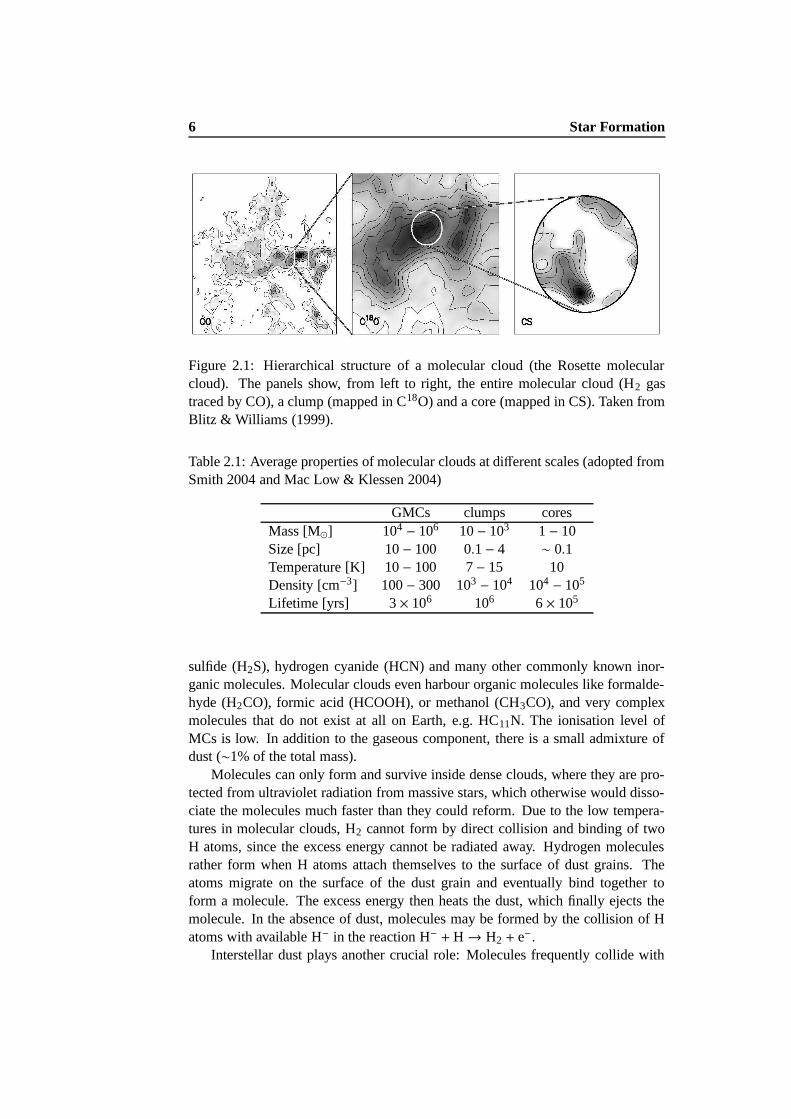
Figure 2.1: Hierarchical structure of a molecular cloud (the Rosette molecularcloud). The panels show, from left to right, the entire molecular cloud (H2 gastraced by CO), a clump (mapped in C18O) and a core (mapped in CS). Taken fromBlitz & Williams (1999).
Table 2.1: Average properties of molecular clouds at different scales (adopted fromSmith 2004 and Mac Low & Klessen 2004)
GMCs clumps coresMass [M] 104 − 106 10 − 103 1 − 10Size [pc] 10 − 100 0.1 − 4 ∼ 0.1Temperature [K] 10 − 100 7 − 15 10Density [cm−3] 100 − 300 103 − 104 104 − 105
Lifetime [yrs] 3 × 10⁶ 106 6 × 10⁵
sulfide (H2S), hydrogen cyanide (HCN) and many other commonly known inor-ganic molecules. Molecular clouds even harbour organic molecules like formalde-hyde (H2CO), formic acid (HCOOH), or methanol (CH3CO), and very complexmolecules that do not exist at all on Earth, e.g. HC11N. The ionisation level ofMCs is low. In addition to the gaseous component, there is a small admixture ofdust (∼1% of the total mass).
Molecules can only form and survive inside dense clouds, where they are pro-tected from ultraviolet radiation from massive stars, which otherwise would disso-ciate the molecules much faster than they could reform. Due to the low tempera-tures in molecular clouds, H2 cannot form by direct collision and binding of twoH atoms, since the excess energy cannot be radiated away. Hydrogen moleculesrather form when H atoms attach themselves to the surface of dust grains. Theatoms migrate on the surface of the dust grain and eventually bind together toform a molecule. The excess energy then heats the dust, which finally ejects themolecule. In the absence of dust, molecules may be formed by the collision of Hatoms with available H− in the reaction H− + H→ H2 + e−.
Interstellar dust plays another crucial role: Molecules frequently collide with
2.1 Molecular Clouds 7
dust grains, which are heated by the energy and emit radiation in the infrared (IR)part of the electromagnetic spectrum. Since molecular clouds are relatively trans-parent in the infrared, the energy is efficiently radiated away. Thus, the dust acts asa temperature regulator keeping the molecular clouds cold.
Molecular clouds have masses from a few solar masses (M) to about 106 M.Clouds with masses M > 104 M are called giant molecular clouds (GMCs), theyhave diameters of 50 pc or more. Molecular clouds are very inhomogeneous ob-jects, they show large density gradients and contain dense clumps and filaments(see Fig. 2.1). The densest parts, which have typical densities of 105 to 106 cm−3
and sizes of less than a parsec, are called cores. They may eventually collapseand form stars. Table 2.1 lists typical parameters of molecular clouds at differentscales. The structure of MCs may be described as fractal (e.g. Scalo 1990; Falgar-one et al. 1991; Stutzki et al. 1998). In this picture, the clouds are scale-free andthe hierarchy of clouds, clumps and cores reflects a self-similar structure. How-ever, there are limits to a self-similar description of cloud structure. It is at leastnot universally appropriate, e.g. in Taurus self-similarity breaks down at a sizescale of ∼ 0.2 − 0.3 pc (Williams 1999). GMCs are self-gravitating, i.e. they areheld together by the mass of the gas. However, their internal structure has to bemaintained by some source of energy injection preventing them from immediatecollapse under their own gravity. In the classical theories the clouds are stabilisedby magnetic fields, today it is believed that supersonic turbulence, which is ob-served ubiquitously in molecular clouds, plays this role (see the discussion in § 2.4to 2.6).
The process of how molecular clouds form is rather poorly understood and itis very likely that there is more than one mechanism (see e.g. Blitz & Williams1999; Ballesteros-Paredes 2004). Earlier models of collisional agglomeration ofsmaller ‘cloudlets’ are in contradiction to observations and can probably be ruledout. Considering a turbulent ISM, clouds may form by the convergence of turbulentflows at large scales, which may be caused by some sort of instability, the passageof spiral density waves, or swept-up shells from supernova remnants.
In the classical picture the lifetime of a molecular cloud is in the order of107 years (e.g. Palla & Stahler 2000; Tassis & Mouschovias 2004). However, thereis now evidence that star formation takes place on relatively short timescales andthat molecular clouds are rather transient objects that form and dissolve in thelarger-scale turbulent flow of the Galactic disc (e.g. Bonnell et al. 2006). Mostof the molecular clouds in the solar neighborhood contain young stars with typ-ical ages between 1 and 3 Myr and a low age spread. This strongly suggeststhat molecular clouds generally form rapidly, produce stars rapidly, and dispersequickly within a timescale of only a few 106 years (Ballesteros-Paredes et al.1999b; Elmegreen 2000; Hartmann et al. 2001; Hartmann 2003; Vazquez-Semadeniet al. 2005). Observations of self-similar structure in molecular clouds (e.g. MacLow & Ossenkopf 2000; Ossenkopf & Mac Low 2002) indicate that interstellar tur-bulence is driven on scales substantially larger than the clouds themselves. Theselarge-scale turbulent flows compress and cool the gas. At sufficiently high densities
8 Star Formation
atomic gas is then quickly converted into molecular form (Hollenbach et al. 1971).These same flows will continue to drive the turbulent motions observed within thenewly formed cloud. Some combination of turbulent flow, free expansion at thesound speed of the cloud and dissociating radiation from internal star formationwill then be responsible for the destruction of the cloud on a timescale of 5 to10 Myr.
2.2 From Clouds to Stars
Stars form from gravitational collapse of gas and dust in dense molecular cloudcores. For this to happen, gravity has to overcome all dispersive or resistive forces.Small density fluctuations in an initially uniform medium are amplified by gravityin a process called gravitational instability. The perturbations become unstableagainst gravitational collapse once their wavelength λ exceeds a critical wavelength
λJ =
√
πc2s
Gρ0, (2.1)
called the Jeans length after the work of Jeans (1902), where cs = (kT/m)1/2 is theisothermal sound speed, G the gravitational constant, ρ0 the initial mass density,and m the average particle mass. Under the assumption of a spherical perturbation,this corresponds to a critical mass (Jeans mass)
MJ =4π3
(
λJ
2
)3
ρ0 =π
6
(
π
G
)3/2c3
s ρ−1/20 . (2.2)
All perturbations with masses larger than MJ will collapse under their own weight.Provided the collapse remains isothermal, the Jeans mass falls as the density in-creases. Therefore, the cloud will fragment into smaller and smaller pieces as longas the process is isothermal. Once the released gravitational energy cannot escapethe system anymore, the temperature rises, thus the Jeans mass increases, and thecollapse is decelerated and eventually stopped. Since the critical density at whichthis occurs depends on the opacity (and the initial temperature) of the gas, it iscalled opacity limit for fragmentation. Although this classical picture of collapseand fragmentation has some inconsistencies, the Jeans criterion is still a centralfeature for the understanding of star formation.
The further evolution of the cloud fragments is as follows (see also Fig. 2.2):During the isothermal collapse, the released gravitational energy heats the mol-ecules, which rapidly pass the energy on to dust grains via collisions. The dustgrains re-radiate energy in the millimetre range, which can escape the core. Oncethe number density in the central part reaches about 1011 cm−3 the gas becomesopaque to dust radiation, therefore the energy cannot be transported outwards any-more. Temperature, pressure, and opacity rise, the core changes from isothermalto adiabatic. The resulting higher thermal pressure counterbalances gravity, the

2.3 Embedded Clusters 9
collapse is stopped and a temporary equilibrium is reached: The first core with adensity of 1013
. n . 1014 cm−3 and a temperature of 100 . T . 200 K is formed.Matter from the envelope keeps falling in onto the core making temperature anddensity increase further. At T ≈ 2000 K the hydrogen molecules dissociate. Thisis an endothermic process, i.e., it consumes energy. Therefore, the rise in tempera-ture and pressure is slowed down, until gravity takes over again and the core goesinto a second collapse. Once the molecules are exhausted, the energy consump-tion in the core is stopped. The thermal pressure decelerates and eventually stopsthe collapse, leading to a second, final protostellar core having a density of about1023 cm−3 and a temperature of about 104 K. This core, which may only possess afew per cent of its final mass, is still surrounded by a massive envelope. Since thegas is rotating, it cannot fall directly onto the core because of angular momentumconservation. It forms an accretion disc around the core, in which the gas is trans-ported inwards by viscous torques (Pringle 1981; Papaloizou & Lin 1995) beforeit is finally accreted by the protostar. If mass is accumulated by the disc faster thanit is removed by viscous transport the disc will become too massive, generatingspiral density waves. These gravitational torques support and increase the inwardtransport of disc material. If the density of the disc is high enough, it may becomeeven more gravitationally unstable and fragment, possibly leading to the formationof brown dwarves or gas planets. A significant fraction of the infalling matter doesnot end up on the star at all, but is released again by bipolar outflows or jets, aphenomenon observed in many accreting protostars. Jets associated with youngstellar objects (YSOs) can reach velocities up to 400 km s−1 (e.g. Konigl & Pudritz2000). The rapid collapse phase is followed by a much slower quasi-static contrac-tion of the protostar. Temperature and pressure keep rising, until the hydrogen inthe core ignites at a temperature of about 107 K and fusion sets in. This results ina new equilibrium and the star has finally reached the main sequence after about107 years.
2.3 Embedded Clusters
Almost all stars form in clusters (see Elmegreen et al. 2000 or Lada & Lada 2003for a review). The theory of star formation therefore has to describe the formationof a stellar cluster rather than that of isolated stars. Lada & Lada (2003) definea cluster as a group of 35 or more physically related stars with mass densitiesρ∗ > 1.0 M pc−3. Stellar clusters are born embedded within dense giant molecularclouds, making them visible only at infrared wavelengths. The extinction due tointerstellar dust can be as high as AV ∼ 100 mag. The degree of embeddednesscorresponds to the evolutionary stage of a cluster: while the least evolved clusters(e.g. Serpens, ρ Ophiuchi) are found in heavily obscured, massive dense molecularcloud cores, the most evolved clusters (e.g. Trapezium, IC 348) are located withinHII regions or at the edges of molecular clouds. Embedded clusters are physicallyassociated with the most massive and densest molecular cloud cores with masses
10 Star Formation
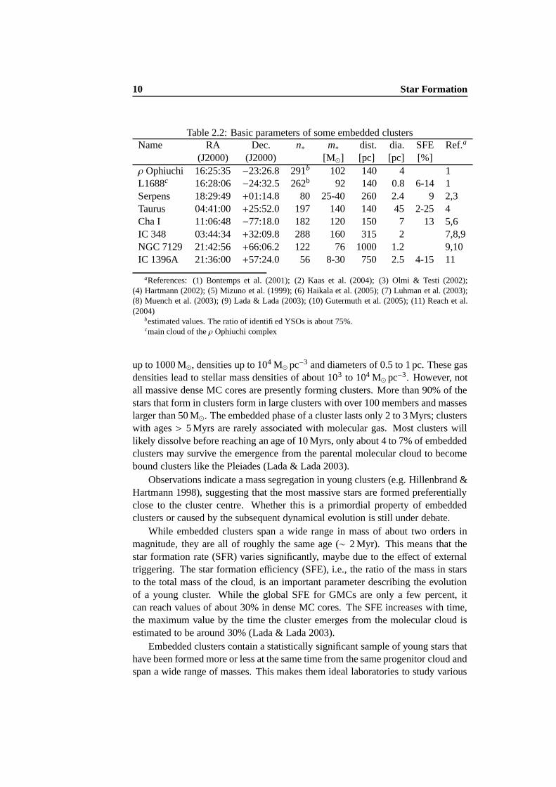
Table 2.2: Basic parameters of some embedded clustersName RA Dec. n∗ m∗ dist. dia. SFE Ref.a
(J2000) (J2000) [M] [pc] [pc] [%]ρ Ophiuchi 16:25:35 −23:26.8 291b 102 140 4 1L1688c 16:28:06 −24:32.5 262b 92 140 0.8 6-14 1Serpens 18:29:49 +01:14.8 80 25-40 260 2.4 9 2,3Taurus 04:41:00 +25:52.0 197 140 140 45 2-25 4Cha I 11:06:48 −77:18.0 182 120 150 7 13 5,6IC 348 03:44:34 +32:09.8 288 160 315 2 7,8,9NGC 7129 21:42:56 +66:06.2 122 76 1000 1.2 9,10IC 1396A 21:36:00 +57:24.0 56 8-30 750 2.5 4-15 11
aReferences: (1) Bontemps et al. (2001); (2) Kaas et al. (2004); (3) Olmi & Testi (2002);(4) Hartmann (2002); (5) Mizuno et al. (1999); (6) Haikala et al. (2005); (7) Luhman et al. (2003);(8) Muench et al. (2003); (9) Lada & Lada (2003); (10) Gutermuth et al. (2005); (11) Reach et al.(2004)
bestimated values. The ratio of identified YSOs is about 75%.cmain cloud of the ρ Ophiuchi complex
up to 1000 M, densities up to 104 M pc−3 and diameters of 0.5 to 1 pc. These gasdensities lead to stellar mass densities of about 103 to 104 M pc−3. However, notall massive dense MC cores are presently forming clusters. More than 90% of thestars that form in clusters form in large clusters with over 100 members and masseslarger than 50 M. The embedded phase of a cluster lasts only 2 to 3 Myrs; clusterswith ages > 5 Myrs are rarely associated with molecular gas. Most clusters willlikely dissolve before reaching an age of 10 Myrs, only about 4 to 7% of embeddedclusters may survive the emergence from the parental molecular cloud to becomebound clusters like the Pleiades (Lada & Lada 2003).
Observations indicate a mass segregation in young clusters (e.g. Hillenbrand &Hartmann 1998), suggesting that the most massive stars are formed preferentiallyclose to the cluster centre. Whether this is a primordial property of embeddedclusters or caused by the subsequent dynamical evolution is still under debate.
While embedded clusters span a wide range in mass of about two orders inmagnitude, they are all of roughly the same age (∼ 2 Myr). This means that thestar formation rate (SFR) varies significantly, maybe due to the effect of externaltriggering. The star formation efficiency (SFE), i.e., the ratio of the mass in starsto the total mass of the cloud, is an important parameter describing the evolutionof a young cluster. While the global SFE for GMCs are only a few percent, itcan reach values of about 30% in dense MC cores. The SFE increases with time,the maximum value by the time the cluster emerges from the molecular cloud isestimated to be around 30% (Lada & Lada 2003).
Embedded clusters contain a statistically significant sample of young stars thathave been formed more or less at the same time from the same progenitor cloud andspan a wide range of masses. This makes them ideal laboratories to study various
2.4 The “Standard Theory” of Star Formation 11
aspects of the star formation process, like the initial mass function (IMF; see § 2.8)or stellar dynamics due to complex interactions.
Table 2.2 lists the basic parameters of the embedded clusters that will be dis-cussed in detail in this work. Columns 1 to 3 contain the name and average posi-tion (right ascension and declination) of the clusters taken from the Simbad database. Columns 4 to 9 give the number of YSOs, total mass of YSOs, distance,linear diameter, and star formation efficiency (SFE) of the cluster according to thereferences listed in the last column. If no information on the linear diameter ofthe cluster was found in the literature, it was computed from the angular diameterand the distance. Note that most of the parameters cannot be measured directly,but have to be inferred by indirect methods or estimated, therefore they may con-tain significant uncertainties. The numbers of YSOs are given for illustrative pur-poses, for a detailed discussion on that subject see § 7.1. An extensive catalogue ofGalactic embedded clusters within ∼2 kpc of the Sun can be found in Lada & Lada(2003), another catalogue, focussing on the positions and dimensions of infrared(i.e. mostly embedded) clusters, was compiled by Bica et al. (2003).
2.4 The “Standard Theory” of Star Formation
Es gibt also keinen klar formulierbaren Unterschied zwischen Mythenund wissenschaftlichen Theorien.
– Paul Feyerabend, Wider den Methodenzwang
In the so-called “standard theory” of star formation (Shu 1977; Shu et al. 1987)stars are formed by the inside-out collapse of gas clumps, whose initial conditionsare a singular isothermal sphere (SIS), i.e. a hydrostatic equilibrium density distri-bution
ρ(r) ∼c2
s
2πGr2(2.3)
(for 0 < r < Rcore), where cs = (kT/m)1/2 is the isothermal sound speed, G thegravitational constant, m the average particle mass, and Rcore the outer radius ofthe core.
In this scenario, molecular cloud clumps are initially in quasistatic equilib-rium and supported against gravitational collapse by magnetic pressure (Mestel &Spitzer 1956). Material diffuses slowly through the magnetic field towards the cen-tre by ambipolar diffusion (ion-neutral drift), resulting in a steadily growing centralcore approximating a SIS. Once the critical density is exceeded, the SIS undergoesan inside-out collapse while the gas stays isothermal. This collapse is initiated bya spherical expansion wave which propagates outward at a speed of about c s. Thegas outside the expansion wave stays more or less stationary, while the gas insidethe expansion wave approaches the central protostar almost in free fall. The proto-star grows roughly linearly with time with a mass accretion rate that only depends
12 Star Formation
on the isothermal sound speed:
M = 0.975c3
s
G(2.4)
(Shu 1977). Since the gas is expected to possess significant angular momentum,only a fraction of the infalling mass is accreted directly by the central protostar,while the remainder forms a circumstellar accretion disc. In the last stage, angularmomentum is removed from the disc and most of the mass will eventually be ac-creted by the young star. The remainder of the disc may form a planetary systemor is dispersed.
This theory, however, experiences several problems and is challenged by bothobservational and theoretical results (see e.g. Mac Low & Klessen 2004). Theoret-ical considerations show that SIS are very unlikely as initial conditions for collapse(Whitworth et al. 1996), and at the same time observations suggest that the centraldensity profiles of cores are flatter than those expected for isothermal spheres (Bac-mann et al. 2000). The SIS paradigm is only applicable to isolated stars, whereasit is now known that the majority of stars form in small aggregates or large clusters(Adams & Myers 2001; Lada & Lada 2003, see also § 2.3). Furthermore, there isboth observational evidence (Crutcher 1999; Andre et al. 2000; Bourke et al. 2001)and theoretical reasoning (e.g. Nakano 1998) showing that most observed cloudcores do not have magnetic fields strong enough to support them against gravita-tional collapse. Similarly, the long lifetimes implied by the quasi-static phase ofevolution in the model are difficult to reconcile, e.g. with observational statisticsof cloud cores (Taylor et al. 1996; Lee & Myers 1999; Visser et al. 2002) and withchemical age considerations (van Dishoeck & Blake 1998; Langer et al. 2000). The“standard theory” predicts constant mass accretion rates, while both observationsand numerical simulations lead to the conclusion that protostellar mass accretionis a highly dynamical and time-variant process (see the detailed discussion in § 5).
These inconsistencies have led to the suggestion that star formation is moder-ated by interstellar turbulence and its interplay with gravity rather than by magneticfields. This approach will be outlined in the following two sections.
2.5 Turbulence
According to an apocryphal story, Werner Heisenberg was asked what he wouldask God, given the opportunity. His reply was: “When I meet God, I am going to
ask him two questions: Why relativity? And why turbulence? I really believe hewill have an answer for the first.”
– found on the web2
The internal velocity dispersions of molecular clouds are supersonic with Machnumbers (the ratio of the speed of the flow to the speed of sound: M = v/cs) of
2e.g. http://en.wikipedia.org/wiki/Turbulence

2.5 Turbulence 13
M ≈ 10 and larger (Larson 1981; Blitz 1993; Williams et al. 2000). The observedbroadening of spectral lines is usually interpreted as the signature of interstellarturbulence. Turbulence means a nonlinear state of fluid motion that is characterisedby random and chaotic motions at many scales. When present, turbulence usuallydominates all other flow phenomena like mixing, heat transfer, or drag. Detaileddescriptions of observations and theory of interstellar turbulence can be found inthe reviews by Franco & Carraminana (1999), Elmegreen & Scalo (2004), Scalo &Elmegreen (2004), and Mac Low & Klessen (2004).
The first theory to describe turbulence was developed by Kolmogorov (1941).In this picture, turbulence is incompressible and driven by energy injected on alarge scale. The turbulent kinetic energy is then dissipated by interacting withsmaller vortices and thus transferred to smaller and smaller scales (i.e. larger wavenumbers k), until the energy has cascaded all the way down to the dissipation scaleλvisc, where viscous dissipation turns the kinetic energy into heat. This cascadeleads to an energy spectrum
E(k) ∝ k−5/3, (2.5)
where k = 2π/λ is the wave number.
The motion of the interstellar gas, however, differs from this picture. The in-terstellar medium is highly compressible and supersonic, and the turbulent drivingis not uniform, but caused by shock waves and other inhomogeneous processes.Supersonic flows in highly compressible gas lead to strong density fluctuations. Insupersonic turbulence, shock waves also account for the dissipation of kinetic en-ergy by transferring energy between widely separated scales, unlike the cascadingnature of incompressible turbulence.
Under molecular cloud conditions, supersonic turbulence likely decays in lessthan one free-fall time (Stone et al. 1998; Mac Low et al. 1998; Mac Low 1999;Padoan & Nordlund 1999). Since it is observed ubiquitously in molecular clouds ofall ages, it has to be driven on large scales. This driving is neither uniform nor ho-mogeneous. Possible driving mechanisms of interstellar turbulence include mag-netorotational instabilities (Dziourkevitch et al. 2004; Piontek & Ostriker 2004,2005), gravitational instabilities (Wada et al. 2002), protostellar outflows (MacLow 2000; Reipurth & Bally 2001; Quillen et al. 2005), and supernovae (e.g. Dibet al. 2006). There is an ongoing debate on which of those is the most impor-tant energy source. The most likely source of large-scale interstellar turbulencein the Milky Way is the combined energy and momentum input from supernovaeexplosions (Mac Low & Klessen 2004). They appear to overwhelm all other possi-bilities. In the outer reaches of the Galaxy and in low surface brightness galaxies,on the other hand, the situation is not so clear. In low-density regions of the inter-stellar medium, like the far outer Galaxy, the magnetorotational instability mightplay an important role (Piontek & Ostriker 2005).
14 Star Formation
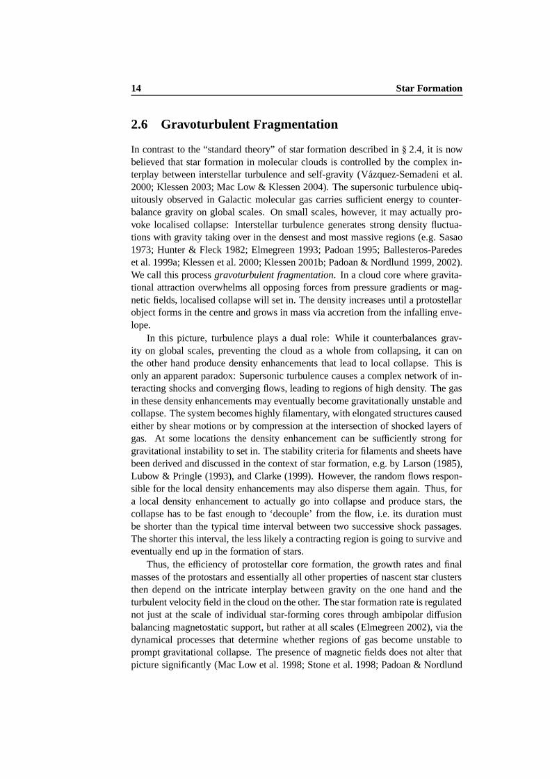
2.6 Gravoturbulent Fragmentation
In contrast to the “standard theory” of star formation described in § 2.4, it is nowbelieved that star formation in molecular clouds is controlled by the complex in-terplay between interstellar turbulence and self-gravity (Vazquez-Semadeni et al.2000; Klessen 2003; Mac Low & Klessen 2004). The supersonic turbulence ubiq-uitously observed in Galactic molecular gas carries sufficient energy to counter-balance gravity on global scales. On small scales, however, it may actually pro-voke localised collapse: Interstellar turbulence generates strong density fluctua-tions with gravity taking over in the densest and most massive regions (e.g. Sasao1973; Hunter & Fleck 1982; Elmegreen 1993; Padoan 1995; Ballesteros-Paredeset al. 1999a; Klessen et al. 2000; Klessen 2001b; Padoan & Nordlund 1999, 2002).We call this process gravoturbulent fragmentation. In a cloud core where gravita-tional attraction overwhelms all opposing forces from pressure gradients or mag-netic fields, localised collapse will set in. The density increases until a protostellarobject forms in the centre and grows in mass via accretion from the infalling enve-lope.
In this picture, turbulence plays a dual role: While it counterbalances grav-ity on global scales, preventing the cloud as a whole from collapsing, it can onthe other hand produce density enhancements that lead to local collapse. This isonly an apparent paradox: Supersonic turbulence causes a complex network of in-teracting shocks and converging flows, leading to regions of high density. The gasin these density enhancements may eventually become gravitationally unstable andcollapse. The system becomes highly filamentary, with elongated structures causedeither by shear motions or by compression at the intersection of shocked layers ofgas. At some locations the density enhancement can be sufficiently strong forgravitational instability to set in. The stability criteria for filaments and sheets havebeen derived and discussed in the context of star formation, e.g. by Larson (1985),Lubow & Pringle (1993), and Clarke (1999). However, the random flows respon-sible for the local density enhancements may also disperse them again. Thus, fora local density enhancement to actually go into collapse and produce stars, thecollapse has to be fast enough to ‘decouple’ from the flow, i.e. its duration mustbe shorter than the typical time interval between two successive shock passages.The shorter this interval, the less likely a contracting region is going to survive andeventually end up in the formation of stars.
Thus, the efficiency of protostellar core formation, the growth rates and finalmasses of the protostars and essentially all other properties of nascent star clustersthen depend on the intricate interplay between gravity on the one hand and theturbulent velocity field in the cloud on the other. The star formation rate is regulatednot just at the scale of individual star-forming cores through ambipolar diffusionbalancing magnetostatic support, but rather at all scales (Elmegreen 2002), via thedynamical processes that determine whether regions of gas become unstable toprompt gravitational collapse. The presence of magnetic fields does not alter thatpicture significantly (Mac Low et al. 1998; Stone et al. 1998; Padoan & Nordlund

2.7 Classification of Young Stellar Objects 15
1999; Heitsch et al. 2001b). In particular, it cannot prevent the decay of interstellarturbulence.
Clusters of stars build up in molecular cloud regions where self-gravity over-whelms turbulence, either because such regions are compressed by a large-scaleshock, or because interstellar turbulence is not replenished and decays on shorttimescales. Then, many gas clumps become gravitationally unstable and syn-chronously go into collapse. If the number density is high, contracting protostellarcores interact and may merge to produce new cores which now contain multipleprotostars. Close encounters drastically alter the trajectories of the protostars, thuschanging their mass accretion rates. This has important consequences for the finalstellar mass spectrum (Bonnell et al. 1997; Klessen & Burkert 2000, 2001; Bonnellet al. 2001a,b; Klessen 2001b; Bate et al. 2002).
Inefficient, isolated star formation will occur in regions that are supported byturbulence carrying most of its energy on very small scales. This requires an unre-alistically large number of driving sources and appears at odds with the measuredvelocity structure in molecular clouds which in almost all cases is dominated bylarge-scale modes (Mac Low & Ossenkopf 2000; Ossenkopf & Mac Low 2002).
Numerical simulations (e.g. Klessen et al. 2000; Klessen & Burkert 2000,2001; Klessen 2001a,b; Heitsch et al. 2001a; Padoan & Nordlund 2002) haveshown that gravoturbulent fragmentation can successfully explain the observationalproperties of star-forming clouds and young stars. It provides a consistent pictureof the entire process of star formation. Some new aspects will be discussed in thiswork.
2.7 Classification of Young Stellar Objects
Young stellar objects are usually divided into four classes on basis of the propertiesof their spectral energy distribution (SED) in the infrared, indicating an evolution-ary sequence. Classes 1, 2, and 33 have been introduced by Lada & Wilking (1984)and Lada (1987); later Class 0 has been added to describe an even younger evo-lutionary stage (Andre et al. 1993). The observational properties of the differentclasses are described in detail in Andre et al. (2000), Lada (2001), or Smith (2004).The basic properties are summarised in Table 2.3, the SEDs typical for each classare shown in Fig. 2.3. A characteristic feature is the slope of the infrared SED, orspectral index, determined in the wavelength range between 2 and 20 µm:
αIR =d(log λS λ)
d(log λ)(2.6)
where S λ denotes the luminosity within each wavelength interval.
3originally, the classes have been denoted with Roman numbers: Class I, II, III, but it has beenpointed out that the later introduced zero is unknown to the Roman system, so, to be consistent,Arabic numbers will be used for all the YSO classes from 0 to 3.
16 Star Formation
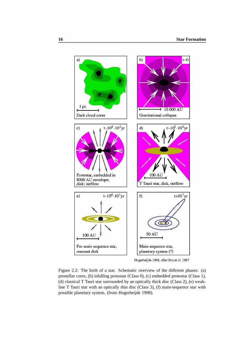
Figure 2.2: The birth of a star. Schematic overview of the different phases: (a)prestellar cores, (b) infalling protostar (Class 0), (c) embedded protostar (Class 1),(d) classical T Tauri star surrounded by an optically thick disc (Class 2), (e) weak-line T Tauri star with an optically thin disc (Class 3), (f) main-sequence star withpossible planetary system. (from Hogerheijde 1998).

2.7 Classification of Young Stellar Objects 17
Figure 2.3: The classification scheme of YSOs according to their SEDs. The ver-tical line is at the wavelength of 2.2 µm (from Lada 2001).
Class 0 and 1 objects are characterised by SEDs that rise with wavelength(αIR > 0) and peak in the submillimetre or far infrared (FIR) range. This indi-cates that these objects are surrounded by a massive infalling envelope of gas anddust, which absorbs the radiation of the protostar and re-radiates it at much longerwavelengths. Class 0 sources are deeply embedded protostars that show a largesub-mm (λ > 350 µm) to bolometric luminosity ratio (Lsmm/Lbol > 0.005). Mostof the Class 0 sources are not detected at wavelengths λ < 20 µm. The Class 0stage is the main accretion phase and lasts only a few 104 years. Class 1 objectsare relatively evolved protostars with ages around 1 − 5 × 10⁵ years surrounded byan accretion disc and a circumstellar envelope of substellar mass (Menv . 0.3 M).The transition phase between Class 0 and 1 is believed to take place when the en-velope mass is about equal to the mass of the protostar. Another indicator for theclass division is the bolometric temperature Tbol: Class 0 corresponds to protostarswith Tbol < 70 K and Class 1 to objects with 70 K < Tbol < 650 K.
Pre-main-sequence stars in Class 2 and 3 correspond to classical T Tauri stars
18 Star Formation
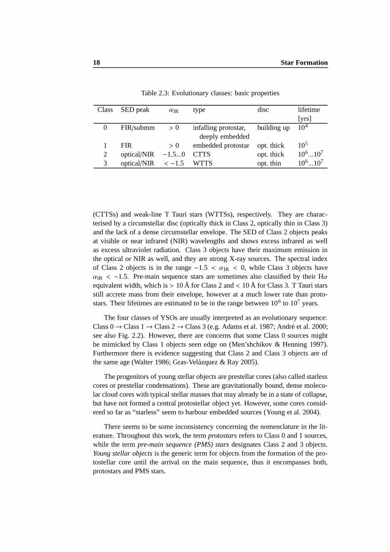
Table 2.3: Evolutionary classes: basic properties
Class SED peak αIR type disc lifetime[yrs]
0 FIR/submm > 0 infalling protostar, building up 104
deeply embedded1 FIR > 0 embedded protostar opt. thick 105
2 optical/NIR −1.5...0 CTTS opt. thick 106...107
3 optical/NIR < −1.5 WTTS opt. thin 106...107
(CTTSs) and weak-line T Tauri stars (WTTSs), respectively. They are charac-terised by a circumstellar disc (optically thick in Class 2, optically thin in Class 3)and the lack of a dense circumstellar envelope. The SED of Class 2 objects peaksat visible or near infrared (NIR) wavelengths and shows excess infrared as wellas excess ultraviolet radiation. Class 3 objects have their maximum emission inthe optical or NIR as well, and they are strong X-ray sources. The spectral indexof Class 2 objects is in the range −1.5 < αIR < 0, while Class 3 objects haveαIR < −1.5. Pre-main sequence stars are sometimes also classified by their Hαequivalent width, which is > 10 Å for Class 2 and < 10 Å for Class 3. T Tauri starsstill accrete mass from their envelope, however at a much lower rate than proto-stars. Their lifetimes are estimated to be in the range between 106 to 107 years.
The four classes of YSOs are usually interpreted as an evolutionary sequence:Class 0→ Class 1→ Class 2→ Class 3 (e.g. Adams et al. 1987; Andre et al. 2000;see also Fig. 2.2). However, there are concerns that some Class 0 sources mightbe mimicked by Class 1 objects seen edge on (Men’shchikov & Henning 1997).Furthermore there is evidence suggesting that Class 2 and Class 3 objects are ofthe same age (Walter 1986; Gras-Velazquez & Ray 2005).
The progenitors of young stellar objects are prestellar cores (also called starlesscores or prestellar condensations). These are gravitationally bound, dense molecu-lar cloud cores with typical stellar masses that may already be in a state of collapse,but have not formed a central protostellar object yet. However, some cores consid-ered so far as “starless” seem to harbour embedded sources (Young et al. 2004).
There seems to be some inconsistency concerning the nomenclature in the lit-erature. Throughout this work, the term protostars refers to Class 0 and 1 sources,while the term pre-main sequence (PMS) stars designates Class 2 and 3 objects.Young stellar objects is the generic term for objects from the formation of the pro-tostellar core until the arrival on the main sequence, thus it encompasses both,protostars and PMS stars.
2.8 The Mass of a Star 19
2.8 The Mass of a Star
The mass of a star is certainly its most important property. Although the Russell-Vogt theorem (Vogt 1926; Russell et al. 1927), which states that the evolution ofstars is fixed at their birth by two inherent fundamental parameters, mass and chem-ical composition, has turned out to be slightly incorrect, it is nevertheless the star’smass at birth, which determines most of its essential parameters like lifetime, lu-minosity, temperature, radius, or density profile (Massey & Meyer 2001). Themass-luminosity relation is considered one of the most fundamental descriptionsof stellar properties. This relation, as well as the lifetime as a function of time,show a different behaviour for high-mass stars than for solar-mass stars.
Stellar masses span a wide range between 0.08 and about 150 M. Below0.08 M, the temperature in the stellar core is not high enough to ignite hydrogen.Objects with masses below this limit and over 0.01 M (about 10 Jupiter masses)may only burn deuterium in their cores. These are Brown Dwarves. While thereis a natural lower limit to the mass of a star, it is not clear, if there exists an upperlimit, and if yes, what causes it. Observations indicate that no stars with masseslarger than 150 M exist (Figer 2005). Stellar masses can either be determined inbinary systems using Kepler’s laws or be inferred from theoretical models usingobservational estimates on age, luminosity and temperature.
The stellar initial mass function (IMF) describes the distribution of masseswith which stars are formed. The IMF is the most fundamental output functionof the star formation process (see Larson 1999, Meyer et al. 2000, Pudritz 2002, orKroupa 2002 for reviews). It can be written as
ξ(M) = cM−(1+x), (2.7)
with the original value of x = 1.35 (Salpeter 1955). Observations of differentstar-forming regions reveal an apparently universal form of the IMF: It has a char-acteristic stellar mass of the order of 1 M, and a power-law decline similar to orsomewhat steeper than the original Salpeter (1955) slope at masses M > 1 M.It flattens over lower masses and peaks at a few tenths of a solar mass, decliningagain toward the lowest masses.
The apparent universality of the IMF is still a challenge for star formation the-ory, since variations according to the different initial conditions in different star-forming regions are expected. It is suspected that the characteristic stellar massis caused by a characteristic scale of fragmentation in star-forming clouds whichis essentially the Jeans scale as given by the typical temperature and pressure inmolecular clouds. The power-law decline of the IMF at large masses suggests thatthe most massive stars are built up by scale-free accretion or accumulation pro-cesses, with interactions between dense prestellar clumps or protostars playing arole as well. The thermal properties of star-forming clouds seem to have an im-portant influence on the fragmentation behaviour. At least for low-mass stars theIMF probably depends on the detailed thermal physics of the cloud (Larson 2005).This is supported by numerical simulations of cloud collapse and fragmentation

20 Star Formation
showing that the equation of state plays an important role in the fragmentation ofclouds and the determination of the IMF (Li et al. 2003; Jappsen et al. 2005).
Chapter 3
Numerical Simulations
Computers are useless. They can only give you answers.
– Pablo Picasso
As outlined in the previous chapter, star formation is a highly complex andchaotic process involving many different physical processes and a wide range ofscales. Observations of molecular clouds and nascent stars are the base of all starformation theories, however, it requires models to obtain a self-consistent pictureof the entire process. Analytical models are restricted to describe the collapse ofisolated, idealised objects. Therefore, numerical simulations play a central role inunderstanding the process of star formation. The first numerical collapse calcu-lations have been performed by Bodenheimer & Sweigart (1968), Larson (1969)and Hunter (1977). While these early works were restricted to a single sphere,numerical simulations are meanwhile able to follow the entire evolution from thefragmentation and collapse of a molecular cloud to the build-up of a stellar cluster.Before we describe the simulations used for this study, the basics of hydrodynamicsand the concept of Smoothed Particle Hydrodynamics will be briefly outlined. Adetailed description of hydrodynamical concepts, and especially their applicationto astrophysical problems is given e.g. by Shu (1992).
3.1 Some Basics of Hydrodynamics
The common approach to study the motion of fluids and gases is by hydrodynamics.In this picture, gases and fluids are large ensembles of interacting particles (atoms,molecules, electrons, dust particles, etc.). The state of the system is described byits location in the 6N-dimensional phase space, where N is the number of particles.The temporal evolution is governed by the equation of motion in phase space. Sincean exact solution is almost impossible for a large number of particles, in analogyto quantum mechanics a probabilistic approach is used. The exact location of thesystem in phase space is then described by the N-body probability distribution
f (N)( ~q1... ~qN , ~p1... ~pN) d ~q1...d ~qN , d ~p1...d ~pN . (3.1)
21

22 Numerical Simulations
Since observables are usually associated with a one- or two-body probability den-sity f (1) or f (2), the probability distribution can be reduced from f (N) to f (n) byintegrating over all but n variables. This leads to the so-called BBGKY-hierarchy(named after Born, Bogoliubov, Green, Kirkwood, and Yvon) of equations of mo-tion. To solve this system of equations, a specific approximation to terminate it isrequired. The lowest level of the hierarchy is represented by the one-body distri-bution function f (1)(~q, ~p, t). It describes the probability of finding a particle at timet in the volume element d3~q at the location ~q with momenta in the range d3~p at ~p.The equation of motion for f (1) is called Boltzmann equation:
d fdt≡ ∂ f∂t+ ~q ~∇q f + ~p ~∇p f =
∂ f∂t+ ~v ~∇q f + ~F ~∇p f = fc. (3.2)
The first part corresponds to the transformation from a comoving to a spatiallyfixed coordinate system. The second part gives the velocity as ~v = ~q and the forceas ~F = ~p. All higher order terms from the BBGKY-hierarchy are contained inthe collision term fc. Since the observable quantities are typically moments of theBoltzmann equation, this allows a further simplification of the description of thesystem. If the expansion of the Boltzmann equation into moments yields well-defined quantities, the thermodynamic approximation is valid. This is the case, ifthe distribution function is a smoothly varying function on the scales of interest,i.e., if the averaging scale is larger than the mean free path of individual particles.However, there are some limitations to this approximation. It does not work e.g.in the case of shocks or phase transitions, and it cannot be applied to fully fractalsystems.
A problem in hydrodynamics is book-keeping, i.e. keeping track of the changesin quantities such as mass, momentum or energy of a fluid element according tothe physical processes acting on it. There are two methods to achieve this. The Eu-lerian approach needs a three-dimensional grid of fixed points. The book-keepingis done by determining the changes (e.g. fluxes through the cell surfaces defined bythe grid) over a huge number of tiny time intervals. The Lagrangian approach, onthe other hand, does not require a grid. The fluid is represented by a large numberof moving interpolation points which follow the motion of the fluid. Each pointcarries a fixed mass and can be considered as a particle.
The hydrodynamic equations are a set of equations for the conserved quanti-ties (ρ, ρ~v, ε) plus a closure equation (the equation of state). The hydrodynamicequations needed to describe a self-gravitating compressible fluid are:
dρdt=∂ρ
∂t+ ~v · ~∇ρ = −ρ~∇ · ~v (3.3)
(continuity equation)
d~vdt=∂~v∂t+ (~v · ~∇)~v = −1
ρ~∇p − ~∇φ + η~∇2~v + (ζ +
η
3)~∇(~∇ · ~v) (3.4)

3.2 Smoothed Particle Hydrodynamics 23
(Navier-Stokes equation)
dεdt=∂ε
∂t+ ~v · ~∇ε = T
dsdt− pρ~∇ · ~v (3.5)
(energy equation)
~∇2φ = 4πGρ (3.6)
(Poisson’s equation)
p = RρT (3.7)
(equation of state)where ρ denotes the density, ~v the velocity, p the pressure, and φ the gravitationalpotential, ζ and η are viscosity coefficients, ε = ρ~v2/2 is the kinetic energy den-sity, T the temperature, s the entropy, and R the gas constant. If external forces(e.g. gravity or a magnetic field) are present, additional evolution equations for thesources that generate these forces are needed.
3.2 Smoothed Particle Hydrodynamics
The concept of Smoothed Particle Hydrodynamics (SPH) was introduced indepen-dently by Lucy (1977) and Gingold & Monaghan (1977). Detailed reviews can befound in Monaghan (1985, 1992), Benz (1990), or Price (2004), the code basicsare given in Monaghan (2001). SPH is a Lagrangian method where the fluid isrepresented by an ensemble of particles i, each having mass mi, momentum mi~vi
and hydrodynamic properties such as pressure, temperature, internal energy or en-tropy. The temporal evolution is governed by the equation of motion plus additionalequations to modify the hydrodynamic properties of the particles. Hydrodynamicobservables are obtained by a local averaging process. Representing a Lagrangianapproach, SPH does not need a grid to calculate spatial derivatives, instead, theyare found by analytical differentiation of interpolation formulae.
In SPH each particle is associated with a smoothing length h, representing thefinite spatial extent of the particle, which can differ in value for separate particles,as well as vary in time. Only those particles lying within the smoothing length ofanother can interact with that one, apart from gravity. Mass is conserved automat-ically, so there is no need to solve a continuity equation. Local averages for anyquantity f (~r) at a position ~r can be obtained by summing contributions from allthose particles j whose smoothing volume overlaps with ~r, weighted by an appro-priate smoothing function (smoothing kernel) W(~r, ~h):
〈 f (~r)〉 =∫
f (~r)W(|~r − ~r j|, h j)d3r′. (3.8)
The optimum value of h is such that every particle has about 50 neighbours withinthe smoothing volume.

24 Numerical Simulations
SPH is able to resolve large density contrasts as particles are free to moveand so naturally the particle concentration increases in high-density regions. Thismakes SPH an obvious and very powerful tool to simulate the star formation pro-cess. Consequently, it has been used extensively for this purpose (e.g. Klessen &Burkert 2000, 2001; Bate et al. 2003; Bonnell et al. 2003, 2004; Hennebelle et al.2003; Delgado-Donate et al. 2003, 2004; Goodwin et al. 2004a,b; Bate & Bonnell2005).
Bate & Burkert (1997) have shown that gravitational fragmentation is repro-duced properly by SPH (i.e., no artificial fragmentation occurs, while true frag-mentation is captured) provided (1) gravity and pressure are smoothed in the sameway, and (2) the minimum resolvable mass is always less than the local Jeans mass.Proper resolution requires about twice the number of neighbours, i.e. ∼100 parti-cles. It has been criticised that this criterion may not be sufficient and may produceartificial fragmentation leading to false multiple fragmentation (Klein et al. 2004).However, Hubber et al. (2006) show that SPH indeed simulates gravitational frag-mentation properly, even at low resolution. Unlike other claims it is very likely that(given the same input physics and initial conditions) grid- and particle-based codesbehave in a similar way concerning fragmentation (Gawryszczak et al. 2005).
3.3 The Models
To adequately describe the fragmentation of turbulent, self-gravitating gas cloudsand the resulting formation and mass growth of protostars, we need to resolvethe dynamical evolution of collapsing cores over several orders of magnitude indensity. Due to the stochastic nature of supersonic turbulence, it is not known inadvance where and when this local collapse occurs. As discussed in the previoussection, we resort to SPH to solve the equations of hydrodynamics. We use thesame smoothing procedure for gravity and pressure forces. This is needed to pre-vent artificial fragmentation (Bate & Burkert 1997). Because it is computationallyprohibitive to treat the cloud as a whole, we concentrate on subregions within thecloud and adopt periodic boundary conditions (Klessen 1997). Once the centralregion of a collapsing protostellar core exceeds a density contrast of ∼ 105, it isreplaced by a so-called sink particle (Bate et al. 1995), which has the ability toaccrete gas from its surrounding while at the same time keeping track of mass aswell as linear and angular momentum. By adequately replacing high-density coreswith sink particles we can follow the dynamical evolution of the system over manyfree-fall times.
We determine the resolution limit of our SPH calculations using the Bate &Burkert (1997) criterion. This is sufficient for the highly nonlinear density fluctu-ations created by supersonic turbulence as confirmed by convergence studies withup to 107 SPH particles (Jappsen et al. 2005; Li et al. 2005).
The suite of models studied here consists of two globally unstable modelsthat contract from Gaussian initial conditions without turbulence (for details see

3.3 The Models 25
Table 3.1: Overview of all models.
Name M k np Mmin Maccr n∗ tgrav
[M] [%]G1 – – 50 000 0.44 93.1 56 0.0G2 – – 500 000 0.044 84.9 56 0.0M01k2 0.1 1..2 205 379 0.058 74.9 95 200.0M01k4 0.1 3..4 205 379 0.058 27.2 3 200.0M01k8 0.1 7..8 205 379 0.058 85.9 3 200.0M05k2 0.5 1..2 205 379 0.058 37.2 23 100.0M05k4 0.5 3..4 205 379 0.058 77.9 48 100.0M05k8 0.5 7..8 205 379 0.058 59.5 48 100.0M2k2 2 1..2 205 379 0.058 75.1 68 25.0M2k4 2 3..4 205 379 0.058 47.9 62 25.0M2k8 2 7..8 205 379 0.058 66.2 42 25.0M3k2 3.2 1..2 205 379 0.058 79.7 65 4.0M3k4 3.2 3..4 205 379 0.058 82.1 37 3.0M3k8 3.2 7..8 205 379 0.058 60.2 17 4.0M6k2a 6 1..2 205 379 0.058 85.4 100 15.0M6k4a 6 3..4 205 379 0.058 62.4 98 15.0M6k2b 6 1..2 195 112 0.058 34.5 50 2.0M6k4b 6 3..4 50 653 0.058 29.7 50 2.0M6k8b 6 7..8 50 653 0.058 35.7 25 2.0M6k2c 6 1..2 205 379 0.058 75.8 110 1.5M6k4c 6 3..4 205 379 0.058 61.9 53 1.5M6k8c 6 7..8 205 379 0.058 6.4 12 2.0M10k2 10 1..2 205 379 0.058 56.5 150 6.1M10k8 10 7..8 205 379 0.058 32.4 54 6.1
Klessen & Burkert 2000, 2001) and of 22 models where turbulence is maintainedwith constant rms Mach numbersM, in the range 0.1 ≤ M ≤ 10. We distinguishbetween turbulence that carries its energy mostly on large scales, at wave num-bers 1 ≤ k ≤ 2, on intermediate scales, i.e. 3 ≤ k ≤ 4, and on small scales with7 ≤ k ≤ 8. The corresponding wavelengths are λ = L/k, where L is the total size ofthe computed volume. The models are labelled mnemonically as MMkk, with rmsMach numberM and wave number k, while G1 and G2 denote the two Gaussianruns. Table 3.1 lists all the relevant details of the models: Mach numberM, drivingwave number k, the number of particles in the simulation np, the SPH resolutionlimit Mmin (requiring that the local Jeans mass is always resolved by at least 100gas particles; Bate & Burkert 1997), the fraction of the total mass that has beenaccreted by the end of the simulation Maccr, the number of formed protostars n∗,and the time tgrav when gravity is “switched on”.
26 Numerical Simulations
To have well defined environmental conditions given by M and k, M is re-quired to be constant throughout the evolution. However, turbulent energy dissi-pates rapidly, roughly on a free-fall timescale (Mac Low et al. 1998; Stone et al.1998; Padoan & Nordlund 1999). We therefore apply a non-local driving schemethat inserts energy at a given rate and at a given scale k. We use Gaussian randomfluctuations in velocity. This is appealing because Gaussian fields are fully deter-mined by their power distribution in Fourier space. We define a Cartesian meshwith 643 cells, and for each three-dimensional wave number ~k we randomly selectan amplitude from a Gaussian distribution around unity and a phase between zeroand 2π. We then transform the resulting field back into real space to get a “kick-velocity” in each cell. Its amplitude is determined by solving a quadratic equationto keepM constant (Mac Low 1999; Klessen et al. 2000). The “kick-velocity” isthen simply added to the speed of each SPH particle located in the cell. We adoptedthis method for mathematical simplicity. In reality, the situation is far more com-plex. Still, our models of large-scale driven clouds contain many features of molec-ular clouds in supernovae-driven turbulence (e.g. Ballesteros-Paredes & Mac Low2002; Mac Low et al. 2004). Conversely, our models of small-scale turbulencebear certain resemblance to energy input on small scales provided by protostellarfeedback via outflows and winds.
Our models neglect the influence of magnetic fields, because their presencecannot halt the decay of turbulence (Mac Low et al. 1998; Stone et al. 1998; Padoan& Nordlund 1999) and does not significantly alter the efficiency of local collapsefor driven turbulence (Heitsch et al. 2001a). More importantly, we do not con-sider feedback effects from the star formation process itself (like bipolar outflows,stellar winds, or ionising radiation from new-born O or B stars). Our analysis ofprotostellar mass accretion rates focuses solely on the interplay between turbulenceand self-gravity. This is also the case in the Shu (1977) theory of isothermal col-lapse. Hence, our findings can be directly compared to the “standard theory of starformation” (§ 2.4).
3.4 Physical Scaling
The dynamical behaviour of isothermal self-gravitating gas is scale free and de-pends only on the ratio α between internal energy and potential energy:
α =Eint
|Epot|. (3.9)
This scaling factor can be interpreted as a dimensionless temperature. We convertto physical units by adopting a physical temperature of 11.3 K corresponding to anisothermal sound speed cs = 0.2 km s−1, and a mean molecular weight µ = 2.36,corresponding to a typical value in solar-metallicity Galactic molecular clouds.With an average number density n = 103 cm−3, which is consistent with the typicaldensity in the considered star-forming regions, the total mass in the two Gaussian
3.5 Determination of the YSO Classes 27
models is 2311 M, and the size of the cube is 3.4 pc. The turbulent models havea mass of 1275 M within a volume of (2.8 pc)3. The global free-fall timescale isτff = 106 yr. If we instead focus on individual dense cores like in ρ Ophiuchi withn ≈ 105 cm−3 (Motte et al. 1998), the total masses in the Gaussian and in the turbu-lent models are 231 M and 128 M, respectively, and the volumes are (0.34 pc)3
and (0.28 pc)3, respectively. This corresponds to 220 thermal Jeans masses. Theturbulent models have a mass of 120 M within a volume of (0.28 pc)3, equiva-lent to 120 thermal Jeans masses1. The mean thermal Jeans mass in all models isthus 〈MJ〉 = 1 M, the global free-fall timescale is τff = 105 yr, and the simula-tions cover a density range from n(H2) ≈ 100 cm−3 in the lowest density regions ton(H2) ≈ 109 cm−3 where collapsing protostellar cores are identified and convertedinto sink particles in the code. This coincides in time with the formation of thecentral protostar to within ∼ 103 yr (Wuchterl & Klessen 2001).
Note that only the derived numerical values of physical parameters (mass...)are influenced by the adopted physical scaling, but neither the dynamical evolutionor the number of stars. For further details on the scaling behaviour of the modelssee Klessen & Burkert (2000) and Klessen et al. (2000).
3.5 Determination of the YSO Classes
The evolutionary classes of YSOs are defined on the basis of observational prop-erties, in particular their SED in the millimetre and infrared range (§ 2.7). Thus,we have to ‘translate’ those criteria such that they can be conveniently applied tothe simulations. The basic parameter indicating the evolutionary stage of a YSO isits mass, or rather the ratio of the current to the final mass (M/Mend). The begin-ning of Class 0 is identified with the formation of the first hydrostatic core. Thishappens when the central object has a mass of about 0.01 M (Larson 2003). Thetransition from Class 0 to Class 1 is reached when the envelope mass is equal to themass of the central protostar (Andre et al. 2000). The determination of the end ofthe Class 1 stage is more difficult, since this is usually done via spectral indices inthe near-infrared part of the SED. Generally, after the Class 1 stage the objects areconsidered classical T Tauri stars that become visible in the optical. Hence we de-termine the transition from Class 1 to Class 2 when the optical depth of the remain-ing envelope becomes unity at 2.2 µm (K-band). Using the evolutionary scheme ofSmith (2000) and the standard parameters as described in Froebrich et al. (2006)the end of Class 0 corresponds to a mass of M∗ ≈ 0.43 Mend, where Mend denotesthe final mass of the star. The end of Class 1 is reached when M∗ ≈ 0.85 Mend.Note that the exact value of the mass at the transition from one phase to the nextdoes not influence our results significantly. Even a change of the opacity value bya factor of four results in a deviation of the corresponding mass of a few per cent
1We use a spherical definition of the Jeans mass, MJ ≡ 4/3 πρ(λJ/2)3 (Equation 2.2), with density
ρ and Jeans length λJ ≡(
πRTGρ
)1/2and where G and R are the gravitational and the gas constant. The
mean Jeans mass 〈MJ〉 is then determined from the average density in the system 〈ρ〉.
28 Numerical Simulations
only. Lacking a feasible criterion to distinguish Class 2 from Class 3 objects, weconsider both classes combined. The same is done for the observational data.
Finding and defining prestellar cores is a more difficult task. Usually one con-siders roughly spherical symmetrical density enhancements containing no visibletraces of protostars (e.g. Motte et al. 1998; Johnstone et al. 2000). We attempt tofollow this procedure and define prestellar cores from the Jeans-unstable subset ofall molecular cloud cores identified in our models. We use a three-dimensionalclump-finding algorithm to determine the cloud structure, similar to the methodof Williams et al. (1994). Further detail is given in Appendix A of Klessen &Burkert (2000). This procedure matches many of the observed structures and kine-matic properties of nearby starless molecular cloud cores (see the discussions inBallesteros-Paredes et al. 2003 and Klessen et al. 2005).
Chapter 4
Observations
Hard to see, the dark side is.
– Yoda in Star Wars Episode I: The Phantom Menace
Since stars are born in dark clouds of gas and dust, their formation process ishard to observe, at least in the optical wavelength range. Therefore, other wave-lengths, where extinction by interstellar dust plays a less dominant role, like ra-dio, (sub)millimetre or infrared bands are preferred. Nevertheless, almost the en-tire electromagnetic spectrum can be used to study different aspects of star for-mation (see Table 4.1). Especially the combination of observations in differentwavelengths is very helpful in identifying and classifying young stars.
The results of the numerical simulations described in the previous chapter aregoing to be compared with observational data, therefore some of the most impor-tant observational methods, their application and their limitations will be discussedbelow. This description is by no means exhaustive, for more details the reader isreferred to Smith (2004), van Dishoeck (2004), or Myers et al. (2000), a detaileddescription of the physical processes responsible for the observed radiation can befound e.g. in Stahler & Palla (2004).
4.1 Radio and Millimetre
Most of our knowledge about molecular clouds comes from radio astronomy. The21 cm (1420 MHz) line of neutral atomic hydrogen (HI) is used to study the large-scale structure of the atomic interstellar medium. The gas in molecular clouds(mainly H2 and He) is much too cold to radiate, but it may be detected due tocollisions with heavier tracer molecules such as CO, NH3, HCN, or H2O. Thosemolecules are visible by emission in spectral lines due to rotational transitions.The most abundant tracer of the gas is CO (10−4 times the abundance of H2). Itis observed not only in the line of 12CO at 2.6 mm, but also in the lines of otherisotopes like 13CO or C18O.
29
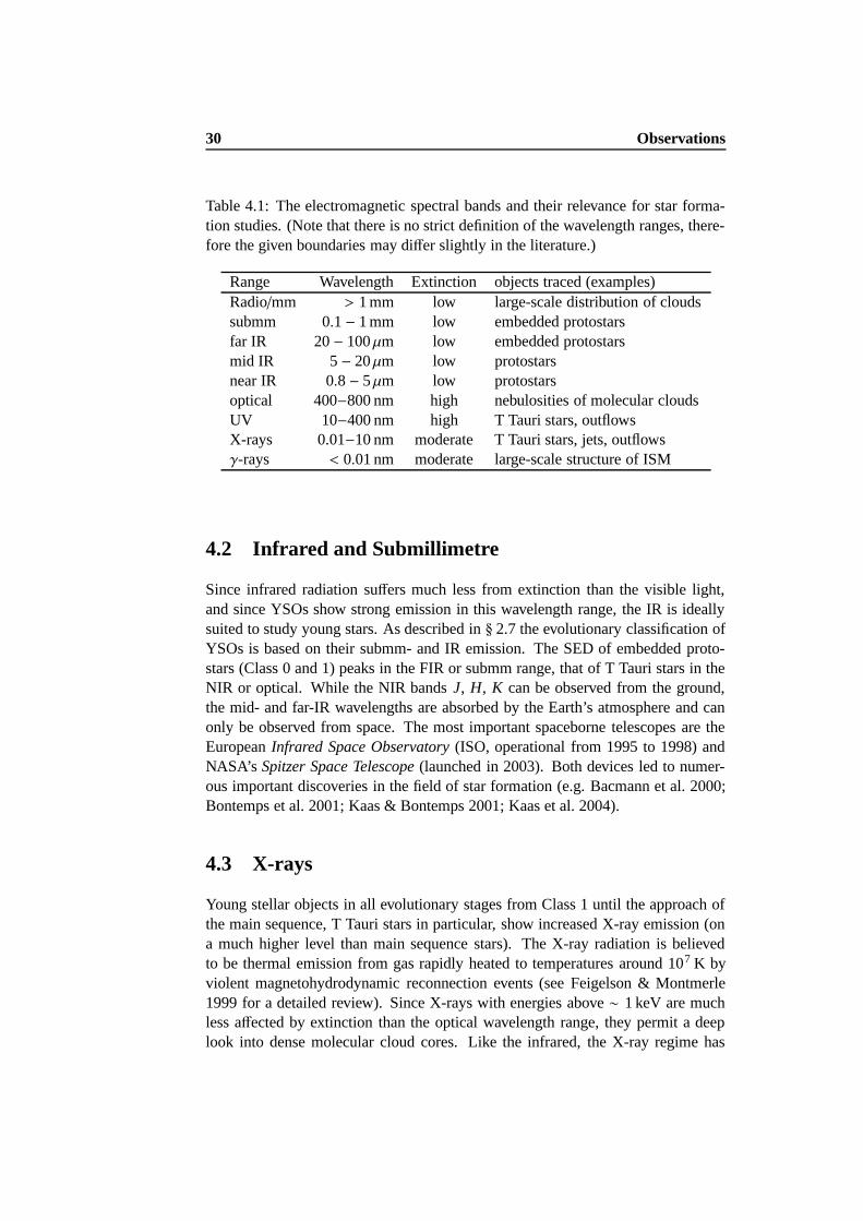
30 Observations
Table 4.1: The electromagnetic spectral bands and their relevance for star forma-tion studies. (Note that there is no strict definition of the wavelength ranges, there-fore the given boundaries may differ slightly in the literature.)
Range Wavelength Extinction objects traced (examples)Radio/mm > 1 mm low large-scale distribution of cloudssubmm 0.1 − 1 mm low embedded protostarsfar IR 20 − 100 µm low embedded protostarsmid IR 5 − 20 µm low protostarsnear IR 0.8 − 5 µm low protostarsoptical 400−800 nm high nebulosities of molecular cloudsUV 10−400 nm high T Tauri stars, outflowsX-rays 0.01−10 nm moderate T Tauri stars, jets, outflowsγ-rays < 0.01 nm moderate large-scale structure of ISM
4.2 Infrared and Submillimetre
Since infrared radiation suffers much less from extinction than the visible light,and since YSOs show strong emission in this wavelength range, the IR is ideallysuited to study young stars. As described in § 2.7 the evolutionary classification ofYSOs is based on their submm- and IR emission. The SED of embedded proto-stars (Class 0 and 1) peaks in the FIR or submm range, that of T Tauri stars in theNIR or optical. While the NIR bands J, H, K can be observed from the ground,the mid- and far-IR wavelengths are absorbed by the Earth’s atmosphere and canonly be observed from space. The most important spaceborne telescopes are theEuropean Infrared Space Observatory (ISO, operational from 1995 to 1998) andNASA’s Spitzer Space Telescope (launched in 2003). Both devices led to numer-ous important discoveries in the field of star formation (e.g. Bacmann et al. 2000;Bontemps et al. 2001; Kaas & Bontemps 2001; Kaas et al. 2004).
4.3 X-rays
Young stellar objects in all evolutionary stages from Class 1 until the approach ofthe main sequence, T Tauri stars in particular, show increased X-ray emission (ona much higher level than main sequence stars). The X-ray radiation is believedto be thermal emission from gas rapidly heated to temperatures around 107 K byviolent magnetohydrodynamic reconnection events (see Feigelson & Montmerle1999 for a detailed review). Since X-rays with energies above ∼ 1 keV are muchless affected by extinction than the optical wavelength range, they permit a deeplook into dense molecular cloud cores. Like the infrared, the X-ray regime has
4.4 Other Wavelengths 31
to be observed from outside the Earth’s atmosphere. The X-ray satellites ROSAT,XMM-Newton and Chandra have been frequently used to carry out surveys of starformation regions and have successfully discovered or confirmed a large numberof embedded YSOs (e.g. Neuhauser & Sterzik 1997; Preibisch 2003; Preibisch &Zinnecker 2002, 2004).
4.4 Other Wavelengths
The optical wavelength range suffers from strong dust extinction and is thereforeless suited for star formation studies. However, cold interstellar gas can be detectedby atomic hydrogen absorption lines in the visible, if the cloud is back-lit by a star.Pre-main sequence stars also radiate significantly in the optical, however, theiremission may be extincted by the molecular cloud.
T Tauri stars show a weak continuum and several strong emission lines in theultraviolet (UV). The observed continuum emission can be significantly strongerthan in comparable main sequence stars. This UV excess is stronger in CTTSs thanin WTTSs. The reason for the UV excess is not entirely clear, probably it is causedby several components, in particular the dissipation of gravitational energy at theboundary layer between the accretion disc and the star (see Gomez de Castro 1998for a review).
Gamma rays do not play an important role in the context of star formation.However, the radioactive isotope 26Al emitting γ-rays may be used to probe thelarge-scale distribution of the interstellar medium (Strong et al. 1982) and to es-timate the Galactic star formation rate (Diehl et al. 2006). Furthermore, γ-rayproduction from accelerators within star-formation regions (e.g. Wolf-Rayet starsor supernova remnants) is expected from theoretical models (Paul 2001).
4.5 Uncertainties and Caveats
Despite the advanced observational methods, the data used is far from being com-plete. Due to the high level of obscuration in star-forming regions and due tothe different techniques involved, uncertainties in the observations are almost un-avoidable: Samples of clusters may be incomplete and the cluster membership ofindividual objects questionable. The classification of YSOs may suffer from insuf-ficient data for the SED as well as from different classification criteria. To addressthis, Froebrich (2005) compiled a complete list of known Class 0 sources fromthe literature and used these data to determine the physical properties (Tbol, Lbol,Lsmm/Lbol, Menv) in order to provide a uniform classification.
For this work, different observational data from a large number of various lit-erature sources will be used. For the analysis and comparison of protostellar massaccretion rates (§ 5) and evolutionary tracks (§ 6) data of individual objects in vari-ous star-forming regions are used, whereas the investigation of YSO number ratios

32 Observations
and structures of young star clusters (§ 7 and 8, respectively) requires a sample ofentire YSO cluster contents as complete as possible.
Chapter 5
Protostellar Mass AccretionRates∗
Gravity, no escaping gravity...
– Placebo: Special K
Almost the entire mass of a star is accumulated during a relatively short phase (inClass 0 and 1 stage). Since the mass of a star is one of the most important pa-rameters, which determines many of its properties, it is essential to understand theprocess how a protostar gains its mass. In the so-called “standard theory” of starformation (Shu 1977; Shu et al. 1987) the mass accretion rate has a constant value.Observations, as well as more advanced models, however, indicate that protostel-lar mass accretion is a highly time-variant process. In this chapter the analysis ofprotostellar mass accretion rates is extended from a single case (Klessen 2001a)to the entire series of numerical models of turbulent molecular cloud fragmenta-tion that covers the entire spectrum of observed star-forming regions, ranging frominefficient and isolated star formation to the fast and efficient build-up of stellarclusters.
5.1 First Approximation
The entire process of molecular cloud collapse and build-up of the stellar clusterlasts several global free-fall times (τff = 105 yr). Likewise, the accretion processof a protostellar core takes place on a timescale of a few τff , comparable to mostother models of star formation.
A simple approximation of the accretion rate can be achieved by dividing thelocal Jeans mass by the local dynamical timescale:
M ≈ MJ/τff (5.1)
∗This chapter is based on Schmeja, S., & Klessen, R. S. 2004, A&A, 419, 405
33
34 Protostellar Mass Accretion Rates
By substituting
MJ =π5/2
6ρ−1/2
0
(
RTG
)3/2
=π5/2
6ρ−1/2
0 G−3/2c3s , (5.2)
where ρ0 denotes the initial density, T the temperature, cs the isothermal soundspeed, G the gravitational constant, and R the gas constant, and
τff =
√
3 π32 Gρ0
, (5.3)
Eq. (5.1) can be written as
M ≈ MJ
τff=
√
323π2
6
c3s
G= 5.4
c3s
G, (5.4)
depending only on the isothermal sound speed (or temperature). For a sound speedcs = 0.2 km s−1 we obtain M = 10−5 M yr−1. This is higher than the accretionrate for the collapse of a singular isothermal sphere: M = 0.975 c3
s /G (Shu 1977).However, the accretion rates in our models vary with time. Typical peak accretionrates are roughly in the range (3−50) c3
s /G or 5×10⁻⁶ to 10−4 M yr−1. The valuesexceed the approximated value MJ/τff due to external compression in the turbulentflow.
5.2 Determination of Mass Accretion Rates
In the protostellar phase of evolution, we determine accretion rates M by measur-ing the amount of mass as a function of time that falls into a control volume definedby each sink particle. Its radius is fixed to 280 AU. Infalling gas particles undergoseveral tests to check if they remain bound to the sink particle before they are con-sidered accreted (see e.g. Appendix A of Jappsen et al. 2005). As all gas particleshave the same mass and as accretion events occur at random times, the resultingaccretion rates are mass-binned and we smooth over a few consecutive accretionevents to get a meaningful description of the temporal evolution of M. We cannotresolve the evolution in the interior of the control volume. Because of angular mo-mentum conservation most of the matter that falls in will assemble in a protostellardisc. There it is transported inwards by viscous and possibly gravitational torques(Pringle 1981; Papaloizou & Lin 1995; see also Jappsen & Klessen 2004 for themodels discussed here). The latter will be provided by spiral density waves thatdevelop when the disc becomes too massive, which happens when mass is loadedonto the disc faster than it is removed by viscous transport. Altogether, the discwill not prevent or delay material from accreting onto the protostar for long. It actsas a buffer and smoothes eventual accretion spikes.
For the mass range considered here feedback effects are too weak to halt ordelay accretion (Wuchterl & Klessen 2001; Wuchterl & Tscharnuter 2003). With
5.3 Time-varying Mass Accretion Rates 35
typical disc sizes of the order of several hundred AU, the control volume thereforefully encloses both star and disc, and the measured core accretion rates are goodestimates of the actual stellar accretion rates. Deviations may be expected onlyif the protostellar core forms a binary star, where the infalling mass must then bedistributed over two stars, or if very high-angular momentum material is accreted,where a certain mass fraction may end up in a circumbinary disc and not accreteonto a star at all.
In the prestellar phase, i.e. before the central protostar forms, we determinethe accretion history by computing the change of mass inside the control volumecentered on the SPH particle that turns into a sink particle during the later evolution.Turbulent compression leads to mass growth, i.e. M > 0, while expansion willresult in mass loss and M < 0. Appreciable mass growth, however, is only achievedwhen gravity takes over and the region goes into collapse.
5.3 Time-varying Mass Accretion Rates
We analyse the full mass growth history of all protostellar cores in our modelsand we find that mass accretion rates from gravoturbulent fragmentation are highlytime-variable. Several examples of the accretion rate M are shown, plotted versustime (Fig. 5.1) and the ratio of accreted to final mass (Fig. 5.2), respectively. Themaximum accretion rate is reached rather rapidly and is then followed by a some-what slower decline. In some cases this decline is interrupted by one or more sec-ondary peaks. As shown above, the maximum accretion rate is significantly higherthan the constant rate predicted by the classical isothermal collapse model (plottedas dotted line in Fig. 5.1 and 5.2), but it falls below that value in later stages. Dueto the dynamical interaction and competition between protostellar cores, the massaccretion rates of cores in a dense cluster are different from those of isolated cores.In the first stage a core accretes local gas from its immediate vicinity. Once thelocal reservoir is depleted, the core may accrete fresh gas streaming in from furtheraway or by encounters with non-collapsed gas clumps (see discussion in Klessen& Burkert 2000). This results in secondary accretion peaks that are also visible inFig. 5.2, where one would expect a single bump in the case of an isolated core. Forexample, the central graph of Fig. 5.2 clearly shows that this particular protostaraccretes only about half of the final mass from its direct environment (first bump),while the rest comes from later accretion events.
The transition phase between Class 0 and Class 1 protostars is believed to takeplace when about half of the final mass has been accumulated (Andre et al. 2000).This time is indicated by the dashed line in Fig. 5.1. Typically it takes place duringor at the end of the peak accretion phase. It determines the lifetime of Class 0objects, which will be discussed below.
We define a mean accretion rate 〈M〉 by averaging M in the mass range 0.1 ≤M/Mend ≤ 0.8, with Mend being the final mass of the protostar. This phase typicallylasts only a few 104 years. This is short compared to the full accretion history. The

36 Protostellar Mass Accretion Rates
Figure 5.1: Mass accretion rates of nine randomly selected protostellar cores ofthree different models: M versus time for a Gaussian collapse (G2; upper row),a turbulent model driven on a large scale (M6k2a; middle row), and a turbulentmodel driven on a small scale (M6k8b; lower row). The thin line represents theactual simulation, the thick line the fit as described in the text. The deviation σ asgiven by Eq. (5.6) is indicated for each object. The dotted line shows the constantaccretion rate that would be expected from the classical Shu (1977) scenario. Thedashed line stands for the assumed transition from Class 0 to Class 1.
bulk of stellar material is therefore accumulated in the short time interval while thesystem is close to maximum accretion.
In Fig. 5.3, we plot the mean accretion rates versus final star mass Mend andversus time of core formation tform, respectively, for the same models as in Fig. 5.1.Not surprisingly, 〈M〉 increases with increasing stellar mass, and decreases whenthe core forms later, although this second correlation is not as clear. In other words,more massive stars have higher mass accretion rates and start to form first. Theycan grow large, because on average they form in the high-density regions of thecluster centre where they are able to maintain relatively high accretion rates over along time as more and more gas falls in from the cluster outskirts.
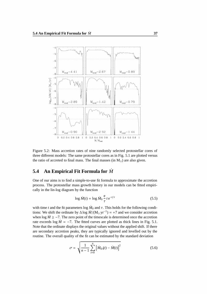
5.4 An Empirical Fit Formula for M 37
Figure 5.2: Mass accretion rates of nine randomly selected protostellar cores ofthree different models: The same protostellar cores as in Fig. 5.1 are plotted versusthe ratio of accreted to final mass. The final masses (in M) are also given.
5.4 An Empirical Fit Formula for M
One of our aims is to find a simple-to-use fit formula to approximate the accretionprocess. The protostellar mass growth history in our models can be fitted empiri-cally in the lin-log diagram by the function
log M(t) = log M0eτ
t e−t/τ (5.5)
with time t and the fit parameters log M0 and τ. This holds for the following condi-tions: We shift the ordinate by ∆ log M/(M yr−1) = +7 and we consider accretionwhen log M ≥ −7. The zero point of the timescale is determined once the accretionrate exceeds log M = −7. The fitted curves are plotted as thick lines in Fig. 5.1.Note that the ordinate displays the original values without the applied shift. If thereare secondary accretion peaks, they are typically ignored and levelled out by theroutine. The overall quality of the fit can be estimated by the standard deviation
σ =
√
√
1n − 1
n∑
t=0
[
Mfit(t) − M(t)]2
(5.6)
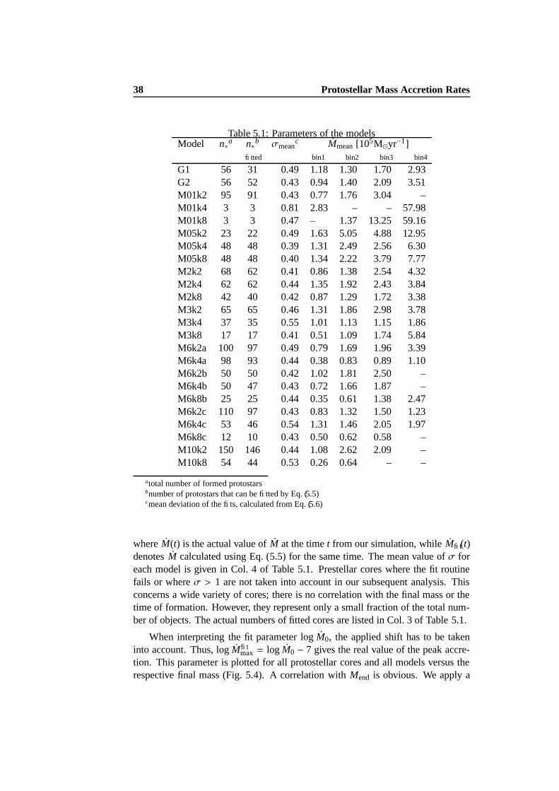
38 Protostellar Mass Accretion Rates
Table 5.1: Parameters of the modelsModel n∗a n∗b σmean
c Mmean [105Myr−1]fitted bin1 bin2 bin3 bin4
G1 56 31 0.49 1.18 1.30 1.70 2.93G2 56 52 0.43 0.94 1.40 2.09 3.51M01k2 95 91 0.43 0.77 1.76 3.04 –M01k4 3 3 0.81 2.83 – – 57.98M01k8 3 3 0.47 – 1.37 13.25 59.16M05k2 23 22 0.49 1.63 5.05 4.88 12.95M05k4 48 48 0.39 1.31 2.49 2.56 6.30M05k8 48 48 0.40 1.34 2.22 3.79 7.77M2k2 68 62 0.41 0.86 1.38 2.54 4.32M2k4 62 62 0.44 1.35 1.92 2.43 3.84M2k8 42 40 0.42 0.87 1.29 1.72 3.38M3k2 65 65 0.46 1.31 1.86 2.98 3.78M3k4 37 35 0.55 1.01 1.13 1.15 1.86M3k8 17 17 0.41 0.51 1.09 1.74 5.84M6k2a 100 97 0.49 0.79 1.69 1.96 3.39M6k4a 98 93 0.44 0.38 0.83 0.89 1.10M6k2b 50 50 0.42 1.02 1.81 2.50 –M6k4b 50 47 0.43 0.72 1.66 1.87 –M6k8b 25 25 0.44 0.35 0.61 1.38 2.47M6k2c 110 97 0.43 0.83 1.32 1.50 1.23M6k4c 53 46 0.54 1.31 1.46 2.05 1.97M6k8c 12 10 0.43 0.50 0.62 0.58 –M10k2 150 146 0.44 1.08 2.62 2.09 –M10k8 54 44 0.53 0.26 0.64 – –
atotal number of formed protostarsbnumber of protostars that can be fitted by Eq. (5.5)cmean deviation of the fits, calculated from Eq. (5.6)
where M(t) is the actual value of M at the time t from our simulation, while Mfit(t)denotes M calculated using Eq. (5.5) for the same time. The mean value of σ foreach model is given in Col. 4 of Table 5.1. Prestellar cores where the fit routinefails or where σ > 1 are not taken into account in our subsequent analysis. Thisconcerns a wide variety of cores; there is no correlation with the final mass or thetime of formation. However, they represent only a small fraction of the total num-ber of objects. The actual numbers of fitted cores are listed in Col. 3 of Table 5.1.
When interpreting the fit parameter log M0, the applied shift has to be takeninto account. Thus, log Mfit
max = log M0 − 7 gives the real value of the peak accre-tion. This parameter is plotted for all protostellar cores and all models versus therespective final mass (Fig. 5.4). A correlation with Mend is obvious. We apply a

5.5 Class 0 Lifetimes and the Influence of the Turbulent Medium 39
Figure 5.3: Mean accretion rates 〈M〉 versus final mass (upper panel) and versustime of core formation (lower panel) for the same models as in Fig. 5.1. The zeropoint of the timescale corresponds to the time when gravity is “switched on”. Notethe different timescales on which the formation of the cluster takes place.
linear fit in the log-log diagram, which is indicated by the straight line. The fittedpeak accretion rates show the same behaviour as the mean accretion rates 〈M〉.
The parameter τ indicates the time of the maximum of the accretion curve.It is plotted for all protostellar cores in Fig. 5.5. In almost all models τ shows acorrelation with the final mass. The parameter indicates how fast the gas falls inonto the core, therefore we expect it to be related to the local free-fall time and,thus, to the local density at the onset of collapse. It lies in the range 104
. τ .
105 yr, which is less than the global free-fall time τff . If we take an average value〈τ〉 ≈ τff/3, this suggests an initial overdensity of almost a factor of ten in thecollapsing regions.
5.5 Class 0 Lifetimes and the Influence of the TurbulentMedium
We calculate the transition times from Class 0 to Class 1, assumed as describedabove. This gives the duration of the Class 0 phase for each protostar; the valuesare plotted versus the corresponding final masses in Fig. 5.6. The duration of theClass 0 phase increases with increasing final mass. Thus, a massive star is markednot only by a higher peak accretion rate but also by a longer time spent in Class 0phase. A more sophisticated analysis of Class 0 lifetimes is presented in § 6.2.5.
The mean accretion rates 〈M〉 of all individual protostellar cores of one model
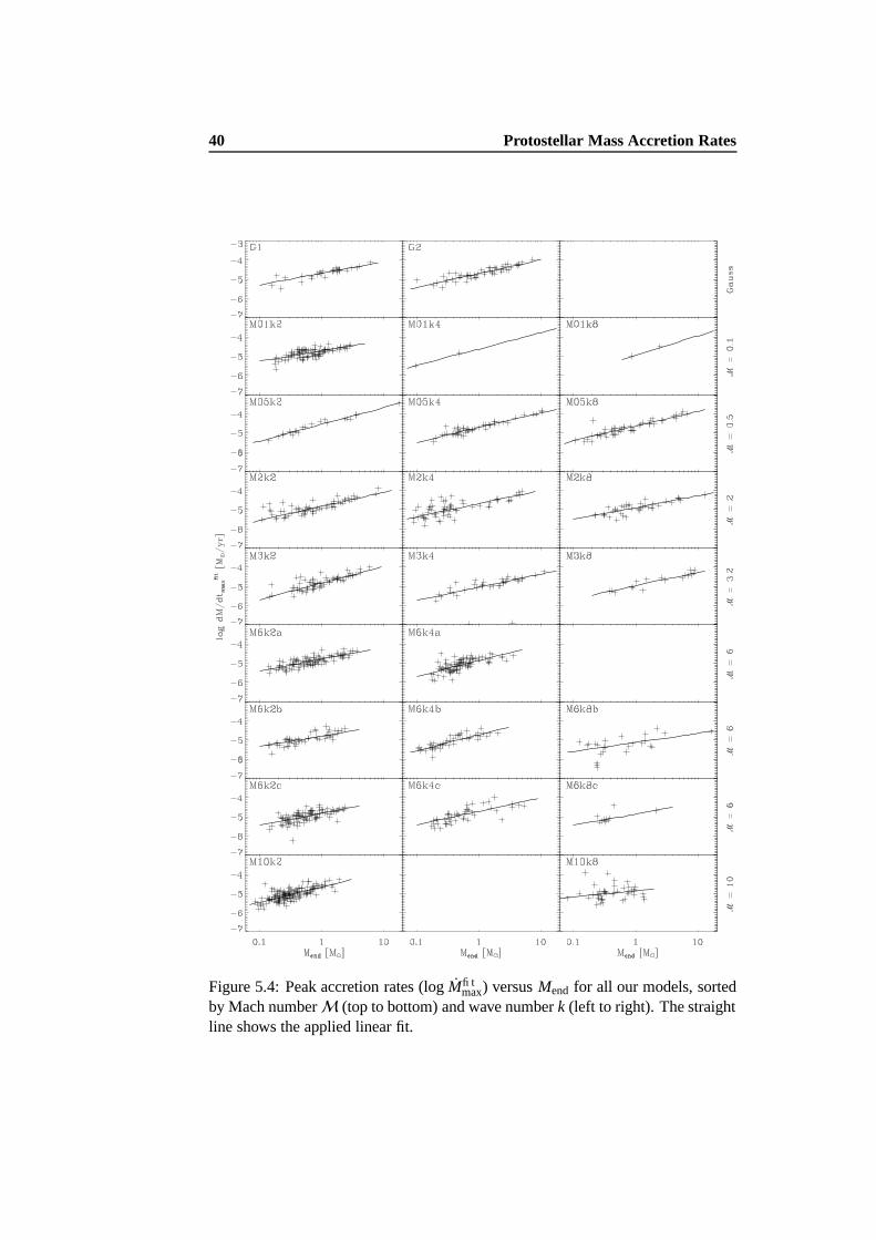
40 Protostellar Mass Accretion Rates
Figure 5.4: Peak accretion rates (log Mfitmax) versus Mend for all our models, sorted
by Mach numberM (top to bottom) and wave number k (left to right). The straightline shows the applied linear fit.
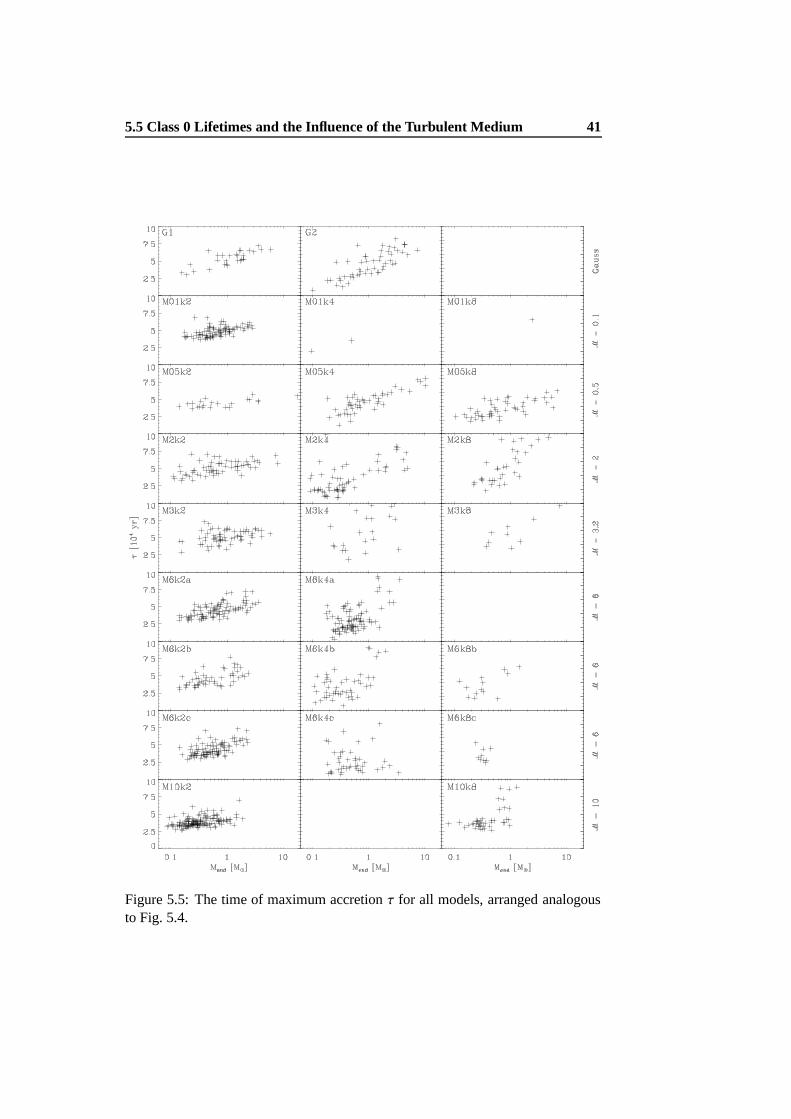
5.5 Class 0 Lifetimes and the Influence of the Turbulent Medium 41
Figure 5.5: The time of maximum accretion τ for all models, arranged analogousto Fig. 5.4.
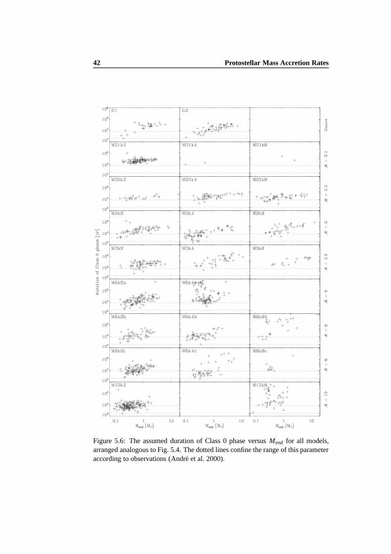
42 Protostellar Mass Accretion Rates
Figure 5.6: The assumed duration of Class 0 phase versus Mend for all models,arranged analogous to Fig. 5.4. The dotted lines confine the range of this parameteraccording to observations (Andre et al. 2000).
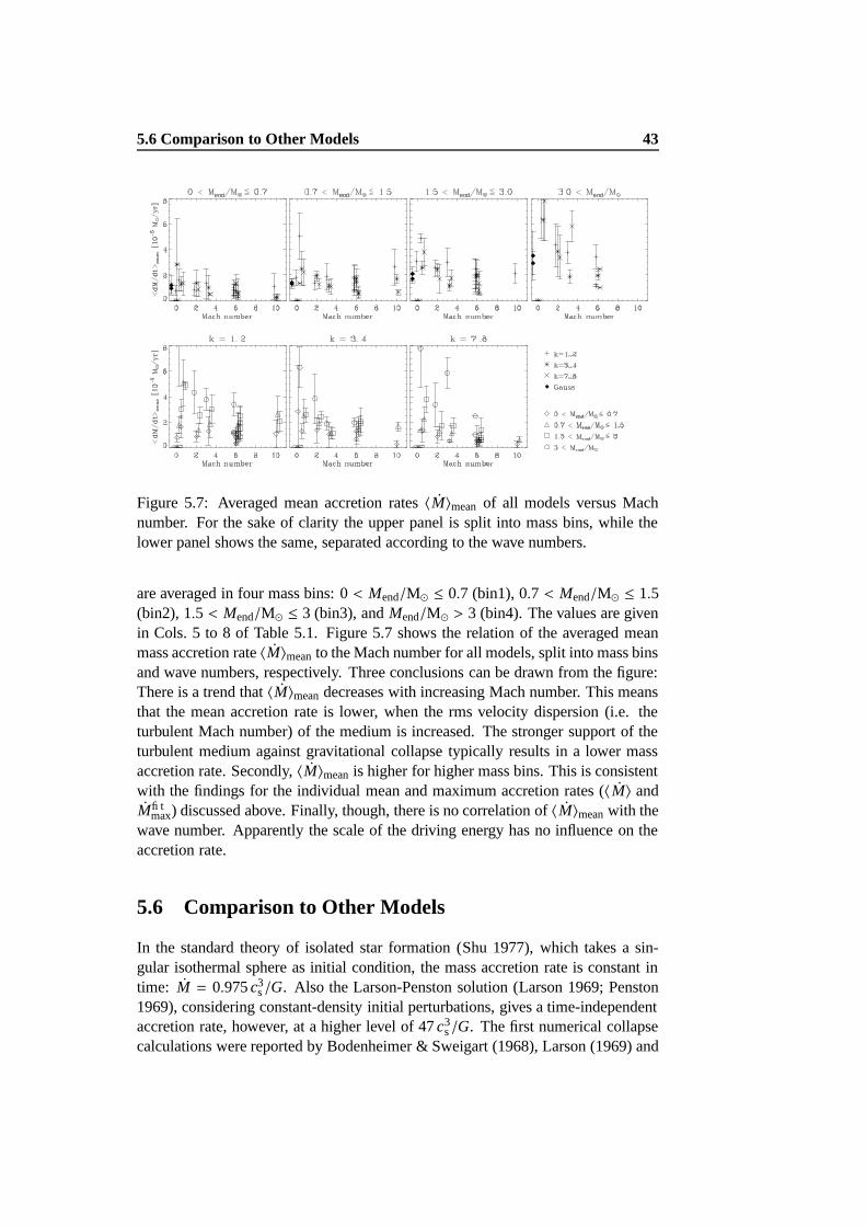
5.6 Comparison to Other Models 43
Figure 5.7: Averaged mean accretion rates 〈M〉mean of all models versus Machnumber. For the sake of clarity the upper panel is split into mass bins, while thelower panel shows the same, separated according to the wave numbers.
are averaged in four mass bins: 0 < Mend/M ≤ 0.7 (bin1), 0.7 < Mend/M ≤ 1.5(bin2), 1.5 < Mend/M ≤ 3 (bin3), and Mend/M > 3 (bin4). The values are givenin Cols. 5 to 8 of Table 5.1. Figure 5.7 shows the relation of the averaged meanmass accretion rate 〈M〉mean to the Mach number for all models, split into mass binsand wave numbers, respectively. Three conclusions can be drawn from the figure:There is a trend that 〈M〉mean decreases with increasing Mach number. This meansthat the mean accretion rate is lower, when the rms velocity dispersion (i.e. theturbulent Mach number) of the medium is increased. The stronger support of theturbulent medium against gravitational collapse typically results in a lower massaccretion rate. Secondly, 〈M〉mean is higher for higher mass bins. This is consistentwith the findings for the individual mean and maximum accretion rates (〈M〉 andMfit
max) discussed above. Finally, though, there is no correlation of 〈M〉mean with thewave number. Apparently the scale of the driving energy has no influence on theaccretion rate.
5.6 Comparison to Other Models
In the standard theory of isolated star formation (Shu 1977), which takes a sin-gular isothermal sphere as initial condition, the mass accretion rate is constant intime: M = 0.975 c3
s /G. Also the Larson-Penston solution (Larson 1969; Penston1969), considering constant-density initial perturbations, gives a time-independentaccretion rate, however, at a higher level of 47 c3
s /G. The first numerical collapsecalculations were reported by Bodenheimer & Sweigart (1968), Larson (1969) and
44 Protostellar Mass Accretion Rates
Hunter (1977). Models with more realistic initial density profiles generally pre-dict accretion rates that decline with time: The models of Hunter (1977; Mmax
≈ 36 c3s /G from numerical integrations of isothermal collapses), Foster & Cheva-
lier (1993; Mmax ≈ 47 c3s /G from numerical hydrodynamic simulations), Tomisaka
(1996; Mmax = (4 − 40) c3s /G from numerical MHD models), Basu (1997; Mmax =
13 c3s /G from a semi-analytical model), Ogino et al. (1999; Mmax ≈ (30−230) c3
s /Gfrom numerical hydrodynamic simulations), Masunaga & Inutsuka (2000; radia-tion hydrodynamic numerical codes), Whitworth & Ward-Thompson (2001) andMotoyama & Yoshida (2003; Mmax & 42 c3
s /G) predict mass accretion rates thatpeak shortly after the formation of the protostar and decrease with time. This showsbetter agreement with observational data than constant accretion rates (see § 5.7).Our results display the same behaviour and our values of Mmax ≈ (3 − 50) c3
s /Gcoincide quite well with those findings. In contrast, some models yield mass ac-cretion rates that increase with time (McLaughlin & Pudritz 1997; Bonnell et al.2001a; Behrend & Maeder 2001).
Theoretical models of star formation usually are scale-free. Thus, the resultsstrongly depend on the adopted physical scaling, e.g. the choice of the initial den-sity or temperature. The comparison of numerical values of accretion rates there-fore requires some care. Again, in most cases the maximum accretion rates scaleapproximately as a few times MJ/τff .
Whitworth & Ward-Thompson (2001) presented an analytical model for pro-tostellar collapse using a Plummer-like density profile as initial condition. Theysuccessfully modelled the prestellar core L1544 in good agreement with observa-tions. Their Mmax≈ 8.1 × 10⁻⁵ M yr−1 corresponds quite well to our Gaussiancollapse cases for the same stellar mass (G1, G2). However, the accretion historyof the collapsing Plummer sphere cannot be matched with our fit formula (5.5).The increase is steeper, while the decrease is slower compared to any of our mod-els. The slow decline might be due to the fact that Whitworth & Ward-Thompson(2001) use a non-truncated, infinite density profile, while our models have finitesizes. A similar model was used by Motoyama & Yoshida (2003) who examinedthe hypothesis that very high mass accretion rates exceeding 10−4 M yr−1 requireexternal triggering, as inferred from some observations. They find that the maxi-mum accretion rate is proportional to the momentum given to the cloud core in theirperturbed collapse model. A momentum of & 0.1 M km s−1 causes an accretionrate of & 10−4 M yr−1.
Smith (1998, 2000, 2002) presented a formula for the mass accretion rate witha sharp exponential rise and a power law decrease in time. This model providesan early peak in which M ≈ 10−4 M yr−1 for 104 years, and eventually becomingM ≈ 10−7 M yr−1 for 106 years. However, his formula (Eq. 6 in Smith 2000)applies to our models only when choosing parameters completely different to thosesuggested, otherwise his accretion curve has a more rapid increase but a slowerdecline than our models.
Bonnell et al. (2001a) analysed competitive accretion in embedded stellar clus-ters by means of SPH simulations. They find that accretion in a cluster is highly
5.6 Comparison to Other Models 45
non-uniform and that the accretion rate is higher for stars near the cluster centre.We do not see this in our results, likely because the protostars in our model are atdifferent stages of evolution at a certain time, so this effect, if existent, is coveredby the strongly time-dependent variation in the accretion rate. Also the evolutionof M with time in their models differs from our results: The mean accretion ratereported by Bonnell et al. (2001a), determined from all protostars in the cluster,increases with time until near the end of the simulation when the gas is signifi-cantly depleted. The difference is probably caused by the different assumptions(e.g. lack of turbulence, clustered potential). Indeed, the recent models of Bonnellet al. (2003) produce nearly constant accretion rates onto the most massive stars inthe cluster. The difference might be due to the fact that the accretion rates in thelatter models are determined by the accretion onto the cluster from outside, whilein the models of Bonnell et al. (2001a) all the mass was already in the cluster.
Reid et al. (2002) used a logatropic equation of state as the basis for their hy-drodynamical simulations of isolated star formation. Their accretion rate dependson the size of the core. It increases cubically and reaches maximum when the ex-pansion wave leaves the core, then it falls steadily. With the adopted scaling, Mmax
is one to two orders of magnitude smaller than in our models. Consequently thewhole accretion process lasts much longer, several 106 years, which is in contradic-tion to estimates of rapid star formation (Elmegreen 2000; Hartmann et al. 2001;Hartmann 2003; Mac Low & Klessen 2004).
The work of Reid et al. (2002) is extended by Sigalotti et al. (2002) performingcalculations of spherical gravitational collapse and accretion of nonsingular loga-tropes. In all their models the accretion rate rises steeply after the formation ofthe core, reaching its maximum when the protostar has accreted ∼40% of its finalmass, followed by a monotonic decrease. Peak values are ∼ 5 − 6 × 10⁻⁵ M yr−1
for cores close to the critical mass and one to two orders of magnitude lowerfor subcritical cores. At the transition from Class 0 to 1 the accretion rate is∼ 0.07−5.5×10⁻⁵ M yr−1, at the Class 1/2 border it is ∼ 0.02−1.4×10⁻⁶ M yr−1.Class 0 lifetimes are predicted as ∼ 0.1 − 1.6 × 10⁶ yr and Class 1 lifetimes as∼ 0.4 − 5 × 10⁶ yr. For Class 0 objects this is about an order of magnitude largerthan estimated from observations (Andre et al. 2000) and the same objections as tothe models of Reid et al. (2002) have to be raised.
Wuchterl & Tscharnuter (2003) find, from models based on radiation hydro-dynamics, time-varying accretion rates of a few 10−6 M yr−1 for the phase <0.8 Mend, which is about an order of magnitude lower than our values, especiallyfor Gaussian collapse or large-scale turbulence. The reason may be that protostellarcores in our models form by external compression before gravity takes over. Thisresults in enhanced accretion rates relative to cores that begin contraction close tohydrostatic equilibrium.
Hennebelle et al. (2003) performed numerical simulations where the collapseis triggered by a steady increase in the external pressure. Mmax is reached imme-diately after the formation of the central protostar (i.e. during the Class 0 phase),followed by a steady decrease of M to the Class 1 phase. The more rapid and
46 Protostellar Mass Accretion Rates
the more prolonged the increase in external pressure, the higher is Mmax, rangingfrom 6.5 × 10⁻⁶ M yr−1 to 2.6 × 10⁻⁵ M yr−1, corresponding to ∼ (4 − 16) c3
s /G.The qualitative behaviour of the accretion process does not differ much from ourmodels, but the peak accretion rates are slightly smaller than ours except in theirmodels with the most rapid compression.
Shu et al. (2004) discuss numerical simulations for a singular isothermal spherewith a uniform magnetic field. The maximum accretion rate of M ≈ 1.1 c3
s /G isclose to the unmagnetised SIS value of 0.975 (Shu 1977), but unlike the latter itdeclines steadily.
Table 5.2 summarises the mass accretion rates from all the models discussed.
5.7 Comparison to Observations
It is very difficult to measure mass accretion rates directly from observations (e.g.from inverse P Cygni profiles), instead they often have to be inferred indirectlybased on the SEDs of protostars or using outflow characteristics (Hartigan et al.1995; Bontemps et al. 1996). The correlation between accretion rates and outflowstrength, however, is still subject of strong debate (Wolf-Chase et al. 2003). ForClass 0 objects typical mass accretion rates are estimated in the range 10−5
.
M/M yr−1. 10−4 (Hartmann 1998; Narayanan et al. 1998; Andre et al. 1999;
Ceccarelli et al. 2000; Jayawardhana et al. 2001; Di Francesco et al. 2001; Maret etal. 2002; Beuther et al. 2002a,b). The growth rate of Class 1 objects is believed tobe about an order of magnitude smaller (Henriksen et al. 1997; Andre et al. 2000),with observational values between ∼ 10−7 and ∼ 5 × 10⁻⁶ M yr−1 (Brown &Chandler 1999; Greene & Lada 2002; Boogert et al. 2002; Yokogawa et al. 2003;Young et al. 2003).
Bontemps et al. (1996) studied the outflow activities in a sample of 45 low-massembedded young stellar objects. They estimate that the observed decline of COoutflow momentum fluxes with time results from a decrease of the mass accretionrate from ∼ 10−5 M yr−1 for the youngest Class 0 protostars to ∼ 10−7 M yr−1 forthe most evolved Class 1 objects. Furthermore, they propose a simple exponentialdependency of the accretion rate with time: M = (M0
env/τ)e−t/τ with initial mass
of the dense clump M0env and a characteristic time τ ≈ 9 × 10⁴ yr. This is com-
parable to our Eq. (5.5). A similar exponential equation is also used by Myers etal. (1998), while Henriksen et al. (1997) describe the accretion rate by an equationthat asymptotically approaches a power-law dependence at late times.
Brown & Chandler (1999), who determined an upper limit of M . (2 − 4) ×10−7 M yr−1 for two Class 1 protostars in Taurus, also conclude that the accre-tion rate is not constant in time and likely is much higher in the early phase. Onthe other hand, Hirano et al. (2003) observed a dozen of deeply embedded youngstellar objects of both Class 0 and 1 and derived the same mass accretion rates of(1 − 5) × 10−6 M yr−1 for all of them. Unlike other authors, they argue that thereis no significant difference in M between Class 0 and Class 1 sources. White &
5.8 Summary 47
Hillenbrand (2004) infer mass accretion rates of Class 1 protostars that are indis-tinguishable from Class 2 objects. They find a median accretion rate of Class 1 and2 objects of only 4×10⁻⁸ M yr−1, within a large range of two orders of magnitude.
Pre-main sequence stars (Class 2 and 3) have accretion rates still lower thanClass 1 (note, however, the contradicting findings of White & Hillenbrand 2004discussed above), they are estimated to be in the range . 10−7 M yr−1 (Muzerolleet al. 2003; Calvet et al. 2004; Furlan et al. 2005). Muzerolle et al. (2003) presenta study of accretion in a sample of 45 young, low-mass objects in a variety ofstar-forming regions and young associations, most of them classical T Tauri stars(i.e. Class 2). They estimate accretion rates in the range 10−12 M yr−1 < M <10−9 M yr−1. They also note a clear trend of decreasing accretion rate with stellarmass, with mean accretion rates declining by 3 to 4 orders of magnitude over 1 −0.05 M. For intermediate-mass T Tauri stars (1.5 − 4 M), Calvet et al. (2004)determine accretion rates between 4 × 10⁻⁹ and 3 × 10⁻⁷ M yr−1. In consistencywith Muzerolle et al. (2003) they find a clear correlation between mass accretionrate and stellar mass. Furlan et al. (2005) investigated a sample of CTTSs in theTaurus star-forming region. From the literature they compile mass accretion ratesin the range 3.5 × 10⁻¹⁰ M yr−1 < M < 6.8 × 10⁻⁸ M yr−1.
The values from observations given above are summarised in Table 5.3. Theycorrespond to the accretion rates derived for the models of gravoturbulent star for-mation discussed here. They also decrease from 10−5 to 10−4 M yr−1 during theClass 0 phase to less than 10−7 M yr−1 in later stages. However, the supposedtransition between Class 0 and Class 1 still takes place during the peak accretionphase. The accretion rates in our models typically do not decline significantly untilabout 80% of the final mass has been accreted (Fig. 5.1). This is unlike e.g. themodel of Reid et al. (2002), where M begins to fall off when about half of the massof the core has been accreted. Given the uncertainties of the mass estimate for theClass 0/1 transition we do not consider this a large discrepancy.
According to observations, Class 0 objects have an estimated lifetime of ∼(1− 3)× 104 yr (Andre et al. 2000). In our models this parameter is widely spread,ranging from ∼ 104 to > 105 yr, but for a 1 M star it lies roughly in the rangededuced from observations (see Fig. 5.6). A more sophisticated analysis of Class 0lifetimes is presented in § 6.2.5.
5.8 Summary
We have studied protostellar mass accretion rates from numerical models of starformation based on gravoturbulent fragmentation. Twenty-four models coveringa wide range of environmental conditions from low to high turbulent velocitiesand different driving scales have been investigated. Our main results may be sum-marised as follows:
1. An order-of-magnitude estimate for mass accretion rates resulting from gravo-turbulent fragmentation is given by M ≈ MJ/τff with MJ being the mean
48 Protostellar Mass Accretion Rates
thermal Jeans mass and τff the corresponding free-fall time.
2. However, protostellar mass accretion is a highly time-variant process. It canbe approximated by the empirical function log M(t) = log M0 (e/τ) t e−t/τ.The peak accretion rate is reached during the Class 0 stage, shortly afterthe formation of the core; its value ranges between about 5 × 10⁻⁶ and10−4 M yr−1. The maximum accretion rate is approximately one order ofmagnitude higher than the constant rate predicted by the collapse of a clas-sical singular isothermal sphere.
3. Around the peak accretion phase the mass accretion rates are roughly con-stant. The mean accretion rates increase with increasing final mass. Moremassive stars have higher mass accretion rates and tend to form first.
4. The same applies to the fitted peak accretion rates, which are also propor-tional to the final stellar mass.
5. There is a similar correlation between the duration of Class 0 phase (assum-ing that half of the final mass is accreted in this phase) and the final mass.
6. 〈M〉mean decreases with increasing Mach number of the turbulent environ-ment, but is not correlated with the driving wave number.
Our results agree well with many other models treating the time evolution of themass accretion process and the value of the peak accretion rate. In particular, theaccretion rates from our models show an exponential decline, as also proposed byBontemps et al. (1996), Myers et al. (1998) and Smith (1998, 2000). They alsomatch observational findings like the supposed decline of the mass accretion ratefrom the Class 0 to Class 1 phase. We conclude that a theory of star formation basedon gravoturbulent fragmentation of molecular clouds is an adequate approach todescribe stellar birth in the Milky Way.

5.8Sum
mary
49
Table 5.2: Protostellar mass accretion rates from models
Reference Form of accretion curve Mmax Mmax
[c3s /G] [10−5 Myr−1]
Shu 1977 constant 0.975 0.16Larson 1969/Penston 1969 constant 47 8.9Hunter 1977 steady decrease 36 5.9Foster & Chevalier 1993 peak, sharp decrease 47 7.6Tomisaka 1996 exponential decline 40 6.5Basu 1997 declining 13 2.5McLaughlin & Pudritz 1997 increasing with timeOgino 1999 declining 30 - 230 5 - 37Smith 1998, 2000, 2002 sharp exp. rise, power-law decline 3.2Masunaga & Inutsuka 2000 declining 1.3Whitworth & Ward-Thompson 2001 sharp increase, exponential decline 8Bonnell et al. 2001a increases with timeReid et al. 2002 sharp increase, slower decline 0.1 - 0.3Sigalotti et al. 2002 sharp increase, slower decline 0.1 - 5Wuchterl & Tscharnuter 2003 time-varying & 0.1Motoyama & Yoshida 2003 sharp increase, exponential decline & 10Hennebelle et al. 2003 increase, slower decline 0.65 - 2.6Shu et al. 2004 steady decline 1.1this work sharp peak, exponential decline 3 - 50 0.5 - 10
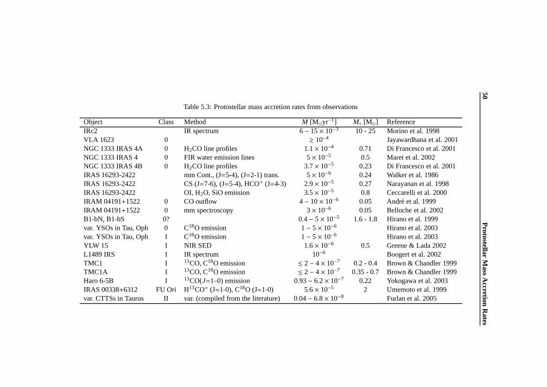
50P
rotostellarM
assA
ccretionR
ates
Table 5.3: Protostellar mass accretion rates from observations
Object Class Method M [Myr−1] M∗ [M] ReferenceIRc2 IR spectrum 6 − 15 × 10−3 10 - 25 Morino et al. 1998VLA 1623 0 & 10−4 Jayawardhana et al. 2001NGC 1333 IRAS 4A 0 H2CO line profiles 1.1 × 10⁻⁴ 0.71 Di Francesco et al. 2001NGC 1333 IRAS 4 0 FIR water emission lines 5 × 10⁻⁵ 0.5 Maret et al. 2002NGC 1333 IRAS 4B 0 H2CO line profiles 3.7 × 10⁻⁵ 0.23 Di Francesco et al. 2001IRAS 16293-2422 mm Cont., (J=5-4), (J=2-1) trans. 5 × 10⁻⁶ 0.24 Walker et al. 1986IRAS 16293-2422 CS (J=7-6), (J=5-4), HCO+ (J=4-3) 2.9 × 10⁻⁵ 0.27 Narayanan et al. 1998IRAS 16293-2422 OI, H2O, SiO emission 3.5 × 10⁻⁵ 0.8 Ceccarelli et al. 2000IRAM 04191+1522 0 CO outflow 4 − 10 × 10−6 0.05 Andre et al. 1999IRAM 04191+1522 0 mm spectroscopy 3 × 10⁻⁶ 0.05 Belloche et al. 2002B1-bN, B1-bS 0? 0.4 − 5 × 10⁻⁵ 1.6 - 1.8 Hirano et al. 1999var. YSOs in Tau, Oph 0 C18O emission 1 − 5 × 10⁻⁶ Hirano et al. 2003var. YSOs in Tau, Oph I C18O emission 1 − 5 × 10⁻⁶ Hirano et al. 2003YLW 15 I NIR SED 1.6 × 10⁻⁶ 0.5 Greene & Lada 2002L1489 IRS I IR spectrum 10−6 Boogert et al. 2002TMC1 I 13CO, C18O emission . 2 − 4 × 10⁻⁷ 0.2 - 0.4 Brown & Chandler 1999TMC1A I 13CO, C18O emission . 2 − 4 × 10⁻⁷ 0.35 - 0.7 Brown & Chandler 1999Haro 6-5B I 13CO(J=1–0) emission 0.93 − 6.2 × 10⁻⁷ 0.22 Yokogawa et al. 2003IRAS 00338+6312 FU Ori H13CO+ (J=1-0), C18O (J=1-0) 5.6 × 10⁻⁵ 2 Umemoto et al. 1999var. CTTSs in Taurus II var. (compiled from the literature) 0.04 − 6.8 × 10⁻⁸ Furlan et al. 2005
Chapter 6
Evolutionary Tracks of Class 0Protostars∗
As discussed in the previous chapter, observational protostellar mass accretionrates are usually not measured directly, but have to be inferred by indirect meth-ods, resulting in large uncertainties. So a direct comparison of the mass accretionrates obtained from the simulations to those from observations is not reasonable.Hence, it is desirable to convert the mass accretion rates from the simulations toeasier observable quantities. The main three are the bolometric temperature1 andluminosity, Tbol and Lbol, and the envelope mass, Menv.
Several such conversion schemes have been developed. Evolutionary modelswere first discussed by Bontemps et al. (1996) and Saraceno et al. (1996). Alongthese lines, Andre et al. (2000) took an exponential decline in both envelope massand accretion rate to predict Lbol-Menv tracks. An analytical scheme was presentedby Myers et al. (1998). They assumed a mass infall rate matching the Shu (1977)solution at early times and then displaying an exponential fall off with time. Thecore which supplies the mass also provides the obscuration, thus fixing evolution-ary tracks on a Tbol-Lbol diagram. Based on this work, Smith (1998, 2000, 2002)presented an evolutionary scheme but adopted alternative analytical forms for themass accretion (exponential increase and power law decrease) which resemble theresults obtained by Whitworth & Ward-Thompson (2001) or this work. This evolu-tionary model, founded on mass transfer between the envelope, disc, protostar andjets, has provided successful interpretations for various sets of observational data(Tbol, Lbol, Menv, outflow luminosity) of Class 0 and Class 1 objects (e.g. Davis etal. 1998; Yu et al. 2000; Stanke 2000; Froebrich et al. 2003). Here, we adopt theSmith (1998, 2000, 2002) scheme but replace the analytical accretion rates withthose derived numerically.
∗This chapter is based on a collaboration led by Dirk Froebrich, published as Froebrich, D.,Schmeja, S., Smith, M. D., & Klessen, R. S., 2006, MNRAS, 368, 435
1The bolometric temperature, introduced by Myers & Ladd (1993), is the temperature of a black-body having the same mean frequency as the observed continuum spectrum.
51
52 Evolutionary Tracks of Class 0 Protostars
The ‘recipe’ how to achieve the comparison can be summarised as follows: (1)Define the parameters of the evolutionary scheme from observations and vary themwithin a reasonable range; (2) Feed the mass accretion rates from the numericalsimulations into the evolutionary scheme; (3) calculate the evolutionary tracks;and (4) compare the resulting tracks with the distribution of the observational databy a three-dimensional Kolmogorov-Smirnov test.
6.1 Observations and Models
6.1.1 Observational Data
We require a statistically significant observational sample of protostars with accu-rate individual properties. The latter demands a uniform observational coverage ofthe entire SED from the NIR to the millimetre range. Several samples of Class 0sources have been published (e.g. Chen et al. 1995; Andre et al. 2000; Shirley et al.2000; Motte & Andre 2001). The latest study, which combines all previous onesand computes the object properties uniformly from all published data, is presentedby Froebrich (2005). There, a list of 95 confirmed or candidate objects was com-piled. Fifty of these sources possess sufficient observational data to be classified asClass 0 or Class 0/1 objects and allow us to determine the three source propertiesTbol, Lbol, and Menv accurately. To ensure a reliable comparison of models andobservations, we apply the following restrictions to this sample:
(1) We omit sources that have distances larger than 500 pc. This reduces thebias towards higher mass objects.
(2) All objects in Taurus are underluminous compared to the other sources,considering Tbol and Menv. Note that this does not only mean a low luminosityof these objects, but rather a low luminosity combined with high envelope mass.The three very low luminosity objects in our sample (see Fig. 6.1) combine lowluminosity (1 L) with low envelope mass (0.2 M) and might form (very) low-mass stars. In total, 25% of the Class 0 objects in the sample are underluminous.We exclude them for the comparison between the models and observations (but seethe discussion in Sect. 6.2.6).
(3) A histogram of the number of sources in a certain Tbol-bin shows that theobservational sample is very incomplete at high bolometric temperatures. Hencethe comparison of observations and models is restricted to Tbol < 80 K.
These selections leave us with a sample of 27 Class 0 sources. This sampleconsists mostly of objects in Perseus, Orion and Serpens.
6.1.2 Adaptation of the Models
The mass accretion rates of the gravoturbulent models (hereafter gt-models) dis-cussed in the previous chapter will be used as an input for the evolutionary scheme.Small number statistics will always be a major concern when comparing models
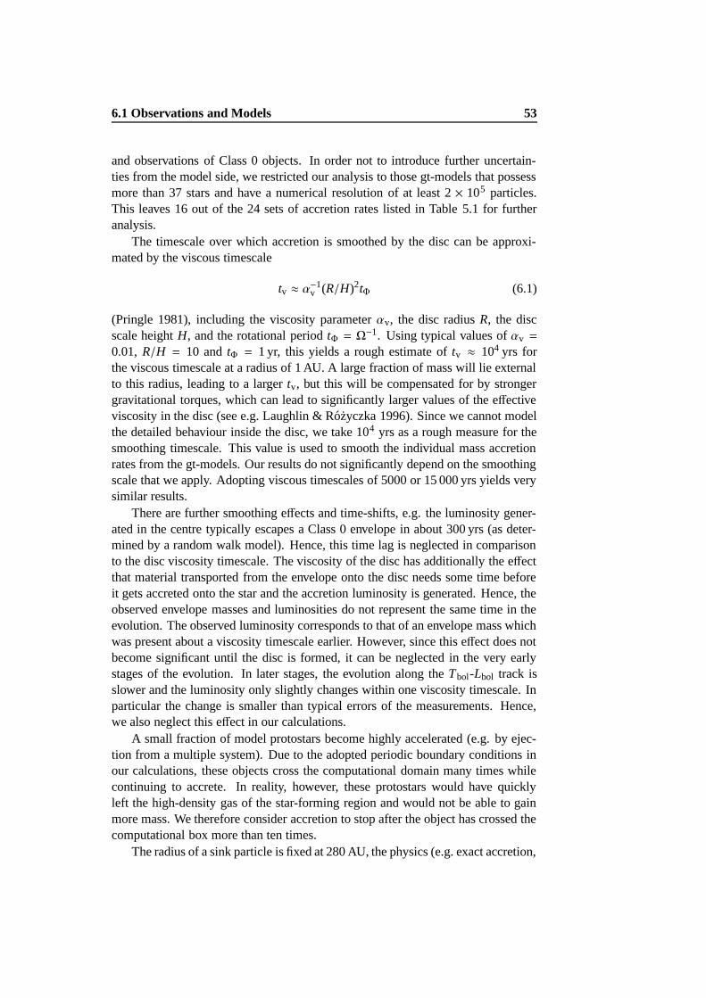
6.1 Observations and Models 53
and observations of Class 0 objects. In order not to introduce further uncertain-ties from the model side, we restricted our analysis to those gt-models that possessmore than 37 stars and have a numerical resolution of at least 2 × 10⁵ particles.This leaves 16 out of the 24 sets of accretion rates listed in Table 5.1 for furtheranalysis.
The timescale over which accretion is smoothed by the disc can be approxi-mated by the viscous timescale
tv ≈ α−1v (R/H)2tΦ (6.1)
(Pringle 1981), including the viscosity parameter αv, the disc radius R, the discscale height H, and the rotational period tΦ = Ω−1. Using typical values of αv =
0.01, R/H = 10 and tΦ = 1 yr, this yields a rough estimate of tv ≈ 104 yrs forthe viscous timescale at a radius of 1 AU. A large fraction of mass will lie externalto this radius, leading to a larger tv, but this will be compensated for by strongergravitational torques, which can lead to significantly larger values of the effectiveviscosity in the disc (see e.g. Laughlin & Rozyczka 1996). Since we cannot modelthe detailed behaviour inside the disc, we take 104 yrs as a rough measure for thesmoothing timescale. This value is used to smooth the individual mass accretionrates from the gt-models. Our results do not significantly depend on the smoothingscale that we apply. Adopting viscous timescales of 5000 or 15 000 yrs yields verysimilar results.
There are further smoothing effects and time-shifts, e.g. the luminosity gener-ated in the centre typically escapes a Class 0 envelope in about 300 yrs (as deter-mined by a random walk model). Hence, this time lag is neglected in comparisonto the disc viscosity timescale. The viscosity of the disc has additionally the effectthat material transported from the envelope onto the disc needs some time beforeit gets accreted onto the star and the accretion luminosity is generated. Hence, theobserved envelope masses and luminosities do not represent the same time in theevolution. The observed luminosity corresponds to that of an envelope mass whichwas present about a viscosity timescale earlier. However, since this effect does notbecome significant until the disc is formed, it can be neglected in the very earlystages of the evolution. In later stages, the evolution along the Tbol-Lbol track isslower and the luminosity only slightly changes within one viscosity timescale. Inparticular the change is smaller than typical errors of the measurements. Hence,we also neglect this effect in our calculations.
A small fraction of model protostars become highly accelerated (e.g. by ejec-tion from a multiple system). Due to the adopted periodic boundary conditions inour calculations, these objects cross the computational domain many times whilecontinuing to accrete. In reality, however, these protostars would have quicklyleft the high-density gas of the star-forming region and would not be able to gainmore mass. We therefore consider accretion to stop after the object has crossed thecomputational box more than ten times.
The radius of a sink particle is fixed at 280 AU, the physics (e.g. exact accretion,
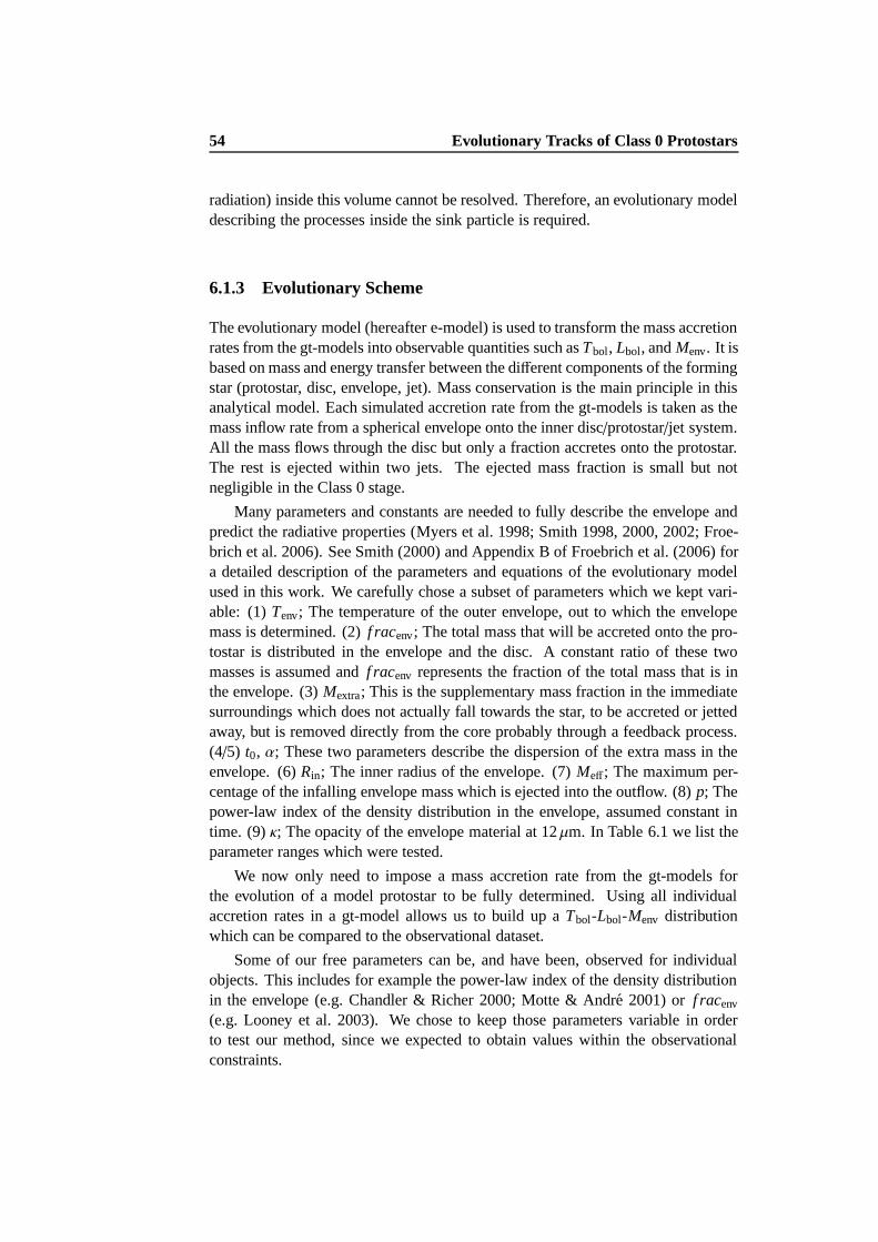
54 Evolutionary Tracks of Class 0 Protostars
radiation) inside this volume cannot be resolved. Therefore, an evolutionary modeldescribing the processes inside the sink particle is required.
6.1.3 Evolutionary Scheme
The evolutionary model (hereafter e-model) is used to transform the mass accretionrates from the gt-models into observable quantities such as Tbol, Lbol, and Menv. It isbased on mass and energy transfer between the different components of the formingstar (protostar, disc, envelope, jet). Mass conservation is the main principle in thisanalytical model. Each simulated accretion rate from the gt-models is taken as themass inflow rate from a spherical envelope onto the inner disc/protostar/jet system.All the mass flows through the disc but only a fraction accretes onto the protostar.The rest is ejected within two jets. The ejected mass fraction is small but notnegligible in the Class 0 stage.
Many parameters and constants are needed to fully describe the envelope andpredict the radiative properties (Myers et al. 1998; Smith 1998, 2000, 2002; Froe-brich et al. 2006). See Smith (2000) and Appendix B of Froebrich et al. (2006) fora detailed description of the parameters and equations of the evolutionary modelused in this work. We carefully chose a subset of parameters which we kept vari-able: (1) Tenv; The temperature of the outer envelope, out to which the envelopemass is determined. (2) f racenv; The total mass that will be accreted onto the pro-tostar is distributed in the envelope and the disc. A constant ratio of these twomasses is assumed and f racenv represents the fraction of the total mass that is inthe envelope. (3) Mextra; This is the supplementary mass fraction in the immediatesurroundings which does not actually fall towards the star, to be accreted or jettedaway, but is removed directly from the core probably through a feedback process.(4/5) t0, α; These two parameters describe the dispersion of the extra mass in theenvelope. (6) Rin; The inner radius of the envelope. (7) Meff; The maximum per-centage of the infalling envelope mass which is ejected into the outflow. (8) p; Thepower-law index of the density distribution in the envelope, assumed constant intime. (9) κ; The opacity of the envelope material at 12 µm. In Table 6.1 we list theparameter ranges which were tested.
We now only need to impose a mass accretion rate from the gt-models forthe evolution of a model protostar to be fully determined. Using all individualaccretion rates in a gt-model allows us to build up a Tbol-Lbol-Menv distributionwhich can be compared to the observational dataset.
Some of our free parameters can be, and have been, observed for individualobjects. This includes for example the power-law index of the density distributionin the envelope (e.g. Chandler & Richer 2000; Motte & Andre 2001) or f racenv
(e.g. Looney et al. 2003). We chose to keep those parameters variable in orderto test our method, since we expected to obtain values within the observationalconstraints.
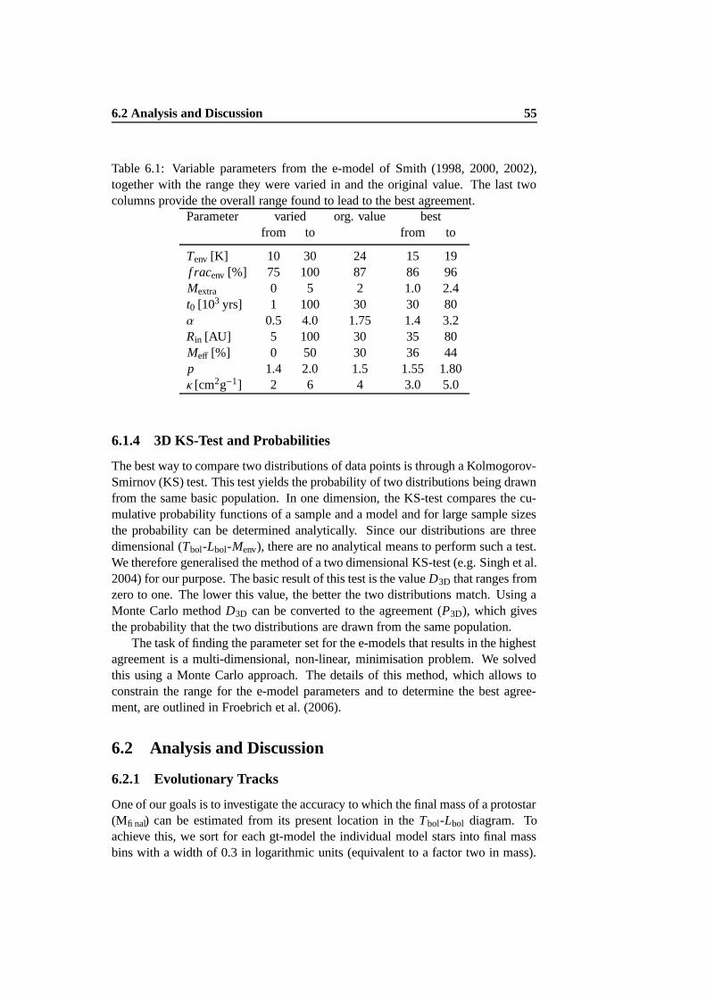
6.2 Analysis and Discussion 55
Table 6.1: Variable parameters from the e-model of Smith (1998, 2000, 2002),together with the range they were varied in and the original value. The last twocolumns provide the overall range found to lead to the best agreement.
Parameter varied org. value bestfrom to from to
Tenv [K] 10 30 24 15 19f racenv [%] 75 100 87 86 96Mextra 0 5 2 1.0 2.4t0 [103 yrs] 1 100 30 30 80α 0.5 4.0 1.75 1.4 3.2Rin [AU] 5 100 30 35 80Meff [%] 0 50 30 36 44p 1.4 2.0 1.5 1.55 1.80κ [cm2g−1] 2 6 4 3.0 5.0
6.1.4 3D KS-Test and Probabilities
The best way to compare two distributions of data points is through a Kolmogorov-Smirnov (KS) test. This test yields the probability of two distributions being drawnfrom the same basic population. In one dimension, the KS-test compares the cu-mulative probability functions of a sample and a model and for large sample sizesthe probability can be determined analytically. Since our distributions are threedimensional (Tbol-Lbol-Menv), there are no analytical means to perform such a test.We therefore generalised the method of a two dimensional KS-test (e.g. Singh et al.2004) for our purpose. The basic result of this test is the value D3D that ranges fromzero to one. The lower this value, the better the two distributions match. Using aMonte Carlo method D3D can be converted to the agreement (P3D), which givesthe probability that the two distributions are drawn from the same population.
The task of finding the parameter set for the e-models that results in the highestagreement is a multi-dimensional, non-linear, minimisation problem. We solvedthis using a Monte Carlo approach. The details of this method, which allows toconstrain the range for the e-model parameters and to determine the best agree-ment, are outlined in Froebrich et al. (2006).
6.2 Analysis and Discussion
6.2.1 Evolutionary Tracks
One of our goals is to investigate the accuracy to which the final mass of a protostar(Mfinal) can be estimated from its present location in the Tbol-Lbol diagram. Toachieve this, we sort for each gt-model the individual model stars into final massbins with a width of 0.3 in logarithmic units (equivalent to a factor two in mass).
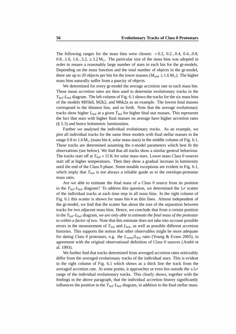
56 Evolutionary Tracks of Class 0 Protostars
The following ranges for the mass bins were chosen: < 0.2, 0.2...0.4, 0.4...0.8,0.8...1.6, 1.6...3.2, ≥ 3.2 M. The particular size of the mass bins was adopted inorder to ensure a reasonably large number of stars in each bin for the gt-models.Depending on the mass function and the total number of objects in the gt-model,there are up to 20 objects per bin for the lower masses (Mend ≤ 1.6 M). The highermass bins naturally suffer from a paucity of objects.
We determined for every gt-model the average accretion rate in each mass bin.These mean accretion rates are then used to determine evolutionary tracks in theTbol-Lbol diagram. The left column of Fig. 6.1 shows the tracks for the six mass binsof the models M05k8, M2k2, and M6k2a as an example. The lowest final massescorrespond to the thinnest line, and so forth. Note that the average evolutionarytracks show higher Lbol at a given Tbol for higher final star masses. This representsthe fact that stars with higher final masses on average have higher accretion rates(§ 5.3) and hence bolometric luminosities.
Further we analysed the individual evolutionary tracks. As an example, weplot all individual tracks for the same three models with final stellar masses in therange 0.8 to 1.6 M (mass bin 4, solar mass stars) in the middle column of Fig. 6.1.These tracks are determined assuming the e-model parameters which best fit theobservations (see below). We find that all tracks show a similar general behaviour.The tracks start off at Tbol ≈ 15 K for solar mass stars. Lower mass Class 0 sourcesstart off at higher temperatures. Then they show a gradual increase in luminosityuntil the end of the Class 0 phase. Some notable exceptions are evident in Fig. 6.1,which imply that Tbol is not always a reliable guide as to the envelope-protostarmass ratio.
Are we able to estimate the final mass of a Class 0 source from its positionin the Tbol-Lbol diagram? To address this question, we determined the 1σ scatterof the individual tracks at each time step in all mass bins. In the right column ofFig. 6.1 this scatter is shown for mass bin 4 as thin lines. Almost independent ofthe gt-model, we find that the scatter has about the size of the separation betweentracks for two adjacent mass bins. Hence, we conclude that from a certain positionin the Tbol-Lbol diagram, we are only able to estimate the final mass of the protostarto within a factor of two. Note that this estimate does not take into account possibleerrors in the measurement of Tbol and Lbol, as well as possible different accretionhistories. This supports the notion that other observables might be more adequatefor dating Class 0 protostars, e.g. the Lsmm/Lbol ratio (Young & Evans 2005), inagreement with the original observational definition of Class 0 sources (Andre etal. 1993).
We further find that tracks determined from averaged accretion rates noticeablydiffer from the averaged evolutionary tracks of the individual stars. This is evidentin the right column of Fig. 6.1 which shows as a thick line the track from theaveraged accretion rate. At some points, it approaches or even lies outside the ±1σrange of the individual evolutionary tracks. This clearly shows, together with thefindings in the above paragraph, that the individual accretion history significantlyinfluences the position in the Tbol-Lbol diagram, in addition to the final stellar mass.
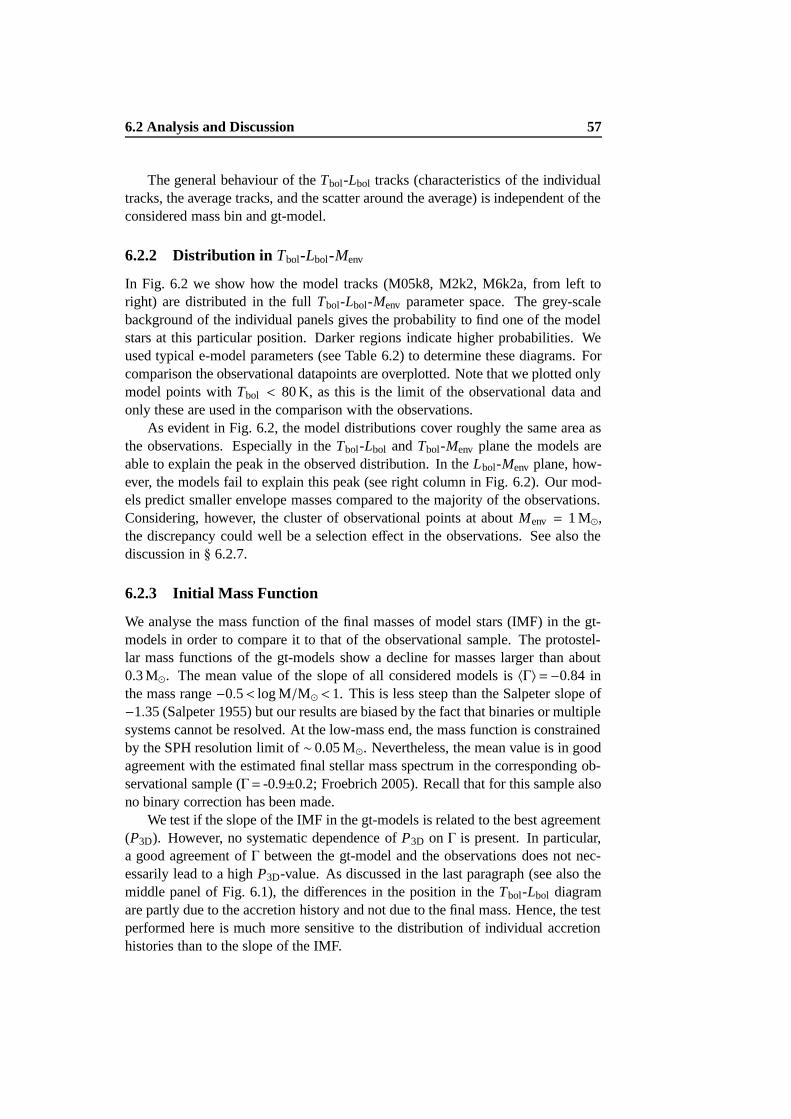
6.2 Analysis and Discussion 57
The general behaviour of the Tbol-Lbol tracks (characteristics of the individualtracks, the average tracks, and the scatter around the average) is independent of theconsidered mass bin and gt-model.
6.2.2 Distribution in Tbol-Lbol-Menv
In Fig. 6.2 we show how the model tracks (M05k8, M2k2, M6k2a, from left toright) are distributed in the full Tbol-Lbol-Menv parameter space. The grey-scalebackground of the individual panels gives the probability to find one of the modelstars at this particular position. Darker regions indicate higher probabilities. Weused typical e-model parameters (see Table 6.2) to determine these diagrams. Forcomparison the observational datapoints are overplotted. Note that we plotted onlymodel points with Tbol < 80 K, as this is the limit of the observational data andonly these are used in the comparison with the observations.
As evident in Fig. 6.2, the model distributions cover roughly the same area asthe observations. Especially in the Tbol-Lbol and Tbol-Menv plane the models areable to explain the peak in the observed distribution. In the Lbol-Menv plane, how-ever, the models fail to explain this peak (see right column in Fig. 6.2). Our mod-els predict smaller envelope masses compared to the majority of the observations.Considering, however, the cluster of observational points at about Menv = 1 M,the discrepancy could well be a selection effect in the observations. See also thediscussion in § 6.2.7.
6.2.3 Initial Mass Function
We analyse the mass function of the final masses of model stars (IMF) in the gt-models in order to compare it to that of the observational sample. The protostel-lar mass functions of the gt-models show a decline for masses larger than about0.3 M. The mean value of the slope of all considered models is 〈Γ〉=−0.84 inthe mass range −0.5< log M/M < 1. This is less steep than the Salpeter slope of−1.35 (Salpeter 1955) but our results are biased by the fact that binaries or multiplesystems cannot be resolved. At the low-mass end, the mass function is constrainedby the SPH resolution limit of ∼ 0.05 M. Nevertheless, the mean value is in goodagreement with the estimated final stellar mass spectrum in the corresponding ob-servational sample (Γ= -0.9±0.2; Froebrich 2005). Recall that for this sample alsono binary correction has been made.
We test if the slope of the IMF in the gt-models is related to the best agreement(P3D). However, no systematic dependence of P3D on Γ is present. In particular,a good agreement of Γ between the gt-model and the observations does not nec-essarily lead to a high P3D-value. As discussed in the last paragraph (see also themiddle panel of Fig. 6.1), the differences in the position in the Tbol-Lbol diagramare partly due to the accretion history and not due to the final mass. Hence, the testperformed here is much more sensitive to the distribution of individual accretionhistories than to the slope of the IMF.
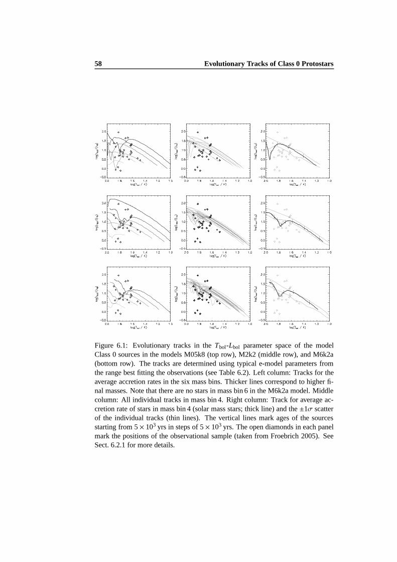
58 Evolutionary Tracks of Class 0 Protostars
Figure 6.1: Evolutionary tracks in the Tbol-Lbol parameter space of the modelClass 0 sources in the models M05k8 (top row), M2k2 (middle row), and M6k2a(bottom row). The tracks are determined using typical e-model parameters fromthe range best fitting the observations (see Table 6.2). Left column: Tracks for theaverage accretion rates in the six mass bins. Thicker lines correspond to higher fi-nal masses. Note that there are no stars in mass bin 6 in the M6k2a model. Middlecolumn: All individual tracks in mass bin 4. Right column: Track for average ac-cretion rate of stars in mass bin 4 (solar mass stars; thick line) and the ±1σ scatterof the individual tracks (thin lines). The vertical lines mark ages of the sourcesstarting from 5 × 10³ yrs in steps of 5 × 10³ yrs. The open diamonds in each panelmark the positions of the observational sample (taken from Froebrich 2005). SeeSect. 6.2.1 for more details.
6.2 Analysis and Discussion 59
0
1
2
2.0 1.8 1.6 1.4 1.2 1.0log[Tbol/K]
log[L
bol/L]
−1
0
1
2.0 1.8 1.6 1.4 1.2 1.0log[Tbol/K]
log[M
env/M
]
−1
0
1
0 1 2log[Lbol/L]
log[M
env/M
]
0
1
2
2.0 1.8 1.6 1.4 1.2 1.0log[Tbol/K]
log[L
bol/L]
−1
0
1
2.0 1.8 1.6 1.4 1.2 1.0log[Tbol/K]
log[M
env/M
]
−1
0
1
0 1 2log[Lbol/L]
log[M
env/M
]
0
1
2
2.0 1.8 1.6 1.4 1.2 1.0log[Tbol/K]
log[L
bol/L]
−1
0
1
2.0 1.8 1.6 1.4 1.2 1.0log[Tbol/K]
log[M
env/M
]
−1
0
1
0 1 2log[Lbol/L]
log[M
env/M
]
Figure 6.2: Distribution of Class 0 observations (circles) and models (grey-scale)in the Tbol-Lbol (left column), Tbol-Menv (middle column), and Lbol-Menv (right col-umn) plane of the parameter space. The plots are shown for the models M05k8(top row), M2k2 (middle row), and M6k2a (bottom row). Darker grey-values inthe model distribution correspond to higher density of model points. As in Fig. 6.1typical e-model parameters are used for the model distributions (see Table 6.2).Only model points with Tbol < 80 K are shown in the plots since this is the limit ofthe observational data.

60E
volutionaryT
racksof
Class
0P
rotostars
Table 6.2: Parameter ranges needed in the e-model to best match the observational data (see Appendix B of Froebrich et al. 2006 fordetails on the parameters). We list the values for the best fitting 5% of the parameter combinations. The last two columns list the medianand average duration of the Class 0 phase of the individual stars in the models.
Model Tenv f racenv Mextra t0 α Rin Meff p κ D3D P3D tmedCl 0 tave
Cl 0
[K] [%] [103 yrs] [AU] [%] [cm2g−1] [%] [103 yrs] [103 yrs]
G2 15-19 81-89 0.6-2.4 35-75 1.4-3.2 30-80 44-47 1.6-1.9 3.0-5.2 0.30-0.35 37.2 - 9.99 41 44M01k2 14-18 87-95 1.0-2.8 20-85 1.4-3.4 40-75 28-44 1.6-1.8 3.0-4.6 0.37-0.42 10.8 - 1.70 39 41M05k4 17-20 89-94 1.2-2.0 35-75 1.6-3.2 45-85 41-44 1.5-1.7 3.0-4.4 0.32-0.37 22.6 - 6.23 31 36M05k8 16-19 90-95 0.9-2.0 25-80 1.9-3.0 40-85 40-46 1.5-1.7 3.0-4.6 0.38-0.44 30.7 - 5.75 31 34M2k2 15-20 86-92 1.0-2.4 35-85 1.6-3.2 35-80 35-43 1.5-1.7 3.4-5.2 0.31-0.38 53.6 - 12.2 32 39M2k4 15-18 86-92 1.0-2.4 35-75 1.4-3.2 40-75 39-43 1.5-1.7 3.2-5.2 0.48-0.52 30.5 - 4.85 15 23M2k8 13-18 80-90 1.0-2.2 30-75 1.2-3.6 35-75 32-41 1.5-1.7 3.4-5.4 0.27-0.36 65.2 - 10.3 45 56M3k2 15-18 82-94 0.6-2.6 20-90 1.4-3.6 35-85 37-44 1.5-1.8 2.8-4.6 0.31-0.38 35.4 - 4.24 44 43M3k4 12-14 80-92 0.6-1.6 25-80 1.4-3.4 30-70 32-44 1.5-1.8 3.2-5.2 0.34-0.39 5.71 - 0.86 87 105M6k2a 16-20 85-95 1.0-2.4 20-85 1.4-3.4 45-85 35-43 1.6-1.8 2.8-4.6 0.32-0.37 41.5 - 16.0 26 32M6k4a 15-20 93-97 0.8-3.2 40-80 1.4-3.2 30-70 12-34 1.6-1.8 3.2-5.2 0.47-0.50 0.04 - 0.01 38 120M6k2b 15-20 82-94 1.2-3.0 35-80 1.6-3.2 35-75 36-40 1.6-1.8 3.2-5.4 0.37-0.41 9.50 - 1.97 26 35M6k2c 15-20 86-96 1.0-3.0 35-75 1.4-3.2 35-75 36-42 1.6-1.9 3.4-4.8 0.38-0.44 4.26 - 0.56 29 51M6k4c 13-18 82-85 0.6-2.6 20-85 1.2-3.2 30-80 28-44 1.5-1.8 3.0-5.2 0.45-0.51 22.2 - 2.17 14 54M10k2 16-22 92-96 1.0-3.6 25-70 1.2-3.0 35-80 10-42 1.6-1.9 3.2-5.4 0.60-0.62 0.003- 0.00 19 24M10k8 14-17 93-98 0.8-3.2 30-85 0.8-3.8 35-80 16-38 1.5-1.7 3.4-5.2 0.45-0.50 1.47 - 0.13 44 124
6.2 Analysis and Discussion 61
6.2.4 Evolutionary Model
To constrain the free parameters in the e-model, we investigate here how the chosenvalues influence the agreement P3D. Table 6.2 contains the range of values whichprovide the highest agreement for each gt-model. In particular we show the valuesfor the best fitting 5% of the e-models. It is more meaningful to provide theseranges instead of the particular parameters for the single best fitting model. Theseare statistically less significant, since not the whole parameter space is tested byour method. We obtain the following results for all gt-models:
• The temperature at the outer envelope boundary is lower than the standardvalue of 24 K. Typically temperatures between 15 and 19 K lead to a goodagreement.
• A wide range for inner envelope radii (Rin) leads to high P3D. Values from35 to 80 AU are typical. This wide range is in agreement with the fact that achange in Rin, while fixing all other parameters, usually results in very smallchanges of P3D. However, the range for the best fitting models does notinclude the hitherto standard value of 30 AU.
• In most cases small amounts of extra mass in the envelope (1.0 < Mextra <
2.4) lead to high agreement.
• The parameter α shows a wide range of possible values for a good agreement(1.4 < α < 3.2). A similar wide range is found for t0 which ranges from 30to 80 × 103 yrs. The larger values found for t0 suggest that the additionalmass stays longer in the envelope to sustain low bolometric temperatures.
• A range of values of p is found to be able to best explain the data. However,in the majority of the cases 1.55 < p < 1.80 leads to the best results. Thesevalues are in between the theoretical solutions for a free falling envelope(1.5) and a singular isothermal sphere (2.0). The range found here seems tobe a compromise between younger and older objects. Since there are prob-ably more older sources in the sample, the best values are closer to p = 1.5.In principle an evolution from p = 2.0 to p = 1.5 would be expected. Ourfindings do not contradict this. Our obtained values are in good agreementwith (sub)-mm observations of envelopes (Chandler & Richer 2000; Motte& Andre 2001).
• We found the mass fraction in the envelope to be in the range from 86 to96%. This would imply a disc mass of 4 to 14% of the envelope mass,mostly smaller than the standard value of 13% used so far, but in agreementwith millimetre interferometric observations (e.g. Looney et al. 2003).
• The amount of mass ejected into the jets is found to range from 36 to 44%.This is a narrow range and somewhat contradictory to the observations and
62 Evolutionary Tracks of Class 0 Protostars
jet launching models which predict that at maximum 30% of the materialis ejected into the jets. We interpret the high amount of ejected materialhere as a combination of two things. (1) Material really ejected into thejets. (2) Material accreted onto the star, but the resulting luminosity escapesdirectly through the cavity generated by the jets and is not observed. If theaccretion luminosity is radiated uniformly away, then the additional ejectedmaterial would imply opening angles between 30 and 60 for the cavities,not an untypical value for many of the older Class 0 sources (e.g. Padmanet al. 1997). To conclusively prove this hypothesis one needs to includethe outflow luminosity for all objects into the comparison of models andobservations.
• The best-fitting opacity range (3.0 to 5.0 cm2g−1) agrees very well with thestandard value of 4 cm2g−1.
6.2.5 Gravoturbulent Models
We now investigate if the initial conditions of the gt-models influence the agree-ment with the observations. The first point to note is that we find no significantcorrelations of P3D or any of the obtained parameter values of the e-models withthe Mach number or wavelength that characterise the turbulence in the gt-model.This is understandable since protostellar collapse is, in essence, a rather localisedprocess, connected to the turbulent cloud environment only via the available massand angular momentum inflow rate.
There are, however, large differences in the quality of agreement between thevarious gt-models and the observations. In the following we investigate the causeof these differences. We determined for each set of accretion rates the median andthe mean duration of the Class 0 phase of the model stars. The median for all gt-models ranges from 14 to 87 × 103 yrs, while the mean duration spans from 23 to124×103 yrs. The much wider range for the average duration is due to some modelstars (outliers) that go through an extremely long Class 0 phase. These objects havea large, secondary accretion peak, which in many cases might not be physical, butcaused by the lack of feedback mechanisms. Due to the mass criterion used, suchpeaks shift the transition from Class 0 to 1 to later times. In Table 6.2 we list themedian and mean duration of the Class 0 phase of all stars in the models in the lasttwo columns.
All gt-models with P3D-values larger than 20% are associated with a mean du-ration of the Class 0 phase between 20 and 60 × 103 yrs. Most of them possessa ratio of median to mean duration of the Class 0 phase of larger than 0.7. Thisindicates that no or only a few outliers are present in the set of accretion rates.When applying these two conditions to all gt-models, we select nine of them (seeFig. 6.3). This includes all models with P3D-values larger than 20% and M01k2(10.8%) and M6k2b (9.5%). Hence 80% of the gt-models with these propertieslead to high agreement. There are seven models that do not fulfil one of the cri-

6.2 Analysis and Discussion 63
teria. Five of these posses P3D-values smaller than 20%. Hence 70% of the gt-models that do not comply with both criteria lead to low agreement. This showsthat high P3D-values are only obtained for gt-models that generate few outliers andthe ‘right’ duration of the Class 0 phase.
The duration of the Class 0 stage shows a linear correlation with the medianof the fit parameter τ defined in § 5.4. This parameter indicates the time it takesuntil the peak accretion rate is reached. It is related to the local free-fall time and,thus, can be used as a rough estimate of the average density of the core at theonset of collapse (see § 5.4). Given our best fitting models and the correspondingClass 0 lifetimes, we infer a range of (1 − 5) × 105 cm−3 for the local density atthe start of the collapse. This is in good agreement with measured central densitiesof pre-stellar cores (e.g. Bacmann et al. 2002). Our results thus suggest that starsmay only form in pre-stellar cloud cores that reach a central density of order of105 cm−3. Obviously, the duration of the Class 0 phase depends directly on theinitial local density.
As can be seen in Table 6.2, gt-models with Mach numbers 0.5 ≤ M ≤ 3 bestdescribe the observations (filled symbols in Fig. 6.3). Six out of seven such modelspossess a high P3D-value, while only one out of eight models with M ≥ 6 has ahigh P3D. The exceptions M3k4 (M < 6, P3D = 5.99%) and M6k2a (M ≥ 6,P3D = 46.5%) as well as the fact that similar gt-models (e.g. M6k2a/b/c) result invery different P3D-values are, however, understandable since protostellar collapseis, in essence, a rather localised process, connected to the turbulent cloud environ-ment only via the available mass and angular momentum inflow rate. It indicatesthat star formation is a highly stochastic process, influenced more strongly by lo-cal properties than by the global initial conditions, a fact which is also found, forexample, by Bate et al. (2003).
The range of Mach numbers found as best explanation for the data reflects thecomposition of the observational sample. It mainly contains sources from Perseus,Orion, and Serpens (Froebrich 2005). There typical Mach numbers are in the range1 ≤ M ≤ 6 (e.g. Castets & Langer 1995; Schmeja et al. 2005). It is, however,interesting to note that the majority of gt-models with M ≥ 6 are not able toexplain the observations, independent of the choice for the e-model parameters.This indicates that the initial conditions do influence the observational propertiesof Class 0 protostars.
6.2.6 Underluminous Sources
We recall that we excluded 25% of the observational data in our determinationof P3D. The excluded data exhibit a much lower bolometric luminosity than theother objects, given their bolometric temperature and envelope mass. They couldbe objects which experience either (a) quiescent states of low accretion or (b) adifferent time dependence of the accretion rate (Froebrich 2005).
A detailed investigation of the individual accretion rates from the gt-modelsrules out the existence of quiet accretion phases as the dominant cause for the low
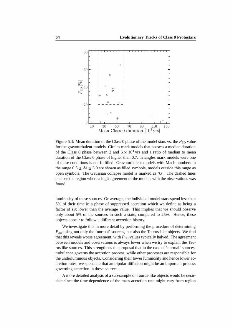
64 Evolutionary Tracks of Class 0 Protostars
0
20
40
60
80
10 30 50 70 90 110 130
Mean Class 0 duration [103 yrs]
P3D
[%]
G
+
+
+
+
+
+ +
.
.
.
.
.
.
.
.
.
.
.
.
.
.
.
.
.
.
.
.
.
.
.
.
.
.
.
.
.
.
.
.
.
.
.
.
.
.
.
.
.
.
.
.
.
.
.
.
.
.
.
.
.
.
.
.
.
.
.
.
.
.
.
.
.
.
.
.
.
.
.
.
.
.
.
.
.
.
.
.
.
.
.
.
.
.
.
.
.
.
.
.
.
.
.
.
.
.
.
.
.
.
.
.
.
.
.
.
.
.
.
.
.
.
.
.
.
.
.
.
.
.
.
.
.
.
.
.
.
.
.
.
.
.
.
.
.
.
.
.
.
.
.
.
.
.
.
.
.
.
.
.
.
.
.
.
.
.
.
.
.
.
.
.
.
.
.
.
.
.
.
.
.
.
.
.
.
.
.
.
.
.
.
.
.
.
.
.
.
.
.
.
.
.
.
.
.
.
.
.
.
.
.
.
.
.
.
.
.
.
.
.
.
.
.
.
.
.
.
.
.
.
.
.
.
.
.
.
.
.
.
.
.
.
.
.
.
.
.
.
.
.
.
.
.
.
.
.
.
.
.
.
.
.
.
.
.
.
.
.
.
.
.
.
.
.
.
.
.
.
.
.
.
.
.
.
.
.
.
.
.
.
.
.
.
.
.
.
.
.
.
.
.
.
.
.
.
.
.
.
.
.
.
.
.
.
.
.
.
.
.
.
.
.
.
.
.
.
.
.
.
.
.
.
.
.
.
.
.
.
.
.
.
.
.
.
.
.
.
.
.
.
.
.
.
.
.
.
.
.
.
.
.
.
.
.
.
.
.
.
.
.
.
.
.
.
.
.
.
.
............. ............. ............. ............. ............. ............. .............
Figure 6.3: Mean duration of the Class 0 phase of the model stars vs. the P3D valuefor the gravoturbulent models. Circles mark models that possess a median durationof the Class 0 phase between 2 and 6 × 10⁴ yrs and a ratio of median to meanduration of the Class 0 phase of higher than 0.7. Triangles mark models were oneof these conditions is not fulfilled. Gravoturbulent models with Mach numbers inthe range 0.5 ≤ M ≤ 3.0 are shown as filled symbols, models outside this range asopen symbols. The Gaussian collapse model is marked as ‘G’. The dashed linesenclose the region where a high agreement of the models with the observations wasfound.
luminosity of these sources. On average, the individual model stars spend less than5% of their time in a phase of suppressed accretion which we define as being afactor of six lower than the average value. This implies that we should observeonly about 5% of the sources in such a state, compared to 25%. Hence, theseobjects appear to follow a different accretion history.
We investigate this in more detail by performing the procedure of determiningP3D using not only the ‘normal’ sources, but also the Taurus-like objects. We findthat this reveals worse agreement, with P3D values typically halved. The agreementbetween models and observations is always lower when we try to explain the Tau-rus like sources. This strengthens the proposal that in the case of ‘normal’ sources,turbulence governs the accretion process, while other processes are responsible forthe underluminous objects. Considering their lower luminosity and hence lower ac-cretion rates, we speculate that ambipolar diffusion might be an important processgoverning accretion in these sources.
A more detailed analysis of a sub-sample of Taurus-like objects would be desir-able since the time dependence of the mass accretion rate might vary from region
6.2 Analysis and Discussion 65
to region (Henriksen et al. 1997). Even though more and more such objects arediscovered (e.g. Young et al. 2004), indicating that the known percentage of theseobjects is clearly a lower limit, the current sample still suffers from too small num-ber statistics to perform a reliable statistical analysis.
6.2.7 Further Discussion
As evident from Table 6.2, the best agreement between observations and models israther low (∼ 70%). Here we will discuss three possible causes for this:
Our procedure: As can be seen in Table 6.1 there are many free parameters,which, in principle, could possess a large range of values. A straight forward testof all possible combinations to solve this highly non-linear minimisation problemof many variables is impossible. We thus used a Monte Carlo method to obtainthe best fitting parameter combination. The obtained probability P3D is a lowerlimit, since not all possible parameter combinations have been tested. Note thatonly slightly smaller values for D3D can lead to probabilities much closer to 100%,especially for models that already possess a high agreement.
When converting D3D to P3D we restricted the random selection to model val-ues with bolometric temperatures smaller than 80 K. This is the limit of our ob-servational sample of Class 0 sources. There are further restrictions in the ob-servational data. No objects are outside a given range in Lbol and Menv. This ismost likely an observational bias. We refrain from applying the other observa-tional limits for the random selection process for the P3D determination becausethe observational limits are not well defined/understood. If we did so, however,we would increase the probabilities for the agreement in many cases significantlytowards 100%.
Observational data: As stated above, the observations clearly cover only alimited range of the Tbol-Lbol-Menv parameter space. All limits, except Tbol < 80 K,are observational biases. Note that the observational sample consists of sourcesfrom several star forming regions. It is possible that e.g. the sensitivity limit forthe bolometric luminosity is not the same in all regions, changing the observedstatistics of low luminosity/mass sources compared to the real one.
As shown in Fig. 6.1, applying a fixed limit for Tbol as divide between Class 0and Class 1 objects is not valid (see also Young & Evans 2005). Most of the solarmass stars undergo this transition at temperatures close to 80 K. However, depend-ing on the individual accretion history of each star, partly significant deviationsfrom this value are evident. Furthermore, lower mass Class 0/Class 1 transitionobjects tend to be warmer than the temperature limit applied here. Thus, the ob-ject sample might suffer from miss-classified objects. This also shows that thereis a difference in the definition for Class 0 protostars based on observations andmodels. Further the observational definition describes a different physical state ofthe object depending on its accretion history and final mass. We overcome most of
66 Evolutionary Tracks of Class 0 Protostars
these uncertainties, however, by applying the Tbol < 80 K restriction when deter-mining P3D.
The models: All our models are constructed on the most basic principles (e.g.the gt-models neglect feedback mechanisms, the disc mass is a constant fraction ofthe envelope mass, etc.). Further all model stars are treated with the same set ofe-model parameters. It is not clear if some of the parameters might depend on thefinal mass of the star. Many parameters are also kept constant in time. This as wellmight be not a valid (e.g. the inner envelope radius, the fraction of mass in the disc,and the powerlaw index of the envelope density distribution might depend on theevolutionary state and final mass of the star). It is in many cases, however, uncer-tain how these dependencies can be parameterised. We thus kept these parametersconstant, not to introduce even more free arbitrary parameters.
Given these three points, we conclude that a very good agreement between themodels and observations should not be expected. It would rather be very worryingif our method would result in a 99% agreement between models and observations.We further have to consider the possibility that star formation, and in particular themass accretion process, might take such a diversity of paths that no simple unifyingmodel can expect to capture them all, leading to small agreements even for futuremuch improved observational samples and models.
6.3 Conclusions
We extracted mass accretion rates within cores generated by gravoturbulent simula-tions and inserted them into a simple protostellar evolutionary scheme to calculateprotostellar evolutionary tracks. A principle dependence of the position of thesetracks in the Tbol-Lbol diagram on the final mass is found. A detailed analysis,however, shows that we are not able to determine the final mass of a particularobject from its measured bolometric temperature and luminosity more accuratelythan a factor of two. The particular shape of an evolutionary track is largely de-termined by the accretion history and by its final mass. Hence, in the context ofthe gravoturbulent model, unique evolutionary tracks do not exist in the Class 0 orClass 0/1 phase, as opposed to the ensuing pre-main sequence evolution. It alsoimplies that Tbol is not always a reliable guide to the envelope-protostar mass ratio,as suggested also by Young & Evans (2005).
A 3D-KS-test was used to compare the distribution of our evolutionary tracksin the Tbol-Lbol-Menv parameter space with an observational sample of Class 0 ob-jects. By varying free parameters associated with the evolutionary scheme, weare able to determine constraints for some of the parameters (Tenv, f racenv , Mextra,Meff , p). Other parameters were found to have no significant influence on theagreement between models and observations (t0, α, Rin, κ). A comparison of theparameter values obtained by our method with observational constraints from indi-
6.3 Conclusions 67
vidual objects (e.g. for f racenv or p) can be conducted. This proves the reliabilityof our method since similar parameter values are obtained.
Only gravoturbulent models generating model stars with a certain density atthe start of the collapse and Class 0 lifetimes between 20 and 60× 103 yrs lead to agood agreement with the observations. This Class 0 lifetime is in good agreementwith estimates of a few 104 yrs based on number ratios or dynamical timescales ofoutflows (see e.g. Andre et al. 2000). It is shown that the Class 0 lifetime is cor-related with the local density at the onset of the collapse. The determined densityrange agrees well with density measurements for pre-stellar cores. Limiting the ac-cretion phase to ten crossings of the computational box in the gravoturbulent modelalways leads to better agreement with the observations. This is consistent with thenotion that protostellar feedback processes (e.g. by outflows or winds) may be animportant mechanism to terminate star formation within two to three dynamicaltimescales.
Apparently the environment (Mach number and scale of the driving turbulence)and the initial mass function do not influence the agreement systematically. Thehighest probability found, that our distributions of model tracks and observationaldata points are drawn from the same basic population, is 70%. This is understand-able, given the uncertainties in the observations and the simple assumptions in themodels. However, the method can be readily adapted to compare larger futuresource samples, different sets of accretion rates or other envelope models.
By applying the KS-test to both the ‘normal’ and underluminous, ‘Taurus-like’objects in the source sample, we find that the determined probability P3D is abouttwice as large when testing only the ‘normal’ objects. This is consistent with theassumption that turbulence governs the accretion rates in the majority of the ob-jects.

68 Evolutionary Tracks of Class 0 Protostars
Chapter 7
Number Ratios of Young StellarObjects∗
Look up at the heavens and count the stars – if indeed you can count them.
– Genesis 15:5
Embedded clusters usually contain young stellar objects belonging to differentclasses. Since these classes form an evolutionary sequence, the numbers of ob-jects in each individual class can tell us something about the evolutionary stage ofthe cluster, e.g. the more Class 3 and the less Class 0/1 objects a cluster has, themore evolved it presumably is. In this chapter, we investigate number ratios ofobjects in these classes in the star-forming regions ρ Ophiuchi, Serpens, Taurus,Chamaeleon I, NGC 7129, IC 1396A, and IC 348. For this purpose we compilean observational sample of absolute numbers of YSOs belonging to the differentclasses from the literature. The number rations can then be compared to the tem-poral evolution of young stars in the simulations in order to constrain the modelsand to possibly determine the evolutionary stage of the clusters.
7.1 Observational Data
The detection and classification of prestellar cores and Class 0/1/2/3 objects re-quires different observational techniques. Thus, we have to construct our samplesfrom various sources. We consider corresponding areas on the sky, but the caveatremains that the combined samples may be far from complete and not homoge-neous. Since it would hardly effect the relative numbers, the problem of unre-solved binaries can be neglected. Besides, we cannot resolve close binaries in theSPH models either. The absolute and relative numbers of YSOs adopted from theobservations for the subsequent analysis are listed in Table 7.1.1 Prestellar cores
∗This chapter is based on Schmeja, S., Klessen, R. S., & Froebrich, D. 2005, A&A, 437, 9111Note that there are discrepancies to the numbers of YSOs given in Table 2.2, which may contain
estimates or consider a larger area and has only illustrative purpose.
69

70 Number Ratios of Young Stellar Objects
Table 7.1: Absolute (upper panel) and relative (lower panel) numbers of YSOs ofdifferent classes from observations (for references see text).
Region prestellar 0 1 2 3ρ Oph 98 2 15 111 77Serpens 26 5 19 18 ∼20Taurus 52 3 25 108 72Cha I <71 2 5 175IC 348 2 2 261NGC 7129 1 20 80IC 1396A 2 6 47 1ρ Oph 0.01 0.07 0.92Serpens 0.08 0.31 0.61Taurus 0.01 0.12 0.87Cha I 0.01 0.03 0.96IC 348 0.01 0.01 0.98NGC 7129 0.01 0.20 0.79IC 1396A 0.03 0.11 0.86
are hard to determine both from observations and in our models, and in particularthey are hard to compare, since the status of the cores (Jeans-critical or subcritical)is often unknown. Some cores considered as “starless” might even in fact turn outto harbour embedded sources (Young et al. 2004). Therefore we do not use themfor the actual comparison, but keep them as an additional test for consistency. Dueto constraints from the models (see § 3.5), we consider Classes 2 and 3 combined.So in the lower panel of Table 7.1 only Class 0, Class 1, and the combined set ofClass 2+3 objects are shown.
7.1.1 ρ Ophiuchi
The ρ Ophiuchi molecular cloud is the closest and probably best-studied star-forming region, offering the most complete sample of YSOs. Bontemps et al.(2001) find a total number of 16 Class 1 sources, 123 Class 2 sources, 38 Class 3sources, and 39 Class 3 candidates. They did not detect the previously known twoClass 0 objects lying within their area. Following the reasoning of Bontemps et al.(2001) and the findings of Grosso et al. (2000) that there might be almost as manyClass 3 as Class 2 objects, we add the candidates to the Class 3 sample, yieldinga total number of 77 Class 3 sources. Stanke et al. (2006) performed a 1.2 mmdust continuum survey of the ρ Oph cloud and detected 118 starless clumps anda couple of previously unknown protostars. About the same number of cores wasdetected by Johnstone et al. (2004) by a 850 µm survey. To obtain a reasonablyhomogeneous sample when combining the Bontemps et al. (2001) and Stanke et
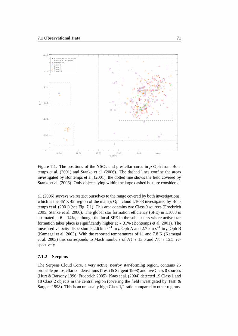
7.1 Observational Data 71
Figure 7.1: The positions of the YSOs and prestellar cores in ρ Oph from Bon-temps et al. (2001) and Stanke et al. (2006). The dashed lines confine the areasinvestigated by Bontemps et al. (2001), the dotted line shows the field covered byStanke et al. (2006). Only objects lying within the large dashed box are considered.
al. (2006) surveys we restrict ourselves to the range covered by both investigations,which is the 45′ × 45′ region of the main ρ Oph cloud L1688 investigated by Bon-temps et al. (2001) (see Fig. 7.1). This area contains two Class 0 sources (Froebrich2005; Stanke et al. 2006). The global star formation efficiency (SFE) in L1688 isestimated at 6 − 14%, although the local SFE in the subclusters where active starformation takes place is significantly higher at ∼ 31% (Bontemps et al. 2001). Themeasured velocity dispersion is 2.6 km s−1 in ρ Oph A and 2.7 km s−1 in ρ Oph B(Kamegai et al. 2003). With the reported temperatures of 11 and 7.8 K (Kamegaiet al. 2003) this corresponds to Mach numbers of M ≈ 13.5 and M ≈ 15.5, re-spectively.
7.1.2 Serpens
The Serpens Cloud Core, a very active, nearby star-forming region, contains 26probable protostellar condensations (Testi & Sargent 1998) and five Class 0 sources(Hurt & Barsony 1996; Froebrich 2005). Kaas et al. (2004) detected 19 Class 1 and18 Class 2 objects in the central region (covering the field investigated by Testi &Sargent 1998). This is an unusually high Class 1/2 ratio compared to other regions.
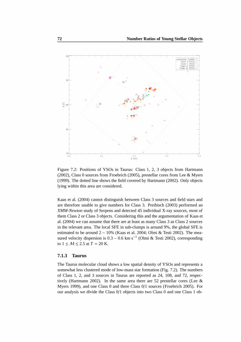
72 Number Ratios of Young Stellar Objects
Figure 7.2: Positions of YSOs in Taurus: Class 1, 2, 3 objects from Hartmann(2002), Class 0 sources from Froebrich (2005), prestellar cores from Lee & Myers(1999). The dotted line shows the field covered by Hartmann (2002). Only objectslying within this area are considered.
Kaas et al. (2004) cannot distinguish between Class 3 sources and field stars andare therefore unable to give numbers for Class 3. Preibisch (2003) performed anXMM-Newton study of Serpens and detected 45 individual X-ray sources, most ofthem Class 2 or Class 3 objects. Considering this and the argumentation of Kaas etal. (2004) we can assume that there are at least as many Class 3 as Class 2 sourcesin the relevant area. The local SFE in sub-clumps is around 9%, the global SFE isestimated to be around 2 − 10% (Kaas et al. 2004; Olmi & Testi 2002). The mea-sured velocity dispersion is 0.3 − 0.6 km s−1 (Olmi & Testi 2002), correspondingto 1 .M . 2.5 at T = 20 K.
7.1.3 Taurus
The Taurus molecular cloud shows a low spatial density of YSOs and represents asomewhat less clustered mode of low-mass star formation (Fig. 7.2). The numbersof Class 1, 2, and 3 sources in Taurus are reported as 24, 108, and 72, respec-tively (Hartmann 2002). In the same area there are 52 prestellar cores (Lee &Myers 1999), and one Class 0 and three Class 0/1 sources (Froebrich 2005). Forour analysis we divide the Class 0/1 objects into two Class 0 and one Class 1 ob-
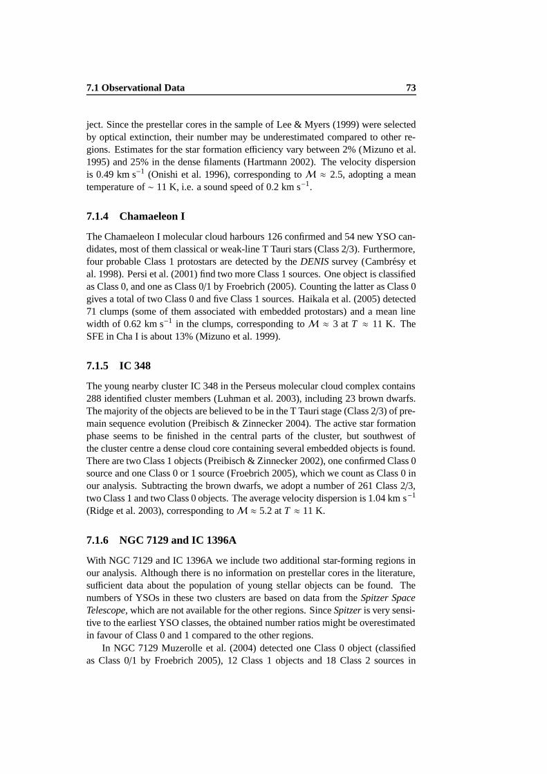
7.1 Observational Data 73
ject. Since the prestellar cores in the sample of Lee & Myers (1999) were selectedby optical extinction, their number may be underestimated compared to other re-gions. Estimates for the star formation efficiency vary between 2% (Mizuno et al.1995) and 25% in the dense filaments (Hartmann 2002). The velocity dispersionis 0.49 km s−1 (Onishi et al. 1996), corresponding to M ≈ 2.5, adopting a meantemperature of ∼ 11 K, i.e. a sound speed of 0.2 km s−1.
7.1.4 Chamaeleon I
The Chamaeleon I molecular cloud harbours 126 confirmed and 54 new YSO can-didates, most of them classical or weak-line T Tauri stars (Class 2/3). Furthermore,four probable Class 1 protostars are detected by the DENIS survey (Cambresy etal. 1998). Persi et al. (2001) find two more Class 1 sources. One object is classifiedas Class 0, and one as Class 0/1 by Froebrich (2005). Counting the latter as Class 0gives a total of two Class 0 and five Class 1 sources. Haikala et al. (2005) detected71 clumps (some of them associated with embedded protostars) and a mean linewidth of 0.62 km s−1 in the clumps, corresponding to M ≈ 3 at T ≈ 11 K. TheSFE in Cha I is about 13% (Mizuno et al. 1999).
7.1.5 IC 348
The young nearby cluster IC 348 in the Perseus molecular cloud complex contains288 identified cluster members (Luhman et al. 2003), including 23 brown dwarfs.The majority of the objects are believed to be in the T Tauri stage (Class 2/3) of pre-main sequence evolution (Preibisch & Zinnecker 2004). The active star formationphase seems to be finished in the central parts of the cluster, but southwest ofthe cluster centre a dense cloud core containing several embedded objects is found.There are two Class 1 objects (Preibisch & Zinnecker 2002), one confirmed Class 0source and one Class 0 or 1 source (Froebrich 2005), which we count as Class 0 inour analysis. Subtracting the brown dwarfs, we adopt a number of 261 Class 2/3,two Class 1 and two Class 0 objects. The average velocity dispersion is 1.04 km s−1
(Ridge et al. 2003), corresponding toM ≈ 5.2 at T ≈ 11 K.
7.1.6 NGC 7129 and IC 1396A
With NGC 7129 and IC 1396A we include two additional star-forming regions inour analysis. Although there is no information on prestellar cores in the literature,sufficient data about the population of young stellar objects can be found. Thenumbers of YSOs in these two clusters are based on data from the Spitzer SpaceTelescope, which are not available for the other regions. Since Spitzer is very sensi-tive to the earliest YSO classes, the obtained number ratios might be overestimatedin favour of Class 0 and 1 compared to the other regions.
In NGC 7129 Muzerolle et al. (2004) detected one Class 0 object (classifiedas Class 0/1 by Froebrich 2005), 12 Class 1 objects and 18 Class 2 sources in
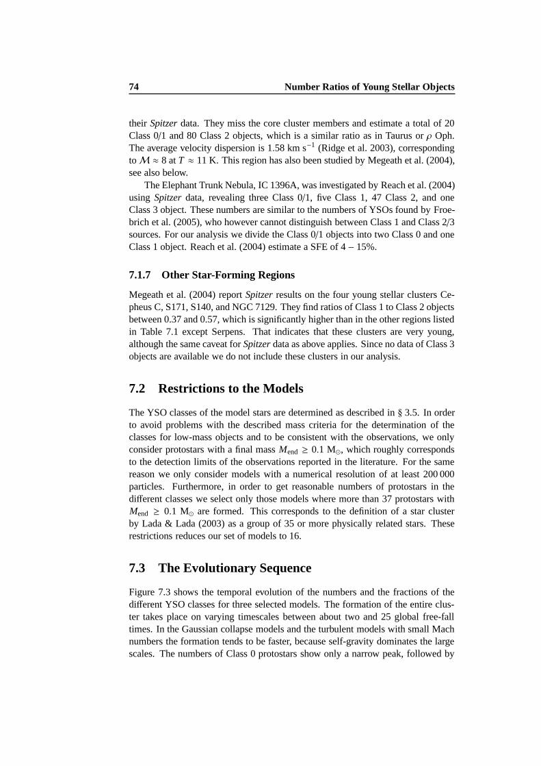
74 Number Ratios of Young Stellar Objects
their Spitzer data. They miss the core cluster members and estimate a total of 20Class 0/1 and 80 Class 2 objects, which is a similar ratio as in Taurus or ρ Oph.The average velocity dispersion is 1.58 km s−1 (Ridge et al. 2003), correspondingtoM ≈ 8 at T ≈ 11 K. This region has also been studied by Megeath et al. (2004),see also below.
The Elephant Trunk Nebula, IC 1396A, was investigated by Reach et al. (2004)using Spitzer data, revealing three Class 0/1, five Class 1, 47 Class 2, and oneClass 3 object. These numbers are similar to the numbers of YSOs found by Froe-brich et al. (2005), who however cannot distinguish between Class 1 and Class 2/3sources. For our analysis we divide the Class 0/1 objects into two Class 0 and oneClass 1 object. Reach et al. (2004) estimate a SFE of 4 − 15%.
7.1.7 Other Star-Forming Regions
Megeath et al. (2004) report Spitzer results on the four young stellar clusters Ce-pheus C, S171, S140, and NGC 7129. They find ratios of Class 1 to Class 2 objectsbetween 0.37 and 0.57, which is significantly higher than in the other regions listedin Table 7.1 except Serpens. That indicates that these clusters are very young,although the same caveat for Spitzer data as above applies. Since no data of Class 3objects are available we do not include these clusters in our analysis.
7.2 Restrictions to the Models
The YSO classes of the model stars are determined as described in § 3.5. In orderto avoid problems with the described mass criteria for the determination of theclasses for low-mass objects and to be consistent with the observations, we onlyconsider protostars with a final mass Mend ≥ 0.1 M, which roughly correspondsto the detection limits of the observations reported in the literature. For the samereason we only consider models with a numerical resolution of at least 200 000particles. Furthermore, in order to get reasonable numbers of protostars in thedifferent classes we select only those models where more than 37 protostars withMend ≥ 0.1 M are formed. This corresponds to the definition of a star clusterby Lada & Lada (2003) as a group of 35 or more physically related stars. Theserestrictions reduces our set of models to 16.
7.3 The Evolutionary Sequence
Figure 7.3 shows the temporal evolution of the numbers and the fractions of thedifferent YSO classes for three selected models. The formation of the entire clus-ter takes place on varying timescales between about two and 25 global free-falltimes. In the Gaussian collapse models and the turbulent models with small Machnumbers the formation tends to be faster, because self-gravity dominates the largescales. The numbers of Class 0 protostars show only a narrow peak, followed by
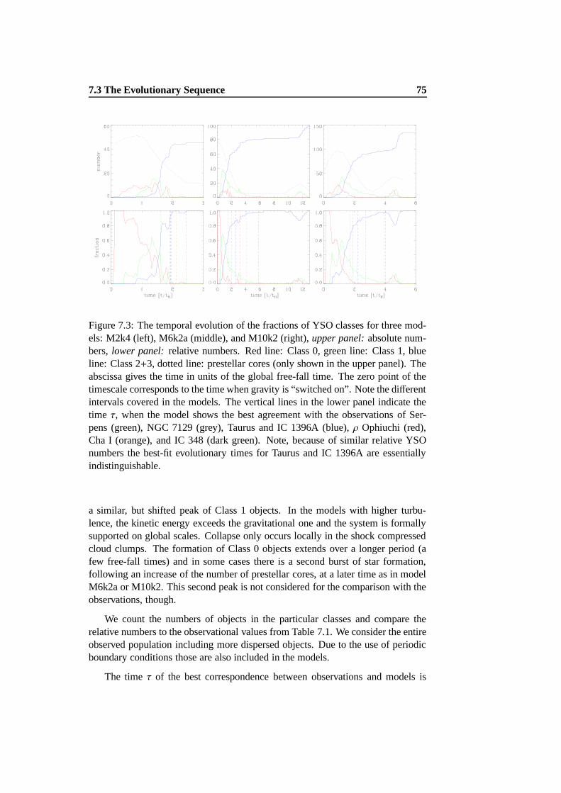
7.3 The Evolutionary Sequence 75
Figure 7.3: The temporal evolution of the fractions of YSO classes for three mod-els: M2k4 (left), M6k2a (middle), and M10k2 (right), upper panel: absolute num-bers, lower panel: relative numbers. Red line: Class 0, green line: Class 1, blueline: Class 2+3, dotted line: prestellar cores (only shown in the upper panel). Theabscissa gives the time in units of the global free-fall time. The zero point of thetimescale corresponds to the time when gravity is “switched on”. Note the differentintervals covered in the models. The vertical lines in the lower panel indicate thetime τ, when the model shows the best agreement with the observations of Ser-pens (green), NGC 7129 (grey), Taurus and IC 1396A (blue), ρ Ophiuchi (red),Cha I (orange), and IC 348 (dark green). Note, because of similar relative YSOnumbers the best-fit evolutionary times for Taurus and IC 1396A are essentiallyindistinguishable.
a similar, but shifted peak of Class 1 objects. In the models with higher turbu-lence, the kinetic energy exceeds the gravitational one and the system is formallysupported on global scales. Collapse only occurs locally in the shock compressedcloud clumps. The formation of Class 0 objects extends over a longer period (afew free-fall times) and in some cases there is a second burst of star formation,following an increase of the number of prestellar cores, at a later time as in modelM6k2a or M10k2. This second peak is not considered for the comparison with theobservations, though.
We count the numbers of objects in the particular classes and compare therelative numbers to the observational values from Table 7.1. We consider the entireobserved population including more dispersed objects. Due to the use of periodicboundary conditions those are also included in the models.
The time τ of the best correspondence between observations and models is
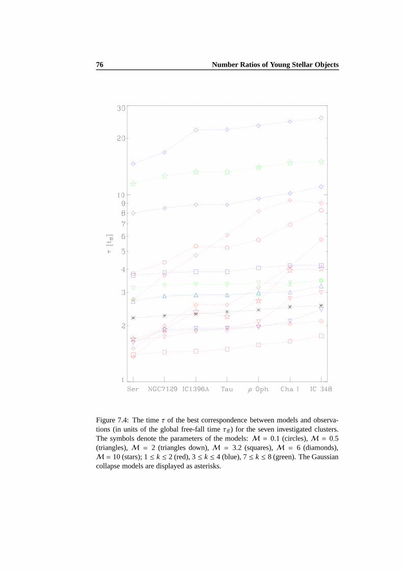
76 Number Ratios of Young Stellar Objects
Figure 7.4: The time τ of the best correspondence between models and observa-tions (in units of the global free-fall time τff) for the seven investigated clusters.The symbols denote the parameters of the models: M = 0.1 (circles), M = 0.5(triangles), M = 2 (triangles down), M = 3.2 (squares), M = 6 (diamonds),M = 10 (stars); 1 ≤ k ≤ 2 (red), 3 ≤ k ≤ 4 (blue), 7 ≤ k ≤ 8 (green). The Gaussiancollapse models are displayed as asterisks.

7.4 Star Formation Efficiency 77
determined when the weighted root mean square of the differences
σ(t) =
√
√
√
√
√
√
√
√
√
√
√
√
12
2∑
i=0|no
i − nmi (t)|2ωi
2∑
i=0ωi
(7.1)
becomes a minimum. The relative number of young stars in Class i (0, 1, 2) fromobservations is expressed as no
i and nmi denotes the relative number of YSOs in
Class i from the models. The factor ωi is a weighting factor, introduced to accountfor the possible scatter due to small number statistics in both, the observations andthe models. The weighting factor is set to ωi =
√
noi · nm
i .The time τ is shown in the lower panel of Fig. 7.3 and displayed for all mod-
els in Fig. 7.4. In general, Serpens is fitted worse than the other clusters. Themean minimal deviation of all models is 〈σmin〉 = 0.005 for ρ Oph and Cha I,〈σmin〉 = 0.008 for Taurus, 〈σmin〉 = 0.010 for NGC 7129, IC 1396A, and IC 348,and 〈σmin〉 = 0.020 for Serpens. In all cases σ(t) has a clearly defined minimum.The scatter of τ is high. Its value varies from about 1.5 to 25 free-fall times for thedifferent models, making it impossible to determine the actual ages of the clustersaccurately. However, all models show the same sequence: τ(Ser) < τ(NGC 7129)< τ(IC 1396A) ≤ τ(Tau) < τ(ρ Oph) < τ(Cha I) < τ(IC 348). In four modelsthe age of IC 1396A is slightly smaller than that of Taurus, in the other modelsthe values are identical. Taking into account the second star-formation burst in themodels M6k2a and M10k2 increases the ages of the older clusters, but it does notchange the overall order. Thus, independent of the applied model, Serpens is theyoungest cluster, NGC 7129 the second youngest cluster, Cha I the second oldest,and IC 348 the most evolved cluster, while Taurus and IC 1396A are at the sameintermediate evolutionary stage. However, the relative numbers of Class 0 and 1objects in NGC 7129 and IC 1396A may be overestimated due to possible obser-vational biases introduced by the Spitzer Space Telescope, as discussed in § 7.1.6.These clusters may thus appear younger relative to the other ones. The fact thatσ(t) always has one well-defined minimum and that all models produce the sameevolutionary sequence independent of the initial conditions, supports a scenarioof a single “burst” of uninterrupted, rapid star formation. This is in agreementwith other theoretical and observational findings of star formation timescales andmolecular cloud lifetimes (see e.g. Hartmann et al. 2001; Ballesteros-Paredes &Hartmann 2006). Several successive “bursts” of star formation within the cloudregion are likely to alter the picture and make a determination of the age from theobserved number ratios difficult.
7.4 Star Formation Efficiency
Figure 7.5 shows the star formation efficiency (the ratio of the mass accreted by theyoung stars to the total mass of the gas) at the time τ versus the Mach number of
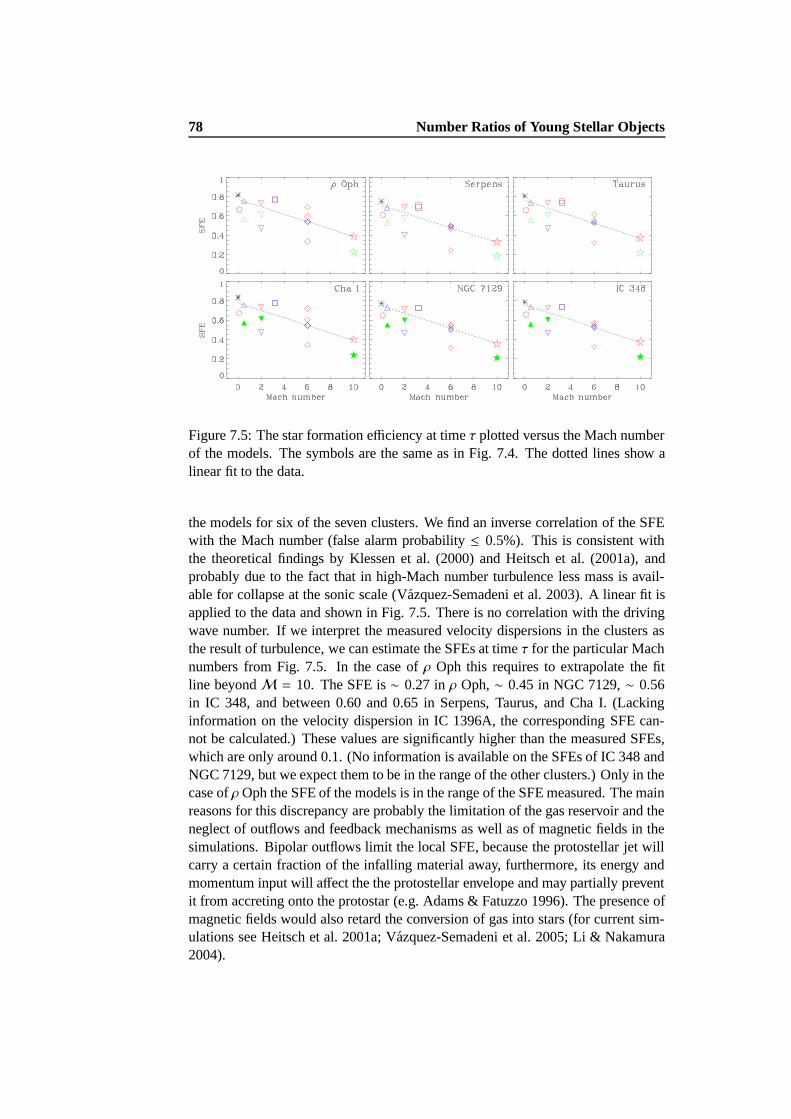
78 Number Ratios of Young Stellar Objects
Figure 7.5: The star formation efficiency at time τ plotted versus the Mach numberof the models. The symbols are the same as in Fig. 7.4. The dotted lines show alinear fit to the data.
the models for six of the seven clusters. We find an inverse correlation of the SFEwith the Mach number (false alarm probability ≤ 0.5%). This is consistent withthe theoretical findings by Klessen et al. (2000) and Heitsch et al. (2001a), andprobably due to the fact that in high-Mach number turbulence less mass is avail-able for collapse at the sonic scale (Vazquez-Semadeni et al. 2003). A linear fit isapplied to the data and shown in Fig. 7.5. There is no correlation with the drivingwave number. If we interpret the measured velocity dispersions in the clusters asthe result of turbulence, we can estimate the SFEs at time τ for the particular Machnumbers from Fig. 7.5. In the case of ρ Oph this requires to extrapolate the fitline beyond M = 10. The SFE is ∼ 0.27 in ρ Oph, ∼ 0.45 in NGC 7129, ∼ 0.56in IC 348, and between 0.60 and 0.65 in Serpens, Taurus, and Cha I. (Lackinginformation on the velocity dispersion in IC 1396A, the corresponding SFE can-not be calculated.) These values are significantly higher than the measured SFEs,which are only around 0.1. (No information is available on the SFEs of IC 348 andNGC 7129, but we expect them to be in the range of the other clusters.) Only in thecase of ρOph the SFE of the models is in the range of the SFE measured. The mainreasons for this discrepancy are probably the limitation of the gas reservoir and theneglect of outflows and feedback mechanisms as well as of magnetic fields in thesimulations. Bipolar outflows limit the local SFE, because the protostellar jet willcarry a certain fraction of the infalling material away, furthermore, its energy andmomentum input will affect the the protostellar envelope and may partially preventit from accreting onto the protostar (e.g. Adams & Fatuzzo 1996). The presence ofmagnetic fields would also retard the conversion of gas into stars (for current sim-ulations see Heitsch et al. 2001a; Vazquez-Semadeni et al. 2005; Li & Nakamura2004).
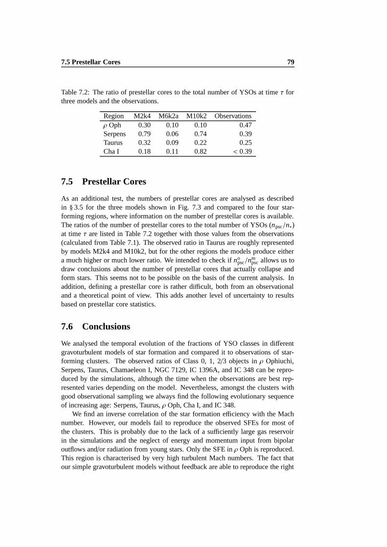
7.5 Prestellar Cores 79
Table 7.2: The ratio of prestellar cores to the total number of YSOs at time τ forthree models and the observations.
Region M2k4 M6k2a M10k2 Observationsρ Oph 0.30 0.10 0.10 0.47Serpens 0.79 0.06 0.74 0.39Taurus 0.32 0.09 0.22 0.25Cha I 0.18 0.11 0.82 < 0.39
7.5 Prestellar Cores
As an additional test, the numbers of prestellar cores are analysed as describedin § 3.5 for the three models shown in Fig. 7.3 and compared to the four star-forming regions, where information on the number of prestellar cores is available.The ratios of the number of prestellar cores to the total number of YSOs (npsc/n∗)at time τ are listed in Table 7.2 together with those values from the observations(calculated from Table 7.1). The observed ratio in Taurus are roughly representedby models M2k4 and M10k2, but for the other regions the models produce eithera much higher or much lower ratio. We intended to check if no
psc/nmpsc allows us to
draw conclusions about the number of prestellar cores that actually collapse andform stars. This seems not to be possible on the basis of the current analysis. Inaddition, defining a prestellar core is rather difficult, both from an observationaland a theoretical point of view. This adds another level of uncertainty to resultsbased on prestellar core statistics.
7.6 Conclusions
We analysed the temporal evolution of the fractions of YSO classes in differentgravoturbulent models of star formation and compared it to observations of star-forming clusters. The observed ratios of Class 0, 1, 2/3 objects in ρ Ophiuchi,Serpens, Taurus, Chamaeleon I, NGC 7129, IC 1396A, and IC 348 can be repro-duced by the simulations, although the time when the observations are best rep-resented varies depending on the model. Nevertheless, amongst the clusters withgood observational sampling we always find the following evolutionary sequenceof increasing age: Serpens, Taurus, ρ Oph, Cha I, and IC 348.
We find an inverse correlation of the star formation efficiency with the Machnumber. However, our models fail to reproduce the observed SFEs for most ofthe clusters. This is probably due to the lack of a sufficiently large gas reservoirin the simulations and the neglect of energy and momentum input from bipolaroutflows and/or radiation from young stars. Only the SFE in ρ Oph is reproduced.This region is characterised by very high turbulent Mach numbers. The fact thatour simple gravoturbulent models without feedback are able to reproduce the right
80 Number Ratios of Young Stellar Objects
number ratios of YSOs forM ' 10 suggests that protostellar feedback processesmay not be important in shaping the density and velocity structure in star-formingregions with very strong turbulence and argues for driving mechanisms externalto the cloud itself (see also the discussion in Ossenkopf & Mac Low 2002 andMac Low & Klessen 2004).
The relative numbers of YSOs can reveal the evolutionary status of a star-forming cluster only with respect to other clusters, as the absolute age is difficultto estimate. Better agreement between models and observations requires a betterconsideration of environmental conditions like protostellar outflows and magneticfields in the simulations. A larger observational sample, achieved by completecensuses of more star-forming regions, is also desirable.
Chapter 8
The Structures of Young StarClusters∗
Understanding the formation and evolution of young stellar clusters requires quan-titative statistical measures of their structure, which may give important clues tothe formation process: A young cluster might still bear the imprint of the physi-cal process(es) that created it and will likely reflect the underlying structure of thedense molecular gas. There are two basic types of clusters with regard to theirstructure (see e.g. Lada & Lada 2003): (1) Hierarchical clusters show a stellar sur-face density distribution with multiple peaks and possible fractal substructure; (2)centrally condensed clusters exhibit highly centrally concentrated stellar surfacedensity distributions with relatively smooth radial profiles that can be described ingood approximation by simple power-law functions (e.g. ρ(r) ∝ r−α).
Different methods have been used to describe the clustering properties of starclusters, e.g. the mean surface density of companions (Larson 1995) or spanningtrees. Cartwright & Whitworth (2004) presented a review of various statisticalmethods for analysing the structures of star clusters, and a detailed investigation ofboth observed and artificially created clusters. We apply their methods to clusterscreated by numerical simulations of gravoturbulent star formation and investigatethe clustering behaviour with time. We extend the analysis of observed clusters byconsidering different evolutionary classes.
8.1 Statistical Methods
8.1.1 Mean Surface Density of Companions
A wide range of statistical methods has been developed to analyse the structure ofstar clusters (see Cartwright & Whitworth 2004 for a review). A simple approach isto study the distribution of source separations, as it has been done e.g. by Kaas et al.(2004) for the Serpens cloud core. Larson (1995), extending the analysis by Gomez
∗This chapter is based on Schmeja, S., & Klessen, R. S. 2006, A&A, 449, 151
81
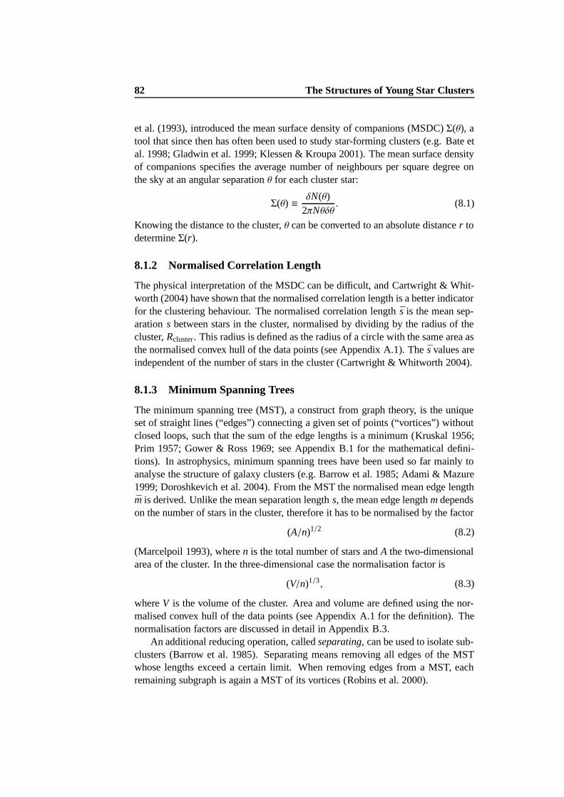
82 The Structures of Young Star Clusters
et al. (1993), introduced the mean surface density of companions (MSDC) Σ(θ), atool that since then has often been used to study star-forming clusters (e.g. Bate etal. 1998; Gladwin et al. 1999; Klessen & Kroupa 2001). The mean surface densityof companions specifies the average number of neighbours per square degree onthe sky at an angular separation θ for each cluster star:
Σ(θ) ≡ δN(θ)2πNθδθ
. (8.1)
Knowing the distance to the cluster, θ can be converted to an absolute distance r todetermine Σ(r).
8.1.2 Normalised Correlation Length
The physical interpretation of the MSDC can be difficult, and Cartwright & Whit-worth (2004) have shown that the normalised correlation length is a better indicatorfor the clustering behaviour. The normalised correlation length s is the mean sep-aration s between stars in the cluster, normalised by dividing by the radius of thecluster, Rcluster. This radius is defined as the radius of a circle with the same area asthe normalised convex hull of the data points (see Appendix A.1). The s values areindependent of the number of stars in the cluster (Cartwright & Whitworth 2004).
8.1.3 Minimum Spanning Trees
The minimum spanning tree (MST), a construct from graph theory, is the uniqueset of straight lines (“edges”) connecting a given set of points (“vortices”) withoutclosed loops, such that the sum of the edge lengths is a minimum (Kruskal 1956;Prim 1957; Gower & Ross 1969; see Appendix B.1 for the mathematical defini-tions). In astrophysics, minimum spanning trees have been used so far mainly toanalyse the structure of galaxy clusters (e.g. Barrow et al. 1985; Adami & Mazure1999; Doroshkevich et al. 2004). From the MST the normalised mean edge lengthm is derived. Unlike the mean separation length s, the mean edge length m dependson the number of stars in the cluster, therefore it has to be normalised by the factor
(A/n)1/2 (8.2)
(Marcelpoil 1993), where n is the total number of stars and A the two-dimensionalarea of the cluster. In the three-dimensional case the normalisation factor is
(V/n)1/3, (8.3)
where V is the volume of the cluster. Area and volume are defined using the nor-malised convex hull of the data points (see Appendix A.1 for the definition). Thenormalisation factors are discussed in detail in Appendix B.3.
An additional reducing operation, called separating, can be used to isolate sub-clusters (Barrow et al. 1985). Separating means removing all edges of the MSTwhose lengths exceed a certain limit. When removing edges from a MST, eachremaining subgraph is again a MST of its vortices (Robins et al. 2000).
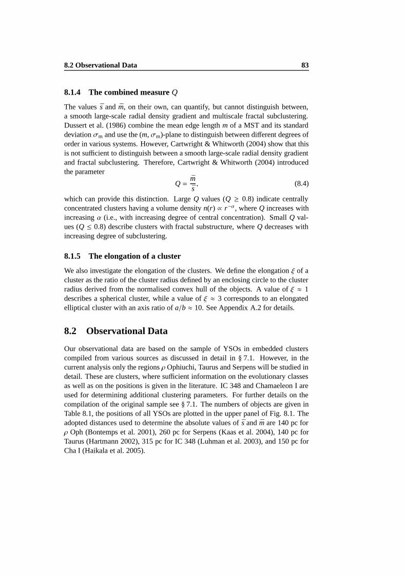
8.2 Observational Data 83
8.1.4 The combined measure Q
The values s and m, on their own, can quantify, but cannot distinguish between,a smooth large-scale radial density gradient and multiscale fractal subclustering.Dussert et al. (1986) combine the mean edge length m of a MST and its standarddeviation σm and use the (m, σm)-plane to distinguish between different degrees oforder in various systems. However, Cartwright & Whitworth (2004) show that thisis not sufficient to distinguish between a smooth large-scale radial density gradientand fractal subclustering. Therefore, Cartwright & Whitworth (2004) introducedthe parameter
Q =ms, (8.4)
which can provide this distinction. Large Q values (Q ≥ 0.8) indicate centrallyconcentrated clusters having a volume density n(r) ∝ r−α, where Q increases withincreasing α (i.e., with increasing degree of central concentration). Small Q val-ues (Q ≤ 0.8) describe clusters with fractal substructure, where Q decreases withincreasing degree of subclustering.
8.1.5 The elongation of a cluster
We also investigate the elongation of the clusters. We define the elongation ξ of acluster as the ratio of the cluster radius defined by an enclosing circle to the clusterradius derived from the normalised convex hull of the objects. A value of ξ ≈ 1describes a spherical cluster, while a value of ξ ≈ 3 corresponds to an elongatedelliptical cluster with an axis ratio of a/b ≈ 10. See Appendix A.2 for details.
8.2 Observational Data
Our observational data are based on the sample of YSOs in embedded clusterscompiled from various sources as discussed in detail in § 7.1. However, in thecurrent analysis only the regions ρ Ophiuchi, Taurus and Serpens will be studied indetail. These are clusters, where sufficient information on the evolutionary classesas well as on the positions is given in the literature. IC 348 and Chamaeleon I areused for determining additional clustering parameters. For further details on thecompilation of the original sample see § 7.1. The numbers of objects are given inTable 8.1, the positions of all YSOs are plotted in the upper panel of Fig. 8.1. Theadopted distances used to determine the absolute values of s and m are 140 pc forρ Oph (Bontemps et al. 2001), 260 pc for Serpens (Kaas et al. 2004), 140 pc forTaurus (Hartmann 2002), 315 pc for IC 348 (Luhman et al. 2003), and 150 pc forCha I (Haikala et al. 2005).
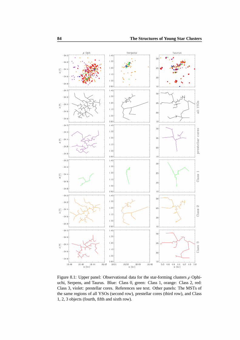
84 The Structures of Young Star Clusters
Figure 8.1: Upper panel: Observational data for the star-forming clusters ρ Ophi-uchi, Serpens, and Taurus. Blue: Class 0, green: Class 1, orange: Class 2, red:Class 3, violet: prestellar cores. References see text. Other panels: The MSTs ofthe same regions of all YSOs (second row), prestellar cores (third row), and Class1, 2, 3 objects (fourth, fifth and sixth row).
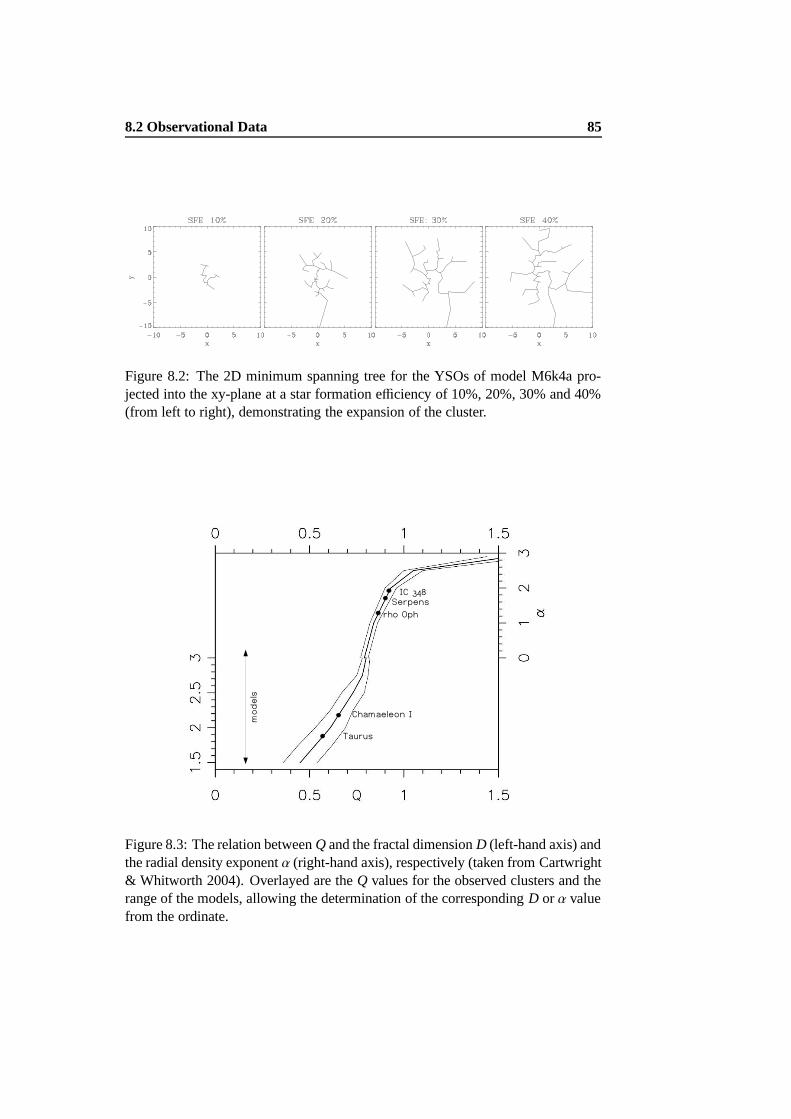
8.2 Observational Data 85
Figure 8.2: The 2D minimum spanning tree for the YSOs of model M6k4a pro-jected into the xy-plane at a star formation efficiency of 10%, 20%, 30% and 40%(from left to right), demonstrating the expansion of the cluster.
Figure 8.3: The relation between Q and the fractal dimension D (left-hand axis) andthe radial density exponent α (right-hand axis), respectively (taken from Cartwright& Whitworth 2004). Overlayed are the Q values for the observed clusters and therange of the models, allowing the determination of the corresponding D or α valuefrom the ordinate.

86T
heStructures
ofY
oungStar
Clusters
Table 8.1: Clustering measures and numbers for the observed star-forming regions for prestellar cores (p), Class 1, 2, 3 sources, and allYSOs. (Note that the total number of YSOs is larger than the sum of objects in the individual classes, because it contains Class 0 sourcesand objects with unclear classification not considered in the analysis of the individual classes.) For details see the discussion in § 8.4.1.
Region Class n s [′] s [pc] m [′] m [pc] s m Q s∗ m∗ Q∗ ξ
ρ Ophiuchi p 98 20.45 0.83 2.71 0.11 0.67 0.55 0.82 0.49 0.40 0.81 1.361 15 11.82 0.48 3.15 0.13 1.13 0.68 0.60 0.77 0.43 0.56 1.472 111 15.86 0.65 2.25 0.09 0.69 0.58 0.83 0.54 0.63 1.15 1.273 77 16.25 0.66 2.53 0.10 0.82 0.63 0.76 0.70 0.66 0.93 1.17
all 205 15.63 0.64 1.67 0.07 0.67 0.57 0.85 0.53 0.45 0.85 1.28Serpens 1 19 3.43 0.26 1.12 0.09 0.99 0.82 0.83 0.27 0.22 0.79 3.61
2 18 7.85 0.59 1.74 0.13 0.74 0.61 0.82 0.52 0.42 0.80 1.42all 80 5.98 0.45 1.06 0.08 0.60 0.54 0.90 0.37 0.32 0.89 1.63
Taurus p 52 281.0 11.47 45.88 1.87 0.77 0.48 0.62 0.59 0.36 0.61 1.291 25 265.6 10.84 73.18 2.98 0.83 0.60 0.73 0.59 0.41 0.70 1.392 108 333.5 13.62 34.30 1.40 0.69 0.41 0.59 0.43 0.54 1.26 1.613 72 414.4 16.96 52.99 2.16 0.84 0.51 0.60 0.77 0.63 0.82 1.09
all 197 356.8 14.58 25.98 1.06 0.67 0.39 0.58 0.46 0.27 0.58 1.45IC 348 all 288 6.86 0.63 0.66 0.06 0.56 0.52 0.93 0.49 0.45 0.92 1.16Chamaeleon I all 180 41.51 1.81 3.74 0.16 0.55 0.37 0.68 0.50 0.34 0.68 1.32
8.3 Application to the Data 87
8.3 Application to the Data
We construct the MST following Prim’s (1957) algorithm (see Appendix B.2). Forboth the observations and the models, the parameters s, m and Q are computed forthe different evolutionary classes independently (provided, there is a sufficientlylarge number of YSOs of that class) as well as for the entire cluster. In no regionis the number of Class 0 sources large enough to be included. In addition, theseparameters are determined at frequent timesteps of the simulations to obtain thetemporal evolution of the parameters. In the case of m, this requires to constructthe MST anew at every chosen timestep. As an example, Fig. 8.2 shows the MSTof one model at different evolutionary stages. While the parameters s, m and Q arecalculated using the normalisation factor given above, s∗, m∗ and Q∗ are determinedwith the normalisation factor and cluster radius of Cartwright & Whitworth (2004)(see also the discussion in the Appendix).
As shown by Cartwright & Whitworth (2004), the effect of binary stars onthe clustering parameters is not negligible. Since binaries create very short edgelengths, a large fraction of binaries will significantly reduce the mean edge length m(and as a consequence also change Q). As the binaries are not part of the clusteringregime, their influence on the clustering parameters has to be minimized. Whilefor most of the clusters this is not relevant, Taurus is known to have a large binarypopulation. Thus we removed the known binary companions from our sample ofYSOs in Taurus.
We calculate the clustering parameters s, m, Q, and ξ for the model clus-ter in three dimensions, and, in order to compare them with the apparent two-dimensional observational data, projected into the xy-, xz-, and yz-plane. Thepositions of the stars are corrected for the periodic boundary conditions. Only ob-jects inside a box of ten times the side length of the original computational box areconsidered, if there are any objects outside this volume, we assume that they haveleft the cluster and are not relevant for the clustering process.
In the initial stages of the cluster as a whole, and of the individual evolutionaryclasses, the number of objects is of course rather low. In such cases the statisticalanalysis may not be very meaningful and has to be taken with a grain of salt.
8.4 Discussion
8.4.1 Observations
Table 8.1 lists the clustering measures introduced in § 8.1 for the observations.Columns 4 to 7 list the (non-normalised) mean separation of objects and meanMST edge lengths in arcminutes and parsec. Columns 8 to 10 give the parame-ters s, m and Q, while Columns 11 to 13 list the same values calculated using thenormalisation of Cartwright & Whitworth (2004) (s∗, m∗, Q∗). The last columngives the elongation ξ. The values of s∗, m∗ and Q∗ agree with the values givenby Cartwright & Whitworth (2004), except for s∗ and m∗ of Taurus (interestingly,
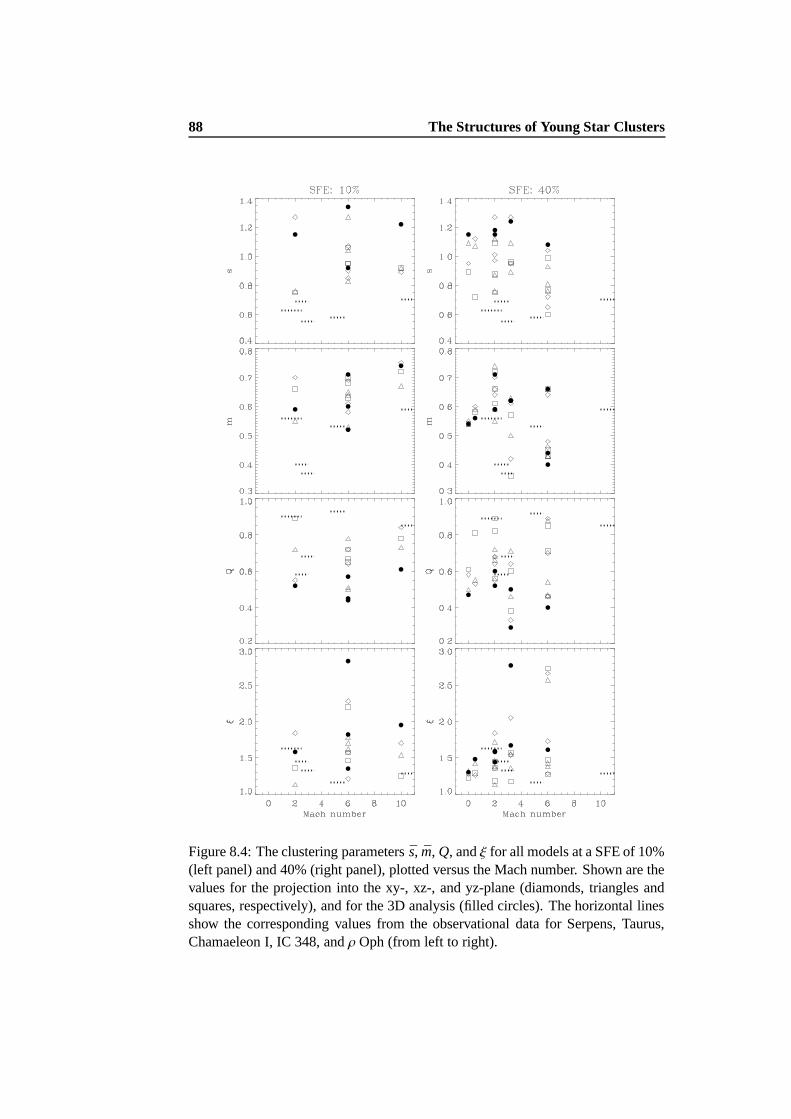
88 The Structures of Young Star Clusters
Figure 8.4: The clustering parameters s, m, Q, and ξ for all models at a SFE of 10%(left panel) and 40% (right panel), plotted versus the Mach number. Shown are thevalues for the projection into the xy-, xz-, and yz-plane (diamonds, triangles andsquares, respectively), and for the 3D analysis (filled circles). The horizontal linesshow the corresponding values from the observational data for Serpens, Taurus,Chamaeleon I, IC 348, and ρ Oph (from left to right).
8.4 Discussion 89
however, our Q∗ is the same as theirs). We attribute small differences to the slightlydifferent underlying samples, and the discrepancy for Taurus to the different treat-ment of binaries. Due to the different definition of the radius/area of the cluster,s∗ and m∗ differ significantly from s and m, while Q and Q∗ are roughly the same,in particular for large samples (see the discussion in Appendix B.3). Taurus andChamaeleon I have substructure, while ρ Oph and IC 348 are centrally concen-trated clusters (see the discussion in Cartwright & Whitworth 2004). Serpens (notdiscussed by Cartwright & Whitworth 2004) has Q = 0.90, corresponding to acentral concentration with a radial density exponent α ≈ 1.9, similar to IC 348.
The linear distances s and m are in the same range for ρ Oph, Serpens, andIC 348, significantly larger for Chamaeleon I, and about an order of magnitudelarger in the case of Taurus, confirming the notion that Taurus represents a some-what less clustered mode of star formation. However, when considering only thecentral part of the Taurus region, the values decrease significantly to s = 3.05 pcand m = 0.49 pc. The latter is comparable to the 0.3 pc estimated as the averagedistance to the nearest stellar neighbour in the central region of Taurus by Gomezet al. (1993) and Hartmann (2002).
The mean separation s increases with the evolutionary class for all three clus-ters investigated in this regard, reflecting the expansion of the cluster, which canalso be seen in Fig. 8.1. While Class 0 protostars are formed in the high-densitycentral regions, more evolved YSOs already had time to move to more remote re-gions (see also Kaas et al. 2004). Note that the prestellar cores do not fit into thissequence, as they are distributed over an area roughly as large as the entire cluster.Thus we speculate that not all objects identified as prestellar cores will eventuallyform stars. Only in the central parts of the cluster may the density be high enough tomake the cores collapse. This is consistent with the findings of Vazquez-Semadeniet al. (2005) that a significant number of “failed cores” should exist, which mayredisperse and which may correspond to the observed starless cores.
The elongation of the clusters ranges from ξ = 1.16 for the almost perfectlyspherical cluster IC 348 to ξ = 1.63 for Serpens. The ξ value can differ signifi-cantly for subclusters, e.g. the filamentary central part of the Taurus region has anelongation of ξ = 1.83.
8.4.2 Models
We compute the clustering parameters s, m, Q, and ξ for all models and com-pare them with each other as well as with those from the observations. Figure 8.4shows the clustering parameters for all models, sorted by the Mach number at astar formation efficiency (SFE) of 10% and 40%. The clustering parameters ofthe observed clusters (from Table 8.1) are shown as horizontal lines at their Machnumber (see § 7.1). The s and m values of the models are in general significantlylarger than those from the observations. A particularly large discrepancy is notedwhen the model cluster is strongly elongated. A large ξ value reduces the nor-malisation factor and increases s and m. While the observed clusters show rather

90 The Structures of Young Star Clusters
Figure 8.5: The temporal evolution of the 3D clustering parameters s, m, Q, and ξfor one model (M6k4a), dotted: Class 0, dashed: Class 1, dash-dotted: Class 2/3,solid line: entire cluster.
Figure 8.6: The temporal evolution of the clustering parameters s, m, Q, and ξ ofthe model M6k4a for the 3D analysis (solid line) and for the projection into the xy-(dotted), xz- (dashed), and yz-plane (dash-dotted).
moderate elongations in the range 1.1 < ξ < 1.6, in some models the stars form ina single filament with an elongation ξ > 3. Model clusters with elongations in therange of the observations show also a good agreement in the other parameters. Forexample, the fairly spherical cluster of model M6k4a (shown in Fig. 8.2) has (at40% SFE and projected into the xy-plane) an elongation of ξ = 1.28 and clusteringparameters of s = 0.72, m = 0.64, and Q = 0.89. These values are almost identicalto those of ρ Ophiuchi (ξ = 1.28, s = 0.70, m = 0.59, Q = 0.85). For the otherprojections the values differ by less than 8%. Most of the Q values, which areindependent of the area, lie in the same range as those from the observations. Wefind no correlation of the clustering parameters with the properties of the turbulentdriving (Mach number or wave number k) of the models. Neither do the valuesfrom the observations show any correlation with the Mach number. Thus we con-clude that if there is any systematic influence of the turbulent environment on theclustering behaviour, it is only existent in the earliest phase of cluster formation,before it is smoothed out by the motions of the individual protostars (see also Bateet al. 1998).
Fig. 8.2 shows the MST of a model cluster (M6k4a) at different evolutionarystages and reveals the expansion of the cluster. We analyse the temporal evolutionof the clustering parameters: s(t), m(t), Q(t), ξ(t) in all models. As an example,Fig. 8.5 shows this sequence for said model M6k4a. The general behaviour is the
8.4 Discussion 91
same for all models: s and m decline with time, while Q increases slowly or stays ata roughly constant value. This evolution is shown by the entire cluster as well as bythe individual classes, although in later stages the latter values might fall to zero asthe number of objects in a particular class becomes zero. Decreasing s and m valuesindicate that star formation sets in in different, rather dispersed regions of the cloud.The cluster becomes denser as more and more gas is turned into protostars. Newstars are formed faster than the cluster expands. According to the Q values, thecluster evolves slowly from fractal subclustering to a more centrally concentratedcluster, although in no model does Q rise significantly above the ‘dividing value’of 0.8. This again shows that the cluster builds up from separate groups whichwill grow into a single, more centrally concentrated cluster, as it was also found byBonnell et al. (2003) and Clark et al. (2005).
8.4.3 The Effect of Projection
Looking at the two-dimensional projections of the 3D model clusters does not sig-nificantly change the picture as a whole. The individual s, m and Q values canindeed differ for the projection into the xy-, xz-, and yz-plane, but the qualitativebehaviour of the evolution is more or less the same, independent of the projection(Fig. 8.6). While the s3D and m3D values usually are higher than the values ofthe projections, Q3D tends to be lower than the values of the projections. The in-vestigation of several hundred randomly created clusters shows that s3D is alwaysexpected to be larger than the value for the projections (s3D/s2D ≈ 1.2), while them values can be in the range 0.95 . m3D/m2D . 1.4 with a mean value of 1.1. Inthe extreme case, Q3D can differ by up to 30% from the 2D value. Note that thephysical interpretation of Q as given by Cartwright & Whitworth (2004) is basedon the two-dimensional analysis. Therefore, for an interpretation of the numericalvalues (and not only the trend) of Q, the projected values have to be used.
The elongation measure ξ, on the other hand, depends strongly on the projec-tion. Obviously, an elongated, filament-like structure seen from the side will lookspherical when observed along its major axis. In the case of the models the three-dimensional value of ξ can be used to describe the true shape of the cluster. A largescatter in the ξ2D values means a high ξ3D value and vice versa.
8.4.4 The Effect of Separating
We separate the observed clusters by successively removing all MST edges withlengths l larger than l + 3σm, l + 2σm, l + σm, and l + 0.5σm, where σm denotesthe standard deviation of the mean edge length of the MST. This process is demon-strated for the Taurus star-forming region in Fig. 8.7. When we compare all threeregions with sufficient data, we see that for Serpens and Taurus only solitary starsin the outskirts of the cluster are removed, while the central part of the cluster staysconnected. However, the more homogeneous ρ Oph cluster breaks down in tworoughly equally large clusters at the last step. In Fig. 8.8 we show the clustering

92 The Structures of Young Star Clusters
Figure 8.7: The MST of the Taurus cluster as a whole (left panel) and separated atl + 2σm, l + σm, and l + 0.5σm (from left to right).
parameters of the largest remaining subcluster (i.e., the one containing the largestnumber of stars after each level of separation). The parameter Q is less affectedby the separating procedure than s and m. Significant changes are only seen whenlarge parts of the cluster are excluded (as in the step from 1 to 0.5σ for ρOph, whenthe cluster breaks up into two large subclusters). The elongation measure ξ variessignificantly with the level of separation. For example, the remaining subcluster inTaurus shows a filamentary structure and thus a larger ξ (ξ = 1.83) than the clusteras a whole.
8.5 Conclusions
We show that the normalised mean correlation length s and the mean edge lengthof the minimum spanning tree m, and in particular the combination of both param-eters, Q, as proposed by Cartwright & Whitworth (2004), are very useful tools tostudy the structures of star clusters, both observed ones and those from numericalsimulations. We refine the definition of the cluster area by using the normalisedconvex hull rather than a circular or rectangular area around the objects. Unlike sand m, the parameter Q is independent of the definition of the area of the cluster.In addition, it is less affected when removing stars from the cluster by separatingthe MST.
We introduce a new measure ξ for the elongation of a cluster. It is defined asthe ratio of the cluster radius determined by an enclosing circle to the cluster radiusderived from the normalised convex hull. This is a stable statistical measure notinfluenced by fractal substructure, which could also be applied to the filamentarystructure of molecular clouds.
The mean separation s increases with the evolutionary class, reflecting the ex-pansion of the cluster. The prestellar cores do not follow that sequence, leading usto the speculation that not all objects classified as prestellar cores will eventuallyform stars. The clustering values of the models lie roughly in the same range asthose from observed clusters. A particularly good agreement is reached when themodel clusters have similar elongation values ξ to the observed ones. No corre-

8.5 Conclusions 93
Figure 8.8: The clustering parameters s (diamonds), m (triangles), Q (squares),and ξ (asterisks; scale on the right-hand axis) of the largest remaining subcluster atdifferent levels of separation. The numbers along the abscissa give the number ofYSOs contained in the particular subcluster.
lation with the Mach number or the wave number of the turbulence is found. Weconclude that possible influences of the turbulent environment on the clusteringbehaviour are quickly smoothed out by the velocity dispersion of the young stars.
The temporal evolution of the clustering parameters shows that the star clusterbuilds up from several subclusters and evolves to a more centrally concentratedstate. New stars are formed faster than the cluster expands. The projection of the3D models into a 2D plane changes the clustering parameters, but not the generalbehaviour with time.

94 The Structures of Young Star Clusters

Chapter 9
Summary and Perspectives
‘The Ultimate Question?’‘Yes!’
‘Of Life, the Universe, and Everything?’‘Yes!’
Deep Thought pondered for a moment.‘Tricky,’ he said.
– Douglas Adams, The Hitchhiker’s Guide to the Galaxy
In this thesis, a large set of numerical simulations of gravoturbulent star forma-tion have been analysed in detail and compared to observational data. Twenty-fourmodels covering a wide range of environmental conditions from low to high turbu-lent velocities and different driving scales with a total number of 1325 protostarshave been investigated in many respects. The models cover the entire spectrum ofobserved star-forming regions, ranging from inefficient and isolated star formationto the fast and efficient build-up of stellar clusters. We investigated the propertiesof individual protostars (mass accretion rates, Tbol/Lbol/Menv) as well as those ofentire clusters (number ratios, structure). Despite their indubitable limitations, thesimulations are able to reproduce those properties without contradictions. Consid-ering the fact that the observations contain (partly large) uncertainties and biases aswell, we can speak of a fairly good agreement. It is safe to state that gravoturbulentfragmentation is an adequate approach to explain the formation of stars, which isclearly superior to the so-called “standard theory of star formation”, in which starformation is regulated by magnetic fields and slow ambipolar diffusion processes.
In the picture of gravoturbulent fragmentation, star formation is a highly chaoticand localised process. Only a few parameters show a correlation with the proper-ties of the turbulent driving, e.g. the mean mass accretion rate or the star formationefficiency of a cluster.
As demonstrated in § 5, protostellar mass accretion is a highly dynamical andtime-variant process. The peak accretion rate, reached during the Class 0 stageshortly after the formation of the protostellar core, can reach values of & 104 M yr−1.The maximum accretion rate is approximately one order of magnitude higher than
95

96 Summary and Perspectives
the constant rate predicted by the collapse of a classical singular isothermal sphere,in agreement with the observations.
A better possibility to compare the model mass accretion rates to observationsis converting them to the observables Tbol, Lbol, and Menv. Our newly developedmethod uses the accretion rates during the Class 0 stage from the simulationsas input for an evolutionary scheme. The resulting distribution in the Tbol-Lbol-Menv parameter space is then compared to observational data of by means of a 3DKolmogorov-Smirnov test. The highest probability found that the distributions ofmodel tracks and observational data points are drawn from the same distribution is70%. The method can be easily applied to future larger source samples, differentsets of accretion rates or other evolutionary models. An extension of the analy-sis to Class 1 objects might be worth considering, however, this requires a moresophisticated envelope model or, ideally, radiative transfer modelling.
In the second part of this thesis, the properties of clusters as a whole are inves-tigated. The ratios of Class 0, 1, and 2/3 objects in observed star-forming clustersare compared to the temporal evolution of the gravoturbulent models in order toestimate the evolutionary stage of a cluster. While it is difficult to estimate theabsolute age of the clusters, the relative numbers of YSOs reveal the evolutionarystatus of a cluster with respect to other clusters. We find an evolutionary sequencewith Serpens as the youngest and IC 348 as the most evolved of the seven investi-gated clusters. Again, this method can be easily applied to other observed clustersas well as to different simulations.
The statistical methods presented in § 8.1 turn out to be very powerful tools toanalyse the structure of star clusters. In this work, only a handful of observed star-forming regions with a maximum of a few hundred YSOs have been discussed,but the methods can be easily applied to data of other clusters as soon as they be-come available. The Spitzer Space Telescope recently revealed clusters with severalhundred up to thousands of YSOs (e.g. Megeath et al. 2005). Such large samplesmake the use of sophisticated methods to analyse their structure worthwhile. Ofparticular interest would be the identification of subclusters or the determinationand possibly quantification of filaments. Kushnir et al. (2006) recently developeda powerful algorithm to study multi-scale clustering. It permits to detect clustersat different scales, as well as to estimate structural and geometrical properties ofthe clusters. The application of this method to new observational data as well as tomore advanced simulations is a promising next step. Another possible extensionis the inclusion of brown dwarves in the analysis in order to address the questionof whether they follow the same clustering behaviour as stars. Finally, it would beinteresting to compare the structure of a stellar cluster to the structure of the un-derlying molecular cloud, which requires an adequate method to compare a pointsource distribution to the continuous distribution of the gas.
Several possible improvements of the simulations have been discussed or al-ready been implemented, e.g. replacing the isothermal equation of state by a poly-tropic one (Jappsen et al. 2005), increasing the numerical resolution by increasingthe number of particles (e.g. Jappsen et al. 2005 with up to 107 particles) or by
97
particle splitting (Kitsionas 2000; Kitsionas & Whitworth 2002), or including out-flows and feedback mechanisms (Dale et al. 2005). On the other hand, a betterobservational sample is needed as well. This requires both, surveys of star for-mation regions that are as complete as possible and larger, unbiased samples ofindividual objects, in particular of Class 0 sources. So far, only about 30 objectsare unambiguously classified as Class 0 protostars (Froebrich 2005). A recentlyimplemented data base1 (Froebrich 2005) is supposed to help collecting data ofnewly identified Class 0 (and eventually Class 1) sources.
1http://www.dias.ie/protostars

98 Summary and Perspectives
Appendix A
The Shape of a Cluster
A.1 Radius and Area
For the normalisation of the parameters s and m the radius and the area (or volume)of the cluster are needed (see Appendix B). Since there is no clearly defined naturalboundary of a star cluster, several approaches to determine the cluster area havebeen used. Cartwright & Whitworth (2004) define the cluster radius as the distancebetween the mean position of all cluster members and the most distant star, and thearea apparently as a circle with the cluster radius: A = πR2
cluster. Adami & Mazure(1999) define the area used for the normalisation of the MST edge lengths as themaximum rectangle of the point set. However, both methods tend to overestimatethe area of the cluster, in particular if the cluster is elongated or irregularly shapedrather than spherical. Therefore, we estimate the area A of the cluster by the convexhull of the data points, normalised by an additional geometrical factor taking intoaccount the ratio of the number of objects inside and on the convex hull:
A = m(H)/[1 − (vH/n)] (A.1)
(Ripley & Rasson 1977; Hoffman & Jain 1983), where H is the convex hull, m(H)its area, vH the number of vertices of H and n the number of objects. This factoris used since the convex hull by itself tends to be smaller than the true samplingwindow. To be consistent, we define the cluster radius as the radius of a circlewith the area A as defined above. In the three-dimensional case the volume V isdefined by the normalised convex hull in the same way as above. The convex hullis computed using the programme Qhull (Barber et al. 1996).
Figure A.1 demonstrates that the definition of the cluster area is crucial, since itcan differ by a factor of two or more. In the given example of randomly distributeddata points, the area of the circle is 46.33, that of the rectangle is 30.40, the areaof the convex hull is 24.19, and the normalised area (Eq. A.1) is 24.83. However,for the calculation of the crucial parameter Q = m/s the size of the radius/area isirrelevant (as long as the area used for the normalisation of m depends on the radiusused for the normalisation of s or vice versa). The radius is cancelled since it is
99
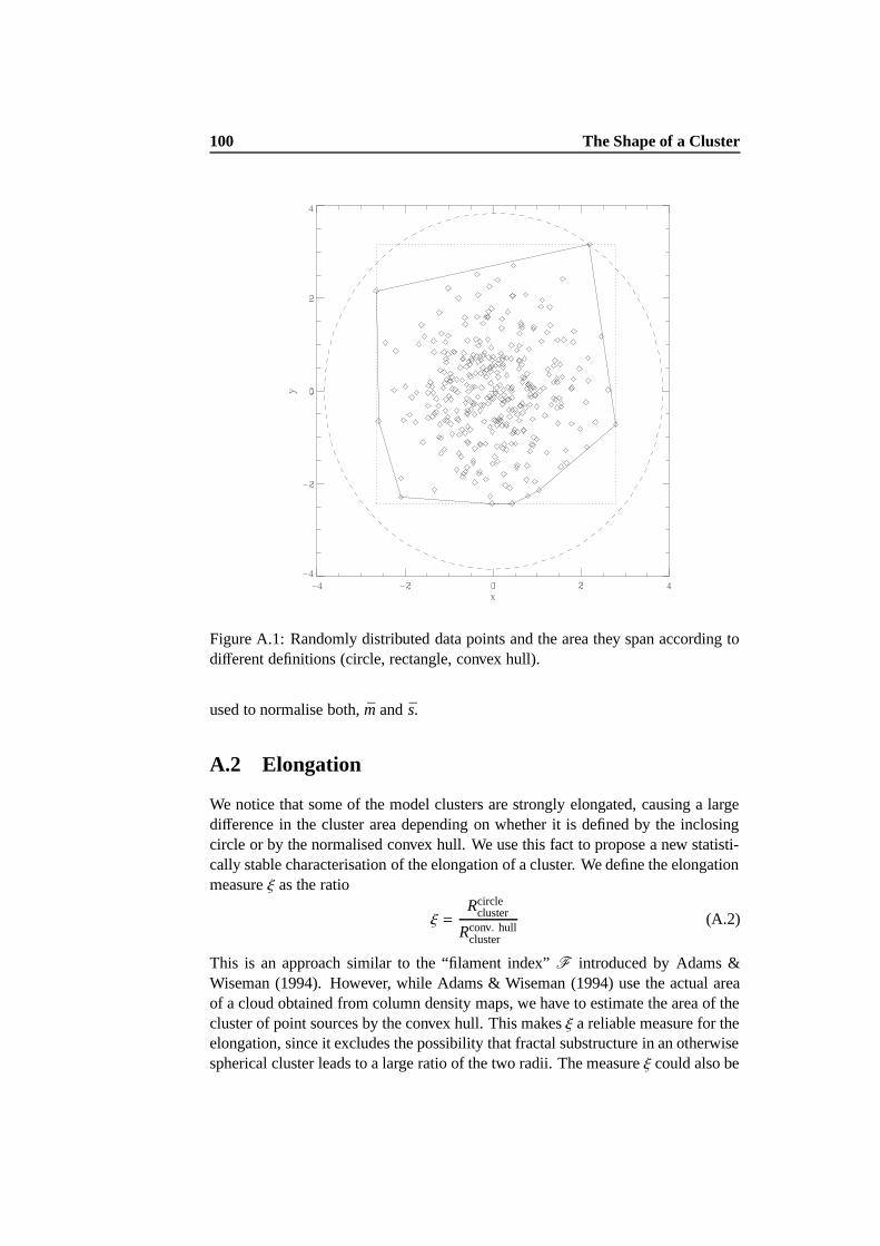
100 The Shape of a Cluster
Figure A.1: Randomly distributed data points and the area they span according todifferent definitions (circle, rectangle, convex hull).
used to normalise both, m and s.
A.2 Elongation
We notice that some of the model clusters are strongly elongated, causing a largedifference in the cluster area depending on whether it is defined by the inclosingcircle or by the normalised convex hull. We use this fact to propose a new statisti-cally stable characterisation of the elongation of a cluster. We define the elongationmeasure ξ as the ratio
ξ =Rcircle
cluster
Rconv. hullcluster
(A.2)
This is an approach similar to the “filament index” F introduced by Adams &Wiseman (1994). However, while Adams & Wiseman (1994) use the actual areaof a cloud obtained from column density maps, we have to estimate the area of thecluster of point sources by the convex hull. This makes ξ a reliable measure for theelongation, since it excludes the possibility that fractal substructure in an otherwisespherical cluster leads to a large ratio of the two radii. The measure ξ could also be
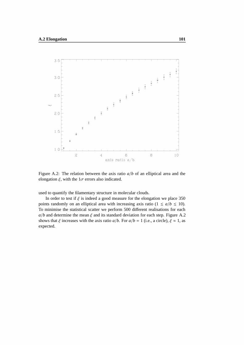
A.2 Elongation 101
Figure A.2: The relation between the axis ratio a/b of an elliptical area and theelongation ξ, with the 1σ errors also indicated.
used to quantify the filamentary structure in molecular clouds.In order to test if ξ is indeed a good measure for the elongation we place 350
points randomly on an elliptical area with increasing axis ratio (1 ≤ a/b ≤ 10).To minimise the statistical scatter we perform 500 different realisations for eacha/b and determine the mean ξ and its standard deviation for each step. Figure A.2shows that ξ increases with the axis ratio a/b. For a/b = 1 (i.e., a circle), ξ ≈ 1, asexpected.

102 The Shape of a Cluster

Appendix B
Minimum Spanning Trees
Minimum spanning trees are a construct of graph theory, related to the well-knowntravelling salesman problem. They have been discussed e.g. by Kruskal (1956),Prim (1957), Gower & Ross (1969), or Robins et al. (2000). Astrophysical ap-plications have been discussed mostly for the analysis of galaxy clusters, e.g. byBarrow et al. (1985), Adami & Mazure (1999), or Doroshkevich et al. (2004).Some details are given below.
B.1 Definitions
A graph G = (X, E) is a structure consisting of a finite set of points X = x1, x2, ...called vertices or nodes and a list of pairs of vertices E = (xi, x j) called edges. Aweighted graph has a weight or cost assigned to each edge. A graph is connected ifthere is a sequence of edges (a path) joining any point to any other point. A tree isa connected graph without closed loops. A tree that contains all the vertices fromthe original graph is called a spanning tree. The minimum spanning tree (MST),finally, is the spanning tree with the minimum total weight. The MST is unique.If some edges have exactly the same weight, the network may not be unique, asthe vertices may be connected in different ways, but the total edge length and thedistribution of edge lengths are always the same.
In our case, the vertices are the positions of the YSOs, and the weight of anedge is the Euclidean distance between the two points connected by that edge.
B.2 Algorithm
There are several ways to construct a MST. The two most popular algorithms bothwork iteratively. At any stage every edge of the MST belongs to one of two sets:Set A contains the edges assigned to the MST, set B those not assigned. Kruskal’salgorithm (Kruskal 1956; named Algorithm I in Gower & Ross 1969) assigns iter-atively to A the shortest edge in B which does not form a closed loop with any ofthe edges already in A. Initially A is empty, iteration stops when A contains (n− 1)
103
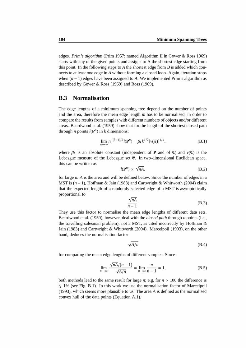
104 Minimum Spanning Trees
edges. Prim’s algorithm (Prim 1957; named Algorithm II in Gower & Ross 1969)starts with any of the given points and assigns to A the shortest edge starting fromthis point. In the following steps to A the shortest edge from B is added which con-nects to at least one edge in A without forming a closed loop. Again, iteration stopswhen (n − 1) edges have been assigned to A. We implemented Prim’s algorithm asdescribed by Gower & Ross (1969) and Ross (1969).
B.3 Normalisation
The edge lengths of a minimum spanning tree depend on the number of pointsand the area, therefore the mean edge length m has to be normalised, in order tocompare the results from samples with different numbers of objects and/or differentareas. Beardwood et al. (1959) show that for the length of the shortest closed paththrough n points l(Pn) in k dimensions:
limn→∞
n−(k−1)/k l(Pn) = βkk1/2[v(E)]1/k , (B.1)
where βk is an absolute constant (independent of P and of E) and v(E) is theLebesgue measure of the Lebesgue set E. In two-dimensional Euclidean space,this can be written as
l(Pn) ∝√
nA, (B.2)
for large n. A is the area and will be defined below. Since the number of edges in aMST is (n− 1), Hoffman & Jain (1983) and Cartwright & Whitworth (2004) claimthat the expected length of a randomly selected edge of a MST is asymptoticallyproportional to √
nAn − 1
. (B.3)
They use this factor to normalise the mean edge lengths of different data sets.Beardwood et al. (1959), however, deal with the closed path through n points (i.e.,the travelling salesman problem), not a MST, as cited incorrectly by Hoffman &Jain (1983) and Cartwright & Whitworth (2004). Marcelpoil (1993), on the otherhand, deduces the normalisation factor
√
A/n (B.4)
for comparing the mean edge lengths of different samples. Since
limn→∞
√nA/(n − 1)√
A/n= lim
n→∞n
n − 1= 1, (B.5)
both methods lead to the same result for large n; e.g. for n > 100 the difference is. 1% (see Fig. B.1). In this work we use the normalisation factor of Marcelpoil(1993), which seems more plausible to us. The area A is defined as the normalisedconvex hull of the data points (Equation A.1).
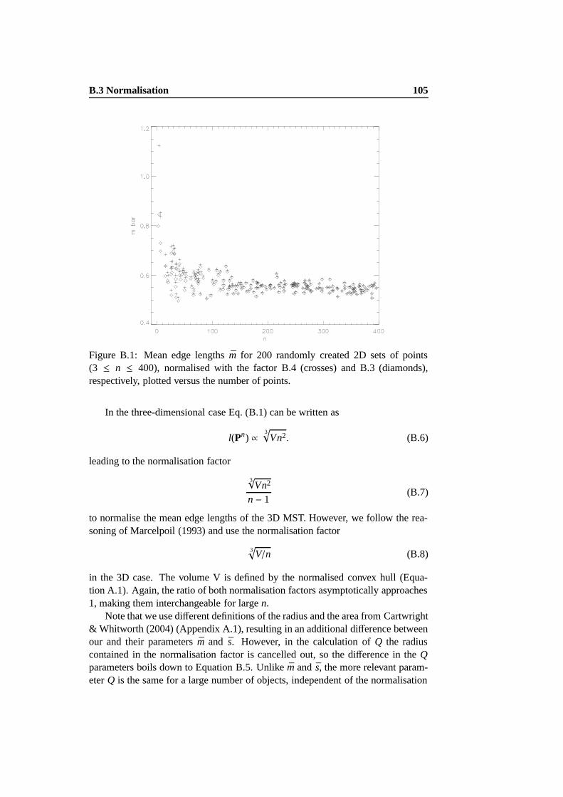
B.3 Normalisation 105
Figure B.1: Mean edge lengths m for 200 randomly created 2D sets of points(3 ≤ n ≤ 400), normalised with the factor B.4 (crosses) and B.3 (diamonds),respectively, plotted versus the number of points.
In the three-dimensional case Eq. (B.1) can be written as
l(Pn) ∝ 3√
Vn2. (B.6)
leading to the normalisation factor
3√Vn2
n − 1(B.7)
to normalise the mean edge lengths of the 3D MST. However, we follow the rea-soning of Marcelpoil (1993) and use the normalisation factor
3√
V/n (B.8)
in the 3D case. The volume V is defined by the normalised convex hull (Equa-tion A.1). Again, the ratio of both normalisation factors asymptotically approaches1, making them interchangeable for large n.
Note that we use different definitions of the radius and the area from Cartwright& Whitworth (2004) (Appendix A.1), resulting in an additional difference betweenour and their parameters m and s. However, in the calculation of Q the radiuscontained in the normalisation factor is cancelled out, so the difference in the Qparameters boils down to Equation B.5. Unlike m and s, the more relevant param-eter Q is the same for a large number of objects, independent of the normalisation

106 Minimum Spanning Trees
method. To allow comparison, we list the parameters computed using the normali-sation factor and the cluster radius according to Cartwright & Whitworth (2004) inTable 8.1 as well.
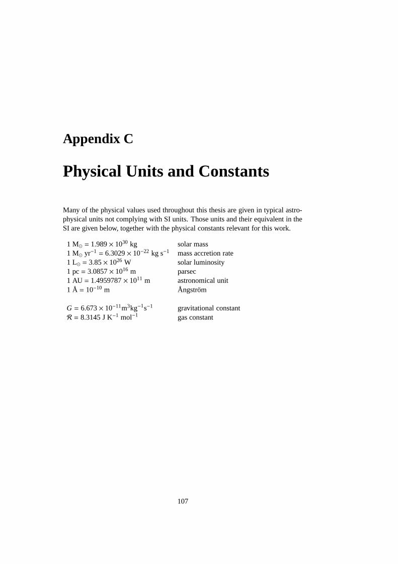
Appendix C
Physical Units and Constants
Many of the physical values used throughout this thesis are given in typical astro-physical units not complying with SI units. Those units and their equivalent in theSI are given below, together with the physical constants relevant for this work.
1 M = 1.989 × 1030 kg solar mass1 M yr−1 = 6.3029 × 10⁻²² kg s−1 mass accretion rate1 L = 3.85 × 1026 W solar luminosity1 pc = 3.0857 × 10¹⁶ m parsec1 AU = 1.4959787 × 10¹¹ m astronomical unit1 Å = 10−10 m Ångstrom
G = 6.673 × 10⁻¹¹m3kg−1s−1 gravitational constantR = 8.3145 J K−1 mol−1 gas constant
107

108 Physical Units and Constants
Bibliography
Adami, C., & Mazure, A. 1999, A&AS, 134, 393
Adams, F. C., & Fatuzzo, M. 1996, ApJ, 464, 256
Adams, F. C., & Myers, P. C. 2001, ApJ, 553, 744
Adams, F. C., & Wiseman, J. J. 1994, ApJ, 435, 693
Adams, F. C., Lada, C. J., & Shu, F. H. 1987, ApJ, 312, 788
Andre, P., Ward-Thompson, D., & Barsony, M. 1993, ApJ, 406, 122
Andre, P., Motte, F., & Bacmann, A. 1999, ApJ, 513, L57
Andre, P., Ward-Thompson, D., & Barsony, M. 2000, in Protostars and Planets IV,eds. V. Mannings, A. P. Boss, & S. S. Russell (Tucson: Univ. Arizona Press), 59
Bacmann, A., Andre, P., Puget, J.-L., et al. 2000, A&A, 361, 555
Bacmann, A., Lefloch, B., Ceccarelli, C., et al. 2002, A&A, 389, L6
Ballesteros-Paredes, J. 2004, Ap&SS, 289, 243
Ballesteros-Paredes, J., & Mac Low, M.-M. 2002, ApJ, 570, 734
Ballesteros-Paredes, J., & Hartmann, L. 2006, Rev. Mex. Astron. Astrofıs., sub-mitted (astro-ph/0605268)
Ballesteros-Paredes, J., Vazquez-Semadeni, E., & Scalo, J. 1999a, ApJ, 515, 286
Ballesteros-Paredes, J., Hartmann, L., & Vazquez-Semadeni, E. 1999b, ApJ, 527,285
Ballesteros-Paredes, J., Klessen, R. S., & Vazquez-Semadeni, E. 2003, ApJ, 592,188
Barber, C. B., Dobkin, D. P., & Huhdanpaa, H. T. 1996, ACM Transactions onMathematical Software, 22, 469, http://www.qhull.org
Barrow, J. D., Bhavsar, S. P., & Sonoda, D. H. 1985, MNRAS, 216, 17
109
110 BIBLIOGRAPHY
Basu, S. 1997, ApJ, 485, 240
Bate, M. R., & Bonnell, I. A. 2005, MNRAS, 356, 1201
Bate, M. R., & Burkert, A. 1997, MNRAS, 288, 1060
Bate, M. R., Bonnell, I. A., & Price, N. M. 1995, MNRAS, 277, 362
Bate, M. R., Clarke, C. J., & McCaughrean, M. J. 1998, MNRAS, 297, 1163
Bate, M. R., Bonnell, I. A., & Bromm, V. 2002, MNRAS, 332, L65
Bate, M. R., Bonnell, I. A., & Bromm, V. 2003, MNRAS, 339, 577
Beardwood, J., Halton, J. H., & Hammersley, J. M. 1959, Proc. Cambridge Philo-sophical Society, 55, 299
Behrend, R., & Maeder, A. 2001, A&A, 373, 190
Belloche, A., Andre, P., Despois, D., & Blinder, S. 2002, A&A, 393, 927
Benz, W. 1990, in The Numerical Modelling of Nonlinear Stellar Pulsations, ed.J. R. Buchler (Dordrecht: Kluwer), 269
Beuther, H., Schilke, P., Sridharan, T. K., et al. 2002a, A&A, 383, 892
Beuther, H., Schilke, P., Gueth, F., et al. 2002b, A&A, 387, 931
Bica, E., Dutra, C. M., & Barbuy, B. 2003, A&A, 397, 177
Blitz, L. 1993, in Protostars and Planets III, eds. E. H. Levy, & J. I. Lunine (Tucson:Univ. Arizona Press), 125
Blitz, L. 2001, Interstellar Molecular Clouds, in Encyclopedia of Astronomy andAstrophysics, http://www.ency-astro.com (London: Institute of PhysicsPublishing and Nature Publishing Group)
Blitz, L., & Williams, J. P. 1999, in The Origin of Stars and Planetary Systems,eds. C. J. Lada & N. D. Kylafis (Dordrecht: Kluwer Academic Publishers), 3
Bodenheimer, P., & Sweigart, A. 1968, ApJ, 152, 515
Bonnell, I. A., Bate, M. R., Clarke, C. J., & Pringle, J. E. 1997, MNRAS, 285, 201
Bonnell, I. A., Bate, M. R., Clarke, C. J., & Pringle, J. E. 2001a, MNRAS, 323,785
Bonnell, I. A., Clarke, C. J., Bate, M. R., & Pringle, J. E. 2001b, MNRAS, 324,573
Bonnell, I. A., Bate, M. R., & Vine, S. G. 2003, MNRAS, 343, 413
BIBLIOGRAPHY 111
Bonnell, I. A., Vine, S. G., & Bate, M. R. 2004, MNRAS, 349, 735
Bonnell, I. A., Dobbs, C. L., Robitaille, T. P., & Pringle, J. E. 2006, MNRAS, 365,37
Bontemps, S., Andre, P., Terebey, S., & Cabrit, S. 1996, A&A, 311, 858
Bontemps, S., Andre, P., Kaas, A. A., et al. 2001, A&A, 372, 173
Boogert, A. C. A., Hogerheijde, M. R., & Blake, G. A. 2002, ApJ, 568, 761
Bourke, T. L., Myers, P. C., Robinson, G., & Hyland, A. R. 2001, ApJ, 554, 916
Brown, D. W., & Chandler, C. J. 1999, MNRAS, 303, 855
Calvet, N., Muzerolle, J., Briceno, C., et al. 2004, AJ, 128, 1294
Cambresy, L., Copet, E., Epchtein, N., et al. 1998, A&A, 338, 977
Cartwright, A., & Whitworth, A. P. 2004, MNRAS, 348, 589
Castets, A., & Langer, W. D. 1995, A&A, 294, 835
Ceccarelli, C., Castets, A., Caux, E., et al. 2000, A&A, 355, 1129
Chandler, C. J., & Richer, J. S. 2000, ApJ, 530, 851
Chen, H., Myers, P. C., Ladd, E. F., & Wood, D. O. S. 1995, ApJ, 445, 377
Clark, P. C., Bonnell, I. A., Zinnecker, H., & Bate, M. R. 2005, MNRAS, 359, 809
Clarke, C. J. 1999, MNRAS, 307, 328
Crutcher, R. M. 1999, ApJ, 520, 706
Dale, J. E., Bonnell, I. A., Clarke, C. J., & Bate, M. R. 2005, MNRAS, 358, 291
Davis, C. J., Smith, M. D., & Moriarty-Schieven, G. H. 1998, MNRAS, 299, 825
Delgado-Donate, E. J., Clarke, C. J., & Bate, M. R. 2003, MNRAS, 342, 928
Delgado-Donate, E. J., Clarke, C. J., Bate, M. R., & Hodgkin, S. T. 2004, MNRAS,351, 617
Di Francesco, J., Myers, P. C., Wilner, D. J., Ohashi, N., & Mardones, D. 2001,ApJ, 562, 770
Dib, S., Bell, E., & Burkert, A. 2006, ApJ, 638, 797
Diehl, R., Halloin, H., Kretschmer, K., et al. 2006, Nature, 439, 45
Doroshkevich, A., Tucker, D. L., Allam, S., & Way, M. J. 2004, A&A, 418, 7
112 BIBLIOGRAPHY
Dussert, C., Rasigni, G., Rasigni, M., Palmari, J., & Llebaria, A. 1986, Phys. Rev.B, 34, 3528
Dziourkevitch, N., Elstner, D., & Rudiger, G. 2004, A&A, 423, L29
Elmegreen, B. G. 1993, ApJ, 419, L29
Elmegreen, B. G. 2000, ApJ, 530, 277
Elmegreen, B. G. 2002, ApJ, 577, 206
Elmegreen, B. G., & Scalo, J. 2004, ARA&A, 42, 211
Elmegreen, B. G., Efremov, Y., Pudritz, R. E., & Zinnecker, H. 2000, in Protostarsand Planets IV, eds. V. Mannings, A. P. Boss, & S. S. Russell (Tucson: Univ.Arizona Press), 179
Falgarone, E., Phillips, T. G., & Walker, C. K. 1991, ApJ, 378, 186
Feigelson, E. D., & Montmerle, T. 1999, ARA&A, 37, 363
Figer, D. F. 2005, Nature, 434, 192
Foster, P. N., & Chevalier, R. A. 1993, ApJ, 416, 303
Franco, J., & Carraminana, A., eds., 1999, Interstellar Turbulence (Cambridge:Cambridge University Press)
Froebrich, D. 2005, ApJS, 156, 169
Froebrich, D., Smith, M. D., Hodapp, K.-W., & Eisloffel, J. 2003, MNRAS, 346,163
Froebrich, D., Scholz, A., Eisloffel, J., & Murphy, G. C. 2005, A&A, 432, 575
Froebrich, D., Schmeja, S., Smith, M. D., & Klessen, R. S. 2006, MNRAS, 368,435
Furlan, E., Calvet, N., D’Alessio, P., et al. 2005, ApJ, 628, L65
Gawryszczak, A. J., Goodwin, S. P., Burkert, A., & Rozyczka, M. 2005, in Proto-stars and Planets V, LPI Contribution No. 1286 (Houston: Lunar and PlanetaryInstitute), Abstract #8102 (CD-ROM)
Gingold, R. A., & Monaghan, J. J. 1977, MNRAS, 181, 375
Gladwin, P. P., Kitsionas, S., Boffin, H. M. J., & Whitworth, A. P. 1999, MNRAS,302, 305
Gomez, M., Hartmann, L., Kenyon, S. J., & Hewett, R. 1993, AJ, 105, 1927
BIBLIOGRAPHY 113
Gomez de Castro, A. I. 1998, in Ultraviolet Astrophysics Beyond the IUE FinalArchive, eds. W. Wamsteker and R. Gonzalez Riestra, ESA SP-413, 59
Goodwin, S. P., Whitworth, A. P., & Ward-Thompson, D. 2004a, A&A, 414, 633
Goodwin, S. P., Whitworth, A. P., & Ward-Thompson, D. 2004b, A&A, 423, 169
Gower, J. C., & Ross, G. J. S. 1969, Applied Statistics, 18, 54
Gras-Velazquez, A., & Ray, T. P. 2005, A&A, 443, 541
Greene, T. P., & Lada, C. J. 2002, AJ, 124, 2185
Grosso, N., Montmerle, T., Bontemps, S., Andre, P., & Feigelson, E. D. 2000,A&A, 359, 113
Gutermuth, R. A., Megeath, S. T., Pipher, J. L., et al. 2005, ApJ, 632, 397
Haikala, L. K., Harju, J., Mattila, K., & Toriseva, M. 2005, A&A, 431, 149
Hartigan, P., Edwards, S., & Ghandour, L. 1995, ApJ, 452, 736
Hartmann, L. 1998, Accretion processes in star formation (Cambridge: CambridgeUniversity Press)
Hartmann, L. 2002, ApJ, 578, 914
Hartmann, L. 2003, ApJ, 585, 398
Hartmann, L., Ballesteros-Paredes, J., & Bergin, E. A. 2001, ApJ, 562, 852
Heitsch, F., Mac Low, M.-M., & Klessen, R. S. 2001a, ApJ, 547, 280
Heitsch, F., Zweibel, E. G., Mac Low, M.-M., Li, P., & Norman, M. L. 2001b, ApJ,561, 800
Hennebelle, P., Whitworth, A. P., Gladwin, P. P., & Andre, P. 2003, MNRAS, 340,870
Henriksen, R., Andre, P., & Bontemps, S. 1997, A&A, 323, 549
Hillenbrand, L. A., & Hartmann, L. W. 1998, ApJ, 492, 540
Hirano, N., Kamazaki, T., Mikami, H., Ohashi, N., & Umemoto, T. 1999, in StarFormation 1999, ed. T. Nakamoto (Nobeyama: Nobeyama Radio Observatory),181
Hirano, N., Ohashi, N., Dobashi, K., Shinnaga, H., & Hayashi, M. 2003, in Proc.of the IAU 8th Asian-Pacific Regional Meeting, Vol. II, eds. S. Ikeuchi, J. Hearn-shaw, & T. Hanawa, ASP Conf. Ser., 289, 141
114 BIBLIOGRAPHY
Hollenbach, D. J., Werner, M. W., & Salpeter, E. E. 1971, ApJ, 163, 165
Hoffman, R., & Jain, A. K. 1983, Pattern Recognition Letters, 1, 175
Hogerheijde, M. 1998, PhD thesis, Leiden University
Hubber, D. A., Goodwin, S. P., & Whitworth, A. P. 2006, A&A, 450, 881
Hunter, C. 1977, ApJ, 218, 834
Hunter, J. H., & Fleck, R. C. 1982, ApJ, 256, 505
Hurt, R. L., & Barsony, M. 1996, ApJ, 460, L45
Jappsen, A.-K., & Klessen, R. S. 2004, A&A, 423, 1
Jappsen, A.-K., Klessen, R. S., Larson, R. B., Li,Y., & Mac Low, M.-M. 2005,A&A, 435, 611
Jayawardhana, R., Hartmann, L., & Calvet, N. 2001, ApJ, 548, 310
Jeans, J. H. 1902, Phil. Trans. R. Soc. London, Ser. A, 199, 1
Johnstone, D., Wilson, C. D., Moriarty-Schieven, G. et al. 2000, ApJ, 545, 327
Johnstone, D., Di Francesco, J., & Kirk, H. 2004, ApJ, 611, L45
Kaas, A. A., & Bontemps, S. 2001, in From Darkness to Light: Origin and Evo-lution of Young Stellar Clusters, eds. T. Montmerle & P. Andre, ASP Conf. Ser.243, 367
Kaas, A. A., Olofsson, G., Bontemps, S., et al. 2004, A&A, 421, 623
Kamegai, K., Ikeda, M., Maezawa, H., et al. 2003, ApJ, 589, 378
Kitsionas, S. 2000, PhD thesis, University of Wales
Kitsionas, S., & Whitworth, A. P. 2002, MNRAS, 330, 129
Klein, R. I., Fisher, R., & McKee, C. F. 2004, in Gravitational Collapse: FromMassive Stars to Planets, eds. G. Garcıa-Segura, G. Tenorio-Tagle, J. Franco, &H. W. Yorke, Rev. Mex. Astron. Astrofıs. (Ser. de Conf.), 22, 3
Klessen, R. S. 1997, MNRAS, 292, 11
Klessen, R. S. 2001a, ApJ, 550, L77
Klessen, R. S. 2001b, ApJ, 556, 837
Klessen, R. S. 2003, Rev. Mod. Astr., 16, 23
Klessen, R. S., & Burkert, A. 2000, ApJS, 128, 287
BIBLIOGRAPHY 115
Klessen, R. S., & Burkert, A. 2001, ApJ, 549, 386
Klessen, R. S., & Kroupa, P. 2001, A&A, 372, 105
Klessen, R. S., Heitsch, F., & Mac Low, M.-M., 2000, ApJ, 535, 887
Klessen, R. S., Ballesteros-Paredes, J., Vazquez-Semadeni, E., & Duran-Rojas, C.2005, ApJ, 620, 786
Kolmogorov, A. N. 1941, Doklady Akademii Nauk SSSR, 30, 301 (reprinted 1991,Royal Soc. London Proc. Ser. A, 434, 9)
Konigl, A., & Pudritz, R. E. 2000, in Protostars and Planets IV, eds. V. Mannings,A. P. Boss, & S. S. Russell (Tucson: Univ. Arizona Press), 759
Kroupa, P. 2002, Science, 295, 82
Kruskal, J. B., Jr. 1956, Proc. Amer. Math. Soc., 7, 48
Kushnir, D., Galun, M., & Brandt, A. 2006, Pattern Recognition, in press
Lada, C. J. 1987, in Star Forming Regions, IAU Symp., 115, 1
Lada, C. J. 2001, Young Stellar Objects, in Encyclopedia of Astronomy and As-trophysics, http://www.ency-astro.com (London: Institute of Physics Pub-lishing and Nature Publishing Group)
Lada, C. J., & Lada, E. A. 2003, ARA&A, 41, 57
Lada, C. J., & Wilking, B. A. 1984, ApJ, 287, 610
Langer, W. D., van Dishoeck, E. F., Bergin, E. A., et al. 2000, in Protostars andPlanets IV, eds. V. Mannings, A. P. Boss, & S. S. Russell (Tucson: Univ. ArizonaPress), 29
Larson, R. B. 1969, MNRAS, 145, 271
Larson, R. B. 1981, MNRAS, 194, 809
Larson, R. B. 1985, MNRAS, 214, 379
Larson, R. B. 1995, MNRAS, 272, 213
Larson, R. B. 1999, in Star Formation 1999, ed. T. Nakamoto (Nobeyama: Nobe-yama Radio Observatory), 336
Larson, R. B. 2003, Rep. Prog. Phys., 66, 1651
Larson, R. B. 2005, MNRAS, 359, 211
Laughlin, G., & Rozyczka, M. 1996, ApJ, 456, 279
116 BIBLIOGRAPHY
Lee, C. W., & Myers, P. C. 1999, ApJS, 123, 233
Li, Z.-Y., & Nakamura, F. 2004, ApJ, 609, L83
Li, Y., Klessen, R. S., & Mac Low, M.-M. 2003, ApJ, 592, 975
Li, Y., Mac Low, M.-M., & Klessen, R. S. 2005, ApJ, 626, 823
Looney, L. W., Mundy, L. G., & Welch, W. J. 2003, ApJ, 592, 255
Lubow, S. H., & Pringle, J. E. 1993, MNRAS, 263, 701
Lucy, L. B. 1977, AJ, 82, 1013
Luhman, K. L., Stauffer, J. R., Muench, A. A., et al. 2003, ApJ, 593, 1093
Mac Low, M.-M. 1999, ApJ, 524, 169
Mac Low, M.-M. 2000, in Star Formation from the Small to the Large Scale, ES-LAB symposium 33, eds. F. Favata, A. Kaas, & A. Wilson, ESA SP-445, 457
Mac Low, M.-M., & Klessen, R. S. 2004, Rev. Mod. Phys., 76, 125
Mac Low, M.-M., & Ossenkopf, V. 2000, A&A, 353, 339
Mac Low, M.-M., Klessen, R. S., Burkert, A., & Smith, M. D. 1998, Phys. Rev.Lett., 80, 2754
Mac Low, M.-M., de Avillez, M. A., & Korpi, M. J. 2004, in How Does the GalaxyWork?, eds. E. J. Alfaro, E. Perez, & J. Franco, ASSL Vol. 315, 339
Marcelpoil, R. 1993, Analytical Cellular Pathology, 5, 177
Maret, S., Ceccarelli, C., Caux, E., Tielens, A. G. G. M., & Castets, A. 2002, A&A,395, 573
Massey, P., & Meyer, M. R. 2001, Stellar Masses, in Encyclopedia of Astron-omy and Astrophysics, http://www.ency-astro.com (London: Institute ofPhysics Publishing and Nature Publishing Group)
Masunaga, H., & Inutsuka, S. 2000, ApJ, 531, 350
McLaughlin, D. E., & Pudritz, R. E. 1997, ApJ, 476, 750
Megeath, S. T., Allen, L. E., Gutermuth, R. A., et al. 2004, ApJS, 154, 367
Megeath, S. T., Flaherty, K. M., Hora, J., et al. 2005, in Massive Star Birth: ACrossroads of Astrophysics, IAU Symp. 227, 383
Men’shchikov, A. B., & Henning, T. 1997, A&A, 318, 879
Mestel, L., & Spitzer, L., Jr. 1956, MNRAS, 116, 503
BIBLIOGRAPHY 117
Meyer, M. R., Adams, F. C., Hillenbrand, L. A., Carpenter, J. M., & Larson, R. B.2000, in Protostars and Planets IV, eds. V. Mannings, A. P. Boss, & S. S. Russell(Tucson: Univ. Arizona Press), 121
Mizuno, A., Onishi, T., Yonekura, Y., et al. 1995, ApJ, 445, L161
Mizuno, A., Hayakawa, T., Tachihara, K., et al. 1999, PASJ, 51, 859
Monaghan, J. J. 1985, Comp. Phys. Rep., 3, 71
Monaghan, J. J. 1992, ARA&A, 30, 543
Monaghan, J. J. 2001, J. Korean Astron. Soc., 34, 203
Morino, J.-I., Yamashita, T., Hasegawa, T., & Nakano, T. 1998, Nature, 393, 340
Motoyama, K., & Yoshida, T. 2003, MNRAS, 344, 461
Motte, F., & Andre, P. 2001, A&A, 365, 440
Motte, F., & Andre, P., & Neri, R. 1998, A&A, 336, 150
Muench, A. A., Lada, E. A., Lada, C. J., et al. 2003, AJ, 125, 2029
Muzerolle, J., Hillenbrand, L., Calvet, N., Briceno, C., & Hartmann, L. 2003, ApJ,592, 266
Muzerolle, J., Megeath, S. T., Gutermuth, R. A., et al. 2004, ApJS, 154, 379
Myers, P. C., & Ladd, E. F. 1993, ApJ, 413, L47
Myers, P. C., Adams, F. C., Chen, H., & Schaff, E. 1998, ApJ, 492, 703
Myers, P. C., Evans, N. J., II, & Ohashi, N. 2000, in Protostars and Planets IV, eds.V. Mannings, A. P. Boss, & S. S. Russell (Tucson: Univ. Arizona Press), 217
Nakano, T. 1998, ApJ, 494, 587
Narayanan, G., Walker, C. K., & Buckley, H. D. 1998, ApJ, 496, 292
Neuhauser, R., & Sterzik, M. 1997, Comm. Konkoly Obs., 100, 369
Ogino, S., Tomisaka, K., & Nakamura, F. 1999, PASJ, 51, 637
Olmi, L., & Testi, L. 2002, A&A, 392, 1053
Onishi, T., Mizuno, A., Kawamura, A., Ogawa, H., & Fukui, Y. 1996, ApJ, 465,815
Ossenkopf, V., & Mac Low, M.-M. 2002, A&A, 390, 307
118 BIBLIOGRAPHY
Padman, R., Bence, S., & Richer, J. 1997, in IAU Symp. 182: Herbig-Haro Flowsand the Birth of Stars, eds. B. Reipurth, & C. Bertout (Dordrecht: Kluwer Aca-demic Publishers), 123
Padoan, P. 1995, MNRAS, 277, 377
Padoan, P., & Nordlund, Å. 1999, ApJ, 526, 279
Padoan, P., & Nordlund, Å. 2002, ApJ, 576, 870
Palla, F., & Stahler, S. W. 2000, ApJ, 540, 255
Papaloizou, J. C. B., & Lin, D .N. C. 1995, ARA&A, 33, 505
Paul, J. 2001, in High Energy Gamma-Ray Astronomy, eds. F. A. Aharonian &H. J. Volk, American Institute of Physics Proc., 558, 183
Penston, M. V. 1969, MNRAS, 144, 425
Persi, P., Marenzi, A. R., Gomez, M., & Olofsson, G. 2001, A&A, 376, 907
Piontek, R. A., & Ostriker, E. C. 2004, ApJ, 601, 905
Piontek, R. A., & Ostriker, E. C. 2005, ApJ, 629, 849
Preibisch, T. 2003, A&A, 410, 951
Preibisch, T., & Zinnecker, H. 2002, AJ, 123, 1613
Preibisch, T., & Zinnecker, H. 2004, A&A, 422, 1001
Price, D. J. 2004, PhD thesis, University of Cambridge
Prim, R. C. 1957, Bell Systems Tech. J., 36, 1389
Pringle, J.E. 1981, ARA&A, 19, 137
Pudritz, R. E. 2002, Science, 295, 68
Quillen, A. C., Thorndike, S. L., Cunningham, A., et al. 2005, ApJ, 632, 941
Reach, W. T., Rho, J., Young, E., et al. 2004, ApJS, 154, 385
Reid, M. A., Pudritz, R. E., & Wadsley, J. 2002, ApJ, 570, 231
Reipurth, B., & Bally, J. 2001, ARA&A, 39, 403
Ridge, N. A., Wilson, T. L., Megeath, S. T., Allen, L. E., & Myers, P. C. 2003, AJ,126, 286
Ripley, B. D., & Rasson, J.-P. 1977, J. Appl. Prob., 14, 483
BIBLIOGRAPHY 119
Robins, V., Meiss, J. D., & Bradley, E. 2000, Physica D, 139, 276
Ross, G. J. S. 1969, Applied Statistics, 18, 103
Russell, H. N., Dugan, R. S., & Stewart, J. W. 1927, Astronomy: A revisionof Young’s Manual of Astronomy: II: Astrophysics and Stellar Astronomy(Boston: Ginn and Co.)
Salpeter, E. E. 1955, ApJ, 121, 161
Saraceno, P., Andre, P., Ceccarelli, C., Griffin, M., & Molinari, S. 1996, A&A,309, 827
Sasao, T. 1973, PASJ, 25, 1
Scalo, J. 1990, in Physical Processes in Fragmentation and Star Formation, eds.R. Capuzzo-Dolcetta, C. Chiosi, & A. di Fazio, ASSL Vol. 162, 151
Scalo, J., & Elmegreen, B. G. 2004, ARA&A, 42, 275
Schmeja, S., & Klessen, R. S. 2004, A&A, 419, 405
Schmeja, S., & Klessen, R. S. 2006, A&A, 449, 151
Schmeja, S., Klessen, R. S., & Froebrich, D. 2005, A&A, 437, 911
Shirley, Y. L., Evans, N. J., II, Rawlings, J. M. C., & Gregersen, E. M. 2000, ApJS,131, 249
Shu, F. H. 1977, ApJ, 214, 488
Shu, F. H. 1992, The Physics of Astrophysics, Volume II: Gas Dynamics (Sausal-ito: University Science Books)
Shu, F. H., Adams, F. C., & Lizano, S. 1987, ARA&A, 25, 23
Shu, F. H., Li, Z.-Y., & Allen, A. 2004, ApJ, 601, 930
Sigalotti, L. di G., de Felice, F., & Sira, E. 2002, A&A, 395, 321
Singh, S., Ma, C.-P., & Arons, J. 2004, Phys. Rev. D, 69, 3003
Smith, M. D. 1998, Ap&SS, 261, 169
Smith, M. D. 2000, Irish Astron. J., 27, 25
Smith, M. D. 2002, in The Origins of Stars and Planets: the VLT view, ESO As-trophysics Symposia, eds. J. Alves & M. McCaughrean, CD-ROM
Smith, M. D. 2004, The Origin of Stars (London: Imperial College Press)
Stahler, S. W., & Palla, F. 2004, The Formation of Stars (Weinheim: Wiley-VCH)
120 BIBLIOGRAPHY
Stanke, T. 2000, PhD thesis, Universitat Potsdam
Stanke, T., Smith, M. D., Gredel, R., & Khanzadyan, T. 2006, A&A, 447, 609
Stone, J. M., Ostriker, E. C., & Gammie, C. F. 1998, ApJ, 508, L99
Strong, A. W., Bignami, G. F., Caraveo, P. A., et al. 1982, A&A, 115, 404
Stutzki, J., Bensch, F., Heithausen, A., Ossenkopf, V., & Zielinsky, M. 1998, A&A,336, 697
Tassis, K., & Mouschovias, T. C. 2004, ApJ, 616, 283
Taylor, S. D., Morata, O., & Williams, D. A. 1996, A&A, 313, 269
Testi, L., & Sargent, A. I. 1998, ApJ, 508, L91
Tomisaka, K. 1996, PASJ, 48, L97
Umemoto, T., Saito, M., Yang, J., & Hirano, N. 1999, in Star Formation 1999, ed.T. Nakamoto (Nobeyama: Nobeyama Radio Observatory), 227
van Dishoeck, E. F. 2004, ARA&A, 42, 119
van Dishoeck, E. F., & Blake, G. A. 1998, ARA&A, 36, 317
Vazquez-Semadeni, E., Ostriker, E. C., Passot, T., Gammie, C., & Stone, J. 2000,in Protostars and Planets IV, eds. V. Mannings, A. P. Boss, & S. S. Russell (Tuc-son: Univ. Arizona Press), 3
Vazquez-Semadeni, E., Ballesteros-Paredes, J., & Klessen, R. S. 2003, ApJ, 585,L131
Vazquez-Semadeni, E., Kim, J., Shadmehri, M., & Ballesteros-Paredes, J. 2005,ApJ, 618, 344
Visser, A. E., Richer, J. S., & Chandler, C. J. 2002, AJ, 124, 2756
Vogt, H. 1926, Astron. Nachr., 226, 301
Wada, K., Meurer, G., & Norman, C. A. 2002, ApJ, 577, 197
Walker, C. K., Lada, C. J., Young, E. T., Maloney, P. R., & Wilking, B. A. 1986,ApJ, 309, L47
Walter, F. M. 1986, ApJ, 306, 573
White, R. J., & Hillenbrand, L. A. 2004, ApJ, 616, 998
Whitworth, A. P., & Ward-Thompson, D. 2001, ApJ, 547, 317
BIBLIOGRAPHY 121
Whitworth, A. P., Bhattal, A. S., Francis, N., & Watkins, S. J. 1996, MNRAS, 283,1061
Williams, J. P. 1999, in Interstellar Turbulence, eds. J. Franco & A. Carraminana(Cambridge: Cambridge University Press), 190
Williams, J. P., De Geus, E. J., & Blitz, L. 1994, ApJ, 428, 693
Williams, J. P., Blitz, L., & McKee, C. F. 2000, in Protostars and Planets IV, eds.V. Mannings, A. P. Boss, & S. S. Russell (Tucson: Univ. Arizona Press), 97
Wolf-Chase, G., Moriarty-Schieven, G., Fich, M., & Barsony, M. 2003, MNRAS,344, 809
Wuchterl, G., & Klessen, R. S. 2001, ApJ, 560, L185
Wuchterl, G., & Tscharnuter, W. M. 2003, A&A, 398, 1081
Yokogawa, S., Kitamura, Y., Momose, M., & Kawabe, R. 2003, in Proc. of the IAU8th Asian-Pacific Regional Meeting, Vol. II, eds. S. Ikeuchi, J. Hearnshaw, & T.Hanawa, ASP Conf. Ser., 289, 239
Young, C. H., & Evans, N. J. 2005, ApJ, 627, 293
Young, C. H., Shirley, Y. L., Evans, N. J., II, & Rawlings, J. M. C. 2003, ApJS,145, 111
Young, C. H., Jørgensen, J. K., Shirley, Y. L., et al. 2004, ApJS, 154, 396
Yu, K. C., Billawala, Y., Smith, M. D., Bally, J., & Butner, H. M. 2000, AJ, 120,1974
Additional References
Textbooks
Barlow, R. J. 1989, Statistics: A Guide to the Use of Statistical Methods inthe Physical Sciences (Chichester: John Wiley & Sons)
Karttunen, H., Kroger, P., Oja, H., Poutanen, M., & Donner, K. J., eds., 2003,Fundamental Astronomy (Berlin: Springer), 4th ed.
Voigt, H. H. 1991, Abriss der Astronomie (Mannheim: BI Wissenschaftsver-lag)
Data bases and websites
Smithsonian/NASA Astrophysics Data System Abstract Servicehttp://adsabs.harvard.edu
arXiv.org e-Print archivehttp://arxiv.org
Protostars Database at the Dublin Institute for Advanced Studieshttp://www.dias.ie/protostars/
SIMBAD Astronomical Databasehttp://simbad.u-strasbg.fr
MathWorld – A Wolfram Web Resourcehttp://mathworld.wolfram.com
Eric Weisstein’s World of Physicshttp://scienceworld.wolfram.com/physics/
LEO English-German dictionaryhttp://dict.leo.org
Merriam-Webster Onlinehttp://www.m-w.com/
122

Publications Related to this Work
Refereed Publications
D. Froebrich, S. Schmeja, M. D. Smith, & R. S. Klessen: Evolution ofClass 0 protostars: Models vs. observations. MNRAS, 368, 435 (2006)
S. Schmeja, & R. S. Klessen: Evolving structures of star-forming clusters.A&A, 449, 151 (2006)
S. Schmeja, R. S. Klessen, & D. Froebrich: Number ratios of young stellarobjects in embedded clusters. A&A, 437, 911-918 (2005)
S. Schmeja, & R. S. Klessen: Protostellar mass accretion rates from gravo-turbulent fragmentation. A&A, 419, 405-417 (2004)
Conference Proceedings and Abstracts
D. Froebrich, S. Schmeja, M. D. Smith, & R. S. Klessen: Comparing Prop-erties of Class 0 Protostars with Model Predictions. In Protostars and Plan-ets V, Abstract #8039, Lunar and Planetary Institute, Houston (CD-ROM)(2005)
S. Schmeja, & R. S. Klessen: Analysing the Structures of Young Star Clus-ters. In Protostars and Planets V, Abstract #8397, Lunar and Planetary Insti-tute, Houston (CD-ROM) (2005)
S. Schmeja, & R. S. Klessen: Mass Accretion of Protostars: A Highly Dy-namical Process. In Protostars and Planets V, Abstract #8402, Lunar andPlanetary Institute, Houston (CD-ROM) (2005)
S. Schmeja, R. S. Klessen, D. Froebrich, & M. D. Smith: Star Formationfrom Gravoturbulent Fragmentation: Mass Accretion and Evolution of Pro-tostars. In “Low-mass stars and brown dwarfs: IMF, accretion and activity”,eds. L. Testi & A. Natta, Mem. Soc. Astron. Ital., 76, 193-198 (2005)
123
124 BIBLIOGRAPHY
S. Schmeja, R. S. Klessen, D. Froebrich, & M. D. Smith: Star Formationin Turbulent Molecular Clouds: Mass Accretion and Evolution of Proto-stars. Astron. Nachr. 325, Suppl. Issue 1 (Short Contributions AG/CAS 2004Prague), 26-27 (2004)
S. Schmeja, & R. S. Klessen: Time-varying protostellar mass accretionrates. In Proceedings of the JENAM 2003 Minisymposium “Early Phasesof Star Formation”, Baltic Astronomy 13, 381-385 (2004)
List of Acronyms
CTTS classical T Tauri starFIR far infraredGMC giant molecular cloudIMF initial mass functionIR infraredISM interstellar mediumISO Infrared Space ObservatoryKS Kolmogorov-Smirnov (test)MC molecular cloudMHD magnetohydrodynamicsMIR mid infraredMSDC mean surface density of companionsMST minimum spanning treeNIR near infraredPMS pre-main sequenceSED spectral energy distributionSFE star formation efficiencySFR star formation rateSI Systeme International d’UnitesSIS singular isothermal sphereSPH smoothed particle hydrodynamicsUV ultravioletWTTS weak-line T Tauri starXMM X-ray Multi-MirrorYSO young stellar object
125

126 BIBLIOGRAPHY
Acknowledgements/Danksagung
• First of all, I would like to thank my advisor Ralf Klessen. From him I learntmany things about star formation and hydrodynamics, he almost always hadtime for questions and discussions, and he provided the numerical simula-tions on which this work is based on.
• I always enjoyed being with the AIP people, especially the members of thestar formation group and the other “inhabitants” of the Schwarzschildhaus.In particular I wish to thank Nicolas (for discussions on Brown Dwarves,IDL and Hertha BSC), Katharina (for coffee & cookies and giving me somany rides from the AIP to the University), Spyros (for coffee & cookiesand in particular for proof-reading this thesis), and Andreas (for his LATEX-help). Ein herzlicher Dank geht auch an die EDV-Abteilung, insbesondereMario Dionies, fur zuverlassige Abhilfe bei Computerproblemen, sowie andie Bibliothekarin, Regina von Berlepsch, fur das rasche Beschaffen vonArtikeln auch aus “exotischen” Zeitschriften.
• I wish to thank my collaborators Dirk Froebrich (Dublin Institute for Ad-vanced Studies), Michael Smith (Armagh Observatory, now at the Universityof Kent), and Dan Kushnir (Weizmann Institute of Science). I am particu-larly grateful to Dirk and the staff at DIAS for their warm hospitality duringmy stay in Dublin.
• My position was funded by the Emmy Noether Programme of the DeutscheForschungsgemeinschaft (grant no. KL1358/1). I acknowledge additionalfinancial support for visits and to attend conferences from the AstronomischeGesellschaft, the organisers of the JENAM 2003 meeting in Budapest, theDublin Institute for Advanced Studies, and the Insitute for Pure and AppliedMathematics, University of California at Los Angeles.
• Ich danke den Potsdamer Schmejas, die mir nicht nur in meinen ersten Wo-chen in Potsdam ein Dach uber dem Kopf gegeben haben, sondern auchmaßgeblich dafur verantwortlich sind, dass ich mich in Potsdam bzw. Ba-belsberg in kurzester Zeit heimisch gefuhlt habe. Zu letzterem beigetragenhaben u.a. auch Roland und Anja, die Besucher des Doktorandenstamm-tisches und die Drachenbootpaddler des Treibgut-Teams.
127

128 BIBLIOGRAPHY
• Ein weiteres Dankeschon gilt meinen Eltern, die mich immer unterstutzthaben. Besonders dankbar bin ich, dass mir auch in Potsdam viele Freundeaus Innsbruck und dem Rest der Welt nahe geblieben sind.
• Last not least: Danke Steffi. Turn around, every now and then I get a littlebit terrified but then I see the look in your eyes ...