QUALITY CONTROL OF OPERATIONAL DATA FROM WASTEWATER ...

Doctoral Thesis

QUALITY CONTROL OF OPERATIONAL DATA FROM

WASTEWATER TREAMTENT PLANTS

submitted in satisfaction of the requirements for the degree of Doctor of Science in Civil Engineering

of the Vienna University of Technology, Faculty of Civil Engineering

Dissertation

ÜBERPRÜFUNG DER BETRIEBSDATEN VON ABWASSERREINIGUNGSANLAGEN

ausgeführt zum Zwecke der Erlangung des akademischen Grades eines

Doktors der technischen Wissenschaft eingereicht an der Technischen Universität Wien Fakultät für Bauingenieurwesen

von

Dipl.-Ing. André Spindler Matrikelnummer 0627171

Zur Quelle 9, 01731 Kreischa OT Saida, Deutschland

Gutachter: Em.O.Univ.Prof. Dipl.-Ing. Dr.techn. Dr.h.c. Helmut Kroiss Institut für Wassergüte, Ressourcenmanagement und Abfallwirtschaft, TU Wien Karlsplatz 13/226-1, 1040 Wien Gutachter: Prof. Peter A. Vanrolleghem, MSc, PhD Department of civil engineering and water engineering, Université Laval Pavillon Adrien-Pouliot - 1065, Médecine avenue, Office 2974, Québec (Québec) - Canada - G1V 0A6 Wien, Jänner 2015 ________________________

Die approbierte Originalversion dieser Dissertation ist in der Hauptbibliothek der Technischen Universität Wien aufgestellt und zugänglich. http://www.ub.tuwien.ac.at

The approved original version of this thesis is available at the main library of the Vienna University of Technology.

http://www.ub.tuwien.ac.at/eng

ABSTRACT

This thesis deals with questions of data quality control based on the principles

of mass conservation. The focus is entirely on operational data from

wastewater treatment plants. The goal was to provide a practically applicable

method for the determination of well-balanced time periods associated with

high data quality in historic data. CUSUM charts were found to be an

appropriate way to evaluate the error vector of mass balances on a day-to-day

basis. This method was called “Continuous mass balancing” and can also be

applied for quasi-online monitoring of current operational data. Contrary to

static mass balancing as commonly applied in the field of wastewater

treatment, continuous mass balancing allows to incorporate the temporal

redundancy contained in the data and can therefore detect even minor

systematic errors. Flow dynamics (hydraulic retention), leading to delayed

output of influent mass flows, have to be considered to achieve good balancing

results. Accumulation would normally also need to be considered in short term

balances. However, on the time scale relevant for continuous mass balancing

its calculation was found to cause too much noise in the balancing error.

In addition to continuous mass balancing an algorithm was developed that

allows the calculation of all possible balancing equations upon definition of the

plant layout and measured and unmeasured variables in all streams. Flow is

treated as an individual variable and therefore balancing equations are

bilinear. The developed algorithm is based on structural redundancy analysis

as known in data reconciliation.

There is hope that this thesis may help to close the existing gap between data

quality evaluation in wastewater treatment and the powerful methods of data

reconciliation developed in the field of process engineering.

CONTENTS

Introduction .................................................................................................................... 4

Problem statement ........................................................................................................ 4

Quality evaluation for off-line data – an overview .......................................................... 7

Goals .......................................................................................................................... 10

Methods ...................................................................................................................... 12

Article summary .......................................................................................................... 15

Scientific contribution .................................................................................................. 19

Conclusions ................................................................................................................ 21

References not cited in articles ................................................................................... 25

Articles .......................................................................................................................... 26

Article 1 – Advanced Mass Balancing for Wastewater Treatment Data Quality Control Using CUSUM Charts ................................................................................................. 27

Article 2 – Structural redundancy of data from wastewater treatment systems. Determination of individual balance equations ............................................................ 38

Article 3 – Quality control of wastewater treatment operational data by continuous mass balancing: Dealing with missing measurements and delayed outputs ......................... 54

Problem statement

4

INTRODUCTION

Problem statement

Wastewater treatment is a key factor in modern water quality management.

High legal standards in many countries require state-of-the-art technical

solutions for municipal and industrial wastewater treatment. In sensitive areas

of the EU, according to the Water Framework Directive 2000/60/EG, the "best

available technique" has to be applied and in many regions of the world the

necessary reuse of wastewater requires treatment to comparable technical

standards.

This high standard of wastewater treatment fundamentally relies on well

trained personnel. Experience shows that motivated personnel with a thorough

understanding of the physical, chemical and biological processes are a key

factor for reliable, sustainable and successful plant operation. To understand

the behavior of the treatment plant in relation to the current requirements at

any time, personnel depend heavily on measurement data. This is partly a

consequence of the high level of automation but also of the fact that the

characteristics of wastewater and sludge composition are not otherwise

accessible for human perception. Reliable and correct measurement data

therefore is an essential component of good wastewater treatment plant

operation.

Besides plant operation there are, of course, more and equally important

requirements for good measurement data quality. The design and especially

the upgrading of wastewater treatment plants depend on sound measurement

data. This applies to tank volumes, strongly correlating with construction costs,

Problem statement

5

but also to equipment such as pumps and blowers. For the latter, adequate

design is even more important as operating costs and even lifetime depend on

optimal operation. So far, however, no scientific consensus has been reached

upon the question which magnitude of (systematic) error is acceptable for

wastewater treatment operational data.

Mathematical simulation of biological treatment processes has become a

common tool for optimization of design and operation. The results of simulation

studies follow the simple principle "garbage in - garbage out". As a

consequence, the necessity of reliable input data is obvious. Until now, major

simulation projects have usually relied on additional measurement campaigns

to generate the input data. This is a very costly approach and probably has led

to a considerable amount of simulation projects never being started. Additional

measurement campaigns in most cases are only representative for a short

time span and do not cover the year-round operational conditions of

wastewater treatment plants. It follows that a method able to continuously

ensure high reliability and correctness of all available operational data would

strongly enhance the value of simulation tools for all purposes.

Last but not least, the documentation of the compliance with legal

requirements has to be based on high quality data. Monitoring by the

authorities can only be performed on a limited number of sampling occasions.

This cannot be enough information for the continuous control of plant

operation. If effluent quality is directly linked to fees for pollution loads (as is

the case in Germany) this leads to the necessity of continuous control of the

reported measurement data.

Problem statement

6

All these requirements on the quality of operational data from wastewater

treatment plants are not met at the current situation. The characteristics of

(municipal) wastewater, particularly the variability of flow and composition,

make it difficult to obtain reliable and representative measurement data. In the

reality of plant operation, the laboratory analysis itself can be one relevant

source of error in measurement data. But even with the best level of quality

assurance at the laboratory, sampling and sample treatment of wastewater

and sludge still remain major sources of systematic and random errors. This is

due to the unequal distribution and varying amount of solids. In addition

automatic flow measurements, too, do not result in reliable and correct data all

the time. From process benchmarking investigations in Austria (e.g. Lindtner

2008) it is well known that on municipal wastewater treatment plants an

average of 5% - 10% of operating costs are spent for monitoring.

It can be concluded that the development of a method for continuous quality

control of the monitoring data will contribute to better and more efficient design

and operation of waste water treatment plants.

Quality evaluation for off-line data – an overview

7


The basis for good data quality is, once more, laid by reliable, well trained

personnel. If workers on wastewater treatments plant know why a

measurement is taken and how it can be biased, and if they are possibly even

involved in the decision making that is based on their sampling and analysis,

this is the perfect environment to achieve reliable data. According to the goals

defined below, the following is mainly concerned with offline data, usually

measured in laboratories.

Additional parallel measurements to verify data are not common on

wastewater treatment plants due to two reasons. First, these measurements

would in many cases be prone to the same type of errors as the original

(operational) measurements. And secondly, with the considerable costs

invested into monitoring already, additional measurements are difficult to

convey. Therefore data quality should be assessed mainly within the existing

data itself.

The trivial approach is simply by plausibility testing. Are the data values

within a typical range? Is the temporal variability of data reasonable? Are there

unexplained gaps in the data?

The more profound approach is to incorporate redundancy within the data.

Redundancy can exist when similar measurements are taken in the same

place, e.g. total nitrogen and ammonium in the influent or biological and

chemical oxygen demand in any stream. Typical ratios between such

measurements are known and can be verified. Another type of redundancy is

derived from the principals of mass conservation. The total amount of an

inert compound (e.g. an element) entering a system will either leave the


8

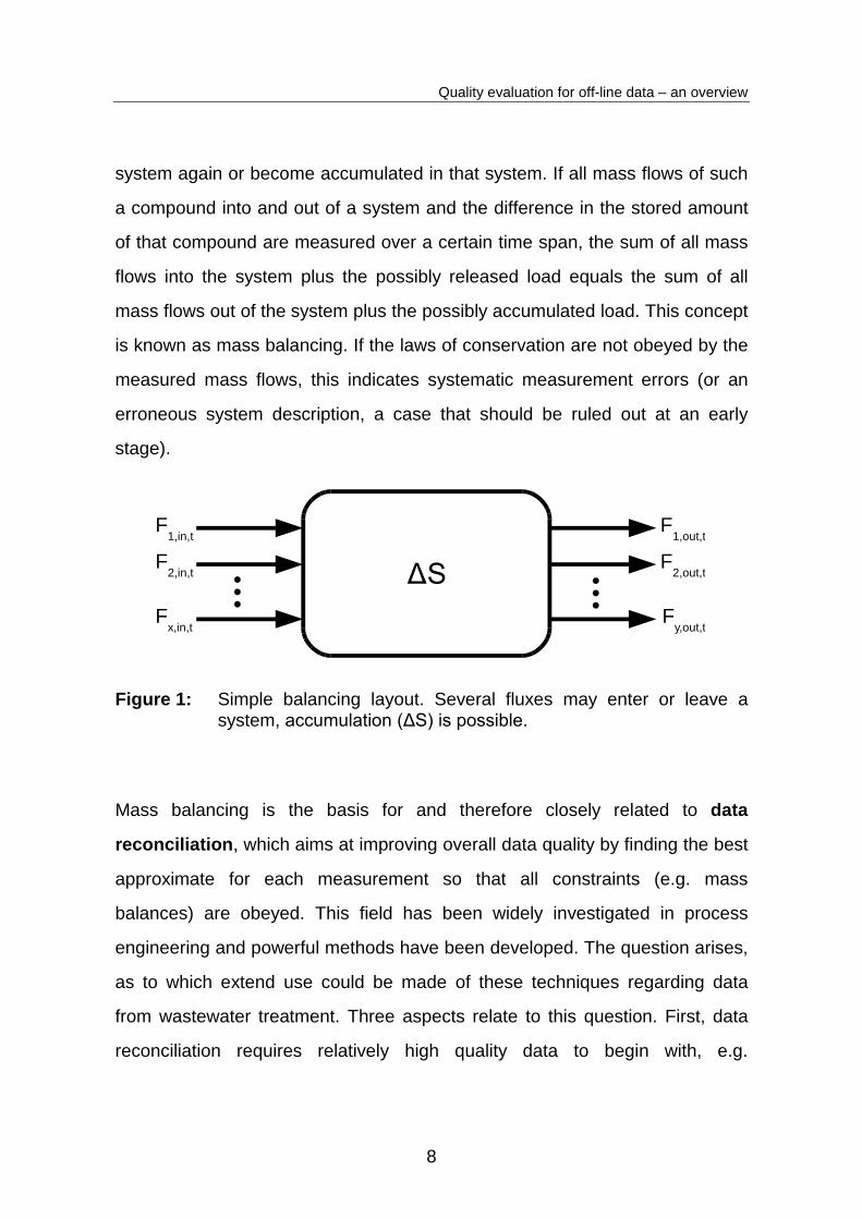
system again or become accumulated in that system. If all mass flows of such

a compound into and out of a system and the difference in the stored amount

of that compound are measured over a certain time span, the sum of all mass

flows into the system plus the possibly released load equals the sum of all

mass flows out of the system plus the possibly accumulated load. This concept

is known as mass balancing. If the laws of conservation are not obeyed by the

measured mass flows, this indicates systematic measurement errors (or an

erroneous system description, a case that should be ruled out at an early

stage).

Figure 1: Simple balancing layout. Several fluxes may enter or leave a system, accumulation (ΔS) is possible.

Mass balancing is the basis for and therefore closely related to data

reconciliation, which aims at improving overall data quality by finding the best

approximate for each measurement so that all constraints (e.g. mass

balances) are obeyed. This field has been widely investigated in process

engineering and powerful methods have been developed. The question arises,

as to which extend use could be made of these techniques regarding data

from wastewater treatment. Three aspects relate to this question. First, data

reconciliation requires relatively high quality data to begin with, e.g.

F1,in,t

F1,out,t

F2,in,t

Fx,in,t

F2,out,t

Fy,out,t

ΔS


9

measurement variability is vital to be known. This is usually not a given fact in

wastewater treatment facilities. Secondly, the dynamics of wastewater flow

and composition as well as the bilinear nature of the data require more

sophisticated approaches to reconcile data (nonlinear and dynamic methods).

This relates to the third aspect. Operators of wastewater treatment plants are

usually not experts in process engineering, but still need a profound

understanding of the biological and physical processes taking place at their

plants. Methods for data quality control therefore gain practical relevance with

simplicity. The goal is not to provide operators with streamlined error-free data

but to support fault localization and thus the process of understanding.

Simple mass balancing is an established and well known method in

wastewater treatment, not so much data reconciliation. However, the

implications and special requirements of mass balancing in wastewater

treatment have hardly been investigated. Relevant contributions were made by

Nowak (2000; see Spindler 2014) and Thomann (2002; see Spindler 2014).

Both focus on static mass balances over long time spans that allow the

assumption of steady state processes. Thomann (2002) also suggests

including accumulation in order to allow balancing on a day-to-day basis,

which he calls "dynamic balancing".

Goals

10

Goals

Even though the focus of this thesis changed slightly with time, it always

remained concentrated on the interpretation of (real) operational data in regard

to their quality. The original motivation came from the question, which

deviation between input and output streams of a (static) mass balance would

be admissible. Among experienced colleges, an error of 10% was widely

accepted, up to 20% appeared reasonable. It soon became clear, that these

assumed limits did not hold in light of the experience made during the course

of this work. To achieve the maximum performance however, the temporal

redundancy in data must not be neglected in mass balancing. This led to the

main concern of this work changing towards a more continuously applicable

method of data quality control.

This became indeed the main goal: to develop and proof the applicability of a

method that allows both, the determination of error-free time periods in historic

data and to continuously monitor the quality of data from wastewater

treatment. "Continuous" in this context is restricted to the meaning of "on a

day-to-day basis" because (offline) concentrations are usually measured in

24h composite samples giving one value per day. The naming "continuous

mass balancing" was chosen mainly to convey the idea that operators at each

given day, that means "always", could check on the quality of the data they are

basing their decisions on.

Some aspects of so-called "continuous mass balancing" were investigated

along with the development of the method itself. One fundamental aspect is to

determine the complete set of theoretically possible and practically applicable

balancing equations. While the latter part of this goal remains to be achieved,

Goals

11

this type of structural (and hopefully later also practical) redundancy analysis

also aids the determination of possibly sensible additional measurements.

Another aspect is to investigate the possibilities of handling mass balances on

a day-to-day basis, when the assumption of a steady state process cannot be

maintained. While accumulation is the classical aspect that comes to mind in

short term balancing, the effect of hydraulic retention also has to be

considered on this time scale.

Methods

12

Methods

The work on this thesis started as a quest for a statistical basis for mass

balancing wastewater treatment operational data. It wasn't clear in the

beginning, what kind of methods would be used or which approaches would be

followed. In fact, data reconciliation as such was totally unknown to the author.

There had hardly been any applications of it in the scientific literature on

wastewater treatment. And obviously no process engineer had taken on the

challenge to establish a link between the two worlds. It wasn't until the author

stumbled upon a paper by Van der Heijden (1994; see Spindler 2014) that he

got in touch with this world. This paper wasn't actually very representative for

process engineering and its state of research at the article's time, because it

only translated the process oriented approach to elemental mass balances

around a lab fermenter. It did, however, point to the determination of

balanceability and calculability of measured and unmeasured data by matrix

algebra. From there on it was clear that it would be worthwhile to further

pursue the original question.

During the author's following stay with the modelEAU group of the Canadian

Research Chair on Water Quality Modeling it still wasn't clear for a long time,

on which basis the (systematic) error of a mass balance should be evaluated.

Only towards the end of this visit the application of CUSUM charts (Page 1954;

see Spindler and Vanrolleghem 2012) led the way to answer this question. It

had become clear, that the temporal redundancy of data in time series would

have to be taken into account. With some knowledge about the classical

methods of data reconciliation, however, there did not seem to be any way

around the necessity of knowing all the measurements' variances. And

because of the strong intention to use only readily available operational data,

Methods

13

the possibility of multiple measurements for the determination of variances was

ruled out. CUSUM charts are a method of statistical process control.

Calculated as a special cumulative sum of consecutive measurement values,

they signal when the process mean significantly deviates from its expected

value. To apply CUSUM charts, balances had to be calculated on a daily basis

which led to the introduction of the error vector (of day-to-day balances) and

suddenly one was dealing with an expectedly stationary process, whose

variability could be calculated easily.

Because CUSUM charts also consider past values, even minor deviations from

the expected mean (in relation to the process's variance) can be detected

reasonably fast and reliably. In the application to mass balances, the expected

process mean (of the error vector) is always zero.

Because certain data (sludge concentrations of balanced components) are

usually not measured in practice, some statistical assessments were required.

The intention was to determine usually unmeasured variables from frequently

measured data such as suspended solids. Data sets from three different large

Austrian wastewater treatment plants where available for investigation, which

was very important to remain in conformity with the intention of working with

real data only. In these data sets all required sludge components had been

measured at least weekly, in some cases as additional analyses in the author's

institute's laboratory. Monte Carlo simulation was then applied to determine

the minimum frequency of such measurements to ensure good approximations

for the typically unmeasured data.

When the algorithm for an automated determination of balance equations was

developed, the existing methods of data reconciliation were finally abandoned.

Methods

14

Individual balance equations are simply not necessary in data reconciliation.

They do have the advantage of being more intuitively applicable for the

practitioner who might not be a process engineer. Based on a matrix

representation of all possible subsystem combinations of a given plant layout

(the extended incidence matrix, Spindler 2014), individual equations were

derived from the classification into redundant and non-redundant measured

variables and calculable and non-calculable unmeasured variables. The

necessary symbolic calculations to derive the individual balancing equations

were executed by a computer algebra system, substituting calculable

unmeasured variables with measured variables. Especially when

concentrations of multiple compounds are measured, the resulting equations

can be complex and therefore difficult to find otherwise.

Article summary

15

Article summary

This thesis is composed of three articles, all written by the (first) author and

supervised by the second author. The investigation of CUSUM charts for mass

balancing of wastewater treatment operational data led to two articles, Spindler

and Vanrolleghem (2012) and Spindler and Krampe (2015). A third article

(Spindler, 2014) was written with the focus on structural redundancy of

measurement data, providing a method for an automated setup of bilinear

balancing equations. This article also intends to strengthen the connection

between mass balancing as known and applied in wastewater treatment and

the field of data reconciliation, broadly investigated in the process engineering

domain.

The principal applicability of CUSUM charts for daily operational data from

wastewater treatment was shown in Spindler and Vanrolleghem (2012).

CUSUM charts were introduced and explained using a synthetic example.

Practical application to two sets of flow data, one comprised of several

influents and one effluent of a treatment plant, the other a flow balance over an

anaerobic digester, revealed that measurement data that appears sufficiently

well balanced on average over a long time period might very well consist of

several poorly balanced shorter time periods with the single errors adding up

to (almost) zero. The CUSUM chart, basically an integration of positive and

negative errors, conveniently displays well balanced and poorly balanced time

periods. The focus on flow data only allowed ruling out additional issues like

accumulation or hydraulic retention. It also underlined the importance of well-

balanced flow data, because these measurements are the basis for the

calculation of mass flows from measured concentrations. Daily cumulative

values for flow are usually available on virtually every wastewater treatment

Article summary

16

plant and mostly measured online. During this first investigation of CUSUM

charts for mass balancing based on daily values it also turned out that the

variability of the error vector (resulting from the single day-to-day balances) is

an important indicator of data quality itself. A low variability of the error vector

(with an expected mean of zero) indicates similar results for the single

balances. This facilitates the detection even of small systematic errors by the

method which inspires more confidence in overall data quality than wildly

scattered random errors with a mean value of zero.

While the application of CUSUM charts for mass balancing was labeled

"dynamic balancing" in the first article, this naming was subsequently changed

to "continuous balancing". The term "dynamic" is strongly associated with

biological modelling where "dynamics" are expressed by kinetic rates of

microbial growth and chemical reactions. "Continuous" is also not quite exact

as described above. However, the term "discrete step mass balancing" is

likewise hardly suited to communicate an easily applicable method to the

practitioner.

The second article on the application of CUSUM charts (Spindler and Krampe,

2015) was based on a research project financed by the Austrian Federal

Ministry of Agriculture, Forestry, Environment and Water Management.

Several aspects of great practical relevance are investigated. Generally, this

article is concerned with (bilinear) mass balances rather than (linear) flow

balances and gives a number of real data examples. Typically balanced

sewage sludge components such as COD, TP and TN are usually measured

rarely, sometimes not at all. Statistically analyzing data sets for primary sludge,

waste activated sludge and digested sludge from three different treatment

plants, it was shown that in most cases these sludge components can be

Article summary

17

determined reliably from practically more convenient and therefore more

regular measurements of (total or volatile) suspended solids. The precondition

for this determination is the monthly measurement of the relevant sludge

components which will usually have to be carried out by an external laboratory.

A linear dependency between total or volatile suspended solids and the

respective sludge component had to be superimposed by a seasonal

component in most combinations of sludge types and components to give the

best results.

The second aspect of continuous mass balancing covered in Spindler and

Krampe (2015) deals with the influences from accumulation and hydraulic

retention. Accumulation (release) in reactors with a fixed volume occurs, when

a component's concentration rises (drops). Stemming from the first aspect

introduced above, this often has to do with increased suspended solids

concentrations in tanks. Surprisingly, the consideration of accumulation led to

a deterioration of the error vector variability. This in turn made it more difficult

to distinguish well balanced from poorly balanced time periods. It is assumed

that this effect was caused by the daily accumulation being calculated from

differentials, and their integration (by the CUSUM method) is known to amplify

noise. And the measurement of suspended solids itself is quite likely to

introduce that noise into the equation, as representative sludge samples are

often difficult to obtain.

When hydraulic retention was regarded instead of accumulation, continuous

balancing gave considerably better results. Owing to the nature of wastewater

and sludge treatment (to a large extend based on phase separation) there are

usually at least two output streams from a subsystem. Often one of those

carries components that have a retention time well above one day. Therefore it

Article summary

18

is clear that component loads entering such a subsystem on one day will not

necessarily leave it entirely on the same day but rather distributed over a long

period depending on the retention time of that component in that subsystem.

With the assumption of an ideal CSTR for the respective subsystem under

evaluation, this behavior can be integrated into mass balancing and the

expected output load (calculated from the measured input load and the starting

concentration in the tank) is balanced against the measured output load.

The third article (Spindler, 2014), chronologically the second, covers an aspect

of mass balancing independent from the measured data itself. Derived from

the methods of structural redundancy analysis and based on a complete

system description together with the information about the availability of

measurements in each stream and reactor, a method is introduced that allows

to automatically set up all theoretically possible mass balance equations for a

system. Due to the bilinear nature of mass flows this can result in non-trivial

solutions, especially when multiple components are allowed. In these cases,

missing flow measurements can be substituted by available concentration

measurements. The method also allows for a simple investigation about the

effect of additional measurements on the overall balanceability (redundancy) of

the system.

Scientific contribution

19


As of today, a clear distinction has to be made between data reconciliation in

the world of process engineering and data quality evaluation in wastewater

treatment. In process engineering the profit driven development has produced

a vast amount of powerful techniques for the reconciliation of measurement

values that supports ever more precise control of production. However, while

the knowledge of each measurement's variability is a crucial element in most

of these techniques and variability of (mass) flows is in most cases reduced to

the minimum in most process engineering applications, the contrary is the

case in wastewater treatment. The main disturbance to the whole system is

the more or less uncontrollable influent (flow and composition!). Adding to this

is the fact that wastewater treatment is a negligible economic factor, driven by

legal requirements and the demand for environmental protection. The effect of

these preconditions are simply less frequent and less reliable measurement

values. This thesis has been an attempt to maximize the information contained

in typically available operational data from wastewater treatment by aiding

operators and other stakeholders to verify the data quality. It therefore belongs

to the gross error detection part of data reconciliation.

There has so far not been a profound investigation on the application of

CUSUM charts for mass balancing in the field of wastewater treatment. Zaher

and Vanrolleghem (2003; see Spindler and Vanrolleghem, 2012) named this

possibility among others without going into details. CUSUM charts have now

been proven suitable for continuous mass balancing even though a number of

open questions remain to be answered. Although not addressed directly in this

thesis, the possibility of the application of CUSUM charts to characteristic

values calculated from plant data is obvious. Characteristic values (sometimes


20

also known as expert knowledge) such as the specific amount of volatile

suspended solids in digested sludge (around 18 g VSS/pe/d) or the typical

specific energy demand for aeration can be used as a target value (instead of

the mean balancing error) of a CUSUM chart. Their usefulness is comparable

to that of classical balances but they often require less input data.

The determination of component loads in sludges from total or volatile

suspended solids, though regularly applied under the assumption of direct

proportionality, has never been based on a thorough statistical examination.

As it turned out, direct proportionality is sometimes given but cannot be

expected in every case. The range of typical ratios (when direct proportionality

is suitable) varies considerably which implies a low probability of free

assumptions to be correct. Operators can clearly improve the general

balanceability of their wastewater treatment plants by having samples of their

sludges analyzed monthly in an external laboratory.

Regarding the automatic determination of bilinear balancing equations, to the

author's knowledge no such algorithm has been published before in

wastewater treatment literature or related fields. This probably results from

process engineering's data reconciliation aiming at entire datasets at once, not

at individual (subsystem) balances. Non-trivial balancing equations have until

now hardly been used in wastewater treatment practice.

Conclusions

21

Conclusions

Continuous mass balancing has the potential to define a new standard in

quality control of wastewater treatment operational data. It gives plant

operators a possibility to evaluate the general integrity of their measurements

on a daily basis. The real data analyzed so far allows the conclusion that

continuous mass balancing can easily determine even minor systematic errors

in data (well below 5% of the input load when hydraulic retention is

considered). This means, the commonly assumed 10% permissible error (or

more) should be abandoned. In scientific studies based on plant data the proof

of good data quality should become a matter of course before any conclusions

are drawn.

A considerable number of aspects remain to be dealt with. Until now,

accumulation and hydraulic retention in continuous mass balances have been

dealt with separately. Although the calculation of accumulation has been

shown to increase random error, it might be feasible to include along with

hydraulic retention if data are filtered in an appropriate way. Typically Kalman

filtering would be used in this case. It remains to be shown if accumulation

does play a significant role when data are analyzed on a daily basis. Negligible

on long term balances, accumulation is likely to have its maximum significance

in balancing periods of around one sludge retention time of the balanced

subsystem.

More practical experience is needed, although continuous mass balancing

gave good results with the real data it has already been applied to. It would be

especially beneficial if detected faults in data could be confirmed by expert

knowledge. The recently much intensified application of the Benchmark

Conclusions

22

Simulation Model (Gernaey et al., 2014) in many areas of wastewater

treatment study would probably be an appropriate way to better assess the

reliability of systematic errors detected by continuous mass balancing. It could

also be applied to answer a number of additional questions.

Still missing is a general assessment of the practical possibility of quality

control for the single variables measured in a wastewater treatment system. It

appears quite likely, that a number of measurements remain practically not

redundant. For example total phosphorus or COD in the effluent have such

minor effect on their respective balances, that quality control of these data

might remain inaccessible by the means of mass balancing. This question is

similar to the determination of identifiability of individual parameters in

modelling and could probably also be investigated using the Benchmark

Simulation Model. The developed algorithm for automatic determination of

balance equations could also be extended by an appropriate sensitivity

analysis. Further improvement of this algorithm is probably possible by the

application of graph theory (Deo, 1994) to determine the initial set of

theoretically possible balance equations.

If, as expected, some typical measurement values in fact do remain non-

verifiable by mass balancing, other means of verification should be applied

regularly. In the case of effluent concentrations this is usually realized already

through external control by the authorities. Further, the question of missing

data has not yet been properly addressed. In smaller wastewater treatment

plants operational data are typically not measured on a daily basis and

therefore much information is missing. It might, however, still be feasible to

ignore missing data and to find a compromise about the minimum time span

that gives one data point for continuous mass balancing. A monthly average of

Conclusions

23

available data values might actually proof a suitable input for the CUSUM chart

and provide a still more detailed analysis than a static balance when the

considered time span is long enough, maybe 2 years or more.

Finally, the influence of autocorrelation on CUSUM charts in their proposed

application remains to be investigated. CUSUM charts are known to be

sensitive to autocorrelation. Wastewater treatment data is clearly

autocorrelated. However, it is not clear that the error vector of a continuous

mass balance is autocorrelated, too. Even under consideration of hydraulic

retention which itself is calculated in an autoregressive way, the error vector of

a continuous mass balance should actually be only noise as long as no

systematic error is present. The investigation into this question is probably best

considered after the practical applicability of continuous mass balancing has

been confirmed further.

In this thesis the intention was not to avoid the merits of data reconciliation.

Obviously, the connection between two similar, though not equal, fields -

wastewater treatment and process engineering - is not very strong at this time.

There is hope that this work will help to bridge the existing gap. It would be a

great success, too, if this work would stimulate contributions by scientists who

are well familiar with data reconciliation but at the same time well aware of the

special implications of wastewater treatment.

In the future, plant operators, administration, engineers and scientists should

no longer be in doubt upon first contact with plant data. It is at the hands of

operators to have their measurements organized and monitored in such a way,

that reliable data quality can be proven at any time. This will considerably

shorten the time of typical data evaluations including the corresponding cost

Conclusions

24

savings. For simulation studies, virtually no additional effort should be

necessary any more, once the simulation model has been initially set up and

calibrated. Today we are still a considerable distance away from this situation.

It is the firm conviction of the author, that the here described methods and

approaches open a practically feasible way to achieve this scenario.

References not cited in articles

25

References not cited in articles

Deo, N. (1994) Graph Theory: with Applications to Engineering and Computer

Science, New Delhi, Englewood Cliffs [N.J.], Prentice-Hall of India, Prentice-

Hall International.

Gernaey, K. V., Jeppsson, U., Vanrolleghem, P. A. and Copp, J. B (eds)

(2014) Benchmarking of Control Strategies for Wastewater Treatment Plants

(IWA Scientific and Technical Report). IWA Publishing, London.

Lindtner, S., Schaar, H., and Kroiss, H. (2008) Benchmarking of large

municipal wastewater treatment plants greater than 100,000 pe in Austria.

Proceedings of the Water Environment Federation, 2008(7), 7655–7657.

26

ARTICLES

This thesis is a cumulative work consisting of three publications in international

peer-reviewed scientific journals. All articles where written by the author, who

proposed the methods, developed and implemented the algorithms and

evaluated the data. Article 1 and article 3 were supervised by the co-authors.

Article 1

Spindler, A. and Vanrolleghem, P. A. (2012) Dynamic mass balancing for

wastewater treatment data quality control using CUSUM charts. Water Science

and Technology, 65(12), 2148–2153.

Article 2

Spindler, A. (2014) Structural redundancy of data from wastewater treatment

systems. Determination of individual balance equations. Water Research, 57,

193–201.

Article 3

Spindler, A. and Krampe, J. (2015) Quality control of wastewater treatment

operational data by continuous mass balancing: Dealing with missing

measurements and delayed outputs. Water Quality Research Journal of

Canada (accepted 08/01/2015).

ARTICLE 1

27

Advanced Mass Balancing for Wastewater Treatment Data Quality Control Using CUSUM Charts

A. Spindler*, P.A. Vanrolleghem**

*Institute of Water Quality and Resource Management, Vienna University of Technology, Karlsplatz 13/226-1, 1040 Wien, Austria

**modelEAU, Dép. de génie civil et de génie des eaux, Université Laval, Québec, QC G1V 0A6, Canada

Abstract

Mass balancing is a widely used tool for data quality control in wastewater treatment. It can effectively detect systematic errors in data. To overcome the limitations of the mean balancing error as a measure of data quality a well-established method for statistical process control (the CUSUM chart) is adopted for application on the error vector of balancing data. Two examples show how time periods with stable low mass balancing errors can be detected by the method. The detectability of such time periods depends on the variability of the balancing error which is an important measure for the precision of the data.

Keywords

data quality control; fault detection; mass balancing; statistical process control

INTRODUCTION

On wastewater treatment plants (WWTP) data is routinely collected for reasons of treatment performance evaluation as well as process monitoring and control. The collected data can be a valuable source of information for process redesign, treatment plant extension or simulation. It usually provides a long term record of the plant performance and is readily available to the engineer. Typically, concentrations of in- and effluents are measured in 24h composite samples and flows are recorded as daily sums. The advantage of routine data is their availability for long time periods at no extra cost. In contrast, dedicated measurement campaigns might provide a higher sampling frequency but are costly in terms of time and labor and can only cover a comparably short period of time.

To serve as a basis for further engineering tasks, the quality of the routine collected data has to be controlled. Simple or advanced plausibility tests as well as mass balancing are generally applied to meet this requirement (Rieger et al., 2010). Plausibility testing is necessary but not sufficient in terms of redundancy. Plausible values can still be (systematically) wrong and sometimes right values might not be plausible. Redundant verification is therefore necessary. Mass balancing can often effectively detect systematic errors in data. Thomann Haller (2002) showed a possibility of testing the significance of the mean balancing error.

ARTICLE 1

28

Basics of mass balancing

Typical compounds for mass balancing include water H2O (as flow), and elemental fluxes such as chemical oxygen demand (COD), total phosphorus (P), total nitrogen (N) and iron (Fe). Other compounds can be balanced over systems in which they are not subject to reactions, e.g. total suspended solids (TSS) in dewatering stages.

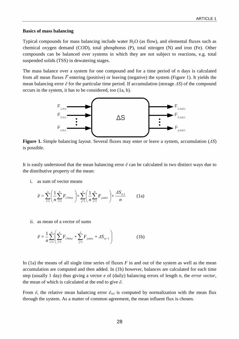
The mass balance over a system for one compound and for a time period of n days is calculated from all mean fluxes F̅ entering (positive) or leaving (negative) the system (Figure 1). It yields the mean balancing error ē for the particular time period. If accumulation (storage ΔS) of the compound occurs in the system, it has to be considered, too (1a, b).

Figure 1. Simple balancing layout. Several fluxes may enter or leave a system, accumulation (ΔS) is possible.

It is easily understood that the mean balancing error ē can be calculated in two distinct ways due to the distributive property of the mean:

i. as sum of vector means

n

ΔS+F

n+F

n=e n

y

=j

n

=ttout,j,

x

=i

n

=tti,%in,

,1

1 11 1

11 ∑ ∑∑ ∑

(1a)

ii. as mean of a vector of sums

∑ ∑∑

−

n

=ttt,

y

=jtout,j,

x

=iti,%in, ΔS+F+F

n=e

11

11

1 (1b)

In (1a) the means of all single time series of fluxes F in and out of the system as well as the mean accumulation are computed and then added. In (1b) however, balances are calculated for each time step (usually 1 day) thus giving a vector e of (daily) balancing errors of length n, the error vector, the mean of which is calculated at the end to give ē.

From ē, the relative mean balancing error ērel is computed by normalization with the mean flux through the system. As a matter of common agreement, the mean influent flux is chosen.

F1,in,t

F1,out,t

F2,in,t

Fx,in,t

F2,out,t

Fy,out,t

ΔS

ARTICLE 1

29

∑ ∑

x

=i

n

=t

rel

Fn

e=e

1 1tin,i,

1 (2)

Measures for data quality

Accuracy and precision are the quality criteria for good data. They correspond to systematic and random errors, respectively. Although mass balancing has been accepted as a method of choice for redundant data quality control in the field of wastewater treatment (with a focus on accuracy), little has been said about decision criteria.

The mean balancing error ē is mainly perceived as most important decision variable. Thomann Haller (2002) also focused on this measure and showed how to find a confidence interval for ē to test its significance. However, an insignificant difference between ē and zero does not determine high data quality alone. A small (relative) mean balancing error can still be significantly different from zero if the precision of the single measurements is high. Low precision might accordingly yield a large confidence interval for ē thus leading to the misinterpretation of a large ērel as not significantly different from zero. Acceptability of a certain mean relative error therefore seems to be more important than significance. The level of acceptability depends on the task that is addressed using the data.

Another aspect is dynamic variability. While a large ērel certainly signals low data quality (or poor system description), a low ērel could still have been calculated from an error vector e that drifts in time from unacceptably high to unacceptably low values. If data quality is checked relying only on the mean, not much can be said about the data quality in the time series. This is of special importance, when historic data is to be used as input for simulation.

The CUSUM method is suggested to approach the dynamic behavior of the error vector. In literature, only Zaher and Vanrolleghem (2003) are known to have used this method in the same context, however without explicitly investigating it. Among other control charts, CUSUM is one of the more sensitive. EWMA charts (exponentially weighted moving average), another sensitive type of control chart, had been investigated, too, but didn't yield results of comparable quality. The detectability of changes of the balancing error by the CUSUM method depends on the variability of the error vector and therefore on the precision of the data. This will become clear in the course of this paper.

THE CUSUM CHART

CUSUM charts, introduced by Page (1954), are used widely in statistical process control to detect small changes (e.g. shifts or drifts) in the mean µ (the target value) of a monitored process variable (Montgomery, 2009). Small in this context means changes of less than one standard deviation.

CUSUM charts are designed to detect one-sided changes (increase or decrease) of the monitored

ARTICLE 1

30

variable X. For the two-sided case (increase and decrease), one upper (positive) and one lower (negative) CUSUM chart have to be combined. For convenience, data is normalized to zero mean and standard deviation one. The CUSUM is a modified cumulative sum of a process variable X, consecutively adding up the values xt, t=1,…,n where n is the length of vector X. The two modifications are:

i. The upper (positive) CUSUM may not drop below zero, the lower (negative) CUSUM may not rise above zero.

ii. A smoothing parameter (reference value k) restricts the sensitivity of the method by constantly drawing the CUSUM series towards the target value (zero for normalized data).

The two-sided CUSUM for normalized data may be defined as:

( )( )ttt

ttt

x+k+Cmin=Cx+kCmax=C

-1

-

+1

+

0,

0,

−

− − with C0 = 0 (3)

The CUSUM series signals an undesired shift Δµ of the process mean by exceeding a chosen control limit (+h or -h). Thus, the reference value k and the control limit h are the two parameters which determine the behavior of the CUSUM chart. The optimal value of k is Δµ/2, half the size of the shift to detect (Lucas and Crosier, 1982). The control limit h may then be chosen according to the desired average run length ARL0 of the CUSUM series (Montgomery, 2009).

The average run length ARL0 is the average number of time steps (i.e. data points) after which the CUSUM series will give a signal even though the true shift of the mean is zero (false alarm). Indeed, due to the probabilistic nature of the data (random errors), a long enough CUSUM series will eventually exceed any control limit. This corresponds to the type I error (false positive) in statistical tests. Therefore, a compromise has to be made. In the past, ARL0 was chosen as 370 which is equivalent to a 3σ control limit on a Shewart control chart (Montgomery, 2009).

When k and h have been chosen, the average run length ARLΔµ (for detection of a true shift Δµ of the mean) can be calculated (Knoth, 2009). ARLΔµ increases with decreasing values of k (when h is adjusted to keep a constant ARL0) and therefore with smaller shifts Δµ. In statistical process control a fast response, i.e. low ARLΔµ is desirable.

Synthetic example

Figure 2 depicts data of a synthetic example on its left side. The time series has length 200. At intervals [1:40] and [91:140] the random data is N(0,1) distributed. In the interval [41:90] the target value (mean) was changed to +0.5. From data point 141 to the end of the series, the mean drifts from 0 to -1. On the right side the results of a CUSUM chart applied to the data are shown. The reference value k was chosen to 0.25 for optimal detection of a shift of ±0.5. ARL0 is kept at 370 with a control limit h of ±8.01 The crucial parts of the CUSUM series are those, where it moves

ARTICLE 1

31

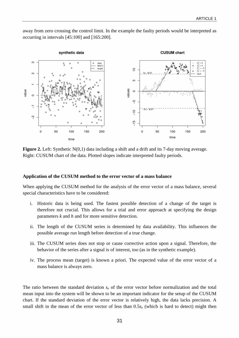
away from zero crossing the control limit. In the example the faulty periods would be interpreted as occurring in intervals [45:100] and [165:200].

Figure 2. Left: Synthetic N(0,1) data including a shift and a drift and its 7-day moving average. Right: CUSUM chart of the data. Plotted slopes indicate interpreted faulty periods.

Application of the CUSUM method to the error vector of a mass balance

When applying the CUSUM method for the analysis of the error vector of a mass balance, several special characteristics have to be considered:

i. Historic data is being used. The fastest possible detection of a change of the target is therefore not crucial. This allows for a trial and error approach at specifying the design parameters k and h and for more sensitive detection.

ii. The length of the CUSUM series is determined by data availability. This influences the possible average run length before detection of a true change.

iii. The CUSUM series does not stop or cause corrective action upon a signal. Therefore, the behavior of the series after a signal is of interest, too (as in the synthetic example).

iv. The process mean (target) is known a priori. The expected value of the error vector of a mass balance is always zero.

The ratio between the standard deviation se of the error vector before normalization and the total mean input into the system will be shown to be an important indicator for the setup of the CUSUM chart. If the standard deviation of the error vector is relatively high, the data lacks precision. A small shift in the mean of the error vector of less than 0.5se (which is hard to detect) might then

ARTICLE 1

32

already mean a considerable change in one of the fluxes associated with the balance. Therefore, a small reference value k has to be selected. A smaller reference value at constant ARL0 causes a higher ARLΔµ.

The CUSUM method can be applied quite straightforwardly to flow data. The application becomes more challenging, when daily changes in storage have to be considered, too. This is the case with all other measured variables, i.e. elemental flux balances. Since storage is strongly coupled with TSS concentrations, reliable and representative measurements of this variable are important.

RESULTS OF APPLICATION TO REAL DATA

The CUSUM method was applied to existing routine data of a large WWTP (170.000 PE). The plant has 6 influents. The two major influents are one municipal and one industrial (refinery). Another two influents stem from the nearby airport (wastewater and surface water). The industrial wastewater (about half of the influent flow) is pretreated in a high-load aerobic stage before joining the aerobic/anoxic treatment for nutrient removal. Because flow Q is the basis for the calculation of fluxes the examples given are 1) a flow balance over the entire treatment plant and 2) a flow balance over the anaerobic digester. Unfortunately, it was not possible to include a phosphorus balance as well due to missing data in some fluxes.

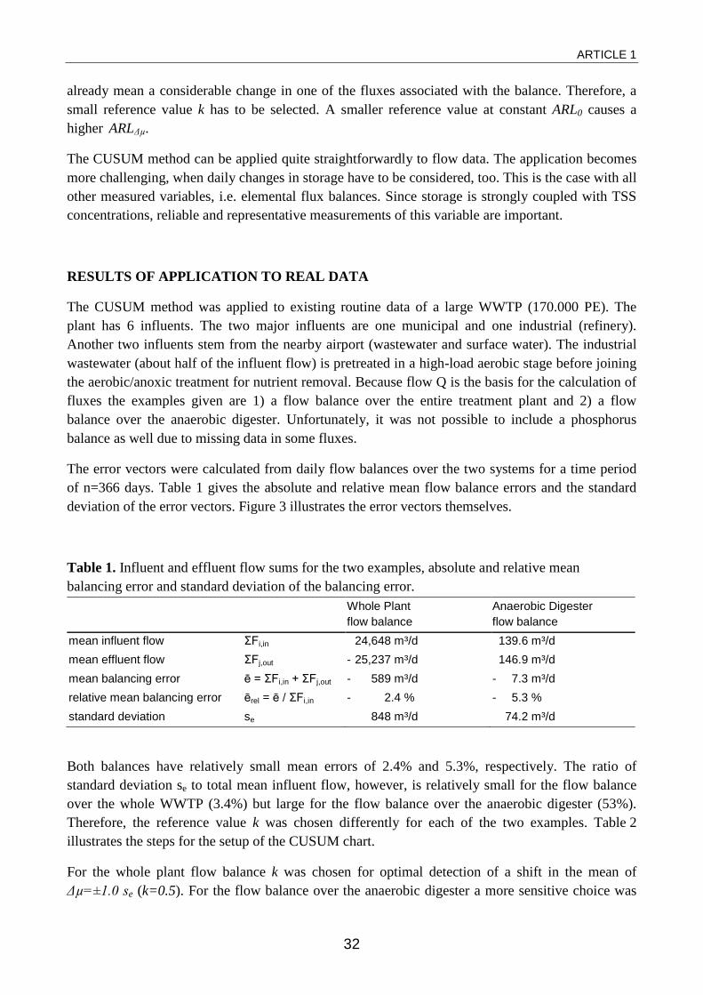
The error vectors were calculated from daily flow balances over the two systems for a time period of n=366 days. Table 1 gives the absolute and relative mean flow balance errors and the standard deviation of the error vectors. Figure 3 illustrates the error vectors themselves.

Table 1. Influent and effluent flow sums for the two examples, absolute and relative mean balancing error and standard deviation of the balancing error. Whole Plant

flow balance Anaerobic Digester flow balance

mean influent flow ΣFi,in 24,648 m³/d 139.6 m³/d mean effluent flow ΣFj,out - 25,237 m³/d 146.9 m³/d mean balancing error ē = ΣFi,in + ΣFj,out - 589 m³/d - 7.3 m³/d relative mean balancing error ērel = ē / ΣFi,in - 2.4 % - 5.3 % standard deviation se 848 m³/d 74.2 m³/d

Both balances have relatively small mean errors of 2.4% and 5.3%, respectively. The ratio of standard deviation se to total mean influent flow, however, is relatively small for the flow balance over the whole WWTP (3.4%) but large for the flow balance over the anaerobic digester (53%). Therefore, the reference value k was chosen differently for each of the two examples. Table 2 illustrates the steps for the setup of the CUSUM chart.

For the whole plant flow balance k was chosen for optimal detection of a shift in the mean of Δµ=±1.0 se (k=0.5). For the flow balance over the anaerobic digester a more sensitive choice was

ARTICLE 1

33

necessary. The reference value was chosen as k=0.15 in order to optimally detect shifts in the mean of Δµ=±0.3 se. Note that the detectable relative mass balance errors (i.e. optimally detectable shifts, step 5 in Table 2) are very different. Even though the example of the anaerobic digester was set up for more sensitive detection only balancing errors of about 16% can be optimally detected.

Figure 3. Error vector e and its 7-day moving average for the two examples

The control limits h were chosen to give an ARL0 of 370. The resulting ARLΔµ are ARL1.0=9.2 and ARL0.3 = 51 (Knoth, 2009). For the flow balance over the anaerobic digester, a “design shift” would be detected approximately 51 data points after its occurrence. Given the length of the error vector (366 data points) this seems to be a reasonable compromise between detectability and run length for detection.

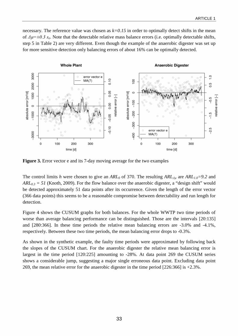
Figure 4 shows the CUSUM graphs for both balances. For the whole WWTP two time periods of worse than average balancing performance can be distinguished. Those are the intervals [20:135] and [280:366]. In these time periods the relative mean balancing errors are -3.0% and -4.1%, respectively. Between these two time periods, the mean balancing error drops to -0.3%.

As shown in the synthetic example, the faulty time periods were approximated by following back the slopes of the CUSUM chart. For the anaerobic digester the relative mean balancing error is largest in the time period [120:225] amounting to -28%. At data point 269 the CUSUM series shows a considerable jump, suggesting a major single erroneous data point. Excluding data point 269, the mean relative error for the anaerobic digester in the time period [226:366] is +2.3%.

ARTICLE 1

34

Table 2. Steps for setup of CUSUM charts for the two examples (for N(0,1) normalized data se = 1). Step Whole Plant

flow balance Anaerobic Digester flow balance

0. consideration of ratio se/ΣF̅i,in se,rel = 3.4 % se,rel = 53 % 1. choice of optimally detectable shift Δµ Δµ = 1.0 se Δµ = 0.30 se 2. reference value k = Δµ/2 k = 0.5 se k = 0.15 se 3. calculation of control limit h to give desired ARL0 h = 4.77 se h = 11.0 se 4. verification of ARLΔµ ARL1.0 = 9.2 d ARL0.3 = 51 d

5. calculation of relative optimally detectable mass balance error

Δµ/ΣF̅i = ± 3.4 %

Δµ/ΣF̅i = ± 16 %

Figure 4. Two-sided (positive and negative) CUSUM charts for the two examples

DISCUSSION

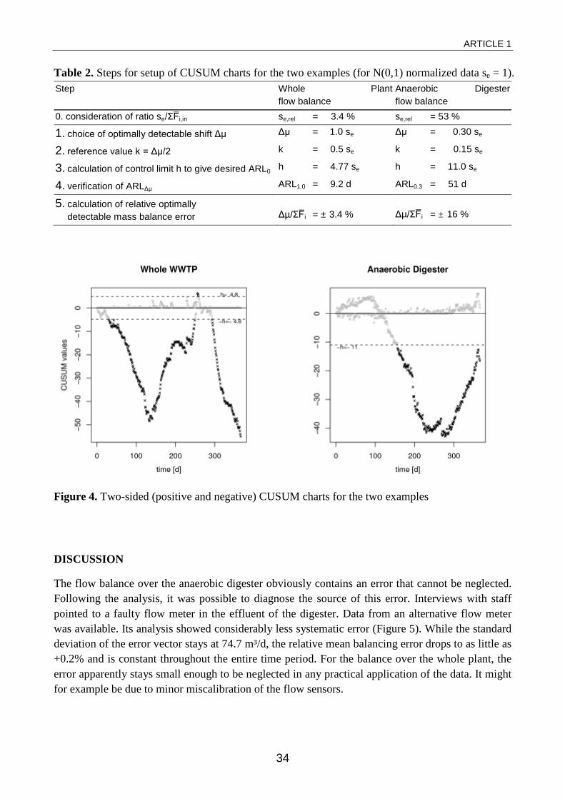
The flow balance over the anaerobic digester obviously contains an error that cannot be neglected. Following the analysis, it was possible to diagnose the source of this error. Interviews with staff pointed to a faulty flow meter in the effluent of the digester. Data from an alternative flow meter was available. Its analysis showed considerably less systematic error (Figure 5). While the standard deviation of the error vector stays at 74.7 m³/d, the relative mean balancing error drops to as little as +0.2% and is constant throughout the entire time period. For the balance over the whole plant, the error apparently stays small enough to be neglected in any practical application of the data. It might for example be due to minor miscalibration of the flow sensors.

ARTICLE 1

35

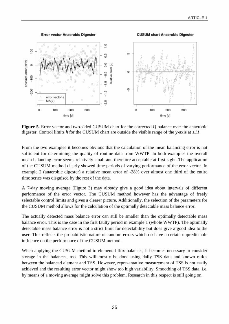
Figure 5. Error vector and two-sided CUSUM chart for the corrected Q balance over the anaerobic digester. Control limits h for the CUSUM chart are outside the visible range of the y-axis at ±11.

From the two examples it becomes obvious that the calculation of the mean balancing error is not sufficient for determining the quality of routine data from WWTP. In both examples the overall mean balancing error seems relatively small and therefore acceptable at first sight. The application of the CUSUM method clearly showed time periods of varying performance of the error vector. In example 2 (anaerobic digester) a relative mean error of -28% over almost one third of the entire time series was disguised by the rest of the data.

A 7-day moving average (Figure 3) may already give a good idea about intervals of different performance of the error vector. The CUSUM method however has the advantage of freely selectable control limits and gives a clearer picture. Additionally, the selection of the parameters for the CUSUM method allows for the calculation of the optimally detectable mass balance error.

The actually detected mass balance error can still be smaller than the optimally detectable mass balance error. This is the case in the first faulty period in example 1 (whole WWTP). The optimally detectable mass balance error is not a strict limit for detectability but does give a good idea to the user. This reflects the probabilistic nature of random errors which do have a certain unpredictable influence on the performance of the CUSUM method.

When applying the CUSUM method to elemental flux balances, it becomes necessary to consider storage in the balances, too. This will mostly be done using daily TSS data and known ratios between the balanced element and TSS. However, representative measurement of TSS is not easily achieved and the resulting error vector might show too high variability. Smoothing of TSS data, i.e. by means of a moving average might solve this problem. Research in this respect is still going on.

ARTICLE 1

36

CONCLUSIONS

When mass balances are used to determine the quality of routine data from WWTP and to search for systematic errors it is also necessary to consider the error vector of the balance rather than the mean balancing error alone. It has been shown that the CUSUM method can be applied to determine time periods of good balancing performance and to calculate the detectability limits for errors. The variability of the balancing error vector, preferably expressed as ratio between standard deviation and total mean input load into a system, is an important indicator for these detectability limits.

ACKNOWLEDGEMENTS

The central parts of this work were developed during the first author's stay at modelEAU in Québec, Canada, which co-funded the exchange. Peter Vanrolleghem holds the Canada Research Chair in water quality modeling.

ARTICLE 1

37

REFERENCES

Knoth, S. (2009). spc: Statistical process control. R package version 0.3. http://CRAN.R-project.org/package=spc

Lucas, J. M. and Crosier, R. B. (1982) Fast initial response for CUSUM quality-control schemes: give your CUSUM a head start. Technometrics, 24(3), 199-205.

Montgomery, D. (2009) Introduction to statistical quality control, Hoboken N.J., Wiley.

Page, E. S. (1954) Continuous inspection schemes. Biometrika, 41(1-2), 100-115.

Rieger, L., Takács, I., Villez, K., Siegrist, H., Lessard, P., Vanrolleghem, P. A., and Comeau, Y. (2010) Data reconciliation for wastewater treatment plant simulation Studies - planning for high-quality data and typical sources of Errors. Water Environment Research, 82(5), 426-433.

Thomann Haller, M. P. (2002) Datenkontrolle von Abwasserreinigungsanlagen mit Massenbilanzen, Experimenten und statistischen Methoden, PhD thesis, Swiss Federal Institute of Technology Zurich.

Zaher, U. and Vanrolleghem, P.A. (2003) Data validation, deliverable 2.2, research report - TELEMAC EU project no. 28156, European Research Framework - Information Society Technologies (IST), pp. 67.

ARTICLE 2

38

Structural redundancy of data from wastewater treatment systems. Determination of individual balance equations.

A. Spindler

Institute of Water Quality and Resource Management, Vienna University of Technology, Karlsplatz 13/226-1, 1040 Wien, Austria (E-mail: [email protected])

Abstract

Although data reconciliation is intensely applied in process engineering, almost none of its powerful methods are employed for validation of operational data from wastewater treatment plants. This is partly due to some prerequisites that are difficult to meet including steady state, known variances of process variables and absence of gross errors. However, an algorithm can be derived from the classical approaches to data reconciliation that allows to find a comprehensive set of equations describing redundancy in the data when measured and unmeasured variables (flows and concentrations) are defined. This is a precondition for methods of data validation based on individual mass balances such as CUSUM charts. The procedure can also be applied to verify the necessity of existing or additional measurements with respect to the improvement of the data's redundancy. Results are given for a large wastewater treatment plant. The introduction aims at establishing a link between methods known from data reconciliation in process engineering and their application in wastewater treatment.

Keywords

data validation; gross error detection; mass balancing; observability; redundancy

INTRODUCTION

This work discusses a fundamental approach to the validation of operational data from wastewater treatment plants through mass balancing. Historic records of plant data reflect the performance of a treatment plant and are regularly exploited for monitoring, benchmarking and simulation, to adjust control strategies and to plan for process redesign or plant extension. However, poor quality of historic data records is the main obstacle for these tasks. This has been agreed upon widely in literature (e.g. Rieger et al., 2010; Puig et al., 2008; Meijer et al., 2002; Barker and Dold, 1995) as well as different IWA workshops on this question (e.g. Mont Sainte-Anne 2010, Budapest 2011).

The type of operational data typically used for these tasks are daily flow volumes and concentrations measured in 24h-composite samples (where flow-proportionality is required for matching balances, especially in flows with strongly varying concentrations such as the influent). Higher frequency sensor data is more relevant in automated process control and therefore not of primary interest here. However, sensor readings are usually adjusted to the less frequent but more

ARTICLE 2

39

reliable laboratory measurements. Therefore, the validation of operational data from composite samples is also of considerable relevance for plant control.

Spindler and Vanrolleghem (2012) showed that the application of CUSUM charts is a suitable approach to continuous mass balancing1 and detects off-balance periods more reliably than mass balances based on long term averages of data. Continuous mass balancing following this method requires individual balance equations which describe redundancy of the measured data.

This work will provide a procedure for the computational determination of the complete set of possible redundancy equations (also: balance equations) for a given plant layout. This aim is different from, but closely related to the principles and objectives of data reconciliation. With mass balancing as the key to data reconciliation and gross error detection, there appears to exist a gap between development and application of methods used in process engineering and wastewater treatment. Therefore a very short overview and comparison of the developments in both fields is given in the following parts of the introduction. After the presentation of the proposed method results will be given for its application to a large and complex wastewater treatment plant.

Data reconciliation in process engineering

Data reconciliation has developed mainly in the field of (chemical) process engineering. It allows improving the measured values of process variables such as flows and concentrations based on the laws of conservation. Data reconciliation requires redundancy of the measured variables which means that they can also be calculated from other measured variables.

A vast amount of literature exists. Research began some 50 years ago when the concept of data reconciliation was introduced by Kuehn and Davidson (1961). Further research developed initially in two lines – the topology oriented approach first presented by Václavek (1969; Václavek and Louĉka, 1976) and the equation oriented approach, represented among others by Crowe (1986; Crowe et al., 1983). Some of the most recent progress in the field has been achieved by Kelly (e.g. 1998; 2004). Four comprehensive books have been written (Madron and Veverka, 1992; Narasimhan and Jordache, 2000; Romagnoli and Sánchez, 2000; Bagajewicz, 2010). Good overviews about research development are also provided in Crowe (1996) and Ponzoni et al. (1999).

A basic step in data reconciliation is the classification of the process variables. A process variable can either be directly measured (observed) or unmeasured. Unmeasured refers to variables that could be measured (at least theoretically) but are not for some reason. A process variable is observable, if it can be calculated from a subset of other measured variables. Measured observable process variables are called redundant. Crowe (1989) also classifies barely observable (unmeasured) variables which require at least one non-redundant measured variable to be calculated. Structural redundancy refers only to the theoretical calculability of a measured variable while practical redundancy also considers numerical and statistical accuracy of this calculation. The following short example is given to illustrate the difference between structural and practical redundancy.

1 The application of CUSUM charts had originally been labelled “dynamic mass balancing” to differentiate from the established approaches. But because it does not actually target kinetic rates this naming will be avoided in the future.

ARTICLE 2

40

The volume of dewatered sludge is negligible compared to influent and effluent of a wastewater treatment plant. For structural redundancy of the overall flow it would, however, still be required to be measured. Obviously the amount of dewatered sludge cannot be reconciled from this balance as the propagation of errors would pose a very high uncertainty on this calculation. On the other hand, in- and effluent would still be practically balanceable without the amount of dewatered sludge being measured.

Data validation in wastewater treatment

So far the concept of data reconciliation has received little attention in wastewater treatment. This becomes obvious in the terminology. The term mass balance is prevalent, possibly inspired by the work of Nowak (1994; 1999). Rieger et al. (2010) actually refer to the order of redundancy as “overlapping balances”. It reveals the practitioner's perspective where the individual mass balances receive higher attention than the reconciliation of the entire data set. This will be discussed further in the following section.

Literature in wastewater treatment focuses mainly on sensor fault detection and so far hardly regards redundancy of measurements. Until recently wastewater related literature cited only two works from the field of data reconciliation in process engineering (Meijer et al., 2002; Puig et al., 2008; Schraa et al., 2006).

Van der Heijden et al. (1994) adapt research from the field of chemical process engineering and apply it to elemental mass balances in fermentation processes. Following works in the field of wastewater treatment (Meijer et al., 2002; Puig et al., 2008) apply the methods of Van der Heijden et al. (1994) thus re-adapting them back into process oriented applications where they originally stem from. Meijer (2002) stress the importance of validation of operational data for use in simulation studies. Puig et al. (2008) point out that the dynamic nature of wastewater treatment makes mass balancing difficult. Both works rely exclusively on the method developed by Van der Heijden et al. (1994) which was implemented in the software Macrobal (Hellinga, 1992). However, when applying data reconciliation to elemental mass balances (Macrobal's purpose) the composition of substances is exactly known (fixed) which is not the case for the composition of wastewater treatment streams. Hence only in volumetric and mass flow rates the measurement variability was accounted for, but not in measured concentrations. Additionally, the high variability of flow measurements (around 50% relative standard deviation) includes process dynamics which is disputable given the fact the steady state is a prerequisite for the applied method of data reconciliation.

Schraa, et al. (2006) does mention data reconciliation citing Crowe (1996) but focuses on sensor fault detection. He did investigate data reconciliation in an earlier publication (Schraa and Crowe, 1998) when he was not yet involved with wastewater treatment.

Very recently two papers on redundancy classification and fault detection based on mass balances where published by Villez et al. (2013a; 2013b). In both papers the methods of data reconciliation are explicitly applied to (synthetic) data from wastewater treatment. The basic applicability of these

ARTICLE 2

41

methods is proven for the situation of sludge thickening in a settler. In the paper on redundancy classification (Villez et al., 2013a) influent TSS is concluded to be observable when measurements are taken only in the activated sludge tank, the wastage sludge and the effluent. The example obviously refers to inorganic TSS in a plant without chemical phosphorus precipitation.

Data reconciliation vs. individual mass balancing

In data reconciliation the aim is to adjust the entire data set to fit the constraints. To achieve this, the remaining random error (after removal of gross errors) is distributed over all variables according to an allowance that is defined by the variance of the single measurement errors. The variance of the measurement error needs to be known. Steady state is another frequent requirement for the established methods of data reconciliation. Even though approaches to integrated data reconciliation and gross error detection exist, considerable difficulties remain in dynamic systems (Narasimhan and Jordache, 2000).

In many industrial applications the preconditions for data reconciliation are met closely enough for its successful application. Substance influents to processes are usually controlled and set point changes of such controlled variables have rather low frequencies. In contrast, the influent is the main disturbance to the process of wastewater treatment and makes the dynamic adjustment of actuators such as pumps and blowers a constant challenge. Therefore wastewater treatment plants, especially those with combined sewer influent, are dynamic systems. This is also true if the measured data consists of daily means of the process variables (flow sums / composite samples). Another important difference to many industrial processes are the low concentrations and significant heterogeneity (dissolved/suspended) of the relevant compounds. The various sources of measurement random errors (representative sampling, interference from additional compounds, range of expected values, dynamic flows and concentrations) add up to comparatively larger uncertainty and make it complex and time-consuming, if not impossible, to determine the random measurement error variances.

Continuous balancing by means of CUSUM charts avoids these two main obstacles. The input variable to this method is the error vector of daily mass balances and therefore error distributions of the single measurements do not need to be known a priori. Continuous mass balancing has been proven suitable for gross error detection in dynamic systems (Spindler and Vanrolleghem, 2012). It requires individual balance (redundancy) equations, the determination of which is addressed in the following.

METHODS

The single steps to determine individual redundancy equations which consist only of measured variables are provided below. While the setup of the incidence matrix and classification of redundancy and observability (steps 1a and 2) are typical for data reconciliation, steps 1b and 3 (incidence matrix expansion and elimination of observable variables) are characteristic for the

ARTICLE 2

42

algorithm described here. It follows the idea, that an observable (i.e. calculable) variable can be removed from an equation by expressing it in terms of other (measured) variables. If the observable variable can be calculated in various ways, several different redundancy equations are found.

Step 1: Incidence matrix setup and expansion

The description of a flow network is commonly given as directed incidence matrix M, where columns represent streams (edges in the network graph) and rows represent single subsystems (nodes in the network graph). The environmental node (Mah et al., 1976) is the source and sink of streams coming into and leaving the overall system, it represents the outside world. The values aij of matrix M are:

• 1, if stream j enters node i,

• -1, if stream j leaves node i and

• 0, if stream j is not incident with node i.

A complete incidence matrix M consists of m independent rows where m is equal to the number of nodes in the process network. In its most evident form the rows of the incidence matrix represent the single nodes themselves (or subsystems, e.g. an activated sludge tank). The representation of a single node in the incidence matrix can be directly transformed into linear and bilinear equations describing (mass) flow in and out of the corresponding subsystem.

Following its setup, the incidence matrix M is expanded to represent all possible combinations of single subsystems of the given process network. This is achieved by finding all XOR-combinations of the m linearly independent rows in M. The new resulting matrix is M2. It needs to be reduced to M3 in an extra step because M2 is likely to contain rows of zero, double entries and rows that represent combinations of subsystems which do not share any stream and thus are physically independent of one another. For example, thickening and dewatering facilities of a wastewater treatment plant usually do not share any input or output streams. When setting up redundancy equations, these types of balances should be avoided. The procedure to clean M2 of the latter type of unnecessary rows is simply by stepwise comparison of each row with all other rows. If other rows have entries different from zero in exactly the same columns as the current row (and maybe more) they can be deleted. A graph theoretical approach to finding the relevant set of subsystem combinations might proof more efficient but was not investigated here.

Step 2: Classification of redundancy and observability

In wastewater treatment, the equations that describe a balance around a node can be of two types. Flow balances contain only measured (volumetric) flows and are therefore linear. Mass balances of a specific compound are calculated from the products of flows and the compound's concentration in

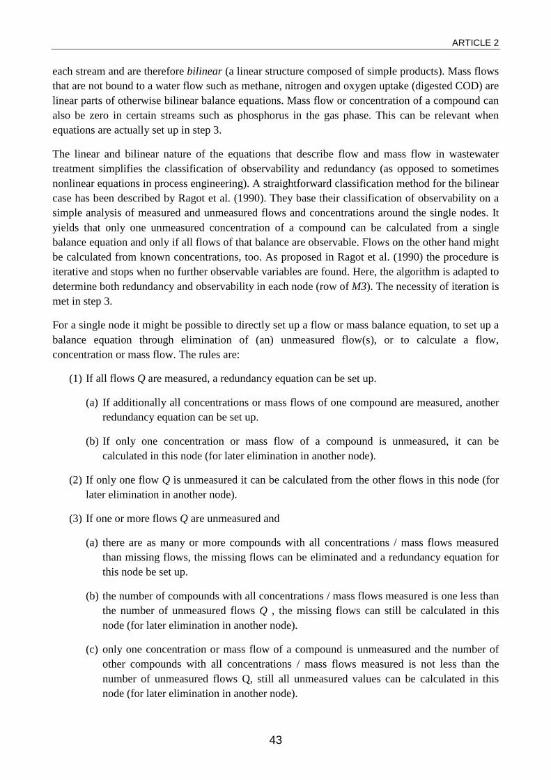
ARTICLE 2

43

each stream and are therefore bilinear (a linear structure composed of simple products). Mass flows that are not bound to a water flow such as methane, nitrogen and oxygen uptake (digested COD) are linear parts of otherwise bilinear balance equations. Mass flow or concentration of a compound can also be zero in certain streams such as phosphorus in the gas phase. This can be relevant when equations are actually set up in step 3.

The linear and bilinear nature of the equations that describe flow and mass flow in wastewater treatment simplifies the classification of observability and redundancy (as opposed to sometimes nonlinear equations in process engineering). A straightforward classification method for the bilinear case has been described by Ragot et al. (1990). They base their classification of observability on a simple analysis of measured and unmeasured flows and concentrations around the single nodes. It yields that only one unmeasured concentration of a compound can be calculated from a single balance equation and only if all flows of that balance are observable. Flows on the other hand might be calculated from known concentrations, too. As proposed in Ragot et al. (1990) the procedure is iterative and stops when no further observable variables are found. Here, the algorithm is adapted to determine both redundancy and observability in each node (row of M3). The necessity of iteration is met in step 3.

For a single node it might be possible to directly set up a flow or mass balance equation, to set up a balance equation through elimination of (an) unmeasured flow(s), or to calculate a flow, concentration or mass flow. The rules are:

(1) If all flows Q are measured, a redundancy equation can be set up.

(a) If additionally all concentrations or mass flows of one compound are measured, another redundancy equation can be set up.

(b) If only one concentration or mass flow of a compound is unmeasured, it can be calculated in this node (for later elimination in another node).

(2) If only one flow Q is unmeasured it can be calculated from the other flows in this node (for later elimination in another node).

(3) If one or more flows Q are unmeasured and

(a) there are as many or more compounds with all concentrations / mass flows measured than missing flows, the missing flows can be eliminated and a redundancy equation for this node be set up.

(b) the number of compounds with all concentrations / mass flows measured is one less than the number of unmeasured flows Q , the missing flows can still be calculated in this node (for later elimination in another node).

(c) only one concentration or mass flow of a compound is unmeasured and the number of other compounds with all concentrations / mass flows measured is not less than the number of unmeasured flows Q, still all unmeasured values can be calculated in this node (for later elimination in another node).

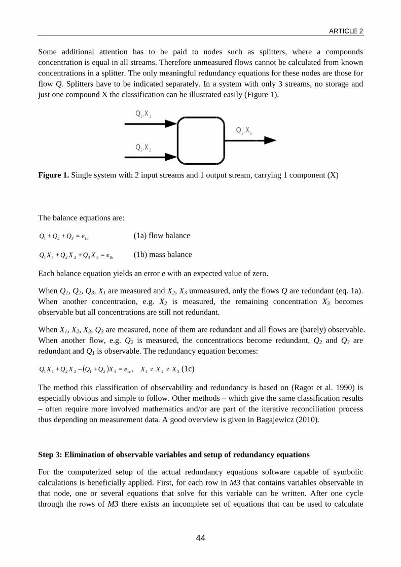
ARTICLE 2

44

Some additional attention has to be paid to nodes such as splitters, where a compounds concentration is equal in all streams. Therefore unmeasured flows cannot be calculated from known concentrations in a splitter. The only meaningful redundancy equations for these nodes are those for flow Q. Splitters have to be indicated separately. In a system with only 3 streams, no storage and just one compound X the classification can be illustrated easily (Figure 1).

Figure 1. Single system with 2 input streams and 1 output stream, carrying 1 component (X)

The balance equations are:

1a32 e=Q+Q+Q1 (1a) flow balance

b32 e=XQ+XQ+XQ 13211 (1b) mass balance

Each balance equation yields an error e with an expected value of zero.

When Q1, Q2, Q3, X1 are measured and X2, X3 unmeasured, only the flows Q are redundant (eq. 1a). When another concentration, e.g. X2 is measured, the remaining concentration X3 becomes observable but all concentrations are still not redundant.

When X1, X2, X3, Q3 are measured, none of them are redundant and all flows are (barely) observable. When another flow, e.g. Q2 is measured, the concentrations become redundant, Q2 and Q3 are redundant and Q1 is observable. The redundancy equation becomes:

( ) 321131211 , XXXe=XQ+QXQ+XQ c22 ≠≠− (1c)

The method this classification of observability and redundancy is based on (Ragot et al. 1990) is especially obvious and simple to follow. Other methods – which give the same classification results – often require more involved mathematics and/or are part of the iterative reconciliation process thus depending on measurement data. A good overview is given in Bagajewicz (2010).

Step 3: Elimination of observable variables and setup of redundancy equations

For the computerized setup of the actual redundancy equations software capable of symbolic calculations is beneficially applied. First, for each row in M3 that contains variables observable in that node, one or several equations that solve for this variable can be written. After one cycle through the rows of M3 there exists an incomplete set of equations that can be used to calculate

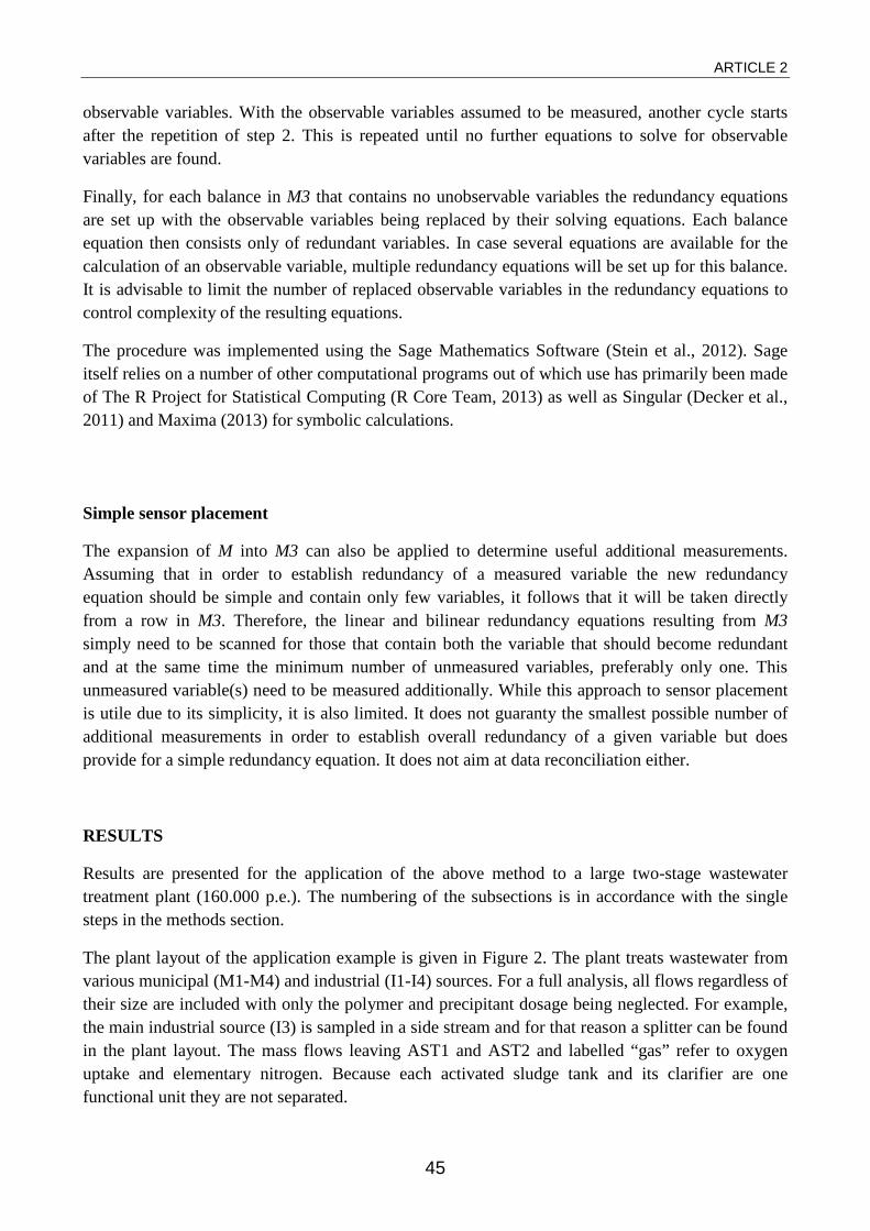
ARTICLE 2

45

observable variables. With the observable variables assumed to be measured, another cycle starts after the repetition of step 2. This is repeated until no further equations to solve for observable variables are found.

Finally, for each balance in M3 that contains no unobservable variables the redundancy equations are set up with the observable variables being replaced by their solving equations. Each balance equation then consists only of redundant variables. In case several equations are available for the calculation of an observable variable, multiple redundancy equations will be set up for this balance. It is advisable to limit the number of replaced observable variables in the redundancy equations to control complexity of the resulting equations.

The procedure was implemented using the Sage Mathematics Software (Stein et al., 2012). Sage itself relies on a number of other computational programs out of which use has primarily been made of The R Project for Statistical Computing (R Core Team, 2013) as well as Singular (Decker et al., 2011) and Maxima (2013) for symbolic calculations.

Simple sensor placement

The expansion of M into M3 can also be applied to determine useful additional measurements. Assuming that in order to establish redundancy of a measured variable the new redundancy equation should be simple and contain only few variables, it follows that it will be taken directly from a row in M3. Therefore, the linear and bilinear redundancy equations resulting from M3 simply need to be scanned for those that contain both the variable that should become redundant and at the same time the minimum number of unmeasured variables, preferably only one. This unmeasured variable(s) need to be measured additionally. While this approach to sensor placement is utile due to its simplicity, it is also limited. It does not guaranty the smallest possible number of additional measurements in order to establish overall redundancy of a given variable but does provide for a simple redundancy equation. It does not aim at data reconciliation either.

RESULTS

Results are presented for the application of the above method to a large two-stage wastewater treatment plant (160.000 p.e.). The numbering of the subsections is in accordance with the single steps in the methods section.

The plant layout of the application example is given in Figure 2. The plant treats wastewater from various municipal (M1-M4) and industrial (I1-I4) sources. For a full analysis, all flows regardless of their size are included with only the polymer and precipitant dosage being neglected. For example, the main industrial source (I3) is sampled in a side stream and for that reason a splitter can be found in the plant layout. The mass flows leaving AST1 and AST2 and labelled “gas” refer to oxygen uptake and elementary nitrogen. Because each activated sludge tank and its clarifier are one functional unit they are not separated.

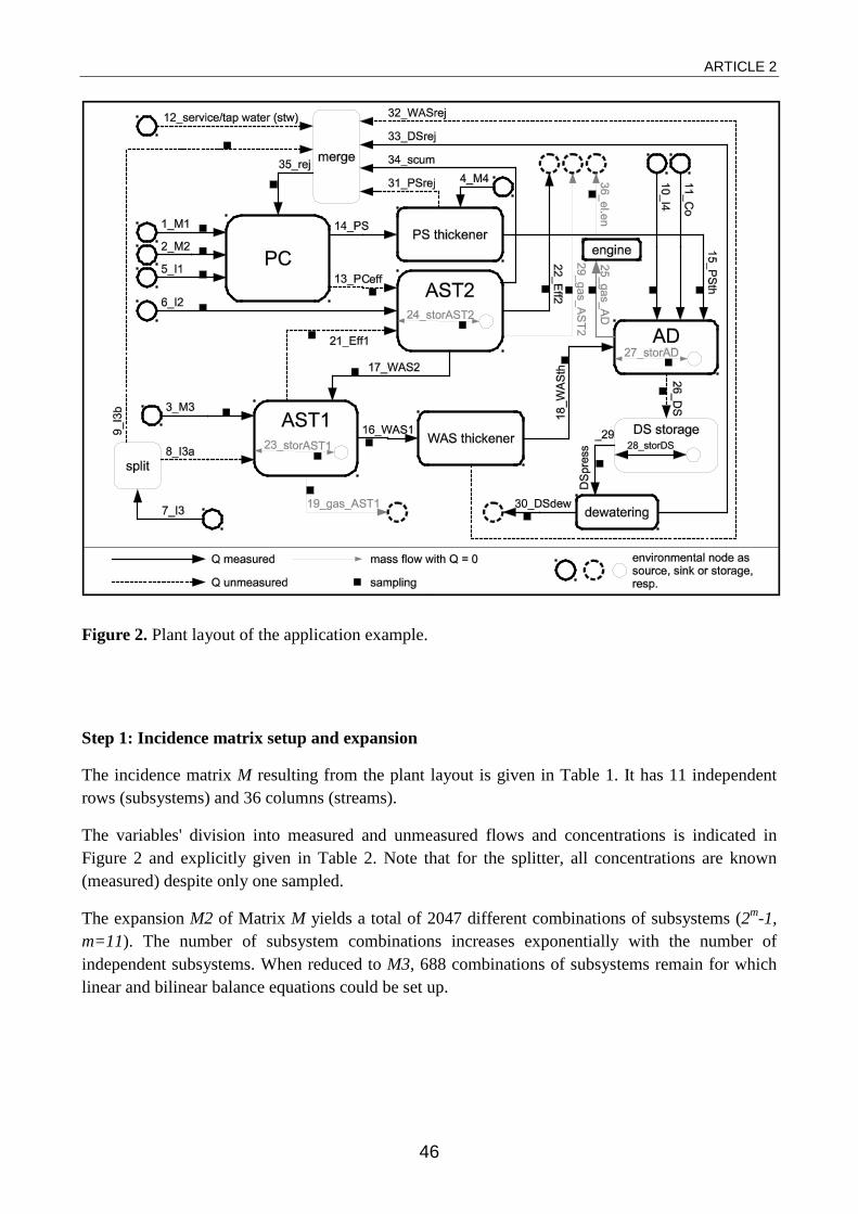
ARTICLE 2

46

Figure 2. Plant layout of the application example.

Step 1: Incidence matrix setup and expansion

The incidence matrix M resulting from the plant layout is given in Table 1. It has 11 independent rows (subsystems) and 36 columns (streams).

The variables' division into measured and unmeasured flows and concentrations is indicated in Figure 2 and explicitly given in Table 2. Note that for the splitter, all concentrations are known (measured) despite only one sampled.

The expansion M2 of Matrix M yields a total of 2047 different combinations of subsystems (2m-1, m=11). The number of subsystem combinations increases exponentially with the number of independent subsystems. When reduced to M3, 688 combinations of subsystems remain for which linear and bilinear balance equations could be set up.

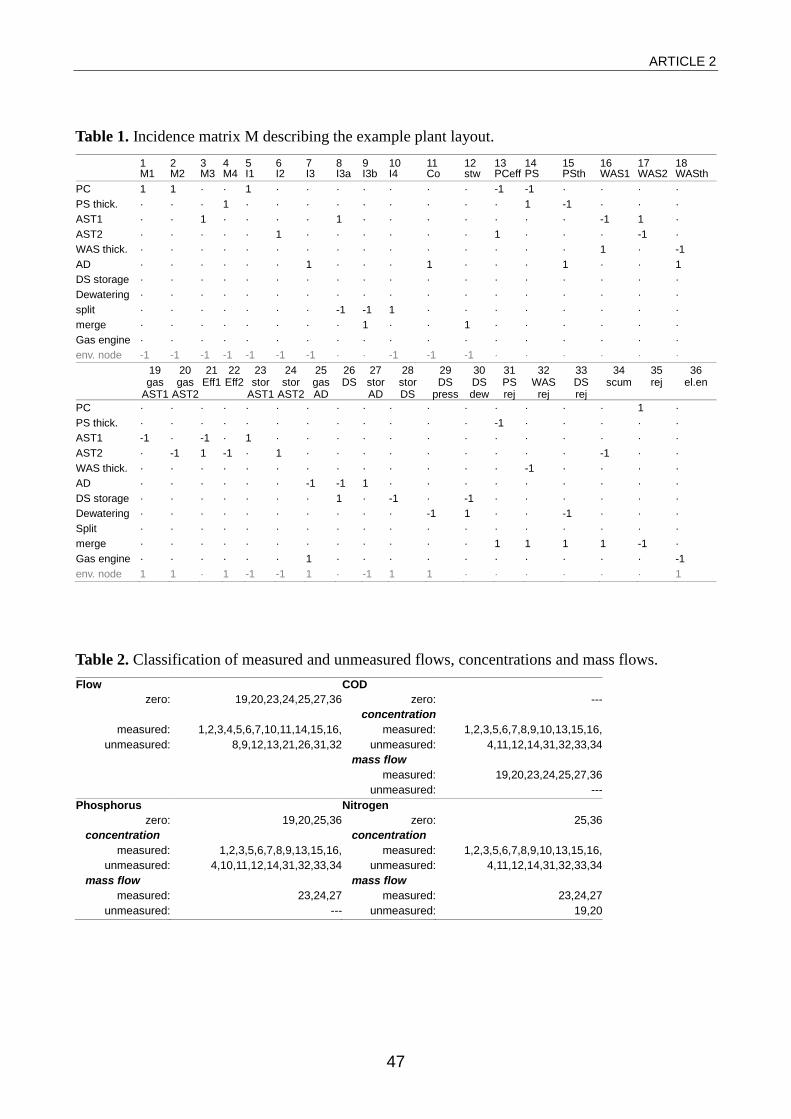
ARTICLE 2

47

Table 1. Incidence matrix M describing the example plant layout.

1 M1

2 M2

3 M3

4 M4

5 I1

6 I2

7 I3

8 I3a

9 I3b

10 I4

11 Co

12 stw

13 PCeff

14 PS

15 PSth

16 WAS1

17 WAS2

18 WASth

PC 1 1 · · 1 · · · · · · · -1 -1 · · · · PS thick. · · · 1 · · · · · · · · · 1 -1 · · · AST1 · · 1 · · · · 1 · · · · · · · -1 1 · AST2 · · · · · 1 · · · · · · 1 · · · -1 · WAS thick. · · · · · · · · · · · · · · · 1 · -1 AD · · · · · · 1 · · · 1 · · · 1 · · 1 DS storage · · · · · · · · · · · · · · · · · · Dewatering · · · · · · · · · · · · · · · · · · split · · · · · · · -1 -1 1 · · · · · · · · merge · · · · · · · · 1 · · 1 · · · · · · Gas engine · · · · · · · · · · · · · · · · · · env. node -1 -1 -1 -1 -1 -1 -1 · · -1 -1 -1 · · · · · ·

19 gas

AST1

20 gas

AST2

21 Eff1

22 Eff2

23 stor

AST1

24 stor

AST2

25 gas AD

26 DS

27 stor AD

28 stor DS

29 DS

press

30 DS dew

31 PS rej

32 WAS

rej

33 DS rej

34 scum

35 rej

36 el.en

PC · · · · · · · · · · · · · · · · 1 · PS thick. · · · · · · · · · · · · -1 · · · · · AST1 -1 · -1 · 1 · · · · · · · · · · · · · AST2 · -1 1 -1 · 1 · · · · · · · · · -1 · · WAS thick. · · · · · · · · · · · · · -1 · · · · AD · · · · · · -1 -1 1 · · · · · · · · · DS storage · · · · · · · 1 · -1 · -1 · · · · · · Dewatering · · · · · · · · · · -1 1 · · -1 · · · Split · · · · · · · · · · · · · · · · · · merge · · · · · · · · · · · · 1 1 1 1 -1 · Gas engine · · · · · · 1 · · · · · · · · · · -1 env. node 1 1 · 1 -1 -1 1 · -1 1 1 · · · · · · 1

Table 2. Classification of measured and unmeasured flows, concentrations and mass flows. Flow COD

zero: 19,20,23,24,25,27,36 zero: --- concentration

measured: 1,2,3,4,5,6,7,10,11,14,15,16, 1 18 22 28 29 30 33 3 3

measured: 1,2,3,5,6,7,8,9,10,13,15,16, 1 18 21 22 26 28 29 30 3 unmeasured: 8,9,12,13,21,26,31,32 unmeasured: 4,11,12,14,31,32,33,34

mass flow measured: 19,20,23,24,25,27,36 unmeasured: ---

Phosphorus Nitrogen zero: 19,20,25,36 zero: 25,36

concentration concentration measured: 1,2,3,5,6,7,8,9,13,15,16,

measured: 1,2,3,5,6,7,8,9,10,13,15,16,

unmeasured: 4,10,11,12,14,31,32,33,34 unmeasured: 4,11,12,14,31,32,33,34 mass flow mass flow

measured: 23,24,27 measured: 23,24,27 unmeasured: --- unmeasured: 19,20

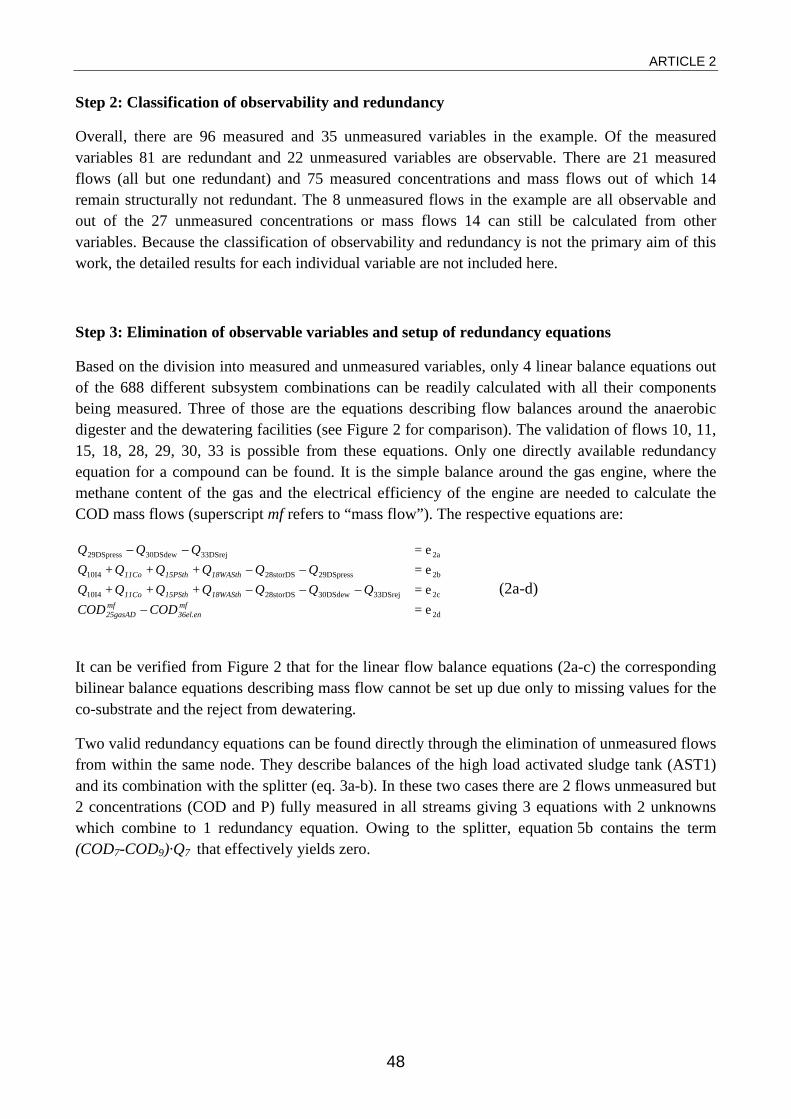
ARTICLE 2

48

Step 2: Classification of observability and redundancy

Overall, there are 96 measured and 35 unmeasured variables in the example. Of the measured variables 81 are redundant and 22 unmeasured variables are observable. There are 21 measured flows (all but one redundant) and 75 measured concentrations and mass flows out of which 14 remain structurally not redundant. The 8 unmeasured flows in the example are all observable and out of the 27 unmeasured concentrations or mass flows 14 can still be calculated from other variables. Because the classification of observability and redundancy is not the primary aim of this work, the detailed results for each individual variable are not included here.

Step 3: Elimination of observable variables and setup of redundancy equations

Based on the division into measured and unmeasured variables, only 4 linear balance equations out of the 688 different subsystem combinations can be readily calculated with all their components being measured. Three of those are the equations describing flow balances around the anaerobic digester and the dewatering facilities (see Figure 2 for comparison). The validation of flows 10, 11, 15, 18, 28, 29, 30, 33 is possible from these equations. Only one directly available redundancy equation for a compound can be found. It is the simple balance around the gas engine, where the methane content of the gas and the electrical efficiency of the engine are needed to calculate the COD mass flows (superscript mf refers to “mass flow”). The respective equations are:

2d

2c33DSrej30DSdew28storDS10I4

2b29DSpress28storDS10I4

2a33DSrej30DSdew29DSpress

e=e=e=e=

mf36el.en

mf25gasAD

18WASth15PSth11Co

18WASth15PSth11Co

CODCODQQQQ+Q+Q+Q

QQQ+Q+Q+QQQQ

−−−−

−−−−

(2a-d)

It can be verified from Figure 2 that for the linear flow balance equations (2a-c) the corresponding bilinear balance equations describing mass flow cannot be set up due only to missing values for the co-substrate and the reject from dewatering.

Two valid redundancy equations can be found directly through the elimination of unmeasured flows from within the same node. They describe balances of the high load activated sludge tank (AST1) and its combination with the splitter (eq. 3a-b). In these two cases there are 2 flows unmeasured but 2 concentrations (COD and P) fully measured in all streams giving 3 equations with 2 unknowns which combine to 1 redundancy equation. Owing to the splitter, equation 5b contains the term (COD7-COD9)·Q7 that effectively yields zero.

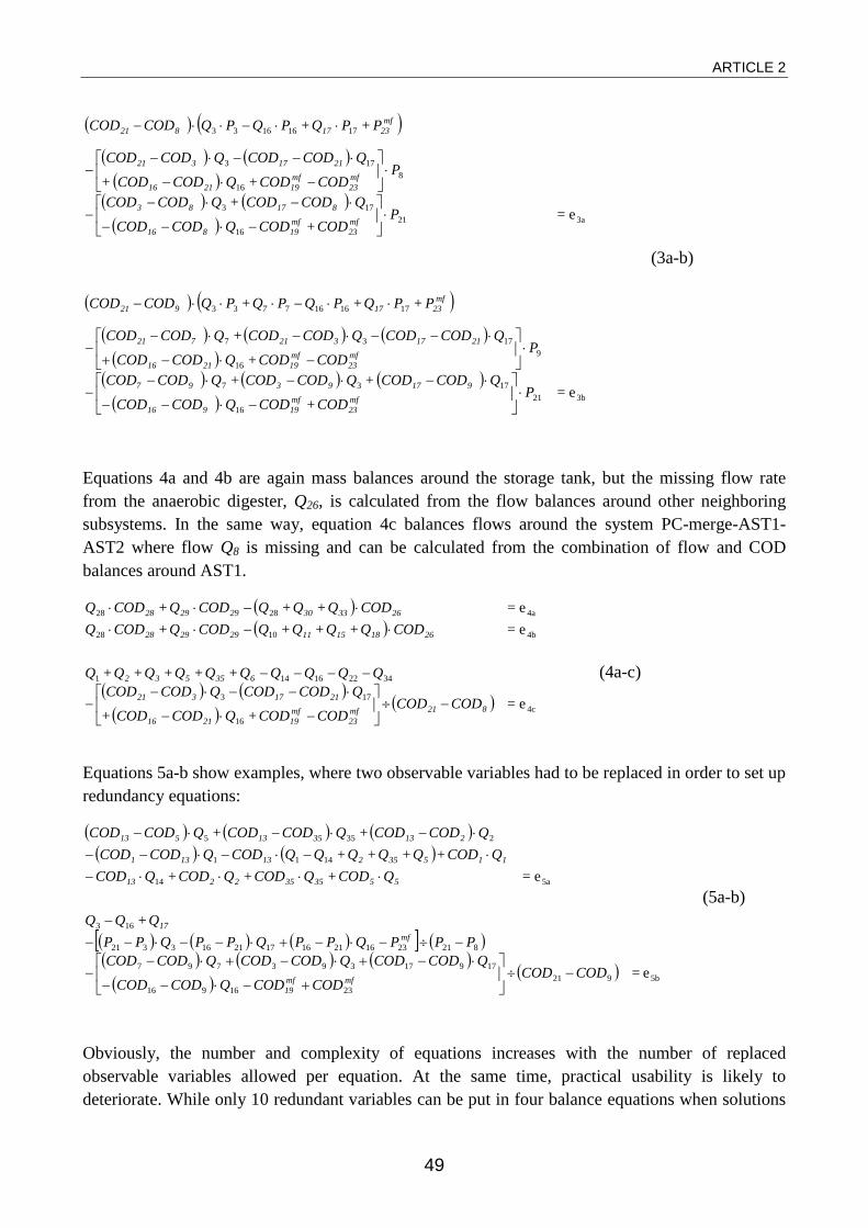
ARTICLE 2

49

( ) ( )( ) ( )( )

( ) ( )( )

( ) ( )( ) ( ) ( )( )

( ) ( ) ( )( ) 3b21

16

1737

916

1737

171616733

3a2116

173

816

173

17161633

e=

e=

PCOD+CODQCODCOD

QCODCOD+QCODCOD+QCODCOD

PCODCOD+QCODCOD

QCODCODQCODCOD+QCODCOD

P+PQ+PQPQ+PQCODCOD

PCOD+CODQCODCOD

QCODCOD+QCODCOD

PCODCOD+QCODCOD+

QCODCODQCODCOD

P+PQ+PQPQCODCOD

mf23

mf19916

9179397

mf23

mf192116

2117321721

mf23177921

mf23

mf19816

81783

mf23

mf192116

2117321

mf2317821

⋅

−⋅−−

⋅−⋅−⋅−−

⋅

−⋅−+

⋅−−⋅−⋅−−

⋅⋅−⋅⋅⋅−

⋅

−⋅−−

⋅−⋅−−

⋅

−⋅−

⋅−−⋅−−

⋅⋅−⋅⋅−

(3a-b)

Equations 4a and 4b are again mass balances around the storage tank, but the missing flow rate from the anaerobic digester, Q26, is calculated from the flow balances around other neighboring subsystems. In the same way, equation 4c balances flows around the system PC-merge-AST1-AST2 where flow Q8 is missing and can be calculated from the combination of flow and COD balances around AST1.

( )( )

( ) ( )( )

( ) 4c16

173

342216141

4b1028

4a2828

e=

e=e=

821mf23

mf192116

2117321

635532

26181511292928

263330292928

CODCODCODCOD+QCODCOD+

QCODCODQCODCODQQQQQ+Q+Q+Q+Q+Q

CODQ+Q+Q+QCODQ+CODQCODQ+Q+QCODQ+CODQ

−÷

−⋅−

⋅−−⋅−−

−−−−

⋅−⋅⋅⋅−⋅⋅

(4a-c)

Equations 5a-b show examples, where two observable variables had to be replaced in order to set up redundancy equations:

( ) ( ) ( )( ) ( )

( ) ( ) ( )[ ] ( )( ) ( ) ( )( )

( ) 5b9212316916

17917393797

821231621161721163321

163

5a14

1411

2355

e =

e=

CODCODCODCODQCODCOD

QCODCODQCODCODQCODCODPPPQPPQPPQPP

Q+QQ

QCOD+QCOD+QCOD+QCODQCOD+Q+Q+Q+QQCODQCODCOD

QCODCOD+QCODCOD+QCODCOD

mfmf19

mf17

5535352213

11535213131

2133513513

−÷

+−⋅−−

⋅−+⋅−+⋅−−

−÷−⋅−+⋅−−⋅−−−

⋅⋅⋅⋅−⋅−⋅−⋅−−

⋅−⋅−⋅−

(5a-b)

Obviously, the number and complexity of equations increases with the number of replaced observable variables allowed per equation. At the same time, practical usability is likely to deteriorate. While only 10 redundant variables can be put in four balance equations when solutions

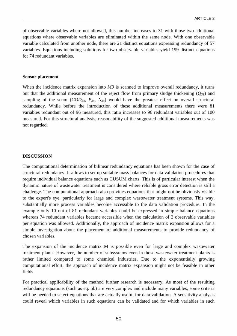
ARTICLE 2

50

of observable variables where not allowed, this number increases to 31 with those two additional equations where observable variables are eliminated within the same node. With one observable variable calculated from another node, there are 21 distinct equations expressing redundancy of 57 variables. Equations including solutions for two observable variables yield 199 distinct equations for 74 redundant variables.

Sensor placement

When the incidence matrix expansion into M3 is scanned to improve overall redundancy, it turns out that the additional measurement of the reject flow from primary sludge thickening (Q31) and sampling of the scum (COD34, P34, N34) would have the greatest effect on overall structural redundancy. While before the introduction of these additional measurements there were 81 variables redundant out of 96 measured, this ratio increases to 96 redundant variables out of 100 measured. For this structural analysis, reasonability of the suggested additional measurements was not regarded.

DISCUSSION

The computational determination of bilinear redundancy equations has been shown for the case of structural redundancy. It allows to set up suitable mass balances for data validation procedures that require individual balance equations such as CUSUM charts. This is of particular interest when the dynamic nature of wastewater treatment is considered where reliable gross error detection is still a challenge. The computational approach also provides equations that might not be obviously visible to the expert's eye, particularly for large and complex wastewater treatment systems. This way, substantially more process variables become accessible to the data validation procedure. In the example only 10 out of 81 redundant variables could be expressed in simple balance equations whereas 74 redundant variables became accessible when the calculation of 2 observable variables per equation was allowed. Additionally, the approach of incidence matrix expansion allows for a simple investigation about the placement of additional measurements to provide redundancy of chosen variables.

The expansion of the incidence matrix M is possible even for large and complex wastewater treatment plants. However, the number of subsystems even in those wastewater treatment plants is rather limited compared to some chemical industries. Due to the exponentially growing computational effort, the approach of incidence matrix expansion might not be feasible in other fields.

For practical applicability of the method further research is necessary. As most of the resulting redundancy equations (such as eq. 5b) are very complex and include many variables, some criteria will be needed to select equations that are actually useful for data validation. A sensitivity analysis could reveal which variables in such equations can be validated and for which variables in such

ARTICLE 2

51

equations no conclusions can be drawn. Much alike, many redundancy equations cannot be set up because they include variables that are in fact negligible. In the example, neglecting Q8 (the flow of the sampling side stream of the industrial influent 7_I3) would allow the setup of a flow balance around the primary clarifier and the activated sludge tanks AST1 and AST2. However, flow Q8 might not be negligible with respect to the merging of the various reject waters. These questions address practical redundancy in addition to structural redundancy of the variables. An extension of the above described algorithm should be possible to find approximate redundancy equations. This would be based on an estimation of all variables, where possible by the classical methods of data reconciliation. Following an analysis of sensitivity, for each equation in M2 the negligible terms would be eliminated before solutions for observable variables and redundancy equations are calculated. Investigations in this direction shall be the objective of a subsequent paper.

CONCLUSIONS

An algorithm is presented that allows the determination of all structurally possible redundancy equations for a given plant layout and classification of measured and unmeasured variables. Due to the separate treatment of flows and concentrations not only linear redundancy equations can be found. The algorithm is derived from data reconciliation methods which are applied extensively in the field of (chemical) process engineering but so far hardly present in wastewater treatment. Because of a possibly large number and high complexity of the resulting redundancy equations, the investigation of practical redundancy appears necessary. The underlying concept of incidence matrix expansion also allows a simple investigation on the effect of additional measurements.

It has been shown, that the setup of individual redundancy equations for data validation based on mass balancing can be fully computerized. This is an important step in the development of automated data validation in wastewater treatment systems.

ACKNOWLEDGEMENTS

The basic ideas of this work were developed during the first author's stay at modelEAU in Québec, Canada, which co-funded the exchange. Peter Vanrolleghem holds the Canada Research Chair in water quality modeling. During the 1st IWA YWP Publication Workshop sponsored by and held at UTM Johor Baru, Malaysia, helpful remarks and intense discussions from and with Gustav Olsson and Helmut Kroiss contributed significantly to improve the paper.

ARTICLE 2

52

REFERENCES

Bagajewicz, M. J. (1998) Gross error modeling and detection in plant linear dynamic reconciliation. Computers & Chemical Engineering, 22, 1789–1809.

Bagajewicz, M. J. (2010) Smart process plants software and hardware solutions for accurate data and profitable operations, New York :, McGraw-Hill.

Barker, P. S. and Dold, P. L. (1995) Cod and Nitrogen Mass Balances in Activated-Sludge Systems. Water Research, 29(2), 633–643.

Crowe, C. M. (1996) Data reconciliation — Progress and challenges. Journal of Process Control, 6(2-3), 89–98.

Crowe, C. M. (1989) Observability and redundancy of process data for steady state reconciliation. Chemical Engineering Science, 44(12), 2909–2917.

Crowe, C. M. (1986) Reconciliation of process flow rates by matrix projection. Part II: The nonlinear case. AIChE Journal, 32(4), 616–623.

Crowe, C. M., Campos, Y. A. G., and Hrymak, A. (1983) Reconciliation of process flow rates by matrix projection. Part I: Linear case. AIChE Journal, 29(6), 881–888.

Decker, W., Greuel, G.-M., Pfister, G., and Schönemann, H. (2011) Singular — A computer algebra system for polynomial computations. Version 3-1-5, [online] http://www.singular.uni-kl.de/Manual/3-1-1/sing_1.htm

Hellinga, C. (1992). Macrobal 2.02. Delft University of Technology. [online] http://www.tnw.tudelft.nl/en/about-faculty/departments/biotechnology/data-software/macrobal/

Kelly, J. D. (2004) Formulating large-scale quantity-quality bilinear data reconciliation problems. Computers & Chemical Engineering, 28(3), 357–362.

Kelly, J. D. (1998) On finding the matrix projection in the data reconciliation solution. Computers & Chemical Engineering, 22(11), 1553–1557.

Kuehn, D. R. and Davidson, H. (1961) Computer Control II. Mathematics of Control. Chemical Engineering Progress, 57(6), 44–47.

Madron, F. and Veverka, V. (1992) Optimal selection of measuring points in complex plants by linear models. AIChE Journal, 38(2), 227–236.

Mah, R. S., Stanley, G. M., and Downing, D. M. (1976) Reconciliation and Rectification of Process Flow and Inventory Data. Industrial & Engineering Chemistry Process Design and Development, 15(1), 175–183.

Maxima (2013) Maxima, a Computer Algebra System. Version 5.30.0, [online] http://maxima.sourceforge.net/

Meijer, S. C., van der Spoel, H., Susanti, S., Heijnen, J. J., and van Loosdrecht, M. C. M. (2002) Error diagnostics and data reconciliation for activated sludge modelling using mass balances. Water Science and Technology, 45(6), 145–156.

Narasimhan, S. and Jordache, C. (2000) Data reconciliation & gross error detection: an intelligent use of process data, Gulf Professional Publishing.

Nowak, O., Franz, A., Svardal, K., Muller, V., and Kühn, V. (1999) Parameter estimation for activated sludge models with the help of mass balances. Water Science and Technology, 39(4), 113–120.

Nowak, O., Schweighofer, P., and Svardal, K. (1994) Nitrification Inhibition - A method for the estimation of actual maximum autotrophic growth rates in activated sludge systems. Water Science and Technology, 30(6), 9–19.

ARTICLE 2

53

Ponzoni, I., Sánchez, M. C., and Brignole, N. B. (1999) A New Structural Algorithm for Observability Classification. Industrial & Engineering Chemistry Research, 38(8), 3027–3035.

Puig, S., van Loosdrecht, M. C. M., Colprim, J., and Meijer, S. C. . (2008) Data evaluation of full-scale wastewater treatment plants by mass balance. Water Research, 42, 4645–4655.

Ragot, J., Maquin, D., Bloch, G., and Gomolka, W. (1990) Observability and variables classification in bilinear processes. Journal A, 17–23.

R Core Team (2013) R: A Language and Environment for Statistical Computing. Version 2.15.3, Vienna, Austria, R Foundation for Statistical Computing. [online] http://www.R-project.org/

Rieger, L., Takács, I., Villez, K., Siegrist, H., Lessard, P., Vanrolleghem, P. A., and Comeau, Y. (2010) Data Reconciliation for Wastewater Treatment Plant Simulation Studies—Planning for High-Quality Data and Typical Sources of Errors. Water Environment Research, 82(5), 426–433.

Romagnoli, J. A. and Sánchez, M. C. (2000) Data processing and reconciliation for chemical process operations, Academic Press.

Schraa, O. J. and Crowe, C. M. (1998) The numerical solution of bilinear data reconciliation problems using unconstrained optimization methods. Computers & Chemical Engineering, 22(9), 1215–1228.

Schraa, O. J., Tole, B., and Copp, J. B. (2006) Fault detection for control of wastewater treatment plants. Water Science & Technology, 53(4-5), 375.

Spindler, A. and Vanrolleghem, P. A. (2012) Dynamic mass balancing for wastewater treatment data quality control using CUSUM charts. Water science and technology: a journal of the International Association on Water Pollution Research, 65(12), 2148–2153.

Stein et al., W. A. (2012) Sage Mathematics Software. Version 5.5, The Sage Development Team. [online] http://www.sagemath.org

Václavek, V. (1969) Studies on system engineering—III optimal choice of the balance measurements in complicated chemical engineering systems. Chemical Engineering Science, 24(6), 947–955.

Václavek, V. and Louĉka, M. (1976) Selection of measurements necessary to achieve multicomponent mass balances in chemical plant. Chemical Engineering Science, 31(12), 1199–1205.

Van der Heijden, R. T. J. ., Heijnen, J. J., Hellinga, C., Romein, B., and Luyben, K. C. A. . (1994) Linear constraint relations in biochemical reaction systems: I. Classification of the calculability and the balanceability of conversion rates. Biotechnology and Bioengineering, 43, 3–10.

Villez, K., Corominas, L., Vanrolleghem, P. A. (2013a). Structural observability and redundancy classification for sensor networks in wastewater systems. Proceedings of the 11th IWA conference on instrumentation control and automation (ICA2013), Narbonne, FR, Sept. 18-20, 2013, Appeared on USB-stick (IWA-12741).

Villez, K., Corominas, L., Vanrolleghem, P. A. (2013b). Sensor fault detection and diagnosis based on bilinear mass balances in wastewater treatment systems. Proceedings of the 11th IWA conference on instrumentation control and automation (ICA2013), Narbonne, FR, Sept. 18-20, 2013, Appeared on USB-stick (IWA-12744).

ARTICLE 3

54

Quality control of wastewater treatment operational data by continuous mass balancing: Dealing with missing measurements and delayed outputs

A. Spindler, J. Krampe

Institute of Water Quality and Resource Management, Vienna University of Technology, Karlsplatz 13/226-1, 1040 Wien, Austria

Abstract

Continuous mass balancing defines a new standard in data quality validation. Likewise relying on the principles of mass conservation it outperforms long term static mass balancing approaches because faults in data can be assigned to their time of occurrence. This research was carried out with practical application to routine operational data in mind and two major aspects are investigated to make this application feasible. Sludge concentrations of typically balanced components (COD, TN, TP) are not routinely measured in wastewater treatment plants. Therefore they need to be determined from alternative, more frequent measurements such as TSS. To provide the necessary statistical basis for such determination, monthly sludge sampling was found sufficient. Further, contrary to long term static mass balancing, the effects of delay between input and output loads must not be neglected in continuous mass balancing based on daily data. While a storage/release approach did not give the desired results, the consideration of hydraulic retention (first-order flow dynamics) fundamentally improved the performance of the proposed method.

Keywords

continuous mass balancing; data quality control; fault detection; statistical process control

INTRODUCTION

Two fundamental aspects of continuous data quality control by mass balancing of operational data are addressed in this work. One is the determination of the concentration of components of sludge flows by using alternative measurements, the other is the influence of storage and retention on short term balances. The aim is to provide a simple method for practical implementation of continuous data quality control.

Mass balancing is a means of gross error detection in measurement data and the fundamental idea behind data reconciliation. Relying strictly on the laws of mass conservation, mass balances must only be carried out for conservative components that can be measured in all input and output streams of a system. Pure elements are always conservative in wastewater treatment and one typical balanceable element is (total) phosphorus. Nitrogen balances are also possible, however when denitrification is involved, off-gas nitrogen is usually not

ARTICLE 3

55

measured. Another typically balanceable “component” is COD, which is basically a sum parameter for free electrons. Other commonly measured components are not conservative and therefore subject to reactions. Mass balancing based only on measuring the concentrations of such components is not generally possible. An example is TSS, because biomass grows converting dissolved organic material into particulate material. For appropriate subsystems (such as a dewatering unit when TSS is considered) the conservative property of such components might, however, be given. Water itself, expressed as flow Q, can also be balanced neglecting the influence of evaporation.

Common approaches to mass balancing require steady state data (Narasimhan, 2000). For highly dynamic wastewater treatment systems this is usually achieved by considering mean values over rather long time periods (at least two sludge ages, typically several months). In perfect steady state, the total input load of a component into a system is equal the total output load when no accumulation or release occurs. The value of mass balancing as the most important approach to redundant data quality control is widely agreed upon in literature (e.g. Barker and Dold, 1995; Nowak et al., 1999; Puig et al., 2008; Rieger et al., 2010; Villez et al., 2013).

Continuous mass balancing , contrary to the static approaches typically used in wastewater 1treatment, reveals the temporal behavior of the balancing error. It allows to distinguish unbalanced from well-balanced time periods in a data set or to continuously monitor the integrity of operational data. The CUSUM chart, a control chart based on a modified cumulative sum and first introduced by Page (1954), has been proven suitable for continuous balancing of flow data from wastewater treatment plants (WWTPs) by Spindler and Vanrolleghem (2012). In their study the variance of the vector of (daily) balancing errors was found to be an important indicator for good data quality. It also influences the applicable parameters (and therefore sensitivity) of a CUSUM chart. A high variance of the vector of balancing errors requires a higher sensitivity of the CUSUM chart in order to detect off-balance periods, which leads to slower detection and vice versa. See appendix A for a short introduction to CUSUM charts. The present paper investigates the application of CUSUM charts to general mass flow data from wastewater treatment with a focus on requirements regarding the handling of sludge loads.

In practice concentration measurements at WWTPs are usually conducted in flow proportional 24h composite samples. Daily loads are then calculated from the product of this average concentration and the cumulated flow of the respective day. Therefore, in this research continuous mass balancing is applied to daily loads. It follows, that measurements are preferably taken daily, without interruption. This requirement is commonly met for most flows and the concentrations of influent, effluent and reject water but hard to achieve for concentrations in primary sludge (PS), waste activated sludge (WAS) or digested sludge (DS). Measurement of typical balanceable sludge components (TP, TN, COD) is complicated because it requires thorough disintegration of the samples and small but representative sample 1 The application of CUSUM charts for mass balancing was labeled “dynamic mass balancing” in a previous paper (Spindler and Vanrolleghem, 2012) to differentiate from the established approaches. However, as this approach does not actually target process dynamics, the naming was changed to “continuous mass balancing”.

ARTICLE 3

56

volumes which are difficult to obtain. Therefore and because these data are circumstantial for daily plant operation, this type of measurement is usually not carried out in practice.

Due to the nature of wastewater treatment, sludge streams are part of virtually every balanceable subsystem of a WWTP. For operation and documentation they are usually characterized by volume and concentration of TSS (total suspended solids). Organic and inorganic constituents of sludge are measured as volatile and nonvolatile suspended solids (VSS and NVSS). TSS, VSS and NVSS are routine parameters and regularly measured on a daily basis. Grab samples are usually sufficient because sludge characteristics change only slowly. Only primary sludge is subject to faster fluctuations but thickened primary sludge can be analyzed instead or online TSS measurement is employed to determine an average value.

A common approach to quantify balanceable sludge components is their determination from TSS or VSS, assuming stable proportionality between the two factors. This is a rational approach, particularly for nitrogen and COD concentrations of WAS and DS, because nitrogen is a constituent and COD a property of the biomass which only the organic fraction of sludge is composed of. Phosphorus, on the other hand can also be chemically precipitated, thus becoming a constituent of the inorganic fraction of WAS and DS. Ekama (2009) includes an overview of literature values on COD and nitrogen concentrations of primary and activated sludge: COD/VSS ratios of activated sludge vary between 1.42 and 1.55, for primary sludge the range is even larger. Nitrogen and phosphorus are also often analyzed to determine nutrient levels for agricultural application. Their concentration in sludge depends heavily on the wastewater composition and treatment and ranges between less than 1% and 10% of TSS (Scharf et al., 1997). The temporal stability of the relations between balanceable sludge components and VSS or TSS within a single sludge is decisive for the reliability of this approach and determines the necessary measurement frequency. Both issues are addressed in this work.

As a second fundamental aspect the influence of delay on short term mass balances is investigated. “Delay” in this work is not meant in its strict meaning referring to flow through an idealized plug-flow reactor. It is rather used to describe the general effect of loads leaving a reactor distributed over a certain time span. For short term mass balances the precondition of steady state, as mentioned above, is not satisfied. Loads entering a reactor on one day do not necessarily leave it on the same day. This can be accounted for by the concept of storage (also: accumulation) and release. These occur when the input load to a balanced subsystem is unequal to the output load in a given time period. For example, the amount of sludge in an activated sludge unit (including clarifiers) depends on the organic influent load and waste sludge flow. When less waste activated sludge is withdrawn from the system, a higher COD, TN and TP load is stored with the sludge.

As it turned out that this storage/release approach is highly sensitive to measurement errors, another concept to account for delayed outputs was investigated. Hydraulic retention (or first-order flow dynamics) can be used to calculate the effluent concentration from a (perfectly mixed) tank, depending on the influent concentration. Here, a constant tank volume was assumed which is typical in wastewater treatment. The assumption of a constant influent flow is derived from the frequency of the measurements the balancing approach is based on (1/d).

ARTICLE 3

57

In continuous balancing based on daily loads the effect of hydraulic retention can be neglected only for streams with very short retention times (less than one day) such as methane or nitrogen gas production. For the effluent with a retention time of roughly one day neglecting this delay is also allowed because it contains only a small proportion of the daily input load and has little influence on the balance.

METHODS

Regression analysis

To investigate the determination of COD, TN and TP from different fractions of suspended solids (SS), three different data sets were used. Data set A contains weekly (at least) routine data from a large Austrian WWTP and covers a time span of almost three and a half years. Data set B stems from a pilot scale anaerobic digestion stationed at another large Austrian WWTP. Sludge concentrations were measured during 47 consecutive weeks. Data set C contains values from sludge samples that were analyzed supplementary to routine operational data in order to achieve balanceability of yet another Austrian WWTP. These samples were taken 21 times over a period of 24 weeks. Plant A and C are subject to strong influence from industries, mainly chemical, accounting for up to 50% of the organic load. Concentrations were measured in the (waste) activated sludge (AS), primary sludge (PS) and digested sludge (DS). On plant B, waste activated and primary sludge are mixed (AS&PS).

Simple and multiple linear regressions with and without intercept are applied to determine concentrations of COD, TN and TP from SS. Different SS fractions are considered, namely total (TSS), volatile (VSS) and nonvolatile (NVSS) suspended solids. For consideration of temporal behavior, the inclusion of trend and seasonality is compared to simple linear dependency from SS. The investigated and here reported regression models are of the following types:

𝑐𝑥 = 𝑎1 ∙ 𝑐𝑆𝑆 eq. (1)

𝑐𝑥 = 𝑎1 ∙ 𝑐𝑆𝑆 + 𝑎2 eq. (2)

𝑐𝑥 = 𝑎1 ∙ 𝑐𝑆𝑆 + 𝑎2 ∙ sin(𝜔𝜔) + 𝑎3 ∙ cos(𝜔𝜔) + 𝑎4 ∙ 𝜔 + 𝑎5 eq. (3)

For evaluation of significance of the regression three different parameters are used: the coefficient of determination (R², calculated as explained variance), Akaike’s Information criterion (AIC, for balancing model fit and complexity, accounting for the number of model parameters) and the relative two standard deviation range around the mean (2σres/µ, containing about 95% of the measured values).

The large number of data points in data set A also allows for evaluation of lower measurement frequencies by Monte Carlo simulation. This was done by investigating the probability of only slightly deteriorated results (an increase of the relative two standard

ARTICLE 3

58

deviation range of not more than 10%) when determining the regression models from only monthly or quarterly (instead of weekly) measured data.

Continuous balancing under the influence of delay

In the second part of this work some exemplary balances are calculated for plant C based on the adequate determination of sludge concentrations. The balancing error e for a chosen subsystem is calculated from the difference between the sum of all input loads and the sum of all output loads (ΣFin and ΣFout). This error can be related to the total input load, giving the relative balancing error erel. The determination of balancing equations for large and complex plants can be facilitated using an automated approach (Spindler, 2014). For continuous balancing, it is the vector of daily balancing errors that needs to be calculated instead of an overall mean balancing error. This error vector is then analyzed using CUSUM charts (see below). An example is given in the results section.

When wastewater treatment balances are calculated on a daily basis, the delay between input and output loads has to be considered. Two different approaches to account for this delay are investigated, i.e. the concept of storage and release and the concept of hydraulic retention. For better comparison of these different approaches each continuous balance will be calculated three times: one directly (without delay), one including storage and release (based on the SS concentration in the reactor) and one under consideration of hydraulic retention.

Storage (∆S) is calculated for component loads (TN, TP, COD) contained in sludge (eq. 4).

∆𝑆𝑖 = 𝑉 ∙ (𝑥𝑖 − 𝑥𝑖−1) i = 1…n eq. (4)

∆𝑆𝑖+ = 𝑚𝑎𝑥(0,∆𝑆𝑖) eq. (4a)

∆𝑆𝑖− = |𝑚𝑚𝑚(0,∆𝑆𝑖)| eq. (4b)

An increasing sludge concentration (storage, ∆Si+) is counted as an additional output mass

flow; a decrease in sludge concentration (release, ∆Si-) is counted as an additional input mass

flow (see results). This way, storage and release loads are regarded as physical streams which makes interpretation (e.g. of the magnitude of average storage and release) more intuitive. It also facilitates the automatic determination of balancing equations according to Spindler (2014).

Note that for a correct determination of daily storage, a component's concentration would actually have to be known exactly at the beginning of each 24h composite sampling cycle. This is not always the case in practice. For sludge, for example, grab samples are commonly used and representativeness for the corresponding composite sample has to be assumed.

Because the storage/release approach did not give the desired results (see below), another approach to account for a delayed output load was investigated. The effect of hydraulic retention is taken into consideration by calculating an "expected output mass flow" from the

ARTICLE 3

59

initial concentration of a component (x0) in the reactor, its influent concentration (xin, assumed constant), the flow rate (Q) and the reactor volume (V). The expected output mass flow can then be balanced against the measured output. Assuming an ideal CSTR the expected output's concentration after a given time (t) is calculated as follows:

𝑑𝑥𝑜𝑜𝑜𝑑𝑑

= 𝑄/𝑉 ∙ (𝑥𝑖𝑖 − 𝑥𝑜𝑜𝑑) eq. (5)

With τ = V/Q (hydraulic retention of the balanced compound) integration yields

𝑥𝑜𝑜𝑑 = 𝑥𝑖𝑖 − (𝑥𝑖𝑖 − 𝑥0) ∙ exp �− 𝑑𝜏� eq. (6)

Equation (5) describes the hydraulic transport through an ideal CSTR. Obviously, this is a purely hydraulic model and reactions must not be regarded. Mass balancing is based on the laws of mass conservation (of a component). Reactions only alter the distribution of a component between different output paths, they do not change its total sum.

For the calculation of the daily error vector, the expected mean output concentration for one day (t=1, index i) is calculated assuming a constant (mean) influent concentration and flow and a constant volume (Qin=Qout=Q):

�̅�𝑜𝑜𝑑,𝑒𝑥𝑒𝑒𝑒𝑑𝑒𝑑,𝑖 = �̅�𝑖𝑖,𝑖 − 𝜏𝑖 ∙ (�̅�𝑖𝑖,𝑖 − �̅�𝑜𝑜𝑑,𝑒𝑥𝑒𝑒𝑒𝑑𝑒𝑑,𝑖−1) ∙ (1 − exp �− 1𝜏𝑖�) eq. (7)

The expected output load is calculated from the expected mean output concentration.

𝐹𝑜𝑜𝑑,𝑒𝑥𝑒𝑒𝑒𝑑𝑒𝑑,𝑖 = 𝑄�𝑜𝑜𝑑,𝑖 ∙ �̅�𝑜𝑜𝑑,𝑒𝑥𝑒𝑒𝑒𝑑𝑒𝑑,𝑖 eq. (8)

This expected output load, which is basically calculated from the measured input load (see eq. 7), is then balanced against the measured output load. An example is given in the results.

In case two output paths exist, retention needs to be considered for the slow path only (usually related to the sludge). For example, methane is produced almost instantly from the organic input load in an anaerobic digester. The delay between input and gas production (fast output path) can be neglected when dealing with daily mean data. The digested sludge, however, has a rather long retention time and delay has to be accounted for. This is achieved by calculating a virtual input concentration discounting the fast output load from the actual input load. In this way, equation (5) has to be solved only for one xout, which is the way it was specified.

�̅�𝑖𝑖,𝑣𝑖𝑣𝑑𝑜𝑣𝑣,𝑖 = (�̅�𝑖𝑖,𝑖 ∙ 𝑄�𝑖𝑖,𝑖 − �̅�𝑜𝑜𝑑,𝑓𝑣𝑓𝑑,𝑖 ∙ 𝑄�𝑜𝑜𝑑,𝑓𝑣𝑓𝑑,𝑖)/𝑄�𝑜𝑜𝑑,𝑓𝑣𝑜𝑠,𝑖 eq. (9)

ARTICLE 3

60

One important question remains: How should the initial concentration in the tank be chosen? It could either be the measured or the previously predicted concentration. In eq. (7), the latter (xout,expected,i-1) was chosen. This value has great influence on xout,expected,i. In fact, with long hydraulic retention, xout,expected,i depends almost entirely on the initial concentration (It holds: lim(exp(-x), x→0) = 1-x). If measured values are used, the expected output concentration xout,expected,i is heavily influenced by the measured output concentration xout,i-1. This leads to deterioration of the actual balance (where xout,i is balanced against xout,expected,i). Therefore, only the initial value xout,0 is taken from measurements, thereafter this value is taken from xout,expected,i-1 of the previous day. This way, all xout,expected are (almost) only calculated from the input which is a precondition for balancing against the measured values xout.

CUSUM charts were calculated according to Spindler and Vanrolleghem (2012, see the appendix for an introduction). In this previous work the method was found to reliably detect even small deviations of the balancing error from the expected zero mean in the case of systematic measurement errors. The CUSUM parameters have to be chosen carefully. Once the choice of an average in control run length ARL0 is made, the control limit h depends only on the reference value k. It was calculated using the spc package (Knoth, 2009) for R (R Core Team, 2013). When the CUSUM chart exceeds the control limit h, it signals a significant deviation from the expected value (0), i.e. an off-balance situation. For ARL0, the classical value 370 (Montgomery, 2009) was chosen. Small reference values k lead to higher sensitivity (smaller optimally detectable error Δµopt) at the cost of slower detection (increasing ARL). Practice has shown that a good choice of k gives Δµopt within 10%-20% of the input load. As the variance of the error vector becomes larger, k is chosen smaller (but not below 0.2) to facilitate detection. Error vectors with a small variance are a good indicator of high data quality themselves. In these cases k can be chosen higher to avoid signals at minor disturbances.

RESULTS & DISCUSSION

The first part of this work was concerned with the determination of sludge component concentrations (TP, TN, COD) from frequent alternative measurements, namely fractions of suspended solids (SS). For application of continuous balancing based on CUSUM charts, daily values for these components are required, a precondition usually not met in practice. The determination of sludge components from fractions of SS does not mean performing balances of SS (in the second part of the results section) which is not generally possible.

Regression analysis for determination of non-measured concentrations

P, N and COD where determined from fractions of SS for three different WWTPs (A,B,C). Data were collected weekly for plants B and C and at least weekly for plant A. Results for the three regression models (eq. 1-3) are given in Table 1. The third regression model also takes into account possible temporal behavior (trend and seasonality) of the variables. The best available model is indicated by “++”. In most cases, this is the model including seasonality. If

ARTICLE 3

61

a simpler model reaches comparable significance, this is indicated by “+”. Significance is given by the coefficient of determination R² and the relative two standard deviation range around the mean. AIC was also calculated but did not give any additional evidence and is therefore not shown in Table 1.

VSS turned out to be the best choice of a SS fraction for the determination of COD. For determination of TN and TP, other fractions give slightly better results in some cases but VSS always remains a good alternative for determination of TN and in most cases for TP, too. Only for the determination of TP in digested sludge (DS) of plant C the volatile fraction alone is not a suitable parameter. In some cases the best results are achieved by assuming VSS and NVSS to be independent, i.e. not constrained by TSS.

Data set A reveals poorer overall regression quality than data sets B and C. It should be kept in mind, however, that this data set covers a time span of almost three and a half years and external influences on sludge characteristics during this period are quite likely. Still, 95% of the residuals lie within ±15% to ±25% of the mean concentration for data set A with the exception of TN and TP values for primary sludge (PS).

Data set B, covering almost one year and analyzed in the laboratory of the authors' home institution, yields coefficients of determination between 0.69 and 0.95. The residuals lie mostly within ±6% to ±13% of the mean concentration. Only for TP determination in mixed sludge (AS&PS) this interval is ±19% of the mean. Data set C, covering only 24 weeks and also analyzed in the authors' home institution, gives similar results. Coefficients of determination lie between 0.60 and 0.96 with one exception (0.43 for TP in PS). The range of residuals is mostly within ±5% to ±9% of the mean concentrations. Again, exceptions occur only for determination of TN and TP in PS.

The determination of COD gives mostly acceptable results (residuals range ±25% or lower), with simple linear regression models being sufficient. In two cases the intercept must not be neglected. Only for the activated sludge (AS) of plant C the temporal behavior requires consideration, too. For determination of TN and TP from data sets B and C acceptable results are achieved in AS and DS. For plant A, the poorer quality of regression models is attributed to the higher number of data as stated above. For the PS however, meaningful regression seems harder to achieve, especially for TP but also for TN.

It is important to notice that this assessment is purely statistical. Therefore, extrapolation of results into different ranges of SS concentrations (e.g. from AS to thickened AS) or time periods is not reliable. The regression can be applied to determine concentrations of less frequently measured sludge components from more frequently (preferably every day) measured fractions of SS. An obvious deterministic relation exists only for direct proportionality between COD (as well as TN) concentrations in sludge and VSS. But although such a relation seems reasonable for these sludge components, counterexamples (mainly for TN) are found in the results.

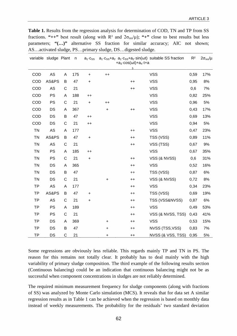
ARTICLE 3

62

Table 1. Results from the regression analysis for determination of COD, TN and TP from SS fractions. “++” best result (along with R² and 2σres/µ); “+” close to best results but less parameters; “(…)” alternative SS fraction for similar accuracy; AIC not shown; AS…activated sludge, PS…primary sludge, DS…digested sludge.

variable sludge Plant n a1·cSS a1·cSS+a2 a1·cSS+a2·sin(ωt) +a3·cos(ωt)+a4·t+a

5

suitable SS fraction R² 2σres/µ

COD AS A 175 + ++ VSS 0,59 17% COD AS&PS B 47 + ++ VSS 0,95 8% COD AS C 21 ++ VSS 0,6 7% COD PS A 188 ++ VSS 0,82 25% COD PS C 21 + ++ VSS 0,96 5% COD DS A 367 + ++ VSS 0,43 17% COD DS B 47 ++ VSS 0,69 13% COD DS C 21 ++ VSS 0,94 5% TN AS A 177 ++ VSS 0,47 23% TN AS&PS B 47 + ++ TSS (VSS) 0,89 11% TN AS C 21 ++ VSS (TSS) 0,67 9% TN PS A 185 ++ VSS 0,67 35% TN PS C 21 + ++ VSS (& NVSS) 0,6 31% TN DS A 365 ++ VSS 0,52 16% TN DS B 47 ++ TSS (VSS) 0,87 6% TN DS C 21 + ++ VSS (& NVSS) 0,72 8% TP AS A 177 ++ VSS 0,34 23% TP AS&PS B 47 + ++ TSS (VSS) 0,69 19% TP AS C 21 + ++ TSS (VSS&NVSS) 0,87 6% TP PS A 189 ++ VSS 0,49 53% TP PS C 21 ++ VSS (& NVSS, TSS) 0,43 41% TP DS A 369 + ++ VSS 0,53 15% TP DS B 47 + ++ NVSS (TSS,VSS) 0,83 7% TP DS C 21 + ++ NVSS (& VSS, TSS) 0,95 5%

Some regressions are obviously less reliable. This regards mainly TP and TN in PS. The reason for this remains not totally clear. It probably has to deal mainly with the high variability of primary sludge composition. The third example of the following results section (Continuous balancing) could be an indication that continuous balancing might not be as successful when component concentrations in sludges are not reliably determined.

The required minimum measurement frequency for sludge components (along with fractions of SS) was analyzed by Monte Carlo simulation (MCS). It reveals that for data set A similar regression results as in Table 1 can be achieved when the regression is based on monthly data instead of weekly measurements. The probability for the residuals’ two standard deviation

ARTICLE 3

63

range to increase by more than 10% above its original value is below 3% in all cases (data not shown). MCS was based on the best available model for each sludge and concentration, in most cases including seasonality. When only quarterly data is simulated, these results cannot be reproduced. Only data that is not influenced by seasonality can be reliably determined from measurements at this low frequency.

Continuous balancing

Following the determination of sludge components from daily measured SS fractions, three different continuous balances were calculated for plant C. Those are the NVSS and COD balances of the anaerobic digester and the total phosphorus balance of the combination of primary clarifier and activated sludge tank (including secondary clarifier). Performing and NVSS balance for the anaerobic digester is in line with the requirement of conservative components as precipitation is negligible. Each balance was calculated three times:

(I) Without consideration of storage and retention (II) With storage based on daily SS-fluctuations (III) With hydraulic retention

A calculation example is given for the COD balance of the digester (for data see appendix B):

Daily input loads (calculated from flow and concentration):

∑ Fin,i = FCo,iCOD + FPS,i

COD + FWAS,iCOD

Daily output loads:

∑ Fout,i = FDS,iCOD + Fgas,i

COD

The error vector without consideration of storage and retention follows as:

(I) erel,i = (∑ Fin,i − ∑ Fout,i)/F�in

Storage and release are easily integrated into (I) as additional loads:

(II) erel,i = (∑ Fin,i + ∆Si− − ∑ Fout,i − ∆Si+)/F�in

For consideration of hydraulic retention, the two output paths have to be considered separately. Methane is produced from input COD practically without delay (fast output path). Hydraulic retention occurs for the digested sludge (slow output path). The virtual input concentration is therefore calculated from the difference between input load and the fast

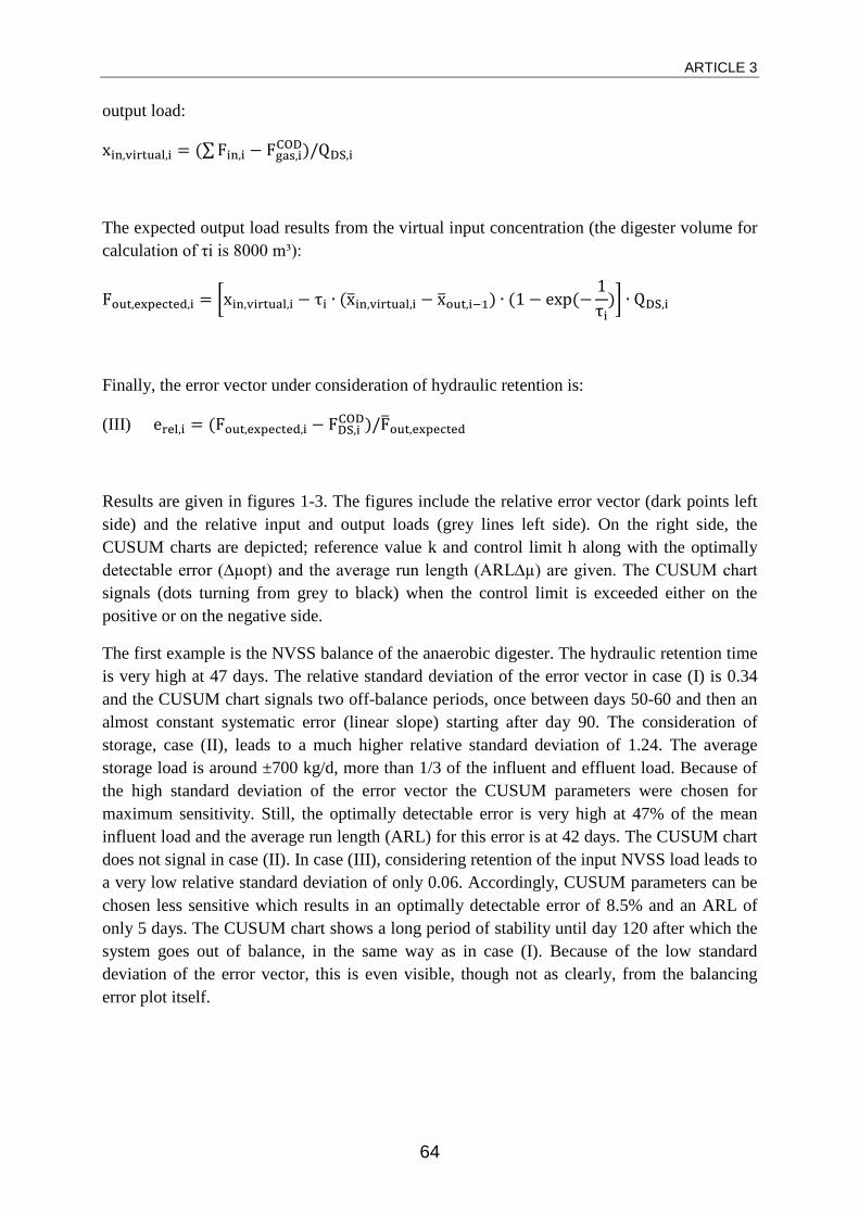
ARTICLE 3

64

output load:

xin,virtual,i = (∑ Fin,i − Fgas,iCOD)/QDS,i

The expected output load results from the virtual input concentration (the digester volume for calculation of τi is 8000 m³):

Fout,expected,i = �xin,virtual,i − τi ∙ (x�in,virtual,i − x�out,i−1) ∙ (1 − exp (−1τi

)� ∙ QDS,i

Finally, the error vector under consideration of hydraulic retention is:

(III) erel,i = (Fout,expected,i − FDS,iCOD)/F�out,expected

Results are given in figures 1-3. The figures include the relative error vector (dark points left side) and the relative input and output loads (grey lines left side). On the right side, the CUSUM charts are depicted; reference value k and control limit h along with the optimally detectable error (∆µopt) and the average run length (ARL∆µ) are given. The CUSUM chart signals (dots turning from grey to black) when the control limit is exceeded either on the positive or on the negative side.

The first example is the NVSS balance of the anaerobic digester. The hydraulic retention time is very high at 47 days. The relative standard deviation of the error vector in case (I) is 0.34 and the CUSUM chart signals two off-balance periods, once between days 50-60 and then an almost constant systematic error (linear slope) starting after day 90. The consideration of storage, case (II), leads to a much higher relative standard deviation of 1.24. The average storage load is around ±700 kg/d, more than 1/3 of the influent and effluent load. Because of the high standard deviation of the error vector the CUSUM parameters were chosen for maximum sensitivity. Still, the optimally detectable error is very high at 47% of the mean influent load and the average run length (ARL) for this error is at 42 days. The CUSUM chart does not signal in case (II). In case (III), considering retention of the input NVSS load leads to a very low relative standard deviation of only 0.06. Accordingly, CUSUM parameters can be chosen less sensitive which results in an optimally detectable error of 8.5% and an ARL of only 5 days. The CUSUM chart shows a long period of stability until day 120 after which the system goes out of balance, in the same way as in case (I). Because of the low standard deviation of the error vector, this is even visible, though not as clearly, from the balancing error plot itself.

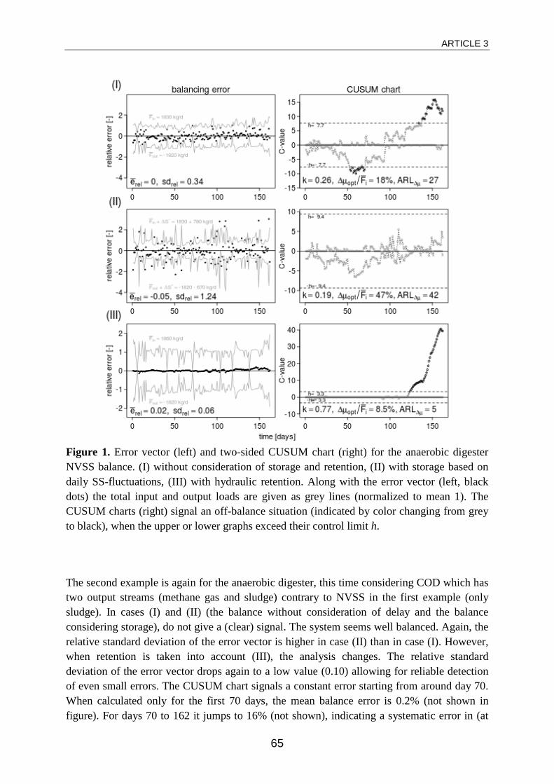
ARTICLE 3

65

Figure 1. Error vector (left) and two-sided CUSUM chart (right) for the anaerobic digester NVSS balance. (I) without consideration of storage and retention, (II) with storage based on daily SS-fluctuations, (III) with hydraulic retention. Along with the error vector (left, black dots) the total input and output loads are given as grey lines (normalized to mean 1). The CUSUM charts (right) signal an off-balance situation (indicated by color changing from grey to black), when the upper or lower graphs exceed their control limit h.

The second example is again for the anaerobic digester, this time considering COD which has two output streams (methane gas and sludge) contrary to NVSS in the first example (only sludge). In cases (I) and (II) (the balance without consideration of delay and the balance considering storage), do not give a (clear) signal. The system seems well balanced. Again, the relative standard deviation of the error vector is higher in case (II) than in case (I). However, when retention is taken into account (III), the analysis changes. The relative standard deviation of the error vector drops again to a low value (0.10) allowing for reliable detection of even small errors. The CUSUM chart signals a constant error starting from around day 70. When calculated only for the first 70 days, the mean balance error is 0.2% (not shown in figure). For days 70 to 162 it jumps to 16% (not shown), indicating a systematic error in (at

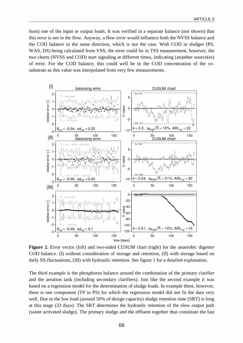
ARTICLE 3

66

least) one of the input or output loads. It was verified in a separate balance (not shown) that this error is not in the flow. Anyway, a flow error would influence both the NVSS balance and the COD balance in the same direction, which is not the case. With COD in sludges (PS, WAS, DS) being calculated from VSS, the error could lie in TSS measurement, however, the two charts (NVSS and COD) start signaling at different times, indicating (an)other source(es) of error. For the COD balance, this could well be in the COD concentration of the co-substrate as this value was interpolated from very few measurements.

Figure 2. Error vector (left) and two-sided CUSUM chart (right) for the anaerobic digester COD balance. (I) without consideration of storage and retention, (II) with storage based on daily SS-fluctuations, (III) with hydraulic retention. See figure 1 for a detailed explanation. The third example is the phosphorus balance around the combination of the primary clarifier and the aeration tank (including secondary clarifiers). Just like the second example it was based on a regression model for the determination of sludge loads. In example three, however, there is one component (TP in PS) for which the regression model did not fit the data very well. Due to the low load (around 50% of design capacity) sludge retention time (SRT) is long at this stage (33 days). The SRT determines the hydraulic retention of the slow output path (waste activated sludge). The primary sludge and the effluent together thus constitute the fast

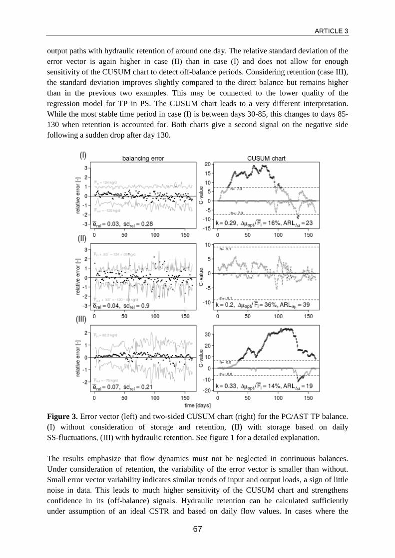
ARTICLE 3

67

output paths with hydraulic retention of around one day. The relative standard deviation of the error vector is again higher in case (II) than in case (I) and does not allow for enough sensitivity of the CUSUM chart to detect off-balance periods. Considering retention (case III), the standard deviation improves slightly compared to the direct balance but remains higher than in the previous two examples. This may be connected to the lower quality of the regression model for TP in PS. The CUSUM chart leads to a very different interpretation. While the most stable time period in case (I) is between days 30-85, this changes to days 85-130 when retention is accounted for. Both charts give a second signal on the negative side following a sudden drop after day 130.

Figure 3. Error vector (left) and two-sided CUSUM chart (right) for the PC/AST TP balance. (I) without consideration of storage and retention, (II) with storage based on daily SS-fluctuations, (III) with hydraulic retention. See figure 1 for a detailed explanation. The results emphasize that flow dynamics must not be neglected in continuous balances. Under consideration of retention, the variability of the error vector is smaller than without. Small error vector variability indicates similar trends of input and output loads, a sign of little noise in data. This leads to much higher sensitivity of the CUSUM chart and strengthens confidence in its (off-balance) signals. Hydraulic retention can be calculated sufficiently under assumption of an ideal CSTR and based on daily flow values. In cases where the

ARTICLE 3

68

hydraulic flow through reactors is better described by a plug flow, the methodology can be adopted accordingly. The calculation of storage from daily fluctuations in SS concentrations appears to be not feasible as it leads to an increased variance of the error vector. There are some reasons that might explain this observation. First, the method relies on daily SS concentration measurements which are not very accurate with random errors of around ±10% to be assumed. This has a great effect especially for reactors with long HRT as the stored mass is much larger than daily input and output mass flows. Secondly, storage and release are calculated from differentials (actual and previous day), the integration of which is known to amplify noise. Filtering might reduce this effect but could also lead to deletion of information contained in data. As a third aspect, SS concentrations should actually be known at a fixed time corresponding to 24h composite sampling to accurately calculate the stored amount of sludge but in practice only grab samples are available. A simple simulation study (results not shown) revealed a considerable influence of using the correct sampling time for the calculation of the stored sludge amounts (which is another source of error). For activated sludge systems, measurement of SS concentrations is also subject to large random errors as sludge can be temporarily stored in the clarifiers. All these influences increase the random error of the calculated storage and therefore lead to larger balancing error variability. The hydraulic retention approach on the other hand, depends on a measurement only for the generation of a starting value and after that determines the effect of delay from the retention model. The choice of the starting value for the concentration in the balanced reactor is of relatively little influence. In case of a systematic measurement error for this measurement (which is also the measurement for the slow response output path) a signal of the CUSUM chart will soon occur. If only the starting value was chosen wrong and the following values are free of systematic errors, the CUSUM chart might signal initially but would soon turn back towards zero.

This work, as it is presented here, omits to a large extend its connection to data reconciliation as known and widely applied in process engineering. Some readers might draw the conclusion that these results might have been reached more efficiently by direct application of existing methods for dynamic, nonlinear data reconciliation. There are a number of reasons for this omission. First, wastewater treatment is very different from the majority of process engineering applications in the way that the influent to the system is the main disturbance rather than a controlled variable. Secondly, in data reconciliation (as the name implies) the correction of measurements is the main focus, with gross error detection as a prerequisite or a byproduct. In practical wastewater treatment applications it is, however, sufficient to become aware of faults in data, possibly along with a conclusion as to which measurement is corrupted. The CUSUM chart offers a very descriptive and easily implementable way to enable operators to draw their own conclusions about the state of their measurements. And as a third aspect, the methods of data reconciliation have not yet been proven to be applicable to operational data from wastewater treatment. With delight the authors would see a process engineer taking on the challenge to improve gross error detection in wastewater treatment data. For this reason, the data used in the second example is included in the appendix.

ARTICLE 3

69

CONCLUSIONS

Continuous mass balancing requires the consideration of the temporal delay between input and output mass flows to correctly determine the quality of operational data. Neglecting this delay is likely to yield erroneous interpretations. While the calculation of storage and release (calculated from fluctuations in SS concentrations) does not seem feasible as it leads to an increased variability of the error vector, hydraulic retention does adequately account for this effect. For the future it would be desirable to investigate further into the correctness of off-balance signals given by CUSUM charts. Because this is often complicated with real data, the application of the Benchmark Simulation model might be appropriate for this task.

The determination of COD, TN and TP from SS fractions is possible in most cases. Purely statistical analysis, in most cases also considering time dependency, yields the best results. Therefore, special care has to be taken when these models are applied; extrapolation beyond the underlying range of time and SS concentrations is not advisable. For long term data, multiple determination is likely to be more appropriate than determination of one single parameter set. Further investigation into this question might be useful. It was found that monthly grab samples are sufficient for the determination of sludge concentrations of COD, TN and TP along with TSS and VSS.

Through this study, the practical applicability of continuous mass balancing has been proven. For a successful outcome of any data evaluation effort including mass balancing, WWTP operators need to be encouraged to ensure balanceability of their measured operational data. This is best achieved by practically calculating those balances that contain the most important measurements but can also be facilitated by redundancy evaluation. In most cases, additional external measurements of sludge components and the corresponding, more frequent, on-site TSS and VSS measurements will be required.

Continuous mass balancing, mastering the insufficiencies of static balances, has the potential to become a standard for data quality verification not only in practice but also in future pilot or technical scale scientific research within the field of wastewater treatment.

ARTICLE 3

70

REFERENCES

Barker, P. S. and Dold, P. L. (1995) COD and nitrogen mass balances in activated-sludge systems. Water Research, 29(2), 633–643.

Ekama, G. A. (2009) Using bioprocess stoichiometry to build a plant-wide mass balance based steady-state WWTP model. Water Research, 43, 2101–2120.

Knoth, S. (2009). spc: Statistical Process Control. R package version 0.3. http://CRAN.R-project.org/package=spc

Montgomery, D. (2009) Introduction to Statistical Quality Control, Wiley, Hoboken N.J.

Narasimhan, S. and Jordache, C. (2000) Data Reconciliation & Gross Error Detection: An Intelligent Use of Process Data, Gulf Professional Publishing, Houston.

Nowak, O., Franz, A., Svardal, K., Muller, V. and Kühn, V. (1999) Parameter estimation for activated sludge models with the help of mass balances. Water Science and Technology, 39(4), 113–120.

Page, E. S. (1954) Continuous inspection schemes. Biometrika, 41(1-2), 100-115.

Puig, S., van Loosdrecht, M. C. M., Colprim, J., and Meijer, S. C. . (2008) Data evaluation of full-scale wastewater treatment plants by mass balance. Water Research, 42, 4645–4655.

R Core Team (2013) R: A Language and Environment for Statistical Computing. Version 2.15.3, Vienna, Austria, R Foundation for Statistical Computing. [online] http://www.R-project.org/

Rieger, L., Takács, I., Villez, K., Siegrist, H., Lessard, P., Vanrolleghem, P. A. and Comeau, Y. (2010) Data reconciliation for wastewater treatment plant simulation studies—Planning for high-quality data and typical sources of errors. Water Environment Research, 82(5), 426–433.

Scharf, S., Schneider, M. and Zethner, G. (1997) Zur Situation der Verwertung und Entsorgung des kommunalen Klärschlammes in Österreich. Monographien Band 095. Bundesministerium für Umwelt, Jugend und Familie, Wien.

Spindler, A. and Vanrolleghem, P. A. (2012) Dynamic mass balancing for wastewater treatment data quality control using CUSUM charts. Water Science and Technology, 65(12), 2148–2153.

Spindler, A. (2014) Structural redundancy of data from wastewater treatment systems. Determination of individual balance equations. Water Research, 57, 193–201.

Villez, K., Corominas, L. and Vanrolleghem, P. A. (2013). Sensor fault detection and diagnosis based on bilinear mass balances in wastewater treatment systems. Proceedings of the 11th IWA Conference on Instrumentation Control and Automation (ICA2013), Narbonne, Sept. 18-20, 2013, Appeared on USB-stick (IWA-12744).

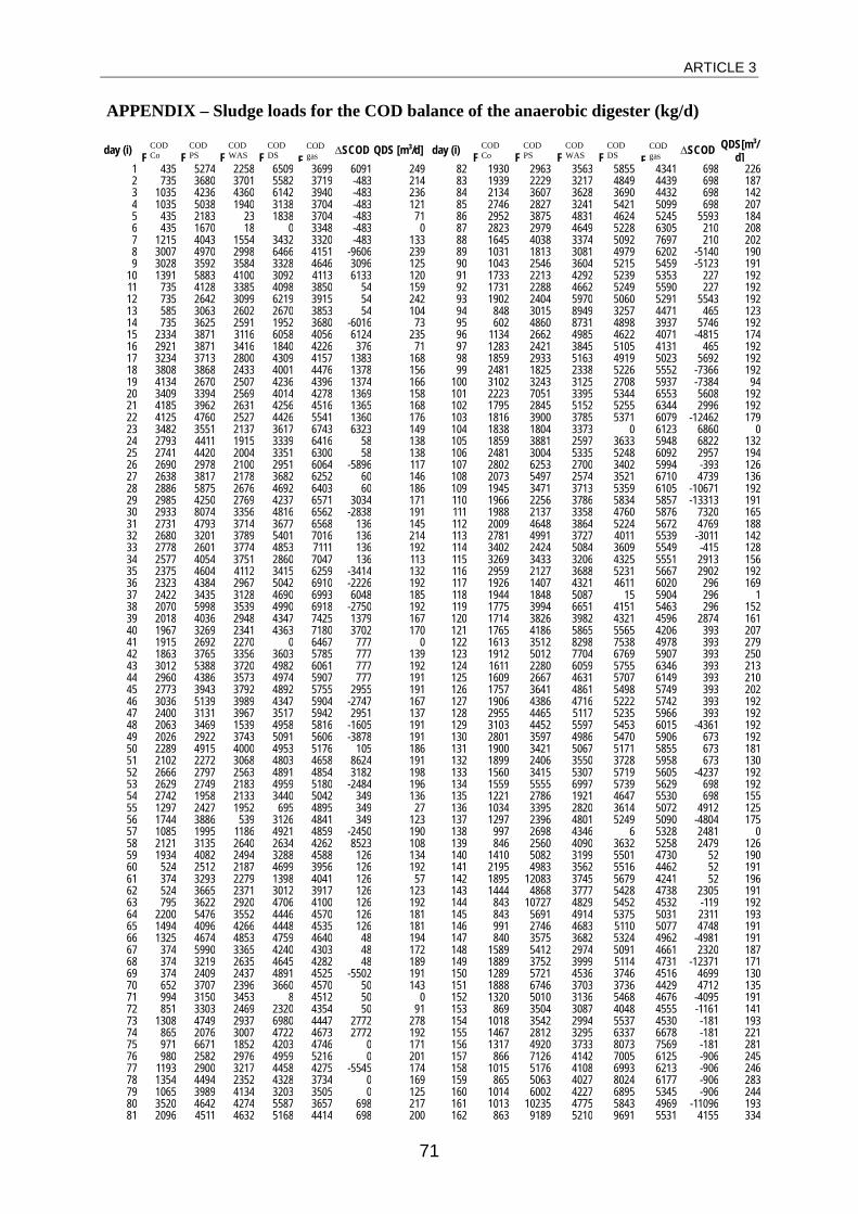
ARTICLE 3

71

APPENDIX – Sludge loads for the COD balance of the anaerobic digester (kg/d)

day (i) FCODCo

F

CODPS F

CODWAS F

CODDS F

CODgas

∆SCOD QDS [m³/d] day (i) FCODCo

F

CODPS F

CODWAS F

CODDS F

CODgas

∆SCOD QDS[m³/d]

1 435 5274 2258 6509 3699 6091 249 82 1930 2963 3563 5855 4341 698 226 2 735 3680 3701 5582 3719 -483 214 83 1939 2229 3217 4849 4439 698 187 3 1035 4236 4360 6142 3940 -483 236 84 2134 3607 3628 3690 4432 698 142 4 1035 5038 1940 3138 3704 -483 121 85 2746 2827 3241 5421 5099 698 207 5 435 2183 23 1838 3704 -483 71 86 2952 3875 4831 4624 5245 5593 184 6 435 1670 18 0 3348 -483 0 87 2823 2979 4649 5228 6305 210 208 7 1215 4043 1554 3432 3320 -483 133 88 1645 4038 3374 5092 7697 210 202 8 3007 4970 2998 6466 4151 -9606 239 89 1031 1813 3081 4979 6202 -5140 190 9 3028 3592 3584 3328 4646 3096 125 90 1043 2546 3604 5215 5459 -5123 191

10 1391 5883 4100 3092 4113 6133 120 91 1733 2213 4292 5239 5353 227 192 11 735 4128 3385 4098 3850 54 159 92 1731 2288 4662 5249 5590 227 192 12 735 2642 3099 6219 3915 54 242 93 1902 2404 5970 5060 5291 5543 192 13 585 3063 2602 2670 3853 54 104 94 848 3015 8949 3257 4471 465 123 14 735 3625 2591 1952 3680 -6016 73 95 602 4860 8731 4898 3937 5746 192 15 2334 3871 3116 6058 4056 6124 235 96 1134 2662 4985 4622 4071 -4815 174 16 2921 3871 3416 1840 4226 376 71 97 1283 2421 3845 5105 4131 465 192 17 3234 3713 2800 4309 4157 1383 168 98 1859 2933 5163 4919 5023 5692 192 18 3808 3868 2433 4001 4476 1378 156 99 2481 1825 2338 5226 5552 -7366 192 19 4134 2670 2507 4236 4396 1374 166 100 3102 3243 3125 2708 5937 -7384 94 20 3409 3394 2569 4014 4278 1369 158 101 2223 7051 3395 5344 6553 5608 192 21 4185 3962 2631 4256 4516 1365 168 102 1795 2845 5152 5255 6344 2996 192 22 4125 4760 2527 4426 5541 1360 176 103 1816 3900 3785 5371 6079 -12462 179 23 3482 3551 2137 3617 6743 6323 149 104 1838 1804 3373 0 6123 6860 0 24 2793 4411 1915 3339 6416 58 138 105 1859 3881 2597 3633 5948 6822 132 25 2741 4420 2004 3351 6300 58 138 106 2481 3004 5335 5248 6092 2957 194 26 2690 2978 2100 2951 6064 -5896 117 107 2802 6253 2700 3402 5994 -393 126 27 2638 3817 2178 3682 6252 60 146 108 2073 5497 2574 3521 6710 4739 136 28 2886 5875 2676 4692 6403 60 186 109 1945 3471 3713 5359 6105 -10671 192 29 2985 4250 2769 4237 6571 3034 171 110 1966 2256 3786 5834 5857 -13313 191 30 2933 8074 3356 4816 6562 -2838 191 111 1988 2137 3358 4760 5876 7320 165 31 2731 4793 3714 3677 6568 136 145 112 2009 4648 3864 5224 5672 4769 188 32 2680 3201 3789 5401 7016 136 214 113 2781 4991 3727 4011 5539 -3011 142 33 2778 2601 3774 4853 7111 136 192 114 3402 2424 5084 3609 5549 -415 128 34 2577 4054 3751 2860 7047 136 113 115 3269 3433 3206 4325 5551 2913 156 35 2375 4604 4112 3415 6259 -3414 132 116 2959 2127 3688 5231 5667 2902 192 36 2323 4384 2967 5042 6910 -2226 192 117 1926 1407 4321 4611 6020 296 169 37 2422 3435 3128 4690 6993 6048 185 118 1944 1848 5087 15 5904 296 1 38 2070 5998 3539 4990 6918 -2750 192 119 1775 3994 6651 4151 5463 296 152 39 2018 4036 2948 4347 7425 1379 167 120 1714 3826 3982 4321 4596 2874 161 40 1967 3269 2341 4363 7180 3702 170 121 1765 4186 5865 5565 4206 393 207 41 1915 2692 2270 0 6467 777 0 122 1613 3512 8298 7538 4978 393 279 42 1863 3765 3356 3603 5785 777 139 123 1912 5012 7704 6769 5907 393 250 43 3012 5388 3720 4982 6061 777 192 124 1611 2280 6059 5755 6346 393 213 44 2960 4386 3573 4974 5907 777 191 125 1609 2667 4631 5707 6149 393 210 45 2773 3943 3792 4892 5755 2955 191 126 1757 3641 4861 5498 5749 393 202 46 3036 5139 3989 4347 5904 -2747 167 127 1906 4386 4716 5222 5742 393 192 47 2400 3131 3967 3517 5942 2951 137 128 2955 4465 5117 5235 5966 393 192 48 2063 3469 1539 4958 5816 -1605 191 129 3103 4452 5597 5453 6015 -4361 192 49 2026 2922 3743 5091 5606 -3878 191 130 2801 3597 4986 5470 5906 673 192 50 2289 4915 4000 4953 5176 105 186 131 1900 3421 5067 5171 5855 673 181 51 2102 2272 3068 4803 4658 8624 191 132 1899 2406 3550 3728 5958 673 130 52 2666 2797 2563 4891 4854 3182 198 133 1560 3415 5307 5719 5605 -4237 192 53 2629 2749 2183 4959 5180 -2484 196 134 1559 5555 6997 5739 5629 698 192 54 2742 1958 2133 3440 5042 349 136 135 1221 2786 1921 4647 5530 698 155 55 1297 2427 1952 695 4895 349 27 136 1034 3395 2820 3614 5072 4912 125 56 1744 3886 539 3126 4841 349 123 137 1297 2396 4801 5249 5090 -4804 175 57 1085 1995 1186 4921 4859 -2450 190 138 997 2698 4346 6 5328 2481 0 58 2121 3135 2640 2634 4262 8523 108 139 846 2560 4090 3632 5258 2479 126 59 1934 4082 2494 3288 4588 126 134 140 1410 5082 3199 5501 4730 52 190 60 524 2512 2187 4699 3956 126 192 141 2195 4983 3562 5516 4462 52 191 61 374 3293 2279 1398 4041 126 57 142 1895 12083 3745 5679 4241 52 196 62 524 3665 2371 3012 3917 126 123 143 1444 4868 3777 5428 4738 2305 191 63 795 3622 2920 4706 4100 126 192 144 843 10727 4829 5452 4532 -119 192 64 2200 5476 3552 4446 4570 126 181 145 843 5691 4914 5375 5031 2311 193 65 1494 4096 4266 4448 4535 126 181 146 991 2746 4683 5110 5077 4748 191 66 1325 4674 4853 4759 4640 48 194 147 840 3575 3682 5324 4962 -4981 191 67 374 5990 3365 4240 4303 48 172 148 1589 5412 2974 5091 4661 2320 187 68 374 3219 2635 4645 4282 48 189 149 1889 3752 3999 5114 4731 -12371 171 69 374 2409 2437 4891 4525 -5502 191 150 1289 5721 4536 3746 4516 4699 130 70 652 3707 2396 3660 4570 50 143 151 1888 6746 3703 3736 4429 4712 135 71 994 3150 3453 8 4512 50 0 152 1320 5010 3136 5468 4676 -4095 191 72 851 3303 2469 2320 4354 50 91 153 869 3504 3087 4048 4555 -1161 141 73 1308 4749 2937 6980 4447 2772 278 154 1018 3542 2994 5537 4530 -181 193 74 865 2076 3007 4722 4673 2772 192 155 1467 2812 3295 6337 6678 -181 221 75 971 6671 1852 4203 4746 0 171 156 1317 4920 3733 8073 7569 -181 281 76 980 2582 2976 4959 5216 0 201 157 866 7126 4142 7005 6125 -906 245 77 1193 2900 3217 4458 4275 -5545 174 158 1015 5176 4108 6993 6213 -906 246 78 1354 4494 2352 4328 3734 0 169 159 865 5063 4027 8024 6177 -906 283 79 1065 3989 4134 3203 3505 0 125 160 1014 6002 4227 6895 5345 -906 244 80 3520 4642 4274 5587 3657 698 217 161 1013 10235 4775 5843 4969 -11096 193 81 2096 4511 4632 5168 4414 698 200 162 863 9189 5210 9691 5531 4155 334

QUALITY CONTROL OF OPERATIONAL DATA FROM WASTEWATER ...

Documents

Transcript of QUALITY CONTROL OF OPERATIONAL DATA FROM WASTEWATER ...