Institut fur Physik, Universitat PotsdamSommersemester 2007

Quantenmechanik II— Theoretische Physik V —

Carsten Henkel

Baustelle ‘Skriptum’

1

Uberblick

Vor zwei Semestern wurde die Vorlesung zum ersten Mal gehalten. Wasam Ende ubrig blieb, sei hier kurz skizziert und mit neuen Elemente verse-hen. Es gilt: kein Anspruch auf Vollstandigkeit, und Fehler konnen uberallauftreten. Diese Notizen enthalten einige Abschnitte, die in der Vorlesungnicht durchgenommen wurden: zur Lekture empfohlen, aber nicht Pflicht.

• Zusammenfassung der Grundlagen der Quantenmechanik→ Kapitel 0

• Streutheorie→ Kapitel 1: Wirkungsquerschnitt, Bornsche Naherung, S-Matrix,Partialwellenentwicklung,→ Anhang 2 zeitabhangige Storungstheorie

• relativistische Quantenmechanik→ Kapitel 3: Klein-Gordon-Gleichung, Dirac-Gleichung, Spinor-Transformation, 1-Teilchen-Zustande, diskrete Symmetrien→ Kapitel 4: Symmetrien und Gruppen in der Quantenmechanik,Darstellungen der Drehgruppe, Addition von Drehimpulsen

• Einfuhrung in die Quantenfeldtheorie→ Kapitel 5: Phononen auf diskretem Gitter, kanonische Quantisierung,skalares, relativistisches Feld (Klein-Gordon-Feld), Zerfall von Teilchen,Quantisierung von Fermionen, Pauli-Prinzip und Vielteilchen-Theorie

2

Chapter 0

Quantum Basics

0.1 Wave mechanicsHistorically, quantum mechanics has been developed in two formulations: thewave mechanics of E. Schrodinger (and others) and the matrix mechanics of W.Heisenberg (and others).

You should be familiar with wave mechanics, and we give a brief reminderhere. We start with a quantum particle in one dimension, with x being theposition coordinate. The particle’s state is characterized by a wavefunctionψ(x, t) ≡ 〈x|Ψ(t)〉 that solves the Schrodinger equation:

ih∂tψ(x, t) = Hψ(x, t) = − h2

2m

∂2ψ

∂x2+ V (x)ψ(x, t), (1)

where H is the Hamilton operator. The last expression is true for a particle ina (one-dimensional) potential V (x). You get this equation from the classicalHamiltonian function by replacing the momentum by a differential operator,

p &→ h

i∂

∂x(2)

The generalization to two and three dimensions is immediate. The general-ization to a system of two or more particles is immediate as well: one gets awavefunction ψ(r1, r2, t). ‘Quantum statistics’ enters here if the particles areindistinguishible: ψ(r2, r1, t) = ±ψ(r1, r2, t), depending on whether the parti-cles are bosons or fermions.

The interpretation of the wavefunction is such that |ψ(x, t)|2dx gives theprobability to find the particle around position x when a measurement is done.We can thus introduce a probability density n(x, t). Particles do not disappearwithout reason, this is why normally the probability is conserved (equation ofcontinuity)

∂tn + ∂xj = 0 (3)

j(x, t) =h

2im

[ψ∗(x, t)

∂

∂xψ(x, t)− c.c.

]= Re

[ψ∗(x, t)

p

mψ(x, t)

](4)

where j is the probability current (density). In three dimensions, this is a vectorfield and ∂xj &→ div j in Eq.(3).

3

A stationary situation is characterized by a time-independent particle den-sity, ∂tn = 0. In that case, div j = 0, either because the wave function is real(bound state) or because an ‘incident current’ is balanced by an ‘outgoing cur-rent’. This can be checked easily in one-dimensional examples.

The following wave function leads to a stationary density, it is thereforecalled a stationary state and solves the stationary Schrodinger equation:

ψ(x, t) = ψ(x) e−iEt/h (5)

Eψ(x) = Hψ(x) = − h2

2m

∂2ψ

∂x2+ V (x)ψ(x). (6)

This is an eigenvalue equation for the Hamiltonian operator H . Only for spe-cific values of E do solutions to the stationary Schrodinger equation exist.1 Theallowed numbers E are called the ‘energy eigenvalues’. Taken together, theyform the ‘spectrum of the Hamiltonian H’.

Examples.Harmonic oscillator, En = hω(n + 1

2 ) with n = 0, 1, . . ..Free particle, Ep = p2/2m with p = −∞ . . . +∞.Hydrogen atom, En = −1/(2n2) in atomic units with n = 1, 2, . . . (bound states)and E = h2k2/2m > 0 (‘continuous spectrum’).

0.2 Operator mechanicsIn the second ‘picture’ of quantum mechanics, operators play a much more im-portant role. Let us briefly discuss this concept to begin with. In this lecture, weshall not put circumflex accents (‘hats’) on the letters for operators. You alreadyknow the momentum operator p: it is the differential operator given in Eq.(2).It ‘acts’ on the wavefunction ψ(x, t) by differentiation. On the (Hilbert) spaceof differentiable functions, the chain rule of differentiation therefore gives thefollowing ‘commutator’

[x, p] ≡ xp− px = i h. (7)

This is the basic difference with respect to classical mechanics, where x and pare numbers. At the most, they act as functions on the phase space (formulationof classical mechanics with Poisson brackets). The nonzero commutator (7)implies the ‘Heisenberg indeterminacy relation’

∆x∆p ≥ h

2(8)

where ∆x and ∆p is the statistical spread (e.g., the standard deviation) of theresults of measurement for x and p. The factor 1

2 is actually a matter of tasteand of definition for the statistical spread.

Remark. The Heisenberg relation (8) is actually a consequence of Fourier transfor-mations: the probability of finding a result p = hk when measuring the particle

1This is different from the time-dependent equation (1) that can always be solved. For potentialsthat vanish at infinity, stationary solutions can, as a general rule, also be found for all E > 0.

4

momentum is proportional to |ψ(k, t)|2 where ψ(k, t) is the (spatial) Fourier trans-formation of ψ(x, t):

ψ(k, t) =

Zdx ψ(x, t) e−ikx. (9)

A well-known property of Fourier transforms is: if ∆x is the ‘typical width’ of|ψ(x)|2, then the typical width ∆k of its Fourier transform |ψ(k)|2 is ∆k ≈ 1/∆x.

The second formulation of quantum mechanics is called the ‘Heisenbergpicture’. Here, the time-dependence is carried by the operators, not the wave-function. The equation of motion of an operator A(t) is given by the commu-tator with the Hamilton operator:

ddt

A(t) =ih

[H, A(t)] (10)

A convenient initial condition is A(0) = A, the operator in the Schrodingerpicture.

In the exercises, you show that the Schrodinger and Heisenberg ‘pictures’give the same physical predictions. This means that the expectation values

〈A(t)〉 = 〈Ψ|A(t)|Ψ〉 (11)

are the same as in the Schrodinger picture where one computes 〈Ψ(t)|A|Ψ(t)〉.In the Heisenberg picture, (average) results of measurements are thus pre-dicted by computing the expectation values (11).

Conserved observables. As a simple consequence of Eq.(10), H(t) = H forall times: energy is conserved. By this we mean that the expectation value〈H(t)〉 is time-independent. Indeed, 〈H(t)〉 = 〈Ψ|H|Ψ〉 and the state |Ψ〉 of thesystem does not depend on time in the Heisenberg picture.

This property holds for all operators K that commute with H : indeed, thedifferential equation (10) shows that [K, H] = 0 is equivalent to K being con-stant. Hence, an observable is conserved if and only if it commutes with H .

‘Canonical quantization’. The quantization of a classical system can be per-formed in the ‘canonical way’ by starting from its classical Hamiltonian. Thisis a function H(xi, pj) of coordinates and (‘canonically conjugate’) momenta.One replaces these functions by non-commuting operators such that

[xi, pj ] = i h δij , (12)

where the Kronecker δij appears. The choice (2) is just a convenient way to‘represent’ this commutator on a suitable space of functions.

As a reminder from classical mechanics: if you start from a LagrangianL = L(x, v) that depends on coordinates x and velocities v = dx/dt, then thecanonical momentum is given by

p =∂L

∂v, (13)

and one obtains the Hamiltonian function by the ‘Legendre transform’

H(x, p) = vp− L(x, v) (14)

where on the right hand side, the velocity v must be expressed in terms of themomentum p.

5

Examples for operators.

• Creation and annihilation operators for the one-dimensional harmonic oscil-lator

a =1

a0

√2

“x + i

pmω

”, a† =

1

a0

√2

“x− i

pmω

”(15)h

a, a†i

= 1. (16)

where a0 =p

h/mω is the typical size of the ground state wave function ofthe oscillator.

• Particle density and particle current operators. They are functions of a c-number valued coordinate q:

n(q, t) = δ(q − x(t)), (17)

j(q, t) =1

2mp(t), δ(q − x(t))

≡ 12m

(p(t) δ(q − x(t)) + δ(q − x(t)) p(t)) (18)

The curly brackets A, B denote the ‘anti-commutator’.

• Orbital angular momentum operator in three dimensions

L = r× p =hir×∇ (19)

(the order of the operators is irrelevant here – why?) with the commutationrelations

[Lx, Ly] = ih Lz (20)

and cyclic permutations. Of course, [Lk, Lk] = 0. You have seen in the quan-tum mechanics I lecture that in a spherically symmetric potential V (r) (a ‘cen-tral potential’), the wave functions can be expanded in eigenfunctions of theangular momentum operator. All three components commute with the Hamil-tonian for a central potential. In addition, all components commute with thesquared angular momentum L2. One conventionally chooses Lz , L2 and H asthree mutually commuting operators.In the exercises, you show that the kinetic energy operator can be written inthe form

− h2

2m( =

h2

2m r∂2

∂r2r +

12mr2

L2 (21)

We can write the wave function as a product of an eigenstate of L2 and of Lz

(these functions are called spherical harmonics) and of a ‘radial wave func-tion’:

ψ(r) = Ylm(θ, ϕ)ψl(r) (22)

where l = 0, 1, 2, . . . and m = −l, . . . , l−1, l. The eigenvalue of L2 is h2l(l+1).The radial wavefunction ψl(r) then solves the ‘radial Schrodinger equation’

Eψl = − h2

2m r∂2

∂r2rψl +

h2l(l + 1)2m r2

ψl + V (r)ψl (23)

where the last two potential terms can be combined into an ‘effective poten-tial’. As in classical mechanics, one has a ‘centrifugal potential’ proportionalto l(l + 1)/r2.

6

Chapter 1

Scattering Theory

In scattering theory, we are dealing with the ‘continuous spectrum’ of a Hamil-tonian operator and the corresponding wavefunctions. We focus in this chapteron the nonrelativistic theory and shall stay in three dimensions for most of thetime.

1.1 Problem formulationWe focus on the scattering of a particle off a potential V (r) that vanishes atinfinity. The potential is significantly nonzero around the origin. We shall ar-gue that this scattering process can be described by a stationary Schrodingerequation with a positive energy eigenvalue E. Far from the potential, thewave function of the particle is similar to a plane wave eikz if we choose thez-direction along the incident wavevector (what we shall do), and the energyis given by E = h2k2/2m.

In classical potential scattering, the particle follows a trajectory along the(negative) z-axis, changes direction upon scattering and emerges in some di-rection specified by the angles θ, ϕ. The relevant quantity is the so-called differ-ential cross section. It is defined by the ratio

dσ

dΩ=

1(incident current density)

(no. of detected particles)dt dΩ

(1.1)

where dΩ is the solid angle subtended (aufgespannt) by the detector. In classicalmechanics, the cross section can be expressed in terms of the scattering angleθ(b) that depends on the ‘impact parameter’ b (a simple exercise, see § 18 inLandau’s Mechanics text). For a spherically symmetric scatterer:

dσ

dΩ=

b

sin θ

∣∣∣∣db

dθ

∣∣∣∣ (1.2)

In quantum mechanics, we are looking for a specific solution to the station-ary Schrodinger equation, a so-called stationary scattering state

Hψ = − h2

2m(ψ + V (r)ψ =

h2k2

2mψ. (1.3)

7

This stationary picture corresponds to a steady flow of particles onto the scat-tering potential. The scattering state is determined by an asymptotic require-ment: far from the origin (where the scattering potential is zero), the wavefunction should correspond to a sum of an incident wave and a scattered wave:

r →∞ : ψ(r)→ eikz + f(Ω)eikr

r(1.4)

where r = |r|. The first term describes the incident plane wave with k-vectoralong the z-axis; the second term an ‘outgoing spherical wave’. This form ischosen such that the stationary probability current points radially outward atlarge r. You have verified this in the exercises. The angular dependence of f(Ω)(Ω combines both θ and ϕ) specifies the angular distribution of the scatteredparticles.

Note. A mathematically more precise formulation for the outgoing spherical waveis the so-called Sommerfeld radiation condition:

limr→∞

r

„ikψsc(r)− ∂ψsc

∂r

«= 0. (1.5)

This applies only to the scattered part of the wave function, ψsc(r) = ψ(r) − eikz ,not the incident one, of course.

The number of particles scattered per unit time into an element of solid angledΩ around the direction Ω is given by

dNsc

dt= lim

r→∞ jr(rΩ)r2dΩ =hk

m|f(Ω)|2dΩ, (1.6)

where we took into account only the outgoing spherical wave to compute theprobability current jr. We use the notation Ω for the unit vector specified bythe angles θ, ϕ. A similar calculation for the incident probability current givesjinc = ezhk/m, taking into account only the incident plane wave. A morecareful approach would also take into account the interference between theincident and scattered wave. Actually this effect is only important for ‘forwardscattering’ (θ = 0). It leads to the so-called ‘optical theorem’ that you shalldiscuss in the exercises.

According to the definition (1.2), the scattering cross section is thus givenby

dσ

dΩ= |f(Ω)|2 (1.7)

To summarize, the scattering problem is solved if we know the ‘scattering am-plitude’ f(Ω) = f(Ω; k) as a function of the scattering angle and the incidentwave vector. Now: how can we get this scattering amplitude?

1.2 Integral equationA convenient tool to solve the Schrodinger equation (1.3) is the transforma-tion to an integral equation, called Lippmann–Schwinger equation in quantummechanics. The advantage of this equation is that it includes the asymptoticboundary conditions (1.4) and that one can formulate easily an approximatescheme to solve it, the so-called Born-von Neumann series.

8

We start from (1.3) and write it in the form

(ψ + k2ψ = U(r)ψ(r) (1.8)

where U(r) = (2m/h2)V (r). Formally, we can consider the right hand side asan inhomogeneity or ‘source term’. Then, the equation can be solved with thehelp of a propagator G0(r, r′; k), that you may know as ‘Green function’ fromelectrodynamics. The propagator is the solution to a point source((+ k2

)G0(r, r′; k) = δ(r− r′) (1.9)

and if we know it, we can write

ψ(r) = eikz +∫

d3r′G0(r, r′; k)U(r′)ψ(r′). (1.10)

This is the Lippmann–Schwinger equation. Note that this equation applies forall positions r, not only far away from the scattering potential. The first term isa solution to the ‘homogeneous equation’. It is chosen to reproduce the incidentwave. The second term gives asymptotically the outgoing spherical wave if wechoose the correct (the ‘retarded’) propagator that behaves like eikr/r for larger. A calculation that we summarize below leads to

G0(r, r′; k) = G0(r− r′; k) = − 14π

eik|r−r′|

|r− r′| . (1.11)

At large distance from the origin, we can assume that |r − r′| ≈ r − r′ · r/rbecause the integration points r′ remain in a bounded region around the ori-gin (this is due to the potential V (r′) under the integral). The leading orderbehaviour is thus given by (we write Ω = r/r)∫

d3r′G0(r− r′; k)U(r′)ψ(r′) (1.12)

≈ − eikr

4πr

∫d3r′ e−ikΩ·r′

U(r′)ψ(r′) (1.13)

From this large-distance behaviour, we can read off the scattering amplitude

⇒ f(Ω) = − m

2πh2

∫d3r′ e−ikΩ·r′

V (r′)ψ(r′) (1.14)

Very nice, this is a formula for the scattering amplitude. If we square it, we getthe cross section dσ/dΩ [Eq.(1.7)]. But again, this is not yet a useful result: wehave only expressed the scattering amplitude in terms of the (unknown) wavefunction ψ(r′) ‘inside the potential’ V (r).

Propagator for the Schrodinger equationThe differential operator in Eq.(1.9) can be ‘inverted’ with the help of a spatialFourier transform. This gives

G0(q) =1

k2 − q2+ Cδ(k2 − q2) (1.15)

9

where the second term corresponds to the ‘homogeneous solution’, with anamplitude to be fixed by the boundary condition at large distance. A choicethat turns out to work is

G±0 (q) =

1k2 − q2

∓ iπδ(k2 − q2) = limε→0

1k2 − q2 ± iε

(1.16)

The limit ε → 0 from positive values will not be written explicitly in the fol-lowing. Indeed, the transformation back to real space gives, as shown in theexercises:

G±0 (r) =

∫d3q

(2π)3eiq·r

k2 − q2 ± iε

=1

4iπ2r

+∞∫−∞

dqeiqr

k2 − q2 ± iε(1.17)

= −e±ikr

4πr(1.18)

Within this ‘ε-trick’ that is widely used in quantum field theory, one takes anintegration path along the real q-axis in Eq.(1.17). The +iε in the denomina-tor with positive ε shifts the pole q = +k slightly into the upper half-plane.Only poles in this half-plane contribute to the result, and one gets the outgoingspherical wave. More details: see exercises.

An alternative argument that does not use the ‘ε-trick’ is based on a deformation ofthe integration contour in Eq.(1.17) (written now for ε = 0) in the complex q-plane.First observation: for any choice of contour, one has a solution to Eq.(1.9). Secondobservation: the way one circles around the poles of the denominator, located atq = ±k, one gets different contributions of outgoing and ingoing spherical waves.In fact, the residues of these poles correspond to ingoing and outgoing sphericalwaves. The contour that encircles the pole at q = +k from below and passes abovethe pole at q = −k gives the outoing wave only that we focus on here.Last variation for mathematicians: never ever evaluate propagators or Green func-tions for real values of k, but take a small, positive imaginary part to ensure theSommerfeld condition (1.5). Indeed, (k + iε)2 − q2 = k2 − q2 + 2ikε has a formsimilar to the denominator in the ‘ε-trick’ (although with a different meaning anddimension for ε).

1.3 Born–von Neumann seriesThe Born–von Neumann series is based on an iterative solution of theLippmann–Schwinger Eq.(1.10). This iteration converges rapidly if the scat-tering potential is ‘weak’ since higher-order terms involve higher powers ofV (r′). In fact, we are dealing here with a variation of perturbation theory inthe context of scattering. (A crash course on perturbation theory follows in anextra section.)

The iteration of the integral equation yields

ψ(r) = ψ(0)(r) + ψ(1)(r) + ψ(2)(r) + . . . (1.19)

Zero’th term: no scattering at all

ψ(0)(r) = eikz (1.20)

10

First term: replace ψ(r) by the plane wave ψ(0)(r) under the integral

ψ(1)(r) = − 14π

∫d3r′

eik|r−r′|

|r− r′| U(r′)eikz′(1.21)

Second term: a double integral

ψ(2)(r) =1

(4π)2

∫d3r′d3r′′

eik|r−r′|+ik|r′−r′′|

|r− r′||r′ − r′′| U(r′)U(r′′)eikz′′(1.22)

and so on.The expression (1.21) is the ‘(first order) Born approximation’. It provides

us (finally!) with an explicit result for the scattering amplitude:

fBorn(Ω) = − 14π

U(q), q = kΩ− kez = k′ − k (1.23)

where U(q) is the spatial Fourier transform of the scattering potential, evalu-ated at the ‘wave vector transfer’ q:

U(q) =∫

d3r′ e−iq·r′U(r′) (1.24)

The vector q is the difference between the outgoing k-vector k′ = kΩ, specifiedby the observation direction Ω, and the k-vector of the incident plane wave,k = kez .

Born scattering cross sectionGoing back to the usual potential V (r), the first Born approximation gives thefollowing differential cross section

dσ

dΩ

∣∣∣∣Born

=∣∣∣∣ m

2πh2 V (q)∣∣∣∣2 (1.25)

where V (q) is the spatial Fourier transformation of the scattering potential,taken at the wave vector transfer q.

For a spherically symmetric potential, the scattering amplitude can be writ-ten in the form

fBorn(θ) = −2m

h2

1q

∞∫0

r dr V (r) sin qr (1.26)

as you show in the exercises. Here, q = 2k sin(θ/2). We defer a comparisonto a square well to a later section when the exact solution in terms of sphericalharmonics (partial waves) is available.

Example: Coulomb scattering

For now, let us focus on the example of electron-proton scattering in the non-relativistic limit. The potential is given by V (r) = −e2/(4πε0r) where −e isthe electron charge. This means that we treat the proton as an immobile and

11

pointlike target and put α = me2/(2πh2ε0) = 2/a0 with a0 the Bohr radius.From Eq.(1.26), we get a scattering amplitude

fBorn(Ω) =2

q2a0(1.27)

Note that the sign of the potential (attractive or repulsive) only enters into thesign of the scattering amplitude, but not into the scattering cross section

dσ

dΩ=

|α|2q4

=4

a20[2k sin(θ/2)]4

(1.28)

Note the strong angular dependence with a pronounced peak in the forwarddirection. Any deviation from this result is a signature of the finite size of thetarget particle. One introduces the technical term of a ‘form factor’ to quantifythis. In particle physics, form factors provide measurements of the size of theproton and the charge distribution of the quarks inside it, for example.

We note that Eq.(1.28) is actually the same result as in classical mechanics, an inter-esting coincidence. In terms of the incident energy E = h2k2/2m, impact parameterb and scattering angle θ are related by (Landau I, § 19):

b =e2

8πε0Ecot(θ/2) (1.29)

and one can easily check that the classical cross section (1.2) gives the same result asthe Born approximation (1.27).Attention. This is a pure coincidence. In fact, the Coulomb potential with its 1/rtail decays too slowly to justify the far-field expansion we have done here. The exactwave function can be found (see, e.g., the book by A. Messiah, vol.I, appendix B) andits ‘spherically outgoing part’ contains terms like

f(θ)ei(kr−γ log(2kr))

r(1.30)

for large r. Note the logarithmic phase correction that goes with the parameterγ = 1/ka0.

Example: scattering by periodic structures

Scattering potential of assembly of identical scattering centres

V (r) =N∑

s=1

V1(r− rs) (1.31)

with positions rs of scattering centres and scattering potential V1 for any ofthem.

Work out Fourier transform: form factor and structure factor

V (q) = V1(q)N∑

s=1

e−iq·rs ≡ V1(q)S(q) (1.32)

Regular lattice, for example in 1D: S(q) is peaked at reciprocal lattice vectorsq = n/d with lattice spacing d. Height of peak is N , width as a function of q isof order 1/(dN).

12

Scattering cross section in first Born approximation

dσ

dΩ=

(m

2πh2

)2

|V1(q)|2|S(q)|2 (1.33)

hence single scattering result multiplied by ‘structure factor’. Peaks in |S(q)|2:information about the lattice symmetry and parameters. ‘Form factor’ |V1(q)|2:information about shape and strength of individual scatterer.

In many experimental situations, one has to average the cross section overthe positions of the scatterers. This happens, for example, in a crystal at finitetemperature, in liquids. We denote this average by angular brackets and havefor the average structure factor

〈|S(q)|2〉 =N∑

s,s′=1

〈eiq·(rs−rs′ )〉 (1.34)

Consider the simplest model where the positions rs are centered , on average,on a perfect lattice and where the deviations us are uncorrelated among thescatterers. We then get

〈|S(q)|2〉 = N2e−q2u2+ N(1− e−q2u2

) (1.35)

with N the number of scatterers and q2u2 = 〈q · u2s〉.

In a perfect lattice, qu - 1, and the cross section is scales like N2. Thisis called ‘coherent scattering’. Note that this regime can apply even at finitetemperature, it is sufficient that the thermal fluctuations u are small enoughcompared to the wavevector transfer q.

The opposite case is that of strongly uncorrelated scatterers: qu . 1. Thenthe cross section ∝ N , this is called ‘incoherent scattering’. In this regime, thesharply defined peaks disappear completely: the lattice structure is destroyedby the thermal fluctuations. One can then define an ‘extinction coefficient’ κ =(total) scattering cross section / volume that is proportional to the density ofscatterers and has units: 1/m.

Convergence of the Born seriesThe first Born approximation is sufficient in the majority of physical applica-tions. A large part of crystallography and X-ray scattering is built on it, forexample, not to mention high-energy physics. Nevertheless, it is instructive toanalyze the range of validity of this approximation. The general rule is thatthe scattering potential ‘be sufficiently weak’. But we shall find that this meansdifferent things at low and high energies.

Heuristic criteria

The first idea is to require that the first order term ψ(1)(r) [Eq.(1.21)] be a smallcorrection compared to the zero’th order term ψ(0)(r). Let us check this in-equality at r = 0, right in the center of the scattering potential.

13

We get, of course, ψ(0)(0) = 1 and

ψ(1)(0) = −1k

∞∫0

dr eikrU(r) sin(kr) (1.36)

where U(r) is assumed with spherical symmetry, for simplicity. To proceed,we shall assume that the radial integral is actually limited to a range r ≤ R.The length R is called the ‘range’ of the scattering potential.

In the regime of high energies, one has kR . 1, and the integral (1.36) canbe handled by partial integration:

kR . 1 : ψ(1)(0) = − i2k

R∫0

dr(1− e2ikr

)U(r) (1.37)

≈ − i2k

R∫0

dr U(r)

− 12ik

[e2ikrU(r)

]R

0+

12ik

R∫0

dr e2ikr∂rU(r)

(1.38)

When the potential is sufficiently smooth (certainly not the case for theCoulomb potential), ∂rU(r) is of the order of U/R. The second line in Eq.(1.38)is the smaller compared to the first by a factor 1/(kR) and can be neglected.Hence to leading order, the inequality |ψ(1)(0)|- 1 leads to the criterion

2R∫

0

dr |U(r)|- k, (1.39)

the scattering potential times its range must be ‘small’ compared to the incidentmomentum. This can always be satisfied at ‘sufficiently high’ energy, if theintegral exists (our approximations actually imply that it exists). Remember, ofcourse, that our treatment is not valid in the relativistic regime.

In the opposite case, low incident energy, we have kR - 1, and the inte-gral (1.36) becomes

R∫0

dr r |U(r)|- 1, (1.40)

the scattering potential times its range squared must be ‘small’ in absolutevalue.

If you prefer to work with V (r), do not forget the factor (2m/h2) to compute U . Uhas the units of wavevector squared, hence multiplied by R2, one gets a dimension-less number.)

Functional analysis

This is a note for mathematical physicists: the Born series can be seen as a geomet-rical series to invert an integral operator, and this series converges if the operator

14

in the series has a norm smaller than ‘unity’. Let us write U(r) = (m/2πh2)V (r)and re-scale the wave function as φ(r) = |U(r)|1/2ψ(r). The Lippmann-Schwingerequation then becomes

φ(r) = φinc(r)−Z

d3r′eik|r−r′|

|r− r′| |U(r)|1/2 U(r′)|U(r′)|1/2

φ(r′) (1.41)

= φinc(r) +

Zd3r′K(r, r′)φ(r′) (1.42)

where K(r, r′) is the ‘kernel’ of an integral operator that can be formally written asK. The Born series thus takes the form

φ = ( −K)−1 φinc = φinc + Kφinc + K2φinc + . . . (1.43)

The functional analysis of this kind of series gives the convergence criterion

1 > ‖K‖2 >

Zd3r d3r′

˛K(r, r′)

˛2=

Zd3r d3r′

|U(r)U(r′)||r− r′|2 . (1.44)

where ‖K‖ is the (supremum) norm of the integral operator:

‖K‖ = sup ‖Kφ‖2; for ‖φ‖2 = 1 (1.45)

and the norm of the state vectors is taken as the L2 norm usual in quantum mechan-ics (the total probability).More details can be found in the mathematical physics literature on scattering the-ory or in the mathematics texts on functional analysis (e.g., W. Rudin) and on so-called ‘Fredholm integral equations’.

1.4 Formal scattering theoryIn a basis-free notation, the Lippmann-Schwinger equation (1.10) takes theform

|ψ(+)k 〉 = |ϕk〉+ G(+)

0 (Ek)V |ψ(+)k 〉 (1.46)

where scattering state is |ψ(+)k 〉, the superscript (+) denoting the spherically

outgoing or “retarded” solution. The incident plane wave (free particle) stateis |ϕk〉 and the (retarded) propagator

G(±)0 (E) = lim

ε→0(E −H0 ± iε)−1 (1.47)

with the free particle Hamiltonian H0. The propagator can be understood asthe limit of the so-called resolvent operator

G0(z) = (z −H0)−1 (1.48)

as the complex energy z → E from the upper half-plane on the real axis. Inthis section, we put 2m/h2 and identify U with V . This means that the energyis Ek = k2.

The propagator G(z) for the full problem that is defined by Eq.(1.48) withH replacing H0 describes how an incident wave is scattered zero, one, two. . . times by the potential. This is useful for some applications, but if we wantto know the scattering amplitude or the cross section, one needs a slightly dif-ferent object, the T-matrix.

15

T-matrix and S-matrixThe T-matrix is defined by the requirement that

V |ψ(+)k 〉 = T (Ek)|ϕk〉. (1.49)

Manipulations with Lippmann-Schwinger equation give

V |ψ(+)k 〉 = V |ϕk〉+ V G(+)

0 (Ek)V |ψ(+)k 〉 (1.50)

= V |ϕk〉+∫

d3k′ V G(+)0 (Ek)|ϕk′〉〈ϕk′ |V |ψ(+)

k 〉 (1.51)

and henceT (E) = V + V G(+)

0 (E)T (E). (1.52)

The iterative solution of this equation is nothing else but the Born series offirst-, second- . . . order scattering. The series converges for the T-operator andprovides a way to evaluate the formal expression (a geometrical series)

T (E) = ( − V G(+)0 (E))−1V (1.53)

if in some suitable operator norm ‖ · ‖, one has

‖V G(+)0 (E)‖ < 1 (1.54)

The formula given in (1.44) is an example with a particular choice of norm.What is the T-matrix good for? Eq.(1.49) is fundamentally important: in-

stead of acting with the potential on the “unknown” scattering state |ψ(+)k 〉, act

with the T-matrix on the free particle state |ϕk〉 and get the same result.This implies in particular that we can get the scattering amplitude:

f(k,k′) = − 14π〈ϕk′ |U |ψ(+)

k 〉 = − 14π〈ϕk′ |T (Ek)|ϕk〉 (1.55)

The first equation follows from a basis-free formulation of Eq.(1.14). Thereforethe important result:

The matrix elements of the T-matrix are the scattering amplitudes betweenincident and outgoing directions.

The S-matrix is defined via its matrix elements between free-particle states:

〈ϕk′ |S|ϕk〉 = (2π)3δ(k′ − k)− 2πi δ(Ek′ − Ek)〈ϕk′ |T (Ek)|ϕk〉 (1.56)

It is a mapping between free particle states. Formally, a mapping between“incident waves” (described by eigenstates of H0 with wavevector k and “out-going waves” (with wavevector k′).

Physically, one expects that “no particles are lost” during the scattering pro-cess. Hence, the norm or total probability of the outgoing state is the same asthe norm of the ingoing state. This is achieved when S is unitary: S†S = .Exercise: prove this. You need the following property of the T-matrix, calledthe ‘optical theorem’.

T †(E)− T (E) = 2πiT †(E)δ(E −H0)T (E) (1.57)

16

Explicit expression

Im〈ϕk|T (Ek)|ϕk〉 = −π

2

∫dΩ(k′) |〈ϕk′ |T (Ek)|ϕk〉|2 (1.58)

Tricky point: to prove also that SS† = , you need another variant of the opticaltheorem (1.57) with the order of T and T † reversed. This can be proven along thesame lines using an alternative equation for the T-matrix:

T (E) = V + T (E)G(+)0 (E)V. (1.59)

This equation is right because it corresponds to the same Born-von Neumann series.

Resolvent operator and density of states

Note the following properties of the resolvent operator G0(z):

(i) it has poles at the eigenvalues of H0

(ii) it has a “cut” along the real axis where H0 has a continuous spectrum. Alongsuch a cut, the (local) density of states is given byX

n

|ψn(x)|2 δ(E − En) = − 1π〈x|Im G(+)

0 (E)|x〉 (1.60)

In the last expression, we strictly speaking use again a discrete spectrum. But sucha sum degenerates into an integral when we deal with the continuous spectrum.For example, in a quantization box of volume V = L3 with periodic boundaryconditions, we get a finite value for the local density of states in the “continuumlimit” V →∞:

ρ(x; E) =1

4π2

√E (1.61)

It is easy to show that this result is identical to the imaginary part of the propagatorG(+)

0 (x− x′) [Eq.(1.18)], taking carefully the limit x′ → x.

Feynman diagrams

The equation for the propagator G including a potential V can be brought intothe following form1

G = G0 + G0V G (1.62)

The iterative solution of this gives the so-called ‘multiple scattering series’. Itcan be organized with the help of Feynman graphs. Give examples.

Similarly, Eq.(1.52) for the T-matrix can be solved by iteration. The corre-sponding Feynman graphs have their “legs stripped off”, the legs correspond-ing to the Green functions of the incident or outgoing waves. In this case, onegets an expansion of the total scattering vertex or the scattering amplitude intoa Born series.

1Eq.(1.62) is called the Dyson equation.

17

Subtleties in the continuum

Free particles states are not normalizable in an infinite volume. But consider

ψ(x; c) =

Zd3k

(2π)3c(k− k) exp(ik · x) (1.63)

With a suitable smooth function c(k − k) peaked around k, one can have a wavefunction whose average momentum is hk and whose momentum spread is arbitar-ily small. The condition of normalization for ψ(x; c) is (Parceval theorem)Z

d3x |ψ(x; c)|2 =

Zd3k

(2π)3˛c(k− k)

˛2= 1 (1.64)

Hence c must be a function in L2( 3).Physicists often work with non-normalizable states |ϕk〉 that behave like

〈ϕk′ |ϕk〉 = δ(k′ − k) (1.65)

It is clear that these states have infinite norm. A suitable wavefunction is

〈x|ϕk〉 = ϕk(x) = (2π)−3/2 exp(ik · x). (1.66)

1.5 Partial wave expansionWe now turn to a second method to solve the scattering problem. It is particu-larly useful in the case of a spherically symmetric potential. The result for thescattering amplitude will be of the form

f(Ω) =∞∑

l=0

2l + 12ik

(e2iδl(k) − 1

)Pl(cos θ) (1.67)

where δl(k) is a phase shift that can be computed from a radial Schrodingerequation and where Pl(cos θ) are Legendre polynomials. Let us explain howthis comes about.

1.5.1 Radial Schrodinger equationWe start from the stationary Schrodinger equation (1.3):

−(

1r

∂2

∂r2r +

L2

h2r2

)ψ + V (r)ψ = k2ψ, (1.68)

where as before U(r) = (2m/h2)V (r). We expand the wave function in spheri-cal harmonics [Eq.(22)]

ψ(r) =∑lm

clmYlm(θ, ϕ)ψl(r) (1.69)

where the coefficients clm must be found and the ‘radial wave functions’ ψl(r)are unknown as well. Since the spherical harmonics form a complete basis forthe dependence on the angles θ, ϕ, we get for each lm the radial Schrodingerequation

−1r

d2

dr2rψl +

l(l + 1)r2

ψl + V (r)ψl = k2ψl (1.70)

18

The solution to this equation can be found subject to the requirement that thewavefunction be regular at the origin.

If the potential is regular at the origin, we can make the Ansatz around theorigin

ψl(r)→ crs (1.71)where c and s remain to be fixed. We put this Ansatz into the radial Schrodingerequation and single out the ‘most singular terms’ (those that scale like ψl/r2).If the potential is less singular than 1/r2 at the origin, we get for the exponent

s(s + 1) = l(l + 1) (1.72)

with the solutions2 s = l or s = −(l + 1). The solution s = −(l + 1) leads to afunction that is locally not integrable at the origin for l ≥ 1. But also for l = 0,this solution can be discarded.

The case l = 0 is more subtle because if ψl → c/r, this is locally still square inte-grable due to the integration measure r2drdΩ. However, the (full) Laplace operatoracting on a function with the behavior c/r gives 4πcδ(r), and this singularity cannotbe balanced by the (regular!) potential in the Schrodinger equation.

The regular solution thus starts like rl at the origin. The constant c is ar-bitrary for the moment. By integrating the differential equation outward, onegets, in the asymptotic region, a real wave function. We have now to compareto the simpler case of a free particle, in the language of the radial equation.

1.5.2 Free particle solutionsThe ‘partial waves’ ψl(r) that we have found so far (at least in principle) areall real. We shall see that they are not suited to the asymptotic condition ofthe stationary scattering state we are eventually looking for. In particular, theycontain at large distances both ‘ingoing’ and ‘outgoing’ spherical waves pro-portional to e±ikr/r.

To see this, we re-define the radial wavefunction to ul(r) = rψl(r), andthen, the radial Schrodinger Eq.(1.70) becomes

u′′l +(

l(l + 1)r2

+ V (r))

ul = k2ul (1.73)

This looks like a one-dimensional problem. The only difference is that the pointr = 0 is special: the physical solution goes like u ∼ rl+1 at r → 0, in particular itvanishes as r → 0. At large distance from the potential, we can neglect both the‘centrifugal potential’ l(l + 1)/r2 and V (r). The solution is then ul(r) = sin kror ul(r) = cos kr. Note that it must be real since nothing is present in Eq.(1.73)that could lead to a complex-valued u(r). Hence, the only information aboutthe scattering potential that is left over in ul(r) is in the phase of the sinusoidaloscillation. The overall amplitude is arbitrary and will be fixed in a secondwhen we have an expression for the incident wave, expanded in spherical har-monics.

This motivates the following definition of the so-called scattering phaseshifts δl(k):

r →∞ : ψl(r)→ csin[kr − lπ/2 + δl(k)]

kr(1.74)

2Exactly these exponents also occur for a free particle, see the spherical Bessel functions (1.90).

19

Hence, the scattering wave function oscillates with a slowly decreasing ampli-tude, with a wavelength given by the incident wavenumber k. The phase isreferenced to a value −lπ/2 that is the one for a free particle, as we shall seenow.

The free particle eikr cos θ is of course a solution to the Schrodinger equationwith potential V = 0. It can be expanded in spherical harmonics as well, andthis is described by the following formula (see A. Messiah)

eikr cos θ =∞∑

l=0

+l∑m=−l

il√

4π(2l + 1)δm,0Ylm(θ, ϕ)jl(kr) (1.75)

where the functions jl(kr) are called ‘spherical Bessel functions’. They solvethe radial Schrodinger equation with only the centrifugal potential l(l + 1)/r2.At large distance, where even this potential vanishes, they go over into simplesinusoidal functions so that Eq.(1.75) becomes

kr →∞ : eikr cos θ ≈∞∑

l=0

+l∑m=−l

il√

4π(2l + 1)δm,0Ylm(θ, ϕ)sin(kr − lπ/2)

kr

(1.76)Since the incident wave does not depend on the azimuthal angle ϕ, only spher-ical harmonics with m = 0 occur in this sum. But we cannot avoid having todeal with all values for l.

Let us compare the radial wave function ψl(r) (1.74) with the incidentwave (1.79). We see that the coefficients of the sum over lm determine theso far unknown prefactors c (they will depend on l). The behaviour as a func-tion of the radial coordinate r is such that the value δl(k) = 0 corresponds tozero potential (free particle).3 We now compute the scattering amplitude andprove Eq.(1.67)

1.5.3 Scattering phase shiftsThe entire wave function is a sum of radial solutions over the values of l andgives an asymptotic behaviour at large distance:

ψ(r)→∑lm

clmYlm(θ, ϕ)sin(kr − lπ/2 + δl(k))

kr(1.77)

We find the coefficients clm by requiring that this expansion matches the usualone,

ψ(r)→ eikr cos θ + f(θ, ϕ)eikr

r

We proceed by re-arranging

ψ(r)− eikr cos θ → f(θ, ϕ)eikr

r(1.78)

3There may be an ambiguity because the phases seem to be defined only up to a multiple of 2π.This can be avoided by requiring that δl(k) varies continuously with k.

20

i.e., the difference between the full wave function and the incident wave is apurely outgoing spherical wave. With the help of the expansion (1.75), we have

eikr cos θ =∞∑l,m

il√

4π(2l + 1)δm,0Ylm(θ, ϕ)jl(kr) (1.79)

→∞∑l,m

il√

4π(2l + 1)δm,0Ylm(θ, ϕ)sin(kr − lπ/2)

kr(1.80)

The difference (1.78) thus becomes

ψ(r)− eikr cos θ → eikr

2ikr

∑lm

(clmYlm(θ, ϕ)e−ilπ/2+iδl

−il√

4π(2l + 1)δm,0Ylm(θ, ϕ)e−ilπ/2)

+e−ikr

2ikr

∑lm

(clmYlm(θ, ϕ)eilπ/2−iδl

−il√

4π(2l + 1)δm,0Ylm(θ, ϕ)eilπ/2)

(1.81)

The third and fourth line contain the spherically ingoing wave with the ‘wrongasymptotics’. Hence the coefficients of this sum must be zero for each lm.(Here, the completeness of the spherical harmonics is used.) We get

clm = δm0ileiδl√

4π(2l + 1) (1.82)

The wave function is now completely specified. From the outgoing sphericalwave, we read off the scattering amplitude

f(Ω) =1

2ik

∑lm

δm0

√4π(2l + 1)Ylm(θ, ϕ)

(e2iδl(k) − 1

)(1.83)

Now, for m = 0, the spherical harmonic reduce to Legendre polynomials[Eq.(1.85)], and we get

f(Ω) =∞∑

l=0

2l + 12ik

(e2iδl(k) − 1

)Pl(cos θ) (1.84)

This is the ‘partial wave expansion’ for the scattering amplitude. Note thatin general, different angular momentum waves interfere in the cross sectiondσ/dΩ = |f(Ω)|2.

Legendre and spherical Bessel functions

The dependence on θ of the incident waves comes from the spherical harmonicsYlm(θ, ϕ) that simplify here to the following form

Yl0(θ, ϕ) =

r2l + 1

4πPl(cos θ) (1.85)

where Pl(cos θ) are Legendre polynomials.

21

The Legendre polynomials are polynomials of order l in cos θ that are orthogonalon the interval θ = 0 . . . π with respect to the integration measure sin θ. They arenormalized such that Pl(1) = 1. The first few Legendre polynomials look like

P0(cos θ) = 1

P1(cos θ) = cos θ

P2(cos θ) = 12

`3 cos2 θ − 1

´(1.86)

The normalization integral is+1R−1

d cos θ [Pl(cos θ)]2 = 2/(2l + 1).

The radial dependence is carried by the function jl(kr), the so-called ‘sphericalBessel function’. This function is the regular solution to the radial Schrodinger equa-tion for a free particle:

−1r

d2

dr2(rψl) +

l(l + 1)r2

ψl = k2ψl (1.87)

With the change of variable x = kr, one immediately gets from (1.87)

1x

d2

dx2(xψl) + ψl − l(l + 1)

x2ψl = 0 (1.88)

This second-order differential equation has two solutions, the spherical Bessel func-tions jl(x) and yl(x). You can find their properties in Abramowitz & Stegun,chap. 10; Gradshteyn & Ryzhik, § 8.46. They are polynomials of finite degree in1/x with coefficients sin x, cos x:

yl(x) + ijl(x) =i−l eix

x

lXk=0

(l + k)!k! (l − k)!

„i

2x

«k

(1.89)

The short distance asymptotics is not easy to work out from this formula becauseone has to expand the exponential eix. The results are

x → 0 : jl(x) → xl

(2l + 1)!!, yl(x) → (2l − 1)!!

xl+1, (1.90)

where (2l + 1)!! = 1 · 3 · · · (2l + 1) is the ‘odd factorial’. Note that yl(x) diverges atthe origin for all values of l ≥ 0. It is hence excluded as a physical solution of theradial Schrodinger equation. The large distance asymptotics can be found from thelowest order term (k = 0) in the expansion (1.89):

x →∞ : jl(x) → Im(i−l eix)x

=sin(x− lπ/2)

x, yl(x) → cos(x− lπ/2)

x(1.91)

The regular solution to the general radial equation, including the scattering poten-tial, is of a similar asymptotic form.

DiscussionThe scattering cross section, from Eq.(1.83) does not depend on ϕ, it is rotation-ally symmetric around the axis of the incoming beam direction. This is intu-itively clear because we deal with a spherically symmetric potential. (“Left-right” asymmetries are often signatures of ‘hidden’ vectors, spins etc. thatbreak that symmetry.)

22

Unitarity limit

The maximum value for the scattering amplitude, for a given partial wave,is reached when e2iδl(k) = −1, hence for δl(k) = (π/2) modπ. This case iscalled the “unitarity limit”. This limit is also relevant for the total scatteringcross section. The easiest way to get it is to apply the optical theorem (see theexercises):

σ =4π

kIm f(ez) (1.92)

=4π

k2

∞∑l=0

(2l + 1)Pl(1) sin2 δl(k) (1.93)

The Legendre polynomials Pl(1) = 1 occur because cos θ = 1 in forward scat-tering. (See around Eq.(1.86).) Hence,

σ =4π

k2

∞∑l=0

(2l + 1) sin2 δl(k) (1.94)

This is a sum of positive terms, σl, say, and we have the upper limit

σl =4π

k2(2l + 1) sin2 δl(k) ≤ 4π

k2(2l + 1). (1.95)

Of course, this limit is not sufficient to make the sum over l converge in (1.94).But it is sometimes the case that only small values of l contribute with a sig-nificant amount. The inequality (1.95) thus provides an upper limit to thesepartial cross sections. It is interesting that one indeed finds an upper limit: itmeans that whatever the strength of the potential, there is an upper limit onthe amount of scattering.

Weak scattering and angular dependence

Let us assume that the phase shifts behave like 1 . δ0 . δ1 . . . .. We shallsee below that this is the case for low energies.

The leading order terms in the scattering amplitude (??) are then

f(Ω) ≈ δ0(k)k

+ 3δ1(k)

kcos θ (1.96)

To lowest order, this gives a spherically symmetric cross section σ0 =|δ0(k)/k|2. This behaviour is typical for low energies. Indeed, we can find from

the Born approximation at low energies, Eq.(1.40), fB =R∫0dr r V (r), which is

independent of the momentum transfer q = 2k sin(θ/2).If only the p-wave is present4, one gets a cross-section σ1 ∝ cos2 θ with

peaks in the forward and backward directions.If both s- and p-waves are present, the cross section shows a forward-

backward asymmetry because of the interference between the two partialwaves:

dσ

dΩ=

|δ0(k) + 3δ1(k) cos θ|2k2

(1.97)

4This may happen if e2iδ0 = 1 or for symmetry reasons.

23

From the angular dependence, one can thus measure both δ0(k) and δ1(k).More generally, it is possible to extract the first few δl(k) if only low-orderpartial waves contribute to the scattering. This is a regime that we discuss inmore detail now.

1.6 Low-energy scatteringWhy only low partial waves are relevant. (i) Classical path: does not hit thepotential if b > r0, b: impact parameter and r0: potential range. Translated intoangular momentum L = |r × p| = bhk, hence partial waves with kb = l > kr0

are not scattered.(ii) Semiclassical approximation: wave function oscillates in classically al-

lowed region r > rl, with Veff(rl) = k2. If rl > r0, then scattering potentialirrelevant in this region. If l is large, rl ≈ l/k. Corresponds again to l/k > r0.

(iii) Bethe’s formula and the Born approximation.

k sin(δ1 − δ2) =∞∫0

dr r2R1(r)R2(r) (V1(r)− V2(r)) (1.98)

for scattering problems 1, 2 with the same k, l. This holds only with the nor-malization of the radial wave functions to asymptotics ψl(r)→ sin(kr− lπ/2+δl(k))/r. Born approximation: take for 2 a free particle and approximateR1(r) ≈ kjl(kr) (free radial wave function):

sin δ1 ≈ k

∞∫0

dr r2 [jl(kr)]2 V1(r) (1.99)

and the function jl(kr) is small for kr < l, hence this region of the potentialdoes not contribute. Hence weak scattering or no scattering at all if r0 < l/k.

Scattering length for the square well. We now discuss the absolute magni-tude of the scattering cross section in the low-energy limit. We have seen thatthe ratio δ0(k)/k determines the scattering amplitude. This motivates the fol-lowing definition for the (s-wave) ‘scattering length’ as

k → 0 : δ0(k)→ −kas. (1.100)

The differential scattering cross section is then |as|2, which integrates over allangles to σtot = 4π|as|2. The s-wave scattering length thus defines an equivalent‘absorbing sphere’ with radius 2as that gives the same cross section.

To elaborate on the physical interpretation of this quantity, let us go backto the example of a square well that has been discussed in the exercises. Thesquare well potential V (r) has the value −V0 for 0 < r < a/2 and vanishes forr > a/2. Inside the potential, the solutions to the radial Schrodinger equationare of the form (we write R(r) instead of R0(r) for simplicity)

R(r) =sin(κr)

rand R(r) =

cos(κr)r

(1.101)

24

where κ2 = k2 + V0. The first solution has the correct behavior at the origin(it goes to a constant), while the second one diverges. Note that the regularsolution can be extended as an odd function to negative values of r. This ishow you found it in the exercises, see Fig.1.1.

V(x)

a

!V0

x

Figure 1.1: Square potential well. In the radial Schrodinger equation, onlyx > 0 is actually meaningful.

At the radius r = a/2, we can match our solution to spherical Bessel func-tions j0(kr) and y0(kr), but these are for l = 0 of a simple form, and we canmake the ansatz

r > a/2 : R(r) = Csin(kr + δ)

r(1.102)

Note that with this ansatz, δ is identical to the scattering phase δ0 The match-ing equations are (note that from the form of the radial kinetic energy in theradial Schrodinger equation, it is the function rR that is continuous and differ-entiable)

sin(κa/2) = C sin(ka/2 + δ) (1.103)κ cos(κa/2) = Ck cos(ka/2 + δ) (1.104)

We get rid of the constant C by taking the ratio of both equations and get

k

κtan(κa/2) = tan(ka/2 + δ) (1.105)

δ(k) = −ka

2+ arctan

[k

κtan(κa/2)

](1.106)

This result is valid for any k and V0, but only in s-wave scattering, of course.Let us now consider the low-energy limit where ka - 1. We keep κa arbi-

trary, compute the linear expansion and find a scattering length:

k → 0 : δ(k)→ −kas, as =a

2− tan(κa/2)

κ(1.107)

For tan(κa) of order unity, the scattering length is of the order of a: the “size”of the scattering potential determines the scattering length and hence the cross section∼ a2.

But if κa/2 = π/2, 3π/2, . . ., the scattering length (1.107) diverges. Thiscondition is similar to the quantization of bound states in the potential well.5In fact, the wave function then has a maximum at r = a/2: the scattering from

5There is a slight shift: the odd bound states in the well −a/2 < r < a/2, the quantized statessatisfy κa/2 = π, 2π, right “in between” the divergences we encouter here.

25

the square potential looks like the scattering from a ‘loose end’ of a string (nophase shift instead of a π shift from a ‘fixed end’). This phenomenon is called‘resonant potential scattering’. It occurs when something like a bound state isentering from below the continuum of scattering states.

The scattering amplitude does not diverge, however: we find a phase shiftδ0 close to π/2 and

f0 =1

2ik

(e−ika κ + ik tan(κa/2)

κ− ik tan(κa/2)− 1

)→ −e−ika + 1

2ik≈ i

k(1.108)

This corresponds to the unitary limit discussed in Eq.(1.95).

Scattering length, general case. Our third illustration for the scatteringlength is valid for any potential. We focus again on the low-energy limitkr0 - 1 where the range r0 of the potential is small compared to the incidentwavelength. Consider first the range of distances defined by the inequalities1/k . r0 > r: the potential V (r) is relevant here. If we express the radiusin terms of r = r/r0, the radial Schrodinger equation becomes (for the partialwave l = 0)

−1r

d2

dr2(rR0) + r2

0V (r0r)R0 − (kr0)2R0 = 0 (1.109)

In the low-energy limit, we can consider (kr0)2 to be small compared tor20V (r0r) and neglect the last term. This gives (going back to the unscaled units)

1/k . r0 > r : −1r

d2

dr2(rR0) + V (r)R0 = 0 (1.110)

which is nothing else than the Schrodinger equation at zero energy. The regularsolution R0 to this equation starts as a constant at the origin and is for r > r0 a‘free particle at zero energy’:

1/k . r > r0 : −1r

d2

dr2(rR0) = 0, R0 = c0

a− r

r(1.111)

The wave function ‘outside the potential’ thus behaves (removing the 1/r fac-tor) like a linear function that intersects the r-axis at the coordinate a. We nowshow that this a is nothing but the scattering length.

In fact, at r > r0, the potential is zero, and we know that the solution goesover into the phase-shifted spherical Bessel function R0 → C sin(kr+ δ)/r Thisfunction can be expanded in the range 1/k . r and gives

1/k . r > r0 : R(r)→ Ckr + δ

r(1.112)

The comparison of the constant and linear terms of these two functions givesδ = −ka, and from the definition (1.100), the s-wave scattering length is indeeda = as.

In the case of resonant scattering, the phase shift δ may be large and wematch Eq.(1.111) to

1/k . r > r0 : R(r)→ Csin(δ) + kr cos(δ)

r(1.113)

26

and this gives

a = − tan δ

k(1.114)

This formula serves to define the scattering length whenever resonances arepresent in the scattering. It goes over into our previous definition (1.100) whenδ(k) → 0 at low energy. The more general expression (1.114) displays a diver-gence whenever δ = π/2, 3π/2, . . . (tan δ = ±∞). In that case, the wave func-tion ‘outside the potential’ becomes a constant that never intersects the r-axis.Around this situation, the “scattering length” defined by Eq.(1.114) changesrapidly from −∞ to +∞. These resonances have recently played an importantrole in the scattering between pairs of ultracold atoms. The maximum value ofthe (s-wave) scattering cross section does not diverge, however: at fixed (butsmall) k, it is limited by the “unitarity limit” (1.95) to σ0 ≤ 4π/k2.

Other topics in scattering theorymulti-channel scattering (different spin states etc.), resonances, elas-tic/inelastic scattering.

analytical properties for complex k, E and bound statescenter of mass system, relative mass, pair interaction potentialinterpretations of scattering amplitude: index of refraction, frequency shift

of incident plane wave.propagation in random media, average over medium fluctuations and av-

erage propagator

27

Chapter 2

Anhang: ZeitabhangigeStorungstheorie

2.1 ProblemstellungGegeben sei ein Hamiltonoperator

H(t) = H0 + V (t) (2.1)

wobei die Zeitentwicklung unter H0 bekannt sei. Zum Zeitpunkt t0 sei dasSystem im Eigenzustand |a〉 von H0 prapariert. Gesucht ist die Wahrschein-lichkeit, das System zum Zeitpunkt t im Eigenzustand |b〉 zu finden:

wab(t) = |〈b|U(t, t0)|a〉|2 . (2.2)

Hier ist U(t, t0) der Zeitentwicklungsoperator zum Hamiltonoperator (2.1).Dieser unitare Operator ist schwieriger auszurechnen als der fur dasungestorte System, und wir werden ihn als Potenzreihe im Potential V (t)suchen.

2.2 Vorarbeiten

2.2.1 Wiederholung: Eigenschaften des Zeitentwicklungsop-erators

Bewegungsgleichung (= Schrodingergleichung)

ih∂

∂tU(t, t0) = H(t) U(t, t0) (2.3)

AnfangsbedingungU(t0, t0) = 1 (2.4)

Differentialgleichung und Anfangsbedingung lassen sich kombinieren in Inte-gralgleichung

U(t, t0) = 1 +1ih

∫ t

t0

dτ H(τ)U(τ, t0) (2.5)

28

Beweis: differenzieren; t = t0 einsetzen.Schwierigkeit: Gl.(2.5) ist eine Integralgleichung, in der U(t, t0) auf beiden

Seiten auftritt.

2.2.2 Wechselwirkungsbild

Idee: zwar konnen wir den Zeitentwicklungsoperator zu H(t) nicht bestim-men, wohl aber den zu H0:

U0(t, t0) = exp(−iH0(t− t0)/h

)(2.6)

Seine Wirkung in der Energiedarstellung |a〉, |b〉, . . . |m〉, . . . ist diagonal:

U0(t, t0)|m〉 = e−iEm(t−t0)/h|m〉 (2.7)

Wir definieren einen neuen Zustand |ψ(t)〉 durch folgende Vereinbarung

|ψ(t)〉 = U0(t, t0)|ψ(t)〉 (2.8)

Wozu ist das gut? Aus der Schrodingergleichung kann man folgende Bewe-gungsgleichung fur |ψ(t)〉 ausrechnen

ih∂

∂t|ψ(t)〉 = V (t)|ψ(t)〉 (2.9)

wobeiV (t) = U†

0 (t, t0)V (t)U0(t, t0) (2.10)

Vorteil von Gl.(2.9): die Zeitentwicklung hangt nur noch vom Wechsel-wirkungsoperator ab.

Wichtiger Begriff: mit Hilfe der unitaren Transformation (2.8) begibt mansich ins Wechselwirkungsbild.

2.2.3 von Neumann-ReiheZeitentwicklungsoperator zur Bewegungsgleichung (2.9):

|ψ(t)〉 = UI(t, t0)|ψ(t0)〉 (2.11)

Anfangsbedingung wie vorher. Damit Integralgleichung:

UI(t, t0) = 1 +1ih

∫ t

t0

dτ V (τ)UI(τ, t0) (2.12)

Wir sind immer noch nicht viel weiter, wenn wir nicht diese Gleichung losen.Wir bekommen aber eine Potenzreihenentwicklung (die “von Neumann-Reihe”), wenn wir (2.12) iterieren, d.h. auf der rechten Seite die linke Seite

29

einsetzen. Man erhalt damit:

UI(t, t0) =∞∑

n=0

U (n)I (t, t0) (2.13)

U (0)I (t, t0) = 1 (2.14)

U (1)I (t, t0) =

1ih

∫ t

t0

dτ V (τ) (2.15)

U (2)I (t, t0) = − 1

h2

∫ t

t0

dτ1dτ2

τ1 > τ2

V (τ1)V (τ2) (2.16)

. . .

Vornehm kann man diese Reihe auch als “zeitgeordnete Exponentialfunktion”schreiben:

UI(t, t0) = T exp(

1ih

∫ t

t0

dτ V (τ))

(2.17)

wobei T den (Super-)Operator der Zeitordnung bedeutet: in der Entwicklungdes nachfolgende Ausdrucks sind Produkte von Operatoren V (τ1)V (τ2) derartzu ordnen, dass die zeitlich spateren zuerst kommen (τ1 > τ2).

Ein wichtiges Ergebnis ist der Ausdruck (2.15) fur den Zeitentwicklungsop-erator in erster Ordnung: er ist dann ein einfaches Integral uber die Wechsel-wirkung.

2.3 Fermi’s Goldene RegelWir kehren jetzt zu der ursprunglichen Fragestellung (Gl. 2.2) zuruck. Diegesuchte Ubergangswahrscheinlichkeit enthalt das Matrixelement

Aab = 〈b|U(t, t0)|a〉 = 〈b|U0(t, t0)UI(t, t0)|a〉 (2.18)

In erster Ordnung wird daraus (die Wirkung von U0 auf die Zustande |a, b〉 istein Phasenfaktor!)

A(1)ab =

e−iEb(t−t0)/h

ih

∫ t

t0

dτ eiEb(τ−t0)/h〈b|V (τ)|a〉e−iEa(τ−t0)/h

=e−iEb(t−t0)/h

ih

∫ t

t0

dτ eiωba(τ−t0)〈b|V (τ)|a〉 (2.19)

hωba = Eb − Ea BOHR’SCHE UBERGANGSFREQUENZ (2.20)

Hier sehen wir, dass die Ubergangswahrscheinlichkeit von einer Art Fouri-ertransformation des Wechselwirkungsoperators abhangt, wobei genau dieBohr’sche Ubergangsfrequenz ins Spiel kommt.

Wir betrachten jetzt eine zeitunabhangige Storung:

V (t) = V (2.21)

Dann kann man das Zeitintegral leicht auswerten und findet

A(1)ab =

1ih

eiωbaT/2〈b|V |a〉 sin(ωbaT/2)ωba/2

(2.22)

T = t− t0 DAUER DER WECHSELWIRKUNG (2.23)

30

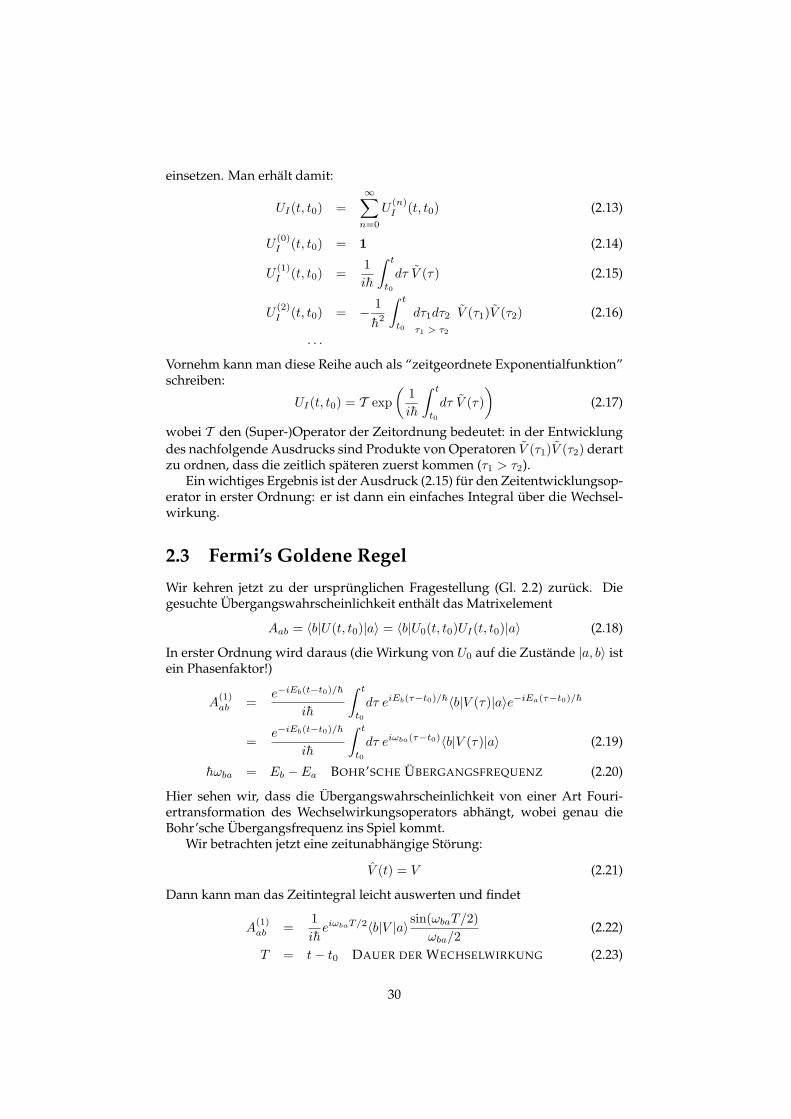
Die Funktion sin(∆ωT/2)/(∆ω/2), die hier auftritt, besitzt fur ∆ω = 0, also furEb = Ea einen scharfen Peak der Breite 2π/T (siehe Abbildung). Fur große

!!""T !""T#$

T

%!""T

Figure 2.1: Die Funktion sin(∆ωT/2)/(∆ω/2). Gestrichelt die Einhullende der Oszil-lationen.

|∆ω| beschreibt sie Oszillationen, deren Amplitude proportional zu 1/|∆ω|abfallt.

Wir erhalten folgenden Ausdruck fur die Ubergangswahrscheinlichkeit:

wab(t) =1h2 |〈b|V |a〉|2 sin2(ωbaT/2)

ω2ba/4

(2.24)

wobei die Breite des Peaks bei Eb ≈ Ea um so kleiner wird, je großer die Dauerder Wechselwirkung ist. Dies sollte aus der Fourier-Transformation bekanntsein: Wirkt die Storung nur kurz, liegt eigentlich ein zeitabhangiges Prob-lem vor, in dem die Energie nicht strikt erhalten ist (Unscharferelation Zeit-Energie).

2.3.1 ResonanzfallAls erstes Beispiel betrachten wir den Fall, dass die Zustande |a〉 und |b〉 diskretsind und exakt Eb = Ea gilt. Die Ubergangswahrscheinlichkeit (2.24) wirddann

wab(t) =1h2 |〈b|V |a〉|2 T 2 (2.25)

Dieser Ausdruck wachst quadratisch mit der Zeit T an. Dieses Verhal-ten ist charakteristisch fur den Resonanzfall. Man bezeichnet die FrequenzΩ = |〈b|V |a〉|/h als RABI-FREQUENZ. Sie gibt die Zeitskala an, auf der dieWahrscheinlichkeit zunimmt, das System im Zustand |b〉 zu finden. Sie wer-den in der Quantenoptik ein Modell kennenlernen, in man sich auf zweiZustande in einem Atom beschrankt (das “Zwei-Niveau-Atom”). Im Reso-nanzfall verhalten sich die Wahrscheinlichkeiten wa(t) und wb(t) wie cos2(ΩT )und sin2(ΩT ). Fur eine genugend kleine Rabi-Frequenz findet man den erstenTerm der Naherung (2.25) wieder.

2.3.2 Anregung in ein KontinuumAls zweites Beispiel kommen wir zu Fermi’s Goldener Regel, wie sie inden Buchern angegeben wird. Dazu betrachten wir den Fall, dass das Sys-

31

tem in ein Kontinuum |B〉 von Endzustanden in der Nahe des typischenZustands |b〉 angeregt wird. Die relevante Große ist nun die Summe derUbergangswahrscheinlichkeit wab(t) uber die moglichen Endzustande. DieseSumme kann als ein Integral uber die Endenergie geschrieben werden

wa→B(t) =∫ Ef +ε/2

Ef−ε/2dEb ρ(Eb)wab(t). (2.26)

Dabei ist ρ(Eb) die ZUSTANDSDICHTE im Energieraum: die Zahl ρ(E)dE istgleich der Anzahl der Zustande, deren Energie im Intervall (E,E+dE) liegt. Inder Wahrscheinlichkeit (2.26) werden alle Endzustande berucksichtigt, derenEnergie bei Ef = Ea liegt, mit einer Breite ε. Diese Breite gibt die “Energieun-scharfe” des Detektors an.

Wir beschranken uns auf den Fall, dass die Energieunscharfe grosser als dieUnscharfe aus der endlichen Wechselwirkungszeit ist:

2πh

T- ε. (2.27)

Aus dem Integral (2.26) erhalten wir:

wa→B(t) =1h2

∫ Ef +ε/2

Ef−ε/2dEb ρ(Eb) |〈b|V |a〉|2 sin2(ωbaT/2)

ω2ba/4

(2.28)

Die Funktion mit dem sin enthalt bekanntlich einen scharfen Peak an der StelleEb = Ea mit der Breite 2πh/T . Um das Integral auszuwerten, nehmen wirweiter an, dass die Zustandsdichte und das Matrix-Element als Funktion vonEb auf der Skala ε langsam veranderlich sind. Damit konnen wir sie aus demIntegral herausziehen und erhalten:

wa→B(t) =1h2 |〈b|V |a〉|2 ρ(Ef )

∫ Ef +ε/2

Ef−ε/2dEb

sin2(ωbaT/2)ω2

ba/4

=2πT

h|〈b|V |a〉|2 ρ(Ef ) (2.29)

Im letzten Schritt haben wir ausgenutzt, dass fur Ef = Ea der gesamte Peakinnerhalb der Energieunscharfe ε liegt und folgendes Integral benutzt:∫ +∞

−∞dx

sin2 x

x2= π. (2.30)

(Beweis: mit Hilfe des Residuensatzes.)Unser Ergebnis (2.29) zeigt, dass die Ubergangswahrscheinlich in ein Kon-

tinuum linear mit T ansteigt. Man beachte den Unterschied zum diskretenEndzustand, Gl.(2.25). Es bietet sich nun an, eine Ubergangsrate einzufuhren:

γa→B =dwa→B

dT=

2π

h|〈b|V |a〉|2 ρ(Ef ) (2.31)

Dies ist nun endlich Fermi’s Goldene Regel, wie sie in allen Buchern zur Quan-tenmechanik steht: die Ubergangswahrscheinlichkeit in ein Kontinuum istgleich dem Quadrat des Matrixelements der Storung, multipliziert mit der Zu-standsdichte an der Energie des Endzustands.

32