eingereicht an der

Technischen Universität Graz

Graz, April 2016

DISSERTATION

Paul Tirk, BSc MSc

Recent Developments in Sample Preparation and Measurementfor Inductively-Coupled Plasma Optical Emission Spectrometry

Em. Univ.-Prof. Dr. techn. Dipl.-Ing. Günter Knapp

Betreuer

Institut für Analytische Chemie und Lebensmittelchemie

zur Erlangung des akademischen Grades

Doktor der technischen Wissenschaften

EIDESSTATTLICHE ERKLÄRUNG

Ich erkläre an Eides statt, dass ich die vorliegende Arbeit selbstständig verfasst,

andere als die angegebenen Quellen/Hilfsmittel nicht benutzt, und die den benutzten

Quellen wörtlich und inhaltlich entnommenen Stellen als solche kenntlich gemacht

habe. Das in TUGRAZonline hochgeladene Textdokument ist mit der vorliegenden

Dissertation identisch.

Datum Unterschrift

Zusammenfassung

Diese Arbeit befasst sich mit verschiedenen Projekten zum Thema „Optische Emissions-spektrometrie mit induktiv gekoppeltem Plasma“ (engl.: inductively-coupled plasma opticalemission spectrometry, ICP-OES). Der erste Teil behandelt die Probenvorbereitung. Eswurde einerseits ein neuer Aufbau des mikrowellenunterstützten Hochdruckdurchfluss-aufschlusssystems charakterisiert als auch Diesel mit Hilfe von mikrowelleninduzierterVerbrennung zur anschließenden Bestimmung von Schwefel aufgeschlossen. Im zweiten Teilwird ein neues optisches Interface für die ICP-OES beschrieben, welches das Plasma von derUmgebung abschließt. Dadurch kann ein Teil der Plasmagase rezykliert werden, was einerhohen Ersparnis der Betriebsmittel gleichkommt. Zusätzlich werden neue Erkenntnisse zumsogenannten „Carbon Enhancement Effect“ präsentiert.

Abstract

In this work different projects in the field of inductively-coupled plasma optical emissionspectrometry (ICP-OES) are presented. The first part deals with sample preparation. Anew approach for microwave-assisted high pressure flow digestion was investigated and,in addition, diesel samples were digested using microwave-induced combustion for thesubsequent determination of sulfur. In the second part a newly constructed optical interfacefor ICP-OES was designed which seals the plasma from the surroundings. This makesit possible to recycle part of the plasma gases leading to high savings of running costs.Furthermore, novel insights into the so-called “carbon enhancement effect” are given.

Danksagung

Am Ende eines Dissertationsunterfangens (bzw. am Anfang der Dissertation) ist Platz umDankbarkeit zu zeigen. Dankbarkeit für die Erfahrungen und die Menschen, die einen imLaufe der Zeit begleitet und bereichert haben.

An erster Stelle gilt mein Dank meinem Betreuer Helmar Wiltsche, welcher mir dasAngebot der Doktoratsstelle am Institut für Analytische Chemie und Lebensmittelchemieunterbreitete und mir schon seit Beginn meiner Masterarbeit immer mit Rat und Tat zurSeite stand. Unter seiner fachlichen Kompetenz habe ich viel im Bereich der angewandtenAtomspektrometrie erfahren und gelernt. Meinem Doktorvater Günter Knapp sei an gleicherStelle für den regen Austausch im gemütlichen Beisammensein und seine Großzügigkeitgedankt.

Dankbar bin ich auch über das großartige Arbeitsklima am Institut, trotz verschiedenerArbeitsgruppen und Fachgebiete herrscht ein Zusammenhalt untereinander und großesgegenseitiges Interesse. Im Besonderen hervorzuheben ist in diesem Zusammenhang meinBüro-/Laborkollege und Freund Herbert Motter, der immer und stets – auch außerhalbder Institutsräumlichkeiten – zwei helfende Hände parat hat und – das muss ehrlicherweiseauch gesagt werden – meine zeitweise schwindende Motivation an der Forschung immerwieder aufleben hat lassen. Ich werde die gemeinsame Zeit definitiv vermissen.

Gerade die letzte Zeit in meinem Leben zeichnete sich durch große Erkenntnisse undVeränderungen aus, die ich zum größten Teil meinen Freunden verdanke, welche mir auch injeder Lebenslage und kleineren Krise immer mit Liebe und Verständnis entgegen kommen.Dasselbe gilt für meine Eltern, sie haben mich bestmöglich auf das Leben vorbereitet undstehen mir immer mit Unterstützung und Rat zur Seite.

Graz, im April 2016 Paul Tirk

Dissertation

Recent Developments in SamplePreparation and Measurement for

Inductively-Coupled Plasma OpticalEmission Spectrometry

Paul Tirk, BSc MSc

————————————–

Institut für Analytische Chemie und LebensmittelchemieTechnische Universität Graz

A F CC

Betreuer: Em.Univ.-Prof. Dr. techn.Dipl.-Ing. Günter Knapp

Graz, im April 2016

Contents

Preface 1

1. Analytical Process 3

I. Sample Preparation 7

2. Sample Preparation 92.1. Pre-Treatment/Homogenization . . . . . . . . . . . . . . . . . . . . . . . . . . . 92.2. Conventional Sample Preparation . . . . . . . . . . . . . . . . . . . . . . . . . . 11

2.2.1. Dry Ashing . . . . . . . . . . . . . . . . . . . . . . . . . . . . . . . . . . . 112.2.2. Wet Decomposition . . . . . . . . . . . . . . . . . . . . . . . . . . . . . . 12

2.3. Flow Digestion . . . . . . . . . . . . . . . . . . . . . . . . . . . . . . . . . . . . . 132.4. Combustion . . . . . . . . . . . . . . . . . . . . . . . . . . . . . . . . . . . . . . . 162.5. Microwave-Induced Combustion (MIC) . . . . . . . . . . . . . . . . . . . . . . . 17

3. Flow Digestion 193.1. Introduction . . . . . . . . . . . . . . . . . . . . . . . . . . . . . . . . . . . . . . . 203.2. Experimental . . . . . . . . . . . . . . . . . . . . . . . . . . . . . . . . . . . . . . 22

3.2.1. Flow digestion system . . . . . . . . . . . . . . . . . . . . . . . . . . . . 223.2.2. Instrumentation . . . . . . . . . . . . . . . . . . . . . . . . . . . . . . . . 253.2.3. Reagents, certified reference materials and samples . . . . . . . . . . . 26

3.3. Results and discussion . . . . . . . . . . . . . . . . . . . . . . . . . . . . . . . . . 263.3.1. Optimization of the microwave field uniformity . . . . . . . . . . . . . 263.3.2. Optimization of the digestion parameters . . . . . . . . . . . . . . . . . 273.3.3. Comparison between flow digestion and closed vessel batch digestion 303.3.4. Effect of the digestion acid cocktail . . . . . . . . . . . . . . . . . . . . 303.3.5. Method validation . . . . . . . . . . . . . . . . . . . . . . . . . . . . . . . 32

IX

3.4. Conclusion . . . . . . . . . . . . . . . . . . . . . . . . . . . . . . . . . . . . . . . . 333.5. Acknowledgements . . . . . . . . . . . . . . . . . . . . . . . . . . . . . . . . . . . 34

4. Microwave Induced Combustion 354.1. Introduction . . . . . . . . . . . . . . . . . . . . . . . . . . . . . . . . . . . . . . . 364.2. Materials and methods . . . . . . . . . . . . . . . . . . . . . . . . . . . . . . . . 39

4.2.1. Instrumentation . . . . . . . . . . . . . . . . . . . . . . . . . . . . . . . . 394.2.2. Samples, reagents and standards . . . . . . . . . . . . . . . . . . . . . . 404.2.3. Sample digestion by the proposed MIC method . . . . . . . . . . . . . 414.2.4. Evaluation of MIC digestion efficiency using a flame retardant . . . . 414.2.5. Evaluation of the proposed procedure accuracy . . . . . . . . . . . . . 42

4.3. Results and Discussion . . . . . . . . . . . . . . . . . . . . . . . . . . . . . . . . 424.3.1. Initial experiments without using flame retardant . . . . . . . . . . . . 424.3.2. Use of glass wool as a flame retardant . . . . . . . . . . . . . . . . . . . 434.3.3. Evaluation of the digestion efficiency . . . . . . . . . . . . . . . . . . . . 454.3.4. Evaluation of the absorbing solution . . . . . . . . . . . . . . . . . . . . 454.3.5. Sulfur determination in diesel oil samples after the MIC method . . . 46

4.4. Conclusions . . . . . . . . . . . . . . . . . . . . . . . . . . . . . . . . . . . . . . . 474.5. Acknowledgments . . . . . . . . . . . . . . . . . . . . . . . . . . . . . . . . . . . 47

II. Analysis 49

5. Atomic Spectrometry 515.1. Fundamentals . . . . . . . . . . . . . . . . . . . . . . . . . . . . . . . . . . . . . . 525.2. Spectral Lines . . . . . . . . . . . . . . . . . . . . . . . . . . . . . . . . . . . . . . 54

5.2.1. Line Broadening . . . . . . . . . . . . . . . . . . . . . . . . . . . . . . . . 545.2.2. Line Profile . . . . . . . . . . . . . . . . . . . . . . . . . . . . . . . . . . . 57

6. Inductively-Coupled Plasma Optical Emission Spectrometry (ICP-OES) 616.1. Enclosed Plasma Interface . . . . . . . . . . . . . . . . . . . . . . . . . . . . . . 626.2. “Carbon Enhancement Effect” . . . . . . . . . . . . . . . . . . . . . . . . . . . . 64

7. Plasma Diagnostics 677.1. Temperature . . . . . . . . . . . . . . . . . . . . . . . . . . . . . . . . . . . . . . 67

7.1.1. Temperature Determination Using Absolute Line Intensities . . . . . 697.1.2. Temperature Determination Using Relative Line Intensities . . . . . . 697.1.3. Thermodynamic Equilibrium . . . . . . . . . . . . . . . . . . . . . . . . 70

7.2. Plasma Robustness . . . . . . . . . . . . . . . . . . . . . . . . . . . . . . . . . . . 71

X

7.3. Electron Density . . . . . . . . . . . . . . . . . . . . . . . . . . . . . . . . . . . . 727.4. Radiofrequency Generator Characteristics . . . . . . . . . . . . . . . . . . . . . 73

8. Enclosed Plasma Interface 758.1. Introduction . . . . . . . . . . . . . . . . . . . . . . . . . . . . . . . . . . . . . . . 768.2. Experimental . . . . . . . . . . . . . . . . . . . . . . . . . . . . . . . . . . . . . . 77

8.2.1. Enclosed plasma interface . . . . . . . . . . . . . . . . . . . . . . . . . . 778.2.2. Argon recycling . . . . . . . . . . . . . . . . . . . . . . . . . . . . . . . . 808.2.3. Instrumentation . . . . . . . . . . . . . . . . . . . . . . . . . . . . . . . . 808.2.4. Reagents . . . . . . . . . . . . . . . . . . . . . . . . . . . . . . . . . . . . 818.2.5. RF stray field . . . . . . . . . . . . . . . . . . . . . . . . . . . . . . . . . 82

8.3. Results and discussion . . . . . . . . . . . . . . . . . . . . . . . . . . . . . . . . . 838.3.1. RF stray field . . . . . . . . . . . . . . . . . . . . . . . . . . . . . . . . . 838.3.2. Thermal considerations . . . . . . . . . . . . . . . . . . . . . . . . . . . . 838.3.3. Analytical characterization of the enclosed plasma . . . . . . . . . . . 858.3.4. Argon recycling and contamination . . . . . . . . . . . . . . . . . . . . 86

8.4. Outlook . . . . . . . . . . . . . . . . . . . . . . . . . . . . . . . . . . . . . . . . . 878.5. Conclusion . . . . . . . . . . . . . . . . . . . . . . . . . . . . . . . . . . . . . . . . 888.6. Acknowledgements . . . . . . . . . . . . . . . . . . . . . . . . . . . . . . . . . . . 888.7. Supplementary Material . . . . . . . . . . . . . . . . . . . . . . . . . . . . . . . . 89

9. Carbon Enhancement Effect 919.1. Introduction . . . . . . . . . . . . . . . . . . . . . . . . . . . . . . . . . . . . . . . 929.2. Experimental . . . . . . . . . . . . . . . . . . . . . . . . . . . . . . . . . . . . . . 94

9.2.1. Instrumentation . . . . . . . . . . . . . . . . . . . . . . . . . . . . . . . . 949.2.2. Reagents . . . . . . . . . . . . . . . . . . . . . . . . . . . . . . . . . . . . 969.2.3. Optical emission-based plasma diagnostics . . . . . . . . . . . . . . . . 969.2.4. Experimental procedure and processing of the spectra . . . . . . . . . 96

9.3. Results and discussion . . . . . . . . . . . . . . . . . . . . . . . . . . . . . . . . . 979.3.1. Repeatability of the excitation temperature determination . . . . . . 979.3.2. Instrumental dependence of the effect of carbon on the signal of Se . 989.3.3. Effect of methanol . . . . . . . . . . . . . . . . . . . . . . . . . . . . . . . 1009.3.4. Effect of phenylalanine and CO2 . . . . . . . . . . . . . . . . . . . . . . 1069.3.5. Effect of bromine . . . . . . . . . . . . . . . . . . . . . . . . . . . . . . . 1089.3.6. Effect of NaCl . . . . . . . . . . . . . . . . . . . . . . . . . . . . . . . . . 1119.3.7. Differentiating between the factors contributing to the carbon en-

hancement effect . . . . . . . . . . . . . . . . . . . . . . . . . . . . . . . . 1129.4. Conclusion . . . . . . . . . . . . . . . . . . . . . . . . . . . . . . . . . . . . . . . . 115

XI

Conclusion 117

Appendices 121

List of Figures 121

List of Tables 123

Bibliography 125

Acronyms 137

A. Octave Script for Electron Density 139A.1. H_gamma.m . . . . . . . . . . . . . . . . . . . . . . . . . . . . . . . . . . . . . . 139A.2. SplitVoigt.m . . . . . . . . . . . . . . . . . . . . . . . . . . . . . . . . . . . . . . . 143A.3. Faddeeva.m . . . . . . . . . . . . . . . . . . . . . . . . . . . . . . . . . . . . . . . 143

B. “Carbon Enhancement Effect” – Supplementary Material 149B.1. Enhancement factors . . . . . . . . . . . . . . . . . . . . . . . . . . . . . . . . . . 150B.2. HV PSU Data Logger Schematics . . . . . . . . . . . . . . . . . . . . . . . . . . 154

XII

Preface

Over the last years I worked on different projects related to the field of analytical chem-istry and especially inductively-coupled plasma optical emission spectrometry (ICP-OES).Achievements were made in both the sample preparation as the essential first step of everyanalysis as well as the instrumentation and measurement. The thesis is therefore divided intotwo parts. The first deals with topics in sample preparation while the second one describesadvances in ICP-OES. At the beginning of every part, underlying theory and concepts arepresented in different chapters. They are followed by the relevant publications.

The first project in sample preparation was part of developing a microwave-assisted highpressure flow digestion system suitable for preparation and digestion of slurries [1] (seechapter 3). In addition, I spent two months at the “Universidade Federal de Santa Maria”(UFSM) in Santa Maria (Rio Grande do Sul, Brazil) working on a project involving thedigestion of diesel samples using the microwave-induced combustion (MIC) method in orderto enable the determination of the sulfur content [2] (see chapter 4).

Developments in ICP-OES include the design and construction of a sealed plasma whichenables the recycling of parts of the argon stream, a feature which saves almost 90% ofargon consumption (see chapter 8). Additionally, new insights into the long discussed“carbon enhancement effect” are given in chapter 9 [3].

1

CHAPTER 1

Analytical Process

Because the two main divisions of this thesis are part of the solution to an analyticalquestion this first chapter tries to briefly summarize the so-called “Analytical Process”. Itdescribes the path from the analytical problem to the solution or result and can be roughlydivided into the following steps:

Definition of the problem At the beginning of every analysis we have to ask ourself thequestion of what exactly do we want to know or achieve. The definition of the analyticalproblem has to include at least the analyte(s) or species of interest and information aboutthe sample’s nature and/or the sample matrix. It then leads us to a selection of the availableanalytical techniques and the necessary sampling and sample pre-treatment steps.

Choice of the method After the desired information has been defined, a suitable ana-lytical technique has to be chosen. Sometimes only one method is available but often itis necessary to select from a variety of possibilities. When selecting the optimal methodwe should consider factors like efficiency, time, errors, selectivity and safety. Ideally, thetechnique of choice is a validated one, which has been tested in various laboratories forits applicability and therefore gives an accurate measurement for the type of analyte andsample. The chosen method also has a big influence on the following sampling and samplepreparation steps.

3

Sampling The next and probably one of the most important steps is “sampling”. Itcrucially determines the quality and outcome of the whole analysis and also poses themost difficulties to overcome. “Sampling” refers to the selection of a small representativeportion from the untreated material of interest. Care must be taken to ensure the sample’srepresentative character, i.e. its qualities and origins have to correspond well with thedesired objectives set in the “definition of the problem”. Attention should be payed alsoto sample storage and transport as to not impair the actual analysis by deteriorating theanalytes. This information should be well defined in a sampling plan, containing proceduresfor selection, collection, transport and preparation of the samples.

Sample preparation After sampling, sample transport and possible storage, the sampleshave to be transformed into a form suitable for the following analyses. These proceduresinvolve for example homogenizing (grinding, sieving, etc.) and belong to “sample prepa-ration”. Different analytical techniques require distinct preparation. Most of the timethe samples are required to be in liquid form. Solid matter therefore has to be dissolved,gaseous substances absorbed. Chapter 2 will provide some more insights into this matter.

Measurement Having prepared the samples, the measurement can be conducted where adetector converts a physical quantity into a number. Depending on the analytical technique,the obtained values can be emission or absorption intensities (atomic/molecular emis-sion/absorption, fluorescence, phosphorescence), concentrations, time or even dimensionlessnumbers.

Calibration Calibration data is used to bring the measured values in relation to thedesired quantity. Ideally a mathematical model exists, e.g. a linear or quadratic, sometimespolynomial dependency. We can distinguish between three main calibration approaches.External calibration is the most commonly used one. A series of reference solutions withknown amounts of the analyte(s) is submitted to the measurement and the calibrationfunction is obtained through the relationship of the analyte concentrations and the measuredsignal. The reference solutions should at least contain the analyte in the same solvent asthe sample. If also the concomitant substances are present we speak of “matrix-matched”solutions. The quality of a calibration depends on three main factors: the repeatabilityof the measurement, the trueness of the standards and the validity of the comparison.These considerations result in statistical confidence bands of the calibration function. As aconsequence, the final results of the analysis should also reflect the calibration uncertainties

4

as confidence limits. When dealing with complex sample matrices (for example petroleum),standard addition is sometimes preferred. The sample – and therefore its matrix – formsthe base for the calibration standards. Again, known amounts of the analyte(s) are addeddirectly to the sample solution. The third concept to mention is internal standardization.A substance which should behave chemically similar to the analyte(s) is added to allcalibration standards and samples. It therefore runs through all sample preparation steps.The measured values are then divided by the signal of the internal standard resulting in aset of ratios, thus eliminating potential losses and signal alterations due to variations in theanalytical instrument. It is obvious that especially in multi-element analysis the choice of asuitable internal standard is difficult or even impossible. In inductively-coupled plasmamass spectrometry (ICP-MS) multiple internal standards are usually added for differentranges of element masses.

Data processing/evaluation By applying the calibration function to the measured datawe obtain the desired concentrations. These have to be interpreted and evaluated by takinginto account quality control measures such as the use of certified reference materials (CRMs)or the determination of blank values which give rise to limits of detection (LODs) and limitsof quantification (LOQs). In the end a number of statistical treatments is usually involvedin the summarization and preparation of the final values. Uncertainties are supplied forevery result. Chemometric techniques are available to help finding correlations and dealwith large amounts of data which readily occur in multi-element determinations. All theseconsiderations are necessary to assess if the results are valid for the given analytical questionor if measurements have to be repeated or altered.

Summing up, it should be pointed out that the most critical and time-consuming step ofthe analytical sequence is the sample preparation. Great care must be taken because therelie most of the potential error sources of the analysis. Many aspects and techniques arepresented in the sample preparation chapter (chapter 2).

5

Part I.

Sample Preparation

7

CHAPTER 2

Sample Preparation

The transformation of samples into the form suitable for the subsequent measurement ispart of the sample preparation step. After the sampling and appropriate storage it is acrucial step in every analysis. Many of the analytical techniques require the samples tobe in a liquid form. An advantage of solutions is that the calibration can be easily doneusing reference solutions and dilutions can be made without great effort. Additionally,the carbon contained in organic samples can significantly impair the measurements inICP-OES and ICP-MS and should be removed as much as possible (see also chapter 9).These circumstances make sample decomposition through wet digestion an advantageousstep. On the other hand, the downside of every sample preparation step is the risk ofcontamination and – in case of wet digestion – further dilution of the analyte(s).

This chapter tries to summarize briefly the procedures and processes of “sample preparation”in order to better understand the articles about “flow digestion” and microwave-inducedcombustion (MIC) which are presented in succession as chapters 3 and 4. It is looselybased on chapters 1, 5 and 9 of the book “Microwave-assisted sample preparation for traceelement determination” [4].

2.1. Pre-Treatment/Homogenization

Depending on the nature and state of the samples additional pre-treatment may be necessary.Most of the time the samples are of rather inhomogeneous composition. In order to obtain

9

a representative sample different homogenization techniques have to be applied. Thesemainly include mechanical procedures for homogenization and preparation for a followingdigestion step. The next paragraphs give an overview of the most common pre-treatmentsteps.

Cleaning can be necessary, for example, when dealing with parts of plants to remove soilor dust. Care must be taken to not bring in more contaminants through the use of thewashing agents. To avoid the risk of leaching the cleaning process should be as short aspossible.

Drying is the controlled removal of water from the samples until a constant weight isachieved. It is a common requirement for solid samples because of their unknown amountof contained water. The temperature has to be chosen such as to not volatilize the analytesbut still high enough to evaporate water. It ranges from 60 – 65 ○C for biological samplesup to more than 1000 ○C for some minerals. Both ovens and desiccants are used. A specialcase of drying is “lyophilization” where the sample is first frozen between −80 and −60 ○Cand then dried in a vacuum at temperatures of −20 and 40 ○C.

Grinding increases the homogeneity of the samples by reducing the particle sizes. Af-terwards the representativity of the samples is achieved because the ground particles canbe mixed more easily. In addition, grinding increases the surface to volume ratio of theparticles which leads to a higher solubility and reactivity towards reagents in the followingdigestion procedures. The comminution through grinding can be considered one of themost critical steps in the analytical sequence as the parts of the mill pose a high riskof contamination depending on their chemical composition. Therefore the hardness orabrasive resistance of the grinding components must be higher than the one of the sample.The collisions between the sample particles and the grinding components generally cause awarming which has to be considered when dealing with volatile analytes.

For matter that is soft, smooth and elastic at room temperature (e.g. most biologicalsamples) cryogenic grinding was developed. It relies on increasing the hardness of thetissues by freezing. As a result very little force is necessary to break the structures.

Sieving separates the particles into classes of different size distributions. It allows theclassification and evaluation of the particle sizes which can provide insights into the

10

effectiveness of the chosen grinding method as well as the achieved homogeneity of thesample. If metal sieves are used there is a risk of contamination similar to grinding.Especially in trace analysis this has to be kept in mind.

Filtering When dealing with solutions which already contain particulate matter, a filteringstep may be necessary. It depends on the selected analytical technique as these particles cancause problems by coagulation and clogging in essential parts of the instruments. EspeciallyICP-based devices use pneumatic nebulizers which are prone to irreversible obstruction.Therefore, filtration through membrane filters is recommended. On the other hand, if we areinterested in the particles, filtration provides a way to separate them from the liquid partsof the sample. The residue on the filter can then be decomposed and analyzed separately.

2.2. Conventional Sample Preparation

Before going into the microwave-assisted sample preparation techniques and their recentdevelopments presented in this thesis, a brief overview of conventional open and closedsystems is given.

2.2.1. Dry Ashing

The probably simplest method to decompose biological and organic samples is dry ashing.Oxidation occurs by pyrolysis and combustion using the oxygen in the air and releasing thecarbon in form of CO2. Depending on the composition of the sample additional productsinclude water and nitrogen compounds. The remaining ashes contain the inorganic elementsmostly in form of metal oxides but also as non-volatile sulfates, phosphates and silicates.

After the sample has been put into a crucible it is placed into a muffle furnace or upona simple laboratory flame. The temperature range for the pyrolysis of organic matter isusually between 450 – 600 ○C. In order to avoid potential losses due to volatilization of theanalytes the heating program has to be chosen carefully. Compounds containing chlorinecan also lead to the formation of metal chlorides (e.g. PbCl2, CdCl2) which are lost easily.Another problem arises when there is a reaction between the analytes and the crucible.Other materials like quartz or platinum are available to counteract these processes.

11

Despite the mentioned potential risks, dry ashing remains a very effective and simpletechnique in preparation of solid samples for trace element determination and is still widelyused as a standard procedure for petroleum products and foods. The dry ashing processrequires little attention of the analyst, sample masses greater than 10 g are possible andthe materials and instruments are rather inexpensive. Variations of this technique employinfrared (IR) or microwave radiation. A more recent development uses microwaves toignite the pyrolysis of the sample under an oxygen atmosphere (see MIC, section 2.5 andchapter 4).

2.2.2. Wet Decomposition

In contrast to simple dry ashing concentrated mineral acids or acid mixtures can be addedto the sample as the oxidizing reagents. These procedures are summarized under the term“wet digestion” or “wet decomposition”. It only requires slightly elevated temperaturesand results in acidic solutions. The analytes are available in simple inorganic forms andthe solutions are readily usable in most atomic spectrometry instruments. For organicand biological samples, nitric, sulfuric and perchloric acids produce clear solutions whichindicate a complete decomposition although the residual carbon content (RCC) shouldbe checked as it can cause interference in the subsequent measurement. Analytes canalso remain retained in undecomposed organic substances. Compared to dry ashing themain advantage of wet digestion is the low reaction temperature. It reduces the risk ofvolatilization of the analytes although requires more attention of the analyst as concentratedacids or acid mixtures are involved.

Wet digestion systems can be divided into two classes: open and closed systems. Inopen systems volatile elements such as halogens, antimony, arsenic, boron, selenium andmercury are obviously prone to be lost through evaporation. Furthermore, the boilingtemperature of HNO3 (azeotrope with water, 121 ○C) is often not sufficient to achieve acomplete decomposition as higher temperatures are needed to destroy the C−C bonds oforganic molecules. The highest oxidation power is provided by HClO4 but due to theformation of unstable perchlorates and their explosive nature it cannot be used as theonly reagent in concentrated form. In case of silica matrices hydrofluoric acid helps todecompose the insoluble residue which also may contain analyte elements.

As stated before, losses due to volatilization are a big concern in open wet digestionsystems. In addition, the highest possible decomposition temperature is limited by theboiling temperature of the solvent or acid at ambient pressure. According to Arrhenius,

12

the temperature also determines the reaction rate, which directly relates to the requiredtime to achieve a sufficient decomposition. It is obvious that by closing the digestionsystem, an increased pressure allows higher reaction temperatures, thus remedying theaforementioned limitations. Furthermore, the digestion solution cannot evaporate thusleading to less reagent consumption while the closed nature of the setup minimizes therisk of contamination. On the other hand, it is clear that a closed system inherently bearsthe risk of explosion and therefore safety measures have to be taken. The vessels can bemade of quartz or fluorinated polymers, the latter ones limit the operating temperatures toless than 260 ○C. At high pressures and temperatures some elements can also diffuse intopolytetrafluorethylene (PTFE). This circumstance is known as “memory effect” becausein addition to the analyte losses the elements located in the vessel walls can be releasedlater, potentially leading to cross-contamination. Modern modifications and copolymershave a lower porosity and help to minimize this problem. For most digestions pure HNO3

is usually sufficient and safe to use. As the oxidation potential increases with temperature,low RCCs are achieved. If hydrofluoric acid has to be added, vessels made of quartz cannotbe used and PTFE becomes the material of choice. Due to the aforementioned explosionrisk of closed systems, perchloric acid is to be avoided strictly, as it can produce pressuregradients which are too high for the safety devices to respond.

2.3. Flow Digestion

In sample preparation three types of systematic errors are found. Contamination by dust,reagents, vessel material and impurities on the vessel’s surface can be prevented by usingclosed systems. Flow digestion systems allow most of the sample handling procedures to bedone in a closed environment while the continuous rinsing of the tubing with the carriersolution effectively avoids both cross-contamination between subsequent samples as wellas adsorption of analytes at the tube walls. Secondly, a closed system avoids potentiallosses of elements due to volatilization while the use of inert materials (e.g. PTFE, PFA)minimizes reactions with the tubing. The third source of errors are interferences withremaining carbon resulting from incomplete decomposition of organic samples. The RCCafter digestion in flow systems is generally higher because of the shorter residence time ofthe samples in the heated digestion zone. More detail on the deleterious effects of carbonin ICP-based analytical techniques is given in chapter 9.

Because of the continuous nature of flow systems only liquid samples or slurries (suspensionof ground solid samples in water or acid) can be digested. In contrast to batch processes,

13

automating the sample handling steps is easier to achieve. Furthermore, direct couplingwith the following measurement devices is possible. The main stages of a flow digestionsystem are sample introduction, heating and as the last step, cooling and degassing. Insample introduction the reagent is added to the sample and mixed, if necessary. A definedvolume is then pushed by the carrier solution into the heated digestion zone. Here thepressure defines the temperature of the boiling equilibrium. For a good decompositiontemperatures of around 200 ○C are desired, depending on the reagents the pressure shouldbe around 20 bar (10% nitric acid in water). After passing through the heated zone thesample solution reaches the cooling and subsequently the degassing stage where the gaseousreaction products are separated from the liquid sample digests. This is done to avoid gasbubbles which on the one hand contain large portions of CO2 (refer to chapter 9 and onthe other hand can cause fragmentation of the sample liquid resulting in fluctuation of theanalyte signal during measurement. At the end of the digestion system the pressure hasto be lowered to ambient conditions in order to receive the digested sample solution forfurther processing.

Although in principle flow digestion systems appear rather simple there are a few disad-vantages to bear in mind. In general, oxidation efficiencies are low due to the rather shortdigestion times. Both the oxidation efficiency and the digestion time can be improved byincreasing the pressure in the system. Cross-contamination can occur between subsequentsamples and is dependent on rinse times, flow velocities and properties of the tubing, suchas diameter and material. Especially the inner diameter of the tube is of importance as itdetermines the maximum allowed particle size in the samples. Particles should not exceedhalf the inner diameter of the tubing. For larger tube diameters clogging tends to happenmore because of swelling or agglomeration of the particles. It has to be kept in mind thata low flow velocity also contributes to segregation of larger particles.

Flow digestion systems can be classified by three characteristics: (1) the operating pressureand temperature, (2) the type of heating (conductive, multimode microwave and focused/-monomode microwave) and (3) the flow program (continuous flow or stopped flow). Themost practically and for the design of the system most relevant aspect is the operatingpressure. Three pressure ranges are described in literature. In ambient pressure systems astrong formation of bubbles is observed due to the low solubility of gases. The atmosphericpressure limits the boiling point of the digestion solution to around 120 ○C, a temperaturewhich provides a rather low oxidation efficiency. These systems are therefore more suitablefor the dissolution of insoluble precipitates. The tubing can be made of PTFE or perfluo-roalkoxy alkane (PFA) and there are no additional valves needed, allowing the use of highlycorrosive acid mixtures without an increased risk of contamination from the valve materials.

14

The upper pressure limit of medium pressure systems is chosen arbitrarily at 25 bar with thecorresponding boiling temperature of 180 ○C. Bubble formation is less pronounced while theRCC remains rather high which can cause interference in the subsequent measurement.

In case of nitric acid as the only reagent a temperature of at least 200 ○C is necessary ifa RCC below 10% is desired. Complete decomposition of organic substances with nitricacid occurs at temperatures of around 300 ○C due to the relatively strong C−C bonds [5,6]. Under these circumstances (> 200 bar pressure) only a liquid phase is present as thegas is totally absorbed. High pressure flow digestion systems operate at pressures greaterthan 25 bar. The introduction of the sample requires HPLC-grade 6-port valves and asample loop while the depressurization is achieved by a restrictor capillary after coolingand degassing of the sample solution. It should be noted, that the temperature limit ofPTFE/PFA material is 250 ○C which in turn limits the possible pressure. In literature, asystem employing a Pt/Ir capillary can be found [7]. It enables a pressure of 300 bar withdecomposition temperatures around 360 ○C.

The energy in flow digestion systems can be introduced both through conventional andmicrowave heating. Microwaves are mostly absorbed by the liquid phase and not by steamresulting in an efficient energy transfer and a kind of boiling equilibrium inside the tube.In comparison, with conventional heating there is always a temperature gradient from theheating element to the flowing medium, meaning that the tube is always hotter than theactual digestion solution. On the other hand a major downside of (multimode) microwavesystems is the heterogeneous field which induces local hotspots. This eventually causesmaterial failure at certain points of the digestion tube. It should be noted that for mediumand high pressure flow digestion systems, the PTFE and PFA tubes have to be surroundedby an additional supporting structure in order to withstand the pressure. Available optionsinclude high-tensile strength fibers or stainless steel tubes.

The project I was working on during the last years is described in further detail in chapter 3.More recent developments of the presented flow system including a different reactor geometrywith higher volume were done by Thiago Linhares Marques and are already publishedin [8].

15

2.4. Combustion

Sample combustion is an attractive alternative to wet digestion. Organic matter is oxidizedalmost completely leaving only the inorganic remains. As the main reagent is oxygen thereis a lower risk of contamination which makes combustion especially interesting for traceelement analysis. After the decomposition the nonvolatile analytes (Fe, Si, Al, alkalineelements, etc.) are found in the ashes and can be further treated. The volatile elementssuch as halogens are released into the gas phase and can be absorbed in a suitable solution.Typically, all absorbing solutions are diluted which is an important aspect considering greenchemistry recommendations. Furthermore, residues and contamination by the reagents canbe minimized. This circumstance also improves blank values and as a result, LODs, whileinterferences in the following measurement due to high concentrations of reagents are alsolowered.

For a sample only containing carbon, hydrogen and oxygen the general formula of thecombustion reaction is given by equation 2.1. In a complete combustion the compoundsreact with the oxygen and decompose into H2O and CO2 leading to clean digests. Thisreaction applies to many organic sample matrices like carbohydrates, lipids and proteins, aswell as to hydrocarbons of crude oil or monomers of a polymer. The oxygen as the oxidantcan be supplied as pure gas or from the surrounding air.

CxHyOz + (x + 1/4 y − 1/2 z)O2 ÐÐ→ x CO2 + 1/2 y H2O (2.1)

In combustion we can also distinguish between open and closed systems. Open combustionsystems were already discussed in section 2.2.1 as dry ashing. Regarding closed systems aseries of developments were made: Schöniger flask and the combustion bomb. In theSchöniger method a simple glass flask is used to burn the sample. Contamination by metalis avoided but the sample mass is limited to around 200mg. In contrast the combustionbomb is a stainless steel container which is able to withstand higher pressures and thereforehigher sample masses are possible, but at the cost of increased contamination due to thebomb material. The later introduced microwave-induced combustion (MIC) combines theconcepts of closed vessel wet digestion and combustion into one single technique. It isdescribed further in the following section.

16

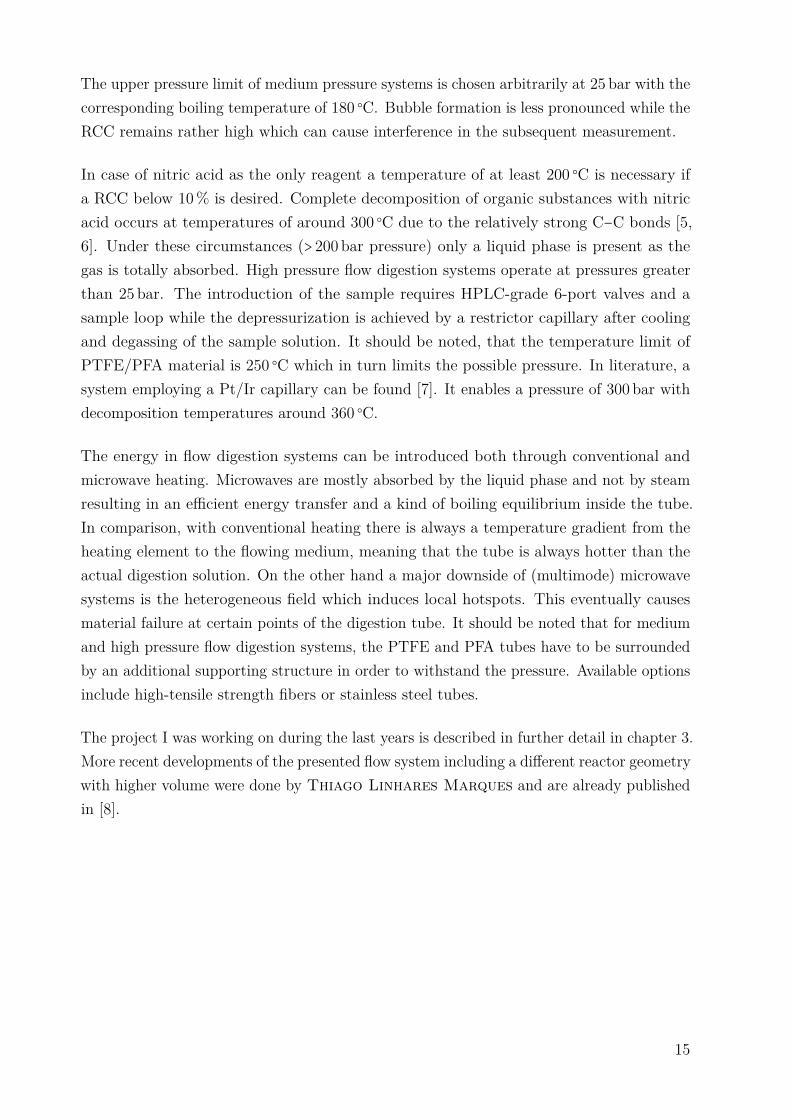
Figure 2.1.: General procedure for MIC in closed vessels [4, p. 154].

2.5. Microwave-Induced Combustion (MIC)

The microwave-induced combustion (MIC) technique was developed in 2004 by ÉricoMarlon de Moraes Flores at the Universidade Federal de Santa Maria in cooperationwith Günter Knapp (Graz University of Technology) [9]. It combines the advantagesof classical combustion bomb techniques and microwave-assisted closed vessel digestioninto a single system. In MIC, the combustion is initiated by microwaves instead of electriccurrents. It is carried out in the same quartz vessels used for wet digestion which reducescontamination with metals, only a quartz sample holder is added. The samples are placedin form of pellets onto the sample holder. Liquid samples have to be wrapped in a suitablematerial such as polycarbonate (PC) capsules or polyethylene (PE) film.

Figure 2.1 depicts the general MIC procedure. After the sample has been placed onto thequartz holder, which has already been prepared with the filter paper, the igniter solution(usually NH4NO3) is added. The sample holder is then inserted carefully into the quartzvessel which contains the absorbing solution. After closing of the vessel it is pressurizedwith oxygen and placed into the microwave system. Ignition occurs within 10 seconds afterstarting the microwave irradiation. Following the combustion a reflux step can be added inorder to improve the absorption of the analytes.

Chapter 4 provides more detail of the project which was done at the “Universidade Federalde Santa Maria” (UFSM) in Brazil.

17

CHAPTER 3

Flow DigestionHelmar Wiltsche, Paul Tirk, Herbert Motter, Monika Winkler and Günter Knapp

The following chapter was published in the “Journal of Analytical Atomic Spectrometry”,Volume 29 (2014), pages 272 – 279 under the title “A novel approach to high pressure flowdigestion” [1].

Abstract

A new high pressure flow digestion system has been developed for sample digestion at a pressure of up to40 bar and a temperature of about 230 ○C. The reaction with acids takes place in a PFA tube and is heatedby microwave radiation in a multimode cavity. As the PFA tube cannot withstand the harsh digestionconditions without support, it is placed inside a coiled glass tube pressurized by 40 bar nitrogen thusforming an autoclave. Corrosion of system components by acid fumes and related sample contamination iscircumvented by establishing a slow but steady flow of the high pressure nitrogen countercurrent to thesample flow. The presented system does not constrain the selection of the digestion reagent. Acid cocktailsof nitric acid with hydrochloric and/or hydrofluoric acid as well as hydrogen peroxide were successfullyused for the digestion of various samples. The method accuracy was validated with five certified referencematerials (BCR 62, DORM-2, NIST SRM 1515, NIST SRM 1567, NIST SRM 1568) and good agreementbetween the determined and the certified values was obtained for Al, Ca, Cr, Cu, Fe, Mg, Mn, Ni, Pb, andZn using inductively-coupled plasma optical emission spectrometry (ICP-OES) for analyte quantification.The flow digestion of the CRMs resulted in clear solutions with residual carbon concentrations (RCCs)between 11 and 40%. Spike recoveries of Al, As, Ba, Be, Bi, Cd, Co, Cr, Cu, Fe, Mg, Mn, Mo, Ni, Pb,Sb, Se, Sr, Ti, V, and Zn were between 94 and 105%. For Hg the spike recovery was 89%. The fullyautomated high pressure flow digestion system is capable of digesting up to 6 samples per hour.

19

3.1. Introduction

Flow digestion is an attractive alternative to closed vessel microwave assisted digestion dueto the ease of automation, the reduced risk of contamination and the capability of directcoupling to analyte quantification techniques. In general the sample is first mixed with thedigestion acid (usually HNO3 or acid cocktails). Then the sample/acid mixture is heated bypassing through a heating zone. In continuous flow systems the sample is pumped throughthe heating zone continuously by a carrier solution [10–12] while in stopped flow systemsthe sample is pushed into the heating zone by the carrier solution, then the carrier flow isstopped and the sample is heated [13–15]. At the end of the digestion period, the sample ispushed out of the digestion zone by turning on the carrier solution again. In most flowdigestion systems reported in the literature microwave heating was used but in some casesconductive heating was employed. After the heating zone, gases that evolved during thedigestion (e.g. nitrous oxides, CO2) can be removed by a gas/liquid separator.

Flow digestion systems can be classified as already noted by their mode of operation(continuous flow or stopped flow), by their means of heating the sample/acid mixture inthe digestion zone (conductive heating, microwave heating) or by the pressure inside thedigestion system. The pressure inside the heated digestion coil is of great importance as itdetermines the maximum temperature of the acid mixture and thereby the efficiency of thedigestion [16]. Three pressure regimes may be distinguished: ambient, medium (< 25 bar)and high pressure (> 25 bar) flow digestion systems. It is well known that the digestionefficiency of any acid digestion system increases with the temperature of the digestion acid.As the boiling point of the acid limits the maximum attainable digestion temperature it ishighly desirable to increase the pressure inside the digestion system.

Ambient pressure systems dominate the literature as they are relatively easy to build.Burguera [17–19] pioneered these systems using microwave assisted sample heating.Ambient pressure flow digestion systems are capable of operating with highly corrosiveacids like HCl or mixtures of HCl and HNO3 as the entire flow path is usually made ofeither inert polymers or glass [19, 20]. The main disadvantage of ambient pressure flowdigestion systems is that gaseous reaction products eject the sample/acid mixture quicklyfrom the heated dissolution zone reducing the effective digestion time and causing undesiredpeak broadening. The maximum digestion acid concentration [21, 22] and the maximumpower level [23–25] in the heated digestion zone are therefore limited by the gas evolution.Moreover, the digestion acid boils at about 120 ○C, causing low efficient oxidation of organicsubstances.

20

In a medium pressure digestion system the digestion acid is pressurized up to about 25 bar.Thereby the acid’s boiling point is considerably increased (e.g. 10% HNO3: 230 ○C) andthe solubility of gaseous reaction products in the digestion mixture is enhanced significantly,reducing dispersion effects [11]. The pressure limit of 25 bar is somewhat arbitrarily chosenas the pressure limit of fiber reinforced PTFE tubes [26]. In medium pressure flow digestionsystems the oxidation efficiency of HNO3 is significantly higher than in ambient pressuresystems.

High pressure flow digestion systems operate at pressures above 25 bar. This pressureregion is comparable with contemporary closed vessel microwave assisted batch digestionsystems. The main difference between batch digestion systems and flow systems in thispressure region is the shorter digestion time in flow systems. Typical digestion times in flowsystems are between 2 and 5min. Haiber and Berndt [27] developed a high pressuresystem operating at up to 360 ○C and 300 bar pressure. In this pressure range all reactionproducts which are gaseous at ambient pressure remain in a liquid phase [28]. The highdigestion temperature resulted in extremely low residual carbon concentrations (<< 1%RCC). A Pt/Ir (80/20) tube was used as the heated pressurized digestion tube [7] as thismaterial showed excellent resistance to nitric and hydrofluoric acid [27, 29]. Nevertheless,mixtures of nitric and hydrochloric acid drastically reduced the digestion tube lifetime [29].The digestion tube was directly heated by clamping a supply voltage to the two ends of thedigestion coil making use of its inherent resistance [27]. It is interesting to note, that Bianet al. [30] encountered losses of Ag, Ga and Sb during high pressure digestion in the Pt/Irtube that increased with rising digestion temperature.

Another high pressure flow digestion system using microwave heating is the pressureequilibrium system described by Knapp et al. [16, 31]. The underlying principle is thatmicrowave energy is dominantly absorbed by the liquid phase, whereas steam and gaseousreaction products are not significantly heated. Thereby, a boiling equilibrium is formedmuch in the same way as in reflux boiling. In the pressure equilibrium system the PTFEdissolution coil is placed in a pressurized vessel, which in turn is located in a microwavefield resulting in nearly equal pressure inside and outside of the PTFE tubing. This reducesthe mechanical stress on the tubing significantly. Nevertheless, the pressure equilibriumsystem had several shortcomings: the length of the digestion tube – and as a consequencethe actively heated volume – is restricted by the size of the waveguide of the used focusedmicrowave oven. Moreover, cross-contamination between successive samples was observedand delicate optimization of the restrictor length, system pressure and carrier flow wasnecessary.

21

The aim of this work was to develop a radical new design of a pressure equilibrium system,overcoming the previous shortcomings. A high degree of automation was considerednecessary to ensure reproducible experimental conditions.

3.2. Experimental

3.2.1. Flow digestion system

A high pressure, continuous flow, pressure equilibrium [16] flow digestion system wasconstructed for this work. Briefly, diluted nitric acid (1% v/v) was continuously pumpedthrough the system by an acid resistant all Ti HPLC pump (Knauer, Germany – fig-ure 3.1, A). If not stated otherwise a carrier flow of 2.0mLmin−1 was used. A 10mLsample loop (figure 3.1, C) connected to a 6-port valve (Knauer, Germany – figure 3.1, B;fluorinated polymer sealed, wide bore channel) was used to inject the samples (figure 3.1, L)into the high pressure stream of the flow system. Automated digestion operation wasattained by using an autosampler for sample handling (ASX-1400, Cetac, USA – not shownin figure 3.1 for clarity). Two autosampler needles were used: one for sample uptake andone for collecting the digests. Slurries were stirred for 10 seconds by a polyether etherketone (PEEK) paddle prior to sampling into the flow digestion system in order to overcomeproblems associated with settling of solids. The PEEK paddle and the needles were rinsedwith water in a separate washing position of the autosampler before sample uptake. Thesample volume introduced into the sample loop was controlled by a high precision dispenser(1-Channel MultiDispenser, ProLiquid, Germany – figure 3.1, D) connected to the 6-portvalve. Many systems reported in literature used a simpler arrangement, in which the sampleloop was completely filled with sample by e.g. a peristaltic pump. Using a high precisiondispenser for sample uptake allowed us to modify the volume introduced into the digestionsystem from 0.5 to 10mL (maximum volume of the sample loop). Drawing the samplethrough the sample loop avoided potential contamination of the dispenser as the samplenever entered the dispenser. Moreover, this mode of dispenser operation allowed embeddingthe sample between two 2mL segments of 30% nitric acid (v/v) [27]. After injecting thesample into the high pressure stream the autosampler needle was moved to the rinsingposition and 10mL rinsing solution (figure 3.1, M) were pumped by the dispenser throughthe needle for cleaning purposes. The sample digestion was performed in a perfluoroalkoxyalkane (PFA) tube (1.5mm inner diameter, 2.5mm outer diameter, 4.5m length) placedinside a coiled borosilicate glass tube (4mm inner diameter, 8mm outer diameter, 270mm

22

coil diameter – figure 3.1, G). By pressurizing the glass tube with nitrogen (40 bar), thepressure inside and outside of the PFA tubing was almost equal during digestion, signifi-cantly reducing the mechanical stress on the tubing during the digestion process. The glasscoil therefore formed a pressurized autoclave for the PFA digestion tube. Nitrogen wasintroduced into the system through the gas/liquid separator (figure 3.1, H) and left theglass coil through an exit port (figure 3.1, E). A restrictor capillary (2m 0.15mm innerdiameter PEEK tube – figure 3.1, F) connected to this exit port maintained the pressureinside the glass coil and limited the flow of N2 to about 1 Lmin−1. This countercurrentflow of N2 removed traces of water and acid from the glass digestion coil that otherwisewould have accumulated there causing corrosion of the stainless steel tubes and samplecontamination. It is important to note, that these traces of liquid resulted not from leakagebut from diffusion of steam through the PFA tube [32]. Similar behavior was also observedin other pressure equilibrium systems [16]. The digestion coil was installed vertically [27]inside a commercial microwave oven (Multiwave 3000, Anton Paar, Austria) designed forpressurized batch digestion. This microwave oven does not employ pulse width modulation(PWM) for regulating the power level but is of a constant power type. Thereby overheatingand violent reactions associated with PWM modulated microwave ovens could be avoided.Moreover, the oven can be operated under conditions of high reflected microwave power asthe magnetron cooling is sufficiently strong, eliminating the need for an absorbing waterballast and enabling fully automated system operation over prolonged time. After leavingthe microwave irradiated zone the digested samples were cooled (figure 3.1, K) and gaseousreaction products were removed in a gas/liquid separator (figure 3.1, H). This gas/liquidseparator was constructed from a 20mm outer diameter quartz tube installed in a PEEKcasing. After depressurization in a restrictor capillary (12m 0.5mm inner diameter PTFEtube – figure 3.1, I) the digests were collected in 50mL sample tubes (figure 3.1, J) usingthe autosampler’s second sampling needle. All system parameters and procedures includingthe autosampler were computer controlled thus allowing unattended system operation.

To suppress microwave leakage from the oven, the glass coil (figure 3.2, C) was connectedto a grounded stainless steel tube (figure 3.2, D). This glass/steel connection was of crucialimportance to the entire system. Both, the glass tube and the steel tube had to stay inplace at a pressure of 40 bar to avoid leakage. Nonetheless, the connection had to be flexibleenough to compensate for thermal expansion of both tubes. A design similar to a packinggland was used to meet both requirements: the glass tube (figure 3.2, C) was fixated by aPEEK ferrule (figure 3.2, F) using a tightening screw (figure 3.2, E). A 1mm gap betweenthe glass and the steel tube allowed thermal expansion of both tubes. Over both tubes a20mm long silicone rubber tube (figure 3.2, G) of 8mm inner diameter was slipped evenly.A lantern ring (2mm long, 8mm inner diameter; not shown in figure 3.2) was then installed

23

40 bar N2A

B

C

D

E

G

J

H

IF

K

L

M

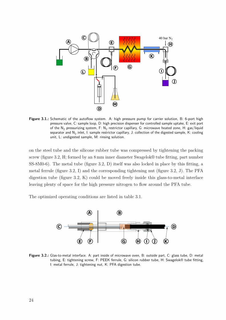
Figure 3.1.: Schematic of the autoflow system. A: high pressure pump for carrier solution, B: 6-port highpressure valve, C: sample loop, D: high precision dispenser for controlled sample uptake, E: exit portof the N2 pressurizing system, F: N2 restrictor capillary, G: microwave heated zone, H: gas/liquidseparator and N2 inlet, I: sample restrictor capillary, J: collection of the digested sample, K: coolingunit, L: undigested sample, M: rinsing solution.

on the steel tube and the silicone rubber tube was compressed by tightening the packingscrew (figure 3.2, H; formed by an 8mm inner diameter Swagelok® tube fitting, part numberSS-8M0-6). The metal tube (figure 3.2, D) itself was also locked in place by this fitting, ametal ferrule (figure 3.2, I) and the corresponding tightening nut (figure 3.2, J). The PFAdigestion tube (figure 3.2, K) could be moved freely inside this glass-to-metal interfaceleaving plenty of space for the high pressure nitrogen to flow around the PFA tube.

The optimized operating conditions are listed in table 3.1.

A B

C D

E G JH IF K

Figure 3.2.: Glas-to-metal interface. A: part inside of microwave oven, B: outside part, C: glass tube, D: metaltubing, E: tightening screw, F: PEEK ferrule, G: silicon rubber tube, H: Swagelok® tube fitting,I: metal ferrule, J: tightening nut, K: PFA digestion tube.

24

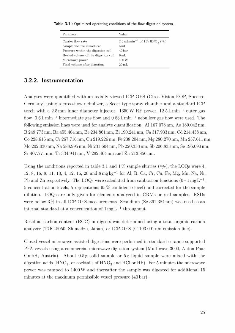
Table 3.1.: Optimized operating conditions of the flow digestion system.

Parameter Value

Carrier flow rate 2.0mLmin−1 of 1% HNO3 (v/v)Sample volume introduced 5mLPressure within the digestion coil 40 barHeated volume of the digestion coil 6mLMicrowave power 400WFinal volume after digestion 20mL

3.2.2. Instrumentation

Analytes were quantified with an axially viewed ICP-OES (Ciros Vision EOP, Spectro,Germany) using a cross-flow nebulizer, a Scott type spray chamber and a standard ICPtorch with a 2.5mm inner diameter injector. 1350W RF power, 12.5 Lmin−1 outer gasflow, 0.6 Lmin−1 intermediate gas flow and 0.83 Lmin−1 nebulizer gas flow were used. Thefollowing emission lines were used for analyte quantification: Al 167.078 nm, As 189.042 nm,B 249.773 nm, Ba 455.404 nm, Be 234.861 nm, Bi 190.241 nm, Ca 317.933 nm, Cd 214.438 nm,Co 228.616 nm, Cr 267.716 nm, Cu 219.226 nm, Fe 238.204 nm, Mg 280.270 nm, Mn 257.611 nm,Mo 202.030 nm, Na 588.995 nm, Ni 231.604 nm, Pb 220.353 nm, Sb 206.833 nm, Se 196.090 nm,Sr 407.771 nm, Ti 334.941 nm, V 292.464 nm and Zn 213.856 nm.

Using the conditions reported in table 3.1 and 1% sample slurries (m/v), the LOQs were 4,12, 8, 16, 8, 11, 10, 4, 12, 16, 20 and 8mgkg−1 for Al, B, Ca, Cr, Cu, Fe, Mg, Mn, Na, Ni,Pb and Zn respectively. The LOQs were calculated from calibration functions (0 – 1mgL−1;5 concentration levels, 5 replications; 95% confidence level) and corrected for the sampledilution. LOQs are only given for elements analyzed in CRMs or real samples. RSDswere below 3% in all ICP-OES measurements. Scandium (Sc 361.384 nm) was used as aninternal standard at a concentration of 1mgL−1 throughout.

Residual carbon content (RCC) in digests was determined using a total organic carbonanalyzer (TOC-5050, Shimadzu, Japan) or ICP-OES (C 193.091 nm emission line).

Closed vessel microwave assisted digestions were performed in standard ceramic supportedPFA vessels using a commercial microwave digestion system (Multiwave 3000, Anton PaarGmbH, Austria). About 0.5 g solid sample or 5 g liquid sample were mixed with thedigestion acids (HNO3, or cocktails of HNO3 and HCl or HF). For 5 minutes the microwavepower was ramped to 1400W and thereafter the sample was digested for additional 15minutes at the maximum permissible vessel pressure (40 bar).

25

The acid concentration in the digested samples was determined by manual titration with0.1mol L−1 NaOH (Roth, Germany) using phenolphthalein as an indicator.

3.2.3. Reagents, certified reference materials and samples

Purified water (18MW cm, Barnstead Nanopure, Thermo Fisher Scientific, USA) and highpurity acids (HCl and HF Suprapur, Merck, Germany; HNO3 purified by subboiling in aquartz still) were used throughout. Calibration standards were prepared from a 100mgL−1

multi element solution (Roth, Germany) in 3% HNO3 (v/v). Calibration solutions for thedetermination of the residual carbon content were prepared from potassium hydrogenphthalate (p.a. quality, Merck, Germany).

Six certified reference materials (CRMs) were used in this work: BCR 62 (olive leaves),CNRC DORM-2 (dogfish muscle), NIST SRM 1515 (apple leaves), NIST SRM 1547 (peachleaves), NIST SRM 1567 (wheat flour) and NIST SRM 1568 (rice flour).

For initial system characterization commercially available milk powder (Aptamil Folgemilch,Milupa, Austria), apple juice (Spar, Austria) and orange juice (Spar, Austria) were used.

Slurries with 1% solids were prepared by thoroughly mixing the solid sample with water,adding concentrated acids and making up to volume with water afterwards. Thereby sampleclotting was avoided. Liquid samples were diluted with the relevant concentrated acids.

3.3. Results and discussion

3.3.1. Optimization of the microwave field uniformity

A common problem in multimode microwave cavities is the inhomogeneous distribution ofmicrowave radiation. To investigate this effect 12 glass vials (volume: 14mL) filled with10mL 3% HNO3 were placed in a circular arrangement (equally spaced, radius: 250mm,height above cavity floor: 170mm) inside the microwave cavity. This setup matched theposition of the glass digestion coil inside the cavity. After heating for 60 seconds with 400Wthe temperature of each vessel was quickly determined with a digital thermometer (300 K,Voltcraft, Taiwan). The error of the temperature measurement was found to be dominatedby the cooling of the liquid in the vials during the measurement as the vial temperature

26

without mode stirrerwith mode stirrer

Tem

pera

ture

, °C

40

50

60

70

80

1 2 3 4 5 6 7 8 9 10 11 12

Figure 3.3.: Temperature distribution inside the microwave cavity with and without a spinning mode stirrer.Values arranged with increasing temperature; error bars not shown for clarity.

was measured consecutively rather than simultaneously. Based on repeated measurementsof the same vial an error of 3 ○C was estimated. The experiment was repeated with a modestirrer (140mm diameter aluminum disc with six wings bent 80mm upwards) installedinside the microwave cavity. This mode stirrer was spun by the digestion vessel rotationmechanism of the Multiwave 3000.

Without the mode stirrer the temperature in the glass vials ranged from 44 to 74 ○C with amedian of 51 ○C. By using the mode stirrer the temperature profile inside the microwavecavity flattened as shown in figure 3.3. The temperature of the diluted nitric acid rangedfrom 49 to 66 ○C with a median of 55 ○C. Moreover, the homogeneity of the microwaveradiation in the region of the digestion coil could be improved. Consequently the modestirrer was used throughout the remaining experiments.

3.3.2. Optimization of the digestion parameters

The residual carbon content (RCC) is commonly used to assess the completeness ofa digestion. Based on previous experience glucose and glycine were selected as testsubstances for RCC determination as their behavior during acid digestion is known to bevery different [16]. Glucose tends to react violently with nitric acid upon reaching thedigestion temperature and serves as a “stress test” for the flow digestion system. Glycineon the other hand is difficult to digest completely.

27

GlucoseGlycine

Resid

ual C

arbo

n, %

0

20

40

60

80

100

120

Microwave Power, W0 200 400 600 800 1000

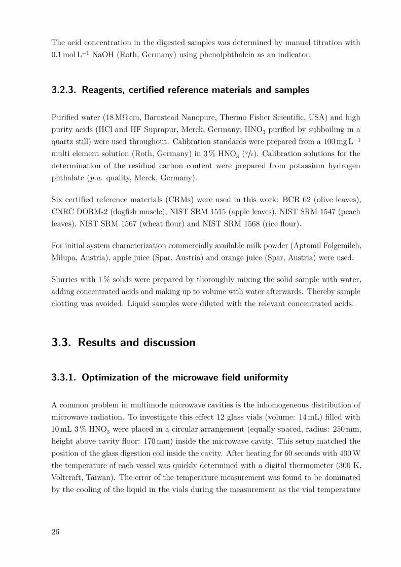
Figure 3.4.: Effect of microwave power on the digestion efficiency of glucose and glycine expressed as RCC,n = 3, error bars smaller than the dots.

The effect of microwave power on the completeness of the digestion was evaluated usingsolutions of 25 gL−1 glucose or 28 gL−1 glycine in 30% nitric acid (v/v) and the instrumentconditions reported in table 3.1. As shown in figure 3.4 the decomposition of glucosestarts at a power level of 300W resulting in a RCC of 24 ± 1% (mean value ± standarduncertainty). With increasing power the RCC decreased almost linear to 14.4 ± 0.8% at800W. For glycine the digestion conditions were not aggressive enough: only at a powerlevel of 800W some of the glycine was completely decomposed resulting in a RCC of96 ± 1%. This behavior can be traced to a digestion temperature significantly below theexpected 250 ○C within the digestion zone. As shown by Pichler et al. [16] glycine isdigested only at temperatures above 235 ○C for a residence time in the heated digestionzone of 3 minutes. From these results it can be estimated that the digestion temperaturein the presented system was between 230 and 235 ○C. This temperature is also in goodagreement with the data reported by Pichler et al. for glucose. A precise measurementof the temperature within the digestion zone was not possible due to potential microwaveleakage and geometrical constraints. We believe that the reason for the somewhat lowdigestion temperature in the presented flow digestion system is the relatively small overallsample volume of 6mL in the microwave cavity. This results in reduced microwave energycoupling. Depending on the digested sample matrix, all further experiments were conductedwith either 400 or 600W.

It is important to note that even at 800W the magnetron temperature remained below60 ○C. An experiment with 1000W was also attempted, but the magnetron temperatureincreased quickly tripping the microwave digestion ovens over-temperature control circuit.According to the instrument manufacturer, below 1000W both magnetrons share the power

28

load, each providing one half. Above 1000W one magnetron operates at full rated powerwhereas the second one is used for power regulation. Compared to pressurized flow digestionsystems employing mono mode cavities (typically about 100W) [16], the power level in thissetup was far higher.

Due to the relatively large multimode cavity the microwave coupling to the liquid phaseinside the digestion coil was low. Consequently, a reduction of the chamber height by afactor of 1.6 was investigated. A tight fitting grounded aluminum sheet was installed insidethe microwave cavity reducing its height from 350mm to 225mm but leaving length andwidth unchanged. In a similar experiment to the one above, no significant change in theRCC was encountered for glucose and glycine. The aluminum sheet was therefore not usedfurther on.

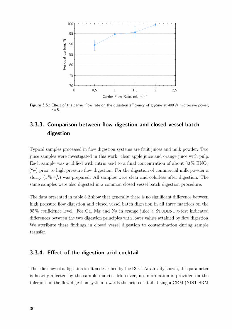
The carrier flow rate defines the residence time of the sample in the microwave heatedzone. Decreasing the carrier flow rate is not only known to improve the digestion efficiencybut also to lengthen the overall time needed to process the sample. The effect of thecarrier flow rate on the RCC was investigated using a test solution of 28 gL−1 glycine in30% nitric acid (v/v) and the instrument conditions reported in table 3.1. Reducing thecarrier flow rate from 2mLmin−1 to 0.5mLmin−1 led to a near linear decrease of the RCCfrom 99 ± 1 to 89 ± 2% for glycine as shown in figure 3.5. It is important to note that byreducing the carrier flow rate the digestion time for one sample increased from 10 to 40minutes. This was deemed impractical and unjustified by the small reduction in RCCdespite the high degree of automation in the presented system. Thus the carrier flow ratewas set to 2mLmin−1 for all further experiments. A stopped flow mode of digestion wasnot attempted with the presented system.

Increasing the sample volume inside the microwave cavity might be another approach toimprove the RCC. Thereby the total volume of liquid inside the cavity would be increased.It was found that regardless of the large radius of the glass coil the introduction of the PFAtube into the coil was not possible for glass coils with more than three turns. During initialtests it was attempted to introduce the PFA tube into a six turn coil. This failed even withthe ample use of ethanol as a lubricating agent (PTFE spray or low viscosity oil proved tobe inferior to ethanol) after about three and a half turns. The radius of the glass coil wasnot further altered, as a smaller radius would have worsened the above mentioned problemswith the PFA tube and a much larger coil radius was not possible due to the cavity size.

29

Resid

ual C

arbo

n, %

70

75

80

85

90

95

100

Carrier Flow Rate, mL min-10 0,5 1 1,5 2 2,5

Figure 3.5.: Effect of the carrier flow rate on the digestion efficiency of glycine at 400W microwave power,n = 5.

3.3.3. Comparison between flow digestion and closed vessel batchdigestion

Typical samples processed in flow digestion systems are fruit juices and milk powder. Twojuice samples were investigated in this work: clear apple juice and orange juice with pulp.Each sample was acidified with nitric acid to a final concentration of about 30% HNO3

(v/v) prior to high pressure flow digestion. For the digestion of commercial milk powder aslurry (1% m/v) was prepared. All samples were clear and colorless after digestion. Thesame samples were also digested in a common closed vessel batch digestion procedure.

The data presented in table 3.2 show that generally there is no significant difference betweenhigh pressure flow digestion and closed vessel batch digestion in all three matrices on the95% confidence level. For Ca, Mg and Na in orange juice a Student t-test indicateddifferences between the two digestion principles with lower values attained by flow digestion.We attribute these findings in closed vessel digestion to contamination during sampletransfer.

3.3.4. Effect of the digestion acid cocktail

The efficiency of a digestion is often described by the RCC. As already shown, this parameteris heavily affected by the sample matrix. Moreover, no information is provided on thetolerance of the flow digestion system towards the acid cocktail. Using a CRM (NIST SRM

30

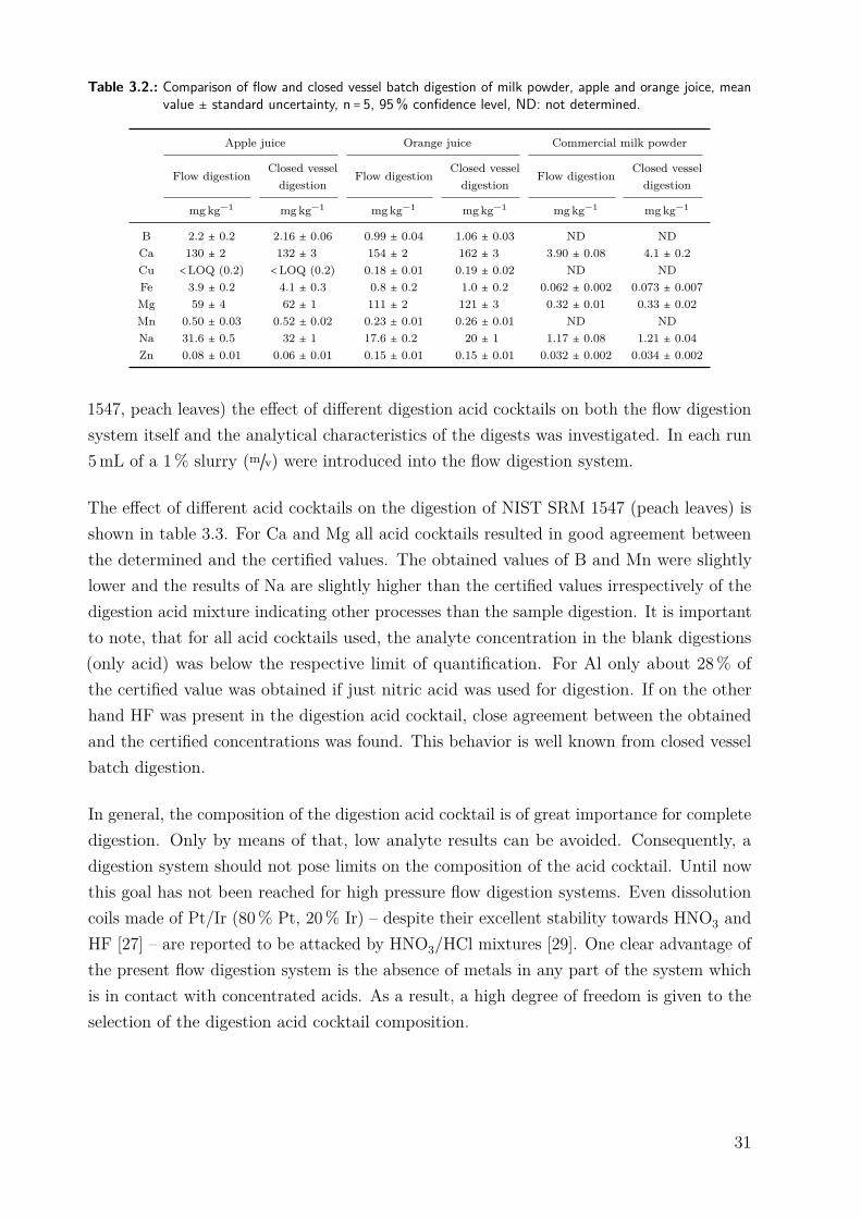
Table 3.2.: Comparison of flow and closed vessel batch digestion of milk powder, apple and orange joice, meanvalue ± standard uncertainty, n = 5, 95% confidence level, ND: not determined.

Apple juice Orange juice Commercial milk powder

Flow digestion Closed vesseldigestion

Flow digestion Closed vesseldigestion

Flow digestion Closed vesseldigestion

mg kg−1 mgkg−1 mgkg−1 mgkg−1 mgkg−1 mgkg−1

B 2.2 ± 0.2 2.16 ± 0.06 0.99 ± 0.04 1.06 ± 0.03 ND NDCa 130 ± 2 132 ± 3 154 ± 2 162 ± 3 3.90 ± 0.08 4.1 ± 0.2Cu <LOQ (0.2) <LOQ (0.2) 0.18 ± 0.01 0.19 ± 0.02 ND NDFe 3.9 ± 0.2 4.1 ± 0.3 0.8 ± 0.2 1.0 ± 0.2 0.062 ± 0.002 0.073 ± 0.007Mg 59 ± 4 62 ± 1 111 ± 2 121 ± 3 0.32 ± 0.01 0.33 ± 0.02Mn 0.50 ± 0.03 0.52 ± 0.02 0.23 ± 0.01 0.26 ± 0.01 ND NDNa 31.6 ± 0.5 32 ± 1 17.6 ± 0.2 20 ± 1 1.17 ± 0.08 1.21 ± 0.04Zn 0.08 ± 0.01 0.06 ± 0.01 0.15 ± 0.01 0.15 ± 0.01 0.032 ± 0.002 0.034 ± 0.002

1547, peach leaves) the effect of different digestion acid cocktails on both the flow digestionsystem itself and the analytical characteristics of the digests was investigated. In each run5mL of a 1% slurry (m/v) were introduced into the flow digestion system.

The effect of different acid cocktails on the digestion of NIST SRM 1547 (peach leaves) isshown in table 3.3. For Ca and Mg all acid cocktails resulted in good agreement betweenthe determined and the certified values. The obtained values of B and Mn were slightlylower and the results of Na are slightly higher than the certified values irrespectively of thedigestion acid mixture indicating other processes than the sample digestion. It is importantto note, that for all acid cocktails used, the analyte concentration in the blank digestions(only acid) was below the respective limit of quantification. For Al only about 28% ofthe certified value was obtained if just nitric acid was used for digestion. If on the otherhand HF was present in the digestion acid cocktail, close agreement between the obtainedand the certified concentrations was found. This behavior is well known from closed vesselbatch digestion.

In general, the composition of the digestion acid cocktail is of great importance for completedigestion. Only by means of that, low analyte results can be avoided. Consequently, adigestion system should not pose limits on the composition of the acid cocktail. Until nowthis goal has not been reached for high pressure flow digestion systems. Even dissolutioncoils made of Pt/Ir (80% Pt, 20% Ir) – despite their excellent stability towards HNO3 andHF [27] – are reported to be attacked by HNO3/HCl mixtures [29]. One clear advantage ofthe present flow digestion system is the absence of metals in any part of the system whichis in contact with concentrated acids. As a result, a high degree of freedom is given to theselection of the digestion acid cocktail composition.

31

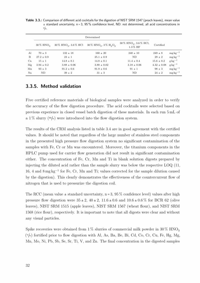
Table 3.3.: Comparison of different acid cocktails for the digestion of NIST SRM 1547 (peach leaves), mean value± standard uncertainty, n = 3, 95% confidence level, ND: not determined, all acid concentrations inv/v.

Determined

30% HNO3 30% HNO3, 3.6% HCl 30% HNO3, 3% H2O230% HNO3, 3.6% HCl,

1.3% HFCertified

Al 70 ± 3 132 ± 18 160 ± 20 240 ± 10 249 ± 8 mgkg−1

B 27.2 ± 0.9 23 ± 1 25.1 ± 0.9 ND 29 ± 2 mgkg−1

Ca 15 ± 1 14.8 ± 0.1 14.8 ± 0.1 11.4 ± 0.4 15.6 ± 0.2 g kg−1

Mg 3.94 ± 0.2 3.88 ± 0.06 3.88 ± 0.02 3.18 ± 0.06 4.32 ± 0.08 g kg−1

Mn 93 ± 3 91.2 ± 0.6 91.9 ± 0.6 91 ± 1 98 ± 3 mgkg−1

Na ND 39 ± 2 31 ± 3 ND 24 ± 2 mgkg−1

3.3.5. Method validation

Five certified reference materials of biological samples were analyzed in order to verifythe accuracy of the flow digestion procedure. The acid cocktails were selected based onprevious experience in closed vessel batch digestion of these materials. In each run 5mL ofa 1% slurry (m/v) were introduced into the flow digestion system.

The results of the CRM analysis listed in table 3.4 are in good agreement with the certifiedvalues. It should be noted that regardless of the large number of stainless steel componentsin the presented high pressure flow digestion system no significant contamination of thesamples with Fe, Cr or Mn was encountered. Moreover, the titanium components in theHPLC pump used for carrier flow generation did not result in significant contaminationeither. The concentration of Fe, Cr, Mn and Ti in blank solution digests prepared byinjecting the diluted acid rather than the sample slurry was below the respective LOQ (11,16, 4 and 8mgkg−1 for Fe, Cr, Mn and Ti; values corrected for the sample dilution causedby the digestion). This clearly demonstrates the effectiveness of the countercurrent flow ofnitrogen that is used to pressurize the digestion coil.

The RCC (mean value ± standard uncertainty, n = 3, 95% confidence level) values after highpressure flow digestion were 35 ± 2, 40 ± 2, 11.6 ± 0.6 and 10.6 ± 0.6% for BCR 62 (oliveleaves), NIST SRM 1515 (apple leaves), NIST SRM 1567 (wheat flour), and NIST SRM1568 (rice flour), respectively. It is important to note that all digests were clear and withoutany visual particles.

Spike recoveries were obtained from 1% slurries of commercial milk powder in 30% HNO3

(v/v) fortified prior to flow digestion with Al, As, Ba, Be, Bi, Cd, Co, Cr, Cu, Fe, Hg, Mg,Mn, Mo, Ni, Pb, Sb, Se, Sr, Ti, V, and Zn. The final concentration in the digested samples

32

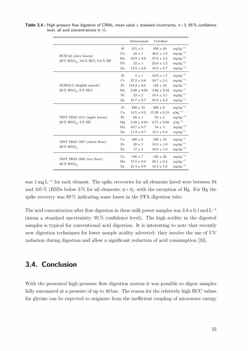
Table 3.4.: High pressure flow digestion of CRMs, mean value ± standard uncertainty, n = 3, 95% confidencelevel, all acid concentrations in v/v.

Determined Certified

BCR 62 (olive leaves)30% HNO3, 3.6% HCl, 0.8% HF

Al 415 ± 9 450 ± 20 mgkg−1

Cu 42 ± 1 46.6 ± 1.8 mgkg−1

Mn 53.9 ± 0.9 57.0 ± 2.4 mgkg−1

Pb 22 ± 1 25.0 ± 1.5 mgkg−1

Zn 13.5 ± 0.6 16.0 ± 0.7 mgkg−1

DORM-2 (dogfish muscle)20% HNO3, 6% HCl

Al 5 ± 1 10.9 ± 1.7 mgkg−1

Cr 37.2 ± 0.6 34.7 ± 5.5 mgkg−1

Fe 153.2 ± 0.6 142 ± 10 mgkg−1

Mn 3.99 ± 0.02 3.66 ± 0.34 mgkg−1

Ni 23 ± 2 19.4 ± 3.1 mgkg−1

Zn 19.7 ± 0.7 25.6 ± 2.3 mgkg−1

NIST SRM 1515 (apple leaves)30% HNO3, 3% HF

Al 290 ± 10 286 ± 9 mgkg−1

Ca 14.5 ± 0.2 15.26 ± 0.15 g kg−1

Fe 68 ± 1 83 ± 5 mgkg−1

Mg 2.49 ± 0.04 2.71 ± 0.08 g kg−1

Mn 49.7 ± 0.7 54 ± 3 mgkg−1

Zn 11.9 ± 0.7 12.5 ± 0.3 mgkg−1

NIST SRM 1567 (wheat flour)30% HNO3

Ca 186 ± 6 190 ± 10 mgkg−1

Fe 20 ± 1 18.3 ± 1.0 mgkg−1

Zn 17 ± 4 10.6 ± 1.0 mgkg−1

NIST SRM 1568 (rice flour)30% HNO3

Ca 136 ± 7 140 ± 20 mgkg−1

Mn 17.5 ± 0.9 20.1 ± 0.4 mgkg−1

Zn 21.4 ± 0.9 19.4 ± 1.0 mgkg−1

was 1mgL−1 for each element. The spike recoveries for all elements listed were between 94and 105% (RSDs below 3% for all elements; n = 4), with the exception of Hg. For Hg thespike recovery was 89% indicating some losses in the PFA digestion tube.

The acid concentration after flow digestion in these milk power samples was 3.8 ± 0.1mol L−1

(mean ± standard uncertainty; 95% confidence level). The high acidity in the digestedsamples is typical for conventional acid digestion. It is interesting to note that recentlynew digestion techniques for lower sample acidity adverted: they involve the use of UVradiation during digestion and allow a significant reduction of acid consumption [33].

3.4. Conclusion

With the presented high pressure flow digestion system it was possible to digest samplesfully automated at a pressure of up to 40 bar. The reason for the relatively high RCC valuesfor glycine can be expected to originate from the inefficient coupling of microwave energy

33

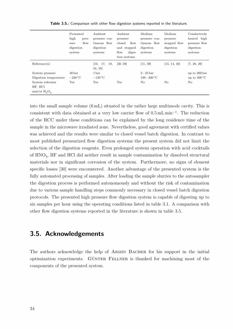
Table 3.5.: Comparison with other flow digestion systems reported in the literature.

Presentedhigh pres-sure flowdigestionsystem

Ambientpressure con-tinuous flowdigestionsystems

Ambientpressureclosed flowand stoppedflow diges-tion systems

Mediumpressure con-tinuous flowdigestionsystems

Mediumpressurestopped flowdigestionsystems

Conductivelyheated highpressure flowdigestionsystems

Reference(s) [10, 17, 19,34, 35]

[36–38] [11, 39] [13, 14, 40] [7, 28, 29]

System pressure 40 bar 1 bar 2 – 25 bar up to 200 barDigestion temperature ~ 230 ○C ~120 ○C 180 – 200 ○C up to 300 ○CSystem toleratesHF, HCland/or H2O2

Yes Yes Yes No No No

into the small sample volume (6mL) situated in the rather large multimode cavity. This isconsistent with data obtained at a very low carrier flow of 0.5mLmin−1. The reductionof the RCC under these conditions can be explained by the long residence time of thesample in the microwave irradiated zone. Nevertheless, good agreement with certified valueswas achieved and the results were similar to closed vessel batch digestion. In contrast tomost published pressurized flow digestion systems the present system did not limit theselection of the digestion reagents. Even prolonged system operation with acid cocktailsof HNO3, HF and HCl did neither result in sample contamination by dissolved structuralmaterials nor in significant corrosion of the system. Furthermore, no signs of elementspecific losses [30] were encountered. Another advantage of the presented system is thefully automated processing of samples. After loading the sample slurries to the autosamplerthe digestion process is performed autonomously and without the risk of contaminationdue to various sample handling steps commonly necessary in closed vessel batch digestionprotocols. The presented high pressure flow digestion system is capable of digesting up tosix samples per hour using the operating conditions listed in table 3.1. A comparison withother flow digestion systems reported in the literature is shown in table 3.5.

3.5. Acknowledgements

The authors acknowledge the help of Armin Bacher for his support in the initialoptimization experiments. Günter Fellner is thanked for machining most of thecomponents of the presented system.

34

CHAPTER 4

Microwave Induced CombustionSandra M. Cruz, Paul Tirk, Flavia M. Dalla Nora, Lucas Schmidt, HelmarWiltsche, Cezar A. Bizzi, Günter Knapp and Erico M. M. Flores

The following chapter was published in “Fuel”, Volume 160 (2015), pages 108 – 113 un-der the title “Feasibility of Sulfur Determination in Diesel Oil by Inductively CoupledPlasma Optical Emission Spectrometry after Microwave-Induced Combustion Using FlameRetardant” [2].

Abstract

Diesel oil sample preparation for further sulfur determination in fuels is considered a critical step duringthe analytical sequence mainly due to the high volatility of this sample. Combustion systems have beena suitable alternative to conventional digestion methods but its applicability for highly volatile matriceslike diesel oil is restrict to low sample masses due to the high pressure generated during combustion. Inorder to overcome this limitation, the possibility of employing glass wool as a flame retardant for themicrowave-induced combustion (MIC) method was investigated in the present work for further sulfurdetermination by inductively coupled plasma optical emission spectrometry. Using flame retardant it waspossible to burn up to 400mg of diesel oil without increasing the pressure in dangerous levels. Nitricacid (2, 4, 7 or 14.4mol L−1 HNO3) was evaluated as absorbing solution and no significant difference wasobserved in sulfur recoveries for solutions. Digestion efficiency was evaluated by means of residual carboncontent determination, which presented values always lower than 1% showing the high digestion efficiency.For comparison of results, S was also determined by the ASTM D 5453-12 method and an agreement betterthan 95% was obtained. The accuracy was better than 97% (analysis of certified reference material),blanks were negligible and the limit of detection was considered as suitable for quality control (2µg g−1).

35

4.1. Introduction

Diesel oil belongs to a class of products obtained by crude oil processing and generally coversthe range of boiling temperatures between 175 and 375 ○C mainly presenting compoundswith about eight to twenty-four carbon atoms (C8 to C24) [41, 42]. Sulfur is an ubiquitouselement in crude oil and the presence of sulfur compounds in diesel oil or in the middledistillate crude oil fraction can cause corrosion leading to damage of metallic parts ofrefineries as well as of combustion engines of automobiles [41, 43, 44]. Other implicationsinclude changes in color, odor and instability of the final product. Remaining sulfuralso contributes to the release of sulfur oxides into the atmosphere causing environmentalpollution like acid rain [43, 45, 46]. Furthermore, it can poison the catalysts used in emissioncontrol systems, consequently, reducing the oxidation effectiveness of carbon monoxide,hydrocarbons and volatile organic compounds [41, 43, 44]. Sulfur compounds are distributedin several crude oil distillation fractions and may also be present in the final products [47].Depending on the origin of formation and maturation conditions of the preceding crude oil,a variety of sulfur compounds can be found [47] and their presence, especially in low andultralow sulfur content diesel oil, is generally belonging to the group of benzothiophenes(BT) and dibenzothiophenes (DBT) as well as derivatives of these compounds containingalkyl substituents, such as 4,6-dimethyl-dibenzo-thiophene (4,6-DMDBT) [43, 48].

Refineries and manufacturers are subject to meet the requirements set by governmentalorganizations. The Environmental Protection Agency (EPA, United States) limits theallowed sulfur concentration for ultra low sulfur diesel to 15mg kg−1 [49]. Similar restrictionsalso exist in European Union as the directive 98/70/EC which sets a limit even lower(10mg kg−1) [50]. In order to comply with these regulations the continuous monitoring ofsulfur is of high importance in the production and quality control of diesel oil.

For sulfur determination in diesel oil, sample preparation can be considered as a criticalstep and several methods have been applied in last years [4]. Direct injection of dieseloil for further inductively coupled plasma based analysis has been currently used forroutine analysis. However, some drawbacks still remain as the need for high dilutionfactors to maintain a stable plasma [51], oxygen addition to nebulization gas and alsothe use of reference solutions especially prepared in organic medium [52]. Even usingmatrix-matched reference samples, changes in plasma can occur making direct injectionof organic substances prone to some inconveniences for trace S determination [53–55].Alternatively, sulfur determination in crude oil and its fractions has been carried out byX-ray fluorescence (XRF) and also by sample combustion with further titration or infrared

36

Table 4.1.: Analysis of lubricating oil, diesel oil and crude oil products using oxygen flask and combustion bombfor further S determination.

Sample Digestion method Technique of determination LOD References

Lubricating oil Combustion bomb IC 1.62% [63]Diesel oil Combustion bomb ICP-OES — [64]Fuel Combustion bomb IC 0.07 µgmL−1 [66]Crude oil products Combustion bomb Titration 0.01% [67]Fuel oils Oxygen flask IC 0.007% [68]

detection [56–60]. Despite some automatic sulfur analyzers allow the direct analysis ofdiesel oil, common procedures for S determination by other techniques involve a previousstep of sample preparation [25]. However, acid digestion procedures can present limitationsdue to the relatively long time required [61] and low digestion efficiency [62]. As an example,Ulrich et al. [53] proposed a procedure involving a 12 h pre-digestion on a hot plate beforeapplying microwave radiation for 30min.

On the other hand, combustion systems provide some advantages over closed vessel wetdigestion when dealing with organic samples. Due to the high temperature during com-bustion (> 1000 ○C) complete oxidation of sample matrix can be achieved, resulting also inlow residual carbon content (RCC) [63]. Classical combustion is normally performed inbombs or oxygen flasks [63, 64]. Both systems present some advantages mainly related tosample ignition and low risk of contamination, respectively [9, 63]. However, for combustionbombs, the use of acid solutions must be avoided to prevent damage to the metallic vesselwalls and low analytical frequency may be considered as one of the main limitations forthis system [63]. The oxygen flask method presents restriction to the maximum samplemass and consequently poor limit of detection (LOD). In addition, both systems needcontinuous attention by the analyst, only one sample is processed in each run and digestiontime is relatively long (up to 3 h considering the cooling step in case of combustion bombs)that decreases the throughput [63]. Normally, for the oxygen flask system, samples of 10to 50mg are burnt in vessels with a volume of 250 to 500mL [65]. Table 4.1 summarizessome selected applications using combustion bombs and oxygen flask, for the subsequentdetermination of sulfur in oils, fuels, lubricants oil and crude oil products [63, 64, 66–68].

Alternatively, microwave-induced combustion (MIC) can overcome some of the mentioneddifficulties and often provides an easy and rapid way for decomposing organic samples [62,69, 70]. Essentially, solid samples are pressed as pellets and ignited using microwaveradiation with a suitable igniter solution [71]. Analytes are retained in a convenientabsorbing solution [65] and it should be noticed that the acid concentration can be muchlower using the MIC method when compared to conventional closed vessel wet digestion

37

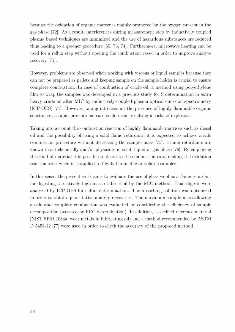
because the oxidation of organic matter is mainly promoted by the oxygen present in thegas phase [72]. As a result, interferences during measurement step by inductively coupledplasma based techniques are minimized and the use of hazardous substances are reducedthus leading to a greener procedure [55, 73, 74]. Furthermore, microwave heating can beused for a reflux step without opening the combustion vessel in order to improve analyterecovery [71].

However, problems are observed when working with viscous or liquid samples because theycan not be prepared as pellets and keeping sample on the sample holder is crucial to ensurecomplete combustion. In case of combustion of crude oil, a method using polyethylenefilm to wrap the samples was developed in a previous study for S determination in extraheavy crude oil after MIC by inductively-coupled plasma optical emission spectrometry(ICP-OES) [71]. However, taking into account the presence of highly flammable organicsubstances, a rapid pressure increase could occur resulting in risks of explosion.

Taking into account the combustion reaction of highly flammable matrices such as dieseloil and the possibility of using a solid flame retardant, it is expected to achieve a safecombustion procedure without decreasing the sample mass [75]. Flame retardants areknown to act chemically and/or physically in solid, liquid or gas phase [76]. By employingthis kind of material it is possible to decrease the combustion rate, making the oxidationreaction safer when it is applied to highly flammable or volatile samples.

In this sense, the present work aims to evaluate the use of glass wool as a flame retardantfor digesting a relatively high mass of diesel oil by the MIC method. Final digests wereanalyzed by ICP-OES for sulfur determination. The absorbing solution was optimizedin order to obtain quantitative analyte recoveries. The maximum sample mass allowinga safe and complete combustion was evaluated by considering the efficiency of sampledecomposition (assessed by RCC determination). In addition, a certified reference material(NIST SRM 1084a, wear metals in lubricating oil) and a method recommended by ASTMD 5453-12 [77] were used in order to check the accuracy of the proposed method.

38

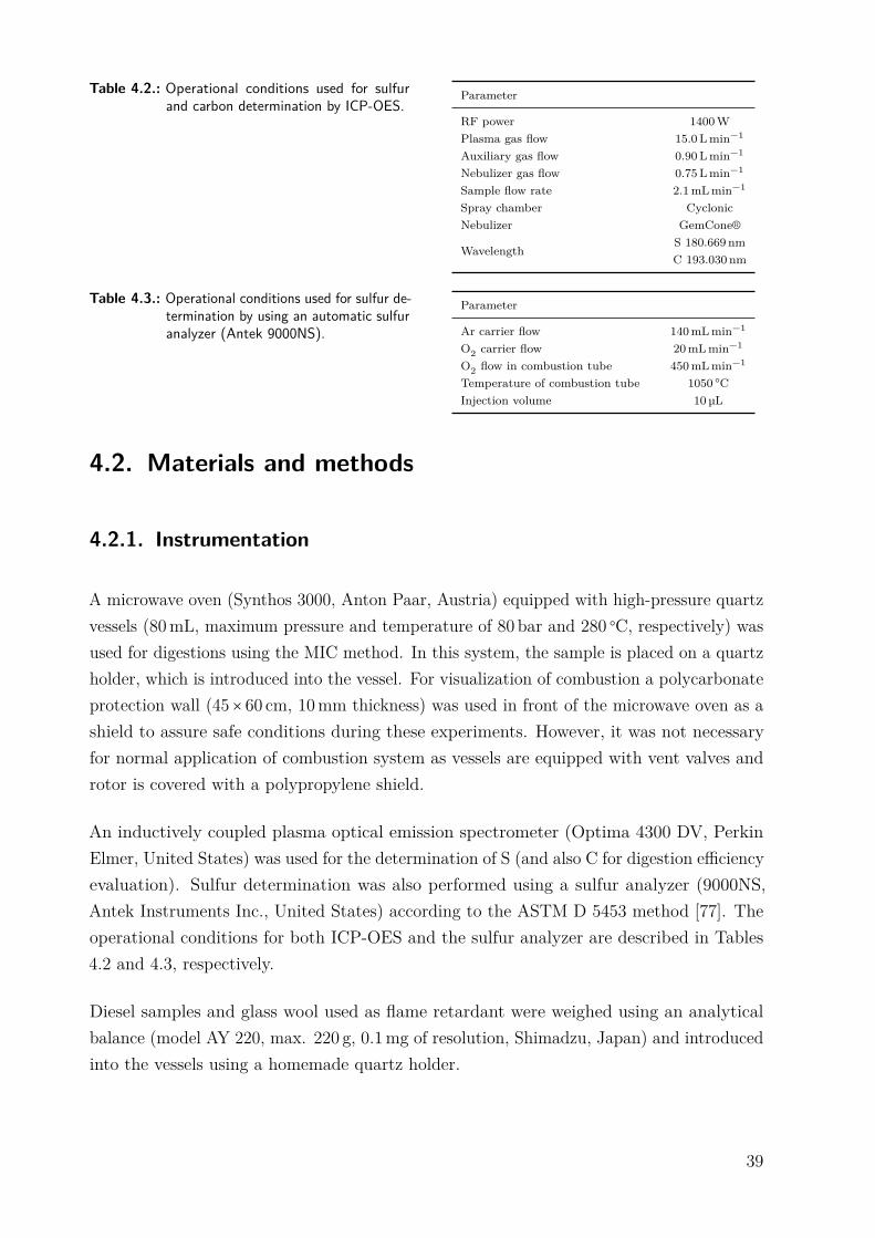
Table 4.2.: Operational conditions used for sulfurand carbon determination by ICP-OES.

Parameter

RF power 1400WPlasma gas flow 15.0 Lmin−1

Auxiliary gas flow 0.90 Lmin−1

Nebulizer gas flow 0.75 Lmin−1

Sample flow rate 2.1mLmin−1

Spray chamber CyclonicNebulizer GemCone®

WavelengthS 180.669 nmC 193.030 nm

Table 4.3.: Operational conditions used for sulfur de-termination by using an automatic sulfuranalyzer (Antek 9000NS).

Parameter

Ar carrier flow 140mLmin−1

O2 carrier flow 20mLmin−1

O2 flow in combustion tube 450mLmin−1

Temperature of combustion tube 1050 ○CInjection volume 10µL

4.2. Materials and methods

4.2.1. Instrumentation

A microwave oven (Synthos 3000, Anton Paar, Austria) equipped with high-pressure quartzvessels (80mL, maximum pressure and temperature of 80 bar and 280 ○C, respectively) wasused for digestions using the MIC method. In this system, the sample is placed on a quartzholder, which is introduced into the vessel. For visualization of combustion a polycarbonateprotection wall (45× 60 cm, 10mm thickness) was used in front of the microwave oven as ashield to assure safe conditions during these experiments. However, it was not necessaryfor normal application of combustion system as vessels are equipped with vent valves androtor is covered with a polypropylene shield.

An inductively coupled plasma optical emission spectrometer (Optima 4300 DV, PerkinElmer, United States) was used for the determination of S (and also C for digestion efficiencyevaluation). Sulfur determination was also performed using a sulfur analyzer (9000NS,Antek Instruments Inc., United States) according to the ASTM D 5453 method [77]. Theoperational conditions for both ICP-OES and the sulfur analyzer are described in Tables4.2 and 4.3, respectively.

Diesel samples and glass wool used as flame retardant were weighed using an analyticalbalance (model AY 220, max. 220 g, 0.1mg of resolution, Shimadzu, Japan) and introducedinto the vessels using a homemade quartz holder.

39

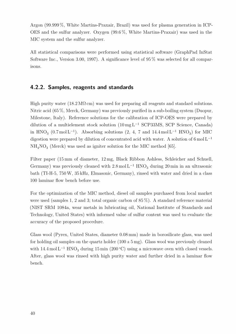
Argon (99.999%, White Martins-Praxair, Brazil) was used for plasma generation in ICP-OES and the sulfur analyzer. Oxygen (99.6%, White Martins-Praxair) was used in theMIC system and the sulfur analyzer.

All statistical comparisons were performed using statistical software (GraphPad InStatSoftware Inc., Version 3.00, 1997). A significance level of 95% was selected for all compar-isons.

4.2.2. Samples, reagents and standards

High purity water (18.2MW cm) was used for preparing all reagents and standard solutions.Nitric acid (65%, Merck, Germany) was previously purified in a sub-boiling system (Duopur,Milestone, Italy). Reference solutions for the calibration of ICP-OES were prepared bydilution of a multielement stock solution (10mgL−1 SCP33MS, SCP Science, Canada)in HNO3 (0.7mol L−1). Absorbing solutions (2, 4, 7 and 14.4mol L−1 HNO3) for MICdigestion were prepared by dilution of concentrated acid with water. A solution of 6mol L−1

NH4NO3 (Merck) was used as igniter solution for the MIC method [65].

Filter paper (15mm of diameter, 12mg, Black Ribbon Ashless, Schleicher and Schuell,Germany) was previously cleaned with 2.8mol L−1 HNO3 during 20min in an ultrasonicbath (TI-H-5, 750W, 35 kHz, Elmasonic, Germany), rinsed with water and dried in a class100 laminar flow bench before use.

For the optimization of the MIC method, diesel oil samples purchased from local marketwere used (samples 1, 2 and 3; total organic carbon of 85%). A standard reference material(NIST SRM 1084a, wear metals in lubricating oil, National Institute of Standards andTechnology, United States) with informed value of sulfur content was used to evaluate theaccuracy of the proposed procedure.

Glass wool (Pyrex, United States, diameter 0.08mm) made in borosilicate glass, was usedfor holding oil samples on the quartz holder (100 ± 5mg). Glass wool was previously cleanedwith 14.4mol L−1 HNO3 during 15min (200 ○C) using a microwave oven with closed vessels.After, glass wool was rinsed with high purity water and further dried in a laminar flowbench.

40

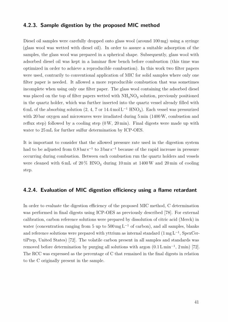
4.2.3. Sample digestion by the proposed MIC method

Diesel oil samples were carefully dropped onto glass wool (around 100mg) using a syringe(glass wool was wetted with diesel oil). In order to assure a suitable adsorption of thesamples, the glass wool was prepared in a spherical shape. Subsequently, glass wool withadsorbed diesel oil was kept in a laminar flow bench before combustion (this time wasoptimized in order to achieve a reproducible combustion). In this work two filter paperswere used, contrarily to conventional application of MIC for solid samples where only onefilter paper is needed. It allowed a more reproducible combustion that was sometimesincomplete when using only one filter paper. The glass wool containing the adsorbed dieselwas placed on the top of filter papers wetted with NH4NO3 solution, previously positionedin the quartz holder, which was further inserted into the quartz vessel already filled with6mL of the absorbing solution (2, 4, 7 or 14.4mol L−1 HNO3). Each vessel was pressurizedwith 20 bar oxygen and microwaves were irradiated during 5min (1400W, combustion andreflux step) followed by a cooling step (0W, 20min). Final digests were made up withwater to 25mL for further sulfur determination by ICP-OES.

It is important to consider that the allowed pressure rate used in the digestion systemhad to be adjusted from 0.8 bar s−1 to 3 bar s−1 because of the rapid increase in pressureoccurring during combustion. Between each combustion run the quartz holders and vesselswere cleaned with 6mL of 20% HNO3 during 10min at 1400W and 20min of coolingstep.

4.2.4. Evaluation of MIC digestion efficiency using a flame retardant

In order to evaluate the digestion efficiency of the proposed MIC method, C determinationwas performed in final digests using ICP-OES as previously described [78]. For externalcalibration, carbon reference solutions were prepared by dissolution of citric acid (Merck) inwater (concentration ranging from 5 up to 500mgL−1 of carbon), and all samples, blanksand reference solutions were prepared with yttrium as internal standard (1mgL−1, SpexCer-tiPrep, United States) [72]. The volatile carbon present in all samples and standards wasremoved before determination by purging all solutions with argon (0.1 Lmin−1, 2min) [72].The RCC was expressed as the percentage of C that remained in the final digests in relationto the C originally present in the sample.

41

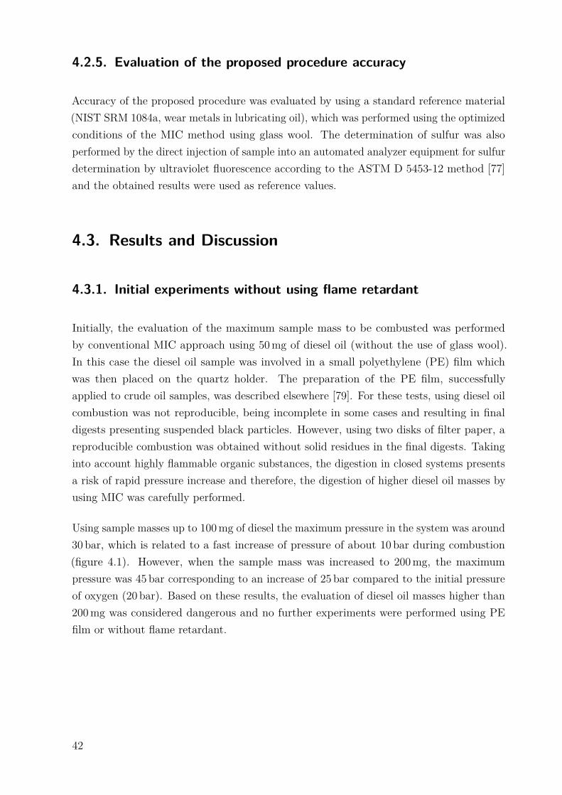
4.2.5. Evaluation of the proposed procedure accuracy

Accuracy of the proposed procedure was evaluated by using a standard reference material(NIST SRM 1084a, wear metals in lubricating oil), which was performed using the optimizedconditions of the MIC method using glass wool. The determination of sulfur was alsoperformed by the direct injection of sample into an automated analyzer equipment for sulfurdetermination by ultraviolet fluorescence according to the ASTM D 5453-12 method [77]and the obtained results were used as reference values.

4.3. Results and Discussion

4.3.1. Initial experiments without using flame retardant

Initially, the evaluation of the maximum sample mass to be combusted was performedby conventional MIC approach using 50mg of diesel oil (without the use of glass wool).In this case the diesel oil sample was involved in a small polyethylene (PE) film whichwas then placed on the quartz holder. The preparation of the PE film, successfullyapplied to crude oil samples, was described elsewhere [79]. For these tests, using diesel oilcombustion was not reproducible, being incomplete in some cases and resulting in finaldigests presenting suspended black particles. However, using two disks of filter paper, areproducible combustion was obtained without solid residues in the final digests. Takinginto account highly flammable organic substances, the digestion in closed systems presentsa risk of rapid pressure increase and therefore, the digestion of higher diesel oil masses byusing MIC was carefully performed.

Using sample masses up to 100mg of diesel the maximum pressure in the system was around30 bar, which is related to a fast increase of pressure of about 10 bar during combustion(figure 4.1). However, when the sample mass was increased to 200mg, the maximumpressure was 45 bar corresponding to an increase of 25 bar compared to the initial pressureof oxygen (20 bar). Based on these results, the evaluation of diesel oil masses higher than200mg was considered dangerous and no further experiments were performed using PEfilm or without flame retardant.

42

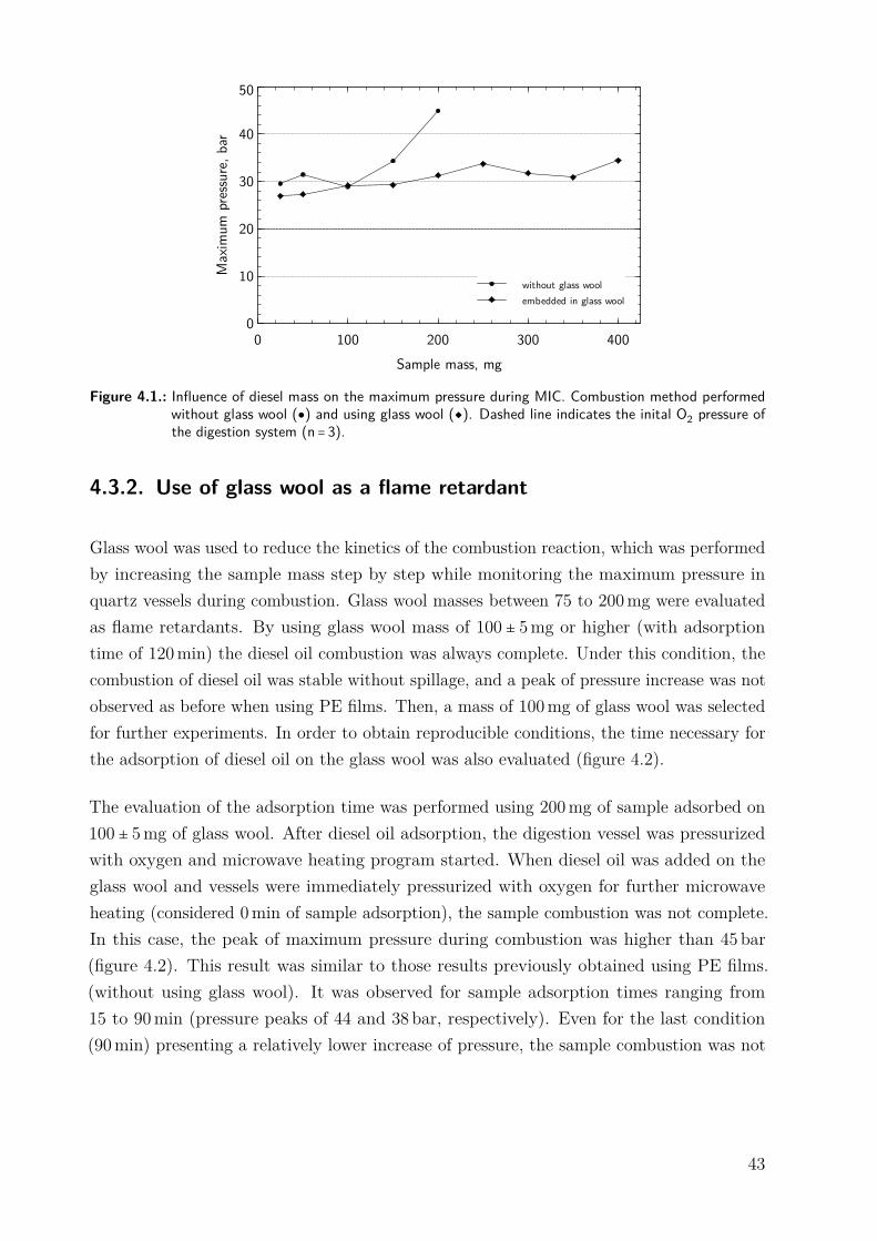
without glass woolembedded in glass wool

Max

imum

pre

ssur

e, ba

r

0

10

20

30

40

50

Sample mass, mg0 100 200 300 400

Figure 4.1.: Influence of diesel mass on the maximum pressure during MIC. Combustion method performedwithout glass wool (●) and using glass wool (◆). Dashed line indicates the inital O2 pressure ofthe digestion system (n = 3).

4.3.2. Use of glass wool as a flame retardant

Glass wool was used to reduce the kinetics of the combustion reaction, which was performedby increasing the sample mass step by step while monitoring the maximum pressure inquartz vessels during combustion. Glass wool masses between 75 to 200mg were evaluatedas flame retardants. By using glass wool mass of 100 ± 5mg or higher (with adsorptiontime of 120min) the diesel oil combustion was always complete. Under this condition, thecombustion of diesel oil was stable without spillage, and a peak of pressure increase was notobserved as before when using PE films. Then, a mass of 100mg of glass wool was selectedfor further experiments. In order to obtain reproducible conditions, the time necessary forthe adsorption of diesel oil on the glass wool was also evaluated (figure 4.2).

The evaluation of the adsorption time was performed using 200mg of sample adsorbed on100 ± 5mg of glass wool. After diesel oil adsorption, the digestion vessel was pressurizedwith oxygen and microwave heating program started. When diesel oil was added on theglass wool and vessels were immediately pressurized with oxygen for further microwaveheating (considered 0min of sample adsorption), the sample combustion was not complete.In this case, the peak of maximum pressure during combustion was higher than 45 bar(figure 4.2). This result was similar to those results previously obtained using PE films.(without using glass wool). It was observed for sample adsorption times ranging from15 to 90min (pressure peaks of 44 and 38 bar, respectively). Even for the last condition(90min) presenting a relatively lower increase of pressure, the sample combustion was not

43

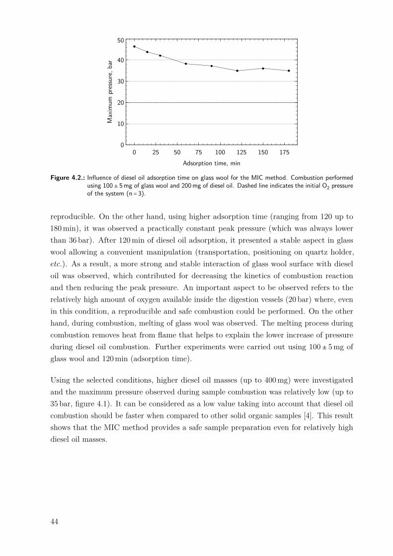
Max

imum

pre

ssur

e, ba

r

0

10

20

30

40

50

Adsorption time, min0 25 50 75 100 125 150 175

Figure 4.2.: Influence of diesel oil adsorption time on glass wool for the MIC method. Combustion performedusing 100 ± 5mg of glass wool and 200mg of diesel oil. Dashed line indicates the initial O2 pressureof the system (n = 3).

reproducible. On the other hand, using higher adsorption time (ranging from 120 up to180min), it was observed a practically constant peak pressure (which was always lowerthan 36 bar). After 120min of diesel oil adsorption, it presented a stable aspect in glasswool allowing a convenient manipulation (transportation, positioning on quartz holder,etc.). As a result, a more strong and stable interaction of glass wool surface with dieseloil was observed, which contributed for decreasing the kinetics of combustion reactionand then reducing the peak pressure. An important aspect to be observed refers to therelatively high amount of oxygen available inside the digestion vessels (20 bar) where, evenin this condition, a reproducible and safe combustion could be performed. On the otherhand, during combustion, melting of glass wool was observed. The melting process duringcombustion removes heat from flame that helps to explain the lower increase of pressureduring diesel oil combustion. Further experiments were carried out using 100 ± 5mg ofglass wool and 120min (adsorption time).

Using the selected conditions, higher diesel oil masses (up to 400mg) were investigatedand the maximum pressure observed during sample combustion was relatively low (up to35 bar, figure 4.1). It can be considered as a low value taking into account that diesel oilcombustion should be faster when compared to other solid organic samples [4]. This resultshows that the MIC method provides a safe sample preparation even for relatively highdiesel oil masses.

44

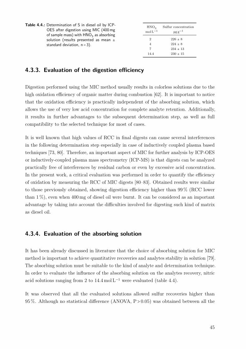
Table 4.4.: Determination of S in diesel oil by ICP-OES after digestion using MIC (400mgof sample mass) with HNO3 as absorbingsolution (results presented as mean ±standard deviation, n = 3).

HNO3 Sulfur concentrationmol L−1 µg g−1

2 226 ± 84 224 ± 87 234 ± 13

14.4 230 ± 15

4.3.3. Evaluation of the digestion efficiency

Digestion performed using the MIC method usually results in colorless solutions due to thehigh oxidation efficiency of organic matter during combustion [62]. It is important to noticethat the oxidation efficiency is practically independent of the absorbing solution, whichallows the use of very low acid concentration for complete analyte retention. Additionally,it results in further advantages to the subsequent determination step, as well as fullcompatibility to the selected technique for most of cases.

It is well known that high values of RCC in final digests can cause several interferencesin the following determination step especially in case of inductively coupled plasma basedtechniques [73, 80]. Therefore, an important aspect of MIC for further analysis by ICP-OESor inductively-coupled plasma mass spectrometry (ICP-MS) is that digests can be analyzedpractically free of interferences by residual carbon or even by excessive acid concentration.In the present work, a critical evaluation was performed in order to quantify the efficiencyof oxidation by measuring the RCC of MIC digests [80–83]. Obtained results were similarto those previously obtained, showing digestion efficiency higher than 99% (RCC lowerthan 1%), even when 400mg of diesel oil were burnt. It can be considered as an importantadvantage by taking into account the difficulties involved for digesting such kind of matrixas diesel oil.

4.3.4. Evaluation of the absorbing solution

It has been already discussed in literature that the choice of absorbing solution for MICmethod is important to achieve quantitative recoveries and analytes stability in solution [79].The absorbing solution must be suitable to the kind of analyte and determination technique.In order to evaluate the influence of the absorbing solution on the analytes recovery, nitricacid solutions ranging from 2 to 14.4mol L−1 were evaluated (table 4.4).

It was observed that all the evaluated solutions allowed sulfur recoveries higher than95%. Although no statistical difference (ANOVA, P > 0.05) was obtained between all the

45

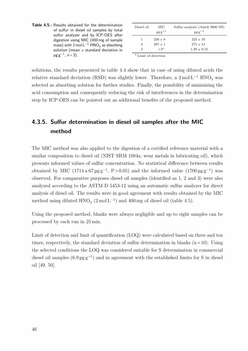
Table 4.5.: Results obtained for the determinationof sulfur in diesel oil samples by totalsulfur analyzer and by ICP-OES afterdigestion using MIC (400mg of samplemass) with 2mol L−1 HNO3 as absorbingsolution (mean ± standard deviation inµg g−1, n = 3).

Diesel oil MIC Sulfur analyzer (Antek 9000 NS)µg g−1 µg g−1

1 226 ± 8 223 ± 102 287 ± 1 275 ± 133 < 2a 1.49 ± 0.12

a Limit of detection

solutions, the results presented in table 4.4 show that in case of using diluted acids therelative standard deviation (RSD) was slightly lower. Therefore, a 2mol L−1 HNO3 wasselected as absorbing solution for further studies. Finally, the possibility of minimizing theacid consumption and consequently reducing the risk of interferences in the determinationstep by ICP-OES can be pointed out as additional benefits of the proposed method.

4.3.5. Sulfur determination in diesel oil samples after the MICmethod

The MIC method was also applied to the digestion of a certified reference material with asimilar composition to diesel oil (NIST SRM 1084a, wear metals in lubricating oil), whichpresents informed values of sulfur concentration. No statistical difference between resultsobtained by MIC (1714 ± 67µg g−1, P > 0.05) and the informed value (1700µg g−1) wasobserved. For comparative purposes diesel oil samples (identified as 1, 2 and 3) were alsoanalyzed according to the ASTM D 5453-12 using an automatic sulfur analyzer for directanalysis of diesel oil. The results were in good agreement with results obtained by the MICmethod using diluted HNO3 (2mol L−1) and 400mg of diesel oil (table 4.5).

Using the proposed method, blanks were always negligible and up to eight samples can beprocessed by each run in 25min.

Limit of detection and limit of quantification (LOQ) were calculated based on three and tentimes, respectively, the standard deviation of sulfur determination in blanks (n = 10). Usingthe selected conditions the LOQ was considered suitable for S determination in commercialdiesel oil samples (6.9 µg g−1) and in agreement with the established limits for S in dieseloil [49, 50].

46

4.4. Conclusions

In this work, the MIC method was modified in order to circumvent the limitations forcombusting highly flammable liquid fuels for further sulfur determination by ICP-OES.By employing glass wool as flame retardant the method was found to be suitable for asafe combustion of diesel oil. Using the optimized MIC conditions, quantitative recoveriesof sulfur were obtained after 5min (combustion and reflux step) using a diluted nitricacid solution (2mol L−1 HNO3) as absorption medium. The use of glass wool allowed toburn up to 400mg of diesel oil sample with very low RCC values. Additionally, a highdigestion efficiency (> 99%) was obtained for relatively high sample mass, also avoiding theuse of concentrated reagents, and significantly reducing possible interferences in analysis byICP-OES. Due to the use of relatively high sample mass and diluted absorbing solutions,the LOD was significantly lower (2µg g−1). Finally, the proposed procedure is in agreementwith green chemistry recommendations because it allows the use of diluted solutions, whichminimize the generation of residues.

4.5. Acknowledgments

The authors are grateful to CNPq, CAPES and FAPERGS for grants and fellowships.

47

Part II.

Analysis

49

CHAPTER 5

Atomic Spectrometry

The term “atomic spectrometry” has its origins in the Latin word “spectrum” (image,apparition) and the Greek word “metria” (µετρια, metron = µετρoν, to measure). Quantumtheory tells us that matter can interact with electromagnetic radiation. Transitions betweendifferent energy levels can be achieved by radiation of the appropriate energy. The excitedstate can then again release the energy by emitting a photon of the same energy/wavelength.Discovered and described by Kirchhoff and Bunsen, this principle is used in atomicspectrometry to quantify the amount of a certain element by measuring the absorption oremission of light.

Figure 5.1 shows the general schematic of optical atomic spectrometry. Atomization ofa sample occurs by means of an energy source such as a flame, a graphite furnace or aninductively-coupled plasma (ICP). Depending on the degree of excitation of the atomseither the emission or the absorption of light is measured. In case of atomic absorptionspectrometry (AAS) an additional light source is needed. The light is then received bythe spectrometer which discriminates the wavelengths resulting in a spectrum. Lastly, thephotons are registered by the detector and evaluated.

Because most of the projects done for this thesis were dealing with ICP-OES, chapter 6therefore will provide more information about the principles of ICP-OES and its applicationin analytical instruments. The remaining chapter further explains the fundamentals ofatomic spectrometry and the properties of the measured atomic emission/absorption lines.

51

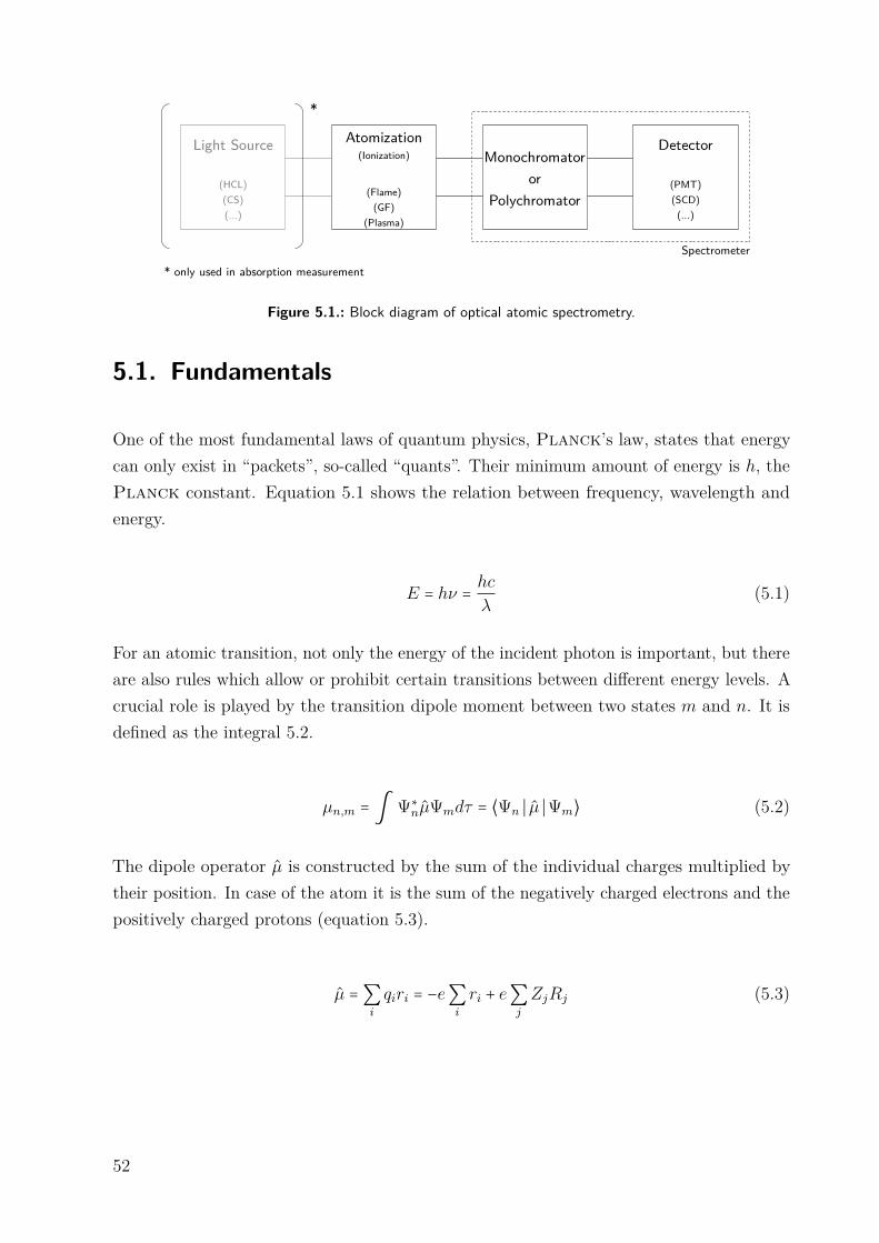
Light Source

(HCL)(CS)(...)

Atomization(Ionization)

(Flame)(GF)

(Plasma)

Monochromatoror

Polychromator

Detector

(PMT)(SCD)(...)

*

* only used in absorption measurementSpectrometer

Figure 5.1.: Block diagram of optical atomic spectrometry.

5.1. Fundamentals

One of the most fundamental laws of quantum physics, Planck’s law, states that energycan only exist in “packets”, so-called “quants”. Their minimum amount of energy is h, thePlanck constant. Equation 5.1 shows the relation between frequency, wavelength andenergy.

E = hν = hcλ

(5.1)

For an atomic transition, not only the energy of the incident photon is important, but thereare also rules which allow or prohibit certain transitions between different energy levels. Acrucial role is played by the transition dipole moment between two states m and n. It isdefined as the integral 5.2.

µn,m = ∫ Ψ∗

nµ̂Ψmdτ = ⟨Ψn ∣ µ̂ ∣Ψm⟩ (5.2)

The dipole operator µ̂ is constructed by the sum of the individual charges multiplied bytheir position. In case of the atom it is the sum of the negatively charged electrons and thepositively charged protons (equation 5.3).

µ̂ =∑i

qiri = −e∑i

ri + e∑j

ZjRj (5.3)

52

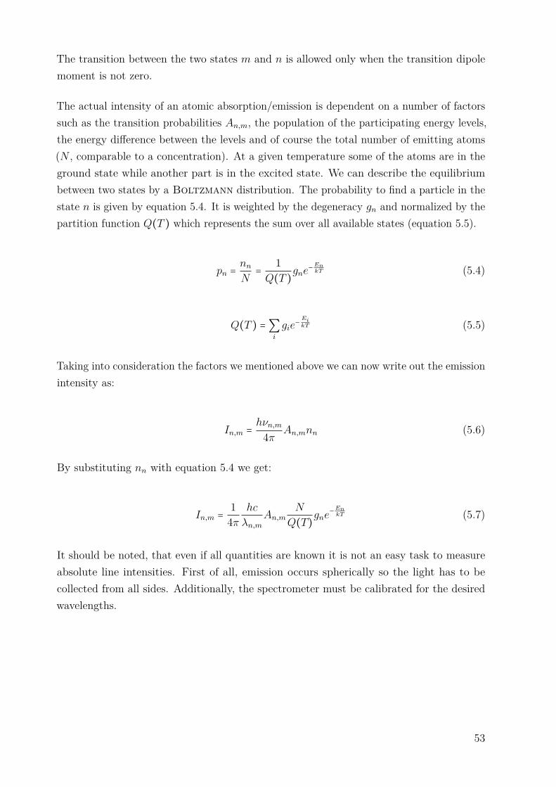
The transition between the two states m and n is allowed only when the transition dipolemoment is not zero.

The actual intensity of an atomic absorption/emission is dependent on a number of factorssuch as the transition probabilities An,m, the population of the participating energy levels,the energy difference between the levels and of course the total number of emitting atoms(N , comparable to a concentration). At a given temperature some of the atoms are in theground state while another part is in the excited state. We can describe the equilibriumbetween two states by a Boltzmann distribution. The probability to find a particle in thestate n is given by equation 5.4. It is weighted by the degeneracy gn and normalized by thepartition function Q(T ) which represents the sum over all available states (equation 5.5).

pn =nnN

= 1Q(T )

gne−EnkT (5.4)

Q(T ) =∑i

gie−EikT (5.5)

Taking into consideration the factors we mentioned above we can now write out the emissionintensity as:

In,m =hνn,m

4π An,mnn (5.6)

By substituting nn with equation 5.4 we get:

In,m = 14π

hc

λn,mAn,m

N

Q(T)gne

−EnkT (5.7)

It should be noted, that even if all quantities are known it is not an easy task to measureabsolute line intensities. First of all, emission occurs spherically so the light has to becollected from all sides. Additionally, the spectrometer must be calibrated for the desiredwavelengths.

53

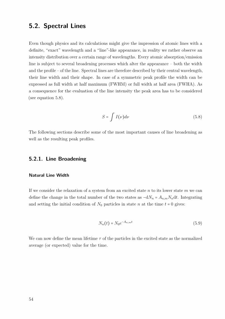
5.2. Spectral Lines

Even though physics and its calculations might give the impression of atomic lines with adefinite, “exact” wavelength and a “line”-like appearance, in reality we rather observe anintensity distribution over a certain range of wavelengths. Every atomic absorption/emissionline is subject to several broadening processes which alter the appearance – both the widthand the profile – of the line. Spectral lines are therefore described by their central wavelength,their line width and their shape. In case of a symmetric peak profile the width can beexpressed as full width at half maximum (FWHM) or full width at half area (FWHA). Asa consequence for the evaluation of the line intensity the peak area has to be considered(see equation 5.8).

S = ∫ I(ν)dν (5.8)

The following sections describe some of the most important causes of line broadening aswell as the resulting peak profiles.

5.2.1. Line Broadening

Natural Line Width

If we consider the relaxation of a system from an excited state n to its lower state m we candefine the change in the total number of the two states as −dNn = An,mNndt. Integratingand setting the initial condition of N0 particles in state n at the time t = 0 gives:

Nn(t) = N0e−An,mt (5.9)

We can now define the mean lifetime τ of the particles in the excited state as the normalizedaverage (or expected) value for the time.

54

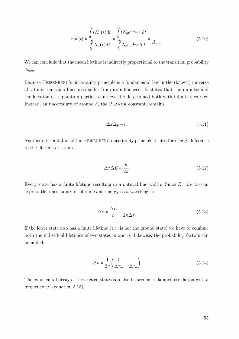
τ = ⟨t⟩ =

∞

∫0tNn(t)dt

∞

∫0Nn(t)dt

=

∞

∫0tN0e−An,mtdt

∞

∫0N0e−An,mtdt

= 1An,m

(5.10)

We can conclude that the mean lifetime is indirectly proportional to the transition probabilityAn,m.

Because Heisenberg’s uncertainty principle is a fundamental law in the (known) universeall atomic emission lines also suffer from its influences. It states that the impulse andthe location of a quantum particle can never be determined both with infinite accuracy.Instead, an uncertainty of around h, the Planck constant, remains.

∆x∆p ∼ h (5.11)

Another interpretation of the Heisenberg uncertainty principle relates the energy differenceto the lifetime of a state.

∆τ∆E ∼ h

2π (5.12)

Every state has a finite lifetime resulting in a natural line width. Since E = hν we canexpress the uncertainty in lifetime and energy as a wavelength:

∆ν = ∆Eh

∼ 12π∆τ (5.13)

If the lower state also has a finite lifetime (i.e. is not the ground state) we have to combineboth the individual lifetimes of two states m and n. Likewise, the probability factors canbe added.

∆ν = 12π (

1∆τm

+ 1∆τn) (5.14)

The exponential decay of the excited states can also be seen as a damped oscillation with afrequency ω0 (equation 5.15).

55

f(t) = e− tτ ejω0t = e− tτ +jω0t = e−t( 1τ−jω0) (5.15)

It is possible to describe it as a superposition of frequencies. Using the Fourier transform wecan obtain the frequency spectrum of the oscillation g(ω). The magnitude of the resultingcomplex function then gives us the frequency distribution as it is recorded in a spectrometer(equation 5.17). This distribution has the form of a Lorentz function.

g(ω) = F (f(t)) =∞

∫0

f(t)e−jωtdt = 11τ + j (ω − ω0)

(5.16)

I(ω) =Mag(g(ω)) = 1√

1τ2 + (ω − ω0)2

(5.17)

We can then finally use the expression ω = 2πν to convert the angular frequencies ω andω0.

I(ν) = 1√

1τ2 + 4π2(ν − ν0)2

(5.18)

Natural line widths lie in the range of 10−5 nm. In comparison to pressure/collisional andDoppler broadening this is usually negligible in line width considerations.

Pressure/Collisional Broadening

It is obvious that collisions between particles can shorten the lifetime of a transition. Thisso-called collisional deactivation is dependent on the rate of collisions which in turn can beinfluenced by changing the pressure (and to some extent the temperature) in the system.If the number density of particles increases, the likelihood of collisions and therefore themean free path length and the lifetime of a state are getting shorter. Depending on thetype of particle we can distinguish between the Stark effect (for electrons and ions), thevan der Waals broadening (caused by induced dipole fields of atoms) and resonancebroadening (energy exchange between same types of particles). The contribution to theline shape is lorentzian for all these effects.

56

Doppler Broadening

In a plasma the radiating particles are moving rapidly in all directions. As a consequencethe apparent frequencies of the emitted photons are changed due to the relative motion fromor towards the observer (i.e. the spectrometer). This phenomenon is called the Dopplereffect. The velocities of the particles are distributed according to a Maxwell distribution.Because the particle speed is well below light speed, we are allowed to define the apparentfrequency as ν = ν0 (1 + v

c). Then, the velocity distribution of the particles becomes (with

dn(v)N being the fraction of particles with the respective velocity v):

dN(v)N

=√

m

2πkT e−mv22kT dv (5.19)

Substituting v by ν we obtain

v = c(ν − ν0)ν0

dv = cdνν0

(5.20)

dN(ν)N

= c

ν0

√m

2πkT e−mc2(ν−ν0)2

2kTν20 dν (5.21)

The resulting equation can be identified as a Gauss function with a halfwidth of:

∆ν = ν0

√8kT ln 2mc2 (5.22)

5.2.2. Line Profile

The previous sections discussed the different aspects and mechanisms of line broadening.We have seen that depending on the underlying mechanism the resulting line profile can begaussian or lorentzian.

Generally, if the broadening mechanism is homogeneous, i.e. all emitters have the sametransition probabilities, the result is a lorentzian-shaped line. These include the naturalline width as well as pressure/collisional mechanisms. The individual contributions can

57

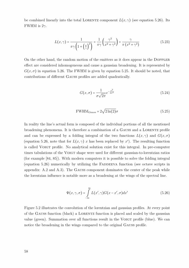
be combined linearly into the total Lorentz component L(x, γ) (see equation 5.26). ItsFWHM is 2γ.

L(x, γ) = 1

πγ (1 + (xγ)2)= 1πγ( γ2

x2 + γ2) =γ

π (x2 + γ2)(5.23)

On the other hand, the random motion of the emitters as it does appear in the Dopplereffect are considered inhomogeneous and cause a gaussian broadening. It is represented byG(x,σ) in equation 5.26. The FWHM is given by equation 5.25. It should be noted, thatcontributions of different Gauss profiles are added quadratically.

G(x,σ) = 1σ√

2πe−

x22σ2 (5.24)

FWHMGauss = 2√

2 ln(2)σ (5.25)

In reality the line’s actual form is composed of the individual portions of all the mentionedbroadening phenomena. It is therefore a combination of a Gauss and a Lorentz profileand can be expressed by a folding integral of the two functions L(x, γ) and G(x,σ)(equation 5.26, note that for L(x, γ) x has been replaced by x′). The resulting functionis called Voigt profile. No analytical solution exist for this integral. In pre-computertimes tabulations of the Voigt shape were used for different gaussian-to-lorentzian ratios(for example [84, 85]). With modern computers it is possible to solve the folding integral(equation 5.26) numerically by utilizing the Faddeeva function (see octave scripts inappendix: A.2 and A.3). The Gauss component dominates the center of the peak whilethe lorentzian influence is notable more as a broadening at the wings of the spectral line.

Ψ(x, γ, σ) =∞

∫−∞

L(x′, γ)G(x − x′, σ)dx′ (5.26)

Figure 5.2 illustrates the convolution of the lorentzian and gaussian profiles. At every pointof the Gauss function (black) a Lorentz function is placed and scaled by the gaussianvalue (green). Summation over all functions result in the Voigt profile (blue). We cannotice the broadening in the wings compared to the original Gauss profile.

58

0,2

0,4

0,6

0,8

1

Figure 5.2.: Voigt line profile. The green curves represent the lorentzian profiles which are scaled by the valueof the gaussian function (black) and summed up for every position into the Voigt profile (shownin blue).

In addition to the aforementioned broadening mechanisms and their resulting line profiles,there is always the influence of the measuring instrument (i.e. the spectrometer) whichalso contributes to the final appearance of the spectral line. The instrument profile canbe of gaussian, voigt, triangular or other shape and has to be convoluted again with theexisting profile function.

59

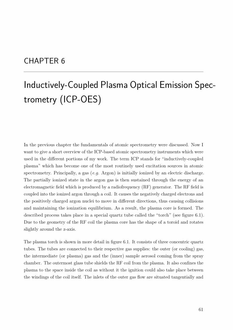
CHAPTER 6

Inductively-Coupled Plasma Optical Emission Spec-trometry (ICP-OES)

In the previous chapter the fundamentals of atomic spectrometry were discussed. Now Iwant to give a short overview of the ICP-based atomic spectrometry instruments which wereused in the different portions of my work. The term ICP stands for “inductively-coupledplasma” which has become one of the most routinely used excitation sources in atomicspectrometry. Principally, a gas (e.g. Argon) is initially ionized by an electric discharge.The partially ionized state in the argon gas is then sustained through the energy of anelectromagnetic field which is produced by a radiofrequency (RF) generator. The RF field iscoupled into the ionized argon through a coil. It causes the negatively charged electrons andthe positively charged argon nuclei to move in different directions, thus causing collisionsand maintaining the ionization equilibrium. As a result, the plasma core is formed. Thedescribed process takes place in a special quartz tube called the “torch” (see figure 6.1).Due to the geometry of the RF coil the plasma core has the shape of a toroid and rotatesslightly around the z-axis.

The plasma torch is shown in more detail in figure 6.1. It consists of three concentric quartztubes. The tubes are connected to their respective gas supplies: the outer (or cooling) gas,the intermediate (or plasma) gas and the (inner) sample aerosol coming from the spraychamber. The outermost glass tube shields the RF coil from the plasma. It also confines theplasma to the space inside the coil as without it the ignition could also take place betweenthe windings of the coil itself. The inlets of the outer gas flow are situated tangentially and

61

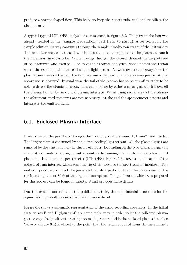
produce a vortex-shaped flow. This helps to keep the quartz tube cool and stabilizes theplasma core.

A typical typical ICP-OES analysis is summarized in figure 6.2. The part in the box wasalready treated in the “sample preparation” part (refer to part I). After retrieving thesample solution, its way continues through the sample introduction stages of the instrument.The nebulizer creates a aerosol which is suitable to be supplied to the plasma throughthe innermost injector tube. While flowing through the aerosol channel the droplets aredried, atomized and excited. The so-called “normal analytical zone” names the regionwhere the recombination and emission of light occurs. As we move further away from theplasma core towards the tail, the temperature is decreasing and as a consequence, atomicabsorption is observed. In axial view the tail of the plasma has to be cut off in order to beable to detect the atomic emission. This can be done by either a shear gas, which blows offthe plasma tail, or by an optical plasma interface. When using radial view of the plasmathe aforementioned measures are not necessary. At the end the spectrometer detects andintegrates the emitted light.

6.1. Enclosed Plasma Interface

If we consider the gas flows through the torch, typically around 15Lmin−1 are needed.The largest part is consumed by the outer (cooling) gas stream. All the plasma gases areremoved by the ventilation of the plasma chamber. Depending on the type of plasma gas thiscircumstance contribute a significant amount to the running costs of the inductively-coupledplasma optical emission spectrometer (ICP-OES). Figure 6.3 shows a modification of theoptical plasma interface which seals the tip of the torch to the spectrometer interface. Thismakes it possible to collect the gases and reutilize parts for the outer gas stream of thetorch, saving almost 80% of the argon consumption. The publication which was preparedfor this project can be found in chapter 8 and provides more details.

Due to the size constraints of the published article, the experimental procedure for theargon recycling shall be described here in more detail.

Figure 6.4 shows a schematic representation of the argon recycling apparatus. In the initialstate valves E and H (figure 6.4) are completely open in order to let the collected plasmagases escape freely without creating too much pressure inside the enclosed plasma interface.Valve N (figure 6.4) is closed to the point that the argon supplied from the instrument’s

62

Sample

Plasma Gas

Cooling Gas

Coil Injector

Normal Analytical Zone (NAZ)

Annular Plasma Core

Plasma Tail

Figure 6.1.: ICP torch schematic. Tangential inlets for plasma and cooling gas are not shown.

Sample Preparation

Monochromatoror

PolychromatorDetector

Spectrometer

Sample

Digestion

ICP-Torch(Ionization, Excitation)

RF Generator

Inte

rface

Argon

Sample Solutions

Figure 6.2.: Schematic overview of an ICP-OES analysis.

63

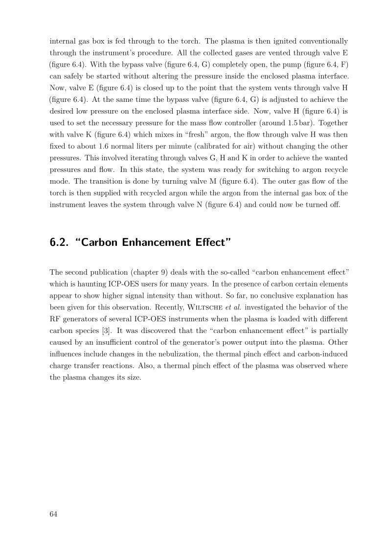
internal gas box is fed through to the torch. The plasma is then ignited conventionallythrough the instrument’s procedure. All the collected gases are vented through valve E(figure 6.4). With the bypass valve (figure 6.4, G) completely open, the pump (figure 6.4, F)can safely be started without altering the pressure inside the enclosed plasma interface.Now, valve E (figure 6.4) is closed up to the point that the system vents through valve H(figure 6.4). At the same time the bypass valve (figure 6.4, G) is adjusted to achieve thedesired low pressure on the enclosed plasma interface side. Now, valve H (figure 6.4) isused to set the necessary pressure for the mass flow controller (around 1.5 bar). Togetherwith valve K (figure 6.4) which mixes in “fresh” argon, the flow through valve H was thenfixed to about 1.6 normal liters per minute (calibrated for air) without changing the otherpressures. This involved iterating through valves G, H and K in order to achieve the wantedpressures and flow. In this state, the system was ready for switching to argon recyclemode. The transition is done by turning valve M (figure 6.4). The outer gas flow of thetorch is then supplied with recycled argon while the argon from the internal gas box of theinstrument leaves the system through valve N (figure 6.4) and could now be turned off.

6.2. “Carbon Enhancement Effect”

The second publication (chapter 9) deals with the so-called “carbon enhancement effect”which is haunting ICP-OES users for many years. In the presence of carbon certain elementsappear to show higher signal intensity than without. So far, no conclusive explanation hasbeen given for this observation. Recently, Wiltsche et al. investigated the behavior of theRF generators of several ICP-OES instruments when the plasma is loaded with differentcarbon species [3]. It was discovered that the “carbon enhancement effect” is partiallycaused by an insufficient control of the generator’s power output into the plasma. Otherinfluences include changes in the nebulization, the thermal pinch effect and carbon-inducedcharge transfer reactions. Also, a thermal pinch effect of the plasma was observed wherethe plasma changes its size.

64

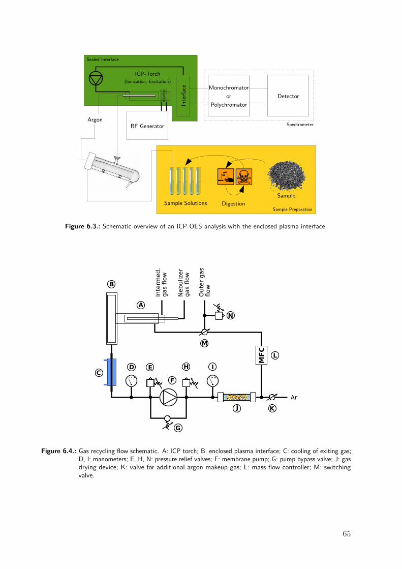
Sample Preparation

Monochromatoror

PolychromatorDetector

Spectrometer

SampleDigestion

ICP-Torch(Ionization, Excitation)

RF Generator

Inte

rface

Argon

Sample Solutions

Sealed Interface

Figure 6.3.: Schematic overview of an ICP-OES analysis with the enclosed plasma interface.

A

B

CD E

G

K

H I

F

L

M

MFC

Inte

rmed

.g

as fl

ow

Neb

uliz

er

gas fl

ow

Ou

ter

gas

flow

Ar

J

N

Figure 6.4.: Gas recycling flow schematic. A: ICP torch; B: enclosed plasma interface; C: cooling of exiting gas;D, I: manometers; E, H, N: pressure relief valves; F: membrane pump; G: pump bypass valve; J: gasdrying device; K: valve for additional argon makeup gas; L: mass flow controller; M: switchingvalve.

65

CHAPTER 7

Plasma Diagnostics

“Photons are clean.” (Gary M. Hieftje)

New developments or changes to parts of an ICP-OES typically influence the formationor the characteristics of the plasma. During the investigation these deviations have to beobserved and recorded. Therefore, a set of parameters have been established to characterizethe plasma. Due to the rather harsh conditions present in a plasma we can imagine thatspecial ways to measure these properties had to be found. These techniques are summedup under the term “plasma diagnostics”. In ICP-OES the most convenient approachis obviously to utilize the (already present) spectrometer and extract information fromemission intensity measurements.

The following sections give a short overview of the most important plasma parameters andhow they can be determined experimentally.

7.1. Temperature

The biggest part of plasma diagnostics deals with the concept of temperature. Generally,the term “temperature” is linked to the movement of particles. In everyday life we referto the motion of the molecules in the air. We can then define the temperature T as theirmean kinetic energy Ekin = 3

2kT . Since a plasma is comprised of a number of different typesof particles, which do not necessarily have the same energy distribution, these simple point

67

of view is not applicable in this case. Therefore we now expand the concept of temperatureto a set of different temperatures which can be used to describe the underlying physicalprocesses. Almost all equations contain an exponential term similar to the Boltzmannequation, the same we have already encountered as equation 5.4.

A detailed explanation of the different temperatures is out of scope but a short introductionshall be given.

Translational or Kinetic Temperature (Tkin) In the section about Doppler broadening(section 5.2.1) we have already encountered the Maxwell distribution which gives us thevelocities of particles (equations 5.19 and 5.21). From this function we can extract thekinetic temperature Tkin which also describes the temperature of the system in case of acomplete thermodynamic equilibrium (CTE). The kinetic temperature can be seen as ameasure to describe the efficiency of the atomization process in the plasma.

Excitation Temperature (Texc) The Boltzmann equation gives us the fraction of acertain energetic state in a population of bound electrons (equation 5.4). Here, it isa function of the excitation temperature Texc. It should be noted, that the excitationtemperature is not necessarily the same for all elements.

Rotational Temperature (Trot) Similar to the excitation temperature Texc, it is possibleto calculate the rotational temperature of a plasma using rotational emission lines ofdiatomic molecules. It is often used interchangeably with Tkin because they are of the samemagnitude.

Ionization Temperature (Tion) The ionization process of the plasma can be describedby the Saha equation, which provides the ratio of ions and atoms.

ninena

= 2Qi(T )Qa(T )

(2πmekT

h2 )32e−

EikT (7.1)

na, ni and ne are the number densities of atoms, ions and electrons, respectively, Qi(T ) andQa(T ) their partition functions and me is the mass of the electron while Ei is the ionizationpotential. Again, we can combine it with the relation for the line intensity (equation 5.7)and yield:

68

ne(I+klApqλ+kl)IpqA+

klλpq= 2gkgp(2πmekTion

h2 )32e−Ei+E+k−EpkTion (7.2)

By evaluating the emission line intensity ratio of the ions to atoms it is possible to determinethe ionization temperature Tion. We should keep in mind that Tion is different for eachelement.

Electron Temperature (Te) The free electrons in a plasma are not bound to any energylevels. Therefore, the radiative recombination with argon ions can be observed as acontinuum in the spectrum. It is governed by its electron temperature Te.

Radiation Temperature (Trad) If the system is in thermal equilibrium the radiationdensity can be calculated by Planck’s formula of radiation. Trad is then equal to theblackbody temperature and, in a CTE, also to the overall temperature T of the system.

7.1.1. Temperature Determination Using Absolute Line Intensities

The temperature Texc can be determined by either directly evaluating the absolute lineintensities or by using relative methods. Absolute line intensities require the knowledgeof the transition probabilities and number densities of the participating species as well asan accurate calibration of the optical system. The line intensity was already described asequation 5.7. For the actual measurement we can add the observation length l, similar asin Lambert-Beer’s law.

Ii =l

4πhc

λiAi

N

Q(Texc)gie

−Ei

kTexc (7.3)

7.1.2. Temperature Determination Using Relative Line Intensities

Because of the reasons mentioned above, methods taking advantage of relative line intensitiesare more easily applicable. One possibility is the so-called Boltzmann plot method. Ituses a set of emission line intensities to extract the exponential factor of the underlying

69

distribution. Firstly, we take the formula for the emission intensity (equation 7.3) andbring all line specific coefficients to the left side, resulting in equation 7.4.

IiλigiAi

= lhcN

4πQ(Texc)e−

EikTexc (7.4)

By taking the logarithm, the function can be linearized. Then we plot the left hand sideusing our set of emission lines with their parameters against the excitation energy. Theslope k of the line equation is then proportional to the excitation temperature Texc.

ln( IiλigiAi)

´¹¹¹¹¹¹¹¹¹¹¹¹¹¹¹¹¹¹¸¹¹¹¹¹¹¹¹¹¹¹¹¹¹¹¹¹¹¹¶y

= ln( lhcN

4πQ(Texc))

´¹¹¹¹¹¹¹¹¹¹¹¹¹¹¹¹¹¹¹¹¹¹¹¹¹¹¹¹¹¹¹¹¹¹¹¹¹¹¹¹¹¸¹¹¹¹¹¹¹¹¹¹¹¹¹¹¹¹¹¹¹¹¹¹¹¹¹¹¹¹¹¹¹¹¹¹¹¹¹¹¹¹¹¶d

− Ei

´¸¶x

1kTexc´¹¹¸¹¹¶

k

(7.5)

Depending on the chosen emission lines, the Boltzmann plot gives the temperature of thedistribution which is governing the respective process in the plasma.

Another simple way of obtaining the temperature is by using a pair of emission lineintensities. This works essentially like a Boltzmann plot but with only two data points.

It should be kept in mind, that detector sensitivity can differ between wavelengths dependingon the construction of the detector. Obviously, line intensities with varying detectorsensitivity cannot be compared without further corrections. As a consequence, the easiestsolution is to only use wavelengths which are projected onto the same detector array.

7.1.3. Thermodynamic Equilibrium

The terms complete thermodynamic equilibrium (CTE) and local thermodynamic equi-librium (LTE) have been used a number of times in the previous sections. In general, asystem is in thermodynamic equilibrium if there is no macroscopic net flow of energy ormatter in the system. Another interpretation can be that the time scales of the exchange ofenergy or matter are much longer than the mean time between collisions. The free electronsin the plasma are primarily responsible for collisions because of their large speed and shortmean free path. Therefore, the electron density ne of a plasma can be used to estimate athermodynamic equilibrium. Methods for obtaining ne are covered in section 7.3.

70

We can speak of a global thermodynamic equilibrium when the intensive parameters such asthe temperature of the system are homogeneous throughout the whole system. In contrast,a LTE exposes variation of the parameters in space and time but at a very slow rate sothat an equilibrium between neighboring spaces can still be assumed.

If the plasma is in a LTE all temperatures from the different distribution functions exceptTrad have the same value and it can be described by a single temperature T (see equation 7.6).A CTE extends the concept by also setting Trad equal. This only applies to blackbodies asthere is no transfer of radiative energy allowed. A blackbody then is solely described byits temperature Trad = T which is only achieved through the absence of any temperaturegradient and – hence – no radiative transport.

T = Te = Tion = Texc = Tkin (7.6)

Because a luminous plasma radiates energy it is obviously not a blackbody and as aconsequence cannot be described only by Planck’s radiation law. Temperature gradientsbetween different zones in the plasma cause radiative energy transfer, therefore the assump-tion of an LTE is not valid. It should be remarked that for its analytical application theICP is not required to be in LTE.

7.2. Plasma Robustness

Apart from rather elaborate procedures for determining the different plasma temperaturesand the plasma’s deviation from LTE, a simpler method exists. Mermet [86] suggested theuse of magnesium emission lines (Mg (II) 280.270 nm/Mg (I) 285.231 nm) for determiningthe deviation of the plasma from LTE. This ratio is now called “plasma robustness”. It isbased on the fact that atomic lines are less sensitive to changes of the plasma operatingconditions than ionic lines. Therefore this simple ratio can serve as an indicator foralterations in the atomization and excitation conditions.

71

7.3. Electron Density

The electron density of a plasma is one of its fundamental properties as it is a measurefor the degree of ionization. It is defined as the number of electrons per volume (ne,electrons m−3). Even though the definition is rather easy (compared to the temperature,refer to section 7.1), the determination is challenging.

It is possible to extract the electron density from the temperature measurements we haveseen previously. The ionization temperature Tion can be used by transforming the Sahaequation (equation 7.1). Another possibility is the continuum radiation of the electronrecombination although it requires the knowledge of the electron temperature Te.

When discussing line broadening mechanisms (section 5.2.1) we already encountered theStark effect. The electrical field of the electrons in the plasma cause the broadening ofvarious emission lines. Therefore, one very convenient method for obtaining the electrondensity is measuring the width of these spectral lines. The width of the analytes’ emissionlines in the ICP is dominated by Doppler broadening but the lines of the hydrogenBalmer series exhibit a strong sensitivity of their line shape towards electrons and alinear Stark effect. In addition, the wavelengths are readily observable in the availablespectrometers which makes them suitable for electron density measurements in ICP-OES.

Gigosos et al. [87] simulated the emission line profiles for the first three lines of the hydrogenBalmer series using different parameters for ion dynamic effects (masses, temperatures andkinetic equilibrium). By combining the results of the simulation they were able to developa formula which is only dependent on either the FWHM or FWHA of the experimentallyobtained line profile.

Because the instrument used for this work (Spectro Ciros Vision EOP) does not havedetector coverage for the most commonly used Hβ line, the Hγ line (434.047 nm) wasrecorded instead. However, it was found difficult to accurately measure the FWHM of theHγ line because of its unusual shape. In argon plasmas there are also two strong backgroundemission lines overlapping the rather broad hydrogen peak (see figure 7.1).

One solution was to write an Octave1 script which uses the data from the detector pixelsto integrate the Hγ line and also tries to remove the interfering peaks by subtracting aVoigt profile. The FWHA is then extracted from the cumulative value of the integral

1GNU Octave, a high-level language for numerical computations – http://www.gnu.org/software/octave/

72

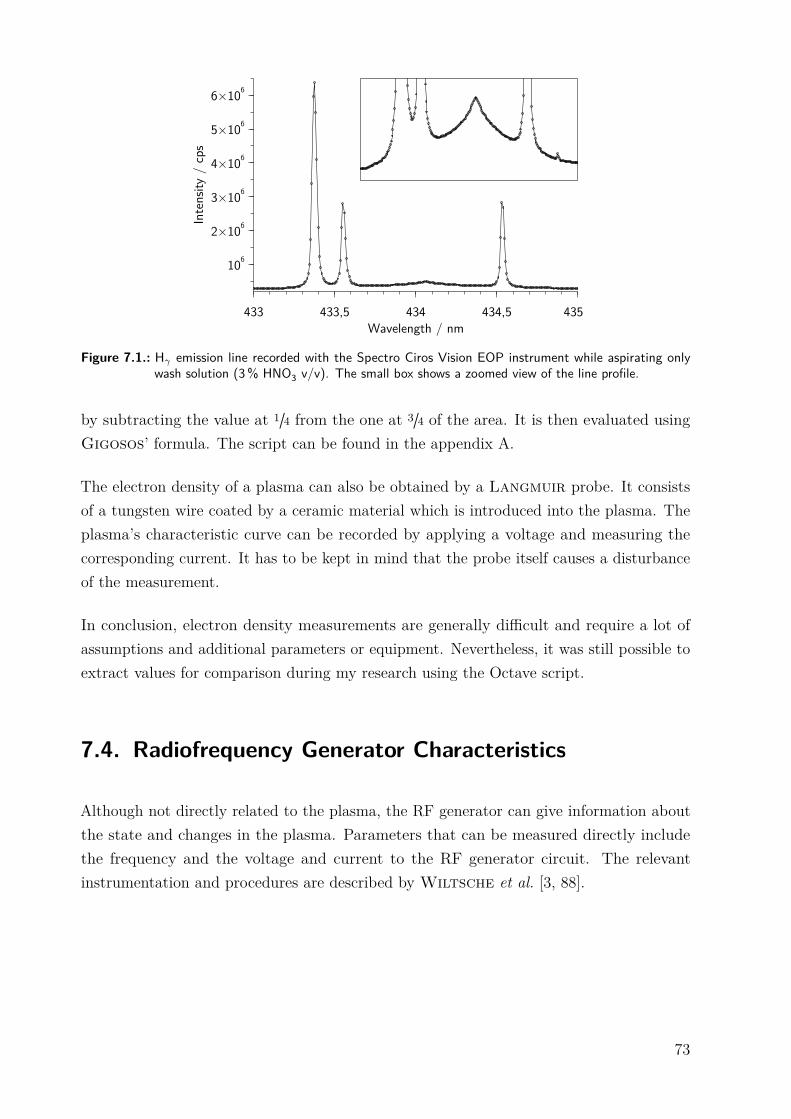
Inte

nsity

/ c

ps

106

2×106

3×106

4×106

5×106

6×106

Wavelength / nm433 433,5 434 434,5 435

Figure 7.1.: Hγ emission line recorded with the Spectro Ciros Vision EOP instrument while aspirating onlywash solution (3% HNO3 v/v). The small box shows a zoomed view of the line profile.

by subtracting the value at 1/4 from the one at 3/4 of the area. It is then evaluated usingGigosos’ formula. The script can be found in the appendix A.

The electron density of a plasma can also be obtained by a Langmuir probe. It consistsof a tungsten wire coated by a ceramic material which is introduced into the plasma. Theplasma’s characteristic curve can be recorded by applying a voltage and measuring thecorresponding current. It has to be kept in mind that the probe itself causes a disturbanceof the measurement.

In conclusion, electron density measurements are generally difficult and require a lot ofassumptions and additional parameters or equipment. Nevertheless, it was still possible toextract values for comparison during my research using the Octave script.

7.4. Radiofrequency Generator Characteristics

Although not directly related to the plasma, the RF generator can give information aboutthe state and changes in the plasma. Parameters that can be measured directly includethe frequency and the voltage and current to the RF generator circuit. The relevantinstrumentation and procedures are described by Wiltsche et al. [3, 88].

73

The frequency of the generator can be monitored by a special pickup coil which is mountedinside the plasma compartment of the instrument. A frequency counter then registers theRF field emitted by the load coil.

For the generator’s input power measurement, the control input of the high voltage powersupply was tapped. The voltage and current feedback of the generator was then recordedusing an analog-digital converter (ADC). Appendix B.2 includes the schematics of the ADCcircuit.

74

CHAPTER 8

Enclosed Plasma InterfacePaul Tirk, Matthias Wolfgang and Helmar Wiltsche

The following chapter was submitted to “Analytical Chemistry” under the title “Reductionof argon consumption to < 2Lmin−1 by gas recycling in inductively-coupled plasma opticalemission spectrometry”.

Abstract

An innovative interface between the torch and the entrance optics for inductively-coupled plasma opticalemission spectrometry (ICP-OES) is proposed. This system is capable of collecting all argon which wasinitially supplied to the torch, cooling and cleaning it and feeding most of the argon back to the outergas port of the torch. Thereby, the total argon consumption could be reduced from 14 to 1.4 Lmin−1

using a standard torch and without restricting the RF power. The excitation- and rotational temperatureof the plasma were identical when comparing the traditional setup with the enclosed plasma interface.However, the limits of detection (LODs) and limits of quantification (LOQs) of 27 elements investigatedwere degraded about 5-fold, though this fact can be expected to stem from a change of the observed zone inthe plasma caused by the slight over-pressure of 2000Pa within the interface. Though the enclosed plasmainterface was located close to the load coil, the RF power coupled to the interface was well below 1W andno RF arcing was observed for two different RF generator designs.

75

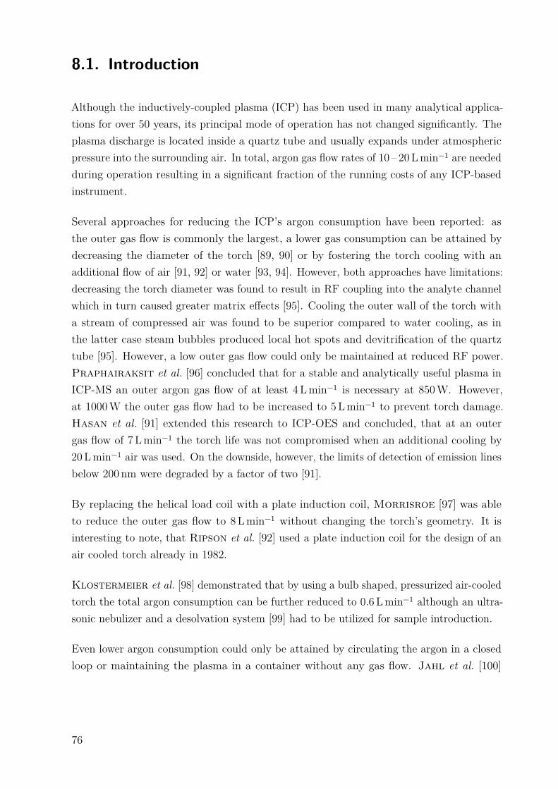
8.1. Introduction

Although the inductively-coupled plasma (ICP) has been used in many analytical applica-tions for over 50 years, its principal mode of operation has not changed significantly. Theplasma discharge is located inside a quartz tube and usually expands under atmosphericpressure into the surrounding air. In total, argon gas flow rates of 10 – 20Lmin−1 are neededduring operation resulting in a significant fraction of the running costs of any ICP-basedinstrument.

Several approaches for reducing the ICP’s argon consumption have been reported: asthe outer gas flow is commonly the largest, a lower gas consumption can be attained bydecreasing the diameter of the torch [89, 90] or by fostering the torch cooling with anadditional flow of air [91, 92] or water [93, 94]. However, both approaches have limitations:decreasing the torch diameter was found to result in RF coupling into the analyte channelwhich in turn caused greater matrix effects [95]. Cooling the outer wall of the torch witha stream of compressed air was found to be superior compared to water cooling, as inthe latter case steam bubbles produced local hot spots and devitrification of the quartztube [95]. However, a low outer gas flow could only be maintained at reduced RF power.Praphairaksit et al. [96] concluded that for a stable and analytically useful plasma inICP-MS an outer argon gas flow of at least 4 Lmin−1 is necessary at 850W. However,at 1000W the outer gas flow had to be increased to 5Lmin−1 to prevent torch damage.Hasan et al. [91] extended this research to ICP-OES and concluded, that at an outergas flow of 7 Lmin−1 the torch life was not compromised when an additional cooling by20Lmin−1 air was used. On the downside, however, the limits of detection of emission linesbelow 200 nm were degraded by a factor of two [91].

By replacing the helical load coil with a plate induction coil, Morrisroe [97] was ableto reduce the outer gas flow to 8Lmin−1 without changing the torch’s geometry. It isinteresting to note, that Ripson et al. [92] used a plate induction coil for the design of anair cooled torch already in 1982.

Klostermeier et al. [98] demonstrated that by using a bulb shaped, pressurized air-cooledtorch the total argon consumption can be further reduced to 0.6 Lmin−1 although an ultra-sonic nebulizer and a desolvation system [99] had to be utilized for sample introduction.

Even lower argon consumption could only be attained by circulating the argon in a closedloop or maintaining the plasma in a container without any gas flow. Jahl et al. [100]

76

designed a spherical discharge container which allowed them to produce either a static or alow flow inductively-coupled plasma at atmospheric pressure. Despite the longer residencetime of the analyte in the discharge region, which improved sensitivity, a complex gashandling equipment and lifetime-limiting devitrification of the discharge tube hampered thesystem. A further restriction to widespread application was the requirement of a gaseousanalyte. A comparable approach was reported by Breer et al. [101] who used a cylindricaldischarge container fed by a low flow of gases. Although it was possible to introduce liquidsamples, the setup was limited to rather short periods of operation due to stability problemswith the discharge tube.

The unifying disadvantage of all these approaches is their inability to work at RF powerlevels in the range of 1500 – 1700W as often required for the analysis of volatile organicsubstances. Particularly for the miniaturized torches, only limited argon consumptionsavings can be claimed.

The aim of this work was to design and build a simple and rugged interface between theICP torch and the entrance optics of an ICP-OES capable of collecting all argon whichwas initially fed into the torch – despite the high temperature present. Moreover, theoperation of the ICP should not be restricted in terms of RF power level, gas flows orsample introduction by this interface. The low argon consumption was thought to beattained by recycling most of the argon back into the outer gas flow of the torch. To avoidcontamination, corrosion and instable plasma conditions, water, acids and salts initiallyintroduced through the aerosol will have to be removed. The intermediate gas flow and thenebulizer gas flow continue to be supplied from an external argon supply.

8.2. Experimental

8.2.1. Enclosed plasma interface

The enclosed plasma interface is a gas-tight enclosure that is mounted onto the entranceoptics of the ICP-OES on one side and surrounds the torch on the other side. Hence, allargon initially fed to the torch can be extracted as hot gas from this enclosure through asingle pipe.

The presented enclosed plasma interface was designed to fit into the plasma compartment ofa commercial ICP-OES (Spectro Ciros Vision EOP, Spectro, Kleve, Germany). It consists

77

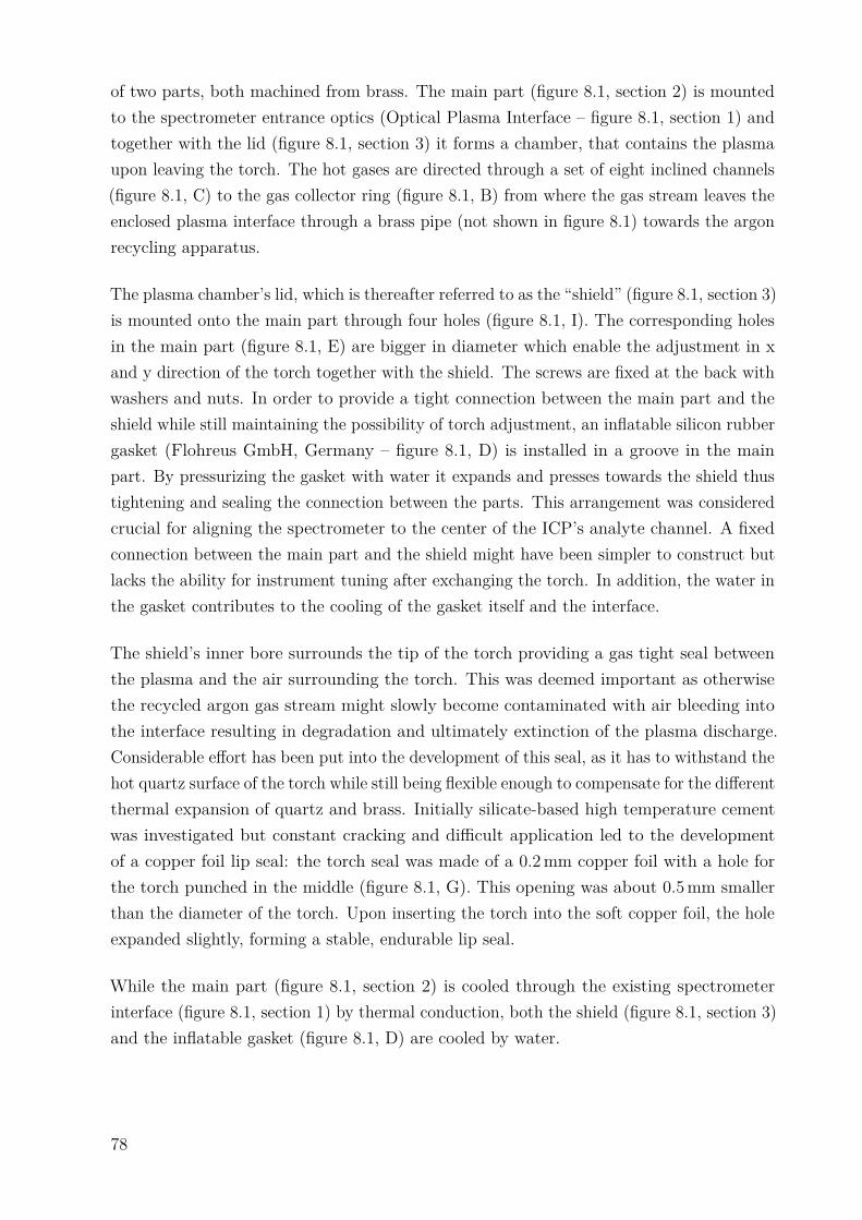
of two parts, both machined from brass. The main part (figure 8.1, section 2) is mountedto the spectrometer entrance optics (Optical Plasma Interface – figure 8.1, section 1) andtogether with the lid (figure 8.1, section 3) it forms a chamber, that contains the plasmaupon leaving the torch. The hot gases are directed through a set of eight inclined channels(figure 8.1, C) to the gas collector ring (figure 8.1, B) from where the gas stream leaves theenclosed plasma interface through a brass pipe (not shown in figure 8.1) towards the argonrecycling apparatus.

The plasma chamber’s lid, which is thereafter referred to as the “shield” (figure 8.1, section 3)is mounted onto the main part through four holes (figure 8.1, I). The corresponding holesin the main part (figure 8.1, E) are bigger in diameter which enable the adjustment in xand y direction of the torch together with the shield. The screws are fixed at the back withwashers and nuts. In order to provide a tight connection between the main part and theshield while still maintaining the possibility of torch adjustment, an inflatable silicon rubbergasket (Flohreus GmbH, Germany – figure 8.1, D) is installed in a groove in the mainpart. By pressurizing the gasket with water it expands and presses towards the shield thustightening and sealing the connection between the parts. This arrangement was consideredcrucial for aligning the spectrometer to the center of the ICP’s analyte channel. A fixedconnection between the main part and the shield might have been simpler to construct butlacks the ability for instrument tuning after exchanging the torch. In addition, the water inthe gasket contributes to the cooling of the gasket itself and the interface.

The shield’s inner bore surrounds the tip of the torch providing a gas tight seal betweenthe plasma and the air surrounding the torch. This was deemed important as otherwisethe recycled argon gas stream might slowly become contaminated with air bleeding intothe interface resulting in degradation and ultimately extinction of the plasma discharge.Considerable effort has been put into the development of this seal, as it has to withstand thehot quartz surface of the torch while still being flexible enough to compensate for the differentthermal expansion of quartz and brass. Initially silicate-based high temperature cementwas investigated but constant cracking and difficult application led to the developmentof a copper foil lip seal: the torch seal was made of a 0.2mm copper foil with a hole forthe torch punched in the middle (figure 8.1, G). This opening was about 0.5mm smallerthan the diameter of the torch. Upon inserting the torch into the soft copper foil, the holeexpanded slightly, forming a stable, endurable lip seal.

While the main part (figure 8.1, section 2) is cooled through the existing spectrometerinterface (figure 8.1, section 1) by thermal conduction, both the shield (figure 8.1, section 3)and the inflatable gasket (figure 8.1, D) are cooled by water.

78

EDCBA

SpectrometerInterface

Main Part Shield

F

G H I

1 2 3

Figure 8.1.: Sectional drawing of the sealed plasma interface parts. A: optical path to the spectrometer; B: gascollector ring; C: inclined gas collector holes; D: inflatable gasket; E: mounting holes for the shield;F: inflatable gasket connector; G: copper torch seal; H: water cooling connector; I: mounting holesof the shield.

Figure 8.2.: Illustration of the interface.

79

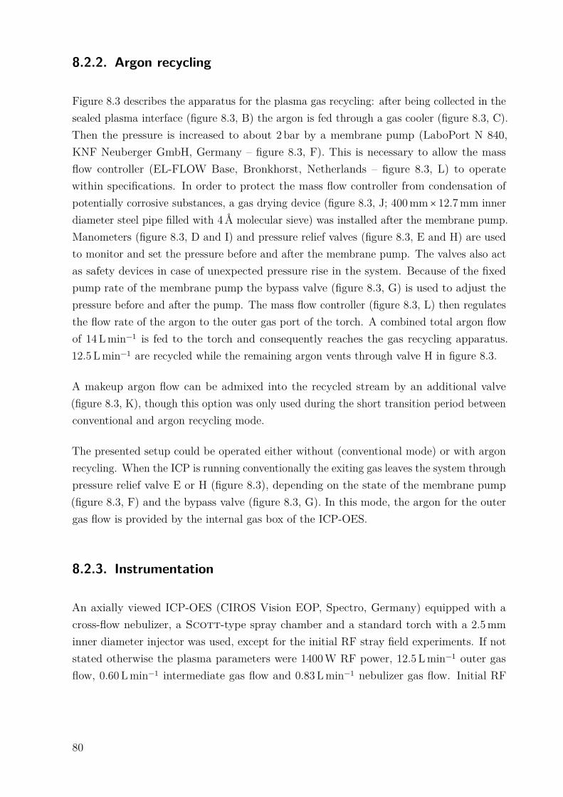
8.2.2. Argon recycling

Figure 8.3 describes the apparatus for the plasma gas recycling: after being collected in thesealed plasma interface (figure 8.3, B) the argon is fed through a gas cooler (figure 8.3, C).Then the pressure is increased to about 2 bar by a membrane pump (LaboPort N 840,KNF Neuberger GmbH, Germany – figure 8.3, F). This is necessary to allow the massflow controller (EL-FLOW Base, Bronkhorst, Netherlands – figure 8.3, L) to operatewithin specifications. In order to protect the mass flow controller from condensation ofpotentially corrosive substances, a gas drying device (figure 8.3, J; 400mm× 12.7mm innerdiameter steel pipe filled with 4Å molecular sieve) was installed after the membrane pump.Manometers (figure 8.3, D and I) and pressure relief valves (figure 8.3, E and H) are usedto monitor and set the pressure before and after the membrane pump. The valves also actas safety devices in case of unexpected pressure rise in the system. Because of the fixedpump rate of the membrane pump the bypass valve (figure 8.3, G) is used to adjust thepressure before and after the pump. The mass flow controller (figure 8.3, L) then regulatesthe flow rate of the argon to the outer gas port of the torch. A combined total argon flowof 14 Lmin−1 is fed to the torch and consequently reaches the gas recycling apparatus.12.5 Lmin−1 are recycled while the remaining argon vents through valve H in figure 8.3.

A makeup argon flow can be admixed into the recycled stream by an additional valve(figure 8.3, K), though this option was only used during the short transition period betweenconventional and argon recycling mode.

The presented setup could be operated either without (conventional mode) or with argonrecycling. When the ICP is running conventionally the exiting gas leaves the system throughpressure relief valve E or H (figure 8.3), depending on the state of the membrane pump(figure 8.3, F) and the bypass valve (figure 8.3, G). In this mode, the argon for the outergas flow is provided by the internal gas box of the ICP-OES.

8.2.3. Instrumentation

An axially viewed ICP-OES (CIROS Vision EOP, Spectro, Germany) equipped with across-flow nebulizer, a Scott-type spray chamber and a standard torch with a 2.5mminner diameter injector was used, except for the initial RF stray field experiments. If notstated otherwise the plasma parameters were 1400W RF power, 12.5 Lmin−1 outer gasflow, 0.60 Lmin−1 intermediate gas flow and 0.83 Lmin−1 nebulizer gas flow. Initial RF

80

A

B

CD E

G

K

H I

F

L

M

MFC

Inte

rmed

.g

as fl

ow

Neb

uliz

er

gas fl

ow

Ou

ter

gas

flow

Ar

J

N

Figure 8.3.: Gas recycling flow schematic. A: ICP torch; B: Enclosed plasma interface; C: Cooling of exitinggas; D, I: Manometers; E, H, N: Pressure relief valves; F: Membrane pump; G: Pump bypassvalve; J: Gas drying device; K: Valve for additional argon makeup gas; L: Mass flow controller;M: Switching valve.

stray field experiments were conducted on an axially viewed ICP-OES (Optima 3000 XL,PerkinElmer, USA).

The excitation temperature Texc and the rotational temperature Trot were determinedby the Boltzmann plot method. Details on the used emission lines and fundamentalconstants are reported in a previous publication [88]. The plasma robustness [86] wascalculated from the Mg (II) 280.270 nm/Mg (I) 285.213 nm ratio. The electron numberdensities were obtained from the width of the Hγ emission line (434.047 nm) using thepredicted formulas as described by Gigosos et al. [87]. Limits of detection (LODs) andlimits of quantification (LOQs) were calculated using the calibration method (calibrationin the range of 0 – 1mgL−1; 5 concentration levels; 5 replications; 95% confidence level).

8.2.4. Reagents

Purified water (18MW cm, Barnstead Nanopure, Thermo Fisher Scientific, USA) and highpurity acids (HNO3, purified by subboiling) were used throughout. The ICP excitationtemperature was determined using a 300mgL−1 Fe solution containing 3% HNO3 (v/v)prepared from a 10 gL−1 Fe single element stock solution (Alfa Aesar, Germany). Standard

81

solutions for instrument calibration were prepared from a 100mgL−1 multi-element stocksolution (Ag, Al, As, B, Ba, Be, Bi, Ca, Cd, Co, Cr, Cu, Fe, K, Li, Mg, Mn, Mo, Na, Ni,Pb, Sb, Se, Sr, Ti, Tl, V, and Zn, Roth, Germany) by dilution with 3% HNO3 (v/v).

8.2.5. RF stray field

Due to the fact, that the shield is in close proximity to the load coil, initial experimentswere conducted to assess the feasibility of the presented approach. Three processes wereconsidered potentially troublesome: 1) high voltage arcing from the load coil to the groundedshield, 2) inductive coupling of RF stray fields to the metallic shield and 3) capacitivecoupling of the RF field to a non-ground referenced shield. Particularly the second processwas thought to result in excessive heating of the shield followed by reduced power couplingto the argon plasma torus.

The ICP-OES used for spectrometric characterization (Spectro Ciros Vision EOP) employs aRF generator based on a Huth-Kühn type power oscillator. The load coil of this instrumentis grounded on one end making an investigation of high voltage arcing impossible. Therefore,a second ICP-OES was used for the initial experiments whose RF generator is based on a40MHz Colpitts power oscillator that creates a high voltage sine of about 3 – 4 kV on theload coil (PerkinElmer Optima 3000XL). Neither side of this RF generators load coil isgrounded, but only a “virtual” grounding exists near the center of the load coil.

The RF stray fields in close proximity to the torch were probed with a copper disk (100mmdiameter, 2mm thick) that could be actuated along the axis of the torch. This disk hada 22mm hole in the center for the torch to penetrate the disk and a 2mm slot from theouter rim to the center hole. It essentially resembled a flat, single turn coil. Two wireswere connected from the two ends of this “coil” to a high-speed diode-based (MBR16-150Schottky diodes) full wave rectifier. A RC network with selectable resistors (2.55W to 1MW)and a constant filtering capacitor of 3.3 nF provided further low pass filtering. The copperdisk was attached via a sheet of FR4 epoxy (45mm isolation distance to the groundedchassis) to a lead screw, which was actuated by a stepper motor. Thereby, the slottedcopper disk could be moved along the axis of the torch, starting in 2mm distance tothe load coil. For safety reasons, a standard glass bonnet was attached to the torch. Athermocouple was also mounted to the copper disk for temperature measurements. Animage of the setup is shown in the supplementary material (section 8.7, figure 8.7). Allexperiments were conducted at 1300W RF power. The RF power coupled to the copperdisc was calculated from the current induced between the two ends of the slotted copper

82

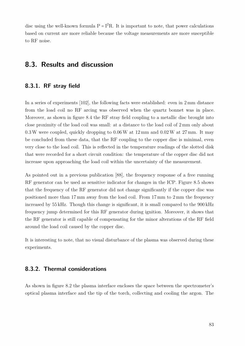
disc using the well-known formula P = I2R. It is important to note, that power calculationsbased on current are more reliable because the voltage measurements are more susceptibleto RF noise.

8.3. Results and discussion

8.3.1. RF stray field

In a series of experiments [102], the following facts were established: even in 2mm distancefrom the load coil no RF arcing was observed when the quartz bonnet was in place.Moreover, as shown in figure 8.4 the RF stray field coupling to a metallic disc brought intoclose proximity of the load coil was small: at a distance to the load coil of 2mm only about0.3W were coupled, quickly dropping to 0.06W at 12mm and 0.02W at 27mm. It maybe concluded from these data, that the RF coupling to the copper disc is minimal, evenvery close to the load coil. This is reflected in the temperature readings of the slotted diskthat were recorded for a short circuit condition: the temperature of the copper disc did notincrease upon approaching the load coil within the uncertainty of the measurement.

As pointed out in a previous publication [88], the frequency response of a free runningRF generator can be used as sensitive indicator for changes in the ICP. Figure 8.5 showsthat the frequency of the RF generator did not change significantly if the copper disc waspositioned more than 17mm away from the load coil. From 17mm to 2mm the frequencyincreased by 55 kHz. Though this change is significant, it is small compared to the 900 kHzfrequency jump determined for this RF generator during ignition. Moreover, it shows thatthe RF generator is still capable of compensating for the minor alterations of the RF fieldaround the load coil caused by the copper disc.

It is interesting to note, that no visual disturbance of the plasma was observed during theseexperiments.

8.3.2. Thermal considerations

As shown in figure 8.2 the plasma interface encloses the space between the spectrometer’soptical plasma interface and the tip of the torch, collecting and cooling the argon. The

83

RF p

ower

cou

pled

to th

e sh

ield,

W

0,000,050,100,150,200,250,300,350,400,45

Distance from load coil, mm0 5 10 15 20 25 30

Figure 8.4.: RF power coupled to the slotted copper disk as a function of the distance from the load coil.

RF g

ener

ator

freq

uenc

y, M

Hz

40,32

40,34

40,36

40,38

40,40

40,42

Distance from load coil, mm0 5 10 15 20 25 30

Figure 8.5.: Frequency of the free running RF generator as a function of the distance from the load coil.

boundary region between the outer tube of the quartz torch and the brass shield is subject toextreme thermal and mechanical stress. The temperature measured 10 minutes after plasmaignition on the foremost tip of the torch and in the absence of the shield was 250 ± 20 ○C ata RF power level of 1100W and increased nearly linear to 540 ± 20 ○C at 1500W. Contraryto Engelhard et al. [103] the temperature was measured by a thermocouple directlyattached to the torch and not by infrared thermography. The RF stray field pickup wasattenuated by feeding the thermocouple leads several times through EMI suppressionferrite toroids. Though only one spot was monitored by this approach, the temperaturecould be read directly without cumbersome calibration of a thermographic camera. Thetorch temperature acquired was comparable between these two approaches: at 1400W RFpower the thermocouple reading was 440 ± 20 ○C, while Engelhard et al. [103] report a

84

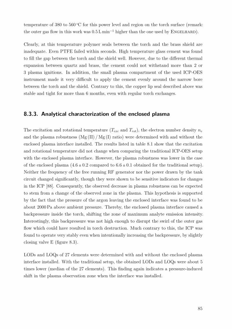
temperature of 380 to 560 ○C for this power level and region on the torch surface (remark:the outer gas flow in this work was 0.5 Lmin−1 higher than the one used by Engelhard).

Clearly, at this temperature polymer seals between the torch and the brass shield areinadequate. Even PTFE failed within seconds. High temperature glass cement was foundto fill the gap between the torch and the shield well. However, due to the different thermalexpansion between quartz and brass, the cement could not withstand more than 2 or3 plasma ignitions. In addition, the small plasma compartment of the used ICP-OESinstrument made it very difficult to apply the cement evenly around the narrow borebetween the torch and the shield. Contrary to this, the copper lip seal described above wasstable and tight for more than 6 months, even with regular torch exchanges.

8.3.3. Analytical characterization of the enclosed plasma

The excitation and rotational temperature (Texc and Trot), the electron number density neand the plasma robustness (Mg (II) /Mg (I) ratio) were determined with and without theenclosed plasma interface installed. The results listed in table 8.1 show that the excitationand rotational temperature did not change when comparing the traditional ICP-OES setupwith the enclosed plasma interface. However, the plasma robustness was lower in the caseof the enclosed plasma (4.6 ± 0.2 compared to 6.6 ± 0.1 obtained for the traditional setup).Neither the frequency of the free running RF generator nor the power drawn by the tankcircuit changed significantly, though they were shown to be sensitive indicators for changesin the ICP [88]. Consequently, the observed decrease in plasma robustness can be expectedto stem from a change of the observed zone in the plasma. This hypothesis is supportedby the fact that the pressure of the argon leaving the enclosed interface was found to beabout 2000Pa above ambient pressure. Thereby, the enclosed plasma interface caused abackpressure inside the torch, shifting the zone of maximum analyte emission intensity.Interestingly, this backpressure was not high enough to disrupt the swirl of the outer gasflow which could have resulted in torch destruction. Much contrary to this, the ICP wasfound to operate very stably even when intentionally increasing the backpressure, by slightlyclosing valve E (figure 8.3).

LODs and LOQs of 27 elements were determined with and without the enclosed plasmainterface installed. With the traditional setup, the obtained LODs and LOQs were about 5times lower (median of the 27 elements). This finding again indicates a pressure-inducedshift in the plasma observation zone when the interface was installed.

85

Table 8.1.: Characteristics of the enclosed plasma interface and the traditional setup; uncertainty of thetemperature determination is dominated by the uncertainty of the linear regression in the Boltzmannplot.

Parameter Enclosed plasma interface Traditional setup

Texc 6500 ± 100 6600 ± 100 KTrot 4400 ± 100 4600 ± 100 Kne 9 ⋅ 1021

± 1 ⋅ 1021 5 ⋅ 1021± 1 ⋅ 1021 electrons m−3

Mg (II) /Mg (I) 4.6 ± 0.2 6.6 ± 0.1

8.3.4. Argon recycling and contamination

Because of the continuous recycling of the outer gas stream the accumulation of water anddecomposition products of acids and samples must be removed, as they would otherwisecause plasma stability problems or severe contamination. Using a pipe filled with molecularsieve, water and potentially some of the particulate matter produced by condensation fromthe hot plasma during the cooling step can be trapped.

The enclosed plasma was operated for more than 4 h while constantly nebulizing dilutednitric acid (3% v/v) without any detectable degradation of the plasma by N2 or O2.

As the reintroduction of particulate matter via the outer gas stream was considered apotential source of contamination, a pathological test setup was selected: a solutioncontaining 50 gL−1 NaCl was nebulized for 5 minutes. During the following 30 minutes,diluted nitric acid (3% v/v) was nebulized while recording the signals of Na and Cl.

From figure 8.6 it is apparent that no contamination of the ICP by particulate matter froma previous analysis was encountered for the enclosed plasma interface as the signal decay ofthe Cl 135.165 nm emission line recorded with the traditional setup closely matches theone obtained while the argon recycling was in operation. Clearly, rinse-out effects in thelarge surface spray chamber dominated the transient Cl signal. It is interesting to note,that a similar pattern was obtained for Na.

Another source of potential contamination was the brass used for constructing the enclosedplasma interface. Particularly the parts of the interface that were in direct contact withthe plasma turned reddish after several hours of operation indicating an evaporation of Znfrom the brass. However, neither Zn 213.857 nm nor Zn 206.200 nm showed signals abovethe background, even after prolonged system operation. A similar finding was encounteredwith an early test setup installed on the second investigated ICP-OES (Optima 3000,PerkinElmer).

86

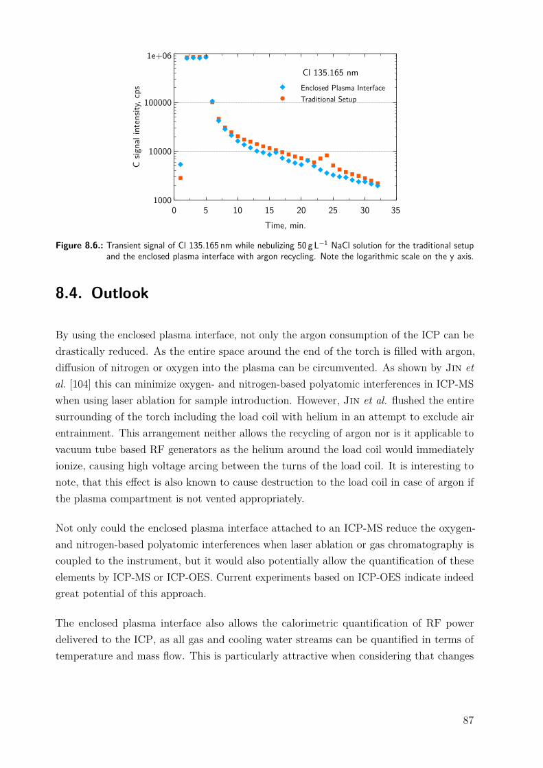
Cl 135.165 nmEnclosed Plasma InterfaceTraditional Setup

C sig

nal i

nten

sity,

cps

1000

10000

100000

1e+06

Time, min.0 5 10 15 20 25 30 35

Figure 8.6.: Transient signal of Cl 135.165 nm while nebulizing 50 g L−1 NaCl solution for the traditional setupand the enclosed plasma interface with argon recycling. Note the logarithmic scale on the y axis.

8.4. Outlook

By using the enclosed plasma interface, not only the argon consumption of the ICP can bedrastically reduced. As the entire space around the end of the torch is filled with argon,diffusion of nitrogen or oxygen into the plasma can be circumvented. As shown by Jin etal. [104] this can minimize oxygen- and nitrogen-based polyatomic interferences in ICP-MSwhen using laser ablation for sample introduction. However, Jin et al. flushed the entiresurrounding of the torch including the load coil with helium in an attempt to exclude airentrainment. This arrangement neither allows the recycling of argon nor is it applicable tovacuum tube based RF generators as the helium around the load coil would immediatelyionize, causing high voltage arcing between the turns of the load coil. It is interesting tonote, that this effect is also known to cause destruction to the load coil in case of argon ifthe plasma compartment is not vented appropriately.

Not only could the enclosed plasma interface attached to an ICP-MS reduce the oxygen-and nitrogen-based polyatomic interferences when laser ablation or gas chromatography iscoupled to the instrument, but it would also potentially allow the quantification of theseelements by ICP-MS or ICP-OES. Current experiments based on ICP-OES indicate indeedgreat potential of this approach.

The enclosed plasma interface also allows the calorimetric quantification of RF powerdelivered to the ICP, as all gas and cooling water streams can be quantified in terms oftemperature and mass flow. This is particularly attractive when considering that changes

87

in the sample composition can result in plasma impedance changes that are followed byRF power level variations [3]. To the best of our knowledge, no other technique thancalorimetry is capable of monitoring the RF generator online while altering the samplecomposition and maintaining an acceptable level of uncertainty.

Another possibility of the enclosed plasma interface is the use of helium instead of argon inthe plasma. Though several publications investigated the potential and limitation of thisapproach [105–108] the costly nature of helium impeded widespread application. However,by adding the possibility to recycle the helium this approach might become attractiveagain.

8.5. Conclusion

The presented work shows that it is possible to enclose an ICP and recycle most of the usedargon. Therefore, the enclosed plasma interface allows to significantly reduce the argonconsumption to about 1.4 – 2 Lmin−1 without the need of changing the torch geometry, thesample introduction system or to accept compromise conditions in terms of maximum RFpower. Neither the ICP’s stability was significantly degraded, nor did the overall excitationcondition of the discharge change when using the enclosed plasma interface. Though simple,the cleaning of the argon collected in the interface was effective even for volatile elementslike Cl. As this argon was only recycled for the outer gas flow, the initial experimentsindicate that no elaborate gas cleaning apparatus is necessary.

The main shortcoming of the current design is the increased pressure inside the enclosedplasma interface resulting in degraded LODs and lower-than-expected plasma robustness.These issues will be corrected in a new interface currently under construction.

8.6. Acknowledgements

Günter Fellner is thanked for skillfully machining the components of the interface.The help of David Puntigam and David Moser is acknowledged.

88

8.7. Supplementary Material

This section includes the electronic supplementary material of the article. It contains apicture of the RF stray field experiments (figure 8.7).

A

B

C

D

E

F

Figure 8.7.: Experimental setup for determining the magnitude of the RF stray field. A: slotted copper disk;B: quartz bonnet; C: load coil; D: actuator for moving the slotted brass disk along the axis of thetorch; E: temperature sensor; F: electrical connection to the high speed rectifier.

89

CHAPTER 9

Carbon Enhancement EffectHelmar Wiltsche, Monika Winkler and Paul Tirk

The following chapter was published in the “Journal of Analytical Atomic Spectrometry”,Volume 30 (2015), pages 2223 – 2234 under the title “Matrix effects of carbon and brominein inductively coupled plasma optical emission spectrometry” [3].

Abstract

In inductively-coupled plasma (ICP) based techniques the signal enhancing effect of carbon on someelements like arsenic or selenium is well documented. However, there is a large spread in the reportedmagnitude of this effect and whether it can be observed for other elements too. In this investigation westudied the effect of larger amounts of carbon on a total of 157 emission lines of 36 elements. A stronginstrument dependence of the “carbon enhancement effect” was encountered in inductively-coupled plasmaoptical emission spectrometry (ICP-OES), despite the use of the same sample solutions and the samesample introduction system. Several potential enhancement sources (carbon in the form of methanol,phenylalanine and CO2 as well as bromine) were compared. By tapping the high voltage power supplyof the RF generator, current and voltage fed to the power oscillator could be recorded simultaneouslywith the emission line signal. From these data it was concluded that the carbon-based matrix effect is acombination of five factors: (1) depending on the source of carbon, changes in the sample nebulization;(2) carbon induced charge exchange reactions; (3) plasma impedance changes caused by the introductionof large quantities of carbon into the ICP: depending on the RF generator used, this effect causes powerregulation problems and results in higher RF power coupled to the discharge; (4) thermal pinch effect – theICP discharge shrinks and becomes smaller; (5) the state of matter (gaseous or liquid) of the introducedcarbon sources is relevant to the magnitude of the carbon enhancement effect.

91

9.1. Introduction

The introduction of larger quantities of carbon into the inductively-coupled plasma (ICP)instrument is reported to increase the sensitivity of elements with the ionization potential(IP) in the range of about 9 to 12 eV [51, 61, 109–120]. This enhancement has beenobserved in both inductively-coupled plasma optical emission spectrometry (ICP-OES)and inductively-coupled plasma mass spectrometry (ICP-MS). Although this “carbonenhancement effect” was reported nearly 25 years ago [61], the understanding of theunderlying mechanism is still unsatisfactory as apparent from the many conflicting resultspublished since then.

By far the largest number of studies describing the “carbon enhancement effect” havebeen performed using ICP-MS as the speciation analysis of As and Se received greatattention and these two elements exhibit in general the largest enhancement by carbon.The differences in the attained level of enhancement are striking: whereas some authorsreported a carbon-induced suppression of the As and Se signal in the range of 50 – 70%(1350W RF power, 2% methanol v/v) [114], most authors observed a signal enhancement bya factor of 2 – 5 (e.g. ref. [73, 111–113, 115, 119, 121]). Even an 11-fold enhancement of theSe-signal has been reported [120]. Indeed, it is difficult to compare these data as differentsources of carbon were used. Several authors [73, 119, 121] concluded that the change innebulization efficiency caused by C-sources such as methanol cannot explain the carboninduced signal enhancement, particularly when considering that the same effect is caused byglycerin [61, 73], glucose [121], ammonium acetate [121] and urea [122]. By using methaneas the carbon source Allain et al. [61] confirmed that differences in the nebulizationefficiency are not the sole reason for the “carbon enhancement effect”. Despite the differentcarbon sources used, most authors [51, 61, 109, 111, 113–115, 119] found that in ICP-MSthe As and Se signal initially increases with increasing carbon content of the sample solution,and then reaches a plateau and decreases again. The maximum enhancement of As and Seappears to be a function of the carbon source and of the instrument used.

The reports on the enhancement or suppression of other elements by carbon are even moreconfusing. Whereas for Au (IP 9.23 eV) [61, 119, 123] and Be (IP 9.32 eV) [51] carboninduced signal enhancement is reported, for Zn (IP 9.39 eV), S (IP 10.36 eV), Hg (IP10.44 eV) and I (IP 10.45 eV) both carbon induced enhancement [51, 61, 73, 111, 113, 119,121, 122] and the absence of this effect [61, 73, 118] are reported.

92

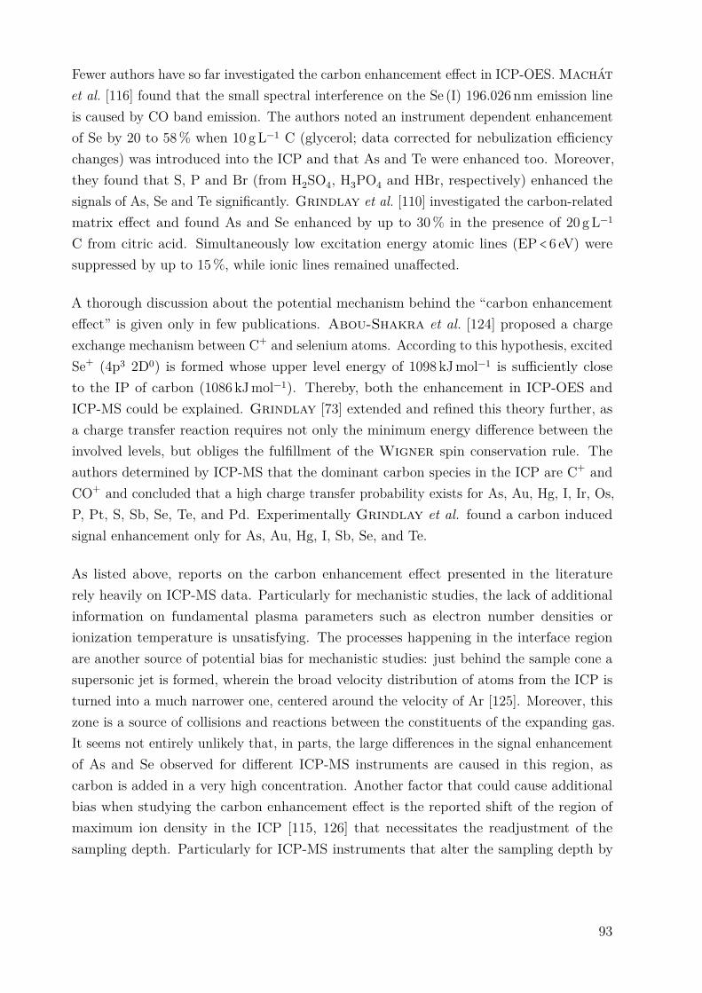
Fewer authors have so far investigated the carbon enhancement effect in ICP-OES. Machátet al. [116] found that the small spectral interference on the Se (I) 196.026 nm emission lineis caused by CO band emission. The authors noted an instrument dependent enhancementof Se by 20 to 58% when 10 gL−1 C (glycerol; data corrected for nebulization efficiencychanges) was introduced into the ICP and that As and Te were enhanced too. Moreover,they found that S, P and Br (from H2SO4, H3PO4 and HBr, respectively) enhanced thesignals of As, Se and Te significantly. Grindlay et al. [110] investigated the carbon-relatedmatrix effect and found As and Se enhanced by up to 30% in the presence of 20 gL−1

C from citric acid. Simultaneously low excitation energy atomic lines (EP < 6 eV) weresuppressed by up to 15%, while ionic lines remained unaffected.

A thorough discussion about the potential mechanism behind the “carbon enhancementeffect” is given only in few publications. Abou-Shakra et al. [124] proposed a chargeexchange mechanism between C+ and selenium atoms. According to this hypothesis, excitedSe+ (4p3 2D0) is formed whose upper level energy of 1098 kJmol−1 is sufficiently closeto the IP of carbon (1086 kJmol−1). Thereby, both the enhancement in ICP-OES andICP-MS could be explained. Grindlay [73] extended and refined this theory further, asa charge transfer reaction requires not only the minimum energy difference between theinvolved levels, but obliges the fulfillment of the Wigner spin conservation rule. Theauthors determined by ICP-MS that the dominant carbon species in the ICP are C+ andCO+ and concluded that a high charge transfer probability exists for As, Au, Hg, I, Ir, Os,P, Pt, S, Sb, Se, Te, and Pd. Experimentally Grindlay et al. found a carbon inducedsignal enhancement only for As, Au, Hg, I, Sb, Se, and Te.

As listed above, reports on the carbon enhancement effect presented in the literaturerely heavily on ICP-MS data. Particularly for mechanistic studies, the lack of additionalinformation on fundamental plasma parameters such as electron number densities orionization temperature is unsatisfying. The processes happening in the interface regionare another source of potential bias for mechanistic studies: just behind the sample cone asupersonic jet is formed, wherein the broad velocity distribution of atoms from the ICP isturned into a much narrower one, centered around the velocity of Ar [125]. Moreover, thiszone is a source of collisions and reactions between the constituents of the expanding gas.It seems not entirely unlikely that, in parts, the large differences in the signal enhancementof As and Se observed for different ICP-MS instruments are caused in this region, ascarbon is added in a very high concentration. Another factor that could cause additionalbias when studying the carbon enhancement effect is the reported shift of the region ofmaximum ion density in the ICP [115, 126] that necessitates the readjustment of thesampling depth. Particularly for ICP-MS instruments that alter the sampling depth by

93

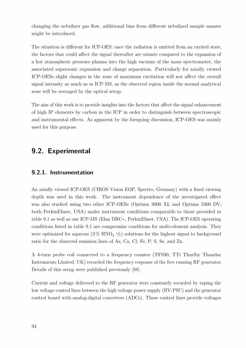
changing the nebulizer gas flow, additional bias from different nebulized sample massesmight be introduced.

The situation is different for ICP-OES: once the radiation is emitted from an excited state,the factors that could affect the signal thereafter are minute compared to the expansion ofa hot atmospheric pressure plasma into the high vacuum of the mass spectrometer, theassociated supersonic expansion and charge separation. Particularly for axially viewedICP-OESs slight changes in the zone of maximum excitation will not affect the overallsignal intensity as much as in ICP-MS, as the observed region inside the normal analyticalzone will be averaged by the optical setup.

The aim of this work is to provide insights into the factors that affect the signal enhancementof high IP elements by carbon in the ICP in order to distinguish between spectroscopicand instrumental effects. As apparent by the foregoing discussion, ICP-OES was mainlyused for this purpose.

9.2. Experimental

9.2.1. Instrumentation

An axially viewed ICP-OES (CIROS Vision EOP, Spectro, Germany) with a fixed viewingdepth was used in this work. The instrument dependence of the investigated effectwas also studied using two other ICP-OESs (Optima 3000 XL and Optima 5300 DV;both PerkinElmer, USA) under instrument conditions comparable to those provided intable 9.1 as well as one ICP-MS (Elan DRC+, PerkinElmer, USA). The ICP-OES operatingconditions listed in table 9.1 are compromise conditions for multi-element analysis. Theywere optimized for aqueous (3% HNO3 v/v) solutions for the highest signal to backgroundratio for the observed emission lines of As, Ca, Cl, Fe, P, S, Se, and Zn.

A 4-turn probe coil connected to a frequency counter (TF930, TTi Thurlby ThandarInstruments Limited, UK) recorded the frequency response of the free running RF generator.Details of this setup were published previously [88].

Current and voltage delivered to the RF generator were constantly recorded by taping thelow voltage control lines between the high voltage power supply (HV-PSU) and the generatorcontrol board with analog-digital converters (ADCs). These control lines provide voltages

94

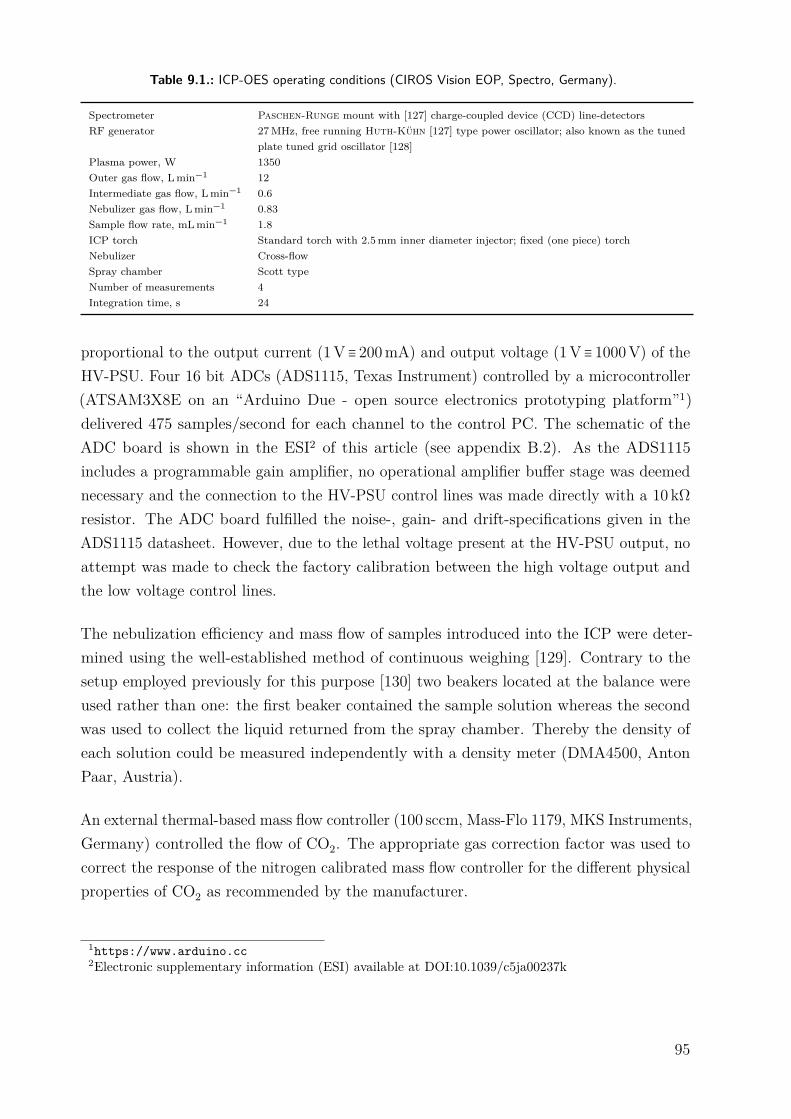
Table 9.1.: ICP-OES operating conditions (CIROS Vision EOP, Spectro, Germany).

Spectrometer Paschen-Runge mount with [127] charge-coupled device (CCD) line-detectorsRF generator 27MHz, free running Huth-Kühn [127] type power oscillator; also known as the tuned

plate tuned grid oscillator [128]Plasma power, W 1350Outer gas flow, Lmin−1 12Intermediate gas flow, Lmin−1 0.6Nebulizer gas flow, Lmin−1 0.83Sample flow rate, mLmin−1 1.8ICP torch Standard torch with 2.5mm inner diameter injector; fixed (one piece) torchNebulizer Cross-flowSpray chamber Scott typeNumber of measurements 4Integration time, s 24

proportional to the output current (1V ≡ 200mA) and output voltage (1V ≡ 1000V) of theHV-PSU. Four 16 bit ADCs (ADS1115, Texas Instrument) controlled by a microcontroller(ATSAM3X8E on an “Arduino Due - open source electronics prototyping platform”1)delivered 475 samples/second for each channel to the control PC. The schematic of theADC board is shown in the ESI2 of this article (see appendix B.2). As the ADS1115includes a programmable gain amplifier, no operational amplifier buffer stage was deemednecessary and the connection to the HV-PSU control lines was made directly with a 10 kWresistor. The ADC board fulfilled the noise-, gain- and drift-specifications given in theADS1115 datasheet. However, due to the lethal voltage present at the HV-PSU output, noattempt was made to check the factory calibration between the high voltage output andthe low voltage control lines.

The nebulization efficiency and mass flow of samples introduced into the ICP were deter-mined using the well-established method of continuous weighing [129]. Contrary to thesetup employed previously for this purpose [130] two beakers located at the balance wereused rather than one: the first beaker contained the sample solution whereas the secondwas used to collect the liquid returned from the spray chamber. Thereby the density ofeach solution could be measured independently with a density meter (DMA4500, AntonPaar, Austria).

An external thermal-based mass flow controller (100 sccm, Mass-Flo 1179, MKS Instruments,Germany) controlled the flow of CO2. The appropriate gas correction factor was used tocorrect the response of the nitrogen calibrated mass flow controller for the different physicalproperties of CO2 as recommended by the manufacturer.

1https://www.arduino.cc2Electronic supplementary information (ESI) available at DOI:10.1039/c5ja00237k

95

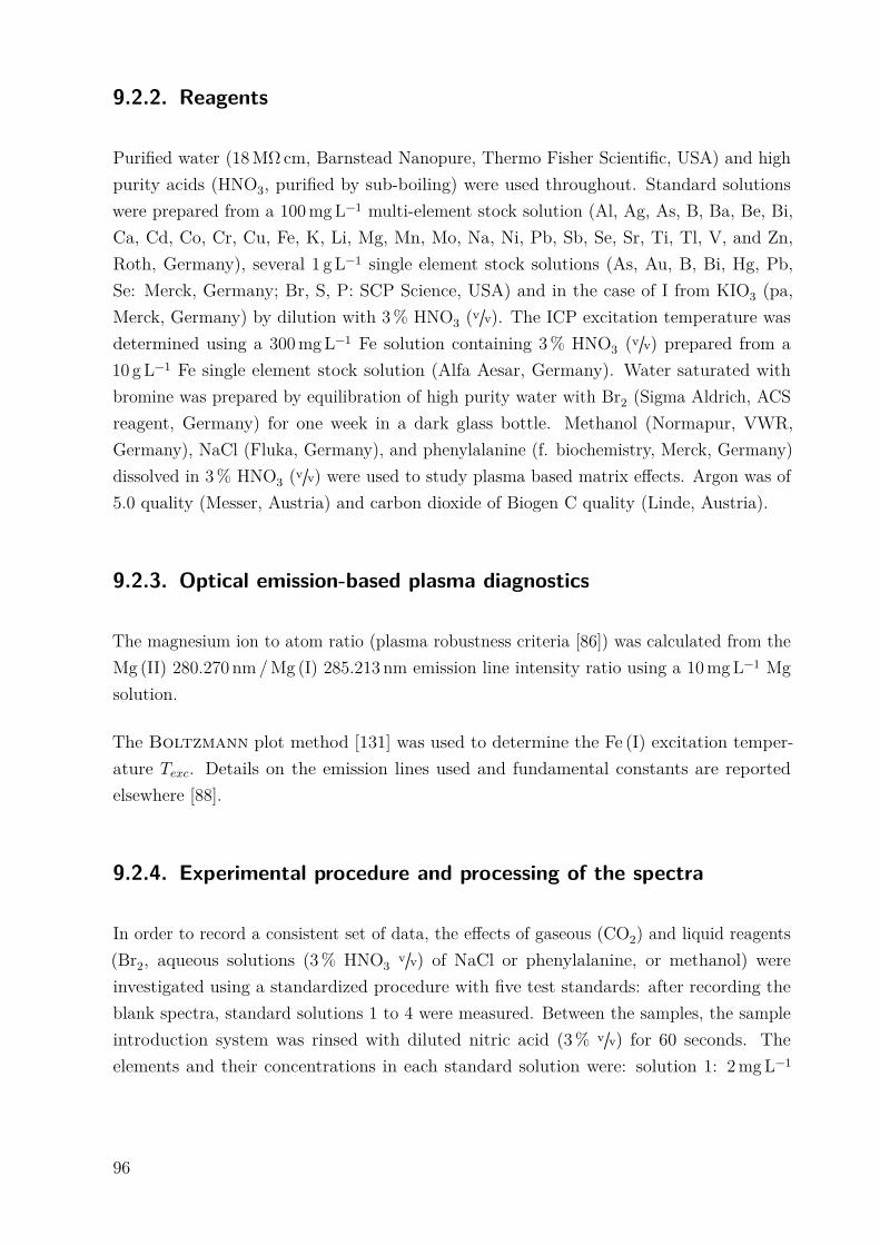
9.2.2. Reagents

Purified water (18MW cm, Barnstead Nanopure, Thermo Fisher Scientific, USA) and highpurity acids (HNO3, purified by sub-boiling) were used throughout. Standard solutionswere prepared from a 100mgL−1 multi-element stock solution (Al, Ag, As, B, Ba, Be, Bi,Ca, Cd, Co, Cr, Cu, Fe, K, Li, Mg, Mn, Mo, Na, Ni, Pb, Sb, Se, Sr, Ti, Tl, V, and Zn,Roth, Germany), several 1 g L−1 single element stock solutions (As, Au, B, Bi, Hg, Pb,Se: Merck, Germany; Br, S, P: SCP Science, USA) and in the case of I from KIO3 (pa,Merck, Germany) by dilution with 3% HNO3 (v/v). The ICP excitation temperature wasdetermined using a 300mgL−1 Fe solution containing 3% HNO3 (v/v) prepared from a10 gL−1 Fe single element stock solution (Alfa Aesar, Germany). Water saturated withbromine was prepared by equilibration of high purity water with Br2 (Sigma Aldrich, ACSreagent, Germany) for one week in a dark glass bottle. Methanol (Normapur, VWR,Germany), NaCl (Fluka, Germany), and phenylalanine (f. biochemistry, Merck, Germany)dissolved in 3% HNO3 (v/v) were used to study plasma based matrix effects. Argon was of5.0 quality (Messer, Austria) and carbon dioxide of Biogen C quality (Linde, Austria).

9.2.3. Optical emission-based plasma diagnostics

The magnesium ion to atom ratio (plasma robustness criteria [86]) was calculated from theMg (II) 280.270 nm/Mg (I) 285.213 nm emission line intensity ratio using a 10mgL−1 Mgsolution.

The Boltzmann plot method [131] was used to determine the Fe (I) excitation temper-ature Texc. Details on the emission lines used and fundamental constants are reportedelsewhere [88].

9.2.4. Experimental procedure and processing of the spectra

In order to record a consistent set of data, the effects of gaseous (CO2) and liquid reagents(Br2, aqueous solutions (3% HNO3 v/v) of NaCl or phenylalanine, or methanol) wereinvestigated using a standardized procedure with five test standards: after recording theblank spectra, standard solutions 1 to 4 were measured. Between the samples, the sampleintroduction system was rinsed with diluted nitric acid (3% v/v) for 60 seconds. Theelements and their concentrations in each standard solution were: solution 1: 2mgL−1

96

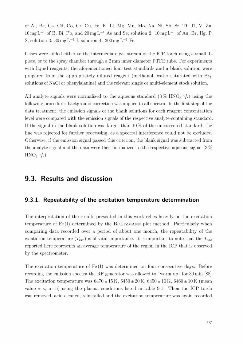
of Al, Be, Ca, Cd, Co, Cr, Cu, Fe, K, Li, Mg, Mn, Mo, Na, Ni, Sb, Sr, Ti, Tl, V, Zn,10mgL−1 of B, Bi, Pb, and 20mgL−1 As and Se; solution 2: 10mgL−1 of Au, Br, Hg, P,S; solution 3: 30mgL−1 I; solution 4: 300mgL−1 Fe.

Gases were added either to the intermediate gas stream of the ICP torch using a small T-piece, or to the spray chamber through a 2mm inner diameter PTFE tube. For experimentswith liquid reagents, the aforementioned four test standards and a blank solution wereprepared from the appropriately diluted reagent (methanol, water saturated with Br2,solutions of NaCl or phenylalanine) and the relevant single or multi-element stock solution.

All analyte signals were normalized to the aqueous standard (3% HNO3 v/v) using thefollowing procedure: background correction was applied to all spectra. In the first step of thedata treatment, the emission signals of the blank solutions for each reagent concentrationlevel were compared with the emission signals of the respective analyte-containing standard.If the signal in the blank solution was larger than 10% of the uncorrected standard, theline was rejected for further processing, as a spectral interference could not be excluded.Otherwise, if the emission signal passed this criterion, the blank signal was subtracted fromthe analyte signal and the data were then normalized to the respective aqueous signal (3%HNO3 v/v).

9.3. Results and discussion

9.3.1. Repeatability of the excitation temperature determination

The interpretation of the results presented in this work relies heavily on the excitationtemperature of Fe (I) determined by the Boltzmann plot method. Particularly whencomparing data recorded over a period of about one month, the repeatability of theexcitation temperature (Texc) is of vital importance. It is important to note that the Texcreported here represents an average temperature of the region in the ICP that is observedby the spectrometer.

The excitation temperature of Fe (I) was determined on four consecutive days. Beforerecording the emission spectra the RF generator was allowed to “warm up” for 30min [88].The excitation temperature was 6470 ± 15K, 6450 ± 20K, 6450 ± 10K, 6460 ± 10K (meanvalue ± s; n = 5) using the plasma conditions listed in table 9.1. Then the ICP torchwas removed, acid cleaned, reinstalled and the excitation temperature was again recorded

97

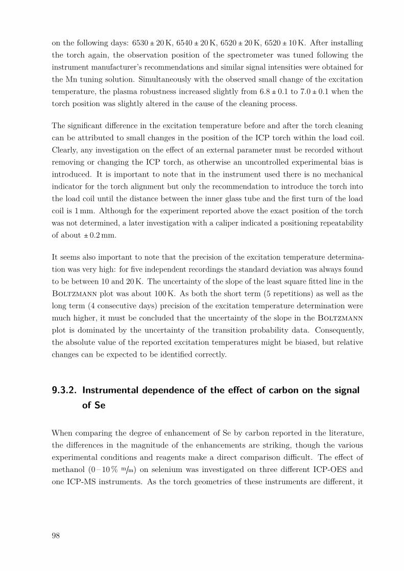
on the following days: 6530 ± 20K, 6540 ± 20K, 6520 ± 20K, 6520 ± 10K. After installingthe torch again, the observation position of the spectrometer was tuned following theinstrument manufacturer’s recommendations and similar signal intensities were obtained forthe Mn tuning solution. Simultaneously with the observed small change of the excitationtemperature, the plasma robustness increased slightly from 6.8 ± 0.1 to 7.0 ± 0.1 when thetorch position was slightly altered in the cause of the cleaning process.

The significant difference in the excitation temperature before and after the torch cleaningcan be attributed to small changes in the position of the ICP torch within the load coil.Clearly, any investigation on the effect of an external parameter must be recorded withoutremoving or changing the ICP torch, as otherwise an uncontrolled experimental bias isintroduced. It is important to note that in the instrument used there is no mechanicalindicator for the torch alignment but only the recommendation to introduce the torch intothe load coil until the distance between the inner glass tube and the first turn of the loadcoil is 1mm. Although for the experiment reported above the exact position of the torchwas not determined, a later investigation with a caliper indicated a positioning repeatabilityof about ± 0.2mm.

It seems also important to note that the precision of the excitation temperature determina-tion was very high: for five independent recordings the standard deviation was always foundto be between 10 and 20K. The uncertainty of the slope of the least square fitted line in theBoltzmann plot was about 100K. As both the short term (5 repetitions) as well as thelong term (4 consecutive days) precision of the excitation temperature determination weremuch higher, it must be concluded that the uncertainty of the slope in the Boltzmannplot is dominated by the uncertainty of the transition probability data. Consequently,the absolute value of the reported excitation temperatures might be biased, but relativechanges can be expected to be identified correctly.

9.3.2. Instrumental dependence of the effect of carbon on the signalof Se

When comparing the degree of enhancement of Se by carbon reported in the literature,the differences in the magnitude of the enhancements are striking, though the variousexperimental conditions and reagents make a direct comparison difficult. The effect ofmethanol (0 – 10% m/m) on selenium was investigated on three different ICP-OES andone ICP-MS instruments. As the torch geometries of these instruments are different, it

98

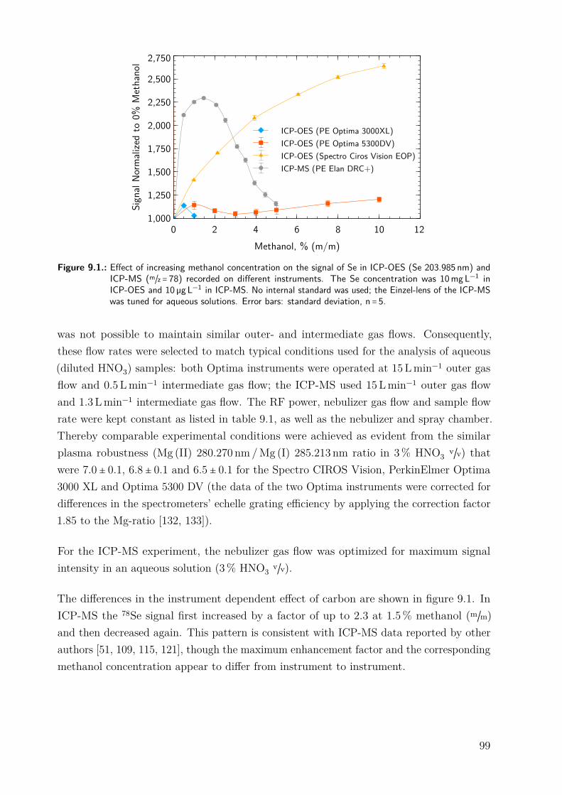
ICP-OES (PE Optima 3000XL)ICP-OES (PE Optima 5300DV)ICP-OES (Spectro Ciros Vision EOP)ICP-MS (PE Elan DRC+)

Sign

al No

rmali

zed

to 0

% M

etha

nol

1,000

1,250

1,500

1,750

2,000

2,250

2,500

2,750

Methanol, % (m/m)0 2 4 6 8 10 12

Figure 9.1.: Effect of increasing methanol concentration on the signal of Se in ICP-OES (Se 203.985 nm) andICP-MS (m/z = 78) recorded on different instruments. The Se concentration was 10mgL−1 inICP-OES and 10 µg L−1 in ICP-MS. No internal standard was used; the Einzel-lens of the ICP-MSwas tuned for aqueous solutions. Error bars: standard deviation, n = 5.

was not possible to maintain similar outer- and intermediate gas flows. Consequently,these flow rates were selected to match typical conditions used for the analysis of aqueous(diluted HNO3) samples: both Optima instruments were operated at 15Lmin−1 outer gasflow and 0.5 Lmin−1 intermediate gas flow; the ICP-MS used 15Lmin−1 outer gas flowand 1.3 Lmin−1 intermediate gas flow. The RF power, nebulizer gas flow and sample flowrate were kept constant as listed in table 9.1, as well as the nebulizer and spray chamber.Thereby comparable experimental conditions were achieved as evident from the similarplasma robustness (Mg (II) 280.270 nm/Mg (I) 285.213 nm ratio in 3% HNO3 v/v) thatwere 7.0 ± 0.1, 6.8 ± 0.1 and 6.5 ± 0.1 for the Spectro CIROS Vision, PerkinElmer Optima3000 XL and Optima 5300 DV (the data of the two Optima instruments were corrected fordifferences in the spectrometers’ echelle grating efficiency by applying the correction factor1.85 to the Mg-ratio [132, 133]).

For the ICP-MS experiment, the nebulizer gas flow was optimized for maximum signalintensity in an aqueous solution (3% HNO3 v/v).

The differences in the instrument dependent effect of carbon are shown in figure 9.1. InICP-MS the 78Se signal first increased by a factor of up to 2.3 at 1.5% methanol (m/m)and then decreased again. This pattern is consistent with ICP-MS data reported by otherauthors [51, 109, 115, 121], though the maximum enhancement factor and the correspondingmethanol concentration appear to differ from instrument to instrument.

99

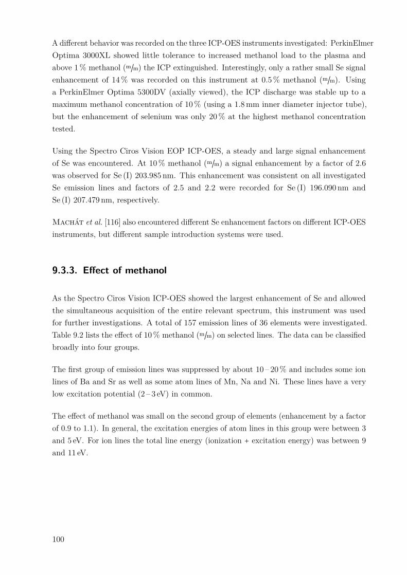
A different behavior was recorded on the three ICP-OES instruments investigated: PerkinElmerOptima 3000XL showed little tolerance to increased methanol load to the plasma andabove 1% methanol (m/m) the ICP extinguished. Interestingly, only a rather small Se signalenhancement of 14% was recorded on this instrument at 0.5% methanol (m/m). Usinga PerkinElmer Optima 5300DV (axially viewed), the ICP discharge was stable up to amaximum methanol concentration of 10% (using a 1.8mm inner diameter injector tube),but the enhancement of selenium was only 20% at the highest methanol concentrationtested.

Using the Spectro Ciros Vision EOP ICP-OES, a steady and large signal enhancementof Se was encountered. At 10% methanol (m/m) a signal enhancement by a factor of 2.6was observed for Se (I) 203.985 nm. This enhancement was consistent on all investigatedSe emission lines and factors of 2.5 and 2.2 were recorded for Se (I) 196.090 nm andSe (I) 207.479 nm, respectively.

Machát et al. [116] also encountered different Se enhancement factors on different ICP-OESinstruments, but different sample introduction systems were used.

9.3.3. Effect of methanol

As the Spectro Ciros Vision ICP-OES showed the largest enhancement of Se and allowedthe simultaneous acquisition of the entire relevant spectrum, this instrument was usedfor further investigations. A total of 157 emission lines of 36 elements were investigated.Table 9.2 lists the effect of 10% methanol (m/m) on selected lines. The data can be classifiedbroadly into four groups.

The first group of emission lines was suppressed by about 10 – 20% and includes some ionlines of Ba and Sr as well as some atom lines of Mn, Na and Ni. These lines have a verylow excitation potential (2 – 3 eV) in common.

The effect of methanol was small on the second group of elements (enhancement by a factorof 0.9 to 1.1). In general, the excitation energies of atom lines in this group were between 3and 5 eV. For ion lines the total line energy (ionization + excitation energy) was between 9and 11 eV.

100

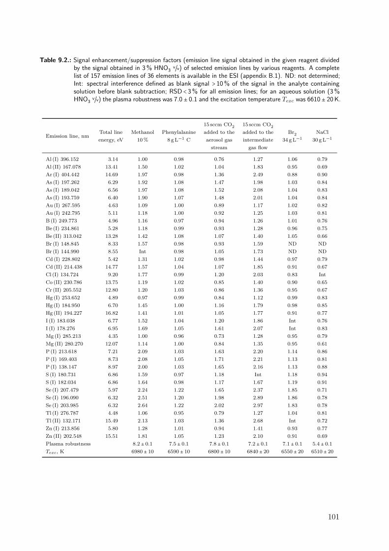
Table 9.2.: Signal enhancement/suppression factors (emission line signal obtained in the given reagent dividedby the signal obtained in 3% HNO3 v/v) of selected emission lines by various reagents. A completelist of 157 emission lines of 36 elements is available in the ESI (appendix B.1). ND: not determined;Int: spectral interference defined as blank signal > 10% of the signal in the analyte containingsolution before blank subtraction; RSD < 3% for all emission lines; for an aqueous solution (3%HNO3 v/v) the plasma robustness was 7.0 ± 0.1 and the excitation temperature Texc was 6610 ± 20K.

Emission line, nmTotal lineenergy, eV

Methanol10%

Phenylalanine8 gL−1 C

15 sccm CO2added to theaerosol gasstream

15 sccm CO2added to theintermediategas flow

Br234 gL−1

NaCl30 gL−1

Al (I) 396.152 3.14 1.00 0.98 0.76 1.27 1.06 0.79Al (II) 167.078 13.41 1.50 1.02 1.04 1.83 0.95 0.69Ar (I) 404.442 14.69 1.97 0.98 1.36 2.49 0.88 0.90As (I) 197.262 6.29 1.92 1.08 1.47 1.98 1.03 0.84As (I) 189.042 6.56 1.97 1.08 1.52 2.08 1.04 0.83As (I) 193.759 6.40 1.90 1.07 1.48 2.01 1.04 0.84Au (I) 267.595 4.63 1.09 1.00 0.89 1.17 1.02 0.82Au (I) 242.795 5.11 1.18 1.00 0.92 1.25 1.03 0.81B (I) 249.773 4.96 1.16 0.97 0.94 1.26 1.01 0.76Be (I) 234.861 5.28 1.18 0.99 0.93 1.28 0.96 0.75Be (II) 313.042 13.28 1.42 1.08 1.07 1.40 1.05 0.66Br (I) 148.845 8.33 1.57 0.98 0.93 1.59 ND NDBr (I) 144.990 8.55 Int 0.98 1.05 1.73 ND NDCd (I) 228.802 5.42 1.31 1.02 0.98 1.44 0.97 0.79Cd (II) 214.438 14.77 1.57 1.04 1.07 1.85 0.91 0.67Cl (I) 134.724 9.20 1.77 0.99 1.20 2.03 0.83 IntCo (II) 230.786 13.75 1.19 1.02 0.85 1.40 0.90 0.65Cr (II) 205.552 12.80 1.20 1.03 0.86 1.36 0.95 0.67Hg (I) 253.652 4.89 0.97 0.99 0.84 1.12 0.99 0.83Hg (I) 184.950 6.70 1.45 1.00 1.16 1.79 0.98 0.85Hg (II) 194.227 16.82 1.41 1.01 1.05 1.77 0.91 0.77I (I) 183.038 6.77 1.52 1.04 1.20 1.86 Int 0.76I (I) 178.276 6.95 1.69 1.05 1.61 2.07 Int 0.83Mg (I) 285.213 4.35 1.00 0.96 0.73 1.28 0.95 0.79Mg (II) 280.270 12.07 1.14 1.00 0.84 1.35 0.95 0.61P (I) 213.618 7.21 2.09 1.03 1.63 2.20 1.14 0.86P (I) 169.403 8.73 2.08 1.05 1.71 2.21 1.13 0.81P (I) 138.147 8.97 2.00 1.03 1.65 2.16 1.13 0.88S (I) 180.731 6.86 1.59 0.97 1.18 Int 1.18 0.94S (I) 182.034 6.86 1.64 0.98 1.17 1.67 1.19 0.91Se (I) 207.479 5.97 2.24 1.22 1.65 2.37 1.85 0.71Se (I) 196.090 6.32 2.51 1.20 1.98 2.89 1.86 0.78Se (I) 203.985 6.32 2.64 1.22 2.02 2.97 1.83 0.78Tl (I) 276.787 4.48 1.06 0.95 0.79 1.27 1.04 0.81Tl (II) 132.171 15.49 2.13 1.03 1.36 2.68 Int 0.72Zn (I) 213.856 5.80 1.28 1.01 0.94 1.41 0.93 0.77Zn (II) 202.548 15.51 1.81 1.05 1.23 2.10 0.91 0.69Plasma robustness 8.2 ± 0.1 7.5 ± 0.1 7.8 ± 0.1 7.2 ± 0.1 7.1 ± 0.1 5.4 ± 0.1Texc, K 6980 ± 10 6590 ± 10 6800 ± 10 6840 ± 20 6550 ± 20 6510 ± 20

101

The third group of emission lines was enhanced by about 20 – 50%. The excitation energyof these lines was in general between 5 and 6 eV and the total line energy of ion lines wasbetween 11 and 14 eV.

Signal enhancements compared to an aqueous solution (3% HNO3 v/v) of more than 50%were observed for atom lines with an excitation potential greater than 6 eV and for somehigh energy ion lines in the region of about 15.5 eV. This fourth group included the atomlines of Ar, As, Br, Cl, I, P, S, and Se as well as some high energy ion lines of Ag, Cd, Tl,and Zn.

It is important to note that the listed energy ranges of the four groups are not sharplydefined and that some emission lines do not follow the listed general trend. Moreover, thereis no clear correlation between the total line energy (excitation potential for atom lines)and the enhancement, but only a trend.

The power drawn by the RF generator plotted as a function of the methanol concentrationnebulized during the measurement is shown in figure 9.2a. The Huth-Kühn type poweroscillator used is current controlled. For every RF power level that can be selected in theinstrument software, a corresponding current is set by the HV power supply. The currentis derived from a factory power calibration. The power oscillator behaves purely resistiveduring normal operation – Ohm’s law therefore applies and the power drawn by the poweroscillator is the product of current (RMS) and voltage (RMS) read directly from the HVpower supply.

From figure 9.2a it is evident that with increasing methanol concentration the power drawnby the RF generator increases significantly (about 250W when changing from diluted nitricacid (3% HNO3 v/v) to 10% methanol). As expected from a current controlled poweroscillator, the power vacuum tube plate current remained constant, but the plate voltageincreased from 3565V to 4000V when the sample solution was switched from 3% HNO3

(v/v) to 10% methanol (m/m). At the same time the frequency of the power oscillatordecreased by 26.1 kHz. It seems interesting to note that for aqueous aerosols an increase ofthe RF generator power is accompanied by a small increase in the frequency. The observedlinear decrease of the RF generator frequency (figure 9.2b) and the simultaneous linearincrease in the power uptake when the methanol concentration in the sample solutionis increased indicates destabilization of the plasma as also observed previously [88]. Inaddition, this can also be concluded from the rising SDs of the plate voltage that increasedthe SDs of the generator input power when the methanol concentration rose.

102

RF G

ener

ator

Inpu

t Pow

er, W

2000

2100

2200

2300

2400

Methanol, % (m/m)0 2 4 6 8 10 12

(a)

RF G

ener

ator

Fre

quen

cy, M

Hz

26,920

26,925

26,930

26,935

26,940

26,945

26,950

Methanol, % (m/m)0 2 4 6 8 10 12

(b)

Figure 9.2.: Power drawn by the RF generator for a nominal output of 1350W (a) and frequency response ofthe generator (b) as a function of the methanol concentration nebulized during measurement. Theerror bars represent the standard deviation of five independent experiments.

103

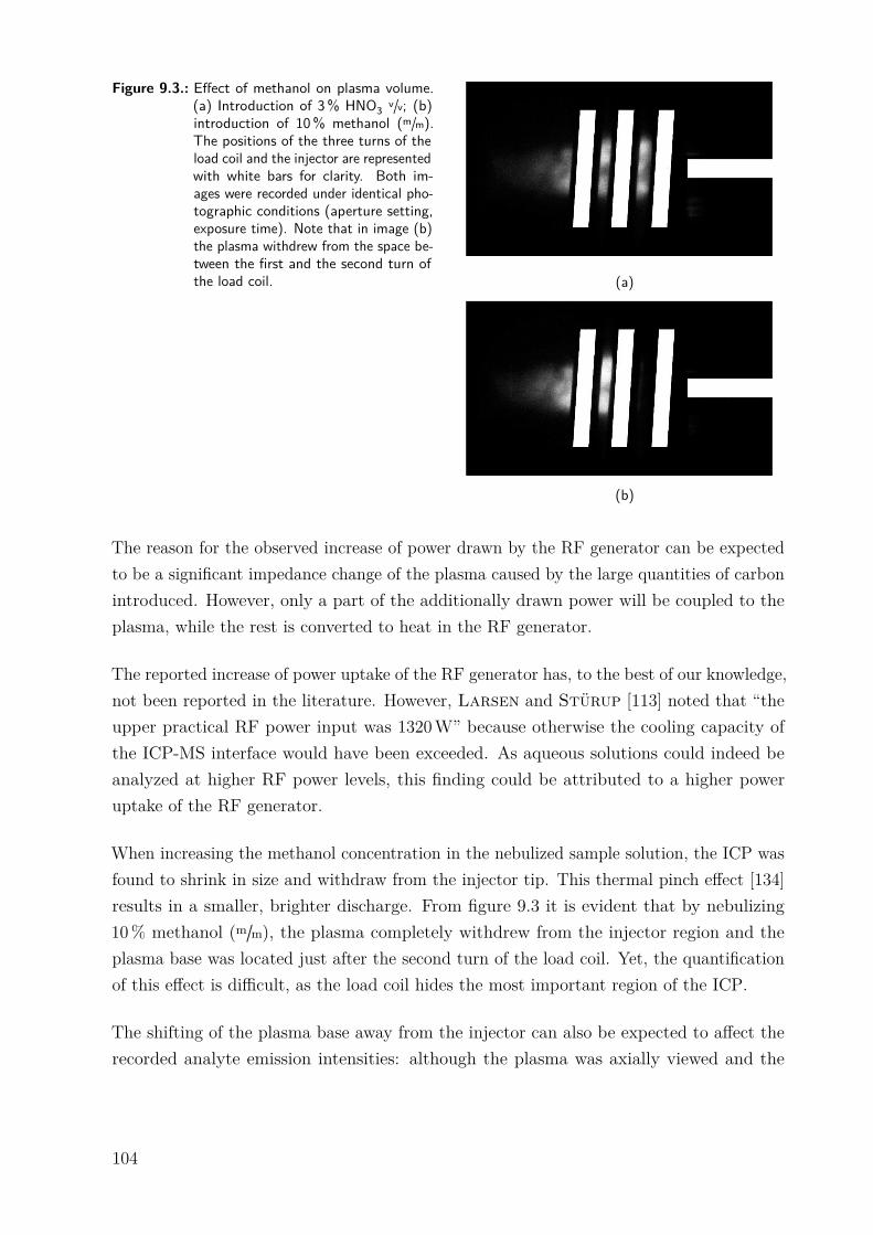
Figure 9.3.: Effect of methanol on plasma volume.(a) Introduction of 3% HNO3 v/v; (b)introduction of 10% methanol (m/m).The positions of the three turns of theload coil and the injector are representedwith white bars for clarity. Both im-ages were recorded under identical pho-tographic conditions (aperture setting,exposure time). Note that in image (b)the plasma withdrew from the space be-tween the first and the second turn ofthe load coil. (a)

(b)

The reason for the observed increase of power drawn by the RF generator can be expectedto be a significant impedance change of the plasma caused by the large quantities of carbonintroduced. However, only a part of the additionally drawn power will be coupled to theplasma, while the rest is converted to heat in the RF generator.

The reported increase of power uptake of the RF generator has, to the best of our knowledge,not been reported in the literature. However, Larsen and Stürup [113] noted that “theupper practical RF power input was 1320W” because otherwise the cooling capacity ofthe ICP-MS interface would have been exceeded. As aqueous solutions could indeed beanalyzed at higher RF power levels, this finding could be attributed to a higher poweruptake of the RF generator.

When increasing the methanol concentration in the nebulized sample solution, the ICP wasfound to shrink in size and withdraw from the injector tip. This thermal pinch effect [134]results in a smaller, brighter discharge. From figure 9.3 it is evident that by nebulizing10% methanol (m/m), the plasma completely withdrew from the injector region and theplasma base was located just after the second turn of the load coil. Yet, the quantificationof this effect is difficult, as the load coil hides the most important region of the ICP.

The shifting of the plasma base away from the injector can also be expected to affect therecorded analyte emission intensities: although the plasma was axially viewed and the

104

viewing depth was not changed, the zone within the ICP imaged onto the entrance slit ofthe spectrometer will follow the shift of the plasma base to some extent. Simultaneouslythe plasma power density changed the behavior of the emission lines, which is not easilypredictable. Chan and Hieftje [135] showed that the magnitude of matrix effects in theICP is not constant when changing the observed location within the ICP. However, the largefocal length of the spectrometer’s entrance optics might reduce this effect when comparedto the plasma cross-sections investigated by Chan and Hieftje or radial viewing.

In conclusion, the large quantities of carbon introduced by nebulizing 10% methanol alteredplasma impedance and thereby led to an increase of the power vacuum tube’s plate voltage.This in turn increased the RF power delivered to the ICP. Simultaneously, the plasmadecreased in size and became hotter as evident from the rise in the excitation temperaturefrom 6610 ± 20K (3% HNO3 v/v) to 6980 ± 10K (10% methanol). It is apparent that anincrease of RF power delivered to the ICP combined with a decrease of the plasma volumeis associated with a change in the analyte emission signal intensity.

While all analyte emission lines that were significantly enhanced by carbon showed a steadysignal increase with rising methanol concentration, plasma robustness only increased upto 6% methanol (m/m) (peak value 8.8) and then decreased again to 8.2 at 10% methanol(m/m).

One of the inherent problems of using methanol as the source of carbon is the difficulty ofquantifying the exact amount of carbon introduced into the ICP. The density of all methanolcontaining solutions was measured prior to the introduction into the spray chamber and inthe waste solution that left the spray chamber after system equilibration.

Moreover, the mass flow of aerosol leaving the spray chamber was determined by themethod of continuous weighing. From these data a mass balance was calculated assuminga constant liquid flow rate from the peristaltic pump of 1.82mLmin−1: by subtracting themass flow of methanol in the drained solution from the mass flow of methanol pumpedto the spray chamber the mass flow of methanol introduced into the ICP was calculated.Using this method corrects for differences in aerosol formation and preferential evaporationof methanol from the surface of the spray chamber and aerosol droplets. Mora et al. [136]found that the D50 (droplet distribution diameter below which 50% of the cumulativeaerosol volume is found) of the primary aerosol of a water–methanol mixture decreaseswith increasing methanol content of the mixture. However, this effect was found to berather small (D50 changed by 3%) when comparing water with 10% methanol.

105

The carbon mass flow introduced into the ICP increased almost linearly with rising methanolconcentration in the sample solution fed to the nebulizer. However, below 4% methanol(m/m) the function bends, indicating less pronounced vaporization of methanol in the spraychamber. At the maximum concentration of 10% methanol (m/m), 8.4mgmin−1 carbon wasintroduced into the ICP. The uncertainty of this calculation was found to be dominatedby the method of continuous weighing: whereas the removal of the liquid from the samplebeaker was constant with time, the draining of the waste solution was discontinuous, asindividual droplets formed on the lower end of the Scott-type spray chamber’s inner tube.Thereby a fluctuating signal was created. The error of the slope was below 6% for the usedrecording time of 10 minutes.

It is interesting to note, that without the described correction for the preferential vaporiza-tion of methanol in the spray chamber the mass flow of carbon introduced into the ICPwould have been underestimated by a factor of 1.7.

9.3.4. Effect of phenylalanine and CO2

Methanol is a volatile liquid that is introduced into the ICP not only as a liquid containedin the aerosol but also as vapor. Though the total mass flow of methanol transported to theICP was quantified, we attempted to separate the effects of these two phases on the analytesignal. Firstly, carbon was introduced in the form of a polar, well-soluble but non-volatilesubstance – phenylalanine was chosen for this purpose. Secondly, a gaseous carbon source(CO2) was investigated, whereby any nebulization-induced bias could be excluded. CO2

was added either to the aerosol or to the intermediate gas stream.

As shown in table 9.2 the effects of these three carbon sources on the investigated analytesare quite different: 8 g L−1 carbon introduced into the ICP as phenylalanine did notchange the signal intensity of most investigated emission lines by more than 5%. Theonly exceptions were As, Be (II), and Se with signal enhancements of 10 – 20%. It is alsointeresting to note that of all carbon containing reagents investigated only phenylalaninedid not alter the emission intensity of the Ar (I) 404.442 nm emission line. Phenylalanineneither changed the excitation temperature significantly nor did it alter the RF generatorfrequency appreciably (about 1 kHz). The power vacuum tube’s plate voltage also remainedconstant. Combined, these facts suggest that carbon introduced as phenylalanine did notalter the plasma impedance and the enhancement of As, Be (II), and Se is not causedby changes in the ICP itself, as observed when using methanol as the carbon source. Itis important to note that the enhancement of As, Be (II), and Se increased with greater

106

phenylalanine concentration in the solution, reaching its maximum at the highest testedreagent concentration (close to the limit of solubility).

In contrast to phenylalanine, CO2 as the gaseous carbon source showed a markedly differentbehavior, as listed in table 9.2. When introduced into the aerosol gas stream, a signalenhancement pattern comparable to that of methanol was recorded, although the signalenhancement factors were between 20 and 40% lower than when using methanol as thecarbon source. The excitation temperature was lower too (6800 ± 10K vs. 6980 ± 10K).Similar to methanol, a pronounced thermal pinch effect was observed when increasing theflow of CO2. The plasma impedance was also found to change, as evident from the higherpower vacuum tube plate voltage (at 15 sccm a plate voltage of 3993V was recorded). Thefrequency of the power oscillator decreased by 28.9 kHz when switching from 0 to 15 sccmCO2. When CO2 was introduced into the intermediate gas flow of the ICP, 5 – 20% highersignal enhancement factors were encountered when compared to methanol, as listed intable 9.2. The excitation temperature was slightly higher and the plasma robustness waslower. Just as with methanol, when CO2 was introduced into the aerosol gas stream, astrong thermal pinch effect was observed, which again was accompanied by high platevoltage and frequency excursion (3950V and 27.4 kHz).

In figure 9.5a the carbon emission signal (C (I) 193.091 nm) of the investigated carbonsources is plotted as a function of the carbon mass flow delivered to the ICP. This massflow was calculated from the determined nebulization efficiency in the case of phenylalanine,or by using the ideal gas law for CO2. For methanol, the method described above that alsoincludes the preferential vaporization was used. The emission signals did not increase in alinear fashion as the mass flow of carbon was extremely high. For CO2 the C emission signalwas surprisingly similar, despite the different gas flows it was introduced into. Althoughbelow 5.5mgmin−1 carbon from CO2, the C emission signal was higher when introducingthe gas into the aerosol stream rather than into the intermediate stream, the differencewas only about 30% at 1mgmin−1 and 9% at 2.7mgmin−1. From figure 9.5b it can bededuced that CO2 introduced into the intermediate gas stream of the ICP acts stronger onthe plasma core than when introduced into the aerosol gas stream, as the power vacuumtube’s plate voltage rises faster due to the impedance changes of the plasma core. Asalready noted, higher C-loading of the ICP caused the base of the discharge – the regionwhere the aerosol gas stream enters the plasma – to withdraw from the region betweenthe end of the injector tube and the first turn of the load coil (“normal position”) to thespace between the first and the second turn of the load coil (thermal pinch effect). Theincreased distance between the injector tube and the base of the ICP can be expected toallow a higher diffusional exchange between the aerosol and the intermediate gas stream.

107

Thereby the carbon loading is not restricted to one of these streams, explaining the observedeffects.

Another interesting feature shown in figure 9.5 is the effect of low concentrations of methanolon the ICP. Whereas high C loading resulting from methanol causes comparable effectson the plate voltage to similar mass flows of C from CO2, low concentrations of methanolshowed significantly less effect on the plate voltage than in the case of CO2. This trendwas even stronger for phenylalanine, where no effect on the plate voltage was found. Theseeffects could be explained by considering that phenylalanine is introduced only in the formof an aerosol. Carbon is released only after decomposition inside the analyte channel andconsequently the diffusion of C into the plasma core can be expected to start much laterthan in the case of a similar mass flow of CO2. Thereby, the mass of C reaching the plasmacore is much lower and the plate voltage reflects this trend. Following this hypothesis, twoprocesses must be considered in the case of methanol: the vapor phase behaves similarlyto gaseous reagents (CO2) whereas the methanol inside the liquid droplets of the aerosolbehaves like phenylalanine. At low methanol concentrations the evaporation of methanolin the spray chamber is not as dominant as at higher concentrations; the lower C emissionsignal and the smaller change in plate voltage for 1.7mgmin−1 C from methanol can berelated to this mechanism.

Generally speaking, the enhancement factors of As and Se reported in the literature for non-volatile carbon sources (glucose, citric acid, oxalic acid or glycerol) were always lower thanfor more volatile reagents such as methanol or even for gases (CH4), both in ICP-OES [110,116, 117] and in ICP-MS [51, 61, 109, 112, 113, 115, 119–121].

9.3.5. Effect of bromine

As already noted many attempts to explain the signal enhancing effect of carbon rely onthe hypothesis of a charge transfer between C+ and the high IP element. If carbon with anIP of 11.26 eV is behaving in this manner, Br with an IP of 11.81 eV can be expected toshow similar effects.

In contrast to previous reports [116] we wanted to avoid variations in the nebulizationefficiency and therefore used water saturated with bromine rather than HBr. Sevenconcentration levels (0 – 34 gL−1 Br2) were prepared from bromine-saturated water. TheBr2 concentration was calculated assuming a solubility of Br2 in water [137] of 33.56 g L−1.All bromine concentrations given below correspond to the mass of bromine dissolved in

108

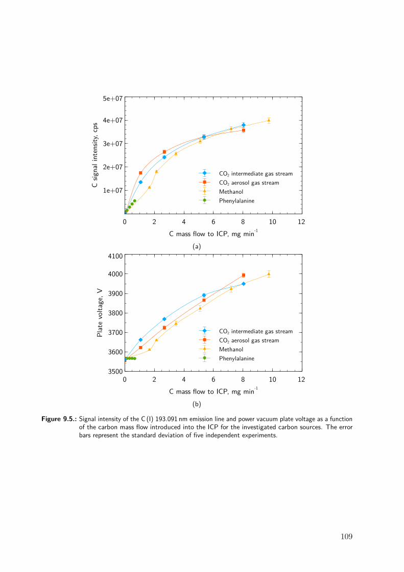
CO2 intermediate gas streamCO2 aerosol gas streamMethanolPhenylalanine

C sig

nal i

nten

sity,

cps

1e+07

2e+07

3e+07

4e+07

5e+07

C mass flow to ICP, mg min-10 2 4 6 8 10 12

(a)

CO2 intermediate gas streamCO2 aerosol gas streamMethanolPhenylalanine

Plat

e vo

ltage

, V

3500

3600

3700

3800

3900

4000

4100

C mass flow to ICP, mg min-10 2 4 6 8 10 12

(b)

Figure 9.5.: Signal intensity of the C (I) 193.091 nm emission line and power vacuum plate voltage as a functionof the carbon mass flow introduced into the ICP for the investigated carbon sources. The errorbars represent the standard deviation of five independent experiments.

109

water. Due to the toxicity of bromine, we have not attempted to quantify the mass flow ofbromine reaching the plasma.

Bromine had little to no effect on most of the investigated emission lines. The signalintensities recorded in a 34 gL−1 Br2 solution differed by less than ± 10% from the signalrecorded from an aqueous solution (3% HNO3 v/v). The only exceptions were P, S and Se.For P and S the signal intensities initially rose quickly with increasing Br2 concentrationreaching a plateau at about 3.4 g L−1 Br2 with signal intensities of about 13% and 20% (Pand S respectively) higher than in an aqueous standard. For Se the signal increased almostlinearly up to 6.7 g L−1 Br2 (67% higher signal than in diluted nitric acid) and then leveledoff, reaching about 85% signal enhancement at 34 gL−1 Br2. It is most interesting to notethat neither As was enhanced by Br2, nor were Au or Hg.

Plasma robustness and the excitation temperature remained constant when switching froman aqueous solution (3% HNO3 v/v) to 34 gL−1 Br2 and neither the plate voltage nor thepower drawn by the RF generator changed significantly. The frequency of the RF generatordropped slightly but significantly by 2.6 kHz.

From these findings it must be concluded that the introduction of bromine did not affectthe RF generator and it can be assumed that the power delivered to the ICP remainedunchanged. The signal enhancement of P, S and particularly Se cannot be attributedto changes in the nebulization efficiency as other elements would have been affected too.Therefore, the effect of bromine on P, S and Se appears to be a true matrix effect of bromineon these three elements.

If a charge transfer process is the underlying mechanism of the observed effects, twoconditions must be met: firstly, the Wigner spin conservation rule [138] must be fulfilled;secondly, the reaction energy defect should be minimal. Grindlay et al. [73] assumedthat this type of reaction is likely to happen if the involved energy levels differ by between−1.0 eV and +0.5 eV.

From the data listed in table 9.3 we can draw the conclusion that the Wigner spinconservation rule is fulfilled for every examined element. However, the energy differencebetween the involved levels appears to explain most of the observed effects of bromine:with the exception of Au, I, P, S, and Se the energy difference between the involved levelsis too large. Iodine was not investigated, as the Br2 used was slightly contaminated withthis element. For P, S and Se a signal enhancement was observed that could consequentlybe attributed to a charge transfer reaction. However, for Au no significant signal increase

110

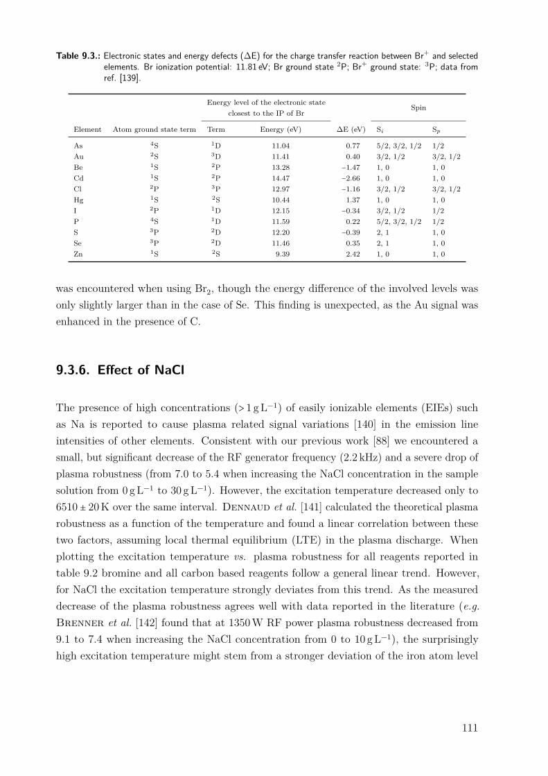
Table 9.3.: Electronic states and energy defects (∆E) for the charge transfer reaction between Br+ and selectedelements. Br ionization potential: 11.81 eV; Br ground state 2P; Br+ ground state: 3P; data fromref. [139].

Energy level of the electronic stateclosest to the IP of Br

Spin

Element Atom ground state term Term Energy (eV) ∆E (eV) Si Sp

As 4S 1D 11.04 0.77 5/2, 3/2, 1/2 1/2Au 2S 3D 11.41 0.40 3/2, 1/2 3/2, 1/2Be 1S 2P 13.28 −1.47 1, 0 1, 0Cd 1S 2P 14.47 −2.66 1, 0 1, 0Cl 2P 3P 12.97 −1.16 3/2, 1/2 3/2, 1/2Hg 1S 2S 10.44 1.37 1, 0 1, 0I 2P 1D 12.15 −0.34 3/2, 1/2 1/2P 4S 1D 11.59 0.22 5/2, 3/2, 1/2 1/2S 3P 2D 12.20 −0.39 2, 1 1, 0Se 3P 2D 11.46 0.35 2, 1 1, 0Zn 1S 2S 9.39 2.42 1, 0 1, 0

was encountered when using Br2, though the energy difference of the involved levels wasonly slightly larger than in the case of Se. This finding is unexpected, as the Au signal wasenhanced in the presence of C.

9.3.6. Effect of NaCl

The presence of high concentrations (> 1 gL−1) of easily ionizable elements (EIEs) suchas Na is reported to cause plasma related signal variations [140] in the emission lineintensities of other elements. Consistent with our previous work [88] we encountered asmall, but significant decrease of the RF generator frequency (2.2 kHz) and a severe drop ofplasma robustness (from 7.0 to 5.4 when increasing the NaCl concentration in the samplesolution from 0 gL−1 to 30 gL−1). However, the excitation temperature decreased only to6510 ± 20K over the same interval. Dennaud et al. [141] calculated the theoretical plasmarobustness as a function of the temperature and found a linear correlation between thesetwo factors, assuming local thermal equilibrium (LTE) in the plasma discharge. Whenplotting the excitation temperature vs. plasma robustness for all reagents reported intable 9.2 bromine and all carbon based reagents follow a general linear trend. However,for NaCl the excitation temperature strongly deviates from this trend. As the measureddecrease of the plasma robustness agrees well with data reported in the literature (e.g.Brenner et al. [142] found that at 1350W RF power plasma robustness decreased from9.1 to 7.4 when increasing the NaCl concentration from 0 to 10 gL−1), the surprisinglyhigh excitation temperature might stem from a stronger deviation of the iron atom level

111

population from the Boltzmann distribution and the associated departure from the LTE.However, the Boltzmann plots of the Fe (I) lines were not significantly curved (calculationbased on an f-test of the residual standard deviations of the Boltzmann plot using either aliner fit or a second order polynomial fit) as reported by Kitagawa and Horlick [143].

The investigated emission lines were in general all suppressed by large quantities of NaCl(30 gL−1) as shown in table 9.2. In contrast to the effect of C, the power vacuum tube’splate voltage remained constant up to about 6 gL−1 and then dropped almost linearly by50V towards the highest investigated NaCl concentration of 30 gL−1. Though this dropis significant, the suppression of the analyte emission signals cannot be related to thisreduction in RF power, as the drop of 50V corresponds to a reduction of the RF generatorinput power of only about 30W.

9.3.7. Differentiating between the factors contributing to the carbonenhancement effect

From the foregoing discussion it can be concluded that the signal enhancing effect of carbonon several elements is a combination of changes in the excitation equilibrium (e.g. causedby a charge transfer reaction) and higher plasma power density. The latter stems from RFgenerator control issues and the thermal pinch effect.

In an attempt to discriminate between these two effects, solutions containing As, Au, Be, Br,Cl, Hg, P, S, and Se (concentration of each element similar to the previously used standardsolutions) in either 3% HNO3 (v/v) or 10% methanol (m/m) together with the respectiveblank solutions (only diluted nitric acid or 10% methanol) were measured at constant torchgas flows (as listed in table 9.1) but at different RF power levels (1300 – 1495W; 50Wincrements; setting a higher power level than 1495W was not possible, as the instrumentcontrol software then increased the outer gas flow in an attempt to protect the torch).

As expected, a rising RF power level resulted, in both 3% HNO3 (v/v) and methanol, inan increase of the blank signal corrected analyte emission intensity. However, distinctdifferences were encountered between the investigated emission lines: methanol had littleeffect on low excitation energy (4 – 5 eV) atom lines (e.g. Au (I) 267.595 or Hg (I) 253.652 nm)as the signal intensity was similar to that in 3% HNO3 (v/v). This finding is consistentwith data presented in table 9.2. For emission lines of higher excitation energy the analyteemission signal in methanol was always higher than in the corresponding aqueous standardfor all RF power levels. This effect became more pronounced with increasing total emission

112

line energy, although only a general trend was encountered but no function was found tosufficiently fit all data points. When plotting the signal intensity for each emission line as afunction of the RF power level used, straight lines were obtained (R2 > 0.999). The slope ofthese lines was always lower in methanol when compared to aqueous solutions. From thisfinding it can be concluded that the magnitude of the carbon enhancement effect is alsodependent on the RF power level used. A similar observation has been reported by Kraljand Veber [121].

To separate the effects of increased plasma power density and changes in the emission lineexcitation equilibrium on the analyte signal, the RF power vs. emission line intensity plotscan be used. When assuming that there is no change in the excitation equilibrium bymethanol (e.g. by a charge transfer reaction), any change in the emission signal caused bymethanol would be dependent on the power density in the ICP discharge. Consequently,“apparent” RF power levels can be calculated from the RF power vs. emission line intensityplots of aqueous standards (3% HNO3 v/v) and the corresponding analyte signal in 10%methanol at a fixed RF power level (e.g. 1350W). These “apparent” RF power levelsdescribe the hypothetical RF power necessary for obtaining the same emission signal foran aqueous (3% HNO3 v/v) solution as in 10% methanol if the change in plasma powerdensity was the only effect of methanol on the ICP. In table 9.4 these “apparent” RF powerlevels are listed for 1350W. There is no clear correlation between these “apparent” RFpower levels and the total energy of the emission line.

The tapping of the RF generator’s HV power supply revealed, as reported above, that in thepresence of 10% methanol the power drawn by the RF generator increased by about 250W.The efficiency of the RF generator (power delivered to the ICP as set in the instrumentcontrol software divided by the generator input power) was about 60%. Thereby it canbe estimated that the power level in the ICP discharge in the presence of methanol wasroughly 1350 W+ 250 W× 0.6 = 1500 W. Simultaneously, the thermal pinch effect decreasedthe volume of the plasma. Using the method of Greenfield and McGeachin [144]the decrease of the plasma volume estimated from figure 9.3 was 20 – 30%. This valuerepresents only a rough estimate, as the boundaries of the ICP are not sharply defined andthe plasma can only be approximated as a geometrical combination of a cylinder and a cone.It appears questionable that these two mechanisms for increasing the power density of theICP are simply additive. Moreover, it is not clear whether the impedance changes of theICP are a consequence of the plasma’s constriction or a change in the total gas composition,or a combination of both effects. In conclusion, too many uncertainties and unknownsare present to even estimate the true power level in the ICP discharge when loaded withmethanol and only calorimetric means appear to be a viable method for providing reliable

113

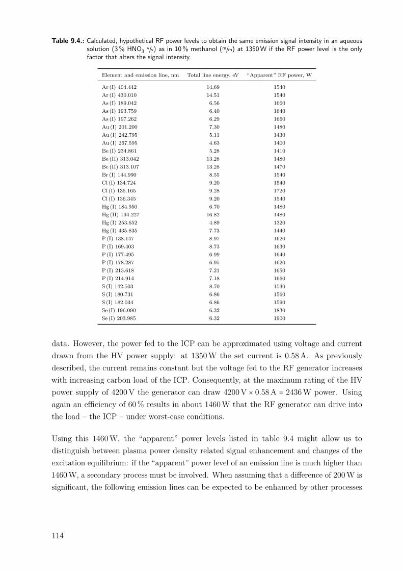
Table 9.4.: Calculated, hypothetical RF power levels to obtain the same emission signal intensity in an aqueoussolution (3% HNO3 v/v) as in 10% methanol (m/m) at 1350W if the RF power level is the onlyfactor that alters the signal intensity.

Element and emission line, nm Total line energy, eV “Apparent” RF power, W

Ar (I) 404.442 14.69 1540Ar (I) 430.010 14.51 1540As (I) 189.042 6.56 1660As (I) 193.759 6.40 1640As (I) 197.262 6.29 1660Au (I) 201.200 7.30 1480Au (I) 242.795 5.11 1430Au (I) 267.595 4.63 1400Be (I) 234.861 5.28 1410Be (II) 313.042 13.28 1480Be (II) 313.107 13.28 1470Br (I) 144.990 8.55 1540Cl (I) 134.724 9.20 1540Cl (I) 135.165 9.28 1720Cl (I) 136.345 9.20 1540Hg (I) 184.950 6.70 1480Hg (II) 194.227 16.82 1480Hg (I) 253.652 4.89 1320Hg (I) 435.835 7.73 1440P (I) 138.147 8.97 1620P (I) 169.403 8.73 1630P (I) 177.495 6.99 1640P (I) 178.287 6.95 1620P (I) 213.618 7.21 1650P (I) 214.914 7.18 1660S (I) 142.503 8.70 1530S (I) 180.731 6.86 1560S (I) 182.034 6.86 1590Se (I) 196.090 6.32 1830Se (I) 203.985 6.32 1900

data. However, the power fed to the ICP can be approximated using voltage and currentdrawn from the HV power supply: at 1350W the set current is 0.58A. As previouslydescribed, the current remains constant but the voltage fed to the RF generator increaseswith increasing carbon load of the ICP. Consequently, at the maximum rating of the HVpower supply of 4200V the generator can draw 4200 V × 0.58 A = 2436 W power. Usingagain an efficiency of 60% results in about 1460W that the RF generator can drive intothe load – the ICP – under worst-case conditions.

Using this 1460W, the “apparent” power levels listed in table 9.4 might allow us todistinguish between plasma power density related signal enhancement and changes of theexcitation equilibrium: if the “apparent” power level of an emission line is much higher than1460W, a secondary process must be involved. When assuming that a difference of 200W issignificant, the following emission lines can be expected to be enhanced by other processes

114

rather than increased RF power: As (I) 189.042 nm, As (I) 193.759 nm, As (I) 197.262 nm,Cl (I) 135.165 nm, P (I) 138.147 nm, P (I) 169.403 nm, P (I) 177.495 nm, P (I) 178.287 nm,P (I) 213.618 nm, P (I) 214.914 nm, Se (I) 196.090 nm and Se (I) 203.985 nm. The excitationenergy of these atom lines is between 6.3 and 9.3 eV. It is interesting to note that allinvestigated emission lines of As, P and Se follow this trend but only one chlorine line(135.165 nm) follows this trend.

On the other hand, the enhancement of emission lines with an “apparent” power levelof ≤ 1460W can be explained solely on the basis of the increased RF power coupledinto the ICP. This group involves Au (I) 242.795 nm, Au (I) 267.595 nm, Be (I) 234.861 nm,Hg (I) 253.652 nm, Hg (I) 435.835 nm and potentially also Au (I) 201.200 nm, Be (II) 313.042 nm,Be (II) 313.107 nm, Hg (I) 184.950 nm and Hg (II) 194.227 nm (the “apparent” power ofthese lines is only 20W above the calculated one). The energy sum of these lines spansfrom 4.6 to 16.8 eV.

For the remaining emission lines (Ar (I) 404.442 nm, Ar (I) 430.010 nm, Br (I) 144.990 nm,Cl (I) 134.724 nm, Cl (I) 136.345 nm, S (I) 142.503 nm, S (I) 180.731 nm and S (I) 182.034 nm)listed in table 9.4 no clear trend can be defined.

9.4. Conclusion

Carbon-based matrix effects in ICP-OES and ICP-MS arise not only from a single causebut appear to be a combination of several factors: (1) depending on the source of carbonused, changes of the sample transport efficiency in the nebulizer and spray chamber due tovariations in viscosity, surface tension or density; (2) matrix-induced excitation of certainenergy levels by mechanisms such as the charge transfer reaction; (3) thermal pinch effectthat results in a constriction of the ICP and consequently a higher power density of theremaining discharge; (4) RF generator related effects due to changes in plasma impedance.Effects 3 and 4 can be expected to be different for every type of RF generator as theimpedance changes will act differently on each specific circuit arrangement (free-runninggenerators or crystal stabilized ones with an additional impedance matching network).Particularly the power control algorithm that regulates current and voltage fed to the powerelectronics can be expected to have a great influence on the stability of the RF generatorwhen loading the ICP with large amounts of carbon. Even the dimensions of the torch orthe operating frequency might cause differences in the effect of carbon. As already reported,slight changes of the torch position were found to alter the excitation temperature. The

115

frequency on the other hand determines the skin depth of the RF current in the ICP and isoften associated with either a three or a four turn load coil (27 or 40MHz respectively).In conclusion, the response of the RF generator to plasma impedance changes appears tobe the dominant reason for the large spread of the enhancement factors reported in theliterature.

Another factor that should be considered in this context is the fact that not the concentrationof carbon in the sample solution determines the degree of matrix effect, but the mass flowof carbon that reaches the ICP and its state of matter. Gaseous reagents affect the plasmacore more readily than non-volatile liquid ones.

Based on the findings presented here, the charge transfer reaction combined with the higherpower density in the ICP discharge appears to explain most of the element enhancementsby C or Br. However, the mechanism fails to explain that in the presence of sufficientcarbon elements that cannot be expected to be enhanced by a charge transfer reaction(very high reaction energy defect) also were strongly enhanced (e.g. some emission lines ofCl). We can only but agree with Grindlay et al. [73] that “additional studies are requiredto explain these anomalies”.

116

Conclusion

We have seen in the previous chapters that despite its long time of existence, there is stillplenty of room for improvements in ICP-OES. These include both the understanding of theoperating principles as well as optimizing the running costs and consumption of resources.

The same applies to the field of sample preparation. Although the principles have notchanged, the methods and techniques can still be applied to different analytical questions.Furthermore, the need for more efficient and “greener” digestion procedures is still growingin the future.

In conclusion, every small development offers a huge variety of possibilities for furtherinvestigation which helps to improve the performance and usability of the ICP-OES inanalytical questions.

All in all, I hope that the efforts made will be of some use to others and can serveas the starting point for even more advances both in sample preparation as well as ininstrumentation for ICP-OES.

117

Appendices

119

List of Figures

2.1. General procedure for MIC in closed vessels. . . . . . . . . . . . . . . . . . . . 17

3.1. Schematic of the autoflow system. . . . . . . . . . . . . . . . . . . . . . . . . . . 243.2. Glass-to-metal interface. . . . . . . . . . . . . . . . . . . . . . . . . . . . . . . . 243.3. Temperature distribution inside the microwave cavity. . . . . . . . . . . . . . . 273.4. Effect of microwave power on the digestion efficiency. . . . . . . . . . . . . . . 283.5. Effect of the carrier flow rate on the digestion efficiency. . . . . . . . . . . . . 30

4.1. Influence of diesel mass on the maximum pressure during MIC. . . . . . . . . 434.2. Influence of diesel oil adsorption time on glass wool for the MIC method. . . 44

5.1. Block diagram of optical atomic spectrometry. . . . . . . . . . . . . . . . . . . 525.2. Voigt line profile. . . . . . . . . . . . . . . . . . . . . . . . . . . . . . . . . . . . . 59

6.1. ICP torch schematic. . . . . . . . . . . . . . . . . . . . . . . . . . . . . . . . . . 636.2. Schematic overview of an ICP-OES analysis. . . . . . . . . . . . . . . . . . . . 636.3. Schematic overview of an ICP-OES analysis with the enclosed plasma interface. 656.4. Gas recycling flow schematic. . . . . . . . . . . . . . . . . . . . . . . . . . . . . 65

7.1. Hγ emission line. . . . . . . . . . . . . . . . . . . . . . . . . . . . . . . . . . . . . 73

8.1. Sectional drawing of the enclosed plasma interface parts. . . . . . . . . . . . . 798.2. Illustration of the interface. . . . . . . . . . . . . . . . . . . . . . . . . . . . . . . 798.3. Gas recycling flow schematic. . . . . . . . . . . . . . . . . . . . . . . . . . . . . 818.4. RF power coupled to the slotted copper disk as a function of the distance

from the load coil. . . . . . . . . . . . . . . . . . . . . . . . . . . . . . . . . . . . 848.5. Frequency of the free running RF generator as a function of the distance

from the load coil. . . . . . . . . . . . . . . . . . . . . . . . . . . . . . . . . . . . 84

121

8.6. Transient signal of Cl 135.165 nm while nebulizing NaCl solution for thetraditional setup and the enclosed plasma interface with argon recycling. . . 87

8.7. Experimental setup for determining the magnitude of the RF stray field. . . 89

9.1. Effect of increasing methanol concentration on the signal of Se in ICP-OESand ICP-MS recorded on different instruments. . . . . . . . . . . . . . . . . . . 99

9.2. Power and frequency response of the RF generator. . . . . . . . . . . . . . . . 1039.3. Effect of methanol on plasma volume. . . . . . . . . . . . . . . . . . . . . . . . 1049.5. Signal intensity of the C emission line and power vacuum plate voltage as a

function of the carbon mass flow. . . . . . . . . . . . . . . . . . . . . . . . . . . 109

122

List of Tables

3.1. Optimized operating conditions of the flow digestion system. . . . . . . . . . 253.2. Comparison of flow and closed vessel batch digestion. . . . . . . . . . . . . . . 313.3. Comparison of different acid cocktails. . . . . . . . . . . . . . . . . . . . . . . . 323.4. High pressure flow digestion of CRMs. . . . . . . . . . . . . . . . . . . . . . . . 333.5. Comparison with other flow digestion systems reported in the literature. . . 34

4.1. Analysis of lubrication oil, diesel oil and crude oil products. . . . . . . . . . . 374.2. Operational conditions used for sulfur and carbon determination by ICP-OES. 394.3. Operational conditions used for sulfur determination by using an automatic

sulfur analyzer. . . . . . . . . . . . . . . . . . . . . . . . . . . . . . . . . . . . . . 394.4. Determination of S in diesel oil by ICP-OES after digestion using MIC. . . . 454.5. Results for S in diesel oil samples. . . . . . . . . . . . . . . . . . . . . . . . . . . 46

8.1. Characteristics of the enclosed plasma interface and the traditional setup. . 86

9.1. ICP-OES operating conditions. . . . . . . . . . . . . . . . . . . . . . . . . . . . 959.2. Signal enhancement/suppression factors of selected emission lines by various

reagents. . . . . . . . . . . . . . . . . . . . . . . . . . . . . . . . . . . . . . . . . . 1019.3. Electronic states and energy defects for the charge transfer reaction between

Br+ and selected elements. . . . . . . . . . . . . . . . . . . . . . . . . . . . . . . 1119.4. Calculated, hypothetical RF power levels. . . . . . . . . . . . . . . . . . . . . . 114

B.1. Signal enhancement/suppression factors of selected emission lines by variousreagents. . . . . . . . . . . . . . . . . . . . . . . . . . . . . . . . . . . . . . . . . . 150

123

Bibliography

[1] H. Wiltsche et al. „A novel approach to high pressure flow digestion“. Journal of Analytical AtomicSpectrometry 29, 2 (2014), pp. 272–279. doi: 10.1039/c3ja50290b (cit. on pp. 1, 19).

[2] Sandra M. Cruz et al. „Feasibility of sulfur determination in diesel oil by inductively coupledplasma optical emission spectrometry after microwave-induced combustion using flame retardant“.Fuel 160 (July 2015), pp. 108–113. doi: 10.1016/j.fuel.2015.07.069 (cit. on pp. 1, 35).

[3] Helmar Wiltsche, Monika Winkler, and Paul Tirk. „Matrix effects of carbon and bromine in induc-tively coupled plasma optical emission spectrometry“. Journal of Analytical Atomic Spectrometry30 (2015), pp. 2223–2234. doi: 10.1039/c5ja00237k (cit. on pp. 1, 64, 73, 88, 91).

[4] E. M. M. Flores. Microwave-assisted sample preparation for trace element determination. 1st.Amsterdam: Elsevier, 2014, p. 400 (cit. on pp. 9, 17, 36, 44).

[5] M. Würfels and E. Jackwerth. „Untersuchungen zur Kohlenstoffbilanz beim Aufschluß biologischerProbenmaterialien mit Salpetersäure“. Fresenius Zeitschrift für Analytische Chemie 322 (1985),pp. 354–358 (cit. on p. 15).

[6] M. Würfels. „Decomposition of Biological Samples with Acids for the Determination of TraceElements“. LABO 3 (1989), pp. 7–15 (cit. on p. 15).

[7] Christiane Gräber and Harald Berndt. „Development of a new high temperature/high pressureflow system for the continuous digestion of biological samples“. Journal of Analytical AtomicSpectrometry 14, 4 (1999), pp. 683–691 (cit. on pp. 15, 21, 34).

[8] Thiago Linhares Marques et al. „High pressure microwave-assisted flow digestion system using alarge volume reactor-feasibility for further analysis by inductively coupled plasma-based techniques“.Journal of Analytical Atomic Spectrometry 30, 9 (2015), pp. 1898–1905. doi: 10.1039/c5ja00194c(cit. on p. 15).

[9] Erico Marlon Moraes Flores et al. „Microwave-Assisted Sample Combustion: A Technique forSample Preparation in Trace Element Determination“. Analytical Chemistry 76, 13 (2004), pp. 3525–3529 (cit. on pp. 17, 37).

[10] M. Burguera et al. „In vivo sample uptake and on-line measurements of cobalt in whole bloodby microwave-assisted mineralization and flow injection electrothermal atomic absorption spec-trometry“. Journal of Analytical Atomic Spectrometry 10 (5 1995), pp. 343–347. doi: 10.1039/JA9951000343 (cit. on pp. 20, 34).

125

[11] Stephen J. Haswell and David Barclay. „On-line microwave digestion of slurry samples with directflame atomic absorption spectrometric elemental detection“. Analyst 117, 2 (1992), pp. 117–120(cit. on pp. 20, 21, 34).

[12] Ralph E. Sturgeon et al. „Continuous-flow microwave-assisted digestion of environmental samplesusing atomic spectrometric detection“. Journal of Analytical Atomic Spectrometry 10, 11 (1995),pp. 981–986 (cit. on p. 20).

[13] Thomas J. Gluodenis and Julian F. Tyson. „Flow injection systems for directly coupling on-linedigestions with analytical atomic spectrometry. Part 2. Reactions in a microwave field“. Journal ofAnalytical Atomic Spectrometry 8, 5 (1993), pp. 697–704 (cit. on pp. 20, 34).

[14] Guy Légère and Eric D. Salin. „Capsule-Based Microwave Digestion“. Applied Spectroscopy 49, 4(1995), 14A–22A (cit. on pp. 20, 34).

[15] Thomas J. Gluodenis and Julian F. Tyson. „Flow injection systems for directly coupling on-linedigestions with analytical atomic spectrometry. Part 1. Dissolution of cocoa under stopped-flow,high-pressure conditions“. Journal of Analytical Atomic Spectrometry 7, 2 (1992), pp. 301–306(cit. on p. 20).

[16] Ulrike Pichler et al. „Microwave-Enhanced Flow System for High-Temperature Digestion of ResistantOrganic Materials“. Analytical Chemistry 71 (1999), pp. 4050–4055 (cit. on pp. 20–23, 27–29).

[17] J. L. Burguera and M. Burguera. „Determination of lead in biological materials by microwave-assisted mineralization and flow injection electrothermal atomic absorption spectrometry“. Journalof Analytical Atomic Spectrometry 8, 2 (1993), pp. 235–241 (cit. on pp. 20, 34).

[18] J. L. Burguera et al. „Determination of iron and zinc in adipose tissue by on-line microwave-assistedmineralization and flow-injection graphite furnace atomic absorption spectrometry“. AnalyticaChimica Acta 308, 1–3 (1995), pp. 349–356 (cit. on p. 20).

[19] M. Burguera, J. L. Burguera, and O. M. Alarcón. „Flow injection and microwave-oven sampledecomposition for determination of copper, zinc and iron in whole blood by atomic absorptionspectrometry“. Analytica Chimica Acta 179 (1986), pp. 351–357 (cit. on pp. 20, 34).

[20] M. Bettinelli et al. „Determination of total urinary mercury by on-line sample microwave digestionfollowed by flow injection cold vapour inductively coupled plasma mass spectrometry or atomicabsorption spectrometry“. Rapid Communications in Mass Spectrometry 16, 15 (2002), pp. 1432–1439 (cit. on p. 20).

[21] S. Hinkamp and G. Schwedt. „Determination of total phosphorus in waters with amperometricdetection by coupling of flow-injection analysis with continuous microwave oven digestion“. AnalyticaChimica Acta 236 (1990), pp. 345–350 (cit. on p. 20).

[22] Andreas Meyer and Georg Schwedt. „Kopplung von Mikrowellenaufschluß und Hydrid-AAS“.LaborPraxis 4 (1993), pp. 44–48 (cit. on p. 20).

[23] M. L. Balconi et al. „Chemical oxygen demand determination in well and river waters by flow-injection analysis using a microwave oven during the oxidation step“. Analytica Chimica Acta 261,1–2 (1992), pp. 295–299 (cit. on p. 20).

[24] M. De la Guardia et al. „On-line microwave-assisted digestion of solid samples for their flameatomic spectrometric analysis“. Talanta 40, 11 (1993), pp. 1609–1617 (cit. on p. 20).

126

[25] Henryk Matusiewicz and Ralph E. Sturgeon. „Comparison of the efficiencies of on-line and high-pressure closed vessel approaches to microwave heated sample decomposition“. Fresenius’ Journalof Analytical Chemistry 349, 6 (1994), pp. 428–433 (cit. on pp. 20, 37).

[26] T Dülcks. „Das Mikrowellen-Aufschlußsystem SpectroPrep im Anwendungstest“. LaborPraxisSeptember 1996 (1996), pp. 68–69 (cit. on p. 21).

[27] Stephan Haiber and H. Berndt. „A novel high-temperature (360 °C)/high-pressure (30 MPa) flowsystem for online sample digestion applied to ICP spectrometry“. Fresenius’ Journal of AnalyticalChemistry 368, 1 (2000), pp. 52–58 (cit. on pp. 21–23, 31).

[28] P. Jacob and H. Berndt. „Online element determination in biological and environmental samplesby flame AAS coupled with a high-temperature/high-pressure flow digestion system“. Journal ofAnalytical Atomic Spectrometry 17, 12 (2002), pp. 1615–1620 (cit. on pp. 21, 34).

[29] Q. Z. Bian et al. „Online flow digestion of biological and environmental samples for inductivelycoupled plasma–optical emission spectroscopy (ICP–OES)“. Analytica Chimica Acta 538, 1–2(2005), pp. 323–329 (cit. on pp. 21, 31, 34).

[30] Q. Z. Bian. „Solid Sample Analysis by ICP-Spectrometry with Femtosecond Laser Ablation andOnline Flow Digestion“. PhD thesis. 2005 (cit. on pp. 21, 34).

[31] G. Knapp. Microwave-heatable pressure reactor. USA Patent 5,672,316. 1995 (cit. on p. 21).

[32] Markus Lafer. „Development of an automated system for trace element analysis based on a novelflow digestion technique“. PhD thesis. 2010 (cit. on p. 23).

[33] J. S. F. Pereira et al. „High-Efficiency Microwave-Assisted Digestion Combined to in Situ UltravioletRadiation for the Determination of Rare Earth Elements by Ultrasonic Nebulization ICPMS inCrude Oils“. Analytical Chemistry 85, 22 (Nov. 2013), pp. 11034–11040. doi: 10.1021/ac402928u(cit. on p. 33).

[34] Marco A. Z. Arruda, Mercedes Gallego, and Miguel Valcarcel. „Flow-through microwave digestionsystem for the determination of aluminium in shellfish by electrothermal atomic absorptionspectrometry“. Journal of Analytical Atomic Spectrometry 10, 7 (1995), pp. 501–504 (cit. on p. 34).

[35] S. Recknagel et al. „Determination of selenium in blood serum by ICP-OES including an on-linewet digestion and Se-hydride formation procedure“. Fresenius’ Journal of Analytical Chemistry346, 6 (1993), pp. 833–836 (cit. on p. 34).

[36] V. Carbonell et al. „On-line microwave oven digestion flame atomic absorption analysis of solidsamples“. Analytica Chimica Acta 238 (1990), pp. 417–421 (cit. on p. 34).

[37] V. Carbonell et al. „Atomic absorption spectrometric analysis of solids with on-line microwave-assisted digestion“. Journal of Analytical Atomic Spectrometry 7, 7 (1992), pp. 1085–1089 (cit. onp. 34).

[38] Edenir R. Pereira-Filho and Marco A. Z. Arruda. „Mechanised flow system for on-line microwavedigestion of food samples with off-line catalytic spectrophotometric determination of cobalt at ngl−1 levels“. Analyst 124, 12 (1999), pp. 1873–1877 (cit. on p. 34).

[39] Heinz Staufenberg. „Vollautomatisches Durchfluß-Mikrowellenaufschlußsystem“. LaborPraxis 11(1993), pp. 58–59 (cit. on p. 34).

[40] Vassili Karanassios et al. „Rapid stopped-flow microwave digestion system“. Journal of AnalyticalAtomic Spectrometry 6, 6 (1991), pp. 457–463 (cit. on p. 34).

127

[41] J. G. Speight. Handbook of petroleum product analysis. New Jersey: John Wiley & Sons, Inc, 2002(cit. on p. 36).

[42] J.H. Gary, G.E. Handwerk, and M.J. Kaiser. Petroleum refining: technology and economics. 5th.Boca Raton: CRC Press, 2007 (cit. on p. 36).

[43] Antony Stanislaus, Abdulazeem Marafi, and Mohan S. Rana. „Recent advances in the scienceand technology of ultra low sulfur diesel (ULSD) production“. Catalysis Today 153, 1–2 (2010),pp. 1–68 (cit. on p. 36).

[44] G. Corro. „Sulfur impact on diesel emission control - a review“. Reaction Kinetics and CatalysisLetters 75 (2002), pp. 89–106 (cit. on p. 36).

[45] A. Sydbom et al. „Health effects of diesel exaust emissions“. The European Respiratory Journal 17(2001), pp. 733–746 (cit. on p. 36).

[46] J. D. McDonald et al. „Effects of low sulfur fuel and a catalyzed particle trap on the compositionand toxicity of diesel emissions“. Environmental Health Perspectives 112, 13 (2004), pp. 1307–1312(cit. on p. 36).

[47] Changlong Yin et al. „Study on the formation, determination, and removal of elemental sulfur inultra-low sulfur gas oil“. Fuel Processing Technology 120 (2014), pp. 16–21 (cit. on p. 36).

[48] Frank Cheng-Yu Wang et al. „Speciation of sulfur-containing compounds in diesel by comprehensivetwo-dimensional gas chromatography“. Journal of Chromatographic Science 41, 10 (2003), pp. 519–523 (cit. on p. 36).

[49] Heavy-duty engine and vehicle standards and highway diesel fuel sulfur control requirements.Environmental Protection Agency. 2000 (cit. on pp. 36, 46).

[50] Directive 98/70/EC of the European Parliament and of the Council of 13 October 1998 relating tothe quality of petrol and diesel fuels and amending Council Directive 93/12/EEC. Official Journalof the European Union, EU. 1998 (cit. on pp. 36, 46).

[51] Zhaochu Hu et al. „Volatile organic solvent-induced signal enhancements in inductively coupledplasma-mass spectrometry: a case study of methanol and acetone“. Spectrochimica Acta Part B:Atomic Spectroscopy 59, 9 (Sept. 2004), pp. 1463–1470. doi: 10.1016/j.sab.2004.07.007 (cit. onpp. 36, 92, 99, 108).

[52] ASTM D 4951-14, Standard Test Method for Determination of Additive Elements in Lubricating Oilsby Inductively Coupled Plasma Atomic Emission Spectrometry. Annual Book of ASTM Standards.2014 (cit. on p. 36).

[53] A. Ulrich and A. Wichser. „Analysis of additive metals in fuel and emission aerosols of dieselvehicles with and without particle traps“. Analytical and Bioanalytical Chemistry 377, 1 (2003),pp. 71–81 (cit. on pp. 36, 37).

[54] A. Montaser. Inductively coupled plasma mass spectrometry. New York: Wiley VCH Inc., 1998,p. 964 (cit. on p. 36).

[55] José-Luis Todolí and Jean-Michel Mermet. „Acid interferences in atomic spectrometry: analytesignal effects and subsequent reduction“. Spectrochimica Acta Part B: Atomic Spectroscopy 54, 6(1999), pp. 895–929 (cit. on pp. 36, 38).

128

[56] ASTM D 4294-98, Standard Test Method for Sulfur in Petroleum and Petroleum Products byEnergy Dispersive X-ray Fluorescence Spectrometry. Annual Book of ASTM Standards. 1998 (cit. onp. 37).

[57] ASTM D 129-95 (reapproved 2000), Standard Test Method for Sulfur in Petroleum Products(General Bomb Method). Annual Book of ASTM Standards. 1995 (cit. on p. 37).

[58] ASTM D 1552-95, Standard Test Method for Sulfur in Petroleum Products (High-TemperatureMethod). Annual Book of ASTM Standards. 1995 (cit. on p. 37).

[59] R. I. Botto. „Sample preparation for crude oil, petroleum products and polymers“. In: Samplepreparation for trace element analysis. Ed. by R. S. Z. Mester. Elsevier: Amsterdam, 2003. Chap. 683-718 (cit. on p. 37).

[60] S. Pessayre et al. „Deep hydrodesulfurization of diesel oils. Matrix effect in the analysis of low sulfurdiesel oils by energy dispersive X-ray fluorescence spectroscopy“. Fuel 78, 7 (1999), pp. 857–860(cit. on p. 37).

[61] Pierre Allain et al. „Signal Enhancement of Elements Due to the Presence of Carbon-ContainingCompounds in Inductively Coupled Plasma Mass Spectrometry“. Analytical Chemistry 63, 14(1991), pp. 1497–1498 (cit. on pp. 37, 92, 108).

[62] Érico M.M. Flores et al. „Sample preparation techniques based on combustion reactions in closedvessels – A brief overview and recent applications“. Spectrochimica Acta Part B: Atomic Spectroscopy62, 9 (Sept. 2007), pp. 1051–1064. doi: 10.1016/j.sab.2007.04.018 (cit. on pp. 37, 45).

[63] Y. S. Fung and K. L. Dao. „Elemental analysis of chemical wastes by oxygen bomb combustion-ionchromatography“. Analytica Chimica Acta 334, 1–2 (1996), pp. 51–56 (cit. on p. 37).

[64] M. G. Liu et al. „Determination of sulfur in diesel oil certified reference materials by oxygenbomb-combustion ICP-OES“. Spectroscopy and Spectral Analysis 23 (2003), pp. 965–967 (cit. onp. 37).

[65] Juliana S. F. Pereira et al. „Chlorine and sulfur determination in extra-heavy crude oil by inductivelycoupled plasma optical emission spectrometry after microwave-induced combustion“. SpectrochimicaActa Part B: Atomic Spectroscopy 64, 6 (2009), pp. 554–558 (cit. on pp. 37, 40).

[66] Y. S. Fung and K. L. Dao. „Oxygen bomb combustion ion chromatography for elemental analysisof heteroatoms in fuel and wastes development“. Analytica Chimica Acta 315 (1995), pp. 347–355(cit. on p. 37).

[67] R. Siegfriedt, S. Wiberley, and R. Moore. „Determination of sulfur after combustion in smalloxygen bomb. Rapid titrimetric method“. Analytical Chemistry 23 (1951), pp. 1008–1011 (cit. onp. 37).

[68] M. J. McCormick. „Determination of total sulphur in fuel oils by ion chromatography“. AnalyticaChimica Acta 121 (1980), pp. 233–238 (cit. on p. 37).

[69] X. Li et al. „Determination of As and Se in coal and coal combustion products using closed vesselmicrowave digestion and collision/reaction cell technology (CCT) of inductively coupled plasmamass spectrometry (ICP-MS)“. International Journal of Coal Geology 124 (2014), pp. 1–4 (cit. onp. 37).

129

[70] S. Dai et al. „Determination of boron in coal using closed vessel microwave digestion and inductivelycoupled plasma mass spectrometry (ICP-MS)“. Energy & Fuels 28 (2014), pp. 4517–4522 (cit. onp. 37).

[71] P. A. Mello et al. „Nickel, vanadium and sulfur determination by inductively coupled plasmaoptical emission spectrometry in crude oil distillation residues after microwave-induced combustion“.Journal of Analytical Atomic Spectrometry 24, 7 (2009), pp. 911–916 (cit. on pp. 37, 38).

[72] Cezar A. Bizzi et al. „Evaluation of a digestion procedure based on the use of diluted nitric acidsolutions and H2O2 for the multielement determination of whole milk powder and bovine liverby ICP-based techniques“. Journal of Analytical Atomic Spectrometry 29, 2 (2014), pp. 332–338(cit. on pp. 38, 41).

[73] Guillermo Grindlay et al. „A systematic study on the influence of carbon on the behavior ofhard-to-ionize elements in inductively coupled plasma – mass spectrometry“. Spectrochimica ActaPart B: Atomic Spectroscopy 86 (May 2013), pp. 42–49. doi: 10.1016/j.sab.2013.05.002 (cit. onpp. 38, 45, 92, 93, 110, 116).

[74] Diogo L. Rocha et al. „Greening sample preparation in inorganic analysis“. TrAC Trends inAnalytical Chemistry 45 (2013), pp. 79–92 (cit. on p. 38).

[75] G. E. Zaikov and S. M. Lomakin. Polymeric flame retardants: problems and decisions. M. Kutz(Ed.) Handbook of Environmental Degradation of Materials. William Andrew, Inc., Norwich, USA,2005 (cit. on p. 38).

[76] J. H. Troitzsch. „Overview of flame retardants“. Chimica Oggi-Chemistry Today 16, 1-2 (1998),pp. 18–24 (cit. on p. 38).

[77] ASTM D 5453-12, Standard Test Method for Determination of Total Sulfur in Light Hydrocarbons,Spark Ignition Engine Fuel, Diesel Engine Fuel, and Engine Oil by Ultraviolet Fluorescence. AnnualBook of ASTM Standards. 2012 (cit. on pp. 38, 39, 42).

[78] E. M.M. Flores et al. „Determination of halogens in coal after digestion using the microwave-inducedcombustion technique“. Analytical Chemistry 80, 6 (2008), pp. 1865–1870 (cit. on p. 41).

[79] Juliana S. F. Pereira et al. „Determination of metals and metalloids in light and heavy crude oil byICP-MS after digestion by microwave-induced combustion“. Microchemical Journal 96, 1 (2010),pp. 4–11 (cit. on pp. 42, 45).

[80] S. T. Gouveia et al. „Determination of residual carbon by inductively-coupled plasma opticalemission spectrometry with axial and radial view configurations“. Analytica Chimica Acta 445, 2(2001), pp. 269–275 (cit. on p. 45).

[81] F. G. Antes et al. „Determination of toxic elements in coal by ICP-MS after digestion usingmicrowave-induced combustion“. Talanta 83, 2 (2010), pp. 364–369 (cit. on p. 45).

[82] Antoaneta Krushevska et al. „Comparison of sample decomposition procedures for the determinationof zinc in milk by inductively coupled plasma atomic emission spectrometry“. Journal of AnalyticalAtomic Spectrometry 7, 6 (1992), pp. 851–858 (cit. on p. 45).

[83] Antoaneta Krushevska et al. „Determination of the residual carbon content by inductively coupledplasma atomic emission spectrometry after decomposition of biological samples“. Journal ofAnalytical Atomic Spectrometry 7, 6 (1992), pp. 845–850 (cit. on p. 45).

130

[84] H. C. van de Hulst and J. J. M. Reesinck. „Line Breadths and Voigt Profiles“. Astrophysical Journal106 (1947), pp. 121–127 (cit. on p. 58).

[85] J. Tudor Davies and J. M. Vaughan. „A New Tabulation of the Voigt Profile“. AstrophysicalJournal 137 (1963), pp. 1302–1305 (cit. on p. 58).

[86] J.M. Mermet. „Use of magnesium as a test element for inductively coupled plasma atomic emissionspectrometry diagnostics“. Analytica Chimica Acta 250 (Oct. 1991), pp. 85–94. doi: 10.1016/0003-2670(91)85064-Y (cit. on pp. 71, 81, 96).

[87] Marco A. Gigosos, Manuel Á. González, and Valentín Cardeñoso. „Computer simulated Balmer-alpha, -beta and -gamma Stark line profiles for non-equilibrium plasmas diagnostics“. SpectrochimicaActa Part B: Atomic Spectroscopy 58 (2003), pp. 1489–1504. doi: 10.1016/S0584-8547 (cit. onpp. 72, 81).

[88] Helmar Wiltsche, Farzaneh Moradi, and Günter Knapp. „Evaluation of the oscillator frequency ofa free running RF generator as a diagnostic tool for inductively coupled plasma-optical emissionspectrometry“. Spectrochimica Acta Part B: Atomic Spectroscopy 71-72 (May 2012), pp. 48–53.doi: 10.1016/j.sab.2012.05.002 (cit. on pp. 73, 81, 83, 85, 94, 96, 97, 102, 111).

[89] Charly D. Allemand, Ramon M. Barnes, and Charles C. Wohlers. „Experimental study of reducedsize inductively coupled plasma torches“. Analytical Chemistry 51, 14 (1979), pp. 2392–2394 (cit. onp. 76).

[90] R. N. Savage and G. M. Hieftje. „Development and characterization of a miniature inductivelycoupled plasma source for atomic emission spectrometry“. Analytical Chemistry 51, 3 (1979),pp. 408–413 (cit. on p. 76).

[91] Towhid Hasan, Narong Praphairaksit, and R. S. Houk. „Low flow, externally air cooled torch forinductively coupled plasma atomic emission spectrometry with axial viewing“. Spectrochimica ActaPart B: Atomic Spectroscopy 56, 4 (2001), pp. 409–418 (cit. on p. 76).

[92] P. A. M. Ripson, L. de Galan, and J. W. de Ruiter. „An inductively coupled plasma using 1 Lmin−1 of argon“. Spectrochimica Acta Part B: Atomic Spectroscopy 37, 8 (1982), pp. 733–738(cit. on p. 76).

[93] Guy R. Kornblum, Wouter Van der Waa, and Leo De Galan. „Reduction of argon consumption bya water cooled torch in inductively coupled plasma emission spectrometry“. Analytical Chemistry51, 14 (1979), pp. 2378–2381 (cit. on p. 76).

[94] Hiroshi Kawaguchi et al. „Water cooled torch for inductively coupled plasma emission spectrometry“.Analytical Chemistry 52, 14 (1980), pp. 2440–2442 (cit. on p. 76).

[95] Gary M. Hieftje. „Mini, micro, and high-efficiency torches for the ICP - toys or tools?“ SpectrochimicaActa Part B: Atomic Spectroscopy 38, 11 (1983), pp. 1465–1481 (cit. on p. 76).

[96] Narong Praphairaksit, Daniel R. Wiederin, and R. S. Houk. „An externally air-cooled low-flowtorch for inductively coupled plasma mass spectrometry“. Spectrochimica Acta Part B: AtomicSpectroscopy 55, 8 (2000), pp. 1279–1293 (cit. on p. 76).

[97] P. J. Morrisroe and P. H. Gagne. High frequency transistor oscillator system. Patent 6329757. 1996(cit. on p. 76).

131

[98] Andre Klostermeier et al. „New torch design for inductively coupled plasma optical emissionspectrometry with minimised gas consumption“. Journal of Analytical Atomic Spectrometry 20, 4(2005), pp. 308–314 (cit. on p. 76).

[99] C. Engelhard et al. „Plasma diagnostic on a low-flow plasma for inductively coupled plasmaoptical emission spectrometry“. Spectrochimica Acta, Part B: Atomic Spectroscopy 63B, 6 (2008),pp. 619–629 (cit. on p. 76).

[100] Matthias J. Jahl, Tracey Jacksier, and Ramon M. Barnes. „Sealed Inductively Coupled PlasmaAtomic Emission Spectrometry: Instrumentation Development“. Journal of Analytical AtomicSpectrometry 7, June (1992), pp. 653–660 (cit. on p. 76).

[101] C. Breer et al. „Enclosed Inductively Coupled Plasma: Spatially Resolved Profiles of RotationalTemperatures and Analyte Atom Distribution“. Applied Spectroscopy 55, 11 (2001), pp. 1462–1468(cit. on p. 77).

[102] Matthias Wolfgang. „Entwicklung und Charakterisierung eines geschlossenen, axialen optischenInterface für die ICP-OES-Spektrometrie“. MA thesis. Technische Universität Graz, 2012 (cit. onp. 83).

[103] C. Engelhard et al. „Application of infrared thermography for online monitoring of wall temper-atures in inductively coupled plasma torches with conventional and low-flow gas consumption“.Spectrochimica Acta Part B: Atomic Spectroscopy 62B (2007), pp. 1161–1168 (cit. on p. 84).

[104] Xianzhong Jin et al. „Inductively coupled plasma mass spectrometry with ambient helium surround-ing ion source“. Spectrochimica Acta Part B: Atomic Spectroscopy 65, 12 (Dec. 2010), pp. 1052–1055.doi: 10.1016/j.sab.2010.11.007 (cit. on p. 87).

[105] S. Chan and A. Montaser. „A He ICP for atomic emission spectrometry“. Spectrochimica ActaPart B: Atomic Spectroscopy 40B, 10-12 (1985), pp. 1467–1472 (cit. on p. 88).

[106] H. B. Fannin, C. J. Seliskar, and D. C. Miller. „Studies of energy transfer and ionisation processesin a He ICP“. Applied Spectroscopy 41, 4 (1987), pp. 621–624 (cit. on p. 88).

[107] L. A. Iacone et al. „Formation and fundamental characteristics of novel free-running heliuminductively coupled plasmas“. Journal of Analytical Atomic Spectrometry 15 (2000), pp. 491–498(cit. on p. 88).

[108] K. Jorabchi and A. Montaser. „New coil geometries for the study of secondary discharge inatmospheric-pressure helium inductively coupled plasma mass spectrometry“. Spectrochimica ActaPart B: Atomic Spectroscopy 59B (2004), pp. 1471–1479 (cit. on p. 88).

[109] B. Gammelgaard and O. Jøns. „Determination of selenium in urine by inductively coupled plasmamass spectrometry: interferences and optimization“. Journal of Analytical Atomic Spectrometry 14,5 (1999), pp. 867–874 (cit. on pp. 92, 99, 108).

[110] G. Grindlay et al. „Carbon-related matrix effects in inductively coupled plasma atomic emissionspectrometry“. Spectrochimica Acta Part B: Atomic Spectroscopy 63, 2 (Feb. 2008), pp. 234–243.doi: 10.1016/j.sab.2007.11.024 (cit. on pp. 92, 93, 108).

[111] M. Kovačevič and W. Goessler. „Direct introduction of volatile carbon compounds into thespray chamber of an inductively coupled plasma mass spectrometer: Sensitivity enhancement forselenium“. Spectrochimica Acta Part B: Atomic Spectroscopy 60B (2005), pp. 1357–1361 (cit. onp. 92).

132

[112] M. Kovačevič et al. „Matrix effects during phosphorus determination with quadrupole inductivelycoupled plasma mass spectrometry“. Analytical and Bioanalytical Chemistry 383, 1 (2005), pp. 145–151 (cit. on pp. 92, 108).

[113] Erik H. Larsen and Stefan Stürup. „Carbon-enhanced inductively coupled plasma mass spectro-metric detection of arsenic and selenium and its application to arsenic speciation“. Journal ofAnalytical Atomic Spectrometry 9, October (1994), pp. 1099–1105 (cit. on pp. 92, 104, 108).

[114] S. Liu and D. Beauchemin. „Effect of methanol and sodium dodecylsulfate on radial profiles ofion abundance in inductively coupled plasma mass spectrometry“. Spectrochimica Acta Part B:Atomic Spectroscopy 61B (2006), pp. 319–325 (cit. on p. 92).

[115] I. Llorente, M. Gómez, and C. Cámara. „Improvement of selenium determination in water byinductively coupled plasma mass spectrometry through use of organic compounds as matrixmodifiers“. Spectrochimica Acta Part B: Atomic Spectroscopy 52, 12 (1997), pp. 1825–1838 (cit. onpp. 92, 93, 99, 108).

[116] Jiří Machát, Vítězslav Otruba, and Viktor Kanický. „Spectral and non-spectral interferences in thedetermination of selenium by inductively coupled plasma atomic emission spectrometry“. Journalof Analytical Atomic Spectrometry 17, 9 (Sept. 2002), pp. 1096–1102. doi: 10.1039/b202167f(cit. on pp. 92, 93, 100, 108).

[117] J. Machát, V. Kanický, and V. Otruba. „Determination of selenium in blood serum by inductivelycoupled plasma atomic emission spectrometry with pneumatic nebulization“. Analytical andBioanalytical Chemistry 372, 4 (2002), pp. 576–581 (cit. on pp. 92, 108).

[118] Maurizio Pettine et al. „Dissolved inorganic carbon effect in the determination of arsenic andchromium in mineral waters by inductively coupled plasma-mass spectrometry“. Analytica ChimicaActa 599, 2 (Sept. 2007), pp. 191–198. doi: 10.1016/j.aca.2007.08.016 (cit. on p. 92).

[119] I. Rodushkin et al. „Improved multi-elemental analyses by inductively coupled plasma-sectorfield mass spectrometry through methane addition to the plasma“. Journal of Analytical AtomicSpectrometry 20 (2005), pp. 1250–1255 (cit. on pp. 92, 108).

[120] E. Warburton and H. Goenaga-Infante. „Methane mixed plasma—improved sensitivity of inductivelycoupled plasma mass spectrometry detection for selenium speciation analysis of wheat-based food“.Journal of Analytical Atomic Spectrometry 22 (2007), pp. 370–376 (cit. on pp. 92, 108).

[121] P. Kralj and M. Veber. „Investigation into nonspectroscopic effects of organic compounds inICP-MS“. Acta Chim. Slovenia 50 (2003), pp. 633–644 (cit. on pp. 92, 99, 108, 113).

[122] Takashi Nakazawa et al. „Comparison of signal enhancement by co-existing carbon and by co-existing bromine in inductively coupled plasma mass spectrometry“. Journal of Analytical AtomicSpectrometry 29, 7 (2014), pp. 1299–1305 (cit. on p. 92).

[123] Assad S. Al-Ammar, Rajesh K. Gupta, and Ramon M. Barnes. „Correction for non-spectroscopicmatrix effects in inductively coupled plasma-mass spectrometry by common analyte internalstandardization“. Spectrochimica Acta Part B: Atomic Spectroscopy 54, 13 (1999), pp. 1849–1860(cit. on p. 92).

[124] Fadi R. Abou-Shakra et al. „Enzymatic Digestion for the Determination of Trace Elements inBlood Serum by Inductively Coupled Plasma Mass Spectrometry“. Journal of Analytical AtomicSpectrometry 12, April (1997), pp. 429–433 (cit. on p. 93).

133

[125] Hongsen Niu and R.S. Houk. „Fundamental aspects of ion extraction in inductively coupledplasma mass spectrometry“. Spectrochimica Acta Part B: Atomic Spectroscopy 51, 8 (July 1996),pp. 779–815. doi: 10.1016/0584-8547(96)01506-6 (cit. on p. 93).

[126] J. Goossens et al. „Elimination of interferences in the determination of arsenic and selenium inbiological samples by inductively coupled plasma mass spectrometry“. Analytica Chimica Acta280, 1 (1993), pp. 137–143 (cit. on p. 93).

[127] E. F. Huth and L. Kühn. Schaltungsweise zur Schwingungserzeugung mit Vakuumröhren. Ger. Pat.,310152. 1917 (cit. on p. 95).

[128] P Wetzl and O. Zehnder. Industrieröhren in Hochfrequenzgeneratoren. Baden, Switzerland: BBCAG, 1980 (cit. on p. 95).

[129] F. J. Maessen, P. J. H. Seeverens, and G. Kreuning. „Analytical aspects of organic solvent loadreduction in normal power ICP by aerosol thermostatting at low temperatures“. SpectrochimicaActa Part B: Atomic Spectroscopy 39B, 9-11 (1984), pp. 1171–1180 (cit. on p. 95).

[130] Helmar Wiltsche et al. „Online combustion followed by carbon dioxide removal: evaluation of anew approach for the analysis of volatile organic substances by inductively coupled plasma opticalemission spectrometry“. Journal of Analytical Atomic Spectrometry 29, 10 (2014), pp. 1767–1777.doi: 10.1039/c4ja00174e (cit. on p. 95).

[131] M. W. Blades. „Excitation mechanisms and discharge characteristics - Recent developments“. In:Inductively Coupled Plasma Emission Spectroscopy. Ed. by P. W. J. M. Boumans. Vol. 90. ChemicalAnalysis. New York: Wiley Interscience, 1987. Chap. 11, pp. 387–420 (cit. on p. 96).

[132] I. B. Brenner and A. T. Zander. „Axially and radially viewed inductively coupled plasmas - acritical review“. Spectrochimica Acta Part B: Atomic Spectroscopy 55B (2000), pp. 1195–1240(cit. on p. 99).

[133] J. C. Ivaldi and J. F. Tyson. „Performance evaluation of an axially viewed horizontal inductivelycoupled plasma for optical emission spectrometry“. Spectrochimica Acta Part B: Atomic Spectroscopy50B (1995), pp. 1207–1226 (cit. on p. 99).

[134] D. G. Weir and M. W. Blades. „Characteristics of a ICP operating with organic aerosols - Part 1“.Journal of Analytical Atomic Spectrometry 9 (1994), pp. 1311–1322 (cit. on p. 104).

[135] George C-Y Chan and Gary M Hieftje. „Spatial emission profiles for flagging matrix interferencesin axial-viewing inductively coupled plasma-atomic emission spectrometry: 2. Statistical protocol.“Analytical Chemistry 85, 1 (Jan. 2013), pp. 58–65. doi: 10.1021/ac3022345 (cit. on p. 105).

[136] J. Mora, V. Hernandis, and A. Canals. „Influence of solvent physical properties on drop sizedistribution, transport and sensitivity in flame atomic absorption spectrometry with pneumaticnebulization“. Journal of Analytical Atomic Spectrometry 6, 7 (1991), pp. 573–579 (cit. on p. 105).

[137] Reaxys Database (Beilstein, Gmelin). Reed Elsevier Properties SA (cit. on p. 108).

[138] C. S. Enos, A. G. Brenton, and A. R. Lee. „A unified view of the spin conservation rule for disparatecollisional processes“. International Journal of Mass Spectrometry 122 (1992), pp. 361–376 (cit. onp. 110).

[139] A. E. Kramida et al. NIST Atomic Spectra Database (ver. 5.2 Online). Gaithersburg: NationalInstitute of Standards and Technology, 2014 (cit. on p. 111).

134

[140] J. L. Todolí et al. „Elemental matrix effects in ICP-AES“. Journal of Analytical Atomic Spectrometry17, 2 (2002), pp. 142–169 (cit. on p. 111).

[141] Jérôme Dennaud et al. „Study of ionic-to-atomic line intensity ratios for two axial viewing-basedinductively coupled plasma atomic emission spectrometers“. Spectrochimica Acta Part B: AtomicSpectroscopy 56, 1 (2001), pp. 101–112 (cit. on p. 111).

[142] I. B. Brenner et al. „Ca and Na interference effects in an axially viewed ICP using low and highaerosol loadings“. Journal of Analytical Atomic Spectrometry 13, 11 (1998), pp. 1257–1264 (cit. onp. 111).

[143] K. Kitagawa and G. Horlick. „Deviation of the Level Populations of Iron Atoms and Ions From theBoltzmann Distribution in an Inductively Coupled Plasma: Part 2. Effect of an Easily IonizableElement“. Journal of Analytical Atomic Spectrometry 7 (1992), pp. 1221–1229 (cit. on p. 112).

[144] S. Greenfield and H. McD McGeachin. „Calorimetric and dimensional studies on inductivelycoupled plasmas“. Analytica Chimica Acta 100, C (1978), pp. 101–119 (cit. on p. 113).

135

Acronyms

AAS atomic absorption spectrometry. 51ADC analog-digital converter. 74, 94, 95ANOVA analysis of variance. 45ASTM American Society for Testing and Materials. 35, 38, 39, 42, 46

BCR Bureau Communautaire de Référence. 19, 26, 32, 33

CAPES Coordenação de Aperfeiçoamento de Pessoal de Nível Superior. 47CCD charge-coupled device. 95CNPq Conselho Nacional de Desenvolvimento Científico e Tecnológico. 47CNRC Conseil National de Recherches Canada. 26CRM certified reference material. 5, 19, 25, 26, 30, 32, 33CTE complete thermodynamic equilibrium. 68–71

EMI electromagnetic interference. 84EP excitation potential. 93EPA Environmental Protection Agency. 36

FAPERGS Fundação de Amparo à Pesquisa do Estado do Rio Grande do Sul. 47FWHA full width at half area. 54, 72FWHM full width at half maximum. 54, 58, 72

HPLC high pressure/performance liquid chromatography. 15, 22, 32HV high voltage. 94, 95, 102, 113, 114, 154

IC ion chromatography. 37ICP inductively-coupled plasma. 11, 13, 25, 51, 61, 63, 71, 72, 76–78, 80, 81, 83, 85–88,

91–98, 100, 104–110, 113–116ICP-MS inductively-coupled plasma mass spectrometer. 87, 94, 98, 99, 104

137

ICP-MS inductively-coupled plasma mass spectrometry. 5, 9, 45, 76, 87, 92–94, 99, 108,115

ICP-OES inductively-coupled plasma optical emission spectrometer. 25, 62, 67, 77, 80–82,85, 86, 94, 98, 100

ICP-OES inductively-coupled plasma optical emission spectrometry. 1, 9, 19, 25, 37–41,45–47, 51, 62–65, 67, 72, 75, 76, 87, 91–95, 99, 100, 108, 115, 117, 121, 123

IP ionization potential. 92–94, 108, 111IR infrared. 12

LOD limit of detection. 5, 16, 37, 46, 47, 75, 76, 81, 85, 88LOQ limit of quantification. 5, 25, 32, 46, 75, 81, 85LTE local thermodynamic equilibrium. 70, 71, 111, 112

MIC microwave-induced combustion. 1, 9, 12, 16, 17, 35, 37–47

NIST National Institute of Standards and Technology. 19, 26, 30–33, 38, 40, 42, 46

PC polycarbonate. 17, 95PE polyethylene. 17, 42, 43PEEK polyether ether ketone. 22–24PFA perfluoroalkoxy alkane. 13–15, 19, 22–25, 29, 33PSU power supply unit. 94, 95, 154PTFE polytetrafluorethylene. 13–15, 21, 23, 29, 85, 97PWM pulse width modulation. 23

RCC residual carbon content. 12, 13, 15, 19, 21, 25, 27–30, 32–34, 37, 38, 41, 45, 47RF radiofrequency. 25, 39, 61, 64, 73–77, 80, 82–85, 87–89, 91, 92, 94, 95, 97, 99, 102–106,

110–116, 121RMS root mean square. 102RSD relative standard deviation. 25, 33, 46, 101, 150

SD standard deviation. 102SRM standard reference material. 19, 26, 30–33, 38, 40, 42, 46

UV ultraviolet. 33

XRF X-ray fluorescence. 36

138

APPENDIX A

Octave Script for Electron Density

This chapter lists the source code of the Octave scripts which were written to evaluatethe width of the Hγ emission line. It was also tried to correct some overlapping peaks bysubtracting a fitted Voigt profile.

A.1. H_gamma.m

1 function [FWHA,N_e] = H_gamma( f i l ename , undesired_peaks )23 more o f f ;45 peak_f igure = f igure ;67 % se t parameters89 lambda = 434 . 0 5 ; % approximate wave length o f hydrogen_gamma l i n e1011 % load data f i l e1213 % for ∗ . spc f i l e14 % M = dlmread ( f i lename , ’ \ t ’ , [ 19540 ,0 ,27830 ,1 ] ) ;1516 % for d e t e c t o r readout17 %M = dlmread ( f i lename , ’ \ t ’ , [ 2 , 1 , 2 089 , 2 ] ) ;1819 % with Helmar ’ s data conver t e r

139

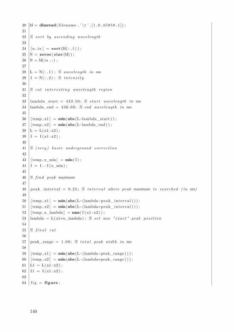
20 M = dlmread( f i l ename , ’ \ t ’ , [ 1 , 0 , 4 5 958 , 1 ] ) ;2122 % sor t by ascending wave length2324 [ n , i x ] = sort (M( : , 1 ) ) ;25 N = zeros ( s ize (M) ) ;26 N = M( ix , : ) ;2728 L = N( : , 1 ) ; % wave length in nm29 I = N( : , 2 ) ; % in t e n s i t y3031 % cut i n t e r e s t i n g wave length reg ion3233 lambda_start = 432 . 5 0 ; % s t a r t wave length in nm34 lambda_end = 436 . 0 0 ; % end wave leng th in nm3536 [ temp , x1 ] = min(abs (L− lambda_start ) ) ;37 [ temp , x2 ] = min(abs (L−lambda_end ) ) ;38 L = L( x1 : x2 ) ;39 I = I ( x1 : x2 ) ;4041 % ( very ) ba s i c underground co r r e c t i on4243 [ temp , x_min ] = min( I ) ;44 I = I .− I (x_min) ;4546 % f ind peak maximum4748 peak_interva l = 0 . 2 5 ; % in t e r v a l where peak maximum i s searched ( in nm)4950 [ temp , x1 ] = min(abs (L−( lambda−peak_interva l ) ) ) ;51 [ temp , x2 ] = min(abs (L−( lambda+peak_interva l ) ) ) ;52 [ temp , x_lambda ] = max( I ( x1 : x2 ) ) ;53 lambda = L( x1+x_lambda) ; % se t new " exac t " peak po s i t i o n5455 % f i n a l cut5657 peak_range = 1 . 0 0 ; % t o t a l peak width in nm5859 [ temp , x1 ] = min(abs (L−( lambda−peak_range ) ) ) ;60 [ temp , x2 ] = min(abs (L−( lambda+peak_range ) ) ) ;61 L1 = L( x1 : x2 ) ;62 I1 = I ( x1 : x2 ) ;6364 f i g = f igure ;

140

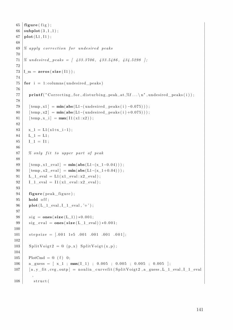
65 f igure ( f i g ) ;66 subplot ( 3 , 1 , 1 ) ;67 plot (L1 , I1 ) ;6869 % app ly co r r e c t i on f o r undes i red peaks7071 % undesired_peaks = [ 433.3706 , 433.5486 , 434.5298 ] ;7273 I_m = zeros ( s ize ( I1 ) ) ;7475 for i = 1 : columns ( undesired_peaks )7677 printf ( " Correc t ing ␣ f o r ␣ d i s tu rb ing ␣peak␣ at ␣%f . . . \ n " , undesired_peaks ( i ) ) ;7879 [ temp , x1 ] = min(abs (L1−( undesired_peaks ( i ) −0.075) ) ) ;80 [ temp , x2 ] = min(abs (L1−( undesired_peaks ( i ) +0.075) ) ) ;81 [ temp , x_i ] = max( I1 ( x1 : x2 ) ) ;8283 x_1 = L1( x1+x_i−1) ;84 L_1 = L1 ;85 I_1 = I1 ;8687 % only f i t to upper par t o f peak8889 [ temp , x1_eval ] = min(abs (L1−(x_1−0 .04) ) ) ;90 [ temp , x2_eval ] = min(abs (L1−(x_1+0.04) ) ) ;91 L_1_eval = L1( x1_eval : x2_eval ) ;92 I_1_eval = I1 ( x1_eval : x2_eval ) ;9394 f igure ( peak_f igure ) ;95 hold o f f ;96 plot (L_1_eval , I_1_eval , ’+ ’ ) ;9798 s i g = ones ( s ize (L_1) ) ∗0 . 0 01 ;99 s ig_eva l = ones ( s ize ( L_1_eval ) ) ∗0 . 0 01 ;100101 s t e p s i z e = [ . 0 0 1 1e5 .001 .001 .001 . 0 0 1 ] ;102103 Sp l i tVo i g t2 = @ (p , x ) Sp l i tVo i g t (x , p) ;104105 PlotCmd = @ ( f ) 0 ;106 a_guess = [ x_1 ; max( I_1 ) ; 0 .005 ; 0 .005 ; 0 .005 ; 0 .005 ] ;107 [ a , y_fit , cvg , outp ] = non l i n_curve f i t ( Sp l i tVo igt2 , a_guess , L_1_eval , I_1_eval

,108 s t r u c t (

141

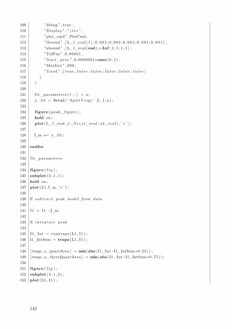
109 " debug " , true ,110 " Display " , " i t e r " ,111 " plot_cmd " ,PlotCmd ,112 " lbound " , [ L_1_eval (1 ) ; 0 . 0 0 1 ; 0 . 0 0 1 ; 0 . 0 0 1 ; 0 . 0 0 1 ; 0 . 0 0 1 ] ,113 " ubound " , [ L_1_eval (end) ;+ Inf ; 1 ; 1 ; 1 ; 1 ] ,114 "TolFun " ,0 . 00001 ,115 " f rac t_prec " ,0 .0000001∗ ones ( 6 , 1 ) ,116 "MaxIter " ,200 ,117 " f i x ed " , [ t rue ; f a l s e ; f a l s e ; f a l s e ; f a l s e ; f a l s e ]118 )119 )120121 f i t_parameters ( i , : ) = a ;122 y_f i t = feval ( ’ Sp l i tVo i g t ’ ,L_1 , a ) ;123124 f igure ( peak_f igure ) ;125 hold on ;126 plot (L_1_eval , y_f i t ( x1_eval : x2_eval ) , ’ r ’ ) ;127128 I_m += y_f i t ;129130 endfor131132 f i t_parameters133134 f igure ( f i g ) ;135 subplot ( 3 , 1 , 1 ) ;136 hold on ;137 plot (L1 , I_m, ’ r ’ ) ;138139 % sub t r a c t peak model from data140141 I1 = I1 .−I_m;142143 % in t e g r a t e peak144145 I1_Int = cumtrapz (L1 , I1 ) ;146 I1_IntSum = trapz (L1 , I1 ) ;147148 [ temp , x_quartArea ] = min(abs ( I1_Int−I1_IntSum ∗0 . 25 ) ) ;149 [ temp , x_threeQuartArea ] = min(abs ( I1_Int−I1_IntSum ∗0 . 75 ) ) ;150151 f igure ( f i g ) ;152 subplot ( 3 , 1 , 2 ) ;153 plot (L1 , I1 ) ;

142

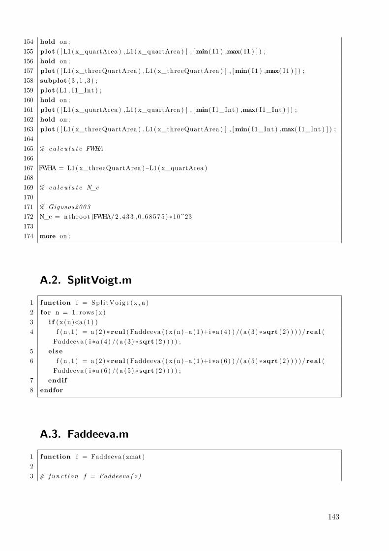
154 hold on ;155 plot ( [ L1( x_quartArea ) ,L1( x_quartArea ) ] , [min( I1 ) ,max( I1 ) ] ) ;156 hold on ;157 plot ( [ L1( x_threeQuartArea ) ,L1( x_threeQuartArea ) ] , [min( I1 ) ,max( I1 ) ] ) ;158 subplot ( 3 , 1 , 3 ) ;159 plot (L1 , I1_Int ) ;160 hold on ;161 plot ( [ L1( x_quartArea ) ,L1( x_quartArea ) ] , [min( I1_Int ) ,max( I1_Int ) ] ) ;162 hold on ;163 plot ( [ L1( x_threeQuartArea ) ,L1( x_threeQuartArea ) ] , [min( I1_Int ) ,max( I1_Int ) ] ) ;164165 % ca l c u l a t e FWHA166167 FWHA = L1( x_threeQuartArea )−L1( x_quartArea )168169 % ca l c u l a t e N_e170171 % Gigosos2003172 N_e = nthroot (FWHA/2 .433 , 0 . 68575 ) ∗10^23173174 more on ;

A.2. SplitVoigt.m

1 function f = Sp l i tVo i g t (x , a )2 for n = 1 : rows (x )3 i f ( x (n)<a (1) )4 f (n , 1 ) = a (2) ∗ real ( Faddeeva ( ( x (n)−a (1 )+i ∗a (4 ) ) /( a (3 ) ∗sqrt (2 ) ) ) ) / real (

Faddeeva ( i ∗a (4 ) /( a (3 ) ∗sqrt (2 ) ) ) ) ;5 else6 f (n , 1 ) = a (2) ∗ real ( Faddeeva ( ( x (n)−a (1 )+i ∗a (6 ) ) /( a (5 ) ∗sqrt (2 ) ) ) ) / real (

Faddeeva ( i ∗a (6 ) /( a (5 ) ∗sqrt (2 ) ) ) ) ;7 endif8 endfor

A.3. Faddeeva.m

1 function f = Faddeeva ( zmat )23 # func t i on f = Faddeeva ( z )

143

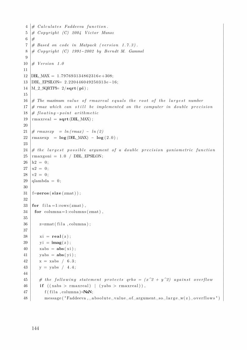
4 # Ca l cu l a t e s Faddeeva func t i on .5 # Copyright (C) 2004 Victor Munoz6 #7 # Based on code in Matpack ( ve r s i on 1 . 7 . 3 ) .8 # Copyright (C) 1991−2002 by Berndt M. Gammel910 # Version 1.01112 DBL_MAX = 1.797693134862316 e+308;13 DBL_EPSILON= 2.220446049250313 e −16;14 M_2_SQRTPI= 2/ sqrt (pi ) ;1516 # The maximum va lue o f rmaxreal e qua l s the roo t o f the l a r g e s t number17 # rmax which can s t i l l be implemented on the computer in doub le p r e c i s i on18 # f l o a t i n g −po in t a r i t hme t i c19 rmaxreal = sqrt (DBL_MAX) ;2021 # rmaxexp = ln ( rmax) − l n (2)22 rmaxexp = log (DBL_MAX) − log ( 2 . 0 ) ;2324 # the l a r g e s t p o s s i b l e argument o f a doub le p r e c i s i on goniometr ic f unc t i on25 rmaxgoni = 1 .0 / DBL_EPSILON;26 h2 = 0 ;27 u2 = 0 ;28 v2 = 0 ;29 qlambda = 0 ;3031 f=zeros ( s ize ( zmat ) ) ;3233 for f i l a =1: rows ( zmat ) ,34 for columna=1: columns ( zmat ) ,3536 z=zmat ( f i l a , columna ) ;3738 x i = real ( z ) ;39 y i = imag( z ) ;40 xabs = abs ( x i ) ;41 yabs = abs ( y i ) ;42 x = xabs / 6 . 3 ;43 y = yabs / 4 . 4 ;4445 # the f o l l ow i n g s ta tement p r o t e c t s qrho = ( x^2 + y^2) aga in s t ove r f l ow46 i f ( ( xabs > rmaxreal ) | ( yabs > rmaxreal ) ) ,47 f ( f i l a , columna )=NaN;48 message ( " Faddeeva , ␣ abso lu t e ␣ value ␣ o f ␣argument␣ so ␣ l a r g e ␣w( z ) ␣ ove r f l ows " )

144

49 end505152 qrho = x .∗ x + y .∗ y ;53 xabsq = xabs .∗ xabs ;54 xquad = xabsq − yabs .∗ yabs ;55 yquad = xabs .∗ 2 .∗ yabs ;5657 a = qrho < 0 .085264 ;5859 i f ( a ) ,6061 # I f ( qrho < 0.085264) then the Faddeeva− f unc t i on i s e va l ua t ed62 # using a power− s e r i e s (Abramowitz/Stegun , equat ion ( 7 . 1 . 5 ) , p .297) .63 # n i s the minimum number o f terms needed to ob ta in the r equ i r ed64 # accuracy .6566 qrho = (1 − y ∗ 0 . 85 ) ∗ sqrt ( qrho ) ;67 n = round( qrho ∗ 72 + 6) ;68 # C++ j = (n << 1) + 1;69 # e1 << e2 = e1 ∗2^( e2 ) ;70 j = n ∗ 2 + 1 ;71 xsum = 1.0 / j ;72 ysum = 0 . 0 ;73 for i=n : −1 :1 ,74 j = j −2;75 xaux = (xsum ∗ xquad − ysum ∗ yquad ) / i ;76 ysum = (xsum ∗ yquad + ysum ∗ xquad ) / i ;77 xsum = xaux + 1 .0 / j ;78 end79 u1 = (xsum ∗ yabs + ysum ∗ xabs ) ∗ −M_2_SQRTPI + 1 . 0 ;80 v1 = (xsum ∗ xabs − ysum ∗ yabs ) ∗ M_2_SQRTPI;81 daux = exp(−xquad ) ;82 u2 = daux ∗ cos ( yquad ) ;83 v2 = −daux ∗ sin ( yquad ) ;8485 u = u1 ∗ u2 − v1 ∗ v2 ;86 v = u1 ∗ v2 + v1 ∗ u2 ;87 else8889 # I f ( qrho > 1 .0) then w( z ) i s e va l ua t ed us ing the Laplace cont inued90 # f r a c t i o n . nu i s the minimum number o f terms needed to ob ta in the91 # requ i r ed accuracy .92 # i f ( ( qrho > 0.085264) && ( qrho < 1.0 ) ) then w( z ) i s e va l ua t ed93 # by a trunca ted Taylor expansion , where the Laplace cont inued

145

94 # f r a c t i o n i s used to c a l c u l a t e the d e r i v a t i v e s o f w( z ) .95 # kapn i s the minimum number o f terms in the Taylor expansion needed96 # to ob ta in the r equ i r ed accuracy .97 # nu i s the minimum number o f terms o f the cont inued f r a c t i o n needed98 # to c a l c u l a t e the d e r i v a t i v e s wi th the r equ i r ed accuracy .99100 i f ( qrho > 1 . 0 ) ,101 h = 0 . 0 ;102 kapn = 0 ;103 qrho = sqrt ( qrho ) ;104 # C++: ( i n t )105 nu = f ix (1442 / ( qrho ∗ 26 + 77) + 3) ;106 else107 qrho = (1 − y ) ∗ sqrt (1 − qrho ) ;108 h = qrho ∗ 1 . 8 8 ;109 h2 = h ∗ 2 ;110 kapn = round( qrho ∗ 34 + 7) ;111 nu = round( qrho ∗ 26 + 16) ;112 end113114 b = h > 0 . 0 ;115116 i f (b) ,117 qlambda = h2 .^ kapn ;118 end119120 rx = ry = sx = sy = 0 . 0 ;121 for n=nu : −1 :0 ,122 np1 = n + 1 ;123 tx = yabs + h + np1 ∗ rx ;124 ty = xabs − np1 ∗ ry ;125 c = 0 .5 / ( tx ∗ tx + ty ∗ ty ) ;126 rx = c ∗ tx ;127 ry = c ∗ ty ;128 i f (b & (n <= kapn ) ) ,129 tx = qlambda + sx ;130 sx = rx ∗ tx − ry ∗ sy ;131 sy = ry ∗ tx + rx ∗ sy ;132 qlambda = qlambda/h2 ;133 end134 end135136 i f (h == 0 . 0 ) ,137 u = rx ∗ M_2_SQRTPI;138 v = ry ∗ M_2_SQRTPI;

146

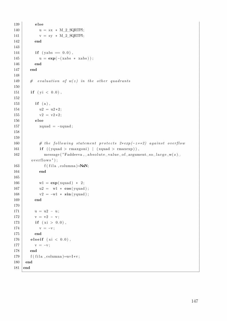
139 else140 u = sx ∗ M_2_SQRTPI;141 v = sy ∗ M_2_SQRTPI;142 end143144 i f ( yabs == 0 . 0 ) ,145 u = exp(−( xabs ∗ xabs ) ) ;146 end147 end148149 # eva l ua t i on o f w( z ) in the o ther quadrants150151 i f ( y i < 0 . 0 ) ,152153 i f ( a ) ,154 u2 = u2 ∗2 ;155 v2 = v2 ∗2 ;156 else157 xquad = −xquad ;158159160 # the f o l l ow i n g s ta tement p r o t e c t s 2∗ exp (− z ∗∗2) aga in s t ove r f l ow161 i f ( ( yquad > rmaxgoni ) | ( xquad > rmaxexp ) ) ,162 message ( " Faddeeva , ␣ abso lu t e ␣ value ␣ o f ␣argument␣ so ␣ l a r g e ␣w( z ) ␣

ove r f l ows " ) ;163 f ( f i l a , columna )=NaN;164 end165166 w1 = exp( xquad ) ∗ 2 ;167 u2 = w1 ∗ cos ( yquad ) ;168 v2 = −w1 ∗ sin ( yquad ) ;169 end170171 u = u2 − u ;172 v = v2 − v ;173 i f ( x i > 0 . 0 ) ,174 v = −v ;175 end176 e l s e i f ( x i < 0 . 0 ) ,177 v = −v ;178 end179 f ( f i l a , columna )=u+I ∗v ;180 end181 end

147

APPENDIX B

“Carbon Enhancement Effect” – SupplementaryMaterial

The contents of the electronic supplementary material of the “Carbon Enhancement Effect”article (chapter 9) is appended here. It can also be found under DOI:10.1039/c5ja00237k.

149

B.1. Enhancement factors

Table B.1.: Signal enhancement/suppression factors (emission line signal obtained in the given reagent dividedby the signal obtained in 3% HNO3 v/v) of selected emission lines by various reagents. ND: notdetermined; LR: line rejected, spectral interference defined as blank signal > 10% of the signal inthe analyte containing solution before blank subtraction; RSD < 3% for all emission lines

Emission line, nmTotal lineenergy, eV

Methanol10%

Phenylalanine8 gL−1 C

15 sccm CO2added to theaerosol gasstream

15 sccm CO2added to theintermediategas flow

Br234 gL−1

NaCl30 gL−1

Ag (II) 224.641 17.95 1.68 1.01 ND ND ND NDAg (I) 328.068 3.78 1.03 0.99 ND ND ND NDAg (I) 338.289 3.66 1.02 0.99 ND ND ND NDAl (II) 167.078 13.41 1.50 1.02 1.04 1.83 0.95 0.69Al (I) 308.215 4.02 1.09 0.98 LR LR LR LRAl (I) 394.401 3.14 1.01 0.98 0.76 1.28 1.07 0.79Al (I) 396.152 3.14 1.00 0.98 0.76 1.27 1.06 0.79Ar (I) 404.442 14.69 1.97 0.98 1.36 2.49 0.88 0.90Ar (I) 430.010 14.51 1.94 0.98 1.34 2.40 0.88 0.91As (I) 189.042 6.56 1.97 1.08 1.52 2.08 1.04 0.83As (I) 193.759 6.40 1.90 1.07 1.48 2.01 1.04 0.84As (I) 197.262 6.29 1.92 1.08 1.47 1.98 1.03 0.84Au (II) 174.050 18.22 LR 0.99 LR LR LR LRAu (I) 201.200 7.30 1.35 1.00 LR 1.47 1.06 0.80Au (I) 242.795 5.11 1.18 1.00 0.92 1.25 1.03 0.81Au (I) 267.595 4.63 1.09 1.00 0.89 1.17 1.02 0.82B (II) 136.246 17.40 LR 1.05 ND ND ND NDB(I) 182.641 6.79 LR 1.01 ND ND ND NDB(I) 208.959 5.93 LR 1.00 ND ND ND NDB(I) 249.677 4.96 1.16 0.98 0.95 1.25 1.01 0.76B (I) 249.773 4.96 1.16 0.97 0.94 1.26 1.01 0.76Ba (II) 230.424 11.19 1.10 1.01 ND ND ND NDBa (II) 233.527 11.22 1.08 1.02 ND ND ND NDBa (II) 455.404 7.93 0.84 1.02 ND ND ND NDBe (I) 234.861 5.28 1.18 0.99 0.93 1.28 0.96 0.75Be (II) 313.042 13.28 1.42 1.08 1.07 1.40 1.05 0.66Be (II) 313.107 13.28 1.42 1.08 1.07 1.41 1.05 0.66Bi (II) 190.241 15.91 LR 0.99 LR 1.43 0.87 0.68Bi (I) 222.825 5.56 1.09 0.98 0.80 1.20 0.92 0.74Bi (I) 223.061 5.56 1.03 0.97 0.78 1.18 0.94 0.74Br (I) 144.990 8.55 LR 0.98 LR 1.73 ND NDBr (I) 148.845 8.33 1.57 0.98 LR 1.59 ND NDBr (I) 154.065 8.05 1.58 0.98 LR LR ND NDCa (II) 183.801 14.55 LR 1.04 LR LR LR LRCa (II) 315.887 13.16 1.24 1.03 0.86 1.44 1.00 0.66Ca (II) 317.933 13.16 1.22 1.03 0.87 1.44 0.99 0.66Ca (II) 393.366 9.26 0.90 1.04 0.69 0.99 0.97 0.65Ca (II) 396.847 9.24 0.90 1.03 0.67 0.95 0.95 0.65Ca (I) 422.673 2.93 0.99 0.96 0.70 1.26 1.29 LRCd (II) 214.438 14.77 1.57 1.04 1.07 1.85 0.91 0.67Cd (II) 226.502 14.46 1.40 1.03 0.98 1.65 0.90 0.68Cd (I) 228.802 5.42 1.31 1.02 0.98 1.44 0.97 0.79

150

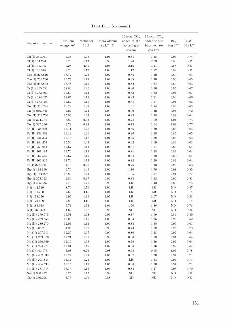
Table B.1.: (continued)

Emission line, nmTotal lineenergy, eV

Methanol10%

Phenylalanine8 gL−1 C

15 sccm CO2added to theaerosol gasstream

15 sccm CO2added to theintermediategas flow

Br234 gL−1

NaCl30 gL−1

Cd (I) 361.051 7.38 1.08 1.04 0.81 1.15 0.96 0.74Cl (I) 134.724 9.20 1.77 0.99 1.20 2.03 0.83 NDCl (I) 135.165 9.28 2.59 1.04 2.16 3.21 0.88 NDCl (I) 136.345 9.20 1.75 1.00 1.12 1.92 0.89 NDCo (II) 228.616 13.72 1.21 1.02 0.85 1.40 0.89 0.65Co (II) 230.786 13.75 1.19 1.02 0.85 1.40 0.90 0.65Co (II) 238.892 13.48 1.15 1.01 0.82 1.34 0.89 0.63Cr (II) 205.552 12.80 1.20 1.03 0.86 1.36 0.95 0.67Cr (II) 283.563 12.69 1.14 1.03 0.83 1.32 0.94 0.67Cr (II) 284.325 12.65 1.13 1.02 0.83 1.31 0.93 0.66Cr (II) 284.984 12.62 1.15 1.04 0.81 1.27 0.94 0.66Cu (II) 219.226 16.22 1.49 1.03 1.01 1.84 0.89 0.63Cu (I) 219.958 7.02 1.24 1.00 0.90 1.40 0.94 0.72Cu (II) 224.700 15.96 1.24 1.01 0.83 1.48 0.88 0.64Cu (I) 324.754 3.82 0.93 1.02 0.74 1.02 1.01 0.75Cu (I) 327.396 3.79 0.92 1.01 0.75 1.04 1.02 0.77Fe (II) 238.204 13.11 1.20 1.01 0.86 1.39 0.85 0.65Fe (II) 239.562 13.12 1.20 1.01 0.86 1.39 0.85 0.65Fe (II) 241.331 13.16 1.18 1.01 0.85 1.38 0.85 0.65Fe (II) 244.451 15.56 1.34 1.00 0.92 1.69 0.84 0.63Fe (II) 259.941 12.67 1.11 1.00 0.81 1.27 0.83 0.64Fe (II) 261.187 12.70 1.11 1.01 0.81 1.28 0.83 0.64Fe (II) 262.567 12.67 1.19 1.01 0.84 1.39 0.85 0.64Fe (II) 262.829 12.74 1.12 1.00 0.82 1.29 0.83 0.64Fe (I) 373.486 4.18 0.96 1.04 0.76 1.13 0.96 0.83Hg (I) 184.950 6.70 1.45 1.00 1.16 1.79 0.98 0.85Hg (II) 194.227 16.82 1.41 1.01 1.05 1.77 0.91 0.77Hg (I) 253.652 4.89 0.97 0.99 0.84 1.12 0.99 0.83Hg (I) 435.835 7.73 1.20 0.99 LR 1.43 0.89 0.75I (I) 142.549 8.70 1.70 1.06 LR LR ND 0.87I (I) 161.760 7.66 LR 1.04 LR LR ND LRI (I) 178.276 6.95 1.69 1.05 LR 2.07 ND 0.83I (I) 179.909 7.83 LR 1.06 LR LR ND LRI (I) 183.038 6.77 1.52 1.04 1.20 1.86 ND 0.76K (I) 766.491 1.62 1.08 0.95 ND ND ND NDMg (II) 279.079 16.51 1.38 0.97 0.87 1.79 0.85 0.59Mg (II) 279.553 12.08 1.16 1.03 0.84 1.35 0.95 0.62Mg (II) 280.270 12.07 1.14 1.00 0.84 1.35 0.95 0.61Mg (I) 285.213 4.35 1.00 0.96 0.73 1.28 0.95 0.79Mn (II) 257.611 12.25 1.07 0.99 0.80 1.28 0.92 0.64Mn (II) 259.373 12.21 1.07 0.99 0.80 1.28 0.91 0.64Mn (II) 260.569 12.19 1.08 1.00 0.79 1.26 0.92 0.64Mn (II) 294.921 12.81 1.15 1.02 0.86 1.36 0.92 0.64Mn (I) 403.076 3.08 0.75 0.98 0.58 0.95 1.06 0.78Mo (II) 202.030 13.22 1.21 1.05 0.87 1.30 0.94 0.71Mo (II) 203.844 13.17 1.21 1.04 LR 1.33 0.94 0.71Mo (II) 204.598 13.15 1.19 1.05 0.86 1.30 0.94 0.71Mo (II) 281.615 13.16 1.15 1.04 0.83 1.27 0.93 0.70Na (I) 330.237 3.75 1.17 0.92 ND ND ND NDNa (I) 330.298 3.75 1.09 0.88 ND ND ND ND

151

Table B.1.: (continued)

Emission line, nmTotal lineenergy, eV

Methanol10%

Phenylalanine8 gL−1 C

15 sccm CO2added to theaerosol gasstream

15 sccm CO2added to theintermediategas flow

Br234 gL−1

NaCl30 gL−1

Na (I) 588.995 2.10 0.86 0.93 ND ND ND NDNa (I) 589.592 2.10 0.86 0.92 ND ND ND NDNi (II) 221.648 14.27 1.31 1.03 0.91 1.55 0.89 0.65Ni (II) 227.021 14.26 1.29 1.02 0.90 1.52 0.88 0.64Ni (II) 231.604 14.03 1.25 1.02 0.88 1.47 0.89 0.64Ni (I) 232.003 5.34 1.11 0.99 0.83 1.27 0.96 0.75Ni (I) 300.249 4.15 0.96 1.01 0.76 1.10 0.98 0.77Ni (I) 341.476 3.66 0.88 1.02 0.71 1.00 1.02 0.82P (I) 138.147 8.97 2.00 1.03 1.65 2.16 1.13 0.88P (I) 168.599 8.76 2.14 1.05 LR LR LR LRP (I) 169.403 8.73 2.08 1.05 1.71 2.21 1.13 0.81P (I) 177.495 6.99 1.89 1.04 1.56 2.00 1.13 0.86P (I) 178.287 6.95 1.87 1.03 LR 2.01 1.13 0.86P (I) 213.618 7.21 2.09 1.03 1.63 2.20 1.14 0.86P (I) 214.914 7.18 2.11 1.03 1.65 2.20 1.14 0.86Pb (II) 220.353 14.79 1.29 0.99 0.88 1.63 0.91 0.65Pb (I) 283.305 4.38 0.97 0.97 0.77 1.16 1.02 0.76Pb (I) 405.778 4.38 0.99 0.99 0.81 1.18 1.07 0.81S (I) 142.503 8.70 1.44 0.97 LR LR 1.17 0.93S (I) 180.731 6.86 1.59 0.97 1.18 LR 1.18 0.94S (I) 182.034 6.86 1.64 0.98 1.17 1.67 1.19 0.91Sb (I) 187.115 6.63 LR 1.00 LR LR 0.98 0.77Sb (I) 206.833 5.99 1.24 1.00 LR LR LR LRSb (I) 217.581 5.70 1.18 1.00 0.92 1.32 0.98 0.78Sc (II) 256.023 11.41 ND ND 1.09 1.07 ND NDSc (I and II) 335.373 — ND ND 1.04 1.02 ND NDSc (II) 355.855 10.05 ND ND 1.05 1.02 ND NDSc (II) 361.384 10.01 ND ND 1.06 1.03 ND NDSc (II) 364.279 9.96 ND ND 1.07 1.05 ND NDSc (I) 390.749 3.17 ND ND 0.88 0.86 ND NDSc (II) 424.683 9.80 ND ND 1.03 0.99 ND NDSc (II) 429.477 10.05 ND ND 1.04 1.01 ND NDSc (II) 432.501 10.02 ND ND 1.06 1.03 ND NDSc (II) 437.446 10.01 ND ND 1.07 1.05 ND NDSe (I) 196.090 6.32 2.51 1.20 1.98 2.89 1.86 0.78Se (I) 203.985 6.32 2.64 1.22 2.02 2.97 1.83 0.78Se (I) 207.479 5.97 2.24 1.22 LR 2.37 1.85 0.71Sr (II) 407.771 10.38 0.89 1.02 0.69 0.96 0.97 0.66Sr (II) 421.552 10.28 0.84 1.02 0.66 0.93 0.98 0.65Sr (I) 460.733 2.69 0.96 0.96 0.68 1.19 1.26 LRTi (II) 307.864 10.88 1.09 1.04 0.80 1.14 0.94 0.70Ti (II) 323.452 10.71 1.05 1.05 0.77 1.10 0.93 0.70Ti (II) 334.941 10.58 1.03 1.04 0.78 1.13 0.95 0.70Ti (II) 336.121 10.54 1.03 1.04 0.78 1.13 0.94 0.70Tl (II) 132.171 15.49 2.13 1.03 1.36 2.68 0.00 0.72Tl (II) 190.864 12.60 LR 1.02 LR LR LR LRTl (I) 276.787 4.48 1.06 0.95 0.79 1.27 1.04 0.81V (II) 292.402 11.38 1.14 1.04 0.85 1.26 0.94 0.71V (II) 292.464 11.35 1.13 1.03 0.84 1.25 0.95 0.71V (II) 309.311 11.15 1.13 1.05 0.84 1.23 0.95 0.70

152

Table B.1.: (continued)

Emission line, nmTotal lineenergy, eV

Methanol10%

Phenylalanine8 gL−1 C

15 sccm CO2added to theaerosol gasstream

15 sccm CO2added to theintermediategas flow

Br234 gL−1

NaCl30 gL−1

V(II) 311.071 11.08 1.10 1.05 0.82 1.20 0.93 0.70Zn (II) 202.548 15.51 1.81 1.05 1.23 2.10 0.91 0.69Zn (II) 206.191 15.40 1.78 1.05 1.21 2.04 0.91 0.69Zn (I) 213.856 5.80 1.28 1.01 0.94 1.41 0.93 0.77Zn (I) 334.502 7.78 1.25 1.00 0.97 1.40 0.91 0.72

153

B.2. HV PSU Data Logger Schematics

The following pages include the schematics of the HV-PSU data logger which was used inthe investigations of the “carbon enhancement effect” (refer to chapter 9).

154

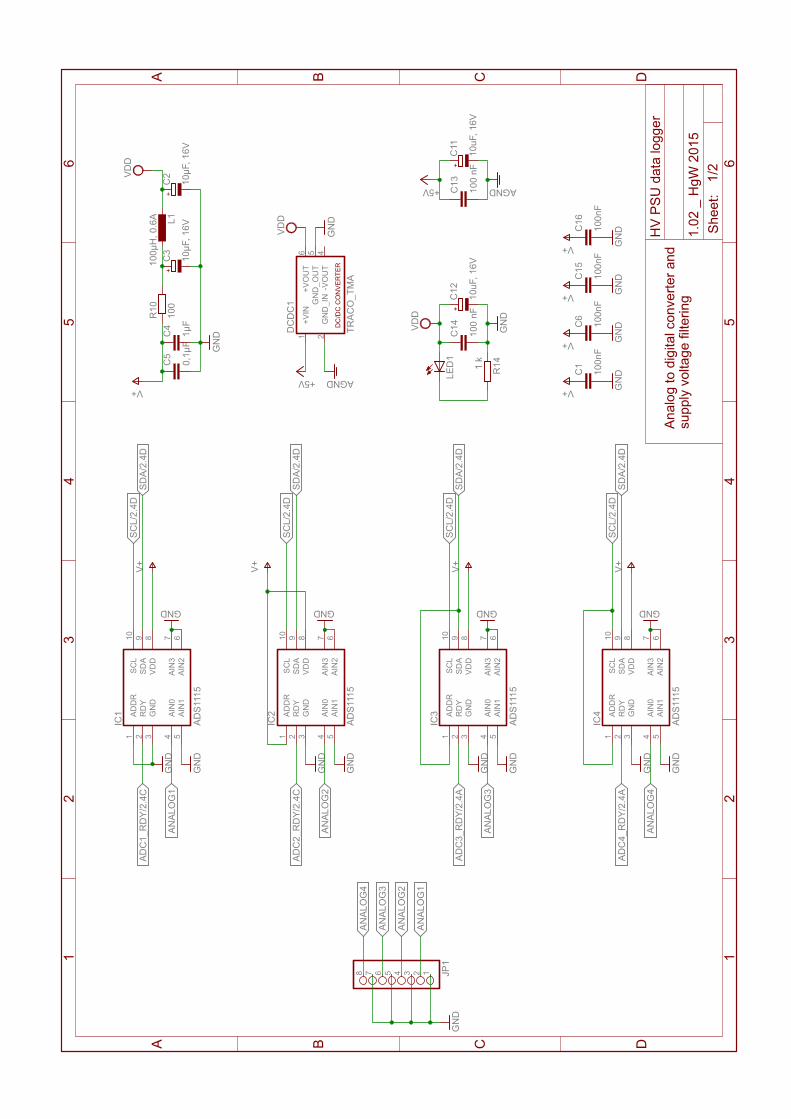
AD

S11

15

GN

D

GN

D

100nF

1µ

F10µ

F, 16V

GN

D

GN

D

GND

0,1

µF

100µ

H, 0.6

A

10µ

F, 16V

100

GN

D

AD

S11

15

GN

D

GND

GN

D

100nF

GN

D

VD

D

+5V AGND

VD

D

GN

D

10uF, 16V

10uF, 16V

100 n

F100 n

F

VD

D

+5V AGND

GN

D

1 k

TR

AC

O_T

MA

V+

V+

AD

S11

15

AD

S11

15

GN

D

GN

D

GN

D

GN

D

GND GND

V+

V+

V+

V+

V+

100nF

GN

D

100nF

GN

D

V+

V+

IC1

SC

L10

SD

A9

RD

Y2

AIN

04

VD

D8

GN

D3

AIN

15

AIN

26

AIN

37

AD

DR

1

JP1

12345678

C1

C4

C2

C5

L1

C3

R10

IC2

SC

L10

SD

A9

RD

Y2

AIN

04

VD

D8

GN

D3

AIN

15

AIN

26

AIN

37

AD

DR

1

C6

C11

C12

C13

C14

R14

LE

D1

DC

DC

1

+V

IN1

GN

D_IN

2

+V

OU

T6

-VO

UT

4G

ND

_O

UT

5

IC3

SC

L10

SD

A9

RD

Y2

AIN

04

VD

D8

GN

D3

AIN

15

AIN

26

AIN

37

AD

DR

1

IC4

SC

L10

SD

A9

RD

Y2

AIN

04

VD

D8

GN

D3

AIN

15

AIN

26

AIN

37

AD

DR

1

C15

C16

SD

A/2

.4D

SD

A/2

.4D

SD

A/2

.4D

SD

A/2

.4D

SC

L/2

.4D

SC

L/2

.4D

SC

L/2

.4D

SC

L/2

.4D

AN

ALO

G4

AN

ALO

G4

AN

ALO

G3

AN

ALO

G3

AN

ALO

G2

AN

ALO

G2

AN

ALO

G1

AN

ALO

G1

AD

C1_R

DY

/2.4

C

AD

C2_R

DY

/2.4

C

AD

C3_R

DY

/2.4

A

AD

C4_R

DY

/2.4

A

An

alo

g t

o d

igita

l co

nve

rte

r a

nd

su

pp

ly v

olta

ge

filte

rin

g

HV

PS

U d

ata

log

ge

r

1.0

2 _

Hg

W 2

01

5

+

+

+

+

DC

/DC

CO

NV

ER

TE

R

1/2

Sh

ee

t:

A B C D

12

34

56

A B C D

12

34

56

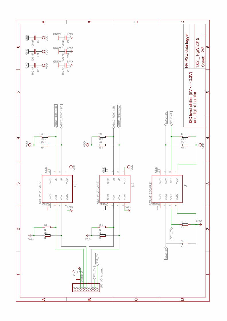
AD

UM

12

50

AR

Z

1.5k

1.5k

VD

D

GN

D

VD

D

GN

D

100 n

F

1k

1k

AG

ND

+3V3

+3V3

+3V3AGND

100 n

F

+5V

AD

UM

12

00

AR

Z

AGNDAGND

GN

D

VD

D

+3V3

1.5k

1.5k

1k

1kV

DD

+3V3

VD

D

GN

D

100 n

F

+3V3AGND

100 n

F

AD

UM

12

00

AR

Z

AGND

GN

D

VD

D

+3V3

1.5k

1.5kVD

D

VD

D

GN

D

100 n

F

+3V3AGND

100 n

F

1k

1k+3V3

VD

D1

1V

DD

28

SC

L1

3S

CL2

6

GN

D1

4G

ND

25

SD

A1

2S

DA

27

U1

R1

R2

C7

R8

R9

C8

VD

D1

1V

DD

28

VIA

2

VIB

3

GN

D1

4G

ND

25

VO

A7

VO

B6

U2

R3

R4

R12

R13

C9

C10

VD

D1

1V

DD

28

VIA

2

VIB

3

GN

D1

4G

ND

25

VO

A7

VO

B6

U3

R5

R6

C17

C18

JP

2_I/O

_A

rduin

o

123456789

R7

R11

SD

A/1

.4A

SC

L/1

.4A

SC

L_3V

SC

L_3V

SD

A_3V

SD

A_3V

AD

C1_R

DY

/1.2

A

AD

C2_R

DY

/1.2

B

AD

C3_R

DY

/1.2

C

AD

C4_R

DY

/1.2

D

I2C

leve

l sh

ifte

r (5

V <

-> 3

.3V

)a

nd

dig

ita

l iso

lato

r

HV

PS

U d

ata

lo

gg

er

1.0

2 _

Hg

W 2

01

5

2/2

Sh

ee

t:

A B C D

12

34

56

A B C D

12

34

56