NBER WORKING PAPER SERIES

RISK SHIFTING AND MUTUAL FUND PERFORMANCE

Jennifer HuangClemens SialmHanjiang Zhang

Working Paper 14903http://www.nber.org/papers/w14903

NATIONAL BUREAU OF ECONOMIC RESEARCH1050 Massachusetts Avenue

Cambridge, MA 02138April 2009

We thank Keith Brown, Jie Cao, Joe Chen, Jonathan Cohn, Ken French, W. Van Harlow, Marcin Kacperczyk,Sheridan Titman, Stefan Ruenzi, Pablo Ruiz-Verdu, Richard Stanton, and seminar participants at GeorgiaState University and the University of Texas at Austin for helpful comments and discussions. Theviews expressed herein are those of the author(s) and do not necessarily reflect the views of the NationalBureau of Economic Research.

NBER working papers are circulated for discussion and comment purposes. They have not been peer-reviewed or been subject to the review by the NBER Board of Directors that accompanies officialNBER publications.

© 2009 by Jennifer Huang, Clemens Sialm, and Hanjiang Zhang. All rights reserved. Short sectionsof text, not to exceed two paragraphs, may be quoted without explicit permission provided that fullcredit, including © notice, is given to the source.

Risk Shifting and Mutual Fund PerformanceJennifer Huang, Clemens Sialm, and Hanjiang ZhangNBER Working Paper No. 14903April 2009JEL No. G11,G12,G23

ABSTRACT

Mutual funds change their risk levels significantly over time. This paper investigates the performanceconsequences of risk shifting, as well as the economic motivations and the mechanisms of risk shifting.Using a holdings-based measure of risk shifting, we find that funds that increase risk perform worsethan funds that keep stable risk levels over time. In addition, funds that expect higher benefits fromrisk shifting are more likely to increase risk and perform particularly poorly after increasing risk. Ourresults are consistent with the notion that agency problems, rather than the ability to take advantageof changing investment opportunities, are the likely motivation behind risk shifting behavior.

Jennifer HuangUniversity of Texas at AustinMcCombs School of Business1 University Station; B6600Austin, TX 78712jennifer.huang@mccombs.utexas.edu

Clemens SialmUniversity of Texas at AustinMcCombs School of Business1 University Station; B6600Austin, TX 78712and NBERclemens.sialm@mccombs.utexas.edu

Hanjiang ZhangUniversity of Texas at AustinMcCombs School of Business1 University Station; B6600Austin, TX 78712hanjiang.zhang@mccombs.utexas.edu

1 Introduction

Mutual funds change their total risk exposure substantially over time. Using the disclosed

holdings of a sample of 2,335 U.S. equity funds over the period between 1980 and 2006, we

document that 27.1% of equity mutual funds change their annualized volatility by more than

2.5% in a given quarter, and 9.6% of funds change their volatility by more than 5%. These

changes are significant given that their average long-term volatility level is only 17.9%. Our

paper studies whether funds that shift risk exhibit different subsequent performance compared

to funds with more consistent risk levels. We further investigate the economic motivations

behind risk shifting and the mechanisms through which risk shifters add or destroy value.

Mutual funds change their risk levels for two potential reasons, which have different perfor-

mance consequences. First, the literature on delegated portfolio management has identified

a potential agency conflict between mutual fund companies and their investors. Whereas

fund investors would like their mutual funds to maximize risk-adjusted returns, mutual fund

companies would like to maximize their profits. Since their profits depend primarily on the

amount of assets under management, mutual funds might have incentives to follow investment

policies that generate money inflows even if these policies reduce the risk-adjusted returns to

their investors. For example, Brown, Harlow, and Starks (1996) and Chevalier and Ellison

(1997) suggest that mutual fund companies strategically change their risk levels to attract

additional fund inflows due to the convex flow-performance relation.1 If agency problems are

the main cause behind risk shifting, then we should not expect superior performance for risk

shifting funds. To the extent that opportunistic risk shifting causes trading costs, constrains

the investment opportunity sets, and distracts fund managers from their goal of investing in

the most promising securities, we should expect risk shifters to perform worse.

The second reason funds change their risk levels is that fund managers might actively adjust

the composition of their portfolios to capitalize on time-varying investment opportunities. If

1Additional papers on the flow-performance relation include Ippolito (1992), Goetzmann and Peles (1997),Sirri and Tufano (1998), Zheng (1999), DelGuercio and Tkac (2002), Lynch and Musto (2003), Nanda, Wang,and Zheng (2004), Huang, Wei, and Yan (2007), and Ivkovich and Weisbenner (2009).

1

funds that actively shift risk have superior investment abilities, then they should perform

better than funds that have more stable risk exposures. If, on the other hand, funds with

inferior investment abilities are more prone to shift risk (because, for example, they erroneously

believe that they have timing ability or lack the confidence to maintain a stable trading

strategy), then funds that shift risk should perform worse.

To measure risk shifting of mutual funds, we propose a holdings-based measure that is

defined as the difference between a fund’s current holdings volatility and its past realized

volatility. The current holdings volatility is the standard deviation of the most recently dis-

closed fund holdings, and the past realized volatility is the standard deviation of the fund’s

actual return. A fund has a positive risk shifting measure if the most recently disclosed

holdings are riskier than the actual fund holdings.

We sort mutual funds into portfolios according to their most recent risk shifting measure

and compare their subsequent performance. We find that funds that increase risk the most

perform significantly worse (with an annualized abnormal return of -2.6% using the Carhart

model) than funds that maintain stable risk levels (with an abnormal return of -0.7%). These

results are robust using alternative performance measures. The poor performance of risk

shifters suggests that they are unlikely to possess superior ability. Instead, risk shifting be-

havior is either an indication of inferior ability or is motivated by agency problems in delegated

portfolio management.

To investigate the potential role of agency problems in risk shifting behavior, we ask

whether the propensity to shift risk and the performance consequences of risk shifting differ

across funds with different benefits of risk shifting. The expected profit of a mutual fund

increases with both the expense ratio and the assets under management. Thus, funds with

higher expense ratios have more to gain from shifting risk. In addition, the literature has

identified younger, smaller funds, and funds that belong to smaller fund families as having

a more sensitive flow-performance relation. Hence, these funds also enjoy larger expected

benefits of risk shifting. Based on these characteristics, we separate funds into subgroups and

2

find that funds with larger benefits of risk shifting are more likely to shift risk and perform

particularly poorly after shifting risk. For example, 14.7% of funds with above-median expense

ratios increase their volatility by more than 2.5% and experience a Carhart alpha of -2.9% per

year, whereas only 10.5% of funds with below-median expense ratios increase their volatility

by the same amount and experience a Carhart alpha of -1.2%. Similarly, younger, smaller

funds and funds that belong to smaller fund families are more likely to shift risk and experience

more severe performance consequences when they shift risk.

To understand the sources of the poor performance of risk shifters, we study the various

mechanisms through which funds can change risk: First, funds can shift risk by changing the

composition between equity holdings and cash holdings. Second, within their equity holdings,

funds can shift risk by changing their exposure to systematic risk (e.g., by switching between

low beta stocks and high beta stocks). Third, funds can shift risk by changing their exposure

to idiosyncratic risk (e.g., by concentrating the holdings on a few positions or industries).

We find evidence that all of these mechanisms are important in explaining the risk shifting

behavior of mutual funds. In contrast, the performance consequences are significant mainly for

funds increasing idiosyncratic risk exposure, whereas both the reduction in cash holdings and

the increase in systematic risk lead to only mild reductions in fund performance. Thus, the

poor performance of risk shifters is driven not by the unsuccessful attempts of fund managers

to time the aggregate market but by their desire to take on idiosyncratic risks. We also

sort funds into subgroups with different turnover to study the impact of transaction costs.

Surprisingly, the poor performance of risk shifters is concentrated in low turnover funds. To

the extent that turnover is a proxy for trading costs, our finding suggests that direct trading

costs are unlikely the main driver of risk shifters’ poor performance.

Several studies have identified a convex flow-performance relation, in which mutual fund in-

vestors tend to invest in funds with stellar performance and do not penalize poor performance

equivalently. This convex flow-performance relation motivates mutual funds to strategically

shift risk levels to attract additional fund flows. For example, Brown, Harlow, and Starks

3

(1996) suggest that mutual funds compete with each other in a tournament and might ma-

nipulate fund risk depending on their prior performance. In particular, they show that funds

with poor past performance tend to increase their risk levels. Chevalier and Ellison (1997)

analyze the convex flow-performance relation and find evidence that mutual funds that are

well ahead of their peers also have an incentive to increase risk to make lists of “top per-

formers.” Koski and Pontiff (1999) confirm this risk shifting behavior and suggest that risk

levels of mutual funds might also change in response to unpredictable fund flows. Further-

more, as discussed by Goetzmann, Ingersoll, Spiegel, and Welch (2007), fund managers have

an incentive to change risk levels to manipulate their performance numbers. Recently, several

theoretical and empirical studies have improved our understanding of risk shifting behavior

of mutual funds.2 Our paper contributes to this literature by investigating the consequences

of risk shifting on fund performance, which have not previously been analyzed. Studying the

performance consequences of risk shifting gives us important insights into the motivations for

risk shifting.

The remainder of this paper is structured as follows: Section 2 derives our holdings-

based measure of risk shifting. Section 3 explains the data sources and gives some basic

summary statistics. Section 4 describes the characteristics of risk shifters and the mechanisms

of shifting risk. Section 5 documents a negative relation between risk shifting and subsequent

fund performance. Sections 6 and 7 investigate the motivations behind risk shifting and the

sources of risk shifters’ poor performance. Section 8 uses a multivariate regression analysis to

control for additional fund characteristics and Section 9 concludes.

2Additional papers on risk shifting include Starks (1987), Grinblatt and Titman (1989), Carpenter (2000),Busse (2001), Elton, Gruber, and Blake (2003), Palomino and Prat (2003), Ross (2004), Elton, Gruber, Krasny,and Ozelge (2006), Li and Tiwari (2006), Basak, Pavlova, and Shapiro (2007), Guasoni, Huberman, and Wang(2007), Massa and Patgiri (2007), Kempf and Ruenzi (2008), Kempf, Ruenzi, and Thiele (2008), Hu, Kale,Pagani, and Subramanian (2008), and Chen and Pennacchi (2009).

4

2 Risk Shifting Measure

Mutual funds can change the total risk of their portfolio by holding assets with different risk

properties or by changing the diversification level of their overall portfolio. To capture the

risk shifting behavior of mutual funds, we examine their portfolio holdings. We measure risk

shifting of a mutual fund f at time t by comparing the current holdings volatility based on

the fund’s most recently disclosed positions σHf,t with the past realized volatility based on the

fund’s realized returns σRf,t:

RSf,t = σHf,t − σR

f,t. (1)

The return of mutual fund f at time t is the scalar product of the portfolio weight wf ,t

and the returns of the assets Rt:

RFf,t = w′f ,tRt =

N∑

i=1

wif,tR

it, (2)

where Rt = [R1t , . . . , R

Nt ]′ is the vector of the returns for all available assets and wf ,t =

[w1f,t, . . . , w

Nf,t]

′ is the vector for the portfolio weights invested in these assets by fund f at time

t. The weights add up to one (w′f ,t1 =

∑Ni=1 wi

f,t = 1).

The variance of the returns of mutual fund f at time t depends on the weights invested in

the various assets and on the N × N variance-covariance matrix of the individual assets Σ.

The variance of a portfolio can be determined by either computing the variance of the portfolio

returns or by pre- and post-multiplying the variance-covariance matrix of the underlying stock

returns by the weight vector.

VAR(RFf,t) = VAR(w′f ,tRt) = w′

f ,tVAR(Rt)wf ,t = w′f ,tΣtwf ,t. (3)

To estimate the current holdings volatility of fund f at time t, we compute the square root

of VAR(RFf,t) by estimating the sample standard deviation of the return of a hypothetical

portfolio that holds the most recently disclosed fund positions over the prior 36 months. This

method is equivalent to calculating the square root of w′f ,tΣtwf ,t.

5

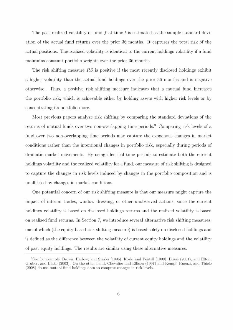
The past realized volatility of fund f at time t is estimated as the sample standard devi-

ation of the actual fund returns over the prior 36 months. It captures the total risk of the

actual positions. The realized volatility is identical to the current holdings volatility if a fund

maintains constant portfolio weights over the prior 36 months.

The risk shifting measure RS is positive if the most recently disclosed holdings exhibit

a higher volatility than the actual fund holdings over the prior 36 months and is negative

otherwise. Thus, a positive risk shifting measure indicates that a mutual fund increases

the portfolio risk, which is achievable either by holding assets with higher risk levels or by

concentrating its portfolio more.

Most previous papers analyze risk shifting by comparing the standard deviations of the

returns of mutual funds over two non-overlapping time periods.3 Comparing risk levels of a

fund over two non-overlapping time periods may capture the exogenous changes in market

conditions rather than the intentional changes in portfolio risk, especially during periods of

dramatic market movements. By using identical time periods to estimate both the current

holdings volatility and the realized volatility for a fund, our measure of risk shifting is designed

to capture the changes in risk levels induced by changes in the portfolio composition and is

unaffected by changes in market conditions.

One potential concern of our risk shifting measure is that our measure might capture the

impact of interim trades, window dressing, or other unobserved actions, since the current

holdings volatility is based on disclosed holdings returns and the realized volatility is based

on realized fund returns. In Section 7, we introduce several alternative risk shifting measures,

one of which (the equity-based risk shifting measure) is based solely on disclosed holdings and

is defined as the difference between the volatility of current equity holdings and the volatility

of past equity holdings. The results are similar using these alternative measures.

3See for example, Brown, Harlow, and Starks (1996), Koski and Pontiff (1999), Busse (2001), and Elton,Gruber, and Blake (2003). On the other hand, Chevalier and Ellison (1997) and Kempf, Ruenzi, and Thiele(2008) do use mutual fund holdings data to compute changes in risk levels.

6

3 Data and Summary Statistics

This section explains the data sources and describes the main characteristics of mutual funds

in our sample.

3.1 Sample Selection

For our empirical analysis, we merge the CRSP Survivorship Bias Free Mutual Fund Database

with the Thomson Financial CDA/Spectrum holdings database and the CRSP stock price

data using the MFLINKS file based on Wermers (2000) and available through the Wharton

Research Data Services. Our sample covers the time period between 1980 and 2006. The CRSP

mutual fund database includes information on fund returns, total assets under management,

different types of fees, investment objectives, and other fund characteristics. The Thomson

Financial database provides long positions in domestic common stock holdings of mutual

funds. The data are collected both from reports filed by mutual funds with the SEC and

from voluntary reports generated by the funds. During most of our sample period, funds

are required by law to disclose their holdings semi-annually. Nevertheless, about 78% of the

observations are from the most recent quarter and only 3% of the holdings are more than two

quarters old.

We focus our analysis on actively-managed domestic equity mutual funds for which the

holdings data are most complete and reliable. Therefore, we eliminate balanced, bond, money

market, international, and index funds.4 We also exclude funds which in the previous month

manage less than $5 million and funds that did not disclose their holdings in the previous 36

months. For funds with multiple share classes, we compute fund-level variables by aggregating

across the different share classes.5

4First, we select funds with the following S&P objectives: AGG, GMC, GRI, GRO, ING, SCG, ENV, FIN,GLD, HLT, NTR, RLE, SEC, TEC, UTI. If a fund does not have any of the above objectives, we select fundswith the following ICDI objectives: AG, GI, LG, IN, PM, SF or UT. If a fund has neither the S&P nor theICDI objective, then we go to the Wiesenberger Fund Type Code and pick funds with the following objectives:G, G-I, IEQ, GCI, LTG, MCG, SCG, GPM, HLT, TCH, or UTL. If none of these objectives are available andthe fund has the CS or SPEC policy, then the fund will be included. Index funds are identified based on theirnames.

5Our sample focuses on actively-managed domestic equity mutual funds, for which the holdings data are

7

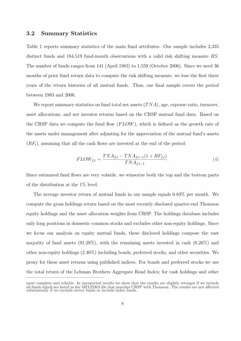
3.2 Summary Statistics

Table 1 reports summary statistics of the main fund attributes. Our sample includes 2,335

distinct funds and 184,519 fund-month observations with a valid risk shifting measure RS.

The number of funds ranges from 141 (April 1983) to 1,559 (October 2006). Since we need 36

months of prior fund return data to compute the risk shifting measure, we lose the first three

years of the return histories of all mutual funds. Thus, our final sample covers the period

between 1983 and 2006.

We report summary statistics on fund total net assets (TNA), age, expense ratio, turnover,

asset allocations, and net investor returns based on the CRSP mutual fund data. Based on

the CRSP data we compute the fund flow (FLOW ), which is defined as the growth rate of

the assets under management after adjusting for the appreciation of the mutual fund’s assets

(RFt), assuming that all the cash flows are invested at the end of the period:

FLOWf,t =TNAf,t − TNAf,t−1(1 + RFf,t)

TNAf,t−1

. (4)

Since estimated fund flows are very volatile, we winsorize both the top and the bottom parts

of the distribution at the 1% level.

The average investor return of mutual funds in our sample equals 0.83% per month. We

compute the gross holdings return based on the most recently disclosed quarter-end Thomson

equity holdings and the asset allocation weights from CRSP. The holdings database includes

only long positions in domestic common stocks and excludes other non-equity holdings. Since

we focus our analysis on equity mutual funds, these disclosed holdings compose the vast

majority of fund assets (91.28%), with the remaining assets invested in cash (6.26%) and

other non-equity holdings (2.46%) including bonds, preferred stocks, and other securities. We

proxy for these asset returns using published indices. For bonds and preferred stocks we use

the total return of the Lehman Brothers Aggregate Bond Index; for cash holdings and other

most complete and reliable. In unreported results we show that the results are slightly stronger if we includeall funds which are listed in the MFLINKS file that matches CRSP with Thomson. The results are not affectedsubstantially if we exclude sector funds or include index funds.

8

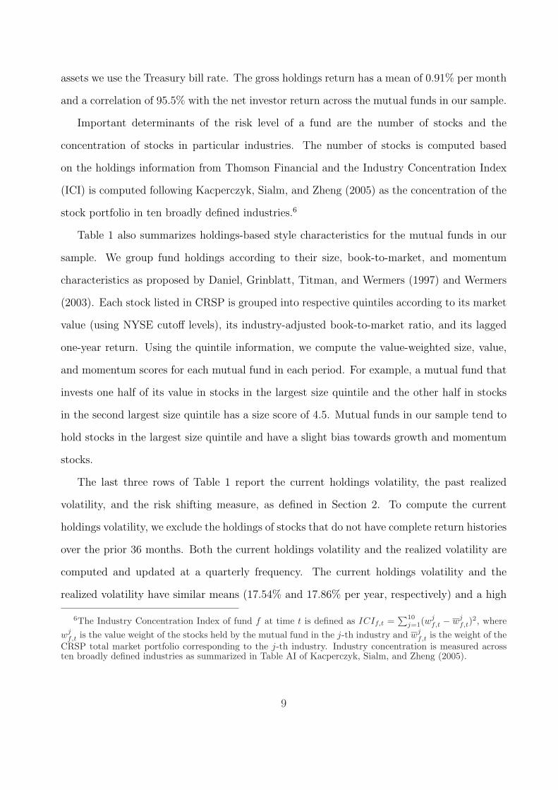
assets we use the Treasury bill rate. The gross holdings return has a mean of 0.91% per month

and a correlation of 95.5% with the net investor return across the mutual funds in our sample.

Important determinants of the risk level of a fund are the number of stocks and the

concentration of stocks in particular industries. The number of stocks is computed based

on the holdings information from Thomson Financial and the Industry Concentration Index

(ICI) is computed following Kacperczyk, Sialm, and Zheng (2005) as the concentration of the

stock portfolio in ten broadly defined industries.6

Table 1 also summarizes holdings-based style characteristics for the mutual funds in our

sample. We group fund holdings according to their size, book-to-market, and momentum

characteristics as proposed by Daniel, Grinblatt, Titman, and Wermers (1997) and Wermers

(2003). Each stock listed in CRSP is grouped into respective quintiles according to its market

value (using NYSE cutoff levels), its industry-adjusted book-to-market ratio, and its lagged

one-year return. Using the quintile information, we compute the value-weighted size, value,

and momentum scores for each mutual fund in each period. For example, a mutual fund that

invests one half of its value in stocks in the largest size quintile and the other half in stocks

in the second largest size quintile has a size score of 4.5. Mutual funds in our sample tend to

hold stocks in the largest size quintile and have a slight bias towards growth and momentum

stocks.

The last three rows of Table 1 report the current holdings volatility, the past realized

volatility, and the risk shifting measure, as defined in Section 2. To compute the current

holdings volatility, we exclude the holdings of stocks that do not have complete return histories

over the prior 36 months. Both the current holdings volatility and the realized volatility are

computed and updated at a quarterly frequency. The current holdings volatility and the

realized volatility have similar means (17.54% and 17.86% per year, respectively) and a high

6The Industry Concentration Index of fund f at time t is defined as ICIf,t =∑10

j=1(wjf,t − wj

f,t)2, where

wjf,t is the value weight of the stocks held by the mutual fund in the j-th industry and wj

f,t is the weight of theCRSP total market portfolio corresponding to the j-th industry. Industry concentration is measured acrossten broadly defined industries as summarized in Table AI of Kacperczyk, Sialm, and Zheng (2005).

9

correlation of 0.83. The risk shifting measure has a mean close to zero and an annualized

standard deviation of 4.58%, which is about one quarter of the average realized volatility.

Thus, mutual funds shift risk significantly.

To test whether the current holdings volatility is a good proxy for the future realized

volatility of a mutual fund, in unreported analysis we regress the future 12-month realized

volatility of a mutual fund on the current holdings volatility and the past realized volatility

over the prior 36 months. We find that the coefficient on the current holdings volatility is

larger and more statistically significant than the coefficient on the past realized volatility.

Thus, the current holdings volatility captures an important aspect of the future risk exposure.

4 Characterization of Risk Shifting

This section discusses the characteristics of risk shifters and clarifies the main mechanisms

through which mutual funds shift risk.

4.1 Characteristics of Risk Shifters

To identify the characteristics of risk shifters, we sort all mutual funds in each quarter into

five portfolios according to the most recent RS measure and compute average characteristics

of these funds. Funds in Portfolio 1 (5) decrease (increase) risk by more than 2.5% per year

and compose 14% (13%) of our sample, whereas funds in Portfolio 3 change risk by less than

1% and compose 41% of our sample.7

Table 2 summarizes the characteristics of mutual funds sorted according to the RS mea-

sure. Funds in Portfolio 1 decrease risk on average by 5.60% per year, which is approximately

26% of their realized volatility over the prior 36 months. On the other hand, funds in Portfo-

lio 5 increase risk by 4.75% per year, which is also approximately 26% of their prior realized

volatility. Thus, funds exhibit significant changes in their overall risk levels over time.

The current holdings volatility and the realized volatility contribute asymmetrically to

7The results in the paper are similar if the mutual funds are sorted into decile portfolios instead.

10

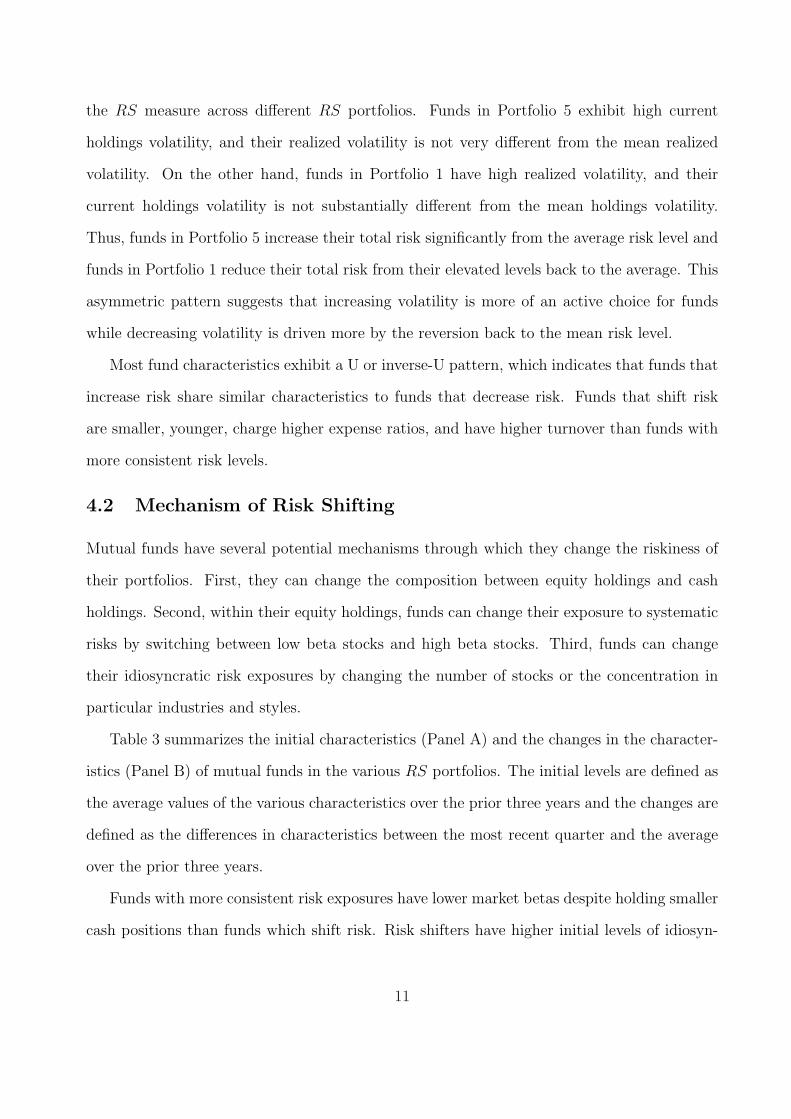
the RS measure across different RS portfolios. Funds in Portfolio 5 exhibit high current

holdings volatility, and their realized volatility is not very different from the mean realized

volatility. On the other hand, funds in Portfolio 1 have high realized volatility, and their

current holdings volatility is not substantially different from the mean holdings volatility.

Thus, funds in Portfolio 5 increase their total risk significantly from the average risk level and

funds in Portfolio 1 reduce their total risk from their elevated levels back to the average. This

asymmetric pattern suggests that increasing volatility is more of an active choice for funds

while decreasing volatility is driven more by the reversion back to the mean risk level.

Most fund characteristics exhibit a U or inverse-U pattern, which indicates that funds that

increase risk share similar characteristics to funds that decrease risk. Funds that shift risk

are smaller, younger, charge higher expense ratios, and have higher turnover than funds with

more consistent risk levels.

4.2 Mechanism of Risk Shifting

Mutual funds have several potential mechanisms through which they change the riskiness of

their portfolios. First, they can change the composition between equity holdings and cash

holdings. Second, within their equity holdings, funds can change their exposure to systematic

risks by switching between low beta stocks and high beta stocks. Third, funds can change

their idiosyncratic risk exposures by changing the number of stocks or the concentration in

particular industries and styles.

Table 3 summarizes the initial characteristics (Panel A) and the changes in the character-

istics (Panel B) of mutual funds in the various RS portfolios. The initial levels are defined as

the average values of the various characteristics over the prior three years and the changes are

defined as the differences in characteristics between the most recent quarter and the average

over the prior three years.

Funds with more consistent risk exposures have lower market betas despite holding smaller

cash positions than funds which shift risk. Risk shifters have higher initial levels of idiosyn-

11

cratic volatility and hold more concentrated portfolios as reflected by the lower number of

stocks and the higher industry concentration index. Risk shifters also differ in their style ex-

posure from funds with more consistent risk exposures as they focus their holdings on small,

growth, and momentum stocks.

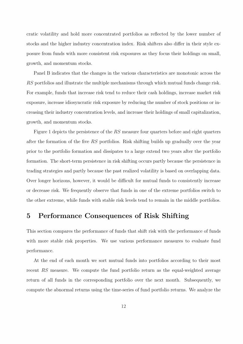
Panel B indicates that the changes in the various characteristics are monotonic across the

RS portfolios and illustrate the multiple mechanisms through which mutual funds change risk.

For example, funds that increase risk tend to reduce their cash holdings, increase market risk

exposure, increase idiosyncratic risk exposure by reducing the number of stock positions or in-

creasing their industry concentration levels, and increase their holdings of small capitalization,

growth, and momentum stocks.

Figure 1 depicts the persistence of the RS measure four quarters before and eight quarters

after the formation of the five RS portfolios. Risk shifting builds up gradually over the year

prior to the portfolio formation and dissipates to a large extend two years after the portfolio

formation. The short-term persistence in risk shifting occurs partly because the persistence in

trading strategies and partly because the past realized volatility is based on overlapping data.

Over longer horizons, however, it would be difficult for mutual funds to consistently increase

or decrease risk. We frequently observe that funds in one of the extreme portfolios switch to

the other extreme, while funds with stable risk levels tend to remain in the middle portfolios.

5 Performance Consequences of Risk Shifting

This section compares the performance of funds that shift risk with the performance of funds

with more stable risk properties. We use various performance measures to evaluate fund

performance.

At the end of each month we sort mutual funds into portfolios according to their most

recent RS measure. We compute the fund portfolio return as the equal-weighted average

return of all funds in the corresponding portfolio over the next month. Subsequently, we

compute the abnormal returns using the time-series of fund portfolio returns. We analyze the

12

future performance of funds after computing the risk shifting measure to avoid any potential

issues of reverse causality.

We report four different performance measures for the fund portfolios. To adjust for risk

and style effects, abnormal returns are computed using the one-factor CAPM, the Fama and

French (1993), the Carhart (1997), and the Ferson and Schadt (1996) models. The Fama-

French-Carhart model is specified as follows:

RFk,t −RTB,t = αk + βMk (RM,t −RTB,t) + βSMB

k (RS,t −RB,t)

+βHMLk (RH,t −RL,t) + βUMD

k (RU,t −RD,t) + εk,t. (5)

The return of portfolio k during time period t is denoted by RFk,t. The index M corre-

sponds to the market portfolio and the index TB to the risk-free Treasury bill rate. Portfolios

of small and large stocks are denoted by S and B; portfolios of stocks with high and low ratios

between their book values and their market values are denoted by H and L; and portfolios

of stocks with relatively high and low returns during the previous year are denoted by U and

D. The Fama-French-Carhart model nests the CAPM model (which includes only the market

factor) and the Fama-French model (which includes the size and the book-to-market factors

in addition to the market factor).

Following Wermers (2003), we use the Ferson and Schadt (1996) conditional model that

nests the Carhart model.

RFk,t −RTB,t = αk + βMk (RM,t −RTB,t) + βSMB

k (RS,t −RB,t) + βHMLk (RH,t −RL,t)

+ βUMDk (RU,t −RD,t) +

5∑

j=1

βjk(RM,t −RTB,t)×MACROj

t−1 + εk,t, (6)

where MACROjt−1 denotes one of five demeaned lagged macro-economic variables including

the Treasury bill yield, the dividend yield of the S&P Composite Index, the Treasury yield

spread (long- minus short-term bonds), the quality spread in the corporate bond market (low-

minus high-grade bonds), and an indicator variable for the month of January.8 In all four

8The market, size, book-to-market, momentum factors and the risk-free rate are obtained from Ken French’s

13

models, the factor loadings βk denote the sensitivities of the returns of portfolio k to the

various factors and are estimated for each of the portfolios separately. The intercepts αk

capture the abnormal returns of the corresponding models and are reported in Table 4.9

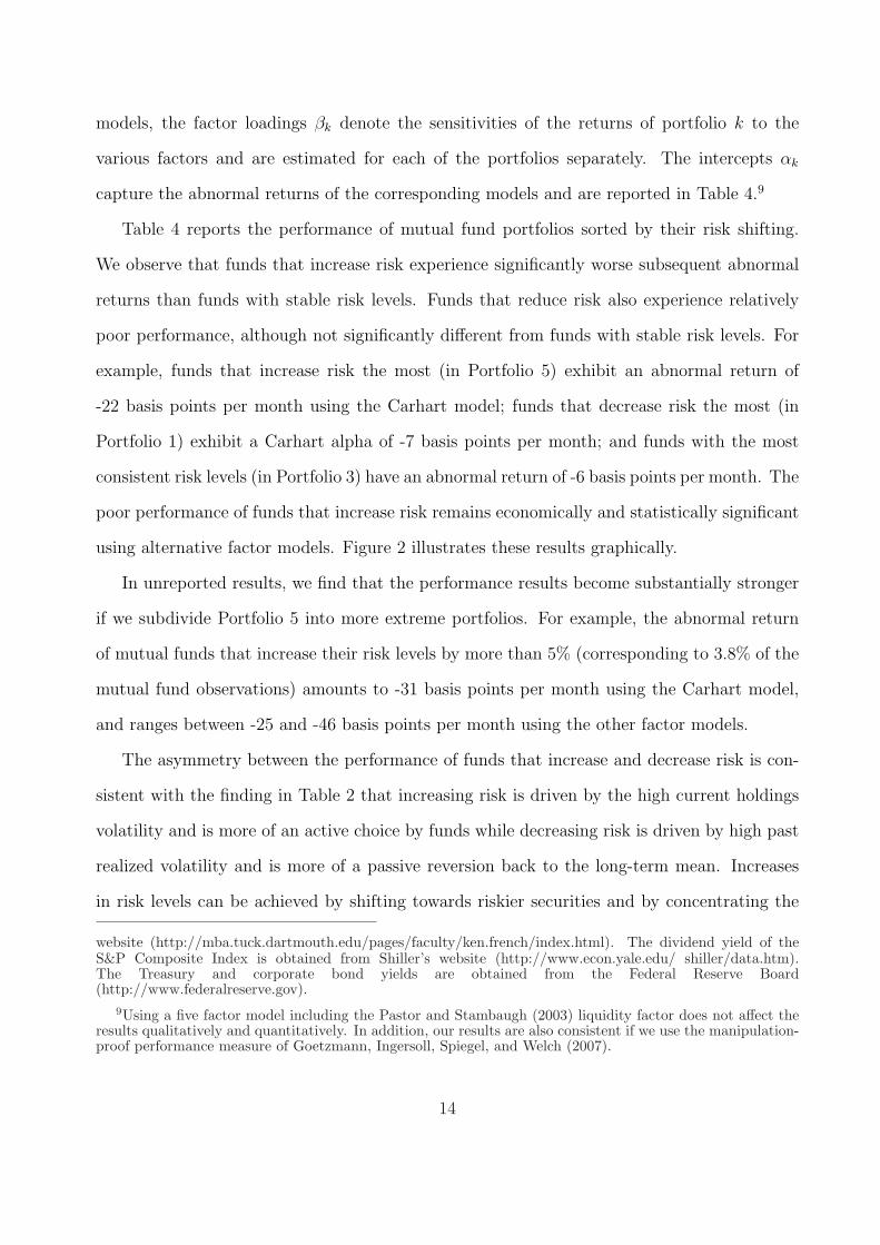
Table 4 reports the performance of mutual fund portfolios sorted by their risk shifting.

We observe that funds that increase risk experience significantly worse subsequent abnormal

returns than funds with stable risk levels. Funds that reduce risk also experience relatively

poor performance, although not significantly different from funds with stable risk levels. For

example, funds that increase risk the most (in Portfolio 5) exhibit an abnormal return of

-22 basis points per month using the Carhart model; funds that decrease risk the most (in

Portfolio 1) exhibit a Carhart alpha of -7 basis points per month; and funds with the most

consistent risk levels (in Portfolio 3) have an abnormal return of -6 basis points per month. The

poor performance of funds that increase risk remains economically and statistically significant

using alternative factor models. Figure 2 illustrates these results graphically.

In unreported results, we find that the performance results become substantially stronger

if we subdivide Portfolio 5 into more extreme portfolios. For example, the abnormal return

of mutual funds that increase their risk levels by more than 5% (corresponding to 3.8% of the

mutual fund observations) amounts to -31 basis points per month using the Carhart model,

and ranges between -25 and -46 basis points per month using the other factor models.

The asymmetry between the performance of funds that increase and decrease risk is con-

sistent with the finding in Table 2 that increasing risk is driven by the high current holdings

volatility and is more of an active choice by funds while decreasing risk is driven by high past

realized volatility and is more of a passive reversion back to the long-term mean. Increases

in risk levels can be achieved by shifting towards riskier securities and by concentrating the

website (http://mba.tuck.dartmouth.edu/pages/faculty/ken.french/index.html). The dividend yield of theS&P Composite Index is obtained from Shiller’s website (http://www.econ.yale.edu/ shiller/data.htm).The Treasury and corporate bond yields are obtained from the Federal Reserve Board(http://www.federalreserve.gov).

9Using a five factor model including the Pastor and Stambaugh (2003) liquidity factor does not affect theresults qualitatively and quantitatively. In addition, our results are also consistent if we use the manipulation-proof performance measure of Goetzmann, Ingersoll, Spiegel, and Welch (2007).

14

portfolio on fewer securities and fewer sectors as documented in Table 3. On the other hand,

decreases in risk levels can be achieved by holding a more balanced and better diversified

portfolio.

Table 5 summarizes the long-term impact of risk shifting. We form mutual fund portfolios

using longer-term lags and report the Carhart alphas of mutual fund portfolios formed based

on lagged RS measures. The first column repeats the performance results from Table 4,

which use the RS measure in the prior quarter to form portfolios. The remaining columns

form portfolios based on the lagged RS measures up to four quarters earlier. The poor

performance of Portfolio 5 remains statistically significant over the first four quarters after

the portfolio formation.

These performance results build on an extensive literature that investigates the investment

ability of mutual fund managers. Whereas the recent mutual fund literature finds that some

mutual fund managers have significant stock selection ability, our paper indicates that risk

shifting does not improve fund performance.10 Instead, consistent with the the timing litera-

ture, we do not find that mutual funds benefit significantly by taking advantage of time-varying

investment opportunities.11

6 Motivation for Risk Shifting

The poor performance of risk shifters suggests that risk shifting behavior is either an indication

of inferior ability or is motivated by agency problems in delegated portfolio management. To

investigate the potential role of agency problems in risk shifting behavior, we conduct two

10See, for example, Grinblatt and Titman (1993), Brown and Goetzmann (1995), Ferson and Schadt (1996),Carhart (1997), Daniel, Grinblatt, Titman, and Wermers (1997), Wermers (2000), Baks, Metrick, and Wachter(2001), Bollen and Busse (2001), Coval and Moskowitz (2001), Chen, Hong, Huang, and Kubik (2004), Cohen,Coval, and Pastor (2005), Kacperczyk, Sialm, and Zheng (2005), Gaspar, Massa, and Matos (2006), Kosowski,Timmermann, Wermers, and White (2006), Kacperczyk and Seru (2007), Mamaysky, Spiegel, and Zhang(2007), Cohen, Frazzini, and Malloy (2008), Cohen, Polk, and Silli (2008), Cremers and Petajisto (2008),Da, Gao, and Jagannathan (2008), Kacperczyk, Sialm, and Zheng (2008), Yuan (2008), Christoffersen andSarkissian (2009), and Brown, Harlow, and Zhang (2009).

11See, for example, Treynor and Mazuy (1966), Henriksson and Merton (1981), Busse (1999), Jiang (2003),Jiang, Yao, and Yu (2007), and Breon-Drish and Sagi (2008).

15

additional analyses in this section. First, we study the potential benefits of risk shifting by

comparing the return distribution of funds that shift risk with funds that follow more stable

risk levels. Second, we ask whether funds that benefit more from risk shifting are more likely

to shift risk and whether these funds experience worse performance when they shift risk.

6.1 Return Distribution of Risk Shifters

Mutual fund investors tend to invest in funds with stellar performance and do not penalize

poor performance equivalently, resulting in a convex flow-performance relation. The mutual

fund literature extensively documents this pattern and suggests that fund managers have an

incentive to shift risk levels to increase the probability of becoming a top-ranked mutual fund.

To verify whether risk shifters are more likely to have extreme future performance, we

report in Figure 3 the cumulative distribution functions of the performance ranking of mutual

funds in different risk shifting groups. At the end of each quarter, we first compute the

percentile ranks for all the funds in our sample. The percentile ranks are based on the

Carhart alphas over the subsequent 12-month period. In a second step, we sort mutual funds

into the same five portfolios as reported in Table 2. Finally, we compute the cumulative

distribution function of the performance ranks for each of the five portfolios. The figure

shows the cumulative distributions for three different groups of mutual funds. The curve RS1

corresponds to funds in Portfolio 1 that reduce risk the most, RS5 to funds in Portfolio 5 that

increase risk the most, and RS3 to funds in Portfolio 3 that maintain stable risk levels. The

intermediate groups RS2 and RS4 are not depicted separately, but fall between the middle

and extreme groups.

Funds that increase risk exhibit significantly higher volatility and are more likely to be

ranked in the extreme of the mutual fund distribution than funds with more stable risk

exposures. For example, 15.2% of mutual funds in the RS5 group and only 8.7% of mutual

funds in the RS3 group rank in the top decile. Furthermore, 1.8% of funds in the RS5

group and only 0.6% of funds in the RS3 group rank in the top percentile of all funds. Not

16

surprisingly, risk shifting also increases the probability of being ranked at the bottom of the

performance distribution. For example, around 17.7% of mutual funds in the RS5 group and

just 7.1% of mutual funds in the RS3 group rank in the bottom decile. The more striking

difference at the bottom decile than at the top decile is the source of the lower average

performance of the RS5 group. Yet, funds might prefer the return distribution of the RS5

group because it enables them to take advantage of the convex flow-performance relation.

6.2 Differential Benefits of Risk Shifting

We investigate whether the propensity to shift risk and the performance consequences of risk

shifting differ across funds with different incentives to shift risk. The incentives of risk shifting

are higher for funds that are better able to reap the benefits of extreme performance. Since the

expected profit for mutual funds increases with both the expense ratio and the assets under

management, we expect the benefits of risk shifting to be higher both for funds with higher

expense ratios and for funds with a more sensitive flow-performance relation. The mutual

fund literature has identified younger, smaller funds, and funds that belong to smaller fund

families as having a more sensitive flow-performance relation. Hence, we consider different

subgroups of funds based on these four characteristics: the expense ratio, fund age, fund size,

and the size of the fund family.

For each characteristic we divide mutual funds in each period into two groups depending

on whether the fund characteristic is above or below the median value. In a second step, we

further divide the two groups of funds into five portfolios according to their most recent risk

shifting measure. The first group of columns in Table 6 summarizes the frequency distribution

of funds across the two groups and the last group of columns reports the subsequent Carhart

alphas for the ten mutual fund portfolios.12

We find that funds with larger benefits of risk shifting are more likely to shift risk and

perform particularly poorly after shifting risk. For example, in Panel A of Table 6, of the

12The frequencies are computed on a quarterly basis and the differences in the frequencies use Newey-Weststandard errors with a lag length of four quarters. The Carhart alphas are computed as described in Section 5.

17

50% of mutual funds that charge above-median expense ratios, 7.36% belong to Portfolio 5

(that decrease risk the most), whereas only 5.27% of funds charging below-median expense

ratios belong to Portfolio 5. In addition, high-expense funds in Portfolio 5 exhibit a Carhart

alpha of -24 basis points per month, which is statistically significant at the 1% level, whereas

low-expense funds in Portfolio 5 have an insignificant alpha of -10 basis points per month.

The row “All” reports the average subsequent performance of high and low expense funds

across the five risk shifting groups. In contrast to the drastic performance difference be-

tween these two groups of funds in Portfolio 5, the average high-expense funds underperform

low-expense funds by only 3 basis points per month. This performance difference, which

is calculated after expenses, is lower than the difference in expense ratios between these two

groups (which amounts to 5 basis points per month). Thus, high-expense funds do not exhibit

inferior investor ability before deducting expenses. Yet, high-expense funds that increase their

risk levels experience very poor subsequent performance, consistent with the notion that these

funds opportunistically shift risk to take advantage of the convex flow-performance relation.

Our result is also consistent with Gil-Bazo and Ruiz-Verdu (2009), who find that high-expense

funds do not perform better than low-expense funds, even before expense. They interpret this

evidence as an agency problem in which high-expense funds target naive investors who are

not responsive to expenses.

Chevalier and Ellison (1997) find that young funds with less established track records have

larger incentives to shift risk since the flow sensitivity to performance is more pronounced for

young funds. They also find smaller funds have more sensitive fund flows. In addition, Huang,

Wei, and Yan (2007) find that funds in smaller fund families have higher flow-performance

sensitivity. Hence, these funds have more significant incentives to shift risk.

Panels B, C and D of Table 6 confirm that young, small funds, and funds affiliated with

relatively small families are more likely to shift risk and they experience particularly poor ab-

normal returns if they increase their risk levels. Since the average performance of funds sorted

by each of these characteristics is similar across the high and low groups, these characteristics

18

are not significantly related to investment ability. The fact that they are all related to the

potential benefits of risk shifting provides supportive evidence that agency problems, rather

than ability, are the likely cause of risk shifting behavior.

7 Sources for the Poor Performance of Risk Shifters

In this section, we study the sources for the poor performance of funds that increase their risk

level. Mutual funds can change the riskiness of their portfolios by changing the composition

between equity holdings and cash holdings, by changing their exposure to systematic risks

within their equity portfolios, and by changing their idiosyncratic risk exposures. We construct

alternative RS measures based on these various mechanisms of risk shifting and investigate

the performance consequences of risk shifting using each alternative measure. This analysis

sheds light on the sources of the poor performance of risk shifters. We also consider several

alternative explanations for the poor performance of risk shifters, for example, the additional

trading costs to implement risk shifting strategies or to accommodate fund flows, and the role

of past fund performance and volatility.

7.1 Cash and Equity Holdings

Table 7 reports the performance consequences of risk shifting based on six alternative RS

measures. The first column reports the Carhart alphas for fund portfolios formed according

to our base case RS measure which is computed using the complete holdings of the fund. The

results correspond to the results in Table 4 using the Carhart risk and style adjustments.

The second column focuses on the aggregate proportion invested in cash and other non-

equity positions and ignores the riskiness of the equity positions. This cash-based measure of

risk shifting is defined as:

RScashf,t = −(wcash

f,t − wcashf,t ), (7)

where wcashf,t is the most recently disclosed proportion invested in cash and other non-equity

securities according to the CRSP mutual fund database and wcashf,t is the average proportion

19

invested in non-equity securities over the prior 36 months. Other non-equity positions include

bonds, preferred stocks, and other securities, and are only 2.46% of fund assets. To be

consistent with the other RS measures in which a higher RS measure corresponds to a riskier

current position relative to the past, we multiply the difference by minus one. The portfolios

are formed using the RScash measure in specific ranges to maintain a similar distribution

of funds in the five groups as in our base case. Portfolio 1 (5) includes funds that increase

(decrease) the proportion invested in cash by more than 7.5% and Portfolio 3 includes funds

that change their cash proportion by less than 2.5%.

The third column considers only the riskiness of the disclosed equity positions and ignores

non-equity positions. This equity-based risk shifting measure is defined as:

RSequityf,t = σH,equity

f,t − σR,equityf,t , (8)

where σH,equityf,t is the current holdings volatility estimated using the returns of the most recently

disclosed equity positions and σR,equityf,t is the realized holdings volatility estimated using the

returns of a hypothetical portfolio that maintains the historically disclosed equity positions,

updated whenever new holdings become available, over the prior 36 months. Portfolio 1

(5) includes funds that decrease (increase) their equity risk by more than 2% per year and

Portfolio 3 includes funds that change their equity risk by less than 1%.

The results from Table 7 indicate that funds that increase risk have poor subsequent

performance, whether they decrease the proportion invested in cash or increase the volatility of

their equity holdings. The impact of increasing the volatility of equity holdings is similar to the

base case result using all the holdings (with a performance difference of about 17 basis points

per month), while the performance consequence of reducing cash holdings is substantially

lower (at 6 basis points per month). Therefore, increasing the volatility of equity holdings is

more costly in terms of their subsequent performance. In addition, the weaker result using

cash holdings suggests that activities that mainly affect the fraction of cash holdings (for

example, fund flows and fund managers’s effort to time the aggregate market) have a smaller

impact on fund performance.

20

7.2 Systematic and Idiosyncratic Risk

Fund managers might shift risk in an effort to take advantage of time-varying investment

opportunities. They might change their exposure to systematic risk if they believe that they

have superior market timing abilities; or they might change the idiosyncratic risk of their

portfolio in order to utilize their (perceived) stock selection ability.

The last three columns of Table 7 compare the future abnormal performance of fund

portfolios sorted by systematic and idiosyncratic risk levels. The fourth column is based on

changes in systematic risk and is defined as:

RSβf,t = βH

f,t − βRf,t, (9)

where βHf,t is the CAPM beta of the most recently disclosed holdings and βR

f,t is the CAPM

beta of the realized returns over the prior 36 months. Portfolio 1 (5) includes funds that

decrease (increase) their CAPM beta by more than 0.15 and Portfolio 3 includes funds that

change their betas by less than 0.05.

The final two risk shifting measures in Table 7 are based on the idiosyncratic volatilities

computed using the CAPM and the Carhart factor models. The idiosyncratic risk shifting

measures are defined as

RSidiosyncf,t = σH,idiosync

f,t − σR,idiosyncf,t , (10)

where σH,idiosyncf,t is the idiosyncratic volatility of the most recently disclosed fund holdings

return and σR,idiosyncf,t is the idiosyncratic volatility of the past realized fund return. The

idiosyncratic volatilities are computed as the standard deviations of the residuals from the

CAPM or the Carhart factor regressions over the prior 36 months. Portfolio 1 (5) includes

funds that decrease (increase) their idiosyncratic risk by more than 2% per year and Portfolio 3

includes funds that change their idiosyncratic risk by less than 1%.

We find a strong relation between risk shifting and fund performance for portfolios sorted

according to changes in idiosyncratic volatilities, but do not find a statistically significant

return pattern for portfolios sorted according to changes in systematic risk. For example,

21

the performance difference between funds that increase their idiosyncratic risk the most (in

Portfolio 5) and funds that maintain stable risk levels (in Portfolio 3) is between -18 and -21

basis points per month, both significant at the 5% level, depending on whether idiosyncratic

risk is measured relative to the market model or the four-factor Carhart model. On the

other hand, the performance difference between funds that increase their systematic risk the

most and funds that maintain stable systematic risk is -5 basis points per month and is not

statistically significant. Thus, the poor performance of funds that increase risk is driven by

the increase in their idiosyncratic risk levels and not by the increase in their systematic risk

exposure. Our results suggest that the main driver of the poor performance of risk shifters

is not their inability to time the aggregate market movements but their tendency to take on

idiosyncratic risk.13

Chevalier and Ellison (1997), Basak, Pavlova, and Shapiro (2007), and Chen and Pen-

nacchi (2009) suggest that, if fund managers are evaluated on their performance relative to

a benchmark, they have an incentive to increase tracking error volatility. Our finding that

some fund managers significantly increase their idiosyncratic volatility is consistent with these

predictions.

7.3 Trading Costs

One potential source of the poor performance of funds that increase risk could be the significant

trading costs incurred by such funds. Since we analyze only the future performance of funds

after computing the risk shifting measure, our performance measures are not contaminated

by the direct trading costs to implement the current risk shifting strategy. However, since risk

shifting is persistent, these funds might also have higher trading costs in the future.

We use turnover as a proxy for trading costs since it captures the majority of trading costs

as described by Chalmers, Edelen, and Kadlec (1999). If trading costs are the main cause

13Ang, Hodrick, Xing, and Zhang (2006) report that stocks with high idiosyncratic volatility based on dailyreturns tend to exhibit relatively poor abnormal returns in the subsequent month. To investigate whether thiseffect can explain our results, we augment, in unreported results, the Fama-French-Carhart factor model byan idiosyncratic volatility factor. Adjusting for the idiosyncratic volatility factor does not qualitatively changeour main result that funds that increase their risk the most experience the worst subsequent performance.

22

of the poor performance of risk shifters, then we should observe that the relation between

performance and risk shifting is particularly pronounced for high turnover funds. We sort funds

into subgroups with different turnover and risk shifting measures, following the procedure in

Section 6.2, and report the frequency distribution and the Carhart alphas in Panel A of

Table 8. Surprisingly, we find that increasing risk has worse performance consequences for

funds with low turnover than for funds with high turnover. For example, the performance

difference between Portfolios 5 and 3 is -25 basis points per month for funds with low turnover

and only -8 basis points for funds with high turnover. Thus, direct trading costs are unlikely

the main reason behind the poor performance of risk shifters.

Another proxy for trading costs is fund flows. Edelen (1999) documents that the extra

trading and the resulting price impact induced by fund flows can significantly reduce the

average performance of mutual funds. In addition, Coval and Stafford (2007), Chen, Hanson,

Hong, and Stein (2007), and Zhang (2008) show that distressed mutual funds experiencing

large money outflows are forced to liquidate their positions in “fire sales.” Such outflows

can increase the total risk level of mutual funds as they reduce their cash positions or as

they reduce their portfolio diversification by selling some of their positions. To examine the

impact of fund flows, we divide mutual funds into groups depending on whether their fund

flows in the prior year are below or above the median level. Panel B shows that there are no

significant differences in the propensities to shift risk for funds in these two groups, suggesting

that most funds are able to undo the effect of funds flows and reach their desired risk level.

In addition, although funds with below-median flows perform slightly worse than funds with

above-median flows when they increase risk, the performance difference is not significantly

different from zero.

Therefore, the poor performance of funds that increase risk is unlikely driven by the

additional transaction costs needed to implement the risk shifting strategy or to accommodate

fund flows.

23

7.4 Past Fund Performance and Volatility

The past fund performance and volatility level may reveal the ability and incentives of fund

managers. Mutual funds with worse prior performance are likely to have inferior ability and

might continue to perform poorly. The literature suggests that past winners and losers have

different incentives to take risk. In addition, funds with higher volatility levels have more

extreme performance and might be able to take advantage of the convex flow-performance

relation without shifting risk. It is therefore important to study the impact of past fund

performance and realized volatility.

Panel C of Table 8 sorts mutual funds by their prior year performance and the risk shifting

measure. We find that funds with relatively disappointing performance are relatively more

likely to shift risk down (in Portfolio 1), whereas funds with superior performance are more

likely to shift risk up (in Portfolio 5). To investigate the relation between prior performance

and risk shifting in more detail, we analyze in unreported results the economic determinants of

risk shifting using a multivariate regression analysis. We find that both funds with very poor

and with very high past performance increase risk above their prior realized risk levels. This

result is consistent with Hu, Kale, Pagani, and Subramanian (2008), who develop a unified

theory that generates a U-shape relation between risk choices and prior performance. They

find evidence that managers that significantly outperform or underperform the benchmark

exhibit higher subsequent risk levels. The asymmetry in the frequency distribution in Panel C

occurs because the incentive to shift risk is on average more pronounced for winner funds than

for loser funds.

The performance consequences of risk shifting are stronger for loser funds than for winner

funds. Within loser funds, we find that funds that increase risk the most underperform

funds that maintain stable risk levels by 16 basis points per month. On the other hand,

the corresponding performance difference for winner funds is only 7 basis points and is not

statistically significantly different from zero.

Panel D of Table 8 reports the results for funds sorted on past realized volatility and risk

24

shifting measures. While it is intuitive that funds with higher risk levels are much more likely

to shift risk down, it is rather surprising that they are also more likely to increase risk further.

Moreover, these high-risk funds that increase risk further suffer the worst future performance,

with a Carhart alpha that is -27 basis points lower than the high-risk funds that maintain

stable risk levels. In contrast, low-risk funds have similar performance across risk shifting

groups, with a performance difference of only -1 basis point between Portfolios 5 and 3. The

different impact of risk shifting for the high- and low-volatility groups is striking, especially

given their similar average performance.

In summary, mutual funds with worse prior performance are likely to have inferior ability.

These funds also perform particularly poorly when they increase risk. We also find that past

realized volatility is not directly related to future risk-adjusted performance but is critical for

the impact of risk shifting behavior. Low-risk funds do not suffer poor performance when

they increase risk while high-risk funds have significantly lower future performance when they

choose to increase risk further.

8 Multivariate Regression

This section uses a multivariate regression analysis to investigate the relation between risk

shifting and subsequent fund performance. This methodology allows us to control for addi-

tional fund characteristics. We run the following Fama-MacBeth specification:

PERFf,t = β0 + β1MAX(0, RSf,t−1) + β2MIN(0, RSf,t−1) + β3σRf,t−1 (11)

+ β4RFf,t−1+β5LOGAGEf,t−1+β6LOGTNAf,t−1+β7EXPf,t−1

+ β8TOf,t−1+β9FLOWf,t−1+εf,t.

The dependent variable in each cross-section is a performance measure of an individual

mutual fund PERF in a particular month. To capture the non-monotonic impact of risk

shifting on performance, we split RS into two components depending on whether it is positive

or negative. The coefficient β1 captures the relation between risk shifting and returns when

25

RS is positive and β2 captures the relation between risk shifting and returns when RS is

negative. The additional control variables are the realized volatility over the prior 36 months

σR, the prior-year return of a fund RFf,t−1, the age of the fund defined as the logarithm of

(1 + AGE), the logarithm of the assets under management LOGTNA, the expense ratio of

the fund EXP , the turnover ratio TO, and the fund flow over the prior year FLOW . All

control variables are lagged by at least one month. In a first step, we run in each month

a cross-sectional regression. In a second step, we compute the means of the cross-sectional

coefficients over the whole time period between 1983 and 2006.

One commonly used methodology to adjust for risk and style in the mutual fund literature

is to first estimate the factor loadings for each fund over a rolling window using prior data

and then compute abnormal returns in the subsequent period as the difference between the

actual fund return and the expected fund return based on the estimated factor loadings. This

methodology is not appropriate in our context since we focus on the risk shifting behavior of

funds over time. The factor loadings estimated over prior windows might not be accurate for

funds that shift risk levels significantly.14 Instead, the risk adjustments for our performance

measures are based on the most recent portfolio holdings.

We use four different performance measures: (1) the raw fund return; (2) the Carhart

abnormal return; (3) the characteristics-adjusted return; and (4) the return gap. The Carhart

alpha of a fund is defined in a similar way to the bottom-up alphas of Elton, Gruber, and

Blake (2007) as the fund return minus the expected factor return:

αCarhartk,t = (RFk,t −RTB,t)−

[βM

k(H),t−1(RM,t −RTB,t) + βSMBk(H),t−1(RS,t −RB,t)

+βHMLk(H),t−1(RH,t −RL,t) + βUMD

k(H),t−1(RU,t −RD,t)]. (12)

The expected factor return is computed as the product of the betas of the most recent

holdings of the fund and the returns of the four Carhart factors. The betas of the most

14Despite this concern, the results are not substantially different if we use fund-specific abnormal returns asdependent variables. This is consistent with the prior portfolio results which indicate that the performanceresults are not very sensitive to alternative factor adjustments.

26

recent holdings are obtained by regressing the hypothetical return of the most recent portfolio

holdings (including non-equity positions) over the last 36 months on the Carhart factors.

The characteristics-adjusted return is defined as the difference between the fund return

and the benchmark return of securities with similar risk and style characteristics:

αCharacAdjk,t = RFk,t −

(N∑

i=1

wif,t[BRi(t−1),t]

), (13)

The weight invested in position i at the beginning of month t in the mutual fund f is

denoted by wif,t and the benchmark return to which position i was allocated during month

t − k is denoted by BRi(t−k),t. For equity positions, we follow Daniel, Grinblatt, Titman,

and Wermers (1997) and define the return on a benchmark portfolio as the value-weighed

return of stocks that fall in the identical size, value, and momentum quintiles as the equity

holdings of a fund. For non-equity positions we set the benchmark returns equal to the returns

corresponding to the Lehman Brothers Aggregate Bond Index (for bonds and preferred stocks)

and to the Treasury bill rate (for cash and other securities).

Finally, the return gap is computed following Kacperczyk, Sialm, and Zheng (2008) as the

residual that captures the impact of unobserved actions on fund returns:

RGf,t = RFf,t −RHf,t + EXPf,t, (14)

where the investor return is denoted by RF , the holdings return by RH, and the expense

ratio by EXP .

Table 9 reports the multivariate regression estimates. All specifications indicate a sig-

nificantly negative relation between risk shifting and the various performance measures for

funds that increase risk and a generally insignificant relation for funds that decrease risk. The

performance consequences of increasing risk are similar in magnitude to the results reported

in Table 4. For example, the first column indicates that an increase in RS from 0 to 5% (cor-

responding roughly to the difference in risk shifting between portfolios 3 and 5 in Table 2),

reduces the raw fund return by 22 basis points per month. The impact of increasing risk by

27

five percentage points ranges between 8 basis points for the return gap and 30 basis points

for the four-factor adjusted fund return.

Including additional control variables does not have a significant impact on the risk shift-

ing coefficients. The level of the realized volatility over the prior 36 months does not have a

significant explanatory power for fund performance, consistent with the evidence in Panel D

of Table 8. The positive coefficient on the lagged return indicates some performance persis-

tence. The coefficient on the expense ratio is significantly different from zero in the first three

specifications which use an after-expense performance measure. On the other hand the ex-

pense ratio has no significant relation to the return gap, which is measured after adjusting for

fund expenses. Finally, funds with higher turnover tend to exhibit slightly higher performance

using all four performance measures.

The results in this section confirm the portfolio results reported in Table 4 that funds that

increase risk perform poorly in the future, even after adjusting for other fund characteristics

and after controlling for risk and style.

9 Conclusions

As more and more investors delegate their portfolio decisions to mutual fund managers, po-

tential agency problems between fund managers and investors have become increasingly im-

portant. Our paper extends the literature on one particular agency problem – the incentive for

fund managers to shift the risk level of their portfolios to increase their personal compensation

– and investigates its consequences for fund investors.

Risk shifting per se does not necessarily hurt fund investors. As long as the act of risk

shifting is well-known and has no performance consequences, investors can form efficient port-

folios by adjusting their allocation to the funds based on the expected ability and risk levels.

However, if investors are not fully aware of the risk shifting behavior or if the changing risk

level hampers their ability to assess fund performance, then individual portfolios are less likely

to be efficient.

28

We find that even if investors are fully aware of the risk shifting behavior, they are better

off avoiding funds that are prone to switch risk over time. The reason is that funds that shift

risk perform worse than funds that keep stable risk levels over time. In addition, funds with

larger incentives to shift risk are more likely to increase risk and perform particularly poorly

after increasing risk. These results are consistent with risk shifting being a consequence of op-

portunistic behavior of fund managers and inconsistent with risk shifting being a consequence

of skilled fund managers taking advantage of time-varying investment opportunities.

29

References

Ang, A., R. Hodrick, Y. Xing, and X. Zhang (2006). The cross-section of volatility andexpected returns. Journal of Finance 61, 259–299.

Baks, K. P., A. Metrick, and J. Wachter (2001). Should investors avoid all actively managedmutual funds? A study in Bayesian performance evaluation. Journal of Finance 56, 45–86.

Basak, S., A. Pavlova, and A. Shapiro (2007). Optimal asset allocation and risk shifting inmoney management. Review of Financial Studies 20 (5), 1583–1621.

Bollen, N. P. B. and J. A. Busse (2001). On the timing ability of mutual fund managers.Journal of Finance 56, 1075–1094.

Breon-Drish, B. and J. S. Sagi (2008). Do fund managers make informed asset allocationdecisions. University of California at Berkeley and Vanderbilt University.

Brown, K. C., W. V. Harlow, and L. T. Starks (1996). Of tournaments and temptations: Ananalysis of managerial incentives in the mutual fund industry. Journal of Finance 51 (1),85–110.

Brown, K. C., W. V. Harlow, and H. Zhang (2009). Staying the course: The role of in-vestment style consistency in the performance of mutual funds. University of Texas atAustin and Fidelity Investments.

Brown, S. J. and W. N. Goetzmann (1995). Performance persistence. Journal of Finance 50,853–873.

Busse, J. A. (1999). Volatility timing in mutual funds: Evidence from daily returns. Reviewof Financial Studies 12 (5), 1009–1041.

Busse, J. A. (2001). Another look at mutual fund tournaments. Journal of Financial andQuantitative Analysis 36 (1), 53–73.

Carhart, M. M. (1997). On persistence in mutual fund performance. Journal of Fi-nance 52 (2), 57–82.

Carpenter, J. N. (2000). Does option compensation increase managerial risk appetite. Jour-nal of Finance 55, 2311–2331.

Chalmers, J. M., R. M. Edelen, and G. B. Kadlec (1999). An analysis of mutual fund tradingcosts. University of Oregon, University of Pennsylvania, and Virginia Tech.

Chen, H.-L. and G. G. Pennacchi (2009). Does prior performance affect a mutual fund’schoice of risk? Theory and further empirical evidence. Forthcoming: Journal of Finan-cial and Quantitative Analysis.

Chen, J., S. Hanson, H. Hong, and J. C. Stein (2007). Do hedge funds profit from mutual-fund distress? USC, Harvard University, and Princeton University.

Chen, J., H. Hong, M. Huang, and J. Kubik (2004). Does fund size erode performance? Liq-uidity, organizational diseconomies and active money management. American EconomicReview 94, 1276–1302.

Chevalier, J. and G. Ellison (1997). Risk taking by mutual funds as a response to incentives.Journal of Political Economy 105 (6), 1167–1200.

Christoffersen, S. and S. Sarkissian (2009). City size and fund performance. Forthcoming:Journal of Financial Economics.

30

Cohen, L., A. Frazzini, and C. Malloy (2008). The small world of investing: Board connec-tions and mutual fund returns. Journal of Political Economy 116, 951–979.

Cohen, R., J. D. Coval, and L. Pastor (2005). Judging fund managers by the company thatthey keep. Journal of Finance 60, 1057–1096.

Cohen, R., C. Polk, and B. Silli (2008). Best ideas. Harvard University, London School ofEconomics, and Universitat Pompeu Fabra.

Coval, J. and E. Stafford (2007). Asset fire sales (and purchases) in equity markets. Journalof Financial Economics 86, 479–512.

Coval, J. D. and T. J. Moskowitz (2001). The geography of investment: Informed tradingand asset prices. Journal of Political Economy 109, 811–841.

Cremers, M. and A. Petajisto (2008). How active is your fund manager? A new measurethat predicts performance. Forthcoming: Review of Financial Studies.

Da, Z., P. Gao, and R. Jagannathan (2008). Informed trading, liquidity provision, and stockselection by mutual funds. University of Notre Dame and Northwestern University.

Daniel, K., M. Grinblatt, S. Titman, and R. Wermers (1997). Measuring mutual fundperformance with characteristic-based benchmarks. Journal of Finance 52 (3), 1035–1058.

DelGuercio, D. and P. A. Tkac (2002). The determinants of the flow of funds of managedportfolios: Mutual funds versus pension funds. Journal of Financial and QuantitativeAnalysis 37, 523–557.

Edelen, R. M. (1999). Investor flows and the assessed performance of open-end fund man-agers. Journal of Financial Economics 53, 439–466.

Elton, E. J., M. J. Gruber, and C. R. Blake (2003). Incentive fees and mutual funds. Journalof Finance 58 (2), 779–804.

Elton, E. J., M. J. Gruber, and C. R. Blake (2007). Monthly holding data and the selectionof superior mutual funds. New York University and Fordham University.

Elton, E. J., M. J. Gruber, Y. Krasny, and S. Ozelge (2006). The effect of the frequencyof holding data on conclusions about mutual fund management behavior. New YorkUniversity.

Fama, E. F. and K. R. French (1993). Common risk factors in the return on bonds andstocks. Journal of Financial Economics 33, 3–53.

Ferson, W. and R. Schadt (1996). Measuring fund strategy and performance in changingeconomic conditions. Journal of Finance 51, 425–462.

Gaspar, J.-M., M. Massa, and P. Matos (2006). Favoritism in mutual fund families? Evi-dence on strategic cross-fund subsidization. Journal of Finance 61, 73–104.

Gil-Bazo, J. and P. Ruiz-Verdu (2009). Yet another puzzle? The relation between price andperformance in the mutual fund industry. Forthcoming: Journal of Finance.

Goetzmann, W., J. Ingersoll, M. Spiegel, and I. Welch (2007). Portfolio performance manip-ulation and manipulation-proof performance measures. Review of Financial Studies 20,1503–1546.

Goetzmann, W. N. and N. Peles (1997). Cognitive dissonance and mutual fund investors.Journal of Financial Research 20 (2), 145–158.

Grinblatt, M. and S. Titman (1989). Adverse risk incentives and the design of performance-based contracts. Management Science 35, 807–822.

31

Grinblatt, M. and S. Titman (1993). Performance measurement without benchmarks: Anexamination of mutual fund returns. Journal of Business 66, 47–68.

Guasoni, P., G. Huberman, and Z. Wang (2007). Performance maximization of activelymanaged funds. Boston University, Columbia University, and the Federal Reserve Bankof New York.

Henriksson, R. D. and R. C. Merton (1981). On market timing and investment performance.II. Statistical procedures for evaluating forecasting skills. Journal of Business 54, 513–533.

Hu, P., J. R. Kale, M. Pagani, and A. Subramanian (2008). Fund flows, performance,managerial career concerns, and risk-taking. Georgia State University and San JoseState University.

Huang, J., K. D. Wei, and H. Yan (2007). Participation costs and the sensitivity of fundflows to past performance. Journal of Finance 62 (3), 1273–1311.

Ippolito, R. A. (1992). Consumer reaction to measures of poor quality: Evidence from themutual fund industry. Journal of Law and Economics 35 (1), 45–70.

Ivkovich, Z. and S. Weisbenner (2009). Individual investor mutual fund flows. Forthcoming:Journal of Financial Economics.

Jiang, G., T. Yao, and T. Yu (2007). Do mutual funds time the market? Evidence fromportfolio holdings. Journal of Financial Economics 86, 724–758.

Jiang, W. (2003). A nonparametric test of market timing. Journal of Empirical Finance 10,399–425.

Kacperczyk, M. and A. Seru (2007). Fund manager use of public information: New evidenceon managerial skills. Journal of Finance 62, 485–528.

Kacperczyk, M., C. Sialm, and L. Zheng (2005). On the industry concentration of activelymanaged equity mutual funds. Journal of Finance 60 (4), 1983–2012.

Kacperczyk, M., C. Sialm, and L. Zheng (2008). Unobserved actions of equity mutual funds.Review of Financial Studies 21 (6), 2379–2416.

Kempf, A. and S. Ruenzi (2008). Tournaments in mutual fund families. Review of FinancialStudies 21 (2), 1013–1036.

Kempf, A., S. Ruenzi, and T. Thiele (2008). Employment risk, compensation incentives andmanagerial risk taking: Evidence from the mutual fund industry. Forthcoming: Journalof Financial Economics.

Koski, J. L. and J. Pontiff (1999). How are derivatives used? Evidence from the mutualfund industry. Journal of Finance 54 (2), 791–816.

Kosowski, R., A. Timmermann, R. Wermers, and H. White (2006). Can mutual fund ‘stars’really pick stocks? New evidence from a bootstrap analysis. Journal of Finance 61,2551–2595.

Li, W. and A. Tiwari (2006). On the consequences of mutual fund tournaments. Universityof Iowa.

Lynch, A. W. and D. K. Musto (2003). How investors interpret past fund returns. Journalof Finance 58, 2033–2058.

Mamaysky, H., M. I. Spiegel, and H. Zhang (2007). Improved forecasting of mutual fundalphas and betas. Review of Finance 11 (3), 359–400.

32

Massa, M. and R. Patgiri (2007). Incentives and mutual fund performance: Higher perfor-mance or just higher risk taking? Forthcoming: Review of Financial Studies.

Nanda, V., Z. J. Wang, and L. Zheng (2004). Family values and the star phenomenon:Strategies of mutual fund families. Review of Financial Studies 17 (3), 667–698.

Palomino, F. and A. Prat (2003). Risk taking and optimal contracts for money managers.RAND Journal of Economics 34, 113–137.

Pastor, L. and R. F. Stambaugh (2003). Liquidity risk and expected stock returns. Journalof Political Economy 111 (3), 642–685.

Ross, S. A. (2004). Compensation, incentives, and the duality of risk aversion and riskiness.Journal of Finance 59, 207–225.

Sirri, E. R. and P. Tufano (1998). Costly search and mutual fund flows. Journal of Fi-nance 53 (5), 1589–1622.

Starks, L. T. (1987). Performance incentive fees: An agency theoretic approach. Journal ofFinancial and Quantitative Analysis 22 (1), 17–32.

Treynor, J. L. and K. Mazuy (1966). Can mutual funds outguess the market? HarvardBusiness Review 44, 131–136.

Wermers, R. (2000). Mutual fund performance: An empirical decomposition into stock-picking talent, style, transactions costs, and expenses. Journal of Finance 55 (4), 1655–1703.

Wermers, R. (2003). Is money really ‘smart’? New evidence on the relation between mutualfund flows, manager behavior, and performance persistence. University of Maryland.

Yuan, K. (2008). Eliciting heterogeneous investor beliefs from portfolio holdings and per-formance evaluation. London School of Economics.

Zhang, H. (2008). Asset fire sales, liquidity provision and mutual fund performance. Uni-versity of Texas at Austin.

Zheng, L. (1999). Is money smart? A study of mutual fund investors’ fund selection ability.Journal of Finance 54, 901–933.

33

Table 1: Summary StatisticsThis table summarizes the characteristics of the mutual funds in our sample over the period between1980 and 2006.

Variable Mean Std.Dev. Median

Total Net Assets (TNA) (in Millions) 1,382.54 4,739.35 277.84Age (in Years) 17.54 15.29 12.00Expense Ratio (in %) 1.28 0.46 1.24Turnover Ratio (in %) 90.65 112.98 66.00Common Stock Proportion (in %) 91.28 12.04 95.00Cash Proportion (in %) 6.26 9.04 3.78Bond Proportion (in %) 1.58 6.49 0.00Preferred Stock Proportion (in %) 0.39 2.57 0.00Other Securities Proportion (in %) 0.49 3.81 0.00Flow (in % per Month) 0.43 5.04 -0.36Investor Return (in % per Month) 0.83 5.34 1.07Holdings Return (in % per Month) 0.91 5.21 1.10Number of Stock Positions 89.23 130.77 62.00Industry Concentration Index 0.12 0.20 0.05Size Score 4.20 0.85 4.53Value Score 2.80 0.46 2.79Momentum Score 3.10 0.59 3.07Current Holdings Volatility (in % per Year) 17.54 7.62 16.41Past Realized Volatility (in % per Year) 17.86 7.93 16.42Risk Shifting (in % per Year) -0.33 4.58 0.01

Total number of funds 2,335Total number of observations 184,519

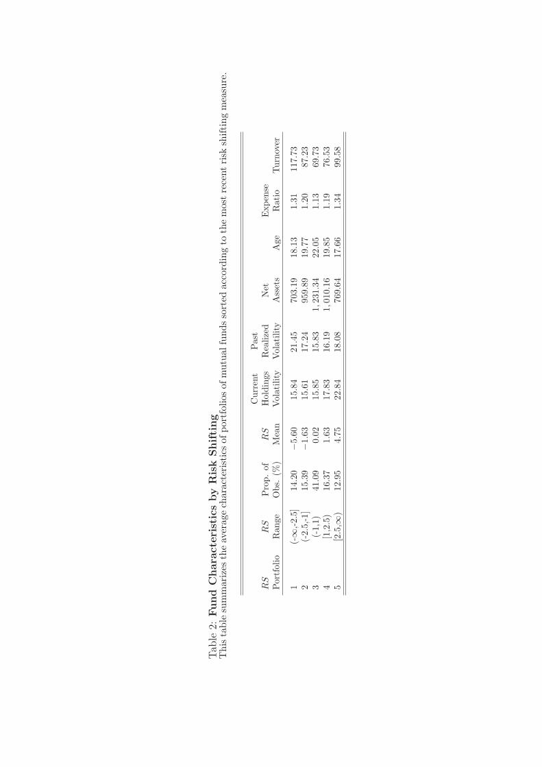
Tab

le2:

Fund

Chara

cteri

stic

sby

Ris

kShifting

Thi

sta

ble

sum

mar

izes

the

aver

age

char

acte

rist

ics

ofpo

rtfo

lios

ofm

utua

lfun

dsso

rted

acco

rdin

gto

the

mos

tre

cent

risk

shift

ing

mea

sure

.

Cur

rent

Pas

tR

SR

SP

rop.

ofR

SH

oldi

ngs

Rea

lized

Net

Exp

ense

Por

tfol

ioR

ange

Obs

.(%

)M

ean

Vol

atili

tyV

olat

ility

Ass

ets

Age

Rat

ioTur

nove

r

1(-∞

,-2.

5]14

.20

−5.6

015

.84

21.4

570

3.19

18.1

31.

3111

7.73

2(-

2.5,

-1]

15.3

9−1

.63

15.6

117

.24

959.

8919

.77

1.20

87.2

33

(-1,

1)41

.09

0.02

15.8

515

.83

1,23

1.34

22.0

51.

1369

.73

4[1

,2.5

)16

.37

1.63

17.8

316

.19

1,01

0.16

19.8

51.

1976

.53

5[2

.5,∞

)12

.95

4.75

22.8

418

.08

769.

6417

.66

1.34

99.5

8

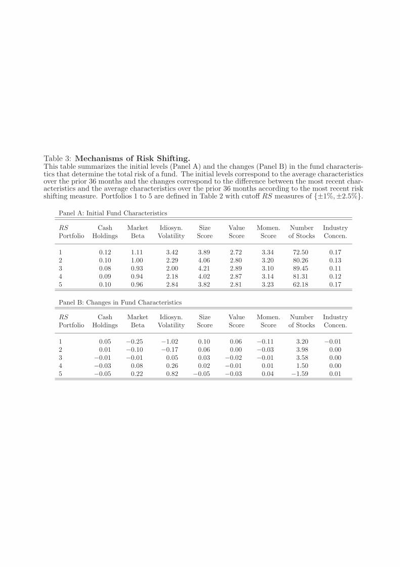
Table 3: Mechanisms of Risk Shifting.This table summarizes the initial levels (Panel A) and the changes (Panel B) in the fund characteris-tics that determine the total risk of a fund. The initial levels correspond to the average characteristicsover the prior 36 months and the changes correspond to the difference between the most recent char-acteristics and the average characteristics over the prior 36 months according to the most recent riskshifting measure. Portfolios 1 to 5 are defined in Table 2 with cutoff RS measures of {±1%,±2.5%}.

Panel A: Initial Fund Characteristics

RS Cash Market Idiosyn. Size Value Momen. Number IndustryPortfolio Holdings Beta Volatility Score Score Score of Stocks Concen.

1 0.12 1.11 3.42 3.89 2.72 3.34 72.50 0.172 0.10 1.00 2.29 4.06 2.80 3.20 80.26 0.133 0.08 0.93 2.00 4.21 2.89 3.10 89.45 0.114 0.09 0.94 2.18 4.02 2.87 3.14 81.31 0.125 0.10 0.96 2.84 3.82 2.81 3.23 62.18 0.17

Panel B: Changes in Fund Characteristics

RS Cash Market Idiosyn. Size Value Momen. Number IndustryPortfolio Holdings Beta Volatility Score Score Score of Stocks Concen.

1 0.05 −0.25 −1.02 0.10 0.06 −0.11 3.20 −0.012 0.01 −0.10 −0.17 0.06 0.00 −0.03 3.98 0.003 −0.01 −0.01 0.05 0.03 −0.02 −0.01 3.58 0.004 −0.03 0.08 0.26 0.02 −0.01 0.01 1.50 0.005 −0.05 0.22 0.82 −0.05 −0.03 0.04 −1.59 0.01

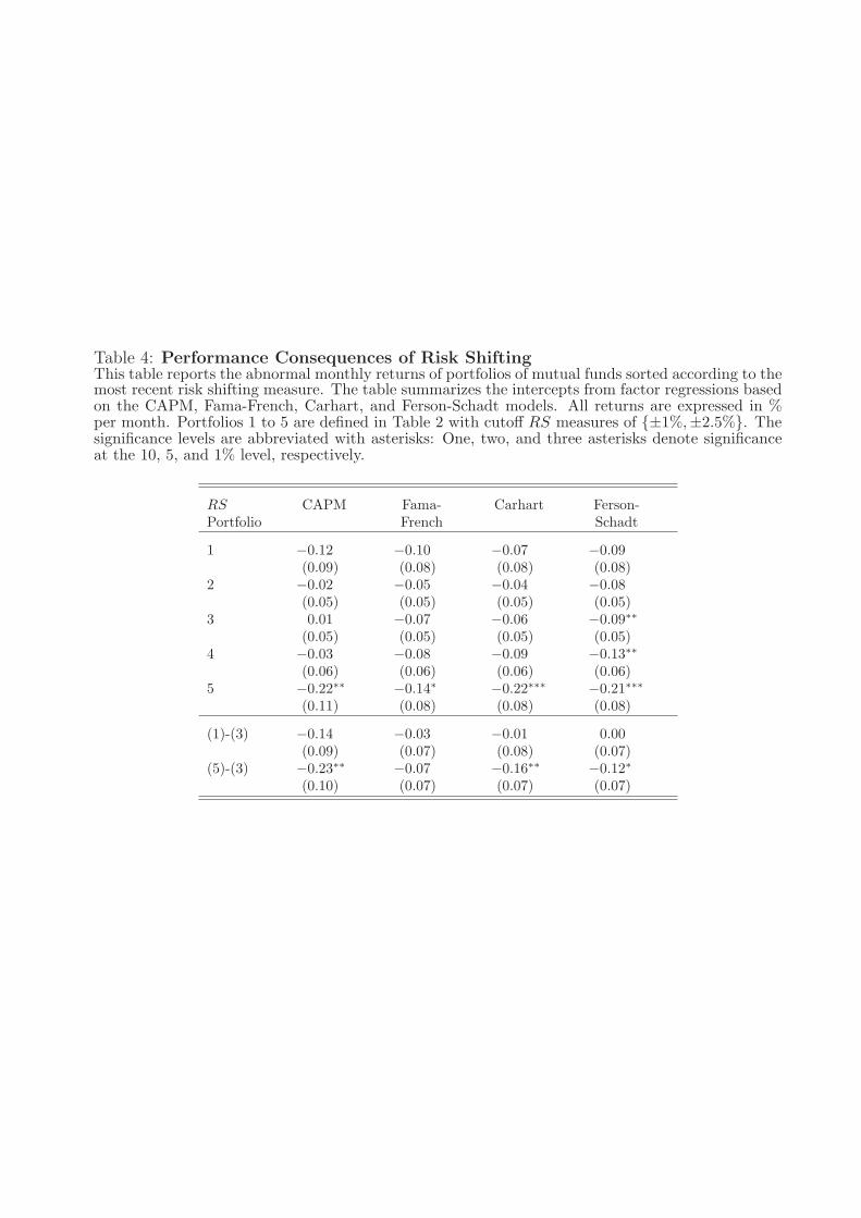
Table 4: Performance Consequences of Risk ShiftingThis table reports the abnormal monthly returns of portfolios of mutual funds sorted according to themost recent risk shifting measure. The table summarizes the intercepts from factor regressions basedon the CAPM, Fama-French, Carhart, and Ferson-Schadt models. All returns are expressed in %per month. Portfolios 1 to 5 are defined in Table 2 with cutoff RS measures of {±1%,±2.5%}. Thesignificance levels are abbreviated with asterisks: One, two, and three asterisks denote significanceat the 10, 5, and 1% level, respectively.

RS CAPM Fama- Carhart Ferson-Portfolio French Schadt

1 −0.12 −0.10 −0.07 −0.09(0.09) (0.08) (0.08) (0.08)

2 −0.02 −0.05 −0.04 −0.08(0.05) (0.05) (0.05) (0.05)

3 0.01 −0.07 −0.06 −0.09∗∗

(0.05) (0.05) (0.05) (0.05)4 −0.03 −0.08 −0.09 −0.13∗∗

(0.06) (0.06) (0.06) (0.06)5 −0.22∗∗ −0.14∗ −0.22∗∗∗ −0.21∗∗∗

(0.11) (0.08) (0.08) (0.08)

(1)-(3) −0.14 −0.03 −0.01 0.00(0.09) (0.07) (0.08) (0.07)

(5)-(3) −0.23∗∗ −0.07 −0.16∗∗ −0.12∗

(0.10) (0.07) (0.07) (0.07)

Table 5: Longer-Term Performance Consequences of Risk ShiftingThis table reports Carhart-adjusted monthly returns of portfolios of mutual funds sorted accordingto the prior risk shifting measure. The performance of the fund portfolios is computed based onthe risk shifting measures of funds over the prior four quarters. All returns are expressed in % permonth. Portfolios 1 to 5 are defined in Table 2 with cutoff RS measures of {±1%,±2.5%}. Thesignificance levels are abbreviated with asterisks: One, two, and three asterisks denote significanceat the 10, 5, and 1% level, respectively.

RS Number of Lags in QuartersPortfolio 1 2 3 4

1 −0.07 −0.02 −0.03 −0.08(0.08) (0.08) (0.08) (0.08)

2 −0.04 −0.05 −0.04 −0.01(0.05) (0.06) (0.05) (0.05)

3 −0.06 −0.06 −0.07 −0.06(0.05) (0.05) (0.05) (0.04)

4 −0.09 −0.08 −0.03 −0.07(0.06) (0.06) (0.05) (0.05)

5 −0.22∗∗∗ −0.21∗∗∗ −0.22∗∗∗ −0.18∗∗

(0.08) (0.08) (0.08) (0.08)

(1)-(3) −0.01 0.04 0.04 −0.02(0.08) (0.08) (0.07) (0.07)

(5)-(3) −0.16∗∗ −0.16∗∗ −0.15∗∗ −0.11(0.07) (0.07) (0.07) (0.07)

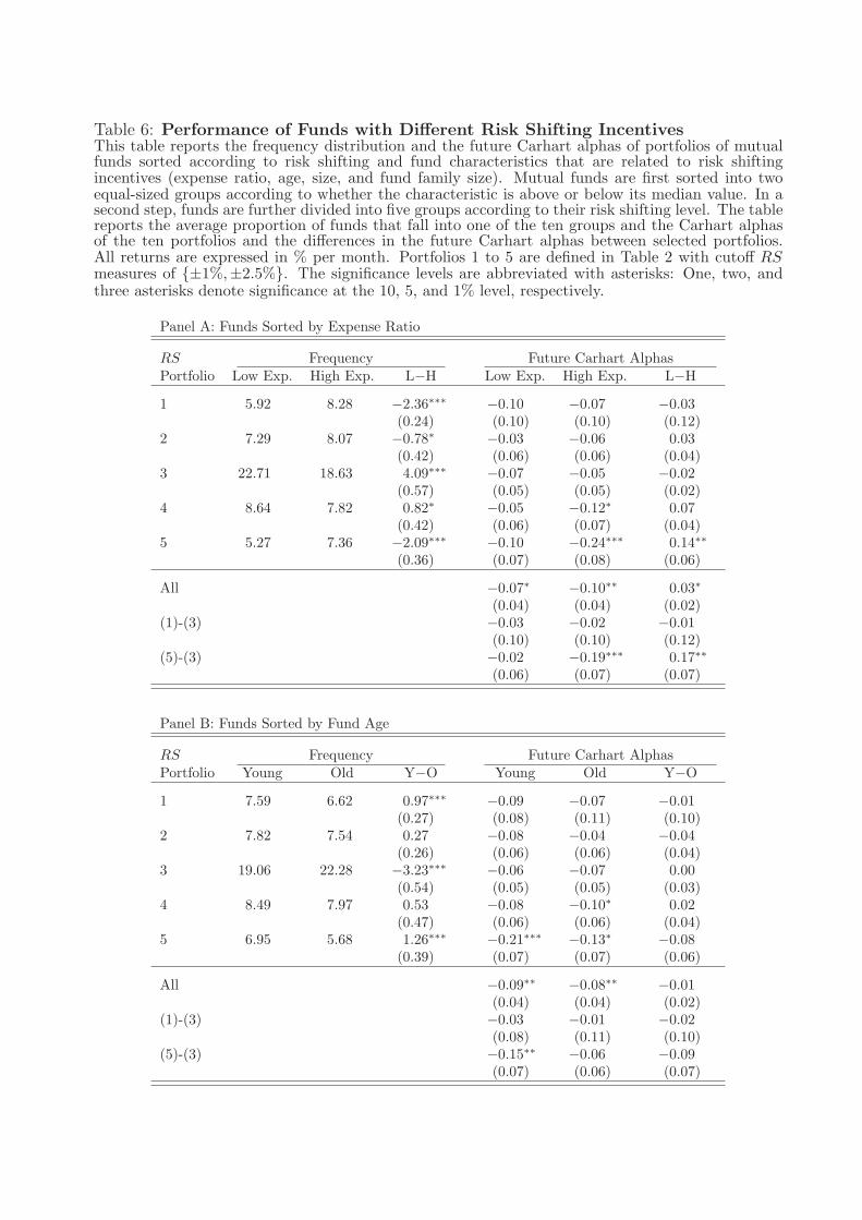
Table 6: Performance of Funds with Different Risk Shifting IncentivesThis table reports the frequency distribution and the future Carhart alphas of portfolios of mutualfunds sorted according to risk shifting and fund characteristics that are related to risk shiftingincentives (expense ratio, age, size, and fund family size). Mutual funds are first sorted into twoequal-sized groups according to whether the characteristic is above or below its median value. In asecond step, funds are further divided into five groups according to their risk shifting level. The tablereports the average proportion of funds that fall into one of the ten groups and the Carhart alphasof the ten portfolios and the differences in the future Carhart alphas between selected portfolios.All returns are expressed in % per month. Portfolios 1 to 5 are defined in Table 2 with cutoff RSmeasures of {±1%,±2.5%}. The significance levels are abbreviated with asterisks: One, two, andthree asterisks denote significance at the 10, 5, and 1% level, respectively.

Panel A: Funds Sorted by Expense Ratio

RS Frequency Future Carhart AlphasPortfolio Low Exp. High Exp. L−H Low Exp. High Exp. L−H

1 5.92 8.28 −2.36∗∗∗ −0.10 −0.07 −0.03(0.24) (0.10) (0.10) (0.12)

2 7.29 8.07 −0.78∗ −0.03 −0.06 0.03(0.42) (0.06) (0.06) (0.04)

3 22.71 18.63 4.09∗∗∗ −0.07 −0.05 −0.02(0.57) (0.05) (0.05) (0.02)

4 8.64 7.82 0.82∗ −0.05 −0.12∗ 0.07(0.42) (0.06) (0.07) (0.04)

5 5.27 7.36 −2.09∗∗∗ −0.10 −0.24∗∗∗ 0.14∗∗

(0.36) (0.07) (0.08) (0.06)

All −0.07∗ −0.10∗∗ 0.03∗

(0.04) (0.04) (0.02)(1)-(3) −0.03 −0.02 −0.01

(0.10) (0.10) (0.12)(5)-(3) −0.02 −0.19∗∗∗ 0.17∗∗

(0.06) (0.07) (0.07)

Panel B: Funds Sorted by Fund Age

RS Frequency Future Carhart AlphasPortfolio Young Old Y−O Young Old Y−O

1 7.59 6.62 0.97∗∗∗ −0.09 −0.07 −0.01(0.27) (0.08) (0.11) (0.10)

2 7.82 7.54 0.27 −0.08 −0.04 −0.04(0.26) (0.06) (0.06) (0.04)

3 19.06 22.28 −3.23∗∗∗ −0.06 −0.07 0.00(0.54) (0.05) (0.05) (0.03)

4 8.49 7.97 0.53 −0.08 −0.10∗ 0.02(0.47) (0.06) (0.06) (0.04)

5 6.95 5.68 1.26∗∗∗ −0.21∗∗∗ −0.13∗ −0.08(0.39) (0.07) (0.07) (0.06)

All −0.09∗∗ −0.08∗∗ −0.01(0.04) (0.04) (0.02)

(1)-(3) −0.03 −0.01 −0.02(0.08) (0.11) (0.10)

(5)-(3) −0.15∗∗ −0.06 −0.09(0.07) (0.06) (0.07)

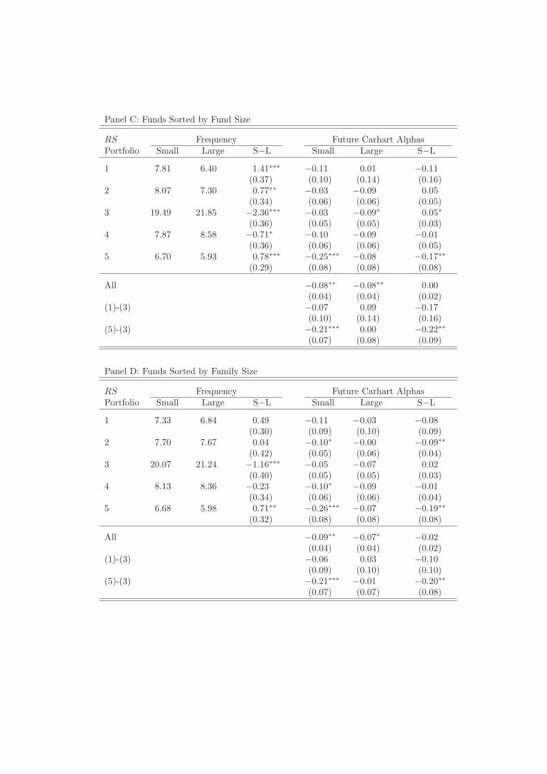
Panel C: Funds Sorted by Fund Size

RS Frequency Future Carhart AlphasPortfolio Small Large S−L Small Large S−L

1 7.81 6.40 1.41∗∗∗ −0.11 0.01 −0.11(0.37) (0.10) (0.14) (0.16)

2 8.07 7.30 0.77∗∗ −0.03 −0.09 0.05(0.34) (0.06) (0.06) (0.05)

3 19.49 21.85 −2.36∗∗∗ −0.03 −0.09∗ 0.05∗

(0.36) (0.05) (0.05) (0.03)4 7.87 8.58 −0.71∗ −0.10 −0.09 −0.01

(0.36) (0.06) (0.06) (0.05)5 6.70 5.93 0.78∗∗∗ −0.25∗∗∗ −0.08 −0.17∗∗

(0.29) (0.08) (0.08) (0.08)

All −0.08∗∗ −0.08∗∗ 0.00(0.04) (0.04) (0.02)

(1)-(3) −0.07 0.09 −0.17(0.10) (0.14) (0.16)

(5)-(3) −0.21∗∗∗ 0.00 −0.22∗∗

(0.07) (0.08) (0.09)

Panel D: Funds Sorted by Family Size

RS Frequency Future Carhart AlphasPortfolio Small Large S−L Small Large S−L

1 7.33 6.84 0.49 −0.11 −0.03 −0.08(0.30) (0.09) (0.10) (0.09)

2 7.70 7.67 0.04 −0.10∗ −0.00 −0.09∗∗

(0.42) (0.05) (0.06) (0.04)3 20.07 21.24 −1.16∗∗∗ −0.05 −0.07 0.02

(0.40) (0.05) (0.05) (0.03)4 8.13 8.36 −0.23 −0.10∗ −0.09 −0.01

(0.34) (0.06) (0.06) (0.04)5 6.68 5.98 0.71∗∗ −0.26∗∗∗ −0.07 −0.19∗∗

(0.32) (0.08) (0.08) (0.08)

All −0.09∗∗ −0.07∗ −0.02(0.04) (0.04) (0.02)

(1)-(3) −0.06 0.03 −0.10(0.09) (0.10) (0.10)

(5)-(3) −0.21∗∗∗ −0.01 −0.20∗∗

(0.07) (0.07) (0.08)

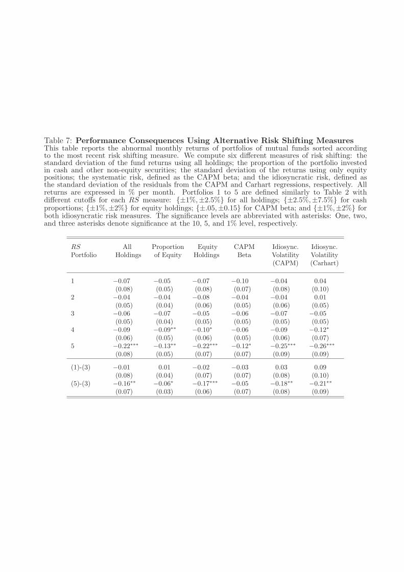
Table 7: Performance Consequences Using Alternative Risk Shifting MeasuresThis table reports the abnormal monthly returns of portfolios of mutual funds sorted accordingto the most recent risk shifting measure. We compute six different measures of risk shifting: thestandard deviation of the fund returns using all holdings; the proportion of the portfolio investedin cash and other non-equity securities; the standard deviation of the returns using only equitypositions; the systematic risk, defined as the CAPM beta; and the idiosyncratic risk, defined asthe standard deviation of the residuals from the CAPM and Carhart regressions, respectively. Allreturns are expressed in % per month. Portfolios 1 to 5 are defined similarly to Table 2 withdifferent cutoffs for each RS measure: {±1%,±2.5%} for all holdings; {±2.5%,±7.5%} for cashproportions; {±1%,±2%} for equity holdings; {±.05,±0.15} for CAPM beta; and {±1%,±2%} forboth idiosyncratic risk measures. The significance levels are abbreviated with asterisks: One, two,and three asterisks denote significance at the 10, 5, and 1% level, respectively.

RS All Proportion Equity CAPM Idiosync. Idiosync.Portfolio Holdings of Equity Holdings Beta Volatility Volatility

(CAPM) (Carhart)

1 −0.07 −0.05 −0.07 −0.10 −0.04 0.04(0.08) (0.05) (0.08) (0.07) (0.08) (0.10)

2 −0.04 −0.04 −0.08 −0.04 −0.04 0.01(0.05) (0.04) (0.06) (0.05) (0.06) (0.05)

3 −0.06 −0.07 −0.05 −0.06 −0.07 −0.05(0.05) (0.04) (0.05) (0.05) (0.05) (0.05)

4 −0.09 −0.09∗∗ −0.10∗ −0.06 −0.09 −0.12∗

(0.06) (0.05) (0.06) (0.05) (0.06) (0.07)5 −0.22∗∗∗ −0.13∗∗ −0.22∗∗∗ −0.12∗ −0.25∗∗∗ −0.26∗∗∗

(0.08) (0.05) (0.07) (0.07) (0.09) (0.09)

(1)-(3) −0.01 0.01 −0.02 −0.03 0.03 0.09(0.08) (0.04) (0.07) (0.07) (0.08) (0.10)

(5)-(3) −0.16∗∗ −0.06∗ −0.17∗∗∗ −0.05 −0.18∗∗ −0.21∗∗

(0.07) (0.03) (0.06) (0.07) (0.08) (0.09)

Table 8: Performance of Funds by Risk Shifting and Other Fund CharacteristicsThis table reports the frequency distribution and the Carhart alphas of portfolios of mutual fundssorted according to risk shifting and other fund characteristics that are related to trading costs andprior fund performance (turnover, prior year flow, prior year return, and realized volatility overprior 3 years). Mutual funds are first sorted into two equal-sized groups according to whether thecharacteristic is above or below its median value. In a second step, funds are further divided into fivegroups according to their risk shifting level. The table reports the average proportion of funds thatfall into one of the ten groups and the Carhart alphas of the ten portfolios and the differences in theCarhart alphas between selected portfolios. All returns are expressed in % per month. Portfolios 1to 5 are defined in Table 2 with cutoff RS measures of {±1%,±2.5%}. The significance levels areabbreviated with asterisks: One, two, and three asterisks denote significance at the 10, 5, and 1%level, respectively.

Panel A: Funds Sorted by Turnover (TO)

RS Frequency Future Carhart AlphasPortfolio Low TO High TO L−H Low TO High TO L−H

1 5.21 8.99 −3.79∗∗∗ −0.12 −0.09 −0.03(0.77) (0.13) (0.08) (0.13)

2 7.02 8.34 −1.32∗∗ −0.04 −0.07 0.04(0.63) (0.06) (0.06) (0.05)

3 24.10 17.22 6.88∗∗∗ −0.06 −0.07 0.01(0.43) (0.05) (0.05) (0.03)

4 8.71 7.75 0.97∗ −0.06 −0.13∗∗ 0.08∗

(0.52) (0.06) (0.06) (0.04)5 4.95 7.70 −2.74∗∗∗ −0.31∗∗∗ −0.15∗ −0.16

(0.56) (0.10) (0.08) (0.10)

All −0.07∗ −0.10∗∗ 0.03(0.04) (0.04) (0.03)

(1)-(3) −0.06 −0.02 −0.04(0.13) (0.07) (0.13)

(5)-(3) −0.25∗∗ −0.08 −0.17∗

(0.10) (0.07) (0.10)

Panel B: Funds Sorted by Prior Year Flows

RS Frequency Future Carhart AlphasPortfolio Low Flow High Flow L−H Low Flow High Flow L−H1 7.04 7.16 −0.11 −0.14∗ −0.01 −0.14

(0.66) (0.07) (0.11) (0.12)2 7.37 8.00 −0.63∗ −0.07 −0.07 0.00

(0.37) (0.06) (0.06) (0.07)3 20.40 20.94 −0.54 −0.06 −0.06 −0.00

(0.72) (0.05) (0.05) (0.04)4 8.58 7.88 0.71∗ −0.08 −0.10∗ 0.01

(0.37) (0.07) (0.06) (0.05)5 6.55 6.08 0.48 −0.18∗∗ −0.13∗ −0.05

(0.49) (0.08) (0.08) (0.09)

All −0.09∗ −0.08∗ −0.01(0.05) (0.04) (0.04)

(1)-(3) −0.08 0.05 −0.13(0.06) (0.11) (0.12)

(5)-(3) −0.12∗ −0.07 −0.05(0.07) (0.07) (0.08)

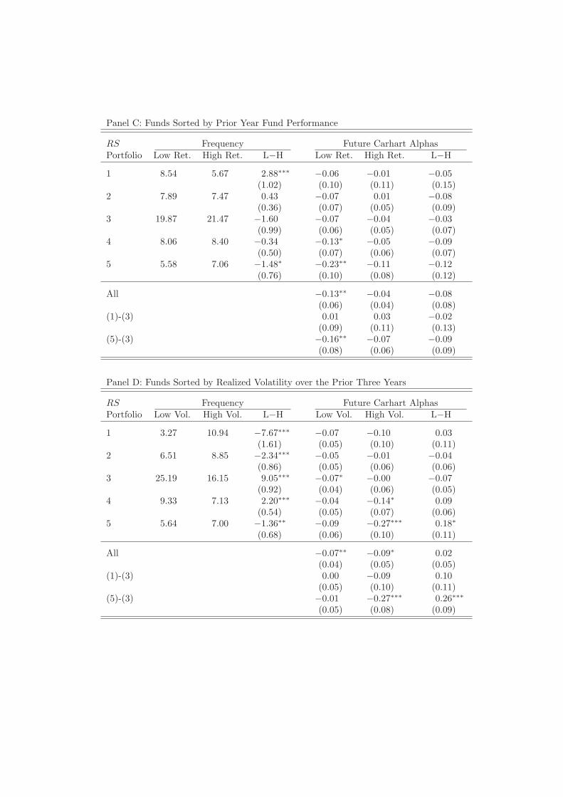
Panel C: Funds Sorted by Prior Year Fund Performance

RS Frequency Future Carhart AlphasPortfolio Low Ret. High Ret. L−H Low Ret. High Ret. L−H

1 8.54 5.67 2.88∗∗∗ −0.06 −0.01 −0.05(1.02) (0.10) (0.11) (0.15)

2 7.89 7.47 0.43 −0.07 0.01 −0.08(0.36) (0.07) (0.05) (0.09)

3 19.87 21.47 −1.60 −0.07 −0.04 −0.03(0.99) (0.06) (0.05) (0.07)

4 8.06 8.40 −0.34 −0.13∗ −0.05 −0.09(0.50) (0.07) (0.06) (0.07)

5 5.58 7.06 −1.48∗ −0.23∗∗ −0.11 −0.12(0.76) (0.10) (0.08) (0.12)

All −0.13∗∗ −0.04 −0.08(0.06) (0.04) (0.08)

(1)-(3) 0.01 0.03 −0.02(0.09) (0.11) (0.13)

(5)-(3) −0.16∗∗ −0.07 −0.09(0.08) (0.06) (0.09)

Panel D: Funds Sorted by Realized Volatility over the Prior Three Years

RS Frequency Future Carhart AlphasPortfolio Low Vol. High Vol. L−H Low Vol. High Vol. L−H

1 3.27 10.94 −7.67∗∗∗ −0.07 −0.10 0.03(1.61) (0.05) (0.10) (0.11)

2 6.51 8.85 −2.34∗∗∗ −0.05 −0.01 −0.04(0.86) (0.05) (0.06) (0.06)

3 25.19 16.15 9.05∗∗∗ −0.07∗ −0.00 −0.07(0.92) (0.04) (0.06) (0.05)

4 9.33 7.13 2.20∗∗∗ −0.04 −0.14∗ 0.09(0.54) (0.05) (0.07) (0.06)

5 5.64 7.00 −1.36∗∗ −0.09 −0.27∗∗∗ 0.18∗

(0.68) (0.06) (0.10) (0.11)

All −0.07∗∗ −0.09∗ 0.02(0.04) (0.05) (0.05)

(1)-(3) 0.00 −0.09 0.10(0.05) (0.10) (0.11)

(5)-(3) −0.01 −0.27∗∗∗ 0.26∗∗∗

(0.05) (0.08) (0.09)

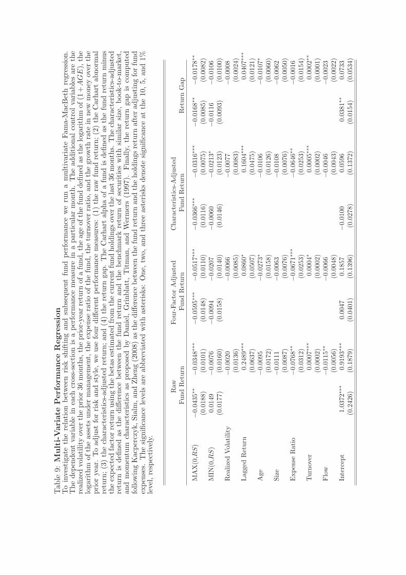
Tab

le9:

Multi-V

ari

ate

Perf

orm

ance

Regre

ssio

nTo

inve

stig

ate

the

rela

tion

betw

een

risk

shift

ing

and

subs

eque

ntfu

ndpe

rfor

man

cew

eru

na

mul

tiva

riat

eFa

ma-

Mac

Bet

hre

gres

sion

.T

hede

pend

ent

vari

able

inea

chcr

oss-

sect

ion

isa

perf

orm

ance

mea

sure

ina

part

icul

arm

onth

.T

head

diti

onal

cont

rolva

riab

les

are

the

real

ized

vola

tilit

yov

erth

epr

ior

36m

onth

s,th

epr

ior-

year

retu

rnof

afu

nd,t

heag

eof

the

fund

defin

edas

the

loga

rith

mof

(1+

AG

E),

the

loga

rith

mof

the

asse

tsun

der

man

agem

ent,

the

expe

nse

rati

oof

the

fund

,the

turn

over

rati

o,an

dth

egr

owth

rate

inne

wm

oney

over

the

prio

rye

ar.

To

adju

stfo

rri

skan

dst

yle,

we

use

four

diffe

rent

perf

orm

ance

mea

sure

s:(1

)th

era

wfu

ndre

turn

;(2

)th

eC

arha

rtab

norm

alre

turn

;(3

)th

ech

arac

teri

stic

s-ad

just

edre

turn

;an

d(4

)th

ere

turn

gap.

The

Car

hart

alph

aof

afu

ndis

defin

edas

the

fund

retu

rnm

inus

the

expe

cted

fact

orre

turn

usin

gth

ebe

tas

esti

mat

edfr

omth

ecu

rren

tfu

ndho

ldin

gsov

erth

ela

st36

mon

ths.

The

char

acte

rist

ics-

adju

sted

retu

rnis

defin

edas

the

diffe

renc

ebe

twee

nth

efu

ndre

turn

and

the

benc

hmar

kre

turn

ofse

curi

ties

wit

hsi

mila

rsi

ze,

book

-to-

mar

ket,

and

mom

entu

mch

arac

teri

stic

sas

prop

osed

byD

anie

l,G

rinb

latt

,T

itm

an,

and

Wer

mer

s(1

997)

.Fin

ally

,th

ere

turn

gap

isco

mpu

ted

follo

win

gK

acpe

rczy

k,Si

alm

,and

Zhe

ng(2

008)

asth

edi

ffere

nce

betw

een

the

fund

retu

rnan

dth

eho

ldin

gsre

turn

afte

rad

just

ing

for

fund

expe

nses

.T

hesi

gnifi

canc

ele

vels

are

abbr

evia

ted

wit

has

teri

sks:

One

,tw

o,an

dth

ree

aste

risk

sde

note

sign

ifica

nce

atth

e10

,5,

and

1%le

vel,

resp

ecti

vely

.

Raw

Four

-Fac

tor

Adj

uste

dC

hara

cter

isti

cs-A

djus

ted

Fund

Ret

urn

Fund

Ret

urn

Fund

Ret

urn

Ret

urn

Gap

MA

X(0

,RS

)−0

.043

5∗∗

−0.0

348∗∗∗

−0.0

595∗∗∗

−0.0

517∗∗∗

−0.0

366∗∗∗

−0.0

316∗∗∗

−0.0

168∗∗

−0.0

178∗∗

(0.0

188)

(0.0

101)

(0.0

148)

(0.0

110)

(0.0

116)

(0.0

075)

(0.0

085)

(0.0

082)

MIN

(0,R

S)

0.01

49−0

.007

6−0

.009

4−0

.020

7−0

.006

0−0

.021

3∗−0

.011

6−0

.010

6(0

.017

7)(0

.016

0)(0

.015

8)(0

.014

0)(0

.014

6)(0

.012

3)(0

.009

3)(0

.010

0)R

ealiz

edV

olat

ility

−0.0

020

−0.0

066

−0.0

077

−0.0

008

(0.0

136)

(0.0

085)

(0.0

083)

(0.0

024)

Lag

ged

Ret

urn

0.24

89∗∗∗

0.08

60∗

0.16

04∗∗∗

0.04

07∗∗∗

(0.0

637)

(0.0

507)

(0.0

475)

(0.0

121)

Age

−0.0

095

−0.0

273∗

−0.0

106

−0.0

107∗

(0.0

172)

(0.0

158)

(0.0

126)

(0.0

060)

Size

−0.0

111

−0.0

063

−0.0

108

−0.0

062

(0.0

087)

(0.0

076)

(0.0

076)

(0.0

050)

Exp

ense

Rat

io−0

.076

8∗∗

−0.0

671∗∗∗

−0.0

646∗∗

−0.0

016

(0.0

312)

(0.0

253)

(0.0

253)

(0.0

154)

Tur

nove

r0.

0007∗∗∗

0.00

04∗

0.00

05∗∗∗

0.00

02∗∗

(0.0

002)

(0.0

002)

(0.0

002)

(0.0

001)

Flo

w−0

.011

5∗∗

−0.0

066

−0.0

046

−0.0

023

(0.0

056)

(0.0

048)

(0.0

043)

(0.0

022)

Inte

rcep

t1.

0372∗∗∗

0.91

93∗∗∗

0.00

470.

1857

−0.0

100

0.05

960.

0381∗∗

0.07

33(0

.242

6)(0

.187

9)(0

.040

1)(0

.139

6)(0

.027

8)(0

.137

2)(0

.015

4)(0

.053

4)

-6

-4

-2

0

2

4

6

-4 -2 0 2 4 6 8

Quarters Around Formation Period

RS

RS1

RS5

RS4

RS3

RS2

Figure 1: Persistence of Risk Shifting.The figure depicts the average risk shifting level for the five risk shifting portfolios fourquarters before and eight quarters after the portfolio formation.

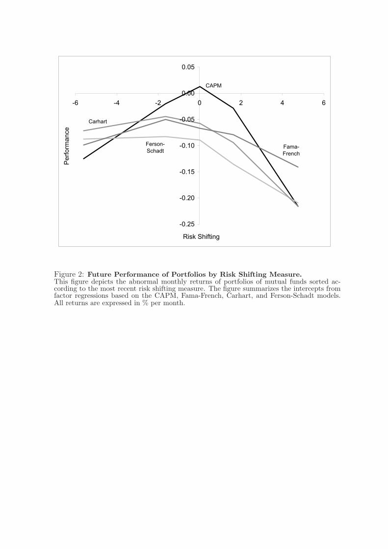
-0.25

-0.20

-0.15

-0.10

-0.05

0.00

0.05

-6 -4 -2 0 2 4 6

Risk Shifting

Pe

rfo

rma

nce

Carhart

CAPM

Ferson-

SchadtFama-

French

Figure 2: Future Performance of Portfolios by Risk Shifting Measure.This figure depicts the abnormal monthly returns of portfolios of mutual funds sorted ac-cording to the most recent risk shifting measure. The figure summarizes the intercepts fromfactor regressions based on the CAPM, Fama-French, Carhart, and Ferson-Schadt models.All returns are expressed in % per month.

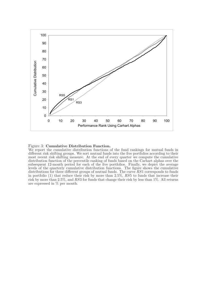
0

10

20

30

40

50

60

70

80

90

100

0 10 20 30 40 50 60 70 80 90 100

Performance Rank Using Carhart Alphas

Cum

ula

tive D

istr

ibution

RS3RS1

RS5

Figure 3: Cumulative Distribution Function.We report the cumulative distribution functions of the fund rankings for mutual funds indifferent risk shifting groups. We sort mutual funds into the five portfolios according to theirmost recent risk shifting measure. At the end of every quarter we compute the cumulativedistribution function of the percentile ranking of funds based on the Carhart alphas over thesubsequent 12-month period for each of the five portfolios. Finally, we depict the averagelevels of the quarterly cumulative distribution functions. The figure shows the cumulativedistributions for three different groups of mutual funds. The curve RS1 corresponds to fundsin portfolio (1) that reduce their risk by more than 2.5%, RS5 to funds that increase theirrisk by more than 2.5%, and RS3 for funds that change their risk by less than 1%. All returnsare expressed in % per month.