Robust Speech Recognition for German and Dialectal ...hss.ulb.uni-bonn.de/2018/5236/5236.pdf ·...
133
Robust Speech Recognition for German and Dialectal Broadcast Programmes Dissertation zur Erlangung des Doktorgrades (Dr. rer. nat.) der Mathematisch-Naturwissenschaftlichen Fakult¨ at der Rheinischen Friedrich-Wilhelms-Universit¨ at Bonn vorgelegt von Diplom-Ingenieur Michael Stadtschnitzer aus K¨ oflach, ¨ Osterreich Bonn 2018
Transcript of Robust Speech Recognition for German and Dialectal ...hss.ulb.uni-bonn.de/2018/5236/5236.pdf ·...

Robust Speech Recognitionfor German and DialectalBroadcast Programmes
Dissertation
zur
Erlangung des Doktorgrades (Dr. rer. nat.)
der
Mathematisch-Naturwissenschaftlichen Fakultat
der
Rheinischen Friedrich-Wilhelms-Universitat Bonn
vorgelegt von
Diplom-IngenieurMichael Stadtschnitzer
aus
Koflach, Osterreich
Bonn 2018
Angefertigt mit Genehmigung der Mathematisch-Naturwissenschaftlichen Fakultat derRheinischen Friedrich-Wilhelms-Universitat Bonn
1. Gutachter: Prof. Dr.-Ing. Christian Bauckhage2. Gutachter: Prof. Dr. Stefan Wrobel
Tag der Promotion: 17. Oktober 2018Erscheinungsjahr: 2018
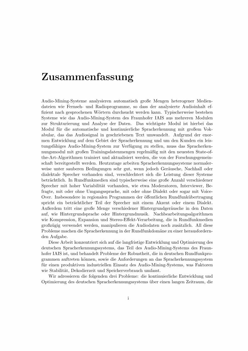
Zusammenfassung
Audio-Mining-Systeme analysieren automatisch große Mengen heterogener Medien-dateien wie Fernseh- und Radioprogramme, so dass der analysierte Audioinhalt ef-fizient nach gesprochenen Wortern durchsucht werden kann. Typischerweise bestehenSysteme wie das Audio-Mining-System des Fraunhofer IAIS aus mehreren Modulenzur Strukturierung und Analyse der Daten. Das wichtigste Modul ist hierbei dasModul fur die automatische und kontinuierliche Spracherkennung mit großem Vok-abular, das das Audiosignal in geschriebenen Text umwandelt. Aufgrund der enor-men Entwicklung auf dem Gebiet der Spracherkennung und um den Kunden ein leis-tungsfahiges Audio-Mining-System zur Verfugung zu stellen, muss das Spracherken-nungsmodul mit großen Trainingsdatenmengen regelmaßig mit den neuesten State-of-the-Art-Algorithmen trainiert und aktualisiert werden, die von der Forschungsgemein-schaft bereitgestellt werden. Heutzutage arbeiten Spracherkennungssysteme normaler-weise unter sauberen Bedingungen sehr gut, wenn jedoch Gerausche, Nachhall oderdialektale Sprecher vorhanden sind, verschlechtert sich die Leistung dieser Systemebetrachtlich. In Rundfunkmedien sind typischerweise eine große Anzahl verschiedenerSprecher mit hoher Variabilitat vorhanden, wie etwa Moderatoren, Interviewer, Be-fragte, mit oder ohne Umgangssprache, mit oder ohne Dialekt oder sogar mit Voice-Over. Insbesondere in regionalen Programmen der offentlichen Rundfunkubertragungspricht ein betrachtlicher Teil der Sprecher mit einem Akzent oder einem Dialekt.Außerdem tritt eine große Menge verschiedener Hintergrundgerausche in den Datenauf, wie Hintergrundsprache oder Hintergrundmusik. Nachbearbeitungsalgorithmenwie Kompression, Expansion und Stereo-Effekt-Verarbeitung, die in Rundfunkmediengroßzugig verwendet werden, manipulieren die Audiodaten noch zusatzlich. All dieseProbleme machen die Spracherkennung in der Rundfunkdomane zu einer herausfordern-den Aufgabe.
Diese Arbeit konzentriert sich auf die langfristige Entwicklung und Optimierung desdeutschen Spracherkennungssystems, das Teil des Audio-Mining-Systems des Fraun-hofer IAIS ist, und behandelt Probleme der Robustheit, die in deutschen Rundfunkpro-grammen auftreten konnen, sowie die Anforderungen an das Spracherkennungssystemfur einen produktiven industriellen Einsatz des Audio-Mining-Systems, was Faktorenwie Stabilitat, Dekodierzeit und Speicherverbrauch umfasst.
Wir adressieren die folgenden drei Probleme: die kontinuierliche Entwicklung undOptimierung des deutschen Spracherkennungssystems uber einen langen Zeitraum, die
i

schnelle automatische Suche nach den optimalen Spracherkennungsdekodierparameternund den Umgang mit deutschen Dialekten im deutschen Spracherkennungssystem furdie Rundfunkdomane.
Um eine hervorragende Leistung uber lange Zeitraume zu gewahrleisten, aktu-alisieren wir das System regelmaßig mit den neuesten Algorithmen und Systemar-chitekturen, die von der Forschungsgemeinschaft zur Verfugung gestellt wurden, undevaluieren hierzu die Leistung der Algorithmen im Kontext der deutschen Rund-funkdomane. Wir erhohen auch drastisch die Trainingsdaten, indem wir einen großenund neuartigen Sprachkorpus der deutschen Rundfunkdomane annotieren, der inDeutschland einzigartig ist.
Nach dem Training eines automatischen Spracherkennungssystems ist einSpracherkennungsdekoder dafur verantwortlich, die wahrscheinlichste Texthypothesefur ein bestimmtes Audiosignal zu dekodieren. Typischerweise benotigt derSpracherkennungsdekoder eine große Anzahl von Hyperparametern, die normalerweiseauf Standardwerte gesetzt oder manuell optimiert werden. Diese Parameter sind oftweit von dem Optimum in Bezug auf die Genauigkeit und die Dekodiergeschwindigkeitentfernt. Moderne Optimierungsalgorithmen fur Dekoderparameter benotigen allerd-ings eine lange Zeit, um zu konvergieren. Daher nahern wir uns in dieser Arbeit derautomatischen Dekoderparameteroptimierung im Kontext der deutschen Spracherken-nung in der Rundfunkdomane in dieser Arbeit an, sowohl fur die uneingeschrankte alsauch fur die eingeschrankte Dekodierung (in Bezug auf die Dekodiergeschwindigkeit),indem ein Optimierungsalgorithmus fur den Einsatz in der Spracherkennung eingefuhrtund erweitert wird, der noch nie zuvor im Kontext der Spracherkennung verwendetwurde.
In Deutschland gibt es eine große Vielfalt an Dialekten, die oft in den Rund-funkmedien, vor allem in regionalen Programmen, vorhanden sind. Dialektale Spracheverursacht eine stark verschlechterte Leistungsfahigkeit des Spracherkennungssystemsaufgrund der Nichtubereinstimmung von Phonetik und Grammatik. In dieser Arbeitbeziehen wir die große Vielfalt deutscher Dialekte ein, indem wir ein Dialektidenti-fizierungssystem einfuhren, um den Dialekt des Sprechers abzuleiten, und um nachfol-gend angepasste dialektale Spracherkennungsmodelle zu verwenden, um den gesproch-enen Text zu erhalten. Fur das Training des Dialektidentifizierungssystems wurde eineneuartige Datenbank gesammelt und annotiert.
Indem wir uns mit diesen drei Themen befassen, gelangen wir zu einem Audio-Mining-System, das ein leistungsstarkes Spracherkennungssystem beinhaltet, das inder Lage ist, dialektale Sprecher zu bewaltigen und mit optimalen Dekoderparametern,die schnell berechnet werden konnen.
ii

Abstract
Audio mining systems automatically analyse large amounts of heterogeneous mediafiles such as television and radio programmes so that the analysed audio content canbe efficiently searched for spoken words. Typically audio mining systems such as theFraunhofer IAIS audio mining system consist of several modules to structure and anal-yse the data.
The most important module is the large vocabulary continuous speech recognition(LVCSR) module, which is responsible to transform the audio signal into written text.Because of the tremendous developments in the field of speech recognition and to pro-vide the customers with a high-performance audio mining system, the LVCSR modulehas to be trained and updated regularly by using the latest state-of-the-art algorithmsprovided by the research community and also by employing large amounts of trainingdata. Today speech recognition systems usually perform very well in clean conditions,however when noise, reverberation or dialectal speakers are present, the performanceof these systems degrade considerably. In broadcast media typically a large number ofdifferent speakers with high variability are present, like anchormen, interviewers, inter-viewees, speaking colloquial or planned speech, with or without dialect, or even withvoice-overs. Especially in regional programmes of public broadcast, a considerable frac-tion of the speakers speak with an accent or a dialect. Also, a large amount of differentbackground noises appears in the data, like background speech, or background music.Post-processing algorithms like compression, expansion, and stereo effect processing,which are generously used in broadcast media, further manipulate the audio data. Allthese issues make speech recognition in the broadcast domain a challenging task.
This thesis focuses on the development and the optimisation of the German broad-cast LVCSR system, which is part of the Fraunhofer IAIS audio mining system, overthe course of several years, dealing with robustness related problems that arise for Ger-man broadcast media and also dealing with the requirements for the employment ofthe ASR system in a productive audiomining system for the industrial use includingstability, decoding time and memory consumption.
We approach the following three problems: the continuous development and opti-misation of the German broadcast LVCSR system over a long period, rapidly findingthe optimal ASR decoder parameters automatically and dealing with German dialectsin the German broadcast LVCSR system.
To guarantee superb performance over long periods of time, we regularly re-train
iii
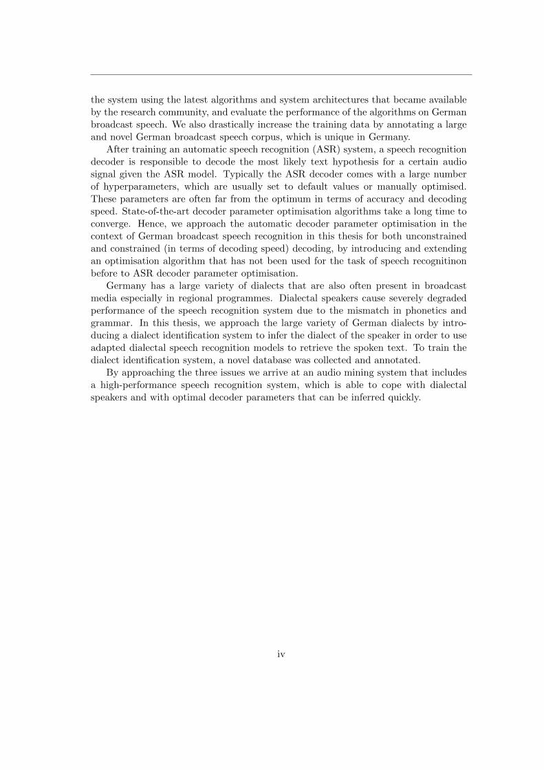
the system using the latest algorithms and system architectures that became availableby the research community, and evaluate the performance of the algorithms on Germanbroadcast speech. We also drastically increase the training data by annotating a largeand novel German broadcast speech corpus, which is unique in Germany.
After training an automatic speech recognition (ASR) system, a speech recognitiondecoder is responsible to decode the most likely text hypothesis for a certain audiosignal given the ASR model. Typically the ASR decoder comes with a large numberof hyperparameters, which are usually set to default values or manually optimised.These parameters are often far from the optimum in terms of accuracy and decodingspeed. State-of-the-art decoder parameter optimisation algorithms take a long time toconverge. Hence, we approach the automatic decoder parameter optimisation in thecontext of German broadcast speech recognition in this thesis for both unconstrainedand constrained (in terms of decoding speed) decoding, by introducing and extendingan optimisation algorithm that has not been used for the task of speech recognitinonbefore to ASR decoder parameter optimisation.
Germany has a large variety of dialects that are also often present in broadcastmedia especially in regional programmes. Dialectal speakers cause severely degradedperformance of the speech recognition system due to the mismatch in phonetics andgrammar. In this thesis, we approach the large variety of German dialects by intro-ducing a dialect identification system to infer the dialect of the speaker in order to useadapted dialectal speech recognition models to retrieve the spoken text. To train thedialect identification system, a novel database was collected and annotated.
By approaching the three issues we arrive at an audio mining system that includesa high-performance speech recognition system, which is able to cope with dialectalspeakers and with optimal decoder parameters that can be inferred quickly.
iv
Acknowledgements
Firstly, I would like to express my sincere gratitude to my advisors Dr. Daniel Stein andDr. Christoph Schmidt for their continuous support of my studies and related research,for their patience, motivation, and immense knowledge. Their guidance helped me inall the time of research and writing this thesis.
Besides my advisors, I would like to thank the rest of my thesis committee: Prof.Dr.-Ing. Christian Bauckhage, Prof. Dr. Stefan Wrobel, for their insightful commentsand encouragement.
My sincere thanks also go to Dr.-Ing. Joachim Kohler, who provided me the op-portunity to join his team, and who gave me access to the department facilities, andalso for his precious pieces of advice regarding this thesis.
Also, I would like to express my gratitude to Bayerischer Rundfunk and SchweizerRundfunk und Fernsehen for the close collaboration and who provided us precious datafor research purposes. Without their help, this research would not have been possibleto conduct.
I thank my fellow mates in the department for stimulating discussions and for allthe fun we had in the last few years.
Last but not least, I thank my family and friends for their motivation and theirpatience through this intense phase of my life.
v
Contents
1 Introduction 11.1 Audio Mining . . . . . . . . . . . . . . . . . . . . . . . . . . . . . . . . . 11.2 Robust Speech Recognition . . . . . . . . . . . . . . . . . . . . . . . . . 11.3 Dialects in Speech Recognition . . . . . . . . . . . . . . . . . . . . . . . 31.4 About This Thesis . . . . . . . . . . . . . . . . . . . . . . . . . . . . . . 3
2 Scientific Goals 42.1 Goals . . . . . . . . . . . . . . . . . . . . . . . . . . . . . . . . . . . . . 4
3 Preliminaries 53.1 Speech . . . . . . . . . . . . . . . . . . . . . . . . . . . . . . . . . . . . . 5
3.1.1 Speech Production . . . . . . . . . . . . . . . . . . . . . . . . . . 53.1.2 Speech Perception . . . . . . . . . . . . . . . . . . . . . . . . . . 6
3.2 Digital Signal Processing . . . . . . . . . . . . . . . . . . . . . . . . . . . 73.2.1 Discrete Fourier transform . . . . . . . . . . . . . . . . . . . . . . 9
3.3 Pattern Recognition . . . . . . . . . . . . . . . . . . . . . . . . . . . . . 103.3.1 Feature Extraction . . . . . . . . . . . . . . . . . . . . . . . . . . 10
Mel-Frequency Cepstral Coefficients . . . . . . . . . . . . . . . . 11Filterbank Coefficients . . . . . . . . . . . . . . . . . . . . . . . . 12
3.3.2 Hidden Markov Models . . . . . . . . . . . . . . . . . . . . . . . 133.3.3 Gaussian Mixture Model . . . . . . . . . . . . . . . . . . . . . . . 133.3.4 Artificial Neural Networks . . . . . . . . . . . . . . . . . . . . . . 15
Recurrent Neural Networks . . . . . . . . . . . . . . . . . . . . . 16Convolutional Neural Networks . . . . . . . . . . . . . . . . . . . 18
3.4 Automatic Speech Recognition . . . . . . . . . . . . . . . . . . . . . . . 193.4.1 History of Automatic Speech Recognition . . . . . . . . . . . . . 193.4.2 Statistical Speech Recognition . . . . . . . . . . . . . . . . . . . 213.4.3 Pronunciation Dictionary . . . . . . . . . . . . . . . . . . . . . . 23
Grapheme-to-Phoneme Conversion . . . . . . . . . . . . . . . . . 243.4.4 Acoustical Model . . . . . . . . . . . . . . . . . . . . . . . . . . . 253.4.5 Language Model . . . . . . . . . . . . . . . . . . . . . . . . . . . 27
m-gram Language Models . . . . . . . . . . . . . . . . . . . . . . 273.4.6 Search . . . . . . . . . . . . . . . . . . . . . . . . . . . . . . . . . 28
vi

Contents
3.4.7 Decoder Parameter Optimisation . . . . . . . . . . . . . . . . . . 293.4.8 Weighted Finite State Transducer . . . . . . . . . . . . . . . . . 293.4.9 Evaluation and Performance Measures . . . . . . . . . . . . . . . 30
Word Error Rate . . . . . . . . . . . . . . . . . . . . . . . . . . . 31Real Time Factor . . . . . . . . . . . . . . . . . . . . . . . . . . . 31Out-Of-Vocabulary Rate . . . . . . . . . . . . . . . . . . . . . . . 32Perplexity . . . . . . . . . . . . . . . . . . . . . . . . . . . . . . . 32
3.5 Dialect Identification . . . . . . . . . . . . . . . . . . . . . . . . . . . . . 333.5.1 Phonotactic Methods . . . . . . . . . . . . . . . . . . . . . . . . 34
Phone Recogniser followed by Language Model . . . . . . . . . . 34Parallel Phone Recogniser followed by Language Model . . . . . 34
3.5.2 Acoustic Methods . . . . . . . . . . . . . . . . . . . . . . . . . . 34Universal Background Model . . . . . . . . . . . . . . . . . . . . 35Gaussian Posterior Probability Supervector . . . . . . . . . . . . 35Gaussian Mean Supervector . . . . . . . . . . . . . . . . . . . . . 36i-Vectors . . . . . . . . . . . . . . . . . . . . . . . . . . . . . . . . 36
3.5.3 Evaluation Metrics and Performance . . . . . . . . . . . . . . . . 36Binary Classification . . . . . . . . . . . . . . . . . . . . . . . . . 36Multi-Class Classification . . . . . . . . . . . . . . . . . . . . . . 37
4 Long-Term Development of a German Broadcast ASR System 394.1 The Fraunhofer IAIS Audio Mining System . . . . . . . . . . . . . . . . 404.2 Baseline Speech Recognition System and Resources . . . . . . . . . . . . 41
4.2.1 Audio Mining Corpus . . . . . . . . . . . . . . . . . . . . . . . . 414.2.2 Difficult Speech Corpus . . . . . . . . . . . . . . . . . . . . . . . 424.2.3 The LinkedTV Evaluation Corpus . . . . . . . . . . . . . . . . . 434.2.4 Baseline Speech Recognition System . . . . . . . . . . . . . . . . 44
4.3 Improvements to the Speech Recognition System . . . . . . . . . . . . . 454.3.1 Large-Scale German Broadcast Speech Corpus . . . . . . . . . . 454.3.2 Extension and Optimisation of the Baseline System . . . . . . . 464.3.3 Subspace Gaussian Mixture Models . . . . . . . . . . . . . . . . 474.3.4 Hybrid Deep Neural Network Hidden Markov Models . . . . . . 484.3.5 Recurrent Neural Network Rescoring . . . . . . . . . . . . . . . . 514.3.6 Deep Neural Networks with p-Norm Nonlinearities . . . . . . . . 524.3.7 Recurrent Neural Networks based on Long Short-Term Memory . 534.3.8 Time Delay Neural Networks . . . . . . . . . . . . . . . . . . . . 544.3.9 TDNN with Projected Long Short-Time Memory . . . . . . . . . 574.3.10 LM Rescoring with Gated Convolutional Neural Networks . . . . 59
4.4 Summary and Contributions . . . . . . . . . . . . . . . . . . . . . . . . . 61
5 Gradient-Free Decoder Parameter Optimisation 655.1 Unconstrained Decoder Parameter Optimisation . . . . . . . . . . . . . 66
5.1.1 Simultaneous Perturbation Stochastic Approximation . . . . . . 665.1.2 GMM-HMM Decoder Parameters . . . . . . . . . . . . . . . . . . 67
vii
Contents
5.1.3 Experimental Setup and Evaluation . . . . . . . . . . . . . . . . 695.2 Time-constrained Decoder Parameter Optimisation . . . . . . . . . . . . 72
5.2.1 Time-constrained Word Error Rate Optimisation . . . . . . . . . 735.2.2 Exponential RTF penalty . . . . . . . . . . . . . . . . . . . . . . 735.2.3 Delta RTF penalty . . . . . . . . . . . . . . . . . . . . . . . . . . 735.2.4 Increasing RTF penalty . . . . . . . . . . . . . . . . . . . . . . . 745.2.5 Comparison of the RTF Penalty Functions . . . . . . . . . . . . 75
5.3 Comparison with State-of-the-art Methods . . . . . . . . . . . . . . . . . 765.3.1 Downhill Simplex . . . . . . . . . . . . . . . . . . . . . . . . . . . 775.3.2 Evolutional Strategies . . . . . . . . . . . . . . . . . . . . . . . . 785.3.3 Gradient Descent . . . . . . . . . . . . . . . . . . . . . . . . . . . 785.3.4 DNN-HMM and SGMM-HMM Decoder Parameters . . . . . . . 785.3.5 Time-Unconstrained Experiments . . . . . . . . . . . . . . . . . . 785.3.6 Time-Constrained Experiments . . . . . . . . . . . . . . . . . . . 81
5.4 Summary and Contributions . . . . . . . . . . . . . . . . . . . . . . . . . 82
6 Dialects in Speech Recognition 856.1 German Dialects . . . . . . . . . . . . . . . . . . . . . . . . . . . . . . . 856.2 German Dialect Identification . . . . . . . . . . . . . . . . . . . . . . . . 87
6.2.1 German Dialect Identification Based on the RVG1 Database . . 876.2.2 Upper German Broadcast Dialectal Database . . . . . . . . . . . 886.2.3 German Broadcast Dialect Identification . . . . . . . . . . . . . . 906.2.4 German Broadcast Dialect Detection . . . . . . . . . . . . . . . . 91
6.3 Dialectal Speech Recognition . . . . . . . . . . . . . . . . . . . . . . . . 926.3.1 Swiss German . . . . . . . . . . . . . . . . . . . . . . . . . . . . . 926.3.2 SRF Meteo Weather Report Dataset . . . . . . . . . . . . . . . . 936.3.3 Swiss German Speech Recognition . . . . . . . . . . . . . . . . . 94
Standard German Speech Phoneme Decoder . . . . . . . . . . . . 94Data-Driven Pronunciation Modelling . . . . . . . . . . . . . . . 94Directly Trained Swiss German Speech Recognition . . . . . . . 95
6.4 Summary and Contributions . . . . . . . . . . . . . . . . . . . . . . . . . 97
7 Scientific Achievements and Conclusions 997.1 Scientific Achievements . . . . . . . . . . . . . . . . . . . . . . . . . . . 997.2 Publications . . . . . . . . . . . . . . . . . . . . . . . . . . . . . . . . . . 1007.3 Conclusions . . . . . . . . . . . . . . . . . . . . . . . . . . . . . . . . . . 101
A Toolkits 103A.1 HTK Toolkit . . . . . . . . . . . . . . . . . . . . . . . . . . . . . . . . . 103A.2 Kaldi . . . . . . . . . . . . . . . . . . . . . . . . . . . . . . . . . . . . . . 103A.3 Eesen . . . . . . . . . . . . . . . . . . . . . . . . . . . . . . . . . . . . . 104A.4 RNNLM . . . . . . . . . . . . . . . . . . . . . . . . . . . . . . . . . . . . 104A.5 IRSTLM . . . . . . . . . . . . . . . . . . . . . . . . . . . . . . . . . . . . 104A.6 Sequitur-G2P . . . . . . . . . . . . . . . . . . . . . . . . . . . . . . . . . 104
viii

Contents
A.7 TheanoLM . . . . . . . . . . . . . . . . . . . . . . . . . . . . . . . . . . 105A.8 Keras . . . . . . . . . . . . . . . . . . . . . . . . . . . . . . . . . . . . . 105
List of Figures 106
List of Tables 109
Bibliography 111
ix
Chapter 1
Introduction
1.1 Audio Mining
Digital media archives are composed of a vast amount of heterogeneous media contentfiles, which are typically annotated only scarcely, manually and inconsistently. Search-ing in the data is often a challenging task and retrieving the seeked information isconsidered to be a lucky strike in the majority of cases.
Audio mining systems solve this problem by automatically analysing vast amountsof heterogeneous media content files. After processing the data, the database can beefficiently searched based on the analysis results. A typical audio mining system like theFraunhofer IAIS audio mining system is composed of several modules (e.g. speaker seg-mentation, gender detection, automatic speech recognition, speaker diarisation, speakeridentification, keyword generation) that employ sophisticated algorithms and modelswhich are trained on large amounts of training data. In order to guarantee a successfulaudio mining system for long periods of time, the modules have to be updated regularlyby using the latest state-of-the-art algorithms and by the usage of sufficient amountsof training data. One of the most important modules of an audio mining system is theautomatic speech recognition module, which is responsible to convert the audio speechsignal into the written text and to provide the time boundaries (start and end time)of the spoken words. The analysis results of the speech recognition module are alsooften used as the input for subsequent modules like the keyword extraction module andtherefore, highly performant and robust algorithms have to be used.
1.2 Robust Speech Recognition
Automatic speech recognition (ASR) is the technique to automatically transform anaudio speech signal into written text. Speech recognition systems typically consist ofan acoustic model, a pronunciation lexicon and a language model. A graph searchalgorithm like the Viterbi algorithm [1] decodes the most likely text hypothesis fromthe audio signal given the model. The acoustic model represents the relationship be-tween the audio signal and the linguistic units that make up speech (usually phonemes,
1
Chapter 1. Introduction
syllables, senones or whole words) and is built by modelling statistical representa-tions (e.g. Hidden-Markov-Models [2]) of the sound units by using audio recordingsof speech and their corresponding text transcriptions. The pronunciation lexicon is amapping between the vocabulary words and the corresponding units e.g. a sequence ofphonemes. The language model calculates the probability distributions over sequencesof words. Usually speech recognition systems perform very well in conditions similar tothe training data. However, if there is a mismatch between the training condition andthe testing condition, these systems typically degrade. Mismatches can occur e.g. dueto background noises, reverberation, or due to speaker variabilities like accents and di-alects. In the last few decades tremendous efforts have been made to improve the speechrecognition algorithms. In the last few years neural network based architectures su-perseded the classical approach based on Gaussian mixture models. Within very shortperiods of time different types of neural network architectures became state-of-the-artin the automatic speech recognition research community. Typically the algorithms aredeveloped by the exploitation of broadly used standard datasets from a certain domain,e.g. the Switchboard corpus [3], which is a corpus containing English telephone speech.It is unclear whether the advances reported for a certain language and domain directlytranslate to another specific language in a different domain.
Hence, and in order to guarantee a successful Fraunhofer IAIS audiomining systemwhich relies on constant development of the speech recognition system, we, amongstother things, approach the continuous development and optimisation of the large-vocabulary German broadcast speech recognition system over a long period of timein this thesis, where we investigate and evaluate different state-of-the-art speech recog-nition algorithms for their employment for German broadcast speech in a productiveaudio mining system. We also extend the training corpus by a large quantity andevaluate the improvements.
After an automatic speech recognition system is trained, a speech recognition de-coding algorithm is employed to decode the most likely text hypothesis from the speechsignal. Speech recognition decoder typically have a large set of hyperparameters, whichare commonly left to default values or which are manually set. These parameter valuesare most often far from the optimum value in terms of accuracy and decoding time.Automatic decoder parameter optimisation algorithms approach this issue, howeverstate-of-the-art algorithms tend to need a large amount of training iterations for thetraining to converge. In this thesis we approach the issues related to speech recogni-tion parameter optimisation by introducing a parameter optimisation algorithm thathas never been used in the context of speech recognition before to ASR decoder pa-rameter optimisation in the German broadcast domain. We investigate and evaluateits use for both unconstrained and constraint optimisation and compare the results tostate-of-the-art methods.
2

Chapter 1. Introduction
1.3 Dialects in Speech Recognition
Germany has a large variety of different dialects. Dialectal speakers are often presentin broadcast media, especially in regional programmes, and can cause impaired per-formance of the audio mining and speech recognition systems due to the phonological,semantical and syntactical differences that appear in dialectal speech compared to thestandard language. One way to cope with dialects in speech recognition is to applya dialect identification system beforehand and then to use specialised dialectal speechrecognition models to decode the text. This is why in this thesis we approach the di-alectal robustness of German broadcast speech recognition system. However, the wayto write down dialectal text is most often not standardised and hence, transcribed di-alectal speech resources are especially rare. That is why in this work a close cooperationwith regional broadcasters is built up to sight dialectal resources in their archives whichare then exploited to build a German dialect identification system and to improve thespeech recognition system.
1.4 About This Thesis
In this thesis, we discuss the long-term development and optimisation of a Germanbroadcast speech recognition system, which is part of a productive audiomining system,namely the Fraunhofer IAIS audio mining system. We evaluate a large number of state-of-the-art speech recognition architectures which became available in the course of thisthesis for the employment in the German broadcast domain. Furthermore, we efficientlyoptimise the parameters of the speech recognition decoder, which is part of the speechrecognition system, both in the unconstrained and in a constrained setting, with properevaluation. We also approach the dialectal robustness of the German speech recognitionsystem, with the help of a close cooperation to regional broadcasters, by the collectionof a dialect database and the creation of a dialect identification system and the use ofsubsequent dialectal speech recognition models.
This thesis is structured as follows: Chapter 2 concisely summarises the scientificgoals that are pursued in this work. Chapter 3 introduces the basics of speech process-ing, machine learning, speech recognition, and dialect identification. The main chaptersof this work address the above mentioned goals: the long-term development and op-timisation of the German broadcast speech recognition system including the creationand exploitation of a large German broadcast speech database is discussed in Chapter4. The fast and efficient speech recognition decoder parameter optimisation approachfor both constrained and unconstrained optimisation is described in Chapter 5. Theissue of dialectal robustness in German speech recognition is dealt with in Chapter 6.
A conclusion and a summary of the scientific achievements of this thesis are givenin Chapter 7.
3

Chapter 2
Scientific Goals
In this chapter, we discuss the topics which will be covered in this work and specifythe scientific goals of this thesis.
2.1 Goals
The following scientific goals were defined at the beginning and adjusted in the courseof the work:
Related to the long-term development of the German broadcast speech recognitionsystem:
• investigate and evaluate state-of-the-art speech recognition systems in the contextof German broadcast speech
• investigate the algorithms for their applicability in a productive audio miningsystem
• extend the amount of training data and exploit the data for training the speechrecognition system
Related to the automatic speech recognition decoder parameter optimisation:
• apply and adapt methods for fast and efficient decoder parameter optimisationin the context of German broadcast speech
• extend the algorithm for the usage in an constrained setting when decoding timeis an issue as it is in a productive system
Related to dialectal robustness of the speech recognition system:
• sight and prepare resources in cooperation with regional broadcasters to facilitatethe improvements
• deal with the manifold of dialects in German broadcast speech
4

Chapter 3
Preliminaries
In this chapter the fundamentals needed to comprehend the techniques discovered anddeveloped in this thesis are described. In Section 3.1, a short introduction to humanspeech is presented, including the human speech production system in Section 3.1.1and the human speech perception system in Section 3.1.2. The chapter then advanceswith the transition from the physical domain to the digital domain and a short intro-duction to digital signal processing in Section 3.2 and a short introduction to patternrecognition in Section 3.3. After that, the chapter then advances with an introduc-tion and the state-of-the-art to the most important techniques covered in this thesis,namely automatic speech recognition (Section 3.4) and dialect recognition (Section 3.5).
3.1 Speech
Speech is the most important means of human communication. In speech, informationis encoded by the vocalisation of a syntactic combination of words derived from avocabulary that is very large (usually more than thousand words). Each vocalisedword is build from a combination of a limited set of phonemes. Phonemes are thesmallest units of speech and can be divided into vowel and consonant phonemes. Alanguage is then made of a vocabulary, a set of phonemes and the word ordering(i.e. the syntax or grammar). In written language on the other hand the text is usuallymade of a set of graphemes (i.e. the smallest unit of text) and again a vocabulary andthe syntax. Graphemes can also be divided into vowel and consonant graphemes forlanguages like English or German.
3.1.1 Speech Production
Speech production is the process of the translation of thoughts into speech. After theselection of the words to be uttered, the vocal apparatus is activated. By taking abreath supported by the diaphragm muscle, air pressure from the lungs is built up and
5

Chapter 3. Preliminaries
then released. Air is flowing through the larynx, or more precisely, through the glottis,which is the interspace between the vocal cords. The airflow causes an excitation ofthe vocal cords. The excitation signal of the glottis can be described as an impulsechain, in case the vocal chords are vibrating (voiced excitation) or as a band-filterednoise if the vocal chords are not moving (unvoiced excitation). The frequency of theoccurrences of the impulses is often referred to as the fundamental frequency f0 orpitch. The fundamental frequency is typically lower for male speakers and higher forfemale speakers. Finally the excitation signal is shaped by the articulators, i.e. nose,mouth, lips and tongue. Depending on the position of the articulators, differentsounds are produced. Words are usually pronounced by shaping the excitation signalby a sequence of different articulator positions. When the pronounced words exit thespeech production system, the information is propagating as longitudinal air pressurewaves through the air with the speed of sound (343 m/s at 20° Celsius air temper-ature). The organs involved in the task of speech production are depicted in Figure 3.1.
nasal cavity
lips
tongue
lungs diaphragm
trachea
larynx
pharynx
Figure 3.1: The speech production system
3.1.2 Speech Perception
Sound waves propagate through the air as fluctuations of air pressure and enter theouter ear of the human. The sound travels through the auditory channel to the eardrum, which separates the outer ear from the middle ear. The movements of the eardrum travel along the auditory ossicles (the malleus, incus and stapes) in the middleear to the oval window in the cochlea. The oval window separates the middle ear fromthe inner ear. The cochlea is filled with fluid and is a spiral-shaped organ. Along
6
Chapter 3. Preliminaries
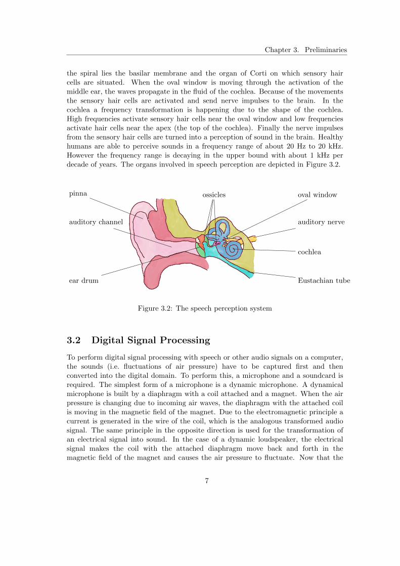
the spiral lies the basilar membrane and the organ of Corti on which sensory haircells are situated. When the oval window is moving through the activation of themiddle ear, the waves propagate in the fluid of the cochlea. Because of the movementsthe sensory hair cells are activated and send nerve impulses to the brain. In thecochlea a frequency transformation is happening due to the shape of the cochlea.High frequencies activate sensory hair cells near the oval window and low frequenciesactivate hair cells near the apex (the top of the cochlea). Finally the nerve impulsesfrom the sensory hair cells are turned into a perception of sound in the brain. Healthyhumans are able to perceive sounds in a frequency range of about 20 Hz to 20 kHz.However the frequency range is decaying in the upper bound with about 1 kHz perdecade of years. The organs involved in speech perception are depicted in Figure 3.2.
pinna
auditory channel
ear drum
ossicles
cochlea
auditory nerve
oval window
Eustachian tube
Figure 3.2: The speech perception system
3.2 Digital Signal Processing
To perform digital signal processing with speech or other audio signals on a computer,the sounds (i.e. fluctuations of air pressure) have to be captured first and thenconverted into the digital domain. To perform this, a microphone and a soundcard isrequired. The simplest form of a microphone is a dynamic microphone. A dynamicalmicrophone is built by a diaphragm with a coil attached and a magnet. When the airpressure is changing due to incoming air waves, the diaphragm with the attached coilis moving in the magnetic field of the magnet. Due to the electromagnetic principle acurrent is generated in the wire of the coil, which is the analogous transformed audiosignal. The same principle in the opposite direction is used for the transformation ofan electrical signal into sound. In the case of a dynamic loudspeaker, the electricalsignal makes the coil with the attached diaphragm move back and forth in themagnetic field of the magnet and causes the air pressure to fluctuate. Now that the
7
Chapter 3. Preliminaries
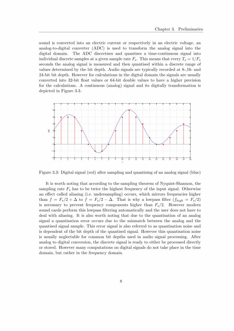
sound is converted into an electric current or respectively in an electric voltage, ananalog-to-digital converter (ADC) is used to transform the analog signal into thedigital domain. The ADC discretises and quantises a time-continuous signal intoindividual discrete samples at a given sample rate Fs. This means that every Ts = 1/Fsseconds the analog signal is measured and then quantised within a discrete range ofvalues determined by the bit depth. Audio signals are typically recorded at 8-,16- and24-bit bit depth. However for calculations in the digital domain the signals are usuallyconverted into 32-bit float values or 64-bit double values to have a higher precisionfor the calculations. A continuous (analog) signal and its digitally transformation isdepicted in Figure 3.3.
0 1 2 3 4 5 6 7 8 9 10 11 12 13 14 15 16 17 18 19 20t
−2
−1
0
1
2
3
4
5
x[t]
Figure 3.3: Digital signal (red) after sampling and quantising of an analog signal (blue)
It is worth noting that according to the sampling theorem of Nyquist-Shannon, thesampling rate Fs has to be twice the highest frequency of the input signal. Otherwisean effect called aliasing (i.e. undersampling) occurs, which mirrors frequencies higherthan f = Fs/2 + ∆ to f = Fs/2 − ∆. That is why a lowpass filter (fhigh = Fs/2)is necessary to prevent frequency components higher than Fs/2. However modernsound cards perform this lowpass filtering automatically and the user does not have todeal with aliasing. It is also worth noting that due to the quantisation of an analogsignal a quantisation error occurs due to the mismatch between the analog and thequantised signal sample. This error signal is also referred to as quantisation noise andis dependent of the bit depth of the quantised signal. However this quantisation noiseis usually neglectable for common bit depths used in audio signal processing. Afteranalog to digital conversion, the discrete signal is ready to either be processed directlyor stored. However many computations on digital signals do not take place in the timedomain, but rather in the frequency domain.
8
Chapter 3. Preliminaries
3.2.1 Discrete Fourier transform
One of the most fundamental transforms in digital signal processing is the discreteFourier transform (DFT). The DFT transforms a sequence of N complex numbersx0, x1, ..., xN−1 into an N -periodic sequence of complex numbers:
Xkdef=
N−1∑n=0
xn · e−2πikn/N , k ∈ Z (3.1)
Due to the periodicity attribute, the DFT is usually just computed for k in theinterval [0, N−1]. Applying the transform to (real-valued) time domain data (e.g. audiosignals, speech signals) the transform is also often referred to as discrete time Fouriertransform (DTFT). The signal x[n] is transformed into a complex valued spectrum Xk.The parameter k then refers to the so-called frequency bin. From the complex-valuedspectrum Xk the magnitude spectrum |Xk| can be derived for each bin k by:
|Xk| =√
Re(Xk)2 + Im(Xk)2 (3.2)
The argument (or phase) of the complex-valued spectrum Xk can be derived by:
arg(Xk) = arctan
(Re(Xk)
Im(Xk)
)(3.3)
From the complex-valued spectrum (or the magnitude spectrum and the phase) thetime domain signal can be perfectly reconstructed by the inverse DFT (IDFT):
xn =1
n
N−1∑k=0
Xk · e2πikn/N , n ∈ Z (3.4)
The fast Fourier transform (FFT) computes the DFT or its inverse. However itreduces the complexity of the algorithm from O(N2) to O(N logN) and is able to speedup calculations especially for large N . The most commonly used FFT algorithm is theCooley-Tukey algorithm [4].
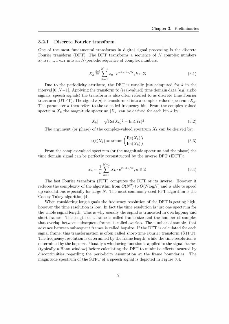
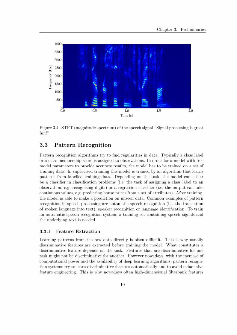
When considering long signals the frequency resolution of the DFT is getting high,however the time resolution is low. In fact the time resolution is just one spectrum forthe whole signal length. This is why usually the signal is truncated in overlapping andshort frames. The length of a frame is called frame size and the number of samplesthat overlap between subsequent frames is called overlap. The number of samples thatadvance between subsequent frames is called hopsize. If the DFT is calculated for eachsignal frame, this transformation is often called short-time Fourier transform (STFT).The frequency resolution is determined by the frame length, while the time resolution isdetermined by the hop size. Usually a windowing function is applied to the signal frames(typically a Hann window) before calculating the DFT to minimise effects incurred bydiscontinuities regarding the periodicity assumption at the frame boundaries. Themagnitude spectrum of the STFT of a speech signal is depicted in Figure 3.4.
9
Chapter 3. Preliminaries
0.0 0.5 1.0 1.5 2.0Time [s]
0
500
1000
1500
2000
2500
3000
3500
4000
Freq
uenc
y[H
z]
Figure 3.4: STFT (magnitude spectrum) of the speech signal “Signal processing is greatfun!”
3.3 Pattern Recognition
Pattern recognition algorithms try to find regularities in data. Typically a class labelor a class membership score is assigned to observations. In order for a model with freemodel parameters to provide accurate results, the model has to be trained on a set oftraining data. In supervised training this model is trained by an algorithm that learnspatterns from labelled training data. Depending on the task, the model can eitherbe a classifier in classification problems (i.e. the task of assigning a class label to anobservation, e.g. recognising digits) or a regression classifier (i.e. the output can takecontinuous values, e.g. predicting house prices from a set of attributes). After training,the model is able to make a prediction on unseen data. Common examples of patternrecognition in speech processing are automatic speech recognition (i.e. the translationof spoken language into text), speaker recognition or language identification. To trainan automatic speech recognition system, a training set containing speech signals andthe underlying text is needed.
3.3.1 Feature Extraction
Learning patterns from the raw data directly is often difficult. This is why usuallydiscriminative features are extracted before training the model. What constitutes adiscriminative feature depends on the task. Features that are discriminative for onetask might not be discriminative for another. However nowadays, with the increase ofcomputational power and the availability of deep learning algorithms, pattern recogni-tion systems try to learn discriminative features automatically and to avoid exhaustivefeature engineering. This is why nowadays often high-dimensional filterbank features
10

Chapter 3. Preliminaries
are often preferred compared to low-dimensional Mel-Frequency Cepstral Coefficients,which were the preferred audio features for decades in speech recognition. Both featuretypes are explained in the following.
Mel-Frequency Cepstral Coefficients
In speech processing amongst the most prominent features are the Mel-Frequency Cep-stral Coefficients (MFCC). To derive the MFCCs of an audio signal, the signal is firstfiltered with a preemphasis filter. The preemphasis filter boosts the high frequencies ofthe signal and is implemented by:
yt = xt − αxt−1, (3.5)
where α = 0.97. Then the signal is usually first split into frames (typically 25 ms,10 ms hop size) and a Hamming window is applied to the signal frames. The Hammingwindow is defined as:
whamming(n) = 0.54− 0.46 cos
(2πn
N − 1
)(3.6)
The MFCCs are calculated for each frame and then stacked to a matrix. To calculatethe MFCCs for a signal frame, the DTFT is calculated and the magnitude spectrum isobtained. The phase is usually neglected. Then the power spectrum is calculated fromthe magnitude response:
Sxx(k) = |Xk|2 (3.7)
The powers of the spectrum are then mapped onto the mel scale using a set of ltriangular overlapping windows (typically l = 23 for 16 kHz sampling frequency andl = 15 for 8 kHz sampling frequency). The mel scale [5] is a perceptual scale of pitchesof equal distances. A commonly used formula [6] to convert the frequency f into melm is:
m = 2595 · log10
(1 +
f
700
)(3.8)
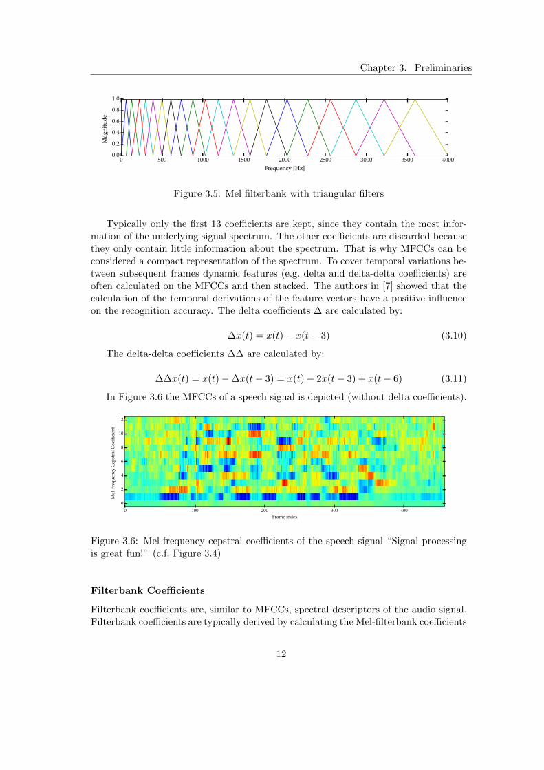
A filterbank with triangular filters set in equal distance along the mel scale isdepicted in Figure 3.5.
Then the logarithm is calculated on each of the obtained mel powers and the discretecosine transform (DCT) is performed upon them to decorrelate the data and to retrievethe MFCCs. Optionally, the coefficients ci are processed with a cepstral lifter accordingto:
ci =
(1 +
L
2· sin(π
i
L)
)ci, (3.9)
where ci is the MFCC at index i, L is the liftering factor (usually 22). The intentionof cepstral liftering is to scale the MFCCs so they have a similar range of values.
11
Chapter 3. Preliminaries
0 500 1000 1500 2000 2500 3000 3500 4000Frequency [Hz]
0.0
0.2
0.4
0.6
0.8
1.0M
agni
tude
Figure 3.5: Mel filterbank with triangular filters
Typically only the first 13 coefficients are kept, since they contain the most infor-mation of the underlying signal spectrum. The other coefficients are discarded becausethey only contain little information about the spectrum. That is why MFCCs can beconsidered a compact representation of the spectrum. To cover temporal variations be-tween subsequent frames dynamic features (e.g. delta and delta-delta coefficients) areoften calculated on the MFCCs and then stacked. The authors in [7] showed that thecalculation of the temporal derivations of the feature vectors have a positive influenceon the recognition accuracy. The delta coefficients ∆ are calculated by:
∆x(t) = x(t)− x(t− 3) (3.10)
The delta-delta coefficients ∆∆ are calculated by:
∆∆x(t) = x(t)−∆x(t− 3) = x(t)− 2x(t− 3) + x(t− 6) (3.11)
In Figure 3.6 the MFCCs of a speech signal is depicted (without delta coefficients).
0 100 200 300 400Frame index
0
2
4
6
8
10
12
Mel
-Fre
quen
cyC
epst
ralC
oeffi
cien
t
Figure 3.6: Mel-frequency cepstral coefficients of the speech signal “Signal processingis great fun!” (c.f. Figure 3.4)
Filterbank Coefficients
Filterbank coefficients are, similar to MFCCs, spectral descriptors of the audio signal.Filterbank coefficients are typically derived by calculating the Mel-filterbank coefficients
12

Chapter 3. Preliminaries
(Section 3.3.1) without the subsequent usage of the DCT. Taking the logarithm afterthe Mel-filterbank coefficients’ calculation, is optional. An advantage compared to theMFCCs is, that no coefficients are discarded. Typically 23 filters are used for 16 kHzsampling rate and 15 filters for 8 kHz sampling rate.
3.3.2 Hidden Markov Models
Hidden Markov models (HMM) are often successfully used in temporal pattern recogni-tion problems, e.g. speech recognition, handwriting recognition or gesture recognition,where the information can be modelled as a temporal sequence of states (e.g. phonemes,graphemes, gestures or subdivisions of those). HMMs were developed in [8]. In HMMs,only the outputs, i.e the observations, are directly visible, the states on the otherhand are not directly visible, that is why they are called hidden. An HMM typicallyconsists of a set of hidden states S = {s1, ..., sn}, a set of of possible observationsY = {y1, ..., ym}, the state transition matrix A ∈ Rn×n, the emission probability ma-trix B ∈ Rn×m and the initial state distribution π ∈ Rn. Stationary HMMs are HMMwhere the state transition probabilities A and the emission probabilities B do notchange over time, an assumption that often holds true. In Figure 3.7 an exemplaryHMM is depicted. Only adjacent states can be reached from a specific state. Also thestate can remain the same. Training of the HMM is usually performed by the expec-tation maximisation (EM) algorithm [9]. Hidden Markov models are used in acousticmodelling for speech recognition in Section 3.4.4.
s1 s2
a1,2
s3 s4
y1 y2 y3
b4,3
Figure 3.7: An HMM with 4 states. It can emit 3 discrete symbols y1, y2 or y3. ai,jis the probability to transition from state si to state sj . bj,k is the probability to emitsymbol yk in state sj . In this exemplary HMM, states can only reach the adjacentstates or themselves.
3.3.3 Gaussian Mixture Model
A Gaussian Mixture Model (GMM) is a probabilistic model which assumes that theobservations D = {x1, ..., xi, ..., xN} are generated from an underlying probability den-
13
Chapter 3. Preliminaries
sity p(x). This density p(x) is defined as a linear combination of a finite number ofweighted Gaussian probability density functions:
p(xi|Θ) =J∑j=1
ωjN (xi|µj ,Σj) (3.12)
where xi is the observation at index i, j is the component index, J is the totalnumber of components, ωj is the weight, µj is the mean vector, Σj is the covariancematrix of component j respectively, and N is the Gaussian probability density function.Θ = {ωj , µj ,Σj}∀j are the model parameters of the GMM. The weights ωj of a GMM
represent probabilities with 0 ≤ ωj ≤ 1,∑J
j=1 ωj = 1. The univariate (i.e. one-dimensional, d = 1) probability density function of the Gaussian distribution is definedas:
N1(x|µ, σ) =1
σ√
2πe−
(x−µ)2
2σ2 (3.13)
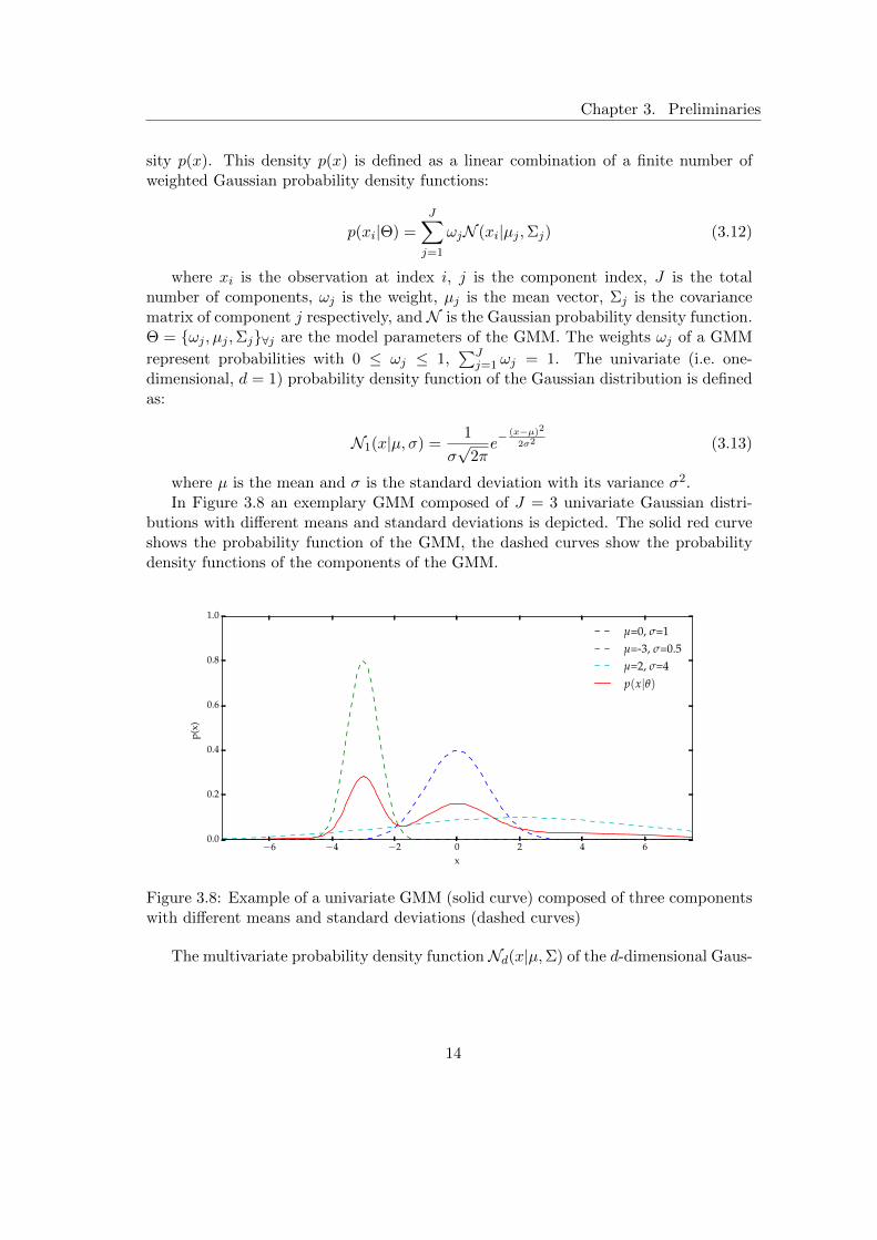
where µ is the mean and σ is the standard deviation with its variance σ2.In Figure 3.8 an exemplary GMM composed of J = 3 univariate Gaussian distri-
butions with different means and standard deviations is depicted. The solid red curveshows the probability function of the GMM, the dashed curves show the probabilitydensity functions of the components of the GMM.
−6 −4 −2 0 2 4 6x
0.0
0.2
0.4
0.6
0.8
1.0
p(x)
µ=0, σ=1µ=-3, σ=0.5µ=2, σ=4p(x|θ)
Figure 3.8: Example of a univariate GMM (solid curve) composed of three componentswith different means and standard deviations (dashed curves)
The multivariate probability density functionNd(x|µ,Σ) of the d-dimensional Gaus-
14
Chapter 3. Preliminaries
sian distribution is calculated as:
Nd(x|µ,Σ) =1√
(2π)d|Σ|e−
12
(x−µ)ᵀΣ−1(x−µ) (3.14)
where |Σ| is the determinant of the covariance matrix Σ.The fitting of a Gaussian Mixture Model to a set of training points is usually done
with the expectation-maximisation algorithm [8].After the fit, the component membership of a data point, i.e. the probability of a
data point x being from component k, can be obtained by:
p(k|x) =wkN (x|µk,Σk)∑Jj=1wjN (x|µj ,Σj)
(3.15)
and the component label of a datapoint, i.e. the component which maximises thecomponent membership for a data point, by:
k = argmaxk
p(k|x) (3.16)
Multiple GMM can be trained for data sets containing multiple classes. Aftertraining, the class label can be obtained for unknown data points by:
c = argmaxc
p(x|Θc) (3.17)
3.3.4 Artificial Neural Networks
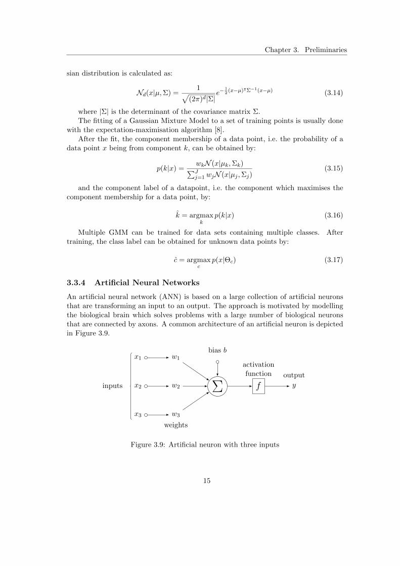
An artificial neural network (ANN) is based on a large collection of artificial neuronsthat are transforming an input to an output. The approach is motivated by modellingthe biological brain which solves problems with a large number of biological neuronsthat are connected by axons. A common architecture of an artificial neuron is depictedin Figure 3.9.
x2 w2 Σ f
activationfunction
y
output
x1 w1
x3 w3
weights
bias b
inputs
Figure 3.9: Artificial neuron with three inputs
15
Chapter 3. Preliminaries
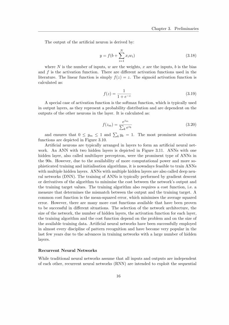
The output of the artificial neuron is derived by:
y = f(b+N∑i=1
xiwi) (3.18)
where N is the number of inputs, w are the weights, x are the inputs, b is the biasand f is the activation function. There are different activation functions used in theliterature. The linear function is simply f(z) = z. The sigmoid activation function iscalculated as:
f(z) =1
1 + e−z(3.19)
A special case of activation function is the softmax function, which is typically usedin output layers, as they represent a probability distribution and are dependent on theoutputs of the other neurons in the layer. It is calculated as:
f(zm) =ezm∑k e
zk(3.20)
and ensures that 0 ≤ ym ≤ 1 and∑
k yk = 1. The most prominent activationfunctions are depicted in Figure 3.10.
Artificial neurons are typically arranged in layers to form an artificial neural net-work. An ANN with two hidden layers is depicted in Figure 3.11. ANNs with onehidden layer, also called multilayer perceptron, were the prominent type of ANNs inthe 90s. However, due to the availability of more computational power and more so-phisticated training and initialisation algorithms, it is nowadays feasible to train ANNswith multiple hidden layers. ANNs with multiple hidden layers are also called deep neu-ral networks (DNN). The training of ANNs is typically performed by gradient descentor derivatives of the algorithm to minimise the cost between the network’s output andthe training target values. The training algorithm also requires a cost function, i.e. ameasure that determines the mismatch between the output and the training target. Acommon cost function is the mean-squared error, which minimises the average squarederror. However, there are many more cost functions available that have been provento be successful in different situations. The selection of the network architecture, thesize of the network, the number of hidden layers, the activation function for each layer,the training algorithm and the cost function depend on the problem and on the size ofthe available training data. Artificial neural networks have been successfully employedin almost every discipline of pattern recognition and have become very popular in thelast few years due to the advances in training networks with a large number of hiddenlayers.
Recurrent Neural Networks
While traditional neural networks assume that all inputs and outputs are independentof each other, recurrent neural networks (RNN) are intended to exploit the sequential
16

Chapter 3. Preliminaries
−2 −1 0 1 2x
−2.0
−1.5
−1.0
−0.5
0.0
0.5
1.0
1.5
2.0
y
Linear
(a)
−2 −1 0 1 2x
−2.0
−1.5
−1.0
−0.5
0.0
0.5
1.0
1.5
2.0
y
Tanh
(b)
−2 −1 0 1 2x
−2.0
−1.5
−1.0
−0.5
0.0
0.5
1.0
1.5
2.0
y
ReLU
(c)
−4 −2 0 2 4x
−2.0
−1.5
−1.0
−0.5
0.0
0.5
1.0
1.5
2.0
y
Sigmoid
(d)
Figure 3.10: Artificial neural network activation functions; a) linear function; b) tangenshyperbolicus function; c) rectified linear unit function; d) sigmoidal function
x1
x2
x3
x4
y1
y2
y3
Hiddenlayer 1
Hiddenlayer 2
Inputlayer
Outputlayer
Figure 3.11: An artificial neural network with two hidden layers. It takes four inputvalues and maps the inputs to three output values by employing two hidden layersconsisting of 5 neurons each.
17
Chapter 3. Preliminaries
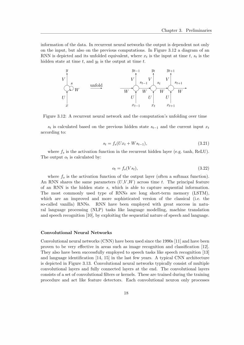
information of the data. In recurrent neural networks the output is dependent not onlyon the input, but also on the previous computations. In Figure 3.12 a diagram of anRNN is depicted and its unfolded equivalent, where xt is the input at time t, st is thehidden state at time t, and yt is the output at time t.
s
y
x
U
V
Wunfold
st−1
yt−1
xt−1
W
U
Vst
yt
xt
U
V
W
st+1
yt+1
xt+1
W
U
V
W
Figure 3.12: A recurrent neural network and the computation’s unfolding over time
st is calculated based on the previous hidden state st−1 and the current input xtaccording to:
st = fs(Uxt +Wst−1), (3.21)
where fs is the activation function in the recurrent hidden layer (e.g. tanh, ReLU).The output ot is calculated by:
ot = fo(V st), (3.22)
where fo is the activation function of the output layer (often a softmax function).An RNN shares the same parameters (U ,V ,W ) across time t. The principal featureof an RNN is the hidden state s, which is able to capture sequential information.The most commonly used type of RNNs are long short-term memory (LSTM),which are an improved and more sophisticated version of the classical (i.e. theso-called vanilla) RNNs. RNN have been employed with great success in natu-ral language processing (NLP) tasks like language modelling, machine translationand speech recognition [10], by exploiting the sequential nature of speech and language.
Convolutional Neural Networks
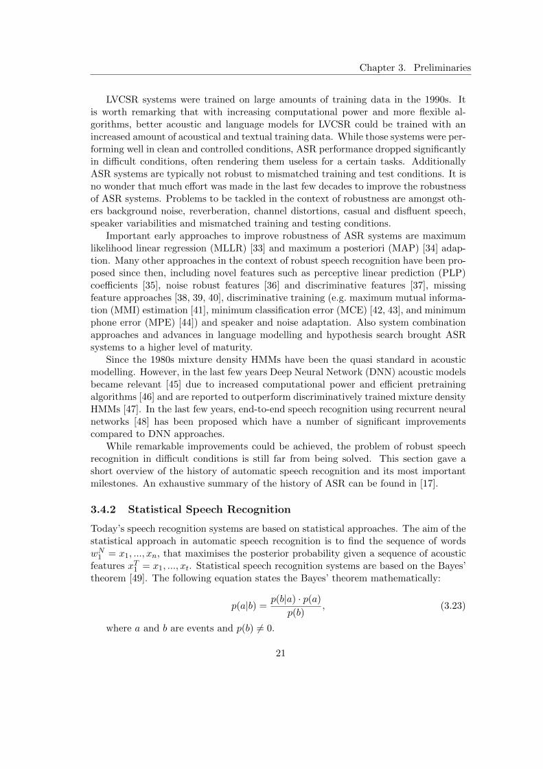
Convolutional neural networks (CNN) have been used since the 1990s [11] and have beenproven to be very effective in areas such as image recognition and classification [12].They also have been successfully employed to speech tasks like speech recognition [13]and language identification [14, 15] in the last few years. A typical CNN architectureis depicted in Figure 3.13. Convolutional neural networks typically consist of multipleconvolutional layers and fully connected layers at the end. The convolutional layersconsists of a set of convolutional filters or kernels. These are trained during the trainingprocedure and act like feature detectors. Each convolutional neuron only processes
18

Chapter 3. Preliminaries
data for its receptive field, which is limited by the size of the kernels. Convolutionallayers apply a convolution operation to the input and then pass the result to thenext layer. Usually a pooling layer is added after each convolutional layer, where thedimensionality of the input is reduced by subsampling (e.g. by taking the maximumvalue or the sum of the inputs). The convolutional neural network can be trainede.g. by the backpropagation algorithm.
Figure 3.13: Typical CNN architecture [16]
3.4 Automatic Speech Recognition
Automatic speech recognition (ASR), or sometimes called “speech to text” (STT), isthe translation of spoken language into text by computers. Speech recognition tasksinclude tasks with a limited vocabulary and grammar (e.g. the recognition of a limitedset of commands, words or numbers) and the recognition of large-scale vocabularycontinuous speech (LVCSR). ASR systems can be speaker-dependent (e.g. if trained orfine-tuned to a specific speaker) or speaker independent (e.g. if trained on a large setof speakers). Nowadays LVCSR systems consist of the acoustic model (i.e. modellingthe probabilities of phonemes given acoustic features derived from the speech signal),the dictionary (i.e. a lexicon which maps the words to a sequence of phonemes) anda statistical language model (i.e. a probability distribution over sequences of words).During decoding, the ASR system is able to provide the most probable word sequenceencoded in the speech signal given the model.
3.4.1 History of Automatic Speech Recognition
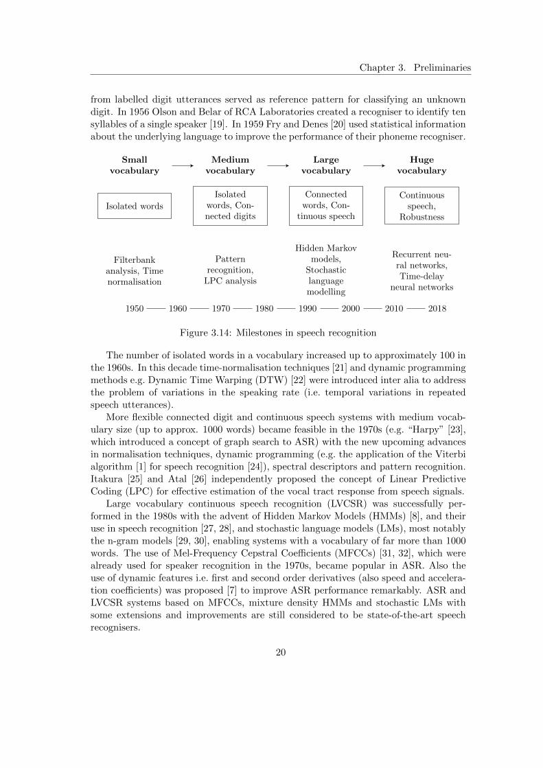
A diagram covering the milestones of the history of automatic speech recognition isdepicted in Figure 3.14. It is an attempt to summarise and update the diagram in [17].Early speech recognition systems in the 1950s only considered a vocabulary consistingof a few words or digits. For example, an early automatic speech recognition systemwas proposed by Davis, Biddulph, and Balashek of Bell Laboratories in 1952 [18].The system measured formant frequencies (i.e. regions of energy concentration in thespeech power spectrum) during vowels regions of digits for single-speaker isolated digitrecognition. Formant trajectories of the first and second formant frequencies derived
19
Chapter 3. Preliminaries
from labelled digit utterances served as reference pattern for classifying an unknowndigit. In 1956 Olson and Belar of RCA Laboratories created a recogniser to identify tensyllables of a single speaker [19]. In 1959 Fry and Denes [20] used statistical informationabout the underlying language to improve the performance of their phoneme recogniser.
Smallvocabulary
Mediumvocabulary
Largevocabulary
Hugevocabulary
Isolated words
Isolatedwords, Con-nected digits
Connectedwords, Con-
tinuous speech
Continuousspeech,
Robustness
Filterbankanalysis, Timenormalisation
Patternrecognition,
LPC analysis
Hidden Markovmodels,
Stochasticlanguagemodelling
Recurrent neu-ral networks,Time-delay
neural networks
1950 1960 1970 1980 1990 2000 2010 2018
Figure 3.14: Milestones in speech recognition
The number of isolated words in a vocabulary increased up to approximately 100 inthe 1960s. In this decade time-normalisation techniques [21] and dynamic programmingmethods e.g. Dynamic Time Warping (DTW) [22] were introduced inter alia to addressthe problem of variations in the speaking rate (i.e. temporal variations in repeatedspeech utterances).
More flexible connected digit and continuous speech systems with medium vocab-ulary size (up to approx. 1000 words) became feasible in the 1970s (e.g. “Harpy” [23],which introduced a concept of graph search to ASR) with the new upcoming advancesin normalisation techniques, dynamic programming (e.g. the application of the Viterbialgorithm [1] for speech recognition [24]), spectral descriptors and pattern recognition.Itakura [25] and Atal [26] independently proposed the concept of Linear PredictiveCoding (LPC) for effective estimation of the vocal tract response from speech signals.
Large vocabulary continuous speech recognition (LVCSR) was successfully per-formed in the 1980s with the advent of Hidden Markov Models (HMMs) [8], and theiruse in speech recognition [27, 28], and stochastic language models (LMs), most notablythe n-gram models [29, 30], enabling systems with a vocabulary of far more than 1000words. The use of Mel-Frequency Cepstral Coefficients (MFCCs) [31, 32], which werealready used for speaker recognition in the 1970s, became popular in ASR. Also theuse of dynamic features i.e. first and second order derivatives (also speed and accelera-tion coefficients) was proposed [7] to improve ASR performance remarkably. ASR andLVCSR systems based on MFCCs, mixture density HMMs and stochastic LMs withsome extensions and improvements are still considered to be state-of-the-art speechrecognisers.
20
Chapter 3. Preliminaries
LVCSR systems were trained on large amounts of training data in the 1990s. Itis worth remarking that with increasing computational power and more flexible al-gorithms, better acoustic and language models for LVCSR could be trained with anincreased amount of acoustical and textual training data. While those systems were per-forming well in clean and controlled conditions, ASR performance dropped significantlyin difficult conditions, often rendering them useless for a certain tasks. AdditionallyASR systems are typically not robust to mismatched training and test conditions. It isno wonder that much effort was made in the last few decades to improve the robustnessof ASR systems. Problems to be tackled in the context of robustness are amongst oth-ers background noise, reverberation, channel distortions, casual and disfluent speech,speaker variabilities and mismatched training and testing conditions.
Important early approaches to improve robustness of ASR systems are maximumlikelihood linear regression (MLLR) [33] and maximum a posteriori (MAP) [34] adap-tion. Many other approaches in the context of robust speech recognition have been pro-posed since then, including novel features such as perceptive linear prediction (PLP)coefficients [35], noise robust features [36] and discriminative features [37], missingfeature approaches [38, 39, 40], discriminative training (e.g. maximum mutual informa-tion (MMI) estimation [41], minimum classification error (MCE) [42, 43], and minimumphone error (MPE) [44]) and speaker and noise adaptation. Also system combinationapproaches and advances in language modelling and hypothesis search brought ASRsystems to a higher level of maturity.
Since the 1980s mixture density HMMs have been the quasi standard in acousticmodelling. However, in the last few years Deep Neural Network (DNN) acoustic modelsbecame relevant [45] due to increased computational power and efficient pretrainingalgorithms [46] and are reported to outperform discriminatively trained mixture densityHMMs [47]. In the last few years, end-to-end speech recognition using recurrent neuralnetworks [48] has been proposed which have a number of significant improvementscompared to DNN approaches.
While remarkable improvements could be achieved, the problem of robust speechrecognition in difficult conditions is still far from being solved. This section gave ashort overview of the history of automatic speech recognition and its most importantmilestones. An exhaustive summary of the history of ASR can be found in [17].
3.4.2 Statistical Speech Recognition
Today’s speech recognition systems are based on statistical approaches. The aim of thestatistical approach in automatic speech recognition is to find the sequence of wordswN1 = x1, ..., xn, that maximises the posterior probability given a sequence of acousticfeatures xT1 = x1, ..., xt. Statistical speech recognition systems are based on the Bayes’theorem [49]. The following equation states the Bayes’ theorem mathematically:
p(a|b) =p(b|a) · p(a)
p(b), (3.23)
where a and b are events and p(b) 6= 0.
21
Chapter 3. Preliminaries
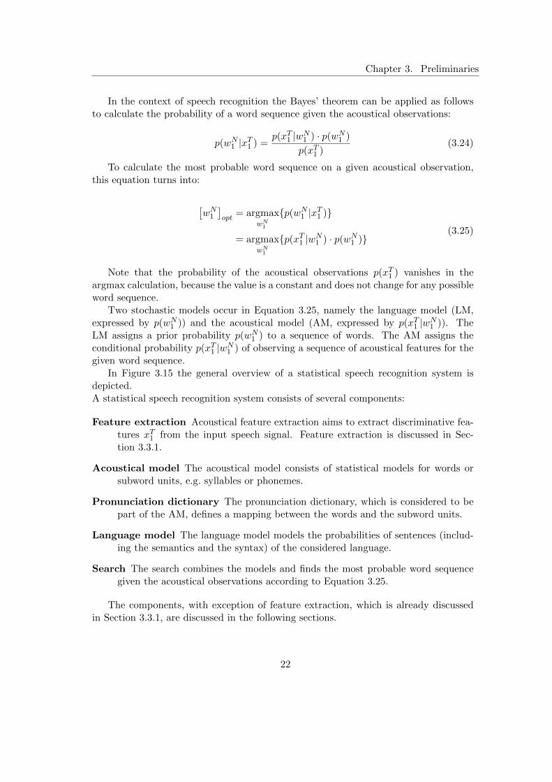
In the context of speech recognition the Bayes’ theorem can be applied as followsto calculate the probability of a word sequence given the acoustical observations:
p(wN1 |xT1 ) =p(xT1 |wN1 ) · p(wN1 )
p(xT1 )(3.24)
To calculate the most probable word sequence on a given acoustical observation,this equation turns into:
[wN1]opt
= argmaxwN1
{p(wN1 |xT1 )}
= argmaxwN1
{p(xT1 |wN1 ) · p(wN1 )}(3.25)
Note that the probability of the acoustical observations p(xT1 ) vanishes in theargmax calculation, because the value is a constant and does not change for any possibleword sequence.
Two stochastic models occur in Equation 3.25, namely the language model (LM,expressed by p(wN1 )) and the acoustical model (AM, expressed by p(xT1 |wN1 )). TheLM assigns a prior probability p(wN1 ) to a sequence of words. The AM assigns theconditional probability p(xT1 |wN1 ) of observing a sequence of acoustical features for thegiven word sequence.
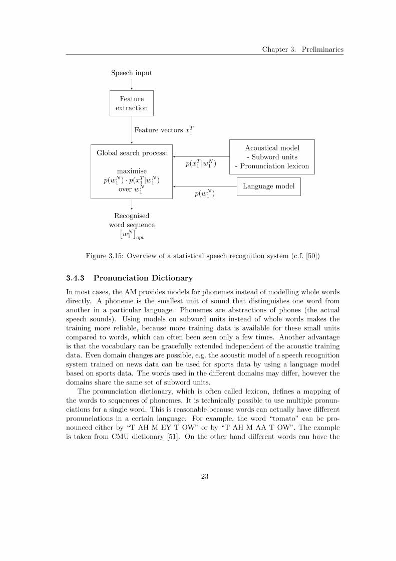
In Figure 3.15 the general overview of a statistical speech recognition system isdepicted.A statistical speech recognition system consists of several components:
Feature extraction Acoustical feature extraction aims to extract discriminative fea-tures xT1 from the input speech signal. Feature extraction is discussed in Sec-tion 3.3.1.
Acoustical model The acoustical model consists of statistical models for words orsubword units, e.g. syllables or phonemes.
Pronunciation dictionary The pronunciation dictionary, which is considered to bepart of the AM, defines a mapping between the words and the subword units.
Language model The language model models the probabilities of sentences (includ-ing the semantics and the syntax) of the considered language.
Search The search combines the models and finds the most probable word sequencegiven the acoustical observations according to Equation 3.25.
The components, with exception of feature extraction, which is already discussedin Section 3.3.1, are discussed in the following sections.
22
Chapter 3. Preliminaries
Speech input
Featureextraction
Global search process:
maximisep(wN1 ) · p(xT1 |wN1 )
over wN1
Recognisedword sequence[
wN1]opt
Acoustical model- Subword units
- Pronunciation lexicon
Language model
Feature vectors xT1
p(xT1 |wN1 )
p(wN1 )
Figure 3.15: Overview of a statistical speech recognition system (c.f. [50])
3.4.3 Pronunciation Dictionary
In most cases, the AM provides models for phonemes instead of modelling whole wordsdirectly. A phoneme is the smallest unit of sound that distinguishes one word fromanother in a particular language. Phonemes are abstractions of phones (the actualspeech sounds). Using models on subword units instead of whole words makes thetraining more reliable, because more training data is available for these small unitscompared to words, which can often been seen only a few times. Another advantageis that the vocabulary can be gracefully extended independent of the acoustic trainingdata. Even domain changes are possible, e.g. the acoustic model of a speech recognitionsystem trained on news data can be used for sports data by using a language modelbased on sports data. The words used in the different domains may differ, however thedomains share the same set of subword units.
The pronunciation dictionary, which is often called lexicon, defines a mapping ofthe words to sequences of phonemes. It is technically possible to use multiple pronun-ciations for a single word. This is reasonable because words can actually have differentpronunciations in a certain language. For example, the word “tomato” can be pro-nounced either by “T AH M EY T OW” or by “T AH M AA T OW”. The exampleis taken from CMU dictionary [51]. On the other hand different words can have the
23
Chapter 3. Preliminaries
same pronunciation, the so-called homophones1. For example, the words “cereal” and“serial” have the same pronunciation, namely “S IH R IY AH L”. Homophones areonly distinguishable in the context of a phrase or sentence, which is modelled by theLM.
The pronunciations of the pronunciation lexicon are either generated manually orautomatically. The manual transcription of (a large quantity of) words into phonemes iscostly, which is usually performed by expert linguists. For common languages typicallylarge pronunciation dictionaries exists, e.g. CMU dictionary [51] for British English, orPhonolex [52] for German.
Grapheme-to-Phoneme Conversion
From these dictionaries, automatic pronunciation generation models can be trained,the so-called grapheme-to-phoneme (G2P) conversion models, which are then able tooffer pronunciations for seen and unseen words with high accuracies. These approachesinclude rule-based and statistical approaches [53]. A grapheme is the smallest textualunit of a writing system of any given language. Graphemes include alphabetic letters,numerical digits, punctuations and other individual symbols. A grapheme may or maynot correspond to a single phoneme of the spoken language. Sometimes, when nopronunciation lexicon is available, the speech recognition system is directly trained onthe grapheme sequence, which works quite well for certain languages e.g. German. Thede-facto state-of-the-art algorithm over the last few years is the statistical approachpresented in [53]. The algorithm is based on joint-sequence models, where the mostlikely pronunciation ϕ ∈ Φ∗ for a given orthographic form g ∈ G∗ is defined by:
ϕ(g) = argmaxϕ∈Φ∗
p(ϕ, g), (3.26)
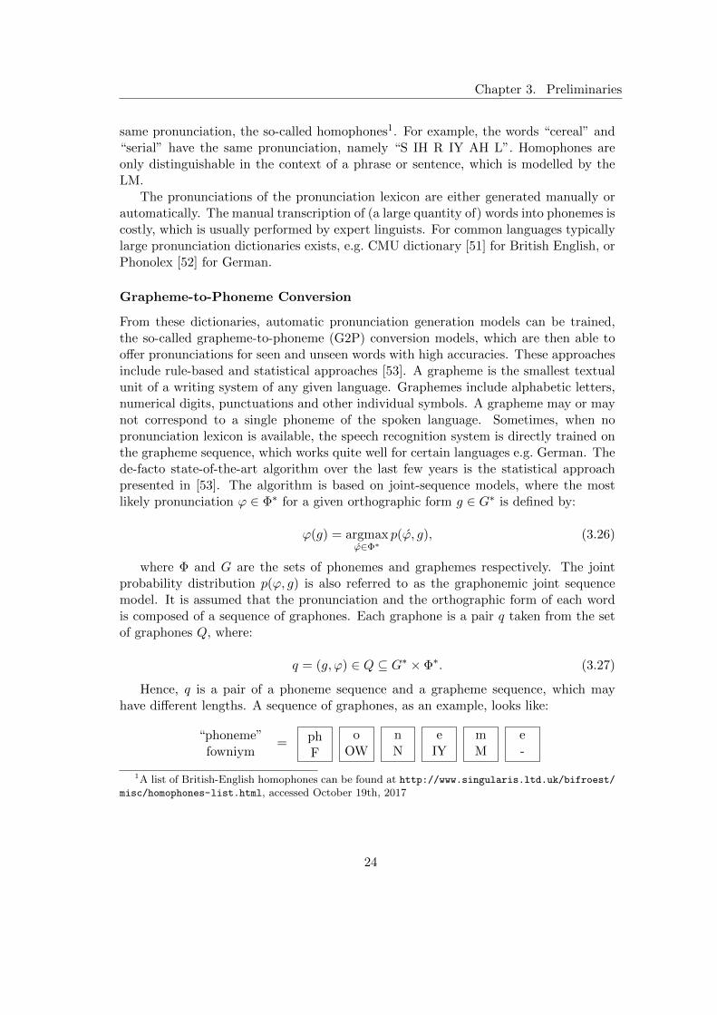
where Φ and G are the sets of phonemes and graphemes respectively. The jointprobability distribution p(ϕ, g) is also referred to as the graphonemic joint sequencemodel. It is assumed that the pronunciation and the orthographic form of each wordis composed of a sequence of graphones. Each graphone is a pair q taken from the setof graphones Q, where:
q = (g, ϕ) ∈ Q ⊆ G∗ × Φ∗. (3.27)
Hence, q is a pair of a phoneme sequence and a grapheme sequence, which mayhave different lengths. A sequence of graphones, as an example, looks like:
“phoneme”fowniym
= phF
oOW
nN
eIY
mM
e-
1A list of British-English homophones can be found at http://www.singularis.ltd.uk/bifroest/misc/homophones-list.html, accessed October 19th, 2017
24
Chapter 3. Preliminaries
The joint probability distribution p(ϕ, g) can be reduced to a probability distribu-tion over graphone sequences p(q) and can be modelled by an m-gram model (Sec-tion 3.4.5):
p(qN1 ) =N∏n=1
p(qn|qn−m+1, ..., qn−1) (3.28)
The graphone size limit L is the maximum number of graphemes or phonemesper graphone allowed by the model. As shown in [53], this model can be trainedusing Maximum Likelihood (ML) training using the Expectation Maximisation (EM)[9] algorithm. After training the model, the pronunciation for a word, which could beunseen by the model during training, can be derived. The most likely graphone sequencematching the spelling of the word is derived, and projected onto the phonemes, by:
ϕ(g) = ϕ( argmaxq∈Q∗|g(q)=g
p(q)) (3.29)
3.4.4 Acoustical Model
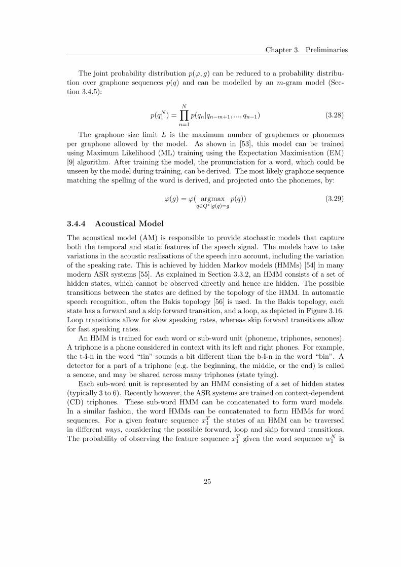
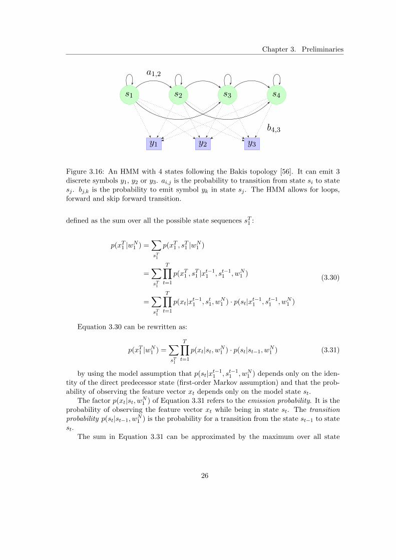
The acoustical model (AM) is responsible to provide stochastic models that captureboth the temporal and static features of the speech signal. The models have to takevariations in the acoustic realisations of the speech into account, including the variationof the speaking rate. This is achieved by hidden Markov models (HMMs) [54] in manymodern ASR systems [55]. As explained in Section 3.3.2, an HMM consists of a set ofhidden states, which cannot be observed directly and hence are hidden. The possibletransitions between the states are defined by the topology of the HMM. In automaticspeech recognition, often the Bakis topology [56] is used. In the Bakis topology, eachstate has a forward and a skip forward transition, and a loop, as depicted in Figure 3.16.Loop transitions allow for slow speaking rates, whereas skip forward transitions allowfor fast speaking rates.
An HMM is trained for each word or sub-word unit (phoneme, triphones, senones).A triphone is a phone considered in context with its left and right phones. For example,the t-i-n in the word “tin” sounds a bit different than the b-i-n in the word “bin”. Adetector for a part of a triphone (e.g. the beginning, the middle, or the end) is calleda senone, and may be shared across many triphones (state tying).
Each sub-word unit is represented by an HMM consisting of a set of hidden states(typically 3 to 6). Recently however, the ASR systems are trained on context-dependent(CD) triphones. These sub-word HMM can be concatenated to form word models.In a similar fashion, the word HMMs can be concatenated to form HMMs for wordsequences. For a given feature sequence xT1 the states of an HMM can be traversedin different ways, considering the possible forward, loop and skip forward transitions.The probability of observing the feature sequence xT1 given the word sequence wN1 is
25
Chapter 3. Preliminaries
s1 s2
a1,2
s3 s4
y1 y2 y3
b4,3
Figure 3.16: An HMM with 4 states following the Bakis topology [56]. It can emit 3discrete symbols y1, y2 or y3. ai,j is the probability to transition from state si to statesj . bj,k is the probability to emit symbol yk in state sj . The HMM allows for loops,forward and skip forward transition.
defined as the sum over all the possible state sequences sT1 :
p(xT1 |wN1 ) =∑sT1
p(xT1 , sT1 |wN1 )
=∑sT1
T∏t=1
p(xT1 , sT1 |xt−1
1 , st−11 , wN1 )
=∑sT1
T∏t=1
p(xt|xt−11 , st1, w
N1 ) · p(st|xt−1
1 , st−11 , wN1 )
(3.30)
Equation 3.30 can be rewritten as:
p(xT1 |wN1 ) =∑sT1
T∏t=1
p(xt|st, wN1 ) · p(st|st−1, wN1 ) (3.31)
by using the model assumption that p(st|xt−11 , st−1
1 , wN1 ) depends only on the iden-tity of the direct predecessor state (first-order Markov assumption) and that the prob-ability of observing the feature vector xt depends only on the model state st.
The factor p(xt|st, wN1 ) of Equation 3.31 refers to the emission probability. It is theprobability of observing the feature vector xt while being in state st. The transitionprobability p(st|st−1, w
N1 ) is the probability for a transition from the state st−1 to state
st.The sum in Equation 3.31 can be approximated by the maximum over all state
26
Chapter 3. Preliminaries
sequences, resulting in the maximum or Viterbi approximation [57]:
p(xT1 |wN1 ) ≈ maxsT1
{ T∏t=1
p(xt|st, wN1 ) · p(st|st−1, wN1 )}
(3.32)
The Viterbi approximation allows for an efficient search procedure. Both Equa-tion 3.31 and Equation 3.32 can be calculated efficiently using dynamic programmingalgorithms [1, 2].
For decades the emission probabilities of the HMMs for speech recognition weremodelled by Gaussian mixture models (Section 3.3.3). In this case the emission proba-bility for a state s is defined by a set of Gaussian densities and corresponding weights:
p(x|s) =J∑j=1
ωjN (x|µj ,Σj) (3.33)
The speech recognition acoustical model architecture that incorporates HMM withGMM emission probabilities is referred to as GMM-HMM in this thesis. These GMM-HMMs are typically trained to maximise the likelihood (ML) of generating the observedfeatures.
3.4.5 Language Model
The language model (LM) models the probability p(wN1 ) of a word sequence wN1 , thuscovering aspects such as the semantics (i.e. the meaning of words, sentences and texts)and the syntax (i.e. the grammar) of a language. It is used with great success inautomatic speech recognition. The most commonly used LM in ASR over the lastdecades is the m-gram model [30].
m-gram Language Models
m-gram models, also known as n-gram models, are based on the chain rule of prob-ability theory (decomposition rule). The total probability of a word sequence can beformulated as a product of conditional probabilities:
P (wN1 ) = P (w1...wN ) =N∏n=1
p(wn|wn−1, ..., w1) (3.34)
m-gram models only consider the m − 1 predecessors (Markov assumption oforder m − 1). It is reasonable to restrict the size of m, because during modeltraining with increasing m it is more unlikely to see an m-gram phrase in thetraining text. Moreover it is intuitive that the words (e.g. the words wi and wj) get in-creasingly independent from each other, with increased distance (j−i) from each other.
27
Chapter 3. Preliminaries
With m-gram models only considering m − 1 predecessors, Equation 3.34 gets re-duced to:
P (wN1 ) ≈N∏n=1
p(wn|wn−1, ..., wn−m+1) (3.35)
For unigram, bigram, and trigram models, Equation 3.35 can be rewritten as:
Unigram (m = 1):
P (wN1 ) =
N∏n=1
p(wn) (3.36)
Bigram (m = 2):
P (wN1 ) =N∏n=1
p(wn|wn−1) (3.37)
Trigram (m = 3):
P (wN1 ) =N∏n=1
p(wn|wn−2, wn−1) (3.38)
During training, the probabilities are estimated from typically a large amount ofexample text. But as already mentioned, with increasing m it is increasingly likely thatnot all possible m-gram phrases are seen during training. Unseen m-grams would obtaina probability of zero, and could not be detected. Language model smoothing algorithms,which deal with the problem of insufficient data, include Katz smoothing [58], Witten-Bell smoothing and the popular modified Kneser-Ney smoothing [59] algorithm.
The performance of a language model is either evaluated directly in the application(e.g. for speech recognition, by comparing the word error rate (WER, Section 3.4.9) ofdifferent configurations on a common test set, which is costly, or by calculation of theperplexity (Section 3.4.9) on a common test text.
3.4.6 Search
Automatic speech recognition systems take a speech data segment as input and pro-cess a list of recognition hypotheses as output. The search algorithm is responsible toefficiently retrieve the most probable word sequence
[wN1]opt
by evaluating the possibleword sequences according to their probability derived from the language and acous-tic model (Equation 3.25). Usually many of the competing hypotheses in the searchprocedure have common subsequences. The Viterbi approximation in Equation 3.32can be solved efficiently by the Viterbi decoding algorithm [1]. The forward-backwardor Baum-Welch algorithm [60] is a generalised approach for solving Equation 3.32 orEquation 3.31. Both algorithms are examples of dynamic programming. Pruning tech-niques during search can be applied to alleviate computational extensive recognitiontasks. The removal of a correct hypothesis from the search space, which could occur
28
Chapter 3. Preliminaries
while pruning, is referred to as a search error. Search errors can be distinguished frommodel errors, which occur due to false model assumptions.
3.4.7 Decoder Parameter Optimisation
Speech decoders (e.g., HTK [61], Julius [62] or Kaldi [55]) typically provide defaultvalues for their parameters, which often appear to be set arbitrarily. The Sphinx [63]Wiki offers detailed ways how to improve the decoding speed or hypothesis quality,but these recommendations have to be transferred manually to the task, usually by agrid search. Because these strategies to select the decoder parameter values are oftensuboptimal, recently, the task of optimising ASR decoder parameters automatically wasapproached by several research groups. Some approaches optimise the word error rate(WER, see Section 3.4.9) or similar metrics directly, e.g. with evolutional algorithms[64], or by employing large-margin iterative programming [65], others also take thedecoding speed, with the real-time factor (RTF, see Section 3.4.9) as a measure, intoaccount. The authors in [66] evaluate the curve of all possible WER for a given RTFand hence, they are able to use the optimal configuration for any speed constraints. Theauthors in [67] use an approach very similar to the Kiefer-Wolfowitz finite-differencestochastic approximation (FDSA) [68], where the influence of each parameter on theWER and the RTF is evaluated separately for a given configuration. In the fieldof machine translation (MT), the parameters of recent decoders are often optimisedeither with Och’s Minimum Error Rate Training [69] or the Downhill Simplex method[70]. Simultaneous Perturbation Stochastic Approximation (SPSA) has been employedfor machine translation as well and has been shown to converge faster than Downhillsimplex, while maintaining comparable results [71].
3.4.8 Weighted Finite State Transducer
A finite-state transducer (FST) is a finite automaton whose state transitions are labelledwith both input and output symbols. Hence, a path through the transducer providesa mapping between an input symbol sequence and an output symbol sequence. Aweighted FST (WFST) puts additional weights on its transitions from the input to theoutput symbols. The weights can encode probabilities, penalties, durations or any othermeasure. The weights get accumulated along the path to calculate the overall weightfor mapping the input sequence into the output sequence. In Figure 3.17 an exemplaryWFST is depicted, covering a (weighted) mapping between the word “tomato” and itsmultiple pronunciations “T AH M AA T O” and “T AH M EY T O”.
In Figure 3.18 a WFST is depicted representing a small language model, containingthree phrases. In this case the input symbols, namely words, are the same as the outputsymbols, however the transitions, and therefore the phrases as well, are weighted. FSTscan be optimised by determinisation and minimisation. The result of the determinisa-tion is that no state has two transitions with the same input label. In Figure 3.17, thetransition from node 4 to 5 has two transitions with the same input label, and hencethe FST can be optimised. Minimisation produces the minimal FST that is equivalent
29
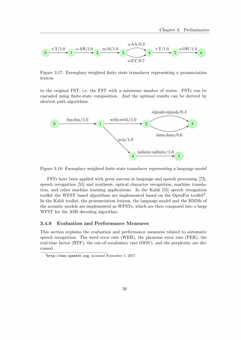
Chapter 3. Preliminaries
0 1 2 3 4 5 6t:T/1.0 o:AH/1.0 m:M/1.0
a:AA/0.3
a:EY/0.7
t:T/1.0 o:OW/1.0
Figure 3.17: Exemplary weighted finite state transducer representing a pronunciationlexicon
to the original FST, i.e. the FST with a minimum number of states. FSTs can becascaded using finite-state composition. And the optimal results can be derived byshortest path algorithms.
0 1 2 3
4 5
fun:fun/1.0 with:with/1.0
signals:signals/0.4
data:data/0.6is:is/1.0
infinite:infinite/1.0
Figure 3.18: Exemplary weighted finite state transducer representing a language model
FSTs have been applied with great success in language and speech processing [72],speech recognition [55] and synthesis, optical character recognition, machine transla-tion, and other machine learning applications. In the Kaldi [55] speech recognitiontoolkit the WFST based algorithms are implemented based on the OpenFst toolkit2.In the Kaldi toolkit, the pronunciation lexicon, the language model and the HMMs ofthe acoustic models are implemented as WFSTs, which are then composed into a largeWFST for the ASR decoding algorithm.
3.4.9 Evaluation and Performance Measures
This section explains the evaluation and performance measures related to automaticspeech recognition. The word error rate (WER), the phoneme error rate (PER), thereal-time factor (RTF), the out-of-vocabulary rate (OOV), and the perplexity are dis-cussed.
2http://www.openfst.org, accessed November 1, 2017
30
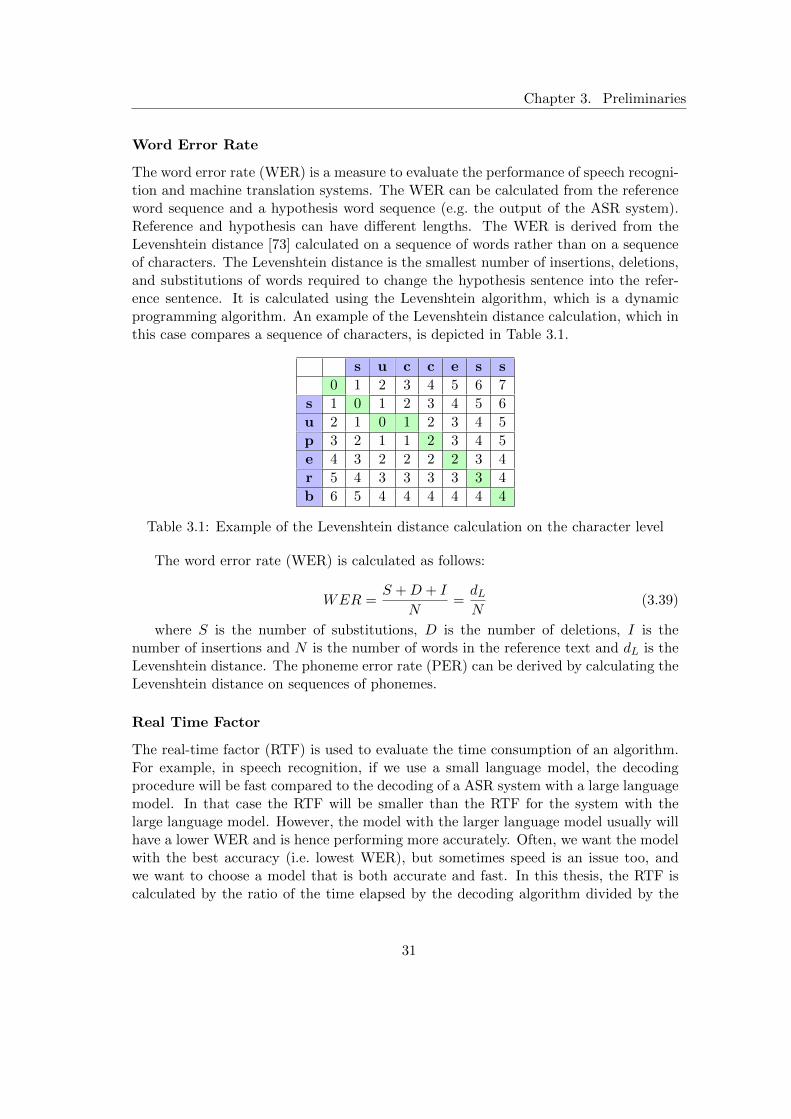
Chapter 3. Preliminaries
Word Error Rate
The word error rate (WER) is a measure to evaluate the performance of speech recogni-tion and machine translation systems. The WER can be calculated from the referenceword sequence and a hypothesis word sequence (e.g. the output of the ASR system).Reference and hypothesis can have different lengths. The WER is derived from theLevenshtein distance [73] calculated on a sequence of words rather than on a sequenceof characters. The Levenshtein distance is the smallest number of insertions, deletions,and substitutions of words required to change the hypothesis sentence into the refer-ence sentence. It is calculated using the Levenshtein algorithm, which is a dynamicprogramming algorithm. An example of the Levenshtein distance calculation, which inthis case compares a sequence of characters, is depicted in Table 3.1.
s u c c e s s
0 1 2 3 4 5 6 7
s 1 0 1 2 3 4 5 6
u 2 1 0 1 2 3 4 5
p 3 2 1 1 2 3 4 5
e 4 3 2 2 2 2 3 4
r 5 4 3 3 3 3 3 4
b 6 5 4 4 4 4 4 4
Table 3.1: Example of the Levenshtein distance calculation on the character level
The word error rate (WER) is calculated as follows:
WER =S +D + I
N=dLN
(3.39)
where S is the number of substitutions, D is the number of deletions, I is thenumber of insertions and N is the number of words in the reference text and dL is theLevenshtein distance. The phoneme error rate (PER) can be derived by calculating theLevenshtein distance on sequences of phonemes.
Real Time Factor
The real-time factor (RTF) is used to evaluate the time consumption of an algorithm.For example, in speech recognition, if we use a small language model, the decodingprocedure will be fast compared to the decoding of a ASR system with a large languagemodel. In that case the RTF will be smaller than the RTF for the system with thelarge language model. However, the model with the larger language model usually willhave a lower WER and is hence performing more accurately. Often, we want the modelwith the best accuracy (i.e. lowest WER), but sometimes speed is an issue too, andwe want to choose a model that is both accurate and fast. In this thesis, the RTF iscalculated by the ratio of the time elapsed by the decoding algorithm divided by the
31
Chapter 3. Preliminaries
length of the audio signals:
RTF =telapsedtdecoded
(3.40)
Since, the computational speed and power varies on different machines, we onlycompare the RTF of different models or configurations on the same machine.
Out-Of-Vocabulary Rate
The out-of-vocabulary (OOV) rate, typically a percentage, is a metric to measure thenumber of unknown words in a vocabulary or a text. A vocabulary, or dictionary, is aunique word list of a given text.
The vocabulary OOV rate is defined as the ratio of the number of unknown wordsin the vocabulary of a test text to the total number of words in the vocabulary of atest text:
OOVvoc =nvoc,unknownnvoc,total
(3.41)
The running OOV rate is defined as the ratio of the number of unknown runningwords in a text to the total number of words in a text:
OOVrun =nrun,unknownnrun,total
(3.42)
It is sometimes beneficial to consider both vocabulary and running OOV rate. Itcan happen, that the vocabulary OOV rate is quite high, however the unknown wordsoccur only very seldomly so that the running OOV rate is low. The lower a OOV rateis, the better.
Perplexity
The best language model is the one that predicts an unseen test set with the high-est probability. Maximising the probability is the same as minimising the perplexity.Perplexity is the probability estimate assigned to a word sequence wN1 by a languagemodel, normalised by the number of words N :
PP := P (wN1 )−1N =
[ N∏n=1
p(wn|wn−1, ..., w1)]− 1
N (3.43)
For m-gram models this formula reduces to:
PPn =[ N∏n−1
p(wn|wn−1, ..., wn−m+1)]− 1
N (3.44)
Without a language model, the perplexity would correspond to the vocabulary size,since the model could choose from any arbitrary word from the vocabulary with the
32
Chapter 3. Preliminaries
same probability. By training a language model, i.e. learning the typical word sequencesof a language, the perplexity is reduced for a similar text.
To obtain a low perplexity (and respectively a high probability) on a given test text,the language model must be trained on a similar training text, where the words andphrases occur likely. For example, if we want to train a language model for the broadcastdomain (news, interviews, documentations, etc.), it is beneficial to use training datacoming from the broadcast domain as well. In contrast, a language model trained onweather reports will perform badly if used for sport reports and vice versa, becausefirst of all, many words will remain unseen by the language model, and many otherswill we seen with a probability either too high, or too low. Hence, a language modelwill have a high perplexity on out-of-domain data. Sometimes it is desired to create ageneral purpose language model for all possible domains, but usually a domain specificLM will optimise the perplexity for a given domain. A common way to achieve lowerword error rates in speech recognition is, amongst others, to reduce the perplexity ofthe language model on a withheld development set [74].
3.5 Dialect Identification
In speech there is, besides the spoken text, paralinguistic information encoded. Theparalinguistic information includes the gender, the age, the health condition, empha-sis and regional accent and dialect of the speaker. The accent refers to variations inthe pronunciation (phone sequences and realisations) and the speaking style (rhythm,variation in pitch) [75]. It can be differentiated between regional accents and foreignaccents. Regional accents are typically harder to identify and show subtler differencescompared to foreign accents. Dialects on the other hand refer to differences in the wordselection and the use of the grammar [75]. Usually speakers that speak dialect also havean accent of the same region. Accent/dialect identification refers to the task of recog-nising the speaker’s regional accent/dialect, within a predetermined language, given asample of his/her speech [76]. Dialect identification systems have been used success-fully for different tasks. Dialect identification systems allow ASR engines to adapt theiracoustic, pronunciation and language models to improve the recognition accuracy [76].Dialect identification systems also allow text-to-speech synthesis to produce regionalspeech [76]. They also have been used for targeted advertising, service customisationand audio forensics tasks [77]. Usually dialect identification methods are similar tolanguage identification methods, which is reasonable. In general it is easier to differen-tiate between languages than between dialect (or even accents). Dialect identificationmethods can be divided into acoustic methods, phonotactic methods and combinationsof both acoustic and phonotactic methods. Acoustic methods exploit differences in theacoustic space (e.g. spectral or prosodic features), while phonotactic methods exploitdifferences in sequences of phonemes.
33
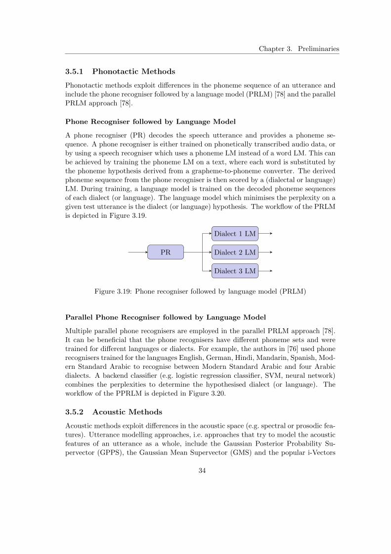
Chapter 3. Preliminaries
3.5.1 Phonotactic Methods
Phonotactic methods exploit differences in the phoneme sequence of an utterance andinclude the phone recogniser followed by a language model (PRLM) [78] and the parallelPRLM approach [78].
Phone Recogniser followed by Language Model
A phone recogniser (PR) decodes the speech utterance and provides a phoneme se-quence. A phone recogniser is either trained on phonetically transcribed audio data, orby using a speech recogniser which uses a phoneme LM instead of a word LM. This canbe achieved by training the phoneme LM on a text, where each word is substituted bythe phoneme hypothesis derived from a grapheme-to-phoneme converter. The derivedphoneme sequence from the phone recogniser is then scored by a (dialectal or language)LM. During training, a language model is trained on the decoded phoneme sequencesof each dialect (or language). The language model which minimises the perplexity on agiven test utterance is the dialect (or language) hypothesis. The workflow of the PRLMis depicted in Figure 3.19.
PR Dialect 2 LM
Dialect 3 LM
Dialect 1 LM
Figure 3.19: Phone recogniser followed by language model (PRLM)
Parallel Phone Recogniser followed by Language Model
Multiple parallel phone recognisers are employed in the parallel PRLM approach [78].It can be beneficial that the phone recognisers have different phoneme sets and weretrained for different languages or dialects. For example, the authors in [76] used phonerecognisers trained for the languages English, German, Hindi, Mandarin, Spanish, Mod-ern Standard Arabic to recognise between Modern Standard Arabic and four Arabicdialects. A backend classifier (e.g. logistic regression classifier, SVM, neural network)combines the perplexities to determine the hypothesised dialect (or language). Theworkflow of the PPRLM is depicted in Figure 3.20.
3.5.2 Acoustic Methods
Acoustic methods exploit differences in the acoustic space (e.g. spectral or prosodic fea-tures). Utterance modelling approaches, i.e. approaches that try to model the acousticfeatures of an utterance as a whole, include the Gaussian Posterior Probability Su-pervector (GPPS), the Gaussian Mean Supervector (GMS) and the popular i-Vectors
34

Chapter 3. Preliminaries
PRLM 2
PRLM 1
PRLM 3
Backend Classifier
Figure 3.20: Parallel phone recogniser followed by language model (PPRLM)
[79], which originate from speaker identification. The major advantage of the utterancemodelling approaches, is that they deliver a utterance feature vector of fixed size, in-dependently of the size of the utterance. Hence, the utterance feature vectors of fixedsize can easily be classified by a subsequent classifier e.g. a Naive Bayesian Classifier(NBC) [80] or a Support Vector Machines (SVM) [81].
Universal Background Model
Consider a GMM (Section 3.3.3) that has been trained on a large quantity of speechdata, ideally covering all the dialects that we want to be able to differentiate and thestandard language itself. The training data should actually cover all the variations,subtleties and nuances of a language. It should also cover a large quantity of speakersof both female and male speakers. However, it should not contain utterances of the testdata, that we want to classify, because good results on training sentences might be dueto overfitting. The GMM that is trained on all the aspects of a language is consideredto be a universal background model (UBM), and is required for the utterance modellingtechniques GPPS, GMS and i-Vectors.
Gaussian Posterior Probability Supervector
Consider a GMM-UBM with the likelihood function which is given in Equation 3.12.The occupance posterior probability [77] for the jth mixture component is calculatedby:
κj =1
T
T∑t=1
ωjN (ot|µj ,Σj)∑Jj′=1 ωj′N (ot|µj′ ,Σj′)
, (3.45)
where T is the total number of feature frames in the utterance.The Gaussian Posterior Probability Supervector (GPPS) is then the vector of the
stacked occupancy posterior probabilities for all J mixture components:
κ = [κ1, ..., κj , ..., κJ ] (3.46)
35
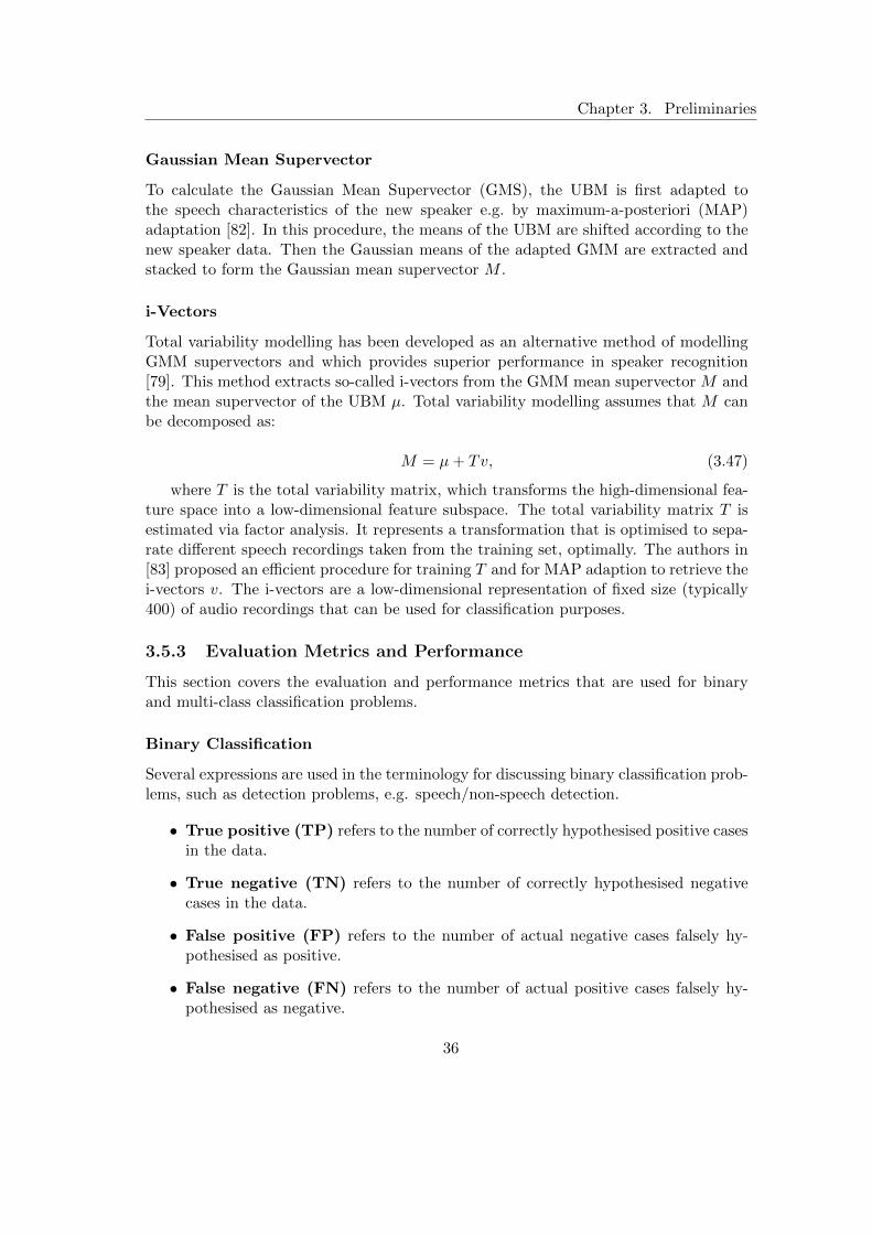
Chapter 3. Preliminaries
Gaussian Mean Supervector
To calculate the Gaussian Mean Supervector (GMS), the UBM is first adapted tothe speech characteristics of the new speaker e.g. by maximum-a-posteriori (MAP)adaptation [82]. In this procedure, the means of the UBM are shifted according to thenew speaker data. Then the Gaussian means of the adapted GMM are extracted andstacked to form the Gaussian mean supervector M .
i-Vectors
Total variability modelling has been developed as an alternative method of modellingGMM supervectors and which provides superior performance in speaker recognition[79]. This method extracts so-called i-vectors from the GMM mean supervector M andthe mean supervector of the UBM µ. Total variability modelling assumes that M canbe decomposed as:
M = µ+ Tv, (3.47)
where T is the total variability matrix, which transforms the high-dimensional fea-ture space into a low-dimensional feature subspace. The total variability matrix T isestimated via factor analysis. It represents a transformation that is optimised to sepa-rate different speech recordings taken from the training set, optimally. The authors in[83] proposed an efficient procedure for training T and for MAP adaption to retrieve thei-vectors v. The i-vectors are a low-dimensional representation of fixed size (typically400) of audio recordings that can be used for classification purposes.
3.5.3 Evaluation Metrics and Performance
This section covers the evaluation and performance metrics that are used for binaryand multi-class classification problems.
Binary Classification
Several expressions are used in the terminology for discussing binary classification prob-lems, such as detection problems, e.g. speech/non-speech detection.
• True positive (TP) refers to the number of correctly hypothesised positive casesin the data.
• True negative (TN) refers to the number of correctly hypothesised negativecases in the data.
• False positive (FP) refers to the number of actual negative cases falsely hy-pothesised as positive.
• False negative (FN) refers to the number of actual positive cases falsely hy-pothesised as negative.
36
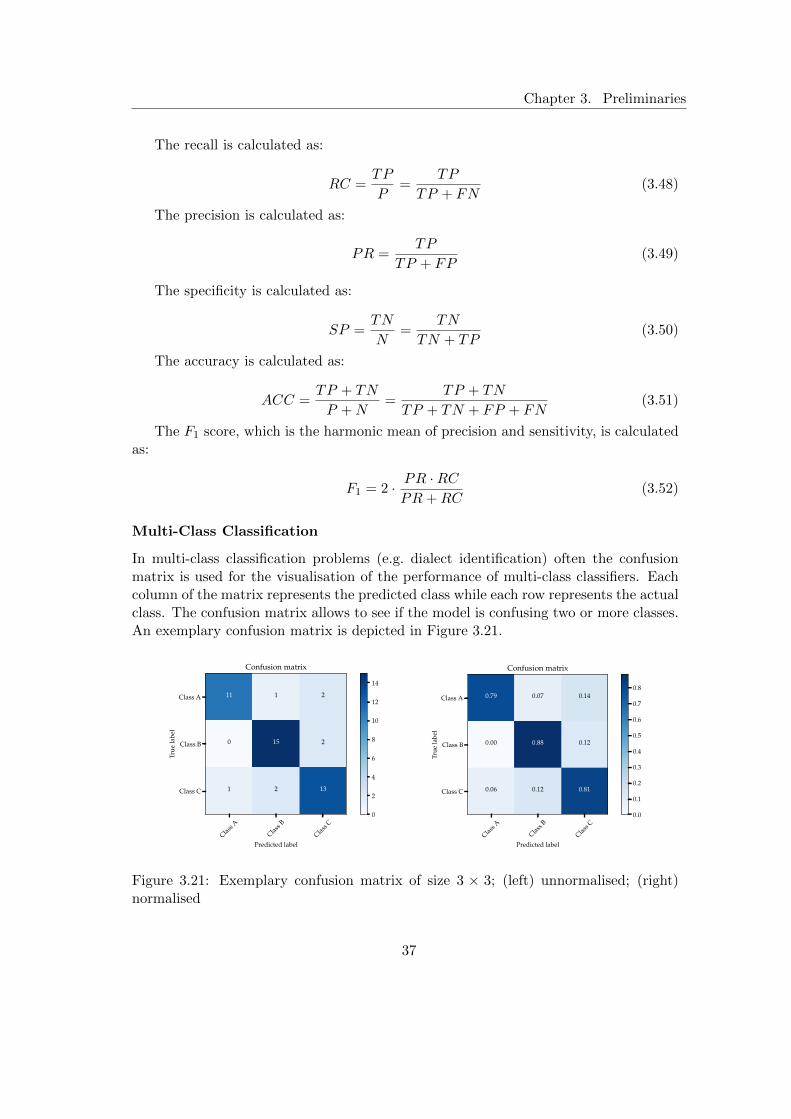
Chapter 3. Preliminaries
The recall is calculated as:
RC =TP
P=
TP
TP + FN(3.48)
The precision is calculated as:
PR =TP
TP + FP(3.49)
The specificity is calculated as:
SP =TN
N=
TN
TN + TP(3.50)
The accuracy is calculated as:
ACC =TP + TN
P +N=
TP + TN
TP + TN + FP + FN(3.51)
The F1 score, which is the harmonic mean of precision and sensitivity, is calculatedas:
F1 = 2 · PR ·RCPR+RC
(3.52)
Multi-Class Classification
In multi-class classification problems (e.g. dialect identification) often the confusionmatrix is used for the visualisation of the performance of multi-class classifiers. Eachcolumn of the matrix represents the predicted class while each row represents the actualclass. The confusion matrix allows to see if the model is confusing two or more classes.An exemplary confusion matrix is depicted in Figure 3.21.
Class A
Class B
Class C
Predicted label
Class A
Class B
Class C
True
labe
l
11 1 2
0 15 2
1 2 13
Confusion matrix
0
2
4
6
8
10
12
14
Class A
Class B
Class C
Predicted label
Class A
Class B
Class C
True
labe
l
0.79 0.07 0.14
0.00 0.88 0.12
0.06 0.12 0.81
Confusion matrix
0.0
0.1
0.2
0.3
0.4
0.5
0.6
0.7
0.8
Figure 3.21: Exemplary confusion matrix of size 3 × 3; (left) unnormalised; (right)normalised
37

Chapter 3. Preliminaries
For confusion matrices of size n× n the accuracy is calculated as:
ACC =
n∑i=1
aii
n∑i=1
n∑j=1
aij
(3.53)
where aij is the matrix element of the i-th row and the j-th column.
38
Chapter 4
Long-Term Development of aGerman Broadcast SpeechRecognition System
Archivists, journalists and content hosters often have the problem of dealing with hugeamounts of heterogeneous audio-visual media data. The media objects are usually onlyaccompanied with few metadata such as the title and probably a few keywords, andsearch algorithms can often only search on this sparse metadata. Hence, finding the re-quested information is often considered a lucky strike or even impossible. Audio miningsystems, like the Fraunhofer IAIS audio mining system [84], solve this issue by automat-ically analysing the media data, and then providing efficient search tools that supportthe users to find the information that they seek. The most important component of anaudio mining system is the speech recognition system, because it automatically trans-lates speech in audio signals into text, which is the key result for subsequent searchand recommendation engines. The field of speech recognition is of broad interest forboth the scientific and the industry community and typically many developments areachieved in this field in short periods of time. Typically the advances of speech recog-nition systems are reported on standard English datasets, e.g. the Switchboard corpus[3] which contains utterances of English telephone speech. Since it is unclear how wellthese techniques perform in the German broadcast domain, and in order to maintaina competitive audio mining system, this chapter deals with the long-term developmentand optimisation of a German broadcast speech recognition system in the context ofthe Fraunhofer IAIS audio mining system, where we employ the latest state-of-the-artalgorithms in the context of German broadcast speech recognition.
We first introduce the Fraunhofer IAIS audio mining system in Section 4.1. Then, inSection 4.2 the baseline speech recognition system component itself, and the resourcesnecessary to train and evaluate it, are described. The baseline speech recognitionconfiguration serves as a starting point of research for this thesis. In Section 4.3 weexpand the training corpus dramatically which is used to train the ASR system, andexplore different ASR architectures that became available in the course of this thesis
39

Chapter 4. Long-Term Development of a German Broadcast ASR System
to improve the speech recognition system. Section 4.4 summarises this chapter.
4.1 The Fraunhofer IAIS Audio Mining System
The architecture of the Fraunhofer IAIS audio mining system is depicted in Figure 4.1.
Web services Messaging
← Analysis priorities
Asset details,processing updates,
deletion updates,synchronization reports →
Analysisrequests
↓
↑Analysisresults
Analysisdeletionrequests
↓
↑Asset status,details
Analysispriorities
↓
↑Asset details,processing updates,crawling reports,synchronization reports
UI
↑Analysis requests ↑
Crawling reports
User
User access
Administrative access
Administrator
Customer monitoring systems
Audio analysissubsystem
Crawlingsubsystem
Monitoringsubsystem
Audio Mining coresubsystem
Fraunhofer IAIS Audio Mining system
Customerclients
Figure 4.1: The Fraunhofer IAIS Audio Mining system architecture
The Fraunhofer IAIS audio mining system is composed of four subsystems:
• The audio analysis subsystem (Figure 4.2) contains services that perform adetailed audio analysis on the media objects, namely audio segmentation,speech/non-speech detection, gender detection, speaker clustering and recogni-tion, automatic speech recognition and keyword extraction.
• The audio mining core subsystem combines a media asset archive, the searchfunctionality and a recommendation engine based on the audio analysis results.
• The audio mining monitor subsystem provides a way to track the progress of theanalysis and to perform administrative tasks.
40
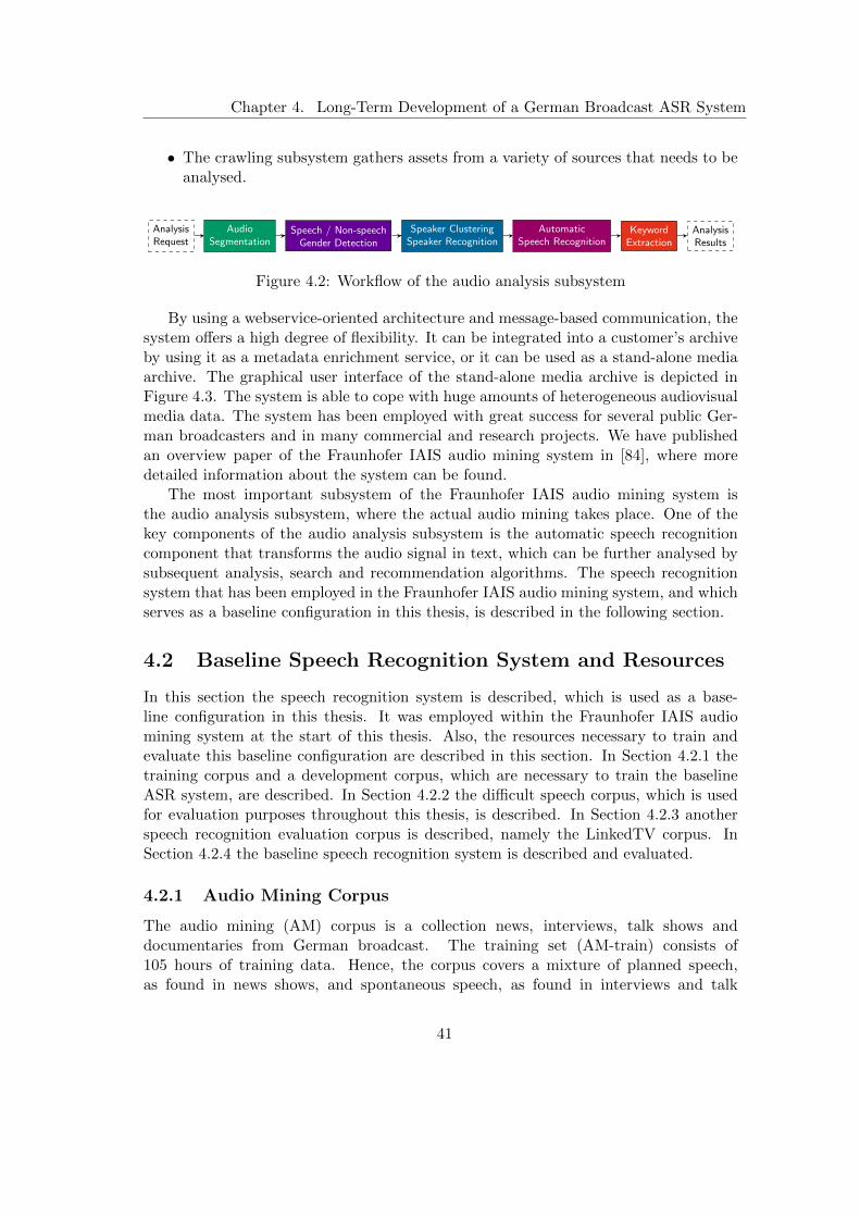
Chapter 4. Long-Term Development of a German Broadcast ASR System
• The crawling subsystem gathers assets from a variety of sources that needs to beanalysed.
AnalysisRequest
AudioSegmentation
Speech / Non-speechGender Detection
Speaker ClusteringSpeaker Recognition
AutomaticSpeech Recognition
KeywordExtraction
AnalysisResults
Figure 4.2: Workflow of the audio analysis subsystem
By using a webservice-oriented architecture and message-based communication, thesystem offers a high degree of flexibility. It can be integrated into a customer’s archiveby using it as a metadata enrichment service, or it can be used as a stand-alone mediaarchive. The graphical user interface of the stand-alone media archive is depicted inFigure 4.3. The system is able to cope with huge amounts of heterogeneous audiovisualmedia data. The system has been employed with great success for several public Ger-man broadcasters and in many commercial and research projects. We have publishedan overview paper of the Fraunhofer IAIS audio mining system in [84], where moredetailed information about the system can be found.
The most important subsystem of the Fraunhofer IAIS audio mining system isthe audio analysis subsystem, where the actual audio mining takes place. One of thekey components of the audio analysis subsystem is the automatic speech recognitioncomponent that transforms the audio signal in text, which can be further analysed bysubsequent analysis, search and recommendation algorithms. The speech recognitionsystem that has been employed in the Fraunhofer IAIS audio mining system, and whichserves as a baseline configuration in this thesis, is described in the following section.
4.2 Baseline Speech Recognition System and Resources
In this section the speech recognition system is described, which is used as a base-line configuration in this thesis. It was employed within the Fraunhofer IAIS audiomining system at the start of this thesis. Also, the resources necessary to train andevaluate this baseline configuration are described in this section. In Section 4.2.1 thetraining corpus and a development corpus, which are necessary to train the baselineASR system, are described. In Section 4.2.2 the difficult speech corpus, which is usedfor evaluation purposes throughout this thesis, is described. In Section 4.2.3 anotherspeech recognition evaluation corpus is described, namely the LinkedTV corpus. InSection 4.2.4 the baseline speech recognition system is described and evaluated.
4.2.1 Audio Mining Corpus
The audio mining (AM) corpus is a collection news, interviews, talk shows anddocumentaries from German broadcast. The training set (AM-train) consists of105 hours of training data. Hence, the corpus covers a mixture of planned speech,as found in news shows, and spontaneous speech, as found in interviews and talk
41

Chapter 4. Long-Term Development of a German Broadcast ASR System
Figure 4.3: Graphical Web User Interface of the Fraunhofer IAIS Audio Mining system
shows. Accompanied to the corpus is a development corpus (AM-dev) with atotal of 2,348 utterances (33,744 words), with a similar composition of planned andspontaneous speech as the training set. Detailed corpus statistics are listed in Table 4.1.
Corpus Size Number of Avg. length Word count Avg. Words(hh:mm) Utterances (seconds)
AM-train 105:24 119,386 3.18 997,996 8.36AM-dev 3:29 2,348 5.33 33,748 14.37
Table 4.1: Audio mining (AM) corpus statistics
4.2.2 Difficult Speech Corpus
The Difficult Speech Corpus (DiSCo) is presented in [85]. This heterogeneous Germanbroadcast corpus covers a variety of serious programmes including several challengingconditions for speech analysis like background noise, cross-talk situations, spontaneous
42
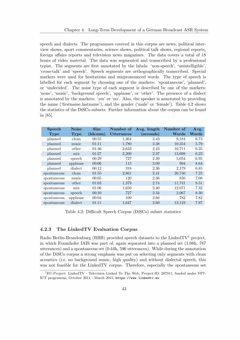
Chapter 4. Long-Term Development of a German Broadcast ASR System
speech and dialects. The programmes covered in this corpus are news, political inter-view shows, sport commentaries, science shows, political talk shows, regional reports,foreign affairs reports and television news magazines. The data covers a total of 18hours of video material. The data was segmented and transcribed by a professionaltypist. The segments are first annotated by the labels: ‘non-speech’, ‘unintelligible’,‘cross-talk’ and ‘speech’. Speech segments are orthographically transcribed. Specialmarkers were used for hesitations and mispronounced words. The type of speech islabelled for each segment by choosing one of the markers: ‘spontaneous’, ‘planned’,or ‘undecided’. The noise type of each segment is described by one of the markers:‘none’, ‘music’, ‘background speech’, ‘applause’, or ‘other’. The presence of a dialectis annotated by the markers: ‘yes’ or ‘no’. Also, the speaker is annotated by providingthe name (‘firstname lastname’), and the gender (‘male’ or ‘female’). Table 4.2 showsthe statistics of the DiSCo subsets. Further information about the corpus can be foundin [85].
Speech Noise Size Number of Avg. length Number of Avg.Type Type (hh:mm) Utterances (seconds) Words Words
planned clean 00:55 1,364 2.43 9,184 6.73planned music 01:11 1,780 2.38 10,354 5.79planned other 01:46 2,633 2.43 16,711 6.35planned mix 01:27 2,200 2.37 13,698 6.23planned speech 00:29 727 2.39 5,054 6.95planned applause 00:06 115 3.09 994 8.64planned dialect 00:12 318 2.36 2,179 6.85
spontaneous clean 01:55 2,861 2.41 20,740 7.25spontaneous music 00:05 120 2.36 850 7.08spontaneous other 01:03 1,379 2.74 11,741 8.51spontaneous mix 01:06 1,650 2.40 12,071 7.32spontaneous speech 00:10 727 2.34 2,067 8.30spontaneous applause 00:04 100 2.66 782 7.82spontaneous dialect 01:11 1,647 2.60 13,123 7.97
Table 4.2: Difficult Speech Corpus (DiSCo) subset statistics
4.2.3 The LinkedTV Evaluation Corpus
Radio Berlin-Brandenburg (RBB) provided speech datasets to the LinkedTV1 project,in which Fraunhofer IAIS was part of, again separated into a planned set (1:08h, 787utterances) and a spontaneous set (0:44h, 596 utterances). While during the annotationof the DiSCo corpus a strong emphasis was put on selecting only segments with cleanacoustics (i.e. no background music, high quality) and without dialectal speech, thiswas not feasible for the LinkedTV corpus. Therefore, especially the spontaneous set
1EU-Project: LinkedTV - Television Linked To The Web, Project-ID: 287911, funded under FP7-ICT programme, October 2011 - March 2015, https://www.linkedtv.eu
43

Chapter 4. Long-Term Development of a German Broadcast ASR System
contains utterances from street interviews, partly with strong Berlin dialect (e.g. “ditJahr war ja nich berauschend bei Hertha wa” instead of “das Jahr war nicht sehrberauschend bei Hertha”), partly with moderate background noise. The statistics ofthe LinkedTV datasets are depicted in Table 4.3.
Corpus Speaking Size Number of Avg. length Word Avg.style (hh:mm) Utterances (seconds) count Words
LinkedTV planned 1:08 787 5.18 10,984 13.96LinkedTV spontaneous 0:44 596 4.42 8,869 14.88
Table 4.3: LinkedTV evaluation corpus statistics
4.2.4 Baseline Speech Recognition System
The baseline configuration has been proposed in [86] and evaluated in [85]. The systemuses the HTK-Toolkit [61], which was considered to be state-of-the-art when this thesiswas launched in the year 2012. For decoding, the Julius [62] decoder was used, whichhas the advantage, that it can be used commercially without a special license. The sys-tem is based on hidden Markov models (HMM) with Gaussian mixture models (GMM)(Section 3.4.4) to model the emission probabilities of the states. It employed context-dependent tied crossword triphones using 32 mixtures per state in 3-state HMMs, lead-ing to 240k Gaussians in 7.5k states. The audio mining training set (“AM-train”)(Section 4.2.1) was used for training the model. The system has a vocabulary size of200,000 words and a trigram language model, which has been trained on texts gatheredfrom broadcast domain covering a total of 75 million running words.
The system has been evaluated on various evaluation sets. The audio miningdevelopment set (“AM-dev”) is described in Section 4.2.1. The DiSCo evaluationsubsets are described in detail in Section 4.2.2. The LinkedTV evaluation sets aredescribed in Section 4.2.3. The evaluation results are listed in Table 4.4. It canbe seen that naturally the ASR system performs better on planned speech than onspontaneous speech, which is more difficult to model. Also, the LinkedTV corpora aretypically more difficult than the clean sets of the DiSCo corpus, since they containnoises of different types as they appear normally in broadcast programmes, in contrastto the clean sets of the DiSCo corpus, which cover only the speech segments with lowor no background noise.
Configuration AM-dev DiSCo DiSCo LinkedTV LinkedTVplanned spontaneous planned spontaneous
clean cleanBaseline HMM-GMM [85] 30.2 26.4 33.5 27.0 52.5
Table 4.4: WER [%] results on various corpora for the baseline configuration
44
Chapter 4. Long-Term Development of a German Broadcast ASR System
4.3 Improvements to the Speech Recognition System
This section covers the advances of the Fraunhofer IAIS speech recognition system,which were developed as part of this thesis. They cover the collection and exploitationof a large-scale German broadcast speech recognition corpus, namely the GerTV1000hcorpus (Section 4.3.1), and the evaluation of different speech recognition system archi-tectures, which emerged throughout the years by the scientific community, for theiremployment in the German broadcast domain.
4.3.1 Large-Scale German Broadcast Speech Corpus
In this section we describe the large-scale German broadcast corpus, which we proposedin [87] and which we call the “GerTV1000h” or the “GerTV” corpus. We collected andmanually transcribed a huge and novel training corpus of German broadcast video ma-terial, containing 2,705 recordings with a volume of just over 900 h. The new corpus issegmented into utterances with a mean duration of approximately 5 seconds, yielding662,170 utterances, and is transcribed manually on the word level. The total numberof running words is 7,773,971 without taking additional annotation into account. Indi-vidual speakers are not annotated, but speaker changes within an utterance are markedand allow for a rough speaker adaptive training scheme. The recorded data covers abroad selection of news, interviews, talk shows and documentaries, both from televisionand radio content across several stations. In addition to the verbatim transcript, thetags in Table 4.5 were used to further describe the recordings. The tags denote theoccurrences of audible background noise, speaker noise, hesitations, speaker changeswithin an utterance, cross-talking speakers, foreign words, mispronounced words, un-transcribable utterances, unintelligible words or word fragments.
Together with the audio mining corpus (Section 4.2.1), which is from now on con-sidered to be included in the GerTV corpus, the corpus has grown to over 1,000 hoursof transcribed German broadcast data. We also adopt the development subset of theaudio mining dataset as the development corpus for the GerTV corpus. All audio isrecorded and stored in 16-bit PCM waveform files, with 16 kHz sampling frequency anda single mono channel.
The corpus was not fully available throughout this thesis, since the annotationprocess was time-consuming. Hence we used different amounts of training data for thecreation of the speech recognition systems. However, we always report the size (inhours) of the training amount when necessary. The different training sets that we usedin this thesis and the development corpus related to the GerTV corpus are listed inTable 4.6. We discarded utterances where mispronunciations or unintelligible words orutterances occurred for the training of the ASR system. That is why the full trainingset has 992 hours of speech data.
45
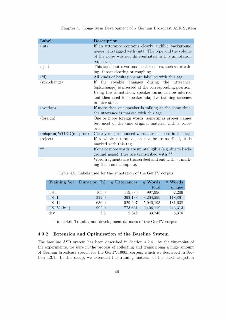
Chapter 4. Long-Term Development of a German Broadcast ASR System
Label Description〈int〉 If an utterance contains clearly audible background
noises, it is tagged with 〈int〉. The type and the volumeof the noise was not differentiated in this annotationsequence.
〈spk〉 This tag denotes various speaker noises, such as breath-ing, throat clearing or coughing.
〈fil〉 All kinds of hesitations are labelled with this tag.〈spk change〉 If the speaker changes during the utterance,
〈spk change〉 is inserted at the corresponding position.Using this annotation, speaker turns can be inferredand then used for speaker-adaptive training schemesin later steps.
〈overlap〉 If more than one speaker is talking at the same time,the utterance is marked with this tag.
〈foreign〉 One or more foreign words, sometimes proper namesbut most of the time original material with a voice-over.
〈mispron〉WORD〈mispron〉 Clearly mispronounced words are enclosed in this tag.〈reject〉 If a whole utterance can not be transcribed, it is
marked with this tag.** If one or more words are unintelligible (e.g. due to back-
ground noise), they are transcribed with **.= Word fragments are transcribed and end with =, mark-
ing them as incomplete.
Table 4.5: Labels used for the annotation of the GerTV corpus
Training Set Duration (h) # Utterances # Words # Wordstotal unique
TS I 105.0 119,386 997,996 62.206TS II 322.0 292,133 3,204,599 118,891TS III 636.0 529,207 5,940,193 181,638TS IV (full) 992.0 773,631 9,406,119 243,313dev 3.5 2,348 33,748 6,376
Table 4.6: Training and development datasets of the GerTV corpus
4.3.2 Extension and Optimisation of the Baseline System
The baseline ASR system has been described in Section 4.2.4. At the timepoint ofthe experiments, we were in the process of collecting and transcribing a huge amountof German broadcast speech for the GerTV1000h corpus, which we described in Sec-tion 4.3.1. In this setup, we extended the training material of the baseline system
46

Chapter 4. Long-Term Development of a German Broadcast ASR System
and hence, used TS II (322 hours of speech data, c.f. Table 4.6) for training the ASRsystem. In order to use the additional data, the training setup using HTK [61] washeavily modified. The initial configuration with approx. 105 h training data (TS I,c.f. Table 4.6) used tied crossword triphones using 32 mixtures per state in 3-stateHMMs, leading to 240k Gaussians in 7.5k states. Since simply increasing the numberof mixtures led to unsatisfactory results, the state tying configuration was adapted.Using fewer states and therefore more training data per state solved the problem ofoverfitting infrequent states and leads to significant improvements in WER, especiallyin acoustically challenging situations like spontaneous speech. The extended modeluses 575k Gaussians for 6k states and generalises well to previously unseen material,as can be seen from Table 4.7. A consistent improvement is noticeable for all theregarded evaluation corpora due to the increased training amount and the increasedcomplexity of the model. For evaluation, we use the GerTV1000h development corpus(Section 4.3.1), the clean datasets of the DiSCo corpus (Section 4.2.2, planned andspontaneous) and the LinkedTV datasets (Section 4.2.3).
By applying the techniques developed in Chapter 5, we optimised the ASR speechrecognition decoder parameters of the extended GMM-HMM system by the employmentof the Simultaneous Perturbation Stochastic Approximation (SPSA) algorithm [88](Section 5.1.1) by the use of the development set and we were able to further improvethe performance of the system by a large margin as evaluated on the evaluation corpora(see Table 4.7).
Configuration Size WER WER WER WER WER(hours) dev DiSCo DiSCo LinkedTV LinkedTV
planned spont. planned spont.GMM-HMM [85] 105 30.2 26.4 33.5 27.0 52.5
GMM-HMM 322 29.6 24.0 31.1 26.4 50.0GMM-HMM-SPSA 322 27.7 22.6 28.4 24.5 45.6
Table 4.7: WER results on several corpora for the baseline configuration, the extendedconfiguration and the extended configuration with the optimised decoder hyperparam-eters by the employment of the SPSA algorithm [88]
4.3.3 Subspace Gaussian Mixture Models
[89] describes an acoustic modelling approach which is called Subspace Gaussian Mix-ture Model (SGMM). In this model all phonetic states share a common Gaussian Mix-ture Model structure, and the means and mixture weights vary in a subspace of thetotal parameter space. Parameters which are shared globally define the subspace. Asthe results derived from the experiments of the authors indicate, the SGMM gives bet-ter results than a conventional modelling approach, particularly with smaller amountsof training data. This style of acoustic model allows for a much more compact repre-sentation. The basic form of the model can be expressed by:
47
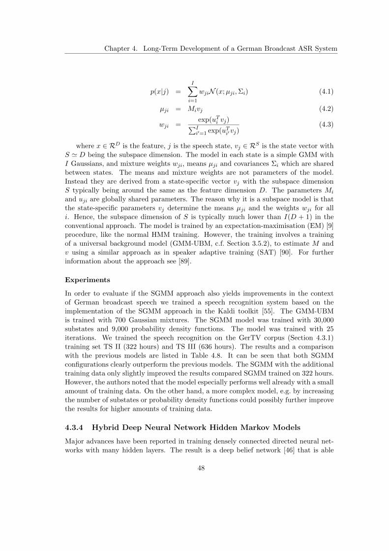
Chapter 4. Long-Term Development of a German Broadcast ASR System
p(x|j) =I∑i=1
wjiN (x;µji,Σi) (4.1)
µji = Mivj (4.2)
wji =exp(uTi vj)∑Ii′=1 exp(uTi′vj)
(4.3)
where x ∈ RD is the feature, j is the speech state, vj ∈ RS is the state vector withS ' D being the subspace dimension. The model in each state is a simple GMM withI Gaussians, and mixture weights wji, means µji and covariances Σi which are sharedbetween states. The means and mixture weights are not parameters of the model.Instead they are derived from a state-specific vector vj with the subspace dimensionS typically being around the same as the feature dimension D. The parameters Mi
and uji are globally shared parameters. The reason why it is a subspace model is thatthe state-specific parameters vj determine the means µji and the weights wji for alli. Hence, the subspace dimension of S is typically much lower than I(D + 1) in theconventional approach. The model is trained by an expectation-maximisation (EM) [9]procedure, like the normal HMM training. However, the training involves a trainingof a universal background model (GMM-UBM, c.f. Section 3.5.2), to estimate M andv using a similar approach as in speaker adaptive training (SAT) [90]. For furtherinformation about the approach see [89].
Experiments
In order to evaluate if the SGMM approach also yields improvements in the contextof German broadcast speech we trained a speech recognition system based on theimplementation of the SGMM approach in the Kaldi toolkit [55]. The GMM-UBMis trained with 700 Gaussian mixtures. The SGMM model was trained with 30,000substates and 9,000 probability density functions. The model was trained with 25iterations. We trained the speech recognition on the GerTV corpus (Section 4.3.1)training set TS II (322 hours) and TS III (636 hours). The results and a comparisonwith the previous models are listed in Table 4.8. It can be seen that both SGMMconfigurations clearly outperform the previous models. The SGMM with the additionaltraining data only slightly improved the results compared SGMM trained on 322 hours.However, the authors noted that the model especially performs well already with a smallamount of training data. On the other hand, a more complex model, e.g. by increasingthe number of substates or probability density functions could possibly further improvethe results for higher amounts of training data.
4.3.4 Hybrid Deep Neural Network Hidden Markov Models
Major advances have been reported in training densely connected directed neural net-works with many hidden layers. The result is a deep belief network [46] that is able
48

Chapter 4. Long-Term Development of a German Broadcast ASR System
Configuration Size WER WER WER WER WER(hours) dev DiSCo DiSCo LinkedTV LinkedTV
planned spont. planned spont.GMM-HMM [85] 105 30.2 26.4 33.5 27.0 52.5GMM-HMM 322 29.6 24.0 31.1 26.4 50.0GMM-HMM-SPSA 322 27.7 22.6 28.4 24.5 45.6
SGMM-HMM 322 23.5 18.1 22.5 21.0 36.6SGMM-HMM 636 23.3 18.1 22.4 20.5 35.9
Table 4.8: WER results on several corpora for the SGMM based ASR models in com-parison to the previous models
to learn a large set of nonlinear feature detectors which can capture sophisticated sta-tistical patterns in the data. First the algorithm initialises the weights of each layerindividually with the use of the acoustical training data. However, the labels are notused during the initialisation step. After the initialisation procedure the entire networkis fine-tuned by the use of labelled training data. This semi-supervised approach usingdeep belief network has proven to be effective in numerous speech, audio, text andimage applications [91, 92, 93, 94].
In [45] a context-dependent model for large vocabulary continuous speech recog-nition is presented which is based on pre-trained hybrid deep neural network hiddenMarkov model (DNN-HMM) architecture. The algorithm trains the DNN to produce adistribution over senones (tied triphone states) as its output. The hybrid DNN-HMMarchitecture is depicted in Figure 4.4. The DNN models the observation likelihood ofall senones [95], and the HMM models the sequential property of the speech signal. Theauthors report a relative sentence error reduction of 16.0 % and 23.2 % compared todiscriminatively trained GMM-HMM trained on the MPE and ML criteria, respectively.
Experiments
In order to evaluate the approach in the context of German broadcast speech recog-nition, we train a hybrid DNN-HMM [45] using the implementation from the Kalditoolkit [55] with the use of the training data of the GerTV corpus (Section 4.3.1). Weuse 4 hidden layers with 1024 neurons in each layer and the tangens hyperbolicus ac-tivation function. The initial learning rate was set to 0.01, and the final learning ratewas set to 0.001. The training was performed for a total of 20 epochs, 15 epochs withreducing learning rate, and 5 extra epochs with the final learning rate.
In Table 4.9 the results are listed in comparison to configurations developed in theprevious sections. Note that with the end of the LinkedTV project the evaluationdatasets became unavailable, which is the reason why we cannot report numbers forsome configurations. It can be derived that the employment of the hybrid DNN-HMMarchitecture drastically reduces the WER on every evaluation dataset. Also, the ex-tension of training material to 992 hours, which is considered to be the full dataset ofthe GerTV corpus (only few utterances are disregarded due to mispronunciations, or
49

Chapter 4. Long-Term Development of a German Broadcast ASR System
Figure 4.4: Diagram of the hybrid DNN-HMM architecture [45]
foreign language), still improves the accuracy of the system. This is the first config-uration that makes use of the complete GerTV corpus. It has been employed in theFraunhofer IAIS audiomining system for several years.
Configuration Size WER WER WER WER WER(hours) dev DiSCo DiSCo LinkedTV LinkedTV
planned spont. planned spont.GMM-HMM [85] 105 30.2 26.4 33.5 27.0 52.5GMM-HMM 322 29.6 24.0 31.1 26.4 50.0GMM-HMM-SPSA 322 27.7 22.6 28.4 24.5 45.6
DNN-HMM 322 23.9 18.4 22.6 21.2 37.6DNN-HMM 636 22.7 17.4 21.5 19.9 35.3DNN-HMM 992 21.3 15.5 19.7 - -
Table 4.9: WER results for the hybrid DNN-HMM systems in comparison to the pre-vious models
50

Chapter 4. Long-Term Development of a German Broadcast ASR System
4.3.5 Recurrent Neural Network Rescoring
The author in [96] proposed a recurrent neural network based language model. Thearchitecture employed is called a simple recurrent neural network or Elman network[97]. The network has an input layer x, and hidden layer s and an output layer y. Theinput vector x(t) is formed by concatenating the vector w representing the current wordand the output from the neurons in the hidden layer s at time t−1. Input, hidden andoutput layers are computed as follows:
x(t) = w(t) + s(t− 1) (4.4)
sj(t) = f
(∑i
xi(t)uji
)(4.5)
yk(t) = g
∑j
sj(t)vkj
(4.6)
where f(z) is the sigmoid activation function and g(z) is the softmax activationfunction. The input vector x(t) represents the word at time t encoded using a 1-of-Nencoding. Hence, the size of the vector x is equal to the size of the vocabulary (inpractice 30k to 500k). The size of the hidden layer s is usually 30 to 500 hidden units,and typically reflects the size of the training text. The output layer y(t) represents theprobability distribution of the next word given the previous word w(t) and the contexts(t−1). The network is trained for several epochs in which all data is sequentially pre-sented. To train the network, the standard backpropagation algorithm with stochasticgradient descent is employed. The starting learning rate α is 0.1. After each epoch,the validation loss is calculated. If the log-likelihood of the validation set increases, thetraining continues in a new epoch. Otherwise the learning rate α is halved. If there isagain no significant improvement, the training stops. The algorithm usually convergesafter 10-20 epochs.
Experiments
To evaluate the approach in the context of German broadcast speech recognition, wetrain an RNN LM on the same text corpus (75 million words from broadcast domain)as for the m-gram language model which is used during decoding. We used the RNNLM implementation of the RNNLM toolkit [98]. The RNN LM is used for rescoringthe n-best hypothesis list (n = 100) using a mixing value of 0.5 between the scores ofthe m-gram and the RNN LM. We evaluated the number of hidden neurons (100, 200,300, 400) for the RNN LM on the development corpus. The best configuration wasthe one with 300 neurons, which we evaluate on the test corpora. The results and acomparison with the previous models is depicted in Table 4.10. It can be seen that theWER can be reduced for all evaluation corpora, compared to the hybrid DNN-HMMapproach without RNN LM rescoring.
51
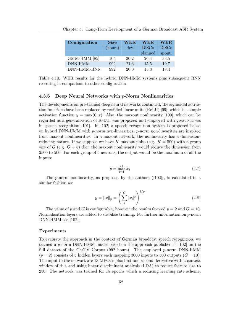
Chapter 4. Long-Term Development of a German Broadcast ASR System
Configuration Size WER WER WER(hours) dev DiSCo DiSCo
planned spont.GMM-HMM [85] 105 30.2 26.4 33.5DNN-HMM 992 21.3 15.5 19.7
DNN-HMM-RNN 992 20.0 15.3 18.4
Table 4.10: WER results for the hybrid DNN-HMM systems plus subsequent RNNrescoring in comparison to other configuration
4.3.6 Deep Neural Networks with p-Norm Nonlinearities
The developments on pre-trained deep neural networks continued, the sigmoidal activa-tion functions have been replaced by rectified linear units (ReLU) [99], which is a simpleactivation function y = max(0, x). Also, the maxout nonlinearity [100], which can beregarded as a generalisation of ReLU, was proposed and employed with great successin speech recognition [101]. In [102] a speech recognition system is proposed basedon hybrid DNN-HMM with p-norm non-linearities. p-norm non-linearities are inspiredfrom maxout nonlinearities. In a maxout network, the nonlinearity has a dimension-reducing nature. If we suppose we have K maxout units (e.g. K = 500) with a groupsize of G (e.g. G = 5) then the maxout nonlinearity would reduce the dimension from2500 to 500. For each group of 5 neurons, the output would be the maximum of all theinputs:
y =G
maxi=1
xi (4.7)
The p-norm nonlinearity, as proposed by the authors ([102]), is calculated in asimilar fashion as:
y = ||x||p =
(G∑i
|xi|p)1/p
(4.8)
The value of p and G is configurable, however the results favored p = 2 and G = 10.Normalisation layers are added to stabilise training. For further information on p-normDNN-HMM see [102].
Experiments
To evaluate the approach in the context of German broadcast speech recognition, wetrained a p-norm DNN-HMM model based on the approach published in [102] on thefull dataset of the GerTV Corpus (992 hours). The employed p-norm DNN-HMM(p = 2) consists of 5 hidden layers each mapping 3000 inputs to 300 outputs (G = 10).The input to the network are 13 MFCCs plus first and second derivative with a contextwindow of ± 4 and using linear discriminant analysis (LDA) to reduce feature size to250. The network was trained for 15 epochs which a reducing learning rate scheme,
52
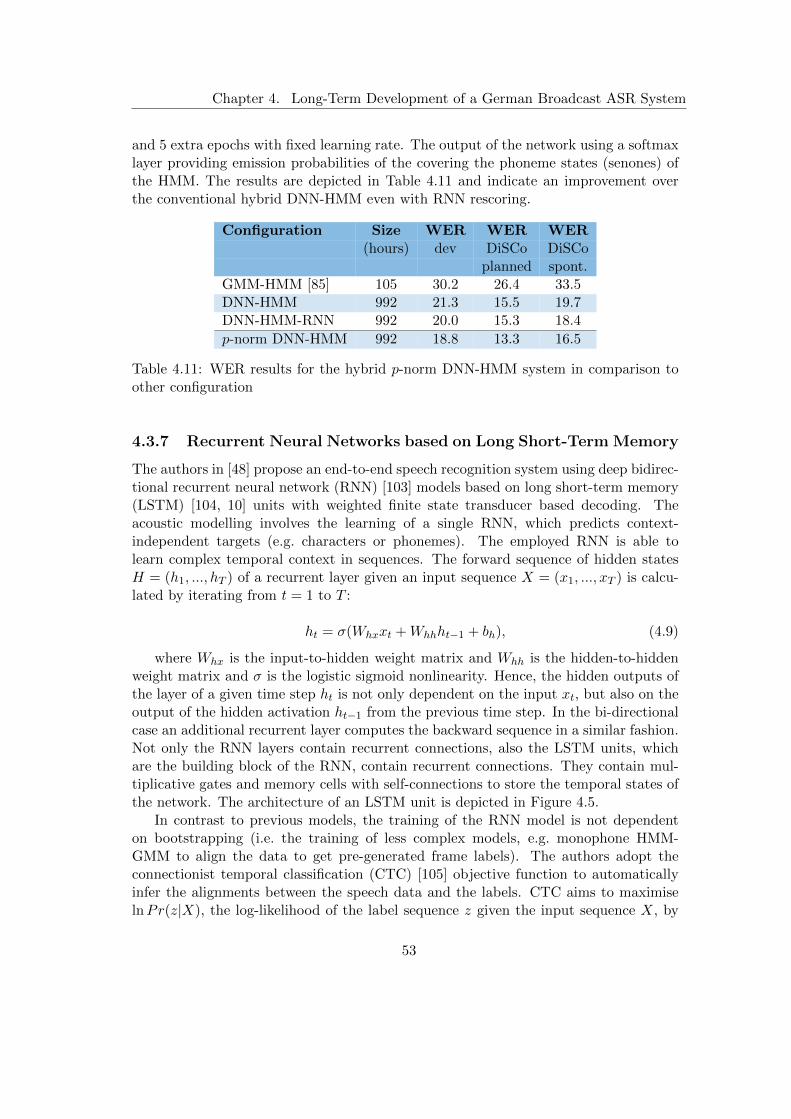
Chapter 4. Long-Term Development of a German Broadcast ASR System
and 5 extra epochs with fixed learning rate. The output of the network using a softmaxlayer providing emission probabilities of the covering the phoneme states (senones) ofthe HMM. The results are depicted in Table 4.11 and indicate an improvement overthe conventional hybrid DNN-HMM even with RNN rescoring.
Configuration Size WER WER WER(hours) dev DiSCo DiSCo
planned spont.GMM-HMM [85] 105 30.2 26.4 33.5DNN-HMM 992 21.3 15.5 19.7DNN-HMM-RNN 992 20.0 15.3 18.4
p-norm DNN-HMM 992 18.8 13.3 16.5
Table 4.11: WER results for the hybrid p-norm DNN-HMM system in comparison toother configuration
4.3.7 Recurrent Neural Networks based on Long Short-Term Memory
The authors in [48] propose an end-to-end speech recognition system using deep bidirec-tional recurrent neural network (RNN) [103] models based on long short-term memory(LSTM) [104, 10] units with weighted finite state transducer based decoding. Theacoustic modelling involves the learning of a single RNN, which predicts context-independent targets (e.g. characters or phonemes). The employed RNN is able tolearn complex temporal context in sequences. The forward sequence of hidden statesH = (h1, ..., hT ) of a recurrent layer given an input sequence X = (x1, ..., xT ) is calcu-lated by iterating from t = 1 to T :
ht = σ(Whxxt +Whhht−1 + bh), (4.9)
where Whx is the input-to-hidden weight matrix and Whh is the hidden-to-hiddenweight matrix and σ is the logistic sigmoid nonlinearity. Hence, the hidden outputs ofthe layer of a given time step ht is not only dependent on the input xt, but also on theoutput of the hidden activation ht−1 from the previous time step. In the bi-directionalcase an additional recurrent layer computes the backward sequence in a similar fashion.Not only the RNN layers contain recurrent connections, also the LSTM units, whichare the building block of the RNN, contain recurrent connections. They contain mul-tiplicative gates and memory cells with self-connections to store the temporal states ofthe network. The architecture of an LSTM unit is depicted in Figure 4.5.
In contrast to previous models, the training of the RNN model is not dependenton bootstrapping (i.e. the training of less complex models, e.g. monophone HMM-GMM to align the data to get pre-generated frame labels). The authors adopt theconnectionist temporal classification (CTC) [105] objective function to automaticallyinfer the alignments between the speech data and the labels. CTC aims to maximiselnPr(z|X), the log-likelihood of the label sequence z given the input sequence X, by
53

Chapter 4. Long-Term Development of a German Broadcast ASR System
Figure 4.5: Diagram of an LSTM unit [48]
optimising the RNN model parameters. The neural network is trained using the back-propagation through time (BPTT) algorithm [106]. The authors report comparableWER to hybrid DNN-HMM systems, while speeding up decoding and simplifying thetraining.
Experiments
To evaluate the approach in the context of German broadcast speech recognition, wetrained a speech recognition system using deep bidirectional RNNs based on LSTM andWFST as implemented in the Eesen Toolkit [48] with the use of the German broadcastcorpus GerTV (Section 4.3.1). The system uses 40 dimensional filter-bank coefficientsand first (∆) and second order (∆∆) derivatives as the input features with a totaldimensionality of 120. The output targets of the RNN are the softmax probabilitiesof the phonemes and the blank character. The features are normalised via variancenormalisation and mean subtraction on the speaker level. We used 97 % of the speechdata for training the RNN and the remaining 3 % for cross validation. We trainedsystems with different numbers of layers (4 and 5) and number of neurons (320, 360,400). The architecture of the best configuration as evaluated on the development corpusis depicted in Figure 4.6.
The results of the optimal configuration on the development and test datasets and acomparison to the previous models is listed in Table 4.12. The RNN model outperformsthe hybrid DNN-HMM configuration including the variant with RNN rescoring and thep-norm DNN-HMM by a large margin consistently on the evaluation datasets.
4.3.8 Time Delay Neural Networks
Recently it has been shown that recurrent neural network architectures are able toefficiently model long term temporal dependencies in speech in the context of speechrecognition [48]. However the training time is higher than for feed forward networks dueto the sequential learning algorithm. Hence, in [107] the authors propose a time delayneural network (TDNN) architecture for speech recognition that uses sub-sampling andwhich models the long term temporal dependencies with training times comparable to
54
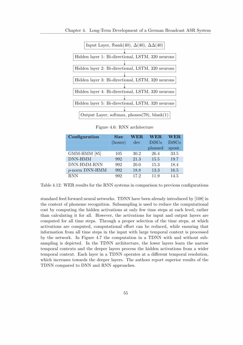
Chapter 4. Long-Term Development of a German Broadcast ASR System
Input Layer, fbank(40), ∆(40), ∆∆(40)
Hidden layer 1: Bi-directional, LSTM, 320 neurons
Hidden layer 2: Bi-directional, LSTM, 320 neurons
Hidden layer 3: Bi-directional, LSTM, 320 neurons
Hidden layer 4: Bi-directional, LSTM, 320 neurons
Hidden layer 5: Bi-directional, LSTM, 320 neurons
Output Layer, softmax, phones(79), blank(1)
Figure 4.6: RNN architecture
Configuration Size WER WER WER(hours) dev DiSCo DiSCo
planned spont.GMM-HMM [85] 105 30.2 26.4 33.5DNN-HMM 992 21.3 15.5 19.7DNN-HMM-RNN 992 20.0 15.3 18.4p-norm DNN-HMM 992 18.8 13.3 16.5
RNN 992 17.2 11.9 14.5
Table 4.12: WER results for the RNN systems in comparison to previous configurations
standard feed forward neural networks. TDNN have been already introduced by [108] inthe context of phoneme recognition. Subsampling is used to reduce the computationalcost by computing the hidden activations at only few time steps at each level, ratherthan calculating it for all. However, the activations for input and output layers arecomputed for all time steps. Through a proper selection of the time steps, at whichactivations are computed, computational effort can be reduced, while ensuring thatinformation from all time steps in the input with large temporal context is processedby the network. In Figure 4.7 the computation in a TDNN with and without sub-sampling is depicted. In the TDNN architecture, the lower layers learn the narrowtemporal contexts and the deeper layers process the hidden activations from a widertemporal context. Each layer in a TDNN operates at a different temporal resolution,which increases towards the deeper layers. The authors report superior results of theTDNN compared to DNN and RNN approaches.
55
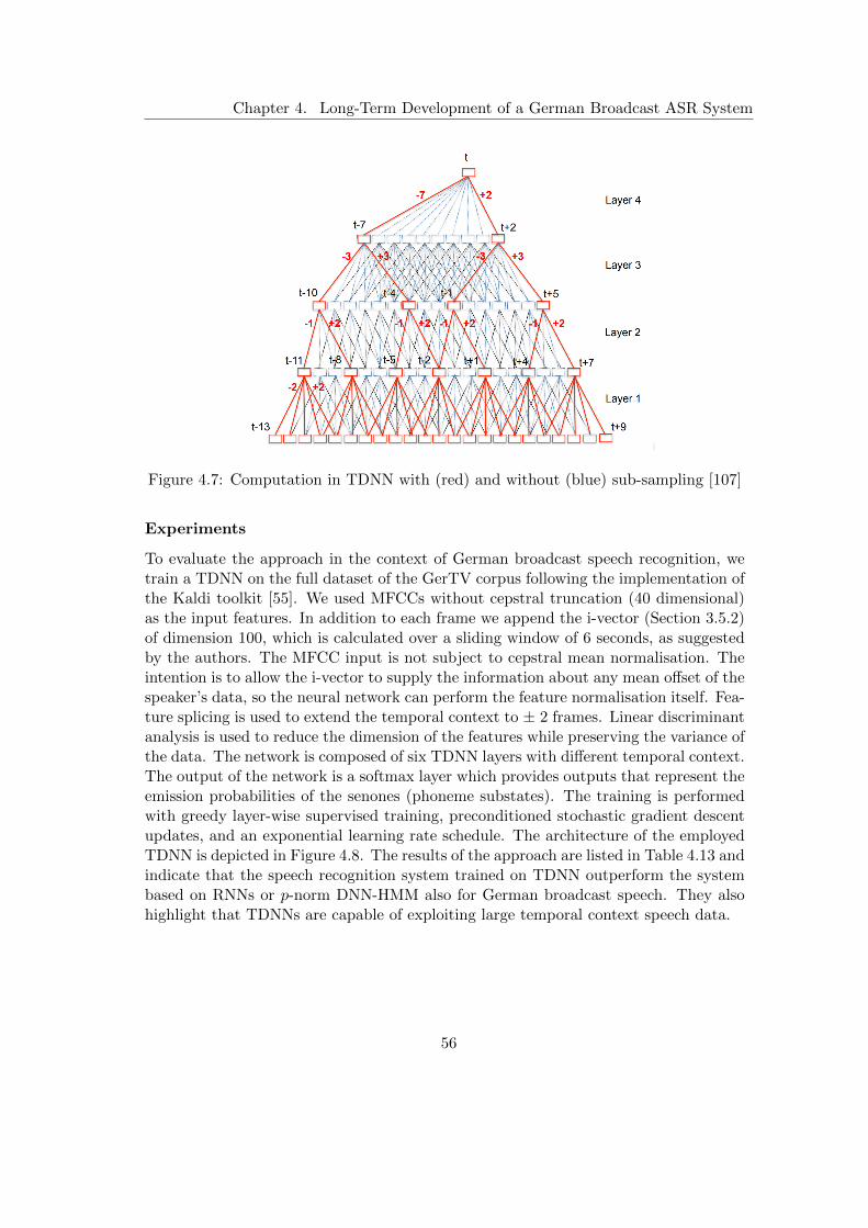
Chapter 4. Long-Term Development of a German Broadcast ASR System
Figure 4.7: Computation in TDNN with (red) and without (blue) sub-sampling [107]
Experiments
To evaluate the approach in the context of German broadcast speech recognition, wetrain a TDNN on the full dataset of the GerTV corpus following the implementation ofthe Kaldi toolkit [55]. We used MFCCs without cepstral truncation (40 dimensional)as the input features. In addition to each frame we append the i-vector (Section 3.5.2)of dimension 100, which is calculated over a sliding window of 6 seconds, as suggestedby the authors. The MFCC input is not subject to cepstral mean normalisation. Theintention is to allow the i-vector to supply the information about any mean offset of thespeaker’s data, so the neural network can perform the feature normalisation itself. Fea-ture splicing is used to extend the temporal context to ± 2 frames. Linear discriminantanalysis is used to reduce the dimension of the features while preserving the variance ofthe data. The network is composed of six TDNN layers with different temporal context.The output of the network is a softmax layer which provides outputs that represent theemission probabilities of the senones (phoneme substates). The training is performedwith greedy layer-wise supervised training, preconditioned stochastic gradient descentupdates, and an exponential learning rate schedule. The architecture of the employedTDNN is depicted in Figure 4.8. The results of the approach are listed in Table 4.13 andindicate that the speech recognition system trained on TDNN outperform the systembased on RNNs or p-norm DNN-HMM also for German broadcast speech. They alsohighlight that TDNNs are capable of exploiting large temporal context speech data.
56
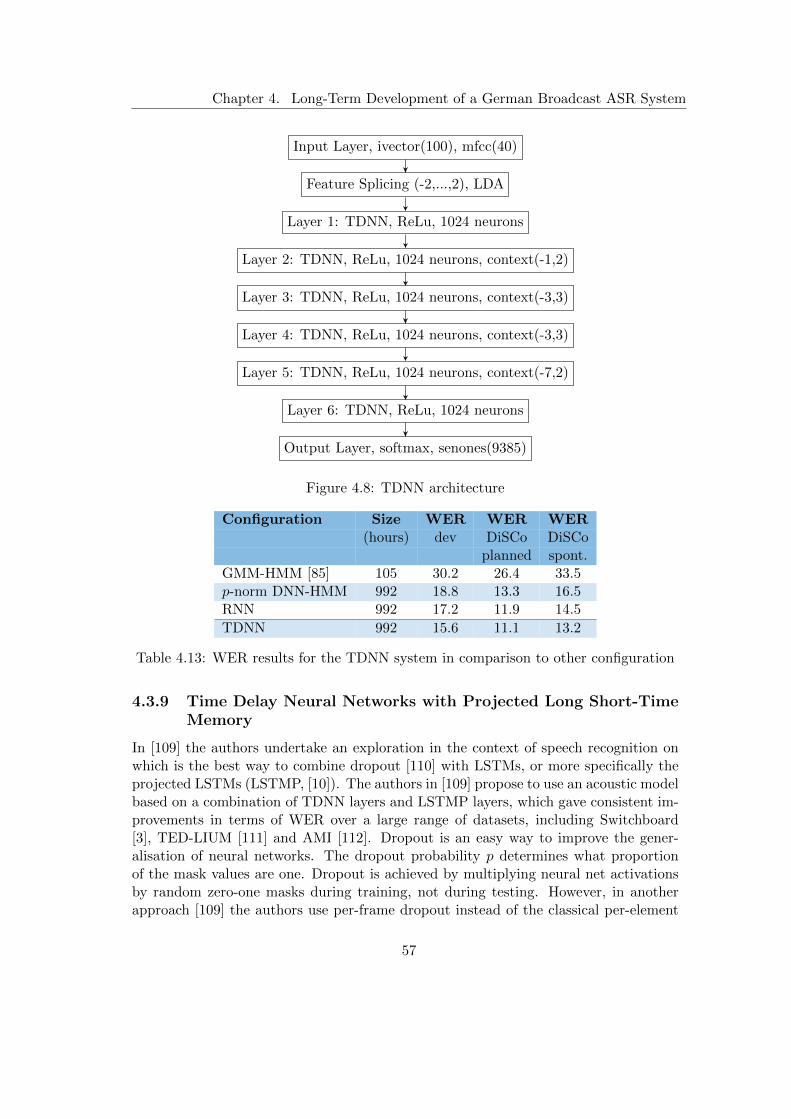
Chapter 4. Long-Term Development of a German Broadcast ASR System
Input Layer, ivector(100), mfcc(40)
Feature Splicing (-2,...,2), LDA
Layer 1: TDNN, ReLu, 1024 neurons
Layer 2: TDNN, ReLu, 1024 neurons, context(-1,2)
Layer 3: TDNN, ReLu, 1024 neurons, context(-3,3)
Layer 4: TDNN, ReLu, 1024 neurons, context(-3,3)
Layer 5: TDNN, ReLu, 1024 neurons, context(-7,2)
Layer 6: TDNN, ReLu, 1024 neurons
Output Layer, softmax, senones(9385)
Figure 4.8: TDNN architecture
Configuration Size WER WER WER(hours) dev DiSCo DiSCo
planned spont.GMM-HMM [85] 105 30.2 26.4 33.5p-norm DNN-HMM 992 18.8 13.3 16.5RNN 992 17.2 11.9 14.5
TDNN 992 15.6 11.1 13.2
Table 4.13: WER results for the TDNN system in comparison to other configuration
4.3.9 Time Delay Neural Networks with Projected Long Short-TimeMemory
In [109] the authors undertake an exploration in the context of speech recognition onwhich is the best way to combine dropout [110] with LSTMs, or more specifically theprojected LSTMs (LSTMP, [10]). The authors in [109] propose to use an acoustic modelbased on a combination of TDNN layers and LSTMP layers, which gave consistent im-provements in terms of WER over a large range of datasets, including Switchboard[3], TED-LIUM [111] and AMI [112]. Dropout is an easy way to improve the gener-alisation of neural networks. The dropout probability p determines what proportionof the mask values are one. Dropout is achieved by multiplying neural net activationsby random zero-one masks during training, not during testing. However, in anotherapproach [109] the authors use per-frame dropout instead of the classical per-element
57
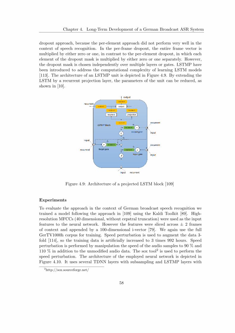
Chapter 4. Long-Term Development of a German Broadcast ASR System
dropout approach, because the per-element approach did not perform very well in thecontext of speech recognition. In the per-frame dropout, the entire frame vector ismultiplied by either zero or one, in contrast to the per-element dropout, in which eachelement of the dropout mask is multiplied by either zero or one separately. However,the dropout mask is chosen independently over multiple layers or gates. LSTMP havebeen introduced to address the computational complexity of learning LSTM models[113]. The architecture of an LSTMP unit is depicted in Figure 4.9. By extending theLSTM by a recurrent projection layer, the parameters of the unit can be reduced, asshown in [10].
Figure 4.9: Architecture of a projected LSTM block [109]
Experiments
To evaluate the approach in the context of German broadcast speech recognition wetrained a model following the approach in [109] using the Kaldi Toolkit [89]. High-resolution MFCCs (40 dimensional, without cepstral truncation) were used as the inputfeatures to the neural network. However the features were sliced across ± 2 framesof context and appended by a 100-dimensional i-vector [79]. We again use the fullGerTV1000h corpus for training. Speed perturbation is used to augment the data 3-fold [114], so the training data is artificially increased to 3 times 992 hours. Speedperturbation is performed by manipulation the speed of the audio samples to 90 % and110 % in addition to the unmodified audio data. The sox tool2 is used to perform thespeed perturbation. The architecture of the employed neural network is depicted inFigure 4.10. It uses several TDNN layers with subsampling and LSTMP layers with
2http://sox.sourceforge.net/
58
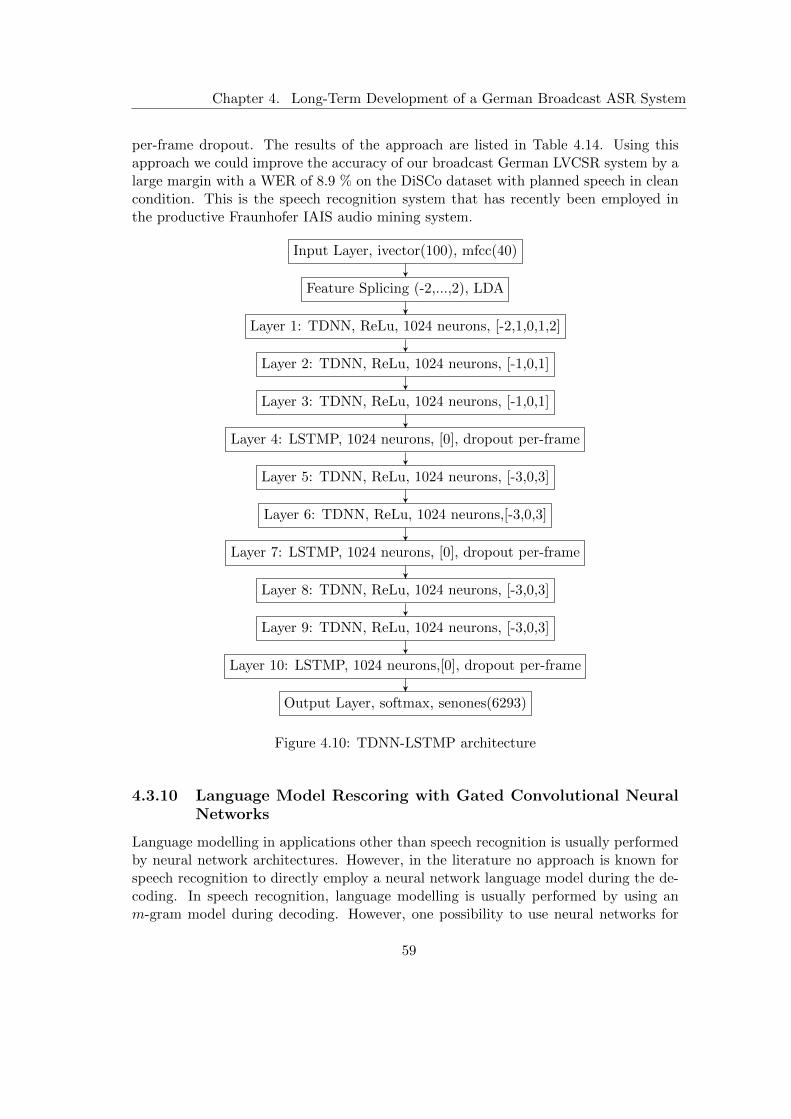
Chapter 4. Long-Term Development of a German Broadcast ASR System
per-frame dropout. The results of the approach are listed in Table 4.14. Using thisapproach we could improve the accuracy of our broadcast German LVCSR system by alarge margin with a WER of 8.9 % on the DiSCo dataset with planned speech in cleancondition. This is the speech recognition system that has recently been employed inthe productive Fraunhofer IAIS audio mining system.
Input Layer, ivector(100), mfcc(40)
Feature Splicing (-2,...,2), LDA
Layer 1: TDNN, ReLu, 1024 neurons, [-2,1,0,1,2]
Layer 2: TDNN, ReLu, 1024 neurons, [-1,0,1]
Layer 3: TDNN, ReLu, 1024 neurons, [-1,0,1]
Layer 4: LSTMP, 1024 neurons, [0], dropout per-frame
Layer 5: TDNN, ReLu, 1024 neurons, [-3,0,3]
Layer 6: TDNN, ReLu, 1024 neurons,[-3,0,3]
Layer 7: LSTMP, 1024 neurons, [0], dropout per-frame
Layer 8: TDNN, ReLu, 1024 neurons, [-3,0,3]
Layer 9: TDNN, ReLu, 1024 neurons, [-3,0,3]
Layer 10: LSTMP, 1024 neurons,[0], dropout per-frame
Output Layer, softmax, senones(6293)
Figure 4.10: TDNN-LSTMP architecture
4.3.10 Language Model Rescoring with Gated Convolutional NeuralNetworks
Language modelling in applications other than speech recognition is usually performedby neural network architectures. However, in the literature no approach is known forspeech recognition to directly employ a neural network language model during the de-coding. In speech recognition, language modelling is usually performed by using anm-gram model during decoding. However, one possibility to use neural networks for
59

Chapter 4. Long-Term Development of a German Broadcast ASR System
Configuration Size WER WER WER(hours) dev DiSCo DiSCo
planned spont.GMM-HMM [85] 105 30.2 26.4 33.5RNN 992 17.2 11.9 14.5TDNN 992 15.6 11.1 13.2
TDNN-LSTMP 992 13.7 8.9 10.4
Table 4.14: WER results for the TDNN-LSTMP system in comparison to previousconfigurations
language modelling in speech recognition is to perform a language model rescoring us-ing neural network language models. In [115] a novel method was proposed to performlanguage modelling with Gated Convolutional Neural Networks (GCNN). In this ap-proach, words are represented by a vector embedding stored in a lookup table D|V |×e,where |V | is the vocabulary size and e is the size of the embedding. A sequence ofwords w0, .., wN is then represented by the word embeddings E = [Dw0 , ..., DwN ]. Thehidden layers h0, .., hL are computed as:
hl(X) = (X ∗W + b)⊗ σ(X ∗ V + c) (4.10)
where X ∈ RN×m is the input of layer hl (either the word embeddings or theoutput of the previous layers), W ∈ Rk×m×n, b ∈ Rn, V ∈ Rk×m×n and c ∈ Rnare learned parameters, σ is the sigmoid function and ⊗ is the element-wise productbetween matrices, where m,n are respectively the number of input and output featuremaps and k is the patch size. The output of each layer is a linear projection X ∗W + bmodulated by the gates σ(X ∗ V + c). The authors call this gating mechanism GatedLinear Units (GLU). Convolution is performed by shifting the convolutional inputs toprevent the kernels to see future context. To obtain model predictions a (hierarchicalor adaptive) softmax layer is employed. For further information on gated convolutionalneural networks for language modelling see [115].
Experiments
In the context of German broadcast speech recognition, we train an 8-layer bottleneckGCNN as proposed in [115], with our standard German broadcast training text data(75 million words) and the same dictionary (500k words), as used in the previousexperiments. The hidden layers are GLU layers with dropout and the output layeris a hierarchical softmax layer. We trained the network with Adagrad optimiser andcross-entropy loss function. The batch size was 32, the initial learning rate was 0.8.The learning rate was halved, when there was no improvement on a left out validationset for 4 validation checks and the network state was set reset to the optimal state.A validation check was performed 25 times per epoch. After training we rescored then-best hypothesis list (n = 100) provided by the TDNN-LSTMP model, trained in
60
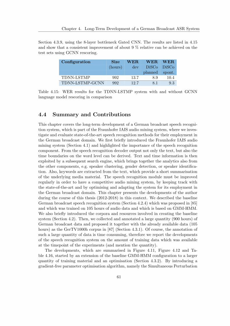
Chapter 4. Long-Term Development of a German Broadcast ASR System
Section 4.3.9, using the 8-layer bottleneck Gated CNN. The results are listed in 4.15and show that a consistent improvement of about 9 % relative can be achieved on thetest sets using GCNN rescoring.
Configuration Size WER WER WER(hours) dev DiSCo DiSCo
planned spont.TDNN-LSTMP 992 13.7 8.9 10.4
TDNN-LSTMP-GCNN 992 12.7 8.1 9.3
Table 4.15: WER results for the TDNN-LSTMP system with and without GCNNlanguage model rescoring in comparison
4.4 Summary and Contributions
This chapter covers the long-term development of a German broadcast speech recogni-tion system, which is part of the Fraunhofer IAIS audio mining system, where we inves-tigate and evaluate state-of-the-art speech recognition methods for their employment inthe German broadcast domain. We first briefly introduced the Fraunhofer IAIS audiomining system (Section 4.1) and highlighted the importance of the speech recognitioncomponent. From the speech recognition decoder output not only the text, but also thetime boundaries on the word level can be derived. Text and time information is thenexploited by a subsequent search engine, which brings together the analytics also fromthe other components, e.g. speaker clustering, gender detection, or speaker identifica-tion. Also, keywords are extracted from the text, which provide a short summarisationof the underlying media material. The speech recognition module must be improvedregularly in order to have a competitive audio mining system, by keeping track withthe state-of-the-art and by optimising and adapting the system for its employment inthe German broadcast domain. This chapter presents the developments of the authorduring the course of this thesis (2012-2018) in this context. We described the baselineGerman broadcast speech recognition system (Section 4.2.4) which was proposed in [85]and which was trained on 105 hours of audio data and which is based on GMM-HMM.We also briefly introduced the corpora and resources involved in creating the baselinesystem (Section 4.2). Then, we collected and annotated a large quantity (900 hours) ofGerman broadcast data and proposed it together with the already available data (105hours) as the GerTV1000h corpus in [87] (Section 4.3.1). Of course, the annotation ofsuch a large quantity of data is time consuming, therefore we report the developmentsof the speech recognition system on the amount of training data which was availableat the timepoint of the experiments (and mention the quantity).
The developments, which are summarised in Figure 4.11, Figure 4.12 and Ta-ble 4.16, started by an extension of the baseline GMM-HMM configuration to a largerquantity of training material and an optimisation (Section 4.3.2). By introducing agradient-free parameter optimisation algorithm, namely the Simultaneous Perturbation
61
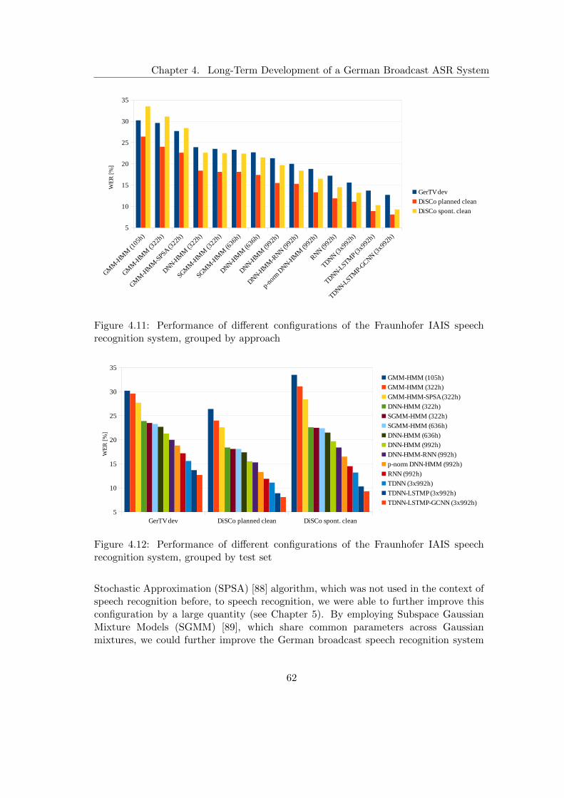
Chapter 4. Long-Term Development of a German Broadcast ASR System
Figure 4.11: Performance of different configurations of the Fraunhofer IAIS speechrecognition system, grouped by approach
Figure 4.12: Performance of different configurations of the Fraunhofer IAIS speechrecognition system, grouped by test set
Stochastic Approximation (SPSA) [88] algorithm, which was not used in the context ofspeech recognition before, to speech recognition, we were able to further improve thisconfiguration by a large quantity (see Chapter 5). By employing Subspace GaussianMixture Models (SGMM) [89], which share common parameters across Gaussianmixtures, we could further improve the German broadcast speech recognition system
62

Chapter 4. Long-Term Development of a German Broadcast ASR System
(Section 4.3.3). With the advent of deep neural networks (DNN) in speech recognition,we followed the approach in [45] and employed a hybrid DNN-HMM for acousticmodelling in the context of German broadcast speech recognition (Section 4.3.4).This is also the first configuration which employed the full GerTV corpus (TS IV,992 hours). Note that we excluded some utterances from the training because theyincluded mispronunciations, foreign language or dialect, as indicated by the annotationmarkers. Results indicated a further improvement of the speech recognition system byusing hybrid DNN-HMM. The hybrid DNN-HMM system was again improved by usingrecurrent neural network language model n-best hypothesis rescoring (Section 4.3.5)by following the approach proposed in [96]. By optimising the non-linearities of theDNN, as proposed in [102], and with the employment of p-norm non-linearities, wecould again improve the German broadcast speech recognition system (Section 4.3.6).By following the RNN approach based on LSTM units [48], which are able to exploitthe temporal information without the use of HMMs more efficiently, we were able tofurther improve the German broadcast system (Section 4.3.7). To reduce the trainingtime of RNNs and to improve the accuracy, the authors in [107] proposed an acousticmodel for speech recognition which is based on Time Delay Neural Networks (TDNN)with subsampling. Following the approach we were able to improve the accuracy of theGerman broadcast speech recognition once again (Section 4.3.8). In [109] the authorcombined the TDNN acoustic model with projected LSTM (LSTMP) recurrent layers.We adapted this approach in the context of German broadcast speech recognitionand were able to improve the system (Section 4.3.9). Finally, Gated ConvolutionalNeural Networks (GCNN) became available for language modelling, which we used forrescoring the hypotheses derived TDNN-LSTMP configuration to improve the systemeven more (Section 4.3.10).
In the course of this thesis (2012-2018), we were able to improve the performance ofthe German broadcast speech recognition by a large margin by carrying out numerousexperiments and by optimising the necessary parameters for our setup. We reducedthe WER of the German broadcast speech recognition system for the clean DiSCo testdataset for planned speech from 26.4 % to 8.1 % WER, which is an improvement of18.3 % WER absolute or 68.2 % relative. In the case of the clean DiSCo test datasetfor spontaneous speech, we were able to improve the system from 33.5 % to 9.3 %,which is an improvement of 24.2 % absolute or 72.3 % relative.
63

Chapter 4. Long-Term Development of a German Broadcast ASR System
Configuration Size WER WER WER(hours) dev DiSCo DiSCo
planned spont.GMM-HMM [85] 105 30.2 26.4 33.5HMM-GMM 322 29.6 24.0 31.1HMM-GMM-SPSA 322 27.7 22.6 28.4DNN-HMM 322 23.9 18.4 22.6SGMM-HMM 322 23.5 18.1 22.5SGMM-HMM 636 23.3 18.1 22.4DNN-HMM 636 22.7 17.4 21.5DNN-HMM 992 21.3 15.5 19.7DNN-HMM-RNN 992 20.0 15.3 18.4p-norm DNN-HMM 992 18.8 13.3 16.5RNN 992 17.2 11.9 14.5TDNN 3x992 15.6 11.1 13.2TDNN-LSTMP 3x992 13.7 8.9 10.3TDNN-LSTMP-GCNN 3x992 12.7 8.1 9.3
Table 4.16: Performance of different configurations of the Fraunhofer IAIS speech recog-nition system
64

Chapter 5
Gradient-Free SpeechRecognition Decoder ParameterOptimisation
As noted in the previous chapters, the speech recognition system (Chapter 4) is thekey component of the Fraunhofer IAIS audio mining system, which enables the efficientsearch of large heterogeneous media archives. In order to be competitive amongst othercompetitors on the market, this system has to be constantly developed by employingthe latest state-of-the-art methods provided by the research community. Also, the sys-tem has to be optimised for the employment in the German broadcast speech domainto be successful. Both the optimisation of the acoustic model and the language modelin automatic speech recognition are well-established task. The actual decoding process,however, also uses a large set of free parameters that should be optimised for the giventask. Some decoding parameters directly weight the models, others affect the size ofthe search space, where it is hard to foresee the effect on the hypothesis quality andon the decoding time. In praxis, these parameters are often left to default values pro-vided by the toolkit manuals, or set empirically in a rather time consuming task. Bothstrategies are usually of limited success and end up with a parameter set that is faraway from the optimum in terms of performance and decoding speed, without unlock-ing the full potential of the ASR system. Automatic decoder parameter optimisationalgorithms solve this problem by performing a gradient approximation to optimise theparameters. Gradient approximation methods, i.e. gradient-free methods, rely on mea-surements of the objective function (e.g. WER), not on measurements of the gradientof the objective function and are usually employed when the measurement of the gra-dient of the objective function is complicated or even impossible, as it is for speechrecognition. State-of-the-art decoder parameter optimisation methods usually need alarge number of iterations and hence, are slow. This is why we introduce a methodfor automatically solving multivariate optimisation problems, namely the simultaneousperturbation stochastic approximation (SPSA) algorithm, which was developed in [116]in a general mathematical context, and which has not been employed in the context of
65
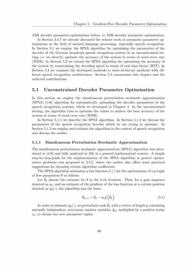
Chapter 5. Gradient-Free Decoder Parameter Optimisation
ASR decoder parameter optimisation before, to ASR decoder parameter optimisation.In Section 3.4.7 we already discussed the related work of automatic parameter op-
timisation in the field of natural language processing, especially speech recognition.In Section 5.1 we employ the SPSA algorithm for optimising the parameters of thedecoder of the German broadcast speech recognition system in an unconstrained set-ting, i.e. we directly optimise the accuracy of the system in terms of word error rate(WER). In Section 5.2 we extend the SPSA algorithm for optimising the accuracy ofthe system by constraining the decoding speed in terms of real time factor (RTF). InSection 5.3 we compare the developed methods to state-of-the-art methods with dif-ferent speech recognition architectures. Section 5.4 summarises this chapter and theachieved contributions.
5.1 Unconstrained Decoder Parameter Optimisation
In this section we employ the simultaneous perturbation stochastic approximation(SPSA) [116] algorithm for automatically optimising the decoder parameters of thespeech recognition systems, which we developed in Chapter 4. In the unconstrainedsetting, the algorithm tries to optimise the values to achieve the best accuracy of thesystem in terms of word error rate (WER).
In Section 5.1.1 we describe the SPSA algorithm. In Section 5.1.2 we discuss theparameters of the speech recognition decoder which we are trying to optimise. InSection 5.1.3 we employ and evaluate the algorithm in the context of speech recognitionand discuss the results.
5.1.1 Simultaneous Perturbation Stochastic Approximation
The simultaneous perturbation stochastic approximation (SPSA) algorithm was intro-duced in [116] and fully analysed in [88] in a general mathematical context. A simplestep-by-step-guide for the implementation of the SPSA algorithm in generic optimi-sation problems was proposed in [117], where the author also offers some practicalsuggestions for choosing certain algorithm coefficients.
The SPSA algorithm minimises a loss function L (·) for the optimisation of a p-tupleof free parameters θ as follows:
Let θk denote the estimate for θ in the k-th iteration. Then, for a gain sequencedenoted as ak, and an estimate of the gradient of the loss function at a certain positiondenoted as gk(·), the algorithm has the form:
θk+1 = θk − akg(θk
)(5.1)
In order to estimate gk(·), we perturbate each θk with a vector of length p containingmutually independent, zero-mean random variables ∆k, multiplied by a positive scalarck, to obtain two new parameter tuples:
66

Chapter 5. Gradient-Free Decoder Parameter Optimisation
θ+k = θk + ck∆k (5.2)
θ−k = θk − ck∆k (5.3)
For a loss function L (·), we then estimate g(θk
)as:
g(θk
)=L(θ+k
)− L
(θ−k
)2ck
∆−1k1...
∆−1kp
(5.4)
We follow the implementation suggestions in [117] and use a ±1 Bernoulli distribu-tion for ∆k, and further set:
ak = a(A+ k + 1)α
with a = 2, A = 8, α = 0.602 (5.5)
ck = c(k + 1)γ
with c = 0.25, γ = 0.101 (5.6)
Using these gain sequences ak and ck, SPSA normally converges in a similar numberof iterations as the classical Kiefer-Wolfowitz FDSA [68], but requires p times fewermeasurements of the loss function, as the decoding performance has to be evaluatedonly 2 times in each iteration, as shown in [88].
α and γ are set to the lowest values satisfying the theoretical conditions for con-vergence, as proposed in [88], leading to larger step sizes in the iteration process andtherefore faster performance.
Since the measurements of L (θ) do not contain noise, we choose c to be a smallpositive number as proposed in [117]. Likewise, we set A = 8 to approximately 10 %of the expected iterations and finally a = 2 so that the steps in the update have areasonable size for the first iterations. During our experiments, we did not experiencea high sensitivity of SPSA for any of its hyperparameters, only the required number ofiterations to reach a stable result changes.
The speech recognition decoder parameters θ which we optimised are discussed inthe following section (Section 5.1.2).
5.1.2 GMM-HMM Decoder Parameters
In this section we describe and discuss the speech recognition decoder parametersthat have been automatically optimised. The corresponding decoder parameters ofthe GMM-HMM approach, as implemented by the speech recognition decoder Julius[62], are:
• m-gram language model weight on 1st pass
67
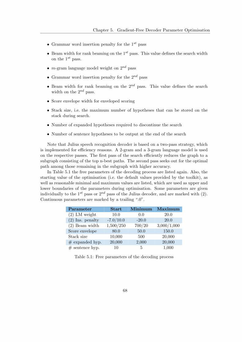
Chapter 5. Gradient-Free Decoder Parameter Optimisation
• Grammar word insertion penalty for the 1st pass
• Beam width for rank beaming on the 1st pass. This value defines the search widthon the 1st pass.
• m-gram language model weight on 2nd pass
• Grammar word insertion penalty for the 2nd pass
• Beam width for rank beaming on the 2nd pass. This value defines the searchwidth on the 2nd pass.
• Score envelope width for enveloped scoring
• Stack size, i.e. the maximum number of hypotheses that can be stored on thestack during search.
• Number of expanded hypotheses required to discontinue the search
• Number of sentence hypotheses to be output at the end of the search
Note that Julius speech recognition decoder is based on a two-pass strategy, whichis implemented for efficiency reasons. A 2-gram and a 3-gram language model is usedon the respective passes. The first pass of the search efficiently reduces the graph to asubgraph consisting of the top n-best paths. The second pass seeks out for the optimalpath among those remaining in the subgraph with higher accuracy.
In Table 5.1 the free parameters of the decoding process are listed again. Also, thestarting value of the optimisation (i.e. the default values provided by the toolkit), aswell as reasonable minimal and maximum values are listed, which are used as upper andlower boundaries of the parameters during optimisation. Some parameters are givenindividually to the 1st pass or 2nd pass of the Julius decoder, and are marked with (2).Continuous parameters are marked by a trailing “.0”.
Parameter Start Minimum Maximum(2) LM weight 10.0 0.0 20.0(2) Ins. penalty -7.0/10.0 -20.0 20.0(2) Beam width 1,500/250 700/20 3,000/1,000Score envelope 80.0 50.0 150.0Stack size 10,000 500 20,000# expanded hyp. 20,000 2,000 20,000# sentence hyp. 10 5 1,000
Table 5.1: Free parameters of the decoding process
68

Chapter 5. Gradient-Free Decoder Parameter Optimisation
5.1.3 Experimental Setup and Evaluation
For the experiments we used the best speech recognition system which was availableat the timepoint of the experiments, namely the extended HMM-GMM ASR system(Section 4.3.2), which was trained on 322 hours of audio material taken from the GerTVcorpus (Section 4.3.1).
We employed the development dataset from the GerTV corpus (Section 4.3.1) forthe approximation of the gradient during the optimisation process. The full list ofparameters that were optimised is described in Section 5.1.2. Also, the default valuesof the decoder parameters as well as the minimum value and the maximum value ofeach parameter, which spans the parameter range that we allow for optimisation, aredescribed in Table 5.1.
Internally, we map the parameter ranges to [−15 · · ·+ 15] for the SPSA iterations.If the parameters are integers, we store them as floating values internally but truncatethem for each evaluation of the loss function.
We optimise the parameters to maximise the accuracy of the speech recognitionsystem in terms of the word error rate (WER), i.e., the number of substitutions, inser-tions and deletion errors divided by the reference length, using it directly as the lossfunction (or rather the objective function) in the SPSA algorithm in the unconstrainedsetting.
The results on the development set are shown in Figure 5.1. The progression of theoptimisation over the iterations is visible in this graph. Also, the WER is depicted, forL(θ+) and L(θ−) for every iteration, which represent the simultaneously perturbatedparameter values from which the gradient is approximated in the SPSA algorithm. Thealgorithm converges after some iterations. In each iteration, the decoding has to takeplace for the parameters θ+ and θ−, and for the optimised parameters after calculatingthe gradient θ. Hence, a total of three decodings is necessary for each iteration. Intotal, the hypothesis quality improved by 1.9 % WER absolute (6.4 % relative) during18 iterations. In a second run, the improvement was similar and it converged after 10iterations already.
To evaluate whether the performance gain by using the optimised parameters alsogeneralises to unseen data, we evaluate the ASR configurations with the optimisedparameters on the clean datasets of the DiSCo corpus (Section 4.2.2, planned speechand spontaneous speech) and the LinkedTV datasets (Section 4.2.3). The results aresummarised in Table 5.2.
The results on the test sets are presented in Figure 5.2 for the DiSCo corpora and inFigure 5.3 for the LinkedTV corpora. It can be seen that the optimisation generalisesnicely on all four test corpora: 1.2 % WER absolute improvement on the planned speechtask, and 2.7 % WER absolute improvement on the spontaneous speech task for theDiSCo datasets (see Figure 5.2).
The same is true for the LinkedTV data, with even higher improvements of 1.9 %and 4.4 % WER respectively. While the resulting error rates for the two “planned”corpora are comparable, the LinkedTV spontaneous dataset performs a lot worse. Thiscan likely be explained by the fact that LinkedTV spontaneous contains partly dialectal
69
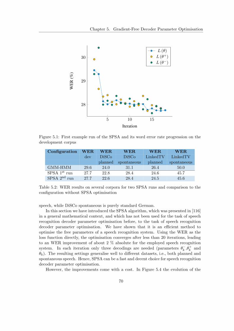
Chapter 5. Gradient-Free Decoder Parameter Optimisation
5 10 15
28
29
30
Iteration
WE
R(%
)
L (θ)
L (θ+)
L (θ−)
Figure 5.1: First example run of the SPSA and its word error rate progression on thedevelopment corpus
Configuration WER WER WER WER WERdev DiSCo DiSCo LinkedTV LinkedTV
planned spontaneous planned spontaneousGMM-HMM 29.6 24.0 31.1 26.4 50.0
SPSA 1st run 27.7 22.8 28.4 24.6 45.7SPSA 2nd run 27.7 22.6 28.4 24.5 45.6
Table 5.2: WER results on several corpora for two SPSA runs and comparison to theconfiguration without SPSA optimisation
speech, while DiSCo spontaneous is purely standard German.In this section we have introduced the SPSA algorithm, which was presented in [116]
in a general mathematical context, and which has not been used for the task of speechrecognition decoder parameter optimisation before, to the task of speech recognitiondecoder parameter optimisation. We have shown that it is an efficient method tooptimise the free parameters of a speech recognition system. Using the WER as theloss function directly, the optimisation converges after less than 20 iterations, leadingto an WER improvement of about 2 % absolute for the employed speech recognitionsystem. In each iteration only three decodings are needed (parameters θ−k ,θ+
k andθk). The resulting settings generalise well to different datasets, i.e., both planned andspontaneous speech. Hence, SPSA can be a fast and decent choice for speech recognitiondecoder parameter optimisation.
However, the improvements come with a cost. In Figure 5.4 the evolution of the
70
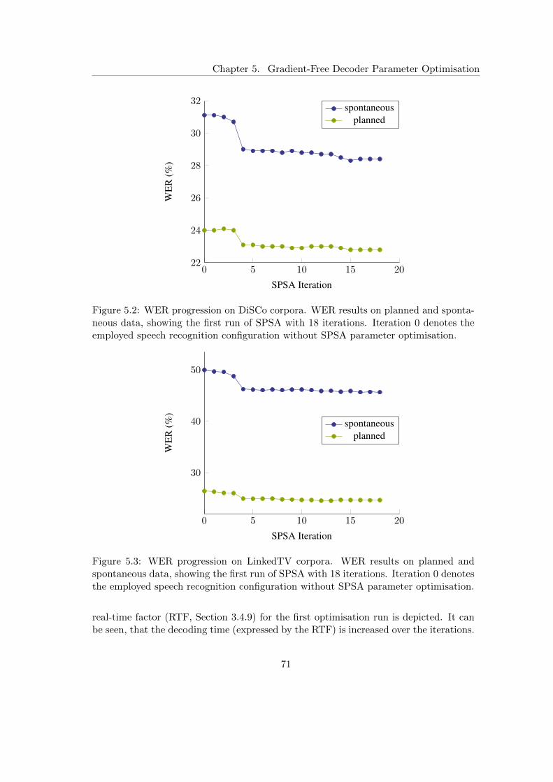
Chapter 5. Gradient-Free Decoder Parameter Optimisation
0 5 10 15 2022
24
26
28
30
32
SPSA Iteration
WE
R(%
)
spontaneousplanned
Figure 5.2: WER progression on DiSCo corpora. WER results on planned and sponta-neous data, showing the first run of SPSA with 18 iterations. Iteration 0 denotes theemployed speech recognition configuration without SPSA parameter optimisation.
0 5 10 15 20
30
40
50
SPSA Iteration
WE
R(%
)
spontaneousplanned
Figure 5.3: WER progression on LinkedTV corpora. WER results on planned andspontaneous data, showing the first run of SPSA with 18 iterations. Iteration 0 denotesthe employed speech recognition configuration without SPSA parameter optimisation.
real-time factor (RTF, Section 3.4.9) for the first optimisation run is depicted. It canbe seen, that the decoding time (expressed by the RTF) is increased over the iterations.
71

Chapter 5. Gradient-Free Decoder Parameter Optimisation
0 5 10 15 20
4
4.5
5
5.5
6
SPSA Iteration
RT
F
plannedspontaneous
Figure 5.4: RTF development on the DiSCo corpora “clean planned” and “clean spon-taneous”, for the first optimisation run using the unconstrained optimisation criterion.
This is often the case when optimising the performance, because often the complexity ofthe algorithm is increased (e.g. by making the decoding graph larger). While for manysettings this might not pose a problem, in time-crucial applications, e.g. in productiveaudio mining systems, this is not desirable. Thus, in the following section (Section 5.2),we take the RTF into account and optimise WER and RTF jointly.
5.2 Time-constrained Decoder Parameter Optimisation
We have shown in the experiments of the previous section (Section 5.1), where weemployed the SPSA algorithm to optimise the accuracy of the speech recognition sys-tem by using the word error rate directly as the objective function (i.e., the loss orcost function), that the algorithm is capable to optimise the performance of a speechrecognition system with a rather small number of iterations and decodings of the de-velopment set. However, the improvements in the performance come partially at theexpense of the decoding speed in terms of RTF (as shown in Figure 5.4 and increasedmemory consumption, because some changes in the parameters increase the complexityof the algorithm. Often this is not a problem when we aim for the best performance ofthe speech recognition system, but in time-crucial applications like in the framework ofan audio mining system this is not desirable. Thus, in this section we try to take theRTF into account and optimise WER and RTF jointly in another set of experiments.
In Section 5.2.1 we introduce the RTF penalty term to the general loss functionof the SPSA algorithm. In the subsequent sections we define RTF penalty terms forthe use of constrained optimisation, namely the exponential penalty (Section 5.2.2, the
72
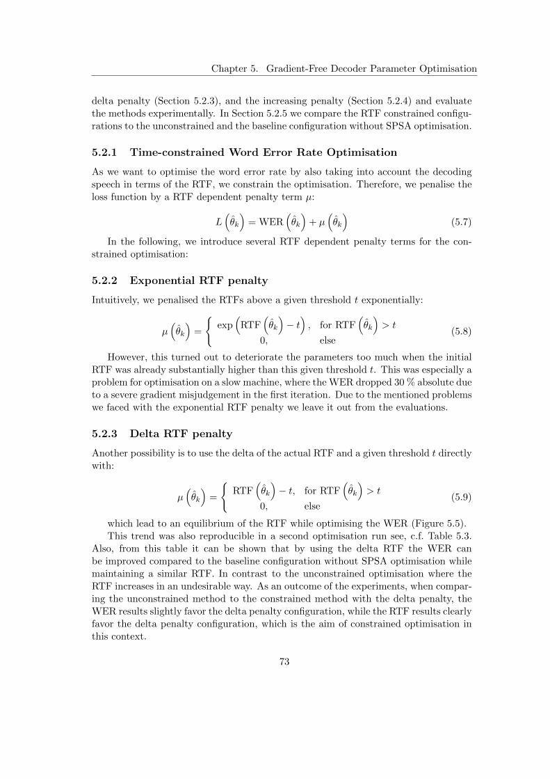
Chapter 5. Gradient-Free Decoder Parameter Optimisation
delta penalty (Section 5.2.3), and the increasing penalty (Section 5.2.4) and evaluatethe methods experimentally. In Section 5.2.5 we compare the RTF constrained configu-rations to the unconstrained and the baseline configuration without SPSA optimisation.
5.2.1 Time-constrained Word Error Rate Optimisation
As we want to optimise the word error rate by also taking into account the decodingspeech in terms of the RTF, we constrain the optimisation. Therefore, we penalise theloss function by a RTF dependent penalty term µ:
L(θk
)= WER
(θk
)+ µ
(θk
)(5.7)
In the following, we introduce several RTF dependent penalty terms for the con-strained optimisation:
5.2.2 Exponential RTF penalty
Intuitively, we penalised the RTFs above a given threshold t exponentially:
µ(θk
)=
{exp
(RTF
(θk
)− t), for RTF
(θk
)> t
0, else(5.8)
However, this turned out to deteriorate the parameters too much when the initialRTF was already substantially higher than this given threshold t. This was especially aproblem for optimisation on a slow machine, where the WER dropped 30 % absolute dueto a severe gradient misjudgement in the first iteration. Due to the mentioned problemswe faced with the exponential RTF penalty we leave it out from the evaluations.
5.2.3 Delta RTF penalty
Another possibility is to use the delta of the actual RTF and a given threshold t directlywith:
µ(θk
)=
{RTF
(θk
)− t, for RTF
(θk
)> t
0, else(5.9)
which lead to an equilibrium of the RTF while optimising the WER (Figure 5.5).This trend was also reproducible in a second optimisation run see, c.f. Table 5.3.
Also, from this table it can be shown that by using the delta RTF the WER canbe improved compared to the baseline configuration without SPSA optimisation whilemaintaining a similar RTF. In contrast to the unconstrained optimisation where theRTF increases in an undesirable way. As an outcome of the experiments, when compar-ing the unconstrained method to the constrained method with the delta penalty, theWER results slightly favor the delta penalty configuration, while the RTF results clearlyfavor the delta penalty configuration, which is the aim of constrained optimisation inthis context.
73

Chapter 5. Gradient-Free Decoder Parameter Optimisation
0 2 4 6 8 10 12 14 16 18
27.5
28
28.5
29
29.5
30
Iteration
WE
R(%
)
0 2 4 6 8 10 12 14 16 182.5
3
3.5
4
4.5
5
5.5
6
RT
F
WERRTF
Figure 5.5: Optimisation run on the development set with delta RTF penalty (Equa-tion 5.9), t = 5.0
dev test planned test spontaneousloss function #iter WER RTF ∆RTF WER RTF ∆RTF WER RTF ∆RTF
1.6GHz 2.6GHz 2.6GHzbaseline 0 29.6 5.3 1.00 24.0 4.6 1.00 31.1 4.0 1.00
unconstrained 18 27.7 7.0 1.32 22.8 5.4 1.17 28.4 5.9 1.48unconstrained 18 27.7 7.3 1.38 22.6 6.1 1.33 28.4 6.1 1.53
delta 18 27.6 5.3 1.00 22.2 4.5 0.98 27.7 4.8 1.20delta 18 27.6 5.1 0.96 22.5 4.2 0.91 27.9 4.4 1.10
increasing 14 32.5 3.0 0.57 26.1 2.2 0.48 31.9 2.3 0.58+28 31.6 2.9 0.55 25.3 2.5 0.54 30.0 2.6 0.65
increasing 12 31.2 3.0 0.57 25.5 2.2 0.48 31.0 2.1 0.53+28 33.6 2.9 0.55 27.5 2.3 0.50 32.1 2.4 0.60
Table 5.3: WER and RTF results on all corpora, for the SPSA iterations and theirrespective loss functions. Each optimisation on a given loss function has been executedtwo times from scratch to check for convergence. The unconstrained runs (Section 5.1)use the WER directly as loss function, delta uses Equation 5.9 and increasing usesEquation 5.10
5.2.4 Increasing RTF penalty
In another setup we penalise the RTF increasingly with each iteration:
µ(θk
)=(
RTF(θk
)− t)· k , for RTF
(θk
)> t (5.10)
with an increasing k = k as long as a RTF threshold t is not reached. For the firstiteration where the RTF is equal or below to the threshold t, k is fixed in order to give
74
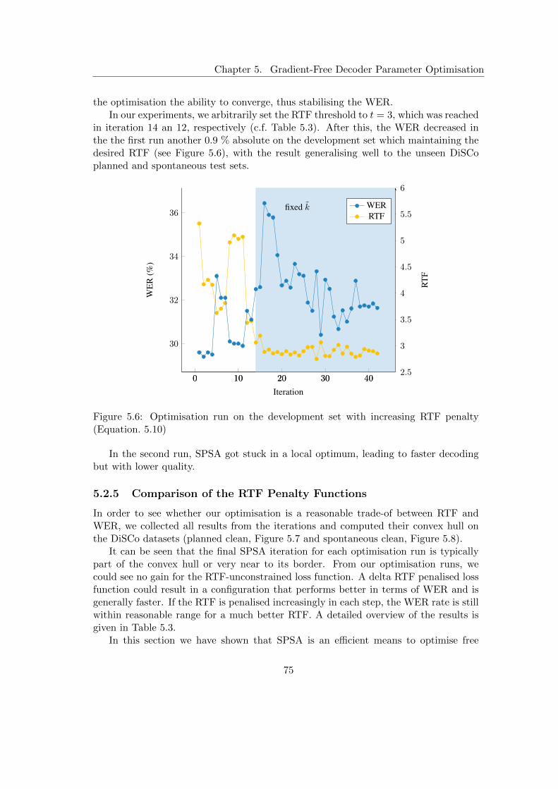
Chapter 5. Gradient-Free Decoder Parameter Optimisation
the optimisation the ability to converge, thus stabilising the WER.In our experiments, we arbitrarily set the RTF threshold to t = 3, which was reached
in iteration 14 an 12, respectively (c.f. Table 5.3). After this, the WER decreased inthe the first run another 0.9 % absolute on the development set which maintaining thedesired RTF (see Figure 5.6), with the result generalising well to the unseen DiSCoplanned and spontaneous test sets.
0 10 20 30 402.5
3
3.5
4
4.5
5
5.5
6
fixed k
RT
F
WERRTF
0 10 20 30 40
30
32
34
36
Iteration
WE
R(%
)
Figure 5.6: Optimisation run on the development set with increasing RTF penalty(Equation. 5.10)
In the second run, SPSA got stuck in a local optimum, leading to faster decodingbut with lower quality.
5.2.5 Comparison of the RTF Penalty Functions
In order to see whether our optimisation is a reasonable trade-of between RTF andWER, we collected all results from the iterations and computed their convex hull onthe DiSCo datasets (planned clean, Figure 5.7 and spontaneous clean, Figure 5.8).
It can be seen that the final SPSA iteration for each optimisation run is typicallypart of the convex hull or very near to its border. From our optimisation runs, wecould see no gain for the RTF-unconstrained loss function. A delta RTF penalised lossfunction could result in a configuration that performs better in terms of WER and isgenerally faster. If the RTF is penalised increasingly in each step, the WER rate is stillwithin reasonable range for a much better RTF. A detailed overview of the results isgiven in Table 5.3.
In this section we have shown that SPSA is an efficient means to optimise free
75

Chapter 5. Gradient-Free Decoder Parameter Optimisation
22 23 24 25 26 27 28
2
3
4
5
6
WER (%)
RT
F
convex hullunconstrained
delta RTF penaltyincreasing RTF penalty
starting point
Figure 5.7: Results for DiSCo “planned clean”. Scatter plot with all configurations,on the DiSCo test corpora. The final optimisation iteration is marked by filled-outsymbols.
parameters of an ASR decoder in terms of both WER and RTF. In an unconstrainedsetting, the WER improves rapidly, but the RTF also increases in an undesirable way,as shown in Section 5.1. By adding the RTF to the loss function, one is able to stabilisethe increase in time requirements. Overall, we have achieved an improvement of 1.8% absolute WER on the DiSCo planned clean task and an improvement of 3.4 %absolute WER on the DiSCo spontaneous task, over the baseline speech recognitionconfiguration without SPSA optimisation, while still having a reasonable RTF. Whena specific RTF is required for an application scenario, using the “increasing” penaltyfunction for SPSA allows reaching reasonable performance, given this constraint. Therisk for local optima seems higher in this setting, though, which is why we wouldrecommend multiple optimisation runs.
5.3 Comparison with State-of-the-art Methods
While there has been recent scientific contributions in the field of automatic speechrecognition decoder parameter optimisation, no thorough comparison of the methods,in terms of convergence speed, decoding speed and performance has been undertaken.Hence, in this section we conduct a series of experiments with three different state-of-the-art decoding paradigms, which were available at the timepoint of the experiments,namely GMM-HMM, DNN-HMM and SGMM-HMM, and evaluate the performance offour different optimisation methods found in the literature including SPSA, both for
76

Chapter 5. Gradient-Free Decoder Parameter Optimisation
28 30 32 34 36
2
3
4
5
6
WER (%)
RT
F
convex hullunconstrained
delta RTF penaltyincreasing RTF penalty
starting point
Figure 5.8: Results for DiSCo “spontaneous clean”. Scatter plot with all configurations,on the DiSCo test corpora. The final optimisation iteration is marked by filled-outsymbols.
unconstrained and time-constrained decoder optimisation and compare the results.First, we introduced the state-of-the-art optimisation methods found in literature.
In Section 5.3.1 the downhill-simplex method is described. The evolutional strategiesalgorithm is described in Section 5.3.2. In Section 5.3.3 the gradient descent method isdescribed. We have already described the SPSA algorithm in both unconstrained andconstrained settings in the previous sections (Section 5.1 and Section 5.2 respectively).Since the decoder parameters from the GMM-HMM decoder (Section 5.1.2), which wasused in the previous experiments, differ significantly from the parameters of the DNN-HMM and SGMM-HMM decoding algorithms, we describe parameters the DNN-HMMand SGMM-HMM approach in Section 5.3.4.
5.3.1 Downhill Simplex
Downhill Simplex was introduced in [70], also known as Nelder-Mead method, performssearching in an n-dimensional space by repeatedly transforming a simplex, which isspanned by a collection of n + 1 vertices in the parameter search space. This resultsin n + 1 loss function calls for initialisation. In each iteration, the highest ranked(i.e. worst w.r.t. the optimisation criterion) vertex is optimised towards the center ofgravity of the remaining vertices. The three standard transforming operations to do soare named reflection, expansion, and contraction, each requiring one loss function call,respectively. If neither operation improves over existing vertices, shrinkage towards the
77

Chapter 5. Gradient-Free Decoder Parameter Optimisation
lowest (“best”) ranked point in the simplex is performed, an operation which requiresn new loss function calls. One iteration can thus vary considerably in terms of timerequirements and either consist of 1, 2, 3, or n+3 loss function calls. For implementationdetails, we use the following algorithmic values: 1.0 for reflection, 2.0 for expansion and0.5 for contraction and shrinkage.
5.3.2 Evolutional Strategies
The optimisation technique was created in the early 1960s and further developed by[118]. Evolutional strategies have been employed for ASR optimisation in [64], wherethe experiments do not take the RTF into account. Evolutional strategies is a stochas-tic nonlinear optimisation algorithm which adopts the idea of natural selection fromDarwin’s theory. The process starts with a number of random parameter tuples, andin each iteration, “offspring” tuples are generated by recombining and mutating theparents. Only the “fittest” solutions can “survive” into next generation. The numberof loss function calls in Evolutional Strategies heavily depends on the choice of thepopulation size while the latter is computed from dimension size of the search space[119] (i.e. the number of parameters required by the speech decoder in our case). Forconvenience, we use the CMAES tool [120].
5.3.3 Gradient Descent
Gradient descent as employed by Hannani and Hain [66] aims at finding the optimalconfiguration by tracking the optimal curve describes the optimum WER at any RTF.To track the curve, a starting point is computed first by applying any unconstrainedsearch method. A set of parameter candidates are generated from perturbation of theprevious point’s parameter set in order to estimate the gradient of the curve. Conse-quently, gradient of the curve and next parameter are chosen under the constraint ofminimal cost. The process is repeated until RTF value is sufficiently small.
In contrast, gradient descent has been used for time-constrained decoding parameteroptimisation but not in an unconstrained setting [66]. Neither of these papers comparethe method to other optimisation methods. Downhill Simplex is a well-establishedmethod that has good convergence but is considered slow.
5.3.4 DNN-HMM and SGMM-HMM Decoder Parameters
In Table 5.4 the decoder parameters for the DNN-HMM and the SGMM-HMM ap-proach are listed.
5.3.5 Time-Unconstrained Experiments
In this section we perform two sets of experiments. First, we compare three gradient-freeoptimisation techniques in terms of error rate improvement and the required numberof loss function evaluations (#eval).
78

Chapter 5. Gradient-Free Decoder Parameter Optimisation
Parameter name Start Minimum MaximumDecoding beam 11.0 1.0 20.0Lattice beam 8.0/6.0 1.0 20.0Acoustic scaling 0.1 0.05 0.2Maximum active states 7,000 1,000 15,000Speaker vector beam 4.0 1.0 10.0
Table 5.4: Free parameters of the decoding process in the Kaldi toolkit. Continuousparameters are marked by a trailing .0. Speaker vector beam is exclusive for SGMMdecoding. Lattice beam defaults to 8.0 for the DNN decoder and 6.0 for the SGMMdecoder.
Here, we use the same GMM-HMM system as employed in the previous sections(Section 4.3.2) for a fair comparison. The GMM-HMM experiments conducted withJulius start with the same, manually set start configuration as in the previous sections,and which is specified in Table 5.1. The results on the development set and the fourtest sets are given in Table 5.5.
Method #eval WER WER WER WER WERDev. DiSCo DiSCo LinkedTV LinkedTV
planned spont. planned spont.GMM-HMM baseline 1 29.6 24.0 31.1 26.4 50.0GMM-HMM + Downhill Simplex 21 29.5 24.7 31.2 26.5 49.8GMM-HMM + Downhill Simplex 95 27.4 22.2 27.5 24.2 45.0GMM-HMM + SPSA 21 27.8 22.7 28.6 25.1 46.5GMM-HMM + SPSA 40 27.7 22.6 28.4 24.5 45.6GMM-HMM + Evolutional Strategies 21 28.2 23.1 28.8 25.2 46.9GMM-HMM + Evolutional Strategies 91 27.7 21.6 26.8 24.5 44.9
Table 5.5: WER [%] results of ASR system configuration on various corpora.
In general, it can be seen that the error rate decreases considerably in all cases.After 21 loss function calls, SPSA has the best results in terms of word error rate(WER) when compared to downhill simplex and evolutional strategies. For SPSA,a first asymptotic behaviour can already be seen after 10 decoder runs – note that,for Julius, these numbers of decoder runs need to be employed just for spanning thestarting simplex alone for the downhill simplex method. See Figure 5.9 for the worderror rate development over time. At full convergence, however, SPSA does not recoverfrom a local minimum and performs slightly worse than the others, probably due to ahasty decay in the perturbation and learning step size (c.f Table 5.5).
The reason why the number of evaluations should be reduced is because an evalua-tion of the parameters on a development set is time consuming, considering the size ofthe employed GerTV development set (Section 4.3.1, which is 3.5 hours of speech datain our case and the RTF which for example was in the range of approximately 1-6 inthe previous experiments (Section 5.2). Hence, it can take several hours per evaluation,especially if the task is not parallelised, which is often the case, e.g. due to memory
79

Chapter 5. Gradient-Free Decoder Parameter Optimisation
0 10 20 30 4027
28
29
30
31
32
#eval
WE
R(%
)
Downhill SimplexSPSA
Evolutional Strategies
Figure 5.9: Comparison between Downhill Simplex, SPSA, Evolution Strategy after 41Julius calls (#eval). Each dot represents one iteration.
limitations.For the second set of the experiments we want to evaluate the unconstrained SPSA
algorithm for different speech recognition configurations, which were considered state-of-the-art at the timepoint of the experiments, namely the GMM-HMM approach (Sec-tion 4.3.2) using Julius decoder [62], and the hybrid DNN-HMM (Section 4.3.4) andSGMM-HMM approach (Section 4.3.3) using the decoder from the Kaldi toolkit [55].
For the GMM-HMM experiments conducted with Julius we use the decoder param-eters as described in Section 5.1.2 with the default values as specified in Table 5.1. Thefree parameters in the DNN and SGMM decoder of Kaldi are more limited in number(Section 5.3.4). For the baseline, we used the predefined values as given in Table 5.4.
The results are listed in Table 5.6. It can be seen that the performance of thedecoder in terms of word error rate always improves for all the different speech recog-nition configurations when applying the SPSA algorithm. However, the improvementsare smaller for the DNN-HMM and the SGMM-HMM approach implemented usingthe Kaldi Toolkit, where we also employed a smaller number of parameters for thedecoding process. Nevertheless, both the decoder parameter optimisation and theemployment of SPSA for decoder parameter optimisation has been proven to bebeneficial for the more recently published approaches, namely the DNN-HMM and theSGMM-HMM approach.
In this section, we investigated several gradient-free optimisation techniques andtheir extensions for the optimisation of free speech decoding parameters in terms ofword error rate. By comparing Downhill Simplex, SPSA and Evolutional Strategies
80
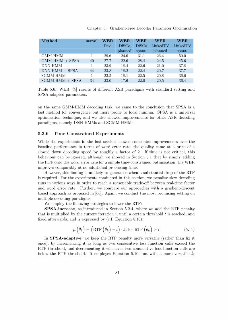
Chapter 5. Gradient-Free Decoder Parameter Optimisation
Method #eval WER WER WER WER WERDev. DiSCo DiSCo LinkedTV LinkedTV
planned spont. planned spont.GMM-HMM 1 29.6 24.0 31.1 26.4 50.0GMM-HMM + SPSA 40 27.7 22.6 28.4 24.5 45.6DNN-HMM 1 23.9 18.4 22.6 21.0 37.8DNN-HMM + SPSA 44 23.8 18.2 22.4 20.7 37.7SGMM-HMM 1 23.5 18.1 22.5 20.8 36.6SGMM-HMM + SPSA 34 23.0 17.6 22.0 20.5 36.4
Table 5.6: WER [%] results of different ASR paradigms with standard setting andSPSA adapted parameters.
on the same GMM-HMM decoding task, we came to the conclusion that SPSA is afast method for convergence but more prone to local minima. SPSA is a universaloptimisation technique, and we also showed improvements for other ASR decodingparadigms, namely DNN-HMMs and SGMM-HMMs.
5.3.6 Time-Constrained Experiments
While the experiments in the last section showed some nice improvements over thebaseline performance in terms of word error rate, the quality came at a price of aslowed down decoding speed by roughly a factor of 2. If time is not critical, thisbehaviour can be ignored, although we showed in Section 5.1 that by simply addingthe RTF onto the word error rate for a simple time-constrained optimisation, the WERimproves comparably at no additional processing time.
However, this finding is unlikely to generalise when a substantial drop of the RTFis required. For the experiments conducted in this section, we penalise slow decodingruns in various ways in order to reach a reasonable trade-off between real-time factorand word error rate. Further, we compare our approaches with a gradient-descentbased approach as proposed in [66]. Again, we conduct the most promising setting onmultiple decoding paradigms.
We employ the following strategies to lower the RTF:SPSA-increase, as introduced in Section 5.2.4, where we add the RTF penalty
that is multiplied by the current iteration i, until a certain threshold t is reached, andfixed afterwards, and is expressed by (c.f. Equation 5.10):
µ(θk
)=(
RTF(θk
)− t)· k , for RTF
(θk
)> t (5.11)
In SPSA-adaptive, we keep the RTF penalty more versatile (rather than fix itonce), by incrementing it as long as two consecutive loss function calls exceed theRTF threshold, and decrementing it whenever two consecutive loss function calls arebelow the RTF threshold. It employes Equation 5.10, but with a more versatile ki
81

Chapter 5. Gradient-Free Decoder Parameter Optimisation
computation: we increment k if RTF exceeds the threshold and decrement otherwise.
ki =
ki−1 + 1, if RTF
(θk
)> t
1, if ki−1 = 1 and RTF(θk
)≤ t
ki−1 − 1, otherwise
(5.12)
In our experiment with gradient descent, the starting point was obtained fromthe solution found by the unconstrained SPSA optimisation run as described above.The algorithm stops when it is unable to find any better tuple (i.e. a decoding run withlower RTF).
The results can be found in Table 5.7. In the experiments, the RTF threshold,which reflects the desired RTF, was set to a smaller RTF (60-80 %) compared to theunoptimised configuration. The desired RTF for the GMM-HMM was set to 3.0. Theresults indicate that the increasing RTF penalty (Figure 5.10) leads to considerablystabler results than the adaptive loss function (Figure 5.11). For the DNN-HMMapproach we set the desired RTF threshold to 0.8 and for the SGMM-HMM approachto 1.5, and were able to obtain these factors with little WER degradation.
Decoding paradigm #eval RTF WER WER WER WER WERDev. DiSCo DiSCo LinkedTV LinkedTV
planned spont. planned spont.GMM-HMM 1 4.2 29.6 24.0 31.1 26.4 50.0GMM-HMM + SPSA unconstrained 40 6.5 27.7 22.6 28.4 24.5 45.6GMM-HMM + SPSA increasing 86 2.8 28.9 23.1 28.5 25.2 46.5GMM-HMM + SPSA adaptive 86 3.0 29.1 23.0 28.1 25.6 46.3GMM-HMM + SPSA + Gradient Descent 80 3.9 28.7 23.6 29.5 25.5 47.6DNN-HMM 1 1.1 23.9 18.4 22.6 21.0 37.8DNN-HMM + SPSA increasing 16 0.8 24.2 18.7 22.8 21.2 38.1SGMM-HMM 1 2.5 23.5 18.1 22.5 20.8 36.6SGMM-HMM + SPSA increasing 28 1.6 24.3 18.9 23.3 21.2 38.0
Table 5.7: WER [%] results of different ASR paradigms with standard setting andSPSA adapted parameters.
As for time-constrained optimisation where a certain RTF is desired, we comparedvarious loss function strategies for SPSA and a gradient descent approach found in theliterature. In our set of experiments, gradient descent was unable to reach the set RTFthreshold. The SPSA extension using an increasing RTF penalty showed comparablebehaviour amongst the decoder paradigms.
5.4 Summary and Contributions
In this chapter we approached the fast, robust and efficient speech recognition decoderparameters optimisation. ASR decoder parameter optimisation is necessary to unlockthe full potential of a speech recognition system by tuning the parameters to sufficecertain requirements. These can be either to provide the optimal parameter for best
82
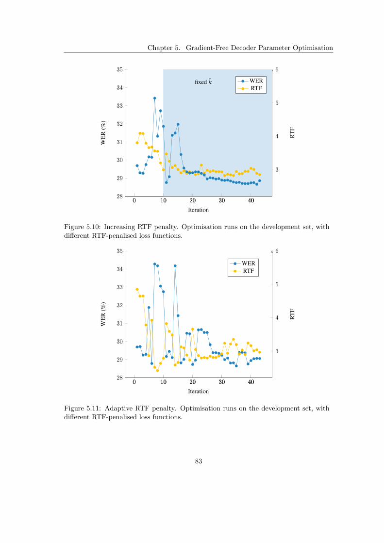
Chapter 5. Gradient-Free Decoder Parameter Optimisation
0 10 20 30 40
3
4
5
6
fixed k
RT
F
WERRTF
0 10 20 30 4028
29
30
31
32
33
34
35
Iteration
WE
R(%
)
Figure 5.10: Increasing RTF penalty. Optimisation runs on the development set, withdifferent RTF-penalised loss functions.
0 10 20 30 4028
29
30
31
32
33
34
35
Iteration
WE
R(%
)
0 10 20 30 40
3
4
5
6
RT
F
WERRTF
Figure 5.11: Adaptive RTF penalty. Optimisation runs on the development set, withdifferent RTF-penalised loss functions.
83

Chapter 5. Gradient-Free Decoder Parameter Optimisation
performance in terms of word-error-rate (WER), or to provide the optimal parametersfor the best performance in a different domain (e.g. telephone data, background carnoise), or to provide a speech recognition system that is fast in terms of real-time-factor (RTF) and accurate as well. Ideally, the optimisation procedure should be fast.This is why we introduced the SPSA algorithm to the task of speech recognition decoderparameter optimisation in this chapter. This algorithm, which was invented in [116]and further developed in [88] in a general mathematical context, has not been employedto the task of ASR decoder parameter optimisation before. In Section 5.1 we employedthe algorithm to optimise the performance expressed in WER in an unconstrainedsetting. We experienced, that the decoding time in terms of real-time-factor (RTF)of the optimised configuration is getting slower due to the increased complexity ofthe resulting configuration. Hence, in Section 5.2 we extend the SPSA algorithm byintroducing a RTF penalty in the loss function, with the intention of getting a fast andprecise speech recognition system. By introducing different RTF penalty terms we wereable to get speech recognition system that are both fast and precise. In Section 5.3we compare the SPSA algorithm for both constrained and unconstrained setting tostate-of-the-art methods, and show that the SPSA algorithm is faster in convergence(in terms of the number of evaluations of the development set) and provides comparableresults, due to the simultaneous perturbation of all parameters at a time. We end upwith a method that is fast in convergence, easy to deploy (by using the implementationguide from [117]) and which allows to receive fast speech recognition systems with highaccuracy.
84

Chapter 6
Dialects in Speech Recognition
Speech recognition systems which are trained on the standard language, like the stan-dard German broadcast speech recognition system which we developed and optimisedin the previous chapters and which is employed in the Fraunhofer IAIS audio miningsystem, nowadays show excellent performance on speech data which has characteristicssimilar to the training data. However, if a mismatch between the training data andthe testing data is present, these systems usually show degraded performance. Mis-matches include background noise, reverberation and the presence of dialectal speech.Mismatches regarding dialectal speech compared to standard language speech includemismatches in vocabulary, syntax, semantics, phonetics and prosody. Germany andother German speaking countries such as Austria and Switzerland have a broad varietyof regional dialects. Each dialect has its own differences compared to the standardlanguage or compared to other dialects. In speech recognition, these differences mostoften cause decoding errors and hence degraded performance. One way to cope withthe manifold of dialects in speech recognition is to identify the dialect in advance andthen use dialectal speech recognition models to decode the data [121]. In order toprovide excellent speech recognition performance in the audio mining system which weaim to deploy for regional broadcasters, we want to adopt this approach. Thereforein this chapter we develop a German dialect identification system, which is able todiscriminate between the standard language and various regional German dialects, andaim to train optimised dialectal speech recognition models to decode the speech data.The related work concerning dialect identification and related measures has alreadybeen discussed in Section 3.5. In Section 6.1 we discuss the manifold of German di-alects. In Section 6.2 we develop and optimise a German dialect identification system.In Section 6.3 we develop dialectal speech recognition models.
6.1 German Dialects
In Germany, Switzerland and Austria, German is among the official languages andthe first language of the majority of the population. These regions also show alarge variety of German dialects. The manifold of German dialects are depicted in
85

Chapter 6. Dialects in Speech Recognition
Figure 6.1. According to this map the German dialects can be grouped into LowGerman (“Niederdeutsch”), Middle German (“Mitteldeutsch”) and Upper German(“Oberdeutsch”) dialects. The Low German dialects may further be divided into WestLow German (“Westniederdeutsch”) and East Low German (“Ostniederdeutsch”) di-alects. Similarly, the Middle German dialects can be divided into West Middle German(“Westmitteldeutsch”) and East Middle German (“Ostmitteldeutsch”) dialects.
Figure 6.1: The structure of the Central European dialects of Germanic descent [122](Status 1900)
Upper German dialects can be divided into East Franconian (“Ostfrankisch”),Bavarian (“Bairisch”) and Alemannic (“Alemannisch”) dialects. Alemannic dialectsinclude the Swabian dialect (“Schwabisch”), and Bavarian dialects include NorthernBavarian (“Nordbairisch”), Middle Bavarian (“Mittelbairisch”) and Southern Bavar-ian (“Sudbairisch”). While linguists distinguish between standard language, colloquialspeech and dialects, the categorisation to these classes is very difficult due to the largevariability. Especially in the south of Germany linguists assume a continuum fromdialect to standard language for the phonetic area [122]. The colloquial languages arecertainly the most widely used language form, the old dialects are losing more and morespeakers and domains, they are superseded in favor of more spacious oriented languageforms, the colloquial languages [122].
86
Chapter 6. Dialects in Speech Recognition
6.2 German Dialect Identification
In this section the development and optimisation of a German dialect identificationsystem for the employment in the German broadcast domain are reported. The di-alect identification system is intended to derive the dialect of a speaker in advance, tochoose the optimal speech recognition models for decoding. It is also intended to enrichthe retrieved information, so that more specialised search queries are possible, whichfacilitates the search, e.g. for journalists.
6.2.1 German Dialect Identification Based on the RVG1 Database
In this section we describe the development of a German dialect identification systemfor the broadcast domain. We first identified existing German dialect corpora, that canbe used for this purpose. We found out that annotated dialectal speech resources arevery rare. The only German speech corpus that covers the utterances from speakers ofseveral German speaking regions including Austria and Switzerland is the BAS-RVG1(Bayerisches Archiv fur Sprachsignale - Regional variants of German) corpus [123]. Itcovers 85 utterances containing digits, connected digits, telephone numbers, phonet-ically balanced sentences, computer command and 1 minute of spontaneous monologper speaker (498 total speakers). The speakers were recorded in an office environmentwith 4 microphones. The utterances were read from a screen. The speakers are groupedaccording to the regional origin into the regions Low Franconian, Western Low German,Eastern Low German, Western Central German, Eastern Central German, Alemannic,East Franconian, South Franconian and Bavarian/Austrian.
We used the monologue sentences of the speakers and the region labels to train adialect identification system based on phone recognition followed by language model(PRLM, Section 3.5.1, [78]). Therefore we employed an open-loop phoneme recogniseron the corpus data and trained a m-gram language model on the recognised phonemestrings for each region. The open-loop phoneme recogniser is based on the standardGerman broadcast speech recogniser based on DNN-HMM trained on 636 hours ofspeech data as described in Section 4.3.4 and which was the best configuration at thetime of the experiments. However, instead of a word-level language model, a phonemelanguage model was employed, which covers the full set of the phonemes with equalprobabilities, so that the phoneme decoder outputs the likeliest phoneme sequenceaccording to the audio data without any knowledge of the underlying language. Thedecoded phoneme sequences are used to train a m-gram language model for each region.10 % of the data was withheld as test data in advance. For each sentence in the testset, we calculate the perplexity (c.f. Section 3.4.9) of each regional language modeland hypothesise the region for which the perplexity is minimal. Table 6.1 shows theaccuracy of the system for different m-gram language model orders. The best accuracyof 19.2 % can be reached with a language model order of 4. Since we have 9 dialectalregions and an equal distribution of regions in the test set, a random choice would havea precision of 1/9=11.1 %. Therefore this approach is well above chance level, thoughthe accuracy is still far from satisfactory.
87
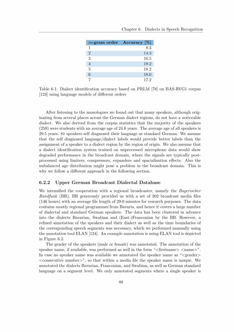
Chapter 6. Dialects in Speech Recognition
m-gram order Accuracy [%]1 8.32 14.33 16.54 19.25 18.26 18.07 17.2
Table 6.1: Dialect identification accuracy based on PRLM [78] on BAS-RVG1 corpus[123] using language models of different orders
After listening to the monologues we found out that many speakers, although orig-inating from several places across the German dialect regions, do not have a noticeabledialect. We also derived from the corpus statistics that the majority of the speakers(259) were students with an average age of 24.6 years. The average age of all speakers is29.5 years. 81 speakers self diagnosed their language as standard German. We assumethat the self diagnosed language/dialect labels would provide better labels than theassignment of a speaker to a dialect region by the region of origin. We also assume thata dialect identification system trained on unprocessed microphone data would showdegraded performance in the broadcast domain, where the signals are typically post-processed using limiters, compressors, expanders and spacialisation effects. Also theimbalanced age distribution might pose a problem in the broadcast domain. This iswhy we follow a different approach in the following section.
6.2.2 Upper German Broadcast Dialectal Database
We intensified the cooperation with a regional broadcaster, namely the BayerischerRundfunk (BR). BR generously provided us with a set of 302 broadcast media files(146 hours) with an average file length of 29.0 minutes for research purposes. The datacontains mostly regional programmes from Bavaria, and hence it covers a large numberof dialectal and standard German speakers. The data has been clustered in advanceinto the dialects Bavarian, Swabian and (East-)Franconian by the BR. However, arefined annotation of the speakers and their dialect as well as the time boundaries ofthe corresponding speech segments was necessary, which we performed manually usingthe annotation tool ELAN [124]. An example annotation is using ELAN tool is depictedin Figure 6.2.
The gender of the speakers (male or female) was annotated. The annotation of thespeaker name, if available, was performed as well in the form “<firstname> <name>”.In case no speaker name was available we annotated the speaker name as “<gender><consecutive number>”, so that within a media file the speaker name is unique. Weannotated the dialects Bavarian, Franconian, and Swabian, as well as German standardlanguage on a segment level. We only annotated segments where a single speaker is
88

Chapter 6. Dialects in Speech Recognition
Figure 6.2: Example of an ELAN annotation for the task of dialect identification
present. The underlying text of the spoken utterances has not been annotated. Wedid not do this, because on the one hand it is a very time consuming process, and onthe other hand because there is no standardised way to annotate dialects other thanstandard German. Also, it is not necessary for the task of dialect identification anddialect detection.
So far we have fine-annotated 52 media files with a total of 2,710 speech segmentsfrom 398 speakers (282 male, 116 female) in an ongoing process with a total segmentsize of 11.8 hours. An average of 106.5 seconds and an average of 6.8 segments havebeen annotated per speaker in this dataset. The average length of a segment is 15.6seconds with a rather high standard deviation of 12.6 seconds, which is not unusualfor real-world data from the broadcast domain. 75 standard German speakers, 149Bavarian dialect speakers, 89 Swabian dialect speakers and 85 Franconian speakershave been annotated. We converted the audio data into RIFF/WAVE format (16 kHzsampling rate, 16 bits per sample, 1 channel).
89

Chapter 6. Dialects in Speech Recognition
Input Layer: Filterbank coefficients (40,6000)
Layer 1: Conv2D, ReLU, 32 kernels, 5x500
Layer 2: Conv2D, ReLU, 32 kernels, 5x5
Layer 3: MaxPooling2D, 2x2
Layer 4: Conv2D, ReLU, 32 kernels, 3x3
Layer 5: MaxPooling2D, 2x2
Layer 6: Flatten
Layer 7: Dense, ReLU, 128 neurons
Output Layer: Softmax Layer (number of classes)
Figure 6.3: CNN architecture
6.2.3 German Broadcast Dialect Identification
In this section we use of the dialect database (Section 6.2.2) to train a dialect identifi-cation system that is able to discriminate between standard German and Franconian,Swabian and Bavarian dialect. We split the data into a training, validation and a testset. First of all, we exclude segments that are smaller than one second from the data. Ina second step, we only keep a maximum of two minutes of speech data per speaker. Webalance the number of speakers per dialect for each subset to have a balanced dataset.Also, speakers are disjunct across the subsets, so that a single speaker can only occur inone of the datasets. The selection which speaker goes to which dataset was performedrandomly. The training set covers the segments of 35 speakers per dialect with a totalof 635 segments (2.6 hours). The validation set covers 20 speakers per dialect with atotal of 341 segments (1.3 hours) and the test set also covers 20 speakers per dialectwith a total of 321 segments (1.3 hours).
For the task of dialect identification we train a convolutional neural network usingthe Keras Toolkit [125] with Tensorflow [126] backend. First, the audio signal is filteredby a first order IIR preemphasis filter (a = 0.97). A set of 40 mel-spaced filterbankcoefficients is extracted for windows of length 25 ms with a hopsize of 10 ms. Thefilters cover the whole range from 0-8 kHz. The filterbank coefficients of the wholesegment (zero-padded, 1 minute maximum) are then fed into a convolutional neuralnetwork (CNN), whose output is a probability function over the investigated dialects,implemented by the softmax output layer. This network has 4 outputs, one for each
90

Chapter 6. Dialects in Speech Recognition
dialect (including standard German). By using the softmax function the network isable to provide either class decisions or class probabilities if a soft decision is desirable.The employed CNN architecture is depicted in Figure 6.3. We use AdaDelta optimiserusing the mean squared error as the loss function. For training we employ an adaptivelearning rate algorithm and an early stopping mechanism based on the validation lossto avoid overfitting.
Germ
an
Bavar
ian
Swab
ian
Franco
nian
Predicted label
German
Bavarian
Swabian
Franconian
True
labe
l
61 8 15 2
5 36 19 20
11 4 54 11
14 15 15 31
Confusion matrix
10
20
30
40
50
60
(a) Segment level
Germ
an
Bavar
ian
Swab
ian
Franco
nian
Predicted label
German
Bavarian
Swabian
FranconianTr
uela
bel
0.71 0.09 0.17 0.02
0.06 0.45 0.24 0.25
0.14 0.05 0.68 0.14
0.19 0.20 0.20 0.41
Confusion matrix
0.1
0.2
0.3
0.4
0.5
0.6
0.7
(b) Normalised
Figure 6.4: Confusion matrix results of the dialect identification system on the test set
The results of this approach on the test set in terms of segment level and normalisedconfusion matrices are depicted in Figure 6.4. The accuracy of the system on the testset is 56.7 %. This is a promising result, considering the number of classes (4), thesmall amount of training data (2.6 hours) and also the fact that this data is collectedfrom a heterogeneous set of real-world broadcast media files with speech segments oflimited and highly variable length.
6.2.4 German Broadcast Dialect Detection
We use the same dialectal database (Section 6.2.2) to train a dialect detection systemthat is able to distinguish between standard German and dialectal speech. Using thesoft decision classifier output the system is able to infer the “dialectness” of a speaker.Also, the algorithm can determine whether the standard German speech recognitionsystem is likely to show degraded performance, which is the case if dialectal speakersare present.
Again, we split the data into balanced training, validation and testing datasets ina similar fashion as in Section 6.2.3. The training set covers the segments of each35 speakers for standard German and dialectal speech with a total size of 1.2 hours.Both the validation and the testing set cover the segments of each 20 speakers forstandard German and dialectal speech. The total size of the validation set is 0.8 hoursand also the total size of the testing set is 0.8 hours. The dialectal speakers are also
91

Chapter 6. Dialects in Speech Recognition
balanced across the dialects Bavarian, Franconian and Swabian. The selection of thespeakers was performed randomly. The employed CNN architecture is again depictedin Figure 6.3 and is similar to the classifier for the dialect identification task. However,in this case the neural network only has 2 outputs, one for standard German and onefor dialectal speech. Also, the training procedure of the neural network is similar tothe approach in Section 6.2.3.
The results of this approach on the test set are depicted in Figure 6.5. The accuracyof the system is 77.1 %, which is a promising result considering the even smaller amountof training data (1.2 hours). Note that the segment level confusion matrix is unbalancedto some extent. Even though we use an equal number of distinct speakers in thetwo categories, the number of annotated segments per speaker is subject to naturaldeviations.
Germ
an
Dialec
t
Predicted label
German
Dialect
True
labe
l
64 22
21 81
Confusion matrix
30
40
50
60
70
80
(a) Segment level
Germ
an
Dialec
t
Predicted label
German
Dialect
True
labe
l0.74 0.26
0.21 0.79
Confusion matrix
0.3
0.4
0.5
0.6
0.7
(b) Normalised
Figure 6.5: Confusion matrix results of the dialect detection system on the test set
6.3 Dialectal Speech Recognition
In this section we describe the development of a Swiss German dialectal speech recog-nition system.
6.3.1 Swiss German
Switzerland has four national languages: German/Swiss German (63%), French(22.7%), Italian (8.1%), Romansh (0.5%); the numbers in brackets are the percent-ages of the population speaking them1. As can be derived from Figure 6.6, French(“Franzosisch”) is spoken in the west, Italian (“Italienisch”) is spoken primarily in Ti-cino (“Tessin”), Val Bregaglia and Val Pschiavo and Romansh speakers are distributedover Graubunden.
1http://www.swissinfo.ch; Accessed on October 27th, 2017
92

Chapter 6. Dialects in Speech Recognition
Figure 6.6: Language map of Switzerland [122]
Swiss German is not a uniform language, but is composed of many regional dialectsof Alemannic origin. Although school and science maintain the standard German high-level language, after the lessons the teacher speaks in dialect to the pupils, as well asthe professor to the students. On television and radio, dialect is spoken, intertwinedwith segments in which the reporter speaks in standard German, with the exception ofa few broadcasts. Swiss German is spoken, standard German is written [122].
6.3.2 SRF Meteo Weather Report Dataset
In this section we describe the Swiss German SRF Meteo dataset, which Schweizer Ra-dio und Fernsehen generously provided us for research purposes. This dataset consistsof Swiss German weather reports of SRF Meteo. The speakers speak Swiss Germandialect, and the textual annotation is standard German. The dataset consists of 290Meteo weather report broadcasts with a total of 10,201 speech segments and a total of6.5 hours of annotated speech and a total of 83,449 annotated words. The containedspeech is to a large extent about weather forecasts and contains a large number of placenames.
For the experiments we separated the Meteo dataset into a training, developmentand a test set as listed in Table 6.2.
Dataset #Shows #Segments #Words Avg. Words #Unique Size(h) Avg. Length (s)Training 260 9,181 75,215 8.2 2,981 5.9 2.3Development 15 493 3,995 8.1 742 0.3 2.2Test 15 527 4,242 8.1 778 0.3 2.2
Table 6.2: Statistics of the Meteo data subsets used in this work
93
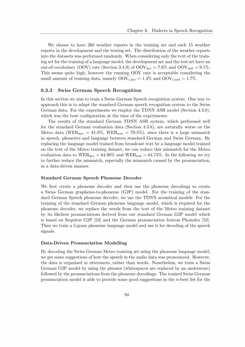
Chapter 6. Dialects in Speech Recognition
We choose to have 260 weather reports in the training set and each 15 weatherreports in the development and the testing set. The distribution of the weather reportsinto the datasets was performed randomly. When considering only the text of the train-ing set for the training of a language model, the development set and the test set have anout-of-vocabulary (OOV) rate (Section 3.4.9) of OOVdev = 7.6% and OOVtest = 9.1%.This seems quite high, however the running OOV rate is acceptable considering thesmall amount of training data, namely OOVr,dev = 1.4% and OOVr,test = 1.7%.
6.3.3 Swiss German Speech Recognition
In this section we aim to train a Swiss German Speech recognition system. One way toapproach this is to adapt the standard German speech recognition system to the SwissGerman data. For the experiments we employ the TDNN ASR model (Section 4.3.8),which was the best configuration at the time of the experiments.
The results of the standard German TDNN ASR system, which performed wellfor the standard German evaluation data (Section 4.3.8), are naturally worse on theMeteo data (WERdev = 81.0%, WERtest = 79.5%), since there is a large mismatchin speech, phonetics and language between standard German and Swiss German. Byreplacing the language model trained from broadcast text by a language model trainedon the text of the Meteo training dataset, we can reduce this mismatch for the Meteoevaluation data to WERdev = 64.98% and WERtest = 64.73%. In the following we tryto further reduce the mismatch, especially the mismatch caused by the pronunciation,in a data-driven manner.
Standard German Speech Phoneme Decoder
We first create a phoneme decoder and then use the phoneme decodings to createa Swiss German grapheme-to-phoneme (G2P) model. For the training of the stan-dard German Speech phoneme decoder, we use the TDNN acoustical models. For thetraining of the standard German phoneme language model, which is required for thephoneme decoder, we replace the words from the text of the Meteo training datasetby its likeliest pronunciations derived from our standard German G2P model whichis based on Sequitur G2P [53] and the German pronunciation lexicon Phonolex [52].Then we train a 5-gram phoneme language model and use it for decoding of the speechsignals.
Data-Driven Pronunciation Modelling
By decoding the Swiss German Meteo training set using the phoneme language model,we get some suggestions of how the speech in the audio data was pronounced. However,the data is organised in utterances, rather than words. Nonetheless, we train a SwissGerman G2P model by using the phrases (whitespaces are replaced by an underscore)followed by the pronunciations from the phoneme decodings. The trained Swiss Germanpronunciation model is able to provide some good suggestions in the n-best list for the
94
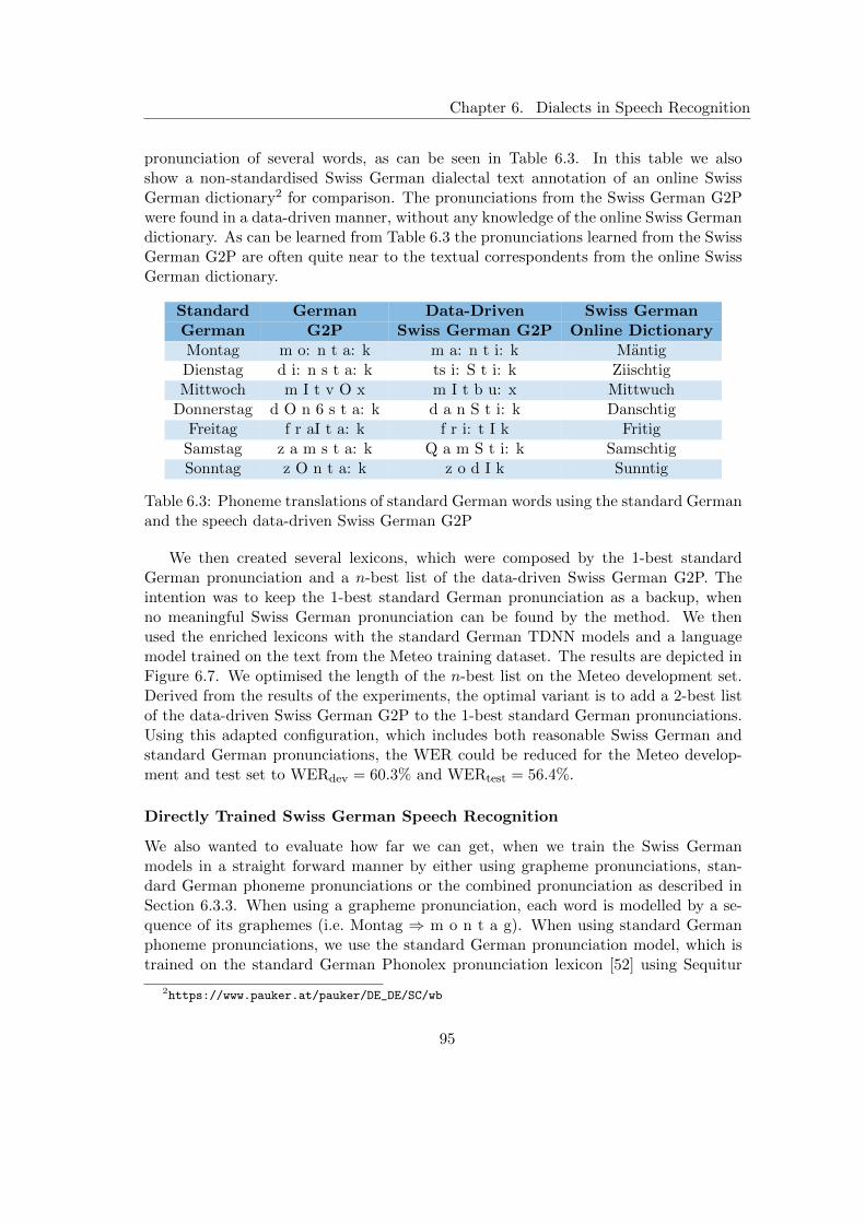
Chapter 6. Dialects in Speech Recognition
pronunciation of several words, as can be seen in Table 6.3. In this table we alsoshow a non-standardised Swiss German dialectal text annotation of an online SwissGerman dictionary2 for comparison. The pronunciations from the Swiss German G2Pwere found in a data-driven manner, without any knowledge of the online Swiss Germandictionary. As can be learned from Table 6.3 the pronunciations learned from the SwissGerman G2P are often quite near to the textual correspondents from the online SwissGerman dictionary.
Standard German Data-Driven Swiss GermanGerman G2P Swiss German G2P Online DictionaryMontag m o: n t a: k m a: n t i: k MantigDienstag d i: n s t a: k ts i: S t i: k ZiischtigMittwoch m I t v O x m I t b u: x Mittwuch
Donnerstag d O n 6 s t a: k d a n S t i: k DanschtigFreitag f r aI t a: k f r i: t I k Fritig
Samstag z a m s t a: k Q a m S t i: k SamschtigSonntag z O n t a: k z o d I k Sunntig
Table 6.3: Phoneme translations of standard German words using the standard Germanand the speech data-driven Swiss German G2P
We then created several lexicons, which were composed by the 1-best standardGerman pronunciation and a n-best list of the data-driven Swiss German G2P. Theintention was to keep the 1-best standard German pronunciation as a backup, whenno meaningful Swiss German pronunciation can be found by the method. We thenused the enriched lexicons with the standard German TDNN models and a languagemodel trained on the text from the Meteo training dataset. The results are depicted inFigure 6.7. We optimised the length of the n-best list on the Meteo development set.Derived from the results of the experiments, the optimal variant is to add a 2-best listof the data-driven Swiss German G2P to the 1-best standard German pronunciations.Using this adapted configuration, which includes both reasonable Swiss German andstandard German pronunciations, the WER could be reduced for the Meteo develop-ment and test set to WERdev = 60.3% and WERtest = 56.4%.
Directly Trained Swiss German Speech Recognition
We also wanted to evaluate how far we can get, when we train the Swiss Germanmodels in a straight forward manner by either using grapheme pronunciations, stan-dard German phoneme pronunciations or the combined pronunciation as described inSection 6.3.3. When using a grapheme pronunciation, each word is modelled by a se-quence of its graphemes (i.e. Montag ⇒ m o n t a g). When using standard Germanphoneme pronunciations, we use the standard German pronunciation model, which istrained on the standard German Phonolex pronunciation lexicon [52] using Sequitur
2https://www.pauker.at/pauker/DE_DE/SC/wb
95

Chapter 6. Dialects in Speech Recognition
0 1 2 3 4 5n
54
56
58
60
62
64
66
WER
[%]
Meteo DevMeteo Test
Figure 6.7: WER for different n for configurations with 1-best standard German pro-nunciation and n-best Swiss German pronunciations from the speech data driven G2Pmodel
G2P [53]. For the training of the acoustical model we use the training dataset of theSRF Meteo dataset. For training the language model we use IRSTLM toolkit [127] andwe use a 5-gram model with modified shift beta algorithm with back-off weights. Fortraining of the Swiss German ASR system, we either use Eesen [48] toolkit, when usinglong short term memory (LSTM) recurrent neural networks (RNN) with connectionisttemporal classification (CTC) training, or the Kaldi toolkit [55], when using HiddenMarkov Models with Gaussian Mixture Models (HMM-GMM), or hybrid HMM withfeed forward Deep Neural Networks (HMM-DNN) or the state-of-the-art time delayneural networks with projected long short-term memory (TDNN-LSTMP) layers. Theresults are shown in Table 6.4. The HMM-GMM, DNN and TDNN-LSTMP modelsfrom the Kaldi toolkit are trained with bootstrapping and provide more stable resultsin this setup (i.e. a setup with a small amount of training data) compared to the RNNmodels, which use Connectionist Temporal Classification (CTC) instead, and whichare trained directly on the audio data. It is also remarkable that there is no big differ-ence when comparing standard German grapheme pronunciations to standard Germanphoneme pronunciations. Both setups perform almost equally well. The use of thecombined standard German and Swiss German pronunciation performed slightly worsecompared to standard German and grapheme pronunciations for the HMM-GMM case.We believe this is the case because during training the algorithm needs a consistentsingle pronunciation, so the algorithm can model the pronunciation including the pos-sible mismatches consistently. The TDNN-LSTM models trained with the standard
96
Chapter 6. Dialects in Speech Recognition
German G2P pronunciations performed best on the Meteo test set (WERtest = 23.8%)given the experiments performed.
Model Pronunciation Development TestHMM-GMM German G2P 39.7 28.9HMM-GMM Grapheme 40.3 29.6HMM-GMM Combined G2P 41.3 30.8RNN German G2P 44.5 32.7RNN Grapheme 45.0 32.3HMM-DNN German G2P 37.1 27.1HMM-DNN Grapheme 37.7 27.0TDNN-LSTMP German G2P 34.9 23.8TDNN-LSTMP Grapheme 34.8 24.3
Table 6.4: WER [%] results on the Meteo development and test set of directly trainedSwiss German speech recognitions systems using different types of pronunciation lexi-cons; standard German G2P, combined data-driven Swiss German and standard Ger-man G2P or grapheme sequences
6.4 Summary and Contributions
In this chapter we approached the dialectal robustness of speech recognition systemsin the German broadcast domain with the aim to provide optimal performance of theFraunhofer IAIS audio mining system also for regional broadcasters. We followed thestrategy to identify the underlying dialect in advance and then use dialectal speechrecognition models to decode the data [121]. Therefore we first briefly discussed themanifold of German dialects in Section 6.1.
In Section 6.2 we developed and optimised a German dialect identification system.However, existing annotated dialectal resources are limited, and often of limited useas we found out in Section 6.2.1, where we trained a dialect identification systemon the data with limited success. Hence, we built up a close cooperation a regionalbroadcaster from Bavaria, namely the Bayerischer Rundfunk, who provided us with 302media files of regional programmes from Bavaria for research purposes. The dialectsthat are covered in the data are Bavarian, Franconian, Swabian and also standardGerman. 2,710 utterances from 52 media files from a total of 398 speakers (282 male,116 female) have been annotated so far in an ongoing process. The current total sizeof the annotated data is 11.8 hours. This data has been used to train and evaluateboth a dialectal identification and a dialect detection system based on convolutionalneural networks (CNNs). The dialect identification system that has been trained on2.6 hours of speech data taken from the proposed corpus is able to distinguish betweenfour dialects with an accuracy of 56.7 %. The dialect detection system which hasbeen trained on 1.2 hours of speech data taken from this corpus is able to distinguishbetween standard German and dialectal speech with an accuracy of 77.1 %. These are
97
Chapter 6. Dialects in Speech Recognition
promising results considering the low amount of training material available and thechallenges that are accompanied with real-world broadcast domain data. To furtherincrease the accuracy of the systems we will continue our efforts to extend the corpussize by annotating a larger amount of regional programmes. Is is also possible to extendthe system to other dialects by exploiting regional programmes from other Germanspeaking regions.
We intend to use specialised dialectal speech recognition models after the dialectidentification step. We approached the adaptation and a training of a dialectal speechrecognition system in Section 6.3. As already mentioned, annotated dialectal resourcesare limited, and the annotation of dialectal resources is costly. However, we establisheda close cooperation with the Schweizer Radio und Fernsehen, who generously providedus an annotated Swiss German dataset (Section 6.3.2). Since there is no standardisedway to write Swiss German other than standard German, the annotations of the SwissGerman audio corpus are standard German, in contrast to the audio material whichis highly dialectical Swiss German. The desired output of the Swiss German speechrecognition system is again standard German. Unfortunately we lacked a Swiss Germanpronunciation lexicon that maps standard German words into Swiss German pronun-ciations. We approached this problem by successfully adapting our standard Germanspeech recognition system to the Swiss German pronunciations by the employment ofa Swiss German G2P model which was learned in a data-driven manner by phonemedecodings derived from the standard German speech recognition system with the use ofa phoneme language model. It turned out that by adding a 2-best list of Swiss Germanpronunciations derived from the data-driven Swiss German G2P model to the 1-beststandard pronunciations, the adapted model provided the best results, when adaptingthe standard German model. However, the training of an ASR system directly on theSwiss German data by replacing the missing Swiss German pronunciation by either astandard German phoneme or grapheme sequences, provided even better results. Theuse of the combined lexicon did not prove to be beneficial in this case when training asystem directly on the Swiss German audio data in contrast to the adaptation of thestandard German model. The standard German TDNN models which perform verywell on standard German data, showed degraded performance on the Swiss Germandata with word error rates as high as 79.5 % on the test corpus. For the Swiss Germanspeech recognition models, the use of TDNN-LSTMP provided the best results withword error rates as low as 23.8 % on the corresponding Swiss German test set. Thisare encouraging results given the small amount of available training data in the SwissGerman case.
The results reported in this chapter are encouraging. We intended to integrateseveral dialects in the dialect identification and speech recognition pipeline. However,a lot of dialectal speech resources need to be acquired, which is a time consuming andcostly task, since many of the required resources simply do not exist in an annotatedform at this time.
98

Chapter 7
Scientific Achievements andConclusions
7.1 Scientific Achievements
In this section, we revisit the scientific goals defined at the beginning of this work inChapter 2 and examine how far we have accomplished them.
Related to the long-term development of the German broadcast speech recognitionsystem (Chapter 4):
• We extended the amount of training data dramatically and exploited the data forthe training of the speech recognition system.
• We evaluated several state-of-the-art speech recognition algorithms that appearedduring the term of this thesis from the scientific community for their employmentin the German broadcast domain.
• We evaluated the speech recognition systems for the employment in a productiveaudio mining system. Two speech recognition models that are the outcome ofthis thesis have been employed in the Fraunhofer IAIS audio mining system.
Related to the automatic speech recognition decoder parameter optimisation (Chap-ter 5):
• We adopted a fast and efficient parameter optimisation algorithm, which has notbeen used in the context of speech recognition before, for the speech recognitiondecoder parameter optimisation.
• We employed the algorithm to optimise the accuracy of the speech recognitionsystem.
• We extended the algorithm to jointly optimise the accuracy and the decodingspeed.
99
Chapter 7. Scientific Achievements and Conclusions
• We compared the algorithm to other state-of-the-art optimisation algorithms.
Related to dialectal robustness of the speech recognition system (Chapter 6):
• We adopted a strategy how to deal with the manifold of dialects for the Germanspeech.
• We established a close and continuing cooperation with regional broadcasters suchas the Bayerischer Rundfunk and Schweizer Rundfunk und Fernsehen.
• We created a novel German dialect corpus for the task of dialect identification inthe broadcast domain, where we annotated a considerable quantity of dialectaland standard German speech.
• We trained dialectal speech recognition systems with the help of data-drivenpronunciation modelling and model adaptation.
7.2 Publications
The following enumeration covers the publications of the author conducted within theterm of this thesis and which are related to the work in this thesis.
• M. Stadtschnitzer, D. Stein, and R. Bardeli, “Employing Stochastic ConstrainedLMS Algorithm for ASR Frontend Processing,” in Proc. of The 2nd CHiMESpeech Separation and Recognition Challenge, Vancouver, Canada, 2013
• J. Schwenninger, D. Stein, and M. Stadtschnitzer, “Automatic Parameter Tun-ing and Extended Training Material: Recent Advances in the Fraunhofer SpeechRecognition System,” Proc. Workshop Audiosignal- und Sprachverarbeitung, 2013
• D. Stein, J. Schwenninger, and M. Stadtschnitzer, “Simultaneous PerturbationStochastic Approximation for Automatic Speech Recognition,” Proc. Interspeech,pp. 622–626, 2013
• D. Stein, B. Krausz, J. Loffler, R. Marterer, R. Bardeli, M. Stadtschnitzer, andJ. Schwenninger, “Automatic Audio and Video Event Recognition in an IntelligentResource Management System,” IJISCRAM, vol. 5, no. 4, pp. 1–12, 2013
• M. Stadtschnitzer, J. Schwenninger, D. Stein, and J. Koehler, “Exploiting theLarge-Scale German Broadcast Corpus to Boost the Fraunhofer IAIS SpeechRecognition System,” in Proceedings of the 9th Language Resources and Eval-uation Conference (LREC), Reykjavik, Iceland, May 2014
• M. Stadtschnitzer, J. Koehler, and D. Stein, “Improving Automatic Speech Recog-nition for Effective Topic Segmentation,” in Proc. DAGA - 40. Jahrestagung furAkustik, Oldenburg, Germany, 2014
100

Chapter 7. Scientific Achievements and Conclusions
• M. Stadtschnitzer, C. Schmidt, and D. Stein, “Towards a Localised German Auto-matic Speech Recognition,” in Proc. 11. ITG Fachtagung Sprachkommunication,Erlangen, Germany, 2014
• T. L. Nguyen, D. Stein, and M. Stadtschnitzer, “Gradient-Free Decoding Pa-rameter Optimization on Automatic Speech Recognition,” in IEEE InternationalConference on Acoustics, Speech and Signal Processing (ICASSP), Florence, Italy,2014, pp. 3261 – 3265
• H. Le, Q. Bui, B. Huet, B. Cervenkova, J. Bouchner, E. Apostolidis,F. Markatopoulou, A. Pournaras, V. Mezaris, D. Stein, S. Eickeler, andM. Stadtschnitzer, “LinkedTV at MediaEval 2014 Search and Hyperlinking Task,”in Proceedings of the MediaEval 2014 Workshop, Catalunya, Spain, October 2014
• M. Stadtschnitzer and C. Schmidt, “Implementation of a Live Dialectal MediaSubtitling System,” in Proceedings of the 16th Annual Conference of the Interna-tional Speech Communication Association (INTERSPEECH), Dresden, Germany,Sep. 2015, pp. 728–729
• C. Schmidt, M. Stadtschnitzer, and J. Kohler, “The Fraunhofer IAIS Audio Min-ing System: Current State and Future Directions,” in Proceedings of the 12th ITGConference on Speech Communication, Paderborn, Germany, 2016
• M. Stadtschnitzer and C. Schmidt, “Joint Standard German and Bavarian Subdi-alect Identification of Broadcast Speech,” in Proceedings of DAGA - 44. Jahresta-gung fur Akustik, Munchen, Germany, Mar. 2018
• M. Stadtschnitzer and C. Schmidt, “Adaptation and Training of a Swiss Ger-man Speech Recognition System using Data-driven Pronunciation Modelling,” inProceedings of DAGA - 44. Jahrestagung fur Akustik, Munchen, Germany, Mar.2018
• M. Stadtschnitzer and C. Schmidt, “Data-Driven Pronunciation Modelling ofSwiss German Dialectal Speech for Automatic Speech Recognition,” in Proc.of 11th Edition of the Language Resources and Evaluation Conference (LREC),Miyazaki, Japan, May 2018
7.3 Conclusions
In this thesis, we have addressed three issues with regard to robust speech recognitionin the German broadcast domain.
First, we developed and optimised the speech recognition system, which is part ofthe Fraunhofer IAIS audio mining system, over a long period of time. Therefore, wecontinuously evaluated a large number of speech recognition algorithms that becameavailable in the scientific community in the course of this thesis for the employment inthe German broadcast domain and found the optimal configuration of the systems for
101

Chapter 7. Scientific Achievements and Conclusions
our use case and extended the training data size by annotating and exploiting a largequantity of speech data.
Second, we introduced a fast and efficient parameter optimisation algorithm, whichhas not been employed in the context of speech recognition before, to speech recog-nition decoder parameter optimisation and compared the algorithm to state-of-the-artdecoder parameter optimisation algorithms. We employed the algorithm to optimisethe accuracy of the speech recognition system and extended the algorithm to jointlyoptimise the accuracy and the decoding speed.
Third, to handle the manifold of German dialects for speech recognition in thebroadcast domain, we adopted an approach to determine the dialect of a speaker inadvance to choose from dialectal speech recognition models. Therefore we acquired,employed and created German dialectal resources to train dialect identification anddialectal speech recognition models.
By approaching the three issues we arrived at a German broadcast speech recog-nition system with high performance and optimal decoder parameters that fulfils therequirements of a productive audio mining system and that is able to cope with themanifold of German dialects which occur in the programmes of the public broadcasterARD and its regional broadcast stations.
102
Appendix A
Toolkits
In this section the software and toolkits that were used throughout this thesis, arebriefly described.
A.1 HTK Toolkit
The Hidden Markov Model Toolkit (HTK) [61] is a toolkit for the training andmanipulation of Hidden Markov Models (HMM). HTK is primarily built for speechrecognition research, however it has also been used for other topics including speechsynthesis and character recognition. HTK is developed and maintained by theUniversity of Cambridge Department of Engineering (CUED). The current stableversion is version 3.4.1.
http://htk.eng.cam.ac.uk/
A.2 Kaldi
The Kaldi Toolkit [55] is a open-source toolkit for the automatic speech recognitionresearch. The speech recognition systems trained with Kaldi are based on finite-statetransducers (implemented by the open-source framework OpenFst). Kaldi includesexample scripts for the training of speech recognition systems for the most prominentspeech recognition research databases (e.g. TIMIT, Switchboard, etc.). Kaldi iswritten in C++ and is written in a very modular fashion (i.e., it consists of a large setof scripts and executables).
http://kaldi-asr.org/
103
Appendix A. Toolkits
A.3 Eesen
The Eesen Toolkit [48] is open-source toolkit for the creation of automatic speechrecognition systems based on bi-directional Recurrent Neural Networks (RNN) withLong Short-time Memory (LSTM) units and on Connectionist temporal classification(CTC) alignment. The toolkit was created by Yajie Miao based on the Kaldi Toolkit.The toolkit discards the exhaustive bootstrapping process by replacing it with astraightforward learning problem.
https://github.com/yajiemiao/eesen
A.4 RNNLM
The RNNLM Toolkit [98] is a open-source toolkit for the training and evaluationof statistical language models (LM) based on recurrent neural networks (RNN) forautomatic speech recognition and machine translation. The toolkit is written byTomas Mikolov. The author reports significant improvements over classic backoffm-gram models.
http://www.fit.vutbr.cz/~imikolov/rnnlm/
A.5 IRSTLM
The IRSTLM toolkit [127] is a open-source toolkit that allows the efficient training oflarge scale n-gram language models. It allows to train language models with billionsof m-grams on conventional computers. The software has been integrated in theopen-source statistical machine translation decoder Moses and is also part of the Kalditoolkit. The software is developed by FBK-HLT in Trento.
http://hlt-mt.fbk.eu/technologies/irstlm
A.6 Sequitur-G2P
Sequitur-G2P [53] is a statistical grapheme-to-phoneme converter developed at RWTHAachen University - Department of Computer Science. The software was developed byMaximilian Bisani. The software is released under the GNU Public License.
https://www-i6.informatik.rwth-aachen.de/web/Software/g2p.html
104
Appendix A. Toolkits
A.7 TheanoLM
TheanoLM [140] is a toolkit for the training of neural network language models andwhich uses the Python library Theano. The authors report significant improvementover back-off n-gram models.
https://github.com/senarvi/theanolm
A.8 Keras
Keras [125] is a high-level neural network library written in Python. It employs eitherTensorFlow or Theano as backend. Keras allows for rapid prototyping and supportsboth recurrent neural networks, convolutional neural networks, dense networks andcombinations of architectures.
https://keras.io/
105
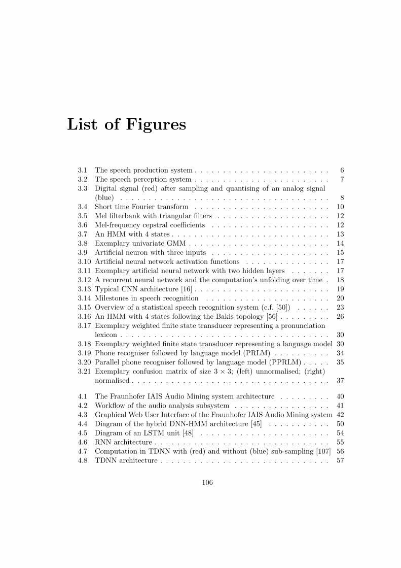
List of Figures
3.1 The speech production system . . . . . . . . . . . . . . . . . . . . . . . . 63.2 The speech perception system . . . . . . . . . . . . . . . . . . . . . . . . 73.3 Digital signal (red) after sampling and quantising of an analog signal
(blue) . . . . . . . . . . . . . . . . . . . . . . . . . . . . . . . . . . . . . 83.4 Short time Fourier transform . . . . . . . . . . . . . . . . . . . . . . . . 103.5 Mel filterbank with triangular filters . . . . . . . . . . . . . . . . . . . . 123.6 Mel-frequency cepstral coefficients . . . . . . . . . . . . . . . . . . . . . 123.7 An HMM with 4 states . . . . . . . . . . . . . . . . . . . . . . . . . . . . 133.8 Exemplary univariate GMM . . . . . . . . . . . . . . . . . . . . . . . . . 143.9 Artificial neuron with three inputs . . . . . . . . . . . . . . . . . . . . . 153.10 Artificial neural network activation functions . . . . . . . . . . . . . . . 173.11 Exemplary artificial neural network with two hidden layers . . . . . . . 173.12 A recurrent neural network and the computation’s unfolding over time . 183.13 Typical CNN architecture [16] . . . . . . . . . . . . . . . . . . . . . . . . 193.14 Milestones in speech recognition . . . . . . . . . . . . . . . . . . . . . . 203.15 Overview of a statistical speech recognition system (c.f. [50]) . . . . . . 233.16 An HMM with 4 states following the Bakis topology [56] . . . . . . . . . 263.17 Exemplary weighted finite state transducer representing a pronunciation
lexicon . . . . . . . . . . . . . . . . . . . . . . . . . . . . . . . . . . . . . 303.18 Exemplary weighted finite state transducer representing a language model 303.19 Phone recogniser followed by language model (PRLM) . . . . . . . . . . 343.20 Parallel phone recogniser followed by language model (PPRLM) . . . . . 353.21 Exemplary confusion matrix of size 3 × 3; (left) unnormalised; (right)
normalised . . . . . . . . . . . . . . . . . . . . . . . . . . . . . . . . . . . 37
4.1 The Fraunhofer IAIS Audio Mining system architecture . . . . . . . . . 404.2 Workflow of the audio analysis subsystem . . . . . . . . . . . . . . . . . 414.3 Graphical Web User Interface of the Fraunhofer IAIS Audio Mining system 424.4 Diagram of the hybrid DNN-HMM architecture [45] . . . . . . . . . . . 504.5 Diagram of an LSTM unit [48] . . . . . . . . . . . . . . . . . . . . . . . 544.6 RNN architecture . . . . . . . . . . . . . . . . . . . . . . . . . . . . . . . 554.7 Computation in TDNN with (red) and without (blue) sub-sampling [107] 564.8 TDNN architecture . . . . . . . . . . . . . . . . . . . . . . . . . . . . . . 57
106

List of Figures
4.9 Architecture of a projected LSTM block [109] . . . . . . . . . . . . . . 584.10 TDNN-LSTMP architecture . . . . . . . . . . . . . . . . . . . . . . . . . 594.11 Performance of different configurations of the Fraunhofer IAIS speech
recognition system, grouped by approach . . . . . . . . . . . . . . . . . 624.12 Performance of different configurations of the Fraunhofer IAIS speech
recognition system, grouped by test set . . . . . . . . . . . . . . . . . . . 62
5.1 First example run of the SPSA and its word error rate progression onthe development corpus . . . . . . . . . . . . . . . . . . . . . . . . . . . 70
5.2 WER progression on DiSCo corpora. WER results on planned and spon-taneous data, showing the first run of SPSA with 18 iterations. Iteration0 denotes the employed speech recognition configuration without SPSAparameter optimisation. . . . . . . . . . . . . . . . . . . . . . . . . . . . 71
5.3 WER progression on LinkedTV corpora. WER results on planned andspontaneous data, showing the first run of SPSA with 18 iterations. It-eration 0 denotes the employed speech recognition configuration withoutSPSA parameter optimisation. . . . . . . . . . . . . . . . . . . . . . . . 71
5.4 RTF development on the DiSCo corpora “clean planned” and “cleanspontaneous”, for the first optimisation run using the unconstrained op-timisation criterion. . . . . . . . . . . . . . . . . . . . . . . . . . . . . . 72
5.5 Optimisation run on the development set with delta RTF penalty (Equa-tion 5.9), t = 5.0 . . . . . . . . . . . . . . . . . . . . . . . . . . . . . . . 74
5.6 Optimisation run on the development set with increasing RTF penalty(Equation. 5.10) . . . . . . . . . . . . . . . . . . . . . . . . . . . . . . . 75
5.7 Results for DiSCo “planned clean”. Scatter plot with all configurations,on the DiSCo test corpora. The final optimisation iteration is markedby filled-out symbols. . . . . . . . . . . . . . . . . . . . . . . . . . . . . . 76
5.8 Results for DiSCo “spontaneous clean”. Scatter plot with all configu-rations, on the DiSCo test corpora. The final optimisation iteration ismarked by filled-out symbols. . . . . . . . . . . . . . . . . . . . . . . . . 77
5.9 Comparison between Downhill Simplex, SPSA, Evolution Strategy after41 Julius calls (#eval). Each dot represents one iteration. . . . . . . . . 80
5.10 Increasing RTF penalty. Optimisation runs on the development set, withdifferent RTF-penalised loss functions. . . . . . . . . . . . . . . . . . . . 83
5.11 Adaptive RTF penalty. Optimisation runs on the development set, withdifferent RTF-penalised loss functions. . . . . . . . . . . . . . . . . . . . 83
6.1 The structure of the Central European dialects of Germanic descent [122](Status 1900) . . . . . . . . . . . . . . . . . . . . . . . . . . . . . . . . . 86
6.2 Example of an ELAN annotation for the task of dialect identification . . 896.3 CNN architecture . . . . . . . . . . . . . . . . . . . . . . . . . . . . . . . 906.4 Confusion matrix results of the dialect identification system on the test
set . . . . . . . . . . . . . . . . . . . . . . . . . . . . . . . . . . . . . . . 916.5 Confusion matrix results of the dialect detection system on the test set . 92
107

List of Figures
6.6 Language map of Switzerland [122] . . . . . . . . . . . . . . . . . . . . . 936.7 WER for different n for configurations with 1-best standard German
pronunciation and n-best Swiss German pronunciations from the speechdata driven G2P model . . . . . . . . . . . . . . . . . . . . . . . . . . . 96
108
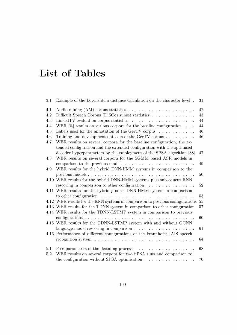
List of Tables
3.1 Example of the Levenshtein distance calculation on the character level . 31
4.1 Audio mining (AM) corpus statistics . . . . . . . . . . . . . . . . . . . . 424.2 Difficult Speech Corpus (DiSCo) subset statistics . . . . . . . . . . . . . 434.3 LinkedTV evaluation corpus statistics . . . . . . . . . . . . . . . . . . . 444.4 WER [%] results on various corpora for the baseline configuration . . . 444.5 Labels used for the annotation of the GerTV corpus . . . . . . . . . . . 464.6 Training and development datasets of the GerTV corpus . . . . . . . . . 464.7 WER results on several corpora for the baseline configuration, the ex-
tended configuration and the extended configuration with the optimiseddecoder hyperparameters by the employment of the SPSA algorithm [88] 47
4.8 WER results on several corpora for the SGMM based ASR models incomparison to the previous models . . . . . . . . . . . . . . . . . . . . . 49
4.9 WER results for the hybrid DNN-HMM systems in comparison to theprevious models . . . . . . . . . . . . . . . . . . . . . . . . . . . . . . . . 50
4.10 WER results for the hybrid DNN-HMM systems plus subsequent RNNrescoring in comparison to other configuration . . . . . . . . . . . . . . . 52
4.11 WER results for the hybrid p-norm DNN-HMM system in comparisonto other configuration . . . . . . . . . . . . . . . . . . . . . . . . . . . . 53
4.12 WER results for the RNN systems in comparison to previous configurations 554.13 WER results for the TDNN system in comparison to other configuration 574.14 WER results for the TDNN-LSTMP system in comparison to previous
configurations . . . . . . . . . . . . . . . . . . . . . . . . . . . . . . . . . 604.15 WER results for the TDNN-LSTMP system with and without GCNN
language model rescoring in comparison . . . . . . . . . . . . . . . . . . 614.16 Performance of different configurations of the Fraunhofer IAIS speech
recognition system . . . . . . . . . . . . . . . . . . . . . . . . . . . . . . 64
5.1 Free parameters of the decoding process . . . . . . . . . . . . . . . . . . 685.2 WER results on several corpora for two SPSA runs and comparison to
the configuration without SPSA optimisation . . . . . . . . . . . . . . . 70
109
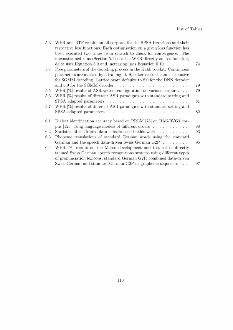
List of Tables
5.3 WER and RTF results on all corpora, for the SPSA iterations and theirrespective loss functions. Each optimisation on a given loss function hasbeen executed two times from scratch to check for convergence. Theunconstrained runs (Section 5.1) use the WER directly as loss function,delta uses Equation 5.9 and increasing uses Equation 5.10 . . . . . . . . 74
5.4 Free parameters of the decoding process in the Kaldi toolkit. Continuousparameters are marked by a trailing .0. Speaker vector beam is exclusivefor SGMM decoding. Lattice beam defaults to 8.0 for the DNN decoderand 6.0 for the SGMM decoder. . . . . . . . . . . . . . . . . . . . . . . . 79
5.5 WER [%] results of ASR system configuration on various corpora. . . . 795.6 WER [%] results of different ASR paradigms with standard setting and
SPSA adapted parameters. . . . . . . . . . . . . . . . . . . . . . . . . . 815.7 WER [%] results of different ASR paradigms with standard setting and
SPSA adapted parameters. . . . . . . . . . . . . . . . . . . . . . . . . . 82
6.1 Dialect identification accuracy based on PRLM [78] on BAS-RVG1 cor-pus [123] using language models of different orders . . . . . . . . . . . . 88
6.2 Statistics of the Meteo data subsets used in this work . . . . . . . . . . 936.3 Phoneme translations of standard German words using the standard
German and the speech data-driven Swiss German G2P . . . . . . . . . 956.4 WER [%] results on the Meteo development and test set of directly
trained Swiss German speech recognitions systems using different typesof pronunciation lexicons; standard German G2P, combined data-drivenSwiss German and standard German G2P or grapheme sequences . . . . 97
110
Bibliography
[1] A. J. Viterbi, “Error bounds for convolutional codes and an asymptotically op-timal decoding algorithm,” IEEE Trans. Information Theory, vol. IT-13, pp.260–269, 1967.
[2] L. Rabiner and B. H. Juang, “An introduction to hidden markov models,” IEEETransactions on Speech and Audio Processing, vol. 3, no. 1, pp. 4–16, 1986.
[3] J. Godfrey and E. Holliman, “Switchboard-1 release 2 ldc97s62,” Web Download,1993, linguistic Data Consortium.
[4] J. W. Cooley and J. W. Tukey, “An algorithm for the machine calculation ofcomplex fourier series,” Math. Comput., vol. 15, pp. 297–301, 1965.
[5] S. Stevens, J. Volkmann, and E. Newman, “A scale for the measurement of thepsychological magnitude pitch,” Journal of the Acoustical Society of America,vol. 8, no. 3, pp. 185–190, 1937.
[6] D. O’Shaughnessy, Speech communication: human and machine. Addison-Wesley, 1987.
[7] S. Furui, “Speaker-independent isolated word recognition using dynamic featuresof speech spectrum,” IEEE Transactions on Acoustics, Speech and Signal Pro-cessing, vol. 34, no. 1, pp. 52–59, 1986.
[8] L. E. Baum and T. Petire, “Statistical inference for probabilistic function of finitestate markov chains,” The Annals of Mathematical Statistics, vol. 37, no. 6, pp.1554–1563, 1966.
[9] A. Dempster, N. Laird, and D. Rubin, “Maximum likelihood form incompletedata via the em algorithm,” Journal of the Royal Statistical Society, Series B,vol. 39, no. 1, pp. 1–38, 1977.
[10] H. Sak, A. Senior, and F. Beaufays, “Long short-term memory recurrent neuralnetwork architectures for large scale acoustic modeling,” in Proc. of INTER-SPEECH, Signapore, 2014, pp. 338–342.
[11] Y. LeCun, L. Bottou, Y. Bengio, and P. Haffner, “Gradient-based learning appliedto document recognition,” in Proceedings of the IEEE, 1998, pp. 1–46.
111
Bibliography
[12] N. Chen, S. Urban, C. Osendorfer, J. Bayer, and P. van der Smagt, “Estimatingfinger grip force from an image of the hand using Convolutional Neural Networksand Gaussian processes,” in 2014 IEEE International Conference on Roboticsand Automation (ICRA), May 2014, pp. 3137–3142.
[13] G. Saon and M. Picheny, “Recent advances in conversational speech recognitionusing convolutional and recurrent neural networks,” IBM Journal of Researchand Development, vol. 61, no. 4, pp. 1:1–1:10, July 2017.
[14] S. Ganapathy, K. Han, S. Thomas, M. Omar, M. V. Segbroeck, and S. S.Narayanan, “Robust Language Identification Using Convolutional Neural Net-work Features,” in Proc. of INTERSPEECH, Signapore, China, 2014.
[15] C. Bartz, T. Herold, H. Yang, and C. Meinel, “Language Identification UsingDeep Convolutional Recurrent Neural Networks,” in Proc. of International Con-ference on Neural Information Processing (ICONIP), Guangzhou, China, 2017.
[16] W. Commons, “Typical CNN architecture,” Available at https://commons.wikimedia.org/wiki/File:Typical cnn.png; Accessed on 2018-02-22., 2015.
[17] B. H. Juang and L. R. Rabiner, “Automatic speech recognition – a brief historyof the technology development,” 2005.
[18] K. H. Davis, R. Biddulph, and S. Balashek, “Automatic recognition of spokendigits,” J. Acoust. Soc. Am., vol. 24, pp. 627–642, 1952.
[19] H. F. Olson and H. Belar, “Phonetic typewriter,” J. Acoust. Soc. Am., vol. 28,no. 6, pp. 1072–1081, 1956.
[20] D. B. Fry and P. Denes, “The design and operation of the mechanical speechrecognizer at university college london,” J. British Inst. Radio Engr., vol. 19, pp.211–229, 1959.
[21] T. B. Martin, A. L. Nelson, and H. J. Zadell, “Speech recognition by featureabstraction techniques,” Air Force Avionics Lab, Tech. Rep., 1764, tech. ReportAL-TDR-64-176.
[22] T. K. Vintsyuk, “Speech discrimination by dynamic programming,” Kibernetika,vol. 4, no. 2, pp. 81–88, 1968.
[23] A. Newell, “Harpy, production systems and human cognition,” Computer ScienceDepartment, Carnegie Mellon University, Tech. Rep., 1978, paper 2319.
[24] J. G. David Forney, “The viterbi algorithm,” Proc. of the IEEE, vol. 61, pp.268–278, 1973.
[25] F. Itakura and S. Saito, “A statistical method for estimation of speech spectraldensity and formant frequencies,” Electronics and Communications in Japan, vol.53A, pp. 36–43, 1970.
112
Bibliography
[26] B. S. Atal and S. L. Hanauer, “Speech analysis and synthesis by linear predictionof the speech wave,” Journal of the Acoustical Society of America, vol. 50, no. 2,pp. 637–655, 1971.
[27] S. E. Levinson, L. R. Rabiner, and M. M. Sondhi, “An introduction to the appli-cation of the theory of probabilistic functions of a markov process to automaticspeech recognition,” Bell Syst. Tech. J., vol. 62, no. 4, pp. 1035–1074, 1983.
[28] J. D. Ferguson, “Hidden markov analysis: An introduction in hidden markovmodels for speech,” Institue for Defense Analyses, Princeton, NJ, Tech. Rep.,1980.
[29] L. R. B. F. Jelinek and R. L. Mercer, “Design of a linguistic statistical decoderfor the recognition of continuous speech,” IEEE. Trans. on Information Theory,vol. IT-21, pp. 250–256, 1975.
[30] L. R. Bahl, F. Jelinek, and R. L. Mercer, “A maximum likelihood approachto continuous speech recognition,” IEEE Transactions on Pattern Analysis andMachine Intelligence, vol. 5, pp. 179–190, 1983.
[31] P. Mermelstein, “Distance measure for speech recognition, psychological and in-strumental,” Joint Workshop on Pattern Recognition and Artificial Intelligence,1976.
[32] J. S. Bridle and M. D. Brown, “An experimental automatic word-recognitionsystem,” Joint Speech Research Unit, Tech. Rep., 1974, technical Report 1003.
[33] C. J. Leggetter and P. C. Woodland, “Maximum likelihood linear regressionfor speaker adaptation of continuous density hidden markov models,” ComputerSpeech and Language, vol. 9, no. 1, pp. 171–185, 1995.
[34] Q. Huo and D.-H. Lee, “On-line adaptive learning of the cdhmm based on theapproximate recursive bayes estimate,” IEEE Trans. on Speech and Audio Proc.,vol. 5, no. 2, 1997.
[35] H. Hermansky, “Perceptual linear pedictive (plp) analysis of speech,” J. Acoust.Soc. Am., vol. 87, no. 4, pp. 1738–1752, 1990.
[36] L. Den, A. Acero, M. Plumpe, and X. Huang, “Large-vocabulary speech recog-nition under adverse acoustic environments,” Proc. Int. Conf. Spoken LanguageProcessing (ICSLP), pp. 806–809, 2000.
[37] D. Povey, B. Kingsbury, L.Mangu, G. Saon, H. Soltau, and G. Zweig, “fMPE: Dis-criminatively trained features for speech recognition,” Proc. Int. Conf. Acoustic,Speech, and Signal Processing, pp. 961–964, 2000.
[38] M. P. Cooke, P. G. Green, and M. D. Crawford, “Handling missing data inspeech recognition,” Proceedings of the 3rd International Conference on SpokenLanguage Processing (ICSLP), pp. 1555–1558, 1994.
113
Bibliography
[39] M. P. Cooke, A. Morris, and P. D. Green, “Missing data techniques for robustspeech recognition,” Proceedings of the IEEE Conference on Acoustics, Speech,and Signal Processing (ICASSP), pp. 863–866, 1997.
[40] R. P. Lippmann and B. A. Carlson, “Using missing feature theory to actively se-lect features for robust speech recogntion with interruptions, filtering and noise,”Proc. Eurospeech, pp. 37–40, 1997.
[41] S. Kapadia, V. Valtchev, and S. Young, “MMI Training for continuous phonemerecognition on the TIMIT database,” in Proceedings of ICASSP, vol. 2, 1993, pp.491–494.
[42] B. H. Juang, W. Chou, and C. H. Lee, “Minimum classification error rate methodsfor speech recognition,” IEEE Transactions on Speech Audio Processing, vol. 5,no. 3, pp. 257–265, May 1997.
[43] E. McDermott, T. Hazen, J. L. Roux, A. Nakamura, and S. Katagiri, “Discrimina-tive training for large vocabulary speech recognition using minimum classificationerror,” IEEE Transactions of Speech Audio Processing, vol. 5, no. 3, pp. 203–223,2007.
[44] D. Povey and P. Woodland, “Minimum phone error and i-smoothing for improveddiscriminative training,” in Proceedings of ICASSP, 2002, pp. 105–108.
[45] G. E. Dahl, D. Yu, L. Deng, and A. Acero, “Context-dependent pre-trained deepneural networks for large-vocabulary speech recognition,” IEEE Trans. AudioSpeech Lang. Processing, vol. 20, no. 1, pp. 30–42, 2012.
[46] G. E. Hinton, S. Osindero, and Y.-W. Teh, “A fast learning algorithm for deepbelief nets,” Neural Comput., vol. 18, no. 7, pp. 1527–1554, 2006.
[47] F. Seide, G. Li, X. Chen, and D. Yu, “Conversational speech transcription usingcontext-dependent deep neural networks,” Proc. Interspeech, pp. 437–440, 2011.
[48] Y. Miao, M. Gowayyed, and F. Metze, “EESEN: End-to-end speech recognitionusing deep RNN models and WFST-based decoding,” in Proceedings of the IEEEAutomatic Speech Recognition and Understanding Workshop, Scottsdale, Arizona,USA, Dec. 2015, pp. 167–174.
[49] T. Bayes, “An essay towards solving a problem in the doctrine of chances,” Philo-sophical Transactions, vol. 53, pp. 370–418, 1763.
[50] H. Ney, “Introduction to automatic speech recognition. technical report,” RWTHAachen University, Aachen, Germany, Lecture script, 2007.
[51] C. M. University, “The CMU Pronouncing Dictionary,” http://www.speech.cs.cmu.edu/cgi-bin/cmudict, version 0.7b, accessed October 19th, 2017.
114
Bibliography
[52] BAS - Bavarian Archive for Speech Signals, “Pronun-ciation lexicon PHONOLEX,” https://www.phonetik.uni-muenchen.de/forschung/Bas/BasPHONOLEXeng.html, 2013.
[53] M. Bisani and H. Ney, “Joint-sequence models for grapheme-to-phoneme conver-sion,” Speech Communication, vol. 50, pp. 434–451, Jul. 2008.
[54] L. R. Rabiner, “A tutorial on hidden markov models and selected applications inspeech recognition,” IEEE, vol. 77, no. 2, pp. 257–286, 1989.
[55] D. Povey, A. Ghoshal, G. Boulianne, L. Burget, O. Glembek, N. Goel, M. Hanne-mann, P. Motlicek, Y. Qian, P. Schwarz, J. Silovsky, G. Stemmer, and K. Vesely,“The Kaldi speech recognition toolkit,” in Proceedings of the IEEE 2011 Work-shop on Automatic Speech Recognition and Understanding (ASRU). HiltonWaikoloa Village, Big Island, Hawaii, US: IEEE Signal Processing Society, Dec.2011, iEEE Catalog No.: CFP11SRW-USB.
[56] R. Bakis, “Continuous speech word recognition via centisecond acoustic states,”Journal of the Acoustical Society of America, vol. 59, no. 1, Apr. 1976.
[57] H. Ney, “Acoustic modeling of phoneme units for continuous speech recognition,”in Proc. European Signal Processing Conference, Barcelona, Spain, Sep. 1990, pp.66–72.
[58] S. Katz, “Estimation of probabilities from sparse data for the language modelcomponent of a speech recognizer,” IEEE Transactions on Acoustics, Speech,and Signal Processing, vol. 35, no. 3, pp. 400–401, 1987.
[59] R. Kneser and H. Ney, “mproved backing-off for m-gram language modeling,” inProc. of ICASSP, vol. 1, 1995, pp. 181–184.
[60] L. E. Baum, “An equality and associated maximization technique in statisticalestimation for probabilistic functions of markov processes,” Inequalities, vol. 3,pp. 1–8, 1972.
[61] S. J. Young, D. Kershaw, J. Odell, D. Ollason, V. Valtchev, and P. Woodland,The HTK Book Version 3.4. Cambridge University Press, 2006.
[62] A. Lee, T. Kawahara, and K. Shikano, “Julius – an Open Source Real-TimeLarge Vocabulary Recognition Engine,” in Proceedings of Eurospeech, Aalborg,Denmark, 2001, pp. 1691–1694.
[63] W. Walker, P. Lamere, P. Kwok, B. Raj, R. Singh, E. Gouvea, P. Wolf, andJ. Woelfel, “Sphinx-4: A Flexible Open Source Framework for Speech Recogni-tion,” Sun Microsystems Inc., Tech. Rep., 2004.
[64] J. Kacur and J. Korosi, “An accuracy optimization of a dialog asr system utiliz-ing evolutional strategies,” in 5th International Symposium on Image and SignalProcessing and Analysis, Istanbul, 2007, pp. 180–184.
115
Bibliography
[65] B. Mak and T. Ko, “Automatic estimation of decoding parameters using large-margin iterative linear programming,” in Proc. of Interspeech, 2009, pp. 1219–1222.
[66] A. El Hannani and T. Hain, “Automatic optimization of speech decoder param-eters,” Signal Processing Letters, IEEE, vol. 17, no. 1, pp. 95–98, 2010.
[67] I. Bulyko, “Speech recognizer optimization under speed constraints,” in EleventhAnnual Conference of the International Speech Communication Association, 2010.
[68] J. Kiefer and J. Wolfowitz, “Stochastic estimation of a regesssion function,” Ann.Math. Stat., vol. 23, pp. 462–466, 1952.
[69] F. Och, “Minimum error rate training in statistical machine translation,”in Proceedings of the 41st Annual Meeting on Association for ComputationalLinguistics-Volume 1. Association for Computational Linguistics, 2003, pp. 160–167.
[70] J. Nelder and R. Mead, “The Downhill Simplex Method,” Computer Journal,vol. 7, p. 308, 1965.
[71] P. Lambert and R. Banchs, “Tuning machine translation parameters with SPSA,”in Proc. IWSLT, 2006, pp. 190–196.
[72] M. Mohri, “Finite-State Transducers in Language and Speech Processing,” Com-putational Linguistics, vol. 23, no. 2, 1997.
[73] V. I. Levenshtein, “Binary codes capable of correcting deletions, insertions, andreversals,” Soviet Physics Doklady, vol. 10, no. 8, pp. 707–710, Feb. 1966.
[74] D. Klakow and J. Peters, “Testing the correlation of word error rate and perplex-ity,” Speech Communication, vol. 38, no. 1–2, pp. 19–28, 2002.
[75] A. Lazaridis, E. Khoury, J.-P. Goldman, M. Avanzi, S. Marcel, and P. N. Garner,“Swiss french regional accent identification,” in Proc. Odessey: The Speaker andLanguage Recognition Workshop, 2014.
[76] F. Biadsy, J. Hirschberg, and N. Habash, “Spoken arabic dialect identificationusing phonotactic modeling,” in Proc. EACL 2009 Workshop on ComputationalApproaches to Semantic Languages, Athens, Greece, Mar. 2009, pp. 53–61.
[77] M. H. Bahari, R. Saeidi, H. V. hamme, and D. V. Leeuwen, “Accent recognitionusing i-vector, gaussian mean supervector and gaussian posterior probability su-pervector for spontaneous telephone speech,” in IEEE International Conferenceon Acoustics, Speech and Signal Processing (ICASSP), Vancouver B.C., 2013, pp.7344–7348.
116
Bibliography
[78] M. A. Zissman, “Comparison of four approaches to automatic language identifi-cation of telephone speech,” IEEE Transactions on Speech and Audio Processing,vol. 4, no. 1, 1996.
[79] N. Dehak, P. J. Kenny, R. Dehak, P. Dumouchel, and P. Ouellet, “Front-endfactor analysis for speaker verification,” IEEE Transactions on Audio, Speech,and Language Processing, vol. 19, no. 4, pp. 788–798, May 2011.
[80] S. Russell and P. Norvig, Artificial Intelligence: A Modern Approach, 2nd ed.Prentice Hall, 2003.
[81] C. Cortes and V. Vapnik, “Support-vector networks,” Machine Learning, vol. 20,no. 3, pp. 273–297, 1995.
[82] W. Campbell, D. Sturim, and D. Reynolds, “Support vector machines using gmmsupervectors for speaker verification,” Signal Processing Letters, vol. 13, no. 5,pp. 308–311, 2006.
[83] P. Kenny, P. Ouellet, N. Dehal, V. Gupta, and P. Dumouchel, “A study of inter-speaker variability in speaker verification,” IEEE Transactions of Audio, Speechand Language Processing, vol. 16, no. 5, pp. 980–988, 2008.
[84] C. Schmidt, M. Stadtschnitzer, and J. Kohler, “The Fraunhofer IAIS Audio Min-ing System: Current State and Future Directions,” in Proceedings of the 12thITG Conference on Speech Communication, Paderborn, Germany, 2016.
[85] D. Baum, D. Schneider, R. Bardeli, J. Schwenninger, B. Samlowski, T. Winkler,and J. Kohler, “DiSCo - a German evaluation corpus for challenging problemsin the broadcast domain,” in Proceedings of the 7th Conference on InternationalLanguage Resources and Evaluation (LREC), Valletta, Malta, May 2010.
[86] D. Schneider, J. Schon, and S. Eickeler, “Towards Large Scale Vocabulary Inde-pendent Spoken Term Detection: Advances in the Fraunhofer IAIS AudiominingSystem,” in Proc. Association for Computing Machinery’s Special Interest GroupInformation Retrieval (ACM SIGIR), Singapore, 2008.
[87] M. Stadtschnitzer, J. Schwenninger, D. Stein, and J. Koehler, “Exploiting theLarge-Scale German Broadcast Corpus to Boost the Fraunhofer IAIS SpeechRecognition System,” in Proceedings of the 9th Language Resources and Evalua-tion Conference (LREC), Reykjavik, Iceland, May 2014.
[88] J. C. Spall, “Multivariate stochastic approximation using a simultaneous pertur-bation gradient approximation,” IEEE Transactions on Automatic Control, vol.37:3, Mar. 1992.
[89] D. Povey, L. Burget, M. Agarwal, P. Akyazi, K. Feng, A. Ghoshal, O. Glembek,N. K. Goel, M. Karafiat, A. Rastrow, R. C. Rose, P. Schwarz, and S. Thomas,
117
Bibliography
“Subspace gaussian mixture models for speech recognition,” in Proc. ICASSP,2010, pp. 4330–4333.
[90] T. Anastasakos, J. McDonough, R. Schwartz, and J. Makhoul, “A compact modelfor speaker-adaptive training,” in Fourth International Conference on SpokenLanguage (ICSLP), Philadelphia, USA, Oct. 1996.
[91] V. Nair and G. Hinton, “3-d object recognition with deep belief nets,” Adv. NeuralInf. Process. Syst., vol. 22, pp. 1339–1347, 2007.
[92] V. Mnih and G. Hinton, “Learning to detect roads in high-resolution aerial im-ages,” in Proc. 11th Eur. Conf. Comput. Vision (ECCV), Sep. 2010.
[93] R. Salakhutdinov and G. Hinton, “Semantic hashing,” in Proc. SIGIR WorkshopInf. Retrieval Applicat. Graph. Models, 2007.
[94] R. Collobert and J. Weston, “A unified architecture for natural language pro-cessing: Deep neural networks with multitask learning,” in Proc. 25th Int. Conf.Mach. Learn. ser. ICML’08, New York, 2008.
[95] M. Hwang and X. Huang, “Shared-distribution hidden markov models for speechrecognition,” IEEE Trans. Speech Audio Process., vol. 1, no. 4, pp. 414–420, Jan.1993.
[96] T. Mikolov, M. Karafiat, L. Burget, J. H. Cernocky, and S. Khudanpur, “Re-current neural network based language model,” in Proceedings of Interspeech,Makuhari, Chiba, Japan, 2010, pp. 1045–1048.
[97] J. L. Elman, “Finding structure in time,” Cognitive Science, vol. 14, pp. 179–211,1990.
[98] T. Mikolov, S. Kombrink, A. Deoras, L. Burget, and J. H. Cernocky, “Rnnlm -recurrent neural network language modeling toolkit,” in IEEE Automatic SpeechRecognition and Understanding Workshop, Dec. 2011.
[99] M. Zeiler, M. Ranzato, R. Monga, and e. a. M. Mao, “On rectified linear unitsfor speech processing,” in Proceedings of 2013 IEEE International Conference onAcoustics, Speech and Signal Processing (ICASSP), Vancouver, Canada, 2013.
[100] J. J. Goodfellow, D. Warde-Farley, M. Mirza, A. Courville, and Y. Bengio, “Max-out networks,” arXiv preprint arXiv:1302.4389, 2013.
[101] Y. Miao, S. Rawat, and F. Metze, “Deep maxout neural networks for speechrecognition,” in Proc. ASRU, 2013.
[102] X. Zhang, J. Trmal, D. Povey, and S. Khudanpur, “Improving deep neural net-work acoustic models using generalized maxout networks,” in Proceedings of2014 IEEE International Conference on Acoustic, Speech and Signal Processing(ICASSP), Florence, Italy, 2014, pp. 215–219.
118

Bibliography
[103] A. Graves, N. Jaitly, and A. rahman Mohamed, “Speech recognition with deeprecurrent neural networks,” in 2013 IEEE International Conference on Acoustics,Speech and Signal Processing (ICASSP), 2013, pp. 6645–6649.
[104] S. Hochreiter and J. Schmidhuber, “Long short-term memory,” Neural computa-tion, vol. 9, no. 8, pp. 1735–1780, 1997.
[105] A. Graves, S. Fernandez, F. Gomez, and J. Schmidhuber, “Connectionist tem-poral classification: labelling unsegmented sequence data with recurrent neuralnetworks,” in Proceedings of the 23rd international conference on Machine learn-ing (ACM), 2006, pp. 369–376.
[106] P. J. Werbos, “Backpropagation through time: what it does and how to do it,”Proceedings of the IEEE, vol. 78, no. 10, pp. 1550–1560, Oct 1990.
[107] V. Peddinti, D. Povey, and S. Khudanpur, “A time delay neural network ar-chitecture for efficient modeling of long temporal contexts,” in Proceedings ofINTERSPEECH, Dresden, Germany, Sep. 2015.
[108] A. Waibel, T. Hanazawa, G. Hinton, K. Shikano, and K. Lang, “Phoneme recogni-tion using time-delay neural networks,” IEEE Transactions on Acoustics, Speech,and Signal Processing, vol. 37, no. 3, pp. 328–339, Mar. 1989.
[109] G. Cheng, V. Peddinti, D. Povey, V. Manohar, S. Khudanpur, and Y. Yan1,“An exploration of dropout with LSTMs,” in Proceedings of INTERSPEECH,Stockholm, Sweden, Aug 2017.
[110] N. Srivastava, G. E. Hinton, A. Krizhevsky, I. Sutskever, and R. Salakhutdinov,“Dropout: a simple way to prevent neural networks from overfitting,” Journal ofMachine Learning Research, vol. 15, no. 1, pp. 1929–1958, 2014.
[111] A. Rousseau, P. Deleglise, and Y. Esteve, “Enhancing the TED-LIUM Corpuswith Selected Data for Language Modeling and More TED Talks,” in Proceedingsof the Ninth International Conference on Language Resources and Evaluation(LREC), May 2014.
[112] J. Carletta and S. A. et. al., “The ami meeting corpus: a pre-announcement,”in Proceedings of the Second international conference on Machine Learning forMultimodal Interaction (MLMI), Edinburgh, UK, 2005, pp. 28–39.
[113] H. Sak, A. Senior, and F. Beaufays, “Long short-term memory based recurrentneural network architectures for large vocabulary speech recognition,” in ArXive-prints, Feb. 2014.
[114] T. Ko, V. Peddinti, D. Povey, and S. Khudanpur, “Audio augmentation for speechrecognition,” in Proceedings of INTERSPEECH, Dresden, Germany, Sep. 2015.
119

Bibliography
[115] Y. N. Dauphin, A. Fan, M. Auli, and D. Grangier, “Language modeling with gatedconvolutional networks,” in Proceedings of the 34th International Conference onMachine Learning, Sydney, Australia, 2017.
[116] J. C. Spall, “A stochastic approximation technique for generating maximum like-lihood parameter estimates,” 1987, pp. 1161–1167.
[117] J. C. Spall, “Implementation of the simultaneous perturbation algorithm forstochastic optimization,” IEEE Transactions on Aerospace and Electronic Sys-tems, vol. 34:3, Jul. 1998.
[118] I. Rechenberg, “Evolutionsstrategie – optimierung technischer systeme nachprinzipien der biologischen evolution,” Ph.D. dissertation, Technical Universityof Berlin, 1971.
[119] N. Hansen and A. Ostermeier, “Completely derandomized self-adaptation in evo-lution strategies,” Evolutionary Computation, vol. 9, no. 2, pp. 159–195, 2001.
[120] N. Hansen, “The CMA evolution strategy: a comparing review,” in Towards anew evolutionary computation. Advances on estimation of distribution algorithms,J. Lozano, P. Larranaga, I. Inza, and E. Bengoetxea, Eds. Springer, 2006, pp.75–102.
[121] F. Biadsy, “Automatic dialect and accent recognition and its application to speechrecognition,” Ph.D. dissertation, Columbia University, 2011.
[122] W. Konig, dtv-Atlas - Deutsche Sprache. Deutscher Taschenbuch Verlag, 2011,iSBN: 978-3-423-03025-0.
[123] S. Burger and F. Schiel, “RVG 1-A Database for Regional Variants of Contempo-rary German,” in Proceedings of the First International Conference on LanguageResources and Evaluation, 1998, pp. 1083–1087.
[124] H. Brugman and A. Russel, “Annotating Multimedia/Multi-modal resources withELAN,” in Proceedings of the 4th International Conference on Language Re-sources and Evaluation (LREC), 2004.
[125] F. Chollet et al., “Keras: The Python Deep Learning library,” https://github.com/fchollet/keras, 2015.
[126] M. A. et al., “TensorFlow: Large-scale machine learning on heterogeneous sys-tems,” https://www.tensorflow.org, 2015.
[127] M. Federico, N. Bertoldi, and M. Cettolo, “Irstlm: an open source toolkitfor handling large scale language models,” in Proceedings of Interspeech, Bris-bane,Australia, 2008.
120

Bibliography
[128] M. Stadtschnitzer, D. Stein, and R. Bardeli, “Employing Stochastic ConstrainedLMS Algorithm for ASR Frontend Processing,” in Proc. of The 2nd CHiMESpeech Separation and Recognition Challenge, Vancouver, Canada, 2013.
[129] J. Schwenninger, D. Stein, and M. Stadtschnitzer, “Automatic Parameter Tun-ing and Extended Training Material: Recent Advances in the Fraunhofer SpeechRecognition System,” Proc. Workshop Audiosignal- und Sprachverarbeitung,2013.
[130] D. Stein, J. Schwenninger, and M. Stadtschnitzer, “Simultaneous PerturbationStochastic Approximation for Automatic Speech Recognition,” Proc. Interspeech,pp. 622–626, 2013.
[131] D. Stein, B. Krausz, J. Loffler, R. Marterer, R. Bardeli, M. Stadtschnitzer, andJ. Schwenninger, “Automatic Audio and Video Event Recognition in an Intelli-gent Resource Management System,” IJISCRAM, vol. 5, no. 4, pp. 1–12, 2013.
[132] M. Stadtschnitzer, J. Koehler, and D. Stein, “Improving Automatic SpeechRecognition for Effective Topic Segmentation,” in Proc. DAGA - 40. Jahrestagungfur Akustik, Oldenburg, Germany, 2014.
[133] M. Stadtschnitzer, C. Schmidt, and D. Stein, “Towards a Localised German Auto-matic Speech Recognition,” in Proc. 11. ITG Fachtagung Sprachkommunication,Erlangen, Germany, 2014.
[134] T. L. Nguyen, D. Stein, and M. Stadtschnitzer, “Gradient-Free Decoding Pa-rameter Optimization on Automatic Speech Recognition,” in IEEE InternationalConference on Acoustics, Speech and Signal Processing (ICASSP), Florence, Italy,2014, pp. 3261 – 3265.
[135] H. Le, Q. Bui, B. Huet, B. Cervenkova, J. Bouchner, E. Apostolidis,F. Markatopoulou, A. Pournaras, V. Mezaris, D. Stein, S. Eickeler, andM. Stadtschnitzer, “LinkedTV at MediaEval 2014 Search and HyperlinkingTask,” in Proceedings of the MediaEval 2014 Workshop, Catalunya, Spain, Octo-ber 2014.
[136] M. Stadtschnitzer and C. Schmidt, “Implementation of a Live Dialectal MediaSubtitling System,” in Proceedings of the 16th Annual Conference of the Inter-national Speech Communication Association (INTERSPEECH), Dresden, Ger-many, Sep. 2015, pp. 728–729.
[137] M. Stadtschnitzer and C. Schmidt, “Joint Standard German and Bavarian Subdi-alect Identification of Broadcast Speech,” in Proceedings of DAGA - 44. Jahresta-gung fur Akustik, Munchen, Germany, Mar. 2018.
[138] M. Stadtschnitzer and C. Schmidt, “Adaptation and Training of a Swiss Ger-man Speech Recognition System using Data-driven Pronunciation Modelling,” in
121

Bibliography
Proceedings of DAGA - 44. Jahrestagung fur Akustik, Munchen, Germany, Mar.2018.
[139] M. Stadtschnitzer and C. Schmidt, “Data-Driven Pronunciation Modelling ofSwiss German Dialectal Speech for Automatic Speech Recognition,” in Proc.of 11th Edition of the Language Resources and Evaluation Conference (LREC),Miyazaki, Japan, May 2018.
[140] S. Enarvi and M. Kurimo, “TheanoLM - An Extensible Toolkit for Neural Net-work Language Modeling,” in Proc. of INTERSPEECH, San Francisco, USA,2016.
122