
Distanzbasierte Sprachkommunikation für Peer-to-Peer-Spiele.
Upload
nguyenmienCategory
view
226download
0
Technische Universität München
Lehrstuhl für Kommunikationsnetze
SIGNALING AND NETWORKING IN UNSTRUCTURED PEER-TO-PEER NETWORKS
Rüdiger Schollmeier
Vollständiger Abdruck der von der Fakultät für Elektrotechnik und Informationstechnik der Technischen Universität München zur Erlangung des akademischen Grades eines
Doktor-Ingenieurs (Dr.-Ing.)
genehmigten Dissertation.
Vorsitzender: Univ.-Prof. Dr. techn. Josef A. Nossek
Prüfer der Dissertation: 1. Univ.-Prof. Dr.-Ing. Jörg Eberspächer 2. Univ.-Prof. Dr.-Ing. Ralf Steinmetz, Technische Universität Darmstadt
Die Dissertation wurde am 20.09.2004 bei der Technischen Universität München eingereicht und durch die Fakultät für Elektrotechnik und Informationstechnik am 12.04.2005 angenommen.

i
ONE AIM "It’s impossible," says Reason.
"It’s reckless," says Experience. "It’s painful," says Pride.
"Try!" says Dream. Toyota Formula 1 Team advertisement following the
poem "Es ist was es ist." by Erich Fried
Abstract This work deals with the efficiency of Peer-to-Peer (P2P) networks, which are distributed
and self-organizing overlay networks. We contribute to their understanding and design by using new measurement techniques, simulations and analytical methods. In this context we first present measurement methods and results of P2P networks concerning traffic and topology characteristics as well as concerning user behavior. Based on these results we develop stochastic models to describe the user behavior, the traffic and the topology of P2P networks analytically. Using the results of our measurements and analytical investigations, we develop new P2P architectures to improve the efficiency of P2P networks concerning their topology and their signaling traffic. Finally we verify our results for the new architectures by measurements as well as computer-based simulations on different levels of detail.
Keywords: Peer-to-Peer networking, overlay networks, communication networks, content availability, signaling traffic, user model, application model, self-organization, random graph theory, generating functions, traffic measurement, topology measurement, simulation, compression, cross layer communication
Zusammenfassung Diese Arbeit behandelt die Architektur, den Verkehr und die Effizienz von
selbstorganisierenden Peer-to-Peer (P2P) Netzen. Es werden Beiträge zur Messung, zur analytischen Beschreibung und zum Entwurf dieser Netze entwickelt. In diesem Zusammenhang werden in einem ersten Schritt Messmethoden und daraus resultierende Ergebnisse, betreffend den Verkehr, die Topologieeigenschaften und das Benutzerverhalten in P2P-Netzen präsentiert. Aufbauend auf diesen Resultaten werden in dieser Arbeit neue stochastische Modelle vorgestellt, um das Benutzerverhalten, den Verkehr und die Topologie in P2P-Netzen analytisch zu beschreiben. Mit Hilfe der Ergebnisse aus den analytischen und messtechnischen Untersuchungen werden abschließend neue P2P Architekturen entwickelt, welche die Effizienz des Verkehrs in P2P-Netzen und deren Topologien verbessern.
ii
Preface When starting my scientific work in January 2001 at the Lehrstuhl für
Kommunikationsnetze, Professor Jörg Eberspächer suggested to have a look at Peer-to-Peer (P2P) techniques and applications beyond file sharing. Knowing hardly more about P2P than Napster or Gnutella, my knowledge at that time was thus similar to that of most people of the communication research community. Although already thousands of mp3 compressed audio files were at hand, nearly no scientific research results were available on P2P.This has significantly changed over the last four years. With increasing traffic volumes due to a growing number of P2P applications an increasing - and still growing - research community evolved. P2P turned out to be the disruptive technology Prof. Eberspächer expected it to be roughly four years ago. Today the concept of P2P is used for Voice over P2P applications, distributed collaboration systems, media streaming and context and location aware services in mobile networks. I hope that also this thesis will push this research further and will help to better understand this new networking paradigm.
This thesis addresses three main topics: measuring, modeling and architecture of P2P networks. "Measuring P2P" describes methods how to measure in distributed communication networks and also provides measurement results concerning the user behavior, the topology and the traffic in P2P networks. "Modeling P2P" offers novel approaches based on random graph theory and stochastics to describe the topology, the user behavior and the traffic in P2P networks analytically. Our work on the “Architecture of P2P” then uses our measurements and analytical considerations to propose efficient P2P solutions.
To achieve the results presented in this thesis, I could always rely on the support of my advisor Professor Dr. Jörg Eberspächer, going far beyond scientific questions. Thank you very much for your support and confidence! I am also very pleased that Professor Dr. Ralf Steinmetz is my second examiner. Together with Vasilios Darlagiannis of his team we had an excellent cooperation. Especially the workshop in Dagstuhl is one of the events, which jump started a number of new ideas and which I will remember for a long time.
Throughout my work the Lehrstuhl für Kommunikationsnetze offered an excellent environment, especially due to the colleagues working at this institute. I particularly thank Dr. Martin Maier and Thomas Kurzhals (Willy) for their excellent technical and personal support. Further on, the collaboration and discussions with one of my best friends and room mate Ingo Gruber as well as with Dr. Hartmann, Dr. Bettstetter, Dominic Schupke, Stefan Zöls, Gerald Kunzmann and Ingo Bauermann was always very inspiring and fruitful. The excellent cooperations with Prof. Dr.-Ing. Tran-Gia, Dr. Tutschku and Andreas Binzenhöfer from the University of Würzburg, with Dr. Kellerer from NTT-Docomo and Michael Finkenzeller from Siemens lead to a number of personal friendships beyond interesting results. Another thanks goes to my graduate students. In particular the collaboration with Elom, Florian, Antoine, Thomas and Roland provided much help in writing this thesis.
A very special „thank you“ goes to my great girlfriend Nadine and my great family. They were always there whenever I needed them. My thanks to all of them!
Munich. September 2004 Rüdiger Schollmeier
iii
Contents Chapter 1 Introduction ........................................................................................................ 1
Chapter 2 P2P Networking: Aspects, Principles and Research Issues ............................ 4
2.1. Basic Principles of P2P Systems ..................................................................... 4 2.2. Unstructured P2P Networks ............................................................................ 7 2.3. Structured P2P............................................................................................... 11 2.4. Application Areas.......................................................................................... 15 2.5. Research Issues.............................................................................................. 18 2.6. Summary ....................................................................................................... 23
Chapter 3 Methods to Analyze P2P Networks................................................................. 26
3.1. Measuring Unstructured P2P Networks ........................................................ 27 3.2. Modeling Unstructured P2P Networks.......................................................... 36 3.3. Simulation of Unstructured P2P Networks ................................................... 58 3.4. Summary ....................................................................................................... 65
Chapter 4 Signaling Traffic and Topology of Unstructured P2P Networks................. 67
4.1. Topology-Characteristics of Unstructured P2P Networks ............................ 68 4.2. Graph Theoretic Analysis of the Topology ................................................... 75 4.3. Traffic Characteristics of Unstructured P2P Networks ................................. 86 4.4. Graph Theoretic Analysis of the Traffic ....................................................... 96 4.5. Signaling Traffic Compression ..................................................................... 99 4.6. Adapting the Virtual Network to the Physical Network.............................. 100 4.7. The Mobile Peer-to-Peer Protocol............................................................... 104 4.8. Summary and Further Work........................................................................ 104
Chapter 5 Zone Based P2P .............................................................................................. 108
5.1. Related Work............................................................................................... 108 5.2. Optimal Representation of Shared Objects ................................................. 110 5.3. General Architecture ................................................................................... 118 5.4. Zone Setup Protocol .................................................................................... 123 5.5. Zone Query and Bordercast Resolution Protocol ........................................ 127

iv
5.6. Content Transmission.................................................................................. 130 5.7. Implementation and Evaluation................................................................... 133 5.8. Summary and Further Work........................................................................ 139
Chapter 6 Conclusions ..................................................................................................... 142
A. Notations and Abbreviations.................................................................... 143
B. Mathematical Notations............................................................................ 144
C. Simplified SDL-Diagrams of ZBP............................................................ 146
Chapter 1 INTRODUCTION
Peer-to-Peer (P2P) really started with Napster in 1999, causing a large amount of traffic in the Internet. Shortly afterwards followed Gnutella, still increasing the traffic significantly. In this new networking paradigm, often entitled a "disruptive technology", the participants establish their own networks by contributing their own resources, e.g. processing power, storage space and bandwidth. The primary goal of these networks was and still is, to share content directly between users, i.e. from peer to peer. The networks administrate themselves and the responsibility for the shared content is distributed among all participants. As every node provides part of the shared resources in P2P, the content is available where it is demanded, i.e. at the edge of IP networks.
The edges of P2P networks are mostly based on TCP connections and are used to distribute route requests for content and network maintenance messages within this virtual network. As P2P networks are established upon the TCP/IP network, we speak of overlay networks. The nodes/vertices in these virtual networks are the personal computers of the users. They are the glue which keeps the network connected. Every node in a P2P network operates at the same time as an overlay network router (to route requests to a node providing the desired content), as a server (to serve matching content requests), and as a client (to initiate requests for other content).
Within the last few years, P2P networking has found an increasing number of applications, primarily for content distribution but also for applications like media streaming overlay networks, distributed collaboration or Voice over P2P. As a result, today P2P traffic in the Internet often represents the dominating traffic, exceeding even WWW-traffic, which has long been dominating. It is a special characteristic of P2P traffic, that signaling traffic often exceeds the traffic caused by the transmission of desired content. Thus a profound understanding of P2P traffic becomes especially important.
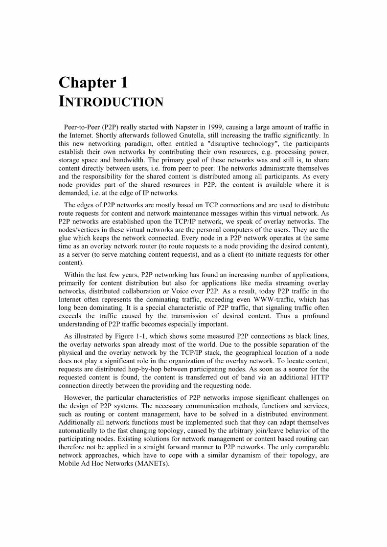
As illustrated by Figure 1-1, which shows some measured P2P connections as black lines, the overlay networks span already most of the world. Due to the possible separation of the physical and the overlay network by the TCP/IP stack, the geographical location of a node does not play a significant role in the organization of the overlay network. To locate content, requests are distributed hop-by-hop between participating nodes. As soon as a source for the requested content is found, the content is transferred out of band via an additional HTTP connection directly between the providing and the requesting node.
However, the particular characteristics of P2P networks impose significant challenges on the design of P2P systems. The necessary communication methods, functions and services, such as routing or content management, have to be solved in a distributed environment. Additionally all network functions must be implemented such that they can adapt themselves automatically to the fast changing topology, caused by the arbitrary join/leave behavior of the participating nodes. Existing solutions for network management or content based routing can therefore not be applied in a straight forward manner to P2P networks. The only comparable network approaches, which have to cope with a similar dynamism of their topology, are Mobile Ad Hoc Networks (MANETs).
Chapter 1 Introduction
2
Figure 1-1 Example of a Gnutella network, as seen from our institute
(measured on 12.08.2002)
Besides several industrial interest and discussion groups, the Internet Engineering Task Force (IETF) established in 2003 a separate Internet Research Task Force (IRTF), with focus on P2P networks and principles. Beyond these standardization and development activities, aspects of P2P also receive growing interest in the research community. This includes investigation of the topology and connectivity of the virtual overlay network and the resulting node/content availability. The investigation of the scalability of P2P networks according to the number of users and the network dynamism (churn rate) is also a key issue in the research of P2P networks. These research issues are a basis to understand and explain the properties, characteristics and effects of P2P.
This thesis contributes to three different research fields of P2P networking:
• Measuring P2P networks: To be able to analyze the weak points of current Peer-to-Peer approaches, we have to measure the characteristics of Peer-to-Peer networks, concerning their traffic behavior, their topology characteristics and their user behavior. Therefore new measurement approaches are developed, which are able to capture the characteristics of a highly distributed system on the application layer as well as on the packet level.
• Modeling P2P networks: For simulations and analytical investigation of P2P networks, we must describe the topology, the user behavior and the application behavior, by models reflecting our measurements. This raises a number of theoretical questions, especially in modeling and describing the random topology of P2P networks.
• Efficient overlay topology and routing management: To reduce the signaling traffic, cross layer communication is employed to adapt the overlay topology to the underlying physical topology. Further on compression algorithms and compression negotiation schemes have to be studied, because the datasets necessary for content based routing are comparatively large. In this research field the issues of load balancing the content responsibility and routing load of P2P in mobile environments are addressed.
The remainder of this thesis is organized as follows: Chapter 2 provides a description of the basic principles characterizing the networking paradigm of P2P. Following a categorization of P2P networks it provides a detailed overview about the major existing P2P systems. Based on this overview we outline the major existing and potential P2P applications and describe the open research issues in the area of P2P networking.
Chapter 3 investigates the methods needed to analyze the characteristics and problems of P2P networks. We first describe in this chapter existing as well as novel approaches to
Chapter 1 Introduction 3
measure the properties of P2P networks, concerning their overlay topology, their signaling traffic and the user behavior. To be able to explain the measured characteristics analytically, it is necessary to develop models of P2P systems. We develop new models to describe the user behavior, the application behavior and the overlay topology. The novel approach to describe overlay topologies is based mainly on concepts from random graph theory and generating functions. The third pillar to analyze communication systems, besides network measurements and network modeling, is the simulation of communication systems, which is addressed at the end of this chapter.
Using the concepts and tools developed in Chapter 3, we provide in Chapter 4 a detailed study of the traffic and the topology of unstructured P2P networks. To identify the reasons for the high signaling traffic of P2P networks, we provide in this chapter a measurement based as well as a graph theoretic analysis of the topology and the traffic characteristics of unstructured P2P networks. The measurements are used to determine the problem areas concerning the traffic and the topology. The theoretical approach then helps to understand and explain the identified problems. To overcome the efficiency problems we additionally propose the employment of compression negotiation for the signaling traffic and/or to adapt the overlay to the underlying physical network via cross layer communication. We thus propose a new P2P approach usable in MANETs.
Chapter 5 uses the approaches described in Chapter 4 and combines them into a novel P2P architecture, the Zone Based Peer-to-Peer protocol (ZBP). ZBP establishes a zone for every peer. For its zone the peer knows the P2P overlay network topology and the available content. If a requested content is not available in its zone, QUERY() messages are used to search for the content in neighboring zones. Using these concepts, ZBP achieves a notably improved signaling performance when compared to other routing approaches such as Gnutella 0.4 or Gnutella 0.6. As a proof of concept, we analyze and compare the signaling performance of ZBP nodes and Gnutella nodes by means of random graph theory and in a packet-level simulation environment.
Finally Chapter 6 summarizes our contributions and provides some directions for further research. Appendices A and B list the used notations and abbreviations. Appendix C provides simplified SDL diagrams of the Zone Based Peer-to-Peer protocol.
Parts of the results and concepts treated in this thesis were previously published in [ES03, ESKZ04, GSK04, KSGN03, KSE04, Scho01, Scho01a, SD03, SGF02, SGN03, SH03, SK04, SKe04, SK03, SS02, TSB03, TKSE04] and have been accepted for publication [GSK04a, SE04, SS04]. Beyond these, several new and unpublished results are presented in this work.
Chapter 2 P2P NETWORKING: ASPECTS, PRINCIPLES AND RESEARCH ISSUES
Until now a significant number of routing protocols and concepts have been developed in order to route in a scaleable, efficient and reliable way to different kinds of objects demanded by the users of P2P networks. However, the terminology to describe the characteristics of routing approaches is not well defined. Thus it is difficult to decide which impact the different P2P systems have on the network performance. Therefore this chapter provides a state of the art overview about the different protocols and systems deployed until now for P2P networking. Additionally we analyze the major protocols according to their current traffic volumes [Abi03] and their weight in current discussions within the research community.
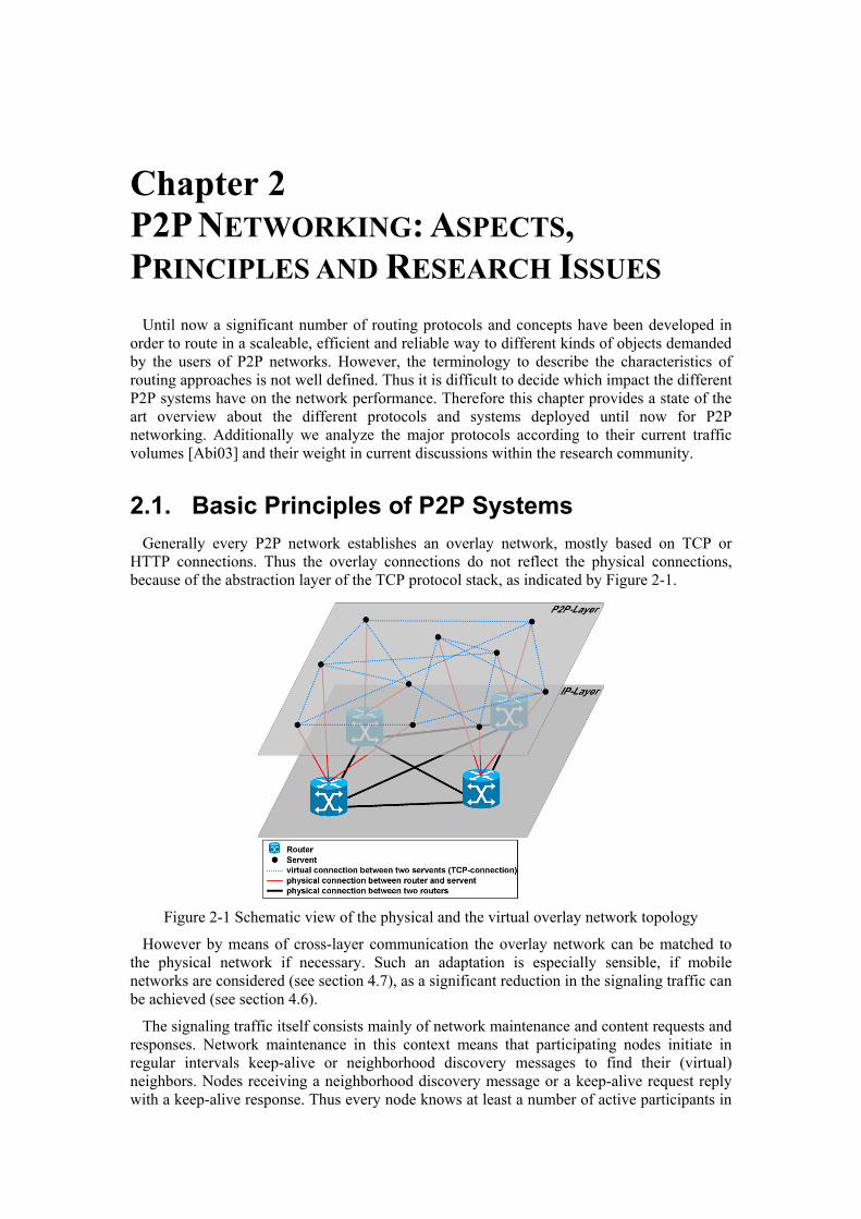
2.1. Basic Principles of P2P Systems Generally every P2P network establishes an overlay network, mostly based on TCP or
HTTP connections. Thus the overlay connections do not reflect the physical connections, because of the abstraction layer of the TCP protocol stack, as indicated by Figure 2-1.
Figure 2-1 Schematic view of the physical and the virtual overlay network topology
However by means of cross-layer communication the overlay network can be matched to the physical network if necessary. Such an adaptation is especially sensible, if mobile networks are considered (see section 4.7), as a significant reduction in the signaling traffic can be achieved (see section 4.6).
The signaling traffic itself consists mainly of network maintenance and content requests and responses. Network maintenance in this context means that participating nodes initiate in regular intervals keep-alive or neighborhood discovery messages to find their (virtual) neighbors. Nodes receiving a neighborhood discovery message or a keep-alive request reply with a keep-alive response. Thus every node knows at least a number of active participants in
Chapter 2 P2P Networking: Aspects, Principles and Research Issues 5
the overlay network, which are at least two hops away in the overlay network. To these nodes a node can connect, if one of its direct neighbors fails.
Secondly, active peers issue in random intervals determined by the user content requests, to find the location of demanded content. As no knowledge about the topology of the network nor the location of the content is available in unstructured P2P networks, these requests have to be flooded through the network. In contrast, in structured P2P networks these requests can be routed through the network (see section 2.3).
Keep-alive responses or content request responses are always routed through the network via the same path the fastest query was transferred through the network. Therefore every node stores the Global Unique ID (GUID) of each request and the node from which it received this response for a certain time.
To be able to enter the virtual network, a new peer has to know at least one IP address of a node already participating in the overlay network. Otherwise a new node can not participate, as it is not able to establish any new connections in the overlay network. For the addresses of currently active nodes a new node may either rely on cached addresses of nodes which were active in a previous session, or it may contact a bootstrap server. The bootstrap server is a well known host with a stable IP-address, which may itself participate in the overlay network, or which simply caches the IP addresses of nodes which used the bootstrap server to enter the network in a kind of FIFO memory. As nodes which just connected to the network are assumed more likely to stay connected further on, the bootstrap server can provide IP addresses of active nodes with a high probability without actively participating in the overlay network. Other methods, like IP broadcasting or multicasting, are hardly applicable, as they are limited to small sub-networks.
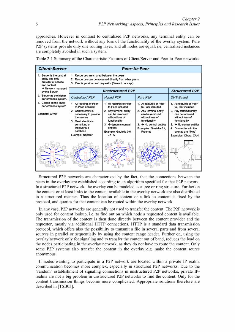
As depicted by Table 2-1 we distinguish throughout this work basically Client-Server and Peer-to-Peer systems. In a Client-Sever system the server is the only provider of service or content, e.g. a web server or a calendar server. The clients in this context only request content or service, e.g. the contents of a web page or the set up of an appointment/meeting. Content in this context may be an mp3-compressed audio file, the profile of a person a user wants to establish a call to, or context information, e.g. where the next taxi can be found. The clients do not provide any service or content to run this system. Thus generally the clients are the lower performance systems and the server is the higher performance system. This does not exclude that a server may be set up as a server farm with one specified entry point for the clients, which may also redirect the clients e.g. to share the load.
In a Peer-to-Peer system, all available resources, i.e. the shared content and services, are provided by the peers, although some central facility may exist, e.g. to locate a given content. A peer in this context is simply an application running on a machine, which may be a personal computer, a handheld or a mobile phone. In contrast to a Client-Server network, we can generally not distinguish between a content requestor (client) and a content provider, as one application participating in the overlay in general offers content to other peers and requests content from other participants. This is often expressed by the term "ServEnt", composed of the first syllable from the term Server and the second syllable of the term Client. Who provides what and which content is available where, is not managed by the network, as in P2P networks no central entity exists. Only centralized Peer-to-Peer networks employ a central instance as a lookup table, or redirector, which responds to peer requests with a list of peers where the requested content is available. Therefore we categorize centralized P2P networks also as unstructured P2P networks, as the overlay network and the content distribution are not managed in any manner.
Further on we subdivide unstructured P2P networks into hybrid and pure P2P networks. They mainly differ in the routing behavior of queries and their search methods in the overlay network [HHWX01, KM02, TR03]. Hybrid P2P networks employ dynamic central entities, which establish a second routing hierarchy to optimize the routing behavior of flat overlay
Chapter 2 P2P Networking: Aspects, Principles and Research Issues
6
approaches. However in contrast to centralized P2P networks, any terminal entity can be removed from the network without any loss of the functionality of the overlay system. Pure P2P systems provide only one routing layer, and all nodes are equal, i.e. centralized instances are completely avoided in such a system.
Table 2-1 Summary of the Characteristic Features of Client/Server and Peer-to-Peer networks
DHT-BasedHybrid P2P Pure P2PCentralized P2P
1. All features of Peer-to-Peer included
2. Any terminal entity can be removed without loss of functionality
3. No central entities4. Connections in the
overlay are “fixed”Examples: Chord, CAN
1. All features of Peer-to-Peer included
2. Any terminal entity can be removed without loss of functionality
3. No central entitiesExamples: Gnutella 0.4,
Freenet
1. All features of Peer-to-Peer included
2. Any terminal entity can be removed without loss of functionality
3. dynamic central entities
Example: Gnutella 0.6, JXTA
1. All features of Peer-to-Peer included
2. Central entity is necessary to provide the service
3. Central entity is some kind of index/group database
Example: Napster
Structured P2PUnstructured P2P
1. Resources are shared between the peers2. Resources can be accessed directly from other peers 3. Peer is provider and requestor (Servent concept)
1. Server is the central entity and only provider of service and content.
Network managed by the Server
2. Server as the higher performance system.
3. Clients as the lower performance system
Example: WWW
Peer-to-PeerClient-Server
Structured P2P networks are characterized by the fact, that the connections between the
peers in the overlay are established according to an algorithm specified for that P2P network. In a structured P2P network, the overlay can be modeled as a tree or ring structure. Further on the content or at least links to the content available in the overlay network are also distributed in a structured manner. Thus the location of content or a link to content is fixed by the protocol, and queries for that content can be routed within the overlay network.
In any case, P2P networks are generally not used to transfer the content. The P2P network is only used for content lookup, i.e. to find out on which node a requested content is available. The transmission of the content is then done directly between the content provider and the requestor, mostly via additional HTTP connections. HTTP is a standard data transmission protocol, which offers also the possibility to transmit a file in several parts and from several sources in parallel or sequentially by using the content range header. Further on, using the overlay network only for signaling and to transfer the content out of band, reduces the load on the nodes participating in the overlay network, as they do not have to route the content. Only some P2P systems also transfer the content in the overlay e.g. make the content source anonymous.
If nodes wanting to participate in a P2P network are located within a private IP realm, communication becomes more complex, especially in structured P2P networks. Due to the "random" establishment of signaling connections in unstructured P2P networks, private IP-realms are not a big problem in unstructured P2P networks to find the content. Only for the content transmission things become more complicated. Appropriate solutions therefore are described in [TSB03].
Chapter 2 P2P Networking: Aspects, Principles and Research Issues 7
2.2. Unstructured P2P Networks In unstructured P2P networks, except for the bootstrap server all connections in the overlay
network are established randomly, as in general no further information is available to optimize the links in the overlay network. Further random behavior is added to the network because of the dynamics in P2P networks, as nodes leave and join frequently, thus constantly changing the topology. Thus a meshed network arises with a large number of redundant paths and thus also circles, as depicted by Figure 3-28 on page 63.
Due to the permanent change of the overlay network, unstructured P2P networks do not put any effort into the management or distribution of the shared content. Content added to the network by new joining nodes is also provided by these nodes and can (initially) only be found at these nodes, as neither the content is distributed in an optimal manner between the nodes, nor are links pointing to the offered content distributed in the network. Only in centralized and hybrid P2P networks, links providing information about the location of specific content is aggregated on a higher routing layer e.g. a Superpeer or the Napster server. Thus in general requests have to be flooded in the network to reach nodes which can provide information where a specific content is available. Flooding in this context means that every incoming message is forwarded to all neighbors, except that neighbor in the overlay the message was received from.
However some rules have to be taken into account, to prevent messages from being forwarded infinitely. Therefore a general message header is attached to every message, which includes a Time-to-Live (TTL) counter and a GUID. The Time-to-Live counter is decreased by every node which forwards a message. As soon as the TTL counter reaches zero, the message is destroyed without being forwarded any further. The same happens, if a node receives a message with the same GUID twice within a certain time. The node discards this message, as it must assume that it received this message twice due to a circle within the overlay network.
Circles within P2P networks can hardly be prevented. As no single node has a complete overview about the network, connections are established randomly. The establishment of additional or new connections depends also on the connections a participant already has in the network. A node can only know nodes to which its neighbors are connected, due to the keep-alive algorithm, as described earlier. Further on, if the bootstrap server is not well designed, e.g. as a LIFO, loops are established too, because a new node connects to the two nodes which connected, before it contacted the bootstrap server. As these two nodes are already connected to each other, a loop arises, as the new node connects to both nodes.
The fact that the overlay network structure is not determined by the protocol is the main characteristic of unstructured P2P networks. Centralized P2P protocols, like the Napster protocol, take a special role within unstructured P2P networks. In this case we can regard the centralized lookup server as the bootstrap server, to which the connection is never released. Thus one could categorize centralized P2P networks as structured P2P networks. However as the connections between the peers and the location of the content are not determined by an algorithm, centralized P2P networks do not fulfill the criteria to be classified as a structured P2P network. As an example of a centralized P2P network we describe in section 2.2.1 the Napster protocol. Hybrid and pure P2P networks clearly fulfill all of the criteria mentioned above. The major protocol in the area of pure P2P networks is Gnutella 0.4. Its characteristics are described in section 2.2.2. Further on we also describe the major protocols in the area of hybrid P2P networks, namely the Gnutella 0.6 protocol and JXTA in section 2.2.3.
2.2.1 Centralized P2P Networks Napster is often considered as the starting point of P2P networks. Due to legal issues and
the centralized responsibility Napster had to shut down its service. However the basic concept
Chapter 2 P2P Networking: Aspects, Principles and Research Issues
8
and architecture of the Napster file sharing system are still used by other applications, e.g. Audiogalaxy [Aud04] or WinMX [Win04]. BitTorrent [Coh04, IUBF04] is a similar file sharing system, the major objective of which is to quickly replicate a single large file to a set of clients. A so called torrent is established by a tracker and all currently active peers, whereas the tracker is the central component, which keeps the meta-information about the currently active peers. It acts as a rendezvous point for all the clients of the torrent.
Napster employs a central server which maintains an index of all shared files of the peers, which are currently logged onto the Napster network. To find content, a peer has to send a QUERY to this server, which returns the ports and IP addresses of all peers sharing the requested file. As the location is thus known, the peer establishes a direct connection with one of the known hosting peers and can download the demanded file from there.
As depicted by Table 2-1 the Napster network can be characterized by its centralized topology. The file searching protocol uses a client/server model with a central index server. However the file transfer is done in a true P2P way. The file exchange occurs directly between the Napster hosts without passing the server.
With Napster, no file can be found, if the central lookup table is not available. Only the file retrieval and the storage are decentralized. Thus the server represents a bottleneck and a Single Point of Failure. The computing power and storage capabilities of the central lookup table must grow proportional to the number of users, which also affects the scalability of this approach. Napster uses a preconfigured structure, with the central lookup server in the middle, to which every node has to connect.
The protocol basis for all signaling and data traffic is the TCP/IP protocol, which adds to the general Napster message Header of 8 Bytes additional 40 Bytes (20 Bytes for TCP and 20 Bytes for IP). As the file exchange is based on HTTP, we have to take into account 180 bytes for the Get-message and 130 bytes plus content for the response message. All messages are transmitted as plain text strings. MD5-Hash Values [Riv92] are only used to check the integrity of downloaded files.
As every node wanting to log into the Napster network has to register at the central server, no keep alive signal or any electronic heart beat must be exchanged between the Napster server and the peer. The server also acts as a “name server” to guide each requesting peer to those peers, which host the demanded content. No additional layer 7 routing is necessary, as the server has the whole network view.
Further on, if the content is shared by at least one participant, the content can be found instantly with one lookup. Thus the content-availability in a Napster network can only take the values zero or one. Zero, if the content is not shared by any node, one if the content is shared by at least one node, assuming that the server and the peers work correctly. If the content is available more than once, only the replication rate, and thus in this case the download performance increases, but not the availability of content.
Therefore no signaling-background noise exists in this system. Background noise in this context describes the signaling traffic initiated and received by an average node participating in the overlay, without actively initiating requests. However, if we assume an average session length of 10 minutes, the bytes for the messages which have to be exchanged at the beginning (1*Login, 1*Login Ack, 10* Client Notification of Shared File, if we assume 10 shared files) can be averaged to a value which results in a background noise of 22,88 bit/s.
For a file exchange we calculate an overhead of 4580 bytes. Therefore we assume, that one file request results on average in 20 file responses sent from the lookup server to the requesting peer. (4130 bytes search and 450 bytes file exchange +content (Download request: ~100 bytes, HTTP-Get: 200 bytes, HTTP_Response: 150 bytes+content)).
Chapter 2 P2P Networking: Aspects, Principles and Research Issues 9
The virtual P2P-Layer based on TCP-connections between the nodes and the server does
not reflect the physical topology of the network. However no zigzag routes, as in Gnutella, are established, as the central server provides all routing information. Due to the central entity, to which every node needs a connection, Napster is not a feasible approach for mobile ad hoc networks.
2.2.2 Pure P2P Networks The most prominent P2P system based on a pure P2P networks is the Gnutella 0.4 system
[Cli01]. Its overlay network consists of a large number of nodes which may be distributed throughout the world, without any central element. The nodes communicate directly with each other. However at the beginning, i.e. in a bootstrap phase, a central entity like a beacon server, from which IP-addresses of active nodes can be retrieved, is necessary. If a node already participated in the network, it may instead be able to enter the network by trying to connect to nodes, whose addresses it cached in a previous session.
Gnutella is a self organizing network. A client sends a message to a node which then sends it to all nodes it is connected to. This is often called "viral propagation". A node becomes part of the network by keeping an average of 3 TCP-connections [SH03] to other active Gnutella nodes. New nodes, to which the node can connect if an active connection breaks, are explored by broadcasting PING messages in the virtual overlay network. These PING messages are also used as keep alive pattern and are broadcasted in regular intervals. Based on our measurements [SD03], we propose one broadcast every 10 minutes, as the average lifetime of a connection is 10 minutes.
All messages are coded in plain text. This results in large messages of QUERY and especially QUERY-HIT messages, as they contain meta data about the queried objects. Like Napster, Gnutella uses additionally MD5 Hash keys [Riv92] to identify objects explicitly. For routing Gnutella employs simple flooding of the request messages, i.e. QUERY and PING messages. Every incoming PING or QUERY, which has not been received before, is forwarded to all neighbors, if the Time-to-Live value (default set to 7 hops) is at least one. Response messages, like PONG or QUERY_HIT messages, are sent back on the same path the request message used. We therefore call it backward routing.
The signaling messages are based on TCP/IP, resulting in an overhead of approximately 40 bytes per message. The file transmission in Gnutella is based on HTTP, which results in 180 bytes for a Get-message and 130 bytes + content for a response message.
Due to the keep alive mechanism in Gnutella and the requests and responses, which have to be routed by the nodes, messages are permanently exchanged between the nodes. Based on our measurements an average node is connected within 7 hops to 379 peers. Assuming that each peer broadcasts one PING every 10 minutes it thus receives 379 PING messages within 10 minutes. As the PING messages account for 16%, the PONG messages for 40%, the QUERY- messages for 22% and the QUERY_HIT messages also for 22% of the Gnutella traffic [SD03], the message load becomes 200307 bytes within 10 minutes which results in an average "background noise" of 333,85 bytes/s or 2.67 kbit/s per node. In Gnutella roughly the same background traffic appears in the up as well as in the down path of each node.
For a file exchange, we assume a replication rate of 0.05. This results in 18.95 received QUERY_HIT messages per QUERY message. Taking the overhead of the HTTP transmission into account, the total overhead results in 4850 bytes per file search and successful exchange.
A high replication rate is critical for Gnutella. If the replication rate is too low, the requested content may not be found in the network, as we shall see below. Therefore such a network can hardly be used to search for objects available only once in the network, e.g. to establish a voice connection between two people.
Chapter 2 P2P Networking: Aspects, Principles and Research Issues
10
In Gnutella 0.4 the virtual P2P layer is not matched to the physical layer, which leads to zigzag routes, as described in [SK03]. Therefore Gnutella can not be used in mobile ad hoc networks. Only enhancements, as described by the approach of geo-sensitive Gnutella [SK03] in section 4.6, provide means to adapt the virtual network to the physical network.
A similarly distributed scheme named Freenet has been proposed in [CMHS02, Ora01], which emphasizes security and anonymity. However, due to lack of specifications there is currently no basis for a detailed analysis of this proposal.
2.2.3 Hybrid P2P Networks
2.2.3.1. Gnutella Protocol 0.6 As outlined above the message load in a Gnutella 0.4 network is very high. Therefore
protocol enhancements to reduce the message load have been proposed in [Roh02], [Roh02a] and [SR02]. [Roh02] and [Roh02a] propose enhancements of the signaling protocol, and [SR02] proposes the creation of a hierarchy in the network to establish a hub based network. These extensions are subsumed in the Gnutella protocol v0.6 [Gnu02]. The messages used in Gnutella 0.4 stay the same, to guarantee downward compatibility. However, they are handled differently as explained below.
An efficient way to reduce the consumption of bandwidth is the introduction of hierarchies, as e.g. in Napster the Napster Server. To keep the advantages of Gnutella, i.e. the complete self organization and decentralization, Superpeers and Leafnodes are introduced in [SR02]. Superpeers establish a higher hierarchy level, in which they form a pure P2P network, i.e. are connected to each other directly via TCP connections (see Table 2-1). To one Superpeer several Leafnodes are connected. The Superpeer shields its Leafnodes from the PING and PONG traffic. It also provides better QUERY routing functionalities by indexing the shared objects of all of its Leafnodes. Thus the Superpeer can answer the QUERY directly, if one of its nodes hosts the requested content. If the content is not hosted by any of its Leafnodes, the Superpeer broadcasts the request in the Superpeer layer.
By introducing the above described enhancements, the load on the network can be reduced without introducing preconfigured, centralized servers. The network is still scalable, but one Superpeer should not have more than 50 to 100 Leafnodes, depending on the processing power and the connection of the Superpeer. Thus it is necessary, that the number of Superpeers increases according to the total number of Leafnodes in the network.
As all the messages, defined in Gnutella 0.4, are also used in Gnutella 0.6, no changes in the overhead for a file transmission occur, it still is 4850 bytes. However, as described in detail in section 4.2, the traffic imposed on the Leafnodes is reduced significantly, whereas the traffic load imposed on the Superpeers increases significantly.
Other protocols which establish a similar hierarchical overlay routing structure are edonkey2000 [Met03] and FastTrack. Applications like Kazaa [Kaz03] or Skype [Sky04] and emule [emu03] or mldonkey [mld03] are based on these. In FastTrack the peers in the higher hierarchical level are called Superpeers and in edonkey2000 they are simply called servers. Both protocols are proprietary and therefore they are not officially and publicly documented. However a number of details of the two protocols have been re-engineered by users and creators of open source alternative applications [Edo03, efa03, Gif03, Klim03]. Already some basic measurements, mostly on IP-level, are available, concerning packet and data rates [BWDD02, KBBF03, Tut04].
2.2.3.2. JXTA Project JXTA [JXTA02, OTG02] was initiated by Sun Microsystems as an open source
project which continues to develop. It is designed to enable connected peers to easily locate
Chapter 2 P2P Networking: Aspects, Principles and Research Issues 11
each other and communicate with each other across different P2P systems and different communities. The major goal of JXTA is to create a framework that can be used for all areas of P2P applications. We used JXTA Version 1.0 (build 74f, 09-17-2002) to analyze the capabilities and requirements of JXTA.
Each peer is assigned a unique peer ID. All available network interface addresses of a peer are encapsulated in a peer endpoint, listing all possibilities how the peer can be contacted. Out of this list another peer can select the most appropriate way to communicate with that peer. To send and receive messages between services and applications virtual communication channels, so called pipes, are established between peers. Pipes are unidirectional and asynchronous channels based on TCP connections.
JXTA is a hybrid concept, similar to the Gnutella 0.6 architecture. So called rendezvous peers, or relay peers, are used as access points for “normal” peers. Thus JXTA peers are connected to each other only via rendezvous peers. As in Gnutella 0.6 the content shared by each peer and all other JXTA network resources are announced with advertisements, included in an initial registration message.
All messages in JXTA are coded as plain text XML messages. This results in large message sizes, compared to which the HTTP and TCP headers are small. The measured overhead caused by XML amounts to nearly 50%, not taking into account the additional TCP/IP and HTTP overhead. The registration message results in a message size of more than 600 bytes for two shared objects. A QUERY message results in more than 400 bytes and a Response message in more than 600 bytes. All implementations we analyzed used HTTP as a protocol basis, which results in an additional overhead of 72 bytes (20 bytes for IP. 20 bytes for TCP and 32 bytes for HTTP).
This results in an average virtual background noise of 8.96 bit/s per node, if we assume also an average session length of 10 minutes (672 bytes/10 min), as compared to 2.67 kbit/s for Gnutella 0.4. For a file transmission we assume HTTP, although it is not specified either. A file transfer would thus result at the requesting node in 400 bytes for the QUERY, 12000 bytes for 20 File response messages, 200 bytes for the HTTP Get message and 150 bytes plus the content for the HTTP-response message, which adds up to 12750 bytes for a single file search and the transmission.
The use of plain text, without any additional XML-elements could also reduce the size of the overhead. An additional and significant decrease in the message size can be achieved, if string compression techniques are employed on the transmitted data [LS99, UHHS02, Sal97, WBX04]. Thus we could reduce the overhead by an average of 40% to 50 %, which shows a significant impact on the signaling load of JXTA and other common P2P protocols. For details see section 4.5. There also exist some attempts to employ JXTA in mobile environments. This project is called JXME [JXM02] or JXTA for J2ME [Sun02]. Arora et al. additionally propose to use only a minimized set of the JXTA protocols and introduce so called relay peers [Aro03].
2.3. Structured P2P Currently there exist a number of concepts which establish structured P2P networks. Chord
[SMKK01], CAN [RFHK01] and PASTRY [RD01] are the most prominent P2P routing concepts which are based on distributed hash tables (DHT). The ID of each node and object may consist of several dimensions, i.e. several IDs for each object. An object in this context may be the content shared within this network or only a description of content available in this network. Chord for example employs only one dimension, meaning that every node has to establish at least two connections. Thus the nodes establish a ring structure. The IDs of content are for example derived from the file size, search keywords or other metadata. From
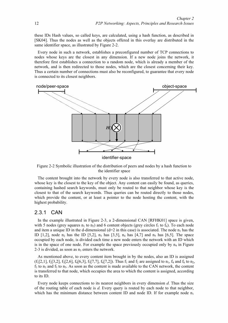
Chapter 2 P2P Networking: Aspects, Principles and Research Issues
12
these IDs Hash values, so called keys, are calculated, using a hash function, as described in [SK04]. Thus the nodes as well as the objects offered in this overlay are distributed in the same identifier space, as illustrated by Figure 2-2.
Every node in such a network, establishes a preconfigured number of TCP connections to nodes whose keys are the closest in any dimension. If a new node joins the network, it therefore first establishes a connection to a random node, which is already a member of the network, and is then redirected to those nodes, which are the closest concerning their key. Thus a certain number of connections must also be reconfigured, to guarantee that every node is connected to its closest neighbors.
⊗H()⊗H()
node/peer-space object-space
identifier-space Figure 2-2 Symbolic illustration of the distribution of peers and nodes by a hash function to
the identifier space
The content brought into the network by every node is also transferred to that active node, whose key is the closest to the key of the object. Any content can easily be found, as queries, containing hashed search keywords, must only be routed to that neighbor whose key is the closest to that of the search keywords. Thus queries can be routed directly to those nodes, which provide the content, or at least a pointer to the node hosting the content, with the highest probability.
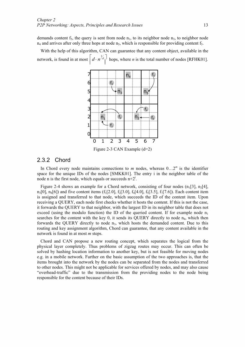
2.3.1 CAN In the example illustrated in Figure 2-3, a 2-dimensional CAN [RFHK01] space is given,
with 5 nodes (grey squares n1 to n5) and 6 content objects (grey circles f1 to f6). To each node and item a unique ID in the d-dimensional (d=2 in this case) is associated. The node n1 has the ID [1,2], node n2 has the ID [5,2], n3 has [3,5], n4 has [4,7] and n5 has [6,5]. The space occupied by each node, is divided each time a new node enters the network with an ID which is in the space of one node. For example the space previously occupied only by n4 in Figure 2-3 is divided, as soon as n5 enters the network.
As mentioned above, to every content item brought in by the nodes, also an ID is assigned (f1[2,1], f2[3,2], f3[2,6], f4[6,3], f5[7,7], f6[7,2]). Thus f1 and f2 are assigned to n1, f4 and f6 to n2, f3 to n3 and f5 to n5. As soon as the content is made available to the CAN network, the content is transferred to that node, which occupies the area to which the content is assigned, according to its ID.
Every node keeps connections to its nearest neighbors in every dimension d. Thus the size of the routing table of each node is d. Every query is routed by each node to that neighbor, which has the minimum distance between content ID and node ID. If for example node n1
Chapter 2 P2P Networking: Aspects, Principles and Research Issues 13
demands content f5, the query is sent from node n1, to its neighbor node n3, to neighbor node n4 and arrives after only three hops at node n5, which is responsible for providing content f5.
With the help of this algorithm, CAN can guarantee that any content object, available in the
network, is found in at most 1
dd n ⋅ hops, where n is the total number of nodes [RFHK01].
0
1
2
3
4
5
6
7
0 1 2 3 4 5 6 7
n1 n2
n3
n4
n5
f2
f1
f3
f5
f6
f4
Figure 2-3 CAN Example (d=2)
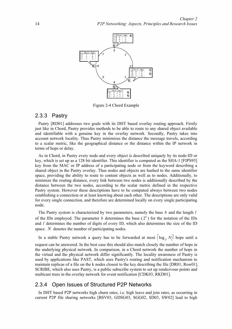
2.3.2 Chord In Chord every node maintains connections to m nodes, whereas 0…2m is the identifier
space for the unique IDs of the nodes [SMKK01]. The entry i in the neighbor table of the node n is the first node, which equals or succeeds n+2i.
Figure 2-4 shows an example for a Chord network, consisting of four nodes (n1[3], n2[4], n3[0], n4[6]) and five content items (f1[2.0], f2[3.0], f4[4.0], f5[3.5], f7[7.6]). Each content item is assigned and transferred to that node, which succeeds the ID of the content item. Upon receiving a QUERY, each node first checks whether it hosts the content. If this is not the case, it forwards the QUERY to that neighbor, with the largest ID in its neighbor table that does not exceed (using the modulo function) the ID of the queried content. If for example node n1 searches for the content with the key 0, it sends its QUERY directly to node n4, which then forwards the QUERY directly to node n3, which hosts the demanded content. Due to this routing and key assignment algorithm, Chord can guarantee, that any content available in the network is found in at most m steps.
Chord and CAN propose a new routing concept, which separates the logical from the physical layer completely. Thus problems of zigzag routes may occur. This can often be solved by hashing location information to another key, but is not feasible for moving nodes e.g. in a mobile network. Further on the basic assumption of the two approaches is, that the items brought into the network by the nodes can be separated from the nodes and transferred to other nodes. This might not be applicable for services offered by nodes, and may also cause “overhead-traffic” due to the transmission from the providing nodes to the node being responsible for the content because of their IDs.
Chapter 2 P2P Networking: Aspects, Principles and Research Issues
14
Figure 2-4 Chord Example
2.3.3 Pastry Pastry [RD01] addresses two goals with its DHT based overlay routing approach. Firstly
just like in Chord, Pastry provides methods to be able to route to any shared object available and identifiable with a genuine key in the overlay network. Secondly, Pastry takes into account network locality. Thus Pastry minimizes the distance the message travels, according to a scalar metric, like the geographical distance or the distance within the IP network in terms of hops or delay.
As in Chord, in Pastry every node and every object is described uniquely by its node-ID or key, which is set up as a 128 bit identifier. This identifier is computed as the SHA-1 [FIPS95] key from the MAC or IP address of a participating node or from the keyword describing a shared object in the Pastry overlay. Thus nodes and objects are hashed to the same identifier space, providing the ability to route to content objects as well as to nodes. Additionally, to minimize the routing distance, every link between two nodes is additionally described by the distance between the two nodes, according to the scalar metric defined in the respective Pastry system. However these descriptions have to be computed always between two nodes establishing a connection or at least knowing about each other. The descriptions are only valid for every single connection, and therefore are determined locally on every single participating node.
The Pastry system is characterized by two parameters, namely the base b and the length l of the IDs employed. The parameter b determines the base ( 2b ) for the notation of the IDs and l determines the number of digits of every ID, which also determines the size of the ID space. N denotes the number of participating nodes.
In a stable Pastry network a query has to be forwarded at most 2
log b N hops until a
request can be answered. In the best case this should also match closely the number of hops in the underlying physical network. In comparison, in a Chord network the number of hops in the virtual and the physical network differ significantly. The locality awareness of Pastry is used by applications like PAST, which uses Pastry's routing and notification mechanism to maintain replicas of a file on the k nodes closest to the key describing the file [DR01, Row01]. SCRIBE, which also uses Pastry, is a public subscribe system to set up rendezvous points and multicast trees in the overlay network for event notification [CDK03, RKD01].
2.3.4 Open Issues of Structured P2P Networks In DHT based P2P networks high churn rates, i.e. high leave and join rates, as occurring in
current P2P file sharing networks [BSV03, GDSG03, SGG02, SD03, SW02] lead to high
Chapter 2 P2P Networking: Aspects, Principles and Research Issues 15
traffic [RGRK04, XMH03]. The traffic may be significantly higher than that currently measured in unstructured P2P networks, thus leading to severe scalability problems [LRS01, RGRK04]. Although stable Chord rings are proven to scale well [BT04], the signaling overhead in unstable, Gnutella-like systems, is an issue [TAD03].
Further on DHT based applications often store a large number of objects, or at least pointers to these objects, on DHT nodes, which must be transferred to other nodes upon a node arrival or departure. Also, routing in DHT-based networks is asymmetric, which may lead to long routes to find the requested content. If content is stored on a preceding node in the DHT structure, the request has to traverse the whole ring (in Chord), even though it would be enough to send a request a few hops backwards [MCV03]. This problem is also addressed in [XM03], [GBRF03] or [KR04].
Another asymmetry problem is that the distribution of keywords describing the offered content may not be uniform. This results in unfair storage consumption between the nodes[LR04]. Harren et al propose a new querying scheme to avoid the necessity for exact match lookups in DHT based overlays [HHHL02]. They establish a relational query processing system on top of a DHT in every participating node [GFBU04].
Other DHT-based approaches try to reduce the signaling traffic by using de Bruijn graphs [Bru46], [KK04, KR04], or by assigning special roles to more stable peers like Kademlia [MM02]. Others try to reduce the signaling overhead by adapting the DHT to the physical topology [ZZ03], [Gum03, ZZ03]. All of these approaches do not address the problem of frequently joining and leaving nodes. Thus structured P2P networks are more suitable for stable environments, but not for the dynamic overlays targeted in this work.
2.4. Application Areas Based on the architectures described in the previous two sections, a significant number of
applications have been developed since the introduction of P2P networks with Napster in 1999. The major reason for the growth in the number of applications in the area of Peer-to-Peer networking is that today's personal computers offer capabilities which could be offered a few years ago only by dedicated servers. The already available access data rate is often larger than 1 Mbit/s and is expected to grow even further by the introduction of Ethernet to the home or even fiber to the home. Further on the processing power of currently available personal computers is sufficient to resolve the routing requests from other peers in the overlay network. To share data in an overlay network, hard-drive sizes of 50 Gbytes are equally sufficient and even RAM reaches today sizes of up to a few GByte. As additionally most IP core networks are over dimensioned by 200%, we currently see no restrictions for users to set up, manage and use their "own" overlay networks for services and contents they are interested in, without having to ask beforehand any central administration.
We categorize in this work the applications into three major areas, the applications developed for service discovery, for resource allocation and for distributed computing. To provide an overview about the wide range of applications and the potential of P2P networks, we discuss below the most promising applications for which P2P will provide a simple basis for more widespread use.
2.4.1 Distributed Computing GRID computing
Due to the requirements of professional communities to access remote resources, federate data sets and/or to pool computers for large scale simulations and data analyses, architectures called GRIDs were developed [Fos02, FI03]. A GRID is a shared environment, implemented
Chapter 2 P2P Networking: Aspects, Principles and Research Issues
16
via the deployment of a persistent, standards based service infrastructure. Just as in P2P applications GRIDs support the creation of distributed communities to share their resources, like computing power, storage space, sensors, software applications and data.
In contrast to applications generally based on P2P networks, we find in these applications a higher degree of trust and accountability and also opportunities for sanctions in case of inappropriate behavior or usage. Due to the different target community, GRIDs can offer a more stable environment, in which the shared resources are more powerful, more diverse, better connected and integrated.
An application employing a GRID is for example the seti@home project. In this project a number of personal computers is employed, to analyze the radio signals received from outer space for extraterrestrial intelligence [ACK02, Set04]. Another GRID application is the Hotpage portal, providing remote access to supercomputer hard- and software [FK99]. The Cactus project uses hundreds of computers at many sites to solve the long open "neg30" quadratic optimization problem numerically [ADF01]. To provide better forecast capabilities for earthquakes, the NEESGRID system integrates a number of earthquake engineering facilities into a national lab [PKF01].
Collaborative Environments Collaboration applications [Leu02], like e.g. Groove [Gro04] rely on the visibility and
authentication of the other members of a certain virtual working group. Otherwise no trustful relationship between the members of this working group can be established.
2.4.2 Service Discovery Active networks
To provide seamless communication with a guaranteed Quality of Service, active, or programmable networks offer the possibility for redundant transmission of e.g. streaming data in the overlay network established by the active network components. Therefore a 2-tier P2P based signaling architecture is proposed in [Bac02] and [BPV 03]. This service discovery architecture can be used to find and establish alternative vertex- and edge disjoint Internet paths to reliably transmit the requested content.
Context and location aware services As described in [SGF02] P2P networks and MANETs have quite a number of
characteristics in common, e.g. the random network structure, although a P2P network is established in the application layer and a MANET on the physical layer. If we leverage these similarities, P2P networks can extend existing MANET solutions to allow content based routing in MANETs. Approaches for P2P in mobile environments are the Mobile Peer-to-Peer protocol (MPP) [ESKZ04, KSGN03, SGN03], the ORION protocol [KCW03] and 7DS [LLC03].
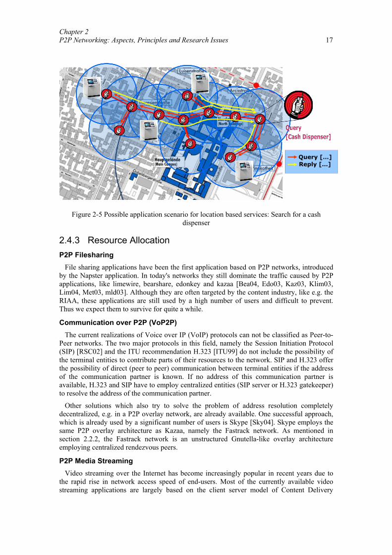
Thus besides the well-known file sharing applications, new wireless applications become feasible. As illustrated in Figure 2-5 context based routing would be supported by the available MANET. The user could then simply send out a request, e.g. for a cash dispenser, which would be broadcasted in a multihop manner, via a pre-configured number of hops in its proximity. All participating nodes would forward the request, until a cash dispenser receives the request. The cash dispenser could then reply with an appropriate response message to the requesting customer and announce its location. Thus a context based routing scheme supports the utilization of Location-based Services (LBS) without the need for centralized elements. Further request categories could thus also include bars, restaurants, taxis or closest bus stops.
Chapter 2 P2P Networking: Aspects, Principles and Research Issues 17
Figure 2-5 Possible application scenario for location based services: Search for a cash dispenser
2.4.3 Resource Allocation P2P Filesharing
File sharing applications have been the first application based on P2P networks, introduced by the Napster application. In today's networks they still dominate the traffic caused by P2P applications, like limewire, bearshare, edonkey and kazaa [Bea04, Edo03, Kaz03, Klim03, Lim04, Met03, mld03]. Although they are often targeted by the content industry, like e.g. the RIAA, these applications are still used by a high number of users and difficult to prevent. Thus we expect them to survive for quite a while.
Communication over P2P (VoP2P) The current realizations of Voice over IP (VoIP) protocols can not be classified as Peer-to-
Peer networks. The two major protocols in this field, namely the Session Initiation Protocol (SIP) [RSC02] and the ITU recommendation H.323 [ITU99] do not include the possibility of the terminal entities to contribute parts of their resources to the network. SIP and H.323 offer the possibility of direct (peer to peer) communication between terminal entities if the address of the communication partner is known. If no address of this communication partner is available, H.323 and SIP have to employ centralized entities (SIP server or H.323 gatekeeper) to resolve the address of the communication partner.
Other solutions which also try to solve the problem of address resolution completely decentralized, e.g. in a P2P overlay network, are already available. One successful approach, which is already used by a significant number of users is Skype [Sky04]. Skype employs the same P2P overlay architecture as Kazaa, namely the Fastrack network. As mentioned in section 2.2.2, the Fastrack network is an unstructured Gnutella-like overlay architecture employing centralized rendezvous peers.
P2P Media Streaming Video streaming over the Internet has become increasingly popular in recent years due to
the rapid rise in network access speed of end-users. Most of the currently available video streaming applications are largely based on the client server model of Content Delivery
Query […]Reply […]
Chapter 2 P2P Networking: Aspects, Principles and Research Issues
18
Networks (CDN) [AWT02]. However this approach faces a number of problems as pointed out in [KSE04].
P2P networks offer characteristics and possibilities which can not be provided by CDNs. P2P networks do not have a single point of failure, the bandwidth is shared between all peers and the content is shared at the edge of the network. As we show in [KSE04], therefore the performance of media streaming can be better in a P2P network based on Multiple Description Compression (MDC) [Goy01], although the probability that a stream breaks is higher [CLL02]. Other approaches to provide media streaming applications based on P2P networks are described in [GSK03, HC04, HHB03, THD04, XHH02].
2.5. Research Issues The major characteristic of Peer-to-Peer networks is their highly dynamic and distributed
structure, which may be based on any IP enabled network. Although this offers application-developers and users a large degree of freedom, the dynamism and the spread of content and nodes is a key issue which has to be addressed by the P2P protocol.
A network with similar characteristics can not be found in fixed environments. Only if we have a look at mobile networks, we find similar network structures. Mobile ad hoc networks (MANETs) [Per00] have a similar random network structure, and have to cope with the constantly changing infrastructure, especially caused by node movements These can be compared to node joins and leaves in P2P networks (personal mobility versus terminal mobility) [SGF02]. Although the two protocols are designed for different OSI layers, i.e. MANET for the physical layer and P2P for the application and transport layer, both networking approaches have the same goal. Auto configuration, self organization and independence from central authorities are therefore important characteristics of MANETs and P2P networks.
In sections 2.1, 2.2 and 2.3, we presented a number of P2P protocols and architectures, which provide the basic functionality to locate and exchange shared content. While some issues are solved, no standard solution for P2P networks has been achieved. The large variety of applications and the diversity of underlying physical access networks generate always new problems to be solved. On the other hand different physical properties also offer new possibilities, which can be used to optimize the protocols, e.g. the availability of locality information in mobile networks. This section therefore provides an overview about current research issues. Although it is by no means complete, it may initiate further research and helps to categorize the contributions of this work.
Quality of Service (QoS) in P2P If any network and/or protocol is intended to form a market and generate revenues, it is
necessary to ensure, that the service is provided reliably. Further on, as in P2P networks the customers also provide a certain amount of their own resources, the users themselves will be interested to restrain unlimited consumption of their resources by other nodes [AH00]. Especially as new multimedia applications, like telephony or media-streaming applications, are emerging in P2P networks, customer demands for some kind of regulation and guarantee of a certain quality may arise.
In P2P networks every node is under the responsibility of a different user. Thus it is necessary to impose QoS mechanisms not only on the network but also on every single peer. First solutions are based on service level agreements [GHM03, GCH03] or a two tier approach [GN02]. Other solutions try to provide QoS by influencing the replication of objects [OSS03] or through the adaptation of the overlay network [HWC04]. However they still rely to a significant extent on a certain level of trust and cooperation between the peers.
Chapter 2 P2P Networking: Aspects, Principles and Research Issues 19
Security, trust and authentication Aspects which are not covered in detail by the P2P research community are the challenges
of trust and security in P2P systems [GS00]. Similar to mobile ad hoc networks, the challenges in this area stem from the distributed and dynamic nature of P2P networks. However a certain amount of trust and security is a crucial prerequisite for business in the area of P2P. A security and trust system should be able to solve the following tasks:
• Guarantee the integrity of exchanged documents (including their descriptions)
• Provide a certain amount of anonymity
• Establish a reputation system
• Provide means to sanction misbehavior
• Provide secure communication channels between endpoints
Based on the analytical work of Marsh [Mar94], Rahman proposed a trust and security architecture for P2P networks [AH00]. Yu establishes a social network among the agents, to provide a distributed trust architecture in electronic communities [YS00]. Similar to distributed approaches, as proposed in [ACDD03, CDGR02, FK99, PS04, VAS04, ZH99], these approaches suffer from scalability and data management problems in networks with high churn rates and a large number of users.
Accounting and access control To be able to effectively use a QoS scheme in a P2P network, we need to implement an
accounting and access control architecture, which awards cooperative and punishes misbehaving peers. This would provide P2P communities with the basic means for trading between each other. It allows nodes to access shared resources only upon commonly agreed policies [DBE04].
Within the MMAPPS project a token based accounting scheme is proposed as a basis to establish market mechanisms in P2P systems [HLM03, SRG03]. In a similar manner, Habib proposes in [HC04] a rank-based incentive mechanism. In this accounting system cooperative users earn a higher rank by contributing resources and are then able to receive higher quality streaming. However, if no trust can be guaranteed in the network, users can circumvent any accounting system comparatively easily and their misbehavior can not be punished. Further work is described in [PWF02, TJM99]
Reliability and availability Due to the distributed structure of pure, hybrid and structured P2P networks a major
advantage of P2P networks is their reliability. As no single point of failure exists, the vulnerability of the network as a whole is very small, although the reliability of the single nodes, establishing the P2P network is comparatively low [BSV03, CLL02]. The high churn rate [SD03] leads to low availability of single nodes. As the nodes also contribute the shared content, the availability of the content offered by a single node depends on the availability of the node. Only because a number of replicas of most objects is provided by other nodes in the P2P network high availability of content is observed in P2P networks [ACKS03, CMN03].
In Voice over P2P networks the communication partner exits only once in the network. Thus the probability to find this object in an unstructured P2P network is nearly zero. In contrast in a structured P2P network, we could also find this object, as long as it is not lost, i.e. as long as the node, being responsible for this object does not fail. To increase the availability of such an object it is therefore necessary to distribute announcements or descriptions of this object in the network, which state where the object can be found [CMN03].
Chapter 2 P2P Networking: Aspects, Principles and Research Issues
20
Load balancing In structured P2P networks, the shared content, or at least a profile, describing the content
and its location, is distributed according to the hash-values of the keywords describing the shared content [ESKZ04]. If a strong hash function is used, we can assume, that the hash functions distribute the resulting hash values according to a uniform distribution in the overlay network [SK04]. However if the keywords themselves are not uniformly distributed, the responsibility for the shared objects is not distributed uniformly among the participating nodes. Examples are the occurrence rate of last names in a phone book or the distribution of keywords in a P2P network. This results in more requests, more responsibility and higher storage and processing power requirements on certain nodes, and thus in a higher vulnerability of the P2P system. Therefore new concepts how to distribute the load in a structured P2P network more evenly have to be found. A first approach to solve this problem is described in [KR04]. In Chapter 5, we target this issue by proposing a balanced architecture.
Routing Due to the abstraction of the TCP layer, the overlay network is independent from the
physical layer. Compared to the Internet, the structure of the overlay is very dynamic. The average session length of general nodes in a P2P network is significantly shorter than the uptime of common core or access routers in the Internet.
As mentioned above, a similar topology dynamism can be found in MANETs. Therefore it is helpful to study the routing approaches available in MANETs, as in these networks the routing protocol has to handle the dynamics of the participating nodes [SGF02]. However routing in a P2P network is content-based, whereas routing in MANETs is address routing. Also, MANETs are developed for a few hundred people, while P2P networks are often used by more than some ten-thousand users.
One of the biggest problems in P2P networks, which directly impacts network providers, is the high signaling load caused by the routing approaches. One reason for this high signaling load, which often exceeds the traffic of the user-data-transfers in P2P networks, is the highly dynamic topology of the overlay. Here the use of compression schemes may result in increased signaling efficiency.
Structured P2P networks try to decrease the routing traffic by arranging the shared content in the overlay so that a route to the requested object can directly be established. Thus flooding can be avoided. However, especially in networks with a high churn rate this structured approach is too inflexible. With every node departure or arrival the structure has to be rearranged. This causes a high amount of traffic and therefore the approach of structured P2P networks may not be applicable to networks with a short session duration [BT04, RGRK04, XMH03]. We target these issues in section 4.5, 4.6, 4.7 and in Chapter 5.
Network organization As described in section 2.1, the overlay topology of P2P networks is independent from the
underlying physical topology. While this provides the application developer and the user with the possibility to adapt the overlay topology to their requirements, it mostly results in random connections in unstructured P2P networks. This justifies to model P2P networks as random graphs. We can thus apply the findings available from random graph theory [Bo85, JLR00].
In structured P2P networks, we have a random assignment of IDs to the nodes. However the network topology between these nodes is predetermined by the structured P2P approach. Random graph theory can therefore not be applied to these networks and new models have to be developed.
Chapter 2 P2P Networking: Aspects, Principles and Research Issues 21
To increase the efficiency of structured P2P networks and to avoid zigzag routes [SK03],
first approaches to determine the position of a node in the overlay depending on its physical location are proposed in [Gum03, RD01, ZZ03]. However if the underlying physical network changes frequently, due to the movement of nodes, as it is the case in a MANET, also the overlay topology is changing frequently. This leads again to a high churn rate, which then also results in a high signaling overhead.
In this work we therefore focus on unstructured P2P networks, as a changing overlay topology does not cause any additional traffic. Unstructured P2P networks are therefore more suitable for heterogeneous networks, where it is important to adapt the overlay structure to the physical topology. If the underlying physical structure is organized efficiently, it can even help to improve the network topology of the overlay (see section 4.6 and 4.7).
Cross layer communication Cross layer communication describes the exchange of information directly between two
layers of the OSI model, although these layers are not neighboring layers. In P2P networks cross layer communication is mostly used to connect the application layer directly with the physical or network layer. Thus the application can retrieve information from these layers and adapt its overlay connections, the employed compression scheme or its overlay routing strategy to characteristics of these layers.
The application can e.g. retrieve information about its location in the physical network, about its geographical position, or connection parameters like delay or error rate. The Mobile Peer-to-Peer protocol uses cross layer communication to adapt the overlay routing structure to the underlying physical network [KSGN03]. Further on cross layer communication can be used to establish connections to nodes with special characteristics, e.g. to nodes with the shortest distance in the physical network [KSE04, SKe04]. Within this work we focus on this issue in sections 4.6, 4.7 and 5.3 to illustrate the possibilities of cross layer communication to improve the performance of P2P protocols.
Scalability In pure P2P networks content can only be found if the request sent out by one peer reaches a
peer sharing the requested content. As no knowledge about the overlay topology or about the location of content is available to route requests, flooding has to be used. For an increasing number of users, this results in a steeply increasing number of messages. Thus this does not scale well with the number of users.
Therefore in Gnutella 0.6 a second dynamic hierarchical layer was introduced, the Superpeer layer. This approach limits flooding to the Superpeer layer and thus scales significantly better than Gnutella 0.4. However such an approach is only applicable for fixed environments. We also have to take into account in hierarchical P2P networks, the increased vulnerability of the system and the extra effort for the selection of Superpeers and load balancing.
To increase the search success rate in overlay networks with many participants, without increasing the signaling traffic significantly, another solution might bring those users sharing similar interests virtually close together. According to interests stated by the user, the peer is connected to the overlay network where already peers with similar interest are located. According to [WHAT04] such interest groups often form geographically close groups. Therefore such an adaptation of the overlay to user interests can also result in better scalability. This is partly implemented in the file-sharing application Audiogalaxy [Aud04].
Considering structured P2P networks, we do not only have to take into account the scalability according to the number of users, but also to the frequency of node joins and leaves/failures. The signaling traffic increases significantly with decreasing average session lengths [RD01, TAD03]. Accordingly we can thus observe a significantly increased
Chapter 2 P2P Networking: Aspects, Principles and Research Issues
22
scalability only in stable environments [BT04, RGRK04] compared to unstructured approaches. However we can further improve the scalability of the routing traffic and lookup delay by the introduction of another hierarchy level in structured P2P networks [KR04, MM02].
Measuring P2P networks A major problem to be solved, if we want to measure the topology of P2P networks is that
in most P2P networks, except in centralized P2P networks, we have only a local view. Thus the number of active participants in a P2P network is not completely determinable. However, with the help of crawlers, as described in section 3.1.1.2, we can measure a large area of the P2P network [RFI02, SK03].
In structured P2P networks it is even harder to determine the network topology and the number of participants. Here we can only use passive monitoring of the messages routed by the peers. Due to the possible shortcuts in the overlay (e.g. fingers in Chord), a convincing approach to estimate the number of active participants in a structured P2P network has not been proposed to our knowledge.
Determining the traffic characteristics of P2P networks, e.g. its self-similarity or its total volume, is comparatively easy, as it occurs locally at every node [And03, AG03, FMLC03, Mar02, SGG02, SD03]. However it is sensible to capture the packets at the packet as well as at the application layer. Thus we can assign the single packets to the different sources more easily and can additionally analyze also the application layer traffic (see section 3.1.1.3). Additionally we can use the traffic measurements from the application layer to measure the user behavior (see section 3.1.2.2). These data can then also be used to develop an analytic user model.
Modeling P2P networks Analytical models of P2P networks are developed to be able to describe the properties of
P2P networks mathematically. With such models we want to provide means to determine the properties of P2P networks of any size, without having to run extensive simulations. As described in [SS04] and [GFJK03], we can compute the availability of documents or the traffic caused by P2P networks. To model the overlay topology of an unstructured P2P network we use methods from random graph theory developed by Bollobas and Erdös [Bo85, Bo98, ER60]. The application of these basic concepts to P2P networks is described in [GFJK03, GDSG03, JA01, Kan03, KIT04, SS04].
In structured P2P networks, the model for the overlay topology is generally comparatively simple. In Chord the overlay can be modeled by a simple ring structure. However here we have to take into account the possibility for shortcuts [BT04]. In contrast to unstructured P2P networks, the network dynamic strongly influences the routing overhead in structured P2P networks. In this area significant further research is necessary.
P2P in heterogeneous networks As described in [GSK04, KSGN03, SGF02], Peer-to-Peer networks do not only occur in
fixed environments but also increasingly in mobile environments and on other access networks. First Peer-to-Peer applications, e.g. for Windows PocketPC, are also already available. Therefore the interest in the research community, to analyze Peer-to-Peer networks in heterogeneous networks is steadily increasing [ESKZ04].
Generally we distinguish in this work fixed wireline access networks, cellular wireless access networks and Mobile Ad Hoc networks. In fixed wireline networks, for which until now most Peer-to-Peer applications have been developed, nearly no restrictions for Peer-to-Peer nodes must be taken into account.
Chapter 2 P2P Networking: Aspects, Principles and Research Issues 23
Cellular wireless networks are characterized by the fact, that in addition to the terminal
mobility these networks also support node mobility, i.e. changes of the geographical position of a node. Cellular systems, like e.g. GSM, additionally provide a TCP/IP layer even across the wireless channel from the base station to the mobile terminal. Therefore it is relatively easy to apply Peer-to-Peer concepts also in cellular wireless systems. However we have to take into account the significantly lower available data rate of the mobile nodes (in GSM 14kbit/s in GPRS~64kbit/s) [EVB01]. Further on we have to assume a lower session duration of the mobile nodes, as the cellular wireless channel is a high cost channel compared to fixed networks. Therefore it might be sensible to develop overlay proxies and gateways for the mobile node.
According to the definition of a MANET in [Per00], we consider MANETs as self configuring wireless multihop networks. Thus we have to take into account in addition to the lower capabilities of the participating mobile nodes (lower access data rate, lower processing power, less storage capabilities, limited energy resources) a random and frequently changing physical access network. Therefore it is necessary to adapt the overlay to the underlying MANET topology. Thus zigzag routes can be avoided, which leads to a significantly reduced resource consumption in the MANET [GSK04, KSGN03, KCW03].
2.6. Summary In this chapter we presented a detailed analysis of different routing protocols and concepts
for application in P2P networks. Our first contribution was the introduction of a classification framework for P2P routing approaches, which distinguishes in a first level of abstraction structured and unstructured P2P networks. Unstructured P2P networks can further on be categorized into centralized, hybrid and pure P2P networks, as introduced in [Scho01a], [Scho01] and [ES03]. A similar classification of P2P routing approaches is also used in [SW04] and [MH03]. We can thus offer a definition for Peer-to-Peer networking and additionally clarify the differences to common so called Client/Server-architectures.
As a second contribution this chapter provided an overview about the state of the art of Peer-to-Peer networking and classifies the currently most important protocols in the area of Peer-to-Peer networking with the help of the proposed definition. We also included protocols like Napster in this overview, although they are currently not used anymore, mainly because of legal issues. However, they used an architecture, which may offer specific characteristics which can not be achieved by other protocols. This provides researchers with a profound and comprehensive summary of the P2P protocols.
As a third contribution we presented in this chapter a detailed performance analysis of the major P2P routing approaches in each of the classes stated above (structured, hybrid, centralized, pure). Parameters which are used to evaluate the performance are e.g. the signaling overhead for search and file transfer, the scalability of the routing approach and the availability of specific content. We especially considered the background noise of each P2P protocol. Therefore we employed measurements from existing networks or computed the values of the traffic with approaches mainly based on random graphs, as explained in detail in Chapter 3.
Background noise in this context describes the signaling traffic initiated and received by an average node participating in the overlay, without actively initiating requests. Comparing these numbers in one graph, as depicted by Figure 2-6, clearly shows the advantage of centralized P2P systems. No distributed search, as e.g. in Gnutella is necessary, as the location of every object can be retrieved from the central lookup table. However this good performance can not compensate the risk of a single point of failure. Such a single point of failure is also a single point of costs and administration, which can be avoided in decentralized systems, like Gnutella.
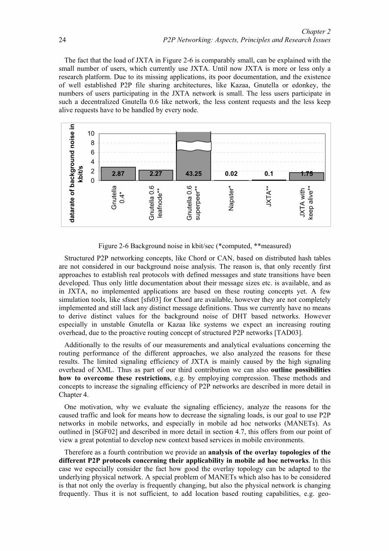
Chapter 2 P2P Networking: Aspects, Principles and Research Issues
24
The fact that the load of JXTA in Figure 2-6 is comparably small, can be explained with the small number of users, which currently use JXTA. Until now JXTA is more or less only a research platform. Due to its missing applications, its poor documentation, and the existence of well established P2P file sharing architectures, like Kazaa, Gnutella or edonkey, the numbers of users participating in the JXTA network is small. The less users participate in such a decentralized Gnutella 0.6 like network, the less content requests and the less keep alive requests have to be handled by every node.
2.87 2.27 43.25 0.02 0.1 1.7502468
10
Gnu
tella
0.4*
Gnu
tella
0.6
leaf
node
**
Gnu
tella
0.6
supe
rpee
r**
Nap
ster
*
JXTA
**
JXTA
with
keep
aliv
e**
dat
arat
e of
bac
kgro
und
nois
e in
kb
it/s
Figure 2-6 Background noise in kbit/sec (*computed, **measured)
Structured P2P networking concepts, like Chord or CAN, based on distributed hash tables are not considered in our background noise analysis. The reason is, that only recently first approaches to establish real protocols with defined messages and state transitions have been developed. Thus only little documentation about their message sizes etc. is available, and as in JXTA, no implemented applications are based on these routing concepts yet. A few simulation tools, like sfsnet [sfs03] for Chord are available, however they are not completely implemented and still lack any distinct message definitions. Thus we currently have no means to derive distinct values for the background noise of DHT based networks. However especially in unstable Gnutella or Kazaa like systems we expect an increasing routing overhead, due to the proactive routing concept of structured P2P networks [TAD03].
Additionally to the results of our measurements and analytical evaluations concerning the routing performance of the different approaches, we also analyzed the reasons for these results. The limited signaling efficiency of JXTA is mainly caused by the high signaling overhead of XML. Thus as part of our third contribution we can also outline possibilities how to overcome these restrictions, e.g. by employing compression. These methods and concepts to increase the signaling efficiency of P2P networks are described in more detail in Chapter 4.
One motivation, why we evaluate the signaling efficiency, analyze the reasons for the caused traffic and look for means how to decrease the signaling loads, is our goal to use P2P networks in mobile networks, and especially in mobile ad hoc networks (MANETs). As outlined in [SGF02] and described in more detail in section 4.7, this offers from our point of view a great potential to develop new context based services in mobile environments.
Therefore as a fourth contribution we provide an analysis of the overlay topologies of the different P2P protocols concerning their applicability in mobile ad hoc networks. In this case we especially consider the fact how good the overlay topology can be adapted to the underlying physical network. A special problem of MANETs which also has to be considered is that not only the overlay is frequently changing, but also the physical network is changing frequently. Thus it is not sufficient, to add location based routing capabilities, e.g. geo-
Chapter 2 P2P Networking: Aspects, Principles and Research Issues 25
sensitive routing. If we for example determine the ID of a node in a structured P2P network, like Chord, according to an algorithm which takes the current location into account, this would scale nicely if we assume a fixed physical network. If we assume moving nodes, as in a typical MANET scenario, this would result in frequently changing IDs of the nodes. A changing ID in a Chord ring corresponds to a node leave and a node join, which results in a huge amount of traffic. Other schemes, which are based on unstructured P2P networks and employ cross-layer communication, definitely scale better, as explained in detail in 4.7.
Another contribution of this section is also the detailed discussion of possibilities and limitations of structured P2P networks. One of the major results of this analysis is, that especially in overlay networks with a high churn rate, as it occurs in current file-sharing applications, structured P2P approaches suffer from severe scalability problems. The signaling overhead to rearrange the routing structure in case of a single node join or leave is significant and can not be neglected.
Chapter 3 METHODS TO ANALYZE P2P NETWORKS
As pointed out in Chapter 2, P2P networks are established as an overlay network, which may be completely independent from any other network topologies and protocols. P2P networks establish a virtual network on top of an IP and physical network. Thus we have to analyze two networks, namely the virtual network at the application layer and the transport network represented in our case by layers 1 to 3. Consequently, we need tools to analyze these P2P networks, to be able to evaluate the effects of these networks as perceived by lower layers, and certainly also to optimize these networks in terms of signaling efficiency, search success rate or reliability and possibly other performance criteria. Therefore we introduce in this chapter new tools to measure, model and simulate P2P overlay networks.
To do so we first describe the measurement tools developed for our work. They can mainly be divided into tools to measure the virtual topology of these networks, tools to analyze the network traffic and tools to analyze the user behavior. Here our focus is clearly set to study the overlay network as is, although we also analyze the effects of the overlay on the physical network, and how the overlay network can be mapped on the physical network.
Based on the results of our measurements we develop mathematical models to describe the different techniques interacting in the overlay networks. To establish our models we use methods of mathematical statistics and random graph theory in finite networks to describe the topology of the overlay network, the user behavior and also the resulting traffic and search efficiency.
To verify our mathematical models and our measurements we also use simulations. Here we have to distinguish simulations of only the overlay or of the whole protocol stack. Simulations taking only the overlay network into account are significantly simpler and scale to a much higher number of nodes. On the other hand, simulations of the whole protocol stack allow us to study effects at the packet level. Thus we can analyze optimizations of the overlay network, e.g. geo-sensitivity or the use of cross layer communication to better adapt to the physical network. The methods described in this chapter are used to understand current networks, find their shortcomings and benefits and thus to optimize existing networks and design better protocols for the establishment of overlay networks.
To understand and develop models of P2P networks, it is necessary to analyze the topology of the overlay network and the traffic caused by P2P applications running on top of that. An advantage when analyzing P2P networks is that the protocol and the clients are often available as open source. Further on, as the network is a virtual network, nearly everybody connected to the Internet can become a member of such a virtual public network, without any additional hardware, simply by installing some software on her/his computer. Therefore measurement software can either be coded as a standalone version, or an existing version of a P2P client can be used to adjust it such that it can be used to measure different parameters of the network. The measurement tools developed and used within our work can be categorized into measurements approaches aiming at the analysis of the overlay topology and its mapping on the physical layer, and tools which capture the traffic caused by P2P applications and its impacts on the remaining traffic.
Chapter 3 Methods to Analyze P2P Networks 27
3.1. Measuring Unstructured P2P Networks 3.1.1 Network Topology Measurements
Most of the measurement approaches proposed so far are based on crawler techniques. Saroui et al. [SGG02] for example published in 2002 work about some measurement results of the Gnutella and the Napster network. They used active and passive measurements to measure the session duration of a single node. They also measured the structure of the Gnutella network, however they did not match the overlay topology to any physical layer.
Jovanovic et al. [JAB01] developed a network crawler specifically designed for the Gnutella network. They evaluated in detail the connectivity of the network. Thus they were able to provide a degree distribution of the network, which we are going to use in Chapter 3. They also investigated the Small World characteristics [ASBS97, WS98] of the Gnutella network.
To describe the connectivity of the Gnutella network was also the aim of Ripeanu et al. [RFI02]. They measured the connectivity and the network structure of the Gnutella network. Additionally they evaluated the probability that the clusters, formed in the overlay network, match the clusters of the underlying physical infrastructure.
The major problem in determining the topology of decentralized networks is that no central instance is available by definition. Thus no central point in the network can be used to determine the topology. The only central instance, which might be employed in such a network is a bootstrap server, which provides the addresses of nodes, which connected through this bootstrap shortly before and therefore can be assumed to be active. However the bootstrap server can only count how many nodes connected through it to the network, but can not provide information about the network structure, as nodes go offline and online frequently and also have different degree, which can not be resolved by the bootstrap server.
3.1.1.1. Measuring an overlay network from a local perspective Unstructured P2P networks, like Gnutella, use keep-alive and content request messages to
stay connected to the network and to search for content. As the nodes do not have any information about the network topology, these request messages have to be flooded in the overlay network, as described in detail in section 2.2. In contrast to the request messages, the according response messages do not have to be flooded. They can be routed from the responding node back to the initiating node on the same path, the responding node received the request on. This route is the shortest route in the overlay network, as the responding node reacts only on the first request it received. These messages can be used to measure the network from a local point of view.
In a first step we therefore use this mechanism to measure the network as perceived by a P2P node completely compliant with the investigated P2P protocol. The measurement node only logs all incoming messages. They can be evaluated after the measurement period, according to the information included in the messages, like the originating IP-address and the hop distance of the originator of a message. In our measurement node implementation we especially concentrate on keep-alive response messages and query-response messages, provoked by actively probing the network from our measurement node with keep-alive requests and content requests for highly available data.
The measurement period has to be short enough to be able to monitor even fast changes in the network. For our measurements in the Gnutella network, we therefore use a period of 200 seconds to measure a stable network, as we found in previous measurements, that the average lifetime of a node is 900 seconds. Within each measurement period, the measurement node writes all incoming response messages into a cache. Besides other information, response
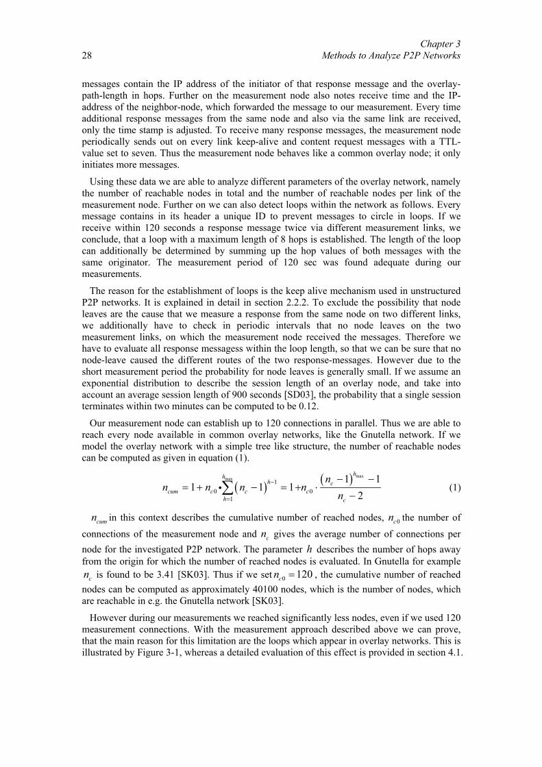
Chapter 3 Methods to Analyze P2P Networks
28
messages contain the IP address of the initiator of that response message and the overlay-path-length in hops. Further on the measurement node also notes receive time and the IP-address of the neighbor-node, which forwarded the message to our measurement. Every time additional response messages from the same node and also via the same link are received, only the time stamp is adjusted. To receive many response messages, the measurement node periodically sends out on every link keep-alive and content request messages with a TTL-value set to seven. Thus the measurement node behaves like a common overlay node; it only initiates more messages.
Using these data we are able to analyze different parameters of the overlay network, namely the number of reachable nodes in total and the number of reachable nodes per link of the measurement node. Further on we can also detect loops within the network as follows. Every message contains in its header a unique ID to prevent messages to circle in loops. If we receive within 120 seconds a response message twice via different measurement links, we conclude, that a loop with a maximum length of 8 hops is established. The length of the loop can additionally be determined by summing up the hop values of both messages with the same originator. The measurement period of 120 sec was found adequate during our measurements.
The reason for the establishment of loops is the keep alive mechanism used in unstructured P2P networks. It is explained in detail in section 2.2.2. To exclude the possibility that node leaves are the cause that we measure a response from the same node on two different links, we additionally have to check in periodic intervals that no node leaves on the two measurement links, on which the measurement node received the messages. Therefore we have to evaluate all response messagess within the loop length, so that we can be sure that no node-leave caused the different routes of the two response-messages. However due to the short measurement period the probability for node leaves is generally small. If we assume an exponential distribution to describe the session length of an overlay node, and take into account an average session length of 900 seconds [SD03], the probability that a single session terminates within two minutes can be computed to be 0.12.
Our measurement node can establish up to 120 connections in parallel. Thus we are able to reach every node available in common overlay networks, like the Gnutella network. If we model the overlay network with a simple tree like structure, the number of reachable nodes can be computed as given in equation (1).
( ) ( ) maxmax 10 0
1
1 11 1 1
2
hhh c
cum c c ch c
nn n n n
n−
=
− −= + − = + ⋅
−∑i (1)
cumn in this context describes the cumulative number of reached nodes, 0cn the number of connections of the measurement node and cn gives the average number of connections per node for the investigated P2P network. The parameter h describes the number of hops away from the origin for which the number of reached nodes is evaluated. In Gnutella for example
cn is found to be 3.41 [SK03]. Thus if we set 0 120cn = , the cumulative number of reached nodes can be computed as approximately 40100 nodes, which is the number of nodes, which are reachable in e.g. the Gnutella network [SK03].
However during our measurements we reached significantly less nodes, even if we used 120 measurement connections. With the measurement approach described above we can prove, that the main reason for this limitation are the loops which appear in overlay networks. This is illustrated by Figure 3-1, whereas a detailed evaluation of this effect is provided in section 4.1.
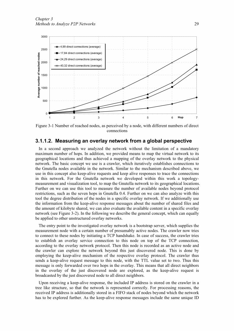
Chapter 3 Methods to Analyze P2P Networks 29
0
500
1000
1500
2000
2500
3000
1 2 3 4 5 6 7Hop
Ave
rage
num
ber o
f rea
ched
nod
es
4,99 direct connections (average)
17,84 direct connections (average)
24,29 direct connections (average)
40,32 direct connections (average)
Figure 3-1 Number of reached nodes, as perceived by a node, with different numbers of direct
connections
3.1.1.2. Measuring an overlay network from a global perspective In a second approach we analyzed the network without the limitation of a mandatory
maximum number of hops. In addition, we provided means to map the virtual network to its geographical locations and thus achieved a mapping of the overlay network to the physical network. The basic concept we use is a crawler, which iteratively establishes connections to the Gnutella nodes available in the network. Similar to the mechanism described above, we use in this concept also keep-alive requests and keep alive responses to trace the connections in this network. For the Gnutella network we developed within this work a topology-measurement and visualization tool, to map the Gnutella network to its geographical locations. Further on we can use this tool to measure the number of available nodes beyond protocol restrictions, such as the seven hops in Gnutella 0.4. Further on we can also analyze with this tool the degree distribution of the nodes in a specific overlay network. If we additionally use the information from the keep-alive response messages about the number of shared files and the amount of kilobyte shared, we can also evaluate the available content in a specific overlay network (see Figure 3-2). In the following we describe the general concept, which can equally be applied to other unstructured overlay networks.
The entry point to the investigated overlay network is a bootstrap server, which supplies the measurement node with a certain number of presumably active nodes. The crawler now tries to connect to these nodes by initiating a TCP handshake. In case of success, the crawler tries to establish an overlay service connection to this node on top of the TCP connection, according to the overlay network protocol. Then this node is recorded as an active node and the crawler can explore the network beyond this just discovered node. This is done by employing the keep-alive mechanism of the respective overlay protocol. The crawler thus sends a keep-alive request message to this node, with the TTL value set to two. Thus this message is only forwarded over two hops in the overlay. This means that all direct neighbors in the overlay of the just discovered node are explored, as the keep-alive request is broadcasted by the just discovered node to all direct neighbors.
Upon receiving a keep-alive response, the included IP address is stored on the crawler in a tree like structure, so that the network is represented correctly. For processing reasons, the received IP address is additionally stored in a FIFO stack of nodes beyond which the network has to be explored further. As the keep-alive response messages include the same unique ID
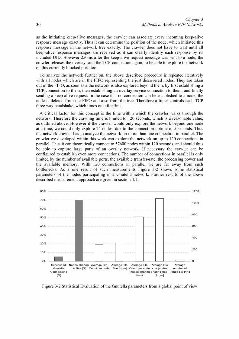
Chapter 3 Methods to Analyze P2P Networks
30
as the initiating keep-alive messages, the crawler can associate every incoming keep-alive response message exactly. Thus it can determine the position of the node, which initiated this response message in the network tree exactly. The crawler does not have to wait until all keep-alive response messages are received as it can clearly identify each response by its included UID. However 250ms after the keep-alive request message was sent to a node, the crawler releases the overlay- and the TCP-connection again, to be able to explore the network on this currently blocked port, too.
To analyze the network further on, the above described procedure is repeated iteratively with all nodes which are in the FIFO representing the just discovered nodes. They are taken out of the FIFO, as soon as a the network is also explored beyond them, by first establishing a TCP connection to them, then establishing an overlay service connection to them, and finally sending a keep alive request. In the case that no connection can be established to a node, the node is deleted from the FIFO and also from the tree. Therefore a timer controls each TCP three way handshake, which times out after 5ms.
A critical factor for this concept is the time within which the crawler walks through the network. Therefore the crawling time is limited to 120 seconds, which is a reasonable value, as outlined above. However if the crawler would only explore the network beyond one node at a time, we could only explore 24 nodes, due to the connection uptime of 5 seconds. Thus the network crawler has to analyze the network on more than one connection in parallel. The crawler we developed within this work can explore the network on up to 120 connections in parallel. Thus it can theoretically connect to 57600 nodes within 120 seconds, and should thus be able to capture large parts of an overlay network. If necessary the crawler can be configured to establish even more connections. The number of connections in parallel is only limited by the number of available ports, the available transfer-rate, the processing power and the available memory. With 120 connections in parallel we are far away from such bottlenecks. As a one result of such measurements Figure 3-2 shows some statistical parameters of the nodes participating in a Gnutella network. Further results of the above described measurement approach are given in section 4.1.
0%
10%
20%
30%
40%
50%
60%
70%
80%
SuccessfullGnutella
Connections[%]
Nodes sharingno files [%]
Average FileCount per node
Average FileSize [kbyte]
Average FileCount per node(nodes sharing
files)
Average Filesize (nodes
sharing files)[kbyte]
Averagenumber of
Pongs per Ping
0
200
400
600
800
1000
1200
Figure 3-2 Statistical Evaluation of the Gnutella parameters from a global point of view
Chapter 3 Methods to Analyze P2P Networks 31
3.1.1.3. Determining the geographic location of nodes
To be able to map the nodes participating in the overlay network to their geographical locations, we additionally have to retrieve their geographical location in terms of longitude and latitude. As a basis we use NetGeo [Net04, PS01]. NetGeo is an Internet geographic database, which can be used to map IP addresses, domain names and AS numbers to their longitude and latitude. NetGeo can be accessed via a CGI interface, as described in [Net04]. It caches the information from previous lookups and if no matching record is found in the database, NetGeo performs one or more whois lookups employing the InterNIC and/or RIPE whois server. If the position of a specific node can not be resolved, it is not displayed on any map.
The mapping procedure of the overlay network is not time critical anymore, as the structure of the network is already stored on the crawler. After having collected all necessary data, a visualization tool implemented on top of the crawler and the location retriever is used to display a world map, with the places marked where an overlay node is located. Additionally the visualization can display the connections between the nodes, stored in the structure established by the crawler (see Figure 4-3 on page 69).
With this tool we can make the overlay network visible up to any hop value (see section 4.1.1). With the help of the location retriever we can also map the overlay network to its geographical locations. We can thus make the main physical paths used by the overlay network visible and can prove the existence of inefficient zigzag routes. An application of the crawler is described in section 4.1. The crawler can also provide further information, depending on the payload of the keep-alive responses, e.g. average number of shared files (288 files per node), the average size of the memory allocated for shared data (312Mbyte) or the average number of nodes sharing no files, so called free-riders (70.06%). More details are provided in section 4.1.
As we can measure the exact network structure with the crawler, we can further on analyze the network according to some common graph attributes, like its cliquishness, the average path length or its cluster coefficient. Thus we can also analyze the small world properties of overlay networks.
Despite the problem of the changing overlay structure, which is solved in our approach by limiting the measurement time, we have to cope with the fact, that a significant part of the nodes participating in the overlay network have private IP addresses, i.e. are located behind a NAT. Thus a crawler can not establish a TCP connection to these nodes, nor can the location retriever resolve the position of this node, if it states the private IP address and not the gateway’s IP address. Thus the topology obtained with the crawler will only be a subgraph of the actual overlay network. However, we can evaluate their data in the statistics as the crawler received a keep-alive response from these nodes, and can display at least the position of their gateway on the map.
3.1.2 Network Traffic Measurements Having analyzed the topology of the overlay network, we also want to understand the traffic
characteristics of overlay networks. Here we are especially interested in the signaling traffic arising from the P2P overlay protocol used to provide connectivity (keep-alive) and the lookup service to find the location of a requested service/data-item.
As this traffic causes already a large fraction of the total traffic in current IP networks, a significant effort has already been spent to analyze the traffic issues of P2P networks [AG03, FP02]. Besides work which tries to analyze the impact of P2P, applications on IP backbones [FMLC03] and across large networks [SW02], other researchers concentrate on the characteristics of specific P2P approaches [And03, IUBF04, KADR04, KWX01, Mar02,
Chapter 3 Methods to Analyze P2P Networks
32
Tut04] or on the differences between web and P2P traffic [GDSG03] and the possibilities to cache P2P requests and responses [LBBS02].
However, beyond existing work it is necessary to measure the traffic at the application layer as well as on the physical layer to fully understand P2P overlay networks. A corresponding measurement approach is described below. With these measurements we then derive traffic characteristics caused by P2P applications, e.g. concerning self similarity or the burstiness of P2P traffic. Further on we also provide general characteristics about the traffic caused by a single node in the overlay network, and the fraction of traffic caused by the different messages.
3.1.2.1. Methodology As shown in Figure 3-3, we use port mirroring at the main switch of our LAN for our
measurements. Thus we can capture all packets transmitted within our LAN (consisting of more than 100 users and machines running different applications) and also from/to the domain of our ISP, the Leibniz-Rechen-Zentrum (LRZ). The port mirror of the switch is connected to a packet logger, which captures all packets using Ethereal, or any other comparable packet capturing software [Eth04, Les01].
We then set up one specific node in the network which additionally takes part in an overlay network, e.g. in the Gnutella network in our investigation. This node acts as a common overlay node within the network, but does not offer any content and does not issue any requests beside keep-alive requests. Thus it acts only as a router within the overlay network.
To be able to measure the traffic at the application layer and to track the ports on which connections in the overlay network are established, we modify an overlay node accordingly. Tracking the ports is necessary so that we can identify the incoming and outgoing traffic caused within the overlay network on our measurement node. Measuring the traffic on the application layer enables us to identify the traffic portions and characteristics of the message types within the overlay network.
Generally we measured the traffic for 2 hours. This measurement time is divided into three periods. In the first period we measure the traffic on the LAN with the overlay node switched off. This first period lasts for 30 minutes and is used to measure the current network traffic, which is assumed to be relatively constant over our 2 hour measurement period. Thus we are able to describe the traffic of the network, without influences of overlay networks. In the second period, which lasts for 60 minutes, the overlay node is switched on and actively participates in the overlay network. In the third measurement period the overlay node is removed from the overlay network, and we again only measure the normal traffic of the investigated LAN, possibly plus a small amount of incoming P2P requests (see e.g. Figure 4-27 on page 88).
Every measurement consists of three phases, namely the above described data acquisition phase, a data pre-treatment phase and a final data analysis phase. The focus of the data acquisition phase is clearly to collect the data and to measure the different flows without influencing the traffic. Therefore we physically mirror the data flowing through the switch, and write them directly to the memory of the packet logger. Thus we avoid buffer overruns at the switch, and do not influence the traffic at the switch, as it performs no additional switching.
The data pre-treatment phase is used to compress and filter the data measured over 120 minutes. This is done after the measurements on the switch are finished. Thus we avoid any interrogations of the packet logger during the data acquisition. For our analysis we are only interested in the packet sizes, the packet inter arrival times and the TCP flow sizes. Thus we delete the contents of the TCP packets and some headers, to reduce the amount of
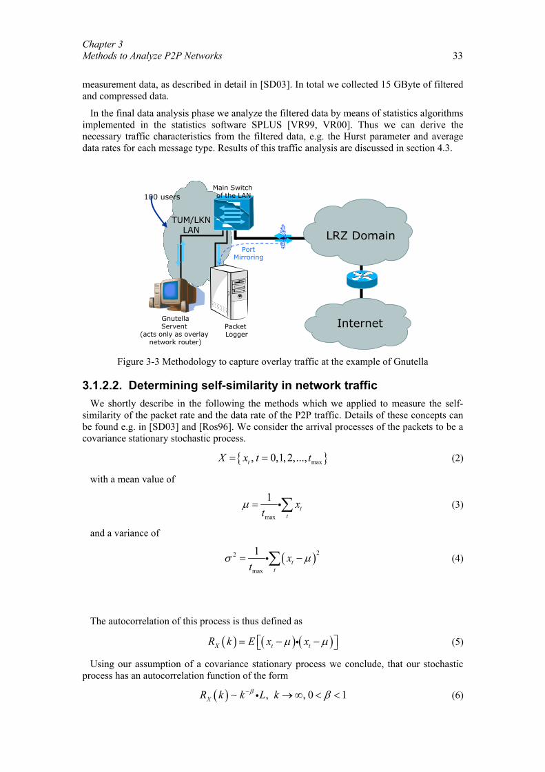
Chapter 3 Methods to Analyze P2P Networks 33
measurement data, as described in detail in [SD03]. In total we collected 15 GByte of filtered and compressed data.
In the final data analysis phase we analyze the filtered data by means of statistics algorithms implemented in the statistics software SPLUS [VR99, VR00]. Thus we can derive the necessary traffic characteristics from the filtered data, e.g. the Hurst parameter and average data rates for each message type. Results of this traffic analysis are discussed in section 4.3.
Figure 3-3 Methodology to capture overlay traffic at the example of Gnutella
3.1.2.2. Determining self-similarity in network traffic We shortly describe in the following the methods which we applied to measure the self-
similarity of the packet rate and the data rate of the P2P traffic. Details of these concepts can be found e.g. in [SD03] and [Ros96]. We consider the arrival processes of the packets to be a covariance stationary stochastic process.
{ }max, 0,1, 2,...,tX x t t= = (2)
with a mean value of
max
1t
t
xt
µ = ∑i (3)
and a variance of
( )22
max
1t
tx
tσ µ= −∑i (4)
The autocorrelation of this process is thus defined as
( ) ( ) ( )X t tR k E x xµ µ= − − i (5)
Using our assumption of a covariance stationary process we conclude, that our stochastic process has an autocorrelation function of the form
( ) , , 0 1XR k k L kβ β− → ∞ < <∼ i (6)
Internet
TUM/LKNLAN LRZ Domain
Main Switch of the LAN
PacketLogger
GnutellaServent
(acts only as overlay network router)
PortMirroring
100 users
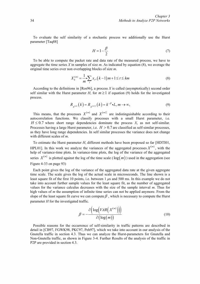
Chapter 3 Methods to Analyze P2P Networks
34
To evaluate the self similarity of a stochastic process we additionally use the Hurst parameter [Taq88]
12
H β= − (7)
To be able to compute the packet rate and data rate of the measured process, we have to aggregate the time series X in samples of size m. As indicated by equation (8), we average the original time series over non overlapping blocks of size m.
( )( ) 1 , 1 1mk t
tX x k m t km
m= − + ≤ ≤∑i (8)
According to the definitions in [Ros96], a process X is called (asymptotically) second order self similar with the Hurst parameter H, for 1m ≥ if equation (9) holds for the investigated process.
( ) ( ) ( ) ( )2 , ,m mX XR k R k k L mβ−= = → ∞i (9)
This means, that the processes ( )mX and ( )2mX are indistinguishable according to their autocorrelation functions. We classify processes with a small Hurst parameter, i.e.
0.7H ≤ where short range dependencies dominate the process X, as not self-similar. Processes having a large Hurst parameter, i.e. 0.7H > are classified as self-similar processes, as they have long range dependencies. In self similar processes the variance does not change with different scales of m.
To estimate the Hurst parameter H, different methods have been proposed so far [HDTI01, HPL01]. In this work we analyze the variances of the aggregated processes ( )mX , with the help of variance-time plots. In variance-time plots, the log of the variance of the aggregated series ( )mX is plotted against the log of the time scale ( ( )log m ) used in the aggregation (see Figure 4-33 on page 93)
Each point gives the log of the variance of the aggregated data rate at the given aggregate time scale. The scale gives the log of the actual scale in microseconds. The line shown is a least square fit of the first 10 points, i.e. between 1 µs and 500 ms. In this example we do not take into account further sample values for the least square fit, as the number of aggregated values for the variance calculus decreases with the size of the sample interval m. Thus for high values of m the assumption of infinite time series can not be applied anymore. From the slope of the least square fit curve we can compute β , which is necessary to compute the Hurst parameter H for the investigated traffic.
( )( )( )( )( )( )
log
log
mVAR X
mβ
∂= −
∂ (10)
Possible reasons for the occurrence of self-similarity in traffic patterns are described in detail in [CB97, FGWK98, PKC97, Peh97], which we take into account in our analysis of the Gnutella traffic in section 4.3. Thus we can analyze the Hurst-parameters for Gnutella and Non-Gnutella traffic, as shown in Figure 3-4. Further Results of the analysis of the traffic in P2P are provided in section 4.3.
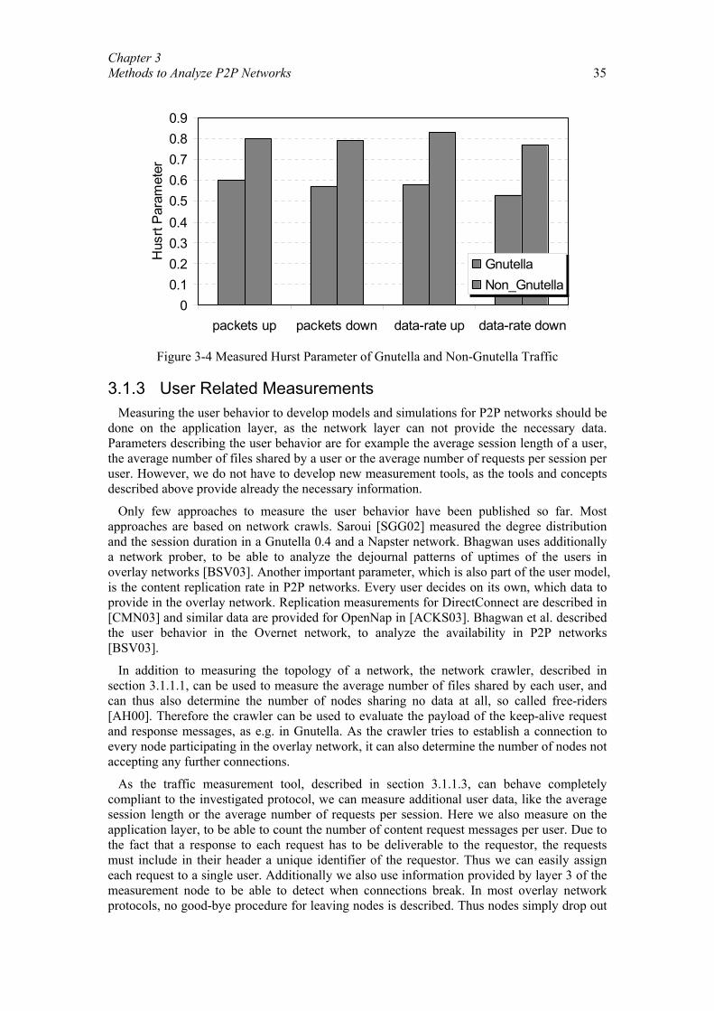
Chapter 3 Methods to Analyze P2P Networks 35
00.10.20.30.40.50.60.70.80.9
packets up packets down data-rate up data-rate down
Hus
rt P
aram
eter
GnutellaNon_Gnutella
Figure 3-4 Measured Hurst Parameter of Gnutella and Non-Gnutella Traffic
3.1.3 User Related Measurements Measuring the user behavior to develop models and simulations for P2P networks should be
done on the application layer, as the network layer can not provide the necessary data. Parameters describing the user behavior are for example the average session length of a user, the average number of files shared by a user or the average number of requests per session per user. However, we do not have to develop new measurement tools, as the tools and concepts described above provide already the necessary information.
Only few approaches to measure the user behavior have been published so far. Most approaches are based on network crawls. Saroui [SGG02] measured the degree distribution and the session duration in a Gnutella 0.4 and a Napster network. Bhagwan uses additionally a network prober, to be able to analyze the dejournal patterns of uptimes of the users in overlay networks [BSV03]. Another important parameter, which is also part of the user model, is the content replication rate in P2P networks. Every user decides on its own, which data to provide in the overlay network. Replication measurements for DirectConnect are described in [CMN03] and similar data are provided for OpenNap in [ACKS03]. Bhagwan et al. described the user behavior in the Overnet network, to analyze the availability in P2P networks [BSV03].
In addition to measuring the topology of a network, the network crawler, described in section 3.1.1.1, can be used to measure the average number of files shared by each user, and can thus also determine the number of nodes sharing no data at all, so called free-riders [AH00]. Therefore the crawler can be used to evaluate the payload of the keep-alive request and response messages, as e.g. in Gnutella. As the crawler tries to establish a connection to every node participating in the overlay network, it can also determine the number of nodes not accepting any further connections.
As the traffic measurement tool, described in section 3.1.1.3, can behave completely compliant to the investigated protocol, we can measure additional user data, like the average session length or the average number of requests per session. Here we also measure on the application layer, to be able to count the number of content request messages per user. Due to the fact that a response to each request has to be deliverable to the requestor, the requests must include in their header a unique identifier of the requestor. Thus we can easily assign each request to a single user. Additionally we also use information provided by layer 3 of the measurement node to be able to detect when connections break. In most overlay network protocols, no good-bye procedure for leaving nodes is described. Thus nodes simply drop out
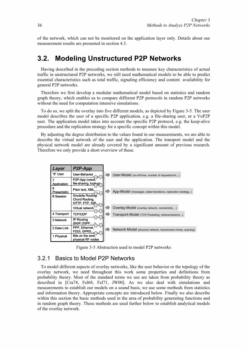
Chapter 3 Methods to Analyze P2P Networks
36
of the network, which can not be monitored on the application layer only. Details about our measurement results are presented in section 4.3.
3.2. Modeling Unstructured P2P Networks Having described in the preceding section methods to measure key characteristics of actual
traffic in unstructured P2P networks, we still need mathematical models to be able to predict essential characteristics such as total traffic, signaling efficiency and content availability for general P2P networks.
Therefore we first develop a modular mathematical model based on statistics and random graph theory, which enables us to compare different P2P protocols in random P2P networks without the need for computation intensive simulations.
To do so, we split the overlay into five different models, as depicted by Figure 3-5. The user model describes the user of a specific P2P application, e.g. a file-sharing user, or a VoP2P user. The application model takes into account the specific P2P protocol, e.g. the keep-alive procedure and the replication strategy for a specific concept within this model.
By adjusting the degree distribution to the values found in our measurements, we are able to describe the virtual network of the user and the application. The transport model and the physical network model are already covered by a significant amount of previous research. Therefore we only provide a short overview of these.
Virtual network
Bits on the wire, physical RF nodes
1 Physical
PPP, Ethernet, FDDI, GPRS,…
2 Data Link
IP-Routing (BGP,OSPF,…)
3 Network
TCP/UDP4 Transport
Gnutella Routing, Chord Routing, HTTP, FTP, SIP,…
5 Session
Plain text, XML, …6 Presentation
P2P-App (voice, file-sharing, lookup)
7 Application
User-Behavior“8” UserP2P-AppLayer
User-Model (on-off-time, number of requests/min,..)
App-Model (messages, state-transitions, replication strategy..)
Overlay-Model (overlay network, connectivity,...)
Transport-Model (TCP-Packeting, retransmissions,..)
Network-Model (physical network, transmission times, queuing)
Figure 3-5 Abstraction used to model P2P networks
3.2.1 Basics to Model P2P Networks To model different aspects of overlay networks, like the user behavior or the topology of the
overlay network, we need throughout this work some properties and definitions from probability theory. Most of the standard terms we use are taken from probability theory as described in [Cra74, Fel68, Fel71, JW00]. As we also deal with simulations and measurements to establish our models on a sound basis, we use some methods from statistics and information theory. Appropriate concepts are introduced below. Finally we also describe within this section the basic methods used in the area of probability generating functions and in random graph theory. These methods are used further below to establish analytical models of the overlay network.
Chapter 3 Methods to Analyze P2P Networks 37
3.2.1.1. Definitions from Probability Generating Functions
For a better handling of discrete probability distributions we use the concept of generating functions. This provides a transformation from the "time" space to the "frequency" spectrum, comparable to the Fourier transformation. It can be applied to non negative integers.
Probability Generating Function
Let X be a discrete, non negative, integer valued, random variable, with the probability mass function (PMF) of
( ) ( )x Xp P fX x x= == (11)
The corresponding Probability Generating Function (PGF) is then defined as
( )00
xx
x
G p zz∞
=
= ∑ i (12)
with 0 1z≤ ≤ .
Probability Generating Functions can be described as a z-transform in the variable 1z− .
Z-transformation
For the sequence of numbers { } 0k ka ∞
= the corresponding z-transform in the variable z is
defined as
{ } ( )0
0
kk kk
k
aZ a z z
∞∞
==
= ∑ (13)
Consequently the PGF ( )0G z of a sequence of numbers ( )Xf x is given by the z-transform
of ( )Xf x in the variable 1z− .
( ) ( ){ } ( ) ( )10 0
0 0
x xX xx X x
x x
G Z f z p zp f xz zx∞ ∞
∞ −=
= =
= = == ∑ ∑i i (14)
The PGF of a given PMF can be computed by applying the z-transform. Knowing the PMF is equivalent to knowing the PGF ( PMF PGF⇔ ). Thus we are able to retrieve the PMF from the PGF in any case, by evaluating the thn derivative for 0z = .
( ) ( )0 0 00X zp f Gx z =
= == (15)
( ) ( )00 0
1 1 ... . . .! !
nnx
n X nxnnxz z
ddp f p q e dp zGn zn n dzdz
∞
== =
= = = = =∑i i (16)
Moments
The thn moments of the PMF can be directly computed from the PGF, by evaluating the thn derivative of the PGF for 1z = .
{ } ( )01 1
nnnn
xx z
dE x p GzxX zdz
∞
= =
= = =
∑ i (17)
The expected value can thus be computed with the first derivative of ( )0G z and the variance, i.e. the second centralized moment, can be computed according to
Chapter 3 Methods to Analyze P2P Networks
38
( ) { } { }[ ]{ } { }( ) { } { }[ ]
( ) ( ) ( )
22 2
22
22
0002111
var
zzz
E Ex XXE E E EX X XX
ddd GGG zzz dzdzdz
σ
===
= = − =
= − + − =
= + −
(18)
Powers To determine the probability distribution of the sum of m independent realizations of a
random process, we need to convolute the PMF describing this object m times. In the frequency spectrum, described by the generating function of this PMF, we simply have to take the thm power of the corresponding PGF. A proof of this fact can be found in [Wil94]. An example for the sum of 2 realizations is given below.
( )[ ]
( ) ( )( ) ( ){ } ( )
22
0,
0 1 20 0 0 1 1 0 0 2 1 1 2 0
10
...
x j kx j k
x j k
x X X x
p zG p p zz
p p z p p p p z p p p p p p z
Z p f f zx x
+
∞ −=
= = =
+ + + + + + =
= = ⊗
∑ ∑ i i
(19)
Accordingly, the product property holds for the sum of different random processes:
( ) ( ) ( ) ( ) ( )
( ) ( ) ( ) ( ) ( )1 2 3
1 2 3
1 2 3
0 0 0 0 0
......
...n
n
n
X X X X X
X X X X X
X X X X Xf f f f fx x x x xG G G G Gz z z z z
= + + + +⇒ = ⊗ ⊗ ⊗ ⊗
⇔ = i i i i
(20)
Branching processes
Let the offspring probability generating function be ( )offG x . The probability generating function of the branching process [HSB77] at generation n can then be computed with the
thn functional iteration of the offspring probability generating function.
( ) ( )( ) ( )( )
( ) ( )( )( )
1
2
...
...n
X off
X off off
X off off off
G z G z
G z G G z
G z G G G z
=
=
=
(21)
3.2.1.2. Definitions from Graph Theory General Graph Theory
We use the methods of graph theory to model the overlay network, as well as to describe the properties of the physical network. Therefore we first have to introduce some basic definitions, which are based on the theory described in [Bo98], [Die00], [Kön36] and [Be58]. We only consider non oriented, finite graphs without parallel edges. Throughout this work, we use the notation as described in [Cra74].
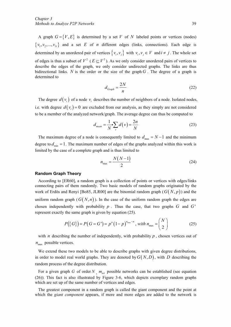
Chapter 3 Methods to Analyze P2P Networks 39
A graph { },G V E= is determined by a set V of N labeled points or vertices (nodes)
{ }1 2, ,..., Nv v v and a set E of n different edges (links, connections). Each edge is
determined by an unordered pair of vertices { },i jv v with ,i jv v V∈ and i j≠ . The whole set
of edges is thus a subset of 2V ( 2E V⊆ ). As we only consider unordered pairs of vertices to describe the edges of the graph, we only consider undirected graphs. The links are thus bidirectional links. N is the order or the size of the graph G . The degree of a graph is determined to
2
GraphNdn
= (22)
The degree ( )id v of a node iv describes the number of neighbors of a node. Isolated nodes,
i.e. with degree ( ) 0id v = are excluded from our analysis, as they simply are not considered to be a member of the analyzed network/graph. The average degree can thus be computed to
( )1 2mean
v
nd d vN N
= =∑i (23)
The maximum degree of a node is consequently limited to max 1d N= − and the minimum degree to min 1d = . The maximum number of edges of the graphs analyzed within this work is limited by the case of a complete graph and is thus limited to
( )
max
12
N Nn
−= (24)
Random Graph Theory According to [ER60], a random graph is a collection of points or vertices with edges/links
connecting pairs of them randomly. Two basic models of random graphs originated by the work of Erdös and Renyi [Bo85, JLR00] are the binomial random graph ( ( ),G N p ) and the
uniform random graph ( ( ),G N n ). In the case of the uniform random graph the edges are chosen independently with probability p . Thus the case, that two graphs G and 'G represent exactly the same graph is given by equation (25).
{ }( ) ( ) ( ) max
max' 1 ,2
n nn NP G P G G p p with n−
= = = − =
(25)
with n describing the number of independently, with probability p , chosen vertices out of
maxn possible vertices.
We extend these two models to be able to describe graphs with given degree distributions, in order to model real world graphs. They are denoted by ( ),G N D , with D describing the random process of the degree distribution.
For a given graph G of order N , netm possible networks can be established (see equation (26)). This fact is also illustrated by Figure 3-6, which depicts exemplary random graphs which are set up of the same number of vertices and edges.
The greatest component in a random graph is called the giant component and the point at which the giant component appears, if more and more edges are added to the network is
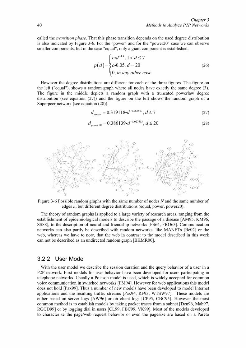
Chapter 3 Methods to Analyze P2P Networks
40
called the transition phase. That this phase transition depends on the used degree distribution is also indicated by Figure 3-6. For the "power" and for the "power20" case we can observe smaller components, but in the case "equal", only a giant component is established.
( )
1.4 , 1 70.05, 20
0,
c d dp d c d
in any other case
− < ≤= =
ii (26)
However the degree distributions are different for each of the three figures. The figure on the left ("equal"), shows a random graph where all nodes have exactly the same degree (3). The figure in the middle depicts a random graph with a truncated powerlaw degree distribution (see equation (27)) and the figure on the left shows the random graph of a Superpeer network (see equation (28)).
0.7665070.319118 , 7powerd d d−= ≤i (27)
1,02765320 0.386139 , 20powerd d d−= ≤i (28)
Figure 3-6 Possible random graphs with the same number of nodes N and the same number of
edges n, but different degree distributions (equal, power, power20).
The theory of random graphs is applied to a large variety of research areas, ranging from the establishment of epidemiological models to describe the passage of a disease [AM95, KM96, SS88], to the description of neural and friendship networks [FS64, FRO63]. Communication networks can also partly be described with random networks, like MANETs [Be02] or the web, whereas we have to note, that the web in contrast to the model described in this work can not be described as an undirected random graph [BKMR00].
3.2.2 User Model With the user model we describe the session duration and the query behavior of a user in a
P2P network. First models for user behavior have been developed for users participating in telephone networks. Usually a Poisson model is used, which is widely accepted for common voice communication in switched networks [FM94]. However for web applications this model does not hold [Pax99]. Thus a number of new models have been developed to model Internet applications and the resulting traffic streams [Pax94, RF93, WTSW97]. These models are either based on server logs [AW96] or on client logs [CP95, CBC95]. However the most common method is to establish models by taking packet traces from a subnet [Den96, Mah97, RGCD99] or by logging dial in users [CL99, FBC99, VK99]. Most of the models developed to characterize the page/web request behavior or even the pagesize are based on a Pareto
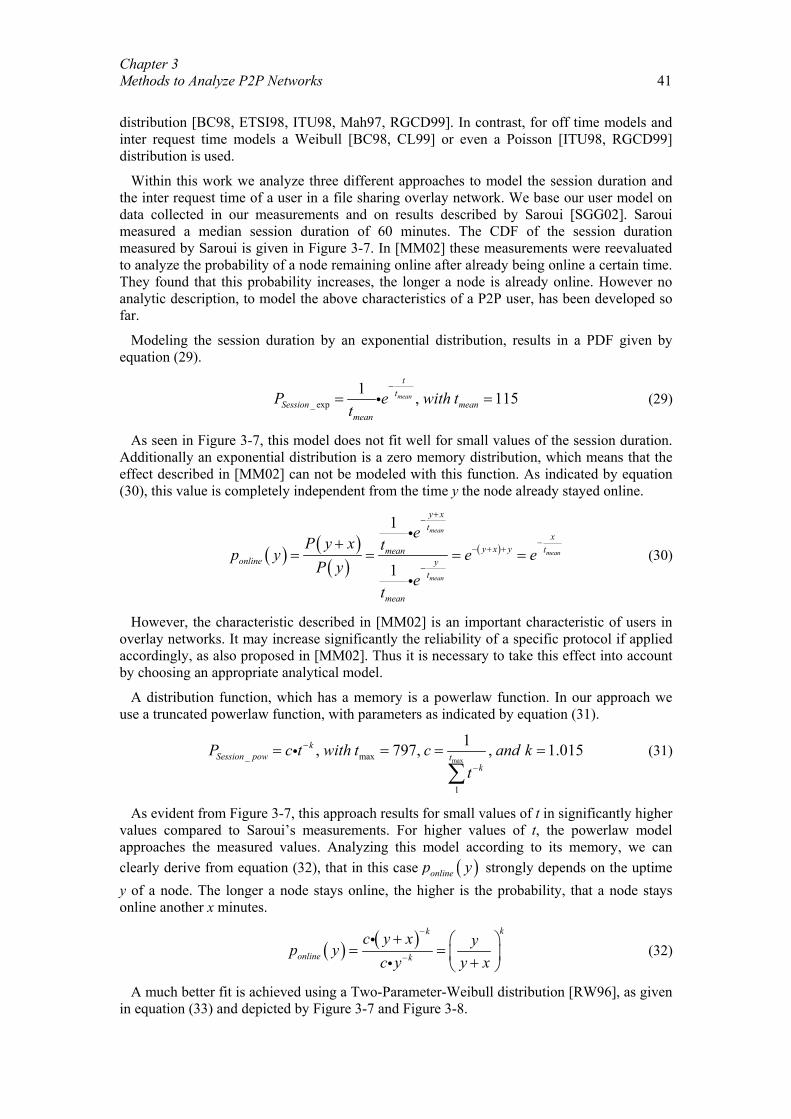
Chapter 3 Methods to Analyze P2P Networks 41
distribution [BC98, ETSI98, ITU98, Mah97, RGCD99]. In contrast, for off time models and inter request time models a Weibull [BC98, CL99] or even a Poisson [ITU98, RGCD99] distribution is used.
Within this work we analyze three different approaches to model the session duration and the inter request time of a user in a file sharing overlay network. We base our user model on data collected in our measurements and on results described by Saroui [SGG02]. Saroui measured a median session duration of 60 minutes. The CDF of the session duration measured by Saroui is given in Figure 3-7. In [MM02] these measurements were reevaluated to analyze the probability of a node remaining online after already being online a certain time. They found that this probability increases, the longer a node is already online. However no analytic description, to model the above characteristics of a P2P user, has been developed so far.
Modeling the session duration by an exponential distribution, results in a PDF given by equation (29).
_ exp1 , 115mean
tt
Session meanmean
P e with tt
−
= =i (29)
As seen in Figure 3-7, this model does not fit well for small values of the session duration. Additionally an exponential distribution is a zero memory distribution, which means that the effect described in [MM02] can not be modeled with this function. As indicated by equation (30), this value is completely independent from the time y the node already stayed online.
( ) ( )( )
( )
1
1
mean
mean
mean
y xt
xy x y tmean
online yt
mean
eP y x tp y e e
P ye
t
+−
−− + +
−
+= = = =
i
i (30)
However, the characteristic described in [MM02] is an important characteristic of users in overlay networks. It may increase significantly the reliability of a specific protocol if applied accordingly, as also proposed in [MM02]. Thus it is necessary to take this effect into account by choosing an appropriate analytical model.
A distribution function, which has a memory is a powerlaw function. In our approach we use a truncated powerlaw function, with parameters as indicated by equation (31).
max_ max
1
1, 797, , 1.015kSession pow t
k
P c t with t c and kt
−
−
= = = =
∑i (31)
As evident from Figure 3-7, this approach results for small values of t in significantly higher values compared to Saroui’s measurements. For higher values of t, the powerlaw model approaches the measured values. Analyzing this model according to its memory, we can clearly derive from equation (32), that in this case ( )onlinep y strongly depends on the uptime y of a node. The longer a node stays online, the higher is the probability, that a node stays online another x minutes.
( ) ( ) kk
online k
c y x yp yc y y x
−
−
+ = = +
ii
(32)
A much better fit is achieved using a Two-Parameter-Weibull distribution [RW96], as given in equation (33) and depicted by Figure 3-7 and Figure 3-8.
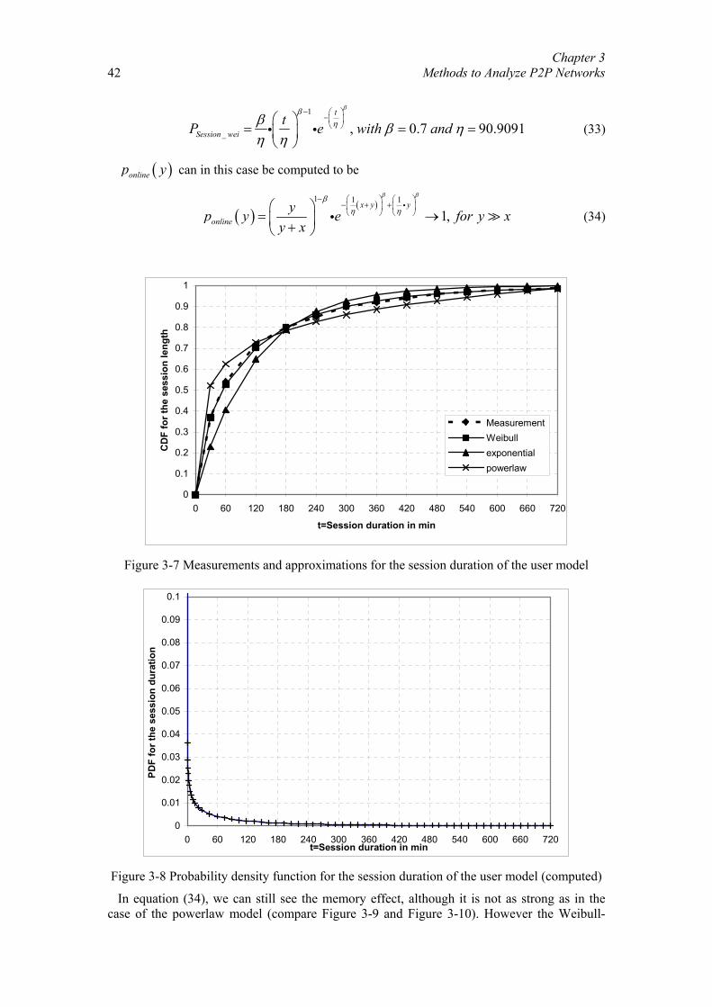
Chapter 3 Methods to Analyze P2P Networks
42
1
_ , 0.7 90.9091t
Session weitP e with and
ββηβ β η
η η
− −
= = =
i i (33)
( )onlinep y can in this case be computed to be
( )( )1 1 1
1,x y y
onlineyp y e for y x
y x
β ββη η
− − + +
= → +
ii (34)
0
0.1
0.2
0.3
0.4
0.5
0.6
0.7
0.8
0.9
1
0 60 120 180 240 300 360 420 480 540 600 660 720
t=Session duration in min
CD
F fo
r the
ses
sion
leng
th
MeasurementWeibullexponentialpowerlaw
Figure 3-7 Measurements and approximations for the session duration of the user model
0
0.01
0.02
0.03
0.04
0.05
0.06
0.07
0.08
0.09
0.1
0 60 120 180 240 300 360 420 480 540 600 660 720t=Session duration in min
for t
he s
essi
on d
urat
ion
Figure 3-8 Probability density function for the session duration of the user model (computed)
In equation (34), we can still see the memory effect, although it is not as strong as in the case of the powerlaw model (compare Figure 3-9 and Figure 3-10). However the Weibull-
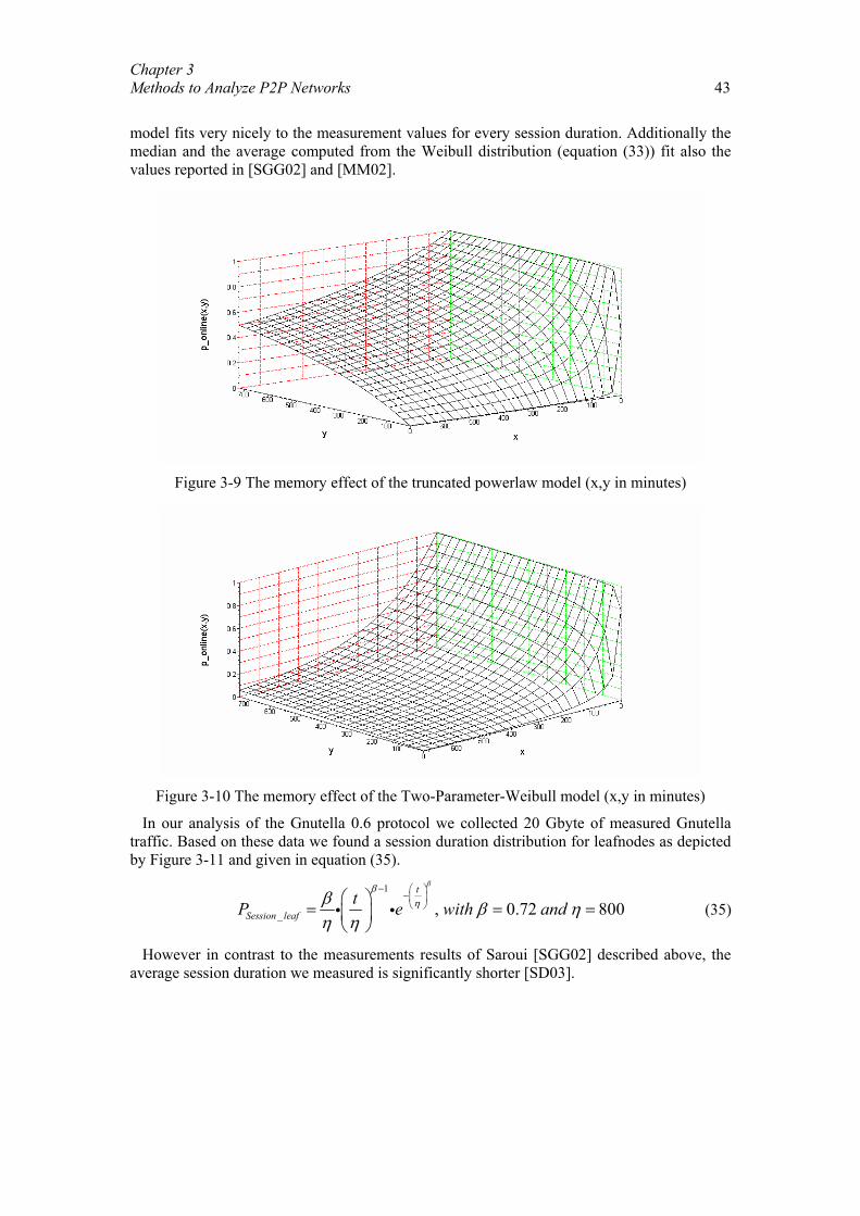
Chapter 3 Methods to Analyze P2P Networks 43
model fits very nicely to the measurement values for every session duration. Additionally the median and the average computed from the Weibull distribution (equation (33)) fit also the values reported in [SGG02] and [MM02].
Figure 3-9 The memory effect of the truncated powerlaw model (x,y in minutes)
Figure 3-10 The memory effect of the Two-Parameter-Weibull model (x,y in minutes)
In our analysis of the Gnutella 0.6 protocol we collected 20 Gbyte of measured Gnutella traffic. Based on these data we found a session duration distribution for leafnodes as depicted by Figure 3-11 and given in equation (35).
1
_ , 0.72 800t
Session leaftP e with and
ββηβ β η
η η
− −
= = =
i i (35)
However in contrast to the measurements results of Saroui [SGG02] described above, the average session duration we measured is significantly shorter [SD03].
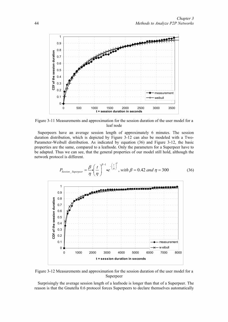
Chapter 3 Methods to Analyze P2P Networks
44
0
0.1
0.2
0.3
0.4
0.5
0.6
0.7
0.8
0.9
1
0 500 1000 1500 2000 2500 3000 3500t = session duration in seconds
CD
f of t
he s
essi
on d
urat
ion
measurementweibull
Figure 3-11 Measurements and approximation for the session duration of the user model for a
leaf node
Superpeers have an average session length of approximately 6 minutes. The session duration distribution, which is depicted by Figure 3-12 can also be modeled with a Two-Parameter-Weibull distribution. As indicated by equation (36) and Figure 3-12, the basic properties are the same, compared to a leafnode. Only the parameters for a Superpeer have to be adapted. Thus we can see, that the general properties of our model still hold, although the network protocol is different.
1
_ , 0.42 300t
Session SuperpeertP e with and
ββηβ β η
η η
− −
= = =
i i (36)
0
0.1
0.2
0.3
0.4
0.5
0.6
0.7
0.8
0.9
1
0 1000 2000 3000 4000 5000 6000 7000 8000
t = session duration in seconds
CD
f of t
he s
essi
on d
urat
ion
measurement
w eibull
Figure 3-12 Measurements and approximation for the session duration of the user model for a
Superpeer
Surprisingly the average session length of a leafnode is longer than that of a Superpeer. The reason is that the Gnutella 0.6 protocol forces Superpeers to declare themselves automatically
Chapter 3 Methods to Analyze P2P Networks 45
as a leafnode, if too few leafnodes are connected to a Superpeer [SR02]. Thus the nodes, which are currently connected to this Superpeer, experience only a single connection break, if the Superpeer functionality is switched off. In contrast the Superpeer gets disconnected, and reconnects to the network as a leafnode. Further on, a user may declare its node as a leafnode, if the Superpeer mode costs too many resources.
Modeling the inter-request time of a user in an overlay network is now fairly simple. Here we rely on the common approach used in telecommunication systems, assuming a Poisson model, with an average of 0.3 queries per minute [Sri01]. The content of the request, i.e. which document is requested, can then be modeled with a Zipf law distribution, which is also generally accepted for the requests in common web traffic [Zip 32].
3.2.3 Overlay Network Model Due to their complete decentralization and the avoidance of any predefined structures,
unstructured overlay networks can be modeled, similar as MANETs [Per00], as random graphs. We do not consider structured overlay networks within this section, as the methods necessary to model structured overlay networks can not be applied to unstructured overlay networks. However an approach to model structured overlay networks with De Bruijn graphs is described in [LKRG03].
Initial work in the area of random graph theory was published in 1960 by Erdös and Renyi [ER60]. They developed the basics of random graph theory to analyze the statistical properties of random graphs, e.g. the size of the giant component or the determination of the transition phase.
In contrast to previous work, Newman et al. study a random graph not as a whole, but by starting from one single node. Thus they are able to determine the number of neighbors as seen from one node [NSW01]. Kant and Iyer published in 2003 first results of their application of graph theory to study the characteristics of overlay networks [Kan03, KIT04]. The network sizes they studied included up to 500 nodes. The model described in [Kan03] is restricted to flat unstructured overlay networks, without any hierarchies.
Another modeling approach, which is not based on random graphs is described in [GFJK03]. In this case the authors develop a modeling framework for different kinds of P2P applications. This model is based on queuing theory. It can thus not describe the structure of the overlay network. Thus it can not be used to determine the availability of objects within an overlay network, and can not model the possibilities of several unconnected sub networks.
In this thesis we extend the results presented in [NSW01] to take into account the effects of a finite environment, which is encountered in practice. This requires basically three modifications of Newman’s approach.
(i) Loop1 Nodes searching for a new node to connect to may accidentally connect to another node which is in the same hop distance in the process of searching too. We will denote that as Loop1. The probability of that to happen is assumed to be zero in [NSW01] as a consequence of an infinite environment.
(ii) Loop2 Several nodes which are currently searching a new node may connect to the same node instead of separate nodes. We will denote that as Loop2. Once again the probability of an occurrence of Loop2 is assumed as zero in [NSW01].
(iii) Changing distribution Nodes with a higher number of links will be hit earlier in the connection process than those which have only a lower number of links. This causes nodes with a higher number of links to gradually disappear from the remaining pool of free nodes.
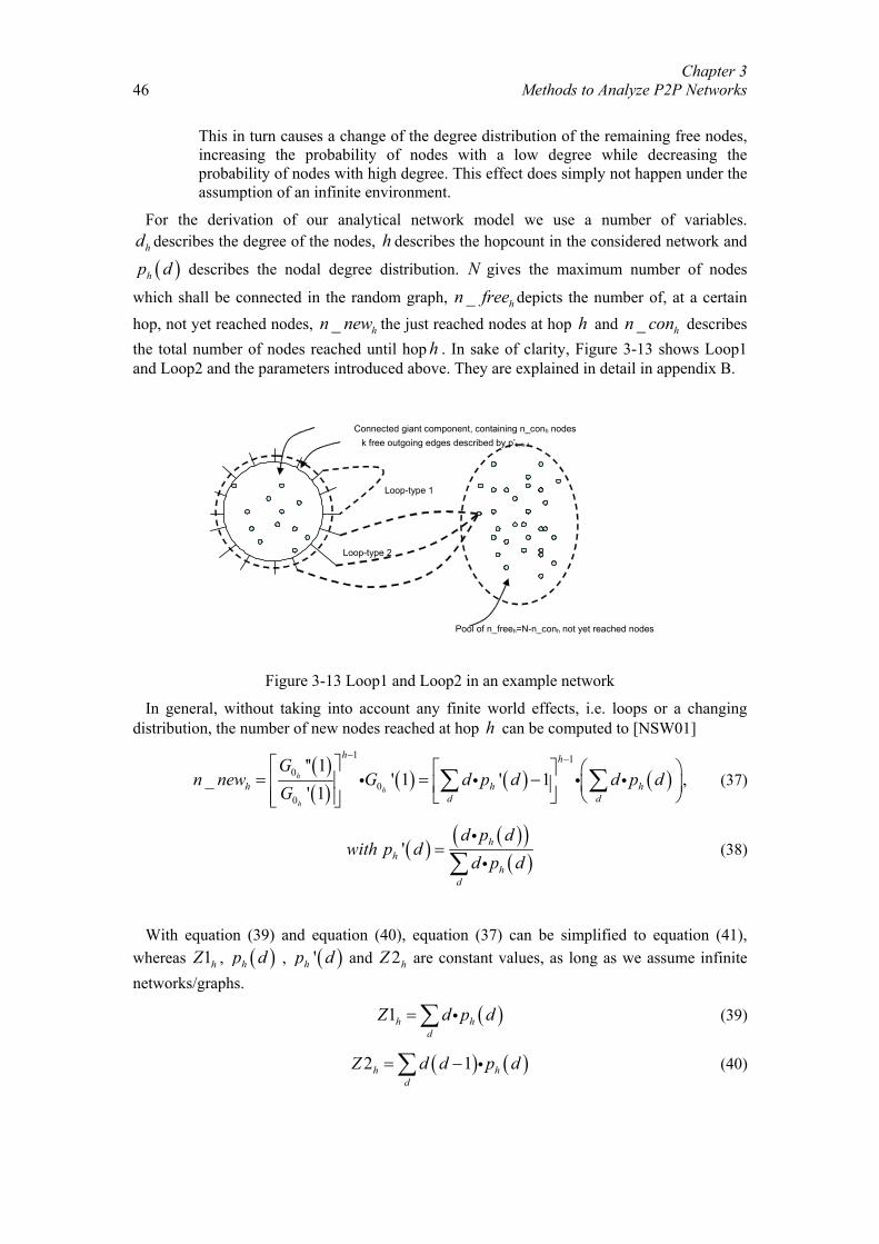
Chapter 3 Methods to Analyze P2P Networks
46
This in turn causes a change of the degree distribution of the remaining free nodes, increasing the probability of nodes with a low degree while decreasing the probability of nodes with high degree. This effect does simply not happen under the assumption of an infinite environment.
For the derivation of our analytical network model we use a number of variables. hd describes the degree of the nodes, h describes the hopcount in the considered network and
( )hp d describes the nodal degree distribution. N gives the maximum number of nodes
which shall be connected in the random graph, _ hn free depicts the number of, at a certain hop, not yet reached nodes, _ hn new the just reached nodes at hop h and _ hn con describes the total number of nodes reached until hop h . In sake of clarity, Figure 3-13 shows Loop1 and Loop2 and the parameters introduced above. They are explained in detail in appendix B.
Loop-type 1
Loop-type 2
k free outgoing edges described by p’k, h-1
Pool of n_freeh=N-n_conh not yet reached nodes
Connected giant component, containing n_conh nodes
Figure 3-13 Loop1 and Loop2 in an example network
In general, without taking into account any finite world effects, i.e. loops or a changing distribution, the number of new nodes reached at hop h can be computed to [NSW01]
( )( ) ( ) ( ) ( )
1 10
00
'' 1_ ' 1 ' 1 ,
' 1h
h
h
h h
h h hd d
Gn new G d p d d p d
G
− − = = − ∑ ∑i i i i (37)
( ) ( )( )( )
' hh
hd
d p dwith p d
d p d=
∑ii
(38)
With equation (39) and equation (40), equation (37) can be simplified to equation (41), whereas 1hZ , ( )hp d , ( )'hp d and 2hZ are constant values, as long as we assume infinite networks/graphs.
( )1h hd
Z d p d= ∑ i (39)
( ) ( )2 1h hd
Z d d p d= −∑ i (40)
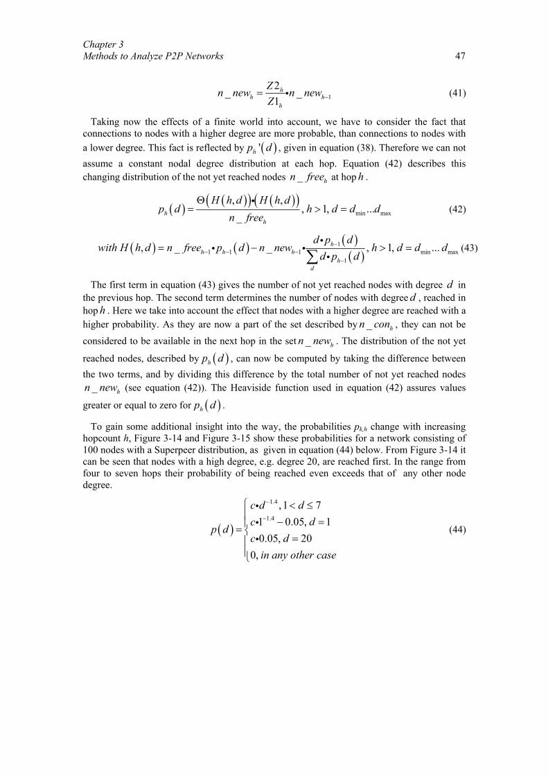
Chapter 3 Methods to Analyze P2P Networks 47
12_ _1
hh h
h
Zn new n newZ −= i (41)
Taking now the effects of a finite world into account, we have to consider the fact that connections to nodes with a higher degree are more probable, than connections to nodes with a lower degree. This fact is reflected by ( )'hp d , given in equation (38). Therefore we can not assume a constant nodal degree distribution at each hop. Equation (42) describes this changing distribution of the not yet reached nodes _ hn free at hop h .
( ) ( )( ) ( )( )min max
, ,, 1, ...
_hh
H h d H h dp d h d d d
n freeΘ
= > =i
(42)
( ) ( ) ( )( )
11 1 1 min max
1
, _ _ , 1, ...hh h h
hd
d p dwith H h d n free p d n new h d d d
d p d−
− − −−
= − > =∑i
i ii
(43)
The first term in equation (43) gives the number of not yet reached nodes with degree d in the previous hop. The second term determines the number of nodes with degree d , reached in hop h . Here we take into account the effect that nodes with a higher degree are reached with a higher probability. As they are now a part of the set described by _ hn con , they can not be considered to be available in the next hop in the set _ hn new . The distribution of the not yet
reached nodes, described by ( )hp d , can now be computed by taking the difference between the two terms, and by dividing this difference by the total number of not yet reached nodes
_ hn new (see equation (42)). The Heaviside function used in equation (42) assures values
greater or equal to zero for ( )hp d .
To gain some additional insight into the way, the probabilities pk,h change with increasing hopcount h, Figure 3-14 and Figure 3-15 show these probabilities for a network consisting of 100 nodes with a Superpeer distribution, as given in equation (44) below. From Figure 3-14 it can be seen that nodes with a high degree, e.g. degree 20, are reached first. In the range from four to seven hops their probability of being reached even exceeds that of any other node degree.
( )
1.4
1.4
,1 71 0.05, 10.05, 20
0,
c d dc d
p dc d
in any other case
−
−
< ≤ − ==
=
iii
(44)
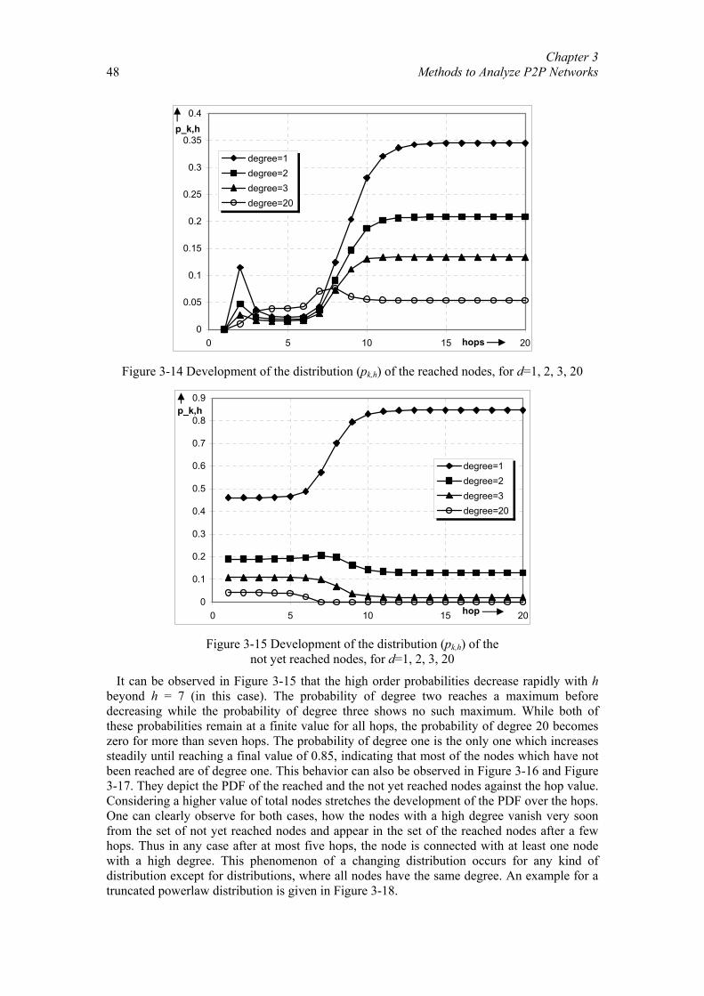
Chapter 3 Methods to Analyze P2P Networks
48
0
0.05
0.1
0.15
0.2
0.25
0.3
0.35
0.4
0 5 10 15 20
degree=1degree=2degree=3degree=20
hops
p_k,h
Figure 3-14 Development of the distribution (pk,h) of the reached nodes, for d=1, 2, 3, 20
0
0.1
0.2
0.3
0.4
0.5
0.6
0.7
0.8
0.9
0 5 10 15 20
degree=1degree=2degree=3degree=20
hop
p_k,h
Figure 3-15 Development of the distribution (pk,h) of the
not yet reached nodes, for d=1, 2, 3, 20
It can be observed in Figure 3-15 that the high order probabilities decrease rapidly with h beyond h = 7 (in this case). The probability of degree two reaches a maximum before decreasing while the probability of degree three shows no such maximum. While both of these probabilities remain at a finite value for all hops, the probability of degree 20 becomes zero for more than seven hops. The probability of degree one is the only one which increases steadily until reaching a final value of 0.85, indicating that most of the nodes which have not been reached are of degree one. This behavior can also be observed in Figure 3-16 and Figure 3-17. They depict the PDF of the reached and the not yet reached nodes against the hop value. Considering a higher value of total nodes stretches the development of the PDF over the hops. One can clearly observe for both cases, how the nodes with a high degree vanish very soon from the set of not yet reached nodes and appear in the set of the reached nodes after a few hops. Thus in any case after at most five hops, the node is connected with at least one node with a high degree. This phenomenon of a changing distribution occurs for any kind of distribution except for distributions, where all nodes have the same degree. An example for a truncated powerlaw distribution is given in Figure 3-18.
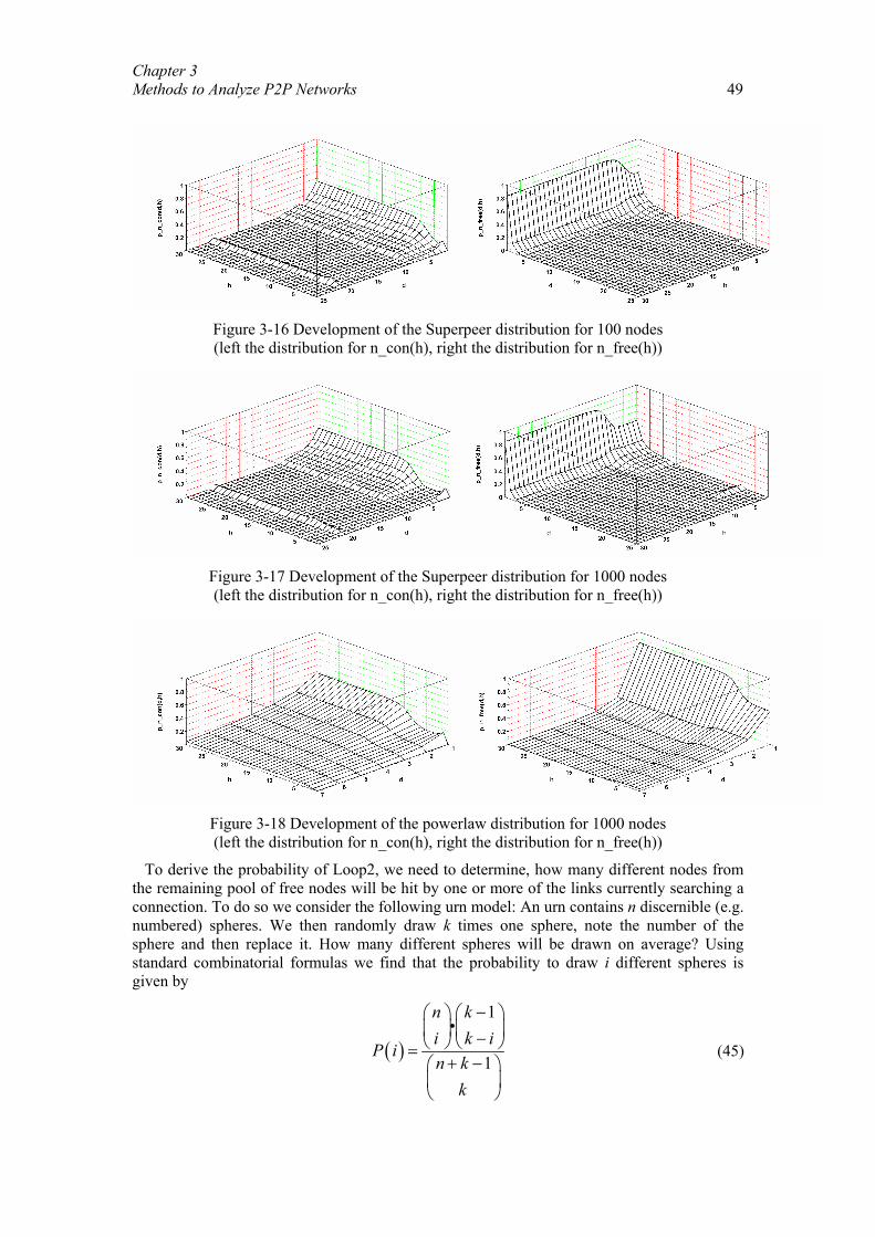
Chapter 3 Methods to Analyze P2P Networks 49
Figure 3-16 Development of the Superpeer distribution for 100 nodes (left the distribution for n_con(h), right the distribution for n_free(h))
Figure 3-17 Development of the Superpeer distribution for 1000 nodes (left the distribution for n_con(h), right the distribution for n_free(h))
Figure 3-18 Development of the powerlaw distribution for 1000 nodes (left the distribution for n_con(h), right the distribution for n_free(h))
To derive the probability of Loop2, we need to determine, how many different nodes from the remaining pool of free nodes will be hit by one or more of the links currently searching a connection. To do so we consider the following urn model: An urn contains n discernible (e.g. numbered) spheres. We then randomly draw k times one sphere, note the number of the sphere and then replace it. How many different spheres will be drawn on average? Using standard combinatorial formulas we find that the probability to draw i different spheres is given by
( )
1
1
n ki k i
P in k
k
− − =
+ −
i (45)
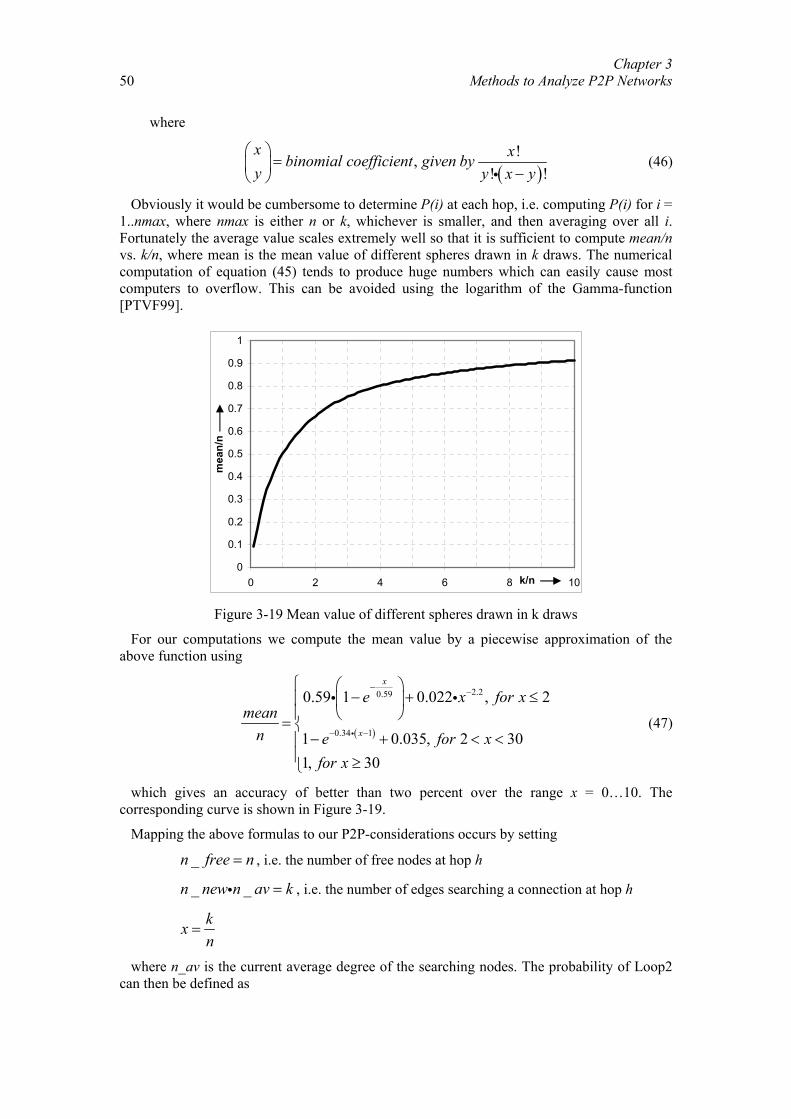
Chapter 3 Methods to Analyze P2P Networks
50
where
( )
!,! !
x xbinomial coefficient given byy y x y
= − i
(46)
Obviously it would be cumbersome to determine P(i) at each hop, i.e. computing P(i) for i = 1..nmax, where nmax is either n or k, whichever is smaller, and then averaging over all i. Fortunately the average value scales extremely well so that it is sufficient to compute mean/n vs. k/n, where mean is the mean value of different spheres drawn in k draws. The numerical computation of equation (45) tends to produce huge numbers which can easily cause most computers to overflow. This can be avoided using the logarithm of the Gamma-function [PTVF99].
0
0.1
0.2
0.3
0.4
0.5
0.6
0.7
0.8
0.9
1
0 2 4 6 8 10
mea
n/n
k/n
Figure 3-19 Mean value of different spheres drawn in k draws
For our computations we compute the mean value by a piecewise approximation of the above function using
( )
2.20.59
0.34 1
0.59 1 0.022 , 2
1 0.035, 2 301, 30
x
x
e x for xmean
n e for xfor x
− −
− −
− + ≤
= − + < <
≥
i
i i (47)
which gives an accuracy of better than two percent over the range x = 0…10. The corresponding curve is shown in Figure 3-19.
Mapping the above formulas to our P2P-considerations occurs by setting
_n free n= , i.e. the number of free nodes at hop h
_ _n new n av k=i , i.e. the number of edges searching a connection at hop h
kxn
=
where n_av is the current average degree of the searching nodes. The probability of Loop2 can then be defined as
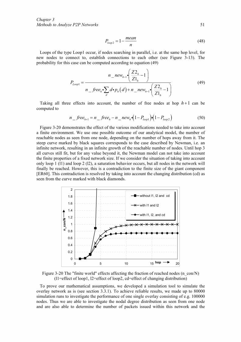
Chapter 3 Methods to Analyze P2P Networks 51
2 1loopmeanP
n= − (48)
Loops of the type Loop1 occur, if nodes searching in parallel, i.e. at the same hop level, for new nodes to connect to, establish connections to each other (see Figure 3-13). The probability for this case can be computed according to equation (49)
( )
1
1
1
2_ 11
2_ _ 11
hh
hLoop
hh h h
d h
Zn newZ
PZn free d p d n newZ
−
−
−
=
+ −
∑
i
i i i (49)
Taking all three effects into account, the number of free nodes at hop 1h + can be computed to
( ) ( )1 1 2_ _ _ 1 1h h h loop loopn free n free n new P P+ = − − −i i (50)
Figure 3-20 demonstrates the effect of the various modifications needed to take into account a finite environment. We use one possible outcome of our analytical model, the number of reachable nodes as seen from one node, depending on the number of hops away from it. The steep curve marked by black squares corresponds to the case described by Newman, i.e. an infinite network, resulting in an infinite growth of the reachable number of nodes. Until hop 3 all curves still fit, but for any value beyond it, the Newman model can not take into account the finite properties of a fixed network size. If we consider the situation of taking into account only loop 1 (l1) and loop 2 (l2), a saturation behavior occurs, but all nodes in the network will finally be reached. However, this is a contradiction to the finite size of the giant component [ER60]. This contradiction is resolved by taking into account the changing distribution (cd) as seen from the curve marked with black diamonds.
0
0.2
0.4
0.6
0.8
1
1.2
1.4
1.6
1.8
2
0 5 10 15 20
n_co
n/N
without l1, l2 and cd
with l1 and l2
with l1, l2, and cd
hop
Figure 3-20 The "finite world" effects affecting the fraction of reached nodes (n_con/N) (l1=effect of loop1, l2=effect of loop2, cd=effect of changing distribution)
To prove our mathematical assumptions, we developed a simulation tool to simulate the overlay network as is (see section 3.3.1). To achieve reliable results, we made up to 80000 simulation runs to investigate the performance of one single overlay consisting of e.g. 100000 nodes. Thus we are able to investigate the nodal degree distribution as seen from one node and are also able to determine the number of packets issued within this network and the
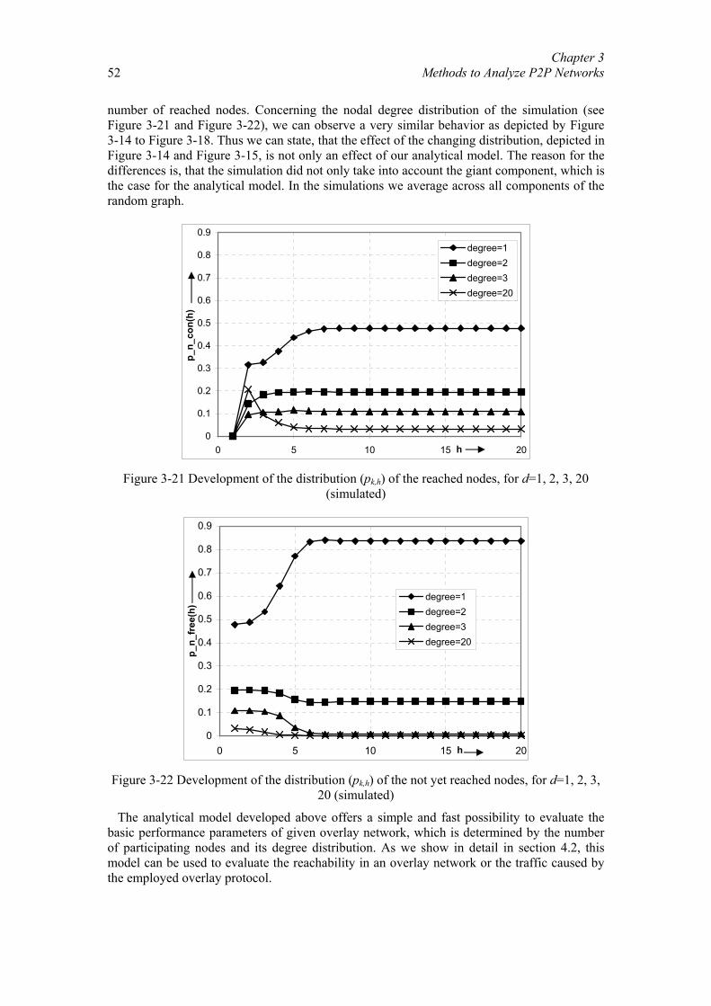
Chapter 3 Methods to Analyze P2P Networks
52
number of reached nodes. Concerning the nodal degree distribution of the simulation (see Figure 3-21 and Figure 3-22), we can observe a very similar behavior as depicted by Figure 3-14 to Figure 3-18. Thus we can state, that the effect of the changing distribution, depicted in Figure 3-14 and Figure 3-15, is not only an effect of our analytical model. The reason for the differences is, that the simulation did not only take into account the giant component, which is the case for the analytical model. In the simulations we average across all components of the random graph.
0
0.1
0.2
0.3
0.4
0.5
0.6
0.7
0.8
0.9
0 5 10 15 20h
p_n_
con(
h)
degree=1degree=2degree=3degree=20
Figure 3-21 Development of the distribution (pk,h) of the reached nodes, for d=1, 2, 3, 20
(simulated)
0
0.1
0.2
0.3
0.4
0.5
0.6
0.7
0.8
0.9
0 5 10 15 20h
p_n_
free
(h)
degree=1degree=2degree=3degree=20
Figure 3-22 Development of the distribution (pk,h) of the not yet reached nodes, for d=1, 2, 3,
20 (simulated)
The analytical model developed above offers a simple and fast possibility to evaluate the basic performance parameters of given overlay network, which is determined by the number of participating nodes and its degree distribution. As we show in detail in section 4.2, this model can be used to evaluate the reachability in an overlay network or the traffic caused by the employed overlay protocol.
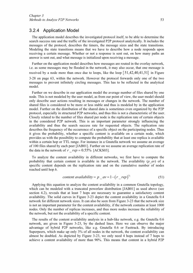
Chapter 3 Methods to Analyze P2P Networks 53
3.2.4 Application Model
The application model describes the investigated protocol itself, to be able to determine the search success rate and the traffic of the investigated P2P protocol analytically. It includes the messages of the protocol, describes the timers, the message sizes and the state transitions. Modeling the state transitions means that we have to describe how a node responds upon receiving a certain message. Whether or not a response is sent out, on how many paths an answer is sent out, and what message is initialized upon receiving a message.
Further on the application model describes how messages are routed in the overlay network, i.e. as some messages may be flooded in the network, it may also occur, that one message is received by a node more than once due to loops, like the loop { }51,42,40,41,51 in Figure 3-28 on page 63, within the network. However the protocol forwards only one of the two messages to prevent infinitely circling messages. This has to be reflected in the analytical model.
Further on we describe in our application model the average number of files shared by one node. This is not modeled by the user model, as from our point of view, the user model should only describe user actions resulting in messages or changes in the network. The number of shared files is considered to be more or less stable and thus is modeled by in the application model. Further on the distribution of the shared data is sometimes even organized by the P2P protocol, especially in structured P2P networks, and thus this is not a characteristic of the user. Closely related to the number of files shared per node is the replication rate of certain objects in the considered P2P network. This is an important parameter strongly influencing the availability and thus the search success rate for requested objects. The replication rate describes the frequency of the occurrence of a specific object on the participating nodes. Thus it gives the probability, whether a specific content is available on a certain node, which provides us with the possibility to compute the probability that at least one replica is available within a certain hop or TTL range. For instance in a Gnutella network we assume an average of 100 files shared by each peer [JAB01]. Further on we assume an average replication rate of the data in the network of _ 0.55%r rep = [ACKS03].
To analyze the content availability in different networks, we first have to compute the probability that certain content is available in the network. The availability (p_av) of a specific content depends on the replication rate and on the cumulative number of nodes reached until hop h.
( )_ 1 _ hzcontent availability p av r rep = = − (51)
Applying this equation to analyze the content availability in a common Gnutella topology, which can be modeled with a truncated powerlaw distribution [JAB01] as used above (see section 4.2), reveals that at least 7 hops are necessary to guarantee a satisfactory content availability. The solid curves in Figure 3-23 depict the content availability in a Gnutella 0.4 network for different network sizes. It can also be seen from Figure 3-23 that the network size is not an important parameter for the content availability, if the network contains at least 1000 nodes. Only the number of replicas increases, and thus more nodes increase the reliability of the network, but not the availability of a specific content.
The results of the content availability analysis in a hub-like network, e.g. the Gnutella 0.6 network, are given in Figure 3-23, by the dashed lines. Here we can observe the major advantage of hybrid P2P networks, like e.g. Gnutella 0.6 or Fasttrack. By introducing Superpeers, which make up only 3% of all nodes in the network, the content availability can almost be doubled. As depicted by Figure 3-23, we only need 4 hops instead of 7 hops to achieve a content availability of more than 90%. This means that content in a hybrid P2P
Chapter 3 Methods to Analyze P2P Networks
54
network can be found significantly faster and also more reliable, as the search request and its corresponding response must be routed across less hops in the overlay network.
0
0.1
0.2
0.3
0.4
0.5
0.6
0.7
0.8
0.9
1
0 5 10 15 20
cont
ent a
vaila
bilit
y
100 power1000 power10000 power100000 power100 super1000 super10000 super100000 super
hops
Figure 3-23: Content availability in a powerlaw (power) and a Superpeer (super) network
With our analytical application model we are also able, together with the user (see section 3.2) and the overlay model (see section 3.2.2), to compute the traffic occurring in average on a single node. For a better understanding this is done in the following at the example of a Gnutella 0.4 protocol.
The Gnutella 0.4 protocol has a general Gnutella header length of 23 bytes, plus zero byte for the PING message, 15 bytes for the PONG message, 80 bytes for the QUERY message and 200 bytes for the QUERY-HIT message [SD03]. As Gnutella routing is based mostly on flooding, we additionally have to take into account loops in the network, on which a message may be transmitted twice by the same node, as mentioned above. Therefore we assume a loop probability of 0.0064 [SH03], i.e. that a node is a member of a loop and thus receives one message twice. An example for such a loop is given by the nodes { }51,42,40,41,51 in Figure 3-28.
The traffic emitted and received by one node depends on the size of the component a node is a member of. To compute the size of the component, i.e. the number of nodes reachable within the hop distance h, we use the concept described in section 3.2.2. With these numbers and our assumptions stated above and the knowledge of the protocol, we can thus compute the signaling traffic caused and received by each node.
In general the traffic caused by a Gnutella node consists of the following parts:
• PING( ) and QUERY( ) messages initiated by one node and broadcasted on all of its virtual edges.
• PING( ) and QUERY( ) messages received by one node, which have to be forwarded on all but one of its virtual edges.
• PONG( ) and QUERY_HIT( ) messages which have to be forwarded as an answer only on one of its virtual edges.
• QUERY_HIT( ) messages, as answer to a matching received QUERY( ) message, which has to be sent on one of its virtual edges.
• PONG( ) messages, as an answer to a received PING( ) message, which has to be sent on one of its virtual edges.
Chapter 3 Methods to Analyze P2P Networks 55
The traffic received by one Gnutella node comprises the following parts:
• PING( ) and QUERY( ) messages initiated by nodes within the predefined hop distance.
• PONG( ) and QUERY_HIT messages which additionally have to be forwarded as answer only on one of its virtual edges.
• PONG( ) and QUERY_HIT( ) messages, as a response to a previously initiated PING( ) or QUERY( ) message.
We sum up the traffic caused by all of the above messages over the average lifetime of one node, i.e. 900 seconds. After 900 seconds the topology has changed because of leaving and new joining nodes, which would again result in the traffic stated above. For this time we assume a stable virtual network topology on average. Thus this does not influence the total data rate of one node. With our mathematical model we can thus analyze the efficiency of a P2P protocol, i.e. evaluate the content availability against the traffic, for different TTL values.
Figure 3-24 and Figure 3-25 depict the average total traffic volumes of single nodes, based on the Gnutella 0.4 protocol in a powerlaw (Figure 3-24) and in a Superpeer topology (Figure 3-25), with the parameters as given by equation (52) and (53).
( )1.4 , 0 7
0,c d d
p din any other case
− < ≤=
i (52)
( )
1.4
1.4
,1 71 0.05, 10.05, 20
0,
c d dc d
p dc d
in any other case
−
−
< ≤ − ==
=
iii
(53)
The dashed lines give the received traffic and the solid lines the sent traffic per node, for different Time-to-Live (TTL) values. In Figure 3-24, the receive transfer rate and the send-transfer rate are nearly equal, which represents the fact of symmetric communication, often observed in flat P2P networks. The traffic for TTL set to 7 hops shown in Figure 3-24 also match simulations we did with the network simulator ns2. In our ns2 implementation we also set the TTL to 7 for all nodes, as this is the standard setting in common Gnutella 0.4 implementations. Thus our mathematical model can adequately describe the traffic characteristics of P2P networks. Further results and a detailed discussion of this analysis method and especially a comparison between different protocols and enhancements are provided in section 4.4.
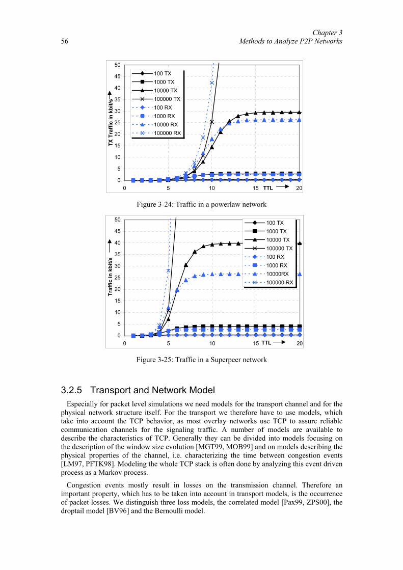
Chapter 3 Methods to Analyze P2P Networks
56
0
5
10
15
20
25
30
35
40
45
50
0 5 10 15 20
TX T
raffi
c in
kbi
t/s
100 TX1000 TX10000 TX100000 TX100 RX1000 RX10000 RX100000 RX
TTL
Figure 3-24: Traffic in a powerlaw network
0
5
10
15
20
25
30
35
40
45
50
0 5 10 15 20
Traf
fic in
kbi
t/s
100 TX1000 TX10000 TX100000 TX100 RX1000 RX10000RX100000 RX
TTL
Figure 3-25: Traffic in a Superpeer network
3.2.5 Transport and Network Model Especially for packet level simulations we need models for the transport channel and for the
physical network structure itself. For the transport we therefore have to use models, which take into account the TCP behavior, as most overlay networks use TCP to assure reliable communication channels for the signaling traffic. A number of models are available to describe the characteristics of TCP. Generally they can be divided into models focusing on the description of the window size evolution [MGT99, MOB99] and on models describing the physical properties of the channel, i.e. characterizing the time between congestion events [LM97, PFTK98]. Modeling the whole TCP stack is often done by analyzing this event driven process as a Markov process.
Congestion events mostly result in losses on the transmission channel. Therefore an important property, which has to be taken into account in transport models, is the occurrence of packet losses. We distinguish three loss models, the correlated model [Pax99, ZPS00], the droptail model [BV96] and the Bernoulli model.
Chapter 3 Methods to Analyze P2P Networks 57
In the correlated model, the packets are considered sequentially in rounds. The probability,
that the first packet is lost is denoted with p . If this packet is not lost, every succeeding packet is lost with exactly the same probability. As soon as the first packet is lost, all succeeding packets are lost with a higher probability q .
The droptail model behaves in a very similar way. Here all packets are also considered sequentially in rounds. Again the first packet of the round is lost with the probability p , and as long as no succeeding packet is lost, every packet is also considered to be lost with the probability p . However in case that one succeeding packet is lost, all succeeding packets of the considered round are lost too. In contrast, in the Bernoulli model each data packet is considered to be independent from every other packet and is lost with probability p . Thus the Bernoulli model does not take any dependencies into account.
Within our packet level simulations we use a FIFO droptail model for every TCP link, which means that every packet that succeeds a certain length of the droptail queue is considered to be lost.
Further important parameters to model transport channels are the data rate of every channel and the delay of each link. For these parameters also a number of models have been developed, ranging from uniform distributions to Pareto distributions. However for our investigations in fixed networks, these parameters are not important, as we are mainly interested in the traffic caused by the applications, based on the overlay and the search efficiency and success rate of the different overlay protocols.
Using realistic models for the physical topology, on which the overlay network is established, is also an important issue for simulations. For our fixed network scenarios we base our models on the results presented in [MLMB01] and [ZCB96]. In contrast to the overlay network we can not assume random networks, as the Internet is structured in different autonomous systems (AS) and backbones. Therefore we can not apply the same methods as developed in section 3.2.2.
Generally a network is modeled by first placing the nodes randomly on a plane. Then the connections between the nodes are established according to the chosen model. The models can be divided into flat router models, as done by Waxman or Barabasi-Albert, and hierarchical models, which are explained below [BOP94, DL93, WE94]. In the last step the link properties are assigned, like the data rate or the link delay.
In the Waxman model [BOP94, DL93, WE94] the connections between the nodes are established according to the Waxman probability density function, given in equation (54)
{ }( ),dLP u v e βα
−= i (54)
where d denotes the Euclidian distance between the nodes u and v , and { },u v denotes the currently considered link determined by node u and v . L is a normalizing factor and gives the maximum distance between two nodes in the considered graph.
According to Barabasi-Albert [AG03] powerlaw distributions of the nodal degrees in network topologies occur due to the incremental growth of networks and the preferential connectivity. Incremental growth in this context means, that networks are established by continuously adding nodes to the network. These nodes show a tendency to connect with a higher probability to a node which already has a lot of connections and is a member of the network. This phenomenon is expressed by equation (55).
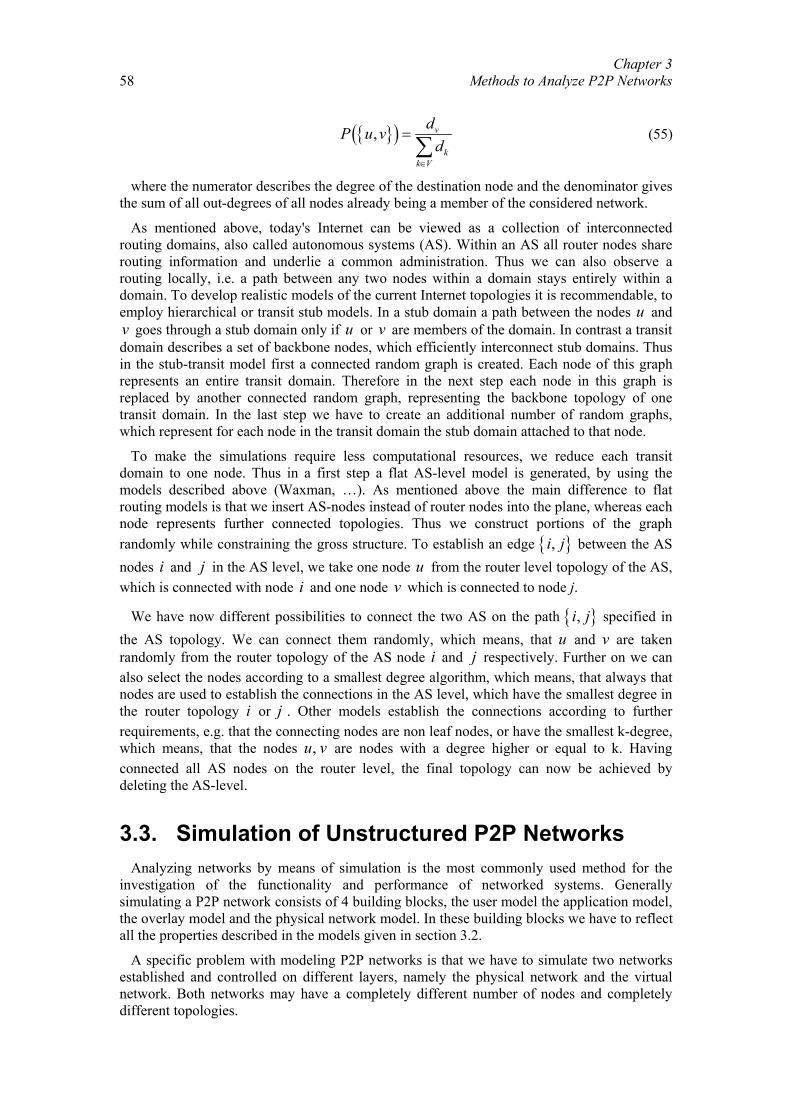
Chapter 3 Methods to Analyze P2P Networks
58
{ }( ), v
kk V
dP u vd
∈
=∑
(55)
where the numerator describes the degree of the destination node and the denominator gives the sum of all out-degrees of all nodes already being a member of the considered network.
As mentioned above, today's Internet can be viewed as a collection of interconnected routing domains, also called autonomous systems (AS). Within an AS all router nodes share routing information and underlie a common administration. Thus we can also observe a routing locally, i.e. a path between any two nodes within a domain stays entirely within a domain. To develop realistic models of the current Internet topologies it is recommendable, to employ hierarchical or transit stub models. In a stub domain a path between the nodes u and v goes through a stub domain only if u or v are members of the domain. In contrast a transit domain describes a set of backbone nodes, which efficiently interconnect stub domains. Thus in the stub-transit model first a connected random graph is created. Each node of this graph represents an entire transit domain. Therefore in the next step each node in this graph is replaced by another connected random graph, representing the backbone topology of one transit domain. In the last step we have to create an additional number of random graphs, which represent for each node in the transit domain the stub domain attached to that node.
To make the simulations require less computational resources, we reduce each transit domain to one node. Thus in a first step a flat AS-level model is generated, by using the models described above (Waxman, …). As mentioned above the main difference to flat routing models is that we insert AS-nodes instead of router nodes into the plane, whereas each node represents further connected topologies. Thus we construct portions of the graph randomly while constraining the gross structure. To establish an edge { },i j between the AS nodes i and j in the AS level, we take one node u from the router level topology of the AS, which is connected with node i and one node v which is connected to node j.
We have now different possibilities to connect the two AS on the path { },i j specified in the AS topology. We can connect them randomly, which means, that u and v are taken randomly from the router topology of the AS node i and j respectively. Further on we can also select the nodes according to a smallest degree algorithm, which means, that always that nodes are used to establish the connections in the AS level, which have the smallest degree in the router topology i or j . Other models establish the connections according to further requirements, e.g. that the connecting nodes are non leaf nodes, or have the smallest k-degree, which means, that the nodes ,u v are nodes with a degree higher or equal to k. Having connected all AS nodes on the router level, the final topology can now be achieved by deleting the AS-level.
3.3. Simulation of Unstructured P2P Networks Analyzing networks by means of simulation is the most commonly used method for the
investigation of the functionality and performance of networked systems. Generally simulating a P2P network consists of 4 building blocks, the user model the application model, the overlay model and the physical network model. In these building blocks we have to reflect all the properties described in the models given in section 3.2.
A specific problem with modeling P2P networks is that we have to simulate two networks established and controlled on different layers, namely the physical network and the virtual network. Both networks may have a completely different number of nodes and completely different topologies.
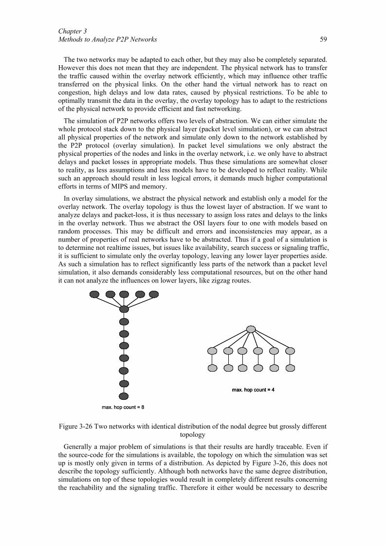
Chapter 3 Methods to Analyze P2P Networks 59
The two networks may be adapted to each other, but they may also be completely separated.
However this does not mean that they are independent. The physical network has to transfer the traffic caused within the overlay network efficiently, which may influence other traffic transferred on the physical links. On the other hand the virtual network has to react on congestion, high delays and low data rates, caused by physical restrictions. To be able to optimally transmit the data in the overlay, the overlay topology has to adapt to the restrictions of the physical network to provide efficient and fast networking.
The simulation of P2P networks offers two levels of abstraction. We can either simulate the whole protocol stack down to the physical layer (packet level simulation), or we can abstract all physical properties of the network and simulate only down to the network established by the P2P protocol (overlay simulation). In packet level simulations we only abstract the physical properties of the nodes and links in the overlay network, i.e. we only have to abstract delays and packet losses in appropriate models. Thus these simulations are somewhat closer to reality, as less assumptions and less models have to be developed to reflect reality. While such an approach should result in less logical errors, it demands much higher computational efforts in terms of MIPS and memory.
In overlay simulations, we abstract the physical network and establish only a model for the overlay network. The overlay topology is thus the lowest layer of abstraction. If we want to analyze delays and packet-loss, it is thus necessary to assign loss rates and delays to the links in the overlay network. Thus we abstract the OSI layers four to one with models based on random processes. This may be difficult and errors and inconsistencies may appear, as a number of properties of real networks have to be abstracted. Thus if a goal of a simulation is to determine not realtime issues, but issues like availability, search success or signaling traffic, it is sufficient to simulate only the overlay topology, leaving any lower layer properties aside. As such a simulation has to reflect significantly less parts of the network than a packet level simulation, it also demands considerably less computational resources, but on the other hand it can not analyze the influences on lower layers, like zigzag routes.
max. hop count = 4
max. hop count = 8
max. hop count = 4max. hop count = 4
max. hop count = 8
Figure 3-26 Two networks with identical distribution of the nodal degree but grossly different
topology
Generally a major problem of simulations is that their results are hardly traceable. Even if the source-code for the simulations is available, the topology on which the simulation was set up is mostly only given in terms of a distribution. As depicted by Figure 3-26, this does not describe the topology sufficiently. Although both networks have the same degree distribution, simulations on top of these topologies would result in completely different results concerning the reachability and the signaling traffic. Therefore it either would be necessary to describe
Chapter 3 Methods to Analyze P2P Networks
60
the properties of the simulated networks in more detail, e.g. by the maximum and average path length and the cliquishness of the simulated topology, or we have to run a high number of different simulations, hoping that the randomly chosen topologies reflect in the end the "average" topology, which is partly indicated by the size of the confidence interval.
To generate reasonably accurate results we have to ensure, that the starting nodes, which we pick at random, reflect reasonably well the generating function we decided to use, i.e. the correct distribution of the degree vs. the number of nodes. For small networks this requires using practically each node in the network as a starting point. This applies up to many thousand nodes in the network and even for still higher numbers it turns out, that we can at best restrict the number of simulation runs to using roughly 80 percent of the nodes as starting points, which causes a significant computational effort.
What turns out to be even more difficult is the fact that for a given number of links and a given number of nodes there is an enormous number of different networks which may be generated. As pointed out in [ER60] the number of different networks which can be built out of nn nodes and nl links is given by
2nn
nl
(56)
Assuming a very small network with 10 nodes and 15 links we end up with roughly 1013 networks. Unfortunately there is no such thing as a "typical" network so that a reasonably accurate simulation would have to be done over a huge number of different networks. While the number of networks to be considered is considerably reduced by requiring a certain probability distribution of the number of nodes vs. degree, simulation is hardly practical for a good forecast of the behavior of a general network.
To provide some evidence concerning the huge number of networks possible even with a precisely defined nodal degree distribution we point out that in a network with n types of nodes, e.g. nodes with degree 1, 2, 3,.. n a node with k links will have (initially)
1n k
k+ −
(57)
ways how to connect to the different types of nodes (i.e. nodes with different degree).
In addition, we also show in Figure 3-27 the number of nodes reached in three different (larger) networks with the same distribution of nodes vs. degree. For this figure, we first generated three different virtual networks and then made 100 simulations, with different starting nodes, for each scenario. The parameter we investigate in this figure is the average number of nodes, which can be reached starting at one randomly selected node in the network. The horizontal axis gives the hop value h, and the vertical axis gives the number of nodes reached until hop h (n_con(h)), divided by the maximum number of connectable nodes (N). The vertical bars represent 95 percent confidence intervals.
As is evident from the figure the results are indeed very different for each network, although all of them have the same nodal degree distribution. This again underlines the need for a computational approach which does not rely on a specific given network topology for cases with an unknown configuration of the virtual network, which is usually the fact in a P2P network. However, if the network topology is known, e.g. from using history, a simulation may well be feasible and provide more accurate results than our general analytic approach described in section 3.2.3, which makes no use of topology information other than the nodal degree distribution.
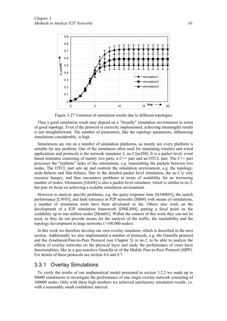
Chapter 3 Methods to Analyze P2P Networks 61
0
0.1
0.2
0.3
0.4
0.5
0.6
0.7
0.8
0.9
0 5 10 15 20
n_co
n/N
simulation1simulation2simulation3
hop
Figure 3-27 Variation of simulation results due to different topologies
Thus a good simulation result may depend on a "friendly" simulation environment in terms of good topology. Even if the protocol is correctly implemented, achieving meaningful results is not straightforward. The number of parameters, like the topology parameters, influencing simulations considerably, is high.
Simulations are run on a number of simulation platforms, as mostly not every platform is suitable for any problem. One of the simulators often used for simulating wireless and wired applications and protocols is the network simulator 2, ns-2 [ns204]. It is a packet level, event based simulator consisting of mainly two parts, a C++ part and an OTCL part. The C++ part processes the "realtime" tasks of the simulations, e.g. transmitting the packets between two nodes. The OTCL part sets up and controls the simulation environment, e.g. the topology, node-failures and link-failures. Due to the detailed packet level simulation, the ns-2 is very resource hungry, and thus encounters problems in terms of scalability for an increasing number of nodes. Glomosim [Glo04] is also a packet-level simulator, which is similar to ns-2, but puts its focus on achieving a scalable simulation environment.
However to analyze specific problems, e.g. the query-response time [HARR03], the search performance [LW03], and fault tolerance in P2P networks [SB04] with means of simulations, a number of simulation tools have been developed so far. Others also work on the development of a P2P simulation framework [DMLS04], putting a focal point on the scalability up to one million nodes [Mont01]. Within the context of this work they can not be used, as they do not provide means for the analysis of the traffic, the reachability and the topology development in large networks (>100.000 nodes).
In this work we therefore develop our own overlay simulator, which is described in the next section. Additionally we also implemented a number of protocols, e.g. the Gnutella protocol and the Zonebased-Peer-to-Peer Protocol (see Chapter 5) in ns-2, to be able to analyze the effects of overlay networks on the physical layer and study the performance of cross layer functionalities, like in a geo-sensitive Gnutella or of the Mobile Peer-to-Peer Protocol (MPP). For details of these protocols see section 4.6 and 4.7.
3.3.1 Overlay Simulations To verify the results of our mathematical model presented in section 3.2.2 we made up to
80000 simulations to investigate the performance of one single overlay network consisting of 100000 nodes. Only with these high numbers we achieved satisfactory simulation results, i.e. with a reasonably small confidence interval.
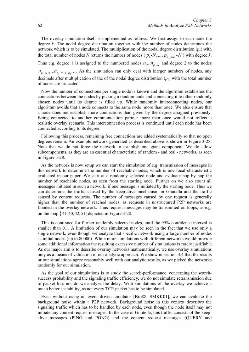
Chapter 3 Methods to Analyze P2P Networks
62
The overlay simulation itself is implemented as follows. We first assign to each node the degree k. The nodal degree distribution together with the number of nodes determines the network which is to be simulated. The multiplication of the nodal degree distribution (pk) with the total number of nodes N returns the number of nodes ( 1 _ max,..., kp N p Ni i ) with degree k.
Thus e.g. degree 1 is assigned to the numbered nodes 11... p Nn n i and degree 2 to the nodes
1 1 21 1...p N p N p Nn n+ + +i i i . As the simulation can only deal with integer numbers of nodes, any decimals after multiplication of the of the nodal degree distribution (pk) with the total number of nodes are truncated.
Now the number of connections per single node is known and the algorithm establishes the connections between the nodes by picking a random node and connecting it to other randomly chosen nodes until its degree is filled up. While randomly interconnecting nodes, our algorithm avoids that a node connects to the same node more than once. We also ensure that a node does not establish more connections than given by the degree assigned previously. Being connected to another communication partner more than once would not reflect a realistic overlay scenario. This interconnection process is continued until each node has been connected according to its degree.
Following this process, remaining free connections are added systematically so that no open degrees remain. An example network generated as described above is shown in Figure 3-28. Note that we do not force the network to establish one giant component. We do allow subcomponents, as they are an essential characteristic of random - and real - networks, as seen in Figure 3-28.
As the network is now setup we can start the simulation of e.g. transmission of messages in this network to determine the number of reachable nodes, which is one focal characteristic evaluated in our paper. We start at a randomly selected node and evaluate hop by hop the number of reachable nodes, as seen from the starting node. Further on we also count all messages initiated in such a network, if one message is initiated by the starting node. Thus we can determine the traffic caused by the keep-alive mechanism in Gnutella and the traffic caused by content requests. The number of messages caused by one request is generally higher than the number of reached nodes, as requests in unstructured P2P networks are flooded in the overlay network. Thus request messages may be transmitted on loops, as e.g. on the loop { }41, 40, 42,51 depicted in Figure 3-28.
This is continued for further randomly selected nodes, until the 95% confidence interval is smaller than 0.1. A limitation of our simulation may be seen in the fact that we use only a single network, even though we analyze that specific network using a large number of nodes as initial nodes (up to 80000). While more simulations with different networks would provide some additional information the resulting excessive number of simulations is rarely justifiable. As our major aim is to describe overlay networks mathematically, we use overlay simulations only as a means of validation of our analytic approach. We show in section 4.4 that the results or our simulations agree reasonably well with our analytic results, as we picked the networks randomly for our simulation.
As the goal of our simulations is to study the search-performance, concerning the search-success probability and the signaling traffic efficiency, we do not simulate retransmission due to packet loss nor do we analyze the delay. With simulations of the overlay we achieve a much better scalability, as not every TCP-packet has to be simulated.
Even without using an event driven simulator [Bro88, SMKK01], we can evaluate the background noise within a P2P network. Background noise in this context describes the signaling traffic which has to be handled by each node, even though the node itself may not initiate any content request messages. In the case of Gnutella, this traffic consists of the keep-alive messages (PING and PONG) and the content request messages (QUERY and
Chapter 3 Methods to Analyze P2P Networks 63
QUERYHIT) messages initiated by neighboring nodes. This traffic depends only on the protocol properties and not on the user behavior and can thus not be influenced by the user.
Figure 3-28 Example topology of a simulated network, with a powerlaw distribution of the nodal degree
However to analyze the location awareness of P2P protocols or to analyze specific effects of physical layers, e.g. in a mobile network, we have to use packet-level simulators, as described shortly in the next section.
3.3.2 Packet level simulations Packet level simulations must take into account the complete protocol stack. Thus we have
to use all four building blocks. The user, the application, the overlay and the physical network. Consequently we have to generate two networks for the simulation. The physical network topology, according to the models described in section 3.2.5, and the overlay topology, according to the models described in section 3.2.3.
To generate the physical network we use the topology generator BRITE, which provides tools to generate Internet topologies according to the models described in section 3.2.5. For the establishment of the overlay network we use a similar algorithm as described in section 3.3.1. To reflect reality, we use a powerlaw distribution for the nodal degree with 1.3k = , a maximum degree of seven and a minimum degree of one as found by [JAB01]. As we are not able to simulate networks with a high number of participating nodes, a focal point of this overlay topology generator is to establish no separated subcomponents. This is achieved by reorganizing the random structure in case of subcomponents with an algorithm, which first opens connections between nodes with a high degree and then connects nodes with a small degree to the network, via the opened connections
The physical network is generated as labeled graph. If no adaptation to the physical network is used, e.g. by means of cross layer communication, an independent overlay network is
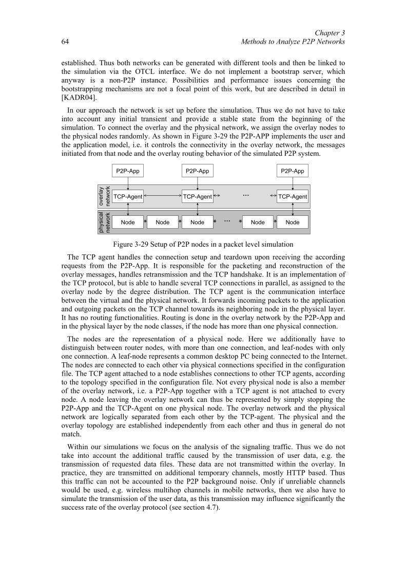
Chapter 3 Methods to Analyze P2P Networks
64
established. Thus both networks can be generated with different tools and then be linked to the simulation via the OTCL interface. We do not implement a bootstrap server, which anyway is a non-P2P instance. Possibilities and performance issues concerning the bootstrapping mechanisms are not a focal point of this work, but are described in detail in [KADR04].
In our approach the network is set up before the simulation. Thus we do not have to take into account any initial transient and provide a stable state from the beginning of the simulation. To connect the overlay and the physical network, we assign the overlay nodes to the physical nodes randomly. As shown in Figure 3-29 the P2P-APP implements the user and the application model, i.e. it controls the connectivity in the overlay network, the messages initiated from that node and the overlay routing behavior of the simulated P2P system.
P2P-App
TCP-Agent
Node
P2P-App
TCP-Agent
NodeNode Node Node…
P2P-App
TCP-Agent …
over
lay
netw
ork
phys
ical
netw
ork
Figure 3-29 Setup of P2P nodes in a packet level simulation
The TCP agent handles the connection setup and teardown upon receiving the according requests from the P2P-App. It is responsible for the packeting and reconstruction of the overlay messages, handles retransmission and the TCP handshake. It is an implementation of the TCP protocol, but is able to handle several TCP connections in parallel, as assigned to the overlay node by the degree distribution. The TCP agent is the communication interface between the virtual and the physical network. It forwards incoming packets to the application and outgoing packets on the TCP channel towards its neighboring node in the physical layer. It has no routing functionalities. Routing is done in the overlay network by the P2P-App and in the physical layer by the node classes, if the node has more than one physical connection.
The nodes are the representation of a physical node. Here we additionally have to distinguish between router nodes, with more than one connection, and leaf-nodes with only one connection. A leaf-node represents a common desktop PC being connected to the Internet. The nodes are connected to each other via physical connections specified in the configuration file. The TCP agent attached to a node establishes connections to other TCP agents, according to the topology specified in the configuration file. Not every physical node is also a member of the overlay network, i.e. a P2P-App together with a TCP agent is not attached to every node. A node leaving the overlay network can thus be represented by simply stopping the P2P-App and the TCP-Agent on one physical node. The overlay network and the physical network are logically separated from each other by the TCP-agent. The physical and the overlay topology are established independently from each other and thus in general do not match.
Within our simulations we focus on the analysis of the signaling traffic. Thus we do not take into account the additional traffic caused by the transmission of user data, e.g. the transmission of requested data files. These data are not transmitted within the overlay. In practice, they are transmitted on additional temporary channels, mostly HTTP based. Thus this traffic can not be accounted to the P2P background noise. Only if unreliable channels would be used, e.g. wireless multihop channels in mobile networks, then we also have to simulate the transmission of the user data, as this transmission may influence significantly the success rate of the overlay protocol (see section 4.7).
Chapter 3 Methods to Analyze P2P Networks 65
3.4. Summary In this chapter we presented a detailed investigation of methods to analyze in depth the
characteristics of P2P networks. We first described tools to measure the network topology of P2P networks. We presented new means to determine the topology of the overlay network in a decentralized environment. We used two approaches. The first consists of a network crawler, which can measure the overall topology without any hop limitations and which can also map the virtual network to its geographical locations. As a second approach we developed a measurement node, which acts to the outside world as a common peer, but establishes a large number of connections and logs internally all messages with addresses and IDs of the nodes it communicates with. Thus we can determine the network topology as perceived by a single node and can additionally analyze the connectivity of a P2P network as seen from one node, i.e. investigate cycles and the cliquishness of the considered overlay network.
The second contribution of this chapter is the development of a network traffic and user measurement tool, which measures the traffic in parallel on the application level, i.e. in the overlay network, and on the physical layer. Thus we can derive the traffic characteristics of P2P networks, i.e. we can determine its self-similarity, its burstiness and its average volumes. By using the data measured on the overlay, we can additionally measure portions of the traffic, i.e. how much traffic is caused by the keep-alive mechanism and how much traffic is caused by content requests. Thus we can not only analyze the different parts of the protocol, but we can also analyze the distribution of the message size for every message specified in the investigated P2P protocol. Further on we can use the measurement tools described above to measure the user behavior in P2P networks. Thus we can derive user properties, like uptime or session length of peers in different configurations and measure their request behavior, i.e. how many requests and for which content are issued by a user in a P2P network.
In practice these tools can thus be used as follows:
• The topology measurement tools provide a sound basis for the development of overlay network models. These models are necessary to achieve meaningful, trustworthy simulation and analytic results.
• Measuring and visualizing the topology of an overlay network provides means to analyze shortcomings and problems of real life P2P network topologies, as well as to understand the mechanisms of P2P, their changing nature and their self-organizational possibilities. Having measured the network offers the potential for further improvements, e.g. geo-sensitive networks or hybrid networks.
• The developed crawler provides an exact snapshot of the Gnutella network and additionally, by employing the attached location retriever, maps the virtual nodes to their geographical locations and visualize them on a world map. Thus the distribution of Gnutella participants on the different countries can easily be retrieved and their interconnections can be made visible. As a result we can show with this tool, that the virtual Peer-to-Peer network is not matched at all to the underlying physical network. We measured and visualized the established zigzag routes across the Atlantic, which shows a significant waste of bandwidth and high delays in the signaling traffic.
• The measurements enabled us to establish a meaningful user and application model for the computational and simulative analysis of P2P networks. As described in section 3.2.4, the application model includes, besides other parameters, the message portions and their size distribution and the cycles which occur in overlay networks. Further on this model also takes into account the replication strategy applied in the considered network and the number of shared files per user.
Chapter 3 Methods to Analyze P2P Networks
66
Based on our measurement results, which are confirmed by other measurements, we developed as our third contribution a novel model to describe the user behavior in P2P networks. We can model the uptime/session length distribution with a Weibull distribution as given in equation (33) and shown in Figure 3-7 and Figure 3-8. Further on, our user model includes the request behavior of the user, which is given as a Poisson distribution, with an average of 2 requests per session. Our analytical user model also describes the memory-effect observed in P2P networks, i.e. the longer a user already stayed online, the higher is the probability, that the user will stay online further on.
Our fourth contribution in this chapter is the development of an analytical model to describe the overlay network as a finite random graph with a given degree distribution. In contrast to previous models we can resolve the contradiction of infinitely growing networks and finite giant components of random graphs. The saturation effect of the number of reachable nodes reflects real world scenarios and fits very well to simulation and measurement results.
The practical usefulness of our models is as follows:
• As our user model is based on different measurements, it offers a basis for meaningful simulations and computational analysis of P2P networks. It is the first analytical model describing the session length of a user and the request behavior of a user in a P2P network.
• The application model describes the behavior of the protocol, i.e. its message sizes, its state transitions and its routing behavior. It is a necessary basis for the computational analysis of specific P2P protocols.
• The analytical overlay network model can be used to estimate the number of nodes reached in a P2P virtual network with a given distribution of nodal degree. The required computational power is much smaller than what would be required by a simulation, so that the method is applicable even for large P2P networks.
• In conjunction with the user model and the application model, our approach is a useful tool to estimate the traffic caused in such a network as well as to estimate the search success rate for a given P2P network structure
• Our analytical network model offers a fast possibility to derive an estimate of the performance of a given P2P protocol. In conjunction with the user model and the application model it also provides an efficient way to compare the performance of different P2P protocols with respect to their signaling traffic, their search efficiency and other parameters.
• Our analytical approach can be applied to other application areas, which show a “random” network structure, e.g. the Internet or Mobile Ad Hoc Networks. With an appropriate application and network model it can also be used to evaluate the performance of the respective protocol in terms of signaling efficiency and search success rate.
Our final contribution concerning the methods used to analyze P2P networks is the implementation of two simulation approaches. Simulations of only the overlay network offer a much better scalability compared to packet level simulations, as in this case the physical environment is abstracted completely, and we do not have to simulate every packet event. Thus simulations of P2P networks of much larger scale than in packet-level simulations can be achieved. In addition, our simulations of the whole protocol stack, down to the physical layer, allow the investigation of cross layer effects.
Chapter 4 SIGNALING TRAFFIC AND TOPOLOGY OF UNSTRUCTURED P2P NETWORKS
The traffic volumes generated by P2P applications are today often the major load on the Internet. Traffic statistics from the Abilene backbone [Abi03] show the enormous amount of traffic, i.e. more than 9 Tbyte per week, caused by P2P networks. Additionally we have to take into account, that a large fraction of the unidentified traffic is also caused by P2P applications, which have not been identified. All this traffic is only signaling traffic, i.e. not a single file transfer is counted within these two traffic amounts. Further on we have to assume, that a significant part of the data transfer is also caused by P2P applications [Gnu04, JXTA02, Küg03, OTG02].
Thus we conclude that the signaling efficiency is a key consideration in P2P protocols and their applications. Signaling efficiency in this work is defined as given by equation (58).
sigsize of the requested object
traffic received and initiated by the node until the object is receivedρ = (58)
This means, the less background noise is caused by the P2P protocol, the better is the signaling efficiency. In P2P networks the overhead is mostly caused by keep alive schemes, query and response messages routed to other destinations, and the query and query-hit messages initiated and received by a node to find the requested object. In the best case, e.g. if a node knows the location of a specific content in advance, the signaling efficiency would be nearly one, as only the HTTP headers would then cause some overhead.
Although the high overhead is certainly a price which one has to pay for decentralization, we argue that one can reduce this overhead by reducing inefficiencies of the considered P2P network and protocol. Therefore we use this chapter to outline the reasons for this high amount of signaling traffic and develop new possibilities how to reduce the signaling traffic. We focus on inefficiencies caused by the protocol itself and by the overlay topology.
We concentrate on unstructured P2P networks, namely the JXTA protocol and the Gnutella protocol. Based on the measurement tools described in Chapter 3, we provide in section 4.1 a detailed analysis of the Gnutella topology, which is very similar to other hybrid topologies, e.g. the JXTA topology or the Kazaa topology. In most cases these topologies are established completely independent from the underlying physical network, leading to inefficiencies concerning look-up delays and an increased background noise caused by signaling traffic.
Concerning the protocol inefficiencies, we analyze the traffic characteristics of a Gnutella node in section 4.3 and study the possibilities of compressing the signaling traffic. We also study the amount of keep-alive traffic, to find out means how to reduce this traffic, which is not needed to look up the location of requested content.
To solve the shortcomings of the overlay topology, resulting from the separation of the physical from the virtual layer, we propose in section 4.6 an enhancement of Gnutella to adapt the physical network better to the virtual network. With this improvement we can show an enhanced signaling efficiency by means of simulations. Further on we propose in section 4.5 a new scheme for compression negotiation, which keeps the flexibility of e.g. XML based JXTA messages, but decreases the signaling traffic by more than 50%.
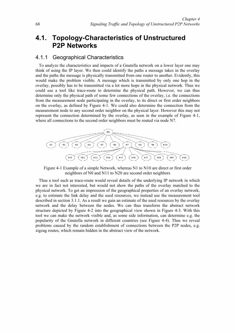
Chapter 4 Signaling Traffic and Topology of Unstructured P2P Networks
68
4.1. Topology-Characteristics of Unstructured P2P Networks
4.1.1 Geographical Characteristics To analyze the characteristics and impacts of a Gnutella network on a lower layer one may
think of using the IP layer. We then could identify the paths a message takes in the overlay and the paths the message is physically transmitted from one router to another. Evidently, this would make the problem visible. A message which is transmitted by only one hop in the overlay, possibly has to be transmitted via a lot more hops in the physical network. Thus we could use a tool like trace-route to determine the physical path. However, we can thus determine only the physical path of some few connections of the overlay, i.e. the connections from the measurement node participating in the overlay, to its direct or first order neighbors on the overlay, as defined by Figure 4-1. We could also determine the connection from the measurement node to any second order neighbor on the physical layer. However this may not represent the connection determined by the overlay, as seen in the example of Figure 4-1, where all connections to the second order neighbors must be routed via node N7.
Figure 4-1 Example of a simple Network, whereas N1 to N10 are direct or first order
neighbors of N0 and N11 to N20 are second order neighbors
Thus a tool such as trace-route would reveal details of the underlying IP network in which we are in fact not interested, but would not show the paths of the overlay matched to the physical network. To get an impression of the geographical properties of an overlay network, e.g. to estimate the link delay and the used resources, we instead use the measurement tool described in section 3.1.1. As a result we gain an estimate of the used resources by the overlay network and the delay between the nodes. We can thus transform the abstract network structure depicted by Figure 4-2 into the geographical view shown in Figure 4-3. With this tool we can make the network visible and, as some side information, can determine e.g. the popularity of the Gnutella network in different countries (see Figure 4-4). Thus we reveal problems caused by the random establishment of connections between the P2P nodes, e.g. zigzag routes, which remain hidden in the abstract view of the network.
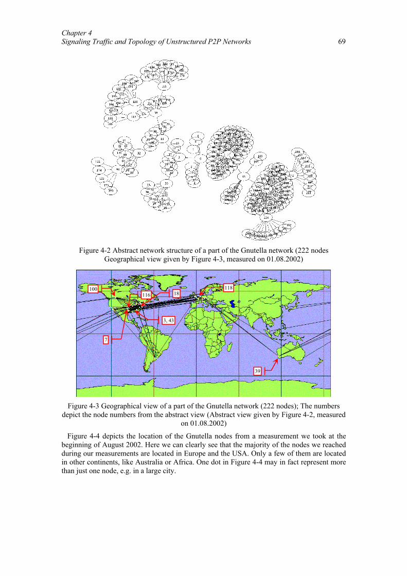
Chapter 4 Signaling Traffic and Topology of Unstructured P2P Networks 69
Figure 4-2 Abstract network structure of a part of the Gnutella network (222 nodes
Geographical view given by Figure 4-3, measured on 01.08.2002)
39
118
7
116
3, 43
18100
Figure 4-3 Geographical view of a part of the Gnutella network (222 nodes); The numbers
depict the node numbers from the abstract view (Abstract view given by Figure 4-2, measured on 01.08.2002)
Figure 4-4 depicts the location of the Gnutella nodes from a measurement we took at the beginning of August 2002. Here we can clearly see that the majority of the nodes we reached during our measurements are located in Europe and the USA. Only a few of them are located in other continents, like Australia or Africa. One dot in Figure 4-4 may in fact represent more than just one node, e.g. in a large city.
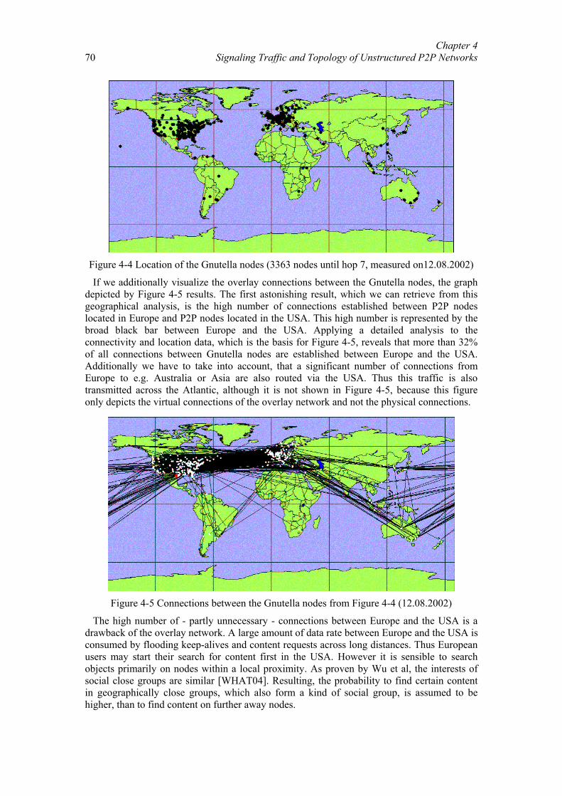
Chapter 4 Signaling Traffic and Topology of Unstructured P2P Networks
70
Figure 4-4 Location of the Gnutella nodes (3363 nodes until hop 7, measured on12.08.2002)
If we additionally visualize the overlay connections between the Gnutella nodes, the graph depicted by Figure 4-5 results. The first astonishing result, which we can retrieve from this geographical analysis, is the high number of connections established between P2P nodes located in Europe and P2P nodes located in the USA. This high number is represented by the broad black bar between Europe and the USA. Applying a detailed analysis to the connectivity and location data, which is the basis for Figure 4-5, reveals that more than 32% of all connections between Gnutella nodes are established between Europe and the USA. Additionally we have to take into account, that a significant number of connections from Europe to e.g. Australia or Asia are also routed via the USA. Thus this traffic is also transmitted across the Atlantic, although it is not shown in Figure 4-5, because this figure only depicts the virtual connections of the overlay network and not the physical connections.
Figure 4-5 Connections between the Gnutella nodes from Figure 4-4 (12.08.2002)
The high number of - partly unnecessary - connections between Europe and the USA is a drawback of the overlay network. A large amount of data rate between Europe and the USA is consumed by flooding keep-alives and content requests across long distances. Thus European users may start their search for content first in the USA. However it is sensible to search objects primarily on nodes within a local proximity. As proven by Wu et al, the interests of social close groups are similar [WHAT04]. Resulting, the probability to find certain content in geographically close groups, which also form a kind of social group, is assumed to be higher, than to find content on further away nodes.
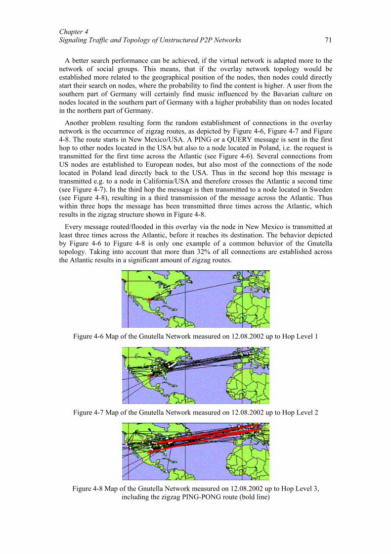
Chapter 4 Signaling Traffic and Topology of Unstructured P2P Networks 71
A better search performance can be achieved, if the virtual network is adapted more to the
network of social groups. This means, that if the overlay network topology would be established more related to the geographical position of the nodes, then nodes could directly start their search on nodes, where the probability to find the content is higher. A user from the southern part of Germany will certainly find music influenced by the Bavarian culture on nodes located in the southern part of Germany with a higher probability than on nodes located in the northern part of Germany.
Another problem resulting form the random establishment of connections in the overlay network is the occurrence of zigzag routes, as depicted by Figure 4-6, Figure 4-7 and Figure 4-8. The route starts in New Mexico/USA. A PING or a QUERY message is sent in the first hop to other nodes located in the USA but also to a node located in Poland, i.e. the request is transmitted for the first time across the Atlantic (see Figure 4-6). Several connections from US nodes are established to European nodes, but also most of the connections of the node located in Poland lead directly back to the USA. Thus in the second hop this message is transmitted e.g. to a node in California/USA and therefore crosses the Atlantic a second time (see Figure 4-7). In the third hop the message is then transmitted to a node located in Sweden (see Figure 4-8), resulting in a third transmission of the message across the Atlantic. Thus within three hops the message has been transmitted three times across the Atlantic, which results in the zigzag structure shown in Figure 4-8.
Every message routed/flooded in this overlay via the node in New Mexico is transmitted at least three times across the Atlantic, before it reaches its destination. The behavior depicted by Figure 4-6 to Figure 4-8 is only one example of a common behavior of the Gnutella topology. Taking into account that more than 32% of all connections are established across the Atlantic results in a significant amount of zigzag routes.
Figure 4-6 Map of the Gnutella Network measured on 12.08.2002 up to Hop Level 1
Figure 4-7 Map of the Gnutella Network measured on 12.08.2002 up to Hop Level 2
Figure 4-8 Map of the Gnutella Network measured on 12.08.2002 up to Hop Level 3,
including the zigzag PING-PONG route (bold line)
Chapter 4 Signaling Traffic and Topology of Unstructured P2P Networks
72
In addition to the high and unnecessary consumption of bandwidth between the USA and Europe, the zigzag routes cause high delays, which can be perceived by any user logged onto the overlay network. At least every third message crosses several times the Atlantic. The performance of the overlay network could be improved by directing the message first to nodes in the local proximity of the querying node and then only once across the Atlantic and similar long distances to distribute the query then in the remote area.
Therefore we propose in section 4.6 a scheme to make the Gnutella network adapt itself automatically during runtime to the physical network. Thus we can avoid zigzag routes, reduce the overall amount of signaling traffic significantly and also reduce the average delay. If we further assume, as demonstrated by [WHAT04], that close social groups have similar interests, and therefore also geographically close groups have similar interests [WHAT04] we can additionally improve the performance of the network, as perceived by the user. Then the content is found faster, it can be downloaded faster and the network load decreases significantly.
4.1.2 Reach Analysis In the section above our goal has been to analyze the Gnutella network from a geographical
point of view. Therefore we used a network crawler, which can locate nodes participating in the network independent from TTL-restrictions. In this section we want to analyze the overlay topology as perceived by a single node, which does not have a global view, because of TTL-restrictions. This limits the reach of the messages from every node to 7 hops in general.
4.1.2.1. Evaluation of the number of reachable nodes We used for this topology analysis a common Gnutella client, with a modified PONG cache
as described in section 3.1.1.1. The modified PONG cache stores additionally to incoming PONG messages also QUERYHIT and PUSH messages issued by peers within the TTL reach. Based on an evaluation of these messages we evaluate the total number of reachable nodes as seen from one single node. We also use this tool to evaluate the number of loops within the network and their impact on the reach within a Gnutella network.
To reach a high number of nodes, the measurement node establishes between 3 and a maximum of 120 P2P connections to different first order neighbors, which actively participate in the overlay network. The motivation for this high number of connections is that with such a high number of first order neighbors we reach even with a TTL-limit of 7 hops all nodes currently participating in the network. However the underlying assumption is that no loops are established between the nodes. If we are not able to reach the theoretical value, this points to the existence of loops within the P2P overlay network, which limit the reach of nodes in a P2P network notably [SS02, SS04].
That there must be a limiting factor can also be observed from Table 4-1. Under the assumption of a tree-structure starting at every direct neighbor and that these trees are not connected to each other, apart from their common root at the measurement node, we can exclude any loops. Based on this assumption we can compute the average number of reachable nodes ( _ hn con ) according to equation (59). In equation (59) the parameter h gives the number of hops, at which the number of reachable nodes is evaluated, 0d describes the degree of the measurement node and d represents the average degree of the nodes participating in the overlay network. Based on earlier measurements, the value of d is set to 3.4d = , as the average number of neighbors per node [RFI02, SD03]. The second parameter h is set to 7h = hops for the computation of the numbers given in (59). This is the default value employed by most Gnutella implementations for the maximum number of hops along which a message is forwarded.
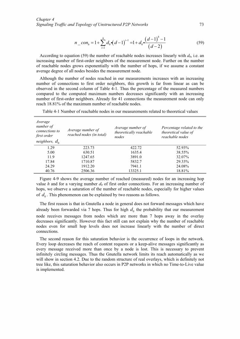
Chapter 4 Signaling Traffic and Topology of Unstructured P2P Networks 73
( ) ( )( )
10 0
1
1 1_ 1 1 1
2
hhi
hi
dn con d d d
d−
=
− −= + − = +
−∑ i i (59)
According to equation (59) the number of reachable nodes increases linearly with d0, i.e. an increasing number of first-order neighbors of the measurement node. Further on the number of reachable nodes grows exponentially with the number of hops, if we assume a constant average degree of all nodes besides the measurement node.
Although the number of nodes reached in our measurements increases with an increasing number of connections to first order neighbors, this growth is far from linear as can be observed in the second column of Table 4-1. Thus the percentage of the measured numbers compared to the computed maximum numbers decreases significantly with an increasing number of first-order neighbors. Already for 41 connections the measurement node can only reach 18.81% of the maximum number of reachable nodes.
Table 4-1 Number of reachable nodes in our measurements related to theoretical values
Average number of connections to first order neighbors, 0d
Average number of reached nodes (in total)
Average number of theoretically reachable nodes
Percentage related to the theoretical value of reachable nodes
1.29 223.73 422.72 52.93% 5.00 630.51 1635.4 38.55% 11.9 1247.65 3891.0 32.07%
17.84 1710.87 5832.7 29.33% 24.29 1912.20 7941.1 24.08% 40.76 2506.36 13325.1 18.81%
Figure 4-9 shows the average number of reached (measured) nodes for an increasing hop value h and for a varying number d0 of first order connections. For an increasing number of hops, we observe a saturation of the number of reachable nodes, especially for higher values of 0d . This phenomenon can be explained by two reasons as follows.
The first reason is that in Gnutella a node in general does not forward messages which have already been forwarded via 7 hops. Thus for high 0d the probability that our measurement node receives messages from nodes which are more than 7 hops away in the overlay decreases significantly. However this fact still can not explain why the number of reachable nodes even for small hop levels does not increase linearly with the number of direct connections.
The second reason for this saturation behavior is the occurrence of loops in the network. Every loop decreases the reach of content requests or a keep-alive messages significantly as every message received more than once by a node is lost. This is necessary to prevent infinitely circling messages. Thus the Gnutella network limits its reach automatically as we will show in section 4.2. Due to the random structure of real overlays, which is definitely not tree like, this saturation behavior also occurs in P2P networks in which no Time-to-Live value is implemented.
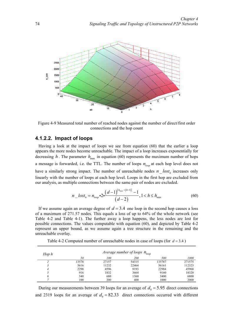
Chapter 4 Signaling Traffic and Topology of Unstructured P2P Networks
74
Figure 4-9 Measured total number of reached nodes against the number of direct/first order
connections and the hop count
4.1.2.2. Impact of loops Having a look at the impact of loops we see from equation (60) that the earlier a loop
appears the more nodes become unreachable. The impact of a loop increases exponentially for decreasing h . The parameter maxh in equation (60) represents the maximum number of hops a message is forwarded, i.e. the TTL. The number of loops loopn at each hop level does not
have a similarly strong impact. The number of unreachable nodes _ hn lost increases only linearly with the number of loops at each hop level. Loops in the first hop are excluded from our analysis, as multiple connections between the same pair of nodes are excluded.
( ) ( )( )
( )
max 1
max
1 1_ 2 ,1
2
h h
h loop
dn lost n h h
d
− −− −= < ≤
−i i (60)
If we assume again an average degree of 3.4d = one loop in the second hop causes a loss of a maximum of 271.57 nodes. This equals a loss of up to 64% of the whole network (see Table 4-2 and Table 4-1). The further away a loop happens, the less nodes are lost for possible connections. The values computable with equation (60), and depicted by Table 4-2 represent an upper bound, as we assume again a tree structure in the remaining and the unreachable overlay.
Table 4-2 Computed number of unreachable nodes in case of loops (for 3.4d = )
Average number of loops loopn Hop h 50 100 200 500 1000
2 13578 27157 54315 135787 271575 3 5616 11232 22464 56161 112323 4 2298 4596 9193 22984 45968 5 916 1832 3664 9160 18320 6 340 680 1360 3400 6800 7 100 200 400 1000 2000
During our measurements between 39 loops for an average of 0 5.95d = direct connections and 2319 loops for an average of 0 82.33 d = direct connections occurred with different
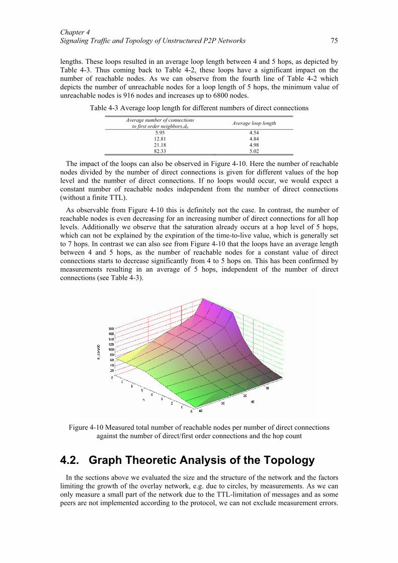
Chapter 4 Signaling Traffic and Topology of Unstructured P2P Networks 75
lengths. These loops resulted in an average loop length between 4 and 5 hops, as depicted by Table 4-3. Thus coming back to Table 4-2, these loops have a significant impact on the number of reachable nodes. As we can observe from the fourth line of Table 4-2 which depicts the number of unreachable nodes for a loop length of 5 hops, the minimum value of unreachable nodes is 916 nodes and increases up to 6800 nodes.
Table 4-3 Average loop length for different numbers of direct connections Average number of connections
to first order neighbors,d0 Average loop length
5.95 4.54 12.81 4.84 21.18 4.98 82.33 5.02
The impact of the loops can also be observed in Figure 4-10. Here the number of reachable nodes divided by the number of direct connections is given for different values of the hop level and the number of direct connections. If no loops would occur, we would expect a constant number of reachable nodes independent from the number of direct connections (without a finite TTL).
As observable from Figure 4-10 this is definitely not the case. In contrast, the number of reachable nodes is even decreasing for an increasing number of direct connections for all hop levels. Additionally we observe that the saturation already occurs at a hop level of 5 hops, which can not be explained by the expiration of the time-to-live value, which is generally set to 7 hops. In contrast we can also see from Figure 4-10 that the loops have an average length between 4 and 5 hops, as the number of reachable nodes for a constant value of direct connections starts to decrease significantly from 4 to 5 hops on. This has been confirmed by measurements resulting in an average of 5 hops, independent of the number of direct connections (see Table 4-3).
Figure 4-10 Measured total number of reachable nodes per number of direct connections
against the number of direct/first order connections and the hop count
4.2. Graph Theoretic Analysis of the Topology In the sections above we evaluated the size and the structure of the network and the factors
limiting the growth of the overlay network, e.g. due to circles, by measurements. As we can only measure a small part of the network due to the TTL-limitation of messages and as some peers are not implemented according to the protocol, we can not exclude measurement errors.
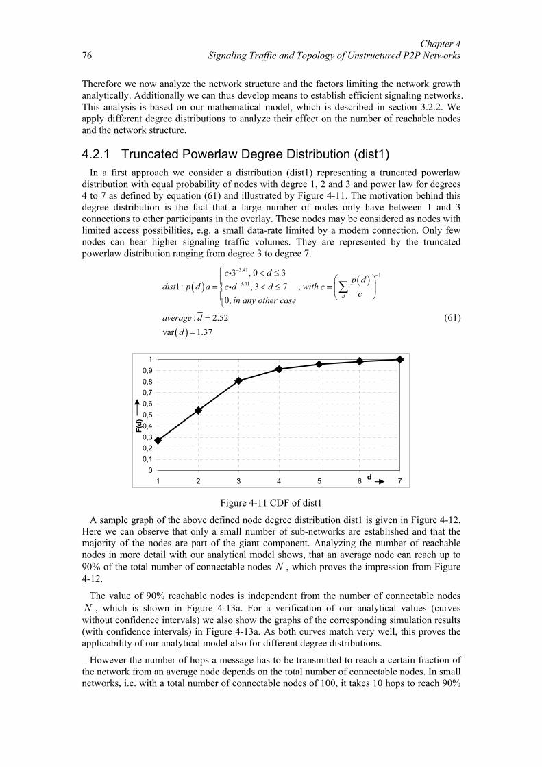
Chapter 4 Signaling Traffic and Topology of Unstructured P2P Networks
76
Therefore we now analyze the network structure and the factors limiting the network growth analytically. Additionally we can thus develop means to establish efficient signaling networks. This analysis is based on our mathematical model, which is described in section 3.2.2. We apply different degree distributions to analyze their effect on the number of reachable nodes and the network structure.
4.2.1 Truncated Powerlaw Degree Distribution (dist1) In a first approach we consider a distribution (dist1) representing a truncated powerlaw
distribution with equal probability of nodes with degree 1, 2 and 3 and power law for degrees 4 to 7 as defined by equation (61) and illustrated by Figure 4-11. The motivation behind this degree distribution is the fact that a large number of nodes only have between 1 and 3 connections to other participants in the overlay. These nodes may be considered as nodes with limited access possibilities, e.g. a small data-rate limited by a modem connection. Only few nodes can bear higher signaling traffic volumes. They are represented by the truncated powerlaw distribution ranging from degree 3 to degree 7.
( ) ( )
( )
3.411
3.41
3 , 0 31: , 3 7 ,
0,
: 2.52var 1.37
d
c dp d
dist p d a c d d with cc
in any other case
average dd
−−
−
< ≤ = < ≤ =
=
=
∑ii
(61)
00,10,20,30,40,50,60,70,80,9
1
1 2 3 4 5 6 7d
F(d)
Figure 4-11 CDF of dist1
A sample graph of the above defined node degree distribution dist1 is given in Figure 4-12. Here we can observe that only a small number of sub-networks are established and that the majority of the nodes are part of the giant component. Analyzing the number of reachable nodes in more detail with our analytical model shows, that an average node can reach up to 90% of the total number of connectable nodes N , which proves the impression from Figure 4-12.
The value of 90% reachable nodes is independent from the number of connectable nodes N , which is shown in Figure 4-13a. For a verification of our analytical values (curves without confidence intervals) we also show the graphs of the corresponding simulation results (with confidence intervals) in Figure 4-13a. As both curves match very well, this proves the applicability of our analytical model also for different degree distributions.
However the number of hops a message has to be transmitted to reach a certain fraction of the network from an average node depends on the total number of connectable nodes. In small networks, i.e. with a total number of connectable nodes of 100, it takes 10 hops to reach 90%
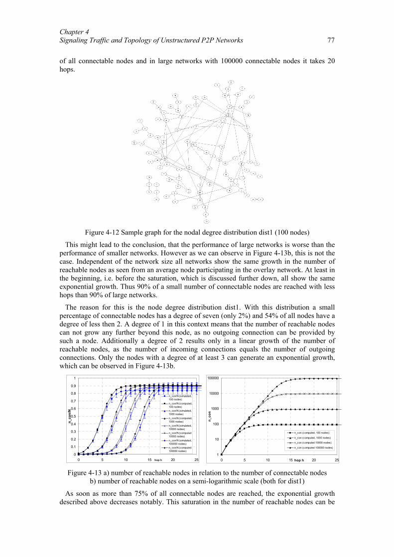
Chapter 4 Signaling Traffic and Topology of Unstructured P2P Networks 77
of all connectable nodes and in large networks with 100000 connectable nodes it takes 20 hops.
Figure 4-12 Sample graph for the nodal degree distribution dist1 (100 nodes)
This might lead to the conclusion, that the performance of large networks is worse than the performance of smaller networks. However as we can observe in Figure 4-13b, this is not the case. Independent of the network size all networks show the same growth in the number of reachable nodes as seen from an average node participating in the overlay network. At least in the beginning, i.e. before the saturation, which is discussed further down, all show the same exponential growth. Thus 90% of a small number of connectable nodes are reached with less hops than 90% of large networks.
The reason for this is the node degree distribution dist1. With this distribution a small percentage of connectable nodes has a degree of seven (only 2%) and 54% of all nodes have a degree of less then 2. A degree of 1 in this context means that the number of reachable nodes can not grow any further beyond this node, as no outgoing connection can be provided by such a node. Additionally a degree of 2 results only in a linear growth of the number of reachable nodes, as the number of incoming connections equals the number of outgoing connections. Only the nodes with a degree of at least 3 can generate an exponential growth, which can be observed in Figure 4-13b.
Figure 4-13 a) number of reachable nodes in relation to the number of connectable nodes
b) number of reachable nodes on a semi-logarithmic scale (both for dist1)
As soon as more than 75% of all connectable nodes are reached, the exponential growth described above decreases notably. This saturation in the number of reachable nodes can be
0
0.1
0.2
0.3
0.4
0.5
0.6
0.7
0.8
0.9
1
0 5 10 15 20 25hop h
n_co
n/N
n_con/N (simulated,100 nodes)n_con/N (computed,100 nodes)n_con/N (simulated,1000 nodes)n_con/N (computed,1000 nodes)n_con/N (simulated,10000 nodes)n_con/N (computed10000 nodes)n_con/N (simulated,100000 nodes)n_con/N (computed100000 nodes)
1
10
100
1000
10000
100000
0 5 10 15 20 25hop h
n_co
n
n_con (computed, 100 nodes)
n_con (computed, 1000 nodes)
n_con (computed 10000 nodes)
n_con (computed 100000 nodes)
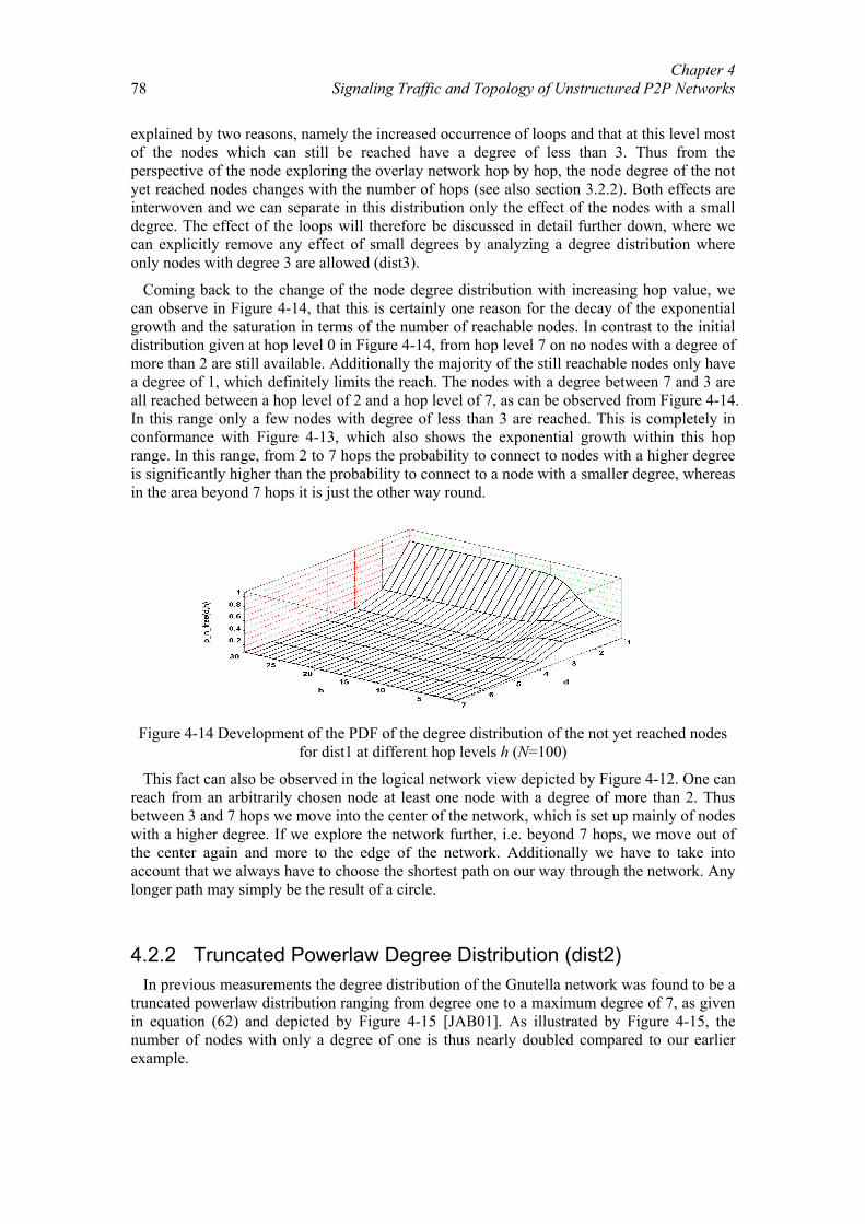
Chapter 4 Signaling Traffic and Topology of Unstructured P2P Networks
78
explained by two reasons, namely the increased occurrence of loops and that at this level most of the nodes which can still be reached have a degree of less than 3. Thus from the perspective of the node exploring the overlay network hop by hop, the node degree of the not yet reached nodes changes with the number of hops (see also section 3.2.2). Both effects are interwoven and we can separate in this distribution only the effect of the nodes with a small degree. The effect of the loops will therefore be discussed in detail further down, where we can explicitly remove any effect of small degrees by analyzing a degree distribution where only nodes with degree 3 are allowed (dist3).
Coming back to the change of the node degree distribution with increasing hop value, we can observe in Figure 4-14, that this is certainly one reason for the decay of the exponential growth and the saturation in terms of the number of reachable nodes. In contrast to the initial distribution given at hop level 0 in Figure 4-14, from hop level 7 on no nodes with a degree of more than 2 are still available. Additionally the majority of the still reachable nodes only have a degree of 1, which definitely limits the reach. The nodes with a degree between 7 and 3 are all reached between a hop level of 2 and a hop level of 7, as can be observed from Figure 4-14. In this range only a few nodes with degree of less than 3 are reached. This is completely in conformance with Figure 4-13, which also shows the exponential growth within this hop range. In this range, from 2 to 7 hops the probability to connect to nodes with a higher degree is significantly higher than the probability to connect to a node with a smaller degree, whereas in the area beyond 7 hops it is just the other way round.
Figure 4-14 Development of the PDF of the degree distribution of the not yet reached nodes
for dist1 at different hop levels h (N=100)
This fact can also be observed in the logical network view depicted by Figure 4-12. One can reach from an arbitrarily chosen node at least one node with a degree of more than 2. Thus between 3 and 7 hops we move into the center of the network, which is set up mainly of nodes with a higher degree. If we explore the network further, i.e. beyond 7 hops, we move out of the center again and more to the edge of the network. Additionally we have to take into account that we always have to choose the shortest path on our way through the network. Any longer path may simply be the result of a circle.
4.2.2 Truncated Powerlaw Degree Distribution (dist2) In previous measurements the degree distribution of the Gnutella network was found to be a
truncated powerlaw distribution ranging from degree one to a maximum degree of 7, as given in equation (62) and depicted by Figure 4-15 [JAB01]. As illustrated by Figure 4-15, the number of nodes with only a degree of one is thus nearly doubled compared to our earlier example.
Chapter 4 Signaling Traffic and Topology of Unstructured P2P Networks 79
( ) ( )
( )
11.4 , 0 72 : ,
0,
: 2.2var 1.63
d
p dc d ddist p d with c
cin any other case
average dd
−− < ≤= =
=
=
∑i
(62)
0
0.2
0.4
0.6
0.8
1
1 2 3 4 5 6 7d
F(d)
Figure 4-15 CDF of dist2
Comparing Figure 4-12 and Figure 4-16 shows that with this distribution the number of sub-components increases whereas the size of the giant component decreases. However the connectivity and the intermeshing in the giant component are similar. Thus we argue that the increased number of nodes with only one connection limits the size of the giant component. This also influences the number of reachable nodes, which is depicted by Figure 4-17. However, as the intermeshing is not changed, this should not reduce the growth of the network in the exponential phase as nodes with a small degree are automatically located at the edge of the network, and do not influence the number of reachable nodes in the exponential growth phase.
Figure 4-16 Sample graph for the nodal degree distribution dist2 (100 nodes)
Analyzing the number of reachable nodes in more detail proves our above interpretation. The results of the mathematical analysis are depicted by Figure 4-17. Figure 4-17a) also gives the simulation results, to verify the correctness of our mathematical model for this distribution. Comparing Figure 4-13 and Figure 4-17 reveals that before the saturation phase beginning at hop 6 for 100 nodes, the growth in the number of reachable nodes is similar. Thus the
Chapter 4 Signaling Traffic and Topology of Unstructured P2P Networks
80
increased number of nodes with only one link does not impact the speed of the growth, as argued above.
However, in the saturation phase the number of reachable nodes is now significantly smaller than with dist1. This results in a smaller number of reachable nodes in the saturation. In contrast to dist1, where we could reach up to 90% of all nodes, we can only reach up to 70% with dist2. This confirms our impression from Figure 4-16 that the number of subcomponents increased and that the size of the giant component decreased significantly.
Figure 4-17a) number of reachable nodes in relation to the number of connectable nodes
b) number of reachable nodes on a semi-logarithmic scale (both for dist2)
Looking at Figure 4-16 reveals that the largest separate sub-component is of size 5. However here we have to take into account, that Figure 4-16 illustrates a network of a comparatively small size. In real networks we expect a significantly higher number of participating nodes, i.e. several thousand nodes up to 100000 nodes. Consequently the size of the sub-components also increases, which is also shown in [CL02, JLR00]. Thus we conclude, that the limited network size we found with our crawler as outlined in section 4.1.1, is caused by the fact that several Gnutella networks exist in parallel, which are not or only sparsely connected. In real networks we additionally would have to take into account dependencies caused by different entry points, i.e. different beacon servers of e.g. Bearshare [Bea04] and Limewire [Lim04], to the different sub components. These dependencies have not been taken into account in our analytical model, which represents a random graph with a degree distribution measured previously in a Gnutella network.
4.2.3 Dirac Degree Distribution (dist3) As described in the sections above the nodes with degree one limit the number of the
reachable nodes or the size of the giant component significantly. Therefore we use in this section a degree distribution where nodes with degree one are excluded. Further on we also want to analyze the impacts of loops on the saturation behavior of the giant component. We consider in this section a network with a Dirac degree distribution as given by equation where all nodes have degree 3 (63).
( )
( )
1, 33 :
0,
: 3var 0
ddist p d
in any other case
average dd
==
=
=
(63)
As expected we are now able to reach 100% of all connectable nodes (see Figure 4-18 and Figure 4-19). Thus separate sub-components are avoided, as we can see from Figure 4-18. Comparing Figure 4-18 to Figure 4-16 or Figure 4-12 shows, that the intermeshing degree seems to be notably higher for the degree distribution dist3. The reason for that is the higher
0
0.1
0.2
0.3
0.4
0.5
0.6
0.7
0.8
0 5 10 15 20 25hop h
n_co
n/N
n_con/N(simulated 100 nodes)
n_con/N(computed, 100 nodes)
n_con/N(simulated, 1000 nodes)
n_con/N(computed, 1000 nodes)
n_con/N(simulated 10000 nodes)
n_con/N(computed, 10000 nodes)
n_con/N(simulated, 100000 nodes)
n_con/N(computed, 100000 nodes)
1
10
100
1000
10000
100000
0 5 10 15 20 25hop hn_
con
n_con(computed, 100 nodes)
n_con(computed, 1000 nodes)
n_con(computed, 10000 nodes)
n_con(computed, 100000 nodes)
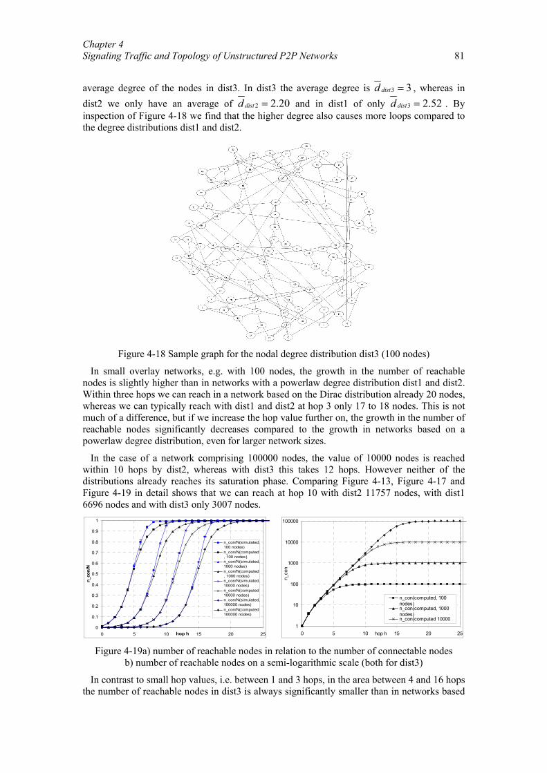
Chapter 4 Signaling Traffic and Topology of Unstructured P2P Networks 81
average degree of the nodes in dist3. In dist3 the average degree is 3 3distd = , whereas in dist2 we only have an average of 2 2.20distd = and in dist1 of only 3 2.52distd = . By inspection of Figure 4-18 we find that the higher degree also causes more loops compared to the degree distributions dist1 and dist2.
Figure 4-18 Sample graph for the nodal degree distribution dist3 (100 nodes)
In small overlay networks, e.g. with 100 nodes, the growth in the number of reachable nodes is slightly higher than in networks with a powerlaw degree distribution dist1 and dist2. Within three hops we can reach in a network based on the Dirac distribution already 20 nodes, whereas we can typically reach with dist1 and dist2 at hop 3 only 17 to 18 nodes. This is not much of a difference, but if we increase the hop value further on, the growth in the number of reachable nodes significantly decreases compared to the growth in networks based on a powerlaw degree distribution, even for larger network sizes.
In the case of a network comprising 100000 nodes, the value of 10000 nodes is reached within 10 hops by dist2, whereas with dist3 this takes 12 hops. However neither of the distributions already reaches its saturation phase. Comparing Figure 4-13, Figure 4-17 and Figure 4-19 in detail shows that we can reach at hop 10 with dist2 11757 nodes, with dist1 6696 nodes and with dist3 only 3007 nodes.
Figure 4-19a) number of reachable nodes in relation to the number of connectable nodes
b) number of reachable nodes on a semi-logarithmic scale (both for dist3)
In contrast to small hop values, i.e. between 1 and 3 hops, in the area between 4 and 16 hops the number of reachable nodes in dist3 is always significantly smaller than in networks based
0
0.1
0.2
0.3
0.4
0.5
0.6
0.7
0.8
0.9
1
0 5 10 15 20 25hop h
n_co
n/N
n_con/N(simulated,100 nodes)n_con/N(computed, 100 nodes)n_con/N(simulated,1000 nodes)n_con/N(computed, 1000 nodes)n_con/N(simulated,10000 nodes)n_con/N(computed10000 nodes)n_con/N(simulated,100000 nodes)n_con/N(computed100000 nodes)
1
10
100
1000
10000
100000
0 5 10 15 20 25hop h
n_co
n
n_con(computed, 100nodes)n_con(computed, 1000nodes)n_con(computed 10000
d )
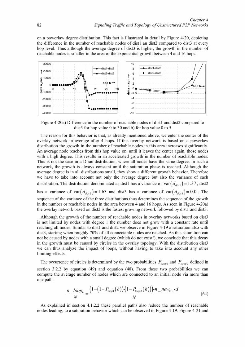
Chapter 4 Signaling Traffic and Topology of Unstructured P2P Networks
82
on a powerlaw degree distribution. This fact is illustrated in detail by Figure 4-20, depicting the difference in the number of reachable nodes of dist1 an dist2 compared to dist3 at every hop level. Thus although the average degree of dist3 is higher, the growth in the number of reachable nodes is smaller in the area of the exponential growth between 4 and 16 hops.
Figure 4-20a) Difference in the number of reachable nodes of dist1 and dist2 compared to
dist3 for hop value 0 to 30 and b) for hop value 0 to 5
The reason for this behavior is that, as already mentioned above, we enter the center of the overlay network in average after 4 hops. If this overlay network is based on a powerlaw distribution the growth in the number of reachable nodes in this area increases significantly. An average node reaches from this hop value on, until it leaves the center again, those nodes with a high degree. This results in an accelerated growth in the number of reachable nodes. This is not the case in a Dirac distribution, where all nodes have the same degree. In such a network, the growth is always constant until the saturation phase is reached. Although the average degree is in all distributions small, they show a different growth behavior. Therefore we have to take into account not only the average degree but also the variance of each distribution. The distribution denominated as dist1 has a variance of ( )1var 1.37distd = , dist2
has a variance of ( )2var 1.63distd = and dist3 has a variance of ( )3var 0.0distd = . The sequence of the variance of the three distributions thus determines the sequence of the growth in the number or reachable nodes in the area between 4 and 16 hops. As seen in Figure 4-20a) the overlay network based on dist2 is the fastest growing network followed by dist1 and dist3.
Although the growth of the number of reachable nodes in overlay networks based on dist3 is not limited by nodes with degree 1 the number does not grow with a constant rate until reaching all nodes. Similar to dist1 and dist2 we observe in Figure 4-19 a saturation also with dist3, starting when roughly 70% of all connectable nodes are reached. As this saturation can not be caused by nodes with a small degree (which do not exist!), we conclude that this decay in the growth must be caused by circles in the overlay topology. With the distribution dist3 we can thus analyze the impact of loops, without having to take into account any other limiting effects.
The occurrence of circles is determined by the two probabilities 1LoopP and 2LoopP defined in section 3.2.2 by equation (49) and equation (48). From these two probabilities we can compute the average number of nodes which are connected to an initial node via more than one path.
( )( ) ( )( )( )1 2 11 1 1 __ loop loop hh
P h P h n new dn loopN N
−− − −=
i i i (64)
As explained in section 4.1.2.2 these parallel paths also reduce the number of reachable nodes leading, to a saturation behavior which can be observed in Figure 4-19. Figure 4-21 and
-40000
-30000
-20000
-10000
0
10000
20000
30000
0 5 10 15 20 25 30
hop h
delta
n_c
on
dist1-dist3
dist2-dist3
-10
-8
-6
-4
-2
02
4
6
8
10
0 1 2 3 4 5
hop h
delta
n_c
on
dist1-dist3
dist2-dist3
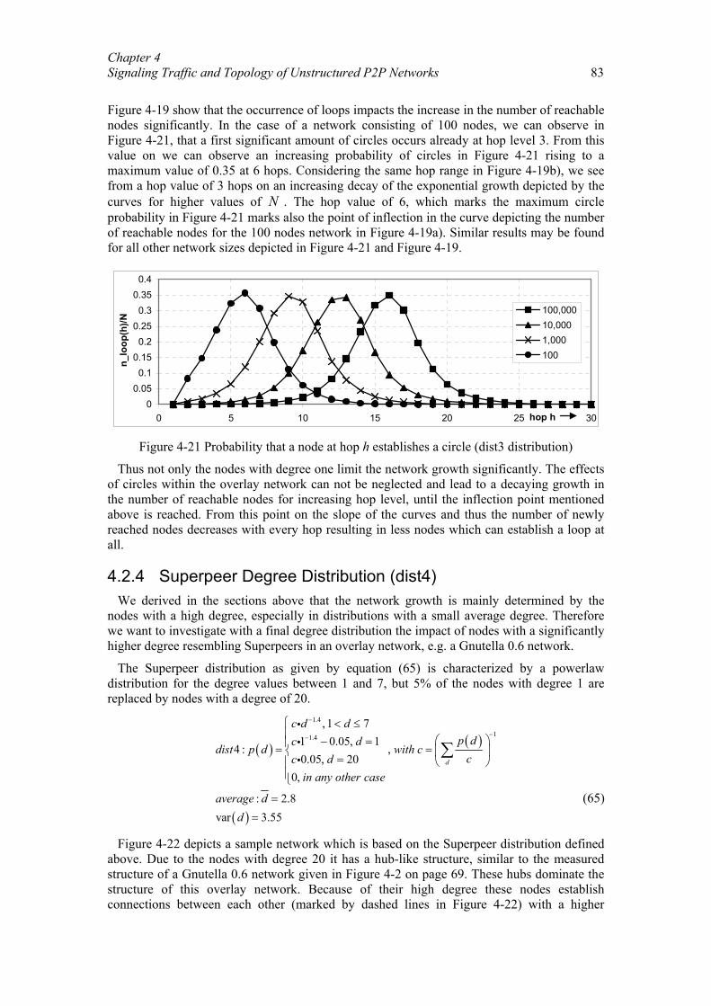
Chapter 4 Signaling Traffic and Topology of Unstructured P2P Networks 83
Figure 4-19 show that the occurrence of loops impacts the increase in the number of reachable nodes significantly. In the case of a network consisting of 100 nodes, we can observe in Figure 4-21, that a first significant amount of circles occurs already at hop level 3. From this value on we can observe an increasing probability of circles in Figure 4-21 rising to a maximum value of 0.35 at 6 hops. Considering the same hop range in Figure 4-19b), we see from a hop value of 3 hops on an increasing decay of the exponential growth depicted by the curves for higher values of N . The hop value of 6, which marks the maximum circle probability in Figure 4-21 marks also the point of inflection in the curve depicting the number of reachable nodes for the 100 nodes network in Figure 4-19a). Similar results may be found for all other network sizes depicted in Figure 4-21 and Figure 4-19.
00.050.1
0.150.2
0.250.3
0.350.4
0 5 10 15 20 25 30hop h
n_lo
op(h
)/N
100,00010,0001,000100
Figure 4-21 Probability that a node at hop h establishes a circle (dist3 distribution)
Thus not only the nodes with degree one limit the network growth significantly. The effects of circles within the overlay network can not be neglected and lead to a decaying growth in the number of reachable nodes for increasing hop level, until the inflection point mentioned above is reached. From this point on the slope of the curves and thus the number of newly reached nodes decreases with every hop resulting in less nodes which can establish a loop at all.
4.2.4 Superpeer Degree Distribution (dist4) We derived in the sections above that the network growth is mainly determined by the
nodes with a high degree, especially in distributions with a small average degree. Therefore we want to investigate with a final degree distribution the impact of nodes with a significantly higher degree resembling Superpeers in an overlay network, e.g. a Gnutella 0.6 network.
The Superpeer distribution as given by equation (65) is characterized by a powerlaw distribution for the degree values between 1 and 7, but 5% of the nodes with degree 1 are replaced by nodes with a degree of 20.
( ) ( )
( )
1.4
11.4
, 1 71 0.05, 1
4 : ,0.05, 20
0,
: 2.8var 3.55
d
c d dp dc d
dist p d with ccc d
in any other case
average dd
−
−−
< ≤ − == =
=
=
=
∑
iii
(65)
Figure 4-22 depicts a sample network which is based on the Superpeer distribution defined above. Due to the nodes with degree 20 it has a hub-like structure, similar to the measured structure of a Gnutella 0.6 network given in Figure 4-2 on page 69. These hubs dominate the structure of this overlay network. Because of their high degree these nodes establish connections between each other (marked by dashed lines in Figure 4-22) with a higher
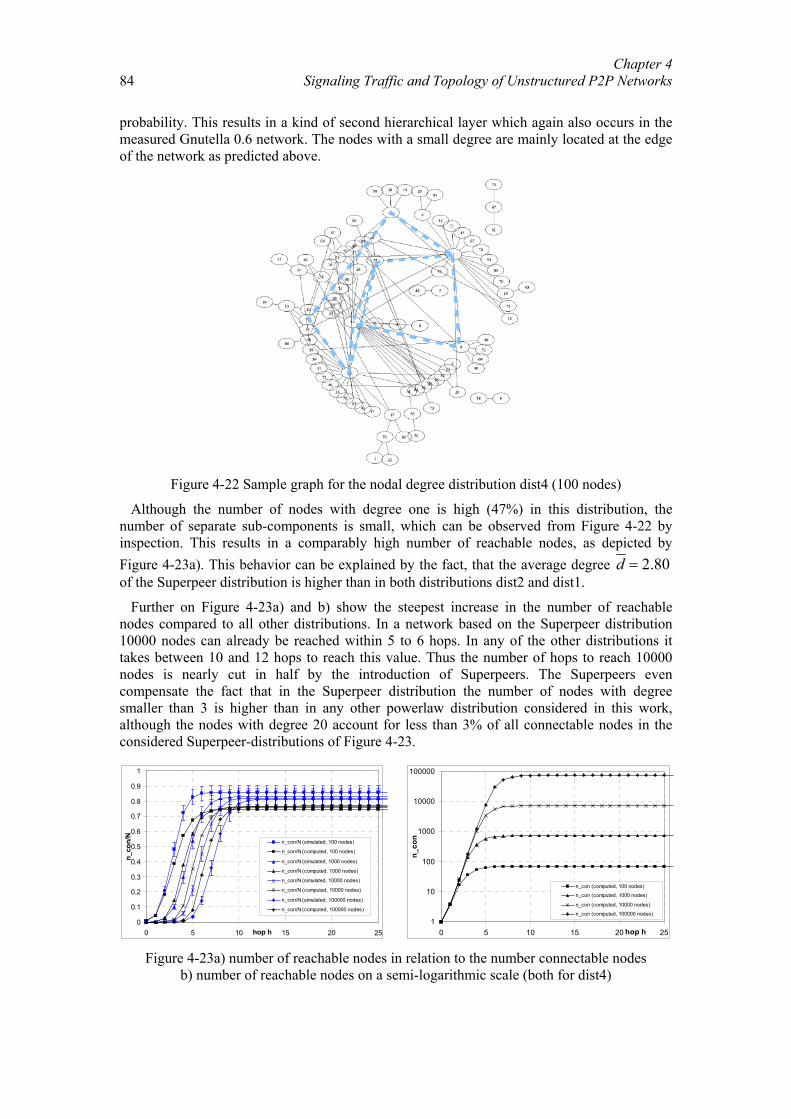
Chapter 4 Signaling Traffic and Topology of Unstructured P2P Networks
84
probability. This results in a kind of second hierarchical layer which again also occurs in the measured Gnutella 0.6 network. The nodes with a small degree are mainly located at the edge of the network as predicted above.
Figure 4-22 Sample graph for the nodal degree distribution dist4 (100 nodes)
Although the number of nodes with degree one is high (47%) in this distribution, the number of separate sub-components is small, which can be observed from Figure 4-22 by inspection. This results in a comparably high number of reachable nodes, as depicted by Figure 4-23a). This behavior can be explained by the fact, that the average degree 2.80d = of the Superpeer distribution is higher than in both distributions dist2 and dist1.
Further on Figure 4-23a) and b) show the steepest increase in the number of reachable nodes compared to all other distributions. In a network based on the Superpeer distribution 10000 nodes can already be reached within 5 to 6 hops. In any of the other distributions it takes between 10 and 12 hops to reach this value. Thus the number of hops to reach 10000 nodes is nearly cut in half by the introduction of Superpeers. The Superpeers even compensate the fact that in the Superpeer distribution the number of nodes with degree smaller than 3 is higher than in any other powerlaw distribution considered in this work, although the nodes with degree 20 account for less than 3% of all connectable nodes in the considered Superpeer-distributions of Figure 4-23.
Figure 4-23a) number of reachable nodes in relation to the number connectable nodes
b) number of reachable nodes on a semi-logarithmic scale (both for dist4)
0
0.1
0.2
0.3
0.4
0.5
0.6
0.7
0.8
0.9
1
0 5 10 15 20 25hop h
n_co
n/N
n_con/N (simulated, 100 nodes)
n_con/N (computed, 100 nodes)
n_con/N (simulated, 1000 nodes)
n_con/N (computed, 1000 nodes)
n_con/N (simulated, 10000 nodes)
n_con/N (computed, 10000 nodes)
n_con/N (simulated, 100000 nodes)
n_con/N (computed, 100000 nodes)
1
10
100
1000
10000
100000
0 5 10 15 20 25hop h
n_co
n
n_con (computed, 100 nodes)
n_con (computed, 1000 nodes)
n_con (computed, 10000 nodes)
n_con (computed, 100000 nodes)
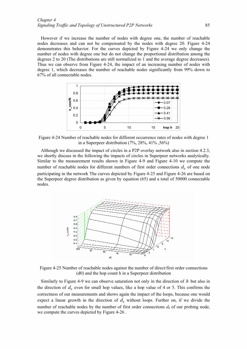
Chapter 4 Signaling Traffic and Topology of Unstructured P2P Networks 85
However if we increase the number of nodes with degree one, the number of reachable
nodes decreases and can not be compensated by the nodes with degree 20. Figure 4-24 demonstrates this behavior. For the curves depicted by Figure 4-24 we only change the number of nodes with degree one but do not change the proportional distribution among the degrees 2 to 20 (The distributions are still normalized to 1 and the average degree decreases). Thus we can observe from Figure 4-24, the impact of an increasing number of nodes with degree 1, which decreases the number of reachable nodes significantly from 99% down to 67% of all connectable nodes.
0
0.2
0.4
0.6
0.8
1
0 5 10 15 20hop h
n_co
n/N
0.070.280.410.56
Figure 4-24 Number of reachable nodes for different occurrence rates of nodes with degree 1
in a Superpeer distribution (7%, 28%, 41% ,56%)
Although we discussed the impact of circles in a P2P overlay network also in section 4.2.3, we shortly discuss in the following the impacts of circles in Superpeer networks analytically. Similar to the measurement results shown in Figure 4-9 and Figure 4-10 we compute the number of reachable nodes for different numbers of first order connections 0d of one node participating in the network The curves depicted by Figure 4-25 and Figure 4-26 are based on the Superpeer degree distribution as given by equation (65) and a total of 50000 connectable nodes.
Figure 4-25 Number of reachable nodes against the number of direct/first order connections
(d0) and the hop count h in a Superpeer distribution
Similarly to Figure 4-9 we can observe saturation not only in the direction of h but also in the direction of 0d even for small hop values, like a hop value of 4 or 5. This confirms the correctness of our measurements and shows again the impact of the loops, because one would expect a linear growth in the direction of 0d without loops. Further on, if we divide the number of reachable nodes by the number of first order connections d0 of our probing node, we compute the curves depicted by Figure 4-26 .
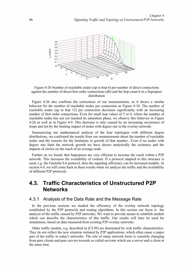
Chapter 4 Signaling Traffic and Topology of Unstructured P2P Networks
86
Figure 4-26 Number of reachable nodes (up to hop h) per number of direct connections
against the number of direct/first order connections (d0) and the hop count h in a Superpeer distribution
Figure 4-26 also confirms the correctness of our measurements, as it shows a similar behavior for the number of reachable nodes per connection as Figure 4-10. The number of reachable nodes (up to hop 12) per connection decreases significantly with an increasing number of first order connections. Even for small hop values of 5 or 6, where the number of reachable nodes has not yet reached its saturation phase, we observe this behavior in Figure 4-26 as well as in Figure 4-9. This decrease is only caused by an increasing occurrence of loops and not by the limiting impact of nodes with degree one in the overlay network.
Summarizing our mathematical analysis of the four topologies with different degree distributions, we confirmed the results from our measurements about the number of reachable nodes and the reasons for the limitation in growth of that number.. Even if no nodes with degree one limit the network growth we have shown analytically the existence and the impacts of circles on the reach of an average node.
Further on we found, that Superpeers are very efficient to increase the reach within a P2P network. This increases the availability of content. If a protocol adapted to this structure is used, e.g. the Gnutella 0.6 protocol, then the signaling efficiency can be increased notably. In section 4.4, we will come back to these results when we analyze the traffic and the availability of different P2P protocols.
4.3. Traffic Characteristics of Unstructured P2P Networks
4.3.1 Analysis of the Data Rate and the Message Rate In the previous sections we studied the efficiency of the overlay network topology
established by the P2P protocols and routing algorithms. In this section our focus is the analysis of the traffic caused by P2P networks. We want to provide means to establish models which can describe the characteristics of this traffic. Our results will later be used for simulations, based on data measured from existing P2P overlay networks.
Older traffic models, e.g. described in [CL99] are dominated by web traffic characteristics. They do not reflect the new situation initiated by P2P applications, which often cause a major part of the traffic in today's networks. The role of many network hosts is currently changing from pure clients and pure servers towards so called servents which are a server and a client at the same time.
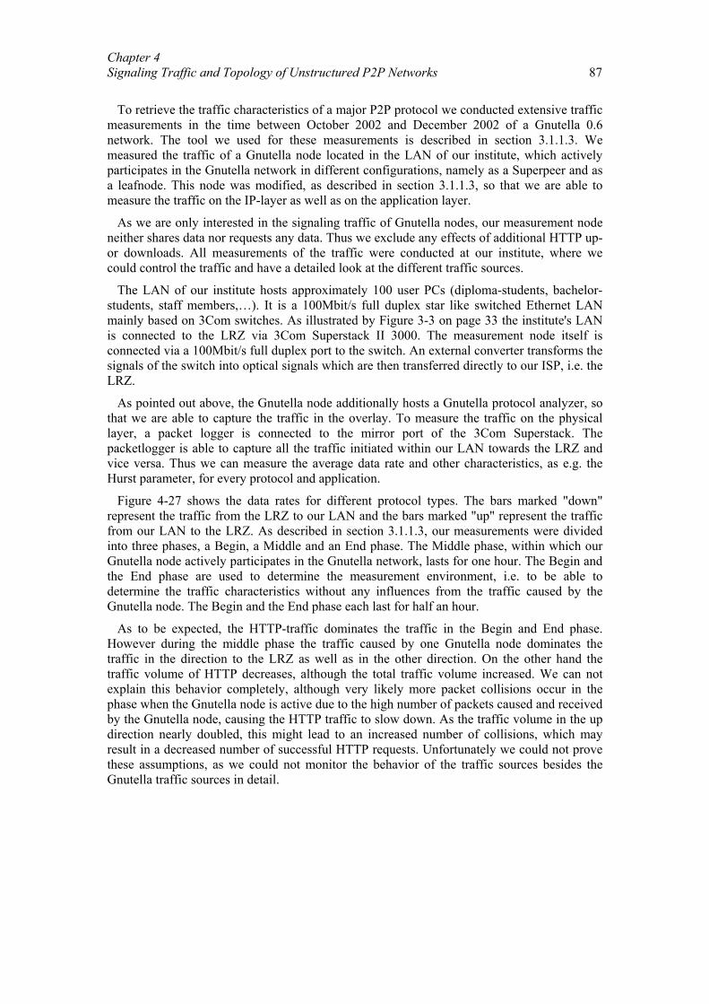
Chapter 4 Signaling Traffic and Topology of Unstructured P2P Networks 87
To retrieve the traffic characteristics of a major P2P protocol we conducted extensive traffic
measurements in the time between October 2002 and December 2002 of a Gnutella 0.6 network. The tool we used for these measurements is described in section 3.1.1.3. We measured the traffic of a Gnutella node located in the LAN of our institute, which actively participates in the Gnutella network in different configurations, namely as a Superpeer and as a leafnode. This node was modified, as described in section 3.1.1.3, so that we are able to measure the traffic on the IP-layer as well as on the application layer.
As we are only interested in the signaling traffic of Gnutella nodes, our measurement node neither shares data nor requests any data. Thus we exclude any effects of additional HTTP up- or downloads. All measurements of the traffic were conducted at our institute, where we could control the traffic and have a detailed look at the different traffic sources.
The LAN of our institute hosts approximately 100 user PCs (diploma-students, bachelor-students, staff members,…). It is a 100Mbit/s full duplex star like switched Ethernet LAN mainly based on 3Com switches. As illustrated by Figure 3-3 on page 33 the institute's LAN is connected to the LRZ via 3Com Superstack II 3000. The measurement node itself is connected via a 100Mbit/s full duplex port to the switch. An external converter transforms the signals of the switch into optical signals which are then transferred directly to our ISP, i.e. the LRZ.
As pointed out above, the Gnutella node additionally hosts a Gnutella protocol analyzer, so that we are able to capture the traffic in the overlay. To measure the traffic on the physical layer, a packet logger is connected to the mirror port of the 3Com Superstack. The packetlogger is able to capture all the traffic initiated within our LAN towards the LRZ and vice versa. Thus we can measure the average data rate and other characteristics, as e.g. the Hurst parameter, for every protocol and application.
Figure 4-27 shows the data rates for different protocol types. The bars marked "down" represent the traffic from the LRZ to our LAN and the bars marked "up" represent the traffic from our LAN to the LRZ. As described in section 3.1.1.3, our measurements were divided into three phases, a Begin, a Middle and an End phase. The Middle phase, within which our Gnutella node actively participates in the Gnutella network, lasts for one hour. The Begin and the End phase are used to determine the measurement environment, i.e. to be able to determine the traffic characteristics without any influences from the traffic caused by the Gnutella node. The Begin and the End phase each last for half an hour.
As to be expected, the HTTP-traffic dominates the traffic in the Begin and End phase. However during the middle phase the traffic caused by one Gnutella node dominates the traffic in the direction to the LRZ as well as in the other direction. On the other hand the traffic volume of HTTP decreases, although the total traffic volume increased. We can not explain this behavior completely, although very likely more packet collisions occur in the phase when the Gnutella node is active due to the high number of packets caused and received by the Gnutella node, causing the HTTP traffic to slow down. As the traffic volume in the up direction nearly doubled, this might lead to an increased number of collisions, which may result in a decreased number of successful HTTP requests. Unfortunately we could not prove these assumptions, as we could not monitor the behavior of the traffic sources besides the Gnutella traffic sources in detail.
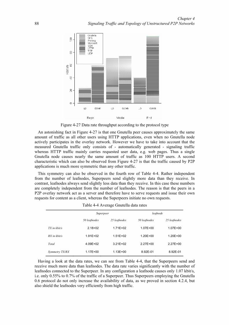
Chapter 4 Signaling Traffic and Topology of Unstructured P2P Networks
88
Figure 4-27 Data rate throughput according to the protocol type
An astonishing fact in Figure 4-27 is that one Gnutella peer causes approximately the same amount of traffic as all other users using HTTP applications, even when no Gnutella node actively participates in the overlay network. However we have to take into account that the measured Gnutella traffic only consists of - automatically generated - signaling traffic whereas HTTP traffic mainly carries requested user data, e.g. web pages. Thus a single Gnutella node causes nearly the same amount of traffic as 100 HTTP users. A second characteristic which can also be observed from Figure 4-27 is that the traffic caused by P2P applications is much more symmetric than any other traffic.
This symmetry can also be observed in the fourth row of Table 4-4. Rather independent from the number of leafnodes, Superpeers send slightly more data than they receive. In contrast, leafnodes always send slightly less data than they receive. In this case these numbers are completely independent from the number of leafnodes. The reason is that the peers in a P2P overlay network act as a server and therefore have to serve requests and issue their own requests for content as a client, whereas the Superpeers initiate no own requests.
Table 4-4 Average Gnutella data rates
Superpeer leafnode
50 leafnodes 25 leafnodes 50 leafnodes 25 leafnodes
TX in kbit/s 2.18+02 1.71E+02 1.07E+00 1.07E+00
RX in kbit/s 1.91E+02 1.51E+02 1.20E+00 1.20E+00
Total 4.09E+02 3.21E+02 2.27E+00 2.27E+00
Symmetry TX/RX 1.17E+00 1.13E+00 8.92E-01 8.92E-01
Having a look at the data rates, we can see from Table 4-4, that the Superpeers send and receive much more data than leafnodes. The data rate varies significantly with the number of leafnodes connected to the Superpeer. In any configuration a leafnode causes only 1.07 kbit/s, i.e. only 0.55% to 0.7% of the traffic of a Superpeer. Thus Superpeers employing the Gnutella 0.6 protocol do not only increase the availability of data, as we proved in section 4.2.4, but also shield the leafnodes very efficiently from high traffic.
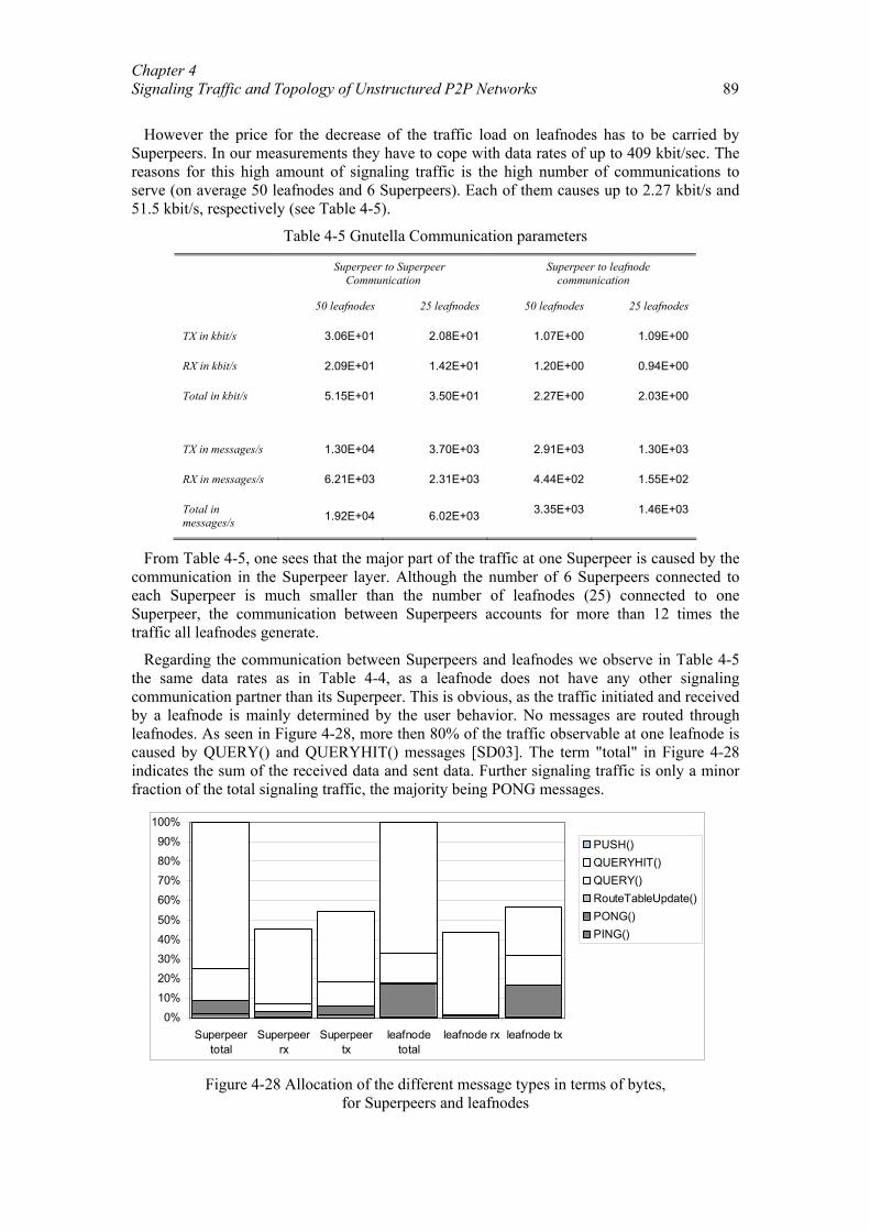
Chapter 4 Signaling Traffic and Topology of Unstructured P2P Networks 89
However the price for the decrease of the traffic load on leafnodes has to be carried by
Superpeers. In our measurements they have to cope with data rates of up to 409 kbit/sec. The reasons for this high amount of signaling traffic is the high number of communications to serve (on average 50 leafnodes and 6 Superpeers). Each of them causes up to 2.27 kbit/s and 51.5 kbit/s, respectively (see Table 4-5).
Table 4-5 Gnutella Communication parameters
Superpeer to Superpeer
Communication Superpeer to leafnode
communication
50 leafnodes 25 leafnodes 50 leafnodes 25 leafnodes
TX in kbit/s 3.06E+01 2.08E+01 1.07E+00 1.09E+00
RX in kbit/s 2.09E+01 1.42E+01 1.20E+00 0.94E+00
Total in kbit/s 5.15E+01 3.50E+01 2.27E+00 2.03E+00
TX in messages/s 1.30E+04 3.70E+03 2.91E+03 1.30E+03
RX in messages/s 6.21E+03 2.31E+03 4.44E+02 1.55E+02
Total in messages/s 1.92E+04 6.02E+03 3.35E+03 1.46E+03
From Table 4-5, one sees that the major part of the traffic at one Superpeer is caused by the communication in the Superpeer layer. Although the number of 6 Superpeers connected to each Superpeer is much smaller than the number of leafnodes (25) connected to one Superpeer, the communication between Superpeers accounts for more than 12 times the traffic all leafnodes generate.
Regarding the communication between Superpeers and leafnodes we observe in Table 4-5 the same data rates as in Table 4-4, as a leafnode does not have any other signaling communication partner than its Superpeer. This is obvious, as the traffic initiated and received by a leafnode is mainly determined by the user behavior. No messages are routed through leafnodes. As seen in Figure 4-28, more then 80% of the traffic observable at one leafnode is caused by QUERY() and QUERYHIT() messages [SD03]. The term "total" in Figure 4-28 indicates the sum of the received data and sent data. Further signaling traffic is only a minor fraction of the total signaling traffic, the majority being PONG messages.
0%
10%
20%
30%
40%
50%
60%
70%
80%
90%
100%
Superpeertotal
Superpeerrx
Superpeertx
leafnodetotal
leafnode rx leafnode tx
PUSH()QUERYHIT()QUERY()RouteTableUpdate()PONG()PING()
Figure 4-28 Allocation of the different message types in terms of bytes,
for Superpeers and leafnodes
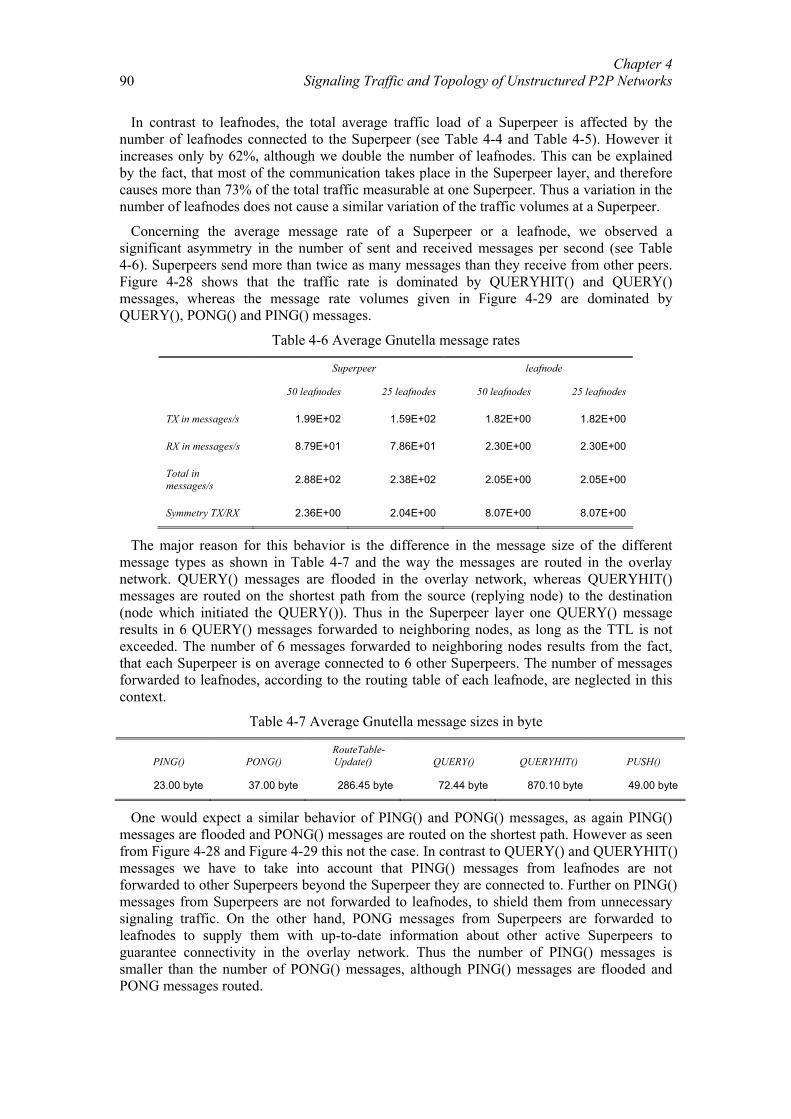
Chapter 4 Signaling Traffic and Topology of Unstructured P2P Networks
90
In contrast to leafnodes, the total average traffic load of a Superpeer is affected by the number of leafnodes connected to the Superpeer (see Table 4-4 and Table 4-5). However it increases only by 62%, although we double the number of leafnodes. This can be explained by the fact, that most of the communication takes place in the Superpeer layer, and therefore causes more than 73% of the total traffic measurable at one Superpeer. Thus a variation in the number of leafnodes does not cause a similar variation of the traffic volumes at a Superpeer.
Concerning the average message rate of a Superpeer or a leafnode, we observed a significant asymmetry in the number of sent and received messages per second (see Table 4-6). Superpeers send more than twice as many messages than they receive from other peers. Figure 4-28 shows that the traffic rate is dominated by QUERYHIT() and QUERY() messages, whereas the message rate volumes given in Figure 4-29 are dominated by QUERY(), PONG() and PING() messages.
Table 4-6 Average Gnutella message rates
Superpeer leafnode
50 leafnodes 25 leafnodes 50 leafnodes 25 leafnodes
TX in messages/s 1.99E+02 1.59E+02 1.82E+00 1.82E+00
RX in messages/s 8.79E+01 7.86E+01 2.30E+00 2.30E+00
Total in messages/s 2.88E+02 2.38E+02 2.05E+00 2.05E+00
Symmetry TX/RX 2.36E+00 2.04E+00 8.07E+00 8.07E+00
The major reason for this behavior is the difference in the message size of the different message types as shown in Table 4-7 and the way the messages are routed in the overlay network. QUERY() messages are flooded in the overlay network, whereas QUERYHIT() messages are routed on the shortest path from the source (replying node) to the destination (node which initiated the QUERY()). Thus in the Superpeer layer one QUERY() message results in 6 QUERY() messages forwarded to neighboring nodes, as long as the TTL is not exceeded. The number of 6 messages forwarded to neighboring nodes results from the fact, that each Superpeer is on average connected to 6 other Superpeers. The number of messages forwarded to leafnodes, according to the routing table of each leafnode, are neglected in this context.
Table 4-7 Average Gnutella message sizes in byte
PING() PONG() RouteTable-Update() QUERY() QUERYHIT() PUSH()
23.00 byte 37.00 byte 286.45 byte 72.44 byte 870.10 byte 49.00 byte
One would expect a similar behavior of PING() and PONG() messages, as again PING() messages are flooded and PONG() messages are routed on the shortest path. However as seen from Figure 4-28 and Figure 4-29 this not the case. In contrast to QUERY() and QUERYHIT() messages we have to take into account that PING() messages from leafnodes are not forwarded to other Superpeers beyond the Superpeer they are connected to. Further on PING() messages from Superpeers are not forwarded to leafnodes, to shield them from unnecessary signaling traffic. On the other hand, PONG messages from Superpeers are forwarded to leafnodes to supply them with up-to-date information about other active Superpeers to guarantee connectivity in the overlay network. Thus the number of PING() messages is smaller than the number of PONG() messages, although PING() messages are flooded and PONG messages routed.
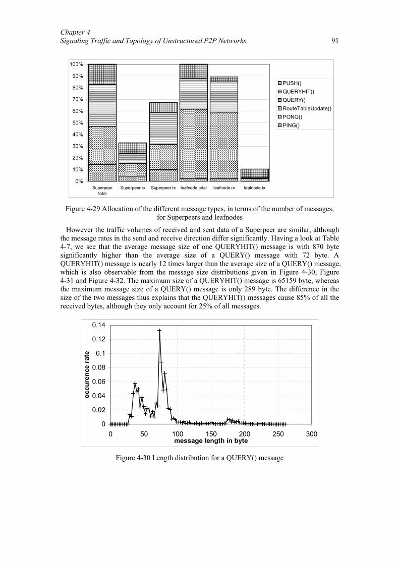
Chapter 4 Signaling Traffic and Topology of Unstructured P2P Networks 91
0%
10%
20%
30%
40%
50%
60%
70%
80%
90%
100%
Superpeertotal
Superpeer rx Superpeer tx leafnode total leafnode rx leafnode tx
PUSH()QUERYHIT()QUERY()RouteTableUpdate()PONG()PING()
Figure 4-29 Allocation of the different message types, in terms of the number of messages,
for Superpeers and leafnodes
However the traffic volumes of received and sent data of a Superpeer are similar, although the message rates in the send and receive direction differ significantly. Having a look at Table 4-7, we see that the average message size of one QUERYHIT() message is with 870 byte significantly higher than the average size of a QUERY() message with 72 byte. A QUERYHIT() message is nearly 12 times larger than the average size of a QUERY() message, which is also observable from the message size distributions given in Figure 4-30, Figure 4-31 and Figure 4-32. The maximum size of a QUERYHIT() message is 65159 byte, whereas the maximum message size of a QUERY() message is only 289 byte. The difference in the size of the two messages thus explains that the QUERYHIT() messages cause 85% of all the received bytes, although they only account for 25% of all messages.
0
0.02
0.04
0.06
0.08
0.1
0.12
0.14
0 50 100 150 200 250 300message length in byte
occu
renc
e ra
te
Figure 4-30 Length distribution for a QUERY() message
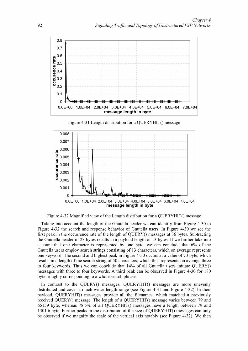
Chapter 4 Signaling Traffic and Topology of Unstructured P2P Networks
92
0
0.1
0.2
0.3
0.4
0.5
0.6
0.7
0.8
0.0E+00 1.0E+04 2.0E+04 3.0E+04 4.0E+04 5.0E+04 6.0E+04 7.0E+04message length in byte
occu
renc
e ra
te
Figure 4-31 Length distribution for a QUERYHIT() message
0
0.001
0.002
0.003
0.004
0.005
0.006
0.007
0.008
0.0E+00 1.0E+04 2.0E+04 3.0E+04 4.0E+04 5.0E+04 6.0E+04 7.0E+04message length in byte
occu
renc
e ra
te
Figure 4-32 Magnified view of the Length distribution for a QUERYHIT() message
Taking into account the length of the Gnutella header we can identify from Figure 4-30 to Figure 4-32 the search and response behavior of Gnutella users. In Figure 4-30 we see the first peak in the occurrence rate of the length of QUERY() messages at 36 bytes. Subtracting the Gnutella header of 23 bytes results in a payload length of 13 bytes. If we further take into account that one character is represented by one byte, we can conclude that 6% of the Gnutella users employ search strings consisting of 13 characters, which on average represents one keyword. The second and highest peak in Figure 4-30 occurs at a value of 73 byte, which results in a length of the search string of 50 characters, which thus represents on average three to four keywords. Thus we can conclude that 14% of all Gnutella users initiate QUERY() messages with three to four keywords. A third peak can be observed in Figure 4-30 for 180 byte, roughly corresponding to a whole search phrase.
In contrast to the QUERY() messages, QUERYHIT() messages are more unevenly distributed and cover a much wider length range (see Figure 4-31 and Figure 4-32). In their payload, QUERYHIT() messages provide all the filenames, which matched a previously received QUERY() message. The length of a QUERYHIT() message varies between 79 and 65159 byte, whereas 78.5% of all QUERYHIT() messages have a length between 79 and 1301.6 byte. Further peaks in the distribution of the size of QUERYHIT() messages can only be observed if we magnify the scale of the vertical axis notably (see Figure 4-32). We then
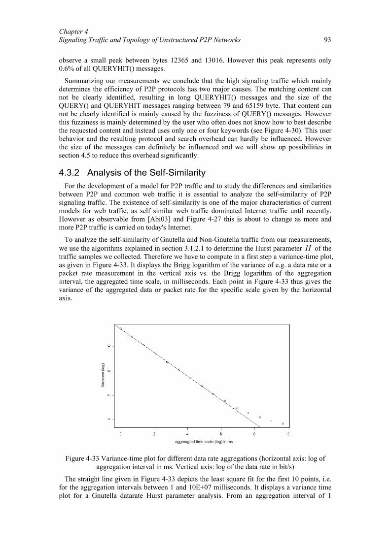
Chapter 4 Signaling Traffic and Topology of Unstructured P2P Networks 93
observe a small peak between bytes 12365 and 13016. However this peak represents only 0.6% of all QUERYHIT() messages.
Summarizing our measurements we conclude that the high signaling traffic which mainly determines the efficiency of P2P protocols has two major causes. The matching content can not be clearly identified, resulting in long QUERYHIT() messages and the size of the QUERY() and QUERYHIT messages ranging between 79 and 65159 byte. That content can not be clearly identified is mainly caused by the fuzziness of QUERY() messages. However this fuzziness is mainly determined by the user who often does not know how to best describe the requested content and instead uses only one or four keywords (see Figure 4-30). This user behavior and the resulting protocol and search overhead can hardly be influenced. However the size of the messages can definitely be influenced and we will show up possibilities in section 4.5 to reduce this overhead significantly.
4.3.2 Analysis of the Self-Similarity For the development of a model for P2P traffic and to study the differences and similarities
between P2P and common web traffic it is essential to analyze the self-similarity of P2P signaling traffic. The existence of self-similarity is one of the major characteristics of current models for web traffic, as self similar web traffic dominated Internet traffic until recently. However as observable from [Abi03] and Figure 4-27 this is about to change as more and more P2P traffic is carried on today's Internet.
To analyze the self-similarity of Gnutella and Non-Gnutella traffic from our measurements, we use the algorithms explained in section 3.1.2.1 to determine the Hurst parameter H of the traffic samples we collected. Therefore we have to compute in a first step a variance-time plot, as given in Figure 4-33. It displays the Brigg logarithm of the variance of e.g. a data rate or a packet rate measurement in the vertical axis vs. the Brigg logarithm of the aggregation interval, the aggregated time scale, in milliseconds. Each point in Figure 4-33 thus gives the variance of the aggregated data or packet rate for the specific scale given by the horizontal axis.
aggreagted time scale (log) in ms
Varia
nce
(log)
Figure 4-33 Variance-time plot for different data rate aggregations (horizontal axis: log of
aggregation interval in ms. Vertical axis: log of the data rate in bit/s)
The straight line given in Figure 4-33 depicts the least square fit for the first 10 points, i.e. for the aggregation intervals between 1 and 10E+07 milliseconds. It displays a variance time plot for a Gnutella datarate Hurst parameter analysis. From an aggregation interval of 1
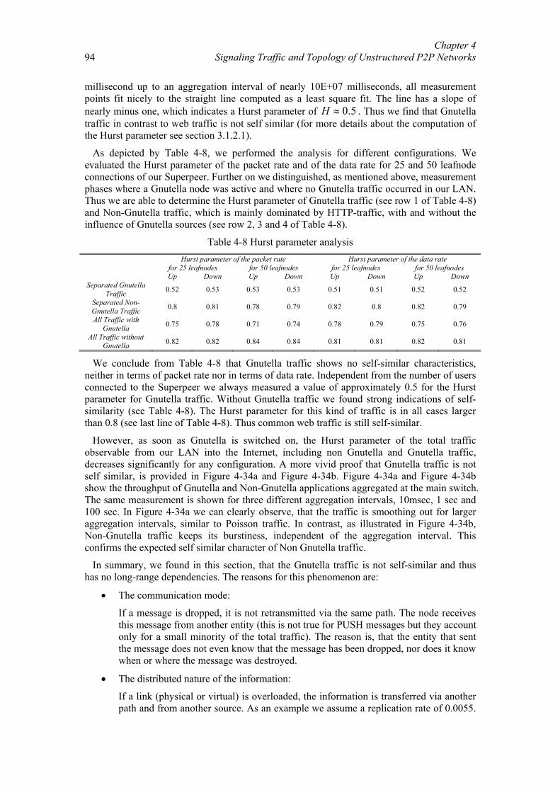
Chapter 4 Signaling Traffic and Topology of Unstructured P2P Networks
94
millisecond up to an aggregation interval of nearly 10E+07 milliseconds, all measurement points fit nicely to the straight line computed as a least square fit. The line has a slope of nearly minus one, which indicates a Hurst parameter of 0.5H ≈ . Thus we find that Gnutella traffic in contrast to web traffic is not self similar (for more details about the computation of the Hurst parameter see section 3.1.2.1).
As depicted by Table 4-8, we performed the analysis for different configurations. We evaluated the Hurst parameter of the packet rate and of the data rate for 25 and 50 leafnode connections of our Superpeer. Further on we distinguished, as mentioned above, measurement phases where a Gnutella node was active and where no Gnutella traffic occurred in our LAN. Thus we are able to determine the Hurst parameter of Gnutella traffic (see row 1 of Table 4-8) and Non-Gnutella traffic, which is mainly dominated by HTTP-traffic, with and without the influence of Gnutella sources (see row 2, 3 and 4 of Table 4-8).
Table 4-8 Hurst parameter analysis Hurst parameter of the packet rate Hurst parameter of the data rate for 25 leafnodes for 50 leafnodes for 25 leafnodes for 50 leafnodes Up Down Up Down Up Down Up Down
Separated Gnutella Traffic 0.52 0.53 0.53 0.53 0.51 0.51 0.52 0.52
Separated Non-Gnutella Traffic 0.8 0.81 0.78 0.79 0.82 0.8 0.82 0.79
All Traffic with Gnutella 0.75 0.78 0.71 0.74 0.78 0.79 0.75 0.76
All Traffic without Gnutella 0.82 0.82 0.84 0.84 0.81 0.81 0.82 0.81
We conclude from Table 4-8 that Gnutella traffic shows no self-similar characteristics, neither in terms of packet rate nor in terms of data rate. Independent from the number of users connected to the Superpeer we always measured a value of approximately 0.5 for the Hurst parameter for Gnutella traffic. Without Gnutella traffic we found strong indications of self-similarity (see Table 4-8). The Hurst parameter for this kind of traffic is in all cases larger than 0.8 (see last line of Table 4-8). Thus common web traffic is still self-similar.
However, as soon as Gnutella is switched on, the Hurst parameter of the total traffic observable from our LAN into the Internet, including non Gnutella and Gnutella traffic, decreases significantly for any configuration. A more vivid proof that Gnutella traffic is not self similar, is provided in Figure 4-34a and Figure 4-34b. Figure 4-34a and Figure 4-34b show the throughput of Gnutella and Non-Gnutella applications aggregated at the main switch. The same measurement is shown for three different aggregation intervals, 10msec, 1 sec and 100 sec. In Figure 4-34a we can clearly observe, that the traffic is smoothing out for larger aggregation intervals, similar to Poisson traffic. In contrast, as illustrated in Figure 4-34b, Non-Gnutella traffic keeps its burstiness, independent of the aggregation interval. This confirms the expected self similar character of Non Gnutella traffic.
In summary, we found in this section, that the Gnutella traffic is not self-similar and thus has no long-range dependencies. The reasons for this phenomenon are:
• The communication mode:
If a message is dropped, it is not retransmitted via the same path. The node receives this message from another entity (this is not true for PUSH messages but they account only for a small minority of the total traffic). The reason is, that the entity that sent the message does not even know that the message has been dropped, nor does it know when or where the message was destroyed.
• The distributed nature of the information:
If a link (physical or virtual) is overloaded, the information is transferred via another path and from another source. As an example we assume a replication rate of 0.0055.
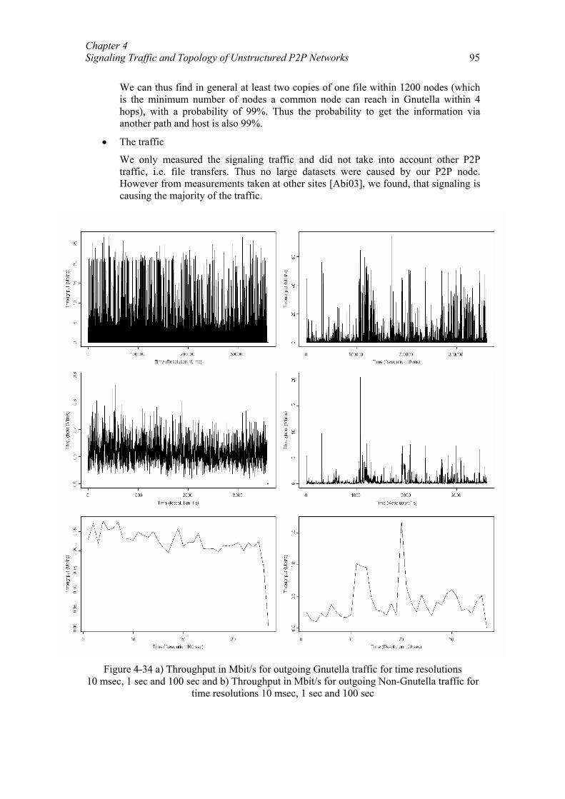
Chapter 4 Signaling Traffic and Topology of Unstructured P2P Networks 95
We can thus find in general at least two copies of one file within 1200 nodes (which is the minimum number of nodes a common node can reach in Gnutella within 4 hops), with a probability of 99%. Thus the probability to get the information via another path and host is also 99%.
• The traffic
We only measured the signaling traffic and did not take into account other P2P traffic, i.e. file transfers. Thus no large datasets were caused by our P2P node. However from measurements taken at other sites [Abi03], we found, that signaling is causing the majority of the traffic.
Figure 4-34 a) Throughput in Mbit/s for outgoing Gnutella traffic for time resolutions
10 msec, 1 sec and 100 sec and b) Throughput in Mbit/s for outgoing Non-Gnutella traffic for time resolutions 10 msec, 1 sec and 100 sec
Chapter 4 Signaling Traffic and Topology of Unstructured P2P Networks
96
4.4. Graph Theoretic Analysis of the Traffic In this section we concentrate on the potential to reduce the signaling traffic. We therefore
evaluate the signaling efficiency and the content availability of the Gnutella protocol analytically, based on the mathematical approach described in section 3.2.2. Thus we are able to analyze the potential of reducing the signaling traffic without extensive simulations. Further on with this analytical approach we can determine the optimal number of connections and the optimal TTL value, which provides sufficient availability while keeping the signaling traffic as low as possible. However we first have to model additionally the nodes' behavior and the P2P protocol, i.e. the Gnutella 0.4 protocol itself.
Based on the measurements described in section 4.3 we assume for the behavior of the nodes in the P2P network an average uptime of 900 seconds, an average of 100 files shared by each peer and two downloads per session. Further on we assume an average replication rate of the data in the network of _ 0.55%r rep = [ACKS03]. Replication rate in this context means, that a certain object is available with a probability of 0.55% on any given node of the P2P network. Our analysis is restricted to the application layer traffic. Thus we do not take into account any additional header, e.g. TCP/IP headers, or aggregation effects of the transport layer. We also assume the same transport layer for all investigated P2P scenarios.
To analyze the content availability in different networks, we first have to compute the probability, that certain content is available in the network. The availability (p_av) of one specific content depends on the replication rate and on the cumulative number zh of nodes reached until hop h.
( )_ 1 1 _ hzcontent availability p av r rep = = − − (66)
Applying this equation to analyze the content availability in a Gnutella topology, which can be modeled with a truncated powerlaw distribution [JAB01] as used above (see equation (62) in section 4.2), reveals that at least 7 hops are necessary to guarantee a satisfactory content availability. The solid curves in Figure 4-35 depict the content availability in a Gnutella 0.4 network for different network sizes.
The results of the content availability analysis in a hub-like network, i.e. a Gnutella 0.6 network, are given in Figure 4-35 by the dashed lines. Here we see the major advantage of hybrid P2P networks. By introducing Superpeers, even if only 3% of all nodes in the network are Superpeers, the content availability can be significantly improved. As depicted by Figure 4-35, we only need 4 hops instead of 7 hops to achieve a content availability of more than 90% with 10000 nodes. Thus content in a hybrid P2P network can be found significantly faster and also more reliably, as the search request and its corresponding response must be routed across less hops in the overlay network.
Concerning the analytical traffic analysis, we analyze the Gnutella 0.4 protocol, with a general Gnutella header length of 23 byte, zero byte for the PING message, 15 byte for the PONG message, 80 byte for the QUERY message and 200 byte for the QUERY-HIT message. As Gnutella routing is based mostly on flooding, we additionally have to take into account loops in the network, on which a message may be transmitted twice via the same link. Therefore we assume a loop probability of 0.0064 (see section 3.1 or [SH03]) that a node is part of a loop and thus receives one message twice.
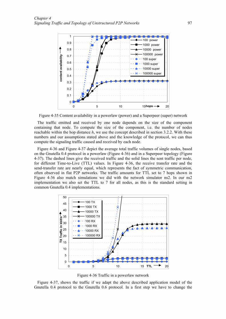
Chapter 4 Signaling Traffic and Topology of Unstructured P2P Networks 97
0
0.1
0.2
0.3
0.4
0.5
0.6
0.7
0.8
0.9
1
0 5 10 15 20
cont
ent a
vaila
bilit
y
100 power1000 power10000 power100000 power100 super1000 super10000 super100000 super
hops
Figure 4-35 Content availability in a powerlaw (power) and a Superpeer (super) network
The traffic emitted and received by one node depends on the size of the component containing that node. To compute the size of the component, i.e. the number of nodes reachable within the hop distance h, we use the concept described in section 3.2.2. With these numbers and our assumptions stated above and the knowledge of the protocol, we can thus compute the signaling traffic caused and received by each node.
Figure 4-36 and Figure 4-37 depict the average total traffic volumes of single nodes, based on the Gnutella 0.4 protocol in a powerlaw (Figure 4-36) and in a Superpeer topology (Figure 4-37). The dashed lines give the received traffic and the solid lines the sent traffic per node, for different Time-to-Live (TTL) values. In Figure 4-36, the receive transfer rate and the send-transfer rate are nearly equal, which represents the fact of symmetric communication, often observed in flat P2P networks. The traffic amounts for TTL set to 7 hops shown in Figure 4-36 also match simulations we did with the network simulator ns2. In our ns2 implementation we also set the TTL to 7 for all nodes, as this is the standard setting in common Gnutella 0.4 implementations.
0
5
10
15
20
25
30
35
40
45
50
0 5 10 15 20
TX T
raffi
c in
kbi
t/s
100 TX1000 TX10000 TX100000 TX100 RX1000 RX10000 RX100000 RX
TTL
Figure 4-36 Traffic in a powerlaw network
Figure 4-37, shows the traffic if we adapt the above described application model of the Gnutella 0.4 protocol to the Gnutella 0.6 protocol. In a first step we have to change the
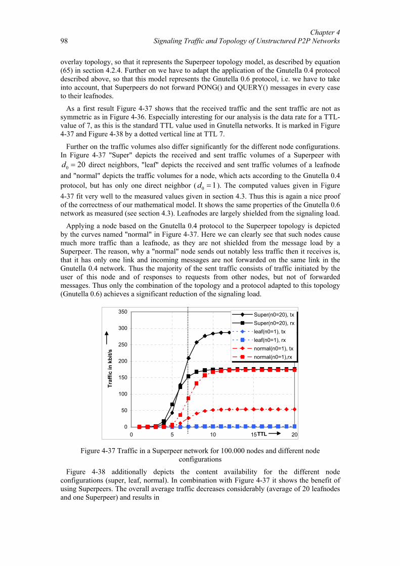
Chapter 4 Signaling Traffic and Topology of Unstructured P2P Networks
98
overlay topology, so that it represents the Superpeer topology model, as described by equation (65) in section 4.2.4. Further on we have to adapt the application of the Gnutella 0.4 protocol described above, so that this model represents the Gnutella 0.6 protocol, i.e. we have to take into account, that Superpeers do not forward PONG() and QUERY() messages in every case to their leafnodes.
As a first result Figure 4-37 shows that the received traffic and the sent traffic are not as symmetric as in Figure 4-36. Especially interesting for our analysis is the data rate for a TTL-value of 7, as this is the standard TTL value used in Gnutella networks. It is marked in Figure 4-37 and Figure 4-38 by a dotted vertical line at TTL 7.
Further on the traffic volumes also differ significantly for the different node configurations. In Figure 4-37 "Super" depicts the received and sent traffic volumes of a Superpeer with
0 20d = direct neighbors, "leaf" depicts the received and sent traffic volumes of a leafnode and "normal" depicts the traffic volumes for a node, which acts according to the Gnutella 0.4 protocol, but has only one direct neighbor ( 0 1d = ). The computed values given in Figure 4-37 fit very well to the measured values given in section 4.3. Thus this is again a nice proof of the correctness of our mathematical model. It shows the same properties of the Gnutella 0.6 network as measured (see section 4.3). Leafnodes are largely shielded from the signaling load.
Applying a node based on the Gnutella 0.4 protocol to the Superpeer topology is depicted by the curves named "normal" in Figure 4-37. Here we can clearly see that such nodes cause much more traffic than a leafnode, as they are not shielded from the message load by a Superpeer. The reason, why a "normal" node sends out notably less traffic then it receives is, that it has only one link and incoming messages are not forwarded on the same link in the Gnutella 0.4 network. Thus the majority of the sent traffic consists of traffic initiated by the user of this node and of responses to requests from other nodes, but not of forwarded messages. Thus only the combination of the topology and a protocol adapted to this topology (Gnutella 0.6) achieves a significant reduction of the signaling load.
0
50
100
150
200
250
300
350
0 5 10 15 20
Traf
fic in
kbi
t/s
Super(n0=20), txSuper(n0=20), rxleaf(n0=1), txleaf(n0=1), rxnormal(n0=1), txnormal(n0=1),rx
TTL
Figure 4-37 Traffic in a Superpeer network for 100.000 nodes and different node configurations
Figure 4-38 additionally depicts the content availability for the different node configurations (super, leaf, normal). In combination with Figure 4-37 it shows the benefit of using Superpeers. The overall average traffic decreases considerably (average of 20 leafnodes and one Superpeer) and results in
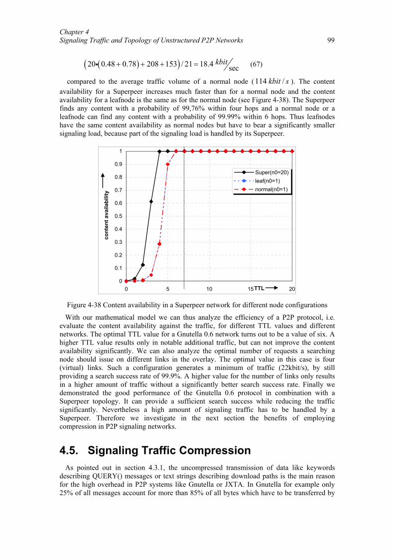
Chapter 4 Signaling Traffic and Topology of Unstructured P2P Networks 99
( )( )20 0.48 0.78 208 153 / 21 18.4 sec
kbit+ + + =i (67)
compared to the average traffic volume of a normal node (114 /kbit s ). The content availability for a Superpeer increases much faster than for a normal node and the content availability for a leafnode is the same as for the normal node (see Figure 4-38). The Superpeer finds any content with a probability of 99,76% within four hops and a normal node or a leafnode can find any content with a probability of 99.99% within 6 hops. Thus leafnodes have the same content availability as normal nodes but have to bear a significantly smaller signaling load, because part of the signaling load is handled by its Superpeer.
0
0.1
0.2
0.3
0.4
0.5
0.6
0.7
0.8
0.9
1
0 5 10 15 20
cont
ent a
vaila
bilit
y
Super(n0=20)leaf(n0=1)normal(n0=1)
TTL
Figure 4-38 Content availability in a Superpeer network for different node configurations
With our mathematical model we can thus analyze the efficiency of a P2P protocol, i.e. evaluate the content availability against the traffic, for different TTL values and different networks. The optimal TTL value for a Gnutella 0.6 network turns out to be a value of six. A higher TTL value results only in notable additional traffic, but can not improve the content availability significantly. We can also analyze the optimal number of requests a searching node should issue on different links in the overlay. The optimal value in this case is four (virtual) links. Such a configuration generates a minimum of traffic (22kbit/s), by still providing a search success rate of 99.9%. A higher value for the number of links only results in a higher amount of traffic without a significantly better search success rate. Finally we demonstrated the good performance of the Gnutella 0.6 protocol in combination with a Superpeer topology. It can provide a sufficient search success while reducing the traffic significantly. Nevertheless a high amount of signaling traffic has to be handled by a Superpeer. Therefore we investigate in the next section the benefits of employing compression in P2P signaling networks.
4.5. Signaling Traffic Compression As pointed out in section 4.3.1, the uncompressed transmission of data like keywords
describing QUERY() messages or text strings describing download paths is the main reason for the high overhead in P2P systems like Gnutella or JXTA. In Gnutella for example only 25% of all messages account for more than 85% of all bytes which have to be transferred by
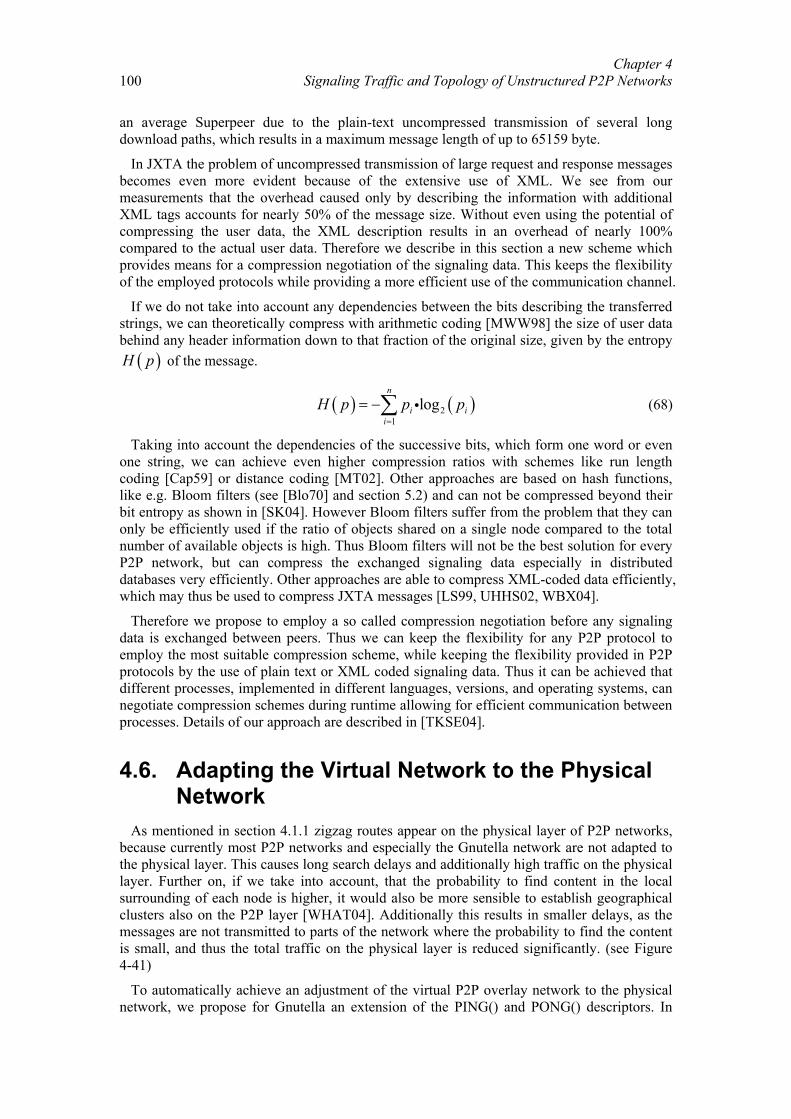
Chapter 4 Signaling Traffic and Topology of Unstructured P2P Networks
100
an average Superpeer due to the plain-text uncompressed transmission of several long download paths, which results in a maximum message length of up to 65159 byte.
In JXTA the problem of uncompressed transmission of large request and response messages becomes even more evident because of the extensive use of XML. We see from our measurements that the overhead caused only by describing the information with additional XML tags accounts for nearly 50% of the message size. Without even using the potential of compressing the user data, the XML description results in an overhead of nearly 100% compared to the actual user data. Therefore we describe in this section a new scheme which provides means for a compression negotiation of the signaling data. This keeps the flexibility of the employed protocols while providing a more efficient use of the communication channel.
If we do not take into account any dependencies between the bits describing the transferred strings, we can theoretically compress with arithmetic coding [MWW98] the size of user data behind any header information down to that fraction of the original size, given by the entropy
( )H p of the message.
( ) ( )21
logn
i ii
H p p p=
= −∑ i (68)
Taking into account the dependencies of the successive bits, which form one word or even one string, we can achieve even higher compression ratios with schemes like run length coding [Cap59] or distance coding [MT02]. Other approaches are based on hash functions, like e.g. Bloom filters (see [Blo70] and section 5.2) and can not be compressed beyond their bit entropy as shown in [SK04]. However Bloom filters suffer from the problem that they can only be efficiently used if the ratio of objects shared on a single node compared to the total number of available objects is high. Thus Bloom filters will not be the best solution for every P2P network, but can compress the exchanged signaling data especially in distributed databases very efficiently. Other approaches are able to compress XML-coded data efficiently, which may thus be used to compress JXTA messages [LS99, UHHS02, WBX04].
Therefore we propose to employ a so called compression negotiation before any signaling data is exchanged between peers. Thus we can keep the flexibility for any P2P protocol to employ the most suitable compression scheme, while keeping the flexibility provided in P2P protocols by the use of plain text or XML coded signaling data. Thus it can be achieved that different processes, implemented in different languages, versions, and operating systems, can negotiate compression schemes during runtime allowing for efficient communication between processes. Details of our approach are described in [TKSE04].
4.6. Adapting the Virtual Network to the Physical Network
As mentioned in section 4.1.1 zigzag routes appear on the physical layer of P2P networks, because currently most P2P networks and especially the Gnutella network are not adapted to the physical layer. This causes long search delays and additionally high traffic on the physical layer. Further on, if we take into account, that the probability to find content in the local surrounding of each node is higher, it would also be more sensible to establish geographical clusters also on the P2P layer [WHAT04]. Additionally this results in smaller delays, as the messages are not transmitted to parts of the network where the probability to find the content is small, and thus the total traffic on the physical layer is reduced significantly. (see Figure 4-41)
To automatically achieve an adjustment of the virtual P2P overlay network to the physical network, we propose for Gnutella an extension of the PING() and PONG() descriptors. In
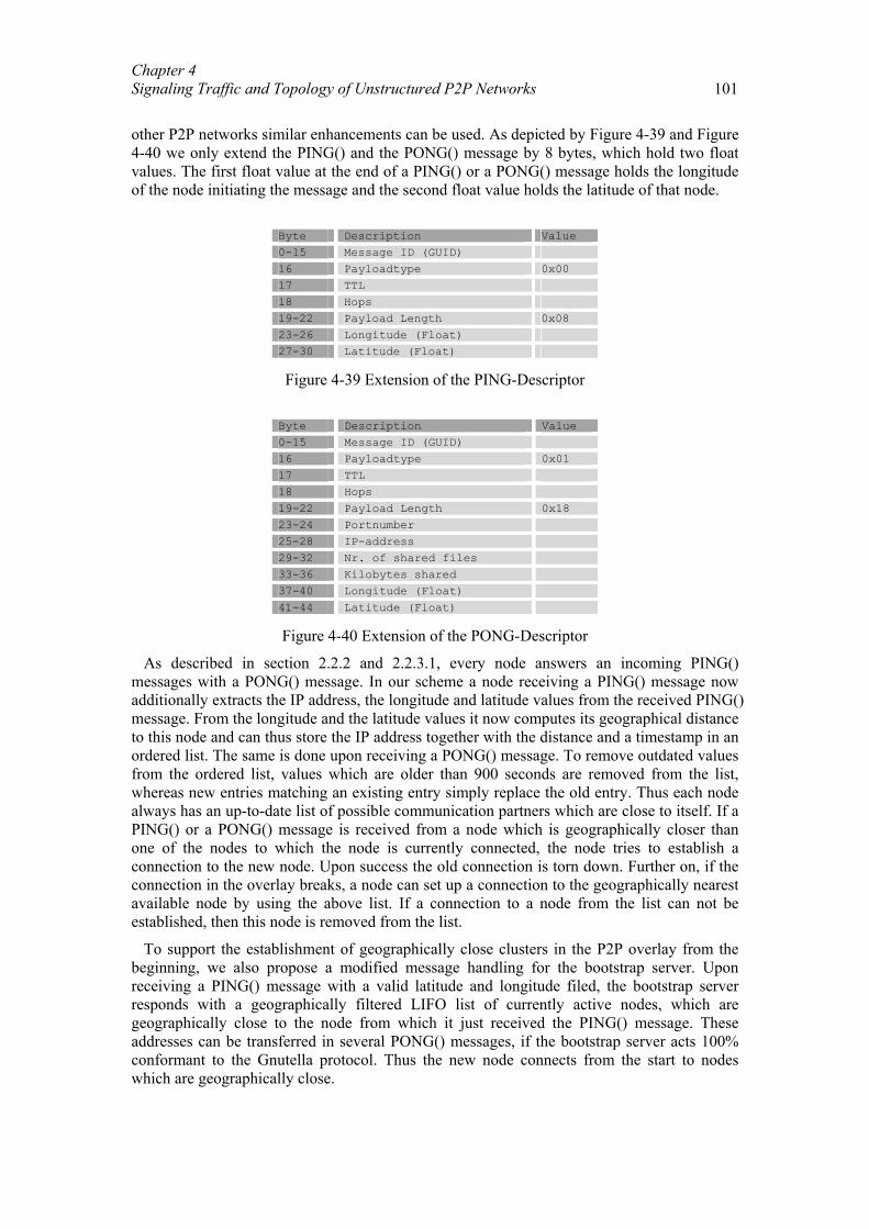
Chapter 4 Signaling Traffic and Topology of Unstructured P2P Networks 101
other P2P networks similar enhancements can be used. As depicted by Figure 4-39 and Figure 4-40 we only extend the PING() and the PONG() message by 8 bytes, which hold two float values. The first float value at the end of a PING() or a PONG() message holds the longitude of the node initiating the message and the second float value holds the latitude of that node.
Byte Description Value 0-15 Message ID (GUID) 16 Payloadtype 0x00 17 TTL 18 Hops 19-22 Payload Length 0x08 23-26 Longitude (Float) 27-30 Latitude (Float)
Figure 4-39 Extension of the PING-Descriptor
Byte Description Value 0-15 Message ID (GUID) 16 Payloadtype 0x01 17 TTL 18 Hops 19-22 Payload Length 0x18 23-24 Portnumber 25-28 IP-address 29-32 Nr. of shared files 33-36 Kilobytes shared 37-40 Longitude (Float) 41-44 Latitude (Float)
Figure 4-40 Extension of the PONG-Descriptor
As described in section 2.2.2 and 2.2.3.1, every node answers an incoming PING() messages with a PONG() message. In our scheme a node receiving a PING() message now additionally extracts the IP address, the longitude and latitude values from the received PING() message. From the longitude and the latitude values it now computes its geographical distance to this node and can thus store the IP address together with the distance and a timestamp in an ordered list. The same is done upon receiving a PONG() message. To remove outdated values from the ordered list, values which are older than 900 seconds are removed from the list, whereas new entries matching an existing entry simply replace the old entry. Thus each node always has an up-to-date list of possible communication partners which are close to itself. If a PING() or a PONG() message is received from a node which is geographically closer than one of the nodes to which the node is currently connected, the node tries to establish a connection to the new node. Upon success the old connection is torn down. Further on, if the connection in the overlay breaks, a node can set up a connection to the geographically nearest available node by using the above list. If a connection to a node from the list can not be established, then this node is removed from the list.
To support the establishment of geographically close clusters in the P2P overlay from the beginning, we also propose a modified message handling for the bootstrap server. Upon receiving a PING() message with a valid latitude and longitude filed, the bootstrap server responds with a geographically filtered LIFO list of currently active nodes, which are geographically close to the node from which it just received the PING() message. These addresses can be transferred in several PONG() messages, if the bootstrap server acts 100% conformant to the Gnutella protocol. Thus the new node connects from the start to nodes which are geographically close.
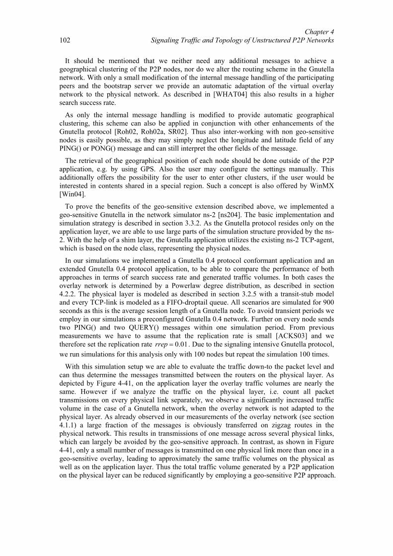
Chapter 4 Signaling Traffic and Topology of Unstructured P2P Networks
102
It should be mentioned that we neither need any additional messages to achieve a geographical clustering of the P2P nodes, nor do we alter the routing scheme in the Gnutella network. With only a small modification of the internal message handling of the participating peers and the bootstrap server we provide an automatic adaptation of the virtual overlay network to the physical network. As described in [WHAT04] this also results in a higher search success rate.
As only the internal message handling is modified to provide automatic geographical clustering, this scheme can also be applied in conjunction with other enhancements of the Gnutella protocol [Roh02, Roh02a, SR02]. Thus also inter-working with non geo-sensitive nodes is easily possible, as they may simply neglect the longitude and latitude field of any PING() or PONG() message and can still interpret the other fields of the message.
The retrieval of the geographical position of each node should be done outside of the P2P application, e.g. by using GPS. Also the user may configure the settings manually. This additionally offers the possibility for the user to enter other clusters, if the user would be interested in contents shared in a special region. Such a concept is also offered by WinMX [Win04].
To prove the benefits of the geo-sensitive extension described above, we implemented a geo-sensitive Gnutella in the network simulator ns-2 [ns204]. The basic implementation and simulation strategy is described in section 3.3.2. As the Gnutella protocol resides only on the application layer, we are able to use large parts of the simulation structure provided by the ns-2. With the help of a shim layer, the Gnutella application utilizes the existing ns-2 TCP-agent, which is based on the node class, representing the physical nodes.
In our simulations we implemented a Gnutella 0.4 protocol conformant application and an extended Gnutella 0.4 protocol application, to be able to compare the performance of both approaches in terms of search success rate and generated traffic volumes. In both cases the overlay network is determined by a Powerlaw degree distribution, as described in section 4.2.2. The physical layer is modeled as described in section 3.2.5 with a transit-stub model and every TCP-link is modeled as a FIFO-droptail queue. All scenarios are simulated for 900 seconds as this is the average session length of a Gnutella node. To avoid transient periods we employ in our simulations a preconfigured Gnutella 0.4 network. Further on every node sends two PING() and two QUERY() messages within one simulation period. From previous measurements we have to assume that the replication rate is small [ACKS03] and we therefore set the replication rate 0.01rrep = . Due to the signaling intensive Gnutella protocol, we run simulations for this analysis only with 100 nodes but repeat the simulation 100 times.
With this simulation setup we are able to evaluate the traffic down-to the packet level and can thus determine the messages transmitted between the routers on the physical layer. As depicted by Figure 4-41, on the application layer the overlay traffic volumes are nearly the same. However if we analyze the traffic on the physical layer, i.e. count all packet transmissions on every physical link separately, we observe a significantly increased traffic volume in the case of a Gnutella network, when the overlay network is not adapted to the physical layer. As already observed in our measurements of the overlay network (see section 4.1.1) a large fraction of the messages is obviously transferred on zigzag routes in the physical network. This results in transmissions of one message across several physical links, which can largely be avoided by the geo-sensitive approach. In contrast, as shown in Figure 4-41, only a small number of messages is transmitted on one physical link more than once in a geo-sensitive overlay, leading to approximately the same traffic volumes on the physical as well as on the application layer. Thus the total traffic volume generated by a P2P application on the physical layer can be reduced significantly by employing a geo-sensitive P2P approach.
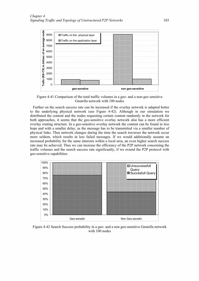
Chapter 4 Signaling Traffic and Topology of Unstructured P2P Networks 103
0
1000
2000
3000
4000
5000
6000
7000
8000
9000
geo-senstive non geo-sensitive
Traf
ic (R
X+TX
) in
bit/s
ec o
f an
aver
age
node
Traffic on the phyiscal layer
Traffic on the application layer
Figure 4-41 Comparison of the total traffic volumes in a geo- and a non-geo sensitive
Gnutella network with 100 nodes
Further on the search success rate can be increased if the overlay network is adapted better to the underlying physical network (see Figure 4-42). Although in our simulation we distributed the content and the nodes requesting certain content randomly in the network for both approaches, it seems that the geo-sensitive overlay network also has a more efficient overlay routing structure. In a geo-sensitive overlay network the content can be found in less hops and with a smaller delay, as the message has to be transmitted via a smaller number of physical links. Thus network changes during the time the search traverses the network occur more seldom, which results in less failed messages. If we would additionally assume an increased probability for the same interests within a local area, an even higher search success rate may be achieved. Thus we can increase the efficiency of the P2P network concerning the traffic volumes and the search success rate significantly, if we extend the P2P protocol with geo-sensitive capabilities.
0%
10%
20%
30%
40%
50%
60%
70%
80%
90%
100%
Geo-sensitiv Non Geo-sensitiv
UnsuccessfullQuerySuccesfull Query
Figure 4-42 Search Success probability in a geo- and a non geo-sensitive Gnutella network
with 100 nodes
Chapter 4 Signaling Traffic and Topology of Unstructured P2P Networks
104
4.7. The Mobile Peer-to-Peer Protocol In this work we distinguish Mobile Ad Hoc networks and cellular networks in mobile
environments. Cellular wireless networks are only one-hop wireless networks. Mobile P2P nodes are thus connected to the fixed Internet only via one wireless link. Resulting we can state, that even if the node moves, the physical path to this node alters not very much. We can regard P2P nodes connected to the Internet via a cellular wireless link as low performance nodes, because we have to take their bandwidths restrictions into account. Significant changes of the P2P protocol, which especially take into account the mobility of the nodes in cellular wireless systems are therefore from our point of view not necessary.
However if we want to operate a Peer-to-Peer network on top of a MANET, we have to take into account the mobility of the nodes. The reason is that MANETs are self configuring, wireless multihop networks, within which we have to assume the possibility that the physical path between two nodes changes frequently, due to the movement of the nodes [GL03]. If the overlay structure would be established completely independent from the underlying MANET topology, this would result in a significant number of long and unstable zigzag routes in the MANET layer. This would lead to high traffic volumes, which might not be bearable by the MANET [KCW03].
In the previous section (section 4.6) we could already observe, that even in a fixed environment the performance of P2P network can be significantly increased if the overlay network structure is adapted to the underlying physical network. The overall traffic caused by the P2P application on the physical layer could be reduced by nearly 90% and the search success rate could be increased from 40% to 75%. Therefore we describe in this section a novel P2P approach, the Mobile Peer-to-Peer protocol (MPP), which adapts the overlay structure to the physical MANET structure via a cross-layer communication channel between the physical network layer and the virtual P2P layer. This integrated approach reduces significantly the messaging overhead and increases the search success rate compared to approaches with a separated treatment of the overlay and the physical network. Further on MPP allows the introduction of a variety of new services, as it provides the possibility for context based routing and location based services, instead of simple address routing as it is provided by current MANET routing algorithms. Thus new services like the search for a Taxi or a cash dispenser in local proximity can be realized without the necessity for further location sensitive sensors and central instances (see also section 2.4). Further details of our approach are described in [GSK04a, GSK04, KSGN03, SGN03].
4.8. Summary and Further Work The motivation for the analysis of the efficiency of unstructured Peer-to-Peer networks in
this chapter is the high amount of signaling traffic caused by P2P networks which can be observed in many IP networks [Abi03, And03, AG03, FMLC03, KBBF03]. To analyze the reasons for this high signaling overhead, we studied the P2P overlay networks of Gnutella and JXTA concerning the traffic characteristics of P2P applications and the characteristics of the overlay network topology and its relation to the underlying physical network.
For our analysis we used the tools developed within this work and described in Chapter 3. Generally we distinguish in this chapter results retrieved from measurements of either real or simulated networks and analytical results retrieved from the random graph model developed in section 3.2.2. The analytical considerations of the network topology and the traffic volumes, described in this chapter, are based on two degree distributions observed in real networks (powerlaw and Superpeer) [JAB01, SD03]. By applying additionally an application model of the Gnutella 0.6 or the Gnutella 0.4 network to these analytical models, we compute the
Chapter 4 Signaling Traffic and Topology of Unstructured P2P Networks 105
search success and the traffic characteristics of these networks. The major original contributions of this chapter can therefore be summarized as follows:
• Determination of the geographical properties of unstructured P2P networks. With the mapping tool developed within this work, we can visualize the location of Gnutella nodes and their overlay connections between them. We can thus make the relationship between the virtual and the physical network visible and can prove the occurrence of zigzag routes in the physical layer. Based on this measurement we develop new possibilities to improve the routing behavior in overlay networks.
• Overlay topology analysis. In further measurements we analyzed the number of reachable nodes in real networks. With this analysis we can show that one of the major factors limiting the growth of a P2P overlay networks in terms of reachable nodes are circles occurring in unstructured P2P networks. Even if we increase the number of first order connections of our measurement node linearly, the number of reachable nodes does not increase linearly. The number of reachable nodes per first order connection even decreases with an increasing number of first order connections.
• Graph theoretic analysis of the overlay topology and the overlay traffic. Based on the random graph model described in section 3.2.2 in conjunction with the user and the application model (see section 3.2 and 3.2.4) we prove the efficiency of a Superpeer topology compared to powerlaw and other topologies. The content availability and the network growth in a Superpeer network are significantly higher. If we further on apply a protocol, which uses the advantages of a Superpeer topology, like the Gnutella 0.6 protocol, we prove the smaller necessary traffic volume with our analytical model. Concerning the circle analysis, the network growth and the reach analysis, our analytical model confirms the results derived from our measurements.
• Investigation of the traffic characteristics. With our measurement approach described in section 3.1.1.3, we show that the keep-alive mechanism does not cause the majority of the traffic in a P2P network. In fact the content request and response messages are responsible for more than 85% of all transmitted bytes, although they only cause 25% of the messages. Thus we found that flooding of small messages is not as harmful as the uncompressed transmission of messages, which may be up to 65159 bytes long.
• Self-similarity of P2P traffic. With an in-depth Hurst-parameter analysis of P2P traffic we show that in contrast to Web traffic P2P traffic does not show any self similar characteristics. The longer the aggregate interval is, the more the traffic smoothes out and shows nearly no traffic bursts anymore. As P2P traffic causes the majority of the traffic observable in current IP networks, influences on the overall self similar behavior of IP traffic are likely. The reasons for this behavior are the communication mode and the distribution of the content. Further on we have to take into account, that the majority of the traffic caused by P2P networks is signaling traffic, which is set up of comparatively small packets. These P2P signaling packets in general do not have interdependencies, which avoids the occurrence of high data bursts.
• Compression Scheme negotiation. From our measurement and analytical analysis of the P2P traffic patterns we found that the uncompressed QUERY() and QUERYHIT() messages cause up to 85% of the signaling overhead in P2P networks, although they only account for 25 % of all transmitted messages. Therefore we propose a new compression negotiation scheme, which is able to keep the flexibility offered by plain text or even XML coded messages, but can reduce the signaling overhead by approximately 60% [TKSE04]. Thus we can increase the signaling efficiency of
Chapter 4 Signaling Traffic and Topology of Unstructured P2P Networks
106
unstructured P2P networks, like JXTA or Gnutella notably, by adding a small extension to the initial handshake messages.
• Geo-sensitive P2P. To avoid the zigzag routes we observe in our geographical analysis of the Gnutella network, we propose to extend the keep alive messages to provide automatic geographical clustering. Thus we are able to reduce the total amount of signaling messages transmitted in the physical layer by more than 90%, although the amount of signaling traffic in the application layer is constant. The reason for this improvement of the signaling efficiency is that the virtual communication layer is much better adapted to the physical layer with this approach. We thus expect that with such an approach the P2P network can also provide increased search success rates, as it is expected that geographically close groups share similar interests [WHAT04]. We can thus increase the search success rate and at the same time reduce the amount of signaling traffic at the physical layer significantly.
• The Mobile P2P protocol (MPP): The Mobile Peer-to-Peer (MPP) protocol stack offers a promising concept, by introducing a cross-layer communication channel between the physical network layer and the virtual P2P network layer. Thus the Peer-to-Peer layer is well aware about the wireless network. Resulting MPP can minimize the signaling traffic significantly and can cope with frequent route breaks. Additionally the network layer is provided with knowledge about the Peer-to-Peer application, in order to establish routes only to the best communication partners. As we could prove by means of simulations, MPP reduces significantly the messaging overhead and increases the search success rate. MPP thus forms the necessary framework to allow the creation of a vast variety of different services over ad hoc networks.
• Collection of basic data for simulations and analytical considerations. Together with our mathematical models, which describe the general behavior of P2P users, nodes and the P2P topology, this collection of our measurements, is a sound basis for future simulations and analytical considerations. By comparing our analytical results with measurement and simulation results we confirmed in this chapter the reliability of our analytical models.
An important aspect of the work described in this chapter is the agreement of the analytical consideration of P2P topology and traffic characteristics (based on random graph theory) and the measurement-based analysis of P2P networks. As illustrated by the analysis of several parameters by means of mathematics and by means of measurements, we show the practical value of our mathematical user-, application- and topology-model in the design of efficient P2P protocols. Additionally we also determine important parameters for research for the simulations of unstructured P2P networks. Even in simulations of structured P2P networks at least our user-model can be used.
By the development of the compression scheme negotiation and the geo-sensitivity of the P2P protocol, we improve the efficiency of unstructured P2P networks notably. Using this proposal, signaling messages can be exchanged more efficiently and the virtual routes along which these messages are exchanged are established more efficiently. However we do not provide a distinctive answer whether certain content is available in an unstructured overlay network. This can be solved in a structured P2P approach, as e.g. in Chord. However structured P2P networks do not allow easy establishing of location aware clusters [ZZ03]. Further on structured P2P networks generally need a stable environment to achieve a good performance [TAD03]. Therefore an approach mixing structured and unstructured P2P approaches, as indicated in [CCR04] may offer interesting properties in the future.
Furthermore it is also necessary to better analyze the efficiency of structured P2P approaches in stable but especially in unstable environments. In this area only few results are available so far. By means of graph theory and stochastic it should be possible to analyze the
Chapter 4 Signaling Traffic and Topology of Unstructured P2P Networks 107
signaling properties of structured P2P networks in a similar manner as described in this work. Establishing sound analytical models for structured P2P networks can certainly help to understand network properties and additionally can reduce the need for computation intensive simulations.
Chapter 5 ZONE BASED P2P
As described in Chapter 4, most of the traffic generated by P2P networks, which is up to 9 TByte per week [Abi03], is caused only by signaling messages of the P2P network. The signaling messages are used to search for data, to announce the presence of data, and to guarantee sufficient connectivity in the P2P network. The current flooding strategy employed in pure (Gnutella 0.4) and parts of hybrid P2P networks (Gnutella 0.6) limits the signaling efficiency of P2P networks. Pure P2P networks omit centralized servers completely. Thus the nodes have no knowledge which peer contains the requested information and how the overlay network is set up in its proximity. Therefore, a peer needs to broadcast messages on the overlay network to detect which nodes are currently available on the network. Only thus the node is able to stay connected to the network, although any neighboring node may leave the network at any time. Further on, QUERY() messages issued by the peers, requesting services, data or information, are also broadcasted in the overlay to every direct neighbor of a peer. Likewise, upon receiving a QUERY(), these peers propagate the QUERY() to all their neighbors and so forth. This model is not efficient because of the large signaling traffic volumes, compared to the amount of transmitted user data.
Many architectures and algorithms have been proposed to solve the inefficiency problems of P2P networks. Most of them suggest hierarchies in the overlay. Gnutella 0.6 e.g. establishes a two-tier concept with so called Superpeers in the higher hierarchy level and so called leafnodes in the lower level. However in the higher hierarchy flooding is still employed to search for content and to provide connectivity. This again leads to high traffic volumes as shown in [SD03] and [SK03].
In this chapter, we propose a novel P2P architecture, Zone Based Peer-to-Peer (ZBP) [SKe04], to reduce broadcasting in the overlay network to a minimum by introducing a limited and dynamic knowledge of the overlay network topology. With this approach we provide a suitable architecture for an efficient search mechanism while keeping the “basic” Peer-to-Peer character of the network. We can improve the efficiency of the Peer-to-Peer network by combining proactive and reactive routing for fast and traffic-efficient location of requested content in a P2P network. ZBP uses no centralized entities and no hierarchies are imposed on the nodes participating in the network. ZBP allows participating members to share all kinds of objects and resources in a Peer-to-Peer overlay network. For a better understanding of the concepts and algorithms used in ZBP, simplified SDL diagrams of all protocol instances are provided in appendix C.
5.1. Related Work In addition to the classification in terms of architectural characteristics into unstructured,
centralized, pure, hybrid and structured P2P networks we can categorize P2P networks based on their search/routing behavior. Here we can distinguish, similar as in Mobile Ad Hoc Networks (MANETs) [Per00], proactive and reactive routing schemes.
Reactive in this context means, that a route from the querying node to the node providing the requested resource is only established upon a request from the querying node. No information about the route is known in advance. Thus route request messages, i.e. content request messages, have to be flooded to a certain extent in the overlay network. Examples for
Chapter 5 Zone Based P2P 109
P2P protocols employing reactive routing schemes are pure, hybrid and centralized unstructured P2P networks, as Gnutella 0.4 and 0.6 as well as JXTA, Freenet or Fasttrack.
The nodes participating in a network employing reactive routing schemes possess only very limited knowledge about the overlay network topology in their proximity. They only know, which P2P nodes are available as their direct neighbors to send to these nodes a request as part of the flooding scheme. However they do not have any knowledge about the shared content in their vicinity, or on which overlay path a node hosting the content can be reached. Also for keep alive issues in traditional systems, peers only know some arbitrarily selected nodes, which are currently connected to the P2P overlay network, and how to connect to them on the transport layer.
In routing protocols using proactive routing the routing path of a request from the requestor to the content provider is already determined before the request is initialized. Thus flooding can be avoided, but higher maintenance traffic is necessary to keep the routing paths for every shared object/content up to date.
P2P systems based on Distributed Hash Tables, like CAN [RFHK01], Chord [SMKK01] or Tapestry [ZHSR04], can be regarded as a first step towards proactive routing. In DHT-based overlay networks the path to a certain content is set before a request for content is issued by the user. Peers and the hosted content are labeled by hash keys (see section 2.3 for details about structured P2P networks). To make sure that content can be found by using the hash key as an indication for a route to the requested content, every new content, brought into the overlay, is transferred to that peer with the minimum distance between the hash value of the content and the node ID. Since content is moved in these P2P networks to facilitate routing, we refer to these systems also as structured P2P networks.
Nodes in a DHT based P2P overlay network connect to each other, depending on their hash key, i.e., the overlay network is built in a way that a node connects always to that node, with the minimum difference according to their hash values. Assuming, that every node has only two neighbors, the network is established as a virtual, ordered chain. Thus routing to nodes is done by simply sending the request in the direction of increasing hash values, as long as the hash value of the request is smaller than the ID of the node receiving the request. This predetermination of the route before a particular request is issued can also be regarded as proactive routing.
The significant decrease of routing overhead in DHT based P2P networks comes at the cost of requirements, which may not be acceptable for every application. In DHT based networks, any content or at least a link to that content brought into the network by participating nodes has to be transferred to that node with the minimal difference between the describing hash values. This may not be applicable for all applications and may also lead to scalability problems especially in unstable environments [LR04]. Further on, any content can only be located by its globally unique ID and all replicas described by one keyword are stored on one node. This presumably leads to a small number of peers which have to store an excessive number of objects, as certain keywords are commonly associated with a large number of files [Zip 32].
Proactive routings schemes, like the DHT based schemes described above are best suited for stable environments, where the overlay links and the underlying physical network do not change often. Therefore average session length of the participants in the overlay should also be significantly higher than currently experienced in unstructured P2P networks, to achieve a small churn rate [RGRK04, XMH03].
Except in structured P2P networks like CAN or CHORD, proactive routing schemes are currently not employed in P2P networks to our knowledge. However proactive routing schemes are employed successfully in Mobile Ad Hoc Networks, e.g. in DSDV [PB94], AODV [JMQ03] or ZRP [HP00].
Chapter 5 Zone Based P2P
110
The Zone Based Peer-to-Peer (ZBP) routing approach described in this work is based on the idea of using proactive routing within a certain zone and reactive routing outside of this zone. The difference between the zone as defined by the zone routing protocol (ZRP) used in MANETs [HP00] and the ZBP approach is that in ZBP zone members do not necessarily need to be geographically close together. Two nodes participating in the ZBP are neighbors when they are connected via a ZBP connection, which is based on a TCP/IP connection.
It is not sensible to employ proactive routing in the whole P2P network and thus to distribute the knowledge about every available item in the whole network. For an overlay lookup protocol to be efficient, changes should only have a local effect. In other words, the creation of a new link is an important local event but most probably not a significant piece of information which has to be communicated to the complete network.
Further on we can assume a certain replication rate for each object available in the P2P network. Using the possibilities offered by the connection handler, described in section 5.3 below, we can assume that the requested object is available within a certain proximity. This proximity is mainly determined by the overlay structure and the replication rate of each object, as described in section 5.7. ZBP thus tries to use the benefit of interest shared locally [WHAT04].
In contrast to ZRP, ZBP is completely independent of the physical layer and provides routing possibilities for any kind of object, not only for addresses of nodes. In this chapter, ZBP is based on TCP/IP as a transport layer, but it may also be used on top of any other transport protocol.
5.2. Optimal Representation of Shared Objects A general problem in proactive routing networks is the necessity to distribute the routing
indexes at least within a certain part of the network. A prominent example for that is the Napster network. Here the Napster server is the only routing instance, which thus has to know which object is accessible on which Napster client. Therefore the Napster client has to transfer all the keywords and other metadata describing the shared objects to the Napster index server (see section 2.2.1). This results in large message sizes, especially if plain text descriptions are employed.
Similarly in ZBP, the index of the shared objects of each joining node has to be distributed within their zone. This enables the nodes in the ZBP to proactively route to content available in their zone. While this shares the load evenly among all nodes and avoids any single point of failure, it requires efficient methods to reduce the size of these index messages. Therefore we discuss in this section two different approaches for the distribution of indexes of shared objects. In the first part we present a more efficient approach of Bloom filters by employing compression. In the second part of this section we present an approach of simple hash indexes, which are very efficient for applications in which the number of locally shared objects is small compared to the total number of available objects.
5.2.1 Compression of Bloom Filters The major goal of most networks is to provide basic mechanisms to exchange data objects.
Therefore firstly the question has to be answered, where which object is located. One approach to answer this question in an efficient way has been introduced in [Blo70] by the development of Bloom filters. Bloom filters are compact data structures, representing a set of objects located on one node or a group of several nodes. By issuing a query, like “Is object X in the set?” to a group of nodes, a lookup in the respective Bloom filter can answer this question.
Chapter 5 Zone Based P2P 111
A Bloom filter is a vector of m bits, within which every element is initialized with “0”.
From every object, which descriptions shall be included within the Bloom filter, k hash values are computed with k independent hash functions of degree m. Then every bit position given by each of the k computed values is set to 1 in the vector of m bits, the Bloom filter. However as a hash function distributes its output values randomly and uniformly distributed between 0 ... 2m , it may happen, that two objects result in the same combination of hash values. The Bloom filter thus returns upon a query, whether object X is available, a positive answer although a wrong object, described by exactly the same hash keys is available. On the other hand a Bloom filter will never return a positive answer although neither the object nor a similar object is available. Thus if a Bloom filter returns a negative answer, we can be sure, that the object is not available. Resulting in [Ram89] this probability is called the false positive probability:
( )( )11 1
kk n d
fp km
= − −
i
(69)
where m denotes the length of the Bloom filter in bit, k the number of employed hash functions, n the number of available objects in the network and d the number of descriptions (keywords) per object. Further details and applications of Bloom filters are described in [BM02, CM03, CMN03, CZH99, FCA98, Grem83, DWB01, Grö01, Hsi01, KBC00, LTS02, LSS02, Mul83, Ram89, RV03].
However as described in detail in [SK04] the size of Bloom filters in number of bytes is still large. If we assume for example a total of 1e+7 shareable objects in the whole network, we can compute the minimal size of a Bloom filter for a false positive probability of 710fp −=
to 3.4e+8 bit and for 110fp −= to 4.8e+7 bit. This is certainly too much data to represent 100 objects, which we assume in average to be shared by every peer in a general P2P network.
With arithmetic coding [MWW98] we can theoretically compress the size of the Bloom filter down to that fraction of the original size, given by the entropy H(p) of the Bloom filter.
( ) ( )21
logn
i ii
H p p p=
= −∑ i (70)
Together with our above assumption that each node stores l objects out of a total of N objects in the whole network, the probability that a bit in the Bloom filter is set to one is
( ) ( , , )1 l k cor m l kpm
=i i
(71)
where k describes the number of employed hash functions and m is the uncompressed size of the Bloom filter.
The probability that a bit is set to zero is accordingly
( ) ( , , )0 m l k cor m l kpm
−=
i i (72)
The correction term ( ), ,cor m l k must be included in equation (71) and equation (72), as we
have to take into account the possibility ( )op i , that one bit in the Bloom filter can be set
more than once. This effect is represented mathematically by equation (73), whereas ( )op i is given in equation (74).
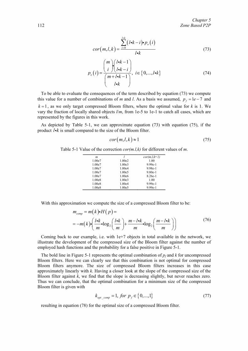
Chapter 5 Zone Based P2P
112
( )( ) ( )
0, ,
l k
oi
l k i p icor m l k
l k=
−=
∑i
i i
i (73)
( ) { }
1
, 0,...,1o
m l ki l k i
p i i l km l k
l k
− − = ∈
+ −
iii
iii
(74)
To be able to evaluate the consequences of the term described by equation (73) we compute this value for a number of combinations of m and l. As a basis we assumed, 1 7fp e= − and
1k = , as we only target compressed Bloom filters, where the optimal value for k is 1. We vary the fraction of locally shared objects l/m, from 1e-5 to 1e-1 to catch all cases, which are represented by the figures in this work.
As depicted by Table 5-1, we can approximate equation (73) with equation (75), if the product l ki is small compared to the size of the Bloom filter.
( ), , 1cor m l k ≈ (75)
Table 5-1 Value of the correction cor(m.l,k) for different values of m. m l cor(m,l,k=1)
1.00e7 1.00e2 1.00 1.00e7 1.00e3 9.99e-1 1.00e7 1.00e4 9.98e-1 1.00e7 1.00e5 9.80e-1 1.00e7 1.00e6 8.26e-1 1.00e8 1.00e3 1.00 1.00e8 1.00e4 9.99e-1 1.00e8 1.00e5 9.99e-1
With this approximation we compute the size of a compressed Bloom filter to be:
( ) ( )
( ) 2 2log log
compm m k H p
l k l k m l k m l km km m m m
= =
− − = − +
i
i i i ii i i (76)
Coming back to our example, i.e. with 1e+7 objects in total available in the network, we illustrate the development of the compressed size of the Bloom filter against the number of employed hash functions and the probability for a false positive in Figure 5-1.
The bold line in Figure 5-1 represents the optimal combination of pf and k for uncompressed Bloom filters. Here we can clearly see that this combination is not optimal for compressed Bloom filters anymore. The size of compressed Bloom filters increases in this case approximately linearly with k. Having a closer look at the slope of the compressed size of the Bloom filter against k, we find that the slope is decreasing slightly, but never reaches zero. Thus we can conclude, that the optimal combination for a minimum size of the compressed Bloom filter is given with
{ }_ 1, 0,...,1opt comp fk for p= ∈ (77)
resulting in equation (78) for the optimal size of a compressed Bloom filter.
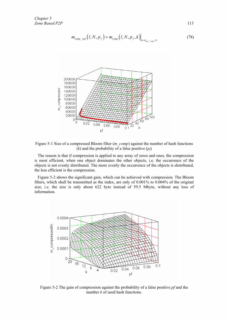
Chapter 5 Zone Based P2P 113
( ) ( )
__ 1
, , , , ,opt comp
comp opt f comp f k km l N p m l N p k
= == (78)
Figure 5-1 Size of a compressed Bloom filter (m_comp) against the number of hash functions
(k) and the probability of a false positive (pf)
The reason is that if compression is applied to any array of zeros and ones, the compression is most efficient, when one object dominates the other objects, i.e. the occurrence of the objects is not evenly distributed. The more evenly the occurrence of the objects is distributed, the less efficient is the compression.
Figure 5-2 shows the significant gain, which can be achieved with compression. The Bloom filters, which shall be transmitted as the index, are only of 0.001% to 0.004% of the original size, i.e. the size is only about 622 byte instead of 59.5 Mbyte, without any loss of information.
Figure 5-2 The gain of compression against the probability of a false positive pf and the
number k of used hash functions.
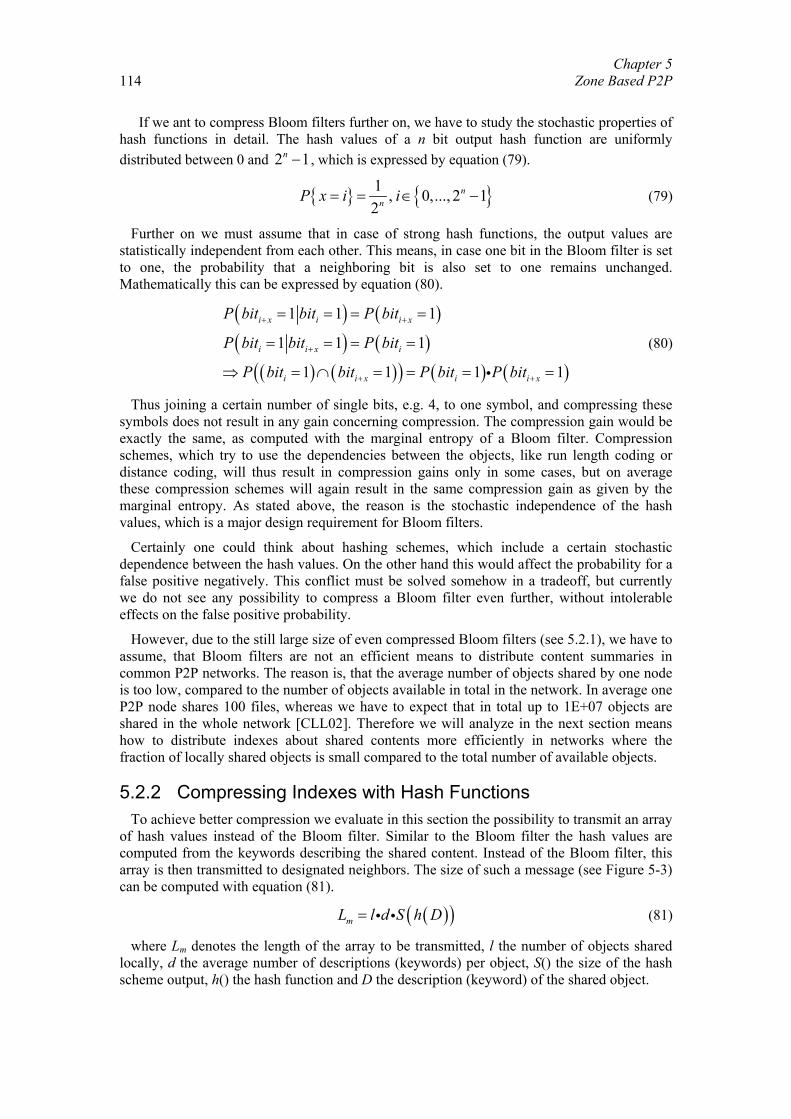
Chapter 5 Zone Based P2P
114
If we ant to compress Bloom filters further on, we have to study the stochastic properties of hash functions in detail. The hash values of a n bit output hash function are uniformly distributed between 0 and 2 1n − , which is expressed by equation (79).
{ } { }1 , 0,..., 2 12
nnP x i i= = ∈ − (79)
Further on we must assume that in case of strong hash functions, the output values are statistically independent from each other. This means, in case one bit in the Bloom filter is set to one, the probability that a neighboring bit is also set to one remains unchanged. Mathematically this can be expressed by equation (80).
( ) ( )( ) ( )
( ) ( )( ) ( ) ( )
1 1 1
1 1 1
1 1 1 1
i x i i x
i i x i
i i x i i x
P bit bit P bit
P bit bit P bit
P bit bit P bit P bit
+ +
+
+ +
= = = =
= = = =
⇒ = ∩ = = = =i
(80)
Thus joining a certain number of single bits, e.g. 4, to one symbol, and compressing these symbols does not result in any gain concerning compression. The compression gain would be exactly the same, as computed with the marginal entropy of a Bloom filter. Compression schemes, which try to use the dependencies between the objects, like run length coding or distance coding, will thus result in compression gains only in some cases, but on average these compression schemes will again result in the same compression gain as given by the marginal entropy. As stated above, the reason is the stochastic independence of the hash values, which is a major design requirement for Bloom filters.
Certainly one could think about hashing schemes, which include a certain stochastic dependence between the hash values. On the other hand this would affect the probability for a false positive negatively. This conflict must be solved somehow in a tradeoff, but currently we do not see any possibility to compress a Bloom filter even further, without intolerable effects on the false positive probability.
However, due to the still large size of even compressed Bloom filters (see 5.2.1), we have to assume, that Bloom filters are not an efficient means to distribute content summaries in common P2P networks. The reason is, that the average number of objects shared by one node is too low, compared to the number of objects available in total in the network. In average one P2P node shares 100 files, whereas we have to expect that in total up to 1E+07 objects are shared in the whole network [CLL02]. Therefore we will analyze in the next section means how to distribute indexes about shared contents more efficiently in networks where the fraction of locally shared objects is small compared to the total number of available objects.
5.2.2 Compressing Indexes with Hash Functions To achieve better compression we evaluate in this section the possibility to transmit an array
of hash values instead of the Bloom filter. Similar to the Bloom filter the hash values are computed from the keywords describing the shared content. Instead of the Bloom filter, this array is then transmitted to designated neighbors. The size of such a message (see Figure 5-3) can be computed with equation (81).
( )( )mL l d S h D= i i (81)
where Lm denotes the length of the array to be transmitted, l the number of objects shared locally, d the average number of descriptions (keywords) per object, S() the size of the hash scheme output, h() the hash function and D the description (keyword) of the shared object.
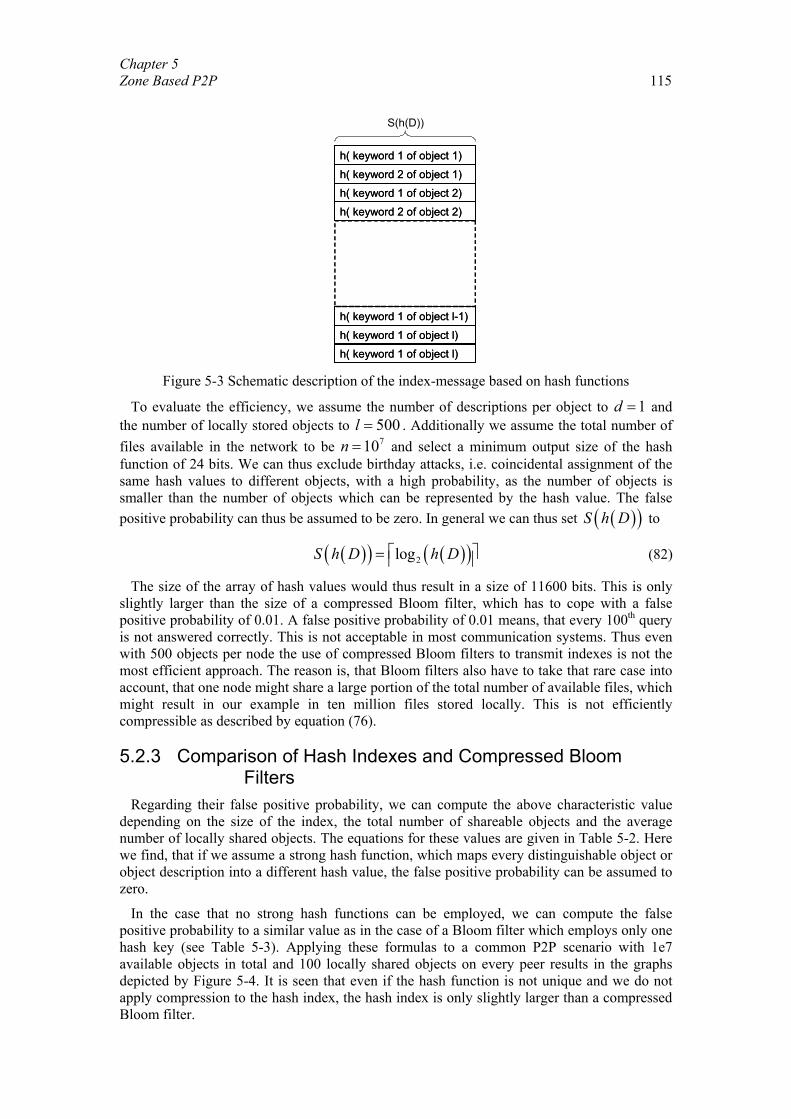
Chapter 5 Zone Based P2P 115
h( keyword 1 of object 1)
h( keyword 2 of object 1)
h( keyword 1 of object 2)
h( keyword 2 of object 2)
h( keyword 1 of object l-1)
h( keyword 1 of object l)
h( keyword 1 of object l)
h( keyword 1 of object 1)
h( keyword 2 of object 1)
h( keyword 1 of object 2)
h( keyword 2 of object 2)
h( keyword 1 of object l-1)
h( keyword 1 of object l)
h( keyword 1 of object l)
S(h(D))
Figure 5-3 Schematic description of the index-message based on hash functions
To evaluate the efficiency, we assume the number of descriptions per object to 1d = and the number of locally stored objects to 500l = . Additionally we assume the total number of files available in the network to be 710n = and select a minimum output size of the hash function of 24 bits. We can thus exclude birthday attacks, i.e. coincidental assignment of the same hash values to different objects, with a high probability, as the number of objects is smaller than the number of objects which can be represented by the hash value. The false positive probability can thus be assumed to be zero. In general we can thus set ( )( )S h D to
( )( ) ( )( )2logS h D h D = (82)
The size of the array of hash values would thus result in a size of 11600 bits. This is only slightly larger than the size of a compressed Bloom filter, which has to cope with a false positive probability of 0.01. A false positive probability of 0.01 means, that every 100th query is not answered correctly. This is not acceptable in most communication systems. Thus even with 500 objects per node the use of compressed Bloom filters to transmit indexes is not the most efficient approach. The reason is, that Bloom filters also have to take that rare case into account, that one node might share a large portion of the total number of available files, which might result in our example in ten million files stored locally. This is not efficiently compressible as described by equation (76).
5.2.3 Comparison of Hash Indexes and Compressed Bloom Filters
Regarding their false positive probability, we can compute the above characteristic value depending on the size of the index, the total number of shareable objects and the average number of locally shared objects. The equations for these values are given in Table 5-2. Here we find, that if we assume a strong hash function, which maps every distinguishable object or object description into a different hash value, the false positive probability can be assumed to zero.
In the case that no strong hash functions can be employed, we can compute the false positive probability to a similar value as in the case of a Bloom filter which employs only one hash key (see Table 5-3). Applying these formulas to a common P2P scenario with 1e7 available objects in total and 100 locally shared objects on every peer results in the graphs depicted by Figure 5-4. It is seen that even if the hash function is not unique and we do not apply compression to the hash index, the hash index is only slightly larger than a compressed Bloom filter.
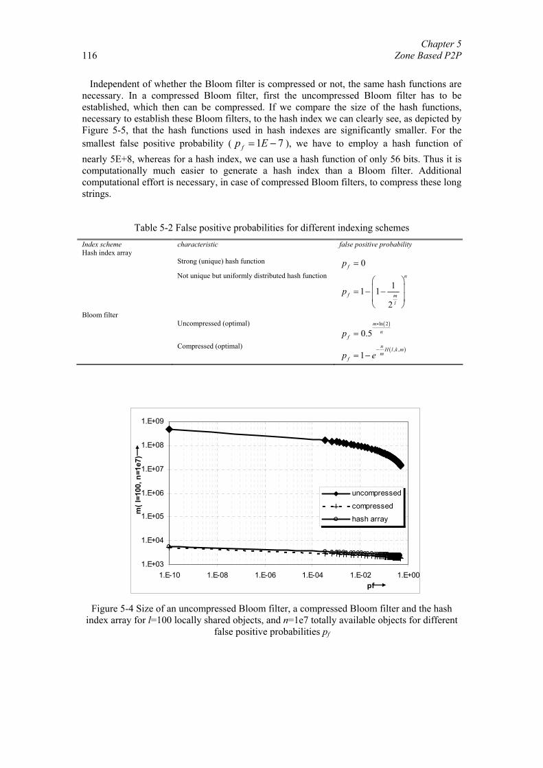
Chapter 5 Zone Based P2P
116
Independent of whether the Bloom filter is compressed or not, the same hash functions are necessary. In a compressed Bloom filter, first the uncompressed Bloom filter has to be established, which then can be compressed. If we compare the size of the hash functions, necessary to establish these Bloom filters, to the hash index we can clearly see, as depicted by Figure 5-5, that the hash functions used in hash indexes are significantly smaller. For the smallest false positive probability ( 1 7fp E= − ), we have to employ a hash function of nearly 5E+8, whereas for a hash index, we can use a hash function of only 56 bits. Thus it is computationally much easier to generate a hash index than a Bloom filter. Additional computational effort is necessary, in case of compressed Bloom filters, to compress these long strings.
Table 5-2 False positive probabilities for different indexing schemes Index scheme characteristic false positive probability Hash index array Strong (unique) hash function 0fp =
Not unique but uniformly distributed hash function 11 1
2
n
f ml
p = − −
Bloom filter Uncompressed (optimal) ( )ln 2
0.5m
nfp =
i
Compressed (optimal) ( ), ,1
n H l k mm
fp e−
= −
1.E+03
1.E+04
1.E+05
1.E+06
1.E+07
1.E+08
1.E+09
1.E-10 1.E-08 1.E-06 1.E-04 1.E-02 1.E+00pf
m( l
=100
, n=1
e7)
uncompressed
compressed
hash array
Figure 5-4 Size of an uncompressed Bloom filter, a compressed Bloom filter and the hash
index array for l=100 locally shared objects, and n=1e7 totally available objects for different false positive probabilities pf
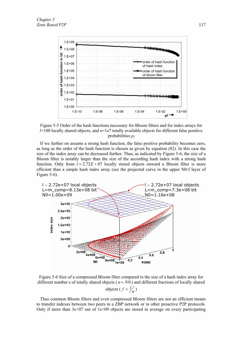
Chapter 5 Zone Based P2P 117
1.E+00
1.E+01
1.E+02
1.E+03
1.E+04
1.E+05
1.E+06
1.E+07
1.E+08
1.E+09
1.E-10 1.E-08 1.E-06 1.E-04 1.E-02 1.E+00pf
orde
r of h
ash
func
tion
in b
itorder of hash functionof hash indexorder of hash functionof bloom filter
Figure 5-5 Order of the hash functions necessary for Bloom filters and for index arrays for l=100 locally shared objects, and n=1e7 totally available objects for different false positive
probabilities pf
If we further on assume a strong hash function, the false positive probability becomes zero, as long as the order of the hash function is chosen as given by equation (82). In this case the size of the index array can be decreased further. Thus, as indicated by Figure 5-6, the size of a Bloom filter is notably larger than the size of the according hash index with a strong hash function. Only from 2.72 07l E= + locally stored objects onward a Bloom filter is more efficient than a simple hash index array (see the projected curve in the upper N0-f layer of Figure 5-6).
l ∼ 2.72e+07 local objectsL=m_comp=7.3e+08 bitN0=1.16e+08
l ∼ 2.72e+07 local objectsL=m_comp=8.13e+08 bitN0=1.00e+09
Figure 5-6 Size of a compressed Bloom filter compared to the size of a hash index array for
different number s of totally shared objects ( 0n N= ) and different fractions of locally shared objects ( lf n= )
Thus common Bloom filters and even compressed Bloom filters are not an efficient means to transfer indexes between two peers in a ZBP network or in other proactive P2P protocols. Only if more than 3e+07 out of 1e+09 objects are stored in average on every participating
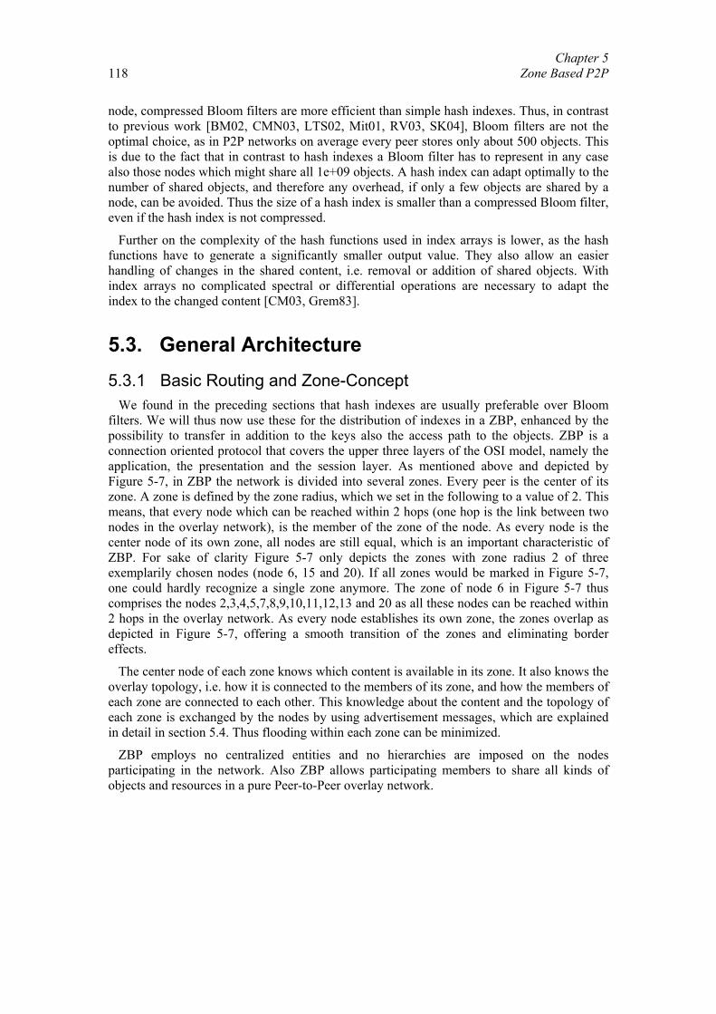
Chapter 5 Zone Based P2P
118
node, compressed Bloom filters are more efficient than simple hash indexes. Thus, in contrast to previous work [BM02, CMN03, LTS02, Mit01, RV03, SK04], Bloom filters are not the optimal choice, as in P2P networks on average every peer stores only about 500 objects. This is due to the fact that in contrast to hash indexes a Bloom filter has to represent in any case also those nodes which might share all 1e+09 objects. A hash index can adapt optimally to the number of shared objects, and therefore any overhead, if only a few objects are shared by a node, can be avoided. Thus the size of a hash index is smaller than a compressed Bloom filter, even if the hash index is not compressed.
Further on the complexity of the hash functions used in index arrays is lower, as the hash functions have to generate a significantly smaller output value. They also allow an easier handling of changes in the shared content, i.e. removal or addition of shared objects. With index arrays no complicated spectral or differential operations are necessary to adapt the index to the changed content [CM03, Grem83].
5.3. General Architecture 5.3.1 Basic Routing and Zone-Concept
We found in the preceding sections that hash indexes are usually preferable over Bloom filters. We will thus now use these for the distribution of indexes in a ZBP, enhanced by the possibility to transfer in addition to the keys also the access path to the objects. ZBP is a connection oriented protocol that covers the upper three layers of the OSI model, namely the application, the presentation and the session layer. As mentioned above and depicted by Figure 5-7, in ZBP the network is divided into several zones. Every peer is the center of its zone. A zone is defined by the zone radius, which we set in the following to a value of 2. This means, that every node which can be reached within 2 hops (one hop is the link between two nodes in the overlay network), is the member of the zone of the node. As every node is the center node of its own zone, all nodes are still equal, which is an important characteristic of ZBP. For sake of clarity Figure 5-7 only depicts the zones with zone radius 2 of three exemplarily chosen nodes (node 6, 15 and 20). If all zones would be marked in Figure 5-7, one could hardly recognize a single zone anymore. The zone of node 6 in Figure 5-7 thus comprises the nodes 2,3,4,5,7,8,9,10,11,12,13 and 20 as all these nodes can be reached within 2 hops in the overlay network. As every node establishes its own zone, the zones overlap as depicted in Figure 5-7, offering a smooth transition of the zones and eliminating border effects.
The center node of each zone knows which content is available in its zone. It also knows the overlay topology, i.e. how it is connected to the members of its zone, and how the members of each zone are connected to each other. This knowledge about the content and the topology of each zone is exchanged by the nodes by using advertisement messages, which are explained in detail in section 5.4. Thus flooding within each zone can be minimized.
ZBP employs no centralized entities and no hierarchies are imposed on the nodes participating in the network. Also ZBP allows participating members to share all kinds of objects and resources in a pure Peer-to-Peer overlay network.
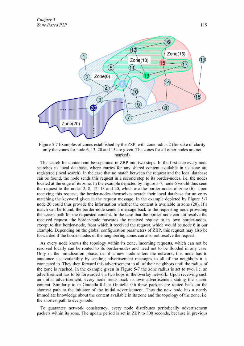
Chapter 5 Zone Based P2P 119
Figure 5-7 Examples of zones established by the ZSP, with zone radius 2 (for sake of clarity
only the zones for node 6, 13, 20 and 15 are given. The zones for all other nodes are not marked)
The search for content can be separated in ZBP into two steps. In the first step every node searches its local database, where entries for any shared content available in its zone are registered (local search). In the case that no match between the request and the local database can be found, the node sends this request in a second step to its border-nodes, i.e. the nodes located at the edge of its zone. In the example depicted by Figure 5-7, node 6 would thus send the request to the nodes 2, 8, 12, 13 and 20, which are the border-nodes of zone (6). Upon receiving this request, the border-nodes themselves search their local database for an entry matching the keyword given in the request message. In the example depicted by Figure 5-7 node 20 could thus provide the information whether the content is available in zone (20). If a match can be found, the border-node sends a message back to the requesting node providing the access path for the requested content. In the case that the border-node can not resolve the received request, the border-node forwards the received request to its own border-nodes, except to that border-node, from which it received the request, which would be node 6 in our example. Depending on the global configuration parameters of ZBP, this request may also be forwarded if the border-nodes of the neighboring zones can also not resolve the request.
As every node knows the topology within its zone, incoming requests, which can not be resolved locally can be routed to its border-nodes and need not to be flooded in any case. Only in the initialization phase, i.e. if a new node enters the network, this node has to announce its availability by sending advertisement messages to all of the neighbors it is connected to. They then forward this advertisement to all of their neighbors until the radius of the zone is reached. In the example given in Figure 5-7 the zone radius is set to two, i.e. an advertisement has to be forwarded via two hops in the overlay network. Upon receiving such an initial advertisement, every node sends back its own advertisement stating the shared content. Similarly to in Gnutella 0.4 or Gnutella 0.6 these packets are routed back on the shortest path to the initiator of the initial advertisement. Thus the new node has a nearly immediate knowledge about the content available in its zone and the topology of the zone, i.e. the shortest path to every node.
To guarantee network consistency, every node distributes periodically advertisement packets within its zone. The update period is set in ZBP to 300 seconds, because in previous
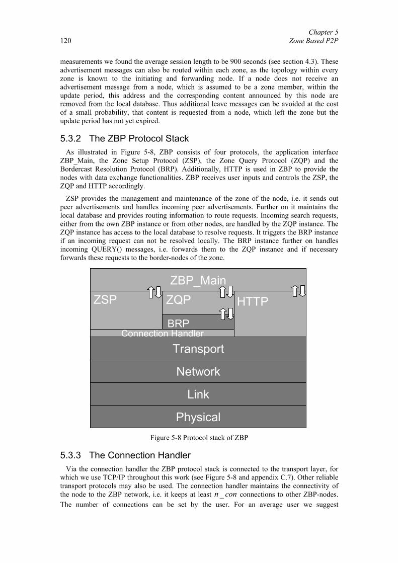
Chapter 5 Zone Based P2P
120
measurements we found the average session length to be 900 seconds (see section 4.3). These advertisement messages can also be routed within each zone, as the topology within every zone is known to the initiating and forwarding node. If a node does not receive an advertisement message from a node, which is assumed to be a zone member, within the update period, this address and the corresponding content announced by this node are removed from the local database. Thus additional leave messages can be avoided at the cost of a small probability, that content is requested from a node, which left the zone but the update period has not yet expired.
5.3.2 The ZBP Protocol Stack As illustrated in Figure 5-8, ZBP consists of four protocols, the application interface
ZBP_Main, the Zone Setup Protocol (ZSP), the Zone Query Protocol (ZQP) and the Bordercast Resolution Protocol (BRP). Additionally, HTTP is used in ZBP to provide the nodes with data exchange functionalities. ZBP receives user inputs and controls the ZSP, the ZQP and HTTP accordingly.
ZSP provides the management and maintenance of the zone of the node, i.e. it sends out peer advertisements and handles incoming peer advertisements. Further on it maintains the local database and provides routing information to route requests. Incoming search requests, either from the own ZBP instance or from other nodes, are handled by the ZQP instance. The ZQP instance has access to the local database to resolve requests. It triggers the BRP instance if an incoming request can not be resolved locally. The BRP instance further on handles incoming QUERY() messages, i.e. forwards them to the ZQP instance and if necessary forwards these requests to the border-nodes of the zone.
Physical
Link
Network
Transport
ZBP_MainZQP
BRP
ZSP
Connection Handler
HTTP
Figure 5-8 Protocol stack of ZBP
5.3.3 The Connection Handler Via the connection handler the ZBP protocol stack is connected to the transport layer, for
which we use TCP/IP throughout this work (see Figure 5-8 and appendix C.7). Other reliable transport protocols may also be used. The connection handler maintains the connectivity of the node to the ZBP network, i.e. it keeps at least _n con connections to other ZBP-nodes. The number of connections can be set by the user. For an average user we suggest
Chapter 5 Zone Based P2P 121
_ 3n con = connections. Decreasing _n con further results in a reduced search performance
(see section 4.2) and increasing the number of connections leads to a significantly increasing traffic volume (see section 4.4).
In contrast to other P2P protocols, the Connection handler in ZBP provides a node with the capability to establish the connections and the zones according to preferences set by the user. The overlay network connections can also be adapted to the physical layer topology to minimize connection distance. It operates as a kind of cross layer communication channel, as it can retrieve information about hop distances or delays from the transport layer. Thus the connection handler can establish connections according to criteria from the application as well as from the transport layer or from the user.
The connection handler can be used to establish interest groups. This possibility facilitates fast search and exchange of content from the interest area, although the nodes may physically be dispersed widely. However as they share the same interest the probability that they share similar resources is significantly higher than with random connections.
To provide the connection handler with the necessary information about available connection partners and their preferences, the connection handler can either retrieve information form its node cache or from the bootstrap server. The node cache is set up and maintained by the ZSP instance (see section 5.4), which parses all received advertisement messages for information about the preferences of the nodes, which initiated these messages. The preferences and the according IP addresses are stored in the node cache. If a new connection is needed, either when the node logs into the overlay or when an existing connection fails, the connection handler can receive information about available nodes from the cache (see also appendix C.7).
In case that no information about nodes is available in the node cache, the node can still contact a bootstrap server. The bootstrap server provides the contact addresses (IP addresses in our case) of nodes which recently logged into the network with similar preferences, as stated in the request (see appendix C.7.1) and section 5.3.4).
To setup an overlay connection, the connection handler instances of the two nodes use a three way handshake, after the TCP connection is established (see Figure 5-9). As soon as the "200 ok" is received from the counterpart, the overlay connection is established and the higher protocol instances can send and receive advertisements and content request messages via the interfaces offered by the connection handler. The connection handler provides the necessary interfaces to the transport layer as well as to the ZSP, the ZQP, and the BRP layer. It maps the messages initiated by the higher instances to the corresponding TCP/IP ports, so that the messages are correctly distributed in the overlay network. Further on incoming messages are distributed by the connection handler to the corresponding protocol instances i.e. advertisement messages to the ZSP instance and content request messages to the BRP instances.
5.3.4 Initialization On startup, ZBP first has to connect to at least one active node in the ZBP overlay network.
Therefore the node has to try to connect to nodes stored in its cache. If no addresses are available, the node has to contact a bootstrap server to receive valid addresses of active ZBP nodes, similar to other P2P approaches. If addresses are available, the ZBP instance triggers its connection handler to establish the according connections.
The connection handler first establishes a TCP connection on the transport layer. Then it exchanges a handshake with the active ZBP node to validate the connection. This connection establishment process is illustrated in Figure 5-9 by the first 9 messages. Figure 5-9 gives the message sequence chart for the case that node 13 wants to participate as a new node in the ZBP network illustrated by Figure 5-7. The resulting zone for node 13 is already shown in
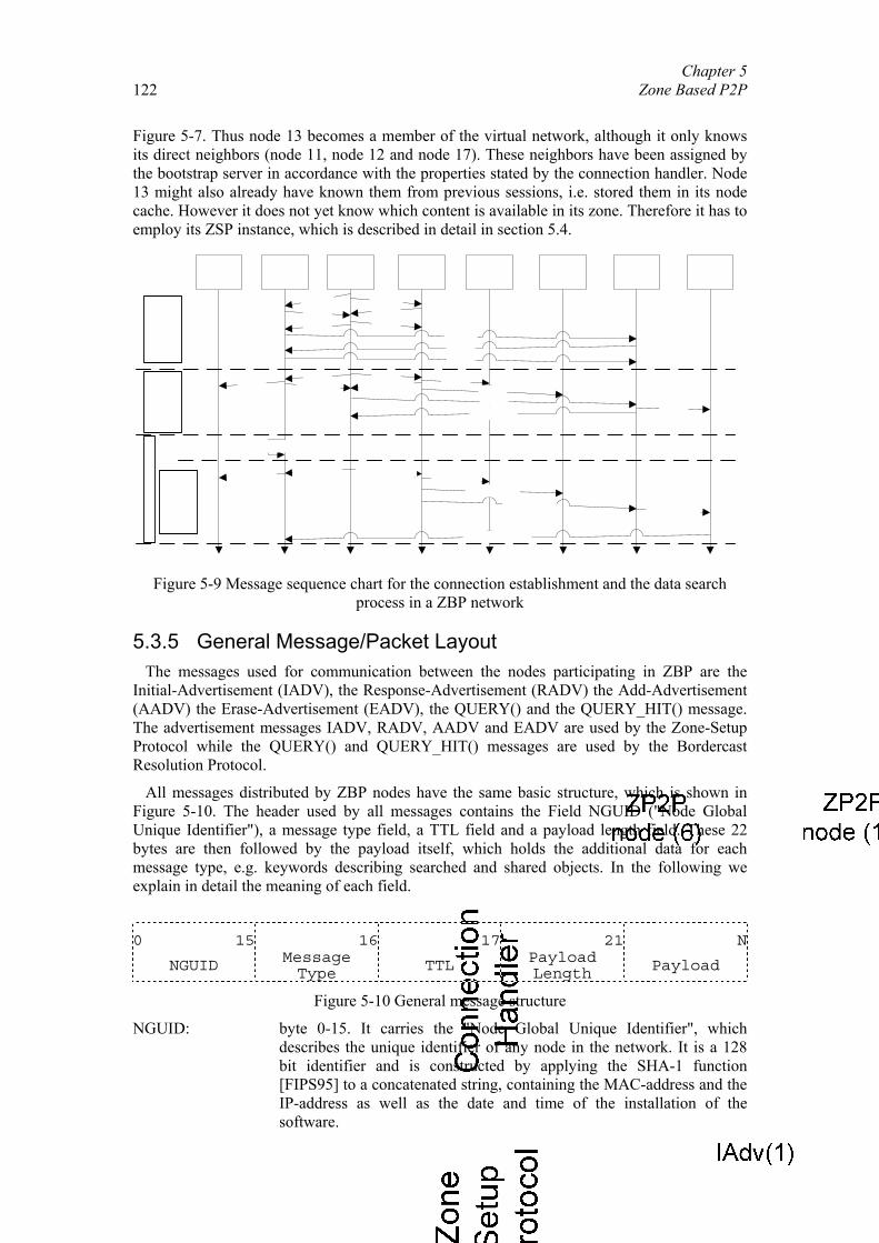
Chapter 5 Zone Based P2P
122
Figure 5-7. Thus node 13 becomes a member of the virtual network, although it only knows its direct neighbors (node 11, node 12 and node 17). These neighbors have been assigned by the bootstrap server in accordance with the properties stated by the connection handler. Node 13 might also already have known them from previous sessions, i.e. stored them in its node cache. However it does not yet know which content is available in its zone. Therefore it has to employ its ZSP instance, which is described in detail in section 5.4.
Figure 5-9 Message sequence chart for the connection establishment and the data search
process in a ZBP network
5.3.5 General Message/Packet Layout The messages used for communication between the nodes participating in ZBP are the
Initial-Advertisement (IADV), the Response-Advertisement (RADV) the Add-Advertisement (AADV) the Erase-Advertisement (EADV), the QUERY() and the QUERY_HIT() message. The advertisement messages IADV, RADV, AADV and EADV are used by the Zone-Setup Protocol while the QUERY() and QUERY_HIT() messages are used by the Bordercast Resolution Protocol.
All messages distributed by ZBP nodes have the same basic structure, which is shown in Figure 5-10. The header used by all messages contains the Field NGUID ("Node Global Unique Identifier"), a message type field, a TTL field and a payload length field. These 22 bytes are then followed by the payload itself, which holds the additional data for each message type, e.g. keywords describing searched and shared objects. In the following we explain in detail the meaning of each field.
0 15 16 17 21 N
NGUID Message Type TTL Payload
Length Payload
Figure 5-10 General message structure
NGUID: byte 0-15. It carries the "Node Global Unique Identifier", which describes the unique identifier of any node in the network. It is a 128 bit identifier and is constructed by applying the SHA-1 function [FIPS95] to a concatenated string, containing the MAC-address and the IP-address as well as the date and time of the installation of the software.
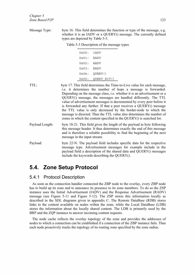
Chapter 5 Zone Based P2P 123
Message Type: byte 16. This field determines the function or type of the message, e.g.
whether it is an IADV or a QUERY() message. The currently defined types are depicted by Table 5-3.
Table 5-3 Description of the message types
0x00: IADV
0x01: RADV
0x02: AADV
0x03: EADV
0x04: QUERY()
0x05: QUERY_HIT()
TTL: byte 17. This field determines the Time-to-Live value for each message, i.e. it determines the number of hops a message is forwarded. Depending on the message class, i.e. whether it is an advertisement or a QUERY() message, the messages are handled differently. The TTL value of advertisement messages is decremented by every peer before it is forwarded any further. If that a peer receives a QUERY() message the TTL value is only decreased by the border-node to which the message is directed. Thus the TTL value also determines the number of zones in which the content specified in the QUERY() is searched for.
Payload Length: byte 18-21. This field gives the length of the payload in byte following this message header. It thus determines exactly the end of this message and is therefore a reliable possibility to find the beginning of the next message in the input stream.
Payload: byte 22-N. The payload field includes specific data for the respective message type. Advertisement messages for example include in the payload field a description of the shared data and QUERY() messages include the keywords describing the QUERY().
5.4. Zone Setup Protocol 5.4.1 Protocol Description
As soon as the connection handler connected the ZBP node to the overlay, every ZBP node has to build up its zone and to announce its presence to its zone members. To do so the ZSP instance uses the Initial Advertisement (IADV) and the Response Advertisement (RADV) message (see Figure 5-11 and Figure 5-12). The ZSP stores this information locally as described in the SDL diagrams given in appendix C. The Remote DataBase (RDB) stores links to the content available on nodes within the zone, while the Local DataBase (LDB) stores the information about the locally shared content. The LDB is primarily used by the BRP and the ZQP instance to answer incoming content requests.
The node cache reflects the overlay topology of the zone and provides the addresses of nodes to which a connection can be established if a connection of the ZBP instance fails. Thus each node proactively tracks the topology of its routing zone specified by the zone radius.
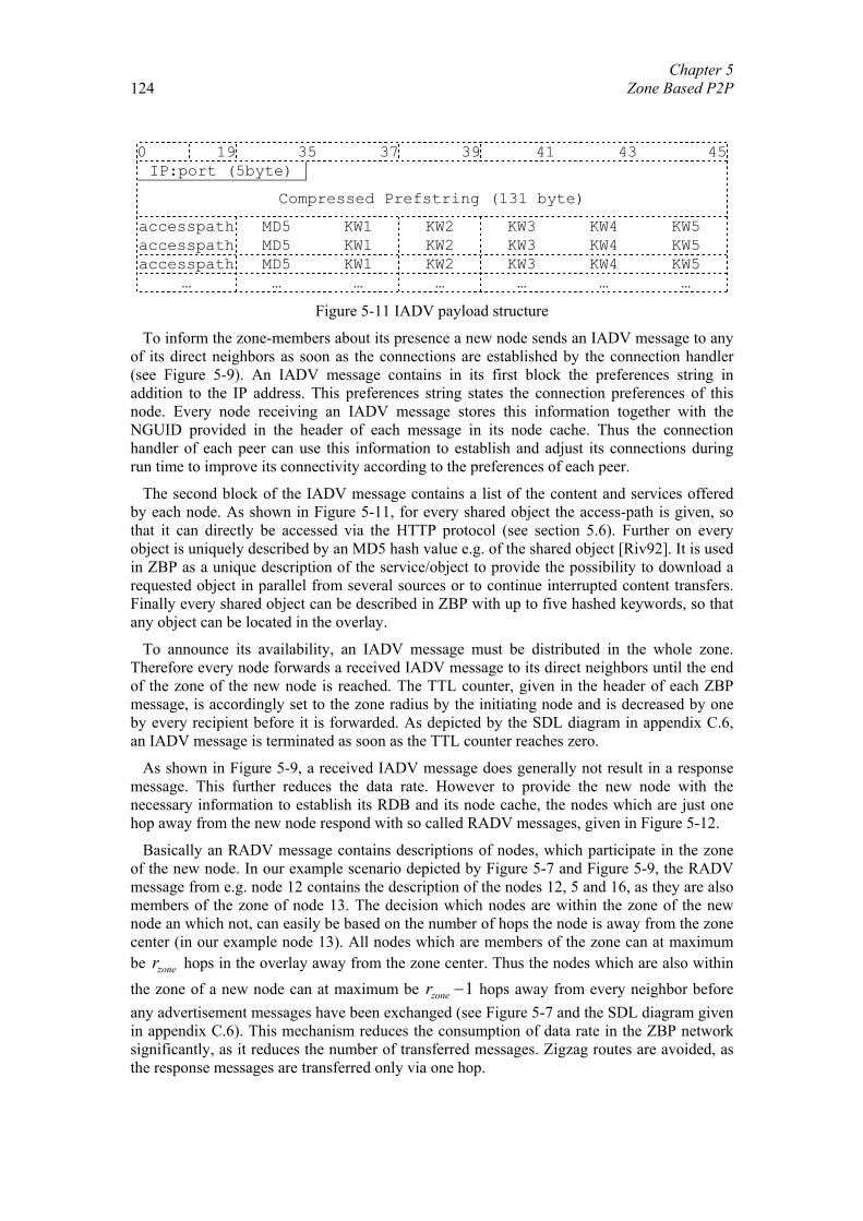
Chapter 5 Zone Based P2P
124
0 19 35 37 39 41 43 45IP:port (5byte)
Compressed Prefstring (131 byte)
accesspath MD5 KW1 KW2 KW3 KW4 KW5 accesspath MD5 KW1 KW2 KW3 KW4 KW5 accesspath MD5 KW1 KW2 KW3 KW4 KW5
… … … … … … …
Figure 5-11 IADV payload structure
To inform the zone-members about its presence a new node sends an IADV message to any of its direct neighbors as soon as the connections are established by the connection handler (see Figure 5-9). An IADV message contains in its first block the preferences string in addition to the IP address. This preferences string states the connection preferences of this node. Every node receiving an IADV message stores this information together with the NGUID provided in the header of each message in its node cache. Thus the connection handler of each peer can use this information to establish and adjust its connections during run time to improve its connectivity according to the preferences of each peer.
The second block of the IADV message contains a list of the content and services offered by each node. As shown in Figure 5-11, for every shared object the access-path is given, so that it can directly be accessed via the HTTP protocol (see section 5.6). Further on every object is uniquely described by an MD5 hash value e.g. of the shared object [Riv92]. It is used in ZBP as a unique description of the service/object to provide the possibility to download a requested object in parallel from several sources or to continue interrupted content transfers. Finally every shared object can be described in ZBP with up to five hashed keywords, so that any object can be located in the overlay.
To announce its availability, an IADV message must be distributed in the whole zone. Therefore every node forwards a received IADV message to its direct neighbors until the end of the zone of the new node is reached. The TTL counter, given in the header of each ZBP message, is accordingly set to the zone radius by the initiating node and is decreased by one by every recipient before it is forwarded. As depicted by the SDL diagram in appendix C.6, an IADV message is terminated as soon as the TTL counter reaches zero.
As shown in Figure 5-9, a received IADV message does generally not result in a response message. This further reduces the data rate. However to provide the new node with the necessary information to establish its RDB and its node cache, the nodes which are just one hop away from the new node respond with so called RADV messages, given in Figure 5-12.
Basically an RADV message contains descriptions of nodes, which participate in the zone of the new node. In our example scenario depicted by Figure 5-7 and Figure 5-9, the RADV message from e.g. node 12 contains the description of the nodes 12, 5 and 16, as they are also members of the zone of node 13. The decision which nodes are within the zone of the new node an which not, can easily be based on the number of hops the node is away from the zone center (in our example node 13). All nodes which are members of the zone can at maximum be zoner hops in the overlay away from the zone center. Thus the nodes which are also within the zone of a new node can at maximum be 1zoner − hops away from every neighbor before any advertisement messages have been exchanged (see Figure 5-7 and the SDL diagram given in appendix C.6). This mechanism reduces the consumption of data rate in the ZBP network significantly, as it reduces the number of transferred messages. Zigzag routes are avoided, as the response messages are transferred only via one hop.
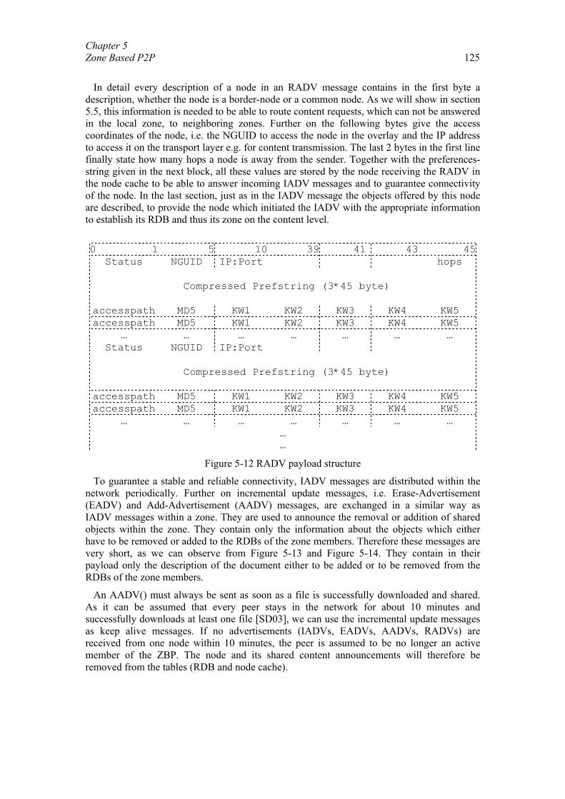
Chapter 5 Zone Based P2P 125
In detail every description of a node in an RADV message contains in the first byte a
description, whether the node is a border-node or a common node. As we will show in section 5.5, this information is needed to be able to route content requests, which can not be answered in the local zone, to neighboring zones. Further on the following bytes give the access coordinates of the node, i.e. the NGUID to access the node in the overlay and the IP address to access it on the transport layer e.g. for content transmission. The last 2 bytes in the first line finally state how many hops a node is away from the sender. Together with the preferences-string given in the next block, all these values are stored by the node receiving the RADV in the node cache to be able to answer incoming IADV messages and to guarantee connectivity of the node. In the last section, just as in the IADV message the objects offered by this node are described, to provide the node which initiated the IADV with the appropriate information to establish its RDB and thus its zone on the content level.
0 1 5 10 39 41 43 45
Status NGUID IP:Port hops
Compressed Prefstring (3*45 byte)
accesspath MD5 KW1 KW2 KW3 KW4 KW5 accesspath MD5 KW1 KW2 KW3 KW4 KW5
… … … … … … … Status NGUID IP:Port
Compressed Prefstring (3*45 byte)
accesspath MD5 KW1 KW2 KW3 KW4 KW5 accesspath MD5 KW1 KW2 KW3 KW4 KW5
… … … … … … … … …
Figure 5-12 RADV payload structure
To guarantee a stable and reliable connectivity, IADV messages are distributed within the network periodically. Further on incremental update messages, i.e. Erase-Advertisement (EADV) and Add-Advertisement (AADV) messages, are exchanged in a similar way as IADV messages within a zone. They are used to announce the removal or addition of shared objects within the zone. They contain only the information about the objects which either have to be removed or added to the RDBs of the zone members. Therefore these messages are very short, as we can observe from Figure 5-13 and Figure 5-14. They contain in their payload only the description of the document either to be added or to be removed from the RDBs of the zone members.
An AADV() must always be sent as soon as a file is successfully downloaded and shared. As it can be assumed that every peer stays in the network for about 10 minutes and successfully downloads at least one file [SD03], we can use the incremental update messages as keep alive messages. If no advertisements (IADVs, EADVs, AADVs, RADVs) are received from one node within 10 minutes, the peer is assumed to be no longer an active member of the ZBP. The node and its shared content announcements will therefore be removed from the tables (RDB and node cache).
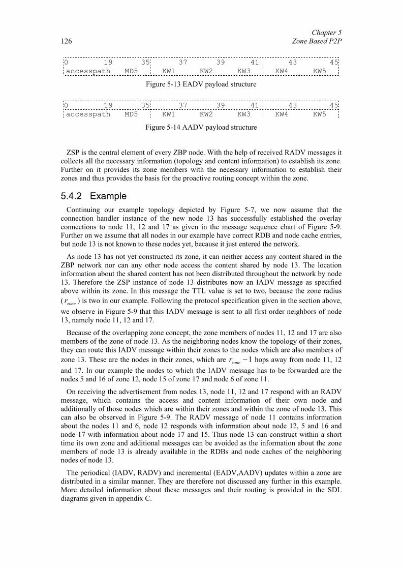
Chapter 5 Zone Based P2P
126
0 19 35 37 39 41 43 45accesspath MD5 KW1 KW2 KW3 KW4 KW5
Figure 5-13 EADV payload structure
0 19 35 37 39 41 43 45accesspath MD5 KW1 KW2 KW3 KW4 KW5
Figure 5-14 AADV payload structure
ZSP is the central element of every ZBP node. With the help of received RADV messages it collects all the necessary information (topology and content information) to establish its zone. Further on it provides its zone members with the necessary information to establish their zones and thus provides the basis for the proactive routing concept within the zone.
5.4.2 Example Continuing our example topology depicted by Figure 5-7, we now assume that the
connection handler instance of the new node 13 has successfully established the overlay connections to node 11, 12 and 17 as given in the message sequence chart of Figure 5-9. Further on we assume that all nodes in our example have correct RDB and node cache entries, but node 13 is not known to these nodes yet, because it just entered the network.
As node 13 has not yet constructed its zone, it can neither access any content shared in the ZBP network nor can any other node access the content shared by node 13. The location information about the shared content has not been distributed throughout the network by node 13. Therefore the ZSP instance of node 13 distributes now an IADV message as specified above within its zone. In this message the TTL value is set to two, because the zone radius ( zoner ) is two in our example. Following the protocol specification given in the section above, we observe in Figure 5-9 that this IADV message is sent to all first order neighbors of node 13, namely node 11, 12 and 17.
Because of the overlapping zone concept, the zone members of nodes 11, 12 and 17 are also members of the zone of node 13. As the neighboring nodes know the topology of their zones, they can route this IADV message within their zones to the nodes which are also members of zone 13. These are the nodes in their zones, which are 1zoner − hops away from node 11, 12 and 17. In our example the nodes to which the IADV message has to be forwarded are the nodes 5 and 16 of zone 12, node 15 of zone 17 and node 6 of zone 11.
On receiving the advertisement from nodes 13, node 11, 12 and 17 respond with an RADV message, which contains the access and content information of their own node and additionally of those nodes which are within their zones and within the zone of node 13. This can also be observed in Figure 5-9. The RADV message of node 11 contains information about the nodes 11 and 6, node 12 responds with information about node 12, 5 and 16 and node 17 with information about node 17 and 15. Thus node 13 can construct within a short time its own zone and additional messages can be avoided as the information about the zone members of node 13 is already available in the RDBs and node caches of the neighboring nodes of node 13.
The periodical (IADV, RADV) and incremental (EADV,AADV) updates within a zone are distributed in a similar manner. They are therefore not discussed any further in this example. More detailed information about these messages and their routing is provided in the SDL diagrams given in appendix C.
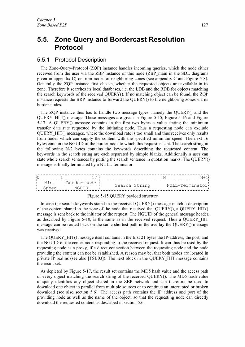
Chapter 5 Zone Based P2P 127
5.5. Zone Query and Bordercast Resolution Protocol
5.5.1 Protocol Description The Zone-Query-Protocol (ZQP) instance handles incoming queries, which the node either
received from the user via the ZBP instance of this node (ZBP_main in the SDL diagrams given in appendix C) or from nodes of neighboring zones (see appendix C and Figure 5-8). Generally the ZQP instance first checks, whether the requested objects are available in its zone. Therefore it searches its local databases, i.e. the LDB and the RDB for objects matching the search keywords of the received QUERY(). If no matching object can be found, the ZQP instance requests the BRP instance to forward the QUERY() to the neighboring zones via its border-nodes.
The ZQP instance thus has to handle two message types, namely the QUERY() and the QUERY_HIT() message. These messages are given in Figure 5-15, Figure 5-16 and Figure 5-17. A QUERY() message contains in the first two bytes a value stating the minimum transfer data rate requested by the initiating node. Thus a requesting node can exclude QUERY_HIT() messages, where the download rate is too small and thus receives only results from nodes which can supply the content with the specified minimum speed. The next 16 bytes contain the NGUID of the border-node to which this request is sent. The search string in the following N-2 bytes contains the keywords describing the requested content. The keywords in the search string are each separated by simple blanks. Additionally a user can state whole search sentences by putting the search sentence in quotation marks. The QUERY() message is finally terminated by a NULL-terminator.
0 1 17 N N+1
Min. Speed
Border node NGUID Search String NULL-Terminator
Figure 5-15 QUERY payload structure
In case the search keywords stated in the received QUERY() message match a description of the content shared in the zone of the node that received that QUERY(), a QUERY_HIT() message is sent back to the initiator of the request. The NGUID of the general message header, as described by Figure 5-10, is the same as in the received request. Thus a QUERY_HIT message can be routed back on the same shortest path in the overlay the QUERY() message was received.
The QUERY_HIT() message itself contains in the first 21 bytes the IP-address, the port, and the NGUID of the center-node responding to the received request. It can thus be used by the requesting node as a proxy, if a direct connection between the requesting node and the node providing the content can not be established. A reason may be, that both nodes are located in private IP realms (see also [TSB03]). The next block in the QUERY_HIT message contains the result set.
As depicted by Figure 5-17, the result set contains the MD5 hash value and the access path of every object matching the search string of the received QUERY(). The MD5 hash value uniquely identifies any object shared in the ZBP network and can therefore be used to download one object in parallel from multiple sources or to continue an interrupted or broken download (see also section 5.6). The access path contains the IP address and port of the providing node as well as the name of the object, so that the requesting node can directly download the requested content as described in section 5.6.
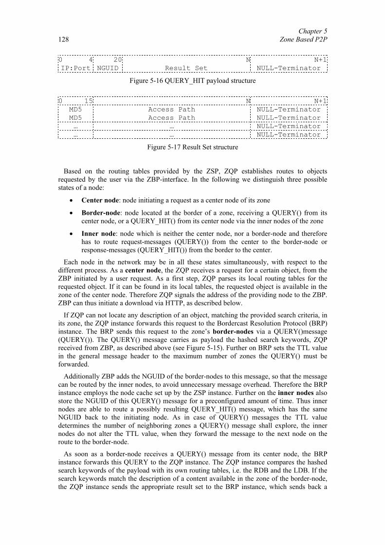
Chapter 5 Zone Based P2P
128
0 4 20 N N+1IP:Port NGUID Result Set NULL-Terminator
Figure 5-16 QUERY_HIT payload structure
0 15 N N+1
MD5 Access Path NULL-Terminator MD5 Access Path NULL-Terminator … … NULL-Terminator … … NULL-Terminator
Figure 5-17 Result Set structure
Based on the routing tables provided by the ZSP, ZQP establishes routes to objects requested by the user via the ZBP-interface. In the following we distinguish three possible states of a node:
• Center node: node initiating a request as a center node of its zone
• Border-node: node located at the border of a zone, receiving a QUERY() from its center node, or a QUERY_HIT() from its center node via the inner nodes of the zone
• Inner node: node which is neither the center node, nor a border-node and therefore has to route request-messages (QUERY()) from the center to the border-node or response-messages (QUERY_HIT()) from the border to the center.
Each node in the network may be in all these states simultaneously, with respect to the different process. As a center node, the ZQP receives a request for a certain object, from the ZBP initiated by a user request. As a first step, ZQP parses its local routing tables for the requested object. If it can be found in its local tables, the requested object is available in the zone of the center node. Therefore ZQP signals the address of the providing node to the ZBP. ZBP can thus initiate a download via HTTP, as described below.
If ZQP can not locate any description of an object, matching the provided search criteria, in its zone, the ZQP instance forwards this request to the Bordercast Resolution Protocol (BRP) instance. The BRP sends this request to the zone’s border-nodes via a QUERY()message (QUERY()). The QUERY() message carries as payload the hashed search keywords, ZQP received from ZBP, as described above (see Figure 5-15). Further on BRP sets the TTL value in the general message header to the maximum number of zones the QUERY() must be forwarded.
Additionally ZBP adds the NGUID of the border-nodes to this message, so that the message can be routed by the inner nodes, to avoid unnecessary message overhead. Therefore the BRP instance employs the node cache set up by the ZSP instance. Further on the inner nodes also store the NGUID of this QUERY() message for a preconfigured amount of time. Thus inner nodes are able to route a possibly resulting QUERY_HIT() message, which has the same NGUID back to the initiating node. As in case of QUERY() messages the TTL value determines the number of neighboring zones a QUERY() message shall explore, the inner nodes do not alter the TTL value, when they forward the message to the next node on the route to the border-node.
As soon as a border-node receives a QUERY() message from its center node, the BRP instance forwards this QUERY to the ZQP instance. The ZQP instance compares the hashed search keywords of the payload with its own routing tables, i.e. the RDB and the LDB. If the search keywords match the description of a content available in the zone of the border-node, the ZQP instance sends the appropriate result set to the BRP instance, which sends back a
Chapter 5 Zone Based P2P 129
QUERY_HIT()- message (see Figure 5-16 and Figure 5-17) on the same path the QUERY() was received. If the ZQP instance can not find a matching record in its zone a QUERY() with the same keywords, a TTL value decreased by one and the received NGUID are transferred to the BRP instance. The BRP instance then checks the TTL value and only if it is larger than 0 it routes this message further on, as described above, to its own border-nodes.
When the BRP instance, which forwarded the previously received QUERY(), receives a QUERY_HIT(), it first checks whether this QUERY_HIT() message was initiated by an own QUERY() message. Therefore it analyses the NGUID field given in the general message header. If the NGUID of the QUERY_HIT message is the same as its own, the result-set is forwarded to its own ZQP instance. Otherwise it is forwarded to the border-node from which it received the initial QUERY() message. Upon further user interaction, the ZBP instance can initiate a download via HTTP, which is described in further detail in section 5.6.
5.5.2 Example Going on with our earlier example for which the overlay topology is described in Figure 5-7,
we assume that node 13 successfully connected to the ZBP network (see Figure 5-9 and section 5.4.2). Further on we assume, that node 13 constructed its zone completely and updated the node caches, the RDBs and the LDBs of its zone members, as described in section 5.4.2 and by the message sequence chart given in Figure 5-9. For this the ZSP and the connection handler have been used.
However to also explain the concept of the ZBP and the BRP, we now assume that node 13 searches for certain content A. This content A could e.g. be Beethoven's symphony number 5 or the user profile of a specific user, stating its SIP address, so that node 13 can establish a voice over IP communication to this user. Let us further on assume that in this example the content A, node 13 is looking for, is only provided by node 20.
After the ZBP instance received this request for content A in a first step the ZBP instance of node 13 searches its local databases, i.e. its LDB and its RDB for a content matching the keywords. However, as the content matching these keywords is only provided by node 20, which is not part of zone 13, this lookup fails. Therefore the ZSP instance has to proceed and transfer this search request to its BRP instance to forward it to the neighboring zones of node 13. These are in our example zones 6, 5, 15 and 16, as indicated by Figure 5-7. To these nodes the BRP instance of node 13 sends a QUERY() message set up by its own NGUID, a TTL value set in this example to 1, the NGUIDs of its border-nodes (6, 5, 15, 16) and the search string which holds the keywords describing content A.
Node 11, 12 and 17 receive this request and route it as inner nodes directly to the responsible border-node, i.e. node 11 to node 6, node 17 to node 15 and node 12 to nodes 5 and 16. As node 20 is a member of zone 6, node 6 in the role of a border-node can answer the received QUERY(). As the TTL of the QUERY() message is set to 1, no border-node forwards this QUERY() any further. Only node 6 sends back a QUERY_HIT() message on the same path in the overlay, via which it received the QUERY() message. Therefore it first sends this message, which carries the same NGUID as the QUERY() message to the inner node 11. Node 11 is able to route it then to node 13, because node 11 stored the NGUID and the node from which it received the QUERY() message long enough.
Upon receiving the QUERY_HIT() message, the BRP instance of node 13 forwards it to its ZSP instance, which then forwards the result to its ZBP instance to display it at the user interface. The user can then initiate a download of the requested content via its HTTP instance, which is described in detail in the following section 5.6.
Chapter 5 Zone Based P2P
130
5.6. Content Transmission To be able to exchange the content located via the ZQP and the BQP instance, every ZBP
node has to implement server as well as client functionalities. Due to the wide area of options and methods offered by the Hypertext Transfer Protocol (HTTP) [FGFM99], the content transfer entity of every ZBP node is based on HTTP (see Figure 5-8 and appendix C).
HTTP is a simple, general stateless protocol located in the application layer of the OSI-model. Because of its general specification and implementation it is also often used in name server systems [KR01] and other distributed systems, like file sharing networks [KMa02]. HTTP is specified in version 1.1 as RFC2616 [FGFM99].
As HTTP is a very simple protocol it only employs two kinds of messages, i.e. request and resulting response messages. Further on it also only specifies two communication endpoints, namely a client, initiating a request as the content/object/service requestor, and a server responding to this request as the content/object/service provider. If a client sends a request to a server it thus expects a response, containing either the requested content or an error message from the server. A detailed description of all of these methods can be found in [FGFM99].
Generally ZBP is conformant to HTTP. Only in some cases ZBP uses additional functionalities like we employ PHP [LT02] to be able to resolve different kinds of content requests without having to provide an absolute path in each content request or use the content range header to provide possibilities for parallel downloads.
Most higher programming languages already contain an implementation of HTTP. We therefore provide in this section only a description of the used extensions. ZBP extends HTTP to handle the absolute path requirement of a HTTP request and the problem of data transfer interruptions. Any other behavior of the HTTP server and client is described in RFC 2616.
In HTTP it is necessary to provide the absolute path to the requested object in the abs_path parameter of a HTTP request. If the path is wrong, the object, although it may be offered by the server, can not be downloaded. The server only replies with an error message, instead of the requested content. However, in ZBP the requestor is provided in a QUERY_HIT message only with a filename but not with the whole access path. Thus we are able to reduce the amount of necessary signaling data, but it is therefore necessary to arrange the content on a HTTP server according to the structure described below. Otherwise the content can not be exchanged, as a HTTP server does not specify any search or data base functionalities.
The directory structure starts at the document root of the HTTP server instance of a ZBP node with a description of all shared data in the profiles.xml file (see Figure 5-19). Additionally the root directory includes a ZBP_DOWNLOAD.php file to be able to handle requests, which provide instead of the object name, only the MD5 digest of the requested file. This is necessary, as explained below, to continue interrupted file transfers.
In the following data folder every object shared by this node is stored with the same filename as stated in the parameter object_name of each xml description, stored in the profiles.xml. This name is thus also the name which was provided in the QUERY_HIT message or an IADV message. Thus any ZBP node can access these data even if it can not provide the full path in the HTTP request.
Chapter 5 Zone Based P2P 131
document_root
profiles.xml
data
<object_name> <file>
<object_name> <file>
<object_name> <file>
<object_name> <file>
…
ZBP_DOWNLOAD.php
Figure 5-18 Directory structure of a ZBP server instance
The xml-file profiles.xml, as given in Figure 5-19, can be used as the basis for the local database (LDB), as it holds all the information about the shared content. In simple implementations it can even be used as the local database. If more efficient database approaches are implemented on a ZBP node, e.g. an SQL database, the XML-file can be used as database input. However parsing the XML file with an average of 100 entries should generally be feasible with a reasonable performance.
Figure 5-19 Syntax of the profiles.xml file
<?xml version="1.0"?> <!DOCTYPE ZBP:object_profiles> <ZBP:object_profiles>
<ZBP:object_profile> <keyword> keyword_1 </keyword> <keyword> keyword_2 </keyword> <keyword> keyword_3 </keyword> … <object_name> object_name </object_name> <full_path> object_access_path </full_path> <MD5> md5_checksum </MD5> </ZBP:object_profile> <ZBP:object_profile>
…
</ZBP:object_profile> … …
</ZBP:object profiles>
Chapter 5 Zone Based P2P
132
ZBP also has to be able to handle the dynamism of the participants in a peer-to-peer environment, i.e. frequent and spontaneous joins and leaves of peers. Therefore the client HTTP instance of a ZBP node has to be able to solve connection breakdowns during a file transfer. It would not be sensible to restart every interrupted download from the beginning from another peer, providing a replica of the requested file, because a significant amount may already be downloaded from the first peer before the interruption.
Most probably, nodes also holding the requested content are already known, as the node received QUERY_HIT message from the nodes offering replicas of the requested file upon its first QUERY. If no further sources are known to the requesting node it has to send out a new QUERY message with the MD5-digest of the requested file.
To continue the download from another peer, ZBP uses the content range header option specified in HTTP 1.1, the syntax of which is given in Figure 5-20.
Figure 5-20 Syntax of the content range option for a HTTP request in ZBP
If for example the download of a 7654 byte large object file print_service.xml interrupted after 1023 bytes, the download of this object can be continued with the following HTTP request:
Figure 5-21 Syntax of a HTTP requesting including the content range header option
To guarantee, that the client continues the download of the requested file and not of a different file which has only the same name, ZBP can also employ the MD5-digest stated in the HTTP response in ZBP. However, as the files are only available by their name and not by their MD5 digest, every ZBP peer should also provide the possibility to execute script languages, as PHP or CGI. In our implementation we employ PHP, as it is widely used in web applications.
As indicated by Figure 5-18, every peer offers a ZBP_DOWNLOAD.php in its root directory. Instead of requesting the file itself, the requesting peer has to request the file ZBP_DOWNLOAD.php together with a parameter stating the MD5-digest of the requested file. The file ZBP_DOWNLOAD.php contains a script, which searches either the file profiles.xml or the employed database for the MD5 digest stated in the received request. Thus the requesting ZBP peer can continue the download of exactly the same file which has been interrupted. Further on this PHP extension of the HTTP instance, can also be used to download files which are only identified by their keywords. Together with the content range header option, ZBP also provides the possibility to download one object in parallel from multiple sources.
Figure 5-22 Syntax of a HTTP request for a file identified by its MD5-digest
GET ZBP_DOWLOAD.php?md5=<md5-digest> HTTP/1.1\r\n Content-Range: bytes 1023-7653/7654\r\n
GET data/print.xml HTTP/1.1\r\n Content-Range: bytes 1023-7653/7654\r\n
Content-Range = "Content-Range" ":" content-range-spec content-range-spec = byte-content-range-spec byte-content-range-spec = bytes-unit SP
byte-range-resp-spec "/" ( instance-length | "*" )
byte-range-resp-spec = (first-byte-pos "-" last-byte-pos)
| "*" instance-length = 1*DIGIT
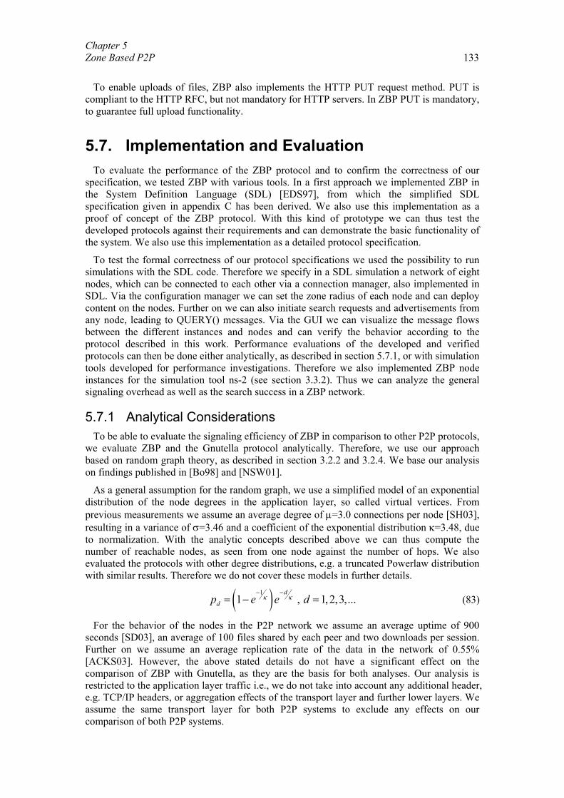
Chapter 5 Zone Based P2P 133
To enable uploads of files, ZBP also implements the HTTP PUT request method. PUT is
compliant to the HTTP RFC, but not mandatory for HTTP servers. In ZBP PUT is mandatory, to guarantee full upload functionality.
5.7. Implementation and Evaluation To evaluate the performance of the ZBP protocol and to confirm the correctness of our
specification, we tested ZBP with various tools. In a first approach we implemented ZBP in the System Definition Language (SDL) [EDS97], from which the simplified SDL specification given in appendix C has been derived. We also use this implementation as a proof of concept of the ZBP protocol. With this kind of prototype we can thus test the developed protocols against their requirements and can demonstrate the basic functionality of the system. We also use this implementation as a detailed protocol specification.
To test the formal correctness of our protocol specifications we used the possibility to run simulations with the SDL code. Therefore we specify in a SDL simulation a network of eight nodes, which can be connected to each other via a connection manager, also implemented in SDL. Via the configuration manager we can set the zone radius of each node and can deploy content on the nodes. Further on we can also initiate search requests and advertisements from any node, leading to QUERY() messages. Via the GUI we can visualize the message flows between the different instances and nodes and can verify the behavior according to the protocol described in this work. Performance evaluations of the developed and verified protocols can then be done either analytically, as described in section 5.7.1, or with simulation tools developed for performance investigations. Therefore we also implemented ZBP node instances for the simulation tool ns-2 (see section 3.3.2). Thus we can analyze the general signaling overhead as well as the search success in a ZBP network.
5.7.1 Analytical Considerations To be able to evaluate the signaling efficiency of ZBP in comparison to other P2P protocols,
we evaluate ZBP and the Gnutella protocol analytically. Therefore, we use our approach based on random graph theory, as described in section 3.2.2 and 3.2.4. We base our analysis on findings published in [Bo98] and [NSW01].
As a general assumption for the random graph, we use a simplified model of an exponential distribution of the node degrees in the application layer, so called virtual vertices. From previous measurements we assume an average degree of µ=3.0 connections per node [SH03], resulting in a variance of σ=3.46 and a coefficient of the exponential distribution κ=3.48, due to normalization. With the analytic concepts described above we can thus compute the number of reachable nodes, as seen from one node against the number of hops. We also evaluated the protocols with other degree distributions, e.g. a truncated Powerlaw distribution with similar results. Therefore we do not cover these models in further details.
( )11 , 1,2,3,...
d
dp e e dκ κ−−
= − = (83)
For the behavior of the nodes in the P2P network we assume an average uptime of 900 seconds [SD03], an average of 100 files shared by each peer and two downloads per session. Further on we assume an average replication rate of the data in the network of 0.55% [ACKS03]. However, the above stated details do not have a significant effect on the comparison of ZBP with Gnutella, as they are the basis for both analyses. Our analysis is restricted to the application layer traffic i.e., we do not take into account any additional header, e.g. TCP/IP headers, or aggregation effects of the transport layer and further lower layers. We assume the same transport layer for both P2P systems to exclude any effects on our comparison of both P2P systems.
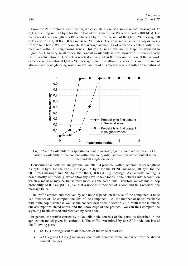
Chapter 5 Zone Based P2P
134
From the ZBP protocol specification, we calculate a size of a single update message of 37 bytes, resulting in 3.7 kbyte for the initial advertisement (IADV()) of a node (100 files). For the general header length of ZBP we have 23 bytes, for the size of the QUERY() message 80 bytes and for a QUERY_HIT() message 200 bytes. The zone radius in our analysis varies from 2 to 7 hops. We thus compute the average availability of a specific content within the zone and within all neighboring zones. This results in an availability graph, as depicted in Figure 5-23. In very small zones, the content availability is low. However, it increases very fast to a value close to 1, which is reached already when the zone-radius is 4. If the network can cope with additional QUERY() messages, and thus allows the node to search for content also in directly neighboring zones, an availability of 1 is already reached with a zone radius of 2.
0
0,1
0,2
0,3
0,4
0,5
0,6
0,7
0,8
0,9
1
0 2 4 6 8hops=zone radius
cont
ent a
vaila
bilit
y
Probability to find contentin the local zoneProbability to find contentin neighbor zones
Figure 5-23 Availability of a specific content in average, against zone radius for κ=3.48
(dashed: availability of the content within the zone, solid: availability of the content in the inner and all neighbor-zones)
Concerning Gnutella we analyze the Gnutella 0.4 protocol, with a general header length of 23 byte, 0 byte for the PING message, 15 byte for the PONG message, 80 byte for the QUERY() message and 200 byte for the QUERY-HIT() message. As Gnutella routing is based mostly on flooding, we additionally have to take loops in the network into account, on which a message may be transmitted twice via the same link. Therefore we assume a loop probability of 0.0064 [SH03], i.e. that a node is a member of a loop and thus receives one message twice.
The traffic emitted and received by one node depends on the size of the component a node is a member of. To compute the size of the component, i.e., the number of nodes reachable within the hop distance h, we use the concept described in section 3.2.2. With these numbers, our assumptions stated above and the knowledge of the protocol, we can thus compute the signaling traffic caused and received by each node.
In general the traffic caused by a Gnutella node consists of the parts, as described in the application model given in section 4.4. The traffic transmitted by one ZBP node consists of the following parts:
• IADV() message sent to all members of the zone at start up
• AADV() and EADV() messages sent to all members of the zone whenever the shared content changes
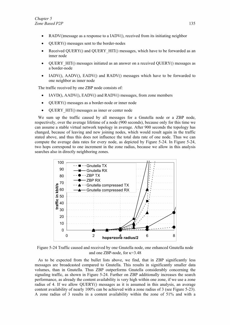
Chapter 5 Zone Based P2P 135
• RADV()message as a response to a IADV(), received from its initiating neighbor
• QUERY() messages sent to the border-nodes
• Received QUERY() and QUERY_HIT() messages, which have to be forwarded as an inner node
• QUERY_HIT() messages initiated as an answer on a received QUERY() messages as a border-node
• IADV(), AADV(), EADV() and RADV() messages which have to be forwarded to one neighbor as inner node
The traffic received by one ZBP node consists of:
• IAVD(), AADV(), EADV() and RADV() messages, from zone members
• QUERY() messages as a border-node or inner node
• QUERY_HIT() messages as inner or center node
We sum up the traffic caused by all messages for a Gnutella node or a ZBP node, respectively, over the average lifetime of a node (900 seconds), because only for this time we can assume a stable virtual network topology in average. After 900 seconds the topology has changed, because of leaving and new joining nodes, which would result again in the traffic stated above, and thus this does not influence the total data rate of one node. Thus we can compute the average data rates for every node, as depicted by Figure 5-24. In Figure 5-24, two hops correspond to one increment in the zone radius, because we allow in this analysis searches also in directly neighboring zones.
0
10
20
30
40
50
60
70
80
90
100
0 2 4 6 8hops=zone radius/2
traf
fic in
kbi
t/s
Gnutella TXGnutella RXZBP TXZBP RXGnutella compressed TXGnutella compressed RX
Figure 5-24 Traffic caused and received by one Gnutella node, one enhanced Gnutella node
and one ZBP-node, for κ=3.48
As to be expected from the bullet lists above, we find, that in ZBP significantly less messages are broadcasted compared to Gnutella. This results in significantly smaller data volumes, than in Gnutella. Thus ZBP outperforms Gnutella considerably concerning the signaling traffic, as shown in Figure 5-24. Further on ZBP additionally increases the search performance, as already the content availability is very high within one zone, if we use a zone radius of 4. If we allow QUERY() messages as it is assumed in this analysis, an average content availability of nearly 100% can be achieved with a zone radius of 3 (see Figure 5-23). A zone radius of 3 results in a content availability within the zone of 51% and with a
Chapter 5 Zone Based P2P
136
QUERY() of 100%. This means that more than 50% of all requests of the user can be satisfied instantly, as a providing source is already in the nodes local tables, generated from the received advertisements. In case the content is not available in its zone, the content can be located with a hop-by-hop, routable QUERY() message sent to its border-nodes.
Concerning Gnutella, it is always necessary to broadcast a QUERY() across at least 5 hops, to be sure to find the content, as indicated by the dashed line in Figure 5-23 ( i.e. zone radius one corresponds to the availability in Gnutella). Broadcasting these messages, which is completely avoided in ZBP, therefore results in notably higher data volumes per node on the receiving as well as on the transmitting part. Even if we compare ZBP to hierarchical approaches, like Gnutella 0.6, ZBP is still better in its traffic behavior. In Gnutella 0.6 a Superpeer with 25 leafnodes has a send data rate of 169.96 kbit/s and a receive data rate of 150.54 kbit/s, whereas a leafnode has a transmit data rate of 1.07 kbit/s and receive data rate of 1.20 kbit/s (see section 4.3.1 and [SD03]). The average transmit and receive data rates of a Gnutella 0.6 node, thus result in 7.56 kbit/s and 6.94 kbit/s respectively, if we assume 25 leafnodes being connected to one Superpeer. In contrast, a ZBP node, with a zone radius of 3 has an average transmit data rate of 0.89 kbit/s and an average receive data rate of 4.45 kbit/s. These data-rates are significantly smaller than those of an average Gnutella 0.6 node, and additionally ZBP avoids nodes with a high load, like the Superpeers in the Gnutella 0.6 network. Further on, the content is available instantly, i.e., in ZBP it is, depending on the zone radius, often not necessary to query the network and to wait until the network responds with according QUERY_Hit() messages.
To verify that the results of ZBP are not only based on reduced message sizes, we additionally implemented a Gnutella Protocol which employs string compression for the signaling messages [Sal97]. Thus we can reduce in general the overhead by an average of 40% to 50%. We therefore assume a common compression factor of 0.6, for the enhanced Gnutella Protocol, depicted by the dash-dot line in Figure 5-24. We can observe, that this compression decreases the signaling traffic notably, but it can not reach the performance of ZBP.
5.7.2 Simulative Analysis To validate the results of our theoretical analysis, we performed simulations for Gnutella
and ZBP, including also the transport and the network layer (see section 3.3.2). The simulative performance evaluation is based on the ns-2 simulator.
As the ZBP protocol stack fits nicely to the OSI-model, we keep a similar structure in the ns-2 implementation. The implementation of the ZBP protocol resides in the application layer of ns-2. With the help of a shim layer, the application utilizes an adapted TCP agent, as depicted by Figure 5-25. The adaptation of the TCP agent is necessary, to provide the ZBP nodes with an efficient possibility to maintain several TCP connections in parallel with just one agent. The TCP agent itself is then based on existing node classes. A detailed overview about the implementation and a documentation of the code is provided in [Mad04].
ZBP-Application
Adapted TCP-Agent
Node-Class
ZBP-Application
Adapted TCP-Agent
Node-Class
Figure 5-25 Implementation structure of ZBP peers
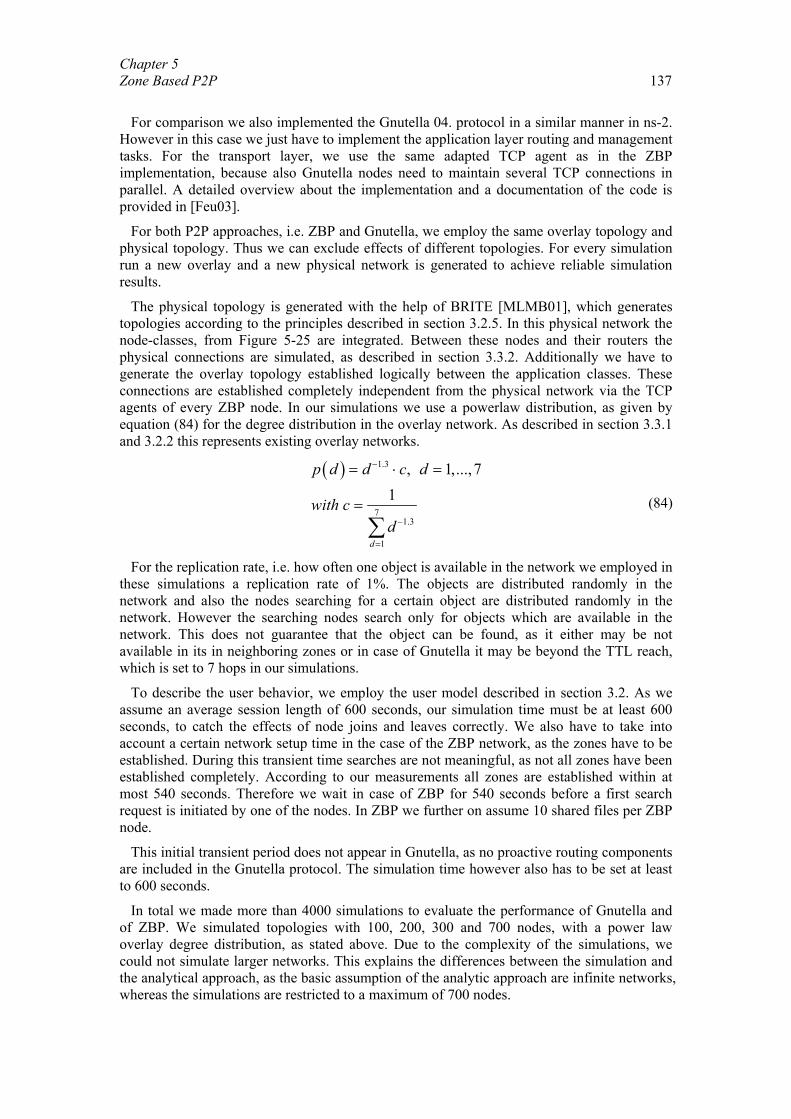
Chapter 5 Zone Based P2P 137
For comparison we also implemented the Gnutella 04. protocol in a similar manner in ns-2.
However in this case we just have to implement the application layer routing and management tasks. For the transport layer, we use the same adapted TCP agent as in the ZBP implementation, because also Gnutella nodes need to maintain several TCP connections in parallel. A detailed overview about the implementation and a documentation of the code is provided in [Feu03].
For both P2P approaches, i.e. ZBP and Gnutella, we employ the same overlay topology and physical topology. Thus we can exclude effects of different topologies. For every simulation run a new overlay and a new physical network is generated to achieve reliable simulation results.
The physical topology is generated with the help of BRITE [MLMB01], which generates topologies according to the principles described in section 3.2.5. In this physical network the node-classes, from Figure 5-25 are integrated. Between these nodes and their routers the physical connections are simulated, as described in section 3.3.2. Additionally we have to generate the overlay topology established logically between the application classes. These connections are established completely independent from the physical network via the TCP agents of every ZBP node. In our simulations we use a powerlaw distribution, as given by equation (84) for the degree distribution in the overlay network. As described in section 3.3.1 and 3.2.2 this represents existing overlay networks.
( ) 1.3
71.3
1
, 1,...,71
d
p d d c d
with cd
−
−
=
= ⋅ =
=
∑ (84)
For the replication rate, i.e. how often one object is available in the network we employed in these simulations a replication rate of 1%. The objects are distributed randomly in the network and also the nodes searching for a certain object are distributed randomly in the network. However the searching nodes search only for objects which are available in the network. This does not guarantee that the object can be found, as it either may be not available in its in neighboring zones or in case of Gnutella it may be beyond the TTL reach, which is set to 7 hops in our simulations.
To describe the user behavior, we employ the user model described in section 3.2. As we assume an average session length of 600 seconds, our simulation time must be at least 600 seconds, to catch the effects of node joins and leaves correctly. We also have to take into account a certain network setup time in the case of the ZBP network, as the zones have to be established. During this transient time searches are not meaningful, as not all zones have been established completely. According to our measurements all zones are established within at most 540 seconds. Therefore we wait in case of ZBP for 540 seconds before a first search request is initiated by one of the nodes. In ZBP we further on assume 10 shared files per ZBP node.
This initial transient period does not appear in Gnutella, as no proactive routing components are included in the Gnutella protocol. The simulation time however also has to be set at least to 600 seconds.
In total we made more than 4000 simulations to evaluate the performance of Gnutella and of ZBP. We simulated topologies with 100, 200, 300 and 700 nodes, with a power law overlay degree distribution, as stated above. Due to the complexity of the simulations, we could not simulate larger networks. This explains the differences between the simulation and the analytical approach, as the basic assumption of the analytic approach are infinite networks, whereas the simulations are restricted to a maximum of 700 nodes.
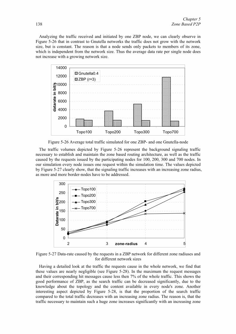
Chapter 5 Zone Based P2P
138
Analyzing the traffic received and initiated by one ZBP node, we can clearly observe in Figure 5-26 that in contrast to Gnutella networks the traffic does not grow with the network size, but is constant. The reason is that a node sends only packets to members of its zone, which is independent from the network size. Thus the average data rate per single node does not increase with a growing network size.
0
2000
4000
6000
8000
10000
12000
14000
Topo100 Topo200 Topo300 Topo700
data
rate
in b
it/s
Gnutella0.4ZBP (r=3)
Figure 5-26 Average total traffic simulated for one ZBP- and one Gnutella-node
The traffic volumes depicted by Figure 5-26 represent the background signaling traffic necessary to establish and maintain the zone based routing architecture, as well as the traffic caused by the requests issued by the participating nodes for 100, 200, 300 and 700 nodes. In our simulation every node issues one request within the simulation time. The values depicted by Figure 5-27 clearly show, that the signaling traffic increases with an increasing zone radius, as more and more border-nodes have to be addressed.
0
50
100
150
200
250
300
2 3 4 5zone-radius
Dat
arat
e in
bit/
s
Topo100Topo200Topo300Topo700
Figure 5-27 Data-rate caused by the requests in a ZBP network for different zone radiuses and
for different network sizes
Having a detailed look at the traffic the requests cause in the whole network, we find that these values are nearly negligible (see Figure 5-28). In the maximum the request messages and their corresponding hit messages cause less then 7% of the whole traffic. This shows the good performance of ZBP, as the search traffic can be decreased significantly, due to the knowledge about the topology and the content available in every node's zone. Another interesting aspect depicted by Figure 5-28, is that the proportion of the search traffic compared to the total traffic decreases with an increasing zone radius. The reason is, that the traffic necessary to maintain such a huge zone increases significantly with an increasing zone
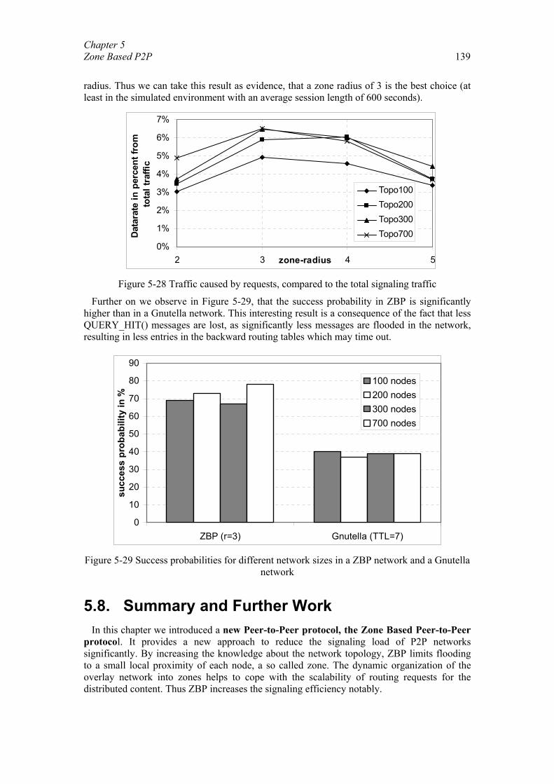
Chapter 5 Zone Based P2P 139
radius. Thus we can take this result as evidence, that a zone radius of 3 is the best choice (at least in the simulated environment with an average session length of 600 seconds).
0%
1%
2%
3%
4%
5%
6%
7%
2 3 4 5zone-radius
Dat
arat
e in
per
cent
from
to
tal t
raffi
c
Topo100Topo200Topo300Topo700
Figure 5-28 Traffic caused by requests, compared to the total signaling traffic
Further on we observe in Figure 5-29, that the success probability in ZBP is significantly higher than in a Gnutella network. This interesting result is a consequence of the fact that less QUERY_HIT() messages are lost, as significantly less messages are flooded in the network, resulting in less entries in the backward routing tables which may time out.
0
10
20
30
40
50
60
70
80
90
ZBP (r=3) Gnutella (TTL=7)
succ
ess
prob
abili
ty in
%
100 nodes200 nodes300 nodes700 nodes
Figure 5-29 Success probabilities for different network sizes in a ZBP network and a Gnutella
network
5.8. Summary and Further Work In this chapter we introduced a new Peer-to-Peer protocol, the Zone Based Peer-to-Peer
protocol. It provides a new approach to reduce the signaling load of P2P networks significantly. By increasing the knowledge about the network topology, ZBP limits flooding to a small local proximity of each node, a so called zone. The dynamic organization of the overlay network into zones helps to cope with the scalability of routing requests for the distributed content. Thus ZBP increases the signaling efficiency notably.
Chapter 5 Zone Based P2P
140
We provided in this chapter as our first contribution an analysis of the optimal representation of shared objects in proactive and hybrid Peer-to-Peer routing approaches. As outlined in section 5.2, in proactive Peer-to-Peer networks it is necessary to distribute the information about the shared/offered objects (routing indexes) to other nodes. In Napster the information about the shared content has to be transmitted to the Napster server, in Gnutella 0.6 to the Superpeers, and in ZBP to the members of the zone. Therefore we compared in our mathematical analysis Bloom filters, often proposed to be used in Peer-to-Peer networks [BM02, Mit01] and simple hash index arrays. We could show analytically that even compressed Bloom filters are by far not as efficient as simple hash index arrays. The reason therefore is, that in P2P networks the nodes generally share only a small percentage of all objects available in the network. This characteristic of P2P networks can be employed by simple hash indexes, the size of which correlates linearly with the number of locally shared objects. We thus use in ZBP enhanced hash index arrays to distribute the routing indexes within a zone.
As a second contribution of this chapter we introduce a new hybrid P2P protocol, the ZBP protocol. We provide a detailed description of the ZBP protocol stack, which spans the application layer to the transport layer. The main characteristic of ZBP is the new concept of overlapping and dynamic zones. The overlapping zones guarantee a smooth transition between the zones and thus also an even distribution of traffic and routing load across all nodes. Thus no single nodes as the Napster server in Napster or the Superpeers in Gnutella 0.6, or the rendezvous peers in JXTA, have to cope with a higher load.
ZBP limits flooding strictly to the distribution of announcement messages within a zone. All other messages (requests and responses) can be routed within a zone and if necessary between the center node and the border-nodes. Therefore ZBP employs the information about the topology of the network within its zone, which every node can extract from the received messages.
ZBP allows instantaneous access to shared resources within its zone, as all information of a zone is available on the center node of that zone. Every peer is the center node of its zone. Especially in conjunction with JXTA, the zone concept of ZBP is expected to be very useful, to support the grouping mechanism of JXTA.
Further on ZBP still offers the possibility to connect the participating nodes in any desired way to each other. This also solves the problem of private IP realms, which may become a severe problem in structured P2P networks like Chord [ESKZ04]. Further on, through the concept of zones, the routing overhead in ZBP scales well, even in networks with high churn rates, which is still a problem in structured P2P networks [RGRK04, XMH03].
An important role in the protocol stack of ZBP is taken by the introduction of a connection handler, which is a further contribution in this chapter. This new concept can be used in ZBP as a kind of cross layer communication channel between the application and the physical layer. Thus the zones, establishing the overlay routing network of ZBP, can be adapted to the underlying physical network or interests shared by the participating users, although the overlay routing layer remains completely separated from the physical layer. This allows the developer of new P2P applications to establish the zones according to preset but dynamically adjustable preferences. In contrast to DHT based P2P networks, ZBP offers therefore the possibility to establish interest groups, which additionally increases the probability to reach requested content within a few hops [WHAT04]. Every ZBP node can thus establish its connections according to criteria and parameters from the application layer as well as from the physical layer.
To provide ZBP nodes with the necessary methods for content transmission, we use HTTP as a basis in ZBP. However to allow reliable and fast downloads with little overhead from the ZBP network, we describe as another contribution in this chapter extensions of HTTP to meet the requirements of a dynamic overlay network. Thus we use the content range header
Chapter 5 Zone Based P2P 141
option to provide ZBP nodes with the possibility to continue interrupted downloads, e.g. due to node leaves (high churn rate in P2P), seamlessly from other nodes, offering a replica of the requested file. Further on the temporary directory structure established on every ZBP node, allows requesting nodes to download content without having to state the full path in the HTTP request, which saves data rate. With the additional employment of PHP interpreters, ZBP nodes can download content by only stating the MD5 digest or keywords describing the requested file. This provides ZBP nodes with the possibility to efficiently download a requested content in parallel from multiple sources.
As a proof of concept we provide in this chapter an implementation of ZBP in the System Definition Language (SDL). A simplified version of all SDL diagrams describing ZBP is provided in appendix C. Besides verifying the correctness of the developed protocols in small simulation scenarios, we also use this implementation as a documentation of the protocols and as the basis for further implementations and analytical investigations.
With our analytical investigation and comparison of the signaling traffic of the ZBP protocol and the Gnutella protocol, we show that ZBP outperforms Gnutella in terms of signaling overhead. Additionally we compare the routing overhead of ZBP and of an enhanced Gnutella protocol. This enhanced Gnutella protocol compresses every message with common string compression techniques before transferring the messages between the nodes. With our mathematical analysis we show, that ZBP also has a significantly better performance, as the routing overhead is significantly smaller than in the enhanced Gnutella. Thus we confirm that the advantage of ZBP does not only result from the reduced message sizes, but also from the very efficient routing approach, which avoids flooding nearly completely. If we additionally compare the signaling traffic of ZBP to the signaling traffic measurements of hierarchical P2P approaches, ZBP still causes less signaling overhead.
Depending on the zone radius, both the availability of data and the signaling traffic either increase or decrease. The larger the zone, the more content is available, but also the more signaling traffic is caused by each node. Based on our analysis, we propose a value for the zone radius of three, which guarantees nearly 100% availability and results in an acceptable total average data rate of 5.3 kbit/s per node. Finally we demonstrate with this mathematical analysis the wide applicability of our models developed in Chapter 3, to describe the overlay routing layer, the application and the user behavior.
As a final contribution of this chapter, we provided an implementation of ZBP and Gnutella in a packet-level simulation environment. To compare their signaling overhead and their search success rates we implemented both protocols in the simulation environment offered by ns2. Here we could show again that the performance of ZBP, according to its routing overhead and its search success rate is significantly better than in Gnutella. Again this confirms the correctness of our mathematical model.
In further work the applicability of ZBP and its connection handler for mobile networks and especially in MANETs should be studied in more detail. Therefore either simulations, also in ns-2, or even evaluation in emulation testbeds, as proposed in [HMT04] offer a promising approach. Another aspect, not covered in detail in this work is the analytical and simulative comparison of ZBP to DHT based structured P2P approaches like Chord. First approaches in this direction are already provided in [BT04] and [RGRK04], which already show the problems of structured P2P networks in environments with high churn rates. More work also needs to be done to provide security, trust and access control in such distributed systems as in ZBP.
Chapter 6 CONCLUSIONS
Unstructured Peer-to-Peer (P2P) networks are applications running on top of the Internets TCP/IP transport layer as a virtual overlay network. Less than four years ago it was a marginal application, often unknown even to communication experts. Since then P2P has grown to cause a large portion of the current total Internet traffic in many networks.
Unlike the majority of other Internet traffic, P2P traffic primarily consists of signaling traffic, caused by the participating users to stay connected on the virtual overlay and to find some desired content anywhere in the Internet. Also, in contrast to most existing communication networks, P2P must deal with frequently leaving and joining nodes and thus with a basically unstable overlay.
To gain better insight into the detailed characteristics of this signaling traffic in unstructured P2P networks we have used measurements, a new analytical approach, based on graph theory and mathematical statistics, and extensive simulations on the application layer as well as on the packet level. Fortunately, our results mutually confirmed each other, suggesting that our approach forms a reliable basis for future work.
The obtained results then lead us to consider new methods to reduce the excessive signaling traffic. It turned out that our new proposals, ranging from location aware organization of the P2P overlay network to efficient coding of the signaling messages and more efficient new protocols, can indeed dramatically reduce the required signaling traffic without giving up the inherently distributed structure of unstructured P2P networks.
It is believed that the wide introduction of such new and efficient signaling schemes, possibly even beyond our specific proposals, and their acceptance by the P2P community will be of key importance for the success of future P2P networking. We also suggest to apply techniques similar to our generic solutions to the field of mobile networks and especially mobile ad hoc networks, as they have to deal with the same characteristics of an unstable network. We therefore are confident that also the high amount of signaling traffic known from P2P networks can be significantly reduced by applying similar techniques as those suggested in this work.

143
A. Notations and Abbreviations AS Autonomous System BGP Border gateway Protocol CDF Cumulative Distribution Function DHT Distributed Hash Table FDDI Fiber Distributed data Interface GPRS General Packet Radio Service HTTP Hypertext Transfer Protocol ISP Internet Service Provider LAN Local Area Network MANET Mobile Ad Hoc Network NAT Network Address Translator OSPF Open Shortest Path First Protocol P2P Peer-to-Peer PDA Personal Digital Assistant PDF Probability Density Function PGF Probability Generating Function PMF Probability Mass Function PPP Point to Point Protocol SIP Session Initiation Protocol TTL Time-to-Live UDP User Datagram Protocol UID Unique Identification (ID) GUID Global Unique Identification (ID) VoIP Voice over IP VoP2P Voice over P2P
BackT Background noise/traffic: this term describes the signaling traffic initiated and received by an average node participating in the overlay, without actively initiating requests
sigρ Signaling Efficiency:
sigsize of the requested object
traffic received and initiated by the node until the object is receivedρ =
rrep parameter describing the replication rate in P2P networks, i.e. it determines the
probability that a certain object is available on a node GPS Global Positioning System GUI Graphical User Interface
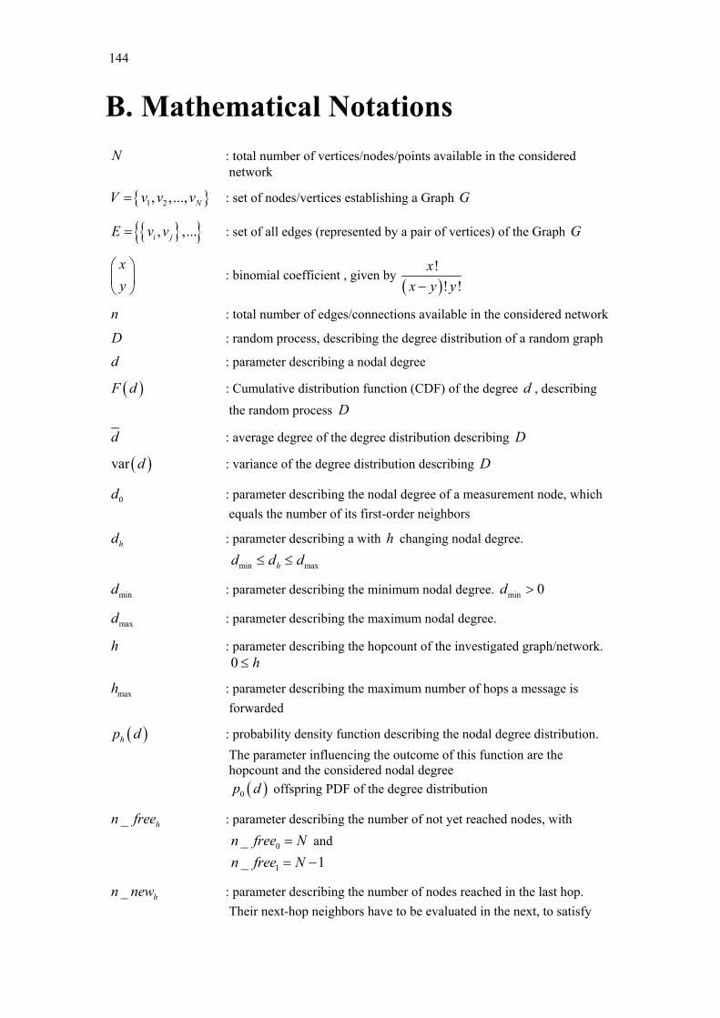
144
B. Mathematical Notations N : total number of vertices/nodes/points available in the considered
network
{ }1 2, ,..., NV v v v= : set of nodes/vertices establishing a Graph G
{ }{ }, ,...i jE v v= : set of all edges (represented by a pair of vertices) of the Graph G
xy
: binomial coefficient , given by ( )
!! !
xx y y−
n : total number of edges/connections available in the considered network
D : random process, describing the degree distribution of a random graph
d : parameter describing a nodal degree
( )F d : Cumulative distribution function (CDF) of the degree d , describing the random process D
d : average degree of the degree distribution describing D
( )var d : variance of the degree distribution describing D
0d : parameter describing the nodal degree of a measurement node, which equals the number of its first-order neighbors
hd : parameter describing a with h changing nodal degree.
min maxhd d d≤ ≤
mind : parameter describing the minimum nodal degree. min 0d >
maxd : parameter describing the maximum nodal degree.
h : parameter describing the hopcount of the investigated graph/network. 0 h≤
maxh : parameter describing the maximum number of hops a message is forwarded
( )hp d : probability density function describing the nodal degree distribution. The parameter influencing the outcome of this function are the hopcount and the considered nodal degree
( )0p d offspring PDF of the degree distribution
_ hn free : parameter describing the number of not yet reached nodes, with
0_n free N= and
1_ 1n free N= −
_ hn new : parameter describing the number of nodes reached in the last hop. Their next-hop neighbors have to be evaluated in the next, to satisfy
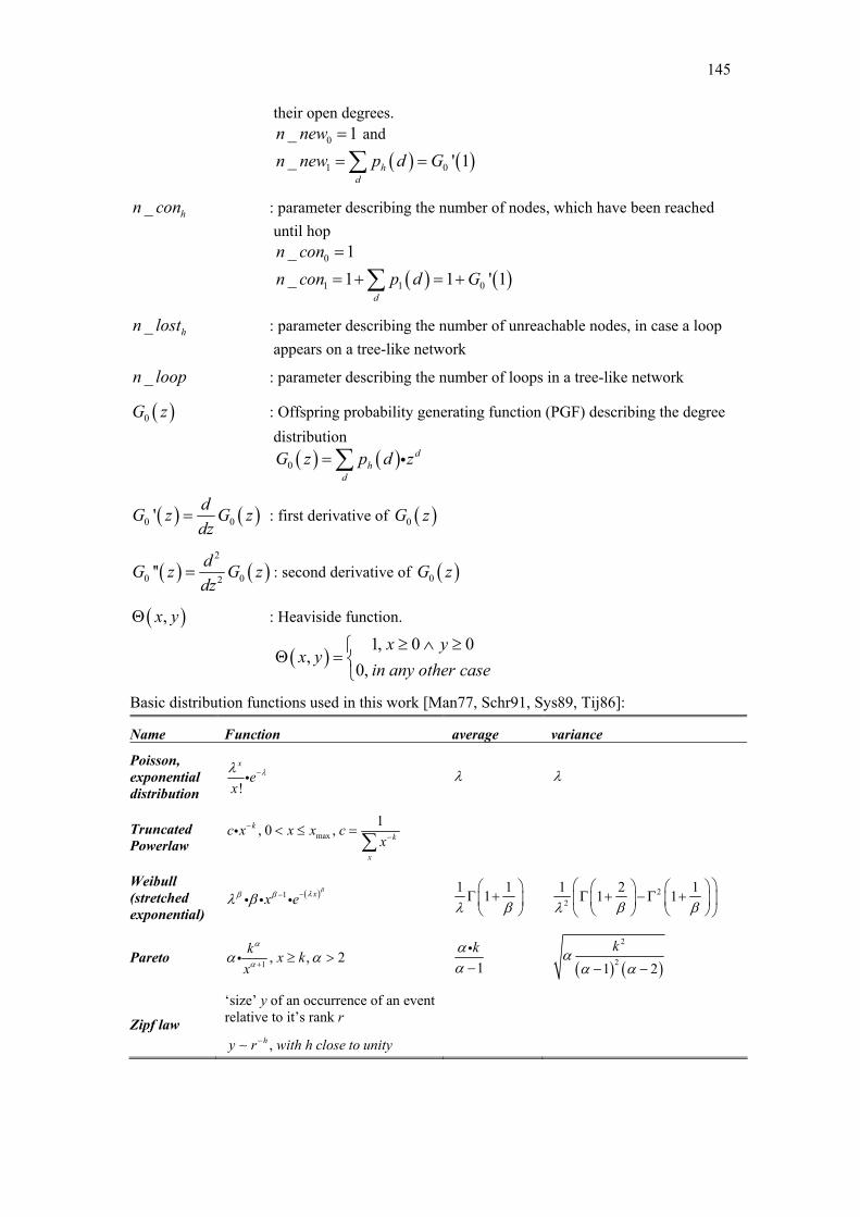
145
their open degrees. 0_ 1n new = and
( ) ( )1 0_ ' 1hd
n new p d G= =∑
_ hn con : parameter describing the number of nodes, which have been reached until hop
0_ 1n con =
( ) ( )1 1 0_ 1 1 ' 1d
n con p d G= + = +∑
_ hn lost : parameter describing the number of unreachable nodes, in case a loop appears on a tree-like network
_n loop : parameter describing the number of loops in a tree-like network
( )0G z : Offspring probability generating function (PGF) describing the degree distribution
( ) ( )0d
hd
G z p d z= ∑ i
( ) ( )0 0' dG z G zdz
= : first derivative of ( )0G z
( ) ( )2
0 02'' dG z G zdz
= : second derivative of ( )0G z
( ),x yΘ : Heaviside function.
( )1, 0 0
,0,
x yx y
in any other case≥ ∧ ≥
Θ =
Basic distribution functions used in this work [Man77, Schr91, Sys89, Tij86]:
Name Function average variance
Poisson, exponential distribution !
x
ex
λλ −i λ λ
Truncated Powerlaw
max1, 0 ,k
k
x
c x x x cx
−−< ≤ =
∑i
Weibull (stretched exponential)
( )1 xx eβλβ βλ β −−i i i
1 11λ β
Γ +
2
2
1 2 11 1β βλ
Γ + − Γ +
Pareto 1 , , 2k x kx
α
αα α+ ≥ >i 1
kαα −i
( ) ( )
2
21 2kα
α α− −
Zipf law
‘size’ y of an occurrence of an event relative to it’s rank r
,hy r with h close to unity−∼
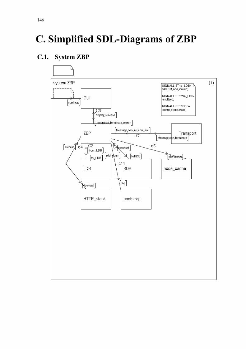
146
C. Simplified SDL-Diagrams of ZBP C.1. System ZBP
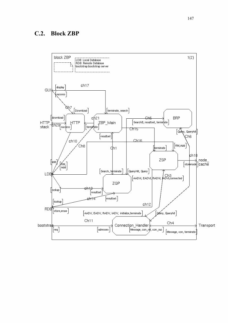
147
C.2. Block ZBP
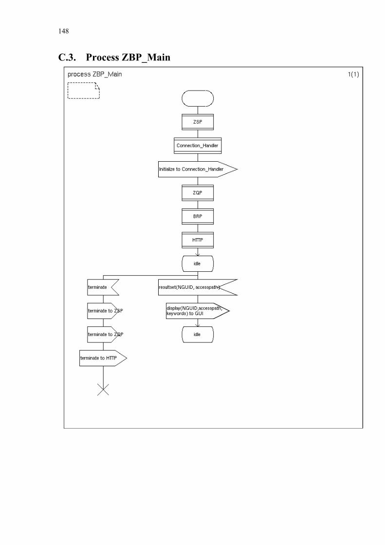
148
C.3. Process ZBP_Main
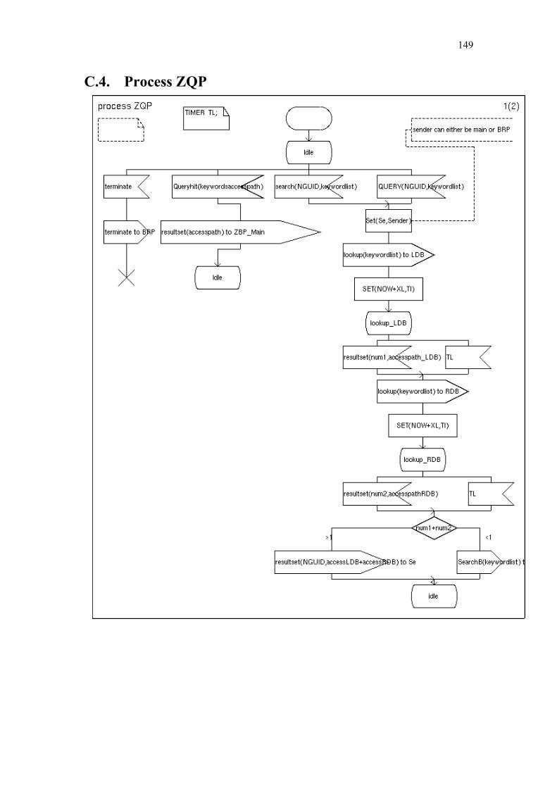
149
C.4. Process ZQP
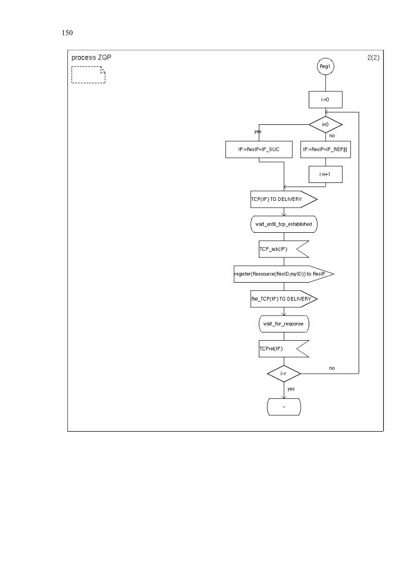
150
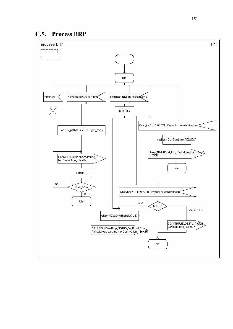
151
C.5. Process BRP
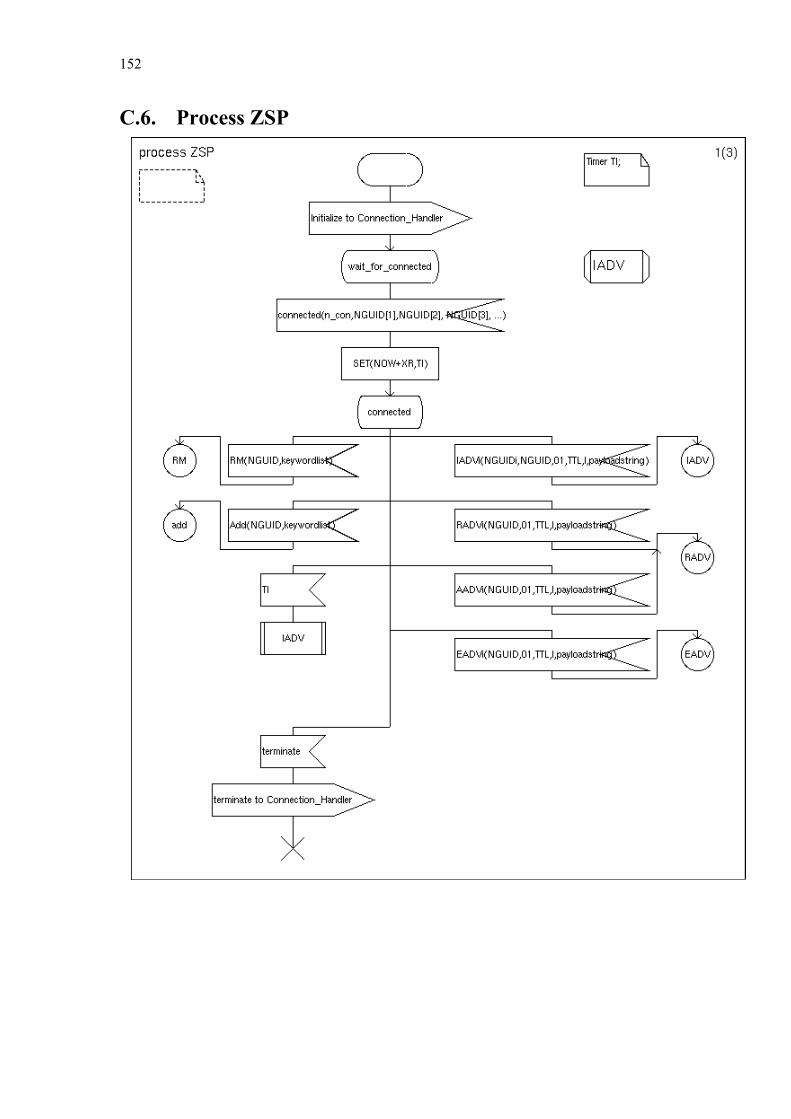
152
C.6. Process ZSP
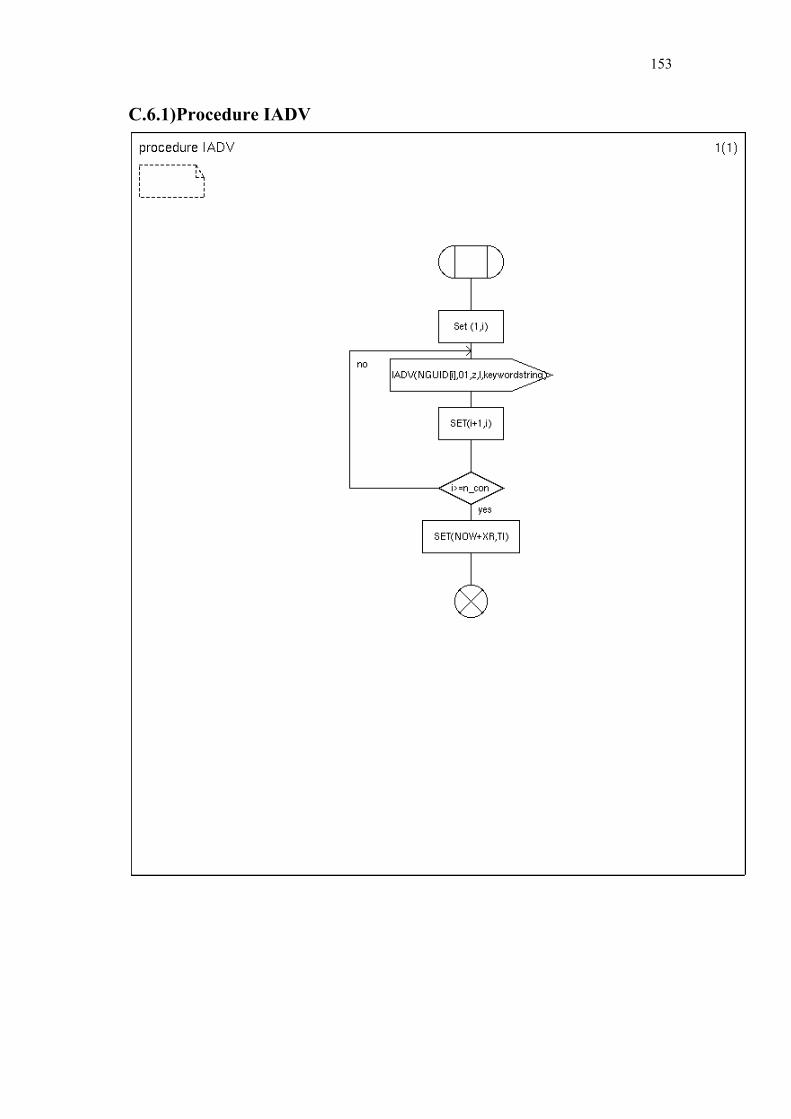
153
C.6.1) Procedure IADV
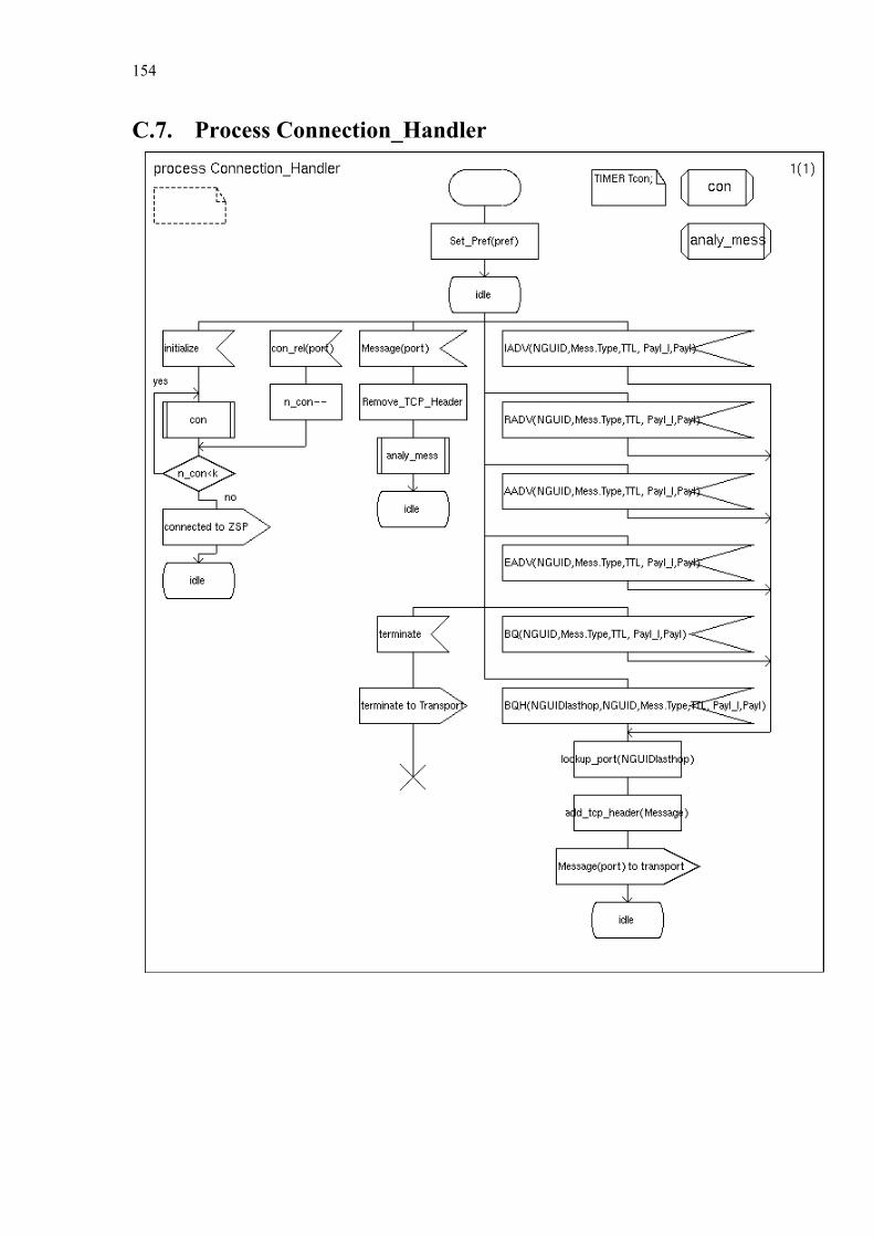
154
C.7. Process Connection_Handler
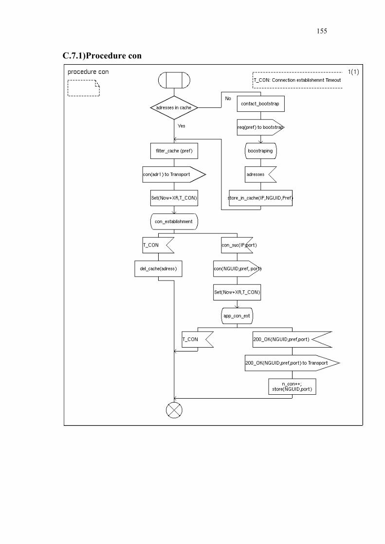
155
C.7.1) Procedure con
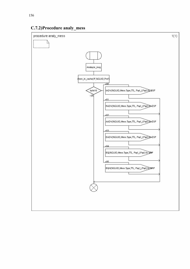
156
C.7.2) Procedure analy_mess
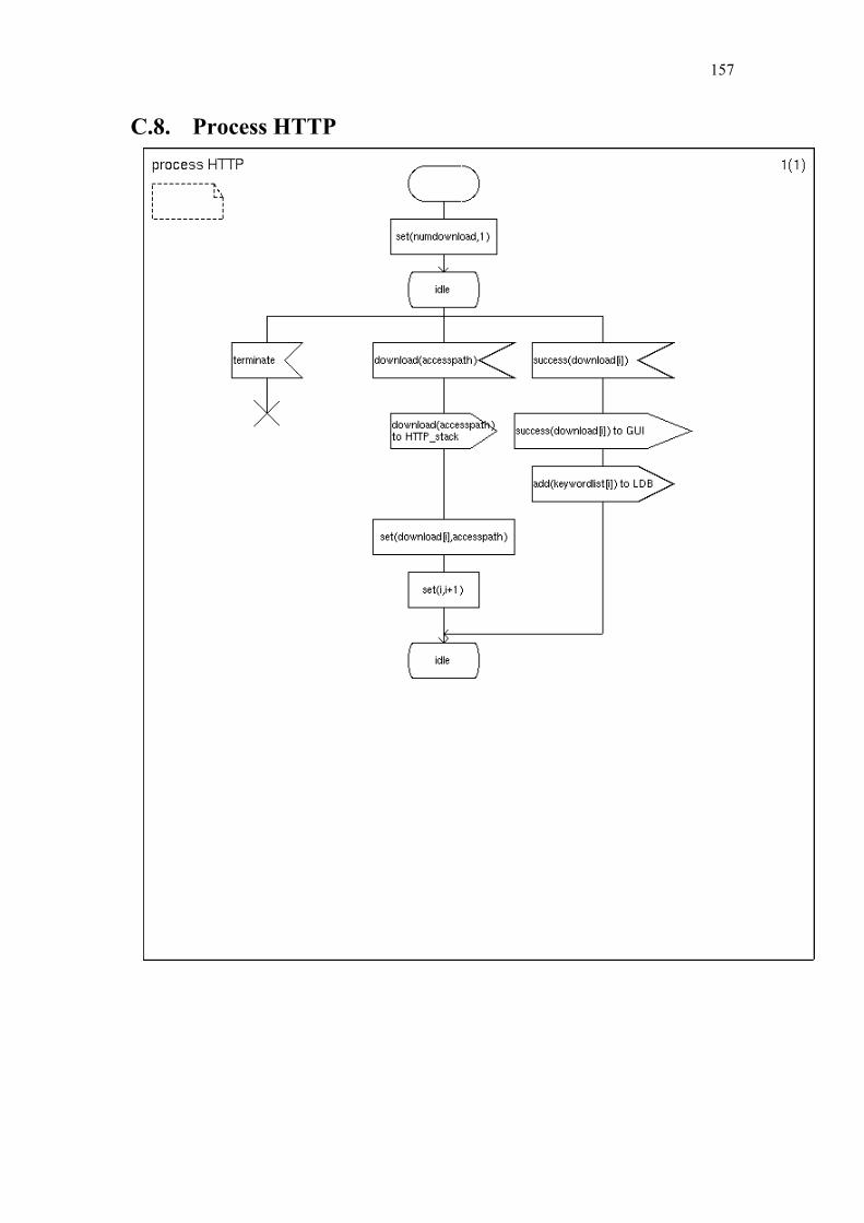
157
C.8. Process HTTP

158
Bibliography [AH00] A. Abdul-Rahman and S. Hailes, "Supporting Trust in Virtual Communities",
presented at 33rd Hawai International Conference on System Sciences, 2000.
[ACDD03] K. Aberer, P. Cudré-Mauroux, A. Datta, Z. Despotovic, M. Hauswirth, M. Punceva, and R. Schmidt, "P-Grid: A Self-organizing Structured P2P System", SIGMOD Record, vol. 32, 2003.
[Abi03] Abilene Backbone, "Internet2 Netflow, Weekly Reports, Week of 20020218, 20020923, 20030505", http://netflow.internet2.edu/weekly, 05.2003, 2003.
[AH00] E. Adar and B. Hubermann, "Free Riding on Gnutella", First Monday, vol. 10, 2000.
[ADF01] G. Allen, T. Dramlitsch, I. Foster, T. Goodale, N. Karonis, M. Ripeanu, E. Seidel, and B. Toonen, "Supporting Efficient Execution in Heterogeneous Distributed Computing Environments with Cactus and Globus", presented at ACM/IEEE conference on Supercomputing (SC'2001), 2001.
[ASBS97] L. A. N. Amaral, A. Scala, M. Barthlmy, and H. E. Stanley, "Classes of Small-World Networks", presented at National Academy of Sciences, 1997.
[ACK02] D. P. Anderson, J. Cobb, E. Korpella, M. Lebofsky, and D. Werthimer, "SETI@home: An Experiment in Public Ressource Computing", Communications of the ACM (CACM), vol. 45, 2002.
[And03] K. Anderson, "Analysis of the Traffic on the Gnutella Network", http://www-cse.ucsd.edu/classes/wi01/cse222/projects/reports/p2p-2.pdf, 05.2004, 2003.
[AM95] R. M. Anderson and R. M. May, "Susceptible-Infectious-Recovered Epidemic Models With Dynamic Partnerships", Journal of Mathematical Biology, 1995.
[AWT02] J. Apostolopoulos, T. Wong, W. Tan, and S. Wee, "On Multiple Description Streaming with Content Delivery Networks", presented at IEEE INFOCOM, 2002.
[AW96] M. Arlitt and C. Williamson, "Web Server Workload Characterization: The Search for Invariants", presented at ACM SIGMETRICS Conference, 1996.
[Aro03] A. Arora, "JXTA for J2ME - Extending the Reach of Wireless With JXTA Technology", Sun Microsystems Inc. White Paper, 2003.
[ACKS03] A. Asvanund, K. Clay, R. Krishnan, and M. Smith, "An Empirical Analysis of Network Externalities in Peer-To-Peer Music Sharing Networks", http://ssrn.com/abstract=433780, 05.2004, 2003.
[Aud04] Audiogalaxy, "Audiogalaxy Homepage", http://www.audiogalaxy.com/, 04.2004, 2004.
[AG03] N. Azzouna and F. Guillemin, "Analysis of ADSL Traffic on an IP Backbone Link", presented at GLOBECOM 2003, 2003.
[Bac02] C. Bachmeir, "Peer-to-Peer (P2P) based Active Signaling Enabling Diverse Protected IP-Multicast", presented at IFIP-TC6 4th Annual International Working Conference on Active Networks (IWAN'2002), 2002.
[BPV 03] C. Bachmeir, J. Peng, H.-J. Vögel, C. Wallace, and G. Conran, "Diversity Protected, Cache Based Reliable Content Distribution - Building on Scalable, P2P and Multicast Based Content Discovery", presented at 6thIEEE International Conference on High Speed Networks and Multimedia Communications (HSNMC'03), 2003.
159
[BWDD02] P. Backx, T. Wauters, B. Dhoedt, and P. Demester, "A Comparison of Peer-to-Peer Architectures", presented at Eurescom Summit 2002, 2002.
[BC98] P. Barford and M. Crovella, "Generating Representative Workloads for Network and Server Performance Evaluation", presented at ACM SIGMETRICS, 1998.
[Bea04] bearshare, "Bearshare Homepage", www.bearshare.com, 2004.
[Be58] C. Berge, Théorie des Graphes et ses Applications. Paris: Dunod, 1958.
[Be02] C. Bettstetter, "On the Minimum Node Degree and Connectivity of a Wireless Multihop Network", presented at 3rd ACM International symposium on Mobile ad hoc networking & computing, 2002.
[BSV03] R. Bhagwan, S. Savage, and G. M. Voelker, "Understanding Availability", presented at 2nd International Workshop on Peer-to-Peer Systems, 2003.
[BT04] A. Binzenhöfer and P. Tran-Gia, "Delay Analysis of a Chord-based Peer-to-Peer File-Sharing System", University of Würzburg Technical Report 332, 2004.
[Blo70] B. H. Bloom, "Space/Time Trade-offs in Hash Coding with Allowable Errors", Communications of the ACM (CACM), vol. 13, 1970.
[Bo85] B. Bollobás, Random Graphs: Academic Press, 1985.
[Bo98] B. Bollobás, Modern Graph Theory. Berlin: Springer, 1998.
[BV96] J. Bolot and A. Vega-Gracia, "Control Mechanisms for Packet Audio in the Internet", presented at IEEE INFOCOM, 1996.
[BOP94] L. Brakmo, S. O'Mally, and L. Peterson, "TCP Vegas: New Techniques for Congestion Detection and Avoidance", presented at ACM SIGCOMM'94, 1994.
[BKMR00] A. Broder, R. Kumar, F. Maghoul, P. Raghavan, S. Rajogaplan, R. Stata, A.Tomkins, and J. Wiener, "Graph Structure in the Web", Computer Networks, 2000.
[BM02] A. Broder and M. Mitzenmacher, "Network Applications of Bloom Filters: A Survey", presented at 40th Annual Allerton Conference, 2002.
[Bro88] R. Brown, "Calendar Queues: A Fast 0(1) Priority Queue Implementation for the Simulation Event Set Problem", Communications of the ACM (CACM), vol. 10, 1988.
[Bru46] N. D. Bruijn, "A Combinatorial Problem", Koninklijke Nderlandse Akademie van Wetenschapen, vol. 49, 1946.
[Cap59] J. Capon, "A Probabilistic Model for Run-Length Coding of Pictures", IT, vol. 5, 1959.
[CCR04] M. Castro, M. Costa, and A. Rowstron, "Should we Build Gnutella on a Structured Overlay?" ACM SIGCOMM Computer Communication Review, vol. 34, 2004.
[CDGR02] M. Castro, P. Druschel, A. Ganesh, A. Rowstron, and D. S. Wallach, "Secure Routing for Structured Peer-to-Peer Overlay Networks", presented at 5th symposium on Operating systems design and implementation SPECIAL ISSUE: Peer-to-peer infrastructure, 2002.
[CDK03] M. Castro, P. Druschel, A.-M. Kermarrec, and A. Rowstron, "Scalable Application-level Anycast for Highly Dynamic Groups", presented at NGC, 2003.
[CP95] L. D. Catledge and J. E. Pitkow, "Characterizing Browsing Strategies in the World Wide Web", presented at hird World Wide Web Conference, 1995.
[CL99] H. Choi and J. Limb, "A Behavioral Model of Web Traffic", presented at International Conference of Networking Protocols'99 (ICNP99), 1999.
[CLL02] J. Chu, K. Labonte, and B. Levine, "Availability and Locality Measurements of Peer-to-Peer File Systems", presented at ITCom: Scalability and Traffic Control in IP Networks, 2002.
160
[CL02] F. Chung and L. Lu, "Connected Components in Random Graphs with Given
Expected Degree Sequences", Annals of Combinatorics Abstract, vol. 6, 2002.
[CMHS02] I. Clarke, S. G. Miller, T. W. Hong, and O. Sandberg, "Protecting Free Expression Online with Freenet", IEEE Internet Computing Journal, vol. 6, 2002.
[Cli01] Clip2, "The Gnutella Protocol Specification v0.4 (Document Revision 1.2)", http://www.clip2.com/GnutellaProtocol04.pdf, 04.2004, 2001.
[Coh04] B. Cohen, "Incentives to Build Robustness in BitTorrent", bitconjurer.org/BitTorrent/bittorrentecon.pdf, 05.2004, 2004.
[CM03] S. Cohen and Y. Matias, "Spectral Bloom Filters", presented at SIGMOD Conference 2003, 2003.
[Cra74] H. Cramèr, Mathematical Methods of Statistics. Princeton: Princeton University Press, 1974.
[CB97] M. E. Crovella and A. Bestavros, "Self-Similarity in World Wide Web Traffic: Evidence and Possible Causes", IEEE/ACM Transactions on Networking, vol. 5, 1997.
[CMN03] F. M. Cuenca-Acuna, R. P. Martin, and T. Nguyen, "Autonomous Replication for High Availability in Unstructured P2P Systems", presented at 22nd International Symposium on Reliable Distributed Systems (SRDS'03), 2003.
[CBC95] C. Cunha, A. Bestavros, and M. Crivella, "Characteristics of WWW Client-based Trace", Boston university, Dept. of Computer Science Technical Report TR-95-010, 1995.
[CZH99] S. Czerwinski, B. Y. Zhao, T. Hodes, A. D. Joseph, and R. Katz, "An Architecture for a Secure Service Discovery Service." presented at MobiCom'99, 1999.
[DMLS04] V. Darlagiannis, A. Mauthe, N. Liebau, and R. Steinmetz, "An Adaptable, Role-based Simulator for P2P Networks", presented at 2004 International Conference on Modelling, Simulation and Visualization Methods, 2004.
[Den96] S. Deng, "Empirical Model of WWW Document Arrivals at Access Link", presented at International Conference on Communications (ICC'96), 1996.
[Die00] R. Diestel, Graph Theory, 2nd ed. Berlin: Springer, 2000.
[DBE04] N. Dimmock, A. Belokosztolszki, D. Eyers, J. Bacon, and K. Moody, "Using Trust and Risk in Role-Based Access Control Policies", presented at Ninth ACM symposium on Access control models and technologies, 2004.
[DL93] M. Doar and I. Leslie, "How Bad is Naive Multicast Routing?" presented at IEEE INFOCOM'93, 1993.
[DR01] P. Druschel and A. Rowstron, "PAST: A Large-Scale, Persistent Peer-to-Peer Storage Utility." presented at HotOSVIII, 2001.
[ES03] J. Eberspächer and R. Schollmeier, "Tutorial on Peer-to-Peer Networking", presented at 9th EUNICE Open European Summer School (EUNICE'03) and the IFIP Workshop on IP and ATM Traffic Management (WATM'03), 2003.
[ESKZ04] J. Eberspächer, R. Schollmeier, G. Kunzmann, and S. Zöls, "Structured Peer-to-Peer Networks in Heterogenous Environments", presented at Second International Conference on Heterogenous Networks (Hetnets'04), 2004.
[EVB01] J. Eberspächer, H. Vögel, and C. Bettstetter, GSM: John Wiley and Sons Ltd, 2001.
[Edo03] Edonkey, "Edonkey Client and Protocol Description", http://silicon-verl.de/home/flo/software/donkey/, 05.2004, 2003.
[efa03] efarm-project, "ed2k Protocol Documentation Client - Serveur Version 3.0", http://www.efarm-project.net/data/docs/Protocol_V3_1_EN.pdf., 05.2004, 2003.
161
[EDS97] J. Ellsberger, H. Dieter, and A. Sarma, SDL - Formal Object-Oriented Language for Communication Systems, 1. ed: Prentice Hall PTR, 1997.
[emu03] eMule, "eMule Project Team Homepage", http://www.emule-project.net., 05.2004, 2002.
[ER60] P. Erdös and A. Rényi, "On the Evolution of Random Graphs", Publ. Math. Inst. Hungar. Acad. Sci., vol. 5, 1960.
[Eth04] Ethereal, "Etherreal Homepage", 05.2004, 2004.
[ETSI98] ETSI, "Universal Mobile Telecommunication System (UMTS); Selection Procedures for the Choice of Radio Transmission Technologies of the UMTS", Technical Report TR101112v3.2.0, 1998.
[FCA98] L. Fan, P. Cao, J. Almeida, and A. Broder, "Summary Cache: A Scalable Wide-Area Web Cache Sharing Protocol", presented at ACM SIGCOMM'98, 1998.
[FS64] T. J. Fararo and M. Sunshine, A Study of a Biased Friendship Network: Syracuse University Press, 1964.
[FBC99] J. Färber, S. Bodamer, and J. Charzinski, "Statistical Evaluation and Modeling of Internet Dial-Up Traffic", presented at Conference on Performance and Control of Network Systems III, 1999.
[FGWK98] A. Feldmann, A. C. Gilbert, W. Willinger, and T. G. Kurtz, "The Changing Nature of Network Traffic: Scaling Phenomena", ACM Computer Communication Review, vol. 28, 1998.
[Fel68] W. Feller, An Introduction to Probability Theory and its Applications, vol. 1, 3rd ed: Wiley, 1968.
[Fel71] W. Feller, An Introduction to Probability Theory and its Applications, vol. 2, 2nd ed: Wiley, 1971.
[Feu03] R. Feuerecker, "Analyse von Gnutella in NS2", Lehrstuhl für Kommunikationsnetze, TUM Diplomarbeit, 2003.
[FGFM99] R. Fielding, J. Gettys, J. Mogul, H. Frystyk, L. Masinter, P. Leach, and T. Berners-Lee, "Hypertext Transfer Protocol - HTTP/1.1", RFC 2616, 1999.
[FIPS95] FIPS, "Secure Hash Standard", Federal Information Processing Standards Publication FIPS PUB 180-1, 1995.
[FP02] G. Foest and R. Paffrath, "Peer-to-Peer (P2P) and Beyond", DFN Mitteilungen, vol. 3, 2002.
[FRO63] C. C. Foster, A. Rapoport, and C. J. Orwant, "A Study of a Large Sociogram: Elimination of Free Parameters", Behavioural Science, vol. 8, 1963.
[Fos02] I. Foster, "The Grid: A new Infrastructure for 21st Century Science", Physics Today, vol. 2, 2002.
[FI03] I. Foster and A. Iamnitchi, "On Death, Taxes, and the Convergence of Peer-to-Peer and Grid Computing", presented at 2nd International Workshop on Peer-to-Peer Systems (IPTPS '03), 2003.
[FK99] I. Foster and C. Kesselmann, The Grid: Blueprint for a New Computing Infrastructure: Morgan Kaufmann, 1999.
[FMLC03] C. Fraleigh, S. Moon, B. Lyles, C. Cotton, M. Khan, D. Moll, R. Rockell, T. Seely, and C. Diot, "Packet-Level Traffic Measurements from the Sprint IP Backbone", IEEE Network, 2003.
[FM94] V. Frost and B. Melamed, "Traffic Modeling for Telecommunications Networks", IEEE Communications Magazine, vol. 3, 1994.
162
[GBRF03] L. Garces-Erice, E. W. Biersack, K. W. Ross, P. A. Felber, and G. Urvoy-Keller,
"Hierarchical P2P Systems", presented at ACM/IFIP International Conference on Parallel and Distributed Computing (Euro-Par), 2003.
[GFBU04] L. Garces-Erice, P. A. Felber, E. W. Biersack, G. Urvoy-Keller, and K. W. Ross, "Data Indexing in Peer-to-Peer DHT Networks", presented at EEE 24th International Conference on Distributed Computing Systems (ICDCS), 2004.
[GFJK03] Z. Ge, D. R. Figueiredo, S. Jaiswal, J. Kurose, and D. Towsley, "Modeling Peer-Peer File Sharing Systems", presented at INFOCOM 2003, 2003.
[GHM03] J. Gerke, D. Hausheer, J. Mischke, and B. Stiller, "An Architecture for a Service Oriented Peer-to-Peer System (SOPPS)", Praxis der Informationsverarbeitung und Kommunikation (PIK), vol. 26, 2003.
[GCH03] J. Gerke, C. J, D. Hausheer, and B. Stiller, "Quality of Service for Application Service Providers", TIK Report Nr. 170 2003.
[Gif03] Gift, "Gift Homepage", http://gift.sourceforge.net/, 05.2004, 2003.
[Glo04] GloMoSim, "GloMoSim Homepage", http://pcl.cs.ucla.edu/projects/glomosim/, 05.2004, 2004.
[Gnu04] GnuNet, "GnuNet Homepage", http://www.ovmj.org/GNUnet/index.php3, 05.2004, 2004.
[Gnu02] Gnutella 0.6, "RFC-Gnutella 0.6", http://rfc-gnutella.sourceforge.net/developer/testing/, 04.2004, 2002.
[Goy01] V. K. Goyal, "Multiple Description Coding: Compression Meets the Network", IEEE Signal Processing Magazine, vol. 18, 2001.
[GS00] T. Grandison and M. Sloman, "A Survey of Trust in Internet Applications", IEEE Communications Society, Surveys and Tutorials, vol. 3, 2000.
[Grem83] L. L. Gremillion, "Designing a Bloom Filter for Differential File Access", Communications of the ACM (CACM), vol. 25, 1983.
[DWB01] S. D. Gribble, M. Welsh, R. v. Behren, E. A. Brewer, D. Culler, N. Borisov, S. Czerwinski, R. Gummadi, J. Hill, A. D. Joseph, R. H. Katz, Z. Mao, S. Ross, and B. Zhao, "The Ninja Architecture for Robust Internet-Scale Systems and Services", Computer Networks, vol. 35, 2001.
[Grö01] B. Grönvall, "Scalable Multicast Forwarding", presented at SIGCOMM'2001 (Poster Session), 2001.
[Gro04] Groove Networks Inc., "Groove Networks Homepage", http://www.groove.net/home/, August 2004, 2004.
[GL03] I. Gruber and H. Li, "Path Expiration Times in Mobile Ad Hoc Networks", presented at European Personal Mobile Communications Conference (EPMCC'03), 2003.
[GSK04a] I. Gruber, R. Schollmeier, and W. Kellerer, "Peer-to-Peer Communication in Mobile Ad Hoc Networks", Ad Hoc & Sensor Wireless Networks (OCP Science Journals), vol. 1, 2004.
[GSK04] I. Gruber, R. Schollmeier, and W. Kellerer, "Performance Evaluation of the Mobile Peer-to-Peer Protocol", presented at Fourth International Workshop on Global and Peer-to-Peer Computing (GP2PC'2004), 2004.
[GN02] X. Gu and K. Nahrstedt, "A Scalable QoS-Aware Service Aggregation Model for Peer-to-Peer Computing Grids", presented at 11 th IEEE International Symposium on High Performance Distributed Computing (HPDC'02), 2002.
[Gum03] K. Gummadi and e. al., "The Impact of DHT Routing Geometry on Resilience and Proximity", presented at ACM SIGCOMM 2003, 2003.
163
[GDSG03] K. P. Gummadi, R. J. Dunn, S. Saroui, S. D. Gribble, H. M. Levy, and J. Zahorjan., "Measurement, Modeling, and Analysis of a Peer-to-Peer File-Sharing Workload", presented at Nineteenth ACM symposium on Operating systems principles, 2003.
[GSK03] Y. Guo, K. Suh, J. Kurose, and D. Towsley, "A Peer-to-Peer On-Demand Streaming Service and Its Performance Evaluation", presented at IEEE International Conference on Multimedia & Expo (ICME 2003), 2003.
[HC04] A. Habib and J. Chuang, "Incentive Mechanism for Peer-to-Peer Media Streaming", presented at Twelfth IEEE International Workshop on Quality of Service (IWQOS 2004), 2004.
[HDTI01] T. Hagiwara, H. Doi, H. Todoe, and V. E.-D. H. Ikeda"High-Speed Calculation Method Of The Hurst Parameter Based On Real Traffic". , NO.5, 2001., "High-Speed Calculation Method Of The Hurst Parameter Based On Real Traffic", IEICE Trans. Inf. & Syst., vol. 84, 2001.
[HHWX01] F. Harrell, Y. Hu, G. Wang, and H. Xia, "Survey of Locating & Routing in Peer-to-Peer Systems", Technical Report Fa01-CSE221 project, 2001.
[HHHL02] M. Harren, J. M. Hellerstein, R. Huebsch, B. T. Loo, S. Shenker, and I. Stoica, "Complex Queries in DHT-based Peer-to-Peer Networks", presented at 1st International Workshop on Peer-to-Peer Systems (IPTPS '02), 2002.
[HP00] Z. Hass and M. Pearlman, "The Zone Routing Protocol (ZRP) for Ad Hoc Networks", Internet Draft, MANET Working Group, 03.2000 2000.
[HLM03] D. Hausheer, N. Liebau, A. Mauthe, R. Steinmetz, and B. Stiller, "Token-based Accounting and Distributed Pricing to Introduce Market Mechanisms in a Peer-to-Peer File Sharing Scenario", presented at 3rd IEEE International Conference on Peer-to-Peer Computing,, 2003.
[HARR03] Q. He, M. Ammar, G. Riley, H. Raj, and R. Fujimoto, "Mapping Peer Behavior to Packet-level Details: A Framework for Packet-level Simulation of Peer-to-Peer Systems", presented at IEEE / ACM International Symposium on Modeling, Analysis, and Simulation of Computer and Telecommunication Systems (MASCOTS'03), 2003.
[HHB03] M. Hefeeda, A. Habib, B. Boyan, D. Xu, and B. Bhargava, "PROMISE: Peer-to-Peer Media Streaming Using CollectCast", Purdue University Technical report, CS-TR 03-016, 2003.
[HMT04] D. Herrscher, S. Maier, J. Tian, and K. Rothermel, "A Novel Approach to Evaluating Implementations of Location-Based Software", presented at 2004 International Symposium on Performance Evaluation of Computer and Telecommunication Systems (SPECTS 2004), 2004.
[HSB77] C. C. Heyed, E. Seneta, and I. J. Bienaymé, Statistical Theory Anticipated. Berlin: Springer, 1977.
[HPL01] S. H. Hong, R. Park, and -. C.B. Lee "". Journal of 12, 2001, "Hurst Parameter Estimation of Long-Range Dependent VBR MPEG Video Traffic in ATM Networks", Visual Communication and Image Representation, vol. 44, 2001.
[Hsi01] P. Hsiao, "Geographical Region Summary Service for Geographical Routing", Mobile Computing and Communications Review, vol. 4, 2001.
[HWC04] D. Hughes, I. Warren, and G. Coulson, "Improving QoS for Peer-to-Peer Applications Through Adaptation", presented at 10th IEEE International Workshop on Future Trends of Distributed Computing Systems (FTDCS'04), 2004.
[ITU99] ITU, "H.323 Packet-Based Multimedia Communications Systems", ITU-T Recommendation 1999.
[ITU98] R. C. S. G. ITU: US TG 8/1, "The Radio CDMA2000 RTT Candidate Submission", ITU TR45-5, 1998.
164
[IUBF04] M. Izal, G. Urvoy-Keller, E. W. Biersack, P. A. Felber, A. A. Hamr, and L. Garcés-
Erice, "Dissecting BitTorrent: Five Months in a Torrent's Lifetime", presented at Passive & Active Measurement Workshop, 2004.
[JMQ03] P. Jacquet, P. Muhlenthaler, and A. Qayyum, "Optimized Link State Routing Protocol", Internet Draft, draft-ietf-manet-olsr-*.txt, 2003.
[JLR00] S. Janson, T. Luczak, and A. Rucinski, Random Graphs: Wileys, 2000.
[JW00] F. Jondral and A. Wiesler, Grundlagen der Wahrscheinlichkeitsrechnung und stochastischer Prozesse für Ingenieure: Teubner, 2000.
[JA01] M. A. Jovanovic, F. S. Annexstein, and K. A. Berman, "Modeling Peer-to-Peer Network Topologies Through "Small-World" Models and Power Laws", presented at IX Telecommunications Forum (TELFOR), 2001.
[JAB01] M. A. Jovanovic, F. S. Annexstein, and K. A. Berman, "Scalability Issues in Large Peer to Peer Networks - A Case Study of Gnutella", Univ. of Cincinati Technical Report, 2001.
[JXM02] JXME Project, "JXME Project Homepage", http://jxme.jxta.org/, 05.2004, 2002.
[JXTA02] JXTA, "JXTA Homepage", http://www.jxta.org, 05.2004, 2002.
[KK04] M. F. Kaashoek and D. R. Karger, "Koorde: A Simple Degree-Optimal Distributed Hash Table", presented at Fifteenth annual ACM-SIAM symposium on Discrete Algorithms, 2004.
[Kan03] K. Kant, "An Analytic Model for Peer to Peer File Sharing Networks", presented at International Communications Conference, 2003.
[KIT04] K. Kant, R. Iyer, and V. Tewari, "A Performance Model for Peer to Peer File-Sharing Services", http://kkant.ccwebhost.com/download.htm, 05.2004, 2004.
[KBBF03] T. Karagiannis, A. Broido, N. Brownlee, and M. Faloutsos, "Filesharing in the Internet: A Characterization of P2P Traffic in the Backbone", Technical Report, 2003.
[KADR04] P. Karbhari, M. Ammar, A. Dhamdhere, H. Raj, G. Riley, and E. Zegura, "Bootstrapping in Gnutella: A Measurement Study", presented at Passive & Active Measurement Workshop, 2004.
[KR04] D. R. Karger and M. Ruhl, "Diminished Chord: A Protocol for Heterogeneous Subgroup Formation in Peer-to-Peer Networks", presented at International Workshop on Peer-to-Peer Systems (IPTPS '04), 2004.
[KR04] D. R. Karger and M. Ruhl, "Simple Efficient Load Balancing Algorithms for Peer-to-Peer Systems", presented at 3rd International Workshop on Peer-to-Peer Systems (IPTPS'04), 2004.
[Kaz03] Kazaa, "Kazaa Homepage", http://www.kazaa.com/us/index.htm, 05.2004, 2003.
[KSGN03] W. Kellerer, R. Schollmeier, I. Gruber, and F. Niethammer, "Mobile Peer-to-Peer Networking". Europe, 2004.
[KSE04] S. Khan, R. Schollmeier, and E. Steinbach, "A Performance Comparison of Multiple Description Video Streaming in Peer-to-Peer and Content Delivery Networks", presented at IEEE 2004 International Conference on Multimedia and Expo (ICME2004), 2004.
[KM02] M. Kleaskar and V. Matossian, "A Study of Discovery Mechanism for Peer-to-Peer Applications", presented at 2nd IEEE/ACM International Symposium on Cluster Computing and the Grid(CCGRID'02), 2002.
[KCW03] A. Klemm, C. Lindemann, and O. P. Waldhorst, "A Special-Purpose Peer-to-Peer File Sharing System for Mobile Ad Hoc Networks", presented at Workshop on Mobile Ad Hoc Networking and Computing (MADNET 2003), 2003.
165
[Klim03] A. Klimkin, "eDonkey Protocol v0.3", http://search.cpan.org/src/KLIMKIN/P2P-pDonkey-0.01/doc/eDonkey-protocol, 05.2004, 2003.
[KMa02] T. Klingberg and R. Manfredi, "Gnutella 0.6 RFC", http://rfc-gnutella.sourceforge.net/draft.txt, 05.2005, 2002.
[Kön36] D. König, Theorie der endlichen und unendlichen Graphen. Leipzig: Springer, 1936.
[KM96] M. Kretschmar and M. Morris, "Measures of the Concurrency in Networks and the Spread of Infectious Disease", Mathematical Biosciences, 1996.
[KR01] B. Krishnamurthy and J. Rexford, Web Protocols and Practice: HTTP/1.1, Networking Protocols, Caching, and Traffic Measurement: Addison-Wesley Professional, 2001.
[KWX01] B. Krishnamurthy, J. Wang, and Y. Xie, "Early Measurements of a Cluster-based Architecture for P2P Systems", presented at ACM SIGCOMM Internet Workshop, 2001.
[KBC00] J. Kubiatowicz, D. Bindel, Y. Chen, S. Czerwinski, P. Eaton, D. Geels, R. Gummadi, S. Rhea, H. Weatherspoon, W. Weimer, C. Welles, and B. Zhao, "Oceanstore: An Architecture for Global-Scale Persistent Storage", presented at 9th International Conference on Architectural Support for Programming Languages and Operating Systems, 2000.
[Küg03] D. Kügler, "An Analysis of GNUnet and the Implications for Anonymous, Censorship-Resistant Networks", presented at Workshop on Privacy Enhancing Technologies, PET'2003, 2003.
[LM97] T. V. Lakshman and U. Madhow, "The Performance of TCP/IP for Networks with High Bandwidth-Delay Products and Random Loss", IEEE/ACM Transactions on Networking, 1997.
[LRS01] K. Lakshminarayanan, A. R. Rao, and S. Surana, "Hyperchord: A Peer-to-Peer data Location Architecture", UC Berkley Technical Report CS-021208, 2001.
[LTS02] J. Ledlie, J. Taylor, L. Serban, and M. Seltzer, "Self Organization in Peer-to-Peer Systems", presented at 10th European SIGOPS Workshop, 2002.
[LBBS02] N. Leibowitz, A. Bergman, R. Ben-Shaul, and A. Shavit, "Are File Swapping Networks Cacheable? Characterizing P2P Traffic", presented at 7th Int. WWW Caching Workshop, 2002.
[LT02] R. Lerdorf and K. Tatroe, Programming PHP: O'Reilly & Associates, 2002.
[Les01] M. Lesko, "Ethereal", Sys Admin Magazine, 2001.
[Leu02] B. Leuf, Peer to Peer: Collaboration and Sharing over the Internet, 1st ed: Addison-Wesley Pub Co, 2002.
[LS99] H. Liefke and D. Suciu, "XMill: An Efficient Compressor for XML Data", University of Pennsylvania Technical Report MSCIS-99-26, 1999.
[LLC03] S. Lim, W. Lee, G. Cao, and C. R. Das, "A Novel Caching Scheme for Internet based Mobile Ad Hoc Networks", presented at International Conference on Compouter Communication Networks (ICCCN'2003), 2003.
[Lim04] Limewire, "Limewire Homepage", http://www.limewire.com/, 05.2004, 2004.
[LW03] T. Lin and H. Wang, "Search Performance Analysis in Peer-to-Peer Networks", presented at 3rd International Conference on Peer-to-Peer Computing (P2P'03), 2003.
[LSS02] M. C. Little, S. K. Shrivastava, and N. A. Speirs, "Using Bloom Filters to Speed-Up Name Lookup in Distributed Systems", The Computer Journal, vol. 45, 2002.
[LR04] L. Liu and K. D. Ryu, "Supporting Efficient Keyword-Based File Search in Peer-to-Peer File Sharing Systems", IBM Research IBM Research Report. RC23145 (W0403-068), 2004.
166
[LKRG03] D. Loguinov, A. Kumar, V. Rai, and S. Ganesh, "Graph-Theoretic Analysis of
Structured Peer-to-Peer Systems: Routing Distances and Fault Resilience", presented at ACM SIGCOMM Conference, 2003.
[Mad04] T. Mader, "Analyse von Zone Based Peer-to-Peer in NS2", Lehrstuhl für Kommunikationsnetze, TUM Diplomarbeit, 2004.
[Mah97] B. Mah, "An Empirical Model of HTTP Network Traffic", presented at IEEE INFOCOM'97, 1997.
[Man77] B. Mandelbrot, The Fractal Geometry of Nature: W.H. Freeman and Company, 1977.
[Mar02] E. Markatos, "Tracing a Large-Scale Peer-to-Peer System: An Hour in the Lifetime of Gnutella", presented at 2nd IEEE/ACM Int. Symp. On Cluster Computing and the Grid, 2002.
[Mar94] S. Marsh, "Formalising Trust as a Computational Concept", Ph.D Thesis, University of Stirling, 1994.
[MH03] A. Mauthe and D. Hutchison, "Peer-to-Peer Computing: Systems, Concepts and Characteristics", Praxis in der Informationsverarbeitung & Kommunikation (PIK), vol. 26, 2003.
[MM02] P. Maymounkov and D. Mazieres, "Kademlia: A Peer-to-Peer Information System Based on the XOR Metric", presented at International Workshop on Peer-to-Peer Systems (IPTPS'02), 2002.
[MLMB01] A. Medina, A. Lakhina, I. Matta, and J. Byers, "BRITE: Universal Topology Generation from a User's Perspective", Technical Report BU-CS-TR-2001-003, 2001.
[MCV03] V. A. Mesaros, B. Carton, and P. V. Roy, "S-Chord: Using Symmetry to Improve Lookup Efficiency in Chord", presented at 2003 International Conference on Parallel and Dis-tributed Processing Techniques and Applications (PDPTA'03), 2003.
[Met03] Meta Search Inc., "edonkey2000 Homepage", http://www.edonkey2000.com, 05.2004, 2003.
[MGT99] V. Mistra, W. B. Gong, and D. Towsley, "Stochastic Differential Equation Modeling and Analysis of TCP-Windowsize Behavior", Performance, 1999.
[MOB99] V. Mistra, T. Ott, and J. Baras, "The Window Distribution of Multiple TCPs with Random Queues", presented at IEEE Globecom, 1999.
[Mit01] M. Mitzenmacher, "Compressed Bloom Filters", presented at 20th Annual ACM Symposium on Principles of Distributed Computing, 2001.
[mld03] mlDonkey, "mlDonkey Homepage", http://mldonkey.org, 05.2004, 2003.
[MT02] A. Moffat and A. Turpin, Compression and Coding Algorithms. New York: Kluwer Academic Publishers, 2002.
[MWW98] R. M. Moffat, N. Witten, and I. H. Witten, "Arithmetic Coding Revisited", ACM Transactions on Information Systems, vol. 16, 1998.
[Mont01] A. Montresor, "Anthill: a Framework for the Design and Analysis of Peer-to-Peer Systems", presented at 4th European Research Seminar on Advances in Distributed Systems, 2001.
[Mul83] J. K. Mullin, "A Second Look at Bloom Filters", Communications of the ACM (CACM), vol. 26, 1983.
[Net04] NetGeo, "NetGeo - The Internet Geographic Database", www.caida.org/tools/utilities/netgeo/, 05.2004, 2002.
[NSW01] M. J. E. Newman, S. H. Strogatz, and D. J. Watts, "Random Graphs with Arbitrary Degree Distribution and their Application", Physical Review, 2001.
167
[UHHS02] U. Niedermeier, J. Heuer, A. Hutter, W. Stechele, and A. Kaup, "An MPEG-7 Tool for Compression and Streaming of XML Data", presented at IEEE International Conference on Multimedia and Expo, 2002.
[ns204] ns-2, "The Network Simulator ns-2 Homepage", http://www.isi.edu/nsnam/ns/, 05.2004, 2004.
[OTG02] S. Oaks, B. Traversat, and L. Gong, JXTA in a Nutshell: O'Reilly & Associates, 2002.
[OSS03] G. On, J. Schmitt, and R. Steinmetz, "QoS-Controlled Dynamic Replication in Peer-to-Peer Systems", Praxis der Informationsverarbeitung und Kommunikation (PIK), vol. 26, 2003.
[Ora01] A. Oram, Peer-to-Peer. Harnessing the Power of Disruptive Technologies: O'Reilly & Associates, 2001.
[PFTK98] J. Padhye, V. Firoiu, D. Towsley, and J. Kurose, "Modeling TCP Throughput: a Simple Model and its Empirical Validation", presented at ACM/SIGCOMM, 1998.
[PS01] V. N. Padmanabhan and L. Subramanian, "An Investigation of Geographic Mapping Techniques for Internet Hosts", presented at ACM SIGCOMM'01, 2001.
[PKC97] K. Park, G. Kim, and M. E. Crovella, "On the Effect of Traffic Self-Similarity on Network Performance", presented at SPIE International Conference on Performance and Control of Network Systems, 1997.
[Pax94] V. Paxson, "Empirically-Derived Analytic Models of Wide Area TCP Connections", IEEE/ACM Transactins on Networking, 1994.
[Pax99] V. Paxson, "End-to-End Internet Packet Dynamics", IEEE/ACM Transactions on Networking, 1999.
[PWF02] L. Pearlman, V. Welch, I. Foster, C. Kesselmann, and S. Tuecke, "A Communication Authorization Service for Group Collaboration", presented at 3rd IEEE Workshop on Policies for Distributed Systems and Networks, 2002.
[Peh97] J. M. Peha, "Retransmission Mechanisms and Self-Similar Traffic Models", presented at IEEE/ACM/SCS Communications Networks and Distributed Systems Modeling and Simulation Conference, 1997.
[PB94] C. Perkins and P. Bhagwat, "Highly Dynamic Destination-Sequenced Distance-Vector Routing (DSDV) for Mobile Computers", presented at SIGCOMM'94 Conference on Communications Architectures, Protocols and Applications, 1994.
[Per00] C. E. Perkins, Ad Hoc Networking: Addison-Wesley, 2000.
[PTVF99] W. H. Pres, S. A. Teukolsky, W. T. Vetterling, and B. P. Flannery, Numerical Recipes in C: Cambridge University Press, 1999.
[PKF01] T. Prudhomme, K. C, T. Finholt, I. Foster, D. Parsons, D. Abrams, J.-P. Bardet, R. Pennington, J. Towns, R. Butler, J. Futrelle, N. Zaluzec, and J. Hardin, "A Distributed Virtual Laboratory for Advanced Earthquake Experimentation and Simulations: Scoping Study", www.neesgrid.org, August 2004, 2001.
[RW96] L. Rade and B. Westergren, Springers Mathematische Formeln. Taschenbuch für Ingenieure, Naturwissenschaftler, Wirtschaftswissenschaftler. Berlin: Springer, 1996.
[Ram89] M. V. Ramakrishna, "Practical Perfomance of Bloom Filters and Parallel Free-Text Searching", Communications of the ACM (CACM), vol. 32, 1989.
[RFHK01] S. Ratnasamy, P. Francis, M. Handley, R. Karp, and S. Shenker, "A Scalable Content-Addressable Network", presented at ACM SIGCOMM Conference, 2001.
[RGCD99] A. Reyes-Lecuona, E. Gonzáles-Parada, E. Casilari, and A. Díaz-Estrela, "A Page-Oriented WWW Traffic Model for Wireless System Simulations", presented at 16th International Teletraffic Congress (ITC'99), 1999.
168
[RV03] P. Reynolds and A. Vahdat, "Efficient Peer-to-Peer Keyword Searching", presented
at ACM/IFIP/USENIX International Middleware Conference, 2003.
[RGRK04] S. Rhea, D. Geels, T. Roscoe, and J. Kubiatowcz, "Handling Churn in a DHT", presented at USENIX 2004 Annual Technical Conference, 2004.
[RFI02] M. Ripeanu, I. Foster, and A. Iamnitchi, "Mapping the Gnutella Network", IEEE Internet Computing Journal, vol. 6, 2002.
[Riv92] R. Rivest, "The MD5 Message-Digest Algorithm", RFC 1321, 1992.
[Roh02] C. Rohrs, "The PING/PONG Scheme", http://rfc-gnutella.sourceforge.net/Proposals/PING-PONG%20Scheme/PING-PONG-scheme.htm., 01.2003, 2002.
[Roh02a] C. Rohrs, "QUERY Routing for the Gnutella Network", http://rfc-gnutella.sourceforge.net/Proposals/QRP/QUERY_routing.htm., 01.2003, 2002.
[Ros96] O. Rose, "Estimation of the Hurst Parameter of Long Range Dependant Time Series", University of Würzburg Technical Report Nr. 137, 1996.
[RF93] O. Rose and M. Frater, "A Comparison of Models for VBR Video Traffic Sources in B-ISDN", IFIP transactions C-24: Broadband communications, 1993.
[RSC02] J. Rosenberg, H. Schulzrinne, G. Camarillo, A. Johnston, J. Peterson, R. Sparks, M. Handley, and E. Schooler, "SIP: The Session Initiation Protocol", RFC 3261 2002.
[RD01] A. Rowstron and P. Druschel, "Pastry: Scalable, Distributed Object Location and Routing for Large-Scale Peer-to-Peer Systems", presented at IFIP/ACM International Conference on Distributed Systems Platforms (Middleware), 2001.
[Row01] A. Rowstron and P. Druschel, "Storage Management and Caching in PAST, a Large-Scale, Persistent Peer-to-Peer Storage Utility", presented at 18th ACM Symposium on Oper-ating Systems and Principles (SOSP 2001), 2001.
[RKD01] A. Rowstron, A.-M. Kermarrec, P. Druschel, and M. Castro, "Scribe: The Design of a Large-Scale Event Notification Infrastructure", presented at NGC2001, 2001.
[Sal97] D. Salomon, Data Compression. The Complete Reference. New York: Springer, 1997.
[SB04] K. Samant and S. Bhattacharyya, "Topology, Search, and Fault Tolerance in Unstructured P2P Networks", presented at 37th Annual Hawaii International Conference on System Sciences, 2004.
[SGG02] S. Saroui, P. K. Gummadi, and S. D. Gribble, "A Measurement Study of Peer-to-Peer File Sharing Systems", presented at Multimedia Computing and Networking 2002 (MMCN '02), 2002.
[SS88] L. Sattenspiel and C. P. Simon, "The Spread and Persistence of Infectious Diseases in Structured Populations", Mathematical Biosciences, 1988.
[Scho01] R. Schollmeier, "A Definition of Peer-to-Peer Networking for the Classification of Peer-to-Peer Architectures and Applications", presented at IEEE Conference P2P 2001, 2001.
[Scho01a] R. Schollmeier, "A Definition of Peer-to-Peer Networking Towards a Delimitation Against Classical Client-Server Concepts", presented at 7th EUNICE Open European Summer School (EUNICE'01) and the IFIP Workshop on IP and ATM Traffic Management (WATM'01), 2001.
[SD03] R. Schollmeier and A. Dumanois, "Peer-to-Peer Traffic Characteristics", presented at EUNICE 2003, 2003.
[SE04] R. Schollmeier and J. Eberspächer, Peer-to-Peer-Systems and -Applications: Springer-Verlag, 2004.
169
[SGF02] R. Schollmeier, I. Gruber, and M. Finkenzeller, "Routing in Mobile Ad Hoc and Peer-to-Peer Networks. A Comparison", presented at Networking 2002. International Workshop on Peer-to-Peer Computing, 2002.
[SGN03] R. Schollmeier, I. Gruber, and F. Niethammer, "Protocol for Peer-to-Peer Networking in Mobile Environments", presented at International Conference on Computer Communications (ICCCN03), 2003.
[SH03] R. Schollmeier and F. Hermann, "Topology-Analysis of Pure Peer-to-Peer Networks", presented at Fachtagung Kommunikation in Verteilten Systemen" (KiVS 2003), 2003.
[SK04] R. Schollmeier and W. Kellerer, "Suitability of Bloom Filters for Network Applications", presented at 2004 International Symposium on Performance Evaluation of Computer and Telecommunication Systems (SPECTS 2004), 2004.
[SKe04] R. Schollmeier and W. Kellerer, "Zone Based Peer-to-Peer", presented at 4. Würzburger Workshop "IP Netzmanagement, IP Netzplanung und Optimierung", 2004.
[SK03] R. Schollmeier and G. Kunzmann, "GnuViz - Mapping the Gnutella Networks to its Geographical Locations", Praxis der Informationsverarbeitung und Kommunikation (PIK), vol. 26, 2003.
[SS02] R. Schollmeier and G. Schollmeier, "Why Peer-to-Peer (P2P) Does Scale: An Analysis of P2P Traffic Patterns", presented at IEEE International Conference on P2P (P2P2002), 2002.
[SS04] R. Schollmeier and G. Schollmeier, "An Analytic Model for the Behavior of Arbitrary Peer-to-Peer Networks", European Transactions on Telecommunications (ETT), Special Issue on P2P Networking and P2P Services, vol. 15, 2004.
[Schr91] M. Schroeder, Fractals, Chaos, Power Laws: W.H. Freeman and Company, 1991.
[SW02] S. Sen and J. Wang, "Analyzing Peer-to-Peer Traffic Across Large Networks", presented at ACM SIGCOMM Internet Measurement Workshop, 2002.
[Set04] seti, "Homepage of the Seti@Home Project", http://setiathome.ssl.berkeley.edu, 07.2004, 2004.
[sfs03] Sfsnet, "Sfsnet Chord Simulator." http://cvs.pdos.lcs.mit.edu/cvs/sfsnet/, 05.2004, 2003.
[SR02] A. Singla and C. Rohrs, "Ultrapeers: Another step Towards Gnutella Scalability", http://rfc-gnutella.sourceforge.net/Proposals/Ultrapeer/Ultrapeers.htm., 01.2003, 2002.
[Sky04] Skype, "Skype Homepage", http://www.skype.com/. 05.2004, 2004.
[Sri01] K. Sripanidkulchai, "The Popularity of Gnutella Queries and Its Implications on Scalability", Technical Report, 2001.
[SW04] R. Steinmetz and K. Wehrle, "Peer-to-Peer Networking and Computing", Informatik Spektrum, vol. 27, 2004.
[SRG03] B. Stiller, P. Reichl, J. Gerke, H. Hasan, and P. Flury:, "Charging and Accounting in High-speed Networks", Journal on Future Generation Computer Systems, Elsevier, vol. 19, 2003.
[SMKK01] I. Stoica, R. Morris, D. Karger, M. Kaashoek, and H. Balakrishnan., "Chord: A Scalable Peer-to-Peer Lookup Service for Internet Applications", presented at ACM SIG-COMM Conference, 2001.
[Sun02] Sun, "Java 2 Platform, Micro Edition (J2ME)", http://java.sun.com/j2me/, 05.2004, 2002.
[Sys89] R. Syski, Random Processes, 2nd edition ed: Marcel Dekker Inc., 1989.
170
[TSB03] P. Tabery, R. Schollmeier, and C. Bachmeir, "Programmable Port Forwarding for
Mobile Peers in Private Networks", presented at 2nd IASTED International Conference on Communications, Internet, & Information Technology (CIIT'03), 2003.
[TAD03] C. Tang, G. Altekar, and S. Dwakadas, "Calot: A Constant-Diameter Low-Traffic Distributed Hash Table", in Under submission, 2003.
[Taq88] M. S. Taqqu, "Self-Similar Processes", Encyclopedia of Statistical Sciences (Wiley), vol. 8, 1988.
[TKSE04] A. Tarlano, W. Kellerer, R. Schollmeier, and J. Eberspächer, "Compression Scheme Negotiation". Europe, 2004.
[PS04] Th. G. Papaioannou and G. D. Stamoulis, "Effective Use of Reputation in Peer-to-Peer Environments", presented at IEEE/ACM CCGRID 2004 (Workshop on Global P2P Computing), 2004.
[TJM99] M. Thompson, W. Johnston, S. Mudumbai, G. Hoo, K. Jackson, and A. Essiari, "Certificate-based Access Control for Widely Distributed Ressources", presented at 8th Usenix Security Symposium, 1999.
[Tij86] H. C. Tijms, Stochastic Modeling and Analysis; A Computational Approach: John Wiley & Sons, 1986.
[THD04] D. A. Tran, K. Hua, and T. Do, "A Peer-to-Peer Architecture for Media Streaming", IEEE Journal on Selected Areas in Communications, Special Issue on Service Overlay Networks, 2004.
[TR03] D. Tsoumakos and N. Roussopoulos, "A Comparison of Peer-to-Peer Search Methods", presented at Sixth International Workshop on the Web and Databases, 2003.
[Tut04] K. Tutschku, "A Measurement-based Traffic Profile of the eDonkey Filesharing Service", presented at Passive & Active Measurement Workshop, 2004.
[VR99] W. N. Venables and B. D. Ripley, Modern Applied Statistics with S-PLUS, 3rd ed. Berlin: Springer, 1999.
[VR00] W. N. Venables and B. D. Ripley, S Programming. Berlin: Springer, 2000.
[VK99] N. Vicari and S. Koehler, "Measuring Internet user Traffic Behavior Dependent on Access Speed", Institute of Computer Science, University of Würzburg Technical Report No. 238, 1999.
[VAS04] V. Vlachos, S. Androutsellis-Theotokis, and D. Spinellis Computer Networks, "Security Applications of Peer-to-Peer Networks", Computer Networks, vol. 45, 2004.
[WS98] D. J. Watts and S. Strogatz, "Collective Dynamics of 'Small-World' Networks", Nature, vol. 393, 1998.
[WBX04] WBXML, "WBXML Homepage", http://www.w3.org/TR/wbxml, 05.2004.
[WE94] L. Wei and D. Estrin, "The Trade-Offs of Multicast Trees and Algorithms", presented at International Conference on Computer Communication Networks (ICCCN'94), 1994.
[Wil94] H. S. Wilf, Generatingfunctionology, 2nd ed: Academic Press, 1994.
[WTSW97] W. Willinger, M. Taqqu, R. Sherman, and D. Wilson, "Self-Similarity Through High Variability: Statistical Analysis of Ethernet LAN Traffic at the Source Level", IEEE/ACM Transactions on networking, vol. 5, 1997.
[Win04] WinMX, "WinMX Homepage", http://www.winmx.com/. 04.2004, 2004.
[WHAT04] F. Wu, B. A. Huberman, L. A. Adamic, and J. R. Tyler, "Information Flow in Social Groups", Physica A: Statistical Mechanics and its Applications, vol. 337, 2004.
171
[XHH02] D. Xu, M. Hefeeda, S. Hambrusch, and B. Bhargava, "On Peer-to-Peer Media Streaming", presented at 22 nd International Conference on Distributed Computing Systems (ICDCS'02), 2002.
[XM03] Z. Xu, R. Min, and Y. Hu, "HIERAS: A DHT-Based Hierarchical Peer-to-Peer Routing Algorithm", presented at 2003 International Conference on Parallel Processing (ICPP'03), 2003.
[XMH03] Z. Xu, R. Min, and Y. Hu, "Reducing Maintenance Overhead in DHT Based Peer-to-Peer Algorithms", presented at 3rd International Conference on Peer-to-Peer Computing (P2P2003), 2003.
[YS00] B. Yu and M. P. Singh, "A Social Mechanism of Reputation Management in Electronic Communities", presented at 4th International Workshop on Cooperative Information Agents, 2000.
[ZCB96] E. W. Zegura, K. L. Calvert, and S. Bhattacharjee, "How to Model an Internetwork", presented at IEEE Infocom'96, 1996.
[ZPS00] Y. Zhang, V. Paxson, and S. Shenker, "The Stationarity of Internet Path Properties", AT&T Center for Internet Research at ICSI Technical Report, 2000.
[ZHSR04] B. Y. Zhao, L. Huang, J. Stribling, S. C. Rhea, A. D. Joseph, and J. D. Kubiatowicz, "Tapestry: A Resilient Global-Scape Overlay for Service Deployment", IEEE Journal on Selected Areas in Communications, vol. 22, 2004.
[ZH99] L. Zhou and Z. J. Haas, "Securing Ad hoc Networks", IEEE Networks, vol. 13, 1999.
[ZZ03] L. Zhuang and F. Zhou, "Understanding Chord Performance", Technical Report CS268, 2003.
[Zip 32] G. K. Zipf, Selective Studies and the Principle of Relative Frequency in Language. Cambridge: Harvard University Press, 1932.