Simulation studies of a novel scintillator detector with ...hebbeker/theses/wirtz_bachelor.pdf ·...
57
Simulation studies of a novel scintillator detector with SiPM readout for muons of cosmic ray air showers von Marcus Wirtz Bachelorarbeit in Physik vorgelegt der Fakult¨atf¨ ur Mathematik, Informatik und Naturwissenschaften RWTH Aachen angefertigt am III. Physikalischen Institut A vorgelegt im September 2014
Transcript of Simulation studies of a novel scintillator detector with ...hebbeker/theses/wirtz_bachelor.pdf ·...
Simulation studies of a novel
scintillator detector with SiPM
readout for muons of cosmic ray
air showers
von
Marcus Wirtz
Bachelorarbeit in Physik
vorgelegt der
Fakultat fur Mathematik, Informatik und Naturwissenschaften
RWTH Aachen
angefertigt am
III. Physikalischen Institut A
vorgelegt im September 2014

Erstgutachter und Betreuer
Prof. Dr. Thomas HebbekerIII. Physikalisches Institut ARWTH Aachen University
Zweitgutachter
Prof. Dr. Martin ErdmannIII. Physikalisches Institut ARWTH Aachen University


Contents
1 Introduction 1
2 Cosmic rays 2
3 Extensive air showers 43.1 Components of an EAS . . . . . . . . . . . . . . . . . . . . . . . 53.2 Atmospheric production depth of muons . . . . . . . . . . . . . 7
4 The Pierre Auger Observatory 104.1 Surface detector . . . . . . . . . . . . . . . . . . . . . . . . . . . 104.2 Fluorescence detector . . . . . . . . . . . . . . . . . . . . . . . . 114.3 Auger update program 2015 . . . . . . . . . . . . . . . . . . . . 13
5 Aachen Muon Detector 145.1 Silicon photomultipliers . . . . . . . . . . . . . . . . . . . . . . . 145.2 Baseline design . . . . . . . . . . . . . . . . . . . . . . . . . . . 15
5.2.1 Scintillating tiles . . . . . . . . . . . . . . . . . . . . . . 165.2.2 Optical fibers . . . . . . . . . . . . . . . . . . . . . . . . 175.2.3 EASIROC . . . . . . . . . . . . . . . . . . . . . . . . . . 18
5.3 Detection of charged particles . . . . . . . . . . . . . . . . . . . 205.4 Implementation in Geant4 . . . . . . . . . . . . . . . . . . . . . 21
6 Performance simulations for AMD 226.1 Dark noise rejection . . . . . . . . . . . . . . . . . . . . . . . . . 226.2 Energy of muons in EAS from CORSIKA simulations . . . . . . 276.3 Photon yield . . . . . . . . . . . . . . . . . . . . . . . . . . . . . 28
6.3.1 Landau fit . . . . . . . . . . . . . . . . . . . . . . . . . . 326.3.2 Dependence on the length of the waveguide . . . . . . . 33
6.4 Optimal threshold for the triggering of muons . . . . . . . . . . 346.5 Trigger efficiency . . . . . . . . . . . . . . . . . . . . . . . . . . 366.6 Finding an optimised tile-size . . . . . . . . . . . . . . . . . . . 386.7 Finding an optimised fiber configuration . . . . . . . . . . . . . 416.8 Comparison between multiclad and singleclad fiber . . . . . . . 42
7 Conclusion 45
References 46


1 INTRODUCTION
1 Introduction
Mankind has been fascinated by the mysteries and the endless vastness of theuniverse for thousands of years. Questions about planetary movement, genesisof stars, cosmic background radiation and numerous other have concerned gen-erations of physicists.In August 1912, the field of research was expanded by a discovery of VictorHess. Measurements of the electrical conductivity as a function of the altitudeduring a balloon ride in heights of up to 5000 meters led him to the assumptionof high energy particles coming from space [1]. These particles, which continu-ously penetrate the atmosphere, are known today as cosmic rays. As a result ofthis discovery considerable efforts were made to learn about the origin of theseparticles.
These efforts are still made today. In order to learn about the origin of cosmicrays at the highest energy levels, scientists at the Pierre Auger Observatory, theworld’s largest detector field for the measurement of cosmic rays, plan to installa supplementary detector for measuring the muonic component of extensive airshowers. As of today, there are several proposals but the final decision for one ofthese concepts has not yet been made. This work is introducing a novel detector,the Aachen Muon Detector (AMD), which has been developed at the RWTHAachen University in order to meet the requirements of muon measurements.
In this context, the focus of this work is on simulation studies to analyse and im-prove the performance of the detector regarding the detection of single incomingmuons. The first chapters will give a brief overview about cosmic rays and theresulting extensive air showers with a focus on the muonic component and theinformation it contains about the chemical composition of the primary particle.Afterwards an introduction of the Pierre Auger Observatory and the AMD isgiven. The latter one contains both the setup of the AMD and a description ofthe particle detection mechanism for this kind of detector.The simulation studies in chapter 6 include three main goals. The first objectiveis to estimate the voltage signal caused by noise phenomena of silcon photomul-tipliers and a comparison to the signal of traversing muons. Second, simulationsare performed to determine the optimal geometry setup of the AMD for the de-tection of muons. Finally, the performance of the system of optical fibers usedin the detector for the transport of photons is investigated by studying twodifferent options of fiber configurations: the singleclad and the multiclad fiber.
1

2 COSMIC RAYS
2 Cosmic rays
The energy spectrum of cosmic rays declines with higher energy and can bedescribed as an exponential function of the form F (E) ∝ E−γ. The spectralindex γ changes with energy, dividing figure 2.1 into four parts. The first part,the lower energy region up to E ≈ 5 · 1015 eV shows a spectral index of γ ≈ 2.7.The following region shows a spectral index of γ ≈ 3.0 and is confined from thefirst part by the knee. At energy levels of E ≈ 1017 eV their exists a secondknee which introduces a spectral index of γ ≈ 3.1. Measurements of cosmic rayswith energy levels around E ≈ 1018.5 eV indicate another change of the spectralindex, which is known as the ankle. Above energies of E ≈ 1020 eV there is acutoff, at which no particles can be measured anymore (cf. figure 2.1).Numerous explanations for the measured energy spectrum are currently dis-cussed in literature and multiple different accelerations mechanisms for cosmicrays are assumed. Suggested origins are supernova shock waves, gamma raybursts, active galactic nuclei and black holes [2],[3].
Figure 2.1: Energy spectrum of cosmic rays, reconstructed from air showers in severalexperiments. The spectrum is multiplied with E2.7 to point out the struc-ture within the data points. The grey rectangular highlights data fromdirect measurements [4].
2

2 COSMIC RAYS
The atomic nuclei with energies up to E ≈ 1015 eV can be measured directly bytelescopes in the orbit and their chemical composition are therefore well known.However, since the flux density of cosmic rays declines with higher energy,thefrequency of ultra high energy cosmic rays (UHECR) penetrating the atmo-sphere is rather small. UHECRs are cosmic rays with energies above 1018 eV.On average, there is a single particle per square kilometer per century and persteradian for an energy of 1020 eV [4]. Even a detector with the dimensions of afootball field covering a hemisphere the solid angle of a hemisphere would detectonly one of these particles every ∼ 1.600 years! These conditions combined withthe fact that large statistics are needed for an exact analysis of cosmic rays leadto the conclusion that any kind of direct measurement is impossible. As a resultthe UHECRs have to be detected indirectly by the air showers they cause in theatmosphere.
As stated above, learning more about the origin of the UHECRs means dealingwith the observation of extensive air showers (EAS). There are three funda-mental properties of the primary particle, which are of particular interest: thearrival direction, the energy and the chemical compound. Especially the latteris very difficult to analyse, since there is no direct access to the primary particle[5]. In this regard, the next chapter illustrates a possibility to estimate the massof the primary particle using the muonic component of extensive air showers.
3
3 EXTENSIVE AIR SHOWERS
3 Extensive air showers
The composition of the primary particle in cosmic rays up to energies of E ≈1014 eV is approximately independent from energy. They are composed of∼ 95%protons, ∼ 4.5% helium and ∼ 0.5% heavier nuclei [6]. The chemical composi-tion for the UHECRs is still unknown and an essential part of current research.If such a particle impacts the upper atmosphere, it interacts with molecules ofthe air and creates hundreds to billions of secondary particles, which is referredto as extensive air shower (EAS).
To examine an EAS more quantitatively, it is necessary to consider that thedensity of the atmosphere drops with increasing altitude according to the baro-metric formula
ρ(h) = ρ0 · e−h/h0 , h0 =p0
ρ0g, (3.1)
where ρ(h) is the density at the altitude h, ρ0 ≈ 1.3 kg m−3 the density onsea level, p0 = 1 bar the atmospheric pressure, g ≈ 9.81 m s−2 the gravitationalacceleration at the Earth and h0 a characteristical altitude as defined in equation(3.1). It is very useful to introduce the atmospheric depth X(h), which is definedas the integrated density over the altitude from infinity down to h (cf. equation(3.2)). Thereby, the atmospheric depth is a measure for the passed matter:
X(h) =
∫ ∞h
ρ(h′)dh′ = ρ0h0 · e−h/h0 ≈ 1020 g cm−2 · e−h/h0 . (3.2)
For declined air showers equation (3.2) has to be multiplied by 1/ cos(θ), recog-nising the fact that the shower has to pass more air.
The longitudinal development of an air shower can be described with a simplemodel, referred to as Heitler model. The cascade is described by a pure electro-magnetic component. An incoming photon with energy E0 produces an electron-positron-pair while the electrons and positrons can create a bremsstrahlung pho-ton in turn. The mean free path λ of the particles depends on the density of airand hence on the altitude due to the changing density, but can be expressed bya constant step length Xstep, since the atmospheric depth is defined.In the Heitler model each particle will create exactly two new particles afterpassing a distance of Xstep. The number of particles will be N = 2n after nsteps (cf. figure 3.1). Another assumption made in this model is that the newparticles equally share half of the energy of the mother particle. Thus, the en-ergy after n steps is given by E = E0/N = E0/2
n. This process will continueuntil the point where the particles reach the critical energy EC . At this energythe ionization effect overcomes the effect of bremsstrahlung, meaning the showerreaches its maximum and will die out [7]. Solving the equations EC = E0/2
nmax
4

3 EXTENSIVE AIR SHOWERS
and Xmax = nmax ·X step for the shower maximum Xmax gives:
Xmax = X step · log2
(E0
EC
). (3.3)
In spite of the strong simplifications, the Heitler model results in a rather goodestimation for the shower maximum.
Figure 3.1: Schematic of an electromagnetic cascade in Heitler’s model. A single pho-ton of the energy E0 splits up in an electron-proton-pair and starts theshower. Adapted from [7].
3.1 Components of an EAS
The processes which take place in a hadronic air shower are much more complex.When a primary particle of the cosmic rays penetrates the upper atmosphereit will hit a molecule’s nucleus. In this collision various nucleus fragments, likemesons (π,K,...) and other hadrons (p,n,...), are generated (cf. figure 3.2).These fragments, building the hadronic component of the EAS, collide withmore air molecules or decay.The produced neutral pions have a rather short life time (τπ0 ≈ 8 · 10−17s)[8]. This means that approximately 30% of the pions decay in two photons inthe process π0 → γ + γ (Γ = 98.8%, indicates the probability of this decaymode) [8], since the charged and uncharged pions (π0,π+,π−) are produced inequal frequencies [9]. This decay is the leading cause for the development ofthe electromagnetic component. A smaller portion of the electromagneticcomponent comes from a muon decay µ− → e− + νµ + νe. Particulary theelectrons and positrons of the electromagnetic component excite molecules like
5

3 EXTENSIVE AIR SHOWERS
nitrogen in the atmosphere. The resulting fluorescence light by the followingdeexication can be used to obtain a calorimetric measurement of the shower.
Figure 3.2: A sketch of some possible interactions which lead to the hadronic, electro-magnetic and muonic component of an air shower.
As shown in figure 3.3, the number of mesons reachs a maximum at an atmo-spheric depth of X ≈ 500 g cm−2 and drops rapidly from this point on due to thedecays of the kaons and pions. The kaons decay with a lifetime of τK ≈ 10−8 sto muons K± → µ±+ ν (Γ = 63.5%) and to pions K± → π±+ π0 (Γ = 20.7%),where ν indicates the corresponding neutrino. The charged pions decay with alifetime of τµ ≈ 3·10−8s into muons π± → µ±+ν (Γ = 99.99%) [8]. In short, themesons cause the muonic component of the EAS. Except for the small propor-tion of the muons which decay to electrons and positrons, the muons reach theground in large numbers since they are much less influenced by bremsstrahlungand multiple scattering due to their higher masses.
Since the fraction of highly boosted muons decaying during the time of flight issmall, the number of muons becomes constant when the meson fraction drops(cf. Fig 3.3). At this plateau, the muon fraction reachs a value of approximately10%. Since the muons are produced in mesonic decays, their total number is anindicator for the total number of hadronic interactions which, in turn, dependson the number of hadrons in the primary particle. This fact makes the prop-erties of the muonic component sensitive to the mass of the primary particle[10].
6

3 EXTENSIVE AIR SHOWERS
Figure 3.3: The typical longitudinal profile of an EAS with a particle energy of E0 ≈1018 eV. Presented is the total number of particles as a function of theatmospheric depth. Adapted from [11].
3.2 Atmospheric production depth of muons
As recent surveys show, especially the muon production depth (MPD) containinformation about the nature of the primary particle [5]. The arrival time ofmuons on the ground allows inferences to their production height z, assumingsome approximations: the muons are produced along the shower axis and aretravelling straight-lined with the speed of light. The muon reachs the groundat a position
Figure 3.4: Reconstructed production height z of muons in air showers. The trajectoryof the muon is assumed as a straight line, such that the travelled distancel can be calculated geometrically. Taken from [5].
7

3 EXTENSIVE AIR SHOWERS
which is defined by the radius r from the impact point and the azimuth angle ζ(cf. figure 3.4) after a travelled distance of
l =√r2 + (z −∆(r, ζ, θ))2 = c · tg . (3.4)
∆ is thereby the distance from the ground impact point to the shower planeas can be seen in figure 3.4. Unfortunately, the delay of the muons is notsolely determined by the different geometrical distances, but is also caused by akinematic delay tε which originates from inelastic collisions with atomic electrons[5]. Therefore, the measured time is t = tg + tε. Furthermore, the productionpoint of muons is not exactly on the shower axis, caused by the additional length〈zπ〉 which the pion travels before the decay. These effects leads to a modificationof the mapping between the arrival times and the production height:
z ≈ 1
2
(r2
c(t− 〈tε〉)− c(t− 〈tε〉
)+ ∆(r, ζ, θ)− 〈zπ〉 . (3.5)
The corresponding atmospheric depth Xµ of the muons can be calculated withequation (3.2). A distribution of the average MPD (Xµ
max) for different eventswith protons and iron nuclei as primary particles can be seen in figure 3.5.
Figure 3.5: A distribution of the muon production depth (MPD) for protons and ironnuclei based on air shower simulations with an energy of 30 EeV andwith zenith angles between 55◦ and 65◦ including the hadronic interac-tion model. The mean and the variance of the distributions show a cleardependence on the mass of the primary particle. Taken from [5].
8

3 EXTENSIVE AIR SHOWERS
It is based on simulated showers with energy E = 30 EeV and incidence an-gles between Θ = 55◦ and Θ = 65◦. The chosen hadronic interaction modelis EPOS-LHC and the MPD is reconstructed according to equation (3.4). Thedistribution of the MPD varies as a function of the mass number of the primaryparticle. The mean as well as the variance of the distibution declines with heav-ier elements [5]. Thus, the measurement of muons will be an important elementfor ground based detector fields because they are a good indicator towards theidentify of the primary particle.
9

4 THE PIERRE AUGER OBSERVATORY
4 The Pierre Auger Observatory
The Pierre Auger Observatory is located in the Pampa Amarilla, Argentina,near the city Malargue. The observatory, which is the largest of its kind isstudying ultra high energy cosmic rays by the extensive air showers producedby them in the atmosphere.The selection of the location is anything but coincidence. Several conditionsmake this Pampa an ideal location: the place is situated 1400 m above sea levelaccording to an atmospheric depth of X0 = 875 g cm−2, whereby the distance tothe shower maximum is reduced. This is necessary in order for the fluorescencelight yield to be as high as possible. A further advantage is the natural pro-tection against cloudy weather provided by the Andes. The landform is ratherflat, which is necessary to reconstruct the incidence angle of the shower as goodas possible.The observatory combines two independent methods of detection into one hybrid-detector. This allows an improvement of the energy and angular resolution andtherefore a more accurate measurement of the shower.
4.1 Surface detector
The surface detector (SD) is the main part of the Pierre Auger Observatory andis composed of over 1600 tanks, filled with 12 m3 pure water. They are placedin a hexagonal array with a distance of 1.5 km each, covering a total area of3000 km2.
Figure 4.1: (a) Map of the Pierre Auger Observatory. The red dots represent the1600 SD stations. The opening angles of the 24 fluorescence telescopesare shown by green lines. [9] (b) Closeup view of a water Cherenkov SDtank [12].
10

4 THE PIERRE AUGER OBSERVATORY
The tanks are fully lightproof. Thus, having a light pulse inside the tank means atraversing charged particle which speed is faster than the speed of light in water.This Cherenkov light will be detected by three photomultiplier tubes watchingthe water from inside the tank. The shower front of an EAS will generate lightin several tanks within a very short period of time. The information is send viacell phone technology to the main station. Up to 30 stations can be triggeredby an extensive air shower of 1019 eV under ideal conditions [13].To calculate the incidence angle of the shower front, the mean arrival timesof the traversing particles are measured. Assuming a particular shape of theshower front (the simplest is a plane), one can use the mean arrival times of eachtriggered SD tank to derive the incidence angle by a geometrical calculation. Ina real air shower event this leads to an angular resolution of 1.1◦ or better [13].
4.2 Fluorescence detector
The SD is supplemented by the fluorescence detector (FD). It is comprised of 4stations, the ’eyes’, which are surrounding the surface detector area and over-seeing the atmosphere above this area. Each eye consists of six fluorescencetelescopes where a camera built out of photomultiplier tubes detects the fluo-rescence light generated by the electromagnetic component of the shower. Theincoming light is focused by a spherical mirror with a diameter of 3.6 m ontothe sensitive area of the camera [14]. Except for a shutter, the whole aperture isbuilt in a housing to minimize interfering light from the surrounding. In addi-tion, the housing provides a temperature control and a protection against dust.Each eye covers a wide field of view of 30◦ in azimuth and 28.1◦ in elevationdirection [15]. A schematic view of the FD is given in figure 4.2.
Since a single ionizing particle can produce up to ∼ 5 fluorescence photonsper m, the 440 camera pixels in the fluorescence telescopes afford a mapping ofthe shower core. The FD therefore allows to track the longitudinal developmentof the shower. Through a linear regression of this trace the shower detectorplane (SDP) is fixed (cf. figure 4.3). While the charged particles moves alongthe shower core, the fluorescence light is produced at different times. Therefore,the angle χ0 and the perpendicular distance Rp is fixed by measuring the dif-ferent arrival times of the incoming fluorescence light as indicated in figure 4.3.The energy can also be estimated with the help of the FD measuring the en-ergy which is deposited into fluorescence light. This allows an energy resolutionwith a systematic uncertainty of 14% [5]. The ability to measure the energycan be gradually adapted by the surface detector using hybrid events, since thereconstructed signal in a distance of 1000 m from the shower core shows a de-pendency on the energy. This adaption significantly improves the uncertaintiesof the energy measurement for the SD [16].
11

4 THE PIERRE AUGER OBSERVATORY
A big challenge concerning the FD is the very limited duty cycle: due to therequirement good weather and absolute darkness in the night for FD measure-ments, as the fluorescence light is very faint, the overall duty cycle of the FD isonly around 10% compared to the 100% duty cylce of the SD [13].
Figure 4.2: Schematic of one telescope of the fluorescence detector. The incoming lightis focused by the spherical mirror and is detected by the photomultipliertubes (PMT) at the camera. To minimize light from the surrounding, thewhole relescope is encircled by a steel construction. Adapted from [13].
12

4 THE PIERRE AUGER OBSERVATORY
Figure 4.3: Reconstruction of the showers incidence angle χ0. Rp is the perpendiculardistance between the detector and the shower core, R eye the distancebetween the detector and the ground position of the shower core and θSDP
the angle between the shower detector plane and the ground plane. Thered arrow represents early produced fluorescence light and the blue arrowfluorescence light produced during the shower development after the time∆t [17].
4.3 Auger update program 2015
Recently, the Pierre Auger Collabaration decided to update the Pierre AugerObservatory for several reasons. Two of their objectives for this upcomingupdate program are formulated as the followings [18]:
• ”elucidate the origin of the flux suppression at the highest energies”
• ”measure the composition of UHECRs up to highest energies, with suffi-cient resolution to detect a 10% proton component”
For this purpose, different proposals of muon detectors compete for the sup-plement of the SD. Some of them share the electronics of the SD-tank. Theproposals are either placed below or above the tank or below the surface ofthe Earth in a distance to the SD-tank [19],[20]. The Aachen Muon Detector(AMD) is a proposal for a detector which is placed below the SD tank and isbased on silicon photomultiplier (SiPM) detection.
13

5 AACHEN MUON DETECTOR
5 Aachen Muon Detector
The Aachen Muon Detector (AMD) is a proposal for the update program of thePierre Auger Observatory and is developed at the RWTH Aachen University atthe III. Physikalisches Institut A. The AMD is planned to be installed directlybelow the SD tank. This provide some advantages: the water tank is used asa shielding against the electromagnetic particles of the air shower which arethe main background for the AMD. The power supply for the electronics canbe shared with the SD tank. In addition, the trigger system of AMD can beimproved by the data of the SD and a direct comparison of both responses ispossible. Since the AMD is a silicon photomultiplier (SiPM) based detector, thenext chapter provides a short overview about the basic characteristics of SiPMs.
5.1 Silicon photomultipliers
SiPMs are a relatively young technology and promising devices for the detectionof light. It is a semiconductor component (cf. Fig. 5.1(a)) composed of an arrayof avalanche photodiodes (APDs). A single SiPM is very compact and has asensitive area of few mm2, featuring the substructure of the APDs (cf. Fig.5.1(b)).
Figure 5.1: (a) Schematic structure of a single photodiode with the different layers ofthe semiconductor. Adapted from [21]. (b) Photograph of a SiPM chipwith an area of 1 mm2 and 100 APDs. The space between the photodiodesis not sensitive [22].
They have several advantages over conventional, commonly used photomultipliertubes (PMTs) like their small size, their immunity to powerful magnetic fieldsand the promising high photon detection efficiency shown by several SiPM pro-totypes. Furthermore, SiPMs do not need such high voltages as PMTs, SiPMsare operated with a moderate voltage of 30-150 V compared to ∼ kV for PMTs.
14

5 AACHEN MUON DETECTOR
The SiPMs are operated as the following: In the p-n-junctions a depletion zoneis formed by applying a reverse bias voltage Vbias to the SiPM. If an incomingphoton hits the depletion zone of one cell, it can creates an electron-hole pair.The charged carriers are accelerated in the pn-junction of the semiconductorand create new electron-hole pairs. This causes an avalanche of charge carriersas the APDs in the SiPM are operated in Geiger-mode. Therefore, there is amaximal amplification and the output signal is equally high, one photon equiv-alent (p.e.), for each detected photon. As the APDs of the SiPM are operatedin Geiger-mode, the avalanche would be self-sustaining and the APD wouldbe damaged thermally. Thus, one quenching resistor has to be connected inserial to each APD of the SiPM. This additional resistor stops the process asthe increasing current during the avalanche causes an increasing voltage at theresistor. Thereby, the voltage at the APD decreases until the APD reaches itsinitial state.
A disadvantage of an SiPM is the strong dependency of the operating tem-perature, which is very well studied in the meantime.However, there are some false signals due to noise phenomena. The ther-mal noise is omnipresent with a mean noise rate of fth ≈ 100 kHz mm−2. Itresults from the thermal production of electron-hole pairs, which can lead toan avalanche. Another noise effect is the optical cross-talk, whereby the photonalso recombines with a neighbouring cell so that an additional electron-hole pairis created. The third important phenomenon is the after pulse, where electronsof the previous avalanche, captured by imperfections in the silicon lattice, cancause a new avalanche while they are released again.These correlated noise effects can be studied in detail by dark count measure-ments. Therefore, the SiPM has to be operated in total darkness. The resultingnumber of cell breakdowns refers then to the dark noise of the SiPM [15].
5.2 Baseline design
A construction of 12 steel I-beams and two 5 mm thick steel plates composethe housing of AMD. The total dimensions of this support structure is approx-imately 4 m x 3.6 m x 10 cm. The space between the steel I-Beams providesshelves for eight trays with a length of 3.6 m each. The trays in turn, provide8 shelves for the scintillating tiles, so that there are 64 tiles in total (cf. figure5.2). The whole setup is highly modular and rarely needs maintenance, sincethe components are very robust and there are no consumables. In contrast tothe fluorescence detector, the AMD is able to work permanently at all timesand all weather conditions leading to a 100% duty cycle.Each tile is readout through an SiPM sitting on one side of the tray, so thatthere are in total 64 SiPMs. A traversing particle produces light in the scintil-lating tiles which is led to the SiPMs through a system of two optical fibers per
15

5 AACHEN MUON DETECTOR
tile.
Figure 5.2: Setup of the AMD. The SD tank is placed on a steel support structure,containing 8 trays with 8 scintillating tiles each.
5.2.1 Scintillating tiles
The purpose of the scintillating tile shall be the production of photons, if acharged particle is crossing its BC-408 scintillator material. The produced pho-tons are emitted isotropic and have a mean wavelength of λ = 430 nm in thecase of BC-408 scintillator [23]. The selection of the pitch size d for the scintil-lating tile is still not decided for the AMD. First of all, the size is limited by thedemand of the steel support, since they have to fit into the shelves between theI-beams. For the case of 8 shelves between the I-beams, the maximum tile-sizeis limited to 360 mm. In principle, there is no lower limit for the tile-size, butthere improves when increasing the tile-size d:
σ x =d√12
(5.1)
For the subsequent simulations tile-sizes between 260 mm and 360 mm will beanalysed, to find the size with the best performance for the triggering of muons.
16

5 AACHEN MUON DETECTOR
5.2.2 Optical fibers
To transport the produced light in the scintillating tile to the SiPM readoutthere is a system of two optical fibers.In the scintillating material of the tiles a groove is milled to house a curvedwavelength shifting fiber (WLS) of 1 mm diameter, the ’sigma fiber’, which hasits name due to its shape (cf. figure 5.3). The WLS is glued into the groovewith a glue whose refractive index should be similar to the refractive index ofthe scintillating tile to minimize surface effects. The side of the fiber endingin the scintillating tile is mirrored to minimize photon losses. There are twoparameters which characterise the course of the sigma fiber within the tile. Thepadding p describes the distance of the sigma fiber to the edge of the tile and theradius r describes the curved radius of the fiber (cf. figure 5.3). The sigma fiberand the tile together are surrounded by a thin aluminium foil, which makes thetiles extra tight against light in addition to the surrounding steel construction.Also, the aluminium foil reflects the produced light in the tile back into thescintillating material to increase the chance that the light enters the WLS fiber.
Figure 5.3: The sigma fiber lays inside a groove, which is milled in the scintillatingtile. The tile-size d refers to the pitch size of the tile, the fiber paddingp to the the distance between the straight pieces of the sigma fiber andthe edge of the tile and the fiber-radius r to the curved radius of thesigma-fiber. Adapted from [24].
17

5 AACHEN MUON DETECTOR
The sigma fiber is connected with a straight optical fiber (waveguide), whichtransports the light to the end of the tray in a distance of 0.3 m - 2.9 m accord-ing to the tile position on the tray. At the end, each waveguide ends on thesensitive area of a 1 x 1 mm2 SiPM. 32 Hamamatsu SiPMs on four trays shareone EASIROC (Extended Analogue SI-pm ReadOut Chip) electronic board forthe readout.At present, there are two discussed options regarding the optical fibers: TheBCF-92 (sigma fiber) and BCF-98 (waveguide) singleclad fiber, which are madeof an cylindric polystyrene-based core with a refractive index of ncore = 1.60 andan acrylic cladding with a refractive index of nclad,1 = 1.49. The alternative is aBCF-92 and BCF-98 multiclad fiber with an additional cladding of fluor-acrylwith a refractive index of nclad,2 = 1.42 [25].
5.2.3 EASIROC
The signal of the SiPMs is analysed by the EASIROC, standing for ExtendedAnalogue SI-pm ReadOut Chip. The EASIROC is a low power front end chipwhich is dedicated to readout SiPM detectors.The EASIROC board as used in the AMD is shown in figure 5.4. The field-programmable gate array (FPGA) is a programmable logic chip that is used forthe steering of the EASIROC. It contains the trigger logic for air shower events
Figure 5.4: The EASIROC board as it will be used for the AMD. The FPGA is anintegrated circuit and contains the trigger logic for the EASIROC. TheEASIROC transforms the voltage trace of the SiPMs in an extended signalto decide if a trigger occured.
18
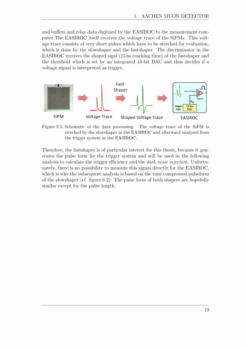
5 AACHEN MUON DETECTOR
and buffers and relay data digitized by the EASIROC to the measurement com-puter.The EASIROC itself receives the voltage trace of the SiPMs. This volt-age trace consists of very short pulses which have to be streched for evaluation,which is done by the slowshaper and the fastshaper. The discriminator in theEASIROC receives the shaped sigal (15 ns reaching time) of the fastshaper andthe threshold which is set by an integrated 10-bit DAC and thus decides if avoltage signal is interpreted as trigger.
Figure 5.5: Schematic of the data processing. The voltage trace of the SiPM isstreched by the slowshaper in the EASIROC and afterward analysed fromthe trigger system in the EASIROC.
Therefore, the fastshaper is of particular interest for this thesis, because it gen-erates the pulse form for the trigger system and will be used in the followinganalysis to calculate the trigger efficiency and the dark noise rejection. Unfortu-nately, there is no possibility to measure this signal directly for the EASIROC,which is why the subsequent analysis is based on the time compressed pulseformof the slowshaper (cf. figure 6.2). The pulse form of both shapers are hopefullysimilar except for the pulse length.
19

5 AACHEN MUON DETECTOR
5.3 Detection of charged particles
The plastic scintillator of the tiles is of the type BC-408 with a refractive index ofn = 1.58. If an incoming charged particle, like a muon, traverses the scintillatorit will excite the atoms of the scintillator. When the atoms move back to theirground state, they emit light. The total deposition of energy in the scintillatoris subjected to statistical fluctuations. The distribution is very well describedby a landau distribution [26]. In a first approximation the number of photonswhich reach the SiPM is also described by a landau function as can be seen infigure 6.12.
Figure 5.6: Sketch of the functional principle of a scintillating tile (blue) combinedwith the ’sigma fiber’ (red). A single incoming muon (green) producesscintillating light (yellow) in the tile. The photons are reflected by theinner boundary of the scintillating tile as long as the incidence angle ishigh enough. The more reflections the higher the possibility for the photonto leave.
When a photon hits the inner boundary, it depends on the incidence anglewether the photon will be reflected or leave the tile. If the incidence angle (inrelation to perpendicular) is less than ΘC = arcsin(1/1.58) ≈ 39◦, the photonwill leave the tile. To get transported to the SiPM, the photons have to enterthe sigma fiber first (cf. figure 5.6). This means that they have to hit the WLSfiber at an incidence angle bigger than ΘC = arcsin(nclad/1.58). A comparisonbetween the refractive indices of the claddings points out that the probability ofentering the fiber is smaller for the multiclad fiber. However, if the photons areinside the fiber it is more difficult for them to leave again. The fiber which showthe best overall performance should be examined in the following simulations.
20

5 AACHEN MUON DETECTOR
5.4 Implementation in Geant4
The simulations in this work are conducted using the Software ’GEANT 4’ [27],a toolkit for the simulation of silicon photomultipliers [28] and mean values fromsimulations with ’CORSIKA’ [29]. The transfer of the setup, as described abovein the Geant4 system can be seen in figure 5.7.The simulations are conducted for the SiPM-model ’Hamamatsu S12651-050’with a total area of 1 x 1 mm2 consisting of an array of 400 photodiodes.This new SiPM-model has a reduced cross-talk probability in comparison tothe model which had been installed in the AMD protoptype when the newmodel was not available yet [30]. The powerful toolkit already contains all noisephenomena as described above and transforms them together with the signalinto a voltage trace. This voltage trace is shaped according to the EASIROC’fastshaper’ to read out the data. In this simulations the shaper is based onmeasurements [31] from the EASIROC output signal.
Figure 5.7: Screenshot of the AMD setup in Geant4. The water tank (yellow) shownis for illustration only and has no influence on the simulations. Shownare the 64 scintillating tiles (red), the sigma fiber (green), the waveguides(blue) and the steel support (grey). The SiPMs are sitting on the frontends of the waveguides.
21

6 PERFORMANCE SIMULATIONS FOR AMD
6 Performance simulations for AMD
The results presented in this chapter are based on simulations with Geant4as described above and single incoming particles, which are adapted to theproperties of particles in a real air shower. The denoted energy intervals E =[10γ 1 , 10γ 2 ] MeV in the simulations refer to an uniform distribution of the expo-nents in the interval [γ 1, γ 2]. The angle intervals refers to a uniform distributionover the solid angle. For the optical fiber the multiclad fiber is used, which willbe compared with the results of the singleclad fiber in section 6.8.
The main aim of theses simulations is to optimise the AMD to an optimalmeasurement of muons. A simple trigger is suggested which should maximisethe efficiency for the triggering of muons on the one hand and minimise thenoise level on the other hand. In a next step, this thesis figures out an opti-mised configuration of the geometry regarding the size of the scintillating tilesand the shape of the ’sigma fiber’ (cf. figure 5.3). This optimised configurationis also characterised by the best possible efficiency for triggering an incomingmuon. To estimate the influence of the dark noise of SiPMs on the signal byincoming muons, the next section presents the dark noise rejection of SiPMs.
6.1 Dark noise rejection
The relatively high noise rate is still a reason for critics to refuse the applica-tion of silicon photomultipliers.Therefore, this chapter estimates the number ofevents which are triggered by dark noise of the SiPM, using a toolkit for SiPMnoise [28]. These results will be compared to the number of events triggered bymuons later on in section 6.4. Therefore, a very simple criterion for the triggeris assumed: if the voltage trace after the EASIROC fastshaper exceeds a fixedvoltage U thres, an event is interpreted as triggered. In this context, the triggerthreshold U thres should be high enough that the dark noise is not able to exceedit. Otherwise, a trigger by a dark noise event would be interpreted as a travers-ing particle. To find this minimal threshold value, the dark noise rejection willbe evaluated:Since the front of air showers traverses a single station of AMD in the time inter-val of ∆t ≈ 10µs, the noise is simulated for this time window as well, as it canbe seen in figure 6.1. This exemplary figure plots two ’normal’ cell breakdownsby thermal noise and one event of two simultaneous breakdowns caused by theeffect of cross-talk (cf. chapter 5.1). In this thesis the dark noise rejection willbe defined as following:
εnoise =N∆t(U∆t < U thres)
N tot
. (6.1)
22

6 PERFORMANCE SIMULATIONS FOR AMD
N∆t(U∆t < U thres) is the part of noise simulations where the voltage of theshaped signal is smaller than the threshold voltage U thres over the whole timewindows ∆t and N tot is the total number of noise events. The simulations pro-vide the voltage trace of the SiPM which has a very short temporal extension.It is possible to use only the maximal value of this voltage trace instead of theshaped voltage trace. However, this would disregard the overlap of two noiseevents which occure in a very short period of time, as it is the case for ’afterpulsing’ (cf. chapter 5.1). In this case, the amplitudes of the shaped signal bythe EASIROC would add up to a higher value and could reach the next thresh-old voltage.
0.00.51.01.52.0
digi
s in
p.e
. Detected noise as rectangular pulses
100
1020304050607080
volta
ge in
a.u
. Transform of the digis in a voltage trace
0 2000 4000 6000 8000 10000time in ns
150100
500
50100150200250300
volta
ge in
a.u
. Pulsform after the Easiroc Fastshaper
Figure 6.1: Simulated dark noise events of a Hamamatsu silicon photomultiplier ofmodel S12651-050. The digis show chronologically the signals of cell break-downs by thermal noise, optical cross-talk and after pulsing. The middlefigure is the simulated resulting voltage trace of the SiPM and the figureon the bottom the signal from the EASIROC fastshaper.
The pulse form after the EASIROC fast shaper is calculated by a convolutionof the SiPM voltage trace with the measured slow shaper response for a shortinput signal (cf. figure 6.2) in consideration of the shorter extension of the fastshaper signal. This calculation is only a first approximation, since the pulseform of the slow shaper and the fast shaper may differ.
23
6 PERFORMANCE SIMULATIONS FOR AMD
hold delay in ns200 400 600 800 1000 1200 1400 1600
hist
ogra
m m
ean
in A
DC
cou
nts
-50
0
50
100
150
25 ns peaking time 50 ns peaking time 75 ns peaking time100 ns peaking time125 ns peaking time150 ns peaking time175 ns peaking time
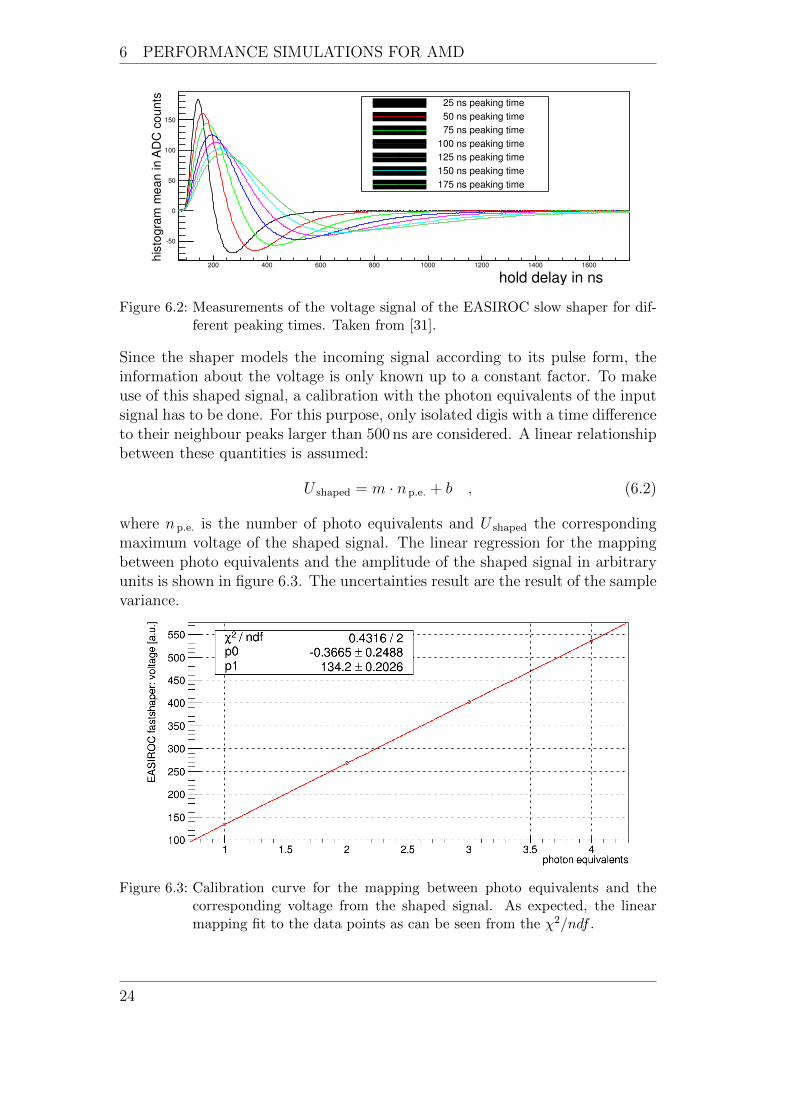
Figure 6.2: Measurements of the voltage signal of the EASIROC slow shaper for dif-ferent peaking times. Taken from [31].
Since the shaper models the incoming signal according to its pulse form, theinformation about the voltage is only known up to a constant factor. To makeuse of this shaped signal, a calibration with the photon equivalents of the inputsignal has to be done. For this purpose, only isolated digis with a time differenceto their neighbour peaks larger than 500 ns are considered. A linear relationshipbetween these quantities is assumed:
U shaped = m · np.e. + b , (6.2)
where np.e. is the number of photo equivalents and U shaped the correspondingmaximum voltage of the shaped signal. The linear regression for the mappingbetween photo equivalents and the amplitude of the shaped signal in arbitraryunits is shown in figure 6.3. The uncertainties result are the result of the samplevariance.
Figure 6.3: Calibration curve for the mapping between photo equivalents and thecorresponding voltage from the shaped signal. As expected, the linearmapping fit to the data points as can be seen from the χ2/ndf .
24

6 PERFORMANCE SIMULATIONS FOR AMD
With the parameters of the linear regression m = (132.9 ± 0.4) a.u. p.e.−1 andb = (1.0± 0.6) a.u. the axis of the shaped voltage trace can be transformed intophoto equivalents.The sample contains 640000 noise simulations each over a 10µs time intervalcorresponding to a total simulated time of 6.4 s. A histogram of the maximalvoltage values of the shaped signal from the EASIROC fast shaper within a timeinterval of 10µs can be seen in figure 6.4. The peaks correspond to the maximalvoltages for the different photon equivalents. The bin value was increased byone entry for representation in the logarithm plot.The number of noise simulation which exceed a voltage of 3 photon equivalentsis rather small. In these simulations there were only 862 of 640000 events with4 p.e. or higher (cf. figure 6.4). A histogram with a bin-width of 1 p.e. canbe seen in figure 6.5. To estimate the maximal voltage value which can beexceeded by pure dark noise, a linear fit to the datapoints in figure 6.5 were done.The intersection of the line with the x-axis is interpreted as the maximal darknoise amplitude which occures for this sample size. This estimation provides amaximal threshold value of (5.93 ± 0.03) p.e. for these simulations (cf. figure6.5).
1 p.e.
2 p.e.
3 p.e.
4 p.e.
5 p.e.
Figure 6.4: Decadic logarithm display of the histogram about the maximal voltagevalues of the EASIROC fast shaper signal within the time interval of 10µs.The peaks correspond to the voltages for the different photon equivalents.
25

6 PERFORMANCE SIMULATIONS FOR AMD
Since the statistic is limited to a samplesize of Nsample = 640000, the probabilityfor a dark noise event which lead to more than 5.93 p.e. in a time interval of10µs is approximately
p =1
640000≈ 1.5 · 10−6 (6.3)
Thus, the probability to get a trigger by a dark noise event in the 10µs timeinterval is negligibly small, assuming a simple trigger logic with a thresholdvalue of 10 p.e.
0 1 2 3 4 5 6photon equivalents
0
1
2
3
4
5
6
7
Log
(en
trie
s+
1)
/ 1
p.e
.
Binning around p.e. of the finger spectrum
Simulated noise events: 640000
Linear Fit
y=m ·x+b χ2 /ndf=15.84/3
m=−1.116±0.006 b=6.616±0.006
Figure 6.5: Decadic logarithm display of the histogram in 1 photon euivalent binningabout the maximal voltage values of the EASIROC fast shaper signal witha time interval of 10µs. A linear regression on the maxima provides anestimate for the maximal reached photon equivalents.
The dark noise rejection can be now determined as a function of the thresholdvalue in photon equivalents. Thereby, threshold values of
n thres = k + 0.5 k ∈ N0 (6.4)
are investigated. The achieved dark noise rejection can be seen in figure 6.6.Already at a threshold of n thres = 3.5 p.e. the dark noise rejection has increasedalmost to 100%. This means that there is almost not a single noise event, whichleads to a false trigger. The number of photons, which hit the SiPM due toa traversing muon, is much higher (around Nγ ≈ 30 simultaneously arriving
26

6 PERFORMANCE SIMULATIONS FOR AMD
photons) as will be shown in the further analysis. Therefore the high noise rateof SiPMs will not cause any problem in the case of AMD considering a timeperiod of 10µs.
0 2 4 6 8 10threshold in p.e.
20
30
40
50
60
70
80
90
100d
ark
nois
e r
eje
cti
on
in
%
Dark noise rejection
Simulated noise events: 640000Rejection about 99.9% at 3.5 p.e.
Figure 6.6: Dark noise rejection as a function of the threshold in photon equivalents.The rejection has already increased to over 99.9% at a threshold of 3.5 p.e..
6.2 Energy of muons in EAS from CORSIKA simulations
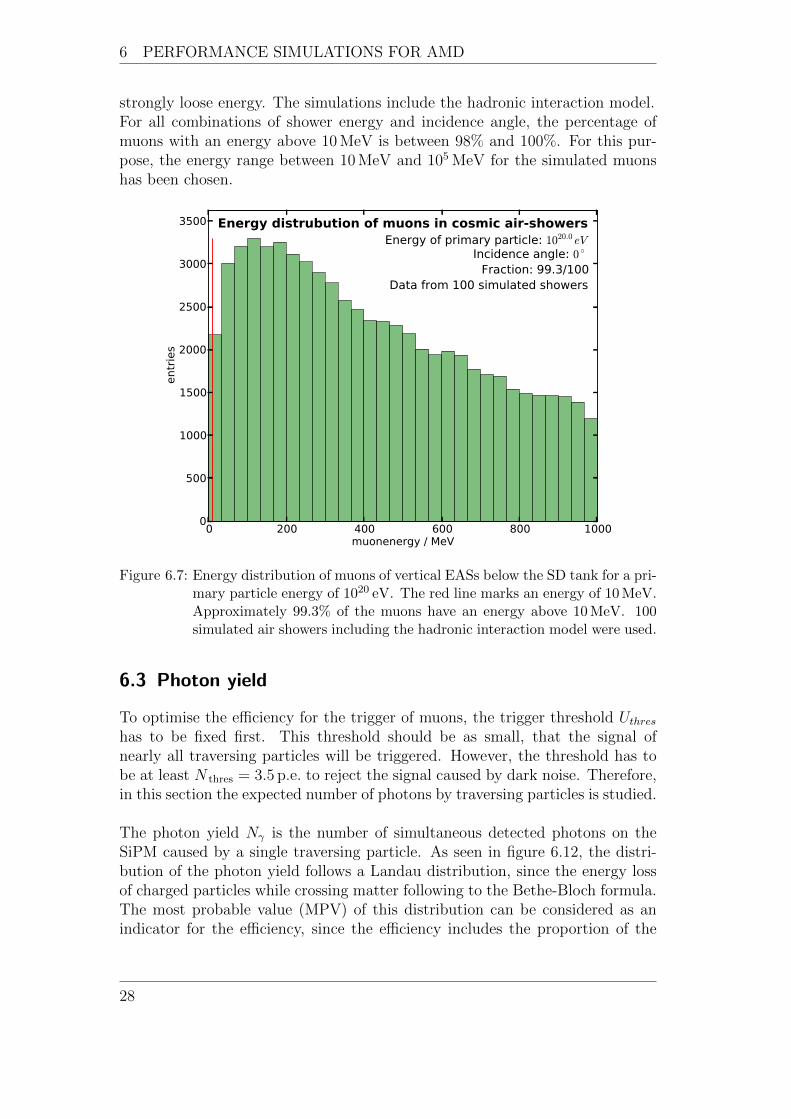
An essential part of this thesis is the determination of an optimised configurationregarding the geometry of the sigma fiber and the tile-size. This configurationis identified with single incoming particles which should have similar propertieslike the particles in a real EAS at the ground.Therefore, this chapter provides an analysis of simulated showers from COR-SIKA in order to adapt the simulated particles to the particles in a real extensiveair shower (EAS). For this, 100 simulated EAS for a primary particle energy of1018 eV, 1018.5 eV, 1019 eV, 1019.5 eV, 1020 eV and 1020.5 eV each with incidenceangles of Θ = 0◦, 20◦, 40◦ and 60◦ respectively, were evaluated. Since many,especially low energy, particles get absorbed in the SD water tank before theycan hit the AMD, these simulations already include the water tank.Figure 6.7 shows an exemplary distribution of the energy for muons leaving thewater tank. Due to the shielding of the tank, ∼ 99.3% of the muons show energylevels of more than 10 MeV, since particles beyond an energy of the MIP energy
27
6 PERFORMANCE SIMULATIONS FOR AMD
strongly loose energy. The simulations include the hadronic interaction model.For all combinations of shower energy and incidence angle, the percentage ofmuons with an energy above 10 MeV is between 98% and 100%. For this pur-pose, the energy range between 10 MeV and 105 MeV for the simulated muonshas been chosen.
0 200 400 600 800 1000muonenergy / MeV
0
500
1000
1500
2000
2500
3000
3500
entr
ies
Energy distrubution of muons in cosmic air-showersEnergy of primary particle: 1020.0 eV
Incidence angle: 0 ◦
Fraction: 99.3/100Data from 100 simulated showers
Figure 6.7: Energy distribution of muons of vertical EASs below the SD tank for a pri-mary particle energy of 1020 eV. The red line marks an energy of 10 MeV.Approximately 99.3% of the muons have an energy above 10 MeV. 100simulated air showers including the hadronic interaction model were used.
6.3 Photon yield
To optimise the efficiency for the trigger of muons, the trigger threshold Uthreshas to be fixed first. This threshold should be as small, that the signal ofnearly all traversing particles will be triggered. However, the threshold has tobe at least N thres = 3.5 p.e. to reject the signal caused by dark noise. Therefore,in this section the expected number of photons by traversing particles is studied.
The photon yield Nγ is the number of simultaneous detected photons on theSiPM caused by a single traversing particle. As seen in figure 6.12, the distri-bution of the photon yield follows a Landau distribution, since the energy lossof charged particles while crossing matter following to the Bethe-Bloch formula.The most probable value (MPV) of this distribution can be considered as anindicator for the efficiency, since the efficiency includes the proportion of the
28

6 PERFORMANCE SIMULATIONS FOR AMD
photon yield with values over the threshold value. However, the efficiency isalso influenced by the width of the distribution.The following results are based on several simulations. There is a set of 20000muons and antimuons with energies between 10−1.5 MeV - 105.75 MeV and in-cidence angles between 0◦ - 90◦ (cf. figure 6.8). A second set of 20000 muonsand antimuons are simulated with energies between 101 MeV - 105 MeV andincidence angles between 0◦ - 10◦ (cf. figure 6.9). Moreover, there are sets of20000 electrons and positrons with energies between 10−1 MeV - 104.5 MeV (cf.figure 6.10) and 10000 protons with energies between 10−1 MeV - 105 MeV (cf.figure 6.11), both with incidence angles between 0◦ - 90◦. The simulations ofthe electrons and protons are done to estimate the signal which is caused bythis undesired components of an EAS.For nearly vertical muons, there are sets for each tile-size and each fiber config-uration.
Figure 6.8 shows the distribution of the photon yield averaged over all incidenceangles. Conspicuous is the significant deviation from the landau distributionfor small numbers of produced photons. This effect results from very inclinedmuons, which interact with the steel support. In this case not the muon tra-verses a scintillating tile but several secondary particles. This can cause up to10 simultaneous photon hits on the SiPM per secondary particle. This effect issignificantly reduced as shown in figure 6.9, as the incoming muons have smallerincidence angles. Furthermore, the most probable value (MPV) decreases withlower incidence angle, due to the shorter path length which the muons travelin the scintillating tile. Since figure 6.8 contains an average over all incidenceangles, the width of the distribution in 6.9 is also smaller.As the incoming electrons, positrons and protons of the air shower are unde-sired, the triggered signals for these components should be as small as possible.Figure 6.10 shows the distribution of the photon yield for incoming electronsand positrons and in figure 6.11 for protons. Since the interactions with thesteel support is more often for electrons, the peak at Nγ < 10 is much higherand should be cutted by the trigger. However, there remains an essential partof ∼ 3900/19702 ≈ 20% of the electrons which cause a number of photonslarger than 10 p.e. (cf. 6.10). For the protons there is no visible Landau dis-tribution any more, due to the strong absorbtion in the steel plate, leading toless protons reaching the scintillating tile. However, there is a small proportionof secondary particles which cause the peak at Nγ < 10. Using a thresholdof Nthres = 10.5 p.e., the proportion of triggered protons is fortunately small∼ 270/9938 ≈ 2.7%.
In order to prevent a trigger caused by a secondary particle it is necessary toensure that the threshold is at least Nthres = 10.5 p.e.. This affects the triggerefficiency of a real traversing muon only rarely, since the Landau distribution ofmuons is negligibly small in this region (cf. figures 6.9,6.15).
29

6 PERFORMANCE SIMULATIONS FOR AMD
0 50 100 150 200number of photons
0
100
200
300
400
500
en
trie
s /
5 p
hoto
ns
Histogram of SiPM-Photons at incoming muon
tile-size: 300 mm
Energy: (10−1.5 - 105.75 ) MeV
Incidence angle Θ: 0 ◦ - 90 ◦
Simulated particles: 19999
Entries: 5076
Figure 6.8: Histogram of photons detected by the SiPMs for a tile-size of d = 300 mmand incoming muons and antimuons for all incidence angles.
0 50 100 150 200number of photons
0
200
400
600
800
1000
1200
entr
ies
Histogram of SiPM-Photons at incoming muon
tile-size: 300
Energy: 101 MeV - 105 MeV
Θ < 10 ◦
Simulated particles: 19999
Entries: 8589
Figure 6.9: Histogram of photons detected by the SiPMs for a tile-size of d = 300 mmand incoming muons and antimuons for incidence angles smaller than 10◦.
30

6 PERFORMANCE SIMULATIONS FOR AMD
0 50 100 150 200number of photons
0
200
400
600
800
1000
1200
en
trie
s /
5 p
hoto
ns
Histogram of SiPM-Photons at incoming electron
tile-size: 300 mm
Energy: (10−1 - 104.5 ) MeV
Incidence angle Θ: 0 ◦ - 90 ◦
Simulated particles: 19702
Entries: 5507
Figure 6.10: Histogram of photons detected by the SiPMs for a tile-size of d = 300 mmand incoming electrons and positrons for all incidence angles.
0 50 100 150 200number of photons
0
20
40
60
80
100
120
140
en
trie
s /
5 p
hoto
ns
Histogram of SiPM-Photons at incoming proton
tile-size: 300 mm
Energy: (10−1 - 105 ) MeV
Incidence angle Θ: 0 ◦ - 90 ◦
Simulated particles: 9938
Entries: 483
Figure 6.11: Histogram of photons detected by the SiPMs for a tile-size of d = 300 mmand incoming protons for all incidence angles.
31

6 PERFORMANCE SIMULATIONS FOR AMD
6.3.1 Landau fit
To calculate the MPV as an indicator for the trigger efficiency for a traversingparticle a Landau distribution have to be fit to the photon yield (cf. Fig 6.12).Therefor, the sample of almost vertical (cf. figure 6.9) incoming muons, will beconsidered. For this case, the uncertainties of the MPV will decrease for thereason of a more distinct maximum. This is due to equal traveled distances inthe scintillating tile as pointed out above.
0 50 100 150 200number of photons
0
200
400
600
800
1000
1200
1400
en
trie
s /
5 p
hoto
ns
Landau-fit of SiPM-Photons at incoming muon
tile-size: 300 mm
Landau-Fit: χ2 /ndf = 165.1 / 35.0
MPV = 34.0 Sigma = 6.1
Entries: 8322
Figure 6.12: Landau fit to the distribution of photons detected by the SiPM aftera muon crossed a scintillating tile. This distribution is shown in figure6.9 except for the bins smaller than 10 p.e.. The relatively high χ2/ndfrepresents the fact that the distribution is not described by a pure Landaudistribution, since there are Gaussian processes regarding the productionof photons and the transmission into the WLS fiber.
Since the peak for Nγ < 10 contains mostly events of secondary particles andnot the number of emitted photons, while the crossing of a muon, the fit doesnot consider values for Nγ < 10. As can be seen in figure 6.12, the model ofa pure Landau distribution does not optimally fit the data points. This is alsorepresented by a high χ2/ndf . The landau distribution describes the energy de-position in the scintillating tile, which is not identical with the photons reachingthe SiPM, since the transformation of the energy into photons, the transmis-
32

6 PERFORMANCE SIMULATIONS FOR AMD
sion of the photons into the sigma fiber and the photon losses in the waveguidealso play an important role. However, the fit of a landau distribution convolvedwith a Gaussian distribution would not improve the situation, since there aretoo many unknown components.
Another reason for the systematically too high χ2/ndf is that the distributionin figure 6.9 is an average over many different tile positions. The next chaptershows the Landau fit seperated by different length of waveguides.
6.3.2 Dependence on the length of the waveguide
0
50
100
150
200χ2 / ndof = 51.6 / 30.0
1019 entriesMPV = 30.0
Sigma = 5.0l = 2.9 m
χ2 / ndof = 54.3 / 30.0962 entriesMPV = 31.7
Sigma = 5.1l = 2.5 m
0
50
100
150
200χ2 / ndof = 38.2 / 33.0
1068 entriesMPV = 31.6
Sigma = 5.5l = 2.2 m
χ2 / ndof = 46.4 / 33.01025 entriesMPV = 32.4
Sigma = 5.4l = 1.8 m
0
50
100
150
200χ2 / ndof = 37.8 / 33.0
1085 entriesMPV = 34.7
Sigma = 5.8l = 1.4 m
χ2 / ndof = 51.9 / 34.01053 entriesMPV = 35.4
Sigma = 5.6l = 1.0 m
0 50 100 150 2000
50
100
150
200χ2 / ndof = 58.6 / 34.0
1088 entriesMPV = 37.1
Sigma = 5.7l = 0.7 m
0 50 100 150 200
χ2 / ndof = 49.6 / 35.0993 entriesMPV = 40.7
Sigma = 6.2l = 0.3 m
number of photons
entr
ies
/ 5
Photo
ns
Figure 6.13: Landau fit for different tile positions and therefore different waveguidelength for muons with incidence angles below 20◦. The MPV shows aclear dependence on the waveguide length l due to the higher photon lossrate, during the transport.
33

6 PERFORMANCE SIMULATIONS FOR AMD
The scintillating tiles have different distances to the SiPMs depending on theirpositions. A higher distance means a longer waveguide and therefore a higherprobability for photon losses in the waveguide. This will influence the MPV ofthe Landau distribution as can be seen in figure 6.13.Whereas the MPV for a waveguide length of l = 0.3 m is still 40.7 p.e., theMPV drops to 30 p.e. at a length of l = 2.6 m. This effect could affect thetrigger efficiency of a tile on the far side of the SiPM in comparison to a tilenext to the SiPM, for the case of a small mean MPV.On average the MPV of the Landau fit to the combined distribution (cf. figure6.12) represents the performance of the different configurations very well, sincethis thesis should figure out an optimised configuration for the whole AMD.Therefore, the subsequent definition of the MPV refers to the fit of the combineddistributions. This value is very close to the mean of all MPVs of the differentwavelength in figure 6.13.
6.4 Optimal threshold for the triggering of muons
To calculate the efficiency for detecting single incoming muons, an optimalthreshold value has to be determined. Analogously to the approach to cal-culate the dark noise rejection, this section will show the trigger efficiency asa function of the threshold value in photon equivalents. Therefor, the set ofvertical incoming muons with an incidence angle below 10◦ is used.
Figure 6.14 shows the chronological signal by photon hits and noise phenom-ena with a binning of 100 ns. The peak at t ≈ 0 ns results from the photons,which are produced through the traversing muon and correlated noise. Thereare two additional signals which are comparatively small and caused by thermalnoise. To calculate the efficiency as a function of the threshold, the efficiency isscanned in the same threshold steps like the dark noise rejection:
nthres = k + 0.5 k ∈ N0 . (6.5)
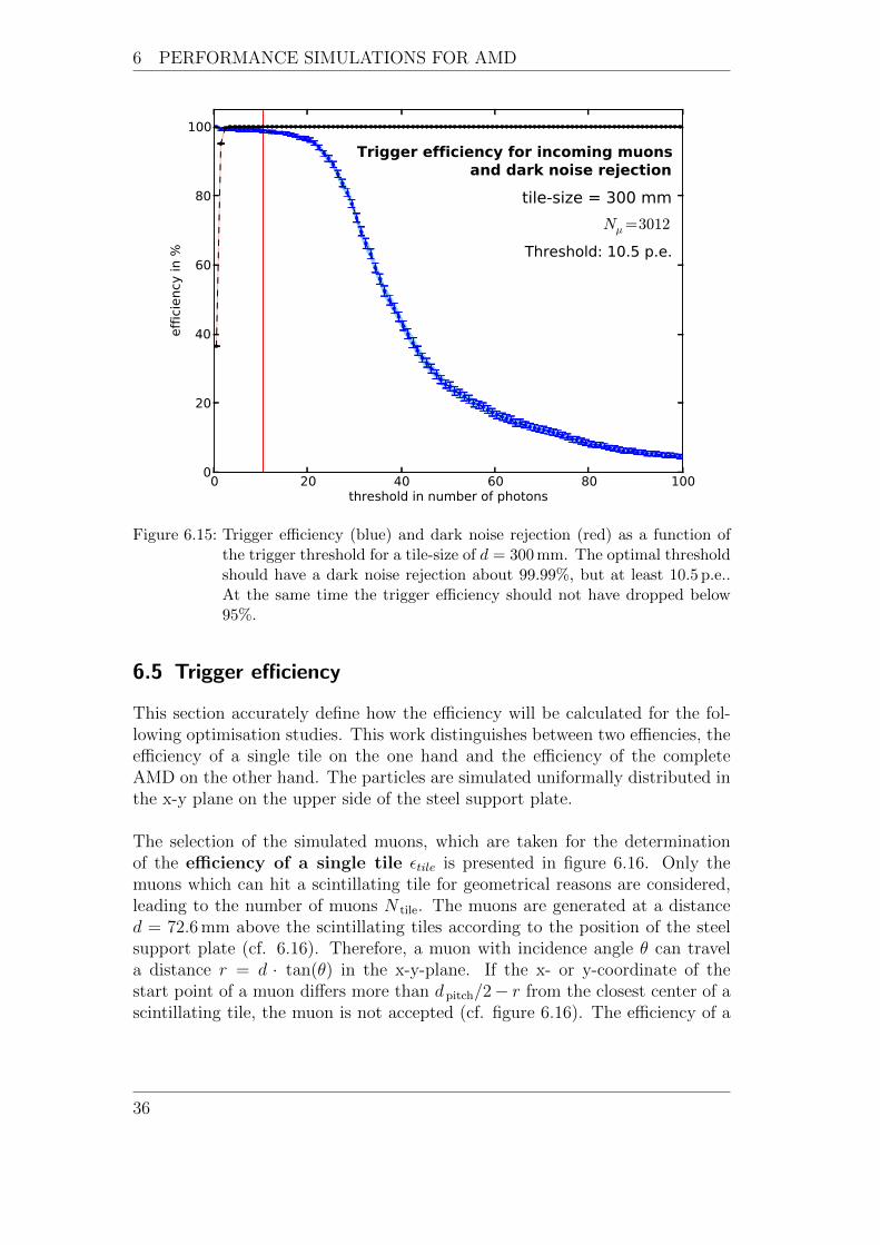
The trigger efficiency as shown in figure 6.15 is the share of events, where theshaped voltage trace is higher than the threshold value in all events. An optimalthreshold value would be characterised by an exeeding from all voltage traces ofmuon signals but at once the threshold value should not be gained by any darknoise event.
34

6 PERFORMANCE SIMULATIONS FOR AMD
Detected hits and noise as rectangular pulses
Figure 6.14: Simulated muon events including noise of the Hamamatsu silicon pho-tomultiplier. The digis show the chronological signal of cell breakdownsby hits and noise phenomena. The middle figure is the resulting volt-age trace and the figure on the bottom the signal from the EASIROCfastshaper.
To determine the optimal threshold value, one could imagine to take the inter-section of this curve and the dark noise rejection. For this case, both the triggerefficiency and the dark noise rejection are fortunately high, about 99.5%. How-ever, this would lead to a threshold from 2.5 p.e. and in turn lead to many triggerevents, caused by secondary particles. For this reason, the threshold should beat least Nthres = 10.5 p.e. as discussed in chapter 6.3. The trigger efficiencywould be still sufficient high, 98.7% for the tile-size of 300 mm.
35
6 PERFORMANCE SIMULATIONS FOR AMD
0 20 40 60 80 100threshold in number of photons
0
20
40
60
80
100
eff
icie
ncy
in %
Trigger efficiency for incoming muonsand dark noise rejection
Nµ=3012
tile-size = 300 mm
Threshold: 10.5 p.e.
Figure 6.15: Trigger efficiency (blue) and dark noise rejection (red) as a function ofthe trigger threshold for a tile-size of d = 300 mm. The optimal thresholdshould have a dark noise rejection about 99.99%, but at least 10.5 p.e..At the same time the trigger efficiency should not have dropped below95%.
6.5 Trigger efficiency
This section accurately define how the efficiency will be calculated for the fol-lowing optimisation studies. This work distinguishes between two effiencies, theefficiency of a single tile on the one hand and the efficiency of the completeAMD on the other hand. The particles are simulated uniformally distributed inthe x-y plane on the upper side of the steel support plate.
The selection of the simulated muons, which are taken for the determinationof the efficiency of a single tile εtile is presented in figure 6.16. Only themuons which can hit a scintillating tile for geometrical reasons are considered,leading to the number of muons N tile. The muons are generated at a distanced = 72.6 mm above the scintillating tiles according to the position of the steelsupport plate (cf. 6.16). Therefore, a muon with incidence angle θ can travela distance r = d · tan(θ) in the x-y-plane. If the x- or y-coordinate of thestart point of a muon differs more than dpitch/2− r from the closest center of ascintillating tile, the muon is not accepted (cf. figure 6.16). The efficiency of a
36

6 PERFORMANCE SIMULATIONS FOR AMD
single tile is therefore defined as:
ε tile ==N(N γ > N thres)
N tile
≤ 1 . (6.6)
N(N γ > N thres) represents the part of events, where at least N thres = 10.5photons are registered on any SiPM.
Figure 6.16: Sketch of the geometrical selection of the muons for calculating the effi-ciency of a single tile. Only muons, which can hit the scintillating tile forgeometrical reasons, will be considered for the calculation. The muonscan travel the distance r = d · tan(θ) on the tile plane according to theincidence angle θ. d is the vertical distance between the tile and the steelplate.
In contrast, for the efficiency of complete AMD εAMD all muons which”start” within the profile of the whole steel support construction in the heightd above the scintillating tiles are considered. This total number NAMD alsoincludes muons, which cannot hit the AMD for geometrical reasons. The nu-merater in the efficiency εAMD (cf. equation (6.7)) is calculated through thefraction of events in NAMD, where at least N thres = 10.5 photons are registeredon any SiPM:
εAMD =N(N γ > N thres)
N tile
≤ 1 . (6.7)
In the following a threshold value Nthres = 10.5 will be used according to thedetermined optimal threshold value for the trigger efficiency of AMD for singlemuons.
37

6 PERFORMANCE SIMULATIONS FOR AMD
6.6 Finding an optimised tile-size
To find an ideal size for the scintillating tile, simulations with tile-sizes of260 mm, 280 mm, 300 mm, 320 mm, 340 mm and 360 mm will be analysed.
Since the efficiency for the trigger of a muon is only influenced by the simultane-ous number of photons which reach the SiPM in this simple model of a trigger,the MPV as a benchmark for the photon yield for different tile-sizes will beconsidered first. The fit of Landau distributions to the distribution of incomingphotons on the SiPM for these simulations show a clear correlation between theMPV and the tile-size (cf. figure 6.17).
260 280 300 320 340 360tile-size in mm
20
25
30
35
40
MPV
in n
umbe
r of
pho
tons
MPV for different tile-sizes at incoming muonswith incidence angles below 10 ◦
Figure 6.17: MPVs from Landau fits for simulations with incoming muons with in-cidence angles below 10◦ and different tile-sizes between 260 mm and360 mm. The MPV shows a clear dependence on the tile-sizes, since thephoton loss in the tiles increase with a higher distance to the sigma fiber.
The MPV and therefore the photon hits on the SiPM decreas with increasingtile-size. This is due to a higher photon loss probability in the scintillating tile.This is caused by an increasing number of reflections on the boundaries, sincethe mean distance between the photon production point and the sigma fiberincreases (cf. figure 5.6) as the fiber-padding and the fiber-radius are kept fixed.
38

6 PERFORMANCE SIMULATIONS FOR AMD
To get a higher photon yield in the single tiles, the tile-size has to be as smallas possible. However, this will reduce the fill factor αd of the sensitive area
αd =64 · d2
tile
AAMD
(6.8)
and therefore the efficiency of the complete AMD εAMD (cf. figures 6.18,6.19)with the total cross-section area AAMD of the whole AMD. Hence, one has tofind a compromise between these effects.Considering the efficiency of a single tile ε tile in figure 6.18 and 6.19 one can seethat the decreasing MPV has a first effect on the efficiency above a tile-size ofd = 320 mm.
Figure 6.18: The efficiency εtile for a single tile and the efficiency εAMD for the com-plete AMD for different tile-sizes. The simulated muons have incidenceangles below 10◦ and an energy range between 10 MeV and 105.75 MeV.
39

6 PERFORMANCE SIMULATIONS FOR AMD
Figure 6.19: The efficiency ε tile for a single tile and the efficiency εAMD for the com-plete AMD for different tile-sizes. The simulated muons have incidenceangles below 10◦ and an energy range between 102 MeV and 105.75 MeV.
For this reason, a tile-size of d = 320 mm would be an ideal size to find acompromise between the photon yield and therefore the efficiency for a single tileε tile on the one hand and the geometrical fill factor and therefore the efficiencyof the complete AMD εAMD on the other hand. This tile-size is therefore alsoused for all further simulations.The efficiency for triggering a vertical single muon with an energy between10 MeV and 105 MeV is approx 92% for a tile-size of d = 320 mm (cf. figure6.18). Considering the same muons with energies about 100 MeV leads to anefficiency of almost 100% (cf. figure 6.19), since the muon does not interact inthe steel support any more.
40
6 PERFORMANCE SIMULATIONS FOR AMD
6.7 Finding an optimised fiber configuration
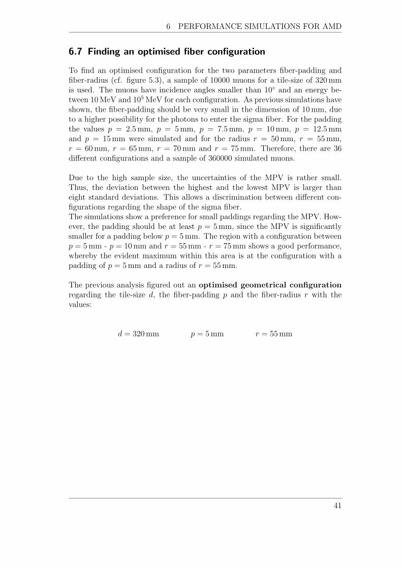
To find an optimised configuration for the two parameters fiber-padding andfiber-radius (cf. figure 5.3), a sample of 10000 muons for a tile-size of 320 mmis used. The muons have incidence angles smaller than 10◦ and an energy be-tween 10 MeV and 105 MeV for each configuration. As previous simulations haveshown, the fiber-padding should be very small in the dimension of 10 mm, dueto a higher possibility for the photons to enter the sigma fiber. For the paddingthe values p = 2.5 mm, p = 5 mm, p = 7.5 mm, p = 10 mm, p = 12.5 mmand p = 15 mm were simulated and for the radius r = 50 mm, r = 55 mm,r = 60 mm, r = 65 mm, r = 70 mm and r = 75 mm. Therefore, there are 36different configurations and a sample of 360000 simulated muons.
Due to the high sample size, the uncertainties of the MPV is rather small.Thus, the deviation between the highest and the lowest MPV is larger thaneight standard deviations. This allows a discrimination between different con-figurations regarding the shape of the sigma fiber.The simulations show a preference for small paddings regarding the MPV. How-ever, the padding should be at least p = 5 mm, since the MPV is significantlysmaller for a padding below p = 5 mm. The region with a configuration betweenp = 5 mm - p = 10 mm and r = 55 mm - r = 75 mm shows a good performance,whereby the evident maximum within this area is at the configuration with apadding of p = 5 mm and a radius of r = 55 mm.
The previous analysis figured out an optimised geometrical configurationregarding the tile-size d, the fiber-padding p and the fiber-radius r with thevalues:
d = 320 mm p = 5 mm r = 55 mm
41

6 PERFORMANCE SIMULATIONS FOR AMD
Figure 6.20: MPVs from landau fits for simulations with incoming muons with inci-dence angles below 10◦ and different fiber configurations with paddingsbetween p = 2, 5 mm− 15 mm and radii between r = 50 mm− 75 mm.
6.8 Comparison between multiclad and singleclad fiber
This chapter contains a comparison of the multiclad fiber and the singlecladfiber for the use as sigma fiber and waveguide in the setup of AMD. The sim-ulation sample includes 100000 muons with incidence angles smaller than 10◦
and energies between 10 MeV and 105 MeV both for the multiclad fiber and thesingleclad fiber.
Figure 6.21 shows the MPV seperated for different fiberlength of the multicladand the singleclad fiber. For all tile-position the MPV of the multiclad fiber isbetween 5 and 8 photon equivalents higher than the MPV of the singleclad fiber.This means that there are more photons which reach the SiPM for the multicladfiber and in turn an improved efficiency. The results of these simulations do notcorrespond with the expectation that the transmission of the photons into thefiber is worse in case of the multiclad fiber, due to the smaller refractive indexof the outer cladding. However, the more efficient photon confinement while the
42

6 PERFORMANCE SIMULATIONS FOR AMD
transport within the curved sigma fiber could be an explanation for this effect.
l=0.3m l=0.7m l=1.0m l=1.4m l=1.8m l=2.2m l=2.5m l=2.9m0
5
10
15
20
25
30
35
40M
PV
38
3433
3231
29 2928
3028
27 2726
24 24 23
MPV for singleclad and multiclad fiber
multiclad fibersingleclad fiber
Figure 6.21: MPVs from Landau fits for the singleclad and the multiclad fiber seper-ated for different fiberlength (cf. figure 6.13). The optimised geometricalconfiguration of AMD (tile-size d = 320 mm, fiber-padding p and fiber-radius r) is used.
In a second step the uniformity of the photon hits on the SiPM is studied. Amore uniform illumination of the SiPM surface also means a more equal demandof each photodiode and therefore a higher dynamic range.The performance of the multiclad fiber regarding the uniformity of photon hitson the SiPM surface is better as well. This distribution is much more uniformfor the multiclad fiber than the distribution of the singleclad fiber (cf. figures6.22 and 6.23). As can clearly be seen in figures 6.22 and 6.23, most photon hitsare within a circle with diameter 1 mm. In the corner regions there are consid-erably less photon hits anymore. This is due to the circular cross-section areaof the waveguides which ends onto the surface of the SiPMs. The uniform thedistribution on the SiPM surface, the more equal the stress for each photodiode.This also means a higher dynamic range for the SiPM.For this reasons, the multiclad fiber is more adequate for the use as sigma fiberand waveguide in the setup of AMD.
43

6 PERFORMANCE SIMULATIONS FOR AMD
0.4 0.2 0.0 0.2 0.4hitpos [x] / mm
0.4
0.2
0.0
0.2
0.4
hit
pos[y
] /
mm
entries, 2017879multiclad fiber
hitposition on sipm
800
1600
2400
3200
4000
4800
5600
6400
entr
ies
Figure 6.22: Photon hit distribution on the 1 mm2 surface of the SiPM for incomingmuons. The optimised configuration and the multiclad model for theoptical fibers have been used.
0.4 0.2 0.0 0.2 0.4hitpos [x] / mm
0.4
0.2
0.0
0.2
0.4
hit
pos[y
] /
mm
entries, 2009793singleclad fiber
hitposition on sipm
800
1600
2400
3200
4000
4800
5600
6400
7200
entr
ies
Figure 6.23: Photon hit distribution on the 1 mm2 surface of the SiPM for incomingmuons. The optimised configuration and the singleclad model for theoptical fibers have been used.
44

7 CONCLUSION
7 Conclusion
The Aachen Muon Detector (AMD) is a proposal for the Pierre Auger updateprogram 2015 for the measurement of the muonic component of extensive airshowers. A prototype is designed and built by our working group at the III.Physikalisches Institut A, RWTH Aachen. The basic concept is the detectionof muons by a combination of scintillating tiles, in which light is produced bytraversing charged particles, and optical fibers for the transport of the producedphotons to the light sensor, an SiPM. This thesis outlined several performancestudies to determine the optimal geometry and setup for the detector.
The distribution of detected photons on the SiPM follows a Landau distribu-tion. The most probable value (MPV) of this distribution for traversing muonsis a good benchmark for the efficiency of the detector. Simulations with differ-ent values for the parameters tile-size d, fiber-radius r and fiber-padding p inthe setup of AMD were analysed. The optimised configuration regarding thisparameters for the trigger efficiency of single muons is:
d = 320 mm p = 5 mm r = 55 mm
The influence of the dark noise of the SiPMs on the signal caused by a travers-ing muon has been investigated and is negligible. The possibility for a noiseevent with more than 3 photon equivalents in a time interval of 10µs, which is atypical time period of an incoming extensive air shower is approximately 0.2%.In contrast, the signal of a muon crossing is approximate 40 photon equivalents.Therefore, the noise phenomena have practically no influence on the trigger ofmuons for an adequate threshold value of 10.5 photon equivalents. This thresh-old has to be chosen to prevent triggers which are caused by the production ofsecondary particles, as found out during the simulation studies.
For the BCF-92 WLS sigma fiber and the BCF-98 waveguide in the setup ofAMD, simulations were done both for the singleclad fiber and the multicladfiber. The photon yield of the SiPM for the multiclad fiber is about 5 photonequivalents higher than the photon yield for the singleclad fiber. In addition,the distribution of SiPM photon hits is more uniform for the multiclad fiber,raising the dynamic range for the AMD in comparison to the singleclad fiber.For this reason, the multiclad fiber should be used as optical fibers to improvethe performance of AMD.
This simulation study optimised the geometry for the AMD regarding the per-formance for the trigger of muons. The promising prototype is suited for asuccessful measurement of the muonic component of cosmic rays air showers.
45

References
References
[1] G. Federmann. ”Victor Hess und die Entdeckung der KosmischenStrahlung”. Diplomarbeit, Universitat Wien, 2003.
[2] M. Bustamante et al. ”Origin of cosmic rays”. 2012.
[3] D. Meschede. Gerthsen Physik. Springer, Berlin, 2010.
[4] L. Drury. ”High-energy cosmic-ray acceleration”. 2009.
[5] Pierre Auger Collabaration. ”Muons in air showers at the Pierre AugerObservatory: Measurement of amospheric production depth”. 2014.arXiv:1407.5919v1.
[6] Particle Data Group. ”Cosmic rays”. 2013.
[7] M. Domenico et al. ”Reinterpreting the development of extensive air show-ers initiated by nuclei and photons”. 2013. arXiv:1305.2331v2.
[8] Particle Data Group. Particle Physics Booklet. California, 2010.
[9] W. Demtroder. Experimentalphysik 4. Kern-, Teilchen und Astrophsik.Springer, California, 2010.
[10] H. Dembinski. ”Aufbau einer Detektorstation aus Szintillatoren zum Nach-weis von kosmischen Teilchenschauern, Simulation und Messung”. Diplo-marbeit, RWTH Aachen University, 2005.
[11] M. Lemoine. Physics and Astrophysics of Ultra-High-Energy Cosmic Rays.Springer, Berlin, 2001.
[12] Pierre Auger Collabaration. Taken from: http://www.scinexx.de/dossier-bild-353-6-8969.html (Access: 7.9.2014 10:14 AM).
[13] S. Fliescher. ”Radio Detection and Detector Simulation for Extensive AirShowers at the Pierre Auger Observatory”. Diplomarbeit, RWTH AachenUniversity, 2005.
[14] C. Peters. ”Design Studies for an Air Fluorescence Telescope with Sili-con Photomultipliers for the detection of Ultra high energy Cosmic Rays”.Masterarbeit, RWTH Aachen University, 2013.
[15] T. Niggemann. ”New Telescope Design with Silicon Photomultipliers forFluorescence Light Detection of Extensive Air Showers”. Masterarbeit,RWTH Aachen University, 2012.
[16] Pierre Auger Collabaration. ”The Fluorescence Detector of the PierreAuger Observatory”. 2009. arXiv:0907.4282.
[17] M. Grigat. ”Large Scale Anisotropy Studies of Ultra High Energy CosmicRays Using Data Taken with the Surface Detector of the Pierre AugerObservatory”. Doktorarbeit, RWTH Aachen University, 2011.
46

References
[18] Pierre Auger Collabaration. ”The Next Frontier in UHECR Research withan Upgraded Pierre Auger Observatory”. 2013. arXiv:1307.0226v3.
[19] FZU IFSC/USP LIP et al, CBPF. ”MARTA (Muon Auger RPC for theTank Array) Design Report”. Auger internal note: GAP-2013-020, 2013.
[20] FZU IFSC/USP LIP et al, CBPF. ”MARTA (Muon Auger RPC for theTank Array) 1st progress report”. Auger internal note: GAP-2013-052,2013.
[21] E. Lorenz and D. Renker. ”Advances in solid state photon detectors”.Journal of Instrumentation, 4, 2009. P04004.
[22] J. Rennefeld and A. Stahl. Studien zur Eignung von Silizium Photomultipli-eren fur den Einsatz im erweiterten CMS Detektor am SLHC. Masterarbeit,RWTH Aachen University, 2010.
[23] Saint-Gobain Crystals. Premium plastic scintillators. Brochure. 2005.
[24] T. Hebbeker et al. ”Muon measurement using scintillator tiles with SiPMreadout”. Auger internal GAP note: GAP-2013-057, 2013.
[25] Saint-Gobain Crystals. Scintillating optical fibers. Brochure. 2005.
[26] Particle Data Group. ”Passage of particles through matters”. 2011.Taken from: http://www-pdg.lbl.gov/2011/reviews/rpp2011-rev-passage-particles-matter.pdf (Access: 27.9.2014 14:00).
[27] S. Agostinelli et al. ”GEANT 4 - a simulation toolkit”. NIM Section A,Volume 506, Section 3, 2003.
[28] T. Niggemann et al. ”A generic Geant4 simulation toolkit for silicon pho-tomultipliers”. https://forge.physik.rwth-aachen.de/projects/g4sipm.
[29] D. Heck et al. ”CORSIKA: A monte Carlo code to simulate extensive airshower”. Vol. 6019. FZKA, 1998.
[30] Hamamatsu Photonics. Technical Information - MPPC models. Brochure.2013.
[31] L. Middendorf. Measurements of the EASIROC slow shaper. Internal pre-sentation. 2014.
[32] R. Abbasi et al. ”Measurement of the Flux of Ultrahigh Energy CosmicRays from Monocular Observations by the High Resolution Fly’s Eye Ex-periment”. Phys. Rev. Lett., 92, 2004. DOI: 10.1103.
[33] D. Perkins. Particle Astrophysics. Oxford University Press Inc., Oxford,2003.
47


Acknowledgements
An dieser Stelle mochte ich mich fur die tolle Zeit bedanken, die ich mit der AugerArbeitsgruppe erleben durfte.
Fur die Ermoglichung dieser Arbeit in diesem hochinteressanten und aktuellen Forschungs-gebiet bedanke ich mich ganz herzlich bei Herrn Prof. Dr. Hebbeker.
Die gesamte Arbeitsatmosphare empfand ich als sehr angenehm. Ein dankeschongilt den vielen netten Personlichkeiten, die ich wahrend meiner Arbeit kennenlernendurfte und die allesamt sehr hilfsbereit waren. Ein ganz besonderes Dankeschon giltdabei meiner Betreuerin Christine Peters die keine Muhen gescheut hat um mir zuhelfen und die Arbeit zur Kontrolle gleich mehrfach gelesen hat. Ebenfalls bedankeich mich bei Tim Niggemann und Lukas Middendorf die mich ebenfalls unterstutzthaben und die Arbeit kontrollgelesen haben.Fur die angenehme Arbeitsatmosphare im Buro mochte ich mich ebenfalls bei FranziskaKnuth und Dominik Sommer bedanken.
Weiterhin gilt mein Dank Patrick Ziegler und Felix Frank fur das Lesen dieser Arbeitund ihren Anregungen.
Zu guter letzt darf selbstverstandlich auch nicht die mentale Unterstutzung von Fam-ilie, Freunden und Freundin in der Heimat vergessen werden!


Erklarung
Hiermit versichere ich, dass ich diese Arbeit einschließlich beigefugter Zeichnungen,Darstellungen und Tabellen selbststandig angefertigt und keine anderen als die ange-gebenen Hilfsmittel und Quellen verwendet habe. Alle Stellen, die dem Wortlaut oderdem Sinn nach anderen Werken entnommen sind, habe ich in jedem einzelnen Fallunter genauer Angabe der Quelle deutlich als Entlehnung kenntlich gemacht.
Aachen, 30. September 2014
Marcus Wirtz